Vanya Horneff – Daniel Liebler – Raimond Maurer – Olivia S. Mitchell

Implications of Money-Back Guarantees for Individual Retirement Accounts: Protection Then and Now SAFE Working Paper No. 263

Implications of Money-Back Guarantees for Individual Retirement

Accounts: Protection Then and Now

Vanya Horneff, Daniel Liebler, Raimond Maurer, and Olivia S. Mitchell

October 21, 2019

Abstract

In the wake of the financial crisis and continued volatility in international capital markets, there is growing interest in mechanisms that can protect people against retirement account volatility. This paper explores the consequences for savers’ wellbeing of implementing market-based retirement account guarantees, using a life cycle consumption and portfolio choice model where investors have access to stocks, bonds, and tax-qualified retirement accounts. We evaluate the case of German Riester plans adopted in 2002, an individual retirement account produce that includes embedded mandatory money-back guarantees. These guarantees influenced participant consumption, saving, and investment behavior in the higher interest rate environment of that era, and they have even larger impacts in a low-return world such as the present. Importantly, we conclude that abandoning these guarantees could enhance old-age consumption for over 80% of retirees, particularly lower earners, without harming consumption during the accumulation phase. Our results are of general interest for other countries implementing default investment options in individual retirement accounts, such as the U.S. 401(k) defined contribution plans and the Pan European Pension Product (PEPP) recently launched by the European Parliament.

Keywords: individual retirement account, investment guarantee, longevity risk, retirement income, life cycle model

JEL: D14, D91, G11

Vanya Horneff

Finance Department, Goethe University Theodor-W.-Adorno-Platz 3 (Uni-PF. H 23) Frankfurt am Main, Germany E-Mail: vhorneff@finance.uni-frankfurt.de

Daniel Liebler

Finance Department, Goethe University Theodor-W.-Adorno-Platz 3 (Uni-PF. H 23) Frankfurt am Main, Germany E-Mail: liebler@finance.uni-frankfurt.de

Raimond Maurer

Finance Department, Goethe University Theodor-W.-Adorno-Platz 3 (Uni-PF. H 23) Frankfurt am Main, Germany E-Mail: maurer@finance.uni-frankfurt.de

Olivia S. Mitchell Wharton School, University of Pennsylvania 3620 Locust Walk, 3000 SH-DH Philadelphia, PA 19104 E-Mail: mitchelo@wharton.upenn.edu

Acknowledgements: The authors are grateful for research support from the German Investment and Asset Management Association (BVI), the SAFE Research Center funded by the State of Hessen, and the Pension Research Council/Boettner Center at The Wharton School of the University of Pennsylvania. We thank the Competence Center for High Performance Computing in Hessen for granting us computing time on the GOETHE-HLR and Lichtenberg Cluster. Data were generously provided by the German Socio-Economic Panel and the Deutsche Bundesbank Panel on Household Finances. Opinions and any errors are solely those of the authors and not of the institutions with which the authors are affiliated nor any individual cited. © 2019 Horneff, Liebler, Maurer, and Mitchell.

1

Implications of Money-Back Guarantees for Individual Retirement

Accounts: Protection Then and Now

1 Introduction

Numerous countries have adopted tax-qualified defined contribution retirement

accounts as a means to fill the gap between retiree income needs and benefits payable under

national social security systems.1 Additionally, many policymakers seek mechanisms to protect

savers against longevity risk and capital market volatility, and one approach has been to require

money-back guarantees for participant contributions. For instance, the European Commission

(2019) recently adopted a European Commission (2017) proposal to establish a Pan-European

Personal Pension Product (PEPP), a standardized tax-qualified funded defined contribution

plan offered by financial institutions such as asset managers, life insurers, and banks; these will

provide pension portability to over 220 million workers across the European Union. During the

worker’s accumulation phase, the provider must offer a default option (called the Basic PEPP)

which governs the plan’s investment strategy if the saver does not provide instructions on how

to invest the funds. Besides the yearly cap on fees and expenses of 1% of accumulated capital,

this default option requires capital protection either in form of a money-back guarantee by the

provider, or some other technique that will ensure that the PEPP saver can recoup the funds

contributed by the end of the accumulation phase.

Prior studies have suggested that such investment guarantees can protect against

shortfall risk and longevity risk to enhance financially-illiterate workers’ retirement security,

yet there are also economic costs of such guarantees which must be financed. For instance,

several Latin American nations instituted government guarantees for pension savings (e.g.

Pennacchi, 1999; Fischer, 1999), and private sector institutions have also provided principal

1 For instance, defined contribution or 401(k) retirement saving plans in the U.S. are the primary tax-qualified mechanism helping private sector workers accumulate retirement assets, now totaling over $5 trillion (ICI, 2018). Ernst & Young (2017) recently showed that individual retirement accounts are available in most European Union countries, though the market is highly fragmented across member states. Total assets under management amount to €600 billion, of which most, €224 billion, is held by the German Riester IRAs.

2

guarantees at market prices: for instance, Lachance and Mitchell (2003) showed that money-

back guarantees cost around 5% of annual contributions for U.S. Individual Retirement

Accounts (IRAs). Nevertheless, that research was conducted in the context of a higher interest

rate environment than is presently the case; since low returns now appear to be persistent

(Horneff et al., 2018), these costs may be even more substantial.

Additionally, previously research has not explored how such guarantees could shape

behavior in the context of a life cycle framework, which is the subject of the present paper.

Accordingly, a key contribution of our work is to build a general model which we use to assess

the costs and benefits of a mandatory money-back pension guarantee. Moreover, we examine

how such guarantees affect saving, investment, and retirement wellbeing, while incorporating

important aspects of the tax structure, social security benefits, and capital markets (e.g., Cocco

and Gomes, 2012; Horneff et al., 2015, 2018). Specifically, we evaluate the case of the IRAs

adopted in Germany in 2002 under the Riester program which permits private sector money

managers, life insurers, and banks to offer tax-qualified individual retirement accounts, as long

as these include embedded mandatory money-back guarantees. Riester accounts are very

popular, with over 35% of eligible German employees holding contracts, making them more

prevalent than occupational pensions (Börsch-Supan et al., 2012, 2015). Not only do product

providers promise participants a money-back guarantee during the accumulation phase, but the

government also subsidizes contributions (to a cap) by workers in the form of deferred taxation

and direct subsidies. In retirement, benefits must be paid as guaranteed lifetime income streams.

Our goal is to determine optimal consumption, stock and bond holdings, and

contributions into and withdrawals from the Riester accounts, taking into account capital market

shocks, uncertainty about labor income and remaining lifetimes, and the rich institutional details

relevant to the tax and social security benefit structure. We then compare results without the

money-back guarantees, in both ‘normal’ and ‘low return’ environments.

3

We present three main findings. First, during what we call ‘historically normal’ capital market

periods, money-back guarantees have only a modest effect on consumption prior to retirement,

but they reduce post-retirement consumption for about 80% of retirees by an average of 2.3%

per year (or €360 annually). This means that eliminating these money-back guarantees would

boost old-age consumption for most elderly. Second, in a persistent low interest regime such as

at present, this type of guarantee has a more complex impact. On the one hand, many people do

benefit from the guarantee protection: the shortfall probability of losing money at age 67

without the guarantee is 18.1%, compared to 6.5% in the ‘normal’ capital market environment.

Yet the costs of protection are so high that 82% of retirees end up with far lower old-age

consumption, by an average of 10% (or €950 per year). In addition, consumption during the

work life is also slightly lower with the guarantee. Third, we ask whether implementing an age-

based life cycle investment approach would be an advantageous risk mitigation technique,

compared to the money-back guarantee. We show that during a ‘normal’ capital market, life

cycle funds provide even less lifetime consumption than guaranteed accounts. In contrast, under

current market conditions, a life cycle fund with sufficiently high equity exposure generates

greater average old-age consumption compared to the money-back guarantee.

In what follows, Section 2 provides additional details on Riester accounts and discusses

how money-back guarantees are priced. Our life cycle model which includes money-back

guarantees in retirement accounts is developed in Section 3. In Section 4, we compare the

outcomes of the life cycle model with, and without, a money-back guarantee. Section 5 presents

robustness analyses using different preferences and fees on contributions; we compare a money-

back guarantee with a life cycle investment strategy. We also show that, with inflation-adjusted

guarantees, consumption is harmed even more. Section 6 concludes.

4

2 Riester Individual Retirement Accounts with Money-Back Guarantees

2.1 Eligibility, Incentives and Plan Sponsors

In 2018, 45 million German employees were entitled to contribute to tax-qualified

Riester IRAs, and 16.6 million of these held this type of contract (see BMAS, 2017). Two

complementary subsidies incentivize workers to save for retirement using such accounts.2 First,

the federal government pays a yearly subsidy of up to €175 plus €300 per child younger than

age 25 into each worker’s IRA. To qualify for the full subsidy, the sum of employee

contributions plus subsidies must equal 4% of pre-tax labor income (to a cap of €2,100). If the

threshold of 4% is not met, subsidies are reduced proportionally. Second, employees earning

higher incomes can benefit from deferred taxation; that is, IRA contributions to an annual cap

of €2,100 are paid from pre-tax income, and investment earnings on account assets are tax-

exempt.3 In all cases, retirement withdrawals are subject to income tax.

Approximately 65% of Riester contracts are held with life insurers, 20% with asset

managers, and 5% with banks; the dominant form is accumulation/decumulation plans of

financial assets which are the focus of this paper.4 Providers of these contracts must fulfill

substantial investment and income guarantees codified in the ‘Certification of Retirement

Pension Contracts Act.’ Here, during the decumulation phase: (i) payouts are allowed only from

age 62 onwards; (ii) not more than 30% of accumulated assets may be withdrawn as a lump

sum; (iii) the remaining assets must be distributed as lifelong non-decreasing guaranteed

nominal benefits; and (iv) mandatory annuitization of the retiree’s remaining capital is required

by age 85 (at the latest). Usually, to fulfill the last requirement, IRA providers devote a share

of their IRA balances at age 67 to buy deferred annuities that pay benefits from age 85. In

addition, product providers must offer a money-back guarantee: that is, if at the end of the

2 For an overview of the governmental incentives to engage in Riester plans see Börsch-Supan et al. (2008). 3 The German tax authorities check whether the deductibility of contributions is more favorable than subsidies and settles corresponding differences through tax refunds. 4 Banks also offer Riester IRAs in the form of special mortgage loan contracts, there they have a 10% market share.

5

accumulation phase the account value is lower than the sum of payments into the IRA, the

provider must cover the shortfall using its own equity capital.

The investment and income guarantees for Riester IRAs have become considerably

more expensive since the scheme was adopted in 2002. The main explanation for this is that the

European Central Bank’s quantitative easing strategy has caused interest rates to plummet from

a historical norm of about 3% down to the current 0% (or even negative) nominal rate. One

result is that premiums for mandatory annuitization have become increasingly expensive. For

example, the price of a deferred annuity purchased at age 67 paying lifelong benefits of €1 from

age 85 onwards rose from €2.63 (with an assumed interest rate of 3%) to €2.92 (at a 0% interest

rate). Another is that the low interest environment has also led to a substantial increase in the

costs of hedging the money-back guarantee, as we show next.

2.2 Costs of Money-Back IRA Guarantees

The impact of very low interest rates on the hedging cost for the money-back guarantee

has been non-trivial. To illustrate how this works, we follow Lachance and Mitchell (2003) and

apply option pricing techniques for a simplified IRA. We assume constant annual contributions

���� = 1, … , by the plan participant until the end of the accumulation phase at time , and

the plan provider is obliged to compensate for any losses below the sum of contributions. The

put hedging approach allows the provider to offer clients participation in the stock market while

transferring shortfall risks of not achieving the guaranteed amount to the capital markets.

Formally, yearly contributions �� are used to buy �� units of an equity portfolio

(represented by a diversified stock index) with price � plus the same number of at-the-money

European put options with price �� and maturity at the end of the saving phase, i.e. �� = �� � +����. Units of the equity portfolio are allocated to the plan participant’s IRA. If the value of the

equity portfolio is lower than the sum of contributions, the provider must pay the difference,

equal to max� ∑ �� − ∑ �� � ,���� 0���� , into the participant’s IRA; this produces an uncertain

final IRA value at time of max� ∑ �� � ,���� ∑ ������ . The put premiums charged by the

6

provider from the participant’s contributions are the cost of the money-back guarantee (see

Lachance and Mitchell, 2003).

To quantify hedging costs for plan participants, we generate 100,000 Monte Carlo

simulation paths, along with the resulting profit and loss (P&L) position of the plan provider.

We posit that the stochastic dynamics of equity investments follow a geometric Brownian

motion; moreover, consistent with the life cycle model we discuss later, we assume a volatility

of 21.41% and a risk premium of 6% per year. Put option premiums are calculated using the

Black and Scholes (1973) approach under both a ‘normal’ interest rate environment (�� = 3%)

and the current low interest rate scenario (�� = 0%). Table 1 summarizes the guarantee costs

for the plan participants, expected guarantee payouts, and the expected P&L for the plan

provider, for different time horizons and the two interest rate assumptions.

Table 1 here

Panel A of Table 1 addresses the cost of the guarantee from the participants’ perspective.

At an interest rate of 3%, guarantee costs as a share of total contributions average 9.7-11.2%,

depending on the plan’s investment horizon. At lower interest rates, guarantee costs increase

since the put options become more expensive. For instance, if the interest rate were 0% and the

horizon 42 years (coincident with the Riester pension accumulation phase), one third (35.8%)

of annual contributions on average would need to be devoted to put options; over a 10 year

horizon, the premiums amount to 19% of annual contributions. Panel B indicates that, in the

3% interest rate environment, expected guarantee payouts to the plan participant (as a

percentage of total contributions) are lowest for long plan horizons, since the portfolio value is

less likely to fall short of the guarantee amount. Yet for low interest rates, a larger share of

contributions must be spent on put premiums which effectively reduces the asset base and

increases guarantee payments from the provider to the client. In all scenarios, guarantee

payments are lower than the put premiums charged to the participants. Hence in expectation,

the provider might make a profit if the premiums were charged to the client and not used to buy

7

put options. For instance, at the longest plan horizon of 42 years,5 guarantee costs exceed

payouts by 6.6% at a 3% interest rate, and by 13.9% in the 0% interest rate scenario. Of course,

such a strategy would results in substantial downside risks to regulatory solvency capital

requirements for the provider.6

If the provider buys options to hedge the risk of payment obligations from the money-

back guarantee, the resulting expected profit/loss appears in Panel C (again expressed in terms

of contributions).7 At a 3% interest rate, the provider expects to suffer losses only for short

investment horizons, and its P&L becomes more positive, the longer the investment horizon.

That is, over a plan life of 42 years, the provider earns an expected gain of 2.2% of

contributions. Conversely, at a 0% interest rate, the P&L worsens as the investment horizon

lengthens, and no gains occur in expectation as initially high option premiums permit only

relatively small investment in the equity index. Thus, strikingly, in the 0% interest scenario,

even if the saving plan lasted for 42 years, losses of 7% of contributions would be expected.

It is not surprising that rising hedging costs in the low interest rate environment have

prompted those offering Riester pensions to question their ability to continue supplying the

market.8 While savers still seem to favor guarantees,9 plan provider concerns about the viability

of the guaranteed IRA market may undermine the future of the funded private pension system

as a complement to the statutory pay-as-you-go old-age scheme. In what follows, we assess

5 Options of such long maturities cannot be bought in markets, yet asset managers could buy replication portfolios. 6 Depending on its legal structure, a provider is required to hold regulatory solvency capital to cover possible liabilities from the money-back guarantee: regulations vary for banks (according to the Capital Requirement Directive), life insurers (according to the Solvency II framework, see Van Hulle, 2019), and asset managers (according to circular 2/2007 by the Federal Financial Supervisory Authority). 7 Gains and losses may be incurred because, despite taking the money to buy portfolio insurance directly from contributions, all put payoffs accrue to the provider which is liable for shortfalls in a participant’s account. Losses occur if put payoffs do not suffice to compensate for shortfall in client accounts, e.g. in downward-trending markets. Gains result from volatile markets when puts bought at high stock index values in intermediate periods come to pay off, while no or little compensation payments are made to client accounts due to an positive account development. 8 Moreover, the German asset managers tend to be subsidiaries of major commercial banks which have also become subject to increasingly tight equity capital requirements in the European context. 9 Union Investment (2018) reported that 88% of their IRA participants said they favored IRAs with money-back guarantees over otherwise identical IRAs without guarantees.

8

whether abolishing these guarantee features could ultimately improve savers’ financial

wellbeing.

3 Evaluating Money-Back IRA Guarantees in a Life Cycle Model

Evaluating how mandatory money-back guarantees in IRAs impact workers’ saving,

investment, and consumption patterns requires us to build and calibrate a discrete-time life cycle

model of consumption and portfolio choice. We posit that the utility-maximizing worker

decides how much to consume and to invest in risky stocks, risk-free bonds, and tax-qualified

IRAs. Our framework incorporates key aspects of the German tax structure, social security

system, labor income processes, and capital market behavior.

3.1 Preferences and Optimization

We consider an individual who lives from time � = 1 (age 25) to � = = 76 (age 100)

and retires at � = � = 43 (age 67, the regular retirement age for persons born after 1964).

Utility is measured by a time-separable CRRA utility function with constant relative risk

aversion !, defined over yearly spending for consumption "�, deflated by the level of a

consumer price index � = �$��1 + %. The price index is assumed to evolve at a constant

and deterministic rate of inflation, %, and Π& is normalized to one. Inflation effectively devalues

the IRA’s money-back guarantee due to the fact that it is a nominal rather than an inflation-

adjusted promise. Accordingly, the model cannot be solved entirely in real terms but instead

requires explicit treatment of inflation (as in Koijen et al., 2010).10

The subjective one-period discount factor is denoted ' and the conditional survival

probability from period � to period � + 1 is (�. Survival probabilities are taken from the

population mortality table provided by the German Federal Statistical Office. The value

10 Our model is solved in a nominal world (i.e. all income figures, tax allowances, etc. grow at the rate of inflation) and the effect of inflation in the intertemporal tradeoff between consuming now and in the future is considered by optimizing real consumption. Results shown in figures and tables are converted back to real terms at the end of the subsequent simulation procedure.

9

function )� depends on current realizations of the state variables: these comprise cash on hand,

*�+ (in real terms); the value of the Riester account, ,-��; the guaranteed amount (i.e. the sum

of contributions and subsidies), .�; the annual payout of the deferred annuity after age 85, /�;

and the labor and retirement income states, 0�. Expected lifetime utility is maximized by solving

the recursive Bellman equation with respect to real consumption, "�/Π�, stock investment,

�, bond investment, 2�, the contribution into the IRA, ��, and lump sum withdrawals 345 from

IRAs:

)��*�+ , ,-�� , .�, /� , 0� = max67,5787,97,:;< =�"�/��$>

1 − ! + '(�?�@)�A��*�A�+ , ,-��A�, .�A�, /�A�, 0�A�BC . (1)

Presumed short-sale and borrowing constraints imply non-negativity of all control

variables, such that:

"�, �, 2�, ��, 345 ≥ 0 . (2)

With up to five state variables (excluding time �), this model is computationally

expensive to solve, especially due to the need to interpolate the future value function over

multiple dimensions. To mitigate the curse of dimensionality, we discretize the labor income

process to FG age-dependent levels; this implies that FG times as many optimization problems

must be solved relative to a continuous income process, but we benefit from interpolating

through one fewer dimension. Given the model’s richness in terms of state variables and the

disproportionate increase in interpolation time as dimensionality increases, discretization

allows considerable reduction in execution time.

Transitions between discretized income states are governed by a Markov chain,11 where

HG7,G7IJ denotes the probability of migrating from a current income state 0� to a subsequent

period’s state 0�A�. Consequently, the expectation of the value function ?�@)�A��∙B is the

11 Hubener et al. (2016) use this approach to model transitions across family states.

10

probability-weighted average of future value functions given today’s income state 0� and

transition probabilities HG7,G7IJ :

?�@)�A��∙B = L HG7,G?�@)�A��*�A�+ , ,-��A�, .�A�, /�A�, 0�A� = 0BG

. (3)

3.2 Budget Constraints and Evolution of Cash on Hand

Prior to retirement (at � = � = 43), available financial resources *� are allocated across

consumption, "�, investment in stocks, �, investment in risk-free bonds, 2�, and contributions

to the IRA, ��. After retirement, additional contributions into IRAs are not possible so the

budget constraint is given by:

*� = ="� + � + 2� + �� for � < �"� + � + 2� for � ≥ � . (4)

Next period’s cash on hand before, at, and after retirement evolves as follows:

*�A� =

⎩⎪⎨⎪⎧ U��1 − V�W�1 − V�55� + �-�A� + 2�-� − ".�A� for � < ��U��1 − V�W + 345�1 − V�55� + �-�A� + 2�-� − ".�A� for � = ��U��1 − V�W + 3��1 − V�55� + �-�A� + 2�-� − ".�A� for � < � ≤ � + 17�U��1 − V�W + /�1 − V�55� + �-�A� + 2�-� − ".�A� for � ≥ � + 18.

(5)

The first component of *�A� is gross income U�, either from work or from statutory

pension benefits after retirement. Gross income is reduced by federal income taxes and required

social security contributions (including unemployment insurance, health benefits, and state

pensions), jointly levied as an average deduction rate V�55�. This formulation reflects the detailed

rules and parameters of the German social security system as well as the progressive income

tax code. (Appendix A provides additional details on the German social security and income

tax system). The average deduction rate is a function of gross income and whether someone is

employed (equivalently, if time � < � = 43) or retired. We apply the rules and parameters as

of 2014 to generate values for V�55� between 10% for retirees with relatively low pension

benefits and 44% for workers with salaries above €150,000. The resulting net income is further

11

reduced by age-dependent housing costs, V�W, which we estimate using data from the German

Socio-Economic Panel (SOEP).12 (Additional details are provided in Appendix B.)

The second component of cash on hand is the market value of last year’s investments in

stocks and bonds including returns earned, �-�A� + 2�-� , less taxes on capital gains ".�A�.

-�A� is the gross return on stocks which is assumed to be lognormally distributed, and -� is the

risk-free return on bonds. Investment income from stocks and bonds is tax-exempt up to an

annual limit of €801 and in excess of this amount a rate of 26.375% applies, so capital gains

taxes are given by ".�A� = maxZ0, ��-�A� − 1 + 2�Z-� − 1[ − 801[ ∙ 26.375%. After

retirement, cash on hand includes lump sum withdrawals 345 (at age 67), withdrawals 3� (from

age 68 onwards) and constant nominal annuity payouts / from the IRA (from age 85 or � + 18

onward), both reduced by income taxes and contributions to health insurance. Subsidies are not

part of cash on hand, as the government directly pays these into workers’ retirement accounts.

In addition, each individual is posited to start the work life with a given level of initial

wealth, which we assume coincides with the worker’s first simulated income level. Levels of

starting wealth are estimated from the Deutsche Bundesbank’s Panel on Household Finances

(PHF) for individuals age 23-27.13 In calibrating capital market parameters, we use post-

German reunification data from June 1991 to December 2015; all calculations are carried out

on a monthly basis and then annualized. All-item consumer prices are taken from Datastream

(time series: BDCONPRCF); interest rate data refer to 1-year German government bonds taken

from Deutsche Bundesbank (time series: WZ9808); and equity data are from Datastream and

correspond to the performance index of the largest German stock index, DAX 30.

12 Property is the largest component of household wealth (Deutsche Bundesbank, 2016), yet its purchase is generally accompanied by significant debt financing, violating our non-negativity assumption on asset holdings. For this reason we do not integrate housing decisions in the model and implicitly treat everyone as tenants. Panel A of Appendix B reports our estimated rental costs as a percentage of net income for the German population (estimated using SOEP). 13 The values of starting wealth from lowest to highest are {€0; €140; €515; €1,250; €2,300; €3,980; €7,300; €12,300; €17,180; €40,300}.

12

For our ‘base case’ in the analysis below, we use sample means for all variables

reflecting what has traditionally been seen as a ‘normal’ capital market environment.

Specifically, the annual inflation rate % is estimated at 1.75%, close to the European Central

Bank’s (2018) inflation target of ‘below, but close to, 2% over the medium term.’ Mean nominal

returns on government bonds �� are set at 3%. The equity risk premium of the stock index is

6.83% with a volatility of 21.41%; we downward-adjust the excess return to 6% in order to

reflect management fees and trading costs.

3.3 Labor Earnings and Retirement Income

To model labor income, most life cycle studies adapt the methodology of Carroll and

Samwick (1997), where earnings are a function of a deterministic trend component as well as

permanent and transitory shocks (e.g. Cocco et al., 2005; Fagereng et al., 2017). By contrast,

Fehr and Habermann (2008) discretized the labor income process to six levels (which they term

productivity levels) with the transition path between the levels governed by a Markov transition

matrix. In what follows, we combine both approaches, such that employees can migrate across

FG = 10 income levels �̂,G (0 = 1, … , 10; we also add a transitory shock lognormally-

distributed with lnZb�,G[ ~d�−0.5eu,sh , eu,sh . This approach retains the essence of Carroll and

Samwick’s (1997) method while being computationally less burdensome. Consequently, during

the work life (� < �), labor income U� is the product of the age and state-dependent income

level �̂,G and the transitory shock b�,G such that:

U�,G = �̂,Gb�,G. (6)

We calibrate the labor income process based on SOEP data (details appear in Appendix

C). Figure 1 shows the 10 resulting estimated labor income levels.

Figure 1 here

13

After retirement at age 67, our model has individuals receiving constant (real) lifelong

benefits from the German statutory pension system; which are included in taxable income.

These benefits are based on individual labor earnings (up to a ceiling) relative to population

average labor income each year in the working life. Given 2014 values for the contribution

ceiling (of €71,400) and mean income (of €34,514), an annual maximum of i�,j&&kj,l�j = 2.0687

pension points can be earned. The sum of pension points earned is then multiplied by a ‘pension

value factor’ (of €343.3) to determine annual pension income. Given 42 working years in the

model, this implies a maximum attainable annual pension benefit of €29,828.14

3.4 The Structure of the Riester IRA

During the working life, the employee decides how much to contribute �� to the IRA

each period. In addition, the government contributes an amount m� that includes the basic

subsidy of up to €175, plus subsidies of up to €300 per child. In the model, we treat the number

of children as deterministic and estimate the count of dependents using the SOEP data.15 Two

requirements must be fulfilled to be eligible to receive the maximum possible subsidy of

mnop = 175 + 300 ⋅ Frstuvwxy. First, the worker must pay at least €60 of own contributions to

receive any subsidy at all, i.e. �� ≥ 60. Second, the sum of the worker’s own contribution ��

plus the government’s subsidy m� must equal the lesser of 4% of last year’s annual gross income

U�$� or €2,100 (formally �� + m� ≥ min �0.04 ∙ U�$�, 2100). Lower IRA payments

proportionally reduce the subsidies. Consequently, the fraction (0 ≤ {� ≤ 1) of the maximum

attainable subsidy granted is given by (�� ≥ 60:

{� = max | ��min�0.04 ∙ U�$�, 2100 − mnop , 1} (7)

14 We use the same number of FG retirement income levels as for labor income, but once the pension state has been set, it remains indefinitely. Numerical values of each level’s mean pension points and benefits (and boundaries between levels) are derived by simulating the income process prior to the optimization. 15 Receipt of Riester child subsidies is contingent on entitlement to governmental child-care allowances, which is not reported in the SOEP. Instead we use the number of children living with parents as a proxy. Panel B of Appendix B reports our estimated numbers of children by age in the population.

14

and the resulting subsidy paid into the IRA is:

m� = {� ⋅ mnop . (8)

During the work life, our model assumes that IRA assets are fully invested in stocks,

and the product provider purchases at-the-money put options to hedge the money-back

guarantee.16 Put premiums �� are directly charged from contributions, determined using the

Black and Scholes (1973) formula. In addition, front-end loads are also paid out of

contributions. In our base case analysis we set fees ~ to 0%, but in sensitivity analysis we allow

for a front-end load of ~ = 5%. Also, our model rules out the possibility of withdrawals from

the IRA before retirement.17

IRA contributions cease at the age of 67 (� = � = 43). If the plan balance at that time

has fallen below the worker’s lifetime sum of contributions and government subsidies, the

product provider must top up the account by paying the difference Υ = max�∑ ��� + m� −����,-�� , 0. Subsequently, the saver may elect to withdraw up to 30% of the IRA value as a lump

sum, 345. From the remaining balance, an assumed share of 20% is spent to purchase a deferred

annuity that provides lifelong, nominally-fixed benefits of / from age 85 onward. In pricing

the deferred life annuity, we assume the discount rate corresponds to the assumed bond return;

we also apply a population mortality table and add a markup of 12.5% to the respective annuity

factor to reflect average loadings observed in the German private annuity market (Kaschützke

and Maurer, 2011).18

Annual withdrawals of IRA assets from age 68 �� = � + 1) until age 84 (� = � + 17)

are governed by the formula 3� = �+97�l$o�x7, which implies that an increasing fraction of the

16 This assumption implies that the guarantee cost we derive is an upper bound. 17 Penalty-free early withdrawals are feasible if the amounts are used to purchase or construct owner-occupied property. Nevertheless, housing decisions are not part of our model. 18 The European Union Directive 2004/113/EC provides that men and women must be treated equally when calculating insurance premiums, so we compute annuity prices based on a unisex mortality table. The corresponding price of a deferred annuity of €1 bought at age 67 making lifelong payments from age 85 onwards at a constant interest rate of 3% (0%) is €2.6309 (€2.9231).

15

remaining balance is withdrawn and full depletion of the account occurs at age 84. The

government also requires that benefits during the payout phase may not decrease. Since the

provider must make up shortfalls with its equity capital, the portfolio allocation is shifted to a

mix of 20% equity and 80% bonds during the payout phase. From age 85 onwards retirees

receive a lifelong income stream from the deferred annuity purchased at age 67. Overall, the

evolution of the IRA’s value is given by:

,-�� =⎩⎨⎧ ,-��$� ⋅ -� + ��� + m��1 − ~ − �� for � < ��,-��$� ∙ -� + Υ ∙ 0.8 − 345 for � = � ,-��$� ∙ Z0.2 ∙ -� + 0.8 ∙ -�[ − 3� 0 for � < � ≤ � + 17for � > � + 17.

(9)

3.5 Calibration and Numerical Solution

We use dynamic stochastic programming to recursively solve the individual’s

optimization problem by backward induction. Derived policies govern how to behave optimally

so as to maximize the present value of utility from today’s and future consumption. During the

retirement phase, for all specifications, the model includes four state variables: cash on hand

(*�), the IRA balance (,-��), payouts from the deferred annuity (/), and the retirement income

state (0). The state space is discretized using a 30(*)×20(,-�)×10(/)×10(0) grid size with

equal spacing in the natural logarithm (measured in €1,000) for the three continuous state

variables (*, ,-�, /). During the work life and with an IRA investment guarantee, the state of

the deferred annuity is replaced by an equal number of grid points tracking the sum of

guaranteed contributions and subsidies (.�), leaving the number of optimizations per time step

unaltered at 60,000. In the absence of a guarantee, this state can be saved which decreases the

problem size by factor of ten relative to the guarantee case. For each grid point, we calculate

the optimal policies and value functions ?�@)�A��∙B using Gauss-Hermite quadrature

16

integration and cubic spline interpolation.19 In the subsequent simulation, 100,000 independent

life cycles are generated using optimal feedback controls.

In a matching procedure closely related to Love (2010), we select preference parameters

such that the model generates average asset holdings consistent with empirical evidence derived

from the Deutsche Bundesbank’s PHF. Specifically, the discount factor ' and the coefficient

of relative risk aversion ! are chosen in model calibration such that the sum of relative squared

differences between average model wealth and the empirical data is minimized using five-year

age groups. The best fit is achieved with a discount factor of ' = 0.93 and relative risk aversion

of ! = 7. Figure 2 displays model-generated and empirical data for the eight age groups.

Figure 2 here

4 Model Results

Next we illustrate the implications of switching from the money-back guaranteed IRA

to an otherwise identical retirement account without the guarantee. In particular, we show how

eliminating the guarantee in the model introduced above alters optimal contributions to the IRA

during the work life, IRA payouts during retirement, liquid asset holdings, and consumption

opportunities over the life cycle for a utility-maximizing worker. Our base case calibration

assumes a nominal risk-free rate of 3% and an inflation rate of 1.75%, while the alternative low

return scenario posits a 0% interest and inflation rate. These alternatives highlight the protective

role of the guarantee as well as its negative consequences for consumption.

Figure 3 shows how pre-tax earnings, liquid asset holdings (stock and bonds), IRA

contributions, balances, and payouts evolve, along with optimal non-housing consumption20 for

a money-back guarantee IRA (Panel A) versus an IRA without a guarantee (Panel B) in the

19 Due to the recursive formulation of the problem, optimizations are independent within each time step and can be parallelized efficiently. 20 In the following, we use the terms ‘non-housing consumption’ and ‘consumption’ interchangeably.

17

base case.21 In both scenarios, consumption is slightly hump-shaped. Rising consumption

during the first decade of the work life results from the well-known effect of constrained

borrowing given rising labor income (Chai et al., 2011). Falling consumption during retirement

is mainly driven by the relatively low subjective discount factor (' = 0.93 that reduces the

demand for consumption smoothing. It is notable that consumption during the work life is

significantly below pre-tax labor income, mainly due to income taxes, social security

contributions, housing costs, and to a lesser extent, savings. For example, at age 50, labor

income peaks and workers earn on average about €39,600 per year. Out of that income, €14,400

is spent on social security, income taxes, and capital gains taxes; €7,900 on housing expenses;

€16,300 on consumption; and only €1,000 is devoted to savings, mostly tax-qualified IRAs.

Figure 3 here

Panel A of Figure 3 shows that, with a guarantee at age 67, the IRA is reduced by about

€40,000, to €80,000. This is because, first, the product provider expends 20% (€23,300) of the

account balance to purchase an annuity with benefits being deferred until age 85. Second, the

retiree withdraws about €16,300 (or 14.5%) of the IRA balance as a lump sum at that point.

This is well below the allowed maximum of 30%, enabling the retiree to enjoy higher

withdrawals later in life. Of this lump sum payout, about one third (35%) goes to income taxes,

and another 50% is used to support consumption. The remaining 15% is shifted into non-

qualified liquid assets (bonds and stocks), which offer more flexibility in asset allocation and

timing of cash flows than the IRA.

At age 68, the saver’s income consists of €15,500 from the social insurance system,

€4,700 from the IRA withdrawal plan, and she sells €5,100 of stocks and bonds. After taxes

and social security payments, €4,000 is spent on housing and €16,300 on non-housing

consumption. Of these expenses, 60% are covered by pension insurance, 18% by IRA payouts,

21 All values are expressed in €2015.

18

and 22% by liquidation of stock and bond holdings. In later periods, consumption smoothing

allows the individual to reduce the sale of stocks and bonds when expected payouts from the

IRA increase. At age 85, her IRA payouts consist only of constant nominal annuity payments.

By then, the share of income stemming from the social insurance program has risen to 67%,

IRA annuity payouts to 27%, and stock and bond sales only amount to 6%. After age 85,

consumption decreases because annuity payouts are devalued by inflation and liquid assets have

fallen to levels inadequate to maintain previous consumption levels (e.g. at age 85 stock and

bond sales amount to only €1,200).

Next we compare consumption, income, and asset holding patterns for the no guarantee

case, depicted in Panel B. While most of the results are similar, one difference is the 12% higher

average IRA balance of €132,700 without the guarantee, versus €118,500 with the guarantee.

Greater IRA saving results partly from lower liquid savings: by retirement, these are crowded

out by about 10% (to only €33,500).22 Additionally, a higher share of consumption is financed

by distributions from the IRA without the guarantee than with it (21% vs. 18% at age 67, 30%

vs. 27% at age 85).

Differences in IRA balances may be attributed to paying hedging costs with a money-

back guarantee, and to differences in contributions and subsidies across the two scenarios.

Figure 4 provides a more detailed picture of optimal IRA contribution patterns over the life

cycle, again with and without investment guarantees. Panel A shows the share of individuals

with positive contributions to the IRA, where results are similar under the two guarantee

scenarios. Starting from a low figure of 25%, the participation rate gradually rises to 65% at

age 40, and then it flattens out. The lower participation rate by young workers is driven by

relatively low (but rising, in expectation) labor incomes and households’ need to build up

precautionary liquid savings before engaging in illiquid retirement saving. Panel B depicts

22 The first two columns of Table 5 summarize the data for the total population and IRAs with (without) money-back guarantee. A breakdown by income classes is provided in Table 2.

19

average IRA contribution rates (including subsidies) as share of gross income, conditional on

participation. Here contribution rates are hump-shaped, rising from 1.7% at age 26 to a peak of

4.3% at age 52, falling thereafter to 1.9-2.4% after age 60. The model-determined falling

contribution rates in later life are due to the fact that the appeal of tax deferral declines as

retirement approaches.23

Figure 4 here

Beyond age 55, Panel B of Figure 4 shows that participation and contribution rates are

systematically higher without the guarantee. Two factors drive this outcome. First, for the

guaranteed IRA, the cost of purchasing put options becomes more relevant with less time to

maturity, leading people to optimally reduce contributions as they near retirement. Second, IRA

participants without the guarantee who experience unfavorable returns late in their work lives

will optimally increase contributions to offset losses. Ultimately, different guarantee costs and

payouts, IRA contributions and withdrawals, and portfolio allocations, jointly translate into

consumption differences.

For our base calibration, the fan chart in the top panel of Figure 5 depicts path-wise

percentage consumption differences without versus with the guarantee, where the IRA with a

guarantee is the reference. The turquoise line in the top panel depicts the mean consumption

difference, while the blue surface illustrates the 5th to 95th percentile with shading being

proportional to the distribution mass. The bottom panel reports the share of people having

higher consumption in the absence of a guarantee. Overall, mean consumption differences are

positive in all periods (except the first), and the dispersion increases with age. Until age 50,

consumption is virtually the same with or without the IRA money-back guarantee, while higher

account balances do result in larger plan withdrawals and annuity payouts that improve old-age

consumption considerably. Importantly, consumption is enhanced most when it is at its lowest

23 The hump-shaped contribution pattern generated by our model is largely in line with actual contribution patterns reported by Dolls et al. (2018), though they show contributions peaking about five years earlier.

20

levels, and the marginal utility of consumption is highest. Put differently, eliminating the

guarantee reduces the impact of longevity risk most, just when unanticipated spending needs

might not be met due to low levels of liquid assets and binding borrowing constraints.

Figure 5 here

The bottom panel of Figure 5 shows that most people would be advantaged if their IRAs

had no guarantee. By retirement age, for instance, three-quarters of all individuals would be

better off without the IRA guarantee, and by the end of their lives, this percentage rises to 92%.

This is because higher withdrawals improve consumption opportunities, and larger annuity

payouts supplement social insurance program benefits after liquid assets are depleted. The

bottom panel only shows the frequency of individuals who have higher consumption without

an IRA guarantee, while the shaded areas in the top panel quantify the magnitudes of the

changes. Overall, the distribution around the turquoise mean line is fairly symmetric, implying

that even persons protected by the guarantee benefit relatively little. For instance, the largest

protection offered by the guarantee occurs at age 67, when consumption with a guarantee on

the 5th percentile would be 3% higher for those with poor capital market experiences. At the

same age, those with positive capital market experiences at the 95th percentile could boost their

consumption by over 6%, if the IRA had no guarantee. Until the terminal period, the level of

protection offered tends to decrease, while excess consumption from abolishing the guarantee

rises. For instance, at age 95, those in the 5th percentile who have the guarantee only receive

1% more consumption. Conversely, those at the 95th percentile would expect 8% higher

consumption if the IRA had no guarantee. In other words, the upside in terms of consumption

from switching to an IRA regime without a guarantee exceeds the downside.

Table 2 examines whether the implications of switching to a non-guaranteed IRA differ

by workers by income group. In our base calibration, Panels A to D report consumption, liquid

savings, IRA balances, and payouts (in €1,000) for the bottom, middle, and top 10% of lifetime

income observations. Panel E quantifies the share of retiree consumption and housing costs that

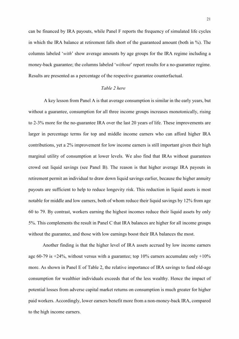
21

can be financed by IRA payouts, while Panel F reports the frequency of simulated life cycles

in which the IRA balance at retirement falls short of the guaranteed amount (both in %). The

columns labeled ‘with’ show average amounts by age groups for the IRA regime including a

money-back guarantee; the columns labeled ‘without’ report results for a no-guarantee regime.

Results are presented as a percentage of the respective guarantee counterfactual.

Table 2 here

A key lesson from Panel A is that average consumption is similar in the early years, but

without a guarantee, consumption for all three income groups increases monotonically, rising

to 2-3% more for the no-guarantee IRA over the last 20 years of life. These improvements are

larger in percentage terms for top and middle income earners who can afford higher IRA

contributions, yet a 2% improvement for low income earners is still important given their high

marginal utility of consumption at lower levels. We also find that IRAs without guarantees

crowd out liquid savings (see Panel B). The reason is that higher average IRA payouts in

retirement permit an individual to draw down liquid savings earlier, because the higher annuity

payouts are sufficient to help to reduce longevity risk. This reduction in liquid assets is most

notable for middle and low earners, both of whom reduce their liquid savings by 12% from age

60 to 79. By contrast, workers earning the highest incomes reduce their liquid assets by only

5%. This complements the result in Panel C that IRA balances are higher for all income groups

without the guarantee, and those with low earnings boost their IRA balances the most.

Another finding is that the higher level of IRA assets accrued by low income earners

age 60-79 is +24%, without versus with a guarantee; top 10% earners accumulate only +10%

more. As shown in Panel E of Table 2, the relative importance of IRA savings to fund old-age

consumption for wealthier individuals exceeds that of the less wealthy. Hence the impact of

potential losses from adverse capital market returns on consumption is much greater for higher

paid workers. Accordingly, lower earners benefit more from a non-money-back IRA, compared

to the high income earners.

22

Panel D summarizes the IRA payouts which mirror results of prior Panels. For the top

(middle) earners, non-guaranteed IRA payouts are 10% (13%) higher than with guarantees; for

low earners, IRA payouts rise by 24%. Yet this large improvement for the lowest earners

provides only a modest (2%) total consumption increase, as their IRA balances and liquid assets

are still low.24 Panel F quantifies the downside risk of switching from a guaranteed to a non-

guaranteed IRA regime for each of the three income groups. By construction, for scenarios with

money-back guarantees, there is no shortfall risk (defined as having an IRA balance at

retirement below the sum of contributions and subsidies). Even without a guarantee, the

shortfall probability for high and middle income earners is moderate, at 3.9% and 5.8%,

respectively. Yet for low earners, the shortfall probability is much higher, at 11.2%. This

difference can be attributed to the fact that low income earners tend to contribute considerably

later, around age 57.3, versus age 48.4 for high and 51.1 for middle income earners. Forgoing

early contributions implies that the low earners build only a small cushion against adverse

capital market developments, and therefore they are more vulnerable to losses in later lives.

Though low earners benefit the least from additional consumption and are exposed to

the increase in shortfall risk without guarantees, Table 3 reveals that the proportion of these

individuals better off without the guarantee is the largest: from ages 60-79, 71% are better off,

and 88% between the ages of 80-100. The proportions are similar for middle earners, at 75%

and 87%, respectively. The smallest group benefited by having no guarantee is the high earners,

yet still the majority is in better circumstances: 69% (77%) of this group enjoys more

consumption between ages 60-79 (ages 80-100).

Table 3 here

24 Bonin (2009) and Börsch-Supan et al. (2008) note that poor households may find it unattractive to save in pension products due to high current consumption utility, such that tax incentives tend to be weaker than for their wealthier counterparts.

23

It is also of interest to compare IRA participation rates, which we do in Table 4. Here

we see that for most income and age groups, the share of workers contributing to an IRA is at

least as high without as with a guarantee.25 Nevertheless, and quite interestingly, high earners

follow a hump-shaped participation pattern over the life cycle. Middle income earners trace out

a flat trajectory, while participation rises for low earners near retirement to boost their private

pension assets after having contributed little during their early and middle years. This pattern

should be of interest to policymakers seeking to reduce retirees’ sole reliance on statutory

pension benefits as a source of old-age income.

Table 4 here

The first two columns of Table 5 provide the same information as Table 2, but results

are now averaged over the entire population instead of by income subsets. Results for a real

guarantee (columns 3 and 6) are discussed below, in the robustness check section. Columns 4

and 5 at the aggregate level show results for the alternative capital market environment with

interest and inflation rates of 0%. Here it is clear that the negative implications of the mandatory

money-back guarantee are amplified, which we ascribe to the disproportionately higher costs

of providing the guarantee. Table 5 also reveals that IRA balances (Panel C) and payouts (Panel

D) during retirement plummet by about 67% under the zero interest rate regime. By contrast,

liquid savings rise by over 40% as of the retirement date (Panel B). Yet the higher liquid savings

are insufficient to fully compensate for lower IRA payouts, so old-age consumption (Panel A)

falls in the low return scenario by around 9% compared to the historically ‘normal’

environment. Importantly, the relative advantage of abolishing the guarantee in terms of old-

age consumption rises substantially from 3% to 11% of retiree consumption, versus the normal

capital market scenario. In other words, eliminating the money-back guarantee would strongly

benefit retirees in the current low return environment.

25 One exception is for the high earners at young ages; this could be because many of them earned little when young and thus had lower participation rates at that time.

24

Table 5 here

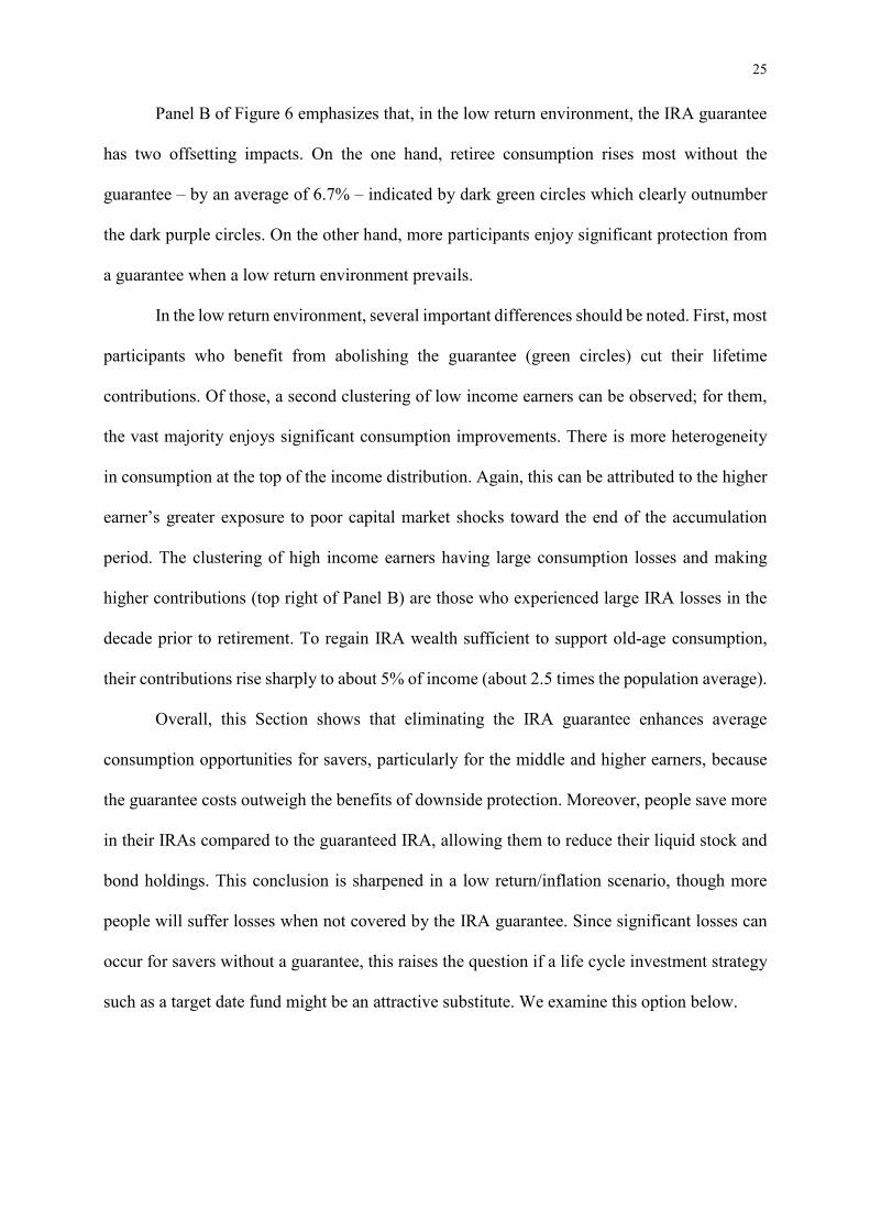
Figure 6 provides insights into the heterogeneous changes in contributions and retiree

consumption by average annual income, without versus with the guarantee. The x-axis shows

average yearly lifetime labor income, while the y-axis displays the change in IRA contributions

(including subsidies, expressed as percent of lifetime labor income) if the IRA’s investment

guarantee were eliminated. Each of the 100,000 circles indicates how much individuals would

gain or lose from abolishing the money-back guarantee. Green (purple) circles depict increases

(decreases) in average yearly retirement consumption, and darker color circles reflect larger

changes (white circles indicate small or zero changes).

Figure 6 here

For the base case calibration with historically normal interest and inflation rates, Panel

A indicates that most participants (about 81%) increase their contributions without the

guarantee. Moreover, the dispersion in contribution changes is wider for high versus low

earners. Consistent with the bottom Panel of Figure 5, green circles dominate, so most retirees

enjoy greater consumption without the guarantee. Those benefitting from elimination of the

guarantee also boost their contributions except for some low income workers whose anticipated

consumption rises, and they therefore can cut back on contributions. The circle colors indicate

that those who neither gain nor lose from the IRA guarantee status predominate among workers

who cut their contributions. Importantly, while average retiree consumption is unaffected,

eliminating the guarantee still leaves them with higher consumption during the accumulation

phase. Moreover, those experiencing reduced old-age consumption are mainly high-income

earners. As shown in Table 2, the relative importance of IRA savings to fund old-age

consumption for wealthier individuals exceeds that of the less wealthy. Consequently, without

the IRA money-back guarantee, the wealthy become more vulnerable to negative capital market

experiences late in life, compared to their less wealthy counterparts.

25

Panel B of Figure 6 emphasizes that, in the low return environment, the IRA guarantee

has two offsetting impacts. On the one hand, retiree consumption rises most without the

guarantee – by an average of 6.7% – indicated by dark green circles which clearly outnumber

the dark purple circles. On the other hand, more participants enjoy significant protection from

a guarantee when a low return environment prevails.

In the low return environment, several important differences should be noted. First, most

participants who benefit from abolishing the guarantee (green circles) cut their lifetime

contributions. Of those, a second clustering of low income earners can be observed; for them,

the vast majority enjoys significant consumption improvements. There is more heterogeneity

in consumption at the top of the income distribution. Again, this can be attributed to the higher

earner’s greater exposure to poor capital market shocks toward the end of the accumulation

period. The clustering of high income earners having large consumption losses and making

higher contributions (top right of Panel B) are those who experienced large IRA losses in the

decade prior to retirement. To regain IRA wealth sufficient to support old-age consumption,

their contributions rise sharply to about 5% of income (about 2.5 times the population average).

Overall, this Section shows that eliminating the IRA guarantee enhances average

consumption opportunities for savers, particularly for the middle and higher earners, because

the guarantee costs outweigh the benefits of downside protection. Moreover, people save more

in their IRAs compared to the guaranteed IRA, allowing them to reduce their liquid stock and

bond holdings. This conclusion is sharpened in a low return/inflation scenario, though more

people will suffer losses when not covered by the IRA guarantee. Since significant losses can

occur for savers without a guarantee, this raises the question if a life cycle investment strategy

such as a target date fund might be an attractive substitute. We examine this option below.

26

5 Robustness Checks

Having investigated the economic implications of a money-back nominal IRA guarantee

on plan participant behavior using a standard CRRA framework and ignoring fees, we next

explore alternative preferences and fee structures, to demonstrate that our results are robust to

these variations. Moreover, we confirm that an inflation-protected guarantee amplifies the

concerns already noted for nominal guarantees. Remarkably, we show that a life cycle or target

date strategy with insufficient equity exposure can be even less attractive than a money-back

IRA guarantee.

5.1 Real Guarantees

Thus far, we have taken as given the existing Riester IRA regulation requiring a nominal

money-back guarantee at the end of the accumulation phase. Nevertheless, some authors have

explored inflation protection over the guarantee contract’s term.26 The appeal of a real guarantee

is that it preserves savers’ purchasing power, though it requires higher costs and therefore can

erode account balances over time. For instance, Pennacchi (1999) and Fischer (1999) discussed

the Latin American pension market where real guarantees were promised during times of high

inflation: here the guarantees were usually not market-based (replicated by combining tradeable

assets) but instead were provided by governments.

To illustrate how an inflation-protected guarantee might work in our context, we replace

the nominal with a real money-back guarantee.27 To this end, instead of buying at-the-money

put options with the contributions, in-the-money put options must be purchased with strike

prices accounting for the change in inflation until retirement. Results for the base calibration in

Column 3 of Table 5 support our conjecture that real guarantees erode consumption even more

26 For instance, Feldstein and Samwick (2002) and Feldstein (2009) considered real guarantees for investment-based Social Security reforms in the U.S. 27 We keep the annuity payouts as nominal to maintain consistency with previous analyses.

27

than nominal guarantees.28 Specifically, old-age consumption under a real guarantee falls short

of the nominal guarantee scheme by 2 to 4% on average (Panel A). The average timing and the

sum of contributions is very similar across guarantee designs, so the approximately 15% decline

in account balances and payouts may be directly attributed to higher guarantee costs (Panels C

and D). To compensate for lower IRA payouts under a real guarantee, liquid saving increases

beyond the levels in the other two cases.

Table 5 here

Since our analysis shows that a real guarantee compounds the negative effects of nominal

guarantees, we conclude that real guarantees also cost more in the form of lower consumption.

5.2 Life Cycle Target Date Funds

Some have proposed that life cycle or target date funds could constitute an alternative

to money-back guarantees as a risk mitigation technique. This type of investment approach

follows an age-based allocation rule, starting with higher equity shares early in life and

gradually rebalancing along a glide path to less risky securities (such as bonds) near and into

retirement (Vanguard, 2017). In the U.S., most of the $5 trillion invested in 401(k) defined

contribution retirement plans is automatically defaulted into target date investment strategies.

The U.S. legislative framework has encouraged this practice, with the 2006 Pension Protection

Act permitting plan sponsors to include target date funds as ‘qualified default investment

alternatives’ in participant-directed defined contribution plans. The regulatory environment for

the European Union’s Basic PEPP also allows providers to use a life cycle strategy under the

presumption that it is ‘consistent with the objective of allowing the PEPP saver to recoup the

capital’ instead of a money-back guarantee (see EU 2019/1238 (54) and Art. 46).

28 For the zero inflation scenario in Column 6 of Table 5, results correspond to those of the nominal guarantee in Column 4.

28

There are many variants of life cycle strategies in the market, but two approaches are

common.29 One starts investors at a relative high equity exposure and reduces this share

annually using a moderate adjustment factor. For example, Malkiel (1996) postulates that the

percentage of IRA assets invested in equities should follow a ‘100 - age’ rule. A second

approach retains a high equity exposure during much of the accumulation period, but imposes

a stronger de-risking pattern near retirement. For instance Cocco et al. (2005) proposed

reducing the 100% equity exposure from age 41 onwards by 2.5 percentage points per year until

retirement (hereafter referred to as ‘100-until-40, -2.5’ rule). Using a simulation approach,

Berardi et al. (2018) have studied a range of other life cycle approaches, finding that the value

of contributions can be preserved with over 99% probability given an intermediate investment

horizon of 40 years; with a 95% probability, the final account balance is likely to be worth at

least 1.8 times the sum of contributions. While these results suggest that a life cycle approach

could be appealing from a shortfall perspective, it is as yet unclear whether decreasing the risky

share is preferable to a money-back guarantee.

Accordingly, we extend our analyses by introducing the two life cycle approaches

sketched above, where the IRA’s equity share during the participant’s work life is set either

using a ‘100 - age’ rule, or a ‘100-until-40, -2.5’ rule. The remainder of the portfolio is then

invested in risk-free bonds. To maintain consistency with the previous setup, we assume that

the IRA switches to a 20% equity exposure after retirement. Results appear in Tables 6 and 7,

for the base ‘normal’ case, as well as the low interest rate and inflation scenario.

Tables 6 and 7 here

For the 3% nominal interest base case, Panel A of Table 6 depicts old-age consumption

when the IRA invests in a ‘100 minus age’ life cycle fund; this proves to be some 6-11% below

that achieved in the guarantee case. Panel A of Table 7 indicates that, during retirement, two-

29 For an overview see Poterba et al. (2006) and Berardi et al. (2018).

29

thirds of plan participants can consume more if they have a guaranteed IRA compared to the

more conservative life cycle fund. This is because people accumulate about one-third less in

their IRAs with the conservative life cycle fund, compared to the guarantee case (Panel C, Table

6).30 As a result, also the share of consumption financed by IRA payouts is 6-8 percentage

points lower than that resulting from a 100% equity exposure with a money-back guarantee.

This highlights the fact that the life cycle glide path reduces the equity share too quickly

during the accumulation phase so – even with higher contributions – asset accumulation is

hampered and less capital can be withdrawn during the payout phase (Panel D, Table 6).

Although this disadvantage can be partly mitigated by the alternative life cycle rule (‘100-until-

40, -2.5’), it cannot be eliminated. Panel F of Table 6 confirms Berardi et al.’s (2018) finding

that, in a normal capital market scenario, shortfalls are rare when the IRA is invested in a life

cycle fund, occurring in only 0.8% (1.3%) of the cases for the ‘100 minus age’ rule (‘100-until-

40, -2.5‘ rule) versus the 6.5% shortfall probability without a guarantee.31

Next we explore how results differ in a less propitious capital market environment.

Guarantee costs for money-back guarantees become more expensive, due to higher put

premiums. Also the larger share of bonds in the life cycle strategy produces lower returns.

Compared to the IRA guarantee case, expected old-age consumption in Table 6 with the

conservative (‘100 minus age’) target date fund falls short by only 1-2% (Panel A), and the

share of consumption (including housing) financed by IRA payouts is only 0.5-0.8 percentage

points lower (Panel E). Panel B of Table 7 shows that less than half (43-44%) of retirees

anticipate consuming more with the life cycle fund in their IRAs, yet the shortfall probability

(Panel F of Table 6) increases substantially to 18.7%.

30 Interestingly, the lower IRA balances are not driven by lower contributions: in fact, the sum of contributions is the highest for the life cycle fund case, averaging €29,785, followed by the no guarantee case (€24,446), and the guarantee case last (€22,682). 31 We note, however, that Berardi et al. (2018) have a money-weighted timing of contributions in the middle of the accumulation phase, while in our case it is about five years later (after 26.2 years); ours provides less time for compounding. Moreover, around half of their bond investments consist of credit-risky bonds, enabling their portfolios to benefit from a risk premium.

30

By contrast, in the zero interest rate scenario, the ‘100-until-40, -2.5’ fund holding more

equity can partly overcome the burden of a high bond allocation during the accumulation phase.

Compared to the money-back IRA, this more aggressive life cycle approach provides 1-2%

more old-age consumption (Panel A, Table 6). Moreover about 55% of retirees can expect to

consume more (Panel B, Table 7), and the share of expenditures in old-age financed by IRA

payouts increases by 1.2-1.8 percentage points (Panel E, Table 6). However, the shortfall

probability is high, at 17.6%, a value inconsistent with the EU regulatory objective of

‘recouping the capital’ of the PEPP saver.

5.3 Epstein-Zin-Weil Preferences

The use of CRRA preferences links the coefficient of risk aversion (!) and the elasticity

of intertemporal substitution (EIS), inasmuch as one is the inverse of the other. To free up these

parameters, we also investigate the Epstein-Zin-Weil utility formulation (Epstein and Zin,

1989; Weil, 1989); this approach allows independent preferences for smoothing across time

and states. Here, consumption differences for the alternative guarantee designs are affected two

ways. First, lowering (increasing) the EIS means relative risk aversion is smaller (larger) than

1/EIS, so the individual will devote less (more) emphasis on consumption smoothing across

states, compared to CRRA preferences. This should decrease (increase) the overall demand for

saving and narrow (increase) differences in resulting retiree consumption under the guarantee.

Second, the relative attractiveness of the with/without guarantee scheme changes. The

guaranteed IRA provides smaller variation in payouts, but it also pays off less compared to the

non-guaranteed IRA. For low (higher) levels of EIS, this makes the guaranteed IRA less (more)

attractive relative to the non-guaranteed IRA, due to the consumer’s weaker preference for

smoothing across states.

Two effects work in opposite directions, so it is unclear which effect dominates, ex ante.

To resolve this, the first four columns of Table 8 provide results using Epstein-Zin-Weil

preferences (as in Córdoba and Ripoll, 2017) for the base case calibration. Holding fixed the

31

coefficient of relative risk aversion, we then reduce (increase) the CRRA-implied �, = 1/! =1/7 to 0.1 (0.2), to permit an assessment of changing the EIS on IRA and liquid savings

demand, and on resulting consumption opportunities. Lowering the EIS produces a substantial

decline in total savings, by about 14% between ages 60-79 (Panels B and C) relative to the

CRRA case with the IRA guarantee, and an even larger reduction, of about 17%, relative to the

CRRA case and no guarantee (Table 5, columns 1 and 2).32 Moreover, for both guarantee

designs, the IRA share as percent of total assets falls by about 5.5 percentage points.33

Accordingly, removing the guarantee enhances savers’ wellbeing less, driven by the substantial

reduction in overall savings more than by a change in relative attractiveness of the two

guarantee designs.

Table 8 here

When the EIS is increased to 0.2, the opposite effects obtain. Total saving rises by 26%

to 28% for the guarantee due to the stronger demand for smoothing across states compared to

results using CRRA parameters. The IRA provides better smoothing across states than liquid

savings due to the embedded deferred annuity, so a higher EIS value translates to more of the

portfolio being held in the IRA. The IRA share as a percent of total assets rises slightly more,

by 6.2% for the guaranteed IRA versus 5.6% for the non-guaranteed scheme. The consumption

improvement resulting from removing the IRA guarantee is greater when the EIS rises, relative

to the CRRA case.

The evidence shows that, of the two channels via which EIS affects consumption, the

adjustment in total savings dominates the effect of changing the guarantee’s attractiveness.

Also, the positive effect of abolishing the guarantee rises when the EIS is higher, meaning that

individuals favor consumption smoothing more strongly across states. Somewhat

counterintuitively, the guaranteed IRA that smooths consumption more loses ground to the non-

32 As the IRA is fully depleted beyond age 84, asset holdings in the final periods cannot be analyzed accurately. 33 For the guarantee case it falls from 70.7% to 65.3%, and with no guarantee, from 74.9% to 69.2%.

32

guaranteed alternative, because the increased consumption gained by abolishing the guarantee

compensates for the individual’s benefit of smoother consumption. In summary, then, results

using Epstein-Zin-Weil preferences confirm the conclusions of prior sections: a non-guaranteed

IRA considerably enhances consumption relative to that feasible with a guaranteed IRA.

5.4 Front-End Loads on Contributions

Thus far we have abstracted from sales charges levied on IRA contributions, yet in the

German context, investing in an IRA requires payment of front-end loads (no fees are charged

on redemptions during the payout phase). Such fees could affect the demand for guarantees for

two reasons. First, the loads might render the IRAs so unattractive that savers could contribute

little or nothing. In such a case, the guarantee specifications become irrelevant. Second, the

loads could interact with expensive guarantee costs and discourage IRA investors from

contributing. In this latter case, the IRA’s appeal would be enhanced by abolishing the

guarantee, and consumption without a guaranteed IRA might be even greater than with the

guarantee (as illustrated in Section 4).

The final two columns of Table 8 document that IRA investments are still substantial

even with a front-end load of 5% on contributions. Yet unsurprisingly, Panels C and D show

that such loads lead to less IRA wealth accumulated for the base calibration; as a consequence,

payouts are also lower than in the absence of such fees (compare the first two columns of Table

5). Importantly, participant contributions do not decline symmetrically. Given the front end

load, lifetime contributions with the guarantee fall by 7.8% (to €20,900); without the guarantee,

contributions drop by only about 4.5% (to €23,300).34 IRA payouts differ by 12% without the

extra loads, but by 13-14% when front-end loads are taken into account. As a result, old-age

consumption differences are greater than without fees. Overall, with realistic sales loads, the

negative consequences of the IRA guarantees are slightly worse.

34 Intuitively, with fees average timing of contributions is a little earlier to give invested capital more time to earn return (about 0.88 years earlier with a money-back guarantee and 0.47 years in absence of a guarantee).

33

6 Conclusions

This study illustrates how money-back guarantees in individual retirement accounts can

alter lifetime consumption opportunities and portfolio decisions. We build and calibrate a

dynamic life cycle model where the saver has access to stocks, bonds, and IRAs of the German

Riester type, and we show that old-age consumption could rise substantially for most people if

the money-back guarantee were eliminated. This is because removing the IRA guarantee saves

money otherwise spent to provide the guarantee, which could instead be directly invested to the

benefit of the saver.

During what many believed to be a ‘normal’ long-term capital market environment, with

a 3% nominal interest rate, we show that average retirement consumption could rise by 1-3% if

the IRA fully invested in equities had no guarantee. Moreover, three-quarters of savers could

consume more early in retirement, rising to almost 90% of retirees near the end of life.

Accordingly, a IRA money-back guarantee is evidently not a cost-effective way to overcome

longevity risk for the older population. Of course giving up the guarantee does expose

participants to shortfall risks that must be weighed against the higher return potential. We show

that switching to a non-guaranteed IRA is appealing overall, despite the fact that those having

adverse capital market experiences would experience losses compared to the guarantee case.

In what we call the ‘new normal’ macroeconomic scenario, with a 0% risk-free rate, our

results are more nuanced. It remains the case that average consumption would rise by 3-11% if

the guarantee were removed. Yet the fraction of people experiencing shortfalls also increases

to 18.1%. Accordingly, examining heterogeneity in outcomes becomes important. Remarkably,

the vast majority of low to middle lifetime earners will be better served in terms of old-age

consumption if they do not have the money-back guarantee; higher income savers benefit the

most from the guarantee. Additionally, in a persistent low return scenario, industry providers

may be unwilling to offer guaranteed IRAs if they must systematically run losses to make up

for shortfalls not covered by hedging payoffs. Such obligations could eventually force IRA

34

providers to abandon the market, which would be detrimental to the future of the funded private

retirement system. If a real rather than a nominal investment guarantee were required, this

would harm savers more.

Against this background, we also evaluated whether life cycle or target date funds

should be considered as a viable alternative to the money-back IRA guarantee approach. For

example, U.S. 401(k) retirement plans and the Pan-European Personal Pension Product (PEPP)

specify such a strategy as a possible default investment option. Here we show that the appeal

depends on the interest rate environment and the design of the glide path. In a normal interest

rate environment, a life cycle fund results in less old-age consumption, compared to the money-

back approach. By contrast, in a low interest rate environment, life cycle funds can provide

consumption comparable to that under the money-back guarantee scenario. For instance, a life

cycle fund with a conservative equity exposure, such as the traditional ‘100 minus age’ rule,

results in lower old-age consumption for both the normal and low interest rate scenarios. By

contrast, a life cycle approach with a higher equity exposure maintained longer (e.g. reducing

a 100% equity after age 40 by 2.5 percentage points per year) can generate higher consumption.

In sum, our work confirms that money-back guarantees were an effective way to protect

workers from investment losses in their IRAs during a ‘normal’ capital market environment.

Unfortunately, when interest rates are persistently low, the money-back IRA does not protect

the saving public; rather it can cause unintended damage eroding old-age consumption below

what it would be otherwise. Life cycle funds with sufficient equity exposure could be seen as

an alternative risk mitigation strategy to the money-back IRA, and we show these are preferable

to a guaranteed IRA.

Our findings have general relevance for policymakers, regulators, and plan sponsors in

many nations implementing individual retirement accounts to build funded pensions, seeking

to respond to the challenges of population aging. These include the U.S. 401(k) retirement

accounts, the Pan European Pension Product (PEPP) recently launched by the European

35

Parliament, and defined contribution plans in Australia, Hong Kong, and Chile. Of key

importance in such funded pension systems is the approporiate design of default investment

options which should, on the one hand, protect savers from downside risks, while at the same

time preserving the opportunity for savers to access the capital markets. Regulators and

consumers will need to better understand the opportunity costs associated with money-back

guarantees and other risk mitigation techniques such as life cycle funds.

36

References

Berardi, A., C. Tebaldi, and F. Trojani (2018). “Consumer Protection and the Design of the Default Option of a Pan-European Pension Product.” Working paper. https://ssrn.com/abstract=3142243

Black, F., and M. Scholes (1973). “The Pricing of Options and Corporate Liabilities.” Journal

of Political Economy 81(3): 637-654.

Bonin, H. (2009). “15 Years of Pension Reform in Germany: Old Successes and New Threats.” Geneva Papers on Risk and Insurance 34(4): 548-560.

Börsch-Supan, A., T. Bucher-Koenen, M. Coppola, and B. Lamla (2015). “Savings in Times of Demographic Change: Lessons from the German Experience.” Journal of Economic

Surveys 29(4): 807-829.

Börsch-Supan, A., M. Coppola, and A. Reil-Held (2012). “Riester Pensions in Germany: Design, Dynamics, Targeting Success and Crowding-In.” In Matching Contributions

for Pensions: A Review of International Experience, Eds. R. P. Hinz, R. Holzmann, D. Tuesta, and N. Takayama. World Bank: 81-102.

Börsch-Supan, A., A. Reil-Held, and D. Schunk (2008). “Saving Incentives, Old-Age Provision and Displacement Effects: Evidence from the Recent German Pension Reform.” Journal of Pension Economics and Finance 7(3): 295-319.

Bundesministerium für Arbeit und Soziales (BMAS, 2017). “Entwicklung der Riester-Verträge. ” Accessed 21-Jun-2017. http://www.bmas.de/SharedDocs/Downloads/DE/ Thema-Rente/riesterrente-I-2017.pdf

Carroll, C. D., and A. A. Samwick (1997). “The Nature of Precautionary Wealth.” Journal of

Monetary Economics 40(1): 41-71.

Chai, J., W. Horneff, R. Maurer, and O. S. Mitchell (2011). “Optimal Portfolio Choice over the Life Cycle with Flexible Work, Endogenous Retirement, and Lifetime Payouts.” Review

of Finance 15(4): 875-907.

Cocco, J. F. and F. J. Gomes (2012). “Longevity Risk, Retirement Savings, and Financial Innovation.” Journal of Financial Economics 103(3): 507-529.

Cocco, J. F., F. J. Gomes, and P. J. Maenhout (2005). “Consumption and Portfolio Choice over the Life Cycle.” Review of Financial Studies 18(2): 491-533.

Córdoba, J. C. and M. Ripoll (2017). “Risk Aversion and the Value of Life.” Review of

Economic Studies 18(4): 1472-1509.

Deutsche Bundesbank (2016). “Monatsbericht März 2016.” Accessed 03-Oct-2017. https://www.bundesbank.de/resource/blob/664820/12eb34cfdb12cf3098c4ab2fca1519c0/mL/2016-03-monatsbericht-data.pdf

Dolls, M., P. Doerrenberg, A. Peichl, and H. Stichnoth (2018). “Do Retirement Savings Increase in Response to Information about Retirement and Expected Pensions?” Journal

of Public Economics 158: 168-179.

Epstein, L. G. and S. E. Zin (1989). “Substitution, Risk Aversion, and the Temporal Behavior of Consumption and Asset Returns: A Theoretical Framework.” Econometrica 57(4): 937-969.

Ernst & Young (2017). “Study on the Feasibility of a European Personal Pension Framework.” https://ec.europa.eu/info/sites/info/files/170629-personal-pensions-study_en.pdf.

37

European Central Bank (ECB, 2018). “The Definition of Price Stability.” Accessed 05-Oct-2018. https://www.ecb.europa.eu/mopo/strategy/pricestab/html/index.en.html

European Commission (2017). “Proposal for a Regulation of the European Parliament and of the Council on a Pan-European Personal Pension Product (PEPP).” Accessed 08-Sep-2017. https://eur-lex.europa.eu/legal-content/EN/TXT/HTML/?uri=CELEX:52017PC0 343&from=EN

European Commission (2019). “Capital Markets Union: Pan-European Personal Pension Product (PEPP).” Accessed 28-Apr-2019. http://europa.eu/rapid/press-release_MEMO-19-1993_en.htm

Fagereng, A., C. Gottlieb, and L. Guiso (2017). “Asset Market Participation and Portfolio

Choice over the Life‐Cycle.” Journal of Finance 72(2): 705-750.

Fehr, H. and C. Habermann (2008). “Risk Sharing and Efficiency Implications of Progressive Pension Arrangements.” Scandinavian Journal of Economics 110(2): 419-443.

Feldstein, M. (2009). “Reducing the Risk of Investment-Based Social Security Reform.” In Social Security Policy in a Changing Environment, Eds. J. R. Brown, J. B. Liebman, and D. A. Wise. University of Chicago Press: 201-218.

Feldstein, M. and A. Samwick (2002). “Potential Paths of Social Security Reform.” Tax Policy

and the Economy 16: 181-224.

Fischer, K. P. (1999). “Pricing Pension Fund Guarantees: A Discrete Martingale Approach.” Canadian Journal of Administrative Sciences 16(3): 256-266.

Fuchs-Schündeln, N., D. Krueger, and M. Sommer (2010). “Inequality Trends for Germany in the Last Two Decades: A Tale of Two Countries.” Review of Economic Dynamics 13(1): 103-132.

Horneff, V., R. Maurer, and O. S. Mitchell (2018). “How Persistent Low Expected Returns Alter Optimal Life Cycle Saving, Investment, and Retirement Behavior.” In How

Persistent Low Returns Will Shape Saving and Retirement, Eds. R. Clark, R. Maurer, and O. S. Mitchell. Oxford University Press: 119-131.

Horneff, V., R. Maurer, O. S. Mitchell, and R. Rogalla (2015). “Optimal Life Cycle Portfolio Choice with Variable Annuities Offering Liquidity and Investment Downside Protection.” Insurance: Mathematics and Economics 63: 91-107.

Hubener, A., R. Maurer, and O. S. Mitchell (2016). “How Family Status and Social Security Claiming Options Shape Optimal Life Cycle Portfolios.” Review of Financial Studies 29(4): 937-978.

Investment Company Institute (ICI, 2018). “Millions of Workers Continue to Save for

Retirement Through 401(k) Plans.” https://www.ici.org/401k/news/18_news_401kday

Kaschützke, B., and R. Maurer (2011). “The Private Life Annuity Market in Germany: Products and Money’s Worth Ratios.” In Securing Lifelong Retirement Income, Eds. O. S. Mitchell, J. Piggott, and N. Takayama. Oxford University Press: 131-158.

Koijen, R. S., T. E. Nijman, and B. J. Werker (2010). “Optimal Annuity Risk Management.” Review of Finance 15(4): 799-833.

Krebs, T. and Y. Yao (2016). “Labor Market Risk in Germany.” IZA Discussion Paper No. 9869.

Lachance, M.-E., and O. S. Mitchell (2003). “Guaranteeing Individual Accounts.” American

Economic Review P&P 93(2): 257-260.

38

Love, D. A. (2010). “The Effects of Marital Status and Children on Savings and Portfolio Choice.” Review of Financial Studies 23(1): 385-432.

Malkiel, B. G. (1996). A Random Walk Down Wall Street: Including a Life-Cycle Guide to

Personal Investing. W. W. Norton. & Co Inc.

Pennacchi, G. G. (1999). “The Value of Guarantees on Pension Fund Returns.” Journal of Risk

and Insurance 66(2): 219-237.

Poterba, J., J. Rauh, S. Venti, and D. Wise (2006). “Lifecycle Asset Allocation Strategies and the Distribution of 401(k) Retirement Wealth.” NBER Working Paper 11974.

Union Investment (2018). “Studie: Anlegerbarometer - drittes Quartal 2018.” Accessed 11-Oct-2018. https://unternehmen.union-investment.de/startseite-unternehmen/presseservice/ %20pressemitteilungen/alle-pressemitteilungen/2018/Studie--Anlegerbarometer---dritt es-Quartal-2018.html

Van Hulle, K. (2019). “Solvency Requirements for EU Insurers.” Intersentia Ltd, United Kingdom.

Vanguard (2017). “How America Saves 2017.” https://pressroom.vanguard.com/nonindexed/ How-America-Saves-2017.pdf

Weil, P. (1989). “The Equity Premium Puzzle and the Risk-Free Rate Puzzle.” Journal of

Monetary Economics 24(3): 401-421.

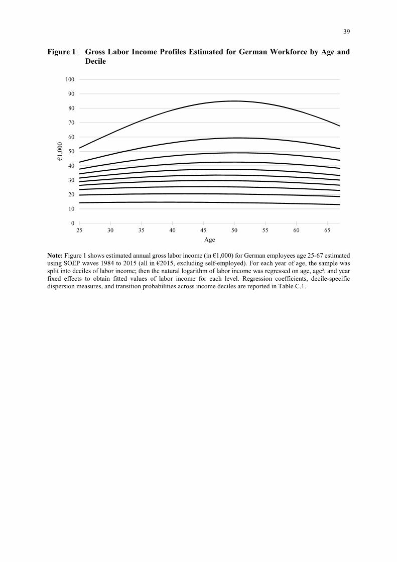
39

Figure 1: Gross Labor Income Profiles Estimated for German Workforce by Age and

Decile

Note: Figure 1 shows estimated annual gross labor income (in €1,000) for German employees age 25-67 estimated using SOEP waves 1984 to 2015 (all in €2015, excluding self-employed). For each year of age, the sample was split into deciles of labor income; then the natural logarithm of labor income was regressed on age, age², and year fixed effects to obtain fitted values of labor income for each level. Regression coefficients, decile-specific dispersion measures, and transition probabilities across income deciles are reported in Table C.1.

0

10

20

30

40

50

60

70

80

90

100

25 30 35 40 45 50 55 60 65

€1

,00

0

Age

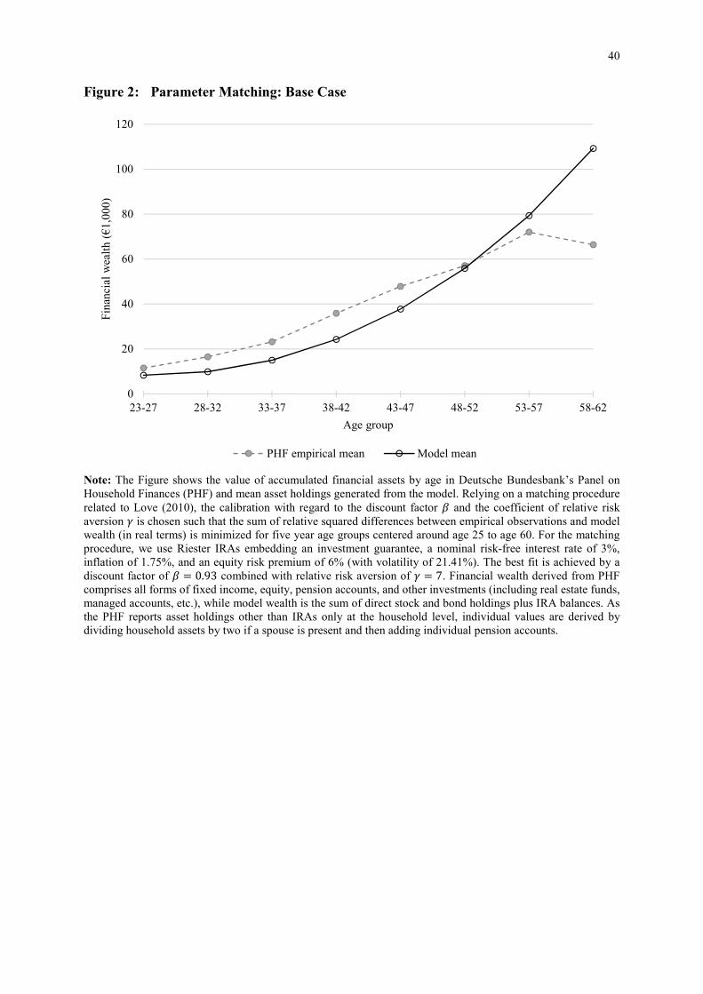
40

Figure 2: Parameter Matching: Base Case

Note: The Figure shows the value of accumulated financial assets by age in Deutsche Bundesbank’s Panel on Household Finances (PHF) and mean asset holdings generated from the model. Relying on a matching procedure

related to Love (2010), the calibration with regard to the discount factor ' and the coefficient of relative risk

aversion ! is chosen such that the sum of relative squared differences between empirical observations and model wealth (in real terms) is minimized for five year age groups centered around age 25 to age 60. For the matching procedure, we use Riester IRAs embedding an investment guarantee, a nominal risk-free interest rate of 3%, inflation of 1.75%, and an equity risk premium of 6% (with volatility of 21.41%). The best fit is achieved by a

discount factor of ' = 0.93 combined with relative risk aversion of ! = 7. Financial wealth derived from PHF comprises all forms of fixed income, equity, pension accounts, and other investments (including real estate funds, managed accounts, etc.), while model wealth is the sum of direct stock and bond holdings plus IRA balances. As the PHF reports asset holdings other than IRAs only at the household level, individual values are derived by dividing household assets by two if a spouse is present and then adding individual pension accounts.

0

20

40

60

80

100

120

23-27 28-32 33-37 38-42 43-47 48-52 53-57 58-62

Fin

anci

al w

ealt

h (

€1

,00

0)

Age group

PHF empirical mean Model mean

41

Figure 3: Life Cycle Profiles With and Without IRA Guarantee: Base Case

Panel A: With guarantee Panel B: Without guarantee

Note: The Figure shows mean values of labor and pension income, non-housing consumption, financial asset holdings (bonds, stocks, and Riester account balances) and retirement plan payouts (in €2015). Panel A refers to the base case, where the nominal risk-free rate is 3% and inflation is 1.75%. Stock investments earn a risk premium

of 6% and volatility of 21.41%. Preference parameters include a discount factor of ' = 0.93 and relative risk

aversion of ! = 7. Panel B refers to the otherwise identical case without a money-back guarantee in the IRA. Mean values are calculated based on 100,000 simulated life cycles which rely on optimal policies that were derived for all possible combinations of current income, cash on hand, IRA balances, guarantee amounts, and annuity payouts. Prior to retirement at age 67, the IRA is fully invested in equities, from age 67 to 84 the asset allocation consists of 20% stocks, and 80% bonds. From age 85 onward, the plan pays out a lifetime annuity. See Section 3 for details.

0

20

40

60

80

100

120

140

25 35 45 55 65 75 85 95

€1

,00

0

Age

0

20

40

60

80

100

120

140

25 35 45 55 65 75 85 95

€1

,00

0

Age

Riester purchase Riester payout Riester account

Income (pre tax) Liquid savings Consumption

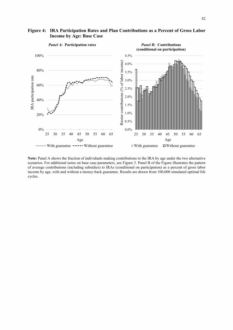
42

Figure 4: IRA Participation Rates and Plan Contributions as a Percent of Gross Labor

Income by Age: Base Case

Panel A: Participation rates

Panel B: Contributions

(conditional on participation)

Note: Panel A shows the fraction of individuals making contributions to the IRA by age under the two alternative scenarios. For additional notes on base case parameters, see Figure 3. Panel B of the Figure illustrates the pattern of average contributions (including subsidies) to IRAs (conditional on participation) as a percent of gross labor income by age, with and without a money-back guarantee. Results are drawn from 100,000 simulated optimal life cycles.

0%

20%

40%

60%

80%

100%

25 30 35 40 45 50 55 60 65

IRA

par

tici

pat

ion r

ate

Age

With guarantee Without guarantee

0.0%

0.5%

1.0%

1.5%

2.0%

2.5%

3.0%

3.5%

4.0%

4.5%

25 30 35 40 45 50 55 60 65

Rie

ster

co

ntr

ibuti

ons

(% o

f la

bo

r in

com

e)

Age

With guarantee Without guarantee

43

Figure 5: Consumption Differences and Percent Better off by Age Without versus With

the IRA Guarantee: Base Case

Note: The fan chart at the top of the Figure illustrates path-wise differences in non-housing consumption drawn from 100,000 simulated optimal life cycles for IRAs without versus with a money-back guarantee. The cyan line represents the mean consumption difference, while darker areas indicate a higher probability density (between the 5 and 95% quantiles). Differences are expressed as a percent of optimal consumption with the money-back guarantee. The bottom panel shows the percentage of individuals with higher optimal consumption without versus with the money-back guarantee. For further notes on base case parameters see Figure 3.

44

Figure 6: Heterogeneity of Impacts by Lifetime Income of Abolishing the IRA

Guarantee: Contributions and Old-Age Consumption

Panel A: �� = 3%, � = 1.75%

Panel B: �� = 0%, � = 0%

Note: This Figure illustrates the effects of abolishing the money-back guarantee on total contributions (including subsidies; in percent of average labor income), and average non-housing consumption during retirement, by average lifetime earnings for a normal (Panel A) and a low (Panel B) interest rate and inflation scenario. Changes in consumption are in percent of the guarantee case. Consumption increases (decreases) are indicated by green (purple) circles and color intensity is stronger for larger changes (white circles indicate tiny changes). Results are drawn from 100,000 simulated optimal life cycles. Further notes on parameters see Figure 3.

45

Table 1: Costs and Benefits of IRA Money-back Guarantees for Participants and

Providers (as a % of total contributions)

Investment horizon (years) 42 30 20 10

Panel A: Guarantee Costs Charged to Participant

if = 3% 9.7 10.7 11.2 10.9

if = 0% 35.8 30.8 25.7 19.0

Panel B: Mean Guarantee Payouts to Participant

if = 3% 3.1 4.3 5.8 7.6

if = 0% 21.9 21.0 19.5 16.9

Panel C: Mean Profits for Provider (Put Hedge Approach)

if = 3% 2.2 1.6 0.7 -0.8

if = 0% -7.0 -6.7 -6.3 -5.5

Note: Table 1 reports mean costs and payouts to the IRA participant and the guarantee product provider resulting from using fairly-priced put options to hedge the money-back guarantee on contributions. The example assumes constant annual contributions, and the guarantee is provided at the end of the investment horizon (retirement). The product provider buys at-the-money put options maturing at retirement to hedge downside risk for each contribution amount. Option pricing follows Black and Scholes (1973) with an assumed equity volatility of 21.41% p.a. and interest rates of 3% and 0%. The simulation relies on 100,000 Monte Carlo paths using the same volatility and an equity risk premium of 6%.

46

Table 2: Heterogeneity Analysis for High, Middle, and Low Income Workers: Base

Case

Lifetime income Top 10% Middle 10% Bottom 10%

Guarantee With Without With Without With Without

Panel A: Consumption (in €1,000 or percent of guarantee case)

Age 25-39 18.31 100% 15.33 100% 11.88 100%

Age 40-59 22.96 101% 15.77 100% 11.26 100%

Age 60-79 25.23 102% 14.97 101% 9.03 101%

Age 80-100 20.89 103% 12.59 103% 6.89 102%

Panel B: Liquid Savings (in €1,000 or percent of guarantee case)

Age 25-39 19.93 100% 9.44 100% 2.89 100%

Age 40-59 77.16 99% 16.40 96% 3.53 95%

Age 60-79 80.44 95% 22.12 88% 8.58 88%

Age 80-100 10.63 91% 2.26 82% 0.95 81%

Panel C: IRA Balance (in €1,000 or percent of guarantee case)

Age 25-39 6.15 106% 2.61 106% 0.32 109%

Age 40-59 70.26 108% 30.79 110% 4.34 118%

Age 60-79 143.21 110% 68.19 113% 12.80 124%

Age 80-84 33.15 110% 15.76 113% 2.93 124%

Panel D: IRA Payouts (in €1,000 or percent of guarantee case)

Age 67: lump sum 31.64 108% 15.55 113% 4.04 126% Age 68-84: drawdown 11.36 110% 5.40 113% 1.00 124% Age 85-100: annuity 11.38 110% 5.44 113% 1.08 124%

Panel E: Share of Consumption and Housing Costs Financed by IRA Payouts (%)

Age 68-84: drawdown 30.8 33.4 20.7 22.8 4.5 5.4

Age 85-100: annuity 40.2 43.2 25.6 28.1 5.7 6.9

Panel F: IRA Shortfall Probability (%)

Age 67 0.0 3.9 0.0 5.8 0.0 11.2

Note: Panels A-D of Table 2 show mean values (in €1,000) of annual non-housing consumption, liquid assets, IRA balances, and payouts, by age ranges, for the top 10%, middle 10%, and bottom 10% of lifetime income earners. Results for columns labeled ‘Without’ indicate the percent of the respective guarantee values. Panel E quantifies the share (in %) of both consumption and housing costs financed by after-tax payouts from the IRA. Panel F reports the share of simulations where the IRA value at retirement falls short of the sum of contributions and subsidies. IRA assets are held entirely in stocks until retirement (protected with the hedges described above), while after retirement only 20% is allocated to stocks and 80% to bonds. Subgroups are generated using 1,000,000 simulation optimal life cycle paths and summing up individual lifetime labor incomes (all in real terms). For further notes on base case parameters see Figure 3.

47

Table 3: Percent of Individuals by Age and Lifetime Income Decile Having Higher

Consumption Without versus With the IRA Guarantee: Base Case

Age 25-39 40-59 60-79 80-100

Top 10% 62 71 69 77

Middle 10% 60 61 75 87

Bottom 10% 51 43 71 88

Note: Table 3 reports the percent of individuals having higher non-housing consumption without the money-back guarantee, by age and lifetime income decile. Subgroups are generated using 1,000,000 simulation paths for optimal life cycles, adding up individual lifetime labor incomes (in real terms). The baseline case calibration uses a nominal risk-free rate of 3% and inflation rate of 1.75%.

Table 4: Percent of Individuals by Age and Lifetime Income Decile Having Positive IRA

Contributions, Without versus With the IRA Guarantee: Base Case

Age 25-39 40-59 60-66 Guarantee With Without With Without With Without

Top 10% 66 64 82 90 71 74

Middle 10% 40 40 68 68 63 65

Bottom 10% 11 12 35 36 63 69

Note: Table 4 reports the percent of individuals with positive contribution rates with and without the money-back guarantee, by age and lifetime income decile. Subgroups are generated using 1,000,000 simulation paths, adding up individual lifetime labor incomes (in real terms). For further notes on base case parameters see Figure 3.

48

Table 5: Impacts of Different Guarantees: Base Case

Guarantee With

(nominal) Without

With (real)

With

(nominal) Without

With (real)

if 3% 0%

1.75% 0%

Panel A: Consumption (in €1,000 or percent of guarantee case)

Age 25-39 15.21 100% 100% 15.15 100% Same as for With (nominal)

Age 40-59 16.22 100% 100% 15.86 101%

Age 60-79 15.69 101% 98% 14.28 103%

Age 80-100 12.98 103% 96% 11.17 111%

Panel B: Liquid Savings (in €1,000 or percent of guarantee case)

Age 25-39 9.96 100% 102% 10.77 95%

Age 40-59 24.42 98% 105% 31.49 89%

Age 60-79 29.42 91% 109% 41.45 82%

Age 80-100 3.25 85% 111% 3.74 67%

Panel C: IRA Balance (in €1,000 or percent of guarantee case)

Age 25-39 2.76 106% 78% 0.77 287%

Age 40-59 32.70 109% 82% 11.56 204%

Age 60-79 71.17 112% 84% 25.44 178%

Age 80-84 16.44 112% 84% 5.12 175%

Panel D: IRA Payouts (in €1,000 or percent of guarantee case)

Age 67: lump sum 16.32 112% 84% 7.92 150% Age 68-84: drawdown 5.64 112% 84% 1.91 175% Age 85-100: annuity 5.68 112% 85% 3.17 170%

Panel E: Share of Consumption and Housing Costs Financed by IRA Payouts (%)

Age 68-84: drawdown 21.0 23.1 18.2 8.3 13.8

Age 85-100: annuity 26.4 28.9 23.1 14.9 23.2

Panel F: IRA Shortfall Probability (%)

Age 67 0.0 6.5 0.0 0.0 18.1

Note: Panels A-D of Table 5 show mean values (in €1,000) of annual non-housing consumption, liquid assets, IRA balances, and payouts for a real rather than a nominal money-back guarantee (the latter as percent of the guarantee case). Panel E quantifies the share (in %) of both consumption and housing costs which is financed by after-tax payouts from the IRA. Panel F reports the share of simulations where the IRA value at retirement falls short of the sum of contributions and subsidies. For the first three specifications the nominal risk-free rate and

inflation rate are assumed as constant at rates of �� = 3% and % = 1.75%, and the equity risk premium is 6% (with

volatility of 21.41%). The latter three specifications refer to a low interest rate and inflation scenario with rates of �� = 0% and % = 0%. Naturally, for zero inflation the results for the real guarantee match those of the nominal

guarantee.

49

Table 6: Outcomes of Alternative Life Cycle Risk Mitigation Techniques versus IRA

Money-Back Guarantee

Plan design With

guarantee LC fund

‘100–age’

LC fund ‘100-until-

40, -2.5’

With guarantee

LC fund ‘100–age’

LC fund ‘100-until-

40, -2.5’

if 3% 0%

1.75% 0%

Panel A: Consumption (in €1,000 or percent of guarantee case)

Age 25-39 15.21 100% 100% 15.15 100% 100%

Age 40-59 16.22 100% 100% 15.86 100% 101%

Age 60-79 15.69 94% 96% 14.28 99% 100%

Age 80-100 12.98 89% 94% 11.17 98% 101%

Panel B: Liquid Savings (in €1,000 or percent of guarantee case)

Age 25-39 9.96 104% 99% 10.77 100% 97%

Age 40-59 24.42 98% 91% 31.49 99% 94%

Age 60-79 29.42 102% 90% 41.45 95% 90%

Age 80-100 3.25 94% 78% 3.74 87% 81%

Panel C: IRA Balance (in €1,000 or percent of guarantee case)

Age 25-39 2.76 89% 116% 0.77 199% 279%

Age 40-59 32.70 86% 112% 11.56 126% 169%

Age 60-79 71.17 67% 86% 25.44 98% 122%

Age 80-84 16.44 64% 83% 5.12 93% 114%

Panel D: IRA Payouts (in €1,000 or percent of guarantee case)

Age 67: lump sum 16.32 60% 79% 7.92 92% 107% Age 68-84: drawdown 5.64 64% 82% 1.91 93% 115% Age 85-100: annuity 5.68 63% 82% 3.17 93% 113%

Panel E: Share of Consumption and Housing Costs Financed by IRA Payouts (%)

Age 68-84: drawdown 21.0 14.7 18.3 8.3 7.8 9.5

Age 85-100: annuity 26.4 18.5 22.9 14.9 14.1 16.7

Panel F: IRA Shortfall Probability (%)

Age 67 0.0 0.8 1.3 0.0 18.7 17.6

Note: Panels A-D of Table 6 show mean values (in €1,000) of annual non-housing consumption, liquid assets, IRA balances, and payouts, by age ranges, for three plan designs and two capital market environments, with the money-back guarantee. Results for columns labeled LC fund ‘100-age’ and LC fund ‘100-until-40, -2.5’ indicate the percent of the respective guarantee values. Panel E quantifies the share (in %) of both consumption and housing costs financed by after-tax payouts from the IRA. Panel F reports the share of simulations where the IRA value at retirement falls short of the sum of contributions and subsidies. The first three (second three) columns use a nominal risk-free rate of 3% (0%) and inflation rate of 1.75% (0%), respectively. For the plan design with the guarantee, IRA contributions (minus put premiums) are invested entirely in stocks until retirement. For the life cycle funds, the fraction of assets invested in risky stocks versus bonds is specified according to a ‘100-age’ rule (or ‘100-until-40, -2.5’ rule, respectively) with no money-back guarantee. To maintain consistency, in all plan designs, after retirement only 20% is allocated to stocks and 80% to bonds.

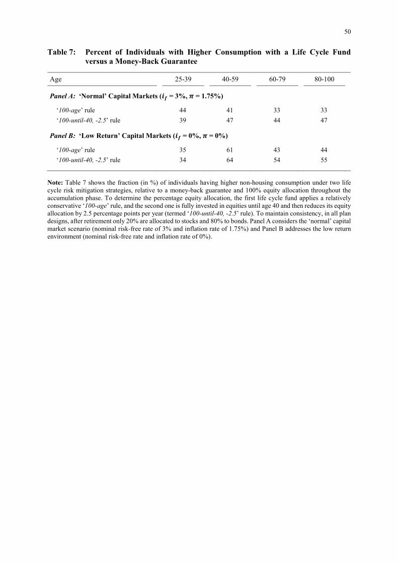
50

Table 7: Percent of Individuals with Higher Consumption with a Life Cycle Fund

versus a Money-Back Guarantee

Age 25-39 40-59 60-79 80-100

Panel A: ‘Normal’ Capital Markets (�� = 3%, � = 1.75%)

‘100-age’ rule 44 41 33 33

‘100-until-40, -2.5’ rule 39 47 44 47

Panel B: ‘Low Return’ Capital Markets (�� = 0%, � = 0%)

‘100-age’ rule 35 61 43 44

‘100-until-40, -2.5’ rule 34 64 54 55

Note: Table 7 shows the fraction (in %) of individuals having higher non-housing consumption under two life cycle risk mitigation strategies, relative to a money-back guarantee and 100% equity allocation throughout the accumulation phase. To determine the percentage equity allocation, the first life cycle fund applies a relatively conservative ‘100-age’ rule, and the second one is fully invested in equities until age 40 and then reduces its equity allocation by 2.5 percentage points per year (termed ‘100-until-40, -2.5’ rule). To maintain consistency, in all plan designs, after retirement only 20% are allocated to stocks and 80% to bonds. Panel A considers the ‘normal’ capital market scenario (nominal risk-free rate of 3% and inflation rate of 1.75%) and Panel B addresses the low return environment (nominal risk-free rate and inflation rate of 0%).

51

Table 8: Sensitivity Analysis for Different Preferences and Fees: Base Case

Specification EZW: lower EIS EZW: higher EIS Front-end load: 5%

Guarantee With Without With Without With Without

Panel A: Consumption (in €1,000 or percent of guarantee case)

Age 25-39 15.34 100% 15.00 100% 15.20 100%

Age 40-59 16.21 100% 16.22 100% 16.20 100%

Age 60-79 15.17 101% 16.54 102% 15.55 102%

Age 80-100 12.13 102% 14.52 104% 12.72 103%

Panel B: Liquid Savings (in €1,000 or percent of guarantee case)

Age 25-39 9.18 100% 11.07 99% 10.06 99%

Age 40-59 22.97 100% 25.95 98% 25.02 97%

Age 60-79 29.95 92% 29.09 91% 31.55 91%

Age 80-100 3.11 79% 4.32 92% 3.64 85%

Panel C: IRA Balance (in €1,000 or percent of guarantee case)

Age 25-39 1.68 100% 4.70 113% 2.66 102%

Age 40-59 25.32 103% 46.88 111% 30.69 110%

Age 60-79 56.49 109% 97.35 112% 65.32 114%

Age 80-84 12.97 109% 22.79 112% 15.06 114%

Panel D: IRA Payouts (in €1,000 or percent of guarantee case)

Age 67: lump sum 14.26 106% 19.89 112% 15.20 113% Age 68-84: drawdown 4.45 109% 7.77 112% 5.16 114% Age 85-100: annuity 4.57 109% 7.69 112% 5.22 114%

Panel E: Share of Consumption and Housing Costs Financed by IRA Payouts (%)

Age 68-84: drawdown 17.3 18.7 26.9 29.4 19.4 21.7

Age 85-100: annuity 22.3 24.0 32.7 35.5 24.7 27.4

Panel F: IRA Shortfall Probability (%)

Age 67 0.0 7.8 0.0 4.9 0.0 7.5

Note: Panels A-D of Table 8 report mean values (in €1,000) of annual non-housing consumption, liquid assets, IRA balances, and payouts, by age ranges, for three different cases with and without guarantee (the latter as percent of the guarantee case). Panel E quantifies the share (in %) of both consumption and housing costs which is financed by after-tax payouts from the IRA. Panel F reports the share of simulations where the IRA value at retirement falls short of the sum of contributions and subsidies. In the first and second case, we allow for Epstein-Zin-Weil (EZW) preferences in order to disentangle risk aversion and elasticity of intertemporal substitution (EIS). Starting from

the CRRA-implied EIS of � = 1/7 = 0.1429 in the first (second) specification, EIS is decreased (increased) to

0.1 (0.2) while holding relative risk aversion constant at ! = 7. In the third specification a front-end load of 5% for each contribution (including subsidies) is charged. In all specifications, the nominal risk-free rate and inflation

rate are assumed constant at �� = 3% and % = 1.75%, and the equity risk premium is 6% (with volatility of 21.41%).

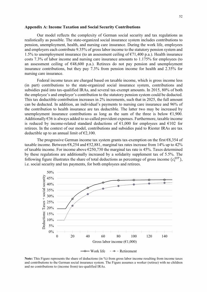
52

Appendix A: Income Taxation and Social Security Contributions

Our model reflects the complexity of German social security and tax regulations as realistically as possible. The state-organized social insurance system includes contributions to pension, unemployment, health, and nursing care insurance. During the work life, employees and employers each contribute 9.35% of gross labor income to the statutory pension system and 1.5% to unemployment insurance (to an assessment ceiling of €71,400 p.a.). Health insurance costs 7.3% of labor income and nursing care insurance amounts to 1.175% for employees (to an assessment ceiling of €48,600 p.a.). Retirees do not pay pension and unemployment insurance contributions, but they pay 7.3% from pension income for health and 2.35% for nursing care insurance.

Federal income taxes are charged based on taxable income, which is gross income less (in part) contributions to the state-organized social insurance system, contributions and subsidies paid into tax-qualified IRAs, and several tax-exempt amounts. In 2015, 80% of both the employee’s and employer’s contribution to the statutory pension system could be deducted. This tax deductible contribution increases in 2% increments, such that in 2025, the full amount can be deducted. In addition, an individual’s payments to nursing care insurance and 96% of the contribution to health insurance are tax deductible. The latter two may be increased by unemployment insurance contributions as long as the sum of the three is below €1,900. Additionally €36 is always added to so-called provident expenses. Furthermore, taxable income is reduced by income-related standard deductions of €1,000 for employees and €102 for retirees. In the context of our model, contributions and subsidies paid to Riester IRAs are tax deductible up to an annual limit of €2,100.

The progressive German income tax system grants tax-exemption on the first €8,354 of taxable income. Between €8,254 and €52,881, marginal tax rates increase from 14% up to 42% of taxable income. For income above €250,730 the marginal tax rate is 45%. Taxes determined by these regulations are additionally increased by a solidarity supplement tax of 5.5%. The

following figure illustrates the share of total deductions as percentage of gross income �V�55�, i.e. social security and tax payments, for both employees and retirees.

Note: This Figure represents the share of deductions (in %) from gross labor income resulting from income taxes and contributions to the German social insurance system. The Figure assumes a worker (retiree) with no children and no contributions to (income from) tax-qualified IRAs.

0%

5%

10%

15%

20%

25%

30%

35%

40%

45%

50%

0 20 40 60 80 100 120 140

Ded

uct

ion

s: T

axes

+ s

oci

al s

ecuri

ty

Gross labor income (€1,000)

Work life Retirement

53

Appendix B: Rental Costs and Number of Children

Panel A: Rental Costs as Share

of Net Income

Panel B: Number of Children Living

with the Parents

Note: Panel A of this Figure illustrates tenants’ rental costs as a fraction of net income (V�W). Raw data are from all waves of SOEP from 1990 to 2015. The definition of housing costs for tenants is broad; besides rental payments we include costs for hot and cold water, heating, garbage disposal and cleaning services. Housing costs in SOEP are provided solely at the household level, so costs are divided by the aggregate of head’s and – if present – spouse’s net income. The population refers to all households in the panel, irrespective of the potential presence of spouses. The subsamples of females and males do indicate singles’ housing costs, but in the model we use population values to avoid the need to make assumptions about relationship status. Panel B illustrates the average number of children living in a household with parents over the life cycle. Raw data were taken from all waves of the Socio-Economic Panel (SOEP) from 1984-2015.

0%

5%

10%

15%

20%

25%

30%

35%

40%

45%

25 35 45 55 65 75 85 95

Age

0.0

0.2

0.4

0.6

0.8

1.0

1.2

1.4

1.6

1.8

2.0

25 30 35 40 45 50 55 60 65

Age

54

Appendix C: The Labor Income Process

Estimation of the discretized Markovian income process relies on non-zero labor income observations of employed persons aged 25-67 from all waves of SOEP until year 2015. All income figures are converted to year 2015 prices (measured in €1,000) and in all specifications and for every age we drop the top and bottom 1% of observations to diminish effects of outliers.

Next, each remaining observation is assigned to one of FG equally-sized income levels. The

lowest (highest) 1/FG of observations are assigned to income level 1 (level FG), etc.35 To estimate deterministic annual income, we conduct pooled OLS regressions for each income

level 0, where the natural logarithm of labor income, ln U�,G, is regressed on first and second

order polynomials in age and year fixed effects. Estimated coefficients are then used to determine predicted age-dependent log income figures, converted to level values and interpreted to (roughly) indicate the level’s middle income.

The second component of the labor income process is the variation of observed log

income, ln U�,G, around the regression-based predicted values, ln U��,G. Using the standard

deviation of the difference, e�,G, as measure of dispersion, a purely transitory shock is added to

the level’s deterministic trend. The natural logarithm of the shock is assumed to be normally

distributed with ln b�,G ~d�−0.5e�,Gh , e�,Gh and is intended to reflect additional variation in

income beyond transitions between income states.

Finally we estimate a Markov transition matrix, which quantifies the probabilities of

migrating from current income state 0� to all other income states in the next period. To derive migration probabilities, we only consider cases where consecutive observations from one age to the next are available and no change in the highest level of education has occurred. Both the transitory shock component within a level and transition probabilities are assumed to be age-invariant.

Panel A of Table C.1 shows state-dependent coefficients of the labor earnings regression

(all being significant at the 1% confidence level). Panel B reports the standard deviations e�,G

between observed (log) income U�,G from predicted (log) income U��,G for all levels. The variation

is U-shaped in income level, meaning that heterogeneity in labor earnings is higher at more extreme income levels. In addition, the top and bottom level variation is more than twice as

high as of the adjacent levels. Panel C quantifies the transition probabilities HG7,G7IJ from current

income level 0� to level 0�A� in the next period. Shading in the Table is darker the higher the probability. The likelihood of remaining in the same income level is especially high for top and bottom income deciles, but also for middle income receivers remaining in the same level is the most likely event.

Table C.2 compares the empirical moments of the SOEP data, and of simulated labor income from applying the Markovian and Carroll and Samwick (1997) methods. Despite simplifications with respect to age-independence of transitory shock components and migration probabilities the empirical moments over age ranges of 10 years are sufficiently close to infer that the Markovian method adequately simulates labor income.

35 Increasing the number of income levels FG, is expected to improve the fit between raw data and simulated income

data, but also increases model runtime. Overall, we find that for the total population and subsamples of females

and males FG = 10 achieves a satisfactory fit of the distribution parameters of the SOEP data (see Table C.2).

55

Table C.1: Gross Labor Income Parameters Estimated by Deciles using SOEP

Panel A: Regression Coefficients from Estimated Models of Log Labor Income by Income Decile

Income decile st 1 2 3 4 5 6 7 8 9 10

Constant 2.479 2.739 2.811 2.825 2.861 2.851 2.884 2.860 2.786 2.500

(63.25) (134.75) (123.44) (220.05) (277.13) (267.68) (247.69) (205.92) (148.21) (72.24)

Age / 100 1.093 1.356 1.916 2.454 2.737 3.233 3.493 4.090 5.121 7.782

(5.57) (13.12) (15.72) (37.62) (53.19) (61.58) (60.53) (61.29) (54.70) (45.78)

Age² / (100)² -1.439 -1.613 -2.150 -2.655 -2.878 -3.372 -3.522 -4.051 -5.050 -7.794

(-6.08) (-12.68) (-14.13) (-33.08) (-45.93) (-53.02) (-50.36) (-50.16) (-44.06) (-37.90)

Number of obs. 17,502 17,463 17,459 17,391 17,382 17,449 17,449 17,399 17,515 17,407

F 4.01 8.72 43.89 168.32 308.38 395.63 475.42 502.74 537.94 262.73

Prob > F 0.0 0.0 0.0 0.0 0.0 0.0 0.0 0.0 0.0 0.0

Adj. R-squared 0.018 0.046 0.151 0.374 0.543 0.620 0.659 0.669 0.661 0.452

Panel B: Standard Deviation: Difference of Actual from Predicted Log Labor Income

Income decile st 1 2 3 4 5 6 7 8 9 10

u,s 0.166 0.073 0.055 0.043 0.037 0.038 0.043 0.053 0.069 0.158

Panel C: Transition Probabilities between Labor Income Deciles ��, ��A� (%)

st+1

1 2 3 4 5 6 7 8 9 10

s t

1 61.9 18.1 7.6 4.2 2.8 1.7 1.2 1.1 1.0 0.5

2 25.1 45.7 15.3 6.0 2.9 2.0 1.1 0.8 0.6 0.5

3 5.9 22.5 41.1 15.9 6.5 3.7 1.9 1.3 0.8 0.4

4 2.7 6.2 21.3 38.5 17.9 7.1 3.5 1.6 0.8 0.4

5 1.7 2.9 7.0 21.4 36.6 18.2 7.1 3.0 1.5 0.6

6 1.0 1.8 3.5 7.4 21.0 37.4 18.3 6.4 2.4 0.9

7 0.6 1.2 1.9 3.6 7.5 20.2 40.0 18.4 5.0 1.5

8 0.5 0.8 1.2 1.8 2.9 6.6 20.1 45.2 17.8 3.2

9 0.3 0.4 0.7 0.8 1.3 2.3 5.3 19.1 55.4 14.5

10 0.2 0.3 0.3 0.5 0.6 0.8 1.5 3.2 14.9 77.6

Note: Panel A of Table C.1 reports regression coefficients and t-statistics for gross labor income deciles estimated using the SOEP (see text); all coefficients are significant at the 1% level. Panel B shows the standard deviation of differences between annual logs of labor income and the regression’s fitted values within each income level. Panel

C depicts the conditional transition probabilities HG7,G7IJ from the individual’s current income level 0� to all possible

future income levels 0�A�. The darkness of the shading is proportional to the transition probability. Standard deviations and transition probabilities are assumed to be age-invariant. Observations with implied hourly wages below 80% of year 2015’s minimum wage and employees working below 20 hours per week are excluded from the estimation. A minimum wage of €8.50 was introduced in 2015 (i.e. all SOEP observations are from the pre-minimum wage period) and omitting this data filter would result in inclusion of observations illegal under current law.

56

Table C.2: Moments of Labor Income (Entire Workforce)

Age 25-34 35-44 45-54 55-64

Panel A: Mean

SOEP 29.54 35.12 36.07 31.12

Markov chain 33.76 38.07 39.62 37.90

Carroll and Samwick (1997) 31.51 34.77 35.35 33.18

Panel B: Standard deviation

SOEP 13.80 17.42 17.78 19.60

Markov chain 13.64 18.34 20.35 19.06

Carroll and Samwick (1997) 8.40 13.93 17.85 19.82

Panel C: Skewness

SOEP 0.15 0.73 0.79 0.76

Markov chain 0.91 1.17 1.24 1.13

Carroll and Samwick (1997) 0.81 1.25 1.64 2.06

Panel D: Kurtosis

SOEP 2.73 3.43 3.50 3.22

Markov chain 4.12 4.51 4.58 4.29

Carroll and Samwick (1997) 4.27 5.89 8.08 12.41

Note: Table C.2 reports the empirical moments of labor income for observed SOEP data as well as for two data-

generating processes. Annual labor income measured in €1,000 refers to the total workforce. The method denoted

‘Markov chain’ is employed in the model (discussed in Section 3.3). The benchmark method is from Carroll and

Samwick (1997) using the regression model ln Ut,� = !& + !� ∙ o�x�,7�&& + !h ∙ o�x�,7���&&� + �t,� and resulting coefficients

!& = 2.6926, !� = 3.7645, !h = −4.0241 (all significant at the 1% level); the variance of the permanent income

shock e�h = 1.69% and variance of the transitory income shock e�h = 5.84%. Using Carroll and Samwick’s

method, Fuchs-Schündeln et al. (2010) and Krebs and Yao (2016) find similar permanent, but higher transitory

shock components for Germany. The lower transitory shock in our estimation is attributed to the additional data

filters applied (outlined in Table C.1). Reported numbers are mean values over age ranges of 10 years from 100,000

simulation paths.

SAFE | House of Finance | Goethe University Frankfurt | www.safe-frankfurt.de | info@safe.uni-frankfurt.de

Recent Issues

No. 262 Andrea Bedin, Monica Billio, Michele Costola, Loriana Pelizzon

Credit Scoring in SME Asset-Backed Securities: An Italian Case Study

No. 261 Monica Billio, Michele Costola, Loriana Pelizzon, Max Riedel

Buildings' Energy Efficiency and the Probability of Mortgage Default: The Dutch Case

No. 260 Matthias Thiemann, Tobias H. Tröger

It’s the Tail-Risk, Stupid!

No. 259 Inaki Aldasoro, Florian Balke, Andreas Barth, Egemen Eren

Spillovers of Funding Dry-ups

No. 258 Anderson Grajales-Olarte, Burak R. Uras, Nathanael Vellekoop

Rigid Wages and Contracts: Time- versus State-Dependent Wages in the Netherlands

No. 257 Baptiste Massenot, Giang Nghiem Depressed Demand and Supply

No. 256 Christian Schlag, Kailin Zeng Horizontal Industry Relationships and Return Predictability

No. 255 Silvia Dalla Fontana, Marco Holz auf der Heide, Loriana Pelizzon, Martin Scheicher

The Anatomy of the Euro Area Interest Rate Swap Market

No. 254 Martin R. Goetz Financing Conditions and Toxic Emissions

No. 253 Thomas Johann, Talis Putnins, Satchit Sagade, Christian Westheide

Quasi-Dark Trading: The Effects of Banning Dark Pools in a World of Many Alternatives

No. 252 Nicole Branger, Patrick Konermann, Christian Schlag

Optimists and Pessimists in (In)Complete Markets

No. 251 Wenhui Li, Christian Wilde Belief Formation and Belief Updating under Ambiguity: Evidence from Experiments

No. 250 Nathanael Vellekoop, Mirko Wiederholt

Inflation Expectations and Choices of Households

No. 249 Yuri Pettinicchi, Nathanael Vellekoop

Job Loss Expectations, Durable Consumption and Household Finances: Evidence from Linked Survey Data