WO 2013/131042 Al o
526
(12) INTERNATIONAL APPLICATION PUBLISHED UNDER THE PATENT COOPERATION TREATY (PCT) (19) World Intellectual Property Organization International Bureau (10) International Publication Number (43) International Publication Date WO 2013/131042 Al 6 September 2013 (06.09.2013) PO PCT (51) International Patent Classification: (81) Designated States (unless otherwise indicated, for every C10G 2/00 (2006.01) kind of national protection available): AE, AG, AL, AM, AO, AT, AU, AZ, BA, BB, BG, BH, BN, BR, BW, BY, (21) International Application Number: BZ, CA, CH, CL, CN, CO, CR, CU, CZ, DE, DK, DM, PCT/US20 13/028730 DO, DZ, EC, EE, EG, ES, FI, GB, GD, GE, GH, GM, GT, (22) International Filing Date: HN, HR, HU, ID, IL, IN, IS, JP, KE, KG, KM, KN, KP, 1 March 2013 (01 .03.2013) KR, KZ, LA, LC, LK, LR, LS, LT, LU, LY, MA, MD, ME, MG, MK, MN, MW, MX, MY, MZ, NA, NG, NI, (25) Filing Language: English NO, NZ, OM, PA, PE, PG, PH, PL, PT, QA, RO, RS, RU, (26) Publication Language: English RW, SC, SD, SE, SG, SK, SL, SM, ST, SV, SY, TH, TJ, TM, TN, TR, TT, TZ, UA, UG, US, UZ, VC, VN, ZA, (30) Priority Data: ZM, ZW. 61/605,547 1 March 2012 (01 .03.2012) US 61/716,348 19 October 2012 (19.10.2012) US (84) Designated States (unless otherwise indicated, for every kind of regional protection available): ARIPO (BW, GH, (71) Applicant: THE TRUSTEES OF PRINCETON UNI¬ GM, KE, LR, LS, MW, MZ, NA, RW, SD, SL, SZ, TZ, VERSITY [US/US]; Office of Technology Licensing, UG, ZM, ZW), Eurasian (AM, AZ, BY, KG, KZ, RU, TJ, Princeton University, Princeton, New Jersey 08544 (US). TM), European (AL, AT, BE, BG, CH, CY, CZ, DE, DK, EE, ES, FI, FR, GB, GR, HR, HU, IE, IS, ΓΓ , LT, LU, LV, (72) Inventors: FLOUDAS, Christodoulos A.; 189 Christoph MC, MK, MT, NL, NO, PL, PT, RO, RS, SE, SI, SK, SM, er Drive, Princeton, New Jersey 08540 (US). BALIBAN, TR), OAPI (BF, BJ, CF, CG, CI, CM, GA, GN, GQ, GW, Richard C ; 6 Dorchester Drive, Southampton, New Jersey ML, MR, NE, SN, TD, TG). 08088 (US). ELIA, Josephine A.; 52 14 Hunters Glen Drive, Plainsboro, New Jersey 08536 (US). Published: (74) Agent: BUCKLIN, Douglas J.; Volpe and Koenig, P.C., — with international search report (Art. 21(3)) United Plaza 30 S. 17th Street, Philadelphia, Pennsylvania 19103 (US). (54) Title: PROCESSES FOR PRODUCING SYNTHETIC HYDROCARBONS FROM COAL, BIOMASS, AND NATURAL GAS P100A P2 Bi ass Syngas Syngas Treatment Generation P0 B Coal Syngas P300 Generation Hydrocarbon Production P600 P4 Heat and Power Product Upgrading Recovery o FIG. 17 o (57) Abstract: Methods of optimal refinery design utilizing a thermochemical based superstructure are provided. Methods of produ cing liquid fuels utilizing a refinery selected from a thermochemical based superstructure are provided. Thermochemical based su perstructures are provided. Refineries are provided.
-
Upload
khangminh22 -
Category
Documents
-
view
0 -
download
0
Transcript of WO 2013/131042 Al o

(12) INTERNATIONAL APPLICATION PUBLISHED UNDER THE PATENT COOPERATION TREATY (PCT)
(19) World Intellectual PropertyOrganization
International Bureau(10) International Publication Number
(43) International Publication Date WO 2013/131042 Al6 September 2013 (06.09.2013) P O PCT
(51) International Patent Classification: (81) Designated States (unless otherwise indicated, for everyC10G 2/00 (2006.01) kind of national protection available): AE, AG, AL, AM,
AO, AT, AU, AZ, BA, BB, BG, BH, BN, BR, BW, BY,(21) International Application Number: BZ, CA, CH, CL, CN, CO, CR, CU, CZ, DE, DK, DM,
PCT/US20 13/028730 DO, DZ, EC, EE, EG, ES, FI, GB, GD, GE, GH, GM, GT,(22) International Filing Date: HN, HR, HU, ID, IL, IN, IS, JP, KE, KG, KM, KN, KP,
1 March 2013 (01 .03.2013) KR, KZ, LA, LC, LK, LR, LS, LT, LU, LY, MA, MD,ME, MG, MK, MN, MW, MX, MY, MZ, NA, NG, NI,
(25) Filing Language: English NO, NZ, OM, PA, PE, PG, PH, PL, PT, QA, RO, RS, RU,
(26) Publication Language: English RW, SC, SD, SE, SG, SK, SL, SM, ST, SV, SY, TH, TJ,TM, TN, TR, TT, TZ, UA, UG, US, UZ, VC, VN, ZA,
(30) Priority Data: ZM, ZW.61/605,547 1 March 2012 (01 .03.2012) US61/716,348 19 October 2012 (19.10.2012) US (84) Designated States (unless otherwise indicated, for every
kind of regional protection available): ARIPO (BW, GH,(71) Applicant: THE TRUSTEES OF PRINCETON UNI¬ GM, KE, LR, LS, MW, MZ, NA, RW, SD, SL, SZ, TZ,
VERSITY [US/US]; Office of Technology Licensing, UG, ZM, ZW), Eurasian (AM, AZ, BY, KG, KZ, RU, TJ,Princeton University, Princeton, New Jersey 08544 (US). TM), European (AL, AT, BE, BG, CH, CY, CZ, DE, DK,
EE, ES, FI, FR, GB, GR, HR, HU, IE, IS, ΓΓ , LT, LU, LV,(72) Inventors: FLOUDAS, Christodoulos A.; 189 ChristophMC, MK, MT, NL, NO, PL, PT, RO, RS, SE, SI, SK, SM,
er Drive, Princeton, New Jersey 08540 (US). BALIBAN,TR), OAPI (BF, BJ, CF, CG, CI, CM, GA, GN, GQ, GW,
Richard C ; 6 Dorchester Drive, Southampton, New JerseyML, MR, NE, SN, TD, TG).
08088 (US). ELIA, Josephine A.; 52 14 Hunters GlenDrive, Plainsboro, New Jersey 08536 (US). Published:
(74) Agent: BUCKLIN, Douglas J.; Volpe and Koenig, P.C., — with international search report (Art. 21(3))United Plaza 30 S. 17th Street, Philadelphia, Pennsylvania19103 (US).
(54) Title: PROCESSES FOR PRODUCING SYNTHETIC HYDROCARBONS FROM COAL, BIOMASS, AND NATURALGAS
P100AP2
Bi ass SyngasSyngas Treatment
Generation
P 0 B
Coal Syngas P300
Generation HydrocarbonProduction
P600 P4Heat and Power Product Upgrading
Recovery
o
FIG. 17
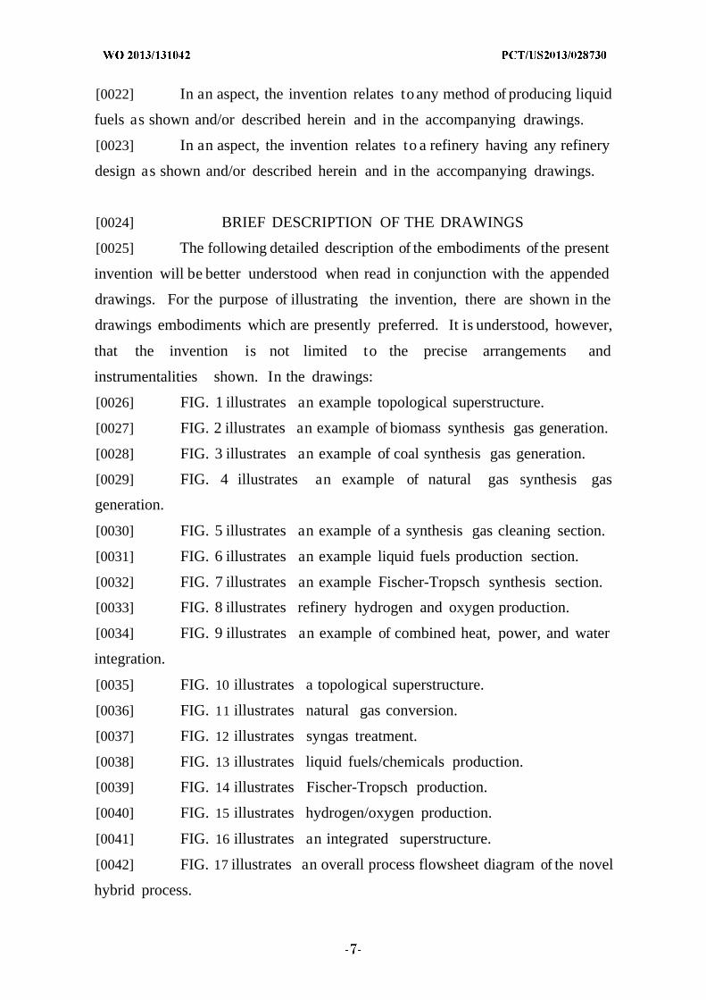
o (57) Abstract: Methods of optimal refinery design utilizing a thermochemical based superstructure are provided. Methods of producing liquid fuels utilizing a refinery selected from a thermochemical based superstructure are provided. Thermochemical based superstructures are provided. Refineries are provided.
[0001] PROCESSES FOR PRODUCING SYNTHETIC HYDROCARBONS
FROM COAL, BIOMASS, AND NATURAL GAS
[0002] This application claims the benefit of U.S. Provisional Application
Nos. 61/605,547, filed March 1, 2012, and 61/716,348, filed October 19, 2012, both
of which are incorporated herein by reference as if fully set forth.
[0003] This invention was made with government support under Grant No.
EFRI-0937706 awarded by the National Science Foundation. The government
has certain rights in the invention.
[0004] FIELD
[0005] The disclosure herein relates to methods of converting coal, biomass
or natural gas feedstocks into synthetic liquid hydrocarbons and processes for
converting natural gas to synthetic liquid hydrocarbons.
[0006] BACKGROUND
[0007] The challenges to reduce dependence on petroleum as energy
sources, coupled with efforts to reduce greenhouse gas (GHG) emissions, are
exigent problems faced by the US transportation sector. Several studies have
been done to explore alternative, non-petroleum based processes to produce liquid
fuels that include the production of synthetic liquid hydrocarbons from biomass,
coal, and natural gas using a synthesis gas (syngas) intermediate. These energy
processes have emerged as viable options to address the given challenges due to
their capabilities to produce liquid fuels via domestically available sources of
carbon-based energy. A common feature of these synthetic processes, however, is
the large CO2 amount emitted from the system.
[0008] In 2008, the United States consumed an average of 19498 thousand
barrels of oil per day (TBD), including 11114 TBD of imports. The 2008
transportation sector requirement of 13702 TBD accounted for 70.2% of the total
U.S. consumption. While it is estimated that liquid fuel use in residential,
commercial, industrial, and electric power sectors will all decrease, on average,
over the next 20 years, the anticipated average annual increase in the
transportation sector requirement of 0.6% forecasts an increase in the total U.S.
liquid fuels consumption. Because domestic oil production is expected to decline
over this time period, the United States will ultimately require an increase in the
percentage of oil consumed by foreign imports.
[0009] Although Canada and Mexico are two of the three largest foreign
suppliers with 2493 and 1302 TBD of oil supplied to the United States in 2008
respectively, these two countries only have 3.2% of the proven global foreign oil
reserves. This fact may prompt the United States to seek increased imports from
Saudi Arabia and other Middle Eastern countries who have a combined 59.9% of
the proven world reserves. However, turmoil within the Middle East and strained
diplomatic relations can have a dramatic effect both on the availability and price
of petroleum from this region. Furthermore, the increased energy usage of
industrialized nations coupled with the rapid growth of China and India is likely
to rapidly raise petroleum demand, which will result in an increase in the crude
oil price. Therefore, it is imperative that the United States research, develop,
and implement different methods for meeting transportation fuel demands using
alternative processes.
[0010] A further concern with the increased use of transportation fuels is
its contribution to the greenhouse gas (GHG) emissions. The transportation
sector accounted for 33.0% of the CO2 emissions in 2007, due almost exclusively
to the direct consumption of fossil fuels. Although extensive research has been
devoted to the use of alternative fuels such as hydrogen and electricity, so far, the
technical and economic challenges have limited their widespread use.
[0011] Several technologies have been considered for the development of
liquid fuels using biological feedstocks, including cellulosic and corn-based
ethanol, soy-based biodiesel, and Fischer-Tropsch (FT) hydrocarbon fuels. The
overall impact that each bio-based feedstock will have on displacing petroleum-
based transportation fuels depends on the scale of production, the potential for
rural economic development, the reduction in GHG emissions, the impact on soil
fertility and agricultural ecology, the water use efficiency, and the costs
associated with the upkeep, harvest, and transportation of the crop. The use of
corn, soybean oil, and other vegetable oils as a feedstock for fuel production has
led to concern regarding the impact on the price and availability of these
substances as sources of food. In addition, the actual well-to-wheel GHG
emissions from a corn-based ethanol fuel is not much of an improvement,
compared to the emissions from gasoline or biodiesel. Bio-based feedstocks can
still play a major role in satisfying transportation demands if the feedstock does
not displace land that would otherwise be used for growing food crops and if the
environmental impact of the feedstock production is minimized. Agricultural and
forestry residues, waste products, and dedicated fuel crops are expected tobe the
dominant bio-based resources, but continuing analysis is required to develop a
holistic approach to the sustainable production of transportation fuels from these
feedstocks.
[0012] SUMMARY
[0013] In an aspect the invention relates to a superstructure for forming a
refinery. The superstructure includes at least one synthesis gas production unit
configured to produce at least one synthesis gas selected from the group
consisting of a biomass synthesis gas production unit, a coal synthesis gas
production unit and a natural gas synthesis gas production unit, wherein the at
least one synthesis gas is determined by a mixed-integer linear optimization
model solved by a global optimization framework. The superstructure also
includes a synthesis gas cleanup unit configured to remove undesired gases from
the at least one synthesis gas, a liquid fuels production unit selected from the
group consisting of a Fischer-Tropsch unit, and a methanol synthesis unit. The
Fischer-Tropsch unit is configured to produce a first output from the at least one
synthesis gas. The methanol synthesis unit is configured to produce a second
output from the at least one synthesis gas. The selection of liquid fuels
production unit is determined by the mixed-integer linear optimization model
solved by the global optimization framework. The superstructure also includes a
liquid fuels upgrading unit configured to upgrade the first output or the second
output. The liquid fuels upgrading unit selection is determined by the mixed-
integer linear optimization model solved by the global optimization framework.

The superstructure also includes a hydrogen production unit configured to
produce hydrogen for the refinery, an oxygen production unit configured to
produce oxygen for the refinery, and a wastewater treatment network configured
to process wastewater from the refinery and input freshwater into the refinery.
The wastewater treatment network is determined by a mixed-integer linear
optimization model solved by a global optimization framework. The
superstructure also includes a utility plant configured to produce electricity for
the refinery and process heat from the refinery. The utility plant is determined
by a mixed-integer linear optimization model solved by a global optimization
framework. The superstructure also includes a CO2 separation unit configured to
recylce gases containing CO2 in the refinery. The at least one synthesis gas
production unit, the synthesis gas cleanup unit, the liquid fuels production unit,
the liquid fuels upgrading unit, the hydrogen production unit, the oxygen
production unit, the wastewater treatment network, the utility plant and the CO2
separation unit are configured to be combined to form the refinery.
[0014] In an aspect, the invention relates to an optimal refinery design
system. The optimal refinery design system includes a superstructure database.
The superstructure database includes data associated with at least one synthesis
gas production unit configured toproduce at least one synthesis gas selected from
the group consisting of a biomass synthesis gas production unit, a coal synthesis
gas production unit and a natural gas synthesis gas production unit. The
selection of the at least one synthesis gas is determined by a mixed-integer linear
optimization model solved by a global optimization framework. The
superstructure database also includes data associated with a synthesis gas
cleanup unit configured to remove undesired gases from the at least one
synthesis gas. The superstructure also includes data associated with a liquid
fuels production unit configured selected from the group consisting of a Fischer-
Tropsch unit and a methanol synthesis unit. The Fischer-Tropsch unit is
configured to produce a first output from the at least one synthesis gas, and the
methanol synthesis unit is configured to produce a second output from the at
least one synthesis gas. The selection of liquid fuels production unit is
determined by the mixed-integer linear optimization model solved by the global
optimization framework. The superstructure database also includes data
associated with a liquid fuels upgrading unit configured to upgrade the first
output or the second output. The liquid fuels upgrading unit is determined by
the mixed-integer linear optimization model solved by the global optimization
framework. The superstructure also includes data associated with a hydrogen
production unit configured to produce hydrogen for the refinery, an oxygen
production unit configured to produce oxygen for the refinery, and a wastewater
treatment network configured to process wastewater from the refinery and input
freshwater into the refinery. The wastewater treatment network is determined
by the mixed-integer linear optimization model solved by the global optimization
framework. The superstructure database also includes data associated with a
utility plant configured to produce electricity for the refinery and process heat
from the refinery. The utility plant is determined by the mixed-integer linear
optimization model solved by the global optimization framework. The
superstructure database also includes data associated with a CO2 separation unit
configured to recycle gases containing CO2 in the refinery. The at least one
synthesis gas production unit, the synthesis gas cleanup unit, the liquid fuels
production unit, the liquid fuels upgrading unit, the hydrogen production unit,
the oxygen production unit, the wastewater treatment network, the utility plant
and the CO2 separation unit are configured to be combined to form the refinery.
The optimal refinery design system includes a processor configured to solve the
mixed-integer linear optimization model by the global optimization framework.
[0015] In an aspect the invention relates to a method of designing an
optimal refinery. The method includes providing any superstructure contained
herein, inserting a data set on each of the each of the at least one synthesis gas
production unit, the liquid fuels production unit, the liquid fuels upgrading unit,
the wastewater treatment network and the utility plant into the mixed-integer
linear optimization model. The method also includes solving the mixed-integer
linear optimization model by the global optimization framework, and thereby
determining each of the at least one synthesis gas production unit, the liquid
fuels production unit, the liquid fuels upgrading unit, the wastewater treatment
network and the utility plant to produce an optimal refinery design.
[0016] In an aspect, the invention relates to a method of designing an
optimal refinery. The method includes providing a superstructure database,
solving the mixed-integer linear optimization model by the global optimization
framework, and thereby determining each of the at least one synthesis gas
production unit, the liquid fuels production unit, the liquid fuels upgrading unit,
the wastewater treatment network and the utility plant to produce an optimal
refinery design.
[0017] In an aspect, the invention relates to a method of producing liquid
fuels. The method includes producing liquid fuels with a refinery having an
optimal refinery design. The optimal refinery design is obtained by providing any
superstructure contained herein, inserting a data set on each of the each of the at
least one synthesis gas production unit, the liquid fuels production unit, the
liquid fuels upgrading unit, the wastewater treatment network and the utility
plant into the mixed-integer linear optimization model. The method also includes
solving the mixed-integer linear optimization model by the global optimization
framework, determining each of the at least one synthesis gas production unit,
the liquid fuels production unit, the liquid fuels upgrading unit, the wastewater
treatment network and the utility plant to produce the optimal refinery design.
[0018] In an aspect, the invention relates to a method of producing liquid
fuels. The method includes providing a superstructure database, solving the
mixed-integer linear optimization model by the global optimization framework,
determining each of the at least one synthesis gas production unit, the liquid
fuels production unit, the liquid fuels upgrading unit, the wastewater treatment
network and the utility plant to produce an optimal refinery design, and
producing liquid fuels by the optimal refinery design.
[0019] In an aspect, the invention relates to any superstructure as shown
and/or described herein and in the accompanying drawings.
[0020] In an aspect, the invention relates to any refinery design as shown
and/or described herein and in the accompanying drawings.
[0021] In an aspect, the invention relates to any method of designing a
refinery as shown and/or described herein and in the accompanying drawings.
[0022] In an aspect, the invention relates to any method of producing liquid
fuels as shown and/or described herein and in the accompanying drawings.
[0023] In an aspect, the invention relates to a refinery having any refinery
design as shown and/or described herein and in the accompanying drawings.
[0024] BRIEF DESCRIPTION OF THE DRAWINGS
[0025] The following detailed description of the embodiments of the present
invention will be better understood when read in conjunction with the appended
drawings. For the purpose of illustrating the invention, there are shown in the
drawings embodiments which are presently preferred. It is understood, however,
that the invention is not limited to the precise arrangements and
instrumentalities shown. In the drawings:
[0026] FIG. 1 illustrates an example topological superstructure.
[0027] FIG. 2 illustrates an example of biomass synthesis gas generation.
[0028] FIG. 3 illustrates an example of coal synthesis gas generation.
[0029] FIG. 4 illustrates an example of natural gas synthesis gas
generation.
[0030] FIG. 5 illustrates an example of a synthesis gas cleaning section.
[0031] FIG. 6 illustrates an example liquid fuels production section.
[0032] FIG. 7 illustrates an example Fischer-Tropsch synthesis section.
[0033] FIG. 8 illustrates refinery hydrogen and oxygen production.
[0034] FIG. 9 illustrates an example of combined heat, power, and water
integration.
[0035] FIG. 10 illustrates a topological superstructure.
[0036] FIG. 11 illustrates natural gas conversion.
[0037] FIG. 12 illustrates syngas treatment.
[0038] FIG. 13 illustrates liquid fuels/chemicals production.
[0039] FIG. 14 illustrates Fischer-Tropsch production.
[0040] FIG. 15 illustrates hydrogen/oxygen production.
[0041] FIG. 16 illustrates an integrated superstructure.
[0042] FIG. 17 illustrates an overall process flowsheet diagram of the novel
hybrid process.
[0043] FIG. 18 illustrates PFD 1 : biomass and coal gassification trains
(P100).
[0044] FIG. 19 illustrates PFD 2 : syngas treatment units (P200).
[0045] FIG. 20 illustrates PFD 3 : hydrocarbon generation section (P300).
[0046] FIG. 21 illustrates PFD 4 : hydrocarbon upgrading section (P400).
[0047] FIG. 22 illustrates PFD 5 : light gases reforming (continuation of
P400).
[0048] FIG. 23 illustrates PFD 6 : hydrogen and oxygen production, heat
and power recovery section (P500 and P600).
[0049] FIG. 24 illustrates break-even oil price (BEOP) of seven process
alternatives using distinct hydrogen prices. In each of panels C-R-A, C-E-A, B-R-
A, B-E-A, H-R-A, H-E-A, and H-R-T, from left to right, the bars represent
$2.50/kg H2, $2.00/kg H2, $1.50/kg H2 and $1.00/kg H2.
[0050] FIG. 25 illustrates break-even oil price (BEOP) using distinct
electrolyzer capital costs and electricity prices. In each of panels C-E-A, B-E-A,
and H-E-A, from left to right, the bars represent $0.08/kWh, $0.07/kWh,
$0.06/kWh, $0.05/kWh, $0.04/kWh, and $0.03/kWh.
[0051] FIGS. 26A-B illustrate performance comparison of hydrogen-
producing technologies (steam reforming of methane and electrolysis). FIG. 26A
illustrates total fuel C vented and FIG. 26B illustrates BEOP. In each of panels
H-R-A, H-E-A, and H-R-T, from left to right, the bars represent w/ Seq. and w/o
Seq.
[0052] FIG. 27 illustrates a framework for the heat exchanger and power
recovery network (HEPN). A simulated process flowsheet is analyzed to
construct a list of (a) hot and cold streams, (b) hot and cold process units, (c) the
process condensate, (d) the process cooling water requirement, and (f) the process
electricity requirement. The hot and cold process units (list item b) are defined as
all units that require heat or release heat at a given temperature. This process
flowsheet information (list items a-f) is used along with a superset of heat engine
operating conditions to sequentially determine (i) the minimum hot/cold/power
utilities, (ii) the minimum number of heat exchanger matches, and (iii) the
minimum annualized cost of heat exchange. The output from the HEPN is the
optimal heat and power recovery network, which includes the total utility
requirement, the operating conditions of the heat engines, and the topology of the
heat exchanger network.
[0053] FIG. 28 illustrates a pictorial description of one heat engine with
operating conditions (Pb , P c , Tt).
[0054] FIG. 29 illustrates optimal HEPN topology for subnetwork 1 of the
H-R-A flowsheet. All inlet and outlet temperatures given correspond to the actual
stream temperatures of the match. Stream labels: HI, reverse water-gas-shift
effluent; H6, fuel combuster effluent; H15, coal gasifier; H29, heat engine (75, 40,
900) precooler; C6, autothermal reactor (ATR) steam input; C7, ATR natural gas
input; C8, ATR oxygen input; C9, ATR recycle light gas input; C33, heat engine
(25, 1, 900) superheater; C34, heat engine (75, 40, 900) superheater; C35, heat
engine (100, 15, 900) superheater. Heat engines are defined by the parameters
P b (bar), c (bar), and T t (°C).
[0055] FIG. 30 illustrates optimal HEPN topology for subnetwork 1 of the
H-E-A flowsheet. All inlet and outlet temperatures given correspond to the actual
stream temperature of the match. Stream labels: HI, reverse water-gas-shift
effluent; H6, fuel combuster effluent; H12, coal gasifier; H27, heat engine (75, 40,
900) precooler; C6, autothermal reactor (ATR) steam input; C7, ATR natural gas
input; C8, ATR oxygen input; C9, ATR recycle light gas input; C33, heat engine
(25, 1, 900) superheater; C34, heat engine (25, 15, 500) superheater; C35, heat
engine (75, 40, 900) superheater. Heat engines are defined by the parameters P b
(bar), P cc (bar), and T t (°C).
[0056] FIG. 31 illustrates optimal HEPN topology for subnetwork 1 of the
H-R-T flowsheet. All inlet and outlet temperatures given correspond to the actual
stream temperature of the match. Stream labels: HI, reverse water-gas-shift
(RGS) effluent; H6, fuel combuster effluent; H17, coal gasifier; Cl, RGS inlet
hydrogen; C2, RGS recycle CO2; C6, autothermal reactor (ATR) steam input; C7,
ATR natural gas input; C8, ATR oxygen input; C9, ATR recycle light gas input;
C33, heat engine (25, 1, 600) superheater; C34, heat engine (75, 1, 900)
superheater; C35, heat engine (100, 15, 600) superheater. Heat engines are
defined by the parameters P b (bar), Pc (bar), and T t (°C).

[0057] FIG. 32 illustrates a Fischer-Tropsch (FT) hydrocarbon production
flowsheet. Each of the six FT units has a distinct set of operating conditions
including catalyst type (cobalt or iron), temperature (low - 240 °C, medium - 267
°C, and high - 320 °C), and water-gas- shift reaction extent (forward, reverse, or
none). Each unit is designed to produce either a minimal or nominal amount of
wax (shown as a dashed line). The mathematical model will select at most two
types of the six FT units to operate in a final process topology. All of the streams
in FIG. 32 are variable.
[0058] FIG. 33 illustrates a First Fischer-Tropsch (FT) hydrocarbon
upgrading flowsheet. The FT effluent may be passed through a series of stripper
and flash units to separate the oxygenates and aqueous phase from the
hydrocarbons. Alternatively, the effluent may be passed over a ZSM-5 catalytic
reactor to convert most of the hydrocarbons into gasoline range species. The raw
ZSM-5 product is then fractionated to remove any distillate or sour water from
the gasoline product. All of the process streams in FIG. 33 are variable.
[0059] FIG. 34 illustrates a second Fischer-Tropsch (FT) hydrocarbon
upgrading flowsheet. The water lean FT effluent is fractionated and passed
through a series of treatment units to recover the gasoline, diesel, and kerosene
products along with some LPG byproduct. Light gases (i .e., unreacted syngas and
C1-C2 hydrocarbons) are collected and recycled back to the process.
[0060] FIG. 35 illustrates a methanol synthesis and conversion flowsheet.
Clean syngas is initially converted to methanol and then split to either the
methanol to gasoline (MTG) or methanol to olefins (MTO) processes. The two
processes utilize a ZSM-5 zeolite to convert the methanol to either gasoline range
hydrocarbons (MTG) or olefins which are subsequently oligomerized to gasoline
and distillate range hydrocarbons (MOGD). The distillate is hydrotreated to form
diesel or kerosene which the gasoline range hydrocarbons are sent to an LPG-
gasoline separation system. All of the streams in FIG. 35 are variable.
[0061] FIG. 36 illustrates an LPG-gasoline product separation flowsheet.
The raw HC products from the FT-ZSM5 unit, the MTG unit, or the MOGD
process are passed through a series of separation units to recover a gasoline
product and an LPG byproduct. Light gases are recycled back to the refinery and

CO2 recovery may be utilized in preparation for sequestration or reaction with H 2
via the reverse water— as-shift reaction. All of the streams in FIG. 36 are
variable.
[0062] FIG. 37 illustrates a parametric analysis of feedstock cost. The
histogram shows the number of counts (out of 27) for break-even oil price (BEOP)
when low, nominal, and high values are used for the costs of coal, biomass, and
natural gas.
[0063] FIG. 38 illustrates a biomass gasification process flowsheet.
[0064] FIG. 39 illustrates a coal gassification process flowsheet.
[0065] FIG. 40 illustrates a syngas cleaning process flowsheet.
[0066] FIG. 41 illustrates a claus sulfur recovery process flowsheet.
[0067] FIG. 42 illustrates a Fischer-Tropsch hydrocarbon production
process flowsheet. All of the streams in FIG. 42 are variable.
[0068] FIG. 43 illustrates a first Fischer-Tropsch hydrocarbon upgrading
process flowsheet. All of the streams in FIG. 43 are variable.
[0069] FIG. 44 illustrates a second Fischer-Tropsch hydrocarbon upgrading
process flowsheet.
[0070] FIG. 45 illustrates a methanol synthesis and conversion process
flowsheet. All of the streams in FIG. 45 are variable.
[0071] FIG. 46 illustrates an LPG-gasoline separation process flowsheet.
All the streams in FIG. 46 are variable.
[0072] FIG. 47 illustrates a recycle gas treatment process flowsheet.
[0073] FIG. 48 illustrates a hydrogen/oxygen production process flowsheet.
[0074] FIG. 49 illustrates a process wastewater treatment process
flowsheet.
[0075] FIG. 50 illustrates a utility cycle wastewater treatment process
flowsheet.
[0076] FIG. 51 illustrates a natural gas conversion flow sheet. Natural gas
is combined with recycle methane and may be converted to (1) synthesis gas (CO,
O2, H2, and H2O) via steam reforming or ATR, (2) methanol using catalytic
partial oxidation, or (3) olefins (ethylene/propylene) via OC.
[0077] FIG. 52 illustrates a flow sheet of natural gas utilities. Natural gas
and recycle fuel gas may be utilized to produce electricity through a GT or
additional process heat via a fuel combustor. The effluent from both of these
processes axe cooled and then are either vented or passed over a CO2 recovery
unit to capture and process the produced CO2.
[0078] FIG. 53 illustrates a Synthesis gas (syngas) handling flow sheet.
Syngas may be passed over a forward/reverse WGS reactor to alter the ¾ to
C /C 2 ratio prior to FT or methanol synthesis. The syngas is then cooled,
flashed to remove water, and may be directed to a one-stage Rectisol unit for CO2
removal. The captured 2 may be vented, sequestered, or recycled back to
process units.
[0079] FIG. 54 illustrates a PFD for case study U-l.
[0080] FIG. 55 illustrates a PFD for case study K-50.
[0081] FIG. 56 illustrates a parametric analysis of natural gas cost. The
BEOP is plotted for the case studies with an unrestricted product composition as
a function of the natural gas price in TSCF.
[0082] FIG. 57 illustrates a natural gas conversion process flowsheet.
[0083] FIG. 58 illustrates a natural gas utility process flowsheet.
[0084] FIG. 59 illustrates a synthesis gas handling process flowsheet.
[0085] FIG. 60 illustrates a Fischer-Tropsch hydrocarbon production
process flowsheet. All of the streams in FIG. 60 are variable.
[0086] FIG. 61 illustrates a first Fischer-Tropsch hydrocarbon upgrading
process flowsheet. All of the streams in FIG. 61 are variable.
[0087] FIG. 62 illustrates a second Fischer-Tropsch hydrocarbon upgrading
process flowsheet.
[0088] FIG. 63 illustrates a methanol synthesis and conversion process
flowsheet. All of the streams in FIG. 63 are variable.
[0089] FIG. 64 illustrates an LPG-gasoline separation process flowsheet.
All of the streams in FIG. 64 are variable.
[0090] FIG. 65 illustrates a hydrogen/oxygen production process flowsheet.
[0091] FIG. 66 illustrates a process wastewater treatment process
flowsheet.
[0092] FIG. 67 illustrates a utility cycle wastewater treatment process
flowsheet.
[0093] FIGS. 68A - 68D illustrate branch-and-bound progression for the
small case studies. At each node in the branch-and-bound tree, the current lower
(lower line) and upper bounds (upper line) (in $/GJ) are shown along with the
optimality gap (dotted line) for feedstock-carbon conversion rates of (a) 25% in
FIG. 68A, (b) 50% in FIG. 68B, (c) 75% in FIG. 68C, and (d) 95% in FIG. 68D.
The upper
[0094] FIGS. 69A - 69D illustrate branch-and-bound progression for the
medium case studies. At each node in the branch-and-bound tree, the current
lower (lower line) and upper bounds (upper line) (in $/GJ) are shown along with
the optimality gap (dotted line) for feedstock-carbon conversion rates of 25% in
FIG. 69A, 50% in FIG. 69B, 75% in FIG. 69C, and 95% in FIG. 69D.
[0095] FIGS. 70A - 70D illustrate branch-branch-and-bound progression
for the large case studies. At each node in the branch-and-bound tree, the current
lower (lower line) and upper bounds (upper line) (in $/GJ) are shown along with
the optimality gap (dotted line) for feedstock-carbon conversion rates of 25% in
FIG. 70A, 50% in FIG. 70B, 75% in FIG. 70C, and 95% in FIG. 70D.
[0096] FIG. 71 illustrates a first wastewater treatment flowsheet. Sour
product upgrading wastewater from the wax hydrocracker (WHC), the
hydrocarbon recovery unit (HRC), distillate hydrotreater (DHT), and naphtha
hydrotreater (NHT) are mixed (MXPUWW) and split (SPPUWW) to either the
biological digestor (BD) or the sour stripper (SS). Post-combustion knockout from
the fuel combustor flash (FCF) and the gas turbine flash (GTF) are mixed
(MXPCKO) and split (SPPCKO) to the (SS) unit, the (BD) unit, or to the outlet
wastewater mixer (MXWW). Acid rich wastewater from the Fischer-Tropsch
upgrading units (MXFTWW), the acid gas flash (AGF), and the Claus flash (CF)
is mixed (MXSS) and sent to the (SS) unit. Output from the (BD) unit is split
(SPBD) and output (MXWW) or sent to the electrolyzer (MXEYZ), the deaerator
(MXDEA), or the cooling tower (MXCLTR). The output from the (SS) unit is split
(SPSS) and sent to the (BD) unit or to the outlet. Sour gas from the (SS) unit is
compressed (SGC) and recycled to the process while the biogas from the (BD) unit
is sent to the Claus combustor (CC). All fixed process units are represented by
110, variable process units are represented by 120, variable process streams are
represented by 210 and all other process streams are fixed unless otherwise
indicated. Splitters are represented by 130 and mixers are represented by 140.
[0097] FIG. 72 illustrates a second wastewater treatment process
flowsheet. The blowdown from the cooling tower (CLTR) is split (SPCLTR) and
either recycled back to the tower (MXCLTR) or sent to the reverse osmosis mixer
(MXRO), the deaerator mixer (MXDEA), or the outlet wastewater mixer
(MXWW). The water leaving the (MXDEA) unit is fed to the deaerator (DEA)
before being split (SPDEA) to the heat and power system (HEP) or generate
steam through the process water boiler (XPWB). The blowdown from the (HEP)
and the (XPWB) is mixed (MXBLR) and split (SPBLR) to either the (MXDEA)
unit, the (MXRO) unit, the (MXCLTR) unit, or the (MXWW) unit. Steam
generated from the XPWB unit is split (SPSTM) and fed to either the biomass
gasifiers (BGS and BRGS), the coal gasifiers (CGS and CRGS), the auto-thermal
reactor (ATR), or the water- gas-shift reactor (WGS). All solid waste from the
reverse osmosis (RO) unit is dumped from the process while the treated water is
split (SPRO) and recycled to various process units. Inlet freshwater is split
(SPH2O) and sent to water treatment units or to the electrolyzer mixer
(MXEYZ). All fixed process units are represented by 110, variable process units
are illustrated by 120, variable process streams are represented by 210, and all
other process streams are fixed process streams unless otherwise indicated. For
clarity, the variable streams leaving the cooling tower are shown as dashed lines.
Splitters are represented by 130 and mixers are represented by 140. The working
fluid for the heat engines is represented by 310 and the process cooling water is
represented by 410.
[0098] DETAILED DESCRIPTION OF THE PREFERRED
EMBODIMENTS
[0099] Certain terminology is used in the following description for
convenience only and is not limiting. The words "right," "left," "top," and
"bottom" designate directions in the drawings to which reference is made. The
words "a" and "one," as used in the claims and in the corresponding portions of
the specification, are defined as including one or more of the referenced item
unless specifically stated otherwise. This terminology includes the words above
specifically mentioned, derivatives thereof, and words of similar import. The
phrase "at least one" followed by a list of two or more items, such as "A, B, or C,"
means any individual one of A, B or C as well as any combination thereof.
[0100] Incorporating biomass in fuel production can help reduce GHG
emissions due to the carbon uptake from the atmosphere during biomass growth
and cultivation, although its amount is limited by the available land area for
biomass. Hybrid processes utilizing coal, biomass, and natural gas can take
advantage of the benefits of each raw material to yield processes that can be
economically competitive with petroleum-based fuels and have reduced GHG
emissions.
[0101] A novel hybrid energy process was developed that utilizes coal,
biomass, and natural gas as feedstocks to produce any given volumetric capacity
of liquid fuels or chemicals, e.g., gasoline, diesel, kerosene. The process will
produce syngas from each of the three feedstocks and subsequently convert that
syngas to liquid fuels via the Fischer-Tropsch reaction or through a methanol
intermediate. The raw hydrocarbons from the Fischer-Tropsch reaction can be
converted to the desired liquid fuels via (a) distillation and additional upgrading
e.g., hydrocracking, hydrotreating, isomerization) or (b) catalytic conversion over
a ZSM-5 zeolite. The intermediate methanol can be upgraded to the desired
liquid fuels using (a) direct conversion over a ZSM-5 zeolite or (b) conversion to
olefins followed by conversion of the olefins over a ZSM-5 zeolite.
[0102] The mixture of feedstocks may mitigate the risk involved with price
and demand uncertainty that may be associated with a single feedstock refinery,
and the combination of feedstocks allows the process to draw on key advantages
of each feedstock that would not be otherwise obtainable. The low cost of coal,
the greenhouse gas reduction potential of biomass, and the high hydrogen
content of natural gas may combine to help design the most economically robust
refinery possible. The refinery may be capable of converting any fraction of input
carbon in the coal, biomass, and natural gas to liquid fuels by recycling CO2 in a
closed-loop system using the reverse water- gas-shift reaction. Through the use of
biomass feedstock, a CO2 recycle loop, and CO2 sequestration, the refinery can be
readily designed to have a very small or net negative amount of total greenhouse
gas emissions for each gallon of product produced.
[0103] Using innovative combinations of unit operations not found in other
process designs, a superstructure detailing a wide array of process topologies is
postulated and a mixed-integer nonlinear optimization model was developed to
examine the economic trade-offs between each topology and choose the solution
with the best economic value. The model for process synthesis was enhanced by
simultaneously including both the costs and emissions associated with utility
generation via gas turbines, steam turbines, and a detailed heat exchanger.
Additionally, the refinery integrates a comprehensive wastewater network which
utilizes a superstructure approach to determine the appropriate series of process
units that are needed to minimize wastewater contaminants and freshwater
intake. The detailed topological superstructure of the proposed refinery provides
definite advantages over current technologies that utilize a specific set of process
units because the current invention may be capable of finding a more efficient
design methodology.
[0104] Referring to FIG. 1, a new process to convert coal, biomass, or
natural gas feedstocks to synthetic liquid hydrocarbons is shown. The proposed
process can address all combinations of one, two, or three of these feedstocks.
The process initially consists of up to three sections that are dedicated to
producing synthesis gas from coal, biomass, or natural gas, respectively. The
technologies involved with coal or biomass synthesis gas generation may include
gasification or pyrolysis based systems which may utilize oxygen or steam to
produce the gas. Recycle gases may be directed to either of these two sections for
generation of additional synthesis gas.
[0105] The process may be a composition of unit operations designed to
convert coal, biomass, and natural gas to gasoline, diesel, or kerosene. This
process involves seven distinct stages including (i) biomass synthesis gas
generation, (ii) coal synthesis gas generation, (iii) natural gas conversion, (iv)
synthesis gas cleanup, (v) liquid fuels production, (vi) recycle gas handling, and
(vii) hydrogen/oxygen production. This is shown as a topological superstructure
in FIG. 1.
[0106] Embodiments include a process flowsheet that utilizes coal, biomass,
natural gas, or any combination of those three and converts them to liquid fuels
or chemicals via (i) a synthesis gas intermediate, (ii) a methanol intermediate,
and (iii) an ethylene intermediate. What is shown in FIG. 1 represents a
superstructure of all possible alternatives for an embodiment of process design.
A superstructure is defined to mean a combination of all possible unit operations
and streams that can convert any or all of the three feedstocks to liquid fuels or
chemicals. All subsets of the superstructure shown in FIG. 1 are embodiments
herein. Individual embodiments include each process design that is part of the
superstructure, even if the covered designs may not contain all of the units or
streams that are present in the flowsheet. All of the arrows shown in Figure 1
may correspond to one or multiple streams that are passed to/from each section of
the refinery. The arrows in the figure are used to convey that material from one
section of the plant may be transferred to another section of the plant, though
this transfer may be accomplished through the use of one or more streams.
[0107] Synthesis gas is produced from gasification of the coal and biomass
using distinct, parallel biomass and coal gasification trains in sections (i) and (ii),
respectively. The biomass and coal gasifiers can either operate with only a solid
feedstock input or in tandem with additional vapor phase fuel inputs from
elsewhere in the refinery. The natural gas feedstock enters downstream of the
Fischer-Tropsch units in section (iii) and is converted to synthesis gas in an auto-
thermal reactor, directly converted to methanol, or directly converted to ethylene.
[0108] The syngas from the gasifier trains is sent to the gas cleanup area in
section (iv) where a reverse water-gas-shift unit may be used to alter the ratio of
H 2 to CO in the feed. Other units in section (iv) are designed to remove acid
gases from the synthesis gas stream and separate out H2O and CO2 if necessary.
CO2 may be recycled to other process units in the refinery or compressed for
sequestration. Once cleaned of all necessary acid gases, the synthesis gas is sent
to section (v) for production of raw hydrocarbons via a Fischer-Tropsch reaction
or a methanol synthesis. One or multiple of six total Fischer-Tropsch reactors
can be utilized to produce a raw hydrocarbon composition that will be upgraded
to liquid product. Methanol may also be produced from the synthesis gas to be
sold as a byproduct or converted to liquid fuels.
[0109] The raw Fischer-Tropsch hydrocarbons and the methanol are then
upgraded to final hydrocarbon products. The Fischer-Tropsch hydrocarbons may
be converted to gasoline via a ZSM-5 catalyst or may be fractionated using a
distillation column and upgraded to gasoline, diesel, and kerosene using a
combination of hydrocrackers, hydrotreaters, isomerizers, reformers, alkylation
units, and additional distillation columns. The methanol may be converted to
gasoline via a ZSM-5 catalyst or converted to diesel and kerosene via an
intermediate conversion to olefins.
[0110] Recycle gases generated from various units throughout the refinery
may be sent to sections (i) and (ii) to feed the gasifiers, to section (iii) for
reforming, to section (iv) for CO2 removal, to section (v) for hydrocarbon
synthesis, or section (vii) for hydrogen production. The hydrogen in the refinery
can be produced through a pressure-swing adsorption unit or via an electrolyzer
unit in section (vii). Hydrocarbon-rich light gases may be fed to the pressure-
swing adsorption unit to produce a near- 100% hydrocarbon stream while the
electrolyzer may input freshwater or recycle process water. The oxygen for the
system can be provided by the electrolyzer unit or a separate air separation unit
which may be utilized to produce a high-purity oxygen stream.
[0111] Referring to FIGS. 2 and 3, examples of coal andbiomass synthesis
gas generation using gasification technology are illustrated, respectively. The
technologies involved with natural gas conversion include, but are not limited to,
auto-thermal reforming, partial oxidation, steam reforming, direct conversion to
methanol, and direct conversion to ethylene. Recycle gases may be directed to
this section for generation of additional synthesis gas.
[0112] Referring to FIG. 4, an example of natural gas synthesis gas
generation using auto-thermal reforming technology is illustrated.
[0113] The synthesis gas generated from biomass or coal sources may be
initially cleaned to remove any acid gases that may poison catalysts during liquid
fuel production. The natural gas entering the synthesis gas generation section
may already be stripped of acidic gases, so the effluent synthesis gas may be
directed either to the syngas cleaning section, the liquid fuel production section,
or it may be recycled back to the process. All acid gases will be removed from the
system in the syngas cleaning section and CO2 may be captured and either
compressed for sequestration or recycled back to the process.
[0114] Referring to FIG. 5, an example of a synthesis gas cleaning section
is illustrated. The raw biomass and coal synthesis gas is partially split to a
water- gas-shift unit where either (i) the forward water-gas-shift reaction is
encouraged to increase the H 2/CO ratio of the gas or (ii) the reverse water-gas-
shift reaction is encouraged to reduce the concentration of CO2. Acid gases are
removed via scrubbing, wastewater removal, sulfur removal, or CO2 removal.
Sulfur free syngas (either CO2 lean or CO2 rich) is directed to liquid fuels
production.
[0115] The sulfur free synthesis gas is converted to a liquid stream via the
Fischer-Tropsch synthesis or methanol synthesis in the liquid fuels production
section. Referring to FIG. 6, an example of this section is shown. Referring to
FIG. 7, a detailed example of a Fischer-Tropsch synthesis section is shown. The
product from the Fischer-Tropsch synthesis section may be directed to either a
separations based upgrading or a ZSM-5 catalytic upgrading section while the
methanol may either be converted to gasoline or to a distillate via conversion over
a ZSM-5 catalyst or conversion to olefins followed by subsequent conversion over
the ZSM-5 catalyst, respectively. Examples of typical hydrocarbons are liquid
fuels such as gasoline, diesel, or kerosene. Embodiments herein are an
improvement on current refineries based on (i) the capability to produce
synthesis gas from coal, biomass, or natural gas, (ii) the capability toproduce any
combination of gasoline, diesel, or kerosene fuels, (iii) the use of one or multiple
technologies to convert the synthesis gas to the final liquid product.
[0116] Examples of technologies present in part (iii) include six Fischer-
Tropsch reactors operating at three different temperatures and using either
cobalt or iron catalyst, the capability to upgrade the raw hydrocarbons produced
in the six Fischer-Tropsch reactors using a ZSM-5 catalyst or a series of
treatment units including a hydrocracker, a reformer, hydrotreaters, isomerizers,
and an alkylation unit, a methanol synthesis reactor to produce methanol for sale
as a byproduct or use as an intermediate, a methanol to gasoline reactor to
convert intermediate methanol to gasoline, and a methanol to olefins and
diesel/kerosene reactor to convert intermediate methanol to diesel and kerosene.
[0117] Referring to FIG. 8, hydrogen and oxygen production for the refinery
is shown. The hydrogen in the refinery can be produced through pressure- swing
adsorption or via electrolysis of water. Hydrocarbon-rich light gases will be fed to
the pressure- swing adsorption unit to produce a near-100% hydrocarbon stream
while the electrolyzer may input freshwater or recycle process water. The oxygen
for the system can be provided by the electrolyzer unit or a separate air
separation unit which may be utilized to produce a high-purity oxygen stream.
[0118] Referring to FIG. 9, in addition to the set of unit operations detailed
above for the process refinery, the process may also contain a combined heat,
power, and water integration as illustrated. Heat may be transferred from the
process refinery and a wastewater treatment section via a heat and power
network which may be used to generate hot, cold, and power utilities needed for
the process refinery and wastewater treatment. Fuel gas may also be provided
from the process refinery for utility generation and may include natural gas or
recycle synthesis gas. Excess utilities may be output from the process and sold as
a byproduct and utilities may also be purchased if necessary. Wastewater
produced from the process refinery and the heat and power network is directed to
the wastewater treatment section where contaminants may be removed from the
water and either recycled back to the refinery or removed from the system.
Treated water is sent to the process refinery or to the heat and power network.
Any steam needed for the process refinery may be generated from the heat and
power network.
[0119] The process may be used to help satisfy the national demand for
liquid transportation fuels using a variety of domestically available types of coal,
biomass, and natural gas. The process has immediate application in key areas
throughout the nation where coal, biomass, or natural gas feedstocks are
abundant and have a low purchase and delivery cost. However, the process can
be used at any location to produce a desired quantity of liquid fuels. The

applicability of embodiments herein may increase in the future with (i)
increasing cost of crude oil, (ii) the implementation of a carbon tax on liquid fuel
production, (iii) enhanced government initiatives to produce liquid fuels from
alternative sources, (iv) increasing feedstock availability, (v) decreasing feedstock
cost, and (vi) decreasing investment cost of unit operations.
[0120] The process includes but is not limited to having the following
features or benefits: (i) the ability to use a combination of coal, biomass, and
natural gas feedstocks to produce synthesis gas, (ii) the utilization of coal and
biomass gasifiers that can be fed either with solid feedstocks or a combination of
solid and vapor feeds, (iii) a reverse water-gas-shift reactor to consume CO2 using
produced hydrogen, (iv) recycle of CO2 throughout the process to consume
additional CO2 within various process units, (v) a combination of six Fischer-
Tropsch units using multiple temperature levels and either iron or cobalt
catalysts to produce different hydrocarbon effluent compositions, (vi) a
combination of a ZSM-5 catalyst or a series of hydrocracker, hydrotreater,
isomerizer, and alkylation units to produce gasoline, diesel, and kerosene, (vii) a
methanol synthesis reactor to produce byproduct or intermediate methanol, (viii)
a combination of methanol to gasoline or methanol to diesel and kerosene units to
produce the liquid fuels, (ix) a hydrogen/oxygen production system including an
air separation unit, a pressure- swing adsorption unit, and electrolyzer units that
is capable of producing hydrogen and oxygen from both carbon and non-carbon
based sources, and (x) a utility plant that will produce electricity and process
heat using a gas turbine, a steam turbine, and a series of heat exchangers.
[0121] The process offers at least the following advantages. First,
embodiments may contain a mixture of at least one of coal, biomass, and natural
gas feedstocks which will inherently mitigate the risk involved with price and
demand uncertainty that may be associated with a single feedstock refinery.
Additionally, the combination of feedstocks allows the invention to draw on key
advantages of each feedstock that would not be otherwise obtainable. The low
cost of coal, the greenhouse gas reduction potential of biomass, and the high
hydrogen content of natural gas may combine to design the most efficient and
economic refinery possible. Second, the process may have the capability to

convert any fraction of the input carbon in the coal, biomass, and natural gas to
liquid fuels. Embodiments may be capable of directly analyzing economic
tradeoffs between using feedstock produce either liquid fuels or byproduct
electricity when given a minimum threshold of carbon conversion. Third, the
process may be capable of producing liquid fuels using a variety of process
technologies. Current processes utilize only a small number of these technologies
within the plant design and may ultimately lead to inefficient process designs.
The current process may produce a more efficient design based on the inclusion of
additional process considerations.
[0122] The limitations of the proposed framework are based upon the
exclusion of certain topologies from consideration in the overall design. These
limitations are overcome by extending the refinery design alternatives to include
specific process units that will fulfill the desired goal that is not met by the
current invention. Examples of these limitations include but are not limited to (i)
the ability to produce only a select group of synthetic hydrocarbons based upon
the outputs of the Fischer-Tropsch reactor or the methanol synthesis reactor, (ii)
the use of only thermochemical based production of liquid hydrocarbons as
opposed to biological or catalytic based production, and (iii) the use of only
indirect liquefaction of feedstocks as opposed direct liquefaction of feedstocks.
[0123] Described herein are novel GTL processes that can convert natural
gas to produce any given volumetric capacity of gasoline, diesel, and kerosene.
Natural gas may be directly converted to higher hydrocarbons or to an
intermediate (e .g., synthesis gas, methanol) which may be subsequently
converted to hydrocarbon species. The synthesis gas may be converted to raw
hydrocarbons via the Fischer-Tropsch reaction or through a methanol
intermediate. Hydrocarbons from the process can be converted to the desired
liquid fuels via (a) distillation and additional upgrading (e .g., hydrocracking,
hydrotreating, isomerization) or (b) catalytic conversion over a ZSM-5 zeolite.
The intermediate methanol may be upgraded to the desired liquid fuels using (a)
direct conversion over a ZSM-5 zeolite or (b) conversion to olefins followed by
conversion of the olefins over a ZSM-5 zeolite. Lifecycle GHG emissions for the
GTL processes may be reduced via CO2 capture and sequestration in geological

formations (e .g., saline aquifers) or capture and recycle of the CO2 to the process
for comsumption via the reverse water- as-shift reaction. The latter method is
an important means of reducing the lifecycle emissions while simultaneously
increasing the overall carbon yield of the liquid fuels.
[0124] Using innovative combinations of unit operations not found in other
process designs, a superstructure detailing a wide array of process topologies is
provided and a mixed-integer nonlinear optimization model was developed to
examine the economic trade-offs between each topology and chose the solution
with the best economic value. The model for process synthesis was enhanced by
simultaneously including both the costs and emissions associated with utility
generation via gas turbines, steam turbines, and a detailed heat exchanger.
Additionally, the refinery integrates a comprehensive wastewater network which
utilizes a superstructure approach to determine the appropriate series of process
units that are needed to minimize wastewater contaminants and freshwater
intake. The detailed topological superstructure of the proposed refinery provides
definite advantages over current technologies that utilize a specific set of process
units because it may always be capable of finding a more efficient design
methodology.
[0125] The processes are economically competitive with petroleum-based
fuels with a level of GHG emissions equivalent to the well-to-wheel emissions for
a standard petroleum refinery. For processes with capacities between 10,000
barrels per day (BPD) - 200,000 BPD that utilize natural gas at a price of
$5/thousand standard cubic foot (TSCF), the liquid fuels produced will be
economically superior when crude oil is priced above $50 - $70 per barrel.
Optimal placement of the refinery in specific locations with lower costs of natural
gas can significantly improve the potential profit achieved from the refinery. For
example, natural gas costing $3/TSCF will make a 10,000 BDP refinery
competitive when crude oil is above $45 - $50 per barrel and a 1,000 BPD refinery
competitive at $80 - $90 per barrel.
[0126] Described herein are process refineries that can convert a natural
gas feedstock to synthetic liquid hydrocarbons (FIG. 10). The refineries consist of
up to six major sections that specifically focus on (a) removal of natural gas

liquids and sulfur t o form a methane-rich natural gas, (b) natural gas conversion
to hydrocarbons or other intermediate materials (e .g., synthesis gas, methanol,
cholrinated hydrocarbons, etc.), (c) conversion of intermediate materials to
hydrocarbons, (d) upgrading of the hydrocarbons to the final liquid product (e .g.,
gasoline, diesel, kerosene), (e) processing of recycle gases, and (f)
hydrogen/oxygen production. The proposed process consists of two major
components: (1) a process synthesis model that is capable of identifying
economically and environmentally superior natural gas to liquids refineries when
given a set of candidate technologies and (2) new process refineries that have
been developed through the model described in (1).
[0127] The technologies involved with natural gas conversion include auto-
thermal reforming, steam reforming, partial oxidation to methanol, and oxidative
coupling t o olefins. Recycle gases may be directed to this section for generation of
additional natural gas conversion products. An example of natural gas synthesis
gas generation using four distinct technologies is present in FIG. 11. The process
synthesis model is capable of analyzing additional natural gas conversion
technologies which include, but are not limited to, compact reforming, carbon
dioxide reforming, and oxygen membrane reforming. Auto-thermal reforming or
steam reforming of the natural gas may generate synthesis gas (e .g., CO, ¾ ,
CO2, H2O) that can be converted t o liquid hydrocarbons. The methane-rich
natural gas may already be stripped of sulfur species (e .g., H2S), so effluent
synthesis gas may not require additional sulfur removal. The synthesis gas is
partially split to a water-gas-shift unit where either (i) the forward water-gas-
shift reaction is encouraged t o increase the H2/CO ratio of the gas or (ii) the
reverse water-gas-shift reaction is encouraged to reduce the concentration of CO2.
CO2 may also be captured and either compressed for sequestration, recycled back
to the process, or vented t o the atmosphere. An example of a synthesis gas
treatment section is shown in FIG. 12 and is considered t o be part of the natural
gas conversion section shown in FIG. 10.
[0128] The synthesis gas is converted to a liquid stream via the Fischer-
Tropsch synthesis or methanol synthesis in the liquid fuels production section.
An example of this section is shown in FIG. 13 and a detailed example of a
Fischer-Tropsch synthesis section is shown in FIG. 14. The product from the
Fischer-Tropsch synthesis section may be directed to either a separations based
upgrading or a ZSM-5 catalytic upgrading section while any methanol may either
be converted to gasoline or to a distillate via conversion over a ZSM-5 catalyst or
conversion to olefins followed by subsequent conversion over the ZSM-5 catalyst,
respectively. Examples of typical hydrocarbons may be liquid fuels such as
gasoline, diesel, or kerosene. The new processes may be an improvement on
current refineries based on (I) the possibility to produce any combination of
gasoline, diesel, or kerosene fuels and (II) the use of one or multiple technologies
to convert the synthesis gas to the final liquid product.
[0129] Examples of technologies present in part (II) include six Fischer-
Tropsch reactors operating at three different temperatures and using either
cobalt or iron catalyst, the capability to upgrade the raw hydrocarbons produced
in the Fischer-Tropsch reactors using a ZSM-5 catalyst or a series of treatment
units including a hydrocracker, a reformer, hydrotreaters, isomerizers, and an
alkylation unit, a methanol synthesis reactor to produce methanol for sale as a
byproduct or use as an intermediate, a methanol to gasoline reactor to convert
intermediate methanol to gasoline, and a methanol to olefins and diesel/kerosene
reactor to convert intermediate methanol to diesel and kerosene.
[0130] Hydrogen and oxygen production for the refinery is shown in FIG.
15. The hydrogen in the refinery can be produced through pressure- swing
adsorption or via electrolysis of water. Hydrocarbon-rich light gases may be fed
to the pressure-swing adsorption unit to produce a near- 100% hydrocarbon
stream while the electrolyzer may input freshwater or recycle process water. The
oxygen for the system can be provided by the electrolyzer unit or a separate air
separation unit which may be utilized to produce a high-purity oxygen stream.
[0131] The new processes may be used to help increase the marketability of
natural gas resources by converting the gas into liquid products that are more
readily transportable to locations that are distant from the natural gas source
location (e .g., stranded natural gas, associated natural gas). The new processes
have immediate application in key areas worldwide where natural gas feedstocks
are abundant, have a low purchase cost, or have minimal marketable value.

However, it can be used at any location to produce a desired quantity of liquid
fuels. The applicability of the new processes may increase in the future with (i)
increasing cost of crude oil, (ii) enhanced government initiatives to produce liquid
fuels from alternative sources, (iii) increasing natural gas availability, (iv)
decreasing natural gas cost, and (v) decreasing investment cost of unit
operations.
[0132] The process synthesis model represents a efficient and robust
methodology for directly comparing the technoeconomic and environmental
tradeoffs between natural gas conversion technologies. The model therefore
offers several advantages over standard natural gas to liquids refinery designs.
The process synthesis model is capable of analyzing thousands of distinct process
designs simultaneously to identify a singular process topology that may be
mathematically guaranteed to be superior to all other considered designs. This
capability offers a substantial reduction in manpower and computational effort
that is required when different process designs must be investigated to minimize
the capital and operating cost or maximize the annual profit. Additionally, the
process topologies that are selected by the model represent novel designs that
may not be considered during a typical design-stage analysis.
[0133] Novel features within the GTL refineries that are selected by the
process synthesis model may include (i) the ability to use one or a combination of
natural gas conversion technologies to directly or indirectly produce liquid
hydrocarbons, (ii) a reverse water-gas-shift reactor to consume CO2 using
produced hydrogen, (iii) recycle of CO2 throughout the process to consume
additional CO2 within various process units, (iv) a combination of Fischer -
Tropsch units using multiple temperature levels and either iron or cobalt
catalysts to produce different hydrocarbon effluent compositions, (v) a
combination of a ZSM-5 catalyst or a series of hydrocracker, hydrotreater,
isomerizer, and alkylation units to produce gasoline, diesel, and kerosene, (vi) a
methanol synthesis reactor to produce byproduct or intermediate methanol, (vii)
a combination of methanol to gasoline or methanol to diesel and kerosene units to
produce the liquid fuels, (viii) a hydrogen/oxygen production system including an
air separation unit, a pressure- swing adsorption unit, and electrolyzer units that

is capable of producing hydrogen and oxygen from both carbon and non-carbon
based sources, and (ix) a utility plant that will produce electricity and process
heat using a gas turbine, a steam turbine, and a series of heat exchangers.
[0134] The new processes may provide a method for economically utilizing
small quantities of natural gas that have minimal marketable value or large
quantities of natural gas in remote areas that must be processed to generated
liquefied natural gas. Utilization of low cost natural gas provides a means for
generating high profit margins and a substantial return on the capital
investment. The GTL refineries may have at most an equivalent level of life-
cycle greenhouse gas emissions when compared to petroleum refineries or
natural gas-based electricity. The GTL refineries may offer both an
environmental and economic advantage to some alternative sources of crude that
require additional costs and emissions to produce.
[0135] The processes may offer the capability to convert any fraction of the
input carbon in the natural gas to liquid fuels. The new processes are capable of
directly analyzing economic tradeoffs between using feedstock to produce either
liquid fuels or byproduct electricity when given a minimum threshold of carbon
conversion. Another advantage is the capability of producing liquid fuels using a
variety of process technologies. Current processes utilize only a small number of
these technologies within the plant design and may ultimately lead to inefficient
process designs. The new processes may produce a more efficient design based on
the inclusion of additional process considerations.
[0136] The new processes may include a (1) process synthesis model that
can simultaneously analyze several process designs to determine the refinery
that can produce liquid fuels at the lowest cost and (2) all novel process topologies
that result from the use of the model in (1). The new processes are capable of
determining the optimal composition of unit operations designed natural gas to
liquid products (e .g., gasoline, diesel, kerosene, LPG). The process topologies
involve six distinct stages including (i) natural gas cleanup, (ii) natural gas
conversion to hydrocarbons or intermediate species, (iii) intermediate product
conversion to hydrocarbons, (iv) hydrocarbon upgrading for liquid fuels

production, (v) recycle gas handling, and (vi) hydrogen/oxygen production. This is
shown as a topological superstructure in FIG. 10.
[0137] In addition to the set of unit operations detailed above for the
process refinery, a combined heat, power, and water integration may also be
included, as shown in FIG. 16. Heat may be transferred from the process
refinery and a wastewater treatment section via a heat and power network which
may be used to generate hot, cold, and power utilities needed for the process
refinery and wastewater treatment. Fuel gas may also be provided from the
process refinery for utility generation and may include natural gas or recycle gas
from the process refinery. Excess utilities may be output from the process and
sold as a byproduct and utilities may also be purchased if necessary. Wastewater
produced from the process refinery and the heat and power network is directed to
the wastewater treatment section where contaminants may be removed from the
water and either recycled back to the refinery or removed from the system.
Treated water is sent to the process refinery or to the heat and power network.
Any steam needed for the process refinery may be generated from the heat and
power network.
[0138] Natural gas is converted via reforming to synthesis gas (e .g., auto-
thermal reforming, steam reforming, compact reforming, or CO2 reforming),
direct conversion to methanol (e .g., partial oxidation), or direct conversion to
hydrocarbons (e .g. , oxidative coupling to form olefins or oxychloroination to form
chloronidated hydrocarbons). The synthesis gas may be passed through a
forward/reverse water-gas-shift unit to alter the ratio of ¾ to CO/CO2 in the
feed. The synthesis gas may also be passed over a CO2 removal unit (e .g.,
physical adsorption via methanol or amine separation) to remove a substantial
portion of the CO2 from the gas stream. CO2 may be vented to the atmosphere,
recycled to other process units in the refinery, or compressed for sequestration.
The synthesis gas may be converted to (1) a methanol intermediate via a
methanol synthesis or (2) hydrocarbons via Fischer-Tropsch synthesis. One or
multiple Fischer-Tropsch reactor types can be utilized to produce a raw
hydrocarbon composition that may be upgraded to liquid product.

[0139] The methanol produced from direct conversion of the natural gas
may be combined with the methanol from the synthesis gas for conversion to
liquid hydrocarbons. The methanol may be convereted to gasoline-range
hydrocarbons or to olefins via a ZSM-5 zeolite catalyst. The composition of
hydrocarbon products from the catalytic conversion of methanol can be dependent
on the operating conditions within the zeolite. Methanol may also be sold as a
byproduct after separation of the entrained water.
[0140] The hydrocarbons produced from direct conversion of natural gas,
Fischer-Tropsch synthesis, or methanol conversion may then be upgraded to final
hydrocarbon products. The hydrocarbons may be converted to a high quality
gasoline-range fraction with high yield via a ZSM-5 zeolite catalyst.
Alternatively, the hydrocarbons may be fractionated using a distillation column
and upgraded to gasoline, diesel, kerosene, or LPG using a combination of
upgrading units including hydrocrackers, hydrotreaters, isomerizers, reformers,
alkylation units, and additional distillation columns.
[0141] Recycle gases generated from various units throughout the refinery
may be sent to section (ii) for additional production of hydrocarbons and
intermediates, to section (iii) for conversion of intermediates tohydrocarbons, or
section (vi) for hydrogen production. The hydrogen in the refinery can be
produced through a pressure-swing adsorption unit or via an electrolyzer unit in
section (vi). Hydrocarbon-rich light gases may be fed to the pressure- swing
adsorption unit to produce a near- 100% hydrocarbon stream while the
electrolyzer may input freshwater or recycle process water. The oxygen for the
system can be provided by the electrolyzer unit or a separate air separation unit
which may be utilized to produce a high-purity oxygen stream.
[0142] Selection of the process units within the optimal refineries may be
limited to the set of design alternatives considered within the process synthesis
framework. That is, the process synthesis framework may only be capable of
analyzing processes that have operational and cost data that are publicly known
via governmental or academic studies. However, this limitation is easily
overcome by extending the refinery design alternatives to include specific process
units that may fulfill the desired goal.

[0143] Operational capability of the units has been taken from literature
data and the results of advanced simulation methods and optimization
approaches developed in house. For all units, mathematical models were
developed to calculate the flow rate and composition of all streams exiting the
unit given the stream inputs and operating conditions of the unit.
[0144] Embodiments include a superstructure. The superstructure may
include at least one synthesis gas production unit configured to produce at least
one synthesis gas selected from the group consisting of a biomass synthesis gas
production unit, a coal synthesis gas production unit and a natural gas synthesis
gas production unit, wherein the at least one synthesis gas is determined by a
mixed-integer linear optimization model solved by a global optimization
framework; a synthesis gas cleanup unit configured to remove undesired gases
from the at least one synthesis gas; a liquid fuels production unit configured
selected from the group including a Fischer-Tropsch unit, the Fischer-Tropsch
unit being configured to produce a first output from the at least one synthesis
gas, and a methanol synthesis unit, the methanol synthesis unit being configured
to produce a second output from the at least one synthesis gas, wherein the
selection of liquid fuels production unit is determined by the mixed-integer linear
optimization model solved by the global optimization framework; a liquid fuels
upgrading unit configured to upgrade the first output or the second output,
wherein the liquid fuels upgrading unit is determined by the mixed-integer linear
optimization model solved by the global optimization framework; a hydrogen
production unit configured to produce hydrogen for the refinery; an oxygen
production unit configured to produce oxygen for the refinery; a wastewater
treatment network configured to process wastewater from the refinery and input
freshwater into the refinery, wherein the wastewater treatment network is
determined by a mixed-integer linear optimization model solved by a global
optimization framework; a utility plant configured to produce electricity for the
refinery and process heat from the refinery, wherein the utility plant is
determined by a mixed-integer linear optimization model solved by a global
optimization framework; and a CO2 separation unit configured to recylce gases
containing CO2 in the refinery. The at least one synthesis gas production unit,
the synthesis gas cleanup unit, the liquid fuels production unit, the liquid fuels
upgrading unit, the hydrogen production unit, the oxygen production unit, the
wastewater treatment network, the utility plant and the CO2 separation unit
may be configured to be combined to form the refinery.
[0145] An embodiment includes an optimal refinery design system. The
optimal refinery design system may include a superstructure database. The
superstructure database may include data associated with at least one synthesis
gas production unit configured toproduce at least one synthesis gas selected from
the group consisting of a biomass synthesis gas, a coal synthesis and a natural
gas synthesis gas. The selection of the at least one synthesis gas may be
determined by a mixed-integer linear optimization model solved by a global
optimization framework. A synthesis gas production unit configured to produce
biomass synthesis gas may be referred to as a biomass synthesis gas production
unit. A synthesis gas production unit configured to produce coal synthesis gas
may be referred to as a coal synthesis gas production unit. A synthesis gas
production unit configured to produce natural gas may be referred to as a natural
gas synthesis production unit. The superstructure database may also include
data associated with a synthesis gas cleanup unit configured to remove undesired
gases from the at least one synthesis gas. The superstructure database may also
include data associated with a liquid fuels production unit configured selected
from the group including a Fischer-Tropsch unit and a methanol synthesis unit.
The Fischer-Tropsch unit may be configured toproduce a first output from the at
least one synthesis gas. The methanol synthesis unit may be configured to
produce a second output from the at least one synthesis gas. The selection of
liquid fuels production unit is determined by the mixed-integer linear
optimization model solved by the global optimization framework. The
superstructure database may also include data associated with a liquid fuels
upgrading unit configured to upgrade the first output or the second output. The
selection of the liquid fuels upgrading unit may be determined by the mixed-
integer linear optimization model solved by the global optimization framework.
The superstructure database may also include data associated with a hydrogen
production unit configured to produce hydrogen for the refinery; an oxygen
production unit configured to produce oxygen for the refinery; and a wastewater
treatment network configured to process wastewater from the refinery and input
freshwater into the refinery. The wastewater treatment network is determined
by the mixed-integer linear optimization model solved by the global optimization
framework. The superstructure database may also include data associated with
a utility plant configured to produce electricity for the refinery and process heat
from the refinery. The utility plant is determined by the mixed-integer linear
optimization model solved by the global optimization framework. The
superstructure database may also include data associated with a CO2 separation
unit configured to recycle gases containing CO2 in the refinery. The at least one
synthesis gas production unit, the synthesis gas cleanup unit, the liquid fuels
production unit, the liquid fuels upgrading unit, the hydrogen production unit,
the oxygen production unit, the wastewater treatment network, the utility plant
and the CO2 separation unit may be configured to be combined to form the
refinery. The optimal refinery design system may include a processor configured
to solve the mixed-integer linear optimization model by the global optimization
framework.
[0146] The biomass synthesis gas production unit may be a biomass
gasification unit. The coal synthesis gas production unit may be a coal
gasification unit. The natural gas synthesis gas production unit may be
generated a natural gas auto-thermal reforming unit.
[0147] The synthesis gas cleanup unit may include one or more of a
hydrolyzer, a scrubber, a rectisol unit, a strupper column, and a claus recovery
system.
[0148] The liquid fuels product unit may be a Fischer-Tropsch unit. The
Fischer-Tropsch unit is selected from the group consisting of a low temperature
cobalt catalyst Fischer-Tropsch unit; a high temperature cobalt catalyst Fischer-
Tropsch unit; a medium temperature low wax iron catalyst Fischer-Tropsch unit;
a medium temperature high wax iron catalyst Fischer-Tropsch unit; a high
temperature iron catalyst Fischer-Tropsch unit; and a low temperature iron
catalyst Fischer-Tropsch unit.
[0149] The first output may be raw hydrocarbons. The second output may
be methanol.
[0150] The liquid fuels upgrading unit may be a ZSM-5 catalytic reactor.
The liquid fuels upgrading unit may be a series of hydrotreating units, a wax
hydrocracker, two isomerization units, a naphtha reformer, an alkylation unit
and a gas separation plant.
[0151] The liquid fuels production unit may be a methanol synthesis unit.
The liquid fuels upgrading unit may be a methanol-to- gasoline reactor. The
liquid fuels upgrading unit may be a methanol-to-olefins reactor and a mobil
olefins-to-gasoline/distillate reactor.
[0152] The hydrogen production unit may be a pressure swing adsorption
unit. The hydrogen production unit may be an electrolyzer unit.
[0153] The oxygen production unit may be an electrolyzer unit. The oxygen
production unit may be a distinct air separation unit.
[0154] The utility plant may include a gas turbine, a steam turbine, and a
series of heat exchangers.
[0155] An embodiment includes a method of designing an optimal refinery.
The method may include providing any superstructure contained herein;
inserting a data set on each of the at least one synthesis gas production unit, the
liquid fuels production unit, the liquid fuels upgrading unit, the wastewater
treatment network and the utility plant into the mixed-integer linear
optimization model and solving the mixed-integer linear optimization model by
the global optimization framework. The method thereby determining each of the
at least one synthesis gas production unit, the liquid fuels production unit, the
liquid fuels upgrading unit, the wastewater treatment network and the utility
plant to produce an optimal refinery design.
[0156] An embodiment includes a method of designing an optimal refinery.
The method may include providing any superstructure database contained
herein; solving the mixed-integer linear optimization model by the global
optimization framework; and determining each of the at least one synthesis gas
production unit, the liquid fuels production unit, the liquid fuels upgrading unit,
the wastewater treatment network and the utility plant to include in the optimal
refinery design.
[0157] An embodiment includes a method of producing liquid fuels. The
method may include producing liquid fuels by an optimal refinery design. The
optimal refinery design may be arrived at by providing any superstructure
herein; inserting a data set on each of the each of the at least one synthesis gas
production unit, the liquid fuels production unit, the liquid fuels upgrading unit,
the wastewater treatment network and the utility plant into the mixed-integer
linear optimization model; solving the mixed-integer linear optimization model by
the global optimization framework; and determining each of the at least one
synthesis gas production unit, the liquid fuels production unit, the liquid fuels
upgrading unit, the wastewater treatment network and the utility plant to
include in the optimal refinery design.
[0158] The method may include providing a superstructure database;
solving the mixed-integer linear optimization model by the global optimization
framework; determining each of the at least one synthesis gas production unit,
the liquid fuels production unit, the liquid fuels upgrading unit, the wastewater
treatment network and the utility plant to produce an optimal refinery design;
and producing liquid fuels by the optimal refinery design.
[0159] A computing device may be used to implement features described
herein with reference to FIGS. 1 - 72. An example computing device includes a
processor, memory device, communication interface, peripheral device interface,
display device interface, and data storage device. A display device may be coupled
to or included within the computing device. Embodiments include a computing
device configured to implement methods herein, a computer-readable medium
including processor-executable instructions to conduct a method herein, and
computer implemented methods.
[0160] The memory device may be or include a device such as a Dynamic
Random Access Memory (D-RAM), Static RAM (S-RAM), or other RAM or a flash
memory. The data storage device may be or include a hard disk, a magneto-
optical medium, an optical medium such as a CD-ROM, a digital versatile disk
(DVDs), or Blu-Ray disc (BD), or other type of device for electronic data storage.

[0161] The communication interface may be, for example, a
communications port, a wired transceiver, a wireless transceiver, and/or a
network card. The communication interface may be capable of communicating
using technologies such as Ethernet, fiber optics, microwave, xDSL (Digital
Subscriber Line), Wireless Local Area Network (WLAN) technology, wireless
cellular technology, and/or any other appropriate technology.
[0162] The peripheral device interface may be configured to communicate
with one or more peripheral devices. The peripheral device interface operates
using a technology such as Universal Serial Bus (USB), PS/2, Bluetooth, infrared,
serial port, parallel port, and/or other appropriate technology. The peripheral
device interface may, for example, receive input data from an input device such
as a keyboard, a mouse, a trackball, a touch screen, a touch pad, a stylus pad,
and/or other device. Alternatively or additionally, the peripheral device interface
may communicate output data to a printer that is attached to the computing
device via the peripheral device interface.
[0163] The display device interface may be an interface configured to
communicate data to display device. The display device may be, for example, a
monitor or television display, a plasma display, a liquid crystal display (LCD),
and/or a display based on a technology such as front or rear projection, light
emitting diodes (LEDs), organic light-emitting diodes (OLEDs), or Digital Light
Processing (DLP). The display device interface may operate using technology
such as Video Graphics Array (VGA), Super VGA (S-VGA), Digital Visual
Interface (DVI), High-Definition Multimedia Interface (HDMI), or other
appropriate technology. The display device interface may communicate display
data from the processor to the display device for display by the display device.
The display device may be external to the computing device, and coupled to the
computing device via the display device interface. Alternatively, the display
device may be included in the computing device.
[0164] An instance of the computing device may be configured to perform
any feature or any combination of features described herein. Alternatively or
additionally, the memory device and/or the data storage device may store
instructions which, when executed by the processor, cause the processor to
perform any feature or any combination of features described herein.
Alternatively or additionally, each or any of the features described herein may be
performed by the processor in conjunction with the memory device,
communication interface, peripheral device interface, display device interface,
and/or storage device.
[0165] A tablet computer is a more specific example of the computing
device. The tablet computer may include a processor (not depicted), memory
device (not depicted), communication interface (not depicted), peripheral device
interface (not depicted), display device interface (not depicted), storage device
(not depicted), and touch screen display, which may possess characteristics of the
processor, memory device, communication interface, peripheral device interface,
display device interface, storage device, and display device, respectively, as
described above. The touch screen display may receive user input using
technology such as, for example, resistive sensing technology, capacitive sensing
technology, optical sensing technology, or any other appropriate touch- sensing
technology.
[0166] As used herein, the term "processor" broadly refers to and is not
limited to a single- or multi-core processor, a special purpose processor, a
conventional processor, a Graphics Processing Unit (GPU), a digital signal
processor (DSP), a plurality of microprocessors, one or more microprocessors in
association with a DSP core, a controller, a microcontroller, one or more
Application Specific Integrated Circuits (ASICs), one or more Field
Programmable Gate Array (FPGA) circuits, any other type of integrated circuit
(IC), a system-on-a-chip (SOC), and/or a state machine.
[0167] As used to herein, the term "computer-readable medium" broadly
refers to and is not limited to a register, a cache memory, a ROM, a
semiconductor memory device (such as a D-RAM, S-RAM, or other RAM), a
magnetic medium such as a flash memory, a hard disk, a magneto-optical
medium, an optical medium such as a CD-ROM, a DVDs, or BD, or other type of
device for electronic data storage.
[0168] Although features are described herein as being performed in a
computing device, the features described herein may also be implemented,

mutatis mutandis, on a desktop computer, a laptop computer, a netbook, a
cellular phone, a personal digital assistant (PDA), or any other appropriate type
of tablet computing device or data processing device. The systems and methods
described herein may be performed on a single computing device or a plurality of
computing devices.
[0169] Although features and elements are described above in particular
combinations, each feature or element can be used alone or in any combination
with or without the other features and elements. For example, each feature or
element as described above may be used alone without the other features and
elements or in various combinations with or without other features and elements.
Sub-elements of the methods and features described above may be performed in
any arbitrary order (including concurrently), in any combination or sub
combination.
[0170] An embodiment includes any superstructure as shown and/or
described herein and in the accompanying drawings.
[0171] An embodiment includes any refinery design as shown and/or
described herein and in the accompanying drawings.
[0172] An embodiment includes any method of designing a refinery as
shown herein and in the accompanying drawings.
[0173] An embodiment includes a refinery having any refinery design as
shown and/or described herein and in the accompanying drawings.
[0174] An embodiment includes any method of producing liquid fuels as
shown herein and in the accompanying drawings.
[0175] Examples - The following non-limiting examples are provided to
illustrate particular embodiments. The embodiments throughout may be
supplemented with one or more detail from one or more example below, and/or
one or more element from an embodiment may be substituted with one or more
detail from one or more example below.
[0176] Example 1 - Toward Novel Hybrid Biomass, Coal, and Natural Gas
Processes for SatisfyingCurrent Transportation Fuel Demands: Process
Alternatives, Gasification Modeling, Process Simulation, and Economic Analysis
[0177] This example discloses a hybrid coal, biomass, and natural gas to
liquids (CBGTL) process that can produce transportation fuels in ratios
consistent with current U.S. transportation fuel demands. Using the principles of
the H2Car process, an almost- 100% feedstock carbon conversion was attained
using hydrogen produced from a carbon or noncarbon source and the reverse
watergas- shift reaction. Seven novel process alternatives that illustrate the effect
of feedstock, hydrogen source, and light gas treatment on the process are
considered. A complete process description is presented for each section of the
CBGTL process including syngas generation, syngas treatment, hydrocarbon
generation, hydrocarbon upgrading, and hydrogen generation. Novel
mathematical models for biomass and coal gasification are developed to model
the nonequilibrium effluent conditions using a stoichiometry-based method.
Input-output relationships are derived for all vapor-phase components, char, and
tar through a nonlinear parameter estimation optimization model based on the
experimental results of multiple case studies. Two distinct Fischer-Tropsch
temperatures and a detailed upgrading section based on a Bechtel design are
used to produce the proper effluent composition to correctly match the desired
ratio of gasoline, diesel, and kerosene.
[0178] Steady-state process simulation results based on Aspen Plus are
presented for the seven process alternatives with a detailed economic analysis
performed using the Aspen Process Economic Analyzer and unit cost functions
obtained from literature. Based on the appropriate refinery margins for gasoline,
diesel, and kerosene, the price at which the CBGTL process becomes competitive
with current petroleum-based processes is calculated. This break-even oil price is
derived for all seven process flowsheets, and the sensitivity analysis with respect
to hydrogen price, electricity price, and electrolyzer capital cost, is presented.
[0179] One of the main concerns regarding bio-based feedstocks is the
amount of land required to produce an adequate fraction of the transportation
fuel demand. The U.S. Department of Energy (DOE) has recently addressed the
feasibility of an annual supply of one billion dry tons of biomass, but it is
essential to quantify the impact that this figure can have on the current demand.
A lower bound on the total biomass required to satisfy all transportation fuel

demand can be found through a simple carbon mass balance. The 2008 demand
for gasoline, diesel, and kerosene was 8803 TBD, 2858 TBD, and 1539 TBD,
respectively. Assuming that each fuel can be assigned an average density and
molecular formula (see Table 1), the total carbon needed to produce the entire
U.S. demand is 5.008 x 10¹¹ kg/yr. If switchgrass is taken as a representative
biomass compound (it has an average carbon dry wt % of 46.96), the total amount
required is 1.176 x 10¹² dry tons annually. It is evident that biomass has the
capability of producing a significant fraction, if not all, of the transportation fuel
requirement. However, a critical assumption here is that all of the carbon present
in the biomass is converted directly into liquid fuels. This is typically not the case
for current FT designs using either biomass or hybrid biomass/coal feedstocks,
which only convert ~33% of the total feedstock carbon to liquid fuels. The key
reason for the lack of carbon conversion lies in the formation of CO2, which must
either be sequestered or vented.
Table 1. Estimated Carbon F ow for the 2 0 Transportation SectorDemand
demand density molecular carbon flofuel (TBD") (g/ ) formula i k /v
gasoline 8803 0.747 C ¾ 3.215 x 10diesel 2858 0.847 C . 5H32 L ! x 0kerosene 539 0.797 C 12H26 6.021 x 10total 5.008 x
TBD thousand barrels per day
[0180] In light of the aforementioned issues, studies have been conducted
to explore alternative, non-petroleum-based processes to produce liquid fuels that
include the production of FT liquids from biomass (BTL), coal (CTL), and natural
gas (GTL) (Kreutz et al, 2008; Larson and Jin, 1999; Vliet et al., 2009; USDOE
contract No. DE-AC26-99FT40342, 2003, which are incorported herein by
reference as if fully set forth). Synthetic gas (syngas) is produced via natural gas
reforming, which is a well-known and industrially applied technology, or via coal
and biomass gasification (Vliet et al., 2009; Sudiro and Bertucco, 2009, which are
incorporated herein by reference as if fully set forth). Furthermore, hybrid
processes that combine features of these processes have also been investigated.
Kreutz et al., 2008, which is incorporated herein by reference as if fully set forth,
studied 16 configurations of CTL, BTL, and a combined coal and biomass process
(CBTL). Particular attention was given to the CBTL process, because of its
potential net-zero GHG emission to the atmosphere (i .e., when the release of CO2
to the atmosphere is equal to CO2 in-take during photosynthesis). Cao et al.,
2008, which is incorporated herein by reference as if fully set forth, combined
CTL and GTL by injecting methane to the gasification reactor and reported a
synergistic effect in producing syngas with a H2:CO ratio of ~2, which is the
stoichiometric requirement of the FT process. Sudiro and Bertucco, 2007, which
is incorporated herein by reference as if fully set forth, coupled the steam
reforming of natural gas and the steam gasification of coal in a reactor that uses
solar energy as a heat source. In another process, Sudiro and Bertucco, 2009,
which is incorporated herein by reference as if fully set forth, used separate
gasification and reforming processes with CO2 recycle to the gas reforming block
and observed a reduction in CO2 emissions from the CTL case. Note that these
BTL, CTL, and GTL technologies can also co-produce hydrogen and electricity
(Yamashita and Barreto, 2005; Chiesa et al., 2005; Kreutz et al., 2005; Sudiro et
al., 2008; Larson et al., 2009; Cormos, 2009; Jimenez et al., 2009, which are
incorporated herein by reference as if fully set forth).
[0181] The common feature of many FT-based processes, however, is the
large CO2 emissions from the system. Although these studies achieved a
reduction in GHG emissions, the processes either vent the produced CO2 or
reduce emissions using carbon capture and storage (CCS) technology. Recently, a
novel process was proposed, denoted as the ¾Car process (Agrawal et al., 2007,
which is incorporated herein by reference as if fully set forth), and its capabilities
of obtaining an almost- 100% conversion of the feedstock carbon using hydrogen
that has been derived from a noncarbon source were shown. Using either wind,
solar, or nuclear energy, hydrogen can be generated from water and reacted with
CO2, utilizing the reverse water-gas-shift (RGS) reaction. The CO generated from
the reaction can then be sent to the FT unit to recover additional liquid fuels. It
is important to note that if the hydrogen does not come from a carbon-free source,

then it is not possible to claim an almost- 100% carbon conversion due to the
sequestration required from the production of hydrogen. However, hydrogen
production from a carbon source (i.e., steam reforming of methane (SRM)) is still
a viable option, because current large-scale production of hydrogen from
noncarbon sources is hindered by the large capital costs associated with wind
turbines, solar panels, nuclear plants, and electrolyzers. These alternatives may
be economical in the future and should still be considered as technology
alternatives. Using hydrogen from SRM still achieves an almost- 100% conversion
of the biomass feedstock, significantly reducing the land area requirement for
feedstock production.
[0182] The production of gasoline, diesel, and kerosene in mass ratios
consistent with the U.S. transportation demand, was investigated, based on the
principles of the ¾Car process. The process will use a carbon-based feedstock
consisting of Illinois No. 6 coal, herbaceous biomass, and natural gas to produce
the liquid fuels (coal, biomass, and natural gas to liquids (CBGTL)). Hydrogen
will be produced off-site from a carbon-based source or on-site using electrolyzers.
The conceptual design of the CBGTL process, is described herein. Seven process
design alternatives are described in full detail and simulated with the Aspen Plus
v7.1 package. Detailed mathematical modeling of several key process units is
described, namely, the novel biomass and coal nonequilibrium, stoichiometry-
based gasifier models. A nonlinear parameter estimation is performed to match
the theoretical output of the gasifiers with several reported experimental case
studies. Results on the simulations of the seven process alternatives are
presented, and a simultaneous heat and power integration is performed as
detailed in Example 2. Finally, a detailed economic analysis is conducted to
determine the price of crude oil at which the CBGTL process is competitive with
current petroleum-based processes. In Example 2, the steps to fully heat and
power integrate each of the seven process alternatives are outlined. The steps
include the minimization of the utility/power cost, followed by minimization of
the annualized cost of heat exchange. A novel heat and power integration model
is developed using heat engines to ensure optimal recovery of the electricity and
cooling water utilities.
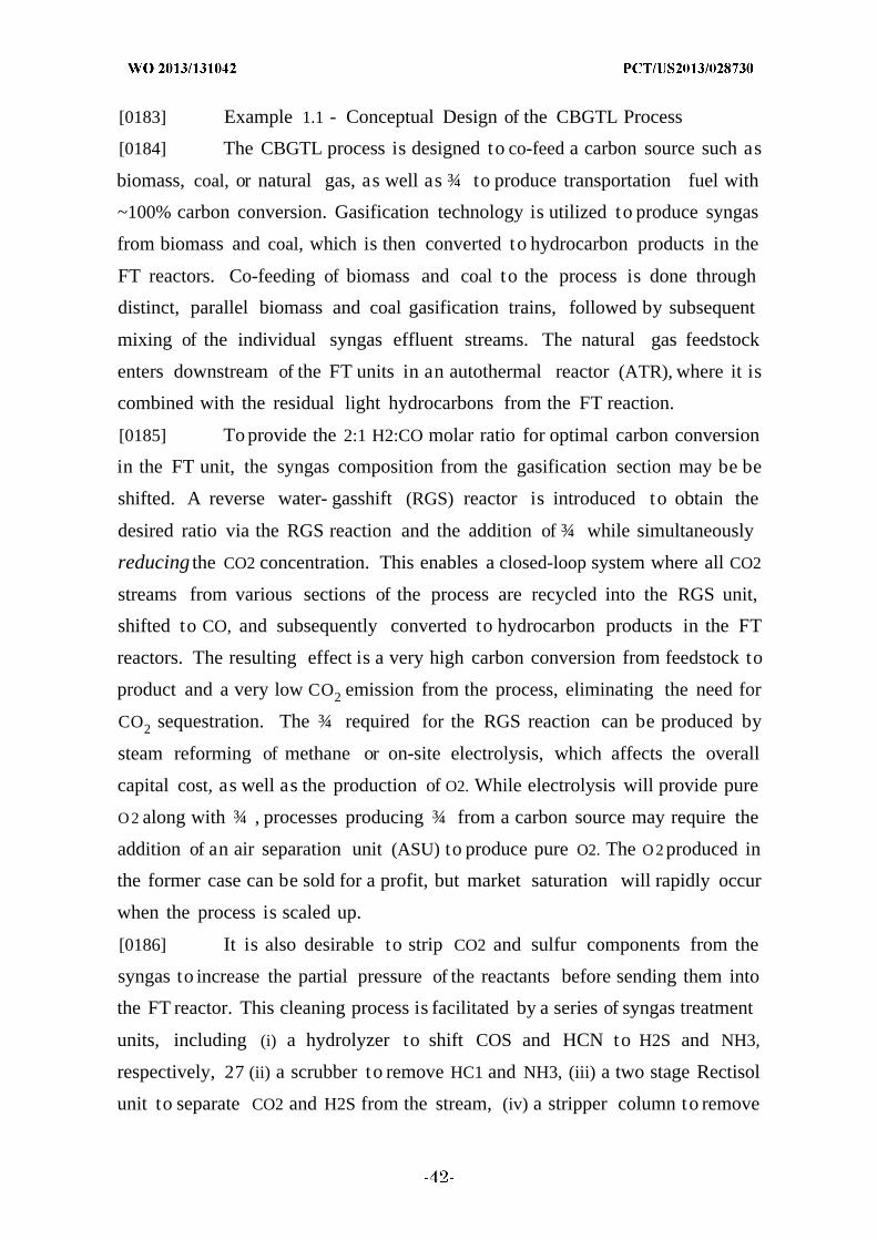
[0183] Example 1.1 - Conceptual Design of the CBGTL Process
[0184] The CBGTL process is designed to co-feed a carbon source such as
biomass, coal, or natural gas, as well as ¾ to produce transportation fuel with
~100% carbon conversion. Gasification technology is utilized to produce syngas
from biomass and coal, which is then converted to hydrocarbon products in the
FT reactors. Co-feeding of biomass and coal to the process is done through
distinct, parallel biomass and coal gasification trains, followed by subsequent
mixing of the individual syngas effluent streams. The natural gas feedstock
enters downstream of the FT units in an autothermal reactor (ATR), where it is
combined with the residual light hydrocarbons from the FT reaction.
[0185] To provide the 2:1 H2:CO molar ratio for optimal carbon conversion
in the FT unit, the syngas composition from the gasification section may be be
shifted. A reverse water- gasshift (RGS) reactor is introduced to obtain the
desired ratio via the RGS reaction and the addition of ¾ while simultaneously
reducing the CO2 concentration. This enables a closed-loop system where all CO2
streams from various sections of the process are recycled into the RGS unit,
shifted to CO, and subsequently converted to hydrocarbon products in the FT
reactors. The resulting effect is a very high carbon conversion from feedstock to
product and a very low CO2 emission from the process, eliminating the need for
CO2 sequestration. The ¾ required for the RGS reaction can be produced by
steam reforming of methane or on-site electrolysis, which affects the overall
capital cost, as well as the production of O2. While electrolysis will provide pure
O 2 along with ¾ , processes producing ¾ from a carbon source may require the
addition of an air separation unit (ASU) to produce pure O2. The O 2 produced in
the former case can be sold for a profit, but market saturation will rapidly occur
when the process is scaled up.
[0186] It is also desirable to strip CO2 and sulfur components from the
syngas to increase the partial pressure of the reactants before sending them into
the FT reactor. This cleaning process is facilitated by a series of syngas treatment
units, including (i) a hydrolyzer to shift COS and HCN to H2S and NH3,
respectively, 27 (ii) a scrubber to remove HC1 and NH3, (iii) a two stage Rectisol
unit to separate CO2 and H2S from the stream, (iv) a stripper column to remove

sour gas from the plant's disposed water, and (v) a Claus recovery system to
extract elemental sulfur from the syngas. The CO2 stream is then compressed
and sent back to the RGS unit while the clean, CO2- free and sulfur-free syngas is
sent to the FT section.
[0187] To produce gasoline, diesel, and kerosene products according to the
U.S. mass demand ratio, we employ FT reactors operating at two different
conditions: FT reactors at high temperature (320 °C) and low temperature (240
°C), each associated with distinct R (chain growth probability measure) values.
This R value is the single parameter used to predict the entire range of
hydrocarbon products in the modeling of a FT reactor. The syngas is split such
that the varied hydrocarbon product distributions given from the two R values
result in the correct product ratio. Fuel quality products are obtained by treating
the FT effluents in a detailed upgrading section. A hydrocracker unit is present
to convert waxes to additional fuels, and hydrotreater units are employed to
upgrade the naphtha and distillate fractions. The naphtha cut is further
reformed and isomerized to improve the octane number. Lighter forms of
hydrocarbons are passed through a series of alkylation and isomerization
processes to form high-octane gasoline blending stock. The off-gases from various
upgrading units are combined in a saturated gas plant and reformed in the
following three alternatives: (i) an ATR unit, (ii) a combustion unit, and (iii) a gas
turbine engine. The fraction to the combustion unit is determined to satisfy the
fuel requirement of the plant. The remaining gases are either sent to a gas
turbine engine, where they are combusted and expanded to produce electricity, or
to the ATR for steam reforming. The ATR unit is where the natural gas feedstock
is introduced into the process. Effluents of the combustion unit and the gas
turbine engine are passed through a one-stage Rectisol unit to separate out C02
from the build-up nitrogen. The CO2 stream, along with effluent of the ATR, are
recycled back to the RGS unit, minimizing CO2 emission from the process.
[0188] Example 1.2 - CBGTL Process Description
[0189] Using several key unit operations that have been reported in the
literature (National Research Council and National Academy of Engineering,
2004; Kreutz et al., 2008; Vliet et al., 2009; Agrawal et al., 2007; National Energy

Technology Laboratory, 2007; Bechtel, 1998; Bechtel, 1992; Hamelunck, 2004,
which are incorporated herein by reference as if fully set forth), a process
flowsheet is generated and developed in Aspen Plus. The CBGTL process is
designed to fulfill the mass ratio of U.S. transportation fuel needs for gasoline,
diesel, and kerosene, by taking combinations of biomass, coal, and natural gas as
feedstock. Referring to FIG. 17, the developed process flowsheet consists of the
following main sections: (i) syngas generation (P100), (ii) syngas treatment
(P200), (iii) hydrocarbon production (P300), (iv) hydrocarbon upgrading (P400),
(v) oxygen and hydrogen production (P500), and (vi) heat and power recovery
(P600). The thermodynamics package for the Peng-Robinson equation of state
with the Boston-Mathias alpha function is used in the simulation. The enthalpy
model used for nonconventional components in the flowsheet (i .e., biomass, coal,
ash, and char) is HCOALGEN, and the density model DCOALIGT is used for
biomass and coal and DCHARIGT is used for ash and char.
[0190] Details on the list of units, Aspen Plus modules used, and their
operating conditions are available in Tables 70 - 73.
[0191] Example 1.3 - Syngas Generation (Area P100).
[0192] Biomass and coal are converted to syngas using distinct, parallel
gasification trains (see FIG. 18). It has been estimated that 416 million dry tons
of biomass are available annually, which would supply ~35% of the
transportation demand on a carbon basis. Therefore, a hybrid feedstock is
developed from biomass, coal, and natural gas, so that 35% of the transportation
demand is satisfied by biomass, 40% is supplied by coal, and 25% is supplied by
natural gas. Assuming a total carbon feedstock input of 2000 tonnes per day
(TPD), a total of 948.62 TPD of biomass and 678.87 TPD of coal are fed to the
gasifiers. The 372.51 TPD of natural gas is input to an ATR unit in the
hydrocarbon upgrading section. The feedstock properties can be found in Tables 2
and 3.
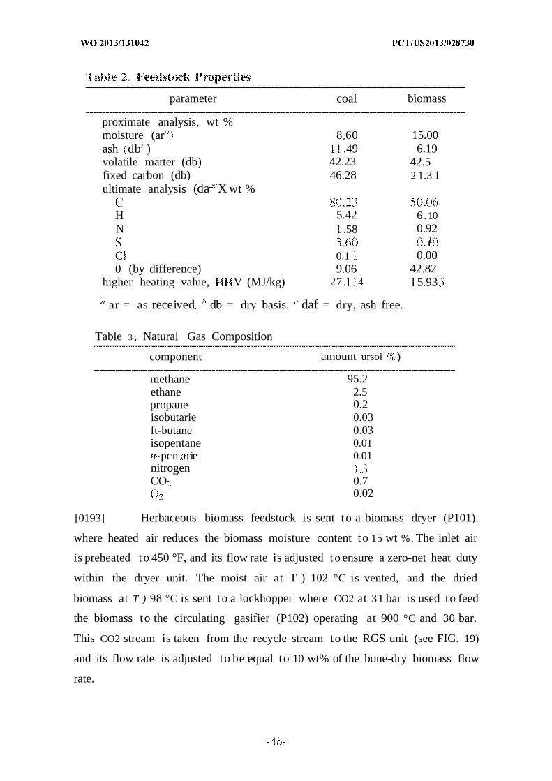
parameter coal biomass
proximate analysis, wt %moisture (ar ' 8 60 15.00ash db' ) .49 6.19volatile matter (db) 42.23 42.5fixed carbon (db) 46.28 2 1.3 1ultimate analysis (da X wt %
_ .H 5.42 6 .10N .58 0.92
. 1
C 0.1 0.000 (by difference) 9.06 42.82
higher heating value, V (MJ/kg) 27 . 4 5.93
ar = as received db = dry basis. daf = dry ash free.
Table 3 Natural Gas Composition
component amount ursoi )
methane 95.2ethane 2.5propane 0.2isobutarie 0.03ft-butane 0.03isopentane 0.01. pcn ie 0.01nitrogenCO 0.7
0.02
[0193] Herbaceous biomass feedstock is sent to a biomass dryer (P101),
where heated air reduces the biomass moisture content to 15 wt %. The inlet air
is preheated to 450 °F, and its flow rate is adjusted to ensure a zero-net heat duty
within the dryer unit. The moist air at T ) 102 °C is vented, and the dried
biomass at T ) 98 °C is sent to a lockhopper where CO2 at 31 bar is used to feed
the biomass to the circulating gasifier (P102) operating at 900 °C and 30 bar.
This CO2 stream is taken from the recycle stream to the RGS unit (see FIG. 19)
and its flow rate is adjusted to be equal to 10 wt% of the bone-dry biomass flow
rate.
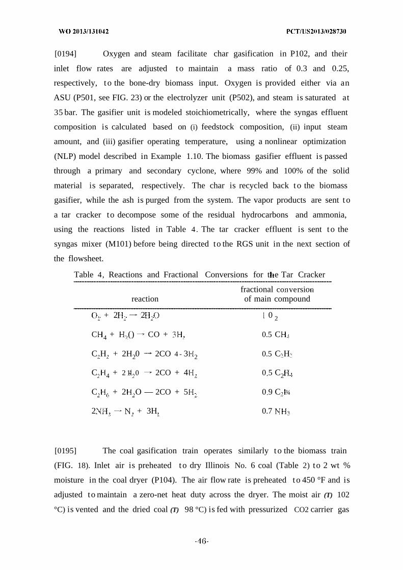
[0194] Oxygen and steam facilitate char gasification in P102, and their
inlet flow rates are adjusted to maintain a mass ratio of 0.3 and 0.25,
respectively, t o the bone-dry biomass input. Oxygen is provided either via an
ASU (P501, see FIG. 23) or the electrolyzer unit (P502), and steam is saturated at
35 bar. The gasifier unit is modeled stoichiometrically, where the syngas effluent
composition is calculated based on (i) feedstock composition, (ii) input steam
amount, and (iii) gasifier operating temperature, using a nonlinear optimization
(NLP) model described in Example 1.10. The biomass gasifier effluent is passed
through a primary and secondary cyclone, where 99% and 100% of the solid
material is separated, respectively. The char is recycled back to the biomass
gasifier, while the ash is purged from the system. The vapor products are sent to
a tar cracker to decompose some of the residual hydrocarbons and ammonia,
using the reactions listed in Table 4. The tar cracker effluent is sent to the
syngas mixer (M101) before being directed to the RGS unit in the next section of
the flowsheet.
Table 4, Reactions and Fractional Conversions for t e Tar Cracker
fractional co versioreaction of main compound
.. + 2 . 2 . 0 2
C 4 + () CO + , 0.5 C
C H + 2H20 2CO 4 - 3 2 0.5 C H
C 4 + 2 1- 0 2CO + 4 . 0 5 C2
C + 2 O — 2CO + 5 0 9 C ¾
2 , , + 3H, 0.7
[0195] The coal gasification train operates similarly to the biomass train
(FIG. 18). Inlet air is preheated to dry Illinois No. 6 coal (Table 2) to 2 wt %
moisture in the coal dryer (P104). The air flow rate is preheated to 450 °F and is
adjusted to maintain a zero-net heat duty across the dryer. The moist air (T) 102
°C) is vented and the dried coal (T) 98 °C) is fed with pressurized CO2 carrier gas
(10 wt % of dry coal flow rate) via a lockhopper into an entrained flow gasifier
(P105) operating at 1437 °C and 31 bar.27 The P105 inlet flow rates of oxygen
and 35 bar of saturated steam are adjusted to maintain a mass ratio of 0.7 and
0.3, respectively, to the bone-dry coal input. The syngas exits the gasifier below
the ash melting point at 891 °C, after which 99% of the ash is removed as liquid
slag. The syngas then enters an ash separator and a fly ash separator (P106),
where 99% and 100% of solid materials are separated, respectively. The solid
char is recycled back to the coal gasifier and the syngas is sent to M101.
[0196] Example 1.4 - Syngas Treatment (Area P200).
[0197] The syngas from M101 is fed to the reverse water -gas-shift (RGS)
reactor (P201) to shift the H2:CO ratio to 2:1 in the effluent stream by ¾
addition (FIG. 19). The effluent is assumed to be in equilibrium, with respect to
the RGS reaction:
CO + ,0 CO . i \ l (1)
[0198] The existence of this RGS unit allows a closed-loop, CO2 recycle
system that yields almost 100% carbon conversion. The CO2 recycle stream from
the acid gas removal unit (P204), combuster (P413) and gas turbine engine (P415)
along with the reformed gases from the ATR (P412) are fed to the RGS unit (FIG.
19). The unit operates at 700 °C, and the only components considered in the
equilibrium calculations are CO, CO2, H2, H2O, and O2. The inlet streams are
preheated to a constant temperature to ensure a net-zero heat duty for the RGS
reactor.
[0199] The RGS effluent is cooled to 185 °C and fed to a hydrolyzer unit
(P202) to undergo the following reactions:
COS + 20 C0 2 + 2S (2
HCN + 0 CO + N (3)
[0200] Only the components present in the above two equations will be
considered in the reaction-constrained equilibrium calculations. The gas is
further cooled to 35 °C and sent to a NH3/HCI scrubber (P203), a flash unit
(P204F), and a two-stage Rectisol unit (P204) combined with the tail gas from the
Claus process. The Rectisol unit recovers a pure CO2 and an acid gas stream,
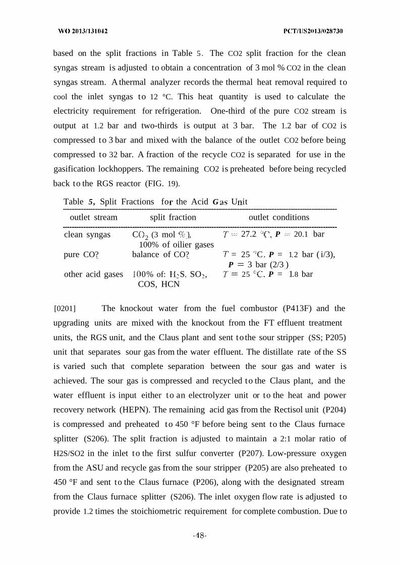
based on the split fractions in Table 5. The CO2 split fraction for the clean
syngas stream is adjusted to obtain a concentration of 3 mol % CO2 in the clean
syngas stream. A thermal analyzer records the thermal heat removal required to
cool the inlet syngas to 12 °C. This heat quantity is used to calculate the
electricity requirement for refrigeration. One-third of the pure CO2 stream is
output at 1.2 bar and two-thirds is output at 3 bar. The 1.2 bar of CO2 is
compressed to 3 bar and mixed with the balance of the outlet CO2 before being
compressed to 32 bar. A fraction of the recycle CO2 is separated for use in the
gasification lockhoppers. The remaining CO2 is preheated before being recycled
back to the RGS reactor (FIG. 19).
Table 5, Split Fractions fo the Acid G U it
outlet stream split fraction outlet conditions
clean syngas C 2 (3 mol , 27.2 P 20.1 bar100% of oilier gases
pure CO? balance of CO? = 25 C. P = 1 2 bar ( i/3),P 3 bar (2/3 )
other acid gases 0% of: S SO , 25 P = 1.8 barCOS, HCN
[0201] The knockout water from the fuel combustor (P413F) and the
upgrading units are mixed with the knockout from the FT effluent treatment
units, the RGS unit, and the Claus plant and sent to the sour stripper (SS; P205)
unit that separates sour gas from the water effluent. The distillate rate of the SS
is varied such that complete separation between the sour gas and water is
achieved. The sour gas is compressed and recycled to the Claus plant, and the
water effluent is input either to an electrolyzer unit or to the heat and power
recovery network (HEPN). The remaining acid gas from the Rectisol unit (P204)
is compressed and preheated to 450 °F before being sent to the Claus furnace
splitter (S206). The split fraction is adjusted to maintain a 2:1 molar ratio of
H2S/SO2 in the inlet to the first sulfur converter (P207). Low-pressure oxygen
from the ASU and recycle gas from the sour stripper (P205) are also preheated to
450 °F and sent to the Claus furnace (P206), along with the designated stream
from the Claus furnace splitter (S206). The inlet oxygen flow rate is adjusted to
provide 1.2 times the stoichiometric requirement for complete combustion. Due to

the high temperature present in the furnace, any ammonia present in the feed
stream will also be completely decomposed via the following reaction:
4NH + MX 2N + 6 20 (4)
[0202] The furnace effluent is then passed through a series of converter
units where the H2S reacts with SO2 to form sulfur via then following reaction:
2H S + S0 2 2 Q + 3S 5)
[0203] The fractional conversions of H2S are determined such that the inlet
stream temperatures of the sulfur separators (P208, P210, P212) are 10 °C
higher than the outlet temperatures. This is done to avoid turning the sulfur
separators into heat sinks in the heat and energy integration calculation, which
are discussed in the second part of this series of papers. All of the sulfur is
extracted in these units and mixed in a sulfur pit (M207). The tail gas from P212
is preheated to 450 °F before being sent to a hydrolyzer (P213) to convert any
remaining gas-phase sulfur species to H2S.27 The hydrolyzer effluent is cooled to
35 °C, sent to a flash unit (P213F) to knock out water, and compressed to 25 bar
before being recycled back to P204.
[0204] Example 1.5 - Hydrocarbon Production (Area P300).
[0205] In the third section, clean syngas is converted into a range of
hydrocarbon compounds in the FT reactors (FIG. 20) via the generic reaction
«CO + (« - p 0.5 ) , ( ) + (// . X(6
where n , m , and p are the number of carbon, hydrogen, and oxygen atoms,
respectively, in a given hydrocarbon compound. The distribution of the
hydrocarbon products formed in the reactors can be assumed to follow the
theoretical Anderson-Schulz-Flory (ASF) distribution, based on the chain growth
probability values (eq 7):
V,, n ( 1 ) ' (7)
where Wn is the mass fraction of the species with carbon number n and R is the
chain growth probability. In the modeling of this unit, the selected R values
predict the yields of hydrocarbon products.
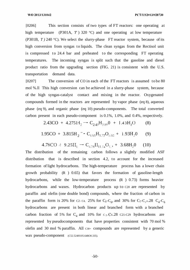
[0206] This section consists of two types of FT reactors: one operating at
high temperature (P301A, ) 320 °C) and one operating at low temperature
(P301B, T ) 240 °C). We select the slurry-phase FT reactor system, because of its
high conversion from syngas to liquids. The clean syngas from the Rectisol unit
is compressed to 24.4 bar and preheated to the corresponding FT operating
temperatures. The incoming syngas is split such that the gasoline and diesel
product ratio from the upgrading section (FIG. 21) is consistent with the U.S.
transportation demand data.
[0207] The conversion of CO in each of the FT reactors is assumed to be 80
mol %.ll This high conversion can be achieved in a slurry-phase system, because
of the high syngas-catalyst contact and mixing in the reactor. Oxygenated
compounds formed in the reactors are represented by vapor phase (eq 8), aqueous
phase (eq 9), and organic phase (eq 10) pseudo-components. The total converted
carbon present in each pseudo-component is 0.1%, 1.0%, and 0.4%, respectively.
2.43CO + 4.2751 C2 4 0 + .4 3 , (8)
1.95CO + 3.815H 2~ C 7O + i 93 0 (9)
4.7 - 9 .25 , C4
, + 3 68H 0 (10)
The distribution of the remaining carbon follows a slightly modified ASF
distribution that is described in section 4.2, to account for the increased
formation of light hydrocarbons. The high-temperature process has a lower chain
growth probability (R ) 0.65) that favors the formation of gasoline-length
hydrocarbons, while the low-temperature process (R ) 0.73) forms heavier
hydrocarbons and waxes. Hydrocarbon products up to C20 are represented by
paraffin and olefin (one double bond) compounds, where the fraction of carbon in
the paraffin form is 20% for C2- C4, 25% for C -C6, and 30% for C -C2 o.28 C4-C6
hydrocarbons are present in both linear and branched form with a branched
carbon fraction of 5% for C4 and 10% for C - 6.28 C21-C29 hydrocarbons are
represented by pseudocomponents that have properties consistent with 70 mol %
olefin and 30 mol % paraffin. All C30+ compounds are represented by a generic
wax pseudo-component (C52.524H105.648O0.335).

[0208] Treatment of the FT effluent streams (FIG. 20) follows from a
Bechtel simulation of a detailed product separation and catalyst recovery process
(Bechtel, 1998, which is incorporated herein by reference as if fully set forth). The
FT effluent streams are mixed and passed through a wax separation unit (P302).
The vapor is cooled, sent to an aqueous oxygenate separator (P303), flashed to
remove entrained water (P304), and passed through a vapor oxygenate separator
(P307). The knocked-out water and oxygenates are sent to the knockout mixer
(M303), while the vapor and organic liquids are sent to the first hydrocarbon
mixer (M306). The wax from P302 is cooled to 150 °C before being sent to an
entrained vapor removal unit (P305). The wax is sent to the second hydrocarbon
mixer (M304) and the vapor is further cooled to 40 °C and sent to a flash unit
(P306) for water knockout. The vapor is sent to M306, the organic liquid is sent to
M304, and the knockout water is sent to M303. All hydrocarbons are directed to
M401 before being sent to the upgrading section.
[0209] Example 1.6 - Hydrocarbon Upgrading (Area P400).
[0210] The role of the fourth section (FIG. 21) is to upgrade the
hydrocarbons to fuel quality. The hydrocarbons are first sent to a hydrocarbon
recovery unit (P401), where they are separated into light gases, C3-C5 gases,
naphtha, kerosene, distillate, wax, and wastewater (Table 6). The wastewater is
sent to the sour water mixer, and the light gases are sent to the saturated gas
plant (P411). The remaining outlet streams are sent to upgrading units based on
a Bechtel design (Bechtel, 1998; Bechtel, 1992, which are incorporated herein by
reference as if fully set forth). Since the process operating conditions for each
upgrading unit are unknown, the distribution of the outlet for each unit is
assumed to be equal to the Bechtel baseline Illinois No. 6 coal case study
(Bechtel, 1992, which is incorporated herein by reference as if fully set forth) For
each upgrading unit, the percentage of carbon present in the effluent is
calculated and the carbon in the inlet is distributed to the effluent in appropriate
proportions. When applicable, the hydrogen balance is satisfied by adjusting the
input flow rate of upgrading hydrogen sent to the reactor. If hydrogen is not sent
directly to a unit, then the atomic balances are satisfied by adjusting the carbon
fractions present in the light gas output, so that the difference between the
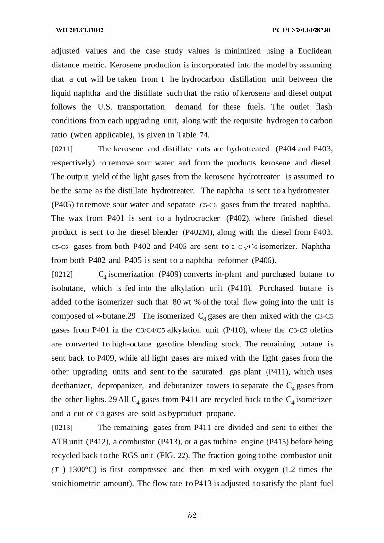
adjusted values and the case study values is minimized using a Euclidean
distance metric. Kerosene production is incorporated into the model by assuming
that a cut will be taken from t he hydrocarbon distillation unit between the
liquid naphtha and the distillate such that the ratio of kerosene and diesel output
follows the U.S. transportation demand for these fuels. The outlet flash
conditions from each upgrading unit, along with the requisite hydrogen to carbon
ratio (when applicable), is given in Table 74.
[0211] The kerosene and distillate cuts are hydrotreated (P404 and P403,
respectively) to remove sour water and form the products kerosene and diesel.
The output yield of the light gases from the kerosene hydrotreater is assumed to
be the same as the distillate hydrotreater. The naphtha is sent to a hydrotreater
(P405) to remove sour water and separate C5-C6 gases from the treated naphtha.
The wax from P401 is sent to a hydrocracker (P402), where finished diesel
product is sent to the diesel blender (P402M), along with the diesel from P403.
C5-C6 gases from both P402 and P405 are sent to a C 6 isomerizer. Naphtha
from both P402 and P405 is sent to a naphtha reformer (P406).
[0212] C4 isomerization (P409) converts in-plant and purchased butane to
isobutane, which is fed into the alkylation unit (P410). Purchased butane is
added to the isomerizer such that 80 wt % of the total flow going into the unit is
composed of «-butane.29 The isomerized C4 gases are then mixed with the C3-C5
gases from P401 in the C3/C4/C5 alkylation unit (P410), where the C3-C5 olefins
are converted to high-octane gasoline blending stock. The remaining butane is
sent back to P409, while all light gases are mixed with the light gases from the
other upgrading units and sent to the saturated gas plant (P411), which uses
deethanizer, depropanizer, and debutanizer towers to separate the C4 gases from
the other lights. 29 All C4 gases from P411 are recycled back to the C4 isomerizer
and a cut of C 3 gases are sold as byproduct propane.
[0213] The remaining gases from P411 are divided and sent to either the
ATR unit (P412), a combustor (P413), or a gas turbine engine (P415) before being
recycled back to the RGS unit (FIG. 22). The fraction going to the combustor unit
(T ) 1300°C) is first compressed and then mixed with oxygen (1.2 times the
stoichiometric amount). The flow rate to P413 is adjusted to satisfy the plant fuel
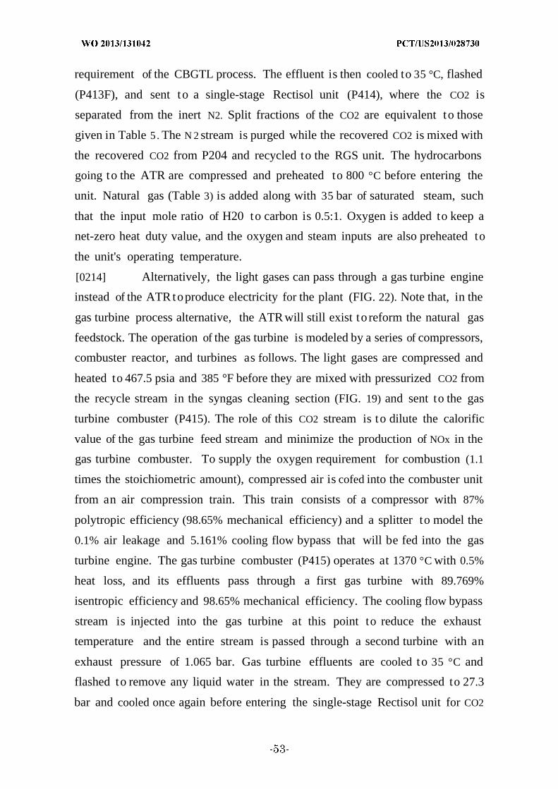
requirement of the CBGTL process. The effluent is then cooled to 35 °C, flashed
(P413F), and sent to a single-stage Rectisol unit (P414), where the CO2 is
separated from the inert N2. Split fractions of the CO2 are equivalent to those
given in Table 5. The N 2 stream is purged while the recovered CO2 is mixed with
the recovered CO2 from P204 and recycled to the RGS unit. The hydrocarbons
going to the ATR are compressed and preheated to 800 °C before entering the
unit. Natural gas (Table 3) is added along with 35 bar of saturated steam, such
that the input mole ratio of H20 to carbon is 0.5:1. Oxygen is added to keep a
net-zero heat duty value, and the oxygen and steam inputs are also preheated to
the unit's operating temperature.
[0214] Alternatively, the light gases can pass through a gas turbine engine
instead of the ATR toproduce electricity for the plant (FIG. 22). Note that, in the
gas turbine process alternative, the ATR will still exist to reform the natural gas
feedstock. The operation of the gas turbine is modeled by a series of compressors,
combuster reactor, and turbines as follows. The light gases are compressed and
heated to 467.5 psia and 385 °F before they are mixed with pressurized CO2 from
the recycle stream in the syngas cleaning section (FIG. 19) and sent to the gas
turbine combuster (P415). The role of this CO2 stream is to dilute the calorific
value of the gas turbine feed stream and minimize the production of NOx in the
gas turbine combuster. To supply the oxygen requirement for combustion (1.1
times the stoichiometric amount), compressed air is cofed into the combuster unit
from an air compression train. This train consists of a compressor with 87%
polytropic efficiency (98.65% mechanical efficiency) and a splitter to model the
0.1% air leakage and 5.161% cooling flow bypass that will be fed into the gas
turbine engine. The gas turbine combuster (P415) operates at 1370 °C with 0.5%
heat loss, and its effluents pass through a first gas turbine with 89.769%
isentropic efficiency and 98.65% mechanical efficiency. The cooling flow bypass
stream is injected into the gas turbine at this point to reduce the exhaust
temperature and the entire stream is passed through a second turbine with an
exhaust pressure of 1.065 bar. Gas turbine effluents are cooled to 35 °C and
flashed to remove any liquid water in the stream. They are compressed to 27.3
bar and cooled once again before entering the single-stage Rectisol unit for CO2

separation. Finally, the ATR and gas turbine effluent are sent back to the RGS
unit.
[0215] Example 1.7 —Oxygen and Hydrogen Production (Area P500).
[0216] The oxygen and hydrogen production section (FIG. 23) consists of
alternative technologies that are presently available or expected to be in
commercial status in the future. Considered alternatives include (i) an ASU that
produces a 99.5 wt % O 2 stream and hydrogen purchase from steam reforming of
natural gas, or (ii) an electrolyzer unit that produces pure H 2 and O 2 from the
plant's water effluent and electricity. Electricity can be obtained from the grid or
alternative sources such as solar, wind, and nuclear technologies as they become
more available in the future.
[0217] If hydrogen is produced off-site, the oxygen input must be obtained
from an ASU. Air is initially compressed from ambient conditions to 190 psia and
then sent to the ASU (P501), where a 99.5 wt % O2 stream (T = 90 °F, P = 125
psia) is recovered and the nitrogen-rich stream (T = 70 °F, P = 16.4 psia) is
vented. A portion of the oxygen stream is split and fed into the low-pressure
Claus furnace, while the balance is compressed to 32 bar for use with the
remaining process units. Hydrogen is purchased from steam reforming of
methane (SRM) technology, such that its total provides the required hydrogen for
the RGS unit and the upgrading units. If hydrogen is produced on-site, an
electrolyzer unit will be utilized to produce pure H 2 and O 2 from the water
effluent of the SS unit. 7 Oxygen that is not consumed by the CBGTL process will
be sold as a byproduct.
[0218] Example 1.8 - Heat and Power Recovery (Area P600).
[0219] The heat and power recovery system utilizes heat engines and
pumps that interact with process streams to produce steam or electricity. Plant
water and additional purchased water are used to produce steam required by the
various process units. The full description and mathematical models of the heat
and power integration step are detailed in Example 2, which outlines a three-
stage decomposition framework consisting of the minimization of hot/cold/power
utility requirement, the minimization of heat exchanger units, and the
minimization of the annualized cost of heat exchange. Once the full heat and

power integration step is completed, the obtained costs are factored into the
economic analysis of the entire process, as described in Examples 1.22 —1.25.
[0220] Example 1.9 - Process Modeling
[0221] Although most of the operating units in the CBGTL process are
modeled using standard Aspen Plus modules (as otherwise described herein), the
gasifiers, FT units, and all upgrading units are modeled using the USER2 block
option. The USER2 block allows the Aspen Plus engine to dynamically link to a
Microsoft Excel spreadsheet, where user-input calculations can provide the
necessary effluent concentrations. The outlet stream conditions of the USER2
blocks can then be set to a given temperature and pressure, based upon
predefined values. The USER2 blocks serve as a means of implementing (i) a
novel stoichiometric model for biomass and coal gasification, (ii) a probabilistic
FT model based on the chain growth factor (a), and (iii) individual models for the
upgrading units based on a Bechtel design. The following section details the
mathematical models designed for the CBGTL process.
[0222] Example 1.10 - Coal/Biomass Gasification.
[0223] The reaction system within a gasifier consists of a series of
pyrolysis, combustion, and gasification steps that are designed to release the
volatile matter within the solid feedstock and subsequently convert the residual
solid to syngas. Though it has been documented that the major gas phase
components (H2O, ¾ , CO, CO2) will be close to thermodynamic equilibrium via
the water gas shift (WGS) reaction (eq 1), the residual gases (C1-C2
Hydrocarbons, H2S, COS, NH3, HCN, HC1, etc.) will often be present in
concentrations far above their equilibrium values. A detailed model of the
kinetics within a gasifier can be a challenging task, especially since the accuracy
of the model will be strongly dependent on the choice of rate constants for the
multiple reactions within the unit. Several models have been developed using
appropriate conditions for entrained flow and circulating flow gasifiers. A novel
stoichiometric gasifier model capable of determining the effluent flow rates based
on a variety of experimental data is disclosed herein.
[0224] Example 1.11 —Biomass Pyrolysis.
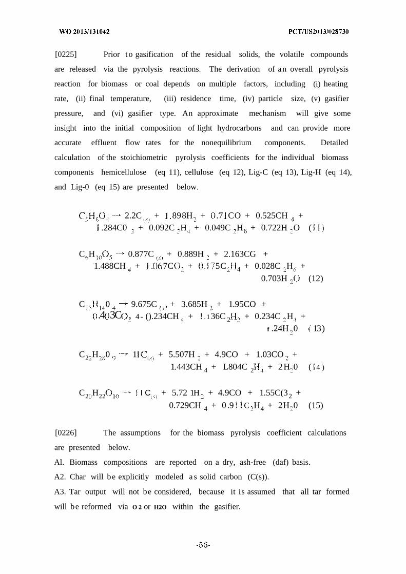
[0225] Prior t o gasification of the residual solids, the volatile compounds
are released via the pyrolysis reactions. The derivation of an overall pyrolysis
reaction for biomass or coal depends on multiple factors, including (i) heating
rate, (ii) final temperature, (iii) residence time, (iv) particle size, (v) gasifier
pressure, and (vi) gasifier type. An approximate mechanism will give some
insight into the initial composition of light hydrocarbons and can provide more
accurate effluent flow rates for the nonequilibrium components. Detailed
calculation of the stoichiometric pyrolysis coefficients for the individual biomass
components hemicellulose (eq 11), cellulose (eq 12), Lig-C (eq 13), Lig-H (eq 14),
and Lig-0 (eq 15) are presented below.
, 2.2C + 898H + .7 CO + 0.525CH +.284C0 + 0.092C H + 0.049C H6 + 0.722H O (
C H 0.877C + 0.889H + 2.163CG +1.488CH + . 7C + . 5C 4 + 0.028C H +
0.703H (12)
C 4 0 9.675C , + 3.685H + 1.95CO +.4 3C , 4 - ().234CH + ! . 136C 2 + 0.234C H +
f .24H 0 13)
C2 H 0 1 + 5.507H + 4.9CO + 1.03CO +
1.443CH 4 + L804C 2 + 2H 0 ( 4 )
C2 H22 I C + 5.72 1H + 4.9CO + 1.55C(32 +
0.729CH 4 + 0.9 C H4 + 2H 0 (15)
[0226] The assumptions for the biomass pyrolysis coefficient calculations
are presented below.
Al. Biomass compositions are reported on a dry, ash-free (daf) basis.
A2. Char will be explicitly modeled a s solid carbon (C(s)).
A3. Tar output will not be considered, because it is assumed that all tar formed
will be reformed via O 2 or H2O within the gasifier.

A4. All products of the pyrolysis reaction will consist of the following compounds:
H20 , H2, CO, CO2, CH4, C2H2, C2H4, C2H6, and char.
A5. The main constituents of biomass are cellulose, hemicellulose, Lig-C, Lig-O,
and Lig-H, which are represented as Η ιοΟ , C5H8O4, C15H14O4, C20H22O10, and
C22H28O9, respectively.
A6. An independent pyrolysis equation will occur for each biomass monomer.
A7. The initial composition of volatiles of hemicellulose and cellulose
decomposition will follow from Table 2 of Yang et al, 2007, which is incorporated
herein by reference as if filly set forth. The residual char will also be based on the
observations in Yang et al, 2007, which is incorporated herein by reference as if
fully set forth.
A8. All unaccounted carbon, hydrogen, and oxygen in the mass balance for the
decomposition from assumption A7 is assumed to be present in H2O, CH4, C2H4,
and CO for cellulose and in H2O, CH4, C2H4, and H 2 for hemicellulose.
A9. Since Yang et al., 2007 do not provide a decomposition framework for each
lignin monomer, one will be adapted from the kinetic model in Table 3 of Ranzi et
al., 2008, which is incorporated herein by reference as if fully set forth, by
assuming that all reactions present in the kinetic model proceed to completion.
A10. All unaccounted oxygen in the mass balance for the decomposition from
assumption A9 is assumed to be present in CO2. All unaccounted carbon and
hydrogen in the mass balance is assumed to be present as tar, which will
decompose into CH4, C2H2, and C2H4 such that CH4 and C2H4 are present in the
same proportions as in the initial volatiles composition. All residual unaccounted
hydrogen is assumed to be present as H2.
[0227] The dry composition of the vapor phase for cellulose and
hemicellulose pyrolysis is given in Table 2 of Yang et al., 2007, which is
incorporated herein by reference as if fully set forth and is reproduced in Table 7.
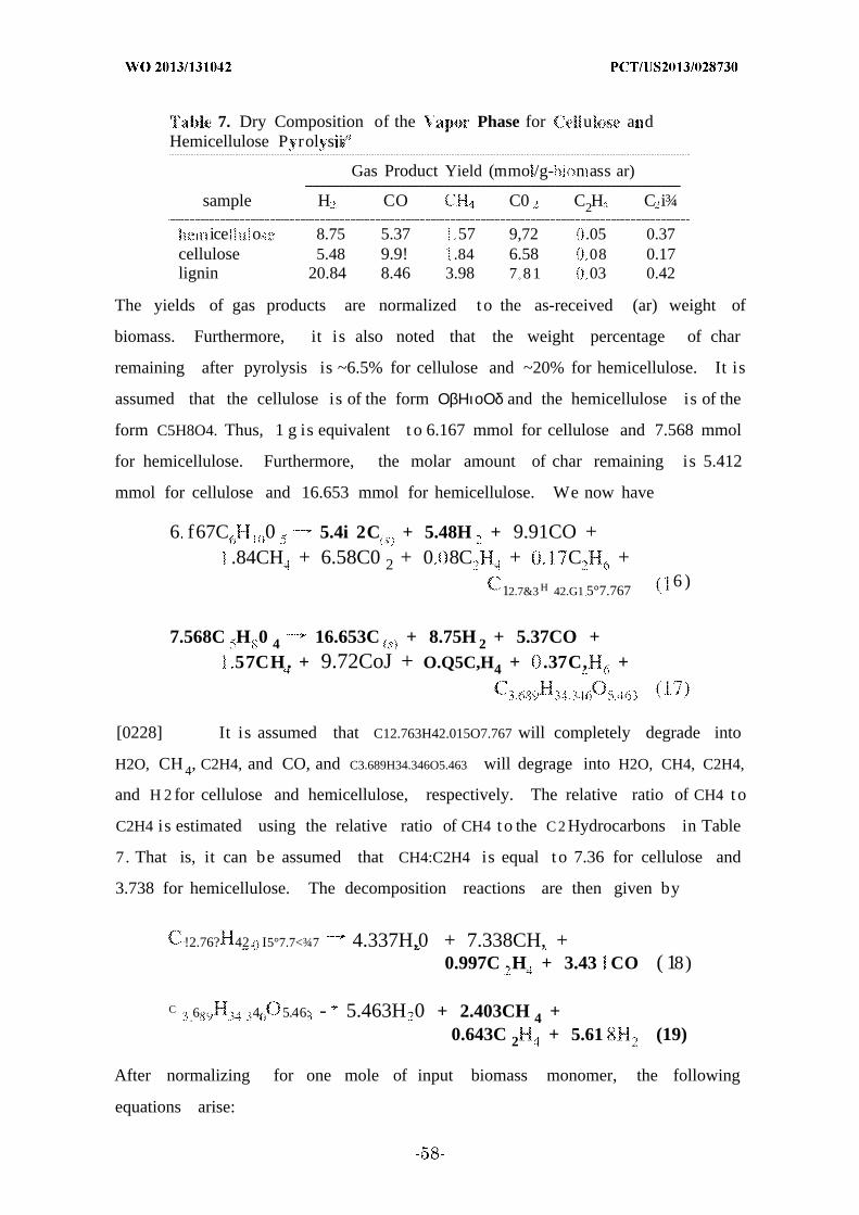
' 7. Dry Composition of the Phase for u a dHemicellulose P rol s i
Gas Product Yield (rnmo /g- n ass ar)
sample H CO C0 C2H C i¾
ice o 8.75 5.37 57 9,72 .05 0.37cellulose 5.48 9.9! .84 6.58 08 0.17lignin 20.84 8.46 3.98 7 81 03 0.42
The yields of gas products are normalized to the as-received (ar) weight of
biomass. Furthermore, it is also noted that the weight percentage of char
remaining after pyrolysis is ~6.5% for cellulose and ~20% for hemicellulose. It is
assumed that the cellulose is of the form ΟβΗιοΟδ and the hemicellulose is of the
form C5H8O4. Thus, 1 g is equivalent t o 6.167 mmol for cellulose and 7.568 mmol
for hemicellulose. Furthermore, the molar amount of char remaining is 5.412
mmol for cellulose and 16.653 mmol for hemicellulose. We now have
6 f67C 0 5.4i 2C + 5.48H + 9.91CO +.84CH + 6.58C0 2 + 0 8C + C +
12.7&3 H 42.G1 5°7.7676 )
7.568C H 0 4 16.653C + 8.75H 2 + 5.37CO +57CH. + 9.72CoJ + O.Q5C,H4 + .37C, +
[0228] It is assumed that C12.763H42.015O7.767 will completely degrade into
H2O, CH 4, C2H4, and CO, and C3.689H34.346O5.463 will degrage into H2O, CH4, C2H4,
and H 2 for cellulose and hemicellulose, respectively. The relative ratio of CH4 t o
C2H4 is estimated using the relative ratio of CH4 t o the C 2 Hydrocarbons in Table
7. That is, it can be assumed that CH4:C2H4 is equal t o 7.36 for cellulose and
3.738 for hemicellulose. The decomposition reactions are then given by
!2.76? 42. I5°7.7<¾7 4.337H,0 + 7.338CH, +0.997C H + 3.43 CO ( 18)
C.6 4 5.46: - 5.463H 0 + 2.403CH 4 +
0.643C 2 + 5.61 (19)
After normalizing for one mole of input biomass monomer, the following
equations arise:
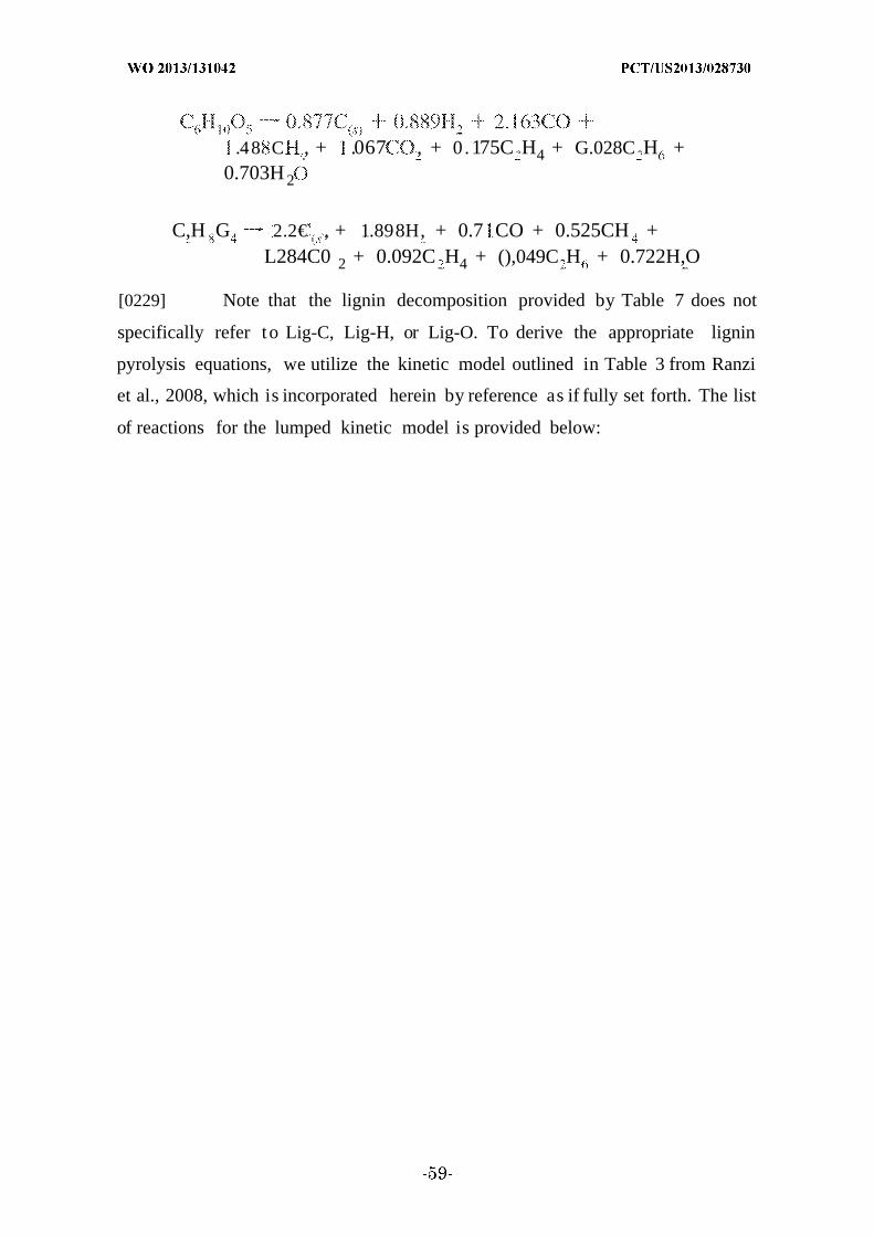
.48 C ., + .067 , + 0.175C H4 + G.028C H +0.703H 2
C,H G 2.2€ , + 1.898H, + 0.7 CO + 0.525CH +L284C0 2 + 0.092C H4 + (),049C H + 0.722H,O
[0229] Note that the lignin decomposition provided by Table 7 does not
specifically refer to Lig-C, Lig-H, or Lig-O. To derive the appropriate lignin
pyrolysis equations, we utilize the kinetic model outlined in Table 3 from Ranzi
et al., 2008, which is incorporated herein by reference as if fully set forth. The list
of reactions for the lumped kinetic model is provided below:

Lig-C 0.35Lig pC ur aryl - 0.08Piienol +
49 2 4 L32GC 2 + 7 4 5C (20)
g H L g 4 C 0 (2 )
Lig-O Lig + CC0 (22)
Lig G3 pCo rm y ·· ·· 0 2 P en l + 035C 3 O +
L2 4 - C).7H 0 + .25 4 4 - 0 25C2
L3G C 2 + 0.5GI CO + 7.5 (23)
L ig 0 - H 0 + C 3 H + GCO ÷! .5G C0 1 + 5C (24)
Lig (25)
Lig .7 -L ÷ Hp .4C 4 - 0.5CO 4 - 0 4C 4
0.2 4 ( 4 0.2 2 0 4C 5C2 4 4-
G fC 4 0.5G + C (26)
GC0 C0 2 (27)
GCO CO (28)
GCOH CO 4 H (29)
where Lig-C, Lig-H, and Lig-0 are represented a s C15H14O4, C22H28O9, and
C20H22O10, respectively.
[0230] It is assumed that (i) all reactions proceed to completion and (ii) the
reaction of Lig f - C11H12O4 is negligible, with respect t o the decomposition of
Lig. Note that assumption (ii) is justified because the rate of reaction of Lig
decomposition is -400 times greater at 500 K. Given these assumptions, Lig- C,
Lig-H, and Lig-0 decomposition reactions are modeled a s follows:
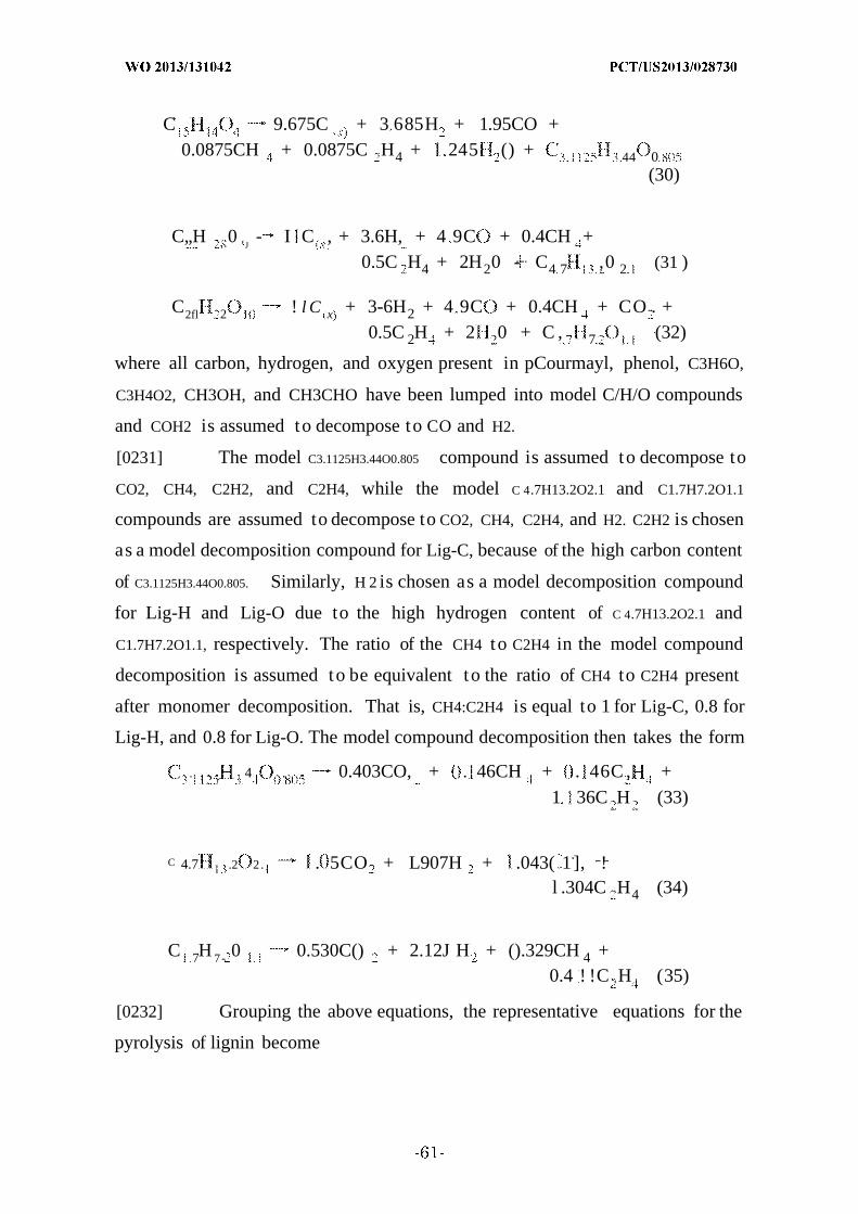
C 9.675C + 3 685H + 1.95CO +0.0875CH + 0.0875C H4 + 245 () + 44 0
(30)
C„H 0J
- I C , + 3.6H, + 4 9C + 0.4CH +0.5C H4 + 2H20 - C4 7 ,0 2 (31 )
C2fl 2 ! l C x + 3-6H2 + 4 9C + 0.4CH + CO . +0.5C 2H + 2 0 + C , 7 (32)
where all carbon, hydrogen, and oxygen present in pCourmayl, phenol, C3H6O,
C3H4O2, CH3OH, and CH3CHO have been lumped into model C/H/O compounds
and COH2 is assumed to decompose to CO and H2.
[0231] The model C3.1125H3.44O0.805 compound is assumed to decompose to
CO2, CH4, C2H2, and C2H4, while the model C 4.7H13.2O2.1 and C1.7H7.2O1.1
compounds are assumed to decompose to CO2, CH4, C2H4, and H2. C2H2 is chosen
as a model decomposition compound for Lig-C, because of the high carbon content
of C3.1125H3.44O0.805. Similarly, H 2 is chosen as a model decomposition compound
for Lig-H and Lig-O due to the high hydrogen content of C 4.7H13.2O2.1 and
C1.7H7.2O1.1, respectively. The ratio of the CH4 to C2H4 in the model compound
decomposition is assumed to be equivalent to the ratio of CH4 to C2H4 present
after monomer decomposition. That is, CH4:C2H4 is equal to 1 for Lig-C, 0.8 for
Lig-H, and 0.8 for Lig-O. The model compound decomposition then takes the form
. 4 . 0.403CO, + . 46CH + . 46C , +1 36C H (33)
C 4.7 .2 2 . . 5CO + L907H + .043( 1·], !l .304C H4 (34)
C 7H 7- 0 0.530C() + 2.12J H + ().329CH 4 +0.4 ! !C H (35)
[0232] Grouping the above equations, the representative equations for the
pyrolysis of lignin become
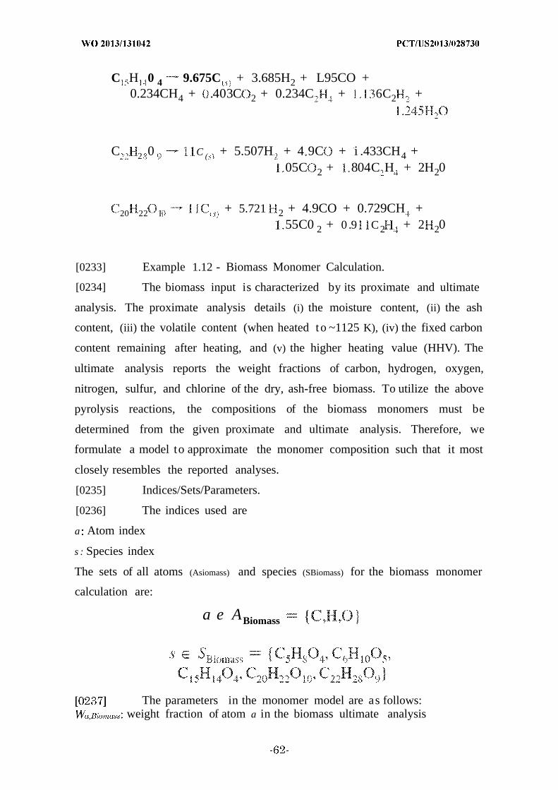
C H 0 4 9.675C + 3.685H2 + L95CO +0.234CH4 + .403C 2 + 0.234C + 6C2 +
C 2 0 C ( + 5.507H + 4 9C + i .433CH4 +05C 2 + 804C H + 2H20
20 22 I + 5.721 2 + 4.9CO + 0.729CH +55C0 2 + 0 .9 C2 + 2 20
[0233] Example 1.12 - Biomass Monomer Calculation.
[0234] The biomass input is characterized by its proximate and ultimate
analysis. The proximate analysis details (i) the moisture content, (ii) the ash
content, (iii) the volatile content (when heated to ~1125 K), (iv) the fixed carbon
content remaining after heating, and (v) the higher heating value (HHV). The
ultimate analysis reports the weight fractions of carbon, hydrogen, oxygen,
nitrogen, sulfur, and chlorine of the dry, ash-free biomass. To utilize the above
pyrolysis reactions, the compositions of the biomass monomers must be
determined from the given proximate and ultimate analysis. Therefore, we
formulate a model to approximate the monomer composition such that it most
closely resembles the reported analyses.
[0235] Indices/Sets/Parameters.
[0236] The indices used are
a Atom index
s : Species index
The sets of all atoms (Asiomass) and species (SBiomass) for the biomass monomer
calculation are:
a e ABiomass
The parameters in the monomer model are as follows:weight fraction of atom a in the biomass ultimate analysis
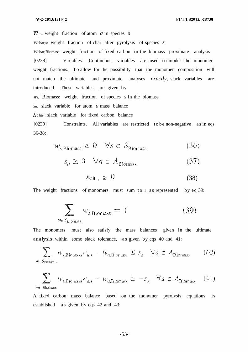
weight fraction of atom a in species s
Wchar,s: weight fraction of char after pyrolysis of species s
Wchar,Biomass: weight fraction of fixed carbon in the biomass proximate analysis
[0238] Variables. Continuous variables are used t o model the monomer
weight fractions. To allow for the possibility that the monomer composition will
not match the ultimate and proximate analyses exactly, slack variables are
introduced. These variables are given by
Ws, Biomass: weight fraction of species s in the biomass
Sa. slack variable for atom a mass balance
cha : slack variable for fixed carbon balance
[0239] Constraints. All variables are restricted t o be non-negative a s in eqs
36-38:
cta ≥ (38)
The weight fractions of monomers must sum t o 1, a s represented by eq 39:
ss
The monomers must also satisfy the mass balances given in the ultimate
a na l sis, within some slack tolerance, a s given by eqs 40 and 41:
$ Biomass
e .¾k,t!sass
A fixed carbon mass balance based on the monomer pyrolysis equations is
established a s given by eqs 42 and 43:

W . Char. C r,. a Ch a
[0240] Objective Function. By minimizing the slack variables (eq 44), the
ultimate and proximate analyses can be approximated as closely a s possible.
i
where l a g 1 is introduced to emphasize the importance of satisfying the atom
balances, compared to the fixed carbon balance. For this analysis, X is set to 100
for all a .
[0241] Example 1.13 - Results.
[0242] The biomass used in the CBGTL process is herbaceous switchgrass.
Using the ultimate analysis given in Table 2, the parameters in Table 8 are
calculated.
Table 8 Parameters of the Biomass Monomer Calculation
C J iomass 0 50576
' .c:. H ,. 0.05463
3
1
C = 0.06216 · .( . . . ν·= 0 ,052490.49332 ¾ o 0.37876
. 0.00650 ~ 0.3 279
Optimization of the biomass monomer model (eqs 36-44) yields the biomass
composition, W .Biomass, which is presented in Table 9.
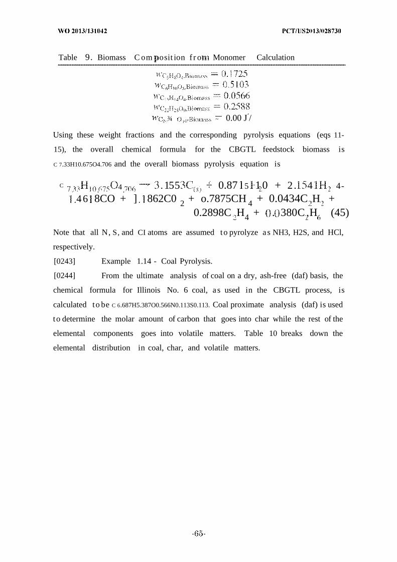
Table 9. Biomass C om osit ion f r o Monomer Calculation
¾ i ~ 0.00 J /
Using these weight fractions and the corresponding pyrolysis equations (eqs 11-
15), the overall chemical formula for the CBGTL feedstock biomass is
C 7.33H10.675O4.706 and the overall biomass pyrolysis equation is
C. , 4 ,
.155 ÷ 0.87 5 1 0 + 2. 4 4-
4 6 8CO + ] 862C0 2 + o.7875CH 4 + 0.0434C H +0.2898C H4 + . 380C ,H (45)
Note that all N, S, and CI atoms are assumed to pyrolyze as NH3, H2S, and HCl,
respectively.
[0243] Example 1.14 - Coal Pyrolysis.
[0244] From the ultimate analysis of coal on a dry, ash-free (daf) basis, the
chemical formula for Illinois No. 6 coal, a s used in the CBGTL process, is
calculated to be C 6.687H5.387O0.566N0.113S0.113. Coal proximate analysis (daf) is used
to determine the molar amount of carbon that goes into char while the rest of the
elemental components goes into volatile matters. Table 10 breaks down the
elemental distribution in coal, char, and volatile matters.
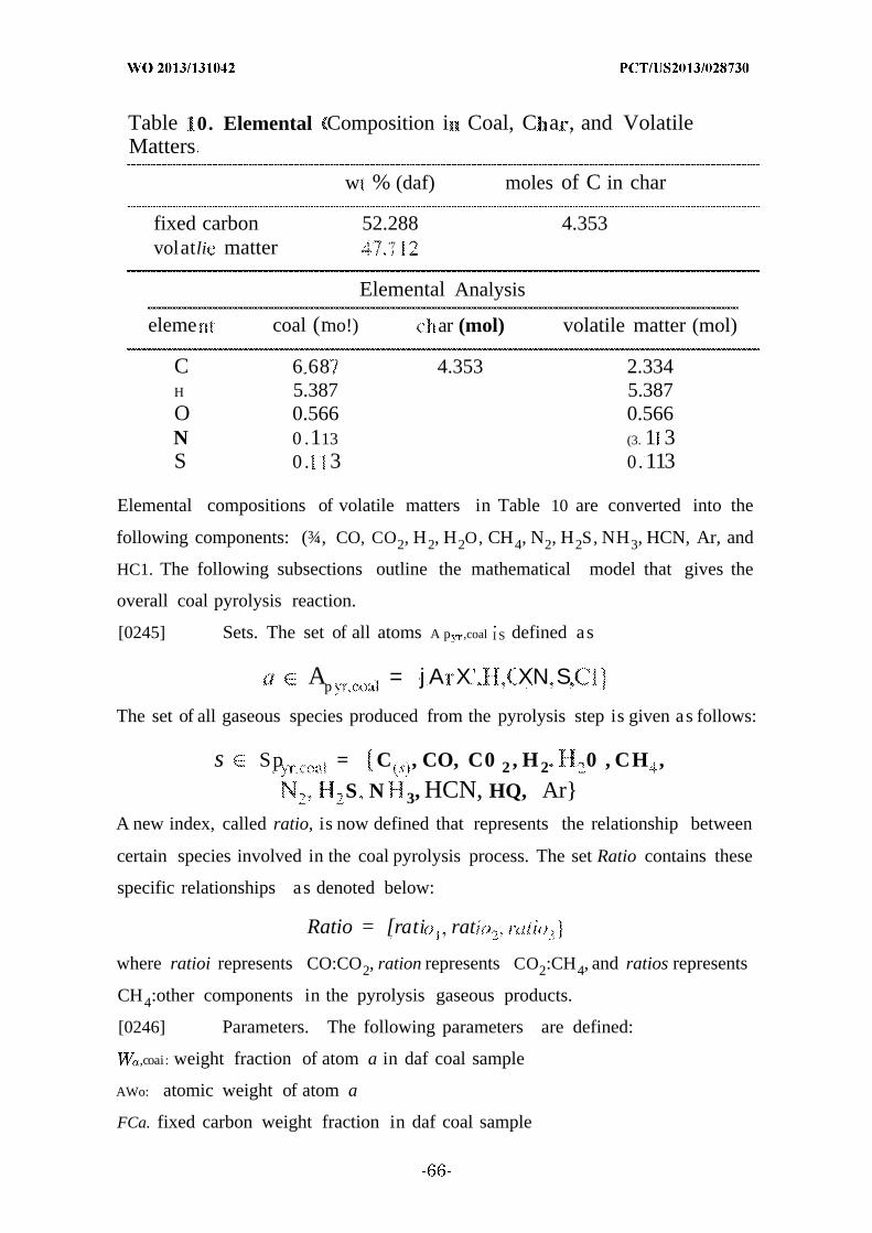
Table 0. Elemental Composition i Coal, C a , and VolatileMatters
w % (daf) moles of C in char
fixed carbon 52.288 4.353volatli matter "7
Elemental Analysis
eleme coal (rno!) ar (mol) volatile matter (mol)
C 6 68 4.353 2.334H 5.387 5.387O 0.566 0.566N 0 .113 (3. 1 3S 0 . 3 0. 113
Elemental compositions of volatile matters in Table 10 are converted into the
following components: (¾, CO, CO2, H2, H2O, CH4, N2, H2S, NH3, HCN, Ar, and
HC1. The following subsections outline the mathematical model that gives the
overall coal pyrolysis reaction.
[0245] Sets. The set of all atoms A p ,coal I S defined as
Ap = j A X XN S
The set of all gaseous species produced from the pyrolysis step is given as follows:
s Sp = C , CO, C0 2 , H 2 0 , CH ,
S N 3, HCN, HQ, Ar
A new index, called ratio, is now defined that represents the relationship between
certain species involved in the coal pyrolysis process. The set Ratio contains these
specific relationships as denoted below:
Ratio = [rati rat
where ratioi represents CO:CO2, ration represents CO2:CH4, and ratios represents
CH4:other components in the pyrolysis gaseous products.
[0246] Parameters. The following parameters are defined:
,coai: weight fraction of atom a in daf coal sample
AWo: atomic weight of atom a
FCa. fixed carbon weight fraction in daf coal sample
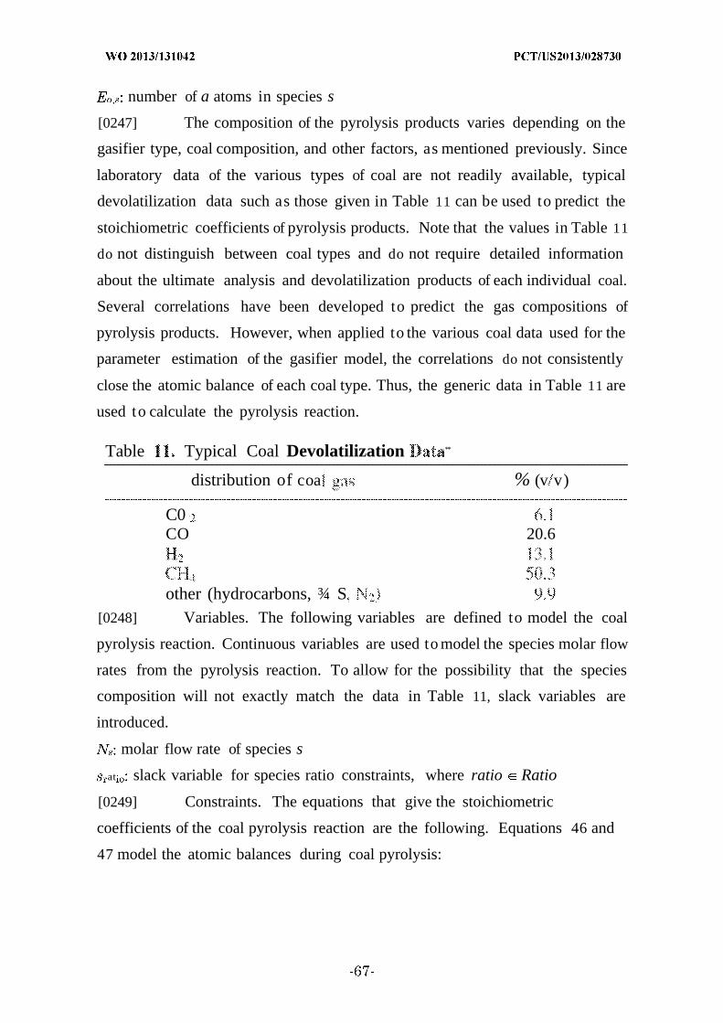
number of a atoms in species s
[0247] The composition of the pyrolysis products varies depending on the
gasifier type, coal composition, and other factors, as mentioned previously. Since
laboratory data of the various types of coal are not readily available, typical
devolatilization data such as those given in Table 11 can be used to predict the
stoichiometric coefficients of pyrolysis products. Note that the values in Table 11
do not distinguish between coal types and do not require detailed information
about the ultimate analysis and devolatilization products of each individual coal.
Several correlations have been developed to predict the gas compositions of
pyrolysis products. However, when applied to the various coal data used for the
parameter estimation of the gasifier model, the correlations do not consistently
close the atomic balance of each coal type. Thus, the generic data in Table 11 are
used to calculate the pyrolysis reaction.
Table Typical Coal Devolatilization **
distribution of coa % (v v)
C0CO 20.6
other (hydrocarbons, ¾ S[0248] Variables. The following variables are defined to model the coal
pyrolysis reaction. Continuous variables are used to model the species molar flow
rates from the pyrolysis reaction. To allow for the possibility that the species
composition will not exactly match the data in Table 11, slack variables are
introduced.
molar flow rate of species s
at slack variable for species ratio constraints, where ratio Ratio
[0249] Constraints. The equations that give the stoichiometric
coefficients of the coal pyrolysis reaction are the following. Equations 46 and
47 model the atomic balances during coal pyrolysis:

where c oai is the mass flow rate of coal. All atoms are assumed to be converted
to volatile species (eq 47), with the exception of carbon. To determine the amount
of carbon that remains as char, the fixed carbon weight fraction is first
subtracted from
the weight fraction of carbon. All the CI atoms from coal are associated with HC1,
and all the S atoms are associated with H2S.
[0250] For the conversion of N atoms in the coal pyrolysis process, it has
been documented that the major nitrogenous products are N2, HCN, and NH3.
The HCN and NH3 yields increase with temperature. At high temperature (1300
°C), the HCN/NH3 ratio is ~1. N 2 continues to be the dominant nitrogenous gas
product (up to 40% yield at 1100 °C, where yield signifies the mass percentage of
elemental nitrogen in total coal nitrogen). Based on these results, it is assumed
that (i) 40% of the nitrogen in coal goes to N2, and (ii) the HCN/NH3 ratio is equal
to 1 at a coal gasifier temperature of 1427 °C (see eqs 48 and 49).
. . =
[0251] Additional constraints are added based on the expected yields of the
coal pyrolysis reactions. The following three constraints utilize information from
Table 11 to constrain the ratio of CO:C02, C02 :CH4, and CH4:other products. The
H 2 amount is left to be determined via the atomic balance.
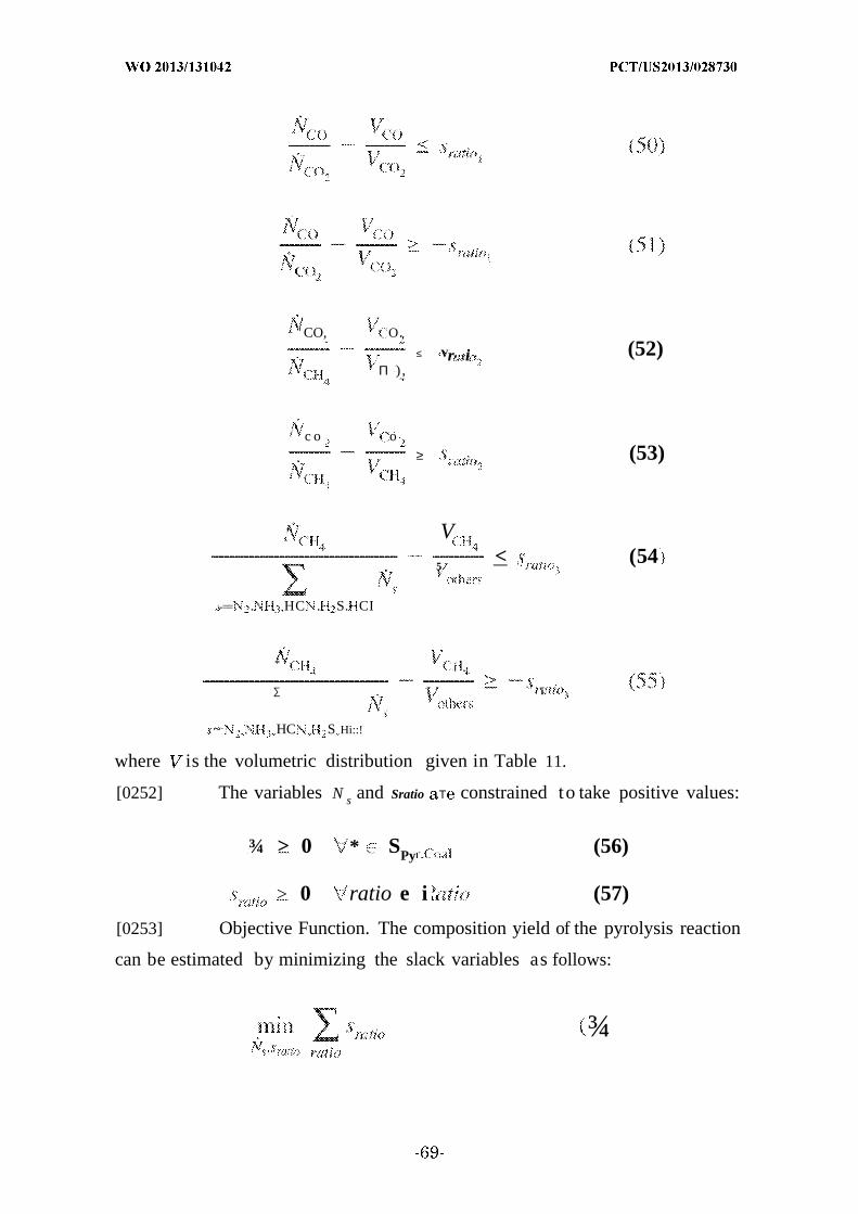
' CO, O.
≤ Vr. , :i: . (52)Π ) ,
c o o≥ .. (53)
' V
5 —< '·(54
-== . HC . S. CI
* ί ..
∑ 'i
~ . HC S Hi::!
where is the volumetric distribution given in Table 11.
[0252] The variables N s and Sratio .Τ constrained to take positive values:
¾ > 0 * SPy (56)
> 0 ratio e i (57)
[0253] Objective Function. The composition yield of the pyrolysis reaction
can be estimated by minimizing the slack variables as follows:
¾

[0254] Optimization Model. The proposed model is a nonlinear optimization
(NLP) model and takes the following form:
m . γ ..,., ,
subject to
V,
COC
CH,,
others
,N HCN.¾S,Ha
Λ C
> 0 V.v e
- > 0 ratio

[0255] Solving this model results in the N s values listed in Table 12, and
the final pyrolysis reaction for the given coal composition is given as follows:
[0256] Example 1.15 - Oxidation.
[0257] After pyrolysis has occurred, the residual gases and char will be
exposed to oxygen to generate the necessary heat for gasification. The following
oxidation assumptions are made:
01. ¾ will be fully oxidized to H2O, because of its high burning velocity, relative
to the other hydrocarbons.
02. The residual O 2 will rapidly combust the char via partial and complete
oxidation.
03. All other gaseous hydrocarbons will have negligible oxidation reactions. 40,51
The oxidation reaction list, based on the previous assumptions, consists of the
complete combustion of char (eq 60), the partial combustion of char (eq 61), and
the combustion of hydrogen (eq 62).
¾ 2 (60)
C . + 0.5O 2~ CO (61 )
+ 0.5O 2 20 (62)
[0258] Example 1.16 - Reduction.
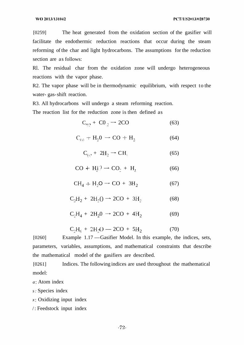
[0259] The heat generated from the oxidation section of the gasifier will
facilitate the endothermic reduction reactions that occur during the steam
reforming of the char and light hydrocarbons. The assumptions for the reduction
section are as follows:
Rl. The residual char from the oxidation zone will undergo heterogeneous
reactions with the vapor phase.
R2. The vapor phase will be in thermodynamic equilibrium, with respect to the
water- gas-shift reaction.
R3. All hydrocarbons will undergo a steam reforming reaction.
The reaction list for the reduction zone is then defined as
C,, , + C0 2CO (63)
! H 0 CO H (64)
C , + 2 CH (65)
CO - Hi ) CO + H, (66)
C 4 -I- Ο CO + 3H2 (67)
C 2 + 2 () 2CO + 3 (68)
C 4 + 2H20 2CO + 4 2 (69)
C + -. — 2CO + 5 2 (70)
[0260] Example 1.17 —Gasifier Model. In this example, the indices, sets,
parameters, variables, assumptions, and mathematical constraints that describe
the mathematical model of the gasifiers are described.
[0261] Indices. The following indices are used throughout the mathematical
model:
a Atom index
s : Species index
x Oxidizing input index
/ : Feedstock input index
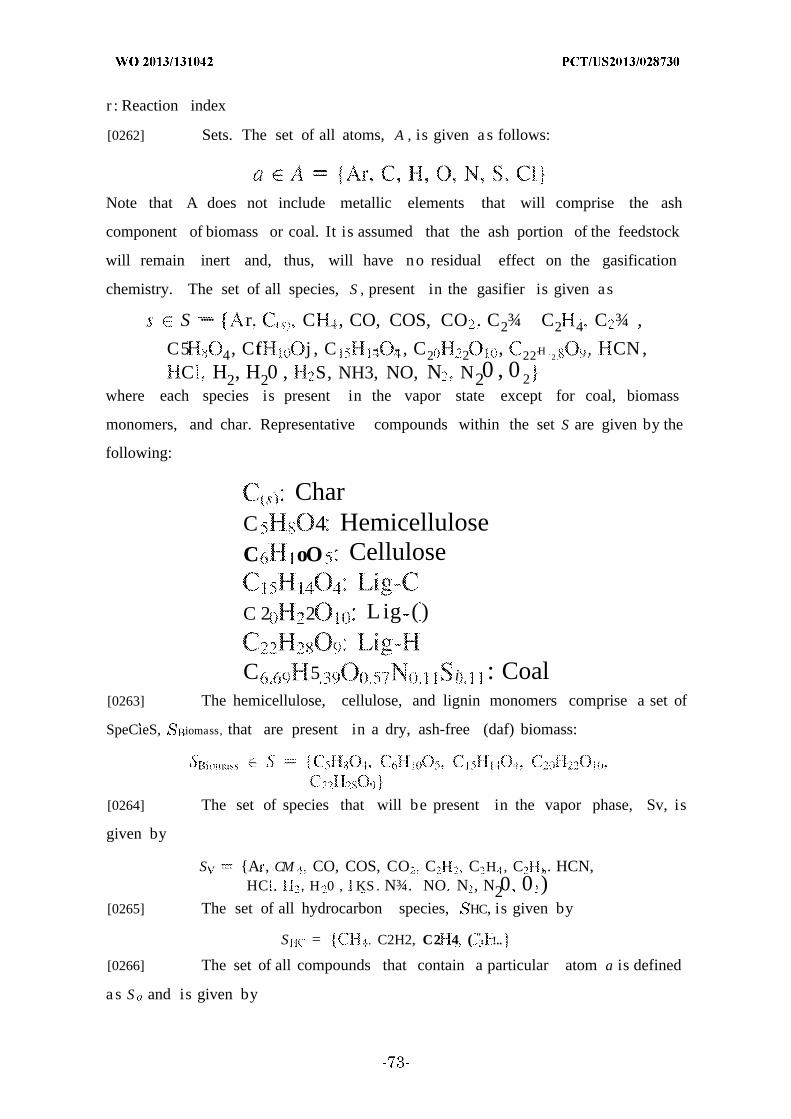
r : Reaction index
[0262] Sets. The set of all atoms, A , is given a s follows:
Note that A does not include metallic elements that will comprise the ash
component of biomass or coal. It is assumed that the ash portion of the feedstock
will remain inert and, thus, will have no residual effect on the gasification
chemistry. The set of all species, S , present in the gasifier is given as
S ····· r. C , CO, COS, CO . C2¾ C2 4 C ¾ ,
C5 4, Cft j , C - - , C2 2 , 22-H2 .
, CN,C H2, H20 , S, NH3, NO, N N20 , 0 2
where each species is present in the vapor state except for coal, biomass
monomers, and char. Representative compounds within the set S are given by the
following:
CharC 4 HemicelluloseC oO Cellulose
C 2 2 L ig ( )
C 5 i : Coal[0263] The hemicellulose, cellulose, and lignin monomers comprise a set of
SpeCieS, iomass, that are present in a dry, ash-free (daf) biomass:
[0264] The set of species that will be present in the vapor phase, Sv, is
given by
S A , CM .. CO, COS, CO .. C C H , C , . HCN,HC . H 0 , KS . N¾. NO N , N20 0 )
[0265] The set of all hydrocarbon species, HC, is given by
S = ... C2H2, C2 4 ( "·. !..
[0266] The set of all compounds that contain a particular atom a is defined
a s S and is given by

S = s £ S : $ contains atom a [0267] To represent all possible oxidizing feeds, we formulate the set Ox by
x Ox = Oxygen, Steam, Air, Enriched Air)where each feed x is described by a set of species Sx.
[0268] The set of all feedstock types, F, is given as follows:
F = C a Biomass, Additional Fuel)
[0269] The set of all reactions, R , within the system is defined as the union
of all reactions occurring within the pyrolysis (eqs 11-15, eq 59), oxidation (eqs
60-62), and reduction (eqs 63-70) zones. The set R is subdivided into subsets for
the pyrolysis zone (R p y ) , oxidation zone (R Ox), and reduction zone (i ¾ed),
respectively.
= (R l 5). K(5 )\/?(60)-/?(62)
= R63 i? 70 ]
[0270] Parameters. The composition of the biomass and coal feedstocks
correspond t o the following set of parameters that represent the dry, ash-free
(daf) feedstock:
Waf. weight fraction of atom a in daf feedstock /
weight fraction of species s in daf biomass
Ea,s number of atom a in species s
Note again that the parameters ,Bi0 mass represent the individual biomass
monomers and are generally not reported for a given biomass sample. We utilize
the ultimate and proximate analyses of the biomass sample to determine the
Ws,Biomass value that most
closely approximates this information in Example 1.12.
The following are known inputs t o the gasifier:
T : operating temperature of gasifierinput mass flow rate of feedstock
: molar flow rate of species s in lock hopper carrier gas¾ ?: niolar flow rate of species s in oxidizer x
molar coefficient of species s i reaction r[0271] Additional parameters are defined by the temperature of the gasifier
bed. For each species s, we define the thermodynamic properties as follows:
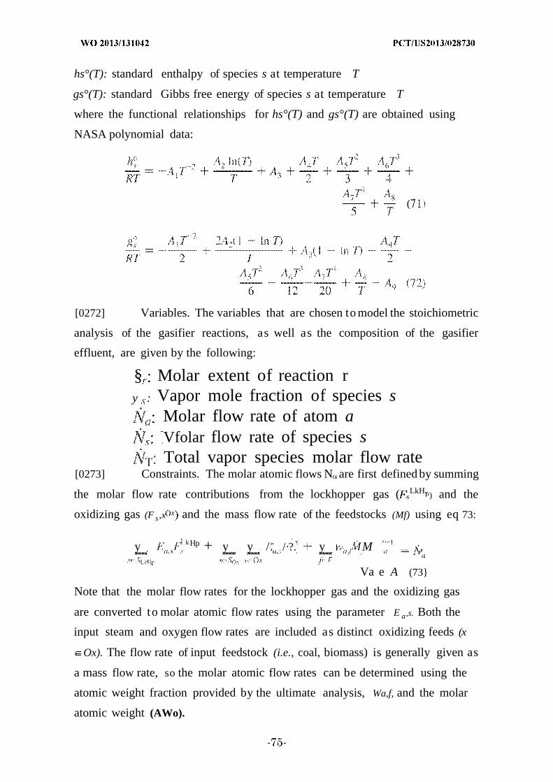
hs°(T): standard enthalpy of species s at temperature T
gs°(T): standard Gibbs free energy of species s at temperature T
where the functional relationships for hs°(T) and gs°(T) are obtained using
NASA polynomial data:
(
[0272] Variables. The variables that are chosen to model the stoichiometric
analysis of the gasifier reactions, as well as the composition of the gasifier
effluent, are given by the following:
§ Molar extent of reaction ry : Vapor mole fraction of species s
Molar flow rate of atom aVfolar flow rate of species sTotal vapor species molar flow rate
[0273] Constraints. The molar atomic flows N are first defined by summing
the molar flow rate contributions from the lockhopper gas ( LkH) and the
oxidizing gas (F s ,x x and the mass flow rate of the feedstocks (Mf) using eq 73:
y Hp + y y /·.· /·?. y · · M '.. .... ,
Va e A (73
Note that the molar flow rates for the lockhopper gas and the oxidizing gas
are converted to molar atomic flow rates using the parameter E a ,s. Both the
input steam and oxygen flow rates are included as distinct oxidizing feeds (x
Ox). The flow rate of input feedstock (i.e., coal, biomass) is generally given as
a mass flow rate, so the molar atomic flow rates can be determined using the
atomic weight fraction provided by the ultimate analysis, Wa,f, and the molar
atomic weight (AWo).

[0274] Through conservation of mass, the molar atomic flow rates can be
directly linked to the output species flow rates by eq 74:
E a N = N a V ≡ A (74 )
[0275] The total molar flow rate of all vapor phase species is calculated by
[0276] The molar composition of the vapor phase species may be obtained
using eq 76:
N = y V e S (76 .)
[0277] The extents of reaction must be constrained based on the initial
molar flow rate of all species and their output molar flow rates, using eq 77:
w v -f - - TV : n
fe F x Ox re R
s S (77)
where n s ,r represents the coefficient of species s in reaction r and is defined to be
positive for raw materials and negative for products.
[0278] It is initially assumed that the water- gas-shift reaction is at
equilibrium, as given by eq 78:
Since the temperature of the gasifier is known, each of the values for g s° may
be explicitly determined from the NASA polynomials listed in eq 72.
Therefore, the right-hand side of eq 78 will be equal to a constant.
[0279] It is assumed that all pyrolysis reactions go to completion, as
represented by eq 79:
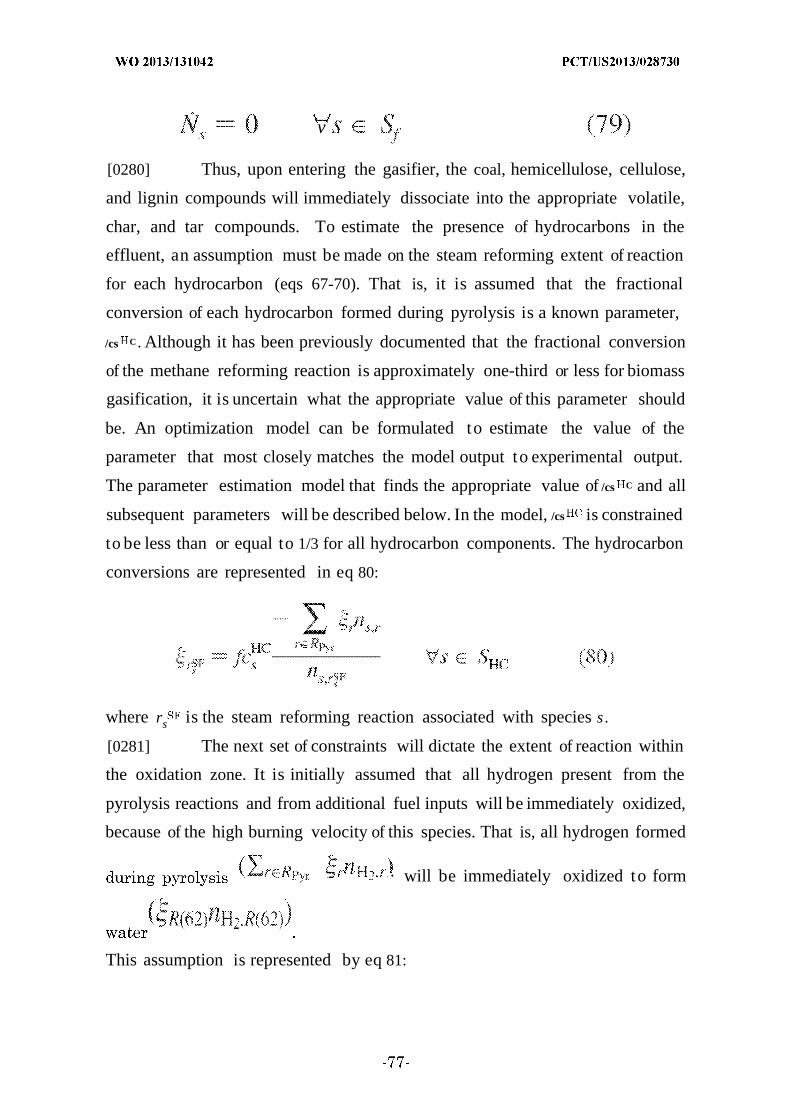
v
[0280] Thus, upon entering the gasifier, the coal, hemicellulose, cellulose,
and lignin compounds will immediately dissociate into the appropriate volatile,
char, and tar compounds. To estimate the presence of hydrocarbons in the
effluent, an assumption must be made on the steam reforming extent of reaction
for each hydrocarbon (eqs 67-70). That is, it is assumed that the fractional
conversion of each hydrocarbon formed during pyrolysis is a known parameter,
/cs C . Although it has been previously documented that the fractional conversion
of the methane reforming reaction is approximately one-third or less for biomass
gasification, it is uncertain what the appropriate value of this parameter should
be. An optimization model can be formulated to estimate the value of the
parameter that most closely matches the model output to experimental output.
The parameter estimation model that finds the appropriate value of /cs C and all
subsequent parameters will be described below. In the model, /cs is constrained
to be less than or equal to 1/3 for all hydrocarbon components. The hydrocarbon
conversions are represented in eq 80:
where rs is the steam reforming reaction associated with species s .
[0281] The next set of constraints will dictate the extent of reaction within
the oxidation zone. It is initially assumed that all hydrogen present from the
pyrolysis reactions and from additional fuel inputs will be immediately oxidized,
because of the high burning velocity of this species. That is, all hydrogen formed
- ·· will be immediately oxidized to form
This assumption is represented by eq 81:

[0282] The remaining oxygen will be consumed by the residual char,
because of the high surface area available for O 2 adsorption. The combustion of
char will occur via complete (eq 60) and partial (eq 61) oxidation in a ratio that is
inversely equal to the exothermicity (∆ ) of each reaction: 40
The exothermicity of each reaction is defined by eqs 83 and 84:
hCO, h°
R T RT RT
where (h s°)/(RT) is obtained using NASA polynomial data. Since the operating
temperature of the gasifier is known, the value for the exothermicity of each
reaction is a constant and the constraint given in eq 82 is linear.
[0283] The presence of char and tar in the gasifier exit stream is dependent
on the system temperature, as well as the flow rate of oxidizing species input to
the gasifier. The model will assume that the tar output by the gasifier is
negligible and that the char output is a function of temperature as given by eq
85:
where c and c 2 are coefficients representing the temperature dependence of
char output. These coefficients will be varied in the parameter estimation model
to determine their optimal values. Although tar is commonly found in biomass
gasifiers, because of the low operating temperature, it is removed with a tar
cracker before entering the FT unit and, therefore, is not considered in the model.
[0284] The next group of constraints focuses on the char reduction
reactions (eqs 63-65). It is assumed that the extent of conversion of these
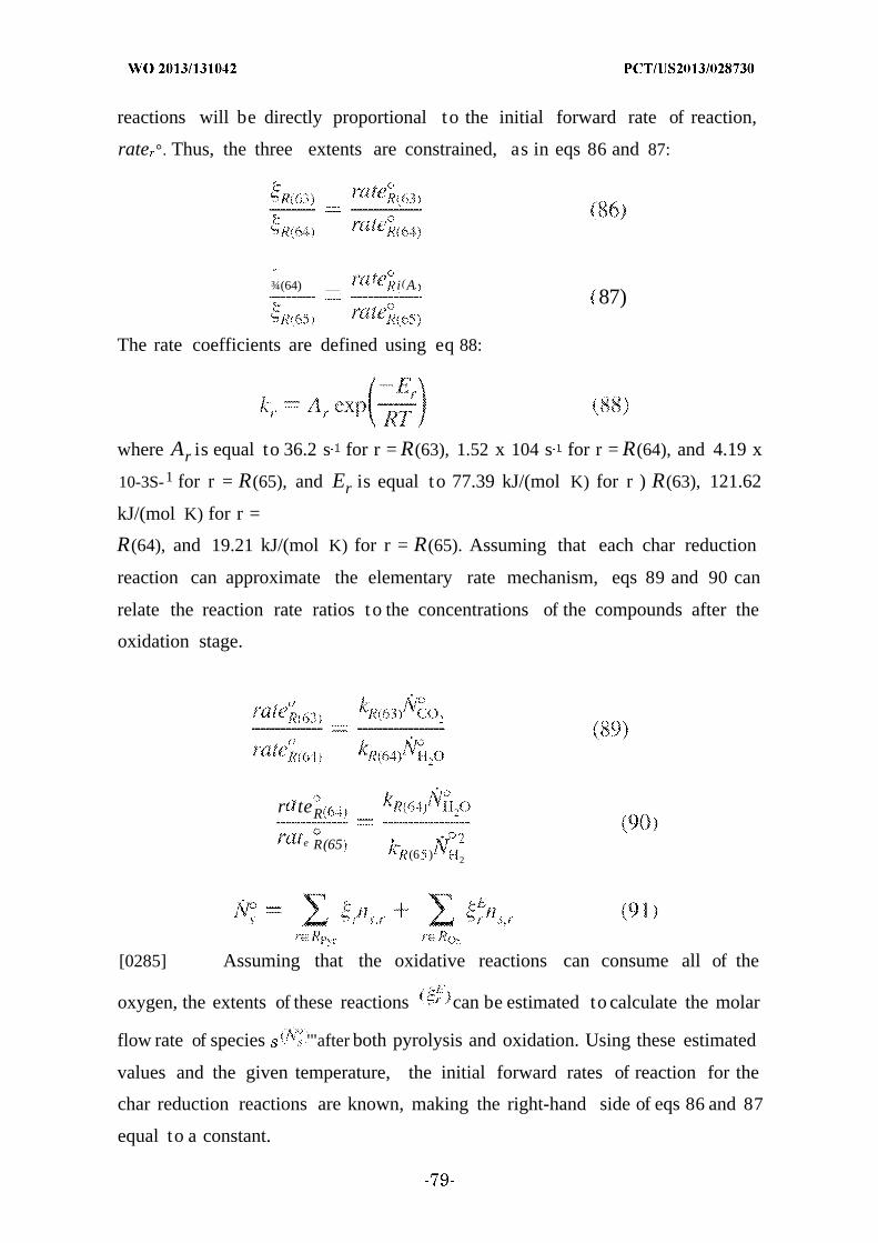
reactions will be directly proportional to the initial forward rate of reaction,
rate °. Thus, the three extents are constrained, as in eqs 86 and 87:
¾(64) _____ ' i (A87)
The rate coefficients are defined using eq 88:
where Ar is equal to 36.2 s for r = R(63), 1.52 x 10⁴ s for r = R(64), and 4.19 x
10-3S-1 for r = R(65), and Er is equal to 77.39 kJ/(mol K) for r ) R(63), 121.62
kJ/(mol K) for r =
R(64), and 19.21 kJ/(mol K) for r = R(65). Assuming that each char reduction
reaction can approximate the elementary rate mechanism, eqs 89 and 90 can
relate the reaction rate ratios to the concentrations of the compounds after the
oxidation stage.
r teR
e R(65 -(6 ) 2
[0285] Assuming that the oxidative reactions can consume all of the
oxygen, the extents of these reactions can be estimated to calculate the molar
flow rate of species '"after both pyrolysis and oxidation. Using these estimated
values and the given temperature, the initial forward rates of reaction for the
char reduction reactions are known, making the right-hand side of eqs 86 and 87
equal to a constant.
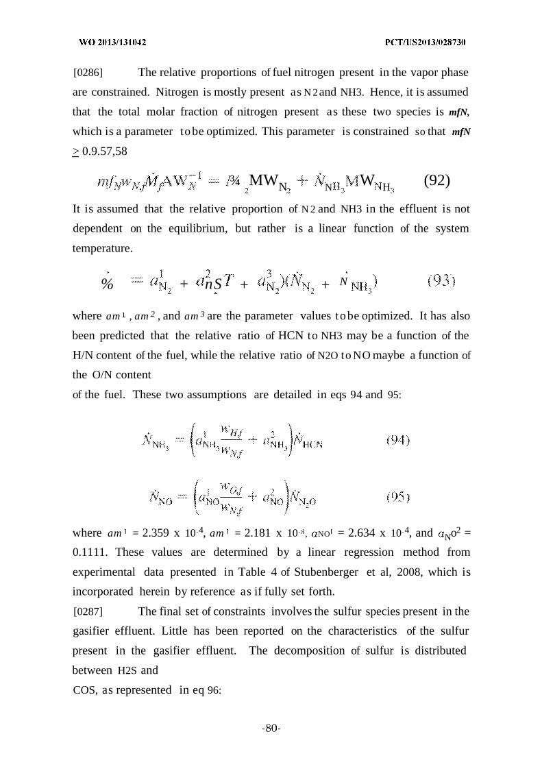
[0286] The relative proportions of fuel nitrogen present in the vapor phase
are constrained. Nitrogen is mostly present as N 2and NH3. Hence, it is assumed
that the total molar fraction of nitrogen present as these two species is mfN,
which is a parameter to be optimized. This parameter is constrained so that mfN
> 0.9.57,58
¾ MWN N W H (92)
It is assumed that the relative proportion of N 2 and NH3 in the effluent is not
dependent on the equilibrium, but rather is a linear function of the system
temperature.
% + nS + + N
where am , am 2 , and am 3 are the parameter values tobe optimized. It has also
been predicted that the relative ratio of HCN to NH3 may be a function of the
H/N content of the fuel, while the relative ratio of N2O to NO maybe a function of
the O/N content
of the fuel. These two assumptions are detailed in eqs 94 and 95:
where am = 2.359 x 10 4, am = 2.181 x 10 , NO = 2.634 x 10 4, and No2 =
0.1111. These values are determined by a linear regression method from
experimental data presented in Table 4 of Stubenberger et al, 2008, which is
incorporated herein by reference as if fully set forth.
[0287] The final set of constraints involves the sulfur species present in the
gasifier effluent. Little has been reported on the characteristics of the sulfur
present in the gasifier effluent. The decomposition of sulfur is distributed
between H2S and
COS, as represented in eq 96:
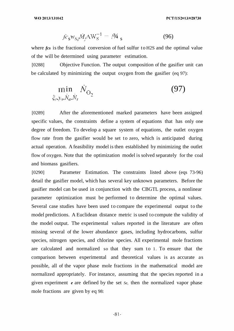
s ¾ s (96)
where fcs is the fractional conversion of fuel sulfur to H2S and the optimal value
of the will be determined using parameter estimation.
[0288] Objective Function. The output composition of the gasifier unit can
be calculated by minimizing the output oxygen from the gasifier (eq 97):
in (97)
[0289] After the aforementioned marked parameters have been assigned
specific values, the constraints define a system of equations that has only one
degree of freedom. To develop a square system of equations, the outlet oxygen
flow rate from the gasifier would be set to zero, which is anticipated during
actual operation. A feasibility model is then established by minimizing the outlet
flow of oxygen. Note that the optimization model is solved separately for the coal
and biomass gasifiers.
[0290] Parameter Estimation. The constraints listed above (eqs 73-96)
detail the gasifier model, which has several key unknown parameters. Before the
gasifier model can be used in conjunction with the CBGTL process, a nonlinear
parameter optimization must be performed to determine the optimal values.
Several case studies have been used to compare the experimental output to the
model predictions. A Euclidean distance metric is used to compute the validity of
the model output. The experimental values reported in the literature are often
missing several of the lower abundance gases, including hydrocarbons, sulfur
species, nitrogen species, and chlorine species. All experimental mole fractions
are calculated and normalized so that they sum to 1. To ensure that the
comparison between experimental and theoretical values is as accurate as
possible, all of the vapor phase mole fractions in the mathematical model are
normalized appropriately. For instance, assuming that the species reported in a
given experiment e are defined by the set Se, then the normalized vapor phase
mole fractions are given by eq 98:
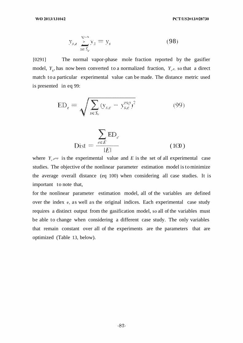
¾ —¾
> v .. 98
[0291] The normal vapor-phase mole fraction reported by the gasifier
model, Ys, has now been converted to a normalized fraction, Ys ,e, so that a direct
match to a particular experimental value can be made. The distance metric used
is presented in eq 99:
E
( 1 30 )
where Ys ,eexp is the experimental value and E is the set of all experimental case
studies. The objective of the nonlinear parameter estimation model is to minimize
the average overall distance (eq 100) when considering all case studies. It is
important to note that,
for the nonlinear parameter estimation model, all of the variables are defined
over the index e, as well as the original indices. Each experimental case study
requires a distinct output from the gasification model, so all of the variables must
be able to change when considering a different case study. The only variables
that remain constant over all of the experiments are the parameters that are
optimized (Table 13, below).

Table 13* Parameters Being Optimized in t e Gasifier Model
parameter biomass coa
/ 0.980! i
7 1¾ 1. 2 x Γ 6 0
0.400! 0.93 0
¾, 1.25 X 0.6976, - 107 5 - 1000
« 2359 x 10 4 2,359 x 0 '«¾H 2.818 x 10 2, 8 x 10 3
a 0.1 1! 0.1 1 1
[0292] The comparison of theoretical and experimental output for the
biomass and coal nonlinear parameter estimation models can be found in Tables
14 and 15, respectively. This comparison reveals that the model performs well in
representing the gasification process. A feature of the model is its generality in
evaluating syngas compositions for a variety of feedstock and gasifier types. The
values of the parameters which provide the predicted results are given in Table
13. These values are used to define the biomass and coal gasifiers used in the
CBGTL process.
[0293] The full mathematical models are included below, with the
corresponding parameters substituted into the equations.
[0294] Biomass Gasifier Model.
min Ν
subject t o
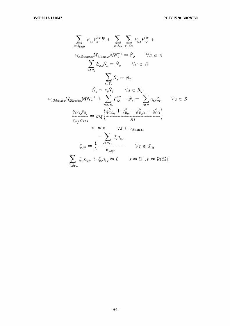
t
i ¾ 0 s 5 ,
n J f
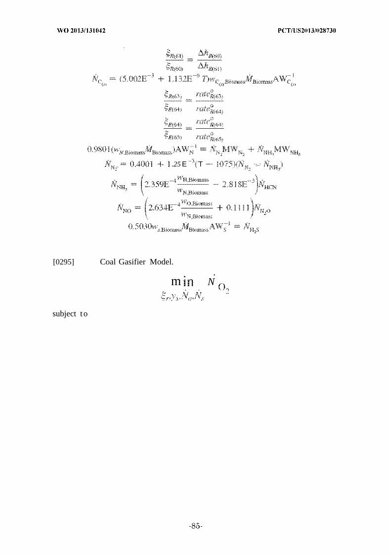
_ - .25 Ε Τ · ·!--
[0295] Coal Gasifier Model.
m N
subject to
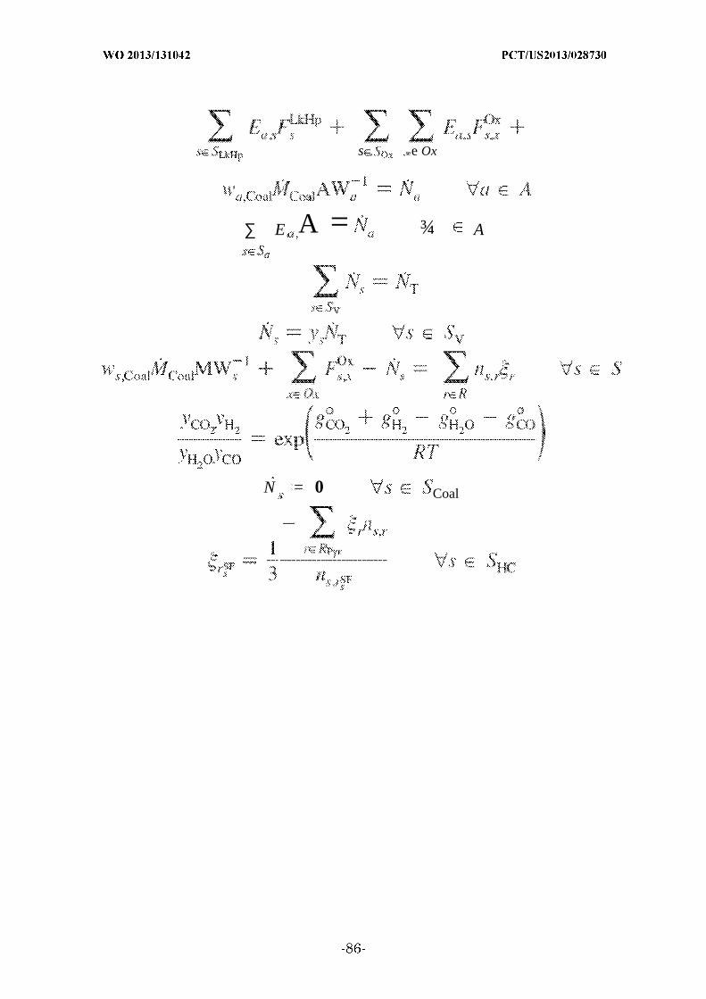
s . see Ox
∑ E A = ¾ A
N = 0 Coal
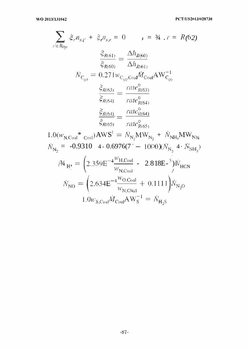
ί + = J = ¾ . = ( 2)
i 64)
N * C A S + ¾
= -0.9310 4 - 0.6976(7 > ) 4 · v
¾ , - 2 818E- )i HCN
C¾ 1


"able 15, Vapor Effluent pari s with R a Gasification Tests
Model dr ¾ i p rt d dry
CO CO; i i . • 0
E . 1 ί . iron) Li e! ?
1 10.67 10.20: 14 . 2 ( 15.70) 0.46 .0 . ( 1 00 ) 6,5.4S 5. ) 2, 0. (9 . 0 ) 13.1 3 1 5.9 , 5 . ( 5.6 ! 0. 5 (0.59) 7 ! .85 ( 9 . 0) 3.69
3 i 0 .6 · . 0 ) 12 6 0 3. 10 8.7 (8.50) 9.06 0 .80) 66.43 (65.60: 1 .8).86 .4 83 ( 3.30! 12.73 9.49) 9.97 .00) 60.50 (6 .90) 9
5 6 7 7 00. 10) 1 .30 0 4 20 . 5. 1 1 .6 0 0.05 (0.59; 71.60 (69.60) 4.366 i 0 .7 ( 1 20) 1 87 0 2.30! 8.94 8.40 i 0.06 (0.80) 6 6 .0 (65.30! 2 767 !3.4S ( : .60 . 2 03 0 .00 ! 0 .82 (9.99, 9.97 0 .00) . 0 (62.5 ! 2.28
14 2.5 .70 ! .74 0 5 50 13 6 8 8.80 ! 0.07 ( . O 5 .2 65.! 0) 0 v ¾
Taken fom k in r , . ( a!.' ,
9 70.55 (70.50) 2.00 0 .89) 27.28 (2 7 30 ) 0 0 1 .40 ) 0 4463.93 i.6 . : 3 .14 (2.50) 3 1.S7 28. i 9 0. (8.10) 9 19
D a Taken · Xlsy <: a! 7
p . 0 ( 10.50! .2 0 5. 0 12 0 0.60! 0.05 (2.3) 64. 8 (60.30) 5.81j '2 11.42 :80) 12.0) 04.30: 4 . i (12310) 0.09 (7.40! 6 i .64 (5 .7 0 ! 5 ,
13 12.65 i 2.2 : 0 .09 ( 13.50) 1 .82 05.29) 0.96 (2.40) 59 . (55.70 .) 4 90
Data Tak«» i Huang al.
1 13.88) i .5 1 0 5 0 . 17.38 04.57! 0.04 (2.91 ! 5 7. (52.70) 8. 1! 5 15.80 ( 17 97) 11 10 0 3. 17! 24.46 0 8. 4 ) 9.05 2.9 3) 48.59 (5 1.8 8725
O. 12.54 : 1 88 04.74! 20.72 i i x.56) 0.94 12.72) 54 . 2 (5 .44! 57-¾2
14 5 2 : 14.30) 0 .75 (0.80) 23 0 8 0 8.08! 0.05 (2 .55 50.60 (5 . ! ? '! 6.0218 9.59 18.02) 14.44 0 7 . 10: 9 .24 7.7577 .0 5.59 56.60 (55.72! 5. J!9 i 1.20 (1.5. 14 12 4 7 0 5.40! 20 . 7 (16.63;. 0.04 12.6 ) 54 . 6 50 .20 8 . 0
Daw Taken ai! ;,i. 7
20 X .97) 1 .84 0 4 40 · 14.80 19 .6 3 0.10 (1.34 63.84 164.62) 5.912 1 7.85 (10.94) 12.77 0 9.30 i 2.86 ( 8 .5 ) 0.10 (0.84) 66.40 (60.87) 0 39?? 4.49 (5 , 1 12 0 4.86! 7.40 i6.48) 0.68 0 .29) 73.5! ( .54) 3 .3 !
: >.:!., T ik i S n bfc i al."
23 2 8 6 0.80 ) 0 . 9 (4.0(9 .78 0 7.90! 0.0? ( . 48 . 5 (44 90) 0.58 <<).<> » .0824 21.98 (23.00) 6.57 0 9.1.0: 26.04 (20 20) O l 0 .70) 44.76 (4 60) 0 54 <i 4 0) 7,23
25 32. !6 i27.60, 9 . 4 (5.10 2 1.03 7. 9 0.98 ( 1 .60) 46.14 (46.50) 0.55 ( 1 30) 7 7026 2 .6 3 22.90: 0.00 (7.50 ) 1 . 7 6. 0 ) 0.98 ( 1 70i 50.01 49 .70) 0.60 ( i 9 0 > .8927 20. 6 y (24,70! 0.05 15.67) i .29 ( .20 ) 0.07 ( 1.69) 40.1 (49.60) 0 59 0 .23! 7.78
28 30.49 (20 50. 0 1 4,96 8.87* 0 6. 9 ) 0.08 j .79) 48.9! (46.30! 0.50 5) 6.3629 30.49 139.50: 0.56 (4.90) 20 . 8.20) 0.97 ( 1 .63) 46.97 (44.00) 0.56 (0 97 5 8
0 27 1 (30.00! .43 (4.47) 17. 1 .40 0.0 ( 1.59) 50.82 146.50) 0.6 ί ( .03 6 .31 1.87 (27.00 0 0 5 .25 2 .60 0 . 0 ) 0.00 0 .95) 43.86 (45.30! 0.53 0 .22) .
a T from nip e l a!. 74
32 0 .6 1 .59 ! 2.5 (IS. 8) 10.1 3 . 8.84 O. ( 1 07i 58.59 J O) 12, 1833 8 66 (10.7 ! 1 . 9 126.96: 16. 1 ( 2,86) 0.09 (0.83) 62.22 '54.551 12.4734 8.8 (8.84 12 . 8 0. 2 : i 7 .6 (9 .9 ) 0.1 1 10.73) 60.55 (5 . 7 ! 6 3
S. i 1.36 : 2, 7 (20.27) 14.60 i 9. 0. 19 (0 .77 64.1 (57.50 1 56
Data Taken ro adte al. 75
36 7 8 6 .6 0 i .70 0 60 ) 8.22 6 .9 0 . i 0 (1.59i 73. 15 1 3 . 0 ) 2. 163? 4 .0 ( 7 80) 8 4 8 0 1. 0 ! 6.85 ( .40 ) 0.00 0 . 0 ) 3. 0 (71.20! 5 8 8
7.77 16.79! i .57 (10.20) .04 16.59! O. ) ( 1 80 ) 7 .74 (74.00) 2, 530 6 85 67.09) i .i l (8 60 ) 5.2 1 .20 0.0? (1.69! 74.75 177,00) 4.44
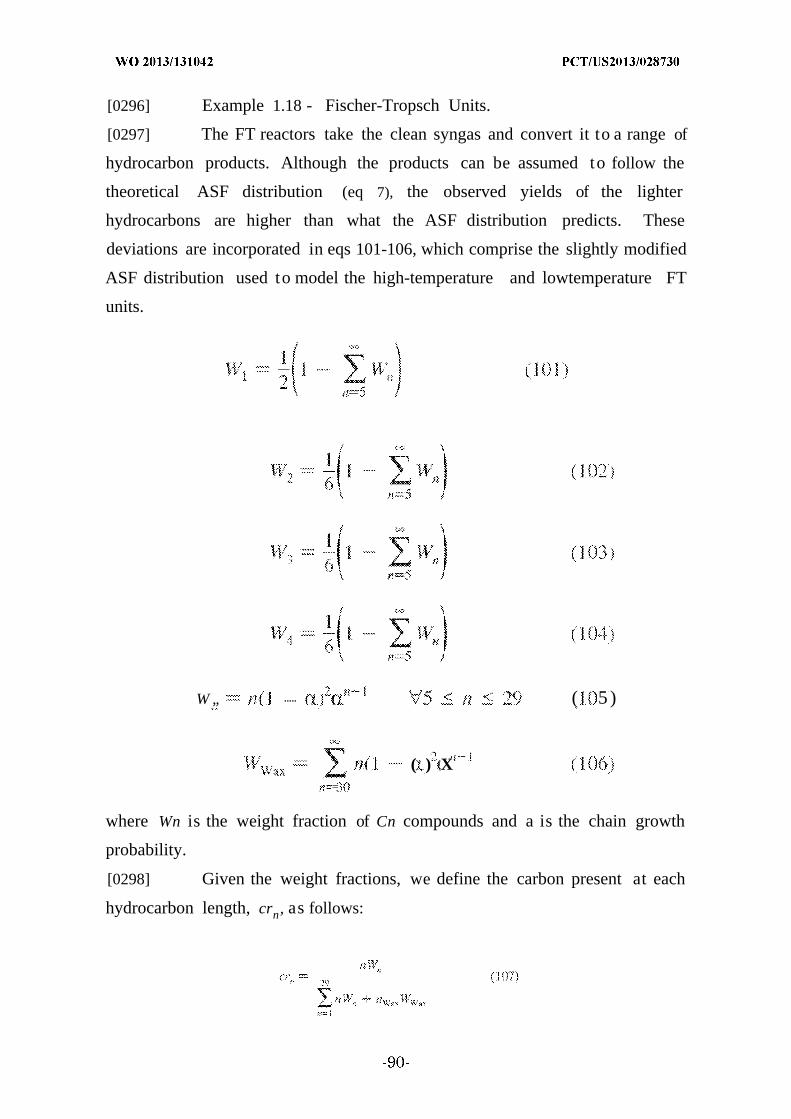
[0296] Example 1.18 - Fischer-Tropsch Units.
[0297] The FT reactors take the clean syngas and convert it to a range of
hydrocarbon products. Although the products can be assumed to follow the
theoretical ASF distribution (eq 7), the observed yields of the lighter
hydrocarbons are higher than what the ASF distribution predicts. These
deviations are incorporated in eqs 101-106, which comprise the slightly modified
ASF distribution used to model the high-temperature and lowtemperature FT
units.
W „ ····· ( 5 )
( ) X=
where Wn is the weight fraction of Cn compounds and a is the chain growth
probability.
[0298] Given the weight fractions, we define the carbon present at each
hydrocarbon length, crn, as follows:
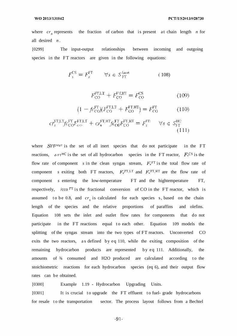
where crn represents the fraction of carbon that is present a t chain length n for
all desired n .
[0299] The input-output relationships between incoming and outgoing
species in the FT reactors are given in the following equations:
108)
i
-FT: :f * c:<> ·· s ί
where FT NE T is the set of all inert species that do not participate in the FT
reactions, S FT i s the set of all hydrocarbon species in the FT reactor, S is the
flow rate of component s in the clean syngas stream, FT i s the total flow rate of
component s exiting both FT reactors, T'LT and T
'T are the flow rate of
component s entering the low-temperature FT and the hightemperature FT,
respectively, /cco T i s the fractional conversion of CO in the FT reactor, which is
assumed t o b e 0.8, and crs is calculated for each species s , based on the chain
length of the species and the relative proportions of paraffins and olefins.
Equation 108 sets the inlet and outlet flow rates for components that do not
participate in the FT reactions equal t o each other. Equation 109 models the
splitting of the syngas stream into the two types of FT reactors. Unconverted CO
exits the two reactors, a s defined by eq 110, while the exiting composition of the
remaining hydrocarbon products are represented by eq 111. Additionally, the
amounts of ¾ consumed and H2O produced are calculated according t o the
stoichiometric reactions for each hydrocarbon species (eq 6), and their output flow
rates can b e obtained.
[0300] Example 1.19 - Hydrocarbon Upgrading Units.
[0301] It is crucial t o upgrade the FT effluent t o fuel- grade hydrocarbons
for resale t o the transportation sector. The process layout follows from a Bechtel
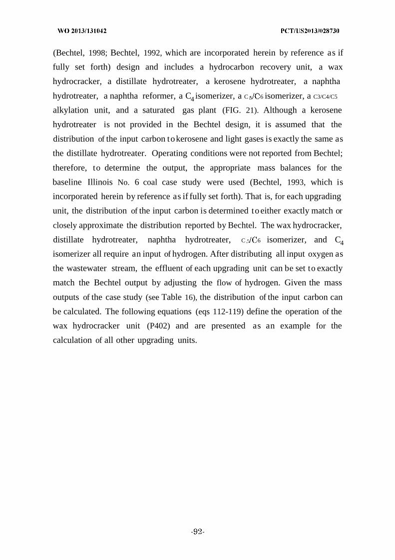
(Bechtel, 1998; Bechtel, 1992, which are incorporated herein by reference as if
fully set forth) design and includes a hydrocarbon recovery unit, a wax
hydrocracker, a distillate hydrotreater, a kerosene hydrotreater, a naphtha
hydrotreater, a naphtha reformer, a C4 isomerizer, a C 6 isomerizer, a C3/C4/C5
alkylation unit, and a saturated gas plant (FIG. 21). Although a kerosene
hydrotreater is not provided in the Bechtel design, it is assumed that the
distribution of the input carbon tokerosene and light gases is exactly the same as
the distillate hydrotreater. Operating conditions were not reported from Bechtel;
therefore, to determine the output, the appropriate mass balances for the
baseline Illinois No. 6 coal case study were used (Bechtel, 1993, which is
incorporated herein by reference as if fully set forth). That is, for each upgrading
unit, the distribution of the input carbon is determined to either exactly match or
closely approximate the distribution reported by Bechtel. The wax hydrocracker,
distillate hydrotreater, naphtha hydrotreater, C 6 isomerizer, and C4
isomerizer all require an input of hydrogen. After distributing all input oxygen as
the wastewater stream, the effluent of each upgrading unit can be set to exactly
match the Bechtel output by adjusting the flow of hydrogen. Given the mass
outputs of the case study (see Table 16), the distribution of the input carbon can
be calculated. The following equations (eqs 112-119) define the operation of the
wax hydrocracker unit (P402) and are presented as an example for the
calculation of all other upgrading units.
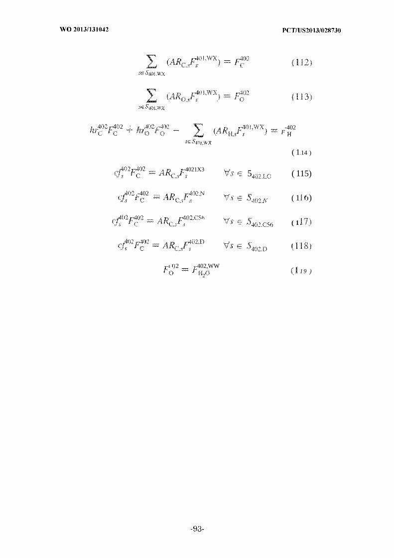
2 : . f -402F
( 1 14 )
-4021X3 5 ( 115)
,-402 ..... -( 1 )
( 1 .
4 2 402,WW19 )
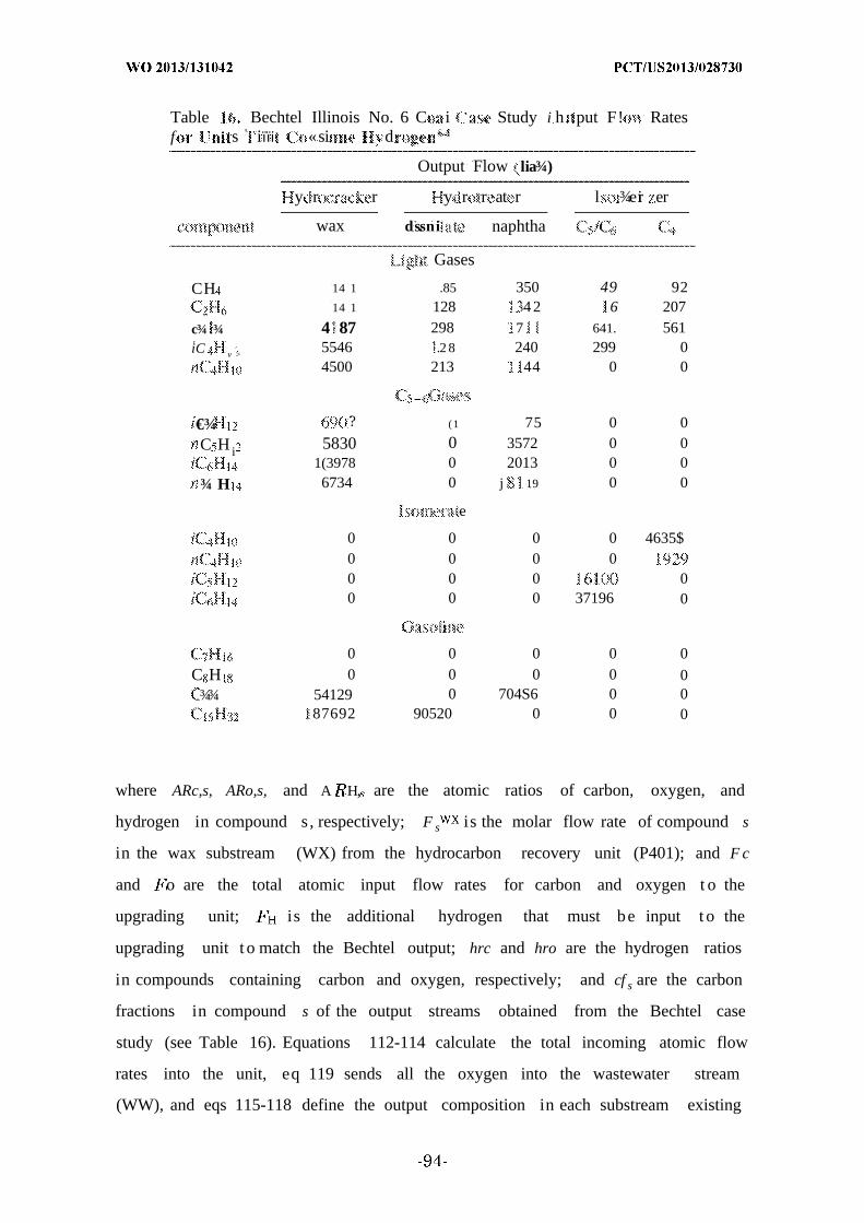
Table Bechtel Illinois No. 6 C i Study i h put F! Ratesf s ' iϊ ϊ ί «si d
Output Flow lia¾)
y r r y r r at r l ¾eri er
wax ds.sni naphtha
Gases
CH 14 1 .85 350 49 9214 1 128 . 4 2 6 207
c¾ :¾ 4 87 298 7 641. 561iC v >
5546 .2 8 240 299 04500 213 44 0 0
€¾ ? (1 75 0 0
C H i 5830 0 3572 0 01(3978 0 2013 0 0
¾ H 6734 0 j 19 0 0
e
0 0 0 0 4635$0 0 0 00 0 0 00 0 0 37196 0
0 0 0 0 0
C H 0 0 0 0 0¾¾ 54129 0 704S6 0 0
87692 90520 0 0 0
where ARc,s, ARo,s, and A H, are the atomic ratios of carbon, oxygen, and
hydrogen in compound s, respectively; F s is the molar flow rate of compound s
in the wax substream (WX) from the hydrocarbon recovery unit (P401); and F c
and o are the total atomic input flow rates for carbon and oxygen t o the
upgrading unit; is the additional hydrogen that must be input t o the
upgrading unit t o match the Bechtel output; hrc and hro are the hydrogen ratios
in compounds containing carbon and oxygen, respectively; and cf s are the carbon
fractions in compound s of the output streams obtained from the Bechtel case
study (see Table 16). Equations 112-114 calculate the total incoming atomic flow
rates into the unit, eq 119 sends all the oxygen into the wastewater stream
(WW), and eqs 115-118 define the output composition in each substream existing
the unit. The mass balances for all other upgrading units are completed similar
to that for this hydrocracker unit.
[0302] Example 1.20 - Steady-State Process Simulation
[0303] Steady- state process simulations on seven process alternatives are
completed to study the efficiency of the proposed hybrid system. The feedstock is
either (i) coal only (C), (ii) biomass only (B), or (iii) a hybrid combination of coal,
biomass, and natural gas (H). Hydrogen is obtained either from SRM purchase
(R) or via electrolysis (E), and light gases are reformed either by an ATR (A) or
combusted using a gas turbine engine (T).
[0304] The seven combinations are as follows: C-R-A, C-E-A, B-RA, B-E-A,
H-R-A, H-E-A, and H-R-T. The feedstocks are normalized to a total of 2000
tonnes/day, as presented in Table 17.

-96-
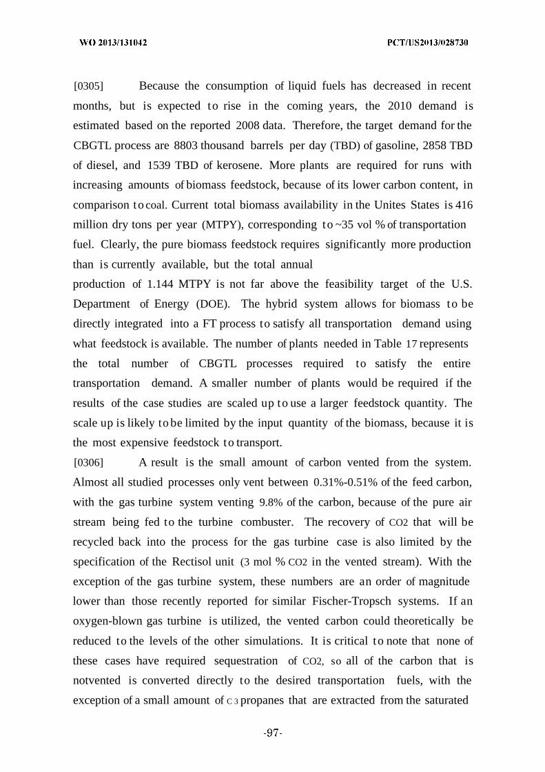
[0305] Because the consumption of liquid fuels has decreased in recent
months, but is expected to rise in the coming years, the 2010 demand is
estimated based on the reported 2008 data. Therefore, the target demand for the
CBGTL process are 8803 thousand barrels per day (TBD) of gasoline, 2858 TBD
of diesel, and 1539 TBD of kerosene. More plants are required for runs with
increasing amounts of biomass feedstock, because of its lower carbon content, in
comparison to coal. Current total biomass availability in the Unites States is 416
million dry tons per year (MTPY), corresponding to ~35 vol % of transportation
fuel. Clearly, the pure biomass feedstock requires significantly more production
than is currently available, but the total annual
production of 1.144 MTPY is not far above the feasibility target of the U.S.
Department of Energy (DOE). The hybrid system allows for biomass to be
directly integrated into a FT process to satisfy all transportation demand using
what feedstock is available. The number of plants needed in Table 17 represents
the total number of CBGTL processes required to satisfy the entire
transportation demand. A smaller number of plants would be required if the
results of the case studies are scaled up to use a larger feedstock quantity. The
scale up is likely to be limited by the input quantity of the biomass, because it is
the most expensive feedstock to transport.
[0306] A result is the small amount of carbon vented from the system.
Almost all studied processes only vent between 0.31%-0.51% of the feed carbon,
with the gas turbine system venting 9.8% of the carbon, because of the pure air
stream being fed to the turbine combuster. The recovery of CO2 that will be
recycled back into the process for the gas turbine case is also limited by the
specification of the Rectisol unit (3 mol % CO2 in the vented stream). With the
exception of the gas turbine system, these numbers are an order of magnitude
lower than those recently reported for similar Fischer-Tropsch systems. If an
oxygen-blown gas turbine is utilized, the vented carbon could theoretically be
reduced to the levels of the other simulations. It is critical to note that none of
these cases have required sequestration of CO2, so all of the carbon that is
notvented is converted directly to the desired transportation fuels, with the
exception of a small amount of C 3 propanes that are extracted from the saturated
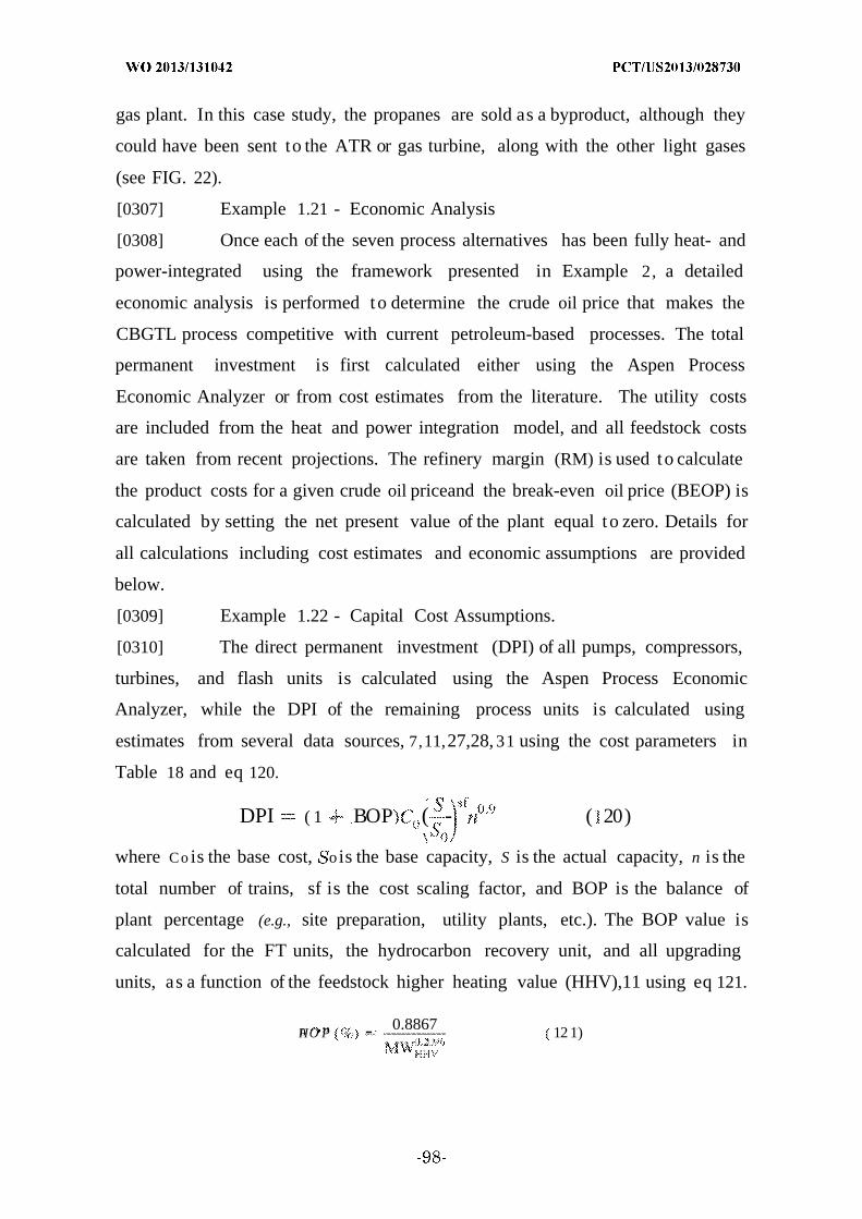
gas plant. In this case study, the propanes are sold as a byproduct, although they
could have been sent to the ATR or gas turbine, along with the other light gases
(see FIG. 22).
[0307] Example 1.21 - Economic Analysis
[0308] Once each of the seven process alternatives has been fully heat- and
power-integrated using the framework presented in Example 2, a detailed
economic analysis is performed to determine the crude oil price that makes the
CBGTL process competitive with current petroleum-based processes. The total
permanent investment is first calculated either using the Aspen Process
Economic Analyzer or from cost estimates from the literature. The utility costs
are included from the heat and power integration model, and all feedstock costs
are taken from recent projections. The refinery margin (RM) is used to calculate
the product costs for a given crude oil priceand the break-even oil price (BEOP) is
calculated by setting the net present value of the plant equal to zero. Details for
all calculations including cost estimates and economic assumptions are provided
below.
[0309] Example 1.22 - Capital Cost Assumptions.
[0310] The direct permanent investment (DPI) of all pumps, compressors,
turbines, and flash units is calculated using the Aspen Process Economic
Analyzer, while the DPI of the remaining process units is calculated using
estimates from several data sources, 7,11,27,28, 31 using the cost parameters in
Table 18 and eq 120.
DPI ( 1 - BOP ( - ( 20)
where C o is the base cost, o is the base capacity, S is the actual capacity, n is the
total number of trains, sf is the cost scaling factor, and BOP is the balance of
plant percentage (e.g., site preparation, utility plants, etc.). The BOP value is
calculated for the FT units, the hydrocarbon recovery unit, and all upgrading
units, as a function of the feedstock higher heating value (HHV),11 using eq 121.
Hn O„P - 0.8867 12 1)

[0311] The BOP value is either assumed tobe 15.5% or included in the base
cost for the remaining process units. All results are expressed in 2010 dollars,
using the Chemical Engineering Plant Cost Index65 and the GDP inflation
index2 to convert the original price when applicable.
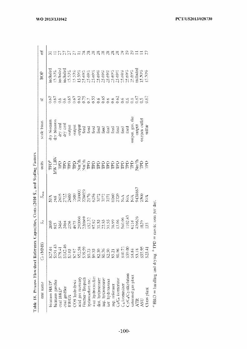
[0312] Example 1.23 - Feedstock and Product Assumptions.
[0313] The price ("asreceived", delivered to plant gate, 2010 $) of
herbaceous biomass, Illinois No. 6 coal, and natural gas is $5.26/GJ HHV,11
$42.16/short ton, and $7.48/103 ft3, respectively (see Table 19). Disposal costs of
wastewater and ash are included in the operating and maintenance costs of the
process units producing those wastes. The utility costs for each process
alternative are taken directly from the results of the heat and power integration
minimum utility model presented in Example 2. Because of the variable
marketability of sulfur, no credit is taken for the sale as a byproduct.
[0314] The resale cost of the transportation fuels is based on the price of
crude oil and the RM for each product. The RM is the difference between the sale
price of petroleum products and the purchase price of crude oil and is estimated
as the 1992-2003 average, 1 after adjustment with the U.S. Gross Domestic Index.
The RM for gasoline, diesel, and kerosene is $0.333/gal, $ 0.266/gal, and
$0.217/gal, respectively (see Table 19). The RM for diesel is $0.05/gal higher than
the average, because of the estimated additional cost for the production of low-
sulfur diesel.
[0315] Example 1.24 - Additional Economic Assumptions.
[0316] Table 20 lists the additional economic assumptions. The total
depreciable capital (TDC) is the sum of the DPI plus general and administrative
(G&A) capital overhead and contract fees, each of which is estimated to be 3% of
the DPI. The total permanent investment (TPI) is the sum of the TDC plus the
capital contingencies, which is estimated to be 18% of the TDC. The distribution
ofthe TPI over the three-year construction/startup period is 1/4 in the first year,
1/2 in the second, and 1/4 in the third. The working capital is estimated tobe 5%
ofthe TPI, to be used during startup in the third year ofthe plant life. The book
life of the plant is taken to be 30 years, with a yearly operating capacity of 8000
h . The salvage value ofthe plant is estimated to be 20% of the TPI.
[0317] All operating costs are also presented in Table 20. The annual
maintenance costs are taken as 4% of the TPI, the labor costs (10 operators, 1
supervisor) are $350/h, and the operating charges are assumed to be 25% ofthe
labor cost. The summation of these three items is termed the operating labor and
maintenance (OL&M) costs. The subtotal operating cost (SOC) is defined as the
sum of the raw materials, utilities, and OL&Mcosts. The G&A operating
expenses are estimated to be 8% of the SOC, and the plant overhead is estimated
to be 50% of the OL&M. The total operating costs is then calculated as the sum of
the SOC, the G&A operating expenses, and the plant overhead.
[0318] Example 1.25 - Break- Even Oil Price.
[0319] Based on the aforementioned assumptions, the net present value
(NPV) of the CBGTL process can be calculated for any given crude oil price
(COP). For each year y in the economic life of the plant, the sales, Sy, can be
calculated as the sum of the three major transportation fuel product sales plus
the sale of byproduct propane (eq 124). The product fuels sales are adjusted for
the appropriate year using the escalation factor, ES Note that the sales will be
equal to zero during the first three years of the plant life (yst ) 3), because of
construction time and startup (see Table 20).
Ρ 1 + + + ¾ ( C P + M D> +
+ M ) ( 22)
Yy ( 1 + o ( 123)
· PR + Y ( 24)
[0320] The total permanent investment (TPI) is distributed during
construction time using the distribution factor a . During plant construction,
we have i a ) 0.25, 2a ) 0.5, and 3
a ) 0.25. The working capital, WCy , is
defined as 5% of the TPI and is only utilized during startup in year 3. The 20%
salvage value of the plant, S Vy, is taken into account at the end of the economic
life of the plant End = 30). The raw material cost is calculated using the flow
rate of biomass, coal, natural gas, butanes, and hydrogen (eq 126) and is
escalated using ¾ s The utility cost is calculated based on the amount of cooling
water and electricity needed for the process (eq 127). Note that the electrolyzer-
based processes will not require hydrogen. The yearly operating costs, OPy, can
be calculated using the raw materials, utilities, operating labor and maintenance,

operating charges, plant overhead, and G&A costs (see Table 20), as outlined
above. The operating labor and maintenance costs will be escalated using the
appropriate factor.
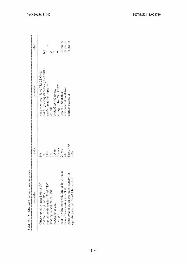
l i S S fi

[0321] Using a straight-line depreciation method over 10 years and a tax
rate (TR) of 40%, the cash flow for a given operating year is defined in eq 128.
The NPV of the plant is then calculated by summing the discounted cash flows
over the entire economic life of the plant, using the desired rate of return (RR)
(see eq 129). Upon completion of a process simulation and the simultaneous heat
and power integration, all of the information in eqs 124-129 is known, except for
the crude oil price (COP). The break-even oil price (BEOP) is defined as the
crude oil price for which the NPV of the process is equal to zero. Since the RM is
used to calculate the selling price of the transportation fuels, this metric is
considered the price of crude oil at which the CBGTL process is economically
competitive with petroleumbased processes. The variability in the BEOP, with
respect to hydrogen, is presented in Table 21 and graphically in FIG. 24.
Hydrogen prices greatly influence the competitiveness of the process because of
the high requirement of hydrogen input to the system. Processes with electrolysis
are not affected by the price changes since hydrogen is produced on-site. Their
high BEOP is due to the high capital cost of electrolyzer and the price of
electricity. For the other cases, the hybrid processes are more competitive than
the coal-only or biomass-only cases at almost all hydrogen price values. At
$1.25/kg ¾ and lower, the coal process also becomes competitive with a BEOP of
$57 and $49. At hydrogen prices above $1.00/kg ¾ , the gas turbine case is more
competitive than the other cases. However, this process is also associated with
higher CO2 emission, as discussed previously. Overall, the results show that fuel
products from this process can be competitive with petroleum-based fuels,
highlighting the important benefits such as near 100% carbon conversion and no
CO2 sequestration required.
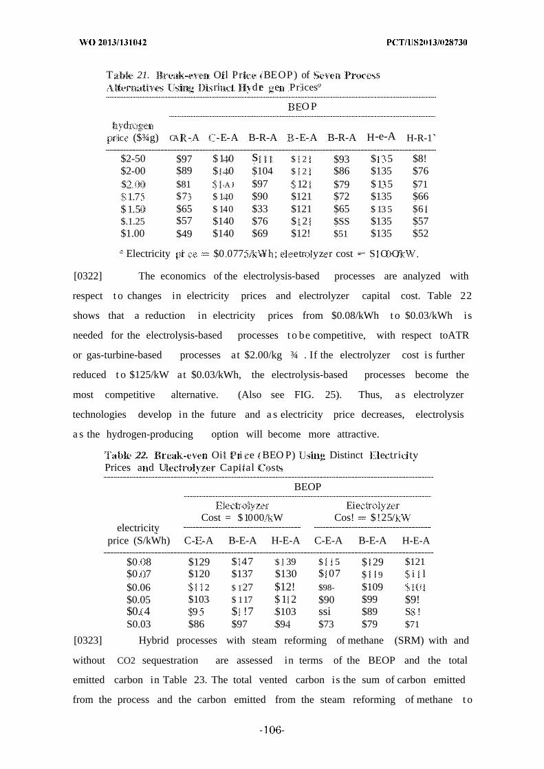
T 21. O l Pr BEOP) of sri d re e Pr ices
O P
dic ($¾g) CA -A -E-A B-R-A -E-A B-R-A H-e-A H-R-1
$2-50 $97 $1 0 s $ 2 $93 $ 5 $8!$2-00 $89 $ 0 $104 $ 2 $86 $135 $76$ $81 A $97 12 $79 $1 5 $71
1.7 $7 $ 1 0 $90 $121 $72 $135 $66$ 1.5 $65 $ 140 $33 $121 $65 $ 13 5 $6$.1.25 $57 $140 $76 $ 2 $SS $135 $57$1.00 $49 $140 $69 $12! $51 $135 $52
Electricity ri $0 077. ¥l ; etr yz r cost - S O O
[0322] The economics of the electrolysis-based processes are analyzed with
respect t o changes in electricity prices and electrolyzer capital cost. Table 22
shows that a reduction in electricity prices from $0.08/kWh t o $0.03/kWh is
needed for the electrolysis-based processes t o be competitive, with respect toATR
or gas-turbine-based processes at $2.00/kg ¾ . If the electrolyzer cost is further
reduced t o $125/kW at $0.03/kWh, the electrolysis-based processes become the
most competitive alternative. (Also see FIG. 25). Thus, a s electrolyzer
technologies develop in the future and a s electricity price decreases, electrolysis
a s the hydrogen-producing option will become more attractive.
22. Oi i e BEO P) Distinct e tri tvPrices a d U . Cap al st
BEOP
Eie r rCost = $1000 W Cos! $!25/
electricityprice (S/kWh) C A B-E-A H-E-A C-E-A B-E-A H-E-A
$0 8 $129 $ 47 $ 39 $ 5 $ 29 $121$0. 7 $120 $137 $130 $ 07 $ 9 i l$0.06 2 $ 127 $12! $98- $109$0.05 $103 $ 117 $ 1 2 $90 $99 $9!$0. 4 9 $ !7 $103 ssi $89 S !S0.03 $86 $97 $9 $73 $79 $71
[0323] Hybrid processes with steam reforming of methane (SRM) with and
without CO2 sequestration are assessed in terms of the BEOP and the total
emitted carbon in Table 23. The total vented carbon is the sum of carbon emitted
from the process and the carbon emitted from the steam reforming of methane t o

produce hydrogen. Based on the figures reported by the National Research
Council, 2004, which is incorporated herein by reference a s if fully set forth, the
CO2 emission from SRM technology is 1.53 kg/kg H 2with sequestration and 9.22
kg/kg H 2 without sequestration, and the corresponding hydrogen prices are
$1.22/kg and $1.03/kg, respectively. The total CO2 emission is then calculated,
and the results are displayed in Table 23. It is shown that the CBGTL processes
that consume hydrogen from SRM give rise t o a higher percentage of vented
carbon, with respect to the total fuel carbon (i.e., CBGTL feedstock and natural
gas feedstock t o produce hydrogen in the steam reforming process). Carbon
sequestration is needed for the stream reforming process to reduce the amount of
vented carbon. FIG. 26 shows that, with a slight increase in the BEOP using CO2
sequestration, a significant reduction in carbon emission is achieved. The tradeoff
between BEOP and carbon emission is even more marked when comparing the
two technology alternatives for hydrogen production. With a substantial increase
in the BEOP from the H-R-A and H-R-T cases t o the H-E-A case, a very low
carbon emission can be achieved.
Table Cora rise n of Hy ogen rc d t! o a ofrom the CBGTL Process
- -A . H-E-A H-R-T
y r ge g yr) 9 93 x O7 8.47C v e 5 82 x !06 5.40 x 6 x 10
CBGTL (kg yr)SRM (Xh vented L52 0 0 x
w/ p fr i n (kg yr)SRM (Xh 9 .6 x 10* 7, 1 X
w/ sequestration (kg/yr)% oe € v ls f 6.86 0.39 12,27
% . C vented 40.06 0,39 42.33w/o i ic
BEOP w/ q s ati $57 $ 13 5 $56BEOP w/o q i fi $5 $ 35 $52
[0324] A novel coal, biomass, and natural gas t o liquids (CBGTL) process
that produces transportation fuels from coal, biomass, and natural gas is
introduced and is shown to possess capabilities of converting almost 100% of the
feedstock carbon using a reverse water -gas -shift reactor. Key components of the
process include the gasification of coal and biomass feedstock, syngas treatment,
hydrocarbon production and upgrading, and hydrogen generation. Stoichiometric-
based mathematical models that predict the output syngas composition of coal
and biomass gasifiers are developed and integrated into the process simulation.
Results from seven process alternatives considered above show that the hybrid
process has the potential to satisfy the U.S. transportation demand with very low
carbon loss, eliminating the need for CO2 sequestration if hydrogen can be
generated from a noncarbon source.
[0325] The economic analysis for the CBGTL processes provides the price of
crude oil for which the processes become competitive with current petroleum-
based systems. A total permanent investment was calculated using both the
Aspen Process Economic Analyzer and cost estimates from several literature
sources. Along with the appropriate product sales, raw material costs, operating
labor and maintenance costs, depreciation, andother economic factors, the net
present value of the CBGTL process is calculated as a function of the crude oil
price. The break-even oil price is strongly dependent on the selling price of
hydrogen, but it is equal to $56/barrel for the hybrid process (H-R-A) if steam
reforming of methane is utilized and generally ranges from $51/barrel to
$79/barrel for hydrogen prices between $1.00/kg and $2.00/kg.
[0326] Example 2 - Simultaneous Heat and Power Integration
[0327] This example presents an approach for the generation of a novel
heat exchange and power recovery network (HEPN) for use with any large-scale
process. A three-stage decomposition framework is introduced to sequentially
determine the minimum hot/cold/power utility requirement, the minimum
number of heat exchanger matches, and the minimum annualized cost of heat
exchange. A superset of heat engine operating conditions is used to derive the
heat engine design alternatives that produce the maximum amount of electricity
that can be generated when there is complete integration with the process
streams. Given the minimum utility loads and the appropriate subnetworks for
each process flowsheet, the minimum number of heat exchanger matches is found
for each subnetwork. Weighted matches and vertical heat transfer are used to
distinguish among the heat exchanger sets, to postulate the appropriate set of
matches that will yield the lower minimum annualized cost. Finally, a minimum
annualized cost model was presented, which uses Aspen Plus process information
to estimate the cost functions for a heat exchanger match and the overall heat
transfer coefficient. The proposed model is then used to analyze the seven
simulated process flowsheets detailed in Example 1. Detailed case studies are
presented for the three hybrid process flowsheets to highlight the key differences
in the HEPN for each process.
[0328] Example 1 detailed the design of the coal, biomass, and natural gas
to liquids (CBGTL) process, including a complete process description and the
novel biomass and coal gasifier models used to determine the composition of the
generated syngas. Seven process alternatives were considered that varied with
regard to the choice of feedstock composition, the hydrogen production, and the
treatment of the light hydrocarbon recycle stream.
[0329] The mathematical models used to fully develop the heat exchanger
and power recovery network (HEPN) for the seven CBGTL process flowsheets is
presented in this example. Given the information provided by the process
flowsheet, the goals of the mathematical model are to determine (a) the hot, cold,
and power utility loads; (b) the heat exchanger matches; (c) the areas of each
match; and (d) the topology of the heat exchanger network. This can either be
achieved through a decomposition of the tasks into subtasks or through a
simultaneous consideration of all goals. Although approaches for the synthesis of
heat exchanger networks without decomposition have been developed, the
simultaneous heat and power integration problem via a decomposition
framework into three tasks (FIG. 27) is disclosed to, first, (I) minimize the total
hot/cold/power utility requirement, then (II) minimize the heat exchanger
matches to meet the given utility requirement, and finally (III) determine the
topology of heat exchangers given the matches, which provides the minimum
annualized cost. The model for part (I) incorporates heat engines to optimally
produce electricity from steam turbines while fully integrating all of the hot and
cold process streams and process units in a heat exchange and power recovery
network. The optimal solution of part (I) will provide the appropriate pinch
points of the system and will decompose the process streams into subnetworks. A

strict pinch criterionl is assumed for part (II), so that no heat transfer occurs
between the subnetworks during parts (II) and (III). This allows the subnetworks
in parts (II) and (III) tobe analyzed individually, reducing the complexity of each
mathematical model.
[0330] The following Examples describe each subtask. Examples 2.1 - 2.3
discuss a novel mathematical model to simultaneously minimize both the cost of
the hot/cold utilities (i.e., steam and cooling water) and the power utilities (i.e.,
electricity). This is accomplished by postulating a series of heat engines with
given steam turbine operating conditions, so that heat can be transferred directly
from the process flowsheet to the heat engines. Examples 2.4 - 2.9 discuss the
model used to find the minimum number of heat exchangers that are necessary
to provide the minimum utility requirements for the process flowsheet. Vertical
heat transfer and weighted matches are used to distinguish between solutions
with the same value. Finally, Examples 2.10 - 2.17 describe the model used to
determine the appropriate topology of the heat exchanger matches. Appropriate
cost functions are defined for each individual heat exchanger match taking into
account both the assumed effect of pressure and stream flow rate on the
annualized cost and the overall heat transfer coefficient. Overall results for each
of the seven process flowsheets will be presented in the Examples. Further
detailed illustrative examples are presented for the three hybrid flowsheets H-
RA, H-E-A, and H-R-T for Examples 2.4 - 2.9 and "Examples 2.10 - 2.1 to show
the proper topology for one representative subnetwork.
[0331] Example 2.1 - Minimum Hot/Cold/Power Utilities
[0332] The waste heat streams from the processes can either provide steam
or generate electricity using a HEPN that consists of heat exchangers, water
boilers, heat engines, and heat pumps. A model for the minimum hot/cold/power
utility cost was proposed using heat engines and pumps toprovide the electricity
to be generated by the hot and cold process streams. However, this model is only
capable of providing target utility usage, since the electricity produced or used by
the process streams is assumed tobe equal to the Carnot efficiency of the engine
or pump. These targets will not be attainable, because of the limitations on the
efficiency of the turbine in the heat engine and the compressor in the heat pump.
A further assumption of the model is the splitting of the process streams, such
that one fraction operates entirely in the process heat exchanger network (i.e.,
hot and cold process streams, hot and cold utilities) while the remaining fraction
operates entirely in the heat engines or pumps (i.e., condensers and boilers of the
working fluid). Such a discretization at the global level may lead to a suboptimal
hot/cold/power utility cost, since the HEPN may require distinct fractions that
interact with the heat engines/heat pumps at distinct temperature intervals.
[0333] To address this issue, the minimum hot/cold/power utility model is
expanded by postulating a set of heat engines that provide the necessary
electricity. The conditions of the turbines and pumps are known a priori, so the
electricity delivered may be directly calculated for a particular heat engine by
specifying the isentropic and mechanical efficiency. Specifically, discrete sets of
boiler pressures (Pb ),condenser pressures (Pc ), and turbine inlet temperatures
(Tt) are selected that define a finite amount of heat engines (FIG. 28). For each
boiler, condenser, and turbine triplet, denoted as (b, c, t), five heat exchangers are
defined including (1) an economizer, (2) an evaporator, (3) a superheater, (4) a
precooler, and (5) a condenser. The economizer, evaporator, and superheater are
designed to heat up the pump outlet to the turbine inlet temperature while the
precooler and condenser will decrease the turbine outlet temperature to the
pump inlet temperature. The heat exchangers are discretized to operate in
regions of sensible and latent heat transfer, because of the varying annualized
costs associated with heat transfer involving a phase change. That is, a kettle
vaporizer will be used to model the evaporator while floating head units model
the other exchangers. Furthermore, the convective heat transfer coefficient is
different for the pure vapor, pure liquid, and mixed vapor-liquid units. Hence, the
annualized cost function is different for each of the five heat exchangers used in
the heat engine. Although these costs are not directly included until the third
stage of the HEPN decomposition, the discretization of the heat exchangers at
this stage allows for the proper calculation of the sensible and latent heat
without introducing additional constraints to the minimum hot/cold/power utility
or minimum matches model. Note that heat pumps are not necessary for the
CBGTL process, because of the large amount of waste heat provided by the
process streams. However, this methodology could be expanded by also
postulating a set of heat pumps.
[0334] A discrete set of heat engines is selected using a superset of possible
operating conditions (FIG. 28). The condenser is allowed to operate at either 1, 5,
15, or 40 bar, the boiler operates at either 25, 50, 75, 100, or 125 bar, and the
turbine inlet temperature is either 500, 600, 700, 800, or 900 °C. Note that the
proposed framework can accommodate a finer discretization scheme for the
operating conditions. It is assumed that the pump inlet temperature is equal to
the saturation temperature at the given condenser pressure. Using the Aspen
Plus v7.1 program and the Peng-Robinson equation of state with the Boston-
Mathias alpha function, the electricity used by a pump and delivered by a turbine
at any set of valid operating conditions (b, c, t) is calculated. A set of operating
conditions is deemed invalid if either (i) the boiler pressure is lower than the
condenser pressure or (ii) the specified set of operating conditions causes the
working fluid (i.e., water) to condense in the turbine. The amount of energy
consumed/delivered per mass of working fluid is determined so that the overall
energy delivered by a heat engine can be calculated simply by scaling up the
working fluid flow rate. Moreover, since the inlet and outlet conditions of the
working fluid are known for both heat exchangers in a heat engine, these may be
treated as process streams of unknown flow rate. Splitting of the process streams
into a distinct heat exchanger network and a heat engine network is therefore
unnecessary.
[0335] Although the heat engines allow for the generation of electricity, the
HEPN is still able to generate steam at various pressure levels to be used as a
feed for specific process units (i.e., gasifiers, autothermal reactor). A large
amount of condensate is produced from the process, but this is not enough to
satisfy the steam demands from any of the considered CBGTL flowsheets.
Process water (25 °C, 1 bar) is purchased to make up the difference between the
steam requirement and the deaerator condensate. The condensate is output from
the sour stripper and is assumed to pass through a deaerator to remove any
entrained vapor. If electrolyzers are used to generate hydrogen, the amount of
input process water is adjusted to reflect the additional water needed by the
electrolyzer units to produce hydrogen. It is assumed that both the condensate
and the process water can be directly used in the electrolyzer units without any
further adjustment of the stream temperature. Steam production is directly
incorporated into the HEPN by first assuming that the condensate will pass
through a deaerator and can be pumped to multiple pressure levels where the
water is then heated up to the saturation temperature and subsequentially
vaporized. If process water is used for steam production, it is first heated up to
the deaerator temperature (100 °C) before being mixed with the deaerator outlet.
[0336] To ensure a complete integration of the CBGTL process, a
comprehensive list of the utility requirements of all process units is compiled
(Table 24). This list allows the CBGTL process to directly include the utility
requirement of feedstock, product handling, and unit operations when this
information is not directly available through Aspen Plus. For instance, operation
of the biomass gasifier includes the gasifier, lockhopper, cyclones, and other
auxiliary units. Although Aspen Plus blocks can model the material balances
within each of these units, no measurement can be made for the electricity
required to operate these units or any additional heating or cooling utilities. To
estimate what the hot/cold/ power utility requirement will be, it is assumed that
the requirement will scale linearly with a given process stream flow rate. For
instance, if the electricity requirement for gasification (including all auxiliary
units) was reported as 13.605 MW for a flow rate of 1 tonne/s, it is assumed that
the electricity requirement for any biomass flow rate is calculated by multiplying
the flow rate by 13.605 MJ/tonne. Utilities can be calculated in a similar fashion
for all units in Table 24. Note that these utilities needed for the CBGTL process
are distinct from the utilities needed to develop the HEPN.
[0337] Table 24 breaks down the utility requirement into (i) cooling water,
(ii) electricity, (iii) plant fuel, (iv) steam required, and (v) steam produced. Prior
to the generation of the HEPN, the process electricity requirement is calculated
for the recycle compressors/pumps in the Aspen Plus simulation and the units in
Table 24. The process cooling water requirement is also calculated using Table
24. These two quantities represent additional utility requirements that must be
added as constants to the cost function in the objective in the minimum
hot/cold/power utility model and have no effect on the operating conditions of the
heat engines that provide the minimum hot/cold/power utility cost. The plant fuel
requirement must be taken into account within the CBGTL process to maintain a
near-100% conversion of the feedstock carbon. Burning fuel to provide heat will
release CO2, which must react with H 2 in the reverse water-gas-shift (RGS)
reactor. Therefore, a fuel combuster is included in the CBGTL simulation, where
the flow rate of the feed is adjusted to maintain the exact fuel requirement
needed for the rest of the process. The plant fuel temperature was assumed tobe
1300 °C.
[0338] Although the process electricity, cooling water, and plant fuel are
directly calculated prior to the development of the HEPN, the steam heating
requirements will be fully integrated within the HEPN. Tobegin, the steam flow
rate requirement is changed into a heating requirement by calculating the heat
released when steam under the given conditions in Table 24 is cooled to a
saturated liquid at the same pressure. This now represents a quantity of heat
that is needed at a temperature at least as high as the saturation temperature.
Thus, the steam utility requirements of all the units in Table 24 can be thought
of as point sinks (requires steam) or point sources (produces steam) of heat at a
given temperature.
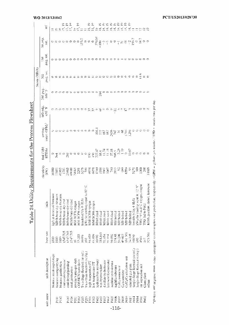
*¾
xam
!st
eaas
«»
*·¾
iati
.,
T=
ts
-s
day.
[0339] Example 2.2 - Mathematical Model for Hot/Cold/Power Utility
Minimization.
[0340] This example describes the mathematical model used to find the
minimum hot/cold/power utility cost. A restricted utility model is used to prevent
heat flow between streams that are either infeasible or are undesirable. These
restrictions are imposed mainly for the point sources of heat that correspond to
process units that require a cooling jacket and include the coal gasifier, the
Fischer-Tropsch (FT) units, the Claus furnace, and the Claus sulfur separators.
As all of these units have a negative heat duty, they generally will form steam
within the plant. By electing to incorporate these units in the HEPN, care must
be taken toprevent them from transferring heat to a process stream. To mitigate
a potential safety risk in the plant, only the heat engines will be allowed to
absorb heat from these units.
[0341] Indices. The indices for this model will be equivalent to those used
for the other stages of the decomposition. They are defined here and referenced in
subsequent sections.
i Hot stream/heat source index
j Cold stream/heat sink index
k Temperature interval index
b Boiler pressure index
c : Condenser pressure index
s : Subnetwork index
t Turbine inlet temperature index
[0342] Parameters. The following mass flow rate parameters are directly
extracted from the Aspen Plus simulation report.
iHP: Mass flow rate of hot process stream i
Fj Mass flow rate of cold process stream j
ea: Deaerator water outlet available for steam generation
iP o : Amount of generated steam utility i that is needed for the process units
[0343] The thermal parameters are calculated using Aspen Plus heating
curves. The point source heat duties are nonzero only in the specific temperature
interval where heat is released/absorbed. The heat capacities are temperature-

interval- dependent and are calculated as the average value of the heat capacity
at the bounds of the temperature interval. The relevant stream information for
the three hybrid flowsheets (i.e., H-R-A, H-EA, and H-R-T) are included. This
information includes (i) the process stream flow rates, (ii) the process stream
heating curves, and (iii) the heat duty given off by the point sources.
C i, ; P : Specific heat capacity for hot process stream i in temperature interval k
Cj,k Specific heat capacity for cold process stream j in temperature interval k
,k Specific heat capacity for cold utility stream j in temperature interval k
Ci,k G Specific heat capacity for hot generated utility stream i in temperature
interval k
C ( ,c , , ;H E : Specific heat capacity for heat engine (b, c, t) hot fluid in temperature
interval k
C(b,c,t),kC E : Specific heat capacity for heat engine (b, c, t) cold fluid in temperature
interval k
, ; P t : Heat released by heat source i in temperature interval k
Qj,k Heat absorbed by heat sink j in temperature interval k
The remaining parameters are listed below. The possible working conditions of
the heat engine correspond to a given amount of produced electricity in the
turbine and consumed electricity in the pump. The parameters W(b,c,t) ,
( , c , m , and T(b,c,t) are calculated using Aspen Plus assuming (a) a 95%
mechanical efficiency of the turbine and pump drivers, (b) a 75% isentropic
efficiency of the turbine, (c) and a pump efficiency calculated using Aspen Plus
default methods.
P b Working pressure of boiler b
P c : Working pressure of condenser c
Turbine inlet temperature
( , c , T : Specific energy generated by heat engine (b, c, t) turbine
( , c , Pum : Specific energy used by heat engine (b, c, t) pump
T(b,c,t) n :Minimum turbine inlet temperature required to maintain vapor phase
within the turbine
EnMax: The maximum number of heat engines allowed in the HEPN

[0344] The final set of parameters is associated with the temperature
intervals of the process flowsheet. The temperature intervals are derived by first
determining the inlet temperature for each process stream, utility stream, and
heat engine stream, as well as the temperature for all heat sources. All values for
the hot streams are then decreased by the minimum temperature approach
( m in ) 10 °C) and a set of all unique temperature values is ordered by decreasing
temperature value. A temperature interval is defined as the region of
temperatures between any adjacent values in the descending list. If the stream
outlet temperature is not within the temperature interval, then the value of AT
for that particular stream in that interval is equal to the full AT of the interval.
If the outlet temperature is contained within the interval, then the stream AT
value is equal to the difference between the outlet temperature and the interval
bound that passes through the stream temperature range. Note that this
criterion does not have to be used with the inlet stream temperatures, because
they were used to construct the bounds of the temperature intervals.
η : Temperature difference of hot stream i in interval k
¾ c : Temperature difference of cold stream j in interval k
AT ,c , ) , ; E : Temperature difference of heat engine (b, c, t) hot stream in interval
k
A , , ), : Temperature difference of heat engine (b, c, t) cold stream in interval
k
ATmi n : Minimum temperature interval approach temperature
[0345] Sets. The sets used in this model correspond to the temperature
intervals (TI), as well as the process streams (HP and CP), utilities (HG and CU),
or point sources (HPt and CPt).
TI: k k is a HEPN temperature interval
HP: i i is a hot process stream
HPt: i i is a hot point source
HG: i i is a generated steam utility stream
CP: j \j is a cold process stream
CPt: j \j is a cold point source
CU: j \j is a cold utility

Eng: (b, c, t) \ (b, c, t) is a feasible heat engine
[0346] Note that there are several (b, c , t) heat engine triplets that
correspond to discrete combinations of impractical operating conditions within
the turbine. Thus, not all (b, c, t) combinations will be included in the model. To
restrict the turbines to feasible operating conditions, the following criteria are
imposed on the operating conditions of a turbine:
where Tb,c m is the minimum temperature needed to maintain a vapor phase in
the turbine during expansion from P b to Pc . Similarly, a feasible pump is
defined by imposing P b > P c . A heat engine is considered feasible if the pump
conditions are feasible and the vapor phase is maintained within the turbine.
Although the optimizer could prevent an infeasible operating condition based on
the objective funtion (i.e., zero work for the turbine or infinite work for the
pumps), to reduce the computational complexity, these infeasible operating
conditions are removed prior to construction of the model.
[0347] Variables. We use continuous variables to represent heat transfer Q ,
residual heat flow R , and fluid flow rate F of the working fluid in the heat engine
or of a utility. We define the unrestricted hot and cold streams to represent all
hot and cold streams that do not have any restrictions on the matches. For
example, in a given temperature interval k , we look at the total heat transferred
by the hot streams that do not have match restrictions and define the
unrestricted hot stream as the composite of all these streams. The same
definition applies for the unrestricted cold stream. Binary variables y are
introduced to represent the logical use of a heat engine in the HEPN. That is, the
variable y(b,c,t) will be equal to 1 if the engine is present in the HEPN and will
be 0 otherwise. The formal variable list is defined below.
R : Residual heat flow of restricted stream i from temperature interval k
R k : Total residual heat flow of all unrestricted hot streams from temperature
interval k
, H : Heat delivered by restricted hot stream i in interval k
Qj,k : Heat absorbed by restricted cold stream j in interval k
Q k : Total heat delivered by all unrestricted hot streams in interval k
k : Total heat absorbed by all unrestricted cold streams in interval k
Qij,k : Heat transferred from restricted hot stream i t o restricted cold stream j
in interval k
Heat transferred from restricted hot stream i to unrestricted cold stream
in interval k
Qj,k Heat transferred from unrestricted hot stream t o restricted cold stream j
in interval k
Q k Heat transferred from unrestricted hot stream to unrestricted cold stream
in interval k
( ,c, En : Flow rate of the working fluid in heat engine (b, c, t)
F i G Flow rate of generated hot utility i
Fj Flow rate of cold utility j
i¾: Flow rate of electricity generated
[0348] Constraints. The unrestricted heat flow is initially defined by
lumping all streams that are allowed t o transfer heat t o any other part of the
process. Specifically, this refers to the heat engine streams, as well as the
consumed and the generated utility streams, since there are no physical or
practical limitations on heat transfer to or from these streams. The unrestricted
heat flow is defined for hot streams in eq 130 and for cold streams in eq 131. In
each equation, the heat flow for a process stream is defined as the product of the
mass flow rate (F), the heat capacity (C), and the temperature change (AT). The
mass flow rate for the heat engines F(b,c,t) , the cold utility (i.e., cooling water)
u , and the hot generated utility (i.e., generated steam) i are variables that
will be selected by the mathematical model. All heat capacities and temperature
changes are output of the Aspen Plus software and are known parameters. The
total heat delivered by each of these streams in a temperature interval k is
summed t o generate a hot Q k and cold Q kc composite stream.
(130)
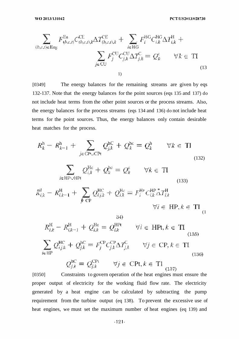
(131)
[0349] The energy balances for the remaining streams are given by eqs
132-137. Note that the energy balances for the point sources (eqs 135 and 137) do
not include heat terms from the other point sources or the process streams. Also,
the energy balances for the process streams (eqs 134 and 136) do not include heat
terms for the point sources. Thus, the energy balances only contain desirable
heat matches for the process.
P(132)
(133)
nil , ...... - P , , . *
fe
(1
[0350] Constraints to govern operation of the heat engines must ensure the
proper output of electricity for the working fluid flow rate. The electricity
generated by a heat engine can be calculated by subtracting the pump
requirement from the turbine output (eq 138). To prevent the excessive use of
heat engines, we must set the maximum number of heat engines (eq 139) and
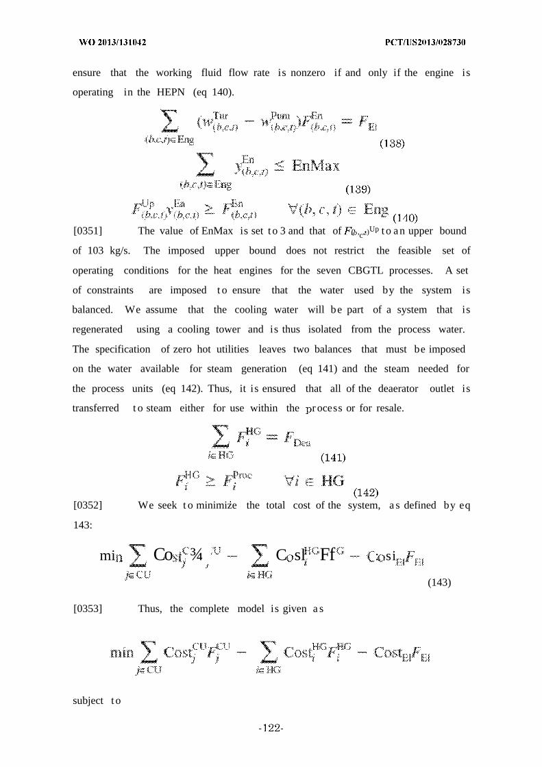
ensure that the working fluid flow rate is nonzero if and only if the engine is
operating in the HEPN (eq 140).
[0351] The value of EnMax is set t o 3 and that of ( ,c, )Up t o an upper bound
of 103 kg/s. The imposed upper bound does not restrict the feasible set of
operating conditions for the heat engines for the seven CBGTL processes. A set
of constraints are imposed t o ensure that the water used by the system is
balanced. We assume that the cooling water will be part of a system that is
regenerated using a cooling tower and is thus isolated from the process water.
The specification of zero hot utilities leaves two balances that must be imposed
on the water available for steam generation (eq 141) and the steam needed for
the process units (eq 142). Thus, it is ensured that all of the deaerator outlet is
transferred t o steam either for use within the r ocess or for resale.
[0352] We seek t o minimize the total cost of the system, a s defined by eq
143:
mi Co ¾ C sl Ff : si
(143)
[0353] Thus, the complete model is given a s
subject t o
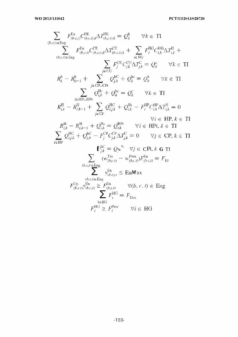
fi ¾ C G Tl
Σ M
iΣ
[0354] Equations 130-143 represent a mixed-integer linear optimization
(MILP) model that can be solved to global optimality using CPLEX13 to obtain (i)
the active binary variables y(b,c,t) that represent the operating conditions of the
heat engine, (ii) the values of the working fluid flow rates of the heat engines
F(b,c,t) , (iii) the amount of electricity produced by the heat engines F , and (iv)
the flow rate of the cooling utility u .
[0355] Example 2.3 - Computational Results. Upon completion of the
simulation for a given flowsheet, several key pieces of data are extracted from the
simulation results to determine (i) steam demand for the process units, (ii)
available condensate, (iii) the electricity requirement of the compressors, and (iv)
the initial cooling water and electricity requirement for other process units using
the information in Table 24. This information is presented in Table 25. Note that
all results are normalized with respect to the total volume of products (in bbl).
Since each process simulation had a total of 2000 tonnes/day of combined
biomasscoal-natural gas feedstock, normalizing the results with respect to the
products allows for a direct comparison of overall utility usage, as well as overall
cost.
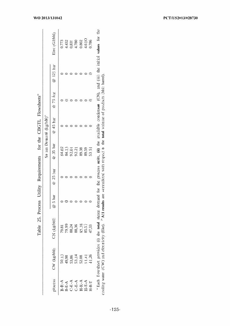
Tab
le25
.Pr
oces
sU
tility
Req
uire
men
tsfo
rth
eC
BG
TL
Flow
shee
ts"
teD
stii
(bi
iC
W(
gb
bC
g@
5ba
r2
535
bar
45
75
i@
12E
ecG
Jb
b
--A
50
79.8
10
04
.2
00
00.
773
B-E
-A49
,98
99
90
084
.0
04.
432
-E-A
53,8
688
,24
00
92
,0
00
0,83
!C
EA
53
,4
88,3
60
09
2.2
00
04.
780
--A
52.0
80
089
.38
00
00.
802
EA
5:
,4.
85.5
"0
089
.59
00
04.
6O
H-R
-T,2
647
,33
00
53
50
0.78
6
"E
ach
flp
(i)
ste
tota
ld
for
ssn
i(i
i)th
ee
sate
(CN
),(i
iva
lues
for
wat
erC
W)
cr
(Eke
).A
1re
sult
sar
e«
it
toth
eto
tal
of
b:
barr
el).
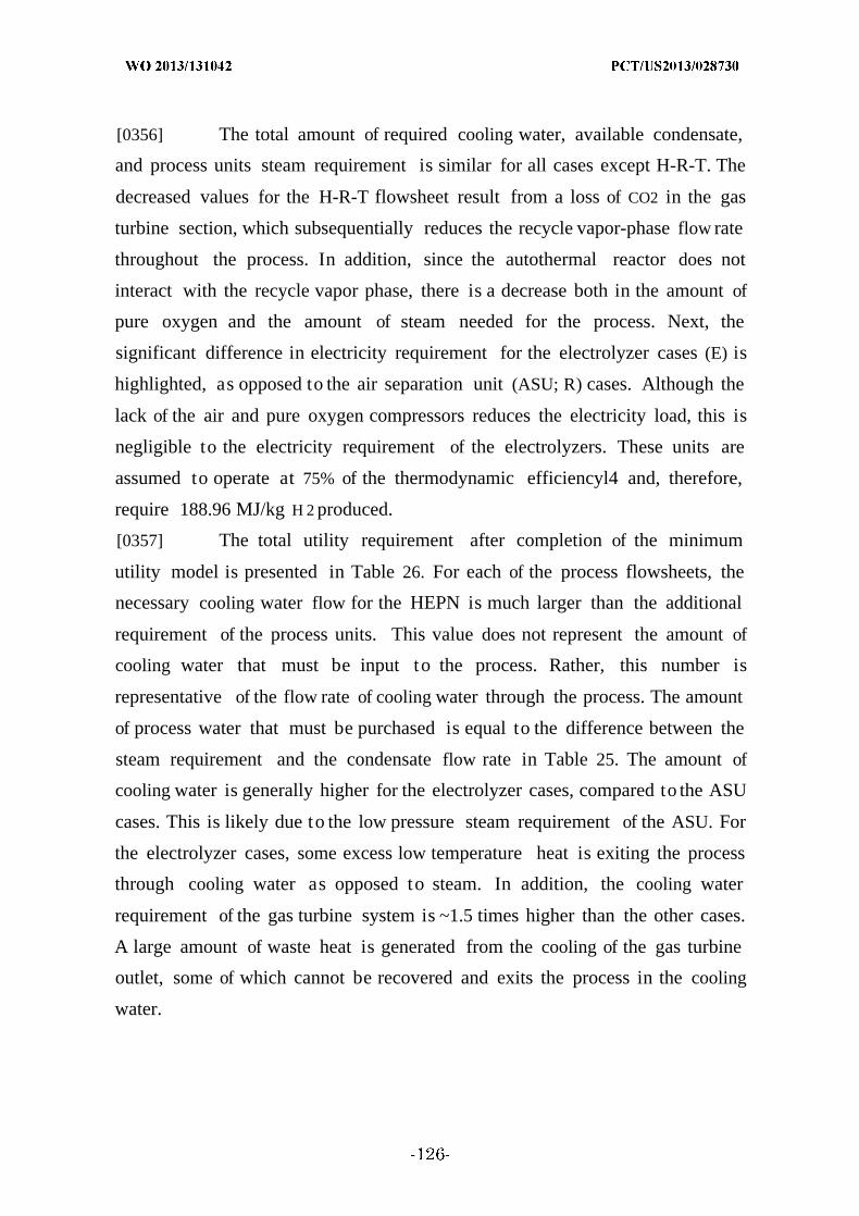
[0356] The total amount of required cooling water, available condensate,
and process units steam requirement is similar for all cases except H-R-T. The
decreased values for the H-R-T flowsheet result from a loss of CO2 in the gas
turbine section, which subsequentially reduces the recycle vapor-phase flow rate
throughout the process. In addition, since the autothermal reactor does not
interact with the recycle vapor phase, there is a decrease both in the amount of
pure oxygen and the amount of steam needed for the process. Next, the
significant difference in electricity requirement for the electrolyzer cases (E) is
highlighted, as opposed to the air separation unit (ASU; R) cases. Although the
lack of the air and pure oxygen compressors reduces the electricity load, this is
negligible to the electricity requirement of the electrolyzers. These units are
assumed to operate at 75% of the thermodynamic efficiencyl4 and, therefore,
require 188.96 MJ/kg H 2 produced.
[0357] The total utility requirement after completion of the minimum
utility model is presented in Table 26. For each of the process flowsheets, the
necessary cooling water flow for the HEPN is much larger than the additional
requirement of the process units. This value does not represent the amount of
cooling water that must be input to the process. Rather, this number is
representative of the flow rate of cooling water through the process. The amount
of process water that must be purchased is equal to the difference between the
steam requirement and the condensate flow rate in Table 25. The amount of
cooling water is generally higher for the electrolyzer cases, compared to the ASU
cases. This is likely due to the low pressure steam requirement of the ASU. For
the electrolyzer cases, some excess low temperature heat is exiting the process
through cooling water as opposed to steam. In addition, the cooling water
requirement of the gas turbine system is ~1.5 times higher than the other cases.
A large amount of waste heat is generated from the cooling of the gas turbine
outlet, some of which cannot be recovered and exits the process in the cooling
water.
Tab
le26
.R
esul
tsof
the
Min
imum
Hot
/Col
d/Po
wer
Util
ityM
odel
Stea
m/
b
CW
W5
®25
33&
45
€73
E.
J.
proc
ess
(kg
bba
rba
rba
rba
rba
rG
Ji
-.-A
42
\0
-84,
020
00
0.
52.
856
BE
A.
986
4.
40
0-
84,
30
03,
91.2
65.9
2Λ
998
3.8
00
-92.
0S
00
00.
28.2
3.
3C
EA
1.9
03.
830
0-9
2.21
00
04
6.
8-
-A2
4.00
00
~0
00
0.20
94.
069
-E-A
1747
44.
020
0--
-¾>
.59
00
04.
000
67.2
4H
-R-T
3046
46
80
-53
.0
00
-0.1
07-0
.809
Cos
t$
31.
79/
0kg
953
80
6.6
7J
Th
eec
bici
iE
ee.
iseq
ual
the
sus
of
ele
ipl
usaf
prod
uced
byT
iiete
(PW
)as
todi
ffer
ence
eeth
ees
rq
ird
bypr
oces
sun
its(i
.e„
aifi
es
dA
Tan
dl
ond
et
teou
tput
from
the
sraf
rT
heift
wat
er(C
W)
seq
ual
tofe
so
thpr
oces
su
ith
eH
EPN
&&
The
prod
uced
ti
ise
sth
ei
for
the
l¾
u-
ea
?ast
eam
iso
td
bypr
oduc
t,th
isi
selt
dd.
the
mili
-vs
.*A
il¾
l†s
xs&
xw
ithre
spec
tto
tota
lvo
lue
tib
bi;
rsi
.
[0358] The electricity requirement in Table 26 represents the sum from the
process, as well as that recovered from the HEPN. The only process that is able
to provide a negative utility cost (from sale of the electricity) is the gas turbine
system. This was anticipated since this flowsheet will have smaller recycle
compression costs due to removal of the CO2. However, the benefit is reduced
somewhat due to the loss of carbon from the system, because not as much product
will be made. The total electricity requirement of the remaining flowsheets is the
smallest for pure biomass, slightly larger for the hybrid system, and largest for
the pure coal processes. Furthermore, for any given feedstock, the electricity
requirement for the ASU cases is more than 1 order of magnitude lower than that
for the electrolyzer cases and is a direct consequence of the high electrolyzer
requirement (Table 25). The overall cost of each system is strongly dependent on
the amount of electricity needed; therefore, it is important to reduce the
electricity usage of the electrolyzers as much as possible. Even when operating at
100% thermodynamic efficiency, the units will still require 141.72 MJ/kg H 2
produced, so the key will be reducing the hydrogen requirement via a formulation
of a rigorous process synthesis problem.
[0359] For these results presented above, several possible heat engines
were postulated, including four condenser pressures ( cc s l bar, 5 bar, 15 bar,
40 bar), five boiler pressures (Pb B e25 bar, 50 bar, 75 bar, 100 bar, 125 bar),
(Pc l bar, 5 bar, 15 bar, 40 bar), five boiler pressures (Pb 25 bar, 50 bar,
75 bar, 100 bar, 125 bar), and five turbine inlet temperatures (Tt 500 °C, 600
°C, 700 °C, 800 °C, 900 °C). When placing an upper bound on the total amount
of heat engines (i.e., the number of steam turbines) equal to three, the resulting
operating conditions are given in Table 27. Note that each process selected three
heat engines, although the selection of operating conditions varies even between
the process flowsheets with the same feed. This is a result of the
absence/presence of the ASU and the necessary steam requirement. We note that
in no case is the 125 bar boiler pressure selected. This is possibly due to the
saturation temperature of the boiler (326.9 °C), which is above the operating
temperature of both FT units (240 and 320 °C). These units will provide a
significant amount of waste heat that will need to be recovered by the heat
engines toprovide the maximum amount of electricity. In addition, note that the
triplet (Pc , P b , Tt) = (25, 1, 900) was selected for six of the seven flowsheets, and
this selection had the highest working fluid flow rate for each of the flowsheets.
The maximum amount of work that is produced for a given boiler pressure is
given by the maximum operating turbine inlet temperature and the minimum
available condenser pressure. Furthermore, the boiler pressure of 25 bar has a
saturation temperature of 223.9 °C, which is lower than both operating
temperatures (within the minimum temperature approach) of the FT units. The
combination of both pieces of information is likely the reason for the common
selection of this engine.

Tab
le27
.H
eat
Eng
ine
Con
figu
ratio
nfo
rth
eO
ptim
alH
ot/C
old/
Pow
erU
tility
Cos
t
(b,
(bar
),T
(X))
Fid
Flow
(g
)
E.
E.
2Fa
.3
1E
n.2
E,
3
R-A
(25,
1,90
0)(5
0,
(25.
800)
30.4
35
128.
03C
-E-A
(25.
,900
)50
.1.
700)
75,
900
28.9
15.
8215
.01
B-
-A90
0)50
.5
.90
0(2
5,,
800)
8.23
21,1
2B
-E-A
(25.
190
0(5
0.5.
800)
(200
,,
7034
.36
£5.2
36.
99-A
25
1,
900)
?5.
40.
90
1
00,
5,
90)
72,9
1.5
9,
5H
.-E
-A,
,(
15,
50
)7
5.4
.90
)76
.04
152
!19
.34
H-R
-T(2
5.,6
00,
,90
0)(2
00,
15.
60
i61
.76
57.6
825
.01
[0361] Example 2.4 - Minimum Number of Heat Exchanger Matches
[0362] The minimum hot/cold/power utility model has provided us with (i)
the required amount of cooling water, (ii) the different levels of steam produced
using the deaerator water, (iii) the amount of additional process water needed to
produce process steam, (iv) the operating conditions and working fluid flow rate
of the heat engines, and (v) the location of the pinch points denoting the distinct
subnetworks. Given this information, the minimum heat exchanger matches are
calculated that are necessary to meet specifications (i), (ii), (iii), and (iv). Note
that the turbines and pumps used in the heat engines, as well as their
corresponding working flow rates, are already defined based on the results of the
minimum hot/cold/power utility model. Thus, the cost of these units is now fixed,
and will not have to be taken into account in a minimization of the total
annualized cost of the HEPN.
[0363] The formulation of a general minimum heat exchanger matches
model results in multiple solutions yielding the same minimum value. A
nonlinear minimum annualized cost model will have to be developed for each
solution, so it is important to distinguish among these solutions at this stage of
the decomposition. Specifically, the focus is on the methods of vertical heat
transfer and weighted matches. The vertical heat transfer model adds a penalty
to the objective function that is incremented when "criss-cross" heat transfer is
used. This method relies on the assumption that maximization of the vertical
heat transfer will lead to the minimum heat transfer area for a given number of
heat exchanger matches. A weighted matches model assigns a priority to each
possible stream match based on proximity within the process flowsheet. The
priority does not have a connection with the possible heat transfer area
associated with a stream match; it is designed to be an indication of the auxiliary
costs associated with a match. The weight for a match is assigned based on the
match priority, and the model objective is the minimization of the sum of the
weight of all matches.
[0364] The use of either one of the above models results in a reduction in
the number of solutions, and we can further distinguish among these solutions by
constructing a new objective function that is a linear combination of the
objectives for each model. A multiplicative coefficient, y, is placed in front of the
weighted matches objective function t o emphasize the relative importance
compared t o the vertical heat transfer objective function.
[0365] Example 2.5 - Mathematical Model for Heat Exchanger Matches
Minimization.
[0366] The minimum utility model has selected a subset of heat engines
that provides the necessary electricity. The sets HOT and COLD are defined a s
follows:
EOT — ! Hot stream i has a positive- flow rate !(144)
COLD = stream j has fl o rate
[0367] This reassignment serves to eliminate all of the heat engine streams
that were not activated in the minimum utility model. The set of potential
matches between process streams, MATCHES, is defined based on the
restrictions imposed in the minimum utility model (eq 146). Specifically, we
restrict a match between a hot process stream and a cold point source (HP x
CPt), a cold process stream and a hot point source (HPt x CP), and a hot point
source with a cold point source (HPt x CPt).
MATCHES = ( \i HOT./ COLD (i f) HPt xCPt x CPt HPt x C .., ,..
- (146)[0368] The HEPN is first discretized into subnetworks (s SUB) based on
the temperature intervals (eq 147) for which the residual heat flow is zero (Rk =
0). This significantly reduces the computational complexity needed to calculate
the total heat exchanger matches, because it is assumed that there will be no
heat flow between subnetworks. That is, the strict pinch case will be employed
for this model using a minimum temperature approach of 10 °C.
SUB ---- a subnetwork of the HEPN
ls e T \k " ≤ k ≤ k ' < k ,
> 0 V r < k )(147)
[0369] For each subnetwork, the superset of all possible intervals for which
a hot stream or cold stream may transfer heat is defined using eqs 148 and 149,
respectively:

\ 3k e T L
[0370] The set HOTs includes intervals where can be zero for a given
stream i , because of the residual heat flow. The set of all possible matches
between streams i and j is then introduced for each subnetwork (eq 150), as well
as the set of all possible stream matches for each temperature interval k (eq 151).
f ) MATCHES.., E TI.. I
[0371] Using appropriate binary variables ¾ Εχ) for each (i, j)
MATCHESs, the presence of a heat exchanger can be logically activated or
deactivated.
[0372] Example 2.6 - General Heat Transfer.
[0373] The hot and cold energy balances for the matches are given by eqs
152 and 153, respectively.
Ί ... .V (152)
: TC ' (153)
Binary variables ¾ Ex are introduced for each element of MATCHESs and are
equal to 1 if heat transfer exists between hot stream i and cold stream j in
subnetwork s (eq 155) and are equal 0 otherwise. The parameter Qij max is defined
as the maximum possible heat flow between two streams (eq 154) and is equal to
the minimum of the total heat load of each respective stream.
[0374] Example 2.7 - Vertical Heat Transfer.
[0375] To develop the model for vertical heat transfer, we partition the
enthalpy into enthalpy intervals (I EI ) based on the subnetwork s . Qi,i and
Qj,fi are defined to be the heat transferred in enthalpy interval I from hot stream
i and cold stream j , respectively. The vertical heat transfer between two streams
in a subnetwork Qij,s is the sum of minimum possible heat transfer in an
enthalpy interval in that subnetwork (eq 156).
[0376] Slack variables Shj, s are then introduced to measure the amount of
"criss-cross" heat transfer between a match (eq 157).
> MATCHES,. SUB
[0377] Example 2.8 - Weighted Matches.
[0378] To determine the match weights, a priority must first be assigned to
each heat exchanger match. This is initially done by considering the process
proximity between two units in a match. This proximity may either be analyzed
at the unit level or a plant level. If the unit level is observed, then a distance
metric should be defined that relates the estimated piping distance necessary to
connect the hot/cold pair. The plant distance metric would focus on the
discretization of the chemical flowsheet into "plants" where the distance between
units in two particular plants is calculated as the number of additional plants
between the two original units. The plant distance metric was chosen (Table 28)
here, since priority assignment based on individual units may be premature
without considering additional costs associated with unit placement in the
vicinity of each of the matched process units.
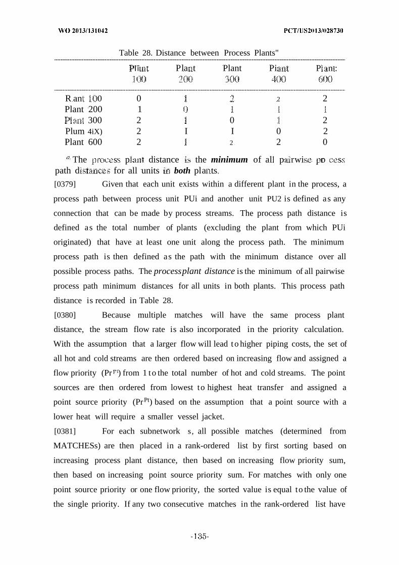
Table 28. Distance between Process Plants"
Ιΐ Pla t Plant Pi P n :
R an 0 0 2 2Plant 200 1
300 2 0 2Plum 4iX) 2 I I 0 2Plant 600 2 2 2 0
: The s p distance the minimum of al p rwi ro spath d for all units both pla ts
[0379] Given that each unit exists within a different plant in the process, a
process path between process unit PUi and another unit PU2 is defined as any
connection that can be made by process streams. The process path distance is
defined as the total number of plants (excluding the plant from which PUi
originated) that have at least one unit along the process path. The minimum
process path is then defined as the path with the minimum distance over all
possible process paths. The processplant distance is the minimum of all pairwise
process path minimum distances for all units in both plants. This process path
distance is recorded in Table 28.
[0380] Because multiple matches will have the same process plant
distance, the stream flow rate is also incorporated in the priority calculation.
With the assumption that a larger flow will lead to higher piping costs, the set of
all hot and cold streams are then ordered based on increasing flow and assigned a
flow priority (Pr 1) from 1 to the total number of hot and cold streams. The point
sources are then ordered from lowest to highest heat transfer and assigned a
point source priority (PrPt) based on the assumption that a point source with a
lower heat will require a smaller vessel jacket.
[0381] For each subnetwork s, all possible matches (determined from
MATCHESs) are then placed in a rank-ordered list by first sorting based on
increasing process plant distance, then based on increasing flow priority sum,
then based on increasing point source priority sum. For matches with only one
point source priority or one flow priority, the sorted value is equal to the value of
the single priority. If any two consecutive matches in the rank-ordered list have

the same process plant distance, flow priority sum, and point source priority sum,
they are sorted based on the increasing total amount of heat transferred between
the match. Note that any restricted matches from the minimum utility model are
not included in the set of possible matches. Each match is then assigned a
priority, P ri ,sTCH, based on the ranking in the final ordered list. The weight for
a match can then be calculated as wi, j , s based on eq 158:
where Nij,s is the total number of possible matches and is equal to the cardinality
of MATCHES,.
[0382] Objective. We first attempt to find the minimum number of matches
for each subnetwork (MinMatchs) without concern for which streams are present
in the final solution (eq 159).
( 1
The complete model below represents a mixed-integer linear program (x s .
min MinMatchs
subject to
Mi: M €( s MATCHES
+ Σ ffi > HOTMATCHES
. C , :
: .?.*.· >«
¾ ¾ ≥ V(? , ) MATCHES
[0383] This model is solved to global optimality using CPLEX 3 to
determine the minimum number of heat exchanger matches (MinMatchs) for each
subnetwork. To distinguish among the different solutions, an objective function
utilizing vertical heat transfer and weighted matches (eq 160) is developed.
∑ ¾ + ¾ SMATCHES, (160)

[0384] To place more importance on the vertical heat transfer criterion, y is
set to a value of 1 x l O6. For each subnetwork, MinMatchs is fixed at the value
found in the previous model and the resulting MILP is represented below for
each subnetwork s .
./ ) MATCHES
subject to
a
MATCHES
MATCHES]
FE C
¾ > / MATCHESj
> fi y ¾ V( ) MATCHES,
[0385] Example 2.9 - Computational Results and Illustrative Examples.
[0386] The results for each subnetwork for all seven process flowsheets are
presented in Table 29. It is initially noted that each flowsheet is discretized into
three subnetworks, although the number of heat exchanger matches (and, thus,
the topology) will be different for each subnetwork. Each of these subnetworks
will be analyzed using the minimum annualized cost model that is described in
the Examples 2.10 - 2.17.
[0387] As an illustrative example, the results for subnetwork one of each of
the three hybrid process flowsheets is presented in Table 30. Although the
topology will be different for each case, there are several common streams
between each of the subnetworks, including the stream exiting the reverse water-
gas shift (RGS) unit (HI), the stream exiting the fuel combuster (H6), the steam
input the autothermal reactor (ATR; C6), the inlet natural gas stream (C7), the
oxygen input the ATR (C8), and the recycle light gases to the autothermal reactor
(C9). Additional streams include the inlet hydrogen to the RGS unit (Cl) and the

recycle CO2 to the RGS unit. A common point source of heat was the coal gasifier
(H15 for H-R-A; H12 for H-E-A; H17 for H-R-T). The final streams in the
subnetworks are the hot (H29 for H-R-A; H27 for H-E-A) and cold (C33-C35 for
H-R-A; C31-C33 for H-E-A; C33-C35 for H-R-T) heat engine streams.
Table 29. Minimum Matches for the CBGTL Process Alternatives
R A C-E-A B-R-A B-E-A H-R-A H-E-A H-R-T
Subnetwork 1 I 1 16 14 14Subnetwork 2 50 4 1 5 3 1 /
Subnetwork 3 4 47 4 59

Tab
le30
.H
eat
Exc
hang
erM
atch
esan
dH
eat
Dut
ies
for
the
Firs
tSu
bnet
wor
kof
Eac
hH
ybri
dFl
owsh
eet'
ah
:Vm
atch
du
vW
)du
tk
snat
chdu
tykW
--A
:Su
bnet
wor
k1
H!··
··<:
34.3
5I-
73
71.
41
H-
91i
50.4
6H
1-C
3312
47
.H
6-C
624
08.4
56
-C
720
7496
H6-
C8
1242
.76
H-
C16
85.5
9H
6-C
3334
38)4
H6-
C34
544.
29.
H6-
C35
430.
345-
C33
5326
8.3
H-
453
65.0
45-
C35
4986
.6«
H29
626
30.
2C
342
.43
H-E
-A:
Subn
etw
ork
···<
:35
44.5
HI-
€31
3532
3.9
H1-
-C32
585.
28-
(94
3\.
98H
6-C
636
!0.3
86
-C
720
74.0
6H
6-C
820
82.1
3H
-C
1427
.67
H6-
C3
135
13.7
0H
6-C
3322
00.5
3C
.34
-532
.412
-C33
7866
.58
H2
C6
370
4H
27-C
934
33.2
3
H-R
-T:
Subn
etw
ork
1
--I
9398
.60
I-2
7643
.79
H~
-6
2355
.58
I-(
6159
.20
H-€
3527
26.8
66
-15
56.5
2H
6-C
215
48.7
4H
6-C
620
74.9
6H
6-7
824
27H
6-C
8\M
MH
6-C
3444
90.9
47-
C34
4562
000
"T
heh
od
poti
lm
odel
prov
ided
pinc
hpo
ints
of6
.'C
for
rhH
RA
s,
482.
54C
for
the
H-E
-Afl
owsh
eet,
and
.C
ot
H-R
-Tlo
she

[0388] Example 2.10 - Network Topologywith Minimum Annualized Cost
of Heat Exchange
[0389] Upon solution of the minimum matches model, we have the optimal
set of stream matches and, thus, aim at determining the heat exchanger topology
with the minimum annualized cost. There are two possible types of heat
exchanger matches: a match between two process streams and a match between
a heat engine stream and a point source. Each point source represents the heat
that is required by or absorbed from a particular process unit at a given
temperature. Although the evolved heat of reaction for the coal gasifier, the
Fischer-Tropsch (FT) unit, and the Claus furnace has been thoroughly modeled in
the Aspen Plus simulation, we are only given estimates of heating requirements
for other units based on the input flow rate to the unit.
[0390] Example 2.11 - Heat Exchanger Cost Functions.
[0391] To formulate the annualized cost of the heat exchanger, we consider
that each heat exchanger will be a shell-and-tube design. A floating head
exchanger will be used for nonevaporating streams, while a kettle reboiler will be
used for all evaporating streams. The free on board purchase price (Cp) of a heat
exchanger is given by eq 161:
where C is the base purchase cost, Fp is a pressure factor, F M is a material
factor, and F L is a length factor. The base purchase cost is given by eqs 162 and
163 for the kettle reboiler and the floating heat exchangers, respectively:
)[0392] The base costs are functions of the heat exchanger area (A) and are
valid in the range of A =150-12000 ft2. Note the scaling factor in the beginning of
eqs 164 and 165 is used to convert from the mid-2000 cost index to the August
2009 index, via the CE plant cost index. 9 The parameters F M and F Lare each

assumed t o be equal t o 1. The pressure factor is determined based on the
shellside pressure (P, given in psig), a s defined in eq 164.
F
[0393] Note that, at this stage of the decomposition, the stream matches
are now defined, so we are able to determine the shell-side pressure for a given
match. If a stream is vaporizing or condensing, that stream is automatically
assigned t o the shell side. Otherwise, the lower pressure (or lower temperature)
stream is assigned t o the shell side.
[0394] Given the base purchase cost of a heat exchanger, we may calculate
the annualized cost by first finding the annuity factor (AF). Assuming the life of
the exchanger to be n years, and assuming an interest rate of i , the value of AF is
given by eq 165. The annualized cost (CA) is then given by eq 166, where CM is
the annual maintenance cost. The maintenance cost is estimated a s a percentage
of the purchase cost for a fluid handling process ( ) ,9 as given by eq 167.
T ί f
I(165)
c(166)
(167)
[0395] An annualized cost is sought that is defined by a power law, a s given
by eq 168. An attempt t o find the best fit between the true annualized cost (CA)
and the estimated annualized cost may be accomplished by adjusting the
parameters C o and sf in eq 168. Using the Euclidean distance a s an objective
function, the annualized cost functions for the floating head and kettle reboiler
are defined in eqs 169 and 170, respectively. For the CBGTL process, the
parameters used are n = 30, i = 15%, and M = 10.3%.
(168)
···· 14.72Fp4 0 580
(169)

[0396] Example 2.12 - Heat Exchanger Overall Heat Transfer Coefficients.
[0397] The areas used to calculate the annualized cost of a heat exchanger
correspond to the outside area of the tubes within the exchanger. Therefore, the
overall heat transfer coefficient for the other tube area is defined as (U), as in eq
171.
(171)[0398] To estimate the value of U, it is assumed that the tube outside
diameter (D 0) is equal to 0.75 in., the tube wall thickness (tw) is 0.065 in., and
both the inner fouling factor (R /,i) and outer fouling factor (R/,0) are equal to 0.002
h ft2 °F/Btu. The material of construction will be carbon steel, which is assumed
to have a thermal conductivity (kw) of 20 BTU/h °F ft. The convective heat
transfer coefficients are calculated from the Nusselt number (Nu), as in eq 172:
, k N
(172)where L is the characteristic length and k is the thermal conductivity of the fluid.
The characteristic length of the tubeside fluid is given by L = D 0 - , whereas
that of the shellside fluid is given by L = (nD 0)/2. The thermal conductivity of the
fluid is given by the Aspen Plus program as a function of temperature and is
averaged for each stream across the temperature interval of interest. The
Nusselt number (Nu) is given by eq 173, where the value will be constant for
Reynolds numbers (R e) of < 3000 and is defined by the Gnielinski correlation for
R e > 3000.
[0399] The Reynolds number (R e) is given by eq 45, where Q is the
volumetric flow rate, L the characteristic length, v the kinematic viscosity, and A
the cross-sectional area. Both Q and v are determined from the Aspen Plus
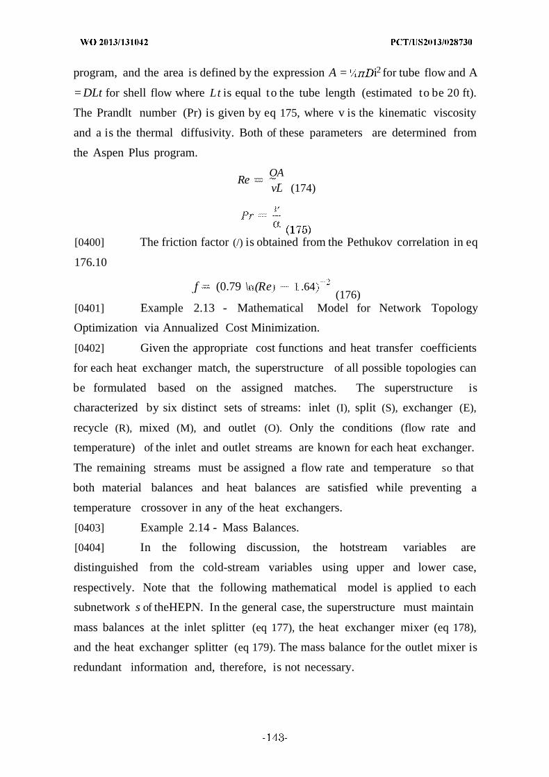
program, and the area is defined by the expression A = i2 for tube flow and A
=DLt for shell flow where Lt is equal to the tube length (estimated to be 20 ft).
The Prandlt number (Pr) is given by eq 175, where v is the kinematic viscosity
and a is the thermal diffusivity. Both of these parameters are determined from
the Aspen Plus program.
OARe
vL (174)
[0400] The friction factor (/) is obtained from the Pethukov correlation in eq
176.10
f (0.79 \ (Re .64(176)
[0401] Example 2.13 - Mathematical Model for Network Topology
Optimization via Annualized Cost Minimization.
[0402] Given the appropriate cost functions and heat transfer coefficients
for each heat exchanger match, the superstructure of all possible topologies can
be formulated based on the assigned matches. The superstructure is
characterized by six distinct sets of streams: inlet (I), split (S), exchanger (E),
recycle (R), mixed (M), and outlet (O). Only the conditions (flow rate and
temperature) of the inlet and outlet streams are known for each heat exchanger.
The remaining streams must be assigned a flow rate and temperature so that
both material balances and heat balances are satisfied while preventing a
temperature crossover in any of the heat exchangers.
[0403] Example 2.14 - Mass Balances.
[0404] In the following discussion, the hotstream variables are
distinguished from the cold-stream variables using upper and lower case,
respectively. Note that the following mathematical model is applied to each
subnetwork s of theHEPN. In the general case, the superstructure must maintain
mass balances at the inlet splitter (eq 177), the heat exchanger mixer (eq 178),
and the heat exchanger splitter (eq 179). The mass balance for the outlet mixer is
redundant information and, therefore, is not necessary.

? , ÷ C . . V/ HOT, Λ' SUB
(179)[0405] The cold-stream balances are similar for the inlet splitter (eq 180),
heat exchanger mixer (eq 181), and the heat exchanger splitter (eq 182):
/ , f VI HE?J COLD s(182)
[0406] To constrain the recycle stream in a region of interest, binary
variables are introduced for the existence of the recycle streams. Using eqs 183
and 184 for the hot streams and eqs 185 and 186 for the cold streams, the hot
recycle streams will be within the values F " and F , while the cold recycle
streams will be within the values /min and / ax. The minimum flow rates are set to
0.1 kg/s and the maximum rates to 100 kg/s.
)
[0407] Example 2.15 - Heat Balances.
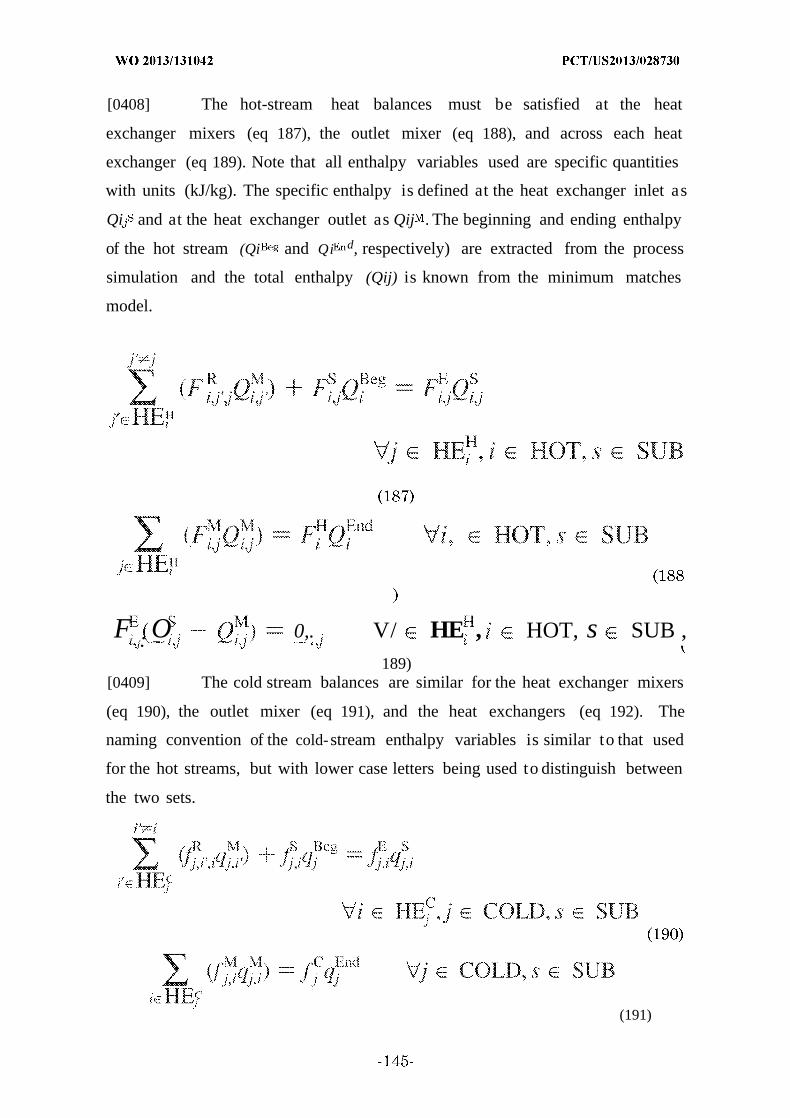
[0408] The hot-stream heat balances must be satisfied at the heat
exchanger mixers (eq 187), the outlet mixer (eq 188), and across each heat
exchanger (eq 189). Note that all enthalpy variables used are specific quantities
with units (kJ/kg). The specific enthalpy is defined at the heat exchanger inlet as
Qi and at the heat exchanger outlet as Qij . The beginning and ending enthalpy
of the hot stream (Qi and Qi d, respectively) are extracted from the process
simulation and the total enthalpy (Qij) is known from the minimum matches
model.
F : O 0,. V/ HE , HOT, s SUB ,189)
[0409] The cold stream balances are similar for the heat exchanger mixers
(eq 190), the outlet mixer (eq 191), and the heat exchangers (eq 192). The
naming convention of the cold-stream enthalpy variables is similar to that used
for the hot streams, but with lower case letters being used to distinguish between
the two sets.
(191)
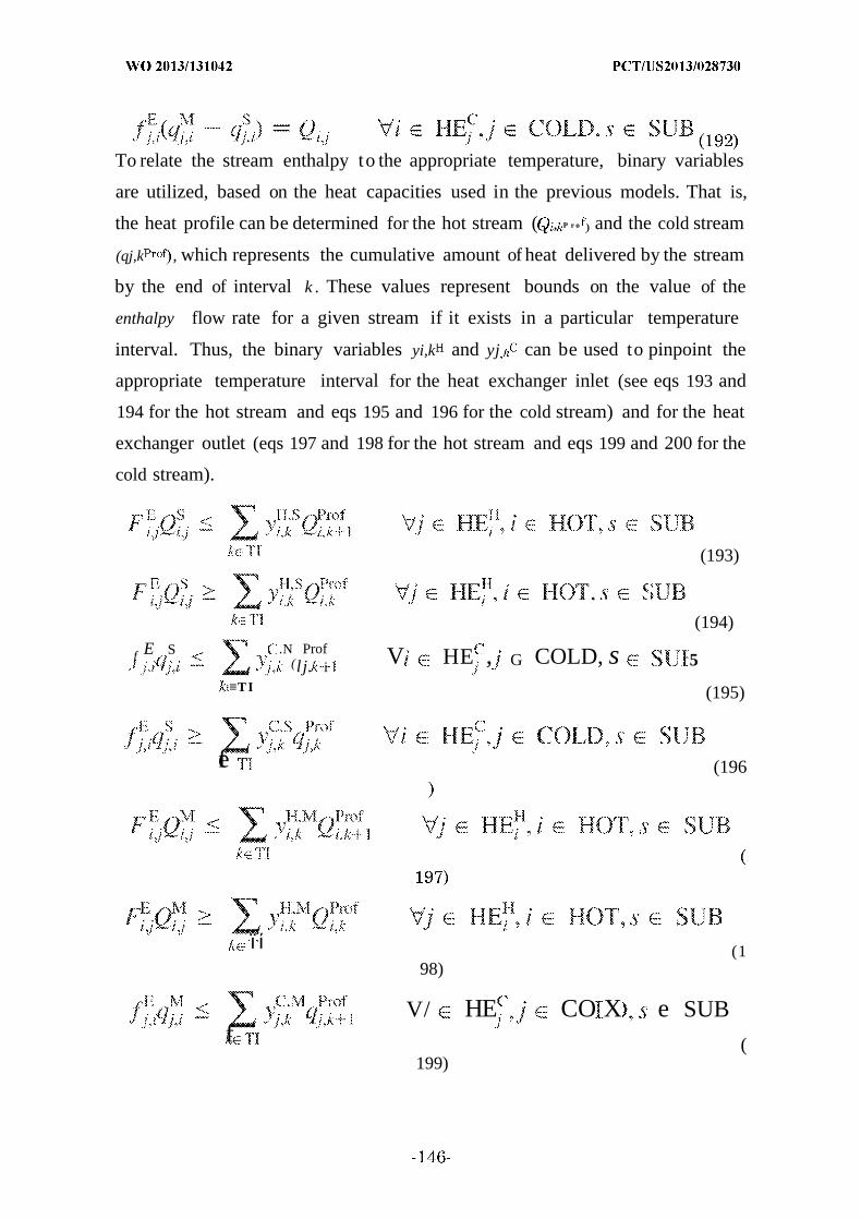
To relate the stream enthalpy to the appropriate temperature, binary variables
are utilized, based on the heat capacities used in the previous models. That is,
the heat profile can be determined for the hot stream ( , P r o ) and the cold stream
(qj,k , which represents the cumulative amount of heat delivered by the stream
by the end of interval k . These values represent bounds on the value of the
enthalpy flow rate for a given stream if it exists in a particular temperature
interval. Thus, the binary variables yi,k and yj can be used to pinpoint the
appropriate temperature interval for the heat exchanger inlet (see eqs 193 and
194 for the hot stream and eqs 195 and 196 for the cold stream) and for the heat
exchanger outlet (eqs 197 and 198 for the hot stream and eqs 199 and 200 for the
cold stream).
(193)
(194)
f E S .N Prof(l j. i
V HE , G COLD, s 5
≡T I (195)
fe (196
ϊ ί (198)
V/ HE CO X e SUBf (
199)
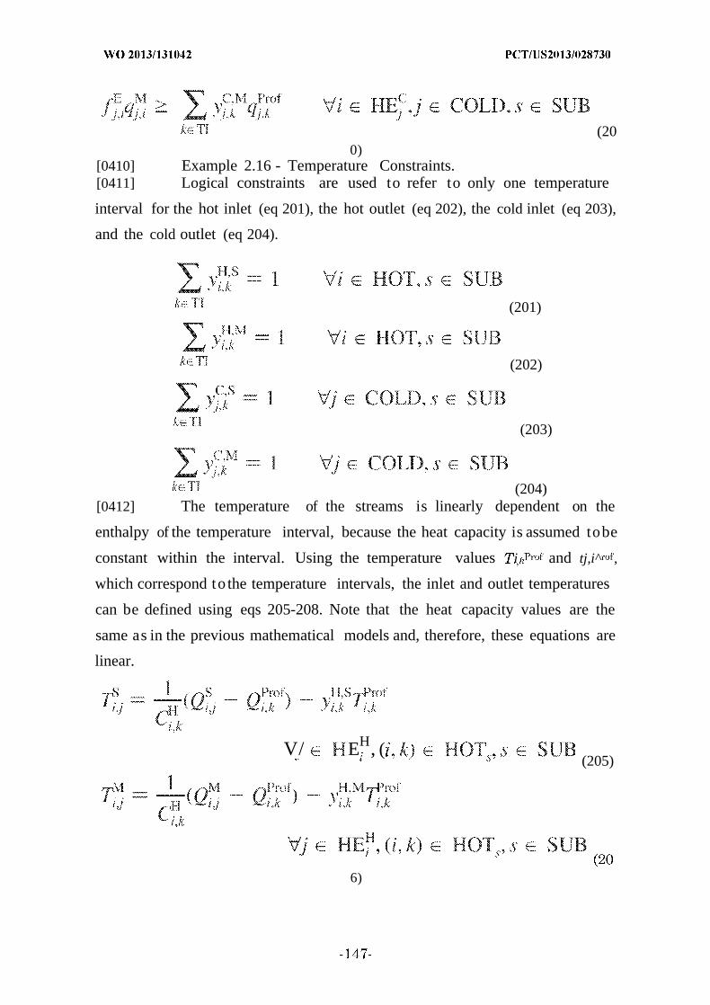
(200)
[0410] Example 2.16 - Temperature Constraints.[0411] Logical constraints are used to refer to only one temperature
interval for the hot inlet (eq 201), the hot outlet (eq 202), the cold inlet (eq 203),
and the cold outlet (eq 204).
(201)
(202)
(203)
(204)[0412] The temperature of the streams is linearly dependent on the
enthalpy of the temperature interval, because the heat capacity is assumed tobe
constant within the interval. Using the temperature values i and tj,i^ ,
which correspond to the temperature intervals, the inlet and outlet temperatures
can be defined using eqs 205-208. Note that the heat capacity values are the
same as in the previous mathematical models and, therefore, these equations are
linear.
V/ EH, ((205)
6)

V/ HE , ( k) COLD , .v G S(207)
V e HE e COLD,, e S ro(208)
[0413] Temperature crossover within the heat exchangers is prevented
using eqs 209 and 210. The minimum temperature approach ( T in) was set to 0.1
°C in this study.
> T V HEf, / e HOT, ' SUB(209)
7 > V/ HEf, HOT G SUB
[0414] The area associated with a heat exchanger is calculated using eq
211, where the log-mean temperature difference (LMTD) is defined in eq 214.
The Patterson approximation is used for LMTD to circumvent the computational
difficulty associated with very small temperature approaches.
-LMTD(211)
A T!
= 1 s1,
LMTD - .- = ¾ ∆ + .) 2 + I ' + A T~ )
)[0415] Objective. The objective is then given by eq 215,
sssssC . f
<!i
2
where the cost ( C 0 , i ) and scaling ( i ) parameters were determined using the
annualized cost calculation described previously.
[0416] Equations 177-215 represent a nonconvex mixed-integer nonlinear
optimization problem (MINLP) that can be solved using DICOPT20 with the
nonlinear solver CONOPT21 and the mixed-integer solver CPLEX.13 The
minimum superstructure is designed for each subnetworkl, by eliminating
impossible connections, using known information about the stream temperatures
for each match. Two hundred (200) initial points are selected by assuming no
recycle flow and different split fractions at the inlet, and the topology with the
smallest annualized cost is selected as the final structure. The selection of
multiple initial points is based on having nonconvex MINLP models for which
local MINLP solvers (e.g., DICOPT) are employed.
[0417] Example 2.17 - Computational Results and Illustrative Examples.
[0418] The overall results for the annualized cost model are presented in
Table 31. The total annualized cost for each subnetwork was normalized by the
amount of products formed to facilitate a proper comparison. From Table 31, the
largest annualized investment cost is $3.288/bbl and all seven process flowsheets
are within a range of $0.858/bbl to each other. Furthermore, this investment cost
is, with regard to magnitude, about one-third to one-fifth of the cost of the HEPN
utilities that are recovered in the Minimum Hot/Cold/Power Utilities model. This
serves to validate the decomposition of the HEPN problem into subtasks. The
total annualized HEPN cost is also shown in Table 31 and is indicative of the cost
benefit of only the HEPN. That is, the electricity associated with the electrolyzers
and compressors in Table 25 is not included in this cost. Note that, in all seven
cases, the HEPN serves to reduce the total cost of the final products. This is not
suprising, because a large amount of electricity is recovered from the Minimum
Hot/Cold/Power Utilities model, which helps avoid the purchase of a large
quantity of this power source.
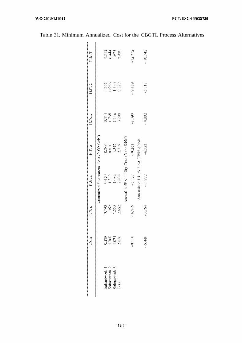
Table 31. Minimum Annualized Cost for the CBGTL Process Alternatives

[0419] To further illustrate the results of the mathematical model, the
topology of subnetwork 1 for each of the hybrid process flowsheets is shown in
FIGS. 29, 30, and 31 for H-R-A, HE-A, and H-R-T, respectively. Also included in
the figures are the inlet and outlet temperatures of both the hot and cold streams
for each match. For clarity, the hot streams are included as dashed lines,
whereas the cold streams are solid lines. The streams present in these figures
include the reverse water- gasshift (RGS) effluent (HI), the fuel combuster
effluent (H6), a heat engine precooler (H29 for H-R-A, H27 for H-E-A), the RGS
inlet hydrogen (Cl), the RGS recycle CO2 (C2), the autothermal reactor (ATR)
steam input (C6), the ATR natural gas input (C7), the ATR oxygen input (C8),
the ATR recycle light gas input (C9), and the heat engine superheaters (C33-C35
for H-R-T and H-R-T, C31-C33 for H-E-A). Also included is the coal gasifier (H15
for H-R-A and H-R-T; H12 for H-E-A). Note that the coal gasifier will not have
corresponding streams, because it is a point source of heat. The temperature for
the coal gasifier remains constant at 891 °C and is shown in italic font in the
figures.
[0420] A few key differences between the process topologies are
immediately obvious. Note that the pinch points for each of these subnetworks
are different, so the topologies are expected to be different. Furthermore, the
operating conditions of the heat engines will be different for each flowsheet, so it
is not expected that the same number of heat engine streams will be present in
each subnetwork. In fact, we only see a hot precooler stream for the H-R-A and
H-E-A subnetworks, because the turbine outlet temperatures of all three heat
engines for the H-R-T subnetwork fall below the pinch point associated with this
subnetwork . Another difference is the presence of cold streams Cl and C2 (inlets
to the RGS reactor) in the H-R-T subnetwork but not in the H-R-A or H-E-A
subnetwork. A design specification in the CBGTL flowsheets was to vary the
input temperature of the RGS input streams, to provide the necessary heat duty
of reaction. This serves to supplement oxygen input to the unit and helps reduce
the hydrogen requirement of the flowsheet. In the H-R-T flowsheet, the RGS inlet
streams were preheated to 710 °C and were thus included in the high
temperature subnetwork. The H-R-A and H-E-A RGS inlet streams were heated
to 472.16 and 473.26 °C, respectively, and thus were not considered in the high
temperature subnetwork.
[0421] Although the topologies are distinctly different, there are several
similarities to note. The ATR unit has each of the feed streams preheated to 800
°C to reduce the oxygen requirement needed to provide the heat of reaction.
Because of the restrictions placed on matches between point sources and process
streams, none of these preheated streams extracts heat from the coal gasifier.
Rather, a combination of the fuel combuster, heat engine precoolers, and RGS
effluent provides the necessary heat. Furthermore, the only streams that
interact with the coal gasifier are the three heat engine superheaters. A second
major similarity is that most of the cold streams interact with the RGS effluent
and then the fuel combustor. This is expected due to the higher temperature of
the fuel combustor effluent (1300 °C, compared to 700 °C). It is finally worth
noting that, although the minimum allowed temperature approach of the streams
was 0.1 °C, the minimum value that is seen in thefigures is ~1 °C. This prevents
the LMTD value of a given match from becoming very small and thus increasing
the area of the heat exchanger to large values.
[0422] A new framework for simultaneous heat and power integration for
the coal, biomass, and natural gas to liquids (CBGTL) process is disclosed. This
was done using a three-stage decomposition where the minimum hot/cold/power
utility cost, the minimum number of heat exchanger matches, and the minimum
annualized cost of heat exchange were sequentially calculated. A superset of
possible heat engines were introduced to produce electricity, using the waste heat
from the process streams. The minimum hot/cold/power utility model found the
set of operating conditions of the heat engines that can recover the most
electricity while explicitly taking into account interaction with the entire process
flowsheet and the necessary cooling water requirement. Using the results of the
minimum utility model, the minimum matches model utilized both weighted
matches and vertical heat transfer to distinguish between solutions with the
same number of heat exchanger matches. Weights were assigned to a given set of
streams based on their proximity in the plant, as well as the relative flow rates of
the streams. The optimal set of heat exchanger matches along with the heat load
of each match was directly transferred to the minimum annualized cost model to
find the optimal heat exchanger topology. Explicit formulas were derived for the
annualized cost functions, assuming that each heat exchanger would either be a
floating-head unit or a kettle reboiler and overall heat transfer coefficients were
estimated for every heat exchanger. The results of the annualized cost model
provided heat transfer areas for each exchanger, which could then be directly
utilized in an economic analysis.
[0423] Example 3 - Process synthesis of hybrid coal, biomass, and natural
gas to liquids via Fischer-Tropsch synthesis, ZSM-5 catalytic conversion,
methanol synthesis, methanol-to- gasoline, and methanol-to-olefins/distillate
technologies.
[0424] Several technologies for synthesis gas (syngas) refining are
introduced into a thermochemical based superstructure that will convert
biomass, coal, and natural gas to liquid transportation fuels using Fischer-
Tropsch (FT) synthesis or methanol synthesis. The FT effluent can be (i) refined
into gasoline, diesel, and kerosene or (ii) catalytically converted to gasoline and
distillate over a ZSM-5 zeolite. Methanol can be converted using ZSM-5 (i)
directly to gasoline or to (ii) distillate via olefin intermediates. A mixed integer
nonlinear optimization model that includes simultaneous heat, power, and water
integration is solved to global optimality to determine the process topologies that
will produce the liquid fuels at the lowest cost. Twenty-four case studies
consisting of different (a) liquid fuel combinations, (b) refinery capacities, and (c)
superstructure possibilities are analyzed to identify important process topological
differences and their effect on the overall system cost, the process
material/energy balances, and the well-to-wheel greenhouse gas emissions.
[0425] The disclosure herein introduces several distinct methods for
conversion of syngas to liquid fuels into the CBGTL process superstructure and
investigates the tradeoffs that arise from these methods. The superstructure in
Examples 1 and 2 converted the syngas into a raw FT hydrocarbon product using
one of four FT units operating with either a cobalt or iron catalyst and at high or
low temperature. The effluent was subsequently fractionated and upgraded using
a series of hydrotreating units, a wax hydrocracker, two isomerization units, a
naphtha reformer, an alkylation unit, and a gas separation plant (i .e.,
deethanizer).
[0426] This example introduces two iron-based FT units that utilize the
forward water—gas-shift reaction to produce the raw hydrocarbons using an input
H 2/CO ratio that is less than the typical 2/1 ratio needed for FT synthesis.
Catalytic conversion of the FT vapor effluent over a ZSM-5 catalyst is considered
as an alternative for producing gasoline range hydrocarbons from the raw FT
effluent.
[0427] Methanol synthesis and subsequent conversion to liquid
hydrocarbons are also introduced into the superstructure. The methanol may be
catalytically converted using a ZSM-5 zeolite to (i) gasoline range hydrocarbons
or (ii) to distillate (i .e., diesel and kerosene) via an intermediate coversion to
olefins. The mathematical modeling and cost functions needed to incorporate the
above alternatives into the superstructure are outlined in detail. The complete
process synthesis optimization model is then tested on a total of 24 case studies
which consist of two liquid product combinations, three plant capacities, and four
plant superstructures. Using low-volatile bituminous coal (Illinois #6) and
perennial biomass (switchgrass), important topological differences between the
case studies are discussed and the results of each component of the process
synthesisframework are illustrated.
[0428] Example 3.1 - CBGTL mathematical model for process synthesis
with simultaneous heat, power, and water integration.
[0429] This example will discuss the enhancements to the previous
mathematical model for process synthesis and simultaneous heat, power, and
water integration that will incorporate a wide variety of designs for syngas
conversion and hydrocarbon upgrading. Modeling of these enhancements will be
described in detail in the following section and the complete mathematical model
is listed in Example 3.15. The nomenclature used in the mathematical
description below is outlined in Table 32, below. Note that this table represents a
subset of the comprehensive list of symbols that are needed for the full
mathematical model. The full list of symbols and mathematical model are
included for reference in Example 3.15.

Table 32. Mathematical model nomenclature
Symbol Definition
indicess Species indexu Process unit index
Sets( , u' Stream from unit to unit u'
( , ' . s) Species s within stream ( , ' )Set of all iron-based FT units
ParametersK wcs Water- gas-shift equilibrium constant for unit u
Methanol synthesis equilibrium constant for unit u
Variables
u.u ,s Molar flow of species s from unit to unit u'
Xs, , ,s Molar concentration of species s from unit u to unit u'
[0430] Example 3.2 - Conceptual design
[0431] The syngas conversion and hydrocarbon upgrading units proposed
herein is based on an extension of the CBGTL refinery superstructure in
Examples 1 and 2. All relevant thermodynamic information (i.e., chemical
equilibrium constants, vapor-liquid equilibrium constants, specific enthalpies,
and heat capacities) for the units and streams in the refinery have been extracted
from Aspen Plus v7.3 using the Peng-Robinson equation of state with the
Boston-Mathias alpha function. The flowsheets depicting the extensions of the
superstructure are shown in Figs. 32-36 of and the complete superstructure is
included. In the figures, fixed process units are represented by 110, variable
process units by 120, splitter units by 130, and mixer units by 140. The variable
process streams are represented by 210 and all other process streams are fixed,
unless otherwise indicated. Note that some units (e.g., compressors, pumps, heat
exchangers) are not included in the figures for clarity, though these units are
thoroughly modeled in the CBGTL refinery.
[0432] The CBGTL superstructure is designed to co-feed biomass, coal, or
natural gas to produce gasoline, diesel, and kerosene. Syngas is generated via
gasification from biomass (FIG. 38) or coal (FIG. 39) or auto-thermal reforming of
natural gas (FIG. 47). Co-feeding of the coal, biomass, or natural gas in a single
gasifier unit was not considered in this study due to the lack of (i) technical
maturity of the process design and (ii) cost and operating data for co-fed units.
Synergy for co-fed biomass and coal gasification and simultaneous reforming the
natural gas using the gasifier quench heat (Adams & Barton, 2011, which is
incorporated herein by reference as if fully set forth) may be important to reduce
the capital cost required for synthesis gas production, and the authors note that
the optimization model is capable of including the technoeconomic benefit of co-
fed gasification if cost and operational data become available.
[0433] The synthesis gas is either (i) converted into hydrocarbon products
in the Fischer-Tropsch (FT) reactors (FIG. 32; FIG 42) or (ii) into methanol via
methanol synthesis (FIG. 35; FIG. 45). The FT wax will be sent to a hydrocracker
to produce distillate and naphtha (FIG. 44) while the FT vapor effluent may be
(a) fractionated and upgraded into gasoline, diesel, or kerosene or (FIG. 43; FIG.
44) (b) catalytically converted to gasoline via a ZSM-5 zeolite (FIG. 33; FIG. 43).
The methanol may be either (a) catalytically converted to gasoline via the ZSM-5
catalyst (FIGS. 35-36; FIGS. 45-46) or (b) catalytically converted to olefins via the
ZSM-5 catalyst and subsequently fractionated to distillate and gasoline (FIG. 35;
FIG. 45).
[0434] Acid gases including CO2, ¾ , and NH3 are removed from the syngas
via a Rectisol unit prior to conversion to hydrocarbons or methanol (FIG. 40).
Incorporation of other acid gas removal technologies (e .g., amine adsorption,
pressure-swing adsorption, vacuum-swing adsorption, membrane separation) and
their relative capital/operating cost as a function of input flow rate and acid gas
concentration is the subject of an ongoing study. The sulfur-rich gases are
directed to a Claus recovery process (FIG. 41) and the recovered CO2 may be
sequestered (FIG. 40) or reacted with ¾ via the reverse water-gas-shift reaction.
The CO2 may be directed to either the gasifiers (FIGS. 38-39), the reverse water-
gas-shift reactor (FIG. 40), or the iron-based FT units (FIG. 42). Recovered CO2
is not sent to the cobalt-based FT units to ensure a maximum molar
concentration of 3% and prevent poisoning of the catalyst. Hydrogen is produced
via pressure-swing adsorption or an electrolyzer unit while oxygen can be
provided by the electrolyzer or a distinct air separation unit (FIG. 48). A
complete water treatment network (FIGS. 49-50) is incorporated that will treat
and recycle wastewater from various process units, blowdown from the cooling
tower, blowdown from the boilers, and input freshwater. Clean output of the
network includes (i) process water to the electrolyzers, (ii) steam to the gasifiers,
autothermal reactor, and water-gas-shift reactor, and (iii) discharged wastewater
to the environment.
[0435] The effluent of each reactor in the CBGTL refinery is based on
either (i) known extents of reaction, (ii) thermodynamically limited equilibrium,
or (iii) a specified composition from a literature source. Reaction system (i) is
used in the gasifiers, the tar cracker, and the combustor units (e.g., fuel
combustor, gas turbine, Claus combustor) and the extents of reaction are based
on known information from literature (gasifiers/cracker) or from the operating
conditions of the unit (i.e., complete combustion using a stoichiometric excess of
oxygen). Reaction system (ii) is used for the water-gas -shift reaction (i.e.,
gasifiers, WGS reactor, FT units, methanol synthesis, auto-thermal reactor),
methanol synthesis, and steam reforming in the auto-thermal reactor. Reaction
system (iii) is used for the FT units, the ZSM-5 hydrocarbon conversion, the MTG
reactor, the MTO reactor, and the MOGD reactor. The effluent composition of
these units is based on known commercial data or pilot plant data for the units
operating at a specified set of conditions (i.e., temperature, pressure, and feed
composition). The CBGTL process is designed to ensure that the appropriate
conditions are met within the reactor to ensure that the effluent composition that
is assumed is valid. Binary decision variables (y) are included within the
mathematical model to logically define the existence of specific process units
(Eqs. 239 - 243). That is, if y = 0 for a particular unit, then no heat/mass flow will
be allowed through the unit and the unit will effectively be removed from the
process topology. If y = 1 for a unit, then the heat/mass flow through the unit will
be governed by the proper operation of the unit.
[0436] Example 3.3 - Fischer-Tropsch units
[0437] The four FT units considered in Examples 1 and 2 utilized either a
cobalt or iron catalyst and operated at high or low temperature. The two cobalt
based FT units would not facilitate the water-gas -shift reaction and therefore
required a minimal level of CO2 input to the units to improve the per—pass
conversion of CO. The two iron-based FT units were assumed to facilitate the
reverse water— as-shift reaction and therefore could consume CO2 within the
unit using H 2t o produce the CO necessary for the FT reactions. A key synergy of
the reaction conditions in the latter units was the heat needed for the reverse
water-gas -shift reaction that is provided by the highly exothermic FT reaction.
Though the reverse water-gas- shift reaction is typically unfavorable at the lower
operating temperatures of the FT units, the reaction may be indeed facilitated
through the use of an appropriate amount of input hydrogen.
[0438] The set of possible FT units herein is expanded to consider iron-
based systems that will facilitate the forward water-gas-shift reaction within the
units. These FT units will require a lower H2/CO ratio for the FT reaction
because steam in the feed will be shifted to H 2 through consumption of CO. These
units may be beneficial since certain syngas generation units (e .g., coal gasifiers)
will produce a gas that generally has a H2/CO ratio that is much less than the
2/1 requirement for FT synthesis (Baliban et al., 2010; Kreutz et al., 2008, which
is incorporated herein by reference as if fully set forth). The downside of the new
FT units will be the high quantity of CO2 that is produced as a result of the
water-gas -shift reaction. The framework developed for the CBGTL
superstructure will directly examine the benefits and consequences for each of
the six FT units to determine which technology produces a refinery with a
superior design.
[0439] FIG. 32 shows the flowsheet for FT hydrocarbon production within
the superstructure. Clean gas from the acid gas removal (AGR) unit is mixed
with recycle light gases from a CO2 separator (CO2SEP) and split (SPCG) to either
the low-wax FT section (SPFTM), the nominalwax FT section (SPFTN), or methanol
synthesis (MEOHS). The FT units will operate at a pressure of 20 bar and
within the temperature range of 240-320 °C. The cobalt-based FT units operate
at either low temperature (LTFT; 240 °C) or high temperature (HTFT; 320 °C)
and must have a minimal amount of CO2 in the input stream. Two iron-based FT
units will facilitate the reverse water-gas -shift (rWGS) reaction and will operate
at low (LTFTRGS; 240 C) and high temperature (HTFTRGS; 320 °C). The other

two iron-based FT units will use the forward reverse water-gas -shift (fWGS)
units, operate at a mid-level temperature (267 °C), and produce either minimal
(MTFTWGS-M) or nominal (MTFTWGS-N) amounts of wax. The operating
conditions of the FT units are summarized in Table 33, below.
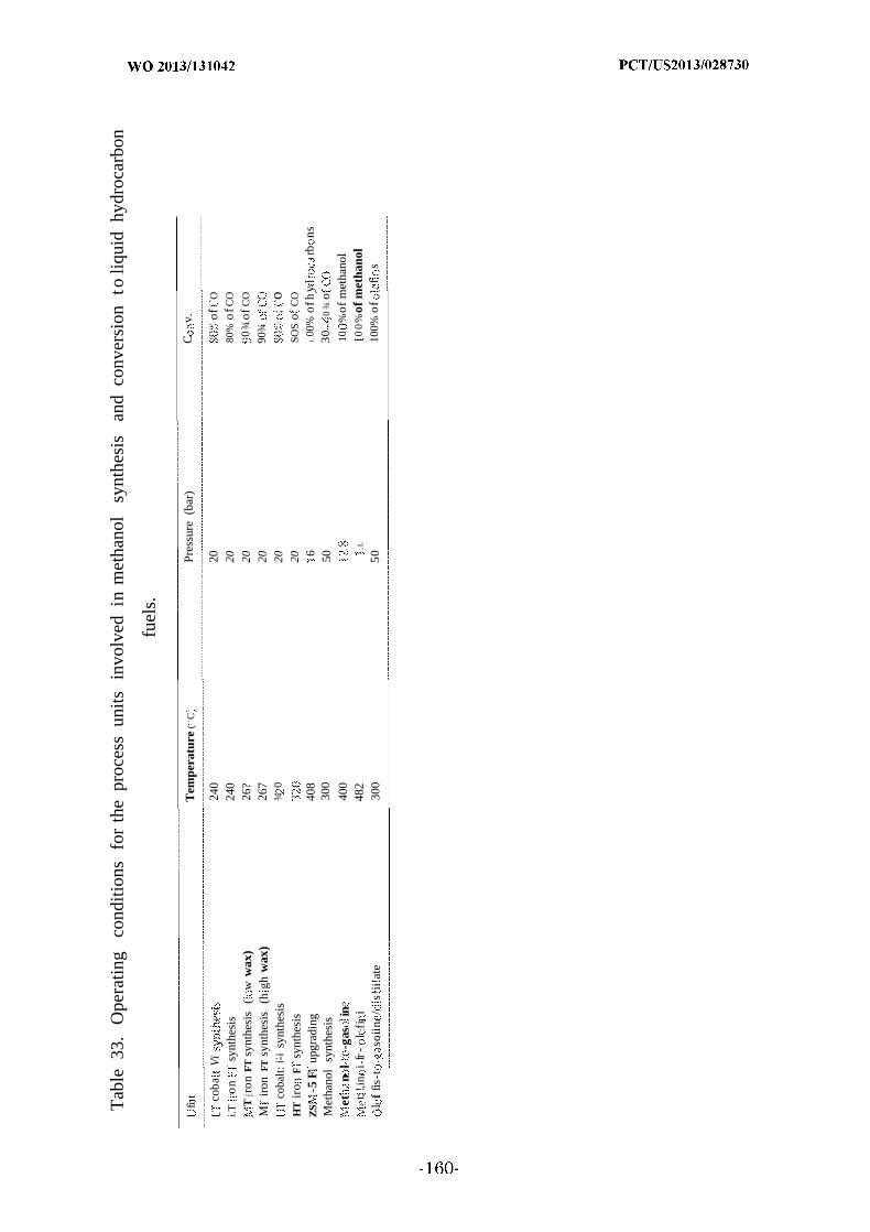
Tab
le33
.O
pera
ting
cond
ition
sfo
rth
epr
oces
sun
itsin
volv
edin
met
hano
lsy
nthe
sis
and
conv
ersi
onto
liqui
dhy
droc
arbo
n
fuel
s.
fit
Tem
pera
ture
(C
Pres
sure
(bar
)C
v.
coba
Vi
240
20of
O
i.To
nsy
nthe
sis
240
2080
%o
fCO
Tro
nFT
synt
hesi
s(
ww
ax)
26?
200
¾of
CO
Mir
onFT
synt
hesi
s(h
ghw
ax)
267
2090
¾
coba
lt:ί-ί
synt
hesi
s¾
020
;o
HT
iro
Fsy
nthe
sis
20SO
So
CO
ZS
-5F
upgr
adin
g40
86
1.00
%o
fhy
rbns
Met
hano
lsy
nthe
sis
300
5030
0¾
o
etn
l-g
asin
400
10%
ofm
etha
nol
t:!,i
ni
fr-
lfi
i48
2.1
.0
0%
ofm
etha
nol
lfi
fis-t
scii
n/
s!ii!
ate
300
5010
0%o
ff
s
[0440] Hydrogen may be recycled to any of the FT units to either shift the
H 2/CO ratio or the H2/CO2 ratio to the appropriate level. Steam may alternatively
be used as a feed for the two iron-based fWGS FT units to shift the H 2/CO ratio.
CO2 may be recycled back to the iron-based rWGS FT units tobe consumed in the
WGS reaction. Similarly, the pressure- swing adsorption (PSA) offgas which will
be lean in H 2 may be recycled to the iron-based rWGS FT units for consumption
of the CO or CO2. The effluent from the auto-thermal reactor (ATR)will contain a
H 2/CO ratio that is generally above 2/1, and is therefore favorable as a feedstock
for FT synthesis (National Academy of Sciences, 2009, which is incorporated
herein by reference as if fully set forth). However, the concentration of CO2
within the ATR effluent will prevent the stream from being fed to the cobalt-
based units. The two streams exiting the FT units will be a waxy liquid phase
and a vapor phase containing a range of hydrocarbons. The wax will be directed
to a hydrocracker (WHC) while the vapor phase is split (SPFTH) for further
processing.
[0441] Modeling of the four original FT units is described in Examples 1
and 2. The effluent from the two additional FT units (iron-based FT fWGS) is
based off of the slurry phase FT units developed by Mobil Research and
Development Corporation in the 1980s (Mobil Research & Development
Corporation, 1983, 1985, which is incorporated herein by reference as if fully set
forth). A H 2/CO ratio of 2/3 is desired for the input feed (Mobil Research &
Development Corporation, 1983, 1985, which is incorporated herein by reference
as if fully set forth), so a sufficient amount of steam must be added to the feed to
promote the forward water—gas-shift reaction. The decomposition of carbon from
CO to hydrocarbons and CO2 is outlined in Table VIII-2 of the minimal-wax FT
report (Mobil Research & DevelopmentCorporation, 1983, which is incorporated
herein by reference as if fully set forth) and Table VIII-2 of the nominal-wax FT
report (Mobil Research & Development Corporation, 1985, which is incorporated
herein by reference as if fully set forth), and a 90% conversion of CO in the inlet
stream is assumed (Mobil Research &Development Corporation, 1983, 1985,
which is incorporated herein by reference as if fully set forth). The syngas species
exiting the four iron-based FT reactors will be constrained by water-gasshift
equilibrium, a s noted in Eq. (216) where (u, u') is the stream exiting the FT unit
u .
O - u ' V i ' ,H2' 'X 2 "
(216)
[0442] The mathematical model will select at most two types of Fischer-
Tropsch units t o operate in the final process design. This constraint is added
because two different kinds of FT units will be able to supply a range of
hydrocarbon species that is diverse enough to provide a target composition of
liquid products without adding unnecessary complexity t o the refinery design (de
Klerk, 2011, which is incorporated herein by reference a s if fully set forth).
[0443] Example 3.4 - Fischer-Tropsch product upgrading
[0444] The vapor phase effluent from FT synthesis will contain a mixture
of C1-C30+ hydrocarbons, water, and some oxygenated species. FIG. 33 details
the process flowsheet used t o process this effluent stream. The stream will be
split (SPFTH) and can pass through a series of treatment units designed t o cool
the stream and knock out the water and oxygenates for treatment. Initially, the
water-soluble oxygenates are stripped (WSOS) from the stream. The stream is
then passed to a three-phase separator (VLWS) to remove the aqueous phase
from the residual vapor and any hydrocarbon liquid. Any oxygenates that are
present in the vapor phase may be removed using an additional separation unit
(VSOS). The water lean FT hydrocarbons are then sent to a hydrocarbon recovery
column for fractionation and further processing (FIG. 34). The oxygenates and
water removed from the stream are mixed (MXFTWW) and sent to the sour stripper
mixer (MXss) for treatment.
[0445] The FT hydrocarbons split from SPFTH may also be passed over a
ZSM-5 catalytic reactor (FT-ZSM5) operating at 408 °C and 16 bar (Mobil
Research & Development Corporation, 1983, which is incorporated herein by
reference a s if fully set forth) t o be converted into mostly gasoline range
hydrocarbons and some distillate (Mobil Research & Development Corporation,
1983, 1985, which is incorporated herein by reference a s if fully set forth). The
ZSM-5 unit will be able to convert the oxygenates to additional hydrocarbons, so

no separate processing of the oxygenates will be required for the aqueous
effluent. The composition of the effluent from the ZSM-5 unit is shown in Table
43 of the minimal- wax FT reactor Mobil study (Mobil Research & Development
Corporation, 1983, which is incorporated herein by reference as if fully set forth)
and in Table VIII- 3 of the nominal- wax FT reactor Mobil study (Mobil Research
& Development Corporation, 1985, which is incorported herein by reference as if
fully set forth). For this study, the ZSM-5 effluent composition is assumed to be
equal to the composition outlined in the minimal-wax FT reactor study (Mobil
Research & Development Corporation, 1983, which is incorporated herein by
reference as if fully set forth). This is modeled mathematically using an atom
balance around the ZSM-5 unit and the effluent composition outlined in Table 43
of the Mobil study (Mobil Research & Development Corporation, 1983, which is
incorporated herein by reference as if fully set forth). The raw product from FT-
ZSM5 is fractionated (ZSM5F) t o separate the water and distillate from the
gasoline product. The water is mixed with other wastewater knockout (MXpuww)
and the distillate is hydrotreated (DHT) t o form a diesel product. The raw ZSM-5
HC product is sent to the LPG- gasoline separation section for further processing
(FIG. 36).
[0446] The water lean FT hydrocarbons leaving MXFTWW are sent t o a
hydrocarbon recovery column (HRC), as shown in FIG. 34. The hydrocarbons are
split into C3-C5 gases, naphtha, kerosene, distillate, wax, offgas, and wastewater
(Baliban et al., 2010; Bechtel, 1998, which are incorporated herein by reference
as if fully set forth). The upgrading of each stream will follow a detailed Bechtel
design (Bechtel, 1992, 1998, which are incorporated herein by reference as if fully
set forth) which includes a wax hydrocracker (WHC), a distillate hydrotreater
(DHT), a kerosene hydrotreater (KHT), a naphtha hydrotreater (NHT), a
naphtha reformer (NRF), a C4 isomerizer (C4I), a C 6 isomerizer (C56I), a
C3/C4/C5 alkylation unit (C345A), and a saturated gas plant (SGP).
[0447] The kerosene and distillate cuts are hydrotreated in (KHT) and
(DHT), respectively, t o remove sour water and form the products kerosene and
diesel. Any additional distillate or kerosene produced in other sections of the
refinery will also be directed t o these units for processing. The naphtha cut is

sent t o a hydrotreater (NHT) t o remove sour water and separate C5-C6 gases
from the treated naphtha. The wax cut is sent t o a hydrocracker (WHC) where
finished diesel product is sent t o the diesel blender (DBL) along with the diesel
product from (DHT). C5-C6 gases from (NHT) and (WHC) are sent t o a n
isomerizer (C56I). Hydrotreated naphtha is sent t o the naphtha reformer (NRF).
The C4 isomerizer (C4I) converts in-plant and purchased butane t o isobutane,
which is fed into the alkylation unit (C345A). Purchased butane is added t o the
isomerizer such that 80 wt% of the total flow entering the unit is composed of n -
butane. Isomerized C4 gases are mixed with the C3-C5 gases from the (HRC) in
(C345A), where the C3-C5 olefins are converted t o highoctane gasoline blending
stock. The remaining butane is sent back t o (C4I), while all light gases are mixed
with the offgases from other unit and sent t o the saturated gas plant (SGP). C 4
gases from (SGP) are recycled back t o the (C4I) and a cut of the C 3 gases are sold
a s byproduct propane.
[0448] Example 3.5 - Methanol synthesis and conversion
[0449] The clean gas split (SPCG) from the acid gas recovery unit may be
directed t o a methanol synthesis unit (MEOHS) for conversion of the syngas t o
methanol (National Renewable Energy Laboratory, 2011, which is incorporated
herein by reference a s if fully set forth). The syngas exiting the acid gas recovery
unit is heated up t o 300 °C prior t o entering the MEOHS unit. The MEOHS unit
operates a t a temperature of 300 °C, a pressure of 51 bar, and will assume
equilibrium between the water-gas -shift reaction (Eq. (217)) and the methanol
synthesis reaction (Eq. (218)) in the effluent stream (MEOHS, u ) (National
Renewable Energy Laboratory, 2011, which is incorporated herein by reference
a s if fully set forth).
V s . N s — wcs N s N sJ E HS, l ,H2
J MEOHS , , MEOHS EOHS, ,H J MEOHS,«, C(217)
[0450] Note that the equations for water-gas -shift equilibrium (Eqs. (216)
and (217)) utilize molar species flow rates while the methanol synthesis
equilibrium (Eq. (218)) and the steam reforming equilibrium (Eqs. (329)-(332))

utilize molar species concentrations. The conservation of total moles across the
water— as-shift equilibrium allows for the use of either species molar flow rates
or molar concentrations in the equilibrium reaction without a need for a total
molar flow rate variable. The mathematical model was formulated using molar
flow rates because the bilinear terms for calculation of the concentration
variables are not required for all syngas species. The remainder of the chemical
equilibrium equations do not conserve the amount of total moles, so the use of
species molar flow rates would require a total molar flow rate variable tobalance
the equation. In this study, it was found to be computationally beneficial to use
species concentration variables to reduce the presence of trilinear or quadrilinear
terms that would arise with the use of species molar flow rates. Note that the
equilibrium constants used in Eqs. (218) and (329)-(332) have been modified
from the values extracted from Aspen to account for the increased pressure of the
units.
[0451] The "state-of- technology" conditions for methanol synthesis used in
this study will require a CO2 input concentration of 3—8% for methanol synthesis
(National Renewable Energy Laboratory, 2011, which is incorporated herein by
reference as if fully set forth), though there could exist a potential synergy from a
higher CO2 input concentration (Toyir et al., 2009, which is incorporated herein
by reference as if fully set forth). However, an increased level of H 2may also need
to be input to the reactor for consumption via the reverse water—gas-shift
reaction. H 2 generated via pressureswing adsorption may not be appropriate if
the H2-lean offgas is primarily used as plant fuel. Alternatively, H 2 provided by
electrolysis of water with a non-carbon-based form of electricity (e .g., wind or
solar) will have a high capital cost of electrolyzers coupled with a relatively high
cost of renewable-based electricity. This may offset the reduction in capital that
is achieved if a CO2 capture technology is not needed for the synthesis gas. The
technoeconomical benefits of higher levels of CO2 input to the methanol synthesis
reactor will be the subject of a future investigation. The raw methanol effluent is
cooled to 35 °C and sent to a flash unit (MEOH-F) to remove over 95% of the
entrained methanol through vapor—liquid equilibrium. The vapor phase is split
and mostly recycled (split fraction: 95%) to the methanol synthesis reactor to

increase the yield of methanol. The methanol leaving the MEOH-F unit is
degassed (MEDEG) via distillation to remove any light vapors. The MEDEG unit
is operated as a split unit with a steam utility requirement derived through
simulation.
[0452] The purified methanol is split (SPMEOH) to either the methanolto-
gasoline (MTG) (Mobil Research & Development Corporation, 1978; National
Renewable Energy Laboratory, 2011, which are incorporated herein by reference
as if fully set forth) process or t o the methanol-to-olefins (MTO) and Mobil
olefins-togasoline/distillate (MOGD) (Keil, 1999; Tabak et al., 1986; Tabak &
Krambeck, 1985; Tabak & Yurchak, 1990, which are incorporated herein by
reference as if fully set forth) processes, both of which were developed by Mobil
Research and Development in the 1970s and 1980s. More recently, the National
Renewable Energy Laboratory performed a full design, simulation, and economic
analysis of a biomass-based MTG process (National Renewable Energy
Laboratory, 2011, which is incorporated herein by reference as if fully set forth).
The MTG process will catalytically convert the methanol to gasoline range
hydrocarbons using a ZSM-5 zeolite and a fluidized bed reactor. The MTG
effluent is outlined in Table 3.4.2 of the Mobil study (Mobil Research &
Development Corporation, 1978, which is incorporated herein by reference as if
fully set forth) and in Process Flow Diagram P850-A1402 of the NREL study
(National Renewable Energy Laboratory, 2011, which is incorporated herein by
reference as if fully set forth). Due t o the high level of component detail provided
by NREL for both the MTG unit and the subsequent gasoline product separation
units, the composition of the MTG reactor used in this study is based on the
NREL report. The MTG unit will operate adiabatically at a temperature of 400 °C
and 12.8 bar. The methanol feed will be heated t o 330 °C and input to the reactor
at 14.5 bar. The MTG effluent will contain 44 wt% water and 56 wt% crude
hydrocarbons, of which 2 wt% will be light gas, 19 wt% will be C3-C4 gases, and
19 wt% will be C5+ gasoline (National Renewable Energy Laboratory, 2011, which
is incorporated herein by reference as if fully set forth). The crude hydrocarbons
are directed to the LPG-gasoline separation section (FIG. 36), from which 82 wt%
will be gasoline, 10 wt% will be LPG, and the balance will be recycle gases. This
is modeled mathematically in the process synthesis model by using an atom
balance around the MTG unit and assuming a 100% conversion of the methanol
entering the MTG reactor (Mobil Research & Development Corporation, 1978;
National Renewable Energy Laboratory, 2011, which are incorporated herein by
reference as if fully set forth).
[0453] Any methanol entering the MTO process unit is heated to 400 °C at
1.2 bar. The MTO fluidized bed reactor operates at a temperature of 482 °C and a
pressure of 1.2 bar (Tabak & Yurchak, 1990, which is incorporated herein by
reference as if fully set forth). The exothermic heat of reaction within the MTO
unit is controlled through generation of low-pressure steam. 100% of the input
methanol is converted into olefin effluent containing 1.4 wt% CH4, 6.5 wt% C2-C4
paraffins, 56.4 wt% C2-C4 olefins, and 35.7 wt% C 5-C11 gasoline (Tabak &
Yurchak, 1990, which is incorporated herein by reference as if fully set forth).
The MTO unit is modeled mathematically using an atom balance and a typical
composition seen in the literature (Tabak &Yurchak, 1990, which is incorporated
herein by reference as if fully set forth). The MTO product is fractionated (MTO-
F) to separate the light gases, olefins, and gasoline fractions. The MTO-F unit is
a rigorous distillation column that is designed so that approximately 100% of the
C1-C3 paraffins are recycled back to the refinery, 100% of the C4 paraffins and
100% of the olefins are directed to the MOGD unit, 100% of the gasoline is
combined with the remainder of the gasoline generated in the process, and 100%
of the water generated in the MTO unit is sent for wastewater treatment. Note
that the MTO-F unit is modeled within the process synthesis model as a
separator unit with the appropriate utilities (i .e., low-pressure steam and cooling
water) that are extracted from simulation of the distillation column.
[0454] The separated olefins are sent to the MOGD unit where a fixed bed
reactor is used to convert the olefins to gasoline and distillate over a ZSM-5
catalyst. The gasoline/distillate product ratios can range from 0.12 to >100, and
the ratio chosen in this study was 0.12 to maximize the production of diesel. The
MOGD unit operates at 400 °C and 1 bar and will utilize steam generation to
remove the exothermic heat of reaction within the unit. The MOGD unit is
modeled with an atom balance and will produce 82% distillate, 15% gasoline, and
3% light gases (Tabak & Yurchak, 1990, which is incorporated herein by
reference as if fully set forth). The product will be fractionated (MTODF) to
remove diesel and kerosene cuts from the gasoline and light gases. The
operational ratio of kerosene to total distillate reported in the literature for the
MOGD process is about 30%, though this number may be increased by tailoring
the operating conditions within the MTO and MOGD units to yield the
appropriate range of hydrocarbons. The MTODF unit will be modeled as a
separator unit where 100% of the C11-C13 species are directed to the kerosene cut
and 100% of the C14+ species are directed to the diesel cut.
[0455] Example 3.6 - LPG-gasoline separation
[0456] The gasoline range hydrocarbons produced by the FT-ZSM5 unit,
the MTG unit, or the MOGD process must be sent to the LPGgasoline separation
flowsheet depicted in FIG. 36. Each hydrocarbon stream is split (SPFTZSM,
SPMTGHC , and SPMTODHC, respectively) and sent t o a hydrocarbon knockout unit
(35 °C, 10 bar) for light gas removal via vapor—liquid equilibrium. The first
knock-out unit (HCKOl) will not incorporate additional CO2 separation, so the
CO2 rich light gases recovered from HCKOl will be recycled back to the process
(SPLG) . The second knock-out unit (HCKO2) will separate out CO2 from the
recovered light gases via a 1-stage Rectisol unit (CO2SEP) for sequestration or
recycle back to additional process units (MXco2c). The CO2 lean light gases will
be recycled back to the process.
[0457] The crude liquid hydrocarbons recovered from the two knockout
units is sent to a deethanizer (DEETH) t o remove any C1-C2 hydrocarbons. The
light HC gases are sent to an absorber column (ABS-COL) where a lean oil
recycle is used to strip the C3+ HCs from the input. The liquid bottoms from the
ABS-COL are then refluxed back to the deethanizer. The C3+ HCs from the
bottom of the deethanizer are sent to a stabilizer column (STA-COL) where the
C3/C4 hydrocarbons are removed and alkylated (ALK-UN) t o produce iso-octane
and an LPG byproduct. Additional iso-butane (INBUT) may be fed to the
alkylation unit for increased alkylate production. The bottoms from the
stabilizer column is sent to a splitter column (SP-COL) to recover a lean oil
recycle from the column top for use in the absorber column. Light and heavy

gasoline fractions are recovered from the column top and bottom, respectively.
The LPG/alkylate from the alkylation unit is split (LPG-ALK) into an LPG
byproduct (OUTLPG) and an alkylate fraction which is blended with the gasoline
fractions from the splitter column (OUTGAS). Each of the distillation units is
modeled mathematically as a splitter unit where the split fraction of each species
to an output stream is given by the information in the Process Flow Diagrams
P850-A1501 and P850-A1502 from the NREL study (National Renewable Energy
Laboratory, 2011, which is incorporated herein by reference as if fully set forth).
All low pressure steam and cooling water needed for each of the units is derived
for each of the units in the NREL study. The total amount of process utility that
is needed per unit flow rate from the top or bottom of the column is calculated,
and this ratio is used as a parameter in the process synthesis model to determine
the actual amount of each utility needed based on the unit flow rate. The alkylate
was modeled as iso-butane (National Renewable Energy Laboratory, 2011, which
is incorporated herein by reference as if fully set forth) and the alkylation unit
was modeled using a species balance where the key species, butene, was
completely converted to iso-butane. Butene is used as the limiting species in this
reaction because it is generally present in a far smaller concentration than iso-
butane.
[0458] Example 3.7 - Unit costs
[0459] The total direct costs, TDC, for the CBGTL refinery hydrocarbon
production and upgrading units are calculated using estimates from several
literature sources (Mobil Research & Development Corporation, 1978, 1983,
1985; National Energy Technology Laboratory, 2007; National Renewable Energy
Laboratory, 2011, which are incorporated herein by reference as if fully set forth)
using the cost parameters in Table 34 and Eq. (219)
sfTDC = ( 1 + BOP) . C - —
° (219)
where C0 is the installed unit cost, S0 is the base capacity, S is the actual
capacity, s/ is the cost scaling factor, and BOP is the balance of plant (BOP)
percentage (site preparation, utility plants, etc.). The BOP is estimated to be 20%
of the total installed unit cost. All numbers are converted to 2009 dollars using

the GDP inflationindex (US Government Printing Office, 2009, which is
incorporated herein by reference as if fully set forth). Detailed cost estimates
were not available for the MTO or OGD process units, so the cost associated with
these units was estimated from the cost of an atmospheric MTG unit provided by
Mobil (Mobil Research & Development Corporation, 1978, which is incorporated
herein by reference as if fully set forth). Note that not all units in FIGS. 32-36 are
represented in Table 34. Some of the units shown in Table 34 represent the cost
of that unit plus any auxiliary units needed for proper unit operation.
Specifically, (a) the three FT aqueous phase knock-out units are included in the
cost of the hydrocarbon recovery column (Bechtel, 1998, which is incorporated
herein by reference as if fully set forth), (b) the cost of the FT ZSM-5 fractionator
is included in the cost of the FT ZSM-5 unit (Mobil Research & Development
Corporation, 1983, 1985, which is incorporated herein by reference as if fully set
forth), (c) the MTO fractionator is included in the cost of the MTO unit (National
Renewable Energy Laboratory, 2011, which is incorporated herein by reference
as if fully set forth), and (d) the OGD fractionator was included in the cost of the
OGD unit (Mobil Research & Development Corporation, 1978, which are
incorporated herein by reference as if fully set forth).
[0460] The total overnight capital, TOC, for each unit is calculated as the
sum of the total direct capital, TDC, plus the indirect costs, IC. The IC include
engineering, startup, spares, royalties, and contingencies and is estimated to 32%
of the TDC. The TOC for each unit must be converted to a levelized cost to
compare with the variable feedstock and operational costs for the process. Using
the methodology of Kreutz et al. (2008), which is incorporated herein as if fully
set forth, the capital charges (CC) for the refinery are calculated by multiplying
the levelized capital charge rate (LCCR) and the interest during construction
factor (IDCF) by the total overnight capital (Eq. (220)).
CC = LCCR . IDCF -TOC (220)
[0461] Kreutz et al. (2008), which is incorporated herein by reference as if
fully set forth, calculates an LCCR value of 14.38%/year and IDCF of 1.076. Thus,
a multiplier of 15.41%/year is used to convert the overnight capital into a capital
charge rate. Assuming an operating capacity (CAP) of 330 days/year and
operation/mainte nance (OM) costs equal to 5% of the TOC, the total levelized cost
(Costu ) associated with a unit is given in Eq. (221).
2 21)
[0462] The levelized costs for the units described for hydrocarbon
production and upgrading are added to the complete list of CBGTL process units
given in Baliban, Elia, and Floudas (2012), which is incorporated herein by
reference as if fully set forth.

Table 34. CBGTL refinery upgrading unit reference capacities, costs (2009$),
and scaling factors

[0463] Example 3.8 - Objective function
[0464] The objective function for the model is given in Eq. (222). The
summation represents the total cost of liquid fuels production and includes
contributions from the feedstocks cost (Cost ), the electricity cost (CostE 1), the
CO2 sequestration cost (CostSe ) , and the levelized unit investment cost (Costu ) .
Each of the terms in Eq. (222) is normalized to the total lower heating value in
G of products produced. For each case study, the capacity and ratio of liquid fuel
products is fixed, so the normalization denominator in Eq. (222) will be a
constant parameter. Note that other objective functions (e.g., maximizing the net
present value) can be easily incorporated into the model framework.
€ost s + CostE + Cost + C st "
u s S « » (222)
[0465] The process synthesis model with simultaneous heat, power, and
water integration represents a large-scale non-convex mixedinteger non-linear
optimization (MINLP) model that was solved to global optimality using a branch-
and-bound global optimization framework that was previously described
(Baliban, Elia, Misener, et al., 2012, which is incorporated herein by reference as
if fully set forth). The MINLP model contains 32 binary variables, 11,104
continuous variables, 10,103 constraints, and 351 non-convex terms (i.e., 285
bilinear terms, 1 trilinear term, 1 quadrilinear term, and 64 power functions). At
each node in the branch-and-bound tree, a mixed-integer linear relaxation of the
mathematical model is solved using CPLEX (CPLEX, 2009, which is incorporated
herein by reference as if fully set forth) and then the node is branched to create
two children nodes. The solution pool feature of CPLEX is utilized during the
solution of the relaxed model to generate a set of distinct points (150 for the root
node and 10 for all other nodes), each of which is used as a candidate starting
point to solve the original model. For each starting point, the current binary
variable values are fixed and the resulting NLP is minimized using CONOPT. If
the solution to the NLP is less than the current upper bound, then the upper
bound is replaced with the NLP solution value. At each step, all nodes that have
a lower bound that is within an e tolerance of the current upper bound

((LBnode/UB) > 1 - e) are eliminated from the tree. For a more complete coverage
of branch and-bound algorithms, the reader is directed to the textbooks of
Floudas (Floudas, 1995, 2000, which are incorporated herein by reference as if
fully set forth) and reviews of global optimization methods (Floudas,
Akrotirianakis, Caratzoulas, Meyer, & Kallrath, 2005; Floudas & Gounaris, 2009;
Floudas & Pardalos, 1995, which are incorporated herein by reference as if fully
set forth).
[0466] Example 3.9 - Computational studies
[0467] The proposed process synthesis model was used to analyze twenty-
four distinct case studies using perennial biomass (switchgrass), low-volatile
bituminous coal (Illinois #6), and natural gas as feedstocks. A global optimization
framework was used for each case study, and termination was reached if all
nodes in the branch-and-bound tree have been processed or if 100 CPU hours
have passed (Baliban, Elia, Misener, et al., 2012, which is incorporated herein by
reference as if fully set forth). The ultimate and proximate analysis of the
biomass and coal feedstocks and the molar composition of the natural gas
feedstock are presented in Examples 3.17 - 3.23. To examine the effects of
potential economies of scale on the final liquid fuels price, three distinct plant
capacities were examined to represent a small, medium, or large capacity hybrid
energy plant. Based on current petroleum refinery capacities (Energy
Information Administration, 2009, which is incorporated herein by reference as if
fully set forth), representative sizes of 10 thousand barrels per day (TBD), 50
TBD, and 200 TBD were chosen, respectively. A minimal carbon conversion
threshold of 40% was enforced for all of the case studies, and no upper bound was
used for the amount of CO2 that is vented or sequestered. This threshold value
was imposed to provide a comparative baseline between all of the case studies,
and does not have an effect on the overall process topologies. If no lower
threshold value is imposed, then the overall conversion for each study will range
between 34% and 39%, which is consistent with the results of a previous study
(Baliban, Elia, Misener, et al., 2012, which is incorporated herein by reference as
if fully set forth). In general, raising the conversion rate produce more liquid fuels
and decrease the byproduct electricity output from the plant, and for a more in-

depth analysis, the reader is directed to the previous study (Baliban, Elia,
Misener, et al., 2012, which is incorporated herein by reference as if fully set
forth). The overall greenhouse gas emission target for each case study is set to
have a 50% reduction from petroleum based processes (Baliban, Elia, & Floudas,
2012; Baliban et al., 2011). The current case studies do not include the cost of a
carbon tax for any GHG emissions, though the process synthesis framework could
be readily extended include a cost for the total lifecycle emissions.
[0468] Four superstructure combinations will be investigated to analyze
the effect of plant topology on the final liquid fuels cost. These superstructures
will consider (1) only Fischer-Tropsch synthesis with fractionation of the vapor
effluent, (2) only Fischer-Tropsch synthesis with ZSM-5 catalytic upgrading of
the vapor effluent, (3) only methanol synthesis with either the MTG or MOGD
process, and (4) a comprehensive superstructure allowing all possibilities from
(1), (2), or (3). Note that in superstructures (1), (2), and (4), any wax effluent from
the Fischer-Tropsch units will be converted to naphtha and diesel via a wax
hydrocracker. Two sets of liquid fuels products (i.e., gasoline/diesel/kerosene and
gasoline/diesel) will be considered to determine the effect of these products on the
optimal plant topology and overall costs. The ratio of liquid fuel production will
be equal to the total 2010 United States demand (Energy Information
Administration, 2011, which is incorporated herein by reference as if fully set
forth). Note that the process superstructure is also capable of analyzing a
variable concentration of output fuels (e.g., max diesel). Each of the 24 case
studies discussed below has a label P-CN where P is the type of products
produced (GDK - gasoline/diesel/kerosene, GD - gasoline/diesel), C is the plant
capacity (S —small, M —medium, L —large), and N is the superstructure number
defined above.
[0469] The cost parameters (Baliban, Elia, & Floudas, 2012; Baliban et al.,
2011, which is incorporated herein by reference as if fully set forth) used for
CBGTL process are listed in Table 35. The costs for feedstocks (i.e., coal, biomass,
natural gas, freshwater, and butanes) include all costs associated with delivery to
the plant gate. The products (i.e., electricity and propane) are assumed to be sold
from the plant gate, and do not include the costs expected for transport to the end
consumer. The cost of CO2 capture and compression will be included in the
investment cost of the CBGTL refinery while the cost for transportation, storage,
and monitoring of the CO2 is shown in Table 35.
[0470] Once the global optimization algorithm has completed, the resulting
process topology provides (i) the operating conditions and working fluid flow rates
of the heat engines, (ii) the amount of electricity produced by the engines, (iii) the
amount of cooling water needed for the engines, and (v) the location of the pinch
points denoting the distinct subnetworks. Given this information, the minimum
number of heat exchanger matches necessary to meet specifications (i), (ii), (iii),
and (iv) are calculated as previously described (Baliban, Elia, & Floudas, 2012;
Baliban et al., 2011; Floudas, 1995; Floudas, Ciric, & Grossmann, 1986, which
are incorporated herein by reference as if fully set forth). Upon solution of the
minimum matches model, the heat exchanger topology with the minimum
annualized cost can be found using the superstructure methodology (Elia et al.,
2010; Floudas, 1995; Floudas et al., 1986, which are incorporated herein by
reference as if fully set forth). The investment cost of the heat exchangers is
added to the investment cost calculated within the process synthesis model to
obtain the final investment cost for the superstructure.

Table 35. Cost parameters 2009$) for the CBGTL refinery.

[0471] Example 3.10 - Optimal process topologies
[0472] The information detailing the optimal process topologies for all case
studies is shown in Table 36. Three possible temperature options were used for
the biomass gasifier (900 °C, 1000 °C, 1100 °C), the coal gasifier (1100 °C, 1200
°C, 1300 °C), the auto-thermal reactor (700 °C, 800 °C, 950 °C), and the reverse
water-gas -shift unit (400 °C, 500 °C, 600 °C). For all 24 case studies, the biomass
and coal solid/vapor fueled gasifiers were utilized in the optimal process design.
Thus, each gasifier employed a vapor phase recycle stream as a fuel input along
with the solid coal or biomass. Recycle of some of the unreacted synthesis gas to
the gasifiers helped to consume some CO2 generated in the process and reduce
the overall process emissions by converting the CO2 to CO for additional liquid
fuels production. For the biomass gasifier, the 900 °C unit is always selected for
superstructure 1 and only selected for superstructure 3 at high capacity levels.
For all other case studies, the 1100 °C unit is selected. For the coal gasifier, the
1300 °C unit was always selected for superstructures 1, 2, and 3 and the 1100 °C
unit was selected for superstructure 4.
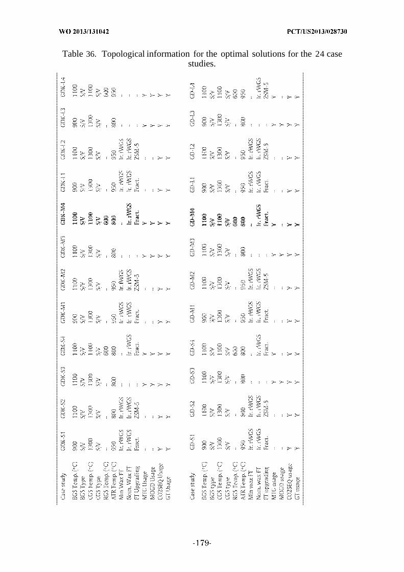
Table 36. Topological information for the optimal solutions for the 24 casestudies.

Specifically listed is the operating temperature of the biomass gasifier (BGS), the
coal gasifier (CGS), the auto-thermal reactor (ATR), and the reverse water-gas-
shift unit (RGS). The gasifiers are also labeled as either solid/vapor (SAO or solid
(S) fueled, implying the presence or absence of vapor-phase recycle process
streams. The presence of a C02 sequestration system (C02SEQ) or a gas turbine
(GT) is noted using yes (Y) or no (-). The minimum wax and maximum wax
Fischer-Tropsch units are designated as either cobalt-based or iron-based units.
The iron-based units will either facilitate the forward (fWGS) or reverse water-
gas-shift (rWGS) reaction. The FT vapor effluent will be upgraded using
fractionation into distillate and naphtha (Fract.) or ZSM-5 catalytic conversion.
The use of methanol-to- gasoline (MTG) and methanol-to-olefins/olefins-to-
gasoline-and-diesel (MTO/MOGD) is noted using yes (Y) or no (-). The results for
the complete superstructure and medium sized capacity (M4) are shown in
boldface.
[0473] Selection of the gasifier operating temperatures in the optimal
topology represents a balance between (i) the levels of oxidant input to the
gasifier, (ii) the extent of consumption of CO2 via the reverse water-gas -shift
reaction, and (iii) the level of waste heat generated from syngas cooling. Lower
gasifier temperatures will have less favorable conditions for CO2 consumption
due to lower values of the water—gas-shift equilibrium constant and a smaller
amount of waste heat for use in steam generation and ultimately electricity
production. However, lower temperatures will require lower levels of O 2 for
combustion within the gasifier which reduces the investment and utility cost for
oxygen generation and may increase the overall efficiency of the gasifier. The
alternative disadvantages with a higher O 2 in the higher temperature gasifiers
are balanced by an increase in the CO2 reduction potential and the additional
waste-heat generated. The operating temperature selected in the 24 case studies
reflects the trade-offs between emissions reduction, electricity production, and
overall process efficiency for the entire refinery.
[0474] The auto-thermal reformer temperature was selected to be 950 °C
for twelve of the case studies and 800 °C for the remaining twelve studies (see
Table 36). A 950 °C unit is always used for superstructure 1, used for

superstructure 2 in the medium and large plants, and used in superstructure 4
for the large plants. Selection of the temperature for the auto-thermal reformer
will have similar topological effects as the gasifiers, though the overall conversion
of CH4 will also increase with increasing temperature. The use of the highest
temperature reformer is beneficial since approximately 90% of the input CH4 can
be converted to syngas using a H20/CH 4 ratio of approximately 1.2-1.5.
Ultimately, this will also decrease the working capacity of the FT synthesis or
methanol synthesis units because the input CH4 is an inert species that will not
be separated until downstream of these units. The selection of the 800°C units for
the remaining studies generally converts 82-85% of the CH4, though the decrease
in the oxygen requirement to the unit provides an economic benefit to the
decreased conversion of the natural gas.
[0475] A dedicated reverse water-gas -shift unit was not selected for either
product composition and plant capacity that used superstructures 1, 2, or 3. For
each of these case studies, the proper syngas ratio requirements for the FT and
methanol synthesis was met via light gas recycle to either the gasifiers or the
auto-thermal reactor units. For the case studies using superstructure 4, a 600 °C
reverse water—gas -shift unit was utilized to both consume CO2 generated in the
process and shift the syngas ratios for conversion. All of the case studies
generated H 2using pressure- swing adsorption and O 2using air separation. The
H 2was utilized mostly for product upgrading and for injection, with the balance
being sent to the reverse water-gas -shift units to consume some CO2. Note that
H 2separation is required for hydrotreating and hydrocracking within the product
upgrading section. Electrolyzers were not utilized in any case study due to the
high capital ($500/kW) and electricity costs of the unit. The electricity input to
the electrolyzers is assumed to come from a non-carbon based source (e.g.,
wind/solar), which was assumed to have a high cost (i.e., $0.10/kWh). Note that
input electricity from a carbon-based source (i.e., biomass/coal/natural gas) is not
considered because the process superstructure accounts for ¾ generation from
pressure- swing adsorption. A decrease in the non-carbon based electricity cost
may have an effect on the electrolyzer use, as noted in a previous study (Baliban
et al., 2011, which is incorporated herein by reference as if fully set forth). Both a
gas and steam turbine are used in each case study to produce electricity for the
process and to partially sell as a byproduct. To reduce the GHG emissions from
the processes, each case study utilized CO2 capture and sequestration both
upstream of synthesis gas conversion and downstream of the gas turbine engine.
[0476] The case studies using superstructures 1 and 2 required FT
synthesis of the hydrocarbons, and each case study utilized an iron-based catalyst
within both the minimal-wax and nominalwax reactors. Additionally, the reverse
water-gas -shift reaction was facilitated in most of the case studies, with the
exception of the minimal- wax reactor in superstructure 2 for the medium and
large capacities. In the former case studies, the iron-based units can take
advantage of the exothermic FT reaction to provide heat for the endothermic
reverse water-gas-shift reaction (Baliban, Elia,& Floudas, 2012; Baliban et al.,
2011, which is incorporated herein by reference as if fully set forth). In the latter
studies, the additional CO2 that is generated from the FT reactors is captured
and recycled back to the process to minimize the GHG emissions. Due to the
constraints of the process superstructure, upgrading of the vapor phase FT
effluent utilized a fractionation scheme for superstructure 1 and the ZSM-5
catalyst for superstructure 2. For superstructure 3, the syngas was converted to
methanol rather than hydrocarbons via the FT reaction. For all case studies
using this superstructure, both the methanol-to-gasoline and methanolto-
olefins/distillate processes are utilized to produce the liquid fuels in the
appropriate output ratios. In the case studies using superstructure 4, the
technologies used for liquid fuels production are highly dependent on the plant
capacity and the type of fuels produced. For the six studies with superstructure 4,
the minimalwax FT unit was never utilized and the methanol-to-gasoline process
was always utilized. The nominal-wax iron-based rWGS FT unit was used for the
two small plants, the two medium plants, and the large plant that does not
produce kerosene. For the five case studies that used FT, the vapor phase was
always converted to gasoline-range hydrocarbons using ZSM-5. The MOGD
process was used to generate diesel and kerosene for all plant sizes in the GDK
case studies. In the GD case studies, the MOGD process was not utilized and all
diesel was generated from wax hydrocracking.

[0477] The results for the complete superstructure and medium sized
capacity (M4) are shown in boldface in Table 36. For each of these cases, both the
biomass and coal gasifiers were solid/vapor fueled units operating at 1100 °C. A
dedicated reverse water-gas- shift unit operating at 600 °C is used and the auto-
thermal reactor operates at 800 °C for both studies. The liquid fuels are produced
via (i) catalytic ZSM-5 upgrading of the iron-based rWGS FT effluent, (ii) wax
hydrocracking, and (iii) methanol-to- gasoline for both studies and by MOGD for
the study requiring kerosene production.
[0478] Example 3.11 - Overall costs of liquid fuels
[0479] The overall cost of liquid fuel production (in $/GJ) is based on the
costs of feedstocks, capital investment, operation and maintenance (O&M), and
CO2 sequestration and can be partially defrayed using byproduct sales of LPG
and electricity. Feedstock costs are based on the as-delivered price for (i) the
three major carbon feedstocks (coal, biomass, and natural gas), (ii) butanes
needed for the isomerization process (Baliban et al., 2010, 2011; Bechtel, 1992,
which is incorporated herein by reference as if fully set forth), and (iii) freshwater
needed to make-up for process losses(Baliban et al., 2012a, which is incorporated
herein by reference as if fully set forth). Table 37 outlines the breakdown of the
cost contribution for each case study, as well as the lower bound and the
optimality gap values. The total cost is also converted into a break-even oil price
(BEOP) in $/barrel based on the refiner's margin for gasoline, diesel, or kerosene
(Baliban et al., 2011; Kreutz et al., 2008, which is incorporated herein by
reference as if fully set forth), and represents the price of crude oil at which the
CBGTL process becomes economically competitive with petroleum based
processes.
[0480] The overall cost values range between $17.33 and $18.79/GJ for a
small plant, $16.06-$17.66/GJ for a medium plant, and $14.76-$16.20/GJ for a
large plant. For a medium sized plant producing gasoline, diesel, and kerosene,
the optimization model for the complete superstructure (i .e., case study GDK-M4)
selects a topology with an overall cost of $16.25/GJ or $79.83/bbl crude oil
equivalent. The upper bound value found at the termination of the global
optimization algorithm is 4.56% above the lower bound value of $15.51/GJ. When

only gasoline and diesel are produced in the general medium sized plant (GD-
M4), the overall cost of liquid fuel production for a medium sized plant with the
most general superstructure is $16.06/GJ or $78.74/bbl crude oil equivalent with
a 5.35% optimality gap from its lower bound value of $15.20/GJ. Negative values
in the cost contributions from electricity and propane represent the profit gained
from selling these items as byproducts. In all of the 24 case studies, the selected
plant topologies are net producers of electricity and propane(see Table 37, below).

Table 37. Overall cost results for the 24 case studies.
The case studies where the plant topologies produce gasoline, diesel, and
kerosene are labeled as GDK, and the topologies that produce gasoline and diesel
are labeled as GD. The small (S), medium (M), and large (L) case studies are each
labeled with the superstructure number, where (1) indicates that only Fischer—
Tropsch synthesis with fractionation of the vapor effluent is considered, (2) only
Fischer-Tropsch synthesis with ZSM-5 catalytic upgrading of the vapor effluent,
(3) only methanol synthesis with either the MTG or MOGD process, and (4) a
comprehensive superstructure allowing all possibilities from (1), (2), or (3). The
contribution to the total costs (in $/GJ) come from coal, biomass, natural gas,
butanes, water, CO2 sequestration (CO2. Seq.), and the investment. Propane is
always sold as a byproduct while electricity may be sold as a byproduct (negative
value). The overall costs are reported in ($/GJ) and ($/bbl) basis, along with the
lower bound values in ($/GJ) and the optimality gap between the reported
solution and the lower bound. The results for the complete superstructure and
medium sized capacity (M4) are shown in boldface.
[0481] For a given capacity level, Table 37 shows that the lowest overall
cost is achieved through the use of the most general superstructure topology.
Additionally, the second lowest cost is consistently found with superstructure 3,
suggesting that the methanol synthesis/conversion process units generally yield a
plant design with a lower overall cost. However, the decrease in cost between
superstructure 3 (only methanol) and superstructure 4 (methanol/FT) implies
that there is a degree of synergy that can be achieved through the use of both
technologies. The resulting level of synergy is likely to be tied to the capacity of
the plant and the composition of liquid fuels that will be produced. The CBGTL
case studies using superstructures 2 (FT with ZSM-5 upgrading) have a lower
cost ultimately due to a decrease in the complexity of the FT synthesis and
upgrading section of the plant. In some case studies (i .e., GDK-L2, GD-L2, and
GD-M2), the investment cost of the plant with ZSM-5 upgrading was higher than
that for the corresponding case study without ZSM-5 upgrading. The increase in
investment is due to a higher overall flow rate of syngas through the refinery due
to (i) increased recycle flow of the unreacted syngas to decrease feedstock costs or
(2) increased flow of the feedstocks to produce additional byproduct electricity.

[0482] Example 3.12 - Parametric analysis
[0483] Table 37 indicates that the largest contribution to the overall fuels
cost is associated with the capital investment (i .e., capital charges and
operation/maintenance). A reduction in total plant cost may be achieved through
innovation of novel technologies rather than relying on economies of scale for
more mature processes (Adams & Barton, 2011, which is incorporated herein by
reference as if fully set forth). However, the coal, biomass, and natural gas may
have a wide variability in the overall cost of liquid fuel production. Depending on
the demand for these materials and the plant location throughout the country,
the feedstock costs may be higher or lower than the national average. Given the
delivered feedstock costs in Table 35 and the feedstock lower heating values in
Table 45, the cost per unit energy is calculated for coal ($3.0/GJ), biomass
($8.0/GJ), and natural gas ($5.5/GJ). These cost parameters represent
conservative estimates (Energy Information Administration, 2011; Kreutz et al.,
2008; Larson et al., 2009; National Academy of Sciences, 2009, which are
incorporated herein by reference as if fully set forth) for the total delivered cost of
a particular feedstock, and it is important to investigate how the BEOP will be
affected if these cost parameters are reduced. As an illustrative example, the
BEOP for case study GDK-M4 is calculated assuming either low, nominal, or
high cost values for each of the three feedstocks. These respective values are (i)
$2/GJ, $2.5/GJ, and $3/GJ for coal, (ii) $5/GJ, $6.5/GJ, and $8/GJ for biomass,
and (iii) $4/GJ, $4.75/GJ, and $5.5/GJ for natural gas. The BEOP was calculated
for each of the 27 parameter combinations, and the histogram of results is shown
in FIG. 37.
[0484] Each cost bin in FIG. 37 represents a $2/barrel window for the
BEOP. That is, the first bin represents all of the parameter combinations that
had a BEOP between $60/bbl and $62/bbl, the second bin is between $62/bbl and
$64/bbl, and so on. The histogram shows a Gaussian-like distribution with two
major peaks in the $68/bbl-$72/bbl range with a total of 13 counts. The shape of
the histogram can be inferred from Table 37 since the contribution of each
feedstock to the overall cost is relatively similar. The singular peak in the
leftmost bin corresponds to a BEOP of $62.7/bbl and is obtained if the low
parameters are used for each feed. The highest BEOP is equal to $80.0/bbl, and is
obtained if all of the high parameter values are used.
[0485] Example 3.13 - Investment costs
[0486] The plant investment cost is further decomposed into cost
contributions from different sections of the plant in Table 38, namely the syngas
generation, syngas cleaning, hydrocarbon production, hydrocarbon upgrading,
hydrogen/oxygen production, heat and power integration, and wastewater
treatment sections. The syngas generation section is consistently the highest
contributing factor in the investment cost due to the capital intensive coal and
biomass gasifier units. The next highest contributing factors are the syngas
cleaning, hydrogen/oxygen production, and heat and power integration sections,
followed by the hydrocarbon production section, and finally the hydrocarbon
upgrading and wastewater treatment sections.
[0487] The total investment cost ranges from $1166 to $1296 MM for small
plants producing gasoline, diesel, and kerosene, $4359-$4823 MM for medium
plants, and $15,446-$17,309 MM for large plants. The normalized investment
costs, however, reveal the economies of scale obtained in larger sized plants,
ranging from $116k to $130k/bpd for small plants, $87k-$96k/bpd for medium
plants, and $78k-$87k/bpd for large plants. Among the small plant case studies,
the case with the most general superstructure (i .e., GDK-S4) is able to achieve
the lowest investment cost. For larger sized plants, however, GDK-M3 and GDK-
L3 case studies have the lowest investment costs for medium and large plants
case studies, respectively. Conversely, the case studies using superstructure 1
from all capacity levels have the highest total investment cost.
[0488] Comparisons between the GDK and GD case studies reveal
interesting trade-offs in investment costs. For the small plants case studies, plant
topologies that produce only gasoline and diesel result in higher investment costs
than the ones that produce gasoline, diesel, and kerosene. The increased cost of
the small GD case studies is due to a higher flow rate of syngas throughout the
process units due to a slightly higher level of recycle than the GDK small case
studies. The increased investment costs for the small GD studies do lead into
smaller levels of feedstock usage than the small GDK studies, and therefore have
a lower overall cost of liquid fuels production (see Table 37). For the medium and
large GD case studies, the topologies that produce gasoline and diesel fuels
consistently yield lower total investment costs than their GDK counterparts due
to the less complicated refining that is needed to produce kerosene.

-190-

The major sections of the plant include the syngas generation section, syngas
cleaning, hydrocarbon production, hydrocarbon upgrading, hydrogen/oxygen
production, heat and power integration, and wastewater treatment blocks. The
values are reported in MM$ and normalized with the amount of fuels produced
($/bpd). The results for the complete superstructure and medium sized capacity
(M4) are shown in boldface.
[0489] Example 3.14 - Material and energy balances
[0490] The overall material and energy balances for the 24 case studies are
shown in Tables 39 and 40, respectively. The biomass and coal flow rates are
based of dry tons (dt) while the natural gas is shown in million standard cubic
feet (mscf). From Tables 38 and 39, it can be seen that coal provides the most
energy input to the plant, followed generally by natural gas, and then biomass.
For example, the most small capacity plant with the most general superstructure
(GDK-S4) requires 69.56 dt/h coal, 51.08 dt/h for biomass, and 1.83 mscf/h
natural gas. These values correspond to 596 MW energy input from coal, 224 MW
from biomass, and 497 MW from natural gas. This distribution remains relatively
consistent when the plant size increases. For the medium sized plant (case study
GDK-M4), 377.39 dt/h is needed for coal, 251.95 dt/h for biomass, and 7.77
mscf/h, corresponding to 3234 MW energy input for coal, 1106 MW for biomass,
and 2114 MW for natural gas. Case study GDK-L4 requires 1607.23 dt/h coal,
997.60 dt/h biomass, and 26.64 mscf/h natural gas, corresponding to 13,775 MW
energy input from coal, 4377 MW from biomass, and 7250 MW from natural gas.
The smaller contribution of biomass relative to the other two feedstocks is due to
the higher $/GJ costs associated with biomass. The highest driving force for the
use of biomass is the lifecycle GHG reduction potential, but the use of CO2
sequestration from the 24 case studies (see Table 39) will reduce the biomass
requirement for the plant. A restriction on the amount of CO2 that is captured for
sequestration (e.g., no nearby available locations for CO2 storage) will ultimately
increase the biomass feedstock requirement, and the biomass could become the
largest energy contributor to the refinery. The authors note that the biomass
requirement for the large case studies (i.e., 200,000/bpd) is necessary to achieve a
life-cycle GHG emissions that is 50% lower than petroleum-based processes.
Though the biomass-based plant designs by the National Renewable Energy
Laboratory use approximately 2000 dry tons/day (National Renewable Energy
Laboratory, 2011; Spath et al., 2005, which are incorporated herein by reference
as if fully set forth), the availability of biomass may be substantially higher in
several counties (e .g., Midwestern United States) after land-use change or an
increase in crop yields (Department of Energy, 2005, which is incorporated herein
by reference as if fully set forth).
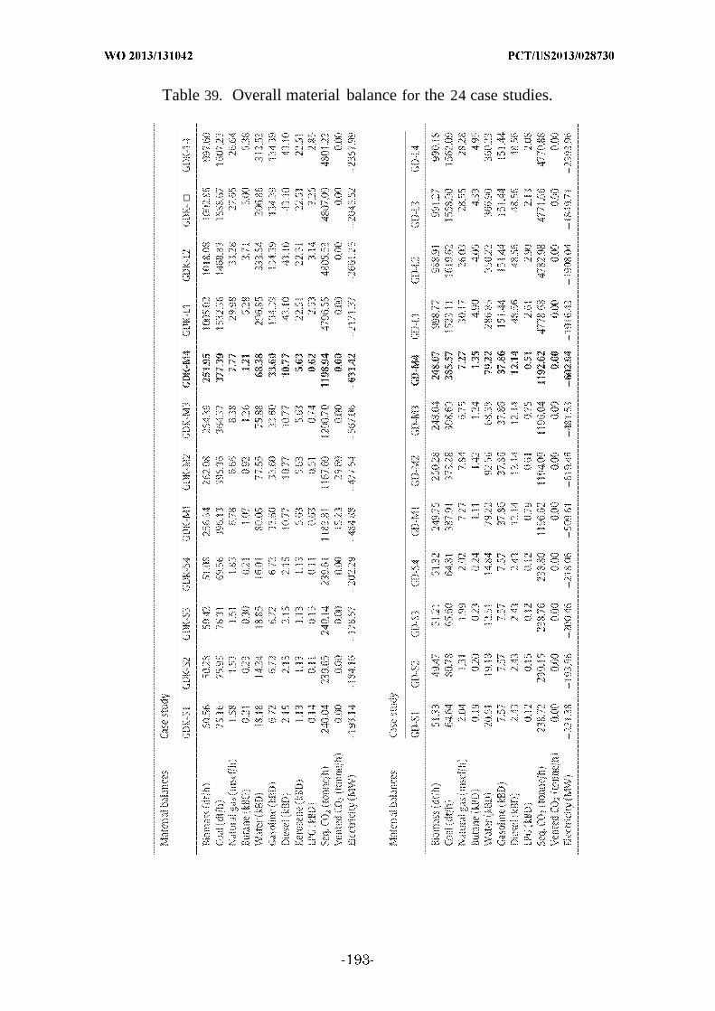
Table 39. Overall material balance for the 24 case studies.
The inputs to the CBGTL process are biomass, coal, natural gas, butane, and
water, while the outputs include gasoline, diesel, kerosene, LPG, sequestered and
vented CO2, and electricity. Biomass and coal are input in dry metric tons per
hour (dt/h), natural gas in million standard cubic feet per hour (mscf/h), liquids in
thousand barrels per day (kBD), and CO2 in metric tons per hour (tonne/h). The
results for the complete superstructure and medium sized capacity (M4) are
shown in boldface.

Table 40. Overall energy balance for the 24 case studies.

The energy inputs to the CBGTL process come from biomass, coal, natural gas,
and butane, and the energy outputs are gasoline, diesel, kerosene, LPG, and
electricity. The energy efficiency of the process is calculated by dividing the total
energy output with the total energy inputs to the process.
[0491] Almost all of the case studies do not vent CO2 from the process, and
utilize CO2 sequestration to reduce the lifecycle GHG emissions of the plant. The
GDK-M1 and GDK-M2 studies vent a small amount of CO2, though the C02 is
only 1-2% of the total CO2 produced by the plant. The balance of the CO2 is
captured for sequestration. The high utilization of CO2 sequestration allows for
an increased use of the cheaper fossil fuels coal and natural gas, which can be
anywhere from $3/GJ to $6/GJ less expensive than biomass. The biomass does
provide negative emission values from CO2 intake from the atmosphere during
cultivation and additional soil storage from land use change, so a level of biomass
input on a mass/energy basis that is roughly equivalent to that of coal or natural
gas is still required. The electricity production ranges from 179 to 221 MW for
small plants, 478-631 MW for medium plants, and 1850-2661 MW for large
plants. In all case studies, a high amount of electricity is produced to help lower
the overall cost of fuels for the plant. The electricity output also improves the
efficiency of the topologies, with GD-S2, GDK-Sl, and GD-Sl achieving the
highest energy efficiencies (i .e., 67.1%, 65.8%, and 65.7%, respectively) compared
to other case studies in their subcategories (see Table 9). The energy efficiency
values are calculated by dividing the total energy output (i .e., fuel products,
propane, or electricity) by the total energy input (i .e., via coal, biomass, natural
gas, butane, or electricity). If electricity is output from the system, the value is
listed as negative in Table 39 and the magnitude of the energy value in Table 40
is added to the total output. If the value is positive in Table 39, then this energy
is added to the total input to the system. The overall energy efficiency of the
CBGTL topologies producing gasoline, diesel, and kerosene ranges between 58.5
and 67.1% for all plant sizes.
[0492] Example 3.15 - Carbon and greenhouse gas balances
[0493] The overall carbon balance for the CBGTL processes is shown in
Table 41 and highlights the eight major points where carbon is either input or
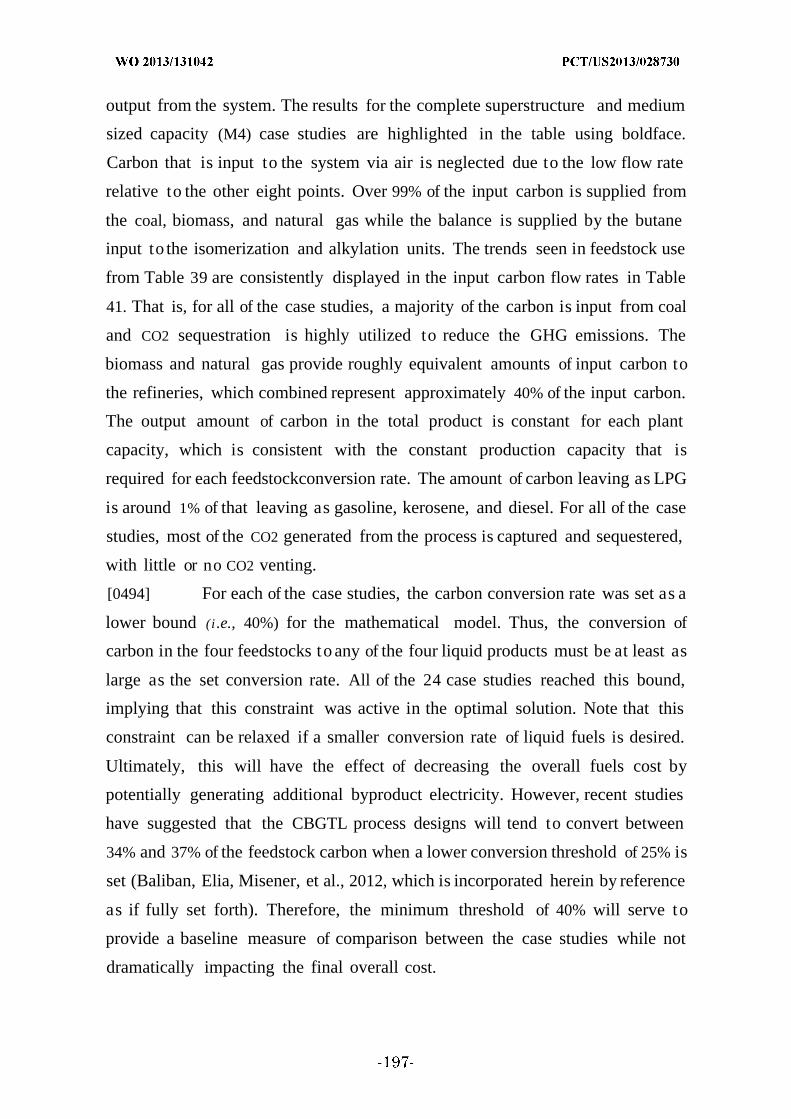
output from the system. The results for the complete superstructure and medium
sized capacity (M4) case studies are highlighted in the table using boldface.
Carbon that is input to the system via air is neglected due to the low flow rate
relative to the other eight points. Over 99% of the input carbon is supplied from
the coal, biomass, and natural gas while the balance is supplied by the butane
input to the isomerization and alkylation units. The trends seen in feedstock use
from Table 39 are consistently displayed in the input carbon flow rates in Table
41. That is, for all of the case studies, a majority of the carbon is input from coal
and CO2 sequestration is highly utilized to reduce the GHG emissions. The
biomass and natural gas provide roughly equivalent amounts of input carbon to
the refineries, which combined represent approximately 40% of the input carbon.
The output amount of carbon in the total product is constant for each plant
capacity, which is consistent with the constant production capacity that is
required for each feedstockconversion rate. The amount of carbon leaving as LPG
is around 1% of that leaving as gasoline, kerosene, and diesel. For all of the case
studies, most of the CO2 generated from the process is captured and sequestered,
with little or no CO2 venting.
[0494] For each of the case studies, the carbon conversion rate was set as a
lower bound (i .e., 40%) for the mathematical model. Thus, the conversion of
carbon in the four feedstocks to any of the four liquid products must be at least as
large as the set conversion rate. All of the 24 case studies reached this bound,
implying that this constraint was active in the optimal solution. Note that this
constraint can be relaxed if a smaller conversion rate of liquid fuels is desired.
Ultimately, this will have the effect of decreasing the overall fuels cost by
potentially generating additional byproduct electricity. However, recent studies
have suggested that the CBGTL process designs will tend to convert between
34% and 37% of the feedstock carbon when a lower conversion threshold of 25% is
set (Baliban, Elia, Misener, et al., 2012, which is incorporated herein by reference
as if fully set forth). Therefore, the minimum threshold of 40% will serve to
provide a baseline measure of comparison between the case studies while not
dramatically impacting the final overall cost.
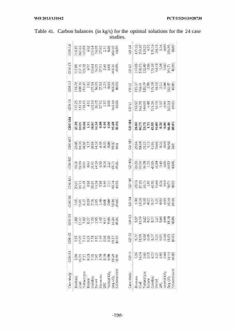
Table 41. Carbon balances (in kg/s) for the optimal solutions for the 24 casestudies.
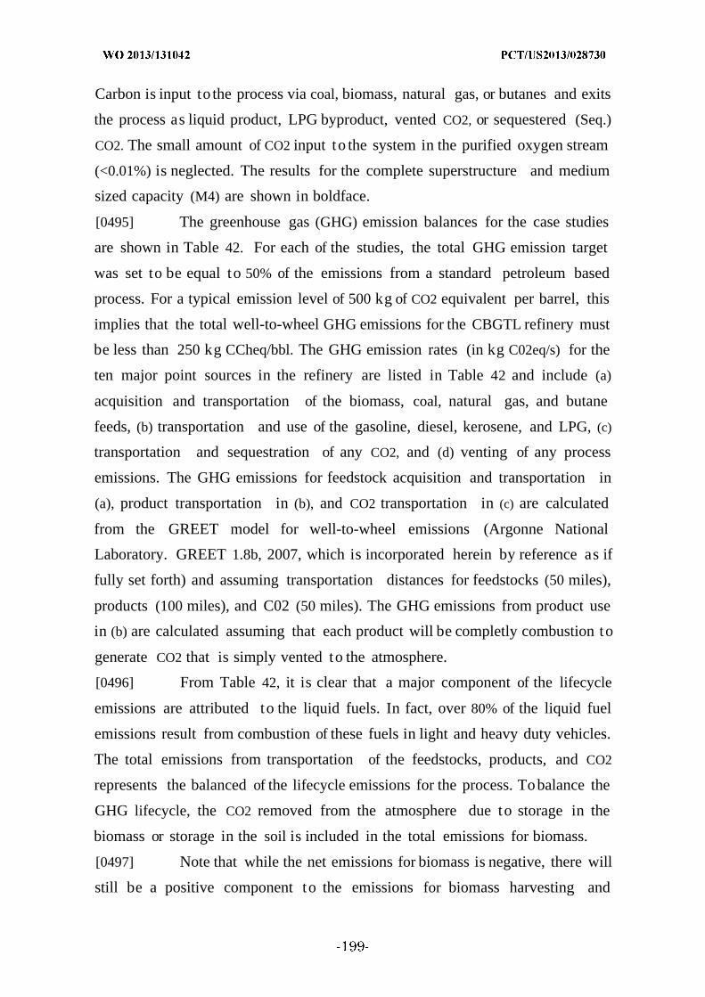
Carbon is input to the process via coal, biomass, natural gas, or butanes and exits
the process as liquid product, LPG byproduct, vented CO2, or sequestered (Seq.)
CO2. The small amount of CO2 input to the system in the purified oxygen stream
(<0.01%) is neglected. The results for the complete superstructure and medium
sized capacity (M4) are shown in boldface.
[0495] The greenhouse gas (GHG) emission balances for the case studies
are shown in Table 42. For each of the studies, the total GHG emission target
was set to be equal to 50% of the emissions from a standard petroleum based
process. For a typical emission level of 500 kg of CO2 equivalent per barrel, this
implies that the total well-to-wheel GHG emissions for the CBGTL refinery must
be less than 250 kg CCheq/bbl. The GHG emission rates (in kg C02eq/s) for the
ten major point sources in the refinery are listed in Table 42 and include (a)
acquisition and transportation of the biomass, coal, natural gas, and butane
feeds, (b) transportation and use of the gasoline, diesel, kerosene, and LPG, (c)
transportation and sequestration of any CO2, and (d) venting of any process
emissions. The GHG emissions for feedstock acquisition and transportation in
(a), product transportation in (b), and CO2 transportation in (c) are calculated
from the GREET model for well-to-wheel emissions (Argonne National
Laboratory. GREET 1.8b, 2007, which is incorporated herein by reference as if
fully set forth) and assuming transportation distances for feedstocks (50 miles),
products (100 miles), and C02 (50 miles). The GHG emissions from product use
in (b) are calculated assuming that each product will be completly combustion to
generate CO2 that is simply vented to the atmosphere.
[0496] From Table 42, it is clear that a major component of the lifecycle
emissions are attributed to the liquid fuels. In fact, over 80% of the liquid fuel
emissions result from combustion of these fuels in light and heavy duty vehicles.
The total emissions from transportation of the feedstocks, products, and CO2
represents the balanced of the lifecycle emissions for the process. Tobalance the
GHG lifecycle, the CO2 removed from the atmosphere due to storage in the
biomass or storage in the soil is included in the total emissions for biomass.
[0497] Note that while the net emissions for biomass is negative, there will
still be a positive component to the emissions for biomass harvesting and

transportation. It is important to observe that though the coal was the highest
energy input to the refinery, the emissions contribution from natural gas is
higher from coal or biomass.
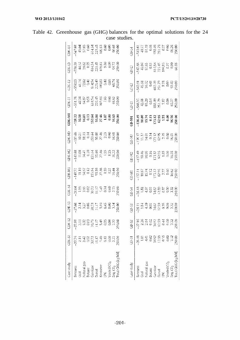
Table 42. Greenhouse gas (GHG) balances for the optimal solutions for the 24case studies.

The total GHG emissions (in CO2 equivalents - kg C02eq/s) for feedstock
acquisition and transportation, product transportation and use, CO2
sequestration, and process venting are shown for each study. Process feedstocks
include biomass, coal, natural gas, and butane while products include gasoline,
diesel, kerosene, and LPG. The results for the complete superstructure and
medium sized capacity (M4) are shown in boldface.
[0498] This example has detailed the development of a framework for the
process synthesis of a thermochemical hybrid coal, biomass, and natural gas to
liquids plant that incorporates multiple possibilities for hydrocarbon production
and hydrocarbon upgrading. The framework also included a simultaneous heat,
power, and water integration to compare the costs of utility generation and
wastewater treatment in the overall cost of liquid fuels. This example expands on
the CBGTL process in Examples 1 and 2 by directly quantifying the economic and
environmental benefits that are associated with (i) Fischer-Tropsch synthesis
and subsequent hydrocarbon upgrading and (ii) methanol synthesis, conversion
to hydrocarbons, and subsequent upgrading. The proposed optimization model
was tested using 24 distinct case studies that are derived from two combinations
of products, three plant capacities, and four superstructure possibilities. The
overall conversion of carbon from feedstock to liquid products was selected to be
40% and the greenhouse gas reduction target was equal to 50% of current
petroleum based refineries. Each case study was globally optimized using a
branch- and-bound global optimization algorithm to theoretically guarentee that
the cost associated with the optimal design was within 3-6% of the best value
possible.
[0499] When producing gasoline, diesel, and kerosene in ratios
commensurate with Untied States demands, the overall cost of liquid fuels
production ranges from $86/bbl to $94/bbl for small plants (10,000 barrels per
day; kBD), $79/bbl-$88/bbl for medium plants (50 kBD), and $72/bbl-$80/bbl for
large plants (200 kBD). When only gasoline and diesel are produced in a ratio
consistent with national demand, the cost decreases for each of the capacities to a
range of $85/bbl-$93/bbl for small, $78/bbl-$86/bbl for medium, and $71/bbl-

$78/bbl for large plants. This decrease in cost is generally due to the reduction in
investment needed to fractionate and convert the distillate to diesel only opposed
to both diesel and kerosene. For the four different superstructure possibilities
investigated in this study, it is evident that FT synthesis followed by
fractionation (superstructure 1) and upgrading is more expensive than FT
synthesis followed by catalytic ZSM-5 conversion to gasoline-range hydrocarbons
(superstructure 2). Additionally, methanol synthesis, conversion to
hydrocarbons, and subsequent upgrading (superstructure 3) is consistently
cheaper than FT synthesis for all capacity levels. This is due to the decrease in
investment cost associated with hydrocarbon production and upgrading when
compared to FT synthesis. These findings indicate that the methanol route is
preferential to the FT route when following an "either or" logic. However,
investigation of a "combination" superstructure that considered all of the
topologies (superstructure 4) in superstructures 1—3 indicates that a combination
of FT synthesis and methanol synthesis will provide the lowest overall cost. In
this case, the MTG route provides a majority of the gasoline while a majority of
the distillate (diesel and kerosene) is generated through fractionation and
refining of the FT effluent. Though over 80% of the final hydrocarbons were
produced via the methanol synthesis route, the final process topologies show that
the ability to consume CO2 in iron-based FT reactors helps to reduce feedstock
costs and therefore provide an economic advantage over a topology that utilizes
only methanol synthesis.
[0500] Example 3.16 - Mathematical model for process synthesis with
simultaneous heat, power, and water integration
[0501] The nomenclature for all terms in the mathematical model for
process synthesis with simultaneous heat, power, and water integration is shown
below. All constraints included in the model are listed subsequently with a
corresponding description of how that particular equation governs proper
operation of the process design.
[0502] Process units
[0503] The set of units, U, is presented in full detail in Table 43 and
defined formally in Eq. (223). Note that several units in Table 43 are listed as un.
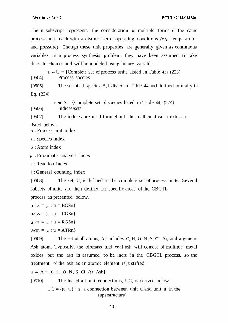
The n subscript represents the consideration of multiple forms of the same
process unit, each with a distinct set of operating conditions (e.g., temperature
and pressure). Though these unit properties are generally given as continuous
variables in a process synthesis problem, they have been assumed to take
discrete choices and will be modeled using binary variables.
u ≡ U = Complete set of process units listed in Table 43 (223)[0504] Process species
[0505] The set of all species, S, is listed in Table 44 and defined formally in
Eq. (224).
s S = Complete set of species listed in Table 44 (224)[0506] Indices/sets
[0507] The indices are used throughout the mathematical model are
listed below.u : Process unit index
s : Species index
a : Atom index
p : Proximate analysis index
r : Reaction index
i : General counting index
[0508] The set, U, is defined as the complete set of process units. Several
subsets of units are then defined for specific areas of the CBGTL
process as presented below.
BGS = u : u = BGSn
cGS = u : u = CGSn
GS = u : u = RGSn
UATR = u : u = ATRn
[0509] The set of all atoms, A, includes C, H, O, N, S, CI, Ar, and a generic
Ash atom. Typically, the biomass and coal ash will consist of multiple metal
oxides, but the ash is assumed to be inert in the CBGTL process, so the
treatment of the ash as an atomic element is justified
a ≡ A = C, H, O, N, S, CI, Ar, Ash
[0510] The list of all unit connections, UC, is derived below.
UC = (u, u') : 3 a connection between unit u and unit u' in thesuperstructure
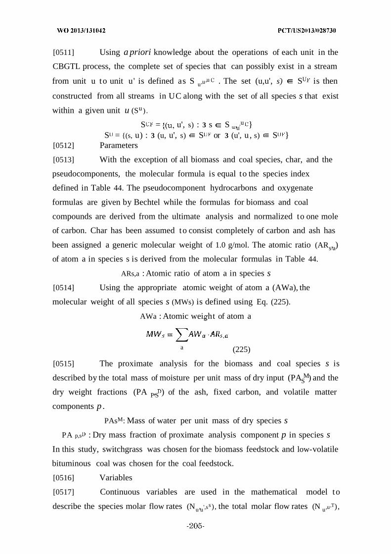
[0511] Using a priori knowledge about the operations of each unit in the
CBGTL process, the complete set of species that can possibly exist in a stream
from unit u to unit u' is defined as S u,u,u . The set (u,u', s) SU is then
constructed from all streams in UC along with the set of all species s that exist
within a given unit u (Su ) .
S = u', s) : 3 s S ,uu
S = (s, u) : 3 (u, u', s) ≡ S or 3 (u', u, s) ≡ S [0512] Parameters
[0513] With the exception of all biomass and coal species, char, and the
pseudocomponents, the molecular formula is equal to the species index
defined in Table 44. The pseudocomponent hydrocarbons and oxygenate
formulas are given by Bechtel while the formulas for biomass and coal
compounds are derived from the ultimate analysis and normalized to one mole
of carbon. Char has been assumed to consist completely of carbon and ash has
been assigned a generic molecular weight of 1.0 g/mol. The atomic ratio (ARs,a)
of atom a in species s is derived from the molecular formulas in Table 44.
ARs,a : Atomic ratio of atom a in species s
[0514] Using the appropriate atomic weight of atom a (AWa), the
molecular weight of all species s (MWs) is defined using Eq. (225).
AWa : Atomic wei ht of atom a
a (225)
[0515] The proximate analysis for the biomass and coal species s is
described by the total mass of moisture per unit mass of dry input (PASM) and the
dry weight fractions (PA P,S ) of the ash, fixed carbon, and volatile matter
components p .
PAsM: Mass of water per unit mass of dry species s
PA p,s : Dry mass fraction of proximate analysis component p in species s
In this study, switchgrass was chosen for the biomass feedstock and low-volatile
bituminous coal was chosen for the coal feedstock.
[0516] Variables
[0517] Continuous variables are used in the mathematical model to
describe the species molar flow rates (Nu,u',ss), the total molar flow rates (N u,u,T),
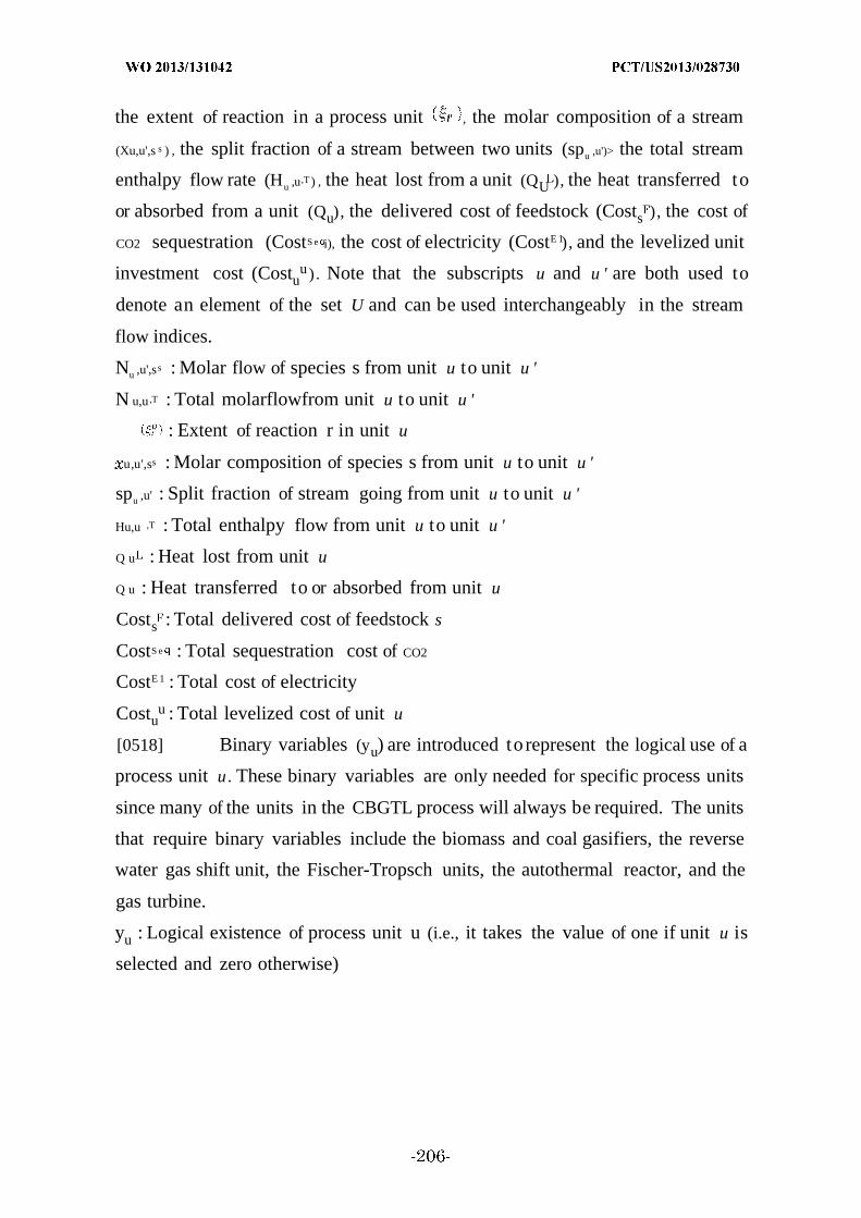
the extent of reaction in a process unit " , the molar composition of a stream
(Xu,u',s s ) , the split fraction of a stream between two units (spu ,u')> the total stream
enthalpy flow rate (Hu ,u,T ) , the heat lost from a unit (QU ), the heat transferred to
or absorbed from a unit (Qu), the delivered cost of feedstock (Costs ), the cost of
CO2 sequestration (CostS e i), the cost of electricity (CostE 1), and the levelized unit
investment cost (Costuu ) . Note that the subscripts u and u ' are both used to
denote an element of the set U and can be used interchangeably in the stream
flow indices.
Nu ,u',s s : Molar flow of species s from unit u to unit u '
N u,u ,T : Total molarflowfrom unit u to unit u '
: Extent of reaction r in unit u
u,u',ss : Molar composition of species s from unit u to unit u '
spu ,u' : Split fraction of stream going from unit u to unit u '
Hu,u ,T : Total enthalpy flow from unit u to unit u '
Q u : Heat lost from unit u
Q u : Heat transferred to or absorbed from unit u
Costs : Total delivered cost of feedstock s
CostS e : Total sequestration cost of CO2
CostE 1 : Total cost of electricity
Costuu : Total levelized cost of unit u
[0518] Binary variables (yu) are introduced to represent the logical use of a
process unit u. These binary variables are only needed for specific process units
since many of the units in the CBGTL process will always be required. The units
that require binary variables include the biomass and coal gasifiers, the reverse
water gas shift unit, the Fischer-Tropsch units, the autothermal reactor, and the
gas turbine.
yu : Logical existence of process unit u (i.e., it takes the value of one if unit u is
selected and zero otherwise)
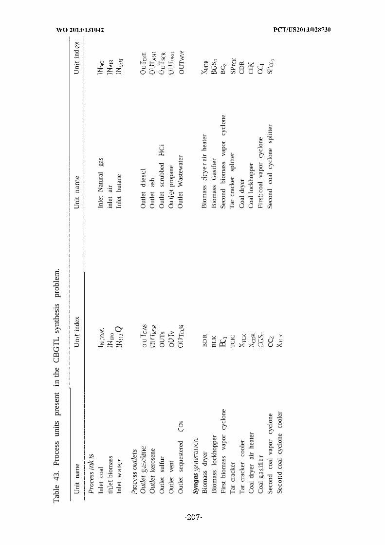
Tab
le43
.Pr
oces
sun
itspr
esen
tin
the
CB
GT
Lsy
nthe
sis
prob
lem
.
Uni
tna
me
Un
inde
xU
nit
na
eU
nin
d
Pro
cess
nks
Inle
tco
alΝ
,Λ
.In
let
Nat
ural
gas
tie
biom
ass
BO
inle
tai
r.
Inle
tw
at
QIn
let
buta
ne
rss
outl
ets
Out
let
OU
AS
Out
let
die
sl
UE
Out
let
kero
sene
Out
let
ash
T
Out
let
sulf
urO
UT
sO
utle
tsc
rubb
edC
iU
S
Out
let
vent
Ov
Ou
tt
prop
ane
Out
let
sequ
este
red
C¾T
¾O
utle
tW
aste
wat
erO
UT
Syng
asB
iom
ass
drye
rB
DR
Bio
mas
sye
rai
rhe
ater
Bio
mas
slo
ckho
pper
BL
KB
iom
ass
Gas
ifie
rS
Firs
tbi
omas
sva
por
cycl
one
BSe
cond
biom
ass
vapo
rcy
clon
eB
C
Tar
crac
ker
TC
ICT
arcr
acke
rsp
litte
rSP
rT
arcr
acke
rco
oler
Coa
ldr
yer
CD
R
Coa
ldr
yer
air
heat
erC
DC
oal
lock
hopp
erC
L
Coa
lg
ifie
rF
irs
:coa
lva
por
cycl
one
C
Seco
ndco
alva
por
cycl
one
ccSe
cond
coal
cycl
one
split
ter
S
Seco
dco
alcy
clon
eco
oler

Syng
ascl
eani
ngR
ever
sew
ater
ssh
ift
unit
CS
RG
Sef
flue
ntco
oler
CGS
hydr
oipe
rC
HH
Qsc
bbe
Aci
dga
sfl
ash
vapo
rco
oler
~A
cid
gas
flas
h2-
phas
eco
oler
Ad
gas
flas
hA
GF
Aci
dga
sth
erm
alan
alyz
erA
cid
gas
rem
oval
unit
RFi
rst
com
pres
sor
recy
cle
com
pres
sor
C2
C2
sequ
estr
atio
nco
mpr
esso
rA
cd
gas
cra
pres
sor
AG
C
reco
very
Aci
dga
ssp
litte
rS
Aci
dga
spr
ehea
ter
Cs
com
bust
orC
CFi
rsts
fur
conv
erte
rFi
rsts
uu
sepa
rato
rSS
-Se
cond
sulf
urco
nver
ter
heat
erSe
cond
sulf
ur' c
onve
rter
SC
2Se
cond
sulf
urse
para
tor
Thi
rdsu
lfur
conv
erte
rhe
ater
X¾
Thi
rdsu
lfur
conv
erte
rT
hird
sulf
urse
para
tor
SS
Sulf
urpi
tTa
lhy
dral
yzer
TG
IT
ailg
asfl
ash
vapo
rco
oler
Tai
lgas
flas
h2-
phas
eco
oler
TCT
ailg
asf
shun
itTa
igas
mpr
essa
rT
G
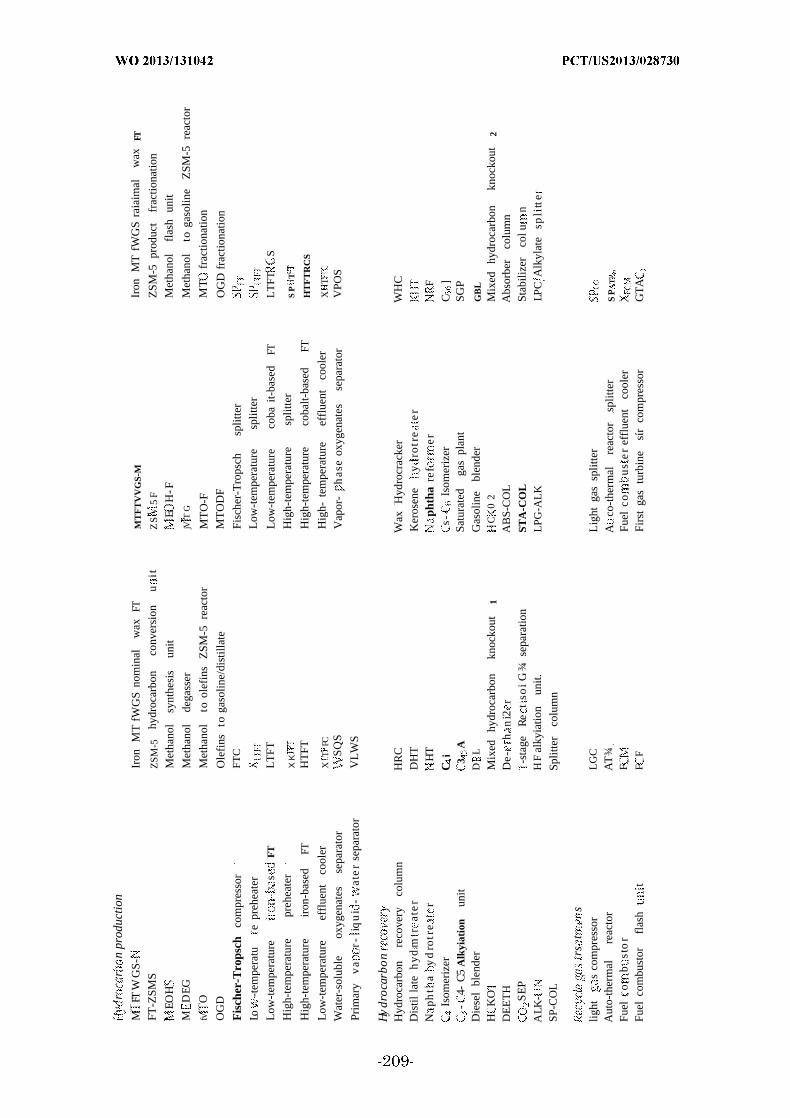
rr
npr
oduc
tion
MFT
WG
S-
Iron
MT
fWG
Sno
min
alw
axFT
MT
FT
VV
GS-
MIr
onM
TfW
GS
raia
imal
wax
FT
FT-Z
SMS
ZSM
-5hy
droc
arbo
nco
nver
sion
uit
ZS
5F
ZSM
-5pr
oduc
tfr
actio
natio
n
EOH
Met
hano
lsy
nthe
sis
unit
EH
-FM
etha
nol
flas
hun
it
MD
EG
Met
hano
lde
gass
erjV
TG
Met
hano
lto
gaso
line
ZSM
-5re
acto
r
fv' O
Met
hano
lto
olef
ins
ZSM
-5re
acto
rM
TO
-FM
Tfr
actio
natio
n
OG
DO
lefi
nsto
gaso
line/
dist
illat
eM
TO
DF
OG
Dfr
actio
natio
n
Fis
cher
-Tro
psch
com
pres
sor
FTC
Fisc
her-
Tro
psch
split
ter
Lo-t
empe
ratu
epr
ehea
ter
Low
-tem
pera
ture
split
ter
Low
-tem
pera
ture
sFT
LT
FTL
ow-t
empe
ratu
reco
bait-
base
dFT
LT
FTS
Hig
h-te
mpe
ratu
repr
ehea
ter
ΧΚ
Hig
h-te
mpe
ratu
resp
litte
rS
PT
Hig
h-te
mpe
ratu
reir
on-b
ased
FTH
TFT
Hig
h-te
mpe
ratu
reco
balt-
base
dFT
HT
FT
RC
S
Low
-tem
pera
ture
effl
uent
cool
erX
TFC
Hig
h-te
mpe
ratu
reef
flue
ntco
oler
XT
Wat
er-s
olub
leox
ygen
ates
sepa
rato
rS
QS
Vap
or-
has
eox
ygen
ates
sepa
rato
rV
POS
Prim
ary
va
r-iq
ui
-at
er
sepa
rato
rV
LW
S
Hydr
ocar
bon
Hyd
roca
rbon
reco
very
colu
mn
HR
CW
axH
ydro
crac
ker
WH
CD
istil
late
hy
dm
rat
er
DH
TK
eros
ene
yro
tre
er
Nph
ta
yd
rotr
er
HT
phth
are
fer
F
Isom
eriz
erC
is-
Isom
eriz
erC
]-
4-C
5A
lkyi
atio
nun
it3
ASa
tura
ted
gas
plan
tSG
PD
iese
lbl
ende
rD
LG
asol
ine
blen
der
GB
L
HK
OM
ixed
hydr
ocar
bon
knoc
kout
1C
02
Mix
edhy
droc
arbo
nkn
ocko
ut2
DE
ET
HD
e-h
ni2
rA
BS-
CO
LA
bsor
ber
colu
mn
SE
P-s
tage
Re
tso
iG¾
sepa
ratio
nST
A-C
OL
Stab
ilize
rco
lun
ALK
-H
Fal
kyia
tion
unit.
LPG
-AL
KLP
CA
lkyl
ate
spli
tte
SP-C
OL
Split
ter
colu
mn
rst
slig
hts
com
pres
sor
LG
CL
ight
gas
split
ter
Aut
o-th
erm
alre
acto
rA
T¾
Aco
-the
rmal
reac
tor
split
ter
SP
T,
Fuel
ob
sto
rF
Fuel
cou
se
ref
flue
ntco
oler
Fuel
com
bust
orfl
ash
tF
FFi
rst
gas
turb
ine
sir
com
pres
sor
GT
A

The subscript n corresponds to multiple forms of the same process unit, each with
a distinct set of operating conditions or ratios of feedstock. Distinct process units
are used in lieu of continuous variables representing the process operating
conditions. This will prevent the use of bilinear terms when specifying feedstock
ratios or highly non-linear equations when specifying equilibrium constants or
species enthalpies.

Tab
le44
.Sp
ecie
spr
esen
tin
the
CB
GT
Lsy
nthe
sis
prob
lem
.
Spec
ies
na
eSp
ecie
sin
dex
Spec
ies
Spec
ies
inde
xSp
ecie
sna
me
Spec
ies
inde
x
Add
gase
sSi
)If
diox
ide
SO,:
Hyd
roge
nsu
lfur
HS
Car
bony
lsu
lfid
eC
OS
Hyd
roge
ncy
anid
eC
NA
mo
nia
NH
ydro
gen
chlo
ride
Car
bon
diox
ide
CG
¾»f
t/n
rc
ron
gase
s
Nitr
ogen
¾A
r
Nitr
icox
ide
NO
Nitr
ons
oxid
eN
0W
ater
H20
rbo
nm
onox
ide
CO
Hyd
roge
nH
svt
Met
hane
C.
Ace
tyle
ne¾
Eth
ylen
eC
H4
Eth
ane
CPr
opyl
ene
¾Pr
opan
eC
H
sosty
en-B
ne
Isob
utan
e<
·.
uta
neH
-Per
e2-
tyi
ban
ePe
nt
n2-
tyi
pnt
a*
n-H
exan
en-
Hep
tars
eC
-Oct
ene
-Nor
sene
Hn-
ona
nn
-Dec
a2
ndec
ere
-Dod
enn
-Dd
nn-
Tiid
ecan
e2
ίe
f:
;.'!
;-P
ntad
cen
en
-Pnt
ads
-ex
adee
ee
½n-
Hex
adec
ane
C½
H¾
-Hp
adce
ne,
n-H
ept
dne
, ?½
l-O
tad
c?»
H:¾
nc
ade
ane
-o
nde
cen
en
-Nn
ade
an
C«
Hn-
Eic
osan
ePs
ed
cp
one
ntC
OP
Psei
sdoc
ompo
nent
3Ps
edo
om
pse
nC
2Q
P24
Pe
doo
pfe
nC
P
Psei
sdoc
ompo
nent
C25
P2
Pseu
doco
mpo
sien
tC
OP
Pse
dorn
pe
nt
??O
P
CPs
eisd
ocom
pone
ntC
;P
Pseu
doo
pon
et
C29
OP
C¾
Pseu
doeo
sYip
onen
rC
¾>
Wax
VP
Oxy
gena
teO
XV
AP
HP
Oxy
gena
teO
XH
CA
Cy
gna
tO
XH
20
-212-
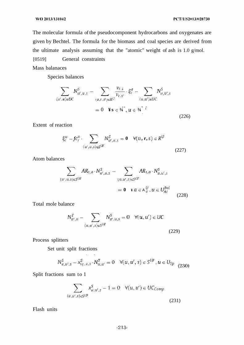
The molecular formula of the pseudocomponent hydrocarbons and oxygenates are
given by Bechtel. The formula for the biomass and coal species are derived from
the ultimate analysis assuming that the "atomic" weight of ash is 1.0 g/mol.
[0519] General constraints
Mass balanaces
Species balances
. .
0 ¥ s ¾ ¾(226)
Extent of reaction
0 , r,
(227)
Atom balances
0 ¥ A ,(228)
Total mole balance
(229)
Process splitters
Set unit split fractions
Split fractions sum to 1
(231)
Flash units
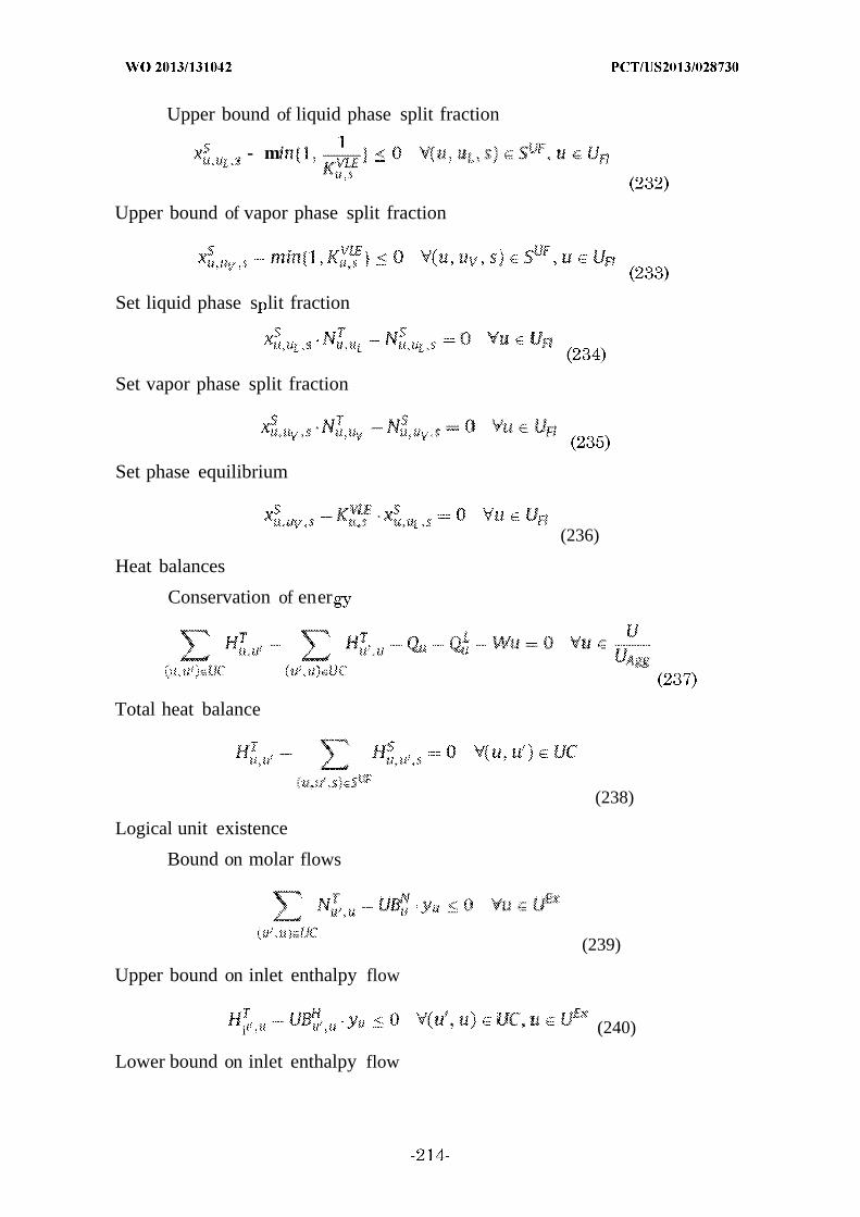
Upper bound of liquid phase split fraction
- m
Upper bound of vapor phase split fraction
Set liquid phase s lit fraction
Set vapor phase split fraction
Set phase equilibrium
(236)
Heat balances
Conservation of ener
Total heat balance
(238)
Logical unit existence
Bound on molar flows
(239)
Upper bound on inlet enthalpy flow
i (240)
Lower bound on inlet enthalpy flow

. - (241)
Upper bound on outlet enthalpy flow
> > " (242)
Lower bound on outlet enthalpy flow
L - < 0 V(ii, ) &
(243)
Process inlets
Feedstock moisture content
Set biomass moisture content from proximate analysis
Set coal moisture content from proximate analysis
(245)
Known stream compositions
Set stream compositions for inlet streams
- ί = V« s) = , 1 τ
Coal to natural gas ratio
Set coal to natural gas inlet ratio based on lower heating value ratios
V - V LHV . ∑ > = 0
Greenhouse gas emissions reduction
Set reduction from petroleum based process
(248)
Sum emissions from CBGTL components
i - G - G G - G C i = 0(249)
Set emissions from feedstock acquisition

emissions from CO2 sequestration
Set emissions from CO2 venting
G - M W - = 0(252)
Process outlet fuel ratios
Set gasoline to diesel output ratio
Set diesel to kerosene output ratio
M W . ¾ - R t _ K -¾ . i! = 0
Syngas generation
Biomass/coal driers
Upper bound for biomass drier activation
' " (255)
Upper bound for coal drier activation
i - - - y < , ) = ( IN AL CDR)' (256)
Lower bound for biomass drier activation
-
Lower bound for coal drier activation
M -M - A - OS ( 1 - ¾ ) ( , ') = ( *CDR)(2 )
Upper bound for biomass drier moisture evaporation
M T - - . ¾ - - ) < 0 (a, ) = (BDR, BUC)
Lower bound for biomass drier moisture evaporation

M , ;„ - « · - U - ( - v ) < 0 ) = fBDR, ELK)(260)
Upper bound for coal drier moisture evaporation
- y , —M . - - · ( - ) <-
Lower bound for coal drier moisture evaporation
Gasifier lockhoppers
Set CO2 lockhopper flow rate
S ¾ 2 C - =
¾ (263)
Biomass gasifier
Water -gas -shift equilibrium
¾ CO i , C . — ' ¾ B C ¾ . C , = S(264)
Hydrocarbon conversion fraction
Hydrocarbon generation from pyrolysis
i ii *,« (266)
Set ratio of NO to N2O
¾ . C L.NO - sr.,, O ¾ = i' (267)
Set ratio of HCN to NH3
¾ , - CN - HCN ¾ € i Ni = V 1 GS
(268)
Set amount input nitrogen t o NH3 and N 2
= 0 V(269)
Set ratio of NH3 to N2
= 0 Va(270)
Set ratio of COS to H2S
- 5 ∞ s - - S = Va e G$- (271)
Amount of char production
= 0 Va e ¾ -
· (272)
Rate of ash removal
Gasifier heat loss
(274)
Logical use of one gasifier temperature
Biomass gasifier solids
Removal of solids from first cyclone
(276)
Removal of solids from second cyclone

B E - 2 , GS ~ 0(277)
Coal gasifier
Set CO2 lockhopper flow rate
(278)
Water -gas -shift equilibrium
(2 )
Hydrocarbon conversion fraction
(280)
Hydrocarbon generation from pyrolysis
«' « (281)
Set ratio of NO to N2O
¾ - 5 - =(282)
Set ratio of HCN to NH3
(283)
Set amount input nitrogen t o NH3 and N 2
cc NH 4 - - yx 2 - nf>
= 0 Y u(284)
Set ratio of NH3 t o N2
¾ , ¾ - i 2 + 2 , H3 + 2 · y
= 0 V«(285)
Set ratio of COS to H2S
Amount of char production
Rate of ash removal
Gasifier heat loss
+ - V = 0 V i
', (289)
Logical use of one gasifier temperature
y - 1 = 0(290)
Coal gasifier solids
Removal of solids from first cyclone
( 91)
Removal of solids from second cyclone
Syngas cleaning
Reverse water-gas-shift unit
Bypass of inert species

Water -gas -shift equilibrium
(294)
Logical use of unit with at most one temperature
« - <GS
(295)
COS-HCN hydrolyzer
Bypass of inert species
(296)
COS-H 2S equilibrium
= 0 C , ) = CCHH, HSC
HCN-NH.3 equilibrium
3
Acid gas recovery
Set CO2 molar fraction in clean output
Set CO2 output flow rates
(300)
Claus sulfur recovery
Set inlet combustor oxygen level
Hydrocarbon production
Fischer-Tropsch
Set ratio of H 2 to CO in cobalt-based inlet
¾ . FTR cI' ) S (V ,w.CO) S F
Set ratio of H 2 to CO and CO2 in iron-based inlet
FTR u -
0 V Uj r∑ FTR u ∞ 3 - ∑ F TRu
w .CO) , S < ·' («' .11. . . V '
(303)
Adjust weight fraction of Ci species
= 5 (304)
Adjust weight fraction of C 2 species
Adjust weight fraction of C 3 species
(306)
Adjust weight fraction of C4 species
w4 =- i - )= (307)
Set weight fraction of Cn species from Anderson-Schultz-Flory distribution

= l - G) i _ V 5 < f < 2 9~ (308)
Set weight fraction of wax
s= ¾3(309)
Set carbon distribution from weight fractions
Set exactly one low-temperature unit
+ - 1 = 0(311)
Set exactly one high-temperature unit
TF + S - = 2 )
Aqueous phase oxygenates separator
Removal of aqueous phase oxygenates
S S,VLWS .= 0 ¾
(313)
Vapor phase oxygenates separator
Removal of vapor phase oxygenates
(314)
Hydrocarbon upgrading
Hydrocarbon upgrading units
Set carbon distribution fractions of total input
(315)
Saturated gas plant
Set fractional recovery of light gases
N - rf —0 VsSG J " SG - i fc ,
(316)
Recycle gas treatment
Fuel combustor
Set inlet combustor oxygen level
( ) (317)
Auto-thermal reactor
Logical use of one temperature
- =
(318)
Water -gas -shift equilibrium
= 0 V( , «·') ,
(319)
Steam reforming equilibrium
= 0 V if') UC, ¾(320)
C2H2 steam reforming equilibrium
Xsu = 0 V " UC, A R
C2H4 steam reforming equilibrium
K
x " = 0 V(« , e UC, a ¾
(322)
C2H6 Steam reforming equilibrium
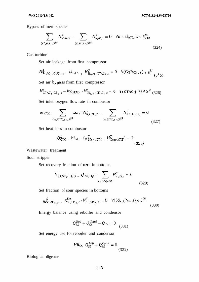
Bypass of inert species
(324)
Gas turbine
Set air leakage from first compressor
CT - N = T C , s e S 2
Set air b ass from first compressor
, = 0 ¥ ( GTAC j ' ·' S (326)
Set inlet oxygen flow rate in combustor
(327)
Set heat loss in combustor
- w -
Wastewater treatment
Sour stripper
Set recovery fraction of H2O in bottoms
_ SS, H , =
i (329)
Set fraction of sour species in bottoms
W .s ,. - . = S SS
(330)
Energy balance using reboiler and condensor
(331)
Set energy use for reboiler and condensor
Biological digestor

Set biogas ratio of CH4 to CO2
Reverse osmosis
Set removal fraction of solids
Cooling cycle
Cooling tower flow rate from ener requirement
¾ : -
Cooling tower evaporation loss
Cooling tower drift loss
Sum total cooling tower losses
Set known cooling tower output solid concentrations
Steam cycle
Set known process steam boiler output solid concentrations
T SP s CLTR>SP ft~ i TR P R = ° ¾
(340)
Set known heat engine boiler output solid concentrations
Outlet wastewater
Upper bound on output wastewater concentrations

Hydrogen/oxygen production
Pressure-swing adsorption
Set recovery fraction of ¾ from inlet
— \ — n
«, PSA5 (343)
Set inlet mole fraction of ¾
Air separation unit
Recover fraction of O
Process hot/cold/power utility requirements
Set electricity needed for process units
Set cooling water needed for process units
Set heating fuel needed for process units
(348)
Set utilities needed for process units
Process costs
Feedstock costs

Levelized cost of biomass feedstock
F INB .BDR,s= P d L V V S ¾ °
(350)
Levelized cost of coal feedstock
o ¾ = Prod V(351)
Levelized cost of natural gas feedstock
¾ .- Pr d LHVp o(IN , C (352)
Levelized cost of freshwater feedstock
= ™ (353)
Electricity costs
Levelized cost of electricity
cEl El _ pEl El
Cost EI — " ' ° "Prod LHVpr d
CO2 sequestration costs
Levelized cost of CO2 sequestration
co 2 - 0 S ouTm . .co C e
CostS =Prod Vρ 0 ά
Levelized investment costs
Total overnight cost of process units
Toc = (1 + iCu ( + BOPU c po' (356)
Variable capital costs of process units
CC = LCCR 1DCF TOC(357)
Levelized cost of process units
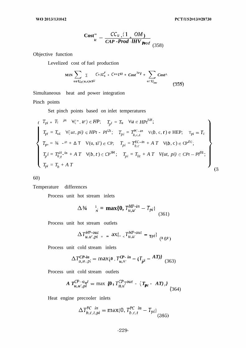
Cost" . + )CAP -Prod lHV Pr (358)
Objective function
Levelized cost of fuel production
M1N ∑ o + o s El + Cost 1 + Cost^
eU, u,s )eS U!nv .(359)
Simultaneous heat and power integration
Pinch points
Set pinch points based on inlet temperatures
( = ΐ ' " . ' Tp = T HPt
T = T ut pi) HPt - PI pi = T V( , c, ) e HEP; T
, = ¾ - ί + ∆ Τ V(u, i') CP; Tpi = + A T V( , c) CP C .
Tpi = Ths - + A T V , ) P ; Tpi = Tlit + A T V(ut, pi) CPt
T = Tb + A T
60)
Temperature differences
Process unit hot stream inlets
¾ = max0,(361)
Process unit hot stream outlets
= m ° < - T 3 2
Process unit cold stream inlets
CP-in 0 CP- in _ ( _ AT), '.', ι ( ' u, ' p (363)
Process unit cold stream outlets
A Tu,u',ui max 0 ,' 11.
7 - TPi' - AT) ,(364)
Heat engine precooler inlets
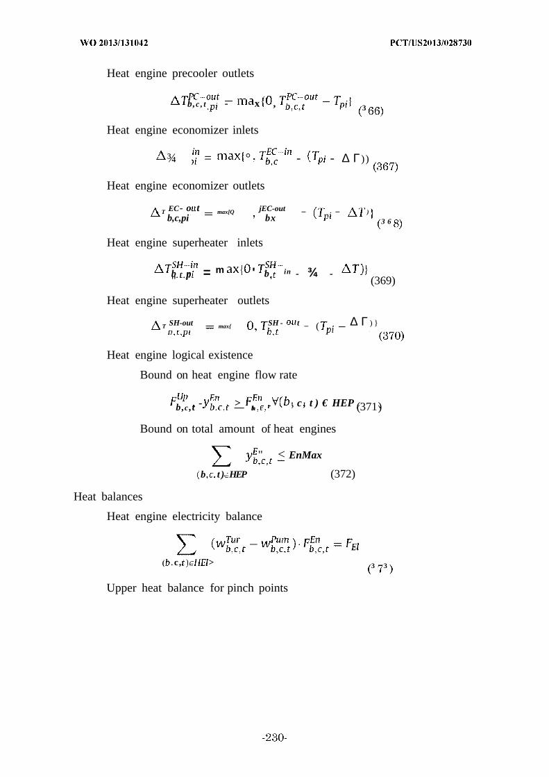
Heat engine precooler outlets
b,c , t - x , 3
Heat engine economizer inlets
¾ = ° - - ∆ Γ))
Heat engine economizer outlets
T EC- o t max[Q jEC-out _ _ )b,c,pi bx 3 6
Heat engine superheater inlets
b p = m ' b in - ¾ -" ' (369)
Heat engine superheater outlets
T SH-out max SH - t _ ( _ ∆ Γ )
Heat engine logical existence
Bound on heat engine flow rate
b,c ,t - >— bh ct ,' c ,' t )' € HEP (371)
Bound on total amount of heat engines
" < EnMax
b t ) HEP (372)
Heat balances
Heat engine electricity balance
( . c, > 3 3
Upper heat balance for pinch points
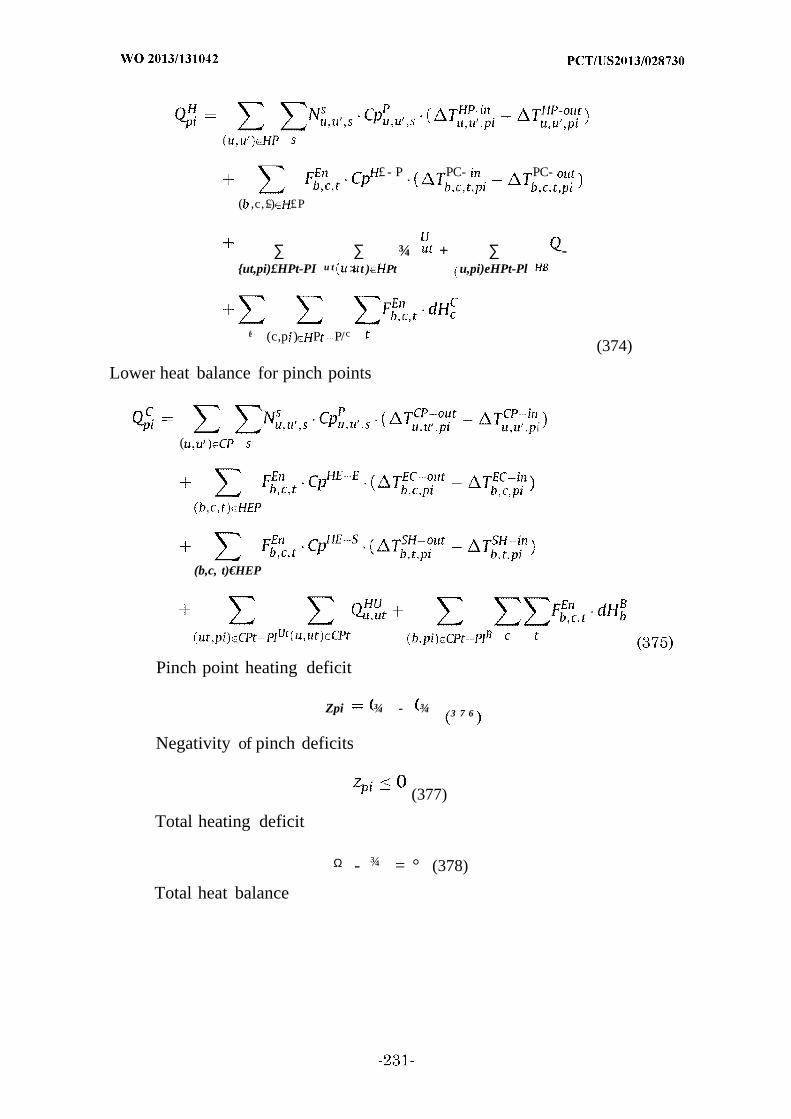
£ - P PC- PC-
( ,c,£-) £P
∑ ∑ ¾ + ∑ -ut,pi)£HPt-PI u t > t ) Pt u,pi)eHPt-Pl
fe (c,p ) P P/c
(374)
Lower heat balance for pinch points
ί
(
(b,c, t)€HEP
Pinch point heating deficit
Zpi ¾ - ¾ 3 7 6
Negativity of pinch deficits
(377)
Total heating deficit
Ω - ¾ = ° (378)
Total heat balance

∑ Cn P-in _ γΗΡ -ο ΐ/ u, u',s " ,u',s ' 1 , ' u.u' >
(u ' eHP s
, E~ f - i PC-out
i ,c, ) P
. H u PtH (b,c, t)eHEP
- . Cp . . ( P- t _ jCP-in
(u,u' )sCP s
(i),c, ) P
SH-t 'n
( , c )g P
[0520] Example 3.17 - CBGTL Process Superstructure Conceptual Design
[0521] The syngas conversion and hydrocarbon upgrading units proposed
herein are based on an extension of the CBGTL refinery superstructure in
Examples 1 and 2. The flowsheets depicting the complete superstructure are
shown in FIGS. 38 —50. In the figures, fixed process units are represented by
110, variable process units by 120, splitter units by 130, and mixer units by 140.
The variable process streams are represented by 210 and all other process
streams are fixed, unless otherwise indicated. The CBGTL superstructure is
designed to co-feed biomass, coal, or natural gas to produce gasoline, diesel, and
kerosene. Syngas is generated via gasification from biomass (FIG. 38) or coal
(FIG. 39) or auto-thermal reaction of natural gas (FIG. 50) and is either (i)
converted into hydrocarbon products in the Fischer-Tropsch (FT) reactors (FIG.
42) or (ii) into methanol via methanol synthesis (FIG. 45). The FT wax will be
sent to a hydrocracker to produce distillate and naphtha (FIG. 44) while the FT
vapor effluent may be (a) fractionated and upgraded into gasoline, diesel, or
kerosene or (FIG. 44) (b) catalytically converted to gasoline via a ZSM-5 zeolite
(FIG. 43). The methanol may be either (a) catalytically converted to gasoline via

the ZSM-5 catalyst (FIGS. 45 - 46) or (b) catalytically converted to olefins via the
ZSM-5 catalyst and subsequently fractionated to distillate and gasoline (FIG. 45).
[0522] Acid gases including CO2, ¾ , and NH3 are removed from the syngas
via a Rectisol unit prior to conversion to hydrocarbons or methanol (FIG. 40).
Incorporation of other acid gas removal technologies (e .g., amine adsorption,
pressure-swing adsorption, vacuum-swing adsorption, membrane separation) and
their relative capital/operating cost as a function of input flow rate and acid gas
concentration is the subject of an ongoing study. The sulfur-rich gases are
directed to a Claus recovery process (FIG. 41) and the recovered CO2 may be
sequestered (FIG. 40) or reacted with ¾ via the reverse water-gas-shift reaction.
The CO2 may be directed to either the gasifiers (FIGS. 38 - 39), the reverse
water-gas-shift reactor (FIG. 40), or the iron-based FT units (FIG. 42). Recovered
CO2 is not sent to the cobalt-based FT units to ensure a maximum molar
concentration of 3% and prevent poisoning of the catalyst. Hydrogen is produced
via pressure-swing adsorption or an electrolyzer unit while oxygen can be
provided by the electrolyzer or a separate air separation unit (FIG. 48). A
complete water treatment network (FIGS. 49 - 50) is incorporated that will treat
and recycle wastewater from various process units, blowdown from the cooling
tower, blowdown from the boilers, and input freshwater. Clean output of the
network includes (i) process water to the electrolyzers, (ii) steam to the gasifiers,
auto-thermal reactor, and water- gas-shift reactor, and (iii) discharged
wastewater to the environment.
[0523] Example 3.18 - Fischer-Tropsch Synthesis
[0524] The four FT units considered in Examples 1 and 2 utilized either a
cobalt or iron catalyst and operated at high or low temperature. The two cobalt-
based FT units would not facilitate the water -gas-shift reaction and therefore
required a minimal level of CO2 input to the units. The two iron-based FT units
were assumed to facilitate the reverse water- gas- shift reaction and therefore
could consume CO2 within the unit using ¾ to produce the CO necessary for the
FT reactions. A key consequence of the reaction conditions in the latter units was
the heat needed for the reverse water-gas-shift reaction would be provided by the
highly exothermic FT reaction. In this study, the set of possible FT units is

expanded t o consider iron-based systems that will facilitate the forward water-
gas-shift reaction within the units. These FT units will require a lower H2/CO
ratio for the FT reaction because steam in the feed will be shifted to H 2 through
consumption of CO. These units may be beneficial since certain syngas
generation units (e .g., coal gasifiers) will produce a gas that generally has a
H2/CO ratio that is much less than the 2/1 requirement for FT synthesis (Baliban
et al., 2010 and Kreutz et al., 2008, which are incorporated herein by reference as
if fully set forth). The downside of the new FT units will be the high quantity of
CO2 that is produced as a result of the water-gas-shift reaction. The framework
developed for the CBGTL superstructure will directly examine the benefits and
consequences for each of the six FT units to determine which technology produces
a refinery with a superior design. The mathematical model will select at most two
units to operate in the final process design.
[0525] FIG. 42 shows the flowsheet for FT hydrocarbon production within
the superstructure. Clean gas from the acid gas removal (AGR) unit is mixed
with recycle light gases from a CO2 separator (CO2SEP) and split (SPCG) to either
the low-wax FT section (SPFTM), the nominal- wax FT section (SPFTN), or methanol
synthesis (MEOHS). Each FT section will have three distinct FT units based on
the operating conditions of the unit. The cobalt-based FT units operate at either
low temperature (LTFT; 240 °C) or high temperature (HTFT; 320 °C) and must
have a minimal amount of CO2 in the input stream. Two iron-based FT units will
facilitate the reverse water- gas- shift (rWGS)reaction and will operate at low
(LTFTRGS; 240 °C) and high temperature (HTFTRGS; 320 °C). The other two
iron-based FT units will use the forward reverse water- gas- shift (fWGS) units,
operate at a mid-level temperature (267 °C), and produce either minimal
(MTFTWGS-M) or nominal (MTFTWGS-N) amounts of wax.
[0526] Hydrogen may be recycled t o any of the FT units t o either shift the
H2/CO ratio or the H2/CO2 ratio to the appropriate level. Steam may alternatively
be used as a feed for the two iron-based fWGS FT units t o shift the H2/CO ratio.
CO2 may be recycled back t o the iron-based rWGS FT units to be consumed in the
WGS reaction. Similarly, the pressure- swing adsorption (PSA) offgas which will
be lean in ¾ may be recycled t o the iron-based rWGS FT units for consumption
of the CO or CO2. The effluent from the auto-thermal reactor (ATR) will contain a
H 2/CO ratio that is generally above 2/1, and is therefore favorable a s a feedstock
for FT synthesis [5] . However, the concentration of CO2 within the ATR effluent
will prevent the stream from being fed t o the cobalt-based units. The two streams
exiting the FT units will be a waxy liquid phase and a vapor phase containing a
range of hydrocarbons. The wax will be directed t o a hydrocracker (WHC) while
the vapor phase is split (SPFTH) for further processing.
[0527] Example 3.19 - Fischer-Tropsch Product Upgrading
[0528] The vapor phase effluent from FT synthesis will contain a mixture
of C1-C30+ hydrocarbons, water, and some oxygenated species. FIG. 43 details the
process flowsheet used t o process this effluent stream. The stream will be split
(SPFTH ) and can pass through a series of treatment units designed to cool the
stream and knock out the water and oxygenates for treatment. Initially, the
watersoluble oxygenates are stripped (WSOS) from the stream. The stream is
then passed to a three-phase separator (VLWS) to remove the aqueous phase
from the residual vapor and any hydrocarbon liquid. Any oxygenates that are
present in the vapor phase may be removed using an additional separation unit
(VSOS). The water lean FT hydrocarbons are then sent to a hydrocarbon recovery
column for fractionation and further processing (FIG. 44). The oxygenates and
water removed from the stream are mixed (MXFTWW) and sent to the sour stripper
mixer (MXSS) for treatment.
[0529] The FT hydrocarbons split from SPFTH may also be passed over a
ZSM-5 catalytic reactor (FT-ZSM5) to be converted into mostly gasoline range
hydrocarbons and some distillate. The ZSM-5 unit will be able to convert the
oxygenates t o additional hydrocarbons, so no separate processing of the
oxygenates will be required for the aqueous effluent. The raw product from FT-
ZSM5 is fractionated (ZSM5F) t o separate the water and distillate from the
gasoline product. The water is mixed with other wastewater knockout
(MXPUWW) and the distillate is hydrotreated (DHT) to form a diesel product.
The raw ZSM-5 HC product is sent to the LPG-gasoline separation section for
further processing (FIG. 46).
[0530] The water lean FT hydrocarbons leaving MXFTWW are sent t o a
hydrocarbon recovery column (HRC), as shown in FIG. 44. The hydrocarbons are
split into C3- C 5 gases, naphtha, kerosene, distillate, wax, offgas, and wastewater
[Bechtel, 1992 and Baliban et al., 2010, which are incorporated herein by
reference as if fully set forth). The upgrading of each stream will follow a detailed
Bechtel design (Bechtel, 1992, which is incorporated herein by reference as if
fully set forth) which includes a wax hydrocracker (WHC), a distillate
hydrotreater (DHT), a kerosene hydrotreater (KHT), a naphtha hydrotreater
(NHT), a naphtha reformer (NRF), a C 4 isomerizer (C4I), a C 6 isomerizer
(C56I), a C3/C4/C5 alkylation unit (C345A), and a saturated gas plant (SGP).
[0531] The kerosene and distillate cuts are hydrotreated in (KHT) and
(DHT), respectively, t o remove sour water and form the products kerosene and
diesel. Any additional distillate or kerosene produced in other sections of the
refinery will also be directed to these units for processing. The naphtha cut is
sent t o a hydrotreater (NHT) to remove sour water and separate C - 6 gases from
the treated naphtha. The wax cut is sent to a hydrocracker (WHC) where finished
diesel product is sent to the diesel blender (DBL) along with the diesel product
from (DHT). C5-C6 gases from (NHT) and (WHC) are sent to an isomerizer (C56).
Hydrotreated naphtha is sent to the naphtha reformer (NRF). The C4 isomerizer
(C4I) converts in-plant and purchased butane to isobutane, which is fed into the
alkylation unit (C345A). Purchased butane is added to the isomerizer such that 80
wt % of the total flow entering the unit is composed of n-butane. Isomerized C4
gases are mixed with the C3- C 5 gases from the (HRC) in (C345A), where the C3-C5
olefins are converted to high-octane gasoline blending stock. The remaining
butane is sent back to (C4I), while all light gases are mixed with the offgases from
other unit and sent t o the saturated gas plant (SGP). C 4 gases from (SGP) are
recycled back to the (C4I) and a cut of the C 3 gases are sold as byproduct propane.
[0532] Example 3.20 - Methanol Synthesis and Conversion
[0533] The clean gas split (SPCG) from the acid gas recovery unit may be
directed to a methanol synthesis unit (MEOHS) for conversion of the syngas to
methanol. The flowsheet for the production and subsequent conversion of
methanol is shown in FIG. 45. The syngas entering MEOHS may be combined
with recycle hydrogen t o increase the H2/CO ratio t o the desired 2/1 level for
synthesis. The raw methanol product is directed t o a degasser (MEDEG) to
remove any unreacted syngas which is recycled back to the process (SPLG). The
purified methanol is split (SPMEOH) into one of two major conversion pathways
including methanol t o gasoline (MTG) and methanol t o olefins (MTO). The MTG
process will utilize the ZSM-5 zeolite t o produce gasoline range hydrocarbons
which are directed to the LPG- gasoline separation section (FIG. 46). The MTO
process also uses the ZSM-5 zeolite to produce a range of olefins which can be
upgraded into a mixture of gasoline and distillate within an oligomerization
reactor (MOGD). The ratio of gasoline t o distillate will vary depending on the
operating conditions in the MTO and MOGD reactors. The raw MOGD product is
then fractionated to produce a distillate cut, a kerosene cut, and a gasoline cut
which are directed t o the DHT unit, the KHT unit, and the LPG-gasoline
separation section, respectively. The operational ratio of kerosene t o total
distillate reported in the literature for the MTOD process is about 30%, though
this number may be increased by tailoring the operating conditions within the
MTO and MOGD units t o yield the appropriate range of hydrocarbons.
[0534] Example 3.21 - LPG-Gasoline Separation
[0535] The gasoline range hydrocarbons produced by the FT-ZSM5 unit,
the MTG unit, or the MTOD process must be sent to the LPG-gasoline separation
flowsheet depicted in FIG. 46. Each hydrocarbon stream is split (SPFTZSM,
SPMTGHC , and SPMTODHC, respectively) and sent t o a hydrocarbon knockout unit
for light gas removal. The first knock-out unit (HCKOl) will not incorporate
additional CO2 separation, so the CO2 rich light gases recovered from HCKOl
will be recycled back t o the process (SPLG). The second knock-out unit (HCK02)
will separate out CO2 from the recovered light gases for sequestration or recycle
back t o additional process units (MXco2c). The CO2 lean light gases will be
recycled back to the process.
[0536] The crude liquid hydrocarbons recovered from the two knock-out
units is sent t o a deethanizer (DEETH) t o remove any Ci-C hydrocarbons. The
light H C gases are sent to an absorber column (ABS-COL) where a lean oil
recycle is used t o strip the C3+ HCs from the input. The liquid bottoms from the

ABS-COL is then refluxed back to the deethanizer. The C3+ HCs from the bottom
of the deethanizer are sent to a stabilizer column (STA-COL) where the C3/C4
hydrocarbons are removed and alkylated (ALK-UN) to produce iso-octane and an
LPG byproduct. Additional isobutane (INBUT) may be fed t o the alkylation unit for
increased alkylate production. The bottoms from the stabilizer column is sent to a
splitter column (SP-COL) to recover a lean oil recycle from the column top for use
in the absorber column. Light and heavy gasoline fractions are recovered from the
column top and bottom, respectively. The LPG/alkylate from the alkylation unit
is split (LPG-ALK) into an LPG byproduct (OUTLPG) and an alkylate fraction
which is blended with the gasoline fractions from the splitter column (OUTGAS).
[0537] Example 3.22 - Mathematical Model for Process Synthesis with
Simultaneous Heat, Power, and Water Integration
[0538] This example will discuss the enhancements t o the previous
mathematical model for process synthesis and simultaneous heat, power, and
water integration that will incorporate a wide variety of designs for syngas
conversion and hydrocarbon upgrading. Modeling of these enhancements will be
described in detail in the following section and the complete mathematical model
is listed in Example 3.15.
[0539] Nomenclature
[0540] The nomenclature used in the mathematical description below is
outlined in Table45. Note that this table represents a subset of the
comprehensive list of symbols that are needed for the full mathematical model.
The full list of symbols and mathematical model are included for reference in
Example 3.15.
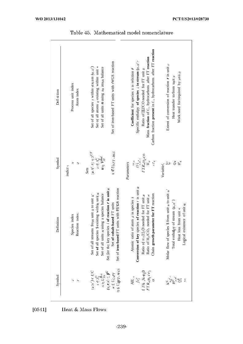
Svm
hol
Def
initi
onSy
mbo
lD
efini
tion
indi
ctSp
ecie
sin
dex
Proc
ess
unit
inde
xR
eact
ion
inde
x.A
tom
inde
x
Sets
:')
fcC
Set
ofa
llst
ream
sfr
oun
itto
unit
'.t
.sSe
tof
all
spec
ies
with
intr
ami
.)
Set
ofal
lsp
ecie
s$
exis
ting
wit
hi
uni
Set
oal
lat
oms
exis
ting
with
inun
it«
Set
ofal
lun
itsus
ing
asp
ecie
sba
lanc
eu
vi
Set
ofal
lun
itsn
usin
ga
ato
bala
nce
(r.
xfi
Se
orth
key
spec
ies
iof
reac
tion
rin
unit
£Se
tof
coba
lt-b
ased
FT
units
eSe
to
fir
on-b
ased
FT
units
with
rWG
Sre
actio
n
t6if
-Se
tof
iron
-bas
edF
Tun
itsw
ithf
GS
reac
tion
Par
amet
ers
AIL
,.A
tom
icra
tioo
fato
min
spec
ies
sV
VC
oeff
icie
ntfo
rsp
ecie
ss
inre
lictio
nr
Con
vers
ion
ofke
ysp
ecie
so
fre
acti
onr
inun
it//
:.
Spec
ific
enth
alpy
ofsp
ecie
sin
stre
am(
.'·
f¾
,¾-
0R
atio
oH
..T
need
edfo
rFT
unit
Rat
ioof
2C
One
eded
for
FTun
it'
Rat
ioof
HC
One
eded
for
FTun
itM
ass
frac
tion
ofC
..hy
droc
arbo
nsaf
ter
FT
reac
tion
Cha
ingr
owth
para
met
erfo
rF
Tre
actio
nC
arbo
nfr
actio
npr
esen
tin
C„
hydr
ocar
bons
afte
rFT
reac
tion
Var
iabl
e!,
Mol
arfl
owof
spec
ies
$fr
omun
itto
unit
'E
xten
tof
conv
ersi
ono
fre
actio
nr
inun
it
Tot
alen
tha
yof
stre
am(
,
QH
eat
tran
sfer
to/f
rom
uit
Hea
tlo
ssfr
omun
it«
Wor
kne
edfo
r/re
quir
edby
ni
v«
Log
ical
exis
tenc
eo
fun
it

[0542] Mass flow for all species is constrained by either a species balance
(Eqn. 1/Eqn. 2 of Baliban et al., 2011, which is incorporated herein by reference
as if fully set forth, or an atom balance (Eqn. 3/Eqn. 3 of Baliban et al., 2011,
which is incorporated herein by reference as if fully set forth. The units requiring
a species balance, Us Bal , will include the mixer units, the splitter units, and the
flash units. The remainder of the units detailed in the above five figures will
require an atom balance, UAtBal . The species balance is used for all units that are
governed by a set of reactions ((u, r, s ) ≡ Ru) with known extents of
conversion - of a key species (Eqn. 381).
(381)
i ' . s S u,u' S (3
82)
[0543] Heat balances across every unit are maintained using Equation 383
(Eqn. 12 of Baliban et al., 2011, which is incorporated herein by reference as if
fully set forth). The relevant terms include the input and output stream
enthalpies (H), the heat transferred to/from the unit (Q), the heat lost from the
unit (Q ), and the work done by the unit (W). Note that Equation 383 is a general
equation for the entire CBGTL refinery, and some of the terms are not needed for
each unit. Specifically, the heat loss across all units in the hydrocarbon
production and upgrading section is negligible (Q = 0). The total enthalpy of a
stream is related to the enthalpy of the individual components through Equation
384 (Eqn. 13 of Baliban et al., 2011, which is incorporated herein by reference as
if fully set forth) only for streams with known thermodynamic conditions. Each
unit in the hydrocarbon production and upgrading section unit will operate at a
known temperature and pressure, so the specific outlet enthalpies of each species,
Hu,u',ss in these units can be determined a priori. Note that Equations 383 and
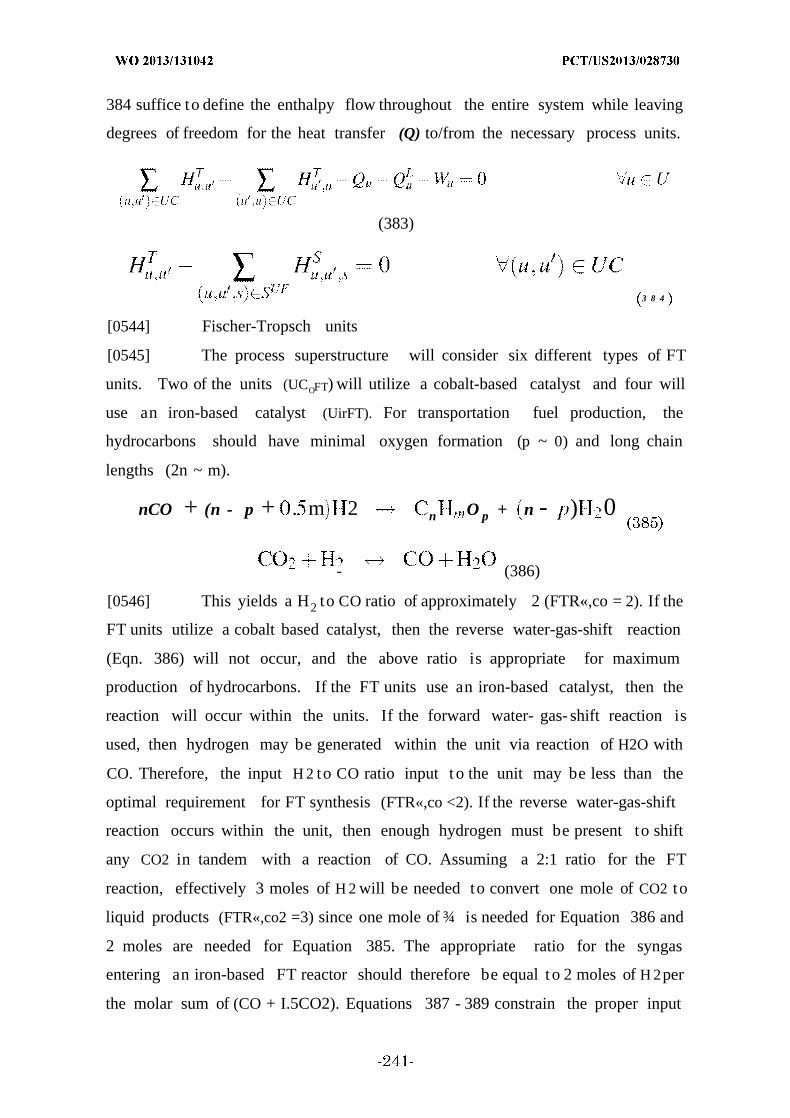
384 suffice to define the enthalpy flow throughout the entire system while leaving
degrees of freedom for the heat transfer (Q) to/from the necessary process units.
(383)
3 8 4
[0544] Fischer-Tropsch units
[0545] The process superstructure will consider six different types of FT
units. Two of the units (UCOFT) will utilize a cobalt-based catalyst and four will
use an iron-based catalyst (UirFT). For transportation fuel production, the
hydrocarbons should have minimal oxygen formation (p ~ 0) and long chain
lengths (2n ~ m).
nCO + (n - p + . m 2 n O p + n - ) 0
- (386)
[0546] This yields a H2 to CO ratio of approximately 2 (FTR«,co = 2). If the
FT units utilize a cobalt based catalyst, then the reverse water-gas-shift reaction
(Eqn. 386) will not occur, and the above ratio is appropriate for maximum
production of hydrocarbons. If the FT units use an iron-based catalyst, then the
reaction will occur within the units. If the forward water- gas- shift reaction is
used, then hydrogen may be generated within the unit via reaction of H2O with
CO. Therefore, the input H 2 to CO ratio input t o the unit may be less than the
optimal requirement for FT synthesis (FTR«,co <2). If the reverse water-gas-shift
reaction occurs within the unit, then enough hydrogen must be present to shift
any CO2 in tandem with a reaction of CO. Assuming a 2:1 ratio for the FT
reaction, effectively 3 moles of H 2 will be needed to convert one mole of CO2 to
liquid products (FTR«,co2 =3) since one mole of ¾ is needed for Equation 386 and
2 moles are needed for Equation 385. The appropriate ratio for the syngas
entering an iron-based FT reactor should therefore be equal t o 2 moles of H 2per
the molar sum of (CO + I.5CO2). Equations 387 - 389 constrain the proper input

ratios for ¾ , CO, CO2, and H2O. Due to the use of the water-gas-shift reaction in
the iron-based units, several light gas streams can also be directed to these units.
The effluent stream from the auto-thermal reactor and the offgas from the
pressure- swing adsorption column are split and maybe partially sent to all four
iron-based FT units. Preheated CO2 and preheated H 2 can also be input to the
two iron-based reverse WGS units while preheated steam can be input to the two
iron-based forward WGS units.
(387)
T -RGS
(388)
(389)
[0547] The iron-based rWGS and cobalt-based FT units are modeled with
stoichiometric reactions with known extents of reaction for each hydrocarbon in
the effluent stream (Eqn. 381). C1-C20 paraffin and olefin hydrocarbons are
modeled directly, while C21-C29 hydrocarbons are represented by
pseudocomponents having properties consistent with 70 mol % olefin and 30 mol
% paraffin. All C30+ compounds are represented by a generic wax
pseudocomponent (C52.524H105.64sO0.335) (Bechtel, 1998, which is incorporated
herein by reference as if fully set forth). Oxygenated compounds formed in the
reactors are represented by vapor phase (C2.43H5.69O), aqueous phase
(C1.95H5.77O1.02), and organic phase (C4 .78H11.14O1.1) pseudocomponents. The total
converted carbon present in each pseudocomponent is 0.1%, 1.0%, and 0.4%,
respectively (Bechtel, 1998, which is incorporated herein by reference as if fully
set forth).
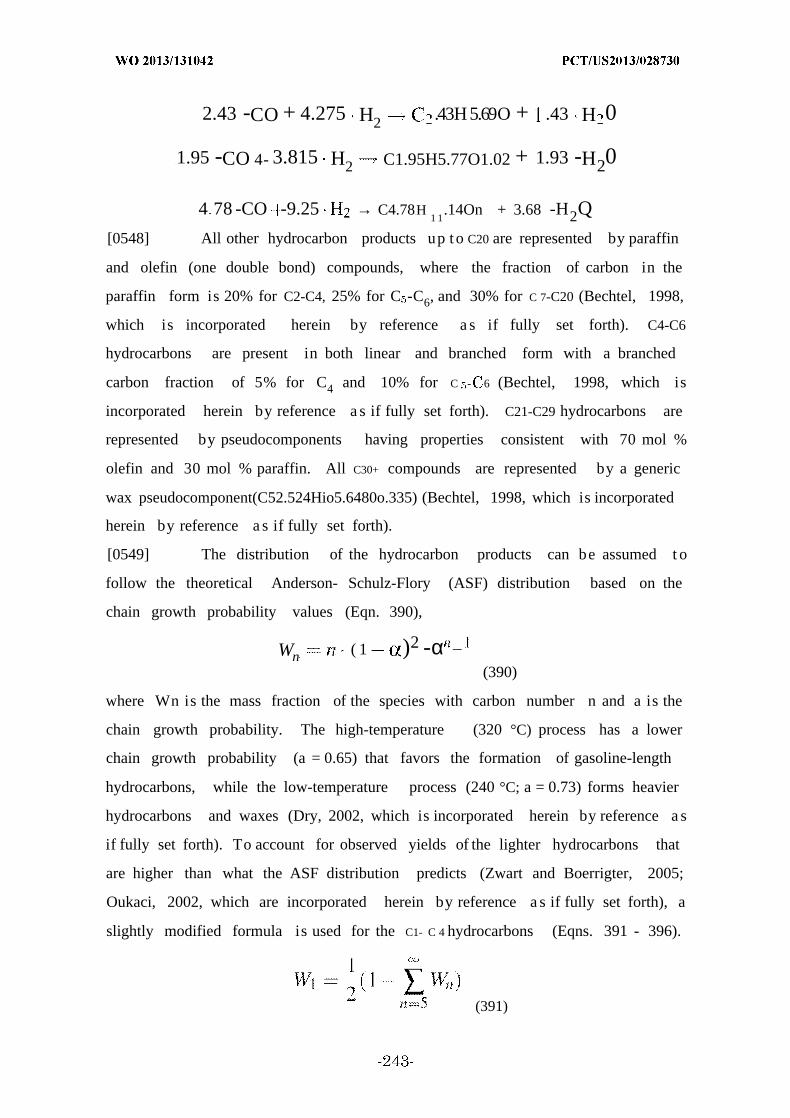
2.43 -CO + 4.275 H2 .43H 5.69O + .43 H 0
1.95 -CO 4- 3.815 H2 C1.95H5.77O1.02 + 1.93 -H20
4 78 -CO -9.25 → C4.78H1 1
.14On + 3.68 -H2Q
[0548] All other hydrocarbon products up t o C20 are represented by paraffin
and olefin (one double bond) compounds, where the fraction of carbon in the
paraffin form is 20% for C2-C4, 25% for C -C6, and 30% for C 7-C20 (Bechtel, 1998,
which is incorporated herein by reference a s if fully set forth). C4-C6
hydrocarbons are present in both linear and branched form with a branched
carbon fraction of 5% for C4 and 10% for C - 6 (Bechtel, 1998, which is
incorporated herein by reference a s if fully set forth). C21-C29 hydrocarbons are
represented by pseudocomponents having properties consistent with 70 mol %
olefin and 30 mol % paraffin. All C30+ compounds are represented by a generic
wax pseudocomponent(C52.524Hio5.6480o.335) (Bechtel, 1998, which is incorporated
herein by reference a s if fully set forth).
[0549] The distribution of the hydrocarbon products can be assumed t o
follow the theoretical Anderson- Schulz-Flory (ASF) distribution based on the
chain growth probability values (Eqn. 390),
Wn ( 1 )2 -α _
(390)
where Wn is the mass fraction of the species with carbon number n and a is the
chain growth probability. The high-temperature (320 °C) process has a lower
chain growth probability (a = 0.65) that favors the formation of gasoline-length
hydrocarbons, while the low-temperature process (240 °C; a = 0.73) forms heavier
hydrocarbons and waxes (Dry, 2002, which is incorporated herein by reference a s
if fully set forth). To account for observed yields of the lighter hydrocarbons that
are higher than what the ASF distribution predicts (Zwart and Boerrigter, 2005;
Oukaci, 2002, which are incorporated herein by reference a s if fully set forth), a
slightly modified formula is used for the C1- C 4 hydrocarbons (Eqns. 391 - 396).
(391)

w6
(393)
> (394)
Wn = n(l )2 V5 < n < 29(395)
(396)
[0550] Given the weight fractions, the fraction of carbon present at each
hydrocarbon length, crn, is defined in Equation 397. The overall conversion of
carbon in each reactor is assumed to be fixed at 80 mol% using a slurry-phase
system (Kreutz et al., 2008, which is incorporated herein by reference as if fully
set forth). For the cobalt based units, this will represent an 80% conversion of the
CO in the input stream and, for the iron rWGS units, this will represent the
combined conversion of CO and CO2 in the input stream. The fractional
conversion of carbon to a given hydrocarbon product is determined using the
expected amount of carbon at the product chain length (crn) and the information
provided by the distribution of paraffin and olefin provided by Bechtel, 1998,
which is incorporated herein by reference as if fully set forth.
n -Wn
[0551] The iron-based FT fWGS effluent composition is based off of the
slurry phase FT units developed by Mobil Research and Development
Corporation in the 1980's (Mobil Research and Development Corporation, 1983;
Mobil Research and Development Corporation, 1985, which are incorporated
herein by reference as if fully set forth). A H 2/CO ratio of 2/3 is desired for the

input feed (Mobil Research and Development Corporation, 1983; Mobil Research
and Development Corporation, 1985, which are incorporated herein by reference
as if fully set forth), so a sufficient amount of steam must be added to the feed to
promote the forward water-gas-shift reaction. The decomposition of carbon from
CO to hydrocarbons and CO2 is outlined in Table 42 of the minimal-wax FT
report [(Mobil Research and Development Corporation, 1983, which is
incorporated herein by reference as if fully set forth) and Table VIII-2 of the
nominal-wax FT report (Mobil Research and Development Corporation, 1985,
which is incorporated herein by reference as if fully set forth). This information is
represented in the mathematical model using the species balance and the extent
of reaction equation (Eqns. 380 - 381) and assuming an 90% conversion of the CO
in the inlet stream (Mobil Research and Development Corporation, 1983; Mobil
Research and Development Corporation, 1985, which are incorporated herein by
reference as if fully set forth).
[0552] The logical use of only one type of minimal- wax FT unit is given by
Equation 398 while the logical use of only one nominal-wax unit is given by
Equation 399.
either (i) fractionate the hydrocarbon stream and upgrade each of the fractions or
(ii) catalytically convert all of the hydrocarbons to gasoline-range hydrocarbons
over a ZSM-5 catalyst. The wax effluent from the FT reactors will be directed to a
hydrocracker to convert the wax into naphtha and distillate (Bechtel, 1998;
(Mobil Research and Development Corporation, 1983; Mobil Research and
Development Corporation, 1985; Baliban et al., 2011, which are incorporated
herein by reference as if fully set forth).
[0555] If fractionation of the vapor effluent is desired, then the water
formed during synthesis of the hydrocarbons must be initially separated from the
stream. The effluent is initially sent to a water soluble oxygenates separator. It is
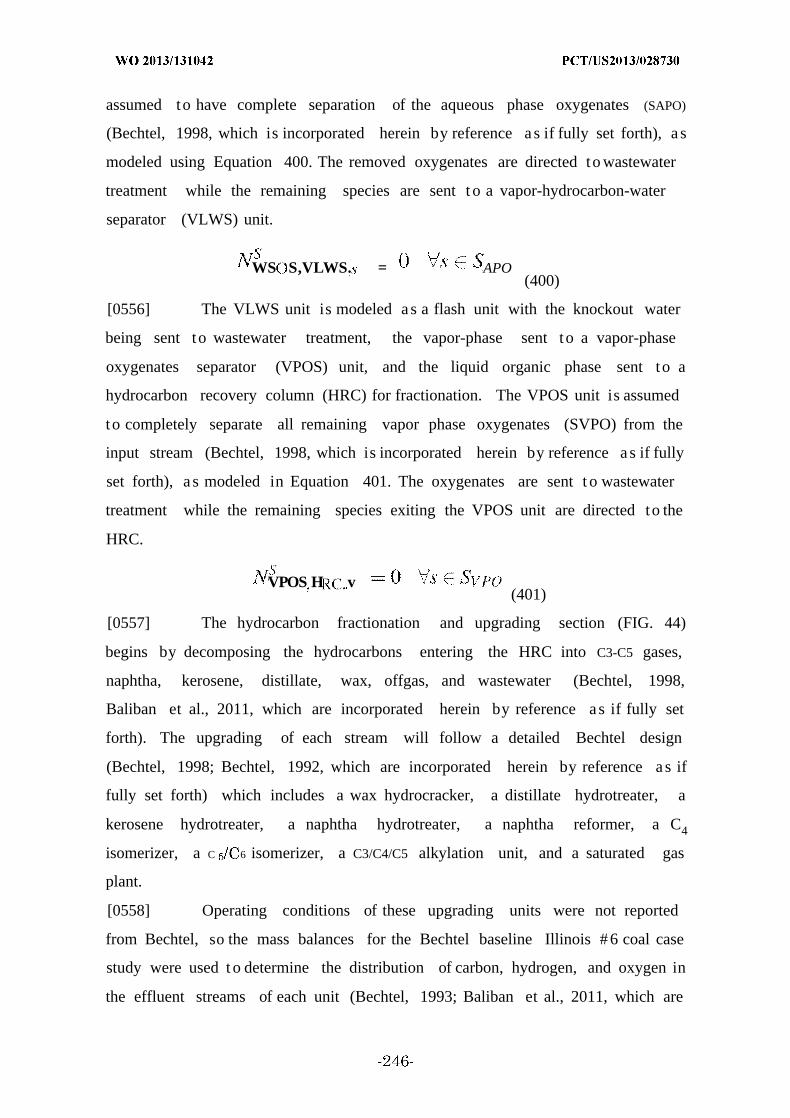
assumed to have complete separation of the aqueous phase oxygenates (SAPO)
(Bechtel, 1998, which is incorporated herein by reference a s if fully set forth), a s
modeled using Equation 400. The removed oxygenates are directed to wastewater
treatment while the remaining species are sent t o a vapor-hydrocarbon-water
separator (VLWS) unit.
WS S,VLWS. = APO(400)
[0556] The VLWS unit is modeled a s a flash unit with the knockout water
being sent to wastewater treatment, the vapor-phase sent to a vapor-phase
oxygenates separator (VPOS) unit, and the liquid organic phase sent to a
hydrocarbon recovery column (HRC) for fractionation. The VPOS unit is assumed
to completely separate all remaining vapor phase oxygenates (SVPO) from the
input stream (Bechtel, 1998, which is incorporated herein by reference a s if fully
set forth), a s modeled in Equation 401. The oxygenates are sent t o wastewater
treatment while the remaining species exiting the VPOS unit are directed to the
HRC.
VPOS H v(401)
[0557] The hydrocarbon fractionation and upgrading section (FIG. 44)
begins by decomposing the hydrocarbons entering the HRC into C3-C5 gases,
naphtha, kerosene, distillate, wax, offgas, and wastewater (Bechtel, 1998,
Baliban et al., 2011, which are incorporated herein by reference a s if fully set
forth). The upgrading of each stream will follow a detailed Bechtel design
(Bechtel, 1998; Bechtel, 1992, which are incorporated herein by reference a s if
fully set forth) which includes a wax hydrocracker, a distillate hydrotreater, a
kerosene hydrotreater, a naphtha hydrotreater, a naphtha reformer, a C4
isomerizer, a C 6 isomerizer, a C3/C4/C5 alkylation unit, and a saturated gas
plant.
[0558] Operating conditions of these upgrading units were not reported
from Bechtel, so the mass balances for the Bechtel baseline Illinois # 6 coal case
study were used t o determine the distribution of carbon, hydrogen, and oxygen in
the effluent streams of each unit (Bechtel, 1993; Baliban et al., 2011, which are
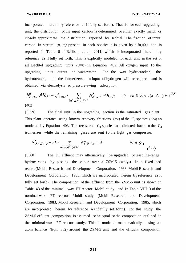
incorporated herein by reference as if fully set forth). That is, for each upgrading
unit, the distribution of the input carbon is determined t o either exactly match or
closely approximate the distribution reported by Bechtel. The fraction of input
carbon in stream (u, u') present in each species s is given by c fu,u0,s and is
reported in Table 6 of Baliban et al., 2011, which is incorporated herein by
reference as if fully set forth. This is explicitly modeled for each unit in the set of
all Bechtel upgrading units (UUG) in Equation 402. All oxygen input to the
upgrading units output as wastewater. For the wax hydrocracker, the
hydrotreaters, and the isomerizers, an input of hydrogen will be required and is
obtained via electrolysis or pressure-swing adsorption.
Nf , AR f , N -AR = 0 V 6 , (a «', i )
(402)
[0559] The final unit in the upgrading section is the saturated gas plant.
This plant operates using known recovery fractions (r/«) of the C4 species (Sc4) as
modeled by Equation 403. The recovered C4 species are directed back to the C4
isomerizer while the remaining gases are sent t o the light gas compressor.
S ∑ s = S403
[0560] The FT effluent may alternatively be upgraded to gasoline-range
hydrocarbons by passing the vapor over a ZSM-5 catalyst in a fixed bed
reactor(Mobil Research and Development Corporation, 1983; Mobil Research and
Development Corporation, 1985, which are incorporated herein by reference as if
fully set forth). The composition of the effluent from the ZSM-5 unit is shown in
Table 43 of the minimal- wax FT reactor Mobil study and in Table VIII- 3 of the
nominal-wax FT reactor Mobil study (Mobil Research and Development
Corporation, 1983; Mobil Research and Development Corporation, 1985, which
are incorporated herein by reference as if fully set forth). For this study, the
ZSM-5 effluent composition is assumed to be equal to the composition outlined in
the minimal-wax FT reactor study. This is modeled mathematically using an
atom balance (Eqn. 382) around the ZSM-5 unit and the effluent composition
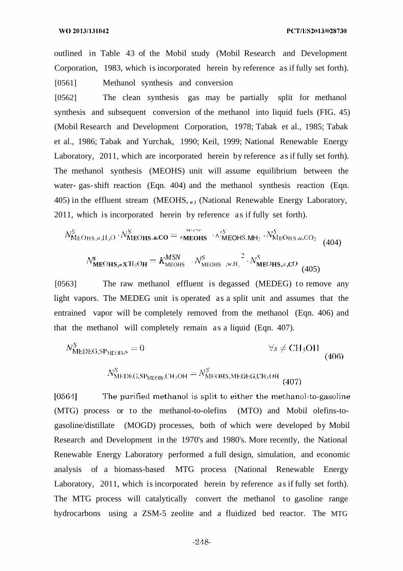
outlined in Table 43 of the Mobil study (Mobil Research and Development
Corporation, 1983, which is incorporated herein by reference as if fully set forth).
[0561] Methanol synthesis and conversion
[0562] The clean synthesis gas may be partially split for methanol
synthesis and subsequent conversion of the methanol into liquid fuels (FIG. 45)
(Mobil Research and Development Corporation, 1978; Tabak et al., 1985; Tabak
et al., 1986; Tabak and Yurchak, 1990; Keil, 1999; National Renewable Energy
Laboratory, 2011, which are incorporated herein by reference as if fully set forth).
The methanol synthesis (MEOHS) unit will assume equilibrium between the
water- gas- shift reaction (Eqn. 404) and the methanol synthesis reaction (Eqn.
405) in the effluent stream (MEOHS, u ) (National Renewable Energy Laboratory,
2011, which is incorporated herein by reference as if fully set forth).
E HS , , , ' E HS .a.CO ^MEOHS ' Λ ' ΜΕΟΗ ΜΗ * ' E H S , .,C(404)
7$ _ MSN rSME HS,«X H MEOHS ' MEOHS ,w.H
7. ME HS, ,C(405)
[0563] The raw methanol effluent is degassed (MEDEG) to remove any
light vapors. The MEDEG unit is operated as a split unit and assumes that the
entrained vapor will be completely removed from the methanol (Eqn. 406) and
that the methanol will completely remain as a liquid (Eqn. 407).
(MTG) process or to the methanol-to-olefins (MTO) and Mobil olefins-to-
gasoline/distillate (MOGD) processes, both of which were developed by Mobil
Research and Development in the 1970's and 1980's. More recently, the National
Renewable Energy Laboratory performed a full design, simulation, and economic
analysis of a biomass-based MTG process (National Renewable Energy
Laboratory, 2011, which is incorporated herein by reference as if fully set forth).
The MTG process will catalytically convert the methanol to gasoline range
hydrocarbons using a ZSM-5 zeolite and a fluidized bed reactor. The MTG
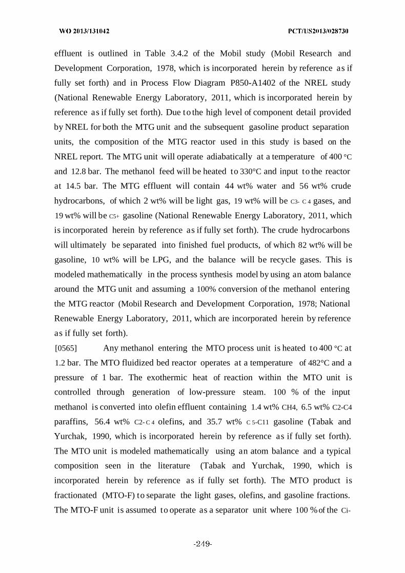
effluent is outlined in Table 3.4.2 of the Mobil study (Mobil Research and
Development Corporation, 1978, which is incorporated herein by reference as if
fully set forth) and in Process Flow Diagram P850-A1402 of the NREL study
(National Renewable Energy Laboratory, 2011, which is incorporated herein by
reference as if fully set forth). Due to the high level of component detail provided
by NREL for both the MTG unit and the subsequent gasoline product separation
units, the composition of the MTG reactor used in this study is based on the
NREL report. The MTG unit will operate adiabatically at a temperature of 400 °C
and 12.8 bar. The methanol feed will be heated to 330°C and input to the reactor
at 14.5 bar. The MTG effluent will contain 44 wt% water and 56 wt% crude
hydrocarbons, of which 2 wt% will be light gas, 19 wt% will be C3- C 4 gases, and
19 wt% will be C5+ gasoline (National Renewable Energy Laboratory, 2011, which
is incorporated herein by reference as if fully set forth). The crude hydrocarbons
will ultimately be separated into finished fuel products, of which 82 wt% will be
gasoline, 10 wt% will be LPG, and the balance will be recycle gases. This is
modeled mathematically in the process synthesis model by using an atom balance
around the MTG unit and assuming a 100% conversion of the methanol entering
the MTG reactor (Mobil Research and Development Corporation, 1978; National
Renewable Energy Laboratory, 2011, which are incorporated herein by reference
as if fully set forth).
[0565] Any methanol entering the MTO process unit is heated to 400 °C at
1.2 bar. The MTO fluidized bed reactor operates at a temperature of 482°C and a
pressure of 1 bar. The exothermic heat of reaction within the MTO unit is
controlled through generation of low-pressure steam. 100 % of the input
methanol is converted into olefin effluent containing 1.4 wt% CH4, 6.5 wt% C2-C4
paraffins, 56.4 wt% C2- C 4 olefins, and 35.7 wt% C 5-C11 gasoline (Tabak and
Yurchak, 1990, which is incorporated herein by reference as if fully set forth).
The MTO unit is modeled mathematically using an atom balance and a typical
composition seen in the literature (Tabak and Yurchak, 1990, which is
incorporated herein by reference as if fully set forth). The MTO product is
fractionated (MTO-F) to separate the light gases, olefins, and gasoline fractions.
The MTO-F unit is assumed to operate as a separator unit where 100 %of the Ci-

C 3 paraffins are recycled back to the refinery, 100 % of the C4 paraffins and 100
% of the olefins are directed t o the MOGD unit, 100 % of the gasoline is combined
with the remainder of the gasoline generated in the process, and 100 % of the
water generated in the MTO unit is sent for wastewater treatment.
[0566] The separated olefins are sent t o the MOGD unit where a fixed bed
reactor is used t o convert the olefins t o gasoline and distillate over a ZSM-5
catalyst. The gasoline/distillate product ratios can range from 0.12 to >100, and
the ratio chosen in this study was 0.12 to maximize the production of diesel. The
MOGD unit operates at 400 °C and 1 bar and will utilize steam generation to
remove the exothermic heat of reaction within the unit. The MOGD unit is
modeled with an atom balance and will produce 82% distillate, 15% gasoline, and
3% light gases (Tabak and Yurchak, 1990, which is incorporated herein by
reference as if fully set forth). The product will be fractionated (MTODF) to
remove diesel and kerosene cuts from the gasoline and light gases. The MTODF
unit will be modeled as a separator unit where 100 % of the C11-C13 species are
directed t o the kerosene cut and 100 % of the C14+ species are directed to the
diesel cut.
[0567] LPG-gasoline separation
[0568] The LPG and gasoline generated from ZSM-5 conversion of the FT
hydrocarbons or the methanol must be passed through a series of separation
units to extract the LPG from the gasoline and alkylate any iso-butane t o a
blending stock for the final gasoline pool (FIG. 46). Light gases are initially
removed via one of two knock-out units, and the crude hydrocarbons are passed
through a deethanizer column, a stabilizer column, an absorber column, a splitter
column, and an LPG alkylate splitter t o separate the LPG from the gasoline
fractions. Each of these units is modeled mathematically as a splitter unit where
the split fraction of each species t o an output stream is given by the information
in the Process Flow Diagrams P850-A1501 and P850-A1502 from the NREL
study (National Renewable Energy Laboratory, 2011, which is incorporated
herein by reference as if fully set forth). All low pressure steam and cooling water
needed for each of the units is derived for each of the units in the NREL study.
The total amount of process utility that is needed per unit flow rate from the top

or bottom of the column is calculated, and this ratio is used as a parameter in the
process synthesis model t o determine the actual amount of each utility needed
based on the unit flow rate.
[0569] In addition t o the distillation columns within this section, there is
also an alkylation unit that is used to convert iso-butane and butene to an
alkylate blending stock for the gasoline pool. The alkylate was modeled as iso-
butane(National Renewable Energy Laboratory, 2011, which is incorporated
herein by reference as if fully set forth) and the alkylation unit was modeled
using a species balance where the key species, butene, was completely converted
to iso-butane. Butene is used as the limiting species in this reaction because it is
generally present in a far smaller concentration than iso-butane.
[0570] Example 3.23 - Feedstock Analyses
[0571] The proximate and ultimate analyses for each of the coal and
biomass feedstocks are indluced in Table 46. The composition of the low-volatile
bituminous coal is obtained from the NETL Quality Guidelines Report (National
Energy Technology Laboratory, 2004, which is incorporated herein by reference
as if fully set forth) and the composition of the switchgrass is obtained from the
ECN Phyllis database (van der Drift and van Doom, 2002, which is incorporated
herein by reference as if fully set forth). The molar composition of the natural gas
feedstock is included in Table 47 and is derived from the Quality Guidelines
Report (National Energy Technology Laboratory, 2004, which is incorporated
herein by reference as if fully set forth).
Table 46. Feedstock proximate and ultimate analysis for biomass and coal.
. . ... Proximate Analysis (db, weight ) Heating va es (kJ/ gFeed Type
Ash VM1 FC2 I V LHV 4 "
Low-volatile Bituminous 0.65 4.77 19.26 75.97 34946 34012Switchgrass 8.2 4.6 79.2 16.2 18636 17360
Ultimate Analysis (db. weight tFeed Type )H N ' C S O
Low-volatile Bituminous 86 1 4.23 1.27 0 19 0.66 2. 17
Switchgrass 46.9 5.85 0,58 0.501 0 . 1 4 .5
1. VM = volatile matters; 2. FC = fixed carbon; 3 HHV = higher healing value;4 . LHV = lower heatins value
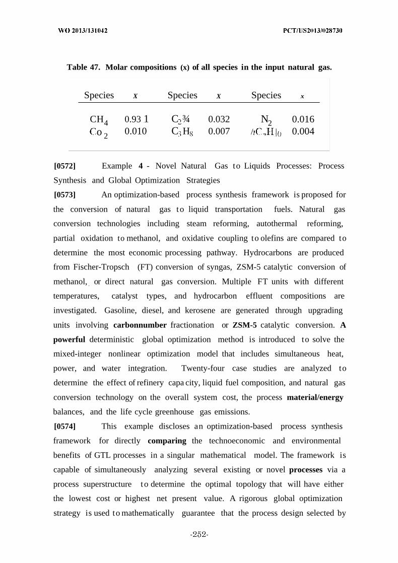
Table 47. Molar compositions (x) of all species in the input natural gas.
Species X Species X Species x
CH4 0.93 1 C ¾ 0.032 N2 0.016o 2 0.010 C H 0.007 / ., | 0.004
[0572] Example 4 - Novel Natural Gas to Liquids Processes: Process
Synthesis and Global Optimization Strategies
[0573] An optimization-based process synthesis framework is proposed for
the conversion of natural gas to liquid transportation fuels. Natural gas
conversion technologies including steam reforming, autothermal reforming,
partial oxidation to methanol, and oxidative coupling to olefins are compared to
determine the most economic processing pathway. Hydrocarbons are produced
from Fischer-Tropsch (FT) conversion of syngas, ZSM-5 catalytic conversion of
methanol, or direct natural gas conversion. Multiple FT units with different
temperatures, catalyst types, and hydrocarbon effluent compositions are
investigated. Gasoline, diesel, and kerosene are generated through upgrading
units involving carbonnumber fractionation or ZSM-5 catalytic conversion. A
powerful deterministic global optimization method is introduced to solve the
mixed-integer nonlinear optimization model that includes simultaneous heat,
power, and water integration. Twenty-four case studies are analyzed to
determine the effect of refinery capa city, liquid fuel composition, and natural gas
conversion technology on the overall system cost, the process material/energy
balances, and the life cycle greenhouse gas emissions.
[0574] This example discloses an optimization-based process synthesis
framework for directly comparing the technoeconomic and environmental
benefits of GTL processes in a singular mathematical model. The framework is
capable of simultaneously analyzing several existing or novel processes via a
process superstructure to determine the optimal topology that will have either
the lowest cost or highest net present value. A rigorous global optimization
strategy is used to mathematically guarantee that the process design selected by

the framework will have an overall cost (or profit) that is within a small
percentage of the best value possible. The disclosure in this example includes (1)
the inclusion and mathematical modeling of steam reforming of natural gas,
direct conversion of natural gas to methanol via partial oxidation, and direct
conversion of natural gas to olefins via oxidative coupling (OC) as conversion
technologies, in addition to autothermal reforming (ATR), (2) the direct usage of
natural gas in the fuel combustor unit to provide process heat and in the gas
turbine (GT) for electricity production, (3) different product compositions (i .e.,
gasoline, diesel, and kerosene) considered, namely the unrestricted composition,
maximization of diesel, maximization of kerosene, and compositions
commensurate with the U.S. demand ratio, and (4) calculations of the life cycle
emissions of GTL systems compared with petroleum-based processes and natural
gas-based electricity production. The framework includes a simultaneous heat
and power integration using an optimization-based heat-integration approach
and a series of heat engines that can convert waste heat into electricity. A
comprehensive wastewater treatment network that utilizes a superstructure
approach to determine the appropriate topology and operating conditions of
process units is utilized to minimize wastewater contaminants and freshwater
intake.
[0575] The process synthesis framework will be utilized to examine (1)
natural gas conversion via steam reforming, ATR, direct conversion to methanol,
and direct conversion to olefins, (2) synthesis gas conversion via Fischer-Tropsch
(FT) or methanol synthesis, (3) methanol conversion via methanol-togasoline
(MTG) or methanol-to-olefins (MTO), and (4) hydrocarbon upgrading via ZSM-5
zeolite catalysis, olefin oiigomerizatiori, or boiling point fractionation and
subsequent treatment. The key products from the GTL refinery will be gasoline,
diesel, and jet fuel (kerosene) with allowable byproducts of liquefied petroleum
gas (LPG) and electricity.
[0576] Example 4.1 - GTL Process Superstructure: Conceptual Design and
Mathematical Modeling
[0577] This example will detail the modeling required to introduce
additional means for natural gas conversion and the subsequent processing of the
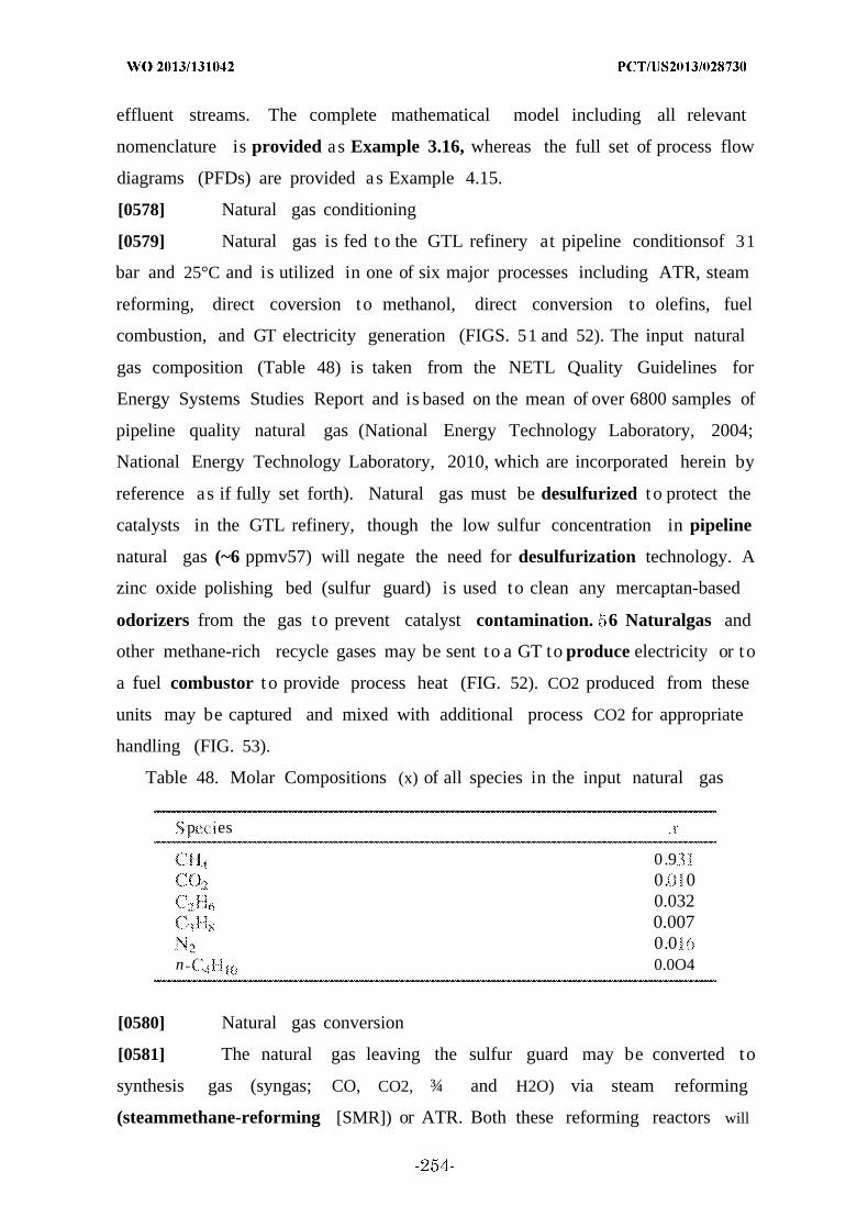
effluent streams. The complete mathematical model including all relevant
nomenclature is provided as Example 3.16, whereas the full set of process flow
diagrams (PFDs) are provided as Example 4.15.
[0578] Natural gas conditioning
[0579] Natural gas is fed to the GTL refinery at pipeline conditionsof 31
bar and 25°C and is utilized in one of six major processes including ATR, steam
reforming, direct coversion to methanol, direct conversion to olefins, fuel
combustion, and GT electricity generation (FIGS. 51 and 52). The input natural
gas composition (Table 48) is taken from the NETL Quality Guidelines for
Energy Systems Studies Report and is based on the mean of over 6800 samples of
pipeline quality natural gas (National Energy Technology Laboratory, 2004;
National Energy Technology Laboratory, 2010, which are incorporated herein by
reference as if fully set forth). Natural gas must be desulfurized t o protect the
catalysts in the GTL refinery, though the low sulfur concentration in pipeline
natural gas (~6 ppmv57) will negate the need for desulfurization technology. A
zinc oxide polishing bed (sulfur guard) is used to clean any mercaptan-based
odorizers from the gas to prevent catalyst contamination. 6 Naturalgas and
other methane-rich recycle gases may be sent to a GT to produce electricity or to
a fuel combustor t o provide process heat (FIG. 52). CO2 produced from these
units may be captured and mixed with additional process CO2 for appropriate
handling (FIG. 53).
Table 48. Molar Compositions (x) of all species in the input natural gas
p es
, 0.90. 00.0320.0070.0
n 0.0O4
[0580] Natural gas conversion
[0581] The natural gas leaving the sulfur guard may be converted to
synthesis gas (syngas; CO, CO2, ¾ and H2O) via steam reforming
(steammethane-reforming [SMR]) or ATR. Both these reforming reactors will

assume an equilibrium is reached for SMR (Eq. (408)) and the water-gas -shift
(WGS) reaction (Eq. (409)). The effluent concentrations of (¾ and higher
hydrocarbons are assumed to be negligible with respect to the concentration of
methane.
C H + 0 CO + 3 , 408
c o + co - >(409)
[0582] Steam Reforming.
[0583] Steam reforming of the natural gas uses a nickel-based catalyst
contained inside high alloy steel tubes. Heat is provided for the endothermic
reforming of methane via combustion of recycle fuel gas and additional input
natural gas over the outside of the tubes. The reformer operates at a pressure of
30 bar with typical reaction temperatures of 700-900°C. The effluent reformed
gas will be constrained by both WGS equilibrium (Eq. (410)) and SMR
equilibrium (Eq. (411)). The WGS equilibrium conserves the total molar flow
rate, so the species molar flow rates (Ns) are sufficient to accurately define the
equilibrium constraint. The SMR equilibrium constraint utilizes molar species
concentrations (x ) to account for the change in total molar flow rate. The
equilibrium constant in Eq. (411) was adjusted from the value extracted from
Aspen Plus for the higher pressure of the reforming unit. Although additional
methods exist for defining the constraints in the steam reformer (e.g., molar
species concentrations in WGS equilibrium), the current mathematical
formulation for the steam reformer provided the best computational performance
for this study. All nonhydrocarbon and nonsyngas species (e.g., N 2 and Ar) are
assumed tobe inert. The effluent reformed gas is directed to syngas cleaning (see
FIG. 53). Ambient air (13°C, 1.01 bar) is compressed to 1.1 bar to provide a 20
o % stoichiometric excess of oxygen needed for combustion of the fuel gas
within the reformer. The combusted fuel gas exits the reformer at 640°C, is cooled
to 120°C to recover waste heat, and is then directed to either the stack or a CO2
recovery unit.
[0584] Auto-thermal Reforming.
[0585] ATR of the natural gas will input a combination of steam for
endothermic reforming and high-purity oxygen for partial combustion within the
same reactor. The autothermal reformer will operate at a pressure of 30 bar with
a temperature between 700 and 1000°C. Oxygen is provided through cryogenic air
separation (99.5 wt %) or electrolysis of water (100 wt %) and is preheated to
300°C prior to entering the reformer. Steam will also be preheated to 550°C, and
the natural gas will be preheated to 300°C t o reduce the oxygen requirement
within the reformer. The molar ratio of steam to total carbon entering the
reformer will vary between 0.5 and 1.5, and the effluent will be governed by the
WGS equilibrium (Eq. (412)) and SMR equilibrium (Eq. (413)). The choice of
mathematical formulation of the autothermal effluent is similar to that of the
steam reformer and is based on computational performance.
[0586] The effluent from the autothermal reformer is directed to the
synthesis gas cleaning section (FIG. 53).
[0587] Direct Conversion to Methanol Via Partial Oxidation.
[0588] Natural gas may be directly converted to methanol via gas-phase
partial oxidation operated by a free radical mechanism. The natural gas is
compressed to 52 bar and then passed into a quartz-lined tubular reactor (POM)
operating at 450°C and 50 bar. The per-pass conversion of methane (fc) is 13%59
(Eq. (414)) with a carbon distribution (cd) of 63% t o CHaOH, 30% t o CO, 6% t o
CO2, and 1% to 2¾ (Eq. (415)), where SpoM represents the set of species that
are formed from conversion of the methane. Under the reaction conditions
assumed in this study, all formaldehyde is assumed to decompose quickly to H 2
and CO. 7 Oxygen is provided via an air separation unit (99.5 wt %) or
electrolysis (100 wt %) with subsequent compression to 52 bar.
(415)
[0589] The effluent from the reactor is combined with the effluent from the
methanol generated from synthesis gas, cooled t o 35°C, and flashed to separate
the methanol/water mixture. The recycle gases are either (1) recompressed and
recycled t o the POM reactor, (2) heated to 500°C and expanded to 30 bar for use in
a GT, or (3) heated to 500°C and expanded to 1.3 bar for use a s fuel gas. The
crude methanol /water mixture is combined with additional methanol from the
plant prior t o degassing and subsequent processing.
[0590] Direct Conversion to Olefins Via OC.
[0591] Natural gas can be contacted with a reducible metal oxide catalyst to
promote oxidative dehydrogenation via free radical formation. The reactor (OCO)
is assumed to operate a t 800°C and 3.8 bar64 with suitable expansion of the
natural gas to recover electricity from a turbine. A typical CH4 conversion (fc)
over a 15% Mn, 5% Na-iP20y S 0 2 catalyst is 22% with a 77% selectivity (cd) t o
C-2+ hydrocarbons.
. .J~ ~ / . V . C ., OC )
:x : .>. , (416)
v..S .... i(417)
[0592] This assumes that the per-pass conversion of CE is 25% (Eq. (416))
with a product composition show in Table 49. The distribution of paraffins and
olefins for C2- 5 hydrocarbons was assumed to be equal to that of the C 2 species,
and the C4- C 5 species were assumed to be linear. Equation (417) shows the
mathematical constraint for distribution of carbon from the input hydrocarbons
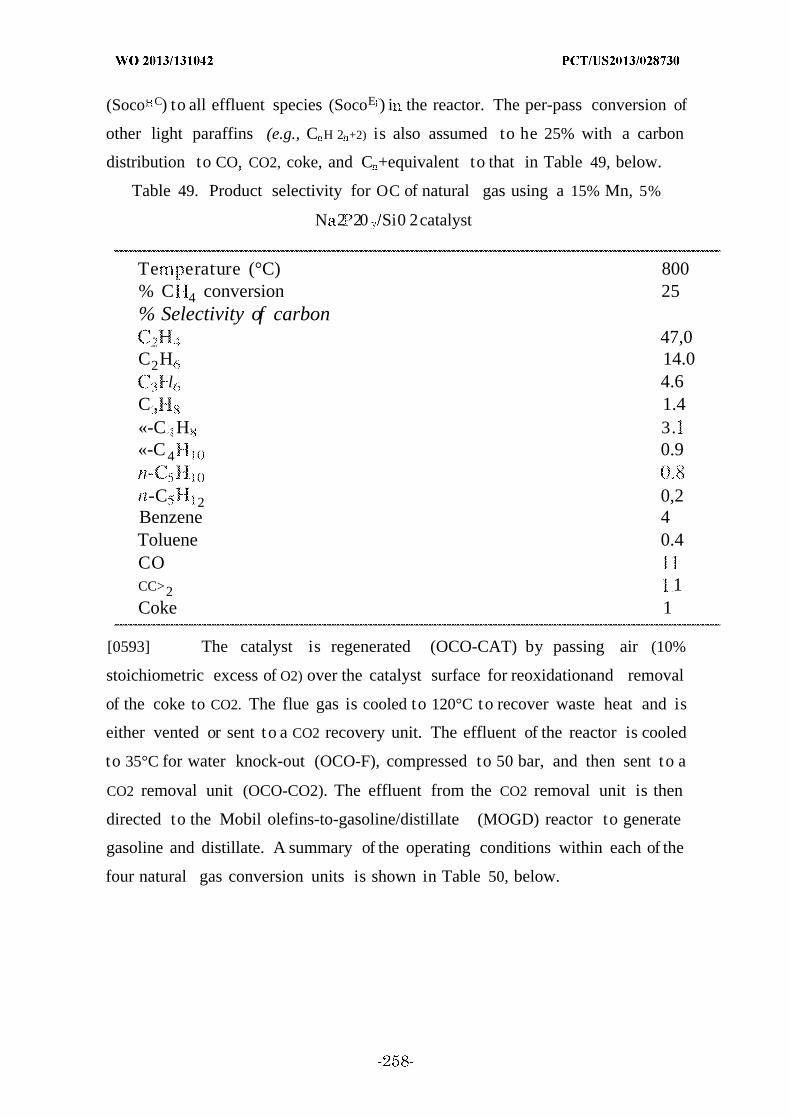
(Soco C) to all effluent species (SocoE ) i the reactor. The per-pass conversion of
other light paraffins (e.g., C H 2 +2) is also assumed to he 25% with a carbon
distribution to CO, CO2, coke, and C +equivalent to that in Table 49, below.
Table 49. Product selectivity for OC of natural gas using a 15% Mn, 5%
N 2 20 Si0 2catalyst
Te erature (°C) 800% C 4 conversion 25% Selectivity of carbon
47,0C2H 14.0
l 4.6C , 1.4«-C H 3.«-C 4 0.9
-C 2 0,2Benzene 4Toluene 0.4COCC>2 1Coke 1
[0593] The catalyst is regenerated (OCO-CAT) by passing air (10%
stoichiometric excess of O2) over the catalyst surface for reoxidationand removal
of the coke to CO2. The flue gas is cooled to 120°C to recover waste heat and is
either vented or sent to a CO2 recovery unit. The effluent of the reactor is cooled
to 35°C for water knock-out (OCO-F), compressed to 50 bar, and then sent to a
CO2 removal unit (OCO-CO2). The effluent from the CO2 removal unit is then
directed to the Mobil olefins-to-gasoline/distillate (MOGD) reactor to generate
gasoline and distillate. A summary of the operating conditions within each of the
four natural gas conversion units is shown in Table 50, below.
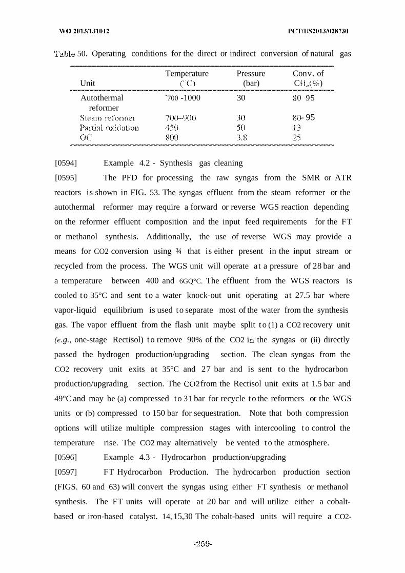
50. Operating conditions for the direct or indirect conversion of natural gas
Temperature Pressure Conv. ofUnit (bar) C , )
Autothermal 700 -1000 30 0 95reformer
- 95
[0594] Example 4.2 - Synthesis gas cleaning
[0595] The PFD for processing the raw syngas from the SMR or ATR
reactors is shown in FIG. 53. The syngas effluent from the steam reformer or the
autothermal reformer may require a forward or reverse WGS reaction depending
on the reformer effluent composition and the input feed requirements for the FT
or methanol synthesis. Additionally, the use of reverse WGS may provide a
means for CO2 conversion using ¾ that is either present in the input stream or
recycled from the process. The WGS unit will operate at a pressure of 28 bar and
a temperature between 400 and 6GQ°C. The effluent from the WGS reactors is
cooled t o 35°C and sent t o a water knock-out unit operating at 27.5 bar where
vapor-liquid equilibrium is used to separate most of the water from the synthesis
gas. The vapor effluent from the flash unit maybe split t o (1) a CO2 recovery unit
(e.g., one-stage Rectisol) to remove 90% of the CO2 i the syngas or (ii) directly
passed the hydrogen production/upgrading section. The clean syngas from the
CO2 recovery unit exits at 35°C and 27 bar and is sent to the hydrocarbon
production/upgrading section. The 2from the Rectisol unit exits at 1.5 bar and
49°C and may be (a) compressed to 31 bar for recycle t o the reformers or the WGS
units or (b) compressed to 150 bar for sequestration. Note that both compression
options will utilize multiple compression stages with intercooling t o control the
temperature rise. The CO2 may alternatively be vented t o the atmosphere.
[0596] Example 4.3 - Hydrocarbon production/upgrading
[0597] FT Hydrocarbon Production. The hydrocarbon production section
(FIGS. 60 and 63) will convert the syngas using either FT synthesis or methanol
synthesis. The FT units will operate at 20 bar and will utilize either a cobalt-
based or iron-based catalyst. 14, 15,30 The cobalt-based units will require a CO2-
lean synthesis gas feed to prevent poisoning of the FT catalyst and increase
conversion of the CO. The iron-based catalysts may use either the C()2 -lean or
CQ2 -rieh syngas, because the WGS reaction will be facilitated by the iron
catalyst. Therefore, these reactors could consume CO2 within the unit using H 2 to
produce the CO necessary for the FT reaction.
[0598] Synthesis gas is split to either the low-wax FT section (SPFTM), the
nominal wax FT section (8PFTN), or methanol synthesis (MEOHS). The FT units
will operate within the temperature range of 240--320°C. The cobalt-based FT
units operate at either low temperature (LTFT; 240°C) or high temperature
(HTFT; 320°C) and must have a minimal amount of CO2 in the input stream. Two
iron-based FT units will facilitate the WGS reaction and will operate at low
(LTFTRGS; 240°C) and high temperature (HTFTRG8; 320°C). The other two iron-
based FT units will operate at a mid-level temperature (267°C), and produce
either minimal (MTFTWGS-M) or nominal (MTFTWGS-N) amounts ofwax. Each
of the four iron-based FT units may facilitate either the forward or the reverse
WGS reaction.
[0599] Hydrogen may be recycled to any of the FT units to either shift the
H 2/CO ratio or the 2 C 2 ratio to the appropriate level. Steam may alternatively
be used as a feed for the two iron-based fW S FT units to shift the H2/CO ratio.
CO2 may be recycled back to the iron-based FT units to be consumed in the WGS
reaction. Similarly the pressure-swing adsorption (PSA) offgas, which will be
lean in ¾ , may be recycled to the iron-based FT units for consumption of the CO
or CO2. The effluent from the autothermal reactor (ATR) will contain a H 2/CO
ratio that is generally above 2/1 and is, therefore, favorable as a feedstock for FT
synthesis. However, the concentration of CO2 within the ATR effluent will
prevent the stream from being fed to the cobalt-based units. The two streams
exiting the FT units will be a waxy liquid phase and a vapor phase containing a
range of hydrocarbons. The wax will be directed to a hydrocracker (WHC),
whereas the vapor phase is split (SPFTH) for further processing.
[0600] FT Hydrocarbon Upgrading.
[0601] The vapor phase effluent from FT synthesis will contain a mixture of
C -C30+ hydrocarbons, water, and some oxygenated species. FIG. 61 details the
process flow sheet used to process this effluent stream. The stream will be split
and can pass through a series of treatment units designed to cool the stream and
knock out the water and oxygenates for treatment. Initially, the water-soluble
oxygenates are stripped from the stream. The stream is then passed to a three-
phase separator to remove the aqueous phase from the residual vapor and any
hydrocarbon liquid. Any oxygenates that are present in the vapor phase may be
removed using an additional separation unit. The water lean FT hydrocarbons
are then sent to a hydrocarbon recovery column for fractionation and further
processing (FIG. 62). The oxygenates and water removed from the stream are
mixed and sent to the biological digestor for wastewater treatment.
[0602] The FT hydrocarbons may a so be passed over a ZSM-5 catalytic
reactor operating at 408°C and 16 bar to be converted into mostly gasoline range
hydrocarbons and some distillate. The ZSM-5 unit will be able to convert the
oxygenates to additional hydrocarbons, so no separate processing of the
oxygenates will be required for the aqueous effluent. The raw product from FT-
ZSM5 is fractionated to separate the water and distillate from the gasoline
product. The water is mixed with other wastewater knock-out and the distillate
is hydrotreated to form a diesel product. The raw ZSM-5 HC product is sent to
the LPG-gasoline separation section for further processing (FIG. 64).
[0603] The water lean FT hydrocarbons are sent to a hydrocarbon recovery
column, as shown in FIG. 62. The hydrocarbons are split into C3-C5 gases,
naphtha, kerosene, distillate, wax, offgas, and wastewater. 12, 70 The upgrading
of each stream will follow a detailed Bechtel design (Bechtel 1998; Bechtel 1992,
which are incorporated herein by reference as if fully set forth), which includes a
wax hvdrocracker, a distillate hvdrotreater, a kerosene hvdrotreater, a naphtha
hvdrotreater, a naphtha reformer, a C isomerizer, a isomerizer, a C3/C4/C5
alkylation unit, and a saturated gas plant.
[0604] Methanol Synthesis.
[0605] The methanol synthesis reactor (FIG. 63) will operate at 300°C and
50 bar and may input either the (XVrich or X lean syngas. The syngas leaving
the cleaning section must be compressed to 51 bar prior to entering the methanol
synthesis reactor. The methanol synthesis reactor will assume equilibrium is

achieved for the WGS reaction (Eq (419)) and the methanol synthesis reaction
(Eq. (418)).
CO + 2H - CH3OH(418)
and the relative concentration of 2O t o methanol in the effluent stream is
largely determined based on the input concentration of CO2 to the reactor. The
effluent from the reactor is cooled to 35°C, and a crude methanol stream is
separated vapor— iquid equilibr ium at 48 bar. The amount of methanol
that is entrained in the vapor phase is dependent on the input concentration of
syngas to the flash unit, but a majority (over 95%) of the methanol can be
recovered by enforcing a stoichiometric amount of 2in the input to the synthesis
reactor (i.e., O +3CO2) = 1). The vapor stream from the flash unit is split,
so that 5% may be purged to remove inert species, and the remaining 95% is
compressed to 51 bar and then recycled to the methanol synthesis reactor. The
purge stream is recycled back to the process and used as fuel gas.
[0607] The crude methanol product from the flash unit is heated to 200°C,
expanded to 5 bar t o recover electricity, and then cooled t o 60°C prior to entering
a degasser distillation column. The degasser will remove a l the entrained gases
from the liquid methanol/water while recovering 99.9% of the methanol. The
entrained gases are recycled back to the process for use as fuel gas. The bottoms
from the degasser will contain methanol and water, with a methanol composition
dependent on the level of CO2 input to the synthesis unit. High levels of water in
the liquid stream are not anticipated to be a concern, because the downstream
methanol processing units will yield 50 wt % water from the hydrocarbon
synthesis.
[0608] Methanol Conversion.
[0609] The purified methanol is split to either the MTG- process or to the
MTO and MOGD processes. The MTG process will catalytically convert the MTG
range hydrocarbons using a ZSM-5 zeolite and a fluidizedbed reactor. The MTG
effluent is outlined in Table 3.4.2 of the Mobil study (Mobil Research and

Development Corporation, 1978, which is incorporated herein by reference as if
fully set forth) and in PFD P850-A1402 of the NREL study (National Renewable
Energy Laboratory, 2011, which is incorporated herein by reference as if fully set
forth). Due to the high level of component detail provided by NREL for both the
MTG unit and the subsequent gasoline product separation units, the composition
of the MTG reactor used in this study is based on the NREL report. The MTG
unit will operate adiabatically at a temperature of 400°C and 12.8 bar. The
methanol feed will be pumped to 14.5 bar and heated to 330°C for input to the
reactor. The methanol will be converted to 44 wt % water and 56 wt % crude
hydrocarbons, of which 2 wt % will be light gas, 9 wt % will be C3-C4 gases, and
19 wt % will be C + gasoline. The crude hydrocarbons will ultimately be
separated into finished fuel products, of which 82 wt % will he gasoline, 10 wt %
will be LPG, and the balance will be recycle gases. This is modeled
mathematically in the process synthesis model using an atom balance around the
MTG unit and assuming a 100% conversion of the methanol entering the MTG
reactor.
[0610] Any methanol entering the MTO process unit is heated to 400°C at
1.2 bar. The MTO fluidized bed reactor operates at a temperature of 482°C and a
pressure of 1 bar. The exothermic heat of reaction within the MTO unit is
controlled through generation of low-pressure steam. One hundred percent of the
input methanol is converted into olefin effluent containing 1.4 wt % CH , 6.5 wt %
C2-C4 paraffins, 56.4 wt % C2-C4 olefins, and 35.7 wt % Ce-Cit gasoline. The MTO
unit is modeled mathematically using an atom balance and a typical composition
seen in the literature. The MTO product is fractionated (MTO-F) to separate the
light gases, olefins, and gasoline fractions. The MTO-F unit is assumed to operate
as a separator unit where 100% of the C1-C3 paraffins are recycled back to the
refinery, 100% of the C paraffins and 100% of the olefins are directed to the
MOGD unit, 100% of the gasoline is combined with the remainder of the gasoline
generated in the process, and 100% of the watergenerated in the MTO unit is
sent for wastewater treatment.
[0611] The separated olefins are sent to the MOGD unit where a fixed bed
reactor is used to convert the olefins to gasoline and distillate over a ZSM-5
catalyst. The gasoline/distillate product ratios can range from 0.12 to >100, and
the ratio chosen in this study was 0.12 to maximize the production of diesel. The
MOGD unit operates at 400°C and 1 bar and will utilize steam generation to
remove the exothermic heat of reaction within the unit. The MOGD unit is
modeled with an atom balance and will produce 82% distillate 15% gasoline, and
3% light gases. The product will be fractionated (MTODF) to remove diesel and
kerosene cuts from the gasoline and light gases. The MTODF unit will be
modeled as a separator unit where 100% of the C11AC13 species are directed to
the kerosene cut and 100% of the C1-1+ species are directed to the diesel cut,
[0612] LPG -Gasoline Separation
[0613] The LPG and gasoline generated from ZSM-5 conversion of the FT
hydrocarbons or the methanol must be passed through a series of separation
units to extract the LPG from the gasoline and alkylate any isobutane to a
blending stock for the final gasoline pool (FIG. 64). Light gases are initially
removed via one of two knock-out units, and the crude hydrocarbons are passed
through a de-ethanizer column, a stabilizer column, an absorber column, a
splitter column, and an LPG alkylate splitter to separate the LPG from the
gasoline fractions. Each of these units is modeled mathematically as a splitter
unit where the split fraction of each species to an output stream is given by the
information in the PFDs P850-A1501 and P850- A1502 from the NREL study
(National Renewable Energy Laboratory, 2011, which is incorporated herein by-
reference as if fuly set forth). All low-pressure steam and cooling water needed
for each of the units is derived for each of the units in the NREL study. The total
amount of process utility that is needed per unit flow rate from the top or bottom
of the column is calculated, and this ratio is used as a parameter in the process
synthesis model to determine the actual amount of each utility needed based on
the unit flow rate.
[0614] In addition to the distillation columns within this section, there is
also an alkylation unit that is used to convert isobutane and butene to an
alkylate blending stock for the gasoline pool. The alkylate was modeled as
isobutane, and the alkylation unit was modeled using a species balance where the
key species, butene, was completely converted to isobutane. Butene is used as the
limiting species in this reaction, because it is generally present in a far smaller
concentration than isobutane.
[0615] Example 4.4 - Hydrogen/oxygen production
[0616] Hydrogen is produced via pressure- swing adsorption or an
electrolyzer unit, whereas oxygen can be provided by the electrolyzer or a
separate air separation unit (FIG. 65).
[0617] Example 4.5 - Wastewater treatment
[0618] A complete wastewater treatment network (FIGS. 66 and 67) is
incorporated that will treat and recycle wastewater from various process units,
biowdown from the cooling tower, blowdown from the boilers, and input
freshwater. Process wastewater is treated using only a biological digestor due to
the negligible quantities of sulfur (e.g., E S) or nitrogen (e.g., NHa) that are
expected to be in the wastewater streams. Clean output of the network includes
(1) process water to the electrolyzers, (2) steam to the autothermal reformer,
steam reformer, and WGS reactor, and (3) discharged wastewater to the
environment.
[0619] Example 4.6 - Unit costs
[0620] The total direct costs, TDC, for the GTL refinery hydrocarbon
production and upgrading units are calculated using estimates from several
literature sources using the cost parameters in Table 1 and Eq. 420
TDC + BOP) -( ,5 (420)
where C0 is the installed unit cost, S is the base capacity, Sr is the actual
capacity, sf is the cost scaling factor, and BOP is the balance of plant percentage
(site preparation, utility plants, etc.). The BOP is estimated to be 20% of the total
installed unit cost. All capital cost numbers are converted to 2011 dollars using
the Chemical Engineering Plant Cost Index. 76 The cost estimates for the four
natural gas conversion technologies are included in Table 51. Cost estimates for
all other process units in the GTL refinery are taken from previous works and are
included in Example 4.
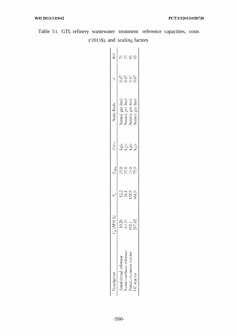
Table 51 GTL refinery wastewater treatment reference capacities, costs
^2011$), and scalin factors

[0621] The total plant cost, T C, for each unit is calculated as the sum of
the total direct capital, TDC, plus the indirect costs, C. The C include
engineering, startup, spares, royalties, and contingencies and is estimated to 32%
of the TDC. The TPC for each unit must be converted to a levelized cost to
compare with the variable feedstock and operational costs for the process. Using
the methodology of Kreutz et al., 2008, which is incorporated herein by reference
as if fully set forth, the capital charges (CC) for the refinery are calculated by
multiplying the levelized capital charge rate (LCCR) and the interest during
construction factor (IDCF) by the total overnight capital (Eq. (421)).
CC LCC X IDCF X TPC(421)
[0622] Kreutz et al. 2008, which is incorporated herein by reference as if
fully set forth, calculates an LCCR value of 14.38%/yr and an IDCF of 7.6%. Thus,
a multiplier of 15.41%/yr is used to convert the TPC into a capital charge rate.
Assuming an operating capacity (CAP) of 330 days/yr and operation/maintenance
(OM) costs equal to 5% of the TPC, the total levelizedcost (Cost ') associated with
a unit is given by Eq. (422).
are added to the complete list of GTL process units in previous studies.
[0624] Example 4.7- Objective function
[0625] The objective function for the model is given by Eq. (423). The
summation represents the total cost of liquid fuels production and includes
contributions from the feedstocks costfor natural gas (CostNG*), freshwater
(CostH20 ), a d butanes (CostBUT ), the electricity cost (Cost ), the CO2
transportation, storage, and monitoring cost (Cost ¾), and the levelized unit
investment cost (Cost ) . Each of the terms in Eq. (423) is normalized to the total
volume of products produced (Prod). Note that other normalization factors (e.g.,
total volume of gasoline equivalent and total energy of products) and other
objective functions e.g., maximizing the net present value) can be easily
incorporated into the model framework.
V C 4 -Cost ¾ ÷ Cos C st C s
[0626] The process synthesis model with simultaneous heat, power, and
water integration represents a large-scale nonconvex mixed-integer nonlinear
optimization model that was solved to global optimality using a branch-and-
bound global optimization framework. At each node in the branch-andbound tree,
a mixed-integer linear relaxation of the mathematical model is solved using
CPLEX, and then, the node is branched to create two children nodes. The
solution pool feature of CPLEX is utilized during the solution of the relaxed model
to generate a set of distinct points (150 for the root node and 10 for all other
nodes), each of which is used as a candidate starting point to solve the original
model. For each starting point, the current binary variable values are fixed, and
the resulting NLP is minimized using CONOPT. If the solution to the NLP is
less tha the current upper bound, then the upper bound is replaced with the
NLP solution value. At each step, all nodes that have a lower bound that is
within an e tolerance of the current upper bound are eliminated
from the tree
[0627] Computational Studies
[0628] The process synthesis model (see Example 3.16 and Example 4.15)
was used to analyze 24 distinct case studies using an average representation of
natural gas feedstock (Table 48). The global optimization framework was
terminated, if all nodes in the branch-and-bound tree were processed or if 100
CPU hours had passed. The case studies were chosen to examine the effect of (1)
plant capacity, (2) product composition, (3) natural gas conversion technology,
and (4) GHG reduction requirement on the overall cost of fuel production and the
optimal process topology. Four representative capacities of 1, 10, 50, and 200
kBD were chosen to examine the potential effect of economy of scale. The capacity
of the plants is defined as "barrels per stream day," which is computed by
dividing the total number of produced barrels by the actual number of days that
the GTL refinery was operational. All of the units are, therefore, appropriately

sized to a "barrels per calendar day" figure using the capacity factor of the
refinery (Eq. (422)). Liquid fuel (i.e., gasoline, diesel, and kerosene) production
was selected to either (a) represent the 2010 United States demand (i.e., 67 vol %
gasoline, 22 vol % diesel, and 11 vol % kerosene), 84 (b) maximize the diesel
production (i .e. >75 vol %), (c) maximize the kerosene production (i.e., >70 vol %),
or (d) freely output any unrestricted composition of the products. These case
studies will be labeled as N - C, where N represents the type of product
composition (i.e., R: 2010 U.S. ratios, D : max diesel, K : max kerosene, and U :
unrestricted composition) and represents the capacity in kBD. For example, the
U-l label represents the 1 kBD capacity refinery with an unrestricted product
composition.
[0629] A second set of case studies will examine the effects of the natural
gas conversion technology on the U-1 refinery. In each case study, the natural gas
conversion technology will be fixed to either ATR, steam reforming, partial
oxidation to methanol, or OC to olefins. These studies will be labeled as G-U-l,
where G represents the type of natural gas conversion technology (i.e., A :ATR, S :
steam reforming, P : partial oxidation, and C : OC). Each of the 20 case studies
described earlier will ensure that the life cycle GHG emissions from the refinery
are at most equal to current fossil-fuel-based processes. That is, the life cycle
GHG emissions must be at most equal to that of a petroleum-based refinery (91.6
kg C0 2 ¾'GJ V) for the liquid fuels or that of a natural gas combined cycle plant
(101.3 kg C0 2 GJ ) for electricity. The final four case studies will examine the
effect of the utilization of CO2 capture and sequestration on all vented streams
from the refineries with an unrestricted product composition. For each of the four
refinery capacities, a maximum of 1% of the input carbon will be allowed to be
vented to the atmosphere as CO2. The balance of the carbon must be contained
within the liquid fuels or in CO2 that is compressed and then sequestered. For
each capacity, C, the case study will be labeled as U-C-Z.
[0630] The cost parameters used for the GTL refinery are listed in Table
52. The costs for feedstocks (i.e., natural gas, freshwater, and butanes) include all
costs associated with delivery to the plant gate. The products (i.e., electricity and
propane) are assumed to be sold from the plant gate and do not include the costs

expected for transport to the end consumer. The cost of CO2 capture and
compression is included in the investment cost of the GTL refinery, whereas the
cost for transportation, storage, and monitoring of the CO2 is shown in Table 52.
Table 52. Cost parameters (2011$) for the CBGTL refinery
tem Cost Item Cost
Natural gas S TSC Fresh ter O..5 / i ri c totanes . 4/ga on Pr pan s ¾ .78/gi or
Electricity S0.07/kW h CO2 TS&M S ; e ri ton
— h standard cubic feet.S& transportation shipping, and monitoring.
[0631] Once the global optimization algorithm has completed, the resulting
process topology provides (1) the operating conditions and working fluid flow
rates of the heat engines, (2) the amount of electricity produced by the heat
engines, (3) the amount of cooling water needed for the engines, and (4) the
location of the pinch points denoting the distinct subnetworks. Given this
information, the minimum number of heat exchanger matches necessary to meet
specifications (l)-(4) are calculated as previously described. On solution of the
minimum matches model, the heat exchanger topology with the minimum
annualized cost can be found using the superstructure methodology.The
investment cost of the heat exchangers is added to the investment cost calculated
within the process synthesis model to obtain the final investment cost for the
superstructure.
[0632] Example 4.9 - Optimal process topologies
[0633] Information about the optimal process topologies for all case studies
is shown in Table 53. For natural gas conversion (NG conv.), the possible choices
are steam reforming (SMR), ATR, partial oxidation to methanol (PO), and OC.
Three possible temperature options were used for the steam reformer (700, 800,
and 900°C), the autothermal reformer (800, 900, and 1000°C), and the reverse
WGS unit (400, 500, and 600°C). For the 20 case studies that did not constrain
the natural gas conversion technology, either the steam reformer or the
autothermal reformer was selected as the optimal unit. Additionally, the
operating temperatures of these units were consistently chosen tobe at the upper
operating limit (900°C for SMR and 1000°C for ATR). The choice of operating
temperature within the reformers represents a balance among (1) the level of
input steam needed, (2) the extent of consumption of C 2 via the reverse WGS
reaction, (3) the extent of methane conversion, and (4) the fuel gas or oxygen
requirement to provide process heating. Lower reformer temperatures will have
less favorable conditions for methane conversion and CO2 consumption due to
lower values of the equilibrium constants in the reformer. Alternatively, both the
steam and the heating requirement will be smaller, decreasing the operating
costs of the unit. Higher temperatures will have higher conversions of methane
and CO2 with a correspondingly higher steam and heating requirement. Selection
of the high-temperature units shows that a key topological decision is the
conversion of methane and CO2 in the reformers. The decrease in the capital
requirement of the downstream process units outweights the increased operating
costs with a higher temperature.
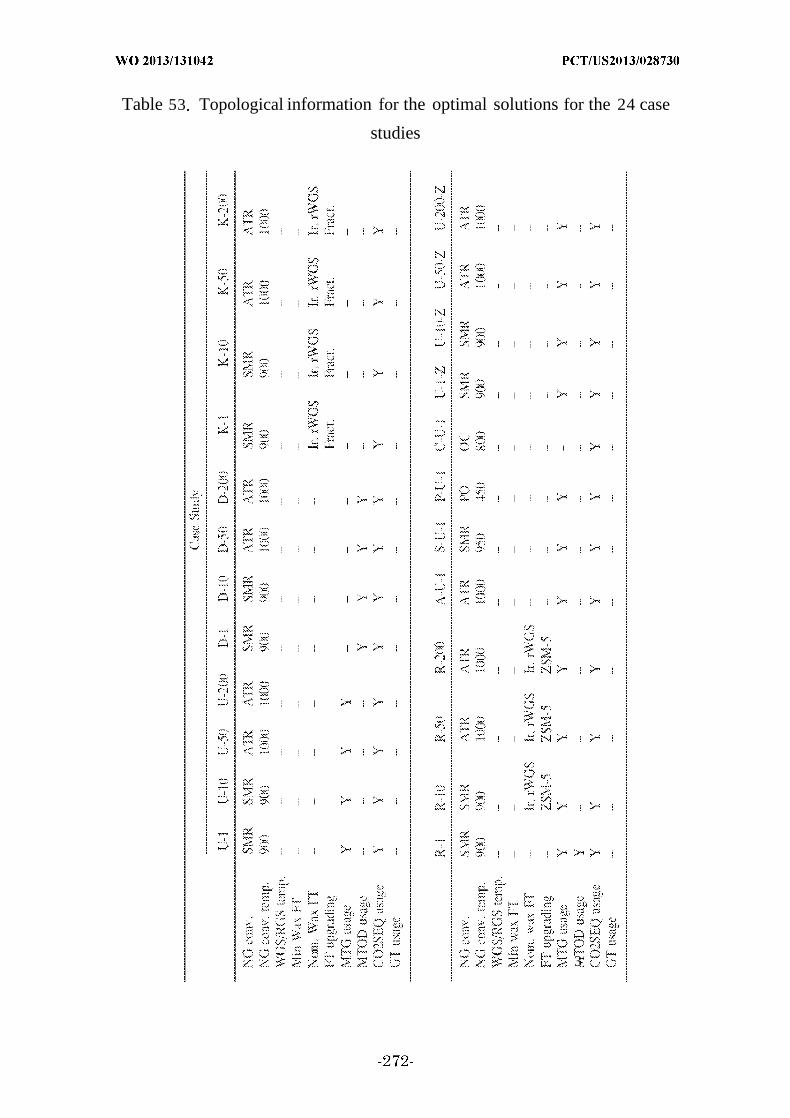
Table 53 Topological information for the optimal solutions for the 24 case
studies
3

The temperature of the conversion technology is selected along with the
operating temperature of the reverse WG unit (RGS), if utilized. The presence of
a CO2 sequestration system (C02SEQ) or a GT is noted using yes (Y) or no (N).
The minimum wax and maximum wax FT units are designated as either cobalt-
based or iron-based units. The iron-based units will either facilitate the forward
(fWGS) or reverse water gas-shift (rWGS) reaction. The FT vapor effluent will be
upgraded using fractionation into distillate and naphtha (Fract.) or ZSM-5
catalytic conversion. The use of' MTG and MTO/MOGD is noted using yes (Y) or
no (2).
[0634] Selection of a specific reformer to convert the natural gas is critical
for two major reasons. First, though the cost of a steam reformer is higher than
the autothermal reformer (Table 51), the additional cost of air separation to
produce high-purity oxygen makes the autothermal reformer a more capital
intensive choice to produce synthesis gas at lower capacity levels. However, as
the refinery capacity increases, there is a definable point where the capital and
operating costs of steam reforming are greater than the sum of ATR and air
separation. An insight can be found by observing that the scaling factor of the
reforming units is assumed to by 0.67 (Table 51), whereas that of the air
separation unit is assumed to be 0.5 based on the study by Kreutz et al., 2008,
which is incorporated herein by reference as if fully set forth, (Table 60). At
some critical capacity level, the capital cost of the air separation unit and the
autothermal reformer will be equal to that of a steam reformer, and it is
anticipated that higher capacity levels will favor ATR, whereas lower capacity
levels favor steam reforming. This is evident when comparing case studies A- -
and S-U-l. Table 55 shows that the use of an autothermal reformer adds about
5% to the investment cost of the plant and ultimately increases the cost of liquid
fuels by 7%.
[0635] Second, the use of an autothermal reformer will generally require
CO2 removal prior to entry into a methanol or FT synthesis unit. The relative
ratio of ¾ to CO or CO2 exiting the autothermal reformer is less than the ideal
stoichiometric ratio, so the synthesis gas composition must be adjusted
appropriately via addition of 2or removal of CO2. This is readily accomplished
through the use of industrially commercialized precombustion CO2 capture
technology, 75 which can provide recycle of the CO2 to the autothermal reformer.
The extent of CO2 recycle vs. venting or sequestration is dependent on the level of
heat integration within the plant and the life cycle GHG emissions requirement.
Conversely, the steam reformer will generally output a synthesis gas that has too
high of a H 2 content e.g., >5). CO2 recycle to the reformer can also be utilized to
reduce the concentration of ¾ and increase the overall carbon efficiency of the
plant. However, the C 2will need to be recovered from an atmospheric pressure
flue gas stream using postcombustion capture technology that is not as
commercially prevalent as the precombustion capture technology and will require
a higher level of process contingency.
[0636] For the autothermal reformer, any ¾ addition must be from a
noncarbon-based source (i.e., electrolyzers), because the production of ¾ from
natural gas will effectively decrease the overall carbo conversion yield of the
process and increase the level of GHG emissions. If electrolyzers were used to
produce additional ¾ , note that they will also be able to provide the 2 for the
autothermal reformer and eliminate the need for an air separation unit.
However, the high capital and operating costs of electrolysis generally prevent
these units from being an economically competitive option. Factors that could
positively impact the use of electrolyzers include (1) reducing the capital cost, (2)
increasing efficiency, (3) the resale value of excess ¾ or O2, and (4) the market
value of electricity.
[0637] None of the 24 case studies utilized a dedicated reverse WGS unit
for CO2 consumption. The equilibrium constant for the WGS reaction at the
expected operating temperatures of the dedicated unit make for less favorable
conditions tha the operating temperatures of the steam reformer or autothermal
reformer. Therefore, in the 22 case studies that used a reformer to convert
natural gas to synthesis gas, a por tio of the CO2 that was captured from the
GTL refinery was directed to the reformer for consumption. In each of the 22 case
studies, C 2 consumption also occurred in the FT or methanol synthesis units.
The reverse WGS reaction was able to occur at these lower temperatures due to
the consumption of CO for the synthesis reactions. This decrease of CO provides
the key driver for the consumption of CO2 that is otherwise unavailable in a
dedicated reverse WGS unit.
[0638] The 12 case studies that allowed for an unrestricted liquid product
composition all selected methanol synthesis and MTG s the optimal technology.
This reflects the expected reduction in capital costs associated with hydrocarbon
productionvia methanol synthesis vs. FT synthesis that come from the reduced
capital cost of methanol synthesis and MTG. Note that gasoline can be produced
from FT synthesis and subsequent conversion of the hydrocarbons to gasoline via
a ZSM-5 catalyst, but this process requires a higher capital investment over
methanol synthesis. Both the MTG and the FT/ZSM-5 processes will produce a
significant amount of byproduct LPG 9 vol %). The four case studies that
maximize the diesel production utilized the methanol-to-olefins (MTO) and the
MOGD processes to produce a high-quality diesel, whereas the four case studies
that maximize kerosene will use a iron-based low-temperature FT synthesis
followed by standard fractionation of the hydrocarbon species. The four case
studies that produce liquid fuels in the ratios consistent with United States
demands show a significant topological trade-off at different capacity levels. That
is, at the 1 kBD capacity, methanol synthesis and subsequent conversion is the
sole method for producing liquid fuels. As the capacity of the GTL refinery
increases, the iron-based low-temperature FT unit is incorporated to provide the
distillate products via wax hydrocracking and the gasoline product through ZSM-
5 conversion. Additional gasoline is produced via the MTG route to provide the
balance of the plant requirement.
[0639] In all 24 cases, CO2 sequestration was utilized to provide a
reduction in life cycle emissions for the GTL refinery. The first 20 case studies
only incorporate CO2 sequestration for a portion of the produced 2, while the
balance of the CO2 is either recycled back to the process or vented. In these cases,
the cost of 2 capture may be required to meet process operating conditions or
economically justified to increase the carbon yield of the process. CO2
sequestration is solely utilized as a basis for GHG reduction and does not provide
any economic benefit to the GTL refinery if a CO2 tax is not imposed on the
process. The final four case studies (U-C-Z) show the effect of forcing a maximum

on the vented CO2. The topological design of the units to produce the liquid fuels
is equivalent to the corresponding case studies that do not impose the upper limit
on the CO2 venting (i .e., U-Q. The only additions that are included in these last
four case studies are the additional CO2 capture/sequestration capacity and the
resulting increase in the capital cost and utility requirement of the plant . For all
case studies, waste heat is converted to steam for use both in the process units
and in the steam cycle toprovide electricity. GTs were not selected for use in any
of the studies.
[0640] As an illustrative example, PFDs for the U-l and the K-50 case
studies are shown in FIGS. 54 and 55. These PFDs highlight the key points for
natural gas conversion, hydrocarbon conversion, hydrocarbon upgrading, and
CO2 handling that are implemented in each of the 24 case studies. Note that
several process units including heat exchangers, compressors, flash units,
distillation columns, and turbines are not shown. The PFD for U-l shows the
natural gas conversion through steam reforming with recycle C 2 being provided
by postcombustion separation. Note that only a portion of the flue gas from the
combustor is passed through the CO2 separation unit, while the balance is sent to
the stack. This split fraction is chosen so as to only capture the CO2 that needs to
be recycled or sequestered. All additional CO2 that will be vented will simply
bypass the postcombustion capture unit and flow to the stack. The heat needed
for the steam reforming reaction is provided by recycle fuel gas passing over the
fuel combustor unit. Therefore, no additional natural gas input is needed to
provide the heat for steam reforming. The syngas exiting the steam reformer
passes through the methanol synthesis section where recycle of the unreacted
syngas yields an overall conversion of 94% of the CO and CO2 to methanol. The
methanol is then converted to raw hydrocarbons via a ZSM-5 catalyst, which are
separated and upgraded to gasoline and LPG. All additional case studies that
utilize steam reforming will implement a natural gas conversion and CO2
handling section that is very similar to that of FIG. 54. The key differences in the
PFDs are found in the hydrocarbon conversion and hydrocarbon upgrading
sections, which are chosen based on the composition of fuels that is desired from
the plant.
[0641] The PFD fo the K-50 case study (FIG. 52) highlights an important
difference in the natural gas conversion and the CO2 handling associated with
ATE. Specifically, the input natural gas is converted to syngas using steam and
oxygen provided by the air separation unit. Precombustion capture technology is
then used on the entire syngas steam to remove the CO2 for recycle or
sequestration. The resulting syngas that exits the CO2 capture unit will,
therefore, have a low CO2 concentration, and an Eb-to-CO ratio of about 2. In this
case study, the syngas is converted to raw hydrocarbons via the low-temperature
FT reactor, which provides a significant quantity of wax that is an ideal feedstock
for distillate production. Reforming of the naphtha fraction from the FT unit will
provide an aromatic-rich gasoline blendstock and an H2-rich offgas stream. Pure
H 2 that is needed for hydrocracking and hydrotreating is extracted from the 3¾-
rich offgas via pressure-swing adsorption. Unreacted syngas from the FT reactor
is mostly recycled to the ATR unit with a portion passing over the fuel combustor
to provide heat for the refinery . Postcombustion capture of the CO2 in the stack
gas is not utilized. The natural gas conversion and O2handling are similar for
a l case studies that utilize the ATR for syngas production.
[0642] Example 4.10 - - Overall costs of liquid fuels
[0643] The overall cost of liquid fuel production (in $/G ) is based on the
costs of feedstocks, capital investment, operation and maintenance, and CO2
sequestration and can be partially defrayed using byproduct sales of LPG and
electricity. Feedstock costs are based on the as-delivered price for natural gas,
butanes needed for the isomerization process, and freshwater needed to make up
for process losses. Table 57 outlines the breakdown of the cost contribution for
each case study, as well as the lower bound and the optimality gap values. The
total cost is also converted into a break-even oil price (BEOP) in $ arr ei (bbl)
based on the refiner's margin for gasoline, diesei, or kerosene and represents the
price of crude oil at which the GTL process becomes economically competitive
with petroleum-based processes. The lower bound found by the global
optimization framework is reported along with the corresponding optimality gap
that ranges between 3 and 6% for each of the case studies.

[0644] The BEOP ranges between $101/bbl and $122/bbl for a 1kBD plant,
$64/bbl and $76/bbl for a 10 kBD plant, $57/bbl and $69/bbl for a 50 kBD plant,
and $52 bbl and $64/bbl for a 200 kBD plant The two major components that
contribute to the overall cost are the natural gas feedstock and the costs related
to capital investment (i .e., capital charges, operation and maintenance). There is
a significant economy of scale that is expected when increasing the plant capacity
from 1 to 10 kBD, because a singular train (i.e., parallel combination of units)
will be needed for most sections of the plant. That is, only one natural gas
conversion unit (steam reformer or direct conversion), FT synthesis, methanol
synthesis, or methanol conversion unit will be needed to produce the given
quantity of liquid fuels. Once the capacity of the plant rises to 50 or 200 kBD,
several trains will be required throughout the GTL refinery to process the large
quantities of material in the plant. Some capital cost savings may be expected,
because multiple units in the same train may share some auxiliary equipment,
and the labor required to install the units is generally less than a linear increase.
However, the effect of economy of scale will be diminished for GTL plants above
10-20 kBD.
[0645] For a given capacity, Table 54 shows that the overall fuels cost will
depend on the type/composition of liquid fuels produced. The unrestricted
composition cases (U) tend to have the lowest overall fuels cost, followed by the
max diesel cases, then the max kerosene cases and finally the United States
ratio cases. The change i the BEOP is primarily due to the change in the
investment cost between these groups of case studies, which is a function of the
GTL refinery complexity that is needed to produce the desired liquid fuels. For
the unrestricted case studies, the sale of byproduct LPG is assumed to provide a
stronger economic benefit than the other case studies If the production of LPG
from the MTG technology is not desired the LPG may be consumed in the
process to produce synthesis gas via steam reforming or AT or converted to C61
aromatics via the Cyclar process. The choice of technology will ultimately depend
on the available market for LPG and aromatic chemicals or the aromatics
requirements of the output gasoline.

[0646] Four case studies that enforce near-zero levels of CO2 venting show
the increase in the BEOP as a result of additional CO2 capture/sequestration
installed capacity. An increase of 5-8% in the overall cost is seen over the U-C
case studies, which is partially due to the increase in investment cost and a
decrease in the sale of byproduct electricity. The four case studies that enforce
one particular type of natural gas conversion technology show that the natural
gas direct conversion case studies are less economically attractive than the
reforming cases. This is consistent with earlier studies of direct conversion
technologies, which are limited by the low conversion of methane that is typically
allowed in these processes. Improvements in the methanol yield from partial
oxidation or olefins content from OC may reduce the capital investment
associated with these processes to a point where it is favorable with the indirect
conversion technologies. The overall cost results are included for six additional
runs where either the autothermal reformer or steam reformer was fixed as the
natural gas conversion teehnolgy. Runs A-U-C show how the BEOP changes for
the autothermal reactor cases as capacity increases, whereas runs S-U-C show
similar results for the steam reformer. For the 1 and 10 kBD case studies, the
steam reformer provides a less expensive means for fue production, wherea s the
autothermal reformer is more economical at 50 and 200 kBD. This is largely due
to increased investment and natural gas costs associated with the autothermal
reformer at low capacities and the steam reformer at higher capacities.
[0647] Parametric analysis
[0648] Table 54 indicates that the two largest contributions to the overall
fuels cost are the fixed/variable capital costs (i.e., capital charges and
operation/maintenance) and the natural gas purchase cost. The case studies
outlined above have assumed that natural gas is available at the national
average price though this may be higher or lower throughout the country
depending on the location, availability, and demand for the feedstock. Therefore,
it is important to investigate how the BEOP will be effected for changing
purchase costs of natural gas. As an illustrative example, the BEOP for the U-C
case studies is calculated, assuming that natural gas is priced from $l/thousand
standard cubic feet (TSCF) to $10/TSCF. Note that the resale value of electricity
may be directly tied to the purchase price of natural gas, so the price of electricity
should change accordingly with the natural gas price. Assuming that the natural
gas cost is 80% of the price of electricity, then the electricity will change linearly
between $0.025/kW h and $0.126/kW h, as the natural gas price increases.
[0649] The resulting parametric analysis is plotted in FIG. 53. For the 1
kBD case study, the BEOP ranges from $70/bbl to $143/bbl at the natural gas
price increases from $1/TSCF to $10/TSCF. The range of BEOP for the 10 kBD
case is $33- 105/bbl, $26-99/bbl for the 50 kBD case, and $20-94/bbl for the 200
kBD case. This analysis highlights the key economic advantages with the
development of a refinery in a location with a low delivered cost of natural gas
(e.g., $1/ T8CF-$3/TSCF). Lower costs of natural gas allow for the small capacity
processes outlined in this study tobe constructed with significantly less economic
risk. Note that the effect of changing the natural gas purchase price will be
similar for other case studies with a similar capacity.
[0650] In addition, the capital costs of the units may also vary
geographically or over time, and there are uncertainties associated with the
nominal capital costs used in this study. Investigating the capital cost effect for
each unit on the optimal topology will require a large combination of parametric
study. To address this, the process synthesis approach using optimization under
uncertainty will be studied as a future subject. In this article, however, a uniform
increase of 5% in the unit capital costs produces a 2-3.5% increase in the overall
cost of fuel production for all case studies.
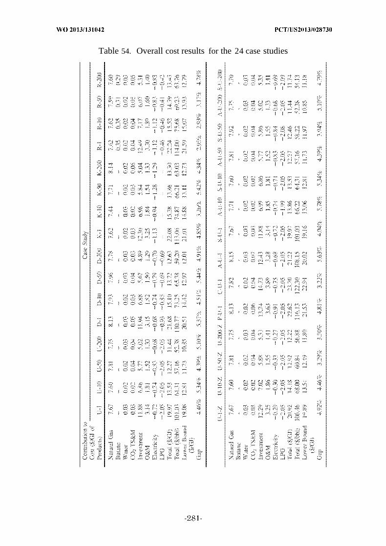
Table 54. Overall cost results for the 24 case studies

The contribution to the total costs (in $/ ) come from natural gas, butanes,
water, CO2 transportation/ storage/monitoring (CO2 TS&M), investment, and
operations/maintenance (O&M). Propane and electricity are sold as byproducts
(negative value). The overall costs are reported in ($/ ) and ($/bbl) basis, along
with the lower bound values in ($/ ) and the optimality gap between the
reported solution and the lower bound.
[0651] Example 4.12 —Investment costs
[0652] The TPC is decomposed into cost contributions from different
sections of the plant in Table 55, namely the syngas generation, syngas cleaning,
hydrocarbon production, hydrocarbon upgrading, hydrogen/oxygen production,
heat and power integration, and wastewater treatment sections. For the case
studies that utilize indirect conversion of natural gas, the syngas generation
section and the hydrocarbon production section are consistently the highest
contributing factors in the investment cost. The cost of utility production (i.e.,
electricity and steam) generally make up the third most expensive component,
with syngas cleaning (i.e., C 2 capture and compression) and hydrocarbon
upgrading following next. The values in Table 55 can be converted to a "total
overnight cost" by adding the anticipated preproduction costs, inventory capital,
financing costs, and other owner's costs and then to a "total as-spent capital" by
figuring in capital escalation an interest on debt that occurs during
construction. Note that this information has been accounted for when
determining the capital charge factor to use for the GTL refinery.
[0653] The TPC ranges from $138 to $171 MM for 1 kBD plants, $798 to
$834 MM for 10 kBD plants, $3354 to $3527 MM for 50 kBD plants, and $11,384
to $12,387 MM for 200 kBD plants. The normalized investment costs reveal the
economies of scale obtained at the different capacity levels and range from $ 38k
to $171k/bpd for 1 kBD, $80k to $84k/bpd for 10 kBD plants, $67k to $70k/bpd
for 50 kBD plants, and $58k to $62 bpd for 200 kBD plants. Among the case
studies, the plants with an unrestricted fuel requirement and the max diesei
cases both provide similar TPCs. The increased costs associated with hydrogen
production and a more complicated hydrocarbon refining section for the max
diesei cases are balanced by an overall increase in the gas capacity required in

the unrestricted cases. The LPG produced in the refineries is not added to the
total plant capacity, because this is not considered to be a liquid transportation
fuel and is merely a byproduct. Therefore, the plants that utilize the MTG
technology must have higher capacities for natural gas conversion and methanol
synthesis, because -10% of the carbon i the process will leave as LPG. The
increase in costs for the max kerosene and the United States ratio cases is mostly
associated with the use of FT synthesis and the upgrading of the hydrocarbon
products, though these two sets of case studies are typically 3-6% higher than
the case studies that utilize methanol synthesis.
[0654] The driving factor for the selection of steam reforming or ATR of
natural gas as the preferred route in all the case studies is most clearly
illustrated in case studies A-U-l, S-U-l, P-U-1, and C-U-1, where the natural gas
conversion technology is imposed in each case study. In Table 55, the case studies
that utilize direct conversion of natural gas (i .e., P-U-1 and C-U-1) have higher
hydrocarbon production/upgrading costs. For the OC case (i.e, C-U-1), the cost of
olefins production is much higher than that for hydrocarbon production from the
indirect cases due to lo conversion rates of methane and the subsequent high
costs of compression for the recycle gases. The units utilized in this topology
include the olefin fractionation (MTO-F), olefins to gasoline to distillate (OGD),
hydrocarbon fractionation (MTODF), distillate and kerosene hydrotreaters (DHT,
KHT), and the units in the LPG-gasoline separation section (see FIGS. 50 and
51). The effect of the low conversion is the high flow rate of recycle gases in
Examples 4., FIG. 64 that increase the volumetric flow rate for the CO2
separation (Table 60) and compression to recycle the gases to various process
units.
[0655] Similarly, the low selectivity of methanol in the partial oxidation of
natural gas (case study P-U-1) has the same effect on the hydrocarbon production
and upgrading costs. The offgas stream in FIG. 63 is high, increasing the capital
cost of the subsequent units. For the case studies enforcing a CO2 venting
maximum, note that the majority of the cost increase is associated with the
syngas cleaning as a result of additional C 2 capture/compression capacity. In

general, this results in an increase of about 5% to the TPC from the other
unrestricted case studies (U-C).
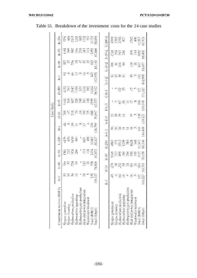
Table 55. Breakdown of the investment costs for the 24 case studies

The major sections of the plant include the syngas generation section, syngas
cleaning, hydrocarbon production, hydrocarbon upgrading, hydrogen/oxygen
production heat and power integration, and wastewater treatment blocks. The
values are reported in MM $ and normalized with the amount of fuels produced
($/bpd).
[0656] Example 4.13 - - Material and energy balances
[0657] The overall material and energy balances for the 24 case studies are
shown in Tables 56 and 57, respectively. The natural gas is shown in million
standard cubic feet per hour (mscf/h), whereas the butane liquid products, and
water are shown in kBD. For all the plants of a given capacity, a similar quantity
of natural gas needed, which is consistent with the cost results in Table 54. The
major differences between the case studies are based on the type and quantity of
liquid fuels that are produced along with the amount of CO2 that is sequestered
and vented. For the unrestricted case studies, the refinery capacity is solely
dedicated to the production of gasoline through the MTG process, with a
byproduct amount of LPG that is approximately equal to 9 vol % of the total
gasoline. The case studies that maximized diesel production were forced to have
at least 75 vol % of the liquid product be diesel. All the case studies produced
exactly 75 vol % diesel, 25 vol % gasoline, and about 3-5 v/v% byproduct LPG.
For the maximum kerosene cases (i .e., at least 75 vol %kerosene), 75 vol %of the
products is kerosene and 25 vol % is an aromatic-rich gasoline blendstock. No
byproduct LPG is produced in these cases, as the Cyclar process was used to
increase the yield of gasoline and kerosene-range aromatics from the refinery.
For these latter sets of case studies, higher volumetric percentages of diesel or
kerosene could be obtained through refining of the gasoline fraction, though the
resulting GTL refineries would be less economically attractive. The composition
of the liquid fuels from the United States ratios case studies was fixed for each
refinery to be approximately 67 vol % gasoline, 22 vol % diesel, and 11 vol %
kerosene. The total amount of LPG formed as a byproduct for these cases is equal
to 2 vol % of the total gasoline/diesel/kerosene produced.
[0658] Variations in the amount of sequestered and vented CO2 can be
observed across the 24 case studies. For the unrestricted case studies and the

maximum kerosene case studies, the amount of vented CO2 represents ~75% of
the total CO2 that is output from the process. The United States ratio studies
show a decrease in the vented CO2 to about 67% of the total, whereas the
maximum diesel cases are around 60-65%. It is important to note that the
amount of CO2 sequestration that is utilized is directly a function of the life cycle
GHG emissions that are required from the process. If no restriction was placed on
the life cycle emissions, then all of the CO2 that is output from the refinery would
simply he vented, resulting in a decrease in the capital and utility costs of the
plant. For the near-zero emissions case studies, a significant increase in the
amount of sequestered C 2 is utilized to meet the restriction imposed on these
studies.
[0659] The electricity production ranges from 1 to 4 MW for 1 kBD plants,
10 to 38 MW for 10 kBD plants, 57 to 218 MW for 50 kBD plants, and 315 to 878
M for 200 kBD plants. In all cases, the maximum kerosene studies yield the
topologies with highest producing electricity, wiiieh helps lower the overall fuels
cost. The smallest amount of electricity is produced from the near-zero CO2
venting case studies, which is anticipated due to the higher utility demand for
these plants. In general, the electricity output from all the case studies improves
the efficiency of the topologies, with the U-10, D-200, and K-10 case studies
achieving the highest energy efficiencies (i .e., 75.6, 75.0, and 75.7%, respectively)
compared with other case studies in their subcategories (Table 57). The energy
efficiency values are calculated by dividing the total energy output (i .e., fuel
products, propane, or electricity) by the total energy input (i.e., natural gas or
butane). As electricity is output from the system in all case studies, the value is
listed as negative in Table 56, and the magnitude of the energy value in Table 57
is added to the total output. If electricity were to be input to the GTL refineries,
then this energy value would be added to the total input to the system. The
overall energy efficiency of the GTL refineries is above 75.0% for all plant sizes.
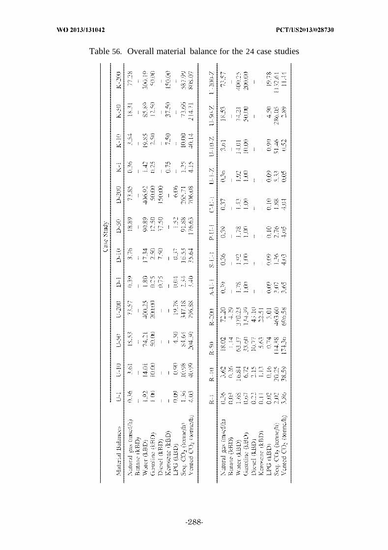
Table 56. Overall material balance for the 24 case studies

The inputs to the GTL refinery are natural gas, butane, and water, whereas the
outputs include gasoline, diesel, kerosene, LPG, sequestered CO2, and vented
C0 .

Table 57. Overall energy balance for the 24 case studies
The energy inputs to the GTL refinery come from natural gas and butane, and
the energy outputs are gasoline, diesel, kerosene, LPG, and electricity. The

energy efficiency of the process is calculated by dividing the total energy output
with the total energy inputs to the process.
[0660] Example 4.14 - Carbon and GHG balances
[0661] The overall carbon balance for the GTL refineries is shown in Table
58 and highlights the eight major points where carbon is either input or output
from the system. Carbon that is input to the system via air is neglected due to
the low flow rate relative to the other eight points. Over 99% of the input carbon
is supplied from the natural gas, whereas the balance is supplied by the butane
input to the isomerization and aikyiation units. The trends seen in liquid fuel
production from Table 56 are consistently displayed in the output carbon flow
rates in Table 58. As the percentage of carbon in each of the liquid products is
relatively similar, this implies that the relative rates of carbon flow associated
with each fuel will be consistent with the volumetric flow rate of each product.
The output amount of carbon in the total gasoline, diesel, and kerosene products
is, therefore, approximately constant for each plant capacity. The amount of
carbon leaving as LPG is around 2-7% of that leaving as gasoline, kerosene, and
diesel.

Table 58. Carbon balances (in kg/s) for the optimal solutions for the 24 case
studies
Carbon is input to the process via natural gas or butanes and exits the process as
liquid product, LPG byproduct, vented CO2, or sequestered (Seq.) CO2. The small

amount of CO2 input to the system in the purified oxygen stream (< 0.01%) is
neglected.
[0662] For each of the case studies, the carbon conversion rate ranges from
69.7 to 78.0%, with most of the case studies achieving a conversion rate above
70%. The high conversion rates are attributed to two key factors in the GTL
refinery, namely the high hydrogen/carbon ratio associated with natural gas and
the utilization of CO2 recycle to increase the overall yield. The fir s factor is
important for the production of a syngas with enough H 2 to convert the CO and
CO2 i the gas with minimal need for CO2 capture. In fact, the ¾ content
associated with steam reforming of natural gas is high enough to allow for input
of CO2 directly into the reformer to help decrease the process CO2. This second
factor is vital for decreasing the capital requirement of all units due to higher
carbon yield and for reducing the CO2 sequestration requirement needed to
achieve a proper life cycle GHG target.
[0663] The life cycle GHG emission balances for the case studies are shown
in Table 59. For each of the studies, the total GHG emission target was set to be
at most equal to that for petroleum-based production of liquid fuels or natural
gasbased production of electricity. For each liquid product, the amount of GHG
produced is calculated by determining the level of CO2 that would be produced
from complete combustion of the product. The life cycle GHG emissions (LGHG)
was set to be the sum of the total emissions from each stage of the process. The
GHG emissions avoided from liquid fuels (GHGAF) are equivalent to the total
energy of fuels produced multiplied by a typical petroleum-based emissions level
(i.e., 91.6 kg CO2eq GJ V), whereas the GHG emissions avoided from electricity
(GHGAE) are equivalent to the energy produced by electricity multiplied by a
typical natural gas-based emissions level (i .e., 101.3 kg CO2eq GJ). The GHG
emissions index (GHGI) represents the division of LGHG by the sum of GHGAF
and GHGAE, and values less than unity are indicative processes with superior
life cycle GHG emissions than current processes.
[0664] The GHG emission rates (in kg C02eq /s) for the eight major point
sources in the refinery are listed in Table 59 and include (a) acquisition and
transportation of the natural gas and butane feed s, (b) transportation and use of

the gasoline, diesel, kerosene, and LPG, (c) transportation and sequestration of
any CO2, and (d) venting of any process emissions. The GHG emissions for
feedstock acquisition and transportation in (a), product transportation in (b), and
CO2 transportation in (c) are calculated from the GREET model for wellto-wheel
emissions (Argonne National Laboratory, 2008, which is incorporated herein by
reference as if fully set forth) and assuming transportation distances for
feedstocks (50 miles), products (100 miles), and CO2 (50 miles). The GHG
emissions from product use in (b) are calculated assuming that each product will
be completely combusted to generate CO2 that is simply vented to the
atmosphere.
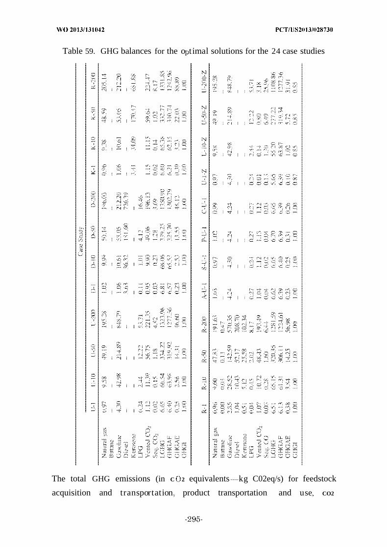
Table 59. GHG balances for the o timal solutions for the 24 case studies
The total GHG emissions (in C 2 equivalents kg C02eq/s) for feedstock
acquisition and transportation product transportation and use CO2

sequestration, and process venting are shown for each study. Process feedstocks
include natural gas and butane, whereas products include gasoline, diesel,
kerosene, and LPG.
[0665] For each of the first 20 case studies, the GHGI is exactly equal to 1,
implying that each of the GTL refineries has emission levels that are exactly
equal to current processes. From Table 59, it is clear that a major component of
the life cycle emissions are attributed to the liquid fuels. In fact, ~70% of the life
cycle GHG emissions result from combustion of these fuels in light and heavy
duty vehicles. The remaining emissions are mostly attributed to acquisition and
transportation of the natural gas and process venting. Natural gas is a
particularly GHG intensive feedstock due tothe small amount of methane that is
leaked to the atmosphere during extraction from the ground. Nevertheless, it is
still economical to develop GTL processes that can have appropriate GHG
emissions targets. The last four case studies provide an indication on how low the
ife cycle GHG emissions can be for GTL processes. The studies have GHGI
values between 0.85 and 0.87, indicating that the ife cycle GHG emissions are
13-15% lower than current fossil-fuel processes. In fact, these values are close to
the upper bound of GHG emissions reduction for GTL processes that do not
produce a significant amount of byproduct electricity. Coproduction of liquid fuels
and electricity at similar energy levels will have lower values for GHGI, as
almost a of the carbon used to produce electricity can be captured and
sequestered. When producing liquid fuels, it is currently not economical to
provide on-board carbon capture for transportation vechiles, so the life cycle GHG
emissions reduction will have a theoretical upper limit. Note that the
introduction of a biomass feedstock to the refinery would allow the refinery to
achieve significantly lower levels of life cycle GHG emissions.
[0666] This example has detailed the development of an optimization-based
framework for the process synthesis of a thermochemical natural gas to liquids
refinery. The framework was used to analyze multiple natural gas conversion
technologies, hydrocarbon production technologies, and hydrocarbon upgrading
technologies to directly compare the teehnoeconomie and environmental benefits
of each approach. The framework a so included a simultaneous heat, power, and

water integration to compare the costs of utility generation and wastewater
treatment in the overall cost of liquid fuels. The proposed optimization model
was tested using 24 distinct case studies that are derived from four combinations
of products and four plant capacities with restrictions placed on the natural gas
conversion technology and the amount of CO2 vented. The overall conversion of
carbon from feedstock to liquid products was consistently found to be over 70%,
and the life cycle GHG emissions was equivalent or less than current fossil-fuel
processes. Each case study was globally optimized using a branch-and-bound
global optimization algorithm to theoretically guarentee that the cost associated
with the optimal design was within 3-6% of the best value possible.
[0667] The overall cost of liquid fuels production ranges between $101/bbl
and $122/hbl for a 1 kBD plant, $64/bbl and $76/bbl for a 10 kBD plant, $57/bbl
and $69/bbl for a 50 kBD plant, and $52/bbl and $64/bbi for a 200 kBD plant. The
variation in the cost for each capacity is largely due to the refinery complexity
needed to produce a desired quantity of liquid fuels. To minimize the overall costs
of fuel production, methanol synthesis and the subsequent MTG route provides
the optimal conversion pathway. A significant portion of the produced C 2can be
recycled back to the reformer, and overall carbon conversion percentages of 70%
are readily obtainable. Although this pathway assumes that about 10 vol %of the
liquid product from the plant will be LPG, the MTG pathway still remains
economically superior if the LPG can be refined to aromatic chemicals using the
Cyclar process or co-reformed with the natural gas.
[0668] In general, the overall costs with hydrocarbon production through
methanol synthesis are lower than those through FT synthesis due to the
simplicity of the unconverted synthesis gas recycle loop and decrease in
complexity that is required for hydrocarbon upgrading. The unreacted synthesis
gas from methanol synthesis may be directly recycled to the methanol synthesis
unit without a concern for byproduct species that are generated in the unit.
However, the unreacted synthesis gas from FT synthesis will contain C1-C4
hydrocarbon species that must be separated out via distillation using
refrigeration or recycled back to a reformer to prevent build-up of these species in
the recycle gas loop. The benefit associated with FT synthesis is the diversity of
products that can be obtained from the process. The range of C 1- C30+
hydrocarhons allows for a diverse array of fuels, chemicals, lubricants, and waxes
that can be readily produced through standard refining practices. The process
synthesis framework outlined in this example is of significant benefit, because it
marks the first work in the scientific literature that is capable of accessing the
technoeconomic and environmental tradeoffs with multiple GTL technologies
when given a desired production capacity and composition.
[0669] Example 4.15 - Investment costs
[0670] Table 60 illustrates the investment costs (in 2011 $) for all units
that are considered in the GTL refinery.
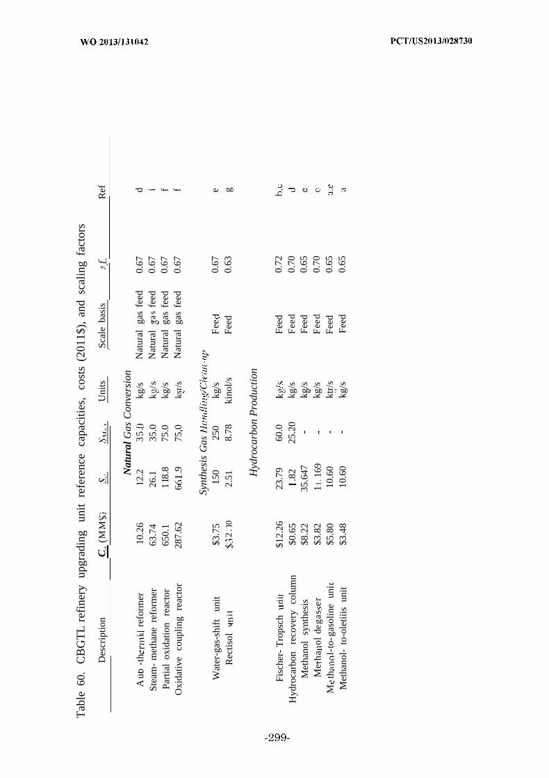
Tab
le60
.C
BG
TL
refi
nery
upgr
adin
gun
itre
fere
nce
capa
citie
s,co
sts
(201
1$),
and
scal
ing
fact
ors
Des
crip
tion
C(M
.M,
Uni
tsSc
ale
basi
s_
Ref
Nat
ural
Gas
Con
vers
ion
Auto
-th
ire
form
er10
.26
12.2
35
.kg
/sN
atur
alga
sfe
ed0.
67d
Stea
m-
met
hane
refo
rmer
63.7
426
.135
.0k
/sN
atur
als
as
feed
0.67
i
Part
ial
oxid
atio
nre
acto
r65
0.1
118.
875
.0kg
/sN
atur
alga
sfe
ed0.
67f
Oxi
dativ
eco
uplin
gre
acto
r28
7.62
6.9
75,0
ksr/
sN
atur
alga
sfe
ed0.
67f
Synt
hesi
sG
asW
ater
-gas
-shi
ftun
it$3
.75
150
250
kg/s
Fee
0.67
e
Rec
tisol
viι
2.1
02.
518.
78ki
nol/s
Feed
0.63
g
Hyd
roca
rbon
Pro
duct
ion
Fisc
her-
Tro
psch
rii
$12.
2623
.79
60.0
Feed
0.72
Hyd
roca
rbon
reco
very
colu
mn
$0.6
5.8
225
.20
kg/s
Fee
d0.
70M
etha
nol
synt
hesi
s$8
.22
35.6
47-
kg/s
Feed
0.65
Me
ha
olde
gas
er$3
.82
11.1
69kg
/sF
eed
0.70
Mth
l-to
-gas
olin
eun
i.$5
.80
10.6
0-
ktr/
sFe
ed0.
65
Met
hano
l-to
-ole
tiiis
unit
$3.4
810
.60
-kg
/sFe
ed0.
65

Hyd
roca
rbon
Upg
radi
ngD
istil
1ate
1\dr
otr
ea
r$2
.25
0.36
81.9
0F
e0.
60d
Ker
osen
eby
drol
real
er$2
.25
0.36
81.
90Fe
ed.6
0d
No
ydro
lrea
le$0
.68
0.26
.90
Fee
d0.
65W
axhy
droc
rack
er$8
.42
1.13
72.4
5kg
/sF
eed
0.55
Nap
htha
refo
rmer
$4.7
00.
4394
.50
kg/s
Fee
d0
.6d
(¾·
.' ·.is
ori
/r
$0.8
60
.31
,50
kg/s
Feed
0.62
dC
4is
orne
rize
r$9
.50
6.21
kgs
Feed
0.60
dC
-C5
alky
latio
nun
it(5
52.2
912
.64
kg/s
Feed
0.60
dSa
tura
ted
gas
plan
t$7
.83
4.23
kg/s
Feed
.60
dF
TZ
SM-5
reac
tor
$4.9
310
.60
-kg
/sF
eed
0.65
b.
01e
ii11
sto
-gas
ole/
' die
sel
$3.4
810
.6-
kg/' s
Feed
0.65
aX
sepa
ratio
nun
it$5
.39
8.54
-kg
/sFe
ed0.
62a
Dee
than
izer
'.O
.1 I
.ikg
/sFe
ed0.
68a,
eA
bsor
ber
clu
rnn
$0.9
10.
96kg
/sFe
ed0.
68a,
eSt
abili
zer
colu
n$
1.0
34.
57-
kg/s
Feed
0.68
a.e
Split
ter
colu
mn
1.1
3.96
-k
/F
eed
0.68
a.e
HF
alky
latio
nun
it$8
.99
0.
-F
eed
0.65
a.e
LP
CT/
lky
1ate
split
ter
$1.0
60.
61Fe
ed0.
68a,
e

Hyd
roge
n/O
xyge
nP
rodu
ctio
nP
ress
ure-
swin
gab
sorp
tion
$7.9
60,
29k
il/
spu
rge
gas
0.65
Air
sepa
ratio
nit
$27.
62
.341
.70.
5h
Air
com
pres
sor
$6.0
310
30e
etr
icit
v0.
67O
xyge
nco
mpr
esso
r$8
.07
1020
MW
elec
try
0.67
hE
lect
roly
zer
$500
-el
ectr
icity
0,9
Hea
tand
Pow
erIn
tegr
atio
ns
Tu
rbi
e$8
1.5
926
633
4el
ectr
icity
0.75
hSt
eam
Tur
bine
$66.
2913
650
0M
Wel
ectr
icity
0.67
Sour
Stri
pper
$399
2.5
2kg
/sFe
ed0.
53i
Bio
logi
cal
Dis
rest
or$4
752
115.
74kg
/sFe
0.7
jR
ever
seO
smos
is$0
37
4.63
kg/s
Feed
0.85
jC
ooli
ns:
Tow
er$4
.(55
4530
.30
-kg
/sFe
ed0.
78i
a.
Mob
ilR
esea
rch
and
Dev
elop
men
t,19
78:
b.
Mob
ilR
esea
rch
ad
Dev
elop
men
t,19
83:
c.M
obil
Res
earc
han
dD
evel
opin
ent.
1985
d.B
echt
elC
orpo
rati
on,
1998
;e.
Nat
iona
lR
enew
able
Ene
rgy
Lab
orat
ory,
201
1;f.
Fox
etal
.,19
90g
Kre
utz
et.
al.,
2008
;h
.L
arso
net
al,2
009:
i.N
atio
nal
Ene
rgy
Tec
hnol
ogy
Lab
orat
ory.
201.
0
j.B
aler
1994
[0671] Example 5 - Global optimization of a MINLP process synthesis
model for thermochemical based conversion of hybrid coal, biomass, and natural
gas to liquid fuels.
[0672] A global optimization framework is proposed for a thermochemical
based process superstructure to produce a novel hybrid energy refinery which
will convert carbon-based feedstocks (i.e., coal, biomass, and natural gas) to
liquid transportation fuels. The mathematical model for process synthesis
includes simultaneous heat, power, and water integration and is formulated as a
mixed-integer nonlinear optimization (MINLP) problem with nonconvex
functions. The MINLP model is large-scale and includes 15,439 continuous
variables, 30 binary variables, 15,406 equality constraints, 230 inequality
constraints, and 335 nonconvex terms. The nonconvex terms arise from 274
bilinear terms, 1 quadrilinear term, and 60 concave cost functions. The proposed
framework utilizes piecewise linear underestimators for the nonconvex terms to
provide tight relaxations when calculating the lower bound. The bilinear terms
are relaxed using a partitioning scheme that depends logarithmically on the
number of binary variables, while the concave functions are relaxed using a
linear partitioning scheme. The framework was tested on twelve case studies
featuring three different plant capacities and four different feedstock-carbon
conversion percentages and is able to solve each study to within a 3.22-8.56%
optimality gap after 100 CPU hours. For 50% feedstock carbon conversion, the
proposed global optimization framework shows that the break-even oil prices for
liquid fuels production are $61.36/bbl for the small case study, $60.45/bbl for the
medium case study, and $55.43/bbl for the large case study, while the
corresponding efficiencies are 73.9%, 70.5%, and 70.1%, respectively.
[0673] Example 5.1 - Conceptual design of process superstructure
[0674] The CBGTL superstructure is designed to co-feed biomass, coal, and
natural gas to produce gasoline, diesel, and kerosene. Synthesis gas (syngas) is
generated via gasification from biomass or coal or auto-thermal reaction of
natural gas and is converted into hydrocarbon products in the Fischer—Tropsch
(FT) reactors which are subsequently upgraded to the final liquid fuels. Co-

feeding of biomass and coal uses distinct, parallel biomass and coal gasification
trains, followed by subsequent mixing of the individual syngas effluent streams.
The gasifiers can either operate with only a solid feedstock input or in tandem
with additional vapor phase fuel inputs from elsewhere in the refinery.
[0675] The raw syngas is split and either directly sent to a gas cleanup
area or to a dedicated reverse water-gas -shift unit to consume CO2 and generate
CO. The dedicated unit is included to facilitate the reverse water-gas -shift
reaction at temperatures that are lower than the operating temperatures of the
gasifiers, but above the operating temperature of the FT reactors. The gases
exiting the reverse water—gasshift unit are then sent to the gas cleanup area.
Acid gases including CO2, H2S, and NH3 are removed from the syngas via a
Rectisol unit prior to use in the FT reactors. The sulfur-rich gases are directed to
a Claus recovery process and the recovered CO2 may be sequestered or recycled
to various units to be reacted with H 2 via the reverse water-gas -shift reaction.
The CO2 may be directed to either the gasifiers, the reverse water-gas- shift
reactor, or the iron-based FT units. Recovered CO2 is not sent to the cobalt-based
FT units to ensure a maximum molar concentration of 3% within the unit and
prevent poisoning of the catalyst. Two FT reactors operate at high temperature
(320°C) and low temperatures (240°C) and will each be associated with distinct
alpha (chain growth probability measure) values.
[0676] Fuel quality products are obtained by treating the FT effluent in a
detailed upgrading section. Waxes are converted into naphtha and distillate in a
hydrocracker unit while hydrotreater units are employed to upgrade the
naphtha, distillate, or kerosene. The naphtha cut is further reformed and
isomerized to improve the octane number. Lighter forms of hydrocarbons are
passed through a series of alkylation and isomerization processes to form high-
octane gasoline blending stock. A stream of input butanes is directed to the C4
isomerizer to enhance the quality of the output product. Offgas streams from
various upgrading units are combined in a saturated gas plant to recover C4
gases for isomerization or C3 species to be sold as byproduct propane (liquefied
petroleum gas). The remaining gases from the saturated gas plant are split to

either (i) an auto thermal reactor, (ii) a combustion unit, (iii) a gas turbine
engine, or (iv) a pressure- swing adsorption unit.
[0677] Hydrogen is produced via pressure- swing adsorption or an
electrolyzer unit while oxygen can be provided by the electrolyzer or a separate
cryogenic air separation unit. Heat and power integration is incorporated into the
process superstructure using a series of heat engines and the approach of Duran
and Grossmann, 1986, which is incorporated herein by reference as if fully set
forth. Steam for the process units is also provided by boiling condensate using
waste-heat from the process. To accompany the above process superstructure, a
complete water treatment network is postulated that will treat and recycle (a)
wastewater from various process units, (b) blowdown from the cooling tower, (c)
blowdown from the boilers, and (d) input freshwater. The graphical
representation of this superstructure is included as Supplementary Information.
[0678] Example 5.2 - Mathematical model nonlinearities
[0679] This section will focus on the nonlinearities that are present within
the mathematical model for process synthesis with simultaneous heat, power,
and water integration. Specifically, each portion of the CBGTL process topology
that gives rise to a nonlinear series of equations will be discussed along with the
number of nonlinear terms introduced and the anticipated bounds of the
variables present in these terms.
[0680] Example 5.2.1 - Origin of bilinear terms
[0681] The nonconvex bilinear terms within the mathematical model arise
from the multiplication of two positive, continuous variables. These terms are
found when a stream composition must be specified, a stream with unknown
composition must be split, or a detailed chemical equilibrium must be enforced.
To reduce the amount of composition variables recorded throughout the process
superstructure, the operation of the process units is generally defined using total
stream flow rates and the corresponding species flow rates. Material balances can
therefore be maintained throughout the process without specifically tracking the
stream compositions for each unit inlet and outlet. However, proper operation of
some process units will require explicit knowledge of the stream compositions to
be determined.
[0682] Example 5.2.1.1 - Flash units - phase equilibrium
[0683] Vapor—liquid phase equilibrium within a unit is generally modeled
using the formula y = Kx where y is the composition of the vapor phase, x is the
composition of the liquid phase, and K is the equilibrium constant. This
equilibrium must be maintained within the four flash units (UFI) of the CBGTL
process superstructure (see Table 61). Given a particular flash unit u, the
concentration xs of each species s in the liquid phase (u, uL, s) and the vapor
phase (u, uv, s) is constrained using Eq. (424), where KVLE is the equilibrium
constant.
^U,Uy ,S ~ ^U,S , ,S ~ i E Upl
The equilibrium constant is generally a function of the temperature, pressure,
and composition of the input stream to the unit. In the CBGTL process
superstructure, the temperature and pressure of the flash units are fixed. A
generic input composition is used to derive the value of the equilibrium constants
from Aspen Plus using the Peng—Robinson equation of state with the Boston—
Mathias alpha function. It is then assumed that the values of the equilibrium
constant will be independent of the variations in the species concentration seen
in the input stream, so the Aspen Plus values will be constants in the
mathematical model. The stream compositions entering the flash units in the
optimization model will not vary significantly (±2%) from the generic composition
used in the Aspen Plus simulation, so the assumption is justified. If the stream
compositions were to have large ranges in the optimization model, then the
equilibrium constant may need to be represented as a variable function of the
composition entering the flash unit.
[0684] To establish the species concentrations in the liquid and vapor
phases, Eqs. (425) and (426) are used along with the species (NS) and total (NT)
molar flow rates. Note that the bilinear terms arise from the combination of total
molar flow rate and species concentration in Eqs. (425) and (426). Each equation
contains | S | bilinear terms where I S | is the total number of species in the flash
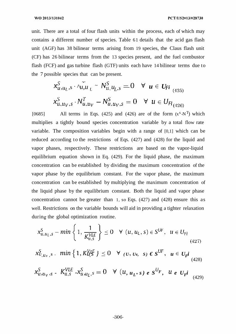
unit. There are a total of four flash units within the process, each of which may
contains a different number of species. Table 61 details that the acid gas flash
unit (AGF) has 38 bilinear terms arising from 19 species, the Claus flash unit
(CF) has 26 bilinear terms from the 13 species present, and the fuel combustor
flash (FCF) and gas turbine flash (GTF) units each have 14 bilinear terms due to
the 7 possible species that can be present.
, ,s ^u,u ~ uL — u U i
[0685] All terms in Eqs. (425) and (426) are of the form (xs -NT) which
multiplies a tightly bound species concentration variable by a total flow rate
variable. The composition variables begin with a range of [0,1] which can be
reduced according to the restrictions of Eqs. (427) and (428) for the liquid and
vapor phases, respectively. These restrictions are based on the vapor-liquid
equilibrium equation shown in Eq. (429). For the liquid phase, the maximum
concentration can be established by dividing the maximum concentration of the
vapor phase by the equilibrium constant. For the vapor phase, the maximum
concentration can be established by multiplying the maximum concentration of
the liquid phase by the equilibrium constant. Both the liquid and vapor phase
concentration cannot be greater than 1, so Eqs. (427) and (428) ensure this as
well. Restrictions on the variable bounds will aid in providing a tighter relaxation
durin the global optimization routine.
U V S - uLs ( U Uv, S ) € S u UFi(428)
, v , - - , s , uL s ) e S F , e UFi(429)

Tab
le61
.In
form
atio
npe
rtai
ning
toth
eor
igin
ofbi
linea
rte
rms
inth
em
athe
mat
ical
mod
el.
Uit
desc
ript
ion
nle
tsp
ecks
No.
of
outle
tst
ream
sN
o.ί
''
'ΐΆϊ
::::
unit
s-
phas
eeq
uili
briu
mA
cid
gas
flas
h(A
G5
Ar.
CH
,,
.C
;..
3,
,¾N
ON
S.S
,HO
,C
OS,
H,N
¾
sfl
ash
(CF5
Ar.
¾,
0N
O,
NH
CN
22
6
¾S.
.HO
,C
OS,
,e
com
bust
orfl
ash
FN
O,
G,
, 0G
astu
rbin
efl
ash
;GIF
)N
0,.N
.0T
otal
:
Spi
?«
s-
evp
iig
Tar
crac
ker
split
ter
(SA
r..
·..c
.co
.<.,
·.,.
..
iC
,H,
¾,N
O,
NO
,HN
S.
S0,
C1
CO
S.N
H,
Coa
lc
ci
split
ter
(SP
)A
r,C
,CO
,C
0.C
,C
9C
HS
..H
,,N
O,
N,H
CN
¾S.
S0
,HO
,C
OS,
N.
,,0
C?3
split
ter
Ar,
¾C
O,
C0
,C,
CH
.H.
0.N
O.
¾0,
,F
ise
rT
rps
ch
split
ter
p-)
Ar,
¾C
O,
CO
;,C
HC
C.H
.H.N
O.
N0
,.0
Aci
dga
ssp
litte
rS
C0
HC
N,
S.S
,CO
S,H
6K
eros
ene
split
ter
'·-
¾H
.6
«,C
i_-,
..
at
re
el
en
tsp
litte
r(S
P<r
r>A
r,.
2N
O,
N0
,N,
27
A-t
er
afr
eact
orsp
litte
r(5
P)
Ar.
.·.
.C
O.
C0
.C2-
,J
:.
55
2C
,H,
0,N
O,
N0
,.
Sour
stri
pper
botto
ms
split
ter
(Wss
)H
0.N
22
Rv
re
o1s
spi
(N
0,T
DS
46
De
era
tr
effl
uent
spiit
ter
WR
?2
0,T
S2
sh
erT
psc
hw
aste
wat
ersp
litte
r(W
)¾
0,C
X¾
,0¾
VA
P,O
X.O
XC
2P
sr.-c
ox
tkw
aste
wat
ersp
litte
r0
,..
NO
,2
,A,
¾,N
34
Tt
:i«
4
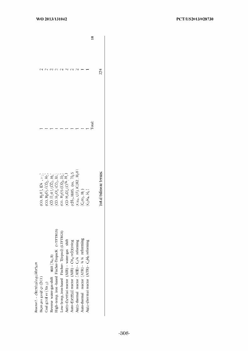
Rea
ctor
?.t
in
Bi
mss
gas
fir
(C
I)(C
O,
H0
¾
]-!
Coa
lg
ifier
Xix
)(C
O,
H.
Rev
erse
wat
er-g
as-s
hift
sit
X$)
0,H
Hig
h-t
emp
iron
-bas
edFi
sche
r-T
rops
cK(!
-!T
FTR
GS)
Oi
.,-
;.
Low
-e
mp
,iro
n-ba
sed
Fisc
her-
To
psc
(LT
FTR
GS)
(CO
..H
).
A-
.r
aire
acto
r(A
IR)
-w
ater
-gas
shif
t.
¾.H
)
Aut
o--
reac
tor
(AIR
)-
Hre
rnr
g(C
Hi0
5.(r
o,5
Ath
erm
alre
acto
rA
T-
¾re
form
ing
HiC
;H2
H0
Aut
o-th
erm
alre
acto
r.A
TR
-
¾¾
refo
rmin
gH
H)
A-
herm
aire
acto
r(A
TR
)-re
form
ing
Tot
al:
18
24

The name in parenthesis represents the unit in the CBGTL superstructure
(Supp. information) for which the nonlinear equations are enforced on the outlet
streams. These terms arise due to vapor—liquid phase equilibrium within the
flash units, chemical equilibrium within specific reactor units, and stream
splitting at the splitter units. The number of bilinear terms for each of the flash
units is equal to the number of species times the number of outlet streams. For
the splitter units, the number of bilinear terms is equal to the number of species
times one less than the number of outlet streams. Two bilinear terms are needed
for each reactor constrained by the water—gas-shift reaction, and six additional
bilinear terms are needed within the auto-thermal reactor to govern equilibrium
of steam reforming reactions for the hydrocarbons.
[0686] Note that Eq. (424) could be reformulated as Eq. (430) without
introducing the species concentration variables:
· , - NUT
Mv = 0 V e U l
This would introduce an equivalent number of bilinear terms, though each of the
bilinear terms would be of the form (Ns · NT) . The increased range of the Ns
variables would lead into relaxations that are looser than those provided with the
species concentration variables. Therefore, this study focused on the bilinear
terms developed using Eqs. (425) and (426).
[0687] Example 5.2.1.2 - Splitter units - stream splitting
[0688] Proper operation of all splitter units (Us ) requires the composition
of all outlet streams, (u, u , to be equal to that of the inlet stream, (ui, u). This
may be done by defining stream concentration variables, , l l , S for each
species in the inlet stream and constraining all outlet streams to have this exact
concentration. Without loss of generality, the species flow rates for each exiting
stream can then be set using the composition of the entering stream (Eq. (431)).
N- ,
N' e s
4 3 1
Note that a species balance around the splitter unit will prevent the need for Eq.
(431) on the splitter inlet. Eq. (431) introduces a total of ( | S | · |U |) bilinear
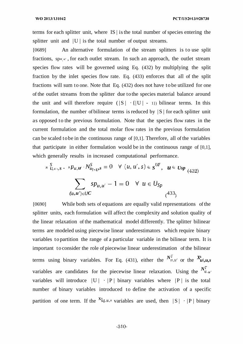
terms for each splitter unit, where IS | is the total number of species entering the
splitter unit and |U | is the total number of output streams.
[0689] An alternative formulation of the stream splitters is to use split
fractions, sp« « , for each outlet stream. In such an approach, the outlet stream
species flow rates will be governed using Eq. (432) by multiplying the split
fraction by the inlet species flow rate. Eq. (433) enforces that all of the split
fractions will sum to one. Note that Eq. (432) does not have to be utilized for one
of the outlet streams from the splitter due to the species material balance around
the unit and will therefore require ( | S | · | U | - 1) bilinear terms. In this
formulation, the number of bilinear terms is reduced by | S | for each splitter unit
as opposed to the previous formulation. Note that the species flow rates in the
current formulation and the total molar flow rates in the previous formulation
can be scaled tobe in the continuous range of [0,1]. Therefore, all of the variables
that participate in either formulation would be in the continuous range of [0,1],
which generally results in increased computational performance.
N U, U >,S - s u U,s = S , u Usp
( ,u' C 433
[0690] While both sets of equations are equally valid representations of the
splitter units, each formulation will affect the complexity and solution quality of
the linear relaxation of the mathematical model differently. The splitter bilinear
terms are modeled using piecewise linear underestimators which require binary
variables to partition the range of a particular variable in the bilinear term. It is
important to consider the role of piecewise linear underestimation of the bilinear
N Xsterms using binary variables. For Eq. (431), either the or the u\,u,s
Nvariables are candidates for the piecewise linear relaxation. Using the u'
variables will introduce |U | · | P | binary variables where | P | is the total
number of binary variables introduced to define the activation of a specific
Xspartition of one term. If the i s variables are used, then | S | · | P | binary
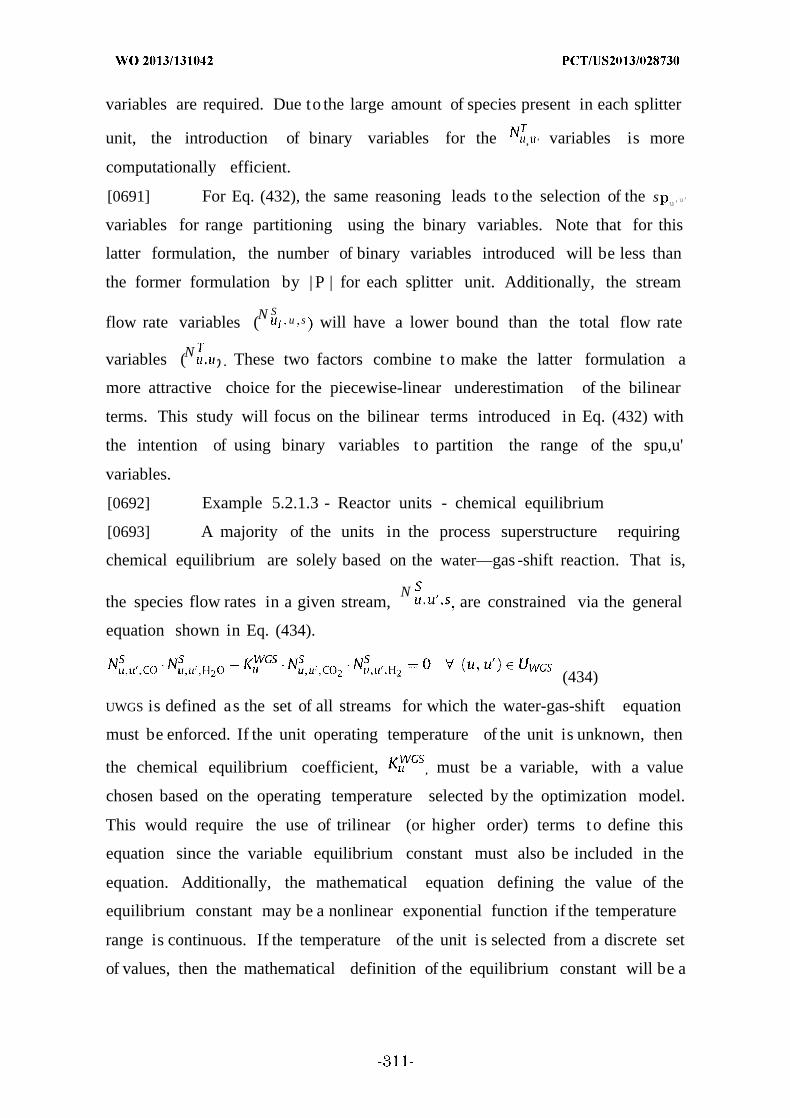
variables are required. Due to the large amount of species present in each splitter
unit, the introduction of binary variables for the , ' variables is more
computationally efficient.
[0691] For Eq. (432), the same reasoning leads to the selection of the s u,u'
variables for range partitioning using the binary variables. Note that for this
latter formulation, the number of binary variables introduced will be less than
the former formulation by | P | for each splitter unit. Additionally, the stream
N Sflow rate variables ( u s will have a lower bound than the total flow rate
Nvariables ( ') . These two factors combine to make the latter formulation a
more attractive choice for the piecewise-linear underestimation of the bilinear
terms. This study will focus on the bilinear terms introduced in Eq. (432) with
the intention of using binary variables to partition the range of the spu,u'
variables.
[0692] Example 5.2.1.3 - Reactor units - chemical equilibrium
[0693] A majority of the units in the process superstructure requiring
chemical equilibrium are solely based on the water—gas -shift reaction. That is,
Nthe species flow rates in a given stream, are constrained via the general
equation shown in Eq. (434).
(434)
UWGS is defined as the set of all streams for which the water-gas-shift equation
must be enforced. If the unit operating temperature of the unit is unknown, then
the chemical equilibrium coefficient, , must be a variable, with a value
chosen based on the operating temperature selected by the optimization model.
This would require the use of trilinear (or higher order) terms to define this
equation since the variable equilibrium constant must also be included in the
equation. Additionally, the mathematical equation defining the value of the
equilibrium constant may be a nonlinear exponential function if the temperature
range is continuous. If the temperature of the unit is selected from a discrete set
of values, then the mathematical definition of the equilibrium constant will be a

linear function of the binary variables for the temperature choices and the
parametric values for the equilibrium constant at each temperature. Linear
relaxation of the trilinear terms can be properly incorporated by using
underestimators to model the convex hull surrounding the term (Meyer &
Floudas, 2003, 2004) or by combining two of the variables to form an auxiliary
bilinear term and then combining the auxiliary term with the third variable to
form a second bilinear term. These two bilinear terms can then be relaxed using
piecewise linear underestimators as defined previously. An additional
consequence of the use of a continuous temperature range is the addition of n on
linear constraints to define the heat and power integration (Duran & Grossmann,
1986). This enhanced computational complexity is not necessary if the operating
temperature of the unit may be chosen from a finite set of discrete values
(Baliban et al., 2011).
[0694] Selection of one of the temperature values is logically enforced using
a binary variable, yu, which will simultaneously select the temperature value and
the equilibrium coefficient for the reactor unit. Note that this formulation allows
Eq. (434) to be rewritten as Eqs. (435) and (436).
o N '. - ¾ ¾ - ¾ - ) < ( , WCS ) € Uwcs
(435)
¾ 5W
¾ -w ¾ - y « 0 V ( · «'· " s ) Uwcs
(436)
UWGS has been defined here to mean the set of all streams (u, u) for which the
water—gas -shift equilibrium must be enforced using the operating conditions of
N S~UBunit UWGS . The value represents the upper bound on the flow rate for
stream (u, u, s). There are a total of six units including the gasifiers, the auto-
thermal reactor, the reverse water—gas-shift reactor, and the iron-based FT units
that must enforce the water—gas -shift equilibrium. Each unit will require two
bilinear terms in the model, leading to 12 total bilinear terms.
[0695] The auto-thermal reactor must also enforce steam reforming
equilibrium for the four output hydrocarbon species (CH4, C2H2, C2H4, and C2H6).
The general form for the steam reforming reactions is shown in Eqs. (437)-(440).

¾ H · , C4 = «') ≡ C , A R
V (ii, C, UATR
(439)
',C0 2 ' , Η - ¾ H · ¾«' . C H · u ' , 2 0 = (u, u') C , ¾ RA
(440)
[0696] Note that combining Eqs. (437) and (438) can produce Eq. (441). Eq.
(442) can be produced from Eqs. (438) and (439) and Eq. (443) can be produced
from Eqs. (439) and (440).
K SR
' C2Ν
2- ' 4
Ν ' = V ( . ' ) ¾
, C H 2
(441)
',C 2 2 - , ( , ' ) UC, UA R
(442)
- , ' 2 (u, u') UC, UATR
(443)
[0697] The equilibrium coefficients in Eqs. (437) and (441)-(443) are
dependent on the selection of operating temperature within the autothermal
reactor. These variables may be eliminated by changing the equality to two
inequalities as shown below. Eqs. (444) and (445) are used in place of Eq. (437),
Eqs. (446) and (447) in place of Eq. (441), Eqs. (448) and (449) in place of Eq.
(442), and Eqs. (450) and (451) in place of Eq. (443).
. . ,H - ¾ H < ¾ o - ¾ C - ¾ 3 ( 1 - ) <0 V (u, u', A R ) UA R
(444)
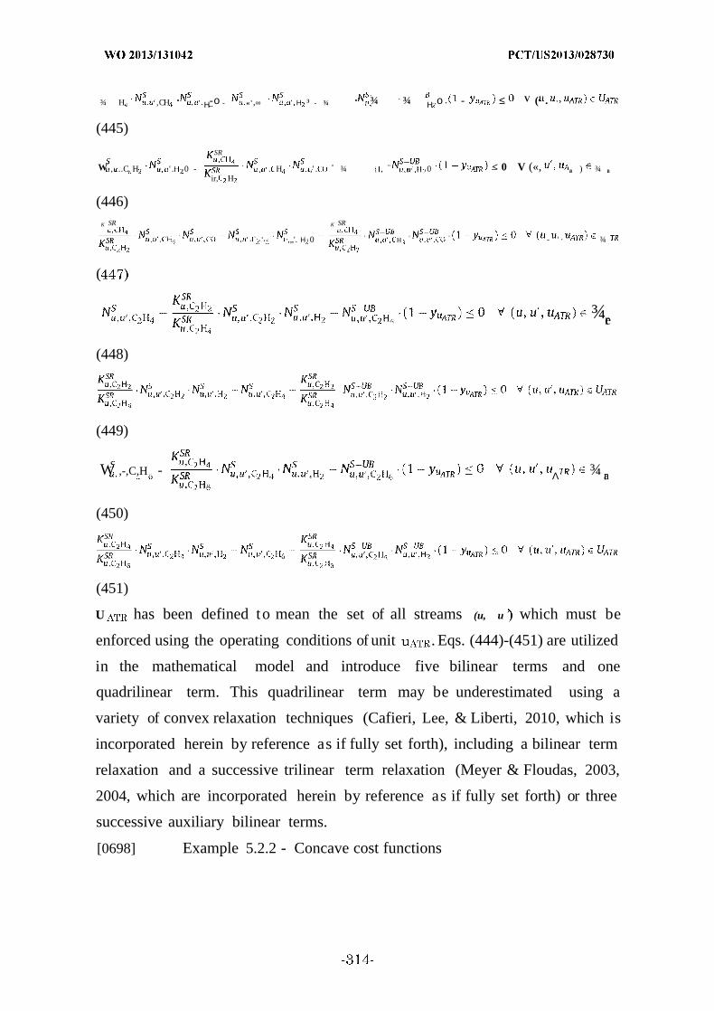
¾ H ,CH · Η-ο - «' ,∞ Η 3 - ¾ · ¾ ¾ Η ο · - ≤ V ( . '
(445)
SR
W , ..C, H ' . 0 - . H ,' . " ¾ , " 0 < 0 V («, ra ) ¾ rair, H
(446)K SR K SR
. .·.. ·.„'. Η 0 ' H ' ' - ' · ¾
(
¾re
(448)
(449)
W ,-,C,H - Λ ¾ ra
(450)
(451)
U has been defined to mean the set of all streams (u, u which must be
enforced using the operating conditions of unit . Eqs. (444)-(451) are utilized
in the mathematical model and introduce five bilinear terms and one
quadrilinear term. This quadrilinear term may be underestimated using a
variety of convex relaxation techniques (Cafieri, Lee, & Liberti, 2010, which is
incorporated herein by reference as if fully set forth), including a bilinear term
relaxation and a successive trilinear term relaxation (Meyer & Floudas, 2003,
2004, which are incorporated herein by reference as if fully set forth) or three
successive auxiliary bilinear terms.
[0698] Example 5.2.2 - Concave cost functions

[0699] The investment cost of the final process topology will be calculated
as the sum of the investment cost of all representative process units, Ulnv,
throughout the superstructure. Though some units in the superstructure will
have a cost function that is solely based on the construction of that unit (e.g.,
compressors, turbines, and flash units), several of the units will have a cost
function that accounts for construction of that unit along with axillary units
necessary for proper operation. For example, the investment cost of the biomass
gasifier will include the cost of the gasifier and the feed lockhopper. A total of 60
cost curves are needed for the process superstructure, each of which is of the form
in Eq. (452).
u = · ¾ V G ¾(452)
oIn this function, represents the base cost, " represents the base flow rate, Su
represents the working flow rate, and sfu represents the scaling factor. Note that
Eq. (452) assumes that units operate without a maximum flow rate. This
assumption was utilized to avoid the mathematical complexity associated with
the restriction of a maximum flow. If a maximum flow rate, , is imposed for a
unit operation, then the total number of unit trains, nu, and the working flow
rate of each train, Stu , must be enforced using Eqs. (454) and (455). The
investment cost of each unit would then be calculated using Eq. (455).
S u — ¾ (454)
S uInv = n 9 · u · V U U nv
(455)
Note that Eq. (455) will contain a discontinuity at all points where the working
flow is an integer multiple of the maximum flow. Additionally, binary variables
would be required to logically define the number of units necessary to operate
given the restrictions on the unit capacity. To circumvent this computational
burden, all cost functions with a maximum flow rate were assigned an auxiliary
cost function of the form in Eq. (452). The parameters of the auxiliary function
were derived so as to most closely approximate the original cost function. Note
that the scaling factor for each process unit is between 0 and 1, exclusive, so each
cost function will be a concave, monotonically increasing function of the working
flow rate.
[0700] Example 5.3 - Deterministic global optimization strategies
[0701] To solve the process synthesis with simultaneous heat, power, and
water integration problem, a branch-and-bound global optimization algorithm
(Misener et al., 2010, 2011; Misener & Floudas, 2010, which are incorporated
herein by reference as if fully set forth) is introduced as described below. At each
node in the branch-and-bound tree, a mixed-integer linear relaxation of the
mathematical model is solved using CPLEX 12.3 (CPLEX, 2009) and then the
node is branched to create two children nodes. The solution pool feature of
CPLEX is utilized during the solution of the relaxed model to generate a set of
150 distinct points, each of which is used as a candidate starting point to solve
the original model. For each starting point, the current binary variable values are
fixed and the resulting NLP is minimized using CONOPT 3.15A. If the solution
to the NLP is less than the current upper bound, then the upper bound is
replaced with the NLP solution value. At each step, all nodes that have a lower
bound that is within an € tolerance of the current upper bound ((LBno de)/(UB) > 1
- ) are eliminated from the tree. Termination of the algorithm is reached if all
nodes in the branch-and-bound tree have been processed or if 100 CPU hours
have passed. Upon completion of the algorithm, the model lower bound
(represented as the minimum value for the lower bound of all nodes yet to be
processed) and the best upper bound are reported.
[0702] The following sections detail specific strategies employed at the root
node and general strategies used at each node of the branch-andbound tree.
[0703] Example 5.3.1 - Bilinear term underestimation
[0704] Each of the bilinear terms is derived from the product of two
continuous, non-negative variables. The tightest possible relaxation of the
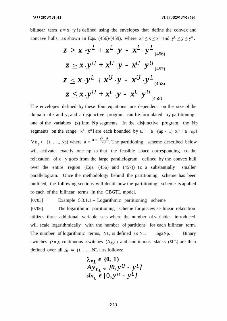
bilinear term z = x ·y is defined using the envelopes that define the convex and
concave hulls, as shown in Eqs. (456)-(459), where xL < x < xu and yL < y < yu .
z > x -y + x y - x y(456)
z x y + x y - x y(457)
z x y x y - x y
z < x y + x y - x yThe envelopes defined by these four equations are dependent on the size of the
domain of x and y, and a disjunctive program can be formulated by partitioning
one of the variables (x) into Np segments. In the disjunctive program, the Np
segments on the range [xL, xu ] are each bounded by [xL + a · (np - 1), xL + a ·np]
V np 1, . . ., Np where a = a =N . The partitioning scheme described below
will activate exactly one np so that the feasible space corresponding to the
relaxation of x ·y goes from the large parallelogram defined by the convex hull
over the entire region (Eqs. (456) and (457)) t o a substantially smaller
parallelogram. Once the methodology behind the partitioning scheme has been
outlined, the following sections will detail how the partitioning scheme is applied
to each of the bilinear terms in the CBGTL model.
[0705] Example 5.3.1.1 - Logarithmic partitioning scheme
[0706] The logarithmic partitioning scheme for piecewise linear relaxation
utilizes three additional variable sets where the number of variables introduced
will scale logarithmically with the number of partitions for each bilinear term.
The number of logarithmic terms, N L, is defined as N L = log2Np. Binary
switches ( n ) , continuous switches (AyNL), and continuous slacks (SLL) are then
defined over all ≡ 1, . . ., NL as follows:
„L e 0, 1)Ay
L[0, y - y ]
sln e , y u - y ]

[0707] Note that there is a one-to-one mapping between the activation of a
one of the Np segments and a combination of the N L binary variables. The N L
elements of λ will activate or deactivate based on the binary representation of the
largest grid point that is less than x, as shown in Eq. (460).
N L N L
x + ¾- · a n < x < a + x + ^2¾- · a λ
¾= i = (460)
The yNLvariables should be equal to (y - yL) for each active NL , as restricted by
Eqs. (461)-(463).
A y n < (y - y ) L
y n y - y - s ln
< sln < y - y ) . ( - n )
[0708] Using the Using the definitions provided above, a logarithmic
partitioning scheme that is equivalent to the previously desired disjunctive
program is introduced using Eqs. (464)—(467).
N L
z > x y L + x -y - y ) + A y
¾= (464)
z > -y + x + a ) (y - y u ) + ∑ · 2¾ 1 · (Ay - (y - y ) ¾ )
¾ = (465)
N
z < x y + (x + a ) ( - y ) + · ¾ _ · y„
" = (466)
z ≥ x -y + x - y ) + ∑ · 2¾ ( Ay„ - y - y ) λ )
¾= (467)
[0709] Example 5.3.1.2 - Flash units - phase equilibrium
[0710] For the flash units, all outlet streams are defined as (u, u ≡ UCFI
and all species within those streams are defined as (u, u , s) ≡ SFI. T O construct
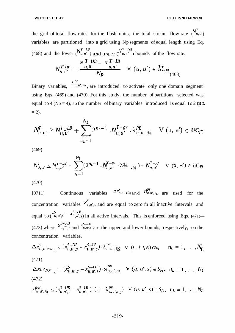
the grid of total flow rates for the flash units, the total stream flow rate (
variables are partitioned into a grid using Np segments of equal length using Eq.
(468) and the lower bounds of the flow rate.
N T _ N T LT-gr u, u,u' , T r
p (468)
λBinary variables, , , , are introduced to activate only one domain segment
using Eqs. (469) and (470). For this study, the number of partitions selected was
equal to 4 (Np = 4), so the number of binary variables introduced is equal t o 2 (N L
= 2).
N > - . . ¾ V (u, a') UC
n = l
(469)
< + -N · ¾ ¾ ) + V ( , «') iiC
(470)
[0711] Continuous variables - ¾an d are used for the
. . . .concentration variables , ,s and are equal to zero m all inactive intervals and
equal t o ( ",«',s) in all active intervals. This is enforced using Eqs. (471)—
S-UB(473) where ,"', and ' are the upper and lower bounds, respectively, on the
concentration variables.
', , ≤ - ¾ V ( ',S) G¾, n = ,...,NL
(471)
iu',s,n l , . . . ,
472)
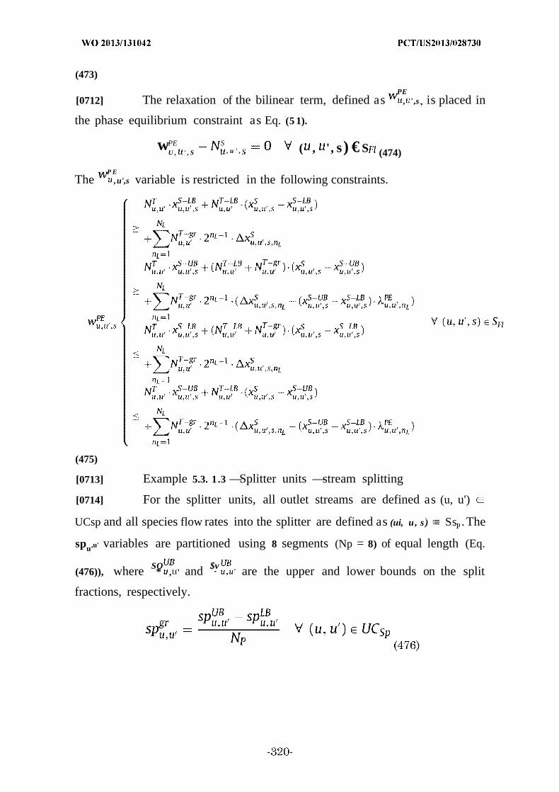
(473)
PE[0712] The relaxation of the bilinear term, defined as , ' ,s is placed in
the phase equilibrium constraint as Eq. (5 1).
w,PE SU , ' , S , u ' , ( , ', s) € S (474)
P E
The ,u',s variable is restricted in the following constraints.
(475)
[0713] Example 5.3. 1.3 —Splitter units —stream splitting
[0714] For the splitter units, all outlet streams are defined as (u, u')
UCsp and all species flow rates into the splitter are defined as (ui, u , s ) ≡ Ss . The
spu,u' variables are partitioned using 8 segments (Np = 8) of equal length (Eq.
SO $v(476)), where * , ' and are the upper and lower bounds on the split
fractions, respectively.
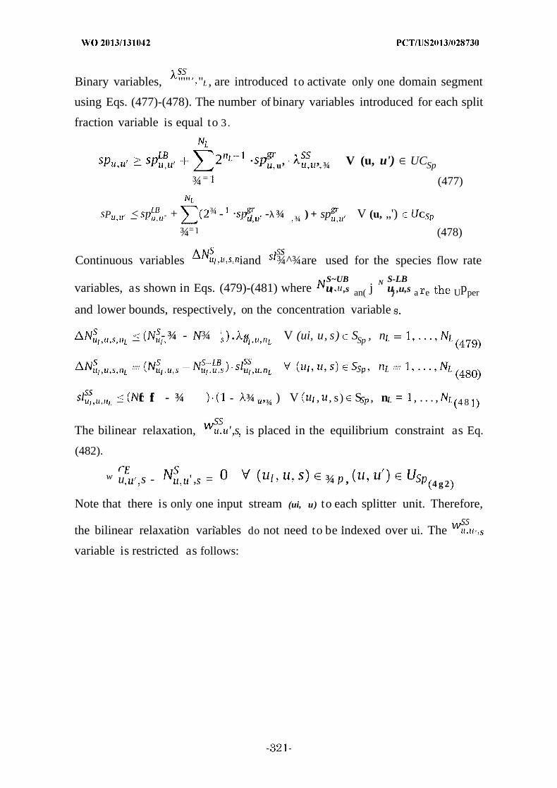
Binary variables, "'" " , are introduced to activate only one domain segment
using Eqs. (477)-(478). The number of binary variables introduced for each split
fraction variable is equal to 3.
· u, , ¾ V (u, u') UCSp
¾= (477)
P < - + ¾ - · l -λ ¾ ¾ ) + sp V (u, „') C
¾= (478)
Continuous variables iand ¾^¾are used for the species flow rate
S~UB N S-LBvariables, as shown in Eqs. (479)-(481) where u ,s an( j u ,u,s a e Upper
and lower bounds, respectively, on the concentration variable
- ¾ - ¾ . « V (ui, u, s) SSp , n
fc ffi - ¾ - ¾ ,¾ ) V , , s) S , n = , . . . , 4 8
The bilinear relaxation, ',s is placed in the equilibrium constraint as Eq.
(482).
w u s - ' , = ¾ , 4 g 2
Note that there is only one input stream (ui, u) to each splitter unit. Therefore,
. . .the bilinear relaxation variables do not need to be indexed over ui. The ' S
variable is restricted as follows:
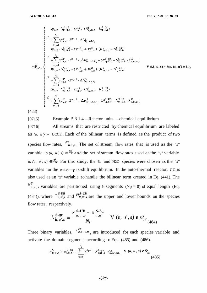
: , ',s V (i.f|, , s) Ssp, ( , u') e
(483)
[0715] Example 5.3.1.4 —Reactor units —chemical equilibrium
[0716] All streams that are restricted by chemical equilibrium are labeled
as (u, u ≡ UCCE . Each of the bilinear terms is defined as the product of two
N sspecies flow rates, u,u',s The set of stream flow rates that is used as the "x"
yvariable is (u, u , s) ≡ and the set of stream flow rates used as the "y" variable
is (u, u , s) C For this study, the ¾ and H2O species were chosen as the "x"
variables for the water— as-shift equilibrium. In the auto-thermal reactor, C O is
also used as an "x" variable to handle the bilinear term created in Eq. (441). The
N,u!,s variables are partitioned using 8 segments (Np = 8) of equal length (Eq.
N S-UB S- LB(484)), where , ,s and , ',s are the upper and lower bounds on the species
flow rates, respectively.
N S-UB _ N S-LS-gr
v :u,u' ,s V (u, ' , s) e S ;N (484)
CEλThree binary variables, ' are introduced for each species variable and
activate the domain segments according to Eqs. (485) and (486).
N JV; Nu'.s —"u,u',s ~ / u,~ g r
,sCu
E.u,',s,n
V (u, u', s) e SxCE
¾=1 (485)
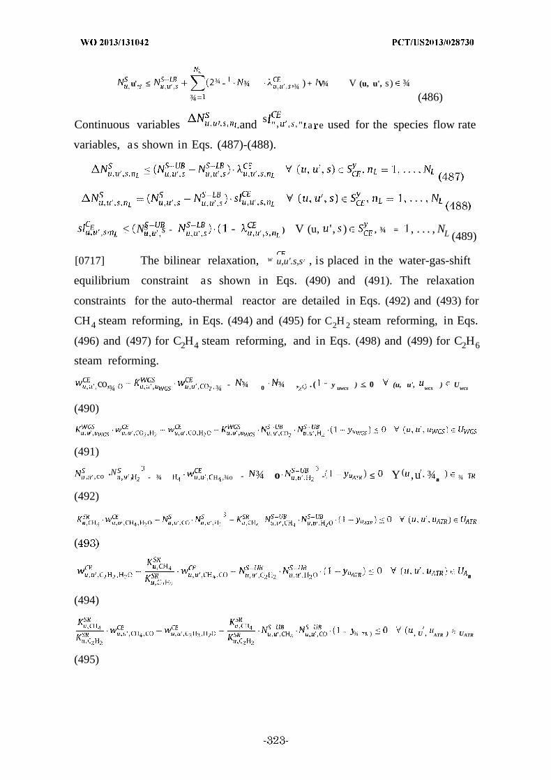
u'. ≤ ¾ - ¾ ,¾ ) + V¾ V (u, u', s) ¾
¾= (486)
, sContinuous variables ' .and " " a e used for the species flow rate
variables, as shown in Eqs. (487)-(488).
E, , < NS s - - ) V (u, ', ) , ¾ = , . . . , NL (489)
[0717] The bilinear relaxation, w u,u'.s,s , is placed in the water-gas-shift
equilibrium constraint as shown in Eqs. (490) and (491). The relaxation
constraints for the auto-thermal reactor are detailed in Eqs. (492) and (493) for
CH4 steam reforming, in Eqs. (494) and (495) for C2H 2 steam reforming, in Eqs.
(496) and (497) for C2H4 steam reforming, and in Eqs. (498) and (499) for C2H6
steam reforming.
co,¾ ¾ - ¾ 0 ¾ , . ( ~ y uwcs ) < 0 (u, u', wcs ) Uwcs
(490)
(491)
, ,co ·N , - ¾ H ,¾o - ¾ o - ≤ Y ( ,u ¾ra ¾
(492)
(
ra
(494)
~ ¾ ) , U , ATR ) UATR
(495)

CE N S-UB5 _,u',¾ H , H
(l - ¾ra ) < 0 V (u, ' ra ).
(496)
K SR2 CE
, ', H . HN S
, ',C HN :S
u.¾H VR
H
(497)
RC -
N :U' :
WCE, ', H , H · ί.·. ,·:. : . ·
(498)
.CE , . .i S-i , ' H ,
N ;' C Hg
N:,u', H Yu',H
u,C H
(499)CE
[0718] The u, f,s,s variables are restricted using Eq. (500), where the set
(u, u, s, s ) defined as all combinations of (u, u , s) Eand (u, u , s
-S*C th t form a product of two species flow rates.
u,u',s,s'V (u, u ', s, s') e *C£
(500)
[0719] Note that Eqs. (492) and (493) both contain a quadrilinear term
which may be underestimated using a convex relaxation, a bilinear term
relaxation and a successive trilinear term relaxation, or three successive
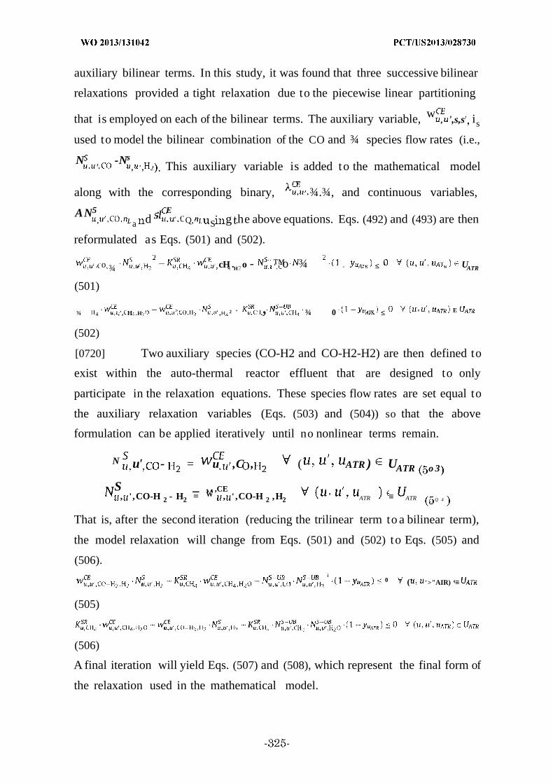
auxiliary bilinear terms. In this study, it was found that three successive bilinear
relaxations provided a tight relaxation due to the piecewise linear partitioning
wthat is employed on each of the bilinear terms. The auxiliary variable, , ',s,s is
used to model the bilinear combination of the CO and ¾ species flow rates (i.e.,
N -Ns' , ' , This auxiliary variable is added to the mathematical model
along with the corresponding binary, ' ¾.¾, and continuous variables,
AN5 ; E, a d ' Q, S g he above equations. Eqs. (492) and (493) are then
reformulated as Eqs. (501) and (502).
. o ¾ cH .H o - ™o ¾ - A ≤ « UATR
(501)
¾ ,', H .H > ,Η 2 " , ¾ 0 ≤ ' E
(502)
[0720] Two auxiliary species (CO-H2 and CO-H2-H2) are then defined to
exist within the auto-thermal reactor effluent that are designed to only
participate in the relaxation equations. These species flow rates are set equal to
the auxiliary relaxation variables (Eqs. (503) and (504)) so that the above
formulation can be applied iteratively until no nonlinear terms remain.
N u' - = u ,C , ( ATR ) UATR o 3
S _ ,CE, ' ,CO-H 2 - H2 = W , ' ,CO-H 2 ,H2 ' ATR ≡ ATR Q 4
That is, after the second iteration (reducing the trilinear term to a bilinear term),
the model relaxation will change from Eqs. (501) and (502) to Eqs. (505) and
(506).
0 ( ' >"AIR) ≡
(505)
(506)
A final iteration will yield Eqs. (507) and (508), which represent the final form of
the relaxation used in the mathematical model.
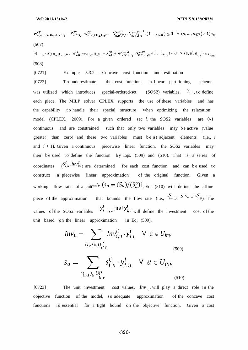
(507)
¾ f«' , H. H o -'.CO-H - H ,H H · · - ATR UATR
(508)
[0721] Example 5.3.2 - Concave cost function underestimation
[0722] T o underestimate the cost functions, a linear partitioning scheme
was utilized which introduces special-ordered-set (SOS2) variables, , t o define
each piece. The MILP solver CPLEX supports the use of these variables and has
the capability t o handle their special structure when optimizing the relaxation
model (CPLEX, 2009). For a given ordered set i , the SOS2 variables are 0-1
continuous and are constrained such that only two variables may b e active (value
greater than zero) and these two variables must b e a t adjacent elements (i.e., i
and i + 1). Given a continuous piecewise linear function, the SOS2 variables may
then b e used t o define the function by Eqs. (509) and (510). That is, a series of
coordinates ( < ) are determined for each cost function and can b e used t o
construct a piecewise linear approximation of the original function. Given a
working flow rate of a unit'** ' , Eq. (510) will define the affine
piece of the approximation that bounds the flow rate (i.e., ~ " ~ ' ) . The
values of the SOS2 variables ' will define the investment cost of the
unit based on the linear approximation in Eq. (509).
(509)
) U(510)
[0723] The unit investment cost values, Inv u, will play a direct role in the
objective function of the model, so adequate approximation of the concave cost
functions i s essential for a tight bound on the objective function. Given a cost
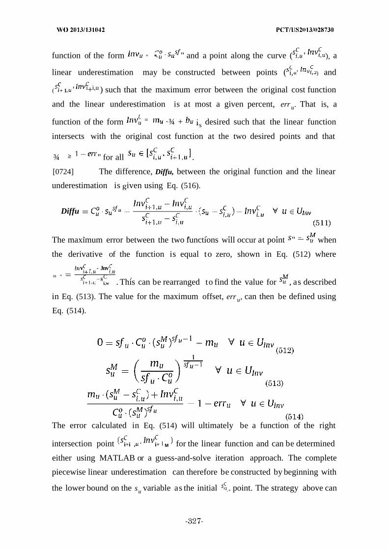
function of the form = *- " and a point along the curve ( ' a
linear underestimation may be constructed between points ( i,«' ν ) and
( + 1 ' i+i,u ) such that the maximum error between the original cost function
and the linear underestimation is at most a given percent, err u. That is, a
function of the form = ·¾ + s desired such that the linear function
intersects with the original cost function at the two desired points and that
¾ ≥ " for all .
[0724] The difference, Diffu, between the original function and the linear
underestimation is iven using Eq. (516).
Diffu
. . . _The maximum error between the two functions will occur at point " when
the derivative of the function is equal to zero, shown in Eq. (512) where
v , - Jnvm " _ C .
+ , ι i,w . This can be rearranged to find the value for , as described
in Eq. (513). The value for the maximum offset, err u, can then be defined using
Eq. (514).
The error calculated in Eq. (514) will ultimately be a function of the right
intersection point i+i , ' i+ M for the linear function and can be determined
either using MATLAB or a guess-and-solve iteration approach. The complete
piecewise linear underestimation can therefore be constructed by beginning with
the lower bound on the su variable as the initial , « point. The strategy above can

be used to find the point that will ensure that the maximum offset error
between and , is equal to err u . The point 2.« is then determined by
utilizing the value for as the left point for the next iteration and the process
s ccontinues until a calculated point is greater than the upper bound for s u .
sOnce this occurs, the final calculated point - is set equal to the upper bound.
(s lnv The set of ί .«' values are used within Eqs. (509) and (510) to ensure that
the maximum error associated with any point along the cost function
approximation is less than err u . For this study, a majority of the process units
were selected to have a maximum error of 10%. The units expected to contribute
the most to the overall cost (i.e., coal gasifier, steam turbines, air separation unit,
and wax hydrocracker) have a maximum error of 5%. Note that since the
investment cost is anticipated to account for approximately 30—35% of the overall
cost, the maximum anticipated error between the best feasible solution and the
lower bound will be in the range of 2-4%. It is possible to reduce this anticipated
error by reducing the value for erru for the process units. However, the
calculation of the lower bound will become increasingly complex due to the
Vinclusion of additional u SOS2 variables needed to define the linear
underestimators. The values for the unit investment cost errors defined above
represent an acceptable balance between solution quality and computational
efficiency.
[0725] Example 5.3.3 - Calculation of initial upper bound
[0726] At the root node of the branch-and-bound tree, it is critical to
identify (1) a high-quality upper bound and (2) tight ranges on the variables that
will be branched on in the tree. Therefore, the initial step of the global
optimization approach is to calculate a high-quality upper bound from a local
solution of the problem. Using the solution pool feature of CPLEX (CPLEX,
2009), 150 points are generated as candidate starting points to a non-linear
optimization (NLP) solver. To expedite the determination of the initial points, all
bilinear terms are modeled using the standard convex envelopes (Np = 1) and the
concave cost functions are modeled using a single linear underestimator. Each

nonlinear term is therefore relaxed without binary variables, and while this does
not provide a tight lower bound, it does serve to find a large array of distinct
initial points (i.e., different topological scenarios) within a short period of time. At
each iteration, the values of the binary variables for the starting point are fixed
and the resulting NLP is solved to find a local solution. The lowest objective value
of all of the local solution is retained as the initial upper bound on the final
solution value (Eq. (515)).
Cost < Cost B
[0727] Example 5.3.4 - Optimality based bounds tightening
[0728] Given the restriction on the upper bound shown in Eq. (515),
rigorous bounds may be then determined for several problem variables. That is,
Eq. (516) can be used as an objective function to find the minimum and maximum
possible value of certain species molar flow rates, total molar flow rates, and unit
working flow rates for the superstructure. For a given iteration, all parameter
C S , C N Ccoefficients ( ,u',s , uf ' and ) are set to zero except for the coefficient
pertaining to the variable of interest, which is set to one. The objective function
reduces to the variable of interest which is minimized and subsequently
maximized to find the lower and upper bounds of this variable. Note that this
step is capable of significantly reducing the variable bounds of each process
variable. The bounds tightening procedure is specifically targeted at the variables
(N , )that will appear in bilinear terms for phase equilibrium ' , stream splitting
' chemical equilibrium ,u' ,s o the cost functions (Su).
min / max c u, ·N F+c ,·Ν , + C - S
(516)
[0729] This procedure is preformed using the complete set of linear
underestimators detailed earlier. That is each model solved using Eq. (516) as the
objective is a MILP with the appropriate piecewise linear underestimators for the
bilinear terms and the cost functions. This was found to provide better solutions
as opposed to solving a quicker, relaxed version of the problem that changes all
0—1 binary variables to 0—1 continuous variables. After each solution is
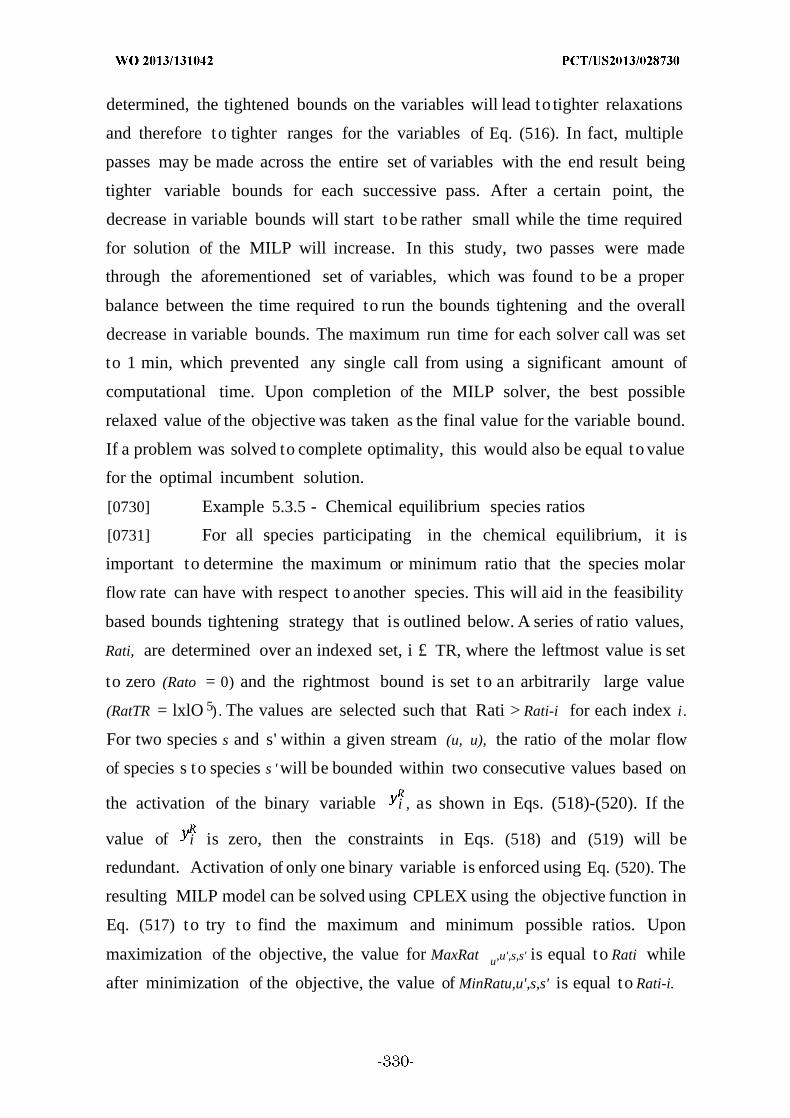
determined, the tightened bounds on the variables will lead to tighter relaxations
and therefore to tighter ranges for the variables of Eq. (516). In fact, multiple
passes may be made across the entire set of variables with the end result being
tighter variable bounds for each successive pass. After a certain point, the
decrease in variable bounds will start to be rather small while the time required
for solution of the MILP will increase. In this study, two passes were made
through the aforementioned set of variables, which was found to be a proper
balance between the time required to run the bounds tightening and the overall
decrease in variable bounds. The maximum run time for each solver call was set
to 1 min, which prevented any single call from using a significant amount of
computational time. Upon completion of the MILP solver, the best possible
relaxed value of the objective was taken as the final value for the variable bound.
If a problem was solved to complete optimality, this would also be equal to value
for the optimal incumbent solution.
[0730] Example 5.3.5 - Chemical equilibrium species ratios
[0731] For all species participating in the chemical equilibrium, it is
important to determine the maximum or minimum ratio that the species molar
flow rate can have with respect to another species. This will aid in the feasibility
based bounds tightening strategy that is outlined below. A series of ratio values,
Rati, are determined over an indexed set, i £ TR, where the leftmost value is set
to zero (Rato = 0) and the rightmost bound is set to an arbitrarily large value
(RatTR = lxlO 5) . The values are selected such that Rati > Rati-i for each index i .
For two species s and s' within a given stream (u, u), the ratio of the molar flow
of species s to species s ' will be bounded within two consecutive values based on
the activation of the binary variable i , as shown in Eqs. (518)-(520). If the
value of i is zero, then the constraints in Eqs. (518) and (519) will be
redundant. Activation of only one binary variable is enforced using Eq. (520). The
resulting MILP model can be solved using CPLEX using the objective function in
Eq. (517) to try to find the maximum and minimum possible ratios. Upon
maximization of the objective, the value for MaxRat u,u',s,s' is equal to Rati while
after minimization of the objective, the value of MinRatu,u',s,s' is equal to Rati-i.

e (520)
[0732] Example 5.3.6 - Branching strategies
[0733] Upon solving a relaxation at a given node using the logarithmically
partitioned bilinear underestimators and the piecewise linear cost function
underestimators, a variable is selected for branching and the value used to
construct the two children nodes is determined. Only the variables used in the
bilinear terms will be candidates for branching. Note that the cost function
variables could be used for partitioning, but branching on these variables is not
beneficial as adding more terms to the piecewise underestimators (i.e., reduce the
error between the relaxation and the original function). The variables selected for
partitioning will be either (i) the stream flow rate variables participating in
chemical equilibrium or (ii) the split fraction variables for the stream splitters. It
should be noted that the branching scheme detailed below is capable of using any
of the variables participating in the bilinear terms. However, the two variable
sets mentioned above were frequently selected as branching candidates and
provided better partitioning of the search space than the other variables. Due to
the binary range partitioning implemented for the "x" variables in the bilinear
terms, it was generally found that branching on these variables provided better
partitioning than on the "y" variables. Therefore, only the ¾ , H2O, and CO
species for (i) the stream flow rate variables will be selected as branching
candidates. The set of stream flow rate variable indices used for branching is
x~brcalled and the set of split fraction variable indices used for branching is
called Css.
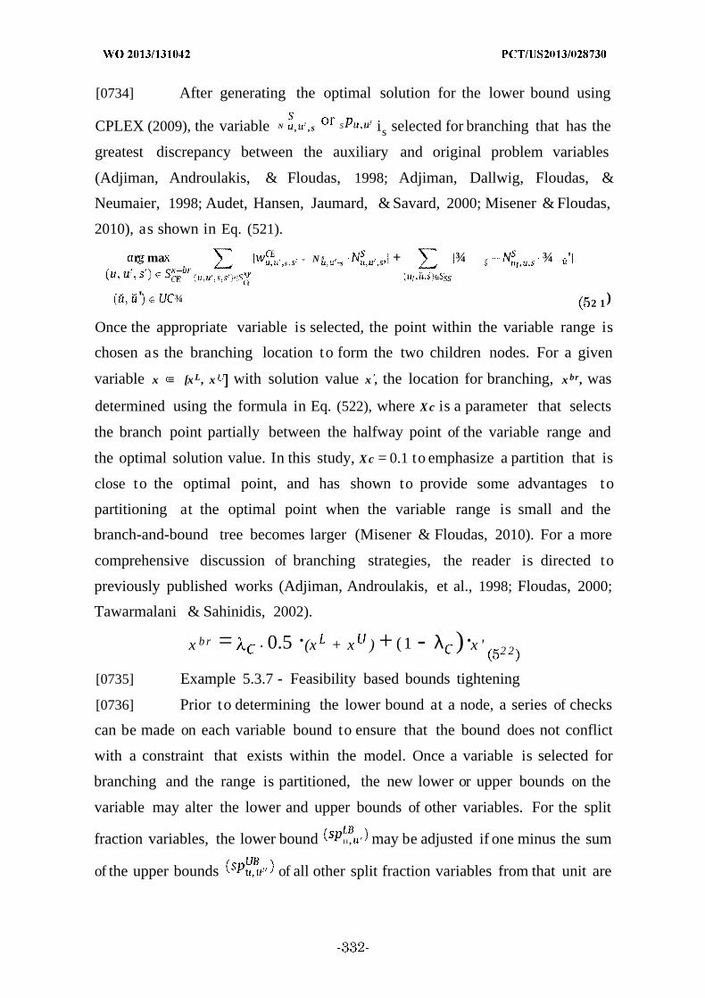
[0734] After generating the optimal solution for the lower bound using
CPLEX (2009), the variable N , ,s S is selected for branching that has the
greatest discrepancy between the auxiliary and original problem variables
(Adjiman, Androulakis, & Floudas, 1998; Adjiman, Dallwig, Floudas, &
Neumaier, 1998; Audet, Hansen, Jaumard, & Savard, 2000; Misener & Floudas,
2010), as shown in Eq. (521).
r ma s - N s _s , + ¾ ¾ '
t
' ¾ 2 1)
Once the appropriate variable is selected, the point within the variable range is
chosen as the branching location to form the two children nodes. For a given
variable x ≡ [x L, x with solution value x , the location for branching, x br , was
determined using the formula in Eq. (522), where Xc is a parameter that selects
the branch point partially between the halfway point of the variable range and
the optimal solution value. In this study, Xc = 0.1 to emphasize a partition that is
close to the optimal point, and has shown to provide some advantages to
partitioning at the optimal point when the variable range is small and the
branch-and-bound tree becomes larger (Misener & Floudas, 2010). For a more
comprehensive discussion of branching strategies, the reader is directed to
previously published works (Adjiman, Androulakis, et al., 1998; Floudas, 2000;
Tawarmalani & Sahinidis, 2002).
x b r = 0.5 ·(x + x ) + (1 - λ )·x ' 2 2
[0735] Example 5.3.7 - Feasibility based bounds tightening
[0736] Prior to determining the lower bound at a node, a series of checks
can be made on each variable bound to ensure that the bound does not conflict
with a constraint that exists within the model. Once a variable is selected for
branching and the range is partitioned, the new lower or upper bounds on the
variable may alter the lower and upper bounds of other variables. For the split
fraction variables, the lower bound ιι , ' may be adjusted if one minus the sum
of the upper bounds , of all other split fraction variables from that unit are
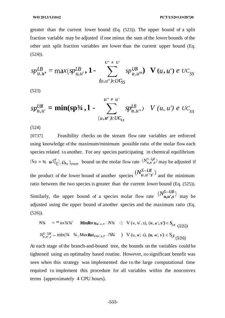
greater than the current lower bound (Eq. (523)). The upper bound of a split
fraction variable may be adjusted if one minus the sum of the lower bounds of the
other unit split fraction variables are lower than the current upper bound (Eq.
(524)).
U" ≠ U'
sp B , = x spuB , 1 - sp u„) V ( , ') e UC
SS
, ) C
(523)
" ≠ '
= min(sp¾ , l - sp „) V (u u') e UCss,u ) Cs s
(524)
[0737] Feasibility checks on the stream flow rate variables are enforced
using knowledge of the maximum/minimum possible ratio of the molar flow each
species related to another. For any species participating in chemical equilibrium
= ¾ u £ e ower bound on the molar flow rate , ', may be adjusted if
the product of the lower bound of another species ' and the minimum
ratio between the two species is greater than the current lower bound (Eq. (525)).
Similarly, the upper bound of a species molar flow rate u,u',s may be
adjusted using the upper bound of another species and the maximum ratio (Eq.
(526)).
¾ = m ¾¾' MinR u ¾ , V («, s), ( , u', s>) SCE
mi ¾ ¾ Rat , V¾ ) V (u, u', s), (u, u', s') SC
At each stage of the branch-and-bound tree, the bounds on the variables could be
tightened using an optimality based routine. However, no significant benefit was
seen when this strategy was implemented due to the large computational time
required to implement this procedure for all variables within the nonconvex
terms (approximately 4 CPU hours).

[0738] Example 5.4 - Computational results of twelve case studies
[0739] The proposed global optimization routine was used to analyze twelve
distinct case studies using perennial biomass (switchgrass), lowvolatile
bituminous coal (Illinois #6), and natural gas as feedstocks. To examine the
effects of potential economies of size on the final liquid fuels price, three distinct
plant capacities were examined to represent a small, medium, or large capacity
hybrid energy plant. Based on current petroleum refinery capacities,
representative sizes of 10 thousand barrels per day (TBD), 50 TBD, and 200 TBD
were chosen, respectively. The trade-offs for C02 handling including
sequestration, venting, and reaction to form CO via the reverse water-gas -shift
reaction were examined by enforcing different levels of feedstock carbon
conversion to liquid fuels. Conversion rates of at least 25%, 50%, 75%, and 95%
were enforced for each of the three plant capacities, resulting in the twelve case
studies that will be presented. The overall greenhouse gas emission target for
each case study is set to have a 50% reduction from petroleum based processes
(Baliban et al., 2011, 2012). The cost parameters used for CBGTL process are
listed in Table 62.
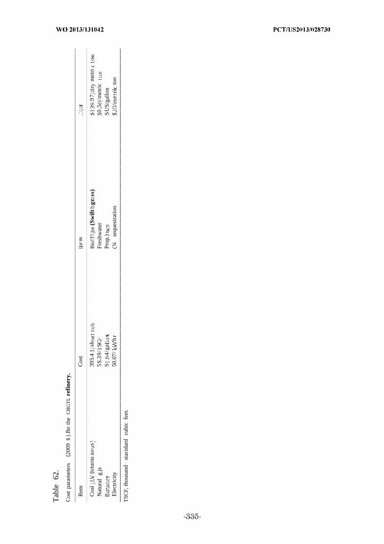
Tab
le62
.
Cos
tpa
ram
eter
s2
009
$
Jbr
the
CB
GT
Lre
fine
ry.
Rem
Cos
te
m·:
·.;··
Coa
lit
urns
aos
393.
4sh
iB
io!T
!.js
s(S
wif
tgr
ss)
.97
rm
etri
Nat
ural
g.js
5S.3
9/SC
Fres
hwat
er0
,5/m
etri
cS
.4
/g.a
sPr
op.)
tS
US/
gallo
nE
lect
rici
ty50
.07/
hr
¾se
ques
trat
ion
/e
too
TSC
F,th
ousa
ndst
acid
ard
cubi
cfe
et.
[0740] Once the global optimization algorithm is completed, the resulting
process topology provides (i) the operating conditions and working fluid flow rates
of the heat engines, (ii) the amount of electricity produced by the engines, (iii) the
amount of cooling water needed for the engines, and (iv) the location of the pinch
points denoting the distinct subnetworks. Given this information, the minimum
heat exchanger matches necessary to meet specifications (i)-(iv) are calculated as
previously described (Baliban et al., 2011; Floudas, 1995; Floudas, Ciric, &
Grossmann, 1986). Upon solution of the minimum matches model, the heat
exchanger topology with the minimum annualized cost can be found using the
superstructure methodology (Elia et al., 2010; Floudas, 1995; Floudas et al.,
1986). The investment cost of the heat exchangers is added to the investment cost
calculated within the process synthesis model to obtain the final investment cost
for the superstructure.
[0741] Example 5.4.1 - Global optimization framework
[0742] The case studies were each tested on a single computer containing 8
Intel Xeon 2.83 GHz processors and shared memory parallelization. The lower
bound of each node in the branch-and-bound tree was solved using CPLEX and
eight parallel threads (CPLEX, 2009), while the upper bound was solved serially
using CONOPT. The computational time for each node was largely spent
computing the lower bound, so the serial computation of the upper bound did not
hinder the progress of the branch-and-bound tree. Parallelization of the entire
branch and bound algorithm using a message passing interface and a shared
memory system on a Beowulf cluster will be the study of a future investigation.
The original MINLP model contains 15,439 continuous variables, 30 binary
variables, 15,406 equality constraints, 230 inequality constraints, 274 bilinear
terms, 1 quadrilinear term, and 60 concave power functions.
[0743] For each lower bound, the bilinear terms were relaxed using a
logarithmic partitioning scheme with 4 partitions for the phase equilibrium
terms and 8 partitions for the remaining terms. The quadrilinear term was
relaxed using three successive bilinear term relaxations with 8 partitions each.
This led to the introduction of an additional 139 binary variables, 1793

continuous variables, and 2747 inequality constraints to fully define the
partitioning scheme. The total amount of constraints does not include the
introduction of the auxiliary variables in the original mathematical model, since
these constraints will simply replace the nonlinear constraints of the original
model. The concave functions were underestimated using a piecewise linear
scheme using 2-5 SOS2 variables for each function, leading to a total of 108
SOS2 variables. The 120 equality constraints generated from the
underestimation replace the 60 nonlinear constraints of the original model. The
complete MILP model for the lower bound therefore contains a total of 17,232
continuous variables, 169 binary variables, 108 SOS2 variables, 15,466 equality
constraints, and 2977 inequality constraints. At each node of the branch-and-
bound tree, the MILP model was terminated upon reaching optimality or after
1800 s (30 min) of computational time. For each upper bound, a multi- start
technique was utilized where the binary variables are fixed and the resulting
NLP was solved to optimality. The resulting NLP model contained 15,439
continuous variables, 15,406 equality constraints, and 230 inequality constraints
along with the same amount of nonconvex terms as the original MINLP model.
[0744] The results of the entire global optimization algorithm are shown in
Table 63. For each case study, the computational results are shown after
completion of the root node and upon termination of the solver. The termination
criterion for the algorithm was set to allow the algorithm to run for 100 CPU
hours (3.6 x 10⁵ s). After 100 CPU hours, the quality of both the lower and upper
bounds did not improve for any of the twelve case studies. At the root node, an
upper bound for the model is initially calculated, followed by the optimality based
bounds tightening and the calculation of the first relaxation (lower bound). From
Table 63, it is evident that a majority of the computational effort at the root node
is spent calculating the upper bound (5466-7047 s for all calls to the solver) and
the bounds tightening (25,337- 28,286 s) while the least amount of effort is spent
on calculating the relaxation (1156-1484 s). This is in contrast to the remaining
nodes of the branch-and-bound tree where the majority of time (>80%) is spent
calculating the relaxation while the balance is spent calculating the feasibility

tightening (<1%) and the upper bound (<20%). The computational effort to
calculate the upper bound is higher at the root node because the multi- start
technique uses 150 initial points, while only 10 initial points are used at
subsequent nodes. Progression of the branch-and-bound tree was not enhanced
when an increased number of initial points was used at the children nodes of the
tree, though the generation of a high-quality feasible points (upper bound) at the
root node does have a noticeable effect on the tree. The value for the upper bound
found at the root node will influence the optimality based bounds tightening and
therefore the quality of relaxations generated at all nodes throughout the tree.
The selection of 150 initial points at the root node was chosen as a proper balance
between the solution quality obtained at the root node and the computational
effort required. That is, as the number of initial points was increased, the upper
bound obtained at the root node showed little or no change. If the number of
initial points at the root node was decreased, the quality of the upper bound at
the root node began to decrease and had an adverse effect on the entire global
optimization algorithm.
[0745] Upon completion of the root node, the optimality gap between the
lower and upper bounds ranges from 12.35% to 36.10% throughout the various
case studies. To enhance the quality of the relaxation at the root node, the
number of partitions used for the bilinear terms and the concave functions could
be used. In fact, if the number of partitions was increased to 32 for each bilinear
term and the error in the cost functions was at most 2% (4-9 SOS2 variables per
function), then the relaxation at the root node can be enhanced enough to reduce
the gap to between (9-16%) for all case studies. The gap still seen with this tight
relaxation implies that a branch-and-bound tree should be used to provide a
tighter guarantee of optimality. Note that when the branch-and-bound algorithm
is used for this large partitioning scheme, the computational time at the root
node ranges from 95,000 to 110,000 s due to a slight increase for the optimality
based bounds tightening (30,000-35,000 s) and a substantial increase for the
relaxation (59,000-65,000 s).
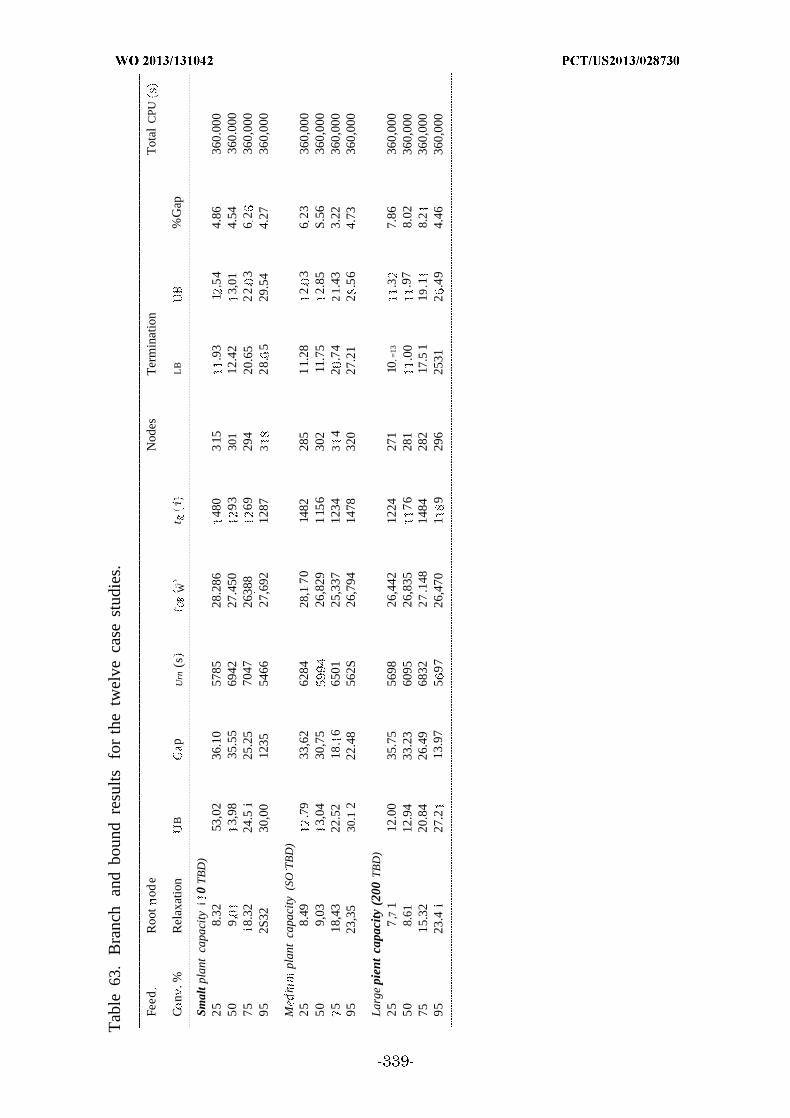
Tab
le63
.B
ranc
han
dbo
und
resu
ltsfo
rth
etw
elve
case
stud
ies.
Feed
Roo
tod
eN
odes
Ter
min
atio
nT
otal
CPU
Cn
.%R
elax
atio
nB
pU
rn(s
Wt
(< i
LB
%G
ap
Smal
tpla
ntca
paci
tyί
0T
BD
)25
8.32
53,0
236
.10
5785
28.2
8648
03
15.9
31
.54
4.86
360.
000
509
,3,
9835
.55
6942
27.4
5093
301
12.4
23,
014.
5436
0.00
075
i8.3
224
.5i
25.2
570
4726
388
6929
420
.65
22.
36
236
0,00
095
2S32
30,0
012
3554
6627
,692
1287
328
.5
29.5
44.
2736
0,00
0
Mr
plan
tca
paci
ty(S
OT
BD
)25
8.49
.79
33,6
262
8428
,170
1482
285
11.
282.
36
2336
0,00
050
9,03
3,04
30,7
526
,829
115
630
211
.75
2.85
S.56
360,
000
518
,43
22.5
218
.6
6501
25,3
3712
343
42
.74
21.
433.
2236
0,00
095
23,3
530
.12
22.4
856
2S26
,794
1478
320
27.2
12
.56
4.73
360,
000
Lar
gepi
ent
capa
city
(200
TB
D)
257
,71
12.0
035
.75
5698
26,4
4212
2427
110
=13
.37.
8636
0,00
050
8.61
12.9
433
.23
6095
26,8
3576
281
.00
.97
8.02
360,
000
7515
.32
20.8
426
.49
6832
27.1
4814
8428
217
.51
19.1
8.2
360,
000
9523
.4i
27.2
13.9
75
9726
,470
19
296
2531
2.4
94.
4636
0,00
0
The total time for finding the upper bound (tUB), the optimality based bounds
tightening (tOB), and relaxation (tR) are listed for the root node along with the
final value of the relaxation (in $/GJ). The total number of nodes used within the
branch-and-bound tree before termination is listed along with the find lower (LB)
and upper (UB) bound (in $/GJ) and the gap at termination. Note that all runs
were terminated when the total CPU time reached 100 h (3.6 x 10⁵ s).
[0746] The benefit of the branch-and-bound tree for the twelve case studies
is evident when looking at the best feasible solution (upper bound) and the
relaxation (lower bound) at termination. For all case studies, the gap ranges
between 3.22% and 8.56% (Table 63). This is substantially reduced from the gap
at the root node due to both an increase in the relaxation throughout the branch-
and-bound tree and a decrease in the upper bound throughout the tree. A
decrease in the upper bound implies that a better feasible solution was found
during the branch-and-bound process than was achieved during the root node. In
fact, several better feasible solutions were found for most of the case studies
during the progression of the tree. This implies the existence of local minima
throughout the mathematical model landscape make it difficult for the solver to
find other feasible solutions that have a lower objective value. Note that a
different initialization technique could be employed at the root node that would
allow the solver to more efficiently find feasible solutions that are obtained later
in the branch-and-bound tree. However, the mathematical guarantee of the
optimality of these solutions is not known until the global optimization algorithm
is used.
[0747] To highlight the change in the lower bound, upper bound, and
optimality gap throughout the branch-and-bound tree, the progression of the tree
is shown in FIG. 68 for the four small capacity case studies, in FIG. 69 for the
four medium case studies, and in FIG. 63 for the large case studies. In each
figure, the upper bound (dark) will generally be flat for several nodes and will
then experience a drop at a given node. When the upper bound remains flat, it
implies that no feasible point was obtained at the node that has a lower objective
value than that of the current incumbent solution. If a better feasible solution is

found at a node, then the upper bound is updated with this lower objective value,
and the curve drops to reflect this change. The lower bound (light), generally
increases for each node based upon the partitioning used throughout the tree.
However, for each case study, there is a point at which the lower bound does not
change as the tree is progressed. At this point, the branch-and-bound tree has
been progressed deeply enough where it becomes difficult to partition the search
space effectively. The optimality gap (dotted) decreases in accordance with the
changes in the lower and upper bounds and generally reaches a threshold value
prior to the termination point.
[0748] Example 5.4.2 - Comparative studies
[0749] To benchmark the proposed global optimization method, a
comparison of the approach with the deterministic global optimization solvers
BARON 9.0.2 and LINDOglobal 6.1.1 was performed using the three 50%
conversion case studies. The results are presented in Table 64. Both BARON and
LINDOglobal were unable to find a feasible solution (upper bound) to the
mathematical model after 100 h of computational time. In addition, the lower
bound reported by these two algorithms was smaller than the lower bound
reported by the proposed global optimization method for each of the three case
studies. The lower bound reported by BARON was 3.4% lower than the lower
bound reported by the proposed method for the small case study, 5.7% lower for
the medium case study, and 4.5% lower for the large case study. The lower bound
for LINDOglobal was 4.7% lower for the small case study, 6.5% lower for the
medium case study, and 4.5% lower for the large case study. This implies that
the proposed method provided a tighter mathematical guarantee of optimality
then either BARON or LINDOglobal was able to do. In addition, the proposed
global optimization algorithm was compared to the local solver DICOPT using a
multi-start technique. The DICOPT solver was able to find feasible solutions, but
could not identify an upper bound that had a lower objective than the upper
bound reported by the proposed method.
[0750] Example 5.4.3 - Overall cost of liquid fuels
[0751] The upper bound value found at termination of the global
optimization algorithm represents the cost of liquid fuels production (in $/GJ) for
each case study. This cost is decomposed in Table 65 to highlight the
contributions of the feedstocks, investment, sequestration, and byproducts to the
final value. The feedstock cost is distributed over the three major carbon based
feedstocks (coal, biomass, and natural gas) along with butanes that are needed
for isomerization and freshwater that is needed to make-up for losses from the
cooling tower and the outlet wastewater. The similarities in the upgrading
section for all twelve case studies causes the cost for the butane to remain
relatively consistent. Though the freshwater input to the process may vary more
widely for each of the twelve case studies, the total cost for the water is minimal
when compared to the cost of the remaining feeds. For the biomass feedstock, the
contribution to the overall cost generally decreases with increasing carbon
conversion rate for each plant size. This is a result of the reduction in the amount
of carbon vented from the process as the feedstock-carbon conversion rate
increases. As each plant is forced to maintain a 50% reduction in greenhouse gas
emissions from petroleum based processes, an increase in the amount of carbon
vented will require an increase in biomass input to the system to properly
balance the CO2 lifecycle. For the coal and natural gas feedstocks, the
contribution toward the overall cost also decreases as the feedstock-carbon
conversion rate increases. This is expected since higher feedstock-carbon
conversion implies that a smaller amount of feedstock is needed to produce a
similar amount of liquid fuels. Note that the general trends for the coal and
natural gas feedstocks are not observed when increasing the conversion rate from
50% to 75%. For each of the three capacities, the biomass cost significantly drops
while the cost for coal and natural gas increases slightly. The increase from 50%
to 75% conversion marks a transition for the CBGTL process that suggests it is
not economically feasible to input additional biomass to balance the CO2 that is
vented from the system. Thus, the CO2 venting is minimized, the biomass input
flow rate is reduced, and the coal and natural gas feedstocks are increased to
provide the additional input carbon. The propane produced from the process is a
byproduct of the upgrading section (Baliban et al., 2010, 2011; Bechtel, 1992) and
therefore is relatively consistent across all twelve case studies.
[0752] CO2 sequestration is only utilized in four of the case studies (S-25,
S-75, M-75, and L-75). For most of the 25% and 50% feedstock carbon conversion
cases, the results of the mathematical model show that it is more economical to
purchase additional biomass and vent the CO2 rather than sequester the CO2 and
purchase cheaper, fossil-fuel feedstocks. In these cases, the CO2 that is vented
largely comes from generation of the electricity via an air-blown gas turbine. The
combination of CO2 and N 2 in the turbine effluent makes CO2 capture and
sequestration an economically unfavorable alternative to simply venting the CO2
and using more biomass as a feed. For the 95% conversion case studies, CO2
sequestration is also not utilized in the final process topology since most of the
CO2 is reacted with H 2 to form CO via the reverse water-gas -shift reaction. The
75% carbon conversion studies all show that CO2 sequestration should be utilized
to handle some of the unreacted carbon. Once a certain feedstock-carbon
conversion threshold is passed, then some of the CO2 must be reacted with H 2 to
obtain the conversion rate necessary. This requires the use of electrolyzers which
input electricity to produce the necessary H2, the result of which can be seen as a
positive contribution of the electricity to the overall cost. Some of this electricity
may be recovered through the use of a gas turbine, but the recovery of CO2 from
the turbine effluent will be limited due to the N 2present in the gas turbine inlet
air. The resulting CO2 within the process is partially sequestered because this
option is economically favorable compared to the high electricity cost of the
electrolyzers. Note that the 95% conversion cases rely heavily on the electrolyzers
and therefore require a significant contribution from non-carbon based
electricity.
[0753] The final contribution to the overall cost comes from the investment
of the process units. For each plant capacity, the investment cost is highest for
the 25% and 95% conversion cases. The 25% conversion cases produce a
significant amount of byproduct electricity (high negative values in Table 65),
which require higher feedstock inputs and larger working capacities across all
units throughout the process topology. As the amount of feedstock-carbon
conversion increases, then a smaller amount of the synthesis gas is directed to
the gas turbines, resulting in a decrease in the output electricity and the
investment cost. The decrease in working flow rates throughout the system also
contributes a smaller amount of waste-heat than the 25% conversion case, which
reduces the electricity output and the investment cost of the heat and power
recovery system. The 75% conversion cases also have a decrease for the medium
and large capacity plants, but there is an increase for the small capacity plant. In
this instance, the decrease in investment cost from smaller working flow rates is
partially offset by the high investment cost of the electrolyzer. This fact is further
emphasized in the 95% conversion cases, as the investment cost is higher than
any other conversion rate. Note that this trend is solely an effect of the
electrolyzer investment cost, and if this unit investment cost was reduced, the
95% conversion cases would likely have the lowest overall investment cost.

Tab
le64
Com
para
tive
stud
ies.
Bou
ndPr
opos
edB
AR
ON
ND
Glo
bl
OP
T
Sra
iipl
ant
capa
city
(10
ΤΏ
)B
13.0
113
.L
B12
,42
12.0
1.8
N/A
Med
ium
pla
tca
paci
ty(5
0B
DU
B.8
5.9
9L
B11
.75
11.
11.0
3N
/AL
arge
plan
t:ca
paci
ty(2
00T
BD
)U
B.9
7.
7L
B1.
0010
.53
10.5
1N
/A
The best upper bound (UB) and lower bound (LB) are presented for each
algorithm when compared for each 50% conversion case study. The
computational time alloted for each algorithm was capped at 100 CPU hours. A
"-" symbol indicates that an algorithm was unable to obtain a feasible solution
after the computational time was exhausted. The "N/A" for DICOPT is present
because this algorithm will not provide information on the lower bound.
[0754] The resulting components of the overall cost combine to provide a
range of $12.54/GJ-$29.54/GJ for the small case studies, $12.03/GJ-$28.56/GJ
for the medium case studies, and $11.32/GJ-$26.49/GJ for the large case studies.
Using the refiner's margin for gasoline, diesel, and kerosene (Baliban et al., 2011;
Kreutz et al., 2008), the corresponding price of crude oil that will be equivalent to
the cost of liquid fuels is calculated and displayed in Table 65. This break- even oil
price (BEOP) can be thought of as the price of crude oil at which the CBGTL
process becomes economically competitive with petroleum based processes. This
cost ranges from $58.68/bbl to $155.56/bbl for the small facilities, $55.77/bbl-
$149.98/bbl for the medium facilities, and $51.73/bbl-$138.18/bbl for the large
facilities. As an illustrative example, the results for 50% conversion of carbon are
shown in boldface in Table 65. The cost ranges from $61.36/bbl for small plants,
$60.45/bbl for medium plants, and $55.43/bbl for large plants.
[0755] The 25% and 50% conversion cases have BEOPs that are at the low
end of the range, and the difference in cost between the 50%, 75%, and 95% cases
is much higher than between 25% and 50%. This is a direct effect of the cost of
electricity and investment needed to power the electrolyzer unit that converts
some CO2 into CO via the reverse water-gas -shift reaction. In this study, the
electricity price is set to $0.07/kWhr and the electolyzer base investment cost is
$1000/kW (National Research Council, 2004). Though a reduction in investment
cost can help reduce the overall costs for the 75% and 95% cases, the bulk of the
price will be from electricity. If cheaper means of electricity production are
obtained, then the BEOP for the 75% and 95% cases will decrease dramatically.
[0756] Example 5.4.4 - Optimal process topologies

[0757] The information detailing the optimal process topologies for all case
studies is shown in Table 66. Three possible temperature options were used for
the biomass gasifier (900°C, 1000°C, 1100°C), the coal gasifier (1100 C, 1200°C,
1300°C), the auto-thermal reactor (700°C, 800°C, 900°C), and the reverse water-
gas-shift unit (700°C, 800°C, 900°C). For the biomass gasifier, the 1100°C unit is
selected for the 25% conversion rate across all three capacities. For the remaining
nine case studies, the 900°C unit is selected. For the coal gasifier, the 1200°C unit
was selected for four of the case studies and the 1300°C unit was selected for the
remaining eight case studies. Note that both the biomass and coal gasifiers for all
twelve case studies were solid/vapor fueled units which employed a vapor phase
recycle stream as a fuel input along with the solid coal or biomass.
[0758] The reverse water-gas -shift unit was selected for all 25% and 50%
conversion case studies with an operating temperature of 700°C or 900 °C. For
the 75% and 95% case studies, no dedicated reverse water-gas-shift unit was
selected in the optimal topology because the consumption of the CO2 occurred
within the iron-based Fischer-Tropsch (FT) units or the gasifiers. In fact, an
iron-based low-temperature FT unit was selected for all of the twelve case
studies, and an iron-based high-temperature FT unit was used in seven of the
studies. Each of these iron-based units can take advantage of the exothermic FT
reaction to provide heat for the endothermic reverse water—gas-shift reaction
(Baliban et al., 2011, 2012). The high-temperature FT units for the remaining
five case studies utilize a cobalt-based catalyst that has a minimum amount of
CO2 input and does not facilitate the water-gas -shift reaction. The auto-thermal
reactor temperature was selected to be 800°C for four of the case studies and
900°C for the remaining eight studies (see Table 66).

Tab
le65
Ove
rall
cost
resu
ltsfo
rth
etw
elve
case
stud
ies.
Cas
est
udy
rtr
ibo
toco
stG
(S/G
J)T
oi.il
(S/
)
Coa
lB
ore
ass
gas
But
ane
Wat
ernv
.E
le,
Prop
ane
S-2S
4.93
7.65
2.21
0.52
(102
0.
5.52
-8.
7-0
.51
12.5
458
.68
S-5
2.41
7,68
1.12
0,51
0.02
0.00
4.73
-2.8
5-0
.60
.01
61.3
6S-
752.
7123
5.9
40
58
0.02
0.54
5.01
.4-0
.5S
22.0
32.
76S-
95.8
42,
581.
320,
570.
03ao
o5.
977.
79-0
.56
29,5
455
.56
-2.
9812
,23
2.1
30,
570.
04ao
o3.
25-8
.80
-0.5
612
,03
55.7
7M
-52.
727.
661.
220.
510,
020,
002.
88-1
.60
0.50
,860
,45
-2.
82.
440.
590.
020.
3923
93
8-0
.58
.43
09.3
4-
52.
042.
570.
920.
62.0
30.
003
519
.45
-0.6
28.5
6\4
9.98
23.
02.
702
170.
610
30.
002
05
-8.6
9-0
.59
11.3
21
.73
-52.
437.
651.
74a
s™
0.03
0.00
1.75
-1.
62-0
.58
11.9
755
.43
75
2,63
2.47
189
0.S0
0,03
0,48
153
10.0
7-0
.50
19.1
96.
2-9
>1,
32.
S613
10.
550,
030.
002
.18
.63
-0.5
426
.49
ί3.
8
CO 00
The small (S), medium (M), and large (L) case studies are each labeled with the
percentage of feedstock carbon that must go to liquid fuels. The contribution to
the total costs (in $/ ) come from coal, biomass, natural gas (Nat. Gas.),
butanes, water, C02 sequestration (C02. Seq.), and the investment (Inv.).
Propane is always sold as a byproduct while electricity (Elec.) may be sold as a
byproduct (negative value) or obtained from a non-carbon based source (positive
value). The results for 50% conversion of feedstock carbon are shown in boldface.

Tab
le66
.T
opol
ogic
alin
form
atio
nfo
rth
eop
timal
solu
tions
for
the
twel
veca
sest
udie
s.
Cas
est
udy
S--2
5s-
soS-
75S
5-2
5M
-50
--75
-1-
25L
-50
-S
10
900
900
900
00
900
900
900
i10!
)30
090
09
0E
CS
Typ
es/
vS/
VS/
VS/
VS
VS/
VS/
VS/
VS/
VS/
VS/
VS/
V
CG
ST
emp.
0no
o30
030
012
0020
00
030
012
00:;
oo0
0C
GS
Typ
eS/
VS/
Vs/
vS/
VS/
VS/
VS/
VS/
VS/
VS/
Vs/
vS/
V
RG
ST
emp,
700
700
700
900
700
70
AT
em
p80
0O
O90
090
080
080
090
090
080
090
090
090
0Y
ZU
sage
Ny
YN
Yy
.N
YY
C0
2SE
Usa
geY
Ny
NY
NY
GV
YY
Y¥
Yy
Yy
i'
::·
on
iron
roo
'o
wΌ
ίϊi
oro
n<:
on
io
nir
on
TT
ype
Co
bal
ba
iron
Co
ba
tlr
io
no
Cob
alt
con
on

Specifically listed is the operating temperature of the biomass gasifier (BGS), the
coal gasifier (CGS), the auto-thermal reactor (ATR), and the reverse water-gas-
shift unit (RGS). The gasifiers are also labeled as either solid/vapor (SAO or solid
(S) fueled, implying the presence or absence of vapor-phase recycle process
streams. The presence of an electrolyzer (EYZ), a C02 sequestration system
(C02SEQ), or a gas turbine (GT) is noted using yes (Y) or no (N). The low and
high-temperature Fischer-Tropsch units (LTFT and HTFT) are designated as
either iron-based or cobalt-based units. The results for 50% conversion of
feedstock carbon are shown in boldface.
[0759] The 25% and 50% conversion case studies do not use an electrolyzer,
but choose to mostly vent the generated CO2. In the S-25 case study, a small
amount of the CO2 is sequestered (see Table 67). All of the 75% and 95% studies
must use an electrolyzer to convert some of the CO2 into liquid fuels, though only
the 75% case studies utilize sequestration to remove the remaining CO2. The
25%, 50%, and 75% conversion studies all have a gas turbine installed to help
recover some of the electricity needed for the process and potentially sell extra
electricity as a byproduct. The gas turbine is not selected for the 95% case study
due to the high cost of CO2 that must be recovered from the turbine outlet.
[0760] The 50% conversion cases are listed in boldface in Table 67. For each
of these cases, the biomass gasifiers were solid/vapor fueled units operating at
900°C. The coal gasifiers were solid/vapor fueled units operating at 1200°C for the
large and medium case studies and 1300°C for the small case study. The reverse
water-gas -shift unit operates at 700°C for the small and large case studies and
900°C for the medium case study. The auto-thermal reactor operates at 800°C for
the small and medium case studies and 900°C for the large case study. The low-
temperature FT reactor used was iron-based for all three studies and the high-
temperature FT reactor was cobalt-based for the small and medium case studies
and iron-based for the large case study.
[0761] Example 5.4.5 - Overall process material balances
[0762] The overall carbon balance for the CBGTL processes is shown in
Table 67 and highlights the eight major points where carbon is either input or
output from the system. The 50% conversion case studies are highlighted in the
table using boldface. Carbon that is input to the system via air is neglected due to
the low flow rate relative to the other eight points. The coal, biomass, and natural
gas inputs generally supply over 99% of the input carbon to the system while the
balance is supplied by the butane input to the upgrading units. Note that the
input carbon flow rate for the feedstocks changes similarly to the changes seen
with the feedstock cost contributions in Table 65. That is, generally, the carbon
input for each feedstock decreases as the carbon conversion rate increases. The
strong decrease in the biomass cost from 50% to 75% conversion seen in Table 65
is supported by the decrease in the carbon input shown in Table 67 for these case
studies. Additionally, it is evident that the carbon vented from the system
decreases by over 95% for each capacity when moving from a 50% to a 75%
conversion of feedstock carbon. In the 75% conversion cases, the unreacted
carbon is sequestered as this proves to be the economically preferable option to
increasing the biomass feedstock.
[0763] The output amount of carbon in the total product is constant for
each plant capacity, which is consistent with the constant production capacity
that is required for each feedstock-conversion rate. The amount of carbon leaving
as propane is around 3% of that leaving as gasoline, kerosene, and diesel. For
eight of the twelve case studies, the remaining carbon exits as CO2 during
venting, as this is the economically preferable option. For the S-25 case study, a
small amount of the carbon is sequestered, and for the three 75% conversion case
studies, a majority of the carbon is sequestered as CO2.

Tab
le67
.O
vera
llca
rbon
bala
nce
for
the
CB
GT
Lpr
oces
s.
Cas
est
udy
Car
bon
inpu
t(
o/s
Car
bon
outp
utk
ol
sC
onve
rsio
n(¾
Coa
lB
iom
ass
Nat
,ga
sB
utan
ePr
oduc
tPr
opan
eV
ent
C0
:<C
O:
S-2
51.
371.
103
40.
02.0
50.
03.0
70.
763
7
S-50
0.72
1.9
0.23
0.02
1.05
0.03
1.08
0.00
50S-
750.
750,
360
30.
021,
050.
030.
0ί
035
75
S-95
0.51
.0.
400.
2(5
0.02
1.05
0.03
(0
60,
009
5
-25
9.45
1.56
0.
2':>
,73
0.
9.9
0,00
35
-53.
795.
870.
350
,5,
230
.3
5.36
0.00
50-7
54
.1.
1.4
0.
25.
230
.16
0.
51.
655
-95
4.9
90
.0
.5,
230
.16
0.28
o.o
95
-25
6.88
39.2
86.
750.
520
.92
0.64
41.
850.
003
4
L-5
013
.55
23.6
45.
420.
4820
,92
0.62
21.5
40.
0050
75
.68
7.65
5.87
0.42
20,9
20.
540.
83(.
32
95
10.
7.91
4.08
0.46
20.9
20.
581
..o
o9
5
CO C
Carbon is input to the process via coal, biomass, natural gas, or butanes and exits
the process as liquid product, propane byproduct, vented CO2, or sequestered
(seq.) CO2. The small amount of CO2 input to the system in the purified oxygen
stream (<0.01%) is neglected. The results for the 50% conversion of feedstock
carbon are shown in boldface.

Tab
le68
.O
vera
llm
ater
ial
and
ener
gyba
lanc
esfo
rth
eC
BG
TL
proc
ess.
Ca
stud
yC
oal
im
as
ai.
.¾?·
.ta
eFr
eshw
ater
Was
tew
ater
Prop
ane
CO
?ve
ntC
O;
' i'' /'
ffi(
CF/
bb
/B
(bb
/bb
(bbl
/bbl
)f
bi
)(
g/
(kg
bb
i
Mat
eria
lba
lanc
esS
-25
96
330
0.S7
2.1
115
.12
.0.
4913
9.1
140
8.74
290.
51
5-50
103.
5930
1,56
1.4S
13.
2.61
0.40
4.2
410.
670.
00S
-75
7,9
292
.35
1.92
>39
2.52
0.26
158.
323,
8013
3.09
S95
73.2
810
!.S
1.30
126.
172.
790
.2
.42
1.6
10.
00V
25
1.5
348
0.33
2, 1
112
6.
72
,80.
0652
.48
759.
840.
00M
-5ί 0
8.42
298.
431.
212
.89
2.07
0.25
136.
4340
7.62
0.00
~7S
ί8.
5895
.74
12
130.
6023
20.
2259
.44
Π.1
525
.48
-5
810
1.0
0.91
37.2
42.
390.
0465
,86
21.
570.
00-2
5ί2
0,65
499
.2.
15
135,
032.
260.
3916
1.52
795.
700.
00L
-SQ
9.8
430
0.39
1.72
126.
172.
S3.0
8S
.740
9.53
.oL-
4.
297
,f7
1,87
0,68
2,37
034
136.
495.
840
.-9
572
.85
100.
481.
3074
2.35
0.2
114
8.63
.1
0.00
O C CC
ase
stud
yC
oal
r¾,!
t.g,
jsr
r1
riP
Prop
ane
fe
y
bala
nces
-
S-25
701
548
249
80-2
746
97
65.3
-537
055
06
91
-7
659
114
73.
S-7
538
521
9S9
321
659
o65
.15
926
218
514
888
603
659
659
.5·:?
52
1643
7812
0143
8-
458
3297
529
65.0
M-5
019
3627
2068
639
2-2
7132
9747
470
.57
¾2
17
873
751
453
20
3297
554
62.0
-2
9215
432
9732
9757
658
.1.
as6
71
787
5-5
894
3,
022
4363
.5-5
6917
0,9
139
24S2
-9
.0
2204
70.1
L-7
574
9435
4242
5153
7S
3,
9089
663
.8L
--95
5203
3663
291
112
,635
1,
020
643
bbi,
barr
els:
B.t
hous
and
br
;D
T,d
ryto
ns;
SC
,m
illio
nst
anda
rdi'
e;
V,
low
erhe
atin
gva
lue.
All material balances are normalized with respect to the volume of products
produced. Negative electricity values in the energy balance represent outlet
energy, and are counted as products for the efficiency rate and positive values are
added as input to the CBGTL process. The results for 50% conversion of feedstock
carbon are shown in boldface.
[0764] For each of the case studies, the carbon conversion rate was set as a
lower bound for the mathematical model. Thus, the conversion of carbon in the
four feedstocks to the final liquid products (i.e., gasoline, diesel, and kerosene)
must be at least as large as the set conversion rate. For nine of the case studies,
the final conversion rate was exactly equal to the rate specified to the model. The
results of the mathematical model suggest that it is more economically favorable
to vent or sequester the CO2 rather than react it with H 2 to produce additional
liquid fuels. This is consistent with the high costs associated with the electrolyzer
to produce the necessary H 2 for reaction. For the 25% conversion case studies,
Table 67 shows that the mathematical model chooses conversion rates between
34% and 37% for the optimal process design. In these instances, it is more
beneficial to produce additional liquid fuels as opposed to electricity via the gas
and steam turbines.
[0765] The overall material and energy balances for each case study are
shown in Table 68. Each component in the material balances is normalized with
respect to the amount of liquid products produced. The coal and biomass flow
rates are based on dry tons while the natural gas is shown in million standard
cubic feet. The change in feedstock flow rate with increasing carbon conversion
rate is consistent with the results shown above, but the normalization of the flow
rates shows that the feedstock flow rates have similar values for the same
conversion rate across all three plant capacities. This is in agreement with the
cost data shown in Table 65 and the similar topological data shown in Table 66.
The remaining feedstocks, butane and freshwater, along with the outlet
wastewater and byproduct propane vary over a small range. The CO2 that is
vented or sequestered from the process decreases as expected with increasing
conversion rate and ranges over all twelve studies from 3.80 kg/bbl for the S-75

case study to a total of 795.70 kg/bbl for both venting and sequestration for the L-
25 case study.
[0766] As an illustrative example, the 50% conversion case studies shown
in boldface in Table 68. The amount of coal feedstock used for the system is
103.59 dry tons/thousand barrels (DT/TB) for the small capacity, 108.42 DT/TB
for the medium capacity, and 96.84 DT/TB for the large capacity. The biomass
input is 301.56 DT/TB for the small capacity, 298.43 DT/TB for the medium
capacity, and 300.39 DT/DB for the large capacity. The natural gas input is 1.46
million standard cubic feet/thousand barrels (MSCF/TB) for the small capacity,
1.21 MSCF/TB for the medium capacity, and 1.72 MSCF/TB for the large
capacity. The freshwater required for the case studies is 2.61 barrels/barrel of
product (bbl/bbl) for the small system, 2.07 bbl/bbl for the medium case, and 2.83
bbl/bbl for the large case while the outlet wastewater is 0.40 bbl/bbl for the small
case, 0.25 bbl/bbl for the medium case, and 0.08 bbl/bbl for the large case. The
CO2 produced from these three case studies is vented at rates of 410.67 kg/bbl for
the small case, 407.62 kg/bbl for the medium case, and 409.53 kg/bbl for the large
case. CO2 sequestration is not utilized for all three studies.
[0767] The energy balances from the process are listed in MW in Table 68.
The small capacity plant is designed to produce 659 MW of fuels on a lower
heating value basis, the medium plant is designed for 3297 MW, and the large
plant for 13,190 MW. The amount of energy needed to produce the liquid fuels
ranges from 765 MW to 1030 MW for the small plants, from 3851 MW to 5284
MW for the medium plants, and from 15,086 MW to 21,327 MW for the large
plants. The efficiency of the system is calculated by dividing the total energy
output (i.e., via products, propane, or electricity) by the total energy input (i.e.,
via coal, biomass, natural gas, butane, or electricity). If electricity is output from
the system, the value is listed as negative in Table 68 and the magnitude of the
energy value is added to the total output. If the value is positive, then this energy
is added to the total input to the system. The efficiency of the twelve studies
ranges from 58.1% for the M-95 process to 73.9% for the S-50 process.
[0768] As an illustrative example, the 50% case studies are shown in
boldface in Table 68. Each of these studies will output electricity as a byproduct,
so the energy required for fuels production is the sum of the lower heating values
of the feedstocks. In general, the biomass is the largest contributor to the energy
input at 550 MW for the small study, 2720 MW for the medium study, and 10,951
MW for the large study. Coal is the next highest contributer with 370 MW needed
for the small study, 1936 MW needed for the large study, and 6917 MW needed
for the large study. The balance of the energy input is split between natural gas
and butanes. The energy output from the process is in the form of liquid product
(i.e., gasoline, diesel, and kerosene), liquid byproduct (propane), or electricity.
The largest output of energy is the liquid product, the second highest is the
propane, and the last is the electricity. The efficiencies for the 50% conversion
cases represent the highest for a given capacity over all conversion rates. The
small plant has the largest overall efficiency of 73.9%, while the medium and
large plants have efficiencies of 70.5% and 70.1%, respectively.
[0769] Example 5.5 - Conclusions
[0770] A novel global optimization framework has been proposed to address
the large-scale coal, biomass, and natural gas to liquids (CBGTL) process
synthesis mathematical model with simultaneous heat, power, and water
integration. Using piecewise linear underestimators with a logarithmic
partitioning scheme for the bilinear terms and piecewise linear underestimators
with a linear partitioning scheme for the concave cost functions, twelve case
studies for the CBGTL model have been optimized to within a 3.22-8.56%
optimality gap after 100 CPU hours. The case studies arise from four distinct
carbon-conversion rates for a small (10 TBD), medium (50 TBD), and large (200
TBD) plant capacities, all of which must have a 50% reduction in greenhouse
gases from petroleum-based processes. The proposed framework shows that the
break-even oil price for liquid fuels production ranges from $58.68/bbl to
$155.56/bbl for the small case studies, $55.77/bbl-$149.98/bbl for the medium
case studies, and $51.73/bbl-$138.18/bbl for the large case studies. For a
feedstock carbon conversion rate of 50%, the cost is $61.36/bbl for the small
study, $60.45/bbl for the medium study, and $55.43/bbl for the large study. Each
of the three 50% conversion case studies did not utilize C02 sequestration to
reduce GHG emissions, but instead incorporated a larger amount of biomass
feedstock into the refinery. While the biomass feedstock represented a large
fraction (over 60%) of the cost of each of the 50% conversion case studies, this
option will be favorable to CO2 sequestration because of the reduction in
byproduct electricity that would occur with the latter choice.
[0771] When the conversion rate of feedstock carbon is analyzed
parametrically using the proposed optimization framework, a clear trend in the
increase of the liquid fuels cost is observed. Utilization of domestic resources to
maximum capability is a high concern for energy sustainability, but there is a
clear point where the cost of feedstock conversion is not justified due to high costs
of electricity and key process units. The proposed framework is able to
systematically identify the point where the conversion rate of the carbon in the
feedstock may be increased without affecting the end consumer of liquid fuels.
The proposed framework represents a rigorous methodology for systematically
analyzing the economic and environmental tradeoffs associated with the
construction of hybrid coal, biomass, and natural gas facilities and can ensure a
process design will have a cost of fuels production that is at the global optimum
of the highly nonconvex search space. The global optimization framework is
instrumental not only in providing a tight lower bound on the optimal solution,
but also in identifying process topologies that were not obtained through local
optimization only. That is, the final process topologies selected from the proposed
framework were different than the topology selected at the root node (i.e.,
through local optimization). This implies that the proposed method is critical for
both reducing the cost of the overall refinery and uncovering process topologies
that may be difficult to obtain based on their location in the search space.
[0772] Example 6 - Wastewater network
[0773] To accompany the above process superstructure, a complete water
treatment network (FIGS. 71 and 72) is postulated that will treat and recycle (a)
wastewater from various process units, (b) blowdown from the cooling tower, (c)

blowdown from the boilers, and (d) input freshwater. The treatment units include
(i) a sour stripper and (ii) a biological digester unit to remove acids and
hydrocarbon components entrained in the water stream and (iii) a reverse
osmosis system to remove suspended and dissolved solids from blowdown
streams. Clean output of the network includes (i) process water to the
electrolyzers, (ii) steam to the gasifiers, autothermal reactor, and water-gas-shift
reactor, and (iii) discharged wastewater to the environment. The biogas from the
biological digester and the sour gas from the sour stripper will be recycled back to
the CBGTL process. All separated solids from the reverse osmosis system will be
discharged as solid waste. The general superstructure allows for single or
multiple water sources with or without contaminants, water-using units, and
wastewater treatment units, with all feasible stream connections considered
between these units.
[0774] Example 6.1 - Process wastewater superstructure
[0775] In the previous model, all process wastewater was treated in a sour
stripper (SS) that removed all entrained vapor from the inlet water. The acid-rich
vapors were recycled back to a sour gas compressor while the treated water was
split and sent to either the deaerator for steam generation or the electrolyzer for
hydrogen/oxygen production. Although the sour stripper can remove a large
portion of the entrained hydrocarbons, CO2, and H2S from the inlet feed, there is
a limitation on the amount of NH3 that can be recovered. To comply with
environmental regulations, the sour stripper effluent must either be diluted with
freshwater or treated in a secondary processing unit.
[0776] Biological digestion via anaerobic and aerobic digestion can reduce
the hydrocarbon and acid gases in the inlet stream by converting them to biogas
(i.e., CH4, CO2, H2, NH3, and Ar), which can be sent back to the Claus combuster
along with the compressed and heated sour gas stream from sour stripper. Thus,
the biological digestor (BD) unit can act as a primary processing unit for streams
that have low enough contaminant level for the operation of the unit (i.e., sour
water from the upgrading section, post-combustion knockout wastewater) and as
a secondary processing unit for the sour stripper effluent. High conversion to
biogas is achieved and the effluent water can be readily used in various water-
using units or disposed as wastewater to the environment.
[0777] FIG. 71 illustrates the outline of the process wastewater stream
superstructure. Fixed process units are represented by 110, variable process
units are illustrated by 120, variable process streams are represented by 210 and
all other process streams are fixed unless otherwise indicated. Wastewater from
the CBGTL process includes knockout water from the acid gas flash unit (AGF),
the Claus flash unit (CF), the aqueous effluent from Fischer-Tropsch
hydrocarbon production (MXFTWW), and the sour water effluent from the
product upgrading units. Based on previous experience with the process, the
concentration of acid gases present in the acid gas flash knockout (AGF) and the
Clash flash knockout (CF) may be too high for operation of the biological digestor
(BD). Therefore, these two streams are passed directly to the sour stripper (SS).
Additionally, the concentration of dissolved hydrocarbons in the FT wastewater
(MXFTWW) exceeds the maximum limit of contaminants for the (BD) unit, so
this stream is also passed directly to the (SS) unit. Direction of the above streams
to the (SS) unit implies that this unit will always be present in any selected
CBGTL process topology. The effluent of the (SS) unit may be split (SPSS) and
sent to the (BD) unit to remove any remaining entrained NH3 in the stream or to
the outlet mixer (MXWW). Treated water from the (BD) unit is split (SPBD) and
recycled as treated water to the electrolyzer, the cooling tower, or the deaerator,
or is discharged as outlet wastewater.
[0778] An additional source of process wastewater comes from the post-
combustion knockout units. This includes the fuel combustor flash (FCF) and gas
turbine flash unit (GTF) which are combined (MXPCKO) before being split
(SPPCKO) to either to (SS) unit, the (BD) unit, or directly to the outlet
wastewater mixer (OUTWW). Note that this is the only process stream that is
directly allowed to go to the outlet due to the low level of contaminants in the
stream. The remainder of wastewater from CBGTL process units is derived from
the hydrocarbon recovery unit (HRC), wax hydrocracker (WHC), distillate
hydrotreater (DHT), and naphtha hydrotreater (NHT) and is combined as one
generic output stream (MXPUWW) before entering the water treatment section.
The process upgrading unit wastewater streams are merged into a singular
wastewater stream based on the modeling in Baliban et al. (2011), which is
incorporated herein by reference as if fully set forth. Due to the rigorous gas
cleaning upstream of the FT units, very little sulfur will existin the product
upgrading wastewater. Composition of phenols andother water-soluble
hydrocarbons have also been reduced by theseries of separation units for the FT
effluents. Thus, further cleaningof this stream can take place in either the (SS)
unit or the (BD)unit.
[0779] Example 6. 2 - Utility wastewater superstructure
[0780] The superstructure for the wastewater generated by the utility units
is shown in FIG. 72. The cooling tower (CLTR) provides the cooling requirement
for the CBGTL process (COOL-P) by heating process water from 25 °C to 55 °C. A
loss fraction due to drift and evaporation will occur in this unit, which is
accounted for in the unit's material and energy balance. The circulating fluid will
begin to accumulate salts and dissolved solids which can foul the heat exchangers
and cause inefficient heat transfer. A blowdown stream must be incorporated
with a flow rate set by the cycles of concentration typically used by the cooling
tower. Steam is generated within the heat engine boilers inside the heat and
power system (HEP) and within the process water boiler (XPWB) for use with the
gasifiers (BGS, BRGS, CGS, and CRGS), the auto-thermal reactor (ATR), or the
water- gas-shift reactor (WGS). Each of these steam-using units is present in the
overall CBGTL superstructure and must have their water requirement satisfied
by the utility wastewater superstructure to guarantee water integration.
Blowdown streams must also be incorporated within the steam cycle to prevent
the build-up of solids and hinder heat transfer. To remove a majority of the solids
present in these blowdown streams, a reverse osmosis (RO) unit is used. The
(RO) unit may collect (MXRO) a fraction of the cooling tower blowdown (SPCLTR)
or the combined blowdown from all process boilers (SPBLR). The effluent of the
(RO) unit is split (SPRO) and can be recycled back to the (RO) inlet or sent to the
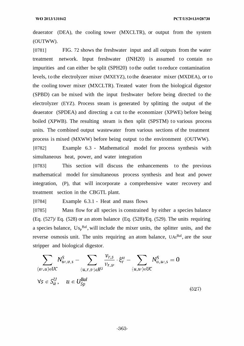
deaerator (DEA), the cooling tower (MXCLTR), or output from the system
(OUTWW).
[0781] FIG. 72 shows the freshwater input and all outputs from the water
treatment network. Input freshwater (INH20) is assumed to contain no
impurities and can either be split (SPH20) to the outlet to reduce contamination
levels, to the electrolyzer mixer (MXEYZ), to the deaerator mixer (MXDEA), or to
the cooling tower mixer (MXCLTR). Treated water from the biological digestor
(SPBD) can be mixed with the input freshwater before being directed to the
electrolyzer (EYZ). Process steam is generated by splitting the output of the
deaerator (SPDEA) and directing a cut to the economizer (XPWE) before being
boiled (XPWB). The resulting steam is then split (SPSTM) to various process
units. The combined output wastewater from various sections of the treatment
process is mixed (MXWW) before being output to the environment (OUTWW).
[0782] Example 6.3 - Mathematical model for process synthesis with
simultaneous heat, power, and water integration
[0783] This section will discuss the enhancements to the previous
mathematical model for simultaneous process synthesis and heat and power
integration, (P), that will incorporate a comprehensive water recovery and
treatment section in the CBGTL plant.
[0784] Example 6.3.1 - Heat and mass flows
[0785] Mass flow for all species is constrained by either a species balance
(Eq. (527)/ Eq. (528) or an atom balance (Eq. (528)/Eq. (529). The units requiring
a species balance, Us Bal, will include the mixer units, the splitter units, and the
reverse osmosis unit. The units requiring an atom balance, UAtBal, are the sour
stripper and biological digestor.

[0786] Heat balances across every unit are maintained using Eq. (529). The
relevant terms include the input and output stream enthalpies (H), the heat
transferred to/from the unit (Q), the heat lost from the unit (QL), and the work
done by the unit (W). Note that Eq. (529) is a general equation for the entire
CBGTL refinery, and some of the terms are not needed for each unit. Specifically,
the heat loss across all units in the wastewater network is negligible (QL = 0) and
work is not required for any treatment unit (W = 0). The total enthalpy of a
stream is related to the enthalpy of the individual components through Eq. (530)
only for streams with known thermodynamic conditions. In addition to the inlet
freshwater, each water treatment unit and splitter unit will operate at a known
temperature and pressure, so the specific outlet enthalpies of each species,
Hsu, s these units can be determined a priori. Note that Eqs. (529) and (530)
suffice to define the enthalpy flow throughout the entire system while leaving
degrees of freedom for the heat transfer (Q) to/from the necessary process units.
∑ ∑ - - Q - Wu , U/UAgg
( .U S) S (530)
[0787] Example 6.3.2 - Sour stripper
[0788] In addition to the general mass/energy constraints, specific
constraints must be written to govern the operation of each treatment unit, the
steam cycle, and the cooling water cycle. The sour stripper is modeled with
specified recovery fraction of water in the bottoms, sS, a s 3
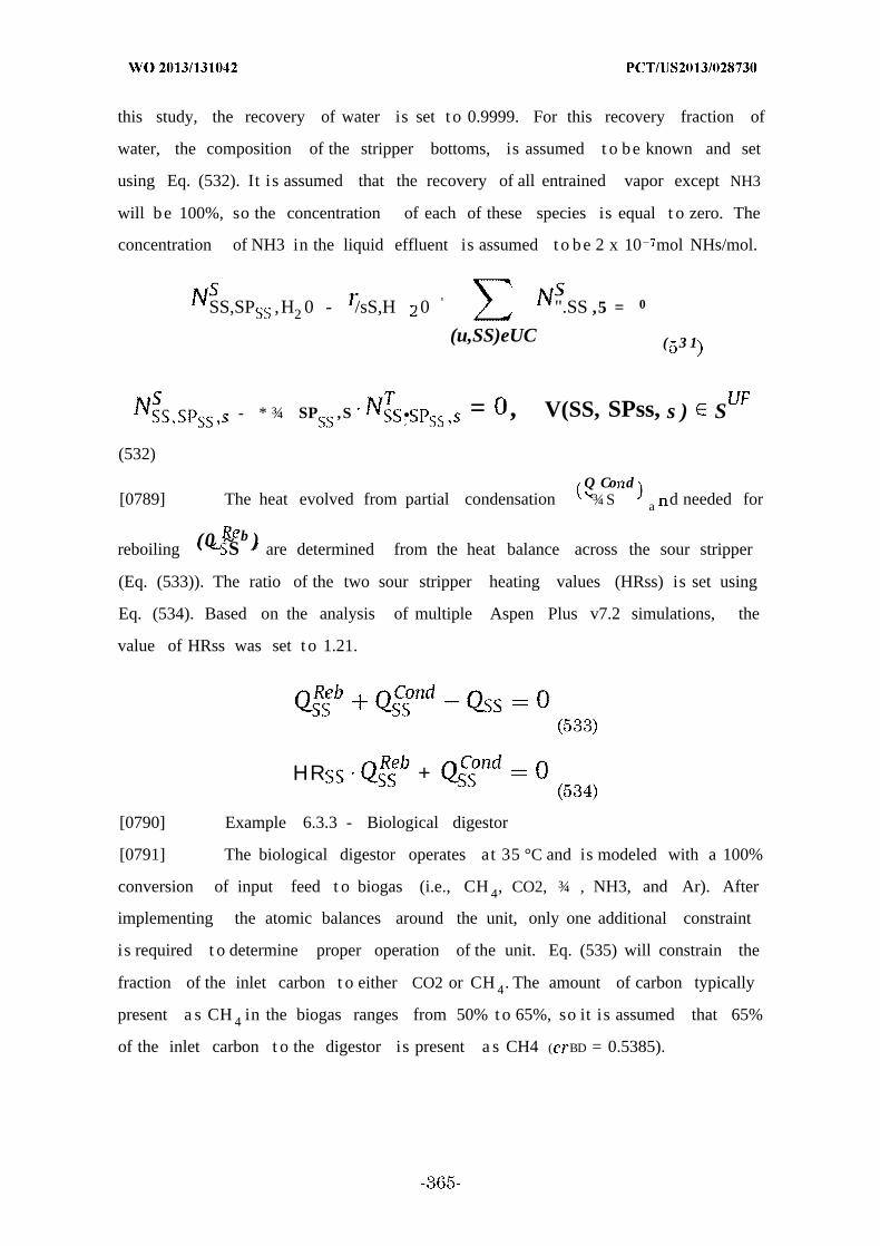
this study, the recovery of water is set t o 0.9999. For this recovery fraction of
water, the composition of the stripper bottoms, is assumed t o be known and set
using Eq. (532). It is assumed that the recovery of all entrained vapor except NH3
will be 100%, so the concentration of each of these species is equal t o zero. The
concentration of NH3 in the liquid effluent is assumed t o be 2 x 10 mol NHs/mol.
SS,SP ,H2 0 - /sS,H 0 ' ".SS ,5 = 0
(u,SS)eUC ( 3 1
- * ¾ SP ,S . = , V(SS, SPss, s ) S
(532)
Q Co d[0789] The heat evolved from partial condensation ¾S a d needed for
reboiling (0 ~Sb ) are determined from the heat balance across the sour stripper
(Eq. (533)). The ratio of the two sour stripper heating values (HRss) is set using
Eq. (534). Based on the analysis of multiple Aspen Plus v7.2 simulations, the
value of HRss was set t o 1.21.
HR +
[0790] Example 6.3.3 - Biological digestor
[0791] The biological digestor operates at 35 °C and is modeled with a 100%
conversion of input feed t o biogas (i.e., CH 4, CO2, ¾ , NH3, and Ar). After
implementing the atomic balances around the unit, only one additional constraint
is required t o determine proper operation of the unit. Eq. (535) will constrain the
fraction of the inlet carbon t o either CO2 or CH 4. The amount of carbon typically
present a s CH 4 in the biogas ranges from 50% t o 65%, so it is assumed that 65%
of the inlet carbon t o the digestor is present a s CH4 ( BD = 0.5385).
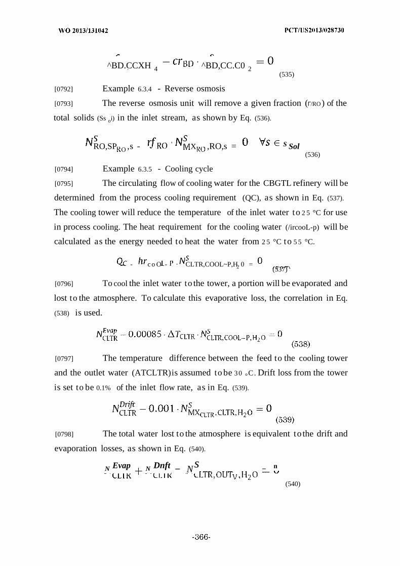
^BD.CCXH 4' ^BD,CC.C0 2
(535)
[0792] Example 6.3.4 - Reverse osmosis
[0793] The reverse osmosis unit will remove a given fraction (Γ/RO) of the
total solids (Ss oi) in the inlet stream, as shown by Eq. (536).
RO,SP O ,s - ' X ,RO,s = S Sol(536)
[0794] Example 6.3.5 - Cooling cycle
[0795] The circulating flow of cooling water for the CBGTL refinery will be
determined from the process cooling requirement (QC), as shown in Eq. (537).
The cooling tower will reduce the temperature of the inlet water to 2 5 °C for use
in process cooling. The heat requirement for the cooling water (/ircooL-p) will be
calculated as the energy needed to heat the water from 2 5 °C to 5 5 °C.
- c o O - · CLTR,COOL~P,H2 0 =(537)
[0796] To cool the inlet water to the tower, a portion will be evaporated and
lost to the atmosphere. To calculate this evaporative loss, the correlation in Eq.
(538) is used.
[0797] The temperature difference between the feed to the cooling tower
and the outlet water (ATCLTR)is assumed to be 3 0 °C. Drift loss from the tower
is set to be 0.1% of the inlet flow rate, as in Eq. (539).
[0798] The total water lost to the atmosphere is equivalent to the drift and
evaporation losses, as shown in Eq. (540).
N Evap N Dnft _ Ns _ n
(540)

[0799] During operation of the cooling tower, salts and dissolved solids will
begin to accumulate in the circulating water that could foul the heat exchangers
and impact heat transfer. A blowdown stream is therefore used to remove these
solids from the tower for proper treatment. The flow rate and concentration of
this blowdown stream is dependent on the cycles of concentration (COC) used to
operate the tower. Cycles of concentration are defined as the ratio of the
concentration of solids in the blowdown to the concentration of solids in the inlet.
Using typical values of COC in industrial practice, the concentrations of
suspended solids and dissolved solids in the cooling tower blowdown are 50 ppm
and 2500 ppm, respectively. These quantities are set in Eq. (541) using the
( v KnT ,SP R , s
known compositions
*CLTR,SP L CLTR,SPCL CLTR, SP ,(541)
[0800] Example 6.3.6 - Steam cycle
[0801] The working fluid in the heat engines requires steam generation to
produce electricity through the steam turbines. Additionally, steam is required
for several process units (i.e., gasifiers, watergas-shift, and auto-thermal reactor).
During steam generation, operation of the boilers will result in accumulation of
solids that can impact heat transfer or unit operation. Similar to the cooling
tower, a blowdown stream will be utilized that helps contain the amount of
dissolved solids in the working heat engine fluid. Using typical values of COC,
the solids concentration in the blowdown stream will be 10 ppm for suspended
solids and 500 ppm for dissolved solids. This is enforced for process steam
generation in Eq. (542) and for heat engine steam generation in Eq. (543).
p ,MX L ,s w X MXBL ,s ol
HEP,MX L ,s HEP,MXB HEP,MX , = - S Sol
[0802] Example 6.3.7 - Outlet wastewater
[0803] The contaminants in the wastewater leaving the CBGTL refinery
must be less than the maximum concentrations specified for wastewater
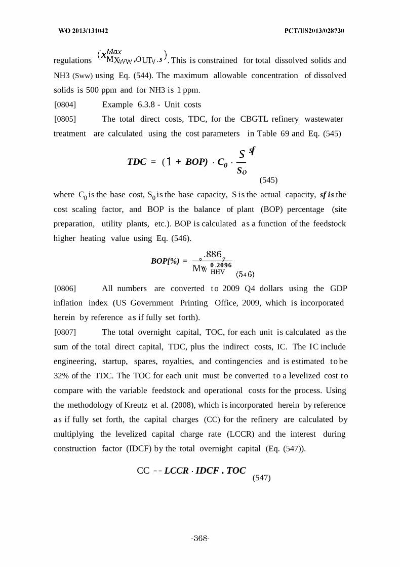
regulations X - UT . This is constrained for total dissolved solids and
NH3 (Sww) using Eq. (544). The maximum allowable concentration of dissolved
solids is 500 ppm and for NH3 is 1 ppm.
[0804] Example 6.3.8 - Unit costs
[0805] The total direct costs, TDC, for the CBGTL refinery wastewater
treatment are calculated using the cost parameters in Table 69 and Eq. (545)
fTDC = ( + BOP) C0 —
S(545)
where C0 is the base cost, S0 is the base capacity, S is the actual capacity, sf is the
cost scaling factor, and BOP is the balance of plant (BOP) percentage (site
preparation, utility plants, etc.). BOP is calculated as a function of the feedstock
higher heating value using Eq. (546).
BOP[%) = °W 0 .20
796
W HHV 4
[0806] All numbers are converted to 2009 Q4 dollars using the GDP
inflation index (US Government Printing Office, 2009, which is incorporated
herein by reference as if fully set forth).
[0807] The total overnight capital, TOC, for each unit is calculated as the
sum of the total direct capital, TDC, plus the indirect costs, IC. The IC include
engineering, startup, spares, royalties, and contingencies and is estimated to be
32% of the TDC. The TOC for each unit must be converted to a levelized cost to
compare with the variable feedstock and operational costs for the process. Using
the methodology of Kreutz et al. (2008), which is incorporated herein by reference
as if fully set forth, the capital charges (CC) for the refinery are calculated by
multiplying the levelized capital charge rate (LCCR) and the interest during
construction factor (IDCF) by the total overnight capital (Eq. (547)).
CC = = LCCR IDCF . TOC(547)

[0808] Kreutz et al. (2008), which is incorporated herein by reference as if
fully set forth, calculates an LCCR value of 14.38%/yr and IDCF of 1.076. Thus, a
multiplier of 15.41%/yr is used to convert the overnight capital into a capital
charge rate. Assuming an operating capacity (CAP) of 330 days/yr and
operation/mainte nance (OM) costs equal to 4% of the TOC, the total levelized cost
(CostU) associated with a wastewater unit is given by Eq. 548.
u CC - + OM)CAP -Prod -LHVprod
(548)
[0809] The levelized costs for treatment units used in the wastewater
network are then added to the complete list of CBGTL process units. Note that
the cost of the cooling utility is now being more rigorously calculated using
cooling tower costs. Additionally, the objective function to calculate the total
fuels cost will no longer have a Cost w term.
[0810] Example 6.3.9 - Objective function
[0811] The objective function for the model is given by Eq. (549). The
summation represents the total cost of liquid fuels production and includes
contributions from the feedstocks cost (CostF), the electricity cost (CostE 1), the
CO2 sequestration cost (CostSe i), and the levelized unit investment cost (Costu ) .
Each of the terms in Eq. (549) is normalized to the total lower heating value in
GJ of products produced. Note that other objective functions (e.g., maximizing the
net present value) can be easily incorporated into the model framework.
MIN s s + + St S q + s
(549)
[0812] The process synthesis model with simultaneous heat and power
integration, (P), and water integration (Eqs. (531) - (549) represent a large-scale
non-convex mixed-integer non-linear optimization (MINLP) model that was
solved to generate high-quality locally optimal solutions using either a
commercial local MINLP solver or by iteratively fixing the binary variables and
solving the resulting non-linear optimization (NLP) model using a commercial
NLP solver such as CONOPT. Generation of the local solutions utilizes a large

amount (100 250) of starting points for the NLP or MINLP solvers. This
procedure determines a variety of local solutions, and the solution with the
lowest overall objective value will be used to determine the topological
superstructure for the CBGTL facility. The model contains 42 binary variables,
25,700 continuous variables, 336 nonlinear and nonconvex terms, and 25,444
constraints. A theoretical guarantee of the identification of the global optimum
may be achieved using a global optimization branch and bound method where
valid convex underestimators are introduced for the nonconvex terms.
[0813] Example 7 - Biomass to liquid transportation fuels (BTL) systems:
Process synthesis and global optimization framework.
[0814] This example introduces the implementation of the invention,
including the process superstructure to convert feedstock to liquid transportation
fuels, the simultaneous heat, power, and water integration, and the global
optimization algorithm to generate the optimal refinery topologies, applied to
biomass to liquid (BTL) systems with agricultural residues, forest residues, and
perennial grasses as feedstock. The refineries can range from 1000-200,000
barrels per day capacities and the fuel product ratios can be maximized to
produce mainly gasoline, diesel, or jet fuel. The overall greenhouse gas emissions
can be less than 50% of petroleum-based processes.
[0815] Example 8 —Biomass and natural gas to liquid transportation fuels
(BGTL): Process synthesis, global optimization, and topology analysis.
[0816] This example introduces the implementation of the invention,
including the process superstructure to convert feedstock to liquid transportation
fuels, the simultaneous heat, power, and water integration, and the global
optimization algorithm to generate the optimal refinery topologies, applied to
biomass and natural gas to liquid (BGTL) systems with agricultural residues,
forest residues, and perennial grasses as the biomass feedstock. The refineries
can range from 1000-200,000 barrels per day capacities and the fuel product
ratios can be maximized to produce mainly gasoline, diesel, or jet fuel.
[0817] Example 9 - Hardwood biomass to gasoline, diesel, and jet fuel: I .
Process synthesis and global optimization of a thermochemical refinery.
[0818] This example introduces the implementation of the invention,
including the process superstructure to convert feedstock to liquid transportation
fuels, the simultaneous heat, power, and water integration, and the global
optimization algorithm to generate the optimal refinery topologies, applied to
hardwood biomass to liquid (BTL) systems. The refineries can range from 800-
10,000 barrels per day capacities and the fuel product ratios can be maximized to
produce mainly gasoline, diesel, or jet fuel.
[0819] Example 10 - Thermochemical conversion of duckweed biomass to
gasoline, diesel, and jet fuel: Process synthesis and global optimization.
[0820] This example introduces the implementation of the invention,
including the process superstructure to convert feedstock to liquid transportation
fuels, the simultaneous heat, power, and water integration, and the global
optimization algorithm to generate the optimal refinery topologies, applied to
duckweed biomass to liquid (BTL) systems. Aquatic biomass such as duckweed
can be produced continually and harvested with simple and low cost mechanical
techniques. The refineries can range from 1000-5000 barrels per day capacities
and the fuel product ratios can be maximized to produce mainly gasoline, diesel,
or jet fuel.

Tab
le69
.C
BG
TL
refi
nery
was
tew
ater
trea
tmen
tre
fere
nce
capa
citie
s,co
sts
(200
9Q
4$)
,an
dsc
alin
gfa
ctor
s.
Des
crip
tion
(MM
$)Sr
.S
Uni
tsSc
ale
basi
sif
BO
PR
e
Sour
stri
pper
$3.9
921
1.52
kg/s
Feed
0.53
Bio
logi
cal
dige
stor
$4.7
5211
5.74
kg/s
Feed
0.71
-R
ever
seos
mos
is$0
.31
74.
63kg
/sFe
ed0.
85b
Coo
ling
tow
er$4
.055
4530
.30
kg/s
Feed
0.78
Nat
iona
lE
nerg
yT
echn
olos
yL
abor
ator
y(2
00.
Bal
mer
nM
atts
son
(99
Tab
le70
.Pr
oces
sun
itna
mes
,A
SPE
Nbl
ock
type
s,an
dop
erat
ing
;ass
umpt
ions
for
syng
asge
nera
tion.
Uni
tA
SPE
NN
ame
mod
elU
nit
Des
crip
tion
Ope
ratin
gA
ssum
ptio
ns
Syng
asG
ener
atio
n-B
iom
ass
Gas
ific
atio
nP1
01H
Hea
ter
Air
Preh
eate
rT
out
=45
0°F
,dP
=-0
.025
bar
P101
USE
R2
Bio
mas
sD
ryer
Tou
t,air
=10
2°C
,T
out,b
iom
ass
=98
°C,
Pout
=1
bar,
moi
stur
eto
15w
t%B
iom
ass
P102
MM
ixer
Loc
khop
per
P=
32ba
r,C
O2/
dry
biom
ass
=0.
1w
t/wt
Top
=T
out
=10
00°C
,P
=3
1ba
r,in
let
O2/
dry
biom
ass
=0.
3w
t/wt,
inle
tP1
02U
SER
2B
iom
ass
Gas
ifie
rH
2O/d
rybi
omas
s=
0.25
wt/w
tPr
imar
yG
asif
ier
P103
S1Se
pC
yclo
neO
utle
tto
P103
M1:
99%
ofso
lids,
0%
ofva
pors
;dP
=0
bar
Seco
ndar
yG
asif
ier
Out
let
toP1
03M
1:10
0%of
solid
s,0%
ofva
pors
;dP
solid
=0
bar,
dPva
por
=-1
P103
S2Se
pC
yclo
neba
rG
asif
ier
Solid
sP1
03M
1M
ixer
Mix
erdP
=0
bar
P103
RSt
oic
Tar
Cra
cker
dH=
0kW
,dP
=-1
bar,
reac
tions
give
nin
Tab
le4
ofte
xtSt
ream
Cla
ssP1
03C
LC
IChn
gC
hang
erN
/A
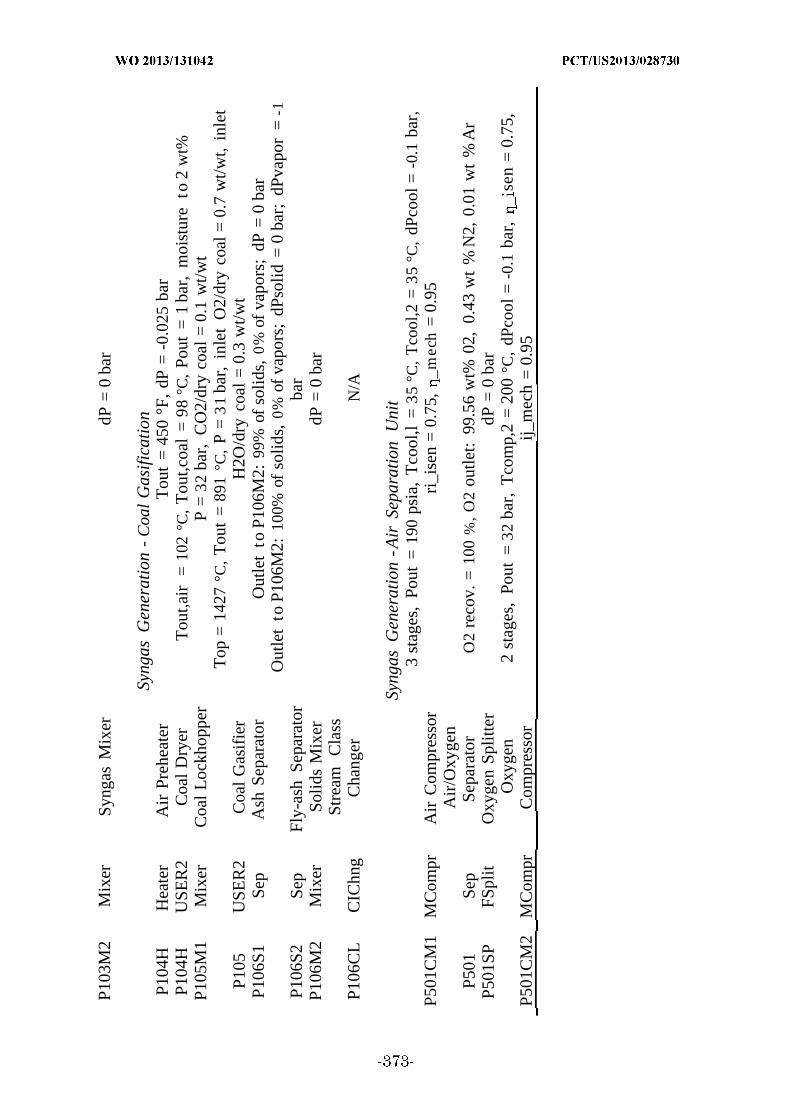
P103
M2
Mix
erSy
ngas
Mix
erdP
=0
bar
Syng
asG
ener
atio
n-
Coa
lG
asif
icat
ion
P104
HH
eate
rA
irPr
ehea
ter
Tou
t=
450
°F,
dP=
-0.0
25ba
rP1
04H
USE
R2
Coa
lD
ryer
Tou
t,air
=10
2°C
,T
out,c
oal
=98
°C,
Pout
=1
bar,
moi
stur
eto
2w
t%P1
05M
1M
ixer
Coa
lL
ockh
oppe
rP
=32
bar,
CO
2/dr
yco
al=
0.1
wt/w
tT
op=
1427
°C,
Tou
t=
891
°C,
P=
31
bar,
inle
tO
2/dr
yco
al=
0.7
wt/w
t,in
let
P105
USE
R2
Coa
lG
asif
ier
H2O
/dry
coal
=0.
3w
t/wt
P106
S1Se
pA
shSe
para
tor
Out
let
toP1
06M
2:99
%of
solid
s,0
%of
vapo
rs;
dP=
0ba
rO
utle
tto
P106
M2:
100%
ofso
lids,
0%of
vapo
rs;
dPso
lid=
0ba
r;dP
vapo
r=
-1P1
06S2
Sep
Fly-
ash
Sepa
rato
rba
rP1
06M
2M
ixer
Solid
sM
ixer
dP=
0ba
rSt
ream
Cla
ssP1
06C
LC
IChn
gC
hang
erN
/A
Syng
asG
ener
atio
n-A
irSe
para
tion
Uni
t3
stag
es,
Pout
=19
0ps
ia,
Tco
ol,l
=35
°C,
Tco
ol,2
=35
°C,
dPco
ol=
-0.1
bar,
P501
CM
1M
Com
prA
irC
ompr
esso
rri
_ise
n=
0.75
,_m
ech
=0.
95A
ir/O
xyge
nP5
01Se
pSe
para
tor
O2
reco
v.=
100
%,
O2
outle
t:99
.56
wt%
02,
0.43
wt
%N
2,0.
01w
t%
Ar
P501
SPFS
plit
Oxy
gen
Split
ter
dP=
0ba
rO
xyge
n2
stag
es,
Pout
=32
bar,
Tco
mp,
2=
200
°C,
dPco
ol=
-0.1
bar,
sen
=0.
75,
P501
CM
2M
Com
prC
ompr
esso
rij_
mec
h=
0.95
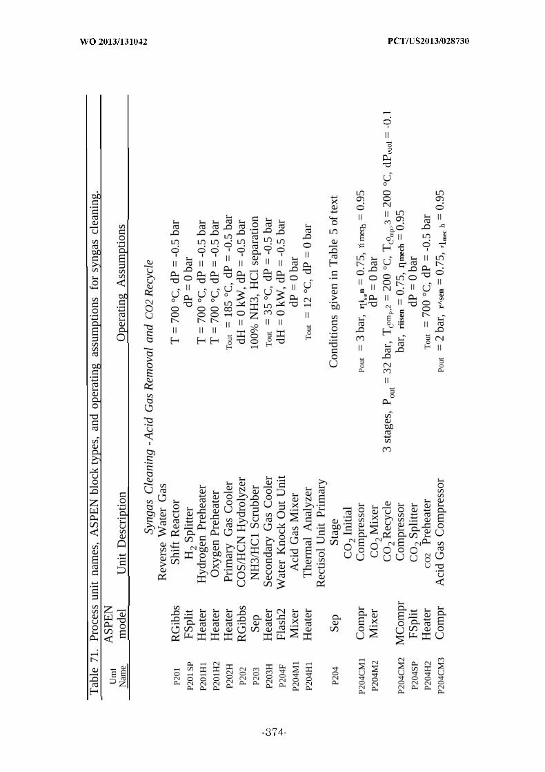
Tab
le71
.Pr
oces
sun
itna
mes
,A
SPE
Nbl
ock
type
s,an
dop
erat
ing
assu
mpt
ions
for
syng
ascl
eani
ng.
Um
ASP
EN
Nam
em
odel
Uni
tD
escr
iptio
nO
pera
ting
Ass
umpt
ions
Syng
asC
lean
ing
-Aci
dG
asR
emov
alan
dC
O2
Rec
ycle
Rev
erse
Wat
erG
asP2
01R
Gib
bsSh
ift
Rea
ctor
T=
700
°C,
dP=
-0.5
bar
P201
SPFS
plit
H2
Split
ter
dP=
0ba
rP2
01H
1H
eate
rH
ydro
gen
Preh
eate
rT
=70
0°C
,dP
=-0
.5ba
rP2
01H
2H
eate
rO
xyge
nPr
ehea
ter
T=
700
°C,
dP=
-0.5
bar
P202
HH
eate
rPr
imar
yG
asC
oole
rT
out
=18
5°C
,dP
=-0
.5ba
rP2
02R
Gib
bsC
OS/
HC
NH
ydro
lyze
rdH
=0
kW,d
P=
-0.5
bar
P203
Sep
NH
3/H
C1
Scru
bber
100%
NH
3,H
Cl
sepa
ratio
nP2
03H
Hea
ter
Seco
ndar
yG
asC
oole
rT
out
=35
°C,
dP=
-0.5
bar
P204
FFl
ash2
Wat
erK
nock
Out
Uni
tdH
=0
kW,d
P=
-0.5
bar
P204
M1
Mix
erA
cid
Gas
Mix
erdP
=0
bar
P204
H1
Hea
ter
The
rmal
Ana
lyze
rT
out
=12
°C,
dP=
0ba
rR
ectis
olU
nit
Prim
ary
P204
Sep
Stag
eC
ondi
tions
give
nin
Tab
le5
ofte
xtC
O2
Initi
alP2
04C
M1
Com
prC
ompr
esso
rPo
ut=
3ba
r,r
i sen
=0.
75,
imec
=0.
95P2
04M
2M
ixer
CO
2M
ixer
dP=
0ba
rC
O2
Rec
ycle
3st
ages
,P
out=
32ba
r,T
Com
P,2
=20
0°C
,T
Com
p>3
=20
0°C
,P2
04C
M2
MC
ompr
Com
pres
sor
bar,
riis
en=
0.75
,m
ech
=0.
95P2
04SP
FSpl
itC
O2
Split
ter
dP=
0ba
rP2
04H
2H
eate
rC
O2
Preh
eate
rT
out
=70
0°C
,dP
=-0
.5ba
rP2
04C
M3
Com
prA
cid
Gas
Com
pres
sor
Pout
=2
bar,
r^se
n=
0.75
,r
mec
=0.
95
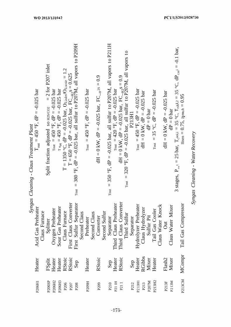
Syng
asC
lean
ing
-C
laus
Tre
atm
ent
Pla
ntP2
06H
1H
eate
rA
cid
Gas
Preh
eate
rT
out=
450
°F,d
P=
-0.0
25ba
rC
laus
Furn
ace
P206
SPFS
plit
Split
ter
Split
frac
tion
adju
sted
soH
2S/C
O2
=2
for
P207
inle
tP2
06H
2H
eate
rO
xyge
nPr
ehea
ter
Tou
t=
450
°F,d
P=
-0.0
25ba
rP2
06H
3H
eate
rSo
urG
asPr
ehea
ter
To
=45
0°F
,dP
=-0
.025
bar
P206
RSt
oic
Cla
usFu
rnac
eT
=13
50°C
,dP
=-0
.025
bar,
=1.
2P2
07R
Stoi
cFi
rst
Cla
usC
onve
rter
T=
650
°F,d
P=
-0.0
25ba
r,FC
_ H2s
=0.
625
P208
Sep
Firs
tSu
lfur
Sepa
rato
rT
out
=38
0°F
,dP
=-0
.025
bar,
all
sulf
urto
P207
M,
all
vapo
rsto
P209
HSe
cond
Cla
usP2
09H
Hea
ter
Preh
eate
rT
out
=45
0°F
,dP
=-0
.025
bar
Seco
ndC
laus
P209
RSt
oic
Con
vert
erdH
=0
kW,d
P=
-0.0
25ba
r,FC
_ H2S
=0.
9Se
cond
Sulf
urP2
10Se
pSe
para
tor
Tou
t=
350
°F,d
P=
-0.0
25ba
r,al
lsu
lfur
toP2
07M
,al
lva
pors
toP2
11H
CO
P21
1HH
eate
rT
hird
Cla
usPr
ehea
ter
Tou
t=
420
°F,d
P=
-0.0
25ba
rP2
11
RSt
oic
Thi
rdC
laus
Con
vert
erdH
=0
kW,d
P=
-0.0
25ba
r,FC
_ H2s
=0.
9T
hird
Sulf
urT
out
=32
0°F
,dP
=-0
.025
bar,
all
sulf
urto
P207
M,
all
vapo
rsto
P212
Sep
Sepa
rato
rP2
13H
1P
213
H1
Hea
ter
Hyd
roly
zer
Preh
eate
rT
out
=45
0°F
,dP
=-0
.025
bar
P213
RG
ibbs
Cla
usH
ydro
lyze
rdH
=0
kW,d
P=
-0.0
25ba
rP2
07M
Mix
erSu
lfur
Pit
dP=
0ba
rP2
13H
2H
eate
rT
ail
Gas
Coo
ler
Tou
t=
35°C
,dP
=-0
.025
bar
Cla
usW
ater
Kno
ckP2
13F
Flas
h2O
utdH
=0
kW,d
P=
-0.0
25ba
rP
213
MM
ixer
Cla
usW
ater
Mix
erdP
=0
bar
3st
ages
,P
ou
t=
25ba
r,T
Cooi
,i=
35°C
,Τ
χι,2
=35
°C,
dPC
00i=
-0.1
bar,
P213
CM
MC
ompr
Tai
lG
asC
ompr
esso
rIl
isen
=0.
75,
me
h=
0.95
Syng
asC
lean
ing
-W
ater
Rec
over
y
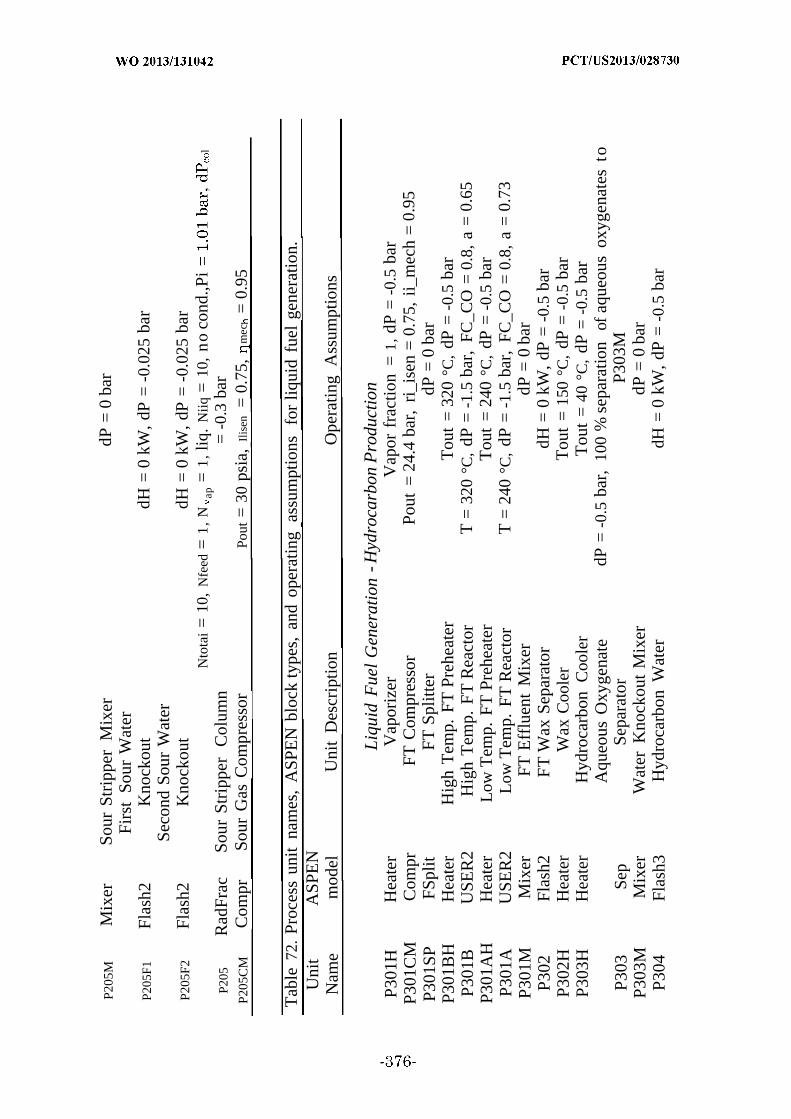
P205
MM
ixer
Sour
Stri
pper
Mix
erdP
=0
bar
Firs
tSo
urW
ater
P205
F1Fl
ash2
Kno
ckou
tdH
=0
kW,d
P=
-0.0
25ba
rSe
cond
Sour
Wat
erP2
05F2
Flas
h2K
nock
out
dH=
0kW
,dP
=-0
.025
bar
Nto
tai
=10
,N
feed
=1
,N
ap=
1,liq
.N
iiq=
10,
no
cond
.,Pi
P205
Rad
Frac
Sour
Stri
pper
Col
umn
=-0
.3ba
rP2
05C
MC
ompr
Sour
Gas
Com
pres
sor
Pout
=30
psia
,Il
isen
=0.
75,
mec
=0.
95
Tab
le72
.Pr
oces
sun
itna
mes
,A
SPE
Nbl
ock
type
s,an
dop
erat
ing
assu
mpt
ions
for
liqui
dfu
elge
nera
tion.
Uni
tA
SPE
NN
ame
mod
elU
nit
Des
crip
tion
Ope
ratin
gA
ssum
ptio
ns
Liq
uid
Fue
lG
ener
atio
n-H
ydro
carb
onP
rodu
ctio
nP3
01H
Hea
ter
Vap
oriz
erV
apor
frac
tion
=1,
dP=
-0.5
bar
P301
CM
Com
prF
TC
ompr
esso
rPo
ut=
24.4
bar,
ri_i
sen
=0.
75,
ii_m
ech
=0.
95P3
01SP
FSpl
itF
TSp
litte
rdP
=0
bar
P301
BH
Hea
ter
Hig
hT
emp.
FT
Preh
eate
rT
out
=32
0°C
,dP
=-0
.5ba
rP3
01B
USE
R2
Hig
hT
emp.
FT
Rea
ctor
T=
320
°C,
dP=
-1.5
bar,
FC_C
O=
0.8,
a=
0.65
P301
AH
Hea
ter
Low
Tem
p.F
TPr
ehea
ter
Tou
t=
240
°C,
dP=
-0.5
bar
P301
AU
SER
2L
owT
emp.
FT
Rea
ctor
T=
240
°C,
dP=
-1.5
bar,
FC_C
O=
0.8,
a=
0.73
P301
MM
ixer
FT
Eff
luen
tM
ixer
dP=
0ba
rP3
02Fl
ash2
FT
Wax
Sepa
rato
rdH
=0
kW,d
P=
-0.5
bar
P302
HH
eate
rW
axC
oole
rT
out
=15
0°C
,dP
=-0
.5ba
rP3
03H
Hea
ter
Hyd
roca
rbon
Coo
ler
Tou
t=
40°C
,dP
=-0
.5ba
rA
queo
usO
xyge
nate
dP=
-0.5
bar,
100
%se
para
tion
ofaq
ueou
sox
ygen
ates
toP3
03Se
pSe
para
tor
P303
MP3
03M
Mix
erW
ater
Kno
ckou
tM
ixer
dP=
0ba
rP3
04Fl
ash3
Hyd
roca
rbon
Wat
erdH
=0
kW,d
P=
-0.5
bar
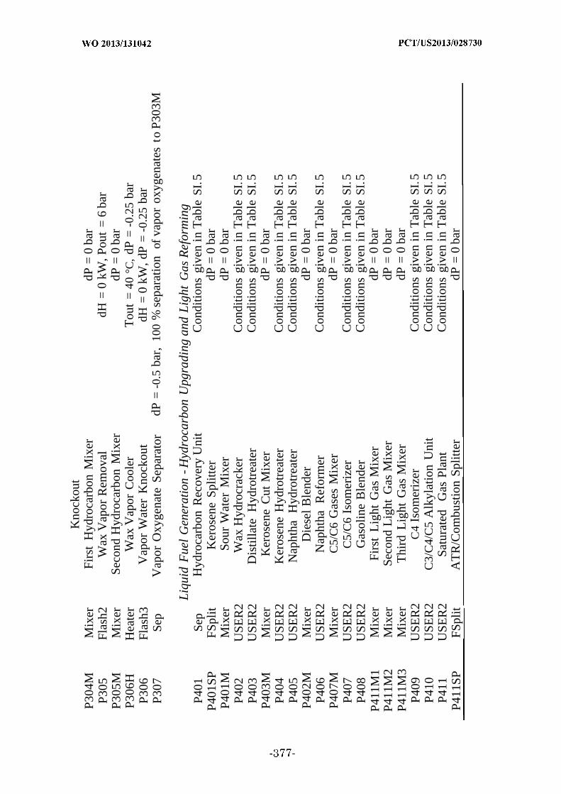
Kno
ckou
tP3
04M
Mix
erFi
rst
Hyd
roca
rbon
Mix
erdP
=0
bar
P305
Flas
h2W
axV
apor
Rem
oval
dH=
0kW
,Pou
t=
6ba
rP3
05M
Mix
erSe
cond
Hyd
roca
rbon
Mix
erdP
=0
bar
P306
HH
eate
rW
axV
apor
Coo
ler
Tou
t=
40°C
,dP
=-0
.25
bar
P306
Flas
h3V
apor
Wat
erK
nock
out
dH=
0kW
,dP
=-0
.25
bar
P307
Sep
Vap
orO
xyge
nate
Sepa
rato
rdP
=-0
.5ba
r,10
0%
sepa
ratio
nof
vapo
rox
ygen
ates
toP3
03M
Liq
uid
Fue
lG
ener
atio
n-H
ydro
carb
onU
pgra
ding
and
Lig
htG
asR
efor
min
gP4
01Se
pH
ydro
carb
onR
ecov
ery
Uni
tC
ondi
tions
give
nin
Tab
leSI
.5P4
01SP
FSpl
itK
eros
ene
Split
ter
dP=
0ba
rP4
01M
Mix
erSo
urW
ater
Mix
erdP
=0
bar
P402
USE
R2
Wax
Hyd
rocr
acke
rC
ondi
tions
give
nin
Tab
leSI
.5P4
03U
SER
2D
istil
late
Hyd
rotr
eate
rC
ondi
tions
give
nin
Tab
leSI
.5P4
03M
Mix
erK
eros
ene
Cut
Mix
erdP
=0
bar
P404
USE
R2
Ker
osen
eH
ydro
trea
ter
Con
ditio
nsgi
ven
inT
able
SI.5
P405
USE
R2
Nap
htha
Hyd
rotr
eate
rC
ondi
tions
give
nin
Tab
leSI
.5P4
02M
Mix
erD
iese
lB
lend
erdP
=0
bar
P406
USE
R2
Nap
htha
Ref
orm
erC
ondi
tions
give
nin
Tab
leSI
.5P4
07M
Mix
erC
5/C
6G
ases
Mix
erdP
=0
bar
P407
USE
R2
C5/
C6
Isom
eriz
erC
ondi
tions
give
nin
Tab
leSI
.5P4
08U
SER
2G
asol
ine
Ble
nder
Con
ditio
nsgi
ven
inT
able
SI.5
P411
M1
Mix
erFi
rst
Lig
htG
asM
ixer
dP=
0ba
rP4
11M
2M
ixer
Seco
ndL
ight
Gas
Mix
erdP
=0
bar
P411
M3
Mix
erT
hird
Lig
htG
asM
ixer
dP=
0ba
rP4
09U
SER
2C
4Is
omer
izer
Con
ditio
nsgi
ven
inT
able
SI.5
P410
USE
R2
C3/
C4/
C5
Alk
ylat
ion
Uni
tC
ondi
tions
give
nin
Tab
leSI
.5P4
11U
SER
2Sa
tura
ted
Gas
Plan
tC
ondi
tions
give
nin
Tab
leSI
.5P4
11SP
FSpl
itA
TR
/Com
bust
ion
Split
ter
dP=
0ba
r
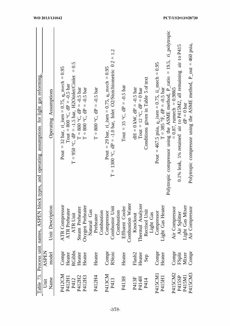
Tab
le73
.Pr
oces
sun
itna
mes
,A
SPE
Nbl
ock
type
s,an
dop
erat
ing
assu
mpt
ions
for
light
gas
refo
rmin
g.U
nit
ASP
EN
Nam
em
odel
Uni
tD
escr
iptio
nO
pera
ting
Ass
umpt
ions
P412
CM
Com
prA
TR
Com
pres
sor
Pout
=32
bar,
ri_i
sen
=0.
75,
_mec
h=
0.95
P412
H1
Hea
ter
AT
RPr
ehea
ter
Tou
t=
800
°C,
dP=
-0.5
bar
P412
RG
ibbs
AT
RU
nit
T=
950
°C,
dP=
-1.5
bar,
H2O
inle
t/Cin
let
=0.
5P4
12H
2H
eate
rSt
eam
Preh
eate
rT
=80
0°C
,dP
=-0
.5ba
rP4
12H
3H
eate
rO
xyge
nPr
ehea
ter
T=
800
°C,
dP=
-0.5
bar
Nat
ural
Gas
P412
H4
Hea
ter
Preh
eate
rT
=80
0°C
,dP
=-0
.5ba
rC
ombu
stio
nP4
13C
MC
ompr
Com
pres
sor
Pout
=29
bar,
ri_i
sen
=0.
75,
_mec
h=
0.95
P413
RSt
oic
Com
bust
orU
nit
T=
1300
°C,
dP=
-1.0
bar,
Inle
tO
2/St
oich
iom
etri
c0
2=
1.2
Com
bust
ion
P413
HH
eate
rE
fflu
ent
Coo
ler
Tou
t=
35°C
,dP
=-0
.5ba
rC
ombu
stio
nW
ater
P413
FFl
ash2
Kno
ckou
tdH
=0
kW,d
P=
-0.5
bar
P414
HH
eate
rT
herm
alA
naly
zer
Tou
t=
12°C
,dP
=0
bar
P414
Sep
Rec
tisol
Uni
tC
ondi
tions
give
nin
Tab
le5
ofte
xtL
ight
Gas
P415
CM
1C
ompr
Com
pres
sor
Pout
=46
7.5
psia
,_i
sen
=0.
75,
ii_m
ech
=0.
95P4
15H
1H
eate
rL
ight
Gas
Hea
ter
T=
385
°F,d
P=
-0.5
bar
Poly
trop
icco
mpr
esso
rus
ing
the
ASM
Em
etho
d,P_
ratio
=19
.5,
ri_p
olyt
ropi
cP4
15C
M2
Com
prA
irC
ompr
esso
r=
0.87
,ru
mec
h=
0.98
65P4
15SP
FSpl
itA
irSp
litte
r0.
1%le
ak,
5%re
tain
edai
rto
P415
M2,
all
rem
aini
ngai
rto
P415
P415
M1
Mix
erL
ight
Gas
Mix
erdP
=0
bar
P415
CM
3C
ompr
Air
Com
pres
sor
Poly
trop
icco
mpr
esso
rus
ing
the
ASM
Em
etho
d,P_
out
=46
0ps
ia,

rupo
lytr
opic
=0.
87,
rum
ech
=0.
9865
Gas
Tur
bine
P415
RSt
oic
Com
bust
erT
=13
70°C
,dP
=-1
0ps
ia,
Inle
tO
2/St
oich
iom
etri
c0
2=
1.1
P415
T1
Com
prG
asT
urbi
ne1
Pout
=23
5.2
psia
,se
n=
0.89
769,
rurn
ech
=0.
9727
P415
M2
Mix
erA
irIn
ject
ion
Mix
erdP
=0
bar
P415
T2
Com
prG
asT
urbi
ne2
Pout
=1.
065
bar,
sen
=0.
8976
9,ru
rnec
h=
0.97
27P4
15H
2H
eate
rE
fflu
ent
Coo
ler
T=
35°C
,dP
=-0
.025
bar
P415
FFl
ash2
Wat
erK
nock
out
dH=
0kW
,dP
=-0
.025
bar
P415
CM
4C
ompr
Gas
Com
pres
sor
Pout
=27
.3ba
r,se
n=
0.75
,ru
rnec
h=
0.95
P415
H3
Hea
ter
Gas
Hea
ter
T=
35°C
,dP
=-0
.5ba
r
Tab
le74
.O
utle
tco
nditi
ons
for
the
upgr
adin
gun
its.
Uni
tN
ame
Uni
tD
escr
iptio
nO
utle
tC
ondi
tions
1
TL
G-
Tc3
-5G
-T
-Τ
κ-
TD
t-
Tw
x-
Tw
w-
100
Hyd
roca
rbon
PLG
=c
3-G
=P
N=
κ=
t=
Pwx
=Pw
w=
50R
ecov
ery
Uni
tps
iaN
/AT
c5-6
G=
150
°F,
TN
=20
0°F
,T
D=
300
°F,
Tsw
=T
LG
=10
0°F
Pc5-
6G=
60ps
ia,
PN
=40
psia
,P
D=
Psw
=20
P402
Wax
Hyd
rocr
acke
rps
ia,
PLG
=50
psia
2.19
516
Dis
tilla
teT
sw=
80°F
,T
D=
90°F
,T
LG
=10
0°F
P403
Hyd
rotr
eate
rPs
w=
PD
=PL
G=
50ps
ia2.
1392
2K
eros
ene
TK
=90
°F,
TL
G=
100
°FP4
04H
ydro
trea
ter
K=
PLG
=50
psia
2.13
922
Nap
htha
Tsw
=70
°F,
Tc5
-6G
=90
°F,
TN
=80
°F,
TL
G=
P405
Hyd
rotr
eate
r10
0°F
2.30
795

Psw
=c
-6G
=N
=PL
G=
50ps
iaT
G=
150
°F,T
H2
G=
120
°F,T
LG
=10
0°F
P406
Nap
htha
Ref
orm
erP
G=
30ps
ia,
PH2G
=PL
G=
50ps
iaN
/AT
G=
TL
G=
100
°FP4
07C
Isom
eriz
erP
G=
PLG
=25
psia
2.35
89T
G=
100
°FP4
08G
asol
ine
Ble
nder
PG
=50
psia
N/A
P409
C4
Isom
eriz
erc
G=
PLG
=50
psia
2.50
646
C3/C
4/C
5A
lkyl
atio
nT
G=
c4G
=T
LG
=10
0°F
P410
Uni
tP
G=
cG
=PL
G=
50ps
iaN
/ASa
tura
ted
Gas
Tsw
=T
c3G
=T
c4G
=T
LG
=10
0°F
P411
Plan
tPs
w=
Pc3G
=c
G=
PLG
=50
psia
N/A
1.
LG
=L
ight
Gas
,C
3G=
C3
Gas
es,
C3-
5G=
C3-
C5
Gas
es,
C4G
=C
4G
ases
,C
5-6G
=C
-C6
Gas
es,
H2G
=H
2R
ich
Gas
es,
N=
Nap
htha
,D
t=
Dis
tilla
te,
Wx
=W
ax,
WW
=W
aste
wat
er,
SW=
Sour
Wat
er,
G=
Gas
olin
e,D
=D
iese
l,K
=K
eros
ene
2.R
efer
sto
the
tota
lpr
esen
tin
all
inpu
thy
droc
arbo
nspl
usin
put
¾

References
[1] R.C. Baliban, J .A. Elia, C.A. Floudas. Toward Novel HybridBiomass, Coal, and Natural Gas Processes for Satisfying CurrentTransportation Fuel Demands, 1: Process Alternatives,Gasification Modeling, Process Simulation, and EconomicAnalysis. Ind. Eng. Chem. Res., 2010:49(16), 7343-7370.
[2] J .A. Elia, R.C. Baliban, C.A. Floudas. Toward Novel HybridBiomass, Coal, and Natural Gas Processes for Satisfying CurrentTransportation Fuel Demands, 2 : Simultaneous Heat and PowerIntegration. Ind. Eng. Chem. Res., 2010:49(16), 7371-7388.
[3] R.C. Baliban, J .A. Elia, C.A. Floudas. Optimization Frameworkfor the Simultaneous Process Synthesis, Heat and PowerIntegration of a Thermochemical Hybrid Biomass, Coal, andNatural Gas Facility. Comp. Chem. Eng., 2011:35(9), 1647-1690.
[4] J . A. Elia, R.C. Baliban, X. Xiao, C.A. Floudas. Optimal EnergySupply Network Determination and Life Cycle Analysis forHybrid Coal, Biomass, and Natural Gas to Liquid (CBGTL)Plants Using Carbon-based Hydrogen Production. Comp. Chem.Eng., 2011:35(8), 1399-1430.
[5] R.C. Baliban, J .A. Elia, C.A. Floudas. Simultaneous ProcessSynthesis, Heat, Power, and Water Integration ofThermochemical Hybrid Biomass, Coal, and Natural GasFacilities. Comp. Chem. Eng., 2012:37(10), 297.
[6] R.C. Baliban, J.A. Elia, R. Misener, C.A. Floudas. GlobalOptimization of a Thermochemical Based Hybrid Coal, Biomass,and Natural Gas to Liquids Facility. Comp. Chem. Eng.,submitted.
[7] R.C. Baliban, J.A. Elia, C.A. Floudas. Toward Novel HybridBiomass, Coal, and Natural Gas Processes for Satisfying CurrentTransportation Fuel Demands, 1: Process Alternatives, GasificationModeling, Process Simulation, and Economic Analysis. Ind. Eng.Chem. Res., 2010:49(16), 7343-7370.
[8] J.A. Elia, R.C. Baliban, C.A. Floudas. Toward Novel HybridBiomass, Coal, and Natural Gas Processes for Satisfying CurrentTransportation Fuel Demands, 2 : Simultaneous Heat and PowerIntegration. Ind. Eng. Chem. Res., 2010:49(16), 7371-7388.
[9] R.C. Baliban, J.A. Elia, C.A. Floudas. Optimization Framework forthe Simultaneous Process Synthesis, Heat and Power Integration ofa Thermochemical Hybrid Biomass, Coal, and Natural GasFacility. Comp. Chem. Eng., 2011:35(9), 1647-1690.
[10] J . A. Elia, R.C. Baliban, X. Xiao, C.A. Floudas. Optimal EnergySupply Network Determination and Life Cycle Analysis for HybridCoal, Biomass, and Natural Gas to Liquid (CBGTL) Plants UsingCarbon-based Hydrogen Production. Comp. Chem. Eng.,2011:35(8), 1399-1430.
[11] R.C. Baliban, J.A. Elia, C.A. Floudas. Simultaneous ProcessSynthesis, Heat, Power, and Water Integration of ThermochemicalHybrid Biomass, Coal, and Natural Gas Facilities. Comp. Chem.Eng., 2012:37(10), 297.
[12] C.A. Floudas, J.A. Elia, R.C. Baliban. Hybrid and Single FeedstockEnergy Processes for Liquid Transportation Fuels: A CriticalReview. Comp. Chem. Eng., 2012:41, 24-51.
[13] R.C. Baliban, J.A. Elia, R. Misener, C.A. Floudas. GlobalOptimization of a Thermochemical Based Hybrid Coal, Biomass,and Natural Gas to Liquids Facility. Comp. Chem. Eng., 2012:42,64.
[14] J . A. Elia, R.C. Baliban, C.A. Floudas. Nationwide Supply ChainAnalysis for Hybrid Energy Processes with Significant CO2Emissions Reduction. AIChE ., 2012:58(7), 2142-2154.
[15] R.C. Baliban, J.A. Elia, V.W. Weekman, C.A. Floudas. Processsynthesis of hybrid coal, biomass, and natural gas to liquids viaFischer-Tropsch synthesis, ZSM-5 catalytic conversion, methanolsynthesis, methanol-to- gasoline, and methanol-to-olefins/distillatetechnologies. Comp. Chem. Eng., in press,doi:10.1016/j.compchemeng.2012.06.032.
[16] Energy Information Administration. Monthly Energy Review,August 2009. Document No. DOE-EIA-0035(2009/09). Available viathe Internet at http://www.eta.doe.gov/mer/, 2009.
[17] Energy Information Administration. Annual Energy Outlook 2009with Projections to 2030. Document No. DOE/EIA-0383(2009).Available via the Internet at http://www.eta.doe.gov/oiaf/aeo/, 2009.
[18] Zittel, W.; Schindler, J . Crude Oil: The Supply Outlook. DocumentNo. EWG-Series No 3/2007, Report to the Energy Watch Group,October 2007.
[19] BP, BP Statistical ReView of World Energy. Available via theInternet at http://www.bp.com/, 2009.
[20] Environmental Protection Agency, Inventory of U.S. GreenhouseGas Emission and Sinks: 1990-2007. Document No. EPA 430-R-09-004, Washington, DC, 2009.
[21] MacLean, H.; Lave, L. Evaluating automobile fuel/propulsionsystem technologies. Prog. Energy Combust. Sci. 2003, 29, 1-69.
[22] National Research Council and National Academy of Engineering.The Hydrogen Economy: Opportunities, Costs, Barriers, and R&DNeeds; The National Academies Press: Washington, DC, 2004.
[23] Lynd, L. R.; Larson, E.; Greene, N.; Laser, M.; Sheehan, J.; Dale, B.E.; McLaughlin, S.; Wang, M. The role of biomass in America'senergy future: framing the analysis. Biofuels, Bioprod. Biorefin.2009, 3, 113-123.
[24] National Academy of Sciences, National Academy of Engineering,and National Research Council. Liquid Transportation Fuels fromCoal and Biomass: Technological Status, Costs, and EnvironmentalIssues. Prepublication; EPA: Washington, DC, 2009.
[25] Department of Energy and Department of Agriculture. Biomass asFeedstock for a Bioenergy and Bioproducts Industry: The TechnicalFeasibility of a Billion-Ton Annual Supply. Document No. DOE/GO-102005-2135,http://wwwl.eere.energy.gov/biomass/publications.html, 2005.
[26] Kreutz, T. G.; Larson, E. D.; Liu, G.; Williams, R. H. Fischer-Tropsch Fuels from Coal and Biomass. Presented at the 25thInternational Pittsburg Coal Conference, 2008.
[27] Larson, E. D.; Jin, H. Biomass Conversion to Fischer-TropschLiquids: Preliminary Energy Balances. In Proceedings of the 4thBiomass Conference of the Americas, 1999.
[28] Vliet, 0.; Faaij, A.; Turkenburg, W. Fischer-Tropsch dieselproduction in a well-to-wheel perspective: A carbon, energy flow andcost analysis. Energy ConVers. Manage. 2009, 50, 855-876.
[29] Bechtel Corporation; Global Energy Inc.; Nexant Inc. GasificationPlant Cost and Performance Optimization, Task 2 Topical Report:Coke/Coal Gasification with Liquids Coproduction, USDOEContract No. DEAC26-99FT40342, 2003.
[30] Sudiro, M.; Bertucco, A. Production of synthetic gasoline and dieselfuel by alternative processes using natural gas and coal: Processsimulation and optimization. Energy 2009, 34, 2206-2214.
[31] Cao, Y.; Gao, Z.; Jin, J.; Zhou, H.; Cohron, M.; Zhao, H.; Liu, H.;Pan, W. Synthesis Gas Production with an Adjustable H2/CO Ratiothrough the Coal Gasification Process: Effects of Coal Ranks andMethane Addition. Energy Fuels 2008, 22, 1720-1730.
[32] Sudiro, M.; Bertucco, A. Synthetic Fuels by a Limited C02 EmissionProcess Which Uses Both Fossil and Solar Energy. Energy Fuels2007, 21, 3668-3675.
[33] Yamashita, K.; Barreto, L. Energyplexes for the 21st century: Coalgasification for co-producing hydrogen, electricity and liquid fuels.Energy 2005, 30, 2453-2473.
[34] Chiesa, P.; Consonni, S.; Kreutz, T.; Williams, R. Co-production ofhydrogen, electricity and C02 from coal with commercially readytechnology. Part A : Performance and emissions. Int. J . HydrogenEnergy 2005, 30, 747-767.
[35] Kreutz, T.; Williams, R.; Consonni, S.; Chiesa, P. Co-productionofhydrogen, electricity and C02 from coal with commercially readytechnology. Part B : Economic analysis. Int. J . Hydrogen Energy2005, 30, 769-784.
[36] Sudiro, M.; Bertucco, A.; Ruggeri, F.; Fontana, M. ImprovingProcess Performances in Coal Gasification for Power and SynfuelProduction. Energy Fuels 2008, 22, 3894-3901.
[37] Larson, E. D.; Jin, H.; Celik, F. E. Large-scale gasification-basedcoproduction of fuels and electricity from switchgrass. Biofuels,Bioprod.Bioref. 2009, 3, 174-194.
[38] Cormos, C. C. Assessment of hydrogen and electricity co-productionschemes based on gasification process with carbon capture and

storage. Int. J . Hydrogen Energy 2009, 34, 6065-6077.[39] Jime'nez, L.; Gadalla, M.; Boer, D.; Majozi, T. Integrated
gasification combined cycle (IGCC) process simulation andoptimization. Comput. Chem. Eng. 2009, DOI:10.1016/j.compchemeng.2009.04.007.
[40] Agrawal, R.; Singh, N. R.; Ribeiro, F. H.; Delgass, W. N.Sustainable fuel for the transportation sector. Proc. Natl. Acad. Sci.U.S.A. 2007, 104, 4828-4833.
[41] Dry, M. The Fischer-Tropsch process: 1950-2000. Catal. Today 2002,71, 227-241.
[42] National Energy Technology Laboratory. Cost and PerformanceBaseline for Fossil Energy Plants. Volume 1 : Bituminous Coal andNatural Gas to Electricity Final Report. Document No. DOE/NETL-2007/1281, http://www.netl. doe .gov/ener gy-analyses/baselinetudies.html, 2007.
[43] Bechtel, Aspen Process Flowsheet Simulation Model of a BattelleBiomass-Based Gasification, Fischer-Tropsch Liquefaction andCombined- Cycle Power Plant, Contract No. DE-AC22-93PC91029,http://www.Fischer-Tropsch.org/, 1998.
[44] Bechtel, Baseline Design/Economics for Advanced Fischer-TropschTechnology, Contract No. DE-AC22-91PC90027, 1992.
[45] Hamelinck, C ; Faaij, A.; Uil, H.; Boerrigter, H. Production of FTtransportation fuels from biomass; technical options, processanalysis andoptimization, and development potential. Energy 2004,29, 1743.
[46] Spath, P. Aden, A. Eggeman, T. Ringer, M. Wallace, B. Jechura, J .Biomass to Hydrogen Production Detailed Design and EconomicsUtilizing the Battelle Columbus Laboratory Indirectly-HeatedGasifier. Document No. NREL/TP-510-37408,http://www.nrel.gov/docs/fy05osti/37408.pdf, 2005.
[47] Holladay, J . D.; Hu, J.; King, D. L.; Wang, Y. An overview ofhydrogen production technologies. Catal. Today 2009, 139, 244-260.
[48] Floudas, C. A. Nonlinear and Mixed-Integer Optimization; OxfordUniversity Press, New York: 1995.
[49] Holiastos, K.; Manousiouthakis, V. Minimum hot/cold/electricutility cost for heat exchange networks. Comput. Chem. Eng. 2002,26, 3-16.
[50] Li, X. T.; Grace, J . R.; Watkinson, A. P.; Ergu denler, A.Equilibrium modeling of gasification: A free energy minimizationapproach and its application to a circulating fluidized bed coalgasifier. Fuel 2001, 80, 195-207.
[51] Yuehong, Z.; Hao, W.; Zhihong, X. Conceptual design andsimulation study of a co-gasification technology. Energy ConVers.Manage. 2006, 47, 1416-1428.
[52] Ranzi, E.; Cuoci, A.; Faravelli, T.; Frassoldati, A.; Migliavacca, G.;Pierucci, S.; Sommariva, S. Chemical Kinetics of Biomass Pyrolysis.Energy Fuels 2008, 22, 4292-4300.
[53] Cuoci, A.; Faravelli, T.; Frassoldati, A.; Granata, S.; Migliavacca,G.; Ranzi, E.; Sommariva, S. A General Mathematical Model ofBiomass Devolatilization Note 1. Lumped kinetic models ofcellulose, hemicellulose, and lignin, Presented at the 30th Meetingof the Italian Section of the Combustion Institute, 2007.
[54] Jand, N.; Brandani, V.; Foscolo, P. U. Thermodynamic Limits andActual Product Yields and Compositions in Biomass GasificationProcesses. Ind. Eng. Chem. Res. 2006, 45, 834-843.
[55] Ratnadhariya, J . K.; Channiwala, S. A. Three zone equilibrium andkinetic free modeling of biomass gasifiersA novel approach.Renewable Energy 2009, 34, 1050-1058.
[56] Nikoo, M. B.; Mahinpey, N. Simulation of biomass gasification in afluidized bed reactor using ASPEN PLUS. Biomass Bioenergy 2008,32, 1245-1254.
[57] Yang, H.; Yan, R.; Chen, H.; Lee, D. H.; Zheng, C. Characteristics ofhemicellulose, cellulose, and lignin pyrolysis. Fuel 2007, 86, 1781-1788.
[58] Narvaez, I.; Orio, A.; Aznar, M. P.; Corella, J . Biomass Gasificationwith Air in an Atmospheric Bubbling Fluidized Bed. Effect of SixOperational Variables on the Quality of the Produced Raw Gas. Ind.Eng. Chem. Res. 1996, 35, 2110-2120.
[59] Gil, J.; Aznar, M. P.; Caballero, M. A.; Frances, E.; Corella, J .Biomass Gasification in Fluidized Bed at Pilot Scale with Steam-Oxygen Mixtures. Product Distribution for Very DifferentOperating Conditions. Energy Fuels 1997, 11, 1109-1118.
[60] Gil, J.; Corella, J.; Aznar, M. P.; Caballero, M. A. Biomassgasification in atmospheric and bubbling fluidized bed: Effect of thetype of gasifying agent on the product distribution. BiomassBioenergy 1999, 17, 389-403.
[61] Yoon, H.; Wei, J.; Denn, M. M. A Model For Moving-Bed CoalGasification Reactors. AIChE J . 1978, 24, 885-903.
[62] Song, B. H.; Jang, Y. W.; Kim, S. D.; Rang, S. K. Gas Yields fromCoal Devolatilization in a Bench-Scale Fluidized Bed Reactor.Korean J . Chem. Eng. 2001, 18, 770-774.
[63] Ma, R. P.; Felder, R. M.; Ferrell, J . K. Evolution of HydrogenSulfide in a Fluidized Bed Coal Gasification Reactor. Ind. Eng.Chem. Res. 1989, 28, 27-33.
[64] Di Nola, G.; de Jong, W.; Spliethoff, H. The fate of main gaseousand nitrogen species during fast heating rate devolatilization of coaland secondary fuels using a heated wire mesh reactor. Fuel Process.Technol. 2009, 90, 388-395.
[65] Liu, H. F.; Liu, Y. H.; Liu, Y. H.; Che, D. F. Experimentalinvestigation on the conversion of nitrogenous gas products duringcoal pyrolysis. J . Fuel Chem. Technol. 2008, 36, 134-138.
[66] Mannan, S. Lees' Loss PreVention in the Process Industries, Vols.1-3; Elsevier: 2005. (Online version available at http://knovel.com/).
[67] Fiaschi, D.; Michelini, M. A two-phase one-dimensional biomass

gasification kinetics model. Biomass Bioenergy 2001, 21, 121-132.[68] Sotudeh-Gharebaagh, R.; Legros, R.; Paris, J . Simulation of
circulating fluidized bed reactors using ASPEN PLUS. Fuel 1998,77, 327-337.
[69] NASA, http://cea.grc.nasa.gov/.[70] Amundson, N. R.; Arri, L. E. Char Gasification in a Countercurrent
Reactor. AIChE J . 1978, 24, 87-101.[71] Herguido, J.; Corella, J.; Gonzalez-Saiz, J . Steam Gasification of
Lignocellulosic Residues in a Fluidized Bed at a Small Pilot Scale.Effect of the Type of Feedstock. Ind. Eng. Chem. Res. 1996, 31,1274-1282.
[72] Yu, Q.-Z.; Brage, C ; Chen, G.-X.; Sjostrom, K. The fate offuelnitrogen during gasification of biomass in a pressurizedfluidized bed gasifier. Fuel 2007, 86, 611-618.
[73] Zhou, J . Simulation of fuel-bound nitrogen evolution in biomassgasification. In Proceedings of the 32nd Intersociety EnergyConversion Engineering Conference, 1997.
[74] Liu, H.; Gibbs, B. M. Modeling NH3 and HCN emissions frombiomass circulating fluidized bed gasifiers. Fuel 2003, 82, 1591-1604.
[75] Stubenberger, G.; Scharler, R.; Zahirovic, S.; Obernberger, I .Experimental investigation of nitrogen species release fromdifferent solid biomass fuels as a basis for release models. Fuel2008, 87, 793-806.
[76] van der Drift, A.; van Doorn, J.; Vermeulen, J . W. Ten residual fuelsfor circulating fluidized-bed gasification. Biomass Bioenergy 2001,20, 45-56.
[77] Zwart, R. W. R.; Boerrigter, H. High Efficiency Co-production ofSynthetic Natural Gas (SNG) and Fischer-Tropsch (FT)Transportation Fuels from Biomass. Energy Fuels 2005, 19, 591-597.
[78] Oukaci, R. Fischer-Tropsch Synthesis. In 2nd Annual Global GTLSummit Executive Briefing, May 28-30, 2002, London, U.K.
[79] Bechtel, Baseline Design/Economics for Advanced Fischer-TropschTechnology. Quarterly Report, January-March 1993, Contract No.DE-AC22-91PC90027, 1993.
[80] Chem. Eng. Mag. Monthly, http://www.che.com/pci/, 2009.[81] Hsi, C. L.; Wang, T. Z.; Tsai, C. H.; Chang, C. Y.; Liu, C. H.; Chang,
Y. C ; Kuo, J . T. Characteristics of an Air-Blown Fixed-BedDowndraft Biomass Gasifier. Energy Fuels 2008, 22, 4196-4205.
[82] Faaij, A.; Ree, R. V.;Waldheim, L.; Olsson, E.; Oudhuis, A.; Wijk, A.V.; Daey-Ouwens, C ; Turkenburg, W. Gasification of biomasswastes and residues for electricity production. Biomass Bioenergy1997, 12, 387-407.
[83] Jayah, T. H.; Aye, L.; Fuller, R. J.; Stewart, D. F. Computersimulation of a downdraft wood gasifier for tea drying. BiomassBioenergy 2003, 25, 459-469.

[84] Watkinson, A. P.; Lucas, J . P.; Lim, C. J . A prediction ofperformance of commercial coal gasifiers. Fuel 1991, 70, 519-527.
[85] Xiao, R.; Zhang, M. Y.; Jin, B. S.; Huang, Y.; Zhou, H. C. High-Temperature Air/Steam-Blown Gasification of Coal in a PressurizedSpout- Fluid Bed. Energy Fuels 2006, 20, 715-720.
[86] Huang, J . J.; Fang, Y. T.; Chen, H. S.; Wang, Y. Coal GasificationCharacteristic in a Pressurized Fluidized Bed. Energy Fuels 2003,17, 1474-1479.
[87] Wang, X. F.; Jin, B. S.; Zhong, W. Q. Three-dimensional simulationof fluidized bed coal gasification. Chem. Eng. Process. 2009, 48,695-705.
[88] Hobbs, M. L.; Radulovic, P. T.; Smoot, L. D. Prediction of effluentcompositions for fixed-bed coal gasifiers. Fuel 1992, 71, 1177-1194.
[89] Ocampo, A.; Arenas, E.; Chejne, F.; Espinel, J.; London~o, C ;Aguirre, J.; Perez, J . D. An experimental study on gasification ofColombian coal in fluidised bed. Fuel 2003, 82, 161-164.
[90] Shadle, L. J.; Monazam, E. R.; Swanson, M. L. Coal Gasification ina Transport Reactor. Ind. Eng. Chem. Res. 2001, 40, 2782-2792.
[91] Elia, J . A.; Baliban, R. C ; Floudas, C. A. Toward Novel HybridBiomass, Coal, and Natural Gas Processes for Satisfying CurrentTransportation Fuel Demands, 2 : Simultaneous Heat and PowerIntegration. Ind.Eng. Chem. Res. 2010, 49, DOI: 10.1021/iel00064q.
[92] Floudas, C. A. Nonlinear and Mixed-Integer Optimization; OxfordUniversity Press: New York, 1995.
[93] Ciric, A. R.; Floudas, C. A. Heat exchanger network synthesiswithout decomposition. Comput. Chem. Eng. 1991, 15, 385-396.
[94] Ciric, A. R.; Floudas, C. A. Application of the simultaneousmatchnetwork optimization approach to the pseudo-pinch problem.Comput. Chem. Eng. 1990, 14, 241-250.
[95] Ciric, A. R. Global Optimum and Retrofit Issues in Heat ExchangerNetwork and Utility System Synthesis, Ph.D. Thesis, PrincetonUniversity, Princeton, NJ, 1990.
[96] Yee, T. F.; Grossmann, I . E. Simultaneous optimization models forheat integrationsll. Heat exchanger network synthesis. Comput.Chem. Eng. 1990, 14, 1165-1184.
[97] Floudas, C. A.; Ciric, A. R. Strategies for overcoming uncertaintiesin heat exchanger network synthesis. Comput. Chem. Eng. 1989,13, 1133-1152.
[98] Floudas, C. A.; Ciric, A. R.; Grossmann, I . E. Automatic synthesis ofoptimum heat exchanger network configurations. AIChE J . 1986,32, 276-290.
[99] Holiastos, K.; Manousiouthakis, V. Minimum hot/cold/electricutility cost for heat exchange networks. Comput. Chem. Eng. 2002,26, 3-16.
[100] Seider, W. D.; Seader, J . D.; Lewin, D. R. Product and ProcessDesign Principles: Synthesis, Analysis, and Evaluation; John Wileyand Sons: New York, 2004.

[101] Incropera, F. P.; DeWitt, D. P. Fundamentals of Heat and MassTransfer; John Wiley and Sons: New York, 2006.
[102] Kreutz, T. G.; Larson, E. D.; Liu, G.; Williams, R. H. Fischer-Tropsch Fuels from Coal and Biomass. In Proceedings of the 25th
International Pittsburg Coal Conference, 2008.[103] N. E. T. L. Cost and Performance Baseline for Fossil Energy Plants.
Vol. 1 : Bituminous Coal and Natural Gas to Electricity FinalReport, Document No. DOE/NETL-2007/1281, 2007 (available viathe Internet at http://www.netl.doe.gov/energy-analyses/baselinetu dies.html).
[104] CPLEX ILOG CPLEX C++ API 11.1 Reference Manual, 2008.[105] National Research Council. The Hydrogen Economy: Opportunities,
Costs, Barriers, and R&D Needs; The National Academies Press:Washington, DC, 2004.
[106] Gundersen, T.; Grossmann, I . E. Improved Optimization Strategiesfor Automated Heat Exchanger Network Synthesis ThroughPhysicallnsights. Comput. Chem. Eng. 1990, 14, 925-944.
[107] Bechtel. Aspen Process Flowsheet Simulation Model of a BattelleBiomass-Based Gasification, Fischer-Tropsch Liquefaction andCombined- Cycle Power Plant. Contract No. DE-AC22-93PC91029,1998 (available via the Internet at http://www. Fischer-Tropsch. org/).
[108] Bechtel. Baseline Design/Economics for Advanced Fischer-TropschTechnology. Contract No. DE-AC22-91PC90027. Quarterly Report,April-June 1992 (http://www.Fischer-Tropsch.org/).
[109] Bechtel. Baseline Design/Economics for Advanced Fischer-TropschTechnology. Contract No. DE-AC22-91PC90027. Quarterly Report,January-March 1993 (http://www.Fischer-Tropsch.org/).
[110] Bechtel. Baseline Design/Economics for Advanced Fischer-TropschTechnology. Contract No. DE-AC22-91PC90027. Quarterly Report,April-June 1994 (http://www.Fischer-Tropsch.org/).
[Ill] Viswanathan, J.; Grossmann, I . E. A Combined Penalty Functionand Outer- approximation Method for MINLP Optimization.Comput. Chem.Eng. 1990, 14, 769-782.
[112] Drud, A. CONOPT: A GRG code for large sparse dynamicnonlinearoptimization problems. Math. Program. 1985, 31, 153-191.
[113] Floudas, C. A. Deterministic Global Optimization: Theory, Methodsand Applications; Kluwer Academic Publishers: Dordrecht, TheNetherlands, 2000.
[114] Floudas, C. A.; Akrotirianakis, I . G.; Caratzoulas, S.; Meyer, C. A.;Kallrath, J . Global optimization in the 21st century: Advances andchallenges. Comput. Chem. Eng. 2005, 29, 1185-1202.
[115] Floudas, C. A.; Gounaris, C. E. A review of recent advances inglobal optimization. J . Global Optim. 2009, 45, 3-38.
[116] Floudas, C. A.; Pardalos, P. M. State-of-the-art in globaloptimization: Computational methods and applicationssPreface. J .Global Optim.1995, 7, 113.
[117] Ind. Eng. Chem. Res., Vol. 49, No. 16, 2010 7387 Comparison ofPiecewise-Linear Relaxations for Pooling Problems. Ind. Eng.Chem. Res. 2009, 48, 5742-5766.
[118] Misener, R.; Floudas, C. A. Advances for the Pooling Problem:Modeling, Global Optimization, and Computational Studies. Appl.Comput. Math. 2009, 8, 3-22.
[119] Adjiman, C. S.; Dallwig, S.; Floudas, C. A.; Neumaier, A. A GlobalOptimization Method, RBB for general twice differentiate NLPssI.Theoretical Advances. Comput. Chem. Eng. 1998, 22, 1137-1158.
[120] Adjiman, C. S.; Androulakis, I . P.; Floudas, C. A. A GlobalOptimization Method, RBB for general twice differentiableNLPssII. Implementation and Computational Results. Comput.Chem. Eng. 1998, 22, 1159-1179.
[121] Adjiman, C. S.; Androulakis, I . P.; Floudas, C. A. GlobalOptimization of Mixed Integer Nonlinear Problems. AIChEJ. 2000,46, 1769-1797.
[122] Baliban, R.; Elia, J.; Floudas, C. Toward Novel Hybrid Biomass,Coal, and Natural Gas Processes for Satisfying CurrentTransportation Fuel Demands, 1: Process Alternatives, GasificationModeling, Process Simulation, and Economic Analysis. Ind. Eng.Chem. Res. 2010, 49, DOI: 10.1021/iel00063y.
[123] Adams, T. A., II, & Barton, P . I . (2010). High-efficiency powerproduction from coalwith carbon capture. AIChE Journal, 56(12),3120-3136.
[124] Adams, T. A., II, & Barton, P. I . (2011). Combining coal gasificationand natural gas reforming for efficient polygeneration. FuelProcessing Technology, 92(3), 639-655.
[125] Agrawal, R., Singh, N. R., Ribeiro, F. H., & Delgass, W. N. (2007).Sustainable fuel for the transportation sector. PNAS, 104(12),4828-4833.
[126] Ahmetovic, E., & Grossmann, I . E. (2010a). Optimization of energyand water consumption in corn-based ethanol plants. Industrial andEngineering Chemistry Research, 49(17), 7972-7982.
[127] Ahmetovic, E., & Grossmann, I . E. (2010b). Global superstructureoptimization for the design of integrated process water networks.AIChE Journal, 57(2), 434-457.
[128] Argonne National Laboratory. GREET 1.8b (2007). The greenhousegases, regulated emisssions, and energy use in transportation(GREET) model, release September 2008.
[129] Baliban, R. C , Elia, J . A., & Floudas, C. A. (2010). Toward novelbiomass, coal, and natural gas processes for satisfying currenttransportation fuel demands, 1 : Process alternatives, gasificationmodeling, process simulation, and economic analysis. Industrial andEngineering Chemistry Research, 49(16), 7343-7370.
[130] Baliban, R. C , Elia, J . A., & Floudas, C. A. (2011). Optimizationframework for the simultaneous process synthesis, heat and powerintegration of a thermochemical hybrid biomass, coal, and natural
gas facility. Computers and Chemical Engineering, 35(9), 1647-1690.
[131] Baliban, R. C , Elia, J . A., & Floudas, C. A. (2012). Simultaneousprocess synthesis, heat, power, and water integration ofthermochemical hybrid biomass, coal, and natural gas facilities.Computers and Chemical Engineering, 37(10), 297-327.
[132] Baliban, R. C , Elia, J . A., Misener, R., & Floudas, C. A. (2012).Global optimization of a MINLP process synthesis model forthermochemical based conversion of hybrid coal, biomass, andnatural gas to liquid fuels. Computers and Chemical Engineering,42, 64-86.
[133] Bechtel (1992). Baseline design/economics for advanced Fischer-Tropsch technology. Contract No. DE-AC22-91PC90027.
[134] Bechtel (1998). Aspen process flowsheet simulation model of abattelle biomass-based gasification, Fischer-Tropsch liquefactionand combined-cycle power plant. Contract number: DE-AC22-93PC91029. http://www.fischertropsch.org/.
[135] Bechtel Corp, Global Energy Inc., and Nexant Inc. (2003).Gasification plant cost and performance optimization, task 2 topicalreport: Coke/coal gasification with Liquids Coproduction. USDOEcontract DE-AC26-99FT40342.
[136] Cao, Y., Gao, Z., Jin, J., Zhou, H., Cohron, M., Zhao, H., et al.(2008). Synthesis gas production with an adjustable H2/CO ratiothrough the coal gasification process: Effects of coal ranks andmethane addition. Energy and Fuels, 22(3), 1720-1730.
[137] Chen, Y., Adams, T. A., II, & Barton, P . I . (2011a). Optimal designand operation of static energy polygeneration systems. Industrialand Engineering Chemistry Research, 50(9), 5099-5113.
[138] Chen, Y., Adams, T. A., II, & Barton, P . I . (2011b). Optimal designand operation of flexible energy polygeneration systems. Industrialand Engineering ChemistryResearch, 50(8), 4553-4566.
[139] Chiesa, P., Consonni, S., Kreutz, T., & Williams, R. (2005). Co-production of hydrogen, electricity and C02 from coal withcommercially ready technology. Part A : Performance and emissions.International Journal of Hydrogen Energy, 30(7), 747-767. CPLEXILOG CPLEX C++API 12.1 Referece Manual, 2009.
[140] de Fraiture, C , Giordano, M., & Liao, Y. (2008). Biofuels andimplications for agricultural water use: Blue impacts of greenenergy. Water Policy, 10, 67-81. de Klerk, A. (2011). Fischer-Tropsch refining. Wiley-VCH Verlag & Co. KGaA.
[141] Department of Energy (2005). Biomass as feedstock for a bioenergyand bioproducts industry: The technical feasibility of a billiontonannual supply. Document number: DOE/GO- 102005-2135.http://wwwl.eere. energy.gov/biomass/publications. html.
[142] Duran, M. A., & Grossmann, I . E. (1986). Simultaneousoptimization and heat integration of chemical processes. AIChEJournal, 32(1), 123-138.

[143] Elia, J . A., Baliban, R. C , & Floudas, C. A. (2010). Toward novelbiomass, coal, and natural gas processes for satisfying currenttransportation fuel demands, 2 : Simultaneous heat and powerintegration. Industrial and Engineering ChemistryResearch, 49(16),7371-7388.
[144] Elia, J . A., Baliban, R. C , Xiao, X., & Floudas, C. A. (2011). Optimalenergy supply network determination and life cycle analysis forhybrid coal, biomass, and natural gas to liquid (CBGTL) plantsusing carbon-based hydrogen production. Computers and ChemicalEngineering, 35(8), 1399-1430.
[145] Elia, J . A., Baliban, R. C , & Floudas, C. A. (2012). Nationwideenergy supply chain analysis for hybrid feedstock processes withsignificant CO2 emissions reduction. AIChE Journal, 58(7), 2142-2154.
[146] Energy Information Administration (2009). Ranking of U.S.Refineries http://www.eia.doe.gov/neic/rankings/refineries.htm.
[147] Energy Information Administration (2011). Annual Energy Outlook2011 with Projections to 2035. Document number: DOE/EIA-0383(2011). http://www.eta. doe.gov/oiaf/aeo/.
[148] Floudas, C. A., Akrotirianakis, I . G., Caratzoulas, S., Meyer, C. A.,& Kallrath, J . (2005). Global optimization in the 21st century:Advances and challenges. Computers and Chemical Engineering,29(6), 1185-1202.
[149] Floudas, C. A. (1995). Nonlinear and mixed-integer optimization.New York: Oxford University Press.
[150] Floudas, C. A. (2000). Deterministic global optimization: Theory,methods and applications. Dordrecht, Netherlands: KluwerAcademic Publishers.
[151] Floudas, C. A., Ciric, A. R., & Grossmann, I . E. (1986). Automaticsynthesis of optimum heat exchanger network configurations.AIChE Journal, 32(2), 276-290.
[152] Floudas, C. A., Elia, J . A., & Baliban, R. C. (2012). Hybrid andSingle Feedstock Energy Processes for Liquid Transportation Fuels:A Critical Review. Computers and Chemical Engineering, 41, 24-51.
[153] Floudas, C. A., & Gounaris, C. E. (2009). A review of recentadvances in global optimization. Journal of Global Optimization,45(1), 3-38.
[154] Floudas, C. A., & Pardalos, P. M. (1995). State of the art in globaloptimization: Computational methods and applications. Journal ofGlobal Optimization, 7(2), 113.
[155] Grossmann, I . E., & Martin, M. (2010). Energy and wateroptimization in biofuel plants. Chinese Journal of ChemicalEngineering, 18(6), 914-922.
[156] Karuppiah, R., & Grossmann, I . E. (2006). Global optimization forthe synthesis of integrated water systems in chemical processes.Computers and Chemical Engineering, 30(4), 650-673.

[157] Keil, F. J . (1999). Methanol-to-hydrocarbons: Process technology.Microporous and Mesoporpus Materials, 29(1-2), 49-66.
[158] Kreutz, T., Williams, R., Consonni, S., & Chiesa, P . (2005). Co-production of hydrogen, electricity and C02 from coal withcommercially ready technology. Part b : Economic analysis.International Journal of Hydrogen Energy, 30(7), 769-784.
[159] Kreutz, T. G., Larson, E. D., Liu, G., & Williams, R. H. (2008).Fischer-Tropsch fuels from coal and biomass. In Proceedings of the25th international pittsburg coal conference
[160] Larson, E. D., & Jin, H. (1999). Biomass conversion to Fischer-Tropsch liquids: Preliminary energy balances. In Proceedings of the4th biomass conference of the Americas(pp. 843-853).
[161] Larson, E. D., Jin, H., & Celik, F. E. (2009). Large-scalegasification-based coproduction of fuels and electricity fromswitchgrass. Biofuels, Bioproducts and Biorefining, 3, 174-194.
[162] Liu, P., Pistikopoulos, E. N., & Li, Z. (2009). A mixed-integeroptimization approach for polygeneration energy systems design.Computers and Chemical Engineering, 33(3), 759-768.
[163] Liu, P., Pistikopoulos, E. N., & Li, Z. (2010a). Decomposition basedstochastic programming approach for polygeneration energysystems design under uncertainty. Industrial and EngineeringChemistry Research, 49(7), 3295-3305.
[164] Liu, P., Pistikopoulos, E. N., & Li, Z. (2010b). A multi-objectiveoptimization approach to polygeneration energy systems design.AIChE Journal, 56(5), 1218-1234.
[165] Lynd, L. R., Larson, E., Greene, N., Laser, M., Sheehan, J., Dale, B.E., et al. (2009). The role of biomass in America's energy future:Framing the analysis. Biofuels, Bioproducts and Biorefining, 3(2),113-123.
[166] Martin, M., & Grossmann, I . E. (2011). Process Optimization of FT-Diesel Production from Lignocellulosic Switchgrass. Industrial andEngineering Chemistry Research, 50(23), 13485-13499.
[167] Mobil Research and Development Corporation (1978). ResearchGuidance Studies to Assess gasoline from coal by methanol-to-gasoline and Sasol-type Fischer-Tropsch technologies. USDOEcontract EF-77-C-01-2447.
[168] Mobil Research and Development Corporation (1986). SlurryFischer-Tropsch/mobil two stage process of converting syngas tohigh octane gasoline. USDOE contract DE-AC22-80PC30022.
[169] Mobil Research and Development Corporation (1985). Two-stageprocess for conversion of synthesis gas to high quality transporationfuels. USDOE contract DE-AC22-83PC60019.
[170] Nashawi, I . S., Malallah, A., & Al-Bisharah, M. (2010). Forecastingworld crude oil production using multicyclic Hubbert model. Energyand Fuels, 24(3), 1788-1800.
[171] National Academy of Sciences. (2009). National Academy ofEngineering, and National Research Council. Liquid transportation
fuels from coal and biomass: Technological status, costs, andenvironmental issues. Washington, DC: EPA.
[172] National Energy Technology Laboratory (2007). Cost andperformance baseline for fossil energy plants. Volume 1 :Bituminous coal and natural gas to electricity final report.Document number: DOE/NETL-2007/1281.http://www.netl.doe.gov/energy-analyses/baseline studies.html.
[173] National Renewable Energy Laboratory (2011). Gasoline from Woodvia integrated gasification, synthesis, and methanol-to- gasolinetechnologies. USDOE contract DE-AC36-08GO28308.
[174] National Research Council (2008). Water implications of biofuelsproduction in the United Stateshttp ://www.nap/e du/catalo g/12039.html.
[175] Spath, P., Aden, A., Eggeman, T., Ringer, M., Wallace, B., &Jechura, J . Biomass to hydrogen production detailed design andeconomics utilizing the battelle columbus laboratory indirectly-heated gasifier. Document number: NREL/TP-510-37408.http://www.nrel.gov/docs/fy05osti/37408.pdf.
[176] Sudiro, M., & Bertucco, A. (2007). Synthetic fuels by a limited C02emission process which uses both fossil and solar energy. Energyand Fuels, 21, 3668-3675.
[177] Sudiro, M., & Bertucco, A. (2009). Production of synthetic gasolineand diesel fuel by alternative processes using natural gas and coal:Process simulation and optimization. Energy, 34, 2206-2214.
[178] Sudiro, M., Bertucco, A., Ruggeri, F., & Fontana, M. (2008).Improving process performances in coal gasification for power andsynfuel production. Energy and Fuels, 22(6), 3894-3901.
[179] Tabak, S. A., & Krambeck, F. J . (1985). Shaping process makesfuels. Hydrocarbon Processing, 64(9), 72-74.
[180] Tabak, S. A., Krambeck, F. J., & Garwood, W. E. (1986). Conversionof propylene and butylene over ZSM-5 catalyst. AIChE Journal,32(9), 1526-1531.
[181] Tabak, S. A., & Yurchak, S. (1990). Conversion of methanol overZSM-5 to fuels and chemicals. Catalysis Today, 6(3), 307-327.
[182] Toyir, J., Miloua, R., Elkadri, N. E., Nawdali, M., Toufik, H.,Miloua, F., et al. (2009). Sustainable process for the production ofmethanol from C02 and H2 using Cu/ZnO-based multicomponentcatalyst. Physics Procedia, 2(3), 1075-1079.
[183] US Government Printing Office (2009). Economic indicators.http://www.gpoaccess.giv/indicators/index.html.
[184] Vliet, 0., Faaij, A., & Turkenburg, W. (2009). Fischer-Tropschdiesel production in awell-wheel perspective: A carbon, energy flowand cost analysis. Energy Conversion and Management, 50(4), 855-876.
[185] Water Science and Technology Board (2008). Water Implications ofBiofuels Productionin the United States.
[186] Weekman, V. W., Jr. (2010). Gazing into an energy crystal ball.
Chemical Engineering Progress, 6, 23-27.[187] Zittel, W., Schindler, J . (2007). Crude oil: The supply outlook.
Document number: EWG-series No. 3/2007. Report to the EnergyWatch Group, October 2007.
[188] R. C. Baliban, J . A. Elia, and C. A. Floudas. OptimizationFramework for the Simultaneous Process Synthesis, Heat andPower Integration of a Thermochemical Hybrid Biomass, Coal, andNatural Gas Facility. Comp. Chem. Eng., 35(9): 1647-1690, 2011.
[189] R. C. Baliban, J . A. Elia, and C. A. Floudas. Simultaneous ProcessSynthesis, Heat, Power, and Water Integration of ThermochemicalHybrid Biomass, Coal, and Natural Gas Facilities. Comp. Chem.Eng., 37(10):297-327, 2012.
[190] R. C. Baliban, J . A. Elia, and C. A. Floudas. Toward Novel Biomass,Coal, and Natural Gas Processes for Satisfying CurrentTransportation Fuel Demands, 1: Process Alternatives, GasificationModeling, Process Simulation, and Economic Analysis. Ind. Eng.Chem. Res., 49(16):7343-7370, 2010.
[191] T. G. Kreutz, E. D. Larson, G. Liu, and R. H. Williams. Fischer-Tropsch Fuels from Coal and Biomass. Proceedings of the 25thInternational Pittsburg Coal Conference, 2008.
[192] National Academy of Sciences, National Academy of Engineering,and National Research Council. Liquid Transportation Fuels fromCoal and Biomass: Technological Status, Costs, and EnvironmentalIssues. Washington, D. C , EPA, 2009.
[193] Bechtel. Aspen Process Flowsheet Simulation Model of a BattelleBiomass-Based Gasification, Fischer-Tropsch Liquefaction andCombined- Cycle Power Plant. Contract Number: DE-AC22-93PC91029. http://www.Fischer-Tropsch.org/, 1998.
[194] Bechtel. Baseline design/economics for advanced Fischer-Tropschtechnology. Contract No. DE-AC22-91PC90027, 1992.
[195] M. Dry. The Fischer-Tropsch process: 1950-2000. Catalysis Today,71(3-4):227-241, 2002.
[196] R. W. R. Zwart and H. Boerrigter. High efficiency co-production ofSynthetic Natural Gas (SNG) and Fischer-Tropsch (FT)transportation fuels from biomass. Energy and Fuels, 19(2):591—597, 2005.
[197] R. Oukaci. Fischer-Tropsch synthesis, 2002. 2nd Annual GlobalGTL Summit Executive Briefing, May 28-30, 2002, London, U.K.
[198] Mobil Research and Development Corporation. Slurry Fischer-Tropsch/Mobil Two Stage Process of Converting Syngas to HighOctane Gasoline. USDOE contract DE-AC22-80PC30022, 1983.
[199] Mobil Research and Development Corporation. Two-Stage ProcessFor Conversion of Synthesis Gas to High Quality TransporationFuels. USDOE contract DE-AC22-83PC60019, 1985.
[200] Bechtel. Baseline Design/Economics for Advanced Fischer-TropschTechnology. Quarterly Report, January-March 1993. Contract No.DE-AC22-91PC90027, 1993.

[201] Mobil Research and Development Corporation. Research GuidanceStudies toAssess Gasoline from Coal by Methanol-To- Gasoline andSasol-Type Fischer-Tropsch Technologies. USDOE contract EF-77-C-Ol-2447, 1978.
[202] S. A. Tabak and F. J . Krambeck. Shaping Process Makes Fuels.Hydrocarbon Processing, 64(9):72-74, 1985.
[203] S. A. Tabak, F. J . Krambeck, andW. E. Garwood. Conversion ofpropylene and butylene over ZSM-5 catalyst. AIChE J., 32(9):1526-1531, 1986.
[204] S. A. Tabak and S. Yurchak. C onversion of methanol over ZSM-5 tofuels and chemicals. Catalysis Today, 6(3):307-327, 1990.
[205] F. J . Keil. Methanol-to-hydrocarbons: process technology.Microporous and Mesoporpus Materials, 29(l-2):49-66, 1999.
[206] National Renewable Energy Laboratory. Gasoline from Wood viaIntegrated Gasification, Synthesis, and Methanol-to- GasolineTechnologies. USDOE contract DE-AC36-08GO28308, 2011.
[207] National Energy Technology Laboratory. Quality Guidelines forEnergy System Studies, 2004.
[208] A. van der Drift and J . van Doom. Analysis of biomass data in ECNdatabase Phyllis http://www.ecn.nl/phyllis/, 2002.
[209] Energy Information Administration. Monthly Energy Review—May2012. Document Number: DOE-EIA-0035(2012/05), 2012. Availableat: http://www.eta.doe.gov/mer/. Accessed Aug. 2012
[210] Energy Information Administration. Annual Energy Outlook 2013with Projections to 2035. Document Number: DOE/EIA-0383(2012),2011. Available at: http://www.eta.doe.gov/oiaf/aeo/. Accessed Aug.2012.
[211] Floudas CA, Elia JA, Baliban RC. Hybrid and single feedstockenergy processes for liquid transportation fuels: a critical review.Comp Chem Eng. 2012:41:24-51.
[212] Lynd LR, Larson E, Greene N, Laser M, Sheehan J , Dale BE,McLaughlin S, Wang M. The role of biomass in America's energyfuture: framing the analysis. Biofuels Bioprod Biorefin.2009;3(2): 113-123.
[213] Department of Energy. Biomass as Feedstock for a Bioenergy andBioproducts Industry: The Technical Feasibility of a Billion-TonAnnual Supply. Document Number: DOE/GO-102005-2135, 2005.Available at:http://wwwl.eere.energy.gov/biomass/publications.htnil. AccessedAug. 2012.
[214] National Research Council. Water Implications of BiofuelsProduction in the United States. National Research Council, 2008.Available at: http://www.nap/edu/catalog/12039.html. The NationalAcademies Press, Washington, DC. Last Accessed Aug. 2012.
[215] de Fraiture C, Giordano M, Liao Y. Biofuels and implications foragricultural water use: blue impacts of green energy. Water Policy.2008;10:67-81.
[216] Kreutz TG, Larson ED, Liu G, Williams RH. Fischer-Tropsch fuelsfrom coal and biomass. In: Proceedings of the 25th InternationalPittsburg Coal Conference, 2008. Pittsburgh, PA, 29 Sept.-2 Oct.,2008.
[217] de Klerk A. Fischer-Tropsch Refining. Weinheim, Germany: Wiley-VCH, 2011.
[218] National Academy of Sciences, National Academy of Engineering,and National Research Council. Liquid Transportation Fuels fromCoal and Biomass: Technological Status, Costs, and EnvironmentalIssues. Prepubiieation. Washington, DC: EPA, 2009.
[219] Agrawal R, Singh NR, Ribeiro FH, Delgass WN. Sustainable fuel forthe transportation sector. Proc Natl Acad Sci USA. 2007;104:4828-4833.
[220] Baliban RC, Elia JA, Floudas CA. Toward novel biomass, coal, andnatural gas processes for satisfying current transportation fueldemands. 1. Process alternatives, gasification modeling, processsimulation, and economic analysis. Ind E g Chem Res.2010;49:7343-7370.
[221] Elia JA, Baliban RC, Floudas CA. Toward novel biomass, coal, andnatural gas processes for satisfying current transportation fueldemands. 2. Simultaneous heat and power integration. Ind EngChem Res. 2010;49:7371-7388.
[222] Baliban RC, Elia JA, Floudas CA. Optimization framework for thesimultaneous process synthesis, heat and power integration of athermochemical hybrid biomass, coal, and natural gas facility.Comp Chem Eng. 2011;35:1647-1690.
[223] Baliban RC, Elia JA, Floudas CA. Simultaneous process synthesis,heat, power, and water integration of thermochemical hybridbiomass, coal, and natural gas facilities. Comp Chem Eng.2012;37:297-327.
[224] Peng XD, Wang AW, Toseland BA, Tij PJA. Single-step syngas-to-dimethyl ether processes for optimal productivity, minimalemissions, and natural gas-derived syngas. Ind Eng Chem Res.1999;38:4381-4388.
[225] Sudiro M, Bertucco A. Synthetic fuels by a limited C02 emissionprocess which uses both fossil and solar energy. Energy Fuels.2007;21:3668-3675.
[226] Cao Y, Gao Z, Jin J , Zhou H, Cohron M, Zhao H, Liu H, Pan W.Synthesis gas production with an adjustable H2/CO ratio throughthe coal gasification process: effects of coal ranks and methaneaddition. Energy Fuels. 2008;22(3): 1720-1 730.
[227] Zhou L, Hu S, Li Y, Zhou Q. Study on co-feed and co-productionsystem based on coal and natural gas for producing dme andelectricity hem Eng J . 2008;136:31-40.
[228] Sudiro M, Bertucco A. Production of synthetic gasoline and dieselfuel by alternative processes using natural gas and coal: processsimulation nd optimization. Energy. 2009;34:2206-2214.
[229] Zhou L, Hu S, Chen D, Li Y, Zhu B, Jin Y. Study on systems basedon coal and natural gas for producing dimethyl ether. Ind EngChem es. 2009;48:4101-4108.
[230] Adams TA II, Barton PI. Combining coal gasification and naturalgas reforming for efficient polygeneration. Fuel Proc Technol.2011;92:639-655.
[231] Adams TA II, Barton PI. Combining coal gasification, natural gasreforming, and solid oxide fuel cells for efficient polygeneration withC02 capture nd sequestration. Fuel Proc Technol.2011;92(10):2105-2115.
[232] Li Z, Liu P, He F, Wang M, Pistikopoulos EN. Simulation andexergoeconomic analysis of a dual- gas sourced polygenerationprocess with integrated methanol/DME/DMC catalytic synthesis.Comp Chem Eng. 2011;35(9):1857-1862.
[233] Borgwardt RH. Biomass and natural gas as co-feedstocks forproduction of fuel for fuel-cell vehicles. Biomass Bioenergy.1997;12(5):333-345.
[234] Dong Y, Steinberg M. Hynol—an economical process for methanolproduction from biomass and natural gas with reduced C02emission. Int J Hydrogen Energy. 1997;22(10-ll):971-977.
[235] Li H, Hong H, Jin H, Cai R. Analysis of a feasible polygenerationsystem for power and methanol production taking natural gas andbiomass as materials. Appl Energy. 2010;87:2846-2853.
[236] Liu G, Williams RH, Larson ED, Kreutz TG. Design/economics oflow-carbon power generation from natural gas and biomass withsynthetic fuels co-production. Energy Procedia. 2011;4:1989-1996.
[237] Baliban RC, Elia JA, Misener R, Floudas CA. Global optimization ofa MINLP process synthesis model for thermochemical basedconversion of hybrid coal, biomass, and natural gas to liquid fuels.Comp Chem Eng. 2012:42:64-86.
[238] Baliban RC, Elia JA, Weekman VW, Floudas CA. Process synthesisof hybrid coal, biomass, and natural gas to liquids via Fischer—Tropsch synthesis, ZSM-5 catalytic conversion, methanol synthesis,methanol-to-gasoline, and methanol- to-oiefins/ distillatetechnologies. Comp Chem Eng. 2012;47:29-56.
[239] Fox JM, Chen TP, Degen BD. Direct Methane Conversion ProcessEvaluations. Contract No. DE-AC22-87PC79814, 1988.
[240] Gradassi MJ, Green NW. Economics of natural gas conversionprocesses. Fuel Proc Technol. 1995;42:65-83.
[241] Iandoli CL, Kjelstrup S. Exergy analysis of a GTL process based onlow-temperature slurry F —T reactor technology with a cobaltcatalyst. Energy Fuels. 2007;21:2317-2324.
[242] Gao L, Li H, Chen B, Jin H, Lin R, Hong H. Proposal of a naturalgas-based polygeneration system for power and methanolproduction. Energy. 2008;33:206-212.
[243] Hao X, Djatmiko ME, Xu Y, Wang Y, Chang J , Li Y. Simulationanalysis of a gas-to-liquid process using Aspen Plus. Chem Eng

Technol. 2008;31(2):188-196.[244] Lee CJ, Lim Y, Kim HS, Han C. Optimal gas-to-liquid product
selection from natural gas under uncertain price scenarios. Ind EngChem Res. 2009;48:794-800.
[245] Kim YH, Jun KW, Joo H, Han C, Song IK. A simulation study ongas-to-liquid (natural gas to Fischer-Tropsch synthetic fuel) processoptimization. Chem Eng J . 2009;155:427-432.
[246] Bao B, El-Halwagi MM, Elbashir NO. Simulation, integration, andeconomic analysis of gas-to-liquid process. Fuel Proc Technol.2010;91:703-713.
[247] Dillerop C, vander Berg H, vander Ham AGJ. Novel syngasproduction techniques for GTL-FT synthesis of gasoline usingreverse flow catalytic membrane reactors. Ind Eng Chem Res.2010;49:12529-12537.
[248] Ha KS, Bae JW, Woo KJ, Jun KW. Efficient utilization ofgreenhouse gas in a gas-to-liquids process combined with carbondioxide reforming of methane. Environ Sci Technol. 2010;44:1412-1417.
[249] Heimel S, Lowe C. Technology comparison of CO2 capture for a gas-to-liquids plant. Energy Procedia. 2009;1:4039-4046.
[250] Bin C, Hingguang J , Lin G. System study on natural gas-basedpolygeneration system of DME and electricity. Int J Energy Res.2008;32:722-734 "'.
[251] Hall KR. A new gas to liquids (GTL) or gas to ethylene (GTE)technology. Catal Today. 2005;106:243-246.
[252] Suzuki S, Sasaki T, Kojima T. New process development of naturalgas conversion technology to liquid fuels via OCM reaction. EnergyFuels. 1996;10:531-536.
[253] Horstman D, Abata D, Keith J , Oberto L. Feasibility study of anonboard natural gas to dimethyl ether reactor for dimethyl etherpreinjection and enjanced ignition. J Eng Gas Turbines Power.2005;127:909-917.
[254] Erturk, M. Economic analysis of unconventional liquid fuel sources.Renew Sustain Energy Rev. 2011;15:2766-2771.
[255] Vliet O, Faaij A, Turkenburg W. Fischer-Tropsch diesel productionin a well-wheel perspective: a carbon, energy flow and cost analysis.Energy Convers Manage. 2009;50(4):855-876.
[256] Martin M, Grossmann IE. Process optimization of FT-dieselproduction from lignocellulosic switchgrass. Ind Eng Chem Res.2011;50:13485-13499.
[257] Ellepola J , Thijssen N, Grievink J , Baak G, Avhale A, vanSchijndelJ . Development of a synthesis tool for gas-to-liquid complexes.Comp Chem Eng. 2012;42:2-14.
[258] Duran MA, Grossmann IE. Simultaneous optimization and heatintegration of chemical processes. AIChE J . 1986;32(1):123—138.
[259] Karuppiah R, Grossmann IE. Global optimization for the synthesisof integrated water systems in chemical processes. Comp Chem
Eng. 2006;30(4):650-673.[260] Ahmetovic E, Grossmann IE. Optimization of energy and water
consumption in corn-based ethanol plants. Ind Eng Chem Res.2010;49(17):7972-7982.
[261] Grossmann IE, Mart_m M. Energy and water optimization inbiofuel plants. Chin J Chem Eng. 2010;18(6):914-922.
[262] Ahmetovic E, Grossmann IE. Global superstructure optimizationfor the design of integrated process water networks. AIChE J .2010;57(2):434-457.
[263] National Energy Technology Laboratory. Quality Guidelines forEnergy System Studies. National Energy Technology Laboratory,
[264] National Energy Technology Laboratory. Assessment of HydrogenProduction with C02 Capture Volume 1 : Baseline State-of-the-ArtPlants. Document Number: DOE/NETL-2010/1434, 2010.
[265] Zhang Q, He D, Li J , Xu B, Liang Y, Zhu Q. Comparatively highyield methanol production from gas phase partial oxidation ofmethane. Appi Catal A. 2002;224:201-207.
[266] Zhang Q, He D, Zhu Q. Recent progress in direct partial oxidation ofmethane to methanol. J Nat Gas Chem. 2003;12:81-89.
[267] Rasmussen CL, Glarborg P. Direct partial oxidation of natural gasto liquid chemicals: chemical kinetic modeling and globaloptimization. Ind Eng Chem Res. 2008;47(17):6579-6588.
[268] Keller GE, Bhasin MM. Synthesis of ethylene via oxidative couplingof methane. I . Determination of active catalysts. J Catal.1992;73(1):9-19.
[269] Jones AC, Leonard JJ, Sofranko JA. The oxidative conversion ofmethane to higher hydrocarbons over alkali-promoted Mn/Si02. JCatal. 1987;103:311-319.
[270] Lee JS, Oyama ST. Oxidative coupling of methane to higherhydrocarbons. Catal Rev—Sci Eng. 1988;30(2):249-280.
[271] Jones AC, Leonard JJ, Sofranko JA. The oxidative conversion ofmethane to higher hydrocarbons over alkali-promoted Mn/Si02.U.S. Patents 4,443,644, 4,443,645, 4,443,646, 4,443,647, 4,443,648,4,443,649, 4,444,984 (1984); 4,448,322, 4,499,323, 4,523,049,4,523,050, 4,544,784, 4,560,821 (1985); 4,567,307 (1986).
[272] Fox JM III, Chen TP, Degen BD. An evaluation of direct methaneconversion processes. Chem Eng Prog. 1990;86:42-50.
[273] Lunsford JH. The catalytic oxidative coupling of methane. AgnewChem Int Ed Engl. 1995;34:970-980.
[274] Hall KR, Holtzapple MT, Capareda SC. Integrated biofuelproduction system. U.S. Patent 8 153,850 (2012).
[275] Hall KR, Bullin JA, Eubank PT, Akgerman A, Anthony RG. Methodfor converting natural gas to olefins. U.S. Patents 6,130,260 (2000);6,323,247 (2001); 6,433,235 (2002); 6,602,920 (2003); 7,045,670,7,119,240 (2006); 7,183,451, 7,208,647, 7,250,449 (2007); 7,408,091(2008).

[276] Mobil Research and Development Corporation. Slurry Fischer-Tropsch/Mobil Two Stage Process of Converting Syngas to HighOctane Gasoline. USDOE contract DE-AC22-80PC30022, 1983.
[277] Mobil Research and Development Corporation. Two-StageProcessfor Conversion of Synthesis Gas to High QualityTransporation Fuels. USDOE contract DE-AC22-83PC60019, 1985.
[278] Bechtel. Aspen Process Flowsheet Simulation Model of a BattelleBiomass-Based Gasification, Fischer-Tropsch Liquefaction andCombined- Cycle Power Plant. Contract Number: DE-AC22-93PC91029, 1998. Available at: http://www.Fischer-Tropsch.org/.Accessed Aug. 2012.
[279] Bechtel. Baseline design/economics for advanced Fischer-Tropschtechnology. Contract No. DE-AC22-91PC90027, 1992.
[280] National Renewable Energy Laboratory. Gasoline from Wood viaIntegrated Gasification, Synthesis, and Methanol-to- GasolineTechnologies. USDOE contract DE-AC36-08GO28308, 2011.
[281] Mobil Research and Development Corporation. Research GuidanceStudies toAssess Gasoline from Coal by Methanol-To- Gasoline andSasol-Type Fischer-Tropsch Technologies. USDOE contract EF-77-C-Ol-2447, 1978.
[282] Tabak SA, Yurchak S. Conversion of methanol over ZSM-5 t o fuelsand chemicals. Catal Today. 1990;6(3):307-327.
[283] National Energy Technology Laboratory. Cost and PerformanceBaseline for Fossil Energy Plants. Vol. 1: Bituminous Coal andNatural Gas to Electricity Final Report. Document Number:DOE/NETL-2007/1281, 2007. Available at: http://www.iietl.doe.gov/energy-analyses/baseline st udies.html. Accessed Aug. 2012.
[284] Chemical Engineering Magazine. Chemical Engineering Plant CostIndex, 2012. Available at: http://www.che.com/pci/ Accessed Aug.2012.
[285] CPLEX. ILOG CPLEX Cll API 12.1 Reference Manual, IBMCorporation, 2009.
[286] Drud A. Conopt: a GRG code for large sparse dynamic nonlinearoptimization problems. Math Program. 1985;31(2):153—191.
[287] Floudas CA. Nonlinear and Mixed-Integer Optimization. New York:Oxford University Press, 1995.
[288] Floudas CA. Deterministic Global Optimization: Theory, Methodsand Applications. Dordrecht, The Netherlands: Kluwer AcademicPublishers, 2000.
[289] Floudas CA, Pardalos PM. State of the art in global optimization:computational methods and applications. J Global Optim.1995;7(2):113.
[290] Floudas CA, Akrotirianakis IG, Caratzoulas S, Meyer CA, KallrathJ . Global optimization in the 21st century: advances and challenges.Comp Chem Eng. 2005;29(6):1185-1202.
[291] Floudas CA, Gounaris CE. A review of recent advances in globaloptimization. J Global Optim. 2009;45(l):3-38.
[292] Energy Information Administration. Annual Energy Outlook 2011with Projections to 2035. Document Number: DOE/EIA-0383(2011),2011. Available at: http://www.eta.doe.gov/oiaf/aeo/. Accessed Aug.2012.
[293] Floudas CA, Ciric AR, Grossmann IE. Automatic synthesis ofoptimum heat exchanger network configurations. AIChEJ.1986;32(2):276-290.
[294] Gregor JH, Gosling CD, Fullerton HE. Upgrading Fischer-TropschLPG with the Cyclar Process. Contract No. DE-AC22-86PC90014,1989.
[295] Argonne National Laboratory. GREET 1.8b, The Greenhouse Gases,Regulated Emissions, and Energy Use in Transportation (GREET)Model. Argonne National Laboratory, Argonne, IL 2007; ReleasedSeptember 2008.
[296] Mobil Research and Development Corporation. Two-Stage ProcessFor Conversion of Synthesis Gas to High Quality TransporationFuels. USDOE contract DE-AC22-83PC60019, 1985.
[297] Mobil Research and Development Corporation. Slurry Fischer-Tropsch/Mobil Two Stage Process of Converting Syngas to HighOctane Gasoline. USDOE contract DE-AC22-80PC30022, 1983.
[298] Mobil Research and Development Corporation. Research GuidanceStudies toAssess Gasoline from Coal by Methanol-To- Gasoline andSasol-Type Fischer-Tropsch Technologies. USDOE contract EF-77-C-Ol-2447, 1978.
[299] Bechtel. Aspen Process Flowsheet Simulation Model of a BattelleBiomass-Based Gasification, Fischer-Tropsch Liquefaction andCombined- Cycle Power Plant. Contract Number:DE-AC22-93PC91029. http://www.Fischer-Tropsch.org/, 1998.
[300] J . M. Fox, III, T.-P. Chen, and B. D. Degen. An Evaluation of DirectMethane ConversionProcesses. Chemical Eng. Progress, pages 42-50, 1990.
[301] E. D. Larson, H. Jin, and F. E. Celik. Large-scale gasification-basedcoproduction of fuels and electricity from switchgrass. Biofuels,Bioprod. Bioref., 3:174-194, 2009.
[302] T. G. Kreutz, E. D. Larson, G. Liu, and R. H. Williams. Fischer-Tropsch Fuels from Coal and Biomass. Proceedings of the 25thInternational Pittsburg Coal Conference, 2008.
[303] National Energy Technology Laboratory. Cost and PerformanceBaseline for Fossil Energy Plants. Volume 1 : Bituminous Coal andNatural Gas to Electricity Final Report. Document Number:DOE/NETL-2007/1281. http://www.netl.doe.gov/energy-analyses/baseline studies.html, 2007.
[304] National Renewable Energy Laboratory. Gasoline from Wood viaIntegrated Gasification, Synthesis, and Methanol-to- GasolineTechnologies. USDOE contract DE-AC36-08GO28308, 2011.
[305] P. Balmer and B. Mattsson. Wastewater treatment plant operationcosts. Wat. Sci. Tech.,30(4):7-15, 1994.
[306] Audet, C , Hansen, P., Jaumard, B., & Savard, G. (2000). A branchand cut algorithm for nonconvex quadratically constrainedquadratic programming. Mathematical Programming, 87(1), 131—152.
[307] Cafieri, S., Lee, J., & Liberti, L. (2010). On convex relaxations ofquadrilinear terms. Journal of Global Optimization, 47(4), 661-685.
[308] Keha, A. B., de Farias, I . R., Jr., & Nemhauser, G. L. (2004). Modelsfor representing piecewise linear cost functions. OperationsResearch Letters, 32(1), 44-48.
[309] Kreutz, T. G., Larson, E. D., Liu, G., & Williams, R. H . (2008).Fischer-Tropsch fuels from coal and biomass. In Proceedings of the25th International Pittsburgh Coal Conference
[310] McCormick, G. P . (1769). Computability of global solutions tofactorable nonconvex programs. Part 1. Convex underestimatingproblems. Mathematical Programming, 10(1), 147-175.
[311] Tawarmalani, M., & Sahinidis, N . V. (2002). Convexification andglobal optimization in continuous and mixed-integer nonlinearprogramming: Theory, applications, software and applications.Norwell, MA: Kluwer Academic Publishers.
[312] Vielma, J . P., Ahmed, S., & Nemhauser, G. (2011). Mixed-integermodels for nonseparable piecewise-linear optimization: Unifyingframework and extensions. Computers and Chemical Engineering,58(2), 303-315.
[313] Vliet, O., Faaij, A., & Turkenburg, W. (2009). Fischer-Tropschdiesel production in a well-wheel perspective: A carbon, energy flowand cost analysis. Energy Conversion and Management, 50(4), 855-876.
[314] Vielma, J . P., & Nemhauser, G. (2011). Modeling disjunctiveconstraints with a logarithmic number of binary variables andconstraints. Computers and Chemical Engineering, 128(1-2), 49-72.
[315] Wicaksono, D. S., & Karimi, I . A. (2008). Piecewise MILP under-and overestimators for global optimization of bilinear programs.AIChE Journal, 54(4), 991-1008.
[0822] The references cited throughout this application are incorporated for
all purposes apparent herein and in the references themselves a s if each
reference was fully set forth. For the sake of presentation, specific ones of these
references are cited at particular locations herein. A citation of a reference at a
particular location indicates a manner(s) in which the teachings of the reference
are incorporated. However, a citation of a reference at a particular location does
not limit the manner in which all of the teachings of the cited reference are
incorporated for all purposes.

[0823] Any single embodiment herein may be supplemented with one or
more element from any one or more other embodiment herein.
[0824] It is understood, therefore, that this invention is not limited to the
particular embodiments disclosed, but is intended to cover all modifications
which are within the spirit and scope of the invention as defined by the appended
claims; the above description; and/or shown in the attached drawings.

CLAIMS
What is claimed is:
1. A superstructure for a refinery comprising:
at least one synthesis gas production unit configured to produce at
least one synthesis gas selected from the group consisting of a biomass synthesis
gas production unit, a coal synthesis gas production unit and a natural gas
synthesis gas production unit, wherein the at least one synthesis gas is
determined by a mixed-integer linear optimization model solved by a global
optimization framework;
a synthesis gas cleanup unit configured to remove undesired gases
from the at least one synthesis gas;
a liquid fuels production unit selected from the group consisting of a
Fischer-Tropsch unit and a methanol synthesis unit, the Fischer-Tropsch unit
being configured toproduce a first output from the at least one synthesis gas, the
methanol synthesis unit being configured toproduce a second output from the at
least one synthesis gas, wherein the selection of liquid fuels production unit is
determined by the mixed-integer linear optimization model solved by the global
optimization framework;
a liquid fuels upgrading unit configured to upgrade the first output
or the second output, wherein the liquid fuels upgrading unit is determined by
the mixed-integer linear optimization model solved by the global optimization
framework;
a hydrogen production unit configured to produce hydrogen for the
refinery;
an oxygen production unit configured to produce oxygen for the
refinery;
a wastewater treatment network configured to process wastewater
from the refinery and input freshwater into the refinery, wherein the wastewater
treatment network is determined by a mixed-integer linear optimization model
solved by a global optimization framework;
a utility plant configured to produce electricity for the refinery and
process heat from the refinery, wherein the utility plant is determined by a
mixed-integer linear optimization model solved by a global optimization
framework; and
a CO2 separation unit configured to recylce gases containing CO2 in
the refinery, wherein the at least one synthesis gas production unit, the synthesis
gas cleanup unit, the liquid fuels production unit, the liquid fuels upgrading unit,
the hydrogen production unit, the oxygen production unit, the wastewater
treatment network, the utility plant and the CO2 separation unit are configured
to be combined to form the refinery.
2. The superstructure of claim 1, wherein the biomass synthesis gas
production unit is a biomass gasification unit.
3. The superstructure of claim 1, wherein the coal synthesis gas
production unit is a coal gasification unit.
4. The superstructure of claim 1, wherein the natural gas synthesis
gas production unit is a natural gas auto-thermal reforming unit.
5. The superstructure of claim 1, wherein the synthesis gas cleanup
unit includes a hydrolyzer, a scrubber, a rectisol unit, a strupper column, and a
claus recovery system.
6. The superstructure of claim 1, wherein the liquid fuels production
unit is the Fischer-Tropsch unit.
7. The superstructure of claim 6, wherein the Fischer-Tropsch unit is
selected from the group consisting of a low temperature cobalt catalyst Fischer-
Tropsch unit; a high temperature cobalt catalyst Fischer-Tropsch unit; a medium
temperature low wax iron catalyst Fischer-Tropsch unit; a medium temperature

high wax iron catalyst Fischer-Tropsch unit; a high temperature iron catalyst
Fischer-Tropsch unit; and a low temperature iron catalyst Fischer-Tropsch unit.
8. The superstructure of claim 7, wherein the liquid fuels upgrading
unit is a ZSM-5 catalytic reactor.
9. The superstructure of claim 7, wherein the liquid fuels upgrading
unit is a series of hydrotreating units, a wax hydrocracker, two isomerization
units, a naphtha reformer, an alkylation unit and a gas separation plant.
10. The superstructure of claim 1, wherein the liquid fuels production
unit is the methanol synthesis unit.
11. The superstructure of claim 10, wherein the liquid fuels upgrading
unit is a methanol-to-gasoline reactor.
12. The superstructure of claim 10, wherein the liquid fuels upgrading
unit is a methanol-to-olefins reactor and a mobil olefins-to-gasoline/distillate
reactor.
13. The superstructure of claim 1, wherein the hydrogen production unit
is a pressure swing adsorption unit.
14. The superstructure of claim 1, wherein the hydrogen production unit
is an electrolyzer unit.
15. The superstructure of claim 1, wherein the oxygen production unit is
an electrolyzer unit.
16. The superstructure of claim 1, wherein the oxygen production unit is
a distinct air separation unit.
17. The superstructure of claim 1, wherein the utility plant includes a
gas turbine, a steam turbine, and a series of heat exchangers.
18. An optimal refinery design system comprising:
a superstructure database, the superstructure database comprising
data associated with:
at least one synthesis gas production unit configured to produce at
least one synthesis gas selected from the group consisting of a biomass synthesis
gas production unit, a coal synthesis gas production unit and a natural gas
synthesis gas production unit, wherein the at least one synthesis gas is
determined by a mixed-integer linear optimization model solved by a global
optimization framework;
a synthesis gas cleanup unit configured to remove undesired gases
from the at least one synthesis gas;
a liquid fuels production unit selected from the group consisting of a
Fischer-Tropsch unit and a methanol synthesis unit, the Fischer-Tropsch unit
being configured toproduce a first output from the at least one synthesis gas, the
methanol synthesis unit being configured toproduce a second output from the at
least one synthesis gas, wherein the selection of liquid fuels production unit is
determined by the mixed-integer linear optimization model solved by the global
optimization framework;
a liquid fuels upgrading unit configured to upgrade the first output
or the second output, wherein the liquid fuels upgrading unit is determined by
the mixed-integer linear optimization model solved by the global optimization
framework;
a hydrogen production unit configured to produce hydrogen for the
refinery;
an oxygen production unit configured to produce oxygen for the
refinery;
a wastewater treatment network configured to process wastewater
from the refinery and input freshwater into the refinery, wherein the wastewater
treatment network is determined by the mixed-integer linear optimization model
solved by the global optimization framework;
a utility plant configured to produce electricity for the refinery and
process heat from the refinery, wherein the utility plant is determined by the
mixed-integer linear optimization model solved by the global optimization
framework;
a CO2 separation unit configured to recycle gases containing CO2 in
the refinery, wherein the at least one synthesis gas production unit, the synthesis
gas cleanup unit, the liquid fuels production unit, the liquid fuels upgrading unit,
the hydrogen production unit, the oxygen production unit, the wastewater
treatment network, the utility plant and the CO2 separation unit are configured
to be combined to form the refinery; and
a processor configured to solve the mixed-integer linear optimization model
by the global optimization framework.
19. The optimal refinery design system of claim 18, wherein the biomass
synthesis gas production unit is a biomass gasification unit.
20. The optimal refinery design system of claim 18, wherein the coal
synthesis gas production unit is generated a coal gasification unit.
21. The optimal refinery design system of claim 18, wherein the natural
gas synthesis gas production unit is a natural gas auto-thermal reforming unit.
22. The optimal refinery design system of claim 18, wherein the
synthesis gas cleanup unit includes a hydrolyzer, a scrubber, a rectisol unit, a
strupper column, and a claus recovery system.
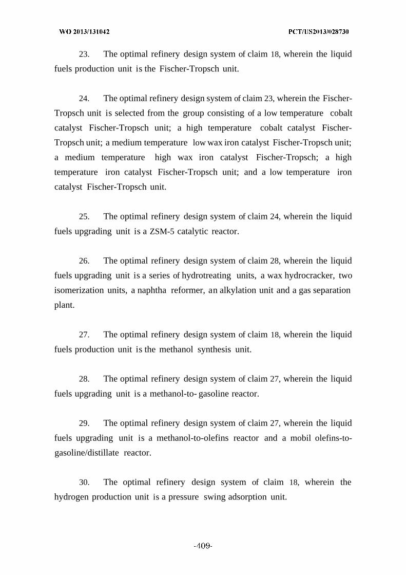
23. The optimal refinery design system of claim 18, wherein the liquid
fuels production unit is the Fischer-Tropsch unit.
24. The optimal refinery design system of claim 23, wherein the Fischer-
Tropsch unit is selected from the group consisting of a low temperature cobalt
catalyst Fischer-Tropsch unit; a high temperature cobalt catalyst Fischer-
Tropsch unit; a medium temperature low wax iron catalyst Fischer-Tropsch unit;
a medium temperature high wax iron catalyst Fischer-Tropsch; a high
temperature iron catalyst Fischer-Tropsch unit; and a low temperature iron
catalyst Fischer-Tropsch unit.
25. The optimal refinery design system of claim 24, wherein the liquid
fuels upgrading unit is a ZSM-5 catalytic reactor.
26. The optimal refinery design system of claim 28, wherein the liquid
fuels upgrading unit is a series of hydrotreating units, a wax hydrocracker, two
isomerization units, a naphtha reformer, an alkylation unit and a gas separation
plant.
27. The optimal refinery design system of claim 18, wherein the liquid
fuels production unit is the methanol synthesis unit.
28. The optimal refinery design system of claim 27, wherein the liquid
fuels upgrading unit is a methanol-to- gasoline reactor.
29. The optimal refinery design system of claim 27, wherein the liquid
fuels upgrading unit is a methanol-to-olefins reactor and a mobil olefins-to-
gasoline/distillate reactor.
30. The optimal refinery design system of claim 18, wherein the
hydrogen production unit is a pressure swing adsorption unit.

31. The optimal refinery design system of claim 18, wherein the
hydrogen production unit is an electrolyzer unit.
32. The optimal refinery design system of claim 18, wherein the oxygen
production unit is an electrolyzer unit.
33. The optimal refinery design system of claim 18, wherein the oxygen
production unit is a distinct air separation unit.
34. The optimal refinery design system of claim 18, wherein the utility
plant includes a gas turbine, a steam turbine, and a series of heat exchangers.
35. A method of designing an optimal refinery comprising:
providing the superstructure of any of claims 1 —17;
inserting a data set on each of the at least one synthesis gas
production unit, the liquid fuels production unit, the liquid fuels upgrading unit,
the wastewater treatment network and the utility plant into the mixed-integer
linear optimization model;
solving the mixed-integer linear optimization model by the global
optimization framework; and
determining each of the at least one synthesis gas production unit,
the liquid fuels production unit, the liquid fuels upgrading unit, the wastewater
treatment network and the utility plant to produce an optimal refinery design.
36. A method of designing an optimal refinery comprising:
providing the superstructure database of any of claims 18 —34;
solving the mixed-integer linear optimization model by the global
optimization framework; and

determining each of the at least one synthesis gas production unit,
the liquid fuels production unit, the liquid fuels upgrading unit, the wastewater
treatment network and the utility plant to produce an optimal refinery design.
37. A method of producing liquid fuels comprising:
producing liquid fuels with a refinery having an optimal refinery
design; wherein the optimal refinery design was arrived at by
providing the superstructure of any of claims 1 —17;
inserting a data set on each of the at least one synthesis gas
production unit, the liquid fuels production unit, the liquid fuels upgrading unit,
the wastewater treatment network and the utility plant into the mixed-integer
linear optimization model;
solving the mixed-integer linear optimization model by the global
optimization framework; and
determining each of the at least one synthesis gas
production unit, the liquid fuels production unit, the liquid fuels upgrading
unit, the wastewater treatment network and the utility plant to produce
an optimal refinery design.
38. A method of producing liquid fuels comprising:
providing the superstructure database of any of claims 18 —34;
solving the mixed-integer linear optimization model by the global
optimization framework;
determining each of the at least one synthesis gas production unit,
the liquid fuels production unit, the liquid fuels upgrading unit, the wastewater
treatment network and the utility plant to produce an optimal refinery design;
and
producing liquid fuels by the optimal refinery design.
39. Any superstructure as shown and/or described in the foregoing and
the accompanying drawings.

40. Any refinery design as shown and/or described in the foregoing and
the accompanying drawings.
41. Any method of designing a refinery as shown and/or described in the
foregoing and the accompanying drawings.
42. Any method of producing liquid fuels as shown and/or described in
the foregoing and the accompanying drawings.
43. Arefinery made by any refinery design as shown and/or described in
the foregoing and the accompanying drawings.
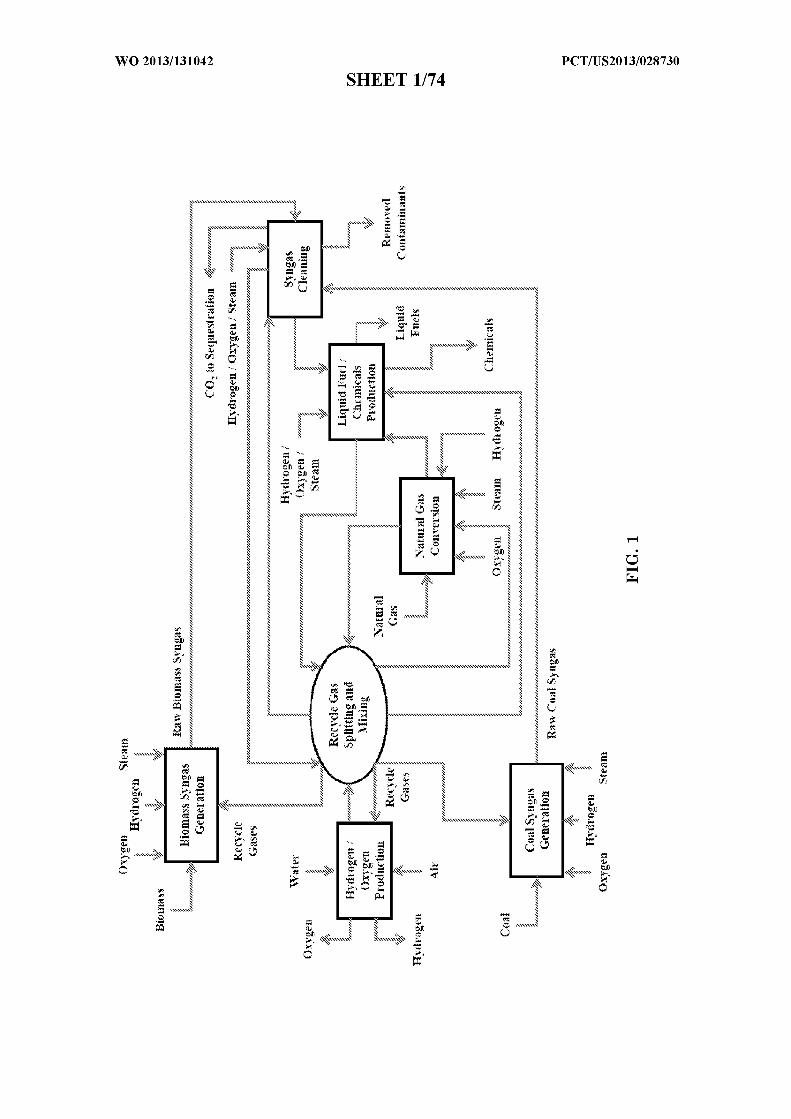
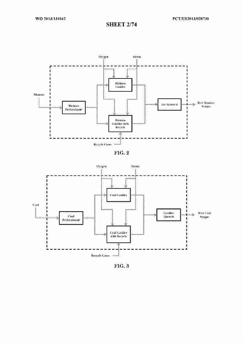


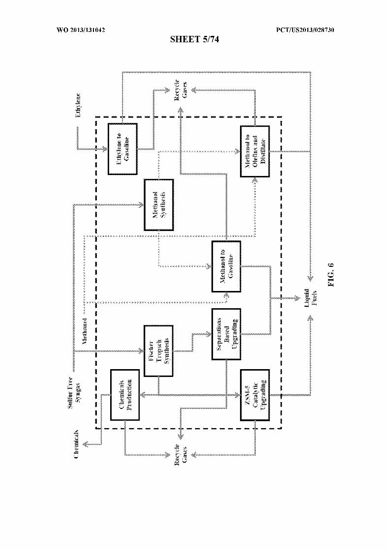

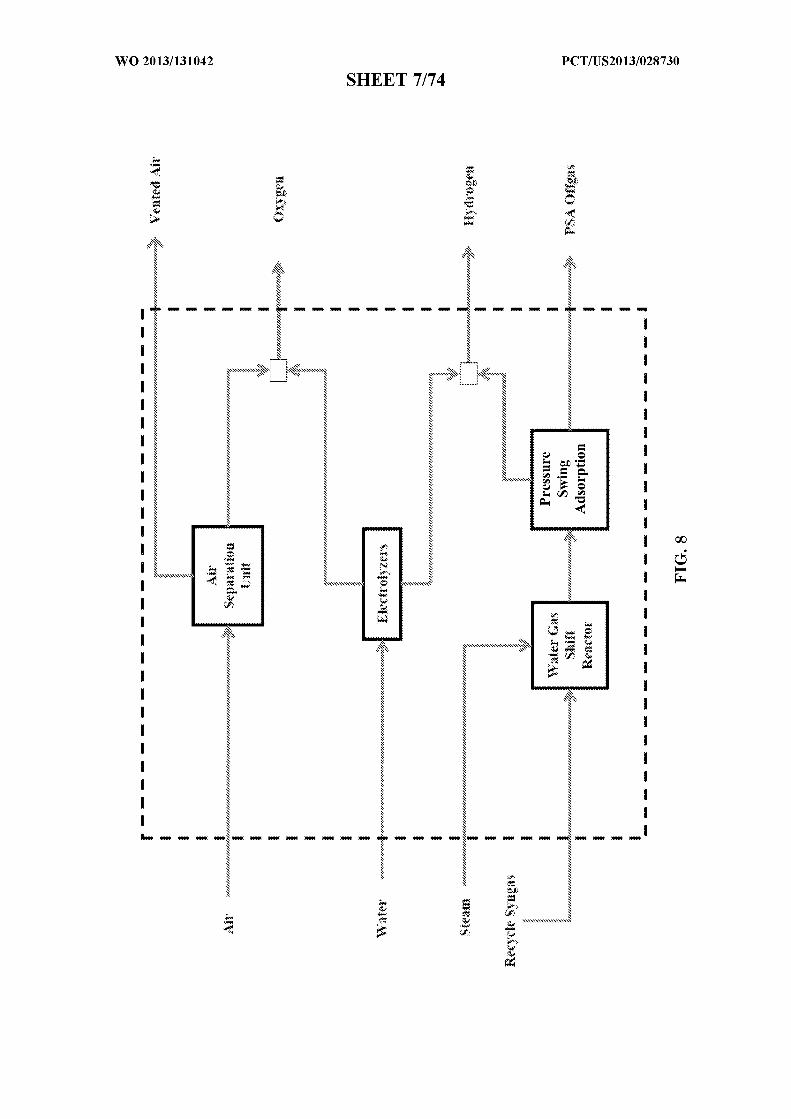
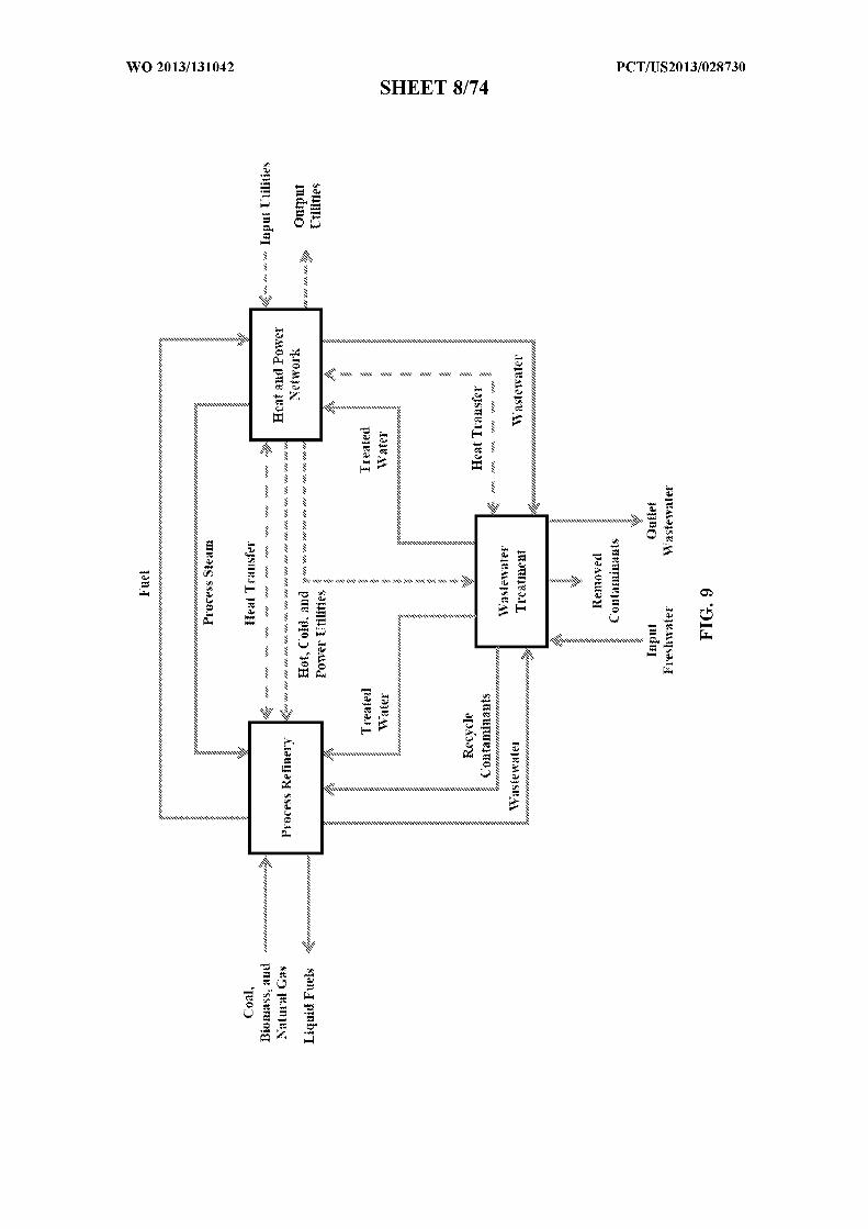
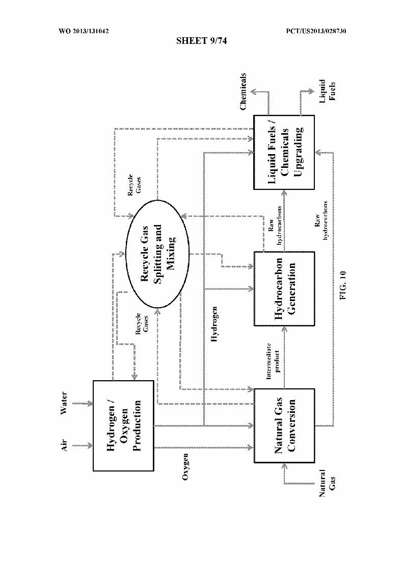
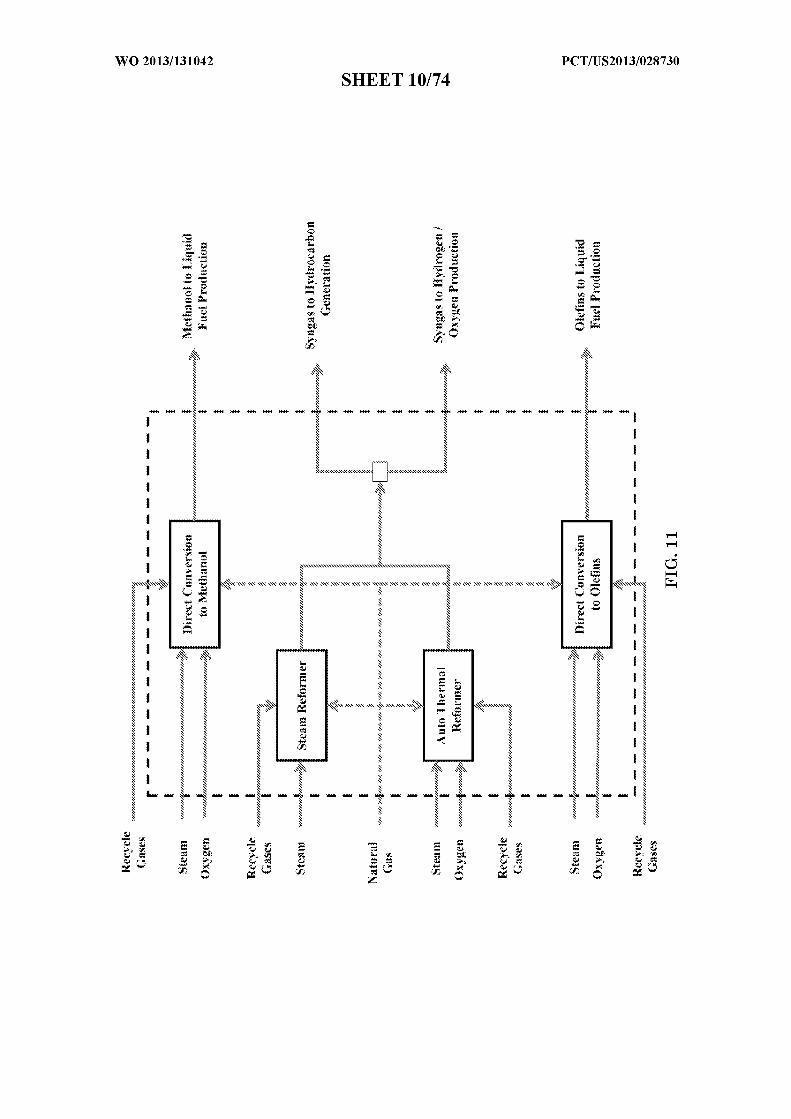

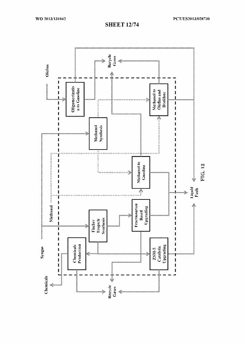
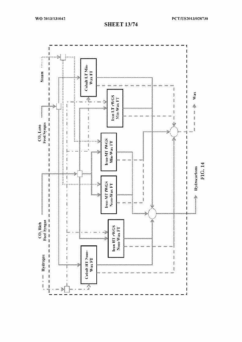
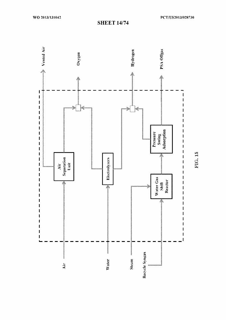

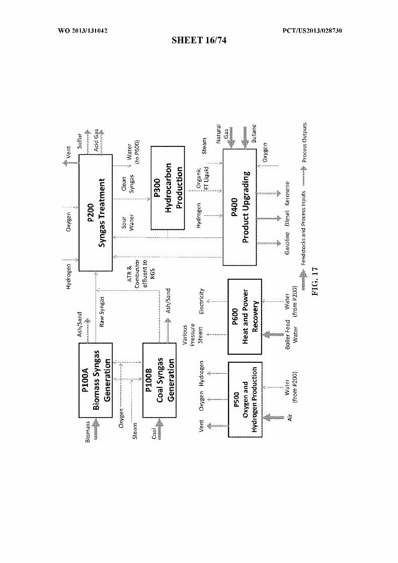
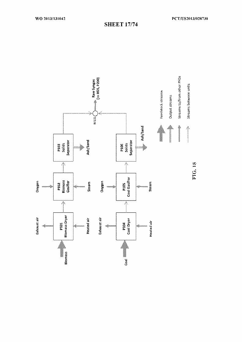
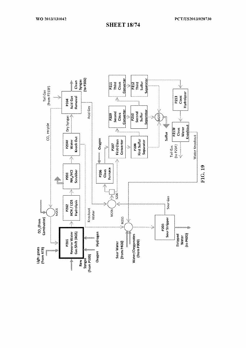


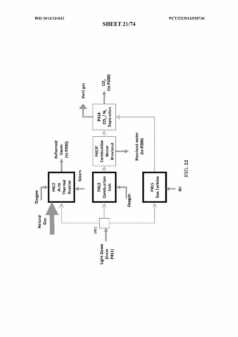

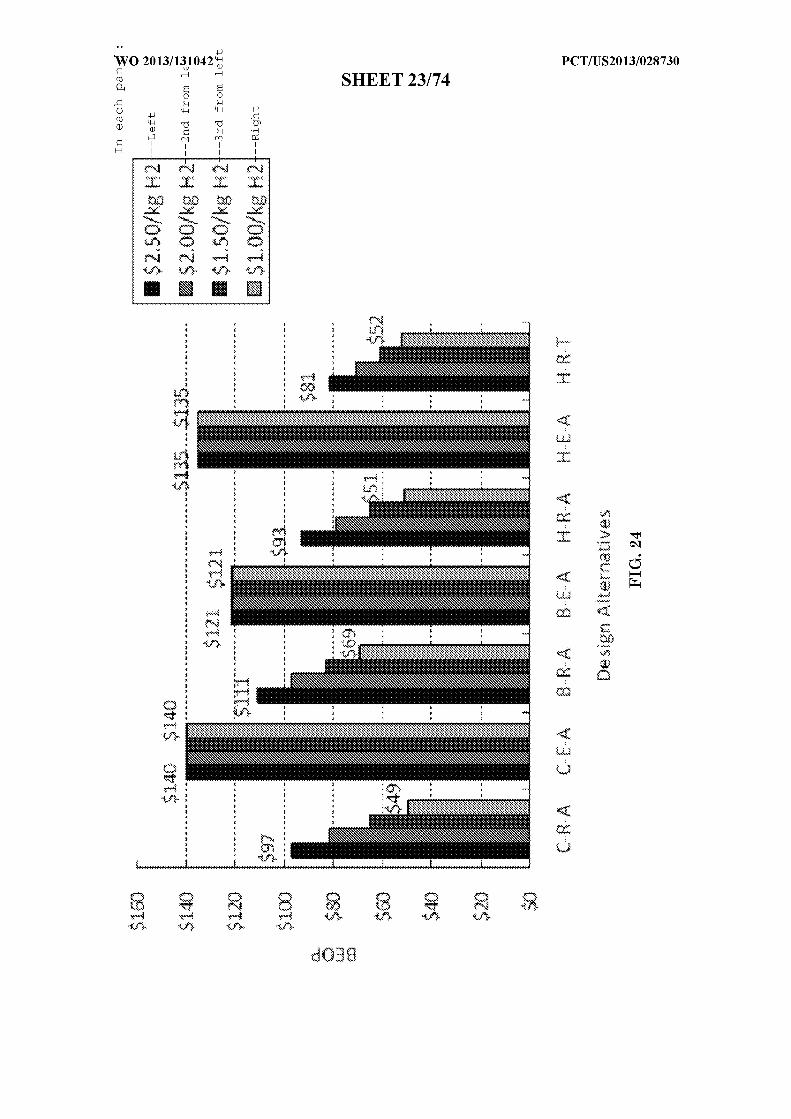


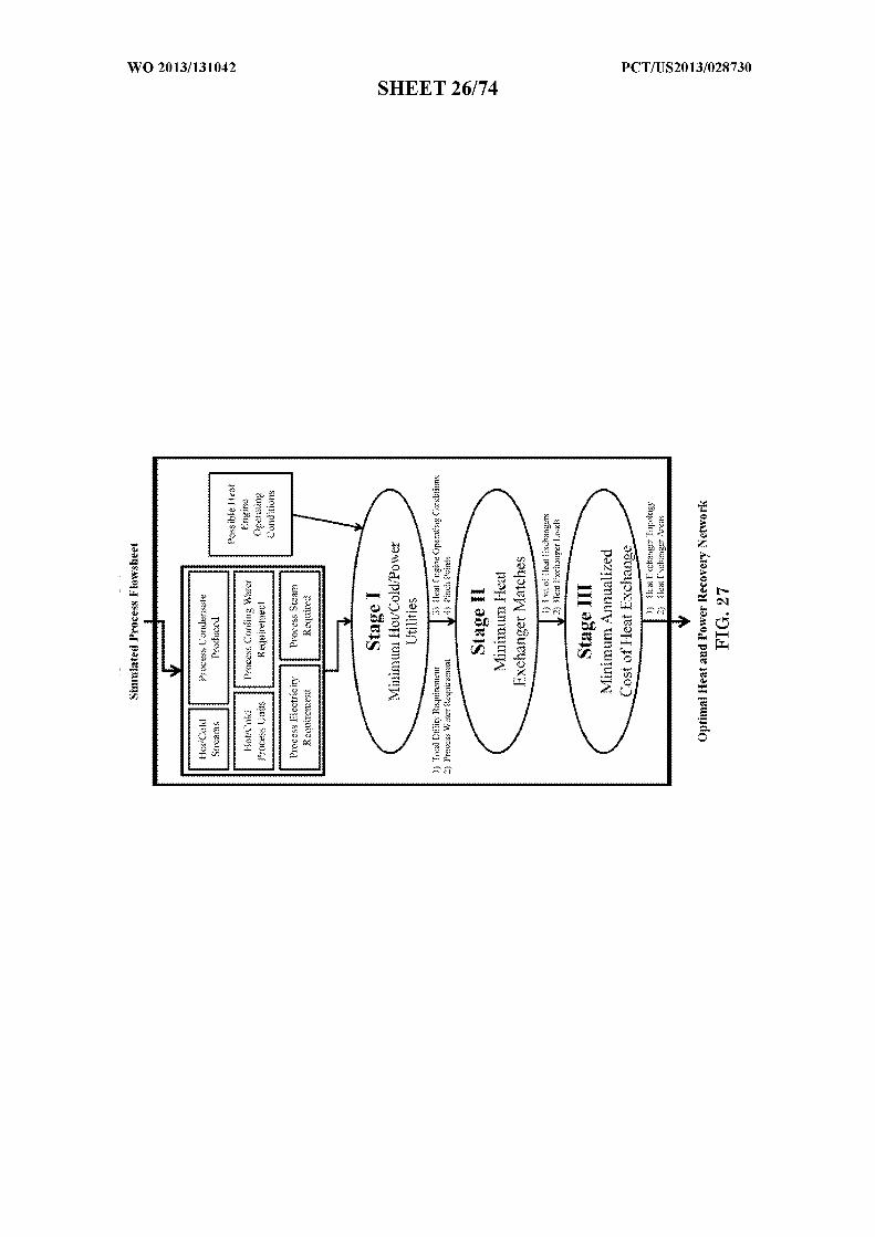
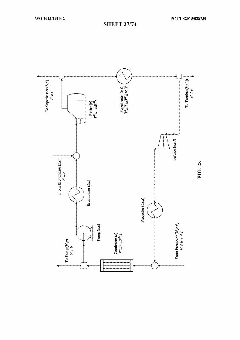


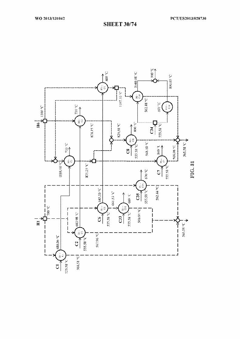
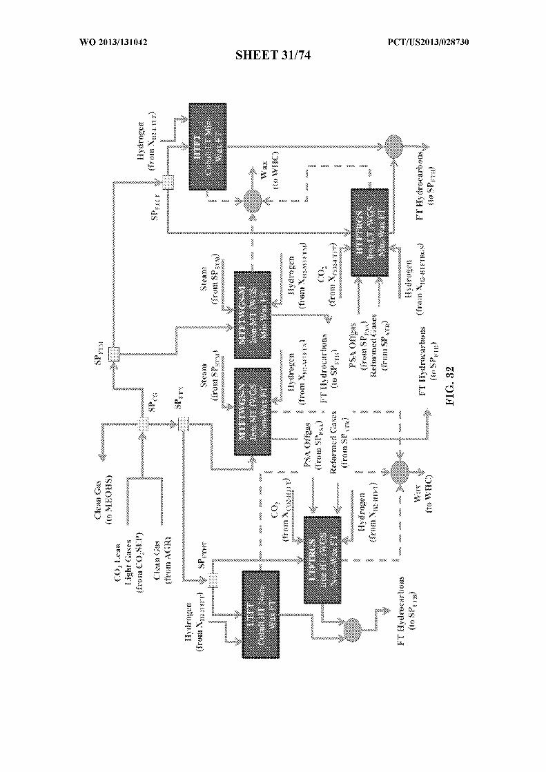

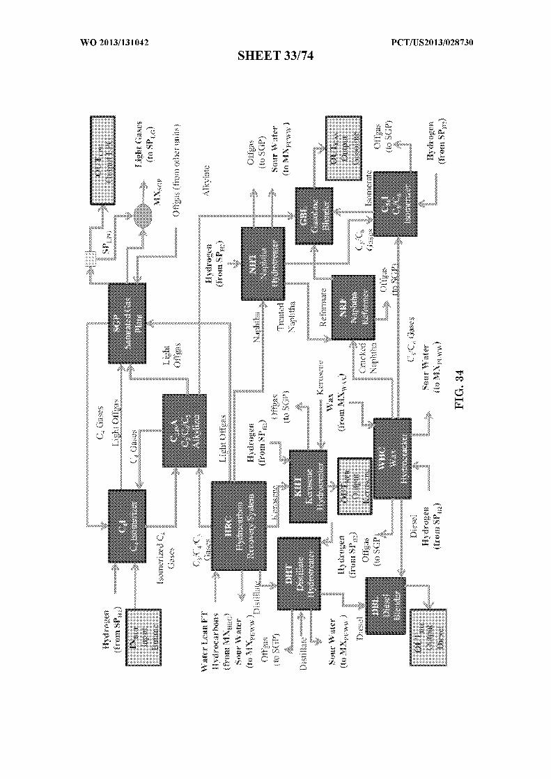
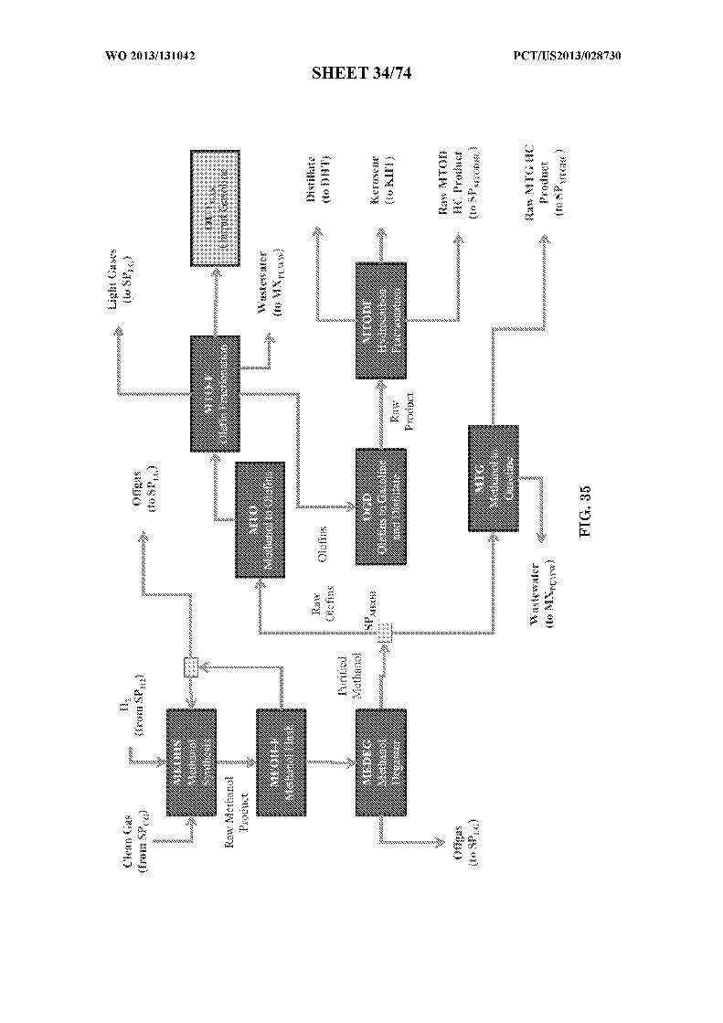


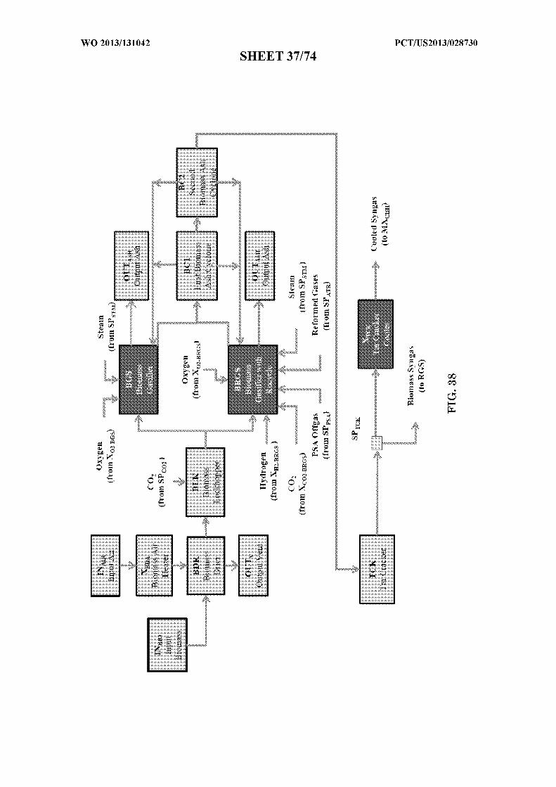

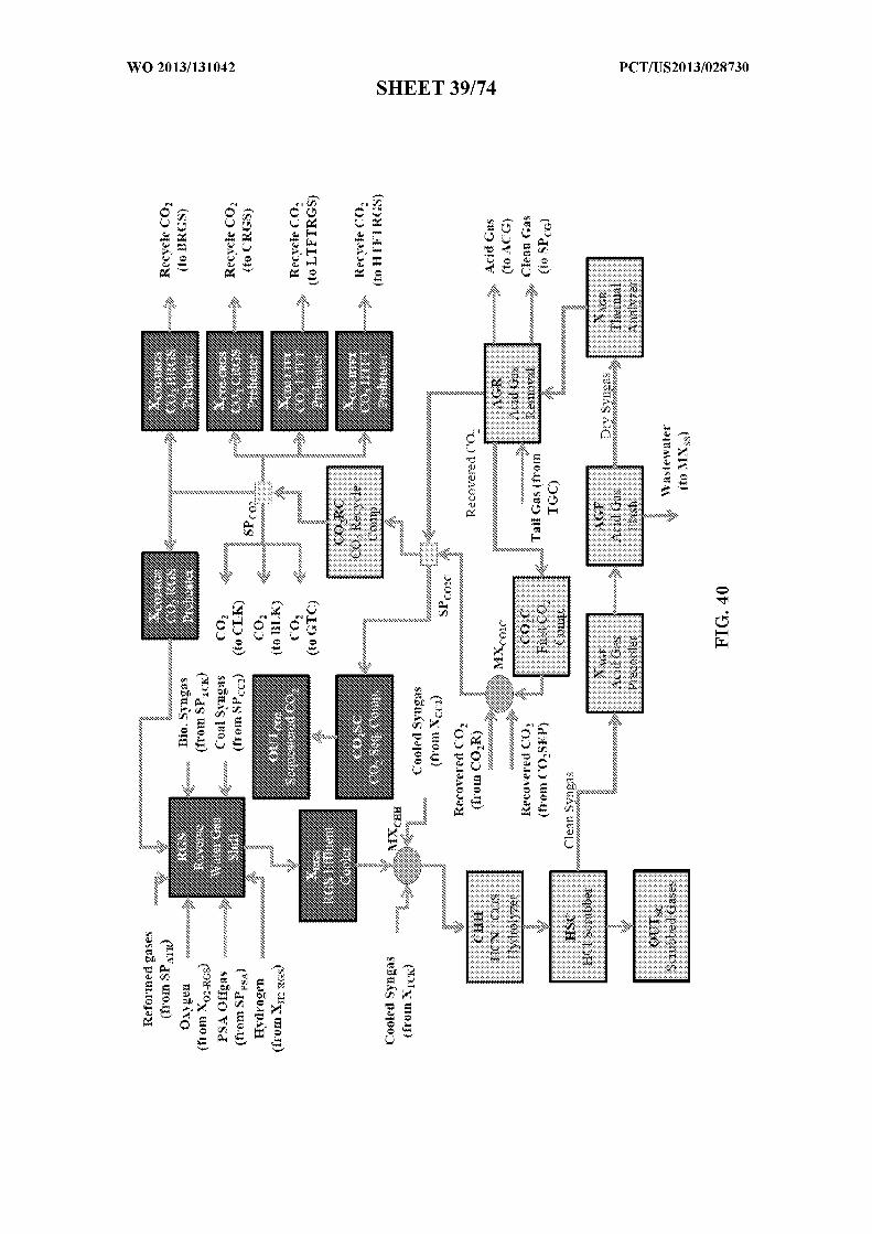


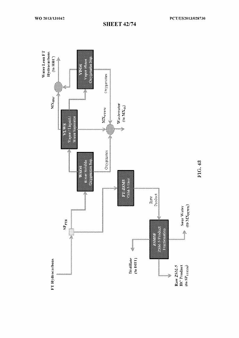
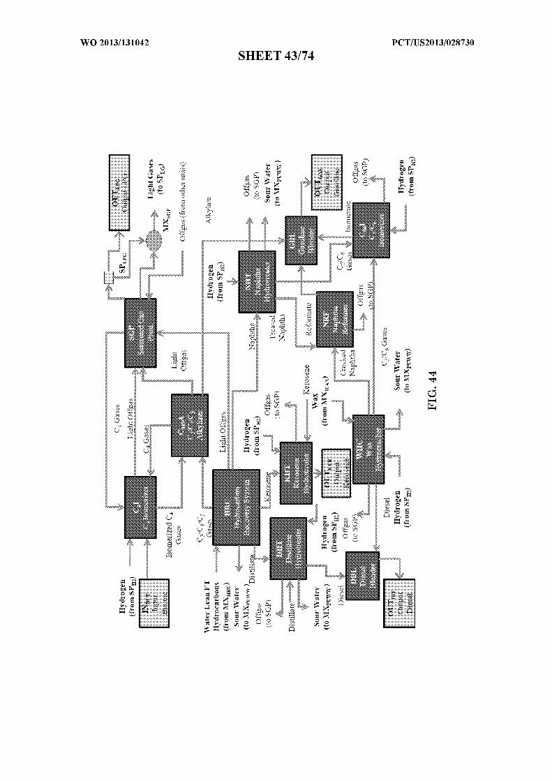


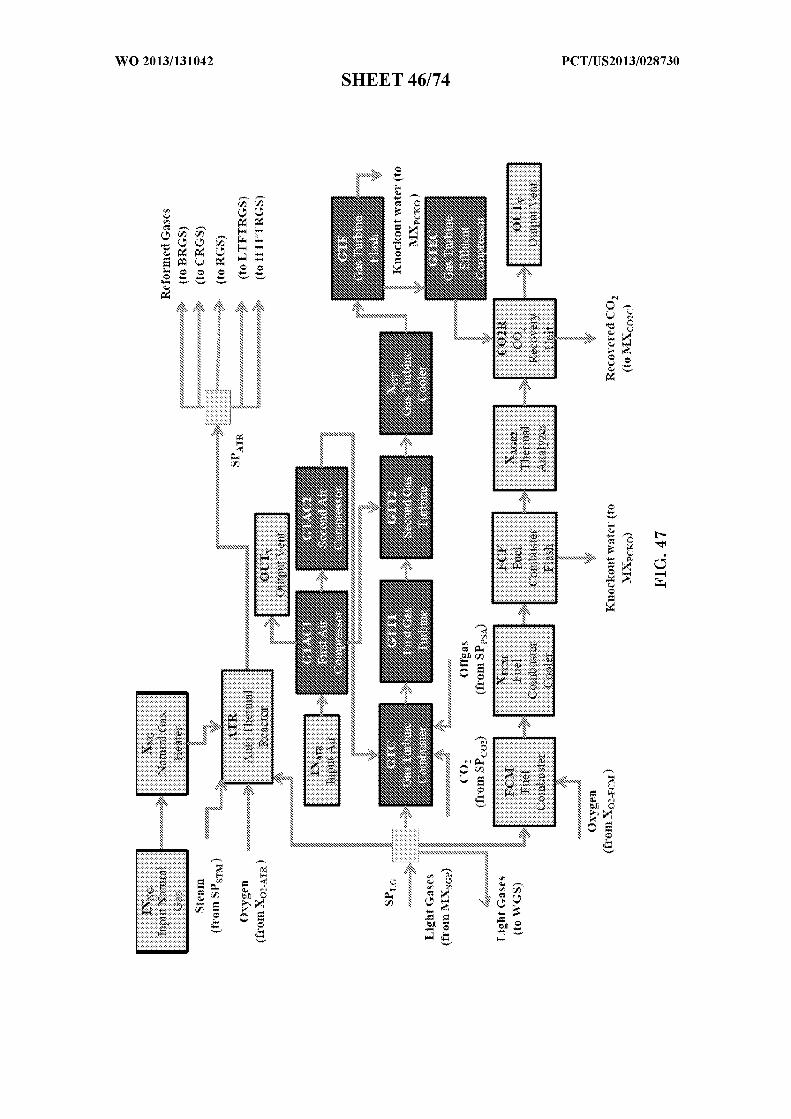

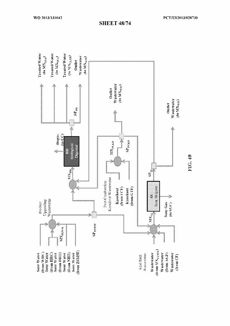

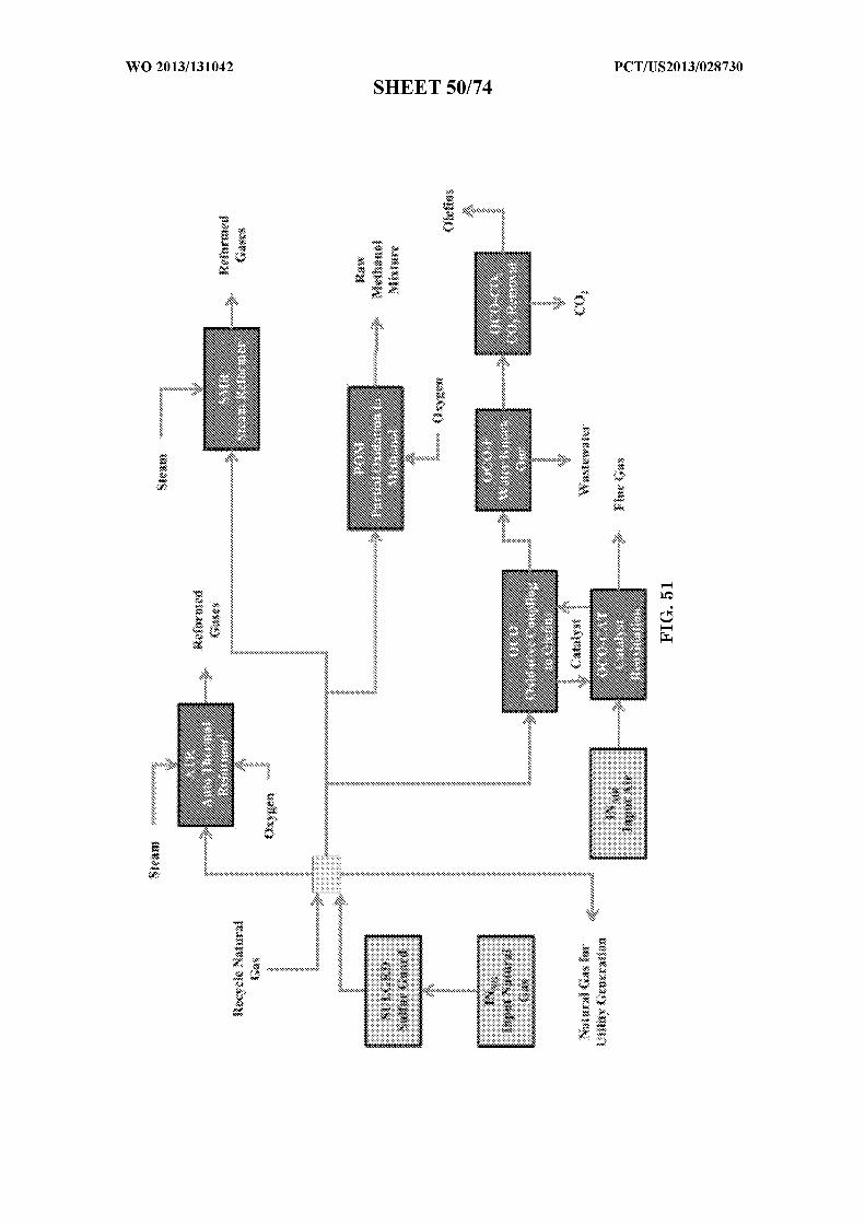
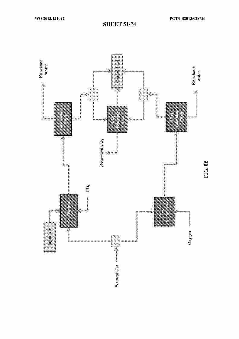

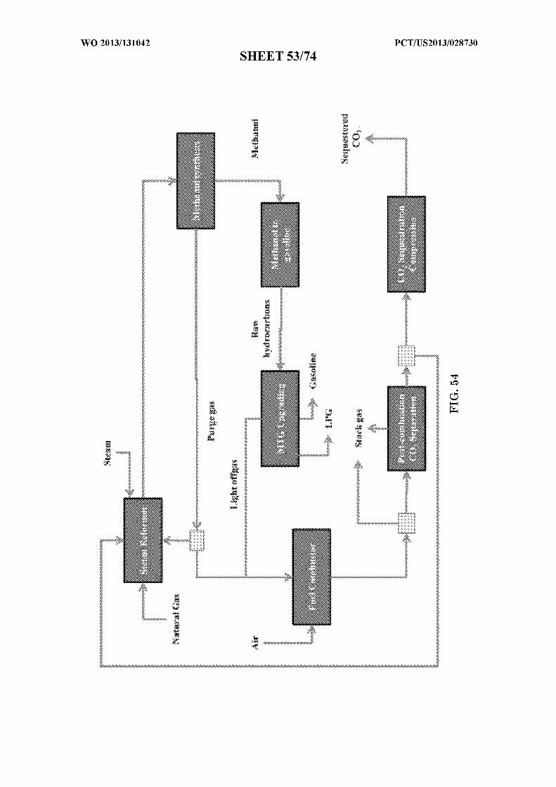
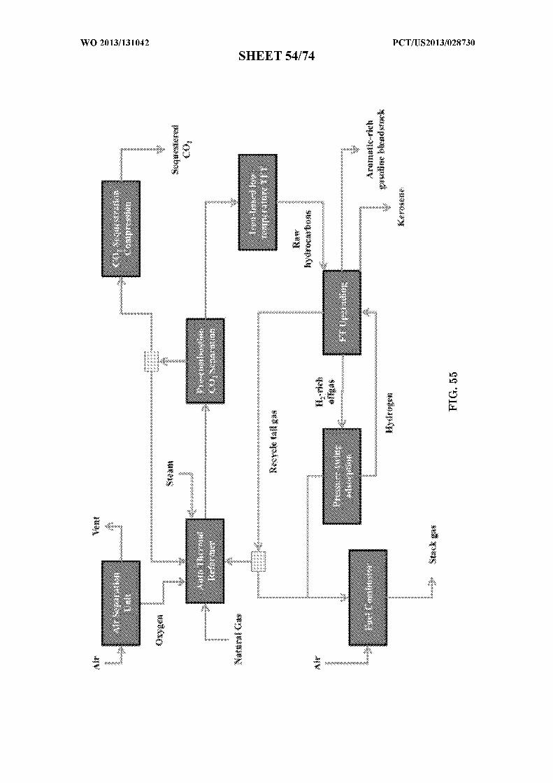

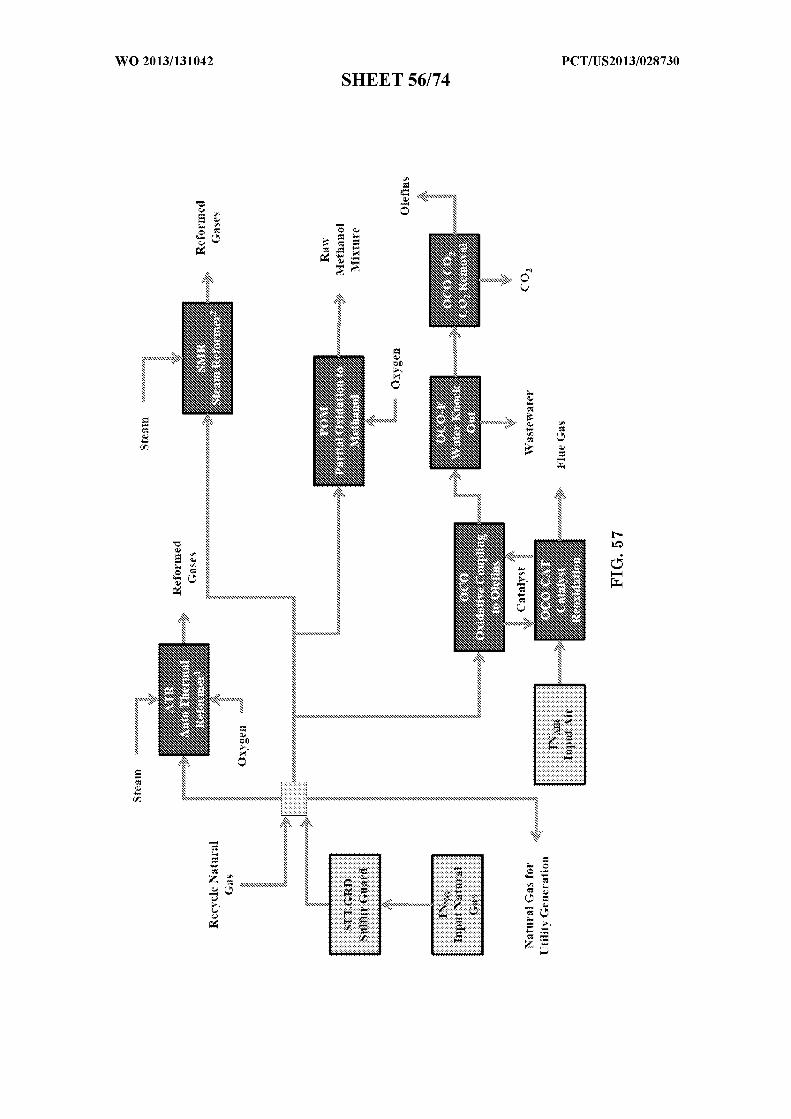


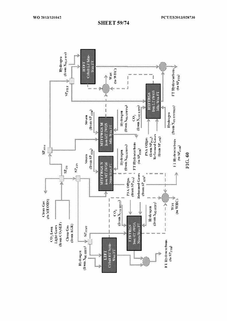


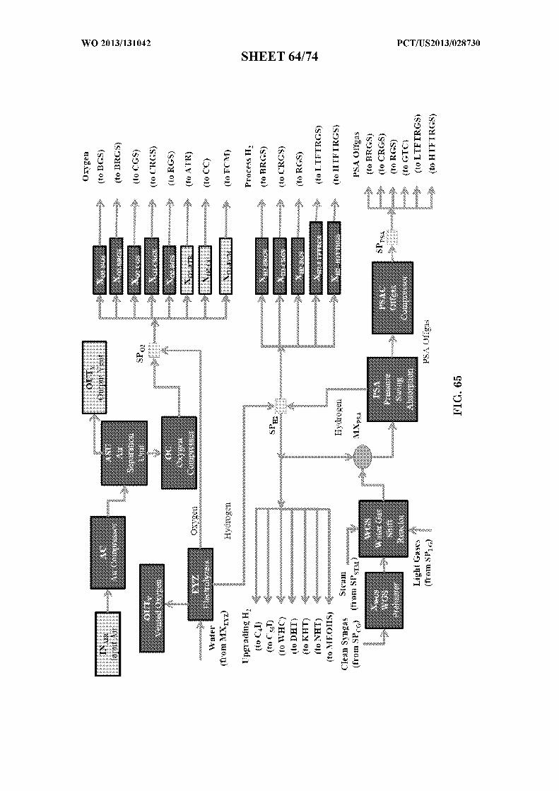

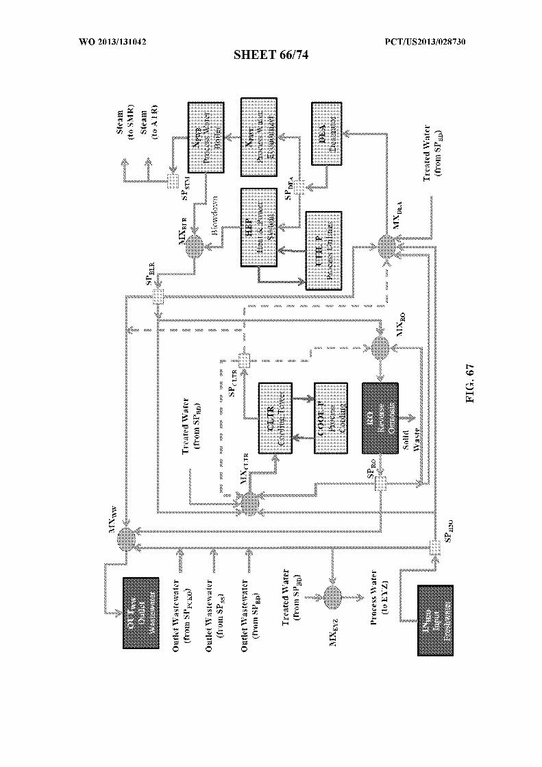


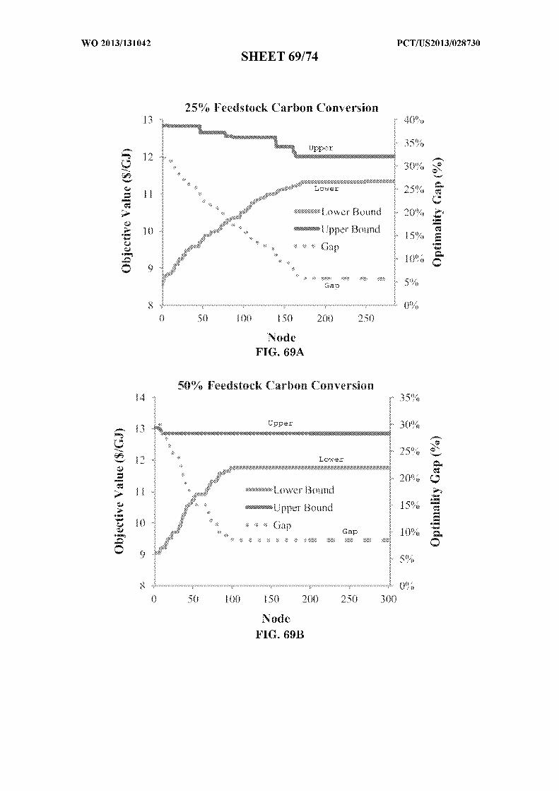
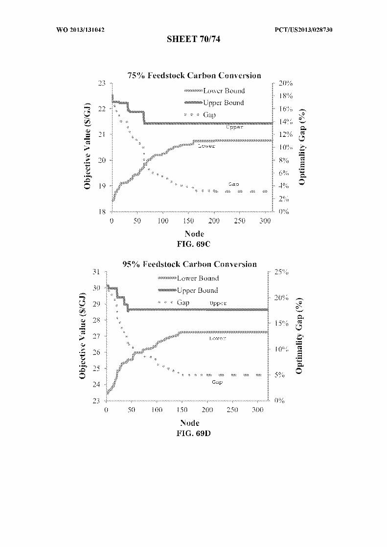
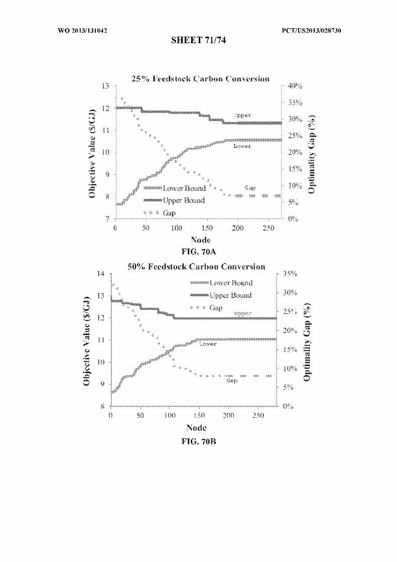

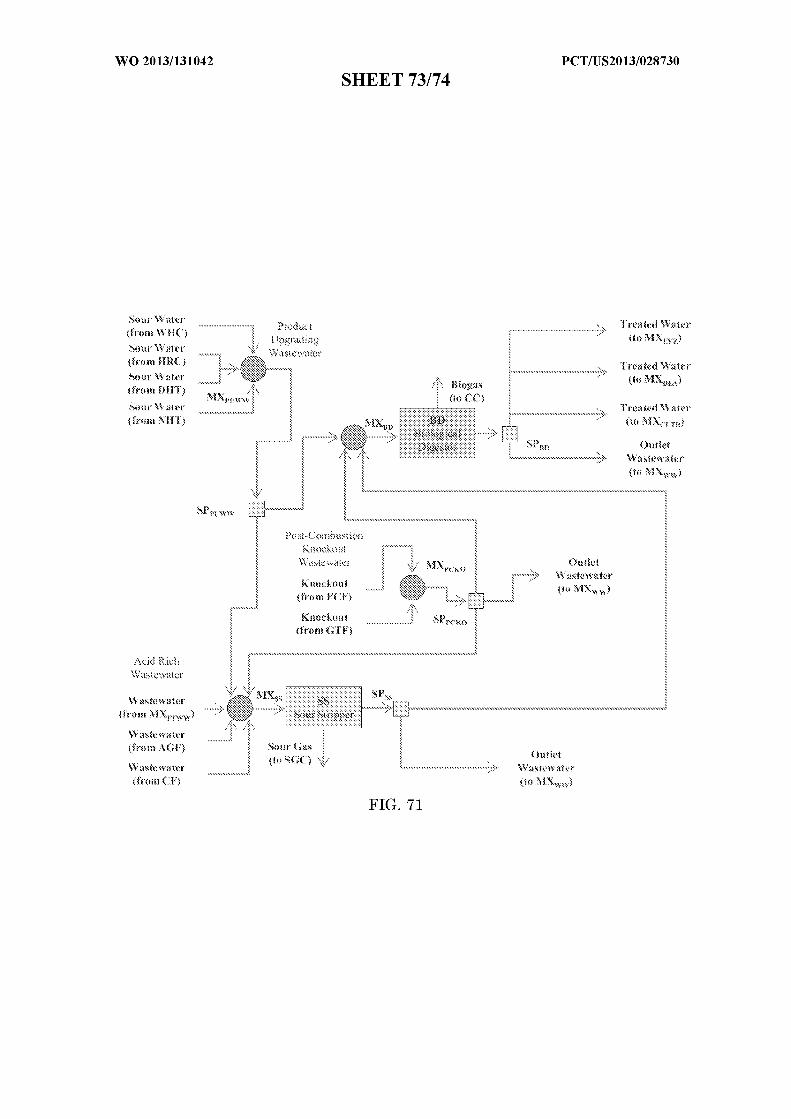

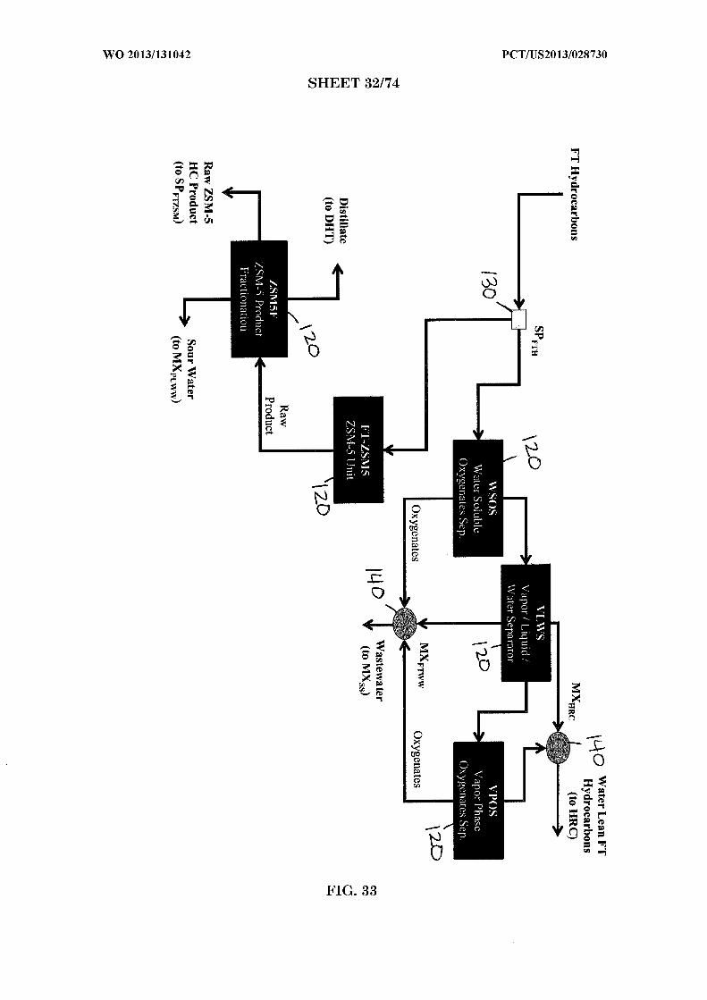
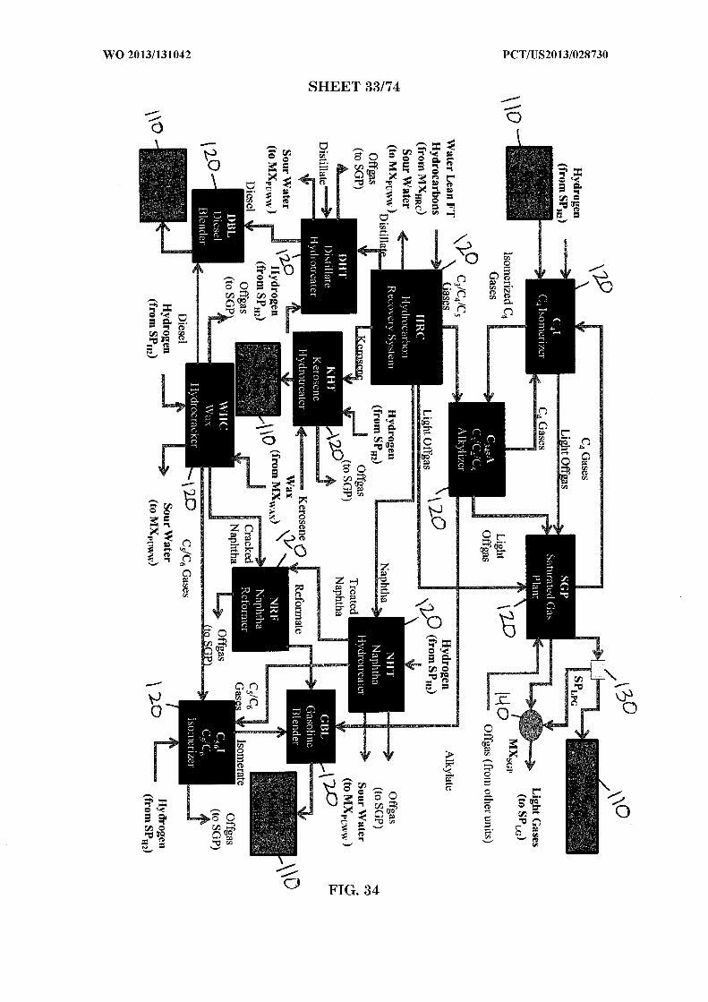
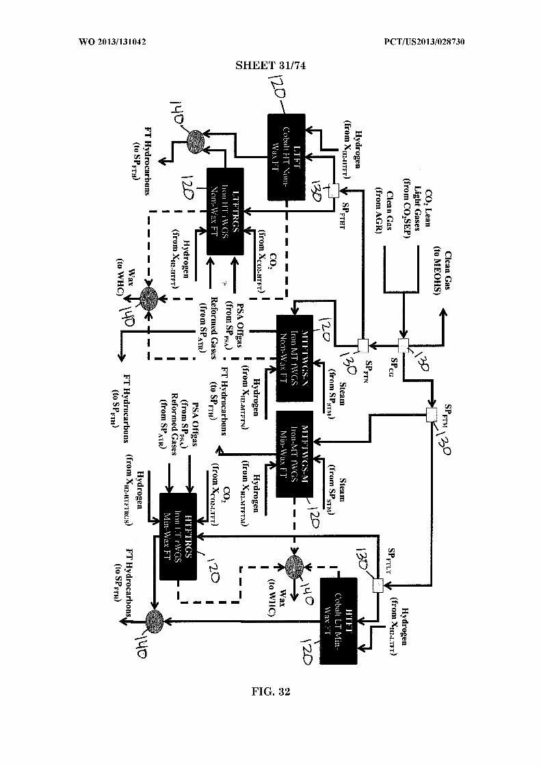


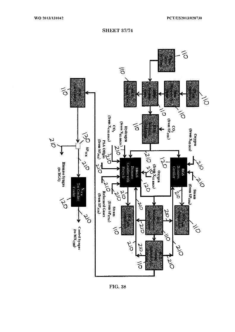


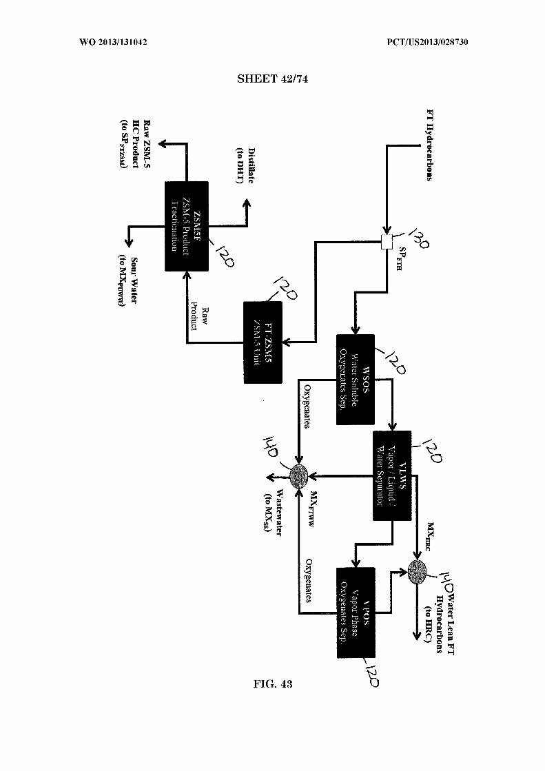

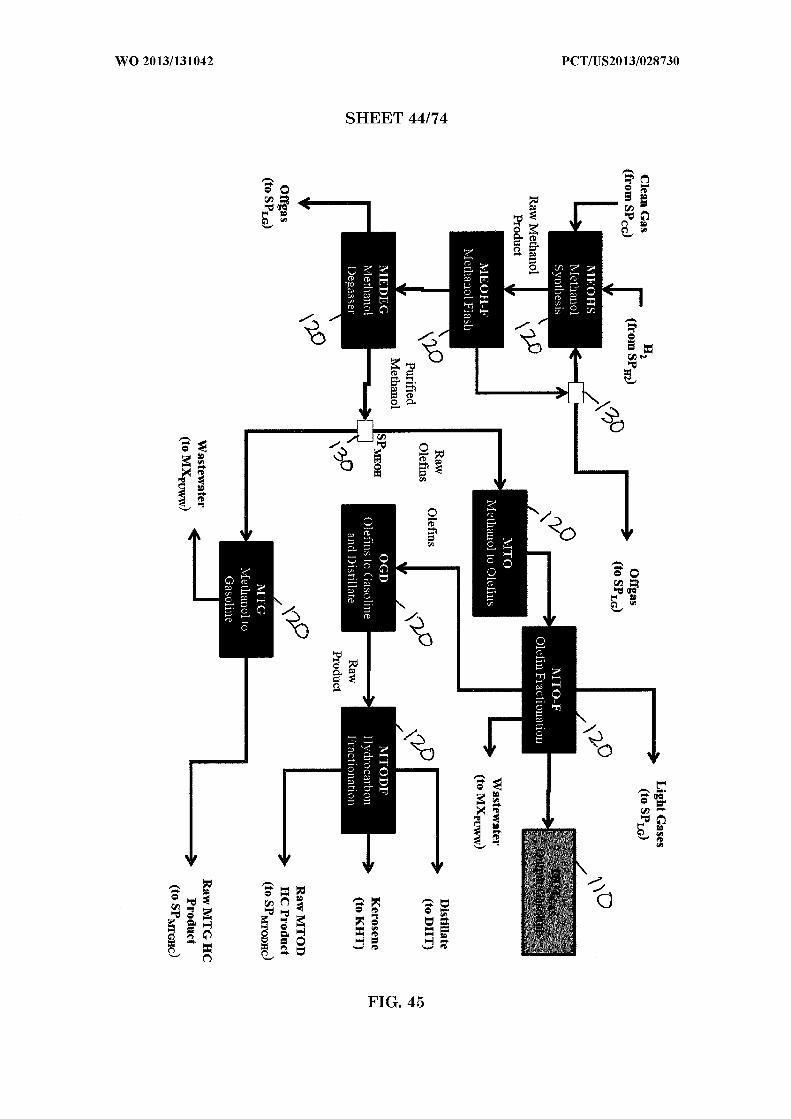


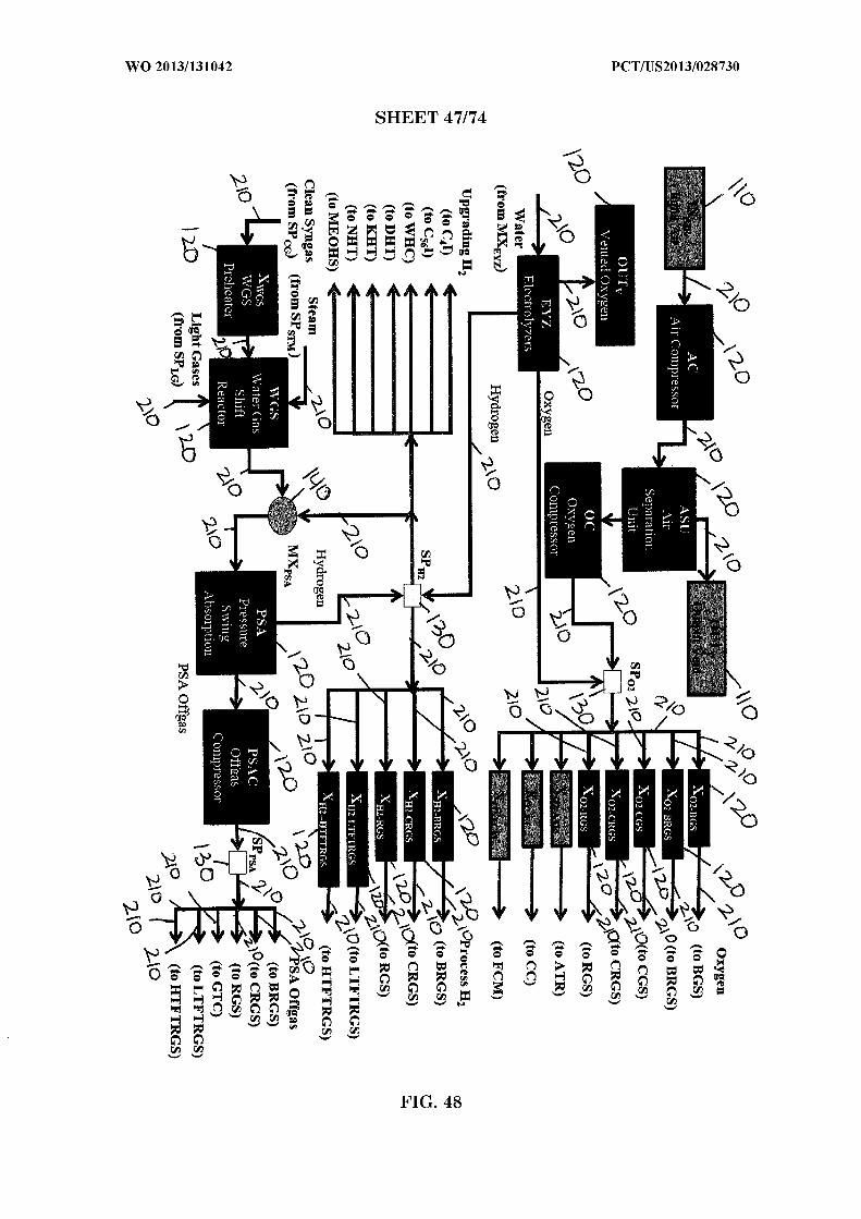

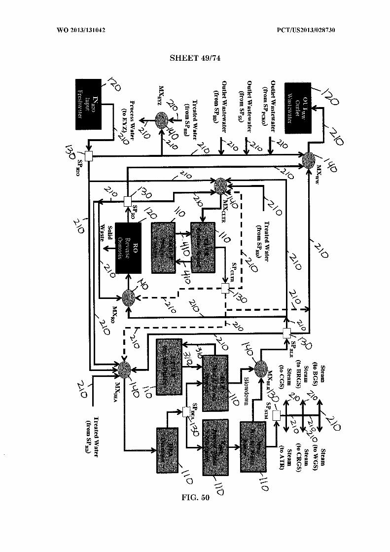

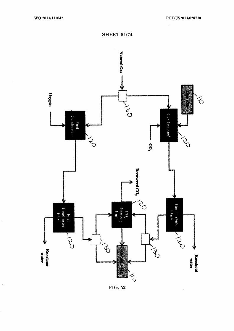


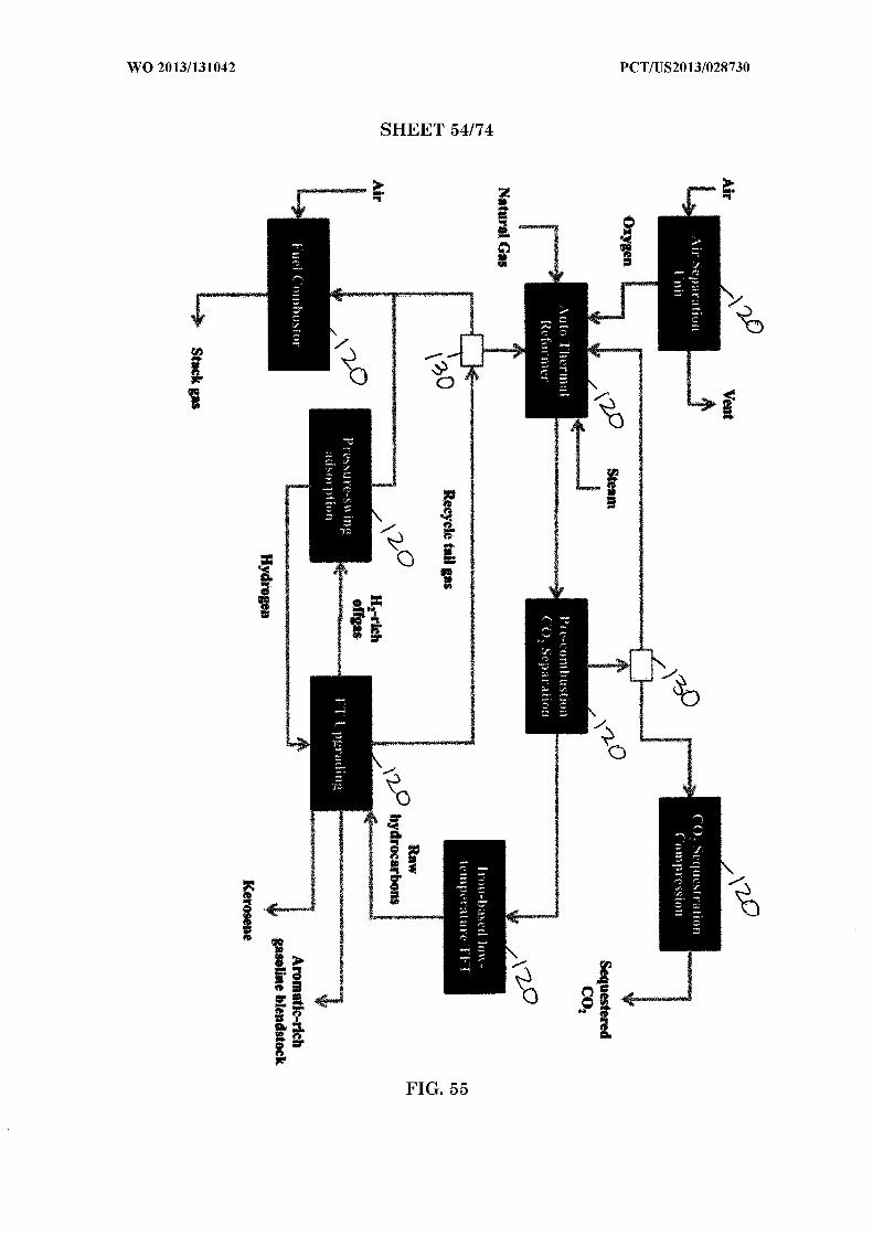
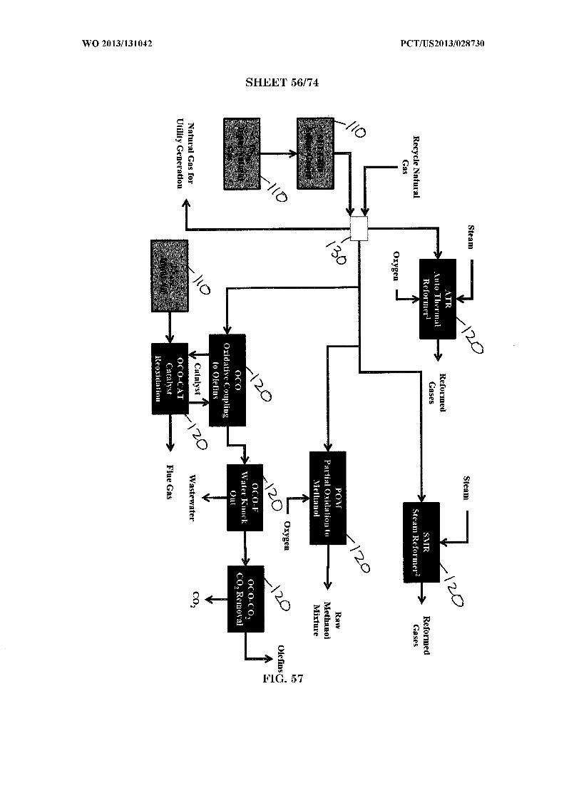
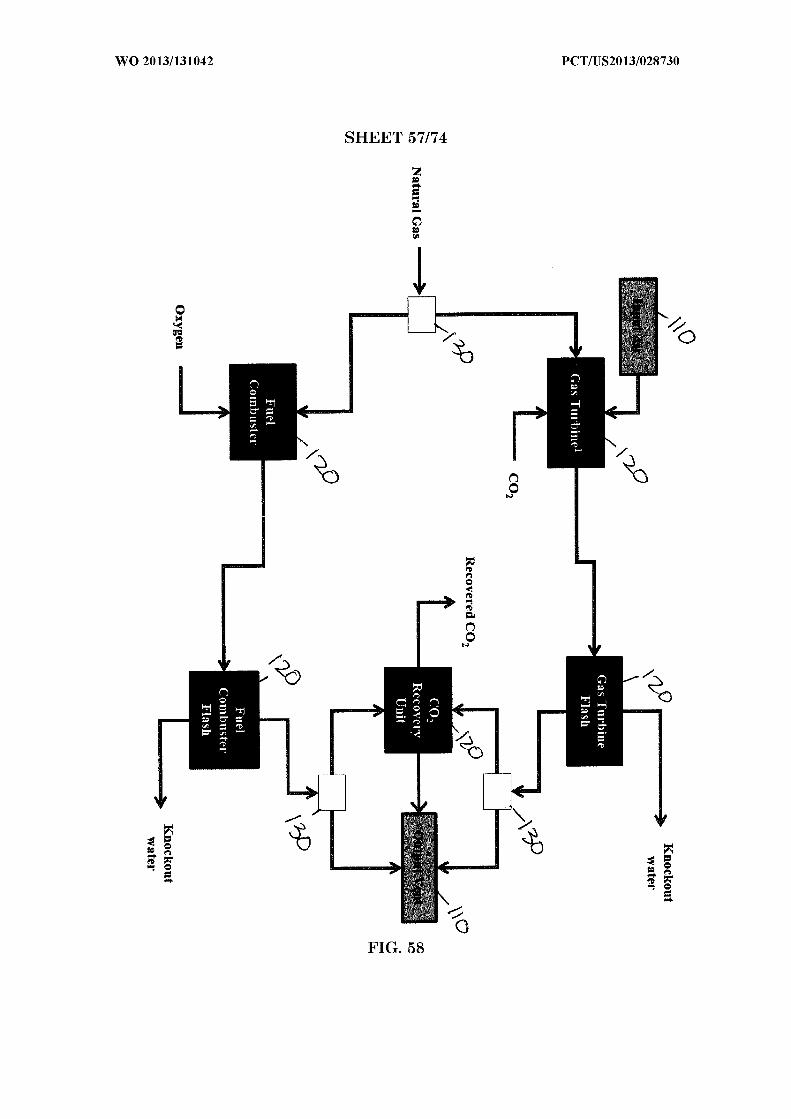
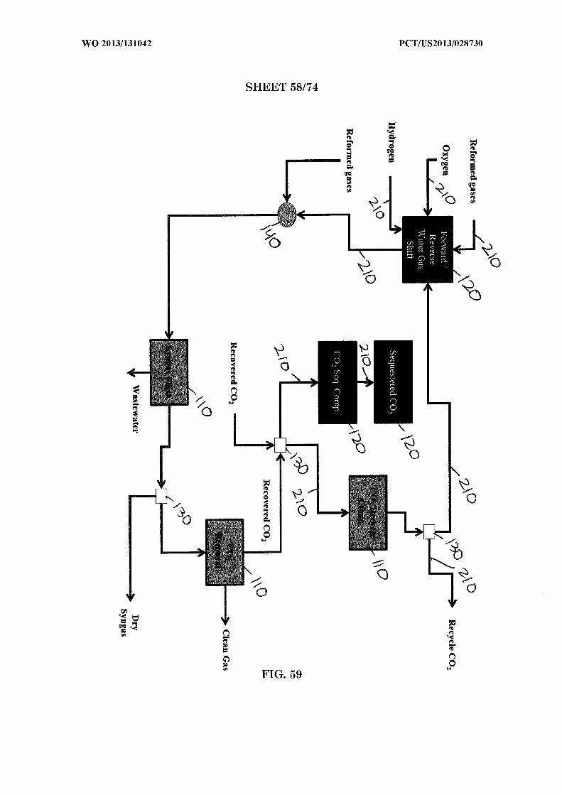
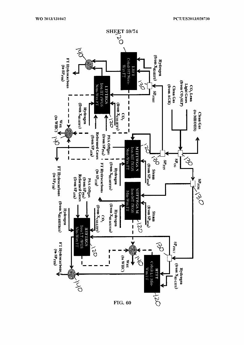


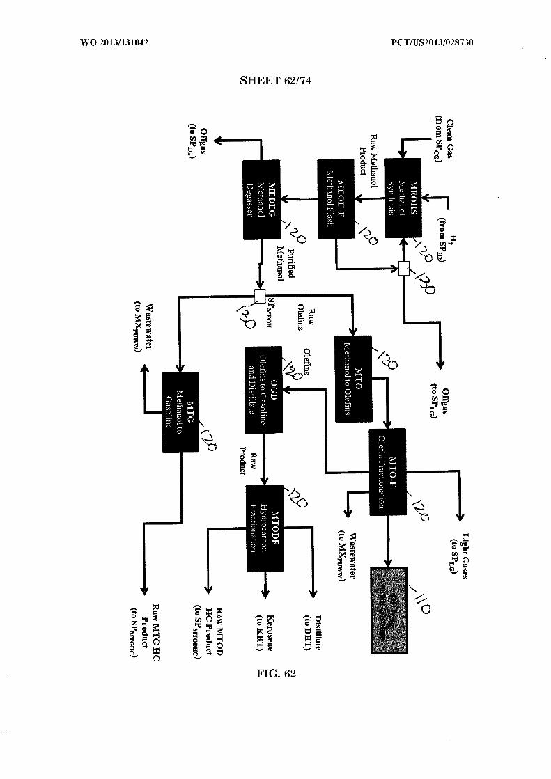
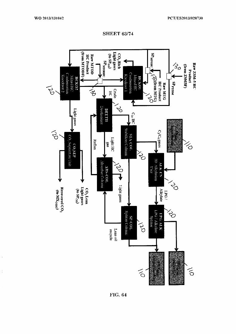
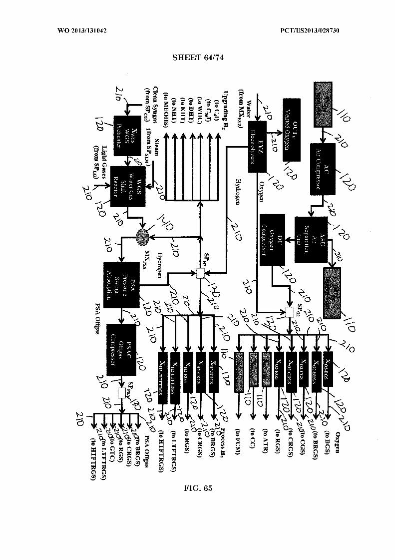
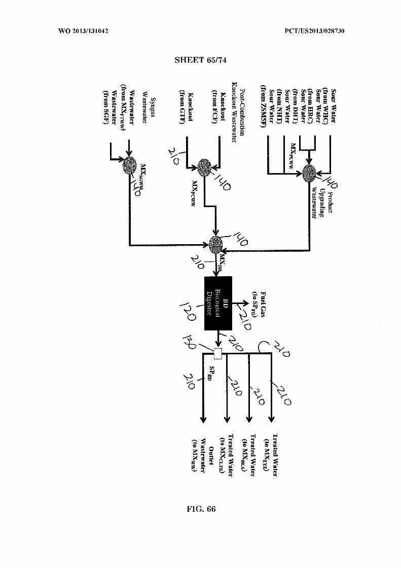
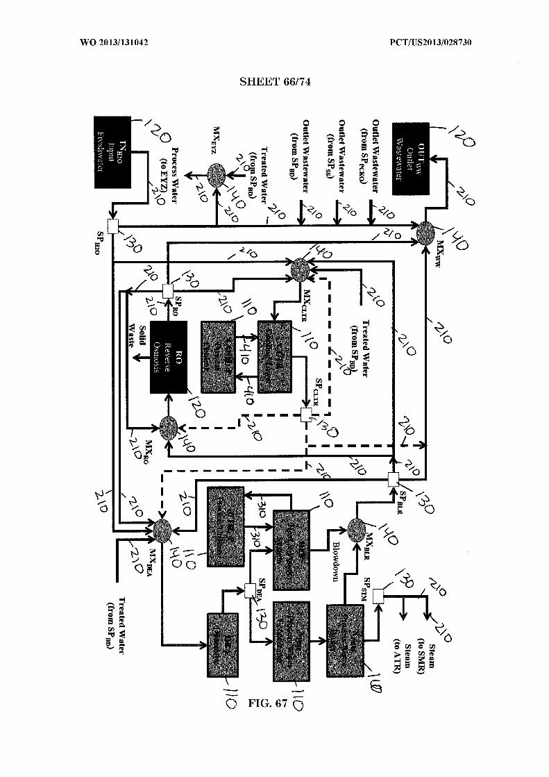


INTERNATIONALSEARCH REPORT International application No.
PCT/US 13/28730
A. CLASSIFICATION OF SUBJECT MATTERIPC(8) - C 10G 2/00 (201 3.01 )USPC - 5 18/700; 422/608; 700/90
According to International Patent Classification (IPC) or to both national classification and IPC
B . FIELDS SEARCHED
Minimum documentation searched (classification system followed by classification symbols)IPC(8) - C10G 2/00 (2013.01 )USPC - 518/700; 422/608; 700/90
Documentation searched other than minimum documentation to the extent that such documents are included in the fields searchedIPC(8) - B01 D 53/62; C10J 1/00; G05B 13/04; G06F 17/50; G06G 7/48USPC -205/450,462; 518/700, 702, 703, 704, 712; 208/400, 403; 422/600; all classes; NPL (key word limited)
Electronic data base consulted during the international search (name of data base and, where practicable, search terms used)Minesoft Patbase, Google Patent/Scholar; Key words: (synthe * or artific * ) w2 (hydrocarbon * or fuel or petrol * or oil or olefin * ), synfuel,syngas, synthetic w2 gas, (superstructure or integral or integrated), refinery, (mixed-integer linear optimization model), (Fischer w2Tropsch) and (methanol w2 synth * ), clean-up, desulf * , desulph *
C . DOCUMENTS CONSIDERED T O B E RELEVANT
Category* Citation of document, with indication, where appropriate, o f the relevant passages Relevant to claim No.
US2008/01 03220 A 1 (Cherry et al.) 0 1 May 2008 (01 .05.2008); para [0003], [0006], [0007], 1-38[0012], [0014], [0022], [0027], [0029], [0035], [0036], [0049], [0050], [0057], [0059], [0063],[0064], [0065], [0067], [0069], [0072], [0073], [0089], [0093]
US 201 1/0066258 A 1 (Torzhkov et al.) 17 March 201 1 (17.03.201 1); para [0003], [0007], [0010], 1-38[0013], [0015], [0018], [0147], [0199], [0200], [0213]
US 2009/0077892 A 1 (Shulenberger et al.) 26 March 2009 (26.03.2009); para [0010] 2, 19
US 2004/0102532 A 1 (Landis et al.) 27 May 2004 (27.05.2004); para [0018] 4 , 2 1
US 7,374,742 B2 (Geostis et al.) 20 May 2008 (20.05.2008); col 8, lines 40-50 5, 22
US 7,884,138 B2 (Mayer et al.) 08 February 201 1 (08.02.201 1); col 3, lines 40-45; col 3, lines 7, 2420-25; col 1, lines 35-45
US 2001/0001448 A 1 (Kapoor et al.) 24 May 2001 (24.05.2001); para [0035], [0055] 8, 25
US 4,709,1 13 A (Harandi et al.) 24 November 1987 (24.1 1.1987); col 1, lines 5-10, col 7, lines 11, 2810-30
US 2006/012901 1 A 1 (Clem et al.) 15 June 2006 (15.06.2006); para [0001] 12, 29
US 6,379,645 B 1 (Bucci et al.) 30 April 2002 (30.04.2002); col 4, lines 1-12 13, 30
Further documents are listed in the continuation of Box C .
Special categories of cited documents: "T"
later document published after the international filing date or priority
A " document defining the general state of the art which is not considered date and not in conflict with the application but cited to understandto be of particular relevance the principle or theory underlying the invention
E" earlier application or patent but published on or after the international "X" document of particular relevance; the claimed invention cannot befiling date considered novel or cannot be considered to involve an inventive
L" document which may throw doubts on priority claim(s) or which is step when the document is taken alonecited to establish the publication date of another citation or other "Y" document of particular relevance; the claimed invention cannot bespecial reason (as specified) considered to involve an inventive step when the document is
O" document referring to an oral disclosure, use, exhibition or other combined with one or more other such documents, such combinationmeans being obvious to a person skilled in the art
P" document published prior to the international filing date but later than "&" document member of the same patent familythe priority date claimed
Date of the actual completion of the international search Date of mailing of the international search report
30 March 2013 (30.03.2013) 2 9 AP R 2013Name and mailing address of the ISA/US Authorized officer:
Mail Stop PCT, Attn: ISA/US, Commissioner for Patents Lee W . YoungP.O. Box 1450, Alexandria, Virginia 22313-1450
Facsimile No. 571-273-3201
Form PCT/ISA/210 (second sheet) (July 2009)
INTERNATIONALSEARCH REPORT International application No.
PCT/US 13/28730
Box No. II Observations where certain claims were found unsearchable (Continuation of item 2 of first sheet)
This international search report has not been established in respect of certain claims under Article 17(2)(a) for the following reasons:
Claims Nos.:because they relate to subject matter not required to be searched by this Authority, namely:
2. Claims Nos.: 39-43because they relate to parts of the international application that do not comply with the prescribed requirements to such anextent that no meaningful international search can be carried out, specifically:
The claims 39-43 are omnibus claims and are indefinite.
Claims Nos.:because they are dependent claims and are not drafted in accordance with the second and third sentences of Rule 6.4(a).
Box No. Ill Observations where unity of invention is lacking (Continuation of item 3 of first sheet)
This International Searching Authority found multiple inventions in this international application, as follows:
1. I I As all required additional search fees were timely paid by the applicant, this international search report covers all searchableclaims.
2. As all searchable claims could be searched without effort justifying additional fees, this Authority did not invite payment ofadditional fees.
As only some of the required additional search fees were timely paid by the applicant, this international search report coversonly those claims for which fees were paid, specifically claims Nos.:
No required additional search fees were timely paid by the applicant. Consequently, this international search report isrestricted to the invention first mentioned in the claims; it is covered by claims Nos.:
The additional search fees were accompanied by the applicant's protest and, where applicable, thepayment of a protest fee.
The additional search fees were accompanied by the applicant s protest but the applicable protestfee was not paid within the time limit specified in the invitation.
No protest accompanied the payment of additional search fees.
Form PCT/ISA/2 10 (continuation of first sheet (2)) (July 2009)
INTERNATIONAL SEARCH REPORT International application No.
PCT/US 13/28730
C (Continuation). DOCUMENTS CONSIDERED TO BE RELEVANT
Category* Citation of document, with indication, where appropriate, of the relevant passages Relevant to claim No.
Y US 2005/0284796 A 1 (Benham) 29 December 2005 (29.12.2005); para [0063], [01 18] 9, 26
Y US 4,950,387 A (Harandi et al.) 2 1 August 1990 (21 .08.1990); col 6, lines '10-15 9, 26
Form PCT/ISA/2 10 (continuation of second sheet) (July 2009)