Wireless Sensor Network Deployment for Monitoring Soil ...
10
Procedia Environmental Sciences 19 (2013) 426 – 435 1878-0296 © 2013 The Authors. Published by Elsevier B.V Selection and/or peer-review under responsibility of the Scientific Committee of the Conference doi:10.1016/j.proenv.2013.06.049 Available online at www.sciencedirect.com F our D ecades of P rogress in M onitoring and M odeling of P rocesses in the S oil - P lant - A tmosphere S ystem : A pplications and C hallenges W ireless Sensor Network deployment for monitoring soil moisture dynamics at the field scale B. Majone a * , F. Viani b , E. Filippi c , A. Bellin a , A. Massa b , G. Toller d , F. Robol b and M. Salucci b a University of Trento, Department of Civil, Environmental and Mechanical Engineering, via Mesiano 77, I - 38123 Trento, Italy b University of Trento, Department of Information Engineering and Computer Science, Via Sommarive 14, I - 38123 Trento, Italy c PESSL INS c TRUMENTS Italia, Via del Porfido 19, I - 38121 Trento, Italy d Fondazione Edmund Mach, Via E. Mach 1, I d - 38010 S. Michele all'Adige, Ital y l Abstract We describe the deployment of a Wireless Sensor Network (WSN) , composed of 135 soil moisture and 27 temperature sensors , in an apple tree orchard of about 5000 m 2 , located in the municipality of Cles, a small town in the Alpine region, northeastern Italy. The orchard is divided into three parcels each one subjected to a different irrigation schedule. The objective o f the present work is to monitor soil moisture dynamics in the top soil to a detail, in both space and time, suitable to analyze the interplay between soil moisture dynamics and plant physiology. The deployment consists of 27 locations (verticals) connecte d by a multi hop WSN, each one equipped with 5 soil moisture sensors deployed at the depths of 10, 20, 30, 50 and 80 cm, and a temperature sensor at the depth of 20 cm. The proposed monitoring system is based on totally independent sensor nodes , which allo w both real time and historic data management and are connected through an input/output interface to a WSN platform. M eteorological data are monitored by a weather station located at a distance of approximately 100 m from the experimental site. Great care has been posed to calibration of the capacitance sensors, both in the laboratory, with soil samples, and on site, after deployment, in order to minimize the noise caused by small oscillations in the input voltage and uncertainty in the calibrat * ion curves. In this work we report the results of a preliminary analysis on the data collected during the growing season 2009. We observed that the WSN greatly facilitates the collection of detailed measurements of soil moisture, thereby increasing the amount of info rmation useful for exploring hydrological processes, but they should be used with care since the accuracy of collected data depends critically on the capability of the system to maintain constant the input voltage and on the reliability of calibration curv es. Finally, we studied the spatial and temporal distribution of soil moisture in all the irrigated parcels, and explored how different irrigation schedules influence * * Corresponding author. Tel . : +33 - 046 - 128 - 2637 E - mail address: B[email protected] . Open access under CC BY-NC-ND license. brought to you by CORE View metadata, citation and similar papers at core.ac.uk provided by Elsevier - Publisher Connector
-
Upload
khangminh22 -
Category
Documents
-
view
1 -
download
0
Transcript of Wireless Sensor Network Deployment for Monitoring Soil ...

Procedia Environmental Sciences 19 ( 2013 ) 426 – 435
1878-0296 © 2013 The Authors. Published by Elsevier B.VSelection and/or peer-review under responsibility of the Scientific Committee of the Conferencedoi: 10.1016/j.proenv.2013.06.049
Available online at www.sciencedirect.com
Four Decades of Progress in Monitoring and Modeling of Processes in the Soil-Plant-
Atmosphere System: Applications and Challenges
Wireless Sensor Network deployment for monitoring soilmoisture dynamics at the field scale
B. Majonea*, F. Vianib, E. Filippic, A. Bellina, A. Massab, G. Tollerd, F. Robolb
and M. Saluccib
aUniversity of Trento, Department of Civil, Environmental and Mechanical Engineering, via Mesiano 77, I-II 38123 Trento, ItalybUniversity of Trento, Department of Information Engineering and Computer Science, Via Sommarive 14, I-II 38123 Trento, Italy
cPESSL INSc TRUMENTS Italia, Via del Porfido 19, I-II 38121 Trento, ItalydFondazione Edmund Mach, Via E. Mach 1, Id -II 38010 S. Michele all'Adige, Italyl
Abstract
We describe the deployment of a Wireless Sensor Network (WSN), composed of 135 soil moisture and 27temperature sensors, in an apple tree orchard of about 5000 m2, located in the municipality of Cles, a small town in the Alpine region, northeastern Italy. The orchard is divided into three parcels each one subjected to a different irrigation schedule. The objective of the present work is to monitor soil moisture dynamics in the top soil to a detail,in both space and time, suitable to analyze the interplay between soil moisture dynamics and plant physiology. Thedeployment consists of 27 locations (verticals) connected by a multi hop WSN, each one equipped with 5 soilmoisture sensors deployed at the depths of 10, 20, 30, 50 and 80 cm, and a temperature sensor at the depth of 20 cm.The proposed monitoring system is based on totally independent sensor nodes, which allow both real time and historic data management and are connected through an input/output interface to a WSN platform. Meteorological data are monitored by a weather station located at a distance of approximately 100 m from the experimental site.Great care has been posed to calibration of the capacitance sensors, both in the laboratory, with soil samples, and on site, after deployment, in order to minimize the noise caused by small oscillations in the input voltage and uncertainty in the calibrat*ion curves. In this work we report the results of a preliminary analysis on the data collected during the growing season 2009. We observed that the WSN greatly facilitates the collection of detailed measurements of soilmoisture, thereby increasing the amount of information useful for exploring hydrological processes, but they should be used with care since the accuracy of collected data depends critically on the capability of the system to maintainconstant the input voltage and on the reliability of calibration curves. Finally, we studied the spatial and temporaldistribution of soil moisture in all the irrigated parcels, and explored how different irrigation schedules influence
* * Corresponding author. Tel.: +33-046-128-2637E-mail address: [email protected].
Open access under CC BY-NC-ND license.
brought to you by COREView metadata, citation and similar papers at core.ac.uk
provided by Elsevier - Publisher Connector
427 B. Majone et al. / Procedia Environmental Sciences 19 ( 2013 ) 426 – 435
© 2013 The Authors. Published by Elsevier B.V. Selection and/or peer-review under responsibility of the Scientific Committee of the conference. Keywords: Wireless Sensor Network; soil moisture dynamics; precision farming.
1. Introduction
Soil moisture is recognized as one of the main drivers for plant ecosystem and an important state variable for hydrological modeling. Soil moisture is strongly variable in space according to the spatial variability of soil properties and landscape characteristics, which manifest differently when upscaled to the catchment scale. This leads to large uncertainty in describing processes controlled by soil moisture dynamics, such as transport of solutes at the hillslope and catchment scale and plant ecosystem dynamics. Monitoring soil moisture at the hillslope scale, from tens to hundred meters, is therefore essential in many hydrologic and agricultural applications. Recently, a new generation of low-cost soil moisture sensors have been introduced in the market, which can be deployed in a network to provide distributed information of soil moisture dynamics at the hillslope scale. However, using a large number of low cost sensors poses problems when the calibration curve is sensor specific and typically requires to deal with a large amount of data. The need to calibrate the sensors, which are sensitive to variations of temperature and supply voltage, has been discussed in the work by Bogena et al. [1]. In addition, Sakaki et al. [2], evidenced that sensor-to-sensor differences in the readings were relatively small, but not negligible. The latter proposed a two-point -mixing model, similar to that used for TDR probes, in order to convert sensor readings into soil water content. Here we describe a deployment of 137 soil moisture sensors (capacitance sensors ECH2O probe model EC-5, Decagon Devices) organized in 27 nodes (5 sensors per node) of a multi hop Wireless Sensor Network (WSN) providing direct access to the data. The advantage of a WSN with respect to the classic deployment with data logger is in the possibility to obtain real-time data from the sensors, including data pertaining their functioning [3].
Respect to state-of-the-art deployments, our proposed solution is based on totally autonomous sensor nodes with multiple sensors of soil moisture and temperature, with the objective of providing a substantial amount of information in order to assess the relationship between the irrigation schedule and the quality of the yield in a apple orchard.
In the present work we first describe the deployment of a WSN, successively the calibration of the relationship between sensor reading and soil water content as a function of the voltage supply is described with reference to the EC-5 capacitance sensors and finally an example of application concerning the optimization of the irrigation schedule is presented and discussed.
2. Experimental site
The experimental site is an apple orchard located at Maso Maiano, in the municipality of Cles (see Figure 1), province of Trento, Italy, at the elevation of 640 m.a.s.l., within the Noce River catchment. The cultivated field has an area of almost 5000 m2. In the orchard are cultivated 1200 apple trees (cultivar Golden Delicious) planted in 2004 in north-south rows 3.5 m apart. Plants have 1 m row-spacing and the canopy height is about 2.5 m. Apple trees have an averaged stem diameter approximately of 0.04 m. In the field the soil surface is managed with a grass cover. The soil profile is composed of a surficial layer of soft soil, more than 2 m thick with a sandy loam texture. Main soil characteristics have been determined by laboratory analysis of an undisturbed sample of about 3.4 kg. Dry bulk density and porosity are 1. 43 g cm-3 and 0.46, respectively.
© 2013 The Authors. Published by Elsevier B.VSelection and/or peer-review under responsibility of the Scientific Committee of the conference
Open access under CC BY-NC-ND license.

428 B. Majone et al. / Procedia Environmental Sciences 19 ( 2013 ) 426 – 435
The deployment consists of 27 nodes (see Figure 1) connected by a multi hop Wireless SensorNetwork (WSN), each one equipped with 5 soil moisture sensors (capacitance sensors ECH2O probemodel EC-5, Decagon Devices) deployed at the depths of 10, 20, 30, 50 and 80 cm, and a temperaturesensor (Sensirion sensors) at the depth of 20 cm, for a total of 135 soil moisture and 27 temperaturesensors. The proposed monitoring system is based on totally autonomous sensor nodes, which allow both real time and historic data management. The EC-5 sensor estimates the soil water content trough thecapacitance method [4]. The EC-5 capacitance sensor operates at a frequency of 70 MHz and requires anexcitation voltage in the range of 2 to 5 V. A meteorological station is located at approximately 100 m from the experimental site, which records the following parameters: precipitations, air temperature, solar radiation, relative humidity, pressure, wind speed and direction (at 3 m and 10 m above the soil surface,respectively).
The automated irrigation system serving the orchard has been set up so that two different wateringffschedules can be applied in two sectors of the field, as shown in Figure 1. The irrigation system iscomposed of drip lines with emitters at 0.40 m spacing and with a flow of 2.1 l h-1. The area with thesensors was divided intro three sectors of an area of approximately 1200 m2 and 330 trees, with irrigation schedules of 0.5 h/day, 1 h/day and 2 h/day, respectively.
Fig. 1. Map of the Maso Maiano apple orchard with indicated the 27 nodes of the WSN system. Soil moisture data at the depth of 0.10 m, 0.20 m, 0.30 m, 0.50 m, 0.80 m and soil temperature data at the depth of 0.20 m are collected at each location. The mapshows the subdivision of the apple orchard into three sectors with different irrigation schedules. The inset shows the location of the Maso Maiano apple orchard (Cles, Italy) with the Noce river basin contoured with a red line.

429 B. Majone et al. / Procedia Environmental Sciences 19 ( 2013 ) 426 – 435
3. Laboratory calibration of the capacitance sensors
The soil moisture sensors provide an output reading in mV, which must be converted in soil volumetric water content (vwc) through a calibration curve. The excitation voltage of the sensor is in the range of 2 to 5 V. The manufacturer provides the following calibration equation: vwc = 11.9 10-4*sr - 0.401, where vwc [-] is the volumetric water content and sr [mV] is the sensor reading, for an excitation voltage of 2.5 V.
Experimental studies conducted with EC-5 sensors [1,2,5,6] showed, however, that the readings depends on several factors in addition to vwc, such as circuitry, operating frequencies, temperature, electrical conductivity and supply voltage, such that a sensor specific-calibration is often needed. Thus, in order to obtain a specific calibration curve, and to explore sensor-to sensor variability we carried out laboratory tests on soil samples taken from the experimental site. Soil samples with different volumetric water content have been prepared with care such as to reproduce as close as possible the bulk density in the field. All the experiments were conducted in the laboratory with a controlled ambient temperature of 25 °C and using distilled water with an electrical conductivity of 0.5 S/cm. The volumetric water content was measured at the end of the test by weighting the sample before and after oven drying following the ASTM D2216 standard [7]. A quadratic
(1) and a two-point -mixing model
(2)
have been fitted to the data. The parameters to be obtained by fitting the models (1) and (2) to the experimental data are a, b and c, for the model (1) and for the model (2), which requires the independent evaluation, through laboratory measurements, of the porosity , and the sensor readings for dry (srdry) and saturated soil (srsat).
In order to investigate sensor-to sensor variability we performed experiments using three different sensors, nine values of vwc and six excitation voltages. Figure 2a shows with symbols the results of the experiments for three sensors with reference to a supply voltage of 2500 mV. Models (1) and (2) were fitted to the vwc-sr data with the least square method, considering all the readings of the three sensors Notice that for the two- -mixing model (2), srdry and srsat were set equal to the mean values registered by the three sensors (see black dots in Figure 2a). The fitting of the model (2) to the experimental data provide =2.01, which is significantly smaller than the value of 2.5 proposed by Sakaki et al. [2] for a wide range of soils. Both models fitted well the data with r2=0.98 and 0.99 for models (1) and (2), respectively. The two curves are barely distinguishable in Figure 2a (see the black and dashed pink lines), which shows with different colors the measurements of the three sensors. The fitting with the model (2) has been performed also separately with the data of the single sensor. Figure 2a shows that despite strictly speaking the calibration curves are sensor specific, the difference is small, thereby suggesting that the use of a single curve may be worth trying.
The results of laboratory measurements conducted with different supply voltages are shown Figure 2b with symbols. Solid lines represent the best fitting of the experimental data with the -mixing model (2). The linear calibration equation suggested by the manufacturer (see the black solid line in Figure 2b) shows the larger deviation from the other calibrated curves, in particular for high vwc values, confirming

430 B. Majone et al. / Procedia Environmental Sciences 19 ( 2013 ) 426 – 435
that the sensors should be calibrated before deployment. These experiments show also that excitation voltage variations have a negligible effect on soil moisture estimates if their absolute value does not exceed 0.1 V (see the 2400 mV, 2500 mV and 2600 mV curves in Figure 2b), while a significant dependence of the sensor reading on the excitation supply voltage emerges for larger variations. This may be problematic in field experiments, when supply voltage may not be stable. In order to reduce as much as possible fluctuations in the excitation voltage, an additional DC/DC converter has been inserted in the sensor architecture as explained in Section 4 and excitation tension was measured such as to convert the output voltage measurements with the proper calibration curve.
Fig. 2. a) Sensor readings versus wvc for a 2500 mV excitation voltage. Two extreme points were determined as the mean of srdry and srsat for the three sensors considered. The continuous lines show the fit of the experimental data with models (1), (2) and sensor-
-mixing models. b)Sensor readings versus wvc for several excitation voltage (2000 mV, 2400 mV, 2500 mV, 2600 mV, 3000 mV and 3500 mV). The continuous lines show the fit of the experimental data with the model (2). The default linear calibration equation valid for a supply voltage of 2500 mV is also presented with a black line.
4. WSN technology and structure
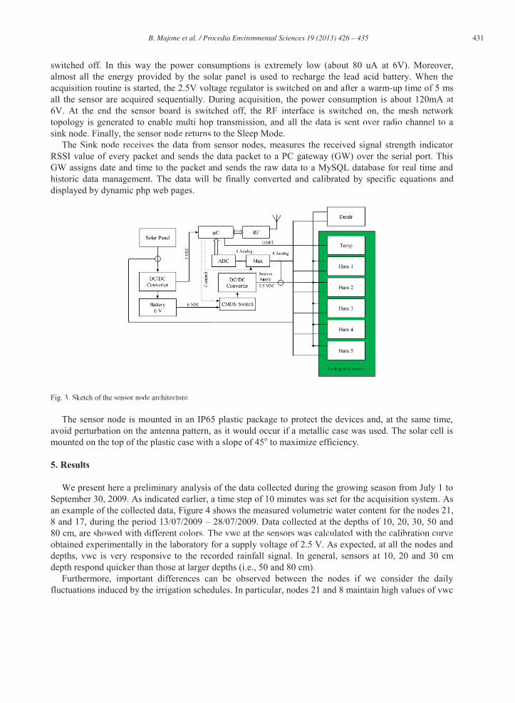
The proposed system is composed by 27 WSN nodes, each one equipped with 5 soil moisture sensors and a subsoil thermometer. Such sensors are connected through an input/output interface to a TinyNode 584 WSN platform. As detailed in Figure 3, the power supply consists of a lead acid battery (6 V 4.5 A/h), a solar panel providing 250 mA at 7 V and a 3V DC/DC converter based on a dual frequency high efficient switching regulator. For a more efficient power management and to provide a 2.5V regulated power supply to the sensors, a second DC/DC converter is used. This voltage regulator is activated only during the acquisition procedure by using an integrated CMOS switch, since the energy needed to acquire the measurements may trigger variations in the power supply voltage. Finally, an additional analog low resistance (0.8 Ohm) multiplexer controlled by the WSN node was used to acquire the 8 analog input channels.
In addition to the excitation voltage, real time monitoring of the system is performed by measuring, at each node, the battery tension, the voltage of the solar panel, and the internal voltage as well as the temperature of the microcontroller. The on-board software routines are written in NesC programming language and based on TinyOS-2.x operating system environment. The acquisition procedure is started every 10 min. between two successive readings the sensor node is in low power operation mode (called also Sleep Mode) and every unnecessary module (such radio frequency, RF, module and sensor) is
431 B. Majone et al. / Procedia Environmental Sciences 19 ( 2013 ) 426 – 435
switched off. In this way the power consumptions is extremely low (about 80 uA at 6V). Moreover,almost all the energy provided by the solar panel is used to recharge the lead acid battery. When the acquisition routine is started, the 2.5V voltage regulator is switched on and after a warm-up time of 5 msall the sensor are acquired sequentially. During acquisition, the power consumption is about 120mA at6V. At the end the sensor board is switched off, the RF interface is switched on, the mesh network topology is generated to enable multi hop transmission, and all the data is sent over radio channel to asink node. Finally, the sensor node returns to the Sleep Mode.
The Sink node receives the data from sensor nodes, measures the received signal strength indicator RSSI value of every packet and sends the data packet to a PC gateway (GW) over the serial port. ThisGW assigns date and time to the packet and sends the raw data to a MySQL database for real time andhistoric data management. The data will be finally converted and calibrated by specific equations and displayed by dynamic php web pages.
Fig. 3. Sketch of the sensor node architecture.
The sensor node is mounted in an IP65 plastic package to protect the devices and, at the same time,avoid perturbation on the antenna pattern, as it would occur if a metallic case was used. The solar cell ismounted on the top of the plastic case with a slope of 45o to maximize efficiency.
5. Results
We present here a preliminary analysis of the data collected during the growing season from July 1 toSeptember 30, 2009. As indicated earlier, a time step of 10 minutes was set for the acquisition system. Asan example of the collected data, Figure 4 shows the measured volumetric water content for the nodes 21,8 and 17, during the period 13/07/2009 28/07/2009. Data collected at the depths of 10, 20, 30, 50 and 80 cm, are showed with different colors. The vwc at the sensors was calculated with the calibration curveobtained experimentally in the laboratory for a supply voltage of 2.5 V. As expected, at all the nodes and depths, vwc is very responsive to the recorded rainfall signal. In general, sensors at 10, 20 and 30 cm depth respond quicker than those at larger depths (i.e., 50 and 80 cm).
Furthermore, important differences can be observed between the nodes if we consider the daily fluctuations induced by the irrigation schedules. In particular, nodes 21 and 8 maintain high values of vwc
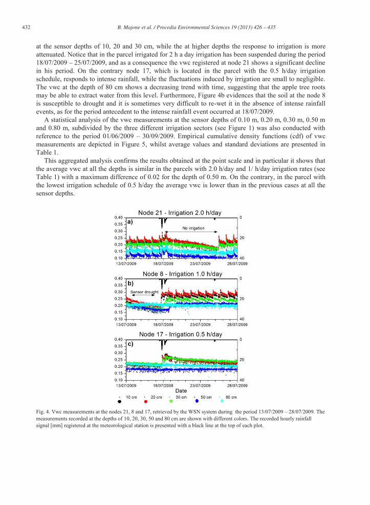
432 B. Majone et al. / Procedia Environmental Sciences 19 ( 2013 ) 426 – 435
at the sensor depths of 10, 20 and 30 cm, while the at higher depths the response to irrigation is more attenuated. Notice that in the parcel irrigated for 2 h a day irrigation has been suspended during the period 18/07/2009 25/07/2009, and as a consequence the vwc registered at node 21 shows a significant decline in his period. On the contrary node 17, which is located in the parcel with the 0.5 h/day irrigation schedule, responds to intense rainfall, while the fluctuations induced by irrigation are small to negligible. The vwc at the depth of 80 cm shows a decreasing trend with time, suggesting that the apple tree roots may be able to extract water from this level. Furthermore, Figure 4b evidences that the soil at the node 8 is susceptible to drought and it is sometimes very difficult to re-wet it in the absence of intense rainfall events, as for the period antecedent to the intense rainfall event occurred at 18/07/2009.
A statistical analysis of the vwc measurements at the sensor depths of 0.10 m, 0.20 m, 0.30 m, 0.50 m and 0.80 m, subdivided by the three different irrigation sectors (see Figure 1) was also conducted with reference to the period 01/06/2009 30/09/2009. Empirical cumulative density functions (cdf) of vwc measurements are depicted in Figure 5, whilst average values and standard deviations are presented in Table 1.
This aggregated analysis confirms the results obtained at the point scale and in particular it shows that the average vwc at all the depths is similar in the parcels with 2.0 h/day and 1/ h/day irrigation rates (see Table 1) with a maximum difference of 0.02 for the depth of 0.50 m. On the contrary, in the parcel with the lowest irrigation schedule of 0.5 h/day the average vwc is lower than in the previous cases at all the sensor depths.
Fig. 4. Vwc measurements at the nodes 21, 8 and 17, retrieved by the WSN system during the period 13/07/2009 28/07/2009. The measurements recorded at the depths of 10, 20, 30, 50 and 80 cm are shown with different colors. The recorded hourly rainfall signal [mm] registered at the meteorological station is presented with a black line at the top of each plot.

433 B. Majone et al. / Procedia Environmental Sciences 19 ( 2013 ) 426 – 435
In this parcel, a closer inspection of the temporal evolution of the vwc at the depths of 10 cm and 20 cm (see Figure 4c) evidences that the upper portion of the soil is characterized by a faster dynamic with respect to the deeper layers with significant short scale fluctuations in the vwc.
Figure 5 shows the sample cdfs of vwc at the 5 depths for the three irrigations schedules. As expected, the cdf of the 0.5 h/day schedule shows a cdf with a mean vwc significantly smaller than for the other two irrigation schedules. Most interestingly, the differences between the other two irrigation schedules are small and reduce with the depth. At depths smaller than 20 cm the 2 h/day irrigation schedule shows a steeper cdf than for 1 h/day, though they have a similar mean.
Table 1. Average vwc measurements at the sensor depths of 0.10 m, 0.20 m, 0.30 m, 0.50 m and 0.80 m, for the three different irrigation schedules: 0.5 h/day, 1.0 mm/day and 2.0 mm/day. Standard deviation is also shown within brackets . The statistics refer to the data retrieved by the WSN system during the period 01/06/2009 30/09/2009.
Irrigation Schedule
Sensor depth [cm]
0.5 [h/day] 1.0 [h/day] 2.0 [h/day]
10 [cm] 0.19 (0.05) 0.27 (0.06) 0.27 (0.04)
20 [cm] 0.18 (0.05) 0.27 (0.06) 0.26 (0.03)
30 [cm] 0.20 (0.05) 0.28 (0.05) 0.27 (0.06)
50 [cm] 0.19 (0.05) 0.23 (0.04) 0.26 (0.08)
80 [cm] 0.21 (0.03) 0.25 (0.06) 0.25 (0.07)
This can be explained by the competition of the apple trees with grass covering the ground, which
induces a larger variability of vwc when the competition is stronger, i.e. for 1 h/day irrigation schedule. At larger depths the differences between the irrigation schedules of 1 h/day and 2 h/day reduces to almost vanish, as the competition with the grass disappears. At the shallow depths (i.e., less than 20 cm) the vwc varies less for the irrigation schedule of 1 h/day than for 2 h/day, as it is shown by the steeper cdf. This suggests that the longer irrigation schedule, which is typically applied by farmers, provides more water than needed to sustain the apple trees. As typically occurs in orchards with grass cover, the apple trees suffers the competition with grass and tend to develop deeper roots to avoid the direct contact with roots of cohabiting herbaceous species if they find water in deeper layers as probably happens with the 2 h/day irrigation schedule. This mechanism of niche selection that consists in a different accessibility to water for woody and herbaceous species, based upon their respective root zone depths, is typical of water-limited ecosystems as observed by Scanlon and Albertson [8]. The larger difference in the cdf between the 0.5 h/day schedule and the other two schedules is larger at depths smaller than 20 cm, showing that the effect of irrigation is more evident at shallow depths (see Figure 5). The cdf of the average vwc along the profile does not change significantly for the irrigation schedules of 1 h/day and 2 h/day, and the 0.5 h/day schedule shows a smaller average and an almost rigid translation of the cdf (Figure 5).
In order to explore quantitatively how the apple trees react to these soil moisture dynamics a simple harvesting experiment has been conducted in the apple orchard. In particular three plants for each sector have been harvested and an analysis of the quality and quantity of the harvested apples has been conducted. The harvesting has been analyzed with an automatic fruit sorting and grading machine to determine weight and color of the apples by means of image processing and weight measurement through load cell. At the end of the process apples were sorted in twenty different price categories, which are typically adopted for the national market.
Weight of the harvested apples and of the related sale income is presented in Table 2. The amount of apple harvested in the parcels with 2.0 h/day and 1/ h/day irrigation schedule is not significantly different,

434 B. Majone et al. / Procedia Environmental Sciences 19 ( 2013 ) 426 – 435
if we consider the typical plant to plant variability of harvesting, with all the other conditions remaining the same. However, the amount of apples harvested in the parcel with the irrigation schedule of 0.5 h/day shows a decrease in quality and quantity with associated significant income losses.
Fig. 5. Empirical cdf of vwc measurements [%] at the sensor depths of 0.10 m, 0.20 m, 0.30 m, 0.50 m and 0.80 m, for the three different parcels during the period 01/06/2009 30/09/2009.
The negligible differences between the parcels characterized by 2.0 h/day and 1/ h/day irrigation rates suggests that a better efficiency of the water use could be accomplished by introducing an irrigation schedule based on the information provided by WSN.
6. Conclusions
We deployed and tested a WSN monitoring system capable to provide spatially distributed hydrological data relevant for eco-hydrological studies.
Table 2. Harvesting statistics for the three irrigation schedules.
Irrigation Schedule Weight [kg] Income [Euro]
0.5 [h/day] 514 215
1.0 [h/day] 612 270
2.0 [h/day] 645 292

435 B. Majone et al. / Procedia Environmental Sciences 19 ( 2013 ) 426 – 435
After describing the deployment and some innovative aspects of the WSN, we presented a preliminary analysis of soil moisture spatial and temporal distribution in parcels irrigated with three schedules leading to different total irrigation volumes.
Great care has been posed to calibration of the capacitance sensors, both in the laboratory, with soil samples, and on site, after deployment. In particular we found that an improvement of the accuracy is obtained when the sensors are calibrated with the site soil prior the deployment instead of using the default calibration equation. Sensor-to-sensor variability has also been evaluated evidencing that in our case study the adoption of a single two- -mixing model for all the deployed sensors can be acceptable. Laboratory experiments conducted with the soil taken from the orchard, showed that the output reading of the sensors is nearly insensitive to the power supply voltage, as soon as its variations remain confined within ±0.1 V, for larger variations the impact cannot be neglected and corrections should be introduced by using suitable calibration curves. In our deployment we reduced the occurrence of supply voltage variations larger than 0.1 V by using a regulated power supply.
We also conducted a harvesting experiment on parcels irrigated with different protocols, which showed that halving the irrigation water volume, by halving the duration of irrigation, resulted in variations of the quantity of production within the typical statistical variation among plants. Overall, this suggests that water consumption can be reduced without compromising quality and quantity of apple production by introducing an irrigation schedule based on the information provided by WSN.
Acknowledgements
Funding has been provided studio delle neces and by European Union FP7 Collaborative Research Project CLIMB (grant 244151). Moreover, we wish to thank the Fondazione Edmund Mach (FEM) for providing support during the network deployment and the following monitoring activities.
References
[1] Bogena HR, Huisman JA, Oberdörster C, Vereecken H. Evaluation of a low-cost soil water content sensor for wireless network applications. J Hydrol 2007;344:32 42, doi:10.1016/j.jhydrol.2007.06.032.
[2] Sakaki T, Limsuwat A, Smits KM, Illangasekare TH. Empirical two-point a-mixing model for calibrating the ECH2O EC-5 soil moisture sensor in sands. Water Resour Res 2008 44, W00D08, doi:10.1029/2008WR006870.
[3] Akyildiz IF, Su W, Sankarasubramaniam Y, Cayirci E. Wireless sensor networks: a survey. Computer Networks 2002;38:393422.
[4] Decagon Devices Inc. EC-20, EC-10, EC- Pullman Wash; 2008; p.23. [5] Jones SB, Blonquist JM, Robinson DA, Rasmussen VP, Or D. Standardizing characterization of electromagnetic water content
sensors: Part 1. Methodology. Vadose Zone J 2005;4:1048-1058, doi:10.2136/vzj2004.0140. [6] Kizito F, Campbell CS, Campbell GS, Cobos DR, Teare BL, Carter B, Hopmans JW. Frequency, electrical conductivity and
temperature analysis of a low-cost capacitance soil moisture sensor. J Hydrol 2008;352:367 378, doi:10.1016/j/jhydrol.2008.01.021.
[7] American Society for Testing and Materials. Laboratory determination of water (moisture) content of soil, rock, and soil-aggregate mixtures (ASTM-D-2216-80). Philadelphia, Pa., American Society for Testing and Materials, 1980; p.8.
[8] Scanlon TM, Albertson JD. Inferred controls on tree/grass composition in a savanna ecosystem: Combining 16-year normalized difference vegetation index data with a dynamic soil moisture model. Water Resour Res 2003;39(8):1224, doi:10.1029/2002WR001881.