Successful Deployment of a Wireless Sensor Network for Precision Agriculture in Malawi
Upload
khangminh22Category
view
4download
0
WIRELESS SENSOR NETWORK
DESIGN
A COURSEPACK TO ACCOMPANY ONLINE VIDEOS FOUND AT: WWW.UVM.EDU/~MUSE
COURSE DEVELOPERS
PAUL FLIKKEMA, NORTHERN ARIZONA UNIVERSITY
JEFF FROLIK, UNIVERSITY OF VERMONT
WAYNE SHIROMA, UNIVERSITY OF HAWAII
TOM WELLER, UNIVERSITY OF SOUTH FLORIDA CREATED WITH FUNDING BY THE NATIONAL SCIENCE FOUNDATION OF
THE MULTI-UNIVERSITY SYSTEMS EDUCATION (MUSE) PROJECT
DUE-0716812 (NAU) DUE-0717326 (UVM) DUE-0717192 (UH) DUE-0716317 (USF)
SPECIAL THANKS TO LEI CHEN FOR HER WORK ON THIS COURSEPACK
©2012 NAU, UVM, UH & USF


Week Module Title Time
Motivation[MOT] 1:09:411 MOT 1 WSN for Environmental Monitoring 11:081 MOT 2 WSN Example: Economics of Sensing 19:201 MOT 3 WSN Engineering: Overview 39:13
Introduction[INT] 1:07:122 INT 1 Complex-Engineered Systems 17:272 INT 2 Introduction to Fundamental Concepts in Wireless 20:362 INT 3 The Wireless Medium & Course Overview 29:09
Systems Engineering Applied to WSN [SEA] 1:05:163 SEA 1 Course Objectives and WSN Overview 19:593 SEA 2 Computing and Constraints in WSN 20:583 SEA 3 Energy and the Big Picture 24:19
Transducers/Sensors [TDX] 56:174 TDX 1 Basic Introductory Overview 6:544 TDX 2 Transducers 23:244 TDX 3 Sensor Node Example 25:59
A/D Conversion [ADC] 1:10:115 ADC 1 Module Objectives & Analog Signal Processing 15:495 ADC 2 Bias and Variance in Measurements 27:445 ADC 3 Quantization Error in ADC & Module Conclusion 26:38
Managing the Sensor: Embedded Computing [EMC] 1:29:026 EMC 1 Introduction 13:096 EMC 2 Hardware 29:406 EMC 3 Software 24:196 EMC 4 Energy Efficiency 21:54
Communication Theory as Applied to WSN [CTA] 3:46:067&8 CTA 1 Module Objectives & WSN Constraints 14:317&8 CTA 2 Modulation Approaches 35:257&8 CTA 3 Modulation for Digital Systems 27:547&8 CTA 4 Source Coding 43:267&8 CTA 5 Channel Coding 40:177&8 CTA 6 Medium Access Control (MAC) 30:247&8 CTA 7 Synchronization, Trade-off Study & Module Conclusion 31:44
1

Week Module Title Time
Radio Frequency Hardware [RFH] 3:07:069&10 RFH 0 Introduction 6:379&10 RFH 1 Overview & Block Diagrams 15:479&10 RFH 2 Filters Part A 23:319&10 RFH 3 Filters Part B 12:379&10 RFH 4 Amplifiers 22:429&10 RFH 5 Up/Down Conversion 20:119&10 RFH 6 Oscillators & Synthesizers 25:549&10 RFH 7 Modulation Basics 18:109&10 RFH 8 Antennas Part A 18:109&10 RFH 9 Antennas Part B 20:11
The Wireless Communication Channel [WCC] 2:23:4311&12 WCC 1 Module Objectives & the Free Space Model 25:4811&12 WCC 2 Large-scale Phenomena and Models 26:1811&12 WCC 3 Small-scale Phenomena and Models 41:1511&12 WCC 4 Fade Mitigation and Link Budgets 30:5111&12 WCC 5 Example Application & Module Conclusion 15:46
Sensor Network Architectures [SNA] 2:22:0213&14 SNA 1 Module Objectives & Deployment Strategies and Topologies 27:5613&14 SNA 2 Connectivity and Coverage 33:0813&14 SNA 3 Toplogy Control 22:5113&14 SNA 4 Routing Protocols 38:1513&14 SNA 5 Trade-off Study & Module Conclusion 17:23
2

Module: [MOT] Motivation
Clip Title: WSNs for Environmental Monitoring
Slide: 1 of 13
Video Time: 00:00 - 01:24
This slide introduces what this course is about, what this lecture is focusing on andthe background of MUSE project.
• This course is about learning complex-engineered systems that are
− multifaceted
− multilayer
− multidisciplinary
− difficult to design
• This lecture is focusing on:
− motivating examples of complex-engineered system and wireless sensor network(WSN)
− specific wireless sensor network applications and environmental sensing
− specific example of wireless sensor network for the application
• This is the first lecture of the Capstone course of the MUSE (Multi-UniversitySystems Education) project. The project is sponsored by the NSF (National ScienceFoundation), and is being developed by four EE professors from four universities:
− Prof. Jeff Frolik, University of Vermont (UVM)
− Prof. Paul Flikkema, Northern Arizona Universiry (NAU)
− Prof. Tom Weller, University of South Florida (USF)
− Prof. Wayne Shiroma, University of Hawaii (UH)
MOT-1-1

Module: [MOT] Motivation
Clip Title: WSNs for Environmental Monitoring
Slide: 2 of 13
Video Time: 01:25 - 03:22
This slide provides the outline of this lecture, the main points that will be covered areshowed as follows:
• Examples of wireless sensor network
− WISARDNet: a wireless sensor network specifically designed for environmentalmonitoring applications
− Other wireless sensor networks
• Wireless sensor network engineering
− Requirement constraints of environmental sensing applications
− Energy efficiency
• Economics of WSNs
• Course overview
− Topics that will be covered this semester
− Learning objectives
MOT-1-2

Module: [MOT] Motivation
Clip Title: WSNs for Environmental Monitoring
Slide: 3 of 13
Video Time: 03:23 - 04:53
This slide illustrates an example of why we need wireless sensor network for envi-ronmental monitoring applications. This is an example about sensing the ecosystem inCalifornia Coastal Redwoods. We can see how it looks with wired infrastructure in thetwo figures:
• On the left is a giant fern mat up about 200 feet, which is instrumented for envi-ronmental sensing, and there is a lot of wires around it.
• On the right is a staff working on cabling the wired sensing infrastructure. Thiswork requires over 1 km of cable per tree.
MOT-1-3

Module: [MOT] Motivation
Clip Title: WSNs for Environmental Monitoring
Slide: 4 of 13
Video Time: 04:54 - 06:11
This slide compares the methods of wired and wireless sensing. By comparison, wecan see the wireless networking provides us a better solution for sensing the environmentsand ecosystem.
• Wired sensing
− very expensive, very invasive
− standalone sensors: difficult to deploy
• Wireless sensing
− can be minimally invasive, easy to maintain
− can improve coverage and spatial density
− can reduce the overall monitoring cost
MOT-1-4

Module: [MOT] Motivation
Clip Title: WSNs for Environmental Monitoring
Slide: 5 of 13
Video Time: 06:12 - 08:06
This slide discusses the WiSARDNet concept for wireless sensing and relay devicenetwork. Step by step, it illustrates the process how everybody who is connected to theInternet gets the data from a remotely located sensor network.
• sensors and the hub are deployed
• sensor network self-organize itself
• data flows through the network to the hub
• data can be either stored or be sent out to the Internet cloud via modem
• database server can be connected to the Internet cloud
• anybody who is connected to the Internet can get the data
MOT-1-5

Module: [MOT] Motivation
Clip Title: WSNs for Environmental Monitoring
Slide: 6 of 13
Video Time: 08:07 - 11:47
This slide discusses why we want to monitor the environment. It sets up some keyecological questions that we would like to address and provides a unifying goal for all ofthese questions.
• Ecological questions:
− Biodiversity
− Effects of global climate change
− Invasive species
− Infectious diseases
− Effects of human land and water use
• The unifying goal for all of these questions:
− construct predictive models of various source of ecological systems across scalesof space and time
MOT-1-6

Module: [MOT] Motivation
Clip Title: WSNs for Environmental Monitoring
Slide: 7 of 13
Video Time: 11:48 - 13:47
This slide discusses the requirements that wireless sensor networks have in the contextof environmental sensing applications:
• Long battery life and minimal invasiveness.
• Scientific accuracy/a measurement system used by scientists.
• Support different probes or transducers.
• Support incremental deployment that the new nodes can join in the network trans-parently.
• Scalability in network size and density, which means the same sensor network tech-nology should work whether the network size or density changes.
• Low life cycle cost/ease of installation and maintenance, which will make sensornetworks economically feasible.
• Support of Internet connectivity and rugged packaging so that the sensor can lasta long time in harsh environments
MOT-1-7

Module: [MOT] Motivation
Clip Title: WSNs for Environmental Monitoring
Slide: 8 of 13
Video Time: 13:48 - 16:08
This slide discusses a typical sensor node - The NAU WiSARD. This node containsthree board stack, you can see inside the polycarbonate box, the bottom board is thesensor data acquisition board, attached to it is the brain board, and what’s located in thelid of the box is the radio board. On either side of the stack board are two battery packs.It’s also a dual-processor architecture, that means there are microcontrollers on both thesensor data acquisition board and brain board, the functions of each of them are showedas follows:
• Microcontroller on sensor data acquisition board (SD board)
− manage the transducers of the actual sensors (e.g. temperature sensors, soilmoisture sensors)
• Microcontroller on brain board
− manage the activities of the entire sensor
MOT-1-8

Module: [MOT] Motivation
Clip Title: WSNs for Environmental Monitoring
Slide: 9 of 13
Video Time: 16:09 - 18:44
This slide lists some highlights of the WISARDNet design, which are as follows:
• Communication and Networking
− uses ISM (industrial scientific and medical) band
− uses FSK (frequency shift keying) modulation
− uses frequency hopping spread spectrum
− uses radio channel sharing algorithm called CRMA
• Self Organization
− can add, move or delete nodes
− can replace failed nodes
− self healing
• Embedded Software Functions
− Power Management: monitor power status
− Scheduler: determine the schedule for all the activities of the sensor
− Dynamic Reporting: report on significant change only
− User Interface: very usable out in the field and comprehensive
MOT-1-9

Module: [MOT] Motivation
Clip Title: WSNs for Environmental Monitoring
Slide: 10 of 13
Video Time: 18:45 - 20:47
This slide introduces WiSARD embedded computing system, which is linked to thephysical world through various transducers and interfaces, each sensor node is an embed-ded system. The capabilities of WiSARD are showed below:
• Interfaces to the external world through transducers
− A/D conversion
− temperature measure
− light measure (PAR)
− soil moisture
− serial communication with smart transducers
− sap flux measure
• Interface with other types of nodes
• Provision for external energy supplies
− autonomously energy switching
− be powered continuously without changing battery (e.g. using solar energy)
MOT-1-10

Module: [MOT] Motivation
Clip Title: WSNs for Environmental Monitoring
Slide: 11 of 13
Video Time: 20:48 - 21:45
This slide shows an example of what the data looks like from the wireless sensornetwork. In this example, the sensors were deployed in Northern Arizona in a grasslandarea. The temperature data has been collected over several days under the followingconditions:
• in the soil
• in the air
• in the sunray
• in shaded cloth
In the plot we can see the difference between the soil and air temperature:
• soil temperature is smooth in blue
• air temperature is much more jagged in red
The reason is the soil acts as a capacitor to temperature, smoothing out the variations.
MOT-1-11

Module: [MOT] Motivation
Clip Title: WSNs for Environmental Monitoring
Slide: 12 of 13
Video Time: 21:46 - 22:58
There are a number of wireless sensor network and node technologies. This slide in-troduces and compares three sensor node designs from the academic research community,specifically they are:
• The BTnodes from ETH Zurich, Switzerland
• The Motes originated in UC Berkeley
• The WiSARDNet at NAU
The differences of these sensor node technologies:
• different hardware and software in the radio design (e.g. different technologies workin different radio frequencies)
• different philosophy in the software use to control activities of the node
MOT-1-12

Module: [MOT] Motivation
Clip Title: WSNs for Environmental Monitoring
Slide: 13 of 13
Video Time: 22:59 - 24:03
There are a number of commercial sensor network technologies, this slide lists threeexamples here.
• Microstrain
− 2.4 GHz node design
− simple single-hop or star technology
• Crossbow (sensor node is called eKo)
− designed for precision agriculture applications
• National Instruments (in cooperation with a group in UCLA)
− high power node
− very capable but very expensive
− uses WiFi
− consumes a lot of battery power
MOT-1-13

Module: [MOT] Motivation
Clip Title: Economics of WSNs for Environmental Monitoring
Slide: 1 of 4
Video Time: 12:15 - 13:01
Previously we have seen examples of wireless sensor node technologies, this slide comesup with two fundamental questions about the economics of wireless sensor networks forthe environmental monitoring application.
• The first question:
− Are the technologies viable? Do the economics make sense?
• The second question:
− Are those technologies necessary? Are there other alternative cheaper tech-nologies?
MOT-2-1

Module: [MOT] Motivation
Clip Title: Economics of WSNs for Environmental Monitoring
Slide: 2 of 4
Video Time: 13:02 - 15:06
This slide presents an example of how much a sensor node cost. A table lists the esti-mated cost of a sensor node in detail. From the table we can see the following importantthings:
• The cost per node is about $500.
• Transducers tend to dominate the cost.
− The transducers cost $410 while the node costs only $70.
• A network with 100 nodes (not a very large network) needs to be about $60k (onthe low side)
• The table doesn’t include all the cost, measuring other things will add to the costas well, such as
− trunk growth
− leaf respiration
− exchange of carbon dioxide between the plants and the atmosphere
− velocity of sap flux
MOT-2-2

Module: [MOT] Motivation
Clip Title: Economics of WSNs for Environmental Monitoring
Slide: 3 of 4
Video Time: 15:07 - 16:51
This slide illustrates the idea of how much a wireless sensor network costs by anexample of monitoring the planet. It also does a comparison between orbiting carbonobservatory and wireless sensor network. The example shows that the sensor networktechnology needs improvement to reduce the cost.
• Monitor the planet by orbiting carbon observatory (OCO)
− A satellite is about $300M
• Monitor the planet by wireless sensor network (WSN)
− Assuming each sensor is about $100
− Assuming deploy 2 sensors per hectare (100m by 100 m area)
− Monitoring the circled green area in the map requires at least about $100M
MOT-2-3

Module: [MOT] Motivation
Clip Title: Economics of WSNs for Environmental Monitoring
Slide: 4 of 4
Video Time: 16:52 - 19:
This slide discusses the reasons why we don’t just use satellites. Specifically, it intro-duces the advantages and shortcoming of satellites. In addition, it lists the usefulness andimportance of terrestrial sensing. Finally, it draws the conclusion that both satellite andterrestrial sensing are needed to better understand and model the planet we are living.
• Advantages of satellites:
− It can measure many things such as surface temperature reflectivity, radiationin the atmosphere, cloud properties and the type of land cover.
− It can cover a large area that one satellite in the right orbit can cover the entireplanet.
• Terrestrial sensing is needed because satellites could not provide us all information,for example:
− Ground truth data: observations on the ground can validate and calibrate thedata coming from the satellite.
− Undercanopy measurement: it’s difficult for the satellite to see through thetree canopy.
− Biotic responses information: we need to understand sap flux in the tree trunkand make leaf-based measurements.
MOT-2-4

Module: [MOT] Motivation
Clip Title: WSN Engineering Overview
Slide: 1 of 12
Video Time: 00:00 - 00:59
To sum up the previously slides, here we have the conclusion that we need wirelesssensor networks, but the technology needs to be dramatically improved. This slide dis-cusses what we are targeting about wireless sensor network and brings up a questionabout other application domains for wireless sensor networks to increase the demand andthereby leverage quantity of scale.
• Improvements in technology resulting lower cost. Reducing the cost of wirelesssensor networks is what we are targeting, which will make a huge difference.
• Question: Are there other application domains for WSN can make for larger overallmarket places for this technology?
MOT-3-1

Module: [MOT] Motivation
Clip Title: WSN Engineering Overview
Slide: 2 of 12
Video Time: 01:00 - 04:15
This slide discusses a variety of application domains and the challenges of this tech-nology.
• Applications
− Built environments.
· security and energy efficiency
− Manufacturing.
· monitoring and controlling manufacturing process
− Structured monitoring.
· predict failures in buildings and bridges
− Public safety.
· detect toxic releases/gas
− Health care.
· connect body area network (BAN) to network in the building
· monitor the vital sides of patients
• The Challenges
− Reporting meaningful change.
− Minimizing cost and energy usage.
· apply WSN technology in a ubiquitous way throughout the society
· make batteries last for years or decades
· scavenge energy from the environment
MOT-3-2
Module: [MOT] Motivation
Clip Title: WSN Engineering Overview
Slide: 3 of 12
Video Time: 04:16 - 04:59
This slide summarizes the fundamentals of wireless sensor network technology, thefirst is sensing and the second is networking.
• Sensing: dataloggers scattered in the environment to make measurements
− takes energy
− the measurements are error-prone
• Networking: take measurement and transmit them to where they can be used
− take much more energy than just sensing
− is very error-prone
MOT-3-3

Module: [MOT] Motivation
Clip Title:WSN Engineering Overview
Slide: 4 of 12
Video Time: 05:00 - 10:32
Energy is important in wireless sensor networks because it dominates the life cyclecost of WSN. This slide presents a model of how much energy a sensor uses and discusseshardware and software approaches to reduce the overall energy.
There are three different activities that sensors do, they are sampling, communicationand hibernation. Suppose qs, qc and qh represent the percentage of time that the sensornode spends in sampling, communicating and hibernating, respectively. All time fractionsadding together equal 1.
1 = qs + qc + qh (1)
Assuming v is a fixed supply voltage, and is, ic and ih are currents in different activities,during the period of time from t0 to t the energy can be expressed as:
E = v(isqs + icqc + ihqh)(t− t0) (2)
Considering the different currents in different modes, it cost 500 time more currentsampling than hibernating, and 1000 time more current needed to communicate wirelesslythan to hibernate.
is = 500ih (3)
ic = 1000ih = 2.5is (4)
Strategies to minimize energy:
• Hardware technology: minimize the currents is, ic and ih. For example, use lowerpower microcontroller or more efficient amplifier for a radio transmitter.
• Software technology: minimize the time not spent in hibernating, in other word,spend less time sampling and communication, and more time hibernating.
MOT-3-4

Module: [MOT] Motivation
Clip Title: WSN Engineering Overview
Slide: 5 of 12
Video Time: 10:33 - 15:02
Based on the understanding from the model, this slide establishes some goals for theengineering of a sensor node and the sensor network. First it discusses embedded systems,and this is part of the sensor that has to do with the computing and the sensing capability.
• First goal: ensure that every electronic component in the sensor uses the minimumamount of energy needed to do its job.
− Optimize process technologies
· include digital, analog, RF and mixed signal technology (e.g. ADC)
− Improve power regulation and management
· increase the efficiency.
• Second goal: make sure no electronic component in the sensor uses energy unless itis doing something useful
− Clock gating
− Power gating
− Dynamic voltages scaling
• Both of goals are very important and independent and can be optimized by differenttechnologies. The first goal has to do with hardware, and the second goal involvesboth hardware and software.
MOT-3-5

Module: [MOT] Motivation
Clip Title: WSN Engineering Overview
Slide: 6 of 12
Video Time: 15:03 - 18:17
This slide continues discussing the second aspect, communication and networking,which also has two overall goals.
• First goal: minimize useless radio operation, useless means:
− transmitting when there is no relevant node to receive the transmission
− listening when no relevant node is transmitting
− summary: use communication energy only when transmitting or receiving data
• Second goal: transmit only what is necessary to solve the problem of model/datainference.
− exploit spatio-temporal redundancy of the data
− use coding to protect data
− summary: make sure the transmitted data is informative, in other words, cor-rect and not redundant
MOT-3-6

Module: [MOT] Motivation
Clip Title: WSN Engineering Overview
Slide: 7 of 12
Video Time: 18:18 - 24:55
A wireless sensor network is a very good example of complex engineered systems.There is a very broad array of disciplines that go into the design of a wireless sensornetwork. This slide lists many of the disciplines in electrical computer engineering andcomputer science that go into the engineering of a wireless sensor network.
• Analog/mixed-signal design
• Microprocessor & peripherals
• Digital & statistical signal processing
• Control engineering
• Embedded system design
• RF/microwave design
• Communication and coding theory
• Networking engineering
• Self-organizing systems
• Mechanical/packaging engineering
MOT-3-7

Module: [MOT] Motivation
Clip Title: WSN Engineering Overview
Slide: 8 of 12
Video Time: 24:56 - 28:59
What motivates this course is the idea of complex engineered systems. This slideintroduces the three very important aspects of the course motivation.
• Today’s engineering curricula have not done a very good job of cultivating andexplaining the concept of systems thinking.
− Systems thinking can be defined as: the ability to envision the underlyingprinciples and architectures of complex engineered systems
• Properties of undergraduate electrical engineering curricula are:
− Specialized
− Compartmentalized
− There isn’t much bridging between courses. There is a need to demonstratethe interplay of concepts and disciplines in real systems.
• Properties of real engineered systems are:
− Multi-layered
− Multi-faceted
− It’s important for engineers to design the system with consideration of thesedifferent layers and different facets.
MOT-3-8

Module: [MOT] Motivation
Clip Title: WSN Engineering Overview
Slide: 9 of 12
Video Time: 29:00 - 30:13
This slide discusses the course objectives. There objectives have two aspects, thefirst aspect is about the multiple subdisciplines required for the design of WSNs, and thesecond aspect is about the systems thinking.
• Develop understanding of multiple subdisciplines required for the design and howthey related to each other.
• Have a better understand of system thinking, which is defined as the ability tointegrate knowledge from the subdisciplines in the engineering of WSNs.
− focuses on environmental monitoring applications
− compares wireless sensor networks with infrastructured wireless networks (e.g.cell phone networks, WiFi networks)
· bandwidth
· power usage
· how to set up the network
− reviews a broad range of technical issues throughout the course
MOT-3-9

Module: [MOT] Motivation
Clip Title: WSN Engineering Overview
Slide: 10 of 12
Video Time: 30:14 - 31:45
This slide introduces the technical content of the course, which is focusing on themodels of layers and interaction between layers. Some details are showed as follows:
• Layering and different models that are used to describe the system at different layers
• Interaction between layers with respect to different performance measures such asfidelity, delay and energy efficiency.
− emphasize how to do modeling, analysis and simulatoin of complex engineeredsystems
− see beyond the parts lists and toolsets of specific disciplines
− weave together the material in all courses and see how they fit together in theengineering of a WSN
MOT-3-10

Module: [MOT] Motivation
Clip Title: WSN Engineering Overview
Slide: 11 of 12
Video Time: 31:46 - 36:45
To capture the entire course, this slide introduces a picture with different layers, com-ponents, and facets of engineering wireless sensor network, which will be seen throughoutthe course.
• Different layers and components of WSN:
− Sensor node
· Radio link layer, Networking layer, Sensing layer, Energy layer
· Embedded software decides what the sensor does
− Sensor network
· Sensor cloud
· Environmental/ecosystem application
· Embedding environment
· Sensing missions
· Real world problems
• Different facets of WSN:
− what are the appropriate behavioral model at each layer
− Interactions between layers
− Control and information pathways
− Engineered system includes three aspects: information, power, control strate-gies/algorithms
− The goals come from sensing missions.
− The constraints come from the embedded environment and the real world prob-lems
MOT-3-11

Module: [MOT] Motivation
Clip Title: WSN Engineering Overview
Slide: 12 of 12
Video Time: 36:46 - 39:13
This slide wraps up with three take home messages. The purpose of this course isto help students see the complex engineered systems, and use the skills obtained in thiscourse to work on not only wireless sensor networks, but many of the engineered systemsthat will be needed in the coming years.
• Complex engineered systems.
− Ubiquitous
− Important
• WSN’s are a great example of complex engineered system.
• Develop skills to tackle critical challenges, solve problems efficiently.
− global climate change
− energy systems
− transportation
Details of these two things will be discussed in the future:
• system thinking
• complex engineered systems
MOT-3-12

Module: [INT] Introduction
Clip Title: Understanding Complex-Engineered systems
Slide: 1 of 7
Video Time: 00:00 - 01:49
This slide introduces a big picture of what the course is about and what topics willbe covered, as well as how this course works.
• The course is about two things:
− Wireless sensor networks.
− Complex-engineered systems (more general than WSN).
• Topics will be covered: Looking at the syllabus.
• How this course works:
− The material is interesting and fun.
− Teach students about system thinking in a context of techolonogy of wirelesssensor network. The goal is to make sure students equip the skills needed sothey can achieve their short-term goal (go to school or get a job) and long-termgoal (engineering management or as a senior engineer).
INT-1-1

Module: [INT] Introduction
Clip Title: Understanding Complex-Engineered systems
Slide: 2 of 7
Video Time: 01:50 - 02:58
This slide introduces the MUSE teaching team. MUSE stands for the “multi-universitysystem’s education”, the primary developers are three professors from three universities.
• Members in the MUSE teaching team:
− Tom Weller:
· He is a professor at EE at Universiry of South Florida (USF).
· His research interests include: microwave, RF circuits, devices and sys-tems.
− Jeff Frolik:
· He is a professor at EE at University of Vermont (UVM), he is also theprinciple investigator of this project which is funded by the National Sci-ence Foundation (NSF).
· His research interests include: sensor networks, wireless communication
− Paul Flikkema:
· He is a professor at EE at Northern Arizona University (NAU).
· His research interests include: wireless networks, network systems, embed-ded computing systems, applications of environmental monitoring.
INT-1-2

Module: [INT] Introduction
Clip Title: Understanding Complex-Engineered systems
Slide: 3 of 7
Video Time: 02:59 - 04:41
This slide discusses what is a complex-engineered system and makes an example ofautomobile to illustrate the definition of the complex-engineered system.
• Definition of complex-engineered systems: they are systems that are con-sists of subsystems that interact. A complex-engineered system has many differentcomponents, and has many different levels that interact with each other.
• Example of a complex-engineered system: modern automobile. The automobilecomposes of the following subsystems, each one of them is complex and play a partin the whole system.
− Chassis/body system
− Propulsion system
− Braking
− Vehicle control
· Basic handling and suspension
· Electronic aids
− Human interface
− Interior
· Steering wheel
· Brake pedal
· Accelerator
− Environmental control
· Heating
· Air conditioning
− Navigation/media
INT-1-3

Module: [INT] Introduction
Clip Title: Understanding Complex-Engineered systems
Slide: 4 of 7
Video Time: 04:42 - 08:28
To continue the example in the previous slide, this slide breaks down the propulsionsystem and further break down its subsystem engine and finally breaks down the valvetrainwithin the engine. Details about these subsystems at different layers and the interactionswithin them are discussed.
• Components of the propulsion system:
− Engine: provides the power to make the car move
− Transmission: connects the engine to drivetrain. The drivetrain consists of:
· drive shaft
· differential
· axles
· wheels and tyres
• Subsystems of engine
− Fuel system: gets fuel into conbustion chamber
− Ignition system: ignites the fuel at the right time
− Lubrication: keeps all the moving parts moving for a long time
− Cooling system: take care of the heat to improve engine’s working efficiency
− emission control
− exhausted system
• Within the engine, we can go something like the valvetrain, which is connected tothe rest of the car such as:
− throttle
− speed of vehicle
− speed of engine
INT-1-4
Module: [INT] Introduction
Clip Title: Understanding Complex-Engineered systems
Slide: 5 of 7
Video Time: 08:29 - 11:36
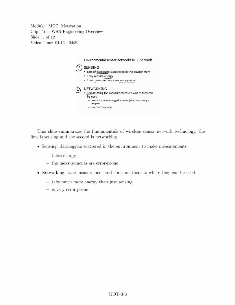
In this slide, another example of complex engineered system is discussed. It shows amodel of bio-molecule network (though it looks like a computer network or an inter-citytransportation network). It is a specific bio-molecule network that occurs in all humancell, which is called the TGF-beta signaling network.
This network is a layer representation in complex engineered system. The idea –Layering, helps us understand how the actual system works at a particular level. In thisdiagram, there are:
• Bio-molecule network model
− Boxes: represented by molecules
− Lines: represented by interactions between molecules
• Tranportation model
− Dotted line: represented by transportation between the outside of the nuclearsof the cell and the inside of the nuclears of the cell where the DNA is located.
INT-1-5

Module: [INT] Introduction
Clip Title: Understanding Complex-Engineered systems
Slide: 6 of 7
Video Time: 11:37 - 14:13
This slide discusses using layer approach to understand how to design complex systemswith all the bits and pieces in different levels. It introduces the idea of partition designand illustrates it by an example. With partition design, you can look at different layersand work on a specific area.
• Advantages of partitioning design,
− all the people on the project don’t have to know everything about it
− make the system more robust
− make the system more evolvable: you can plug in new capabilities at a layerand not corrupt the entire system because the other layer is above or below it
• Example of partition design:
− layer n : a particular layer of the system, deals with molecules
− layer n-1 :lies below layer n, deals with atoms
− layer n+1 :lies above layer n, deals with part of cell signaling
− interfaces binding layers
INT-1-6

Module: [INT] Introduction
Clip Title: Understanding Complex-Engineered systems
Slide: 7 of 7
Video Time: 14:14 - 17:27
This slide illustrates layer design and modularity by the examples of three viewsof the model for networking protocols. Modularity is very useful to partition design, itallows different teams work on different aspects, it also makes the design flexible andevolvable.
• layering
− OSI model: seven layers
− DARPA model: four layers
− TCP/IP model: four layers
• Modularity
− flexible: you can replace a module with another module on the same layerwithout breaking the design
− evolvable: you can plug in new designs that have the interfaces that correspondto lower layer and higher layer so you don’t need to redesign the entire stackas a result of the change of one layer.
INT-1-7
Module: [INT] Introduction
Clip Title: Introduction to Fundamental Concepts in WSN
Slide: 1 of 4
Video Time: 00:00 - 05:32
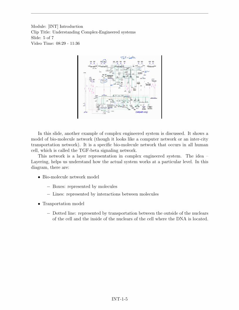
This slide discusses the basic concepts of wireless sensor network and starts withsensing. An example of sensing light is presented and the process of turning the light intofinal reading is detailed. It also introduces how to to deal with the information conversionusing signal processing and how a packet of information is built.
• Information transformation:
− Information starts as light.
− Photo diode senses the light and generate a current that is proportional tothe intensity of the light.
− The current turns into a voltage which probably needs to be amplified.
− Analog to digital converter (ADC) turns the voltage into a raw analog todigital reading.
− Finally, microcontroller (MCU) turns the raw data into a reading of light.The software embedded in MCU schedules the activities of signal processingand controls various subsystem:
· control the analog circuitry, turn the circuitry on or off to save energyconsumption
· control ADC. Often time ADC is integrated on MCU.
· takes the number from ADC, turns it into a meaningful number
• Signal processing: basic fundamental idea is to take multiple measurements andaverage them to increase the signal to noise ratio (SNR)
• Packet building: This packet of information is a collection of bits, which basiclyconsists of (1) light intensity; (2) time at which it occurred; (3) sensor ID.
INT-2-1

Module: [INT] Introduction
Clip Title: Introduction to Fundamental Concepts in WSN
Slide: 2 of 4
Video Time: 05:33 - 10:25
This slide states that the notion of communication system engineering is a fundamentalpart of wireless communication (wireless sensor networks, mobile phones, WiFi, etc).The “Father of communication system engineering” Claude Shannon’s contribution ispresented. This slide also introduces several steps in wireless communication after packetis built.
• Claude Shannon laid the ground work for all modern digital communication. Hiscontributions include:
− He found mathmatical connection between the electronics and digital logic, aswell as mathmatics of Boolean logic.
− He laid out the discipline of information theory (or Shannon theory), where heclearly defined what communication is: the fundamental problem of commu-nication is that of producing at one point (of space or time) either exactly orproximately a message selected at another point.
− He set up a very clear idea of how to do communication in optimal way andfound the fundamental limit set by nature on communication.
• The packet has to go through the following steps before goes into antenna:
− Modulation: turns the signal (a sequence of bits) into a waveform or a radiosignal that can be transmitted over the air.
− Upconversion: changes the low frequency content of the signal to a high fre-quency that allows for an efficient antenna to take it from current to an elec-tronics wave.
− Amplification: increases the signal strength to combat noise that occurs in thecommunication system.
INT-2-2

Module: [INT] Introduction
Clip Title: Introduction to Fundamental Concepts in WSN
Slide: 3 of 4
Video Time: 10:25 - 15:28
Shannon proposed a simple model for the design of communication systems that weare still using today. This slide uses the model as a start to look at how we buildcommunication systems. The components of the model have been introduced using thecommunication system perspective. This model has been extraordinary successful and itleds to the information revolution that we now essentially take for granted.
• Components in the Model:
− Information Source
− Transmitter
· Source Coder: strips out redundant information, compresses information(e.g. zip)
· Channel Coder: adds redundancy to protect information from noises thatcorrupt signal
· Modulator: the transmission of a signal by using it to vary a carrier wave
− Channel: Media across which the information gets from source to sink
− Receiver: essentially reverses steps of transmitter
· Demodulator: recovers the information content from the modulated carrierwave
· Channel Decoders: decode scrambled signal to make it interpretable
· Source Decoders: recover original information (e.g. unzip)
− Information Sink
INT-2-3

Module: [INT] Introduction
Clip Title: Introduction to Fundamental Concepts in WSN
Slide: 4 of 4
Video Time: 10:29 - 20:36
There are things that are part of the communication system not showed in Shannon’smodel, this slide talks about a block diagram of communication system that combines thecommunication system perspective with a RF microwave circuit perspective.The unshaded part of the diagram is close to Shannon’s model but the source coder andsource decoder are missing, which are assumed to be already done for the perspective ofthis design.
• The two shaded blocks are in the domain of RF microwave modeling, which include:
− Transmitter RF
· Filter.
· Upconverter (mixer driven by oscillator): upconverts low frequency signalto high frequency RF signal.
· Power Amplifier.
· Antenna: propagates the information through the air or space.
− Receiver RF
· Two filters: removes interference.
· Low Noise Amplifier (LNA).
· Two Downconverters: converts high frequency RF signal down to lowerfrequency signal that is easier to demodulate.
INT-2-4

Module: [INT] Introduction
Clip Title: The wireless medium and course overview
Slide: 1 of 7
Video Time: 00:00 - 07:42
This slide discusses wireless medium in terms of propagation from receiver antenna totransmitter antenna. The idea of propagation is where communication systems thinkingand electromagnetics are joined. At a fundamental level, we are dealing with Maxwell’sequation and the propagation of electromagnetic waves through space. But in practicewhen we engineer the system we abstract without detail and come up simplified modelsthat lead to attenuation of the signal.
This slide also introduces the following typical effects when we model propagtionsystems:
• Free-space pathloss: the weakening of signal strength attenuation of an electro-magnetic with no object in the space to cause reflaction or diffraction, this is anideal case.
• Other propagation phenomena that cause attenuation to be worse:
− Propagation over the Ground: signal reflected off the ground surface whiletravelling from the source to the receiver.
− Shadowing: large object (hill/mountain/building) get in the way betweentransmitter and receiver such that signal will be lost.
− Fading: caused by multipath propagation where there are reflected paths fromobject so the signal travels by two or more paths from transmitter to receiver.The multiple copies of the transmitted signal add up at the receiver and theycan add either constructively or destructively due to the differences in phaseshift, delay and attenuation.
INT-3-1

Module: [INT] Introduction
Clip Title: The wireless medium and course overview
Slide: 2 of 7
Video Time: 07:43 - 16:30
This slide discusses challenges of detecting the signal on the receiver and how todetermine the receiver performance on the system level.
• Challenges of signal detection in the receiver:
− Attenuation. Signal is weakended through propagation, the received powercan be very weak if considering ground plane propagation, shadowing andfading.
− Noise is added to the signal. The noise comes from the following resources:
· Primarily, the noise is added in the low noise amplifier (LNA). This actu-ally determine the entire noise performance of the receiver since the mostof the noise comes from the first stage of the receiver.
· Interference in the air between transmitter antenna and receiver antenna.
· Thermal noise comes from the agitation or jostling of charge carriers insidethe electronics (especially the LNA).
• Characteristics of noise:
− Random: the tools of probability and random processes will be used to designthe receiver.
− Very wide bandwidth: in frequency domain, the noise is extremely broad band,it’s also refer to as white noise,
• The performance of receiver is determined by a ratio Eb/N0, which is a dimension-less quanlity. The probability of bit error is a function of this ratio Eb/N0.
− Eb: bit energy (in joule or watt·second)
− N0: noise power spectral density (PSD), which is a function of power measuredin watt/Hz. In most communication systems it’s considered to be basicallyconstant or flat.
INT-3-2
Module: [INT] Introduction
Clip Title: The wireless medium and course overview
Slide: 3 of 7
Video Time: 16:31 - 23:16
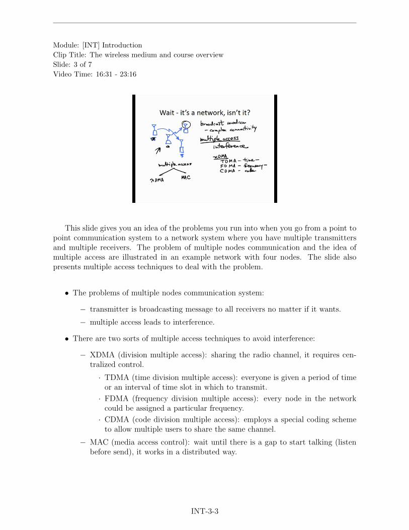
This slide gives you an idea of the problems you run into when you go from a point topoint communication system to a network system where you have multiple transmittersand multiple receivers. The problem of multiple nodes communication and the idea ofmultiple access are illustrated in an example network with four nodes. The slide alsopresents multiple access techniques to deal with the problem.
• The problems of multiple nodes communication system:
− transmitter is broadcasting message to all receivers no matter if it wants.
− multiple access leads to interference.
• There are two sorts of multiple access techniques to avoid interference:
− XDMA (division multiple access): sharing the radio channel, it requires cen-tralized control.
· TDMA (time division multiple access): everyone is given a period of timeor an interval of time slot in which to transmit.
· FDMA (frequency division multiple access): every node in the networkcould be assigned a particular frequency.
· CDMA (code division multiple access): employs a special coding schemeto allow multiple users to share the same channel.
− MAC (media access control): wait until there is a gap to start talking (listenbefore send), it works in a distributed way.
INT-3-3

Module: [INT] Introduction
Clip Title: The wireless medium and course overview
Slide: 4 of 7
Video Time: 23:17 - 25:35
This slide provides a overview of the lectures in a context of the big picture of thewhole course. The engineering details with various aspects and how they are related toeath other are in the remainder of the course.
The following big issues will be covered throughout the course:
• Real World Problem: most engineering problems start with some real world prob-lems that we are trying to solve.
• Sensing Missions: there are many different sensing missions (safety/environmentalcontrol).
• Embedding Environments: the wireless sensor network design differs with the envi-ronments (factory/office).
• Environmental/Ecosystem Sensing: real world applications
• Sensor Cloud: all the sensors are placed in a site of deployment. Each sensor has asubsystem with:
− Radio Link
− Networking
− Sensing
− Energy
− Embedded Control
INT-3-4

Module: [INT] Introduction
Clip Title: The wireless medium and course overview
Slide: 5 of 7
Video Time: 25:35 - 26:36
This slide discusses the highlight of course structure. The definition and details ofcourse structure can be found in the syllabus.
• Videos on the web: It has at least two benefits as follows.
− It allows professors to combine expertise from different areas in electrical en-gineering in one course.
− It allows students to watch the lectures any time any where.
• In-class Q & A discussion: you can spend in-class time going over questions andbring up new ideas.
• The others are covered in the syllabus and will be discussed live in class:
− Exams
− Experiments
− Project
− Concept Inventories
− In-class Participation
INT-3-5

Module: [INT] Introduction
Clip Title: The wireless medium and course overview
Slide: 6 of 7
Video Time: 26:37 - 28:03
This slide introduces the outline of the technical topics of the course for the first sevenweeks:
• Week 1: Motivation, Introduction and Overview (MOT and INT). The strategy ofthis section is:
− start from sensing physical information in the environment (e.g.temperature).
− turn the sensed data into a meaningful number on the computer.
• Week 2: System Engineering Applied to Wireless Sensor Networks (SEA): give anoverview of the broad picture of how we can view them as complex engineeredsystems and how we approach them.
• Week 3: Transducers(TDX)
• Week 4: A/D Conversion (ADC)
• Week 5-6: Radio Frequency Hardware (RFH)
• Week 7: The Wireless Communication Channel (WCC)
INT-3-6

Module: [INT] Introduction
Clip Title: The wireless medium and course overview
Slide: 6 of 7
Video Time: 28:03 - 29:09
This slide continues introducing the outline of the technical topics of the course forthe next eight weeks. Throughout the course there will be some hands-on experiencethat helps students get better understanding of some of the issues that involved in theengineering of wireless sensor networks.
• Week 8-9: Communication Theory as Applied to Wireless Sensor Networks (CTA)
• Week 10-11: Sensor Network Architectures (SNA)
• Week 12-13: Managing the Sensor: Embedded Computing (EMC)
• Week 14: Bringing it All Together: System Thinking in Systems Engineering (FIN)
• Week 15: Student Videos Presentation (STV)
INT-3-7

Module: [SEA] Systems Engineering applied to WSN
Clip Title: Course Objectives and WSN Overview
Slide: 1 of 6
Video Time: 00:00 - 03:04
This slide reviews characteristics of complex engineered systems.
• It is important to understand behavioral models of complex engineered systems atdifferent layers, for example:
− understanding the behavior of electron using circuit model
− understanding the behavior of electromagnetic waves using Maxwell’s equa-tions.
• Think about how the layers interact and the models of interaction between layers.Understand how to determine performance with respect to a variety of criteria whichare associated with WSN, such as:
− temporal and spatial fidelity
− information quality
− delay
− energy efficiency
• Think about WSN as an example of complex engineered systems, specifically:
− In contrast to the subdiscipline-specific courses, this course will focus on themodeling, analysis and simulation of complex engineered system. in an inter-disciplinary way.
− A goal is to understand how specific subdisciplines fit into the overall structureof the design of WSN, not just parts lists and toolsets of a specific disciplinesuch as networking using TCP/IP stack or the tools of microwave circuit design.
SEA-1-1

Module: [SEA] Systems engineering applied to WSN
Clip Title: Course Objectives and WSN Overview
Slide: 2 of 6
Video Time: 03:05 - 04:42
This slide introduces the outline of the [SEA] module. Carrying on from the discussionin the [INT] module, [SEA] will cover the following:
• Differences between WSN and other kinds of wireless networks
• Networking aspects
• What to do with the data
• Embedded computing systems
• How WSN’s enable new applications and new technologies
• Mesh-connected society that links people and things of the physical world
− Pros and cons
− challenges and pitfalls
SEA-1-2

Module: [SEA] Systems Engineering applied to WSN
Clip Title: Course Objectives and WSN Overview
Slide: 3 of 6
Video Time: 04:43 - 07:40
This slide illustrates the concept of WSN based on the example of environmen-tal/ecosystem monitoring. Specifically, it introduces the components of the WSN andthe data gathering process. The idea is that the application of WSN can be seen as the‘eyes and ears’ of the Internet among the physical world.
• The example starts from deploying two things in the environments, they are
− Sensor nodes: monitor the environment for all kinds of data (e.g. light, tem-perature, soil moisture)
− Gateway (network hub): collect all the information from sensor nodes
• The process of gathering data from physical world to Internet can be abstractedinto two steps:
− The WSN self-organizes into a data gathering tree, through which sensor nodessend data to the gateway (network hub)
− The information at gateway (network hub) is sent to Internet by a satellitelink, a cell modern, or a direct ethernet connection.
SEA-1-3

Module: [SEA] Systems engineering applied to WSN
Clip Title: Course Objectives and WSN Overview
Slide: 4 of 6
Video Time: 07:41 - 09:44
This slide pulls together many of the different subdisciplines of wireless sensor networkengineering, which have a very broad diversity. The perspective of integrating multiplesubdisciplines can help students to come up with good efficient design of the engineeredsystems. The list of subdisciplines are as follows:
• Analog/mixed-signal design
• Software-programmable digital hardware (microprocessors) and peripherals
• Digital and statistical signal processing
• Control theory
• Embedded systems design
• RF/microwave design
• Communication and coding theory
• Network engineering
• Self-organizing systems
• Mechanical/packaging engineering
SEA-1-4

Module: [SEA] Systems engineering applied to WSN
Clip Title: Course Objectives and WSN Overview
Slide: 5 of 6
Video Time: 09:45 - 14:08
This slide focuses on the communication and network engineering subdiscipline ofWSN. It elaborates on the difference between the classical networks and point-to-pointcommunication systems. It also discusses the difference between wireless sensor networksand other kinds of important networks.
• Mobile telephony network
− there are hand held devices communicating with the base stations that arelocated at the cell phone towers (required infrastructure).
• Base station
− An access point is a form of base station that allows wireless devices to connectto a wired network
• Ad hoc networks
− are self-organizing networks, there is no centralized point (e.g. base station,access point or a tower) to maintain and control the network.
• Mesh networks
− it’s a special type of ad hoc networks, where the nodes are forming a mesh.
SEA-1-5

Module: [SEA] Systems engineering applied to WSN
Clip Title: Course Objectives and WSN Overview
Slide: 6 of 6
Video Time: 14:09 - 19:59
Timing issues are very important in regards to the performance of wireless sensornetworks. This slide discusses the reasons that why time matters from several differentaspects.
• Two critical points:
− Latency:
· end to end, source to gateway delay in transmission
− Throughout
· rate of the information (b/s, kbit/s, mbit/s) transfered from a sensor nodeto gateway
• Coordination & control
− synchronized sensing: all the sensors take measurements at particular timeaccurately.
− coordinated response:
· sensors nodes collaborate and share information to detect objective eventscorrectly
· actuator control
SEA-1-6

Module: [SEA] Systems Engineering applied to WSN
Clip Title: Computing and Constrains in WSN
Slide: 1 of 5
Video Time: 00:00 - 03:29
Wireless sensor nodes are a form of networked embedded computing systems. Thisslide introduces what an embedded computing system is and discusses how to design sucha system.
• Networked embedded computing systems
− are designed to be coupled with and interact with the physical world in realtime.
− in contrast with desktop systems, embedded computing systems often have torespond to an event in the physical world.
• Aspects related to designing the computing systems:
− Intelligent signal processing: the sensor nodes need to gather data and processthem into something meaningful since the raw data are
· noisy
· error-prone
· coming from different places in the network
· difficult to deal with
− Autonomic networks (self-* networks)
· self-organization
· self-configuration
· self-healing
· self-optimization
· self-protection
SEA-2-1

Module: [SEA] Systems Engineering applied to WSN
Clip Title: Computing and Constrains in WSN
Slide: 2 of 5
Video Time: 03:30 - 07:01
The final step of WSN is to process the data into knowledge, or something we canunderstand. Dealing with data plays an important role in the WSN engineering. Thisslide makes several points of what to do with the data once the data is gathered from theenvironment.
• Data management
− Networking
− Web programming
− Archiving
• Visualization & Analysis
− Data characteristics: noisy, error-prone
− The noise comese from:
· transducer/measurement noise
· unreliable communication
SEA-2-2

Module: [SEA] Systems Engineering applied to WSN
Clip Title: Computing and Constrains in WSN
Slide: 3 of 5
Video Time: 07:02 - 11:03
This slide continues to introduce other characteristics of sensed data in WSN anddiscusses how to deal with the datasets according to these properties so that we canimprove the knowledge of an environment.
• Besides being noisy, the datasets are:
− temporal - data streams are vector time series, we are getting data as a functionof time
− spatial - datasets come from sensor nodes at different locations
• Visualization and computer graphics are needed, which have the following charac-teristics:
− Signal processing & statistics: to understand what the data is like, take intoaccount the fact that the randomness in the data is due to:
· measurement noise and channel errors
· uncertainty
− Scientific workflows (“mashup”): merging of datasets, which allows us to ag-gregate and integrate various datasets into useful information. These compli-mentary datasets involves:
· Remote sensing
· Archival data
− Building predictive models of the sensed environment such as
· diversities in basic species
· climate change
SEA-2-3

Module: [SEA] Systems Engineering applied to WSN
Clip Title: Computing and Constrains in WSN
Slide: 4 of 5
Video Time: 11:04 - 15:45
This slide discusses financial aspects of design and how it relates to the engineering ofcomplex systems. To design systems in a cost-effective way, we need to consider budgets.There are two things goes into budgets: non recurring expanses and recurring expenses,they are at different stages of the design cycle.
• NRE: non recurring expenses
− occur a lot in the R&D phase: doing development, building printed circuitboard, designing software
− at the stage before manufacturing the products
• RE: recurring expenses
− materials and assembly cost for building the sensor network
− at manufacturing stage
• Parts of recurring expanses:
− Bill of materials (BOM): number and cost of every single part in a device, thisis the key part of recurring expanses
− Cost of manufacturing: the cost to build the entire sensor node
− Life cycle cost: support, marketing and sales (disposal, not noted, is alsoimportant)
SEA-2-4

Module: [SEA] Systems Engineering applied to WSN
Clip Title: Computing and Constrains in WSN
Slide: 5 of 5
Video Time: 15:46 - 20:59
After discussing the cost, this slide introduces another important aspect of WSNengineering - power. In particular, it presents a way of looking at the system design viaa link budget in the context of communication link.
• The method to deal with a communications link is link budget (link power budget).
• Goals of Link budget:
− Track the power level of the signal from the transmitter through the channelto the detector (demodulator) in the receiver.
− Track gains and losses.
· Gains: come from amplifier (power amplifier in the transmitter, low noiseamplifier in the receiver), antenna gains.
· Losses: the greatest loss is due to propagation.
· All gains and losses are multiplicative, and they tend to be very large orvery small in magnitude, we use decibels so multiplication and divisionbecome addition and subtraction. The decibel can be expressed as:
LdB = 10log10P1
Po
(1)
For example: 10−10 = 10log10(10−10) = −100dB = 100dB loss
• Overall goal of the link budget: determine the link margin.
− Link margin: the excess or the deficit of power (dBm) to achieve a particularperformance level (e.g., bit error rate - BER).
− Find out if the power level is enough to achieve the bit error rate in sensornetworks.
SEA-2-5

· Positive link margin: the power level is more than required to achieve thedesired BER
· Negative link margin: the power level is less than required to achieve thedesired BER
6

Module: [SEA] Systems Engineering applied to WSN
Clip Title: Energy and the Big Picture
Slide: 1 of 7
Video Time: 00:00 - 02:50
Previously two dimensions have been introduced, the financial dimension and powerwith respect to communications link, this section further discusses the third dimension -energy. This slide briefly introduces the main content of this section, the idea of energybudget, and scaveng/harvesting energy. As a start point of introducing energy budget, itdiscusses various activities of the sensor networking.
• The main content of this section one must understand:
− Energy budget.
− How the energy budget relates to battery lifetime.
− How the requirement of the sensor relates to the ability to scavenge/harvestenergy from the environment.
· solar energy
· wind energy
· enegy from temperature differences and vibration
• Embedded systems: control the activity states of sensor node, these activity statesinclude:
− communicatoin state
− sleep state
− state of taking measurements
− state of doing system maintenance
− startup/shutdown
SEA-3-1

Module: [SEA] Systems Engineering applied to WSN
Clip Title: Energy and the Big Picture
Slide: 2 of 7
Video Time: 02:51 - 07:13
This slide introduces a simple model of a sensor network energy budget. Based on thismodel, it discusses the strategies to minimize energy consumption. This model is showedas follows:
E = v(isqs + icqc + ihqh)(t− t0)
where E is the total energy, which is power integrated overtime from t0 to t, v is afixed supply voltage, qs, qc, qh represented the percentage of time that the sensor node istaking measurement, communicating and hibernating, the amount of current consumedat different states are is, ic, ih. Typically,
is = 500ih
ic = 1000ih = 2.5is
• There are two strategies to minimize energy consumption
− Hardware technology
· efficient processing
· efficient architectures
− Software-level design strategies
· increase the percentage of hibernation state to minimize the energy
• Notes about the energy budget model:
− Beware of simple models
− Need to consider more complex models with transient energy cost.
SEA-3-2

Module: [SEA] Systems Engineering applied to WSN
Clip Title: Energy and the Big Picture
Slide: 3 of 7
Video Time: 07:14 - 10:08
Considering how to improve energy efficiency, this slide discusses various aspects of awirelessly networked embedded systems.
• First goal: hardware oriented, make sure that every electronic component uses theminimum amount of energy to do its job
− Optimize process technologies in all aspects of digital, analog, RF and mixedsignal.
− Improve power regulation and mangement.
• Second goal: software oriented
− Clock domains and gating: gate the clock to different domains at differentclock rates
− Power domains and gating: depower subsystems of chips or subsystems ofcircuits
− Dynamic voltage scaling: tune in the voltage to minimize the power consump-tion in a particular state.
SEA-3-3

Module: [SEA] Systems Engineering applied to WSN
Clip Title: Energy and the Big Picture
Slide: 4 of 7
Video Time: 10:09 - 13:34
This slide discusses another aspect of how to improve energy efficiency - communi-cation and networking. It explains the reason why communications consumes most ofenergy in most WSN and discusses the ways to optimize it.
• Minimize useless radio operations:
− do not transmit when there is no one to receive
− do not listen when no node is transmitting
− note: use communications energy only when transmitting or receiving data.
• Transmit only what is necessary to solve the problem of model/data inference
− use source coding techniques to minimize redundancy
− use channel coding to protect data
− note: ensure the transmitted or received data is useful or informative
SEA-3-4

Module: [SEA] Systems Engineering applied to WSN
Clip Title: Energy and the Big Picture
Slide: 5 of 7
Video Time: 13:35 - 16:48
This slide generalizes from the environmental/ecosystem monitoring to other applica-tions for wireless sensor network. It discusses how to apply the WSN technology to theseapplications and what is the fundanmental challenges in all of them.
• Here are some of the applications:
− Indoor monitoring.
· monitoring of built or synthetic environment (e.g. art museum, office build-ings).
− Manufacturing process control
· use wireless equipment in the factories to monitor the manufacturing pro-cess.
− Structural monitoring
· monitoring structures such as bridges, buildings, highways.
− Public safety
· monitoring hazadous pollutant, chemical or nuclear releases, leaks of ra-dioactive material
− Health care
· Body area network (BAN’s)
• The fundamental challenges of all applications
− report meaningful change to whomever or whatever needs it
− report when it is needed
− report at minimum cost (life cycle cost)
SEA-3-5

Module: [SEA] Systems Engineering applied to WSN
Clip Title: Energy and the Big Picture
Slide: 6 of 7
Video Time: 16:49 - 21:47
Wireless sensor networks are an application of mesh networking. This slides introducesthe mesh-connected networking, the pros and cons of developing these kind of technologiesand finally discusses the relevant issues of WSN from this point of view.
• All technologies are double-edged swords
• Issues with mesh networking in WSN:
− Security: protect the data from the following actions:
· unauthorized actions
· alteration
· destruction of data
− Privacy: is about control
· who can collect the information
· how to use the information
· what the information will be used for
· beware of the unintended consequences
SEA-3-6

Module: [SEA] Systems Engineering applied to WSN
Clip Title: Energy and the Big Picture
Slide: 7 of 7
Video Time: 21:48 - 24:19
This slide summarizes the module and reviews all the points and aspects that have beendiscussed. The theme is understanding complex engineered systems using the example ofwireless sensor networks.
• Discuss WSN from the point of view of system engineering
− Networking
− Time
· Latency
· Throughput
− Computation
− Data to knowledge
− How WSN relate to analysis, visualization, and inference of models/data
• Various dimensions of quantifying the design of WSN
− financial aspect
− link power budgets
− energy budgets
• Generalize from environmental/ecosystem sensing to other other applications
• Generalize from sensor network application to the idea of a mesh connected society
SEA-3-7

Module: [TDX] Transducers
Clip Title: Basic introductory overview
Slide: 1 of 3
Video Time: 00:00 - 00:47
This slide introduces the main content of the Transducers (TDX) module, which wasmade by Tom Weller and Tom Richard from the University of South Florida (USF). TheTDX module contains two parts:
• The first part of module
− review some forms of energy conversion or transduction and the scientific prin-ciples behind various types of sensors.
• The second part of the module
− present advanced concept for wireless sensor node technology that ties togethertransducer concepts directly with wireless communications.
TDX-1-1
Module: [TDX] Transducers
Clip Title: Basic introductory overview
Slide: 2 of 3
Video Time: 00:48 - 03:53
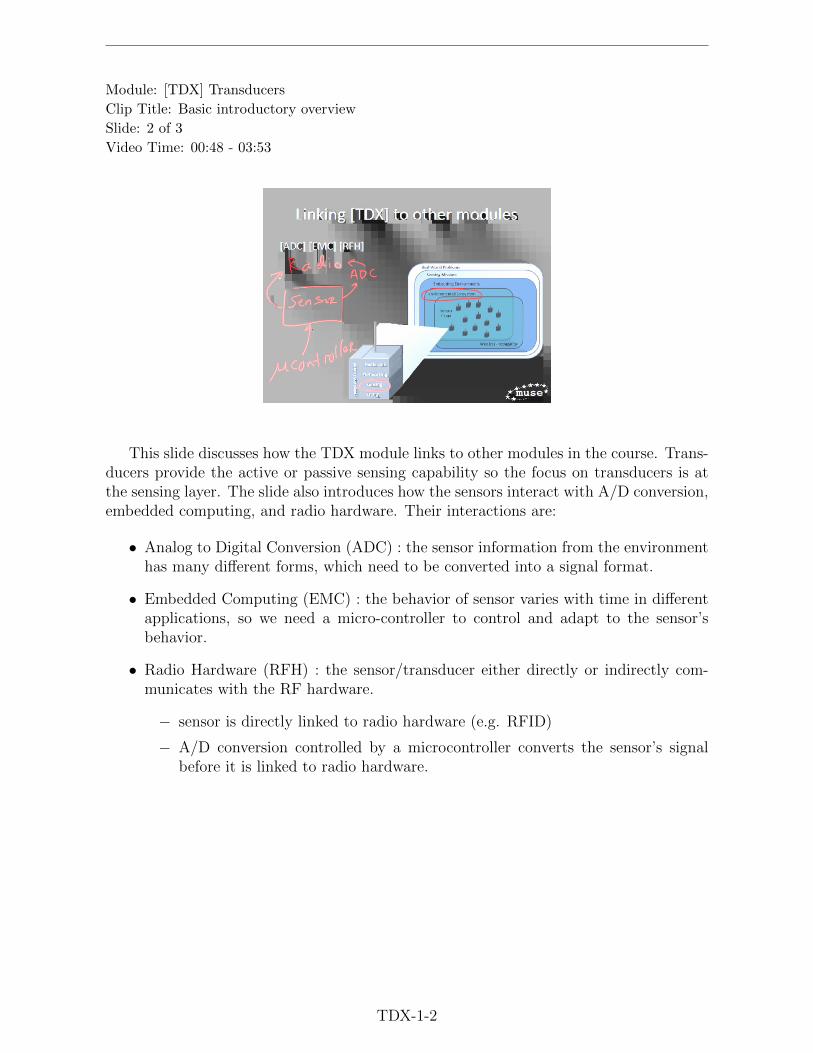
This slide discusses how the TDX module links to other modules in the course. Trans-ducers provide the active or passive sensing capability so the focus on transducers is atthe sensing layer. The slide also introduces how the sensors interact with A/D conversion,embedded computing, and radio hardware. Their interactions are:
• Analog to Digital Conversion (ADC) : the sensor information from the environmenthas many different forms, which need to be converted into a signal format.
• Embedded Computing (EMC) : the behavior of sensor varies with time in differentapplications, so we need a micro-controller to control and adapt to the sensor’sbehavior.
• Radio Hardware (RFH) : the sensor/transducer either directly or indirectly com-municates with the RF hardware.
− sensor is directly linked to radio hardware (e.g. RFID)
− A/D conversion controlled by a microcontroller converts the sensor’s signalbefore it is linked to radio hardware.
TDX-1-2

Module: [TDX] Transducers
Clip Title: Basic introductory overview
Slide: 3 of 3
Video Time: 03:54 - 06:54
After discussing how TDX module relates to other modules, this slide introduces howtransducers relate to the overall concepts of systems thinking, particularly for wirelesssensor networks. This slide also summarizes the factors that need to be considered whendesigning a system.
• Relations between Transducer/Sensor and the other parts of system:
− At the node level: the sensor can greatly impact the energy budget and em-bedded control.
− At the systems level:
· Environment/Ecosystem: the sensor provides the ability to probe the en-vironment.
· Embedding environment: we need to consider the type of environment inwhich the sensor is embedded. (e.g. corrosive environment, high vibrationenvironment)
· Sensing mission: this impacts sensor requirements such as resolution, dy-namic range and repeatability.
• Other things that have to be taken into account when designing a system andselecting a sensor:
− Energy.
− Cost.
− Embedded control of the sensors to minimize the energy requirements.
− Environment that the sensor network would be operating in.
TDX-1-3

Module: [TDX] Transducers
Clip Title: Transducers
Slide: 1 of 19
Video Time: 00:00 - 01:11
This slide introduces the main content of the TRANSDUCERS module. Instead ofgoing into details of transducer technologies, this module presents a very general intro-duction to the transducers with come examples of commonly used types of transducers.The topics that are covered in this module include:
• Basic energy conversion principles.
• Transducer related terminology.
• Packaging and integration issues.
TDX-2-1

Module: [TDX] Transducers
Clip Title: Transducers
Slide: 2 of 19
Video Time: 01:12 - 2:05
This slide discusses the definition of transducers for sensing purpose, examples ofdifferent energy forms and why energy conversion is used.
• What is a transducer: A transducer is a device that converts energy from one formto another.
• There are many kinds of energy forms such as:
− mechanical
− visual
− aural
− electrical: this is the focus in this course, examples of electrical energy eitheras input or output will be given.
− thermal
− chemical
• The usage of energy conversion: change information into a form that can be easilytransferred, stored, processed, or interpreted
TDX-2-2

Module: [TDX] Transducers
Clip Title: Transducers
Slide: 3 of 19
Video Time: 2:06 - 3:38
The next few slides introduce types of transducers that we might see in everydayapplications. This slide starts with electromagnetic transducer and takes two examples(Receiving antenna and Transmitting antenna) to illustrate the energy conversion princi-ple.
• Receiving antenna
− takes an incident electromagnetic field and changes that field into electric cur-rent that can be down converted in frequency and amplified.
• Transmitting antenna
− takes a high power RF current and in turn radiates electromagnetic field. TheEM field can be latter received by the receiving antenna.
TDX-2-3

Module: [TDX] Transducers
Clip Title: Transducers
Slide: 4 of 19
Video Time: 3:39 - 4:20
This slide discusses electrochemical transducers which can either detect or in somecases initiate a chemical reaction and change the energy attained from the chemical reac-tion into an electrical voltage. Examples of electromechanical transducers are pH Probeand Fuel Cell as follows.
• pH Probe:
− detects the relative PH of the solution in which it submerges. Application:water quality monitoring.
• Fuel Cell:
− develops a considerable amount of electrical power, based on the chemicalreactions that are taking place internal to it.
TDX-2-4

Module: [TDX] Transducers
Clip Title: Transducers
Slide: 5 of 19
Video Time: 4:21 - 5:49
This slide introduces electromechanical transducers which are able to translate phys-ical movement into electrical voltage. Generator, Motor and Phonograph Cartridge areexamples of electromechanical tranducers.
• Generator
− Rotational energy turns a series of conducting coils in the generator through amagnetic field to generate a current.
• Motor
− works on almost the exactly opposite principle of generator.
− the input current in the motor causes the conducting coils to move throughthe magnetic field and output force resulting in rotational motion.
• Phonograph Cartridge
− use a stylus (also called needle) which fits inside the grooves of the phono-graph record to move a small magnet through a magnetic field and then out-put electric current that is proportional to the information contained on thephonograph record.
TDX-2-5

Module: [TDX] Transducers
Clip Title: Transducers
Slide: 6 of 19
Video Time: 5:50 - 7:34
Similar in principle to electromechanical transducers, electroacoustic transducers alsotranslate physical movement to electrical voltage, but the movement is the result of soundwaves which are either incident on the device or are to be produced from the device. Thisslide introduces two examples of electroacoustic transducers: microphones and loudspeak-ers.
• Microphones
− work on a very similar principle to phonograph cartridges.
· the input of phonograph cartridge is vibration caused by rotating phono-graph record.
· the input of microphone is sound vibration that reaches the microphonethrough the ambient air.
− sound vibrations move a diaphragm back and forth within the microphone, andthe diaphragm moves a magnet contained within magnetic field thus producinga current.
• Loudspeakers
− work on the opposite principle of a microphone.
− the electrical current applied to the coil in loudspeaker moves a magnet backand forth, the magnet moves a diaphragm (some kind of light weight, low massmaterial) which mechanically vibrates to produce sound waves.
TDX-2-6

Module: [TDX] Transducers
Clip Title: Transducers
Slide: 7 of 19
Video Time: 7:35 - 8:54
This slides introduces photoelectric transducers for which light forms one side of theequation whether it is input or output. In the example of lightbulb the light is outputwhile in photodiode the light is input.
• Lightbulb
− within the lightbulb an electrical causes high resistance filament to heat upand by radiant metric principles the lightbulb will emit light.
• Photodiode
− takes light as an input, this light contains a certain amount of photonic en-ergy which causes changes in the diode conductivity. Those changes in diodeconductivity can be used as a switch in a circuit parameters.
TDX-2-7

Module: [TDX] Transducers
Clip Title: Transducers
Slide: 8 of 19
Video Time: 8:55 - 10:21
The last type of transducer introduced in this section is thermoelectric transducer.Similar with photoelectric transducers, thermoelectric transducers deal with conversionbetween thermoenergy and electrical energy. The examples of thermoelectric transducers(hotplate and thermistor) are compared with those of photoelectric transducers (lightbulband photodiode).
• Hotplate
− the electrical current flow through a high resistance filament, the filament thengenerates heat which is transferred to the hotplate surface.
− compared with lightbulb, the output of hotplate is heat instead of light.
• Thermistor
− the changes in temperature results in the change in the resistance of the ter-mistor.
− compared with photodiode, the input of thermistor is the change in tempera-ture instead of the change in photonic energy.
TDX-2-8

Module: [TDX] Transducers
Clip Title: Basic introductory overview
Slide: 9 of 19
Video Time: 10:22 - 11:58
The earlier slides illustrated several types of energy conversions and examples of howthese conversions are implemented. The next few slides introduce some specific energytransformations methods. This slide starts with capacitive transducers.
• Capacitive transducers use the principle of parallel plate capacitor as follows:
Vab = E · d
− Vab: voltage difference between the charged plates of parallel capacitor
− E: magnitude of the electric field that exists in the material between the plates
− d: distance between the plates
• The total capacitance can be calculated by the following formula:
C =εA
d.
− ε: permitivity of the dielectric material between the plates
− A: area of plates
− d: distance between the plates
TDX-2-9

Module: [TDX] Transducers
Clip Title: Basic introductory overview
Slide: 10 of 19
Video Time: 11:59 - 12:44
This slide introduces the Piezoelectric principle which transforms the mechanical en-ergy to electrical energy. Piezoelectric transducers rely on the type of mechanical forcesacross the piezoelectric material (e.g., crystals, ceramics), these forces result in a voltagebeing generated between the edges of the material.
• The voltage is dependent on the magnitude and direction of force in the form of:
− compression: a force trying to push the crystal together
− tension: a force trying to pull the crystal apart
• Type of Piezoelectric materials:
− Natural crystals (quartz, rochelle salts)
− Synthetic crystals (lithium phosphate)
− Ferroelectric ceramics (barium titanate)
TDX-2-10

Module: [TDX] Transducers
Clip Title: Basic introductory overview
Slide: 11 of 19
Video Time: 12:45 - 13:55
This slide goes into detail with another example of electromechanical transducer - thetrackball.
• In the trackball mouse there are two dimensional movement of the trackball, whichwill cause some sort of proportion to be applied either to a horizontal sensor, or avertical sensor.
• The horizontal and vertical sensors will sum up a indication of vector displacementover time of the position of the mouse.
• In this sense mechanical motion or displacement is converted into changes in elec-trical voltage.
TDX-2-11

Module: [TDX] Transducers
Clip Title: Transducers
Slide: 12 of 19
Video Time: 13:56 - 14:57
This slide introduces the principle behind photovoltaic transducers. In this type ofenergy transformation, the light is incident upon the panels of the solar cell, the properwavelength in that light will turn to ionize atoms in silicon base. In other word, itdisplaces the electrons from the silicon material in the base, and these displaced electronsare recombined by flowing through the load thus it produces electric current. Example ofphotovoltaic transducers are:
• solar cell
• solar battery
• solar charger
TDX-2-12

Module: [TDX] Transducers
Clip Title: Transducers
Slide: 13 of 19
Video Time: 14:58 - 16:46
This slide presents some basic terms and definitions related to transducers. Some ofthe properties and the vocabulary that we use to identify those properties are introducedas follows:
• Measurand: the property that you are measuring, or you can think of it as input tothe transducer.
• Passive transducer: one that draws operating power from the measurand, it requiresno external power. This type of transducer is also known as sensor.
• Active transducer: one that requires external power supply, some type of externalvoltage or current.
• Accuracy: refers to the output signal, and how closely that matches to the actualvalue of the input signal.
• Resolution: how fine of a measurement we can make. Mathematically it’s how manydecimal places are actually having meaning in the output signal of the transducer.
• Range: refers to the input or the output signal. The input range is what type ofvariation can we expect in the measurand, and the output range is what type ofvariation can we expect in the output signal.
TDX-2-13

Module: [TDX] Transducers
Clip Title: Transducers
Slide: 14 of 19
Video Time: 16:47 - 18:01
This slide presents additional transducer related terms and properties.
• Sensitivity: a measure of the changing output for a given changing input.
• Linearity: how does the output change uniformly with the input. A linear changeis easier to work with than a non-linear change.
• Repeatability: given the same measurand value, the output value should be alwaysthe same (this is also known a precision).
• Response time: how quickly does the transducer output respond to changes in themeasurand value.
TDX-2-14

Module: [TDX] Transducers
Clip Title: Transducers
Slide: 15 of 19
Video Time: 18:02 - 20:00
This slide discusses considerations for dealing with transducer packaging and integra-tion issues. The factors that affect the method of packaging and integration include:
• Technology: what energy conversion principle is being used, which is going to influ-ence the size, and shape of the transducers.
• Environment: what is the environment that the transducer is going to be installedin and used. (e.g. the ambient temperature, the humidity, and corosion in theenvironment)
• End user: what’s going to be the end user of the output signal (e.g., human interface,computer interface, machine environment).
• Cost: the major factor in terms of consumer goods, but it could be secondary interms of aerospace or military applications.
TDX-2-15

Module: [TDX] Transducers
Clip Title: Transducers
Slide: 16 of 19
Video Time: 20:01 - 20:33
Miniaturization is very important in the design of transducers. The general rule ofpackaging and integration is that smaller is better, especially for consumer electronics.
Two samples of relative transducer sizes are showed in the pictures, one being com-pared to the dime, the other to the finger tip.
TDX-2-16

Module: [TDX] Transducers
Clip Title: Transducers
Slide: 17 of 19
Video Time: 20:34 - 21:50
This slide introduces one very important technique in the miniatualization of tranduc-ers and components: MEMS, which is an acronym for Micro Electro Mechanical Systems.This techonology holds a lot of promise for transducer design and implemetation, althoughit’s a technique that can’t always be used.
MEMS is a technique that uses electromechanical deposition, masking and etching tocreate structure that are needed. This structure can be produced on a very small scale.In the picture, an example of the scale is showed to be 50 micrometers, which is roughlyhalf the thickness of the human hair.
TDX-2-17

Module: [TDX] Transducers
Clip Title: Transducers
Slide: 18 of 19
Video Time: 21:51 - 22:50
This slide summarizes the discussion and lists the major points that we need to re-member:
• First, a transducer is a device that converts energy from one form to another.
• Second, a passive transducer is called a sensor, which gets the power from themeasurand and it doesn’t require external supply.
• Third, there is a big trade-off between transformer form and transformer function,one affects the other.
• Fourth, The trend in packaging is to have sensor package as small as possible.
• Fifth, MEMS holds great promise for sensor design and packaging when that par-ticular technology can be used.
TDX-2-18

Module: [TDX] Transducers
Clip Title: Transducers
Slide: 19 of 19
Video Time: 22:51 - 23:24
Finally the last slide lists some further sources of information for reading.
• The first three books present a general overview of transducer design principles andapplications.
• The last text is a good undergraduate level electromagnetics text book, which goesinto a great levels of details on the electrical conversion techniques.
TDX-2-19

Module: [TDX] Transducers
Clip Title: Future WSN Sensor Technology
Slide: 1 of 12
Video Time: 00:51 - 01:38
This slide provides an outline of this particular module, the main points of which werelisted below:
• First, start by asking the question: how can we build better sensors?
• Second, present sensors for embedded applications, this part is mostly covered byDr.Flikkema.
• Third, review the new wireless sensor network concept that’s being studied by UVMand USF.
• Lastly, summarize the module.
TDX-3-1

Module: [TDX] Transducers
Clip Title: Future WSN Sensor Technology
Slide: 2 of 12
Video Time: 01:39 - 07:00
This slide discusses how can we build better sensors. Among all the aspects listedbelow, new WSN concepts focus on sensors with low-cost material and manufacturingvolume, as well as low energy that’s provided by other parts of the network. The aspectswe want to be concerned with include:
• Mission/Environment
• The design of Hardware/Software
− Aspects of the hardware that applied to all applications
∗ Cost
Material
Labor
Manufacturing volume
Design process
∗ Energy
Internal sources (typically a battery): transducer types, control soft-ware, semiconductor chips.
External sources (energy scavenging): light, vibration, heat, some-where else in the network.
− Other aspects:
∗ Resolution
∗ Dynamic range
∗ Repeatability
∗ Ruggedness
∗ Packaging
TDX-3-2

Module: [TDX] Transducers
Clip Title: Future WSN Sensor Technology
Slide: 3 of 12
Video Time: 07:01 - 09:44
Another aspect for new WSN approaches is focusing on the embedded sensors. Thisslide discusses types of application, mission types and challengings for embedded sensor.
• Types of application for embedded sensors could include: monitoring of buildings,bridges, roads, all different types of infrastructure. even biomedical
• Mission types could include things like:
− Tracking temperature in buildings
− Looking at corrosion and vibration in bridges
− Looking at blood flow and temperature inside human bodies
• The idea of embedded sensor is about:
− Reducing cost
− Providing mobility
− Extending lifetime
• Challenges:
− The common threat is that the sensors are fully inside the structure of body.
− Replacing the sensors is very difficult and costly, long life sensors are desirable.
− Wireless propagation may bring about severe multipath and other time delayeffects.
TDX-3-3

Module: [TDX] Transducers
Clip Title: Future WSN Sensor Technology
Slide: 4 of 12
Video Time: 09:45 - 11:20
This slide discusses a new WSN concept and illustrates it in a simple way. Specifically,it introduces main components in the system, the principal operation and the idea of thisnew concept.
• There are three main pieces in the system:
− Interrogator
− Channel
− Node
• The principal operation is very straightforward: the transmitter which located insidethe interrogator sends a signal into the channel toward the node at frequency f . Thenode receives the signal and transmit 2 ∗ f back toward the interrogator.
• The idea is the state of the sensor affects the characteristics of the signal that getsback from the node to the interrogator.
TDX-3-4

Module: [TDX] Transducers
Clip Title: Future WSN Sensor Technology
Slide: 5 of 12
Video Time: 11:21 - 14:55
This slide looks into the operation of this sensor configuration in more detail. It alsoprovides many examples to help the viewer understand the content. The major pointsof how the system works are listed below. The concept might seem simple, but thereare actually very difficult technical challenges to implement the approach. Most of thesechallenges come from the fact that there is no local energy at the nodes.
• Signal from Interrogator to Sensor: The signal that gets transmitted by the inter-rogator varies across some bandwidth as a function of time. This total bandwidthof this interrogator sweep is broken down into subchannels, each subchannel corre-sponds to individual sensor node. The operation frequency indicates which sensornode the interrogator is trying to communicate with.
• Operation of Sensor: As the sensor detects changes in the environment, this changesthe state of the sensor and the node is designed such that the frequency at which thetransceiver inside the node has a peak in the sensitivity will depend on the sensorstate. The peak sensitivity frequency of the node can vary over the bandwidth, andthis is indicating at this point of time, the sensor node is peaking at that particularfrequency.
• Response received back from Sensor to Interrogator: When the signal from the in-terrogator matches the peak sensitivity frequency of the node, the response receivedback by the interrogator is also going to peak. In this way the interrogator candetermine the state of the sensor.
TDX-3-5

Module: [TDX] Transducers
Clip Title: Future WSN Sensor Technology
Slide: 6 of 12
Video Time: 14:56 - 18:39
This slide discusses two questions about the new concept sensor technology, answersof these questions are provided by Prof. Tom Weller.
• Question 1: Base on the use of common interrogator, would there be a limit to thenumber of usable sensors despite the deal of narrow bandwidth because of possibleinterference?
− The interference between different nodes is not a big issue because it can beminimized by providing adequate filtering on the receive side and adequateseparation between different sensors in terms of frequency separation, as wellas signal modulation in the interrogator.
− What is limited is the minimal bandwidth that any particular sensor canachieve and the total bandwidth over which the system can operate. So we haveto divide the total bandwidth by the minimal bandwidth for a given sensor tofind the system capacity.
• Question 2: how do we know if a particular sensor node is giving us a valid infor-mation and how do we know if it’s operational at all given that there is low or nolocal energy in the sensor?
− As far as testing the validity of any given sensor and the information thatis sending back, there is no way to independently verify one node except bycomparing it to responses from neighboring nodes. We need to design both thesensor and the system well to get trustful information.
TDX-3-6

Module: [TDX] Transducers
Clip Title: Future WSN Sensor Technology
Slide: 7 of 12
Video Time: 18:40 - 19:58
This slide shows an illustration of one of the prototypes using printed circuit boardtechnology in order to investigate the feasibility of this new WSN concept. In this il-lustration, the size of this device is approximately 40 mm by 10 mm by 1.5 mm. Thecomponents of this device include:
• a receive or input antenna
• a transmit or output antenna
• a multiplier which converts f signal into 2 · f
• a diode that mimics the sensor that would be used in the next generation of thedevice
TDX-3-7

Module: [TDX] Transducers
Clip Title: Future WSN Sensor Technology
Slide: 8 of 12
Video Time: 19:59 - 22:14
This slide shows the setup of testing the printed circuit board device in the chamber.It introduces the components in the setup and what are the key challenges of this type ofapplication.
• In the setup, there are three main components as follows:
− Transmitting antenna: sends a 1.3 GHz signal toward the sensor node.
− FDR (frequency doubling rectenna): where the sensor node is located. TheFDR doubles the signal to 2.6 GHz and sends it back to the receiving antenna.
− Receiving antenna: receives the 2.6 GHz signal from FDR.
• Challenges:
− Make the frequency doubling occur at high efficiency.
− Obtain narrow bandwidth to minimize the noise floor.
TDX-3-8

Module: [TDX] Transducers
Clip Title: Future WSN Sensor Technology
Slide: 9 of 12
Video Time: 22:15 - 24:24
This slide introduces a vibration sensor, specifically, a diamagnetic design. The work-ing principle of this sensor and the goal of design are discussed.
• How the sensor works
− In this design, magnetic forces cause one plate, or the parallel plate capacitor,to float above the lower plate. Absent of external forces the floating plateremains center above the base, whereas small vibration will cause the floatingplate to drift, which can be detected as a change in capacitance.
• The goal of this design
− Make it smaller: miniaturize the design to be under order of tens of micron insize.
− Drive the cost down: bring down the material cost and many devices can bemanufactured.
TDX-3-9

Module: [TDX] Transducers
Clip Title: Future WSN Sensor Technology
Slide: 10 of 12
Video Time: 24:25 - 26:37
The capacitive levitation sensor is only one part of the total sensor node architecture.This slide presents a whole system. The overall goal is to reduce the printed circuit boardprototype down to the order of 10 millimeters per side.
In the system, the capacitive levitation sensor is directly coupled to a MEMS device.The system is further connected to a three dimensional wire antenna.
• MEMS device:
− has the ability to simultaneously filter (for narrow bandwidth) and multiplythe signal that is received from the interrogator (for high efficiency).
− the dimensions are very small, feature size in the order of twenty nano metersare needed.
− with the levitation sensor and the feedback loop, the vibration state will causethe capacitance to change, and this will directly vary the peak frequency re-sponse of the MEMS filter multiplier.
• Three dimensional wire antenna:
− is integrated directly onto the package that houses the sensor.
TDX-3-10

Module: [TDX] Transducers
Clip Title: Future WSN Sensor Technology
Slide: 11 of 12
Video Time: 26:38 - 27:58
As showed in the figure, this slide introduces a benchtop chamber where we can testthe system for laboratory development. This chamber is called the reconfigurable channelemulator, which has been developed by a team of graduate and undergraduate studentsat UVM and USF during the past few year. The functions of this chamber is as follows:
• allows wireless hardware to be tested under a wild variety of channel propagationconditions in a very low cost and repeatable manner.
• the chamber modifies the multipath conditions between transmit and receive an-tennas using both mechanical reconfiguration of reflective surfaces and electricalselection of elements in an antenna array.
TDX-3-11

Module: [TDX] Transducers
Clip Title: Future WSN Sensor Technology
Slide: 12 of 12
Video Time: 27:59 - 29:42
The last slide gives a summary of this module, the main points are listed below.
• All WSN applications present challenges and some may not be feasible with today’stechnology.
• There is great benefit in designing lower power microncontrollers and smart software.
• The whole goal is to start thinking more about systems-centric approaches.
• For the new WSN concept, sensor nodes that have no local energy source makingit possible for very long operation of lifetime.
• The closing question: In the new WSN concept system, where will the most energybe used?
TDX-3-12

Module: [ADC] A/D Conversion
Clip Title: Module objectives, Analog signal processing
Slide: 1 of 7
Video Time: 00:00 - 00:53
This slide reviews [TDX] module and the overall approach for this wireless sensornetwork course. It also briefly introduces the main content of this module.
• The approach for presenting this course is to link all the technologies and engineeringsubdisciplines that are involved in taking data from physical world and turning itinto useful information.
• The [TDX] module discussed the transducers which takes information from thephysical world and turn it into electrical signal.
• This module will discuss what happens next to that electrical signal: analog signalprocessing, analog-to-digital conversion, and the digital signal processing.
ADC-1-1

Module: [ADC] A/D Conversion
Clip Title: Module objectives, Analog signal processing
Slide: 2 of 7
Video Time: 00:54 - 01:54
This slide introduces a couple of aspects of the idea of wireless sensor networks, in-cluding the mission and specific two tasks.
• WSN can be considered the eyes and ears of the internet, the idea is to provideknowledge about physical world, it involves the technology of wireless networkedembedded systems
• Mission: turn some parameters of the physical environment into the knowledge thatwe can use
• First task: choose/understand transducers, which is discussed in [TDX] module
• Second task: how to interface the sensor network node to various transducers, thiswill be discussed in this module
ADC-1-2

Module: [ADC] A/D Conversion
Clip Title: Module objectives, Analog signal processing
Slide: 3 of 7
Video Time: 13:02 - 15:06
This slide discusses the themes emphasized in this module, those themes include thegoals, the models of how the signal is processed, how to characterize good measurementusing very specific terminology, strategies and different kind of error sources.
• Goals
− From physical world to measurement (discussed in this clip)
− From measurement to knowledge (discussed in subsequent clips)
− Bridging the physical world and cyber world
• Models
− How the signal is processed, this involves analog signal processing, analog todigital conversion, and digital processing
• How good is a measurement ?
− Accuracy
− Precision
− Resolution
• Strategies
− Analog signal processing
− Digital and statistical signal processing
• Error sources
− Transducer and electronic noise
− Analog-to-digital conversion
ADC-1-3

Module: [ADC] A/D Conversion
Clip Title: Module objectives, Analog signal processing
Slide: 4 of 7
Video Time: 13:02 - 15:06
Making connections or links between the different subdisciplines is an important issuethroughout this course. This slide lists all the connections involved in these specificmodules.
• Analog circuit design
− Signal conditioning that occurs between the signal coming out the transducerand the analog to digital converter.
− Amplification
− Filtering
• Mixed signal circuit design
− Analog-to-digital conversion
− Specifying the conversion speed, the quantization noise, dynamic range, andlinearity of analog-to-digital converters
• Signals and systems, DSP (digital signal processing)
− Filtering
− Sampling rate
− Linearity
• Statistical signal processing (advanced digital processing)
− Measure and manage various kind of noise
− Transducer noise and bias, quantization noise, inteference
ADC-1-4

Module: [ADC] A/D Conversion
Clip Title: Module objectives, Analog signal processing
Slide: 5 of 7
Video Time: 13:02 - 15:06
This slide shows the hardware block diagram considered in this learning module. Itdiscusses the components in the diagram and the issues involved in the operation.
• The components in the hardware block diagram:
− Transducer (discussed in TDX)
− Analog Circuitry: does the analog signal processing or signal conditioning ofthe signal from the transducer
· Amplification: amplify the signal
· Filtering: reduce noise and interference
− A/D Conversion: is usually built into the MCU
− Microprocessor (MCU)
• Issues involved in the operation:
− Save Power: only operate the transducer and the circuitry when they are beingused
− Need stimulus to turn power on and off (power stimulus and signal stimulus)
ADC-1-5

Module: [ADC] A/D Conversion
Clip Title: Module objectives, Analog signal processing
Slide: 6 of 7
Video Time: 13:02 - 15:06
This slide presents a more complete hardware model of the signal processing chain.This signal processing model can be divided into three different areas: analog, mixedsignal, and digital; each of these areas plays an important role in the system design. Thedetail of each component of this model is introduced.
• Multiple transducers (examples)
− temperature sensor
− light sensor
− other kind of sensors
• Analog Mux:
− provides the ability switching the different transducers into the system
• Analog circuitry (signal conditioning)
− Amplification
− Current to Voltage transformation
− Filtering
• A/D Conversion
− Sampling
− Quantization
− Encoding
• Microprocessor
− It’s the brain of the sensor node
ADC-1-6

Module: [ADC] A/D Conversion
Clip Title: Module objectives, Analog signal processing
Slide: 7 of 7
Video Time: 13:02 - 15:06
To help understand the various kind of ways a sensor measurement can be, this slidediscusses three terms about the quantitative fidelity.
• Accuracy
− is relative to the true value
− higher bias (or DC offset) means lower accuracy
− the bias or offset is deterministic
• Precision
− has to do with uncertainty between measurements
− higher noise means higher uncertainty and lower precision
• Resolution
− bits of resolution, this has to do with how many bits in the analog to digitalconverter, and how many quantization bins associated with that. The numberof quantization bins can be expressed by the following formula:
number of quantization bins = 2b
where b is the number of bits that are in the analog to digital converter. Themore bit, the better the representation but the greater the data and bandwidthrequirements.
ADC-1-7

Module: [ADC] A/D Conversion
Clip Title: Bias and variance in measurements
Slide: 1 of 7
Video Time: 00:00 - 02:26
The slide discusses what the electrical signal from the transducer looks like. Alltransducers have some form of bias and measurement noise, a simple model is built toillustrate the transducer signal as follows:
y = x∗ + β + ε
ε ∼ (0, σ2)
• x∗: the true value (unknown)
• y: the measurement, which is a function of x∗
• β + ε: the error
− β: bias or offset that affects the accuracy
· β with a larger absolute value means low accuracy
− ε: the measurement noise, which is a random variable having two parameters:
· mean
· variance (σ2): the larger variance, the lower precision
ADC-2-1

Module: [ADC] A/D Conversion
Clip Title: Bias and variance in measurements
Slide: 2 of 7
Video Time: 02:27 - 05:56
This slide further discusses the noise and the mathmatical ideas of quantifying arandom phenomenon. The noise ε is a random variable, or a random quantity, which canbe described by a distribution. We can model the distribution as a probability densityfunction (PDF), and we take the zero-mean Gaussian distribution (normal distribution)as an example justified by the Central Limit Theorem.
ε ∼ (0, σ2)
The good thing about random variable is that it can be manipulated or operated likethe other variables, then we can keep track of what’s happening to the distribution. Therandom variable ε is parameterized by the following things:
• a mean of zero, the mean is also known as expected value
• a variance of σ2, the variance determines the distribution around the mean
There exists more than one way to model random phenomenon. Recalling the previ-ously introduced model, the measurement equals the true value plus an offset β, plus ameasurement noise ε.
y = x∗ + β + ε
The β and ε can be combined into η, then the above model turns into:
y = x∗ + η
where η has a mean that is given by β and a variance given by σ2.
η ∼ (β, σ2)
ADC-2-2

Module: [ADC] A/D Conversion
Clip Title: Bias and variance in measurements
Slide: 3 of 7
Video Time: 05:57 - 09:38
This slide considers what sort of issues or problems we have with the signal comingfrom the transducer. It discusses two steps and several substeps how to deal with thesignal.
• First step: Evaluation and calibration (fidelity)
− Determine accuracy
· find the bias data
− Determine the precision
· find the noise variance (power), the random power of the signal is propor-tional to the square of that signal
· for a random signal, dealing with the statistical phenomenon of varianceis dealing with physical phenomenon of the power
p(t) = v(t)i(t) ∝ v2(t)
• Second step: Design algorithms to get desired performance
− manage the noise
· is connected with determining how bad the noise is
− subtract the bias
· in a powerful but useful way
ADC-2-3

Module: [ADC] A/D Conversion
Clip Title: Bias and variance in measurements
Slide: 4 of 7
Video Time: 09:39 - 15:44
In order to further understand what bias (β) is, this slide illustrates the definitionof bias (β) as well as how to estimate the it. The idea is when we take N independentmeasurements, the noise is statistically independent from measurement to measurement,the equation can be expressed as:
Yi = x∗ + β + εi, i = 1, . . . , N
where
• x∗ is true value
• β is bias term
• εi is random measurement noise, and εi ∼ (0, σ2) means all of the bias is capturedby the term β
We can rewrite the equation by subtracting the truth from the measurement Yi:
Zi = yi − x∗ = β + εi
To estimate (β) of bias, we can compute the sample mean from a set of measurementZ1, . . . , ZN. The definition of this sample mean is:
βN =1
N
N∑i=1
Zi
ADC-2-4

Module: [ADC] A/D Conversion
Clip Title: Bias and variance in measurements
Slide: 5 of 7
Video Time: 15:45 - 19:29
This slide discusses how to estimate the measurement noise by using sample variance.It introduces and compares two expressions for the sample variance estimates, one isbiased and the other is unbiased. Each of these expressions for the sample variance isused in different cases and if the number of sample is large, there won’t be too muchdifference. The first estimate is biased, which takes the average of the variation squaredas follows:
Vz =1
N
N∑i=1
(Zi − β)2
The second estimate of measurement noise is called the unbiased estimate, the differ-ence from the previous expression is dividing by N − 1 instead of N . This estimate hasthe expression as:
Vz =1
N − 1
N∑i=1
(Zi − β)2
The measurement noise (ε ∼ (0, σ2)) has an estimated variance of Vz , this varianceis the power, i.e. the estimate of σ2 or the power of the measurement noise is Vz.
ADC-2-5

Module: [ADC] A/D Conversion
Clip Title: Bias and variance in measurements
Slide: 6 of 7
Video Time: 19:30 - 23:41
This slide introduces signal processing algorithms to deal with the signal in the field.Specifically, it discusses managing the amount of noise and removing the bias. In otherword, the objective is to minimize the effect of the noise and to eliminate the uncertainty.First is to understand how much noise there is, the variance of the estimate turns out tobe the variance of the noise ε divided by N.
V ar[(βN)] =V ar[ε]
N=σ2
N
• More measurements get the estimate closer to the true value, i.e., increasing thevalue of N reduces the variance of the estimate.
• important proviso: independent measurements
− the noise is usually thermal noise or Gaussian noise, it exists in every electroniccomponent including transducers and the analog electronics follows them.
− the noise is independent from sample to sample. That is, the noise at time tis statistically unrelated to noise at time t + 1, as long as the interval is largeenough.
ADC-2-6

Module: [ADC] A/D Conversion
Clip Title: Bias and variance in measurements
Slide: 7 of 7
Video Time: 23:42 - 27:44
This slide summarizes what has been covered so far. It discusses what happens in thelab and in the field and reviews the equations that have been introduced.
yi = x∗ + β + εi
Zi = β + εi
• In the lab: calibration
− assuming there are M calibration samples
− assuming x∗ is known by using a calibration device
− First task: estimate the bias
(β)M =1
M
M∑i=1
Zi
− Second task: estimate the noise variance
Vz =1
M
M∑i=1
Zi − β2
• In the field: data acquisition
− Task: sample N measurements and average those samples
VN =1
N
N∑i=1
yi = x∗ + β +1
N
N∑i=1
εi
V ar(VN) =σ2
N
ADC-2-7

Module: [ADC] A/D Conversion
Clip Title: Quantization error in ADC, Module conclusion
Slide: 1 of 8
Video Time: 00:00 - 04:01
The previous clip discussed issues with respect to the fidelity of the data coming fromthe transducer. This clip focuses on the fidelity of the data when it is converted fromanalog to digital value. In this slide, it introduces the reason why A/D conversion candistort the value of the signal, the different error types and how to remove the bias.
• Error types
− resolution
− quantization noise
− nonlinearities
• How to remove bias
− change the characteristics of quantization
− center the quantization bins
ADC-3-1

Module: [ADC] A/D Conversion
Clip Title: Quantization error in ADC, Module conclusion
Slide: 2 of 8
Video Time: 04:02 - 08:25
This slide introduces a classical signal processing model of the analog-to-digital con-verter, and points out the errors that play in the model. As showed in the slide, thisanalog-to-digital model includes the following members:
• xa(t): a continuous time continuous amplitude signal
• sampler: sampling the signal at periodic intervals in time
• x[n]: a discrete time continuous amplitude signal
• quantization: take discrete time signal and quantize its amplitudes
• xq[n]: discrete in both time and in amplitude
• encoding: encode the quantized value to bit stream
• xd[n]: bit stream
There are two kinds of errors that come into play:
• sampling error: set up the sampling frequency of the signal, this frequency has to beat least of two times of the highest frequency component by the Nyquist samplingtheorem.
• quantization error: turn a signal that is continuous in amplitude into a signal thatis discrete in amplitude. These finite number of quantization levels can be thenencoded with a finite number of bits.
ADC-3-2

Module: [ADC] A/D Conversion
Clip Title: Quantization error in ADC, Module conclusion
Slide: 3 of 8
Video Time: 08:26 - 10:33
In order to answer the question of how many bits of resolution does one need to get ahigh-quality signal, this slide translates this question into that of determining what levelof quantization noise can be tolerated.
• a b− bit quantizer (analog-to-digital converter) has 2b quantization bins
• if the input range is R in the system, then the resolution (in volts) is
resolution =R
2b
• resolution you can think of as the width of each quantization bin:
− smaller resolution is better
• for fixed input range R, the more number of bits, the finer the resolution, whichmeans there is less quantization noise
ADC-3-3

Module: [ADC] A/D Conversion
Clip Title: Quantization error in ADC, Module conclusion
Slide: 4 of 8
Video Time: 10:34 - 13:41
This slide continues discussing the characteristics of an analog-to-digital converter. Itintroduces how the quantization error is generated with an example, figures and equations.
• the analog to digital converter is not an ideal device, the resolution is not infinite.
• the quantization interval (i.e., resolution) can be seen as the bin size (∆b) for b bits.
∆b =R
2b(1)
• all the analog values in the within the bin size is represented as one digital valuethus we have quantization error (or round off).
ADC-3-4

Module: [ADC] A/D Conversion
Clip Title: Quantization error in ADC, Module conclusion
Slide: 5 of 8
Video Time: 13:42 - 17:49
This slide presents a model for the quantization noise and discusses the rationale ofthis model.
• Basics
− quantization bin: quantization interval (∆b)
− input values: could be anywhere in the continuum of quantization interval, thedistribution is uniform
− quantized representative value: on average in the middle of quantization inter-val
• Modeling
− use tools from probability and statistics
− the quantization noise is uniformly distributed in the range from −∆b
2to ∆b
2
− the uniform distribution is flat
− all the probabilities sum up to 1
− the quantization noise has a mean qi
− the variance can be computed as ∆b2
12
− the bigger ∆b is, the worse resolution gets and we have a larger variance ofquantization noise
− variances are statistical measurements of power
ADC-3-5

Module: [ADC] A/D Conversion
Clip Title: Quantization error in ADC, Module conclusion
Slide: 6 of 8
Video Time: 17:50 - 22:11
With a good model for the power (variance) of the quantization noise, this slide dis-cusses how to calculate the improvement in going from a b bit analog-to-digital converterto a b + 1 bit converter.
• SQNR: signal power to quantization noise power ratio, which is defined as
SQNR(b) =P
∆b2/12
∝ P
∆b2
where
− P is the signal power
− ∆b2/12 is the quantization noise power
• If we increase from b bit to b + 1 bit
− the quantization noise interval becomes ∆b+1 = ∆b
2
− the quantization noise power is reduced
− the SQNR gets 6dB gain for each additional quantization bit
SQNR(b + 1)
SQNR(b)=
∆b2
∆b+12 = 4 = 10 · log10(4)dB = 6dB
• important rules of thumb
− control the quantization noise by increasing more bits of resolution on A/Dconverter (improve the system performance by spending money)
− design the system so that the quantization noise power is about 110
of thetransducer noise power, any better performance will not see an impact at thesystem level.
ADC-3-6

Module: [ADC] A/D Conversion
Clip Title: Quantization error in ADC, Module conclusion
Slide: 7 of 8
Video Time: 22:12 - 25:24
This slide addresses a couple of remaining points that are important in the A/D design.
• How often to sample
− This determines the data rate for our system
− Depends on the Nyquist frequency and Nyquist rate for the phenomena
• Where to sample (where to put sensors)
− expectations of the designer and end user of the data
− temporal sample rate is in second−1, spatial sampling rate is in meter−1
• How to encode the information for transmission
− source coding (compression)
− channel coding (error correction)
• How to use the information for the construction of predictive models (top-levelpicture)
− the information: represents physical phenomena
− the models: predict the environment
ADC-3-7

Module: [ADC] A/D Conversion
Clip Title: Quantization error in ADC, Module conclusion
Slide: 8 of 8
Video Time: 25:25 - 26:38
This concluding slide discusses the issues in analog, digital and mixed signal processingin the context of the overall diagram for a WSN. Those issues are presented in the contextof the application or the embedding environment. They come to play since they will drivetransducer design, which in turn and drive how we manage electrical signal produced bythat transducer.
• sensing
− connecting a transducer to a sensor
− how to manage the sensing
• embedded control
− the analog-to-digital converter as well as some analog electronics may be onchip with the microcontroller
ADC-3-8

Module: [EMC] Managing The Sensor: Embedded Computing
Clip Title: Introduction
Slide: 1 of 8
Video Time: 00:00 - 01:24
This slide reviews the characteristics of complex engineered systems and introducesthe topic of [EMC] module - embedded computing. Complex engineered systems are morethan just the sum of their parts and have the following characteristics:
• multilayered
• multifaceted
• multidisciplinary
• tend to be distributed
• have embedded intelligence
Wireless sensor networks are an example of a complex engineered system, where eachsensor node has embedded microcontroller, which is used to manage the sensor. Howdo we engineer the intelligence into the sensor to achieve the desired performance of thewhole system?
EMC-1-1

Module: [EMC] Managing The Sensor: Embedded Computing
Clip Title: Introduction
Slide: 2 of 8
Video Time: 01:25 - 02:01
Wireless sensor networks can be viewed as a type of networked embedded system.This slide outlines this module and lists the aspects that will be covered.
• Key ideas
• Hardware
• Software
• Energy efficiency (very important)
EMC-1-2

Module: [EMC] Managing The Sensor: Embedded Computing
Clip Title: Introduction
Slide: 3 of 8
Video Time: 02:02 - 04:01
This slide discusses what are embedded systems and compares them with interactivecomputing systems. While interactive computing systems interact with human beingsand there is no time deadline to get the information, embedded systems are different atthe following aspects:
• interact with the physical world at its time-scale. There are numerous applicationsof embedded systems such as:
− microwaves or ovens
− mobile phones or smart phones
− many medical devices
• must be real-time systems, the computation must meet a deadline
− soft deadline
− hard deadline
• are often used in life critical systems, must have reliability and guaranteed respon-siveness
− aircraft control
− vehicle control such as cars and trucks
EMC-1-3

Module: [EMC] Managing The Sensor: Embedded Computing
Clip Title: Introduction
Slide: 4 of 8
Video Time: 04:02 - 05:13
This slide introduces an example of a networked embedded systems; that is, electronicstability control.
The electronic stability control (ESC) system is like sensor network that is on boarda vehicle. which can be used to control the dynamics of the vehicle by:
• using wheel speed sensors to monitor for skidding (ASC - automatic skid control)
• using yaw sensors for the yaw control (AYC = automatic yaw control)
• using an actuation system to take over for the driver safely
EMC-1-4

Module: [EMC] Managing The Sensor: Embedded Computing
Clip Title: Introduction
Slide: 5 of 8
Video Time: 05:14 - 07:01
This slide introduces another example of networked embedded system, a satellite calledCloudSat. The slide discusses in detail how the satellite tracks the structure of cloudsthus help scientist to better predict the change of weather. A satellite is a networkedembedded system since it has
• many control systems
• many sensors
• many actuators and they are distributed
• there is no central computer
EMC-1-5

Module: [EMC] Managing The Sensor: Embedded Computing
Clip Title: Introduction
Slide: 6 of 8
Video Time: 07:02 - 09:18
This slide discusses some facts about embedded systems. In particular, there are threekey aspects.
• Embedded systems are pervasive in today’s world, 99% of all the digital silicon isused in embedded systems. The processor market is huge.
• In terms of the parts list, the embedded systems contain the following things:
− sensors
− actuators (as was seen for electronic stability control)
− analog/mixed-signal electronics
− digital hardware
− software
• Many embedded systems are networked using:
− wired communication
− wireless communication
EMC-1-6

Module: [EMC] Managing The Sensor: Embedded Computing
Clip Title: Introduction
Slide: 7 of 8
Video Time: 09:19 - 11:14
WSN nodes are a deeply embedded systems in that they have close contact with outphysical environments through sensors and potentially actuators. This slide discussessome requirements of WSN nodes:
• Sensor networks require many nodes, and many nodes implies
− have low total system cost
− cost of each node is small
• In order to have low cost design, sensor nodes utilize:
− a low clock frequency (e.g. 10Mz)
− small program memory (e.g. 64kB)
− small data memory (e.g. less than 10kB)
− long battery life
• In order to have long battery life, sensor nodes leverage:
− low power consumption
− energy harvesting (e.g., systems powered by solar wind, vibration, or temper-ature differences)
EMC-1-7

Module: [EMC] Managing The Sensor: Embedded Computing
Clip Title: Introduction
Slide: 8 of 8
Video Time: 11:15 - 13:09
This slide discusses the reasons why energy consumption is a critical factor and reviewsthe WSN energy consumption issues.
• Low energy consumption of WSN hardware is a critical factor for two reasons:
− Makes feasible energy scavenging that enables long node life.
− The total life cycle cost of the sensor network has to be economically feasiblefor people to adopt them. Long node life lowers this cost.
• Digital hardware must be optimized for WSN node applications, but
− Full-custom is very expensive for small volume markets.
− FPGA power consumption is decreasing, but it doesn’t have strong support ofperipherals.
− Currently the best solution is software programmable hardware or microcon-troller units (e.g., TI’s MSP430).
EMC-1-8

Module: [EMC] Managing The Sensor: Embedded Computing
Clip Title: Hardware
Slide: 1 of 14
Video Time: 00:00 - 00:42
This slide revisits the outline of the [EMC] module and introduces what will be coveredin this clip.
• hardware used in networked embedded systems or more specifically wireless sensornodes
• focus: the computational part of the hardware
• software programmable hardware called microcontroller units (MCU)
EMC-2-1

Module: [EMC] Managing The Sensor: Embedded Computing
Clip Title: Hardware
Slide: 2 of 14
Video Time: 00:43 - 02:39
A microcontroller unit (MCU) has a number of resources that can be used for imple-menting the main functions that the sensor node must perform. This slide describes theseresources and the main functions.
• The resources include:
− Central processing unit (CPU)
− Program memory
− Data memory
− Peripherals
− Power management hardware
• There are essentially three main functions the WSN node accomplishes:
− Sense
· needs to do computations and control the transducers and actuators
− Communicate
· also involves computation such as source coding or data compression
− Hibernate
· turns off as many as possible resources to save energy
EMC-2-2

Module: [EMC] Managing The Sensor: Embedded Computing
Clip Title: Hardware
Slide: 3 of 14
Video Time: 02:40 - 04:25
This slide discusses the differences between a microprocessor (MPU) found in com-puters and smart devices, and a microcontroller (MCU) found in wireless sensor networksand numerous other embedded systems.
• An MCU performs dedicated functions within an overall system, it contains a num-ber of resources that an MPU doesn’t have
• The resources MCU’s contain (MPU’s don’t have):
− rich set of on-chip peripherals, which includes
· analog-to-digital converters
· counters
· timers
· general-purpose inputs/outputs (I/O)
· analog circuitry
− two kinds of on-chip memories
· on-chip program memory, which is designed to be non-volatile (the chipdoes not need to be reprogrammed every time)
· on-chip data memory, which is usually volatile (random access memory)
EMC-2-3

Module: [EMC] Managing The Sensor: Embedded Computing
Clip Title: Hardware
Slide: 4 of 14
Video Time: 04:26 - 05:28
This slide presents a basic block diagram of a typical computer, which includes notonly microprocessors (MPU) but also microcontrollers (MCU).
• A computer contains these subsystems:
− processor
− memory
− input/output (I/O)
• The subsystems are connected together by the interconnection structure
EMC-2-4

Module: [EMC] Managing The Sensor: Embedded Computing
Clip Title: Hardware
Slide: 5 of 14
Video Time: 05:29 - 08:28
This slide provides a detailed view of the processor blocks from the computer organi-zation point of view.
• Computer processor contains three main components:
− control unit
− bus
− data processing unit
• Arithmetic logic unit (ALU) serves as a connection to computer architecture (orinstruction set architecture). ALU is designed according to the target instructionset of the processor.
• Instruction set architecture (ISA) contains three main components:
− instruction set: the core basic instructions the processor can implement
− data path width: e.g., 8, 16 or 32 bits
− addressing modes: include indirect addressing, indexed addressing, indexedindirect addressing and several other modes
• Important blocks in control unit:
− program counter: points to the executing instruction or the instruction thatwill be executed shortly
− address logic: makes sure the processor can talk to external (on-chip) memories
EMC-2-5

Module: [EMC] Managing The Sensor: Embedded Computing
Clip Title: Hardware
Slide: 6 of 14
Video Time: 08:29 - 09:59
This slide presents a block diagram of a typical microcontroller unit and discusses itfrom the central processing unit (CPU) perspective.
• There are a lot of components in MCU besides CPU
• The processor core is surrounded by:
− Two types of on-chip memories
· FLASH: dedicated to program memory
· SRAM (static RAM): dedicated to data memory
− Memory management unit (MMU): connects the processor core to on-chipmemories
EMC-2-6

Module: [EMC] Managing The Sensor: Embedded Computing
Clip Title: Hardware
Slide: 7 of 14
Video Time: 10:00 - 12:35
This slide introduces various types of off-chip non-volatile memories.
• Reasons for using off-chip memory
− program code space is not enough, so off-chip storage is needed
− data archival for logging system activities or data acquisition activities
− to save system state in case of power failure or crash
• There are three kinds of non-volatile memory
− FLASH: most popular and lowest cost
· NOR: good for program storage (allows for random access)
· NAND: good for data storage (is used in MP3 players and USB drivers)
− FRAM
· much longer lifetime in terms of write cycles
· high speed
· good random access
· low power consumption
− MRAM
· no known wear-out process
· very high-speed
· quite expensive
· memory capacity is very small
EMC-2-7

Module: [EMC] Managing The Sensor: Embedded Computing
Clip Title: Hardware
Slide: 8 of 14
Video Time: 12:36 - 13:41
This slide revisits the block diagram of a MCU and details what defines the micro-controller.
• Microcontroller is defined by all the peripherals
− port configurator: maps peripherals to physical pins on the chip, such as
· timers
· pulse width modulation (pwm)
· temperature sensors
− peripheral control registers: the processor core writes to this register to controlthe peripherals/ports
EMC-2-8
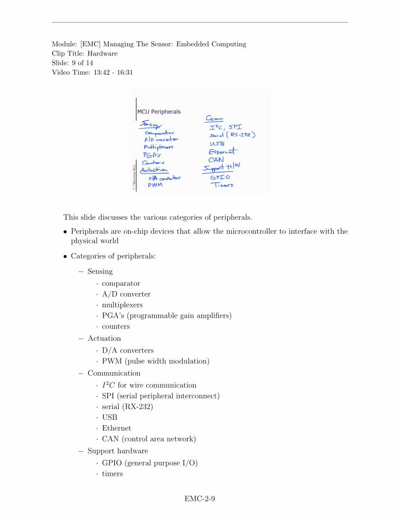
Module: [EMC] Managing The Sensor: Embedded Computing
Clip Title: Hardware
Slide: 9 of 14
Video Time: 13:42 - 16:31
This slide discusses the various categories of peripherals.
• Peripherals are on-chip devices that allow the microcontroller to interface with thephysical world
• Categories of peripherals:
− Sensing
· comparator
· A/D converter
· multiplexers
· PGA’s (programmable gain amplifiers)
· counters
− Actuation
· D/A converters
· PWM (pulse width modulation)
− Communication
· I2C for wire communication
· SPI (serial peripheral interconnect)
· serial (RX-232)
· USB
· Ethernet
· CAN (control area network)
− Support hardware
· GPIO (general purpose I/O)
· timers
EMC-2-9

Module: [EMC] Managing The Sensor: Embedded Computing
Clip Title: Hardware
Slide: 10 of 14
Video Time: 16:32 - 17:55
This slide describes two different aspects of improving energy efficiency for embeddedsystems.
• Ensure that every electronic component uses the minimum amount of energy to doits job
− optimize process technologies used in developing and fabricating the device,which include:
· digital
· analog
· radio frequency (RF)
− improve power regulation and management
• Ensure that no electronic component uses energy unless it is doing something useful
− clock domains
− power domains
− dynamic voltage scaling
EMC-2-10

Module: [EMC] Managing The Sensor: Embedded Computing
Clip Title: Hardware
Slide: 11 of 14
Video Time: 17:56 - 20:28
This slide uses an example of an MCU to illustrate how embedded system maximizesenergy efficiency. The example is using STM32 from ST micro, which is a 32-bit MCUbased on one of the ARM cores.
• STM32 contains four domains, each of them has a different voltage to maximize theefficiency of the device for the various activities.
− Slave main power domain (in blue)
· CPU core & peripheral
· FLASH
· RAM
− Master voltage domain (in red)
· Main voltage supervisor
· Low power control & independent watchdog
− RTC voltage domain (in yellow)
· Real-time clock (RTC)
· Backup registers (low leakage)
− External battery power (in green)
· Power switch
• The master voltage domain is almost always on thus allows the slave main powerdomain go to sleep, it can also put the entire device to sleep.
• When the device is in a sleep, back up the state of the system in the backup registersas opposed to CPU core saves a lot of energy.
• The power switch allows the real-time clock battery to last much longer by switchingthe power sources.
EMC-2-11

Module: [EMC] Managing The Sensor: Embedded Computing
Clip Title: Hardware
Slide: 12 of 14
Video Time: 20:29 - 23:56
Writing the software for MCUs in embedded systems is very difficult, and debuggingtakes the majority of time for system development. This slide introduces some tools thathelp with debugging.
• In-circuit debugging
− in the form of JTAG hardware support
− allows interrogating the processor to understand its states (what is in registers,memory, etc.)
− no overhead
− however does requires custom interface and special software
• Tracing (logging) (old tool)
− serial communication to log into to PC
− flexibility
− significant overhead (particularly in terms of timing)
• Power debugging (new tool)
− understands what power is being used and how to debug code systematicallyto minimize power use
EMC-2-12

Module: [EMC] Managing The Sensor: Embedded Computing
Clip Title: Hardware
Slide: 13 of 14
Video Time: 23:57 - 26:58
This slide discusses how to choose a MCU for a sensor node design.
• When picking a MCU for a particular application, we need to consider the followingaspects:
− datapath width
· there is 4-bit, 8-bit, 16-bit and 32-bit data path, the expense of MCU raisesas the data path width increases
− development toolchain
· it’s important to understand the capabilities of the toolchain and beingable to get support
− memory
· FLASH
· OTP (one-time programmable)
· RAM or SRAM
− power consumption
· low power SRAM retention
− peripherals
· real-time clock
· A/D converter (resolution and speed)
· D/A converters (resolution and speed)
· communication
− voltage
· different devices require different supply voltages
EMC-2-13

Module: [EMC] Managing The Sensor: Embedded Computing
Clip Title: Hardware
Slide: 14 of 14
Video Time: 26:59 - 29:03
This slide uses a hardware block diagram of an example sensor node to illustrate theidea of system thinking. As shown in the block diagram, this design includes three printedcircuit boards and two MCUs.
• Radio board (on the left)
• Brain board (in the middle)
− MCU (PIC18F452)
· controls the activities of the sensor
· connects to the radio transceiver which is on radio board
− external memory: SRAM, FLASH, FRAM
− power management: allows for automatic power supply switching
· internal battery power
· external power
• Sensor board (on the right)
− MCU (PIC18F8720)
· deals with all the analog I/O with transducers (light, temperature andgeneral-purpose transducers)
EMC-2-14

Module: [EMC] Managing The Sensor: Embedded Computing
Clip Title: Software
Slide: 1 of 9
Video Time: 00:00 - 00:29
This slide introduces the main content of this clip. As shown in the outline, the focusof this clip is energy efficiency of networked embedded systems (particularly, wirelesssensor networks).
EMC-3-1

Module: [EMC] Managing The Sensor: Embedded Computing
Clip Title: Software
Slide: 2 of 9
Video Time: 00:30 - 03:01
This slide shows a block diagram of power flows in an embedded system.
• Sources of energy
− Batteries
− Renewable sources (solar, wind, vibration, temperature difference, etc.)
• Regulator: routes the power between power sources and the actual power consumer
• Energy consumer
− Radio (the most significant energy consumer)
− MCU
− Analog peripherals
− Digital peripherals
EMC-3-2

Module: [EMC] Managing The Sensor: Embedded Computing
Clip Title: Software
Slide: 3 of 9
Video Time: 03:02 - 08:32
This slide models the power consumption of an embedded system.
• Assuming x is the index of a power state of the system, for each power state thereis an associated voltage vx and associated current ix.
− vx’s and ix’s are determined by two things:
· process technologies
· chip design and power domains
− The choice of the power state x is determined by the software running on theMCU.
− The energy used can be expressed as:
E = pT = T∑x
pxqx = T∑x
vxixqx
x ∈ s, c, h
· px: the power associated with each power state x
· qx: the percentage of time spent in each power state x
− x can stand for three possible states:
· sensing (s)
· communication (c)
· hibernation (h)
− Within each of those states (s, c, h), there can be a lot of sub-states. There maybe n different transducers connected to the sensor and each one of those hasa different power draw (px) because of its associated voltage (vx) and current(ix).
EMC-3-3

Module: [EMC] Managing The Sensor: Embedded Computing
Clip Title: Software
Slide: 4 of 9
Video Time: 08:33 - 11:15
This slide discusses how to measure power and energy in an embedded system.
• There are two basic types of management.
− On-line
· Switched capacitors (current mirror design)
· high-resolution, expensive
· Precision resistor with on-chip ADC
· low cost, difficult to work in sleep mode
· Monitor regulator
· requires switching regulator
− Off-line
· uses equipment external to the embedded system, depends more on build-ing models based on measurements
• In all these cases it’s difficult to deal with signal measurement as discussed in thenext slide.
EMC-3-4

Module: [EMC] Managing The Sensor: Embedded Computing
Clip Title: Software
Slide: 5 of 9
Video Time: 11:16 - 13:08
This slide discusses why measuring energy used in embedded systems can be difficult.
• The power signal is wideband
− brief pulses (< 1 ms) of activity
− hours or days of hibernation => sharp short pulses => wide bandwidth
− needs high-quality multi resolution measurement of time
• The power signal is multi-scale in magnitude
− up to ∼ 50mA when active
− as low as ∼ 2µA when hibernating
− requires scaling or multi resolution measurements
EMC-3-5

Module: [EMC] Managing The Sensor: Embedded Computing
Clip Title: Software
Slide: 6 of 9
Video Time: 13:09 - 15:23
This slide revisits the question of how to improve the energy efficiency for embeddedsystems and discusses it from hardware-oriented/software-oriented perspective.
• Hardware-oriented goal
− Ensure that every electronic component uses the minimum amount of energyto do its job
• Software-oriented goal
− Ensure that no electronic component uses energy unless it is doing somethinguseful
· Clock domains and gating: turn on or turn off the clock for particularsubsystems
· Power domains and gating: turn on or turn off the power for specificsubsystems
· Dynamic voltage scaling: fine-tuning the minimum required voltage forspecific subsystems
EMC-3-6

Module: [EMC] Managing The Sensor: Embedded Computing
Clip Title: Software
Slide: 7 of 9
Video Time: 15:24 - 16:50
This slide discusses the idea of cross layer design and its challenges. Different layersthat must be considered and impact each other:
• PHY and MAC
• Routing and application (self-organization)
• MAC and embedded software (co-design)
• Embedded software and ULP (ultra low power), MCU’s
• Source and channel coding
EMC-3-7

Module: [EMC] Managing The Sensor: Embedded Computing
Clip Title: Software
Slide: 8 of 9
Video Time: 16:51 - 18:49
This slide uses MSP430 MCU as an example to illustrate the interaction between thesoftware running on the embedded system and hardware technology.
• The MSP 430 MCU is a popular microcontroller from Texas Instrument, it is oneof the lower power consumption devices available.
• In the block diagram of the MSP 430 MCU, the power management module andsupply voltage supervisor interacts with software. We can choose the supply voltagefor the core by programming with software.
• The plot on the bottom shows that:
− if the clock runs at 12 MHz, the voltage supply can be 1.8 V
− if the clock runs at 25 MHz, then 2.5 V supply will be needed
− lower clock speed, lower power consumption
EMC-3-8

Module: [EMC] Managing The Sensor: Embedded Computing
Clip Title: Software
Slide: 9 of 9
Video Time: 18:50 - 21:54
This slide recaps what has been covered in this [EMC] clip.
• WSN node design is complex
− Hardware platform
· there are a lot of different subsystems and components (include MCU)
− System software
· controls all the subsystems and peripherals
− Energy efficiency
· needs to consider co-design and the interaction between hardware andsoftware
• New MCU provides more opportunities for optimizing the energy efficiency designat the cost of increased complexity
• New and better software design approaches are needed to understand energy con-sumption upfront.
EMC-3-9

Module: [EMC] Managing The Sensor: Embedded Computing
Clip Title: Energy Efficiency
Slide: 1 of 11
Video Time: 00:00 - 00:30
This slide describes the main content of this clip. The focus of this clip is software fornetworked embedded system, in particular the deeply embedded systems that are designedinto wireless sensor network nodes. It will give a basic introduction and highlight thedifferences between writing software for embedded system and for traditional interactivecomputer systems.
EMC-4-1
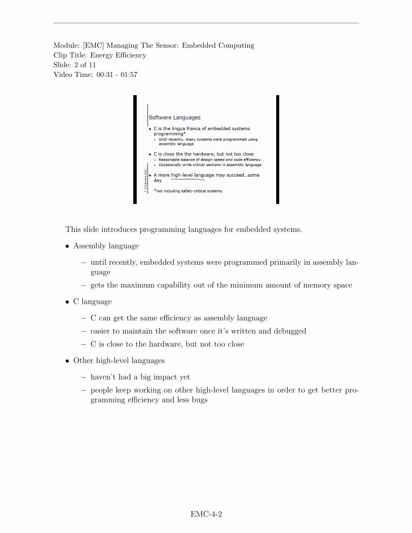
Module: [EMC] Managing The Sensor: Embedded Computing
Clip Title: Energy Efficiency
Slide: 2 of 11
Video Time: 00:31 - 01:57
This slide introduces programming languages for embedded systems.
• Assembly language
− until recently, embedded systems were programmed primarily in assembly lan-guage
− gets the maximum capability out of the minimum amount of memory space
• C language
− C can get the same efficiency as assembly language
− easier to maintain the software once it’s written and debugged
− C is close to the hardware, but not too close
• Other high-level languages
− haven’t had a big impact yet
− people keep working on other high-level languages in order to get better pro-gramming efficiency and less bugs
EMC-4-2

Module: [EMC] Managing The Sensor: Embedded Computing
Clip Title: Energy Efficiency
Slide: 3 of 11
Video Time: 01:58 - 04:13
The C-language was not designed for embedded systems interacting with the physicalworld. We have had to come up with a combination of software and hardware to controland manage the peripherals on an MCU. This slide introduces two methods to accomplishthis.
• Direct access
− directly writes to control and data registers of the peripheral
− tedious for programmer since it requires one to understand every aspect of theperipheral
− lean and fast
− less portable (not portable from device to device within an MCU family)
• Library access
− access via function calls
− easier for programmer
− invokes overhead in terms of processor cycles
− more portable
EMC-4-3

Module: [EMC] Managing The Sensor: Embedded Computing
Clip Title: Energy Efficiency
Slide: 4 of 11
Video Time: 04:14 - 07:24
One of the most important aspects of embedded systems is interfacing with the physicalworld and dealing with asynchronous events. This slide discusses two approaches to handleasynchronous events.
• Polling
− program checks periodically whether a signal has changed
• Interrupts
− requires additional specialized hardware and software
− when an event occurs, the hardware latch will trigger and the interrupt hander(ISR) will be invoked as soon as the current instruction completes execution
EMC-4-4
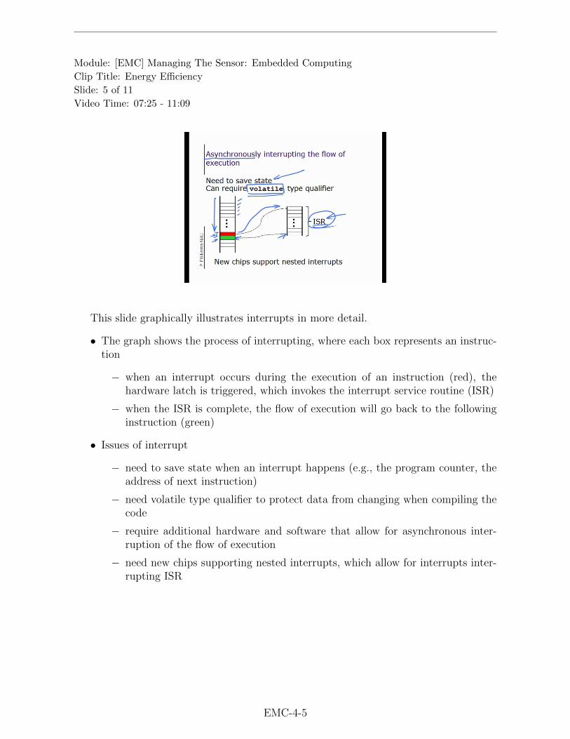
Module: [EMC] Managing The Sensor: Embedded Computing
Clip Title: Energy Efficiency
Slide: 5 of 11
Video Time: 07:25 - 11:09
This slide graphically illustrates interrupts in more detail.
• The graph shows the process of interrupting, where each box represents an instruc-tion
− when an interrupt occurs during the execution of an instruction (red), thehardware latch is triggered, which invokes the interrupt service routine (ISR)
− when the ISR is complete, the flow of execution will go back to the followinginstruction (green)
• Issues of interrupt
− need to save state when an interrupt happens (e.g., the program counter, theaddress of next instruction)
− need volatile type qualifier to protect data from changing when compiling thecode
− require additional hardware and software that allow for asynchronous inter-ruption of the flow of execution
− need new chips supporting nested interrupts, which allow for interrupts inter-rupting ISR
EMC-4-5

Module: [EMC] Managing The Sensor: Embedded Computing
Clip Title: Energy Efficiency
Slide: 6 of 11
Video Time: 11:10 - 14:21
This slide reviews the pros and cons of polling and interrupts
• Polling
− simple
− can waste time and energy
− easy to debug
− does not scale well to have a lot of inputs, difficult to poll them sufficientlyoften.
• Interrupts
− require special hardware
− easy to code
− hard to debug as creating all possible asynchronous interrupt scenarios is dif-ficult
− useful in handling rare events (e.g. toxic gas release detection)
− useful in programming models for some MCU’s
EMC-4-6

Module: [EMC] Managing The Sensor: Embedded Computing
Clip Title: Energy Efficiency
Slide: 7 of 11
Video Time: 14:22 - 16:39
Embedded systems can get complex but we can use operating systems to manage thecomplexity. This slide discusses purposes of operating systems.
• Manages and allocates resources via scheduler
− disk space
− memory space
− execution time, which is allocated on different hardware resources includingCPU, direct memory access (DMA), peripherals
• Provides mediated, abstracted interfaces to
− memory (e.g. file system)
− peripherals
− input/output (I/O)
EMC-4-7

Module: [EMC] Managing The Sensor: Embedded Computing
Clip Title: Energy Efficiency
Slide: 8 of 11
Video Time: 16:40 - 17:39
This slide shows the software design hierarchy for embedded systems.
• Hardware (the foundation) that code is being written for
• Assembly language layer
• Interface between hardware and assembly language layer
− assembler: turn assembly language into machine code
− linker: links together different modules
− loader: installs the code on hardware
• Libraries
− for example, library to do 16-bit calculations on 8-bit controllers.
EMC-4-8

Module: [EMC] Managing The Sensor: Embedded Computing
Clip Title: Energy Efficiency
Slide: 9 of 11
Video Time: 17:40 - 18:58
This slide moves up the software design hierarchy and introduces two more layers.
• C language
− can be compiled into assembly language
− there can be also a set of libraries for C language
• Operating system (OS) or event loop
− provides application program interface (API)
− provides resources for the program
EMC-4-9

Module: [EMC] Managing The Sensor: Embedded Computing
Clip Title: Energy Efficiency
Slide: 10 of 11
Video Time: 18:59 - 22:22
This slide shows a table comparing different types of operating systems (OS) fromsimple to complex.
• Event loop
− simplest, periodic execution, little overhead
− hand-written
• Time-triggered executive
− time-triggered, system-tick (systick) drives the program evolution forward.
− WiSARD executive, developed at NAU, is an example.
• Cooperative OS
− event-driven
− TinyOS
• Pre-emptive OS
− most complex, priority-driven
− Linux
EMC-4-10

Module: [EMC] Managing The Sensor: Embedded Computing
Clip Title: Energy Efficiency
Slide: 11 of 11
Video Time: 22:23 - 24:19
The last slide concludes this segment on software with a look forward.
• Better programs than C and assembly are needed
• Prototyping should be easier
• Time should be a first-class concept
• To minimize energy consumption and develop energy efficient embedded systems,software design process should incorporate:
− co-design with hardware
− energy-awareness
EMC-4-11

Module: [CTA] Communication Theory as Applied to Wireless Sensor Networks
Clip Title: Module Objectives and WSN Constraints
Slide: 1 of 6
Video Time: 00:00 - 02:34
This slide describes the goal of this lecture clip, namely to link the methods fromcommunication theory to the requirements of wireless sensor networks. In particular, theclip will emphasize the understanding of the following points:
• Understand the constraints of wireless sensor networks and how they influence ourcommunication theory choices.
• Understand the choice of digital communications over analog schemes.
• Understand the choice of digital phase modulation over frequency or amplitudeschemes.
• Other objectives: the costs and benefits of implementing source and channel coding.
• Understand the fundamental concepts of medium access control (MAC).
• Understand the importance of node synchronization which is to ensure data is beingreceived when intended
• Examples of the tradeoff between energy and bandwidth will be presented.
CTA-2-1
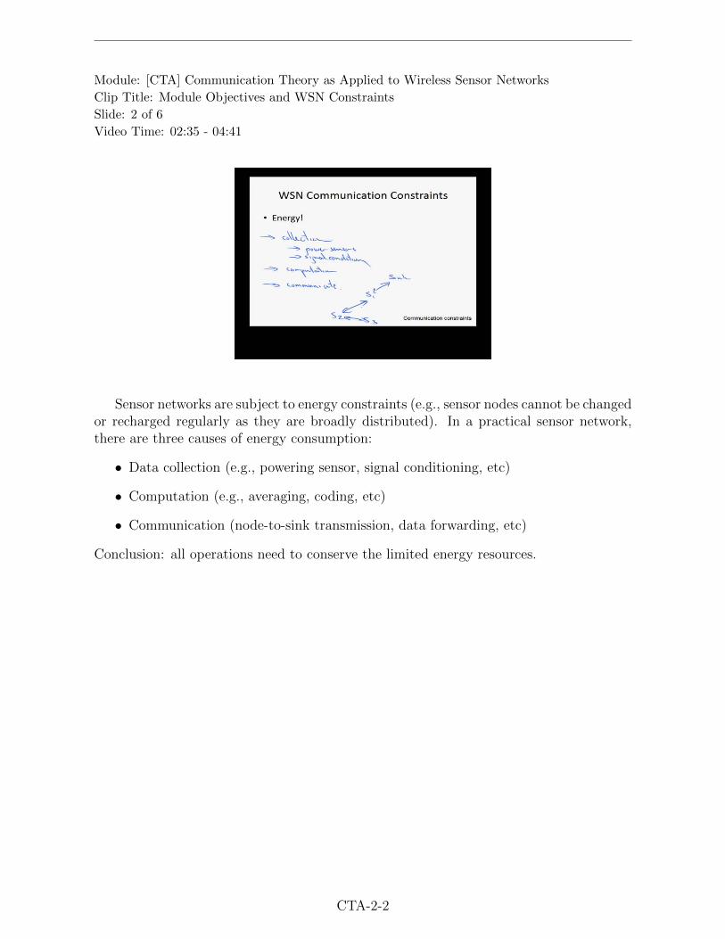
Module: [CTA] Communication Theory as Applied to Wireless Sensor Networks
Clip Title: Module Objectives and WSN Constraints
Slide: 2 of 6
Video Time: 02:35 - 04:41
Sensor networks are subject to energy constraints (e.g., sensor nodes cannot be changedor recharged regularly as they are broadly distributed). In a practical sensor network,there are three causes of energy consumption:
• Data collection (e.g., powering sensor, signal conditioning, etc)
• Computation (e.g., averaging, coding, etc)
• Communication (node-to-sink transmission, data forwarding, etc)
Conclusion: all operations need to conserve the limited energy resources.
CTA-2-2

Module: [CTA] Communication Theory as Applied to Wireless Sensor Networks
Clip Title: Module Objectives and WSN Constraints
Slide: 3 of 6
Video Time: 04:42 - 06:50
This slide discusses the data collection costs, which are associated with acquiring thedesired data.
• Each sensor or transducer may have unique power requirements.
• Each sensor may have unique signal conditioning circuits.
− Different sensors may require different operating voltages.
− To limit current draw, we may design a circuit that only enables a sensor whendata is being collected.
− Therea are advantages to implementing the digital communication system in-stead of analog systems, but such systems need energy to support A/D con-version.
CTA-2-3

Module: [CTA] Communication Theory as Applied to Wireless Sensor Networks
Clip Title: Module Objectives and WSN Constraints
Slide: 4 of 6
Video Time: 06:51 - 08:31
This slide analyzes the energy use in computation, which is performed primarily by amicro controller unit (MCU).
• In particular, the energy consumption in computation mainly comes from the fol-lowing four aspects:
− Basic life support: clock circuitry, wake up and sleep operations.
− Simple data processing: evaluating statistics and running additional algo-rithms.
− Censoring and aggregation: look at not only the sensor’s own data but alsothat from neighbors.
− Source and channel coding (e.g., for data compression and error correctioncoding)
• The use of energy for computation is a lot cheaper than the energy cost for trans-mitting data.
CTA-2-4

Module: [CTA] Communication Theory as Applied to Wireless Sensor Networks
Clip Title: Module Objectives and WSN Constraints
Slide: 5 of 6
Video Time: 08:32 - 11:42
This slide discusses the the communication costs, which refers to the energy requiredto transmit and receive data.
• The power depends on not only the amount of transmit power, but also on the largeand small-scale propagation effects.
− The transmitter power needs to be increased as the T-R distance increases
− Each wireless sensor has a radio chip, and each radio chip will have a uniquecurve that relates its transmit power to the current requirements.
• The cost of receiving or the modulating wireless communication signal is also con-siderable.
• A sensor node can utilize a MTP protocol (Minimum Transmit Power) to transmitonly the power that is needed, but not any additional power.
CTA-2-5

Module: [CTA] Communication Theory as Applied to Wireless Sensor Networks
Clip Title: Module Objectives and WSN Constraints
Slide: 6 of 6
Video Time: 11:43 - 14:31
This slide summarizes the overall model of communication costs by integrating differ-ent parts together.
• The communication cost is due to both reception and transmission of data:
1. The cost per received bit is essentially constant
2. The transmission costs per bit are dependent on the T-R distance
3. A simplistic model
Ecom = ERX + ETX = α + βdn.
Where α and β are constants related to receiving and transmitting respectively.
• The total energy needed can be given as:
Etot = Ea + Ep + ERX + ETX ,
which is the sum of following parts:
− Data collection and acquistion (Ea)
− Computaton and processing (Ep)
− Receiving data (ERX)
− Transmitting data (ETX)
• It is important to quantify these needs through the use of a power budget.
• In the remainder of this clip, we will focus on techniques which influenced thecommunication costs. The goal is to justify the choice of methods used in wirelesssensor networks using energy needs and energy constraints as a guide.
CTA-2-6

Module: [CTA] Communication Theory as Applied to Wireless Sensor Networks
Clip Title: General Modulations Approaches
Slide: 1 of 14
Video Time: 00:00 - 00:09
This slide states the main points of this clip:
• Modulation basics
• Amplitude Modulation
• Frequency Modulation
• Phase Modulation
CTA-3-1

Module: [CTA] Communication Theory as Applied to Wireless Sensor Networks
Clip Title: General Modulations Approaches
Slide: 2 of 14
Video Time: 00:10 - 02:17
This slide introduces the fundamentals about modulation and discusses the motivationfor digital communications.
• Modulation is the process of varying a high-frequency tone (which we call the carrier)with an information signal, which produces the modulated signal.
− The information is contained in modulated signal and at high-frequency andtherefore suitable for wireless communications.
• The motivations for digital communications
− Coding or other mathematical manipulation can be done on digital data
− The digital data can be readily stored.
− More importantly, digital modulation methods or energy-efficient.
CTA-3-2

Module: [CTA] Communication Theory as Applied to Wireless Sensor Networks
Clip Title: General Modulations Approaches
Slide: 3 of 14
Video Time: 02:18 - 03:24
This slides reviews what is a sinusoid and thus discusses three modulation methods.Each method modifies a different parameter of the sinusoid carrier.
• A sinusoid can be defined as
c(t) = Ac · cos(2πfc + θc)
Here, Ac is the carrier’s amplitude, fc is the frequency, and θc is the phase.
• In modulation, we can modify these three parameters: the amplitude, the frequency,and the phase, resulting in three modulation methods:
− Amplitude modulation
− Frequency modulation
− Phase modulation
These three methods will be reviewed in terms of using a generic information signal.
CTA-3-3

Module: [CTA] Communication Theory as Applied to Wireless Sensor Networks
Clip Title: General Modulations Approaches
Slide: 4 of 14
Video Time: 03:25 - 04:32
This slide introduces amplitude modulation, particular the simplest formulation calleddouble-sideband-suppressed carrier (DSB-SC). The modulation is simply done by multi-plying the carrier with the information signal m(t), resulting in:
φDSB−SC(t) = m(t) · cos(2πfct).
The next slide will discuss where the terms “double-sideband” and “suppressed-carrier”come from.
CTA-3-4

Module: [CTA] Communication Theory as Applied to Wireless Sensor Networks
Clip Title: General Modulations Approaches
Slide: 5 of 14
Video Time: 04:33 - 07:15
This slide derives the frequency representation for DSB-SC using the frequency-shiftproperty.
• It starts with a time-domain representation, as follows
φDSB(t) = m(t) cos(2πfct) = m(t) cos(ωct).
, where 2πfc := ωc.
• By employing the frequency shift property of the Fourier transform, as
F [m(t)e−jωct] = M(ω + ωc).
Here, M is the Fourier transform of m. Combining the derivation above results in
F [m(t)cos(ωct)] =1
2(M(ω − ωc) +M(ω + ωc)) .
as from Euler’s expansion
cos(ωct) =1
2e+jωct +
1
2e−jωct.
CTA-3-5

Module: [CTA] Communication Theory as Applied to Wireless Sensor Networks
Clip Title: General Modulations Approaches
Slide: 6 of 14
Video Time: 07:16 - 12:32
This slide illustrates the process of DSB-SC modulation.
• The first figure (top) shows the spectrum of the information signal, which is band-limited, meaning no energy exists outside the range of +B/-B (Hz).
• The second figure (bottom) shows how the spectrum of the modulated signal isgenerated by shifting two copies of the original spectrum, one to the left and theother to the right.
− With this figure, it also explains the upper side band and lower side band, andthus why this is called double sideband.
− The modulated signal that is has energy concentrated about our carrier fre-quency, and its total bandwidth requirement is simply twice that of our originalinformation signal.
CTA-3-6

Module: [CTA] Communication Theory as Applied to Wireless Sensor Networks
Clip Title: General Modulations Approaches
Slide: 7 of 14
Video Time: 12:33 - 17:16
This slide explains how a coherent receiver extracts the original infomation, m(t), froma modulated signal via demodulation.
The figure shows the diagram of both a transmitter and a coherent receiver. Formally,the demodulation process goes through two steps:
• Generates an intermediate signal as follows
e(t) = m(t) cos(ωct) · cos(ωct) = m(t) cos2(ωct)
=m(t)
2+m(t)
2cos(2ωct).
• Applies a low-pass filter to remove the second high frequency component
This slide finally emphasizes the importance of coherence: the carriers in modulationand demodulation should have the same frequence and phase.
CTA-3-7

Module: [CTA] Communication Theory as Applied to Wireless Sensor Networks
Clip Title: General Modulations Approaches
Slide: 8 of 14
Video Time: 17:17 - 19:27
This slide discusses the double-sideband, large-carrier technique (DSB-LC), which wasdeveloped to overcome the difficulty of amplitude modulation that relies on a coherentreceiver (i.e., a synchronous detector). The mechanism is as follows
• The information signal m(t) is first offset by a large DC component A, resulting inA+m(t), prior to modifying the amplitude of our carrier.
• Then we can employ an envelope detector in the receiver to process the signal.
• A is chosen subject to the constraint: A + m(t) ≥ 0, and we can characterize thiswith modulation index:
µ :=|m(t)|max
A,
which has 0 ≤ µ ≤ 1.
CTA-3-8

Module: [CTA] Communication Theory as Applied to Wireless Sensor Networks
Clip Title: General Modulations Approaches
Slide: 9 of 14
Video Time: 19:28 - 21:29
This slide discusses the frequency domain representation of DSB-LC.
• It first expands the time-domain representation as follows
φAM(t) = [A+m(t)] cos(ωct) = A cos(ωct) +m(t) cos(ωct)
The first term corresponding to the carrier and the second term is the information-modulated signal. Even when the information becomes zero, the first term remains.
• The frequency domain representation is given by
ΦAM(ω) = Aπδ(ω − ωc) + Aπδ(ω + ωc) +1
2M(ω − ωc) +
1
2M(ω + ωc).
Here, the delta-functions are solely related to the fact that we have a carrier andagain if the information signal goes away, this “large carrier” component remains.
CTA-3-9

Module: [CTA] Communication Theory as Applied to Wireless Sensor Networks
Clip Title: General Modulations Approaches
Slide: 10 of 14
Video Time: 21:30 - 25:14
This slide illustrates the information signal (in sinusoidal form), modulated signal, aswell as their frequency spectrum.
• It identifies the carrier and information components respectively.
• It explains the working mechanism of an envelop detector based on this example.
• The limitation: in order to implement this, a large component or large amount ofthe total signal power must be allocated to the carrier, thus reducing overall energyefficiency.
CTA-3-10

Module: [CTA] Communication Theory as Applied to Wireless Sensor Networks
Clip Title: General Modulations Approaches
Slide: 11 of 14
Video Time: 25:15 - 28:10
This slide introduces frequency modulation (FM), in which the carrier’s instantaneousfrequency is linear dependent on our information signal.
• The instantaneous frequency changes as the signal voltage m(t) changes, as
ωi(t) = ωct+ kfm(t).
• As a result, the instantaneous phase is linearly dependent on the integral of ourinformation signal, as
θi(t) = ωct+ kf
∫m(t)dt.
• FM is not a linear modulation method. The argument relies on the fact that cos(α+β) 6= cos(α) + cos(β) in general.
• As a consequence of nonlinearity, FM has bandwidth requirements that exceed thoseof AM which is a linear technique.
CTA-3-11

Module: [CTA] Communication Theory as Applied to Wireless Sensor Networks
Clip Title: General Modulations Approaches
Slide: 12 of 14
Video Time: 28:11 - 31:02
This slide illustrates the FM technique using a 1kHz tone as an example informationsignal.
• The left figure shows the time-domain waveforms.
− The modulated signal has nearly constant envelope, which benefits us on thereceiving end as it is less susceptible to the additive noise than AM is.
• The right figure shows the spectrum of the FM-modulated signal.
− Multiple sideband components (at 1kHz intervals) arise due to the nonlinear-ity of FM. The overall bandwidth requirements for FM for this example isapproximately 6 kHz.
− As the carrier component is not dominating the overall spectrum, the overallpower efficiency for FM exceeds that of AM.
• Modifying frequency is much more efficient than modifying amplitude and thussensor nodes should use nonlinear modulation technique as opposed to employ am-plitude modulation.
CTA-3-12

Module: [CTA] Communication Theory as Applied to Wireless Sensor Networks
Clip Title: General Modulations Approaches
Slide: 13 of 14
Video Time: 31:03 - 32:20
This slide introduces phase modulation, as follows.
• The instantaneous phase of the carrier is linearly dependent on the informationsignal, as
θi(t) = ωct+ kpm(t).
• As a result, the instantaneous frequence is dependent on the derivative of the infor-mation signal, as
ωi(t) = ωc + kpm′(t).
• Phase modulation is also a nonlinear technique and hence it will too have a constantenvelope and significant power in the spectral sidebands.
CTA-3-13

Module: [CTA] Communication Theory as Applied to Wireless Sensor Networks
Clip Title: General Modulations Approaches
Slide: 14 of 14
Video Time: 32:21 - 35:25
This slide discusses the trade-off between bandwidth requirement and energy efficiencyof the modulation schemes.
• FM and PM, as nonlinear modulation techniques, generally require more bandwidththan that of AM.
− The amount of bandwidth can be approximated using Carson’s rule:
BφM = 2B(β + 1),
where β is the modulation index for FM/PM.
• The graph demonstrates the trade-off between signal power and bandwidth.
− As β is increasing, meaning that more bandwidth is required, there is moresignificant improvement on signal-to-noise ratio (SNR), meaning better qualityof the received signal.
• For sensor networks, using more bandwidth than we would expect given the datarates is typical as techniques such as error correction coding and spreading areemployed.
CTA-3-14

Module: [CTA] Communication Theory as Applied to Wireless Sensor Networks
Clip Title: Modulation for Digital Systems
Slide: 1 of 8
Video Time: 00:00 - 00:09
This slide lists the main points that are going to be covered by the clip.
• Quadrature Modulation
• BPSK
• QPSK
• BER Performance
CTA-4-1

Module: [CTA] Communication Theory as Applied to Wireless Sensor Networks
Clip Title: Modulation for Digital Systems
Slide: 2 of 8
Video Time: 00:10 - 06:07
This slide uses a sensor network with nodes collecting two types of measurements(lightand temperature) to motivate the use of digital methods.
• In this example, the ranges of voltage of the thermometer and photodetector differgreatly: the former is 0 - 5 V, while the latter is 0 - 10 mV.
• The 8-bit A/D converters are used to convert the voltage outputs to digital repre-sentation (bit strings).
• A digitial system yields bit strings to represent numbers, enabling operations thatare difficult to perform in analog systems, including
− mathematical manipulation (e.g., averaging)
− data compression
− storing the numbers to RAM
• A good understanding of the expected range of phenomena is necessary for choosingthe transducer appropriately, and one has to ensure the A/D operates over thedesired voltage range.
CTA-4-2

Module: [CTA] Communication Theory as Applied to Wireless Sensor Networks
Clip Title: Modulation for Digital Systems
Slide: 3 of 8
Video Time: 06:08 - 10:56
This slides introduces quadratic modulation for transmitting digital data.
• Digital data can be represented by a stream of bits. The 0-bit and 1-bit are assignedwith different voltages in transmission. Consequently, a bit stream is converted toa time varying signal, denoted by m(t).
• Consider double-sideband suppressed carrier modulation
− A mixer can be used to multiply the information signal with a cosine carrrier,resulting in
φI(t) = mI(t) cos(ωct)
− The sine function can also be used as the carrier, resulting in
φQ(t) = mQ(t) sin(ωct)
− Due to the orthogonality between cosine and sine function, the two modulatedsignals described above can be added together and sent simultaneously acrossthe channel. This technique is referred to as quadrature amplitude modulation.
· Here, φI(t) and φQ(t) are respectively referred to as inphase componentand quadrature component.
• In digital systems, these individual signals mI(t) and mQ(t) will take on a finitenumber of voltages, and two common methods are often used in sensor networksthat are introduced later: BPSK and QPSK.
CTA-4-3

Module: [CTA] Communication Theory as Applied to Wireless Sensor Networks
Clip Title: Modulation for Digital Systems
Slide: 4 of 8
Video Time: 10:57 - 13:40
This slide introduces BPSK (binary phase shift keying) and uses the figure to illustratethe modulated signal.
• The top and bottom windows in this figure respectively show the inphase andquadrature phase components of the modulated signal produced by BPSK.
• With BPSK, only inphase component is used, and there is nothing in the quadraturephase.
• Here, 1-bits are represented by +1 volt signal and 0 bits are represented by -1 voltsignal.
• The time-domain representation of the modulated signal
φ(t) = m(t) cos(ωct).
when sending data 1, the modulated signal is cos(ωct), and when sending data 0,the modulated signal is −cos(ωct).
• There is a 180 phase shift between these two signals.
CTA-4-4

Module: [CTA] Communication Theory as Applied to Wireless Sensor Networks
Clip Title: Modulation for Digital Systems
Slide: 5 of 8
Video Time: 13:41 - 16:23
This slide introduces QPSK (Quadrature Phase Shift Keying), and briefly discussesits advantage over BPSK.
• QPSK employs both inphase and quadrature passes, and hence two information sig-nals are sent across the channel at the same time and at the same carrier frequency.
• The bit stream is split into two paths: for example, one with all even bits, and theother with all odd bits, which are respectively represented by the inphase signalmI(t) and the quadrature phase signal mQ(t).
• Each quadrature signal takes on only one or two values, e.g. 1-bits may be repre-sented by positive voltages, and 0-bits by a negative voltages.
• Using QPSK as a comparison to BPSK, we can either reduce the required bandwidthin half or double the overall data rate using the same bandwidth.
CTA-4-5

Module: [CTA] Communication Theory as Applied to Wireless Sensor Networks
Clip Title: Modulation for Digital Systems
Slide: 6 of 8
Video Time: 16:24 - 21:59
This slide introduces constellation plots as a convenient way to demonstrate digitalquadrature modulation, and based on such plots, illustrates the impact of noises on QPSKdemodulation.
• In QPSK, there are four possible data pairs: (1, 1), (1, 0), (0, 1), and (0, 0), whichcorrespond to four different points in the constellation plot.
− For example, when both even bit and odd bit are 1, then both inphase andquadrature voltages are positive, resulting in the composite carrier with phaseangle 45.
− Likewise, the phase angle for (1, 0) is 135, and that for (0, 0) is −135, etc.
− In the plot, the length of each one of the four vectors is the same, but takeson distinct phases.
• The signal being transmitted across the channel is impacted by noise, which resultsin an altered constellation plot, as shown in the bottom right of the slide. The fourpoints are not as distinct as in the noiseless case.
• The bits can still be recovered without error, provided that the noise is not signficantenough to generate deviations that move the signal across the decision boundary.
CTA-4-6

Module: [CTA] Communication Theory as Applied to Wireless Sensor Networks
Clip Title: Modulation for Digital Systems
Slide: 7 of 8
Video Time: 22:00 - 24:24
This slide uses the bit-error-rate vs energy-per-bit curves to justify the use of digitalphase modulation as opposed to frequency modulation.
• The choice of digital phase modulation is originated from the desire to conserveenergy resources in sensor networks.
• In this figure, the vertical-axis is the bit-error-rate (BER), while the horizontal-axisis the energy per bit.
• It can be seen from this graph that at 10−3 bit error rate, the energy consumptionof phase shift keying is 3dB less than that of frequency shift keying.
• In general, such curves can be used to ascertain how good our digital communicationscheme is.
• The efforts in communication theory is to develop schemes (e.g., error correctioncoding) that move the curves to the lower left direction.
CTA-4-7

Module: [CTA] Communication Theory as Applied to Wireless Sensor Networks
Clip Title: Modulation for Digital Systems
Slide: 8 of 8
Video Time: 24:25 - 27:54
This slide uses the BER vs energy-per-bit curves to justify the use of QPSK as opposedthe schemes that send more bits at a time (e.g., 8PSK).
• In general, more energy is needed if more bits are sent at the same time.
• The curves show that QPSK is as efficient (in terms of energy efficiency) as BPSK,but the schemes with n = 3, 4, 5 bits sent at the same time are not as efficient.
− As n increases beyond 2, the boundaries between the constellation points de-creases as we add constellation points, and consequently, to ensure that thesepoints remain separated when noise is added, the signal voltage needs to in-crease, incurring higher energy consumption.
• The conclusion is that moving to digital modulation schemes beyond QPSK is notenergy efficient choice and such techniques are thus not implemented in practice forwireless sensor networks.
CTA-4-8

Module: [CTA] Communication Theory as Applied to Wireless Sensor Networks
Clip Title: Source Coding
Slide: 1 of 10
Video Time: 00:00 - 00:09
This slide lists the main points of the clip.
• Motivation for source coding.
• Lossless methods.
• Lossy methods.
• Other data reducing techniques.
CTA-5-1

Module: [CTA] Communication Theory as Applied to Wireless Sensor Networks
Clip Title: Source Coding
Slide: 2 of 10
Video Time: 00:10 - 05:49
This slide discusses the motivation for the use of source coding (commonly known asdata compression), and describes two forms of source coding: lossless and lossy compres-sion.
• The key motivation of source coding is to send less bits, and thus reduce the energy(or bandwidth) needed for data transmission.
• Compression techniques used for other systems are primarily motivated by the needof improving throughput and minimizing bandwidth/storage requirements, whichare different from that in sensor networks, where compression is mainly for energyefficiency.
• Source coding need to preserve good data. The sense of “being good” is application-specific, and is related to the quality-of-service (QoS) issues.
• Source coding comes in two forms:
− Lossless compression, in which original bits can be reconstructed.
− Lossy compression, part of the original information are lost. Hopefully theimportant information that was represented in the bits is captured in the fewerbits that are sent across the channel.
CTA-5-2

Module: [CTA] Communication Theory as Applied to Wireless Sensor Networks
Clip Title: Source Coding
Slide: 3 of 10
Video Time: 05:50 - 15:02
This slide descibes two ways of doing lossless source doing: zip coding and entropycoding.
• Compressing files into a zip file is a popular form of lossless source coding.
− When several files are to be sent, which are essentially a set of bits, one cancompress them into a zip file, which contains fewer bits.
− At the receiving end, the original files can be exactly recovered by uncompress-ing the zip file, with nothing loss.
− The cost of doing source coding is that some computation power is needed atboth the transmitting node and receiving node.
− The advantage is that this additional computation energy is much much lessthan the communication energy that would be needed to send all the informa-tion.
• Entropy coding is another way of lossless source coding.
− The basic idea is to assign bits proportional to the information contained inthe message to be sent.
− The information of a message is quantified as
Ii = log2
1
Pi
.
Pi is the probability that the message i occurs.
− A certain event, namely the event that always happen, i.e. Pi = 1, has zeroinformation.
CTA-5-3

− Entropy encoding assigns fewer bits to something is more likely to happen,and more bits to something that is less likely to happen, thus on average thenumber of bits to be sent will be less.
− Consider an example of sending characters in alphabet: the letter “E” occurs10% of the time, compare that to the letter “Z”, whose probability is 1%,then the information for the letter E is I = log2(1/10) = 3.3 bits, and theinformation for the Z is I = log2(0.01) = 6.6 bits.
− The source entropy is defined to be
H =n∑
i=1
IiPi.
This is the average number of bits per message using entropy coding, which isthe theoretical minimum for lossless source coding.
4

Module: [CTA] Communication Theory as Applied to Wireless Sensor Networks
Clip Title: Source Coding
Slide: 4 of 10
Video Time: 15:03 - 20:02
This slide first discusses the limitations with entropy coding, and then describes runlength coding, and again discusses its limitations.
• The problems with entropy coding:
− The data statistics needed to derive the coding scheme is generally unavailablefor WSN.
− Different sensors may have different data statistics, and thus a single code maynot suit all nodes equally well.
• Run-length coding: multiple occurrences of value is sent and in one bulk of trans-mission.
− A light sensor is advisable to send a compressed message stating that “thereis no light throughout six hours at night” rather than repeatedly sending “nolight” messages.
− The problem of run-length coding is long delay. One way to address is issue isto only send changes in our data set, that is the note only transmits the whendata changes.
− The problem with this method is difficult to distinguish between no data beingsent and a dead sensor, or lost transmission.
• In sum, lossless compression techniques for sensor networks remains in need of agood solution.
CTA-5-4

Module: [CTA] Communication Theory as Applied to Wireless Sensor Networks
Clip Title: Source Coding
Slide: 5 of 10
Video Time: 20:03 - 23:19
This slide introduces lossy compression techniques and uses rate-vs-distortion curvesto illustrate the underlying rate distortion theory.
• The difficulty of implementing lossless compression is minimizing the bits while stillachieving full data recovery.
• A lossy compression technique reduces the number of bits by giving up some fidelity,while preserving the most important pieces of information.
• The technique is based on the rate distortion theory, which is a branch communi-cation theory that deals with the theoretical bounds for compression given certainfidelity constraints.
• The slide shows a graph, where the horizontal axis is rate, i.e. number of bits weneed to send, and the vertical axis is the measurement of distortion.
− Generally, the distortion increases as the bit rate decreases.
− It is desirable to develop a compression scheme such that the amount of dis-tortion doesn’t increase very much, even as the rate drops quite a bit. It isonly when the rate goes very low that the distortion increases considerably.
− Such curves provide a way to quantify the quality resulting from a particularlossy compression technique.
• An important lossy compression technique, that is the JPEG compression for im-ages, is to be introduced in the next slide.
CTA-5-5

Module: [CTA] Communication Theory as Applied to Wireless Sensor Networks
Clip Title: Source Coding
Slide: 6 of 10
Video Time: 23:20 - 26:39
This slide shows two images: the left one is the original image, and the right one isa compressed version by JPEG, and uses this two images to illustrate the idea of lossycompression.
• With JPEG coding, the information that describes the sharp changes are loss. Thusthe result is a blurred version of the original image.
• JPEG coding, when applied to different images, tend to give the same amount ofcompression, while the quality can change.
− In the given example, the original image is 67.7K, while the compressed versionis 1.65K, about 2.5% of the original size.
• JPEG coding first converts the image (two dimensional signal) via cosine transforminto the frequency domain, and discards high frequency components that describethe sharp details.
− The quality of the compression depends on how much of the high frequencyinformation is loss.
− Whether the quality is good enough depends on particular application context.
CTA-5-6

Module: [CTA] Communication Theory as Applied to Wireless Sensor Networks
Clip Title: Source Coding
Slide: 7 of 10
Video Time: 26:40 - 29:09
The slide compares two compressed images to illustrate the rate distortion theory.
• The size of the left image (A) is 3.35 K and that of the image on the right (B) is1.45K.
• It can be seen that the left image has higher quality than the right one, preservingmore details.
• From these images, one can draw a rate distortion curve that reflects the trade-offbetween quality and data compression.
• For a particular application, the trade-off of adding twice many bits for significantlyimproved quality may be worthwhile. For other applications, the more compressedimage may still be of sufficient quality.
CTA-5-7

Module: [CTA] Communication Theory as Applied to Wireless Sensor Networks
Clip Title: Source Coding
Slide: 8 of 10
Video Time: 29:10 - 32:43
This slide discusses the constraints of using lossy compression in sensor networks, andtwo practical ways of doing lossy compression in sensor networks.
• The constraints of using lossy compression:
− Lossy compression generally requires a lot of data to work well, and there maynot be a lot of data at a sensor network.
− Acquiring a lot of data takes a lot of samples and that may introduce delaysin our system.
• Practical ways of doing lossy compression in sensor networks:
− Transform the data. Particularly, the sensor nodes can calculate statistics(mean, max, min, standard deviation, etc) and in some applications, onlytransmitting these statistics would be enough.
− Using prediction based on models. The end-user and the sensor nodes runthe same models, and the sensor nodes only transmit anomalous value, thedeviation from the model prediction.
· If a piece of data isn’t sent, then the end-user assumes that the data isconsistent with the model. But it is difficult to distinguish no data fromnode or link failures.
CTA-5-8

Module: [CTA] Communication Theory as Applied to Wireless Sensor Networks
Clip Title: Source Coding
Slide: 9 of 10
Video Time: 32:44 - 35:39
This slide discusses other actions that a sensor network can employ to reduce theamount of data to transmit.
• The first action is adaptive sampling where the rate which data is being collectedis not uniform in time.
− The nodes would be programmed to adjust the rate at which samples are takenadaptively.
− Some kind of collaboration between user and node to determine what thissampling rate will be.
• The second action is censoring, where some nodes are suppressed and do not trans-mit information to the end-user.
− If a particular node detects that the information it is providing to the end-useris redundant when compared to its neighbors, it will not transmit.
− It is sort of a collaboration between nodes and these notes step out of thenetwork in terms of providing information.
• Both techniques rely on collaboration and modeling.
− There’s a chance that these models are not correct, which would cause a nodeto transmit more often or less often than it should.
− There’s risks of losing important information due to the node being censoredor data sampling at too slow of a rate.
CTA-5-9

Module: [CTA] Communication Theory as Applied to Wireless Sensor Networks
Clip Title: Source Coding
Slide: 10 of 10
Video Time: 35:40 - 37:35
This slide describes in-network processing, as a technique to reduce the amount of bitsto be transmitted.
• A way of network processing is data aggregation, where data from multiple nodesis summarized before being delivered to the end-user.
− Consider a group of nodes, as illustrated in the diagram. They may be takingtheir data reporting it to each other and then coming up with a summary ofwhat is going on in this particular geographical area, which is then sent to theend-user.
• There’s risk of losing specific important pieces of information during the process ofaggregation.
CTA-5-10

Module: [CTA] Communication Theory as Applied to Wireless Sensor Networks
Clip Title: Channel Coding
Slide: 1 of 6
Video Time: 00:00 - 00:09
This slide lists the main points of the clip:
• Motivation for channel coding
• Error correction
• Error detection
CTA-6-1

Module: [CTA] Communication Theory as Applied to Wireless Sensor Networks
Clip Title: Channel Coding
Slide: 2 of 6
Video Time: 00:10 - 05:35
This slide discusses channel coding techniques. Channel coding or forward error cor-rection coding and is the process of adding additional bits to the data stream to enablethe receiver to detect and/or correct errors.
• While adding redundant bits to the data stream increases the transmission energyor bandwidth, it can reduce overall energy needs.
− if the data is sent and it’s corrupted, then the receiver asks for data to beresent again. With these redundant bits, the receiver can correct these errorsand these additional packets don’t need to be sent.
• A channel coding process takes in with k bits of information and then sends out nbits, where n > k.
• There are two general categories of codes: block codes and convolution codes.
− Block code, also called the linear code, can be viewed as a linear mapping froma vector of length k to a vector of length n.
− In convolution codes, bits are put out for every new bit coming in, and this isdone on a running basis. In particular, new bits coming out of the encoder,are dependent on current and previous bits.
CTA-6-2

Module: [CTA] Communication Theory as Applied to Wireless Sensor Networks
Clip Title: Channel Coding
Slide: 3 of 6
Video Time: 05:36 - 09:31
This slide discusses the constraints in sensor networks for channel coding and justifieswhy block coding is more appropriate in the context of sensor networks.
• Convolution codes are not appropriate for sensor networks.
− In general convolution codes and more approaches called Turbo codes are muchmore efficient than block codes, which is, however, this assumes the conditionwhere there are large data sets.
− A general sensor network can be thought of as a bursty data source and thedata that the nodes send out are relatively small packets (it is unusual to seeanything beyond 1000 bits).
• Block coding is implemented with a linear operation: the encoder takes in a k bitvector d and produces a code word c of n bits via a generator matrix of size k × n,as
dG = c.
This is simply a matrix multiplication where the elements of the matrix are onesand zeros and operation is mod 2.
CTA-6-3

Module: [CTA] Communication Theory as Applied to Wireless Sensor Networks
Clip Title: Channel Coding
Slide: 4 of 6
Video Time: 09:32 - 21:18
This slide uses a simple example to illustrate how systematic block coding works inpractice to help the receiver to correct errors. The example is a a (6, 3) systematic blockcode. The encoder brings in k = 3 bits and yields n = 6 bits.
• The generator matrix have dimensions k × n, as
G =
1 0 0 1 0 10 1 0 0 1 10 0 1 1 1 0
.
− Suppose the input data is [1 0 1]. Then the resultant code is [1 0 1 0 1 1]. Thefirst three bits here as identical to the incoming data.
− The second part of the generator matrix G have distinct rows, and each rowin this part has more than one 1-bits.
− This particular code is designed to correct a single error that can occur any-where in the 6 bits that we were transmitting.
• At the receiving end, the received data multiply another matrix as below to createthe syndrome.
1 0 10 1 11 1 01 0 00 1 00 0 1
− Consider an example where the second bit is erroneous, then the received code
is [1 1 1 0 1 1].
CTA-6-4

− That the received vector times this new matrix results in [0 1 1] as the syn-drome. Comparing this output with the new matrix indicates that the secondbit is wrong.
− The syndrome corresponding to any valid code has all zero bits.
• Generating the code words to send across the channel is a very simple operation,and at the receiving end this operation is very easy to undo.
• The problem with this though is that it assumes that you have this fixed numberof bits, that is not necessarily true for the data streams that are produced by realsensor nodes.
5

Module: [CTA] Communication Theory as Applied to Wireless Sensor Networks
Clip Title: Channel Coding
Slide: 5 of 6
Video Time: 21:19 - 34:25
This slide first explains why error correction coding is not actually implemented insensor networks, and then describes a very popular error detection code: the CRC code.
• Real sensor networks in practice haven’t implemented error correction, but focusmore on error detection.
− The reason is that the amount of data that a sensor may send is variable, andthus it’s difficult to design a code that is efficient.
− Designing error correction code for the smallest amount of data may not leadto efficiency benefits.
• Error detection codes detect errors but not necessarily tell where the error occurs.
• A typical data packet comprises three parts: a header with 2 to 20 bytes, a payloadlimited to 127 bytes, and a footer with 2 bytes. The payload length varies withinthe limit.
• The error detection can be done via CRC code (cyclic redundancy check). The CRCcode is implemented by dividing the data polynomial with the CRC polynomial. Theslide uses two examples to illustrate this.
− Example 1: encode data [0 1 0 1]. The data polynomial is x2 + 1. Dividing itwith the CRC polynomial x + 1 ends up with a reminder 0. The sent data is[0 1 0 1 0]
− Example 2: encode data [1 0 1 0 1]. The data polynomial is x4 + x2 + 1.Dividing it with the CRC polynomial x+ 1 ends up with a reminder 1. In thiscase, the data together with the CRC parity is [1 0 1 0 1 1].
• One bit CRC code can only detect single-bit error. To detect more errors, sensornetworks typically use 16-bit CRC codes.
CTA-6-5

− The CRC approach is appropriate for sensor networks, as in highly multipathenvironment, it often loses a big chunk of the packet that is lost and CRC hasgood performance under these conditions.
− Techniques are available to implement CRC codes very efficiently, and the costof doing CRC is very small.
7

Module: [CTA] Communication Theory as Applied to Wireless Sensor Networks
Clip Title: Channel Coding
Slide: 6 of 6
Video Time: 34:26 - 40:17
This slide concludes the discussion of channel coding by looking at the benefits ofemploying error correction techniques along with the costs.
• In the figure shown in the slide there are two BER curves, the curve on the rightcorresponds to a system using BPSK (without error correction), and the curve onthe left corresponds to a system using (7, 4) block coding
− The (7, 4) code is a block code and it will correct the single error in the 7 bits.
− We have backed off the transmission power in the coded case so that the energycost for the two scenarios is equivalent.
• The following can be observed from the curves
− At a bit error rate of 10−5, the scheme employing error correction coding wouldreduce the power requirements by 1dB.
− For the same power, it would be able to decrease the bit error rate by nearlyone order of magnitude.
− The reason why this shift is small is that the code is very small. Codingschemes become more efficient as more data are available to work with.
• In summary, channel coding can get the same bit error rate at lower power, or getimproved bit error rates at same power.
CTA-6-6

Module: [CTA] Communication Theory as Applied to Wireless Sensor Networks
Clip Title: Medium Access Control (MAC)
Slide: 1 of 10
Video Time: 00:00 - 00:09
This slide lists the main points of the clip.
• Necessity for channel coordination (MAC)
• Contention-based methods
• Contention-free methods
• IEEE 802.15.4
CTA-7-1

Module: [CTA] Communication Theory as Applied to Wireless Sensor Networks
Clip Title: Medium Access Control (MAC)
Slide: 2 of 10
Video Time: 00:10 - 02:40
MAC protocols (Median Access Control protocols) are techniques which enable wire-less devices to share the communication channel.
In terms of wireless communication frequencies, sensor networks operate in what arereferred to as unlicensed spectrum, called ISM.
• These bands were originally intended for industrial, scientific and medical use butnow serve for variety of commercial networks.
• The ISM bands are at 900 MHz, 2.4 GHz and 5 GHz.
• Most of sensor networks are using the 2.4 GHz band.
− This figure shows that the 2.4 GHz band is occupied by both a 802.11 b Wi-Finetwork and a 802.11 g network (the green one is 802.11 b and the orange oneis 802.11 g).
− 802.11 g is much more efficient in utilizing the same amount of bandwidth.
− To set up a sensor network, it is advisable to choose a channel that would notinterfere with or be bothered by existing systems such as the two shown in thefigure.
CTA-7-2

Module: [CTA] Communication Theory as Applied to Wireless Sensor Networks
Clip Title: Medium Access Control (MAC)
Slide: 3 of 10
Video Time: 02:41 - 05:19
This slide introduces MAC protocol design and describes briefly two categories ofMAC protocols: contention-based and contention-free.
• The design of a MAC protocol should take several factors into consideration: (1) thenumber of nodes, (2) transmit intervals, and (3) the packet lengths, which increasethe load on the channels.
• The MAC protocol has the objective of minimizing delay and maximizing spectralefficiency, or simply to make efficient use of spectrum.
• The MAC protocols fall into two categories: contention-based and contention-free.
− In contention based protocols, there’s no prior coordination, and there is thepossibility that two nodes would want to transmit at the same time and wouldinterfere or collide.
− In contention free protocols, each node is allocated a specific time slot to trans-mit, and thus collisions do not occur.
CTA-7-3

Module: [CTA] Communication Theory as Applied to Wireless Sensor Networks
Clip Title: Medium Access Control (MAC)
Slide: 4 of 10
Video Time: 05:20 - 07:38
This slide describes the simplest MAC protocol: ALOHA, as below.
• In ALOHA, the transmitter of each node sends the data whenever they are readywithout any coordination with other nodes.
• This is a way to send data from various distributed locations through a satellite toanother location.
• The main advantages of ALOHA is its simplicity:
− No coordination: nodes don’t have to communicate with each other to bescheduled in order to transmit data.
− No synchronization: no node has to worry about particular start time whenthey want to send data.
− No waiting: if a particular node has a lot of data to send, just simply send itright away.
• The main disadvantage of ALOHA is strong potential for collisions.
− When two packets are being sent at the same time, neither gets received dueto a collision.
− However, when the offered loads are very low, ALOHA may be of use.
CTA-7-4

Module: [CTA] Communication Theory as Applied to Wireless Sensor Networks
Clip Title: Medium Access Control (MAC)
Slide: 5 of 10
Video Time: 07:39 - 11:15
This slide discribes Carrier Sense Multiple Access (CSMA), which improves on ALOHAin that nodes first listen before transmitting.
• In CSMA, when a node has data to send, if the channel is idle the node will sendit, otherwise, it will check again after some random time.
• The advantage of CSMA is that if the channels are already occupied, the nodeswon’t waste energy trying to transmit, thus leading to (1) fewer collisions, and (2)greater energy efficiency (as compared to ALOHA).
• Networks where the packet lengths are really short in comparison to the packettravel time such as a satellite communication systems are not suitable for CSMA.
− The state of the channel is detected by the node that’s doing the listeningwould not be current, and a node may judge that the channels is idle whenthere is already a packet in transmission.
− This scenario is not applicable for sensor networks because the distances thatsignals are to be delivered through are really short.
• Problems with CSMA: The idleness detected by a listener doesn’t necessarily meanthat the channel is actually idle.
− This is illustrated by the figure in the slide. Considering three nodes A, B,C. Suppose A and C are simultaneously sending data to B, and as they resideat different sides of B, they do not hear the other side’s commuication. Thisproblem is referred to as the hidden terminal problem.
CTA-7-5

Module: [CTA] Communication Theory as Applied to Wireless Sensor Networks
Clip Title: Medium Access Control (MAC)
Slide: 6 of 10
Video Time: 11:16 - 13:57
This slide uses a figure to compare the performance of two MAC protocols: ALOHAand CSMA. Overall, it shows that with CSMA, the throughput is improved with thenodes listening before talking.
• The horizontal axis of the figure is the channel load, and the vertical axis of thefigure is the throughput, i.e., the channel efficiency.
• For ALHOA, it can be observed that the throughput begins to roll off beyond thepoint of 10% load, with more and more collisions. The maximum throughput forALOHA is 18%, which occurs when the load is 50%.
• The CSMA protocol results in fewer collisions. It starts to roll off a little bit beyondthe point of 25% load.
• In summary, CSMA has significant advantages over ALOHA:
− It leads to few collisions, and thus fewer retransmissions, and less delay.
• Most WSN protocols do incorporate a CSMA type strategy as listening is cheaperthan retransmitting.
CTA-7-6

Module: [CTA] Communication Theory as Applied to Wireless Sensor Networks
Clip Title: Medium Access Control (MAC)
Slide: 7 of 10
Video Time: 13:58 - 18:27
This slide introduces two techniques to further reduce the risk of collision, as improve-ments upon CSMA, which are collision avoidance and time slot reservation.
• The collision avoidance method is described as follows:
− Consider a simple network consisting of three nodes: A, B, and C. In collisionavoidance, prior to sending the data, A first sends an RTS(request to send) toB. If B is available to receive the data from A (e.g., C is not already sendinga packet to B), B will respond to the RTS with a CTS (clear to send).
− This technique is referred to in conjunction with CSMA as CSMA/CA. Here,CA stands for collision avoidance.
• The other method is based on TDMA (Time Division Multiple Access).
− In TDMA, each node is assigned a slot, and thus it can always use that slotwithout fear of having a collision with somebody else.
· This is very inefficient when there are many nodes, especially when onlya few nodes are transmitting and they have a lot of data. Nodes have towait for their slot to come round each time in order to send out a packet.
· It requires all the nodes be synchronized for this to work
− Reservation can be used to address the issues: the first slot of the frame isbroken into a bunch of smaller slots. If the node has a packet to send itwill transmit a short request within this first set of slots and compete forreservation, and send the data through the slots that it successfully reservesduring the contention phase.
CTA-7-7

Module: [CTA] Communication Theory as Applied to Wireless Sensor Networks
Clip Title: Medium Access Control (MAC)
Slide: 8 of 10
Video Time: 18:28 - 21:36
This slide introduces the IEEE 802.15.4 protocol, the standard developed for low ratewireless personal area networks with a star topology.
• In a network with star topology, a set of nodes are to transmit to a single node,called coordinator or cluster head, as illustrated in the figure.
• 802.15.4 employs a frame structure for sending data and frames are used to breakup time:
− The frame begins with the coordinator transmitting a short beacon, followedby a set of slots which are in contention. Here, CSMA/CA is employed toreduce collision.
− Another set of slots which are reserved for a particular node may be requestingin one of the contention slots.
• The protocol uses CSMA in the set of time where the slots are reserved. Data thengets sent and then the whole network goes to sleep. These frames repeat over andover again.
CTA-7-8

Module: [CTA] Communication Theory as Applied to Wireless Sensor Networks
Clip Title: Medium Access Control (MAC)
Slide: 9 of 10
Video Time: 21:37 - 25:32
The slide describes the bandwidth allocation details of the 802.15.4 protocol.
• Sensor networks utilize the ISM spectral allocations, and commonly operate in the2.4 GHz band and that ranges from 2.4- 2.48 GHz.
− The spectral allocations broken into 16 channels on space that 5 MHz intervalsin these channels are numbered 11 to 26.
• 802.15.4 is intended for low data rate applications thus this standard is designed tosupport applications requiring up to 250 kb per second.
• 802 15.4 is employs a Direct Sequence Spread Spectrum (DSSS), which maps lowdata rate information into a higher data rate code sequence.
− In DSSS, 4 bits of information come in and create one of 16 symbols, and eachone of these symbols gets mapped to a unique 32 chips sequence.
− The bits-to-clips is 8 to 1 ratio and thus the outgoing chip rate is 2 mega chipsper second.
− Chips can be thought of bits, that are just shorter in duration, thus we canuse our digital modulation techniques. In particular, we use IQ modulationto send this chip stream and it’s a form of QPSK, thus the total bandwidthrequirements for 802.15.4 is approximately 3 MHz.
CTA-7-9
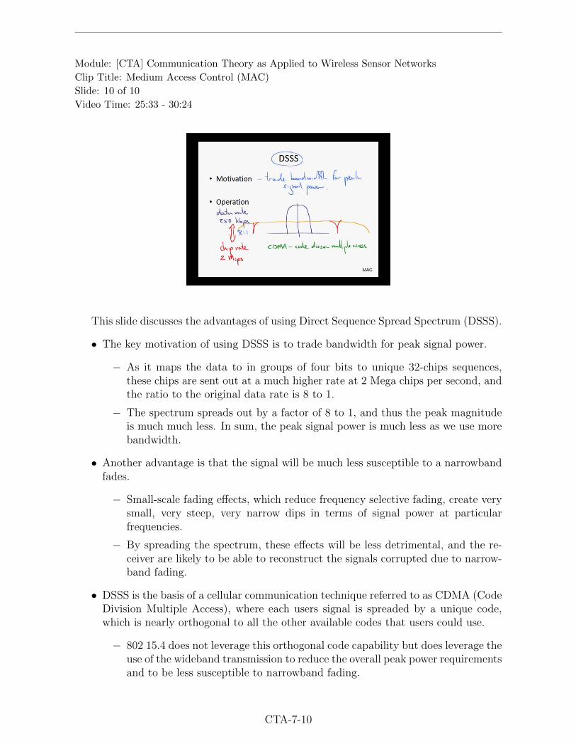
Module: [CTA] Communication Theory as Applied to Wireless Sensor Networks
Clip Title: Medium Access Control (MAC)
Slide: 10 of 10
Video Time: 25:33 - 30:24
This slide discusses the advantages of using Direct Sequence Spread Spectrum (DSSS).
• The key motivation of using DSSS is to trade bandwidth for peak signal power.
− As it maps the data to in groups of four bits to unique 32-chips sequences,these chips are sent out at a much higher rate at 2 Mega chips per second, andthe ratio to the original data rate is 8 to 1.
− The spectrum spreads out by a factor of 8 to 1, and thus the peak magnitudeis much much less. In sum, the peak signal power is much less as we use morebandwidth.
• Another advantage is that the signal will be much less susceptible to a narrowbandfades.
− Small-scale fading effects, which reduce frequency selective fading, create verysmall, very steep, very narrow dips in terms of signal power at particularfrequencies.
− By spreading the spectrum, these effects will be less detrimental, and the re-ceiver are likely to be able to reconstruct the signals corrupted due to narrow-band fading.
• DSSS is the basis of a cellular communication technique referred to as CDMA (CodeDivision Multiple Access), where each users signal is spreaded by a unique code,which is nearly orthogonal to all the other available codes that users could use.
− 802 15.4 does not leverage this orthogonal code capability but does leverage theuse of the wideband transmission to reduce the overall peak power requirementsand to be less susceptible to narrowband fading.
CTA-7-10
Module: [CTA] Communication Theory as Applied to Wireless Sensor Networks
Clip Title: Sychronization, Trade-off Study and Module Conclusion
Slide: 1 of 11
Video Time: 00:00 - 00:09
This slide lists the main points of the clip
• Synchronization
• Synthesis: The Energy/Bandwidth Tradeoff
• Module Conclusions
CTA-8-1

Module: [CTA] Communication Theory as Applied to Wireless Sensor Networks
Clip Title: Sychronization, Trade-off Study and Module Conclusion
Slide: 2 of 11
Video Time: 00:10 - 02:42
This slide motivates the use of synchronization and gives an overview of the two scalesof synchronization used in networks.
• The key motivation of doing synchronization is to schedule activities so that com-munication can be efficiently conducted
− we need to ensure that activities are scheduled to make best use of their energyand thus on times need to coincide.
• Synchronization needs to occur on multiple scales:
− At the gross scale (without much accuracy), it is to to ensure nodes are on atthe same time.
− At the fine scale it is for accurate communication, particularly to ensure thatthe data is being received correctly.
CTA-8-2

Module: [CTA] Communication Theory as Applied to Wireless Sensor Networks
Clip Title: Sychronization, Trade-off Study and Module Conclusion
Slide: 3 of 11
Video Time: 02:43 - 05:48
This slide discusses the three operational states of nodes, and how they can be sched-uled.
• There are three states we want our sensor nodes to operate.
1. Sleeping. The node is not participating in the network’s mission.
2. Listening. The node is ascertaining the status of the network to collect infor-mation as whether to move to a higher state or to back off to sleep state.
− The node can “probe” in this state. It may send out messages and collectresponses to determine the next action.
3. Transmitting. This is also called the active state. The node is fully participat-ing in the network’s mission.
• These three activities will need to be scheduled through the programs built into thenodes or coordination with other nodes in the network.
• Another aspect is scheduling is topology control. The basic idea is that not all nodesneed to participate to achieve the mission objective of the network.
− Some nodes will basically be in a extended sleep state. They will only comeonline as other nodes in the network fail.
CTA-8-3

Module: [CTA] Communication Theory as Applied to Wireless Sensor Networks
Clip Title: Sychronization, Trade-off Study and Module Conclusion
Slide: 4 of 11
Video Time: 05:49 - 11:13
This slide describes a simple scheme for sleep scheduling in a distributed network,called S-MAC, in which the network is partitioned in to virtual clusters, and sleep sched-ules are autonomously developed within each cluster. This scheme is illustrated with asimple case with two clusters as shown in the figure.
• Within each cluster, the nodes will be on where the “X” symbols are along the timeline. These on times are synchronized.
− The node may be listening for a another node to be transmitting and willadjust the clock accordingly or take the initiative to send out transmissions tosynchronize with its neighbors.
• The nodes within each virtual cluster are synchronized in the way described above.In order to get a fully connected network, different clusters are bridged via boundarynodes, which are on at the union of the on times of both clusters.
• In sum, the key aspects are periodic sleep cycles and virtual clusters that synchro-nize.
• There remain some problems:
− The boundary nodes are a lot more active than other nodes in the network,using energy at at a higher rate and thus having a shorter life. Their failureswould lead to difficulties of maintaing the connectivity of the whole network.
− It remains a issue how to adjust the period to meet the requirement of capturingthe phenomena of interest, and once one node is adjusted, how to get the othersnodes to synchronize with it.
CTA-8-4

Module: [CTA] Communication Theory as Applied to Wireless Sensor Networks
Clip Title: Sychronization, Trade-off Study and Module Conclusion
Slide: 5 of 11
Video Time: 11:14 - 14:53
This slide introduces several synchronization techniques to guarantee effective com-munication.
• The first level of synchronization is with the carrier, which is to ensure that thereceipts carrier is coherent in frequency and phase within the incoming signal.
− These operations are performed by phase locked loop installed in the receiverhardware.
• The second level of synchronization is bit/symbol cyclization, using additional bitsto signal the incoming of information.
− Here, start/stop edges are used. In particular, special strings of bits are usedinstead of pure ones or zeros to signal the start/ends.
• The final level is frame synchronization, for the nodes to ascertain where the infor-mation stream begins.
− Here, we use Start Frame Delimiter (SFD), which is a known sequence. Whenthe receiver node sees this string of bits and recognizes that at the end of it, itis ready to receive the actual data.
CTA-8-5

Module: [CTA] Communication Theory as Applied to Wireless Sensor Networks
Clip Title: Sychronization, Trade-off Study and Module Conclusion
Slide: 6 of 11
Video Time: 14:54 - 19:13
This slide puts multiple components that have been introduced together and uses adiagram to show how they are integrated to form a communication system for a sensornetwork.
• The observed phenomena are captured by transducer to yield the signal m(t).
• The signal m(t) is converted to a bit stream through A/D process, with techniqueslike pulse code modulation (PCM).
• Source coding is used to compress the bits, such that transmitter can be on lesstime, saving energy.
• Channel coding is then used, which adds additional bits but in a smart way, to makeit robust to channel affects.
• The encoded signals are then sent off to the channel, which may be subject to fadingeffects.
• These activities are coordinated through scheduling and medium access control(MAC).
CTA-8-6

Module: [CTA] Communication Theory as Applied to Wireless Sensor Networks
Clip Title: Sychronization, Trade-off Study and Module Conclusion
Slide: 7 of 11
Video Time: 19:14 - 24:17
This slide uses M-ary signaling and channel coding as two examples to demonstratethe energy/bandwidth trade-off in wireless communication systems.
• M-ary signaling enables one to send more than one bit at a time, but requires morepower.
− Compare the constellations of QPSK and 8PSK. In QPSK, each symbol rep-resents 2 bits, and in 8PSK, each symbol represents 3 bits. 8PSK can reducethe overall bandwidth needs by two thirds over QPSK.
− The gaps between the consolation points in 8 PSK are much more close thanthose between QPSK. In order to achieve equal gap in both methods, one hasto increase the power in 8PSK, moving the constellation points out to thesefurther locations, as illustrated by the top figures.
• In channel coding, the trade-off is switched.
− In channel coding, redundant bits are added, and thus outgoing data rate aswell as the overall bandwidth have to increase.
− The benefit is that the bit error rate for the same amount of energy could besignificantly reduced, which puts the BER curves to the lower left.
These are two traditional arguments for trading energy and bandwidth, the M-ary signaling is using more energy and less bandwidth, and in channel coding, thereverse is the case.
CTA-8-7

Module: [CTA] Communication Theory as Applied to Wireless Sensor Networks
Clip Title: Sychronization, Trade-off Study and Module Conclusion
Slide: 8 of 11
Video Time: 24:18 - 26:25
This slides discusses another bandwidth/energy trade-off: whether to employ a singleor multi-hop network.
• In multi-hop network, data is sent over multiple short links to the data sink, whilea single hop network would send data directly from the source to the sink.
• The energy requirement for the single hop case would be significant for these veryremote nodes as opposed to the lower energy draw from multiple nodes.
• The multi-hop transmissions need sufficient bandwidth to be successful, that is amulti-hop network puts a greater load on the channel while a single hop work puta greater load on a node’s energy.
• If the distance between the source and sink is too large, single hop would not work,the question becomes whether to use lot of really short hops or to make fewer butgreater longer hops.
CTA-8-8

Module: [CTA] Communication Theory as Applied to Wireless Sensor Networks
Clip Title: Sychronization, Trade-off Study and Module Conclusion
Slide: 9 of 11
Video Time: 26:26 - 28:43
This slide discusses another scenario that demonstrates the trade-off between band-width and energy, which contrasts the sink polling for data as opposed to sensor is pushingdata to the sink.
• In the polling case, the sink requests data from particular nodes in a coordinatedfashion, and nodes have to be expending energy to listen.
• In the pushing case, the source nodes that have information simply transmit it tothe sink. This is uncoordinated and thus it requires more bandwidth as opposed inpolling.
• In summary, with polling, source nodes have to expand more energy by listeningregularly. With pushing, more bandwidth is required due to the fact that thetransmission is uncoordinated.
CTA-8-9

Module: [CTA] Communication Theory as Applied to Wireless Sensor Networks
Clip Title: Sychronization, Trade-off Study and Module Conclusion
Slide: 10 of 11
Video Time: 28:44 - 31:14
This slide concludes our module on communication theory for wireless sensor networks([CTA]) by summarizing several key points.
• Digital communication approaches to sensor networks have advantages in terms ofrobustness, energy and bandwidth performance over analog approaches.
• Employing source coding, that is compressing the number of bits that need to sendacross channel, reduces our overall energy requirements.
• Channel coding schemes improve overall data reliability by minimizing the need forretransmission. MAC and routing strategy should be designed appropriately for thenetworks.
• As the nodes in sensor networks tend to operate at very low duty cycles, synchro-nization is necessary.
• Finally, the integration of all these techniques is what enables a network to operateeffectively and efficiently.
CTA-8-10

Module: [CTA] Communication Theory as Applied to Wireless Sensor Networks
Clip Title: Sychronization, Trade-off Study and Module Conclusion
Slide: 11 of 11
Video Time: 31:15 - 31:44
More materials are available from the textbooks and papers listed in this slide.
• B. Lathi. Modern Analog and Digital Communication Systems, 3rd edition. Oxford,1998.
• B. Krishnamachari. Networking Wireless Sensors. Cambridge Press, 2005.
• J. Frolik. Implementation Handheld, RF Test Equipment in the Classroom and theField. IEEE Transaction on Eduation, Vol 50, No 3, August 2007.
CTA-8-11

Module: [RFH] RF Hardware
Clip Title: Introduction
Slide: 1 of 3
Video Time: 00:00 - 00:39
This slide introduces what will be covered in the [RFH] module on radio frequencyhardware. The module will discuss in detail two topics:
• The RF block diagram that is typical of the transceivers used in wireless sensornodes
• Many of the RF components and devices that are part of the block diagram
RFH-2-1

Module: [RFH] RF Hardware
Clip Title: Introduction
Slide: 2 of 3
Video Time: 00:40 - 03:52
This slide illustrates how the module on radio frequency hardware is linked to othermodules in the course, in particular those on the wireless communications channel (WCC),analog-to-digital conversion (ADC), transducers (TDX) and the sensor network architec-ture (SNA).
As one of the primary parts of a transmitter or receiver, the RF hardware plays animportant role in defining the overall sensor network architecture:
• In terms of wireless sensor networks, RF hardware interfaces between the sensornode and the wireless channel
• Within the sensor node, RF components may directly connect to various transduc-ers, or interface to the transducers through some form of analog to digital conversion.
RFH-1-2

Module: [RFH] RF Hardware
Clip Title: Introduction
Slide: 3 of 3
Video Time: 03:53 - 06:37
This slide discusses briefly how the RF hardware is related to systems thinking andhow this hardware fits into the overall scheme of the sensor network architecture.
• As part of the radio link, the RF hardware is a key part of the sensors that makeup the sensor cloud
• Within each of the sensors, the RF hardware design is especially important to theenergy budget since the power amplifiers that are used in the transmitters canconsume large fraction of the node’s overall energy.
• Wireless propagation environment and the distance between sensor nodes have animpact on the size and power consumption of the power amplifiers.
• Sensing mission and embedding environment also impact the radio design in termsof its size, operational frequency, and cost.
RFH-1-3

Module: [RFH] RF Hardware
Clip Title: Overview & Block Diagrams
Slide: 1 of 11
Video Time: 00:00 - 01:02
This slide introduces three main objectives in this first clip on radio design:
• Understand the performance requirements of each component in the RF block dia-gram, these requirements are linked to the communication systems analysis.
• Understand the design and technology challenges for each of the components in theblock diagram.
• Describe implications on the RF design due to various types of scaling, such as size,frequency, cost, power, data rate and so forth. These implications influence thewireless sensor networks design.
RFH-2-1

Module: [RFH] RF Hardware
Clip Title: Overview & Block Diagrams
Slide: 2 of 11
Video Time: 01:03 - 01:57
This slide shows the outline for the different clips that are in the [RFH] module:
• Overview and RF Block Diagram
• Four topics that cover various the components:
− Filters
− Amplifiers
− Up/Down Conversion and that basically means looking at mixers
− Oscillators and Synthesizers
• Four topics that are on the system level:
− Modulation Basics
− Antennas
− Chip-Level Radios
− Integration and Packaging
RFH-2-2

Module: [RFH] RF Hardware
Clip Title: Overview & Block Diagrams
Slide: 3 of 11
Video Time: 01:58 - 03:15
This slide presents an overview of radio design and the RF block diagram, with anemphasis on the RF analog hardware. This clip will be covering the following points:
• Functional view of the radio, i.e. the performance specifications that apply to theradio as a subsystem.
• RF analog hardware
• Different diagram representation and requirements
• Different design and architecture issues
• Future radio design technology
RFH-2-3

Module: [RFH] RF Hardware
Clip Title: Overview & Block Diagrams
Slide: 4 of 11
Video Time: 03:16 - 04:10
Following the overview, this slide first elaborates on the functional view of the radio. Itdefines the term RF analog subsystem and discusses multiple perspectives of the system.
• RF analog subsystem: refers to the parts of the wireless system that link the infor-mation (data) and the channel (the medium between two wireless devices)
• Multiple perspectives of the RF analog system:
− High level: how information is processed and what analog hardware is required.
− Mid level: breaks the analog portion into different components (e.g. filters,amplifiers) and shows how they all fit together.
− low level: design of each component, a discussion that is the subject of otherclips in the [RFH] module.
RFH-2-4

Module: [RFH] RF Hardware
Clip Title: Overview & Block Diagrams
Slide: 5 of 11
Video Time: 04:11 - 05:50
This slide illustrates the different steps in the information processing sequence. Theanalog block diagram contains five components:
• Baseband digital signal: zeros and ones sequence that captures the information.
• RF transmitter (analog devices): up-converts the baseband signal to a RF carrierand transmits the signal to the receiver through the channel.
• Channel: the signal is injected into the channel via the antenna and retrieved fromthe channel with a second antenna at the receiver.
• RF receiver (analog devices): reverses the process in RF transmitter.
• Baseband digital signal: the data is extracted
RFH-2-5

Module: [RFH] RF Hardware
Clip Title: Overview & Block Diagrams
Slide: 6 of 11
Video Time: 05:51 - 08:19
This slide shows an expanded view of part of the analog demodulator section, specifi-cally the part that receives the signal from the channel and down converts the signal fromthe RF carrier frequency to an intermediate or lower frequency. This slide illustrates theprocess of demodulation and heterodyne.
• Amplification stage
• Heterodyne (mixing or down conversion) stage
• Detection stage
RFH-2-6

Module: [RFH] RF Hardware
Clip Title: Overview & Block Diagrams
Slide: 7 of 11
Video Time: 08:20 - 10:50
This slide further details the block diagram for the RF analog receiver in the previousslide and compare it with the block diagram for the transmitter. The RF analog blockdiagram contains the following components in a sequence as:
• antenna
• band select filter
• low noise amplifier (LNA)
• image reject filter
• mixer and a local oscillator
• channel select filter
• IF amplifier
Comparing with the receiver block diagram, the block diagram for the transmitter basi-cally performs the same steps in the opposite order. There are only a few differences:
• the LNA will be replaced by a power amplifier (PA)
• the band select filter is moved before the power amplifier and no further filteringafter the power amplifier and before the antenna.
RFH-2-7

Module: [RFH] RF Hardware
Clip Title: Overview & Block Diagrams
Slide: 8 of 11
Video Time: 10:51 - 11:47
This slide shows a representative block diagram for a transceiver, which combinesboth transmit and receive functions. In this analog block diagram, there are severalpoints worth noting:
• The receiver path on the top is essentially the same as the diagram on the previousslide, except that two mixers are being used.
• This receiver is called the IQ receiver where I is for the in phase signal and Q is forthe quadrature phase signal.
• This diagram indicates the point where the analog and digital portions meet.
• The local oscillator signal (LO) can be shared between the receiver and transmitterportions of the radio.
RFH-2-8

Module: [RFH] RF Hardware
Clip Title: Overview & Block Diagrams
Slide: 9 of 11
Video Time: 11:48 - 14:08
This slide introduces the radio design technologies including board level design andchip level design. It also discusses some aspects of radio architecture that the designersneed to consider.
• Most radios today are of a hybrid or board level design:
− Radios contain many discrete devices (oscillators, amplifiers, mixers, filters,capacitors and so forth), which are all typically surface mounted devices.
− These devices are bonded to a printed circuit board and connected using signaltraces.
− The printed circuit boards usually have multiple layers including a DC powerlayer.
• A more advanced technology is the chip level radio, it’s a very promising approachfor small radios.
− All or most of the components are built into a silicon wafer, including all ofthe analog and digital parts.
− This chip can be packaged into a plastic and integrated into a larger system
− The downside of this technology:
· It’s expensive to develop each radio
· Once the chip is designed, it’s very application-specific
• The issues of architecture design:
− Down-conversion approaches: Single, Dual, Zero
− Multi-band (e.g. they need to work world-wide)
− Multi-channel (e.g. receivers on space satellites)
RFH-2-9

Module: [RFH] RF Hardware
Clip Title: Overview & Block Diagrams
Slide: 10 of 11
Video Time: 14:09 - 14:57
This slide discusses the front end of a software defined radio (SDR).
• All devices are digital except for the antennas and power amplifiers
• Requirements of this approach:
− extremely high-speed, high-performance analog to digital (A/D) and digital toanalog (D/A) converters, which often have a high DC power draw
Advantage of this approach
− nearly the entire radio can be redefined through software modifications
RFH-2-10

Module: [RFH] RF Hardware
Clip Title: Overview & Block Diagrams
Slide: 11 of 11
Video Time: 14:58 - 15:47
This slide concludes the overview and block diagram section:
• RF analog hardware links the data/information and wireless channel
• Functional and then component-level block diagrams are the starting points forradio design
• By using the block diagram that defines the particular architecture for the radio,system designers can then determine the specifications for each of the components.
RFH-2-11

Module: [RFH] RF Hardware
Clip Title: Filters A
Slide: 1 of 10
Video Time: 00:00 - 00:39
This slide provides an overview that what this clip will be covering:
• Different filter characteristics and types
− low pass filter
− high pass filter
− band stop filter
• Difference among filter technologies
− surface acoustic wave (SAW) filter
− planar filter
− lumped element filter
• Filter performance on communication system design
RFH-3-1

Module: [RFH] RF Hardware
Clip Title: Filters A
Slide: 2 of 10
Video Time: 00:40 - 01:42
This slide provides an outline of this clip - Filters, the main points are listed as below:
• Overview of some general considerations for filter design performance
• Performance parameters
• Filter technologies and considerations
• Design process for discrete element filter
• Simulation techniques (CAD tools)
• Advanced filter technologies (BAW, MEMS)
• Impact of filter performance on system design
RFH-3-2

Module: [RFH] RF Hardware
Clip Title: Filters A
Slide: 3 of 10
Video Time: 01:43 - 04:58
This slide introduces the various functions filters perform in wireless system, using atypical wireless receiver block diagram. It also discusses the challenges and significanceof filter design and performance.
• The functions filters perform:
− keeping unwanted signals out of the receiver (noise, harmonics, mixing prod-ucts)
− separating DC and high-frequency signals
• The components and their functions in a typical wireless receiver:
− Antenna: receives the RF signal
− Band select filter: selects the signal of interest within a bandwith
− Amplifier: amplifies the signal
− Image reject filter: removes the image frequency
− Mixer: the signal is mixed with the local oscillator signal (LO) and downconverted to the intermediate frequency (IF)
− Channel select filter: selects the IF signal and rejects the other mixing product
− IF amplifier: amplifies the IF signal
• The significance of filter design and performance:
− the overall cost, size, and performance of a wireless system is highly dependenton the characteristics of its filters
− filter performance can impact the entire system design in terms of communi-cation range, data rate and carrier frequency
RFH-3-3

Module: [RFH] RF Hardware
Clip Title: Filters A
Slide: 4 of 10
Video Time: 04:59 - 08:20
This slide uses a plot to illustrate how filter performance is characterized. This plotshows a comparison between a simulated and measured 20 GHz band-pass filter. Thered curves are the simulated response, and the blue curves are the measured response.Observations about this plot are listed as follows:
• The S parameters are showed in dB
• S21: transmission parameter
− increases in the pass-band, the transmission is increasing
− decreases in the stop-band, the transmission is decreasing
• S11: reflection parameter, which does basically the opposite of S21.
− decreases in the pass-band, less reflection occurs
− is close to zero dB in stop-band, as most of the signal is being reflected
• In comparing the simulated response S21 with the measured response S21, there issome attenuation occurring in the transmitted signal and that happens because ofloss in the filter.
• There is a secondary peak in S21 outside of the pass-band, which is the parasiticpass-band that the filter designer needs to deal with.
RFH-3-4
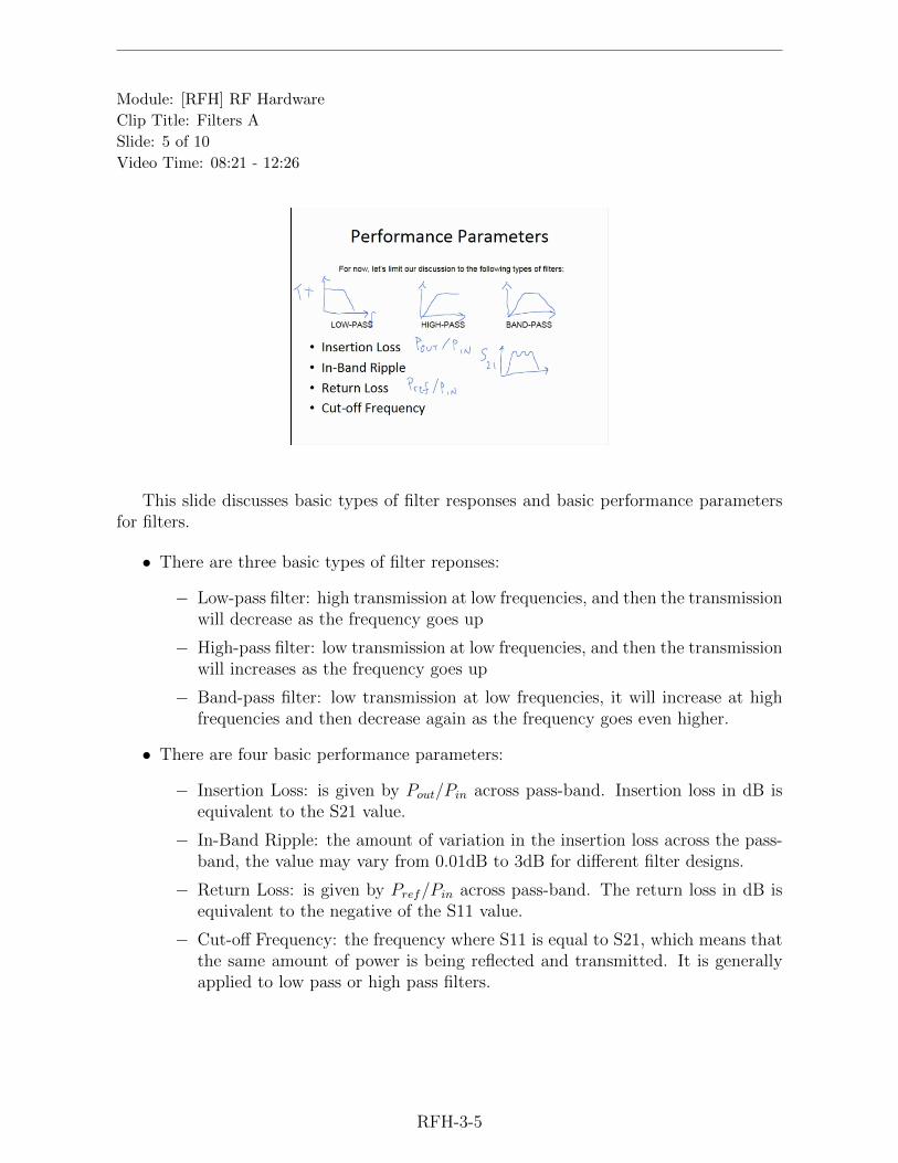
Module: [RFH] RF Hardware
Clip Title: Filters A
Slide: 5 of 10
Video Time: 08:21 - 12:26
This slide discusses basic types of filter responses and basic performance parametersfor filters.
• There are three basic types of filter reponses:
− Low-pass filter: high transmission at low frequencies, and then the transmissionwill decrease as the frequency goes up
− High-pass filter: low transmission at low frequencies, and then the transmissionwill increases as the frequency goes up
− Band-pass filter: low transmission at low frequencies, it will increase at highfrequencies and then decrease again as the frequency goes even higher.
• There are four basic performance parameters:
− Insertion Loss: is given by Pout/Pin across pass-band. Insertion loss in dB isequivalent to the S21 value.
− In-Band Ripple: the amount of variation in the insertion loss across the pass-band, the value may vary from 0.01dB to 3dB for different filter designs.
− Return Loss: is given by Pref/Pin across pass-band. The return loss in dB isequivalent to the negative of the S11 value.
− Cut-off Frequency: the frequency where S11 is equal to S21, which means thatthe same amount of power is being reflected and transmitted. It is generallyapplied to low pass or high pass filters.
RFH-3-5

Module: [RFH] RF Hardware
Clip Title: Filters A
Slide: 6 of 10
Video Time: 12:27 - 16:29
Following the previous slide, this slide discusses a few more performance parameters.
• Bandwidth: is given by ∆f/f0, where ∆f is the frequency span between the lowerand upper cutoff frequencies in a band-pass response, f0 is the center frequency. Itapplies to the band-pass filters.
• Out-of Band Rejection: is specified at a certain absolute or relative offset frequencyfrom the center or edge of the pass-band, and that indicates how much attenuationis occurring at that point.
• Group Delay: is given by dθ/dω, where θ is the phase angle of S21.
− A constant group delay versus frequency is often desirable since it means thatthe different frequency components of the broadband signal will all have thesame time delay when they pass through the filter, otherwise it can lead todistortion of the wideband signal.
• Power Handling: how much power the filter can handle without being destroyed
RFH-3-6
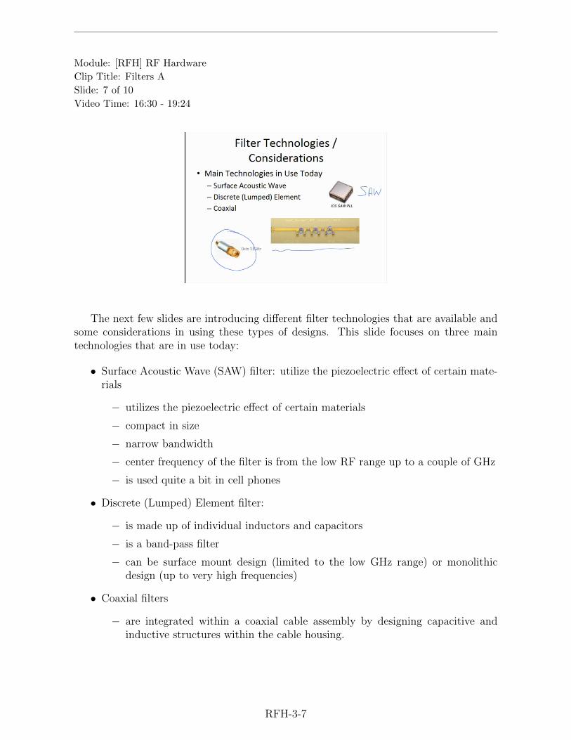
Module: [RFH] RF Hardware
Clip Title: Filters A
Slide: 7 of 10
Video Time: 16:30 - 19:24
The next few slides are introducing different filter technologies that are available andsome considerations in using these types of designs. This slide focuses on three maintechnologies that are in use today:
• Surface Acoustic Wave (SAW) filter: utilize the piezoelectric effect of certain mate-rials
− utilizes the piezoelectric effect of certain materials
− compact in size
− narrow bandwidth
− center frequency of the filter is from the low RF range up to a couple of GHz
− is used quite a bit in cell phones
• Discrete (Lumped) Element filter:
− is made up of individual inductors and capacitors
− is a band-pass filter
− can be surface mount design (limited to the low GHz range) or monolithicdesign (up to very high frequencies)
• Coaxial filters
− are integrated within a coaxial cable assembly by designing capacitive andinductive structures within the cable housing.
RFH-3-7

Module: [RFH] RF Hardware
Clip Title: Filters A
Slide: 8 of 10
Video Time: 19:25 - 22:53
This slide introduces two other filter technologies: Ceramic filters and Planar filters.
• Ceramic filters
− multi-GHz frequency range
− inexpensive
− are constructed using one or more resonators that are one quarter to one halfwavelength in size
− low loss
− stable temperature
− are applied in consumer applications such as cell phones and other wirelesslocal area network applications
• Planar filters
− low cost (the least inexpensive type of filter)
− can operate on a frequency up to hundreds of GHz
− high loss
RFH-3-8

Module: [RFH] RF Hardware
Clip Title: Filters A
Slide: 9 of 10
Video Time: 22:54 - 23:28
This slide introduces one more filter technology that is in use today - Waveguide filter,which has the following attributes:
• low loss
• can be designed to handle very large amounts of power
• is applied in high-powered radars, large radio transmitters and similar applicationswhere weight and cost are not an issue, but high power levels are required
• big and bulky
• relatively expensive
RFH-3-9

Module: [RFH] RF Hardware
Clip Title: Filters A
Slide: 10 of 10
Video Time: 23:29 - 25:31
To summarize the differences between the filter technologies and their main attributes,this slide shows two plots to give a qualitative comparison between loss and size, as wellas loss and cost.
• Comparison between loss and size (on the left-hand side)
− General trend: as the size increases, the loss decreases
− SAW filters tend to have the most compact design and the greatest amount ofloss
− Waveguide filters tend to have the largest size and lowest amount of loss
• Comparison between loss and cost (on the right-hand side)
− General trend: lower loss, higher cost
− Waveguide filter tend to be the most expensive type of design
− Planar filter tend to be the most inexpensive type of technology
RFH-3-10

Module: [RFH] RF Hardware
Clip Title: Filters B
Slide: 1 of 10
Video Time: 00:00 - 01:27
The next several slides are focusing on filter design methods. This slide discusses the“Two-Step” process to design filters for RF and microwave application.
• Two Step Process
− Design
· assumes ideal capacitors and inductors based on discrete or lumped ele-ment filters
· the design process is well documented and relatively straightforward
− Implementation
· actual filter technology may be different from the ideal design method
· the capacitor and inductor values from design phase may not be practical
· the resulting filter response by implementation only resembles the originalor ideal response to a certain degree
RFH-4-1

Module: [RFH] RF Hardware
Clip Title: Filters B
Slide: 2 of 10
Video Time: 01:28 - 02:15
In this slide we see how a design is implemented in two different ways. As shown inthe schematic in the upper left, the circuit topology and the ideal inductor and capacitorvalues are determined in the design process. This schematic can be implemented eitheras a discrete filter or as a planar filter, as long as the implementation has the same orsimilar electrical response as the design.
• A discrete filter (on the left)
− has physical resemblance to the original schematic
• A planar filter (on the right)
− has no physical resemblance to the original schematic but is electrically equiv-alent
RFH-4-2

Module: [RFH] RF Hardware
Clip Title: Filters B
Slide: 3 of 10
Video Time: 02:16 - 03:24
This slide introduces how to design a filter and takes the low pass filter as an example.
• Need a circuit that allows low frequency signals to pass but blocks while high-frequency signals
• Frequency selective device by using elements with frequency-dependent impedances:
− inductors
− capacitors
• two solutions to get a low pass response:
− design the device to have a series impedance that changes from low to high asfrequency increases, this can be realized using a series inductor
− design the device to have shunt impedance that changes from high to low asfrequency increases, this can be realized using a shunt capacitor
RFH-4-3

Module: [RFH] RF Hardware
Clip Title: Filters B
Slide: 4 of 10
Video Time: 03:25 - 04:58
This slide details the shunt capacitor solution for low pass filter. It analyzes thecharacteristics of the shunt capacitor circuit with the illustration of its schematic and theplot of its impedance as a function of frequency.
• Low frequency response:
− at low frequency, the impedance is very high
− the shunt capacitor appears as an open circuit and the signal can pass fromthe input to the output
• High frequency response:
− at high frequency, the impedance is very small
− the shunt capacitor could be approximated as a short-circuit in which the signalwill be reflected back to the input
RFH-4-4

Module: [RFH] RF Hardware
Clip Title: Filters B
Slide: 5 of 10
Video Time: 04:59 - 06:24
This slide discusses higher order filters that provides more freedom to design an ap-propriate filter response. It introduces the requirements for designing the higher orderfilter and the most common filter design approach.
• In order to realize more complex responses, the following are needed:
− More elements (inductors and capacitors)
− Some methods to determine the value of each element
• The most common filter design approach is insertion loss method
− A mathematical function is selected that yields the desired filter response
− An equation for the insertion loss of the selected filter topology is generated
− The equation is forced to fit the mathematical function by selecting the propervalues of each of the elements
RFH-4-5

Module: [RFH] RF Hardware
Clip Title: Filters B
Slide: 6 of 10
Video Time: 06:25 - 07:26
Two very common mathematical functions that are used for the insertion loss methodof filter design are the Butterworth and Chebyshev functions. This slide shows a symbolicrepresentation of the Butterworth design and its frequency response.
• N = 5: fifth order design
• FP = 1000 MHz: cutoff frequency is 1 GHz (S11 = S21)
• The frequency response has a smooth shape: these filters are also called maximallyflat
• Blue trace: the reflection coefficient (S11)
• Pink trace: the transmission coefficient (S21)
• At 2 GHz the S21 has fallen to approximately -30 dB
RFH-4-6

Module: [RFH] RF Hardware
Clip Title: Filters B
Slide: 7 of 10
Video Time: 07:27 - 08:56
This slide discusses the response characteristic of Chebyshev filter and compares itwith Butterworth filter.
• Features of Chebyshev response:
− N = 5: fifth order design
− FP = 1000 MHz: cutoff frequency is 1 GHz
− AP = 1 dB: the in band ripple is 1 dB
− Return loss (S21) has noticeable ripple in the pass-band and relative higherattenuation
− At 2 GHz the S21 has fallen to approximately −45 dB
• Comparison between Chebyshev filter and Butterworth filter:
− Compare with Butterworth response, Chevyshev response gets more out ofband attenuation at the expense of more in band ripple
− Both filters are fifth order but the L and C component values are different
RFH-4-7

Module: [RFH] RF Hardware
Clip Title: Filters B
Slide: 8 of 10
Video Time: 08:57 - 10:16
After completing the basic design phase, the more typical and difficult phase is toimplement the design. This slide discusses the main issues of filter design implementation.
• If a lumped element filter is being built, the implementation from the electricalschematic to the printed circuit board layout is relatively straightforward.
• If an alternative topology is being built (e.g. planar filter), the response of the LCcircuit needs to be mapped into the new type of filter.
• It’s possible to transform in a fairly straightforward way the low pass response andschematic to those for high pass, band-pass and band stop filters.
RFH-4-8

Module: [RFH] RF Hardware
Clip Title: Filters B
Slide: 9 of 10
Video Time: 10:17 - 11:55
Filters are a critical part of communication system and researchers are continuallylooking for better solutions. This slide introduces three state-of-the-art approaches forfilter design.
• Bulk Acoustic Wave (BAW) Filters
− similar to Surface Acoustic Wave (SAW) filters in that using piezoelectric ma-terial
− zinc oxide is used in this design
− the center frequency depends mainly on the thickness of the zinc oxie material
• MEMS Vibrating Filters
− involve an electrical to mechanical transduction
− extremely narrow band response can be obtained
• Micromachined Filters
− small filter structures can be created using materials such as silicon with ex-tremely high precision
− can be scaled to millimeter wave frequencies
RFH-4-9

Module: [RFH] RF Hardware
Clip Title: Filters B
Slide: 10 of 10
Video Time: 11:56 - 12:37
This slide summarizes the filter topic as follows:
• Filters are important to radio systems and thus to overall wireless system
• Goals of filter design:
− Select the desired frequency range from all incident electromagnetic energy
− Reject unwanted signals that may come from inside or outside the radio
• The most difficult part of the process is often the implementation phase
• Many different methods for implementation exist and new ones are always beinginvestigated
• The goals for performance usually push the limits on filter size and cost
RFH-4-10

Module: [RFH] RF Hardware
Clip Title: Amplifiers
Slide: 1 of 18
Video Time: 00:00 - 01:14
This clip covers low noise and high-power RF amplifiers that are typical of wirelesscommunication systems. This slide gives an outline.
• Examples of amplifiers and their performance parameters
• Design and technology issues
• In the process of designing an amplifier, designers need to make trade-offs betweensuch things as:
− Gain efficiency
− Bandwidth
− Linearity
• Impact of amplifiers on system design
RFH-5-1

Module: [RFH] RF Hardware
Clip Title: Amplifiers
Slide: 2 of 18
Video Time: 01:15 - 01:38
This slide reviews the block diagram that was previously shown in the [RFH] moduleoverview. As pointed out in the diagram, there are two different types of amplifiers thatare of interest:
• Low noise amplifiers (LNA): in the receive chain
• Power amplifiers (PA): in the transmit chain
RFH-5-2

Module: [RFH] RF Hardware
Clip Title: Amplifiers
Slide: 3 of 18
Video Time: 01:39 - 03:50
This slide discusses an example of a coaxial low noise amplifier (LNA). Some importantfeatures and electrical specifications of this particular LNA (Mini Circuits ZEL 1724LN)are pointed out as follows:
• Features
− Low noise figure
− Wideband performance
• Electrical specifications
− Gain: 20 dB
− Maximum Power: 8 dBm at the 1dB compression point
− Intercept point: 22 dB
− DC power: 1 W
• Discussion
− The efficiency of this amplifier is low however this is not a major concernbecause the total DC power is relatively low
− A higher intercept means higher linearity or lower harmonic output (i.e. lowerdistortion)
RFH-5-3

Module: [RFH] RF Hardware
Clip Title: Amplifiers
Slide: 4 of 18
Video Time: 03:51 - 04:50
This slide introduces a coaxial PA which has different purpose compared with an LNA.
• High power
• DC consumption: 24 V and 5 A or 120 Watts
• Efficiency is less than 10%
• Wide bandwidth
• Useful as a laboratory instrument due to its versatility but not desirable for RFinstallation because of its low efficiency
RFH-5-4

Module: [RFH] RF Hardware
Clip Title: Amplifiers
Slide: 5 of 18
Video Time: 04:51 - 05:57
This slide introduces a small packaged LNA that would be appropriate for the boardlevel radio design. Along with the functional block diagram, the features, selected speci-fication, and applications of this small packaged LNA are described.
• Small size: 1.3 x 2.0 x 0.4 mm
• Operational voltage: 3 volts (work with the battery-operated device)
• Input power: -13 dBm at the 1 dB compression point
RFH-5-5

Module: [RFH] RF Hardware
Clip Title: Amplifiers
Slide: 6 of 18
Video Time: 05:58 - 06:42
This slide shows another packaged PA that measures 3 x 3 mm. It lists selectedelectrical characteristics, primary application and key features. The following are someimportant features that are emphasized:
• Small size: 3 x 3 mm
• Usable frequency range: 1860 - 1910 MHz
• High Efficiency: 40%
• Upper output power: 28 dBm or 630 mW
• Primary application: mobile phone
• Power supply: 2.7 volts
RFH-5-6

Module: [RFH] RF Hardware
Clip Title: Amplifiers
Slide: 7 of 18
Video Time: 06:43 - 07:24
This slide shows a discrete field effect transistor (FET) that might be used in a lownoise amplifier. The chip measure is about 0.6 x 0.5 mm. In order to obtain an amplifierwith desired gain, noise figure, and impedance match, multiple FETs might be used alongwith impedance matching networks which are made up of inductors and capacitors.
RFH-5-7

Module: [RFH] RF Hardware
Clip Title: Amplifiers
Slide: 8 of 18
Video Time: 07:25 - 08:13
This slide introduces another device that is appropriate for a power amplifier design.Key features and typical packaging for this power device are shown in the slide.
• Device size: 1 x 2 mm, this PA is about seven times larger than that from theprevious slide that was appropriate for LNA
• Typical packaging: it has large flanges which carry high current levels and alsoefficiently transfer heat away from the device
• Matching networks would also be needed to complete the amplifier design.
RFH-5-8

Module: [RFH] RF Hardware
Clip Title: Amplifiers
Slide: 9 of 18
Video Time: 08:14 - 10:16
This slide reviews some basic issues related to designing amplifier in terms of designdrivers, main technologies, and other important issues.
• Design driver:
− Low Noise Amplifiers: Noise Figure, Gain, Linearity
− High Power Amplifiers: Efficiency, Output Power, Bandwidth, Linearity
• Semiconductor technologies
− Low Noise Amplifier: CMOS (Silicon), Bi-CMOS (Silicon and Germanium),GaAs
− High Power Amplifier: LDMOS (Silicon), MOSFET (GaN and GaAs)
• Other issues relevant to LNAs and PAs:
− Cost, Packaging, Wideband Performance
RFH-5-9

Module: [RFH] RF Hardware
Clip Title: Amplifiers
Slide: 10 of 18
Video Time: 10:17 - 11:51
PA efficiency is one of the critical performance parameters that designers are constantlytrying to improve. This slide shows a typical comparison of power amplifier efficiency ofdifferent devices using different wireless protocols.
• This particular comparison includes two results:
− Silicon LDMOS: Laterally diffused metal oxide semiconductor
− GaN: gallium nitride
• Two curves represents results for two wireless protocols:
− WCDMA: wideband code division multiple access
− OFDM: orthogonal frequency division multiplex
• The results show that the efficiencies are now exceeding the 50% barrier
RFH-5-10

Module: [RFH] RF Hardware
Clip Title: Amplifiers
Slide: 11 of 18
Video Time: 11:52 - 12:47
This slide runs through an overview of the amplifier design process. The following arethe basic steps of amplifier design:
• Prepare to compromise
• Select the transistors and other components
• Find the best computer-aided design (CAD) models available for the parts
• Select the DC operating condition
• Design appropriate input and output impedance matching networks
RFH-5-11
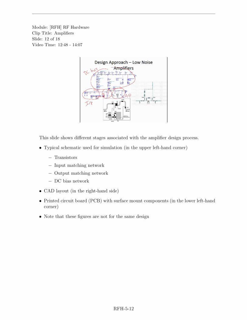
Module: [RFH] RF Hardware
Clip Title: Amplifiers
Slide: 12 of 18
Video Time: 12:48 - 14:07
This slide shows different stages associated with the amplifier design process.
• Typical schematic used for simulation (in the upper left-hand corner)
− Transistors
− Input matching network
− Output matching network
− DC bias network
• CAD layout (in the right-hand side)
• Printed circuit board (PCB) with surface mount components (in the lower left-handcorner)
• Note that these figures are not for the same design
RFH-5-12

Module: [RFH] RF Hardware
Clip Title: Amplifiers
Slide: 13 of 18
Video Time: 14:08 - 15:19
There is a good deal of compromise that is usually involved in amplifier design inorder to meet all of the various performance requirements. This slide lists the aspectsthat amplifier designers need to consider:
• Noise figure
• Gain
• Impedance match
• Bandwidth
For example: one must track noise figure for Impedance Match (or vice versa).
RFH-5-13

Module: [RFH] RF Hardware
Clip Title: Amplifiers
Slide: 14 of 18
Video Time: 15:20 - 16:14
After preparing for making compromises, the next thing is to select the devices thatwill be used for the design. This slide introduces what components the amplifier designerneeds to choose and what these choices are dependent on..
• Selecting the components
− Transistor/technology
− Passive components (inductors and capacitors used for the matching networks)
• Considerations for making the choice:
− Frequency performance
− Cost of the amplifier
RFH-5-14

Module: [RFH] RF Hardware
Clip Title: Amplifiers
Slide: 15 of 18
Video Time: 16:15 - 17:26
Today most designer uses computer-aided design (CAD) software for amplifier design,especially for RF applications. This slide discusses why CAD models are so important.
• Accurate models are needed in order to get an accurate prediction of amplifierperformance.
• The CAD approach can simulate accurate models which you can’t do with penciland paper, for example:
− representing parasitic effects which are non-ideal effects of the devices operatingin the non-linear region
− capturing the distributive effects of the interconnects
RFH-5-15

Module: [RFH] RF Hardware
Clip Title: Amplifiers
Slide: 16 of 18
Video Time: 17:27 - 18:43
This slide discusses how to select the operating conditions of the device and illustratesit by a schematic and a board layout.
• Use CAD tools to perform DC simulation and select the operating points including
− operating voltage
− operating current
• Aspects that influence the determination of the operating point:
− power supply (DC bias)
− gain
− noise figure
− etc
• These performance parameters ultimately impact the design of the matching net-works
RFH-5-16

Module: [RFH] RF Hardware
Clip Title: Amplifiers
Slide: 17 of 18
Video Time: 18:44 - 21:45
The design of the input and output matching networks comprises a bulk of the amplifierdesign process. This slide discusses the matching networks with figures and equations.
• The figure in upper left presents a schematic of matching networks including inputmatching network, output matching network and transistors
− The goal of input matching network: transform the 50Ω input terminationimpedance to ZS
− The goal of output matching network: transform the 50Ω output terminationimpedance to ZL
− ZS: the impedance that is presented to the base of the transistor
− ZL: the impedance that is presented to the collector
• ZS and the voltage reflection coefficient ΓS are related as follows:
ΓS =ZS − Z0
ZS + Z0
(1)
− Z0: reference impedance that is typically equal to 50Ω
− Each of the other impedance Zin, Zout and ZL also have corresponding voltagereflection coefficients which are given by similar equations with the change ofsubscripts.
• The importance of these reflection coefficients is that they determine the gain of theamplifier GT , as shown in lower left-hand equation:
− S21: transmission parameter or transmission coefficient for the transistor itself
− S22: output reflection coefficient of the transistor
• The figure in the lower right gives as an example what the input and output matchingnetworks look like when the design is finished
RFH-5-17

Module: [RFH] RF Hardware
Clip Title: Amplifiers
Slide: 18 of 18
Video Time: 21:46 - 22:42
This slide concludes this amplifier clip:
• System level requirements eventually flow down to amplifier specifications
• System designer should have a good understanding of different amplifier technolo-gies, as well as capabilities and limitations of each
• Two biggest impacts on the system design
− Communication range: transmitting higher power from the PA will increasethe range, LNA is equally important
− Battery life: PAs are one of the largest consumers of DC power in a sensornode
RFH-5-18

Module: [RFH] RF Hardware
Clip Title: Up/Down Conversion
Slide: 1 of 13
Video Time: 00:00 - 00:59
This slide presents a general overview of this clip on frequency up/down conversion:
• Functional requirements (system-level perspective)
• Typical mixer topology (RF subsystem block diagram, circuit level design)
• Nonlinear mixing process (mathematics, demonstration)
• Design and technology issues
• System-level implications
RFH-6-1

Module: [RFH] RF Hardware
Clip Title: Up/Down Conversion
Slide: 2 of 13
Video Time: 01:00 - 02:47
This slide shows a figure to illustrate the mixing or heterodyning process, in this casefor frequency down conversion in a receiver.
• Amplitude modulated RF carrier at frequency f1
• Local oscillator (LO) continuous wave signal at frequency f2
• These two signals are combined in the mixer which outputs a signal at the interme-diate frequency (IF)
• The IF frequency is referred to as the beat frequency and is the algebraic differencebetween f1 and f2
fbeat = |f2 − f1|
• By adjusting the LO frequency, different RF frequencies can be converted to a singlevalue of IF frequency
RFH-6-2

Module: [RFH] RF Hardware
Clip Title: Up/Down Conversion
Slide: 3 of 13
Video Time: 02:48 - 04:49
This slide presents a top-level view of the requirements for a mixer:
• Converts between the RF and the IF frequency. It is important to do this processefficiently (i.e. minimize the conversion loss)
• Suppresses unwanted mixing products (feed-through, harmonics), the total mixeroutput can include:
output = m · LO ± n ·RF
where m,n are integer values.
• Needs adequate operational bandwidth (this is a circuit design issue)
• Determines the amount of LO power that is needed to drive the mixer (the efficiencyof the mixing process is dependent upon the strength of the LO signal)
RFH-6-3

Module: [RFH] RF Hardware
Clip Title: Up/Down Conversion
Slide: 4 of 13
Video Time: 04:50 - 05:13
As a reminder, this slide reviews the front end of the RF receiver.
• Amplifier: amplify RF signal
• Mixer: creates through the device’s nonlinearity the product of the amplified RFsignal and the local oscillator signal
• Filter: selects desired IF signal
RFH-6-4

Module: [RFH] RF Hardware
Clip Title: Up/Down Conversion
Slide: 5 of 13
Video Time: 05:14 - 06:49
This slide provides a numerical example of down conversion using a block diagram.
• The antenna receives a 915 MHz RF signal.
• The RF signal is amplifier, filtered, and combined with the 985 MHz LO signal inthe mixer.
• The mixer outputs the difference frequency at 70 MHz using Schottky diodes becauseof the nonlinear current voltage response.
• The Schottky diode I-V curve resembles a switch, when its voltage is below 0.7 V,the switch is off, and above that voltage the switch is on.
• It’s the local oscillator (LO) signal that turns the diode on and off at the LOfrequency.
• The BPF rejects other other products (e.g. (915+985)MHz)
RFH-6-5

Module: [RFH] RF Hardware
Clip Title: Up/Down Conversion
Slide: 6 of 13
Video Time: 06:50 - 07:57
This slide presents a circuit design for a typical diode mixer. This type of topology iscalled a single-ended mixer because the design uses only one diode. The following are theimportant parts of the mixer design:
• The object in the center is called a coupler, its job is to
− combine the RF and LO inputs and apply them simultaneously across thediode
• The DC return path and harmonic tuning stub are used to
− improve the conversion efficiency
− block unwanted mixing products from exiting the mixer
RFH-6-6

Module: [RFH] RF Hardware
Clip Title: Up/Down Conversion
Slide: 7 of 13
Video Time: 07:58 - 10:18
This slide presents an outline of a mixer demonstration that will be continued inthe following slides. Specifically the demonstration will show how the nonlinear currentvoltage response of the diode creates the mixing products.
• The demonstration of mixer process was conducted in Mathcad and uses the fol-lowing very low frequency parameters:
− LO frequency at 30 Hz with a peak voltage of 0.5 V
− RF frequency at 20 Hz with a peak voltage of 0.05 V
− A DC bias voltage across the diode of 0.2 V
• The demonstration shows the input voltages and current in the time and frequencydomain, as well as the resulting diode current assuming that all three of the voltagesare applied simultaneously.
• The demonstration generates the following outputs:
− LO signal (1st LO harmonic)
− RF signal (1st RF harmonic)
− signal components at frequencies LO ±RF
− DC component
RFH-6-7

Module: [RFH] RF Hardware
Clip Title: Up/Down Conversion
Slide: 8 of 13
Video Time: 10:19 - 11:53
The slide presents two frames of the Mathcad output, one shows RF and LO voltagesin the time domain, and the other shows output current in the time domain.
• The top frame: RF and LO voltages in the time domain
− LO signal: the blue curve, which has a larger amplitude and higher frequencyof 30 Hz
− RF signal: the red curve, which has a lower amplitude and lower frequency of20 Hz
• The lower frame: output current in the time domain
− There are multiple peaks in the plot
− The frequency components contained in the current can be attained by takingthe Fourier transform of this time domain signal
RFH-6-8

Module: [RFH] RF Hardware
Clip Title: Up/Down Conversion
Slide: 9 of 13
Video Time: 11:54 - 14:14
This slide shows the same input and output data as the previous slide but in thefrequency domain.
• The top figure: Fourier transform of the total input voltage
− The total voltage input to the diode has the DC, RF and LO components
− The y-axis is the amplitude of the total voltage and the x-axis is frequency
− The peaks are at 0 Hz, 20 Hz and 30 Hz, corresponding to DC, RF and LOsignal
• The bottom figure: Fourier transform of the output diode current
− The mixer generates these components:
m ·RF ± n · LO
which includes the desired IF of LO-RF
− Certain design techniques in the mixer can minimize the unwanted mixingproducts
RFH-6-9
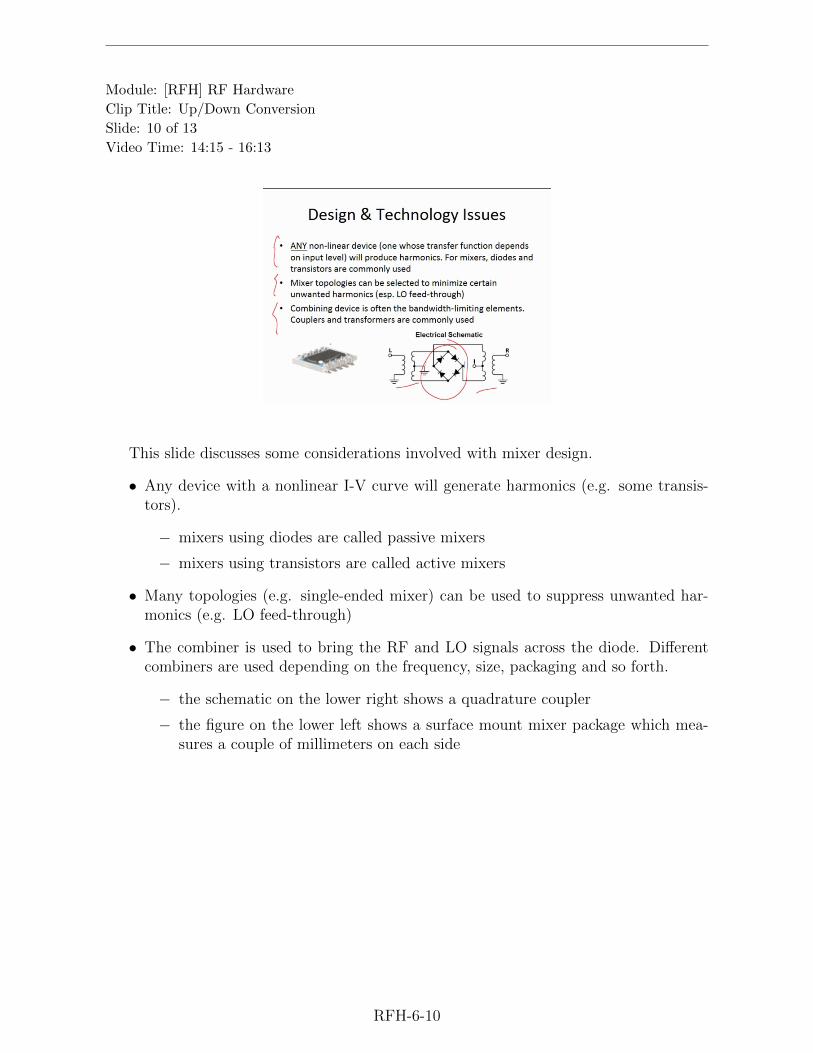
Module: [RFH] RF Hardware
Clip Title: Up/Down Conversion
Slide: 10 of 13
Video Time: 14:15 - 16:13
This slide discusses some considerations involved with mixer design.
• Any device with a nonlinear I-V curve will generate harmonics (e.g. some transis-tors).
− mixers using diodes are called passive mixers
− mixers using transistors are called active mixers
• Many topologies (e.g. single-ended mixer) can be used to suppress unwanted har-monics (e.g. LO feed-through)
• The combiner is used to bring the RF and LO signals across the diode. Differentcombiners are used depending on the frequency, size, packaging and so forth.
− the schematic on the lower right shows a quadrature coupler
− the figure on the lower left shows a surface mount mixer package which mea-sures a couple of millimeters on each side
RFH-6-10

Module: [RFH] RF Hardware
Clip Title: Up/Down Conversion
Slide: 11 of 13
Video Time: 16:14 - 18:01
This slide discusses the conversion efficiency of the mixer which is also called theconversion loss.
• The definition of conversion loss is given by the following equation:
Lc = 10 log
[RF input power
IF output power
]dB
− The IF output is usually smaller than the RF input, so the conversion loss isa positive dB value
• The graph at the bottom shows conversion loss versus frequency at different localoscillator signal levels for commercial mixer
− the red curve corresponds to a local oscillator signal at +1 dBm, which has theconversion loss varying from 9 dB down to 6.3 dB
− the lowest conversion loss corresponds to the highest efficiency
− the conversion loss decreases as the local oscillator signal increases from +1 to+4 and +7 dBm
− the graph tells how large the LO signal should be to get the desired conversionloss
RFH-6-11

Module: [RFH] RF Hardware
Clip Title: Up/Down Conversion
Slide: 12 of 13
Video Time: 18:02 - 19:18
This slide discusses some of the system-level implications related to mixers.
• Conversion loss can affect the amount of gain that is required in the amplificationstages
• The unwanted mixing products can lead to signal distortion so proper filtering isneeded to eliminate them
• Impedance matching at the ports of the mixer is very important for every compo-nents in block diagram
• LO signal generation is needed for mixers and this requires DC energy
RFH-6-12

Module: [RFH] RF Hardware
Clip Title: Up/Down Conversion
Slide: 13 of 13
Video Time: 19:19 - 20:11
This slide summarizes this clip on frequency up/down conversion.
• The process of up-and-down converting the carrier frequency allows the internalparts of a radio to operate at a different and much lower frequency than was broad-cast across the wireless channel.
• Frequency conversion requires a device with a nonlinear current voltage relationship(i.e. a mixer).
• Mixer performance influences requirements for amplifiers, filters, DC supply, etc.
RFH-6-13

Module: [RFH] RF Hardware
Clip Title: Oscillators & Synthesizers
Slide: 1 of 17
Video Time: 00:00 - 01:29
This clip covers oscillators and synthesizers which are the sources of the RF signalsused in microwave and wireless systems. This slide presents the outline for this topic.
• Functional description of oscillator
• Practical implementation
• System-level perspective and the implications of oscillator performance
RFH-7-1
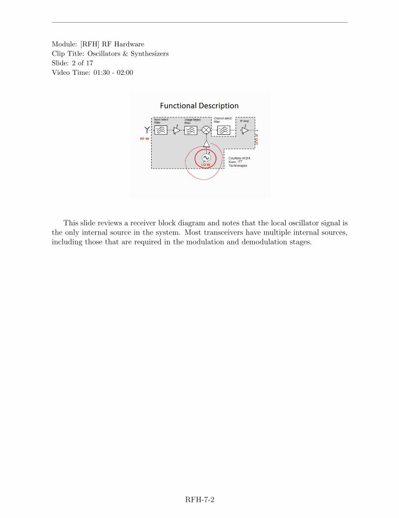
Module: [RFH] RF Hardware
Clip Title: Oscillators & Synthesizers
Slide: 2 of 17
Video Time: 01:30 - 02:00
This slide reviews a receiver block diagram and notes that the local oscillator signal isthe only internal source in the system. Most transceivers have multiple internal sources,including those that are required in the modulation and demodulation stages.
RFH-7-2

Module: [RFH] RF Hardware
Clip Title: Oscillators & Synthesizers
Slide: 3 of 17
Video Time: 02:01 - 03:55
This slide shows a conceptual illustration of an oscillator circuit.
• The oscillator circuit includes:
− Amplifier with gain Av
− Feedback loop with the transfer function β
− Input voltage Vi
− Output voltage Vo
− Feedback voltage Vf
− The total input to the amplifier Vd = Vi + Vf
• The overall transfer function is shown at the bottom of the slide.
• The goal is to make the feedback voltage combine in phase with the input signal atthe desired frequency, this positive feedback leads to oscillation.
• Both the amplifier and feedback path transfer functions are functions of frequency,so designer should make the positive feedback occur only at the oscillation frequencyof interest
RFH-7-3

Module: [RFH] RF Hardware
Clip Title: Oscillators & Synthesizers
Slide: 4 of 17
Video Time: 03:56 - 06:52
This slide discusses the operation of the oscillator and Barkhausen criterion. Thecriterion comes from the requirement that an output signal exists with zero input signal,and the reason for that is that the oscillator is seen as a source of RF energy.
• The Barkhausen criterion:β(jω) · A(jω) = 1
Where
− A is the gain of the amplifier so |A| > 1
− β is the transfer function of the passive circuit so β < 1
• In practice, there is a nonzero input that exists due to electronic noise
• The Bakhausen criterion is frequency dependent, so the oscillation condition ideallywill occur only at a single frequency
RFH-7-4

Module: [RFH] RF Hardware
Clip Title: Oscillators & Synthesizers
Slide: 5 of 17
Video Time: 06:53 - 08:55
After reviewing the conceptual view of oscillator, this slide discusses its implementa-tion in terms of actually designing an oscillator.
• An oscillator circuit is identical to an amplifier circuit except that the input portis replaced with a termination. In this diagram the input matching network isregarded as terminating the left-hand side.
• To satisfy the Barkhausen criterion, the design of the matching network shouldmake the circuit unstable.
• Consider this diagram as being an oscillator, the output may be on Port 2. ZIN
is the impedance looking toward the transistor and ZS is the impedance lookingtoward the matching network
• Note that ZIN is not the impedance of the transistor itself because ZIN is alsoinfluenced by whatever comes after the transistor
RFH-7-5

Module: [RFH] RF Hardware
Clip Title: Oscillators & Synthesizers
Slide: 6 of 17
Video Time: 08:56 - 12:02
Take the left-hand side of the network from previously diagram, this slide furtherdiscusses designing an oscillator.
• The total impedance in the circuit is the sum of ZL and ZIN
− ZL is the input impedance looking toward the matching network which inprevious slide was called ZS
− ZIN is impedance looking toward the transistor
• The Barkhausen criterion is equivalent to this relationship:
ΓIN(jω0)ΓL(jω0) = 1
• Take one step further, this relationship is equivalent to:
Rin(ω0) +RL(ω0), Xin(ω0) +XL(ω0)
whereRin + jXin = Zin RL + jXL = ZL
So the occurrence of oscillation requires that the total impedance is zero:
ZIN + ZL = 0
• Example of design: If ZIN is capacitive, XIN will be negative, hence XL needs tobe positive to cancel out XIN . Assuming that RL is positive, then RIN needs to benegative.
RFH-7-6

Module: [RFH] RF Hardware
Clip Title: Oscillators & Synthesizers
Slide: 7 of 17
Video Time: 12:03 - 13:34
This slide discusses how to design the output matching network such that RIN (thereal part of ZIN) is negative. In the oscillator design process, almost any transistor canbe made to be unstable by choosing the right frequency, bias condition, and matchingnetworks.
RFH-7-7

Module: [RFH] RF Hardware
Clip Title: Oscillators & Synthesizers
Slide: 8 of 17
Video Time: 13:35 - 14:58
A short summary of the oscillator design process is as follows:
• Transistor is biased and configured so it is potentially unstable. Equations can beused to determine these conditions.
• Output or input matching network is designed to present a negative impedance atthe opposite port.
• Input or output matching network is designed to achieve the Barkhausen conditionat the desired frequency of oscillation.
• The design can be done by starting on either side of the transistor in general, it canbe shown mathematically that if one side of a transistor is oscillating then the otherside is as well.
RFH-7-8

Module: [RFH] RF Hardware
Clip Title: Oscillators & Synthesizers
Slide: 9 of 17
Video Time: 14:59 - 16:06
This slide introduces voltage controlled oscillator (VCO), which has a separate DCinput that controls the frequency of oscillation, in other word, the frequency at which theBarkhausen criterion is satisfied will change as a function of the DC control voltage.
• This functionality is typically achieved by including a voltage dependent reactancein the feedback path or one of the matching networks. One often used approach isto include a varactor diode in the matching networks.
• A typical performance specification for VCO is tuning sensitivity, which tells howmany MHz the oscillation frequency will change per volt change in the DC controlvoltage.
RFH-7-9

Module: [RFH] RF Hardware
Clip Title: Oscillators & Synthesizers
Slide: 10 of 17
Video Time: 16:07 - 16:35
The slide shows a typical schematic for a varactor based voltage controlled oscillators(VCO). Notice that the diode in the matching network is reverse biased so that it won’tdraw current and only will provide a bias dependent capacitance that becomes part ofthe matching network.
RFH-7-10

Module: [RFH] RF Hardware
Clip Title: Oscillators & Synthesizers
Slide: 11 of 17
Video Time: 16:36 - 19:32
This slide discusses what kind of oscillator output is desired and how to generate thedesired signal.
• Theoretically, the Barkhausen criterion should only be met at a single frequency.In other words, the output of an oscillator on a spectrum analyzer is a perfect spikeat a single frequency.
• In reality, the oscillator output signals have a slightly different frequency. Thespectrum of the signal peaks at one frequency and then drops gradually off as thefrequency varies away from the center frequency.
• The more narrow the spectrum is, the cleaner the signal is considered, and this isdesired.
• One way to clean up the signal is designing the oscillator so the impedance willchange very rapidly as a function of frequency.
• The figure in the left-hand side shows an example design using narrow band res-onators in the feedback path to generate a clean signal.
RFH-7-11

Module: [RFH] RF Hardware
Clip Title: Oscillators & Synthesizers
Slide: 12 of 17
Video Time: 19:33 - 20:36
The graph on this slide demonstrates two important oscillator characteristics.
• The oscillator is generating output signals at multiple harmonics, filtering may beneeded to remove the harmonics content. (The right-hand side figure shows theoutput signal amplitude versus the harmonic index, which is the integer multiple ofthe design frequency)
• Outputs from different points in the oscillator have different power. The blue arrowsmay correspond taking the output from the drain side while the red arrows maycorrespond taking output from the gate site. The output corresponding to bluearrows has larger power.
RFH-7-12

Module: [RFH] RF Hardware
Clip Title: Oscillators & Synthesizers
Slide: 13 of 17
Video Time: 20:37 - 22:13
The table shows various performance specifications for voltage controlled oscillators(VCO).
• The specification parameters that have been discussed in previous slides:
− Output frequency rage
− Output power
− Phase noise (dBc/Hz)
− Tuning sensitivity (MHz/V)
− Harmonics levels
• Other parameters that have not been discussed:
− Pulling: is related to changes in the output frequency due to changes in theimpedance of whatever the oscillator is connected to. (typically 50Ω)
− Pushing: is related to the sensitivity in the output frequency due to changesin the supply versus changes in the control voltage
− Modulation bandwidth: is related to how fast the output frequency can bechanged by a time varying control voltage
RFH-7-13

Module: [RFH] RF Hardware
Clip Title: Oscillators & Synthesizers
Slide: 14 of 17
Video Time: 22:14 - 23:10
This slide shows some representative VCO data. The six figures present how thespecification parameters changes with tuning voltage in volts, including frequency, poweroutput, harmonic levels, frequency pulling/frequency pushing and phase noise.
RFH-7-14

Module: [RFH] RF Hardware
Clip Title: Oscillators & Synthesizers
Slide: 15 of 17
Video Time: 23:11 - 23:42
This slide shortly introduces the synthesizer.
• Synthesizer is basically a programmable oscillator. There is an automated con-trol loop that will adjust the VCO until the desired frequency and power level aregenerated.
• A synthesizer is typically part of the instrumentation that is used for measurementor characterization of microwave devices.
RFH-7-15

Module: [RFH] RF Hardware
Clip Title: Oscillators & Synthesizers
Slide: 16 of 17
Video Time: 23:43 - 24:45
Oscillators are essential in the design of communication systems and the performancecan impact the overall system design in the following ways:
• Oscillators are essentially transformers between DC and RF energy and the efficiencywith which the RF signal is generated impacts the overall DC requirements for thesystem.
• The accuracy of the frequency generated by the oscillator must be controlled ex-tremely accurately, usually in terms of tenths of a percent in order to avoid com-munication errors.
• Generating “clean” signals that have low harmonic content and low phase noiselevels will ease the filter requirements and improve the overall sensitivity of thesystem.
RFH-7-16

Module: [RFH] RF Hardware
Clip Title: Oscillators & Synthesizers
Slide: 17 of 17
Video Time: 24:46 - 25:54
The last slide concludes the clip by discussing some system-level implications.
• Oscillators convert noise into RF signals and are thus the basic component of anyRF source.
• Basically an amplifier, an oscillator is designed such that positive feedback is achievedat a specific frequency.
• VCO’s use tunable reactance to change the frequency at which positive feedbackoccurs (i.e. the frequency of oscillation).
• DC consumption, phase noise, harmonic output, frequency accuracy and tunabilityare related system level issues.
RFH-7-17

Module: [RFH] RF Hardware
Clip Title: Modulation Basics
Slide: 1 of 8
Video Time: 00:00 - 01:04
This first slide introduces what will be covered in this clip related to modulation basics.
• Functional description of modulation and demodulation. Different modulation ap-proaches are involved.
− Analog methods: single sideband, double sideband, double sided band sup-pressed carrier
− Digital methods: on-off keying, frequency shift keying, and so forth
• How modulation is implemented at the component level (take frequency shift keyingas an example)
• System-level implications
RFH-8-1

Module: [RFH] RF Hardware
Clip Title: Modulation Basics
Slide: 2 of 8
Video Time: 01:05 - 03:14
The block diagram in this slide shows the process of down converting the RF carrierinto the intermediate frequency (IF) signal.
• The message (e.g. voice, video, data, and so forth) is carried by two signals:
− RF carrier
− IF signal
• The steps converting RF carrier to IF signal:
− Antenna
− Band select filter
− Low noise amplifier
− Image reject filter
− Mixer (frequency down conversion stage)
− Channel select filter
− Amplifier
• Modulation/demodulation
− Stripping off the message from the IF signal is the process of demodulation
− The process of getting the message onto the IF signal is modulation
− Modulation or demodulation can be seen as being the interface between themessage and IF signals
RFH-8-2

Module: [RFH] RF Hardware
Clip Title: Modulation Basics
Slide: 3 of 8
Video Time: 03:15 - 06:11
This slide discusses the analog single sideband modulation process as an example ofimplementation.
• Message signal: m(t) = Acos(ωmt) with the amplitude A and frequency ωm, bothA and ωm could vary with time
• IF carrier signal: Bcos(ωIF t) with the amplitude B and frequency ωIF
• Ideal modulator output: V (T ) = Ccos(ωm + ωIF )t with the amplitude C and fre-quency ωm + ωIF
• Real modulator output: V ′(t) = V (t)+n(t), where n(t) is noise, the output containsinformation from the message and its frequency and/or its amplitude will change asn(t) changes.
RFH-8-3

Module: [RFH] RF Hardware
Clip Title: Modulation Basics
Slide: 4 of 8
Video Time: 06:12 - 07:37
This slide introduces an implementation of modulation.
• Message signal: m(t) = Acos(ωmt)
• IF signal: Bcos(ωIF t)
• Modulated IF signal with up-converted frequency: Ccos(ωm + ωIF )t
RFH-8-4

Module: [RFH] RF Hardware
Clip Title: Modulation Basics
Slide: 5 of 8
Video Time: 07:38 - 10:55
This slide shows the modulation and demodulation process together. One of thecritical issues is synchronization between the transmitter and receiver in terms of theintermediate frequency signal.
• Modulation process (inside the transmitter)
− The message signal m(t) is combined in a mixer with the intermediate fre-quency (IF), the signal will be filtered and then the output is Ccos(ωm +ωIF )t
The modulation output gets up converted to the RF frequency and then gets injectedinto the wireless channel, received on the other side of the channel and then getsdown converted to the IF frequency.
• Demodulation process (inside the receiver)
− This IF signal is combined in a mixer with the local generated IF signal, theoutput will be cos(ωm + ωIF − ωIF )t
• Synchronization between the transmitter and receiver
− In the demodulation output, the first frequency component ωIF was generatedin the transmitter, the second component ωIF is generated in the receiver. Tocancel those two frequency, the receiver needs to generate the same frequencyand with the same phase as the transmitter, that’s synchronization.
− A phase lock loop oscillator is used in achieving synchronization.
RFH-8-5

Module: [RFH] RF Hardware
Clip Title: Modulation Basics
Slide: 6 of 8
Video Time: 10:56 - 16:28
This slide shows a block diagram for a digital modulation approach using frequencyshift keying. The top figure shows the modulation process and the bottom figure showsthe demodulation process.
• Modulation (Transmitter side)
− The message signal m(t) controls the voltage that supplied to an oscillator,and depending on the value of m(t), the oscillator will generate a signal eitherat ω1 or at ω2.
• Demodulation (Receiver side)
− There are two separate sources in the demodulator, One is running at cos(ω2t)and the second one is running at cos(ω1t)
− The modulated IF signal cos(ωt) is split and injected into two different mixers:one on the top and one on the bottom.
RFH-8-6

Module: [RFH] RF Hardware
Clip Title: Modulation Basics
Slide: 7 of 8
Video Time: 16:29 - 17:33
This slide discusses several system-level implications.
• DC power should meet specific requirement since the modulation process requiresone or more local signal sources.
• The efficiency of the mixer, which is measured in terms of the conversion loss, affectsthe gain of amplifier.
• The amount of noise that gets added in the modulation and demodulation processneeds to stay below the detection limit since it requires a certain signal-to-noiseratio to detect the message information.
RFH-8-7

Module: [RFH] RF Hardware
Clip Title: Modulation Basics
Slide: 8 of 8
Video Time: 17:34 - 18:10
This slide shortly reviews the modulation basics and concludes this clip.
• Modulation is the process of converting message information onto IF carrier signal.
• Almost all modulation techniques involve mixers.
• Filtering is important in signal selection/shaping.
RFH-8-8

Module: [RFH] RF Hardware
Clip Title: Antennas A
Slide: 1 of 7
Video Time: 00:00 - 00:58
This clip presents a general overview on antennas and the role they play in a wirelesscommunication system. Fundamental concepts that are common to almost all antennasare described, along with specific characteristics of some selected designs. The focus isprimarily on small antennas that are typical of handheld devices or small communicationsnodes, such as sensor nodes.
• General overview of antennas
• Performance parameters
• Design and technology issues
• Types
− Wire antennas
− Planar antennas
− High-gain antennas/Arrays
• Impacts of antenna performance on sensor network design
RFH-9-1

Module: [RFH] RF Hardware
Clip Title: Antennas A
Slide: 2 of 7
Video Time: 00:59 - 02:15
This slide reviews the roles antenna plays in wired and wireless domain.
• For wireless devices, antenna is the primary interface between the wired and wirelessdomains.
− Wired domain is everything contained inside the radio
− Wireless domain is everything in the wireless channel
• Energy in radio is guided by a transmission line and eventually is fed to the antenna,and the antenna will direct the energy into the wireless channel.
• There are many things in the channel that cause interference such as building, roadsand automobiles.
• Antennas are often described as a transformer between the free space electromag-netic wave and the guided waves that are inside the wireless device.
RFH-9-2

Module: [RFH] RF Hardware
Clip Title: Antennas A
Slide: 3 of 7
Video Time: 02:16 - 05:32
This slide discusses the transformer concept for antennas from two different perspec-tives, one being a circuit standpoint and the second being from the electromagnetic fieldstandpoint. As an example, a coaxial transmission line that’s connected to a dipole an-tenna is used to illustrate the concept.
• From a circuit standpoint, the antenna acts as a transformer between the free spaceimpedance and the circuit impedance. Without this impedance transformation theenergy would not be transferred across wired/wireless boundary efficiently.
− The free space impedance is given by EH
= 377Ω
− The circuit impedance is given by VI
, and that’s typically 50Ω
• From the electromagnetic field standpoint, the antenna is a transformer betweentransverse electromagnetic fields in free space and electromagnetic field configurationthat exists on a transmission line.
• From both standpoints, the antenna acts to straddle the circuit and electromagneticworlds.
RFH-9-3

Module: [RFH] RF Hardware
Clip Title: Antennas A
Slide: 4 of 7
Video Time: 05:33 - 06:48
This slide discusses the important concept of reciprocity.
• Reciprocity means the antennas receive and transmit energy in an identical fashion.
• This concept is very useful in describing the behavior of antennas because sometimesit’s easier to consider transmission, and other times it’s easier to consider reception.
RFH-9-4

Module: [RFH] RF Hardware
Clip Title: Antennas A
Slide: 5 of 7
Video Time: 06:49 - 08:15
This slide discusses how to think about an antenna in a circuit.
• In receive mode, the antenna collects energy and appears as a source that sendsenergy into the circuit
• In transmit mode, the circuit acts as the power source, the antenna appears as aload and radiates energy into free space
RFH-9-5

Module: [RFH] RF Hardware
Clip Title: Antennas A
Slide: 6 of 7
Video Time: 08:16 - 14:37
This slide shows several different performance parameters that are used to describeantenna and these include:
• Input impedance (Z): ratio of voltage to current
Z =V
I
− Given the input impedance Z, characteristic impedance Z0, and input powerPin, we have the expression of reflection coefficient Γ and reflected power Pref
as:
Γ =Z − Z0
Z + Z0
Pref = Pin|Γ|2
• Polarization: is a term that defines the direction of the electric field as a functionof time
• Radiation pattern: the way that the antenna radiates power as a function of anglefrom the antenna
• Efficiency (η): the ratio of transmitted power to the incident power
• Directivity: the ratio of the radiation intensity in a given direction to the averageradiation intensity over all directions. The maximum value for directivity is givenby:
D0 =Umax
Uavg
• Gain (G): is a product of the directivity times efficiency
G = Dη
RFH-9-6

Module: [RFH] RF Hardware
Clip Title: Antennas A
Slide: 7 of 7
Video Time: 14:38 - 19:26
This slide takes dipole antenna as an example illustrating how radiation occurs froman antenna and how a radiation pattern is formed.
• The dipole antenna is affected by a two wire transmission line, one is positive poten-tial, the other is negative potential. Current on both sides is made up of a collectionof tiny radiators, each of the radiator will radiate the electromagnetic energy in anidentical way.
• The radiators are spatially distributed along the antenna, so depending on thedistribution, in some regions there are constructive interference, and in other regionsthere are destructive interference. The interferences of these fields determine theradiation pattern.
• There is a distinct difference between far field and the near field patterns.
− In the near field, the shape of the field is very complex and doesn’t resembletransverse electromagnetic wave
− In the far field, the field is taking the form of transverse electromagnetic planewaves. The distance to get to the far field is
2D2
λ
Where D is the maximum dimension of the antenna.
RFH-9-7

Module: [RFH] RF Hardware
Clip Title: Antennas B
Slide: 1 of 7
Video Time: 00:00 - 03:56
This slide discusses some design and technology issues that antenna designers have todeal with, including size, bandwidth and packaging.
• Size
− A typical “small” antenna is at least a quarter wavelength (e.g. λ4
= 8cm at915 MHz)
− As antennas become smaller their efficiency goes down
• Bandwidth
− Impedance bandwidth: frequency range over which the input impedance isclose to 50Ω
− Pattern bandwidth: frequency range over which the radiation pattern remainsacceptable (This usually is quite broader than the impedance bandwidth)
• Packaging
− Conformal antenna design is desirable but more difficult to make than a stan-dard antenna design. As an example, dipole antenna conformal and standarddesigns are shown in the slide.
RFH-10-1

Module: [RFH] RF Hardware
Clip Title: Antennas B
Slide: 2 of 7
Video Time: 03:57 - 06:44
This slide discusses how size efficiency and bandwidth are interrelated.
• Bandwidth is proportional to 1Q
, where Q is the quality factor and gives the ratioof energy stored to energy dissipated. If Q goes up then bandwidth goes down.
• The relationship between size and Q factor is given by this equation:
Qlb = ηr((1
ka)3 + (
1
ka))
ηr = efficiencyk = 2π
λ
a = radius of volume enclosing antenna
− As the antenna gets smaller (the product ka reduces), the Q factor becomeshigher, and the bandwidth becomes smaller.
• How size and efficiency are related: the more efficiently an antenna fills the volumeof space surrounding the antenna, the higher its radiation efficiency will be.
RFH-10-2

Module: [RFH] RF Hardware
Clip Title: Antennas B
Slide: 3 of 7
Video Time: 06:45 - 10:15
This slide discusses the input impedance Zin and the maximum directivity G0 of threecommon wiring antennas: short dipole, half-wavelength dipole and quarter-wavelengthmonopole.
• Concept review
− Input impedance Zin = VI
= Zr + jZi
− Maximum directivity D0 refers to the ratio maximum radiation intensity tothe average radiation intensity over all space
− At resonance the imaginary part of input impedance is zero (Zi = 0 @ reso-nance), that’s typically the center frequency of operation for the antenna.
• Short dipole
− The length l is much less than a wavelength λ
− Zin is proportional to l(λ)2
− D0 ∼ 1.8dB
• Half-wavelength dipole
− l = λ2
− Zin ∼ 73Ω@resonance
− D0 ∼ 2.2dB
• Quarter-wavelength monopole
− l = λ4
− Zin ∼ 36.5Ω@resonance
− D0 ∼ 2.2dB
RFH-10-3
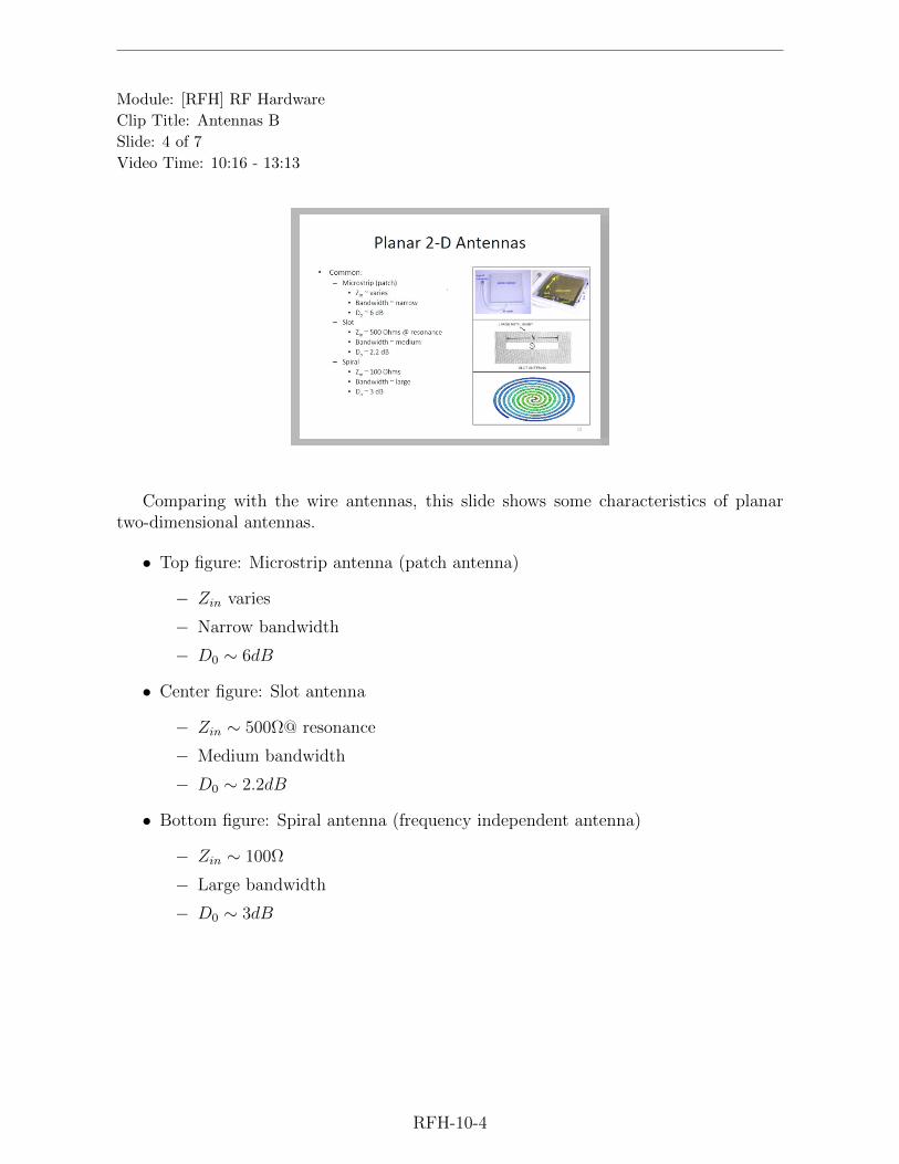
Module: [RFH] RF Hardware
Clip Title: Antennas B
Slide: 4 of 7
Video Time: 10:16 - 13:13
Comparing with the wire antennas, this slide shows some characteristics of planartwo-dimensional antennas.
• Top figure: Microstrip antenna (patch antenna)
− Zin varies
− Narrow bandwidth
− D0 ∼ 6dB
• Center figure: Slot antenna
− Zin ∼ 500Ω@ resonance
− Medium bandwidth
− D0 ∼ 2.2dB
• Bottom figure: Spiral antenna (frequency independent antenna)
− Zin ∼ 100Ω
− Large bandwidth
− D0 ∼ 3dB
RFH-10-4
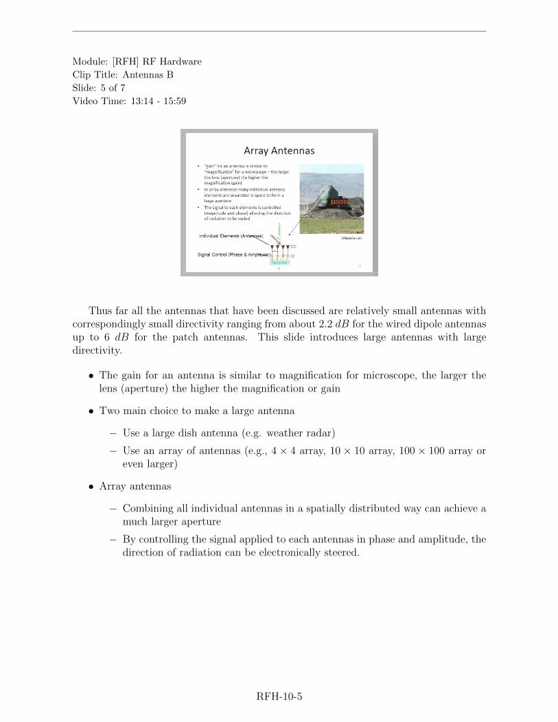
Module: [RFH] RF Hardware
Clip Title: Antennas B
Slide: 5 of 7
Video Time: 13:14 - 15:59
Thus far all the antennas that have been discussed are relatively small antennas withcorrespondingly small directivity ranging from about 2.2 dB for the wired dipole antennasup to 6 dB for the patch antennas. This slide introduces large antennas with largedirectivity.
• The gain for an antenna is similar to magnification for microscope, the larger thelens (aperture) the higher the magnification or gain
• Two main choice to make a large antenna
− Use a large dish antenna (e.g. weather radar)
− Use an array of antennas (e.g., 4 × 4 array, 10 × 10 array, 100 × 100 array oreven larger)
• Array antennas
− Combining all individual antennas in a spatially distributed way can achieve amuch larger aperture
− By controlling the signal applied to each antennas in phase and amplitude, thedirection of radiation can be electronically steered.
RFH-10-5

Module: [RFH] RF Hardware
Clip Title: Antennas B
Slide: 6 of 7
Video Time: 16:00 - 17:54
This slide summarizes the section on antenna design characteristics by discussing howthey impact the overall design of a sensor network.
• Antennas with high gain will increase communication range
• Antennas with high gain requires careful alignment between the transmitter andreceiver
• Antennas with high gain typically used only for fixed installations
• Sensor nodes typically use low gain antennas in order to receive/transmit effectivelyin all or most directions (in a plane).
− In a sensor network design, the orientation between transmit and receive an-tenna is random due to the interference or obstruction, it’s desirable to use alower directivity antenna
− It’s advantageous to use a small antenna from a size perspective for a sensornode
RFH-10-6

Module: [RFH] RF Hardware
Clip Title: Antennas B
Slide: 7 of 7
Video Time: 17:55 - 20:11
This slide makes conclusions about the discussion on antennas with three points.
• Antennas lie the boundary between electromagnetic and circuit design.
− physical boundary between free space and radio
− transformation between transverse electromagnetic waves and the waves in thetransmission line
• Antennas control the direction, concentration and polarization of the electromag-netic wave transmitted between two wireless devices. All three of these things relateto the radiation pattern and directivity.
• For small devices such as sensor nodes, the antennas are often the size limitingaspect, and performance tends to degrade as the antennas are made smaller.
RFH-10-7

Module: [WCC] The Wireless Communication Channel
Clip Title: Module Objectives and the Free Space Model
Slide: 1 of 8
Video Time: 00:00 - 00:10
This slide presents the main points that will be covered in this clip:
• Motivation for understanding the wireless channel
• Learning objectives for module
• The free-space model
WCC-2-1

Module: [WCC] The Wireless Communication Channel
Clip Title: Module Objectives and the Free Space Model
Slide: 2 of 8
Video Time: 00:11 - 02:15
This slide draws a simple block diagram illustrating a wireless communication channel,which is essentially the environment between the transmitter and receiver, the informationsignal goes from transmitter to receiver through the channel.
Throughout this module we will be considering the channel as effectively a filter, wherethere is an input signal from transmitter and an output signal which goes to receiver. Thisfiltering effect due to the channel is linear and most likely will be time varying.
WCC-2-2

Module: [WCC] The Wireless Communication Channel
Clip Title: Module Objectives and the Free Space Model
Slide: 3 of 8
Video Time: 02:16 - 05:25
The slide introduces the objectives of this wireless communication module.
• Understand fundamentals of free-space propagation. This is the best case scenarioappropriate for satellite communications or between two very tall towers.
• Define key sources of propagation effects both at the large- and small-scales.
• Understand the key differences between wireless sensor network channels and mobilecommunication channels.
• Employ diversity schemes to mitigate small-scale effects. Approaches include changesin position, time and frequency for wireless sensor network.
• Use a link budget as an important tool for designing systems.
WCC-2-3

Module: [WCC] The Wireless Communication Channel
Clip Title: Module Objectives and the Free Space Model
Slide: 4 of 8
Video Time: 05:26 - 05:31
This slide shows the outline of this module.
• Free-space propagation
• Large-scale effects and models
• Small-scale effects and models
• Mobile communication channel vs. wireless sensor network channels
• Diversity schemes
• Link budgets
• Example Application: WSSW
WCC-2-4

Module: [WCC] The Wireless Communication Channel
Clip Title: Module Objectives and the Free Space Model
Slide: 5 of 8
Video Time: 05:32 - 09:19
This slide introduces the foundations of free-space propagation model. The scenarioconsiders a transmitter and a receiver that are separated by distance d (T-R distance).Between the transmitter and receiver, there are no large physical objects, or other thingsto impair the signal (it’s a flat channel).
• The free space model is appropriate for:
− satellite to satellite communications
− satellite to ground station communications
− tower to tower communications
• The power that can be captured by receiver under isotropic conditions is given by
PT4πd2
(in W/m2)
− PT is the transmitted power
− d is T-R distance
− Energy being transmitted can be seen as being distributed uniformly acrossthe sphere that is surrounding the transmitter. The power at the receiver isthus the power transmitted (PT ) divided by the area of the sphere with radiusequal to the distance of the receiver (4πd2).
WCC-2-5

Module: [WCC] The Wireless Communication Channel
Clip Title: Module Objectives and the Free Space Model
Slide: 6 of 8
Video Time: 09:20 - 16:24
This slide discusses the key equations for modeling the free space environment, whichinclude Friis equation and EIRP. The Friis equation helps us answer the questions: (1)What is the power received at distance d from the transmitter? (2) what distance d canstill achieve the required received power?
• EIRP: effective isotropic radiated power, which is given by:
EIRP = PT ·GT
− PT is the transmit power (in Watts)
− GT is the transmit gain of the antenna (unitless)
• Friis equation
PR(d) =PTGT
4πd2· Ae
− d: T-R distance
− 4πd2: determines the power density at the receiver
− Ae: the effective area of the receive antenna (in m2)
• Since the gain for the receive antenna can be written as GR = 4πAe
λ2, we can rewrite
the Friis equation as:
PR(d) =PTGT
4πd2· GR
4π· λ2
where λ is the wavelength corresponding to the carrier frequency.
• The key thing to note is that we have some control over transmit power and theantenna size and coverage.
WCC-2-6

Module: [WCC] The Wireless Communication Channel
Clip Title: Module Objectives and the Free Space Model
Slide: 7 of 8
Video Time: 16:25 - 22:45
This slide discusses a log formulation of the Friis equation, which can be used to figureout the power received at some distance d if we know the power received at a referencedistance d0.
• Recall the Friis equation from the previous slide is:
PR(d) =PTGT
4πd2· GRλ
2
4π
− The right term Geλ2
4πis the effective area Ae in (m2)
− The left term PTGT
4πd2is the power flax density (PFD) in ( W
m2 )
• Considering an electromagnetic representation, the PFD (power flux density) canbe rewritten as
PFD =PTGT
4πd2=|E|2
η
− E = Vm
: the electric field strength
− η : intrinsic impedance of free space which is 377Ω or 120πΩ
• Power received at some distance d in dBm can be expressed as follows:
PR(d)|dBm = 10 log10[PR(d0)
1mW] + 2 · 10 · log10[
d0d
]
− d0 is the reference distance at which the received power is known.
− The left term 10 log10[PR(d0)1mW
] converts the power received at d0 to dBm.
− The right term ·10 · log10[d0d
] represents the change based on the ratios of thedistances, and 2 is the path loss exponent of free space.
WCC-2-7

Module: [WCC] The Wireless Communication Channel
Clip Title: Module Objectives and the Free Space Model
Slide: 8 of 8
Video Time: 22:46 - 25:48
This slide discusses the usefulness of the free space model (Friis equation) for wirelesssensor networks.
• Free space model assumes there is nothing between the transmitter and receiver,which only applies to satellite to satellite communication, satellite to ground com-munication or high tower to high tower communication.
• The environment of wireless sensor network is much worse than that of the freespace scenario, that will make the received signal much less than predicted by thefree space model.
• The free space model provides a best case scenario to start from but we also have toconsider the environment in general, which includes many large- and small-effects.
WCC-2-8

Module: [WCC] The Wireless Communication Channel
Clip Title: Large-scale Phenomena and Models
Slide: 1 of 8
Video Time: 00:00 - 00:09
In this clip, there are two main points that are discussed:
• Large-scale phenomena
• Modeling of large-scale effects
WCC-3-1

Module: [WCC] The Wireless Communication Channel
Clip Title: Large-scale Phenomena and Models
Slide: 2 of 8
Video Time: 00:10 - 03:06
This slide discusses three effects related to large-scale propagation.
• Reflection
− The environment includes a very large structure such that in addition to adirect or line of sight component, there is a reflected path.
− This structure is very large (e.g., a wall, a building, the ground etc.) such thatits size is much greater than the operating wavelength.
• Diffraction
− When transmitter and receiver are on opposing side of some structure, thesignal can bend its way around.
• Scattering
− In the midst of communication link, there is some structure or elements in thestructure that reflects or scatters the signal (e.g., a tree). The elements maybe of size on the order of a wavelength or less.
WCC-3-2

Module: [WCC] The Wireless Communication Channel
Clip Title: Large-scale Phenomena and Models
Slide: 3 of 8
Video Time: 03:07 - 09:02
To understand the potential effects of reflection, this slide discusses the Plane-Earthmodel. As illustrated in the figure, the transmitter (located at height ht) and the receiver(located at height hr) are separated by distance d. As opposed to the free space model,this scenario includes a very large structure (the earth) which is modeled as a plane. Inaddition to the line of sight path, there is a secondary component reflected off the earth.
• We can model the reflection coefficient (Γ⊥) off a plane boundary, which is given bythis ratio:
Γ⊥ =sinθ −
√εr − (cos θ)2
sinθ +√εr − (cosθ)2
(1)
− θ: incident angle of the perpendicularly (⊥) polarized signal
− εr: medium permittivity
− Assuming d ht, hr, then θ ' 0, therefore Γ⊥ ' −1, which indicates the lineof sight component and reflected component are comparable in magnitude.However they are different in terms of phase.
• The Plane-Earth model states that:
Pr(d) = PtGtGrh2th
2r
d4
− Pt: transmitted power
− Gt, Gr: the gains of transmit antenna and receive antenna, respectively
− The path loss exponent is n = 4, which indicates the power in Plane-Earthenvironment degrades significantly faster than predicated by the free spacemodel with n = 2.
WCC-3-3

Module: [WCC] The Wireless Communication Channel
Clip Title: Large-scale Phenomena and Models
Slide: 4 of 8
Video Time: 09:03 - 12:33
This slide discusses the Knife-edge model which is used to model the impact of diffrac-tion. The model considers the structure between the transmitter and receiver to be a knifeedge.
• As illustrated in the right figure, the signal from bends around the object betweenthe transmitter and the receiver, thus produces constructive and deconstructiveinterference.
• To understand the impact of diffraction, we need to know the Fresnel-Kirchiff diffrac-tion parameter, which is expressed as follows:
v = h
√2(d1 + d2)
λd1d2(2)
− h: screening height, the distance from the line of sight path to the top of theobject.
− d1: distance from the transmitter to the object
− d2: distance from the object to the receiver
− The larger the screen height, the higher the diffraction parameter; the smallerthe wavelength, the higher the diffraction parameter
− Note that this diffraction parameter is dependent on very large distances andvery large objects.
• The figure on the left shows the knife-edge diffraction gain, which is in the negativedB scale. As the diffraction parameter increases, we have increasing loss, the gainbecomes more negative.
− For small diffraction parameters (v < 0), the gain isn’t affected much.
− For large diffraction parameters (v > 0), the gain decreases significantly.
WCC-3-4

Module: [WCC] The Wireless Communication Channel
Clip Title: Large-scale Phenomena and Models
Slide: 5 of 8
Video Time: 12:34 - 16:47
This slide discusses the third large-scale effect, scattering, by considering a bistaticradar set up. The scenario is that the transmitter sends a signal up towards the objectthat we wish to detect and we are counting on its reflective energy towards receiver. Wecan think about this as two separate free space links: from the transmitter to the objectoccurring over distance d1 and from the object to receiver occurring over distance d2.
• The power captured from the transmitter by the object:
Ps =PtGt
4πd12 ·RCS (3)
− RCS: radar cross-section area, the larger this area is, the easier for the radarto see the object.
• The power reflected towards received from the object:
Pr =Ps
4πd22· Ae
− Ae: the effective area of the receive antenna
• Putting these two equations together we get the power that will be received:
Pr =PtGtGr[RCS]λ2
(4π)3(d1)2(d2)2
− The RCS is proportional to physical size of the object, but some ”stealthy”objects may RCS areas significantly smaller than their actual physical size.
WCC-3-5

Module: [WCC] The Wireless Communication Channel
Clip Title: Large-scale Phenomena and Models
Slide: 6 of 8
Video Time: 16:48 - 20:38
This slide discusses path loss and log-normal models.
• path loss is the signal strength decay from our transmitter to the receiver. Onaverage, the pass loss at some distance d is going to be proportional to the ratio ofthat distance to some reference raised to the path loss exponent (n).
PL(d) ∝ (d
d0)n
− for free space model, n = 2, for the plane-earth model, n = 4.
• Log-normal model: The average path loss at some distance d in terms of dB canexpressed as follows:
PL(d)|dB = PL(d0) + n · 10 log10(d
d0)
− PL(d0): the path loss at a reference distance d0
− n · 10 log10(dd0
): additional loss driven by the path loss exponent
− Note that the lognormal model based on a single parameter, the path lossexponent.
• If the environment is not homogeneous, the log-normal shadowing model can beused to account for random effects:
PL(d)|dB = PL(d) +Xσ
− PL(d): the average loss from the log-normal model
− Xσ ∼ N(0, σ): shadowing term, which is zero-mean, Gaussian distributed
− the larger the σ in dB, the more variability we would suspect in the environ-ment.
WCC-3-6

Module: [WCC] The Wireless Communication Channel
Clip Title: Large-scale Phenomena and Models
Slide: 7 of 8
Video Time: 20:39 - 23:31
As an example, this slide shows a log-log plot for the log-normal and log-normalshadowing models. In the plot, x-axis is distance in log scale, y-axis is loss in dB.
• The three solid-line curves are examples of the log-normal model
− for the bottom line, path loss exponent n = 2
− for the top line, path loss exponent n = 4
− for the middle line, path loss exponent n = 3
− note that as the path loss exponent increases we expect greater loss for thesame distance.
• the variability for each distance is due to the shadowing model
− the distribution of these points is by the Gaussian distribution N(0, σ).
− as σ increases, the variability becomes larger, there would be more and moreshadowing,
WCC-3-7

Module: [WCC] The Wireless Communication Channel
Clip Title: Large-scale Phenomena and Models
Slide: 8 of 8
Video Time: 23:32 - 26:18
The previous slide shows that given a path loss exponent and a shadowing coefficient σ,we can synthesize loss as a function of distance. This slide discusses the reverse problemthat how do we fit empirical data to these models. The data shown in the figure wascollected for cell site survey conducted in Germany.
• On average the path loss exponent that was found to best fit this data is n = 2.7,which means the environment is more severe than free space model (n = 2) but notas severe on average as plane-earth model (n = 4).
• The shadowing coefficient for this particular data is 11.8 dB, which means there isa lot of variability on average for this environment, using (n = 2.7) will not give usa very accurate prediction.
• In terms of distances, this data was collected from 100 meters to 10 km, which bringsthe point that these large-scale effects do occur over very large distances. But forsensor networks, where link lengths are comparatively small, small-scale effects (thesubject of the next clip) are more important.
WCC-3-8

Module: [WCC] The Wireless Communication Channel
Clip Title: Small-scale Phenomena and Models
Slide: 1 of 15
Video Time: 00:00 - 01:36
This slide outlines this clip.
• Multipath, the underlying phenomenon for small-scale effects
• Time and frequency response in the channel due to a multipath environment
• Models that characterize small-scale effects
WCC-4-1

Module: [WCC] The Wireless Communication Channel
Clip Title: Small-scale Phenomena and Models
Slide: 2 of 15
Video Time: 01:37 - 04:48
This slide discusses the multipath phenomena.
• Scenario
− The multipath environment has a lots of objects between the transmitter andreceiver, when the signal propagates through these objects over the distance,there will be many versions of the signal received, each with a unique delayand a unique attenuation factor.
• The impulse response of the multipath channel can thus be described as follows:
h(t) =N∑k=0
αkδ(t− τk)
− N + 1 refers to the number of total paths
− τk is the delay associated with the k − th path (or component)
− αk is the voltage associated with the k − th path (or component)
WCC-4-2

Module: [WCC] The Wireless Communication Channel
Clip Title: Small-scale Phenomena and Models
Slide: 3 of 15
Video Time: 04:49 - 07:09
This slide illustrates the effects of multipath by considering an example of two com-ponents arriving at the receiver at the same time.
• In terms of distance, the path difference between the primary path and secondarypath is 0 meters.
• In terms of the voltages, the secondary component is 1.7 dB down than the primarycomponent.
• The impulse response for this scenario is a delta function δ(t)
• The Fourier transform of the transfer function by definition is:
H(ω) =
∫ inf
−infh(t)e−jωtdt
=
∫ inf
−infδ(t)e−jωtdt
= e−jω = 1
• Taking log of 1 is 0 (dB), so we see a flat channel across the entire band in thefrequency response. The 2.4 GHz band showed in the lower right figure is theunlicensed band where many sensor networks operate in.
WCC-4-3

Module: [WCC] The Wireless Communication Channel
Clip Title: Small-scale Phenomena and Models
Slide: 4 of 15
Video Time: 07:10 - 08:20
This slide shows a second example that the primary and secondary components arriveat the receiver at slightly different time.
• The secondary path has traveled an additional distance of 1.5 m which converts interms of time is 5 nanosecond.
• Voltages are the same for consistency throughout the examples.
• The transfer function is no longer flat. The signal across the entire band is attenu-ated. In the region within the red circle, the fading is at least 10 dB down.
• Note that just due to these two components arriving at slightly different time, wehave a complete different channel response.
WCC-4-4

Module: [WCC] The Wireless Communication Channel
Clip Title: Small-scale Phenomena and Models
Slide: 5 of 15
Video Time: 08:21 - 09:23
This slide shows a third example of multipath effects that the two components areseparated by a larger distance, thus they arrive at the receiver at relative different time.
• The primary and secondary paths are separated in terms of path links by 4 m, whichconverts in terms of time is about 12 nanosecond.
• For the transfer function, there is a sharpening or increased depth across a muchnarrow band. This effect is due to the increased distance between the two compo-nents.
WCC-4-5

Module: [WCC] The Wireless Communication Channel
Clip Title: Small-scale Phenomena and Models
Slide: 6 of 15
Video Time: 09:24 - 10:50
This slide shows the last example of multipath effects. In this case, we increase thedistance difference of the primary and secondary paths from 4 m (last time) to 4.5 m,and we find frequency response is significantly different.
• In terms of frequency response, before there is only one dip around 2.43 GHz, aftersimply delaying the secondary component by half a meter, the dip moves to 2.46GHz and there is another dip at the left edge of the band.
• For this particular case we only consider the impulse response is a summation of onlytwo components, but in general there will be more components. Depending on thecomplexity of the environment, there could be a number of significant componentsthat impact the channel.
WCC-4-6

Module: [WCC] The Wireless Communication Channel
Clip Title: Small-scale Phenomena and Models
Slide: 7 of 15
Video Time: 10:51 - 14:45
This figure shows measurements taken to illustrate the effects that a large metallicstructure have on the communication channel. These measurements were conducted insidethe bus across the ISM (industrial, scientific and medical) band.
• We used a network analyzer to characterize the loss across the 2.4 GHz unlicensedband and tested three scenarios (indicated by three traces, purple, orange and red).
− The purple trace is relatively benign, the signal variation is about 10 dB
− The orange trace is more severe than the purple trace, it has a couple of dips
− The red trace has very severe fading of over 30 dB within the band
• The difference of these test scenarios is that the antenna was located in slightlydifference location.
• The data shows that depending on how the test is set up and where the transmitterand receiver located, the frequency responses can be significantly different.
WCC-4-7

Module: [WCC] The Wireless Communication Channel
Clip Title: Small-scale Phenomena and Models
Slide: 8 of 15
Video Time: 14:46 - 17:23
This slide discusses the randomness in the channel in terms of its sources and impacts.
• Sources of randomness
− exact locations of transmitter and receiver
− orientation of transmitter and receiver antennas
− movement within dynamic environment
− frequency of operation
• Impacts we could potentially get in which
− small changes can cause large impacts in terms of the fades in the channelresponse
− we have models to help us statistically understand the channel response priorto deploying sensors so we can design the system appropriately
WCC-4-8

Module: [WCC] The Wireless Communication Channel
Clip Title: Small-scale Phenomena and Models
Slide: 9 of 15
Video Time: 17:24 - 19:54
This slide introduces TWDP representation (two waves with diffuse power), which isutilized to model the components received at the receiver.
Vreceived = V1e−jθ1 + V2e
−jθ2 +N∑k=3
Vke−jθk
The TWDP contains two parts:
• Specular components (V1e−jθ1 + V2e
−jθ2), which is consist of
− line of sight component V1e−jθ1
− reflection component due to large-scale effects V2e−jθ2
• Diffuse components (∑N
k=3 Vke−jθk)
− multipath due to small-scale effects
WCC-4-9

Module: [WCC] The Wireless Communication Channel
Clip Title: Small-scale Phenomena and Models
Slide: 10 of 15
Video Time: 19:55 - 22:04
This slide discusses the baseline of Rayleigh fading.
• The Rayleigh fading representation by TWDP model:
Vreceived =N∑k=3
Vke−jθk , V1 = V2 = 0
• The real and imaginary portion of the received voltage can be modeled as randomvariable X and Y , by the central limit theorem X and Y are Gaussian distribution.
Re(Vreceived) ⇒ X ∼ N(0, σ)
Im(Vreceived) ⇒ Y ∼ N(0, σ)
• Review: the central limit theorem states that under general conditions the samplemean of a sufficiently large number of independent random variable tends to bedistributed as a normal (i.e., Gaussian) distribution.
WCC-4-10

Module: [WCC] The Wireless Communication Channel
Clip Title: Small-scale Phenomena and Models
Slide: 11 of 15
Video Time: 22:05 - 30:27
This slide derives a statistical model for the Rayleigh distribution.
• The probability density function (PDF) for the real and imaginary portion (X, Y )of the received voltage:
fx(x) =1√2πσe−x
2/2σ2
fy(y) =1√2πσe−y
2/2σ2
Since X and Y are independent and identically distributed (i.i.d), their joint distri-bution is:
fx,y(x, y) = fx(x) · fy(y) =1√
2πσ2σe−(x
2+y2)/2σ2
• Consider the Cartesian representation, the magnitude R and angle θ for the receivedvoltage signal are:
R =√x2 + y2 θ = tan−1(y/x)
• The magnitude is a Rayleigh distribution, phase is uniformly distributed, and theirpdfs are:
fθ(θ) =1
2πθ ∈ [−π, π]
fR(R) =R
σ2e−R
2/2σ2
, R ≥ 0
• The cumulative distribution function (CDF) can be used for analyzing the envi-ronment and determining the fading margins. Thus we derive the CDF for themagnitude as:
FR(R) =
∫ R
−∞
r
σ2e−r
2/2σ2
dr = 1− e−R2/2σ2
R ≥ 0
WCC-4-11

Module: [WCC] The Wireless Communication Channel
Clip Title: Small-scale Phenomena and Models
Slide: 12 of 15
Video Time: 30:28 - 33:36
This slide analyzes a cumulative distribution function (CDF) plot for Rayleigh distri-bution. This plot tells the probability of receiving certain fade levels.
• Review: the CDF expression for Rayleigh distribution is given by:
FR(R) = 1− e−R2/2σ2
• The CDF plot of Rayleigh distribution shows that:
− This plot is in the semi-log scale, the x axis is voltage in dB, and the y axis isCDF value ranging from 0.0001 to 0.
− The green curve is the CDF for Rayleigh distribution. When R gets large, theCDF approaches 1.
− The red line at 0 dB voltage indicates the medium received voltage, its crossingwith the green line is at 50% (the median).
− The signal above the median can be seen as constructive interference, and theregion to the left of the median can be seen as destructive fading.
− The point at −20 dB on the x-axis corresponds to 1% on the y-axis, whichmeans that the probability of receiving fade of 20 dB or more relative to themedian value is 1%.
WCC-4-12
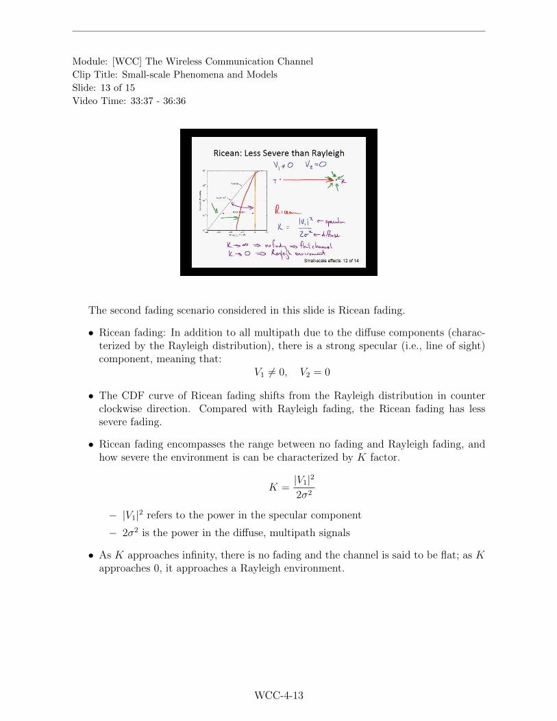
Module: [WCC] The Wireless Communication Channel
Clip Title: Small-scale Phenomena and Models
Slide: 13 of 15
Video Time: 33:37 - 36:36
The second fading scenario considered in this slide is Ricean fading.
• Ricean fading: In addition to all multipath due to the diffuse components (charac-terized by the Rayleigh distribution), there is a strong specular (i.e., line of sight)component, meaning that:
V1 6= 0, V2 = 0
• The CDF curve of Ricean fading shifts from the Rayleigh distribution in counterclockwise direction. Compared with Rayleigh fading, the Ricean fading has lesssevere fading.
• Ricean fading encompasses the range between no fading and Rayleigh fading, andhow severe the environment is can be characterized by K factor.
K =|V1|2
2σ2
− |V1|2 refers to the power in the specular component
− 2σ2 is the power in the diffuse, multipath signals
• As K approaches infinity, there is no fading and the channel is said to be flat; as Kapproaches 0, it approaches a Rayleigh environment.
WCC-4-13

Module: [WCC] The Wireless Communication Channel
Clip Title: Small-scale Phenomena and Models
Slide: 14 of 15
Video Time: 36:37 - 38:32
Previous slide discusses Ricean fading which was shown to be more benign thanRayleigh fading. This slide discusses a phenomenon more severe than Rayleigh fading,which is referred to hyper-Rayleigh fading.
• Hyper-Rayleigh fading is bounded by the two-ray model, which is an adaptation ofthe TWDP model.
• Two-ray model: there are only two specular paths and no diffuse components,meaning that:
V1 = V2 6= 0
• The plane-earth model is often referred to as the two-ray model for large-scaleeffects. This scenario is similar but at the small scale.
• If the system is designed for a Rayleigh fading environment but in fact the envi-ronment is more severe, then the severity of fades will be underestimated, and thesystem will not perform as intended.
WCC-4-14

Module: [WCC] The Wireless Communication Channel
Clip Title: Small-scale Phenomena and Models
Slide: 15 of 15
Video Time: 38:33 - 41:10
In this section it has been demonstrated that small-scale fading can cause huge vari-ations in the received signal strength. This slide summarizes the impact of small-scalefading and the consequences of using an improper model.
• The small-scale fading impacts the network conductivity
− In order to determine how closely nodes need to be placed, it’s important touse an appropriate model.
• Consequences of using an improper model
− Underestimate fading
· poor node conductivity, some sensors may fail to establish communication
− Overestimate fading
· deploy nodes too densely, using more resources in terms of the number ofnodes
· design for higher transmit power, wasting resources in terms of the size ofthe energy source to support higher transmit power
WCC-4-15

Module: [WCC] The Wireless Communication Channel
Clip Title: Fade Mitigation and Link Budgets
Slide: 1 of 10
Video Time: 00:00 - 03:11
This slide discusses the differences between mobile communication systems and sensornetworks.
• Mobile communication systems
− Deployment environment: the wireless device is moving hence the environmentis dynamic
− Position of wireless device: away from the large surfaces (walls, floors, etc.)
− Frequency of operation: 800 - 900 MHz, or 1800 - 1900 MHz
• Sensor networks
− Deployment environment: sensor networks tend to be fixed in position, thusthe environment is being most likely static or quasi-static.
− Position of wireless device: mounted on a structure or embedded within thestructure
− Frequency of operation: 2.4 GHz band. The signal wavelength is much shorter,therefore more susceptible to smaller variations and small-scale effects.
WCC-5-1

Module: [WCC] The Wireless Communication Channel
Clip Title: Fade Mitigation and Link Budgets
Slide: 2 of 10
Video Time: 03:12 - 05:14
This slide discusses the channel effects on a mobile communication system and a sensornetwork.
• The mobile communication system channel is time-varying
− The figure shows some data collected for a mobile communication system. Thisdata is from a vehicle traveling at about 75 mph in a very short period of time(a quarter of the second in total).
− The statistics of this time variation in terms of the fading is a Rayleigh envi-ronment. The range of fading goes from 15 dB down to about 30 dB.
• Sensor network
− The sensor network channel is static or quasi static (not quickly time-varying).
− The fading as a function of frequency or position can be significant.
WCC-5-2

Module: [WCC] The Wireless Communication Channel
Clip Title: Fade Mitigation and Link Budgets
Slide: 3 of 10
Video Time: 05:15 - 06:45
This slide revisits the real world data and presents how these measurements can becharacterized in terms of a fading model.
• The upper left plot shows the data taken inside metallic structure where one antennaor another was moved slightly to get different traces.
− Across frequency there is a lot of variations as a function of frequency.
− The differences between traces indicate there are variations as a function ofspace.
• The right figure shows the fading statistics for each of these traces in the left figure.
− The relatively benign trace has a Ricean distribution
− The solid trace follows a Rayleigh distribution
− The very severe trace, where there is very deep fades, approaches a two-raydistribution
WCC-5-3

Module: [WCC] The Wireless Communication Channel
Clip Title: Fade Mitigation and Link Budgets
Slide: 4 of 10
Video Time: 06:46 - 10:37
This slide discusses diversity schemes which take advantage of differences in paths offrequency, time and space, to mitigate some fading.
• Frequency diversity
− choosing between frequencies
− if one channel is bad, choose another channel
• Time diversity
− this approach is used in mobile systems
− RAKE receiver technique: receive multiple delayed version of the communica-tion signal and combine them
− the hardware of implementing time diversity is relatively more sophisticatedthan what is used in a wireless sensor node
• Space diversity
− using multiple antennas
− if two antennas are separated by half wavelength or more, the signal variationsare considered statistically independent of each other
− combining the input of multiple antennas can improve the overall power re-ceived
WCC-5-4

Module: [WCC] The Wireless Communication Channel
Clip Title: Fade Mitigation and Link Budgets
Slide: 5 of 10
Video Time: 10:38 - 12:50
This slide presents how to combine inputs of multiple antennas or multiple diversitypaths. There are two approaches being illustrated.
• Selection combining
− receiver chooses the strongest path
· If signal on antenna A is stronger than that in B, A will be selected andused for communication link
· if antenna A turns out to have a signal degradation, receiver will switchto B to see if that’s a better choice
• Maximum ratio combining (MRC)
− receiver continuously combines the inputs from all the antennas
· by adjusting the amplitude and phase of each path, the signal vectors fromantennas are lined up and added together coherently
· costs are more significant since there is need for additional hardware andprocessing, which needs to be continuously running to adjust phase shiftersand attenuators
WCC-5-5

Module: [WCC] The Wireless Communication Channel
Clip Title: Fade Mitigation and Link Budgets
Slide: 6 of 10
Video Time: 12:51 - 15:57
To illustrate the benefits of diversity techniques, this slide presents CDF curves forselection combining.
• Comparing the three cases: using a single antenna, selecting one of two antennasand selecting one of four antennas, we can see the more diversity is added, the moreimprovement there is in the overall system.
• Example 1: suppose there is 20 dB margin in the system, which is operating in atwo-ray environment
− using a single antenna: the link reliability (or system reliability) is 96% (theprobability of 20 dB fade is 4%)
− using two diversity paths: the link reliability increases to 99.8% (the probabilityof a 20 dB fade is 0.2%
• Example 2: suppose the system is operating in an Rayleigh environment and 99%reliability is wanted
− using a single antenna: a 20 dB margin is needed
− using two diversity paths: only a 10 dB margin is needed
WCC-5-6

Module: [WCC] The Wireless Communication Channel
Clip Title: Fade Mitigation and Link Budgets
Slide: 7 of 10
Video Time: 15:58 - 19:02
This slide develops a link budget to show the impact of the wireless communicationchannel on the overall system design.
• Recall the Friis equation for free space propagation environment:
Pr =PtGtGr
4πd2λ2
4π
• The Friis equation contains many of the link parameters as follows:
− Pt: transmit power, which for sensor networks will be very low (mW or dBm)
− Gt, Gr: antenna gains (dBi)
− λ: wavelength in meters
− d: distance in meters
− n: path loss exponent (accounts for large-scale effects)
WCC-5-7

Module: [WCC] The Wireless Communication Channel
Clip Title: Fade Mitigation and Link Budgets
Slide: 8 of 10
Video Time: 19:03 - 21:29
This slide discusses the antenna budget.
• The link parameters that the designer has control over include:
− Pt: transmitted power
− Gt: gain of the transmit antenna
− Gr: the gain of the receive antenna.
− d: distance between nodes.
• There is a trade-off between the transmit power (Pt) and antenna gain (Gt) inachieving the same EIRP (PtGt). To extend the lifetime of node, we can use lowertransmit power and increase antenna gain.
• The problem of increasing antenna gain is that the antenna coverage will decreasebecause the antenna becomes more directional.
• In general, the antenna is assumed to have omnidirectional coverage, which doesn’thave a very high gain but the 360 coverage can ensure the network conductivity.
• Compared to a satellite communication system where the beam is very focusedbecause the antenna gains are very high, the antenna gains for sensor networks arevery small (0 − 3dBi).
WCC-5-8
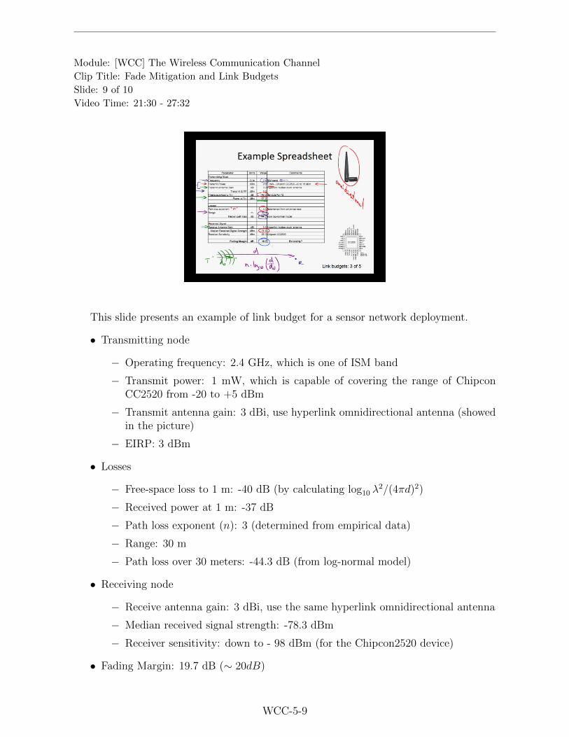
Module: [WCC] The Wireless Communication Channel
Clip Title: Fade Mitigation and Link Budgets
Slide: 9 of 10
Video Time: 21:30 - 27:32
This slide presents an example of link budget for a sensor network deployment.
• Transmitting node
− Operating frequency: 2.4 GHz, which is one of ISM band
− Transmit power: 1 mW, which is capable of covering the range of ChipconCC2520 from -20 to +5 dBm
− Transmit antenna gain: 3 dBi, use hyperlink omnidirectional antenna (showedin the picture)
− EIRP: 3 dBm
• Losses
− Free-space loss to 1 m: -40 dB (by calculating log10 λ2/(4πd)2)
− Received power at 1 m: -37 dB
− Path loss exponent (n): 3 (determined from empirical data)
− Range: 30 m
− Path loss over 30 meters: -44.3 dB (from log-normal model)
• Receiving node
− Receive antenna gain: 3 dBi, use the same hyperlink omnidirectional antenna
− Median received signal strength: -78.3 dBm
− Receiver sensitivity: down to - 98 dBm (for the Chipcon2520 device)
• Fading Margin: 19.7 dB (∼ 20dB)
WCC-5-9

Module: [WCC] The Wireless Communication Channel
Clip Title: Fade Mitigation and Link Budgets
Slide: 10 of 10
Video Time: 27:33 - 30:46
This slide discusses how to find the link reliability for a variety of different fadingenvironments given a margin and vice versa.
• Suppose we have 20 dB of margin, from the CDF plot we can see that:
− In Ricean environment, the link is very reliable
− In Rayleigh environment, the link reliability is about 99%
− In two-ray environment, the link reliability is about 96%
• There are two ways to achieve a 99% link reliability in two-ray environment:
− increase transmit power by 10 dB so there will be 30 dB link margin
− shorten T-R distance in order to have a higher median receive power at thereceiver
WCC-5-10

Module: [WCC] The Wireless Communication Channel
Clip Title: Example Application and Module Conclusion
Slide: 1 of 8
Video Time: 00:00 - 05:16
This slide discusses the motivation of utilizing the sensors themselves to monitor thechannel, it also introduces the WSSW (wireless sensors, sensing wireless) approach tomeasure and monitor the channel conditions.
• Motivation: there are issues with the test equipment method:
− costly (relative expensive) equipment
− take time to implement
− the measurements are only valid for that particular position at that particulartime
• Approach:
− WSSW (wireless sensors, sensing wireless)
− To implement WSSW, we can use two features in the radio chip:
· RSSI (received signal strength indication)
· channel selection
WCC-6-1

Module: [WCC] The Wireless Communication Channel
Clip Title: Example Application and Module Conclusion
Slide: 2 of 8
Video Time: 05:17 - 07:46
This slide presents an example of a WSSW implementation where there are five nodesdeployed in the mesh network, as showed in the plot on the right. Using this WSSWapproach, sensor nodes themselves can be utilized to determine the channel characteristics.
• The plot on the upper left shows the signal strength between any two pair as afunction of frequency
− measure the large-scale effects
− determine whether those links on average are good or poor.
• The plot on the lower left shows the CDF of links in the network to
− categorize the small-scale effects associated with particular links
− determine the link reliability
WCC-6-2

Module: [WCC] The Wireless Communication Channel
Clip Title: Example Application and Module Conclusion
Slide: 3 of 8
Video Time: 07:47 - 09:55
This slide summarizes a few key points of [WCC] module.
• Path loss on average increases with T-R distance
• Large-scale effects determine the rate of signal strength degradation with distance
• Small-scale effects may severely impact signal strength depending on the environ-ment that nodes are deployed in
• Diversity techniques can mitigate the small-scale effects (e.g., using multiple anten-nas)
• WSN are unique from mobile systems due to the operating frequency and lack ofmobility, so WSN need to be modeled differently
• Link budgets are critical in understanding requisite transmit powers, expected con-nectivity length, and the overall link reliability
• Sensor nodes themselves can be utilized to measure and determine the channelcharacteristics
WCC-6-3

Module: [WCC] The Wireless Communication Channel
Clip Title: Example Application and Module Conclusion
Slide: 4 of 8
Video Time: 09:56 - 10:15
This slide provides additional resources of this module.
• much of the material regarding modeling was from this book: Wireless Communi-cations: Principles and Practice by T. Rappaport
• some additional material on hyper-Rayleigh fading and diversity gains are from thework at the University of Vermont
WCC-6-4

Module: [WCC] The Wireless Communication Channel
Clip Title: Example Application and Module Conclusion
Slide: 5 of 8
Video Time: 10:16 - 10:58
This slide shows an example of utilizing MATLAB to determine the time and frequencyresponse.
• The top plot shows channel impulse response, where there are two paths s1 and s2
• The bottom plot shows the channel frequency response or transfer function
WCC-6-5

Module: [WCC] The Wireless Communication Channel
Clip Title: Example Application and Module Conclusion
Slide: 6 of 8
Video Time: 10:59 - 12:36
This slide presents the MATLAB code of plotting channel response for the particularexample in the previous slide. .
• In terms of magnitude, the primary path is s1 = 0.55 and the secondary path is1− s1 = 0.45, so the difference in magnitude is 1.7 dB
• The secondary component is delayed by the phase θ = 2π · f · d/c, where
− f is the frequency which varies across the 2.4 GHz band
− d/c is the time delay (the path difference divided by the speed of light)
• The received signal is calculated by x = 20 log10 |s1 + s2|, which is a log-scale
WCC-6-6

Module: [WCC] The Wireless Communication Channel
Clip Title: Example Application and Module Conclusion
Slide: 7 of 8
Video Time: 12:37 - 13:06
This slide shows an example of utilizing MATLAB to create CDF plots given the inputdata. The input data is the channel loss as a function of frequency.
WCC-6-7

Module: [WCC] The Wireless Communication Channel
Clip Title: Example Application and Module Conclusion
Slide: 8 of 8
Video Time: 13:07 - 15:41
This slide presents the MATLAB code for creating the CDF plot.
• Sort the loss vector from deepest fade to lowest fade, or most negative to leastnegative in terms of loss (in dB)
• create a vector to represent the probability of the losses occurring
• determine the point where the probability is 50% (the median value)
• normalize the sorted vector by the median value
• plot the remaining points relative to the median value in semi-log scale
• the CDF plot shows that the maximum probability value is 1, and the minimumprobability values is determined by the reciprocal of the number of data points
WCC-6-8

Module: [SNA] Sensor Network Architectures
Clip Title: Module Objectives, Deployment Strategies and Topologies
Slide: 1 of 11
Video Time: 00:00 - 00:10
This slide lists the main points of the clip.
• Introduction and objectives
• Deployment Strategies
• Network Topologies
SNA-2-1

Module: [SNA] Sensor Network Architectures
Clip Title: Module Objectives, Deployment Strategies and Topologies
Slide: 2 of 11
Video Time: 00:11 - 02:05
This slide discusses topics related to the architectures which sensor networks mayutilize, as well as the tools and methods that can be used to design an effective deployment.Particularly, specific objectives include
• To become familiar with how application needs impact deployment strategies.
• To understand key benefits and costs associated with different topologies.
− For example, understand where to place the nodes and how to determine whatnodes will communicate with what nodes in the network.
• To understand key benefits and costs associated with homogeneous network (a net-work where all the nodes are the same) and heterogeneous network (a network wheresome nodes may have additional resources).
• To introduce simple metrics to assess network connectivity.
• To understand common routing protocols (how data are shipped in the network)
• Finally, to synthesize these concepts to ascertain the energy requirements for variousnetwork topologies.
SNA-2-2

Module: [SNA] Sensor Network Architectures
Clip Title: Module Objectives, Deployment Strategies and Topologies
Slide: 3 of 11
Video Time: 02:06 - 06:18
This slide discusses important factors in designing the deployment of a sensor network,and how application needs influence the deployment.
• Deployment refers to where and how and when we will place the nodes in theenvironment being sensed.
• Designing a deployment needs to ensure that two criteria are met: coverage andconnectivity.
− Coverage: nodes need to be placed appropriately to sense the desired phenom-ena.
− Connectivity: nodes need to be placed so that they communicate to get datato the end user.
• Where and how nodes are placed depends very much on the application.
− If the phenomena is very localized, then the location of the node is critical forcoverage.
− In general environmental monitoring, placement may be driven by connectivityneeds.
− If the network is monitoring the natural environment, nodes may need to beplaced on existing infrastructure so as not to further disturb the habitats.
− Lifetime requirement and accessibility to the site will influence the deploymentstrategies.
• The difficulty or cost of the deployment may also influence and strategy.
− If it is a very remote location or it is costly to reach, one may do airdrop, flyingover with sensors and dropping them out.
− In this airdrop scenario we have things like a random and potentially over-deployment of nodes.
SNA-2-3

Module: [SNA] Sensor Network Architectures
Clip Title: Module Objectives, Deployment Strategies and Topologies
Slide: 4 of 11
Video Time: 06:19 - 08:33
This slide introduces two deployment strategies: random deployment and structureddeployment.
• Research literature often assume random deployment, and researchers quantifywhether the desired coverage and connectivity will be achieved given the numbernodes distributed.
• In the second strategy, one assumes a structured deployment, which makes compar-ative analysis more straightforward.
• In practice today, however, neither of these deployment strategies are very useful.
− Sensor nodes are still too expensive to drop in mass and as such they are handdeployed neared the phenomena of interest. The nodes are manually placed toensure both coverage and connectivity
− In testbeds, nodes are often deployed along lines. This is a nice thing to doin the lab they have regular intervals but in practice not a lot of applicationswould benefit from this tile layout.
− In short, deployment today are still very much labor-intensive. One decidesnot only where to place but when to deploy them.
SNA-2-4

Module: [SNA] Sensor Network Architectures
Clip Title: Module Objectives, Deployment Strategies and Topologies
Slide: 5 of 11
Video Time: 08:34 - 11:00
This slide introduces two strategies as to when to deploy nodes: incremental deploy-ment and over-deployment.
• If nodes are located at a site where the network is readily accessible, then nodes canbe easily replaced over time or deployed in an incremental approach.
• If getting to the site is not very convenient and one may have only one chance todeploy, then one needs to over-deploy the network, meaning to deploy more nodesthan are needed to achieve a network’s initial coverage and connectivity requirement.
• The methods that decide what nodes are on in a over-deployed case are referred toas topology control.
− In the over-deployed case, not all the nodes that we have out there are activeat the same time. Some that are in extended sleep state and may come onlinewhen other nodes fail.
− One may try to maintain a constant number of active nodes even though thetotal number of nodes in the network exceeds that amount.
SNA-2-5

Module: [SNA] Sensor Network Architectures
Clip Title: Module Objectives, Deployment Strategies and Topologies
Slide: 6 of 11
Video Time: 11:01 - 12:02
This slide discusses the motivation of choosing network topology and three differenttypes of network topologies.
• Motivation in choosing a network policy is to ensure reliable delivery of the data inan energy efficient manner.
• There are three types of network topologies: Star, Flat mesh and Tiered.
SNA-2-6

Module: [SNA] Sensor Network Architectures
Clip Title: Module Objectives, Deployment Strategies and Topologies
Slide: 7 of 11
Video Time: 12:03 - 13:45
This slide describes the star topology, where all nodes directly send data to the sink.
• The star topology is illustrated in the figure, where the blue node represents thesink.
• The data are sent over a single transmission and thus this is referred to as a singlehop network.
• The physical extent of our network, that is the total area that can be covered bythe deployment, is limited by the device’s communication range.
− Star topology is only useful when only a small coverage area is considered.
• One advantage of the star topology is that the requirements on the MAC protocolcan be less stringent.
SNA-2-7

Module: [SNA] Sensor Network Architectures
Clip Title: Module Objectives, Deployment Strategies and Topologies
Slide: 8 of 11
Video Time: 13:46 - 18:33
This slide describes the mesh network topology, in which nodes can connect to anyother node within the communication range.
• The topology is illustrated by the figure on the left.
• If a node can talk to every other node, the network is a full mesh but in generalthat will not be the case.
• Nodes can communicate with multiple nodes and not just the data sink.
• There are several advantages of using a mesh topology
− The physical extent of the network can be greater than in a star topology sincemultiple hops can be used to get the data to the sink
− Mesh networks are robust to link and node failures, as the data can be reroutedwhen a particular communication link fails.
− Likewise, they are also robust to nodes failing.
− The individual communication links may be shorter in comparison to an equiv-alent star network. Individual transmission costs may be less.
• Mesh networks are also referred to as a flat topology, as there’s no hierarchy in thenode types
• Mesh networks often operate as an ad hoc network in that the mesh is automaticallyformed.
SNA-2-8

Module: [SNA] Sensor Network Architectures
Clip Title: Module Objectives, Deployment Strategies and Topologies
Slide: 9 of 11
Video Time: 18:34 - 21:58
This slide describes the tiered network topology, in which network nodes are configuredin multiple clusters, and the nodes in each cluster route the data to cluster heads.
• The figure illustrate this topology, using different symbols to represent the nodes ofdifferent roles. The circle node is the sink, the square nodes are the cluster heads,and the crosses represent end nodes (also called leaf nodes).
• The advantages of a tiered network are that the communication links are short justlike the mesh network and that is also has some structures, which simplify the taskof how data is routed to the sink.
• There are some critical nodes in the network, whose failures would lead to the lossof connectivity to a good portion of the network.
• The cluster heads would be required to utilize more energy than the end nodes.They not only have to send their own data but they have to route all the data isbeing sent to them.
SNA-2-9

Module: [SNA] Sensor Network Architectures
Clip Title: Module Objectives, Deployment Strategies and Topologies
Slide: 10 of 11
Video Time: 21:59 - 25:49
This slide compares two strategies to deal with the problems of the cluster heads usingenergy at a higher rate, for both heterogeneous and homogeneous network designs.
• The heterogeneous design is to enhance the capabilities of the cluster heads (pro-viding a larger battery, making them more physically robust, etc).
− As illustrated by the figure on the right, in a heterogeneous design, end nodesgenerally is relatively less expensive, while cluster heads are equipped withmore resources, and the sink needs to be most reliable.
• As illustrated by the figure on the left, in a homogeneous network all the devices(except the sink) are identical.
− With such design, the nodes as cluster heads tend to fail faster than end nodes,could lead to the collapse of the entire network.
− This issue can be addressed by rotating the responsibility of operating as thecluster head among the nodes that are in the cluster.
− In this way, the nodes within a single cluster tend to fail at the same rate andas such the overall network life is going to be maximized.
SNA-2-10

Module: [SNA] Sensor Network Architectures
Clip Title: Module Objectives, Deployment Strategies and Topologies
Slide: 11 of 11
Video Time: 25:50 - 27:56
This slide compares single-hop networks and multi-hop networks, as well as theirrespective advantages in practice.
• In a single hop network, all nodes communicate directly with the data sink; whilein a multi-hop network, nodes may relay their data to multiple other nodes in orderto get into the sink.
• The figures illustrate the star topology for single-hop network, and the mesh/tieredtopology for multi-hop networks.
• The advantages of the multi-hop network includes greater physical extent of cover-age, while for single-hop network, the coverage radius is limited within the distanceof direct communication.
• The mesh design results in more complicated MAC and routing aspects of thenetwork.
SNA-2-11
Module: [SNA] Sensor Network Architectures
Clip Title: Connectivity and Coverage
Slide: 1 of 12
Video Time: 00:00 - 00:09
This slide lists the main points of the clip
• Connectivity
• Coverage
SNA-3-1

Module: [SNA] Sensor Network Architectures
Clip Title: Connectivity and Coverage
Slide: 2 of 12
Video Time: 00:10 - 03:04
This slide discusses the motivation of studying connectivity and how this can be ana-lyzed using tools from graph theory.
• The motivation of studying network connectivity is to ensure that data from sensornodes can get to the end user.
− This occurs when there are robust communication links between a sufficientnumber of nodes.
• Tools in graph theory can be employed to study connectivity.
− A network can be considered as a graph, with the nodes being vertices, andthe connections between them being edges.
− The study of connectivity is to quantize whether there are enough edges toensure there is a path or connection between vertices.
SNA-3-2

Module: [SNA] Sensor Network Architectures
Clip Title: Connectivity and Coverage
Slide: 3 of 12
Video Time: 03:05 - 06:05
This slide discusses two parameters of a graph that would influence the network con-nectivity, and use a random graph model to illustrate how they actually impact theconnectivity.
• The connectivity of a graph is influenced by two parameters:
− The first parameter is how far each node can communicate.
− The second parameter is how closely packed the nodes are, which can be mea-sured in terms of the number of nodes per area (node density).
• A geometric random graph model G(N,R) has two parameters:
− R: radius of communication, and
− N : the number of nodes that are deployed, which influences node density.
• The figure on the bottom right shows a simple example, with two nodes A and B.
− With the initial setting, they are not connected to each other.
− They can be connected using two means:
· Increase the communication radius R to encompass B within A’s range.
· Adding nodes (say C and D) to connect between them, that is, increasethe node density.
SNA-3-3

Module: [SNA] Sensor Network Architectures
Clip Title: Connectivity and Coverage
Slide: 4 of 12
Video Time: 06:06 - 09:22
This slide shows three geometric random graph models whose communication radiusdiffer, and compare their connectivity.
• In the first case (shown on the upper right) with R = 0.35, the communicationradius is sufficient to connect nodes over upper left and the nodes to the lower rightin clusters. But this network does not have full connectivity over the entire network,and thus is referred to as a disconnected graph.
• In the second case (shown on the left) with R = 0.4, the increased communicationradius is sufficient to connect between the two clusters. But there is not a lot ofredundancy here, and thus the network is highly susceptible to link failures, andit is referred to as sparse connectivity. The failure of the single link between twoclusters will render the network disconnected.
• In the third case (shown on the lower right) with R = 0.5, there are a lot of linksbetween deployed nodes. This is referred to as dense connectivity, and it is robustto the failures of any particular links.
SNA-3-4

Module: [SNA] Sensor Network Architectures
Clip Title: Connectivity and Coverage
Slide: 5 of 12
Video Time: 09:23 - 12:14
This slide discusses the problems of random graph model, particularly the underlyingassumptions which are often too idealistic in practice.
• In a random graph model G(n,R), the link reliability is assumed to be 1 withinsome communication radius R, and 0 beyond that distance.
• This simple assumption does not represent well the real propagation environment.
− In real wireless network, good reliability is very good within a very close dis-tance, and then some degradation the T-R distance increases, due to shadowingor multipath effects.
− Also, the propagation effects are non-isotropic. Generally, due to antenna pat-terns and environmental conditions, the communication range of a particularnode is a function of both distance and direction.
− This can be depicted using a communication footprint as shown in lower left.
• In sum, graph theory offers some useful tools, but they are dependent on conditionsor assumptions, which may be too idealized.
SNA-3-5

Module: [SNA] Sensor Network Architectures
Clip Title: Connectivity and Coverage
Slide: 6 of 12
Video Time: 12:15 - 14:46
This slide describes K-connectivity, a metric that measures how connected a graph is.
• Formally, K-connectivity is the minimum number of nodes that any particular nodeis connected to.
• In the left figure, a node is completely isolated, and thus its K-connectivity is 0.
• In the right figure, the K-connectivity is 2.
• A positive K-connectivity does not guarantee full connectivity in general. In theright figure, if the link between two clusters is gone, the K-connectivity remains 2,but the network is not fully connected.
• The connectivity is not guaranteed simply by a particular setting of n and R in arandom graph model. In both cases shown in this slide, n = 10 and R = 0.4, theright one is fully connected, but the left one is not.
SNA-3-6

Module: [SNA] Sensor Network Architectures
Clip Title: Connectivity and Coverage
Slide: 7 of 12
Video Time: 14:47 - 17:23
This slide describes two approaches to improving connectivity and compares the costsassociated with them.
• The first approach is to add more nodes, i.e., increasing N .
− This approach will incur the most costs spent on the nodes that need to bedeployed.
− This will also increase the number of communication links and thus this willimpact the demand on the channel and thus the MAC requirements
• The second approach is to increase communication distance, i.e., increasing R.
− This will require more energy resources to support higher RF transmissionpower.
− The range is still limited by the maximum transmission power which is specifiedby FCC for the ISM bands.
SNA-3-7

Module: [SNA] Sensor Network Architectures
Clip Title: Connectivity and Coverage
Slide: 8 of 12
Video Time: 17:24 - 19:41
This slide discusses the motivation for coverage and the graph theory tools used tostudy it.
• The key motivation for coverage is to ensure that nodes are properly located tosense the phenomenon of interests.
• Graph theory tools can be used to study coverage, based upon some assumptions:
− First, the sensors have some sensing radius, which can measure the parameterof interest not only at a particular point but over some distance.
− The phenomena are spatially correlated, which means what is measured for aparameter at one spot will be very much similar to what are measured a smalldistance away.
SNA-3-8

Module: [SNA] Sensor Network Architectures
Clip Title: Connectivity and Coverage
Slide: 9 of 12
Video Time: 19:42 - 23:02
This slide introduces the Voronoi diagram as a tool for understanding coverage. TheVoronoi diagram is created by drawing lines that bisect vertices.
• The animation of this slide illustrates the process of creating a Voronoi diagram.
− The bisecting lines between pairs of vertices are extended to create cells thatrepresent the area that the sensor node is assumed to cover.
• Any point within a cell about a node is closer to that node than to others.
• If a cell is too big for a node to monitor the phenomenon, exceeding the sensingrange of a node, the phenonmenon does not get full coverage. In such cases, onecan add more nodes to improve the coverage.
• Full connectivity does not guarantee full coverage, and vice versa.
SNA-3-9

Module: [SNA] Sensor Network Architectures
Clip Title: Connectivity and Coverage
Slide: 10 of 12
Video Time: 23:03 - 24:23
This slide introduces K-coverage, a metric to measure how well the environment isbeing covered.
• K-coverage equals K means that any portion of the monitored area has at least Knodes monitoring it.
• The figure in the slide illustrates a point with K = 3 coverage and another pointwith K = 2 coverage.
• In terms of the entire network, the K-coverage is determined by a point that hasthe minimum amount of covers.
• Coverage depends on the density and in addition the range which the phenomenoncan be sensed.
SNA-3-10

Module: [SNA] Sensor Network Architectures
Clip Title: Connectivity and Coverage
Slide: 11 of 12
Video Time: 24:24 - 29:22
This slide uses four figures to summarize the discussion of graph theory and its use inunderstanding sensor networks.
• The node deployment is driven by two constraints connectivity and coverage.
• The figure on the top right shows a network with sparse connectivity. To guaranteereliable communication, adding additional nodes to improve connectivity may beprudent.
• The figure on the bottom right shows a Voronoi diagram, which can be used toanalyze the effectiveness of a network in terms of coverage.
− For a network deployed for target detection, there is a metric: maximum breachpath, from which we can analyze the maximum distance that a target is fromany sensing node.
• The figure on the bottom left shows a Delauney diagram, from which we can obtainthe maximum support path. This is the path that one travels from cell to cell takingthe shortest paths between them.
• These complementary representations the Voronoi and delauney diagrams have usesto help design the network to either ensure that the nodes are properly detectingsomething or to help design path which mobile devices can travel and best contactstatic sensor nodes.
SNA-3-11

Module: [SNA] Sensor Network Architectures
Clip Title: Connectivity and Coverage
Slide: 12 of 12
Video Time: 29:23 - 33:08
This slide discusses the problems of using graph theory tools to assess network cover-age.
• First it assumes the phenomenon can be sensed at a distance, which may not betrue for phenomenon that is very localized.
• Second it assumes the phenomenon is spatially correlated, which may not be truefor the stuff that has a high variability.
• When using Voronoi and Delauney diagrams to understand the coverage, one needsto use practical information to decide whether the end result is sufficient for thephenonena that are being monitored.
− If the phenomenon is localized and highly variable, more nodes might be neededfor coverage.
SNA-3-12

Module: [SNA] Sensor Network Architectures
Clip Title: Topology Control
Slide: 1 of 4
Video Time: 00:00 - 00:09
This slide states the main point of the clip, which is topology control.
SNA-4-1

Module: [SNA] Sensor Network Architectures
Clip Title: Topology Control
Slide: 2 of 4
Video Time: 00:10 - 05:21
This slide discusses the basic idea and motivations of topology control.
• Topology control determines which nodes in the network are active, so as to providea sufficient number of active nodes to meet the users’ needs while saving energy.
• The first motivation is to save energy, by sending only the data that are needed.
• The second motivation is to adjust to network dynamics
− Consider stream monitoring, when the weather is dry, the network need notbe very active. However, when there is a storm, all nodes have to participateto provide data in a timely fashion.
• The third motivation is to support over deployment strategy.
− In the case where there are difficulties in doing a deployment, one tends todeploy more nodes than the initial need to put part of the nodes in sleep state.These nodes are waken up when they are needed to replace failed nodes.
SNA-4-2

Module: [SNA] Sensor Network Architectures
Clip Title: Topology Control
Slide: 3 of 4
Video Time: 05:22 - 15:07
This slide describes one topology control method - Probing Environment and AdaptiveSleep (PEAS).
• This method is appropriate for multi-hop, multi-cluster deployments. In PEAS,different clusters maintain the same activity rate (i.e., data delivery rate).
− Each node in a cluster with more nodes tend to be less active than those withina cluster with smaller number of nodes.
• In PEAS, nodes operate in three states: sleep, probing or active.
• PEAS works as follows
− Nodes are in the sleep state will wake up at a random interval with a expo-nential distribution.
· The probability density function (PDF) of an exponential distribution ofrate λ is given by
f(x;λ) =1
λe−λx, x ≥ 0.
− When a node wakes up, it moves to a probing state, and sends out a requestor probe to the network, and then adjusts its behavior according to the reply.
· If there is no response (indicating that the network is not active), the nodemoves to the active state
· Otherwise, the node adjusts the rate as follows
λupdate = λcurrent ·λd
λ.
Here, λd is the desired rate, and λ is the current rate that the probing nodeascertains to be the activity of the network.
SNA-4-3

− Generally, if the present activity is higher than what is desired, the node de-creases its rate, otherwise it increases the rate.
− The desired rate λd is pre-defined.
• PEAS can adjust the the wake-up rate of nodes so as to maintain a constant activityof the network, but it cannot address the changes to the environmental dynamics,that might require changing network activity.
4
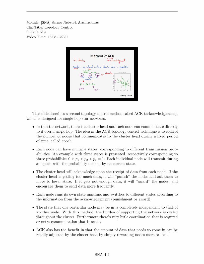
Module: [SNA] Sensor Network Architectures
Clip Title: Topology Control
Slide: 4 of 4
Video Time: 15:08 - 22:51
This slide describes a second topology control method called ACK (acknowledgement),which is designed for single hop star networks.
• In the star network, there is a cluster head and each node can communicate directlyto it over a single hop. The idea in the ACK topology control technique is to controlthe number of nodes that communicates to the cluster head during a fixed periodof time, called epoch.
• Each node can have multiple states, corresponding to different transmission prob-abilities. An example with three states is presented, respectively corresponding tothree probabilities 0 < p1 < p2 < p3 = 1. Each individual node will transmit duringan epoch with the probability defined by its current state.
• The cluster head will acknowledge upon the receipt of data from each node. If thecluster head is getting too much data, it will “punish” the nodes and ask them tomove to lower state. If it gets not enough data, it will “award” the nodes, andencourage them to send data more frequently.
• Each node runs its own state machine, and switches to different states according tothe information from the acknowledgement (punishment or award).
• The state that one particular node may be in is completely independent to that ofanother node. With this method, the burden of supporting the network is cycledthroughout the cluster. Furthermore there’s very little coordination that is requiredor extra communication that is needed.
• ACK also has the benefit in that the amount of data that needs to come in can bereadily adjusted by the cluster head by simply rewarding nodes more or less.
SNA-4-4

Module: [SNA] Sensor Network Architectures
Clip Title: Routing Protocals
Slide: 1 of 8
Video Time: 00:00 - 00:09
This slide states the main point of this clip, which is routing protocols.
SNA-5-1

Module: [SNA] Sensor Network Architectures
Clip Title: Routing Protocals
Slide: 2 of 8
Video Time: 00:10 - 01:29
This slide introduces the motivation for choosing a routing protocol and two classesof protocols.
• Motivation
− identify a data path from source to the sink so that the path is
· energy efficient
· robust
• Two classes of protocols:
− Metric-based protocol
· aims at minimizing some metric (e.g., number of hops to ensure energyefficiency).
− Diversity-based protocol
· aims at enhancing the number of routes or diversity to ensure robustnessof the routing to individual node or link failures.
SNA-5-2

Module: [SNA] Sensor Network Architectures
Clip Title: Routing Protocals
Slide: 3 of 8
Video Time: 01:30 - 05:27
This slide illustrates the simplest routing protocol greedy forward. In this techniquea node forwards the data to the note which is closest to its desired destination.
• Case 1:
− Node A (the source) wants to send data to node B (the sink), but B is out ofthe connectivity range of A.
− Node C, D and E are within the radius of the communication range of A.
− Since D is closest to B, it is the ideal node that node A will transmit data to.However if the link from D to B fails, there’s no opportunity to recover.
• What is often done is to define a inner radius (r) where the communication link ismore reliable, and then operate the greedy algorithm in the same way.
• Case 2:
− Within the inner radius r of A, node E is closest to the desired sink B, so nodeA will transmit data to E.
− Likewise, choosing node within the communication radius, E will transmit datato node D, and D will transmit data to sink B.
• Note that if the sink is different, the routing paths will be different. In order forgreedy forwarding to work, nodes need to have geographic information about whereall the other nodes are.
SNA-5-3

Module: [SNA] Sensor Network Architectures
Clip Title: Routing Protocals
Slide: 4 of 8
Video Time: 05:28 - 13:01
This slide uses an example to illustrate ETX (expected number of transmissions)metric protocol.
• Scenario:
− Consider the previous network where node A (the source) wants to send datato node B (the sink), between the source and the sink there are node C, Dand E. Suppose the connectivity of this network is shown by the blue edges.
− The reliability of each link is given by packet reception:
d = df · dr· df : the forward reliability,
· dr is the reverse reliability of the acknowledgement
− Assume the packet reception rate of each link is determined.
· short link: dAC = dCD = dDB = 0.9
· median link: dAE = dEB = 0.75
· long link: dAB = 0.3
• In order to find the most reliable path, we need to find the route with the smallestnumber of expected transmission (E[TX]).
− for the top route (A− C −D −B), E[TX] = 3 · 1d
= 3 · 10.9
= 3.33
− for the middle route (A−B), E[TX] = 1d
= 10.3
= 3.33
− for the bottom route (A − E − B), E[TX] = 2 · 1d
= 2 · 10.75
= 2.66 (the bestroute using ETX metric)
• Note that this technique assumes each transmission is equivalent in energy, no powercontrol is being accounted. This protocol also depends on knowing the link reliabilityof the network which may not be known or may not be constant.
SNA-5-4

Module: [SNA] Sensor Network Architectures
Clip Title: Routing Protocals
Slide: 5 of 8
Video Time: 13:02 - 18:43
This slide uses an example to illustrate the extreme opportunistic method (ExOR).
• Scenario:
− Consider the same network where A (the source) wants to send data to B (thesink), along the way there are node C, D and E.
− The packet contains not only the data, but also a priority list of possiblerecipients
− Each node that receives the packet also hears acknowledgements of all thenodes that have received the packet.
• Case 1
− Assume node A’s priority list is B − D − E − C. Also, suppose everyone inthe list is able to receive the packet except for B.
− When the packet gets transmitted throughout the network, D, E and C suc-cessfully receive the data and they know that B doesn’t. Since D is the nexthighest in the priority list, it will be D’s responsibility to forward it on.
− Again node D will route the packet according to its priority list.
• Case 2
− Assume node A still has its priority list of B − D − E − C, suppose only Cand E receives the packet due to the link failure.
− When the packet gets transmitted, C and E learned that out of the nodes inthe priority list only E and C have received it. Since E has higher prioritythan C, it will be E’s job to send the data out.
• This ExOR approach requires additional communications with acknowledgements,it also requires that each node established its priority list internally.
SNA-5-5

Module: [SNA] Sensor Network Architectures
Clip Title: Routing Protocals
Slide: 6 of 8
Video Time: 18:44 - 24:11
In the gradient routing methods, all nodes have a table with the expected cost to geta packet to the data sinks. This slide uses an example to illustrate the gradient routingapproach.
• Scenario:
− Consider the previous network where A (the source) wants to send data to B(the sink), along the way there are C, D and E.
− Suppose each node has a cost to sink store in it. When a packet wants tobe sent, it has to be assigned a certain amount of currency (e.g. units, hops,transmissions). When a packet is sent, it includes two fields:
· cost accrued
· remaining assets
• Assume a packet is assigned currency of 8, and the cost to sink for each node isCAB = 5, CCB = 4, CEB = 3 and CDB = 2.
• If A sends out a packet, its accrued cost will be 5 and the remaining assets will be 3.Since the packet is broadcasted, all nodes in the network could potentially receiveit.
− If C receives the packet, accrued cost = 9, remaining asset = -1 (will notretransmit)
− If D receives the packet, accrued cost = 7, remaining asset = 1 (will retransmit)
− If E receives the packet, accrued cost = 8, remaining asset = 0 (will retransmit)
• The gradient technique enables packets to travel multiple paths, but it puts a capon the total number of transmissions each route can take.
• Each node needs to know the cost to different sinks in the network.
SNA-5-6

Module: [SNA] Sensor Network Architectures
Clip Title: Routing Protocals
Slide: 7 of 8
Video Time: 24:12 - 33:04
This slide discusses lifetime maximizing routing and load balancing routing approaches.
• Lifetime maximizing routing
− the cost to send a packet from node i to node j depends on three parameters:
cij = T aijRi
bEic
· Tij: link transmission cost, the number of hops or the energy used for thatparticular hop
· Ri: residual energy in transmitting node
· Ei: initial energy of transmitting node
· a, b, c: weighting factors
− If only consider transmission cost, (a, b, c) = (1, 0, 0)
− If only consider residual energy, (a, b, c) = (0, 1, 0)
− The lifetime maximizing formulation allows for flexibility in establishing rout-ing criteria
• Load-balancing routing
− A node forwards its packet to its neighbor with a probability inversely propor-tional to its cost metric
− Consider the previous network where A wants to send a packet to B, B is outof range of A, and it will route through nodes C, D and E.
− Each link has a cost associated with it, the cost can be determined by thelifetime maximizing metric.
SNA-5-7

− Note that in this technique, a packet will only be sent to one of intermediatenodes as opposed to the ExOR routing or gradient routing where all thesenodes could potentially receive the packet.
− The probability of going from node i to node j is
Pij =1/cij∑
1/cik
· cij is the cost going from node i to node j
− Suppose the cost associate with each link A to C, A to D, A to E is CAC = 2,CAD = 4, CAE = 3, and the probabilities of going these links are:
PAC =1/2
1/2 + 1/4 + 1/3= 0.5/1.08 = 0.47
PAD =1/4
1/2 + 1/4 + 1/3= 0.25/1.08 = 0.23
PAE =1/3
1/2 + 1/4 + 1/3= 0.33/1.08 = 0.3
− When A wants to send a packet, it will roll the dice and take one of these threenodes (C, D or E) to send the packet to with these probabilities.
− The burden of routing the data through the network gets shared amongst thesenodes and through sharing, not any particular route will be overly burdenedand causing those nodes in the route to fail.
8

Module: [SNA] Sensor Network Architectures
Clip Title: Routing Protocals
Slide: 8 of 8
Video Time: 33:05 - 37:46
This slide discusses a strategy called data mules, which uses mobile nodes to addressthe issue of lack of connectivity in sparse sensor networks.
• Consider the case with a network of monitor points that are far from each other, suchthat the distances between them are too great to achieve any sort of connectivity.
• While one approach to solve this problem is to add additional nodes to achievenetwork connectivity, it is often too costly.
• Data mules are mobile nodes which move through the environment and collect datafrom static notes when they are in communication range.
− The scenario is that the coverage is achieved and the nodes are too sparse toensure connectivity.
− This is illustrated by the figure, where the green curve represent the trajectoryof a data mule.
• There are costs associated with the data mule approach.
− Data mules need to be energy rich.
− There can be a huge delay between the times that the mobile node comesaround to collect the data and that the data are collected.
− Some source coding may be needed to prevent the storage of the static nodesfrom being filled up while waiting for the mule to collect it.
SNA-5-8

Module: [SNA] Sensor Network Architectures
Clip Title: Trade-off Study and Module Conclusion
Slide: 1 of 5
Video Time: 00:00 - 00:09
This slide lists the main points of the clip
• Tradeoffs in Single -vs. Multi-hop Networks
• Module Conclusions
SNA-6-1

Module: [SNA] Sensor Network Architectures
Clip Title: Trade-off Study and Module Conclusion
Slide: 2 of 5
Video Time: 00:10 - 08:01
This slide compares the transmission energy costs for two different network topologies:single-hop and double-hop.
• The scenario is as follows, there are three nodes A, B, and C. Here, C is the datasink, and B is between A and C. In a star network, A and B directly send data toC. In a tiered network, B directly send to C, while the data from A are first sentto B, which are then forwarded to C by B.
• It is assumed that the cost of transmitting from A to B and that from B to C areequivalent.
• First, it compares under the setting that the transmission cost is proportional tothe square of the distance (free space model).
− Let the transmission cost between B and C be
EBC = K = kd2.
Then the transmission cost between A and B is also EAB = K.
− The cost of direct transmission from A to C is
EAC = k(2d2) = 4K.
− In total, the transmission cost associated with the single-hop network is
EAC + EBC = 4K + K = 5K,
while that associated with the double-hop network is
EAB + EBC + EBC = 3K.
SNA-6-2

− power control is feasible to use but a star network is certainly going to penalizenodes that are far from the cluster head to a factor of 4 to 1. In the tierednetwork, nodes that are further in are going to have a more severe energy drawbecause they must not only send their own data but also the data of nodesrouting through them.
• Second, in the planar model with path loss coefficient being 4, the energy consump-tion of the star network is going to be worse, as
EAC = k(2d)4 = 16K.
Hence, using a multi-hop mesh in environments with high path loss exponent willlead to great benefit of energy saving.
3

Module: [SNA] Sensor Network Architectures
Clip Title: Trade-off Study and Module Conclusion
Slide: 3 of 5
Video Time: 08:02 - 13:36
This slide compares the single-hop network as opposed to the tiered network with fourend nodes. As shown in the figure, C is the data sink, B is a node that is closer to Cwhich also serves as the cluster head in the tiered network, and A, X, Y , Z are end nodesthat are further from C (double distance).
• The comparison is under a free space model (path loss exponent is 2).
• For the tiered model, the energy cost of each link is the same (say K). But thecosts of different nodes are uneven. The energy cost of node B is 5K, as it has tosend its own data while relaying the data from end nodes.
• In tiered network, this intermediate node that the data is going through is gettingseverely impacted in terms of its energy use, hence such nodes should be given moreenergy to accomplish their routing task or a mechanism should be used to rotatethe burden.
• For the star topology, the end nodes are to directly send data to C, with cost 4Kfor each of the four end nodes. This requires a lot more energy for those nodes, andthe energy is even higher if under a model with higher path loss exponent.
• The trade-off is not straightforward, and the choice of topology should depend onparticular situation, e.g., the available resources, etc.
SNA-6-3

Module: [SNA] Sensor Network Architectures
Clip Title: Trade-off Study and Module Conclusion
Slide: 4 of 5
Video Time: 13:37 - 16:14
This slide concludes the module on sensor network architecture [SNA].
• Multi-hop networks promise broader coverage and robustness at the cost of increasedcomplexity.
• Homogeneous node architectures simplify deployment strategies but may requiremore capable hardware.
• Node connectivity is dependent on the node placement and communication channel.
• Network coverage requirements may not coincide with network connectivity require-ments.
• Routing schemes depend on defining an appropriate cost metric.
• Network architectures drive node and system design and therefore energy and band-width requirements.
SNA-6-4

Module: [SNA] Sensor Network Architectures
Clip Title: Trade-off Study and Module Conclusion
Slide: 5 of 5
Video Time: 16:15 - 16:50
This page recommends two books to those who would like to explore more on thistopic.
• B. Krishnamachari, Networking Wireless Sensors, Cambridge Press (2005).
− A very good survey.
• H. Karl and A. Willig, Protocols and Architectures for Wireless Sensor Networks,Wiley (2007).
− provides a lot more details.
SNA-6-5
Copyright © 2022 FDOKUMEN