Outdoor Localization System Using RSSI Measurement of Wireless Sensor Network

International Journal of Innovative Technology and Exploring Engineering (IJITEE)

ISSN: 2278-3075, Volume-2, Issue-2, January 2013

1

Outdoor Localization System Using RSSI

Measurement of Wireless Sensor Network

Oguejiofor O.S., Okorogu V.N., Adewale Abe, Osuesu B.O

Abstract- This paper present a system that utilizes RSSI based

trilateration approach to locate the position of blind nodes (nodes

that are not aware of there positioning in the network) amongst

other nodes in the network. The system automatically estimates the

distance between sensor nodes by measuring the RSSI (received

signal strength indicator) at an appropriate number of sensor

nodes. Through experiments, we clarified the validity of our data

collection and position estimation techniques. The results show that

when the anchor nodes were increased from three to four, the

localization error decreases from 0.74m to 0.56m.

Index terms- localization, nodes, Trilateration, RSSI

I. INTRODUCTION

Wireless Sensor Network (WSNs) has been widely

considered as one of the most important technologies for the

twenty – first century [1]. Enabled by recent advances in

micro electromechanical system (MEMS) and wireless

communication technologies, tiny, cheap, and smart sensors

deployed in a physical area and networked through wireless

links and the internet provide unprecedented opportunities for

a variety of civilian and military applications, for examples,

environmental monitoring, pipeline monitoring, battle field

surveillance, and industry process control [2]. If sensor nodes

are appropriately designed, they can work autonomously to

measure temperature, humidity luminosity and so on. Sensor

nodes send sensing data to a sink node deployed for data

collection. In future, sensors will be cheaper and deployed

everywhere: thus, user-location- dependent services and

sensor locations will be important. Distinguished from

traditional wireless communication network, for example,

cellular system and mobile adhoc networks (MANET), WSNs

have unique characteristics for example denser level of node

deployment, higher unreliability of sensor nodes, and severe

energy, computing and storage constraints [3], which presents

many new challenges in the development and application of

WSNs. A WSN typically consists of a large number of low-

cost, low-power, and multifunctional sensor nodes that are

deployed in a region of interest [4].

These sensor nodes are small in size but are equipped with

sensors, embedded microprocessors, and radio transceivers,

and therefore have not only sensory capability, but also data

processing and communicating capabilities. Manuscript received on January, 2013. Oguejiofor O.S, Electronics and Computer Engineering, Nnamdi Azikiwe

University, Awka (Anambra), Nigeria Okorogu V.N, Electronics and Computer Engineering, Nnamdi Azikiwe

University, Awka (Anambra), Nigeria

Adewale Abe, Electrical and Electronics Engineering, Ekiti State University, Ekiti (Ekiti), Nigeria

Osuesu B.O, Electronics and Computer Engineering, Nnamdi Azikiwe

University, Awka (Anambra), Nigeria

They communicate over a short distance via a wireless

medium and collaborate to accomplish a common task. Sensor

locations are important too, because sensing data are

meaningless if the sensor location is unknown in

environmental-sensing application such as pipeline

monitoring. Methods using ultrasound or lasers achieve high

accuracy, but each device adds to the size, cost, and energy

requirements. For these reasons, such methods are not suitable

for sensor networks. An inexpensive RF-based approach with

low configuration requirements has been studied[5,6].These

studies showed that the received signal strength indicator

(RSSI) has a larger variation because it is subject to the

delirious effects of fading and shadowing. A RSSI-based

approach therefore needs more data than other methods to

achieve higher accuracy [7].In this paper tpr2420 ca sensor

node will be used for the experiments because our technique

was implemented in it. This device was developed by the

University of California, Berkeley.

II. LOCALIZATION SYSTEM MODEL

This section presents localization system model that can be

used to establish the 2D Cartesian coordinates of the blind

nodes. Real time experiments were also carried out on an

experimental TinyOS-based WSN testbed environment to

measure Received Signal Strength Indicator (RSSI) at the

receiving nodes in other to estimate distance between

communicating nodes. In this paper, the focus is on a pipeline

segment which runs on a few kilometers (1-2 km); the sensor

nodes on a pipeline segment are assumed to transmit their

sensed data (temperature, light and humidity) to one base

station (sink) located in a distance far away from the remote

site; and the sensed data is collected through a multihop

forwarding scheme. Consider a case where sensor nodes are

deployed along a pipeline consisting of N sensor nodes {N1, --

----, Nn}. This is used to monitor an oil pipeline segment of

length (L= 1km). Here, the pipeline segment is assumed to be

a straight line. The closest to the sink is Nn and node N1 is the

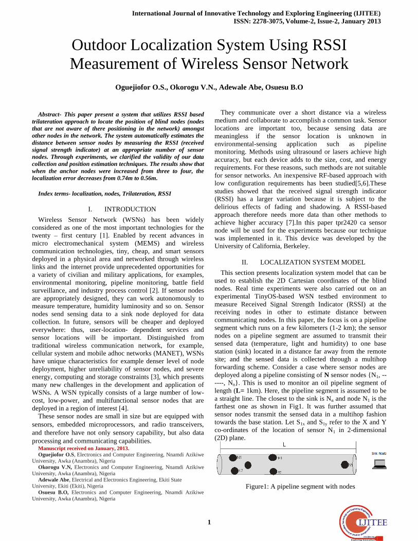
farthest one as shown in Fig1. It was further assumed that

sensor nodes transmit the sensed data in a multihop fashion

towards the base station. Let S1x and S1y refer to the X and Y

co-ordinates of the location of sensor N1 in 2-dimensional

(2D) plane.

Figure1: A pipeline segment with nodes

Sink Node

Outdoor Localization System Using RSSI Measurement of Wireless Sensor Network

2

To determine location of sensor nodes along the pipeline

constitutes the localization problem. However, some sensor

nodes are aware of their own positioning through manual

configuration or by placing it in an already known position;

these nodes are known as anchor or beacon nodes. All other

nodes that are not aware of their position are called blind

nodes; these nodes localize themselves with the help of

location references received from the anchors. It was assumed

that there are a set of B beacon nodes among the N sensors,

and there positions (xb, yb) for all b Є B. The positions (xn, yn)

for all blind nodes n Є N would be found. The localization

system model is comprised of both the signal propagation

model and the trilateration model. Trilateration is a

localization technique used when there is an accurate estimate

of distance between a node and at least three anchor nodes in a

2D plane. This method finds the intersection of three circles

centered at anchor as the position of the node.

A. TRILATERATION MODEL

Considering the basic formula for the general equation of a

sphere as shown in equation (1);

𝑑2 =𝑥2 +𝑦2+𝑧2 (1)

For a sphere centered at a point (xa, ya, za) the equation is

simplified as shown as in equation (2);

𝑑2= 𝑥 − 𝑥𝑎 2+ 𝑦 − 𝑦𝑎

2+ 𝑧 − 𝑧𝑎 2 (2)

Since we assume all the nodes spans out on the same plane,

consider the three anchor nodes (a, b and c) that has distance

(da, db, dc) to the blind node as illustrated in Fig. 2;

Figure 2: Intersection of three spheres in 2D

The formula for all spheres on one plane is shown below in

the following equations:

Sphere A; 𝑑𝑎2 = 𝑥 − 𝑥𝑎

2+ 𝑦 − 𝑦𝑎 2 (3)

Sphere B; 𝑑𝑏2 = 𝑥 − 𝑥𝑏

2+ 𝑦 − 𝑦𝑏 2 (4)

Sphere C;𝑑𝑐2 = 𝑥 − 𝑥𝑐

2+ 𝑦 − 𝑦𝑐 2 (5)

Equations (3), (4) and (5) can further be expanded to bring

about the following equations:

𝑑𝑎2= 𝑥2- 2x.xa + xa

2 + y

2 - 2y.ya + ya

2 (6)

𝑑𝑏2= 𝑥2- 2x.xb + xb

2 + y

2 - 2y.yb + yb

2 (7)

𝑑𝑐2= 𝑥2- 2x.xc + xc

2 + y

2 - 2y.yc + yc

2 (8)

The three equations (6), (7) and (8) are independent non-linear

simultaneous equations which cannot be solved

mathematically; however, using method proposed by Dixon

[8] to obtain radical plane for sphere intersection, equation (8)

was subtracted from equation (7) to get the following linear

equation:

𝑑𝑏2 - 𝑑𝑐

2 =2x (xc - xb) + xb

2 - xc2 +2y (yc - yb) + yb

2 - yc2 (9)

And subtracting equation (6) from equation (7), the following

linear equation is obtained:

𝑑𝑏2 - 𝑑𝑎

2 =2x (xa - xb) + xb

2 – xa2 +2y (ya - yb) + yb

2 – ya2 (10)

Rearranging the equation (9) to produce a new equation and a

new variable as follows,

x(xc-xb)+y (yc - yb) = 𝑑𝑏

2−𝑑𝑐2 − 𝑥𝑏

2−𝑥𝑐2 − 𝑦𝑏

2 −𝑦𝑐2

2= 𝑣𝑎 (11)

Rearranging the equation (10) to produce a new equation and

a new variable as follows,

x(xa-xb)+y(ya - yb) = 𝑑𝑏

2−𝑑𝑎2 − 𝑥𝑏

2−𝑥𝑎2 − 𝑦𝑏

2 −𝑦𝑎2

2= 𝑣𝑏 (12)

Resolve the equation (11) and equation (12) to gain the

intersection point „x‟ and „y‟ of these two equations as the

following equation for „y‟ value and equation for „x‟ value

respectively:

y= 𝑣𝑏 xc− xb − 𝑣𝑎 (xa− xb)

ya− yb xc− xb − yc− yb xa− xb (13)

x= 𝑣𝑎−𝑦 yc− yb

(xc− xb) (14)

The values for x and y gives us the accurate position in two

dimension (2D) for the blind node. This Model is developed

using MATLAB and programmed into tpr 2420ca nodes,

hence after initialization of the nodes, once the blind node can

receive packets from at least three anchor nodes, it can

localize its position using references received from the

anchors. But these values can‟t be obtained without the signal

propagation model.

B. SIGNAL PROPAGATION MODEL

In this section the signal propagation model in wireless

sensor network will be addressed. The most common signal

propagation model in wireless sensor Network (WSN) is the

free space model. The free space model assumes that the

receiver within the communication radius can receive the data

packet. One possibility to acquire a distance of the node from

another node is by measuring the received signal strength of

the incoming radio signal. The idea behind Received Signal

Strength (RSS) is that the configured transmitted power (Pt) at

the transmitter device directly affects the received power (Pr)

at the receiving device. According to frii‟s free space

transmission equation [9], the detected signal strength

decreases quadratically with the distance to the sender.

𝑃𝑟(𝑑) = 𝑝𝑡𝐺𝑡𝐺𝑟𝜆

2

(4𝜋𝑑 )2 (15)

Where Pr (d) = Received power at the receiver

Pt = Transmission Power of sender

Gt = Gain of Transmitter

Gr = Gain of Receiver

λ = Wavelength

d = Distance between the sender and the receiver normally

Gt = Gr = 1, in embedded devices.



3

Power Law Model

The majority of embedded system operates in a non-line-of

sight (NLOS) environment. Based on empirical data, a fairly

general model has been developed for NLOS propagation.

This model predicts that the mean path loss PL(di) [dB] at a

transmitter receiver separation di is:

PL(di) [dB] = PL(d0) [dB] + 10n log10(𝑑𝑖

𝑑0) (16)

Where n = pathloss exponent

PL(d0) = pathloss at known reference distance d0

For free space model n is regarded as 2. The free-space

model however is an over idealization, and the propagation of

a signal is affected by reflection, diffraction and scattering. Of

course, these effects are environment (indoors, outdoors, rain,

buildings, etc.) dependent. However, it is accepted on the

basis of empirical evidence that it is reasonable to model the

pathloss PL(di) at any value of d at a particular location as a

random and log-normally distributed random variable with a

distance-dependent mean value [10]. That is:

PL(di) [dB] = PL(d0) [dB] + 10n log10(𝑑𝑖

𝑑0) + S (17)

Where S, the shadowing factor is a Gaussian random

variable (with values in dB) and with standard deviation

[dB]. The path loss exponent, n, is an empirical constant

which depends on propagation environment.

To determine the pathloss coefficient n of the test bed area/

environment. Equation (17) can be used to manually compute

as:

n = 𝑃𝐿 𝑑𝑖 − 𝑃𝐿 𝑑0

10𝑙𝑜𝑔10 𝑑𝑖𝑑0

(18)

Received Signal Strength is related to distance using the

equation below.

RSSI [dBm] = -10n log10 (d) + A [dBm] (19)

Where n is the propagation pathloss exponent, d is the

distance from the sender and A is the received signal strength

at one meter of distance. In other to determine the pathloss

exponent to be used in this paper, the RSSI values within 10m

of the sink will be measured with a step size of 1m and the

root mean square (RMS) of the measured RSSI values will be

calculated and then the best value for the pathloss exponent n

for the test bed area will now be determined.

III. EXPERIMENTAL TESTBED ENVIRONMENT

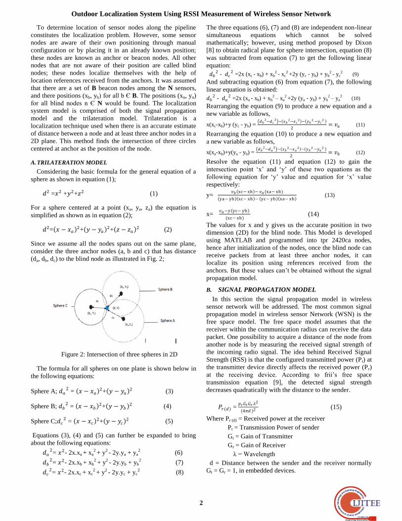
The test bed environment is depicted in figure 3. The

Environment consists of the outdoor environment of the

faculty of engineering wing B, (Area around the packing site

for staff). The test bed has four(4) telos B motes(TPR

2420CA) equipped with a chipcon CC2420 radio chip

operating in the 2.4 GHz frequency band and running on tiny

operating system(tiny OS). The nodes both anchor and blind

are deployed at the test bed. The sink node is located at the

department of Electronics and Computer Engineering which is

situated at the First floor of the faculty of engineering

building. The sink node is usually attached to an Hp personal

computer where the monitoring is carried out.

Figure 3: Experimental Testbed Environment

The environment is located at awka, Anambra state of south-

east of Nigeria. Most of the measurements were carried out

during the later end of the rainy season (August) and early

october.The area is not a level ground but somewhat sloppy,

and the temperature ranges between 28-33 degree centigrade.

The area also has high rise buildings scattered around

A. MEASUREMENT INSTRUMENT

The instrument used for measurement includes:

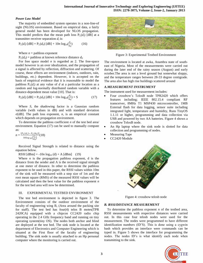
Four crossbow‟s TelosB node TPR2420 which offers

features including; IEEE 802.15.4 compliant RF

transceiver, 8MHz T1 MSP430 microcontroller, 1MB

External flash for data logging, sensor suite including

integrated light, temperature and humidity, Runs TinyOS

1.1.11 or higher, programming and data collection via

USB and powered by two AA batteries. Figure 4 shows a

crossbow TelosB node.

An Hp laptop where the sink node is slotted for data

collection and programming of nodes.

Measuring Tape

CC2420 Module

.

Figure 4: crossbow telosb node

B. RSSI/DISTANCE MEASUREMENT

To determine the pathloss exponent n of the testbed area,

RSSI measurements with respective distances were carried

out. In this case four telosb nodes were used for the

measurement. The nodes were programmed to have different

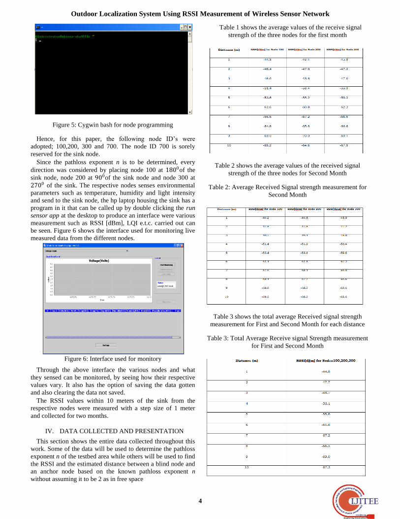
identification numbers (ID‟S). This is done using a cygwin

bash which provides an interface were commands can be

typed in. Figure 5 shows the interface for programming the

nodes. The nodes ID‟s is what identify each node when

transmitting to the sink.


4

Figure 5: Cygwin bash for node programming

Hence, for this paper, the following node ID‟s were

adopted; 100,200, 300 and 700. The node ID 700 is sorely

reserved for the sink node.

Since the pathloss exponent n is to be determined, every

direction was considered by placing node 100 at 1800of the

sink node, node 200 at 900of the sink node and node 300 at

2700 of the sink. The respective nodes senses environmental

parameters such as temperature, humidity and light intensity

and send to the sink node, the hp laptop housing the sink has a

program in it that can be called up by double clicking the run

sensor app at the desktop to produce an interface were various

measurement such as RSSI [dBm], LQI e.t.c. carried out can

be seen. Figure 6 shows the interface used for monitoring live

measured data from the different nodes.

Figure 6: Interface used for monitory

Through the above interface the various nodes and what

they sensed can be monitored, by seeing how their respective

values vary. It also has the option of saving the data gotten

and also clearing the data not saved.

The RSSI values within 10 meters of the sink from the

respective nodes were measured with a step size of 1 meter

and collected for two months.

IV. DATA COLLECTED AND PRESENTATION

This section shows the entire data collected throughout this

work. Some of the data will be used to determine the pathloss

exponent n of the testbed area while others will be used to find

the RSSI and the estimated distance between a blind node and

an anchor node based on the known pathloss exponent n

without assuming it to be 2 as in free space

Table 1 shows the average values of the receive signal

strength of the three nodes for the first month

Table 2 shows the average values of the received signal

strength of the three nodes for Second Month

Table 2: Average Received Signal strength measurement for

Second Month

Table 3 shows the total average Received signal strength

measurement for First and Second Month for each distance

Table 3: Total Average Receive signal Strength measurement

for First and Second Month



5

The tables 1 – 3 present the various RSSI values for nodes

with respect to the sink. From Table 3 the data collected was

used to develop a matlab script for computing the pathloss

exponent n of the testbed area. From the computation n was

computed to be 2.2. Hence, n = 2.2 will be used as the

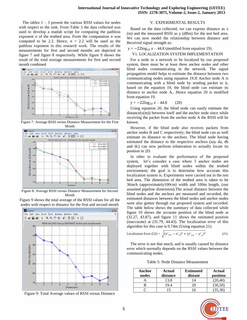
pathloss exponent in this research work. The results of the

measurements for first and second months are depicted in

figure 7 and figure 8 respectively. While figure 9 shows the

result of the total average measurements for first and second

month combined

Figure 7: Average RSSI versus Distance Measurement for the First

Month

Figure 8: Average RSSI versus Distance Measurement for Second

Month

Figure 9 shows the total average of the RSSI values for all the

nodes with respect to distance for the first and second month

Figure 9: Total Average values of RSSI versus Distance

V. EXPERIMENTAL RESULTS

Based on the data collected, we can express distance as x

(m) and the measured RSSI as y (dBm) for the test bed area.

We can now model the relationship between distance and

Received signal strength as:

y = −22log10 𝑥 – 44.8 (modified from equation 19).

V1. LOCALIZATION SYSTEM IMPLEMENTATION

For a node in a network to be localized by our proposed

system, there must be at least three anchor nodes and other

blind nodes communicating in the network. The signal

propagation model helps to estimate the distance between two

communicating nodes using equation 19.If Anchor node A is

communicating with a blind node by sending packet to it,

based on the equation 19, the blind node can estimate its

distance to anchor node A,. Hence equation 20 is modified

from equation 19.

y = −22log10 𝑥 – 44.8 (20)

Using equation 20, the blind node can easily estimate the

distance(x(m)) between itself and the anchor node since while

receiving the packet from the anchor node A the RSSI will be

known.

However, if the blind node also receives packets from

anchor nodes B and C respectively; the blind node can as well

estimate its distance to the anchors. The blind node having

estimated the distance to the respective anchors (say da, db

and dc) can now perform trilateration to actually locate its

position in 2D.

In other to evaluate the performance of the proposed

system, let‟s consider a case where 3 anchor nodes are

deployed together with blind nodes within the testbed

environment; the goal is to determine how accurate this

localization system is. Experiments were carried out in the test

bed area. The dimension of the testbed area is taken to be

36inch (approximately100cm) width and 100m length, (our

assumed pipeline dimension).The actual distance between the

blind nodes and the anchors are measured and recorded, the

estimated distances between the blind nodes and anchor nodes

were also gotten through our proposed system and recorded.

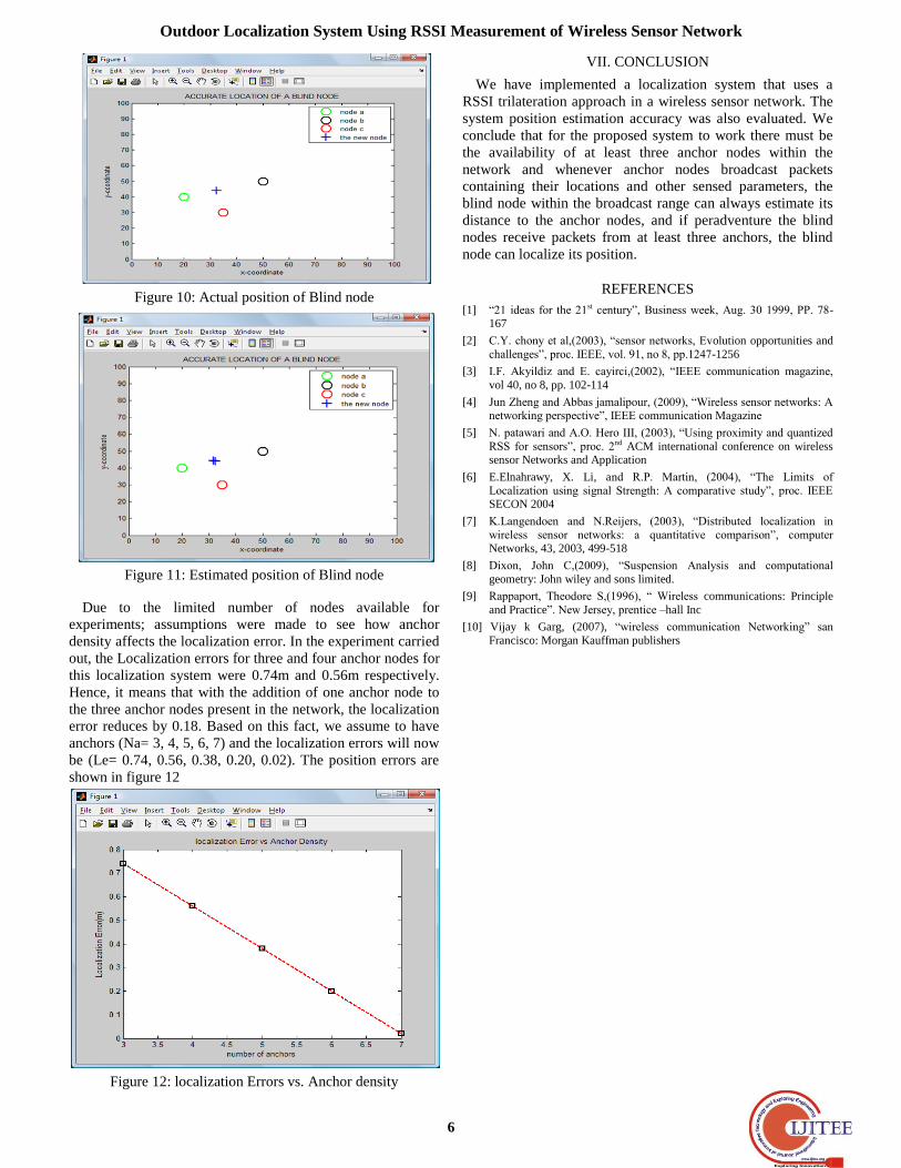
The table below shows the summary of data collected while

figure 10 shows the accurate position of the blind node at

(32.27, 43.87), and figure 11 shows the estimated position

(inaccurate) at (31.79, 44.43). The localization error of this

algorithm for this case is 0.74m (Using equation 21).

Localization Error (LE) = (𝑥𝑖𝑒𝑠𝑡 − 𝑥𝑖

𝑎)2 + (𝑦𝑖𝑒𝑠𝑡

− 𝑦𝑖𝑎

)2 (21)

The error is not that much, and is usually caused by distance

error which normally depends on the RSSI values between the

communicating nodes.

Table 5: Node Distance Measurement

Anchor

nodes

Actual

distance

Estimated

distant

Actual

position

A 13.8 14 (20,40)

B 19.4 20 (50,50)

C 15 16 (35,30)


6

Figure 10: Actual position of Blind node

Figure 11: Estimated position of Blind node

Due to the limited number of nodes available for

experiments; assumptions were made to see how anchor

density affects the localization error. In the experiment carried

out, the Localization errors for three and four anchor nodes for

this localization system were 0.74m and 0.56m respectively.

Hence, it means that with the addition of one anchor node to

the three anchor nodes present in the network, the localization

error reduces by 0.18. Based on this fact, we assume to have

anchors (Na= 3, 4, 5, 6, 7) and the localization errors will now

be (Le= 0.74, 0.56, 0.38, 0.20, 0.02). The position errors are

shown in figure 12

Figure 12: localization Errors vs. Anchor density

VII. CONCLUSION

We have implemented a localization system that uses a

RSSI trilateration approach in a wireless sensor network. The

system position estimation accuracy was also evaluated. We

conclude that for the proposed system to work there must be

the availability of at least three anchor nodes within the

network and whenever anchor nodes broadcast packets

containing their locations and other sensed parameters, the

blind node within the broadcast range can always estimate its

distance to the anchor nodes, and if peradventure the blind

nodes receive packets from at least three anchors, the blind

node can localize its position.

REFERENCES

[1] “21 ideas for the 21st century”, Business week, Aug. 30 1999, PP. 78- 167

[2] C.Y. chony et al,(2003), “sensor networks, Evolution opportunities and

challenges”, proc. IEEE, vol. 91, no 8, pp.1247-1256

[3] I.F. Akyildiz and E. cayirci,(2002), “IEEE communication magazine,

vol 40, no 8, pp. 102-114

[4] Jun Zheng and Abbas jamalipour, (2009), “Wireless sensor networks: A networking perspective”, IEEE communication Magazine

[5] N. patawari and A.O. Hero III, (2003), “Using proximity and quantized

RSS for sensors”, proc. 2nd ACM international conference on wireless sensor Networks and Application

[6] E.Elnahrawy, X. Li, and R.P. Martin, (2004), “The Limits of

Localization using signal Strength: A comparative study”, proc. IEEE SECON 2004

[7] K.Langendoen and N.Reijers, (2003), “Distributed localization in

wireless sensor networks: a quantitative comparison”, computer Networks, 43, 2003, 499-518

[8] Dixon, John C,(2009), “Suspension Analysis and computational

geometry: John wiley and sons limited.

[9] Rappaport, Theodore S,(1996), “ Wireless communications: Principle

and Practice”. New Jersey, prentice –hall Inc

[10] Vijay k Garg, (2007), “wireless communication Networking” san

Francisco: Morgan Kauffman publishers

Outdoor Localization System Using RSSI Measurement of Wireless Sensor Network

Documents

Transcript of Outdoor Localization System Using RSSI Measurement of Wireless Sensor Network