Wind Effects onLaunchVehicles - NATO STO

AGARDograph Number One Hundred and Fifteen

Wind Effects onLaunchVehicles

I

The Advisory Group for Aerospace &search and Development of NATO

Editor

E.D. GEISSLER - Director

Authors

G. F. McDONOUGH - Deputy Chief, Dynamics and Flight 'Mechanics Division

W. D. MURPHREE - Scientific Assistant to Director

J. C. BLAIR - Chief, Optimization Theory Branch, Astrodynamics and Guidance Theory Division

J. R SCOGGINS - Deputy Chief, Aerospace Environment Division

T. G. REED - Chief, Unsteady Aerodynamics Branch, Aerophysics Division

E. L. LINSLEY - Chief, Aerodynamic Design Branch, Aerophysics Division

V. S. VERDERAIME - Special Assistant to Chief, Dynamics and Flight Mechanics Division

J. A. LOVINGOOD - Deputy Chief, Astrodynamics and Guidance Theory Division

M.H. RHElNJWRTH - Chief, Control Theory Branch, Dynamics and Flight Mechanics Division

R.S. WAN - Chief, Dynamics Analysis Branch, Dynamics and Flight Mechanics Division

All of the Aero-Astrodynamics Laboratory, George C. Marshall Space Flight Center, Huntsville, Alabama, U. S . A.

a*

Printed and published by

Technivision Services Slough, England

A Division of Engelhard Hanovia International Ltd.

Copyright

February 1970 'The Advisory Group for Aerospace Research and Development, NATO

Standard Book No. 85102.015.1 Library of Congress Catalog Card No. 69-10027

9

Contents

Chapter 1 Introduction

1-1 General Remarks 1-2 Configuration Selection 1-3 The Saturn Family of Launch Vehicles

1-3-1 Description of Saturn Stages 1-3-2 Saturn Guidance and Control Systems

1-3-2(a) Guidance System 1-3-2(b) Control System

References

Chapter 2 The Wind Field

2-1 2-2

2-3

2-4

2-5 2-6

Introduction Surface Winds (Below 150 meters) 2-2-1 Measurements

2-2-l(a) Methods 2-2-l(b) Data Available

2-2-2 Climatology 2-2-3 The Wind Profile

2-2-3(a) Representation 2-2-3(b)

Wind Shear, Gusts, and Turbulence

Wind Profiles for Space Vehicle Response Studies

2-2-4 In-flight Winds (150 meters - 80 kilometers) 2-3-1 Measurements

2-3-l(a) Methods 2-3-1 (b) Data Available

2-3-2 Climatology 2-3-3 Turbulence (Small-scale Motions) 2-3-4 Range and Crossrange Wind Speed Profiles 2-3-5 Synthetic Wind Profiles

2-3-5(a) Idealized Wind Profiles 2-3-5(b)

2-3-5 (d) Construction Statistical Representations of the Wind Field

Wind Shear and Wind Speed Change 2-3-5( C ) Gusts

2-3-6 Pre-Launch Wind Monitorship 2-4-1 Surface Winds 2-4-2 In-flight Winds The Global Distribution of Wind Standard and Reference Atmospheres Symbols References Tables

Page

13

13 16 19 19 31 31 31 32

33

33 35 35 35 35 35 38 38

40 43 43 43 43 44 44 47 52 52 52 57 58 58 62 63 63 63 64 6 5 65 G5 68

10

Chapter 3 Aerodynamic Considerations 75

3-1 Introduction 75 3-2 Preflight Loads on the Launch Pad 75

3-2-1 Determination of Loads - Steady Wind 76 3-2-l(a) Steady Drag and Lift 76 3-2-l(b) Unsteady Drag and Lift 78

3-2-2 Prediction of Loads - Unsteady Wind 82 3-2-3 Ground Wind Loads and Launch Operations 85

3-3 Flight Loads 87 3-3-1 Steady State Aerodynamics 87

3-3-l(a) Influencing Parameters 87 3-3-1 (b) Aerodynamic Methods for Ascent 89 3-3-1 (c) Aerodynamics of Special Areas 99

3-3-2 Unsteady Loads 105 3-3-2(a) Aerodynamic Damping 105 3-3-2(b) Buffeting Loads 105 3-3-2( c)

and Gusts 106 Symbols 108 References 110

Loads due to Atmospheric Turbulence

Chapter 4 Structural Aspects of Airframe Design

4-1 Introduction 4-2 Rigid Body Flight Loading

4-2-1 Axial Force 4-2-2 Bending Moments 4-2-3 Normal Shear Forces

In-flight Elastic-body and Propellant Effects 4-4-1 Vehicle Mode Shapes and Natural Frequencies

4-4-l(a) Analytical Techniques 4-4-l(b)

4-3 Prelaunch and Launch Loading 4-4

Ground Testing to Determine Vehicle Characteristics

4-4-2 Response of Vehicles to In-flight Winds 4-4-2(a) Elastic Response 4-4-2(b) Effects of Nonlinearities 4-4-2( c) Effect of Structural Damping 4-4-2(d) Response to Random Inputs

4-4-3( a ) Liquid Propellants 4-4-3(b) Solid Propellants

4-4-4 (a ) Acceleration 4-4-4(b)

Coupling of Torsional and Lateral Modes

4-4-3 Propellant Dynamics

4-4-4 Longitudinal Motion Effects

Coupling of Lateral and Longitudinal Modes

4-4-5

Symbols References

4-5 Airframe Structural Design

115

115 116 118 118 122 122 123 125 125

131 134 134 137 138 142 144 144 152 152 152

153 153 154 158 160

e

11

Chapter 5 Guidance and Control

5- 1 Introduction 5-1-1 5-1-2 Wind Effects on Control Objectives

Wind Effects on Guidance Objectives

5-2 Guidance Concepts 5-3 Conventional Control Design

5-3-1 Rigid Body Vehicle Model 5-3-2

5-3-3 Control System Selection

Vehicle Model Including Structural Bending and

5-3-3(a) Rigid Body Control Concepts 5-3-3(b) Elasticity Effects

Fuel Slosh Dynamics Effects

5-4 Advanced Control Concepts 5-4-1 Advanced Load Relief Systems 5-4-2 Worst Wind Determination 5-4-3 Stochastic Methods Symbols References

Chapter 6 Wind-Vehicle Interaction in Flight: Methods of Analysis

6-1 Introduction 6-2 Deterministic Vehicle Dynamic Analysis

6-2-1 Rigid Body Equations 6-2-2 6-2-3 Forces and Moments

Direction Cosines and Euler Angles

6-2-3(a) Gravity 6-2-3(b) Aerodynamics

6-2-3(d) Engine Inertia Control Equation and Engine Servo

6-2-6(a) Rigid Body Equations 6-2-6(b) Elastic Body Equations

6-2-3( C) Thrust

6-2-4 6-2-5 Elastic Body Equations 6-2-6 Simplified Equations of Motion

6-3 Statistical Vehicle Dynamic Analysis 6-3-1 General Statistical Concepts 6-3-2 Power Spectrum Analysis 6-3-3 Nonstationary Statistical Methods

6-3-3(a) State Space Representation 6-3-3(b) Impulse Response Representation

6-4 Computational Considerations Symbols References

163

163 163 165 169 170 170

174 175 177 185 186 187 190 192 195 196

198

198 198 198 201 203 203 204 204 204 205 206 207 207 210 211 211 215 218 218 221 223 2 24 226

12

Chapter 7 Vehicle Response to Atmospheric Disturbances

7-1 Introduction 7-2 Parameters for Evaluation of Response 7-3 Fundamentals of Analysis

7-3-1 Rigid Body 7-3-l(a) Applicability in Design 7-3-l(b) Equations of Motion 7-3-1 (c) Solutions for Specific Wind Inputs

and Angle-of-Attack Feedback

Areas of Applicability in Design 7-2-2 Elastic Body

7-3-2(a) 7-3-2(b) Bending Dynamics Influence

7-3-3 Propellant Sloshing 7-3-3(a) Influence on Loads 7-3-3(b) Response

7-4 Influence of Wind Characteristics on Response 7-4-1 Individual Wind Profiles 7-4-2 Vehicle Response to Ensemble

7-4-2(a) Rigid Body 7-7-2(b) Elastic Body with Sloshing 7-4-2( c ) Control System Optimization

7-4-3(a) Long-Term Wind Buildup 7-4-3(b) Shear Effect 7-4-3( c ) Steady-State Influence

Response Using Statistics of Wind Field 7-4-4(a) Spectrum of Turbulence 7-4-4(b)

7-4-3 Response to Synthetic Profiles

7-4-3(d) Gust 7-4-4

Statistics of Total Wind Field 7-4-5 Comparison of Methods

7-5-1 Wind Penetration 7-5-2 Aeroelasticity Symbols References Tables

7-5 Vehicle Model Refinement

229

229 229 232 232 232 234

235 238 239 239 242 24 2 242 244 244 250 250 250 258 264 2 64 268 268 268 268 268 272 272 278 278 284 284 287 288

13

1

Introduction

E.D. GEISSLER (Editor), G.F. McDONOUGH, W.D. MURPHREE, J.C. BLAIR

1-1 General Remarks

Since the effects of winds on launch vehicles have long been a major theme of investigation at Marshall Space Flight Center and in particular at the Aero- Astrodynamics Laboratory, we agreed to the suggestion of the AGARD Fluid Dynamics Panel to write a monograph on the subject in spite of many other urgent activities; the manuscript was prepared accordingly in June 1967. While almost all of the material covered had been published in bits and pieces in various places, a comprehensive survey of all major aspects of this topic, which i s of no small concern to the design of launch vehicles, did not exist. main themes of this treatise can be found in references (1), (2 ) and (3).

This monograph, which addresses itself primarily to engineers and scientists active in fields related to the effects of winds on launch vehicles, attempts to present the following: (a) methods and results, in sufficient detail fo show the relationship between the various disciplines, where wind affects the design of space vehicles; (b) a description of practical methods of investigation from preliminary design to operational analysis; and (c) a picture of the quantitative importance of specific phenomena by illustration with numerical results.

Ideally, all of this should have been presented in sufficient generality to apply readily to all types of launch vehicles, regardless of size of specific design features of a given configuration. Considerable differences in emphasis and significance of certain phenomena and their mutual relations occur with change of fundimenta1 vehicle parameters. The long history of the writer 's association with the development of missiles and vehicles of all s izes and types would make such an investigation quite tempting; however, the preparation of this monograph would have required an effort far beyond available t ime and resources.

This monograph is focused primarily upon wind effects on large launch vehicles as represented by the family of Saturn vehicles. Numerical examples are mostly taken from studies of the Saturn V vehicle, presumably the largest launch vehicle ever designed. in a particular area, as well as the nature of the critical constraints to be considered, varies with the type of vehicle. Several examples of such variations a r e pointed out in the text, but no attempt a t completeness has been made in this respect. Some justification for this approach (beyond mere expediency) can be made by pointing out that the significance of wind disturbances increases generally with increasing vehicle size, and consequently the need for the most sophisticated type of analysis, with respect to the structural loads and control problems, is indicated for the very largest vehicles. ployed for large vehicles should make it relatively easy to tailor their application to smaller vehicles. On the other hand, the methodology developed here includes promising avenues for future launch vehicles of st i l l bigger size o r more exotic design.

A short exposition of the

Methods described are general, but the need for more o r l e s s analysis

A thorough understanding of the basic considerations and methods em-

14

For smaller vehicles with high accelerations there may be little concern with structural loads, but the most important problem posed by wind may be its effect upon targeting, especially if ground targets a r e to be hit with high accuracy. In this case special guidance techniques a r e required, which could range all the way from a simple bias based on expected winds to elaborate wind correcting schemes built into inertial guidance or, in the extreme, target-seeking devices. Problems of this type are not included in the present treatise. Missiles designed to be employed against moving targets must exhibit high lateral maneuverabili* consequently, wind loads a r e not a significant factor for structural design.

This monograph consists of seven chapters, each of which was written by a different author or group of authors. expediency to produce a fairly voluminous treatise in a short time, sacrificing some of the consistency and internal coherence obtainable by a single author. we believe that there is sufficient coherence and unity of viewpoint between the chap- t e r s to make this an effective monograph, based on the fact that all authors are members of a team who have worked together on this subject for many years. Moreover, i t is believed that specific advantages accrue from the selected method in that the individual differences in the approach taken by the authors, influenced by personality and technical background, give more depth and perspective to the discussion than would have been obtained by a single author. on i ts own without much reference to the others.

At the end of the introductory chapter, there is a section devoted to a description of the Saturn vehicle family in which, for the convenience of the reader, are compiled those data and characteristics of significance in the following chapters plus some further references. Blair.

Chapter 2, 'The Wind Field', written by Dr. J. Scoggins, introduces the 'protagon- ist. ' A fairly condensed and quantitative description of the characteristics of the wind field is given, illustrated with sufficient examples to show the type of statistical material available and to give some feel for the magnitudes included. Then follows a more detailed discussion of the synthetic design profile which was used for the bulk of the Saturn vehicle development work. Other approaches for the representation of the wind field and operational usage of wind data a r e sketched.

Considerable restraint has been exercised in the compilation of this chapter to keep i t from becoming too voluminous. made in this laboratory and elsewhere concerning the better understanding of the fine structure of both ground winds and winds at higher altitudes, jet stream level, which has only been touched upon here. phenomena and atmospheric composition of very high altitudes (80 kilometers) have been omitted because of their small impact on present Saturn vehicle design.

Chapter 3, 'Aerodynamic Considerations', has been written by Mr. T. Reed (unsteady flow phenomena) and Mr. E. Linsley (steady flow phenomena). This chapter contains first a discussion of ground wind problems which a r e a 'sore point' insofar as the subject matter is not sufficiently understood today to permit practical and safe engineering solutions for large launch vehicles. points out the shortcomings in present knowledge and the practical actions taken so f a r than discusses the numerous theoretical attempts at solution which have not yet been successful.

Also, the treatment of nonstationary flow phenomena in flight was kept fairly sketchy, although this subject is an extensive one and could easily f i l l a volume far more extensive than this entire monograph. This rather short treatment was held to be justified because practical experience has shown a fairly unsophisticated

Again, this approach could be considered a simple

However,

Each chapter can be read

This section was written by Mr. W. Murphree and Mr. J.

There is a substantial research effort being

Also, current efforts to explore wind

The text of this section rather

15

treatment by quasi-steady-state aerodynamics to be sufficient in most cases, simply because either active damping from the control system or structural damping of elastic fuselage oscillations outweighed the nonsteady aerodynamics phenomena for the configurations considered. This trend will not necessarily hold for all configurations, especially not for configurations with larger wings and fins. amount of theoretical and experimental work has been devoted at this agency to a better understanding of nonstationary aerodynamics; this is illustrated by several references.

A fair

The discussion of steady-state aerodynamics not only outlines sources of textbook material, but also provides an insight into the relatedness to other factors. The discussion endeavors to give practical viewpoints and approaches to various areas of aerodynamics, even though some are only indirectly related to wind problems.

Chapter 4, 'Structural Aspects of Airframe Design', by Mr. V. Verderaime and Dr. G. McDonough, covers first some fundamental relations needed for defining loads. Then follows a discussion of several structural dynamic factors needed later for a dynamic analysis of vehicle response to wind. This includes both the fundamental bending characteristics of the airframes and the propellant dynamics. While the latter subject is given rather condensed treatment, because it has been well described in recent literature and because it is of minor importance compared to the former, a fairly extensive discussion is devoted to the methods and results regarding description of a i r f rame dynamic mode shapes, frequencies and damping. This subject represents a very critical input to the layout of the control system for the evaluation of structural loads, andhas been given little coverage in the literature so f a r . A section on general airframe design viewpoints will be helpful in particular for the control engineer and aerodynamicist but may also be of interest to designers not familiar with the design of large space vehicles.

After the more expository chapters treated so f a r , Chapter 5, 'Guidance and Con- trol', by Mr. J. Lovingood and Mr. J. Blair, goes to the heart of the matter by discussing the influence of wind upon guidance and control objectives and then devel- oping, in some detail, the rationale of synthesis of a control system to minimize the structural loads on a given airframe. external constraints such as schedules, manufacturing lead times, etc., will necessitate a design freeze of the structure relatively early during the development cycle, whereas the control system permits more flexibility and then will be the primary element which will be optimized. the fact that wind interacts with the control system in a much more pronounced way than with the guidance systems. The latter is activated only during second stage flight, when atmospheric influences are almost negligible for Saturn vehicles. Also, loads and control forces imposed by space vehicle guidance systems are generally small. The emphasis in Chapter 5 is on viewpoints and general relations rather than on numerical results, which follow later in Chapter 7 in more detail.

The discussion of advanced control concepts, referring to systems beyond those employed on current launch vehicles, is again kept fairly brief because the intense studies carr ied out at MSFC and other places on this subject would not fit into the frame of this monograph and have been given a fair amount of publicity (3). Un- doubtedly, advanced control concepts represent an area where important changes are certain to occur with the next generation of launch vehicles. Basic tools for implementing ambitious on-board computations have been advanced to a state of reliability which makes them acceptable for practical use. Further optimization and/or increase in size of vehicle structures, as well as their use over a wide spectrum of environmental conditions, will call for full utilization of the potential improvements offered by advanced methods.

While Chapters 2 to 5 have covered the whole range of subject matter as far as a

This situation is probably typical insofar as

The rather short treatment of guidance reflects

16

general discussion of physical inputs and their relations a r e concerned, the last two chapters describe in a more systematic fashion the methods of systems analysis and the numerical results obtained thereby.

Chapter 6, 'Wind-Vehicle Interaction in Flight : Methods of Analysis', by Mr. M. Rheinfurth, develops the equations needed for a system analysis both for the deterministic and for the statistical approach. While the statistical approach is fundamentally the natural one for our problem, there are still shortcomings in the theoretical tools which have severely limited their practical applications, more so for vehicles than for aircraft .

In Chapter 7, 'Vehicle Response to Atmospheric Disturbances', by Mr. R. Ryan, systematic discussions of typical results of certain types of analysis applied a t various stages of development are presented to indicate their usefulness and, at the same time, to show their typical deployment through the development cycle to get some insight into the numerical relations and relative importance of various dynamical phenomena and certain effects for the Saturn V vehicle. By a comparison between deterministic and statistical results, proof is furnished of the adequacy of the synthetic wind profile for the Saturn vehicles which was used largely during their development.

It i s hoped that this treatise will be of some use to others engaged in, o r preparing for , similar activities. It i s recognized that there a r e many shortcomings as to depth of treatment and selection of subject matter. Many readers would no doubt like to see more elaboration on some of the subjects and less on others. commitments, and our realization of the quick obsolescence of advanced technical subject matter, have induced u s to push our compromise, that is, between the goals of satisfaction obtained by a thorough scholarly treatment and attainment of the objective within a limited time span, rather heavily toward the latter. however, that the rather considerable effort by members of our team over a number of years on the subject matter will help to overcome the shortcomings in presentation, convey somewhat the sense of fascination experienced by the authors in their work, and make this publication a worthwhile addition to the series of previously published AGARDographs.

1-2 Configuration Selection

The selection of the overall dimension of a space vehicle configuration is a very complex affair usually subject to a host of constraints and considerations of a very different character, ranging from straightforward technical trade-offs to such extraneous matters as utilization of existing manufacturing facilities o r launch support equipment. a vehicle configuration will b e selected so as to optimize the performance subject to constraints of simplicity, such as ease of manufacturing and reliability, and optimal use of existing components and facilities. Existing components have in the past almost invariably included the engines, o r frequently even the propulsion system, leaving open essentially only the number of engines and their geometrical arrangement, but they have occasionally even included a whole stage; e. g., the S-IVB stage i s second stage for the S-IB and third stage for Saturn V. This building-block philosophy, while imposing certain constraints on the.technica1 optimization, has usually been very advantageous for reasons of economy through reduced development costs and increased reliability through more accumulation of flight test experience. Examples of the other types of constraint have included a maximum allowable diameter for the Saturn V airframe, governed by manufacturing facilities, and a maximum height, again dictated by available buildings. It is not within the scope of this treatise to t race historically all the factors which did materially affect the configuration selection of the Saturn launch vehicles - this has been done elsewhere. It might be tempting to consider the question of how a Configuration would

Other

We believe,

A guiding philosophy may be safely formulated on the premise that

17

be optimized, if it could be done strictly based on technical trade-offs; however, even this question would lead US too far into structural design questions to be com- patible with the scope of this treatise. To give some insight into how optimization might be achieved, three of the more important factors to be optimized will be discussed: stabilization techniques,i. e. fins vs thrust vector, choice of propellant tank geometry, and some structural considerations in choice of gross vehicle shape.

First , we will consider the question of the choice of passive (aerodynamic stability) versus artificial stabilization. of typical launch vehicles or missiles are usually unstable, unless equipped with fins. Rigid body controllability, characterized by the ratio of control torque per unit control deflection over aerodynamic torque per unit angle of attack, tends to in- c rease with increasing slenderness ratio due to the decreasing lift forces produced for a constant volume with increasing length (1). However, this advantage i s counteracted by decreasing rigidity for more slender configurations and also by the fact that the structural weight assumes normally a minimum value for fairly stubby configurations (close to the condition where upper and lower bulkheads of tanks meet each other). Parametric studies have also been conducted to explore the merits of fuselage shapes other than cone-cylinder -frustum configurations, such as to include conical and other shapes, with respect to controllability, rigidity and overall structural weight (4). No significant advantages could be identified. Aerodynamic stability, i f desired, is obtained most economically by fins in all cases where fins can be designed to withstand environmental conditions. case for bodies which have to re-enter the atmosphere a t high speed; such cases are excluded from the present discussion.

The question is then reduced simply to the choice between fins and artificial stabilization. signed by this agency shows examples of all types of solutions: from configurations equipped with fins sufficient to ensure aerodynamic stability through the entire flight spectrum of Mach numbers (Redstone) to some entirely unstable and completely dependent on artificial stabilization (Jupiter). with fins which leave the configuration slightly unstable for all Mach numbers except close to M = 1 (the center of pressure is about 1-1; diameters in front of the center of gravity).

Ideally one might postulate the most desirable configuration to be one which i s just neutrally stable over the entire Mach number regime; actually this is hard to realize because of the stability changes with Mach number exhibited by most configurations.

Theoretically, such a configuration would require the smallest control forces for maneuvering since only inertial forces would have to be overcome. t rue that angular acceleration towards a desired angle of attack i s aided by negative stability, this advantage is offset by the need for negative t r im torques to maintain finite angles of attack and by the tendency to overshoot equilibrium conditions. Structural steady state bending loads resulting at a given angle of attack a r e equal for the finned and the control stabilized vehicles, if both stabilizing forces act a t the same longitudinal body station. Local structural design conditions may favor one or the other solution.

The dimensioning of required control deflections will normally necessitate values which are capable of fairly rapid angular response in order to assure adequate stability in the presence of off-nomial conditions : the dispersion of the center of pressure (c.P.) position as a function of Mach number, angle of attack and Reynolds number will usually b e considerable, especially during the early stages of design where little wind tunnel information is available.

At the outset, it should be pointed out that airframes

This is not necessarily the

A look a t the family of launch vehicles and missiles which have been de-

The Saturn V vehicle is equipped

While i t is

18

Aerodynamic (passive) instability is a disadvantage for manned vehicles because control failures may occur which could lead to rapid buildup of angles of attack with subsequent structural failure. The divergence of the uncontrolled vehicle should remain small enough to permit a safe abort of the astronaut after establishing the need for abort. urn vehicle. The control deflection possible with the F-1 engine would probably permit safe stabilization even for the unfinned vehicle. Of course, we have to realize that the design had to be frozen a t an early time when this fact was not assured and the adoption of fins represented a conservative design approach. One further advantage of this control reserve is the fact that the vehicle has a good chance to survive many engine-out situations; i. e. , control can still be continued if one control engine fails except in unusual circumstances.

The advantages of eliminating fins are obvious; they complicate the design and are bothersome especially during the lift-off phase where they introduce a r i sk of collision with the surrounding launch structure. It was for this reason that the Jupiter vehicle was designed without fins.

The stability of thrust vector controlled and stabilized vehicles may be affected critically by the sloshing of liquid propellants when the natural frequencies of slosh are close to those of the control system. The slosh problem is examined in detail in later chapters; the discussion here will be limited to how the shape and location of the tanks influence the effects of propellant sloshing on vehicle stability and response. Damping of the fluid oscillations decreases the effects of sloshing on stability; however, since the damping of a smooth-wall tank is nearly zero, i t provides little help in stabilizing fluid motions. Because vehicle design i s usually fixed before extensive stability studies are performed, it has been common practice to design a baffle system to suppress sloshing and virtually eliminate all propellant oscillation effects on stability. current practice is concerned. procedures for choice of tank design can be attained.

As would be expected, effects of propellant sloshing on vehicle stability increase with an increase of the ratio of slosh mass, not total propellant mass, to vehicle total mass. the diameter, the main determinant of slosh mass is tank diameter for all but the lowest propellant levels. diameter lowers slosh frequency and brings it closer to the control system f re - quency, which is less than one cycle per second. ratio of slosh mass to total mass increases and the stability situation becomes more critical. Another aspect of the effect of slosh mass on stability is the location of the mass with respect to the vehicle c. g. ; a t the time of maximum aerodynamic loading on the vehicle, the f i r s t stage propellant levels have lowered considerably and the slosh mass locations move considerably aft of the c. g. of the vehicle. This increases both the rigid body rotation of the vehicle and also the bending moment, since the lever a r m increases because the f i r s t stage slosh mass and the vehicle C. g. are moving in opposite directions along the vehicle axis.

Possible tank designs to alleviate this situation include clustering of propellant tanks in the first stage as in Saturn I. mode frequency and reduce coupling between sloshing and the control system; however, the smaller diameter tanks have lower slosh masses.

The above discussion on first-stage propellant slosh effects is based on the Saturn vehicles, which use kerosene for fuel and LOX for oxidizer. of these two propellants are approximately the same, positioning of either tank for - ward of the other is not critical.

This was the primary reason for selecting the fin size for the Sat-

Hence, the following discussion is academic as far as It does, however, show how more nearly rational

For a cylindrical tank the length of which is considerably greater than

This can be considered in another way: that increasing

As propellants are used up, the

The main effect is to ra i se the fundamental slosh

Since the densities

If two very dissimilar propellants, such as LH,

19

and LOX, were used, there would be an advantage in locating the denser material closer to the c . g. of the vehicle. tudinal loads of the heavier propellant must be carried through a greater length of airframe, thus increasing airframe weight. For upper stages using LH, and LOX (e.g., the second and third stages of Saturn V), putting the heavier propellant tank closer to the c. g. also results in this tank being farther aft, the more advantageous location fo r least-weight airframe design. for these vehicles is chosen for optimum a i r f rame design for axial loads; the helpful effect on propellant slosh effects was a secondary consideration.

An alternative approach is to divide the cylindrical tank into sectors with longitudinal dividers. This lowers the slosh mass, but has the disadvantage of increased weight. Generally, this weight penalty has eliminated this configuration from consideration because the weight could better be utilized by adding slosh baffles to suppress the motion through added effective damping.

Density differences between fuel and oxidizer are the reason for the differences in shape of the tanks for the two propellants. The denser oxidizer i s contained in a spherical o r ellipsoidal or similarly shaped tank, whereas the lighter fuel is contained in a cylindrical tank, the lower bulkhead of which is the upper bulkhead of the oxidizer tank. This leads to minimum-length design which, of course, i s desirable for least weight.

From the above discussion it is apparent that extensive trade-off studies a r e required for the optimum choice of propellant tank configuration. To date other considerations have been overriding in the design of large launch vehicles such as the Saturn systems; however, for future designs, which will demand even greater optimization than that attained for Saturn, tank shapes and locations will be optimized as much as possible.

1-3 The Saturn Family of Launch Vehicles

Throughout this monograph reference is made to the Saturn family of vehicles, and most of the data given in examples and illustrations are based upon either the Saturn I, the uprated Saturn (IB) o r the Saturn V. While there is general worldwide knowledge about these vehicles, it is appropriate to discuss certain characteristics which will help clarify portions of this monograph when the Saturn vehicles are used as a basis of discussions.

1-3-1 Description of Saturn Stages

The Saturn family of launch vehicles falls into three types or groups. Primarily, each vehicle reflects the evolution of the Saturn family, but certain features are basic to all vehicles within a group. In fact, all three groups have many features in common, which, along with the unique characteristics, will be described in the following paragraphs.

The Saturn I launch vehicles consisted of two types or blocks. I had one live stage called the S-I, and two dummy stages, which reflected the three- stage configuration of the Saturn I family. vehicle was 163 feet (Figure 1-1). The S-I stage consisted of eight tanks, each 70 inches in diameter, clustered around a central tank 105 inches in diameter. Four of the outer tanks were fuel tanks while the remaining four, which were spaced alternately with the fuel tanks, and the center tank were liquid oxygen tanks. The fuel tanks were interconnected, as were the liquid oxygen tanks; therefore, any engine could obtain propellant from any tank. tanks drained a t the same respective rates.

A possible disadvantage of so doing is that longi-

A s a matter of fact, the tank location

The Saturn I, Block

The typical height of a Saturn I, Block I

All fuel tanks and a l l liquid oxygen

20

The thrust for this stage came from eight engines, each producing a thrust of 165 000 pounds for a total thrust of over 1 300 000 pounds. arranged in a double pattern: the four inboard engines were fixed in a square pat- ternaround the stage axis, canted outward slightly, while the remaining four engines were locatedoutboard in a larger square pattern offset 45 degrees from the inner pattern. Each outer engine could be gimbaled; that is, each could be swung through an a r c (in this case, an arc of 14 degrees) in two directions. engines were gimbaled, as a means of steering the vehicle, by letting the control system of the vehicle correct any deviation in the vehicle's powered trajectory. Since the Block I vehicle had no fins, engine gimbaling was the only means of guiding and stabilizing the vehicle through the lower atmosphere.

The Saturn I, Block I1 vehicle had two live stages and was basically in the two-stage configuration of the Saturn I vehicle; that is, it did not loft any dummy third stages. The first stage was an improved version of the Block I, S-I stages. While the tank arrangement and engine patterns were the same, there were marked differences between the Blocks I and I1 versions. aerodynamic stability in the lower atmosphere. Four of these fins were larger than the other four, and the two se t s were arranged alternately (Figure 1-2). engines were still arranged in the two-square pattern with both squares centered on the vehicle axis. combined thrust of 1 500 000 pounds.

The Block I1 second stage, called the S-IV, used liquid hydrogen and liquid oxygen as i t s propellant. pounds for a total combined thrust of 90 000 pounds. for a i 4 degree square (Figure 1-3). orbital capability for a variety of payloads. duiiimy Apollo spacecraft and meteoroid detection satellites were orbited as payloads by this two-stage configuration.

The Block 11, Saturn I vehicles differed from each other depending upon the mission. Another major difference involved the instrument unit which was vastly improved for tlie later vehicles. therefore, the later Block I1 vehicles were a few feet shorter than the earlier Block I1 vehicles. Although the height varied, a typical height for a later Block IIvehicle was approximately 188 feet.

The uprated Saturn I, formerly called the Saturn IB, i s an improved version of the vehicle which achieved an unprecedented ten for ten successful launch record in the Saturn I research, development and operational flights. There are major differences between the vehicles, especially between the second stages. While both use liquid hydrogen for fuel, the second stage of the uprated Saturn I, the S-IVB stage, obtains 200 000 pounds of thrust from a single engine compared to 90 000 pounds of thrust from six smaller engines. engine up to * 7 degrees. engine stage i s also used as tlie third stage of the Saturn V, which will be discussed later.

The first stage of the uprated Saturn I has the same general appearance as the Block I1 S-I stage. uprated Saturn are all the same size. Saturn I first stage.

At the t ime of writing there have been three flights of the uprated Saturn I, all of which have been successful.

The differences between the Saturn I and the uprated Saturn seem insignificant when

The engines were

The outboard

The latter had eight fins added for greater

The

All Block II engines had a thrust of 188 000 pounds each for a

This stage had six engines each producing a thrust of 15 000 Each engine was gimbaled

As a two-stage vehicle, the Saturn I had full For example, a Jupiter nose cone, a

These later instrument units were lighter and smaller;

Attitude control is obtained by gimbaling the Figure 1-4 is a schematic of this stage. This single-

Both are 2 1 feet in diameter; each has eight fins but the fins of the Figure 1-5 is an illustration of the uprated

Research and development flights are continuing.

21

PAY LOAD Bnh -J3L DIAMETER 120 in.

S - V DUMMY

S - IV DUMMY

S - I STAGE

1 I

+ 220 in.

257 in.

163 f r

Fig 1-1 Typical Saturn I Block I vehicle

22

I S - IV STAGE

S - I STAGE

- 220 in.

i 1E

I

c- 257 in.

4 LARGE

y/ I

Fig. 1-2 Typical Saturn I, Block I1 vehicle

23

4 ULLAGE ROCKETS

COMMON \ FIN LINE Ill

\ FIN1 BULKHEAD

FIN lNES LINE ,@I I I C- FIN

AFT END VIEW

2 RETROROCKETS

Fig. 1-3 Cutaway drawing of the S - IV stage

LIQUID HYDROGEN LIQUID OXYGEN CONTAINER CONTAINER \ \ COMMON BULKHEAD

- z 3 ULLAGE MOTORS 4 RETRO

FORWARD SKIRT

.INE IV

LINE I

J - 2 . ENGINE

MOTORS

Fig. 1-4 S - IV B stage inboard profile

4 OUTBOARD H - 1 ENGINES

4 INBOARD H - 1 ENGINES

- Fig. 1-5 Saturn S - IB stage

24

these two vehicle families are compared to the Saturn V family. The Saturn V, sometimes called the moon rocket because it is the vehicle which will be used to place the f i r s t astronauts on the moon, is 364 feet high with i t s Apollo payload. This vehicle consists of three stages, the S-IC, the S-I1 and the S-IVB described earlier. of four distinct units, which could be classed as stages but are referred to as modules.

Figure 1-6 shows the first stage of the Saturn V, the S-IC stage, which embodies an entirely different design approach from that of the earlier Saturns. This stage consists of one tank each for fuel and oxidizer in tandem arrangement. The stage is 33 feet in diameter and 138 feet long, making it the largest structure of i t s kind in the free world today. produce a total thrust of 7.5 million pounds. and liquid oxygen, respectively. pattern around the central fixed engine. degrees in a square pattern for steering purposes. fixed fins are incorporated for added aerodynamic stability.

The second stage of the Saturn V launch vehicle, the S-I1 stage, has the same diameter as the S-IC stage but is just a little more than half i t s length, 81 .5 feet. It consists of a single tank each for fuel and oxidizer arranged in tandem. In fact, a common bulkhead separates the liquid oxygen from the liquid hydrogen, the oxidizer xnd fuel, respectively. Figure 1-7, a schematic representation of the stage, i l lus - trates this design feature. S-IVB stages. The propulsion system for the S-I1 stage consists of five 5 - 2 engines, eachmitlia rated thrust of 200 000 pounds. as those in the S-IC stage with the capability of gimbaling f 7 degrees for steering purposes.

Located atop the S-IVB. which i s the third stage of the Saturn V, i s the guidance and control equipment for the launch vehicle. i s the same diameter as the S-IVB, about 21.5 feet, and is about 3 feet high.

It i s appropriate to describe in general t e rms the payload for the Saturn V launch vehicle since i t s configuration is a definite factor in considering the effect of winds on the vehicle. The present payload consists of a Lunar Excursion Module (LEM), a Service Module (SM), a Command Module (CM) and a Launch Escape System (LES). Spacecraft.

The Lunar Excursion Module, which consists of two stages and weighs about 30 000 pounds, i s housed in a cone frustum &EM Adapter) immediately above the Instru- ment Unit. and 13 feet respectively and the frustum is about 28 feet high.

The Service Module is a cylindrical 'stage' 15 feet high which rides atop the LEM. The SM weighs about 50 000 pounds and is propelled by a 22 000 pound thrust engine. Attitude control i s maintained by auxiliary rockets.

Finally, the Command Module, the re-entry capsule which will return the as t ro- nauts toenrth after their lunar mission, is a conical body. in diameter and weighs about 11 000 pounds. Certain features of the CM and the Launch Escape System are depicted in figure 1-9. launch vehicle with i t s Apollo payload.

In addition to these three stages, the Apollo spacecraft system consists

The propulsion system consists of five F-1 engines which The fuel and oxidizer are kerosene

These four engines can be gimbaled i 5 Four of the engines are arranged in a square

Similar to the uprated Saturn,

This same feature is incorporated in the S-IV and the

The engines are arranged exactly

This Instrument Unit is cylindrical and

This system, depicted in figure 1-8, is usually referred to as the Apollo

The major and minor diameters of this frustum are about 21.5 feet

The CM is about 13 feet

Figure 1-10 shows the Saturn V

25

1

I I

I

I I

, I

I I

I I I

5 F - 1 ENGINES

396 in DIAMETER

i CONTAINER

LOX CONTAINER

Fig. 1-6 S - IC stage inboard profile

396 in. DIAMETER

LH2 CONTAINER

ULLAGE MOTOR / I- 81ft 6 in. --

Fig. 1-7 S - I1 stage inboard profile

26

L-. 154 in. -_I Fig. 1-9 Launch Escape Vehkle with Command Module

27

-I- - s - IVI

-

s - I l

jTAGE

---. rAGE

S - IC STAGE

4

260 in.

364ft 360 in. c

Fig. 1-10 The Saturn V Apollo vehicle

28

STAB I LlZED PLATFORM

-1 - - - - - - - - - - - - - - - - - I

INTEGRATING I ACCELEROMETERS RESOLVERS I

I I

ACCELEROMETER ATTlTU DE OUTPlJTS

IGITAL I I ADAPTER COMPUTER UPDATING

INFORMATION

ATTITUDE ERROR

COMMANDS

ATTITUDE -1 RATE GYROS RATE d-1 CONTROL

COMPUTER

I CONTROL

COMMANDS SATURN I ONLY)

I

I (SATURN V ONLY)

REACTION JETS ENGINE

POSITION

Fig. 1-11 Block diagram of Saturn navigation, guidance and control system

h ( k m )

200

160

120

80

LO

0

29

s - l l s - I V B (

50-

LO-

30-

20-

10-

0-

S - IC CUTOFF CUTOFF CUTOFF

-' - - - _ _ I 0 I I

I I c c I

/ DYNAMIC PRESSURE, q

VELOCITY, Vs I I

I I

I I I - 4 7 - t - 100 200 300 LOO 500 600 700 t

TIME (sec)

Fig. 1-12 Typical Saturn V trajectory parameter

BODY STATION (m)

vs itsec 1

loo i * O i 6oi CENTRE OF PRESSURE

Lo+lP CENTRE OF MASS

o+,-.7 r I- ~11- 0 20 40 60 80 100 lL0 140 160

TIME OF FLIGHT (sec)

10 000

8 000

6 000

L 000

2 000

.O 0

Fig. 1-13 Variation of centre of pressure and centre of mass during flight

30

GAIN: a. (degldeg), a1 (degldeglsec), 92 (deg/m/sec)

6 .0 1 7 r - - - -

L . 0 '"1 3 .O -I

I \

I \

I - - - - ACCELERATION, 92 8 GAIN

I \ - - - ATTlTlJDE RATE, a l

\

\ - ATTITUDE ERROR, a. I

I I

I I

\

\

I \

I -- --

I

1.0 I

\ I----

0 20 40 60 80 100 120 140 160

FLIGHT TIME (sec)

Fig. 1-14 Typical uprnted Saturn I control gain program

GAINS: a,(deg/deg), a, Idegldeglsec)

ATTITUDE ERROR GAIN,a, 1

o'21 0 20 L O 60 80 100 120 140 160

FLIGHTTIME (sec)

Fig. 1-15 Typical uprated Saturn V control gain program

31

1-3-2 Saturn Guidance and Control Systems

The Saturn guidance and control systems are designed to provide the proper trajectory and attitude orientation for the vehicle over a range of expected missions, while a t the same time meeting the overall requirement of a high level of reliability. The following section briefly describes the functional aspects of the Saturn guidance and control systems, a simplified block diagram of which is shown in figure 1-11. In the following discussion, that portion of the system which measures and calcul- ates the vehicle's state (e. g., position and velocity, etc. ), and which is commonly called the navigation system, will be considered part of the guidance system.

1-3-2 (a) Guidance System. A launch vehicle guidance system has the function of computing a nearly fuel-minimum flight path for the vehicle to fly in order to achieve the desired end conditions, even under a variety of off-normal situations. The Saturns use inertial guidance systems. The basic sensor input for the system i s a four-gimbal stable platform on which are mounted three integrating accelerometers with their axes mutually perpendicular. The outputs of these accelerometers are the three coordinates of the inertial velocity of the vehicle with the exception of gravity effects. The accelerometer outputs are fed to an on-board digital computer, where the gravity compensation is applied to get true inertial velocity and position. This navigational information is then input into the guidance equations which determine the optimum thrust direction for the condition existing a t that time. Also, the equations generate engine cut-off commands for the final stage.

Some typical trajectory parameters for the Saturn V a r e show1 in figure 1-12. It can be seen from the curve of the dynamic pressure, q, that the first stage trnvers- e s the dense part of the atmosphere. Since vehicle structural loads due to n i ; m -

euvers and winds are of primary importance during the high dynamic pressure por- tionof flight, no attempt is made to fly a minimum-fuel trajectory for the first stage. Instead, a time-programmed pitch maneuver is executed so that the expected structural loading is held to a minimum. For upper stage flight, the determination of a trajectory which will minimize fuel expenditure and thus maximize payload becomes of primary importance. The guidance system achieves optimal flight and the des- i red end conditions through a computational scheme for upper stage flight known as the iterative guidance mode, which uses a simplified mathematical model of the optimal trajectory problem to compute thrust direction and engine cut -off information. Simplifications, such as the assumption of a flat earth, make it possible to obtain a closed form expression for the trajectory problem which can be solved in rapid time with onboard computing equipment. repeated, to update the information and minimize the e r r o r introduced by the assumptions.

1-3-2 @) Control System. While the guidance system prescribes the flight path the vehicle will follow, the control system enforces the attitude of the vehicle which is necessary to maintain the flight path. In the Saturn vehicles the commands generated by the guidance system are combined with attitude information, derived from the stable platform gimbal resolvers, to produce attitude e r ro r signals. proportional feedback signals are generated from ra te gyros, and also from normal accelerometers in the case of the uprated Saturn I. All of these signals are gain- adjusted, filtered and summed in an analog control computer, then a r e fed to the hydraulic actuators which position the engine gimbals. The S-IB, S-IC and S-I1 stages have four outer engines gimbaled to produce control torques in pitch, roll, and yaw. The S-NB stage has i t s single engine gimbaled in pitch and yaw, with roll control exerted by a separate system of reaction jets.

The Saturn vehicles a r e statically unstable over essentially all atmospheric flight. That is, the center of aerodynamic pressure is aft of the center of mass, so that angular perturbations tend to increase instead of decrease.

The solution is then iterated, o r

Other

Figure 1-13 shows the

32

center of pressure and center of mass position versus flight t ime for the Saturn V vehicle. The attitude e r ro r feedback compensates for this unstable condition and provides positive static stability so that the guidance commands are followed. r a t e gyro feedback provides positive dynamic stability and well-damped transient response to commands or disturbances. In the uprated Saturn I, a normal accelerometer signal is used in the first stage to reduce lateral drift and structural loading resulting from winds. No normal accelerometer is used for the Saturn V, since less benefit is achieved on this vehicle by use of the accelerometer and since the structure is of adequate strength for a simple attitude and attitude ra te control law.

The

Gains of the control feedback signals are adjusted as a function of time to compensate for the wide variation in vehicle parameters as the fuel mass is consumed and the velocity and altitude vary. The gains are set to maintain a control frequency of approximately 0.2 cycles per second, which is a value chosen to compromise between suitably fast response to commands and anomalies and adequate separation from elastic mode frequencies. in figure 1-14 and Saturn V gains are shown in figure 1-15.

Each control feedback signal is filtered in the analog flight control computer to ensure adequate stability of the elastic and slosh modes. the f i r s t stage of the Saturn V is phase-stabilized (i.e., i t s damping is enhanced) in order to reduce elastic mode interaction with the control mode and to lessen the elastic contribution to the bending moment. The higher modes are gain-stabilized (attenuated) so that they do not regenerate through the control loop.

Almost all of the guidance and control hardware upstream of the thrust vectoring system is contained in the Instrument Unit. This integrated unit functions for all flight stages, thus providing a high degree of commonality of guidance and control hardware.

Uprated Saturn I gains in pitch and yaw are shown

The first elastic mode of

References

1. Geissler, Ernst D., 'Problems in Attitude Stabilization of Large Guided Missiles', Aero Space Engineering Volume 19, October 1960.

2. Lovingood, Judson A. and Geissler, Ernst D., 'Saturn Flight-Control Systems', Astronautics and Aeronautics, May 1966.

3. Blair, J.C., Lovingood, J.A. andGeissler, E.D., 'AdvancedControl Systems for Launch Vehicles', Astronautics and Aeronautics, August 1966.

Beard, Nathan L., urative Design of Space Vehicles on the Structural Bending Frequencies and Aerodynamic Stability', NASA MTP-AERO-62-35, April 30, 1962.

4. 'Theoretical Investigation of the Effects of the Config-

33

2

The Wind Field

J.R. SCOGGINS

2-1 Introduction

Wind is one of the most important atmospheric parameters influencing the design of space vehicles. Because it has temporal and spatial variations, representation of the data in a simple and concise form i s not possible for all purposes of design and operation of space vehicles. Caution must be exercised in the employment of wind data to ensure consistency with the physical interpretation relative to the specific design problem.

In this report, the t e rm 'surface winds' refers to winds below a height of 150meters. Most surface wind measurements available were made a t a height of only a few meters; however, the quasi-steady-state design wind speed envelopes may be determined with reasonable accuracy from these measurements to a height of 150 meters. Because of local influences, surface winds have characteristics peculiar to the measurement location. The complete specification of surface winds is not possible at this time, although the information provided in this section should be sufficient for most general design studies.

In-flight winds are presented and used in many ways in design and operation studies relating to space vehicles. quired for defining the statistics of the wind field. quired and some of the statistical representations a r e quite complex. particularly true when high resolution wind profile data a r e employed because of the increased number of data points which define the profile.

Representation of appropriate observed features of the wind field in a relatively simple way for engineering applications poses a complex problem. even if one could be developed complex and comprehensive enough to account for all important features of the wind field in combination, would be too complex to apply to engineering problems. On the other hand, a wind model which is too simple may not account for even the most important features. Therefore, a model somewhere between these two extremes must be used and judgement applied to account for shortcomings in the model and/or engineering methods.

This chapter consists of a broad treatment of the statistical properties of the wind field, and presents a wind model of modest complexity which incorporates quasi- steady-state wind speeds, wind shears, gusts and small-scale motions. bination of these parameters is based on measured data, experience, scientific knowledge and engineering judgement. A s time goes on, more and better data resulting from scientific investigations, engineering methods, etc., will, no doubt, indicate that changes in the model should be made. will be made as deemed appropriate. isions to the model will be required in the near future.

In most cases, a representative sample of data i s re - Several years of data are re-

This is

A wind model,

The com-

If this is the case, changes However, it does not appear that major rev-

34

Jhfinitions:

Surface Winds:

Quasi-Steady-State Wind Speed measured at a fixed height.

Winds below a height of 150 meters.

A two-minute average of the surface wind speed

Average Wind Speed An average of the wind speed measured a t a fixed height and, in general, synonymous with the quasi-steady-state wind speed.

Scalar Wind Speed

Wind Direction:

The magnitude of the wind speed without regard to direction.

The direction from which the wind is blowing measured clockwise from true North.

Reference Height (Surface Winds): The height above the ground at which wind speeds are refer red for purpose of establishing climatological conditions and quasi-steady-state wind speed profiles.

Peak Wind Speed The highest wind speed reached during a two-minute interval for our model; obtained by multiplying the quasi-steady-state wind speed by an average gust factor of 1.4.

Daily Peak Wind Speed The maximum (essentially instantaneous) wind speed observed during a 24-hour period.

Calm Winds: A wind speed of less than one knot (0.5 m/sec).

Windiest Monthly Reference Pe r iod The month that has the highest wind speeds at a given probability level.

Gust Factor:

Percentile:

The ratio of peak wind speeds to the quasi-steady-state wind speed.

For a given reference period, the percentage of observations in which

Wind Shear: The vector difference between wind velocities measured at two heights

a variable does not exceed a given magnitude.

divided by the height interval.

Gust: A finite increase or decrease in the wind speed relative to the quasi-steady- state value over a short interval of t ime or height.

Turbulence: A series of irregular gusts, generally synonymous with small-scale motions associated with detailed vertical wind profiles.

Free Standing Winds: Surface winds experienced by the vehicle while standing on the launch pad, with or without fuel, prior to launch and after any service structure or shelter has been removed.

Maximum surface winds in which the vehicle can be launched. Launch Winds:

In-flight Winds;

Quasi-Steady-State In-flight Winds: The wind speeds as measured by the conventional rayinsonde system which are averaged over approximately 600 meters in the vertical direction.

Winds occurring above a height of 150 meters.

Wind Speed Change: Difference in speed of two winds measured a t different heights.

I

I i

! I I

I

I I

1

35

Scale-of-Distance: The vertical distance between two wind measurements, used I in computing wind shears. ,

Reference Altitude (In-flight Winds): The altitude referred to in constructing a synthetic wind profile; it usually represents the altitude of interest for calculating space vehicle responses.

1

I 2-2 Surface Winds (Below 150 meters) I I

2 -2- 1 Measurements

I 2-2-1 (a) Methods. Surface winds are normally measured by instruments called

When anemometers. or cups for measuring wind speed and a vane for measuring wind direction. measuring quasi-steady-state wind speeds (defined as a time average over two minutes), either type of anemometer provides adequate data. However, because of the slow responses of the commonly used type (l), they are not suited for resolving frequencies above approximately one cycle per second. Most wind measurements available today, and those used herein to establish quasi-steady-state profiles, were obtained by slow response anemometers but are considered adequate for most purposes.

High frequency gusts are usually measured by high response researchwiented

The gust data presented in this chapter were based primarily on measurements

Among commonly used types are those employing either a propeller

I

I

I

anemometers. spheres, etc., are not commonly used because of operational and other difficulties.

from anemometers of the research type. large quantities and are generally available only from the original investigator.

2-2-1 (b) Data Available. Systematic wind measurements have been made at designated observing stations all over the world for a number of years. These measurements usually consist of average wind speed and direction at a single height a few meters above the ground, or on top of some convenient building or other similar location, and usually at designated times. In addition, meteorological towers about 150 meters high or less have been erected at specific locations to collect data for investigations of the wind field with height. These data usually have a limited distribution and frequently can only be obtained from the organization responsible for the tower facility. single height in the Cape Kennedy, Florida, area are available. Similar data are available for many locations. The data from Cape Kennedy are used quite extensively in the analysis which follows.

2-2-2 Climatology

Two-minute time-averaged wind measurements have been employed to describe the surface wind climatology for the Cape Kennedy, Florida area. Figures 2- la and 2-lb show the monthly surface wind roses for the period 1950-1959 based on data measured at Patrick Air Force Base, located about 15 kilometers south of Cape Kennedy, once each hour at a height of 23.5 meters (2). These wind roses show the probability of occurrence of wind speeds for sixteen compass points.

Figure 2-2 shows the monthly scalar wind speed distributions for selected probability levels at the 23.5-meter height (2). (Note: Quasi-steady-state values are used in this section except where noted as daily peak values. ) during early summer and fall, which were caused by thunderstorms and hurricanes,

These anemometers, which employ hot wires, soNcs, drag

I

High frequency gust data do not exist in

Approximately 15 years of surface wind data measured at a

~

Except for the peaks

, there is little change in wind speed throughout the year for a given probability level.

36

-PERCENTAGE OF TOTAL WIND DIRECTIONS -50 PERCENTILE (MEDIAN) - WIND MEAN, KNOTS o 84.13 PERCENTILE - 1u WIND, KNOTS A 97.72 PERCENTILE - 2,7 WIND, KNOTS 0 99.865 PERCENTILE - 3 0 WIND, KNOTS

Fig. 2-la Surface wind roses for Eastern Test Range (Patrick AFB , Florida), January to June, reference height 23 .5 meters above natural grade

37

- PERCENTAGE OF TOTAL WIND DIRECTIONS - 50 PERCENTILE (MEDIAN) - WIND MEAN, KNOTS o 84.13 PERCENTILE - 1 cr WIND, KNOTS h 97.72 PERCENTILE - 2 oWIND, KNOTS o 99.865 PERCENTILE- 3 0 WIND, KNOTS

Fig. 2- lb Surface wind roses for Eastern Test Range (Patrick AFB, Florida), July to December, reference height 2 3 . 5 meters above natural grade IC'

38

Figures 2-3a and 2-3b show the same probabilities of occurrence as in figure 2-2 of sca la r wind speeds as a function of the hour of the day for January and July. These measurements were made each hour on the hour. variation with t ime of day during January, but show a well-defined variation during July. This is because of the association between wind speeds and their generating forces. During the winter the pressure gradient is stronger and thermal effects are less pronounced than in the summer. The higher wind conditions during the afternoon in July are caused by thunderstorms and the sea breeze. During early morning hours in summer, the atmosphere becomes more stable, the land breeze subsides and, since the pressure gradient is weak, the wind speeds decrease below the winter values.

The wind speeds show little

Selected percentile values of daily peak, nearly instantaneous wind speeds for each month, season and year (3) for the period February 1950 to January 1964 are shown in table 2-1 for a reference height of 10 meters: a discussion on determining winds a t a given reference height is given in section 2-2-3. fourteen-year serially complete data sample which combines Cape Kennedy and Patrick Air Force Base observations; hurricane influenced winds were omitted from the sample. The data presented in table 2-1 show that, except for high percentiles, daily peak wind speeds are almost independent of the t ime of year.

It is frequently desirable to know the probability of not exceeding a given quasi- steady-state wind speed at some reference height. A cumulative percentage frequency (CPF) distribution over an 8-year period at a height of 10 meters is presented in figure 2-4. This figure represents an envelope of monthly wind speed as a function of percentile. Design values taken from section 2-2-3 (b) are shown in the figure. Hurricane influenced winds were omitted from the data. The percentiles given on the abscissa may be interpreted as the percentage of observations in which the corresponding wind speeds, read from the ordinate, were not exceeded.

Table 2-2 shows the frequency of calm winds at the 10-meter reference height as a function of t ime of day and month (2). The maximum percentage of calms appears in the summer and during the early morning hours, with the minimum percentage appearing throughout the year during the afternoon.

Figure 2-5 shows annual exposure period probabilities of daily peak wind speeds based on the data from Cape Kennedy and Patrick Air Force Base for the period February 1950 to January 1964 (3). The abscissa represents the number of consecutive days of exposure, with a rb i t ra ry t ime origin, during which a given magnitude of daily peak surface winds will occur at least once, and the ordinate represents the probability in percent that the daily peak wind speed at the lometer reference height will equal o r exceed selected values at least once during the exposure periods given on the abscissa. For example, at the point'x' on the figure, there is a 79 percent chance that 12.9 m/sec will be exceeded a t least once during any arbitrary 15-day period. For a given probability, the daily peak wind speed increases as the exposure period increases or, equivalently, the probability that a given wind speed will be observed increases with the exposure period. be expected that a vehicle free-standing on the launch pad will experience greater wind loading if exposed over a long t ime period than over a short one.

2-2-3 The Wind Profile

2-2-3 (a) Representation. The earth's surface exerts a frictional force on the lower layers of the atmosphere, causing a decrease in the average wind speeds near the surface. that the proportionality constant var ies linearly with height, the steady-state wind speed profile may be represented by a logarithmic function of height (4).

These data are based on a

All observations were made once each hour on the hour.

Thus it may

Assuming that stress is proportional to the vertical wind shear, and

This

39

30 -

25 -

20 -

15 - 10 -

5 -

SPEED

(knots)

t fmr

50.0% . JAN FEB MAR APR MAY JUN JUL AUG SEP OCT NOV DEC

Fig. 2-2 Monthly scalar wind distribution (Patrick AFB) , reference height 23.5 meters above natural grade

SCALAR WIND (knots)

C (m/sec)

30- 15-

25 -

20- 10-

0 51 o 4 a 12 16 20 24

EST (hr)

Fig. 2-3a Hourly surface scalar wind distribution (Patrick AFB) for January, reference height 23- 5 meters above natural grade

SCALAR WIND (knots)

1 (m/sec) A

15

10 99.9% 99.0% 95.016

50.0%

O J 0- 0

Fig. 2-3b

4 8 12 16 20 24 EST (hr)

Hourly surface scnlnr wind distribution (Patrick AFB) for July, reference height 23- 5 meters above natural grade

40

representation turns out to be approximately valid during neutral to slightly unstable stability conditions, which usually include high wind speeds.

An empirical formulation, which approximates the logarithmic function, has been widely used in scientific as well as engineering work. This formulation is called the ‘power law’ and i s given, for example in (5), by

U = U, @ - -

where U i s the wind speed a t height h, U, is the wind speed at the reference height h, and p i s an exponent. Once p is known, the wind speed need only be measured at the reference height to define the entire profile envelope to a height of about 150 meters.

The exponent p is a function of wind speed, ground roughness, stability, etc., and increases as the wind speed decreases (6). For moderate ground roughness conditions, such as exist for Cape Kennedy, and during high wind speeds, the value of p is usually 0.2 or less. For purposes of establishing design envelopes, a value for p of 0.20 is employed when the three-meter height steadystate wind speed is between 7 and 15 m/sec, and a value for p of 0.14 i s used when the steady-state wind speed is between 22 and 30 m/sec (7). The above values of p are the only values used in this chapter. in reading values from graphs or data.

Using the power law profile, wind measurements at any height may be transformed, o r referred, to any other height. This is frequently done when measurements are made at different locations and heights so that statistical values for wind measurements can be combined or comparisons made. This was done with data measured at Patrick Air Force Base and Cape Kennedy for some of the results presented in this chapter, and to establish the design envelopes of wind speeds for various percentage values. approximately 150 meters for establishing the envelope of wind speeds.

2-2-3 @) Wind Profiles for Space Vehicle Response Studies. The data presented in this section provide basic wind speed profile, o r envelope, information for use in studies to determine load factors for test, free standing, launch and lift-off conditions to ensure satisfactory performance of the space vehicle. To establish vehicle design requirements, the surface winds are assumed to act normal to the longitudinal ax is of the vehicle on the launch pad and to be from the most critical direction. The quasi-steady-state and peak wind speeds with reference to the windiest monthly reference period for the Cape Kennedy, Florida, area are given in tables 2-3a and 2-3b. Similar data have been compiled for numerous locations:(8) to (11).

To establish these wind speed envelopes, all available hourly surface quasi-steady- state wind speed data were reduced to a common reference height using the power law described above, and a statistical analysis was made of the data to determine the percentile values. Statistical envelope values for the quasi-steady-state wind speeds a t other heights were determined by use of the power law equation. for peak wind speeds were obtained by multiplying the steady-state wind speeds by an average gust factor of 1.4. The values given here are for monthly reference periods, and are frequently used in design studies when the question of exposure period o r pad stay t ime is in the order of a few hours. Reference (3) contains information on potential operational r i sks for the Cape Kennedy, Florida, area when the pad stay time is a few days o r longer.

These specific values are given to avoid ambiguities

The power law profile i s usually considered valid below a height of

I

I

1

Values

Due to the complex nature of surface wind fluctuations as a function’of terrain fea- 1

41

WIND SPEED (m/sec)

16

14 -

10- INFLUENCED WINDS FOR AUGUST AND SEPTEMBER. 8-

6-

0 DESIGN VALUES

0.1 1 10 50 90 99 99.8 99.99

PERCENTILE

Fig. 2-4 Cumulative percentage frequency curve for surface quasi- steady-state wind speeds for the windiest monthly reference period (Cape Kennedy. Florida), reference height 10 meters above natural grade

5.1 mlsec 7.7 mlsec 10.3 mlsec (10 k n o t v ( 1 5 k n W ( 2 0 knots)

(25 knots)

\ U * = 15.4mlsec (30 knots)

- .-A t

D -I/ (35 knots) 6 0 4 / 51

20.6 mlsec (40 knots) - 23.2 mlsec

10 (46 knots)

c . 25.7 mlsec (50 knots)

s, 20.3 mlsec (55 knots) 30.9 mlsec (60 knots)

EXPOSURE PERIOD (day)

Fig. 2-5 Annual exposure period probabilities of daily peak wind speeds (Cape Kennedy and Patrick AFB, Florida) - 5110 observ a t ' ions - reference height 10 meters above natural grade

42

ALTITUDE (km)

0 20 LO 60 80 SCALAR WIND SPEED (mlsec)

Fig. 2-6 Scalar wind profiles measured by rawinsonde and FPS - 16 radar/ Jimsphere methods at Cape Kennedy, Florida, April 27, 1965

43

timated to vary between approximately 5 and 20 degrees. smoothing, the rawinsonde and other similar systems cannot provide measurements of the small-scale wind motions which may be important in some space vehicle problems.

The FPS-16 radar/Jimsphere system provides considerably more accurate wind

Because of inherent

Vertical air motions are not measured by this system.

'I velocity profile data than does the rawinsonde (13), (16), (17). The measurements

44

are averaged over 25 to 50 meters in the vertical direction and have an RMS e r r o r of approximately 0.5 meters per second in wind speed and 1 degree in wind direc - tion (18). Thus, these wind profile data contain information on small-scale motions as well as gross motions such as are provided by the rawinsonde. There is some question whether or not vertical air motions can be measured with this system.

The smoke trail method provides data comparable to that obtained by the FPS-16 radar/Jimsphere system. A column of smoke is established with a small rocket then photographed to determine movement of the trail, which is assumed to indicate wind speed. This method is quite expensive and has been used for making only a limited number of measurements.

A comparison of wind profiles measured by the rawinsonde and FPS-16 radar/Jim- sphere systems is shown in figure 2-6. Smoothing o r averaging of the rawinsonde- measured wind data is clearly shown in the figure.

2-3-1 (b) Data Available. system at many locations throughout the United States, and by similar systems over much of the earth, are available. Approximately ten years ' accumulation of data is available for the major test ranges used by NASA. file at the National Weather Records Center, Asheville, North Carolina, are considered adequate for establishing climatological wind conditions for the respective locations.

Approximately two years ' accumulation of wind profile data measured twice daily with the FPS-16 radar/Jimsphere system, as well as other measurements in support of space vehicle launches and special studies, is available for the Eastern Test Range, Florida. Some of these data are available in published form (18). Smaller data samples are available for the Pacific Missile Range, California, and the White Sands Missile Range, New Mexico. While these data samples are much smaller than those for the rawinsonde-measured winds, they are sti l l adequate in many respects for investigating the response of space vehicles to the smaller-scale winds which are not included in the rawinsonde measurements (see Chapter 7).

2-3-2 Climatology

The subject of wind climatology for any area, if treated in detail, would make up a voluminous document. topics for Cape Kennedy, Florida, which are frequently considered in space vehicle development and operations problems. Additional information on the limited topics covered, or topics not covered a t all, may be found in textbooks and elsewhere.

Figure 2-7 shows the distribution of wind speeds for several percentiles as a func- tionofwind direction a t 12 kilometers altitude in January and July. i s chosen for illustration since it corresponds closely with the altitude of maximum dynamic pressure for most large space vehicles. the plotting procedure i s reviewed. Wind velocity is reported as a speed and a direction from which the wind i s blowing. In usual vector notation a horizontal wind blowing from 270 degrees would be represented by a vector with i t s origin at the intersection of the two horizontal axes and pointing toward 90 degrees with a length proportional to the wind speed. Figure 2-7 was plotted using this convention. Strictly speaking, it is not a vector diagram, but is usually thought of as representing vector components in the pitch and yaw planes.

To illustrate the use of figure 2-7, consider a launch azimuth of 90 degrees during the month of January. Reading from the figure, the 97.72 percentile wind values are: tail 74 m/sec, head near zero, right c ros s 37 m/sec and left c ros s 23 m/sec. Wind components for any percentile and launch azimuth may be found analogously

'

Large quantities of data measured by the rawinsonde

These data, which are on

The intent here is to give a brief treatment of selected

This altitude

Before interpreting this figure,

45

FLIGHT AZIMUTH (deg)

J A N U A R Y

* 50 PERCENTILE 84.1 PERCENTILE

A 97.72 PERCENTILE 0 99.865 PERCENTILE

I FLIGHT AZIMUTH (deg)

JULY

Fig. 2-7 Empirical range and crossrange wind component envelopes for various percentiles (Cape Kennedy, Florida), 12 km altitude, January and July

I

46

PROBABILITY OF WIND AROVE U,

0 7

0 6

0 5

0 4

0 3

0 2

0.1

0

Fig. 2-8 Probability of maximum scalar wind in 10 to 15 km layer existing above specified values, U. (m/sec), during March for n consecutive 12-hour periods, Cape Kennedy, Florida

PROBABlLlTV OF WIND ABOVE U,

A

PROBABILITY OF WIND BELOW U.

I 4 12 2 4 36 60 8 4 I20 2 4 0 360 480

HOURS

Flg. 2-9 Probability of maximum scalar wind in 10 to 15 km layer existing above and below specified values, U (m/sec), during July for n consecutive 12-hour periods, Cape Eennedy, Florida

47

for any month of the year from similar data. Plots similar to figure 2-7 have been developed from 1 to 27 kilometer altitudes, but are too voluminous to include here.

% For missions with specified launch windows, it is often desirable to know the probability that a given wind magnitude will be less than a certain value at least once, thus affording at least one launch opportunity, during a period equal to the launch window. The eight years of serially completed (missing data, that is, having been filled in by interpolation, extrapolation or continuity) rawinsonde wind profile data for Cape Kennedy, Florida (19), were used to determine the probability of maximum winds in the 10-15 kilometer altitude layer being below a specified value at least once during K consecutive 12-hour periods. 2-4 for January as a function of wind speed and t ime period. empirical probabilities for January, in the 10-15 kilometer altitude layer, of getting at least one wind speed equal to or less than the values shown during K (1 to 10) consecutive 12-hour periods. speed of 55 m/sec or less will occur during any 3 consecutive 12-hour periods; a 100 percent chance that a wind speed of 75 m/sec or less will occur during any 7 consecutive 12-hour periods etc. These statistics are based on available twice- daily wind profile measurements and would be somewhat different for data taken a t other sampling intervals. In determining the probabilities, only the maximum wind speed was used from each profile over the altitude interval 10-15 kilometers inclus- ive. The maximum wind speeds given, in general, extended over only a fraction of the 10-15 kilometer layer.

The persistence of winds over varying intervals of time is important in the launch of space vehicles. (equaling o r exceeding its present value) over varying t ime periods is useful information in determining,from a knowledge of present wind conditions, launch probabilities within specified t ime periods for wind-limited vehicles.

The persistence of higher wind speeds in March at Cape Kennedy, Florida, is shown in figure 2-8, and of some lower wind speeds in July in figure 2-9. In figure 2-8 the probability is given that a wind speed will persist over n consecutive 12-hour periods once it has occurred, while figure 2-9 shows also the probability that a wind speed will be greater or less than a given measured value over n consecutive 12-hour periods. twice-daily rawinsonde wind profile measurements.

2-3-3 Turbulence (Small-scale Motions)

The small-scale motions associated with vertical detailed wind profiles are characterized, in general, by a superposition of discrete and mostly irregular gusts containing random frequency components. Turbulence is defined as a series of i r reg- ular gusts. Spectral methods have been employed to specify the characteristics of small-scale motions.

A digital filter was developed to separate small-scale motions from the quasi- steady-state wind profile (20). separation process approximates those obtained by the rawinsonde system. definition was selected to permit the use of the much larger rawinsonde data sample, in association with a continuous-type gust representation). Thus a spectrum of small-scale motions is representative of the motions included in the FPS-16 radar/ Jimsphere measurements which are not included in the rawinsonde measurements. Therefore, a spectrum of these motions should be added to the quasi-steady-state wind profile to obtain a representation of the detailed wind profile. Spectra of the small-scale motions associated with zonal (West-East), meridional (South-North), and scalar (non-directional) wind profiles for various probability levels have been determined from measurements made at Cape Kennedy, Florida, and are presented

These probabilities are given in table The table shows the

I I For example, there is a 79 percent chance that a wind

I

~

I

The length of time that a measured wind speed will persist

I

I These persistence calculations are based on available

I

,

The quasi-steady-state wind profile defined by the @his

,

48

in figures 2-10 through 2-12. The spectra were computed from approximately 200 detailed wind profile measurements by computing the spectra associated with each profile, then determining the percentiles of spectral density as a function of frequency. centile levels. altitude range of data, usually between approximately 2 and 16 kilometers.

Energy (variance) of the small-scale motions is not homogeneous; that is, it is not constant with altitude. The energy content over limited latitude intervals and for limited frequency bands may be much larger than that represented by the average spectra, the 50th percentile, in the figures. The range of energy content is given approximately by the 1st and 99th percentile envelopes. should be kept in mind when employing spectra of small-scale motions tointerpret the significance of vehicle responses.

Also shown in figures 2-10 to 2-12 are envelopes of spectra for detailed profiles without filtering. 20 cy/4000 meters and less, by an equation of the form

Thus the spectra represent envelopes of spectral density for the given per- ’

Spectra associated with each profile were computed over the entire

This range of energy

These spectra are well represented] over wave numbers of

@ (k) = a0k-’ where q)is the power spectral density at wave number k, p is the slope of spectrum] and +o = @ (1). It should be noted that the units of @ and k are m2 sec-2 (cycles (4000m)-1)-1 and cycles (4000m)-1, respectively. Properties of all the spectra are summarized in table 2-5. Data presented in the table show that the small-scale motions associated with the meridional profiles] generally c ross - wind components in the yaw plane, contain more energy that those associated with either the zonal o r scalar profiles by a factor of approximately 4/3.

Because of computational difficulties, the spectra do not extend to wavelengths longer than 4000 meters. Variances associated with the spectra are also given in table 2-5. Spectra of the total wind speed profiles may be useful in control systems and other slow response parametric studies for which the spectra of small-scale motions may not be adequate.

P r e s s (21) presented a discussion of atmospheric turbulence in which he gave the formula

where

O W

L = the scale of turbulence] m

51 = rad/m

+ (0)

= the root-mean-square gust velocity, m/sec

= spectral density, (m/sec)Z/(rad/m)

for the spectrum of vertical and lateral gust velocity. This equation appears to be valid for aircraft-measured turbulence data when L = 1000 feet (300 meters). A number of similar representations for turbulence spectra are given in reference (12).

The formula presented by P r e s s differs from the spectra presented above in two important ways: in the slope of the curve, and in the shape of the curve at low frequencies. turbulence and to the axes along which the measurements were made.

These differences are probably due to differences in the definition of The spectra

49

SPECTRAL DENSITY (m2/sec2/cy/4000 m)

100.0

10.0

1.0

0.1

0.01

0.001

0~0001

0~00001

ENVELOPES OF SPECTRA

ASSOCIATED WITH

--- OF SMALL -SCALE MOTIONS

QUASI -STEADY -STATE \ PROFILES

PE RCENTl LE

99th

90th

50th

I * 1 5 10 20 LO 80 100

WAVE NUMBER, k (cy/4000 ml

Fig. 2-10 Spectra of detailed wind profiles - scalar

50

,

SPECTRAL DE NSl TY (ma /sec’ /cy/4000m)

100.0

10.0

1.0

0.1

0.0 1

0.001

0.0 0 0

0.0000 1

-0 - ENVELOPES OF SPECTRA OF SMALL -SCALE MOTIONS ASSOCIATED WITH QUASI - STEADY -STATE PROF1 LES

- ENVELOPES OF SPECTRA OF TOTAL DETAILED WIND

6 = 12k-2.54

6 = 7 k-2.59

4 I 1 I . . - - *

1 5 10 20

I PERCENTILE

I 80 100

WAVE NUMBER, k(n//4000m)

Fig. 2-11 Spectra of detailed wind profiles - zonal

51

I '

1

SPECTRAL DENSITY (ma /sec2 /cy/4000m)

ENVELOPES OF SPECTRA

ASSOCIATED WITH OF SMALL -SCALE MOTIONS

Fig. 2-12 Spectra of detailed wind profiles - meridional

52

presented in figures 2-10 to 2-12 give good results in space vehicle response studies (see Chapter ?) and appear to be superior for this purpose to spectra obtained from aircraft measurements.

2-3-4 Range and Crossrange Wind Speed Profiles

Questions frequently arise regarding the probability that a given wind speed will occur in the pitch and yaw planes with a given launch azimuth. questions can be answered satisfactorily from component wind profiles for limited azimuths at Cape Kennedy.

Pitch (range) and yaw (cross range) plane wind profiles obtained from measurements at Cape Kennedy, Florida, for January to April are given in figures 2-13 and 2-14 for several percentiles and for a flight azimuth of 90 degrees measured clockwise from north. These profiles are envelopes of wind speed for each of the percentile levels. every other altitude. This does not mean there is no correlation between speeds from one altitude to the next, or that the entire profile occurs at a given time.

Positive pitch plane winds are tail winds, blowing toward the firing azimuth; negative winds are head winds, blowing from the firing azimuth. Positive yaw plane winds are right c ros s winds, blowing from right to left across the flight path; negative winds a r e left c ros s winds, blowing from left to right across the flight path.

2-3-5 Synthetic Wind Profiles

In-flight wind speed profiles are used in vehicle design studies for flight through the atmosphere. The design in-flight wind speeds may or may not be the same percentile as the surface wind speed. since the two desigm wind conditions are essentially independent statistical events.

In-flight wind information is basically of three types: (a) samples of measured profiles, @) statistical distributions and (c) discrete or synthetic profiles. Additional information about these three types of presentation may be found in reference (22), and limited accountsinsections 2-3-1, 2-3-3 and 2-3-6 of this chapter. Each of these wind input types has certain limitations and i t s utility in design studies depends upon a number of considerations. Some of these are: accuracy of basic measurements, tolerable complexity of input, economy and practicality for design use , representation of significant features of the wind profile, statistical assumption versus physical representativeness, ability to ensure control system and structural integrity, and flexibility in design trade-off studies.

The oldest method of representation of in-flight design wind data involves the synthetic type of wind profile. For this method, various features of the wind profile (i.e., wind speeds, shears and gusts) are described and design values established. Synthetic wind profile-type data are presented because this method of presentation. appears to provide a reasonable and economical approach for most design studies when properly employed. understood and employed by most aerospace design organizations.

2-3-5 (a) Idealized Wind Profiles. Idealized quasi-steady-state scalar wind speed profile envelopes are presented to an altitude of 80 kilometers. These winds are not expected to be exceeded by the given percentage of observations, two per day, during the month with highest wind speeds. other months. surface of the earth. haps for elastic body considerations. applied without regard to flight directions to establish initial vehicle design require-

Most of these

They show the percentile of wind speeds at each altitude independent of

This depends upon the desired launch capability,

In addition, the concept of synthetic profiles is generally

The percentages are higher for all The wind data represent horizontal wind flow with reference to the

The influence of vertical wind flow is negligible except per - The horizontal wind speeds are normally

53

B,ASED ON 1956 - 1961 SERIAL COMPLETE WIND DATA

ALTITUDE (km MSL) ALTITUDE (km MSL)

-80-60-40-20 0 20 40 60 80 100

32 28 24

20 16 1 2 8

L

0 -80-60 -40 -20 0 20 40 60 80 100

SPEED (m/sec) SPEED (n i /sec) (JANUARY ) ( F E B R U A R Y )

FOR 90" FLIGHT AZIMUTH POSITIVE VALUES TA1 L WIND NEGATIVE VALUES HEADWIND

FOR 270" FLIGHT AZIMUTH POSITIVE VALUES HEAD WIND NEGATIVE VALUES TAIL WIND


32 28 24 20 16 1 2 8 L

0 -80-60-40-20 0 20 LO 60 80 100 IO

SPEED (mlsec) SPEED (ndseci ( APRIL 1

PERCENTILE ( MARCH 1

a 0.135 e84.100 b 2.280 f 97.720 C 15.900 99.865 d 50.000

Fig. 2-13 Empirical range wind profile envelopes (Cape Kennedy, Florida) for 90-degree and 270-degree flight azimuths - January to April

54

BASED ON 1956 - 1961 SERIAL COMPLETE WIND DATA


-80 -60 -40 -20 0 20 LO 60 80 100 SPEED h/sec)

(JANUARY)

-80 -60 4 0 - 2 0 0 20 40 60 80 100 SPEED (m/sec)

(FEBRUARY)

FOR 90" FLIGHT AZIMUTH POSITIVE VALUES WIND FROM RIGHT NEGATIVE VALUESWIND FROM LEFT

FOR 270' FLIGHT AZIMUTH POSITIVE VALUES WIND FROM L E F l NEGATIVE VALUES WIND FROM RIGHT


32 32 28 28

24 24

20 20

16 16 12 12

8 8 4 4 0 0 -80 -6040-20 0 20 40 60 80 100 -80-60-40-20 0 20 40 60 80 100

SPEED (mlsec) (APRIL 1 SPEED (m/sec)

( MARCH PERCENTILE

a 0.135 e84.100 b 2.280 f 97.720 C 15.900 99.865 d 50.000

Fig. 2-14 Empirical crossrange wind profile envelopes (Cape Kennedy, Florida) for 90-degree and 270-degree flight azimuths - January to April

I I

55

f ALTITUDE (kml

4 0

WIND SPEED (mlsecl

Fig. 2-1 5 Scalar wind speed profile envelopes (quasi-steady-state) for Cape Kennedy, Florida

SHEAR (l/secl

0.100 I WINDSPEED rmlsecl

0 0 4 0

0’020

0 0 1000 2000 3000 4000 5000

SCALE OF DISTANCE Imi Fig. 2-16 Idealized 99 percentile wind shear (l /sec) envelopes for

various scales-of-distance corresponding to wind speeds in the 1 to 80 km altitude region for Cape Kennedy, Florida

56

I WIND SPEED CHANGE 1m/sec)

various scales-of-distance corresponding to wind speeds in the 1 to 80 km altitude region for Cape Kennedy, Florida

I ALTITUDE IDEALIZED WIND

ENVELOPE PLUS I SPEED PROFILE t I

50 TO 300 m 9 m/sec PER 25 m Ah

I

10.36 l lsec gradient)

I

I .I

BUILDUP I 9 m/sec ____

I - -IDEALIZED WIND SPEED ENVELOPE ENVELOPE

WIND SPEED c

Fig. 2-18 Relationship between established gusts and/or embedded jet characteristics (quasi-square wave shape) and the idealized wind speed (quasi-steady-state) profile envelope

57

ments. kilometer altitude consist of records of at least five years of twice-daily wind profile observations.

Generally, large space vehicles for use in comprehensive space research are de- signedfor scalar wind speeds without regard to specific wind directions. in special situations, when a vehicle i s restricted to a given launch site and to rather narrow flight azimuths (within approximately 20 degrees), for a specific configuration and mission, winds based on components (head, tail, left-cross o r right- cross) may be used (see section 2-3-4). For a given percentile, the magnitudes of component winds are less than those of the scalar winds. wind speed profile envelopes for Cape Kennedy, Florida, are given in figure 2-15 for several percentile levels. of geographical location and should be established for the specific location of interest.

The statistical data employed to establish the data points below the 30

However,

Non-directional scalar

The shapes of these idealized profiles are a function

The profiles discussed above are envelopes of quasi-steady-state wind speeds a t each point on the profile for a given probability level. For example, the 95 percentile envelope represents wind speeds that will not be exceeded, a t any altitude, in more than 5 percent of the observations during some specified reference period. (In t e rms of r i sk this means that, for any individual measurement selected at random during the reference period, there is a 5 percent r i sk that the measurement will be greater than the 95 percentile envelope wind speed value, relative to the data sample employed in this analysis). In this section a monthly reference period is used. The profile envelopes represent wind conditions for the given percentile level and for the windiest monthly reference period. This means that the envelope values at any altitude will be exceeded by the specified percentage during only one month - the windiest month. During the other 11 months, the wind speeds represented by a given percentile envelope should be less. The 95 percentile envelope shown in fig- u re 2-15 has been employed in constructing synthetic wind profiles for use in numerous space vehicle design studies, and will be used below to illustrate the construction of synthetic profiles. analogous manner.

2-3-5 (b) Wind Shear and Wind Speed Change. representative information on the wind shear and associated wind speed change for altitude layers, o r scales-of-distance, between 100 and 5000 meters (7). Wind shear is defined as the vector difference between two wind velocities measured at different altitudes divided by the altitude interval. Wind speed change o r wind buildup r a t e is obtained by multiplying the wind shear by the appropriate scale-of- distance. Values of wind speed change o r wind shear for a vehicle with other than a vertical flight path are found by multiplying the shear o r wind speed change by the cosine of the angle between the vertical axis and the vehicle trajectory.

An envelope of the 99 percentile wind speed change or shear is used in constructing synthetic wind profiles. between the shears for the various scales-of -distance. exist, depending upon the scale-of-distance and the wind speed magnitudes considered. these relationships.

Wind shear statistics for various locations vary somewhat, partly due to data sample size, accuracy of basic data, prevailing meteorological conditions and orographic features. Wind shear and windspeed envelopes for Cape Kennedy, Florida, are given in figures 2-16 and 2-17. These envelopes are probably different for most locations and should be established lor the specific location of interest. These envelopes were constructed from data measured by the rawinsonde and FPS-16 radar/ Jimsphere systems, and a limited aniount of data obtained by the smoke trailmethod.

Any other percentile envelope may be used in an

The data in this section provide

This envelope i s not meant to imply perfect correlation Certain correlations do

Research is being conducted to establish more quantitative information on

58

2-3-5 (c) Gusts. The quasi-steady-state in-flight wind speed envelopes presented above do not contain small-scale motions, the high frequency content of the wind profile. insonde system. These measurements represent wind speeds averaged over approximately 600 meters in the vertical direction and, therefore, eliminate features with smaller scales. profiles measured by the FPS-16 radar/Jimsphere system.

A number of attempts have been made to represent discrete gusts present in vertical wind profiles in a form suitable for use in vehicle design studies. attempts result in gust information which could be used for specific applications, but t o date no universal gust representation has been formulated. gust representations are still widely used by various design organizations, the use of continuous gust representations, commonly referred to as turbulence, in vehicle design studies is being intensively investigated.

Discrete gusts are specified in an attempt to represent, in a physically reasonable manner, characteristics of important small-scale features of vertical wind velocity profiles. use in vehicle design studies, discrete gusts are usually idealized, because of their complexity, to enhance their utilization.

Well-defined, sharp-edged and repeated sinusoidal gusts are important types in t e rms of their influence on space vehicles. Rather sharp-edged gusts with amplitudes of approximately 9 meters per second have been measured. These gusts are frequently referred to as 'embedded jets' or 'singularities' in the vertical wind profile. state value; therefore, these gust representations are employed on top of the quasi- steady - stat e wind profiles.

Figure 2-18 shows a schematic representation of a sharp-edged gust with wavelengths varying between 50 and 300 meters and with an amplitude of 9 meters per second. The shear buildup rate a t the leading and trailing edges of the gust is 9 meters per second per 25 meters. The relationship of the gust to the idealized wind speed envelope and the wind buildup envelope is shown in the figure.

Another form of discrete gust which has been observed is approximately sinusoidal in nature, where gusts occur in succession. Figure 2-19 shows the number of consecutive, approximately sinusoidal gusts which may occur and their respective amplitudes. This information was obtained by curve-fitting measured data with trigonometric functions (23) and equating the energy content of the assumed trigonometric function to that of the actual gust. It is extremely important when applying these gusts in vehicle studies to realize that these purely sinusoidal representations have never been observed to occur in nature, although nearly sinusoidal waves have been observed. The degree of purity of these sinusoidal features on the vertical wind profiles has not been established. These gusts, which are distinguished from turbulence by the definition given in section 2-3-3, should be superimposed symmet- rically on the quasi-steady-state profile. The data presented here on sinusoidal discrete gusts are at best preliminary and should be treated as such.

2-3-5 (d) Construction. Synthetic wind profiles are constructed, in principle, from quasi-steady-state wind speed and wind shear or speed change envelopes as follows (an example is shown in figure 2-20): beginning with the wind speed envelope valueat a given reference altitude, subtract the wind speed changes over the respective altitude layers, or scales-of -distance, from the wind speed envelope value at the reference height; then plot the points a t the bottom of the shear layer, measured from the reference altitude downward. points then represents the shear buildup rate leading into the quasi-steady-state

The quasi-steady-state wind profile is defined as that obtained by the raw-

These smaller -scale features are represented in the detailed

Most of the

Although discrete

Gust structure usually is quite complex and not well understood. For

A gust is by definition a wind speed in excess of the defined quasi-steady-

I

4 I

A smooth line joining these

\

59

4 NUMBER OF CYCLES AND PEAK TO PEAK AMPLITUDE. A~ (m/los)

0 100 000 1200 1600 2000 2400 . GUST Wi

- D O ELENGTH. A (m)

Fig. 2-19 Best estimate of expected ( 3 99 percentile) gust amplitude and number of cycles as a function of gust wavelength

WINOSPEED. U I d a C l 4

IO Fig. 2-20 Synthetic wind profile construction based on 39 percentile wind

buildup rates associated with the 95 percentile wind speed profile envelopes at the 12 km reference altitude

60

ALTITUDE Ikm) 95 PERCENTILE IDEALIZED STEADY STATE WINDSPEED

ENVELOPE

16-

%PERCENTILE WIND SHEAR

BUILOUP ENVELOPE

EXTENSION OF BUILDUP RATE ENVELOPE TO SURFACE

%PERCENTILE WIND SHEAR

BUILDUP

WIND SPEED: I m / w ) 0 20 LO 60 80 100 120

Fig. 2-21 .Example of three (10 km, 12 km, 14 km altitude) synthetic wind buildup profile constructions and extension to surface as applied to 95 percentile idealized steady-state wind speed envelope

th+30- a,

t h + i 5 - a1

t h - a,

t A h

30 - a l

15- a1 Q2

SHEAR BUILDUP ENVELOPE ,A

STEADY STATE WIND SPEED

J ENVELOPE

0961 m

T Fig. 2-22 Relationship between revised gust shape (embedded jet) , stendy-

state wind speed envelope and wind shear buildup envelope ( re fer to text for definition of symbols)

~ 61

wind speed envelope a t the reference height. the origin to the lowest point on the wind buildup envelope. imposed on the profile as shown in figure 2-18.

Correlations between speeds, shears and gusts are not taken into account in the construction of synthetic profiles as described above. is being studied, but results have not been formulated from which functional relationships can be taken into account in constructing synthetic profiles. is known that shears calculated over small altitude intervals ( s 1 ki1ometer)and gusts are poorly correlated with quasi-steady-state wind speeds, while shears over larger altitude intervals ( L 1 kilometer) and quasi-steady-state wind speeds have a high positive correlation. Little i s known about correlations between shears over various altitude intervals, except that high-probability-of -occurrence shears over more than two altitude intervals are poorly correlated. Even though functional relationships between wind speeds, shears and gusts are not adequately known, reasonable approximations can be made in constructing synthetic profiles.

The simplified construction of synthetic profiles described above does not consider correlations (or lack of them) between shears, speeds and gusts. In view of the lack of precise knowledge of such correlations, one may make the assumption that shears and gusts are statistically independent of wind speeds. This is approximated by multiplying all shears and wind speed changes and the sharp-edged gust by a factor of 0.85 before constructing the synthetic profile. This factor is obtained by assuming that wind shears and gusts are independent, then approximating the response using linear theory. The gust may also be represented by a one-minus- cosine shape, since line segments may tend to exaggerate vehicle responses.

For continuity, a line is drawn from ~

The gust is then super-

I

l This problem has been and

However, it ! ~

I

I 1

~

I The MSFC synthetic wind profile employs the 95 percentile wind speed envelope, the 99 percentile wind shear envelope and the sharp-edged gust. centage level for shear is used since wind shears, particularly over the smaller altitude intervals, cannot be accurately measured by the rawinsonde system, whereas steady-state wind speeds can be measured with much greater relative accuracy. r i sk involved due to shears, provided the 95 percentile wind speeds are not exceeded.

otherwise limited.

The following steps may be taken to construct synthetic profiles considering rela - tionships between shears, speeds and gusts, using the quasi-steady-state wind speed envelopes, wind shears or wind speed changes and the sharp-edged gust given above:

1. where this line merges tangentially into the shear buildup envelope (multiplied by 0.85) (Figure 2-21).

2. struction of the shear buildup profile is as described above.

3. (0.85) = 0. 0765sec-1 of the shear buildup envelope, to the point where it becoines tangent to the one-minus-cosine shape gust

The higher per-

Thus when launching a space vehicle there is no more than a one percent

I This philosophy eliminates the requirement for monitoring wind shears prior I to launch, provided a one percent r i sk level is acceptable and the vehicle is not

I

1

I The wind increases linearly, beginning a t zero altitude and velocity, to a point

Beginning at this point, the line follows the 99 percentile wind envelope. Con-

The superimposed gust s t a r t s with an extension of the final slope of (0.09) X I

(Figure 2-22).

(i) The gust consists of: the linear extension of the shear buildup envelope; the buildup to the gust speed which is a one-minus-cosine curve with a half wave length of 30 meters, the altitude, and a double amplitude, the total wind speed increase, of 0.85 x 9 m/sec = 7.65 m/sec; the constant velocity plateau; and

62

the tail-off which is the second half of the one-minus-cosine wave. 'thickness' of the gust will be defined by the altitude difference of the inflection points of the buildup and the tail-off curves

(ii) Referring to the point where the shear buildup envelope intersects the steady-state envelope, the gust is described (Figure 2-22) by the following equations:

The

(Figure 2-22).

0 C Ah Q a2

a2 C Ah 5 30 - a,

30 - al Q Ah Q th - a,

th - al C Ah Q th + 30 - a, th + 30 - a, 5 Ah AU, = 0

AU, = (0.09)(0.85) Ah = 0.0765 Ah

AU, = 3.825 l-COS[& (Ah + a11

AU, = 7.65

AU, = 3.825 1-cos [& (Ah + 30 + a, - tha

where:

Ah is altitude difference (m)

A& is gust wind speed (m/sec)

al is the shift of the one-minus-cosine buildup required to a tangential change-

a2 is the tangent point of the shear buildup envelope and the gust (m)

th is the 'thickness' of the gust (m)

a, = a 2 = 0.916 m.

Obviously the 'thinnest' gust that can b e simulated equals the half-wave-length of the cosine so that

30 m 5 gust thickness Q 275 m.

After the gust is reduced to zero at the end of the tail-off, the synthetic wind

over from the shear buildup envelope and the gust (m)

4. profile follows the 95 percentile wind speed envelope.

It should be recognized that no single wind profile representation is applicable to all design problems. The synthetic profile given here has been used quite successfully in many studies, but i t s limitations and shortcomings must be recognized.

The validity of synthetic wind profiles for use in space vehicle design studies has been established by comparing vehicle responses to synthetic and measured detailed (FPS-16 radar/Jimsphere) wind profiles. Flight through a large number of measured detailed profiles is simulated on a computer and the statistical distributions of various vehicle parameters are determined. Values of the parameters for high percentiles correspond very closely to those obtained by simulating flight through the synthetic profile. This procedure is covered in more detail, and results are presented, in a paper by Ryan and Scoggins (24) and in Chapter 7.

2-3-6 Statistical Representations of the Wind Field

Methods have been developed for defining properties of the wind field using statistical methods rather than the synthetic wind profile approach described above; see,

63

for example, reference (25). These statistical methods usually employ covariance matrices and correlation functions for winds at various altitudes, and represent an attempt to find more rigorous solutions to the simultaneous effects of wind speed and i t s change. space vehicle designers, probably because it has not been possible to define adequately the statistics of the wind field or accommodate the non-linear characteristics of the vehicle's response. The improved wind measurements as provided by the FPS-16 radar/Jimsphere system will be adequate for establishing these statistics as soon as a sufficient data sample has been obtained. location is quite voluminous and is not presented here - see, for example, reference (26); however, data are available, and calculations have been made, for a number of locations around the world using rawinsonde-measured wind data.

If it is assumed that the statistical distribution of the wind is Gaussian at each altitude, the covariance matrices and correlation functions can be used to calculate vehicle responses for any given probability level. However, if the measurements indicate a strongly non-Gaussian character, it will seriously restrict the usefulness of the above statistical methods. of vehicle responses at a given probability level than is obtainable with synthetic profiles is desired, analysis based on responses to individual profiles with subsequent statistical evaluation of vehicle parameters is probably indicated. This may or may not include the fine structure. A more specific discussion with results is given in Chapter 7.

2-4 Re-Launch Wind Monitorship

2-4-1 Surface Winds

Space vehicles are designed to accommodate wind speed magnitudes corresponding to a specified probability-of-occurrence level. When the wind exceeds the design value, a r i sk of overstressing the structure of the vehicle on-pad is involved. In addition, the r i sk of having a collision with the launch umbilical tower must be considered. The r i sk involved in launching the vehicle can be reduced by monitoring the ground winds and postponing the launch if required.

Anemometers are located on poles at a height of 18 meters in a properly exposed area in the vicinity of the launch complex, also on top of the service structure which is usually at a height exceeding 100 meters. meters are used as the reference level winds and an envelope of wind speeds is established using the power law profile. Wind measurements from the top of the service structure are monitored to ensure that the envelope at that height is not exceeded. utes during high wind speeds has been verified to be a reasonably accurate representation of the wind field. This method for monitoring ground winds is somewhat, but not overly, conservative and reduces the r i sk involved during launch. Recently, also, the base bending moment has been monitored rather than ground wind. In either case, the r i sk involved in launching the space vehicle is reduced by closely monitoring conditions and postponing the launch if the vehicle structural capability is being approached or exceeded.

However, these methods have not been generally accepted by

Statistical data for even one

Where higher accuracy in the determination

Wind measurements at a height of 18

The envelope of steady-state wind speeds averaged over two to five min-

2-4-2 In-flight Winds

Space vehicles are designed to accommodate a high percentage of occurrences of in-flight winds, but st i l l there is a finite possibility of yinds occurring that exceed the structural or control capability of the vehicle. In-flight winds are closely monitored during the last 12 hours before launch in order to minimize the r i sk involved at launch.

64

In-flight wind profiles are measured by the FPS-16 radar/Jimsphere system at predetermined intervals of time. program which provides an assessment of the severity of the winds on the vehicle. A flight simulation is performed for each wind profile measurement up to and including launch. A launch postponement may result i f the r i sk involved is higher than the acceptable limit. launch in-flight winds depends upon having adequate data transmission and computer facilities available to permit immediate data reduction and flight simulation.

The acceptable level of probability for launch postponements due to high winds is , of course, generally higher than the acceptable r i sk of losing a vehicle in flight, but for many missions such launch delays are highly undesirable. Concerted efforts towards adequate design of a i r f rame and control system should be made to reduce such risks. this need.

2-5 The Global Distribution of Wind

These winds are used as input to a flight simulation

The effectiveness of this method of monitoring pre-

, I

The limited launch windows for some space vehicle missions illustrate ,

I

For space vehicle development and operation, ground winds and in-flight winds in the vicinity of the maximum dynamic pressure region are of greatest importance. Ground winds are greatly influenced by the terrain, surface roughness and stability a t the specific location of interest. precludes anything more than a brief treatment of the subject here.

The atmosphere obtains i t s energy directly from the sun. differential heating between the equator and the poles, between continents and oceans, etc., down to very smal l scales. t u re gradients which are, in turn, a function of the absorption and radiation of energy and the distribution of energy by the motions themselves.

The vertical change of the horizontal wind with height, the vertical wind shear, is related to the horizontal temperature gradient. The absorption, emission and distribution of solar radiant energy in the atmosphere produce a horizontal tempera- tu re gradient which changes with altitude in such a way as to produce an increase of wind with height in the lower atmosphere, and a decrease with height at higher altitudes. The altitude a t which the winds stop increasing and begin decreasing with height is called the jet stream level. It is a t this altitude that the maximum wind speeds occur. It turns out that this altitude is near the altitude of maximum dynamic pressure for most space vehicles. The jet stream, which is a core of maximum wind speeds, does not occur a t all t imes at a given location and is observed to meander around the globe usually a t latitudes above 20 degrees. ments over a period of years show that the strongest jet s t r eams occur off the east coast of Asia in the vicinity of Japan, off the east coast of North America in the North Atlantic Ocean, and east of the Mediterranean in the Near East (27).

In-flight winds are variable enough, even along the East coast of the United States between Florida and Maine, to require that design wind profiles be developed for the specific locations where the vehicles are launched. If over-conservatism is to be avoided, and vehicles developed which have a high capability of launch with some definable risk, it is necessary to specify in-flight wind criteria for the launch location. This report discusses in some detail one process for establishing the wind design criteria; that is, the synthetic wind profile approach. However, there are other approaches being investigated and as more and better data become available these methods will no doubt assume a prominent role in the design and launch of space vehicles.

I The highly variable nature of ground winds

Winds are caused by

Winds aredirectly related to tempera-

I

i Wind measure-

65

2-6 Standard and Reference Atmospheres

Thermodynamic properties of the atmosphere are taken into account in space vehicle flight simulation programs. is to take place within a few hours as, for example, for prelaunch wind monitorship (see section 2-4), or may be obtained from a 'standard' o r 'reference' atmosphere. The 'U. S. Standard Atmosphere, 1962' (28) represents atmospheric conditions at latitude 45"N, while 'A Reference Atmosphere for Patrick Ai r Force Base, Florida, Annual (1963 Revision)' (29) represents atmospheric conditions for that specific location. Since atmospheric density is an important parameter in flight simulation studies and varies considerably with location and climatological conditions, reference atmospheres developed for the specific location of launch are recommended. These atmospheres present average and ex- t r eme conditions but do not consider monthly, diurnal, etc. changes. The atmosphere developed in reference (29) should be used when the space vehicles are to be launched from Cape Kennedy, Florida.

These properties may be measured if the launch

Both are based on measured data.

Symbols

U

h

P, s, a1 9 a2

cp

*cl

k

Ah

AUG

th

References

wind speed

altitude

non-dimensional parameters

spectral density

spectral density of fundamental wave number

wave number

an increment of altitude

gust wind speed

thickness of wind shear layer

1. Camp, Dennis W., Whitley Series 50 and Climet Model Cl-14 Anemometers', NASA TM X- 53271, NASA, Marshall Space Flight Center, Huntsville, Alabama, 1965.

Smith, J. W. and Smith, 0. E., 'Surface Wind Statistics for Patrick Ai r Force Base (Cape Canaveral) Florida', MTP-AERO-61-78, NASA, Marshall Space Flight Center, Huntsville, Alabama, 1961.

Lifsey, J. David, 'An Empirical Analysis of Daily Peak Surface Wind a t Cape Kennedy, Florida for Project Apollo', NASA TM X-53116, NASA, Marshall Space Flight Center, Huntsville, Alabama, 1964.

State University, University Park, Pennsylvania, 1957.

Pagon, Watters W., Engineering News-Record, 1935.

'Analysis of Wind Tunnel Data for Several Beckman and

2.

3.

4. Panofskp, Hans, 'Introduction to Dynamic Meteorology', The Pennsylvania

5. 'Wind Velocity in Relation to Height Above Ground',

66

6. Singer, Irving A. and Raynor, Gilbert S., 'A Study of the Wind Profile in

No. 2, Brookhaven National Laboratory, Long Island, New York, 1959.

Daniels, Glenn E., Scoggins, James R., and Smith, Orvel E., 'Terrestrial Environment (Climatic) Criteria Guidelines for Use in Space Vehicle Devel- opment', 1966 Revision, NASA TM X-53328, NASA, Marshall Space Flight

B. Court, Arnold, 'Wind Extremes as Design Factors', Journal of Franklin Institute, Vol. 256, pp. 39-56, 1963.

'Handbook of Geophysics', Revised Edition, The Macmillan Company, New York, 1960.

World Weather Records, 1950 through 1961, United States Department of Commerce, U.S. Weather Bureau, Washington, D. C.

Thom, €I. C. S., 'Distributions of Extreme Winds in the United States', Journal of Structural Division Proceeding of the A. S. C. E., pp. 11-24, 1960.

Lumley, John L. and Panofsky, Hans A., 'The Structure of Atmospheric Turbulence', John Wiley and Sons, New York, 1964.

Scoggins, James R., 'An Evaluation of Detail Wind Data as Measured by the FPS-16 Radar/Jimsphere Balloon Technique', NASA TN D-1572, NASA, Marshall Space Flight Center, Huntsville, Alabama, 1963.

the Lowest 400 Feet of the Atmosphere', BNL 540 (T-138), Progress Report I I

7. I

I

I Center, Huntsville, Alabama, 1966. I

9. I

I

10.

~

11.

12.

13.

I

14. Middleton, W. E. Knowles and Spilhaus, Athelstan F., 'Meteorological Instruments', University of Toronto Press, Toronto, Canada, 1953.

'Meteorological Equipment Data Accuracies', IRIG Document 111-64, 1965.

Eckstrom, Clinton V., 'Theoretical Study and Engineering Development of

G. T. Schjeldahl Company, Northfield, Minnesota, 1965.

15.

16. Jimsphere Wind Sensor', Final Report NASA Contract NAS8-11158, I

17. Scoggins, James R., 'Balloon Motions and the Measurement of Wind Pro- I files', Ph. D. Thesis, Department of Meteorology, Pennsylvania State University, University Park, Pennsylvania, 1966.

18. Scoggins, J a m e s R. and Susko, Michael, 'FPS-16 Radar/Jimsphere Wind Data Measured at the Eastern Test Range', NASA TM X-53290, Marshall Space Flight Center, Huntsville, Alabama, 1965.

Canfield, Norman L., Smith, Orvel E. and Vaughan, William W., ress in Circumventing Limitations of Upper Wind Records', Journal of Applied Meteorology, Vol. 5, No. 3, American Meteorological Society, Boston, Massachusetts, 1966.

Scoggins, James R., 'Spherical Balloon Wind Shear Behavior', Journal of Applied Meteorology, Vol. 4, No. 1, American Meteorological Society, Boston, Massachusetts, 1965.

21. Press, Harry, 'Atmospheric Turbulence Environment with Special Refer - ence to Continuous Turbulence', AGARD Report 115, North Atlantic Treaty Organization, 195 7.

19. 'Prog-

I

20. I

I

67

Scoggins, James €2. and Vaughan, William W., 'Problems of Atmospheric Wind Inputs from Missile and Space Vehicle Design', Journal of Spacecraft and Rockets, Vol. 1, American Institute of Aeronautics and Astronautics, 1964.

Ulbrich, D.R. and Fichtl, G.H. , 'Analysis of Periodic Turbulence', Research and Analysis Section Tech Memo No. 53, Northrop Space Laboratories, Huntsville, Alabama, 1965.

Ryan, Robert S. and Scoggins, J a m e s R., 'The Use of Wind Shears in the Design of Aerospace Vehicles', Paper presented at 23rd Meeting of the Structures and Materials Panel, AGARD, October 1966, ONERA, Paris, France.

22.

23.

24.

25.

26.

27.

28.

29.

Bieber, Richard E., 'Missile Structural Loads by Non-Stationary Statistic- al Methods', Technical Report No. LMSD 49703, L o c p e e d Missile and Space Division, Sunnyvale, California, 1959.

Daniels, Glenn E. and Smith, Orvel E., 'Scalar and Component Wind Correlations Between Altitude Levels for Cape Kennedy, Florida, and Santa Monica, California', in publication as NASA Technical Note, Marshall Space Flight Center, Huntsville, Alabama, 1967.

Reiter, Elmar R., 'Jet-Stream Meteorology', University of Chicago Press, Chicago, Illinois, 1963.

'U. S. Standard Atmosphere', United States Government Printing Office, Washington 25, D. C., 1962.

Smith, Orvel E. and Weidner Don K., Air Force Base, Florida', Annual (1963 Revision), NASA TM X-53139, Marshall Space Flight Center, Huntsville, Alabama, 1964.

'A Reference Atmosphere for Patrick

68

Table 2-1 Daily peak surface winds selected percentile values (m/sec) , Cape Kennedy, Florida, February 1950 to January 1964, reference height 10 meters

Percentile Calendar Period 1 5 10 25 50 75 90 95 99 99.9

Jan 3 . 1 4 .1 . 4 .6 6.2 8 .2 11.3 13.9 16.0 18.5 22.1

Feb 3 .6 Mar 4.1 APr 3.6 May 4 .6 Jun 4.2 J u l 3 .6

4 .6 5 .1 5 .1 6 .2 5 . 1 . 6.2 5 . 1 5.7 5.1 5.7 4.6 5.1 4.6 5.1 4.6 5.1 4.6 5.1 4 .1 4 .6 4.1 4 .6

6 .7 8.2 6.7 8 .8 6 . 7 8.2 6.7 8.2 6.2 7.7 6 . 2 7.2 6.2 7.2 6.2 7.7 6.7 8.2 6.2 7 . 7

6.2 7 . 7

11 .3 ' 14.9 17.0 21.1 22.1 11.3 15.4 17.0 21.1 27.8 10.8 14.4 16.5 22.1 24.2 10.3 12.4 15.4 19.0 25.2 I

3.6 SeP 3.6 Oct 3.6 Nov 3.6 Dec 3.6 ~~

Winter 3.1 4 . 1 5 . 1 6 .2 8.2 11.3 14.4 16.5 20.1 27.3 Spring 4.6 5.1 6.2 6.7 8.2 10.8 13.9 16.5 21.6 26.8 Summer 4.1 4.6 5.1 6.2 7.7 9 .8 13.4 16.0 21.6 26.8 Fall 3.6 4.6 5 .1 6.2 8.2 11.3 13.4 16.0 21.1 28.8

I

10.3 13.4 16.5 22.1 32.9 9.8 12.9 16.0 21.6 24.7 9.8 12.9 14.9 20.6 25.7

11.3 14.4 18.0 21.1 22.1 11.8 13.9 16.0 19.0 27.8 10.3 12.9 14.4 20.6 28.8 11.3 14.4 16.0 20.6 29.3

Annual 3.6 4.6 5 . 1 6.2 7 .7 10.8 13.9 16.5 21.1 28.8

69

Table 2-2 Frequency (percent) of calm wind at 10-meter level above natural grade, Cape Kennedy, Florida, December 1956 to November 1964

Hour Month Em Jan Feb Mar Apr May June July Aug Sept Oct NovDec Annual

00 4 .8 4.0 3.6 1 . 3 7.3 9 .2 11.7 13.7 6 .3 6 . 9 6 . 3 6 . 0 6.8 01 2 .8 1 . 3 2.4 1.7 8 . 9 8 . 3 10.9 14.1 7 . 1 4 8 6 . 3 6 . 5 6.3 02 4 .8 2.2 3.6 2 .9 7 . 7 10.0 11.7 13.7 10.4 7 .3 5 . 4 4 . 0 7 . 0 03 5.2 3.1 2.0 3.8 8 .5 12 .1 11.3 17.3 12.1 5 . 2 2 . 9 3 . 2 7 .3 04 2.8 4.4 2.4 3.8 5.2 13.8 14.5 13.7 10 .8 5 . 2 4 . 6 2 . 8 7.0 05 4.4 4 .0 3.2 2.9 9.7 16.3 15.3 18.5 13 .3 3 . 6 4 . 6 4 . 4 8 . 0 06 4.4 4 .0 4.4 2.9 8.9 16.3 19.8 19.0 13.3 3.2 5 . 0 5 . 2 8 .9 07 3.6 4.4 4.8 6.3 10.5 1 6 7 1 8 . 1 19.4 15.8 4.4 5 . 4 5 . 6 9.6 08 3.6 6.6 6 .5 2.9 2.4 5.4 6.0 6 .9 4 .6 4 . 0 8 . 8 4 . 4 5.2

09 3.6 1 .8 2.0 2 . 1 2 .8 3 .8 4 .8 1 . 6 4.2 0 . 8 4 . 6 5 . 6 3 .1

10 0.4 1.8 1 .6 1.7 0.4 3 .8 4 .0 2.8 2 . 1 * 1 . 3 2 . 4 1 .8

11 0.4 1 . 3 1 .2 1.7 0.8 1 . 3 2.4 0.8 2 . 9 0 . 8 1 . 7 0 . 8 1 . 3

12 1.6 0.4 * * * 0.8 0.8 0.4 1 . 3 0 . 4 2 . 1 1 . 2 0.8

13 2.0 0.4 * * 0.4 1 . 3 0.4 1 . 6 0 . 8 0 . 4 1 . 7 0 . 4 0.8

14 0.8 4.0 0 .8 0.4 0.4 0.8 1.2 1.6 1 . 3 0.8 * 0 . 4 0.7

15 0.4 1 . 3 * * * 0.8 0.4 1 . 6 2 . 5 0 . 4 0 . 4 0 . 4 0.7

16 0.4 0.4 0.4 * 0.8 0.4 0.8 0.4 1 . 3 0 . 8 * 0 . 8 0 .5

17 1 . 6 0.4 * 0.4 0.4 2:l 0 .8 3.2 2 . 1 1 . 6 1 . 7 2 . 0 1.4

18 4 . 0 1 .8 0.8 0.4 1 . 6 2 .5 3.2 4.0 2.9 1 . 2 5 . 0 7 . 7 2.9

19 2.8 3.5 2.0 * 1.6 5 .0 2.8 5.2 4 .6 1 . 2 7 . 1 6 . 5 3 .5

20 4.4 3.5 2 . 8 1.7 3.2 6 . 7 5.6 8 .5 7 . 5 1 . 6 6 . 3 6 . 0 4 .8

21 5 .2 4 .0 3.2 1 . 3 4 .8 7 . 5 10.5 8.9 8 . 3 4.4 5 . 0 6 . 0 5.8

22 3 .6 2.2 2.4 1 .7 6.0 7 . 5 7.7 12.9 7 . 9 4 . 8 6 . 3 5 . 2 5.7

23 5.6 3 .5 4 .8 0.8 6 .5 8 . 3 10.5 15 .3 10.0 5 . 6 4 . 6 5 . 2 6 .8

A l l h o u r s 3 . 1 2.5 2.3 1.7 4 . 1 6.7 7 .3 8.6 6.4 2 . 9 4 . 0 3 . 9 4.5

* values < 0.4 percent

e*

70

I I Table 2-3a Surface wind speed envelopes, 95 percentile, for Eastern Test Range

Height above Quasi-steady- Peak wind natural grade state wind I

( m ) ( f t ) (m/sec) (knots) (m/sec) (knots)

3.0 10 7.2 14.0 10.1 19.6 9.1 30 9.0 17.4 12.6 24.4 18.3 60 10.3 20.0 14.4 28.0 30.5 100 11.4 22.2 16.0 31.1 61.0 200 13.1 25.5 18.4 35.7 91.4 300 14.2 27.6 19.9 38.6 121.9 400 15.1 29.3 21.1 41.0 152.4 500 15.7 30.6 22.0 42.8

The 95 percentile winds a re , in general, exceeded during heavy rain showers, thunderstorms in the a rea or over the site, squall lines, some frontal passages, strong pressure gradients, and hurricanes.

I

Table 2-3b Surface wind speed envelopes, 99 percentile, f o r Eastern Test Range

Height above Quasi - steady- natural grade state wind

Peak wind

3.0 10 9.5 18.4 13.3 25.8 9.1 30 11.8 22.9 16.5 32.1 18.3 60 13.5 26.3 18.9 36.8 30.5 100 15.0 29.2 21.0 40.9 61.0 200 17.2 33.5 24.1 46.9 91.4 300 18.7 36.3 26.1 50.8 121.9 400 19.8 38.5 27.7 53.9 152.4 500 20.7 40.2 29.0 56.3

The 99 percentile winds are, in general, exceeded during thunderstorm over the site, squall lines, occasional frontal passages and hurricanes.

71

Table 2-4 Probabilities that the maximum wind magnitude in the 10-15 km altitude region will be equal to or less than a specified value at least Once during K consecutive 12-hour periods during January, Cape Kemedy, Florida, based on eight years' serially completed rawinsonde data.

GRP* K1 K2 K3 K4 K5 K6 K7 K8 K9 IC10 5 . o . o . o . o . o . o . o . o . o . o

10 . o . o . o . o . o . o . o . o . o . o 15 . O . O . O . O . O . O . O . O . 2 . 4 20 . O . O . O . O . O . 2 . 6 1 . 0 1 .4 1.8 25 2 . 0 3 . 0 4 . 0 5 . 0 6 . 0 7 . 1 8 . 3 9 . 3 1 0 . 3 1 1 . 3 30 6 . 3 8 . 9 10.7 12.5 14.1 15.7 17.1 18.5 20.0 21.4 35 12.5 16.3 19.4 22.2 24.4 26.6 28.8 30.8 32.9 34.5 40 21.0 27.0 31.9 36.1 39.9 43 .1 46.4 49 .0 51.4 53.2

Wind 45 34.3 42.7 49.0 54.2 58.3 61.5 64.3 66.5 68.5 70.4

50 49.6 58.5 65.3 69.8 73.6 76.4 79 .0 81.3 83.3 84.7 Speed (m/sec)

55 64.9 73.6 79.0 83.1 86.3 88.5 90.1 91.3 92.3 93.1 60 76.4 83.5 87.9 91.1 93.5 95.4 96.6 97.6 98.4 99.2 65 84.1 88.5 91.5 93.8 95.2 96.4 97.2 98.0 98.6 99.2 70 88.9 93.1 95.8 96.8 97.4 97.8 98.2 98.6 99.0 99.4 75 94.0 96.4 98.0 98.8 99.4 99.8 100.0100.0 100.0100.0 80 96.6 98.6 99.4 99.8 100.0 100.0 100.0100.0 100.0 100.0 85 98.4 99.4 99.8 100.0 100.0 100.0 100.0 100.0 100.0 100.0 90 99.8 100.0 100.0 100.0 100.0 100.0 100.0 100.0 100.0 100.0

100 99.8 100.0 100.0 100.0 100.0 100.0 100.0 100.0 100.0 100.0

110 100.0 100.0 100.0 100.0 100.0 100.0 100.0 100.0 100.0 100.0 - * K is number of 12-hour intervals.

72

Table 2-5 Parameters defining spectra of detailed wind profiles

Percentile 50 90 99

t 7 12 19 (zonal) PO 2.59 2.54 2.47 WX

war IT 8.16 15.57 26.30

war )S 0.85 . 1.63 2.68

w7. % 9 18 33 (Meridional) po 2.66 2.70 2.70

Nar )T 9.45 21.34 40.71

war 1s 0.96 1.78 2.96

V *" 7 12 20 (Sca la) PO 2.59 2.54 2.46

War )T 7.58 15.72 25.04 war 1s 0.86 1.70 2.75

Var

T refers to total profiles S

variance (ni2/sec2) associated with spectra

refers to small-scale motion profiles

The equation defining power spectruni of detailed wind profiles is given by I

+(k) = cfi,,k-l'

where

k

*(k)

+" p

= wave number, cycles/4000 ni = power spectral density, ni2/sec2/cy/4000 m = + (I), ni2/sec2/cy/4000 m = slope of power spectrum, dimensionless

74

r------ I I I I I I I I I I . I I

I I I I I I I I

I

t I I I I I I I I I I I I I I I I

AERODYNAMICS CONTROL RESPONSE I

I r l I I

I

AERODYNAMICS STRUCTURE RESPONSE

CONTROL SYSTEM --*--

Fig. 3-1 Aerodynamic loads on' launch vehicles

75

3

Aerodynamic Considerations

T.G. REED E.L. LINSLEY

3-1 Introduction

The principal perturbing forces for launch vehicles, both on the launch pad and in flight, are the aerodynamic loads produced by winds. Because these wind loads are a major structural consideration, they greatly influence the design of the flight control system.

The in-flight loads can be broken down into two categories as shown in figure 3-1: the externally imposed loads produced by wind, including gusts and turbulence, and the loads produced by the vehicle response. Here, the aerodynamics due to con- t ro l response will include loads due to any aerodynamic control surfaces and the loads due to low frequency (rigid body) vehicle response. The aerodynamics due to structural response will include loads due to elastic body response, including panel and shell modes, and response due to buffeting. possibility of a direct input to the control system through an angle-of-attack indicator.

Since a launch vehicle constantly accelerates through the atmosphere, it is never in a 'steady' flight condition, and the Mach number, dynamic pressure, density and Reynolds number are continuously varying as a function of time. These effects appear to be negligible with respect to aerodynamic coefficients, and the quasi- steady approximations as used in classical aircraft stability theory are applicable. The aerodynamic loads are then considered to be functions of angle of attack o r yaw, at constant Mach number, and the rate of change of these quantities, as well as the rate of change of pitch angle. The roll angle is constrained by the control system, and the coupling of the pitch and yaw motions is neglected. Pitch-yaw coupling can be neglected only for nearly axisymmetric vehicles. Configurations with any large asymmetry such as that produced by 'strap-ons' o r a winged payload will not be included here. p ressure at a Mach number near 1.5 for liquid-fueled vehicles.

Only recently have methods become available for the determination of unsteady aerodynamic loads due to vehicle bending oscillations, gust penetration and turbulence.

3-2

The dash line indicates the

Maximum loads are generally obtained near maximum dynamic

A s a result, slender body theory is often used.

Preflight Loads on the Launch Pad

A launch vehicle exposed to surface wind for more than a few hours while erected on the launch pad may be subjected to critical wind loads. The r i sk of damaging the vehicle increases as the exposure t ime increases. Wind loads have been a design factor for many years in the design of buildings, smoke stacks, bridges, etc.; however, the conservative safety factors which apply in these cases are obviously inapplicable for launch vehicles. primarily designed for powered flight and, if the ground wind loads are found to b e

The structure of a launch vehicle is

critical, a means must be found to protect the vehicle without penalizing the payload capability.

In the natural environment the wind is a vector quantity which var ies in both space and time, and thus the wind loads should be considered as a dynamic input to the vehicle structure. From the aerodynamic point of view, the problem falls in the category of viscous separated flow around a bluff body. Although such flows have been studied for many years, there does not exist an adequate approximation to aerodynamic transfer functions which would relate the dynamic wind vector to the dynamic load on the body; therefore, the usual quasi-steady assumptions must be used.

To simplify the problem the wind is broken down into steady and unsteady components (Figure 3-2), and the resulting static and dynamic loads are superposed. The second order loads which result from the interaction of the static and dynamic wind components are neglected in the present state of the art.

A well known characteristic of the steady flow around bluff bodies is the formation of an unsteady wake with resulting unsteady forces on the body. The unsteady l i f t load which is generated by the wake is the load of greatest concern for launch vehicles because i t s magnitude is unpredictable. In contrast, the steady drag loads, which may be of the same order, are somewhat predictable. A customary practice during the preliminary design phase of a vehicle is to estimate the steady drag bending moment corresponding to the expected peak wind, allowing a 50 percent margin for dynamic loads. This estimate has proven to be unconservative for some Saturn configurations. The static and dynamic loads are finally determined by testing an aeroelastic model in a wind tunnel. The structural design of the vehicle must be nearly finalized before such a model can be designed. It is important that the ex- te r ior configuration be closely reproduced, including all areas of local roughness and all protuberances. Any adjacent structures such as an umbilical tower should be duplicated, and wind azimuth becomes a primary variable.

3-2-1

The loads of interest are (Figure 3-3):

Determination of Loads - Steady Wind

(a) steady drag

(b) steady lift

(c) unsteady drag

(d) unsteady lift.

Of these loads (a) and (d) are the largest and most important. only (a) can be estimated analytically and (b) , (c) and (d) must be determined in wind tunnel tests.

At the present time,

3-2-1 (a) Steady Drag and Lift. To determine the steady drag, a drag coefficient must be estimated as a function of vehicle roughness and Reynolds numbers, and the effect of adjacent structures, such as an umbilical tower, and the wind profile must be included. The elevation and configuration of the launch pad also require consideration, because a large elevated pad may distort the wind profile at the location of the vehicle.

For the Saturn vehicles, the surface roughness is sufficient to eliminate Reynolds number effects in the velocity range of interest, and the drag coefficient is constant. The surface roughness and protuberances considerably increase the drag

77

WIND PROFILE LAUNCH VEHICLE

Fig. 3-2 Launch vehicle exposed to ground winds

OSCl LLATORV

RESULTANT

WIND VECTOR

OSCl LLATORV

RESULTANT

W ~ N D VECTOR

Fig. 3-3 Aerodynamic forces

70

coefficient from the value of about 0.55 for a smooth cylinder to a value of about 0.75 to 0.80. variation with altitude, a fair approximation to the drag bending moment can be obtained using s t r ip theory. only when the vehicle is upstream of the umbilical tower. When the Saturn V vehicle and tower are side by side in a plane normal to the velocity vector, the bending moment is increased by twenty to thirty percent; when the vehicle is downstream of the tower, the bending moment is perhaps 10 percent of the estimated value. results are applicable only to a given launch pad configuration such as that shown in figure 3-4. which depend on Reynolds Number, and different umbilical tower effects may be observed (l), (2).

As already mentioned, the steady lift cannot be estimated in general. Values of lift coefficient as large as 0.6 have been observed for smooth configurations with isolated discrete roughness elements (l), (2). orientation of roughness have indicated values of C, of approximately 0.2 and an unpredictable variation with wind azimuth. erally have only a small effect on the resultant bending moment.

3-2-1 (b) Unsteady Drag and Lift. The unsteady loads in a steady wind can be attributed to three sources:

By using a drag coefficient of this order and considering the velocity

The bending moment obtained in this manner applies

These

Smoother vehicles may have drag coefficients of the order of 0.55

Tests of Saturn vehicles with random

Bending moments produced by lift gen-

1. Vortex shedding - The interaction of the vehicle and the unsteady wake may I

produce large dynamic lateral loads, perhaps including motion excitation o r flutter-type loads. This is usually the most serious loading condition.

I

2. Buffeting - The vehicle is exposed to the wake of an adjacent structure I such as a11 umbilical tower. If the c ross section of the tower is smaller than I the c ros s section of the vehicle, large periodic loads may be produced by the tower wake (2).

3. Galloping excitation - Because of. a lack of axial symmetry, the variation of lateral force with angle of attack @/U) is negative, thus producing motion excitation. This type of excitation has not been observed specifically in wind tunnel tes t s of launch vehicles, but has been observed in tes t s of stacks as discussed by Scruton (3).

Although a tremendous volume of research has been devoted to the unsteady wake o r vortex shedding problem, very few results are applicable to the launch vehicle problem. at Reynolds numbers up to a few million. rough and the wind loads of interest may occur at large Reynolds numbers up to thirty million. It is customary to use power spectral concepts to describe the fluctuating velocities and pressures in the wake, as well as the fluctuating forces on a bluff body. spectrum of the nondimensional forces or bending moments is given as a function of the reduced frequency fd/U . A variety of spectrum shapes has been obtained as a function of configuration, surface roughness, Reynolds number, etc., as shown in references (1) and (2). The occurrence of a sharp peak in the nondimensional spectrum, figure 3-5, at a particular value of reduced frequency, is an indication of the characteristic 'vortex shedding' frequency of the body and identifies a wind velocity a t which large dynamic loads may be obtained. At low Reynolds numbers, the reduced frequency at which vortex shedding occurs for a smooth circular cylinder is about 0.20 and is identified as the Strouhal number, S,. Both C, and S, for smooth and rough cylinders are plotted in figure 3-6. that S, var ies approximately as 1/C, for smooth cylinders. in S, and C, as a function of Reynolds number above 300 000 for the smooth cylinder

The research programs are usually concerned with very smooth cylinders In contrast, most launch vehicles are

The

Notice The large variation ,

79

Fig. 3-4 Saturn V launch pad

80

POWER SPECTRAL DENSITY OF LATERAL AERODYNAMIC FORCES

0.28.

0.24.

0.20.

0.16

0.12.

0.08

0.04

REDUCED FREQUENCY, f dlU

Fig. 3-5 Maximum power spectral density, Saturn V

CD 0.5

0 4

0.3

0.2

0.1

0

(ROUGH) (SMOOTH)

(SMOOTH) (ROUGH)

Fig. 3-6 Variation of C, and S, for smooth and rough cylinders

81

is a result of the large variations in flow pattern and wake width rather than a direct result of viscosity. The variation in C, for the rough cylinder is much smaller; similarly, the variation in Strouhal number is hypothesized to be smaller, and the Strouhal number for rough cylinders at high Reynolds number is probably nearly constant. There are very few data available on the wake frequencies of rough cylinders, and the variation with 1/C, has not been verified. The available data from launch vehicle models and full scale smoke stacks seem to indicate a behavior as shown in figure 3-6.

Other quite unpredictable peaks often occur in the reduced frequency range from 0.05 to 0.12, as shown in reference (1). However, these peaks usually indicate intensified random vortex shedding, and the resulting dynamic loads are not a s severe as the loads obtained near the Strouhal frequency of 0.20 where motion excitation is most often observed.

Large dynamic lateral loads may be obtained for launch vehicles when the Strouhal frequency coincides with the first cantilever mode frequency of the vehicle, and this will occur over a narrow range of wind speeds for each weight condition. If an estimate of the Strouhal number can be made as a function of surface roughness and Reynolds number, then the critical wind velocity can be obtained for each weight condition; however, there is no way to estimate .the magnitude of the forcing function. The equation of motion in the first mode can be written as

MsV + 2{wM,i + o2M,q = F (Eh. 3-1)

where w is the f i r s t cantilever mode frequency and F is the forcing function. In a general form, F can be written as

F = F, cos wst + F. (4) + (Eq. 3-21 7

where F, is constant and the term F, cosw,t represents the vortex shedding forcing function that would be observed for a rigid stationary model. The equation is strictly applicable only near the vortex shedding (prouhal) frequency ws. F(t) represents a random Gaussian function, and F (q) includes the effect of motion excitation. Physically, the motion excitation t'krm can be considered either a s an amplification of the vortex shedding function o r as an increasing spatial correlation associated with the random function F(t). The advantage of this simple mathematical model o r similar models is that the effect of a change in structural characteristics for the vehicle can be evaluated if the magnitude of the individual forcing functions can be determined. The predominance of any one of these functions seems to depend on the vehicle configuration, surface roughness, structural damping and the azimuth of the wind vector as referred to the vehicle-umbilical tower plane; however, no straightforward correlation has been found between large bending moments and the above variables. Although the largest loads a r e encountered in the case of motion excitation which is represented by the damping term above, this type of forcing function has occurred for only a few vehicle configurations; for example, Saturn V. More often, the response indicates a mixed forcing function including sinusoidal and random inputs.

Wind tunnel tests of an aeroelastic model are therefore mandatory for determining the dynamic response of a launch vehicle to steady winds. The structural dynamic properties, including the reduced frequency, fd/U, the structural damping, (, and a mass ratio of the generalized mass in the fundamental mode to the mass of air displaced by the vehicle, must now be considered in scaling. Reynolds number is duplicated if possible, although this may not be a necessity for rough configurations. damping of the model, both to safeguard the model and to bracket the expected full scale value.

It is quite desirable to have the ability to vary remotely the structural

a2

Several stations along the model are usually instrumented to determine the bending moment distribution, particularly the steady drag moment, and an accelerometer at the nose can be used to check for response in second and higher modes. data are recorded on magnetic tape for later detailed analysis. The use of a two- axis oscilloscope and camera (3) is extremely desirable so that the total loads can be monitored in real time.

In the analysis of the data, the loads are broken down into steady and dynamic components because the steady loads scale aerodynamically, while the dynamic loads must be extrapolated using aeroelastic scale factors. Also, the load distribution along the vehicle must be determined separately for the static and dynamic cases, and the results summed station by station. The base of the vehicle may not be the most critical station because hold-down or rebound loads may determine the structure. The base bending moment is often used as a reference, however, as an indicator of the load distribution which will produce critical stresses at some vehicle stations.

All

A detailed analysis using the data recorded on magnetic tape is required to identify the components of the forcing function. distribution of the peaks of the recorded response in determining the proportion of sinusoidal to random input (2). Another method using the second and fourth moments of the sample distribution is given in reference (5). A less precise approach consists of determining the ratio of peak response to the r.m.s. response (1).

Motion excitation or a negative damping component is often immediately apparent as a violent, constant amplitude, sinusoidal response. The magnitude of such a t e rm can sometimes be determined by examining the variation of peak bending moment with < . 3-7 and 3-8.

3-2-2

Although wind tunnel testing of an aeroelastic model is the best available method of determining ground wind loads, the wind tunnel does not provide a complete description of the atmospheric input. In addition to the wind profile effects, the wind tunnel does not reproduce gusts or atmospheric turbulence. In this context, the t e rm 'gust' applies to the low frequency turbulence components; that is, frequen- c ies well below the vehicle frequency.

Considerable effort is being made, both theoretically and experimentally, under the direction of the Ames and Langley Research Centers and the Marshall Space Flight Center, to develop methods of handling unsteady wind loads (6). A principal bottle- neck i s the lack of full scale data for the evaluation of any proposed methods. Al- though various full scale programs are now in progress, sufficient data are not yet available. measurements are difficult to implement in the vicinity of the test vehicle, explicit wind inputs cannot easily be obtained. Most present programs attempt to describe the local environment statistically, and power spectral methods are used to estimate vehicle response.

The simplest method for analytically estimating unsteady wind effects was mentioned earlier as a preliminary design tool. are considered. A 1 .4 gust factor is applied to the steady-state wind, and this peak wind is used for drag calculations using a steady-state drag coefficient. sumptions inherent in this technique are (a) perfect correlation of gust over the vehicle length and @) a gust duration sufficient to establish steady-state drag. believed that this procedure is conservative, although there are insufficient data on low frequency gust structure, including spatial correhtion, magnitude, duration and

It may be useful to examine the probability

Some typical results for the Saturn IB and V vehicles are shown in figures

Prediction of Loads - Unsteady Wind

Since the meteorological programs associated with f u l l scale load

For simplicity only the low frequency 'gusts'

The as-

It is

83

1.5 -

1.0

0.5-

BENDING MOMENT

I I UNFUELED

SATURN V 5 20.01

DESIGNBENDINGMOMENT ; I ,'* ,

SATURN I B '- - SATURN I,

BLOCK II

04 I I I I I I I = -

0 10 20 30 10 50 60 70 WIND VELOCITY, FULL SCALE (mph)

Fig. 3-7 Maximum ground wind loads for Saturn configuration

goo

CRITICAL WIND AND AZIMUTH VALUES

SATURN V

SATURN18

1800

Fig. 3-8 Dependence of ground wind loads 011 azimuth angle

84

UNSTEADY

(TURBULENCE) DRAG -------

STEADY DRAG

Fig. 3-9 Total wind loads on launch vehicle

85

frequency of occurrence, for a true evaluation. mic responses in the bending modes are neglected.

Except for the uncertainty in the aerodynamics, the theoretical framework for determining the complete vehicle response spectrum which results from a turbulent input spectrum is fairly well established. Only now are sufficient data being obtained to establish the input wind spectrum.

Earlier dynamic response calculations were based on the assumption that the tur - bulent velocity components varied randomly in time but were correlated over the vehicle length. be used with the assumption of isotropic turbulence and a scale of turbulence independent of height. servative results.

The lateral and longitudinal dyna-

Experimental o r theoretical power spectrums o r turbulence could

Response calculations of this type appear to give quite con-

I f*

More recently, attempts have been made to include the influence of the spatial correlation of the lateral turbulent components, and c ross spectra are required as a function of the vertical separation between points on the vehicle. Reed (4) has developed analytical expressions for the cross-correlation functions for the lateral and longitudinal components of turbulence with the assumption of homogeneous, isotropic, atmospheric turbulence convected a t the mean wind speed. This analytical model shows fairly good agreement with the few experimental results which are available for comparison, and the predicted vehicle loads appear to be more reasonable. are used.

Several experimental programs are in progress to develop methods of more closely simulating atmospheric properties in the wind tunnel; much of this work i s reported in reference (6). more sophisticated atmospheric simulations.

3-2-3 Ground Wind Loads and Launch Operations

The static and dynamic loads discussed in the preceding paragraphs can be combined vectorially to obtain the final load (Figure 3-9). This method is believed to provide a conservative estimate. tent in the design phase, the structural integrity of the vehicle will be, in general, jeopardized only by unexpectedly large vortex shedding loads. must be made of launch pad operations to determine the t ime f rame of vehicle exposure and the associated r i sk of structural damage or launch delay. It must be emphasized that difficulties of this type should be anticipated for any new vehicle configuration and continuing appraisal made of possible launch operations and schedules from the earliest conception of the design. Extended exposure of the un- protected vehicle should be avoided and the r i sk attendant to any proposed pad schedule should be established. The r i sk includes not only structural damage but the possibility of schedule slip and failure to obtain a desired launch date o r time.

Launch vehicles smaller than Saturn V are generally assembled on the launch pad using a large enclosed gantry for adequate wind protection. If the predicted vortex shedding wind speed is low enough to entail a substantial r i sk for expected exposure periods, then wind restrictions are placed on the removal of the gantry. portant practical consideration in imposing wind restrictions is a comparison of the t ime required to position the gantry with the 'forecast t ime' associated with the critical wind speed. Wind restrictions are not a cure-all, especially when launch opportunities are limited to a given launch window. In these cases, a means must be found to alleviate the wind loads, and an attempt usually is made to suppress the dynamic loads due to vortex shedding. passive dampers and servo dampers, are available.

A weakness in the above methods is that quasi-steady aerodynamics However, there is no better approximation available.

Launch vehicle tes t s have not yet been attempted with these

Since most of these loads can be determined to some ex-

In this case, a study

An im-

Various aerodynamic devices, as well as A comprehensive survey of

86

DRAG COEFFICIENT, CD AND WEIGHT, W

I

I I I I I I I I I I I I \ \ \ \ \

M x1.5

\ \

0 =25'

/ 0

0 - A

CONE HALF -ANGLE, 6

Fig. 3-10 Typical weight and drag coefficient of cones

4 (a) ( b) (C)

Fig. 3-11 Vehicle nose shroud development

I the problem i s given in reference (7).

The Saturn V vehicle presented new problems because of i t s extremely large size and the unique methods used for assembly and check-out. on a portable launcher which is complete with umbilical tower, and i s given an initial check-out in a large vertical assembly building. a r e then transported to the firing pad by a crawler and secured in place for final check-outs. moved to the pad to provide access to a l l sections of the vehicle. cess, the vehicle is inevitably exposed to the wind without protection and, in addition, the mobile service structure does not provide complete protection when in place. The feasibility of a variety of 'fixes' for reducing sensitivity to ground winds was studied. stacks, would be effective in suppressing vortex shedding. a r e not suitable because the loads due to atmospheric turbulence would not be diminished, the drag loads would increase by 20 percent, and the strakes would be difficult to remove before launch. passive damper connecting the vehicle to the umbilical tower, was selected. The damper not only decreases the vortex shedding loads, but also decreases the dynamic loads caused by atmospheric turbulence. effect of steady state winds. to less than one percent for a pad stay-time of 30 days.

3-3 F l i g h t b a d s

3-3-1 Steady-State Aerodynamics

'Aerodynamics' defines the pressure fields and loads that exist on a launch vehicle due to the reaction of ambient flow. If flow changes are gradual, and vehicle response is a lso gradual, reactions can be studied under steady-state conditions. These steady-state conditions are the subject of this section which, f irst , considers the factors involved in aerodynamic configuration selection and the methods of calculation, then includes some general observations.

3-3-1 (a) Influencing Parameters: 1. Nose Design. A vehicle payload is often undefined a t the t ime the vehicle is being sized and, furthermore, most vehicles will ca r ry a variety of payloads. volume, packaging of payload, weight, drag, acoustics, influence of vehicle bending moments, and separation t ime and technique.

To obtain optimum performance, a nose shape has to be selected with consideration of both minimum drag and minimum weight. Figure 3-10 illustrates the result of a study of conical shrouds. At extremely small cone angles, both friction drag and weight would be excessive and, fortunately, there is little need for the application of th i s type. creasing drag value for shorter cones is compensated by a decreasing weight due to the smaller surface area.

surface areas, since the aerodynamic pressure on the blunted cone builds at a high rate. The shape and the bucket location of the weight curve illustrated are

The vehicle is assembled

The launcher and vehicle

I A service structure, which i s also transported by the crawler, is

~

During this pro-

1

Aerodynamic devices such as strakes, often used on smoke However, these devices

A more satisfactory solution, consisting of a ~

However, it does not reduce the The r i sk of wind damage can in this way be decreased

I

I

The factors involved in a shroud design are

At larger cone angles where pressure drag predominates, the in-

However, a minimum weight is reached a t about a 25- 1 degree half-angle. After this, a rise in weight takes place even with smaller

valid for any material used and for both skin-stringer and honeycomb construction. I I

Trajectory studies of performance have shown the optimum half-angle of a conical shroud to be about 15 degrees, although this i s not a unique angle that will always provide the best performance characteristics. Mach number, p ressure and altitude influence the geometry of the shroud to a small degree, although the shroud ejection t ime i s the primary factor. If the shroud can be ejected at f i r s t staging, low drag i s emphasized, whereas if payload

Trajectory parameters such as

88

heating or contamination requirements demand the shroud to be carried farther, minimum weight should be emphasized.

Blunt shrouds with high expansion corners create high local buffeting and acoustic loads around the shoulder at transonic Mach numbers. Nevertheless, a blunt cone with a cylindrical extension is usually more desirable for the packaging of payloads than a long slender cone. A compromise is illustrated in figure 3-11 showing a generalized shell that has been adopted for some Saturn vehicles. fairly blunt cone, the high expansion shoulder was rounded off as shown in figure 3-llb. curve was approximated by the series of frustums shown in figure 3- l lc . This evolved to the single frustum, shown in figure 3-lld, which still has far better volume utilization than a straight slender cone, and expansion corners that are reasonably small. Another benefit of this modified shape is that the expansion around the first corner reduces the initial pressure coefficient on the frustum to low values, resulting in a relatively low drag contribution from this large surface area. definition of local shock locations than on ogive type shrouds.

Two advantages of the very blunt cone are that its normal force is lower and the induced normal force distribution on the afterbody is moved downstream. This is very effective in reducing downstream bending moments and increasing the aerodynamic stability, if the performance loss from increased drag can be accepted. However, bending moments alone are not the only structural criterion, since the great increase in compression loads from aerodynamic drag can neutralize the gain.

2. Stability Augmentation. Any body shaping that can draw the center of pressure aft i s considered advantageous from the stability and control viewpoints. Aside from the blunt nose concept as discussed in the previous section, aft center of pressure movement is gained by tapering the body to increase the volume toward the aft end. stability benefits are not necessarily realized. aft, although not so much as the center of pressure. a r m of the aft end control force i s reduced as the c. g. moves back and this may neutralize any gain in aerodynamic Stability.

In practice, bodies are normally stepped by a series of cylinders and frustums for simple and low cost fabrication. frustum for stabilization without a radical effect on the c. g. loss due to drag is extreme and is also completely unnecessary, since fins at this location have higher lifting efficiency without the large drag penalty.

The least desirable aerodynamic shape is a hammerhead shroud, a shroud in which the diameter is larger than that of the booster. The destabilizing effects of this have to be compensated by fins and control reactions and, further, if the shroud wake effects are large, the fins will be in a lower-energy, buffeting environment. Additionally, flow separation from the hammerhead shroud will create shocks and acoustic energy at reattachment on the body; also hysteresis and nonlinear effects on lift may occur.

3. Interstage Frustums. stages of different diameter. with a structural trusswork is not considered appropriate. can be just as well utilized in the shell and, at the same time, there is better con- t ro l of the flow field; i. e., crossflows through the cavity at angles of attack are eliminated and the violent turbulence and acoustic loads are diminished.

Even clean frustums have design problems, caused by flow separation over the

Starting with a

Since compound surfaces are more difficult and expensive to fabricate, the

Furthermore, the fixed expansion points of the general shroud allow a better

This could be accomplished with tapered o r conical tanks; however, The center of gravity is a l so moved

Even so, the shorter moment

Another method would be to use an aft-end flared However, performance

Frustum shells must be used on interstages between The postulated use of open interstages connected

The structural material

89

frustum and by expansion to low pressures on the afterbody, followed by unstable reattachment shocks. The wide variation in external pressures along the body in the vicinity of the frustum creates another problem. must normally be vented during ascent to minimize high internal overpressures. However, the frustum and adjacent cylindrical skirts usually form a common compartment. No venting system can hope to optimize the various compartment segments under the influence of a common compartment pressure. It is good practice, therefore, to maintain low frustum angles of about a 20 degree half-angle or less, if possible.

4. Fin Sizing. lity must be provided by thrust vectoring. a force which, in combination with the body force, provides a net restoring torque at angles of attack. Directional steering requirements and control at low dynamic pressures specify a thrust vectoring system of some size, after which aerodynamic surfaces can be applied to augment the stability at high load conditions. lizing fins are placed at the aft end adjacent to the control force, their capabilities can be traded. the optimization process.

The generation of fin lift on a body of revolution is due not only to i t s own lifting efficiency but also to the influence of the vehicle body upwash field and the induced pressure field on the body from the presence of the fins. increase the effectiveness of a given fin by 50 o r 60 percent, depending on fin span. Fin plan-forms and profiles are generally selected to optimize span, provide good stiffness against flutter, and place main spars at vehicle structural tie points. It is sometimes advantageous to have the root section relatively thick, to replace shrouds that might be needed for aerodynamic protection of the engine bells. If the fins are large enough, the fin structure may also b e used to support and hold down the vehicle before lift -off. In almost all cases, blunt rather than sharp trailing 'edges are used, since fin drag is normally less than 2 percent of total vehicle drag and any gain by a sharp trailing edge would b e very small.

Most launch vehicles are surrounded by external equipment on the pad, such as support and hold-down a r m s and umbilical towers. usually desirable to minimize the span of fins. A wind-loaded, bent vehicle will tend to snap straight at the instant of release, requiring appropriate clearance at the base. Following this, most vehicles have little capability of maneuvering in the first seconds of flight, where drift and fins can cause collision problems. solution is to minimize the span of fins by using a trapezoidal fin with a longer chord-length or to use a larger number of smaller fins. The thickness of a fin is normally defined by an optimization of structural weight and aerodynamic drag. If three or four fins are used, the umbilical tower can often be located between fins to widen the clearance envelope.

Interstage compartments

If a vehicle is not already aerodynamically stable, artificial stabi- Fins or thrust vectoring have to produce

If stabi-

Many other factors besides aerodynamics must be considered in

This augmentation can

For clearance purposes, it is

One

3-3-1 @) Aerodynamic Methods for Ascent: 1. Bodies. The aerodynamic forces and moments on a launch vehicle are one of the basic problems of vehicle design. The major application of these data is to define the control deflections required to stabilize the vehicle and to define structural loads. Theoretical procedures used to determine forces and moments on bodies of revolution are well known and readily obtainable.

Steady-state aerodynamic characteristics are provided by various methods in different Mach number regions. On bodies of revolution, the following theoretical methods are appropriate for zero and small angles of attack:

90

Subsonic Incompressible Flow:

(i) Slender Body Theory - Small contour changes and no discontinuities in the second derivative of r (8), (9).

(ii) Axial Source and Dipole Distribution - Continuous (10).

(iii) Surface Source Distribution (ll), (12).

Transonic Flow:

(i) Linearized 'Theory (13), (14).

(ii) Finite-Difference Methods

(iii) Time-Dependent Methods

Supersonic Flow (15):

(i) Linearized Theory - Shock attached up to Mach numbers in which Mach angle approaches initial body slope. Aft of initial shock, flow is a continuous, irrotational, frictionless, adiabatic, shock-free, perfect gas (16), (17).

(ii) Second Order Potential Theory (18), (19).

(iii) Generalized Shock Expansion Method - A simplification of character - i s t i r s theory for calculating three-dimensional flows by a two-dimensional method.

(iv) Method of Characteristics - Fully developed supersonic flow field through point -to-point calculation including entropy gradients and conserva- tion of energy, momentum, and mass flow.

Divergence of streamlines tangent to a surface must be small (20).

Inviscid flow only (9), (21), (22).

Hypersonic Flow:

Newtonian Impact Theory - Shock waves lie on the body surface. p ressure imparted from momentum change normal to surface of fluid turning tangent to surface (23), (24).

Surface .

Empirical results are needed in the transonic Mach regime; examples of this type a r e available in references (25) and (26). wind tunnel test of cone-cylinder and cone-cylinder frustum-cylinder configurations with a Mach range of 0.7 to 2.0. cone angles, cylinder lengths, frustum angles and diameter ratios. The total normal force coefficient gradient and center of pressure on a vehicle would be determined by adding the body of revolution data and the fin and interference data. In the first analysis, force and moment data are usually provided in gradient form; i.e., slope through zero angle of attack.

The variation of the normal force coefficient and center of pressure as a function of angle of attack can be estimated by the use of references (27), (28) and (29). These methods, in general, use the crossflow drag coefficient with a sin2 CY variation which i s added to the normal force coefficient gradient. force coefficient, i.e., the influence due to fins, shrouds and interference effects, is considered linear with the angle of attack in the first analysis. must be followed with detailed experimental studies of non-linear effects at high

These data are based on a parametric

The test results define the effects of various nose

The tailbarrel normal

However, this

91

angles of attack. A body of revolution usually has a normal force coefficient that i s overlinear because of the buildup of cross-flow. fins are normally concentrated behind the center of pressure, the center of pressure moves rearward with increasing angle of attack. most favorable from a control point of view because the ratio of destabilizing moment to control moment decreases with angle of attack. mal force and forward center of pressure movement can exist on vehicles that include engine shrouds and protuberances. effects is very unpredictable and must normally be determined by extensive testing.

The effects of protuberances a r e generally neglected for the first stability analysis unless some unusually large protuberances a r e known to be on the vehicle. In the preliminary design phase, the shape and location of all protuberances will not have been defined. The effect of Reynolds number through the Mach number regime i s also neglected for the first vehicle stability analysis.

The forebody axial force coefficient is also obtained from the previously mentioned theories. The base axial force for the power-on condition is the most difficult force to define. For the first analysis, the power-on base axial force i s usually obtained from previously known similar configurations.

Tests of small wind tunnel models are run shortly after the theoretical analysis has been completed, to verify the design data. These models would not have protuberances for the same reason that the theoretical analysis would not include them. When the configuration has been frozen, large scale tests of models with protuberances should be run to update the theoretical and small-model design data. effects of Reynolds number variation should be investigated as far as possible with available facilities, although, for vehicles as large as the Saturn V, present wind tunnel facilities provide Reynolds numbers below those of free flight by a factor of 10 at best and normally by more than a factor of 30. stability data due to Reynolds number should be defined, and design stability data should be provided as close to flight Reynolds number as possible. Wind tunnel tests of hot and cold flow models of the base region, which a r e conducted to determine the power-on base axial force coefficient, must simulate as closely as poSS- ible the actual flight conditions with respect to geometry, nozzle flow and external flow.

2. Aerodynamic Methods for Fins. Available theoretical methods have reniark- able accuracy in the supersonic flow regime. very simple to use because they have been reduced to one equation o r a series of equations to account for the various interference effects. useful in preliminary fin sizing. used to verify the preliminary analysis. methods which can be used in fin design:

Since the larger diameter and

This type of variation is

However, underlinear nor-

The adverse influence of interference

This axial force is assumed constant with changing angle of attack.

The

Any major variations in

Many of these theories are often

This simplicity is very More complex and sophisticated theories can be

The following is a list of theoretical

Linearized wing theory (21) is used to compute basic fin nornial force for thin fins.

Busemann's thickness corrections, which can be applied to the above theory, yield excellent results up to thickness ratios of 20 percent.

Tip relief effects on trapezoidal.fins can be determined by the method in reference (10).

body can be determined by Beskin's potential

92

Carry-over normal force from the fin to the body can be determined by the data provided in reference (31).

The normal force of multi-finned vehicle tailbarrels can be determined by using the empirical method presented in reference (32).

The above methods are mainly applicable in the supersonic Mach regime, which is usually the most cri t ical region of fin design. pared with experimental data in figure 3-12. is presented because fin normal force is usually linear to angles of attack of 25 degrees in the supersonic Mach regime.

3. Power-On Base Drag. with the base and external flow completely modifies power-off base drag. Engine ignition and operation at vehicle lift-off induce a flow along the side of the vehicle. This flow pumps air away from the base of the vehicle, thereby causing a base pressure less than ambient. This effect, commonly re fer red to as base aspiration, is diminished as the vehicle leaves the launch pad and is negligible when the vehicle is five or six diameters from the pad. aspiration axial force are usually determined by model test including pad geometry. This short period load is generally neglected in preliminary design. The best determination of base drag is usually from previous flight tests or model tests.

For supersonic flight, power-on base drag f o r a single engine may be determined by calculating the interaction of plume and free stream by the method of characteristics. Power-on base pressure for a single engine is a function of ambient pres - sure, free-stream Mach number, engine exit pressure, engine flow characteristics and the geometry of engine and base. The determination of power-on base drag for clustered engines is much more complex because of plume interaction problems, along with base flow and eventual choking of the backflow between engines. There is a considerable pressure gradient over the base of vehicles with clustered engines, shrouds and scoops where the pressure a t the center of the cluster is usually very high, decreasing radially outward. Preliminary design data for clustered engines are normally obtained by using data on similar configurations that have been flight tested. V base drag coefficients. The Redstone, Jupiter and Saturn I data are based on flight tests and Saturn V data are based on hot and cold flow model tests. The small variation of base drag from one configuration to another validates the procedure of assuming a power-on base drag for preliminary design based on previous vehicles. The ratio of total engine exit area to the base area is about 0.2 for each of the vehicles shown.

When engines are clustered, they are subjected to aerodynamic loads induced by exposure to the ambient flow and to the power-on base pressures. portion of flight, the aerodynamic load will tend to tuck the engines in. However, as the free s t ream dynamic pressure decreases and base pressure increases, the load reverses and tends to push the engines outward. be measured in a large wind tunnel with cold flow through the engines simulating power-on base pressure. geometry and specific heat ratio of the exhaust gases.

4. Pressure and Load Distributions. Theoretical procedures can provide preliminary pressure distributions on a body. These theories, mentioned under force s and moments, will also yield the local normal force coefficient gradient and local axial force coefficient, as well as the local pressure coefficient as a function of vehicle length. i t ems such as escape towers, fins, shrouds, o r very large protuberances have local normal forces that are added as vector loads. The vectors are added at the

Some of the above theories are com- The normal force coefficient gradient

For powered’flight, the engine mass flow interacting

The magnitude and variation of the base

Figure 3-13 shows a comparison of Redstone, Jupiter, Saturn I and Saturn

During the f i r s t

Engine aerodynamic load may

For such tests, it is desirable to simulate the effective

In addition to the body normal force and axial force distribution,

93

NORMAL FORCE COEFFICIENT GRADIENT, CN (per rad1

(Y

0.7

0.6

0.5

0.4

0.3

0.2

0.1

C

C

O0

0.4

THICKNESS RATIO = 17.5%

- THEORETICALDATA - 0 EXPERIMENTAL DATA

-

I

0 1 ;

Fig. 3-12 Coniparison of. linearized wing theory plus Buseniann thickness correction with wind tunnel data

94

I@ I@ 2.667111

REDSTONE JUPITER

'@ * 4 10.06m

SATURN I SATURN V

EASE DRAG COEFFICIENT, CD

0.4

0.2

0

-0.2

- 0 4

-0.6 0 1 2 3 4 5

MACH NUMBER, M

Fig. 3-13 First stage power-on base drag coefficients

c

95

Fig. 3-14 Effects of angle of attack on shock fields at transonic Mach numbers

dCNl/d (dd) ----WIND TUNNEL DATA

I LINEARIZED THEORY -

3-

2-

t

'$1 I

-1- I

-2-

I I I I I I I I I I 1 10 9 8 7 6 5 I 3 2 1 0

x/d

Fig. 3-15 Comparison between linearized theory and faired wind tunnel data, at M = 1.7

96

LES + CIM + cNF + S C = / dCN . d (xld) + CN

N~~~~~ d (xld)

dCN d (xld)

0.5

0.4

0.3

0.2

0.1

0

- 0.1

- 0.2 1 0 9 8 7 6 5 4 3 2 1 0 xld

NOTE: LES, LAUNCH ESCAPE SYSTEM; CIM, COMMAND MODULE; F + S, FINS + SHROUDS

,0705 ,2262 ,0590 0.4

0.3

0.2

0.1

0

- 0.1 10 9 8 7 6 5 4 3 2 1 0 xld

Fig. 3-16 Typical normal and axial force distributions

97

center of pressure of the individual components.

Theoretical methods are always based on techniques that fundamentally produce gradual and consistent changes to the flow properties and pressure loads along a body. In the actual case, with boundary layer, viscous separation regions and local shock fields, normal force distributions are very erratic with spikes and peaks located in the vicinity of expansion and compression corners.

An example of shock fields that generate local negative load distributions for a near transonic case is illustrated in figure 3-14. It is characteristic of these shock cones to lag nearly to a fixed plane perpendicular to the stream flow even as the body rotates to angles of attack within these cones. As a result, the pressure r i s e on the body from the shock front is skewed to the body axis and this actually creates negative local normal force spikes in this area.

Linearized potential theory and wind tunnel data for a typical launch vehicle are compared in figure 3-15. It can be seen from the figure that theory does not account for the detached shocks that cause a negative spike in the local normal force distributions. However, these sharp spikes have such a small area of coverage that their effects on total stability and total bending moment are minor.

The local normal force coefficient and local axial force coefficient distributions a r e determined for final design data by testing large scale pressure models. The configurations tested for obtaining load distributions must not include protuberances,

. since these components create local flow disturbances that would invalidate the body analysis. Although composite models could be used for obtaining load distributions, too excessive a number of pressure taps would be required on and around each protuberance to be able to integrate each individual contribution. Protuberances can be better tested as individual entities and their local effect on the vehicle then defined in conjunction with clean pressure models. i t e force models which produce total effects, including all interactions such as shock waves, wakes and downstream interactions with other components.

Normal force distributions from pressure models and total data from force models with protuberances must be made to balance with respect to both forces and nioni- ents. Local vector quantities are quite appropriate to describe the loads of individual components.

The distributed load over the tailbarrel of the Saturn V vehicle was determined by a separate pressure test. The fins, the shrouds and the body surface in between were instrumented with pressure orifices. The results were then integrated to determine the distributed load over the tailbarrel body, fins and shrouds, and the data used directly fo r fin and shroud structural design.

When pressure test data are available, the distributed normal force i s usually presented fo r various Mach numbers and specific angles of attack. Typical local normal force coefficient and axial force coefficient distributions are presented in fig- u re 3-16. The axial force coefficient distribution is presented only for zero angle of attack since it is assumed to be nearly constant with angles of attack normally encountered.

This can be followed with compos-

Local flow properties, such as local pressure coefficient, local Mach number and local temperature, can be determined from second order shock expansion theory and the method of characteristics. Local flow field properties, needed for aerodynamic heating analysis along the vehicle skin, are normally required in the high supersonic Mach regime. Although some wind tunnel testing can be done to im- prove confidence o r to verify the theoretical data, past experience has indicated that theoretical data are sufficiently accurate for the heating analysis as long as the

98

(a1

( b l DISCHARGE COE F F IClEN T 4 K l K o

MOMENTUM RATIO

( Pi vi2 I THE0

( Pm v m 2 I I I I I I I W

0 0.5 I 1 .o 1.5 2.0 2.5 3.0

( c l C 0 M PAR 1 M E N T P R E S S U R E

pc- POD

NOMINAL

M I N t (sec)

Fig. 3-17 Typical inflight venting parameters

99

vehicle will fly at relatively small angles of attack. tuberances that considerable testing must be done for analysis of heating, not only on the component but also on the nearby vehicle surface and in the wake. The in- tersections of adjacent protuberance shocks produce the highest heat loads.

3-3-1 (c) Aerodynamics of Special Areas: 1. Protuberances. Protuberances of various shapes, a necessity on most launch vehicles, consist of conduits, attitude propulsion modules, 'etc. However, it is necessary to consider f i rs t the performance trade-Gff between internal and external mounting of a component; for example, the stringers associated with the structure of an interstage compartment. Internal mounting may require cutting and beef-up of ring frames, with considerable weight increase over external mounting. creased aerodynamic drag and local a r eas of heating and acoustic loads associated with the external mounting. ending on which stage the component is on.

Given an external mounting, a general criterion is that streamline fairings are usually beneficial. acoustics and wake are all reduced. For blunt components, fore and aft cones or wedges a r e appropriate, although it is sometimes questionable whether the aft-end fairings contribute much unless they a r e relatively shallow to minimize flow separation. Hat section stringers must always be closed off at the front end to prevent flow resonance effects within the tubes. brackets unevenly spaced to prevent formation of destructive waves of the conduit itself. shock or the wake on orifices that a r e used to vent compartments. should always be avoided as much as possible. must normally be vented, and on long conduits the venting problem is compounded by the large variations in local external pressure fields along the body.

It is always desirable to have a symmetric arrangement of protuberances. Since protuberances increase the lift of the Saturn V by about 5 percent, any asymmetry of the protuberances modifies pitch and yaw stability and induces roll torque at intermediate angles of combined pitch and roll.

Classical aerodynamic body theories can be used to define basic loads on protuberances. However, at angles of attack, the lift load should be essentially double that of the f ree stream load because of the influence of vehicle body upwash, which doubles the local flow angle near the body surface. Even though a particular protuberance may be.normally submerged in the vehicle boundary layer, all forces are determined based on the assumption that there is no boundary layer, since i t could be momentarily excluded at angle of attack.

2. Compartment Venting. or an inert gas that must be vented during flight to minimize the structural requirements of the shell in conjunction with the other superimposed loads. Ideally, a venting process should maintain at least a degree of overpressure in the compartment, since this creates the desirable properties of ring s t r e s s on bulkheads as opposed to crushing loads and maintains an inflated contour of panel sections rather than causing local depressions of these areas . The local depressions themselves have an insignificant effect on the aerodynamics of the vehicle, but could affect the surface flow so as to cause local shock waves. A rigid skin panel is also much less susceptible to flutter, particularly in the first mode.

Venting design becomes very difficult for interstage compartments which comprise a frustum and the cylindrical sections of adjoining stages. the distribution of external pressure coefficients over a typical frustum interstage for a near-transonic Mach number. The design logic is to select the locations and

It is only with respect to pro-

This must be balanced against the in-

Each of these factors has a different influence, dep-

In return for fairing weight, the local loads, drag, heating,

Tubular conduits should have mounting

An indirect protuberance influence is the effect of the pressure field of the This interaction

The protuberance volume itself

At lift-off, each vehicle compartment contains dry air

Figure 3-17a illustrates

100

0.1 I E

0

-0.1

- 0.2

0

- THEORETICAL

I - , I 1 *

0 2 L 6 8 10 xld

a = 0' o EXPERIMENTAL

MOMENT (lo4 kg m)

t FOUR CONTROL

10- ENGINES AT 1'

AERODYNAMIC MOMENTS FROM SIX BREAKS AT 1'

ECCENTRIC MASS MOMENTS FROM SIX BREAKS AT 1' FIN AT 1'

RADIAL CENTER OF GRAVITY AT 1'

0 20 LO 60 80 100 120 t (sec)

Fig. 3-18 Normal force and moment contributions of non-aligned bodies

101

s ize of orifices so that there is the best compromise on structural loadings between the sections. A study of gas expansion from an initial chamber condition must include the gas expansion process, the leakage through the various gaps and seams of the compartment wall, and the characteristics of the vent orifices. The geometrical parameters of the orifices are size, shape and location. the orifices depends on pressure ratio, boundary layer thickness and mass flow properties of the adjacent stream. The orifice effectiveness or discharge coefficient, K, is defined as the ratio of the actual to theoretical mass flow ratio and i s thus used to correct the mass flow predicted by an isentropic expansion process. Discharge coefficients have been determined experimentally for various steady state chamber and external flow conditions and for several s izes and shapes of orifice. The classical discharge coefficient, KO, i s the discharge coefficient for venting through an orifice into quiescent air which tests have shown to be primarily a function of the external to internal pressure ratio (15, 33). However, when venting perpendicular to a moving external stream an additional correction factor, K/K,, must be applied which is a function of the orifice jet to local f ree stream momentum ratio (Figure 3-1%); s e e also references (34) and (35). When presented in this manner this factor permits a correct prediction of mass flow rates for gases that have properties markedly different from those of the ez;ternal stream. The K/K, curve, however, is dependent on Mach number and to some extent on boundary layer thickness for the low momentum ratios (< 1.0).

A typical variation of compartment pressure with flight t ime is shown in Figure 3-17c. The accuracy band@, max and pcmin) depends upon the number of unkno\vns or uncertainties in each particular venting analysis and the effect these uncertainties have on compartment pressure. The resulting compartment pressure curves are trajectory dependent and thus must be re-evaluated if the.flight path of the vehicle is changed.

3. Misalignments. dynamic moments and forces but also create other problems; for example, the radial center of gravity shifts. The body itself will be misaligned primarily a t stations of assembly and staging, since, in practice, the individual stages a r e well aligned by comparison.

The aerodynamic influence on a bent vehicle is best illustrated by figure 3-18a, which is taken from reference (36). misalignment, that induced total normal forces are very small, the primary influence being a torque contribution to pitching moments. linearized theory in which the forebody was inclined a t a unit angle, with the afterbody aligned to the stream. With this condition, all the afterbody forces are wholly induced by the inclination of the forebody. This can then be resolved into a moment contribution per unit misalignment, E , being independent of angle of attack and superimposed on the a moments. Any given moment such as this would enter into a vehicle motion study as a directional, bias moment.

A specification of allowable tolerances must include the accumulated effects of all assembly stations. tributed with a random inclination in the radial direction around the body, statistical methods are required similar to analysis of other independent asymmetries. There usually results a specification of end-face angle relative to the centerline of each stage; this angle normally falls in the range of three to s ix minutes for the maximum tolerance allowable.

Figure 3-18b gives the order of magnitude for some misalignments determined for a Saturn I vehicle which used eight engines for first stage propulsion. Six stations along the body were misaligned by one degree each, and the moment contributions

The effectiveness of

,

! ~

The alignment deviations of a vehicle not only induce aero-

I I

It is a characteristic of each break, .i.e., body

The theory indicated is

Since successive breaks can add or subtract and are also dis-

I

I 1 g+

102.

were added in a geometric summation. first break were a l so geometrically summed. Magnitudes are shown for a simple radial displacement of the center of gravity by one inch and for one 50-square-foot fin by one degree. T o weigh these values against the thrust vector requirements, the counter moment of four control engines deflected one degree is shown. actual tolerances to which vehicles are designed, the net influences are not large but neither are they negligible. On the vehicle used in the example, seven degrees of control deflection is available of which only a small fraction of one degree would be required for misalignment compensation.

The eccentric mass moments above the

For

4. Lift-off. Lift-off aerodynamics should normally be separated into two phases. I

First, in the presence of the ground and service towers, non-uniform wind velocity profiles exist over the vehicle length. Secondly, after clearing the towers, a more uniform cross-flow velocity and angle of attack distribution exist.

While on the pad, the non-uniform ground surface velocity distribution and service tower influences must normally be determined by tests, often in conjunction with unsteady, dynamic-response model tests. Between initial lift-off and the end of the first 10 o r 15 seconds of flight, the local angles of attack and dynamic pressures are greater over the forward portion of the vehicle than over the aft portion because of the ground wind velocity gradient. During this t ime the cross-flow load along the vehicle must be weighted in proportion to the local flow conditions, as well as including the interference effects of service towers.

At high angles of attack, it is customary to consider only the cross-flow component in producing loads along the body. The technique is to consider the normal force distributions along the body contributed by the viscous cross-flow drag of circular cylinders. on vehicle bodies.

In the literature, there is an abundance of cross-flow drag data for low Reynolds numbers but extremely little for the conditions imposed by the size of present day vehicles such as the Saturn V. b e r s up to 20 million on this vehicle. Available information is summarized in reference (37) and in figure 3-19, in which the solid curve represents a smooth cylinder drag. nolds number even for completely incompressible flow. However, this curve is not necessarily appropriate for vehicle design if the vehicle surface is roughened with protuberances. re t ro- and ullage-rockets, etc. is essentially constant near 0.8 across the Reynolds number range, as indicated by the upper curve.

5. Aerodynamic Tolerances. Aerodynamic tolerances are highly dependent on the degree of sophistication used in obtaining a se t of data. differential values are often more important than absolute magnitudes, although this criterion reverses when the shapes have been finalized.

The tolerances usually applied to preliminary theoretical analysis or small scale wind tunnel tes t s are about *lo percent on normal force coefficient, *O. 3 caliber on center of pressure and *15 percent on axial force. As more is learned about the vehicle configuration, tail-barrel, protuberances, etc. , and large scale test data become available, the above variations are reduced. Experience has shown they can approach k6 percent, k0.2 caliber and *lo percent respectively.

When tolerances have been established for the stability data, incremental load distributions must a l so be added to the nominal distributions to account for the toler-

I

A key to this is the definition of the local cross-flow drag coefficient

The maximum ground winds induce Reynolds num-

I I As shown here, the drag coefficient increases with increasing Rey-

Saturn vehicles have interstage stringers, conduits, antennae, The result is that the cross-flow drag coefficient

I In initial sizing studies,

I

I ances applied. I

103

DC CROSS FLOW DRAG COEFFICIENT, C

1.2

1 .o

0.8

0.6

0.4

0.2

0

1 06

REYNOLDS NUMBER, RN

Fig. 3-19 Incompressible cross-flow drag coefficient

104

PERCENT OF 0 QUASI-STEADY PREDICTIONS CRITICAL DAMPING A EXPERIMENTAL RESULTS

--- ATTACHED FLOW TREATMENT

0.8 3rd BENDING MODE

0 4

0 0.8 1.0 1.2 1 4 1.6 1.8 2.0

MACH NUMBER

Fig. 3-20 Aerodynamic damping at a = 0 of Saturn I Apollo vehicle with escape rocket, disk on

105

Other aerodynamic analyses of such subjects as separation, hinge moment, venting, lift-off, etc. , have their own variations that are determined according to the depth of analysis, the availability of wind tunnel data and the degree of confidence in wind tunnel simulations.

3-3-2 Unsteady Loads

3-3-2 (a) Aerodynamic Damping. the aerodynamic damping forces for the complete Mach number range of interest for either rigid body or elastic body oscillations. from the control system is an order of magnitude greater than the aerodynamic damping in the rigid body mode and the f i r s t bending mode. It i s thus sufficient to check the damping in the second and third bending modes to insure that there is no strong tendency for body flutter. body modes is generally negligible as compared to structural damping except in those rare cases when the damping is strongly negative and body flutter may occur.

If it becomes necessary to determine the rigid body damping derivatives, i.e., for an uncontrolled vehicle or re-entry body, there are various approximate theories (38) (39) (40) which are applicable for fairly slender bodies in the low supersonic Mach number range; Newtonian Theory applies at high Mach numbers. However, instability is most often encountered in the transonic range, and the damping derivatives can only b e determined experimentally in the wind tunnel or ballistic range.

For pointed bodies without large separated flow regions, the linearized method of characteristics presently appears to give the most accurate results at low supersonic Mach numbers. large areas of flow separation, semi-empirical quasi-steady theories typified by reference (41) must b e used.

The aerodynamic damping for the first three bending modes can be estimated by the methods described in reference (41) for most launch vehicle configurations. experimentally determined load distribution is used, and the loads in separated flow regions are partitioned into components which are dependent only on (a) the local angle of attack and (b) the upstream angle of attack or body displacement. loads which have an upstream dependence and resulting t ime lag or phase shift contribute to the aerodynamic damping. complex form to determine both in-phase and out-of -phase lumped load derivatives which can be integrated for a given bending mode. against the results of wind tunnel tests of an aeroelastic model of Saturn I and good agreement with experiment was obtained for the first three bending modes (see figure 3-20).

For any new vehicle configuration, an estimate of the damping is made using the quasi-static method. checked experimentally. a segmented model, thus avoiding the cost and complication of an aeroelastic model.

3-3-2 (b) Buffeting Loads. result of oscillatory pressures in separated flow regions or a t the locations of oscillating shock waves, and are most severe in the transonic Mach number range.

Although transonic buffeting is not produced by atmospheric phenomena, it is mentioned here because the dynamic loads must be combined with loads produced by atmospheric or other effects. tunnel that an oscillating shock wave will respond to extraneous excitation such as turbulence or structural vibration.

It i s virtually impossible to predict analytically

Fortunately, the damping obtained

Aerodynamic damping in the elastic

For blunt-nose or hammer-head vehicles and for the case of

The

The

In practice, the loads are broken down in

The method has been checked

If indications of instability are obtained, the results are Often the stability of a given mode can be checked using

The buffeting loads on launch vehicles are usually the

Some indications have been obtained in the wind

A similar effect might be obtained in response

106

to atmospheric turbulence or vehicle motions. bable that vehicle vibration would provide the predominant input. unaffected by the small angles of attack which are typical of launch vehicles, i.e., less than two degrees.

Buffet loads are usually considered in connection with the dynamic excitation of the low frequency elastic body modes and various experimental and analytical methods have been developed to attack the problem. modes may also be excited and, in fact, those vehicle failures which have been attributed to buffeting were generally considered to be a result of high frequency excitation. However, the high frequency response problem is quite difficult to attack either experimentally or analytically, and satisfactory methods for design use have yet to be developed. A fairly recent summary of the buffeting problem has been given by Rainey (42).

If that should be the case, it is pro- Buffet loads are

Higher frequency shell modes or panel

3-3-2 (c) Loads Due to Atmospheric Turbulence and Gusts. Two methods are available for determining the vehicle response to turbulence: the discrete gust concept and power spectral concept. The prediction of aerodynamic loads is the weakness in both methods. loads resulting from penetration of a step gust or unit impulse gust (43). Although some insight is gained as to the magnitude of unsteady effects, the usual limitations of supersonic linearized theory apply, and the influence of regions of separated flow is unknown. shape can be determined by superposition from the indicia1 response to a unit step or unit impulse. other simplified methods for gust response as applied to Saturn V.

The simplest concept is the 'immersion' gust, for which the vehicle is essentially considered a point and for which the appropriate static loads a r e obtained instantaneously as the reference point t raverses the gust. For gust wave lengths which are long compared to the vehicle length, the predicted loads are reasonable. The vehicle length is used as a reference length only when the aerodynamic load is distributed over the complete vehicle. small fraction of the total length, the immersion gust should be satisfactory. rule of thumb for supersonic flow, a 'characteristic time' can be determined using the vehicle velocity and the length of the load carrying area,

Only recently has progress been made in determining the

The loads resulting from penetration of a discrete gust of any

The results of reference (43) have been used for comparison with

If the aerodynamic load is concentrated over a As a

AL:

At = AL/V (Eq. 3-31

If At is small compared to the period of the dynamic motions of interest, then penetration effects can be neglected. tained.

It is pointed out that only in-phase loads are ob-

Although the step gust slender body theory of Miles (44) included aerodynamic inertia and penetration effects, the predicted loads for a typical launch vehicle are unconservative because no lift is predicted for cylindrical sections of the vehicle. For Saturn V the predicted loads are approximately 20 percent too low as compared to the results of the method in reference (43).

The most powerful method for typical launch vehicles is that of quasi-steady gust penetration. appropriate to a given body station is instantaneously obtained as the gust front passes the station. agreement was obtained with the unsteady linearized theory for the Saturn V configuration (Figure 3-21). This configuration consists of several lifting areas - cones, cone frustums - in tandem, separated by essentially nonlifting sections. The t ime lag associated with lift buildup therefore corresponds to the length of a given lifting area rather than the vehicle length.

Aerodynamic inertia effects are neglected and the steady-state load

This method was used in the studies of section 7-5-1. Good

The method would not be as suit-

107

1.75

1.50

1.25-

1.00

0.75

0.50

NORMAL FORCE. N ( lo3 kg)

4

/ / P /

5 0 I 0.15 0.20 0.2 5

TIME (sec)

1

Fig. 3-21 Normal force for Saturn V at M = 1 . 3 5 encountering unit step gust

108

able for a body, such as a cone, which generates lift over the entire length. immediate extension of the method would be the use of experimentally determined load distributions in order to include separated-flow effects. load derivatives, as obtained by quasi-steady methods (41) (45) can be used for the purpose, and will provide the most valid representation possible for a vehicle with large areas of separated flow.

The power spectral approach provides a more realistic description of the continuous nature of atmospheric turbulence. forcing function, and the response spectra are obtained through use of the vehicle frequency response function. The frequency response function includes an aerodynamic transfer function, which relates the sinusoidal variation of turbulent velocity components and vehicle motion to the vehicle loads over the frequency range of interest. The rigid vehicle loads resulting from a sinusoidal gust can be obtained from the indicia1 solutions discussed above. Here again, the most promising approach lies in the use of quasi-steady lumped-load derivatives. The vehicle frequency response function can be calculated numerically for a range of sinusoidal gust frequencies and used with any desired turbulence spectrum. The upper limit of vehicle frequency for which this method is applicable depends on the particular configuration under consideration.

An

The complex lumped-

The turbulence power spectra are used as a

Symbols

C speed of sound

CA axial force coefficient

dCA /d(x/d)

CD drag coefficient D/qS

local axial force coefficient

c ros s flow drag coefficient %

cN(Y

C L lift coefficient L/qS

normal force coefficient gradient

dC, /d(x/d) local normal force coefficient gradient

CP pressure coefficient

c. g. center of gravity

D

d reference diameter

E alignment angle

f frequency, cps

K

KO

L

AL incremental length

CY

drag force along wind direction

orifice discharge coefficient into external flow

orifice discharge coefficient into still air

vehicle length, or lift force normal to wind direction

109

lift to drag ratio

characteristic length

Mach number V/c

generalized mass

differ entia1 pressure

dynamic pressure 1/L p V2

body radius

Reynolds Number QV/v

radial location from body centerline

frontal area of vehicle

Strouhal number f d m

time

incremental time

wind speed

flight velocity

weight

body location in diameters

coordinate in lift direction

rigid body angle of attack

kinematic viscosity

density

cone half angle

structural bending mode damping, percent of critical

normal coordinate of bending mode

angle of yaw

angular frequency radians/sec

stream conditions

jet conditions

110

References

1.

2.

3.

4.

5;

6.

7.

I I

8.

9.

10.

11.

12.

13.

14.

15.

16.

17.

Buell, D.A., Mccullough, G.B. andsteinmetz, W.J., 'AWind-Tunnel Investigation of Ground-Wind Loads on h i s y m m e t r i c Launch Vehicles', NASA TN D-1893, October 1963.

McCullough, G.B. and Steinmete, W. J., 'A Wind-Tunnel Study of Ground- Wind Loads on Launch Vehicles Including the Effects of Conduits and Adjacent Structures', NASA TN D-2889, July 1965.

Scruton, C., 'On the Wind-Excited Oscillations of Stacks, Towers and Masts', NPL Paper No. 16, Teddington, England, June 1963.

Reed, W.H. II, 'Models for Obtaining Effects of Ground Winds on Space Vehicles Erected on the Launch Pad. ' in Space Technology, Virginia Polytechnic Institute, Engineering Extension Series, Circular No. 4, Part C, August 1964.

Pope, J. E., 'Separation of the Distribution of a Sine Wave Plus Noise into its Respective Components', LMSC, HREC Doc. No. TDR/A782414, March 1966.

Conference on the Role of Simulation

Compilation of Papers presented at the NASA Langley Research Center, Meeting on Ground Wind Load Problems in Relation to Launch Vehicles, June 1966.

Tomlin, D.D. and Williams, J. G. M., 'Designs to Control Saturn V Vehicles Response to Vortex Shedding, ' NASA KSC TR-89, October 1964.

Munk, M. M., 'The Aerodynamic Forces on Airship Hulls', NACA Report 184, 1923.

'High Speed Aerodynamics and Jet Propulsion', Princeton, New Jersey, 1958 (12 Vol. )

von Karman, Th., 'Calculation of P res su re Distribution on Airship Hulls', NASA TM 574, 1930.

Landweber, L., 'The Axially Symmetric Potential Flow about Elongated Bodies of Revolution', David Taylor Model Basin Report 761, 1951.

Vandrey, F., 'A Direct Iteration Method for the Calculation of the Velocity Distribution of Bodies of Revolution and Symmetrical Profiles', Aeronautical Research Council, Reports and Memoranda 3374, August 1951.

Guderley, K.G., 'Theory of Transonic Flow', Pergamon Press, 1962.

Spreiter, John R. and Alksne, A. Y., 'Slender-Body Theory Based on Approximate Solution of the Transonic Flow Equation', NASA TR R-2, 1959.

'Handbook of Supersonic Aerodynamics', NAVWEPS Report 1488, Vol. 3, Section 8, 1961.

Shapiro, A. H. , 'The Dynamic and Thermodynamics of Compressible Fluid Flow', The Ronald Press, New York, 1953 (2 Vol. )

Dorrance, W. H., Supersonic Flow around Bodies of Revolution with Experiments at Mach

Princeton University Press,

'Report No. 2, First Order and Linearized Theories for

111

Number 1.90', University of Michigan, Report UMM-54, June 1, 1950.

Van Dyke, Milton D., 'Practical Calculation of Second-Order Supersonic Flow Past Nonlifting Bodies of Revolution', NACA TN 2744, July 1952.

Van Dyke, Milton D., 'First-and Second-Order Theory of Supersonic Flow Past Bodies of Revolution', Journal of the Aeronautical Sciences, Vol. No. 3, March 1951.

Syvertson, C. A. and Dennis, D. E., 'A Second-Order Shock Expansion Method Applicable to Bodies of Revolution Near Zero Lift', NACA Report 1328, 1957.

Ferri, A., 'Elements of Aerodynamics of Supersonic Flows', New York, The Macmillan Company, 1949.

OswaLitsch, Klaus, 'Gas Dynamics', Academic Press, New York, 1956.

von Karman, Th., 'Isaac Newton and Aerodynamics', Journal of the Aeronautical Sciences, Vol. 9, No. 14, December 1942.

Grimminger, G., Williams, E. P. and Young, G.B.W., 'Lift on Inclined Bodies of Revolution in Hypersonic Flow', Journal of the Aeronautical Sciences, Vo1.17, No. 11, November 1950.

Hamner, R.L. and Leff, A.D., 'Linear Aerodynamic Loads on Cone- Cylinders at Mach Numbers from 0 . 7 to 2. O', NASA CR-413, March 1966.

Thompson, J. E'., 'Aerodynamic Characteristics for Cone-Cylinder-Frus- tum-Cylinder Configurations at Mach numbers from 0 . 7 to 1.96, Vol. I, Linear Load Distributions', NASA CR-737, April 1967.

Allen, H. Julian and Perkins, Edward W., 'A Study of Effects of Viscosity on Flow Over Slender Inclined Bodies of Revolution', NACA Report 1048, 1951.

Gowen, Forrest E. and Perkins, Edward W., 'Drag of Circular Cylinders for a Wide Range of Reynolds Numbers and Mach Numbers', NACA TN 2960, June 1953.

Perkins, Edward W. and Kuehn, Donald M., 'Comparison of the Ekperimen- tal and Theoretical Distributions of Lift on a Slender Inclined Body of Revo- lution at M = 2. O', NACA TN 3715, May 1956.

Bonney, E. Arthur, 'Engineering Supersonic Aerodynamics', McGraw- Hill, 1950.

Pitts, William C., Nielsen, Jack N. and Kanttari, George E. ,'Lift and Center of Pressure of Wind-Body-Tail Combinations at Subsonic, Transonic and Supersonic Speeds', NACA Report 1307, 1959.

Mulholland, John D., 'A Note on the Normal Force of a Multi-Finned Tail Assembly', Journal of the Aerospace Sciences, Vol. 26, No. 12, p. 837, December 1959.

Cullaghan, Edmund E. and Bowden, Dean T., 'Investigation of Flow Co- efficient of Circular, Square and Elliptical .Orifices at High Pressure Ratios', NACA TN 1947.

18.

~ 19.

~ 20.

21.

~

22.

23.

24.

I 25.

I 26.

1 27. I

I 28.

~ 29. I

30.

31.

I 32.

I 33.

112

34.

35.

36.

3 7.

38.

39.

I 40.

41.

42.

43.

44.

45.

Jump, Roger A. and Henson, Victor K., 'In-Flight Venting of Launch Vehicle Compartments', NASA/MSFC, R-AERO-IN-30-65, November 1965.

Dewey, Paul E. and Vick, Allen R., 'An Investigation of the Discharge and Drag Characteristics of Auxiliary-Air Outlets Discharging into a Transonic Stream', NACA TN 3466, 1955.

Gapcynski, John P., i s t ics of a Body at Mach No. of 2. Ol', NASA TM X-56, September 1959.

Jones, G. W., Cincotta, J. J. and Walker, R. W., a Stationary and Oscillating Two-Dimensional Cylinder a t High Reynolds Numbers', Proposed NASA TN.

Platzer, M. F. and Hoffman, G. H., 'Quasi-Slender Body Theory for Slowly Oscillating Bodies of Revolution in Supersonic Flow', NASA TN D 3440, June 1966.

'The Effect of Camber on the Aerodynamic Character-

'Aerodynamic Forces on

Platzer, M. F., 'Aerodynamic Pitch Damping of Slowly Oscillating Pointed Bodies of Revolution in Linearized Supersonic Flow', NASA TM X-57417, August 1963.

Platzer, M. F. and Sherer, A.D., 'A Linearized Characteristics Method for the Dynamic Stability Analysis of Bodies of Revolution in Supersonic Flow', Paper presented at the AIAA Guidance, Control, and Flight Dynamics Conference a t Huntsville, Alabama, August 1967.

Ericcson, L. E. and Reding, J. P., Aerodynamics', LMSC A65 0215, February 1964.

Rainey A. G., 'Progress on the Launch-Vehicle Buffeting Problem', NASA Paper presented at the Fifth Annual AIAA Structures and Materials Confer- ence, Palm Springs, California, April 1964.

Glaux, W. D., Vehicle Systems', Final Report Contract No. NASA 11012, Par t 3, Septem- ber 1965.

Miles, J. W., 'The Potential Theory of Unsteady Supersonic Flow', Cam- bridge University Press, 1959.

Ericsson, L.E., Reding, J.P., French, N.J. and Jecmey, D.M., on the Aeroelastic Characteristics of the Saturn IB and Saturn V Launch Vehicles', LMSC M-37-65-1, March 1965.

'Report on Saturn I-Apollo Unsteady

'Study for the Indicia1 Load Effects on Multi-Stage Space

'Report

114

R 4 APOLLO CAPSULE

LUNAR MODULE

FUEL

LOX

LOX

FUEL

TANK

TANK

TANK

.TANK

Fig. 4 - 1 Saturn V vehicle.

115

4

Structural Aspects of Airframe Design

V.S. VERDERAIME G. F. McDONOUGH

4-1 Introduction

Wind effects represent the most important environmental factor in the design of launch vehicle systems. tail of the parts of the several stages, but also the choice of structural system of the airframe and the choice of the overall configuration. to require fins for stabilization, permissible vehicle slenderness ratio, location of propellant tanks and even requirements for ground handling and launch equipment are often based on the effects on the vehicles of ground winds as well as in-flight winds.

The nature of the winds and the forces exerted by these winds on the vehicle, before and during launch and during boost flight, are described in other chapters. described elsewhere are the basic techniques for analyzing the overall stability and response of flexible launch vehicle systems. by which the results of these stability and wind response analyses are used in determining the forces and bending moments applied to the vehicle structure. These forces and moments are the basis for the design of the vehicle. Since it is beyond the scope of this chapter to consider the details of the analysis used to determine s izes and spacings of the members of the vehicle airframe structure o r the design of joints and splices in the vehicle, such aspects of design are described in just enough depth to give the flavor of the tasks which confront the vehicle structural designer. selecting a vehicle configuration does not fit into the philosophy of this chapter, h t a description of some aspects of the methods of choosing the configuration is necessary for some insight into the impact of wind effects upon configuration design.

On this basis, the structural aspects described in this chapter begin with the rigid body flight loading, in section 4-2, which accounts for the gross overall motions of the vehicle as i t responds to wind forces during flight. The vehicle tends both to rotate and to translate as a rigid body as the wind forces act on it and, depending on the control and guidance scheme philosophies, may be allowed to drift with the wind, turn into the wind, or attempt to maintain the original trajectory. choice of control philosophy is one of the most important factors determining the loads on the vehicle, rigid body analyses are usually performed early for preliminary design before the added complication of vehicle flexibility i s introduced. Next, the loading on the vehicle produced by ground winds before launch and during lift-off is discussed in section 4-3, where the effects on the vehicle of support structures and umbilical towers are considered; however, the analysis of such structure per se is not included. The analyses of the elastic body motions of the vehicle and the motions of the propellants, which are important in the final choice of a configuration, in the location of propellant tanks and in the detail design of the airframe, are described in section 4-4.

The term 'design' is used here to include not only the de-

Such decisions as whether

A typical design, the Saturn V Apollo vehicle, is shown in figure 4-1.

Also

This chapter deals with the means

Similarly, an exhaustive description of the many considerations in

Since the

116

Section 4-5 presents the conceptual design of the airframe structure. philosphy of design is described from the point of view of how vehicle configuration i s determined from the types of loading to be imposed on the vehicle. is an extensive subject in itself and since it is beyond the scope of this chapter, no structural analysis, such as that used for detailed design of the airframe, i s included.

4-2 Rigid Body Flight Loading

In addition to i ts propulsive thrust, a launch vehicle traversing the atmosphere is subjected to aerodynamic forces which also significantly affect the airframe structural performance. These combined external forces, which vary in magnitude and direction throughout the boost flight, a r e internally resisted only by the vehicle inertial force. The combination, distribution and variation of all three principal forces - propulsion, aerodynamic and inertial - critically affect different vehicle stations a t different times. To understand their characteristic behavior relative to the airframe structure a t discrete times, i t is convenient to investigate their orthogonal force components first along the rigid-body axis. Thus, we will temporarily postpone a discussion of propellant sloshing and elastic bending effects until section 4-4.

The basic

Since this

In the preceding chapters, we have observed the complexity of the atmospheric environment and the local aerodynamic forces resulting along an airframe as it moves through this atmosphere. However, in analyzing the magnitudes of local aerodynamic forces for structural studies, we need concern ourselves only with the aerodynamic coefficients of the vehicle, the Mach number, the free s t ream dynamic pressure and the angle of attack. While the local aerodynamic characterist ics of the vehicle as a function of Mach number and angle of attack are theoretically calculated and experimentally verified, the Mach number, the dynamic pressure and the angle of attack for any flight time are determined from flight control studies, treating the total wind as a forcing function. Therefore, using quasi-steady-state assumptions, we express the normal component of the local aerodynamic force by

dN(t) = 'T d q a (x) [dCN, /d (x/d)] dx , (Eq. 4-1) 4

which is applicable for either pitch or yaw planes for vehicles having aerodynamic symmetry. The axial component of the local aerodynamic force is given by

dA(t) = 2 d q[dCA /d (x/d)] dx , (Eq. 4- 2) 4

and is considered to be insensitive for angles of attack less than 0.2 radians.

The propulsive thrust, which is a force external to the launch vehicle, has i t s principal component nearly parallel to the longitudinal axis. A portion of this thrust is intermittently diverted by mechanical schemes to a normal force component, to provide a reliable and constant source of control force for maneuvering through the atmosphere. For liquid rocket engines, axial and normal components of this external force are assumed to act a t a point aft of the active stage propellant tanks, which is often referred to as station zero. While the total thrust may vary with altitude, because of fixed exit nozzles (1) or programmed propellant flow rates, the normal component magnitude is modified in response to control commands. In currently used cluster systems having fixed arid gimbaled engines, the normal force component is simply the product of gimbaled engine thrust and the sine of the gimbal angle. Since gimbal angles are relatively small, the axial

117

thrust component of the active propls ion system may be used directly from the nominal trajectory for particular flight times, and the nominal force component may be conveniently assumed to be linearly proportional to gimbal engine thrust and gimbal angle in radians. ponents act as external concentrated loads a t station zero and a re given by

For any instant of time these propulsion force com-

TA (t) = Tf + Tg ; TN (t) = Tg f l (Eq. 4-3)

Using D'Alembert's principle, inertial loadings along the vehicle are straight- forwardly determined for any instant of unbalanced external loads and mass change. Because we are interested in the airframe structural performance, mass distributions considered for normal components of inertial loadings may or may not coincide with distributions considered for axial components. This is illustrated by examples applied to the second stage configuration of figure 4-2. We notice that the thrust structure and attached engine systems a r e supported by the airframe a t station 42.6 meters, and we necessarily assume that normal and axial components of the inertial load are concentrated at this single station. Similarly, the oxidizer and surrounding bulkhead masses a r e supported a t a single station on the airframe, and therefore the axial and normal inertial components a re assumed to act a t station 44 .4 meters only. time, but the magnitude varies. supported by the common bulkhead attached to the frame a t station 44 .4 while being laterally supported by the vehicle surface structure over many meters of length. Consequently, the axial'component of this inertial load is assumed to be concentrated a t a single station, and the normal component is assumed to be distributed over the length of the wetted surface structure. axial inertial forces a re not coincident, and the application, as well as the magnitude of the normal inertial component, is time-dependent. of the illustrated high performance launch vehicle, the structural near-symmetry is translated into inertial near-symmetry and, accordingly, the inertial coupling effects about the control axis a r e small.

Another internal load, not previously mentioned, is the pressurization of compartments having walls common to the surface structure. stantially different from external ambient pressures, impose axial and tangential loadings on the airframe which may represent a significant part of the local combined loading. location along a multistage launch vehicle. tank pressure will fluctuate during flight time in response to engine suction requirements, while, independently, the external ambient pressure is decreasing and f ree s t ream dynamic pressure is increasing. Intertanks, skirts and interstages also experience pressure differentials whose variations during flight a r e frequently based upon natural venting.

To evaluate the effects of combined loading on an airframe cross section, we add all axial loads directly, but reduce normal loads to an equivalent system of moments and shears and add together these equivalents. Because such a system of axial loads, shears and bending moments is more suitably related to the vehicle elastic stiffness and structural integrity a t any desired station, we shall proceed to formulate it for all the imposed forces discussed. And if we confine i t to the Saturn V class vehicle, which has aerodynamic and structural symmetry, we need only derive loading equations for a planar analysis which would be representative of either pitch or yaw conditions.

In both cases, the application is independent of flight Now we observe that the fuel mass is axially

Thus, applications of normal and

As would be expected

Internal pressures, sub-

This pressure differential will often vary with flight time and Certainly, the active stage propellant

118

4-2-1 Axial Force

To determine the total axial force acting on an airframe cross section a t any station, xk, local axial components of all applied loads discussed a r e summed over the segment of interest and may be written in the form

I

I (Eq. 4-4)

In equation 4- 4, as in succeeding equations of this discussion, the integration is started from the boost engine thrust point, xT, with negative te rms denoting compression forces. First and second te rms a r e direct substitutions of aerodynamics and propulsion components given by equations 4-2 and 4-3, respectively. The third term is recognized to be the axial force due to compartment pressure differential, AP. acceleration defined by

The last term is the inertial contribution based upon the rigid body axial

(Eq. 4- 5)

4-2-2 Bending Moments

Normal components of external loads applied locally on the vehicle airframe introduce bending moments which a r e products of normal forces and longitudinal dis- tances to the station of interest, xk’ anced, the rigid body experiences a rotational acceleration about the center of gravity, as well as translational acceleration. additional bending moments due to the resulting local inertial loading, in accordance with the reversed effective force principle. about any desired station is

I

I

If these normal loads are not mutually bal-

Both types of acceleration impose

Consequently, the local moment

X k

(Eq. 4-6) I ,

where the rigid body location of the center of mass is calculated from I , XN XN

x,, = JxT m, x dx + Jx m, d~ . T

(Eq. 4-7)

A point to be emphasized in equation 4-7 is that all mass characteristics required in the bending analysis, including mass moment of inertia, must be derived from a single source of data, specifically the normal mass distribution data. an intolerable accumulation of e r r o r s may occur. namic characteristics where the local normal force coefficient gradient distribution should be the sole source of data used to compute the total center of pressure and the total normal force in addition to local normal forces.

Rather than equation 4-6, a more useful form of the total bending moment is obtained by writing the rotational and translational accelerations as a function of each independently applied external normal force. Accordingly, the rigid body

Otherwise, This is also true of aerody-

119

STATION

- 76.3

AIRFRAME TYPE I SECTION I CONSTRUCTION

DESIGN

(COMPRESSION1 MATERIALS CONDITIONS

I.U. HONEYCOMB ALUM

F W D. SKIRT s~:(!N:~~~E AL-7076- T6 MAX q

DIAGONALLY

STIFFENERS LH TANK MILLED A L - 2 0 1 4 . ~ 6 ‘i;GD 2

STRINGERS.

FRAMES

I FWD.SKIRT I

MAX qa A L . 7075. T6

I I I I GROUND MILLED

INTEGRAL LH2 TANK STRINGERS

&RING FRAMES -I- AFT. SKIRT

-1 FRAMES

MILLED INTEGRAL

LOXTANK STRINGERS- & RING FRAMES

CORRUGATED

WINDS

AL - 2014. T65

MAX THRUST

AL. 7075. T6

AL. 2219-T87 MAX q

AND THRUST CUTOFF

AL. 7075. T6

AL. 2219. T87 LAUNCH

Fig. 4-2 Airframe structure of Saturn V launch vehicle

120

L

2

0 o i o 20 30 LO 50 60 70 80 90 100 i i o

STATION (meters)

Fig. 4-3 Typical bending coefficients of Saturn V vehicle

I 121

I bending moment about any station, xk, may be read as a linear function of two flight parameter 8,

I

1

where the bending moment coefficients M' and M' a re dependent both on vehicle station and flight time. mass and aerodynamic characteristic by

The angle of a t t a a coefficient is related to the vehicle

(Eq. 4-9)

where the translational acceleration of the vehicle center of mass per radian angle of attack is

I

l and the rotational acceleration is

?r X N .. 9, = (Eq. 4-11)

;i d 9 J,, [dCN /d(x/d)] (Xcm -XI dx

l: m z (x c m -XI' dx

The angle of attack, a, used in equation 4-8 is that of the rigid body axis in pre- ference to the local angle of attack proposed in equation 4-1. eliminates all those terms related to the local effects which a re insignificant The control force coefficient is similarly described by

This simplification (2).

I

(Eq. 4- 12)

, ~ X k

MI = T ~ X ~ - zB JxT m, (xk - X) dx B X

k

-5 , LT mZ (xk - X)[Xcm - '1 dx 9

where the translational acceleration per radian of engine gimbal angle is I X

N XB = T g + L q dx (Eq. 4-13)

T I

I and the rotational acceleration is

Distribution of both bending coefficients along the Saturn V vehicle &s is illustrated in figure 4-3 for a critical flight time.

122

4-2-3 Normal Shear Forces

We have, in addition to the axial force acting perpendicular to the airframe cross section and the bending moment acting in a plane perpendicular to the c ross section, a shear force acting parallel to this surface. This shear force is associated with the same normal components of externally applied loads and resulting inert ial forces that established the local bending moment of equation 4-6. In fact, the shear force on a beam-like member is defined as the rate of change of the bending moment. equation 4-8, we obtain the shear force a t any station, xk, as a function of the same two flight parameters:

Therefore, differentiating the preceding bending moment

Shear force coefficients are similarly expressed by

VIa = d LT [dC, /d(x/d)] dx Xk

U

@S. 4-15)

(Eq. 4-16)

for the angle of attack, and

(Eq. 4-17)

for the control force angle. tional acceleration a r e identically those developed for the bending moment coefficients above.

4-3 Prelaunch and Launch Loading

The center of mass and all translational and rota-

This section concerns the effect of wind on the vehicle during the period from just i

I before release of the hold-down mechanism until the vehicle has completely cleared the launch tower structure. has been expended in launch analysis is that of drift of the vehicle. for these analyses that the vehicle a t lift-off is in an undeflected state such that i t s initial motion i s vertical. Under these conditions bending moments induced in the vehicle a r e smaller than those experienced at later flight times or in the hold-down position before launch, when ground winds may surpass the allowable values for launching. in the vehicle if it collides with the tower or launch hold-down mechanism. How- ever, since this is not a design condition, but a possible condition for catastrophic failure of the vehicle, no analysis is made of the loads induced by such a collision.

The prelaunch problem of the interaction of the vehicle with i t s supporting structure, including launch umbilical tower and hold-down mechanism, has been treated analytically for certain vehicle systems. One of the most complex systems is that of the Saturn V, launched from atop a crawler mechanism which also car r ies the launch umbilical tower (LUT). For this situation tower modes are coupled with those of the vehicle through the oscillations of the base.

It happens that the lowest natural frequencies of the Saturn V LUT, as determined from theoretical studies, lie in the same range as do the lowest natural frequencies of the vehicle. Therefore, extensive coupling will occur between the wind-induced oscillations of the vehicle on the pad and those of the LUT because of the elasticity of the support structure. Preliminary results from dynamic tests of a one-fortieth

The major wind problem upon which almost all effort It is assumed

I

Of course, very large forces and moments can be induced

I

,

tary vehicles carried on mobile launchers and fired under the adverse conditions which commonly occur, particularly in the tactical situation. A full definition of

1 4-4 In-flight\Elastic-body and Propellant Effects

The vehicle response to flight loads and the resulting bending moments have been discussed for the rigid-body case, where the airframe elasticity does not affect

mations whose magnitudes and the resulting bending moments are strongly dependent on the relative frequencies of wind gusts and turbulence, body bending modes, propellant slosh modes, control modes and engine modes. the stability of the vehicle system depends on the spacing of the frequencies of these modes.

, the loading on the vehicle. This section deals with elastic-body dynamic defor-

In addition,

I I The philosophy of design and techniques of analysis described for both elastic body

and propellant oscillation effects are basically those developed for the Saturn launch vehicles. These methods are general enough, however, to be applicable to a wide range of launch vehicles. Furthermore, the methods can be applied to almost any

I I

124

A 70'LOX T A N K C O N N E C T I O N TO S P I D E R B E A M

B 7 0 ' F U E L TANK C O N N E C T I O N TO S P I D E R B E A M

C 105' LOX TANK C O N N E C T I O N TO S P I D E R B E A M 0 S - I C STAGE TO S - I V S T A G E C O N N E C T I O N

E 105'LOX TANK C O N N E C T I O N TO B A R R E L ASSY.

F 70' F U E L T A N K C O N N E C T I O N TO O U T R I G G E R ASSY. G 7O'LOX TANK C O N N E C T I O N TO O U T R I G G E R A S S Y .

.Fig. 4-4 Saturn I booster details

125

payload presently in use or under consideration, as well as most types which might be developed in the future. To extend further the generality of this description, a few special topics have been included. solid-propellant motor dynamics contains methods of analysis applicable to any solid-fuel vehicle system. By combining these methods with the methods described for clustered liquid-fueled boosters such a s the Saturn I, it is possible to analyze clustered solid rocket boosters.

4-4-1

4-4-1 (a) Analytical Techniques. Figure 4-2, which shows the Saturn V-Apollo vehicle airframe strueture, includes the type of construction, types of material and criteria of design. The Saturn I-Apollo, the predecessor of Saturn V, has the same upper stage configuration; the third stage and above for Saturn V is essentially identical to the second stage and above of Saturn 1. The Saturn vehicles a r e typical of advanced liquid-propellant launch vehicle systems; the main differences between them lie in the much shorter length and the much more complex clustered first stage configuration of Saturn I (see figure 4-4). Clustering small diameter tanks has the advantages of using existing stage hardware from ear l ier vehicles a s well as reducing propellant slosh effects since these increase with increasing tank diameter. The resulting structure is so complex that an entirely new set of analytical techniques is required to describe adequately the dynamics of the vehicle. It is apparent that the propellant tanks have individual degrees of freedom; therefore no single beam theory, which had been the basis of vehicle bending analysis, can describe adequately the bending modes of this vehicle. analytical techniques developed to calculate these bending modes and associated frequencies are among the most advanced methods available for determining vehicle dynamics and have wide application beyond the Saturn I vehicle system. These techniques a r e described in the following paragraphs. The relative importance of physical characteristics is discussed, along with the methods used for calculating modal parameters. in control and stability analyses for which the system frequency of interest is generally below twenty cycles per second and quite often below ten cycles per second. quire more detailed representation in areas where loads or deflections can be critical. motions, and generally do not include the shell radial deflection modes which a re significant only in the analysis of local effects.

The general approach for dynamic solutions involving large systems is to develop a mathematical model describing the system mass and structure, calculate normal modes of vibration and then, using normal mode theory, apply the external forces and couple in the control system to obtain total response. analysis can be only as accurate as the mathematical model representing the vehicle system, development of these models is of major importance. these models are idealizations and approximations of the real system, the proper choice of which elements are dominant contributes greatly to the successful representation of the system. The mathematical description of this model is a large set of simultaneous linear ordinary differential equations. Such se t s of equations lend themselves quite well to matrix techniques and solution by digital computer techniques. After the vehicle has been approximated by the mathematical model, this set of governing equations is developed considering the dynamic equilibrium, or energy relationship, of the system under applied external forces. For an undamped system the general form of these equations, in matrix notation, is

For example, a section on

Vehicle Mode Shapes and Natural Frequencies

The

Primary attention is focused on parameters important

Applications for loads analysis follow the same principles, but may re-

The models described a r e used to determine gross lateral vehicle

Because the dynamic

Also, since

[ml (8 + [Kl (4 = (F) (Eq. 4- 18)

126

where [m] is the mass matrix, [K] is the stiffness matrix, (z) and (i3 a r e the displacement and acceleration vectors, respectively, and (F) is the external force vector.

Since elastic systems vibrate in natural orthogonal modes, the total displacement of a system can be expressed as a summation of individual natural mode displacement given by

(2) = [+I (7) (Eq. 4-19)

where [+] is the matrix of mode shapes and T i i s the time-dependent amplitude of mode i. Substituting equation 4-19 into equation 4-18 yields

[ml [GI (ii) + [KI [+I (7) = (F). (Eq. 4-20)

Multiplying both sides of equation 4-20 by [+]I, the transpose of [+I, gives

[GI' [ml [+I (ii) + [+I' [KI [+I (7) = [ + I t (F). (Eq. 4-21)

Orthogonality and harmonic motion of the natural modes requires that

[+I* rmi [+I = [MI

where [MI is the generalized mass matrix, and

(Eq. 4-22)

(Eq. 4-23) I

where [ w 2 ] is the frequency-squared matrix.

Substituting equations 4-22 and 4-23 into equation 4-21 yields I

(v) + [ w 2 ] ( V I = [MI-' [@]I (F) = [Mfl (Q). (Eq. 4-24) i Equation 4-24 is a set of i uncoupled equations in te rms of vi, wi, the generalized mass, Mi, and the generalized force, Qp The solutions of these equations identify the time-dependent values of vi, which a r e then used in equation 4-19 to give complete system response.

The use of normal mode theory requires the determination of these natural modes of vibration. zero, then equation 4-18 can be written as

I I

I

If harmonic motion is assumed and the applied forces a r e equal to I

or 2

(z) = w [K]-'[m] e). (Eq. 4-25)

Each of these equations is in a form suitable for solution to obtain the orthogonal modes and their natural frequencies.

Elastic properties can be expressed in lumped fashion either as a set of flexibility coefficients, CU, or stiffness influence coefficients, Kij, where Cij is the deflection of point i due to a unit load at j and Ku is the force produced at point i due to a unit deflection at joint j if all coordinates other than j a r e temporarily re- strained. The choice of approach is generally made on the basis of personal pre- ference since either method is adequate. The one-dimensionalbeam representation

I

I

127

is the simplest lateral model and may not fulfil all necessary requirements for a specific problem. (sloshing), local response characteristics (engines) o r multiple load paths not accounted for in the simple beam analogy. then necessary. crete point masses, the number of which determines the degrees of freedom given to the model. modes to be calculated. It has been found that for one-dimensional beam bending models the required number of mass stations should be approximately ten times the number corresponding to the highest elastic bending mode to be calculated. For example, if three elastic bending modes are to be calculated, then approximately thirty mass stations are required to represent adequately the bending dynamics of the third mode. culating mode shape, frequency and generalized mass corresponding to the first three elastic bending modes for typical vehicle configurations in which the number of mass stations used.was successively increased from eighteen to forty. As expected, the accuracy increased as additional stations were used; however, no significant increase in accuracy resulted from using more than thirty masses. For a more complex model such as one with branched beams, the above general rule may not be strictly applicable. For a branched system, the general rule may be applied to the primary beam of the system, and masses lumped on the secondary branches in about the same distribution. It must be emphasized that, as the model diverges from the single beam concept, the above mass lumping rules become less applicable and more reliance must be placed upon the experience of the analyst.

Notice that only rigid masses are to be included in this distribution; that is, only those masses which can be considered to act as an integral part of the unrestrained beam during its vibrations. p m p s , equipment, pods, etc., which are actually, o r simulated as, mounted elastically to the main structure may significantly alter the bending characteristics of the higher frequency modes. Whether such masses are to be treated as integral to the beam o r as separate, elastically attached masses, depends upon whether or not the frequencies of the body modes to be computed are less o r greater than the mount frequencies of the discrete masses, and whether o r not these masses are great enough to materially affect the result.

Thrust-vector control of liquid-propellant vehicles is generally maintained by gini- baling the engines. Since the entire engine is gimbaled rather than just the thrust vector, this gimbaling action will produce inertial forces as well as thrust forces. These inertial forces are appreciable, and their lateral components wlll equal those of the thrust forces when the engine is gimbaled sinusoidally a t a particular frequency; at higher frequencies they can exceed thrust forces. The thrust vector displacement is determined by two effects: (a) the displacement contained within the elastic mode with the servo positioning system locked and (b) the additional degree of rotational freedom added to represent the motion accompanying the action of the positioning servo. cludes the engine and control systems, it is necessary to include the engine characterist ics in the lateral model. The engine is incorporated into the lateral model by attaching a mass and moment of inertia a t the appropriate location on the one- dimensional beam. Since the engine itself is relatively stiff, only the elasticity of the mounting structure and actuator system usually is considered. Because of the complexity of this structure, testing is often required to determine i t s characteristics; for example, vibration tests are done to determine the resonent frequency of the engine on i t s mounts. The lowest frequency is often within the range of the lower vehicle bending frequencies and, as a result, can be significant in bending stability.

This can necessitate recognition of nonstructural modes

A further refinement of the model i s The distributed mass and inertia data must be lumped into dis-

The number of mass stations is influenced by the number of bending

This criterion has been established empirically by cal-

It cannot be over-emphasized that items such as

For an adequate representation in analysis which in-

128

PAY LOAD

PROPELLANT

THRUST STRUCTURE

r PROPELLANT TANK

THRUST STRUCTURE

I- +

ENGINES -b fl-H Fig. 4-5 Example of branched system

VEHICLE MASSES ? SHROUD MASSES

PAY LOAD SHROUD

SLOSH MASS

THRUST STRUCTURE MASS

0 ENGINE MASS

SLOSH MASS

SLOSH MASS

THRUST STRUCTURE MASSES

ENGINE MASSES

I

I

I

I

, I

I

I I

i

I

i

i 4

i

129

Frequently, vehicle construction is such that major components a r e cantilevered within other structures or are connected through multiple load paths. Examples are: payloads enclosed in protective shrouds, engines of upper stages suspended in interstage adapters, and multi-engine vehicles having independent load paths for each engine, such as a center engine supported on the tank cone and outer engines converted to ,the outer cylindrical structure. Some examples are shown in figure 4-5. Realistic representations of these arrangements a r e required to define overall vehicle response and to investigate possible interference between parts. As long as the analysis is limited to one-dimensional motion, the branch beams add no significant complexity since the compatibility relationships a t the junction points can be satisfied easily. In the model shown in figure 4-5, branch beams are attached by secondary beam elements. Another possible attachment method is to concentrate the flexibility in lateral and angular springs. The only mathematical consideration involved i s that the beam element influences more elements of the flexibility, o r stiffness, matrix than i s the case for springs because of the off-diagonal cross-coupling terms.

Generally, these branch beam conditions involve relatively small masses and do not alter the gross vehicle modes significantly except when these branch beanis involve engine displacements. For other portions of the vehicle, they should be included to obtain proper load distribution and clearance envelopes. One of the major difficulties encountered in describing a vehicle i s the effect of local structures, such as joints between intermounted structures, o r play-in joints - for example, engine gimbal blocks when the engine is not under thrust. Depending on the characteristics of the joint, this could lead to a significant e r ro r in frequency and mode shape. The variation in stiffness of the joint under these conditions is difficult to determine analytically and testing is usually necessary to determine the significance of this effect.

Similar problems can exist for local structures which suppt-t engines or payloads, since these structures are often redundant in transmitting loads to the flexible airframe. It is possible to obtain these influence coefficients analytically, but a final check with test results is advisable. The free play occasionally found in connections such as an upper stage engine gimbal during first stage flight is random and difficult to represent. In cases where the mass involved is appreciable, this free play can produce some significant low frequency modes. Simple spring- mass analogies usually are sufficient to establish whether further consideration is necessary.

An additional effect which must be considered in the analysis of large flexible launch vehicle systems is nonlinearity, which is generally a local effect and extremely difficult to analyze.

As mentioned previously, clustered stages like those of Saturn I introduce additional complexity. For liquid boosters, a peripheral ring of p r o p l l m t tanks is attached to a center tank and the engines are supported on truss members connecting the tanks; for solid boosters, the motors are attached to a central solid o r liquid booster. well as in some cases planes of symmetry, resulting in a more complicated lateral model where a number of cylindrical tanks are coupled by their elastic connections and must be allowed freedom in several directions for an adequate description of vehicle modes.

For preliminary design i t is sufficient to choose approximate planes of symmetry and analyze the vehicle for bending modes in pitch and yaw planes using branch beams connected to the central core by translational and rotational springs.

AS shown, multiple paths can be treated using appropriate branch beams.

This topic is discussed in detail in a later section.

These clustered-tank designs destroy the axial symmetry, as

In

130

frequencies and mode shapes decreases with increasing number. Fortunately, for most vehicles, most of the response is obtained from the first few modes. sequently, large e r r o r s in the higher modes produce only a small net e r r o r in total

Con-

some cases, the vehicle characteristics are not, and sometimes even cannot, be known with sufficient accuracy to justify any consideration of the effects of non- symmetry. For such configurations testing is required to determine all the primary modes. Analysis of a clustered configuration must provide displacement and rotation in two mutually perpendicular planes (preferably principal axes), torsion and longitudinal motion; the model of the tanks for displacement and rotation in each of the two planes is very similar to that of the single-cylinder booster. motion of the center tank; it is also possible that longitudinal motion will couple with lateral and torsional displacement. Then it is possible to find a mode where the external tanks a r e bending, causing moments and deflections a t the connection to the center tank which will result in longitudinal motion of the tank, as well as modes in which the longitudinal motion of the outer tanks causes bending of the center tank. Since it is similar to the formation of the lateral models, formation of the torsional and longitudinal models will not be discussed here. The complete model for the clustered booster consists of the lateral model in two planes, the torsional model and the longitudinal model, all of which a r e then combined through the elasticity and geometry of the connections to provide the stiffness and mass coupling.

Longitudinal motions of the outer tanks can couple with the bending

131

4-4-1 (b) Ground Testing to Determine Vehicle Characteristics. vehicle configurations often have dynamic characteristics which cannot be determined to the required degree of accuracy, either for structural design or for control system stability analysis. In such cases it is necessary to resor t either to ground testing of a prototype vehicle or to a scale model of the vehicle. f i l l scale testing of large launch vehicle systems is extremely expensive as well as time consuming; however, a single in-flight failure is f a r more expensive than an entire test program, even a large one. med can be decided only after a dynamic analysis, even though of a necessarily preliminary nature, has indicated that potential problems exist. can be of the type which indicates that available analytical techniques are inade- quate to describe the vehicle dynamics or that which indicates that peculiarities of the vehicle exist which can be defined only empirically. After potential problems have been identified, an assessment must be made of the importance of the unknown effects. Finally, the availability of vehicle hardware, manpower, launch schedules and funding must be surveyed to establish the feasibility of performing dynamic testing. It is to be expected that dynamic tests would be required only for very unusual vehicles which either have peculiar configurations or a re extremely large and flexible and are nonlinear in behavior.

In recent years the state of the a r t of building and testing dynamic scale models of launch vehicle systems has advanced to the point where model tests can be used to supplement, and in some cases even replace, full scale testing. Such tests are f a r l ess expensive and less disruptive of hardware scheduling than a re prototype tests, which almost always use stage hardware borrowed from other test functions, if not the actual flight hardware. .it can be done in a more orderly manner; i. e., test hardware is more readily available and test schedules can be planned far in advance. Model tests can be worked into the program fairly early, after preliminary designs have been completed and analysis has pointed up potential problems. When the model is completed, i t can be analyzed to check the adequacy of analytical techniques. Often, i t will not be necessary for this plrpose that the model be a replica of the full scale vehicle but only that i t possess certain important characteristics of the prototype. data will supply empirical constants for use in the analysis, i t may be possible to eliminate full scale dynamic testing. to the flight vehicles after static testing or minimum dynamic testing of critical structural components may be performed or even no testing may be necessary where the added risk would be acceptable. The decision on whether full scale testing will be required obviously must be made on the basis of the individual case; general rules are difficult to formulate and a re inherently dangerous. Where the decision is made to make ful l scale dynamic tests, results of the model tests can be extremely useful in planning by indicating what tests are required and what measurements must be made. Model tests can also be used to evaluate support system effects and other such factors; this helps in the design of the test system.

There a re difficulties in model testing, of course. scale model testing lies in the difficulties of adequately scaling all vehicle parameters simultaneously. and structural parameters; this prevents the complete scaling of the liquid- structural interaction. Another problem lies in the geometrical scaling of very thin-shell structures: for example, a skin thickness of . 010 inch, which tins been used in actual prototype stages, scales to . 001 inch for a one-tenth scale model. Such skin thickness would be extremely difficult to attain in a model in a meaningful way. To overcome these problems, compromises must be made. For example, models can be tested in an empty condition to eliminate fluid-scaling difficulties.

New or unusual

Whether or not dynamic testing must be perfor-

These problems

An additional advantage of model testing is that

If the analytical techniques are adequate for the model, or if model test

Either the analysis can be applied directly

An important problem with

An example is the difference in scaling fluid parameters

Fluid effects can be added theoretically or empirically based on

132

TOWER SUPPORT POINTS

SPRING PACKAGES

CABLE SUSPENSION

YOKE ATTACHED TO VEHICLE EASE

SHAKER

Fig. 4 - 6 Saturn dynamic test tower and vehicle support systems

133

tests in containers similar to those of the model. Also, thin-skin stages can be approximated by using materials of reduced modules of elasticity or strength to give the correct overall behavior even if local behavior differs considerably from that of the prototype. Such difficulties are being overcome successfully and continued improvement is to be expected.

A detailed description of test procedures is beyond the scope of this chapter; for such a treatment, see references (4) t o (6). A brief description of the methods of full scale testing is given here as an introduction; the procedures given are equally applicable to model and prototype vehicles. Two types of vehicle support are used in these tests, one approximating a free-free o r in-flight condition and the other a cantilevered o r on-the-pad condition. In both cases the test vehicle is usually suspended vertically in a test tower which shields the vehicle from winds and which provides access platforms for erecting and working on the vehicle. One such tower, shown in figure 4-6a, is the dynamic test tower a t Marshall Space Flight Center which has been used for several years for testing Saturn I vehicles. A similar but larger tower has been built at MSFC in which a full-scale Saturn V vehicle weighing more than 6 million pounds and standing more than 360 feet high has been tested. Shown in this figure is the cable-spring suspension system used for these tests. It consists of a yoke attached to the vehicle at i ts base with cables connecting the yoke to the support points on the tower. Spring packages are attached between the cable ends and tower support points to soften the suspension, which in turn will detune the system should the vehicle oscillations couple with those of the cable-spring system. Also shown are the shakers used as the source of excitation; these provide a sinusoidal forcing function. The shakers a r e attached a t the lower end of the vehicle, near the first stage engine gimbal plane. Other shaker locations are possible and even advantageous in some respects; the choice of location is dependent on the objectives of the test. Shown in figure 4-6b is a schematic of a hydraulic support system used to replace the cable system for the Saturn V test; four such supports are used. They are suitable as vehicle test pedestals for storage between testing periods and for lateral testing (both free-free and cantilevered), longitudinal testing and torsional testing. The vertical spring constant is continuously variable by changing pressure in t k system; lateral and rotational degrees of freedom are provided by oil bearings shown in the figure. Another advantage is that the damping, which is relatively low, can be determined accurately by monitoring the hydraulic system. Similar advanced systems which used air bearings have been developed.

The instrumentation of the vehicle consists of accelerometers and rate gyros attached to the vehicle structure. Usually, a complete se t of flight instrumentation is used with backup instruments a t a few locations and additional accelerometers spaced along the length of the vehicle to define its motion better. The objectives of dynamic testing are to determine the natural frequencies and associated uncoupled modes of oscillation in the low frequency range, i.e. below 20 cycles per second, and the modal damping o r response characteristics. Response oft en is determined in the form of transfer functions; that is, the displacement output at a sensor location for a given force input. Thus, the bending deflection a t a flight sensor location for a given force input at the engine gimbal can be determined from the dynamic test and is directly applicable to the flight situation in which it is necessary to know the deflection caused by engine lateral forces a t that location. Before testing is begun, analyses are made of the entire system - vehicle plus shakers plus support system - and natural frequencies are calculated. These are the basis for a frequency sweep of the vehicle to locate peak frequencies. After the frequency sweep is made, a narrow-range sweep is performed and the peaks defined with regard both to width and maximum value of the response. From these characteristics, the vehicle damping in each mode can be determined. Analysis is based on certain simplifying assumptions which

134

always yield uncoupled modes, whereas test results seldom yield plre natural modes. the most important ones in the study of wind effects, are attributable to non- symmetry, misalignments, damping and support system nonlinearities.

A typical se t of test data for a Saturn I vehicle is shown in figures 4-7 and 4-8. Figure 4-7 shows the variations with flight time of frequencies associated with the several lowest modes. The changes are due to the decrease in propellant level with increasing flight time. Also shown in this figure are the bending mode frequencies calculated using the MSFC multi-beam analysis (7); the agreement of measured and calculated frequencies leads to a high degree of confidence in the analytical techniques used to determine the stability and response of the flight vehicles to wind inplts. plex arrangement of f i rs t stage propellant tanks plays an important part; i t is included to indicate the requirements for sophisticated analytical descriptions of vehicle dynamics.

4-4-2 Response of Vehicles to In-flight Winds

The differences which usually are not great for the lowest frequencies,

Figure 4-8 shows a typical mode shape in which the com-

The plrpose of this section is to show a few fundamental aspects of response calculation and to describe the philosophy of response determination, rather than to present a full description of the techniques of calculating dynamic response of elastic vehicle systems. First , the general elastic response problem is treated for deterministic inplts, both for ideal and nonideal structural characteristics (e.g. local nonlinearities). Next, the effects of structural damping on elastic response a re treated and, finally, the problem of determining response to non- deterministic, or random, inplts is considered.

4-4-2 (a) Elastic Response. The total response of the vehicle to in-flight winds l is generally considered in terms of the bending moments. moments are usually considered: moments due to angle of attack (i. e. direct wind load moments), moments due to engine deflected thrust as the control system gimbals these engines in response to the rigid body motions of the vehicle, andmoments induced by the dynamic elastic response of the vehicle airframe and the sloshing of propellants. The expression for total bending moment is generally given as

Three sources of

I I

M, = M ' ( y ~ + M' 6 + B MkL q i (Eq. 4- 26)

where Q! is angle of attack, B is engine gimbal angle, and qi is the i th bending mode deflection where the M' terms simply represent coefficients which, when multiplied by the appropriate deflection, give the bending moment caused by that deflection.

,

I Studies have shown that no simple relationship can be determined between rigid body and elastic body dynamics. The ratio between these two types of moment is strongly dependent on the vehicle station for any vehicle and on the characteristics of the wind profile; therefore, i t is impossible to make generalizations concerning the relative magnitudes. For the Saturn V vehicle some very crude and preliminary analog computer studies showed that the effects of elastic body dynamics are less than 20 percent of the rigid body effects throughout the booster portions of the vehicle, i.e. first , second and third stages, during maximum loading times (near q m u ) ; however, the relative effect increases rapidly toward the nose of the vehicle. The reasons are obvious: the center of pressure and engine gimbal plane are well aft and the forward part of the vehicle is relatively lightly loaded. body response of the vehicle is usually described in terms of transfer functions, that is, the response of the vehicle at one location to a. force inplt a t some other

Results of recent studies are covered i n Chapter 7. The elastic

\

135

Fl O.T. OUTER TANK

FLIGHT TIME (sec)

Fig. 4-7 Resonant frequency profile during boost (pitch excitation)

136

- 30

/ -20

- 10

0 5 1 .o 1.5 RELATIVE DISPLACEMENT

LOX 3 --

30 - TIME = 68 sec

FREQUENCY z 2 . 8 6 cps

SHAKER - FORCE

Fig. 4-8 Typical mode shape of multiple-tank first stage for Saturn I dynamic test vehicle

137

location. Generally, for control system studies the input location is the engine gimbal plane and the output location is that of some sensor, most often a t the instrument unit (I. U. ). icle by dynamic testing, the loading conditions imposed are simply a sinusoidal input a t the engine gimbal plane. For a slightly damped, symmetrical vehicle normal modes are excited which are reasonably free of coupling; this will be discussed more fully in the following section. be described independently of that in any other mode and the system becomes essentially a series of single-degree-of-freedom systems. can be described by the simple expression

When determining the response characteristics of the veh-

Then the response in each mode can

Each modal response

(Eq. 4-27)

where vi is bending amplitude of the i th mode, qi is the equivalent viscous damping coefficient, w is the natural frequency of the i th mode, F(t) is the sinusoidal forcing function, and Mi is the generalized mass of the vehicle in the i th mode. From the form of this equation, i t can be seen that, as for the single-degree-of- freedom oscillation, response in any mode is inversely proportional to the damping. Figure 4-9 shows a se t of responses measured a t the nose of the Saturn I vehicle during dynamic testing. The definite and separate response peaks with very low response a t frequencies between these peak response frequencies indicate the validity of the uncoupled mode assumption for response to simple sinusoidal inputs a t one point.

The response of the vehicle to distributed and randomly varying wind forces as well as engine forces is much more complex, but much basic knowledge of the response characteristics of the vehicle can be acquired through this simplified approach. How- ever, in the next three sections of this chapter, three special topics on response will be treated on the basis of this simplified approach: structural nonlinearities, the effects on response of damping and randomness of input forces. These topics are included to help give a better understanding of these aspects of the total problem of the response of launch vehicle systems to random inputs.

4-4-2 (b) Effects of Nonlinearities. gories: first, overall vehicle nonlinearities, which can result from the nonideal stress-strain curves of the material used in manufacturing the vehicle, or from a design philosophy which permits joints to undergo large deformations under flight loadings, to increase vehicle structural damping, for example; and, second, local nonlinearities, which arise from any one of a large number of possible local effects including inelastic deformation, unsymmetric geometry of local structure and joint effects. Although overall vehicle nonlinearities have not been shown to be a significant factor in launch vehicles, local nonlinear effects have been important. Therefore, this discussion will cover primarily local nonlinearities.

If there are important nonlinearities in the vehicle system, i t s response cannot be determined adequately by means of analyses based on the normal mode techniques described under section 4-4-1 (a). additional modes which characterize the local behavior of the structure. such analysis (8) which will be described here has been performed for a vehicle whose existing nonlinearities cause the overall oscillation of the vehicle to be non- planar; it is however generally applicable to any local nonlinearity.

The mathematical model consists of a series of beams connected by interstages the elastic characteristics of which are represented by flexibility matrices. bending of each of the individual beams is given by arbitrary shape functions for

Response is considered in much more detail in other chapters.

Nonlinearities can be placed into two cate-

Instead, i t is necessary to include One

The

138

each principal direction. In addition to the nonlinearity of the interstages, an overall nonlinearity is introduced by allowing the noncoincidence of the principal axes of adjacent beams. The equations of motion a re developed from a Lagrangian approach in a straightforward fashion with solution by standard eigenvalue evaluation methods. The key to the problem is the choice of bending displacement function coefficients as coordinates. These can be obtained quite readily from static testing of scale models or prototype vehicles or, in some cases, from static analysis alone. as ordinary modes in the calculation of vehicle response.

In this way quasi-normal modes are obtained which can be treated

Results of the calculation of the pitch and yaw normalized response of a sample beam a r e shown in figure 4-10. The beam consists of five rectangular cross- section segments of equal lengths. The bending stiffness in the second principal direction is twice that in the first, and the principal axes of the first beam segment are rotated 30 degrees from those of the other segments. The complexity of the resulting mode shape can be seen readily from this figure. Notice that the nodes and antinodes in the pitch and yaw directions do not coincide. Results of calculations for a beam similar but with coincident principal axes of the segments and a non-symmetrical n o n h e a r interstage show similar deflection patterns with an additional discontinuity, i.e. a cusp, at the interstage. These methods developed to determine the cause of nonlinear behavior in Saturn vehicles during dynamic testing have been applied successfully to that problem.

4-4-2 (c) Effect of Structural Damping. Structural dissipative (damping) forces exist in the vibrating structure as a result of material strain hysteresis and coulomb friction in structural joints. Because the nature of these damping effects is uncertain, they a r e not easily analyzed except by approximate empirical treatment, where the gross effect of these scattered dissipative mechanisms, represented as an equivalent viscous damping, is added to each mode as appropriate. The damping is assumed to produce no coupling between modes. mechanization is not entirely realistic, it is justified by the fact that the actual damping is very low and is found by test to produce little coupling. p re , normal modes of a system may be excited and the system vibrations observed to decay almost harmonically. This indicates that velocity-dependent coupling is very small. Damping in a structure produces two significant dis- crepancies with predictions based on the assumption of zero damping. First, damping makes possible finite steady-state vibration amplitudes at resonance and, second, free vibrations following transient disturbances decay with time. Analy- s e s of undamped structures predict persistent f ree vibrations. It is important to point out that, in almost all other respects, assuming zero damping provides accurate results for a lightly damped structure; in particular, is provides good estimates of natural frequencies and mode shapes which a re useful for determining the approximate response of the damped structure a t resonance. In most cases, where external dampers a r e not employed and aerodynamic damping is insignificant, essentially all vehicle damping a r i se s from internal sources in the structure. The major dissipative forces are the friction forces acting at structural joints and the nonelastic components of internal s t resses of deformed elements. Such dissipative forces introduce what a r e commonly referred to as structural damping and material damping to the system.

Energy losses from structural damping and material damping are usually observed as areas of hysteresis loops of the force-displacement and stress-strain relationships. The differential equations of motion of a structure exhibiting hysteresis do not lend themselves readily to exact solution by known methods; however, approximate methods of analyzing damped steady-state vibrations are available, according to which analytical results can be meaningfully verified by experiments.

While this

Thus, nearly

I

i39

x ~ ~ . , /SHAKER FORCE I D - ~ , , ~ I , ~ I

t

Fig. 4-9 Response at nose for pitch excitation at gimbal plane

COORDINATE STATION

t

- I i, NORMALIZED RELATIVE AMPLITUDE

Fig. 4-10 Sp ica1 three-dimensional mode shape

140

Steady-state resonant amplitudes of a lightly damped structure can be determined if the following basic assumptions are made:

Amplitudes of damped vibration become extremely large a t resonance and the displacement is primarily in the corresponding undamped mode. The justification of this assumption for material damping alone is based on experimental observations and can be extended to include combined material damping and structural damping;

Frequencies of peak amplitudes and frequencies of 90 degree phase shift between excitation and response are extremely close to the undamped natural frequencies. This assumption is, again, based on experimental knowledge.

An analysis, based on these assumptions, was made of the Saturn I vehicle, and results compared with dynamic test data (9). First , an elastic analysis of the free vibrations of the structure was made, with damping neglected, to calculate mode shapes and natural frequencies. Next, the total work done on the structure by the exciting force at resonance for each cycle of vibration was calculated by integrating the product of excitation and corresponding velocity of structure deformation over a cycle; an expression was developed for the work in te rms of modal frequency and amplitude. The energy dissipated per cycle of oscillation a t resonance was calculated by integrating the specific damping (Le., energy dissipation per cycle per unit volume of the material) over the volume of the structure. The resulting expression for the dissipation contains the modal frequency, amplitude and damping properties of the material; joint damping may be included as lumped damping force.

The work done to the structure is equated with the energy dissipated by i t in each cycle. The resulting algebraic equation can be solved for the resonant amplitude in te rms of the modal frequency, material properties and forcing function amplitude. modal amplitudes are known in te rms of corresponding natural frequencies.

The main difficulty in determining response of damped structures is that damping laws for frictional dissipations a t typical structural joints are not known, primarily because of the lack of experimental data on joint damping. The analytical method described here is intended to serve as a basis for obtaining required damping data from dynamic tests.

For use as the independent variable, a large number of candidates are available: for example, amplitudes of s t ress , strain, displacement, mechanical energy density, total energy level, and others. Because the chosen dependent variable i s an extensive sca la r quantity (the total energy dissipation of the vehicle is equal to the sca la r sum of all dissipations), the amplitude of the total kinetic energy during resonance presents a most logical and convenient choice as the independent variable.

1. when the kinetic energy due to rigid body motions is negligible. energy level, in turn, measures the amount of disturbance from the un- deformed state, upon which dissipation is likely to depend.

2. The measurement of the peak total kinetic energy is independent of assumptions regarding elastic and damping properties of the structure, since the effects of these properties are included in the measurement.

Finally, an equivalent viscous damping can be obtained for each mode if

The advantages are as follows:

It provides a measurement of the peak total strain energy a t resonance, The strain

141

3. The peak total kinetic energy level is independent of the mode shape. The amount of energy dissipation a t the same peak kinetic energy level may be measured for many entirely different modes of deformation. If there are wide differences in damping for two modes with the same peak energy, the source of this difference can be identified by examining the amplitude of motion along the vehicle in the two modes.

4. In an experiment, the kinetic energy is an easily measured quantity.

Extensive results have been obtained from dynamic tests of Saturn I; results for one configuration are shown in figure 4-11. peak kinetic energy from 0.0025 kg-m to 15 kg-m, although no single mode was tested over the entire range. data in figure 4-11, namely, the relationship

The tests cover a broad range of

An obvious trend can be seen for the 109 points of

k D, = J To (Eq. 4- 28)

where D, is the energy dissipated per cycle , To is the total vehicle energy, J and k are constant: J is called the damping constant and k the damping exponent. This relationship holds approximately over the entire range for all modes, all propellant levels, and all test suspensions. equation 4-28 are J = 0.198 and k = 0.80. ting curve,

The optimum values for the constants in A k2dBband centered about the resul-

D, = 0.198 To O S 8 O , (Eq. 4-29)

would include 83 percent of the data.

The fact that the energy dissipated per cycle is dependent only on peak energy in the cycle and is independent of mode shape indicates that the sources of damping are well distributed throughout the vehicle. Hence, damping can be treated as a distributed phenomenon. were observed from the test data are as follows:

Some specific features of the damping mechanisms which

Suspension System - Since test data on damping obtained for the same vehicle configuration, but using different suspension systems, agree very well, the suspension system either does not contribute significantly to the total damping or, a t least, contributes the same amount regardless of the suspension configuration or vehicle condition.

Friction of Outer Tank Connections - Comparison of energy dissipation in a group of bending vibration modes in which the connections between booster outer tanks and the center structure undergo appreciable deformation o r rotations, with another group in which such deformations do not occur, shows the contrihtion to energy dissipation caused by work of the friction forces a t these connections. Although the results are not conclusive, indications are that the amount of energy dissipated at these points is not large enough to be observable. though large relative slippage does occur between members a t these joints, there are only a few of them in the vehicle; therefore, the total dissipation is only a small fraction of the gross energy loss of the entire vehicle due to all damping mechanisms.

Propellant Levels - It is also observed from available test data that the major differences in vehicle response induced by different fill conditions are in the natural frequency and in the mode shape, but not in the damping properties. The equivalent damping constant obtained in tests with various fill levels may

A possible explanation of this phenomenon is that, al-

142

show considerable differences, however, because tests were conducted at different energy levels. By specifying damping in terms of energy dissipation, for example, with equation 4-28, this discrepancy can be eliminated.

Aerodynamic Damping - There have been no direct data, for the Saturn vehicles, on the relative importance of aerodynamic damping. test results, it can be assumed that aerodynamic damping is low compared with the total damping.

Material and Structural Damping - For many aluminum alloys, and for partial interfacial slipping between members of a structure, i t is well known that the damping exponent is 1.0; therefore, it is difficult to explain the observed damping exponent of 0.8. However, since pure coulomb friction between structural members cannot limit response amplitude at resonance, the damping exponent is 0.5 in that case. A possible explanation is that some among the large number of structural joints in a Saturn I vehicle are stressed beyond the critical level during vibrations; that, therefore, gross slipping can actually occur among these joints, causing a lowering of the overall damping exponent from 1 . 0 to 0.8.

Attached Hardware - It is expected that internal hardware attached to the airframe structure also contributes damping. Without experimental measurements on the dynamics of these components, however, it is not possible to estimate the relative importance of these contributions.

From other

The concept of damping presented here, that dissipation is dependent only on peak kinetic energy, leads to the conclusion that the damping laws developed from Saturn I testing should apply to a broad class of launch vehicle systems. liminary results of dynamic tests of the Saturn V launch vehicle indicate that this larger vehicle does indeed exhibit the same damping characteristics as the Saturn I and that all data points fall within the scatter band shown in figure 4-11.

4-4-2 (d) Response to Random Inputs. simplified beam representations of the vehicle to wind forces which are described by their statistical characteristics. fairly wide application in determining the response of elastic structure to force or displacement inputs which a re random in nature. the general problem of stability and response of elastic system to random disturbances, determine one characteristic of the response which is crit ical for some space applications. This is the rate at which instability occurs or, in other terms, the rate of divergence of the amplitude of oscillation of an elastic (linear) system under the action of a random force input. to a single problem,that of a simply supported plate acted on by edge loads of random magnitude but known distribution, is given here; a fuller treatment of the problem can be found in reference (10). shell structures and even to liquid free-surface instability.

Standard formulations a re used for determining the differential equation of dynamic lateral displacement of the elastic plate in terms of the edge forces, stiffness of the plate, mass per unit area, and damping properties. Solutions of this differential equation for displacements a r e sought in terms of a double series, summed over the modes of lateral oscillation, of the product of eigen functions of the plate and arbitrary functions of time for each mode. usual forced vibration solution only in that the edge force is treated as two separate components: the first is a mean force and the second a random fluctuation with zero mean. Solutions of the double ser ies a r e found in the form of integral expression for any given mode. Since we a r e interested only in stability, not in a

Pre-

Other sections cover the response of

Statistical mechanics techniques have found

This section does not treat

h t rather describes a particular technique which is being developed to

Only a brief summary of the application

The method also has been applied to

This solution differs from the

143

I ENERGY DISSIPATION PER CYCLE, DJkg mlcvclel

10-3 10 I I l l 1 I 1 1 1 1 1 I I I I I

10-1 1.0 IO PEAK TOTAL KINETIC ENERGY,, To Ikg n i l

j/ 10

10

9 m 5

FREO. Icprl

1.59 - 2.90 1.72 - 1.99 2.54 - 6.52 3.22 - 4.25 3.83 - 4.71 4.66 - 8.12 7.70 - 9.49 6.00 - 10.05

12.19 - 14.28 11.11 - 11.78 10.24 - 13.28 5.81 - 11.43

TYPE OF MODE

COUPLED TANK 1st BENDING TANK 2nd BENDING 3rd BENDING COUPLED BENDING COUPLED BENDING 4th BENDING

5th BENDING

Fig. 4-11 Damping of bending vibration for Saturn I test vehicle

144

quantitative stable response, the solution can be simplified considerably. Using a standard white noise process as the random input further simplifies the solution. Correlation functions between principal modes are used in the solution of these equations; these functions are developed in te rms of the ensemble average of the modal frequencies. If the correlation function is bounded as time becomes large and if the quadruple series representing the ensemble average of the squared deflection converges, then the plate deflections are stable in the mean-squared sense. Bounding of the correlation function is determined using the standard Routh-Hurwitz stability criterion. Three cases can be examined readily: in case 1, if there is damping and no random component of disturbance (i.e., only a steady-state forcing function), the system may be unstable in the lower modes for compressive forces but stable in higher modes; for tensile loads the system is always stable. case 2, if there is no damping and a random force component, the system is unstable for both tensile and compressive loads. In case 3, that of small damping and a random force component, the system becomes unstable in the higher modes for both tensile and compressive loading if the random force is large enough and damping is small enough.

Preliminary numerical results have been obtained for case 2 using an analog simulation.

The input used is a Gaussian white noise process with zero mean, and the output is response amplitude as a function of time; no damping is included; however, a very small amount of dampingexists in the analog circuits and cannot be eliminated. The amount of this damping can be seen from the decay in the output signal, shown in figure 4-12a, in which only an initial condition voltagqand no white noise, is input. amplitude versus time; the records are terminated by the overload of an amplifier as indicated by the 'O/L' mark. initial voltage then inputting the white noise. that can be expected in the output for nominally the same i n p t - that is, of white noise. time rate of change of the response amplitude envelope is plotted versus a para-

siderable scatter in the time-scale, as indicated by figure 4-12b and 4-12c, there appears to be a definite straight-line trend. studied, as i s the solution as a whole.

4-4-3 Propellant Dynamics ,

4-4-3 (a) Liquid Propellants. The most important liquid-propellant dynamic behavior is sloshing, which is the oscillation of the liquid free-surface produced by both rigid body motions and elastic deformations of the vehicle. lowest natural frequencies of slosh are close to those of the vehicle elastic body modes and of the control system, strong coupling of these modes can be expected. Because the liquid propellants constitute such a large portion of the total vehicle mass, and since a large percentage of the fluid mass participates, sloshing is a major part of the overall vehicle dynamics. the vehicle by the sloshing propellants are a function of the excitation level and frequency, propellant characteristics, tank location and geometry, and damping.

The exact theory of the oscillation of fluids in containers subjected to forced vibrations is very complex and highly nonlinear. For this reason, heavy reliance has been placed on experimental investigation of the sloshing behavior of fluids; the results of these experinents have led to simplifying assumptions which, in turn, have made possible a fairly simple description of fluid behavior.

In

I

Figures 4-12b and 4-12c show envelopes of typical traces of response I

Each of the solutions is begun by inp t t ing an These envelopes show the differences

An attempt to correlate the data obtained has been made where an average

meter governing the response frequency of the system. Although there is con- I

This correlation is being further

Since the

The forces and moments exerted on

145

(a) RESPOI\ISE AMPLITUDE A

WITH0J-r NOISE I TIME I I

(b)

RESPONSE AMPLITUDE

(C)

RESPONSE AMPLITUDE

- OIL

TIME *

- O/L

- O/L

OIL = AMPLIFIER OVERLOAD

TIME __c

Fig. 4-12 Envelopes of time variation d / L of response amplitude.

146

ks 2 - - k s

2

M f

H

Fig. 4- 13 Equivalent mechanical model of propellant dynamics

147

Liquid Propellants: Mechanical Analogs - It always is more convenient t o analyze systems such as the overall launch vehicle system (that is, the airframe and the propulsion and sloshing propellant systems) if a common basis of modelling can be found for each part. tural components in this way; however, the sloshing propellants present somewhat greater difficulties. With some simplification, a mechanical model analogous to the fluid behavior can be developed; then the overall system can be treated as a mechanical one for the determination of stability and response under the effects of wind-induced loads. The equivalent model, which is made to duplicate the frequencies, damping, forces and moments of the propellants, consists of fixed and oscillating equivalent masses connected to the tank walls by springs and dashpots. An alternative approach using pendulums and dashpots i s often used, but will not be described here because i t differs only in detail not in concept.

The mechanical analog of sloshing for most launch vehicle systems can be simplified greatly because of the relative unimportance of higher modes of propellant oscillation. in a circular cylindrical tank is only about 3 percent of the total; the effect of higher modes is correspondingly less. Thus, it is adequate in such cases, a t least for preliminary analyses, to u se a simple model with a single natural frequency. almost one-half as large as that of the first mode. In this case, higher modes than the fundamental mode obviously must be considered.

In figure 4-13 is shown the simple mechanical model which describes the behavior of propellants in a circular cylindrical tank (11). The model consists of: a fixed mass, M, representing the nonsloshing part of the propellant, connected rigidly to the tank a t a distance H below the origin, which is a t the center of mass of the undisturbed fluid; a disc having only rotational inertia representing the total rotary properties of the fluid and connected to the tank through a dashpot; and a se t of translatable masses, M,, connected through springs and dashpots to the tank wall. Both the fixed and moving masses are located along the longitudinal centroidal axis. Typically, motion occurs only in the z direction in the xz plane.

On the basis of the model described above, the following equations of motion are developed for the lateral forced oscillations of the fluid in a circular cylindrical tank:

There is no difficulty in modeling the mechanical and struc-

For example, the second mode contribution to overall lateral sloshing

For sectored tanks, however, the second mode can have a contribution

These represent the various sloshing modes.

CO .. .. .. s= 1

F, + M f ( i + H Y ) + Z M , ( Z + Z , + h , $ ) = O (Eq. 4-30)

(Eq. 4-31)

(Eq. 4-32)

where F, is the lateral force in the pitch plane and My is the moment about the pitch axis.

148

The equations a re suitable for inclusion in the set of simultaneous equations used to examine the stability of the launch vehicle. set describing the elastic body dynamics of the vehicle is comparable to adding a branched beam element to the vehicle, as discussed in section 4-4-1 (a). similar set of equations, based on the same type of model, can be developed for any tank shape. cedure has been developed and programmed which will determine all the characterist ics of the mechanical model for tanks of arbitrary cross sections having rotational symmetry. The c o m p t e r program developed from this analysis (12), the basis of fuel slosh analysis for launch vehicle design and analysis a t the Marshallspace Flight Center, has found widespread use throughout the aerospace industry of the United States. This analysis later was expanded to six degrees of freedom (13) in order to include arbitrary motion when the center of rotation is off the vehicle axis. Also included in this upgraded analysis a r e the distributions of the slosh forces on the walls as needed for an analysis of vehicle bending, as well as the effects of tank wall elasticity. Both of the above programs have a s inputs only the dynamic characteristics of the fluid, the fluid level, and the geometry of the tank, together with i ts elastic properties where considered.

Although for most cases only one sloshing mode needs to be considered, as many a s five modes a r e used at times especially in exhaustive analyses of control system 'adequacy. parameters for as many as ten modes; thus, they a r e adequate for any conceivable application in the determination of launch vehicle response to winds. In addition to lateral sloshing there also occur rotational and longitudinal sloshing. Rotational sloshing is produced both by the torsional or roll motion of the vehicle and by the nonlinear coupling of in-plane and out-of-plane sloshing components. Nonlinear effects a r e generally of minor importance. Longitudinal sloshing generally is not excited by atmospheric disturbances unless considerable coupling of longitudinal and lateral motion occurs. citation producing the motion is generally longitudinal and is, therefore, not attributable directly to the wind. stage booster; longitudinal sloshing in the clustered first stage tanks has been shown analytically, and verified experimentally (14), to be a contributing factor to lateral oscillations of the vehicle. disturbances at least, both longitudinal and torsional slosh can be neglected in the control system analysis and structural design of launch vehicle systems.

Liquid Propellants: Damping - As in the case of the response of the vehicle airframe to atmospheric disturbances, the magnitude of the liquid propellant response is influenced by the amount of damping of the motion; for uncoupled modes, the response magnitude doubles when the damping is halved. amount of damping of the fluid motion is of extreme importance in control system design. Another important aspect of this problem is that it is difficult to stabilize the lowest structural bending modes and lowest slosh modes adequately using a conventional control system, primarily because of filter design difficulties for the closely spaced frequencies. suppressing baffles to reduce fluid oscillations to acceptable levels. a highly desirable passive means of stabilization; furthermore, through proper design, baffles can be designed to provide maximum damping when required while minimizing the weight penalty. their backup structural elements as load-carrying components of the vehicle airframe. a t the expense of increased local loads in the vehicle, although not necessarily of increased bending moments on the overall vehicle.

Including these equations in the

A

To simplify the computations involved, a general numerical pro-

These programs will calculate the required mechanical model

Even in cases where this coupling occurs, the ex-

An exception to this is the case of the Saturn I first

Experience has shown that, for atmospheric

Therefore, the

This problem can be alleviated by using slosh- This provides

This is accomplished by using the baffles and

One drawback in using baffles is that fluid motion is, of necessity, damped

149

I

The mechanism of damping in unbaffled tanks of the simplest shapes, such as a right circular cylinder, is reasonably well understood: damping in unbaffled containers is generally negligible. However, the mechanism in baffled tanks is only in the early stages of in-depth analytical investigation. knowledge regarding baffle damping is extensive testing of many tank configurations under many types of excitation. Results of these tests are fitted into empirical descriptions of the behavior of the fluid o r are used to define constants in expressions developed from simplified analyses.

Damping devices which have been investigated include solid and perforated ring baffles, flexible ring baffles, floating mats and cans, conical baffles, cruciform baffles and cylindrical baffles. successfully, but have several disadvantages. Solid ring baffles are preferred for most applications. A complete description of the advantages and limitations of various slosh damping devices is beyond the scope of this chapter. Only a few salient features of the favored ring baffle are given to indicate some important characteristics and effects of these baffles. Design of the baffle system consists of choosing the best combination of baffle width and spacing, a s well a s considering the possible advantage of perforation or increased flexibility, to provide adequate damping, o r frequency shift if the decoupling of slosh and elastic body modes i s desired,with the minimum structural complexity.

In choosing baffle spacing and width, a major consideration is that the effectiveness of a baffle is a t a maximum when the fluid surface is at or near the baffle. the baffle is below the surface, damping is considerably reduced. slosh damping in a tank with baffles varies greatly as the propellant drains. spacing produces greater damping uniformity but also greater construction difficulty; wider baffles increase damping but also cause greater bending moments at the supporting structure. The magnitudes of these moments will be discussed in the following sections.

Liquid Propellants: Loads on Tank Walls - Because the f i r s t slosh mode so strongly dominates the motion in cylindrical tanks, it is satisfactory to consider only this mode in determining slosh loads on tank walls. sis sufficiently to permit a relatively simple expression for tank wall pressure to be written, a t least for rigid cylindrical tanks, as follows (15)

The main source of

Floating slosh suppressors have been used

When Therefore,

Closer

This simplifies the analy-

cosh[ l .84a- l (hd- hr)] sinw; P = Po + p g h , + p E p (Eq. 4-34)

cosh (1.84 a-1 hd)

where P = P = g = c = a = h, = 01 =

4 =

tank internal pressure fluid density longitudinal acceleration maximum wave height at tank wall tank radius fluid depth lowest slosh mode frequency depth of fluid displacement from free surface a t rest .

The maximum possible pressure can be found by considering that this occurs just before turbulent breakup of the slosh wave; this gives, for a flat-bottomed tank,

150

Sw R I EXPERIMENTAL LIU THEORY

(VALUES ARE RMS PRESSURES FOR zo/2a = 0.00417, 0.00833 &0.0107) SOLID RING - w/a = 0.157 WATER - hd/a > 2

DIMENSIONLESS BAFFLE PRESSURE (PEAK - PEAK) Plpar,

a - r - W

(a - r) /w = 0.32 0 = 60'

0

BAFFLE DEPTH, d,/a

Fig. 4- 14 Comparison between theoretical and experimental baffle pressure

151

p i a - ' cosh [1.84am1 (hd - h.)] P,,, = Po + p g h , + (Eq. 4-35)

1.84 sinh (1.84a-1 hd)

For depths equal to or greater than one radius, this can be further simplified to

P,,, = P o + p g p +0.545 pgaexp( -1 .84a - lh r ) . (Eq. 4-36)

This expression is applicable to tanks with other than flat bottoms; for depths less than one radius, it is conservative to use the above equation.

For longitudinal oscillations, the following expression is adequate, and conservative for depths of less than one radius:

P,,, = Po + p i h, + 0.261 a Jn (3' 83 a- exp (-3.83 a-'h,) (Eq. 4-37) J,(3.83)

where Jo is a zero-order Bessel function of the f i rs t kind.

Liquid Propellants: Loads on Baffles - No adequate theory is available for describing the pressures on baffles; however, one simplified procedure (16) has been found to give reasonably good agreement with test data and can be used to give estimates of baffle pressures. Because the analysis does not yield conservative results at all times, testing is required if baffle pressure is a critical consideration.

The analysis uses conformal mapping techniques to transform the complex geometry of tank wall and baffle into a plane for which a solution to Bernoulli's equation is obtainable, under the assumptions of a perfect and incompressible fluid. The solution, which consists of velocity and baffle pressure distribution, is inversely transformed to yield a solution for the real geometry.

The theoretical dimensionless baffle pressure and the results of model tests (17) a r e compared in figure 4-14. considering the uncertainties of measurements and the simplified fluid representation, 'distribution of pressure is not as well defined. simple sine distribution, with maximum pressure at 0 = 0 degrees and zero pressure a t 0 = 90 degrees, is adequate.

For preliminary design calculation, a simpler analysis can be used (15). assumptions follow those of the preceding section. peak pressure is

Although the agreement is good for peak pressure,

For most situations a

The The resulting equation for

P,,, = 1.09 p Ea. (EcJ. 4-38)

Assuming a sinusoidal distribution, the total pressure on a flat ring of width w i s n

P = Q P,,, w (2a - w)4. (Eq. 4-39)

Liquid Propellants: Overall Effects on Vehicle - The effects of propellant oscillations on vehicle stability and response a r e evaluated elsewhere in this report. In most cases, a ground rule of vehicle analysis and control system design i s that no instability can be tolerated. In large vehicles, such a s Saturn V, this philosophy leads to the almost complete suppression of sloshing by baffling in all tanks.

152

It is possible to design filter circuits to stabilize slosh modes, but this is less certain and can be ineffective when the modes are very near the control frequency. Furthermore, this technique adds complication to the control system and thus reduces reliability. Some vehicles are designed to allow sloshing to reach a limit cycle (18). On the basis of the above discussion, i t can be stated that slosh effects are eliminated, where important, through the addition of damping devices; therefore, these effects are of importance only in the structural design of the damping devices, supporting structures and tank walls.

The design of propellant tanks is not affected greatly by slosh forces except in that the support structure for the baffles doubles as reinforcement for the tank walls. In this way the baffle system becomes an effective part of the vehicle airframe design. This decreases the weight penalty occasioned by using slosh suppression devices rather than a control system circuit to stabilize the slosh modes.

4-4-3 (b) Solid Propellants. The dynamic behavior of solid-propellant boosters obviously differs greatly from that of liquid-propelled boosters and, as might be expected, the methods of analysis are completely dissimilar. have a relatively thin outer shell, which constitutes both a propellant tank and thrust chamber. variable thickness liner, has a star-shaped perforation along the longitudinal axis of the motor.

Results of dynamic tests of solid rocket motors show that available analytical techniques are adequate for describing the dynamics of these motors (19). for this adequacy can be given for solid propellant motors currently in use. First , the propellants used have very low shear strength and cannot transmit enough shear force to effectively reinforce the outer shell. Second, the natural frequencies of the motor are considerably higher than the usual control system frequencies; therefore, e r r o r s in frequency calculation are fa r less important than for liquid- propelled vehicles with lower bending and slosh frequencies. It is not entirely safe to use this condition as a general rule for all future vehicles, because propellant characteristics and casing stiffness can change radically in future designs.

The best available analytical techniques treat the motor as a hollow thin-walled cylindrical beam the elastic properties of which are provided entirely by the case. The only effect of the propellant is to add mass to the beam. analysis with test results indicates that simple Timoshenko beam theory is’in- adequate; however, when transverse shear deformation in the shell and rotatory inertia are considered the comparison is improved to an acceptable level.

4-4-4 Longitudinal Motion Effects

4-4-4 (a) Acceleration. strength of the vehicle has been described in section 4-2-1. is the change in bending frequency caused by longitudinal acceleration. effect is well defined theoretically (20) and has been shown to be of a negligible order for vehicles with manned payloads or other payloads with similar restrictions on allowable longitudinal acceleration. frequencies change by only a small percentage a t most, and the corresponding mode shapes remain essentially unchanged.

The problem becomes more severe for very high longitudinal acceleration, which military vehicles undergo, particularly those carrying warheads or other payloads equally insensitive to acceleration effects. Prime examples of such vehicles are anti-missile missiles and air-to-air missiles, which must a t t a 9 very high longi-

This can be done when sloshing effects on stability are small.

I I

I

Solid rocket motors

The rubber-like solid propellant, which is bonded to this shell by a

Two reasons

I

Comparison of I

The effect of longitudinal acceleration on the effective An additional effect

This

In general the nine important lower

153

tudinal accelerations, possibly a s high as 100 g's , to be effective in the intercep- tion of high velocity warheads or high performance aircraft.

No general rules of thumb can be given for the &level at which longitudinal acceleration becomes important enough to be considered in dynamic analysis. depends on the slenderness of the vehicle and the distribution of vehicle mass. A slender flexible vehicle with mass concentrated forward is obviously the most critical configuration. Any such vehicle should be given at least a cursory analysis for longitudinal acceleration effects.

The Saturn vehicle configurations a r e such that most of the mass i s propellant, concentrated well back from the nose of the vehicle for any stage of booster flight. Therefore, these vehicles can be expected to be insensitive to longitudinal acceleration effects and very high accelerations would be required to affect significantly the natural frequencies and mode shapes of the vehicle. Figure 4-15, taken from reference (23), shows the effect of longitudinal acceleration on the f i rs t four bending mode frequencies for an approximate model of the Saturn V launch vehicle. The change in frequency for a 10-g acceleration is only 5 percent or less for the f i rs t three modes. sis; mode shapes are equally unaffected.

Two interesting cases of instability a r e shown in this figure. indicated by o1 = 0, is a static buckling instability; the second, which is indicated by the coalescence of the second and third frequencies, is a dynamic instability. Both instabilities occur at acceleration levels well above 100 g's. frequency is not plotted, but it is obvious that no coalescence between it and the fourth frequency occurs within the range of this figure.

4-4-4 (b) Coupling of Lateral and Longitudinal Modes. Coupling of lateral and longitudinal modes has not been a problem in past flights, although it is possible that such coupling has occurred in several launch vehicles because lateral and longitudinal natural frequencies often have been in close proximity. practical importance is the parametric excitation of lateral modes through longitudinal forcing functions. Although a large body of knowledge of parametric excitation of this kind exists, it has not been applied to launch vehicle analysis. Analytical techniques are being developed to define the longitudinal-lateral mode coupling for launch vehicles of the Saturn class (21); however, no numerical results are available.

Another type of coupling between lateral modes and longitudinal modes occurs in clustered vehicles such as Saturn I. In this case the longitudinal motion of the outrigger tanks couples directly, through the spider beam and thrust structure, to the bending of the upper stages. This coupling, discussed in section 4-4-1 (a), is a major determining factor of vehicle bending characteristics.

4-4-5 Coupling of Torsional and Lateral Modes

In general, for launch vehicles of simple configuration, the torsional mode frequencies a r e well separated from the lateral modes; therefore, coupling is only a second order effect and can be neglected in the analysis of vehicle response. Even for the Saturn V vehicle, for which the first torsion frequency is well below 10 cycles per second, there is sufficient separation to minimize coupling with at least the f i rs t four or five bending modes. The control system for such vehicles can be designed to stabilize the two types of modes separately. Thus, large torsional response and resulting loads can be expected only if large torsional excitation occurs.

This

This is a negligible effect from the point of view of dynamic analy-

The first, which is

The fifth natural

Of particular

'

154 I

For clustered vehicles, such as Saturn I, the lowest torsional modes occur in the same frequency range as the lower bending modes and considerable coupling occurs between these modes. dynamic tests of Saturn I vehicles (22), some of the lowest modes are labeled as 'outer tank torsion'. bending-torsion modes. The advanced techniques described in section 4-4-1 (a) were developed to analyze this behavior sufficiently for adequate control systems to be designed. the adequacy of this method of analysis as a basis for control system design to stabilize the vehicle under the effects of wind excitation.

4-5 Airframe Structural Design

The shape and size of a launch vehicle airframe are generally specified by aerodynamic, propulsion and payload performance requirements. selection is based primarily upon environmental and fabrication considerations (24). res i s t applied forces using a minimum volume of material. We have seen how wind forces are transformed into moments and shears a t the airframe c ross section. It is now of particular interest to follow these forces through the surface structure and see how the airframe is designed to admit these simultaneous forces.

Consider the Saturn V airframe in figures 4-1 and 4-2. structure built and possesses aerodynamic, inertial and geometric symmetry. The entire vehicle is covered with a stiffened skin which acts as an aerodynamic surface and primary structure. Whenever practical, this skin also serves as a wall for propellant tanks, system compartments and payloads which, if internally pressurized, influence the structural performance. Because airframe radii are usually several hundred times greater than skin thicknesses, radial s t r e s ses are insignificant. loading discontinuities will not be discussed. only remaining forces acting on the skin are tangential, tensile, unit loading caused by compartment internal pressure,

In fact, when classifying the bending modes obtained in

These are not pure normal modes but rather are coupled

Data from the successful flights of the Saturn I vehicles indicated

The material

However, structural elements of the airframe are designed to transmit and

It is the largest airframe

Also, radial unit loadings associated with geometric and applied Hence, a t zero angle of attack, the

n o = A P a , (Eq. 4-40)

and axial unit loading from the longitudinal loads, A

2 n a ll* = - . (Eq. 4-41)

The axial load, A, given by equation 4-4, is assumed negative in compression. Now, for very large ratios of diameter to skin thickness, the skin is structurally unstable under realist ic unit compressive loadings nA . Therefore, the skin is stiffened by attaching longitudinal members, or stringers. To maintain the circular shape of the airframe and further stabilize stringers for an optimum weight structure, discretely spaced transverse rings, or frames, are joined to the skin. Milled integral stiffeners are used where riveting or extensive welding of stringers and frames i s undesirable, such as in a propellant tank section.

A bending moment resulting from wind disturbances imposes an axial, varying unit loading

nb = - cos 0 @q. 4-42) n a2

around the airframe in accordance with the elementary,beam theory. moment, Ivg , includes rigid and elastic body effects of equation 4-26.

The bending The angular

155

FRI

2 5 %

20.

15-

10

5

0

JENCY (radlsec)

I I

50 100

I I L 0

ACCELERATION (g’s)

Fig. 4-15 Saturn V bending frequency versus longitudinal acceleration

156

coordinate 0 is assumed zero a t 90 degrees from the bending neutral axis where the unit loading is maximum. add algebraically and the airframe construction is observed to be in tension when nb + nA > 0. failure under combined axial and bending loads is axial compressive unit loading a t e = r .

The other force associated with wind disturbances is the lateral shear of equation 4-15 which introduces a uniformly varying load around the airframe cross section expressed by

Because nb and nA are coincident and parallel, they

Wlt, except for some joints, the controlling mode of structural

n v = x n a sin e . (Eq. 4-43)

The skin, a primary structural element, res i s t s this shear unit loading. Though the thin skin buckles at relatively small shear loads, additional shear loading is transmitted to the skin through the diagonal buckling formation. Thus, instead of pure shear loading on the skin, we introduce tension along the diagonal wrinkles. Shear tends to load the stringers in two ways: the skin diagonal tension loading on the wrinkled skin increases the stringer axial compressive loading; and, particularly in small diameter sections, buckling wrinkles of adjacent panels tend to decrease the curvature, by bending the included stringer inwar& Since the maximum shear unit loading occurs 90 degrees away from maximum compression unit loading, the interaction does not significantly increase the structural requirements. Another airframe loading not previously discussed is the wind dynamic pressure acting normal to skin and stringers. If this external wind pressure is greater than the compartment internal pressure, str ingers behave as beam columns, which must be stabilized by increasing section modulus with possible increase in weight. Transition sections and interstages a r e susceptible to this behavior.

Variations of stringer-skin-frame design have been effectively used on Saturn V. The f i r s t stage intertank is a ring and corrugated skin construction. This un- pressurized section supports the largest unit axial compression of the entire vehicle and requires a small spacing of the stiffeners, which is provided by continuous shaping of the skin. The fuel tank of the third stage is a diagonally stiffened skin. The network of crossing diagonals serves as skin stiffeners and generally behaves as an orthotropic material. The instrument unit and interstage above i t are shells stiffened by honeycomb construction for axial compression, shear and aerodynamic pressure loadings. and stiffeners. whose loading conditions a re suitable for an efficient monocoque construction. But, in selecting skin thickness and stiffener spacing for the various airframe sections to satisfy structural general stability and minimum weight requirements, geometric ratios conducive to panel flutter must be avoided. Though not thoroughly understood, variations of such parameters a s skin stiffness, panel aspect ratio, curvature and in-plane s t resses a r e known to promote local structural failure when exposed to supersonic flow in a range of critical dynamic pressure. Since tension s t r e s ses a r e opposed to flutter, the panels associated with propellant tanks which a r e pressurized during flight experience substantial bi-axial tensile s t ress , and a r e thus not affected by this local phenomenon.

All other tank cylindrical sections a r e milled integral rings Actually, there are no airframe sections on this Saturn vehicle

l

I

While the vehicle is anchored on the launch pad, i t behaves as a cantilevered beam with wind pressures producing bending moments which increase continuously from zero a t the nose of the vehicle to a maximum a t the base. vehicle dead weight a r e also zero a t the nose and increase continuously to a maximum a t the base. pressurized tank walls of the second and third stages. The limiting mode is unit axial compression loading interacting with normal external wind pressure.

Axial loads due to

Airframe sections critical to this action a r e the fueled, un-

During

157

flight, the maximum axial compressive force is experienced in the aft sections and increases in the forward sections a s f i rs t stage propellants are consumed (see equation 4-4). Maximum bending moment and lateral shear load resulting from wind effects occur at approximately 7 2 seconds of flight time. bending moment, combined with associated axial compression loads, occurs at the intertank of the first stage and constitutes the critical design condition. loaded at maximum qa condition a re all the airframe sections between stations 44 and 7 0 meters (Figure 4-1). After 84 seconds, the wind effects and propellant masses diminish, and the axial thrust becomes the critical loading condition for airframe sections between station 20 and 44 meters. These limiting modes a re shell compression tmckling in all cases except for the flanged joint a t station 76 meters, where bolt tension loading i s critical.

Airframe components must be connected by nonhomogeneous joints to form the complete vehicle assembly. Bolts, rivets, screws and other types of fasteners are used to facilitate stage fabricating, field splicing and flight staging. While the structural integrity of such joints presents no novel conditions, their nonlinear elastic behavior in vehicle response studies is of particular interest. Generally, nonlinear deflections of joints a r e produced by the magnitude and sense of axial loading distribution, looseness of fasteners, flexibility of fittings and local deformation of the shell. to be strongly related to the cross section diameter and to the ra t io of vehicle bending moment to axial load.

Consider the conventional flanged joint of the Saturn V vehicle at station 76 meters. For minor wind disturbances, the ratio of bending moment to axial load is small and the peripheral axial loading along the flange is compressive. This preloads and maintains the structure in a linear range for small elastic oscillations. But strong wind disturbances that inflict ratios of bending moment to axial load in excess of one fourth the cross section diameter will cause the joint to deflect, f i r s t because of bolt looseness or fabrication tolerance and then because of bolt elongation and flange rotation. Not only is the flange joint deflection nonlinear with respect to bending moment, but i t is also not amenable to rigorous analytical description.

Riveted lapped joints exhibit a similar behavior, tmt this depends more on manufacturing tolerances; screwed lapped joints a r e even more dependent on tolerances. frequencies. crease accordingly, and the relative importance of joint local deflections to wind response diminishes for conventional vehicle designs.

Increasing concern over the boil-off of cryogenic propellants in upper stages having res ta r t capabilities may introduce complex, discrete supports and joints designed to reduce heat shorts. The extensive use of point isolation joints for tanks, payloads, and thrust structure assemblies will pose significant vibration and design problems.

Though the Saturn V vehicle airframe excludes monocoque construction, this is most suitable for solid propellant booster cases because of the shell-stabilizing effect of the solid propellant material under pre-launch loading and because of the predominant tension s t resses realized during flight. In the pre-launch condition, the thin shell is subjected to axial compression s t resses due to bonded propellant weight, forward payload and ground wind bending moment. While the axial compressive strength of the shell is provided by the casing material, elastic buckling is avoided by the stiffening effect of the massive, thou* structurally weak, propellant material. That is, the thick solid propellant grain acts as a

The maximum

Critically

For specific types of joints, deflection behavior may be shown

All these local joint influences result in a lowering of the vehicle bending But, as vehicle structural size increases, section diameters in-

158

continuous radial stiffener. In flight, the case serves as a pressure shell rein- forcing the combustion chamber, which is the solid propellant cavity. As such, i t again requires no additional stiffening as it experiences only biaxial tensile s t r e s ses in the tangential and longitudinal fields, even with the longitudinal compression component of bending moment from wind loads superimposed upon it. Because the tangential tensile unit loading is more than twice the longitudinal, an efficient shell construction might well be a nonisotropic construction such as that provided by low-density filaments of graphite and glass or even ultra-strong whisker materials. in Aerojet's 6.6 meter diameter motor), tough maraging steels are preferred. Solid motor cases constructed of filamentary composites, as used in Polaris and Minuteman, have realized increased system performance and relatively simple fabrication equipment and facilities compared with metal construction.

In summary, the essential function of a launch vehicle airframe is to provide the most efficient and reliable structure for conveying each specified system of loads over a given region. Present methods of structural weight and reliability optimization are elementary in that each component of a complex structure is optimized separately and then in combination by trial and e r r o r methods. highly selective process of optimization which depends notably upon the designer's judgment. Though current optimization techniques have simplified the weight strength analyses of elementary loading systems, the interaction of wind loads and other dynamic variables intensely complicates the unified analysis of launch vehicle airframes.

However, where first-shot reliability is required (for example

This is a

axial force energy dissipated per cycles a t resonance external force vector location of fixed mass relative to liquid center of mass disk moment of inertia fixed mass moment of inertia stiffness matrix of vehicle elastic structure generalized mass matrix of vehicle elastic structure bending moment

fixed mass generalized mass of i th mode slosh mass of s th mode lateral bending moment coefficient for angle of attack

lateral bending moment coefficient fo r thrust deflection lateral bending moment coefficient for elastic mode acceleration of i th mode lateral or normal force propellant tank internal pressure airframe differential p ressure generalized force

159

T, T, To V, a cylindrical tank or airframe radius cd damping coefficient or disk

c, d reference diameter

d,

fixed thrust of propulsion engines deflected thrust of propulsion engines total vehicle energy a t resonance lateral shear load on rigid body

damping coefficient for s th slosh mode

slosh baffle depth below fluid free surface dC, /d(x/d) local aerodynamics axial force coefficient gradient dC, /d(x/d) local aerodynamics normal force coefficient gradient

longitudinal acceleration fluid depth depth of fluid displacement from surface a t rest location of s th slosh mass relative to liquid center of gravity spring constant for s th slosh mode mass matrix of vehicle elastic structure longitudinal mass distribution for axial loading

longitudinal mass distribution for normal loading unit loading normal to airframe c ross section resulting from axial loading unit loading normal to airframe cross section resulting from bending moment unit loading in airframe cross section resulting from shear Iaqding tangential unit loading in airframe cross section free s t ream dynamic pressure radial distance from vehicle centerline t ime slosh baffle width station along vehicle longitudinal axis vehicle station a t center of mass

vehicle station a t rigid body bending moment of interest vehicle station at nose vehicle station a t engine thrust application vehicle pitch axis vehicle yaw axis rigid body angle of attack local angle of attack thrust deflection angle

160

maximum wave height at tank wall

equivalent viscous damping coefficient of i th mode damping ratio of s th slosh mode .normal coordinate of i th bending mode angular coordinate in a i r f rame cross section plane fluid density modal matrix amplitude of pitching oscillation rotational angle of disk relative to tank circular frequency of i th bending mode

1. 2.

3.

4.

5.

6.

7.

8.

9.

10.

11.

12.

13.

14.

15.

%eon, G. P., 'Rocket Propllsion Elements', John Wiley & Sons, N. Y. Townsend, D., 'A Method for the Determination of Control Law Effect on Vehicle Bending Moment', NASA TMX-53077, July 2, 1964. 'Investigations Relative to Wind-Induced Oscillations of the Saturn Boosters in the Vertical Launch Position', CR-64-40, Martin Company, Denver, September 1964. Rothe, F., Chrysler Corporation, Technical Report HSM-R094, Dec. 31, 1964, Huntsville Operations. Faison, J., et al., 'Saturn V DTV Data Reduction Techniques', The Boeing Company, Document A, No. D5-15210, March 7, 1966. Ernsberger, G.R., 'Dynamic Test Results of SAD-6', NASA TMX-53029, April 6, 1964. Kiefling, L., 'Multiple Beam Vibration Analysis of Saturn I and IB Vehicle', NASA TMX-53072, January 24, 1964. Whetstone, W. D. and Pearson, M. L., 'Vibrational Characteristics of Large Complex Space Vehicles', Contract No. NAS8- 20161, Lockheed Missiles and Space Company, Dec. 20, 1966. Chang, C. S., 'Damping in Multi-Beam Vibration Analyses', 2 vols., Contract No. NAS8-11148, Lockheed Missiles and Space Co., November 1964. Fontenot, L. L., 'Stability of Nonlinear Vehicle Systems', General Dynamics, Convair, GD/C DDF 66-009, Dec. 12, 1966. M e r , €I. F., 'Fluid Oscillations in the Containers of a Space Vehicle and Their Influence Upon Stability', NASA TR-R187, MSFC, Feb. 1964. Lomen, D.O., 'Digital Analysis of Liquid Propellant Sloshing in Mobil Tanks with Rotational Symmetry', NASA CR-230, 1965. Lomen, D.O., 'Analysis of Fluid Sloshing', Report No. GDC-DDE-66-018, General Dynamics, Convair, June 1966. Kiefling,L., 'Longitudinal Propellant Vibration', NASA, MTP-AERO-64- 1, MSFC, Jan. 15, 1964. 'NASA Space Vehicle Design Criteria', "-346, Vol. III, Part B, Ch. 3, Sec. 4, June 4, 1065.

I

'Saturn Dynamic Test Data Reduction and Analysis Methods',

1

I

I

1 I

I

16.

17.

18.

19.

20.

21.

22.

23.

24.

161

LN, F. C.; 'Pressure on Baffle Rings Due to Fuel Sloshing in a Cylindrical Tank', Internal Note 4-64, NASA-MSFC, Jan. 1964. Garza, L.R., 'A Comparison of Theoretical and Experimental Pressures and Forces Acting on a Ring Baffle Under Sloshing Conditions', Contract No. "8-1555, Southwest Research Institute, May 1965. 'Flight Dynamics and Control Analysis of the Centaur Vehicle (Atlas/ Centaur AC-4)', Report No. GD/A-DDE64-077, General Dynamics/ Astronautics, Oct. 1964.

Flippin, L. G., et al., 'Resonance Frequency of Large Solid Propellant Rocket Motors Determined by Mechanical Impedance', The Shock and Vibration Bulletin 34, Part 3, Dec. 1964. Silverberg, S., 'The Effect on Longitudinal Acceleration Upon the Natural Modes of Vibration of a Beam', EM 9-5, Space Tech. Lab., Aug. 31, 1959.

Kincaid, et al., 'Influence of Damping and Mass-Stiffness Discontinuities, etc. I, Contract NAS8-11255, Northrop Space Laboratory. 'Final Report of Total Vehicle Testing of Saturn IB Dynamics Test Vehicle', Chrysler Corporation, Report No. HSM-R856, Huntsville, Alabama, Jan. 31, 1966. Glaser, R. F., Vehicles', NASA TND-2533, MSFC, Jan. 1965. Lucas, W.R., Metals Engineering Quarterly, American Society for Metals, Feb. 1966.

'Vibration and Stability Analysis of Compressed Rocket

'The Past, Present and Future of Metals for Liquid Rockets',

163

Guidance and Control

1 J.C. BLAIR J.A. LOVINGOOD

5-1 Introduction

The guidance and control systems of a launch vehicle act together to cause the vehicle to fly a flight path which takes i t to the desired terminal conditions. This is the primary objective of the combined guidance and control systems; however, each system has i ts own particular requirements. The main objective of the guidance system is to determine the flight path to achieve end conditions, and the main objective of the control system is to enforce the correct attitude of the vehicle in order to achieve the desired flight path. Each system has a number of secondary objectives which in some cases can become the overriding considerations. Both systems must

the systems to be kept as simple as possible.

I

I meet the important objective of reliability, a consideration which usually requires

As a secondary objective, the guidance system must produce a flight path which is I I optimal or near optimal in the sense that the flight path yields the maximum, or near

maximum, payload a t the end conditions. In the case where the guidance system is closed-loop, i t must correct for anomalies in the vehicle and i t s environment, such as sensor e r rors , variations in predicted thrust level, mass and air density, and for disturbances such as winds. The corrections commanded by the guidance system as a result of these off-nominal situations should also be made in a near-optimal manner.

I I I

The secondary control system objectives include reducing aerodynamically-induced structural loads (vehicle bending moments), providing stability of body bending and fuel slosh modes, and satisfying attitude restrictions imposed by platform gimbal limits and stage separation limits. The control system is always closed-loop, and one of its most important functions is to provide correction for anomalies and disturbances which affect its operation. The major anomalies affecting the control system are variations in predicted aerodynamic characteristics, variations in predicted structural bending characteristics, and hardware anomalies. turbances a r e thrust misalignments and wind, with wind being by far the more significant of the two.

The major dis-

5-1-1 Wind Effects on Guidance Objectives

The wind effects come into play when the guidance system attempts to meet the objective of maximizing payload. There a r e two ways in which the flight path as determined by the guidance system influences the payload. One is the obvious flight- mechanical effect of optimizing the lift-drag-direction relationship for a trajectory through the earth's atmosphere and gravitational field. The second factor, on which the wind has a direct influence, is the effect of flight path on vehicle bending moment and hence on structural weight. ine gimbaling for example, and by aerodynamic side forces which a r e induced by side winds and vehicle maneuvering.

,

Bending moment is caused by control forces, eng-

The size of bending moment on a vehicle

Fig.

- - 5

- -10

164

f

5-1 Payload-structural loading trade-off for lifting trajectories. Saturn V

REFERENCE

I

AIR FLOW

REFERENCE A

CENTER OF PRESSURE

N = AERODYNAMIC NORMAL FORCE A = AERODYNAMIC AXIAL FORCE Tg = DEFLECTED THRUST

/3 = ENGINE GIMBAL ANGLE 6 = ATTITUDEERROR a = ANGLEOFATTACK V = VEHICLEVELOCITY U = WINDSPEED i = VELOCITYNORMAL

Tf = FIXED THRUST

TO REFERENCE ATTITUDE

/Y

Fig. 5-2 Rigid launch vehicle dynamic model

165

determines in part the structural strength requirements and, thus, the structural weight of the vehicle. With all other factors considered equal, higher structural weight results in lower payload. the guidance system must consider not only the flight-mechanical aspects, but also the wind-induced bending moments.

While the vehicle is within the atmosphere, the bending moment considerations a r e much more significant than the other flight-mechanical effects. In order to niini- mize the bending moment, a nominal wind is assumed, usually zero, and the guidance system output commands a trajectory which will produce zero side force if the nominal wind is actually encountered. If the actual wind encountered i s equal to the nominal wind, and the control force exerted is negligible, the zero-lift trajectory is the minimum bending moment trajectory. In order to achieve additional payload, a lift trajectory may be flown after the period of flight where the winds and dynamic pressures are the highest and the maximum bending moments have been encountered. A trade-off curve of payload increase versus maximum q a for Saturn V is shown in figure 5-1, where q is dynamic pressure and a is angle of attack. The abscissa of the plot is the change provided by the lift trajectory in payload weight in a 100 nauti- cal miles circular orbit from an optimized zero lift trajectory during first stage flight. The q a quantity is roughly proportional to vehicle bending moment. It may be noted that a small percentage of added payload may be achieved by a lifting trajectory without exceeding the structural loading experienced for a zero-lift trajectory.

5-1-2 Wind Effects on Control Objectives

By far the most significant factor affecting control system design is upper altitude winds. A s mentioned, the control system functions primarily to maintain a prescribed flight path as generated by guidance on preprogrammed attitude tilt commands. cause the flight path to differ from that anticipated by the guidance system. Ideally, the control system should minimize this difference. However, there is a cost in- cur red in attempting to respond precisely to the guidance commands, and the cost appears in t e r m s of bending moments and resulting structural loading on the vehicle. The fact that winds are acting on the vehicle makes this cost excessive.

Winds are frequently of such a large magnitude, especially in the maximum dynamic pressure region, that large dispersions in guidance-system-prescribed attitude and flight path angles occur. persions, large bending moments are imposed on the vehicle. being designed for an already-designed vehicle structure, these loads can be so large that the vehicle would exceed its design loads and break up. On the other hand, if the control system design is for a vehicle in the preliminary design stage so that structural requirements a r e yet to be determined, the large bending loads can result in excessively complex, heavy, o r expensive structural configurations. Consequently, because of the in-flight winds, bending moments on the vehicle become the overriding consideration in controller design.

Since winds are a predominant factor in system design, the question may be raised as to how winds are incorporated in performing the analysis required to design an acceptable control system.

Several wind models are available for use in analysis and the particular one chosen depends on several factors. First, one must decide upon a particular design philosophy. Should the system be designed for a very low probability of failure due to winds, o r should one accept a greater r i sk of failure? The wind model utilized depends upon which of these philosophies is to be followed.

Therefore, in choosing the optimal flight path,

Off-nominal values of vehicle parameters and the presence of winds will

In order for the control system to decrease these dis- If a controller is

That is, what wind models must be considered?

166

SHEAR

0.10 -

008 -

0.06-

OOL-

002-

0-

(l/sec) WIND

120

100

80

60

LO

2a

I

WIND !

100 -

80 -

60-

L O -

20.

a

(m/sec) 99 PERCENTILE WIND SHEAR, CORRESPONDING TO WIND PEAKING AT 95 PERCENTILE MAXIMUM q WIND SPEED CONDITION

I I I 1 20 60 60 80 ALTITUDE (km)

Fig. 5-3a Design wind speed and shear

- - - - 95% WIND SPEED WITH REDUCED 9996 SHEAR BUILDUP AND GUST

- 95% WIND SPEED WITH ASSOCIATED 99% SHEAR BUILDUP

-----

w 60 $0 do 9b TIME AFTER LAUNCH (sec)

Fig. 5-3b Synthetic wind profile

167

A second factor is the particular phase of the design problem under consideration. Launch vehicle systems, like almost everything else, are designed in phases. first phase sees simplified mathematical models of the physical system being studied. tail and model accuracy being incorporated from one phase to the next. Thus, the particular wind model chosen depends upon the phase of analysis which is being considered.

Detailed information is contained in Chapter 2 concerning the types of wind models available and the methods required for constructing them. relate this information specifically to the control problem, some discussion of wind modeling is included here.

Before discussing wind models, some clarifications are necessary concerning the type of problem considered. which is assumed to be normal to the plane of the first stage trajectory. Further- more, it is assumed that this yaw plane motion is decoupled from both the motion in the trajectory o r pitch plane and the roll motion. While these assumptions are not necessary they significantly simplify the presentation of the salient concepts and make them more easily understood. contained in Chapter 6.

With these assumptions, figure 5-2 illustrates the forces and torques acting on the vehicle and describes the geometry employed in performing control studies. Con- sidering yaw-plane motion, the reference attitude is vertically upward. The wind, U, is assumed to act transverse to the pitch plane. measurements at Cape Kennedy over a span of several years as explained in Chapter 2. One way of representing the wind for use in control system design studies is by giving wind speed and wind shear values as a function of altitude for different probability levels. For example, figure 5-3a shows 95 percent-probable wind speed values and associated 99 percent-probable shear values as a function of altitude. Measurements determine probability level; for example, over some period - a month, a year, etc. - is counted the number of t imes the measured winds at each altitude exceed some specified value (see Chapter 2). Such wind representations are called synthetic wind profiles. This allows a deterministic representation of the wind which can be used as an input forcing function to differential equations representing motion of the vehicle. Any combination of speed and shear probability levels can be used, depending upon the designer's purpose and upon the design philosophy being employed.

In the Saturn program a low probability of failure design philosophy has prevailed. 95 percent wind speed and 99 percent wind shear profiles are used in the first phase of the control system design. Why is a lower wind speed than wind shear probability level used ?

Since wind speed measurements can b e made at the Cape up until a few hours before launch, a decision can be made not to launch if wind speeds exceed the levels used in design. On the other hand, while wind shear measurements also can be obtained, it is not practical to reduce these data to a useful form in t ime to make launch decisions. Thus, to minimize the r i sk of aborting a mission after launch, 99 percent shear values are used for design. Since the launch can be postponed if wind speed values exceed the design level, smaller probability, 95 percent, wind speed values are used fo r design. probability and an even higher probability of not having to abort a mission after a decision to launch has been made.

Gust data are generally specified for use in profiles by admitting only certain geometrical structures; for example, rectangular, triangular, and sinusoidal gusts.

The

Subsequent phases are usually of a building block nature with increasing de-

However, in order to

Emphasis is on motion in a single plane of flight,

Discussions utilizing more detailed models are

Values of U are based on

In this manner the structure is designed to yield a high launch

168

TILT ANGLE.Xldeg1

0 50 100 150 200

FLIGHT TIME (recl

Fig. 5-4 Typical tilt program for first stage flight - pitch plane

169

There are several reasons for using such simplified representations of the gust. The most important is the lack of a good statistical description of the fine structure of the winds ( see Chapter 2 ) . Another is that design analysis is simplified considerably by using simpler representations. Gust data are typically given as length of altitude duration, the wavelength, versus amplitude of gust fo r different probability levels. Using vehicle trajectory data to relate altitude to time, histories of the wind can be constructed from the profile data given in figure 5-3a. The plot below it shows a resulting typical wind for control design studies. A rectangular gust has been superimposed at the t ime of peak wind speed. This profile combines the largest shear values with the highest gust at the point of peak wind speed. Since a design based on such a wind would be very conservative, shear and gust values are reduced by 15 percent to obtain the wind profile used in design studies fo r the Saturn vehicles. The 15 percent figure has been determined heuristically and is largely based on engineering judgment. This reduction takes into account the fact that the largest shears and gusts are not likely to occur at the same time. Figure 5-3b shows the corresponding wind used in design studies. designing on the bas i s of lower probability level wind speed and wind shear curves. Stochastic models of the wind can a l so be used i f desired. This method is considered in section 5-4-2 for synthesizing control systems and in Chapter 7 for analyzing the performance of the already-designed system.

5-2 Guidance Concepts

In most launch vehicles, the atmospheric phase of flight coincides roughly with the first stage flight. Current design philosophy uses a closed-loop guidance system which makes onboard measurements and calculations for second stage and higher portions of flight. However, f i r s t stage guidance is accomplished by an open- loop, predetermined tilt program which is a function of t ime only. Fo r conventional vehicles and systems, the closed-loop guidance system of the upper stages can compensate for a fairly wide range of trajectory dispersions which may exist at the end of first stage burn. f i r s t stage flight. The tilt program of f i r s t stage flight is ordinarily based on the zero-lift trajectory described in section 5-1-1. wind disturbance, the equations of the zero-lift trajectory are

where m = vehicle total mass, V = velocity, T = thrust, A = dktg, g = gravitational acceleration, and x = tilt angle from vertical. In computing a zero-lift trajectory, it is necessary to have an initial turning maneuver to attain non-zero initial conditions on V and x before starting integration of the zero-lift equations. This initial maneuver period i s adjusted in magnitude and duration to provide the desired end conditions, and the remainder of the first stage trajectory is specified by the zero-lift equations. The resultant tilt program ( x versus t ime) is stored in the on-board computer and is used as a command to the control system during f i r s t stage flight. A typical tilt program is shown in fig- u r e 5-4. Since there is a large variation in probable wind magnitude and azimuth from month to month, it is common practice to assume that the expected wind is zero, i. e., zero-mean, fo r launch vehicles which are expected to be launched throughout the year. Therefore, the zero-lift tilt program for this case assumes no wind disturbances. However, i f the period of launch is narrowed to one o r two months, then the mean wind may be non-zero. In this case it may be desirable to incorporate the mean wind information as a 'bias' in the tilt program. This biased tilt program will then insure that a zero-lift trajectoi-y i s flown if the nominal wind is encountered. 'Wind biasing, as this procedure is called, has the disadvantage of added computational and operational complexity.

A less conservative approach could be taken by

Therefore, closed-loop guidance is unnecessary f o r

Under the assumptions of negligible side thrust and no

m e = T-A-mg cos x and V i = g sin x

I

170

To carry this concept further, it might be possible to wind-bias for a shorter period of time than a month, thus reducing the region of uncertainty about the nominal wind which must be accommodated by the vehicle. winds measured just prior t o launch has been suggested as a means of reducing possible bending moment values. tional complexity; and in order t o predict expected bending moments, questions of wind persistence would have to be investigated. The upper stage, closed-loop guidance system becomes effective at too high an altitude for the wind to be considered a primary, direct disturbance on these systems. The wind does, however, have an influence through i t s effect on the terminal trajectory dispersion of f i r s t stage flight. The closed-loop guidance system must be Cap- able of performing acceptably over the full range of these f i r s t stageterminalcondi- tions which then become the initial conditions for second stage flight. The closed- loop system generally attempts to compute near-optimal trajectories from whatever is i t s current state. Ideally, the guidance system would compute the true optimum trajectory from whatever i t s present state might be to the desired terminal conditions. However, this is impossible with realistic onboard computers, so one of two other approaches i s taken. Either the system approximates the true optimum which has been determined by ground computation, o r it actually solves a simplified optimization problem onboard and updates the simplified problem periodically to approximate more closely the true physical situation. The Saturn upper stage guidance system, which follows the latter philosophy, is described in detail in reference (1).

5-3 Conventional Control Design

5-3-1 Rigid Body Vehicle Model Assuming a reference frame with coordinate axes x and z where the z axis is normal to the pitch plane and the x axis rotates so as to be tangent to the reference trajectory, the rigid body equations of motion in the x-z (yaw) plane are

For instance, biasing according to

However, this would require even further opera-

* * ' Tr-A T N x = - ,,I

COS + 2 COS ( h + P ) - - sin 4 - g cos x m

.. - Tr-A T, N z - - 11, s in 4 + sin ( @ + 8) + - cos ct, m

- - - .. -TgXT x p - XT d, = - sin fi + ___ N

I I .U-Z tan ( a - h) = -. X

(Eq. 5-1)

(Eq. 5-2)

(Eq. 5-3)

(Eq. 5-4)

This set of equations describes the motion of the vehicle in the yaw plane, considering the vehicle as a rigid body, and provides the fundamental relations required for determining a feedback control law. Note, however, that these equations are nonlinear and additionally contain parameters which are functions of time: each of the coefficients of the sine and cosine t e rms depends upon aerodynamic and mass characteristics of the vehicle and through this dependence are functions of the t ime along the trajectory. Since control system analysis and synthesis are simplified considerably if the differential equations of the system are linear and time invariant, it is desirable to make some additional assumptions along these lines. Assuming 4, p, and CY are small angles, the equations become

171

N T, b + m T-A .. -

z = m + + - m

I where T = T, + T, = total thrust. I A further linearization i s effected by assuming the aerodynamic normal force to be

a linear function of the angle of attack. N = N CY 1

Q I when N is the slope of the normal force versus Q curve near Q = 0.

The resulting linearized equations of motion are LY j

.. x - - - T-A - g cos x

m

m m m T-A T N

z = - n + s P + A Q

I I ..

I$ = C 1 i Y - C 2 B

(Eq. 5-5)

(Eq. 5-6)

N I I I x - XT XT

where the cy$ product from the - 4 t e rm in the a second order term, and

equation is neglected since it is

- - -

I C, = T, - a

Ncy' I c 1 = - p

I

I The resulting differential equations are now linear in x, y and 4, but remain intractable for analysis because of the time-varying coefficients. For many applications, however, thrust, mass, inertia, center of mass, center of aerodynamic pressure and the normal force slope N can be assumed constant since the response of the control system is fast compared t g the variation of these parameters. Assum- ing these parameters are fixed, the differential equations are linear with constant coefficients. (The t e rm g cos x is a time-varying forcing function to the system, since x is the programmed attitude and, thus, a function of time. although not necessary, t o assume x and g are also constant, in order to have l inear differential equations with constant coefficients in x, z, Q, and a. ) However, the algebraic relationship equation 5-8 is not linear in the dependent variables because of the f factor in the denominator of the right-hand side. This last difficulty can be circumvented in two possible ways. The particular way chosen depends on which of the physical variables are most critical - or, in other words, on which of the variables' responses it is desired to have the mathematical model most accurately describe. Suppose, f irst , that only the attitude response and drift ra te i are of interest: if one assumes g and x are constant over the period of interest, equation 5-5 can be easily integiated.

It is convenient,

Integration yields

2 = [F - g cos (t-to) + x (to).

172

Now, if x and the t ime interval (t-t ,,) are sufficiently small that their product is smal l compared to k(t J, that is, if

T-A - g c o s x (t-to) << k (t,, [m 3 (Eq. 5-9)

then the assumption

k = k (to) = v = constant

can be made. the t ime in t e rvd of interest).

(Also one might assume k to be constant a t i t s average value over Then equation 5-8 becomes

a- $ = - 1 (U-2) (Eq. 5-10) V where V is constant and all of the relations are linear.

If i t is desirable to have an accurate model for computing z as well as @, then substituting equation 5-10 into equations 5-7 and 5-6 after solving for CY gives

.. 6 = - c1 [$ + y] - c2 B .

Collecting t e rms and rearranging in the last two equations gives I (Eq. 5-11)

I

(Eq. 5-12) C C l * $ = -c1 $ - c p + - z - 'U. ..

2 V V I

i Since neither x nor i t s derivatives appear in equations 5-11 and 5-12, exceptfor k = V = constant, and since neither $ nor z nor their derivatives appear in the x equation, these differential equations are uncoupled. the response of attitude+ and drift ra te 2, it suffices to use equations 5-11 and 5-12 as the mathematical model.

On the other hand, suppose it is desirable to compute angle of attack, a, accurately in addition to $ : in this case, it is best to eliminate z and i t s derivatives in the following manner. making neither linearization nor constant parameter assumptions, differentiation of equation 5-4 gives

Consequently, in order t o obtain I ,

Going back to the original system of equations 5-1 to 5-4 and I

I

. . ~-; - u-2 .. sec2 (a-$) (a-$) = - x .

x - x ' z -

Now, linearization gives

173

together with equations 5-5 to 5-8. Substituting equation 5-5 for E, equation 5-6 for z and equation 5-8 for h, after rearranging, into equation 5-13 gives

Of course, @ese equations are not independent. I

1 T U +--gcosx a -4 f l+F

X [ : T-A m ] mx x . . a = 9 - -g cos x @ - 7 -

X

I NOW, assumingk = v = constant,

T U 1 mV V . . ~y = + - 3 cos x + - - g cos x a - f3 +--. (Eq. 5-X4)

V

Now equations 5-7 and 5-14 suffice to describe the response of a and @since these equations are not coupled with the other equations.

Note that in the preceeding derivations no linearization or constant parameter assumptions were made until after the apprqpriate equations were obtained. is, in differentiating in order to determine a, the nonlinear relationship equation 5-4 was used and the constant velocity assumption was not made until after the differential was performed. tions, a more accurate model is obtained. Observe that, if the constant velocity assumption were made prior to differentiation, the two models which have been derived for the system would be identical.

Summarizing, linearization and constant parameters assumptions are made in deter - mining two mathematical models for representing motion of the vehicle in the yaw plane. If the drift rate response is of interest together with attitude response, the equations are

,

, That

By delaying the introduction of the simplifying assump-

I

U - i v a ! = + + -

If angle of attack response is of interest together with attitude response, the equa- l tions are

” + = -c, a - cz B

174

i = U - V(a - 4).

Note that a and k can be computed using the first and last equations of M, after i and and $I a r e determined.

are determined and that 2 and 5 can be similarly computed using Ma after a

5-3-2 Vehicle Model Including Structural Bending and Fuel Slosh Dynamics Effecta

Since a very detailed treatment of the derivation of the differential equations representing structural bending and fuel slosh dynamics is contained in Chapter 6, only the form of the equations which are used in control syhthesis problems will be given here.

It should be emphasized, a t this point, to what degree bending and slosh effects are of interest in control system design. portant roles. respond to the guidance or tilt program commands. excessive structural loads on the vehicle when maneuvering the vehicle in the presence of winds. far as they affect these two functions of the control system.

Fuel slosh has very little effect on these two functions, so that in conceptual studies for synthesizing a control system it can be neglected. However, before a final evaluation of a control system is made, effects of slosh must be considered. Chapter 7 gives a treatment of slosh in the analysis phase of system design and thus slosh effects will not be considered here.

Structural bending can affect the two roles of the control system in two ways, through coupling in the forward loop of the system and through coupling in the feedback loop. Forward loop coupling corresponds to the case in which the bending of the vehicle affects the vehicle response directly. derived in the preceding section have additional te rms which represent the effects of elastic deformations. Physically, this situation can occur if deflections, say at the nose of the vehicle, cause changes in the aerodynamic load distribution on the vehicle with subsequent change in, for example, center of pressure and normal force.

Feedback loop coupling cgrresponds to bending and affects the response indirectly. Physically, this means that control system sensors detect the bending motion and feed this information back to the flight controller. ted near the nose of the vehicle, then bending deflections at the nose will appear to the gyro to be rotational motion of the vehicle about the center of mass. tically, the feedback loop coupling introduces additional te rms into the feedback signal from the control system sensors.

For the Saturn vehicles with Apollo or Voyager payloads, forward loop coupling is significant only in i ts effect on structural loads. of mass is not affected significantly by bending, but moments due to structural bending at certain locations on the vehicle a r e significant. forward loop effect on structural loads will be considered. vehicle bending moment at a distance x from the engine gimbal point can be approximated by

Recall that the control system has two im-. First , it serves as a servo-mechanism in causing the vehicle to

Second, i t avoids imposing

Consequently, bending and slosh effects a r e of concern only in so

Mathematically, the rigid body equations

For example, if a gyro is loca-

Mathema-

That is, rotation about the center

Consequently, only the At a given time, the

175

n (Eq. 5-15)

(see Chapter 4 for a derivation of this equation). The prime on M denotes partial derivatives with respect to the subscripted variables the argument x denotes vehicle station, and ti (x) denotes the deflection of the ith mode at station x. Additional te rms also appear in the equation for bending moment (see Chapter 4), but are small comparedxith those in equation 5-15.

Each bending mode's dynamic response is represented by a second order differential equation of the form

ti (x) +2riwit i i (XI + o f t i ( x ) = f , ( x , t ) i = 1 , 2 , ..., n (Eq. 5-16)

where ( and w i are the damping ratio and frequency of the ith mode and f i(x, t) is the forcing te rm resulting from aerodynamic and thrust effects. obtained by representing the elastic vehicle's motion by the partial differential equation of a free-free beam. ing the time response of the bending deflection for each vehicle station x.

The significant forward loop coupling of structural bending has been accounted for by equation 5-15. t e rms into the equations representing feedback variables. For example, suppose a ra te gyro is located at station x on the vehicle. motion sensed by the gyro would be QS (x)=6 where + is the rigid body ra te obtained from the set of equations MI and M, in the previous section. To include the effect of bending on the sensed signal, additional te rms are added, viz.,

This relation is

Separation of variables yields equation 5-16 govern-

Feedback loop coupling is accounted for by introducing additional

If bending were not present, the

where x (x) is the slope of the ith bending mode at station x. can be oktained for the other sensed variables (see Chapter 6).

In summary, the effects of structural bending can be included in control system synthesis studies by using equation 5-16 representing the deflection motion, equation 5-15 for the bending moment, and equation 5-17 and other appropriate equations for the feedback signals. tem design studies.

5-3-3 Control System Selection

Control torques are generated by gimbaling the four outer engines in the cluster of eight engines on the Saturn IB and the four outer engines in the cluster of five engines on the SaturnV. Other methods for obtaining control torques include second- a ry fuel injection, jet vane deflection and auxiliary propulsion devices. Also, aerodynamic surfaces such as'fins and canards can be used to generate control torques. In the following, it is assumed that engine gimbaling is employed to generate control torques, although the results are applicable to any launch vehicle system with a single control force located off the mass center.

Having determined the most important mathematical relations describing the motion of the vehicle, consideration can be given to the selection of a control system.

Similar expressions

Slosh dynamics can be neglected in conceptual control sys-

In

176

LAUNCH VEHICLE

DY NAMlCS

CONTROL SYSTEM GAINS

Fig. 5-5 Common rigid-body control configuration

U X D

Fig. 5-6 Load - minimum control

177

the past, the control designer has been fortunate in that the natural frequencies of launch vehicle structural bending modes have been several t imes larger than the desired rigid body response frequencies. This frequency separation permits the designer to divide the control system synthesis effort into two parts. First , the bending dynamics are neglected and a basic control system is determined, using only the equations representing rigid body motion, together with the bending moment equation with (Y and p terms. Then the bending mode equations are included in the vehicle model so that any required modifications or additions to the control system can b e incorporated in order to compensate for these additional effects. In the following, these two phases of control system design will be discussed, considering first the rigid body control synthesis.

5-3-3 (a) Rigid Body Control Concepts. ation based on rigid body dynamics only is given in figure 5-5. mand signal is of the form

A very important control system configur- The control coni -

p = a o + + a l + + b 0 a (Eq. 5-18)

The importance of this particular form s tems primarily from the flexibility it offers in the variety of trade-offs possible between aerodynamically-induced loads and flight path e r rors . b e considered.

In order to see this, some special cases of this equation will

Suppose, for example, that a. = 0 . Then

p = a l 4 + b o a. (Eq. 5-19)

The engine is gimbaled in order to reduce angle of attack to zero; consequently aerodynamic loads on the vehicle are reduced. An undesirable feature of this system is that it is unstable. Suppose that the vehicle is moving with velocity directed upward with zero attitude e r r o r and that a constant wind is encountered. attack occurs, causing a positive gimbal deflection and a resulting counter -clockwise rotation of the vehicle.

This is clearly the case as one sees from figure 5-6.

Immediately a positive angle of

This assumes, of course, that the control moment

is greater than the aerodynamic moment - - x - x

N. P I

This causes the vehicle to weathercock into the wind. will be that the vehicle turns completely into the wind, because there is no intermediate stable equilibrium condition.

The instability of the system using equation 5-19 for the feedback law can be predicted using either the set of equations MI o r the set M,. the characteristic equation for the closed loop system using MI is

However, the overall result

For using equation 5-19,

178

+ C, (ao+bo) + :-) a,] s +

,[(C,% 1 - C, % ) a o - C, -bo T m -A - C, F] = 0. (Eq.5-20)

And using M,, the characteristic equation is

+ 1 \= /No + A- T bo .+ - T-A - g cos x)] + m m

m + C, (a, +bo) +

1 ) T

C, A- C, g c o s x a, - C, g c o s x bo No +qc , y + c , - - m m - C1 g COS x = 0 . (Eq.5-21)

Suppose that a, = 0 in equation 5-20. Then the t e rm independent of s is

Putting a, = 0 in equation 5-21 makes the constant te rm

Now, consistent with the assumption that the control moment is greater than the aerodynamic moment,

IC,b, 0 1 > I Cl 0 1 . . Assuming a statically unstable configuration, C, < 0; thus for a # 0

C , b o > - c, or

-C,bo - C, < 0.

Thus by the Routh-Hurwitz criterion, equations 5-20 and 5-21 each have at least one positive root.

For a statically stable configuration, C, > 0 and the constant te rm in the characterist ic equation is always negative, thus assuring the existence of a positive root. Consequently, the instability of the control system employing equation 5- 19 occurs for both statically stable and statically unstable launch vehicle configurations.

179

Another important special case of the control system in figure 5-5 is obtained by selecting a, and b o to be such that the aerodynamic and thrust forces normal to the desired flight direction are exactly balanced when the vehicle flies with a constant attitude angle. drift from the reference flight path is an important consideration.

In order to have a constant attitude angle, one requires 6 = 6 = 0. The condition, tha t forces normal to the reference direction cancel, requires i' = 0. The latter condition implies that the acceleration of the vehicle's mass center will be directed vertically, since the normal component of the total force is zero. By considering the geometry of figure 5-2, one can see that a constant attitude of zero, with angle of attack and gimbal angle also zero, will give this drift minimum situation.

However, the value OL = 0 is here obtained by i = U, which for realistic winds produces an undesirably high drift rate.

While the above indicates that the drift minimum condition can be achieved for a, = p = 4 = 0, there could be other possible values of the variables which satisfy the condition z = 0. In fact, using the set of equations MI as the vehicle model, drift minimum is predicted to occur for non-zero values of a, @, and +. On the other hand, using equations M,, one predicts that the drift minimum condition is OL = B = Q = 0. varying equations 5-1 to 5-4. give different results for the drift minimum condition by considering the two characterist ic equations.

The condition z = 0 is, independent of the model chosen,

The desirability of such a system i s apparent if the minimization of

Therefore, this is not a satisfactory solution.

This discrepancy can be resolved only by simulating the nonlinear time- One can obtain an indication of why the two models

Tf-A T N - sin + + 2 sin (++s) + m m cos 4 = o (Eq. 5-22)

If one linearizes the left side of equation 5-22 about becomes

= 0 = $J = 0, the condition

(Eq. 5-23)

This linearization, in order to determine the drift minimum relation, i s not very desirable in that it immediately res t r ic t s the range of validity of any conclusions to small values of 0 , p , and @ . analytical tractability, such a linearization is attractive.

Substituting from equation 5-18 for P , equation 5-23 becomes

However, from the standpoint of simplicity and

(Eq. 5-24)

T where the t e rm a, is set equal to zero, since a constant attitude is desired when i' = 0 is achieved.

Also, requiring that 5 = 0 and using the linearized equation 5-7 gives

C , a + C , P = O .

180

Hence (c, + C, bola + C, a, $ = 0. @q. 5-25)

Simultaneous satisfaction of equations 5-24 and 5-25 assures that the drift minimum condition is achieved. Obviously, (I = 4 = 0 satisfies both 5-24 and 5-25, but are there other solutions? If so, it is necessary that

1 c, T-A + c, T-A m b , -[c, NCY - c, 2 a, = o @q. 5-26)

Comparing this with equation 5-20, equation 5-26 makes the constant t e rm zero, thus yielding a characteristic root at the origin when using M, for the model. The integrating effect of this root will necessarily cause non-zero values of a and 4 to occur for a constant wind, as can be seen by examining the a /U and @/U closed loop transfer functions. Thus by the nature of the system, satisfaction of equation 5-26 is sufficient to give non-zero values of a and 4 when using M,

On the other hand, clearly equation 5-26 does not render the constant te rm of equation 5-21 zero, In fact, from equation 5-26,

Thus, the constant t e rm in equation 5-21 becomes

t T-A +IC2 m (a, + bo) + Cl[% - g cos XI- C, g cos x (a, + bo) .

'

T-A And since we require m- > g cos x, in order for the vehicle to accelerate upward, a, and bo can be chosen sufficiently large that the constant t e rm is positive; hence, guaranteeing characteristic roots with negative real parts. Note that, if the system is statically stable (C, > 0), the system is stable for all values of a, and bo.

Hence Mz predicts o! = @ = 0 for a constant wind since all roots have negative real p'wts.

Notwithstanding the difference in steady-state values which the two models predict for the drift minimum condition, it is significant that the models give approximately the same transient response. This occurs because, although the constant t e rm in equation 5-21 is positive, it is very near zero for the range of gains, a, and bo, which can be used. Thus, the characteristic time of the response is such that the (I = + = 0 = 0 steady-state condition is not achieved until after a long period of time. Using Saturn V parameters, figures 5-7 and 5-8 provide a comparison between the responses of the two systems.

Additional Control Laws - A more general form of the control equation 5-18 is

p = a, + + a l $ + b o a + g z Yx +Xi. '

Each of the variables here can be measured by conventional sensors. e r ro r , 9, is the difference between a programmed or guidance commanded attitude and the actual attitude as measured by the inertial gyroscope. Attitude e r ro r rate, 4 is the output of a r a t e gyro, whose location is determined by elastic-mode stability requirements. The ?, is sensed by a body-fixed accelerometer, the precise

Attitude

181

1.0

O B

0.6

0.4

0.2

0

0.2

1'

Fig. 5-7 Response to initial conditions - equation set MI, velocity constant

*M im/sec) 6~~ AND Idcgl 2

10 1 .o

8 0 8

6 0 6

4 0.1

0 2 2

0 0

0 2

TIME Irec)

Fig. 5-8 Response to initial conditions - equation set M,, velocity constant

182

BENDING MOMENT COEFFICIENTS (lo* Newton mlrad) +

BENDING MOMENT (106 N m) f l (deg) ANGLE OF ACK 1

3.5

3.0

2.5

2.0

1 .5

1 .o

0.5

0 0 0.5 1.0 1.5 2 .o

Fig. 5-10 Accelerometer gains effect on bending moment

I 183

I location of which is determined by stability considerations. The k is the integral of the output of a linear accelerometer located on the inertial platform. attack, a , can be measured by either a wind vane or a Q-ball on the nose of the vehicle.

Angle of

Control Frequency and Damping Ratio - The damping ratio of the closed loop sys-

damping from the bending modes will not cause an undesirable response. For the Saturn, this ratio is usually chosen around 0.7.

The choice of control frequency depends on several considerations. frequency of the first body-bending mode se t s an upper bound on it. the control frequency should be one-fifth or less of the first bending mode frequency to keep the rigid and elastic modes separated. Second, lower bounds on the control frequency are established by sensitivity considerations and the operating frequency of the guidance system. Small frequency values cause the system to be sensitive to various vehicle parameters. Tolerance of engine-alignment e r r o r is of the order of one-fifth the total gimbal angle available for control. Consequently, the control frequency should be sufficiently large to minimize the closed-loop effect of such an alignment e r ror . The designer must insensitize the system to aerodynamic and mass parameters; and this affects frequency selection.

I tem should be made large enough so that any anticipated reduction in overall system

First, the If possible,

I The Saturn vehicles have no closed loop first-stage guidance. Instead, the control system must execute time-programmed attitude maneuvers. Therefore, the con- t ro l frequency must be sufficiently larger than attitude-command input frequencies to assure adequate response of the vehicle. I

I Another factor affecting the control frequency is vehicle bending moment. High frequencies cause the control system to react fast to wind disturbances, resulting in large gimbal angles. On the other hand, low frequencies produce a more slug- gish gimbal response, but, in so doing, permit larger values of angle of attack when a wind is encountered. The best frequency depends on the relative contributions of aerodynamic and thrust forces to vehicle bending moment.

Bending Load Considerations - The relative contributions of aerodynamic and thrust forces to bending moment are an important consideration in deciding which form of the control equation to use; that is, whether the drift-minimum condition should be imposed, whether the equation 5-18 should be employed based on a cr i te r - ion other than drift minimum, or whether some completely different form of control law should be applied.

Some insight can b e obtained into the type of control law and value of frequency required by examining the aerodynamic and thrust coefficients in the bending moment

I

I , relationship

M , = M ' a + M'B. a B

Figure 5-9 plots these coefficients for the Saturn V vehicle in the vicinity of the niax q flight condition; the abscissa represents vehicle station in meters, where zero is the gimbal point.

~

I

, It is clear that the relative contributions of thrust and aerodynamic forces depend on vehicle station. gimbal-angle coefficient to angle-of-attack coefficient is approximately three to one. This ratio is larger for aft stations and smaller for forward stations. Thus, based on these plots, the designer might expect thrust forces to contribute more to bending loads a t aft stations and aerodynamic loads to contribute more at forward stations.

Near station 25, where coefficients become largest, the ratio of

184

4

STATION (m)

100

80

60

LO

20

0

/ RATIO OF ELASTIC MODE CONTRIBUTION OF TOTAL

0 0.5 1.0

RATIO BENDING MOMENT DUE TO BENDING DYNAMICS

Fig. 5-11 Bending contribution to total. bending moment

185

However, the designer must also consider the relative values of angle of attack and gimbal angle as well as the coefficients Mh(x) and M' (x). Thus, whether aerodyn- B amic o r thrust forces dominate, the bending moment depends upon an additional factor, the characteristic of the wind disturbance. Winds with high shear and gust

gimbal angles.

I

I I content usually cause large transients in the control loop, and consequently large

build-up in angle of attack and usually bring small gimbal angle requirements. On the other hand, winds low in shear and gust content cause a slow

I To illustrate how the rigid-body control law affects the relative values of angle of attack and gimbal angle, figure 5-10 shows the peak angle of attack and peak gimbal angle for Saturn V using the design wind, assuming the shorter form of the control equation. The g, gain is varied, while holding the closed loop frequency and damping ratio constant. minimum condition. The zero-gain condition corresponds to attitude plus attitude rate feedback only.

As the graph shows, increasing the accelerometer gain causes a decrease in angle of attack. On the other hand, except for small values of accelerometer gain, the gimbal angle increases with increasing gain. Thus, i f the angle of attack contributes more to bending loads than the gimbal angle, the graph suggests that some accelerometer feedback should be incorporated in the control loop.

and 80. ing load, an increase in the accelerometer gain causes a continual decrease in bending moment. accelerometer gain causes first a reduction and then an increase in bending moment. Notice how the trend of the ,%curve is reflected in the moment a t station 10 and how the trend in the a-curve is reflected in the moments at stations 30 and 80. station 10 were critical with respect to bending loads, 0 would be dominant, and the designer would select a smaller g z value, say 0.2 or 0.3. ical, a larger accelerometer gain setting, say 1.5, would bring smaller bending moments.

What has just been outlined illustrates the type of analysis performed in determining the basic control law. Similar analyses must be conducted utilizing the other t e rms

networks in one or more of the feedback channels has proved to be an effective way of reducing bending loads.

Thus, there are many possible systems, each of which must be thoroughly investigated to determine which is best.

5-3-3 (b) Elasticity Effects. effects of elasticity are the contribution of the elastic modes to the bending moment

1 I I

! The g, gain value is normalized so that g, = 1 gives the drift

I This graph also shows the maximum rigid-body bending moments a t stations 10, 30, At stations 30 and 80, where angle of attack contributes more to the bend-

At station 10, where thrust forces dominate the load, increasing the

I If

If station 30 were c r i t -

I

I I I shown in the form of the rigid-body law cited first. Also, the use of lead and lag

For a more detailed account, see Chapter 7.

As stated previously, the two most pronounced

1 and their destabilizing effect through coupling into the control loop.

Figure 5-11 tells an interesting story. elastic mode deflections to total bending moment versus the vehicle station. data are obtained assuming only attitude plus attitude-rate control, and assuming that measurements can be made f r ee of bending; i.e., that +and 6 can b e measured free of 11 and control system, but rather operate open-loop; only the natural damping of the air - f rame causes the oscillations to subside. the ratio of the graph is computed at the t ime of peak bending moment.

It plots the ratio of bending moment due to These

te rms . Thus, the elastic vibrations are not being fed through the

Again, the design wind is utilized, and

I

I The graph reveals that the effect of bending dynaniics on bending moment is greater at the forward stations of the vehicle, being approximately 80 percent of the total

I

186 I

moment a t the nose. For aft stations the elastic contribution is less than 5 percent of the total, increasing to 10 percent a t station 70, where a sharp r i s e occurs in the curve.

From these data two conclusions can b e drawn. adequate for selecting the control system on the basis of bending loads for points aft of station 70. Second, shaping filters that compensate for bending-mode pickup by the sensors must do more than simply eliminate bending t e rms from the signal. Just eliminating the bending signal causes open-loop operation of the elastic modes, and consequent large bending moments at the nose of the vehicle, as shown in the graph. So the control system must not only decouple the elastic from the rigid modes, but must also provide additional damping to the elastic modes.

Elastic oscillations can be controlled in either of two ways. Practice combines the two. In the first, phase stabilization, engine gimbaling motion at the bending-mode frequency in question is phased to counteract any oscillations in the airframe. Thus, the control system provides additional damping to the elastic modes. In the second method, gain-stabilization, the engine actuation is rendered virtually free of any oscillation a t the frequency of the mode gain-stabilized, so guaranteeing that air- f rame vibrations will not be reinforced by the action of the control system, but at the same time not augmenting the damping of the mode. Gain-stabilization, then, i s tantamount to open-loop operation of the bending modes.

Because the elastic modes contribute so much to bending moment, it is desirable to phase-stabilize and thereby increase the damping of as many modes as possible. Saturn V has both first and second bending modes phase-stabilized by the insertion of passive electrical networks in the gimbal-command channel. A low-pass filter in this channel gain-stabilizes the higher modes. In theory it would be possible to phase-stabilize the higher modes but, because of the uncertainty in data character- izing them, gain-stabilization is preferred.

As to filter selection, the system must meet several stability criteria, usually given in t e r m s of gain and phase margin.

tional phase lag that the system can tolerate without becoming unstable. The control mode usually must have both a gain margin of 2 (6dB)and a phase margin of 30 degrees. margin, and gain-stabilized modes require a6-dB gain margin.

For the attitude system used in obtaining the data given in figure 5-11, phase stabilization of the first two modes and gain stabilization of the higher modes to the specifications above cause the ratio of elastic to total bending moment to be reduced to approximately 0.2 at the nose. Further reduction in this ratio might be obtained.by using more complicated filter networks to obtain greater phase and gain margins.

5-4 Advanced Control Concepts

Existing launch vehicle control systems are all based on 'Conventional' control technology. tems, it has not been necessary to go beyond conventional systems, which are linear systems with gains adjusted as a function of time, for even the largest current launch vehicle, the Saturn V. However, the expanding demands of mission flexibility for current vehicles and the anticipated problems of future vehicles challenge the capabilities of these conventional control systems. Advanced, unconventional control methods have been extensively studied during recent years and offer possible solu- tionsforfuture launch vehicle control problems as well as the opportunity for im- proving current control capabilities.

First, the rigid-body model proves

Gain margin is the factor by which the overall system gain can be increased before instability occurs. Phase margin is the addi- I

I

Phase-stabilized bending modes require a minimum of 40 degrees phase

I

I

While some airplanes are now flying with adaptive flight control sys-

187

I

Several areas of advanced control theory can be made applicable to the problem of controlling launch vehicles in the presence of a wind disturbance. Primary areas which relate to this problem are: (a) advanced load relief systems, which include nonlinear systems, input adaptive systems and optimal systems, (b) worst wind determination and (c) stochastic methods. The remainder of this chapter will be devoted to describing these advanced control methods and indicating areas of their application.

5-4-1 Advanced Load Relief Systems

The use of advanced load relief systems to reduce vehicle bending moment below the minimum value obtained with a conventional control system provides an obvious demonstration of the benefits of advanced control methods. In the section on conventional design concepts, the reduction of bending moment by selection of feedback signals and gains was described. It is common to use a lateral accelerometer signal to accomplish this objective.

In searching for advanced techniques to provide more load-relief capability than conventional linear acceleration feedback provides, the designer's f irst step might be to develop a system which minimizes bending moment without regard to other control constraints. objective of control, there will be no bounds on how far the vehicle will turn to re- lieve load, and it will exhibit unstable drift characteristics, thus losing i t s trajectory-following ability. The load-relief and trajectory-following objectives must, therefore, both be considered. Since some drift i s acceptable, a certain amount of drift instability can be tolerated for short periods of, time to obtain load reduction, particularlyin the region of maximum dynamic pressure, where wind effects and bending moments are largest. A measure of drift o r drift ra te from the nominal trajectory may be fed back from the inertial reference after the period of high dynamic pressure has been passed, in order to bring the vehicle back to the desired terminal conditions. This signal actually performs a guidance-type function, but is considered to be part of the control system.

Bending moment depends on the form and magnitude of the wind disturbance. investigating advanced control methods for load relief, it is reasonable to consider systems which adapt to changes in disturbance force; these have sometimes been called input-adaptive systems. general extension of the concept of wind biasing used for the guidance system. input-adaptive system attempts to compensate for the actual wind disturbances as they are encountered. sing the wind value and (b) determining what action to take in adjusting the control law for the measured wind value.

An example of an input adaptive system used for load relief is known as the 'switched integral controller' as described in reference ( 2 ) . matically in figure 5-12, uses a pendulous accelerometer to sense an approxiniate wind value, and the control law is adapted priniarily on this signal. winds the system chooses a feedback configuration which minimizes drift from the nominal trajectory but, when the wind effect exceeds a pre-determined value, the system switches to a 'load minimum' control which reduces the bending nioment at the expense of drift by turning the vehicle to fly into the wind. After the exTreme wind peak has passed, the system rever t s to drift minimum control. A wind response time history is shown in figure 5-13. Bending moment values achieved with this system for the Saturn V vehicle are shown in figure 5-14. It can be seen that there is an undesirable sensitivity to the wind magnitude; however, the niaxinium bending moment within the class of winds considered is reduced by the switched integral controller. In any adaptive system the designer must be aware of the undesirable added complexity that adaptation entails.

However, if minimization of bending moment is made the sole

'

hi

Input-adaptation to wind may be tliouglit of as a The

The major problems in designing such a system are (a) sen-

* This system, shorn sche-

For low level

188

Another category of unconventional load relief systems is nonlinear control; that is , the use of nonlinear elements in the feedback channels. An example of nonlinear control is a fairly simple system which has been studied for the Saturn V vehicle. It consists of a conventional attitude, attitude rate, and accelerometer feedback system with a limiter on the accelerometer signal. The accelerometer gain is adjusted to provide drift minimum characteristics, or possibly is set somewhat higher to provide slightly unstable load relief characteristics. Then the acceleration signal limiter is set a t a level which will cut off the acceleration response signal for extreme winds. This maintains the desirable anticipatory characteris- t i cs of acceleration feedback while eliminating the undesirable over-response to high wind shears that increases bending moment in a conventional system. major disadvantage of the use of nonlinear control systems is the fact that the nature of the vehicle response with such a system is dependent on the magnitude of the input disturbance; thus, the powerful linear stability analysis techniques are no longer valid and we must analyse the vehicle transient behavior for a wide range of inputs, thereby increasing the design effort. Theoreticians a r e currently involved in efforts to develop more generalized stability analysis techniques which should apply to nonlinear systems as well. The development of such techniques would enhance the desirability of using a nonlinear system for load relief.

A third category of advanced load relief methods is that of optimal load relief. Mathematicians and engineers have devoted a very large amount of effort over the past few years to the development of optimal control theory. optimal control is the following: the system to be controlled is represented by a system of differential equations such as

A

The basic concept of

dx ;If- = !(X,U,W,t)

where 5 is the state variable vector U is the control variable w is the wind disturbance t is time

and the control objective is represer-.,, system variables such as

r t,

a s --.? minimization of a function of the

J = g@@,)) + ) h@,u,w,t)dt

t0

where to is initial t ime and t f i s final time. The problem is now mathematical, to find the optimal control, U *, which i s the control that minimizes the function, J. When this optimal control problem can be solved, we are assured that we have the best control as defined by our mathematical problem. This appears to be an ideal situation, but there a r e some serious drawbacks. First , i t is difficult to express all the actual control objectives as the minimization of a given function, so we must settle for an approximation of our t rue objectives. Second, the solution of the generalized mathematical problem is often quite difficult or, for current practical purposes, impossible. Third, of those problems whose solution is obtainable, only a small portion yield a U which is a function of the state variables, x. That is to say, a great number of optimal control problems do not result in a solution in feedback form, which we must have for a practical system in order to provide stability and insensitivity to disturbances and anomalies. indicate the 'best' control system and can be a valuable tool in reducing the amount of iterative effort involved in preliminary design.

However, optimal control does

189

ANGLE, e - - - DRIFT

CONTROL PROPORTIONAL COMMAND, 6

PLUS - INTEGRAL PATHS

~ A

SWITCHED - INTEGRAL

CONTROL

(

e

DRIFT --- MINIMUM

CONTROL

MINIMUM

INTEGRATOR

IRELIEF

1

MODE

i

WIND ANGLE OF ATTACK

(degl

BENDING MOMENT

(10' in. Ib)

4 ) ATTITUDE RATE. 6

DRIFT RATE (m/sec)

- - - - - - - - - LOAD RELIEF I DRIFT MINIMUM + I

0 6 0 12 16 20 26 28 TIME (sec)

Fig. 5-13 Time history - switched-integral versus drift-minimum response

190

In the application of optimal control theory to launch vehicle load relief, the formulation which has received the most study is that of 'linear optimal control. ' This formulation considers the vehicle to be represented by linear differential equations and the performance index to be represented by an integral quadratic form, i.e.,

where A(t) is the free vehicle coefficient matrix b(t) is the control coefficient vector c(t) is the disturbance coefficient vector -

J = (t' (XQX _ _ + u2)dt

where Q is a quadratic form weighting matrix. bal angle and drift ra te in the performance index with appropriate weighting and consider the zero-wind case, the minimization of J will approximately minimize the RMS value of bending moment subject to drift rate trade-off. This problem has a known solution and produces a linear feedback control law for initial condition dis- turhunces.

When the wind disturbance i s included in the problem, complications develop. primary difficulty here is that the optimal control in this case does not appear as a feedback control but as two terms: one t e rm is feedback control as before, but the other te rm, that which is caused by the wind disturbance, is strictly a function of time. Efforts to convert the time function into optimal feedback control have not been successful to date. Nevertheless, work is continuing in this area and certainly optimal control should be considered in preliminary control design to point the way to the best system.

The nature of the load relief problem changes from vehicle to vehicle, so that the control system which is effective for one vehicle may not be effective for another. The primary reason fo r this difference is that the critical station, that point in the structure where the vehicle will break first in a wind-loaded situation, occurs at different points for different vehicles. Bending moment is primarily a function of angle of attack and control thrust angle, with the angle of attack component dominating at forward stations and the control thrust angle dominating a t aft stations. Thus, for a vehicle having a forward critical station, the most effective load relief system may reduce angle of attack while permitting some control thrust angle increase. angle i s of primary importance.

An indication of the vehicle-dependency of some of the load relief systems described previously is given in figure 5-15. Here the baseline controlsystem is pureattitude control, and the percentage of load reduction obtained by these systems is shown for two different vehicles, one having a forward and the other an aft critical station. The drift minimum and switched integral systems primarily reduce angle of attack, and therefore were most effective for the forward station vehicle. The limited acceleration system exhibited greater load relief for the aft station vehicle.

5-4-2 Worst Wind Determination

Present design philosophy u s e s the worst wind of a class of winds in determining loads for which the structure must be designed. causes the vehicle to experience maximum structural loading. With linear well- damped, that is conventional, control systems, design experience has led to the

If we include angle of attack, gim-

The

For a vehicle having an aft critical station. reduction of control thrust

The worst wind is that which

191

BENDINGMOMENT ll@'nlbl

1 SWITCHED-INTEGRAL

OPTIMIZED FOR BASIC PROFILE

220

180

140

100

30 40 50 eo 70 80

REDUCTION I N BENDING MOMENT 1%)

4

Fig.

DRIFT MINIMUM

LIMITED ACCELERATION

SWITCHED INTEGRAL

30 40 SO 60 70 80 90 WIND MAX im/ocl

5-14 Wind effect on switched-integral control perforniance

VEHICLE A AFT

CRITICAL STATION

VEHICLE B FORWARD

CRITICAL STATION

0 10 20 30 0 10 20 m u ) PERCENT LOAD REDUCTION

UNDER AlTITUDE CONTROL VALUE

Fig. 5-15 Comparison of load-relief system for two vehicles

192

selection of extreme wind values, such as 95 percent wind speed and 99 percent wind shear and gusts, to construct a synthetic wind profile that serves as the design worst wind. niques.

When nonlinear feedback systems are employed such as the load relief system previously discussed, winds must st i l l satisfy the statistically stated constraints, but there is no assurance that a wind profile constructed using extreme values will necessarily be the worst wind. Consequently, to follow worst wind design philosophy the designer must have techniques for determining what the worst disturbance will be for any particular control law. Unfortunately, the generalized problem of worst wind determination has not been solved to date. Some results for linear systems have been obtained, however, which can be useful and which offer hope of extension to the nonlinear case. If the vehicle dynamics and control system are assumed to be linear, then worst winds in the following classes of winds may b e determined. The simplest class is (a) those winds bounded in magnitude only. The worst wind in this case will b e a 'bang-bang' function; that is, it will exhibit infinite shears and will switch instantaneously from the upper bound to the lower bound. Of course, such winds are not realistic. By an additional computational complexity we may determine the worst wind for a more realistic class, @) those winds bounded in both magnitude and ra te . outlined in NASA CR-546 (3). may b e computed is (c) those winds whose integral square value is bounded; that is, where

This procedure was described in the previous section on conventional tech-

The computational algorithms for classes (a) and (b) are A third c lass of winds from which the worst wind

jomwZdt G M

where w is wind speed and M is the bound on the integral-squared value. In class (c) 'worst wind' has a slightly different meaning: it is then the wind which effectively maximizes the RMS value of bending moment, an approximation of maximizing the peak value of bending moment. class (c) is outlined in NASA TMX-53473 (4). It should b e noted here that none of the wind classes described are completely satisfactory representations of the actual wind class. This can only be described by statistical means which will be discussed in the next section. ermination techniques are valid for linear systems only. extension to nonlinear systems as well; however, in their present form they can be useful in preliminary system design and as a means of gaining insight into the wind disturbance problem.

5-4-3 Stochastic Methods

The wind environment through which a launch vehicle must fly is randomly formed and, when we attempt to define it deterministically, we must compromise reality in some way. Current design methods estimate a given probability level of wind disturbance through the use of a synthetic deterministic wind profile as a design wind. Since a synthetic profile may not precisely represent the desired percentile wind, a conservative approach is taken in treating uncertainties in the definition of wind effects and the construction of the profile. If the wind could be treated as a statis- t ical quantity, one could design to the desired probability level. any conservatism inherent in the current methods could then be transformed into relaxed load requirements on the vehicle.

Methods exist of computing the expected values and probability distribution of vehicle variables under the influence of a statistically defined disturbance if the vehicle model and the wind model a r e sufficiently restricted.

The procedure for worst wind determination for

Also it is re-emphasized that the existing worst wind det- Some offer promise of

The reduction of

Under these conditions a

I i 1

I

I

I I

I

i

i

I

,

I ~

193

SENSOR GAIN

GUIDANCE 1 SYSTEM I COMMAND I

I +

I + + +

1,1 VARYING

, +&+ I ,

BODY NORMAL ACCELERO-

o

0.35

o

ATTITUDE SENSOR

I

X

Fig. 5-16 Statistically - designed controller

194

BENDING MOMENT REDUCTION (percent)

6C

U

2(

80 REFERENCE: DRIFT MINIMUM CONTROL

72 61,

TIME OF WIND PEAK

(secs)

56

Fig. 5-17 Reduction of maximum bending moment: statistically - designed controller

195

system may also be designed to optimize a performance measure defined in statistical terms. u re 5-16 as reported in reference (5). ing assumptions:

An example of a statistically-designed system is shown in fig- This system was designed under the follow-

(a), The vehicle is described by a set of time-varying, linear equations.

(b) The wind can be described as a Gaussian, time-varying random process

(c) The significant information about the probability of exceeding bending

with known characteristics.

moment or terminal constraints can be approximated by an upper -bound likelihood statistic.

The resultant system is linear, with time-varying gains on feedback signals from sensors of attitude, attitude rate, normal acceleration, angle of attack and drift. A feed-forward signal equal to the value of the wind expected from wind statist ics is a lso used. The reduction in maximum bending moment as compared with that for a conventional drift minimum system is shown in figure 5-17 for various synthetic winds.

There are two major obstacles to exploiting a statistical design technique. The f i r s t is a problem in theory. When the designer formulates the control problem as a stochastic optimization problem - by writing expressions for the probability of exceeding various vehicle limits which are then to be minimized - he finds that the problem is mathematically intractable and must immediately s ta r t to make approximations and simplifications, the most common approximation being the assumption of Gaussian characteristics for the wind statistics, though current data indicate that wind may not be Gaussian. The second problem is concerned with the wind statis- t i cs themselves. Currently there is not a sufficient quantity of accurately measured wind data to define adequately a statistical wind model for control system de- signuse; however, this body of knowledge is increasing daily, and it is reasonable to expect that in the near future this latter problem will no longer exist. in the classes of problem amenable to solution should then result in the design of control systems on a statistical basis becoming an acceptable philosophy.

Symbols

Most of the reduction is attributable to the bias signal.

Advances

d a€ axial force aerodynamic moment coefficient thrust moment coefficient acceleration of gravity total vehicle moment of inertia mass bending moment lateral bending moment coefficient for angle of attack lateral bending moment coefficient for thrust deflection lateral bending moment coefficient for elastic mode acceleration aerodynamic normal force aerodynamic normal force gradient

196

q

Tf

T, T

U V - xP

dynamic pressure fixed thrust deflected thrust Tf + T, - total thrust wind speed I

total velocity of vehicle distance from aerodynamic center of pressure to point of I

application of thrust distance from center of mass to point of application of I thfust I

co-ordinate tangent to reference trajectory slope of ithbending mode I coordinate perpendicular to reference trajectory velocity of vehicle in plane of flight, normal to reference trajectory angle of attack thrust deflection angle deflection of ith bending mode attitude e r ro r command attitude angle from vertical

i

I

I

,

vehicle longitudinal station t ime

References

1. Baker, C. D., Vehicles, ' Aero-Astrodynamics Research Review No. 3, NASA TM X-53389, October 1965.

'Concepts of the Iterative Guidance Law for Saturn Launch

2. Klenk, W. J., Launch Vehicles,

Graham, K. D., 546, July 1966.

Carter, T. E., Analytical Control System Synthesis, ' NASA TM X-53473, June 1966.

'An Adaptive System for Load Relief and Accurate Control of A M Paper 64-239, June 1964.

3. 'Minimax Control of Large Launch Boosters, ' NASA CR-

4. 'A Worst Disturbance Design Criterion in the Theory of

5. Skelton, G.B., et al., 'Design of a Load Relief Control System, Honey- well Document 12013-FR1, Contract NAS8-20155, May 1966.

Additional detailed information on the application of advanced control concepts to launch vehicles can be found in the following reports on research performed under this agency's sponsorship.

197

Advanced Load Relief Systems:

6. Gates, Richard M., Launch Vehicles, ' The Boeing Co., Technical Summary Report, Contract NAS8-11417, Feb. 1965.

C o p e , G. W., Memorandum LMSC/HREC A783386, October 1966.

'A Study of Load Alleviating Control Systems for Large

7. 'Nonlinear Accelerometer Load Relief, ' Lockheed Technical

Minimax Control:

8. ' Aero-Astrodynamics Research Review No. 1, ' NASA TMX-53189, Oct. 1964.

Bass, R. W., et al., . 'Minimax Attitude Control of Aeroballistic Launch Vehicles, ' Hughes Aircraft Co. Report P65-76 NASA CR 350, July 1965.

9.

10. Johnson, C. D., 'Study of Optimal and Adaptive Control Theory, UARI Research Report 39, October 1966 (To be issued as a NASACR).

Stochastic Control:

11. Bailey, J. E., Hayes International Report No. 1193, November 1965.

'Launch Vehicle Wind Response by Statistical Methods,

Advanced Bending Stabilization:

12. Decker, D. W., et al., System, ' Northrop Space Laboratories R&A Technical Memo # 42, Dec. 23, 1964.

'Feasibility Study of the Multiple Rate Gyro Control

13. Data Requirements for In-Flight Synthesis and Multiple Blender Studies, Honeywell Final Report, NASA CR 548, Dec. 1965.

'Study of Structural Bending Adaptive Control Techniques for Large Launch Vehicles, ' Autonetics Final Report, NASA CR-76056.

14.

Optimal Control:

15. Dashiell, J.N., Lockheed Report LMSC/HREC A782527, March 1966.

Rynaski, E., Whitbeck, R. and Wierwille, W., 'Optimal Control of a Flexible Launch Vehicle, ' Cornel1 Aeronautical Laboratory Report IH-2089- F-2, July 1966 (To be issued as a NASA-CR).

'Synthesis of an Optimal Load Relief Control System, '

16.

199

6

Wind-Vehicle Interaction in Flight: Methods of Analysis M.H. RHEINFURTH

6-1 Introduction

Research workers and design engineers have investigated and used various analytical methods for the calculation of aerodynamic loads on a launch vehicle during i t s powered flight through the atmosphere. The applicability of these methods depends largely on the form in which the information on the wind disturbances is available and on the desired accuracy of the results. Basically there are three different descriptions of wind disturbances in use. The most desirable and complete description is that of the total wind profile itself as obtained from balloon soundings or smoke trail techniques. However, it is easily recognized that this approach requires the analysis of a rather large number of representative wind profiles in a Monte Carlo type manner. Depending on the complexity of the mathematical model used for the launch vehicle, this can easily lead to an excessive expenditure of manpower and computer time. Therefore i t is common practice to describe the wind disturbance by a single 'synthetic' wind profile. This wind profile encompasses several important statistical properties of the entire wind field. Since only one forcing function is used, i t is possible to conduct parametric studies on various launch vehicle systems with a minimum amount of computer time. The drawback of this approach is that the statistical properties incorporated in the synthetic profile & not completely define the aerodynamic loads over a large class of launch vehicle systems, so that design criteria obtained in this fashion have to be viewed with extreme care. strictly statistical representation as a stochastic process. approach is to circumvent the time-consuming Monte Carlo method. time, however, the statistical analysis of the wind field is not satisfactorily developed beyond f i r s t and second-order statistics. This res t r ic t s the analysis essentially to a Gaussian stochastic wind process and linear dynamical systems.

The analysis of aerodynamic loads naturally rests upon the equations of motion of the launch vehicle and i ts control systems. In the following sections only the former are treated in greater detail, the latter having been discussed in the previous chapter. their final form only where their complexity does not become prohibitive. the analysis will always be carr ied to a point from where the reader can easily derive the equations of motion in detail.

6-2 Deterministic Vehicle Dynamic Analysis

6-2-1 Rigid Body Equations

The launch vehicle in flight is a rather complicated dynamical system. However, in preliminary load analyses the launch vehicle is regarded as a rigid body. The simplification resulting from this assumption is considerable. Nevertheless the ensuing equations of motion are still so complex that their solution can only be ob-

The third approach to describing the wind field consists of i ts The idea behind this

At the present

Due to the complexity of the equations of motion, they will develop in However,

200

tained from a digital program on a high-speed computer. The rigid body analysis is often used in the analysis of loads on a malfunctioning vehicle (needed in connection with astronaut abort studies) which precludes the use of perturbation equations about a reference trajectory and necessitates a six-degree-of-freedom analysis.

The equations of motion for launch vehicles are conventionally written with respect to body axes rather than stability axes as for aircraft. The reason for this pref- erence is that aerodynamic forces for launch vehicles are theoretically and experimentally resolved in normal and axial components and not in lift and drag components. The body axes system is right-handed and orthogonal with its origin at the mass center. The direction of the x-axis is conventionally aligned with the geometric longitudinal direction. launch vehicle for symmetric mass distribution, this cannot be achieved exactly. Therefore the body axes system deviates slightly from a principal axes system, which will cause the occurrence of non-zero products of inertia in the inertia tensor.

For the body fixed axes chosen, the equations of motion of translation and rotation become inertially (not aerodynamically ! ) decoupled. In vector form they become, when referred to this moving reference frame,

Although provision is made in the design of the I

1 + dv' + - B

F = m - + m ( w x v) dt

where w' represents the angular velocity of the reference f rame against inertial space. For the accuracy requirements of a loads analysis, it is permissible to neglect the rotation of the earth and adopt an earth-fixed launch site c%ordinate system as an inertial reference frame. The angular momentum vector h is given by the relation

I

.+ * h = t 7 . w (Eq. 6-31

where t7 is the inertia dyadic (tensor). axes system are then:

The components of h in the body fixed

h x = w x I,, + wy I,, + w, 1 x 2

h = w , I Y x + w Y I Y Y + w z l Y Z Y

h, = wx 12, + wy 12, + w, I,,

With this the equations of motion have the scalar components

F, = m (+, + v, wy - vy 0 , )

F, = m (+, + v, w, - v, w,)

F, = m (+, + v, w, - v, wy )

and L, = h, + h, wY - h, W,

L = h, + h, W, - h, W,

L, = h, + h, W, - h, w,,. y .

(Eq. 6-4)

(Eq. 6-51

(Eq. 6-6)

, 201

I 6-2-2 Direction Cosines and Euler Angles

Since the body-fixed axes adopted for the equations of motion a r e moving with the launch vehicle, they cannot yield information on the orientation and position of the vehicle relative to inertial space. Therefore additional equations have to be in-

1 (inertial) frame. There are practically two schemes for doing this. One is the The transformations

I cluded for the transformation from the body-fixed (moving) f rame to a space-fixed

use of direction cosines, the other the use of Euler angles. can most conveniently be described by matrix notation.

Turning our attention first to the direction cosine technique, we define the direction cosine matrix as

1 I

I

(Eq. 6-7)

The direction cosine matrix expresses the components of a vector { a ) of the moving f rame in t e rms of the components of a vector { A \ of the inertial f rame by the formula

{ a ) = D { A \ . (Eq. 6-8) T

I With { a \ = { x ,y , z IT and { A } = { X, Y, Z} this equation can be written in com- , ponent form as

x = d1, X + d1z Y + d13 Z y = dz1 X + dz, Y + dz3 Z

z = d3, X + d3, Y + d3, Z. ~

(Eg. 6-9)

I Since the direction cosine matrix is continuously changing with time, a (matrix) differential equation is needed from which the direction cosines can be determined once their initial values are known.

I I

I

This equation is given by

I D = - 5 1 D (Eq. 6-10)

I where 51 is the angular velocity matrix given by

(Eq. 6-11)

Once the direction cosines are known at each instant of flight, i t is also possible to find the flight path of the launch vehicle by transformation of the body-fjxed velocity components (v, , vy , v Z ) to space-fixed velocity components (X, Y, Z ) via equation 6-11 and subsequent integration. It should be noticed that tlfe direction cosine matrix is orthogonal, i.e.

I ( I = unit mat r ix) . (Eq. 6-12) D D ~ = I

This property is very useful for finding the inverse of equation 6-8 which is given using equation 6-12 as

( A ) = D-'{a) = DT { a ) . (Eq.6-13)

202

Frequently it is desirable to check the numerical integration of the equations of motion. unit vectors must a t all t imes be orthogonal to each other and of unit length.

The matrix equation 6-12 is equivalent to six nonlinear algebraic equations in the direction cosines. Since there are nine direction cosines and six equations of constraint relating them, only three direction cosines are independent. Therefore one can introduce a set of three independent parameters by which the orientation of a rigid body can be specified. One useful set of parameters are the Eulerian angles. They are defined by a series of three ordered rotations starting from an initial orientation for which the moving frame (x, y, z) coincides with the inertial f rame (x, Y, Z). The x-axis of the moving coordinate system is conventionally aligned with the geometrical longitudinal direction and the y-axis perpendicular to the standard flight plane. a t e system.

The three rotations are:

This can also be done using equation 6-12 which states that the body-fixed

The z-axis is then chosen to define a right-handed orthogonal coordin-

(a) a positive rotation J/ (yaw) about the z-axis, resulting in a primed system;

@) B positive rotation 0 (pitch) about the y-axis, resulting in a double- prinied system;

(c) a positive rotation @ (roll) about the x-axis, resulting in the final un- priiiied body-fixed system.

It can be shown that the elements of the direction cosine matrix D of equation 6-7 can be expressed in t e rms of the Euler angles as

d,, = cos J/ cos 0

dl, = - s in 0

d,, = - sin J/ cos @ + cos 9 s in 0 sin @

d,, = cos 9 cos h + sin J/ sin 0 sin @

d, ,= cos 0 s in Q,

d,, = sin J/ sin h + cos + s i n e cos cp

d,, = - cos 8 s in cf, + sin \L sin 0 cos @

d,, = sin JI cos e

d,, = COS 0 COS ch. (Eq. 6-14)

In order to find the direction cosine matrix in te rn is of Euler angles, it is necessary to establish agnin a set of differential equations which relate the angular velocity w' to the t ime ra te of change of the Euler angles. This is given by Euler's kinematical equations:

w , = 6 - $ sin e w,, = i cos + + 3. cos 0 sin + W , = - t i sin++ri /cose C O S + .

(Eq. 6-15)

203

Solving for 4, b, $ yields the desired result as: 6 = o x + t a n e ( w y sin + + w , cos +)

4 = w , cos + - w , sin + 4 = (oy sin + + w , cos $ 1 / cos e.

(Eq. 6-16)

In contrast to the corresponding se t of differential equations 6-10 for the direction cosines, it is seen that equation 6-16 is badly nonlinear and singular for 0 = f n/2 (gimbal lock). On the other hand the Eulerian angles represent the attitude of the vehicle by the minimum number of independent coordinates. Comparing the direction cosine method with the Euler angle method, there seems to be a given amount of complexity which can be spread more thinly over several variables or taken concentrated with a minimum of variables. The main disadvantage of the Euler nieth- od is its i i e r e n t singularity. Of course, one could introduce different se t s of Euler angles, such that gimbal lock , occurs either in yaw or roll, which is rather awkward. common practice to use the direction cosine method for analyses where 'gimbal lock' conditions are possible. computations, because of the linearity of the differential equations 6-10.

It should be mentioned that recently the quaternion approach originally introduced by Euler has been recliscovered. It uses four so-called 'Euler parameters' and can be interpreted physically as a rotation through some angle about son18 specific axis. Like the direction cosine method, the quaternion method has no singularity and thus allows unrestricted rotation of the body axis system. The quaternion method seems to have no particular advantage over the direction cosine method f rom a physical or computational standpoint and will, therefore, not be discussed in more detail.

6-2-3 Forces and Moments

The equations of motion 6-5 and 6-6 contain applied forces and moments. They arise f rom several sources, which will be discussed in the subsequent sections.

This res t r ic t s the attitude motion to i 90 degrees.

Therefore, it has become

The direction cosine method is preferred in analog

6-2-3 (a) Gravity. the calculation of aerodynamic loads must provide a satisfactory accuracy for the launch vehicle trajectory. The gravitational forces are usually obtained from the negative gradient of a gravitational potential. gravitational potential is given in reference (1) as

6H J R z r

H R 3

The mathematical model of the gravitational field to be used in

A commonly used expression for the

+ = -[I +-r~- (T) ( 1 - 3 Sin2 6 )

- + 3 (y) ( 3 - 5 sin2 6 ) s i n 6 +31T K (-) R 4 (3 - 30 sin2 6 + 35 sin4 6) +. . . ]

r

(Eq. 6-17)

where J, H, and K are called the coefficients of the second, third and fourth harmonics of the earth's gravitational potential, R is the earth 's equatorial radius, M the mass of the earth and 6 the geocentric latitude. The values for J, H , and K are usually determined from the geoid, the mathematical model used for the shape of the earth. such convenient model. Other models such as the Clarke ellipsoid of 1880 exist, and their differences are of the order of 200 meters. harmonics of the earth's gravitational potential are given as

The International Ellipsoid of 1924, the Hayford Ellipsoid, is one

For the Clarke ellipsoidthe

J = 1660.301 X cont.

204

H = 0 (no 'pear shape')

K = 10.894969 x 10-6.

(Eq. 6-18)

The discussion of what values should be used for J, H, K is beyond the scope of this chapter.

Since the calculation of aerodynamic loads is mainly concerned with the dynamic analysis in a rather restricted flight regime, the use of an inverse square law will provide sufficient accuracy with less computing time.

6-2-3(b) Aerodynamics. In addition to the gravity force, the atmosphere exerts pressure on the launch vehicle which results in aerodynamic forces and moments. They are functions of the properties of the atmosphere and the linear and angular velocities as well as of accelerations of the launch vehicle itself. Several models for the standard atmosphere are in use, depending on the launch site of the vehicle. The ICAO Standard Atmosphere as defined in reference (2) should provide acceptable accuracy for determining aerodynamic loads at any launch site. The derivation of the aerodynamic forces and moments was treated in Chapter 2. Here, only their formulation for the aerodynamic load calculation will be discussed. Aerodynamic forces and moments for a boost trajectory can be treated as functions of Mach number, angle of attack and angle of sideslip. These two angles a r e required for the specification of aerodynamic forces on the fins. For axially symmetric vehicles the absolute angle of attack is sufficient. It is desirable to have the capability to break the launch vehicle down into several aerodynamic segments in order to incorporate the effects of gradual gust penetration. placed by Saturn-type launch vehicles is about 0 . 1 percent of the total thrust and can be neglected.

6-2-3 (c) Thrust. thrust depends not only on the mass flow rate m and the effective exhaust velocity v, but also on the ambient pressure and thus on the altitude of the vehicle. The thrust is then given by

The buoyancy due to the air dis-

For a given propellant combination and rocket motor geometry,

T = I ~ v , + A , ( p , -p , ) . (Eq. 6-19)

The mass flow rate m is evaluated as a positive number. Ae represents the nozzle exit area, p e the static pressure of the gas a t the plane of exit, and p, the atmospheric pressure. and i s seen to increase with altitude.

It i s often desirable to express the thrust in t e rms of combustion chamber pressure p, and throat area A, in the form

The second te rm of equation 6-19 is known as 'pressure thrust '

(Eq. 6-20)

where C . i s the thrust coefficient, which depends on the four independent quantities ( y , AL.!AL, p, , po ) where y is the specific heat ratio of the flame gases. the atmospheric pressure p, is the only parameter which goes through significant changes during booster flight, the use of a single-entry table is sufficient for the calculation of the thrust force. t e rms of two ordered rotations per swivel engine in a manner similar to the Euler- ian angle technique discussed above.

6-2-3 (d) Engine Inertia. In response to commands from the guidance and control computer, the swivel engines can be deflected at substantial angular acceleratims. This gives r i s e to inertia forces and moments caused by the engine inertia. inertia force acting on the vehicle i s given by

Since

The direction of the thrust vector may be defined in

The

205 ..

F,, = 'E (Eq. 6-21)

where SE is the f i r s t moment of the swivel engine about the gimbal point. inertia moment about the center of mass of the vehicle is

The

.. M,, = - (IE + SE GT) @ (Eq. 6-22)

where I E is the moment of inertia of the swivel engine about i ts mass center and 2 , the distance of the gimbal point to the mass center of the vehicle.

If the engine rotation i s assumed to be harmonic, there is a frequency at which the inertia moment of the swivel engine cancels the moment due to the thrust force. This frequency is called the 'tail-wags-dog' frequency and i s given by

(Eq. 6-23)

This frequency ranges from 4 to 6 cycles per second, depending on vehicle and engine design; above it there will be a 180-degree phase shift in force output.

The engine inertia effect can be of importance for high wind shear conditions but is often overshadowed by lag effects of servo-actuator, engine compliance and shaping networks.

6-2-4 Control Equation and Engine Servo

The guidance and control of a launch vehicle is usually achieved by thrust vector control through gimbal engines o r jet tabs. The deflection of the thrust vector is regulated by the control system which consists of sensing elements, a signal pro- cessor, a control computer and a hydraulic actuator system. for booster flight is usually open-loop, such that guidance commands are functions of t ime being stored in the guidance computer. Conventionally the control system generates engine deflections through a linear feedback law of the form

The guidance scheme

(Eq. 6-24)

in which the gain values a,, al, etc., are given functions of time. represents the command signal to the swivel engines for deflections in the pitch plane. Only three feedback paths are shown in the above equation: attitude, attitude rate and angle of attack. The values X and X represent the commanded pitch and pitch r a t e from the guidance computer. Various other feedback paths can be used for proper vehicle control, as was shown in the previous chapter.

Due to the inertia of the hydraulic actuator system and engine compliance, the true engine deflection 6 will not follow exactly the command signal P . The functional relationship between these two quantities is rather complex and nonlinear, depending on valve flow characteristics, effective orifice leakage, hydraulic fluid spring constants, etc. It is common practice to use a linear mathematical model which matches experimentally determined amplitude and phase characteristics. Satisfactory agreement with test data can be obtained by using third order linear gimbal engine dynamics of the form

Equation 6-24

Similar control equations hold for the yaw and roll plane command signals.

t

0

.. P + 2 c E w E + u E 2 P = K .f ( 8 , - B ) d t (Eq. 6-25)

where w e is the natural frequency of the swivel engine, c E i t s damping ratio. This

206 I , linear model does not, of course, take into account the limited angular deflection and speed of the swivel engines. in the digital o r analog computer program. swivel engine are usually included in the experimental tests. from vehicle motion is more difficult t o simulate in the laboratory and is often neglected in loads analyses. I

These limitations are usually built in separately The inertial loading effects of the

Inertia feedback

6-2-5 Elastic Body Equations

For more accurate prediction of aerodynamic loads, it is necessary to include the dyiianiic effects of lateral bending and propellant oscillations in the loads analysis. Bending of the vehicle structure is approximated by superposition of several free- free beam mode shapes in the form

I

I

I

(Eq. 6-26)

th Here Yi (x) denotes the normalized mode shape of the i generalized coordinate. the vehicle confibwration and computer storage available. bending modes should provide sufficient accuracy.

The effect of the propellant oscillations is conventionally described by a spring- mass-dishpot analogy which matches the forces and moments exerted by the propellant on the tank for harmonic excitation. It is common practice to use only one slosh niode for each tank, because the slosh masses of higher modes decrease very rapidly for cylindrical tank configurations.

A rigorous derivation of the equations of motion including vehicle flexibility can be obtained by using Ligrange's equation. re fer red to inertial space and the energy expressions are expressed in t e r m s of gcrieralized coordinates. ever unduly coinglcx and their programming leads to low computing speed. therefore, more expedient to transform the Lagrangian equations to a moving reference franie (3). r ef er enr e f rame reads then

mode and 0 its associated The number of mode shapes to be considered depends on

Usually three to four

The classical fo rms of these equations are

The resulting forms of the equations of motion are how- It is,

The Lagrangian equation for the rotation about the x-axis of the

v, - aT - - L, (Eq. 6-27) aT + v y - - d aT 3T - wz - I

a% JVZ 8% I I

where L, is the external moment about the x-axis. equations are obtained by cyclic permutation of the indices.

For the translational motion of the coordinate frame, the Lagrangian equations assume the forni

The two other corresponding I I

(Eq. 6-28) I

where F, is the external force in the x-direction. The two other corresponding translational equations follow again by cyclic permutation of the indices. I

The above equations reduce, of course, to equations 6-5 and 6-6 for the case of a rigid body. from flexibility retain their classical form

The Lagrangian equations for the additional degrees of freedom arising

(Eq. 6-29) 1

20 7

In order to keep inertia coupling te rms a t a minimum, it is desirable to compute the free-free bending modes with the propellant assumed frozen and swivel enoines fixed. computed if the engine masses are excluded; then one has to retain the proper inertia coupling t e rms in the equations of motion.

Frequently, however, elastic modes can be more accurately and easily

Since the Lagrangian approach in an inertial reference frame i s too cumbersome and the Lagrangian equations for quasi-coordinates less familiar to many engineers, it is common practice to use the rigid body equations 6-5 and 6-6 and to incorporate the dynamical effects of bending flexibility and propellant sloshing through inertia forces in some appropriate manner. In this case the rigid body equations are developed for the 'reduced' vehicle, which excludes the sloshing portion of the propellant and the engine masses. The derivation i s less rigorous and the equations of motion obtained by this approach often show differences among various authors and are open to dispute.

A more detailed discussion of both approaches is beyond the scope of the present monograph. The practicing engineer should, however, not find much difficulty in setting up the expressions for the kinetic energy and the generalized forces of equations 6-27 and 6-28 from which the equations of motion are obtained by simple d i f - ferentiation. The resulting set of nonlinear differential equations with time-varying coefficients contains numerous t e rms which can be safely discarded without loss of significant accuracy. The identification and deletion of these t e rms is not only a difficult task which requires a high degree of experience and physical insight, but a l so an absolute necessity in order to keep computer storage and time within acceptable limits.

6-2-6 Simplified Equations of Motion

During the early phases of feasibility and design studies, it is desirable and necessary to simplify the overall problem in order to be able to establish general design cri teria and predict the relative influence of various system parameters on structural loads and control deflections. This involves the introduction of various assumptions which allow the simplifications of the equations without destroying their physical sense. Needless to say, there has to be a harmonious compromise between lack of complexity and satisfactory accuracy a t each phase of the design studies. Thus there is practically no coupling between the longitudinal and lateral motion. As a consequence a high degree of accuracy can be preserved by analyzing the mo- tionof the vehicle in either pitch o r yaw plane separately, as long as controllability of the roll mode-is maintained. about the planar motion of a launch vehicle.

6-2-6 (a) Rigid Body Equations. The simplest mathematical model of a launch vehicle is based on several restrictive assumptions. The effects of bending, sloshing, inertia and compliance of swivel engines are omitted. equation is assumed to be linear, omitting actuator lags and control filters, and a l l sensing elements are assumed to be ideal. Although these assumptions appear to be highly restrictive at f i r s t sight, it has been verified by more exact simulation that essential features of the launch vehicle behavior are sti l l preserved. Preliminary load studies investigate the motion of the launch vehicle perpendicular to the standard flight plane (yaw plane) near maximum dynamic pressure. The reason is that the yaw plane motion generally produces higher loads than the pitch plane motion for a symmetrical vehicle. Assuming small angular deflections of the swivel engines, the equations of motion are

A welcome feature of launch vehicles is their strong stabilization in roll.

The following discussion will, therefore, center

Furthermore, the control

(Eq. 6-30)

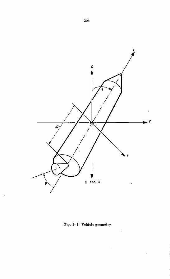
208

X i

Fig. 6-1 Vehicle geometry

209

m ( i y + v x I I / ) = ~ g o + ~ a ( a + a , " ) + ( m g c o s x ) 9

I $ = -TgZT/3 + M a ( a + a,)

(Eq. 6-31)

(Eq. 6-32)

with ow the wind induced angle of attack. (See figure 6-1). aerodynamic t e rms have been retained. motion, it i s necessary to restrict the analysis to small angles of attack such that

Only the significant In order to linearize the equations of

(Eq. 6-33)

This allows one to drop the nonlinear te rm vy 4 in the x-equation and rewrite the equations of motion in the form

m < , = T - A - m g c o s x = T o (Eq. 6-34)

m v x ( & - & ) = TgH + (N ,+T , ) a + ( n 1 g c o s x ) $ + N a a , , . (Eq.6-35) ..

I $ = - T , & P + Ma ( a + a w ) . (Eq. 6-36)

Information on the inertial velocity of the launch vehicle perpendicular to the flight path can readily be obtained from the transformation equation 6-9 as

Y =d12 Vx + d2, Vy + d32 V L (Eq. 6-37)

or assuming small attitude angles J/ :

+ = v x ( J / - (U). (Eq. 6-38)

The control equation for the yaw plane analysis i s given by

p = a , $ + a , $ + b o ( a +a,") (Eg. 6-39)

Frequently the analysis is restricted to short intervals of flight time and constant mass and inertial properties are assumed during this interval. analysis of the stability and response characteristics of the launch vehicle with classical analytical methods. and 6-36 is of the third order. ent the frequency and damping of the rotational mode. negative and is called drift root. steady state responses due to a constant angle of attack a gravitational te rm (mg cos x ), the steady-state attitude angle becomes

This allows an

The characteristic equation of equations 6-34, 6-35 Two of i t s roots a r e conjugate complex and repres-

Of particular interest in the load studies are the Neglecting the small

The third root is rea l and

.

To (Ma - T, SZT bo a w 9 =

(M, + N, iiT + T, E,) T, a, (Eq. 6-40)

and the steady-state lateral drift velocity

To (Ma - Tg ZT bo) + a, T, (Ma + N, SIT) V, (Eq. 6-41) @ W .

- - y = (Ma + NaXT + To X T ) Tyao

It is seqn that for increasing angle of attack feedback bo the steady state values of J/ and Y are decreasing and eventually become negative. comes zero for

The lateral velocity be-

(Ma + Na X T ) a, + (To/xT)Ma bo = (Eq.6-42)

To I T

210

This control mode is refer red to as 'Drift-Minimum Control. load relief and minimization of lateral drift has been discussed in Chapter 4.

6-2-6 (b) Elastic Body Equations. It was mentioned above that a more accurate load analysis of large launch vehicles has to include such effects as body bending, propellant oscillations, engine compliance and control filters. The analytical procedure to derive the nonlinear differential equations for planar motion usually starts with Lagrangian equations. For the planar motion the Lagrangian equations can b e used either for a body-fixed reference f rame employing 'quasi-coordinates' or in the classical form in an inertial reference frame. plexity of the resulting equations of motion is insignificant. consistency with the previous discussion, the equations for the flexible launch vehicle will be given for a body-fixed coordinate system. for the planar (yaw) motion for the rigid-body degrees of freedom assume the following form

Its importance for

The difference in the com- In order to preserve

The Lagrangian equations

(Eq. 6-43)

(Eq. 6-44)

(Eq. 6-45)

The Lagrangian equations for the flexible degrees of freedom retain their classical form ~

I

xaq, [ " ' I - [E]=Qi. (Eq. 6-46) I The detailed expressions for the kinetic energy and the generalized forces will be omitted. However, the resulting equations of motion are given in a form where all insignificant t e r m s are deleted. It should be mentioned that the following equations of motion are based on a free-free beam analysis with rotary inertia which includes the engines and liquid propellant considered frozen but the latter not contributing to rotary inertia. This makes the computation of the mode shapes more complicated but unburdens the equations of motion.

I

The rigid body equations are then

m (GX + g COS x ) = (T - A ) = m z (Eq. 6-47)

The equation fo r the propellant oscillation of the s-th tank is

In addition to the above equations of motion, the load analysis for a flexible launch vehicle has to include the engine compliance and actuator dynamics and the effect of the shaping networks. Engine compliance and actuator dynamics can be simulated with sufficient accuracy by a third order linear dynamical system as given in equation 6-25. The effect of the shaping networks (control filters) can be computed from the electrical components. Input-output relations of these fi l ters are usually given in transfer function form. In Laplace transform notation this can be expressed as

: ,

Fc ( s ) = a. F (s ) 5 ( 6 ) + a F - ( 6 ) s$(s ) + b o Fa (s) a! (s). .. (Eq.6-52) 9 l 9 I The.overbar denotes the Laplace transform of the original t ime functions involved.

transformed into the t ime domain which yields the necessary differential equations

Fq, .F3, , and F, represent the transfer functions of the control filters in the respective feedback channels. For digital simulation studies equation 6-52 has to be

relating the control deflection p, (t) to the command signals from the various sensing elements. The analytical procedures for this transformation are discussed in more detail in reference (5).

It should be noticed that the longitudinal velocity v, c a t b e directly obtained from equation 6-47 for a standard trajectory along which g, g and X are given as functions of time. equations with time-varying coefficients. from the expression for the angle of attack a as given in equation 6-33. ization was discussed previously. the yaw motion of a flexible launch vehicle can be performed using a set of linear differential equations with time-varying coefficients.

6-3 Statistical Vehicle Dynamic Analysis

In principle it is possible to compute the responses of a launch vehicle to a large number of high resolution wind profiles and to evaluate the results in a Monte Carlo type statistical analysis. This is both expensive and t ime consuming, especially if one wants to assess the influence of various system and control parameters on the vehicle responses. The statistical techniques of dynamic analysis attempt to avoid the disadvantage of the Monte Carlo approach by relating the statistics of the input (wind) to the statistics of the output (loads) of a dynamical system (launch vehicle). In order to establish these relations, some general statistical concepts are needed. Since various definitions of these statistical quantities are found in the engineering

This will avoid misunderstanding in interpreting familiar relationships and final results. more detailed treatment of the subject see reference (6).

I

,

It is seen that the equations 6-48 through 6-51 are linear differential The only nonlinearity remaining comes

I t s linear- In summary, a rather accurate load analysis for

~

~

I literature, they will b e introduced briefly in the following section. For a

I I 6-3-1 General Statistical Concepts

A stochastic process is defined as an ensemble of time, or space, functions of infinite domain, whose properties can be characterized only by statistical parameters.

I I correlation functions. They represent generalizations of the correlation coeffici- I Particularly important statistical characteristics of stochastic processes are the

ents employed in elementary statistics.

The autocorrelation function shall be defined as the ensemble average

212

W" w VIW I I I I

I Fig. 6-2 Stochastic processes

h ( t , d

t

Fig. 6-3 Unit impulse response of time -varying system

213 N

1 rxx (t, 7 ) = lim - xk (t) xk ( t + T ) N+CO N k = l

l and the crosscorrelation function as the ensemble average N

I , = < Xk ( t ) Y k ( t + 7 ) > I

(Eq. 6-53)

(Eq. 6-54)

where xk (t) and yk (t) represent member functions of two different ensembles of random time functions and N the number of available records. functions are, in general, functions of two independent variables @, T ). able t is called reference time and T correlation time, or lag. certain stochastic processes, the correlation functions become invariant with respect to t ime translations such that

1 The correlation The vari-

See figure 6-2. For I I

rxx (t + t o , 7 ) = rxx ( t , 7 ) = K,, ( 7 ) (Eq. 6-55)

I rxy (t + t o , 7 ) = rxy ( t , ~ ) = K,, ( 7 ) . (Eq. 6-56) I

These processes are called stationary in the wide sense, or weakly stationary. I Wide-sense stationarity involves only first and second-order statistical moments.

Stationary processes are often assumed to exhibit the further property that their ensemble averages taken over a large number of member functions are identical with

I 1

their corresponding t ime averages on a single member function, i.e.

1 Kxy ( 7 ) = lim - . T x k ( t ) yk ( t + 7 ) dt = Rxy ( 7 ) Vk T-w 2T -T

(Eq. 6-57)

(Eq. 6-58)

~

These stochastic processes are called 'ergodic'. For most practical cases ergodicity cannot be experimentally determined, because the number of member functions is usually very limited. However, the recorded t ime of observation is often sufficiently long to obtain a satisfactory time average. Therefore, it is common practice to assume ergodicity of the stochastic process and to replace ensemble averages by t ime averages wherever they occur in the analysis. The weakly stationary correlation functions exhibit several important properties which can be derived from their

therefore briefly stated.

I

, definition equations 6-53 and 6-54. Some of these will be needed later and are

K,, ( 7 ) = K,, ( - 7 ) (Eq. 6-59)

In* (Eq. 6-61)

214

(Eq. 6-62)

The time functions k (t) and 9 (t) represent the t ime derivatives of their respective stochastic processes. function is zero at its origin ( T = 0 ) because it assumes a maximum a t this point. Fror.1 equation 6-61 follows therefore

It should be noticed that the derivative of the autocorrelation

KIXx ( 0 ) = K,; ( 0 ) = < X k ( 0 ) &k ( 0 ) > = 0 . (Eq. 6-63)

This proves that xk e) and kk (t) are mutually independent stochastic processes.

In the following discussion it is assumed that the stochastic processes have zero mean. ion are sometimes replaced by autocovariance function and covariance function, respectively. If a stochastic process has a mean value, it can be extracted and treated as a deterministic forcing function. The total response of the system is then the sum of the response to the mean and the remaining stochastic process with zero mean. For these stochastic processes the correlation functions approach zero for infinite correlation t ime 7. They are also absolutely integrable, i.e.

In this case, the t e rms autocorrelation function and crosscorrelation funct-

This will not be done in the present chapter.

(Eq. 6-64)

A s a consequence, it is possible to subject correlation functions to a Fourier transformation. This frequency domain transform is only useful for stationary processes. For nonstationary processes one has to apply two-dimensional Fourier transforms. The resulting formulas are unusable for practical computations.

The Fourier transforms of the stationary auto and cross-correlation function are known as power spectrum and cross-power spectrum, respectively. defined as

They are

W

(Eq. 6-65)

(Eq. 6-66)

Because the autocorrelation function is an even function (6), the power spectrum is a real function of o and therefore is also written as S ( U ) rather than S (iw ). In addition it can be shown that the power spectrum assumes only positive values. The cross-power spectrum is, in general, complex. concepts will not be discussed here. definition integrals 6-65 and 6-66 are

The physical significance of both The inversion formulas corresponding to the

(Eq. 6-67)

(Eq. 6-68)

215

Another important statistical measure is the average number a particular response level is exceeded. recoverable launch vehicles subject to random disturbances. based upon the assumption of an ergodic stochastic process having a Gaussian distribution with zero mean. We consider a single t ime function x e) and denote i t s t ime derivative by 2 e). Since the stochastic process x (t) and i t s t ime derivative are statistically independent (see equation 6-63) their joint probability density function is given by

This quantity i s important in operational-life t ime studies of The calculation is

(Eq. 6-69)

where = - RYx (0). The ba r denotes the t ime average over a single stochastic process; see reference ( 6 ) . The probability of finding x ( t ) between x and x + dx when i t s derivative k lies between x + dk i s given by

= R,, (0). and

d2w(x, %) = p(x, %) d % d x (Eq. 6-70)

which can be written with d x = k dt as

dZw(x, %) = p(x, %) d k (;r d t ) . (Eq. 6-71)

The average number of crossings at the response level x per unit t ime with any possible positive slope (0 . . . k . . . 50 ) is given by the integral

111

Inserting equation 6-69 and integrating yields

(Eq. 6-72)

@q. 6-73)

The averag: number of exceeding positive and negative values of x is twice the number of n'(x) and is called the number of exceedances. If the total number of zero crossings per unit time is No, then the average number of exceednnces is given as

@q. 6-74)

A reasonably simple formula for the variance of the average number of exceedances does not exist.

6-3-2 Power Spectrum Analysis

The determination of aerodynamic loads by power spectrum analysis i s restricted to linear time-invariant differential systems with stationary input processes. evident that the flight of a launch vehicle through the atmospliere is a strongly nonstationary process. propellant consumption but also the atmospheric flight conditions.

It i s

There vary not only the system parameters due to the rapid The difficulty

216

can partly be circumvented by restricting the analysis to small time intervals and assuming the spatial characteristics of the wind process to have local stationarity. The latter condition is approximately satisfied for the wind turbulence (see Chapter 1). A widely used power spectrum model for the turbulence is that of H. Press:

(Eq. 6 - 7 5 )

where and U T the variance of the turbulence. At altitudes below 50 000 feet, this power spectrum seems to be an acceptable model for the atmospheric turbulence. scale of turbulence ranges from 500 to 1000 meters, depending on the altitude and the variance of the turbulence from 1 to 4 m2/sec2. spectra are discussed in Chapter 1. In order to apply the power spectrum model of equation 6-75 in the dynamic analysis of the launch vehicle, it is necessary to transform it from the space domain to the t ime domain according to

is the spatial frequency in radians per meter, L is the scale of turbulence

The

Other possible forms of power

(Eq .6 -76 ) W a=

where V is the vertical velocity of the launch vehicle.

The Press turbulence model approximates only the variance of wind but poorly approximates that of the wind shear. power spectrum model becomes infinite. the number of exceedances for a vehicle with angle of attack feedback. case the number of exceedances becomes infinite. using a power spectrum model which conforms to specified wind and wind shear variances.

In fact the variance of the wind shear of this This presents a problem in calculating

For this This difficulty can be avoided by

A particularly useful model is given by

(Eq. 6-77 )

(dW). where ow2 is the variance of the wind and U,” the variance of the wind shear - d h Its corresponding autocorrelation function is

(Eq. 6 - 7 8 )

The relationship between the power spectrum of the output of a dynamical system to i t s input power spectrum is established by the autocorrelation theorem. owing steps are taken in i t s derivation: according to the superposition integral, the input-output relation of a linear system with unit-impulse response g ( C Y ) is given as

The foll-

For an output signal at t ime t + 7, we obtain

(Eq. 6-79)

(Eq. 6-80)

Since the statistical average operator <> commutes with the integral, we obtain

(Eq. 6-82)

This is the desired relation between the output and input statistics of a linear time- invariant system. By Fourier transfo.rmation of both sides, we obtain the relation in the frequency domain as

2 Syy(u) = I T,, ciw) I S A W ) . (Eq. 6-83)

Ty, (j w ) i s the frequency response between the output y (t) and the input x (t). course, this relation alone does not provide enough information to determine the probability density of a stochastic process which is needed for load estimates. If, however, the further assumption is made that the stochastic process be Gaussian, then the probability and exceedances can be determined. The frequency response T (j 0) can readily be obtained by Laplace transformation of the linearized equations of motion and setting the Laplace operation S = j w. The variance of any output signal is given by the inversion formula 6-67 for zero argument.

Sometimes i t is advantageous in statistical simulation studies to construct a random signal as the output of a dynamical system excited by an independent Gaussian stochastic process - white noise.

White noise is characterized by a constant power spectrum. white Gaussian process is an idealized concept, because it would have infinite power as well as power at infinite frequencies. It is quite feasible, however, to generate a stochastic process with a nearly constant power spectrum over a wide frequency band. One re fers to such a process as 'band (width)-limited white noise'. The linear dynamical system which generates a stochastic process with a prescribed power spectrum is called a shaping filter. In order to establish a shaping filter, i t is necessary to approximate the measured power spectrum by a rational function, a rational power spectrum, satisfying the condition of being a real, even and non- negative function. Such a rational power spectrum has a pole-zero configuration which is symmetric to both the imaginary and real axes of the complex j w -plane. It can, therefore, always be factorized in the form

Of

It is obvious that the

(Eq. 6-84)

where J, fj w ) contains only poles and zeroes in the upper half ju -plane. (*) denotes the conjugate complex quantity. filter is then directly given by T (S) = + (S). generate the power spectrum model of H. P r e s s (equation 6-75) is

The s ta r

A s an example, the shaping filter to The transfer function of the shaping

L l + d m s

and for the power spectrum of equation 6-72 it is

(Eq. 6-85 )

218

(Eq. 6-86 )

6-3-3 Nonstationary Statistical Methods The assumptions necessary for the power spectrum analysis are rather restrictive. Consequently it is necessary for a more accurate analysis to employ nonstationary methods for the structural load analysis. varying system and a Gaussian distribution of the wind input. Although one should try to keep the necessary assumptions at a minimum, it is standard in engineering applications to assume also that the nonstationary stochastic wind process can be adequately approximated by ,a linear time-varying differential system, a shaping filter, excited by white noise. This is analogous to the assumptions for rational spectra in the stationary theory. results in a considerable simplification in the mathematical analysis. on how the linear dynamical system is specified mathematically, there are basically two methods of analysis which a r e discussed in the subsequent sections.

6-3-3(a) State Space Representation. tion are given as a se t of m second-order simultaneous differential equations. convert this set of differential equations into the desired state space form, it is necessary to introduce new variables for the higher order derivatives. tration, consider the second-order system characterized by

These methods assume a linear time-

It will be seen subsequently that this assumption Depending

In general, the linearized equations of mo- To

As an illus-

.. x + a(t) h + b(t) x = f(t). (Eq. 6-87)

Let x - x and x, = xl. XI = x,

Then one obtains l ;

x, = - b(t) x1 - a(t) x, + f(t). (Eq. 6-88)

With these new variables the linear dynamical system is represented by a set of f irst-order differential equations. matrix

Introducing the state vector in form of a (2 x 1)

and ( 2 x 2) matrices

and a disturbance vector in form of a ( 2 x 1) matrix

@q. 6-90)

(Eq. 6-91)

the set of first order linear differential equations 6-88 can be written in matrix form

X = A ( t ) x + B (t) we) . (Eq. 6-92) - - - - Extensions of this state space concept to higher order systems are obvious. will consider equation 6-92, the standard matrix form of the linearized equations of motion, where in general A (t) is an (nx n) matrix of scalar functions,

We

(t) the

219

(n x 1) state vector, puts. In general the system input y (t) will consist of several components. the case of a launch vehicle, the input components are the yaw wind and pitch wind. In a planar analysis there is only a single input. As mentioned above, it i s common practice to describe the wind as a stochastic process which is generated as the output of a dynamical system, the wind filter, excited by white noise. a dynamical system can also be written in standard matrix form as

an (n x m) matrix and y(t) the (m x 1) vector of wind in- For

Such

- w = C ( t ) w + - D (t) u(t) (Eq. 6-93)

where x , represents now the state vector of the wind disturbance and 2 (t) the vector- valued white noise excitation.

For a slowly varying wind process, the wind filter of equation 6-86 could be used. In this particular case the various matrices of equation 6-93 would be

and

(Eq. 6-94)

(Eq. 6-95)

The linear matrix equations 6-92 and 6-93 can now be combined into a composite system as

- - - - & * = A*(t) x*+ B*(t) u*(t) = A ( t ) x"+ s*(t) (Eq. 6-96)

where x' is a generalized state vector which includes both the vehicle state and the wind sGte and a" (t) = E* (t) The various matrices of equation 6-96 are then d%fined in partitioned form as

" (t) for brevity.

(Eq. 6-97)

(Eq. 6-98)

where 2 is the null matrix. and reads:

The solution of equation 6-96 is given in reference (7)

(Eq. 6-99)

The proof follows by direct verification of the initial condition and substitution in equation 6-96. composite system.

It can be shown (7) that the i-th column of the matrix I$

all components of the vector initial condition (to) equal to zero, except the i-th component which is se t to unity, and solving the homogenous equation 5" =A* (t) x? This procedure Can be readily implemented by numerical integration on a digital- computer.

The matrix - 4 @, T ) is called the 'state trimsition matrix' of the

(t, to) i s obtained by setting

It is seen that the solution ?* @) of equation 6-99 depends on the be-

220

havior of (b (t, T ) as a function of i t s second argument T , whereas the above described procedure yields the state transition matrix as a function of i t s f irst argument. This is a tedious task, for it involves repeating the numerical integration for many initial t ime points to = T . cedure has to be found which specifies the transition matrix as a function of i t s second argument. which is defined as

In order to circumvent this difficulty, a pro-

Such a procedure is available by introducing the 'adjoint system'

(Eq. 6-100)

where A*" (t) is the transpose of A (t). of the adjoint system by $' (t, to ) ,Tt can be shown (7) that

If we denote the state transition matrix

- $T (t, to) = 9 (t", t) Vt, to. (Eq. 6-101)

The response of the system 6-99 can, therefore, be rewritten as

(Eq. 6-102)

It is important to notice that the state transition matrix pT ( T , t ) has to be established for T< t for the evaluation of the integral in equation 6-102. that the adjoint system has to be integrated numerically with the time running backward, starting the initial conditions of the adjoint system at time t . effort in computing the response of the system to ai input 5 ( T ) has obviously to, be expended for the calculation of the state transition matrix $T ( T , t). this matrix is known, the response can be calculated by s i m p k integration. For load studies, it is often only of interest to find the response at a few selected time points: maximum dynamic pressure, Mach 1, etc. In this case equation 6-102 would be useful for a Monte Carlo type study where 2 ( T ) would represent the input for the different deterministic wind profiles. then not be restricted to a Gaussian distribution of the wind process. one would have still to assume linearity of the system.

The next a i d final step of this statistical approach is to obtain the covariance mat- r ix of the generalized state vector x * (t) from which the variance of the bending moment can be obtained. 6-102 as

This means

The m+n

Once

The statistical evaluation would However,

The resFonse covariance matrix follows from equation

< - - x'(t) x*T(t)> = - S(t) = (Eq. 6-103)

t

Now comes the decisive simplification, which is possible in the evaluation of this equation due to the fact that the composite system has a white noise excitation. ks aconsequence

<U*(T) - > = Oand <U*(T) - - U*T(T) > = E . (Eq. 6-104)

where E is the unit matrix. Equation 6-103 reduces therefore to

221

t

s(t) = $0, to)s ( to) pT (t, to) + Q ( 7 , t ) - - - B'(T) fi) ICI ( ~ , t ) d ~ . (Eq. 6-105) - -

Differentiation with respect to time yields the desired differential equation for the covariance matrix of the generalized state vector 5 (t):

(Eq. 6-106)

The variance of the bending moment or any other response of interest can then be easily obtained from the covariance matrix S e). It seems appropriate to mention that the computational effort of integrating tfie covariance matrix differential equation 6-106 becomes extremely cumbersome for systems of only moderate order even if a high-speed digital computer is used. This is due to the fact that equation 6-106 represents a system of n ( n + 1) first-order differential equations which have to be solved simultaneously.

6-3-2b) Impulse Response Representation. input single-output linear t ime varying system represented by

2

In this section we consider a single-

(Eq. 6-107)

d where p is the differential operator . Let us consider the homogeneous equation.

n- 1 p n x + al(t)p x + .-. a,-l(t)px + an(t) = 0. (Eq. 6- 108) . ..

If we use the state vector x=(x, x, x . . . x@-l)) then we can write

(Eq. 6-109) 1 = 4 (t)x

where

A(t) = - 1 0 1 o . . . o 0 0 1 . . . 0 0 0 o . . . o

-an -an-l . . . -al . . . . . . . . .

The adjoint state equation is by definition given as T - j I = A M Y . (Eq. 6-110)

If we let the state vector of the adjoint system be 41 = (yl, y2 . . . y), reads:

then it

PY1 = a n Y n PY2=an-,Yn - Y l . . . . . . . . . PYn = a l Y n - Yn-1.

Multiplying the k-th equation by (-l)k" p k- l and adding the resulting equations, we obtain

n l n l (-l)npnyn + (-1)' - ) p( - (alyn) + . . . (-1) p (an-lyn) + anyn = 0. (Eq.6-112)

222

Therefore it is reasonable to call the operator

- n l n l L (P, t) = (-11~; + (-I)( - p( - )(al . . .) + . ..a, @q. 6-113)

the adjoint operator of L (p, t).

Since the above representation directly relates the output x (t) to the input f (t), it is natural to consider the impulse response of the system. The unit-impulse response h (t, 7 ) is defined as the zero-state response of the system at time t to a unit impulse applied at an earlier t ime T ; see reference (7). Figure 6-3 illustrates the behavior of he, T ). Note that h (t, T ) = 0 for all t < 7, which indicates that the system does not respond prior to the application of the impulse. Mathematic- ally the impulse response can be obtained by integrating the homogeneous differential equation 6-107 with the initial conditions

= O k = O , l . . .n - 2 (Eq. 6-114)

Assuming zero initial conditions, the response of the system to an input f(t) is given bY

t

x(t) = h(t, 7 ) f (7) d7. (Eq. 6-115) t 0

Here we face the same situation as in the previous section, that, in order t o obtain the response of a system, the unit-impulse response h (t, r ) has to be known as a function of its second argument 7 which is the excitation t ime of the system. can be proved (7) that this can be done by numerically integrating the adjoint system backwards in t ime starting at t and going to to. Denoting the unit-impulse response of the adjoint system with w (t, to), we obtain a relation analogous to equation 6-100 in the form

It

w(t, tJ = h(to, t). (Eq. 6-116)

The initial conditions for the adjoint system are

It should be mentioned that the adjoint system can be very elegantly programmed on an analog computer by modifying the computer program of the given system by the following set of simple ru les (8):

(a) Reverse the inputs and outputs of all computing elements

(b) Generate all t ime varying parameters in the system as if the independent variable (time) were decreasing from time t to to rather than increasing from to to t.

In order to obtain the variance of the response of a time-varying system at t ime t,

223

the adjoint method also employs a suitable time-varying shaping filter. By combining this filter with the original system, a new composite system is formed with a white-noise input. The variance for such a system is then obtained from equa- tion6-115and 6-116 assuming a white noise input as

a t a <x (t) > = w (T,t) d r

t 0

@q. 6-118)

The implementation of the adjoint method on an analog computer offers an attractive means for statistical system optimization, because it does not require a white noise generator.

In retrospect, one becomes aware of a striking analogy between equations 6-115 and 6-118 and equations 6-102 and 6-105 respectively. latter two formulas are nothing else but generalizations of the former two to multiple-input multiple-output systems. significance to the state transition matrix 9 (t, 7 ). Its element @ik (t, 7 ) represents the zero-state response of the i-th (integrator) output at time t to a unit impulse applied at the k-th (integrator) output at time 7 . tion the rules for obtaining the adjoint system from the original system on the analog computer can be directly deduced from equations 6-100 and 6-101. Rule 1 Is a consequence of taking the transpose of $' T @, to) which exchanges the indices i and k. But this means interchanging input and output. Rule 2 follows from the minus sign in equation 6-100 which indicates that dt has been replaced by -dt in the derivative and that consequently t ime is running backward.

6-4 Computational Considerations

Except when the most extreme simplifications are employed, the equations discussed in the previous sections admit of no analytical solution. It is therefore necessary to take recourse to automatic computing equipment. There are three possible computational techniques: analog, digital and hybrid computation.

Analog computers have the advantage of high computation speed. 'parallel fashion so that solution t ime is independent of problem complexity. Their output of data does not slow computation and is available in easily assimilated graph- ical form. uine feel for the operator of the physical process under investigation. computer should be considered a research tool rather than a calculator. tion, the analog computer allows an easy introduction into the computer setup of actual physical components, rmch as hydraulic and electric servos, control su r - faces, human pilots and autopilots. This'technique is, of course, superior to any analytical representation of the dynamic characteristics of these elements, especially if nonlinearities, back lash, dry friction, etc. are involved. limitations of the analog computer concern its precision and resolution; its typical accuracy is 0 . 5 percent to 5 percent. Also, discrete calculation and complex logic functions are usually clumsy. automatic programming methods are not available.

Digital computers are inherently sequential machines, performing each mathematical operation through repeated addition. problem, the slower the computer's repetition period. Because of this, the digital computer is generally limited to the solution of problems in which the input variables change slowly with time. Its advantage over the analog computer consists in its unlimited precision and resolution of numerical variables and its floating-point arithmetic, which eliminates scaling problems.

It is quickly realized that the

In this light it is possible to attach a physical

With this observa-

They operate in

A decisive advantage of the analog computer is that it provides a gen- The analog

In addi-

The basic

Storage capability and memory are limited and

A s a consequence the more complex the

224 I Quite frequently the practising engineer is confronted with problems which call for high accuracy and computation speed. In this case, either computer used alone would have to be quite large and a hybrid digital-analog combination is desirable. Problems which lead to hybrid computation are found in statistical analysis requiring repeated solution of differential equations, including Monte Carlo methods for deterministic problems. This is essentially a data-storage and simple-evaluation task around the solution of differential equations. The effort is divided between the computers such that the equations of motion are programmed on the analog computer and the digital computer provides the parameter changes and statistical evaluation. Other applications of hybrid computation are found in real t ime aerospace vehicle dynamical studies where a full simulation of the vehicle, i t s digital and continuous control and its human operator is necessary either for training or the evaluation of flying qualities. The list of possible problems is growing steadily and we may expect a wider application of hybrid computation in the future.

Symbols

A

D

D

9

F

axial force

drag, Newton

direction cosine matrix

moment of inertia dyadic

external force, Newton

acceleration of gravity, m/sec2

longitudinal acceleration, m/sec2

angular momentum, kg-m2/sec 1

moment of inertia of total vehicle, kg-m2

moment of inertia of swivel engine about i t s mass center, kg-m2

external torque, Newton-M

mass of vehicle, kg

aerodynamic moment gradient, Newton-M

generalized mass of i-th bending mode, kg

slosh mass, kg

normal force gradient, Newton

generalized aerodynamic force gradient of i-th bending mode, kg

radius of earth, M

first moment of swivel engine about swivel point, kg-M

kinetic energy of total vehicle, kg-m2/sec

tot? thrust, Newton

225

thrust of swivel engines, Newton

comflonent of velocities along x-axis

component of velocities along y-axis

component of velocities along z-axis

vertical component of vehicle velocity, m/sec 1

location of slosh mass, M

distance of slosh mass from mass center of total vehicle, M

longitudinal location of swivel point, M

distance of center of mass to point of application of thrust, M

i-th bending mode shape

slope of i-th bending mode shape, M 1

rigid body angle of attack

wind-induced angle of attack

thrust deflection angle

thrust command angle

damping ratio of swivel engine

damping ratio of i-th bending mode

damping ratio of slosh mode

generalized coordinate of i-th bending mode, M

amplitude of slosh mass, M

generalized force of i-th quasi-coordinate

gravitational potential, Newton-M

command attitude angle from vertical

yaw angle

natural frequency of i-th bending mode, sec 1

natural frequency of swivel engine, sec 1

natural frequency of the first slosh mode in the s-th tank, sec

angular velocity vector, sec 1

angular velocity matrix

226

V universal quantifier 'for all'

<>' ensemble average (expected value)

Other symbols and abbreviations are explained in the text.

References

1. Heiskanen, W. and,Mainesz, V., 'The Earth and Its Gravitational Field', McGraw-Hill Book Co., New York, 1958.

Altitudes to 65 800 F't.' , 1955.

Whittaker, E.T., and Rigid Bodies', Cambridge University Press .

Lester, Harold C. and Morgan, Homer G., Vehicle Response to Detailed Wind Profiles' , TMX-51048, 1964.

Andrus, J. F., Technical Paper MTP-COMP-63-2.

2. NACA Report 1235, 'Standard Atmosphere -Tables and Data for

3. 'A Treatise On the Analytical Dynamics of Particles

4. 'Determination of Launch-

5. 'Closed Form Solution to Control Equations', NASA

6. Papoulis, Athanasios, 'Probability, Random Variables and Stochastic Processes ' , McGraw-Hill Book Co., New York, 1965.

7. Zadeh, L.A. and Desoer, CA., 'Linear System Theory', McGraw- Hi l l Book Co., New York, 1963.

8. Fifer, Stanley, 'Analogue Computation', Vol. N, McGraw-Hill Book Co., 1961.

228

80

LO

A /

,- \ / / w.

WIND VELOCITY (m/sec)

TOTAL ANGLE OF ATTACK (des)

ENGINE DEFLECTION (deg)

BENDING MOMENT, STATION 20.62

(lo6 N m)

LOAD INDICATOR, STATION 12.75

FLEXIBLE VEHICLE REFERENCE 3 a -----

A

3

2

1

0

A LO

30

20

10

0

A

O B E C O C O M M A N D G A I N S W I T C H I ~~

C E C O

0 i o 6b 60 i o 100 120 li0 160

FLIGHT TIME (SEC)

Fig. 7-1 Total dynamic response to a 69 m/sec, 300 degree design wind during S-IC flight

1

229

t

O*

7

Vehicle Response to Atmospheric Disturbances

R.S. RYAN

7-1 Introduction

The interpretation of the response of a space vehicle to atmospheric disturbances is very complicated because the vehicle response depends on and interacts with the various characteristics of the wind - magnitude, shear, gust - the vehicle dynamics - rigid body, elastic body, propellant oscillations - and the control system. An attempt is made to assess the various aspects of this interaction using a series of systematic parametric studies covering variations of vehicle parameters and various atmospheric disturbances. Several types of vehicles and various degrees of approximation, corresponding to different design phases, are considered, as well as the influence of refinements in model descriptions and the effects of advanced control systems.

7-2 h a m e t e r s for Evaluation of Response

The determination of a space vehicle's response to atmospheric disturbances cannot be reduced to the evaluation of one discrete set of response criteria, such as vehicle loads, but must include many response parameters, the choice of which as criteria depends upon the vehicle configuration and specific mission. Neither is it practical to use only one method for all phases of vehicle design: different approaches and methods of evaluation must be used as the particular phase demands. include preliminary design, final structural design, guidance and control system design and optimization (preliminary and final), and establishment of limits and procedures for launch and flight operations. In each of these areas, three things must be considered

(a) tical dynamic model to describe adequately the vehicle characteristics relevant to a particular design phase. For example, a rigid body analysis may be adequate for preliminary structural design, while a complete elastic simulation to generate loads envelopes would be required for final structural design. Again for preliminary design, a discrete synthetic wind profile is usually adequate; on the other hand, flight operations require an individual detailed wind of the Jimsphere type (1).

(b) wind field, and the lack of capability to completely predict the vehicle characteristics - aerodynamic forces, structural weight and thrust. (2) is used to create the 'worst' response case for the parameter, taking the 3 0 deviation from nominal for the aerodynamic force, structural weight and thrust (where U is the standard deviation). These 3 U variations are necessary to describe statistically the response spectrum, that is, to establish a probability level, and to determine fully the probability of different levels of exceedances of parameters. Examples of the nominal and 3 U response to a given design wind profile for Saturn V space vehicles are given in figures 7-1 and 7-2.

The phases

The f i r s t is the choice of the methods for analysis and the choice of an analy-

The second problem concerns the difficulty of obtaining statistics of the

A Monte Carlo technique

The statistics of the

230

wind field can be included in the analysis by simulating the flight through many individual wind profiles, using either synthetic profiles o r statistics of the total wind field (see Chapter 2). application to particular phases of design. profiles is by far the most accurate approach; however, the digital computer time needed is prohibitive. Synthetic profiles, although not as accurate as individual winds, require the least amount of computer t ime and are simple to implement on the computer. Using the statist ics of the total wind field is complicated by non- stationarity conditions, but still requires much less computer t ime than individual wind profiles. The solutions of the equations are formidable, although this is being alleviated somewhat by such methods as the adjoint technique (see Chapter 6). The proper selection of the representation, then, becomes a trade-off between the more accurate input (individual wind profiles) using large amounts of computer t ime and the slightly less accurate input (discrete profiles) which considerably saves computer time. The final determination of the approach to be taken depends upon the design phase and the type of vehicle.

(c) on the characterist ics and missions of the vehicles being studied. To illustrate, th ree vehicles a r e compared to show the constraints required by their structural design and their available control forces. small, high-accelerating vehicles having a marginal control force provided by jet and air vanes. characteristics required for maneuvering, vehicles of this type have no structural load problem from wind. In fact, since the vehicle has a structural margin more than adequate for any anticipated wind loading, the overriding constraint placed on this vehicle is from the control mechanism. The parameters for evaluating the response of this type of vehicle to atmospheric disturbances are, therefore, only deflection and deflection r a t e s of the control devices.

Each wind representation has i t s mer i t s and i t s specific The use of individual detailed wind

.

Another consideration is the identification of critical constraints depending

First, the Pershing is representative of

Because of high longitudinal acceleration and structural design

A second group of vehicles, represented by Saturn V, has a quite different set of parameters to be considered. Although these vehicles have ample control force, the structural integrity for man rating, plus the optimization of the vehicle design to maximum payload, require that the designer concentrate on the influence of wind on both structural loads, which can b e described primarily as unit-compressive, and tension loads at various longitudinal vehicle stations. Any significant shear forces present must a l so be evaluated, and the control system must be optimized with respect to these structural loads. Thus, the control system design engineer must consider all aspects, control and structural, of the vehicle design to ensure that structural constraints are not violated. like the Saturn V, the f i r s t step i s usually to optimize the control system for drift to achieve drift minimum and then to compute the preliminary load spectrum using this control system. allows a preliminary optimization of the control system gains with respect to poten- tially weak structural areas. Later, more refined structural analyses or tests may show where the design can be simplified or, at least, such analysis will give us a better understanding of the actual limits. The effect of winds on the lateral bending moment is shown on figure 7-3, which is a load indicator plot for critical flight t ime as a function of vehicle station. When these values are compared to the assumed or actual structural capability of the vehicle, weak points can be identified. these weak points have been found, a more detailed analysis is made to determine the final optimal gains. optimized, to permit a maximum of operational flexibility, by decreasing the restrictions versus allowable launch winds and thus increasing the launch opportunities.

The third group of vehicles is, in several respects, a combination of the first two in that both a limited control force is available and the structural capability is

For the preliminary design of vehicles

This first determination of the structural characteristics

Once

Based on these values, the control system is then further

231

ENGINE DEFLECTION

(deg)

ATTlTU DE ERROR

(deg)

ATTITUDE RATE

(deglsec)

3 LEXIBLE VEHICLE

2

1

0

1

2

REFERENCE

4 1.2

0.8

04

0

0 4

0.8

1.2 8 ROLLlTl LT GAIN OBECO COMMAND SWITCH CECO

I l l I I I ! I I1

0 20 LO 60 80 100 120 1LO 160 FLIGHT TIME (sec)

Fig. 7-2 Yaw response to a 69 m/sec, 300-degree design wind during S - IC flight

232

restricted. sion, is typical of this group. For these vehicles both the control system design and structural design must be evaluated in grea te r detail and must consider engine deflection, engine deflection rate, and the unit-compressive and tension loads.

For the preliminary design of these vehicles, the envelope of engine deflection and engine deflection ra te as a function of the control system gains must be established (control frequency and damping). Once a set of gains has been obtained such that deflection and deflection rate constraints are not exceeded (figure 7-4), structural design is begun, using load envelopes which were determined from this basic system. Determination of preliminary structural characteristics allows a trade-off between loads, control constraints, and operational procedures such as wind biasing. essential. First, the amplitude of the propellant oscillations in the tank must be controlled so that they do not cause an early cutoff in the case of propellant level being used as a criterion. Sometimes, in achieving the desired responses by control system filters, stability margins of various vehicle modes are diminished; a trade-off between desired response and desired stability boundaries is therefore necessary. Also, during the final design phases, incompatibilities between original mission requirements and vehicle constraints are usually encountered. toring during the launch phase or the use of wind biased trajectories become necessary.

For manned vehicles, the setting of abort limits for the safety of astronauts must be considered. failure, on the vehicle response must be studied for all possible winds. The parameters which must now be evaluated are the output of the emergency detection sensors, such as ra t e gyros, attitude sensors, accelerometers, etc. Because of the large deviations from nominal conditions, detailed characteristics of the winds as well as the dynamics of the vehicle itself must be included in the analysis.

7-3 Fundamentals of Analysis

If the elastic body frequencies are high as the vehicle reacts to an atmospheric disturbance, the mathematical representation of the dynamics of the vehicle can be simplified. In these instances, preliminary design values can be obtained by treating the rigid and elastic bodies separately. If the frequencies are low, this approach cannot be used.

The Saturn I, which may be manned or unmanned depending on its mis-

In the final design stage of these vehicles, two additional parameters are

Second, the stability margins must b e controlled.

To solve these problems, wind moni-

The effect of malfunctions, such as engine-out and control system

7-3-1 Rigid Body

7-3-1 (a) Applicability in Design. Representing a space vehicle as a rigid body has a basic application in the,preliminary phase of design. rigid body, and using 3 U variations of the vehicle parameters along with a synthetic wind profile, allows not only the basic response characteristics to be determined but a l so the approximate sizing of the structure. It also gives insight into the interaction of vehicle dynamics and control law formulations, giving a basis for establishing guidelines. for design of the control system.

Several approaches have been used for rigid body analysis. proposed a simplified method which considers two parameters of any individual wind profile: first, the maximum wind speed and, second, the integral of the t ime history of the wind speed. vehicle.

Another method, introduced by B. E. Clingan (3), simplifies the rigid body equations by neglecting rotational velocities and accelerations, which gives a system of first

Treating the vehicle as a

Van Der Maas (3) has

These two parameters are correlated with the loads on the

I

233

BENDING MOMENT INCLUDING 1.4 SAFETY FACTOR

(lo6 N m) (lo6 inch Ib)

-50

PREDICTED MOMENT

Fig. 7-3 Saturn V failing moment and predicted moment versus vehicle station: 70 seconds flight time

ENVELOPES ARE GIVEN FOR PITCH (RANGE) AND YAW (CROSSRANGE) COMPONENTS OF FIVE WINDS PEAKING AT

5, 8, 10, 12, AND 14, KILOMETERS

AT SPIDER BEAM (STA.

55 65 75 85 55 6 5 75 8 5 5 5 6 5 75 85 FLIGHT TIME (sec)

YAW BENDING MOMENT AT SPIDER BEAM (STA. RIGID BODY YAW ANGLE 0.5 ENGINE GIMBAL ANGLE 10-1 1 IN YAW (deg) 21.89) (lo6 in. Ib) OF ATTACK (des)

O l O U O L 1

5 5 6 5 75 8 5 5 5 6 5 75 85 55 6 5 75 85 Fig. 7-4 Response of the Saturn IB/202 vehicle to flight through a s p e c l r ~ n ~ of

synthetic wind profiles based on seasonal (Augmt) and directional ( 105-degree azimuth) envelopes

234

order differential equations of time-varying coefficients. efficients to be constant over discrete time slices, an analytical solution which can be rapidly applied to a large number of wind profiles can be obtained.

AviDyne developed a third method that uses large numbers of wind soundings and, at the same time, reduces computer t ime (3). computer t ime is a less accurate solution. This method is based on the development of influence coefficients which define the loads on the vehicle using basic profiles such as ramps and steady-state wind speeds. sounding is evolved from a superposition of the influence coefficients. quires the use of a linear system which, for certain vehicles, is unrealistic.

Results obtained from these rigid body methods are compared in reference (3) f o r several vehicles (Table 7-1, p288 1. methods are, first , that the resulting linear systems do not include all pertinent vehicle characteristics and, second, that elastic body characteristics are excluded. Where an elastic body simulation is required, rigid body alone cannot be used because high frequency winds and vehicle bending characteristics must be included.

By assuming the co-

The penalty for this reduction in ,

The response to an actual This re-

I The disadvantages of using rigid body

Although the three methods described above have their respective merits, the most generally acceptable approach is the use of a set of time-varying coefficients along with a synthetic wind profile such as that described in section 7-4. validity of these methods must be verified for each vehicle considered, this additional operation reduces to some extent their overall efficiency.

7-3-1 (b) Equations of Motion. by including certain assumptions such as constant coefficients and the M1 coordin- a te system described in Chapter 5. This approach leads to basic insights into the control system and vehicle dynamics. Although conservative results may b e obtained because of the assumption of constant coefficients, the trends are valid. It is possible to extend this approach, to account for t ime changes in the coefficients, by assuming the coefficients to be constant over small t ime slices and using the final values of the previous time step as initial conditions for the next t ime slice. This process i s not included here, but should reduce e r r o r s in the constant coefficient approach.

The following are rigid body equations as formulated in Chapter 5:

Because the

Rigid body equations of motion are best formulated

$ + C 1 Q + c,p = 0 @=@-I+-. ' U

v v The bending moment equation is

M, ( x , t ) = M' CY (x , t ) (Y ( t ) + Mb (x , t ) 0 (t).

The control law equation i s

(Eq. 7-4)

p=a,$ + al$ + b o a + e,y + ely. (Eq. 7-51

The control law. written in this form is fairly general and is representative of several systems. body motion in t e rms of the source of sensed accelerations (0, (Y ) can be expressed as

.For example, the output of a body-fixed accelerometer for rigid

235

(Eq. 7-6)

thus producing the same control law with only a modification of gains.

7-3-1 (c) Solutions for Specific Wind Inputs and Angle-of-Attack Feedback. 1. General Solution - This set of equations i s solved by usinkfrozencoefficients and setting e, (lateral position gain) and e (lateral velocity gain) equal to zero for two representative wind inputs: steady wind profile), which are the step winds and the ramp winds, respectively. The characteristic equation, which i s used to obtain these solutions, i s formulated in t e rms of vehicle parameters as follows:

the severe gust and the slow wind buildup (quasi-

"1

V V V s ] s3 + 52 [ alcz - - - -- %(ao + b o ) + c1 - - ( c & - cF3;]

- [ - c F 1 + a, ( c& - c1K3) - bo c&Cl = 0. V 11

A simpler form in t e rms of the roots

s = o

s = A,

s = u * i w

1

2

3, 4

is

(Eq. 7-7)

(Eq. 7-8)

s j 53 + s2 ( -A, - 20) + s (2A1u +U' + w ' ) +[-A,( U' + w ' ) ] I = 0. (Eq. 7-9)

Equating coefficients of powers of s between equations 7-7 and 7-9 allows the roots to be expressed in t e rms of vehicle parameters and control system gains. logical to express the control system gains a. and a i , and the drift root Ai, as a function of control system gain b, , control frequency w c J and control damping t; . This yields

It i s

- XwZB, + 2B3cZ<, W , + AB3 - CZB'WZ a, =

- ~ X C Z < , W , - X 2 - C 3 W s

CzB3 - ?AB,<, W , + BZA - B1CzWZ al =

-2XC,<,W, - A 2 - cf w:

Xc2Bz + BlA2 + c3 B3 A, =

2Xc2<,wc - X 2 -. C 2

where KZ ' B, =2ccw, + - V

(Eq. 7-10)

(Eq. 7-11)

(Eq. 7-12)

(Eq.7-13)

B, = -c1 + w," - czbo (Eq. 7-14)

(Eq. 7-15) Kl B3 = - 7 ( ~ 1 + b,cz)

236

w c (rad/sec)

i bo - C 1/Cg

I I 1 1 -0.05 0 0.05 0.10 0.15 0

Al (rad/sec)

Fig. 7-5 A, a s a function of control system gains, bo, and control frequency, WC

wC (rad/secl

2

1

0 I I I 1 -1 0 1 2 3

a 0

Fig. 7-6 a , a s a function of control system gains, bo, and control frequency, WC

wC (radlsecl

2.0

5 , = 0.707 c1 = -0.077 C2 = 1.067 K 1 = 18.580 1.0 K p 6.960 Kg = 15.660

0 ' I I I 0 1.0 2.0 3.0

al (l/sec)

Fig. 7-7 a l a s a function of control system gains, bo, and control frequency, WC

237

t

(Eq. 7-16) 1 X = - V (c2K2 - c~K, )

U = - r c c w

w z = U2 + 0 2 .

(Eq. 7-17)

(Eq. 7-18)

Figures 7-5, 7-6, and 7-7 are typical plots of drift root (Ad, position gyro gain (ao), and the rate gyro gain (a 3 for the maximum dynamic pressure flight time of the Saturn V. Figure 7-5 shows the effect of control frequency and angle of attack gain on the drift root (Ax). Low control frequencies (Uc) have a large influence on A1 where the angle of attack gain (bo) is the parameter. frequency moves the drift root toward a constant value. Oc, all A1 roots, regardless of the bo gain value approach the root determined for bo = -c, . Pure attitude control systems (bo = 0) produce a stable value of drift root (A,) regardless of the control frequency (Uc). The major control gain influencing the drift is the angle-of-attack gain (bo). If wc i s considered constant and bo is varied, an increasing bo causes Al to become unstable. As will be shown later, this moving of the drift root toward instability has a marked influence on the vehicle drift and steady state lateral bending moment. The well known drift minimum condition occurs when the drift root (Al) is equal to zero.

The only apparent effect (Figure 7-6) on the rate gyro gain (a,) is the control frequency ( U , ) , withdamping c c = .707. creases as angle of attack gain (bo) decreases for a constant frequency (Uc); increasing wc increases a, for a constant bo. The set of differential equations is solved in t e rms of these roots and the system parameters. Only one solution is given, the response to a ramp wind Kt, where K is the slope of the wind speed buildup and t is time in seconds. This is sufficient for a step wind and impulse wind, since the t ime derivative of the ramp produces the response to a step and the derivative of the step is the impulse. Although solutions for all the response parameters are easily obtained only the solution for the bending moment is shown.

2. Bending Moments - As previously shown by equation 7-4, the bending moment is written as

Increasing the control In fact, with increasing

CZ

The position gyro gain (a,) (Figure 7-7) in-

M, (x, t) = M'a + M'fl . (Eq. 7-19) a 0

By defining

R(x) = M h / M ' (Eq. 7-20) 0' M, (x, t ) = M' (R(x) a + 0 ). (Eq. 7-21)

B Writing the equations in t e rms of the solutions of a and fi yields the expression for the bending moment:

1 M, (X, t) = Y , ( O . W,Al) R(x) + Y2(0, U, A i ) + - { Y 3(4, U, A,) R(x) A1

+ y s ( u , ~ , A l ) R ( x ) + Y , ( u , w , A l ) ~ l / ~ e u t s i n ( w t +%) . (Eq. 7-22)

To illustrate certain trends, let us set w = 1.2 and 5 = 0..6 with a step wind input. Then, the bending moment f o r gyfo control (A: = -0.031) becomes

238 I

M, (x,t) = - K M' e-0*722[(0.051 R2(x) + O . 12R(x) +0.09)1/2]sin(0.882t+y) B + K M' (x, t) (0.714 R(x) + 0.13) e-O*0St B

where

= tan-l 0.22 R(x) + 0 . 3 0.244 R(x) + 0.27

(Eq. 7-23)

(Eq. 7-24) I

For the drift minimum condition (A, = 0 ) , the bending moment is 1 I

M,(x. t)=-K M' ( ~ ) @ . 7 2 ~ [ ( 0 . 1 7 4 R2(x) +0.428 R(x)+O. 3l)l/2]sin(0.882t+y) P + K M'P (x. t) (0 .64 R(x) + 0.113) , (Eq. 7-25)

where

y =tan- ' 0.21 R(x) + 0.452 . 0.359 R(x) + 0.332

(Eq. 7-26) ~

Since for most of the stations on the Saturn V vehicles R(x) Q 0.3, the engine deflection ( 0 ) contributes the major portion of the transient part of the solution for the bending moment, while the angle of attack (a) has more influence on the quasi- I steady-state portion. Changing the drift root from negative to zero increases the amplitude caused by the transient solution, but decreases the par t caused by the drift root. The choice then becomes one of a trade-off between the transient and I the steady-state solutions. by increasing bo the drift root becomes more positive; this reduces quasi-steady I

state loads, but increases transient loads even more. icle, an overall load reduction is made possible by increasing the angle of attack gain b). 1

I

This choice can b e related to changing the gains, since,

In general, for a rigid veh-

7-3-2 Elastic Body

The influence of elastic body oscillations can be determined in two ways: either by solving the total system of equations with all coupling terms, or by neglecting all coupling t e rms and solving each bending equation separately using the rigid body a and B t e rms as forcing functions on each individual bending mode. Although using the f i r s t approach yields the more accurate results, the second more simplified approach (4) produces good approximate values for the bending mode response and, hence, the bending moments, at a great reduction in complexity and in the amount of computer t ime required(5). The equations of motion are the previously given rigid body equations 7-1, 7-2, 7-3 and 7-5 plus an equation for each bending mode in the form

I

where i is the mode, is structural damping and is control damping. The bending moment equation must be altered to account for bending dynamics:

I

I (Eq.7-28) ,

239

Solving this set of equations provides a quick preliminary assessment of the elastic body effects on bending moment or loads.

7-3-2 (a) Areas of Applicability in Design. characteristics in vehicle design considerations depends upon the general vehicle characteristics. only with respect to the available control force. influences on the control surface o r engine deflections are small, they can add to the rate limits and should be included for the rigid body if the rate limits are approached.

Where vehicle dynamics have a large influence on structural loads, elastic body dynamics become important. It is clear that, in preliminary design work, it is practically impossible to include this refinement because of insufficient structural information.

The significance of elastic body

Very stiff vehicles can be treated as rigid bodies and are critical Although, in general, elastic body

7-3-2 @) Bending Dynamics Influence. The influence of bending dynamics on vehicle responses will b e discussed in two parts: first, vehicle parameters in general and, second, the effects of bending dynamics on loads. the major influence of bending dynamics on response is on the loads. were determined from a complete vehicle simulation with all coupling te rms included.

1. Vehicle Parameters - The influence of elastic body responses on the local angle of attack is most significant a t vehicle stations near each end. cases, this effect ,is a t a maximum at the vehicle nose and is of the order of 10 percent of the average angle of attack. The change in the average angle of attack r e - sulting from elastic body dynamics is negligible (Figure 7-8). The change in engine deflection due to elastic body dynamics for the Saturn V is also small, about 10 percent (see Figure 7-9). The influence of elastic body effects on the swivel engine's deflection rate is more significant, about 15 percent (see Figure ?- lo), and should be included in any analysis where this response i s a critical constraint. cluding elastic body effects changes the liquid propellant response very little, unless a sloshing frequency and bending frequency become near resonance. Since these frequencies are not near resonance in present vehicles, elastic body effects have negligible influence on propellant response; see figure 7-11. or accelerometer sensors are used in flight operation procedures, such as red lines for abort decisions, the elastic body effects can become significant. Analyses conducted to determine these limits should include elastic body effects.

2. Bending Moment or Load - The interaction of total flexible vehicle dynamics with the control law is much more complicated than the interaction of the rigid vehicle responses with the control law. Transient response becomes more significant for simulations which include flexible body dynamics, to the extent that load reduc- tions obtained through the introduction of alpha control are offset by load increases from flexible body transient loading. To show the effect of the control system and vehicle dynamics interaction, the total vehicle dynamics with time varying coeffi- cientsis solvedusing a synthetic wind profile as forcing function. meter feedback control system is used for this analysis; however, an equivalent to the angle-of-attack control law can easily be established. dynamics on the bending moment is illustrated by dividing the moment into two parts (5): that due to rigid body loads

This division i s made since These results

hi most

In-

Where rate sensors

The accelero-

The effect of bending

and that due to elastic body dynamics

(Eq. 7-29)

240

TIME (sec1

Fig. 7-8 Elastic-body effect on rigid-body angle of attack

TIME Iscc1

Fig. 7-9 Elastic-body effect on engine deflection

L 241

I

I P

TOTAL vEnicLE SIMULATION INCLUDING

--RIGID BODY ELASTIC BODY

TIME b c l

Fig. 7-10 Elastic-body effect 011 engiiie deflectioii rate

o . 0 8 t [ 7

I

Fig. 7-11 Elastic-body effect on sloshing amplitude /

i /

2 42

(Eq. 7-30)

Figure 7-12 shows the t ime response of the bending moment for a rigid body vehicle simulation and an elastic body simulation, illustrating the effect of elastic dynamics on the response. body, shows the highly damped transient response resulting from the design profile. The effect of bending dynamics insthis region (station 90 meters in the spacecraft) increases the bending moment by 40 percent (see figure 7-13). The bending moment response of the complete vehicle simulation when superimposed over the rigid body bending moment response shows this increase, which is discernible because of the large variance and frequency content.

The fairly smooth curve, representing the contribution from rigid

Because of the small amount of damping present in the vehicle structure, the influence of bending dynamics lasts for a long period of time. This persistence of oscillations can add significantly to the bending moment if cyclic shears are present, particularly if their frequency content occurs near bending mode frequencies.

The ratio of elastic body bending moment to rigid body bending moment is computed by the following:

M~ (total) - M ~ (rigid) M, (total)

R = (Eq. 7-31)

The effect is summarized in figure 7-13, where the ratio is plotted versus vehicle longitudinal stations using accelerometer gain (gz) as a parameter (5).

Bending dynamics effects dominate the loads near the upper end of the vehicle, while rigid body effects dominate the loads in the first and second stages. Depending on the vehicle station, the reduction in rigid body loads will b e counteracted by the increase in the bending dynamic loading. Increasing the accelerometer gain,. g,, in- c reases the bending dynamic effects while at the same time reducing the r iqd body effect, thus making control system optimization more difficult. solution is obtained by a trade-off between reducing rigid body loads and increasing elastic loads as g, increases.

7-3-3 Propellant Sloshing

The basic influence of propellant oscillations is a function of the stability of the oscillations. Because of the influence of the control system and baffles on the response of the liquid, this influence will constitute the major part of the discussion.

7-3-3 (a) Influence on Loads. is found to be negligible for most vehicles. tions on the bending moment for the Saturn V vehicle var ies with vehicle station, it always remains under 2 percent of the local bending moment (6). Thus, from the bending moment standpoint, propellant sloshing is not important (Figure 7-14).

7-3-3 @) Response. the stability of the vehicle, some means must be used to stabilize adequately the propellant, tanks. magnitude until the control system was saturated; the vehicle thus lost control and broke up in space (7). Several factors have been found to influence vehicle stability: tank location and size, baffles, and the control system.

A compromise

Stability is obtained through the use of baffles and the control system.

The effect of propellant oscillations on vehicle loads Although the influence of these oscilla-

Because the liquid response has a great deal of influence on

Several veNcles have been lost because of propellant sloshing in the The propellant oscillations, excited by wind disturbances, increased in

2 43

i

BENDING MOMENT, STATION Bo ( l @ N ml

06

0.5

04

0.3

0.2

01

0

Fig. 7-12

TIME Iseel

Bending moment response (station 90) for rigid and elastic vehicles

100

90

80

70

6 0

50

40

30

2 0

10

0 RATIO

0 02 04 06 0.8 1.0

F i g . 7-13 Rate of bending moment due to bending dynamics to total be. moment as function of vehicle station

/

244

1. Tank Location and Size - For a rigid vehicle with an ideal attitude control system and one propellant tank (14), a tank located between the vehicle's center of gravity and center of instantaneous rotation produces unstable liquid motions (Fig- ure 7-15). slosh mass to total vehicle mass, it also has a major influence on the stability of the system. The tank thus has a large influence on the amount of damping required (Figure 7-15). The slosh mass ratio is larger when the ratio of fluid height to tank radius is small, as in elliptical o r spherical tanks. Including more than one tank in the simulation changes the stability regions (8) (14); for a two-tank vehicle, the effective slosh mass and slosh mass location determine the stability regions. The relative slosh mass and slosh mass location depend upon tank spacing and vehicle mass characteristics.

Determining the effective slosh mass and slosh mass location is complex, and the designer has no simple rule for determining the required damping. The only effective approach i s to make numerous stability studies with damping in individual tanks as the parameter. Figure 7-16 illustrates a stability study using two individual tanks on the vehicle. By assuming different slosh mass ratios (PI, p 2) for the two tanks, various combinations of slosh mass coupling are obtained. p = 0 duplicates the single tank case. cess through which an adequate baffle system can be determined.

2. Baffles and Damping - Adding baffles to the propellant tanks reduces the propellant sloshing and stabilizes the liquid motion (see Chapter 4). baffle system is a se r i e s of rings of a specified width, spaced throughout the length of the tank to provide an average damping value throughout flight as the fluid height decreases. Therefore, the prediction of the pressure distribution of the liquid on the baffle caused by the motion of the liquid becomes of major importance for adequate structural design. Figure 7-17 shows a typical t ime response for the pressure on the tip of a ring baffle using a synthetic wind profile as forcing function.

3. Control System Influence - Although the influence of the control system on propellant oscillations i s very difficult to determine, two factors are readily apparent; the control law chosen and the networks used for bending mode stability.

By the use of an ideal control system for a rigid vehicle with one propellant tank, some reduction in the damping required for neutral slosh stability can be obtained by introducing accelerometer feedback. Also, the wider the separation of control frequency and sloshing frequency, the less the amount of damping required for stability (Figure 7-18). Introducing networks for bending mode stability (Figure 7-19) can reverse the stable and unstable regions found for the ideal control system, requiring the use of excessive baffling o r delaying baffle design until a representative control.system has been established. A typical root locus for a two- tank vehicle with control system gain and phase lag artificially introduced is shown on figure 7-20, illustrating the control system's effects on sloshing stability (15).

7-4 Influence of Wind Characteristics on Response

7-4-1 Individual Wind Profiles

Three methods are available for generating individual detailed wind profiles. The first uses detailed individual measured Jimsphere profiles as a function of altitude and wind direction. The second generates a profile by properly filtering the output of a white noise generator to obtain the variance and turbulence portion, which is then added to the monthly mean. The third method, a slight variation of the second, uses rawinsonde profiles and adds the turbulence to these profiles by filtering the output of a white noise generator (Figure 7-21).

Since the geometry of the tank determines to a large extent the ratio of

The larger the slosh mass ratio, p , the larger the instability.

The case of Numerous stability studies provide a pro -

The principal

,

In all three methods, the

245

PERCENT OF BENDING MOMENT DUE TO PROPELLANT OSCILLATIONS

4

VEHICLE STATIONS I ~ n e l e i s )

Fig. 7-14 Percentage of total bending moment contributed by propellant dynamics

DAMPING REOUIRED FOR NEUTRAL SLOSHING, is

- 600 -4'00 -200 0 200 LOO VEHICLE STATION (,N

Fig. 7-15 Influence of slosh' mass location and slosh magnitude on damping required for neutral slosh stability

246

STABLE UNSTABLE I t 2.8

-1.03

-.977

- 1.10 -.go1

- 1.02

- 1.63

.115 - 1.56

-.138

I I I

U

DAMPING VALUES

NORMALIZED FREQUENCY V1 = Vq = 2 (rad/=)

Y 1 = 0.005, Y2 = 0.005

p i AND p2 VARY

= 0.2

= 0.1

= 0.1

0 8; = 0.1

0 8; = 0.1

A 2, = 0.1 . L

= 0.1 0 :; = 0.2

REAR TANK LOCATION VARIES AS PARAMETER GIVEN FROM VEHICLE C.G. IN NORMALIZED FORM WITH NEGATIVE VALUES FORWARD OF VEHICLE C.G.; THE DISTANCE BETWEEN THE TWO TANKS REMAINS CONSTANT

Fig. 7-16 Root locus for propellant sloshing: two-tank case

PRESSURE, AP lIb/in.21

A

247

30 35 i5 - 50 TIME (SEC1

Fig. 7-17 Time response for pressure on a baffle for synthetic wind profile

I , DAMPING REQUIRED FOR NEUTRAL STABILITY

-1600 -1200 -BOO -coo 0 coo e VEHICLE STATION linc'

Fig. 7-18 Stability boundary for rigid spacecraft with a real accelerometer control

t

0' SI

248

I,, DAMPING REQUIRED FOR NEUTRAL STABILITY

6 OF 90'CORRESPONDS TO IDEAL CONTROL SYSTEM SLOSH MASS RATIO, p = 0.3

Fig. 7-19 Effect of control system phase lag on stability boundary

SLOSHING 2 SLOSH DAMPING 7 1 SLOSH MASS RATIO "1 = 0.2, p 2 = 0.1

= 0.005, 7 2 = 0.005 i w

t FROM SWIVEL POINT

STABLE UNSTABLE SLOSH FREQUENCY V1 = V2 = 2 rad/sec Xs1 = 5 m, Xs2 = 45 m TANK LOCATION 9

G = CONTROL SYSTEM GAIN ARTIFICIALLY INTRODUCED

SLOSHING 1 i w

I C'I I - 0

-2 -1 0 1 2 3 -0.08 -0.04 0 0.04 0.08

Fig. 7-20 Root locus (two-tank case) with phase lag as parameter

I

34 0

-2 -1 0 1 2 3 -0.08 -0.04 0 0.04 0.08

2 49

INDIVIDUAL WINDS

PROBABILITY DISTRIBUTION

TlON

SIMULATION

(SATURN V)

? l M B @ @ 0

Fig. 7-21 Schematic for the analog simulation of wind profiles

250

winds are stored on tape and can be used on either analog or digital computers. 1 An attempt has been made to define gusts (turbulence) in a meaningful way by sep- arating a detailed wind velocity profile into three profiles on the basis of frequency content.

The wind content to be filtered out of the total wind profile is determined by the relationships between the rawinsonde and FPS-16 radar/Jimsphere profiles and the frequency response characteristics of the vehicle to be used - in this case, the '

Saturn V. The statistical properties of the gust profile, such as normality and stationarity, are also considered. sulting filtered profile approximates the rawinsonde-measured profile (see Chapter 2). whole frequency spectrum of the elastic vehicle. The statistical distribution of the gusts is approximately Gaussian, thus enhancing interpretation of the vehicle responses as well as providing a basis for assessing the influence of gusts not measured by the rawinsonde technique.

In a study which used a sample of 407 detailed wind velocity profiles measured by the FPS-16 radar/Jimsphere system, these profiles were separated into gust (turbulence ensemble), quasi-steady-state (filtered ensemble), and total wind profiles (unfiltered ensembles), using the filter function described in Chapter 2. A typical set of these profiles for one wind measurement is presented in figure 7-22. Phas- ing between the filtered and unfiltered profiles is introduced to prevent overlap in plotting the profiles. In a study described in reference (4), two wind ensembles containing over 4000 profiles each were generated by using the rawinsonde profiles in conjunction with the filtered output of a white noise generator.

7-4-2 Vehicle Response to Ensemble

7-4-2 (a) Rigid Body. The response of a rigid vehicle is determined for the Saturn V by using an ideal control system, t ime varying coefficients, a yaw plane analysis, with the 4000 rawinsonde profiles as the forcing function, and the same 4000 profiles with turbulence added as forcing function (4). Figure 7-23 shows that the addition of turbulence, in the case of drift-minimum and a control frequency of 0 . 2 cycles per second, adds about 10 percent to the bending moment value a t station 25, which

The basic profile is filtered to represent the quasi-steady-state-wind I 1 speeds, and the difference between these two represents only the gust or turbulence.

i i 1 A filter function (9) is defined so that the re- I

The separate gust o r turbulence profile contains frequencies that cover the

i ]

approximates the change in magnitude of the wind when turbulence is added. I

7-4-2 (b) Elastic Body with Sloshing. The effect of the wind on vehicle response is much more pronounced for an elastic vehicle than for a rigid vehicle. To obtain some insight into the factors that contribute to the vehicle loading, the responses of the complete elastic vehicle simulation using non-ideal to a discrete measured wind profile are illustrated in figures 7-24 and 7-25. correlation between the effect of turbulence for specific vehicle stations and the influence of bending dynamics on the bending moment.

These responses show a direct

At station 25, the contribution of bending dynamics to the bending moment is about 5 ~

percent of the rigid body contribution (Figure 7-24). The turbulence increases the bending moment at this station by about 7 percent. At station 90, where the effect of bending dynamics on the bending moment is equal to the rigid body effect, turbulence contributes about 20 percent of the total bending moment (Figure 7-25).

The high influence of short duration wind on the bending moment is due to two factors: first, a highly elastic vehicle with low structural damping and, second, wind disturbances with characteristics that will excite these elastic responses. vehicle elastic body frequencies are 1 and 2 Hertz for the first and second bending modes, respectively. 0.5 percent of critical; however, 5 percent additional damping is provided by the

I

The

The structural damping of these modes is approximately 1

251

I V I l I ' 1 ' 1 . - U l m / s e c )

LO

30

20

10

0 0 20 40 60 80 100

Fig. 7-22 Unfiltered, filtered and turbulence wind profiles

FLIGHT TIME (ret!

BENDING MOMENT, STATION 25 l105N m)

2 4

20

16

12

BENDING MOMENT VALUE

8

L

0 - I

0.01 0.2 2 10 30 50 70 90 98 99.9 99.99 PROEABI LlTY 1961

Fig. 7-23 Rigid vehicle bending moment versus probability of exceedance using a drift minimum control law with wind turbulence as

I parameter

2 52

control system for the f i r s t mode. t ro l damping can be introduced in the second mode. a t the f i r s t and second bending modes because the wind contains a substantial amount of turbulence at the 1 and 2 Hertz level.

Because of other required constraints, no con- The second factor is critical

Isolating the profiles which cause excessive bending moment values helps to determine further the effect of turbulence on vehicle response. In isolating severe profiles, using the bending moment a t station 90, two distinct types are found: first , high wind magnitude with moderate wind shears and, second, moderate wind magnitude with large wind shears (Figures 7-26 and 7-29). At station 25, only the large wind magnitude profile produces severe loads.

The bending moment a t station 25 resulting from the high wind magnitude shows only a negligible increase caused by the turbulence (Figure 7-27). the bending moment a t station 90 shows a higher sensitivity to the turbulence than to the mean wind magnitude. with the large wind speed creating a substantial part of the load (Figure 7-28).

The moderate wind magnitude, high wind turbulence profile, found to be severe at station 90 (Figures 7-29 to 7-31),shows large excitation of the bending dynamics due to turbulence. The small mean wind value of this profile results in only a moderate bending moment response a t station 25. This particular profile produces the largest bending moment value obtained from the whole ensemble at station 90 (5.2 x lo5 Nm) . The large wind magnitude profile produces a bending moment value of 4 . 8 x lo5 Nm a t this station. station 90, six are of this low wind speed, large turbulence variety. that this type of wind may influence operational procedures if the vehicle has critical stations in i t s forward portion, as does Saturn V. Thus, a decision to launch cannot be made on the wind measurements alone, but must include the monitoring of the vehicle response to these winds. These winds, which are measured until approximately two hours before flight, must include details of wind turbulence. Prelaunch monitoring simulates the vehicle flight through winds measured during various periods before the predicted launch, determining the expected dynamic load. Using these loads and the statistics of wind persistence, a launch decision can be made in t e rms of structural capability.

Various techniques have been used for obtaining winds and making launch decisions in the operational phase of space vehicle design. use a rigid vehicle simulation and monitor the engine deflection and angle of attack. The results obtained from the two previous winds illustrate the fallacy of this approach. Figures 7-32 and 7-33 show that the low wind magnitude, high wind turbulence profile produces an angle of attack of 3 degrees and an engine deflection of 0 . 2 9 degrees. The corresponding values for the high wind magnitude, low turbulence profile (Figures 7-34, 7-35) are an angle of attack of 8 . 6 degrees and an engine deflection of 0 . 8 6 degrees, A launch would appear appropriate in one case, while possibly marginal in the other, if the decision were based on engine deflection and angle of attack. As was shown previously, the two profiles produced practically the same total load a t vehicle station 90. This disparity shows that flight operational procedures should be based on total vehicle simulation using detailed wind profiles, o r using some method for including wind turbulence.

The question confronting the design engineer is: what are the loads to be considered in designing a structure that will have a given probability of withstanding the effects of the environment ? After a configuration has been designed, the question then arises: what is the probability that a vehicle can be launched successfully in speci- f ic environmental conditions ? The launch probability can be expressed either in t e r m s of launching during a specific period of the year - for example, the month of the worst wind magnitude - or as an overall probability.

For this same wind,

However, the influence of turbulence is still moderate,

Of the twenty most severe wind profiles, out of 407, for It i s obvious

A typical approach has been to

Thus, results are

253

BENDING MOMENT, STATION 25 110' Nml

/ /'

30 LO ! 1 60 70 80 4

0 TIME Iw1

Fig. 7-24 Bending moment at station 25 versus time ( sec ) for filtered and unfiltered wind profiles

BENDING MOMENT,STATION 90 110. Nm)

Fig. 7-25 Bending moment at station 90 versus time (sec) for filtered and unfiltered wind profiles i

I

254

WIND VELOCITY (mlsec)

Fig. 7-26 Wind velocity versus flight time : high magnitude wind

0 50 100 TIME (sec)

BENDING MOMENT (N ml 30

20

Fig. 7-27 Bending moment response (station 25) : 10 high magnitude wind

0

0 50 100 -10

BENDING MOMENT (N m) 6

I

Fig. 7-28 2

0

50 100 -2 0

TIME (sec1

TIME (sec)

Bending moment response (station 90) : high magnitude wind

1

I I

I 1 I I

I

~

I

1

I i 1

I I

I I

I

I

I I I

I

255

80

6 0

40

WIND VELOCITY (m/sec)

I

Fig. 7-29 Wind velocity versus flight time : high turbulence wind

BENDING MOMENT (106 N m) 30

20

Fig. 7-30 Bending moment response (station 25) : 10 high turbulence wind

0

-lo-. 0 50 1

TIME (sec)

BENDING MOMENT ( 1 0 5 ~ m)

8

6

Fig. 7-31 Bending moment response (station 90) :

4 high turbulence wind

2

0 0 50 100

TIME (sec).

256

ANGLE OF ATTACK, a (degl

ENGINE DEFLECTION, (deg)

Fig. 7-33 Engine deflection response to low magnitude, high shear wind profile

257

ANGLE OF ATTACK, (Y (deg)

11.44

8.58

5.72

2.86

0 50 70 80 90

TIME (sec)

Fig 7-34 Angle of attack response to high wind magnitude

ENGINE DEFLECTION, B (deg)

' TIME (sec)

Fig 7-35 Engine deflection response to high wind magnitude 9

258

presented fo r the worst month (March) and for the total wind ensembles*(filtered, unfiltered and turbulence) spread over a two-year period. Additional results are shown on the graphs fo r the synthetic profile with and without gust.

Figure 7-36 shows the probability of a bending moment value not being exceeded when simulating flight through an ensemble of winds for vehicle station 25 (10). The influence of turbulence on this bending moment is relatively small, again showing the correlation between the influence of turbulence and the influence of bending dynamics on bending moment values. sponse to turbulence is added to the same probability level of the vehicle response to the filtered ensemble, the resulting value closely approximates the response value obtained for the total ensemble. on intuitive reasoning, is shown to agree well with the results of the statistical analysis. Although results from station 90 (Figure 7-37) show the same trends, the influence of turbulence, as was expected, is much higher; in fact, 30 percent. As already pointed out, this corresponds to a region where bending dynamics has a large influence on the bending moment. The spectral density of the turbulence shows a large concentration of energy in the 1 to 2 Hertz region (see Chapter 2), indicating the source of bending dynamics excitation.

The total unit-compressive load follows the same trend as the bending moment, except that the longitudinal loading dilutes the effects of bending dynamics. At station 25, turbulence contributes only about 4 percent to the total load. The contribution of turbulence to the total load at station 90 is about 10 percent (Figures 7-38 and

When one probability level of the vehicle re-

The synthetic profile, constructed partially

7-39).

As shown above, both the vehicle's bending moment and compressive load can be influenced significantly by wind turbulence (10). mined by the frequency characteristics of the vehicle and of the turbulence. these frequency conditions are met, the influence of turbulence can be related to the influence of elastic body dynamics on the total bending moment.

For gyro control systems, the influence of the wind input on the engine deflection is only slight (Figure 7-40) due to wind turbulence, in contrast t o other control systems (see section 7-4-2 (c)). being due to the increased maximum wind speed values (Figure 7 - 4 1 ) . Figure 7-42 shows that the sloshing outputs are influenced slightly by turbulence. The only significant influence of turbulence is on the bending moment; this influence is most apparent at stations of high bending dynamics effect.

7-4-2 (c) Control System Optimization. The influence of wind shears on control system design is more complicated to assess than their influence on structural loads. Many factors are important in control system optimization; for example, the trade-off between vehicle response and stability margins. Again, turbulence makes itself most felt through its influence on bending dynamics. Using an accelerometer control system and optimizing the gains for bending moment a t station 25, we find that the optimum values of control gains show a negligible influence of turbulence. This indicates that a reasonable reduction in bending moment can be obtained for station 25 by increasing the accelerometer gain, g,, i f the control frequency w , i s kept constant. Figure 7-43 shows that both the filtered and unfiltered profiles show approximately the same percentage reduction of the bending moment. The difference in total value is due to the higher peak winds of the unfiltered profiles.

In sharp contrast to station 25, the influence of turbulence on the bending moment is quite pronounced a t station 90 (Figure 7-44). Very little reduction in bending moment is possible using the unfiltered profiles; however, the filtered profiles show a good reduction in bending moment value, and the bending moments produced by the

The amount of influence is deter- When

The same is true for angle of attack, the major increase

2 59

L O .

35.

30.

25-

20.

15.

10.

5 -

0-

BENDING MOMENT RESPONSE TO TURBULENCE 12 MB IlO'N m l )

BENDING MOMENT, STATION 25 12MB I 10' N ml I

t t 55

50

4 5

10

35

30

25

20

15 0.01 0 5 5 20 50 80 90 95 98 99.9 99-99

PROBABILITY 1%1

Fig 7-36 Bending moment at station 25 versus probability of not

BEN

LO

35

30

25

20

15

10

5

0 I

5 20 5b 7 b 9 9 9 9s PROBARlLlTY I-, ,)

__L

9

Fig. 7-37 Bending moment at station 90 versus probability of not exceeding it

260

40- 90-

35- 85-

COMPRESSIVE LOAD RESPONSE TO TURBULENCE (103 N m)

~

40- 90-

35- 85-

30- BO----

25- 75-

70-

COMPRESSIVE LOAD, STATION 90 ( 1 0 3 ~ m)

SYNTHETIC PROFILE WITH GUST

SYNTHETIC PROFILE WITHOUT GUST

TOTAL WIND ENSEMBLE 7 FILTERED ENSEMBLE 15- 65-

10- 60-

/

TURBULENCE - 0.5 5 20 50 . 80 90 95 98 99.9 99.99

PROBABILITY (%)

Fig. 7-39 Total load at station 90 versus probability of not exceeding it

261

TURBULENCE

I

i

2000p. ENGINE DEFLECTION (radians)

40 SYNTHETIC PROFILE WITH GUST

( U N F I L T E R E D ~ \ ~ / MARCH WIND 30

25

20

15 TOTAL WIND ENS€MBLE FILTERED ENSEMBLE

10

5 J

Fig 7-40 Engine deflection versus probability of not exceeding it

200 a, ANGLE OF ATTACK (radians)

, SYNTHETIC PROFILE WITH GUST

3o 35 1 -J- SYNTHETIC -- --- PROFILE --- W I T ; ; ~ - - - -- MARCH WIND (UNFILTERED) 7' /

25

2 0 TOTAL WIND FILTERED ENSEMBLE

10

0.01 0.5 5 20 50 80 90 95 98 99.9 99.99 PROBABILITY (%)

Fig. 7-41 Angle of attack versus probability of not exceeding it

262

- 50 t2, SLOSH AMPLITUDE, SI - C FUEL TANK (ml

SYNTHETIC PROFILE WITH GUST '"1 /

TOTAL WIND ENSEMBLE - / /

,TURBULENCE I

0 ' I I I 1 I I I I I I 1 I I I I I I

5 20 50 80 90 95 98 99.9 99.99 I 0.5

PROBABILITY (%) 1

(

Fig. 7-42 S - IC LOX tank slosh mode amplitude versus probability of not exceeding it I

4

I

263

BENDING MOMENT RESPONSE TO TIIRBULENCE 1106 N ml

Fig 7-43

BENDIN(

22 5

20.0

17.5

15.0

12.5

10.0

7.5

5.0

)MENT.STATION 15110" Nml

- MI CONlRUL SYSTEM PROPOSEOACCECEROMETER CONTROL SYSTEM, g2 VARIES

Y2 - U --- ----- - 0.03 74;

5 20 50 80 95 98 99.9 ! 4 99

PROBABILITY \%)

Bending moment at station 25 versus probability of not exceeding it for total wind ensemble and filtered ensemble

Fig. 7-44 Bending moment at station 90 versus probability of not exceeding it for total wind ensemble and filtered ensemble

264

turbulence profiles increase with increasing accelerometer gains. summarized by plotting the bending moment response versus the ratio of accelerometer gain to position gyro gain (Figure 7-45). Also included are the results obtained using the spectrum of the turbulence. This figure shows that increasing the accelerometer gain increases the bending moment for the turbulence profiles while decreasing the moment for the unfiltered and filtered ensemble, the reduction being l e s s for the unfiltered ensemble (10). shears must be included if control system gains are to be optimized for forward vehicle stations. Stations where bending dynamics effects are small show very little change in the optimal gains between the filtered and unfiltered winds. The effect of small scale shears on control system design is therefore determined by the critical vehicle station for which the gains are to be optimized. this can be determined only after the structure has been designed. design, the vehicle response is evaluated and compared with the structural design values to indicate the weak areas. the vehicle, turbulence should be included in final control system optimization (10).

These same trends can be illustrated by plotting the mean and variance of any response versus flight t ime where the parameter varied is the accelerometer gain g2. The mean value of the bending moment is reduced with increased g2. increasing g, increases the variance of the bending moment (Figure 7-46 and 7-47).

In summary, the use of load relief techniques can compensate for quasi-steady wind components. icle is made worse when basic load relief techniques are used. crease of the response depends upon the elasticity of the vehicle. tion of the vehicle to these high frequency effects aggravates elastic body effects. For the longer, more slender vehicles, such as Saturn V, detailed wind inputs are necessary for accurate design.

7-4-3 Response to Synthetic Profiles

Because it offers simplicity of simulation and requires fewer cases for analysis, the synthetic profile has become the basic wind input for vehicle design. I t s value has already been illustrated by the many successful flights of missiles and space vehicles. Two basic types of synthetic profile are now in general use. One type has wind shear and wind speed; the other type attempts to introduce turbulence effects through the use of a discrete square wave o r cosine gust, superimposed on the basic wind shear and wind speed profile. The synthetic profile, in general, is considered to be conservative, therefore more refined techniques are needed to establish less conservative winds for specific mission phases. Although i t s usefulness for design work is indisputable, it has many limitations in flight operations and, in this phase of vehicle development, it must be discarded in favor of the individual detailed profiles.

7-4-3 (a) Long Term Wind Buildup. speeds create vehicle lateral drift. chosen. This effect can be illustrated by generating the synthetic wind profile in two ways. The first satisfies the shear condition for only the last four kilometers and, therefore, s t a r t s the wind buildup from zero velocity a t some initial altitude, while the other type s t a r t s with zero wind velocity a t the ground and meets the wind shear wind velocity specifications a t four kilometers below the gust peak altitude. For a drift minimum type of control system, both profiles produce approximately 'the same response, while for attitude control systems, the initial altitude profile penalizes the response because little. drift can build up, thereby modifying the load. Figure 7-48 shows these trends for two accelerometer control systems and two attitude control systems for the bending moment at three vehicle stations. .

The results are

This leads to the conclusion that small

In general, At this stage of

If these weak areas occur in the forward third of

However,

On the other hand, the influence of short duration shears on the veh- The degree of in-

Quick compensa-

Slowly varying, o r quasi-steady-state; wind The amount of drift depends on the control law

265

99% BENDING MOMENT VALUE OF STATION 90 ( lo4 N m)

301

w c CONSTANT f c CONSTANT

3 U VALUE I (GENERALIZED HARMONIC ANALYSIS)

I I I I I I 0.01 0.02 0.03 0.04 0.05 0

92 I a0

Fig. 7-45 Comparison of analog results using detailed wind profiles with generalized harmonic analysis using spectrum for turbulence

-266

o ’, VARIANCE OF BENDING MOMENT. STATION 25 (10” N2 m21

80

70

60

50

40

30

20

10

0 . 0 10 20 30 4 0 50 60 70 80 90 100 TIMEisecl

Fig. 7-46 Mean of bending moment (station 25)

j i , MEAN BENDING MOMENT, STATION 25 (2MB 1 1 6 N mj I

-m 0 i o z o io i o So 60 70 eo 90 100 TIMEM

Fig. 7-47 Variance of bending moment (station 25)

267

BENDING MOMENT 1106 N m)

32

28

26

20

16

12

8

4

0

STA. 25 B

A - ACCELEROMETER CONTROL (DRIFT MINIMUM CONTROL LAW)

B - ATTITUDECONTROL

- SYNTHETIC PROFILE INITIAL FROM ALTITUDE

FYJ - SYNTHETIC PROFILE INITIAL FROM LIFT OFF

STA. 60 B

STA. 90 A B

Fig. 7-48 Bending moment response to synthetic profile

268

7-4-3 (b) Shear Effect. into the vehicle responses. angle of attack and engine deflection increases until the steady-state wind speed i s reached. are shown on figures 7-49 and 7-50 for both the attitude and drift minimum control modes. The introduction of drift minimum control increases this transient behavior.

7-4-3 (c) Steady-State Influence. The steady-state wind speed creates aerodynamic loads on the vehicle by causing an angle of attack which the control force attempts to balance. The resulting load can then be reduced through angle of attack feedback by turning the vehicle into the wind, thus reducing the angle of attack. Theprevious figures, 7-46 through 7-48,show this reduction in steady-state response.

7-4-3 (d) Gust. The addition of the discrete gust to the synthetic profile extends the high shear period and, at the same time, introduces the effects of turbulence into the system. The overall effect is to produce an increased overshoot of the angle of attack and engine deflection. tic modes which, as shown previously, is expected from turbulence. ings which are associated with the gust are strongly dependent on the phasing through the control system. t ro l deflection, as is the case with real control systems, then the respective peak responses do not occur a t the same instant, and therefore the loading can be less than that obtained from an ideal control system which has no lag.

Another type of gust (Chapter 2) which is used in design analyses fo r an elastic vehicle, is the sinusoidal gust (Figure 7-51), which may be tuned to various natural frequencies of the system such as control mode, bending modes, slosh modes, etc. This type of gust produces very little difference in peak response values from those obtained using the synthetic profile with square gust; however, the t ime of maximum value occurs later for the sinusoidal gust and continues with large sinusoidal excur- sions as long as the gust persists. Figure 7-52 shows the effect on the firstbending mode response of tuning the gust frequency to the first bending mode. ponse is compared to the response obtained using the synthetic profile with a square gust.

7-4-4 Response Using Statistics of Wind Field

Another method of analyzing vehicle response to wind disturbances is the use of statistics, which offers advantages over the t ime integration of the equations of motion in t e rms of computer time. The main disadvantage of using statistical methods is the difficulty in simplifying the representation of the statistics of the wind field which are necessary to allow efficient theoretical treatment. Either of two approaches may be used: generalized harmonic analysis, which is limited to wind field turbulence only because of stationarity restrictions inherent in this approach, or the adjoint technique.

7-4-4 (a) Spectrum of Turbulence. Although the generalized harmonic analysis technique has been used for a long t ime in the aircraft industry, only in recent yea r s has this approach been attempted for space vehicles. of necessary assumptions - frozen flight coefficients - this technique produces acceptable response values in t e rms of the turbulence properties of the atmosphere, the results being given as output spectrum, exceedances, probability and variances. The dynamic system and disturbing force are represented by frequency spectrums, the input turbulence of which is shown in Chapter 2. spectrum is obtained by using the input spectrum of the wind turbulence (Chapter 2). htegration of the vehicle response output spectrum yields the vehicle response val-

The change in wind speed (shear) introduces transients As the wind shear builds, the ra te of change of the

These transient responses then increase the vehicle load. These effects

This produces a higher response in the elas- These load-

If there is a phase lag between the angle of attack and the con-

This res-

Within the limitations

The vehicle response output

269

ANGLE OF ATTACK, U (radians)

--------- ATTITUDE SYSTEM

ACCELEROMETER SYSTEM (DRIFT MINIMUM)

0.16 -

0.12 -

0.08-

I 1 0 10 20 30 40 50 60 70 80 90

FLIGHT TIME (sec).

Fig. 7-49 Effect of altitude and drift minimum control modes on angle of attack response to synthetic wind profile

ENGINE GIMBAL ANGLE,B (radians)

--------- ATTITUDE SYSTEM

ACCELEROMETER SYSTEM (DRIFT MINIMUM)

0.020

0.0151

i 0.010

0 10 20 30 60 50 60 70 80 90

FLIGHT TIME (sec)

Fig. 7-50 Effect of altitude and drift minimum control modes on engine deflection response to synthetic wind profile

2 70

80 -

7 0 -

60 -

5 0 -

LO -

30 -

20 -

10 -

A

o t 1 I I I I I *

56 60 64 68 72 7 6 80 84 88 TIME (sec)

Fig. 7-51 Sinusoidal wind profile

FIRST BENDING MODE DISPLACEMENT (N m)

0 . 0 2 4 - ELASTIC BODY, SINUSOIDAL GUST ----- ELASTIC BODY, SQUARE GUST t 0.020

0.01 6

0.012

0.008

0.006

0 58 62 66 7 0 74 7 8 82 8 6 TIME (sec)

Fig. 7-52 First bending mode response to sinusoidal wind

2 71

PROBABI LlTY

BENDING MOMENT (N m)

Fig. 7-53 Probability versus bending moment (station 90) for wind turbulence

272

ues in a statistical form. Figure 7-53 is a typical plot of the probability versus the bending moment for vehicle station 90. The effect of introducing accelerometer gains (load relief) (1) on the vehicle response for a total vehicle simulation is summarized in figures 7-54 through 7-57. The engine deflections decrease as g, is increased (Figure 7-54) but for the first bending mode deflection increases (Figure 7-55). Changing the position gain a, (increasing the control frequency) reduces the bending mode displacement, but increases the engine deflection. 90, shows an increased moment as g, is increased, but a decreased moment as a, is increased.

7-4-4 @) Statistics of Total Wind Field. Because the application of the statistics of the total wind field to vehicle response is very complex, very little work has been done in th i s area. since non-stationary random inputs are applicable, and the results using this approach compare well with other methods. One study described in Chapter 6, using the adjoint technique with Press power spectrum as input (Figure 7-57), has been made. obtained using the adjoint technique is shown on figure 7-58 for the bending moment. The influence of the turbulence scale factor, L, on the bending moment and the vehicle lateral drift is shown on figure 7-59 as a function of accelerometer gain g, (13). The accelerometer gain increases the bending moment while reducing the drift velocity until drift minimum is reached, then the drift increases for higher g, values. The same influence is shown for angle-of-attack feedback (Figure 7-60). Increas- ing the scale factor increases the bending moment and increasing g, increases the moment, for station 90. simulation, from rigid body to elastic, show the same trends as obtained for other methods of analysis and wind input representation. ed using the Press spectrum until the appropriate scale factor and variance have been verified for vertical vehicle flight.

7-4-5 Comparisqn of Methods

The mer i t s of the different techniques of handling wind inputs have already been indicated by showing values obtained from the synthetic profile with and without gust, from unfiltered, filtered and turbulence ensembles, and from generalized harmonic analysis (Chapter 6). Table 7-2 (p288 ) compares the 99.8 percent values obtained from the ensembles with the synthetic profiles and the spectral analysis for an attitude control system for the Saturn V space vehicle.

The values obtained from generalized harmonic analysis are slightly conservative when compared with those values obtained from the turbulence ensemble, with the exception of the engine deflection where the use of generalized harmonic analysis produces a lower value. bending moment a t station 90 when compared to the unfiltered ensemble. Other- wise, a good comparison is obtained between the synthetic profile without gust and the filtered ensemble, and between the synthetic profile with gust and the unfiltered ensemble. structural design can be obtained using almost any combination of methods which account for the gust or turbulence.

The effect of the various wind input techniques on optimization of the control system is shown by comparing the bending moment a t station 90, using various accelerometer gains as the parameter; station 90 was chosen because it shows the greatest sensitivity to the methods used. Table 7-3 shows the influence of various wind input methods on the accelerometer gain, g2, using a constant control frequency. At station 25, the results obtained using the synthetic profile compared with the results obtained using the unfiltered wind ensemble, which are not shown in the table, have

Figure 7-56, a plot of the bending moment at station

However, the adjoint technique (Chapter 6) has some merit,

The influence of the accelerometer gain, g,, on peak vehicle responses

The results obtained from various degrees of vehicle

Design values cannot be obtain-

The synthetic wind profile with gust produced a large

These results indicate that, for vehicles like the Saturn V, a good

L

2 73

1-

3 0 VALUE ENGINE DEFLECTION, 0 (102deg)

I I 0.2 I

3 1 I a0 = 1.2

\ \

I DRIFT MINIMUM I I -t

I I

- , .ti 0 0.04 0.08 0112 0 .I16 0.120 0 . h 921ao

Fig. 7-54 Effect of control system gains on engine deflection using spectru111 of wind turbulence

3 0 VALUE FIRST BENDING MODE DEFLECTION,v, (m)

a0=0.2 -

\ \ 0 .02

\ I

1 I I I

0 0.04 0.08 0.12 0.16 0120 0124 g2la0

Fig. 7-55 Effect of control gain on bending mode deflection at vehicle nose first mode

r

274

2 -

1 -

O -

-1 -

-2 -

-3

3a VALUE BENDING MOMENT, STATION 90 (104 N m)

VEHICLE VELOCITY = 525 mlsec L = 1000m, D = 2.5mlsec

L = 304m. U = 1.414 m/sec

1 I I 1 1 1 1 1 1 I 1 I 1 1 1 1 1 1 I ' 1 9 ' 1 ' " I 1 ' " 1 1 ' 1 1 ' 1 1 1 1 1 1

\

\, DRIFT MINIMUM \ \

5 1 \ \

I I 0.12 0116 oh0 o h L

0.04 0.08 0

92/aO

Fig. 7-56 Effect of control system gains in bending moment using spectrum of wind turbulence

POWER SPECTRAL DENSITY (m2/sec2/rad/sec)

w (rad/sec)

Fig. 7-57 Power spectra of atmospheric turbulence

275

3 M ~ , BENDING MOMENT (103 N m)

00

70

60

50

40

30

20

10

0

---- RIGID VEHICLE X, = 0 RIGID VEHICLE X, = -5

0 ONE BENDING MODE X, = 0 A ONE BENDING MODE X, = -5

(X,, ACCELEROMETER LOCATION IN METERS FROM VEHICLE C.G.) ' i

/ /

0 N = 1.414 L =304m a. = 48 al = 1.1

0 0.01 0.02 0.03 0.04 0.05

ACCELEROMETER GAIN

Fig. 7-58 Influence of accelerometer gain on bending moment response

276

30y. LATERAL DRIFT fm/sec)

1.8

1.6

1.4

1.2.

1.0 -

0.8.

0 .6.

0.6 -

0 . 2 .

0.

Fig. 7-59

I 1 30 M ~ , BENDING MOMENT ( 1 0 5 ~ m)

180

160

140.

1 2 0 .

100.

80 -

6 0 -

LO -

2 0 -

0-

X, ACCELEROMETER LOCATION IN METERS FROM C.G. = 0

\ \ \ \ \ \ \ \ \ '\ 3 o y L = l o o o m

o = 2.5mlsec \ \ \ \ \ \ \

/ 30

30 Ms L = 304

/ o = 1.414 \ ---/

30 y = 304 o = 1.414

0.0 5 ,

0 0.0 1 0.02 0.03 0.04

g,, ACCELEROMETER GAIN

Combined effect of accelerometer gain and turbulence scale factor on bending moment

277

50

3uy, LATERAL DRIFT (m /sec)

I I I

ACCELEROMETER LOCATED AT VEHICLE C. G., X, = 0 L = 304 M U = 1.414m/sec ONE BENDING MODE

3

Fig. 7-60 Influence of angle-of-attack meter gain on bending moment and drift velocity

2 78

shown that the synthetic profile is a good representation of wind input for gyro control. However, a t station 90 (Table 7-3), where there is more sensitivity to wind turbulence than to wind magnitude, it is too severe for gyro control. minimum control (gz = 0.03), the synthetic profile is a good representation of the wind input for obtaining the bending moment at both stations. Also, for high load reduction accelerometer gains, the synthetic profile is too optimistic a t stations that are sensitive to turbulence producing a lower bending moment than the total wind ensemble. c lass of vehicles, the synthetic profile can be a very useful tool.

7-5 Vehicle Model Refinement

7-5-1 Wind Penetration

As a vehicle flight is simulated through a wind profile, resultant variations in local wind components along the length of the vehicle change the local angle of attack. This effect i s referred to as wind penetration (Figure 7-61). The relative importance of this effect during a particular trajectory can be shown by investigating the difference between an average angle of attack and one obtained for an instantaneous constant wind distribution over the entire vehicle length. This involves a comparison of the length of the vehicle with the wave length of the penetrating wind. As the velocity of the vehicle increases, a given exciting wind frequency has a longer wave length, which reduces the variation in the local angle of attack.

The relationship between angle-of-attack e r ro r profiles as a function of wind penetration frequency and vehicle flight t ime is shown on figure 7-62 for the boost stage of the Saturn 201 vehicle (68.5 meters). tained by averaging local angles of attack, they a r e reasonably accurate. pret the curves, the following example may be used. Neglect of wind penetration of a wind excitation a t 1.7 cycles per second occurring at 80 seconds flight t ime will result in a 50 percent e r ro r in angle of attack. Further examination of these e r ro r profiles (Figure 7-63) reveals that including wind penetration effects is significantly more important for an aerodynamic load evaluation than even the lowest bending mode a t flight t imes near the maximum dynamic pressure region.

Wind penetration effects can be included in the flight simulation analysis of a vehicle using a wind profile. Such an analysis would compute vehicle angle of attack, not at a single point, but at many stations along the vehicle, and would numerically integrate for the overall aerodynamic effect. For such a refined vehicle model, the expression for the local angle of attack, a x, of a flexible vehicle with a local wind component, V,, , a t a particular vehicle station, x, i s

For drift

The results indicate that, once it has been verified for a particular

Although these percentile curves were ob- To inter-

(Eq. 7-32)

The net aerodynamic force acting on the vehicle is obtained by summing the dynamic pressure, reference area and local angle of attack.

The net aerodynamic moment acting a t the vehicle's center of gravity is

(Eq. 7-33)

2 79

FREQUENCY ( C

Fig.

0

Fig. 7-61 Reference wind penetration

P S I

i sec. )

7-62 Angle of attack error profiles resulting from neglecting wind penetration for Saturn 201 flight

280

1.10-1 j SA - 9.80 sc

FLIGHT CONDITIONS

ANALYTICAL WITH WIND PENETRATION ANALYTICAL YllTHOUT WIND PENETRATION

---- --- FLIGHT TEST DATA

I I 1 I I * 0 1 2 3 L 5

I

FREQUENCY (c/s) I

Fig. 7-63 Gimbal engine deflection to wind excitation transfer function

28 1

U I U (radlmlsec) SA - 9,BO S ~ C FLIGHT CONDITION

""-'I

1

ANALYTICAL WITH WIND PENETRATION ---- ANALYTICAL WITHOUT WIND PENETRATION ,

FLIGHT TEST DATA ---

1.10-2 I I I I I I 0 1 2 3 4 5

FREQUENCY i d s )

Fig. 7-64 Angle of attack to wind excitation transfer function

~ I U f l I s e c J SA - 9,8O~ec FLIGHT CONDITION ,

0 1 2 3 4 5

FREQUENCY (C/S)

Fig. 7-65 Wind penclration cffccts on gcncralized bending mode transfer function

282

% INCREASES IN TOTAL VEHICLE AERODYNAMIC MOMENT

3 2 1

28 -

24-

20-

16-

12-

MACH = 1.2

MACH = 1.0

MACH = 0.9

‘1 0 0 4 8 12 16 20 24

ANGLE OF ATTACK (degl

Fig. 7-66 Saturn V total vehicle normal aerodynamic force increases due to static aeroelasticity

% INCREASES IN AERODYNAMIC BENDING MOMENT, STATION 76

MACH

MACH 24

20

16

12

MACH

= 1.2

= 1.0

= 0.9

0 1 0 4 8 12 16 20 24

ANGLE OF ATTACK (deg)

Fig. 7-67 Saturn V aerodynamic load increases due to static aeroelasticity

283

(Eq. 7-34)

The generalized aerodynamic bending force for the ( p = m ) bending mode i s

A,,, = qs Cg, a, Y,, dx. lL (Eq. 7-35)

The aerodynamic relationships using local wind distribution were evaluated in the frequency domain and results compared with actual flight test data for the Saturn SA-9 vehicle. The SA-9 control system used a fully inertial guidance platform, which generated the attitude e r ro r signals, a body-fixed control accelerometer located in the Instrument Unit which provided partial load relief, and a three-axis control rate gyro package for angular rate control.. Angle-of-attack components were measured by an F16 Q-ball angle-of-attack transducer mounted on the top of the Launch Escape System. The engine gimbal deflections were telemetered for each individual actuator position.

The mathematical technique of computing transfer functions is to determine the La- Place transform of the equations of motion and to evaluate the variables as a function of frequency. Fourteen equations a r e required to represent the vehicle's dynamic response in the yaw plane. The vehicle i s assumed to be elastic and is represented by the first bending mode, which should be fairly accurate to the upper limit of the telemetered flight test values. mode of each of the five propellant tanks are included in the mathematical model.

The transfer functions, including the wind penetration effects, were evaluated at 80 seconds flight time, a t which time the vehicle i s known to experience relatively high loads during the flight trajectory. The resulting analytical transfer functions for the gimbal engine deflection and angle of attack are shown as solid lines on figures 7-63 and 7-64, respectively. For comparison, corresponding transfer functions, indicated as dashed lines in figures 7-64 and 7-65, were evaluated for a wind distribution instantaneously constant over the entire vehicle - that is , with no wind penetration. For this particular condition, the wind penetration effects a r e more pronounced in the gimbal engine transfer function than in the angle of attack. In fact, the wind penetration effects for the gimbal engine deflection a r e five times greater at 1 . 7 cycles per second than the corresponding analytical value without wind penetration.

Furthermore, the gimbal engine deflection and angle-of-attack transfer functions indicate that the wind penetration effects a r e strongly coupled to the first bending mode, with a peak at 2 .3 cycles per second. A transfer function plot of the first bending generalized coordinate, 7) i , shows that the effect of wind penetration in- c reases the amplitude of the first bending generalized coordinate transfer function by a factor of 2 . 6 a t 2 . 3 cycles per second and a factor of 6 . 6 at 4 . 0 cycles per second. This, in effect, states that neglecting wind penetration effects results in underestimating the bending mode coupling by a considerable margin.

A spectral analysis of recorded SA-9 flight test data was made to corroborate the wind penetration effects. of attack and engine deflection were also plotted. Even with the uncertain amount of noise content associated with flight telemetry data, the results of the test data and the results of the analytical data a r e surprisingly close. The comparison of engine gimbal deflections indicates the flight test results to be much closer to those analy-

In addition, the characteristics of the first slosh

The corresponding amplitude transfer functions of angle

tical values which include wind penetration effects. The comparison of angle-of- attack transfer functions indicates the flight test amplitudes to be within 15 percent of analytical values and in general closer to those computed using wind penetration effects. are limited to low frequencies.

Analysis of the average spectral density of Saturn V wind speed velocities indicates that inclusion of wind penetrations will result in approximately a 5 percent change in local bending moment a t vehicle station 90 meters during maximum q. vehicle stations, this bending moment effect will be smaller.

7-5-2 Aeroelasticity

An important, yet often neglected, vehicle model refinement is the inclusion of the iterative aerodynamic load growth which is induced by vehicle flexibility. effect is a component of 'static aeroelasticity' which occurs when the vehicle, subjected to sustained flight loads, deflects, thereby increasing local angle of attack which in turn increases the aerodynamic flight loads. vehicle flexibility and aerodynamic load growth can be evaluated by iterating from loading to deflections to induced aerodynamic loadings, etc. this aeroelastic solution is further complicated by the necessity of including the aerodynamic nonlinearity.

The static aeroelastic effect, computed for the Saturn V vehicle using asuperposition influence coefficient technique, was found to be appreciable, especially for the high design load conditions. The percentage increase in the total normal aerodynamic moment about the engine gimbal station is plotted versus angle of attack a t various Mach numbers in figure 7-66. angle of attack at Mach 1.2, the total vehicle aerodynamic moment is 22.2 percent greater than that of a rigid vehicle. static deflection and 5.0 percent due to the iterative aerodynamic load growth. ure 7-67 shows that the aerodynamic vehicle bending moments at a forward station, 76 meters, is increased by 2 6 . 0 percent due to aeroelasticity. This 26.0 percent is composed of 19 .0 percent due to static deflection and 7.0 percent due to the i ter- ative aerodynamic load growth. The percentage increases of aeroelasticity associated with static deflections are normally included by elastic body representation (see section 7-3-2). with the iterative aerodynamic load growth are additional loadings not previously considered by the elastic body representation.

In general, the nonlinearity characteristic of aeroelasticity precludes any readily available numerical factor by which this effect can be superficially added. as the flight dynamic pressure is increased, the aeroelastic effect increases in a much larger proportion causing large aeroelastic load increases during maximum dynamic pressure.

With ten-samples-per-second telemetry data, flight test transfer functions

At lower

This

The final equilibrium between

For the Saturn vehicle,

For a nominal flight design condition 12 degrees

This 22.2 percent includes 17.2 percent due to Fig-

However, the percentage increases in aeroelasticityassociated

USUally,

ff rigid-body angle of attack

CY, local angle of attack

PE P C engine command angle

thrust deflection angle (engine deflection)

normalized slosh damping pressure difference on slosh baffle

y ,

Ap

285

artificial phase lag introduced in control system

damping ratio of a sloshing mass

accelerometer damping percent critical

control frequency damping percent critical

structural bending mode damping ratio

structural bending mode acceleration

structural bending mode velocity

structural bending mode displacement

slosh mass ratio to total vehicle mass

sloshing model displacement

standard deviation of any parameter

angular acceleration

angular rate

attitude e r r o r

6

Cs

CA

CB .. rl

i

rl

i

J15

W A

W C

angle contained in particular solution of differential equation

accelerometer frequency, rad/sec

control frequency

slosh frequency, rad/sec

structural bending mode natural frequency

real root of characteristic equation (drift root)

indicated acceleration (accelerometer output)

position gyro signal gain factor

ra te gyro signal gain factor

angle-of-attack meter signal gain factor

aerodynamic moment coefficient

thrust moment coefficient

generalized aerodynamic force for bending mode

reference diameter

local aerodynamic force coefficient gradient

S

X

- xr

286

translational velocity signal gain factor

translation position signal gain factor

thrust force coefficient for bending mode

vehicle longitudinal acceleration

accelerometer signal gain.

arbitrary gain factor

normalized aerodynamic normal force gradient

normalized control force gradient

turbulence scale

generalized mass

lateral bending moment

lateral bending moment coefficient for angle of attack

lateral bending moment coefficient for thrust deflection

lateral bending moment coefficient for elastic mode acceleration

unit compressive load

dynamic pressure

cross-sectional area

Laplace operator

complex roots of characteristic equation

deflected force (swivel engine thrust)

wind speed

local wind component

normalized slosh frequency, rad/sec

longitudinal vehicle velocity

vehicle station in meters

distance from vehicle center of mass to point of application of thrust force

center of mass of vehicle

distance from sloshing mass to vehicle center of gravity

translation of vehicle center of gravity from nominal

287

P Y

y(x, t)

Y(x) normalized bending mode deflection

Y'( x)

lateral velocity of vehicle center of gravity

lateral acceleration of vehicle center of gravity

total lateral displacement at any vehicle station

normalized bending mode deflection slope

References

1.

2.

3.

4.

5.

6.

7.

8.

9.

10.

11.

12.

'13.

14.

15.

Cardinale, S.V., England, F.G. and Kakodo, M.M. 'Load Requirements for Aerospace Vehicle Structures, 'FDL-TRD-64-5 Wright- Patterson Air Force Base, Ohio, November 1964. Lovingood, J.A. 'A Technique for Including the Effects of Vehicle Para- meter Variations in Wind Response Studies, 'NASA TM-X 53042, May 1, 1964. 'Simplified Analytical Methods for Use in Preliminary Design of Vertically Rising Vehicles Subjected to Wind Shear Loads, 'FDL-TDR-64-8, Part I, Wright-Patterson A i r Force Base, Ohio, May 1964. Ryan, Robert S. and Teuber, Dieter, 'A Practical Approach to the Optimi- zation of the Saturn V Space Vehicle Control System Under Aerodynamic Loads, ' NASA TMX-53298, July 21, 1965. King, Alberta, 'The Effect of Bending Dynamics and Control Gain on the Bending Moment, ' NASA TMX-53387, February 2, 1966. 'Aero-Astrodynamic Research and Development Research Review No. 1, ' NASA TMX-53189, October 1, 1964. Ryan, Robert S., 'Control Stability Characteristics for Jupiter 1OC Missile, ' MTP-AERO-60-18, December 16, 1960. King, Alberta, 'The Effect of Location and Size of Propellant Tanks on the Stability of Space Vehicles Considering Sloshing in Two o r Three Tanks, ' NASA TMX-53034, October 13, 1964. Scoggins, James R., 'Spherical Balloon Wind Sensor Behavior, ' J. Appl. Meteor. Ryan, Robert S. and Scoggins, James R., 'The Use of Wind Shears in the Design of Aerospace Vehicles, ' presented a t the 23rd Meeting of the Structures and Materials Panel, AGARD, October 4-11, 1966, ONERA, Paris, France. Ryan, Robert S. and Harcrow, Harry, 'A Technique for Analyzing Control Gains Using Frequency Response Methods, ' AIAA Paper No. 66-484, presented a t the 4th Aerospace Science Meeting, Los Angeles, California, June

Harcrow, Harry, MTP-AERO-63-41, May 23, 1963. Bailey, J. E., 'Launch Vehicle Wind Response by Statistical Methods, ' Hayes Engineering Report No. 1193, November 29 1965. Bauer, Helmut, 'The Effect of Propellant Sloshing on the Stability of an Accelerometer Controlled Rigid Space Vehicle, 'MTP-AERO-61-16, March 6, 1961. Townsend, Don, 'Saturn V Wind Responses Studies, ' MTP-AERO-63-63, September 10, 1966.

27-29, 1966. 'Prediction of Saturn SA-2 Response to Turbulence,

288

Table 7-1 Percentage maximum error in resultant bending moment; comparison between Clingan method and influence coefficient method

Vehicle: Clingan Influence Influence coefficient method (50 ft/sec profiles in Drofiles in \aw DlaneY

Method ficient method Site ( 1 ft/sec profiles) pitch plane 200 ft/s c

I .

Atlas: Long Beach 2 7 . 1 16 .3 13.6

Keflavik 2 6 . 7 14 .4 13 .2 Montgomery 2 7 . 3 1 3 . 0 9 .7

Minuteman: Long Beach . 2 7 . 4 * 8.0 Montgomery 5.0

6 . 2 5 . 4

Thor: Long Beach 5 2 . 1 13. 1 Seattle 4 8 . 8 13 .7 Montgomery 4 8 . 0 1 3 . 1 Tripoli 39.6 11 .4

1 1 . 5 10 .7 17.0 10.2

*For Minuteman, only the yaw bending moment for one site, Long Beach. was determined.

Table 7-2 Table of 99.8 percent values obtained from various wind inputs for altitude control system of Saturn V vehicle at maximum dynamic pressure

Variable Synthetic Synthetic Unfilt. Filt. Turb. Generalized without gust with gust harmonic

analvsis

a 9 . 8 0 " 11 .74" 11 .50 ' 10 .30 ' 0 . 8 6 0 ' 0 . 9 2 0 ' 1.07" 1 .17" 1 .05" 1 .00" 0 .055 ' 0 .035 '

27 .00 2 5 . 5 0 " 27 .00 2 . 5 0 0 2 . 8 0 0 B M,* (25 ) 24 .00

M i (90 ) 0 . 4 5 0 . 5 9 0 . 5 7 0 . 4 5 0 . 1 3 0 0. 140

*Bending moment (M,) given in Nm x 10 6

Table 7-3 Table of 99.8 percent values obtained from various wind inputs for three control systems of Saturn V vehicle at maximum dynamic pressure

Accelero- Synthetic Synthetic Unfilt. Filt. Turb. Generalized meter gain g, without gust with gust harmonic

analysis

0.00 45 59 57 45 1 3 . 0 1 4 . 0

0.05 39 4 7 53 4 1 14 .3 15 .0 0 . 0 3 42 5 0 55 4 3 13.4 1 4 . 4

4 Bending moment a t station 90 given in Nm x 10

Wind Effects onLaunchVehicles - NATO STO

Documents

Transcript of Wind Effects onLaunchVehicles - NATO STO