AGARD-AR-138.pdf - NATO STO
612
NORTH ATLANTIC TREATY ORGANIZATION ADVISORY GROW FOR AEROSPACE RESEARCH AND DEVELOPMENT (ORGANISATION DU TRAlTE DE L'ATLANTIQUE NORD) AGARD Advisory Report No. 138 EXPERIMENTAL DATA BASE FOR COMPUTER PROGRAM ASSESSMENT REPORT OF THE FLUID DYNAMICS PANEL WORKING GROUP 04
-
Upload
khangminh22 -
Category
Documents
-
view
4 -
download
0
Transcript of AGARD-AR-138.pdf - NATO STO

NORTH ATLANTIC TREATY ORGANIZATION
ADVISORY GROW FOR AEROSPACE RESEARCH AND DEVELOPMENT
(ORGANISATION DU TRAlTE DE L'ATLANTIQUE NORD)
AGARD Advisory Report No. 138
EXPERIMENTAL DATA BASE FOR COMPUTER
PROGRAM ASSESSMENT
REPORT OF THE FLUID DYNAMICS PANEL
WORKING GROUP 04

THE MISSION OF AGARD
The mission of AGARD is to bring together the leading personalities of the NATO nations in the fields of science and technology relating to aerospace for the following purposes:
- Exchanging of scientific and technical information;
- Continuously stimulating advances in the aerospace sciences relevant to strengthening the common defence posture;
- Improving the co-operation among member nations in a.-rospace research and development;
Providing scientific and technical advice and assistance to the North Atlantic Military Committee in the field of aerospace research and development;
- Rendering scientific and technical assistance, as requested, to other NATO bodies and to member nations in connection with research and development problems in the aerospace field;
- Providing assistance to member nations for the purpose of increasing their scientific and technical potential;
Recommending effective ways for the member nations to use their research and development capabilities for the common benefit of the NATO community.
The highest authority within AGARD is the National Delegates Board consisting of officially appointed senior representatives from each member nation. The mission of AGARD is carried out through the Panels which are composed of experts appointed by the National Delegates, the Consultant and Exchange Programme and the Aerospace Applications Studies Programme. The results of AGARD work are reported to the member nations and the NATO Authorities through the AGARD series of publications of which this is one.
Participation in AGARD activities is by invitation only and is normally limited to citizens of the NATO nations.
The content of this publication has been reproduced directly from material supplied by AGARD or the authors.
Published May 1979
Copyright O AGARD 1979 All Rights Reserved
ISBN 92-835-1323-1
Printed by Technical Editing and Reproduction Ltd Harford House, 7-9 Charlotte St, London, WIP IHD

AGARD Advisory Report No.138 Advisory Group for Aerospace Research and Development, NATO EXPERIMENTAL DATA BASE FOR COMPUTER PROGRAM ASSESSMENT - Report of the Fluid Dynamics Panel Working Group 04 Published May 1979 642 pages
The economical advantages of applying transonic flow technology to aircraft design has created a large number of computational methods to predict and analyse transonic flows. The proof of validity and the refinement o f such methods depend primarily on experimental results. Consequently errors inherent to data generated by any individual test facility may enter the computer codes thus restricting their applicability.
P.T.O.
AGARD Advisory Report No.138 Advisory Group for Aerospace Research and Development, NATO EXPERIMENTAL DATA BASE FOR COMPUTER PROGRAM ASSESSMENT - Report of the Fluid Dynamics Panel Working Group 04 Published May 1979 642 pages
The economical advantages of applying transonic flow technology to aircraft design has created a large number of computational methods to predict and analyse transonic flows. The proof of validity and the refinement of such methods depend primarily on experimental results. Consequently errors inherent to data generated by any individual test facility may enter the computer codes thus restricting their applicability.
P.T.O.
AGARD Advisory Report No.] 38 Advisory Group for Aerospace Research and Development, NATO EWERIMENTAL DATA BASE FOR COMPUTER PROGRAM ASSESSMENT - Report of the Fluid Dynamics Panel Working Group 04 Published May 1979 642 pages
The economical advantages of applying transonic flow technology to aircraft design has created a large number of computational methods to predict and analyse transonic flows. The proof of validity and the refinement of such methods depend primarily on experimental results. Consequently errors inherent to data generated by any individual test facility may enter the computer codes thus restricting their applicability.
P.T.O.
AGARD-AR-I 38
Aerodynamic characteristics Computer programs Assessments Mathematical models Data processing Aerodynamic configurations
AGARD-AR-I 38
Aerodynamic characteristics Computer programs Assessments Mathematical models Data processing Aerodynamic configurations
AGARD-AR-138
Aerodynamiccharacteristics Computer programs Assessments Mathematical models Data processing Aerodynamic configurations
AGARD-AR-138
Aerodynamic characteristics Computer programs Assessments Mathematical models Data processing Aerodynamic configurations

To aid in the development and refinement of computational methods and to improve their applicability and compatibility an EXPERIMENTAL DATA BASE was established, presenting selected test results and detailed geometric descriptions of respresentative airfoil, wing, wing-body and bodyalone confwrations. In addition, the basic limitations of the available data as well as suggestions for future tests designed to reduce these limitations are discussed in detail.
ISBN 92-835-1323-1
To aid in the development and refinement of computational methods and to improve their applicability and compatibility an EXPERIMENTAL DATA BASE was established, presenting selected test results and detailed geometric descriptions of respresentative airfoil, wing, wing-body and body-alone configurations. In addition, the basic limitations of the available data as well as suggestions for future tests designed to reduce these limitations are discussed in detail.
ISBN 92-835-1323-1
To aid in the development and refinement of computational methods and t o improve their applicability and compatibility an EXPERIMENTAL DATA BASE was established, presenting selected test results and detailed geometric descriptions of respresentative airfoil, wing, wing-body and body-alone configurations. In addition, the basic limitations of the available data as well as suggestions for future tests designed to reduce these limitations are discussed in detail.
ISBN 92-835-1323-1
Telephone 746.0810 . Telex 610176 I
N A T O <$ O T A N
7 R U E A N C E L L E 92200 N E U I L L Y - S U R . S E I N E
F R A N C E
~-
AGARD does NOT huld stocks o f AGARD publications at the above address for general distribution. Initial distribution of AGARD publications is made tu AGARD Member Nations through the following National Distribution Centres. Further copies are sometimes available from these Centres, but if not may b e purchased in Microfiche or Photocopy form from the Purchase Agencies listed below.
NATIONAL DISTRIBIITION CENTRES BELGIUM ITALY
Cuordunnateur A(;ARU VSL Aeronautic2 Militare ktat-Major de la Force ACrienne Ufticio del Delegato Nazionale all'ACARD Quartier Reine Elisabeth 3, Piarzale Adenauer Rue d'Evere. 1140 Uruxelles RumaiEtJR
CANADA LUXEMBOURG Defence Scientific Information Scrvice See Belgium Department of Natiunal Defence Ottawa, Ontario K I A 0 2 2 NETHERLANDS
Netherlands Delegation t o AGARD DENMARK National Aerospace Laboratory, NLR
Danish Defence Research Buard P.O. Box 126 Qsterbrogades Kaserne Delft Cupenhagen 0
NORWAY FRANCE Nonvcgian Defence Research Establishment
O.N.E.R.A. (Directiun) Main Library 29 Avenue de la Division Leclerc P.O. Box 25 92 Ch=tillun sous Bagneux N-2007 KjeUer
a DISTRIBUTION OF UNCLASSIFIED
AGARD PUBLICATIONS
GIKMANY PORTUGAL Zcntralstellc fur Luft. und Raumfahrt- Direcfao d o Servifa de Material dokumentation und -informatiun da Forca Aerea cia Fachinformationr~entrum Energie, Rua da Escola Politecnica 4 2 Pllysik, Mathematik GmbH Lisbaa Kernforschungs~entrum Attn: ACARD National Delegate 75 14 Eggenstein-Leopuldshafen 2
TURKEY GREECE Department of Research and Development (ARGE)
Hellenic Air Force General Staff Ministry of National Defence, Ankara Research and Development Directorate Holargos. Athens, Greece UNITED KINGDOM
Defence Research Information Centre ICELAND Station Square House
Director of Aviation St. Mary Cray c/o Flugrad Orpington. Kent BR5 3RE Reykjavik
UNITED STATES National Aeronautics and Space Administration (NASA) Langley Field, Virginia 23365 Attn: Report Distribution and Storage Unit
I I I I I \111.1JS1.\1l .SN\~10Y41. UISTKIBI'TIOS( k h T R I I \ ' . % S \ I U O ~ S UOTllOLI) 5TOChS O l AIo.\KIJ I'I BLI('4TIO\S. A>I) APPI.IChTIOYS I .ORCOPl tS 51101~LI) Hf' %IAl) t
L ~ I I < I ( T 1 0 T I I I . h . \T lOhAI TI ( I lKl ( ' . \L INtORSIAl'IONSt.K\'I( I I V I I S J A T T I I b O D K t S S BCLOU
National Technical Information Service (NTIS) 5285 Port Royal Road Springfield Virginia 22161, USA
PURCHASE AGENCIES
Microtiche Space Documentation Service European Space Agency 10, rue Mario Nikis 75015 Paris. France
Microfiche Technology Reports Centre (DTI) Station Square House S t . Mary Cray Orpington, Kent BRS 3 R F England
Requests for microtiche or photocopies of ACARD documents should include the AGARD serial number, title, author or editor, and publication date. Requests t o NTIS should include the NASA accession report number. Full bibliographical references and abstracts
of ACARD publications are given in the following journals:
I Scientific and Technical Aerospace Reports (STAR) Government Reports Announcements (GRA) published by NASA Scientific and Technical published by the Nations1 Technical
k Information Facility Information Services, Springfield Post Office Box 8757 Virginia 22161. USA Ballimore!Washington International Airport Maryland 2 1240: USA
f in fed b.v Tecknicnl Editingand Reproduerion Lrd Horfijrd House, 7-9 Chorlorre Sr. London WIP IHD
ISBN 72-335-1323-1
-

REPORT DOCUMENTATION PAGE
1.Recipient's Reference 3. Further Reference
ISBN 92-835-1323-1
2.0riginator's Reference
AGARD-AR-138
4.Security Classification of Document
UNCLASSIFIED
S.Originator Advisory Group for Aerospace Research and Development North Atlantic Treaty Organization 7 rue Ancelle, 92200 Neuilly sur Seine, France
6.Title EXPERIMENTAL DATA BASE FOR COMPUTER PROGRAM ASSESSMENT - Report of the Fluid Dynamics Panel Working Group 04
7.Resented at
8. Author(s)
Various
10.Author's Address
Various
9.Date
May 1979
11.Pages
624 pages
12.DistributionStatement This document is distributed in accordance with AGARD policies and regulations, which are outlined on the Outside Back Covers of all AGARD publications
13.Keywords/Descriptors
Aerodynamic characteristics Mathematical models Computer programs Data processing Assessments Aerodynamic configurations
14. Abstract
The economical advantages of applying transonic flow technology t o aircraft design has created a large number of computational methods t o predict and analyse transonic flows. The proof of validity and the refinement of such methods depend primarily on experimental results. Consequently errors inherent to data generated by any individual test facility may enter the computer codes thus restricting their applicability.
T o aid in the development and refinement of computational methods and to improve their applicability and compatibility an EXPERIMENTAL DATA BASE was established, presenting selected test results and detailed geometric descriptions of representative airfoil, wing, wing-body and body-alone configurations. In addition, the basic limitations of the available data as well as suggestions for future tests designed t o reduce these limitations are discussed in detail.

The economical advantages of applying transonic flow technology t o aircraft design has created a large number of computational methods to predict and analyse transonic flows. The proof of validity and the refinement of such methods depend primarily on experimental results. Consequently errors inherent t o data generated by any individual test facility may enter the computer codes thus restricting their applicability.
To aid in the development and refinement of computational methods and t o improve their applicability and compatibility an EXPERIMENTAL DATA BASE was established, presenting selected test results and detailed geometric descriptions of representative airfoil, wing, wing-body and body-alone confgurations. In addition, the basic limitations of the available data as well as suggestions for future tests designed t o reduce these limitations are discussed in detail.
Professor Dr. J.BARCHE Chairman Fluid Dynamics Panel Working Group 04

CONTENTS
PREFACE by J.Barche
Page
iii
Reference
INTRODUCTION AND OVERVIEW OF CONFIGURATIONS by J.Barche
LIMITATIONS OF AVAILABLE DATA by T.W.Binion
RECOMMENDATIONS FOR FUTURE TESTING by K.G.Winter and L.H.Ohman
CONCLUDING REMARKS by J.Barche
APPENDIX A - 2-D CONFIGURATIONS by J .Sloof
NACA 0012 AIRFOIL by J.J.Thibert, M.Grandjacques and L.H.Ohman
NLR QE 0.1 1 - 0.75 - 1.375 AIRFOIL by NLR and NAE
SUPERCRITICAL AIRFOIL CAST 7 SURFACE PRESSURE, WAKE AND BOUNDARY LAYER MEASUREMENTS
by EStanewsky, W.Puffert, R.MuUer and T.E.B.Bateman
NLR 7301 AIRFOIL by NLR Amsterdam
AIRFOIL SKF 1 .l. WITH MANEUVER FLAP by E.Stanewsky and J .J .Thibert
AEROFOIL RAE 2822 - PRESSURE DISTRIBUTIONS, AND BOUNDARY LAYER AND WAKE MEASUREMENTS
by P.H.Cook, M.A.McDonald and M.C.P.Firmin
PRESSURE DISTRlBUTlONS FOR AIRFOIL NAE 75-036-113: 2 AT REYNOLDS NUMBERS FROM 14 TO 30 MILLION
by NAEINRC
SUPERCRITICAL AIRFOIL MBB-A3-SURFACE PRESSURE DISTRIBUTIONS, WAKE AND BOUNDARY CONDITION MEASUREMENTS
by G.Bucciantini. M.S.Oggiano and M.Onorato
EXPERIMENTAL INVESTIGATION OF A 10 PERCENT THICK NASA SUPERCRITICAL AIRFOIL SECTION
by C.D.Harris
APPENDIX B - 3-D CONFIGURATIONS by P.J.Bobbitt
PRESSURE DISTRIBUTIONS ON THE ONERA-M6-WING AT TRANSONIC MACH NUMBERS
by V.Schmitt and F.Charpin
TRANSONIC MEASUREMENTS ON THE 'ONERA AFV D' VARIABLE SWEEP WING IN THE 'ONERA S2 MA' WIND TUNNEL
by F.Manie and J.C. Raynal

Reference
MBB.AVA PILOT-MODEL WITH SUPERCRITICAL WINC-SURFACE PRESSURE AND FORCE MEASUREMENTS
by H.Korner, W.Lorenz-Meyer, A.Heddergott and A.Eberle
PRESSURE DISTRlBUTION MEASURED IN THE RA 8ft x 6ft TRANSONIC WIND TUNNEL ON RAE WING "A" IN COMBINATION WITH AN AXI-SYMMETRIC BODY AT MACH NUMBERS OF 0.4,0.8 and 0.9
by D.A.Treadgold, A.F.lones and K.H.Wilson
PRESSURE DISTRIBUTIONS MEASURED ON AN NASA SUPERCRITICAL-WING RESEARCH AIRPLANE MODEL
by C.D.Harris and D.W.Bartlett
APPENDIX C - BODY-ALONE CONFIGURATIONS by T.W.Binion
1.5 D OGIVE - CIRCULAR CYLINDER BODY, LID = 21.5 by K.Hartmann
MBB- BODY OF REVOLUTION N0.3 by W.Lorenz-Meyer and F.Aulehla
PRESSURE DISTRIBUTION DATA FOR A 1OoCONECYLINDER AT ZERO INCIDENCE IN THE MACH NUMBER RANGE 0.91 to 1.22
by the High Speed Aerodynamics Laboratory NAE/NRC
ONERA CALIBRATION MODEL C5 by X.Vaucheret

1. INTRODUCTION AND OVERVIEW OF CONFIGURATIONS
by Jiirgen Barche
DFVLR-AVA, Sunsenstr. lo, D-3400 Gottingen
1.1 Objectives and Scope of Work
The well-known economical advantages of applying transonic flow technology to aircraft design has created a world-wide interest in methods predicting and analysing such flows. Consequently, a large number of computer codes exist today reflecting past and present theoretical and numerical standards in the solution of the basic flow equations. Since proof of validity and refinements of computational methods are primarily based on experi- mental results, erros inherent to data generated by any individual test facility may easily enter a computational method thus restricting its general applicability and com- patibility.
To improve the applicability of transonic technology to practical aircraft design the AGARD Fluid Dynamics Panel (FDP) established the Specialist Working Group WG 0 4 :
EXPERIMENTAL DATA BASE FOR COMPUTER PROGRAM ASSESSMENT
with the
OBJECTIVES
"To assess, screen and identify the highest quality 2-D (section) and 3-D (wing-body) data available, particularly in the transonic speed regime, which is urgently needed as reference data in the development and refinement of costly computer programs for aircraft design. Data will be analysed with consideration for relevancv to oeometric confiourations suitable for analvtic ~ ~ ~ ~~ 2 ~~
~ ~
comparison needs, test instrumentation, procedures, conditions, corrections, and adequacy of range of test variables.''
As a consequence of the urgent need for the Data Base a period of only one year was given the Group to accomplish its task. To guide the Working Group FDP defined the
SCOPE OF WORK
"The Group will recommend at the earliest possible date the best 2-D and 3-0 data available, if acceptable as a base data set, and provide detailed geometric descriptions of models. The Group will define required additional testing to establish adequacy of and confidence in the data. A programme of action will be recommended including which facilities should be utilized to obtain the needed data in an expedient manner without excessive demands on any one country or faci- lity. The final selected data will be published as an AGARD report."
1.2 Group Members and Meetings
To assess, screen and identify the highest quality data available for the Data Base and to assemble these data into a final report specialists in theoretical and experimental transonic flow research have been nominated by the delegates of the Fluid Dynamics Panel. The WG thus formed had the following members:
T.W. Binion G. Bucciantini P.J. Bobbitt H. Korner M. Monnerie L.H. Uhman J. Slooff E. Stanewsky H. Viviand K.G. Winter
ARO-AEDC Aeritalia NASA-Langley DFVLR-Braunschweig ONERA NAE NLR DNLR-Wttingen ONERA RAE-Bedf ord
USA Italy USA Germany France Canada Netherlands Germany France UK
The Group was chaired by
J. Barche DFVLR-Gottingen Germany
and assisted by numerous specialists from industry and research institutes of various countries.
To accomplish the tasks two meetings were arranged. The first one was held at AGARD-Head- quartes at Neuilly, France, during Dec. 8 through Dec. 1 0 , 1976. Here evaluation criteria were established, and configurations and data previously submitted by the members were reviewed and a pre-selection carried out according to these criteria. The second meeting was hosted by ONERA at Modane from Sept. 22 through Sept. 2 4 , 1977. Topics of this meet- ing were the final selection of configurations and data to be included in the Data Base,

recommendations for additional testing on existing and new configurations and the set-up of guide lines and a final time schedule for the preparation of this AGARD report.
1.3 Overview of Configurations
1.3.1 Evaluation and classification
To select the highest quality data from all data submitted by the WG members, a general set of EVALUATION CRITERIA was used covering items related to (see Table 1.1)
the type of model the actual model geometry the range of freestream conditions and testing techniques employed, and the wind tunnel and instrumentation used in gathering a specific set of data.
The application of the criteria was supported by questionnaires which had to be completed for each configuration submitted. These questionnaires also form the basis for the pre- sentation of all information on models, wind tunnels, test environments, etc. in this report.
To facilitate the selection of data by a potential user, the configurations and associated data analysed and presented here are divided into three categories:
two-dimensional configurations (airfoils) wings and wing-body combinations, and body-alone confiqurations.
The data for each category are presented in Appendices A, B, and C, respectively, with a "Guide to the data" preceding each set of configurations.
1.3.2 Two-dimensional configurations
The final selection of two-dimensional configurations was based on the criteria' listed in Table 1.1 with emphasis, however, placed on the knowledge of
the transition location the magnitude of wall interference corrections and the availability of measured boundary conditions, and on the number of facilities in which a model was tested.
The model uniaueness was used as an additional criterion of same weiaht in order to Dro- vide a wide range of test cases without, however, disregarding the cciteria mentione2 above.
The list of two-dimensional configurations finally selected starts with the conventional airfoil NACA 0012 which has been and still is widely used as reference model for the in- vestigation of wall interference effects.
The symmetrical shock-free supercritical airfoil NLR QE 0.11-0.75-1.375, designed by the Nieuwland Hodograph method, was tested specifically to verify experimentally the existence of shock-free supercritical flow.
The CAST 7 is a 12% thick supercritical design of moderate rear loading. The data set for this airfoil includes results from boundary-layer profiles and tunnel wall pressure measu- rements as well as surface pressures. The NLR 7301 represents with 16.5% the thickest of all supercritical airfoils submitted. For the supercritical configuration SKF 1.1 data with extended maneuver flap are included while for the subcritical design RAE 2822 a set of boundary layer data is provided covering subcritical as well as supercritical local flows with at least one example of shock induced boundary layer separation. For the super- critical airfoil NAE 75-0.36-13.2, designed for low lift, upper and lower wall pressures are included. The MBB A3 is the thinnest airfoil of the set (8.9%): furthermore, the supercritical wing of the 3-D configuration "MBB-AVA Pilot Model" of data set 83 is based on this airfoil. Similarly airfoil 9a, the last in the list of 2-D configurations and a Whitcomb design, is used on the TF-BA supercritical wing research airplane, presented as data set B5.
The airfoils included here together with characteristic geometric parameters and parti- dular features of a specific data set are listed in Table 1.2; the complete data sets are given in Appendix A.
1.3.3 Three-dimensional configurations
Due to the increased complexity of testing and computing three-dimensional flows, the number of 3-D configurations found adequate for inclusion into the Data Base was less than the number of 2-D configurations. It is assumed, however, that the five configura- tions and associated data selected represent a sufficiently wide range of geometries and experimental results to allow an assessment and future refinement of three-dimensional computational methods.

As simplest examples of three-dimensional flows two half-wing models have been included The first one is the low aspect-ratio wing ONERA M6 tested over a wide range of Reynolds numbers. The second, the ONERA AFV-D with a rectangular planform, was tested at sweep angles between zero and 60" with corresponding aspect ratios of 2.7 to 8, respectively. Winq-body interference effects are demonstrated and can be assessed by the results for the wing-fuselage configurations "MBB-AVA Pilot Model" with a wing based on the supercri- tical airfoil MBB A3 of data set A8 and the "RAE Wing A". Both models represent rather low aspect ratio designs. The supercritical wing research airplane TF-8A - AR = 6.8 - was chosen as an example of a complete model with vertical and horizontal tail. The model was developed for flight-testing a wing based on the Whitcomb supercritical airfoil of data set A9
The three-dimensional configurations included here are listed in Table 1.3; the complete data sets are presented in Appendix B.
1.3.4 Body-alone configurations
It was also felt that experimental results for representative body-alone configurations should be included here. Four configurations were selected. The first, an ogive-circular- cylinder model, represents a typical missile-type body while the second, MBB-AVA Body of Revolution, is more representative of an aircraft fuselage. The latter model was used extensively to investigate the influence of various aft-body shapes on the flow develop- ment.The NAE T3, a cone-cylinder model, and the ONERA C5, a body of revolution with a distribution of cross section area representative of a complete transport type aircraft, were extensively used to study wall interference effects.
The body-alone configurations included are listed in Table 1.4; the data sets are given in Appendix C.
EVALUATION CRITERIA Table 1.1
TYPE OF MODEL - Application of data - Complexity of model - Type of design pressure destribution
Pressure gradients in the supersonic region Sustained adverse pressure gradients and demand on boundary layer Presence of shock waves Sensitivity to changes in Reynolds number and location of transition
- Type of geometry ACTUAL MODEL GEOMETRY
- Accuracy in determining actual model geometry - Deviations from desired qeometry -' Aeroelastic effects
RANGE OF FREESTREAM CONDITIONS AND TESTING TECHNIQUE - Freestream conditions ~
Mach number Model attitude Reynolds number Temperature equilibrium
- Testing technique Transition, free or forced Location and type of transition fixing Transition verification
WIND TUNNEL AND INSTRUMENTATION - Test section/model size
Tunnel width/model span Tunnel height/chord Blockage ratio Wall corrections applied Flow quality in test section proper Length/test section height 2-0 aspect ratio - Was model tested in other tunnels or in free flight Agreement of results

Table 1.2
I TWO-DIMENSIONAL CONFIGURATIONS I no. I desiqnation test facility 1)
ONERA s 3 m NAE 5x5 ft,2-D insert
NAE 5x5 ft,2-D insert NLR Pilot Tunnel
DWLR 1x1 Meter DWLR TWB ARA 18"x 8"
NLR Pilot Tunnel
remarks
conventional symmetrical airfoil, t/c = 12%. widely used to determine wall corrections, high Re-data and W/T wall pressures included
shock-free symmetrical airfoil, t/c = 11.7%. high Re-number data included, design b= 0.786 (theory)
shock-free supercritical airfoil, moderate rear loading, t/c = ll.8%, design: M a = 0.76, CL = 0.57, wall pressure and boundaw layer data included
aft-loaded shock-free supercritical airfoil, t/c = 16.3%, design (theory) : M4 = 0.721, CL = 0.60 thickest airfoil of the set
DWLR 1x1 Meter supercritical airfoil with maneuver flap, t/c = 12.07%,
ONERA S3XA design: Mcs= 0.769, CL = 0.532, W/T wall pressures included I
1 A 6 / RAE 2822 RAE 8x6 ft rear loaded, subcritical airfoil, t/c = 12.1%, design: M a = 0.66, CL = 0.56, B/L measurements for sub- and supercritical conditions
low-lift supercritical airfoil, t/c = 13% NAE 75-0.36-13:2 NAG 5x5 ft,2-D insert design: M, = 0.75, CL = 0.36,
high Re-data and wall pressures included
ARA 18"x 8" shock-free supercritical airfoil, t/c = 8.9%,
Politecnico Torino(PT design: MI = 0.75, CL= 0.58, thinnest airfoil of the set. used on wina of data set B 3. I
I I I I pressure distributiorsnear top and bottom W/T wall included I
-
1) only facilities for which data are included are listed
A 9 Airfoil 9a NASA-Langley 8 ft
supercritical airfoil, t/c = lo%, design: M a = 0.79, CL m 0.70, airfoil used on TF-8 A supercritical wing research airplane - see data set B 5 -

I THREE-DIMENSIONAL CONFIGURATIONS I no.
B 1
B 2
B 3
1 designation
1) See foot-note of Table 1.2
ONERA Wing M 6
AFV-D Wing
MBB-AVA Pilot Model
B 4
1 B 5 1 TF-8 A
Table 1.4
1
test facility1'
RAE 8x6 ft RAE Wing A
remarks
ONERA 52 MA
ONEPA 52 MA
DFVLR 1x1 Meter
wing/body model, AR = 6, ALE = 36.65', kpE = 22.34'. TR = 0.33, airfoil RAE 101
NASA-Langley 8 ft Flight tests
half wing, AR = 3.8, ALE = 30' , TR = 0.562, peaky profil ONERA D, Re-numbers between 1 .5.1 o6 and 15.106 half wing, rectanqular planform, variable sweep O'LAG 60' ARmax = 8, peaky profil ONERA D
wing/body model, AR = 4.5, ALE = 35". ATE = 14.25',TR = 0.33. wing based on supercritical airfoil MBB-A 3 - see A8 -
wing/body/vertical and horizontal tail, AR = 6.8, A25 = 42.3d0, AT^ = 35.10, TR = 0.36, wins based on supercritical airfoil 9a - see A9 -
BODY-ALONE CONFIGURATIONS
MBB-AVA-Body of DFVLR 1x1 Meter I cubic fore and aftbody plus cylindrical center part, Revolution No.3 L = 774 mm, omax = 120 mm
I
no. 1 designation
1.5 D-Oqive Circular-Cylinder
NAE Calibration NAE 5x5 ft 10' cone-cylinder model, overall L/D = 12, Model T3 trisonic W/T D = 127 rrm
base dianeter: 85.2 m, max. diameter: 152.7 mm, ransonic W/T Ltotal = 1057.8 mm
I-
test facility1)
DFVLR lxl Meter
1 ) See foot-note of Table 1.2
remarks
ogive: L = 1 .SD,cylinder: L - 20 D, D = 45 mm

2. LIMITATIONS OF AVAILABLE DATA
by
Travis W . Binion
Sverdrup/ARO. Inc., Arnold Air Force Station, Tennessee 37388
2.1 General Remarks
In making wind tunnel tests at transonic speeds for the purposes of aircraft design, em- phasis is placed on the attainment of high Reynolds number in order to approach as near as possible to flight conditions. On the other hand, for the purpose of providing data to assist in the development of calculation methods the test requirements may be con- sidered from a somewhat different point of view. It is quite clear, for the type of pressure distributions associated with modern wing designs, that viscous effects are sig- nificant even at full-scale Reynolds numbers; for example, it is not uncommon to find a reduction of as much as 20% in lift for a typical design condition compared to expecta- tions from inviscid flow calculations. It is probably true to say that viscous effects will continue to be an important aspect of all subsonic aerodynamic designs in which the vital function is to decelerate the flow over a surface from the high velocity, which provides the lift, to the maximum pressure recovery at the trailing edge without flow separation. The more rapidly this deceleration can be performed, the greater the extent of the surface over which the lift can be maintained; hence, in general, the most suc- cessful design will be the one which achieves the most rapid pressure recovery without separation of the boundary layer. The consequen& of this is that boundary-layer growth and its effects will be large. Any worthwhile calculation method will have to include the boundary-layer effects. Thus, for the purposes of validating calculation methods the requirement for achieving high Reynolds number may not be so great. Of course, the Reyn- olds number must not be so low that the character of the flow is changed, thereby demand- ing a completely different representation from that at the target full-scale Reynolds numbers at which the calculation methods must aim. In addition, the position of transi- tion must be known.
The other dominant factor requiring attention is the test environment. It is unfortunate that the facilities required for testing at transonic speeds introduce two difficulties. Whereas the use of ventilated tunnels ameliorates the constraint effect of the walls, the precise nature of the boundary conditions at the walls is generally unkr~own and the fluc- tuating disturbances introduced into the flow are increased compared with solid walls. Experiments are required in which the constraint effects are not only small--even at the expense of reduced Reynolds numbers, on the basis of the argument above--but in which the boundary conditions are determined directly by flow-field measurements. As far as flow disturbances are concerned the emphasis so far has been placed too strongly on the meas- urement of pressure fluctuations and insufficiently on the identification, separately, of the vorticity-mode or acoustic-mode of the disturbance field. Further discussion of the various factors which may influence the reliability of the data is given in the following sections. Significant advances have been made in recent years toward a better under- standing of some of these effects and further work is in progress.l*
2.2 Flow Non-Uniformity
Spatial velocity and angularity gradients, of course, affect the flow uniformity and could be interpreted as local changes in wing twist or sweep. Jn general practice, wind tunnels are calibrated with an empty test section by measuring the centerline static pressure distribution from which the centerline Mach number distribution is calculated using an average total pressure measurement from the stilling chamber. Flow angularity is either inferred from upright and inverted model tests or, on occasion, from point measurements made with various types of probes. Rarely, however, are detailed spatial measurements of the velocity and flow angularity fields made in regions occupied by typi- cal models. For most test objectives these presumably small gradients may be of little consequence. For precise data assessment, however, they can be significant. The flow uniformity information which does exist on each of the tunnels is given with the respec- tive data sets.
2.3 Three-Dimensional Effects in Two-Dimensional Tests
The influence of the walls normal to the span (the sidewalls in most instances) has not been Studied adequately in two-dimensional (2D) tests. For a lift-curve slope of 2n the simple model of ~reston2 gives as the downwash correction at the centerline of an airfoil of aspect ratio A, spanning a tunnel of width b, with displacement thickness of the boundary layer on the sidewalls 6*, as
*Superscript numbers refer to references listed at the end of each section of the report.

Preston's model does not correspond closely to experiments. The results of Bernard- ~ u e l l e ~ and the more recent unpublished work by Chevallier at ONERA have led to an ap- proximate empirical result
which appears to be independent of the airfoil aspect ratio. The result holds only for flow with no strong shock waves. For supercritical flows the magnitude of the constant of proportionality varied rapidly between zero and 8 with angle of attack and Mach nuder. At present, there is no theoretical basis for a data correction nor any evidence that the empirical corrections devised are directly applicable to other facilities. However, values of the ratio of the displacement thickness of the boundary layer on the sidewall to the semi-width of the tunnel are given in the data sets so that the effect may be evaluated when a reliable method for doing so is devised.
It is known that three-dimensional (3D) effects readily develop in the turbulent boundary layer of flows which are nominally two dimensional. This three-dimensionality is likely to be amplified by interaction with a shock wave or in a separated flow. In a definitive experiment it is, therefore, essential to determine spanwise variations of the boundary- layer properties and to eliminate them if possible. Spanwise variations can arise from variations in transition position caused by irregularities in the free stream, in theair- foil surface, or in a transition trip. For the two cases (A3 and A6) for which boundary- layer results are presented the measurements do not satisfy the simple form of the boundary-layer integral momentum equation. For A3 the discrepancies are irregular; but, for A6, in accordance with boundary-layer experiments for other airfoils, the measured growth of momentum thickness in regions*of adverse pressure gradients tends to exceed that calculated from the measured shape parameter, skin friction, and pressure gradient. In the past this type of discrepancy has been variously attributed to the effects of the normal stress terms omitted from the momentum equation, to the effects of normal pressure gradients, or to convergence of the flow. The explanation is not identified in the pres- ent data; however, because the measurements are made over an appreciable spanwise extent, flow convergence is unlikely to be the full explanation. It is important that the effect should be explored further in future measurements.
2.4 support Interference for Complete Model Tests
Examples have been published where major influences of the effect of the model-support sting have been shown on afterbody and tail-surface pressured and on afterbody drag.5 These examples were, however, rather extreme in that the insertion of the sting into the models involved large distortions of the aft end, and the stings passed beneath the tail- planes in fairly close proximity. The configurations (B3, 84, 85) of the present data sets which were sting supported all had relatively large bases and it was not considered necessary to include information on the geometry of the stings.
2.5 Aeroelastic Effects
The term aeroelastic in the context of this report means the static deformation of the test article caused by the aerodynamic loads. The aeroelastic problem is to determine the deformed coordinates and attitude of the test article at the test conditions of interest. The aeroelastic effects can be manifested in the ZD case as spanwise changes in incidence and distortion of the airfoil and in the 3D case as changes in attitude, di- hedral, wing twist and chordwise deformations. The deformations are aggravated under conditions of high dynamic pressure, thin wings and swept wings. However, most 2D wind tunnel models are relatively short span and solidly constructed so that aeroelastic deformations are negligible. A possible exception is the thin-trailing-edge, rear-loaded configurations which would be affected by aeroelastic deflection of the rear portion of the airfoil, if it occurs. For 30 models, wing bending, wing twist, and model support deflections can significantly affect the model coordinates and attitude. State-of-the- art correction methods6 generally require the specification of stiffness coefficients ap- plicable to the particular configurations. Aeroelastic corrections have been applied to the RAE wing model (84). and wing-bending data are presented for the NASA F-8A model (B5).
2.6 Flow Unsteadiness
Of the three modes of flow unsteadiness--turbulence, noise, and temperature spottiness-- noise appears to be the most important in present transonic wind tunnels.' However, the measurement of turbulence at transonic speeds is not straightforward, and the information in most transonic tunnels is limited to measurement of pressure fluctuations. Although there is still no completely reliable method of predicting boundary-layer transition lo- cation for the general case with various types of disturbances, it is well established that tunnel noise does influence transition l~cation,~ presuming of course transition is not fixed by mechanical roughness. Hence, for those cases in which the unit Reynolds number is below about 3 x 10⁷ per meter, noise can have, indirectly, a significant effect on measured data. The noise influence can perhaps be characterized by an "effective" Reynolds number for non-laminar boundary layers. Unfortunately, a priori definition of the proper effective Reynolds number is not yet pos~ible.~ Much more understanding of the physice of boundary-layer/turbulence/noise interaction is needed before the effective Reynolds number concept can be used with confidence for transonic testing. Turbulence/

noise information has been given, when available, for the data presented. It is hoped that at some later date this information may be used to assess the turbulence/noise ef- fects on the data with free transition.
Although there are indications10*" that free-stream turbulence can have an influence on attached boundary layers and may affect the conditions for separation onset, neither ef- fect has been fully investigated. There is little evidence to show that noise, after it affects transition location, further affects either the development of the turbulent boundary layer or separation, per se. Experiments dealing with this problem have pro- duced either inconclusive or negative results.12
2.7 Wall Interference
Perhaps the largest unknown in the data presented herein is the effect of wall interfer- ence. In classical wall interference theory13 the wall interference effects were mani- fested as an incremental velocity (blockage), incidence (upwash), drag (bouyancy), and lift and pitching moment (streamline curvature). The magnitude of the corrections is de- pendent upon the test section shape, wall geometry, and a model-to-tunnel-size parameter. The theory has been successfully applied to relatively low-speed solid and open wall wind tunnels in which the wall boundary conditions are well known (zero velocity normal to the wall or constant boundary pressure for the solid or open wall, respectively), and the model could be represented by a single vortex or doublet. With the advent of the venti- lated wall wind tunnel in the late 1940's, the concept of a homogeneous wall boundary condition was introd~cedl4,~~ in which the discrete wall slots or holes were replaced by an equivalent homogeneous wall. However, independent verification of the homogeneous concept has never been satisfactorily demonstrated even at low speeds.
In those cases in which the theory has been used, the equivalent homogeneous boundary condition was determined numerically to satisfy empirical criteria, i.e., the boundary condition was used as a best-fit constant. Concern about tunnel boundary effects in the transonic speed range has led to a re-examination, in recent years, of the ventilated Wall interference at transonic speeds. The results16 reveal that the boundary condition is a strong function of the wall configuration and the boundary-layer development along the wall. The effect of the wall boundary layer appears so strong that its modification by the model-imposed pressure gradient is significant. Thus, not only is the boundary condition unique for a particular tunnel, it is also unique for the particular model- tunnel combinationr17 and the test conditions, i.e., Mach number, model incidence, and Reynolds nunber.18.19,26 Since the transonic interference field is dependent upon the model shape, it is not appropriate to represent the model by a single vortex and doublet. The model must be represented by an appropriate distribution of equivalent thickness and lift. Although the test condition bounds are not clear, there are some cases with super- critical flow18,20which do appear to be amenable to simple Mach number/incidence correc- tions. For cases in which the supercritical flow region cannot be considered small with respect to the tunnel dimensions, the corrections are no longer manifested simply as a blockage, bouyancy, upwash, and curvature effects, but as a more complicated distortion of the flow field.16 which can strongly influence the airfoil shock and separation pat- tern. In the worst cases there simply is not an equivalent free-air flow condition cor- responding to the one the model is subjected to in the wind tunnel.
Unfortunately, precise quantitative assessment of the effects of wall interference in ventilated wind tunnels operating at transonic conditions is beyond the present state-of- the-art except in those two-dimensional cases in which sufficient measurements have been taken near the tunnel boundaries to allow realistic prescribed boundary conditions to be used.16.18 However, some qualitative information can be obtained from 2D inviscid anal- yses. TSFOIL developed by Murman, et al.,Zl was employed to determine the possible sensitivity to wall interference of several of the airfoil/tunnel/test condition combina- tions presented herein. The analysis employs a finite difference solution to the tran- sonic small perturbation equation for a 2D flow past a lifting airfoil in free air or with ideal homogeneous boundary conditions at the tunnel wall. It should be emphasized that the method cannot be considered exact because of the small-perturbation assumptions which are expected to be less reliable in a confined than in an unconfined flow. The treatment of shock waves is also not correct, no allowance is made for viscous effects, the test section is considered to be infinitely long, and the wall boundary conditions used are idealized for either porous or slotted walls as the case may be. It is con- venient to characterize the tunnel boundary condition in terms of an ideal wall interfer- ence parameter, P, defined such that P = 0 corresponds to a solid wall and P = 1 corre- sponds to an open jet. For a slotted wall, P is a function of the tunnel semi-height and the number, width, and spacing of the slots, whereas for a porous wall, P is a function of Mach number, the pressure drop across the wall, and the velocity normal to the Wall. Calculations have been made for free air, a solid wall (P = 0), P = 0.2 which corresponds to a slightly ventilated wall (perhaps a 0.5 to 1% porous wall or a slotted wall with four slots and 4% open area), and P = 0.5 which corresponds to a rather open tunnel (per- haps a 5% to 6% open, 60 degree, inclined hole wall, a 20% open normal hole wall or a slotted wall with 8 slots and 7% open area) which would have small blockage interference at subcritical conditions. These examples of wall configurations corresponding to P = 0.2 and 0.5 should not be construed as having any universal significance. Because of the many variables which influence ventilated wall crossflow characteristics, values of P for a given tunnel may deviate substantially from the examples cited.
The theoretical effects of variations in the homogeneous boundary condition for the RAE 2822 airfoil in a tunnel with a height-to-airfoil-chord ratio, H/c, of four is shown in Fig. 2.1. At subcritical conditions, Fig. 2.la, the perturbed pressure distributions

exhibit the effects expected from classical theory. The flow over the airfoil is accel- erated, compared to free air, in a solid wall tunnel and decelerated if the tunnel is too open. The magnitude of the interference only qualitatively conforms to classical theory which predicts zero interference in the neighborhood of P = 0.5. Simple classical theory does not, however, consider the effects of model thickness and lift distribution. The interference at P = 0 and 0.2 is well within experimental accuracy. At the supercritical condition, however, Fig. 2.lb, the interference is significant at all values of P. The fact that the terminal shock location with P = 0 and 0.2 agrees with the free-air loca- tion is fortuitous. Since the sonic line intersects the tunnel wall with P = 0 and 0.2 forming a bounded supersonic channel flow, the terminal shock must move to the airfoil trailing edge which is where the shock happens to be in the free air. The tunnel wall does cause a distortion of the supersonic region, compared to the unbounded case, which results in the increased static pressure over the airfoil upper surface. At the higher value of P, the boundary condition causes a sufficient decrease in local velocities so that the sonic line is much lower than the unbounded case.
Other calculations are available for the RAE 2822 airfoil at one condition which compare the pressure distribution obtained with wall constraint included and at an equivalent free-air condition. The equivalent free-air condition was obtained by applying the classical constraint and blockage corrections. The calculations were made with the RAE VISTRAN program,22 which includes airfoil boundary-layer effects, combined, in the case of wall constraint included, with the method of Catherall.23 The comparison is shown in Fig. 2.lc where it can be seen that apart from the region of the shock wave on the upper surface there is good correspondence between the two calculations. It would, however, be dangerous to generalize from this one example that such good correspondence could be obtained for all conditions with supercritical flow.
The theoretical interference at zero lift is illustrated in Fig. 2.2 for the NLR QE 0.11- 0.75-1.375 airfoil in tunnels with H/c = 3 and 6, respectively. In each case the inter- ference closely resembles classical theory in that the interference is negligible at P = 0.5. The calculations also imply that H/c = 6 is sufficiently large toavoid interference effects regardless of the boundary condition. This is not the case at lifting conditions, however, as shown in Fig. 2.3 where the interference on the Cast 7 airfoil is presented for P = 0.2 and 0.5 and several values of H/c. At P = 0.2, even at conditions in which the sonic line does not reach the wall, the calculations indicate the tunnel is too open to attain the correct expansion over the upper surface and that H/c = 6.6 is not large enough to make the interference negligible. The situation is worse with P = 0.5.
Finally, the calculations shown in Fig. 2.4 are presented to illustrate that it is diffi- cult to generalize, even with a homogeneous boundary condition, the effects of wall in- terference at supercritical conditions. The SKF 1.1 and Cast 7 airfoil have very similar contours; yet, comparison of Figs. 2.4a and b shows the interference can be somewhat dif- ferent for the same test and boundary condition. In order to provide some feel for the magnitude of the interference effects, calculations were also made using TSFOIL to deter- mine the free-air conditions corresponding to the pressure distributions obtained for the Cast 7 airfoil with P = 0.2 and 0.5 at M, = 0.76, ao= 0.20, Fig. 2.4b. For P = 0.2 the equivalent free-air condition is M = 0.77, a = -0.2 ; whereas, for P = 0.5 the equivalent free-air condition is M = 0.77, a = -0.70. To obtain the free-air data at M = 0.76, a = 0.20, the test with P = 0.2 and 0.5 should be conducted at M = 0.75, a = 0.7O and M = 0.76, a = l.EO, respectively.
Unfortunately, interference calculations for 3D models at transonic speeds is beyond the state-of-the-art. It is felt, however, that H/c and the extent of the supercritical re- gion are the critical parameters for the assessment of wall interference. Both of these factors are much more favorable for the 3D data presented herein than they are for the 20 data. Thus, it is expected that the wall interference effects are significantly less in the 3D data.
Blockage factors were calculated for the body of revolution data with the largest block- age ratio, C-1, using a subsonic theory with the Prandtl-Glauert correction.24 The results indicate perturbations in Cp of less than 10-2 at free-stream Mach numbers equal to or less than 0.9.
2.8 Wave Reflections
The only evidence of wave reflections affecting the data is contained in the pressure distributions from the bodies of revolution, Appendix C. Each body which was tested at Mach numbers greater than unity was disturbed by waves reflected from the tunnel wall. The disturbed regions at zero incidence are quite evident and should pose no interpreta- tion problem. The data upstream of the wave-model intersection are, of course, not af- fected. At supersonic Mach numbers and non-zero incidence, however, pressure gradients appear along the bodies which, although caused by shed vortices, resemble disturbances caused by spurious waves. Thus, the effects of reflected waves are not so evident in those cases, and the data should be interpreted carefully.
2.9 Measured Boundary Conditions
Five sets of the 2D data (Al, A3, A5, A7, and A8) contain pressures measured along or near the tunnel walls. These data, along with an appropriate assumption regarding the upstream and downstream velocity profiles, provide an outer boundary condition for the theoretical calculations which contains the effects of the tunnel walls. Theories which employ the measured boundary conditions should provide more physically realistic solu- tions than those which do not. It should be recognized, however, that significant local

gradients can occur in the wall pressures for a number of reasons not associated with the model-induced flow field. In addition, while three techniques have been used to measure the boundary pressures--orifices in the wall (Al, A3, and A51, orifices in an elliptical rail parallel to the free stream (A7), and a traversing static probe away from the wall (A8)--an investigation has not been conducted to determine if either method is satisfactory to measure the static pressure in the highly non-uniform velocity fields which can exist along the walls above and below the model. Thus, it seems justifiable for the user to employ a smoothed version of the wall pressure distribution, if neces- sary, to avoid numerical instability problems in the theoretical solutions.
REFERENCES
1. Windtunnel Testing Techniques Subcommittee of the Fluid Dynamics Panel. "A Further Review of Current Research Related to the Design and Operation of Large Windtunnels." AGARD-AR-105, August 1977.
2. Preston, J. H. "The Interference on a Wing Spanning a Closed Tunnel, Arising from Boundary Layers on the Side Walls, with Special Reference to the Design of Two- Dimensional Tunnels." ARC R4M 1924, 1944.
3. Bernard-Guelle, Rene. "Influence des Couches Limites Laterales de Soufflerie dans les Essais Transsoniques en Courant Plan." 12e Colloque Aerodynamique Appliquee ENSMA/CEAT, Poitiers, France, November 1975.
4. Carter, E. C. "Some Measurements of the Interference of a Sting Support on the Pres- sure Distribution on a Rear Fuselage and Tailplane at Subsonic Speeds." ARA Wind Tunnel Note No. 67, October 1967.
5. Loving, Donald L. and Luoma, Arvo A. "Sting Support Interference on Longitudinal Aerodynamic Characteristics of Cargo-Type Airplane Models at Mach 0.70 to 0.84." NASA TN D-4021, July 1967.
6. Hemp, W. S. "Analytical Representation of the Deformation of Structures. " AGARD Manual of Aeroelasticity, Vol. 1, Chapter 1, August 1959.
7. Ross, R. and Rokne, P. B. "The Character of Flow Unsteadiness and Its Influence on Steady State Transonic Wind Tunnel Measurements.'' Paper 45, AGARD CP-174, March 1976.
8. Pate, S. R. and Schueler, C. J. "Radiated Aerodynamic Noise Effects on Boundary Layer Transition in Supersonic and Hypersonic Wind Tunnels." AIAA Journal, Vol. 7, March 1968.
9. Whitfield, J. D. and Dougherty, N. S. "A Survey of Transition Research at AEDC." AGARD CP-224, October 1977.
10. Green, J. E. "On the Influence of Free Stream Turbulence on a Turbulent Boundary Layer, as It Relates to Wind Tunnel Testing at Subsonic Speeds." AGARD 11-602, April 1973.
11. Otto, H. "Systematical Investigations of the Influence of Wind Tunnel Turbulence on the Results of Force-Measurements." AGARD CP-174, March 1976.
12. Hartzuiker, J. P., Pugh, P. G., Lorenz-Myers, W., and Fasso, G. E. "On the Flow Quality Necessary for the Large European High-Reynolds Number Transonic Wind Tunnel LEHRT." AGARD R-644, March 1976.
13. Garner. H. C., Rogers, E. W. E., Acum, W. E. A., and Maskell, E. C. "Subsonic Wind Tunnel Wall Corrections." AGARDograph 109, October 1966.
14. Goodman, T. R. "The Porous Wall Wind Tunnel, Part 11, Interference Effect on a Cylindrical Body in a Two-Dimensional Tunnel at Subsonic Speeds." Cornell Aero Lab Report No. AD-594-A-3, 1950.
15. Davis, Don D., Jr., and Moore, Dewey. "Analytical Study of Blockage - and Lift- Interference Corrections for Slotted Tunnels Obtained by the Substitution of an Equivalent Homogeneous Boundary for the Discrete Slots." NACA-RM-L53EO7b. June 1953.
16. Jacocks, J. L. vAn Investigation of the Aerodynamic Characteristics of Ventilated Test Section Walls for Transonic Wind Tunnels.'' Ph.D Dissertation, The University of Tennessee, December 1976.
17. Kraft, E. M. "An Integral Equation Method for Boundary Interference in Perforated- Wall Wind Tunnels at Transonic Speeds." Ph.D Dissertation, The University of Tennessee, December 1975.
18. Mokry, M., Peake, D. J., and Bowker, A. J. "Wall Interference on Two Dimensional Supercritical Air Foils Using Wall Pressure Measurements to Determine the Porosity Factors for Tunnel Floor and Ceiling." NRC-No. 13894, National Aeronautical Estab- lishment, Ottawa, Canada, February 1974.

19. Vaucheret, Xavier and Vayssaire, Jean-Charles. "Corrections de Parois en Ecoulement Tridimensional Transsonique dans des Veines a Parois Ventilees." AGARD CP-174, March 1976.
20. Blackwell. James A., Jr., and Pounds, Gerald A. "Wind Tunnel Wall Interference Ef- fects on a Supercritical Airfoil at Transonic Speeds." Journal of Aircraft, vol. 14, No. 10. October 1977.
21. Murman, Earl1 M., Bailey, Frank R., and Johnson, Margaret L. "TSFOIL - A Computer Code for Two-Dimensional Transonic Calculations." In Aerodynamic Analyses Requiring Advanced Computers, Part 11, NASA-SP-374, March 1975.
22. Hall, M. G. and Firmin, M. C. P. "Recent Development Methods for Calculating Tran- sonic Flow Over Wings.'' ICAS Paper 74-18, August 1974.
23. Catherall, D. "The Computation of Transonic Flows Past Aerofoils in Solid, Porous or Slotted Wind Tunnels." Paper 19, AGARD CP-174, March 1976.
24. Binion, T. W., Jr., and Lo, C. F. "Application of Wall Corrections to Transonic Wind Tunnel Data." AIAA Paper 72-1009, September 1972.
- Free Air ..... Solid Wall
P . 0 2 P . 0 . S
Chordwire Position, xlc
VISTRAN Equivalent Free Air -1.4 ----
- I 6 t - VISTRAN with Wall Conrlraintr
a. M, = 0.6, a = 2.57 deg b. M, = 0.75, a = 3.19 deg c. M, = 0.725, a = 2.62 deg
Fig. 2.1 Theoretical Wall Interference, RAE 2822 Airfoil, H/C = 4

Sonic Line
--- Free Air 0.15 ---.- Solid Wall 0.49
~ ~ 0 . 2 a 33 P = O ~ a 11 0 8 -
,--I
u- - c . 0 . 2 -- .- - - a2 0
U 0 "
m "? a
L 0. ! .-
0.4 .-
0. t I 1 1 0 0.2 0.4 0. t 0.8 I. 0
Chorrlwlse Position, xic
-Free Air 0.15 .--.- Solid Wal l 0.24
P = 0 . 2 a 22
F i g . 2 . 2 T h e o r e t i c a l Wal l I n t e r f e r e n c e E f f e c t s on N R L QE 0 . 1 1 - 0 . 0 7 5 - 1 . 3 7 5 A i r f o i l , M, = 0 . 8 , a = 0
-1.8 -
-1.6 -
-1.4 -
Sonic Line Extent. zlc
---- Free Air I. 50 u .- - - -- - nlc - 4 Note'
-0.6 - - Hlc . 5 1. 82 U cv - --- a
Hlc-6 .6 1.61
2 "? 'Sonic l ine intersects tunne l -0.4 - wal la tx lc -0 .6 to1.4 .
0.
0.6 I I I o 0.2 0.4 0.6 0.8 1.0
Chordwise Position, xlc
a . P = 0 . 2 b . P = 0 . 5
F i g . 2.3 T h e o r e t i c a l E f f e c t o f Tunnel He igh t o n 2D C a s t 7 A i r f o i l ,
M, = 0 . 7 6 , a = 1 . 5 deg


3. RECOMMENDATIONS FOR FUTURE TESTING
by
K.G.Winter, RAE, Bedford, and L.H.Ohman, NAE, Ottawa
3.1 General remarks In the terms of reference of the Working Group it was stated that "The group will
define required additional testing to establish adequacy of and confidence in the data and will specify the preferred measurable parameters and method of presentation to enhance the usefulness and utilization of results. A programme of action will be recom- mended including which facilities should be utilised to obtain the needed data in an expedient manner without excessive demands on one country or facility." Having assessed the most suitable data available the Group concludes that, although some recommendations for specific improvements to the test data can be made, the assessment indicates that there is a need for refined test cases for future use and suggestions for such test cases are made accordingly.
It should be stated that the emphasis in the recommendation is on the acquisition of highly reliable data for the intended purpose of the Working Group. This emphasis leads to an outlook different from that which would be reached if the purpose were inten- ded to lead to improvements in tunnel techniques in general testing or to the acquisition of data for design purposes.
3.2 Two-dimensional tests
In the design of practical wings for aircraft it is clear that a successful outtome will result only if the design process takes full account of the three-dimensional features of the flow, the planform, the camber and twist, the thickness variation and the influence of the body. For a low aspect ratio wing these features will have a dominating influence and the performance of an isolated section may not have a direct correspondence to a section in the wing; on the other hand for a wing of high aspect ratio, sections in the mid semi-span region will have characteristics closely related to those of the sec- tion in two-dimensional flow. For such wings it is appropriate to utilise two-dimensional tests and calculations as a starting point for wing design. Thus, there is a need for reliable test results to validate calculation methods. For this purpose an ideal test should take place in interference-free and disturbance-free flow, should cover a range of conditions and should include measurements of pressure distribution, drag by wake traverse and determination of boundary-layer properties.
As noted in Chapter 2, there are still some uncertainties as to what constitutes the appropriate wall correction for each case. However, for those cases in which wall boun- dary conditions have been measured, a basis does exist for applying the correction, the finite-difference calculations now becoming available providing a more refined means of assessment than has been possible in the past with the classical methods. For a solid- wall tunnel, given the upstream conditions approaching the model, the boundary conditions are fully specified at the wall, provided the wall boundary-layer displacement surface is known. If the wall boundary layer can be ignored, the boundary conditions are of course specified by the zero normal velocity at the wall. In this case measurement of the wall- pressure distribution gives a means of checking the calculated interference. Alterna- tively by representing the measured perturbations at the wall by an appropriate singu- larity distribution the interference at the model may be calc lated for subcritical flows. Y For a ventilated tunnel the technique proposed by Mokry et a1 uses measured pressures to deduce wall porosity, by matching the pressures to a theoretical model of the inter- ference. To provide a check on this type of estimation for a ventilated wall, equivalent to the zero normal velocity condition for a solid wall, measurements of v as well as u near the wall are required. Such measurements could also be used to derive directly the wall boundary conditions. It is therefore suggested that for a datum test case the full boundary conditions should be measured including determination of the flow upstream and downstream of the model. To make use of these boundary conditions a complete finite- difference flow-field calculation would be required. For flows with shock waves it is by no means clear that the outcome would be a set of tunnel corrections. Because of the non-linear nature of the problem, it is possible that there are some cases of constrained flow for which there exists no corresponding free-air solution which approximates the constrained flow with acceptable accuracy. In these cases the free flow could only be obtained by a further calculation, so that the tunnel tests essentially become a step in the development of a calculation method.
It is observed in Chapter 2 that a further possible shortcoming of the test results is the presence of three-dimensional effects arising either from the influence of the side- wall boundary layer or self-induced in the aerofoil boundary-layer flow. A reliable test case should explore these effects. Thus the main recommendation is that a datum test should be undertaken in which the following measurements be made:
(1) The boundary conditions for the inviscid flow in the vicinity of the roof and floor
(2) Upstream and downstream boundary conditions
(3) Determination of sidewall boundary-layer thickness for at least two values of the thickness changed, for instance, by applying suction
( 4 ) Flow disturbance level including identification of acoustic and vorticity contrihutions

(5) Aerofoil pressure distribution and its spanwise variation
(6) Drag by wake traverse and its spanwise variation
(7) Boundary-layer development
(8) Wake development near the trailing edge
(9) Determination of the aeroelastic deformation of the aerofoil
The full set of measurements above are intended for a test to be undertaken in a two- dimensional test facility. If the measurements could be made in a self-correcting wind tunnel, in which the condition of zero interference caused by the tunnel walls which are parallel to the span of the aerofoil could be demonstrated, then, of course, measurement (1) would be incidental to the correction procedure. The datum test could, however, be made in a general purpose wind tunnel of size 2 to 3m (for example the NASA Langley 8-foot Tunnel, Ames 11 foot Tunnel or ARA 9 foot x 8 foot Tunnel) on an aerofoil of relatively small chord, say 0.3m. Because both the tunnel height : model chord ratio and model aspect ratio would then be of the order of 10, the constraint and blockage effects and sidewall interference effects should be small, reducing the importance of making measurements (1). ( 2 ) and (3) but because of the high aspect ratio measurement (9) would be important. The minimum test conditions should include both a case with a wholly subcritical flow and a case with a supercritical flow with a strong shock wave. The chosen aerofoil should be of advanced design and could be one of those for which data are already presented in this report (eg A3, A7, A8 or A9, with the extensive tests already made on A3 making it a prime candidate.) The achievement of a high Reynolds number would be advantageous but is not an over-riding criterion and would be restricted by the considerations of the load on a model of such high aspect ratio. The Reynolds number should however be sufficiently high that transition can be fixed without resorting to an excessively large trip. The use of air jets for tripping should be considered.
The above proposal is expensive and ambitious. A compromise is to see how far the present data might be improved. The cases for which the proposal is most nearly met are A3, A6, A7 and A8. For A3 the measurement of boundary conditions in the DFVLR lm x lm tunnel, in which the boundary layer measurements were made, would make this a more complete test case. For A6 no measurements of boundary conditions were made and there would be some difficulty in doing so because the tunnel has only 5 slots per wall, and several measure- ment positions would be required to ensure that an average condition was being determined. For A7 and A8 boundary conditions have in part been measured: the addition of boundary- layer measurements would further improve the usefulness of the data. There are however some reservations on A8 on account of the low Reynolds numbers of the tests for which the boundary conditions have been measured.
Other recommendations are that data should be sought for an aerofoil thinner than those in the current data base, (the lowest value of thickness-chord ratio is 9%) and that there is a general need for data containing results of boundary-layer measurements, including flows with separation.
3.3 Three-dimensional tests
The same type of recommendation as for two dimensions is made for a three-dimensional (wing-body) model. Of the five test cases selected B1 and B2 are half models without fuse- lage. B3 and B5 are aimed at aircraft design and only 84 had an initial aim of providing data on a wing-body combination with minimum wind-tunnel interference. The model has a blockage of 0.69, a ratio of span to tunnel width of 0.375, and of mean chord to tunnel height of 0.08. However this case has the drawback that the wing does not have the type of pressure distribution appropriate to a modern design, the Reynolds number is also low - one million - although in the context of the wing section used this raised no problems because of careful attention to the choice of boundary-layer trip. Case B5, although of complex geometry, may be particularly valuable since the model represents an actual air- craft for which flight test data are available. Furthermore, the same model was tested in both the Langley 8 foot and 16 foot transonic tunnels. The data in B5 are from the 8 foot tunnel where special measures were taken to minimize blockage effects.
For the reasons given above it is felt justifiable to make a recommendation for two datum test series:
(1) a wing-body combination with a wing of high aspect ratio, say 7 01 greater and thickness 12% with 30' sweep
(2) a wing-body combination with a wing of low aspect ratio, say 4 and thickness 6% with tapered planform and leading edge sweep 45'.
The models should have sections of supercritical type with aft-loading. It would be advan- tageous if at some conditions of the test a three-shock pattern were exhibited (forward and rear shocks inboard merging to a single shock outboard), since this type of flow is a severe test of calculation methods. Both models should be tested in a minimum interference environment say blockage less than 0.5%. and span : tunnel width less than 0.5 and tunnel height : chord ratio greater than 10. If possible the boundary conditions should be measured in the vicinity of all four walls. This would be a far more difficult task to accomplish than for a two-dimensional test and a compromise would probably have to be accepted of measuring only a static pressure distribution (and even this would not be

straightforward). The same comments apply, as fog two-dimensional models, as regards Reynolds number. A minimum value of about 2 x 10 should be aimed at but even more care would be needed on the selection of the transition trip because of the wing taper and consequent variation of Reynolds number across the span. The aeroelastic distortion should be measured or estimated.
The model of case B3, tested in a larger tunnel, would provide an approximation to the second of the two proposed datum tests.
3.4 Bodies
The test cases provide a reasonable variety of geometry and have blockage ratio as low as 0.15%. Even so, as noted in Chapter 2, interference effects are present in most of the results and the occurrence of reflected disturbances limits the usefulness for Mach numbers near unity and above. A further shortcoming is that there is little informa- tion on boundary-layer development. It is however difficult to. formulate a simple practi- cal recommendation which would result in a significant improvement in the qu2lity and usefulness of the information. On the basis of the analysis given by Binion the results for configuration C4 (ONERA model C5) in the NASA Ames llft tunnel are virtually inter- ference-free and this configuration therefore forms a good test case. The measurement of boundary-layer developments to complement the pressure distributions would provide a complete test case.
REFERENCES
1 Mokry M Wall interference on two-dimensional supercritical Peake D J aerofoils using wall pressure measurements to determine Bowker A J the porosity factors for tunnel floor and ceiling.
NRC Aeronautical Report LR-575. February 1974
Tests of the ONERA Calibration models in three transonic wind tunnels. AEDC-TR-76-133. November 1976.
CONCLUDING REMARKS
by
Jtirgen Barche
DFVLR-AVA, Bunsenstr. 10, D-3400 Gijttingen
This report presents an experimental data base intended as support in the development of new and the refinement of existing computer codes in the transonic speed regime. The data are believed to belong to the "highest quality" experimental results available to- day. As is outlined in Chapter 2, however, there are certain limitations, which a user should keep in mind:
In analysing a large number of potential test cases a lack of information on the test environment was observed with the largest unknown being the effect of the test section wall interference on the flow about the test article. Calculations carried out on the basis of two-dimensional inviscid small-perturbation theory - see Chapter 2 - clearly demonstrate the appreciable influence of the geometry of the test section walls on the airfoil pressure distribution. Hence, to get the full benefit of the costly tests in transonic flow much more emphasis must be placed on reducing wall interference effects by optimizing the wall geometry and by establishing correction procedures that will produce results more presentative of free-air conditions.
Unfortunately, the precise quantitative assessment of the effects of wall interference in ventilated wind tunnels operating at transonic conditions is beyond the present state-of-the-art. An exception are those tests in which sufficient measurements have been taken near the tunnel boundaries - including velocity distributions upstream and downstream of the model - to allow realistic prescribed boundary conditions to be used in a computer code.
As is pointed out in Chapter 3, however, it is still doubtful1 that this information also might lead to a useful1 set of tunnel corrections if large supersonic regions with terminating shock waves are present.
To obtain more complete test cases for computer program asssssment in the near future additional tests on two- and three-dimensional configurations are recommended in Chapter 3. The essence of the recommandation is that a datum test should be undertaken where the entire boundary conditions be determinded, disturbance levels and their influence be identified and the effect of the side wall boundary layer thickness - in the case of the 2D tests - be investigated. Measurements should incluce surface pressures, wake traverses and the determination of the boundary layer and wake development. The additio- nal testing could be directed towards supplementing the present data - prime condicates being A 3 , A6, A7, A8 and B3 ; see table 1.2 and 1.3 - or towards carrying out a full set of new measurements. The latter has the advantage that the model and test environment most appropriate for the present objective can be selected,while a disadvantaqe lies in the somewhat longer time it would take to realize a full set of new measurements.
In spite of the limitations of the present data and the need for additional testing, it is believed that the data base presented here will largely meet the set objective. This is mainly due to the fact that for all of the configurations selected a fairly large amount of information on actual model geometry, wall interference, wall boundary condi- tions and on test conditions as well as an estimation of the data accuracy is presented. This will enable the user to judge the merit of each individual data set and allow him to draw conclusions concerning the quality of and necessary refinements to his computer code.

APPENDIX A
2-D CONFIGURATIONS
0. Guide t o the data
The object ive of t h i s data base being t o compile, i n the i n t e r e s t of the experimental veri- f i oa t i on of computational methods f o r 2-D transonic flows, the beet avai lable 2-D a i r f o i l t e s t da ta , much e f fo r t has been put i n providing the potent ia l user with a l l the ava i lab le infomat ion on the geometrical and physical environments i n which t i e a i r f o i l s were tested. This, suppoeedly, should help the uaer i n forming h i s awn judgement on the usefulness of each data s e t f o r h i s spec i f ic purpose.
For consistency and t o f a c i l i t a t e the use o f the data spec i f ic information on eaoh data s e t has been put i n t o one s ingle format. The f a m a t contains information on model geometry, wind tunnel/model configuration (wall interference!), t e s t set-up, t e s t conditions, instru- mentation, accuracy e t c , a s well a s a guide t o the ac tua l data tab les and graphs. Background infomat ian and addit ional remarks a r e given i n the introduction t o each data se t . The (po t en t i a l ) user is, i n h i s own i n t e r e s t , encouraged t o take f u l l no t ice of both the format and background information.
I n o r d e ~ t o help the uaer i n se lec t ing i n f o n a t i o n t o meet h i s needs from the nine d i f fe ren t 2-D a i r f o i l configurations included i n t h i s data base some important spec i f ic propert ies of the various canfieurat ions and t e s t s are s-arized below. - - Air fo i l geometry
Of eaoh a i r f o i l e i t h e r t h e ac tua l measured coordinates are given a r the nominal ( t heo re t i ca l ) coordinates plus the deviation from those measured an the model. In t h i s way one ~ o s s i b l e sowoe of dimerepglcy bs6rssn omputat ional and erperimental r e su l t s i s p r a i t i oa l i y eliminated. -.
- Wall in te r fe rence Although i n a l l oases it has been attempted t o reduce wind tunnel wall interference a s much as possible and t o provide the best avai lable da ta on wall interferenoe correct ions, there is, a s mentioned alrea* i n Chapter 2 of t h i s report , no absolute cer ta in ty about the r e a l magnitude of wall interferenoe effects . Where correct ions have been applied, the method of doing t h i s i s indicated i n order t ha t the uncorrected data may be recovered, should the user wish t o do so. I n two s e t s of da ta ( A 7 , NAE t e s t s and A 8 , Palitechnioo d i Torino t e s t s ) t h i s problem has been circumvented by measuring s t a t i c pressures a t a small distanoe from both the t ap and bottom vent i la ted walls. I n data s e t s A3 (DFVGR TWB t e a t s ) and A5 (ONERA t e s t s ) ppeesures have been measured at the top and bottom walls. With the assumption of pa ra l l e l flow a t the reference s t a t i c pressure point upstream of t h e model and a t some distance downstream, and the assumption t h a t the wall pressures are su f f i c i en t l y representat ive f o r a "homogeneous" boundary condition, these data s e t s p ~ o v i d e the pos s ib i l i t y of solving the problem of an a i r f o i l i n a channel with given (measured) boundary conditions an the channel boundaries. I n a comparison between computational r e s u l t s thus obtained and the experimental r e su l t s , w a l l interference, a s a eource of discrepancy, may, i n pr inc ip le , be eliminated.
I n two other s e t s of data ( A 1 end A Z ) , concerning s y m e t r i c a l a i r f o i l s a t zem angle Of a t tack , one type of wall interference, t ha t due t o l i f t , i s absent. From the point of view of concern about wall interfe'erenoe ef fec ts these da ta s e t s a r e a f special i n t e r e s t . Far the remaining l i f t i n g cases possible discrepanoiea between theory and experiment due t o l i f t - induced wall interferenoe may, of course, be reduced by the fami l ia r procedure of comparing f o r the same l i f t ra ther than f o r the same angle of attack. However, by doing ao, the possi- b i l i t y is introduced of confusing tunnel interference e f f ec t s and r e a l a i r f o i l (such a s viscous) effects..
- Test conditions In many p rac t i ca l applicat ions it i s often more important t o be able t o predict the variat ion o f t h e aeradynsmio coef f ic ien ts with Mach number, angle of a t t a ck and Reynolds number than t o nredict the absolute leve l . Far )his reason most da ta s e t s contain one Mach number a e g p a t constant angle of a t tack , a t l e a s t one angle-of-attack sweep at constant Mach number, and i n one case (A3, TWB t e s t a ) aleo Reynolds number sweeps a t constant angle of a t tack and Mach number. Mach number sweeps of SuPfioiently wide range are contained by data s e t e A l , A2, A3, A4, A5,A7, ~ 8 , and A9. Angle-of-attack sweeps af su f f i c i en t l y wide range can be found i n A3, A4, A5,A7, A8 and A9. A t the p r ac t i ca l leve l of a i r f o i l design it i s of equal i f not even grea ter importance t o be ab l e t o predic t the differenoe between the aerodynamic charaoter i s t ioa of one a i r f o i l and another. In aerodynamic t e s t i n g t h i s i s , f o r obvious reasons, preferably establ ished i n one and the same wind tunnel. Checking the predict ive capab i l i t i e s of computational methods i n t h i s respect would seem very important i f not a premquis i te . Although the present data base was not compiled Por t h i s spec i f ic purpose it contains several exam~les of d i f fe ren t a i r f o i l s t e s t ed i n one and the same tunnel;
NAE 5 x 5 e: NACA 0012 ( ~ l ) , NLR QE (A2), NAE 75-036-13.2 (AT)

ARA 8x18 inch : CAST l ( n 3 ) , MBB ~ . 3 ( ~ 8 ) ONERA 53 MA : NACA 0312 ( ~ l ) , SKF 1.1 (A5) NLR P i l o t T m e l : NLR QE ( A ~ ) v NLR 7301 (A4)
A s p e c i a l case is famed by t h e SKF 1.1 s e t (A5) which contains da ta f o r severa l f l a p deflect ions.
- Reynolds numbers 6 The da ta cover a Reynolds number range of 0.4 - 40 x 10 . "Xigh Reynolds number" d a t a (> 10 x 106) can be found i n da ta s e t s A l , A2, A3, A T , "moderate Reynolds number" d a t a (4-10x10~) i n -41, A39 A59 A6. A99 'boderately low Re.no. " da ta (1- lo6) i n A2, A3, A4, A5, A6 and "low (<1x10⁶) Re. no " d a t a i n A 8
- Trans i t ion position A very important parameter f o r t h e aero4ynamic c h a r a c t e r i s t i c s o f an a i r f o i l , i n p a r t i c u l a r intranmcmLcflow, i e t h e pos i t ion of boundaq l a y e r t r a n s i t i o n . I n d e w of t h e modest s t a t e of the a r t of t r a n s i t i o n pred ic t ion methods (due, of oourse, t o t h e complexity of t h e mechanism of t r a n s i t i o n ) , d a t a on t h e p o s i t i o n of t r a n s i t i o n should form an e s s e n t i a l p a r t of an experimental da ta base f o r computer program assessment. I n t h e following d a t a s e t s t h e major i ty of da ta p o i n t s was taken with t r a n s i t i o n f ixed by a roughness s t r i p : A2 (NLR d a t a ) , A3, A4, A6, A9. I n data s e t s A4 and A9 t h e boundary l a y e r t r i p w a s posi t ioned r e l a t i v e l y far aft, so t h a t under flow condit ions with s i g n i f i c a n t adverse pressure g rad ien ts near t h e 10- edge n a t u r a l -sition n49. have t&bn plsos i n f r o n t of t h e t r i p . I n A4 it has been ind ica ted when t h i s was t h e caae. The looa t ion of natural boundary l a y e r t r a n s i t i o n was determined by means of flaw v i s u a l i z a t i o n techniques i n da ta s e t s A2 (NLR da ta ) and A4. For t h e remaining data s e t s A l , A5, A 1 and A8 t h e pos i t ion of t r a n s i t i o n , if not evident from t h e pressure d i s t r i b u t i o n , may be estimated by means of one of t h e p ~ e d i c t i o n methods ava i lab le i n t h e l i t e r a t u r e . The uncer ta in ty i n ~ l v e d with such procedure should not be too la rge i n cases with high adverse pressure g rad ien ts near t h e nose. More caut ion is required i n cases of f l a t o r s l i g h t l y s loping pressure d i s t r ibu t ions .
- Boundam l a y e r da ta Boundary l s y e r and wake da ta allowing t h e d e t a i l e d comparison of computed and measured f law f i e l d s can be found i n da ta s e t s A3 and A6.
It is f i n a l l y mentioned that, i n case f u r t h e r information on a s p e c i f i c da ta s e t is required, t h e faxmats contain t h e name and addreas of t h e person t o be oontacted a t t h e organizat ion t h a t perfomed t h e wind tunnel t e a t s .

1 . NACA 001 2 AIRFOIL
J.J. TBIBERT, 8. GRANDJACQUES - OmRA L.H. OHMAN - N A E ~ B C
1 . l . Introduction
The NACA 0012 airfoil was selected for the following reasons :
i. This airfoil has been tested in most wind tunnels in the world and these data can be used far comparisons with other test results.
ii. Tests were perfamed at moderate Reynoldsnumbers in the ONERA S3MA wind tunnel and at high Reynolds number in the 2-D insert of the NAE 5 ft x 5 ft transonic wind tunnel, so there are differences between the two test configurations (height/chord ratio 3.71 versus 5 span/chord ratio 2.67 vsrsus 1.27). The ONERA data include static presaure distributions on tap and bottom walls which can be used to detedne wall interference correotians.
iii.The data at zero angle of attack (which are not affected by wall interference due to lift) for various Reynolds number are good tests for methods involving coupled inviacid flow and boundary layer computations.
ONERA S3MA data are given in section 1.2 while NAE data are given in section 1.3.

112. WTA rn FROM CNERR Wmim 1. Airfoil
1.1. Airfoil designation
1.2. Type of airfoil
1.2.1. airfoil geometry
nose radius raxirmm thlolmess base thickness
1.2.2. design condition
1.3. Additional rawrks
1.4. Referenoea on airfoil
NACA 0012
ametrical (see fig. 1.11)
U - + 0.60 (0.2969 \JR- 0.126 X - 0.516 8 4 + 0.2843 x3 - 0.1015 X )
0.0158 chord 0.012 chord O.O(P5 chord
mathematical definition corresponding to pre-existing efficient airfoils
none
ref. 1
2. M e 1 geometq
2.1. Chord length 0.210 m
2.2. Span 0.560 m
2.3. Actual model co-ordinates a m accuracy See table 1-.1 and figvre 1.1
2.4. Mimum thickness 0.1205 chord
2.5. lhse thickness 0.a3 chord
2.6. Additional rewrks none
2.7. References on model none
3. Wind tunnel
3.1. DesignatiM
3.2. Type of tunnel
3.2.1. stagnation pressure
3.2.2. stagnation temperature
3.2.3. humidity/dew point
3.3. Test sectiM
3.3.1. dimensions
3.3.2. type of walls
3.4. Flow field (empty test section)
3.4.1. reference static pressure
3.4.2. flow angularity
3.4.3. Mach number distribution
3.4.4. pressure gradient
3.4.5. turbulence / noise level
3.4.6. side wall boundary layep
blow down
variable between 1 and 4 bar
Ti mean - 273 K varying slightly during a blow down see figure 1.2
humidity ( 0.5g % 0 / & e air
rectangular See figure 1.3
height - 0.78 m ; width = 0.56 m
9.7 $ perforated top and bottom walls. Solid side ball., separate top and bottom plenum, holes are n c m l to the flow direction
taken at side wall 8.19 chords upstream of the model
c I 0 . ~ 5 7
see figure 1.4
flaps (flg.1 .3) are adJusted to give zero Mach number gradient between the leading edge of the model and the wake rake for the empty test section
see figure 1.5
6 (* = 0.99) - 60 m for M - 0.4 50 m for M = 0.6 43 mm for M = 0.8
at 0.25 chords of the profile and Pi = 1.2 tar
3.5. Additional remarks

3.6. References on wind tunnel ref. 2 and 3
4.
4.1. Type of measurements
4.2. %nnel/model dimensions
4.2.1. height/chord ratio
4.2.2. widtwchord ratio
4.3. Flow donditiona included in present data base
4.3.1. angle of attack
4.3.2. Mach number
4.3.3. Reynolds number
4.3.4. bransition - position of free transition - transition fixing
4.3.5. temperature equilibrium
4.4. Additional renvlrks
4.5. References on tests
5. Instrumentation
5.1. Surface pressure measurements
5.1.1. pressure holes
- size - spanwise station (5) - chordwise positions
5.1.2. type of transducers and s w i n g devices
5.1.3. other
5.2.2. streannrise position (s)
5.2.3. type of transducers and scanning devices
5.3. mundary layer measurements
- surface pressure - wake pitot pFessure - top and bottom wall pressure distributions
M
0.3
0.4
0.5
0.6
0 - 0.4 ; depth 1 to 2 mm
See figure 1.7 See table 1.2
0.7
0.75
0.8
0.83
+ 25 PSI Statham differential pressure transducers accuracy : + 0.01 5 PSI see table 1.2 for hcls coordinates on top and bottom walls
exo Force measurements
-2 < oC< + 14
-2 <a < +12
-2 <a < +lo
-2 < w < +g
Y e s
moving rake: See figure 1.8
wake rake at one chord downstream of the tmillng edge at mid-apan
t 10 PSI Statham differential pressure transducers accuracy : + 0.008 PSI None
cxO pressure measurements
0/4
-
O/2/4/6/8
4
see figure 1.6
Free
was not determined
none
NO
the leading edge of the model is located 71 mm ahead of the origin of the wall pressure hole abscissa (window axis fig 1.4) see reference 4
-2 <= < +g
-2 <'X < +7
-2 < w < +6 -2 <oc< +6
5.3.1. type/size of instruments
0/4
0/1/2/3/4
0
0

5.3.2. locations
5.3.3. type of transducers and scanning devices
5.4. Skin f r i c t ion measurements None
5.4.1. type/size of instruments
5.4.2. locations
5.4.3. type of transducer
5.5. Flaw visualisation
5.5.1. flow f i e ld
5.5.2. surface flow
5.6. Other
None
None
5.7. Additional remarks
5.8. References on i n a t m e n t a t i o n
6.1. Accuraoy (wall interference excluded)
6.1.1. angle of at tack se t t ing t 0.04O
6.1.2. f ree stream mch number : 0.003
- se t t ing
- variation during one pressure 8 C B n
6.1.3. pressure coefficients A C p < O . 0 0 5 + 0.01 lCpl BMo = 0.7
6.1.4. aerodynamic coefficients see 6.1.6.
6.1.5. boundary layer quanti t ies
6.1.6. repeatabil i ty
6.1.7. remarks
6.2. W a l l interference corrections ( indicate estimated accuracy)
+ MA0.5 C, 0.005 C, - 0.001 C,, f 0:0006
+ + M=0.3 C, -0 ,011 C,-0.002 C , , ~ 0 . 0 0 0 3
None
fir M - 0.75 and o( 2" the magnitude of the wall oorrections are
6.2.1. angle of at tack A* - 0.5"
6.2.2. blockage (solid/wake) A M .u 0.0016
6.2.3. streamline curvature ( l i f t ) AC, u 0 . W
6.2.4. other AC, .u O.WC6
6.2.5. remarks I h e porosity factor has been determined t o provide the same CZ, for the corrected t e s t s with porous and sol id walls. (P = 0.6 i s the value re ta ined f o r a l l the t e s t s ) .
6.2.6. references on wall interference reference 5 mi-motion
6.3. Presentation of data
6.3.1. aerodynmic coefficients see table 1.3 .?or condi t io i~s of 5 4.3 and f i g u r e 1.9

6.3.2. surface pressures
6.3.3. boundary layer quantities
6.3.4. wall interference correctiorls irtoluded ?
6.3.5. corrections for model deflection
6.3.6. empty test section calibration taken into account ?
6.3.7. other corrections included ?
6.3.8. additional remarks
6.4. Were tests carried out in different facilities on the current nerofoil ? If so, what facilities. Are data included in the present data base ?
6.5. To be Contacted for further information on tests
7. References
1. I H Abb0tt A.E von Doenhoff
2. M. Pierre - G. Fasso
3. M. Eazin
5. M. Mokry
8. List of symbols
see table 1.4 and figure 1.10 d = o" MO = o.~/o. 5/0.7/0.75/0.8/0.83 d . 4" MO = 0.3/0.5/0.6/0.7/0.75 (P. A1.9, 10, 1 1 )
and m addition Mo = 0.5 6 = 2/6/8 (P. A1.12 Mo = 0.75 d = 1/2/3 (P . h1.13
See table 1.3
None
Yes
None
Yes at NAE T&T - some data included in section 1.3 CAISPAN - no data included
"Theory of wing sections". Ilc Graw-Hill publications in Aeronautical science. 1949
Note Techniqde ONERA no 166 (1970) Le Centre d'essais a6rothermodynam'ques de 14odde- A v ~ i e u
Note Technique C I T 3 no 203 (1972) Dispositif d'essais de profils en courant plan dans la soufflerie S3 de Modane -Avrieu.
Essais B SjW des profils NACA 0012 et NACA 0012 B bard d'attaqile cambr6 en 6coulement plan PV no 61/1$9 ANC ( n o t publ i she? , )
Hieher-order theory of two dimensional subsonic wall interference in a perforated wall wind tdmel NRC Aero Report LR 553 (1971)
PI = PI0 stagnation pressure (daPc) PO = reference static pressure MO = upstream lrach number PD = dynamic pressure (dam) TI0 = stagiatiorl temperature ('K) ALPHn = angle of attack (degrC) CZ = lift coefficient in aerodynamic axes CM = pitching moment CXS = wake drag coefficient
WL coorrlirm,tes related to chord Z/L { =
F = pressure :wasurement on the model CP = pressare coefficient lie = Reynolds nJmber related ta chord

Table 1.1 ACRW luch 0012 CWRDINATES
Chord : 210 1
TABLE COORDINATES OF PRESSURE HOLES
WALLS
The abscissa of the model l e a d i n g edge i s - .071 m
No
1 0 2 3 4 5 6 7 8 9 10 11 12 13 14 15 16 17 18 19
0.2096 0.05791 0 .I895 0.05680 0.1697 0.05536
0.0803 0.04319 64 0.0505 0.03577 65 0.0298 0.02841
N'
32 33 34 35 36 37 38 39 40 41 42 3 44 45 46 47 48 49 50
Lopier
X / C
0.0197 0.0296 0.0590 0.0697 0.0989 0.1195 0.1801 0.1997 0.2200 0.2400 0.2902 0.3200 0.3495 0.4103 0.4396 0.4698 0.5001 0.5302
Surface
Z/C
0 -0.02334 -0.02823 -0.03813 -0.04084 -0.04670 -0.04986 -0.05613 -0.05742 -0.05841 -0.05910 -0.05996 -0.05996 -0.05953 -0.05750 -0.05622 -0.05470 -0.05292 -0.05092
Upper
X / C
0.9701 0.9102 0.8797 0.8503 0.8198 0.7900 0.7304 0.6994 0.6696 0.6396 0.6095 0.5792 0.5494 0.5192 0.4893 0.4591 0.3994 0.3691 0.3393 0 .3102
Surface
z/c
0.00547 0.01323 0.0171fi 0.02056 0.02408 0.02738 0.03367 0.03679 0.03961 0.04225 0.04486 0.04727 0.04953 0.05171 0.05364 0.05538 0.05804 0.05900 0.05979 0.06005

Table 1.3 AERODYNAMIC COEFFICIENTS
YAC* 0012 in S3>VL
" a l l correcrionr included


Table 1
ALPHA = -0 "5
MODEL I WALIA Ne I CI' IN ' 1 CP IN' [ CP I N ' I CP
PRESSURE DISTRIE3UTIONS
RE =2.39 x l o 6 WALL!
CP
0.0350 0.0293 0.0157 0.0147 0.0163 0.0156 0.0130 0.0202 0.0152 0.0132 0.0168 0.0011 0.0041 -0.0023 -0.0094 0.0216 -0.0096 -0.0060 -0.042 -0.0080 -0.0018 -0.0168 -0.OOTi -0.Olu -0,0103 -0.0061 -0.0050 -0.0055 -0.0051 -0,0076 -0.0032 -0.Oog8 0.0091 0.1007
WCII = 0.756 RE =4.01 x 10 6
N'
35 36 37 3 39 40 41 42 43 44 45 46 47 48 49 50 51 52 53 54 55 56 57 9 59 60 61 62 63 64 65 66 67 68
,,LY,qA = -0.01
CP
0.482 0.0009 -0.W72 -0.oOg4 -0.0128 -0.0134 -0.Ol1l5 -0,0178 -0.0252 -0.0172 -0.0133 -0.049 -0.0150 -0.0150 -0.0122 -0.0043 -0.046 -0.0077 -0.0054 -0.0037 -0.0020 -0.0026 0.0053 0.0053 0.0155 0.0104 0.0104 0.0109 0.0143 0.0110 o.onf6 0.0193 0.0098 0.0036
- N'
1 2 3 4 5 6 '! 8 9 10 11 12 13 14 15 16 17 18 19 20 21 22 23 24 25 26 27 28 29 39 31 32 33 34
WALL!
CP
0.0442 0.03% 0.0162 0.0188 0.0205 0.0294 0.024' 0.0311 0.0281 0.0328 0.W50 0.0049 O.OO92 0,0010 -0.0057 0.~16 -0.0141 -0.0127 -0.0133 -0.0169 -0.0120 -0.0275 -0.C162 -0.0197 -0. 0182 -0.Dlyl -0.0% -0.0088 -0.0031 -0.0051 -0.0022 -0.01118 0.0076 0.1284
CP
0.1801 0.0345 0.0431 0.014 -0.0220 -0.059 -0.1022 -0.1357 -0.1633 -0.1844 -0.2088 -0.2275 -0.2589 -0,2874 -0.3267 -0.3528 -0.368 -0.426 -0.4915 -0.5564 -0,5950 -0.644R -0.6625 -0.68% -0.7143 -0.7202 -0.6924 -0.6623 -0.6211 -0.5769 -0.5462 -0.5240 -0.j676 -0.262 -0.0195
MODEL CP
1.1452 0.0414 -0.1827 -0.4269 -0.4752 -0,9386 -0.6318 -0.6743 -0.6977 -0.6719 -0,6272 -0.5554 -0,4108 -0.4863 -0.41% -0.947 -'0.3345 -0.7359 -0.2764 -0.2234 -0.1901 -0.173 -0.1178 -0.0915 -0.681 -0.092 -0.0094 0.0353 0.649 0.1109 0.1572
N*
32 33 34 35 3 37 3 3 40 41 42 43 44 45 46 47 48 49 50 51 52 53 54 55 56 57 58 59 60 61 62 63 64 65 66
NQ
35 36 37
3 40 41 42 43 4!4 45 46 47 48 49 50 51 52 53 54 55 56 57 58 59 60 61 62 63 64 65 6 6 67 ti8
CP
0.1019 0.0010 -0.00'3
:8-0.0094 -0.0113 -0.0121 -0.0163 -0.0221 -0.0334 .0.0240 -0.0209 -o.mm -0.0241 0.W34 0.0213 -0.0198 -0.0143 -0.0125 O.OO"'8 -0.0049 -0.0027 O.OCW3 O.Oo?'i 0.0134 0.0141 0.025 0.0241 0.0265 0.0302 0.0192 0.0131 0.0192 0.0119 0.0033

Table 1.4 PRESSURE DISTRIBUTIONS (CONID)
Mnctl = 0, " = 2.93 x 10"
mn,m 1 WALL? No I CP IN' I CP I No I CP 1 N' I CP
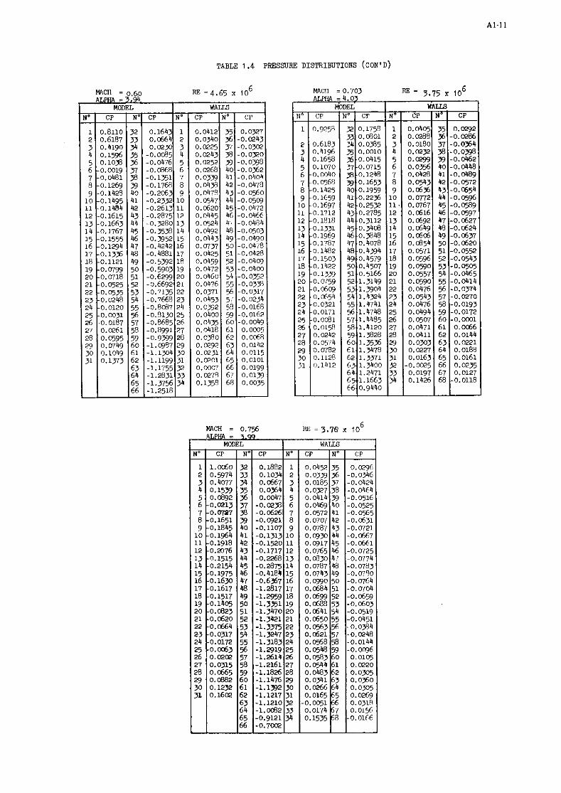
TABLE 1.4 PRESSURE DISTRIBUTIONS (CON'D)
WCl l = 0.60 =4.65 x 1 0 6 ALPHA = 3.9'4
MODEL I WAILS N ' I CP I N ' I C P I N ' I C P I N ' [ CI'

T a b l e 1.4 PRESSITRE DISTRIBUTIONS ( C O N I D )
MACH = 0.502 " = 2.91 x 10
hnCH = 0.503 RT, = 6 MAC11 - 0,503 F!E = 2.85 r l o 6 2.93 x 10 ALPHA = 6.05 ALPHA = 8,02 m E L I WALL5
No I C P I NO1 CP IN' I C P IN' I C P
6
MCa)EL I WAILS N' I CP I No I CP I N o I CP I ND I CP
4LPH4 c 2.06
N'
1 2 9 4 5 6 7 8
I1 12 13 14 15
17 18 19 20 21 22 23 24 25 26 27 28 29 30 31
N'
1 2 3 4 5 6 7 8 9
10 11 12 13 14 15 16 17 18 19 2Q 21 22 23 24 25 26 n 20 29 30 31 32 33 X
CP
0 .977532 0.3095 0.1139
-0.1166 -0.1462 -0.2361 -0.2560 -0.2730
9 - 9 . 2 9 4 6 4 0 10-0 .283241
-0.2703 -0.2690 -0.2685 -0.2679 -0.2467
1 6 - 0 . m O 9 4 7 -0.1851 -0.1696 -0.1448 -0.1274 -0.1036 -0.1060 -0.0720 -0.0522 -0.0511 -0.0136 -0.0055
0.0284 0.0461 0.0816 0.1186
CP
0 .035035 0.0293 0.0167 0.0172 0.0160 0.0172 0.0192 0.0245 0 .022443 0.0241 0.0285 0.0149 0.0192 0.0132 0.0112 0.038950 0.0070 0.0113 0.0111 0.0096 0.0133 0.0011 0.0082 0.0045 0.0054 0.0104 o.oos4 0.0058 0.0057 0.0024 0.0041
-0.0048 0.0151 0.1149
M 3 D Z N'
33 34 35 36 37 % 39
42 43 44 45 46
48 49 50 51 52 53 54 55 56 57 58 59 60 61 62 63 64 65
WALW No
36 37 38 39 40 41 42
44 45 46 47 48 49
51 52 53 54 55 56 57 58 59 60 61 62 63 64 65 66 67 68
CP
0.1395 0.0509 0.0111
-0.0164 -0.0486 -0.0793 -0.1183 -0.1469 -0.1749 -0.1956 -0.2186 -0.2%0 -0.2676 -0.2855 -0.7265 -0.3370 -0.3839 -0.4189 -0.4515 -0.4743 -0.4828 -0.5479 -0.5906 -0.6146 -0.6366 -0.6610 -0.6819 -0.7060 -0.7268 -0.7264 -0.7339 -0.7556 -0.7430 -0.7447
CP
0.0448 -0.0179 -0.0253 -0.0275 -0.0326 -0.0320 -0.0349 -0.0383 -0.0451 -0.0389 -0.03% -0.0337 -0.0338 -0.0339 -0.0316 -0.0299 -0.0264 -0.0254 -0.0225 -0.0208 -0.0214 -0.0202 -0.0126 -0.0112 -0.0106 -0.0027 -0.0005
0.0030 0.WBO 0.0052 0.0046 0.0125 0.0086 0.0040

TABLE 1.4 PRESSURE DISTWBUI?ONS (CON 'D)
~ V \ C H = 0,754 RE = 3.80 x 10 6 ALP^ = 2.98
No
1 2 3 4 5 6 7 8 9
10 11 12 13 14 15 16 17 18 19 20 21 22 23 24 25 26 27 28 29 30 31
MODEL CP
1.C651 0.4850 0.2767 0.Q37
-0.0325 -0.1491 -0.1849 -0.2631 -02850 -0.2878 -0.2817 -0.2770 -0.8% -0.2896 -0.2609 -0.2154 -0.2122 -0.179 -0.1475 -0.1263 -0.1010 - 0 . w -0.%07 -0.0378 -0.Cem 0 . W 3 O.Cel3 0,%73 O.CB28 0.126 0.166
N O
1 2 3 4 5 6 7 8 9
10 11 12 13 14 15 16 17 18 19 20 21 22 23 24 25 26 27 28 29 30 31 2 33 3'4
N'
2 33 34 35 35 37 j8 jg 40 41 42 43
' 44 45 46 47 4E 49 50 51 52 53 54 55 56 57 58 59 60 61 62 63 64 65 66
CP
0.1891 0.0952 0.0555 0.0165
-0.013'3 -0.0449 -0.0921 -0.1263 -0.1515 -0.1731 -0.1915 -0.2017 -0.2226 -0.2275 -0.256 -0.2664 -0.9516 -1.1655 -1.1899 -1.2258 -1.2294 -1.2278 -1.2165 -1.262 -1.1968 -1.1653 -1.1219 -1.C815 - 1 . O j 5 1 -1.0190 -0.9991 -0.9892 -0.8561 -0.7626 -0.5507
CP
0.0450 0.0331 0.0186 O.&O 0 .026 0.0373 0.0431 0.0558 0.05% 0.0745 0.0709 0.0538 0.0594 0.0533 0.0507 0.0719 0.0441 0.0454 0.0435 0.0400 0.0428 0 . o w 0 .033 0.0341 0.0364 0.OH 0.031 0 . 0 3 0.0253 0.@217 0.0150
4.0019 0.m16 0.1560
WALIS N'
35 S 37 3 39 40 41 42 43 44 % 6 pT 48 49 50 51 52 53 % ?j 8 37 5) 59 60 61 @ 63 f34 6j % cq @
CP
0.0462 -0.0247 -0.020 -0.03'45 -0.031 -0.037 -0.04'10 -0.0508 -0.0599 -0.0571 -0.0559 -0.057 -0.630 -0.621 0.614
-0.ffill -0.0553 -0.0513 -0.0480 -0.0404 -0.0E4 -0.0300 -0.0178 -0.0101 -0.oc61 0.0095 0.0177 O.CP44 0.02% 0.W44 0.@201 O.Ce% o . o l n
-0.064

Mg. 1.2 EVOLUTION O F THE STAGNATION lEMPEPARTm W R I N G A BLOW DOWN
moving wall
, ,
Detai l o f the
perforations
moving f l a p s 22 .d 3
I - perforated w a l l , \ model a
-3 -2 -1 o 1 X ( m ) _ 5
Fig. 1.3 MODEL I N S T A U T I O N I N THE S3MA TRANSONIC WIND RTNNEL

window axis
P1.1.2 bur
I ' ' .'? -.-.-. I.
-0.2 0.86 walls I '
~ , , . , I I , , Xp .. -t 1 m 5 -1 -0.5 0 0.8U 0.92
R;ri.rence t
- wake measurement section
Fig. l.4a Mch number distribution in the wind tunnel
Window axis
RO I
0.9 A M = .Ol
0.8
0.7
0.5
L.3
I I xnm
mode l leadinc e d ~ e mooel traili?~ e c c c - 200. -1 00. 0. 100. 200.
Fig. l.4b Mach number distributions in the model region
Fig. 1.4 S3M '!XNNEL EMPTY mST SECTION CALIERATION DATA
-6 Re. 10
4
0 5 4.0 0.3 0.5 07 0.9
Fig. 1 .5 NOISE LEVEL Fig. 1 . 6 REYNOLDS NUMBER BASED ON CHORD LEllGTH

line
Fig.1.7 SPANWISE IACATION OF THE mmL PrnSSUIIE HOIES D.tlll .< . StrtlD pn..un 0-b-
Mg.L.8 WAKE RAKE
03 0.5 0.7 09 0 10
L i f t and drag versus Mach number L i f t and drag versus angle af attack
FIG.1.9 EVOWTIONS OF THE AERODYNAMIC COEFFICIEhPTS

I upper surface I upper surface
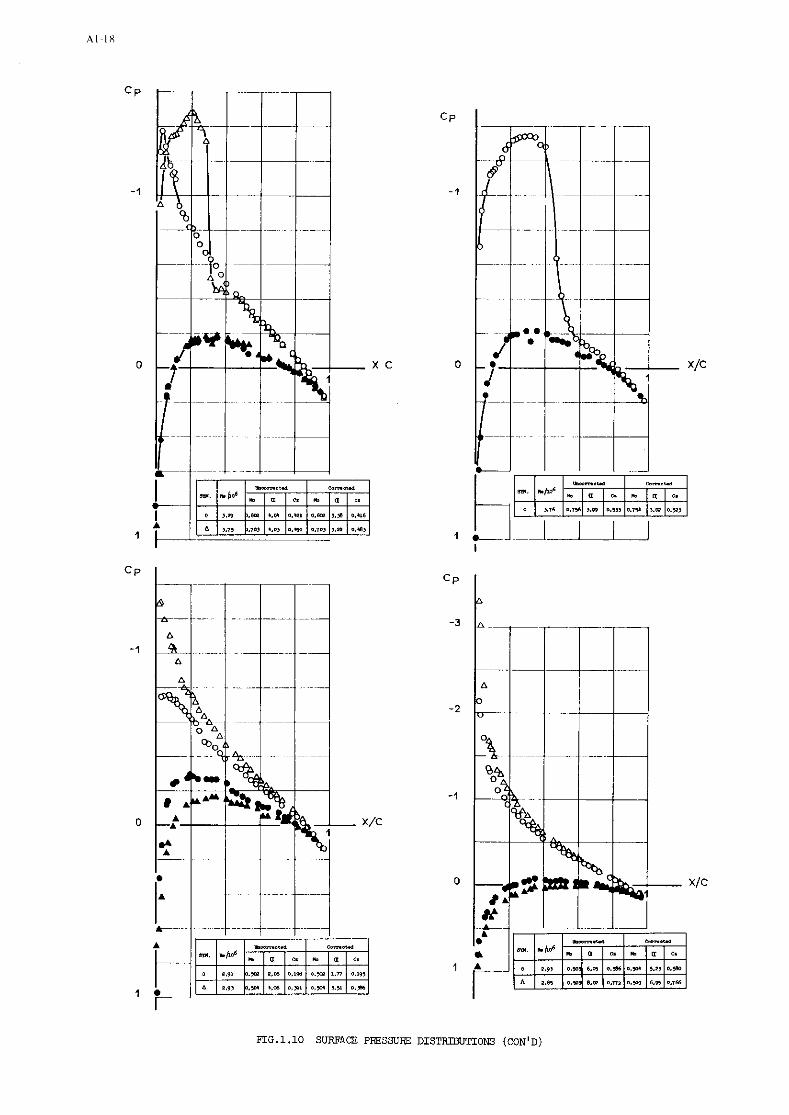

FIG.l.10 SURFACE PRESSURE DISTRD3UTIONS (CON'D)

1.5 DATA SET FROM ii.'lE HIGH SPEED TLTNI9EL
These data are extracted from a larger body of data obtained in a collaborative program with ONERA. The selected data is primarily aimed at providing high Reynolds number experimental results under as close to interference free conditions as possible.
1. Airfoil
1.1 Airfoil designation
1.2 Type of airfoil
1.2.1 airfoil geometry nose radius maximum thickness base thickness
1.2.2 design condition
1.3 Additional remarks
NACA 0012
symmetrical
Figure 1.11 r/c = 1.58% t/c = 12% 0.252% chord - None
1.4 References on airfoil 1
2. Model geometry
2.1 Chord length 0.300 m
2.2 Span 0.381 m
2.3 Actual model co-ordinates Table 1.5 and accuracy
2.4 Maximum thickness t/c = 12%
2.5 Base thickness 0.252% chord
2.6 Additional remarks None
2.7 References on model 2
3. Wind tunnel
3.1 Designation NAE 5-ft x 5-ft trisonic W/T with 2-D insert
3.2 Type of tunnel Blowdown
3.2.1 stagnation pressure 2-11 bars
3.2.2 stagnation temperature 293 K, max drop ..5K during a run
3.2.3 humidity/dew point 0.0002 kg HzO/Kg air
3.3 Test section Rectangular, Fig.1.12
3.3.1 dimensions 0.38m x 1.52m
3.3.2 type of walls Perforated top and bottom 20.5% porosity $ 12.7 mm normal holes at 26.4 mm spacing
3.4 Flow field (empty test section)
3.4.1 reference static pressure at sidewall 6.48 chord upstream of model LE
3.4.2 flow angularity -not determined
3.4.3 Mach number distribution Fig.1 .l3
3.4.4 pressure gradient Fig.1 .I3
3.4.5 turbulence/noise level free stream rms= 0.008. at M_ = 0.8
3.4.6 side wall boundary layer 6* 5 2.5 mm
26*< 0.013 B - 3.5 Additional remarks sidewall suction over an area
1.8 x 2.4 chord around model
3.6 References on wind tunnel 3, 4
4.1 Type of measurements
4.2 Tunnel/model dimensions
4.2.1 height/chord ratio
4.2.3 width/chord ratio
force balance surface pressure wake pitot pressure

4.3 Flow conditions included in present data base
4.3.1 angle of attack
4.3.2 Mach number
4.3.3 Reynolds number
4.3.4 transition
-position of free transition
-transition fixing
4.3.5 temperature equilibrium
4.4 Additional remarks
4.5 References on tests
5. Instrumentation
5.1 Surface pressure measurements
5.1.1 pressure holes
-size
-spanwise station(s)
-chordwise positions
5.1.2 type of transducers and scanning devices
5.1.3 other
5.2 Wake measurements
5.2.1 type/size of instrument (s)
5.2.2 streamwise position(s)
5.2.3 type of transducers and scanning devices
5.3 Boundary layer measurements
5.3.1 type/size of instruments
5.3.2 locations
5.3.3 type of transducers and scanning devices
5.4 Skin friction measurements
5.4.1 type/size of instruments
5.4.3 type of transducer
5.5 Flow visualisation
5.5.1 flow field
5.5.2 surface flow
5.6 other
5.7 Additional remarks
5.8 References on instrumentation
6. Data
6.1 Accuracy (wall interference excluded)
nominally 0'
0.5 - 0.93 I see Table 1.6 17 to 43 x lo6
free transition
not established
yes
8 0
0.40 mm
centre span in a line 15O to flow direction
see Table 1 .5
Two D9 scanivalves with 200 psia Kulite VQS-500-200A
scan rate for 5.1.2 20 ports/sec.
Traversing probe, see Fig.t.12 OD/ID = 2.286/1.524 mm
1.27 x chord downstream of TE
50 psid Statham PM 131 TC
at a = 5O M_ = 0.76 Re = 24x10~ and g
different sidewall suction (Data not included in Data Base)
two three-component balances for force measurements
6.1.1 angle of attack setting f O.OZO

6.1.2 free stream Mach number:
- setting - variation during one pressure scan
6.1.3 pressure coefficients
6.1.4 aerodynamic coefficients
6.1.5 boundary layer quantities
6.1.6 repeatability Generally A C N ~ f0.005 ACXp f0.0005 ACMp f0.0005
6.1.7 remarks
6.2 Wall interference corrections No corrections (indicate estimated accuracy)
6.2.5 remarks since supplied data are for nearly zero lift all wall corrections can be considered negligible.
6.2.6 references on wall interference 5, 6 correction
6.3 Presentation of data
6.3.1 aerodynamic coefficients
6.3.2 surface pressures
6.3.3 boundary layer quantities
6.3.4 wall interference corrections included ?
6.3.5 corrections for model deflection
6.3.6 empty test section calibration taken into account ?
6.3.7 other corrections included ?
6.3.8 additional remarks
Table 1.6
Table 1.7 - 1.15, Figure 1.14 - 1.22
NO
Yes
NO
Wake drag data are those obtained from probe on E only.
6.4 Were tests carried out in different Yes. in ONERA 53 wind tunnel. facilities on the current airfoil ? If so, what facilities. Are data included in the present data base ?
6.5 To be contacted for further information L.H. Ohman - High Speed Aerodynamics Laboratory on tests.
NAE/NRC Ottawa, Ontario, Canada.
7. References
1. I.H. Abbott / A.E. von Doenhoff Theory of wing sections. Dover Publications Inc., New York
2. R.C. Dixon
3. L.H. Ohman et a1
4. L.H. Ohman
5. D.J. Peake / A.J. Bowker
6. M. Mokry et a1
High Reynolds Number Investigation of an ONERA model of the NACA 0012 Airfoil Section NRC/NAE LTR-HA-5x5/0069 1975
The NAE High Reynolds Number 15in x 16in two-dimenstional test facility NRC/NAE LTR-HA-4 April, 1970
The NAE 15in x 60in two-dimenstional test facility: new features and some related observations, results of new centre line calibration at 20.5% porosity NRC/NAE LTR-HA-15 March, 1973
A simple streamwise momentum analysis to indicate an empirical correction to angle of incidence in two-dimensional, transonic flow, due to a perforated floor and ceiling of the wind tunnel. NRC/NAE LTR-HA-11 January, 1973
Wall interference on 2D supercritical airfoils, using wall pressure measurements to determine

6. M. Mokry et a1 (cont.) the porosity factors for tunnel floor and ceiling. NRC/NAE LR-575 February, 1974
8. List of symbols
B tunnel width = model span
C model chord
H tunnel height
M, MLOC local Mach number
M_,MTUN free stream Mach number
P local static pressure
P_,PS free stream Static pressure
PO free stream total pressure
Re Reynolds number based on model chord
q_,Q free stream dynamic pressure
V/U relative sidewall suction velocity I sidewall free stream velocitv P-P
Cp,Cp - pressure coefficient q- -
C~,CN normal force coefficient
Cx,Cx chord force coefficient
CM,CMC4 pitching moment coefficient, about 1/4 chord
CDW wake drag coefficient
X streamwise coordinate model origin: LE W/T origin: balance % = 0.364 model X/C
ag geometric angle of attack, angle between chordline and tunnel &
subscript P refers to pressure data
B balance data
d design data
m model aata
L lower surface
U upper surface

T a b l e ..- 1 . 5 Model Geometry and P r e s s u r e H o l e ~ ~~. ~
P r e s s u r e Hole
( X / C ) rn
(Y /C ) rn -- - - - -- - - - - -- - - -. -. - . -. - . .. . -
L o c a t i o n s . . . . -. . . .. .

TABLE 1 .6
AERODYNAMICS COEFFICIENTS
Re PRESSURE BALANCE
TABLE FIG M- a C ~ p
C C M~ 'NB
C RUN SCAN 9 X~ 'MB D~ NO. NO.

TABLE 1 .I
SURFACE PRESSURE MEASUREMENTS
SCAN 2
M 0.490
TUBE
1 u 2u 3u 4U 5 u 6U 7 u 8U 9U
1 OU 11U 12U 13U 14u 15U ! 6U 17U 18U 19U 2ou 21 U 22U 23U 24U 25U 26U 27U 28U 29U 30U 31U 32U 33u 34u 35U 36U 37U 38U 40U 42U
OLE 1 L 2L 3 L 4L 5L 6L 7 L 8L 9L
1 0L 1 I L 12L 13L 14L 15L 16L 17L 18L 19L 20L 21L 22L 23L 24L 25L 26L 27L 28L 29L 30L 31 L 34L 35L 3 6 1 37L 3RL 39L 40L 41L
RUN NUMBER 2777 O N E 2 b 2D
REIF6 D O - 0 P I 17.51 87.44 536.52 74.16
X I C CP MLCC P/PO P/PS

SCAN 2
M 0.693
TUBE
8 u 9U
IOU 1 I U 12U 13U 14U 15U 16U 17U 18U 19U 20U 2 1 u 2 2 u 23U 24U 25U 26U 27U 28U 29U 30U 31U 32U 33U 34u 35u 36U 3 7 u 38U 40U 42U
OLE I L 2L 3 L 4 L 5 L 6 L 7 L 3 L
TABLE 1.8
SURFACE PRESSURE MEASUREMENTS
RUN NUMBER 2763 DNERA 2D
RE/E6 -0 540.31
P I 22.15 87.24 63.32
TESTS
0 21 - 2 5
MTUN

TABLE 1.9
SURFACE PRESSURE MEASUREMENTS
RUN NUMBER 2 7 6 7 ONERA 2D TEITS
SCAN M RE/EC T 0 0 V/U 545.97
P I 1 0.696 36.70 146.00 105.62 35.82 0.0028
*U8C X I C CP MLOC P/PO P/PS MTUN
OLE I L 2 L 3 L 4L 5 L CL 7 L 9 L 9 L
10L 1 1 L 1 2 L 1 3 L 1 4 L 15L 1 6 L 1 7 L 1 8 L 1 9 L 20L 21L 22L 23L 2 4 L 2 5 L 26L 2 7 1 28L 29L 3 0 L 31L 34L 35L 36L 37L 38L 39L 40L 41L

S C A N 1
TUBE
1 u 2 u 3 u 4U 5 u 6U 7 u 8U 9U
1 OU 11U 12U 13U 14U 15U 16U 17U 18U 19U ZOU 2 1 u 2 2 u 23U 24U 25U 26U 27U 28U 29U 30U 3 1 u 32U 3 3 u 3 4 u 3 5 u 36U 37U 38U 40U 42U
CLC 1 L 2L 7 L 4L 5 L 6L 7 L 3 L DL
1 0 L 1 I L 12L 1 3 L I 4 L 15L 1 6 L 17L 1 8 L 1 9 L 20L 21 L 22L 23L 5 4 L 2 5 1 26L 27L 28L 2 9 L 3 0 1 31L 34L 35L 36L 37L 38L 39L 40L 41 L
TABLE 1.10
SURFACE PRESSURE MEASUREMENTS
PUN NUMBSF 2788 O N 5 9 A 2D T E S T S
PEIE6 7 0 P I 0 23.7A 87.15 538.49 55.50 24.70
XIC CP MLOC P I P 0 P I P S MTUN

TABLE ! . l l
SURFACE PRESSURE MEASUREMENTS
RUN NUMBER 2753 ONFRA 2D TESTS
SCAN M RFIEC 0 0 T 0 P I 0 V/U 2 0.814 24.70 87.20 532.51 55.37 26.19 0.0025
TUBE X / C C P MLOC P/PO P/PS MTUN
OLE 1 L 2 L = L 4 L 5 L b L 7 L 8 L 9 L
1 OL I 1 L 12L 1 3 L 1 4 L 15L 1 6 L 1 7 L 1 8 L 1 9 L ZOL 2 l L 2 2 L 23L 2 4 L 2 5 L 2 6L 27L 28L 2 9 L 3OL 31L 3bL 35L 35L 37L 3 3 1 39L 40L 41L

TABLE 1 . I 2
SURFACE PRESSURE MEASUREMENTS
QUN NUMBER 2801 ONFPA 2D T E S T 5
SCAN M R ? / E 6 '0 P I Q V I U
1 0.817 32.26 116.63 549.92 75.23 35.15 0.3025
TUBE X I C CP MLOC D/>O P / P S M T U N
OLE 1 L 2L 3 L 4L 5 L hL 7L 3 L 9L
10L 11L l 2 L 13L 14L 15L 16L 17L 13L 19L 20L 21 L ?2L 2 3 1 24L 25L 25L 27L 23L 29L 30L 31L 34L 35L 35L 37L 3 3 1 39L 40L 41 L
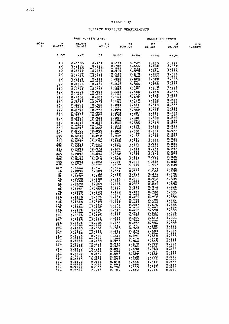
TABLE 1.13
SURFACE PRESSURE MEASUREMENTS
RUN NUMBER 2789 ONERA 2D TESTS
SCAN M RE/F6 P 0 TO P I 0 V/U 1 0.835 24.65 87.17 538.04 55.22 26.93 0 -0025
TUBE X/C CP MLOC P/PO P/PS MTUN
OLE I L 2 1 3L 4L 5 L b L 7 L 8 L 9L
1 DL 11L l 2 L 13L 14L 15L 16L 17L 19L 19L 20L 21L 22L 2 3 1 24L 25L 25L 27L 28L 21L 30L 31L 34L 35L 3e.L 37L 38L 39L 40L 41 L

TABLE 1.14
SURFACE PRESSURE MEASUREMENTS
RUN NUMBEF 2 7 7 5 ONEQA 2D T E S T S
SCAN M R E I E € T 0 P I 0 V I U 2 0 .918 2 5 - 9 4 8 7 . 2 8 533.97 50.59 29.86 3 . 3 0 2 5
TUBE X I C CP MLOC P / P O P I 0 5 MTUN

TABLE 1.15
SURFACE PRESSURE MEASUREMENTS
RUN NUMBER 2784 3NERA 20 TESTS
SCAN M RE/E6 0 0 TO PI Q V/U 1 0 - 9 3 0 42.75 145.92 541.94 83 47 50.56 0 .0025
OLE 1 L 2L 3 L 4 1 5L C L 7L 8 L 9 L
10L 11L 12L 13L 14L 15L 1 5 L 1 7 L 19L 19L 2OL 21L 22L 23L 24L 25L 26L 27L 28L 29L 30L 31 L 34L 35L 36L 37L 38L 39L 40L 41 L

: - 0.0,5.
, I . I . L ,
NACA 0012 AIRFOIL
". 1
0.- F I G . 1 .14 - PRESSURE D I S T R I B U T I O N
O.$ "., I> "., Y 4 a,, ".. 0.1 0 : . " . 9 " , C
a- ............)...... .= 0 - "i, - 0 YOOZL
7
-2 x/o
F I G . 1 . 1% uu wvusra ocrrambnon, i r p n Ti:: 5r;:mA:. ~ l i c lsin X B O ~ ~ P - ~ ~ a s i i i .
u . # "'t F I G . 1 .15 - PRESSURE DISTRIBUTIOI !

m.#
0.5
.." -.a c. . . I
-.. - .5
....
. . I
-.z
-. ,
rn.L
0.2
o.>
o . * .
'
0.7 0.. @ .,., / , . . " . ' e ".l 0.2 0.1 0.- 0 .3 0.. 0.7 e.. " . " . , < I . I
F I G . 1 . 1 6 - PRESSURE DISTRIBUTIOII
-.. -.. %,
-:
. . b
- . 3
-.. -. 3
.
. ,
". 8
".Z
a. 3
u..
u.5;
- . a '
~ ~ ~ a
~.~ ' O . o . . .
O . O .
~~~ ~ ". '
~ A ' . . . . . - . .r . .
~
"'. ~.
o b . O : .
~. "b* > * a , ,C&" 1
' " m , . , - ~. . b...L s*",.<L ~ ". 32.3.8". ~ m.,h s"",.'. ~. .".,3
<"I "."".
P I G . 1 . 1 9 - PRESSURE DISTRIBUTIOI?
".I O.I "., I . 6 . "., &. ".," ,<,."
~ o m . ..~. . ..O . . . -:. -.
.*.
--. a. _ _ _ _ _ _ _ _ - - _ _ r . .
0. - . .~ . * .. .* . ~ ' 0 . - . .~ ."" m,, LC" 2 . . Y ..... Y.,YL .O .. >d.,.>#. - W E . .".,Y. . . .o.,, '
d. ... 1. F I G . 1 . 1 8 - PRESSURE DISTRIBUTIO; ;
..I m.z 0 . I * . I @ . I 0,. 0 0:. 6 _ ~ . X i , . " . ~ d
* . I .# .O _ 0 " O
_.O . . . . . ~
.O.-.
* . O ' O -.
- " - . - . . - _ _ _ .i,. . ~. ~.
L:. ~. ~. """ >7." sc." 8 . " "..>\ . UsPC" L Y L I A ' I 'I
.% il.l.i". ~ ,-.~ s"~."c . . , ~".,, . cb* "."".
F I G . 1 . 2 0 - PRESSURE DISTRIBUTIO:! " Y. . Y . ' ":. 0 . l ".. u:. 0:. u : r . , r , . u " ' ' u
F I G . 1 . 1 7 - PRESSURE DISTRIBUTIO;
, -.. ~.. ~.. ~ . *
. . ~ . , -.. -. 8
Y.,
" .a
0 . 8
~.. ~.. ' " ..?
-.. -. 5
-.. . . I
- 2
..,
0. L
"., "., ".'
~ ,. .. ; .. . . . p .' .- . . . . . .. ' a . .
,I.- .& .d
0 . I
DO.
_. . - = _ r . . ~ * .
"0" >9 . , *'A" 2 . " ".">. . "*"a, S"...CC ./ Il...,". - -r. Sb.,.'.
* . , rls "..."
F I G . 1 . 2 1 - PRESSURE DISTRIBUTION
u., o., o., 0 . l 0 . l 0.' u . r a , . o . r . , r I T "

2. NLR QE 0.11 - 0.75 - 1.375 airfoil
contributed by
National Aerospace Laboratory NLR Amsterdam, The Netherlands
and
National Aeronautical Establishment Ottawa, Canada
2.1 Introduction
The NLR (Q)uasi (E)lliptioal airfoil 0.11-0.75-1.375 was selected primarily for the following reasons:
i. It is a symmetrical ("shock-free") airfoil and thus provides, at zero incidence, a case where the aerodynamic characteristics (such as shock position) of a supercritical airfoil, as measured in the wind tunnel, are not affected by wall interference due to lift. One significant source of possible discrepancy between interference free computa- tional results and wind t m e l experiment is thus absent.
ii.Tests were performed at low Reynolds number (=2 x lo6), both with free and fixed transition, in the NLR Pilot Tunnel and at high Reynolds number (=20 x lo6) in the 2-D insert of the NAE 5 ft x 5 ft transonic wind tunnel. In spite of the fact that '
there are mat differences between the two tunnel confipations (slotted versus porous walls, height/chord ratio 3.1 versus 6.0, span/chord ratio 2.3 versus 1.5) there is a canforting degree of similarity between the two data sets, suggesting that blockage effects in both tunnela were indeed small.
It should finally be mentioned that the tests were performed specifically to verify experimentally the existence of aupercritioal shock-free flow on an airfoil that was designed theoretically to exhibit this feature. For this reason more than usual care was taen to perform the experiments as accurately as possible.

2.2. DATA SET FROM NLR TUNNEL
1. Airfoil 1.1. Air fo i l designation 1.2. Type of a i r f o i l
1.2.1. a i r f o i l geometry nose radius maximum thickness baee thickness
1.2.2. design condition
design pressure d is t r ibu t ion
1.3. Additional remarks
1.4. References on a i r f o i l
2. Model geometry
2.1. Chord length 2.2. span 2.3. Actual model co-ordinates
and accuracy 2.4. Maximum thickness 2.5. Base thickness 2.6. Additional remarks
2.7. References an model
3. Wind tunnel
3.1. Designation 3.2. 'ILype of tunnel
3.2.1. stagnation preseure 3.2.2. stagnation temperature 3.2.3. hmidity/dew point
3.3. Test seotion 3.3.1. dimensions
3.3.2. type of walls
3.4. Flow f i e l d (empty t e s t sect ion) 3.4.1. reference s t a t i c pressure
3.4.2. flow angulari ty
3.4.3. Mach nmber d is t r ibu t ion 3.4.4. pressure gradient 3.4.5. turbulence/naise leve l 3.4.6. s ide wall boundary layer
3.5. Additional remarks
3.6. Referenoes on wind tunnel
4.
4.1. Type of measurements
4.2. ~unnel/model dimeneions 4.2.1. height chord patio 4.2.2. width / chord r a t i o
4.3. Flow conditions included i n present data base
4.3.1. angle af a t tack 4.3.2. Mach number 4.3.3. Reynolds number 4.3.4. t r ans i t i on
- posi t ion of f ~ e e t r ans i t i on - t r ans i t i on f i r i n g
NLR QE 0.11-0.75-1.375 synnnetrical, "peaky1--type shock-free s u p e r c r i t i c a l designed by means of Nieuwland hadograph method see f ig. 2.1 and t ab l e s 2.1 , 2.2
!k.=1?:2 -~ - . potent ia l flow (hodograph theory) : M = 0.786, a = O0 experiment (NLR Pi lot tunnel) Mt = 0.789, o = O0
see f i g . 2.1 , t ab l e 2.1
none
re f . 1
0.1795 m 0.42 m
f ig . 2.2
t /c = 11.% 0.05 mm f i n i t e t rai l ing-edge (base) thicloless was obtained by outting-off theore t ica l a i r f o i l a t 99.7 % chord see ref. 2
NLR Pi lo t tunnel oantinuous, olosed c i r cu i t atmospheric 313 +_ 1 K var ies with atmospheric condition (stagnation temperature ohosen such t ha t condensation i a avoided) see f i g . 2.3 rectangular height 0.55 rn, width 0.42 m 1% s lo t t ed top and bottom walls , so l i d s ide walls separate top and bottom plenums
taken a t s ide wall 3.6 chords upstream of model upwash do = 0.12' (5 0.03')
(with respect t o tunnel reference plane) see f ig . 2 . b see f ig . 2.4b see f ig2 .5and ref . 5 thiokness 1% of t e s t section aemi-width, no special treatment f o r two-dimensionality of the flaw see ref . 4 ref. 3
surfaoe pressures wake p i t o t pressures surfaoe flow visual inat ion flow f i e l d visual izat ion
ZeFO
0.30 t o 0.85 about 2 x lo6 ( s e e f ig . 2.6) f r ee and f ixed see fig.2.7 grit no. 220 oarbomdum a t 5-1% chord

4.3.5. temperature equilibrium
4.4. Additional remarks
4.5. References on t e s t s
5. Instrumentation
5.1. Surface pressure measurements 5.1.1. pressure holes
- s i z e
- spanwise s t a t i o n ( s ) - ohordwise pos i t ions
5.1.2. type of transduoers and scanning devices
5.1.3. o ther 5.2. Wake measurements
5.2.1. type/size of instrument(s)
5.2.2. atreamwise p o s i t i o n ( s ) 5.2.3. type of t ransducers and
scanning devices
yes
with f r e e t r a n s i t i o n a laminar separat ion bubble was present between 9 and 1% chord a t design condition r e f . 2
diameter 0.1 ma on f i r s t 2% chord, 0.25 mm a f t of 20% chord; d e ~ t h 1 mm . - staggered (+ 25 mm around cen te r l i n e )
-
t a b l e 2.3 one + 7.5 p s i and one + 5 p s i Statham d i f f z r e n t i a l transduoe? + Scanivalvee; reference pressure P_ none
s ing le t r a n s l a t i n g total-head pressure tube of 1.5 mm diameter 0.8 chords downstream of t r a i l i n g edge
+ 2.5 p s i Statham d i f f e r e n t i a l pressure Transducer referenced t o p
none 5.3. Boundary layer measurements 5.3.1. type/size of instruments 5.3.2. loca t ions 5.3.3. type of t ransducers and
scanning devices 5.4. Skin f r i c t i o n measurements none
5.4.1. type/size of instruments 5.4.2. locat ions 5.4.3. type of t ransducer
5.5. Flow v isua l iza t ion 5.5.1. flow f i e l d shadow and Sohlieren p ic tures 5.5.2. surfaoe flow detect ion of t r a n s i t i o n pos i t ion by subl i-
mation teohnique (acenaphtene) and surface o i l flow
5.6. o ther no
5.7. Additional remarks none
5.8. References on instrumentation none
6.1. Accuracy (wall interfepence excluded)
6.1.1. angle of a t t a c k s e t t i n g 6.1.2. f r e e stream Mach number;
- s e t t i n g - var ia t ion during one
pressure scan 6.1.3. pressure c o e f f i c i e n t s
6.1.4. aerodynamic c o e f f i c i e n t s 6.1.5. boundary l a y e r q u a n t i t i e s 6.1.6. r e p e a t a b i l i t y 6.1.7. remarks
6.2. Wall interferenoe correct ions ( i n d i c a t e estimated acouracy)
6.2.1. angle of a t t a c k 6.2.2. blockage (solid/wake) 6.2.3. streamline curva twe 6.2.4. o ther 6.2.5. remarks
6.2.6. referenoes on wall in te r fe rence correct ions
2 0.002 t o +_ 0.020, depending on l o c a l pressure l e v e l and dynamic pressure
unhown n.a. un)olown none
n.a. IAM 1G0.005
n.a.
wal l in te r fe rence i n NLR P i l o t tunnel i s p resen t ly being reassessed
ref. 6
6.3. R e s e n t a t i o n of data 6.3.1. aerod.pwaic c o e f f i c i e n t s f i g . 2.8 , t a b l e 2.4 6.3.2. surface preseures fig. 2.9 , t a b l e 2.4 6.3.3. boundary l a y e r q u m t i t i e s n.a. 6.3.4. wal l in te r fe rence cor rec t ions no
included?

6.3.5. oorreot ions f o r model def lec t ion 6.3.6. m p t y t e s t sec t ion c a l i b r a t i o n
taken i n t o account? 6.3.7. o ther cor rec t ions inoluded? 6.3.8. add i t iona l remarks
6.4. Were t e s t s c a r r i e d out i n d i f f e r e n t f a c i l i t i e s an the current a e r o f o i l ? If so, what f a c i l i t i e s . Are da ta inoluded i n the present da%a base?
6.5. To be contacted f o r f u r t h e r information on t e s t s
7. References
1. Boerstoel, J.W.
2. Spee, B.M., and Uylenhoet, R.
3. Zwaaneveld, J.
4. Dambrink. H.A.
5. Ross, R.and Rohne, P.B.
6. Smith, J.
no f ixed t r a n s i t i o n surface pressure data are a f f e c t e d by dis turbances due t o t r a n s i t i o n band Yes, NAE 5 x 5 ft 2-D i n s e r t Data inoluded i n present da ta base
J.A. van Egmond National Aerospace Laboratory NLR Anthony Fo!&emeg 2 Amsterdam 1017 Netherlands
A survey of symmetrical t ransonic p o t e n t i a l flows around q u a s i - e l l i p t i c a l ae rofo i l sect ione NLR Report T. 136, 1967
Press- measurements on symmetrical quaai- e l l i p t i c a l a e r o f o i l sec t ions designed f o r ahock-free t ransonic flow NLR TR 69041
Pr inc ipa l da ta of the NLL P i l o t Tunnel NLR MP. 185
Inves t iga t ion of t h e two-dimensionality of tp flow around a p r o f i l e i n t h e NLR 0.55~0.42 m t ransonic wind tunnel NLR MemoFandum AC-72-018
Noise environment i n t h e NLR t ransonic wind tunnel HST NLR TR 74128 U
Values of wal l in te r fe rence cor rec t ions f a r t h e NLR P i l o t Tunnel with 16 open t e s t sec t ion NLR Memorandum AC-74-01

8. L i s t of ~ p b o l s
8.1. used i n t e x t and f i g u r e s
Cp (CP) pressure coef f ic ien t
C * o r i t i c a l pressure coeff icient P
c a i r f o i l chord length cd (CD) drag coef f ic ien t
C1 lifi c o e f f i c i e n t -
pi tch ing moment c o e f f i c i e n t (wi th respect t o .25c)
i i n t e g e r i n d i c a t i n g pressure hole number M(UA-iT0)free stream Mach number a madmum l o c a l Mach number
P l o c a l s t a t i c pressure p_ free stre,am s t a t i c pressure
f r e e stream stagnat ion pressure
4 dynamic pressure Reynolds number based on chord
"
Rn leading edgs rad ius - t a i r f o i l madmum t h i c h e s s
x 9 s a i r f o i l coordinate system x+,z+ windtlmnel coordinate ~ y s t e m
~ " ( A & A ) angle of a t t a c k
subscript
t re fe rs t o uncorrected values
8.2. w e d i n data t a b l e s
alpha Od cpi ,cp
CPW i ma.nom macs mace
P PO r e
o (degrees) (with respect t o flow d i rec t ion)
3 " P
wake t o t a l head d e f i c i t pressure ooeffioient i n t e g e r ind ica t ing pressure hole nwber nominal, "set" Mach number Mt a t beginning of scanning cycle Mt, a t end of soanning cycle
2 l o c a l s t a t i c pressure (kgf/m )
2 f r e e stream stagnat ion pressure (!qf/m )
Rec
C/R curvature of nose 0
e surfaoe slope

TABLE 2.1 Moin choracteristicr of oerofoil section 0.11 -0 .75- 1.375
TABLE 2.2 Dttoiled co .ordinoter of quasi -elliptical oerofoil section 0.11 -0.75 - 1.375
TABLE 2.2 Detailed co -ordinates of quasi -ellipticof oerofoil section 0.11 -0 .75- 1.375


"d o m 9 1
mca 0.601 NC. 0.601 -0 0.5%
lu. 0.5%
WAKE MODEL WAKE MODEL
o.rm no. 0.101
WAKE MODEL WAKE I MODEL
.IP~ o m n.mm 0.7W 6 re. 2.23 10 PO 10L16
MODEL
I l p k 0.m I l ."O,". 0.140 6 n 2.a.49 P 102%
MODEL
L d 0.0118
in". 0.140 mc. 0.110
WAKE
m c * 0.7u m c e 0.7L1
WAKE
o b u 0.076 0.1 20 0.168 0.218
TABLE 2.4.1 Free ironsition dola fcon'dl I
TABLE 2.4.2 Fixed transition dota (cm'dl
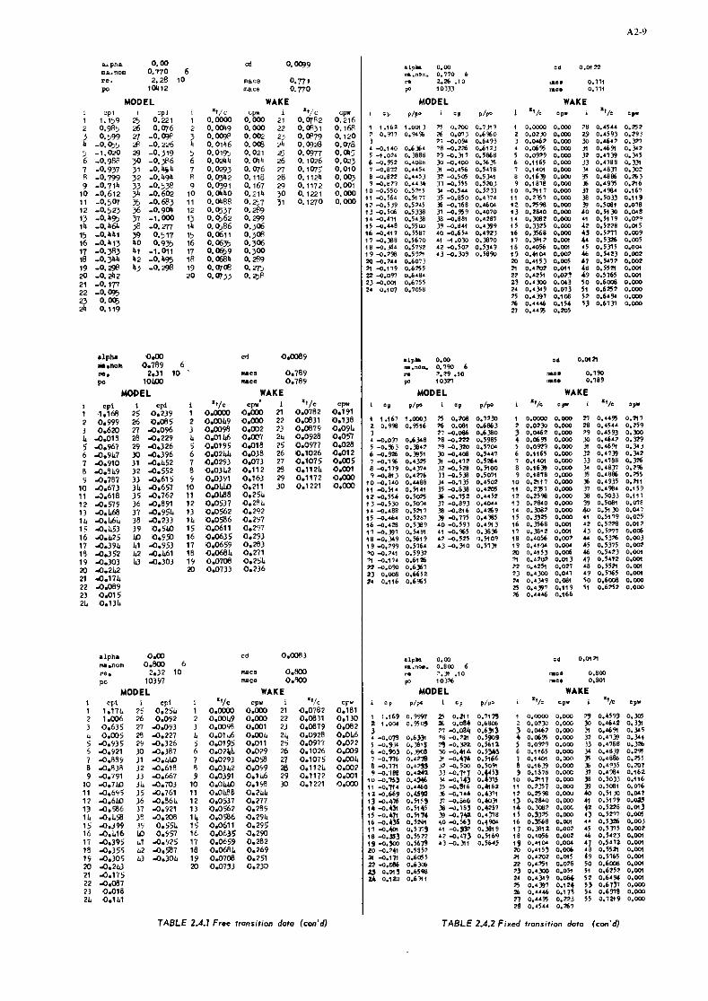
o . a n
Ips. D."?, -5. 0.773
MODEL WAKE WAKE
mcs 0.789 mce 0.789
WAKE MODEL WAKE i .p PIP" i CP P!P~ i .*Ic c p i '*,c 8)"
MODEL
.I?.. 0.m 5d 0 . m a -.no.. 0.8m 6 n 7 . 3 . 1 0 I... o . 8 ~ p 103% .nc. 0.901
MODEL WAKE i c p ~ / p L cp p/po I =lie rpr i OF.
'.no 0.W 6 "11. 2.32 10 PO 101Y7
MODEL "F"
0.181 0.130 0.082 0.0b6 0.072 oms O a L 0.w2 0.Wl 0.033
WAKE rpu I ='I<
0.m 21 0.0782 0.033 22 0.0831 u.mi 23 0.070879 o m & 21, 0.0926 0.011 25 0.0971 0.029 26 0.1026 0.058 27 0.1075 0.059 0.112L O.lU 29 0.1172 0.158 30 0.1221 O.2LL 0.271 0.235 0.291, 0.295 0.24) 0.282 0.269 0.251 0.233
TABLE 2.4.1 Free transition doto (con'd) T A B L E 2.4.2 Fixed transition dato (cm 'd )

MODEL WAKE I MODEL WAKE
i o n ./PO I =P F/+ 1 "/c c p I "b op-
.lph. 0.m Cd 0 I O m -.no" 0.8s 6 I .ID- a.m
I.-,.. 0.850 6 D.. .2.38 10 me. 0.851 n 2.n.w no 10335 nuca 0.851 s 402%
I cpi 25 O.30L 26 0.160 21 0.029 28 9.135 29 4.688 IO 4.7M
WAKE MODEL P/P i DP
% % d l 25 0 . 4 9 O.%O? 26 o.,m
1" 4.- 0.6- 28 4 . I 5 J 0.3758 29 4 .55, 0.3771 XI -0.711 0.450 n 4 . ? r 0.409 32 4.680 (1..141 33 4.655 0.L48 )1 4.651 0 . ~ 6 4 a -0.6- 0.W1 16 4.644 0.4037 31 4 .111 0.UX)Y 3 4 . 6 3 0.34, 3 4 . 6 d 0.3303 40 4 .4% 0.3x 4 , 4 . " & ? 0.R.l 4 2 4 . 6 3 9 . 8 8 r 4 1 -0.33. 0.1675 0.591- 0.6, 35 0.6377 0.66E
WAKE
C P 1
0.Cw 35 0.m 33 0.m n 0.w 3 0.w fl 0.003 4 0 0.001 L1 0.010 42 0.MJ a3 0.016 8 1 0.019 45 0.021 * 0.026 n - 0.0% .B 0.0% 4 9 0.09 50 0.0.2 5, O . M 52 0.053 5 1 0.06, 5. 0.073 55 0.093 56 0.3,. 57 0 . 9 3 5b 5 % C o.tm M 0.262 6' 0.261 6: 3.80 6' 0.325 65 0.333 66 0.3 67 0.128 68
TABLE 2.4.1 Free tronrition doto (conc1ud.d)
I TABLE 2.4.2Fixed tronrition dota (concluded)

.*
PIPo EXPERIMENT
.4
.6
I
,-.-IONIC LINE
0 .1 .4 .6 .I 1.0
Fig.2.lAirfoil shape ood design pressure dirfribvfion
A . (mnl
f -UPPER SURFACE --- LOWER SURFACE
.04 1 ,
Flg.2.ZDeviaf;on of realired model profile lrom theorecicol shope f"... regton)
DIMENSIONS IN mm
Fq. 2.3 Tronronic test section of the NLR p ~ l o t tunnel

a) MACH NUMBER DISTRIBUTION \
Fig.2 .4NLR pilot tunnel empty
Fig.2.5Noire bvs l in NLR pilot tunnel (-d in s*)
bl PRESSURE GRADIENT
test section calibration dot.
Fig.2.6Rsynoldr number based on chord length or function of Mach number
Fig.2.7Tronrition position as a function of Mach number (u-O'J Fig.2.8Drog verrur Moch number

TRANSITION FREE
TRANSITION FREE
ALFA = 0.00 MA.NO= - 3 0 0 C O = - 0 0 9 5
TRANSITION FIXED
TRANSITION FIXEO
ALFA = 0.00 MASNO= - 3 0 0 CO = .0118
TRANSITION FREE
ALFA = 0.00 MA-NO= - 5 0 0 CO = - 0 0 9 8
TRANSITION FIXEO
ALFA = 0.00 MA.NO= - 5 0 0 CO = .0118
Fig.2.9Prerrure distributions

TRANSITION FREE C P * - _ _ - _ _ _ _ _ _ _ - - - - - - - - - - - -
-1 .C
TRANSITION FREE
C P ALFA = 0.00 MA.NO= .boo CO = .0097
0
I TRANSITION FIXED
C P * _ _ _ _ _ _ _ _ _ _ - - - - - - - - - - - - -
TRANSITION FIXEO
ALFA = 0.00 MASNO= .bOO CD = ~ 0 1 1 5
-1 .a
C P
0
1.0
Fig .2 .9Presrvre distributions (con 'd )
TRANSITION F I X E D
ALFA = 0.00 MA.NO= - 7 0 0
= .0118
"c
-1 .a
C P
0
1.0
TRANSITION F I X E D
ALFA = 0.00 MA.NO= - 7 4 0 CD = . D l 1 8 - - - - - - - - - - - - - - - -

TRANSITION FREE TRANSITION FIXED
-1 .C TRANSITION FREE
C P ALFA = 0.00 MASNO= - 7 7 0 CO = - 0 0 9 9 - - - - - - - - - - - -
0 x /c
-1 .d TRANSITION FIXED
C P ALFA = 0.00 MA.NO= - 7 9 0 CD = .0121 - - - . - .. - - -
-1.0
CP
0
' ."I TRANSITION F I X E D
TRANSITION FIXEO
PiLFA = 0.00 MASNO= - 7 7 0 CO = .0122 - - - - - - - - - - - -
C P ALFA = 0.00
MASNO= .BOO CD = . D l 2 1
Fig.2.9Prsrsure distributions (con'dl
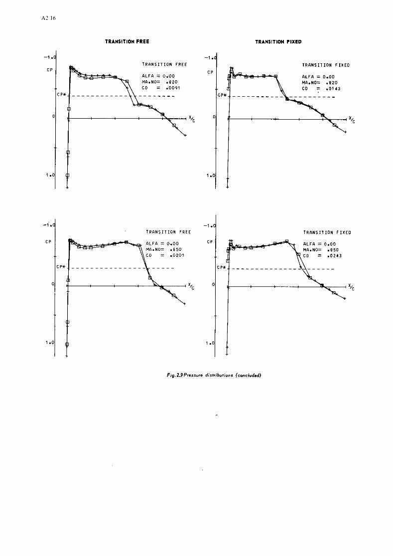
TRANSITION FIXED TRANSITION FREE
-1 .d I .. TRANSITION FREE
ALFA = 0.00 MA.NO= .a20 CO = .0091
-1 .0
C P
0
1.0
Fig.LOPrersure dirtributionr (concluded)
TRRNSITION F I X E D
ALFA = 0.00 MA.NO= ~ 8 2 0 C D = - 0 1 4 3
+
TRANSITION FIXED
ALFA = 0.00 MA.NO= .a50 CO = - 0 2 4 3
+
-1.
C P
0
1.0
-1 .0 TRANSITION FREE
ALFA = 0.00 CP
MA.NO= - 8 5 0 CO = .OZ01
0
I
7
[I
1.0

2.3 DATA SET FROM NAE TUNNEL
1.- 1.1. Airfoil designation
1.2. 'Pype of airfoil
1.2.1. airfoil geometry nose radius maximum thickness base thichess
1.2.2. design condition
design pressure distribution
1.3. Additional remarks
1.4. References on airfoil
2. Model geometry
2.1. Chord length
2.2. Span
2.3. Actual model co-ordinates and accuracy
2.4. Maximum thichess
2.5. Base thicloless 2.6. Additional remarks
2.7. References on model
3. Wind tunnel
3.1. Designation
3.2. Type of tunnel
3.2.1. stagnation pressure 3.2.2. stagnation temperature 3.2.3. hwnidity / dew point
3.3. Test section
3.3.1. dimensions 3.3.2. type of walls
3.4. Flow field (empty test section)
3.4.1. reference static pressure 3.4.2. flow angularity 3.4.3. Mach number distribution 3.4.4. pressure gradignt 3.4.5. turbulenoe/noiee level
3.4.6. side wall boundary layer
3.5. Additional remarks
3.6. References on wind tunnel
4. 4.1. Type of measurements
4.2. ~unnel/model dimensions
NLR BE 0.11-0.15-1.375
spetrioal, "pe&yq,-type shook-free super- critical designed by means of Nieuwland hadograph method sea fig.2.lOand tables 2.6 , 2.7 R/G = 4.4% t/c r 11.% Zero
potential flow (hgdograph theory) M = 0.786, o = 0 experiment M = 0.789 , a =oO t
see fig. 2.10 , table 2.6 none
ref. 1.
10 inch (0.254 m)
15 inch (0.381 m)
tableZ.I(theoretica1 coordinates obtainea by spline fit through table 2.6 data), fig. 2.11
t/c = 11.7 % 0.010 inch (0.25 mm) finite trailing edge (base) thickness obtained by symmetric increase of thiokness from 9% - 100% chord see ref. 2
NAE 5ft r 5ft transonic W/T with 2-d insert
blowdown
2 - 11 bars 0 293 K, max. drop 5' during rm
0.0002 @ H~O/ ki3 air
figure 2.12
60 x 15 inoh perforated; tap and bottom walla 20.$ open d 12.7 mm straight holes at 26.4 mm spaeing solid sidewalls (except for small porous area amund model location)
at sidewall, 7.7 chords upstream of model L.E. Aa = -0.29' + 0.020 f i m e 2.17-
side wall suction applied thmugh porous material around model location with objective to prevent side wall b.1. separation
ref 3, 4
force balance measuremente,surfaoe preesures, W&B pitot PFeSBUPB8

4.3. Flow conditions included i n present data base
4.3.1. angle of a t tack 4.3.2. Mach number 4.3.3. Reynolds number 4.3.4. t r ans i t i on
- posi t ion of f r e e t r ans i t i on - t r ans i t i on f i x ing
4.3.5. temperature e q u i l i b r i m
4.4. Additional remarks
4.5. References on t e s t s
5. Instrumentation
5.1. Surface pressure measurements
5.1.1. pressure holes - s i ae - spanwise s t a t i on ( s ) - ohordwiae posi t ions
5.1.2. type of transducers and manning devices
5.1.3. other
5.2. Wake measurements
5.2.1. type/siee of instrument(s)
5.2.2. stSamwise pos i t ion(s ) 5.2.3. type of transducers and
scanning devioes
5.3. Boundary l ayer measurements
5.3.1. type/size of instruments 5.3.2. locat ions 5.3.3. type of transducers and
scanning devices
5.4. Skin f r i c t i o n measurements
5.4.1. type/size of instruments 5.4.2. locat ions 5.4.3. type of transducer
5.5. Flow visua l i sa t ion
5.5.1. flow f i e l d 5.5.2 surface flow
5.6. other
5.7. Additional remarks
5.8. Referenoes on i n s t m e n t a t i o n
6.1. Accuracy (wall interference excluded)
6.1.1. angle of a t t a ck s e t t i ng
6.1.2. f r ee stream Mach number: - s e t t i n g - variat ion during one pressure
Scan 6.1.3. pressure coef f ic ien ts 6.1.4. aerodpamic coef f ic ien ts 6.1.5. boundary layer quan t i t i e s
f r e e only near leading edge; exact posi t ion d o w n n.a.
Ye6
Ref. 2
o.gr mn a t mid span; staggered near leading edge aee t ab l e 2 .7
48 port D g Scanivalves + 200 p s i a Kuli te VQS - 500-200A pressure transducers
t ravers ing probe, see f igure 2.12 diameter outer/inner 1.6/0.51 mu 1.5 chords downstream of T.E
25 ps id Statham FBI 131 TC
none
none
none
three-oamponent side-wall balances
re f . 4
+ - 0.003
+ - 0.003 - -
n.a. A'cn?.i+0.m2, Aom*+0.0005
0 + 0.0002 subsonic Acdw - 2 0.0010 transonic

6.2. Wall interference corrections ( ind ica te estimated acouracy)
6.2.1. angle of a t tack
6.2.2. blockage (solid/w&e)
6.2.3. streamline curvature ( l i f t ) 6.2.4. other 6.2.5. remarks
6.2.6. references on wall interference oorrection
6.3. Presentation of data
6.3.1. aerodynamic coef f ic ien ts 6.3.2. surface pressures 6.3.3. boundary layer quant i t ies 6.3.4. wall interference correct ions
included? 6.3.5. correct ions f o r model deflec-
t i on 6.3.6. Empty t e s t seotion cal ibrat ion
taken i n t o account? 6.3.7. other correct ions included? 6.3.8. addit ional remarks
6.4. Were t e s t s car r ied out i n different f a c i l i t i e s on the current aerofoi l? I f ao, what f a c i l i t i e s . Are data included i n the present data base?
6.5. To be contacted f o r fur ther infomat ion an t e s t 8
7. References
1. Boerstoel J.W.
2. Kacprzynshi J.J.
3. Ohman L.H.
4. ohman L.H.
5. Peake D.J. / Bowker A.J.
nae - 1.2 c, a t M = 0.75
solid/wake blockage negligible, l i f t - induced blockage A M = - 0.012 cl a t M = 0.75
- values given estimated f a r P = 1.5 and P = 0.5 up
lo
tab le 2.8 , f ig . 2.14 tab le 2.8 , f i g . 2.15 n.a.
No angle of a t t a ck includes defleot ian due t o s ide wall support
Yes
No wake drag data given is the average from two probes about 2 0 . 1 ~ off center l ine
Yes. In NLR P i lo t Tunnel, but an different model. Inoluded i n data base
A survey of symmetrical t ransonic potent ia l flows around quas i -e l l ip t ica l aerofa i l sect ions NLR TRT.136, 1967
Wind t m n e l t e s t s of a Boerstoel shockless symmetrical a i r f o i l 0.11-0.75-1.375 NAE Report 51[5/0061, 1972 The NAE high Reynolds number 15-ins x 60-ins two-dimensional t e s t f a c i l i t y NRC/NAE LTR-HA-4 1970
The NAE 15-ins x 60 i n s two-dimensional t e s t f a o i l i t y ; new fea tures and some r e l a t ed observations. Result of new oentre l i n e ca l ibra t ion a t 2 0 4 porosity. NRC/NAE LTR-HA-15 1973
A simple streamwise momentum analysis t o ind ica te an empirical correct ion t o angle of incidence i n two-dimensional, t ransonic flow, due t o a perforated f l o o r and ce i l i ng of the wind tunnel NRc/NAE LTR-HA-11 1973
Wall interference on ZD supe rc r i t i c a l a i r f o i l s , using wall pressure measurements t o determine the porosi ty f ac to r s f o r tunnel f l oo r and cei l ing. NRC/NAE LR-575 1974

8. List of Symbols
8.1. uaed in text and fiprea
B width of test section
C~ pressure coefficient
C* critical pressure coefficient P
c airfoil chord length
'd drag coefficient
lift coefficient
'm pitohing moment coefficient (with respeot to .25c) i integer indicating pressure hole number
maximum local Mach number Mach number
P wall porosity factor P local static pressure p, free stream static pressure
free stream stagnation preeaure 3 dynamic pressure
Rec Reynalde number based on chord
Ro leading edge radius
t airfoil maximum thiolaess x streamwise coordinate, model 0rigin;L.E
W 4 T or $@#loglance g 1 014 model x / c E a rfol ess co rdlna e n w l e of attack - subsoript t refers to uncorrected values
8.2. used iin data tables
C chord length CC tangential force coefficient (from balance) O W drag ooefficient (from wake measurements) CM o (balance) CN
m normal force coefficient (balance) M LOC Local Mach number p/m P/P~ W N G L E at

2 7 p ~ z ~ ~ ~ 2 z z ~ z 2 ~ 2 < ~ z ~ ~ < ; ; ~ ~ ~ ~ ; ~ ~ ~ < ~ : = ~ : : ~ , ; ~ ; , ~ ~ ~ i ; . ~ : ~ ~ ~ < ~ ~ ~ : : . : ~ : : ....... - . I . . . . . . . . D . n I I . . . = . . C ...... ....... . . . . . . . . . . . . o. - ^ _ . , \ _ ^ _ _ ^ _ _ ..., ,.,, - : O O O E ' , L i 5 , 7 Y C 5 0 0 0 7 . : . . : ..:a " C ' , C _ C O L S . : , L j _ i C . L C . : L L i i i - >,:, -
. . . . 2 g : - c * a 2 D = s a . . .
. 3 = c 2 ? - > < . . = = . > = ..a<. & = - 2 , . ,:==.: . c e . < ' . = > = = < . . L C C
. r ,, .. "
. P - - ~ - . - P D S - l > * - n - l 2 - > ^ . , , < 5 j - j . n 5 - r Y . . . . . i ^ ' - ~ Y _ . " _ _ . . ,- ! - 2 * - - - & 0 - * - - < . - - - e . c c . ~ ~ *,.-?, ::,: .......... > m . - - m . = -,,. *.. . . a . - - . - : m . ." . . a - . - s m > A L - . > :-:-;;;::-::>:.c:::::-.
a .. < " ~ ~ ~ ' ~ ~ ~ : ~ ~ . ; ~ ~ ; ; ~ z : z : ~ : : . ~ : : ~ ; ; ~ ~ ~ ; ; ~ ; ; ~ ; ~ : : ~ ~ ~ ~ ~ . ; . ; , . . + -::< . . . 0 2 c u s ; , o s 7 ; s o s c c o c . - c r . ,,.; .,,,,,; ,,,.;: , . c ~ ~ < , . L c , . , ,: , L 2 . , , ,
2 t - - 0" 2 . . . . . , L c . - > ~ < , < , , ~ ~ ~ c . . - = . ; ...,: ,-.. , : - . . . ..: ........... . . d ,...< /: .......... C i _ .. . < ' . > > _=:: i _ C C , . : : . . t
.... L c > - - - - - - - -.-- . . . . a . - . c " . . . . . . > . . . . ..=.,. ? . ? . ? , < .. C ~ C ~ ~ ~ ~ ~ ~ ~ ~ Z ~ ~ ~ ~ ~ c . ............... 0 . .
.-...: - < . - -.-- K 5 > . 3 0 5 0 i - 5 i - i = 0 5 i c i i .. < , < I C " 5 0 ' . ' : . : . . : . > .c ..< :,=: - ... = -x

SMOCKLESS SYMMETRICAL A I R F O I L 0 .1100-0 .1500-1 .315 SHUCKLESS SVWMETRICAL A I R F O I L O . I lCO-0 .1500-1 .315
RUN 1 1 3 SCAN I MACH NUMBEK=0.438 REVNOLOS NO.-19.08110**6 Y.l.ANGLE= 0 . 2 1 OFG CN =-0.017
PKESSURE O I S T R L 8 U T 1 O N CN THE L O U t R SURFLCE
I I C L P P I P 0 H LOC
PRESSURE O I S l R I 8 U T l O N ON THE UPPER SURFALE
X I L CP P I P 0 M LOC
RUN 7 7 5 SCAN MACH NUMBER-0.518 REVNOLOS NU.=21.81*10**6 U.l.ANGLE= 0.17 OEG
~.... ifi = 0 .0042 CC - 0 .0639 COY- 0 .0082
PRESSURt U l S l R l B U T l O N ON THE LOWER SURFACE
XIC CP PIPO n LOC
PRESSURE O l S T R l B U T l O N ON THE UPPER SURFACE
X I C CP P I P 0 H LOC
TABLE 2.8 Force dato ond rvrfoce p r e s s u r e distributions
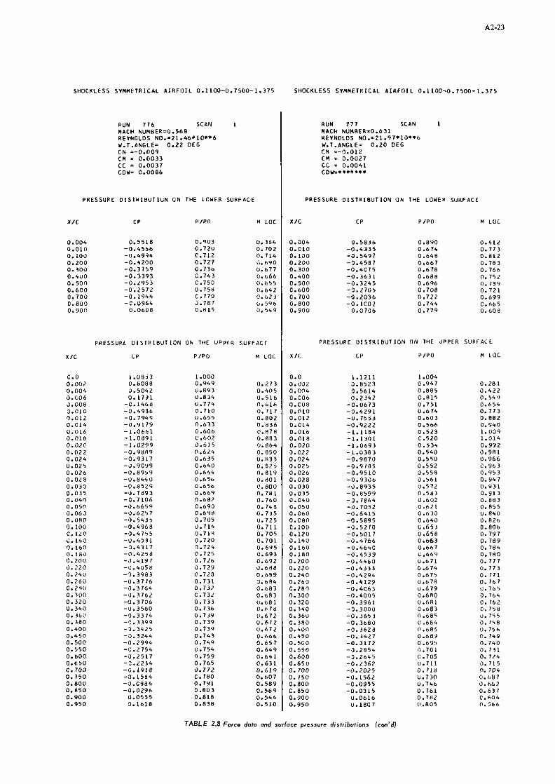
SHOCKLESS SVMMETRLCAL A I R F I I I L 0.1100-0.1500-1.315 SHOCKLESS SVMUEIRICAL A I R F O I L 0 .1100-0 .1500-1 .375
RUN 7 7 7 SCAN 1 MACH NUM8ER=0.631 REVNOLDS NO.=21.97*10**b Y.T.ANGLE= 0.20 DEG CN - -0 .012
PRESSURE D l S l R l 8 U T l U N ON THE LOUER SURFACE PRESSURE D l S T R l 8 U T l O N UN THE LOYEP SURFACE
X I C CP P l P l l H LOC X I C CP P I P 0 * L 0 C
TABLE 2.8 Force doto ond surface pressure distributions (cw'd)
PRESSURL D l S T R l 8 U T l O N ON THE UPPER SURFACI
x /C CP P /PO M LOC
PRESSURE O l S T R L B U T l O N ON THC UPPER S U U F A i L
X I C CP P l P 0 El LOC
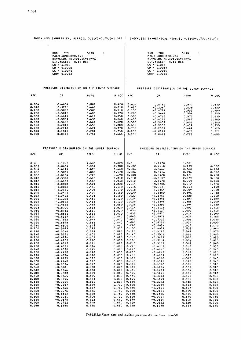
RUN 1 7 9 SCAN I MACH NUMBER=O.691
SHOCKLtSS SVMMETRICAL A I R F O I L 0.l lCO-0.75UO-1.375
R E V N O L O S ~ N O . = L ~ . ~ ~ * I O * * ~ Y.l.INGLE= 0.18 OEG CN --0.013
ShUCKLESS SVHMElRICbL b l R F 0 L L 0.1100-0.75011-1.375
PRESSURE O l S l R l 8 U l l O N ON THE LOVER SURFACE
XIC CP PIPO n LOC
XIC
0.0 0.002 0.004 0.006 0.008 0.010 0.012 0.014 0.016 0.018 0.020 0.022 0.024 0.025 0.026 0.028 0.030 0.035 0.040 0.050 0.060 0.080 0 .100 0.120 0.140 0.160 0. 1 8 0 0.200 0.220 0.240 0 .260 0 .280 0.300 0.320 0 .340 0.360 0.380 0.600 0.450 0.500 0.550 O.bOO 0.650 0.700 0 .750 0.800 0.850 0.900 0.950
PRESSURE O L S T R l 8 U l
CP
I O N ON THE UP
P I P 0
1 .a00 0.937 0.875 0.800 0.723 0.645 0.568 0.527 0.459 0.427 0.420 0.421 0.652 0.463 0.487 0.515 0.514 0.518 U.530 0.547 0.566 0.573 0.588 0.597 0.602 0.607 0.610 0.611 0.616 0.615 0.610 0.620 0.622 5.622 0.627 0.630 0.628 0.629 C.635 0.6C3 0.651 0.659 0.667 0.676 0.688 0.704 0.723 U.7*8 C.776
'PER
RUN 7 8 0 SLbN 1 MICH NUNRC1=0.736 - - - -~ .- REYNOLDS NO.=21.94*10**6 V.l.bNGLE= 0.17 OEG CN =-0.015
PRESSURE D l S l R l H U T l U N ON THL LOVER SURFdCt
KIC C P P I P 0 w L O C
PRESSURE O I S l R I 8 U l l
C P
ION ON THE UPPEP
P I P "
SUHFPCt
M LOC
TABLE 2.8 Force doto and surface pressure distributions (con'd)

SHOCKLESS S I M H F T R I L I L f i I R F O I 1 0 .1100-0 .7500-1 .375 SHOCKLESS SVMMETRICAL A I R F O I L 0 . 1 1 0 0 - 0 . 7 5 0 0 - 1 . 3 7 5
RUN 7 6 8 SCAN 1 MACH M I M B E R i O . 7 8 9 REYNOLDS NO.=20 .83*10* *6 W.T.bNGlE= 0 .12 OEG CN =-0.025 CM = 0 . 0 0 0 7 CC = 0 . 0 0 6 3 COY= 0 .0092
PRESSURE O l S l R 1 8 U T l O N ON THE LOYER SURFLCE
X I C c P P I P 0 * LOC
PRESSURE O l S T R l B U T l U N ON THE UPPER SURFACE
X I C CP P I P 0 n L a c
RUN 7 6 6 SCAN r i c ~ w n e t ~ - o . l 9 9 REVNOLOS NO.=20.97*10**6 Y . l . LNGlE- 0 .29 OEG
PRESSURE O l S T R l B U T I O N ON THE LOWER SURFACE
PRESSURE O I S T R I 8 U l l O N ON T H t UPPFR SURFICE
X I C CP P I P 0 M LO(
TABLE 2.8 Force data ond surfocs pressure distributions (con'd)

RUN 7 6 0 SCbN 1 M b C H NUMRER-0.815 REYNOLDS NO.-21.20*10*.6 Y,T.ANGLE= 0.10 OEG CN =-0.019
SHOCKLESS 5VHI(ETRIC&L A I R F O I L 0.1100-0.7500-1.375
RUN 1 8 1 SCbN MArH MI*11ER=O.U34 9EINOLOS NO.~20.97*10"6 Y1T.dW6LF= 0.23 OEG CN =-0,003 CM = 0,0023 CC = 0,0157 COW= 0,0171
SWCKLESS ~ Y H ~ I E T R ~ C A L A I R F D I L 0.1100-0.7500-1.375
PRESSURE OISTRIBUTION ON THE LOWER SURFACE
X I C CP P I P 0 t i LCC
l.OO* 0.936 I). 8 6 4 0.790 0 .713 0 .630 0.549 0 .499 0.627 0.397 d. 3 8 0 0 .368 0 .368 0.368 0 .368 0.371 0 .373 0 .378 0 .378 0.395 0 .416 0 . 4 1 1 0 . 4 2 2 0.623 0.*27 0 . 4 2 7 10.+25 0 .624 0.*36 0 .420 @.'.I8 0.418 O.LI* 0.413 0 . L l 3 0.*1* 0 .416 0.630 O.*LO 0 .515 0.559 0 .562 0.571 0.586 0 .606 0 . 6 2 9 0.656 0 .687 0 .120
PRESSURE O l S T R l 8 U l l O N ON THF LOWER SUVFACE
X I C CP P I P 0 H LOG
PRESSURE O l S T R l 8 U T l O N ON THE UPPER SURFPCE
x IT. CP PIPO M LUC
TABLE 2.8 Force data end rurfoce pressure distribution. (con'dl
PRESSURE O l S T R l B U T l O N ON THE UPPER SURFACE
X I C CP P / P O n LOG

SHOCKLESS S Y M M E T R I C A L A I R F O I L 0 . 1 1 0 0 - 0 . 1 5 0 0 - 1 . 3 7 5
a I IN 782 S C A N 1 . - MACH N U M B F R = O . 8 6 2 R E Y N O L D S N O . = 2 1 . 2 7 * 1 0 " 6 Y . T . P f f i L E = 0 . 1 7 OEG
P R F S S l l R E O l S T R l 8 U r l O N ON TtlE LOWER SURFACE
X I C CP P / P O H LOG
P R E S S U R E O I S T R I ~ U T I O N ON THE UPPER S U R F I C E
XIC CP P / P O n LUG
TABLE 2.8 Force doto and wrfoce pressure distributions f c ~ c I ~ d e d J

Fig. 2.11Discreponcier between octuol ood theoretical model thickness co -ordinoter
Fig.2.12The NAE 15 in x M in 2 - 0 insert

o MREF. .01- o o O o O O o o o o O o O
0 - 0 O 0 0 0 0 ,699
SIDE WALL SUCTION
VIu = ,056 (1-0, =.012 S ~ X , ~ )
, 0 4 7
C -C NAE. R.-21. lo6 .01- 0 0
O o o O O O O 0 0 0 0 0 0 ° 0 0 ~ 0 . 8 9 Dw
-0- NLR FREE TRANSITION
+ NLR FIXED TRANSITION 0- v/u = O .03 -
.01- 0 O O ~ o O ~ O 0 0 0 ~ 0 0 0 0 0 0 0 0 . 7 9 6
0- VU - 0 .01 -
.01- O o o o o o o O O o o o o o o O o o o 0.619
0 - Y u - 0
.01- 0 o o o 0 0 0 ° 0 0 0 0 0 0 0 0 0 0 0 0 . 5 5 0
0 - YU= 0 MODEL
- 2 -1 0 I .5 .6 .7 IAd.;1 .9
Fig. 2 .13s Moch number distribution. empty test section
NAE 15 in x 60 in 2 - D insert
RUN WW
113 I
WCH NWER 0 . U 8 ALPIU 0.2100 CN -Q.0110 REYNOLD1 NUILR I * . O H I O I
F i g . 2 . 1 4 Woke drag dato
RUN 176 SCAN I WCH NWER 0.818 ALPHA 0.1400 CY -0.0110 REYNOLDS N W r n 21.81.1-
-0.0.
0.2
Fig.2.15Svrlace pressure dirtr ibvtionr
, A , 0.1 0.2 0.3 0.4 0.8 0.8 0.7 0.4 dk 1.0
XIC A

nun 716 SCAN I YLCH NUWER 0.668 ALPHA 0.2240 CN -0.0000 REYNOLDS NUYlER 21.46.10..6 ,
-0.0 0.1 0.2 0.3 0.4 0.6 0.8 0.7 0.8 qs 1.0
XIC 0.2 A
RUN 770 SCAN I YLCH NUUER 0.8VI ALPHA 0.1OSO CN -0~01110
I .O REYNOLDS Y W E R 21.14.lOud
o . ~ 1 XIC
RUN 777 sckn I MCH N W E R 0.831 ALPMA 0.2010 CN -0.0120 REYNOLDS N W E R 2l.Vl.IOUd
RUN 780 SCAN I YLCH NUUBfR 0.138 ALPYA 0.1740 CN -0.01S0 REYNOLDS NUIMER 21.V4.1M.6
RUN 788 XW I LYlCW N W E R 0.7VV ALPHA 0.28V0
CN REYNOLDS N W E R ZO.VT*lWO0 0.0030
Fig.2.15Surfoce pressure distributions (can'dl

RUN 160 SCAN I MACH NUMBER 0.813 ALPHA 0.0880 CN -0.0190 REYNOLDS NLIMBER 21.W.IOHL)
-0.0 ? : , 0.1 0 .2 0.3 0.4 0.4 0.4 0 . 1 0 . 4 ~ 0 0 1.0
XIC 0 .2
4 A
RUN 102 acAN I W H H W l R 0.442
%iP" 0 . IT20
-0.0080 REYMLOS HU.ER 2 1 . 2 T . I W
RUN TO 1 SCAN 3 WlCH NUUER 0.434 UPHA 0.2330 CN -0.0010 REYNOLDS N W E R 2 0 . 0 1 . 1 W
Fig.2.15 Surface pressure distributions (concluded)

3. Supercri t ical Airfoil CAST 7 - Surface p res su re , wake and boundary layer measurements
E. Stanewsky, W. Puffert, E l . Milller
Deutsche Forschungs- und Versuchsanstalt fur Luft- und Haumfahrt E. V.
and
T. E. B. Bateman
Aircraf t Research Association (ARA), Bedford, England
3. 1 Introduction
This data s e t contains selected experimental r e su l t s fo r the supercr i t ica l airfoil CAST 7 f rom
- surface p res su re , wake and wall p res su re measurements in the
0.34 m x 0.60 m Transonic Wind Tunnel Braunschweig (TWB) of the DFVLR.
- surface p res su re and wake measurements in the 8in x 18in (0.2 m x 0.46 m )
transonic tunnel of the ARA Bedford and
- boundary layer and flow field measurements in the 1 x 1 Meter Transonic
Tunnel of the DFVLR-AVA G(lttingen(DFVLR 1 x 1 Meter)
The flow conditions included he re a r e l isted in Table 3. 3 . All tes t c a s e s presented were run with
transition fixed a t about I . 5 $ chord on upper and lower surfaces . T e s t s a t increasing Reynolds
numbers and observation of the corresponding d rag behavior indicated that transition occurred a t the
location of the roughness band.
The tes t sections of the ARA tunnel and the D F K R - T W B consist of solid side walls and slotted
top and bottom walls. Tes t s with different s ize models of the same a i r fo i l - the NPL 3111 in the
ARA tunnel and the NACA 0012 in the DFVLR-TWB - have shown that blockage correc t ions fo r
these tunnels a r e ze ro up to M = 0.80, the highest f r ees t r eam Mach number included here . m
Downwash (angle of attack) and curvature (lift and pitching moment) correc t ions derived f r o m the
ARA tes t s a r e given in Section 6. 2 of this data se t . The ARA data a r e included in correc ted form.
The DFVLR-TWB tes t s have indicated that downwash and curvature correc t ions a r e sma l l and es-
sentially only required a t Mach numbers around M = 0. 60. Since correc t ion procedures for that m
range have not yet been finalized, only uncorrected data a r e included.
A description of the DFVLR 1 x 1 Meter Transonic Tunnel including correc t ion procedures i s given
in Chapter A5 of this repor t . Since the flow about the model in the c a s e of the present boundary
layer measurements i s not only affected by wall constraints but a l so by the cover of the probe
drive mechanism, s tar t ing one chord length downstream of the model trai l ing edge, no attempt was
made to co r rec t the data, i . e . , to find f r ees t r eam conditions that would correspond to the measured
surface p res su re distributions in a ' f r e e air ' tes t environment.
The boundary layer velocity profiles were determined f rom the measured total and s ta t ic p res su res
assuming constant total temperature a c r o s s the boundary layer . The relat ions used to der ive the
various boundary layer parameters f rom the velocity profi les a r e given in the L i s t of Symbols (8).
All data related to the boundary layer measurements a r e presented in a fo rm (Table 3. fi ) that
allows re-analys is of the r e su l t s by the user .
In condluding the Introduction i t should be mentioned that the a i r fo i l CAST 7 i s extremely sensit ive
to sma l l changes a t f r ees t r eam conditions close to the design point, i . e . , " 0. 76 and e 2 0. 5.
This i s demonstrated by the Mach number sweep of Figure 3 .8 (p A3-30, top righthand figure) and
the angle of attack sweep of Figure 3. 9(p A3-32, top left hand f igure) . This sensit ivity i s a l so shown
by the higher lift and lower d rag of Run 2520, Figure 3 .8 (p A3-30), aa compared to the corresponding
data of Run 2486, Figure 3. 7(p A3-28). the difference in lift and d r a g baing mainly due to wear of the roughness band.

1. Airfoil 1. 1. Airfoil designation
1. 2. Type of airfoil
1. 2.1. airfoil geometry
nose radius
maximum thickness
base thickness
1 . 2.2. design condition
design p ressu re distribution
1 .4 . Reference on airfoil
2 . Model geometry
2. 1. Chord length
2.2. Span
CAST 7
Supercri t ical airfoil designed by a modified Mur- man/Cole/Krupp-method. Shockfree design, roof- top p res su re distribution, medium r e a r loading.
t / c = 11.8 $ at 35 $ c Table 3. 1
tTE/c = 0 . 5 % and Figure 3. 1
M,,, = 0.76
c = 0. 513 L 0 = o O Table 3. 2 and Figure 3. 2
Reference on design method and airfoil: [ 1 , 2 ]
1) Numbers a @ @ a r e hereaf ter used to identify wind tunnels, models, etc. of ARA Bedford and DFVLR
2) P r e s s u r e distribution and wake measurements 3) Boundary layer and flow field measurements
2. 3. Actual model co-ordinates Table 3. 1 and Figure 3. I and accuracy
2.4. Maximum thickness Q @ t / c = 11.73 ? 2. 5. Base thickness a 0 . 3 6 % @ 0 . 5 0 %
2. 6. Additional r e m a r k s Models S P 120 and S P 125 were designed and built by DFVLR-AVA Model C P 7 was designed and built by ARA Bedford
2. 7. References on model Ll.2. 51
3. Wind tunnel
3. 1. Designation
3.2. Type of tunnel
Q DFVLR Transonic Wind Tunnel Braunschweig (TWB)
@ ARA 8in x 18in (0. 2m x O.46m)
@ DFVLR 1 x 1 Meter
Blow down
3.2.1. stagnation p r e s s u r e @ Variable between 1. 5 and 4. 5 bar
@ Variable between 1 . 3 and 4.0 bar
3 .2 .2 . stagnation temperature
3. 2. 3. humidity / dew point
@ - 260 K. Temperature decrease during a run : @ 7' Q
@ - 290 K.
3 . 3. Tes t section Two-dimensional ( Figure 3. 3 ) T ~ l l information given he re applies to tunnels and @ For information on the DFVLR 1x1 Meter
Transonic Tunnel see data se t of Chapter A 5.

3.3.1. dimensions
3. 3.2. type of walls
@ 0 . 3 4 m x 0 . 6 0 m
@ 0. 203 m x 0. 451 m
@ Side walls solid, top and bottom walls slotted. @ Open a r e a ra t io 2.35 4 (Figure 3. 3)
@ Open a rea ra t io 3. 2 9; each slotted wall has s ix s lo ts 0 . 9 4 mm wide and two s lo ts 0 . 4 6 m m wide
3.4. Flow field (empty tes t section)
3.4.1. reference stat ic p res su re P r e s s u r e orifice on top wall (Figure 3. 4 )
@ Wall stat ic p res su re 650 mrn upstream of model centreline on top wall
3. 4.2. flow angularity @ t 0 . 0 7 ~ @ : i 0. OsO
3. 4.3. Mach number distribution a Figure 3.4
f 3
* Variation over a distance ranging f rom one chord length upst ream to one chord length down- s t r e a m of model
@ AM < 0. 002 at M m 5 0.82 on centreline over model chord length
I
3.4.4. pressu re gradient
3.4. 5. turbulence / noise level
3.4. 6. s ide wall boundary layer
0.8
3.6. References on wind tunnel
AM* 0.003 1 0. 003 0.004 1 0. 0045 1 0.0045
0.47
4. Tests 4. 1. Type of measurements
0.7 0. 6
4.2. Tunnel/ model dimensions
4.2. 1. height/ chord ra t io
4. 2.2. width / chord rat io
0.75
4. 3. Flow conditions included in present data base
4. 3.4. transition
- transition fixing
a Figure 3.4
@ Mach number gradient along length of model: < 0.002 at Mm 5 0.82
a Has not yet been determined
@ Under investigation using Kulite t ransducers
No special treatment. Boundary layer growth i s compensated by diverging top and bottom walls.
@ Top and bottom walls diverge. 2 6 /b = 0.015
@ Surface p res su re and wake lneasurements
@ Upper and lower wall p res su res
@ Boundary layer measurements
@ @ Schlieren observations
Table 3. 3
Glass sphe res - w i d t h : 000 1 . 0 9 ~
b/c
1.7
4
1. 6
Tunnel
DFVLR - TWB
DFVLR 1 x 1 Meter
8in x 18in ARA
H/c
3
4
3. 6
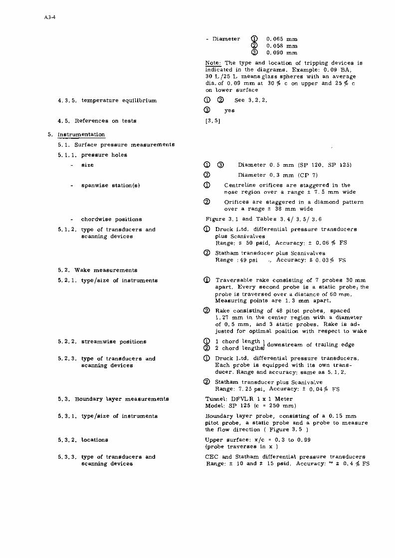
- Diameter 0.065 m m 8 0.058 m m @ 0.090 m m
4. 3. 5. temperature equilibrium
4. 5. References on t e s t s
5. Instrumentation
5. 1. Surface p res su re measurements
5. 1.1. p r e s s u r e holes
- s i ze
- spanwise stat ion(s)
chordwise positions
5.1.2. type of t ransducers and scanning devices
5.2. Wake measurements
5. 2. 1. type/size of instruments
5.2.2. s t reamwise positions
5.2.3. type of t ransducers and scanning devices
5.3. Boundary l aye r measurements
5. 3.1. typefsize of instruments
5.3.2. locations
5. 3.3. type of t ransducers and scanning devices
Note: The type and location of tripping devices i s - indicated in the d iagrams. Example: 0. 09 BA, 30 L 125 L means glass sphe res with an average dia. of 0 .09 m m at 30 & c on upper and 25 & c on lower surface
@ Q See 3. 2.2.
O y e s
13.51
a @ Diameter 0. 5 m m (SP 120, S P 125)
@ Diameter 0. 3 m m ( C P 7)
a Centreline or i f ices a r e staggered in the nose region over a range + 7 . 5 m m wide
@ Orifices a r e staggered in a diamond pattern over a range i 38 m m wide
Figure 3. 1 and Tables 3. 41 3. 51 3 . 6
0 Druck Ltd. differential p res su re t ransducers plus Scanivalves Range: i 50 psid, Accuracy: i 0.06 & FS
Statham t ransducer plus Scanivalves Range : 49 psi ., Accuracy: i 0 .03$ FS
@ Traversable rake consisting of 7 probes 30 m m apar t . Every second probe i s a stat ic probe; the probe i s t raversed over a distance of 60 mm. Measuring points a r e 1. 3 m m apar t .
@ Rake consisting of 48 pitot probes, spaced 1.27 m m in the center region with a diameter of 0. 5 m m , and 3 stat ic probes. Rake i s ad- justed for optimal position with respect to wake
a chord length downstream of trai l ing edge a 2 chord length
a Druck Ltd. differential p r e s s u r e t ransducers Each probe i s equipped with i t s own t r ans - ducer . Range and accuracy: same a s 5. 1 . 2 .
@ Statham t ransducer plus Scanivalve Range: 7. 25 psi, Accuracy: + 0. 04% FS
Tunnel: DFVLR 1 x 1 Meter Model: S P 125 (c = 250 m m )
Boundary l aye r probe, consisting of a 0. 15 m m pitot probe, a s ta t ic probe and a probe to measure the flow direction ( Figure 3. 5 )
Upper surface: x / c = 0. 3 to 0.99 (probe t r a v e r s e s in x )
CEC and Statham differential p res su re t ransducers Range: i 10 and i 15 psid. Accuracy: a i 0.4 & FS
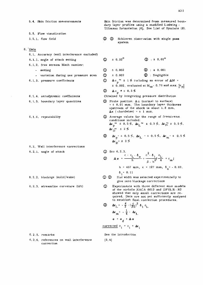
5.4. Skin friction measurements
5. 5. Flow visualization
5. 5. 1. flow field
6. 'Data - 6. 1. Accuracy (wall interference excluded)
6.1.1. angle of attack sett ing
6. 1.2. f r e e s t r e a m Mach number:
- sett ing
- variation during one p ressu re scan
6. 1. 3. p res su re coefficients
6.1.4. aerodynamic coefficients
6. 1. 5. boundary layer quantities
6. 1. 6. repeatability
6.2. Wall interference corrections
6.2.1. angle of attack
6. 2. 2. blockage (solidlwake)
6 . 2 . 3. s t reamline curvature (lift)
6 . 2 . 5. r e m a r k s
6. 2.6. references on wall interference correction
Skin friction was determined f rom measured boun- dary layer profiles using a modified Ludwieg - Tillmann formulation [6]. See L i s t of Symbols (8).
@ @ Schlieren observation with single pass sys t em
0 + 0.002 @ : Negligible
Q A c n q i 1 $ including an e r r o r of AM = r
0.002, evaluated a t Ma= 0. 76 and max. lcDl
Obtained by integrating p ressu re distribution
@ Probe position: A z (normal to surface.) = +_ 0.01 mm. The boundary layer thickness upstream of the shock i s about 1 . 8 mm. Ax ( chordwise) = f 1 mm.
Average values f o r the range of f r e e s t r e a m conditions included: ACpg t 0 . 5 $, kLq + 0.3 $, &Z . 0 . 5 6, &,,- i 2 $
a See 6. 2.3. C . C
2 L. 60 c . 6 c
Q A U = 1 L
h $37 + C m l
P . h
h = 457 mm, c = 127 m m , 6 = - 0.03 0
6 = 0 .11 1
@ Slot width was selected experimentally to give ze ro blockage correc t ions
Q Experiments with three different s i ze models of the airfoil6 NACA 0012 and DFVLR - R2 showed that only smal l correc t ions a r e r e - quired. Data a r e not yet sufficiently analysed to establish final correc t ion procedures.
Q & ; - n c 2 L 2 (E' 6 1 C ~
corrected c . = c . + &. 1 1
See the Introduction
13.41

6.3. Presentation of data
6. 3.1. aerodynamic coefficients
6. 3.2. surface p res su re
6. 3.3. boundary layer quantities
6 . 3.4. wall in ter ference correc t ions included?
6 . 3. 5. correc t ions f o r model deflection
6. 3.6. Empty t e s t section calibration taken into account?
6. 3.8. additional r e m a r k s
6.4. Were t e s t s ca r r i ed out in different facil i t ies on the cu r ren t aerofoil? If so, what facil i t ies. Are data included in the present data base?
Tables: 3. 4/ 3. 5 Figure. : 3.6
Tables: 3. 4/ 3. 5 Figures: 3. 713. 813. 9
Table: 3. 6 Figure: 3. 10 Schlieren pictures: Figure 3. 10
0 0 NO Q y e s
NO
Yes
No special notation i s used to identify correc ted and uncorrected data.
See 2.1. of this questionnaire and Table 3. 3
A comparison of ARA and DFVLR-TWB pressu re distributions i s given in Figure 3. 7
6. 5. T o be contacted for fur ther @ W. Puffert information on t e s t s DFVLR
D-3300 Braunschweig
Q T . E . B . Bateman Aircraf t Research Association (ARA) Manton Lane Bedford, MK41 7 P F England
@ E. Stanewsky DFVLR-AVA BunsenstraDe 10 D-3400 G6ttingen
7. References
[ I ] KijHL. P. The design of airfoils for t ranspor t a i r c r a f t with improved high speed ZIMMER, H. character is t ics
DORNIER GmbH, Report 74/16B, 1974
[2] STANEWSKY, E . Development and wind tunnel t e s t s of three supercr i t ica l airfoils f o r ZIMMER, H. t ranspor t a i r c ra f t .
Z. Flugwiss. 23 (1975), Heft 718
[3] STANEWSKY, E . The DFVLR Transonic Wind Tunnel Braunschweig: Calibration resul ts PUFFERT, W. fo r the modified tes t section and re su l t s fo r the airfoil CAST 7. M ~ L E R , R. DFVLR Report IB 151-77/10, 1977
[4] HAMMOND, B. F . L . Some notes on model testing in the ARA two-dimensional facility. Aircraf t Research Association Memo No. 170, 1975
[5] HAMMOND, B . F . L . ARA model t e s t note T 2814, Ai rc ra f t Research Association, Bedford
[6] SASMAN, P.K. Compressible turbulent boundary layer with p r e s s u r e gradient and CRESCI, R.J . heat t ransfer .
AIAA Journal , Vol.4, No.1. January 1966, pp 19-25

8. L i s t of symbols
b span, tunnel width
C . I , L model chord
C P
p res su re coefficient
C * P
p ressu re coefficient a t M L
C~ Lift coefficient
'w' 'D M, Ma. Mm
ML
MB
H, h
P
Po. H
P~
Re, R , E-6* RE
(I
6 , DEL
6*. DEL'
pitching moment coefficient (based on 0.25 c )
d rag coefficient
f r ees t r eam Mach number
local Mach number (airfoil surface, f ( p / po ) )
tocal Mach number (boundar
layer, f (pg/pT))
tunnel height. shape factor
s ta t ic p res su re
f r ees t r eam total p res su re
total p res su re in the boundary layer
Reynolds number. based on f r ees t r eam conditions and chord length
nose radius
f r ees t r eam total temperatur
velocity in the boundary layer
maximum thickness
coordinates (Figure 3 . 1) ( Z i s in the case of the boundary layer measure - ments taken normal to the a i r fo i l surface)
angle of attack
boundary layer thickness (u/ue= 0.99)
displacement thickness
Relations used in the reduction of the boundary layerddata
6 = 1 - . L) . d z u
e e 6
u U e e
H = 6 * / 0
c = (0.246 . e (-1. 561 . Hi) . Reo -0.268 f ) I
Assumptions: P = 1
TWITte = 1
Tw Wall temperature
Tte total temperature a t edge of boundary layer (T
te = To)
Subscripts
m f rees t r eam conditions
TE trai l ing edge
u upper surface
1 lower surface
e , E edge of boundary layer
B boundary layer
O, THETA momentum thickness
Y ra t io of specific heats

Table 3. 1 Coordina tes of the airfoi l CAST 7 Table 3 . 2 Design p r e s s u r e a . Model: SP 120 (TWB t e s t s ) , , dis tr ibution
Pressure distribution at (x, + -) Rs ; 6 . lo6 Boundary layer: turbulent
Mm = 0 . 7 6 0 0 = 0 . 0
CL = 0 . 5 7 3 C,,, = - 0 . L 3 5 5 1
CD 0 . 0 0 4 5 8 C . 3 4 . 5 5 8 7 P
0 .07580 0 .12895 0 . 12695 0 . 24141 0.21113 0 . 4 8 2 2 1 0 .46230 0 .70025 0.70051 O B Z 8 2 0 O S 2 8 9 Y 1. ,3835 I . 14076
0 . 9 1 2 3 < 0.111(8 0.53289 0 .55421 0 .35108 0 . 4 3 4 9 5 0 . 20055 0 .36309 0 .00269 (I. Z i S i l
-0 .21<08 0 . I 8454 -0.43112 0 . l0ZOI -0.61032 0 .03930 - 0 . 7 5 1 3 2 - 0 O Z S B I - 0 8 2 0 S B -0 .09221 -0.88111 -0 . 19051 -0.81114 -0.32130 -0 .90171 - 0 5 8 S i l - D . L l S l B B -0 .39120 -0.88738 - 0 . 3 2 9 2 1 -0.88810 -0 .23556 - 0 7 B 1 0 2 -0. lZB.0
manufac tured a i r fo i l s e e Fig. 3. 1 - 0 . 8 3 2 7 1 -0.01747 -0.61581 0 .09305 -0 .5276% 0.19929 -0.98832 0 . 2 9 2 1 1 -0.21118 0 .36020 -0.10430 0.39117 -0.00889 0 . 3 9 3 5 7
0 .01860 0 . 5 1 8 3 0 0 .19893 0 .31661 0.2U143 0 . 3 2 9 1 3
0.29324 0 . 29385 b. Model: C P 7 (ARA t e s t s ) 0 , t i s o l 0.17118
0.10612 O L O S B B 0.00021 0.06(101
Upper Surface (mml Lower surface (mm) 0 . 0 3 8 ~ 8 0 . 0 3 5 8 5 O . O L i 8 5 0 D l 7 8 5
x/c x [mm) ~ e s i s n ~ c t u l l ~ r r o r I*#isn AcCu.1 Zrror Exper iment ARA: Table 3. 5 and Figure 3 . 2
0.115 14.605 6.114 6 .739 +O.OOS -1.468 4 9 r0.028
0.155 19.685 7 . 6 7 . 3 6 0 Exper iment DFVLR-TWB: Figure 3 . 2
-5.131 -1.156 +0.025
0.215 27.305 8.016 7.998 -0.018 -5.883 8 9 tO.010
0.275 34.925 8.402 8.379 -0.023 -6.304 -6.312 rO.0011
0.335 42.545 8.618 8.603 -0.OlS -6.383 -6.383 0 -The location of the p r e s s u r e o r i f i c e s 0.395 50.161 8.700 8.694 - 0 . ~ 6 -6.142 -6.137 -0.00s i s given with the su r f ace p r e s s u r e 0.655 57.785 8.656 8,651 - 0 . ~ 5 -5.626 - 5 . 6 1 8 -0.008 distr ibutions in Tab le s 3. 4 . 3 . 5 and
0.515 65.405 8.479 8.476 -0.003 3. 6 and in F igure 3 . 1
-4.895 -6.1179 -0.016
0.515 73.025 8 . 1 U 8.146 0 -4 .W3 -3.980 -0.021
0.635 80.615 7.630 7.628 -0 .W2 -3.010 - 2 . 8 -0,025
0.695 88.265 6.886 6.891 rO.Ws -1.989 -1.9111 -0.03I
0.755 95.885 5.890 5.883 -0.007 -1.026 -0.99l -0.035
0.815 103.125 1.651 4.64, -0.010 -0.264 -0.221 -0.043
0.875 111.125 3.226 1.121 -0,005 0.132 0.168 -0.036 l.O,04%C 1 +0.05
0.920 116.840 2.096 1.088 -0.008 0.099 0.117 -0.018 AZmm
0.950 120.650 0.336 1.114 O -0.079 -0.081 +0.002 0
0.978 12h.111 0.627 0 .621 -0.002 -0.113 5 6 rO.023
I . W O 127.000 0.043 0.038 -0.005 -0.589 -0.599 tO.Ol0 -0.05 I-ao4-1.6
- u1s ---US
LI.di* edge in.p.ered by *eru,ir. ceq1.c.. ."d Sh.dorgr.ph r.eh.ique.
kccuracp: +0.007 m
ARA CAST 7 a i r fo i l (Model C P 7 ) Measured e r r o r s of manufac tured airfoi l
-.%
\ --__
-. -.. --._ --.._,,.'
:,,
-LA'. 101* (127mmJ

Table 3 . 3 Flow conditions included in present data set
Transition .068& 7/7L means: Roughness band of . 0 6 mm diameter glass spheres in 7 * c 0" upper and lover surface.
I' Corrected angles of attack " Compared fo design presaure distribution (Figure 3 . 21
~ ~ b l ~ 3 . 4 D F m R - T W B tests. Aerodynamic coefficients, airfoil surface and top and bottom wall pressure distributions
Transition at 7 $ c on upper and lower surface. b. Airfoil surface and top and bottom wall
a. Aerodynamic coefficients pressures E : The upper surface and top wall pressures
a r e L-t. " I . *LC* E - W R I &PIU
NR. PSACli E-6.RE &PHA CA C* C Y n ,763 5.9, -1.1.
2493 . 6 P I 5.88 - 2 . m -.I8867 ,889632 BIP5 ,761 6 .86 -1.88 ,1478 -.I1858 . 8 8 9 3 U l 24'16 .783 5.PB .88 -.I1876 .Be95511 x n CP XVIL SPI
e491 . l e t 5.97 >.Be ,5482 - .a1877 .BIB416 2498 , 781 5.94 2.88 . ~ B S B - .he979 . B L P ~ W .**a 1.aa9s - 5 . ~ 5 -...I* 2499 , 7 8 2 5 . 9 6 3 . m .P857 - . 1 1 3 6 9 .821677 .**a .age. - 4 . 5 -.. .76 8588 +699 5 . 9 5 I . a B 1.8617 - .12588 ,839835 .6SP5 -3 .16 -...47 8581 ,788 5.9 , 4.58 1.8297 -.,I691 1868949 .*I5 .a816 -3.B. -.I.1@ 25BP +6PP 5.98 5 . B B 1.8187 - .11898 ..sS .I1SP -8 .9s [email protected] .*a - . I S 9 6 - I . % # . I I W
.SM -.a651 -1.85 .1118 P I P @ .761 5.98 - 1 . B B .I867 -.I1769 .818196 .@a* 7 -1.m .11 81 m a 4 5 .9 , -1.88 . 2 6 ~ ~ - . l l e m . a ! e ~ a x . I* . - . S 4 9 1 - . 7 5 ...St
ell85 9 5.98 .88 .a268 - .19195 .811441 .I.* U S - .5* -
P486 . ? b l 6.BI .58 .St611 -.IPP)P .BLLllb . I @ @ 7 3 -.D5 -.#Oat PIP! ,768 5.99 . 7 5 ,5789 - . I P S P I . B I I B J @
3 .11 -.a556 9487 .168 5.92 1.88 ,6897 - .1311a .813658 . P M - . I 838 .PI - . I P s e 2488 ,759 6.88 1.58 ,7187 - . I 4 I S P .BIPPIB .lo. .S1 - . l l s l BILIP , 7 6 8 5.94 2.88 ,7258 -.I1538 +841963 . 3 U -.55P8 .11 - . l e e 1 21198 ,761 5.99 3 . W ,7384 - . I 2548 ,861552
. l o 1 - . S M 1 I...
.a** - . S T 1 3 1.95 -.@109 -.5S.@ 1 . 5 -..Tee
2511 ..a1 5 . m .58 . J @ I e -.B*BBI +a89738 .5SO -.5985 8.75 -.IS11 25x2 +4PP 5 . 7 6 . 5 8 .1$91 -.8P495 .8@8745
4 -.65.5 D . I O -..a87
2514 ,682 5.86 + 5 B .a812 -.IBEBB .BBIIP73 - . U P 5 P.91 -..,Pa
~ 5 1 5 ,658 5 . 8 . 5 8 ,4448 - .>a659 .Rae466 . 6 P I -.6546 0 . 5 s -.IJPe
P516 .782 5.88 .58 .a674 - + 1 1 9 1 6 .81@!74 .m. - 3 9.75 - . I 393
P517 ,717 5.81 . 5 8 .4Sa1 -.I1458 .8a99(13 . S I B -.PSPO 1.58 -.IS99
2518 .11P 5.81 .$a .a965 -.I1114 . I I e J $ P -..64. - 5 . 2 5 -.II1# D S L P , 7 5 1 5.96 . S B . w e e - . t e t m .*nnana . 9 S .I359 -4 .58 - . @ I S 8
e5ea .75P 5.97 . .5PSB -.18JS5 .81@711 .915 . # I 4 0 - 1 . 1 5 . Ian8
8524 . 7 6 5 5.88 .58 .SD IO - . IB1.8 . * I l l91 I...* . , I S 9 -I... .em4
D581 .7,8 5.99 .5e . , a le - . , 3 3 e 3 .#IPB@7 .erne t .mes -e.zs .e111
PSBP .,re 5.s~ .$B .s,.e - . I J ~ & .~1639a .*I4 -.I818 -1.58 .el119
9 5 2 3 .se! 5.92 .5a - . 1 3 m a .neeme .ems -.UEB - 1 . ~ 5 ..IBP .#PI -.a556 - I . B I ..PPI .*S -.I966 - . 7 5 . B l s P
P581 .1%9 4 . 1 .58 .S161 -.IPB5I .0IP171 I - .3151 -.5@
~ $ 8 5 .761 5.18 .sB .5PP8 - . I P S 4 9 .811555 . IS* -.amas - . 95 . w a e
P586 .168 5.81 .58 - . l S J a D .*IBS99 .as. - .5113 .em - . w e 3
~ S B I .,6, 7 .85 .5e .%,PI - . tea52 .e1@5se .D50 - . 6 P l l .95 - . a111
PSBB . w e ~ e . m . .sap6 - . I ~ P D ~ . a e e e e ~ .ISe - . 5 5 5 @ .58 -.llPO
9589 .758 t I . 7 7 .58 .54111 -.le9*4 +0183P* .a51 - .3376 .15 -...*I
2518 ,768 13.41 . 58 -.I1991 . I I I I P 4 . I S # -.I371 1.8. .1113 . 6 M .a454 I . P , 8 .lW 9 1.5. .# I96
2525 ,768 4.89 8 . m . 1 1 ! 6 - . I J I 9 P .a48354 .a50 .DPeI 7 .816S
e5Pb .768 5.83 2 . m .1Pl9 - . 1 1 $ 5 S .eJIIY)* 1.9.e . I I I 9 P.ll 11113
8587 . . n.sa .raar -.139&6 .e1sI99 *.E5 -.Be79
e 5 3 i ,762 7.8, 8.~31 .,a88 - . I , P J 6 .a39436 e.sa - . ears OSJB ,759 9.96 2 . m . I T , * -.la711 . I 3 1 7 9 3 2 .75 -..a47 2589 , 7 5 8 il.78 P.@@ .7116 -.I4793 .#3e559 1.58 - .Be19
9 5 ~ 8 , 7 5 9 13.49 2 . m .,.)re -.I4957 . 13 lSbl
L model chord
MR. MACW K-6.RS U P U
U S . T ~ P 5.96 ..I XIL ' CP x m cpv
.eee 1 . 1 3 , ~ -..PI -...em
.*a4 .I756 -4.5, - . IS58
...1 .S110 - 1 . 1 5 -.##as
. . I $ .DIP7 -3.a.
..SI -.em9 -..DS ... $I
..U -.SSP1 -1.5. ...S4
..W -.a#.. - I . . % ..I69
.we -.85%8 -1.I. .#.I P - .S111 -.11 -..as2
. I - -.1661 - .51 -..IIs -.6658 - . *5 -.,4S7
.Pa. - .1871 .#a -.me16
.sM -.81%0 . ~ 5 - . 1 5 1 8
.3.. -..a14 .%I - . I , # &
.JU - . . I . , .11 -.1.11
.18@ -.6188 I... -.I1PI
.as* -..a11 1.95 -.!Is$
...I -.66$P 1.5, -.#SSP -.6636 1.15 -.a648 -.6911 9.I. -..539 -.711P 8.81 -.#a66 - . l a 9 3 9.5. -.#a43
.?I# -.53Ps 0.71 -..a18 8 -.9981 3.5. -..3.9
-.1611 - 5 . 8 5 -.a811 .95. ..Jea -4 .m -...a6 7 .lMl - 1 . 1 5 .e161
1.111 .Wll - 3 . m .Be96 . a m 1.1119 - 9 . 9 5 .e,6e 4 .Is96 - I . $ . ....a .#I. -.~P.s - I . P , .eee, ,191 -.16.. -1.e. .eJI.
-.as42 - .75 .e118 ! -.I726 - 5 .eJSO . ~ s s - . n r e s -.PS . a 1 1 6 .en. - . m a 6 .ee . a a . ~
-.a686 .P5 .IS.$ . 3 W - 4 .% .,PI6 . a I B -.a861 . 1 S . I D 6 5 .55* -.!165 I . s l .IJI. .6S. ..688 1.PS .1588 .731 .PIS1 t . 3 .a879 .851 3 L.7, . I t91
1.111 .B9m P.es . I t * . s . P 5 -.111. 2.3s - . ~ s P 9.15 -.@I** 1.W .a146
xw location of wall orifices(with reference to model cp airfoil surface pressure coefficients leading edge)
CPW wall pressure coefficient

Table 3 . 4 Continued
X Y I L
NR. MACH i - - R E ALP- NR. MACH I -6 .R I ALPHA
8 7 1761 5.9s I... 4 .759 6.l . , .%a
CPY I CP X Y I L CP"
YR. IaCII E-6.RZ L P H L MI. MhCH =-LIRE L P I U NR. MACH L-6.RE L P H A
EN. 6 1.9s -e.a. east .76. 1.99 .IS * ~ P B . ,el 5.99
x n CP XI& CPI X A CP x w n CPW CP XYIL CPY x n

Table 3 . 4 Continued
IR. MACH E - b S R l U P U
E41)1) ,782 5.96 3.00
X R CP X V R CPW
CR CP X I I R CPY
x n CP X Y R CPY
NII. MACH E-b*RE U P U NR. NACH L - 6 . R E U P H A
e l 9 8 .7e1 5.94 8 . m
X / L CP X Y R CPY

Table 3 . 4 Continued
X A CP X Y A CPY
NR. MACH C - e 8 1 %PHL
e511 .a81 5.Ae .50

Table 3 . 4 Continued
X h CP X l h CPY I
MR. MACH I-6.RS U.PU WR. MACH i-6.RZ U.PW
D51. 161e 5.86 .S* S t .618 5 . 8 .5.
X R CP x m CPW I .a CP X W R CPV X R CP X Y R I
X n . CP X Y R C P I I X/L CP xw CPW
NR. IIAEH E-6.RE
P52a .159 5.97
X R CP X Y R
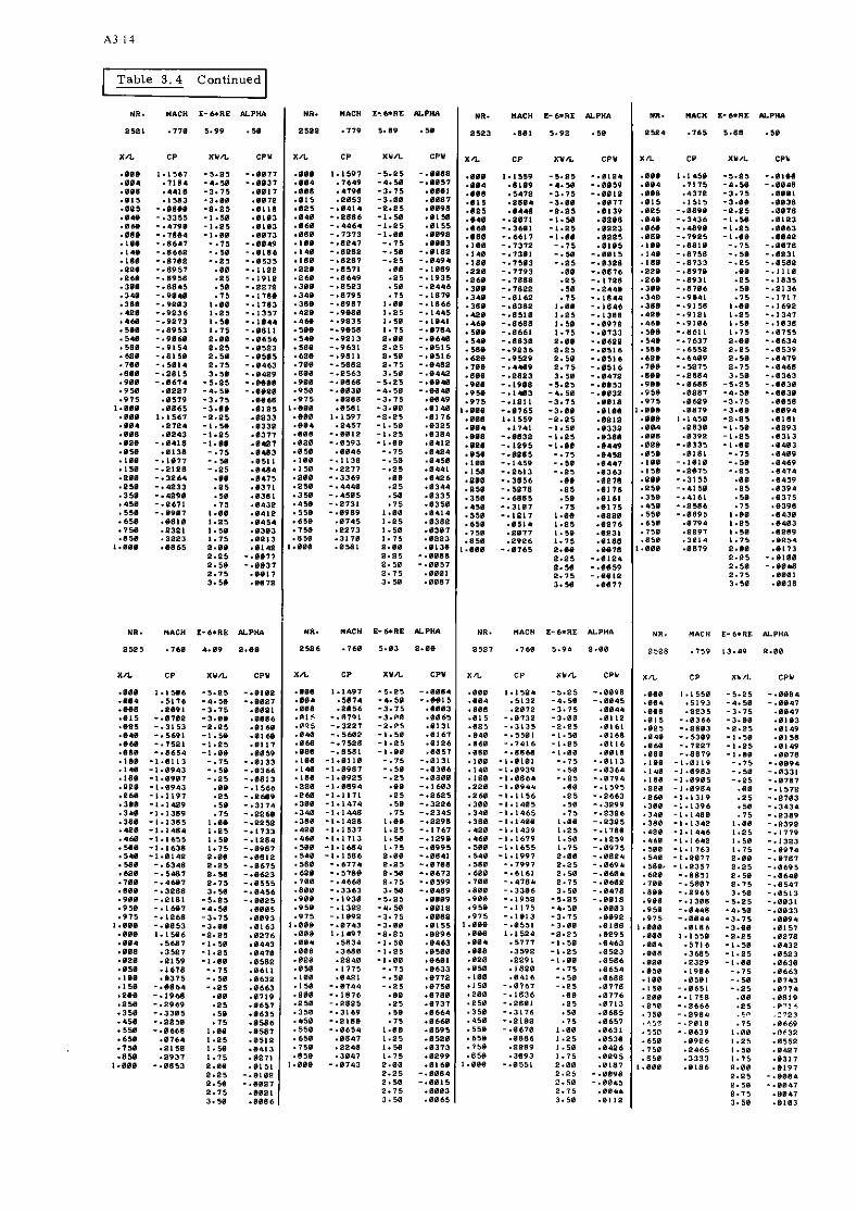
Table 3 . 4 Continued
.me
.*ma ,918 .a15 ..81 . I U .em .*a1 I . . . I .@ 1 1 1 1 .8PI .P61 .31# .,a@ . a m . .0I . 468 .51. . 5 U .50O . a.3 .,.e .*em 4 9 1 .958 . P I S
1.119 ,919
.Be8
..a*
. I S @
.,as
.IS$
.989 ,919 ,359 .458 . 5 M .65* .15s .85*
1.811
CP X Y h CPY
X R CP x w n CPY
x n CP X Y R CPY
x n CP X Y R CPY X R CP X l h CPC
X R CP X Y R CPY
X R CP x w n CPY

Table 3 . 4 Concluded
Table 3 . 5 ARA tests . Airfoil surface pressure distributions.
Nate: The aerodynamic coefficients are listed in the respective plots. Transition at 8 $ c on upper and lower surfaces. Re = 6 . 10'
WR. MACH E-6.RI U_PW
PSJL .76P 7 P.l.
x n CP X Y ~ CPY
N I . MACH E-6.RI IY.P"A
8589 .158 11.18 P.IB
X R CP X Y ~ L CPY
YR. "ACH E-6.RI *LPW
e5ze .~SP 9.96 *.as
X R CP x r n c ~ u

Table 3 . 5 Concluded
108
0.161
0.26
C. PIB 0.101 ,7106 0.034 , 6 0 1 -0.014 ,61111 -0.239 ,6149 -0.61' ,5666 -0.119 ,1115 -0.602 ,1166 -0,806 ,6582 -0.793 ,6618 -0.727 .18W -0.666 ,4969 -0.609 ,1127 -0.754 ,67211 -0.849 .U61 -0.823 .b111 - 0 . 8 ,6458 - 0 . 7 ,4357 - 0 . 9 ,6347 -0.840 . U B 9 - 0 . 6 3 , 4 2 5 -0.712 . -0,519 ,1175 -0.113 . 6LI l 0.101 ,7101 0.667 ,8103 0.967 ,9429
1.150 ,9992 0.635 ,8567
-0.198 ,6266 - 0 . 5 , 6 7 8
0 . 0 l l ,6870 -0.016 ,6655 -0.096 ,6545 -0.205 ,6245 -0.361 ,5813 - 0 . h l l ,5659 -0.156 , 5 8 6 -0.248 ,6125 -0.091 ,6550
0.079 .TO28 0.228 ,7441 0.110 , 7751 0.281 ,7588
98
0.752
0.73
106
0.760
-1.17
5 P I N 0.111 .7161 0.MO ,6915
-0.081 ,6195 -0.139 ,6165 -0.616 .568h -0.lll ,1398 +.I82 ,5220 -0.616 .51Z? -0.tA1 . I057 4 . 6 2 2 .1109 -0.601 .1161 -0.1117 ,6206 -0.176 ,5236 -0.117 ,5316 -0 . I l l ,51811 -0.122 , 5 8 5 -0.126 7 -0.111 ,1929 -0.112 .511t -0.116 .Ill? -0.G11 , 5 5 7 -0.211 ,6122
0 . 0 7 ,7171 0.171 ,7816 0.101 ,8768 1.082 ,9806
0.093 .981l 0.2111 .7605
+.921 ,6287 0 . 6 0 6 -0.211 ,6180 -0.284 ,6042 -0.330 ,5911 -0 .6 l l 6 9 -0.118 ,5210 -0.199 5 5 -0.670 ,5530 -0.127 5 2 -0.149 ,6114 0.040 ,6914 0.196 .7161 0.113 ,7687 0.211 ,7571
1.W 0.95) 0.8- 0.819 0.769 0.698 0.659 0.619 0.579 0.540 0.499 0.660 (1.419 0.379 0.119 0.100 0.110 0.199 0. I&P 0.101 0.011 0.010 0.016 0.016 0.W8 O W 2
-r
[I O_M1 (1.011 0.020 0.010 0.070 0.100 0.1&9 0.22'1 0.120 0.590 0.659 0.119 0.640 0.7'0 0.819 0.912
111
0.761
0.49
e. PI^ 0.106 ,7105 0.011 ,6908
-0.085 ,6579 -0.260 ,6150 -0.418 ,5659 -0.129 ,5350 -0.600 . l l S h -0.625 ,5085 -0.W ,5016 -0.73D ,6171 -0.876 ,4193 -0.891 ,4314 -0.9JO .&?a1 -0.910 ,4244 -0.885 ,4367 -0.9'2 ,6210 -0.948 .& I94 -0.936 ,6125 -0.900 ,6125 -0,877 ,4590 - 0 . 7 ,6805 -0.119 ,5267 -0.113 ,6311 0.060 ,6979 0.630 ,8000 0.922 ,9360
i . l l fL .WO0 0.666 ,8653
-0.109 ,6512 0 . 6 6 9 0.061 ,6991
-0.019 ,6761 -0.061 , 6 3 8 -0 . l73 ,6235 -0.110 ,5902 - 0 ,1718 0 . 6 5 -0.234 ,6167 -0.08' ,65110
0.086 ,7050 0.231 ,7458 0.343 ,7761 0.281 ,7596
107
0.719
-0.22
C. PIR 0. l12 ,7136 0.036 ,6926
-0.081 ,6592 -0 .242 ,6162 -0.&20 ,5671 -0.110 ,5367 -0.6W ,5174 -0.666 .W9& -0.748 ,6767 -0.142 .<185 -0.728 ,1823 -0.7IO . U 1 3 -0.678 '961 -L?.640 .I064 -0.619 ,5121 - 0 . 1 , 5 4 7 - 0 . 7 5 9 -0.790 6 -0.766 ,1776 -0.765 6 - 0 . 6 ,1007 -0.419 5 6 -0.050 ,6688 0.196 ,7360 0.5'6 ,8329 1.002 ,91086
1.141 .9'HP 0.526 . B I T 6
-0.399 ,5745 - 0 . 5 0 -0.013 ,6708 -0.111 ,6511 -0.171 ,6117 -0.270 ,6083 -0.121 ,5656 - 0 . 4 0 ,5532 -0.194 ,5143 - 0 . 7 ,6071 -0.111 ,6516 0.061 ,7007 0 . l l i ,1824 0.310 ,7117 0 .277 , 7 5 9 1
c. PIR 0 . 7 , 7 6 5 0.011 ,6964
-0.089 ,6632 -0.217 ,6203 -0.126 ,5711 -0.119 .Ib08 -0.614 ,5205 -0.659 . I O l l -0.677 ,1036 -0.626 ,5111) -0.190 ,5270 - 0 . 3 , 5 9 2 -0.982 .&10Z -0.981 ,1190 -0.966 ,4259 -1.009 ,4129 -1.011 . 4 I I P -0.999 ,1117 - 0 . 8 ,6200 -0.960 ,6264 -0.786 7 -0.632 ,1155 -0.2" ,6210 -0.010 ,6848 0.166 ,7868 0.815 ,9256
I , 9 9 9 0.116 ,8897
-0.010 . U L 8 0 ,7206 0.111 ,7180 0.021 ,6936
-0.025 ,6807 -0.116 ,6501 -0.288 6 9 -0.118 ,1927 -0.105 .601> -0.212 , 6 9 7 -0.071 ,6682 0.091 ,1128 0.238 , 7 5 2 1 0.316 . 1 $ 1 G 0.286 ,7651
109
0.161
0.71
c. P I E 0.101 ,7101 0.011 ,6906 -0.LMI ,6186 -0.113 ,6170 -0.398 ,5716 -0.487 ,1169 -0.516 ,5960 -0.562 ,5261 -0.908 ,4307 -0.969 . & I 1 7 -0.911 . & I 2 7 -0.990 .*a80 -0.991 ,4065 -0.9116 ,4091 -0.968 ,4139 -0.991 ,4061 -0.99' .'070 -0.975 .& I21 -0.956 . 6 V 8 0 . 9 ,1251 - 0 . 6 ,1127 -0.6W . l L % -0.214 ,6223
0.019 ,6866 0.390 ,7892 0.892 ,9279
1.151 ,9994 0.732 .BBP6
-0.031 ,6721 0.107 .,,I0 0.103 ,7098 0.014 ,6853
-0.032 ,6725 -0.164 ,6616 -0.3W ,5985 -0.363 . I 8 1 l -0.316 ,5942 -0.219 ,6209 -0.071 ,6610 0.092 ,7069 0.138 .7472 0.347 , 7771 0.285 ,7602

Table 3 . 6 DFVLR 1 x 1 Meter tests . Boundary layer data. . ............................................................... I B O I IS9 ma-0.71U U P & = 2.52 911r-175.1 PO-512.1 70-305.1 I ~ n o w 158 nb-O.76V 1111- 2.52 Pllf-175.3 PO-512." ?D-30..0 I
I E i O _ > V E 0 7 8 I s e = O . I V E 0 1 I !llCI 0.5500 I.= 1.528 0 . 9 UE-297.UB CPI--0.3661 ! I I / C - 0.5000 Z8= 1.527 me0.925 UE-2'19.02 CP*-O.IPOI !

'Table 3 . 6 Continued
1.01 161 i)i=O.765 AL.A= 2-52 911.-115.1 PO-552.7 90-101.0 I I R " 1 162 "1-0.765 1L.1. 2 . 5 2 P I I I - I , I . V P-551.9 to-101.. 1 I . I -0.2YI ill I I RI.O.2"E 0 , I 0 . 0 0 = 5 . 6 0 . 8 0~28u.011 C P P - O - I Y I ~ I 11,~- 0.8000 e l k 7.166 ae=0.1~7 08-219.11 ce~=-o.ouss I

Table 3 . 6 Continued . . . . . . . . . . . . . . . . . . . . . . . . . . . . . . . . . . . . . . . . . . . . . . . . . . . . . . . . . . . . . . . ...
110.165 .&-O.IeV ALP&= 2 - 5 2 Pr1F-176.0 PO-553.5 10-10V.0 1 (no1 166 n&-D.I6$ ALP*- 1.52 P 1 l l I l . . 8 PO-511-3 10-30U.11 I I IE -0 .2YE 0 7 I I 1E10.2YE 0 7 I 1°C- 0.V000 I P 2.815 8 b l . 2 l Y Y B 1 7 5 . 1 2 CP*-1.0732 I I r I E - 0.1000 ZE- &.PO0 .E=?.IQ9 01-181.52 CPP-I.OSYII !

Table 3 . 6 Continued ............................................................... ...............................................................
11111 l95 ih=O-766 ALP&= 2.50 PII.*175.1 P0=551.1 10=101.5 # I s " # 161 a1-0.7*V ) i l ? L = 2 .52 0111=161.1 P c = l U S _ I T O - 1 0 V . I I I l l . 0 . 2 Y O 0 7 1 I /E= C.9900 L1=(1.165 S P O - 6 6 6 2 2 . 6 E P P 0.2150 I I
REi0 .2Ve 0 1 I
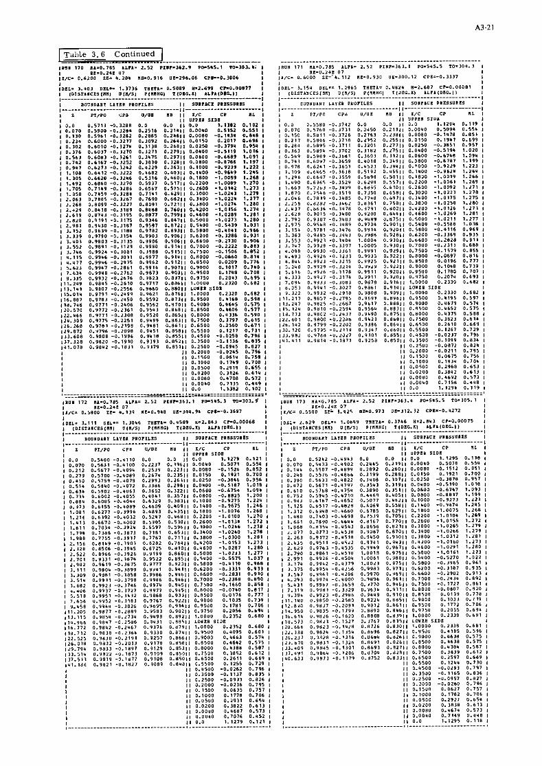
Table 3.6 Continued ............................................................... ..... 1.01 110 .A-0.785 LIII- 2.52 PIW-161.9 PWS1S.1 F0-101.l; I ~ B u r 111 8110.785 ALP*= 2.12 PI1r-16J.I PO-SYS-5 TO-1OV.J I I B E - O . 2 Y I 111 I I sP=O_IUI 0 7 8
1 t I / C = 0.6000 Z E = - U _ 1 1 2 11E.0.910 UE=300_12 CPCi-O.II37 I

1 Table 3 . 6 Continued ( .............................. ............................................................... I I U I $7. 1,-0.785 II.11- 1.52 PI,-163-1 PC-595-5 -303.9 I I x u H 175 i r - 0 . 7 8 5 r L n - 2.52 Prrr= lr , . l PO-5u5.7 to-302.0 I I In-0.2VB 0 1 I I IE-0.2VB 0 1 I I I / C - 0.5200 ili 2.612 11-1.091 0-3YI.99 ClI--0.6801 I j I /C= 0 .5000 ZE= X.110 I I I - I . Z U 1 0-178.72 CPI=-0.9662 I
I 0 . 0 1 0 . 0 7 0 I 0 . 1 0 " 1 0 . 1 3 1 I 0 . 8 6 0 I i l _ l B P I 0.2JO 1 0.275 1 0.105 I O.JJ9 I 0 . l ' t 1 0 . 0 6 6 I 0 . 5 V B i 0.60" I 0.67" I 0 . 7 4 2 10.111, i U _ Y I I I 0.98" 1 1.1161 , , _ I " , I l.191 1 1 . 1 1 1 I I."", I 1 . 5 5 1 I 1.6V1 1 I . IU9 1 i . i l l t I 2 . 0 1 8 , 1 . 2 0 8 I 2 . J " ) I 1 . 7 1 6 I 1 . 8 2 0 I 5 . 6 I B I 1 . 5 5 9 I Y . 6 6 3 111.105 I I I _ V I ( U , ? 5 . , * 5 110.811 l i i . b b 1 1 2 6 . 1 1 3 1 1 0 . 1 1 2 113.6112 I l d . 0 0 1
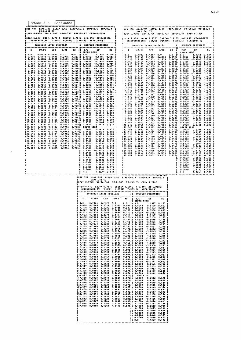
Table 3 . 6 Concluded ------------------ .-...-.-...-..--------------- ' 1.01 307 81-0-785 ALP&= 2.50 P111-162.1 P-511G.L -303.11 I I e U l 3 % a1=0_165 ALIL= 2.50 P I W h 1 6 2 . 5 PO-5Y1.8 101302.9 I I 11-0.211 0 7 I I SE=O_T*E 0 1 I 8 0 0 11- 6.912 aP0.1 '12 OP260.67 ClW-0.025. I

M- MBP Referenn porn1 of prlchmg m m m I
2 Geometric data: Chord c = 200 m m Maximum t / c = 11 .8% a t x / c = 35% C r o s s section F ' 3063mm
P Trail ing edge thickness z / c = 0. 38% Diameter of p res su re or i f ices d = 0.5 m m
TE B
a . Contour and location of p res su re or i f ices
b. Measured e r r o r of manufactured airfoil (a lso s e e Table 3. l a )
Figure 3. 1 Airfoil CAST 7 - Model S P 120 (c = 200 mm): Contour, location of p res su re orif ices and
deviation f rom design coordinates (see Table 3. l b for deviation on ARA model)
- THEORY U - 0.760 RLPHR s 0 CL = 0.673 ca = -o. i tss RE c 6sE6
o EXPERIflENT UOOEL CP 7 TRRNSITIONI 0.06 BR 7L/7L RUN 164 U = 0.761 RLPHR = .4a CL E 0.688 CU r -. 126 RE s 6mE6
a . DFVLR - TWB tes t s b. ARA te s t s
Figure 3 . 2 Design p ressu re distribution. Comparison between theory and experiment.

Figure 3. 3 Tes t section of the DFVLR Transonic Wind Tunnel. Braunschweig (TWB)
Figure 3. 4 DFVLR-TWB. Mach number distribution in the tes t section
a . Geometry of slotted top and bottom walls
H = 0 . 6 m Wall divergence
Figure 3 . 5 Boundary layer probe of DFVLR 1x1 Meter t e s t s
V2A = Stainless steel. A11 dimensions a r e in mi l l imeters
0.5
0.1 L -2.5 -2.0 -1.5 - 1.0 4 .5 0 0 5 1.0 x / H 15
k Reference slolic pressure 4 Model cenlrelrne k o l h
0 0 0 0 0 0 0 0 0 0 0 0 0 0 0 0 0 0 0 0 0 0 0 0 0 c 0 0

-0.07
CAST 7 R e - 6 . lo6
- 0.08 Trons. : 0.06 BA. 7L / 7 L
4- DFVLR-TWB
-0.09 -6- ARA
Figure 3 . 6 DFVLR-TWB and ARA tests. Aero- dynamic coefficients.
A
CAST 7
0.028 Re= 6 . 1 0 ~ Trons.: 0.06EA. 7L /7L
CD -0- DFVLR-TWB
0.026
a. Angle of attack variation

U - 0 . 5 . ~ e - 6 . 1 0 ~ Trons 0.06 BA. 7L/7L
0.60 0.65 0.50 0.55 0.60 0.65 0.70 0.75 0.81 Ma
Figure 3 . 6 Continued
b. Mach number variation (TWB tests)
CAST7 Ma - 0.76
Trons.: 0.06 BA, 7 L / 7 L C
Figure 3 . 6 Concluded
CAST 7 Mo - 0.76
Trons : 0.06 BA, 7 L / 7 L
CAST 7 Ma - 0 . 7 6 Trans.: 0.06 B A , 7 L / 7 L
c . Reynolds number variation (TWB tests)

- 1.0 CRST 7
. .8 -)t TUB MOOEL SP 120 TRRNSITIONt - .6 0.06 BR 7L /7L
. .4 0 RRR MOOEL CP 7 TRRNSITIONI
. .2 0.06 BR a L / a L
0 RE = 6mE6
.4 2w ".'
.6 0 .2 .4 .6 8 I 1
Nr. M. Re.10'' Alph.[ol CA Cm.. CW X 2488 0.761 6.W 0.80 0.818 -0.1223 0.01116
108 0.781 8.08 n.18 o.sm -o.irss 0 .0~076
Figure 3 .7 Comparison ot pressure distributions from ARA and DFVLR-TWB tests
CRST 7
0 RRR NOOEL CP 7 TRRN~IT IONI 0.01 BR.BL/IL
* TUB MODEL SP 120 TRRNSlTION1 0.06 BR .7L/7L
o RRR MOOEL CP 7 TRRNSlTIONr 0.06 BR BL /&L
N r . Ma ~e.10.' AlphaIOl CA Cmm CW X 94.7 0.701 6.97 l . W 0.842 -0.1108 O.ol040
69 D.701 6.98 0.78 0 . 0 -0.1108 0.01001
-& I 'm MODEL SP 1 2 0 T R A N S I l I O N : 0 . 0 6 BA 7L17L
0 ARA MOOEL CP 7 I R A N S I T I O N : 0.08 BA I L I I L
~ r . M. ~e.10.' A1~h.101 CA Cmrs CW ~ r . M a R. 10.' ~ l p h . bl CA Cm,s CW X 2488 0.7SI 8.00 1.60 0.719 -0.1416 O.OlIa4 A 2192 0.761 5.99 3.00 0.736 -0.1255 0.06155 . 110 0.780 8.08 1.18 0.700 -0.1378 0.01710 O l I 2 0.781 6.05 2.68 0.772 -0.1316 0.04695

0 .a .4 .a .s .I1 t
Nr. Ma R..~o" AI~h. lo1 C1 Cm,. Cw

Nr. Ma Ra.10.' Alph.lo1 CA Cm.. CW
RE s 6mE6
RLPHR = 0.60
0 .2 .I .O .B . / I 1
Nr. Mm R..~o" Alph.101 CA Cmas CW
Nr. Ma R..~o.' Alph.IOl CA Cmrs CW Nr. Ma Re.10.' Alpha101 CA Cm2. CW
* 2514 I I .7BS 5 .88 0.50 0.627 -0.1251 0.0111S a 2504 0.7SB 4.LI 0 . S D 0.518 -0.1206 0.0123.
2BLL 0.770 5.99 0.50 0.547 -0.1332 0.012OL 2510 0.760 19.41 0.50 0.541 -0.1192 0.01012
Figure 3 . 8 Continued.
b . Mach number variation C . Reynolds number variation

~~~~
Figure 3 . 8 Concluded
c . Reynolds number variation
a 59 07m 5.98 076 0528 -DIIOB OOIWI i 60 0701 599 Ill 0688 -010% 001172
Figure 3 . 9 ARA tests. Surface pressure distributions a . Angle of attack variation

AIRFOIL. CAST I ARA
RUN M Rx10-' a' c, c, cD + 106 0760 6 0 -117 0240 -01217 001042 0 1 0 0759 605 -022 0414 -01224 DO1042 x 1C8 0761 605 026 OM3 -01233 001075 o 154 o m 1 sr r , om 0555 -01246 o o i f f i i
AIRFOIL CAST 7
M = 0.76
RUN M RXI@ a' cL cm= c0 + ta 0761 6.06 o n om0 -01zffi om156 o 110 om 6.06 i !a o m 2 -0.1376 amno x 111 0759 6.03 1.67 0.758 -0.1413 0023% 0 112 0761 605 2 6 8 0772 -01316 0046%
Figure 3 .9 C o n t i n u e d
a. Angle of attack variation

Figure 3 . 9 Concluded b. Mach number variation
AIRFOL CAST 7 ARA
T P A N r n 0l.c U.L
R. *lo' a.072-
I WC


4. NLR 7301 airfoil
contributed by
National Aerospace Laboratory NLR Amsterdam, The Netherlands
4.1 Introduction
The NLR 7301 airfoil was selected because it represents the thickest (16.$) of all supercritical airfoils submitted for inclusion in this data base and appears t o be close to the limits of useful exploitation of the supercritical shack-free airfoil concept. Because of the rather extreme nose radius the airfoil represents probably a hard test case for Cartesian grid based methods, in particular if also based an the transonic small perturbation assumption. The faot that the airfoil represents a rather extreme specimen f thick, aupercritical 8 airfoils is, in the present law Reynolds number teats (= 2 x 10 ), reflected, i.a., in the typical variations with angle of attack and Maoh number of the aerodynamic coeffi- oients. It appears that, even at aubcritical conditions, and both with free and fixed transition, the boundary layer on either the upper surface, or the lower, or both, is stressed to the limits or beyond. As a result the effects of variations in trsneition position and transition fixing are rather dramatic. This situation suggests that the airPoil would be a difficult test case for all methods involving coupled inviscid flow and boundary layer computations. Note that when transition was free, it occurred generally thmugh a laminar aeparati~n~hubble which is often reflected in the pressure distribution (see e.g. fig. 4.10, o = .85 , M = 0.5 - 0.7, lower surface 509b chord). With fixed transit- ion at 3C$ chord the trip caused generally a local perturbation of the presaure distribut- ion. A point of concern (although not a privilege of the present tests) is the amount of wall interference contained by the test data. The wall interference corrections given in section 6.2 of the data set have been determined by correlating classical ventilated wall interferenoe theory with the downwash determined experimentally by means of solid/slotted wall comparisons and by means of the "brag balance" method (difference between wake drag and pressure + friction drag). At the time of the preparation of this data set, work was in progress to determinewall interference from measured static pressure distributions near the top and bottm wall. The reader is encouraged to watoh the literature for publication of this work. It is emphasized that the observed difference between potential flow and experimental design Mach number for shock-free flow for this airfoil of 0.026 (fig. 4.1) is not a measure of the blockage in the testa. The difference can be explained by the viscous de-cambering near the trailing-edge. The decambering causes a reduction in circulation and an associated loss in upper surface supervelocity. To restom the local (shook-free) Mach number distribution the angle of attack and free stream Mach number have to be increased above the potential flow values. It is worth mentioning that the tests were done with the specific purpose of verifying for the first time the aerodpamic characteristics of a aupercritical shock-free airfoil designed by means of the Boerstcel hodograph method. The airfoil has also been tested under oscillatory conditions in the same tunnel. At the time of preparation of this data set a program of high Reynolds number tests in the Lockheed Georgia Compressible Flow Facility was partially co leted andtestsin the NASA Ames 11 ft x 11 Ft tunnel (steady and unsteady, Re ~ 1 5 x loz? were about to be started.

4.2 DATA SET.
1. Airfoil 1.1. Ai r fo i l designation 1.2. Type of a j r f o i l
1.2.1. a i r f o i l geometry nose radius
maximum t h i c h e s s base t h i c h e s s
1.2.2. design condition
design pressure d is t r ibu t ion
1.3. Additional remarks
1.4. Reference8 on a i r f o i l
2. Model ~ e o m e t q
2.1. Chord length 2.2. span 2.3. Actual model 00-ordinates and
accuracy 2.4. Madmum t h i c h e s s 2.5. Base t h i c h e s s 2.6. Additional remarks
2.7. References on model
3. Wind t m e l
3.1. Designation 3.2. Type of t-el
3.2.1. s tagnation pressure 3.2.2. s tagnation temperature 3.2.3. humidity/dew point
3.3. Test sect ion
3.3.1. dimensions
3.3.2. type af walls
3.4. Flow f i e l d (empty t e s t sect ion)
3.4.1. reference s t a t i c pressure
3.4.2. flow angularity
3.4.3. Mach number d is t r ibu t ion 3.4.4. pressure gradient 3.4.5. turbulenoe/noise leve l 3.4.6. s ide wall boundary layer
3.5. Additional remarks
3.6. References on wind tunnel
4. Tests 4.1. Type of measurements
4.2. ~unnel/model dimensions
4.2.1. height chord r a t i o 4.2.2. width / chord r a t i o
4.3. Flaw oanditians included i n present data base
NLR 7301 ( a l s o NLR RT 7310810) th ick , aft-loaded, shook-free supercr i t ica l5 designed by means of Boerstoel hodograph method
see f i g . 4.1 and t ab l e 4.1
R o c " % t/0 = 16.3%
eero
potent ia l flow (hadograph theory): M = 0.721 c1 = 0.60
experiment ( f r e e t r ans i t i on , NLR P i lo t ~ u n n e l ) : Mt = 0.747, clLs 0.45
see f ig . 4.1 : t ab l e 4.1
design method described i n ref . 1
none
see t ab l e 4.2 and f i g . 4.2 t /c = 1 6 . 9 0.1% chord f i n i t e trailing-edge (base) t h i c h e s s was obtained by cutting-off theore t ica l a i r f o i l a t 9 8 . 9 chord none
NLR P i lo t t m e l continuous, closed c i r c u i t
atmospheric 313 + 1 K -
var ies with atmospheric condition (stagnation temperature chosen such t ha t condensation is avoided)
see f i g . 4.3
rectangular height0.55 m, width 0.42 m 1046 s lo t t ed top and bottom walls , so l i d s ide walls separate top and bottom plenums
taken a t aide wall 3.6 chords upstream of model upwash Ao = 0.12' (+ 0.03') (with r e s ~ e c t t o tunnel reference plane) see f ig. 4.4a see f i g . 4.4b see f ig. 4.5 and re f . 4 t h i c h e s s 1% of t e s t sect ion semi-width, no spec ia l treatment
f o r two-dimensionality of the flow see ref . 3
ref . 2
surfaoe pressures ( l i f t , pi tching moment) wake p i t o t pressures (drag) surface flow visual izat ion flow f i e l d v isua l iza t ion

4.3.1. angle of a t t a c k
4.3.2. Mach number
4.3.3. Reynolds number
4.3.4. t r a n s i t i o n
- pos i t ion of f r e e t r a n s i t i o n
- t r a n s i t i o n f i x i n g
4.3.5. temperature equilibrium
4.4. Additional remarks
4.5. References an t e a t s
5. Instrumentation
5.1. Surface pressure measurements
5.1.1. pressure holes - s i z e - spanwise s t a t i o n ( s ) - chordwise pos i t ions
5.1.2. type of transduoere and scanning devices
5.1.3. o ther
5.2. Wake measurements
5.2.1. type/siee of instrument(6)
5.2.2. atreamwise position(^) 5.2.3. type of t ransducers and
scanning devices
5.3. Boundary l a y e r measurements
5.3.1. type/size of instruments 5.3.2. loca t ions 5.3.3. type of t ransducers and
scanning devices
5.4. Skin f r i c t i o n measurements
5.4.1. type/aize of instruments 5.4.2. loca t ions 5.4.3. type of t ransducer
5.5. Flow v i s u a l i s a t i o n
5.5.1. flow f i e l d 5.5.2. surface flow
5.6. o ther
5.7. Additional remarks
5.8. References on instrumentation
-4' t o + 4' f o r Mt = 0.747
0.30 t o 0.85 f o r at = 0.85' 6
about 2 x 10 (see f i g . 4.6)
f r e e and f ixed
see f ig . 4.7
s i z e 130 (90-106p) b a l l o t i n i ( g l a s s beads) bands of &m width a t 3046 chord on upper and lower surface
Yes
1 ) without boundary l a y e r t r i p t r a n s i t i o n oocured general ly through a laminar separat ion bubble.
2) there a n ind ica t ions f o r i n c i p i e n t r e a r separat ion a t a l l flaw condit ions eltoept a t low c and arolmd t h e design condition
1 wi th f r e e t r a n s i t i o n
ref. 5
diameter 0.25 mm; depth lmm staggered (+_ 20 mm) around cen t re l i n e Bee 4.3 and fig. 4.2a one 2 7.5 p s i and two + 5pei Statham d i f f e r e n t i a l Dressure t ransducers + 48 s t e m Scaniwrlvea; reference pressure p-measured with C.E.C. 15 p s i absolute prsasure t ransducer (aocuraoy 2 0.05 $) no
wake rake ( f ig . 4.3); 69 tubes, spacing according t o t a b l e 4.4 tube diameter ou te r / imer : 1.0/0.7 ma 0.8 chords downstream of t r a i l i n g edge two 2 2.5 pa i Statham d i f f e r e n t i a l pressure t ransducers + 48 s t e p s Scanivelves; reference pressure p , meaeured with C.E.C.
15 p s i absolute presaure t ransducer (accu- racy 2 0.05 %)
no
shadargmph picture8 de tec t ion of t r a n s i r i o n posi t ion b eublimation Technique (acenaphteney
no
length of pressure tubee 4m; scanning r a t e 2 preesures/sec.
none

6.1. Accuracy (wall in te r fe rence excluded)
6.1.1. angle of a t t a ck s e t t i n g 6.1.2. f r ee stream Mach number: - s e t t i n g - var ia t ion during one
pressure soan 6.1.3. pressure coef f ic ien ts
6.1.4. aerodynamic coef f ic ien ts 6.1.5. boundary layer quan t i t i e s 6.1.6. r epea t ab i l i t y
6.1.7. remarks
6.2. Wall in te r fe rence correct ions ( ind ica te estimated accuracy)
6.2.1. angle of a t t a ck
6.2.3. streamline curvature
6.2.4. other 6.2.5. remarks
6.2.6. refemnces on w a l l in te r fe rence correct ions
6.3. Presentation of data
6.3.1. aercdpamic coef f ic ien ts 6.3.2. surface pressures
6.3.3. boundary layer quan t i t i e s 6.3.4. wall in te r fe rence correct ions
included?
6.3.5. correct ions f o r model deflect ion 6.3.6. Empty t e s t sect ion ca l ibra t ion
taken i n t o account? 6.3.7. other correct ions included? 6.3.8. addi t iona l remarks
6.4. Were t e n t car r ied out i n d i f fe ren t f a c i l i t i e s an the current aerofc i l? If 8 0 , what f a c i l i t i e s . Are data included i n the present data base?
6.5. To be contacted f o r fur ther infamat ion on t e s t s
2 0.001 ACD =*0.002 t o 0.02 depending an looal
pressure leve l and dpamic pressure "nk"0wn n.a. Aclwt 0.004; Acd%+_ 0.0005; Ac *+_ 0.001 m none
Aa = -1.4 x c 1 + 0.56 ( c ~ +0.25cl) /m (degrees)
wall interference i s presently being reassessed
re f . 6
fige. 4.8, 4.9 , t ab l e 4.5 t ab l e 4.5 ; fig. 4.10 (table4.5 includes w a k e rake gressures) - tabulated da ta f o r a , cl and c a re presented m with and without c c r r e c t i m s f o r downwash and streamline c-ture. No blockage correct ions No correct ions on c and C Figures present d P' only uncorrected values no
no no f ixed t r ans i t i on surface pressure data a re a f fec ted by loca l disturbances due t o t r ans i t i on band ( i n pa r t i cu l a r hales number 15, 47 and 48)
6 1) Tests a t various Reynolds numbers (3-30110 )
conducted i n Lookheed Ga. Compressible Flow Faci l i ty . Not included i n present da ta base
2) Unsteaqy (o sc i l l a t i ng a i r f o i l ) t e s t s on other model i n same tunnel. Not included
i n data base. 3) Uns t eaq (o sc i l l a t i ng a i r f o i l ) t e s t 6 a t
15 x 10 Re number planned i n 2-a t e s t set-up of NASA Ames 11 x 11 foot Tunnel. Not included i n data base
J. Zwaaneveld National Aerospace Laboratory NLR Anthony Fokkemeg 2 Amsterdam 1017

7. References
1. J.W. Boerstael G.H. Huizing
2. J. Zwaaneveld
3. H.A. Dambrink
4. R. R O E S P. Rohne
5. J. Zwaaneveld
6 . J. Smith
"Transonic shock-free ae ro fo i l design by ana ly t ic hodograph methods" NLR MP 73023 U Also AIAA Paper 74-539
Principal Data of the NLL P i lo t Tunnel Report MP. 185
Invest igat ion of the 2-dimensionality of the flow around a p ro f i l e i n t h e NLR 0.55 x 0.42 m2 t ransonic wind tunnel NLR Memorandum AC-72-018
N o i ~ e environment i n the NLR transonic wind tunnel HST NLR TR 74128 U
Aerodpamic cha rac t e r i s t i c s of the s u p e r c r i t i c a l shook-free a i r f o i l sect ion NLR 7301
Valuee of wall interference correct ions for the NLR P i lo t Tunnel with I@ open t e s t sect ion NLR Memorandum AC-74-01
8. L i s t of Symbols
8.1. used i n t e x t and f igures
C pressure ooefficient
c! c r i t i c a l pressure coeff icient Y
c a i r f o i l chord length 0.4 ® coefficient
.A
lift coefficient
c pitching moment coeff icient (with respect t o .25c) m
M f r e e stream Mach number p_ f ree stream s t a t i c preseure
f ree stream stagnation pressure 3 m a m i c pressure
Reo Reynolds number
R* leading edge radius - t a i r f o i l maximum t h i c h e s s X , Z a i r f o i l coordinate system x+, z+ windtunnel coordinate system " " 01 angle of a t t a ck
subscript t refers t o uncorrected values
8.2. used i n data tab les
ALWA ALPHAT
CDPB CDP CLB
CM CPIB
MAB PI m
t* (with reepect t o tunnel reference plane)
pressure drag coefficient , uncorrected pressure drag coef f ic ien t , corrected f o r wall interference
clt o1 , corrected f o r wall interference
C
c , corrected f o r wall interference
C; (uncorrected)
t o t a l head de f i c i t pressure coeff icient i n wake f ree stream Mach nmber , unc r rec ted 3 loca l s t a t i c pressure ( ~ / m ) stagnation pressure (kgf/m2) f r ee stream dynamic pressure (kgf/m2)
Rec curvature surface slope

TABLE 4.1 Technical toblar of oorofoil NLR H T 7310810

UPPER PART
Z X Z
LOWER PART
N.B.
redefined coordinate system for which
adeaign = -0.194'
TABLE4.2Co-ordinates of oerofoil NLR HT 7310810

TABLE 4.3 Co -ordinores of the model pressure holes TABLE 4.4 r -ordinates of the wake rake tot01 ~ r e s r v r c tuber
TRANSITION FREE TRANSITION FIXED
Tube
1 2 3 4 5 6 7 8 9 10 1 1 12 13 14 15 16 17 18 19 20 21 22 23 24 25 26 21 28
Upper Surface
..I# 0.310 .L*".l o..,*a II*". 0 .aI . I llrr . I l # t ~ r trr I"" 612 C,,"*
o.,o,s CL 0.>027
C"" I . O Q I . i ns -1.111.
.*.O'.. G I .(...,I ca , 0 3 0 ,
hole
1 2 3 4 5 6 7 8 9
10 1 1 12 13 14 15 16 17 18 I9 20 2 1 22 23 24 25 26 21
Lower Surface z (m)
192.0 176.0 160.0 144.0 128.0 112.0 96.0 88.0 80.0 72.0 64.0 60.0 56.0 52.0 48.0 44.0 40.0 36.0 32.0 30.0 28.0 26.0 24.0 22.0 20.0 18.0 16.0 14.0
28 29 30 31
hole
32 33 34 35 36 37 38 39 40 41 42 43 44 45 46 47 48 49 50 51 52 53 54 55 56 57 58
180.05 mm
x /C
0 ,0033 ,0124 ,0207 .0299 ,0397 ,0499 ,0600 ,0748 .0998 ,1300 ,1649 ,1995 .2b98 ,2998 ,3497 ,3993 ,4492 .4996 ,5493 .5993 .6493 ,6993 ,7494 .7982 ,8385 .8786
-128.0 -144.0 -160.0
4.0 68 -176.0 2.0 69 -192.0
35 0.0
Tube
36 37 38 39 40 4 1 42 43 44 45 46 47 48 49 50 51 52 53 54 55 56 57 58 59 60 61 62 63
z / ~
-.0004 ,0196 .0369 .Oh54 .0511 ,0554 ,0590 ,0618 ,0651 ,0691 ,0741 .0781 ,0813 ,0841 ,0869 ,0881 ,0883 ,0876 ,0860 ,0832 ,0792 .0736 ,0661 .a573 ,0475 .0388 .0297
.9184
.9479 ,9184
1 .OOOO
/ C x
,9781 ,9487 ,9188 ,8785 .a377 ,7994 ,7597 ,7193 ,6791 .6393 ,5996 .5496 ,4998 ,4497 ,3999 ,3499 ,2998 .2499 .ZOO0 ,1649 ,1300 .loo0 .0650 .0370 .Ol80 ,0079 .0018
z (mm)
- 2.0 - 4.0 - 6.0 - 8.0 - 10.0 - 12.0 - 14.0 - 16.0 - 18.0 - 20.0 - 22.0 - 24.0 - 26.0 - 28.0 - 30.0 - 32.0 - 36.0 - 40.0 - 44.0 - 48.0 - 52.0 - 56.0 - 60.0 - 64.0 - 72.0 - 80.0 - 88.0 - 96.0 -112.0
.0207 ,0140 .0074 .0030
chord =
- z / ~
,0037 ,0047 .0043 .0013 -.0039 -.oio4 -.0185 -.0273 -.0361 -.0447 -.0526 -.0613 -.0684 -.0733 -.0760 -.0710 -.0767 -.a750 -.0718 -.0685 -.0643 -.0598 -.0525 -.Oh37 -.0340 -.0247 -.0134

"""kL "p, .%""c,,.,L, , <,.I* sill." , ,.,I* ,,.*"el , ...I > " . I I I X , _. .I . , " . l a , " . .,., ,,6 U.&,>9 , .,.*,? O..""? .1,.7 O.*..L , .>., 6' 0.66." " .l.,,, 2 #..a31 , . "_ l7 , O.6.I.
>" .".*," 0.7t.o >, .",,,. O.?Z.? .".,., a.73.1 (, _..IJo n.7.3* !. .,,.l 11 0.7.". >, .,,.. 13 0,750" I. _".*"l 003>* >, _".,." 0 , l l " .
.o,"e7 *.,b,> ,. .n., 11 0 .7b I " I" .a.a,. ,.7,"5 ,, ... 11) i.7LII ,> .(.. "1 3.71." ... "O' 0.1.11 I" ... I.. 0.7.7, >, .o.I.. #. l l , . ). .".LO. a,",., ), _ " _ , , Z , ..a110 *. o . . I I O . l . . L ?, i.Y.I &."I.. 1* O...II ,s # , > I , & o."T>a ,) ..*.I 0 . 1 0 1 , ....*. ,. o.,." a,"..> ,, ",,.> 0...2, o.... "."ll.! ,, ",I", 0 . 1 7 6 1 ," ",I.' a,"..? ," "."I, o..>>t ." "_*.. D.."?"
TRANSITION FREE
?,,.O
S.7,OI m.,zxa 0_.11. D,'.,P I..,.' *.',I, O..,.' O..I I . I,',., D....) 0.*"6' ~.',OI O.'*8l (.'I,, ..'.I. 0 . 7 8DI ..*I,. c..,.*
TRANSITION FIXED
TABLE4.5Aemdynom;c tart dota fcm'd)

TRANSITION FREE I TRANSITION F IXED
"A". .."C S"rl%""Er".r *""RC* =?"a
. I 0.00. "> 0 . 0 0 3 " 3 o.oo* ." o , o o * *, ~ , O O O .. .~,OOO -7 0 . ~ 0 ~ "" -0.009 "9 ~ . O O O 5" ~ , O O O 5 1 0 . ~ 0 0 5 2 0 . ~ 0 0 3, 0 , m o 3" 0 . 0 ~ 0 3, 0.0mo 8' 0 . 0 ~ m s. 0 , O ~ m 3" o.om1 5. 0.00m 6 0 0 . 0 0 0 6, 0.00m 62 &,a00 6, m.mm0 6. ~ . O O O -3 & , o m '& ~ , O O O s. ~ . O O O 'a 0.090 '9 0 . ~ 0 0


A4-1:
TRANSITION FREE
1." .11" .L1,.1 -1.000. I,"". .._ .,,, "CC .?,C.O, P,# 0" >,,,. comg
- .a097 CL .oo., cop
. .om, C"R -.o.*, C"
. o m ,
cn .."..9
1 1 0 n
".KC "."F . " I I I Y " C I U C """ill. <.I.
. I I...,
.I ..,ID
.a 0.211 1. 0.1,. .I ..,.I .' o,o,a .. 0 . 0 1 1 .a 0.0,s .. 0.0,. II e.131 $1 0.033 I S 0.0.. 3. a.0.. I. O.~.. s ..om, 5. 0.0.. I. q.o.2 58 . .001 I, *.am0 '0 I . 0 0 0 'I 0.0.. 'I ..ooe 'a 0 . m o '1 I.0(1/) 'I o.*eo 6. . . O O I ' 7 0 . 0 ~ ~ ' I 0,OOQ '. 0.90m
1 TRANSITlON FIXED
TABLE4.5Aerodynamic test doto fcm'd)


TRANSITION FREE TRANSITION FIXED

01 AIRFOIL SHAPE AND POSITION O F PRESSURE HOLES. SECTION NLR 7 3 1
A~-~..o."..d-.th.o." .04
0 0 .[."I
-.01
bl DEVIATION OF REALISEO MODEL PROFILE FROM THEORETICAL SHAPE
Fig.4.1Airfoil shape ond design pressure dtstribution Ftg.4.2Model shape and porltdoo of prexrurc holes
A 0 Y .5 .6 .7 .8 M, .
-1 MACH NUMBER DISTRIBUTION
DIMENSIONS I N mm
b l PRESSURE GRADIENT
Fig.4.3Model inrtallation in the tronronic test section of the Fig.4.4NLR tunnel empty test section colibrotion data NLR pilot tunnel

Fig.4.5Noire level in N L R pilot tunnel measured in stream
Ft9.4.6Reymfdr number bored on chord lenght os functmn of Moch number
M, = ,748
W TRANSITION FREE +--+TRIPPING BAND
AT x/e =.a 1
Fig.4.8 Lift , drag ond pltchlng moment or a funtion of ongle of F,g.4.9Lif i , drag ond pitching or o funtion of
ottock at M -.748 Moch number ot rr, =.85-

TRANSITION FREE TRANSITION FIXED
Fig. 4.10 Surface pressure distributions

TRAUSITIOU FREE TRAUSITIOY FIXED ....................... ...................... +

TRANSITION FIXED -4++ + +
6 + ....... + .......... +. Q O d .A : .+. + oOOO
0 0 +
.. 0 0 +
0 +
0 0 + - . + - ( X + 0
/c MI = ,726 0 +++
0 + 3
a, = .as 0 0 OoO
C P *
0 . b
.a::
TRANSITION FREE -tpt" + +
+ + + + $. ..... t. .@. ...............
0 + c p *
OoOo 0 0 + .. o0 +
+
0 0 + 0 + 1;1 + I XlC 0.;
0 M, = ,724
*++ 0 +
0
3 0 R, = .85 0 0 ~ 0
I -
,f+++ + + + +
+ +
0 0 + + + . ............. cp*,.. .. 0, @ a. .9
00 0 0
..O + 0
+ 0
0 0 + . + + W . +
0 I x/c
MI = ,748 0 + + + 0 + U, = .85 OOOoO
3
c,*
0-
.8-
+ * + f * . +
* + +
-.8.- + ,. ... .a uo.J.0 b . . .+' ........ 3303
(2 + .. @ 0 + +
0 0 + 0 I x/c 0.
0 ' + +
0 M , = ,747 +
0 0 + U, = .85
9 0 0 oOO
.8
0
9
up+++++ + + + + 6 + + +
0 0 0
o 0 o $ b ~ ~ ? ....................
..o + 0 +
0 + o 0 +
+ kl +
t 0 + "c
MI = ,775 o + + 0 +
a, = .as OoOoo 3
I
-.8..
c ,*
0-
.8.-
Fig. 4.10 Surface pressure distributions (cm'd)
up+*+++ + + + + + • + + +
0 0 0 0 0 -.8.'
0 0 0 , ............ : ....... c ,*
.. 0
+ 0 0 +
+ . 0 I XlC 0. 0 +
+ 0 +++ M, = ,774 0 0 +
a, = .85 3 O o O O
0
.8..
f > f
i *

TRANSITION FREE TRANSITION FIXED
oOOoo 0 0 0
0 0
0000 0 0 0 0
0
0
-8.P
C
0..
.8-.
O + . . . . . . . . . . . . . . . .+... x . ...... cp*. + + + 0 +
+ +
+ + 0 *++
0 , + +
00 + o n . - 0.. I "c
+ M, = ,748
O" 0 ;& CL, = -4
t &
8..
f
......... . o . .+ .+ .* . ....... + + + +
0 + + + + 0 +
C+ + 0 0 *+ + 0
+ M , = ,749
OL, = -4
<&
f 1 Fig.4.10 Surface pressure distributions (cw'd)

1 TRANSITION FREE t
TRANSITION F I X E D 0
0 0 0 o o O o O 0
-.8--
c,*.o
0-
Fig. 4.10 Surfoce pressure distributions (con'd)
+ + * * + + *
+ + , Q : Q 6 + -.B- aOOO O + ....................... C P * . $
0 + +
0 +
0 + U)
0 + +
0 ' + I qc 0..
+ M, = ,748 0 +++ 0
3 +
a, = 0 0 0 0 oOO
++ + ++ 0 + + 0
0 + + + + + o0;6 6 + 0 .............*..........
0 + + 0 +
0 0 +
0 + " - +
+ 0
"c + M, = ,748 0 +++ 3 o0
+ CL, = 0 0 000

TRANSITION FREE
Fig 4.10 Surioce pressure distributions (concluded)

5. Airfoil SKF 1. 1 with Maneuver Flap
E . Stanewsky and J. J. Thibert
Deutsche Forschungs- und Versuchsanstalt fiir Luft- und Raumfahrt
and
Office National d 'k tudes e t de Recherche6 ~ Q r o s ~ a t i a l e s
5 .1 Introduction
This data s e t contains experimental r e su l t s for the supercr i t ica l airfoil SKF 1 . 1 with deflected
maneuver f lap obtained in the wind tunnels ONERA 53 Modane and DFVLR 1x1 Meter with the s a m e
model. Included a r e r e su l t s f o r
- the Configuration 5 which showed the best performance of the s ix configurations
investigated (Figure 5. 21,
- the Configuration 4 which d i f f e r s f rom Configuration 5 in the s lo t width between
flap and airfoil and
- the airfoil with re t rac ted maneuver flap (basic airfoil) . Here , only a few resu l t s a r e
shown in o rde r to demonstrate the sensitivity of this airfoil to changes in Reynotds
number and to transition fixing.
h ' rees t ream conditions (Table 5. 5) include angle of attack variat ions a t M = 0. 70 and M = 0. 76 and m m a Mach number variation a t a = 2 ° i 0 ~ ~ ~ ~ - t e s t s ) and a = 3 ° ( ~ ~ V L ~ - t e s t s ) . The ONERA-data
g g contain in addition to the r e su l t s obtained in the perforated tes t section two tes t c a s e s for the t e s t
section with al l four walls closed.
The data presented h e r e a r e not correc ted for wall constraints. Wall interference effects a r e reduced
by the use of the ventilated tes t section walls; however, the tes t sections of both tunnels a r e too
open s o that the data a r e not interference-free1). Semi-empirical correc t ion procedures a r e given
in Section 6.2 of the data se t . These allow an estimate of the effective f r e e s t r e a m conditions; how-
eve r , it i s uncertain whether the f r ees t r eam conditions thus determined and the corresponding data
truly represent a f r ee -a i r , i . e . , no constraint, s ta te (also s e e Chapter 2 of the r epor t ) .
6 The majori ty of the DFVLR-tests was ca r r i ed out a t Re 2 . 3 . 10 and f r ee transit ion. Under
these c i rcumstances transition generally occurs due to s t rong adverse p res su re gradients ; the t r an -
sition location can, therefore , in most instances be identified f rom the p r e s s u r e distributions. At 6
the Reynolds number of the ONERA-tests (Re ' 7. 7 10 ) transition i s generally tr iggered close
to the leading edge due to disturbances emanating f rom the p res su re orif ices.
The effect of increasing Reynolds number and of transition fixing on the flow about the basic airfoil
i s demonstrated in Figures 5 .7 /5 .8 . Changes - besides being smal l and negative (drag inc rease ! ) - a r e mainly caused by an upstream movement of the transition point when increasing the Reynolds
number o r fixing transition upst ream of the point where i t would occur naturally, a s i s the c a s e
he re , and the corresponding thickening of the boundary layer . Differences between the ONERA - and
DFVLR - data - and this applies to near ly al l r e su l t s presented in this data s e t - a r e mainly due
to differences in the wall boundary conditions (effective angle of attack) a s can be seen by com-
paring r e su l t s at equal l i f t coefficients.
The DFVLR 1x1 Meter Tunnel has a slanted-hole perforation with an open a r e a ra t io of 6 $. This corresponds to an open a r e a ra t io of about 20 % for a tes t section with normal holes. The normal- hole perforation of the 53 Modane i s 9. 7 $ open. The data (see, f o r instance, Figure 5. 9) c lear ly reflect the difference in open a r e a rat io.
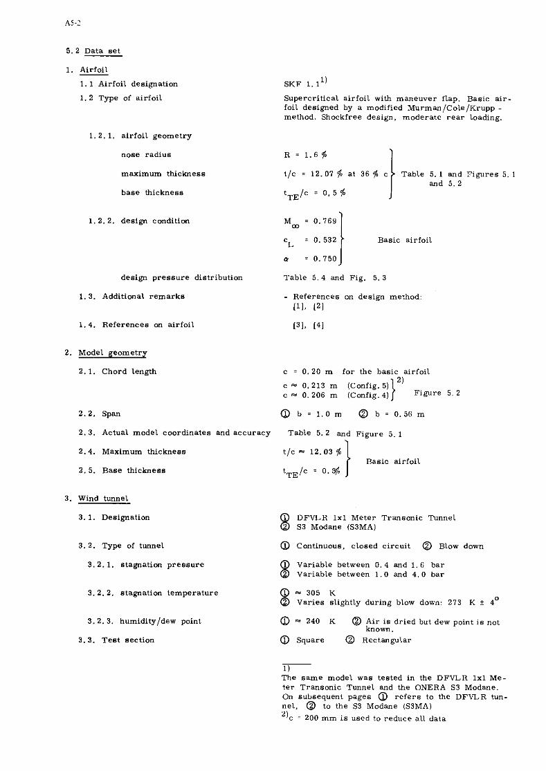
5. 2 Data s e t
1. Airfoil - 1. 1 Airfoil designation
1. 2 Type of airfoil
1 .2 .1 . a i r fo i l geometry
nose radius
maximum thickness
base thickness
1 . 2.2. design condition
SKF 1. 11)
Supercri t ical airfoil with maneuver flap. Basic a i r - foil designed by a modified Murman/Cole/Krupp - method. Shockfree design, moderate r e a r loading.
t / c = 12.07 $ at 36 $ c Table 5. 1 and Figures 5. I and 5 . 2
tTE/c = 0 . 5 %
Ma = 0,769
c = 0. 532 L
Basic airfoil
design p r e s s u r e distribution Table 5 . 4 and Fig. 5. 3
1. 3. Additional r e m a r k s - References on design method:
I l l . 121
1 .4 . References on airfoil P I , f41
2. Model geometry
2.1. Chord length
2.2. Span
c = 0. 20 m f o r the basic airfoil
c - 0.213 m (Config. 5) c - 0.206 m (Config. 4)
2.3. Actual model coordinates and accuracy Table 5. 2 and Figure 5. 1
2.4. Maximum thickness
2. 5. Base thickness
3. Wind tunnel
3. 1. Designation
3.2. Type of tunnel
3.2.1. stagnation p ressu re
t / c - 12.03 $ Basic airfoil
tTE/c = 0. %
1 DFVLR 1x1 Meter Transonic Tunnel 8 53 Modane (S3MA)
@ Continuous, closed c i rcui t @ Blow down
between 0. 4 and I . ti bar Varlable between 1 .0 and 4 . 0 ba r
3.2. 2. stagnation temperature @ - 305 K @ Varies slightly during blow down: 273 K f 4 0
3.2. 3. humidityldew point
3.3. Tes t section
a " 240 K @ Air i s dried but dew point i s not known.
@ Square @ Rectangular
- 1) The s a m e model was tested in the DFVLR 1x1 Me- t e r Transonic Tunnel and the ONERA 53 Modane. On subsequent pages @ r e f e r s to the DFVLR tun- nel , a to the S3 Modane (S3MA)
= 200 rnm i s used to reduce all data

3.3. 1. dimensions
3.3.2. type of walls a 6 $ open perforated (fixed porosity) walls with holes slanted 30' to the flow direction(Fig. 5.4)
@ 9.7 $ open perforated top and bottom walls , solid side walls, holes normal to flow direction (Fig. 5. 4)
3 .4 . Flow field (empty tes t section)
3.4. 1. reference stat ic p res su re a Plenum chamber p r e s s u r e
3. 4. 2. flow angularity
3.4. 3. Mach number distribution
3.4.4. p res su re gradient
3 .4 . 5. turbulence/noise level
3.4.6. side wall boundary layer
3. 5. Additional r e m a r k s
3.6. References on wind tunnel
4 . Tests
4. 1. Type of measurements
4. 2 . Tunnel/model dimensions
4.2. 1. heightlchord ra t io
4. 2 . 2. widthlchord ra t io
4. 3. Flow conditions included in present data base
-7
4.3. 1. angle of attack
4.3.2. Mach number
@ Side wall p r e s s u r e orif ice 8. 19 chords ups t ream of the model
0 t 0.05' @ < 0.05'
@ Flaps a r e adjusted to give z e r o p res su re gradient f o r the empty tes t section (Figure 5. 5b)
a Low noise level ( d n . F(n) e 0.001). Measured on body of revolution NACA RM 12. Low tu r - bulence level (measurements a r e in p rogress )
@ Figure 5. 6
a 2 6 / b 0. 18 a t M = 0.76, measured a t x / c = O m
and po= 1 bar
@ 2 6/b = 0. 21 a t Ma= 0. 40 0.18 a t M = 0. 60 0 .15 a t M ~ = 0.80
m measured at x / c = 0 . 2 5 and p = 1 bar
0
Reference on noise level: [5]
[el, [I1
- Surface p res su re distributions - Wake rake - Shadograph pictures (ONERA-tests) - Upper and lower wall p res su re distributions
(ONERA-tests)
Table 5. 5

4.3. 3. Reynolds number @ R e - 2 . 2 . lo6 @ R e - 7 . l o6
4.3.4. transit ion F r e e
position of f r ee transition Was not determined. @ Transit ion occurs gene- ra l ly due to adverse p res su re gradients. @ Transition occurs close to leading edge, since relatively high Reynolds number.
- transition fixing See Fig. 5. 715.8 f o r effect of Reynolds number and transition fixing (basic airfoil only)
4.3. 5. temperature equilibrium a Yes @ See 3.2. 2.
4. 5. References on t e s t s [8. 9.101
5. Instrumentation
5. 1. Surface p res su re measurements
5. 1. 1. p r e s s u r e holes - s ize
- spanwise s ta t ion(s)
Diameter = 0. 5 m m (d/c = 0.0025)
- Center line or i f ices were staggered in the nose region t 7. 5 m m
- 16 orif ices were located in spanwise direction a t x /c = 0. 50 on the upper su r face (Table 5. 3)
- chordwise positions Table 5. 3 and Figure 5. 1
5 .1 .2 . type of t ransducers and a CEC and Statham differential p res su re t r ans - scanning devices ducers plus Scanivalves
Range: t 10 psi Accuracy: + 0.40 $ FS
@ Statham differential p res su re t ransducer Range: f 25 psi Accuracy: ? 0. 12 p FS
5.2. Wake measurements
5.2. 1. typels ize of ins t rument(s) a Wake rake consisting of 47 Pitot probes and 14 stat ic probes. Pitot probes a r e spaced 2 . 5 m m apar t in the center region (Figure 5 .4a)
5. 2.2. s t reamwise position(8) 2 chords downstream of trai l ing edge
5.2.3. type of t ransducers and scanning devices
CEC and Statham differential p res su re t rans- ducers plus Scanivalves Range: i 5 psi Accuracy: * 0.3 $ FS
@ - Figure 5.4b and c - ID/OD = 0. 5 /1 .2 m m - 1 chord downstream of trai l ing edge - Statham differential p res su re t ransducer
Range: t 10 psi Accuracy: t 0.20 fb FS
5. 5. Flow visualisation
5. 5.1. flow field Shadowgraph pictures (ONERA-tests) [ I l l . Not included in data se t .
6 . Data
6. 1. Accuracy (wall interference excluded)
6. 1. 1. angle of attack sett ing f 0 . 0 2 ~ @ i 0 . 0 2 ~
6.1.2. f r ee s t r e a m Mach number - setting 0 i 0.001 @ i 0.002 - variation during one p ressu re s c a n a * 0.001 @Not known

6.1 . 3. p r e s s u r e coefficients
6 .1 .4 . aerodynamic coefficients
6. 1. 6. repeatability
a A c p - * 1 $ assuming worst possible combina-
nation of e r r o r s including an e r r o r of AM m = * 0 . 0 0 2 , evaluated a t Mm = 0.76 and max.
lCpl Obtained by integrating p ressu re distributions
A c = * 0.0003 m
a Average over the range of M and o investi- m
gated:
A C p 0. 5c m i 0 . 4 0 $ , A c L a i 0 . 3 $
A c D - * 1.2 $, A cmm 5 0.40 $
Q Mm > 0 . 5
A cL = * 0.005 A c D = * 0.0002
A c m = * 0.001
6.2. Wall interference correc t ions The data included a r e uncorrected.
6.2. 1. angle of attack
6. 2. 2. blockage (solidlwake)
The effective angle of attack can be approximated by:
A a = - 0 . 0 4 6 6 . c L
@ a t Mm a 0.75 and o L" 2': A a s 0.5' g
a Not yet well established, but can be approxi- mated by
2 AMm= -(1+0. 2 Mm ) . Mm. (0. 003) for c = 0 L
( M a c o r r e c t e d = Mm + A M m ]
6. 2. 3. s t reamline curvature ( l if t) a Can be approximated by:
@ at M m " 0.75 and o " 2' : g
(c. = ci + A c i ) 'corrected
6 . 2 . 5. r e m a r k s a c o r r e c t i o n fac tors were obtained empirically by testing different s ize models of the s a m e airfoil
@ Porosity fac tors were determined by matching c fo r t e s t s wrth solid and porous tes t section La
walls. The data obtained with solid walls were correc ted using the method of (121
6. 2.6. references on wall interference @ (121

6. 3. Presen ta t ion of data
6. 3. 1. aerodynamic coeff icients - Basic a i r fo i l : Tab l e s 5. 615. 7, F igu re 5. 7 (Ef fec t of Reynolds number and t rans i t ion fixing only)
- Airfoi l with extended maneuver f lap: Tables 5 . 61 5. 7 , F i g u r e s 5. 915. 10
6.3. 2. s u r f a c e p r e s s u r e s Bas ic Ai r fo i l : ' rable 5. 8 , F igu re 5. 8 (Effect of Reynolds number arid t rans i t ion f ixing only) Ai r fo i l with extended maneuve r f lap: Tab l e s 5 .81 5.9, F i g u r e s 5. 12 /5 .13
Compar i son ONERA-DFVLR: F igu re 5. 11 Wall p r e s s u r e d i s t r ibu t ions (ONERA-tes t s ) : Table 5. 9
6 . 3 .4. wall i n t e r f e r ence c o r r e c t i o n s Na inc luded?
6. 3. 5. c o r r e c t i o n s fo r mode l deflect ion ? No
6. 3 . 6. E m p t y t e s t sec t ion ca l ib ra t ion taken Yes in to account?
6.4. W e r e t e s t s c a r r i e d out in d i f fe ren t Data s e t inc ludes r e s u l t s f r o m ONERA-S3MA- fac i l i t i es on the c u r r e n t a e ro fo i l ? and DFVLR-1x1 M e t e r T ranson i c Tunnel - tes t s . If so , what fac i l i t i es . A r e da t a included in the p r e sen t da t a b a s e ?
6 . 5. T o be contacted fo r f u r t he r a E . Stanewsky information on t e s t s DFVLR-AVA Gottingen
10 BunsenstraDe D-3400 Gdttingen
@ J. J. Thibe r t ONERA 92320 Chatillon ( F r a n c e )
7. Re fe r ences
[ I ] KOHL, P. ZIMMER. H
[2] STANEWSKY, E , ZIMMER, H.
[3] ZIMMER, H.
[4] WELTE, D.
[5] HOLST. H. GROSCHE, F. R. BINDER, B.
The design of a i r fo i l s f o r t r a n s p o r t a i r c r a f t with improved high speed c h a r a c t e r i s t i c s DORNIER GmbH, Repor t 74/16 B, 1974
Development and wind tunnel t e s t s of t h r e e supe rc r i t i c a l a i r f o i l s f o r t r an spo r t a i r c r a f t Z. F lugwiss . 23 (1975), Heft 718
Aerodynamic design of the SKF-a i r fo i l DORNIER GmbH, Note B F 10-0242
Definition of th ickness and des ign condit ions f o r the SKF-a i r fo i l DORNIER GmbH, Note B F 10-0180
Measu remen t of p r e s s u r e f luctuat ions in the Transonic Wind Tunnel of the DFVLR-AVA Gottingen DFVLR-AVA Repor t I B 75 A 17, 1975
[6] HOTTNER, TH. T h e t ransonic wind tunnel of the Aerodynamische Versuchsans ta l t LORENZ-MEYER, W. Gottingen
DGLR-Yearbook 1968, pp 235-244
r 7 I Note technique ONERA No. 166 (1970) and ONERA No. 203 (1972)
[8] STANEWSKY, E . M ~ ~ L L E R , H.
Wind tunnel invest igat ion of a two-dimensional supe rc r i t i c a l wing with maneuve r f lap and s l a t DFVLR-AVA Repor t I B 251 75 A 35 and I B 251 75 A 35a

[g] MOIROUD, H
[ l o ] CONSTANT, A.M.
[I21 MOKRY, M.
speed of sound
span, tunnel width
E a s a i s h S3MA d'un profi l Dornier en 6coulement plan ONERA P. V . No. 1/3207 ANG (1976)
Etudes en courant plan relat ives au project Dornier de voilure supercri t ique ONERA R. T. No. 8/3207 AN
Shadograph pictures of the ONERA-tests DORNIER GmbH, Note BF 60-0425
Higher-order-theory of two-dimensional subsonic wall interference in a perforated wall, wind tunnel National Research Council Report L R 553, 1971
model chord K maneuver flap
p res su re coefficient [(p-p ) /q ] T E trai l ing edge m m
pressu re coefficient a t %= 1 US upper surface
lift coefficient L S lower surface
pitching moment coefficient (based on 0 . 2 5 ~ )
d rag coefficient
frequency of p r e s s u r e fluctuation
9
Re, Rec
t
Subscripts
m f rees t r eam conditions
reduced frequency, f . c/V m
f r ees t r eam Mach number
local Mach number
tunnel height
dynamic p res su re
Reynolds number, p m Vm. c /pm
maximum thickness
f r e e s t r e a m velocity
.. Y coordinates (see Fig. 5.1) Z
"g' " geometric angle of attack
B
6 maximum thickness, t / c boundary layer thickness(sidewal1)
P density
P dynamic viscosity

a h 5. 1 Design (:oordlnates for rhe a i r f o ~ l S K F 1 . i irlclud~ng maneuver flap) Hasic alrfoil - I'pper suriare
sore
F z lmml
- 10.254 - 10.331 - 10.396 - 10.444 - 1 0 484 - lo. 515 - 10,538 - l o . 552 - LO. 558 - LO. 554 - 10. 542 1 - 10. 521
Basic airfoil - Inner contour
-i r: l50mm
Also see Rg 5 1
I Note: The coordinates given here are actual model, coordinates
I Maneuver nap
hard Line I
NG,. I.di", 1 ; 1%
r .150mm
Note: The coordinates given here are - actual. coordinates. They are based on the chord line of the basic airfoil,

1T_ahle 5. 2 Measured coordinates of the airfoil SKF 1 . 1" I i.ourer. surface
Note: - For plot of measured error of the manufactured airfoil s ee Figure 5 . 1
Table 5 . 3 Coordinates of the pressure orifices - Basic airfoil
7. 052
10.243
1 5 . 7 1 2
20.812
25.709
32. 756
4 5 0 4 0
55.039
67.035
8 2 0 3 2
100.026
115.022
131. 022
') See Figure 5 . 1 . The coordinates shown here are actual coordinates (except spanwise orifices)
1 ) Only basic airfoil model. For maneuver flap s e e Table 5 . I
6. 504
1 .177
9.276
10.266
10.893
11,804
12. 756
13. 238
13.575
13.696
13,510
12.984
, 1 7 5 9
6. 574
7 7Y6
9 .278
10.248
10.960
11. 743
12.766
13. 322
13.618
13 616
13.448
1 2 . 8 5 0
11. 734
11,1110
0 . 021
0 ,002
. 0.018
. 0 0 3 3
. 0 . 061
U O l O
0 . 083
0 .043
. OOZO
. 0.082
. 0. 144
. 0 . 025
7.1152
1 0 4 2 3
1 1 . 5 4 8
20.296
26.244
32. 756
45 .040
55. 039
87.035
83.033
101.029
li5.023
127. 019
4 l i 7 1 ;
- 5. 498
- 6 295
- 7 .220
- 8 .023
- 6.767
- 9 ,771
- 10. 288
- 10.542
- 10.254
- 9. 105
- 7 . 6 8 8
- 6 220
4 . 71111
- 5. 5 3 0
- l i . 3 3 4
- 7 264
- 6.036
- 8. 702
- 9.674
- 10.160
- 10.426
- 10. 198
- 9 .098
- 7 .670
- 6 .152
0.1112
11.11:11
O O J ' I
0 0 4 4
0.013
- 0 . 0 6 5
- 0. 097
- 0.108
- 0.116
- 0 056
- 0 .017
- 0 .018
- 0 . 0 6 8
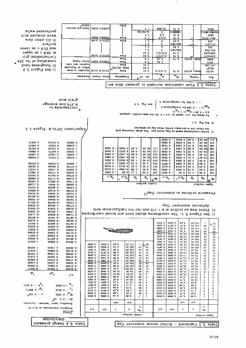
s ~ l e m paln.zoj.zad y$!m pauxelqo slam
Elep J w i o l l v (E aae3.111~
Jam01 UO 3 $ S Z pUE ~ a d d n uo s 6 0 s l e $ 7 ~ 2 runpun.zOq.ze3
022 'ON jo Buns!suos 1 pueq ssauq2nox ( 2
z 'S a.zd!J aas ( I
i "o!,..'d1,"~ 20, $go .0 - = z ' s '81d aaa
s "O!,.."S~JYOJ 401 )SO 0 - . J / ~ S .
=in= + .insx + S S O ; 3). nndiuoo IIOJJIV ~1s.q aq& JOJ o . s i x uo pam~q S I X ul.LqO ol +
9ZLSO '0- LOL6L '0- OSLBO '0 6EOTO'O 8EP89'0- 00SS0'0 l S T 6 0 0 E E S S i O - OSI iO ' 0 EZSOZ 0 EGOSZ'O- OOSEO'O LEOZE 0 SOSPO'O- OOSZO'O i O t Z t ' 0 999S1'0 OSL10'0 ILSZS ' 0 06862 '0 OSE10'0 98998'0 OLLSt ' 0 OSLOO'O O I E E O I 68688 ' 0 OSZOO ' 0
85892 '1 6 I t F 1 'I OSE00'0- SLSEO'I P8OS6'0 OOSTO'O- 8SE8L'O 66SEL'O OOSEO'O- 6 1 8 1 5 0 6StOS ' 0 OOPIO'O- SEOSE '0 ES6LZO OOSLl O - SSP21 '0 SStSI 'O OOOSEO- 01660'0 15660'0 OOSLS'O- LISSO'O 81990'0 ooses.o-
dalj .zai\naueru palsaljap ql!m uo!le.~nB!juoa ayl JOJ mru O L I = x i e a>!j?.zo ou sem a=aqL (Z
saleulploos l snlss aJe aJaq umoqs saleu!pJoos aq& ' 1 'S a ~ n 8 ! ~ aas (1

I Table 5 . 6 DFVLR 1x1 Meter tests . Aerodynamic coefficients1) 1
Table 5 . 7 ONERA SSMA tests . Aerodynamic coefficients 1)
1) All data are uncorrected 2 ) See Figure 5. 2 3) See Foot-note '2) of Table 5 . 5 4) Solid test section walls
Table 5 . 8 DFVLR 1x1 Meter tests . Pressure distributions I a . Basic airfoil (See Table 5 . 6 for test conditions and aerodynamic coefficients)
RVI 60 Run 84 Run 157 R XII CP CP C P ML
UPPER S U l F l C E . ..

Run 63 *(I X I I
UPPER SURFICE L 0.0 2 0.0012 3 0.0OBI + 0.0155 5 0.0250 6 0.0315 1 0.0645 B 0.0791 '1 0.0990 10 0.1400 11 0.1100 12 D.2200 13 0.2595 14 0.2995 15 0.3391 Ib 0.3100 11 0.4200 18 0.4600 19 0.5000 20 0.5395 21 0.5195 22 0.6200 L1 0.6600 2, 0.7000 25 0.7685 2 6 0.7985 21 O.BC90 28 0.8990 29 0.0695 30 0.97+5 3, 1.0000
LOWER SURFICE
Table 5.8 Continued
Run 2 3 4 NR X I I
UPPCR S U V F l C E
a . Basic a i r fo i l (See Table 5. b f o r tes t conditions and aerodynamic coefficients)
I Run 160 ML NII
UPPE 0.1718 1 0.6860 2 0.8645 3 0.9158 r 0.9936 5 1.0866 6 1-1965 7 1.2685 8 1.3111 9 1.3216 LO 1.3.00 I1 1.3438 12 1.3469 I3 1.3693 14 1.3110 15 1.3727 16 1.36.8 I7 1.3281 1s 1.1083 19 0.9996 20 0.9531 21 0.9330 22 0.9223 23 0.9023 24 0.8191 25 0.8526 26 0.8225 27 0.1962 211 0.7625 29 0.1539 30 0.7+62 31
LMEW 0.111e 1 0.1120 2 0.3455 3 0.5138 I 0.6259 5 0.6958 6 0.1298 1 0.1629 8 0.185. 9 0.8235 lo 0.0W 11 0.7959 11 0.7294 I3 0.6153 11 0.6601 15 0.6*23 16 0.6411 17 0.6601 18 0.7662 1 9
X J L R SURFIL 0.0 0.0032 0.00117 0.0155 0.0250 0.0315 0.0615 0.0191 0.0990 O.L*OO 0.1700 0.2200 0.2595 0.2995 0.3397 0.31100 0.6200 0.1600 O.IO0O 0.5395 0.51PS 0.6200 0.6600 0.T000 0.7485 0.7985 0.8.90 0.8990 0.9495 O.P7$5 1.0000
I SURFACE 0.0 0.0032 0.0070 0.0182 0.0587 0.09111 0.1500 5.2000 0.2492 o.3r92 O.,.92 0.5500 0.6650 0.7500 0.0000 0.8.90 0.a992 0.9495 1.0000
b. Airfoil with deflected maneuver flap 1)
uc21 I a,," I?& .. ! Run 235 I r C T l l l N H I
1) See Table 5 .6 f o r tes t conditions and aerodynamic coefficients. "section IIS: See Figure 5. 1

Run 236 NR X I L
UPPEP s w 6 a c r 1 0.0 2 0.00'2 3 0.5107 C 0.0'55 5 0.0150 6 O.O?'! 7 0.0615 B 0.019' 9 0.0190
10 0.1420 11 0.7700 12 @,2100 1 1 0.2595 1, 0.20 '5 15 0.3191 l b 0.1900 ? 7 5.4200 18 0 .6600 I 0.5300 20 0.53'5 21 0 . 5 1 p C 22 O . L : O o 2 3 0 . b l O D 2L 0.7000 75 0.7575 26 0.7"'r 27 3 . P 2 7 5 7 5 0.8'0"
LOYEI I S " T r & r C 1 0.0 2 0.0032 3 O.OO'0 C 0 . 0 ? ' 2 5 0 . 0 4 P 1 6 0.0'"
0.:500 8 0.2000 9 0.2192
1 c J.3<CI> I 1 0.4'92 12 0 . 5 5 0 2 I 3 0.6453 IC O.'COO I 5 0 . 7 5 0 0 1 6 j . 7 5 2 ' 1 7 0.7'70 19 0-IC"O 19 O.PI25 20 3 . 8 5 0 0
Table 5. 8 Continued
Run240 NR X I L
UPPER SUPFICE 1 0.0 2 0.00'2 3 0.0087 6 0.0155 5 0.0250 b 0.0365 I O.O6LS 8 0.6747 9 0.0990
10 0.1+03 1 1 0.1700 12 0.2200 1 3 0.2595 LL 0.2995 15 0 .1391 16 0.3800 1 7 0.1200 1 8 0.rbOO 1 9 0.5000 20 0 . 5 3 5 21 0.5195 22 0.t200 23 0.tbOO 2, 0.7000 25 0.7525 26 0.7815 27 0.8275 2 8 0 .8500
LOWER S U I F L L E 1 0.0 2 0.00?1 3 0.0010 4 0.D'PZ 5 0.0487 6 0.09e7 7 0.1500 8 0.2003 9 0.i492
10 0 . I ' - 7 11 0.'492 1 2 0.:.00 1 3 0 . 6 4 5 0 16 0.1003 1 5 0.7500 1 6 0.7525 1 7 0.7670 18 0.7900 1 9 O.PO25 20 0.?500
b. Continued
SECTION CP
1)
~~ ~ ~
1 . L O 2 9 1.+080 1 LOYFR I U I F L C E :.LO52 0.0 0.71'9 0.3931 l.LO23 I 0.0160 0.982G 0.2298 ? 3'152 0.0440 0 . 6 5 3 5 0.4260 j:1937 1 0.1060 0.6326 O.L36T
1.1213 0.6010 0.5058 0.+9Lb 1.0519 1 0.5050 0.1121 0.5350 ].no36 1 1.0000 0.2103 0.6183 0.9'?! 0.8779 Run 237 F L I P 3.R5Q7 XI1 0 . * 3 ! 1 UPPER SmFLCL
0.7189 0.3936 3.3130 -0.45L5 0.8.32
0.'392 O.O*LO -0.1813 0.7651 0 . 0 0.10.0 -0.2125 0.7807 1 0.1640 -0.7391 0.9841 0.""'. O.2SBO -0.7561 0.9907 5.'7'2 0.?100 -0 .7637 0.9939 0 . 5 5 1 3 0.4100 -0.6073 0.9319 0.5847 0.5170 -0.3176 0.8212 0.*!63 0.7180 -0.1910 0.7756 O.bL!O 0.9000 -0.1170 0.7$+8 3.6626 1.0000 -J.0311 0.7122 U . b C 7 7 0 . 6 ~ z g LOYEP SURFLCE 0.5787 0.0 0.7189 0.3*16 0.5725 0.0160 0.9710 0.2393 0.5715 0.0440 0.6265 0.6391 0 .1704 0.1060 0.6047 O.LL9P 9.rp?7 0.2510 0.55+1 0.1732 0.5639 0.4010 0.5130 0.4917 0 . 5 5 5 6 0-b3lO O.LI'L 0.5716 0.8202 0.8053 0.11hL 0.5151
1.0000 -0.0316 0,7122
H I I Run240 rLnp *L X/L CP
UPPER SURFLCE 0.0 I 0.0 0.6600 0.6196 0.0130 -9.5460 0.6047 I 0.0440 -0.221T 0.0901 0.1 060 -0.1751 0.7850 0.1610 -0.6155 0.8691 1 0.2'80 -0.6144 0.9819 0.3300 -1.1281 1.0557 0.L100 -1.084: I.OS+A 1 0.5770 -0.27'4 1.1011 0 . 7 3 8 0 -0.0261 1.1052 0.9000 0.103' 1.0%8 1 1.0000 0.1741
1.1172 ;:;160
0.6600 1.1263 !.0000 1.1217 0-OLLO 0.6147 L.'195 0.1060 0.6019 1.136' 1 0.2531 0.55011 1 .?543 0.LOlO 0.5-1'0 1.1563 1 0.6010 0.1172 1.1609 0.8050 0 . ? 8 2 1 1.1912 1.0000 0.1711 9.76?7 :.2583 Run241 FLbP 1.0569 X I 1 CP 0.9522 l l P P I l l SIlPFdCE 0.90'2 0 -0 0.7076
3.1130 -0.5125 0.Q 0 . O L L O - 0 .20 *7 O.LL(O 3.1140 -0.2326 0.6199 O . : b 4 0 -1.0957 O . ' L 3 L 3.2'80 - O . h t Z S 0.8068 0.""" -0.5863 0.8?01 1.C100 -0 .4367 0.e476 0 . 5 7 ' 0 -1 .1579 0.8t57 3.T1R0 -O.O!?' 0.8750 1 . 1 0 0 3 3.09Pq 0 . 4 t . R 7 ' .0000 0 . 1 5 6 7
Run 237
N9 I / L UPPER SURFACE
1 0.0 Z 0.0032 3 0.0081 , 0.0155 5 0.0150 6 0.03'5 1 0.0645 8 0.01PI 9 0.o'loo
10 0.1'00 11 0.1100 12 0.2200 1 3 0.2595 1 1 0.2995 1 5 0.3397 1 6 0.3800 17 0.4200 1 8 O.LbO0 19 0.5000 20 0.5191 21 1.5795 22 0.6200 23 0.6600 - 2 0.7000 25 0.7525 1 ; 0.7815
0.8275 28 0.8500 I LOYFR S U I F L C E
I : :::032 0.3070 I : 0.0182 0.9187
0.2003 9 0.1192 I I 0 0.3192
I 1 0.*"2 0.5500 I :: 0.6450 0.7001 I :: 0.7500
16 0.7525
0.7900 0.8025 1 0.8500
NR I1L UPPER SUPFACf
1 0.0 2 0.0032 3 0.0087 * 0.0155 5 0.0250 6 O . C I 4 . 7 O.CC.5 8 0.0797 9 0.0a90
1 0 0.1400 11 9.1709 12 0.2z00 13 0.2SG5 LL 0.2??5 15 0.3397 1 6 0.3800 17 0.6200 111 O.'~OO 1 9 0.5000 20 0 .53 '5 21 0.5745 22 0.6200 2 1 O.LCOO
1.iooo
2 0.OC32
0.0-87
10 0.3L92 1 1 1 0.1192
1 2 0 . 6 5 0 0 0.6150
0.7500 1 0.7525 1 7 0.7610 I :g 0.??00
".PO25 20 0.8500 I
1) See Table 5. b' for test conditions and aerodynamic coefficients. Section HS. See Figure 5. 1


Run 230 NR X I I
UPPER S U R F I C E 1 0.0 L 0.0012 3 0.0087 + 0.0155 5 0.0250 6 0.0345 7 0.06'5 8 0.0797 9 0.0590 10 0.1400 11 0.1100 12 0.2200 13 0.2595 14 0.2995 1 5 3.3'97 It 0.3900 1' 0.4700 18 0.6600 19 0.5301 20 0.5'95 21 0 . 5 7 9 5 22 0 . 6 2 0 0 23 0.6600 2* 0.IOOO 15 0.7525 26 0.7815 21 0.8215 28 0.1500
LOYER I U V F A C E > 0."
Table 5 . 8 Concluded
Run 271 NR I / L
UPPE9 IUCFLCE
b. Concluded
S E C T I O N C P
1)
1) See Table 5. 6 for test conditions and aerodynamic coefficients. "section HS: See Figure 5. 1


Table 5 .9 Concluded b. Top and bottom wall p res su res
1) Solid tes t section walls
. 11000
.09000
.07000
.05000
.03000
.01000 -.01000 -.03000 -.05000 -.07000 -.09000 -. 11000 - . L3000 -. 15000 -. 20000 -. 25000 - . 28000 - .34000 -. 44000 -. 54000 -.64000 -.63000 -1.2300
Bottom w a l l -1.78000 -1.48000 -1.14000
- .64000 - .54000 -.49000 -.39000 -.34000 -.25000 -.ZOO00 - . I5000 - . I 3 0 0 0 7 . 11000 -.09000 -.07000 -.05000 - .03000 -.O1000
OLOOO .03000 . Q 5 0 0 0 . , 0 7 0 0 0 ,09000 ,11000 ,13000 ,15000 ,20000 . 25000 ,35000 ,39000 ,49000 ,57000 ,62000 ,72000
2 ) The leading edge of the model i s located 0. 107 m upstream of x = 0 fo r the wall p res su re or i f ices
- . I 4 9 6 - . I584 - . 1623 - . 1660 - . 1732 -.L648 - . I648 - . I620 -.I515 -.I440 -. 1335 - . I076 - . 0 8 1 4 -.0447 - 0 4 5 1 -.O164
,0089 0 2 3 6 ,0249 , 0331 . ,0338 .018 l ,0169
,0321 .0187 ,0112 ,0546 .07" ,0730 ,1071 ,1222 ,1466 ,1640 ,1625 ,1686 ,1810 ,1862 ,1840 , 2044 . ,861 ,1895 ,1846 .181(J ,1881 ,1673 ,1745 ,1854 ,1631 , 1 6 1 4 ,1395 ,1164 . 0 1 l 9 , 0 5 0 3 .OZol
- .0183 ,0070 ,1289
-. LLZZ - . 1186 - . 1201 - . 1 1 9 4 - . 1219 - . I166 -. 1 1 4 4 - . I118 .. 1050 -. 1007 -.0848 - .0760 ..O659 - . 0 5 7 4 - . a323 - .0071 - . 0 0 8 2
,0208 ,0166 ,0223 ,0818 ,0128 ,0165
,0329 , 0169 , 0 1 2 4 ,0389 , 0 5 6 4 ,0600 ,0810 ,0945 ,1147 . 1299 . 1427 . ,280 . ,431 . 1480 ,1439 . 1705 ,1457 ,1489 , 1501 , 1 4 8 4 . 1536 . 1342 . 1439 . 1373 . 1343 . 1337 , 1195 ,1039 ,0691 ,0515 ,0236
-.0096 ,0132 . 1379
-. 1701 -. 1615 -. 1855 -. ,877 -. ,997 - . 16.50 - . 1816 - . 1805 - . 1722 - . I628 -. 1475 -. 1217 .. 1036 -.O896 -.0448 - .0075
,0140 , 0 2 7 2 ,0325 , 0 3 9 5 ,0447 , 0 2 0 4 ,0172
,0369 ,0194 ,0121 ,0611 ,0645 , 0 6 6 4 . ,148 . 1355 ,1617 . 1788 . 1546 . 1714 . 1807 . 1964 . ,866 . 2129 . 1948 . 1963 . 1867 . 183+ ,1853 ,1642 ,1664 ,1512 ,1533 . 1539 . 1264 . I008 ,0593 ,0351 ,0022
-.042L -.DL75 . 1127
-. ,353 - . 1461 - . 1508 -. 1537 - . 1574 - . I 4 5 3 -. 1425 - . I 8 5 2 -. 1218 - . I077 - .0960 -.O706 -.O562 -.O419 -.O057
,0219 , 3 9 4 . 462 ,0419 ,0430 ,0463 ,0212 ,0205
,0415 .OZl l , 0 1 4 3 ,0533 0 7 4 2 ,0751 ,0968 ,1139 ,1336 . ,163 . ,611 . 1469 . 1583 . 1669 . 1598 ,1852 . 1623 . 1660 . 1657 . 1618 . 1695 . ,519. . I566 . 1487 ,1473 ,1469 . 1322 , 1 1 2 5 , 0773 , 0 5 7 2 , 0 2 0 2
-.0189 ,0056 . ,392
. . l 55Z
.. 1127
.. 1763 - . ,831 - . I886 - . I747 - . I683 - . I586 - . I428 - . I269 .. 1069 -.0789 - 0 5 9 6 - .0457 - .0051
,0281 ,0457 ,0548 ,0488 ,0497 ,0532 ,0255 ,0200
,0422 ,0220 ,0132 ,06111 ,0837 ,0869 ,1130 ,1326 ,1528 . 1654 . 1804 ,1640 ,1781 ,1898 ,1771 . I 9 6 6 ,1760 ,1788 ,1746 -1696 ,1767 ,1531 1 6 2 9 ,1510 ,1485 ,1468 ,1262 ,1013 ,0624 .0427 ,0149
-.Om0 -.On37
, 1 3 9 2
..0870 - 0 9 4 1 ..OS36 -.O880 - . 0 9 1 2 ..0799 -.0817 -.0840 ..0761 -.0758 ..0722 -.0691 ..0560 - .0548 - .OM8 - .0242 -.0179 - .008 l -.0065
,0025 ,0074 ,0021 ,0148
,0294 ,0143 ,0096 ,0235 , 0 3 1 6 ,0336 ,0489 . a 5 7 1 ,0809 ,0691 ,1099 ,0805 ,1038 ,1109 , 1025 . 1274 . 1084 . 1 1 4 4 . 1118 . 1072 . 1154 . 1021 . 1082 . lo07 . 1020 ,1002 ,0843 ,0828 ,0547 , 0 4 5 1 , 0283 ,0098 ,0286 . 1261
. . 0901
..O984 - .0896 - .a945 -.0986 ..0882 - .0660 - .0869 ..O616 - .0796 . . O 1 8 0 - .0637 . .a566 - . 0 5 4 4 - .a362 -.0180 -.0086
,0013 ,0025 ,0073 , 0 1 6 4 , 0 0 8 4 ,0170
. U 3 1 U ,0137 ,0116 ,0267 ,0437 .0425 , 0 6 2 2 ,0756 ,0826 ,1070 ,1234 ,1065 . 1169 . 1216 . 1216 . ,433 . 1251 . 1 2 9 4 . 1290 . 1267 ,1306 , 1 1 4 7 . 1253 . 1159 . 1162 . I208 . 1064 ,0878 ,0615 ,0487 ,0302 ,0023 ,0253 ,1318
..0969
.. ,036
.. 1028 -.O969 - . I030 ..0865 - .0950 -.0940 ..a881 - .a869 -.0811 -.666 ..0597 - 0 5 5 7 -.O342 - . O 1 4 5 - .0012
, 0 0 8 3 ,0070 , 0 1 3 3 , 0234 ,0085 ,0179
,0338 ,0128 ,0133 ,0308 ,0470 ,0497 ,0672 ,0845 ,1019 . 1161 . 1291 ,1145 ,1277 ,1343 ,1327 , 1 5 5 7 . 1380 . 1366 . 1370 . 1387 . 1421 . 1252 ,1374 ,1256 ,1240 ,1267 ,1143 ,0962 ,0645 ,0506 ,0338
-.0008 , 0 2 1 2 . 1146
. .3531
. .3892
.. 4123 -. 4483 - . a 8 1 ..4936 -.5026 ..4778 ..4171 . .4111 .. 3690 - .3173 -. 2822 - . 2531 - . I 8 6 5 -. 1349 - . I 1 0 5 - .0664 - .0470 ..0216 ..0030
.OOL5
.OIZI
,0160 ,0089 ,0060 ,0211 , 0 3 1 4 ,0321 ,0477 ,0618 , 0 7 4 5 ,0836 ,0952 ,0789 ,0873 ,0898 ,0871 . LO91 ,0839 , 0 8 6 2 , 0 8 1 3 , 0802 , 0844 ,0651 ,0660 ,0605 ,0603 ,0567 ,0448 ,0306 ,0077
- .0057 - . a174 - .a320
,0014 , 1 0 6 3
- .3731 . . a 9 7 .. 4253 -. 4606 -.1901 ..5093 - .5065 -. 4794 -.1428 - .4Ll7 -.3696 - .3183 -. 2793 -. 2581 - . L 6 l l - . 1300 -.LO27 - .0649 - 0 4 7 - .0202 -.On23
,0054 ,0109
, 0 1 3 4 ,0120 , 0 0 4 2 ,0192 ,0338 ,0503 ,0366 ,0609 ,0750 ,0727 ,0885 ,0697 ,0769 , 0 7 9 3 ,0673 ,0691 , 0 5 9 4 , 0 5 8 2 .0562 ,0526 , 0 5 5 1 , 0 3 4 2 ,0360 ,0250 , 0 2 7 4 ,0263 ,0096 ,0018
-.0251 - . 0 3 1 0 - .0402 - . O X 3 - .OH6
,0902

Geometric data: Chord c = 200 m m Max. t / c = 1 2 . 07 a t 3 6 % c Trail ing edge thickness tTR/c = 0. 5% Maneuver flap chord cK = 50 m m
Maneuver F L ~ Contour leee ~ l g . 5 . 2 )
e c r n - .&. / / &
.- All dimensions given a r e in mi l l imeters
a . Airfoil contour (also s e e Table 5. 1)
for m&l cowdlnatesl /
// Chwd line [reference
!%sic Airfoil
/ Mm
M o n m Flap
5 0 -
I R Pressure Orifices
b. Location of p res su re or i f ices (also see Table 5. 3 )
c . Measured e r r o r s of manufactured airfoil (a lso see Table 5. 2)
Figure 5. 1 Airfoil SKF 1. 1 - Contour and location of p res su re or i f ices

- Canfiguration 5 --- Configuration 6
I Reference point d pitchng moment
x)c:gFrn }see Fig.5.1 Ln w cK = 50 rnm
xHB= 120rnrn10.6.c I
[Airfoil SKF 1.1 [basic airfoil 1 I
\ m l y r.r these configurations are included. A, ONERA only Configuration 5 in addifion to the basic airfoil was tested.
Figure 5 . 3 Design pressure distribution
Figure 5 . 2 Flap configurations investigated

Strotn Go
Woke R o b
+ Flow
"Oft ALL dimenshons are m mllllmeters
GeOmetrlc Data
M o d e l span b = ,000 mm
Tunnel helght /chord H / c 5
Span/chord b / c 5
Solid blockage t / H 0 023
a. DFVLR 1x1 Meter Transonic Tunnel
removable wall
I Detai l of the h 1322 762
p e ~ f o r a t i o n
moving flaps
... - 7 . 2 ~ ~ , " ~ 3 ~ , ,
perforated w a l l ' yOOo
-3 - 2 -1 0 1 rn 5 -
MODEL INSTALIATION I N TI+ S MA TEANSONIC WIND TJNNEL 3
Wind
b. ONERA SSMA
Figure 5 . 4 Test set-up

0 1.7 - Woll dvergerre I side w l l s l H = 1000 mm Mk- fictitious plenum chamber
Mm Mach number
d ~ & o n L s t m i g h t Fer(odion 4 a. DFVLR 1x1 Meter Transonic Tunnel
window axis Pt.1.2 bur
L rnJ 1.1
,,.,,,,,,,,,' 0.2
0.90 _.-._. -0.2
0.46 walls ., r,,,,,,, 7~7,
b . ONERA S3MA
1 t wake measurement section
Mach number distribution (empty test section)
Figure 5. 5 Empty test section Mach number distribution
Figure 5. 6 Noise level [ONERA SSMA)
\ Microphone mounted on the top wall one chord upstream of the model leading edge
Mach - ___)
40
5
0 5 1.0
0
\
- . --

'Isre Table 5 . 5
']see Table 5 . 5
Figure 5. 8 Effect of Reynolds number and transition fixing - Pressure distributions

SKFl1 wlh extended rmnPIM( flop
Conf#gurd\on 5 l&=070
1.6
=L SKF 11 wlh extended
1.L rnon~lver flap GmfiguDtlon 5 M,= 0.76 Free honwbon
1.2 o DFVLR-Wr R p x 2 . 3 1 0 ~ n ONERA-tests Rez7.7 - lo6
IreeTable 5.6 15.7 t~ 1.0 &ids l
Figure 5 . 9 Aerodynamic coefficients - \
Angle of attack variation
Figure 5. 10 Aerodynamic coefficients - Mach number variation
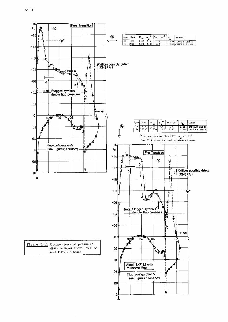
y m Hun
0 2 2 1 0 .60 3 . 0 2 . 0 1 1.054 DFVLR 1x1 M 8 6 1 0 0 .60 Z . O G 8 . 6 1 1.038 ONERA S3 MA
distributions from ONERA and DFVLR te s t s
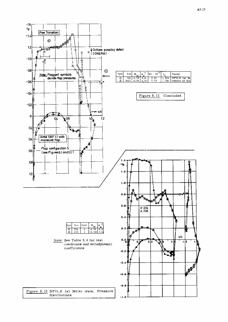
~ ~ r n l ilunl M I e ' l ~ . ' ] cL I 'Tunnel m g
0 241 0 . 7 8 3.0 2. 31 1 . 2 2 3 DFVLR 1x1 M A 9t iZ1 0 . 7 6 2 . 0 5 7 . 7 3 1.2011 ONERA S3 M A
Figure 5.11 Concluded

Note: See Table 5. 6 for test conditions and - aerodynamic coefficients
Figure 5. 12 Continued

Note: See Table 5. 6 for test conditions and aerodynamic coefficients
Figure 5. 12 Concluded

Note: See Table 5 . I for aerodv- narnic coefficients
Figure 5 . 1 3 ONERA S3MA tests. Pressure distributions


6. AEROFOIL RAE 2 8 2 2 - PRESSURE DISTRIBUTIONS, AND BOUNDARY LAYER AND WAKE MEASUREMENTS
by
P. H. Cook, M. A. McDonald and M. C. P. Firmin
Royal Aircraft Establishment. Farnbarough, Hants, United Kingdom
I. INTRODUCTION
The examples presented have been selected to give a range of conditions from wholly subcritical flow to conditions where a comparatively strong shock wave exists in the flow above the upper surface of the aerofoil. In at least one example some boundary layer separation occurs due to the shock wave but reattach- ment occurs ahead of the trailing edge of the aerofoil.
The data include surface pressure measurements and mean flow boundary layer and wake profiles deduced fromtraversesof pitot and static pressure measuring probes. Where the measurements have been made close to the aerofoil (ie xlc r 1.025) the probes have been mounted from within the model, thus keeping the probe support interference to a minimum.
In all examples presented, attempts have been made to fix boundary-layer transition near to the lead- ing edge af the aerofoil (xlc = 0.03 or xlc = O.11), but as the measurements were made for a range of Reynolds numbers and Mach numbers, in some cases without changing the transition trip, the roughness size may be larger than would normally be used at the higher Reynolds numbers. In some examples the presence of the roughness has clearly had a strong local effect on the pressure distribution. The local disturbance to the boundary layers has not been measured but the downstream developments, of course, include the influence of the trip.
In parts of the flow the normal boundary-layer assumptions are violated by the normal pressure gradients which are significant near the trailing edge of the aerofoil and in the region of a shock wave. Ideally it is necessary to take account of the normal pressure gradients in defining the boundary layer integral parameters and in one example the data are presented with and without allowance for the normal pressure gradients (Case 9 - configurations CI and C2 respectively). Where boundary layers are measured downstream of a shock wavethe total pressure measured by the pitot tube is affected by the total head loss due to the shock wave. However the edge of the boundary layer was usually well defined. For traverses made in the near wake the measurements have been treated as two separate boundary layers, without extra- polation to a surface but with the division between the two parts taken at the point of minimum velocity ratio. Examples are given of traverses made well behind the trailing edge of the aerofoil the purpose of which has been to determine the total drag. Consequently the traverse has included as far as possible the complete region behind the shock wave as well as the viscous wake. The definition of momentum thickness is then different from that used for the boundary layers where shock losses outside the viscous layer are excluded.
In the data reduction it has been assumed that the flow is two-dimensional, and so the surface pressure distribution measured near the centre section of the aerofoil (see Fig 6.4) has been used in nearly all cases as the value of the static pressure at the aerofoil surface for determining the velocity profiles and any variation of the static pressure within a profile is only taken into account if actual measurements exist. The variation of the static pressure through the boundary layer andlor wake has normally been obtained from a traverse at one spanwise station and used at others. Although for the main part of the data this assumption is satisfactory, there are cases, for instance when the boundary layer is close to separation, where a significant difference may exist. The data presented in the tables have as far as possible been presented so that re-analysis is possible by the reader.
2. BOUNDARY LAYER AND WAKE ANALYSIS
2 . 1 Measured profiles
The local Mach number (M,,), within the boundary layer or wake, has been obtained from values of total pressure (P ) and static pressure (P ) at the measurement point from the equation
0 L
When ML S 1 then Po = Po . the measured value of the pitot pressure, and ML can be obtained directly. M
When ML > I then PO # POM and is given by
Thus for ML , 1 equations (I) and (2) were solved by iteration. Where the variation of static pressure has not been measured at the appropriate xlc location, the static pressure is assumed to be constant through the layer. The static pressure used in determining the local conditions is quoted for each point or profile as appropriate.


The experimental values for 6* and 9 were then obtained by numerical integration of Eq.(8) and (9) using Eq.(lO) and (11). As described in the next section analytic expressions were used to extend the profiles to the wall fram the measured point nearest to the wall.
2.3 Extrapolation of the measured profiles to the surface
The extrapolation is based on the logarithmic form of the velocity profiles given by Winter and ~audet3 and the corresponding equation for the viscous sublayer,
These equations are modified slightly, 60 that they are written in terms of the local skin friction coefficient, and in terms of quantities measured in the experiments as follows
where
and Re is the Reynolds number for the experiments and based on the aerofoil chord and T is the corresponding stagnation temperature in K . 0
From the values of u/Up deduced previously it is possible using Eq.(14) to obtain an apparent skin friction coefficient (Cf) as a function of height above the aerofoil surface, which can then be used to extrapolate the profile to the aerofoil surface using in addition the profile for the viscous sublayer as given in Eq.(15). In practice a mean value has been obtained for the skin friction coefficient by averaging the values obtained for all measured points with "/Up r 0.6 or, where there are less than three points meeting this condition, by averaging the values for the three points closest to the surface. The spread of values used is indicated by the vertical bars in Fig 6.6 with the symbol indicating the value used in the extrapolation to the surface*. The profile is assumed to change to the form of the viscous sublayer at the point where the two equations intersect, ie
A check was made to see that measurements were not used in the extrapolation procedure if they were within the sublayer thickness of the surface. This did not occur unless the boundary layer was close to separation.
The contributions to the displacement and momentum thicknesses fram the first measured point to the surface were then obtained by numerical integration using Eq.(14) and (15), with Eq.(3) and (4) ta derive the densitv ratio.
* Near the trailing edge, the larger height of the vertical bar is caused by the boundary layer not obeying the law of the wall form up to u/U = 0.6 , as the boundary layer approaches separation. P

3. DATA SET
I . Ae ro fo i l
1 . 1 Aerofo i l des igna t ion
1 . 2 Type of a e r o f o i l
1.2 .1 a e r o f o i l geometry
nose r ad ius
maximum thickness
base th ickness
1 . 2 . 2 design cond i t ion
design p ressu re d i s t r i b u t i o n
1.3 Addit ional remarks
2 . Model geometry
2 . 1 Chord l eng th
2 . 2 Span (exposed)
2 . 3 Actual model co-ordinates and accuracy
2 . 4 Maximum thickness
2 . 5 Base th ickneas
3 . Wind tunne l (Test cond i t ions i n b racke t s )
3.1 Designat ion
3 . 2 Type of tunne l
3 . 2 . 1 s t a g n a t i o n p ressu re
3 . 2 . 2 s t a g n a t i o n temperature
3 . 2 . 3 humidity
3 . 3 Tes t s e c t i o n
3.3 .1 dimensions
3 . 3 . 2 type of w a l l s
3 . 4 Flow f i e l d (empty t e s t s e c t i o n )
3 . 4 . 1 r e fe rence s t a t i c p ressu re
3 . 4 . 2 flow a n g u l a r i t y
3 . 4 . 3 Mach number d i s t r i b u t i o n
3 . 4 . 4 pressu re g rad ien t
3 . 4 . 5 turbulence/noise l e v e l
3 . 4 . 6 r o o f l f l o o r boundary l a y e r
4 . Tes t s - 4.1 Type of measurements
RAE 2822
rear- loaded, s u b c r i t i c a l , roof-top type p ressu re d i s t r i b u t i o n a t des ign cond i t ions . Designed by second o rde r method given i n Ref 4
see Fig 6 . 1 and Table 6.1
0 .00827 chord
0.121 chard
0
M_ = 0 . 6 6 , CL = 0.56 (a = 1.06')
see Fig 6 . 2 and Ref 5
c h a r a c t e r i s t i c s of a e r o f o i l s e c t i o n are descr ibed i n Ref 5
0 .61 m
1 . 8 3 m
see Table 6 . 1
RAE 8 f r x 6 f t t r a n s o n i c wind tunnel
cont inuous, c losed c i r c u i t
10 t o 355 kN/m2 ( 3 6 t o 100 kN/m2)
290 t o 323 K (308 t o 323 K)
' 0 . 0 0 3 abeolute humidity
h e i g h t - 1 . 8 3 m, width - 2.43 m, r ec tangu la r wi th co rne r f i l l e t s 160.5 mm x 45'
1 . 6 % s l o t t e d s ide-wal ls having 5 s l o t s 5 . 8 4 m wide a t 353 m cen t res symmetrical about t h e c e n t r e l i n e of each w a l l , s o l i d roof and f l o o r , l a r g e volume s i n g l e plenum chamber
plenum chamber
~ 0 . 0 3 ~ i n the incidence plane A0.125O i n the plane normal t o t h e incidence plane
AM < ?0.001 on t h e cen t re l i n e i n the region 0 . 7 5 m upstream t o 1.25 m downstream of 0 . 2 5 ~ f o r 0 . 3 < M < 0 . 8
see Fig 6 . 3 (from Ref 6 )
n o t measured, approximately 4% t o 5% of the t e s t s e c t i o n semi-height a t t h e model, no s p e c i a l t reatment
s u r f a c e p ressu res wake p i t o t and s t a t i c p ressu res boundary l a y e r p i t o t and s t a t i c p ressu res o i l f l o w determinat ion of flow separa t ions

4.2 Tunnel/model dimensions
4.2.1 he igh t l chord r a t i a
4.2.2 widthlchord r a t i o
4.3 Flaw cond i t ions included i n p resen t d a t a base
4.3.1 angle of a t t a c k
4.3.2 Mach number
4.3.3 Reynolds number
4.3.4 t r a n s i t i o n
- t r a n s i t i o n f i x i n g
4.3.5 temperature equ i l ib r ium
5. Ins t rumentat ion
5.1 Surface p ressu re measurements
5.1.1 pressu re h o l e s
- s i r e
- p o s i t i o n
5.1.2 type of t ransducer and scanning devices
5.2 Wake measurements
5.2.1 type
- s i z e
5.2.2 l o c a t i o n s
5.2.3 type o f t ransducers and scanning devices
5.2.3.1 pressu re measurements
5.2.3.2 p o s i t i o n a l measurements
5.3 Boundary-layer measurements
5.3.1 type
- s i z e
5.3.2 l o c a t i o n s
5.3.3 type of t ransducers and scanning devices
5.3.3.1 pressu re measurements
5.3.3.2 p o s i t i o n a l measurements
5.5 F l w v i s u a l i z a t i o n
5.5.2 su r face flow
NB model mounted v e r t i c a l l y 4.0
f i x e d
b a l l o t i n i (g la s s spheres ) , see Table 6.2
mn diameter x l c - 0 t o 0.01875 mm diameter x /c - 0.02709 t o 0.95 nrm diameter x /c - 0.975 t o 1.0
depthldiameter r a t i o 2.0
see Table 6.3 and 6.4, and Fig 6.4 tunnel centre l i n e a t y l c = 1.625
d i f f e r e n t i a l - p r e s s u r e capsule-manometers wi th s t a g n a t i o n re fe rence p ressu re . 1 atmosphere range c a l i b r a t e d to give tO.03X FSD accuracy. Pressure readings f rozen when s t eady and then scanned
p i t o t s t a t i c
0.5 mn OD 1.0 om, OD 0.25 mm ID
s e e Table 6.5
x /c - l .O and 1.025, t h in - f i lm potent iometers c a l i b r a t e d to t0.05 mn accuracy x / c - 2.0, t unne l cen t re - l ine - r ig r o l l - u n i t g iv ing f0.5 w accuracy
p i t o t s t a t i c
r ec tangu la r (x/c < 0.6) 1.0 rm OD 1.2 mn x 0.15 w o v e r a l l 1.0 om, x 0.05 mm o r i f i c e c i r c u l a r (x/c .> 0.6) 0.5 w OD 0.25 w ID
see Table 6.5
t h in - f i lm potent iometers c a l i b r a t e d t o give an accuracy of t r a v e l of 0.1% FSD f o r a range varying between 10 m and 40 mn
o i l f l n r recorded an video t ape (case 10)

6. Data
6.1 Accuracy (wall interference excluded)
6.1.1 angle of attack setting
6.1.2 free stream Mach number
- setting - variation during one boundary layer or wake traverse
6.1.3 pressure coefficients
6.1.7 remarks
6.2 Wall interference corrections
6.2.1 angle of attack
6.2.2 blockage
6.2.3 streamline curvature
6.3 Presentation of data
6.3.1 aerodynamic coefficients
6.3.2 surface pressures
6.3.3 boundary layer quantities
6.3.4 wall interference corrections included?
6.3.5 corrections for model deflection
6.3.6 empty test section calibrations taken into account?
6.3.7 other corrections included7
6.3.8 additional remarks
CN and Cm deduced from:
datum angle of attack determined from measurements made on a syonnetrical aerofoil
CC L
2 bx = - 6 + 6 (L C + Cm) radians
h 0 Bh2 1 4 L
with
M 6o 6 l ~0.7 -0.065 f 8% 0.175 + 17% 0.725 -0.040 0.100 (derived experimentally as in Ref 8 by tests with aerofoils of different chord)
6 cc aw. 61CC~ Oh and - - NB-w. - - a x
5h2
8.. Ref 7
set to zero by selecting slat width see Ref 8
see 6.2.1
CN , Cm and CD - see Table 6.2
C and p/H vs xlc see Table 6.7 and Fig 6.5 P
u/UP , C vs Z/C 8.. Table 6.8 Pstatic
' 6* , 8 , H see Table 6.9 and Fig 6.6
wing twist measured and found to be <O.O1°
ye9
'displacement' correction to position of circular section pitot tubes of 0.18 x OD (Azlc - 0.00015), no correction to position of rectangular pitot tubes
c - with erroneous manometer readings eliminated P
X / C - design values for pressure holes NB - the manometers were read in groups designated
by Bank number. The variation of Mach number with Bank number is given in Table 6.7 and the associated xlc positions can be obtained from Tables 6.3 and 6.6
datum for boundary layers the model surface, datum for wakes the chordal plane except xlc = 1.025 where the datum is arbitrary

Tablee 6.7 and 6.8 the contents of these tables are available on paper tape
6.4 Were tests carried out in different no facilities on the current aerofoil?
6.5 To be contacted for further information on tests
Mr M.C.P. Firmin Mr P.H. Cook Aerodynamics Department, Royal Aircraft Establishment, Farnborough.
7. References
I D.F. Myring The effects of normal pressure gradients on the boundary layer momentum integral equation. RAE Technical Report 68214 (1968)
2 J . Zwaaneveld Comparison of various methods for calculating profile drag from pressure measure- ments in the near wake at subcritical speeds. AGARD-CP-I24 Paper No. I0 (1973)
3 K.G. Winter Turbulent boundary layer studies at high Reynolds number at Mach numbers between L.Gaudet 0.2 and 2.8.
ARC R b M 3712 (1970)
Second-order method for estimating the subcritical pressure distribution on a two-dimensional aerofoil in compressible inviscid flow. TD Memorandum ESDU 72025 (1973)
5 M.C.P. Firmin Proposals for investigation of shock wave boundary layer interactions in the RAE G.F. Moss 8ft x 6 ft (2.4m x 1.8m) transonic wind tunnel.
RAE Technical Memorandum Aero 1285 (1971)
6 D.G. Mabey Boundary layer transition measurements on the AEDC 10' cone in three RAE wind tunnels and their implications. RAE Technical Report 76077 (1976)
7 H.C. Garner Subsonic wind tunnel wall corrections. E.W.E. Rogers AGARDograph 109 (1966) W.E.A. Acum E.C. Maekell
8 M.C.P. Firmin Detailed exploration of the compressible viscous flow over two-dimensional T.A. Cook aerafoile at high Reynolds numbers.
(Lecture, International Council of Aeronautical Sciences 6th Congress, Munich, September 1968) RAE Technical Memorandum Aero 1076 (1968) ICAS Paper 68-09
8. List of symbolsi
c(C) chord length
C~ drag coefficient
Cf local skin friction coefficient based on conditions at the wall (see section 2.2)
C~ lift coefficient
pitching moment coefficient (Ref 0.25~)
C~ normal farce coefficient
Cp(CP) pressure coefficient
C* critical pressure coefficient P
(Cp)~ pressure coefficient at point P
h height of tunnel
H total head pressure, also 6*/8
L(M) free-stream Mach number
M~ local Mach number
M Mach number defined by local static pressure and the total pressure at the edge of the boundary P layer or wake
t Additional symbols in brackets are used in line-printer output.

Po Re (RE)
u (ALPHA)
surface static pressure
total pressure
free-stream Reynolds number
maximum thickness of aerofoil section
local velocity within the boundary layer or wake
velocity obtained from the pitot pressure measured at the edge of the boundary layer or wake and static pressure measured at the appropriate value of zjc
value for Up at wall or centre of the wake
equivalent incompressible friction velocity (see Ref 3)
non-dimensional mean wall-interference velocity at mid-chard
chordwise ordinate (datum at leading edge)
spanwise ordinate (datum 76 m outside working section at the tunnel roof, see Fig 6.4) (y/c - 1.625 for tunnel centre line)
section ordinate, also position in the boundary layer from the model surface and the distance across the wake
geometric incidence
interference parameter associated with w.
interference parameter associated with streamline curvature
displacement thickness corrected for normal static pressure gradient
momentum thickness when measured, see Eq. (8) and (9)
kinematic viscosity at edge of boundary layer
deneity at point in boundary layer defined in the same way as U P
p p at the wall or centre of the wake

Table 6 . 1
S E C T I O N R A E 2 8 2 2 S T A T I O N Y l C a 1 . 5 0 4
D E S I G N O R D I N A T E S X I C Z I C
U P P E R L O V E R
M E A S U R E D O R D I N A T E S Z I C
LIPPER F R R O R LOWER E R R O R

Table 6.2
TEST CASES
NB I ) see table 6.5 for probe configurations.
2 ) Case 9 - Configuration C2 is the results of CI analysed with the assumption of constant static pressure across the boundary layer or wake.
Configuration Dl measurements include repeats of CI.
3) Case I2 - Configuration D measurements include repeats of C.


Table 6.4
HEASUKEU LOCATION OF SURFACE PRESSURE HOLES (Accuracy of measurement - r0.00004)
Hole No.
40 4 1 42 43 44 45 46 47 48 49 50 51 52 53 54 55 56 57 58 59 60 61 62 63 64 64 66 67 68 69 70 71 72 73 74 75 76 7.7 78 79
Surface
U U L L L L L L L L
y / c
1.64164 1.64995 1.65821 1.66656 1.67489 1.68329 1.69171 1.69995 1.70825 1.71677 1.72501
1.74684
1.74620 1.74622 1.74615 1.74632
1.75676 1.73527 1.75603
1.75664 1.73591 1.75680 1.73592
1.73577 1.75659 1.73590 1.75664 1.73580 1.75666 1.73583 1.75710 1.73589 1.75670
Y / C
2.84947 2.84410
2.59894 2.61248 2.62567 2.63922 2.65277 2.66474 2.67824 2.69159 2.70498 2.71847 2.73313 2.74526 2.75957 2.8702 2.78831 2.79960 2.81024 2.82202 2.82653 2.83192 0.19978 1.25447 1.42107 1.58787 2.02552 2.24209 2.48377 2.88576 1.23005 1.40097 2.00629 2.25214 2.41767 2.61758 3.05087
x l c
0.98817 0.99419
0.09977 0.14972 0.19988 0.24980 0.29973 0.34973 0.39980
x/c
0.00109 0.00159 0.00259 0.00356 0.00462 0.00579 0.00710 0.00863 0.01022 0.01244 0.01440
0.02671 0.037191.74620 0.04978 0.06230 0.07478 0.09972 0.149191.74643 0.19965 0.22176 0.25015 0.277771.73515 0.29988 0.32492 0.34963 0.37463 0.399571.75680 0.42546 0.44974 0.47470 0.49980 0.52483 0.54971 0.57498 0.59977 0.619321 0.64981
Hole No. 1
0 ! 1 i 2
3 1 4 i 5 ! 6
7 i 8 9
10 1 1 12 13 14 15 16 17 I8 19 20 2 1 22 222 23 24 25 26 2 7 28 29 30 3 1 32 33 34 35 36 37 38
,
80 1.73585
Surface
U U U U U U U U U U U U U U U U U U U U U U U U U U U U U U U U U U U U U U U U
Surface
U U U U U U U U U U U U U L L L L L L L L L L L L L L L L L L L L L L L L L L L
0.67703 39
L ! 0.44978 L 10.49972 L 0.54985 L 0.59973 L 0.64985 L 0.69970 L 10.77558
y l c
1.75666 1.73372 1.73366 1.72254 1.75300
1.68878 1.67750 1.66625 1.65504 1.64373 1.63824 1.63288
1.59965 0.002191.59125
1.58303 1.57482 1.56632 1.55803 1.54969 1.54136 1.53302 1.52478 1.51649 1.50435 1.50428 1.50436 1.50435 1.50443 1.50417 1.50442 1.49523 1.51500 1.49412 1.51488 1.49391 1.51495 1.49391
x/c
0.69975 0.75025 0.77521 0.80006 0.82513 0.850051.69996 0.87519 0.90009 0.92505 0.95008 0.97540 0.98787 0.99394
0.00149
0.00327 0.00444 0.00565 0.00700 0.00827 0.00998 0.01209 0.01434 0.01833 0.02658 0.03734 0.04986 0.06230 0.07482 0.09983 0.14978 0.19986 0.24986 0.29986 0.32493 0.34992 0.37497 0.39998
U
L L L L L L U U U U U U U U U U U U U U U
L
10.82556 0.87555 0.92540 0.97564 0.98813 0.99433 0.19978 0.19972 0.19969 0.19965 0.19965 0.19969 0.19955 0.19964 0.69981 0.69985 0.69982 0.69978 0.69978 0.69978 0.69960
1.51472 0.42494
Hole No. 1 Surface
81 L 82 1 L
L :: L 85 L 86 1 L 87 L 88 i L
x/c
0.44996 0.47500 0.50005 0.52499 0.55006 0.57492 0.59993 0.62355 0.64980 0.67696 0.70009 0.75018 0.77529 0.80015 0.82508 0.85020 0.87506 0.90003 0.92508 0.95003 0.97493 0.98762 0.99387
0.09959 0.14921 0.19972 0.29965 0.34969 0.39970 0.44863 0.49967 0.54963 0.59829 0.64983 0.69971 0.77555 0.82545!2.88883
90 89 91 92 93 94 95 96 97 98 99 100 101 102 103 104 105 106 107 108 109 110 1 1 1 112 113 114 115 116 117 118 119 120
L L L L L L L L L L L L L L L U U U U U U U U U U U U U U U U U
121
0.87523 2 87747 ! . 0.97570 12.85490
I
y l c
1.49427 1.51503 1.49418 1.51512 1.49432 1.51504 1.49410 1.51484 1.49405 1.51616 1.49426 1.51427 1.51956 1.53076 1.54196 1.55327 1.56449 1.57590 1.58745 1.59973 1.61074 1.61497 1.62050
2.68358 2.70171 2.72004 2.75663 2.77446 2.79381 2.81097 2.82919 2.84722 2.86562 2.88361 2.90174 !2.90015
U I i I
HoleNa.
122 123 124 I25 126 127 128 129 130 131 132 133 134 135 136 137 138 139 140 141 142 143 144 145 146 1466 147 148 149 150 151 152 153 154 155 156 157 158

Table 6.5
BOUNDARY LAYER AND WAI(E TRAVERSES
Table 6.6
SURFACE PRESSURE HOLE CONNECTIONS
Type of probe
p i t o t P i t o t P i t o t P i t o t P i t a t P i c o t P i t o t P i t o t P i t o t and s t a t i c
P i t o t P i t o t p i t o t p i t o t p i t o t
Configurat ion
B
C
C1 e x t r a s t a t i c a t X / C = C.498 C2 no s t a t i c s except a t X / C = 2.0
D
Dl e x t r a s t a t i c a t X / C - 0.498 y/c = 1.34 D2 no s t a t i c s except a t X/C = 2.0
x / c
3.152 0.179 0.319 0.75 0.90 0.95 1.00 1.025 2.00
0.152 0.179 0.319 0.404 0.498 0.574 0.65 0.75 0.90 1.00 1.025 2.00
0.152 0 . 1 0.319 0.404 0.498 0.574
0.65 0.75 0.90 l.W 1.025 2.00
Y/C Surface
1.17 1.04 1.15 2.18 2.64 2.44 2.02 2.82 1.5
1.17 1.04 1.15 1.20 1.34 1.31
2.42 2.29 2.40
2.60 2.21 2.43 2.02 2.82 1.5
1.17 I 0 4 1.15 1.20 1.34 1.31
2.60 2.21 2.43 2.02 2.82 1.5
I '
2.00 1.88 1.98 2.03 2.17 2.14
~ o w e r Upper Upper Upper Upper Upper Wake Wake Wake
Lower Upper Upper Upper Upper
2.42 2.29 2.40 2.45 2.59 2.56
Wake I P i t o t and s t a t i c Wake ! P i t o t and s t a t i c Wake , P i t o t and s t a t i c
, L w e r P i t o t Upper / P i t o t Upper P i t o t Upper , P i t o t Upper i P i t o t Upper 1 P i t a t and s t a t i c
Upper Upper Upper Wake Wake Wake
a t yJc = 1.31 P i t o t and s t a t i c P i t o t P i t o t and s t a t i c P i t o t and s t a t i c P i t o t and s tat ic P i t o t and s t a t i c

Table 6.7
SURFACE PRESSURE DISTRIBUTION
CASE l M - 0.676 ALPHA = 2.40 RE = 5700000
BANK MACH NO H (KNISQ .M) REYNOLDS NO
1 0.6768 84.29 5678000 2 0.6766 84.48 5690000 3 0.6773 84.48 5692000 4 0.6769 84.43 569 1000
: R SURFACE P / d
0.7639 b.7671 0.7611 0.7491 0.7350 0.7223 0.7105 0.6988 0.6875 0.6770 0.6665 0.6564 0.6347 0.6261 0.6130 0.6004 0.5931 0.5831 0.5755 0.56d5 0.564d 0.5609 0.5590 0.5569 0.5545 0.5528 0.5.523 0.5524 0.5496 0.5443 0.5412 0.5465 0.5474 0.5397 0.5317 0.5307
H SUHFAC P / H
0.9330 0.9799 0.9944 0.9985 0.9941 0.9825 0.9681 0.9539 0.9386 0.9275 0.9136 0.8902 0.8845 0.8645 0.8392 0.8124 0.7901 0.7725 0.7640 0.74>2 0.7210 J.7025 0.6851 3.6691 0.6614 0.6548 0.6513 0.6510 0.6566 U.6646 0.6734 0.6842 0.6942 0.7051 0.7150

UPPt X / C
0.9938 0.9875 0.9150
Table 6.7 (continued)
SURFACE PRESSURE DISTRIBUTION
CASE 2 M = 0.676 ALPHA =-2.18 RE = 5700000
BANK MACH NO H(KN/SQ.M) REYNOLDS NO
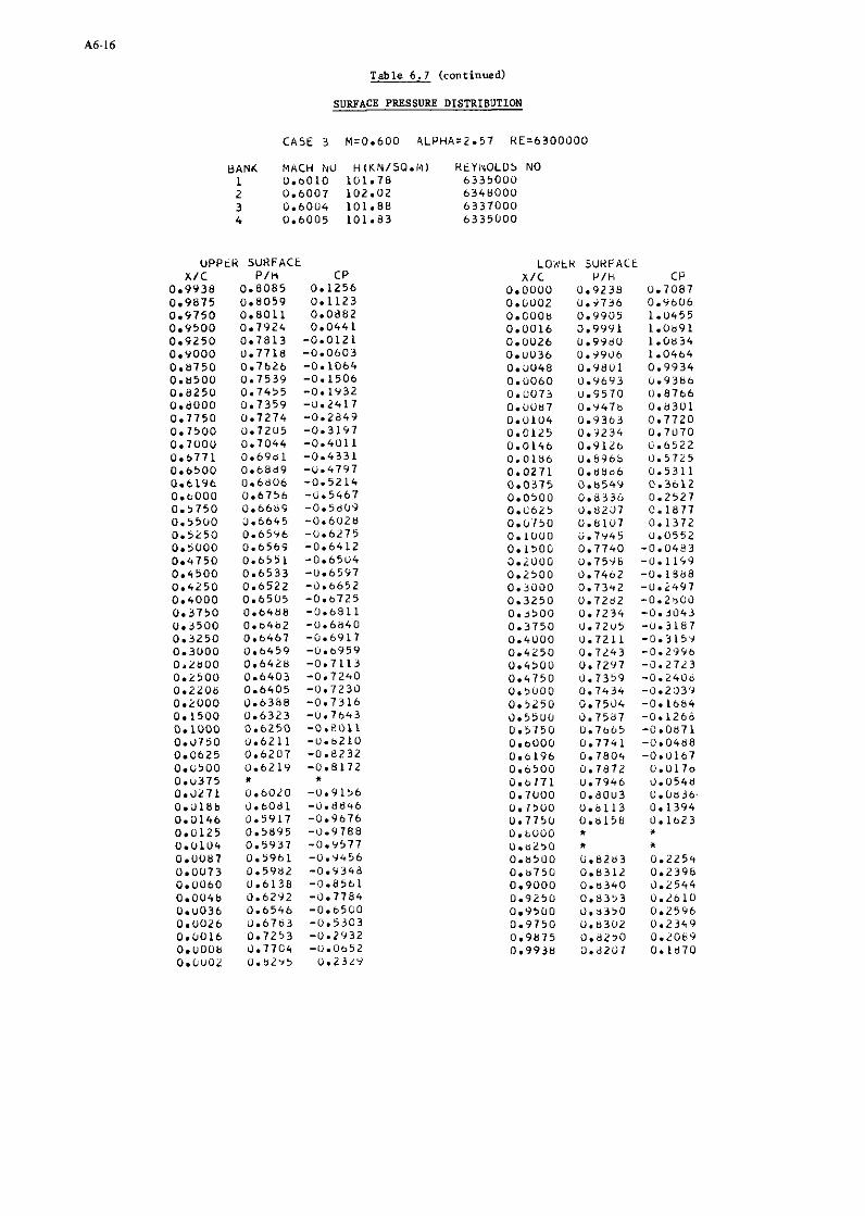
Table 6.7 (continued)
SURFACE PRESSURE DISTRIBUTION
CASE 3 M=0.600 4LPHA-2.57 RE=6300000
BANK MACH iVU H(I(N/SO.I~I) KtYIUOLD5 NO I 0.b010 101.78 6335000 2 0.6007 102.02 6348000 3 0.6004 101.88 6337000 4 0.6005 101.a3 6335000

Table 6 . 7 (continued)
SURFACE PRESSURE DISTRIBUTION
C A S E 6 M r U . 7 2 5 ALPHf\=2.'12 HE=65000J0

Table 6.7 (continued)
SURFACE PRESSURE DISTRIBUTION

Table 6 . 7 (continued)
SURFACE PRESSURE DISTRIBUTION
eANk MACH NO H(KNI5O.M) K t Y k O L D S NO 1 J . 7 2 9 1 94.08 bb2bOOO L J . 7 2 8 6 Y4.0b 6b25U00 3 0 . 7 2 1 3 94 .1b 6 6 3 6 0 0 0 4 d . 7 L e 3 94 .08 6 6 2 5 0 0 0
I C R S J R F h i P / d
0 . 9 l u * J . S t a 5 U.46b2 O.ZYU7 0 .9972 i).YY>7 3.Y700 0 . 9 6 3 1 0 . 9 4 8 5 0 . 9 3 7 3 *

T a b l e 6.7 (cont inued)
SURFACE PRESSURE DISTRIBUTION
CASE 9 N'0.730 ALPHA-^.^^ RE=6500000
dANK MACH NO H(KN/bU.M) HkYdULU5 ,&U I U.73J7 69.59 6ZlVIJUU 2 0.7322 90.07 651100U 3 0.7290 90.41 b5lYOCU

Table 6.7 (continued)
SURFACE PRESSURE DISTRIBUTION
CASE 10 M=0.750 ALPHA-3.19 RE=6200000
l5AFrK MACH NU HIKNI5O.M) HtYNOLO5 PIU I 0.75u2 85-11 bj35000 2 0.7491 84.97 62700C0 3 0.7510 84.77 6 2 3 9 3 ~ 0

Table 6 . 1 (continued)
SURFACE PRESSURE DISTRIBUTION
bANK MACH NU H(KN/SO.MI K ~ Y I V O L U ~ l iU L 0.7286 36.24 L7UJUOO L U.7294 36.34 L715UOU 3 0.7280 36.53 ~ 7 2 3 0 0 0

Table 6.7 (continued)
SURFACE PRESSURE DISTRIBUTION
UPF XIC
0.9937 0.9875 0.9'150 0.9500 0.9250 0.9000 0.8750 0.8500 0.8250 0.8000 0.7750 0.7500 0.7000 0.6771 0.6500 0.6196 0.6000 0.5750 0.5500 0.5250 0.5000 0.4750 0.4500 0.4250 0.4000 0.3750 0.3500 0.3250 0.3000 0.2192 0.2500 0;2208 O.ZUOO 0.1500 0.1000 0.13150 0.0625 0.0500 0.0375 0.0271 0.0187 0.0146 0.0125 0.0104 0.0087 0.OU73 0.0060 0.UU47 0.0036 0.0025 0.001s 0.0007 0.0002
CASE 13 M-0.745 ALPHA=3.19 RE=2700000
BANK MHCH NO H1KNISO.M) HtYNUL05 NU I 0.7428 37.55 2710'JUU 2 0.7460 37.31 L69dOOU 3 0.7468 36.83 2667UUU
'tR SURFAC P/H
0.7102 0.7084 0.7044 0.6962 0.6876 0.6789 0.6696 0.6593 0.6495 0.6393 0.6291 0.6182 0.5961 0.5852 0.5720 0.5556 0.5417 0.5174 0.4558 0.3645 0.3660 0.3773 0.3807 0.3787 0.3836 0.3879 0.3936 0.3914 0.3972 R
0.4249 0.4207 0.4222 0.4228 0.4269 0.4048 0.3968 0.3887 0.3916 0.4855 0.4496 0.4677 0.4815 0.4975 0.5095 0.5237 0.5460 0.5723 0.6041 0.6380 0.6964 0.7369 0.8216
.( SUHFAC PIH
0.9245 0.9755 0.9913 0.9972 0.9933 0.9824 0.9672 0.9525 0.9374 0.9242 0.9069 0.8935 0.8785 0.8576 0.8336 0.8004 0.7735 0.7560 0.7424 0.7197 0.6875 0.6642 0.6417 0.6193 0.6079 0.5994 0.5927 0.5930 0.5978 X
0.6185 0.6311 0.6432 0.6558 0.6687 0.6796 0.6875 0.6926 0.7091 0.7172 0.7328 0.73'26 0.7455 0.7508 0.7555 0.7587 0.7619 0.7620 * 0.7508 0.7410 0.7329

Table 6.7 (concluded)
SURFACE PRESSURE DISTRIBUTION
U P t X / C
0.9937 0.9815 0.9150 0.9500 0.YZ50 0.9UUU 0.8750 0.e500 0.bZ50 0.eu00 0.7750 0.7500 0.7UU0 0.0771 0.6500 0.6196 O.bU00 0.5150 0.5500 0.5250 0.5000 U.+750 u.r500 0.4250 0.4UOU 0.3750 0.3500 0.3250 U.jU0O 0.27Yi 0. 2 5UG 0.2208 O.ZUO0 0.1500 0.1000 0.0750 0.0625 0.u5UD 0.0375 0.U271 O.bl87 0.5146 0.U125 0.C104 0.0087 0.5073 O.L'U60 U.C'U47 0.Y036 0.CU25 0.UU15 0.0007 0.0002
CASE 13A Mz0.740 ALPHA=3.19 RE-2700000
EANK YACH NU H(KI4 ISU.M) KtYf\lULUb Fib I 1 - 1 3 3 6 - 3 8 L7490UU
Lor X I C
O.UUU0 0.0uu2 0.0007 0.0015 0.UU25 0.3036 0.9047 0.0060 0.UL173 0.DU87 0.L1U4 U.Clri5 0.U146 0.0186 0.UL'll 0.0375 0.05UO 0.0625 0.U750 0.lU00 0.15U0 U.iuU0 0.25UO 0.3000 0.3250 0.35UU 0.3750 0.4U00 0.s25U 0.4500 0.4150 0.5UOU 0.5250 0.5500 0.5150 0.6000 0.6196 0.6500 0.6111 O.7UOO 0.7500 0.7150 O.YU00 0.8250 0.b500 0.8750 0.4UUO 0.9250 0.9500 0.9150 0.Yb75 0.ZY37

Table 6 . 8
BOUNDARY LAYER AND WAKE PROFILES
CASE 1 PROBES 8
*a 0 . 6 7 6 ALPLA= 2 . 4 0 UE.5700000
X I C . 0 . 1 5 2 YIC. 1 . 1 7 LONER XIC. 0 . 1 5 2 v I C . 2 . 4 2 LOWER X/C8 0 . 1 7 9 V IC* 1 . 0 4 UPPER
CONSTANT CP(STAl IC) . -0 .066 CONSTlNT C P O T A T I C l = - 0 . 0 6 6 CONBTANT CPOlATIC)..O.813
XIC. 0 , 1 7 9 YIC. 2.29 UPPER
CONlTANT CPIS lATIC) . -0 .813
XIC. O .J l9
CONSTANT C I

Table 6 . 8 (continued)
BOUNDARY LAYW AND WAKE PROFILES
CASE 1 PROBES B (concluded)
tI. 0 . 6 7 6 ALPHA. 2 . 4 9 n E ~ 5 7 0 0 0 0 0
XIC. 0 , 7 5 0 VIC. 2 . 1 8 UPPER X/Cm 0 . 9 0 0 VlC. 2 .64 UPPER XIC. 0 . 9 5 0 VIC. 2 - 4 4 UPPER
Z I C UIUP 0 . 0 0 0 9 6 0 . 3 3 0 0 0 . 0 0 1 3 2 0 .3446 0 . 0 0 1 7 6 0 . 3 7 1 1
xIC. 1 . 0 0 0 v IC . 2 . 0 2 WAKE X/Cs 1 . 0 2 5 y/C. 2 . 8 2 uAKE XIC. 2 . 0 0 0 vlC. ? . i n UAKE
CONSTANT Cp(STAT1CI. 0 . 1 6 5
ZIC UlUP - 0 . 0 2 5 9 0 1 . 0 0 0 0 .O.O2L02 1 . 0 0 0 0 0 , 0 2 8 0 .9991 -0 .0193S 0 . 9 9 6 4 - 0 , 0 1 7 4 5 0 . 9 8 5 2 - 0 . 0 1 5 1 3 0 . 9 5 8 5 - 0 , 0 1 2 8 9 0 , 9 2 5 5 - 0 . 0 1 0 9 0 0 , 8 8 9 4 - 0 , 0 0 8 5 7 0 . 8 4 1 2 - 0 . 0 0 6 4 1 0 . 7 9 1 8 - 0 , 0 0 4 3 4 0 . 1 5 4 8 - 0 . 0 0 2 1 7 0 . 6 9 4 2 -0 .00729 0 . 6 0 3 9 - 0 . 0 0 0 1 5 0 . 2 3 6 9
0 . 0 0 0 3 3 0 . 2 5 1 9 0 . 0 0 2 1 2 0 . 3 1 3 7 0 . 0 0 4 5 7 0 . 3 8 0 1 0 . 0 0 6 6 2 0 . 6 5 1 9 0 . 0 0 8 8 2 0 . 5 2 5 4 0 , 0 1 1 1 1 0 .6115 0 . 0 1 3 0 2 0 . 6 8 4 9 0 , 0 1 5 0 7 0 . 7 6 6 7 0 . 0 1 7 1 6 0 . 8 4 1 6 0 . 0 1 9 2 7 0 , 9 0 8 2 0 .02139 0 . 9 6 0 8 0 . 0 2 3 6 1 0 . 9 8 9 3 0 . 0 2 5 4 0 0 . 9 9 8 1 0 .02739 0 . 9 9 9 8 0 , 0 2 9 2 7 1 . 0 0 0 0

Table 6 . 8 (continued)
BOUNDARY LAYER AND WAKE PROFILES
CASE 2 PROBES 0
!I. 0.676 LLPHA.'2.18 RE. 5700000
XIC. 0 .179 V l C . 2 .29
CONSTANT CP(STATIC).-0.
I/ C UIUP
UPPER
1 a0
ZIC UIUP o.ono13 0.6476 0.00021 0.7087 0.00035 0,7027
XIC. O.31V VlCS 1.15 UPPER
CONSTANT CP(STATIC1.-0.314
Z IC UIUP 0.00013 0.5356 0 .00018 0.5810 U.00025 0.6241 o.noo30 0.6391 O.UOOJ7 0.6586 0.00046 0.6829 0.00052 0.6965 0.00060 0 ,7193 0.00079 0.7487 O.OUU87 0.7631 0 ,00097 0.7782 0.00115 0.8059 O.OU135 0 ,8303 0.00154 3 ,8520 0.00163 0.8624 0.00115 0.8762 0.00194 0.8913 0.00208 0 ,9072 U.00221 0191n6 0.002J7 0.9309 0,00254 0,9465 0,00280 0,9615 0.00296 0,9685 0.00319 0.9804
Z IC UIUP 0.00012 0.6272
XIC. 0.319 V I C . 2.40 UPPER
CONSTANT CP(STATIC).-0.314
Z IC UlUP U.00014 0.5635
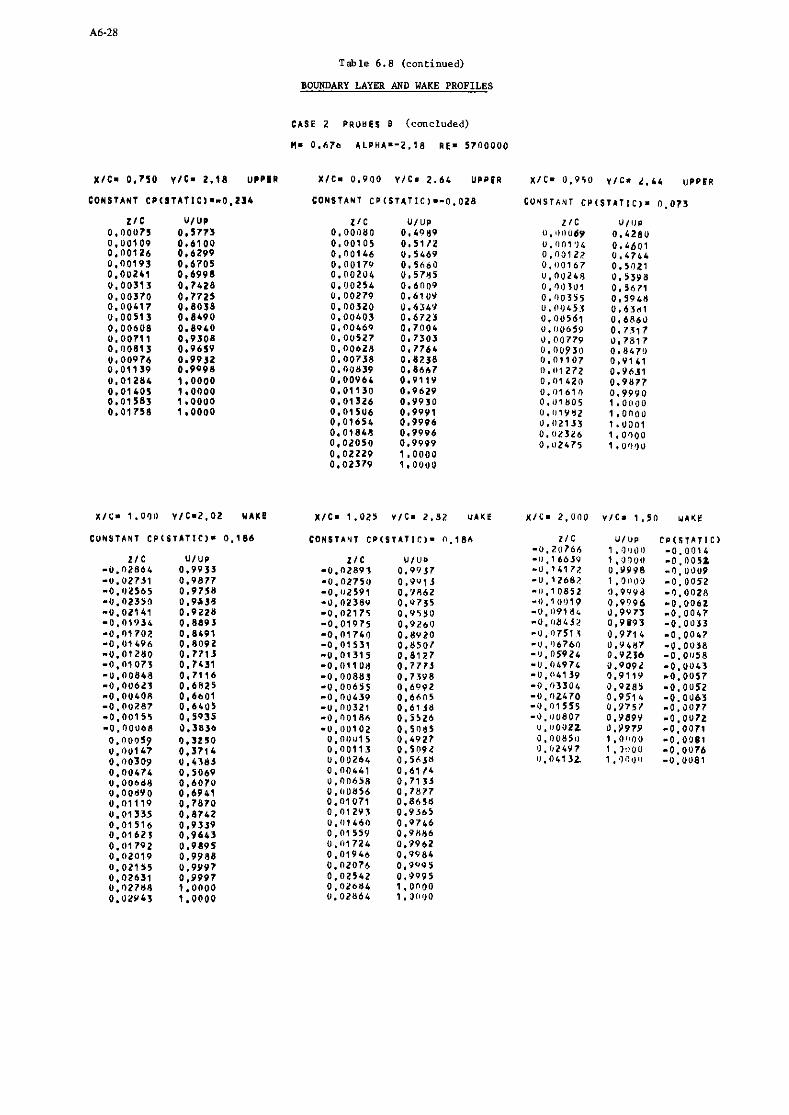
Table 6.8 (continued)
BOUNDARY LAYER AND WAKE PROFILES
CASE 2 PRUL)€S B (concluded)
M = 0 . 6 7 a ALPHA=-2.18 RE. 5700000
CONSTANT CP(STATIC1.-0.234 CONSTANT CP(STATIC). -0.028 C U ~ S T A N T CP(ST4TIC) . 0 . 0 7 3
Z I C UlUP 0 . 0 0 0 7 1 0 . 1 7 7 3
CUNSTANT CP(STATIC). 0 . 1 8 6

Table 6 . 8 (continued)
BOUNDARY LAYER AND WAKE PROFILES
CASE J PROBES 0
M. 0 . 6 0 0 ALPMA. 2 .57 P E s 6 3 0 0 0 0 0
XIC. 0 .152 VIC. 1 . 1 7 LONER XIC. 0 . 1 5 2 YlCm 9 , 4 2 LONER XIC. U.179 YlC. 1 . 0 4 UPPER
C O N S T A N T C P I S T A T I C ) . - 0 . 051 CONSTANT CP(ITITIL). - 0 . 0 5 1 CONSTANT CP(ITATIC). .n.?bs
2 1 c U IUP I I C U l U P 0.110012 0 , 6 0 3 8 0 .0032S 0 , 7 1 8 3 0 . 0 0 0 5 3 0 . 7 6 6 7
Z l C U IUP 0.UOO15 0 .6152 o . n o o z 3 0 . 6 6 4 7 0 . 0 0 0 3 8 0 ,6953 0 .00052 0 .7279 0 . 0 0 0 6 2 0 .7502 0 .00U83 0 .7840

Table 6.8 (continued)
BOUNDARY LAYW AND WAKE PROFILES
CASE 5 PRObES B (continued)
0 . 6 0 0 ALPHA. 2 . 5 7 R E . 6 3 0 0 0 0 0
XIC. 0 . 1 7 9 Y IC. 2 - 2 9 UPPER XIC. 0 . 3 1 9 YlC. 1 . 1 5 UPPER X/C. 0 . 3 1 9 VIC. 2 . 4 0 UPPER
CONSTANT C P I S T A I I C ) . - 0 . 7 4 5 C O N l l r N l C P I S T A T I C ) . - 0 . 6 9 3 COMETANT C P I S T A T I C ) . - 0 . 6 9 3

XIC. 0 . 7 5 0 VIC. 2 . 1 8 UPPER
CONSTANT C P I S T A T I C ) . - 0 . 1 2 0
Table 6 . 8 (continued)
BOUNDARY LAYER AND WAKE PROFILES
CASE 3 PROBES B (concluded)
M m 0 . 6 0 0 ALPHA. 2 . 5 7 REm63OOOUO
Z I C U l U P u.011085 U . 4 o r l
Z I C U I U P 0 . 0 0 0 5 7 0 . 3 0 5 3
XIC. 1 . 0 0 0 VIC. 2 . 0 2 W A K E X IC. 1 , 0 2 5 VIC. 2 . 8 2 u r K E X I C - 2 . 0 0 0 v / C - 1 . 5 0 urKE

Table 6 . 8 (continued)
BOUNDARY LAYER AND WAKE PROFILES

Table 6.8 (continued)
BOUNDARY LAYER AND WAKE PROFILES
crse 6 P n n n ~ t 8 (concluded)
n. 0.725 r L p a l . 2.92 RE.6500000

Table 6.8 (continued)
BOUNDARY LAYER AND WAKE PROFILES
CISE 7 PRnpeC a
M.0.72- A L P H A . 2 . 5 5 RE.6500000
x l r . 0 . 1 5 1 v / C . 1 . 1 7 L O W E R 11tm 0 . 1 5 2 v l C . 7 . 4 7 LOWER ' I t . rn 1 7 9 V l C s 1 . 0 4 IUPPER
C O N S T ~ Y T C P ( S T A T I C I . - 0 . 0 1 1 CONSTAUT c P ( S T A T I C ~ ~ - 0 . 0 5 1 C O N I T l Y l CP(STAT!c) . . O , 5 h l
UPPER
, 0 2 5

Table 6 . 8 (cont inued)
BOUNDARY LAYER AND WAKE PROFILES
C A s E 7 P a o a r s 0 (concluded)
H.0.72q ALPHA. 2 . 5 5 RE.6500000
2 I C U I U P - n . n z q n 1 ,0000 -o.n22?3 0.99AV -0.01868 0.9717 -0.01 s 7 1 0.9L73 - 0 . 0 1 1 O.RRL6 -0. no950 0.8709 -0.00647 0.7q74 - a . o n r r n 0.6606 -0.00361 0.5654 -0 .00271 0.L766 -0.00112 0 .4110 -0.00090 0.1779
O.non13 0.3073 O.00271 0.4026 0.00574 0.4856 0 .00844 0.5018 a . n r r r n o .6 " ro 0 . 0 1 L i 4 0.7573 n . n l 7 0 8 0.1316 0,01964 0.90L6 o . n z a i r 0.9553 0.07'57 0.9709 0 .02111 0.9953 o.n?915 0.9990 n . n 3 ) 4 ~ 0.9998 0 . n 3 q i r r . n a n o

Table 6 . 8 (cont inued)
BOUNDARY LAYER AND WAKE PROFILES
x l e . 0 . 1 5 2 VIC. 1 . 1 7 L O W E R XIP. 0 . 1 3 2 VIC. 2 . 4 2 L O W E R
C O N S T A N T CP(STITIC). 0 . 0 1 2 C O N S T A N T C P ( S T A T I C ) ~ 0 . 0 1 2
x I C - 0 . 3 1 9 v/Cm 2 . 4 P UPPER
C O N S T ~ N T C P ( S T A T I C ) = - 1 . 1 6 8

Table 6.8 (continued)
BOUNDARY LAYER AND WAKE PROFILES
C A S F 8 D R o 8 E s 8 (concluded)
M . O . 7 2 8 A L P H A . 3 . 2 2 le.65UOOd
x I C . 0 . 9 0 0 V I C . 2 . 6 4 U P P E R
Y / C = 1 . 0 2 5 V I C . 2 . 8 7 W A K E
C O N S T A N T C P ( S T A l I C ) * 0 . 1 4 2
Y l t . 0 . 9 5 0 V I C . 2 .44 U P P P R
C O N S T A N T C P ( S T A T I C I . 0 . 0 6 2
Z I C U I I I D
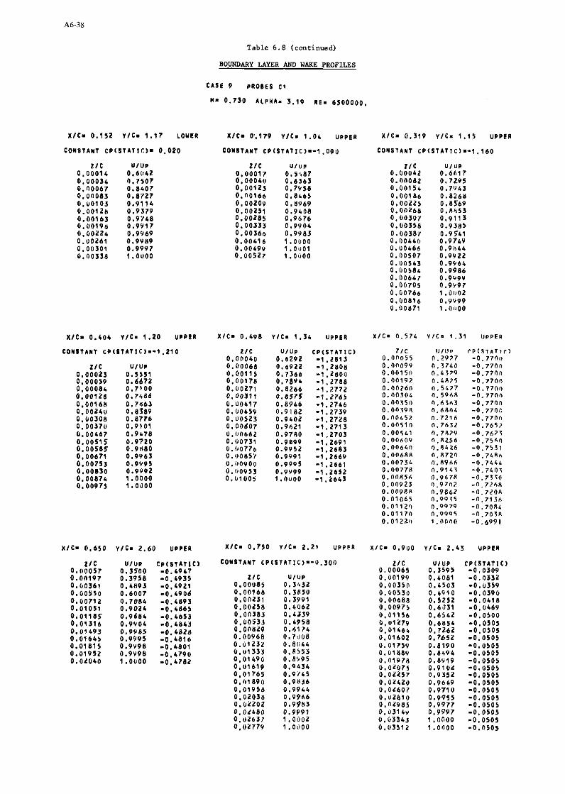
Table 6 . 8 (continued)
BOUNDARY JAYER AND WAKE PROFILES
CASE 9 PROBES C l
M. 0.730 ALPHA- 3 .19 RE. 6500000 .
XIC. 0.152 YIC. 1 . 1 7 LOUCR XIC- O'.179 YIC. 1 . 0 4 UPPER X/C= 0.319 Y I C . 1 .15 UPPER
ZIC UIUP 0.00042 0 .6617 o.on082 0.7295 0 .00156 0.7'143 0.00186 0.8268 0.00125 0.8569 0.00268 0.1h53 0 .60307 0 .9113 0.00358 0.9385 0.00387 0.9541 0.00446 O.974V 0.00466 O.VO44 0.00507 0.9922 0 .00543 0 .9964 0 ,00584 0.9986 0 .00641 0.9U9V 0.00705 O.VY97 0 .60766 1 .OlJ02 0 .00816 0.9999 0.00171 1.0 i~OO
XIC. 0.404 VIE. 1.20 UPPER XICm 0.498 Y l C m 1 . 3 4 UPPER X/C. 0 .574 Y I C s 1.31 UPPER
CONSTANT CP(STATIC).-1
ZlC UIUP
.210
UPPER
2 l C U lUP CP(STAT1C) 0.00057 0.3500 -0 .4947 0 .00197 0.3958 - 0 4935
XIC. 0 .750 YIC. 2.21 UPPER
CONSTANT CP(STATIC).-0.300
Z IC UIUP 0.00085 0 .3932 0.00168 0.3850 0.00231 0 .3991 0.00158 0 ,4062 o.on383 0.4339 0 .00533 0.4958 0.00119 0 .0174 0.00968 0.7d08 0 . ~ 1 2 3 2 0.8044 0 .01333 0 .8553
ZIC UlUP 0 . 0 0 0 6 5 0.3595 0.00119 0,4081 0.00350 0 .4503 O.DO530 0.4ClO 0 .00688 0 .5212 0.00975 0.6031 0.01156 0.6541 0.01279 0.6854 0.01464 0 ,7262 0.01602 0.7652 0.01759 0.8190 0.D1889 0.8494 o . n i ~ 7 8 O . B Y ~ P 0.01075 O.91OL 0.02257 O19J52 O.OZ420 0.9049 0 . 0 L 6 0 1 0 .9710
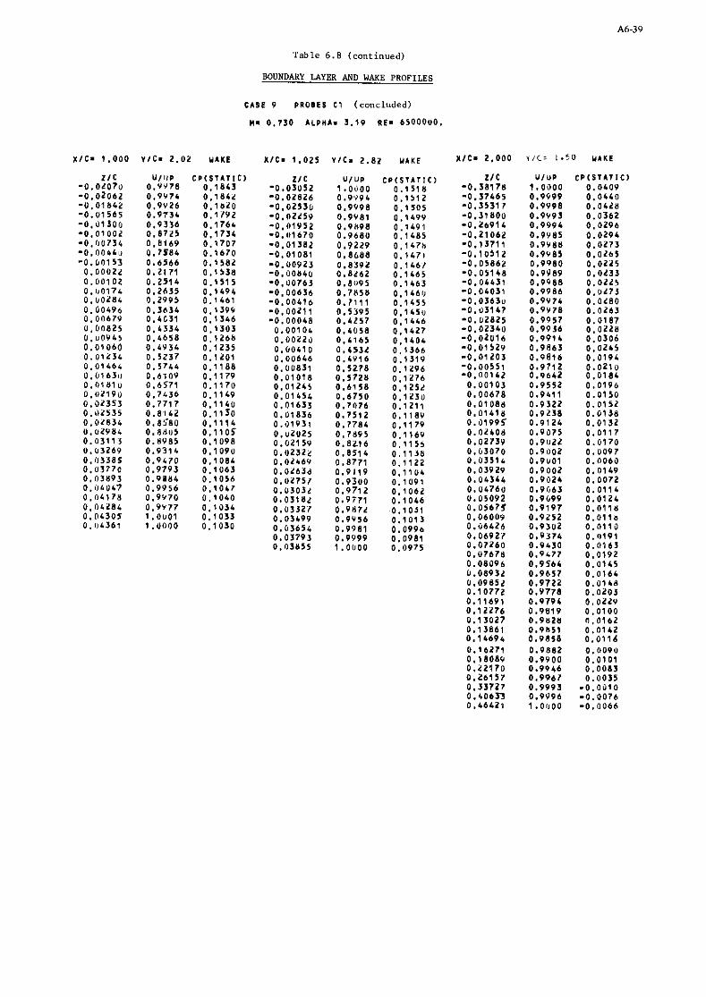
Table 6 . 8 (continued)
BOUNDARY LAYER AND WAKE PROFILES
CASE 9 PROOES C1 (concluded)
M. 0.730 ALPHA. 3.19 RE. 65000UO.
XIC. 1 . 0 0 0 Y I C . 2 .02 UAKE X/C. 1 .025 Y I C m 2.82 MAKE XIC. 2,000 TIC- 1 .50 MAKE
UIUP 1.0000 0.9'294 0.9V98 0.9V81 O.PU98 0.9680 0.9229 0 .8688 0.8392 0 .8162 0.8(195 0 .7858 0.7111 0.5395 O.4t57 0.4058 0.4165 0 . 4 5 3 1 0.1V16 0.5278 0 .5728 0 .6158 0 .6750 0.7076 0 .7512 0.7784 0 . 7 8 9 5 0.8216 0 .8514 0.8771 0.9119 0 .9300 0 .9712 0 . 9 i 7 1 0 .9*72 O.9V56 0 .9981 0.9999 1 .ouoo
UIUP 1 .0000 0.9999 0.9998 0.9993 0 .9994 0.9981 0 .9988 0.9V85 0.9980 0.9Y89 0 .9988 0.9986 0.9974 0.9978 0.9957 0.99J6 0.9974 0.9863 0.9816 0.9712 0.9642 0.9552 0.9411 0.9322 0.9238 0.9124 0.9075 0.9U22 0.9002 0.9UOl 0 .9002 0.9024 O.Pt63 0.9099 0.9197 0.9252 0.9302 0 ,9374 0.9630 0.9'77

Table 6.8 (continued)
BOUNDARY LAYER AND WAKE PROFILES
C I I C 9 rannFS e l
u. 0 . 7 1 0 i l o H 1 . 3 . 1 9 RE. 6 5 0 0 0 0 0

Table 6 . 8 (continued)
X I C . r . n n n v ~ e - 2 .02 urrc
BOUNDARY LAYER AND WAKE PROFILES
c r s n 9 pnoncs ca (concluded)
u. 0 . 7 7 0 A L O H A . 3 .10 Re. 6500000 .

O U U O ' L O d L O U ' O b O b 6 ' U L Z b O o ' o 9 b b b ' U L Y V O O ' O 6 b b b ' U Z L V O O ' O S L 6 b ' U 1 1 S 0 0 ' 0 S b V b ' U L U S O O ' O L U 7 b ' V b 9 Z O O ' U Z V L Y ' U L Y b O O ' O z k v u . u r 9 b O O ' O 6 Z Y L ' V 6 U U O O ' U S V 0 9 ' U L S O O O ' O 6 1 Y S ' U C Z U O U ' O
r n l n J I ~
b - m ( 3 I L l L S ) d J A U l L S N O 3
Y O ' L - 3 I A b L L ' O m 3 l X

Table 6 . 8 (continued)
BOUNDARY LAYER AND WAKE PROFILES
CASF 9 enOBFI D l (continued)
Y. 0.710 rLeur . 3.10 RF. 6 ~ ~ o n o o .
XIC. 0 . r n r v ie . 1.20 LIPPER XIC. 0 . ~ 0 ~ YIC. 2 .03 I I P P E ~ XI? . O . L ~ L
CONSTANT CP(SThT le ) . -1210 CONITMNT ~ P ( ~ T L T I C I . - ~ ? l t l CON(TAU1 PPI
IIC UIUP TIC UIIIO 71r n .00019 0.5105 0.00021 0.6101 0 . n o n r a 0.00011 0.3709 o . o n n 5 z n .6877 0.000116 0.00051 0.6663 0 . r n r i n 0 .7412 0 .00175 0.00074 6.6900 0 . 0 0 1 6 ) 0,7911 0 .00277 0.00112 0.7411 0 . 0 0 7 1 2 n .8402 o.nn1n8 0 . 0 o i r s 0.7706 O . ~ O J L Z n . 1 0 7 5 n . n n ~ r g 0.00200 0.8000 n . o n w g n . o ? ~ n n . 0 0 ~ 8 7 0 .00228 0.8171 o . o o ~ n 7 0.0735 0 . 0 0 ~ 7 9 0 . 0 0 ~ 7 3 n .8607 0.0061n n .0015 0 . 0 0 5 J 8 O . O O Y Z X n .8801 0.00723 n.9096 0 . 0 0 6 ~ 4 0 . 0 0 ~ ~ 8 n.0048 n . n @ r & n r . n o n t 0 . 0 0 7 1 8 o.on&Zz n .9119 0 . 0 0 9 ? s 0 .90od 0. 00.300 0 .00488 n .0611 n . o n o n g r .onno o . n o n ? , ~ 0.00558 0.9817 o.nob&4 n . v o v 0.00729 n .0018 0 . 0 0 7 9 ~ q .nono o.non7o 1 .oon2 0 .00071 r .00n0
V i C m 7.45 IIPPER
S l - 1 710
U I I I * 1 .5257 n .7107 n . 7 7 0 1 n.11401 n .1771 n.AP14 e . 9 2 1 0 0 . 0 ~ 0 1 " . o a r 1 n.0955 0 . 0 0 0 1 n.ooo0 3 . nnnn
x / C = 0 . 5 7 1 Y I C = 1 .31 IIDPER x / C = 0 . 5 7 b v I C = 7 .14 UPPFP XIC. O.57L

T a b l e 6.8 (continued)
BOUNDARY LAYER AND WAKE PROFILES
C A S F 9 e a 0 B r t 0 1 (concluded)

Table 6.8 (continued)
BOUNDARY LAYER AND WAKE PROFILES
CASE 1 0 PROBES C 1
Mc 0 . 7 5 0 ALPHA* 3 . 1 9 RE. 6 7 0 0 0 0 0 .
n . 1 5 2 y I C 8 ? . I 7 LOWER XIC. 0 . 1 7 9 VIC. 1 . 0 4 U P P E R XIC. 0 . 3 1 9 V IC. 1 . 1 5 UPPEP
C O N S T A N T c P ( s T h T r c ) . - n . 0 1 0 CONSTINT C P ( S T h T I C ) = - 0 . 9 9 5 CONSTANT C P ( S T ~ T l c ) = - l . 0 9 5
X I C = ll.l.98 V IC. 1 . 3 4

Table 6 . 8 (continued)
BOUNDARY LAYER AND WAKE PROFILES
C1SE 1 0 PRORES C1 (continued)
PI. 0 . 7 5 0 11PMAa 3 . 1 9 HE. 6 2 0 0 0 0 0 .
X I C . 0 . 7 5 0
CONSTANT C P (
7 1 c o . o n o 9 9
v I C . 2 . 4 3 U P P E R

Table 6.8 (continued)
BOUNDARY LAYER AND WAKE PROFILES
C A S E 1 0 P R O B E S C 1 (concluded)
M = 0 . 7 5 0 r i p r r ~ 3 . 1 9 R E = 67nnooo .

Table 6.8 (continued)
BOUNDARY LAYER AND WAKE PROFILES
CASE 1 2 PROBES C
I!. 0 . 7 3 0 ALPHA. 3 . 1 9 R E . Z l U 0 0 0 0 .
X I C S 0 . 1 5 1 Y,C= 1 . 1 7 L ~ Y F Y XIC. 0 .179 YIC. 1 .04 UPPER
C O N S T A N T C P ~ S T ~ T I C ) = o . n n 3 C O N S T A N T CP(STATIC)= -~ .U IZ
x I C = 0 . 4 0 4 Y l F a 1 . 2 0 UPPCR X I C * 0 . 4 9 8 Y l C * 1 . 3 4 UPPER
CONSTANT C P ( S T A T I C ) = - 1 . 1 7 6 CONSTANT C P ( S l A T l i ) = - 0 . 9 1 6 ~
Z I C U I ' IP U.U,~US9 0 .510v u . u n u 3 v 0 . 5 ~ ~ 4 U. l 'O059 0 . 6 4 4 8 u.110108 0 .7003 U . o O l 2 8 0 . 7 1 7 J 0 . ~ 0 1 6 6 0 . 7 5 5 8 u . u o Z u n 0 . ~ 8 ~ 0 . 0 0 1 3 7 U . 8 0 5 0 0 . 0 9 Z 6 7 0 . 8 2 0 5 U . ~ r 0 3 0 1 0 . 8 3 7 6 0 . 0 0 3 5 4 0 . 8 6 4 6 0 . 0 0 3 7 0 0 . 8 7 6 2 0 . 0 0 4 1 4 0 . 8 9 7 4 0 . 0 U 4 3 8 0 . 9 0 5 1 O.OI?471 0 . 9 1 8 V O.OOSZ3 0 . 9 L 1 3 U.00568l 0 . 9 5 4 1 U .005PJ 0 . 7 6 6 1 o.oo6i.a 0 . 9 7 6 6 0 . 0 0 7 0 6 0 . 9 8 5 7 U .UC?bS 0 , 9 9 2 3 U . 0 0 8 0 9 0 . V 9 7 3 U.OO866 O.VVH6 u . u n v 3 d U .V?PV 0 . 0 1 0 0 8 0 . 7 9 9 7 U. IJ (U87 (.OVOU

Table 6 . 8 (cont inued)
BOUNDARY LAYER AND WAKE PROFILES
C A S E 1 2 D P n R E S C (concluded)
X I C . 0 . 7 5 0 Y I C . 2 .21 U P P E R
U I U P c P ~ S l A l I C ~ 0 .4475 - 0 . 4 5 9 6 0 . 4 9 7 2 - 0 . 4 5 9 2 0 . 5 4 5 5 - 0 . 4 5 8 6 0 . 5 7 1 2 - 0 . 1 5 8 1 0 . 6 1 7 2 - 0 . 4 5 7 4 0 . 6 5 8 7 - 0 , 4 5 6 9 0 . 7 0 4 3 - 0 . 4 5 6 4 0 . 7 4 5 7 - 0 . 4 5 5 7 O . 7 R l 4 - 0 . 4 5 5 1
U l U P C P ( L 1 A l I C ) 0 . 2 5 5 1 - 0 . 0 3 0 2 0 . 2 8 0 1 - 0 . 0 3 0 6 Z I C U I U P
0 . 0 0 0 7 8 0 . 3 7 9 4 0 .00140 0 . 4 1 7 3 0 . 0 0 2 1 7 0 , 4 3 9 2 0 . 0 0 2 5 8 0 . 4 6 2 4
0 . 8 3 5 6 - 0 ; 0 3 8 9 0 . 8 7 8 1 - 0 . 0 3 9 6 n . 0 1 0 ~ .n o t o z
X I C . 1 . 0 0 0

- 0 3 " 3
O X .

Table 6.8 (continued)
BOUNDARY LAYER AND WAKE PROFILES
C A S E 1 2 P R O B E S D (continued)
Ms 0 . 7 3 0 A L P H A - 3 . 1 9 R E * 2 7 0 0 0 0 0 .
XIC. 0.319 Y I C . 1.15 UPPER XIC* 0.319 Y / C = 1.98 UPPER XIC- 0 .319 vIC. 2 .40 UPPER
CONSTANT CP(STATIC).-1.142 CONSTANT CP(STATIC).-1.142 CONSTANT CP(STATIC)*-1 . I 4 2
ZIC UIUP 0.00012 0 .5107 0.0002IJ 0 .6290
Z IC UIUP 0.00025 0.5867 0.00038 0.6383 0,00050 0 .6686 0.00060 0 ,6812 0.00072 0 .6987 0.00098 0.7283 0.00126 0 .7527 0.00146 0.7708 O.UO176 0.7912 0.00222 0.8226 0,00255 0.8131 0.00283 0.8631 0.00312 0.8789 O.UO342 0.8953 0.00369 0.9087 0.00400 0 .9232 O.OFb31 0.9365 O.UObJ7 0,9471 0.00195 0 .9610 0.00527 0.9729 0.00567 0 .9827 0.00607 0.9899 0,00643 0,9946 0.00676 0.9978 0.00676 0 ,9980 0 .00681 0,9977 0.00712 0 .9090 0.00752 0.9997 0.00784 0.9098 0.00809 0.9998 0.00845 1 ,0000
xIC. 0 .404 Y I C . 1.20 UPPER XIC. 0.404 YIC. 2.03 UPPER XIC. 0 .406 Y I C . 2 .45 UPPER
CONSTANT cP(S~ATlC) . -1 .176 CONS TAN^ C P ( S ~ A ~ I C l . - 1 . ~ 7 6 CONSTANT C P ( S ~ A T l c l . - 1 . 1 7 6
ZIC UIUP ZIC UIUP 0 .00033 0.5666

Table 6 . 8 (continued)
BOUNDARY LAYER AND WAKE PROFILES
S E 1 2 P R O B E S D (continued) C A
n UPPER
. 9 1 6
0 . 7 3 0 A L P H I . 3 . 1 9 R E = 270OC
XIC. 0 . 4 9 8 VIC. 2 . 1 7 UPPER
CONSTANT CP(S~A11C) . -0 .916
Z I C UIUP 2 I C UIUP
0 . 9 q o i 0 .9495 0 .9V98 1 . O ' l O O 1 . 0 0 0 0
Y lC* 2 .56 UPPER XIC. 0 .574 ylC. 2 . l l UPPER
UIUP

Table 6 . 8 (continued)
BOUNDARY LAYER AND WAKE PROFILES
C A S E 1 2 P R O B E S D (concluded)
XIC. 0 .650 v/C. 2.60 UPPER XIC. 0.750 V I C . 2.21 UPPER XIC. 0 .900 v / C = 2 .43 UPPER
2 l C UlUP 0.U0078 0.3670 0.0014X 0 .4122 O.UOl89 0.4297 0 .00230 0.4457 O.l l0300 0.4789 0 ,00300 0.4631 0.00300 0 .4686 o.no341 0.4?99 0.00390 0 .4912 O.OO403 0.5215
XIC. 1 .000 V I C . 2 .02 WAKE XlC. 1.025 V IC* 2.82 U I K E IIC. 2.000 v I C . 1.50 W A K E
UlUP 1 .oooo 1 .oooo 0.9993 0.9993 0.9960 0.9897 0.9730 0.9529 0.9270 0.8851 0.8461 0.7997 0.8025 0.8036 0.7527 0.6438 0.4707 0.3045 0.2800 0.3008 0.3515 0.3971 0.4528 0.5141 0.5696 0.6302 0.6865 0.7371 0.7971 0.8437 0.8939 0.9321 0.9557 0.9744 0.9849 0.9930 0.9939 0.9958 0.9973 t .oono

Table 6 . 8 (continued)
BOUNDARY LAYER AND WAKE PROFILES
CASE 1 3 PROBES D
n= 0.76s r i p n r . 3.19 aE, 2700000.
CONSTANT CPlSTATIC).-0.018 CONSTANT CP(STATIC).-0.018 CONST~NT C P I S T A T I C ) ~ - O . ~ ~ ~
Z l C UIUP ZIC UIUP ZIC UIUP O.llCU13 0.5681 0.00018 0 .6472 0.QU016 0.7311 0 . 0 ~ 0 4 3 0 .7990 0.00012 0 . i i l b 2 O.no062 0 .8370 U.UO075 0 .8563 O.'Il1082 O.8bv1 0.110095 0.8836 0.110103 0.818L
XIC. 0.179 VIC. 1.04 UPPER XIC. 0.179 V I C . 1 . 8 8 UPPER XIC. 0.179 Y I C * 2.29 UPPER
CONSTANT CP(SlAl lC) . -0.996 CONSTANT CP(STATIC).-0.996 CONSTANT t P ( S T A T I C > ~ ~ O . 9 9 6
ZIC UIUP 0.U0017 0 .4893 0.~10024 0 .5565
ZIC UIUP 0.00023 0.5492 0.00030 0 .5996 0 .00036 0 . b 3 3 l
ZIC UlUP 0 .00017 0.5063 0 .00035 0 .6b14

Table 6 . 8 (continued)
BOUNDARY LAYER AND WAKE PROFILES
CASE 1 3 PROBES D (continued)
n- 0 . 7 6 5 ALPnr. 3 . 1 9 R E . 1 7 0 0 0 0 0 .
X I C . 0 , 3 1 9 VIC. 1 . 1 5 UPPER x I C . 0 . 3 1 9 V I E . 1 . 9 8 UPPER XIC. 0 . 3 1 9 Y I C . 2 . L O UPPER
CONSTANT C P ( I l A T I C ) . - 1 . 1 1 0 CONSTANT E P ( S T A l I C ) ~ - 1 . 1 1 0 C O N S l A N l C P ( S ~ A 1 1 C ) . - 1 . 1 1 0
X I C . 0 . 4 0 4 YIC. 1 . 2 0 UPPER
C O N S T A N T C P ( S T A I I C ) . - ~ . I L ~
Z I C U I U P 0 . 0 0 0 2 2 0 . 5 6 0 9 0 . 0 0 0 1 ? 0 . 6 0 4 0

Table 6.8 (continued)
C A S E 1 3 PROBES D (continued)
H. 0.7&5 ALPHA. 3.19 RE. 170U000.
XIC. 0.498 Y I C . 1 .34 UPPER X/Cm 0 .498 Y I C . 2.17 UPPER XIC. 0.498 Y I C . 2 .50 UPPER
CONSTANI CP(STA'IIC).-1 .202 CONSTANT CP(STATIC).-1.202 CONSTINT cP(STATIC). -~.ZO~
Z IC U lUP 0.00U10 0 .4756 0.0002X 0 .5886 0,00036 0 .6276 0 .00055 0.6525 0 . 0 0 0 6 d 0.6693 0.00087 0.6618 O.OO09) 0.6'244 0 .00115 0.78129 0.00115 0.7124 0.00135 0 .7214 0.00155 0.734) 0 .00175 0.7433 0.00194 0.7591 0 .0021 t l 0.7706 0 .00125 0.7764 0.00110 0 .7818

Table 6.8 (continued)
BOUNDARY LAYER AND WAKE PROFILES
ChSE 1 3 PROBES D (continued)
M. 0.745 ALPHA. 3.19 RE. 170U000.
XlC. 11.650 VfL. 2 . 0 0 UPPER XlC. 0 .750 YfL. 2.21 UPPfH XIC. 0.9dO YIL. 2.43 UPPER
UlUP O.LG61 U . I 3 V I O.2383 0.Zh49 0.7878 0 . 3 0 2 5 0.371'6 11.3344 0.3911 0 . 3 3 3 2 0 .3373 1). 3738 0.4134 0.3883 0.3757 0.4106 U . 4 2 3 8 0.4364 0.4118 0.4879 0.4746 0 .4740 U. 5150 0.5969 0 .6648 0 .7303 0.7845 0.85'1'1 0.9304 0.9768 O.YY67 1 .0002 ~).OOP8 1 . n ~ ~ n o
CONSTANT CP(STATICI.-U.Z720 UlUP 0 . 1 ~ 7 8 U.238L 10.29VS 0 .3376 0.391) 0.4LOS 0.4997 0 .5412 0.5359 0 .6434 u.6743 0 . 7 0 0 5 0.7389 0 . 7 9 9 8 0 .8062 0 .8108 0.RZVV 0 .8304 0.8676 0 .9064 0.9726 0.9347 0.9493 0.9524 U.Y698 0.0755 0.9867 O.V84? U.9937 0.9995 i . n * , n r 1 . nu00 n .9997 0.OV91 1 . ouou l .OU01 '1.0000

Table 6 . 8 (continued)
BOUNDARY LAYER AND WAKE PROFILES
C A S E 1 3 PROBES D (concluded)
M. 0 . 7 4 5 A L P H A - 3 . 1 9 RE. 1 7 0 U 0 0 0 .
Z l C U l U P C P ( S T 4 T I C ) - 0 . U 2 5 1 5 1 . 0 ~ 0 0 0 . 1 1 3 0
Incomplete traverse

Table 6 . 8 (continued)
BOUNDARY LAYER AND WAKE PROFILES
CASE 1 3 6 PROBES C2
M = 0 . 7 4 0 ALPHA. 3 . 1 9 RE. 2 7 0 0 0 0 0 .
XICm 0 . 1 5 2 YIC. 1 . 1 7 LOWER XIC. 0 . 1 7 9 YIC. 1 . 0 4 UPPER
CONSTANT CP(ST IT1C) . 0 .000 CONSTANT CP(STATIC).-1,038
xIC. 0 . 4 0 4 YIC. 1 . 2 0 UPPER
CONSTANT CP(S IAT IC ) . - 1 .172
Z I C U IUP 0 . 0 0 0 4 3 0 . 6 1 5 8 0 . 0 0 0 5 5 0 .663 "
XIC. 0 .498 Y IC . 1 . 3 4 UPPER
CONSTANT c ~ ( s ~ A l I c ) = - l . 2 3 2
Z I C U IUP 0 . 0 0 0 3 2 0 . 5 6 4 2 0 . 0 0 0 4 7 0 . 6 2 4 6

Table 6 . 8 (concluded)
BOUNDARY LAYER AND WAKE PROFILES
CASE 1 3 1 PROBES C2 (concluded)
M. 0 . 7 4 0 ALPHA. 3 . 1 9 RE. d 7 0 0 0 0 0 .
XIC. 0 . 6 5 0 V I C Z 2 . 6 0 U P P E R XIC. 0 . 7 5 0 v I C . 2 . 2 1 UPPER X I C I 0 . 9 0 0 VIC. 2 . 4 3 UPPER
CONSTANT C P ( S T A T I L ) . - O , L ~ O CONSTANT CP(STAT IC) . - 0 .275 CONSTANT c P ( S T A T I C ) ~ ~ O . O ~ ~
1 . b o o o 1 . OUOO 0 . 9 9 9 6 0 . 9 Y 8 7 0 . 0 9 9 0

Table 6.9
BOUNDARY LAYER AND WAKE PARAMETERS
6 Case 1 M- - 0.676, u - 2.40°, Re = 5.7 x 10 , Probes B
6 Case 2 M_ - 0.676, o - -2.18'. Re - 5.7 x 10 , Probes B
X / C ~ I c Surface
0.152 1.17 Lower 0.004021 0.000271 0.000150 1.813 0.152 2.42 Lower 0.004029 0.000285 0.000157 1.809 0.179 1.04 Upper 0.004351 0.000321 0.000197 1.632 0.179 2.29 Upper 0.004138 0.000307 0.000184 1.667 0.319 1.15 Upper 0.003163 0.000650 0.000385 1.688 0.319 2.40 Upper 0.003411 0.000629 0.000380 1.654 0.75 2.18 Upper 0.002123 0.002124 0.001230 1.728 0.90 2.64 Upper 0.001668 0.003364 0.001887 1.783 0.95 2.44 Upper 0.001435 0.004072 0.002207 1.845 1.00 2.02 Upper wake - 0.006364 0.003074 2.070 1.00 2.02 Lowerwake - 0.006052 0.003793 1.596 1.00 2.02 Totalwake - 0.012416 0.006867 1.808 1.025 2.82 Wake - 0.009963 0.006036 1.650 2.00 1.50 Wake - 0.004949 0.003935 1.258
H
1.692 1.700 1.811 1.864 1.836 1.799 1.812 1.910 2.102 2.342 1.559 2.079 1.805 1.256
X/C
0.152 0.152 0.179 0.179 0.319 0.319 0.75 0.90 0.95 1 .OO 1.00 1 .OO 1.025 2.00
Case 3 M = 0.600, a - 2.57'. Re = 6.3 x lo6, Probes B
Y I C
1.17 2.42 1.04 2.29 1.15 2.40 2.18 2.64 2.44 2.02 2.02 2.02 2.82 1.50
X / C
0.152 0.152 0.179 0.179 0.319 0.319 0.75 0.90 0.95 1 .OO 1.00 1.00 1.025 2.00
Surface
Lower Lower Upper Upper Upper Upper Upper Upper Upper Upper wake Lower wake Total wake Wake Wake
y l c
1.17 2.42 1.04 2.29 1.15 2.40 2.18 2.64 2.44 2.02 2.02 2.02 2.82 5 0
6 * l c
0.000236 0.000277 0.000391 0.000402 0.000801 0.000773 0.002813 0.004740 0.006818 0.009472 0.003189 0.012661 0.010994 0.005321
0.004348 0.004037 0.003783 0.003455 0.00281 1 0.003067 0.001806 0.001308 0.000930 -
- - - -
e / c
0.000140 0.000163 0.000216 0.000216 0.000436 0.000430 0.001553 0.002482 0.003244 0.004044 0.002046 0.006090 0.006091 0.004239
Surface
Lower Lower Upper Upper Upper Upper Upper Upper Upper Upper wake Lowerwake Totalwake Wake Wake
6*/c
0.000343 0.000369 0.000850 0.001072 0.001629 0.001089 0.003556 0.006077 0.007912 0.010887 0.003157 0.014044 0.012665 0.006204
0.004241 0.003990 0.003400 0.003196 0.002609 0.003101 0.001688 0.001173 0.000875 -
- - - -
e l =
0.000229 0.000240 0.000542 0.000678 0.000990 0.000698 0.002061 0.003255 0.003928 0.004662 0.002090 0.006752 0.006849 0.005030
H
1.497 1.536 1.569 1.581 1.645 1.561 1.726 1.867 2.015 2.335 1.511 2.080 1.849 1.233

Table 6.9 (continued)
BOUNDARY LAYER AND WAKE PARAMETERS
6 Case 6 M- = 0.725, o = 2.92', Re - 6.5 x 10 , Probes B
6 Case 7 M - 0.725, u - 2.5s0, Re = 6.5 x 10 , Probes B
X/C
0.152 0.152 0.179 0.179 0.319 0.319 0.75 0.90 0.95 1.00 1.00 1.00 1.025 2.00
6 Case 8 M - 0.728, o - 3.2z0, Re - 6.5 x 10 , Probee B
NB x l c = 2.0, includes shack losses. -
y/c
1.17 2.42 1.04 2.29 1.15 2.40 2.18 2.64 2.44 2.02 2.02 2.02 2.82 1.50
H
1.635 1.649 1.959 1.936 1.965 1.974 - 2.140 2.213 2.471 1.619 2.214 1.959 1.291
Surface
Lower Lower Upper Upper Upper Upper Upper Upper Upper Upperwake Lowerwake Total wake Wake Wake
NB x/c = 2.0, includes shock losses.
Cf
0.004180 0.003839 0.003230 0.003162 0.002723 0.002677 - 0.000892 0.000787 -
- - - -
Surface
Lower Lower Upper Upper Upper Upper Upper Upper Upper Upperwake Lowerwake Total wake Wake Wake
X / C
0.152 0.152 0.179 0.179 0.319 0.319 0.75 0.90 0.95 1.00 1.00 1.00 1.025 2.00
X/C
0.152 0.152 0.179 0.179 0.319 0.319 0.75 0.90 0.95 1 .OO 1.00 1.00 1.025 2.00
Cf
0.004210 0.003640 0.003016 0.002913 0.002726 0.002739 - 0.000924 0.000740
- - - - -
y l c
1.17 2.42 1.04 2.29 1.15 2.40 2.18 2.64 2.44 2.02 2.02 2.02 2.82 1.50
NB x / e = 2.0. includes shock l a s s e s .
6 * l c
0.000311 0.000388 0.000601 0.000584 0.001011 0.000995
- 0.009289 0.011954 -
- -
0.014895 0.011161
6 * l c
0.000311 0.000382 0.000535 0.000595 0.000997 0.000966 - 0.007295 0.009263 0.011919 0.003374 0.015293 0.013314 0.006902
y / c
1.17 2.42 1.04 2.29 1.15 2.40 2.18 2.64 2.44 2.02 2.02 2.02 2.82 1.50
6 * / c
0.000305 0.000419 0.000610 0.000641 0.001025 0.001001 - 0.007850 0.010243 0.012949 0.003192 0.016141 0.013899 0.008103
0/c
0.000190 0.000231 0.000273 0.000307 0.000508 0.000490 - 0.003409 0.004185 0.004823 0.002083 0.006906 0.006796 0.005346
e / c
0.000191 0.000236 0.000292 0.000291 0.000497 0.000490 - 0.004415 0.005466 -
- -
0.007690 0.008758
Surface
Lower Lower Upper Upper Upper Upper Upper Upper Upper Upper wake Lowerwake Total wake Wake Wake
H
1.631 1.647 2.056 2.005 2.035 2.028 - 2.104 2.187 -
- -
1.937 1.274
e / c
0.000188 0.000250 0.000305 0.000322 0.000513 0.000500 - 0.003761 0.004663 0.005530 0.002005 0.007535 0.007135 0.006319
=f
0.004121 0.003799 0.002947 0.003149 0.002705 0.002783 - 0.000929 0.000777 -
- - - -
H
1.622 1.673 2.001 1.994 1.998 2.002 - 2.087 2.197 2.342 1.592 2.142 1.948 1.282


Table 6.9 (continued)
BOUNDARY LAYER AND WAX@ PARAMETERS
Case 10 Mm = 0.750, u = 3.19~. Re - 6.2 x lo6 P r o b e s CI
Case 12 M_ = 0.730, u - 3.19O, Re = 2.7 x lo6 Probes C
x/c
0.152 0.179 0.319 0.404 0.498 0.574 0.65 0.75 0.90 t1 .OO
1 .OO 11.00 11.025 2.00
Case 12 M_ - 0.730, o = 3.19'. Re = 2.7 x lo6 Probes D
NB x l c - 2.0, includes shock l o s s e s t Linear extrapolation t o edge of wake * Near separation, method of deduction not accurate
Surface
Lower Upper Upper Upper Upper Upper Upper Upper Upper Upper wake Lower wake Total wake Wake Wake
y / c
1.17 1.04 1.15 1.20 1.34 1.31 2.60 2.21 2.43 2.02 2.02 2.02 2.82 1.50
x l c
Cf
0.003983 0.002602 0.002871 0.002596 0.002421
t * + 0.000591 -
- - - -
NB x l c - 2.0, includes shock l o s s e s
Y / C Surface
Lower Upper Upper Upper Upper Upper Upper Upper Upper Upper wake Lower wake Total wake Wake Wake
X/C
0.152 0.152 0.152 0.179 0.179 0.179 0.319 0.319 0.319 0.404 0.404 0.404 0.498 0.498 0.498 0.574 0.574 0.574 0.65 0.75 0.90 1 .OO 1 .OO 1 .OO 1.025 2.00
6 * / ~
0.000359 0.000810 0.001022 0.001293 0.001660 0.002857 0.009403 0.017408 0.016740 0.029063 0.002931 0.031994 0.019007 0.015919
Cf
0.005053 0.002993 - 0.002844 0.002213 - 0.001683 0.001323 0.000961 -
- - - -
0.152
NB Far traverses 0.65 r x / c 6 1.025. p r o b e s s i tuated upstream may a f f e c t results.
L x/c - 2.0, includes shock losses
Y / C
1.17 2.00 2.42 1.04 1.88 2.29 1.15 1.98 2.40 1.20 2.03 2.45 1.34 2.17 2.59 1.31 2.14 2.56 2.60 2.21 2.43 2.02 2.02 2.02 2.82 1.50
1.17
e l c
0.000213 0.000386 0.000500 0.000613 0.000775 0.001209 0.002437 0.004016 0.006588 0.010528 0.001710 0.012239 0.009871 0.012314
6 * / c
0.000340 0.000946 - 0.001591 0.002571 - 0.003977 0.005814 0.009854 0.015553 0.003846 0.019399 0.018150 0.008693
H
1.688 2.097 2.043 2.109 2.143 2.364 3.859 4.335 2.541 2.761 1.714 2.614 1.926 1.293
0.179 ' 1.04 0.319 I 1.15 0.404 ' 1.20
e /c
0.000197 0.000444 - 0.000759 0.001231 - 0.001940 0.002729 0.004231 0.005857 0.002191 0.008048 0.008295 0.006722
0.498 0.574 0.65 0.75 0.90 1 .OO 1 .OO 1 .OO 1.025 2.00
6 * / c
0.000355 - 0.000379 0.000894 0.000851 0.000859 0.001163 0.001282 0.001318 0.001614 0.001697 0.001543 0.002665 0.002474 0.002679 - 0.003441 0.003575 0.004084 0.005830 0.010859 0.019805 0.003847 0.023653 0.018124 0.008766
e / c
0.000209 -
0.000213 0.000427 0.000411 0.000411 0.000576 0.000627 0.000633 0.000762 0.000810 0.000743 0.001264 0.001162 0.001274 - 0.001645 0.001656 0.001964 0.002707 0.004767 0.005295 0.001931 0.007227 0.008298 0.006774
Surface
Lower Lower Lower Upper Upper Upper Upper Upper Upper Upper Upper Upper Upper Upper Upper Upper Upper Upper Upper Upper Upper Upper wake Lower wake Total wake Wake Wake
H
1.725 2.130 - 2.097 2.088 - 2.051 2.131 2.329 2.656 1.755 2.410 2.188 1.293
1.34 1.31 2.60 2.21 2.43 2.02 2.02 2.02 2.82 1.50
H
1.696 - 1.781 2.094 2.068 2.087 2.018 2.044 2.081 2.117 2.094 2.075 2.108 2.129 2.104 - 2.092 2.159 2.080 2.154 2.278 3.740 1.992 3.273 2.184 1.294
! Cf
0.005077 - 0.004618 0.003239 0.003288 0.003382 0.003685 0.003402 0.003197 0.002749 0.002850 0.003137 0.002068 0.002054 0.002222 - 0.001775 0.001638 0.001598 0.001261 0.000903 -
- - - -
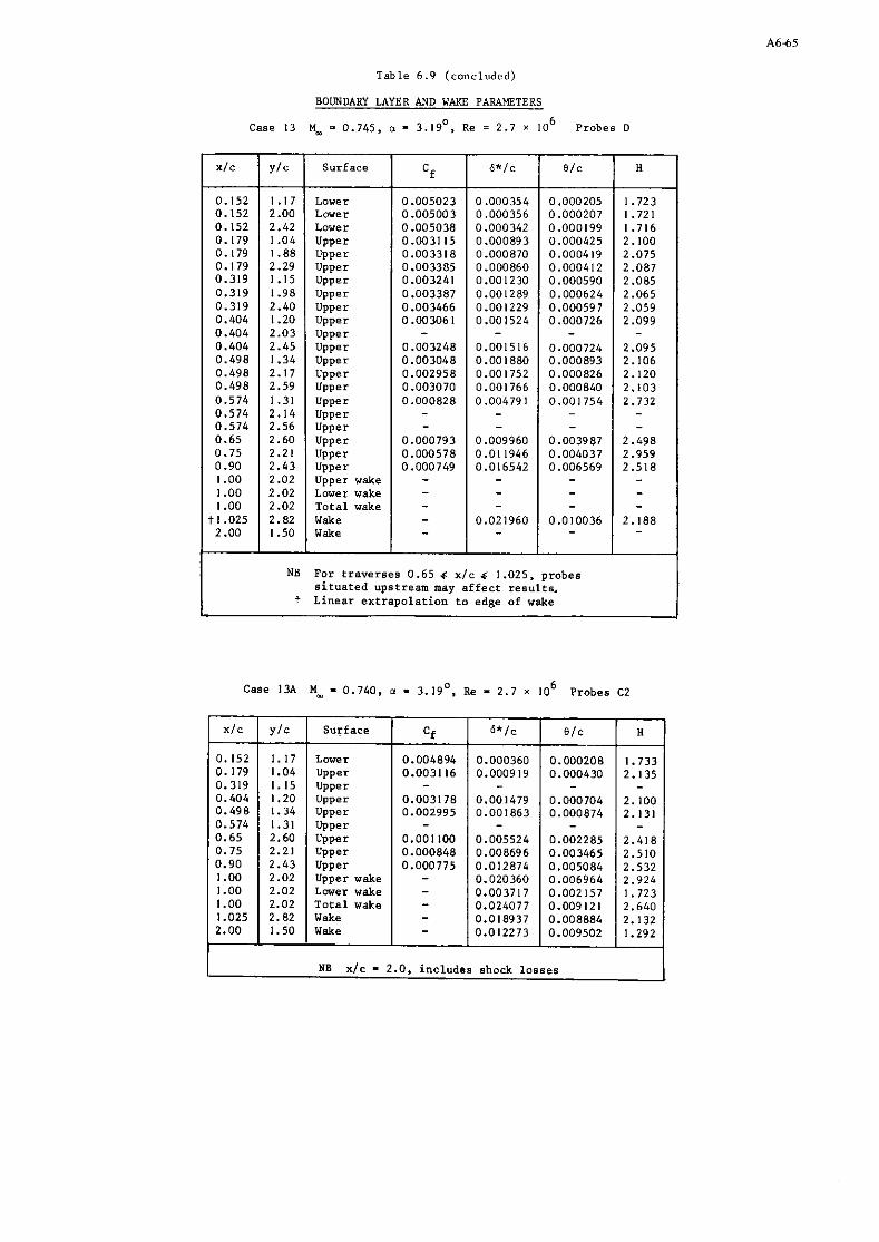
Table 6.9 (conc luded)
BOUNDARY LAYER AND WAKE PARAMETERS
Case 13 M - - 0.745, a - 3.19', Re = 2.7 x lo6 Probes D
Case 13A M - 0.740, o - 3.19'. Re - 2.7 x lo6 Probes c2
xlc
0.152 0.152 0.152 0.179 0.179 0.179 0.319 0.319 0.319 0.404 0.404 0.404 0.498 0.498 0.498 0.574 0.574 0.574 0.65 0.75 0.90 1 .OO 1.00 1 .OO
t1.025 2.00
NB For traverses 0.65 4 xlc 4 1.025, probes situated upstream may affect results.
t Linear extrapolation to edge of wake
ylc
1.17 2.00 2.42 1.04 1.88 2.29 1.15 1.98 2.40 1.20 2.03 2.45 1.34 2.17 2.59 1.31 2.14 2.56 2.60 2.21 2.43 2.02 2.02 2.02 2.82 1.50
XIC
0.152 0.179 0.319 0.404 0.498 0.574 0.65 0.75 0.90 1.00 1.00 1.00 1.025 2.00
Surface
Lower Lower Lower Upper Upper Upper Upper Upper Upper Upper Upper Upper Upper Upper Upper Upper Upper Upper Upper Upper Upper Upper wake Lower wake Total wake Wake Wake
NB xlc - 2.0, includes shock losses
ylc
1.17 1.04 1.15 1.20 1.34 1.31 2.60 2.21 2.43 2.02 2.02 2.02 2.82 1.50
Surface
Lower Upper Upper Upper Upper Upper Upper Upper Upper Upper wake Lower wake Total wake Wake Wake
Cf
0.005023 0.005003 0.005038 0.0031 15 0.003318 0.003305 0.003241 0.003387 0.003466 0.003061 - 0.003248 0.003048 0.002958 0.003070 0.000828
- -
0.000793 0.000578 0.000749 -
- - - -
6*/c
0.000354 0.000356 0.000342 0.000893 0.000870 0.000860 0.001230 0.001289 0.001229 0.001524 - 0.001516 0.001880 0.001752 0.001766 0.004791 -
- 0.009960 0.011946 0.016542 -
- -
0.021960 -
81c
0.000205 0.000207 0.000199 0.000425 0.000419 0.000412 0.000590 0.000624 0.000597 0.000726 - 0.000724 0.000893 0.000826 0.000840 0.001754
- -
0.003987 0.004037 0.006569 -
- -
0.010036 -
Cf
0.004894 0.003116 - 0.003178 0.002995 - 0.001100 0.000848 0.000775 -
- - - -
H
1.723 1.721 1.716 2.100 2.075 2.087 2.085 2.065 2.059 2.099
- 2.095 2.106 2.120 2.103 2.732 -
- 2.498 2.959 2.518 -
- -
2.188 -
6*/c
0.000360 0.000919 - 0.001479 0.001863 - 0.005524 0.008696 0.012874 0.020360 0.003717 0.024077 0.018937 0.012273
B/C
0.000208 0.000430 - 0.000704 0.000874 - 0.002285 0.003465 0.005084 0.006964 0.002157 0.009121 0.008884 0.009502
H
1.733 2.135 - 2.100 2.131 - 2.418 2.510 2.532 2.924 1.723 2.640 2.132 1.292

Boundary layer probe Boundary layer probe \ I
wiring ond pressure tubing \ Wir~ng and pressure tubing
Oounaary layer probe
Dctochable leading edge
1 Detachable troiling edge
I I 100 rnm Scale
I 1 5 . 0 inches
Fig 6.1 Cross-section through a normal chord illustrating the suction ducts and various probes


BOUNDARY LAYER TEAVERSE MECHANISMS BOUNDARY LAYER/ (UPPEE SURFACE) W A K E TRAVERSE
WIRING AND PRESSURE
TUNNEL F L
T U B I N G DUCT BOUNDARY LAYER T R A V E R S E MECHANISM ( LOWER SURFACE)
+ UPPER SURFACE PRESSURE HOLE3 0 LOWER SURFACE PRESSURE HOLE3 - 200 rnm I 10.0 INCHES
F i g 6.4 Plan view of model showing locat ions of t raverse mechanisms and surface pressure holes


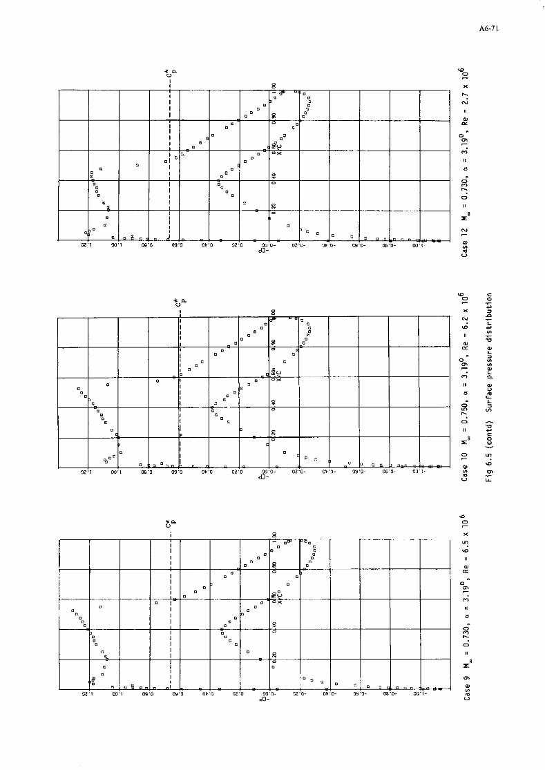
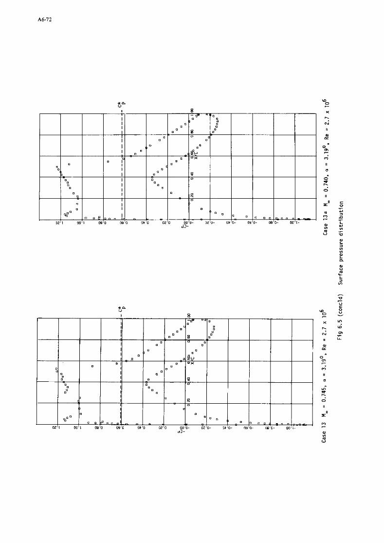

s~aJatueJed ayen pue Adepunog 9.9 6 k j
$1 x L'S = aU ',8L'z- = a ' 9 ~ 9 . 0 . 8 saqodd 2 ase3
90L x L'S = a8 'OOb'Z = a '919'0 = -W 9 SaqOdd L aSe3

sdaqalueded a l e n pue JaXel Xdepunog (pluo2) 9.9 6kj


Case 13 Probes D
M- = 0.745, a = 3.19'. Re = 2.7 x 10 6
F i g 6 .6 (concld)
Case 13a Probes C2 M_ = 0.740, o = 3.19'. Re = 2.7 x 10 6
Boundary layer and wake parameters

7. PRESSURE DISTRIBUTIONS POR AIRFOIL NAE 75-036e13: 2
AT REYNOLDS NUMBERS FROM 14 TO 30 MILLION
submitted by
High Speed Aerodynamics Laboratory, NAE/NRC, Canada
This is a 13% thick section designed for a lift coefficient of 0.36 at a Mach number of 0.75, but with the constraint that the lower surface Mach number must not exceed 0.93. The data comprise pressure distributions with trailing edge pressure, wake drag, aerodynamic coefficients from balance measurements as well as pressure integration and floor and ceiling pressure distributions.
1. Airfoil
1.1 Airfoil designation NAE 75-036-13:2 (also DHC JJK 13)
1.2 Type of airfoil LOW lift, near shockless, supercritical
1.2.1 airfoil geometry Fig. 7.1, Table 7.1
nose radius r/c - 2.2% maximum thickness base thickness
1.2.2 design condition Potential flow, direct method
(lower surface)) C* + 0.2 Proin P
T.E. angle 15'
Viscous calcs for Re = 20 x 10 6
design pressure distribution - 1.3 Additional remarks Buffet free operation required up to M=Md+0.05
C =1.5 C L Ld
1.4 References on airfoil 1, 2
2. Model Geometry
2.1 Chord length
2.2 Span
2.3 Actual model co-ordinates and accuracy
2.4 Maximum thickness
2.5 Base thickness
2.6 Additional remarks
2.7 References on model
2. Wind tunnel
3.1 Designation
3.2 Type of tunnel
3.2.1 stagnation pressure
3.2.2 stagnation temperature
3.2.3 humidity/dew point
3.3 Test section
3.3.1 dimensions
3.3.2 type of walls
0.254 m
0.381 m
Table 7.2 Y in Table 7.2 obtained by cubic sgline fit to values given in Table 7.1
t/c = 13%
0.1% chord
surface finish 6 0.25 um theoretical shape altered after 95% chord to accommodate finite TE
2
NAE 5-ft x 5-ft trisonic W/T with 2-D insert
Blowdown
2 - 11 bars 293 K, max drop -5K during a run
0.0002 kg H20/Kg air
Rectangular, Fig. 7.2
0.38m x 1.52m
Perforated top and bottom 20.5% porosity 012.71~11 normal holes at 26.4 nun spacing

3.4 Flow field (empty test section)
3.4.1 reference static pressure
3.4.2 flow angularity
3.4.3 Mach no. distribution
3.4.4 pressure gradient
3.4.5 turbulence/noise level
3.4.6 side wall boundary layer
3.5 Additional remarks
3.6 References on wind tunnel
4. TeStS
4.1 Type of measurements
at sidewall, 7.7 chord upstream of model LE
not determined
Fig. 7.3
Fig. 7.3
free stream = 0.008 at MI = 0.8
6 * \< 2.5 mm
< 0.013
sidewall suction over an area 1.8x2.4 chord around model
Force balance surface pressure wake pitot pressure
4.2 Tunnel/model dimenstions
4.2.1 height/chord ratio 6/1
4.2.3 width/chord ratio 1.5/1
4.3 Flow conditions included in present Fig.7.4 and Table 7.3 data base
4.3.1 angle of attack 0 to 4' for MI = 0.75 2' for other MI
4.3.2 Mach number 0.5 to 0.84
4.3.3 Reynolds number 14, 25 and 30 x lo6 based on 10" chord.
4.3.4 transition free transition
-position of free transition Not established
-transition fixing
4.3.5 temperature equilibrium Yes
4.4 Additional remarks
4.5 Reference on tests 2
5. Instrumentation
5.1 Surface pressure measurements
5.1.1 pressure holes
-size
-spanwise station (s)
-chordwise positions
5.1.2 type of transducers and scanning devices
5.1.3 other
5.2 Wake measurements
80
'$ 0.37 mm, depth/diameter ratio -1.7
centre span
Table 7.2
Two D9 scanivalves with 200 psia Kulite VQS-500-200A
scan rate for 5.1.2 20 ports/sec.
5.2.1 type/size of instrument(s) Traversing probe, see Fig.7.2 OD/ID = 1.6/0.51 mm
5.2.2 streamwise position(s) 1.5 x chord downstream T.E.
5.2.3 type of transducers and 50 psid Statham PM 131 TC scanning devices

5.5 Flow visualisation
5.5.2 surface flow at CN = 0.36, M = 0.75, 0.8, Re = 25 x lo6
5.7 Additional remarks Two three-component side wall balances for force measurements
5.8 References on instrumentation 4
6.1 Accuracy (wall interference excluded)
6.1.1 angle of attack setting i 0.02'
6.1.2 free stream Mach number:
-setting f 0.003
-variation during one f 0.003 pressure scan
6.1.6 repeatability
6.2 Wall interference corrections (indicate estimated accuracy)
6.2.1 angle of attack
Generally: A C N ~ < t0.005 ACXp < t0.0005 ACMp< i0.0005
ACNB < f0.005 ACXB < t0.0005 ACMB< ?0.0005
ACDW < f0.0015
duo&-1.2 CL at M = 0.75
(estim. for PU = 1.5, PL = 0.5)
6.2.2 blockage (solid/wake) Negligible (lift) AM-0.013 CL at M = 0.75
(estim. for PU = 1.5, PL = 0.5)
6.2.3 streamline curvature (lift) Negligible
6.2.4 other
6.2.5 remarks
6.2.6 references on wall interference correction
6.3 Presentation of data
6.3.1 aerodynamic coefficients
6.3.2 surface pressures
6.3.3 boundary layer quantities
6.3.4 wall interference corrections included 7
6.3.5 corrections for model deflection
6.3.6 empty test section calibration taken into account 7
6.3.7 other correction included 7
6.3.8 additional remarks
Results from pressure measurements with wall mounted rails, with pressure ports 4.8 cm from the wall, are included for evaluating wall
corrections. Tables 7.4 - 7.20 5. 6
Table 7.3
Table 7.4-7.20 Figure7.5-7.21
6.4 Were tests carried out in different No facilities on the current airfoil 7 If so, what facilities. Are data included in the present data base 7
Yes
wake drag data are those obtained from probe on E only
6.5 To be contacted for further D.J. Jones, High Speed Aerodynamics Laboratory, information on tests NAE/NRC ,
Montreal Road, Ottawa, Ontario, Canada KIA OR6

7. References
1,J.J. Kacprzynski Low lift supercritical 13% thick airfoil (CONFIDENTIAL) NRC/NAE LTR-HA-19 January, 1974
2.5.5. Kacprzynski Wind Tunnel test results of 2-D flow past the supercritical airfoil DHC JJK 13. NRC/NAE LTR-HA-5x5/0089 February, 1975
3.L.H. Ohman et a1 The NAE high Reynolds number 15in x 16in two-dimensional test facility. NRC/NAE LTR-HA-A April, 1970
4.L.H. Ohman The NAE 15in x 60in two-dimensional test facility: new features and some related observations. results of new centre line calibration at 20.5% porosity. NRC/NAE LTR-HA-15 March, 1973
5.D.J. Peake, A simple streamwise momentum analysis to indicate an empirical A.J. Bowker correction to angle of incidence in two-dimensional, transonic
flow, due to a perforated floor and ceiling of the wind tunnel NRC/NAE LTR-HA-11 January, 1973
6.M. Mokry et a1 Wall interference on 2D supercritical airfoils, using wall pressure measurements to determine the porosity factors for tunnel floor and ceiling. NRC/NAE LR-575 February, 1974
8. List of symbols
B
c
H
M
M, P
Pa PO
Re
Pu' P~
tunnel width = model span
model chord
tunnel height
local Mach number
free stream Mach number
local static pressure
free stream static pressure
free stream total pressure
Reynolds number based on model chord
porosity factor for upper and lower walls (ceiling and floor of W/T). See reference 6
free stream dynamic pressure
relative sidewall suction; velocity 1 sidewall free stream velocity
pressure coefficient %,
CNt CN normal force coefficient
Cxp CX chord force coefficient
CM, CMC4 pitching moment coefficient about 1/4 chord
CL lift coefficient
CDP pressure drag coefficient
C ~ w wake drag coefficient
streamwise coordinate, model origin: LE W/T origin: balance E = 0.4 model X/c
ag geometric angle of attack, angle between chordline and tunnel centre line.
subscript P refers to pressure data
B balance data
d design data
m to model data
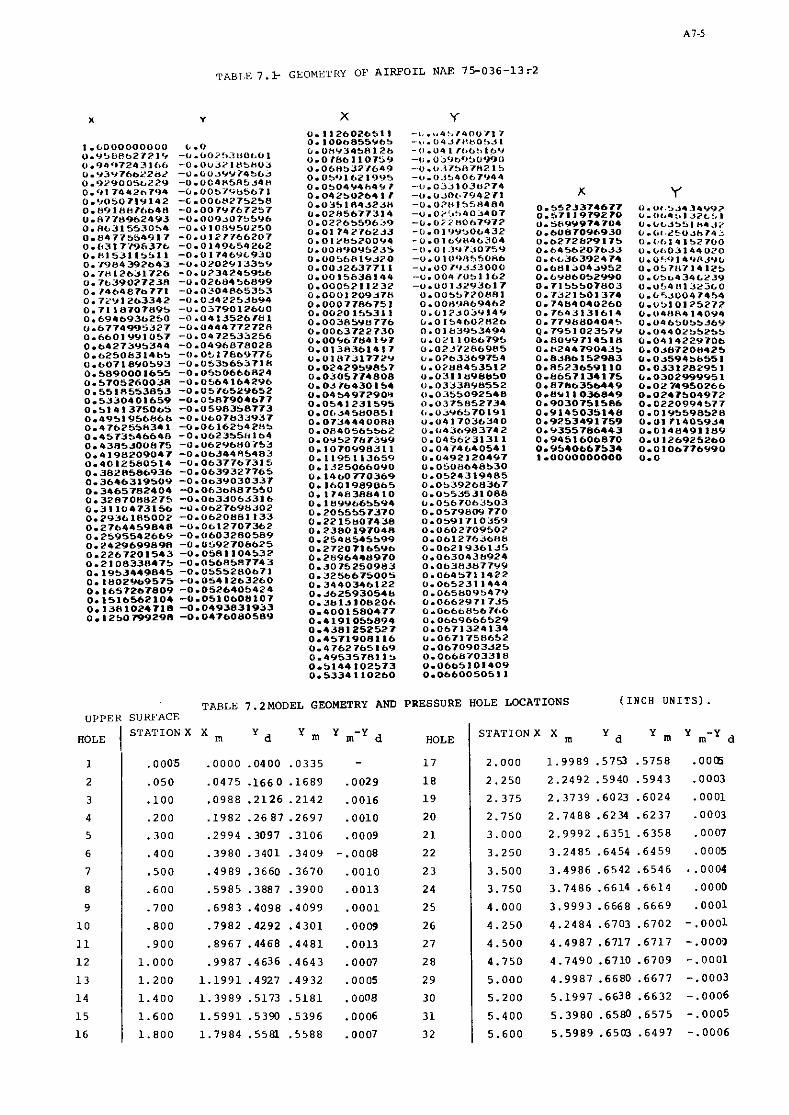
TAB1.E 7 . k GEOMETRY OF A I W O I L NAE 7 5 - 0 3 6 - 1 3 r 2
TABLE 7.2MODEL GEOMETRY AND PRESSURE HOLE LOCATIONS (INCH U N I T S ) . UPPER SURFACE
HOLE I STATION X X rn Y d Y Y m-Y d HOLE I STATION X X rn y d m m-Y d

TAR1.E 7.2 (Cont. )
LOWEK S U R F A C E
HO1.E STATION X X - f a Y m Y m - Y d UPPER S U R F A C E
5 3 .050 .0479 -.0994 -.I016 -.0022 H0I.E S T A T I O N X X y d Y n , Y m - Y a 54 .LOO .lo10 -.I496 -.I498 -.0002
TABLE 1 .3
55 .ZOO .I997 -.2141 -.2135 .0006
-.0004 56 .300 .2988 -.2610 -.2603 .0007
-.0001 57 ,400 .3995 -.2983 -.2978 .0015
-.0003 58 .500 5003 -. 3297 -,3286 .0011
-.0005 59 .750 .7490 -.3894 -.3882 .001 2
-.0006 60 1.000 .9995 -.4366 -.4356 .0010
-.0013 61 1.500 1.4991 -.5085 -.5069 ,0016
-.0005 Bal. Pins 1.750
-.0003 62 2.000 1.9976 -.5592 -.5582 ,0010
.0001 63 2.500 2.5006 -.5974 -.5962 .0012
.0005 64 3.000 2.9974 -.6234 -.6227 .DO17
.0010 65 3.500 3.4996 -.6374 -.6367 .0007 -.0023 66 4.000 3.9998 -.6379 -.6375 ,000 4
.OO% 67 4.500 4.4983 -.6261 -.6255 .000 6
.OO% 68 5.000 4.9984 -.6056 -.GO49 ,001 7
.ON5 69 5.625 5.6233 -.5698 -.5697 .ooo 1
.0008 70 6.000 5.9997 -.5420 -.5419 .0001
.0009 Bal. Pins 6.250
.0013 71 6.500 6.4988 -.4874 -.4872 ,0002
.0017 72 7.000 6.9991 -.4033 -,4030 .0003
73 7.250 7.2491 -.3513 -.3512 -.0001
74 7.500 7.4988 -.2976 -.2977 -.0001
7 5 7.750 7.7496 -.2464 -.2464 -.0000
7 6 8.000 7.9987 -.2004 -.ZOO7 -.0003
7 7 8.250 8.2475 -.1600 -.I602 -.0002
7 8 8.500 8.5003 -.1248 -.1251 -.0003
79 9.000 9.0000 -.0726 -.a726 .OOOO
8 0 9.500 9.5021 -.0318 -.0342 -.0024
T . E . 10.000 10.OO1l -.0050 -. AERODYNAHIC COEFFICIENTS
PRESBURS BAi l lSCE
TiiBLE C I C . n- nexio-6 --.\
C% CDw RUN SCAN

511kFdCr FhFSSUkk MLASURFMFNTS Pl lh i I . I IMPFP ~ 4 5 7 9 T C A Q NLIMBFv = 2 r' lNcIGUFITIOFI = DHCJJK T c S T P P C h MUMfiER= 0.511 F r V E I C L r J S FlUMHtF = O.1435E 08 INCIP ihCElNCPTHl= 1.919 P 0 = 61.84OSIA Q = 12.50PSI V I U I S I O E k L L L I -0.0052 c v = 0.335 C X =-.00567 C U C A =-0.0416 CL = 0.3354 c n ~ - 0.0050
A7-7
TABLE 7 . 4
1PIFICE X I C CF M l l 3 C A L l
70 0.6000 -0.2560 0.579 7 1 0.h500 -0.2369 0.575 72 0.7000 -0.1131 0.543 7 3 n.7250 -0.oz81 0.521 7 .r 0.7500 0.0429 0.503 7 5 0.77'0 0.1148 0.483 7 L. O.ROO0 0.1602 0.471 7 7 0.8250 0.1695 0.462 7 1 0.8500 0.2091 0.456 7 9 0.'?000 0.2193 0.453 ?'I 0.1500 0.2266 0.451
. C , d t Q 1.d000 0.2395 0.445
AT CEIL ING &NO FLOOR
FLOOR Y Ce M
0.514 0.007 0.511 0.513 0.006 0.510 0.516 0.005 0.512 0.513 0.002 0.512 0.514 0.006 0.513 0.514 0.005 0.512 0.515 0.015 0.510 0.516 0 - 0 1 2 0.510 0.515 0.011 0.511 0.515 0.012 0.510 0.519 0.019 0.509 0.517 -0.005 0.514 0.517 0.015 0.509 0.E17 0 - 0 2 0 0.509 0.517 0.016 0.510 0.517 0.017 0.509 0.519 0.015 0.510 0.51e 0.017 0.508 0.518 0.012 0.509 0.519 0.022 0.508 0.518 0.011 0.512 0.518 0.020 0.509 0.519 0.025 0.508 0.519 0.029 0.507 0.518 0.023 0.509 0.51e 0.029 0.507 0.518 0.024 0.509 0.518 0.027 0.507 0.520 0.021 0.509 0.516 0.026 0.508 0.517 0.001 0.514 0.516 0.024 0.509 0.515 0.020 0.510

T U Q F t C F P ~ E S S ' I R E MFASURFMFNTS ?UN "IM8F'I = 4 9 7 6 SCAN NUMI'P = 3 CONFIGUUATION = OHCJJK T F S T MACH YUMRFR= 0 . 6 9 9 REVNOLOS YUt4IER = 0 . 1 4 3 4 E 08 I Y C I D E N C c ( Y ' l r l T H l = 1 . 9 9 4 P 0 = 6 5 . 1 I P S I A 3 = l b . 0 7 P S I V I U ( s l n E w 8 L L l = O . O O ~ R CY = 0 . 3 6 6 C X = - , 0 0 5 4 7 CMC4 =-0 .0476 C L = 0 . 3 6 5 8 C D P = 0 . 0 0 7 3
TABLE 7 . 5

'1P I F ICE UPPFP
5 I
SIJRFACF PRFSSVRF MEASURF*FNTS QUW N ( l Y R C P ~ 4 9 7 4 SC4N NOUeCP = 5 CflNF lc<IR4TlC1N = OHCJJK ' 'ST M A C H t4VMREH= 0.754 PCYNOLDS Y l l Y U E R = 0.1344F 08 IYClDFNCF(YnXTHl= 1.904 P 0 = 60.15PS14 0 = I6 .41PSI V / l l (SIDEWALL1 =0.005? C '4 = 0.389 C X =-.00530 CYC4 =-0.0408 C L = 0.3PPQ C'IP = O.OOP2
A7-9
TABLE 7 . 6
FLOOR c P n
0.013 0.755 0.013 0.753 0.017 0.751 0.01R 0.753 0.317 0.751 0.322 0.749 0.325 0.74e 0.025 0.748 0.972 0.749 0 - ) 7 3 0.751 O J ? O 0.746 0.009 0.755 0.037 0.744 0.030 0.745 0.132 0.745 0.035 0.746 0.2?7 0.746 0.127 0.749 0.074 0.749 0.331 0.746 0.928 0.747 O.J?h 0.744 0.375 0.744 O.J4! 0.742 0.340 0.741 0. 144 0.741 0.366 0.740 0.J47 0.742 0.071 0.743 0.J;II 0.741 0.137 0.759 0.J'-0 0.741 0.037 0.743 0.337 0.743 0.37n 0.743 0.3'6 0.744 0.0'7 0.744 0 . 0 3 2 0.746 0.07'1 0.747 0.121 0.750
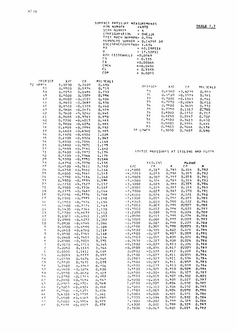
511QF4CF PQFSS'IPc YEASURFYFNTZ PIIN kUY8FR ~ 4 9 7 0 SSAN hJUYOCD = 4 CqNFIGURlTl1lN = DHCJJK TFST MACH NIIWRFRi 0 . 7 0 4 RtYNOLOS YUYSER = 0.1429E OR I Y C I n F N ~ ~ l F i n ~ T H I = 1.474 P 0 = 60.19PS16 B = 17.52PSI V/Il ISIQEW41 L l =0 .0049 r u = 0 .235 r x -0 .00066 CYC4 =-0.0496 CL = 0.3353 COP = 0 .0003
TABLE 7 . 7
S f l L I Y S FLOOR X / C Y D Y C P U
1 . ~ 1 1 0.911 I . R l 0
O.-.lO 0.R04 0 .007 0. R05 3.804 'I. 504 '1.au4 0.801 0.'07 0 . 7 0 0 1 . 7 9 9 'I. R07

ZURFACE PRESSURE MEASUREMENTS TON YUyRER - 4 9 4 4 SCAN NOMRFR = 2 CONFIGUR4TION = OHCJJK TFST MACH NlIMRER= 0.702 9EYNOLDS NUYHER = 0.2553E 08 IYCIOENCF IUORTH)= 1.9s9 P I -114.ROPSlA 0 = 25.52PSI V I U ISIDEWALLI =0 .0051 C Y = 0 .391 C X =- .00557 CMC4 =-0.0417 CL 0.3R14 COP = 0.0077
STATIC PRESSURFS AT C E I l
A7-I1
TABLE 7 .8 .
FLOOR C P M
0.002 0 .707 0.007 0 .703 0.007 0.705

clJI)FF.CL P P C 5 5 ! J F F HEASIJPF~FYTS P i J N NUY 3F? =4036 S C b h ' UIJ 'AREF = 1 TiNr lGURf lT l f lN = OHrJJK T C S T UnCH Y V M R E Q i 0.754 i i rYhflL. lZ ' I I J ~ R F P = O.251PE OR I N C 1 0 C ' 4 C F l Y P D T H l = - 0 . 0 4 7 P 0 =109.96PSIb 0 = 30.01PSI V I I I I S I O F r l A l I l ~ 0 . 0 0 3 6 C Y = Q.102 f X =0.00295 C " C 4 =-0.0408 CL = 0.1023 C O P = 0.0029
TABLE 7 .9
cTATlC PRFSSURC5 A T CFIL INF AND FLnOQ
' F I L ING C D
0.007 0.016 0. >oo 0.016 0.021 0.319 0.316 0.017 0.006 0.009 0.004

SUQFACC PRESSURE HFASUREMFNTS RUN NIIMBFR =4916 5CON NUWBFR = 3 CqNFIGUSATIOY = DHCJJK T F S T rAcn YUMPFR= 0 . 7 5 ~ REYNPLOS YIlYRER = 0.2541F 08 INCIDEYCFIYOPTHl= 0.9h7 P 5 =109.URPSIA 0 = 30.06PSI V/!l ISIDENALL) =0.0025 C N = 0.246 CX =0.00125 CMC4 =-0.0501 CL = 0.2456 CDP = 0.0054
A7-13
TABLE 7.10
ORIFICE X I C CP MILOCAL) T r UPPFR 1.0000 O.?h99 0.645 7 P I F I C F X I C C P MILOCALI
5 1 n.0500 0.1880 0.687
- - - 7 8 0.R5CO 0.2357 0.660 7 9 O."OOO 0.2506 0.651 9 0 0.0500 0.2572 0.650
T F LOWER 1.0000 O.Zh9q 0.645
STbTIC ORFSSIJQFS AT CEILING AND FLOOR

SUoFACC PhtSSbFF CFASUREMSNTS kUN hUP8EF = 5 0 0 1 S C A U kUlrp.FR = I CnMF16UFPTION = OHCJJK I r S T MbCH kUWPER= 0.756 FrYVCLDS h U Y M l F = 0.2515E 08 TNC I L E t ~ C T i h U h T H l = 1.485 PO =109.99DSIA 0 = 30.14PSI V / U ( S I D C w I L L I =0.0047
-0.4830 0.954 -0.4e92 0.972 -0.5085 0.180 -0.5513 0.998 -0.5522 1.014 -0.6283 1.035 -6.6321 1.036 -0.6486 1.044 -0.6564 1.047 -0.64t5 1.042 -0.6485 1.042 -0.6183 1.028 -0.6163 1.026 -0.6039 1.021 -0.589h 1.016 -0.5833 1.014 -0.5P50 1.013 -0.6606 1.048 -0.7711 I. LOR -0.a164 1.1~0 -v rHLd7 1.122 -0.8179 1.122 -0.7957 1.111 -0.755' 1.093 -0. t644 1.062 -0.6569 1.049 -0.6377 1.039 -0.6875 1.061 -0.PO95 1.119 -0.8030 I. 1 4 4 -U.8156 1.120
6.4357 0.949
TABLE 7.11
i T C F I L
w
ING b M FLOOP

X I C 1 . OOUO~ 0 .9500 0 .9250
URFACF PRtSSUPE MEASUFEMENTS K~JN hUMBEk = 500 1 SCAN hUM8ER = 2 CONFIGURATION = OHCJJK 'LSf C P C H NUMPER= 0 .757 PtYNCLOs FlUMBtF = 0.2529E 08 lNttCEF;tF(IUURTHI= 1 .742
V I U (SIOEWPLL) -0.0047 C N = 0.368 CX =-.00243 C M C 4 =-0.0485 r L = 0.3678 CDP = 0.00R7
A7-I 5
TABLE 7.12
STATIC PRESSURES AT CFILLNG AND FLOOR
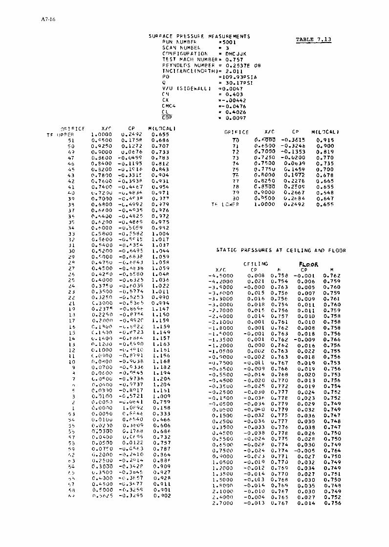
SURFACE PPESSUFF MFASUREMENTS RUN hUlrBFh 2 5 0 0 1 S C P Y NUMGEC = 3 CnYF16UPBTlON = OHCJJK T E S T MAC11 NUMRER= 0.757 PFYNOLnS NUMPER = 0.2537F 0 8 I N C I l t N C E l Y C ~ T H ) = 2 .011 PO =109.93PSIA C = 30.17PSI V I U I S IOEWCLL I 30.0047 C Y = 0.403 CX = - - 0 0 4 4 2 CMC4 -0.0476 C L - = 0.4026 CDP = 0.0097
TABLE 7 . 1 3
XIC
0 . m 0 .6500 0 .7000 0 .7250 0 .7500 0.77511 O.RO00 0.8250 C.RSOU 0.9000 0.Q500 1.0000
STATIC P Y F S U P E S AT C k I L I N G A W FLOOR
C F I L I N G FLOOR X I T r p c r p

X I C C P 1. )GO0 0.7601 l).c500 0.19hR 0.0750 0.1388
SUPFACC PRESSIJRF MEASIJREMENTS V I IN NUMRER ~ 4 9 3 7 C C b h NlJYSF4 = 3 ~ r l h F I G U 9 4 T I ' l Y = DHCJJK T F S T MAC){ N V Y I F R = 0.754 RFYFIOLD5 NiJMRCP = 0.2537F 08
A7-17
TABLE 7.14
I O I F I C F X I C C P M l L 3 C b L l
7 0 0.tUOO -0.3373 0.900 7 1 0.6500 -0.2936 0.585 7 2 0.7000 -0.1212 0.911 7 3 0.7250 -0.0167 0.765 74 0.7500 0.0777 0.727 7 5 u.77C.0 0.1515 0.695 7 6 o.a1oo 0.1757 0.676 77 0.R750 0.2294 0.661 7 R 0.R5OO 0.2575 0.650 7 1 O."OOO 0.2631 0.646 P 0 0.0500 0.2675 0.644
T F L U U € ? 1.0000 0.2601 0.447
S T A T I C P R F 5 5 U R F S 4 T C F l L I Y G AND FLOQR

ORIFICE TE UPPER
SURFACE PRESSUQF MEASUREMFNTS RUU NUMIIEq 14938 SCAN YUMSER = I CPUFIGuR4TlnY = DHCJJK TFST YACH NUYRER= 0.751 PEYNOLllS NUMRER = 0 -2514F 08 INCIOFNCEINORTHI- 3.034 PO =109.96PSlA 0 = 29.R7PS1 V I U (STOFWALL) 1 0 - 0 0 3 6 C N = 0.574 C X = - -01398 CMC4 =-0.0394 CL = 0.5342 CDP = 0.0143
PRESSURES
CFIL ING C P
0.014 0.014
-0.001 0.019 0.070 0.027 0.017 0.017 0.039 0.006 0.007
-0.002 -0.003 -0.002 -0.004 -0.ooe -0.015 -0.01" -0.070 -0.026 -0.029 -0.035 -0.039 -0.0'37 -0.3'0 -0.014 -0.0'4 -0.C31 -0.07a -0.077
TABLE 7 . 1 5
AT CEILING AND FLOOP

q R I F ICF UPPEP
SIJRFACT PRFSSIIRF MEASURFMFNTS KUY NUMRER =493R SCAN NUMYFQ = 7 CnNFIGURATlnN = DHTJJK TEST MACH NUMREF= 0.752 RCYNrJLQS NllMRFP = 0.25?0E 08 I'dCInFNCCIWOPTH)= 4.057 P 0 =109.9aPSIA 0 = 79.91PSI V I U ISIDEWALLI =0.0036 CY = 0.659 C X =-.01R32 C Y t 4 =-0.0410 CL = 0.65R2 COP = 0.02P3
X I C C D W(LOCAL1 1.0000 0.?791 0.438 0.9500 0.1821 0.541 0.9250 0.1262 0.705 0.9000 0.0617 0.731 O.Rh0O -0.0579 0.781 0.4400 -0.17LR 0.80'4 0.R200 -3.1877 0.816 0.7R00 -0.3124 0.989 0.7603 -0.36lR 0.709 0.7400 -3.4021 0.927 0.7200 -0.4237 0.937 0.7000 -0.4349 0.341 0 . bPOO -0.432s 0.940 0.6600 -5.4199 0.934 0.6405 -9.4129 0.932 O.f?OO -3.4145 0.937 O.600O -0.415q 0.937 0.5800 -0.4339 0.940 0.5h00 -0.4207 0.935 0.5400 -0.42?R 0.937 0.5200 -3.4135 0.934 0.q000 -!).'*I91 0.937 0.4750 -0.445U 0.747 0.4500 -3.6070 1.318 0.47=0 -1.0416 1.?25 0.4005 -1.2044 1.313 0.3750 -1.2050 1.314 0.3500 -1.>037 l.'?Y3 0.3257 -1.?076 1.315 0.'000 -1.2154 1.316 0.2375 -1.?274 1.321 0.2250 -1.2171 1.320
A7-I9
TABLE 7.16
X P l F l C F X I C CP MILOCAL)
STbTIC PRFSSIIKCS AT C F l L l N G AND FLOOR
X I C -4.5003 -4.7000 -7.9000

I P I F I C F X I C TF IJPPFQ 1.0000
5 1 0.4500 50 0.9250 49 0.9000 47 0.4600 46 0.8400 4 5 0.8200 4 3 0.7P00 42 0.Th00 41 0.7400 40 0.7200 37 0.7000 38 0.6800 3 7 0.6600 3 6 0.6400 3 5 O.hL'lO 34 O.hO00 3 3 0.5800 32 0.5600
BUGFACF PRESSURt MEASUREMENTS FUN hUMHER ~ 4 9 9 9 SCAN NUMBER = 1 CI>NFIGUPATION = DHCJJK TEST V4CH NUMRt9- 0.806 PEVNOLDS tJUM8C-R = 0.2487E 08 INCILENCEINURTH)= 1.465 PO =105.03PsIA 0 = 31.14PSI VIU ISIDEWLLLI -0.0044 CN = 0.338 C x =0.00366 CMC4 =-0.0572 CL = 0.3379 L O P 0.0123
H I LOCAL 1 0.695 0.720 0.740 0.763 0.807 0.831 0.861 0.908 0 -9 32 0.950 0.965 0.998 1.069 1.224 1.238 1.242 1.246 1.245 1.231 1.226 1.209 1.204 1.201 1.207 1.201 1.196 1.192 1.1 54 1.184 1.184 1.178 1.178 1.173 1.165 1.153 1.142 1.126 1.121 1.116 1.109 1.116 1.128 1.146 1.146 1.119 0.933 0.735 0.119 0.404 0.545 0.685 0.770 0.817 0.847 0.881 0.968 0.995 1.026 1.072 1.107 1.110 0.990 0.994
, . TS 79 B 0
TE LOWER
TABLE 7.17
M I LOCAL)
1.014 0.979 0.873 0.820 0.787 0.750 0.727 0.710 0.698 0.691 0.688 0.695
STbTIC P A E S S W E S AT CEICI1YG AN0 FLOOR
CEILING C P
0.007 0.020
-0.001 0.013 0.018 0.021 0.020 0.016 0.010 0.004 0.005 0.004 0.005 0.006 0.000
-0.004 -0.004 -0.014 -0.018 -0.023 -0.030 -0.034 -0.039 -0.040 -0.038 -0.041 -0.041 -0.038 -0.032 -0.031 -0.025 -0.018 -0.018 -0.015 -0.014 -0.012 -0.010 -0.007 -0.006 -0.010

SUQFACF PRFSSURF MFBSUREMENTS RUN NIIMBET( = 4 Q 5 1 5CAN NUMSFR = 3 CONFIGURATIIJN = DHCJJK TEST MACH NUMBER= 0 . R 4 1 REYNOLOS NUMRFR = 0 . 2 5 1 9 6 OR I Y C I O F Y C F l N I J R T H l = 1 . 0 0 1 P 0 = 1 0 2 . 9 9 P S I A 0 = 3 2 . 0 9 P S 1 V I U I S I f l F W A L L l ~ 0 . 0 0 3 3 C N = 0 . 1 1 3 C X = 0 . 0 2 5 4 8 CYC4 = - 0 . 0 0 4 3 C L * 0 . 1 1 3 0 COP = 0 . 0 2 7 5
UPPFR O Q I F I C F xlr T P
A7-2 1
TABLE 7.18
S T A T I C P Q E \ S U D E $ AT C F I L I Y G ANn F l l i l l R
0.Q000 1 . L'OO 1.7OCO

ClRIF UPPER
I C E
SUaFACE PRFqSURE MEASURE~FNTS PUN NUMflEQ =49fl2 SCAN NUPREQ = 1 CCNFIGU~4TION = CHCJJK T C S T PACH NUHS€K= 0.756 REYNOLDS NUMRER = 9 . 2 9 6 ~ ~ 08 INCIDFNCElNOUTHl= 2.017 PI) =129.8OPSIA 13 = 35.57PSI V IU I SI1)EWALLl =0.0036 CN = 0.400 C X =-.00401 CMC4 =-0.0478 CL = 0.399% C O P = 0.5100
O P l F I C t X I C
7 0 O.b33J 7 1 0.65GO 72 0.7000 73 0.7250
TABLE 7.19
STATIC PRESSURFS A T CEILING AND FLOOR
CElL ING F L O O R XIC CP M C P t4
-4.5JOO 0.009 3.759 0.002 0.761 -4.2000 0.014 0.755 0.002 0.76C

A7-23
TABLE 7.20 SURFACE PRESSURE MEASUREMENTS
HUN hUMBER =4986 SCAN NUMBER I I CONFIGURATION = OHCJJK TFST MACH NUYBER= 0.801 REYNOLDS NUHBEP = 0.2996E 0 8 INCIDENCEINORTHI= 2.000 P 0 =127.OOPSIA Q = 37.41PSI V I U (SIOEWALL) =0.0034 C N = 0.393 CX =0.00073
C L COP
E XIC 1.0000 0.9500 0.9250 0.9000 0.8600 0.8400 0.8200 0.7800
ORIFICE XIC CP MILOCAL)
7 0 O.6GJO -0.4395 1.911 7 1 0.65CO -0.3753 C.980
STATIC PRFSSURES A T C F l L l N C AND FLf l f lR
CEILING C P
0.007 0.018
-0.005
FLOOR C P H
-0.000 O.ROC 0.000 0.805 0.307 0.805

FIG- 7.1 NAE 75-036-13:2 AIRFOIL


8 . S U P E R C R I T I C A L A I R F O I L MBB-A3 S u r f a c e p r e s s u r e d i s t r i b u t i o n s ,
wake a n d b o u n d a r y c o n d i t i o n measurements.
Bucciant in i G. , Oggiano M.S., Onorato M. A e r i t a l i a Torino, Pol i tecnico d i Torino
8 . 1 INTRODUCTION
The present data set, obtained t es t i ng the same model o f the MBB-A3 a i r f o i l a t the A.R.A. Bedford wind tunnel and a t the Turin Polytechnic wind tunnel (P.T.), covers a wide range o f condit ions: whollysubsonic flow, superc r i t i ca l shockless o r near shockless flow, superc r i t i ca l flow w i th r e l a t i v e l y strong shockwave producing, i n some extreme cases, boundary layer separation. Moreover due t o the great dif ference i n Rey- nolds number between the two tunnels ( the P.T. transonic f a c i l i t y i s operated a t low Reynolds number be- cause of power l im i t a t i ons ) , d i f f e r e n t condit ions of po ten t ia l flow-boundary layer i n t e rac t i on are pres- ented. I n the cases o f measurements w i th f r ee t r ans i t i on , the Polytechnic o f Tur in experiments show a lambda shaped shock wave, t yp i ca l of shock wave impinging on a laminar boundary layer; on the contraryfor the A.R.A. r esu l t s the i n te rac t i on appears t o be tu rbu len t ( i t has t o be not iced t ha t even though the re - s u l t s from A.R.A. are t r ans i t i on free, the disturbances from the pressure holes are l i k e l y t o promote t r a n s i t i o n upstream o f the shock waves). Also on the lower surface the flow f i e l d shows d i f f e r e n t behav- iour , due t o the d i f f e r e n t growth of the boundary layer , p a r t i c u l a r l y i n the rear p a r t o f t he sectionwhere a concavity i s present.
The pressure d i s t r i bu t i ons on the a i r f o i l obtained i n the two tunnels become comparable when the t ran- s i t i o n i s f ixed i n the P.T. experiments, both on the upper and on the lower surface and when wal l i n t e r - ference correct ions are applied!see Fig.8.6 and comnents t o Tables 8.4).
The MBB-A3 p r o f i l e , designed by the Eberle hodograph method i s supe rc r i t i ca l , shockless, s lopingroof- top. Moreover the MBB-A3 a i r f o i l i s the section fo r the MBB-AVA-Pilot Model (one o f the 3-d configura- t ions selected f o r the present data co l l ec t i on ) and i s the th innest section f o r which data are pres- ented. For a l l the cases reported surface pressure measurements are presented; experiments from A.R.A. wind tunnel include wake t o t a l and s t a t i c pressure survey (on ly the values o f the drag coe f f i c i en t s are reported here); data from P.T. wind tunnel include s t a t i c pressure d i s t r i bu t i ons above and below the mod- e l a t a distance from the chord o f about 213 o f hal f -heiahtof the t e s t section. The l a s t information i s
~A ~ ~~
~~~~ ~ ~ ~
important i n view of the aim of t h i s data col1ection;i f measured boundary condit ions are ava i lab le andare used fo r the assessment of computer programs, empir ical correct ions fo r tunnel wal l in ter ference are not necessary.
About the A.R.A. data the e f f ec t i ve freestream condit ions can be estimated applying the semi-empirical wal l interference cor rec t ion procedures given i n the questionnaire (see 6.2.5).
Both A.R.A. and P.T. data presented here are not corrected for wa l l in ter ference e f f ec t s .
8.2 DATA SET
1 . A i r f o i l
1.1 A i r f o i l designation MBB-A3
1.2 Type of a i r f o i l Superc r i t i ca l shockless
1.2.1 a i r f o i l geometry Fig.8.1; Tablcs8.1 and 8.2 nose radius 0.0075 c maximum thickness 8.9% base thickness 0
1.2.2 design condi t ion &=0.76, a=1.3" , C ~ = 0 . 5 8 design pressure d i s t r i b u t i o n Fig.8.2 ( repr in ted from r e f . [ l ] )
1.3 Addit ional remarks None
1.4 References on a i r f o i l 11 1 , 121
2. Model g e o m e t r r
2.1 Chord length 0.127 m
2.2 Span 0.203m; 0.4m(see 2.6)
2.3 Actual model co-ordinates and accuracy Table 8.2
2.4 Maximum thickness 8.9%
2.5 Base thickness 0
2.6 Addi t ional remarks The span o f the same model, prev iously testedat the A.R.A. Bedford wind tunne1,has been increased f o r the tes ts i n the Turin Polytechnic wind tunnel (Pic- t u re 1 ).
2.7 References on model [11 , [21
3. Wind t u n n e l s
3.1 Designation A.R.A. Bedford 20 transonic tunnel (A.R.A.) Ga l l e r i a transonica e supersonica, Po l i tecn ico d i Torino (P.T.)

3.2 Type of tunnel Blow down (A .R .A. ) ;cont inuous(P .T . )
3.2.1 s tagnat ion pressure
3.2.2 stagnation temperature
3.2.3 humidityldew p o i n t
3.3 Test Sect ion
3.3.1 dimensions
3.3.2 type of wa l l s
3.4 Flow f i e l d (empty t e s t sec t ion )
3.4.1 reference s t a t i c pressure
3.4.2 f l ow a n g u l a r i t y
3.4.3 Mach number d i s t r i b u t i o n
3.4.4 pressure gradient
3.4.5 turbulence/noise l e v e l
3.4.6 s ide w a l l boundary l a y e r
3.5 Addi t ional remarks
3.6 References on wind tunnel
4 . T e s t s - 4.1 Type of measurements
4.2 Tunnel/model dimensions
4.2.1 height/chord r a t i o
4.2.3 width/chord r a t i o
4.3 Flow condi t ions inc luded i n present data base
4.3.1 annle o f a t tack
4.3.2 Mach number
4.3.3 Reynolds number
4.3.4 t r a n s i t i o n
- p o s i t i o n o f f r e e t r a n s i t i o n - t r a n s i t i o n f i x i n g
4.3.5 temperature e q u i l i b r i u m
4.4 Addi t ional remarks
4.5 References on t e s t s
5. I n s t r u m e n t a t i o n
5.1 Surface pressure measurements
5.1.1 pressure holes - s i z e - spanwise s ta t ions
- chordwise p o s i t i o n s
5.1.2 type o f transducers and scanning devices
From 1.5 t o 4 atmospheres(A.R.A.) up t o 0.46 atmospheres (P.T.)
290°K(A.R.A.); 300°K (P.T.)
24O0K(A.R.A.); 223°K (P.T.)
Rectangular (A.R.A.); square (P.T.)
0.457 m x0.203 m (A.R.A.) 0.40 m x0 .40 m(P.T.)
S lo t ted top and bottom (A.R.A.-P.T.) open-area r a t i o o f 3.2% (A.R.A.) open-area r a t i o ~f 50%;porosity i s c o n t r o l l e d by a moving p l a t e i n s i d e the plenum chamber (see F ig . 8.5 and Pic ture l)(P.T.)
On the top l i n e r , 5 chords upstream of model L.E.(A.R.A.) a t s idewal l 2 chords upstream of model L.E. (P.T.)
t 0.05' (A.R.A.) - Mach number gradient alonq the model: 0.001 up t o M, = 0.65, increasing t o 0.002 a t M, = 0.82 and t o 0.003 a t M, = 0.85 (A.R.A.) Fig.8.3a (P.T.)
See 3.4.3
Under i n v e s t i g a t i o n us ing K u l i t e transducers (A.R.A.) (AC,) ,.,-, = 0.014 a t M, = 0.75, see a lso Fiq.8.3b(P.T.) . .. 6" = 1.5mn f o r M, = 0.7 (A.R.A.) 6(U ~ 0 . 9 9 Ue) =31 mnfor M , = 0 . 6
=29.5mnfor M,=0.7 - 2 8 innfor M- ~ 0 . 7 5 I (P.T.)
=27 mnfor M L - 0 . 8 1 None
[l],[41 (A.R.A.); [31 (P.T.)
Sowface oressures 1A.R.A.-P.T.) .. ... -- - -- wake p i t o t and s t a i i c pressure; (A.R.A.) s t a t i c pressures above and below the model a t a d i s - tance of 132 mnfrom t h e model chord (P.T .)
3.6 (A.R.A.); 3.15 (P.T.)
1.6 (A.R.A.); 3.15 (P.T.)
See Table 8.4a and 8.4b
See Table 8.4a and 8.4b
See Table 8.4a and 8.4b
No a r t i f i c i a l t r i p , however pressure holes probably induce t r a n s i t i o n forward o f shock wave.(A.R.A.) f ree and f i x e d (P.T.) n o t establ ished b a l l o t i n i (g lass spheres),see Table 8.4b
At' du r ing run > 5'K (A.R.A.); yes (P.T.)
None
111,[21 (A.R.A.)
0 = 0.25 mn on f i r s t 13% chord.0.3 mn a f t of 13%chord staggered alona a V l i n e i n the c e n t r a l p a r t o f the model see Table 8.3
Scanivalve system w i t h 25 P.S.I. d i f f e r e n t i a l t rans- ducer; backing pressure r e s e r v o i r s e t a t 22 P.S.1. (A.R.A.)
5.1.3 o ther A manometer board i s photographed; l i q u i d : d i b u t y l phthalate (P.T.)

5.2 Wake measurements
5.2.1 type/size of instrument(s)
5.2.2 streamwise pos i t ion(s )
5.2.3 type o f transducer and scanning devices
5.5 Flow v isua l i za t ion
5.5.1 f low f i e l d
5.5.2 surface flow
5.6 Boundary condit ions measurements
5.6.1 type ls ize of instruments
5.6.2 locat ions
5.7 Addi t ional remarks
5.8 References on instrumentation
6.
6.1 Accuracy (wa l l in ter ference excluded)
6.1.1 angle o f at tack se t t i ng
Rake o f 48 p i t o t and 3 s t a t i c tubes;see Fig.8.4(A.R.A)
250 mndownstream o f T.E.(A.R.A.)
Scanivalve system w i t h 7.5 P.S.I. d i f f e r e n t i a l trans- ducer; backing pressure by uppermost rake pitot(A.R.A)
Schl ieren photography (A.R.A.)
Two dimensional i ty was checked by o i l f l ow (P.T.)
S ta t i c pressure d i s t r i b u t i o n i n the v i c i n i t y of the upper and lower wa l l s (P.T.)
Two conical s t a t i c pressure probes w i t h four o r i f i ces see Fia.8.5 (P.T.)
132nm from the model chord, moving i n streamwise d i - rec t ion , a t a distance o f 200 nm from the s idewal ls (P.T.)
None
[4] (A.R.A.)
+ 0.003' (A.R.A.); + 0.005"(P.T.) - 6.1.2 f r ee stream Mach number:
- se t t i ng - + 0.001 (A.R.A.); + 0.005 (P.T.) - va r i a t i on dur ing one pressure scan Var iat ion neg l ig ib le , pressuresal l sealed simultaneous-
l y i n separate reservoi rs and'recorded a f t e r end o f run (A.R.A.); none (P.T.) fo r s t a t i c pressure measurements on the model: + 0.005 (P.T.I fo r s t a t i c oressure meas- urements i n t he v i c i n i t y o f ' the upper and lower t e s t section wal ls
6.1.3 pressure coe f f i c i en t s
6.1.4 aerodynamic coe f f i c i en t s
6.1.5 boundary layer quant i t ies
6.1.6 r epea tab i l i t y
6.1.7 remarks
6.2 Wall interference correct ions
6.2.1 anqle of at tack
6.2.2 blockaqe (sol idlwake)
6.2.3 streamline curvature ( l i f t )
6.2.4 other
6.2.5 remarks
ACp = + 0.59: (A.R.A.); model surface AC < + l%o fmax - imum value (P.T.); boundaries ACp < L 48 of maximum value (P.T.)
CL and CM obtained from surface pressure d i s t r i bu - tions(A.R.A.-P.T.); Cg .obtained from wake t o t a l head and s t a t i c pressures using an energy method [5] (A.R.A.)
Model boundary layer no t measured (A.R.A.-P.T.)
AC - A C L =ACM =~0.59:; ACg =+2% (A.R.A.) P - ACp <+ 1% o f maximum value (P.T.)
The two probes used for the s t a t i c pressuremeasurements (P.T.) on the upper and lower boundaries have been ca l - ib ra ted and t h e i r behaviour f o r small angle of yaw,*. has been ve r i f i ed . For M, = 0.75 + = 2' Aplq = 0.002
11 = 5" Ap/q = 0.005 $ = 7 " Aplq = 0.009
See 6.2.5 (A.R.A.); Auo- -1.4 CL a t M, = 0.75 (P.T.)
Neg l ig ib le (A.R.A.-P.T.)
See 6.2.1
Standard expressiomused fo r downwash and curvature ef- fec ts :
Aa = (c/h)CL So+ (c/h)'(0.25 CL t C ~ ) 6 ~ / 6
ACL = -(n/2) (c/Bh) '6,CL
ACM = ( n / 8 ) ( ~ / B h ) ~ 6 , C ~
the constants 6, and 6, fo r A.R.A. tunnel [41 have been derived t es t i ng a t same Re three models of th; NPL 3111 (RAE 2815) section having chord lenghts of 3 , 5" and 7';6, = -0.03, 6, = 0.11 (A.R.A.)
6.2.6 references on wall in ter ferencecorrect ion [~!,[61 6.3 Presentation o f data
6.3.1 aerodynamic coe f f i c ien ts CL , CM and Cg see Tables 8.4a (A.R.A.) and 8.4b(P.T.)
6.3.2 surface pressures Cp and p/po vs. x/c see Tables 8.5 (A.R.A.), 8.6 (P.T.) and Figs. 8.6 (A.R.A.-P.T.); 8.7(A.R.A.), 8.8 (P.T.)

6.3.3 pressures on boundaries See Table 8.7 and F ig . 8.8 (P.T.)
6.3.4 wa l l in ter ference cor rec t ions inc luded 1 No (A.R.A.-P.T.)
6.3.5 co r rec t ions f o r model d e f l e c t i o n No (A.R.A.-P.T.)
6.3.6 empty t e s t sec t ion c a l i b r a t i o n taken i n t o No (A.R.A.-P.T.) account ?
6.3.7 o ther co r rec t ions i n c l u d e d ? no (A.R.A.-P.T.)
6.3.8 a d d i t i o n a l remarks a) Wall in ter ference cor rec t ions f o r A.R.A. data can be ca lcu la ted by expressions given i n 6.2.5;
b) w a l l i n te r fe rence cor rec t ions f o r P.T. data a reno t necessary f o r the assessment of computer programs if the actual boundary condi t ions, wich a re given, a re used.
6.4 Were t e s t s c a r r i e d ou t i n d i f f e r e n t f a c i l i - Yes, A.R.A. and P.T. wind tunnels; yes t i e s on the cur ren t a i r f o i l ? I f so,what fac- i l i t i e s . Are data inc luded i n the present data base?
6.5 To be contacted for fu r the r in format ion on Mr.6.F.L. HAMMOND - A.R.A. Manton Lane, Bedford, MK41 t e s t s 7PF (England)
Mr.M.ONORAT0 - I s t i t u t o d i Meccanica Appl icata P o l i - tecnico d i Torino - C.so Duca d e g l i Abruzzi.24 -10129 TORINO ( I t a l y )
7 . R e f e r e n c e s
8 . L i s t o f Symbo ls
[I] A. Eberle; P. Sacher:MBB 4.02-4 TragfZUgeZentwurf f i lr t m n s s o n i s c h e StrUmungen,1973
121 B.F.L. Ham0nd:A.R.A. T e s t s on A i r f o i l S 126/3,1974
(31 C. F e r r a r i ; G. Jarre; S. Noci l l a : k Rice rca Scien- t i f i c~ , vo1 .2,n.2,1963
[4] B.F.L. Hamnond: Some Notes on ModeZ T e s t i n g i n t h e A.R.A. Two-DimensionaZ F a c i l i t y , A.R. A. Mem.n . I70 , 1975
[5] Computation f o r Two-Dimensional AirfoiZs, A .R.A Mem. n.73
[6] H.C. Garner; E.W.E. Rogers; W.F.A. Acum;F.C.Maskell: Subsonic Wind hcnnel WaZZ Comect ions , AGARDograph, 109,1966
M, f ree stream Mach number U f l o w v e l o c i t y p l o c a l s t a t i c pressure p, f ree stream s t a t i c pressure po f r e e stream t o t a l pressure AP = Ptrue - Pmeasured q dynamic pressure s. free stream dynamic pressure Re Reynolds number based on model chord Cp = (p - pm)/q, pressure c o e f f i c i e n t
CL l i f t c o e f f i c i e n t CN n o m l fo rce c o e f f i c i e n t CM p i t c h i n g moment c o e f f i c i e n t (0.25 c ) CD drag coe f f i c ien t c a i r f o i l chord h tunnel he ight X/C nondimensional streamwise coord inate;or ig in L.E. z/c nondimensional o rd ina te o f the a i r f o i l contour u angle of attack,deg
6 = JV~ 6 boundary l a y e r thickness 6* boundary layer displacement th ickness
S u b s c r i p t s
u upper contour e lower contour t thickness c chamber e external f low

T a b l e 8 . 1
MBB-A3 - THEORETICAL CONTOUR
x/c z,/c zL/c zt/c zc/c
0 . 0 0 2 5 0 0 0 . 0 0 9 4 7 2 - 0 . 0 0 3 6 7 6 0 . 0 0 6 5 7 4 0 . 0 0 2 8 9 8
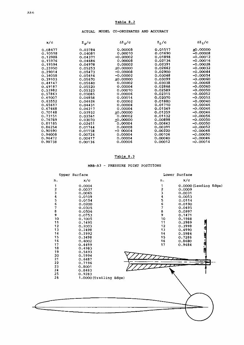
Table 8.2
ACTUAL MODEL CO-ORDINATES AND ACCURACY
Table 8.3
MBB-A3 - PRESSURE POINT POSITIONS
Upper Surface
n. X/C
Lower Surface
n. X/C
1 0.0000 (Leading Edge) 2 0.0009
26 1 . O m 0 (Trailing Edge) \

T a b l e 8 . 4 a
FLOW CONDITIONS INCLUDED
MBB-A3 A i r f o i l A.R.A. B e d f o r d T u n n e l
Run Re x lo-'
M, "' b a s e d o n c h o r d C~ ( 0 . 2 5 ~ ) C~ CM
8 4 0 . 7 0 0 2.01 6 .08 0 . 5 0 1 -0.0494 0 . 0 0 7 8 5 8 6 0 . 7 0 0 3.02 6 . 2 6 0 . 6 4 9 -0 .0455 0 . 0 0 8 7 7 8 8 0 . 6 9 9 4 .01 6 .21 0 . 8 4 1 -0 .0393 0 . 0 1 5 6 1 93 0 . 6 9 8 5 . 0 0 6 . 1 7 1 . 0 0 3 -0.0414 0 . 0 3 0 8 5 94 0 . 6 9 8 5 . 4 9 6 .17 1 . 0 2 4 -0 .0405 0 . 0 3 7 2 0
4 0 . 7 5 0 1 .71 6 . 1 8 0 . 5 1 2 -0 .0566 0 . 0 0 8 3 1 1 3 0 . 7 5 5 1 . 8 9 6 .01 0 . 5 5 3 -0 .0562 0 . 0 0 8 1 8 1 7 0 . 7 5 9 1 . 5 0 6 . 0 0 0 . 4 8 7 -0 .0578 0 . 0 0 7 8 0 1 8 0 . 7 6 0 1 . 8 9 6 .01 0 . 5 6 4 -0 .0577 0 . 0 0 8 0 3 2 2 0 . 7 6 0 2.21 6 .01 0 . 6 2 6 - 0 . 0 5 8 3 0 . 0 0 8 7 0 2 3 0 . 7 6 0 2 . 7 5 6 . 0 0 0 . 7 3 4 -0 .0643 0 . 0 1 5 1 8 24 0 . 7 5 8 3 . 7 3 5 . 9 8 0 . 8 8 0 -0.0851 0 . 0 4 1 1 0 25 0.761 4 . 7 4 6 . 0 0 0 . 9 2 0 -0 .1039 0 . 0 6 4 5 8 1 6 0 . 7 6 5 1 . 8 9 6 . 0 0 0 . 5 7 4 -0 .0597 0 . 0 0 8 3 2 4 4 0 . 7 7 1 1 . 9 0 6 . 0 9 0 . 5 9 4 -0 .0648 0 .00952
1 0 0 0 . 7 9 8 2 . 0 1 6 . 2 0 0 . 6 4 1 -0 .0992 0 . 0 2 7 4 4 1 0 6 0 . 8 0 1 5.01 6 . 1 3 0 . 8 3 7 -0.1174 0 . 0 7 8 5 9 1 1 3 0 . 8 5 0 2.01 6 .08 0 . 5 1 5 -0 .1165 0 . 0 3 2 3 6 1 1 8 0 . 8 5 1 4 .47 6 .12 0 . 7 1 6 -0 .1227 0 .05897
T a b l e 8 . 4 b
FLOW CONDITIONS INCLUDED
MBB-A3 A i r f o i l - P o l y t e c h n i c o f T u r i n T u n n e l
a Re x 1 0 - ~ CM T r a n s i t i o n B o u n d a r y Run M, b a s e d o n c h o r d C~ ( 0 . 2 5 ~ ) t r i p ('1 c o n d i t i o n s
~ 3 3 0 . 7 5 1 f . 1 2 0 . 4 0 0 0 . 3 6 8 -0.0484 n o y e s ~ 3 6 0.768 2 . 2 5 0.406 0 .483 -0.0413 n o y e s ~ 9 6 0 .759 2 . 8 3 0.403 0 .566 -0.0380 y e s y e s ~ 9 7 0 .759 3 . 4 8 0.403 0.618 -0.0369 y e s y e s ~ 3 7 0.754 4 .61 0.401 0 .712 -0.0343 n o y e s P78 0 .765 4 . 6 1 0 . 4 0 5 0 . 7 8 3 -0 .0497 y e s n o ~ 3 9 0.802 1.30 0 .419 0 . 3 9 9 -0.0614 n o y e s ~ 9 9 0 .795 2 . 0 0 0.414 0.511 -0.0593 y e s y e s P ~ O 0 .793 2.90 0 . 4 1 4 0 .562 -0.0568 n o y e s ~ 1 0 8 0 .797 3.90 0 .416 0 . 6 8 5 -0.0656 y e s y e s P41 0 . 7 9 9 5 . 4 3 0 . 4 1 9 0 . 7 0 4 -0 .0617 n o y e s P R ~ 0 . 8 0 0 5 . 4 3 0 . 4 1 9 0 . 7 5 4 -0 .0720 y e s n o
P ~ O O 0 .849 0 .80 0.434 0 .375 -0.0871 y e s y e s P I 3 0 . 8 4 8 1.77 0 . 4 3 3 0 . 3 5 5 - 0 . 0 7 9 1 n o n o P82 0 . 8 5 1 1 . 7 7 0 . 4 3 6 0 . 4 1 9 -0 .0772 y e s n o ~ 1 0 9 0.842 2 . 0 0 0.432 0.521 -0.0910 y e s y e s ~ 1 0 2 0.841 3.20 0 .432 0 .592 -0.0841 y e s y e s ~ 8 5 0 . 8 5 5 4 .18 0 . 4 3 8 0 . 6 1 9 -0 .0831 y e s n o
( O ) T r ~ n ~ i t i o n trip device: ballotini, average diameterO.E%m, position x/c = 0.28 f 0.30 on upper surface, x /c=0 .39 + 0.41 on lower surface. The location of transition has not been verified. Transition likely occurs close to thelead- ing edge for the A.R.A. tests and at the position o f the tripping device (may be insome cases near domstream) for t h e P.T. tests. The different location of transition between A.R.A. and F.T. experiments may explain the ad- verse Reynolds number e f f e c t on separstion shown in Fig.8.6.
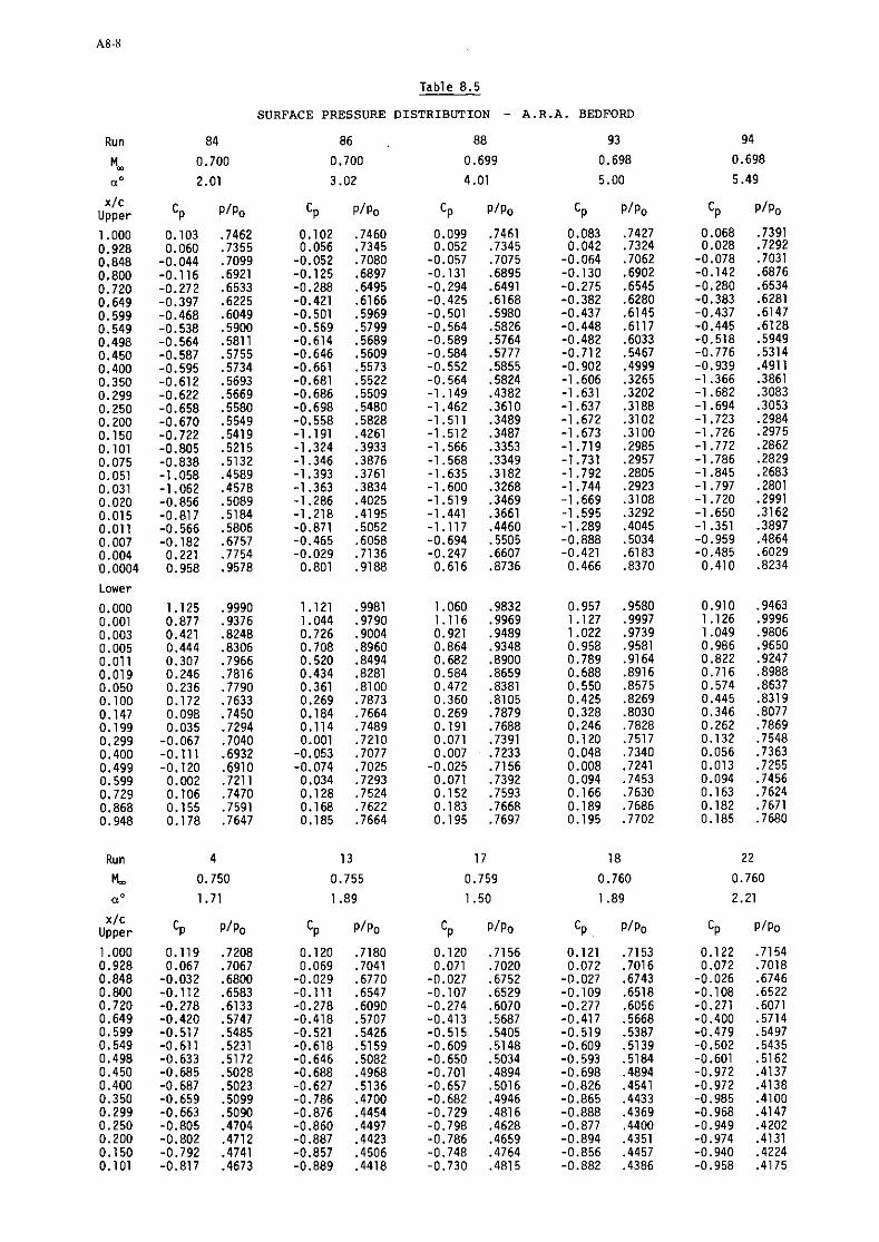
Table 8.5
SURFACE PRESSURE D I S T R I B U T I O N - A . R . A . BEDFORD
Run
", uD
cp PIP0 cp PIP0
Lower
0.000 0.001 0.003 0.005 0.011 0.019 0.050 0.100 0.147 0.199 0.299 0.400 0.499 0.599 0.729 0.868 0.948
Run
M, a'
x l c Upper PlPo

x / c Table 8.5 ( c m
U p p e r Cp p/p0 Cp P/PO Cp P / P ~ Cp P/P, Cp P/PO 0.075 -0.866 ,4540 -0.905 ,4374 -0.764 ,4721 -0.892 ,4357 -0.962 ,4164 0.051 -0.933 .4358 -0.948 ,4257 -0.845 .4493 -0.930 ,4252 -0.985 ,4100 0.031 -0.773 .4791 -0.788 ,4695 -0.688 ,4930 -0.770 ,4693 -0.835 ,4514 0.020 -0.626 ,5188 -0.651 ,5068 -0.535 ,5351 -0.633 .5074 -0.712 ,4854 0.015 -0.595 ,5273 -0.626 ,5137 -0.496 ,5459 -0.606 ,5146 -0.698 ,4893 0.011 -0.351 ,5936 -0.373 ,5829 -0.260 ,6108 -0.356 .5835 -0.431 ,5630 0.007 0.038 ,6990 0.017 ,6898 0.113 ,7135 0.033 ,6910 -0.035 ,6722 0.004 0.414 .8010 0.395 ,7932 0.487 ,8166 0.408 ,7945 0.341 ,7761 0.0004 1.061 ,9764 1.054 ,9734 1.089 ,9824 1.059 ,9741 1.033 ,9668 L o w e r
Run 23 24 25 16 44
Mm 0.760 0.758 0.761 0.765 0.771
a" 2.75 3.73 4.74 1.89 1.90
x / c U p p e r C~ P/P, C~ P/PO Cp P ~ P O cp P/PO Cp P /PO
L o w e r

Table ec; ( ~ o n t , " ~ ; ~ cp PIP,,
Run
Fb. a0
Lower

Table 8.6
PRESSURE DISTRIBUTION - POLYTECHNIC OF TURIN (P.T.1
P36 P96 P97
0.768 0.759 0.759
2.25 2.83 3 .48
cp P/PO cp P/Po cp P / P O
SURFACE
Run
M, a"
Lower
Run
M, ae
x/c Upper

Table 8.6 ( c o n t d . )
cp P I P 0 -p P IP0
0.020 -1.025 ,3935 0.015 -0.927 ,4208 0.011 -0.701 ,4836 0.007 -0.330 ,5867 0.004 0.089 ,7033 0.0004 0.889 .9260
Lower
Run P41
M, 0.799 a0 5.43
x l c Upper Cp P/PO
Lower

Table 8.6 ( c o n t d . )
x /c Upper cp P IP0 cp P IP0 cp P IP0 cp P/P0 Cp P IP0
Run PI09 PI02 P85
k 0.842 0.841 0.855
a' 2.00 3.20 4.18
Lower
0.000 0.001 0.003 0.005 0.011 0.019 0.050 0.100 0.147 0.199 0.299 n 400
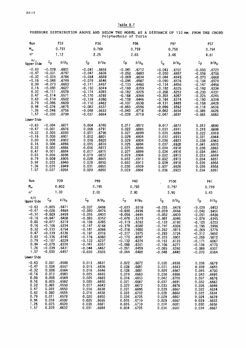
Table 8.7
PRESSURE DISTRIBUTION ABOVE AND BELOW THE MODEL AT A DISTANCE OF 1 3 2 m FROM THE CHORD Polytechnic of Turin
Run P33 P36 P96 P97 P37 M, 0.751 0.768 0.759 0.759 0.754
a0 1.12 2.25 2.83 3.48 4.61
X I - Upper Side 'P P/Po
Lower Side
Run P39 P99 P40 PlO8 P41
b 0.802 0.795 0.793 0.797 0.799 a0 1.30 2.00 2.90 3.90 5.43
x/c Upper Side 'P P/PO
Lcwer Side

Table 8.7 (contd. )
Run p l 00 PI09 ~ 1 0 2
k 0.849 0.842 0.841
a0 0.80 2.00 3.20
Lower Side
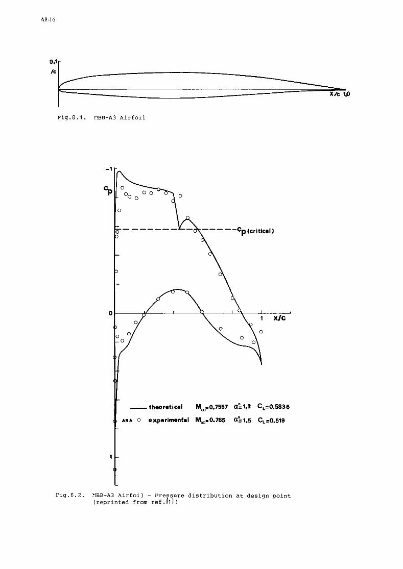
Fig.G.l. f!BB-A3 Airfoil
riq.C.2. f1BB-A3 Airfoil - I'ressure distribution at design point (reprinted from ref. [ll )

J -100 > MODEL P O s l r l O ~ ,< 100 r(mrn>
Fig .8 .3a . Turin Polytechnic Wind Tunnel-Longitudinal Mach number dis tr ibut ions i n empty t e s t s ec t ion .
Fig .8 .3b. Turin Polytechnic Wind Tunnel-Variation of tunnel pressure f luctuations with Mach number.

Fiq.8.4. ARA Bedford Wind Tunnel - Wake Rake
slotted wall
Fiq.8.5. Turin Polytechnic Wind Tunnel -Static pressure probe for boundary conditions measurements and sketch cf installa- tion (all dimensions in nun ).
113 - loo, t .
10
'4 holes " f M)

AARA Run 24 M _ = 0.758 c i s 3.73 CL = 0.880
0 PT Run P37 & = 0.754 ma= 4.61 CN = 0.712
x PT Run P78 & = 0.765. a'= 4.61 CN = 0.783 ( w i t h t r i p p i n g device)
AARA Run 113 = 0.850 aO= 2.01 CL = 0.515
0 PT Run P13 11- = 0.048 an= 1.77 CN = 0.355
X PT Run P82 M, = 0.851 a'= 1.77 CN = 0.419 (w i th t r i p p i n g device)
t AARA Run 106 & = 0.801 aO= 5.01 CL = 0.837
1 OPT Run P41 & = 0.799 a'= 5.43 CN = 0.704
xPT Run P8l M = 0 800 '= 5.43 CN = 0.754 (w i th t r i p p n g device7
-1 -
X
a A - x X a A A A a
3 X x A
p X x A X
a x
, A , d , xtc , 0
L A A A 1
A >a T t
AARA Run 118 & = 0.851 aO= 4.47 CL = 0.716
; x PT Run P85 & = 0.855 a'= 4.18 CN = 0.619 ( w i t h t r i p p i n g device)
F i g . 8 . 6 . YBB-A3 A i r f o i l - Comparison between r e s u l t s obtained a t the A.R.A Bedford wind tunnel and a t the Turin Polytechnic wind tunnel. T tripping device.

o o m 2 E E Z d d d

m o o 8 ~ n w
E h h h . . . 0 0 0

Run P97 M, = 0.751 a"= 1.12 CN = 0.368 M, = 0.759 a" = 3.48 CN = 0.618
Run P36 Run P39
M, = 0.768 a' = 2.25 CN = 0.483 M, = 0.802 a" = 1.30 CN = 0.399 1 i 1
Fig.8.8. MBB-A3 Airfoil - Results obtained at the Turin Polytechnic wind tunnel Opressure coefficients on the model surface
opressure coefficients at a distance of 132mmfrom the model chord a- bove and below the model
T tripping device
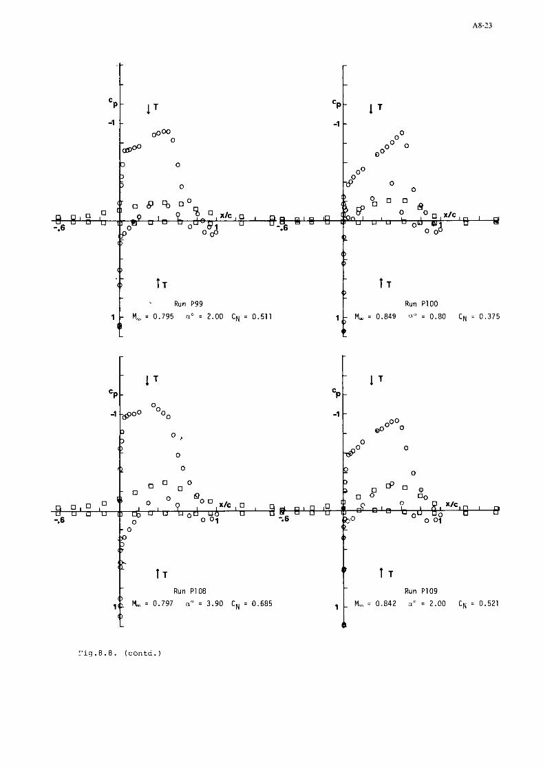
Run P l O O
Run PI09


9. EXPERIMENTAL INVESTIGATION OF A 10 PERCENT THICK NASA SUPERCRITICAL AIRFOIL SECTION
by
Charles D. Harris NASA Langley Research Center, Hampton, Va. 23665
9.1 INTRODUCTION
This contribution contains representative samples of data obtained for a supercritical airfoil section tested in the Langley 8-foot transonic pressure tunnel. Airfoils with various trailing edge geometries and two maximum thicknesses were tested in the investigation,but only data for a 10 percent maximum thickness airfoil with a 1.0 percent thick trailing edge with cavity are presented in this compilation. Drag, normal-force, pitching-moment and pressure-distribution data are included for small angles of attach and Mach numbers from 0.60 to 0.81.
9.2 DATA SET
1. General Descrivtion
1.1 Airfoil designation Supercritical airfoil 9a.
1.2 Type of airfoil Supercritical.
1.2.1 Airfoil geometry
Nose radius
Base thickness 0.01 c
Maximum thickness 0.10 c
1.2.2 Design condition
Design pressure distribution
1.3 Additional remarks
1.4 References on airfoil
2. Model geometry
2.1 Chord length
2.2 Span
2.3 Actual model ca-ordinates and accuracy
2.4 Maximum thickness
2.5 Base thickness
2.6 Additional remarks
2.7 References on model
Cn = 0.7 M = 0.79
Flat top. Rear loaded.
Airfoil tested with various trailing edge cavities.
NASA TM X-2336 "Wind-Tunnel Investigation of Effects of Trailing-Edge Geometry on NASA Supercritical Airfoil Section," by Charles D. Harris
0.635111 (25.0 in.)
2.18 m (85.8 in.)
See Table I and figure 9.1.
NASA TM X-2336 "Wind-Tunnel Investigation of Effects of Trailing-Edge Geometry on NASA Supercritical Airfoil Section," by Charles D. Harris

3. Wind tunnel
3.1 Designation
3.2 Type of tunnel
3.2.1 Stagnation pressure
3.2.2 Stagnation temperature
3.2.3 tlumidity/dew point
3.3 Test section
3.3.1 Dimensions
3.3.2 Type of walls
3.4 Flow field (empty test section)
3.4.1 Reference static pressure
3.4.2 Flow angularity
3.4.3 Mach number distribution
3.4.4 Pressure gradient
3.4.5 Turbulence/noise level
3.4.6 Sidewall boundary layer
3.5 Additional remarks
3.6 References on wind tunnel
4 . Tests
4.1 Type of measurements
4.2 Tunnel/model dimensions
4.2.1 Heightlchord ratio
4.2.2 Widthlchord ratio
4.3 Flow conditions included in present data base
4.3.1 Angle of attack
4.3.2 Mach number
4.3.3 Reynolds number
4.3.4 Transition
- position of free transition
- transition fixing
8-Foot Transonic Pressure Tunnel
Continuous flow, pressure tunnel
Can be varied from apcrox. 15 to 68 k ~ / m ~
322 K (120 F)
Air dried sufficiently to avoid condensation.
Slotted top and bottom, solid sides (3% overall open area ratio)
Measured in plenum. Values in Table I 1
'faximum lateral velocitv comoonents arc . ~~
about 0.005 of free stream at all Mach numbers.
Streamwise variations of approximately +0.002 over Mach number range. -
Lateral fluctuating velocity components S/U, and S/U, have not been measured. 'iT/[l, varies from 0.002 at M = 0.2 to about 0.02 at high Mach numbers.
Thickness varies but is on the order of 7 to 8 cm.
Surface pressure; wake profiles.
From 0.60 to 0.80
See figure 9.2. Reynolds number simulations based on refs. 2 and 3
No. 90 carborundum grains; 0.25 cm wide (0.10 in.) bands along x/c = 0.28 on upper and lower surfaces.
4.3.5 Temperature equilibrium
4.4 Additional remarks
4.5 References on tests

5. Instrumentation
5.1 Surface pressure measurements
5.1.1 Pressure holes
- size - spanwise station(s) - chordwise positions
5.1.2 Type of transducers and scanning devices
5.1.3 Other
5.2 Wake measurements
5.2.1 Typefsize of instrument(s)
5.2.2 Streamwise position(s)
5.2.3 Type of transducers and scanning devices
5.3 Boundary layer measurements
5.3.1 Typefsiee of instruments
5.3.2 Locations
5.3.3 Type of transchcers and scanning devices
5.4 Skin friction measurements
5.4.1 Typefsize of instruments
5.4.2 Locations
5.4.3 Type of transducer
5.5 Flow visualization
5.5.1 Flow field
5.5.2 Surface flow
5.6 Other
5.7 Additional remarks
5.8 References on instrumentation
0.51 mm (0.020 inch) inside dia.
0.32 chord from tunnel center line
Concentrated near the leading and trailing edges as illustrated in figure 9.3. See Table 111.
Electronically actuated differential- pressure scanning valves with transducer ranges of +69kN/m2 (10 lb/inchz) for the upper surface and 252kN/m2 (7.5 lbfinchz) for the lower surface. Accuracy within 0.5 percent of full scale.
See figure 9.4. 52 pitot probes spaced 0.0036~ in region of boundary-layer losses, 0.072~ in region of shock losses.
6 static pressure probes spaced about 0 . 0 6 ~ in region of boundary layer losses, about 0 . 2 ~ in region of shock losses.
Approximately 1 chord length downstream of trailing edge
Electronically actuated differential- pressure scanning valves with transducer ranges of +17kN/m2 (2.5 lhfinchz) in boundary-layer wake and +7k~/m2 (1 lbfinch2) for shock and static losses. Accuracy within 0.5 percent of full- scale.
Two dimensionality of flow was determined by fluorescent oil flow.

6.1 Accuracy (wall interference excluded)
6.1.1 Angle of attack setting - +O. 050 6.1.2 Free stream Mach number:
- setting +O. 003 -
- Variation during one None pressure scan
6.1.3 Pressure coefficients Less than 2% of maximum value.
6.1.4 Aerodynamic coefficients Less than 240 of maximum value.
6.1.5 Boundary layer quantities
6.1.6 Repeatability Repeatability checked but not plotted
6.1.7 Remarks
6.2 Wall interference corrections (indicate estimated accuracy)
6.2.1 Angle of attack
6.2.2 Blockage (solidfwake)
No corrections applied.
6.2.3 Streamline curvature (lift)
6.2.4 Other
6.2.5 Remarks
6.2.6 References on wall interference correction
6.3 Presentation of data
6.3.1 Aerodynamic coefficients See figure 9.5
6.3.2 Surface pressures See figure 9.6 and Table IV.
6.3.3 Boundary layer quantities None
6.3.4 Wall interference No corrections included?
6.3.5 Corrections for model None deflection
6.3.6 Empty test section calibration taken into account?
6.3.7 Other corrections included?
6.3.8 Additional remarks
6.4 Were tests carried out in different facilities on the current airfoil? If so, what facilities. Are data included in the present data base?
6.5 To be contacted for further information on tests
Charles D. Harris NASA Langley Research Center Mail Stop 359 Bampton, VA 23665

7. References
1. NASA TM X-2336 entitled "Wind-Tunnel Investigation of Effects of Trailing-Edge Geometry on NASA Supercritical Airfoil Section," by Charles D. Harris.
2. NASA TN D-5003 entitled "Preliminary Study of Effects of Reynolds Number and Boundary-Layer Transition on Shock-Induced Separation,: by James A. Blackwell, Jr.
3. NACA TN 4363 entitled "Simplied Method for Determination of Critical Height of Distributed Roughness Particles for Boundary-Layer Transition at Mach Numbers From 0 to 5," by Albert L. Braslow and Eugene C. Knox.
8. List of symbols Values are given in both SI and U. S. Customary Units. The measurements and calculations were made in the U. S. Customary Units.
C~ pressure coefficient , 'L - P-
Cp,sonic pressure coefficient corresponding to local Mach number of 1.0
c chord of airfoil, cm (inches)
Cd section drag coefficient , >h @
%I section pitching-moment coefficient,
cn section normal-force coefficient,
Mach number
static pressure, ~/m' (lb/ft2)
dynamic pressure, ~ / m 2 (lb/ft2)
Reynolds number based on airfoil chord
airfoil thickness, cm (inches)
free stream fluctuating velocity components
free stream velocity
ordinate along airfoil reference line measured from airfoil leading edge, cm (inches)
ordinate vertical to airfoil reference line, cm (inches)
vertical distance in wake profile, cm (inchesl)
angle of attack of airfoil reference line, degrees
Subscripts:
L local point on airfoil
2 lower surf ace
te trailing edge
- f r r e s t r r u m v n l o c

TABLE I. AIRFOIL COORDIXATLS TABLE 11. TUNNEL STATIC PRESSURES
Mach Number 2 Static Pressure (NN/m )
0.80 0.0664
0.79 0.0671
0.76 0.0691
0.70 0.0730
0.60 0.0794
TABLE 1 1 7
CHORDWISE LOCATION OF PRESSURE TP-PF
UPPER SURFACE LOWER SURFACE
x/c XI c

TABLE I V . TABULATE0 PRESSURE DISTRIBUTION FOR RANGE OF MACH NUMBERS AN0 ANGLES OF ATTACK
MACH = 0 . 6 0 (I = lo M A C H r 0 . 6 0 a - 2 0 M A C H = O . ~ O a = 1 ° STATION STATION STATION STATION STAT ION STATION
x/c CP x/c CP x/c CP x/c CP x/c CP x/c CP
UPPER SURFACE LOWER SURFACE UPPER SURFACE LOWER SURFACE UPPER SURFACE LOWER SURFACE

TABLE I V . TABULATE0 PRESSURE DISTRIBUTION FOR RANGE OF MACH NUMBERS AN0 ANGLES OF ATTACK (CONTINUED)
MACH = 0.70 a = z0 M A C H = O . ~ ~ a = .so MACH = 0.76 * = 10
STATION STATION STATION STATION STATION STATION
x /c CP x/c CP x/c CP x/c CP x/c CP XlC CP
UPPER SURFACE LOWER SURFACE UPPER SURFACE LOWER SURFACE UPPER SURFACE LOWER SURFACE

TABLE IV. TABULATED PRESSURE OISTRIBUTION FOR RANGE OF MACH NUMBERS AND ANGLES OF ATTACK (CONTINUEO)
MACH = 0.76 0 = 2' M A C H = O . ~ ~ a = 2 . s 0 MACH = 0.79 a = . 50
STAT!ON STAT IOH STATION STATION STATION STATION
x /c CP x /c CP X/C CP x;c CP XIC CP x/c CP
UPPER SURFACE LOWER SURFACE UPPER SURFACE LOWER SURFACE UPPER SURFACE LOWER SURFACE

TABLE I V . TABULATED PRESSURE DISTRIBUTION FOR RANGE OF MACH NUMBERS AN0 ANGLES OF ATTACK (CONTINUED)
M A C H = O . ~ a = i O MACH = 0.79 a = 2' M A E H = O . ~ O a = . 5 0
STATION STATION STATION STATION STATION STATION
X I C CP XIC CP X/C CP x /c CP x/c CP X I C CP
UPPER SURFACE LOWER SURFACE UPPER SURFACE LOWER SURFACE UPPER SURFACE LOWER SURFACE
,0040 .0100 .0200 ,0300 .0500 .0700 . i ono ,1500 .2000 .2500 .3000 .3500 ,4000 .4500 .5000 ,5500 ,6000 ,6500 .7000 ,7500 ,8000 ,8500 .9000 .9300 ,9500 ,9700 ,9800
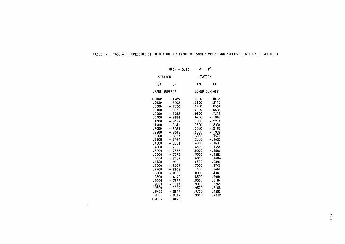
TABLE I V . TABULATED PRESSURE DISTRIBUTION FOR RANGE OF MACH NUMBERS AN0 ANGLES OF ATTACK (CONCLUDED)
MACH = 0.80 a = l o
STATION STATION
X/C CP x/c CP
UPPER SURFACE LOWER SURFACE

c-63.5 cm(25 in . )
.010c -L 7-
(tic)-- 0.10 ~ a s i c Airfoil
~ - 3 ~ I Y k Z
1.0- percent-thick trail ing edge with cavity
Trailing-edge geometry for a i r fo i l 9a
F i g u r e 9 . 1 . - A i r f o i l Geometry
F i g u r e 9 .2 . - V a r i a t i o n w i t h Mach number o f t e s t wind- tunnel Reynolds number and s i m u l a t e d f u l l - s c a l e Reynolds number.

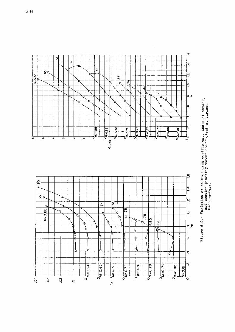
L w .3 0 w 0 w a * 0 E o m 6
M 0 a e * I 0 M
E C .3 0 s
.A 0 * + o .A
g a " i E *
w o o 1
F O Z 3 0 o m c .3 (li * 0 r d P 0 .i c d * rda rd >


APPENDIX B
3D Configurations
0. Guide to the data.- The purpose of this compilation is to make readily availahle data of high quality for a variety of wing and winglbody configurations for use in validating theoretical methods. The accuracy of the latest numerical methods in solvine various forms of the transonic flow equations is a particular concern, therefore, special emphasis has been placed on the inclusion of high-suhsonic-speed data. A further desire has been to include configurations ranging from simple to the most complex. Configuration B-2 (ONERA AFVD), for example, is an untapered wing with constant airfoil section from root to tip and no body while configuration R-5 is a complete aircraft configuration with as complicated a wing geometry as one is likely to encounter.
To facilitate the utilization of this data base a single format has been used to present the information for all the configurations,paralleling very closely that used for the 2D configuration. Sections are included giving a general description of the model. the eeometric characteristics of the model. the characteristics of the wind tunnel ~- , ~~
used, detaiis of how the tests were conducted, thk types and accuracies of the instrumet- ation and, finally, a listing of the data tables and plots appended. References are given for most of the configurations from which the reader may obtain additional details on the model, the test procedures, the data obtained and the wind tunnel used.
A brief summary of the geometric characteristics and test conditions for the five wing and winglhody data sets are given below. It can be seen that the Reynolds numbers range from 1 to approximately 11.7 million (B-4 and B-l respectively) and Mach numbers from 0.4 (B-4) to 0.99 (B-5). With the exception of R-4 aeroelastic corrections have not been applied to the data. Measured angles of attack. have been corrected for induced wall effects in both B-4 and B-5; sufficient data is given in E-1, B-2 and R-3 to enable the reader to apply corrections if be desires.
Finally, it should be noted that if additional information is desired on the tests or wind tunnel facilities, addresses of the organizations which carried out the tests are given in item 3.10 of each data set.
MODEL GEOMETRY AND TEST CONDITIONS FOR WING AND WING/BODY DATA
Data Set
B-1
B-2
8-3
B-4
8-5
Aspect Ratio
3.8
8.0 for 00 sweep and 2.7 for 600 sweep
4.5
6.0
6.8
Wing Wing/Body
Semi-span Wing
Semi-span Wing
Wing/body
Wing/hody
Winglbody
Taper Ratio
0.562
1.0
0.33
0.33
0.36
..... .
Leading Edge Sweep
3 0° 3 0°
Variable, data given for 00, 30° and 50°
3 5O
36.65O
44.340
Data
Mach Range
0.7 to 0.92
0.7 to 0.92
0.65to 0.92
0.4 to 0.0
0.5to 0.90
Presented
Angle of Attack Range
O" to 6O
00 to 60
-2to 80
O0 to 20
-4Oto 11°
For - RN Range Based on
m.a.c.
-11.7 x lo6
2.5 x lo6 based on chord normal to L.E.
1.12 x 10⁶ to 1.34 x lo6
1 x lo6
2 . 3 7 ~ 1 0 6 to 2.68 x lo6
--

1. PRESSURE DISTRIBUTIONS ONME ONERA-M6-WIG
AT TRANSONIC MACH NUMBERS
by
Y. SCHNITT and F. CHARPIN
OFFICE NATIONAL D'ETLTDES ET DE RECHERCHES AEROSPATIALES
92320 - CHATILLON - FRANCE
1.1 - INTRODUCTION - In 1972, the ONERA Aerodynamics Department designed a swept back wing very well instrumented to beused as an experimental support for basic studies of three-dimensional flows at high Reynolds mbers from law to transonic speeds.
Wind tunnel data from this model called M6-winghave been constituting a good base both for computer program assessment and for understanding varj.0us flow phenomena like shock wave-boundary layer interaction or flow separation.
The selected data set was obtained in the ONERA S2MA wind tunnel at Mach numbers of 0.7, 0.84, 0.88 and 0.92 for angles of attack up to 6 degrees and a Reynolds number of about 12 million .
1.2 - DATA SET - 1 . General description
1.1 Model designation or name ONERA Wing M6
1.2 Model type ( e . , fbll span wing-body; semi-span wing (see also figures B1-1 and ~1-2) semi-span wing7.
1 3 Design requirements/conditions
1.4 Additional remarks
2. Model geometry
2.1 Wing data
2.1 .1 Wing planf o m
2.1.2 Aspect ratio
2.1.3 Leading-edge sweep
2.1.4 Trailing-e 'ge sweep
2.1.5 Taper ratio
2.1 .I Mean aerodynamic chord
2.1.8 Span or semispan
2.1.9 Number of airfoil sections used to define wing
2.1.10 Spanwise location of reference qection and section coordinates (note if ordinates are design or actual measured values)
2.1.11 Lofting procedure between reference sections
this model was designed to be used for studies of three-dimensional flows from low to transonic speeds at high Reynolds numbers.
it is derived from the ONERA calibration model series M and represents the external third of the wing.
swept back ( s e e figure B1-1)
3.8
30°
15.W
0.562
without twist
c = 0.64607 m
b = 1.1963 m
1
y/b = 0 section coordinates of the symmetrical profile (design values) : 3ee table B1-1. The .ject~cv is OI!ERA D n,,,mrl to the generator a t 40.18 $ cl o:
conical generation
2.1.12 Form of wing-body fillet, strakes
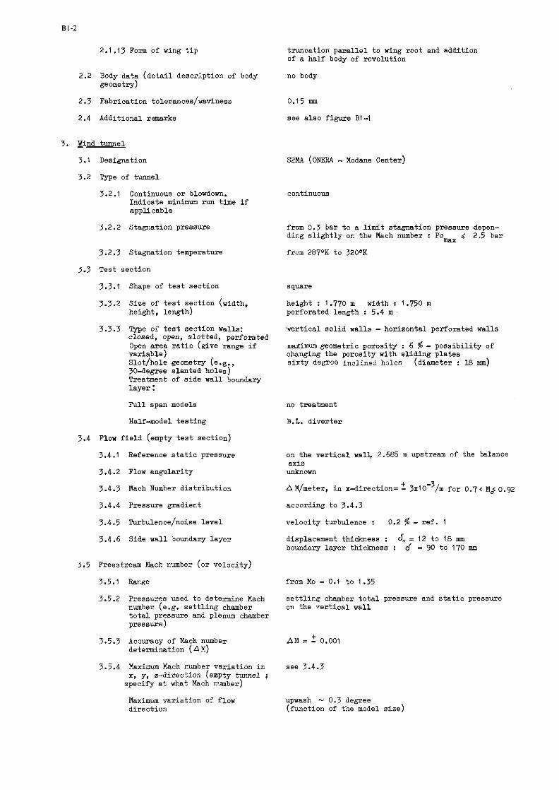
truncation parallel to wing root and addition of a half body of revolution
2.1 .13 Form of wing tip
2.2 Body data (detail des-5.ption of body geometry)
no body
2.3 Fabrication tolerances/waviness 0.15 mm
see also figure Bt-1 2.4 Additional ranarks
3. Wind tunnel
~ 2 ~ 4 (ONERA - Modane center) 3. 1 Designation
3.2 Type of tunnel
3.2.1 Continuous or blowdown. Indicate minim run time if applicable
continuous
3.22 Stagnation pressure from 0.3 bar to a limit stagnation presaure depen- ding slightly on the Mach number : Po 5 2.5 bar max from 28I0K to 3200K 3.23 Stagnation temperature
3.3 Test section
3 . 3 Shape of test section square
3.3.2 Size of test section (width, height, length)
height : 1 .I70 m width : 1 .I50 m perforated length : 5.4 m
3.33 Type o' test section walls: closed, own, slotted, mrforated
wrtical solid walls - horizontal perforated walls maximum geometric porosity : 6 % - possibility of changing the porosity with sliding plates sixty degree inclined holes (diameter : 18 mm)
Open area ratio (give &nge if variable) ~lot/hole geometry (e.g., 3Odegcee slanted holes) Treatment of side wall bovndary layer :
fill span models no treatment
B.L. diverter Half-model testing
3.4 Flow field (empty test section)
3.4.1 Reference static pressure
3.4.2 Flow angularity
an the vertical wall. 2.685 m upstream of the balance axis unlolonn
t A M/meter, in x-direction= - 3110-~/m for 0.7 < M~0.92
according ta 3.4.3
velocity turbulence : 0.2 % - ref. 1
displacement thickness : J, = 12 to 18 mm boundary layer thichess : d = 90 to 170 mm
3.43 Mach Number distribution
3.4.4 Pressure gradient
3.4.5 Turbulence/noise level
3.4.6 Side wall boundary layer
5.5 Freestream Mach number (or velocity)
3.5.1 Range from Mo = 0.1 to 1.35
3.5.2 Pressures used to determine Mach number (e.g. settling chamber total pressure and plenum chamber pressure)
settling chamber total pressure and static pressure on the rrertical wall
3.5.3 Accuracy of Mach number determination (AM)
3.5.4 Maximum Mach number variation in x, y, a.-direction (empty tunnel ; specify at what Mach number)
see 3.4.3
Maximum variation of flow direction
upwash - 0.3 degree (function of the model siee)

Maximum Mnch number variation during a run
3.6 Reynolds number rangc
3.6.1 Unit Reynolds number range (give range at representative Mnch numbers ; l/m)
3.6.2 Means of varying Reynolds number (e.g., by pressurization)
3.7 Temperature range and dewpaint. Can temperature be controlled ?
3.8 Model attitudes
3.8.1 Angle of attack, yaw, roll
3.8.2 Accuracy in determining angles
3.9 Organization operating the tunnel and location of tunnel
3.10 Who is to be contacted for additional information
3.11 Literature concerning this facility
3.12 Additional remarks
4. Tests
4.1 Type of tests
4.2 Wing span o r semispan to tunnel width
4.3 Test conditions
4.3.1 Angle of attack
4 . 3 2 Mach number
4.5.3 Dynamic pressure
4.3.4 Reynolds number
4.3.5 Stagnation temperature
4.6 Transition
4.4.1 Ekee or fixed
4.4.2 Position of free transition
4.4.3 Position of fixed transition, width of strips, size and type of roughness elements
4.4.4 Were checks made to determine if transition occured at trip locations ?
4.5 Bending or torsion under load
4.5.1 Describe any aeroelestic measurements made during tests
the Mach number is adjustable at + 0.001. during a
contin~ialia angle of attack variation the Kqch il:mber is not kept strictly con::tant and depends on model uizc and Mo.
stagnation pressure Po = 0.3 to 2.5 bar for M s 0 . 7 0.3 to 1.75bar for Ma 1 0.3 to 2.1L.ar far R = 0.8 0.3 to 1.9 bar for M = 0.9
+ + stagnation temperature To = 292 K - 5 to 315 K - 5 cannot be controlled humidity < 0.2g H ~ O / Kg a i r
motorization for the 3 angles up to 35O (for complete model)
0.03 degree
ONERA - Centre de Modane-Avrieux
ONERA - Direction GME - Chetillon - FRANCE
ref. 2 , 3
on line data return
pressure Aistributians, aeradynmic forces and moments, flow studies by visualieation (wall streamlines and boundary layer transition), unsteady measurements
0.7
during pressure measurements : D ( m a ~ ( l 4 ~ for all Kach numbers and Rec < 18x106 ifor force measurements, be-ause a: the llml eL capaiimy 01 ' e balance, there is a large variation of a! max with M and Re )
0.27 < Mo < 1.33
1600 c qo < 60700 ~ / m 2
free
variable
not relevant
not relevant
unsteady bending measured by strain-gauge an the wing root

4.5.2 Describe results of any bench not relevant calibrations
4.6 Were different sized models used in wind-tunnel investigation 5 If s o , indicate sizes
4.7 Areas and lengths used to form coefficients
4.8 References on tests
4.9 Related reports
5. Instrumentation
5.1 Surface pressure measurements
5.1.1 Pressure orifices in wing. Location and number on upper and lower surfaces
5.1.2 Pressure orifices on fuselage. Location and number
5.1.3 Pressure orifices on components, give components and orifice loca- tion
5.1.4 Geometry of orifices
5.1.5 Type o f pressure transducer and scanning devices used. Indicate range and accuracy
5.2 Force measurements
5.2.1 Type and location of balacce
5.2.2 Forces and moments that can be measured. Maximum loads and accuracy
5.2.3 Forces and moments on components
5.3 Boundary layer and flow-field measurements
5.4 Surface flaw visualization
5.4.1 Indicate method used to determine
- streamline pattern - boundary-layer transition
5.4.2 Accuracy of method
5.5 Skin friction measurements
5.6 Simulation of exhaust jet
5.7 Additional remarks
6. Data
6.1 Accuracy
6.1 .1 Pressure coefficients
6.1.2 Aerodynamic coefficients
ref. 4 , 5
ref. 6, 7
271 pressure orifices divided in 7 sections (y/b = 0.20/0.44/0.65/0.80/0.90/0.96 and 0.99) see also figure B1 -1 and table B1-2
not relevant
not relevant
6 transducers CEC 4312 (k 12.5 PSID - Accuracy : * 0.012 PSI) 6 scanivalves (type D)
wall dynamometric 5 components balancev$ 120 m"
+ axial force : 12000 - 12 N normal3 orce : 65000 2 65 $1 colliilg moment : 8000 !: 8 mN pitching moment : 2500 2.5 mN yawing moment : 1400 f 1.4 mN not relevant
none
by means of fluid paints
by sublimation
qualitative methods
none
not relevant
there is strain gauge, hlite end accelerometer instrumentation for buffeting analysis

6.1.7 Boundary layer and wake quantities
6.1.4 Repeatability
6.2 Wall interference corrections
6.3 Data presentation
6.3.1 Aerodynamic coefficients
6.3.2 Surface pressure coefficients
6.33 Flow conditions for
- aerodynamic coefficient data - pressure data
not relevant
see tables B1-2 and B1-3 or 81 -1 0 and B1-1 1
no corrections
none
Cp (x/l) for all sections defined 5.1 .l
not relevant
Mo 0.70/0.84/0.'28/0.92 at Re - 1 1 .7 10 6 and angles of attack a = Oo to 6 O
detail : T2 means table El-2 F7 means figure 81-3
6.3.4 Boundary layer and/or wake none data
6.3.5 Flow conditions for boundary layer and/or wake data not relevant
6.3.6 Wall interference corrections no included ?
6.3.7 Aeroelasti; corrections no included ?
6.3.8 Other corrections ? no
6.4 Were tests carried out in different not at transonic Mach numbers facilities on the current model ? If so, what facilities. Are data included in ~resmt data base ?
2. M. PIERRE G. FASSO
Fluctuations acoustiques engendrdes par les parois pemeables dfune soufflerie transsonique AGARD CP 174 (~ctabre 15'75)
The aerodynamic test center of Modane-Avrieux ONERA Technical Note no 166E (1972)

3 M. PIERRE 0. FASSO
4. M. GOUSSE
6. B. MONNERIE F. CHARPIN
7. C . ARMAND
8. List of svmbols
Exploitation du ~entre d'essais aCrothemodynamiques de Modane-Avrieux Note tech,lique ONERA no 181 (1 911 )
Etuds de 1'6coulement autour de l'aile M6 en transsonique h S2MA P.V. no 2/0065 GY (1913) - not published Etude de 116caulement autaur de l'aile M6 en transsonique h S2MR P.V. no 5/17! 3 ANG (1 914) - not published Essais de tremblement (buffeting) d'une aile en flkche en transsonique L'A6ronautique et 1'Astronautique no 50 (1915-I), p. 3-16
Etude de la couche limite par d&tecteurs h film chaud en dcoulement subsonique et transsonique La Recherche ACrospatiale no 1976-3, p. 127-133
: semi-span
: local chord
: mean aerodynamic .chord
: wing area
: distance measured along the local chord from the leading-edge of the wing section
: distance measured spanwise
: distance from the plane of the wing
: distance measured chordwise from wing apex
: angle of attack
: free stream Mach number
: local Mach number
: stagnation pressure
: free stream static pressure
: free stream dynamic pressure
: local static pressure
D-po : pressure coefficient Cp = qo
: stagnetion temperature
: Reynolds number based on c
: eial force coefficient
: normal force coefficient
: rolling moment coefficient
: pitching moment coefficient
: yawing mament coefficient
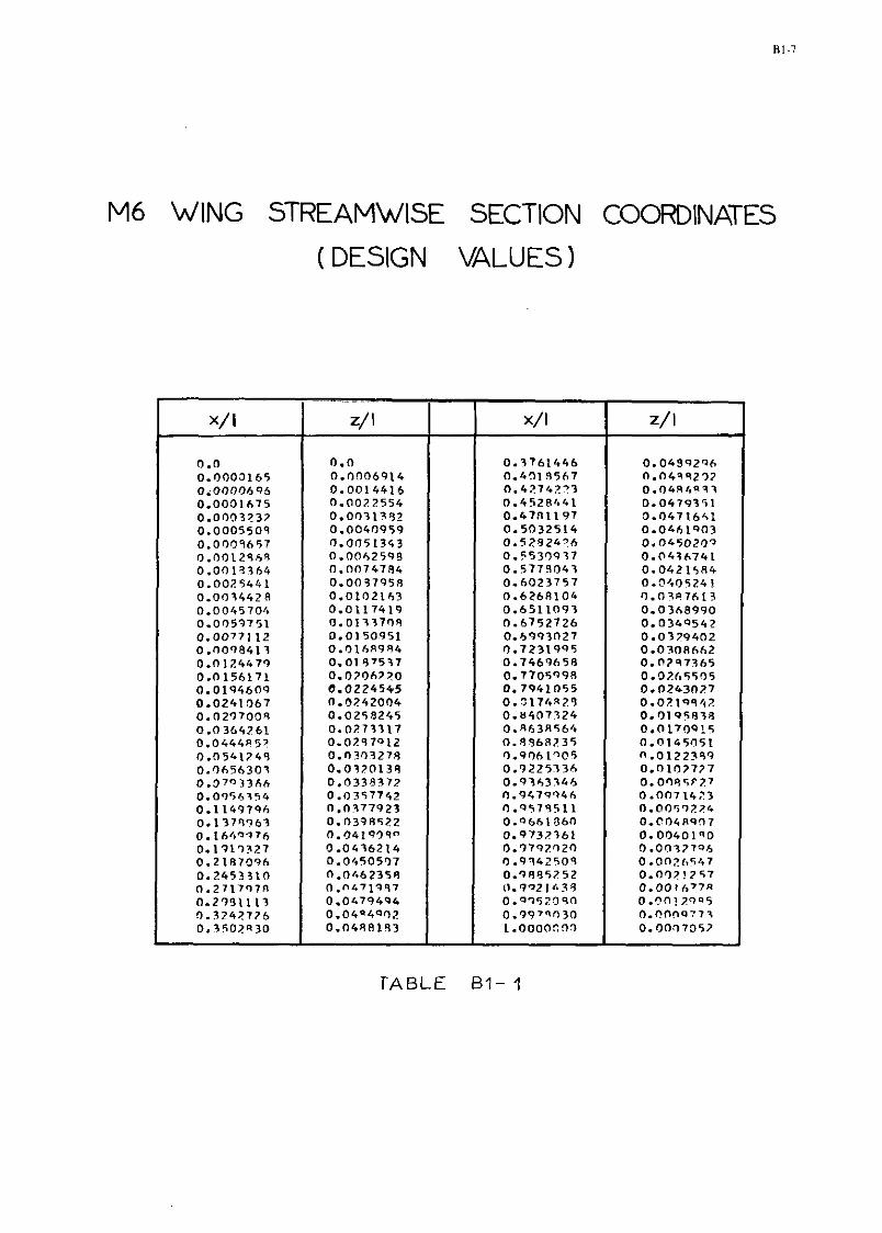
M6 WING STREAMWISE SECTION COORDINATES
( DESIGN VALUES 1
TABLE 61- 1

Y4 WING - $ 1 1 9 F A C E P R F S 5 l l R F D I S T R I s U T I O N S T E S T 2309
no = . b o p s ALPH4 = . n~ R E C = 1 1 . 7 L t l O t * h
TABLE B1- 2

T E S T 2 5 5 1
TABLE 81- 3

M6 U I N G - S U U F 4 C E P R F S S U R F D I S T R I R U T I O N S T E S T 2 3 1 0
MU = . 7 n 0 7 ALPHA = 1 . 0 8 R E C = 1 1 . 7 f ~ * l O * t 6
TABLE B1-4

T E S T 2 3 1 1
M O = .71101 &LPHA = ?."P R E C = 1 1 . 7 4 * 1 0 * * 6
I C C l l n Y 1 I C C T I 3 N 2 l l l l l O N J S ~ C , , D " '
N P XI1 111. C P ill Z / L C P X,L 2 1 1 CP "11 Z,L < P
TABLE 81-5

T E S T 2 3 1 2
MO = . h 0 9 0 ALDHA = R E C = 1 1 . 7 4 * 1 9 * t 6
TABLE B1-6

M6 U I N G - T l l R F R C E F R F S S U R F D I S T Q I R U T I O N S T E S T 2 3 1 3
NO = . 7P19 ALPHA = 1 . 0 9 R E C = 11.77*lgt*6
TABLE B1-7

Y b W I N G - t L I Q F & t c P Q r S f l J R F D l t T R I 1 U T I O N S T E S T Z 5 L l
NO = . 7 @ l * ALPHA ' 5.06 R E C = l l . 6 6 t l J + k h
TABLE B1-8


T E S T 2385
0 1 -4591 ALPI4A = - 0 4 R E C = 1 1 . 7 ? * 1 ' l * * h
TABLE B1-10
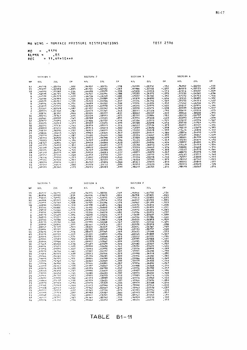
T E S T 2 3 9 6
M O = . S T 7 1 ALPHA = . 0 3 R E C = l l . h Q * l O * * C
TABLE 01-11
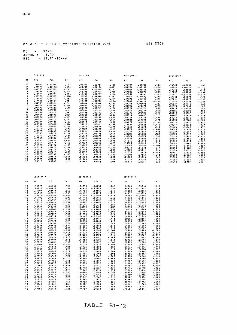
M 6 U I N G - t l l P F 9 C c P Q c ? S ( l Q F D I 5 T R I R U T I O N S T E S T 2 3 J 6
NO = . * T o n ALPHA = 1.07 R E C = 11.71+13khf
TABLE B1- 12

M6 W I N G - ? U 9 F l r c P Q r ? S U P F D I S T R I R U T I O N S T E S T 2357
Y O = . S 3 S h L L P U l = 7 - 0 6 R E C = 1 1 . 7 7 * 1 0 1 * 6
TABLE B1- 13

M6 N I N G - s U R F 4 C E P R F S S U R E D I S T R I S U T I O N S T E S T 2308
no = . 9 3 9 5 A L P H I = 3 .P6 R E C 1 1 1 . 7 2 * 1 0 k * 6
TABLE B1- 14

M6 Y I N G - q U S F L C E P R E S S U R E D I S T R I 9 U T I O N S T E S T 2 5 6 3
NO = . q T 5 o ALPHA = 4.OR R E C = 1 1 . 8 1 * l q * * h
TABLE B1-15

M6 U I N 6 - SURFACE P P E S !
MO = . R L 1 7 RLPHA = 5.06 REC = 11.7RtlO*th
T E S T 2 5 6 4
TABLE 81- 16

M6 d I N S - S U R F A C E P R F S S I J Q E D I S T R I R U T I O N S T E S T 2 5 6 5
M O = .337i! )ILPHh = 6.06 R E C = 11.71*?ot*h
TABLE 61- 17

M6 W I N G - S U R F 9 C E P R E S S I J R F D I S T Q I R U T I O N S T E S T 2 5 0 0
M O = .??I40 ALPHA = - 0 3 R E C = 11 .71 *10 * *6
TABLE B1-18

N6 Y I N S - S U Q F 4 C E P Q C S S U R E D I S T R I 9 U T I O N S T E S T 2301
NO = . s x 3 ~ ALPHA = 1 . n ~ R E C = 1 1 . 7 7 * 1 0 * * 6
TABLE B1-19

T E S T 2 5 0 2
"1 = ..9Rrl5 ALPHL = 7 .05 R E C = 11.7R*10**6
TABLE B1- 20
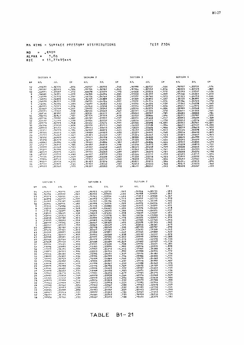
M O V l N t - F U Q F A C E P P F S Y U R F D I S T R I B U T I O N S T E S T 7 3 0 4
MO = .Sq00 ALPHA = 7 . f l b R E C = 1 1 . 7 7 * 1 9 * * 6
TABLE 61- 21
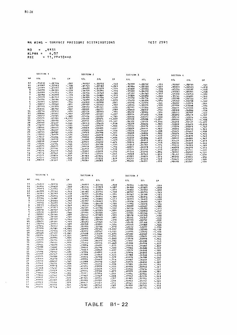
M6 WING - S119FACE PRESSURE D l S T R I R U T l O N S T E S T 2 5 9 1
M Q = . 8 ? 3 1 ALPHA = b . 0 7 R E C = 11.7P*10**6
TABLE B1- 22
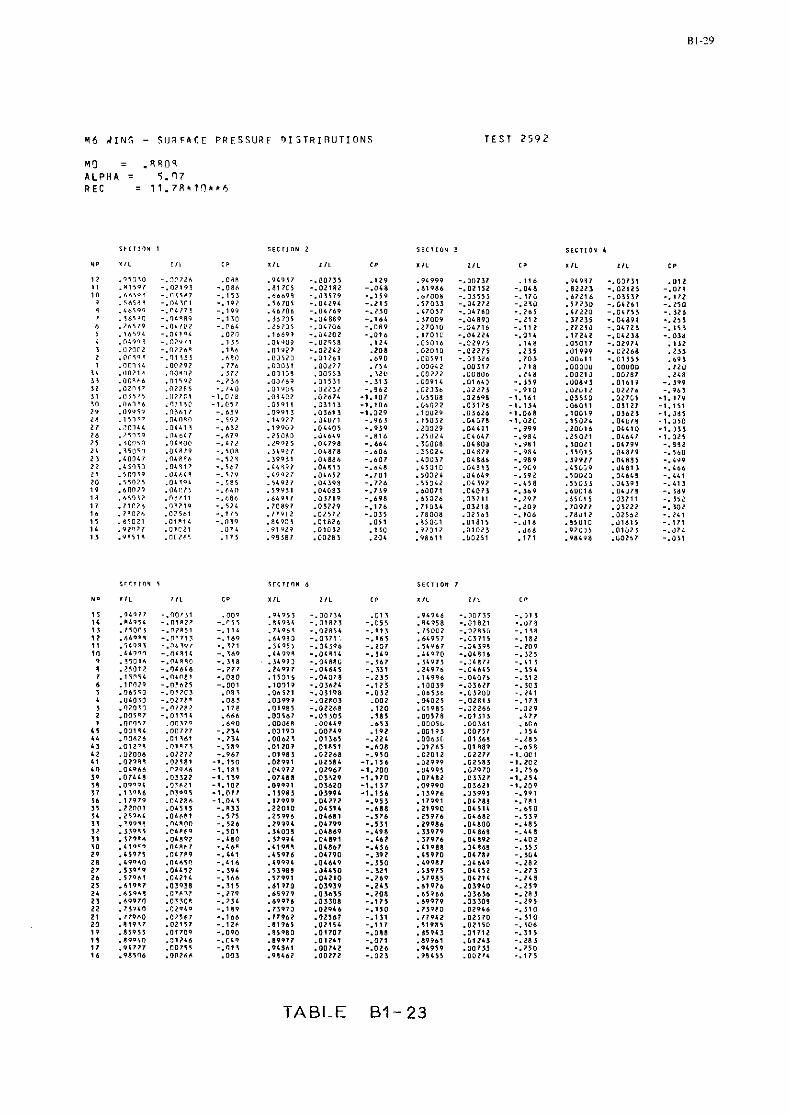
N 6 W I N 6 - S l J 1 F A C t P R E S S U R F O I 5 T R I R U T I O N S T E S T 2 5 9 2
M ! l = . 8 8 f l q ALPHA = 5 . n 7 R E C = 11.7RtlO*th
, 0 1 2 - . 0 1 1 - . I 7 2 - . 1 5 0 -. 326 - . 2 1 1 - . , 5 , -.0111
. , I 2 ,233 . b O , ,7211 . > A 8 -. JPP
..Pbl - 1 . 1 1 9 -,.,>, -1.085 - 1 . 0 5 0 - 1 . 5 1 1 - 1 . 3 2 1
- . a 3 2 -. 560 ..'*P - . 4 6 6 . .'A, -. '1 1 -. $89 -. J I 1 -. 302 - _ 2 < 1 -.,,, ..J7' -.a>,
TABLE 87-23

M 6 Y I N G - Y U P F l C E P R F S S U R E D I S T Q I 9 U T I O N S
NO = -8868 A L P H I = 6.07 R E C = 1 1 . 4 7 k l O * * h
T E S T 2593
TABLE B1- 24

N 6 W I N G - S I J R F A C F P P F S 1 ; 1 1 9 p D I S T R I R U T I O N S T E S T 2 Z 9 6
MU = -9707 ALPHP. = -03 R E C = 11.7P*lO**h
TABLE B l - 25

M 6 U l M G - S U R F A C E P R F S S U R l O I S T S I 9 U T I O N S T E S T 2297
M O = .o204 ALPHA = 1 . 0 7 R E C = 1 1 . 7 9 * 1 0 * * 6
TABLE B1- 26

M6 W I N G - < U P F A C E PRESSURE D I S T R I R U T I O N S T E S T 2 2 9 8
TABLE 01- 27

M6 U I N G - S l l Q F A C E P P f S S l l R E D I S T R I 9 1 1 T I O N S T E S T 2 2 9 9
MO = . 9 1 9 0 ALPHA = 3.07 R E C = 11.77tlO**h
TABLE B1- 28

M 6 W I N G - S U Q F A C E D P F S S U Q F D I S T Q I n U T I O N S T E S T 2 5 8 3
M O = - 0 2 6 7 ALPHA = L.09 R E C T 11.73*10**h
TABLE B1- 29

M6 W I N G - S I J Q F A C C P P E S S U R E D I S T R I R U T I O N S T E S T 2 5 8 4
TABLE B1-30

M 6 4If46 - S U R F A C E PRFSSIJRF DISTRISUTIONS T E S T 2 5 8 5
TABLE B l - 3 1


FIGURE B l - 3
i E S 1 : 2 305
no ; 40.833
ALI'HR : +0.011 OEG.
FIGURE B l - 4
l E S l : 2 306
MU : 40.039
RLPHR : '1.07 O E C .

FIGURE B1- 5
rcsr : 2 3 0 7
n0 ; +0.830
HLPHR ; 42.06 OEC.
F IGURE B1- 6

FIGURE B l - 7
FIGURE B l - 8

FIGURE B l - 9
TEST . 2 565
MU :40.837
RLPHA ; '6.06 OEC.
FIGURE B l - 1 0

FIGURE B1-11
FIGURE B l - 12
It51 . 2 306
no : .o.sao RLFIlR : '3.06 OEC.

FIGURE B l - 13

2. TRANSONIC MEASUREMENTS ON TIE -0NERA AFV D- VARIABLF SWEXP WING
IN TXE -ONERA 52 MA- WIND TUNNEL
by F. MANIE & J.C. RAYNAL
OFFICE NATIONAL D'ETLTDES ET DE RECHERCHES AEROSPATIALES
92320 CHATILLON - FRANCE
2.1 - INTRODUCTION - The ONERA AFV D Variable Sweep Wing designed with the symmetrical ONERA D peaky type airfoil has been chosen as a basic tool to study three-dimensional flows and to provide an experimental data base for comparisons with calculation methods from low to transonic speeds at sweep angles from 00 to 60°.
!!'his contribution contains selected data from those obtained in the ONERA SZMA Transonic Wind Tunnel.
Tables and graphs are presented for three values of the wing sweep angle.
2.2 - DATA SET - 1. General descri~tion
1.1 Model designation or name
1.2 Nodel type (e.g. full span wing- body, semi-span wing)
1 Design requirements/canditions
1.4 Additional remarks
2. Model geometq
2.1 Wing data
2.1 .1 Wing planf o m
2.1.2 Aspect ratio
2.1.4 Trailing-eage sweep
2.1.5 Taper ratio
2.1.6 Twist
2.1.7 Mean aerodynamic chord
2.1.8 Span or semispan
2.1.9 Number of airfoil sections used to define wing
2 .I .10 Spanwise location of refermce section and section coordinates (note if ordinates are design or actual measured values)
2.1.1 1 Lofting procedure between reference sections
2.1.12 Form of wing-body fillet, shakes
2.1.13 Form of wing tip
2.2 Body data (detail description of body geometry)
ONERA VARIABLE SWEEP WING AFV D
semi-span wing : see fig. B2-1
variable sweep angle
the reference section of the wing is the "ONERA D" Airfoil : ( S ) maa = 0.105 ; 'LE = 0.0143 See table BS-1 C
rectan~lar
2.7g A'B
00 L h C 600
00 a P. + 600
1
without twist
c = 0.2 m for A = 00
0.43 ,< b ,< 0.8 m for On,( A 6 60. 1
ETA = O at A = Oo
profile D ordinates : (ee table 02-1 (design values)
cylindrical ge-erstion
no bo;y, no strke, no fillets
truncation normal to the leading edge
no body
2 .3 Fabd cation tolerances/waviness

2.4 Additional remarks inspection hae shown same slight differences between the design and the real model : see table B241
3. Wind tunnel
3 1 Designation s2 MA (ONERA - Modane center) 3.2 Type of tunnel
3.2.1 Continuous or blowdann. Indicate minimum run time if applicable
continuous
3.2.2 Stagnation pressure from 0.3 to a limit stagnation pressure depending slightly on the Mach number ; Po max 4 2.5 bar
from 287 to 320 K 3.23 Stagnation temperature
3.3 Test section
3.3.1 Shape of test section square
3.32 Siae of test section (width, height, length)
height21 .I70 m width : 1 .I50 m perforated length : 5.4 m
vertical solid walls horizontal perforated walls maximum geometric porosity : 6 % - Possibility of changing the porosity with slidicg plates sixty degree inclined hales (diameter : 18 mm)
3.33 Type of test section walls: closed, open, slotted, perforated Open area ratio (give range if variable) ~lot/hole geometry (e.g., 30-degree slanted holes) Treatment of ajde wall boundary layer
Full span models
Half-model testing
no treatment
b.1. diverter
see 3.11
on the vertical wall 2.685m upstream of the balance axis unlcnavn
+ A~/meter in w -direction :- 3a10-~/m.far 0.76 Ms 0.92
according to 3.4.3
velocity turbulence - 0.2 96 - ref. 1
displacement thickness d - 12 to 18 mm boundary layer thiohess d 90 to 170 mm
3.4 Flow field (empty test section)
3.4.1 Reference static pressure
3.4.2 Flow angularity
3.4.3 Mach number distribution
3.4.4 Pressure gradient
3.4.5 kbulence/noise level
3.4.6 Side wall boundary layer
3.5 Freestream Mach number (or velocity)
3.5.1 Range from M, = 0.1 to M, = 1.35
3.5.2 Pressures used to determine Mach number (e.g., settling chamber total pressure and plenum chamber pressure)
settling chamber stagnation presgure and static pressure on the vertical wall
3.5.3 Accuracy of Mach number determination (AM)
3.5.4 Maximum Mach number variation in I, y, z-direction (empty tunnel : specify at what Mach number)
see 3.4.3
Maximum variation of flow direction upwash u 0.3O degree (dependent on model size)
Maximum Mach number d a t i o n durirg a pun
function of the model size ( s e e 6.3.9)
3.6 Reynolds number range
3.6.1 Unit Remolds number ranee. (give renge at representative Mach numbers ; I/m)

3.6.2 Means of varyi:~;: Rcynolds >lumber ( e . ~ . by prcssurizntion)
3.7 Temperature range and dewpoint Can temperature be controlled ?
3.8 Model attitudes
3.8.1 Angle of attack, yaw, roll
3.82 Accuracy in determining angles
3.9 Organisation operating the tunnel and location of tunnel
3.10 Who is to be contacted for additional information
3.11 Literature concerning this facility
3.12 Additional remarks
4. Tests
4.1 Type of tests
4.2 Wing span or semispan to tunnel width
4.3 Test conditions
4.3.1 Angle of attack
4.3.2 Mach number
4.3.3 Dynamic pressure
4.3.4 Reynolds number
4.3.5 Stagnation temperature
4.4 Transition
4.4.1 Free or fixed
4.4.2 Position of free transition
4.4.3 Position of fixed transition, width of strips, riize and type of roughness elements
4.4.4 Were checks made to determine if transition occurred at trip 1ocati.ons ?
4.5 Bending or torsion under load
4.5.1 Describe any aeraelastic measure- ments made during tests
4.5.2 Describe results of any bench calibrations
stagnation prcssurr F, = 0 3 to 2.5 bar for M , 4 0.7 0.3 t o 1.75bar far M, )/ 1. 0.3 t o 2.1 bar for Mo = 0.8 0.3 to 1.9 bar for M, = 0.9
+ stagnation temperature To = 292 K - 5 to 315 K * 5 ; cannot be controlled humidity (0.2g 50fig air
angle of attack : x - motorization up to 35" sweep angle : A = 0/30/40/50/60~
Acr = 0.03 degree
ONERA - Centre de Modane-Avrieuu
Direction GME - ONERA - CMtillon (FRANCE)
ref. 2,3
steady measurements of : - aerodynamic farces - pressure distributions at various span sections (I to L.E.)
for : A = 0/30/40/50/60~
4 30°;limited by the structure of the wing
0.275 d M, < 1.300
5000 r q> 35000 ~ / m 2
RE = = 2.5.5110 6 Y
( c = chord normal to L.E)
free
variable
not relevant
not relevant
bending and torsion measvred by strain gauges on the wing root (for safety control only)
not relevant

4.6 Were different sized models used in wind- tunnel investigation ? If so, indicate sizes
4.7 Areas and lengths use,: to form coefficients
4.8 References on tests
4.9 Related reports
5. Instrumentation
5.1 Surface pressure measurements
5.1.1 Pressure orifices in wing. Loca- tion and number on upper end lower surfaces
5.1.2 Pressure orifices on fuselage. Location and number
5.1.3 Pressure orifices on components, ,vive components and orifice location
5.1.4 Geometry of orifices
5.1.5 Type of pressure transducer and scanning devices used. Indicate range and accuracy
5.2 Force measurements
5.2.1 Type and location of balance
5.2.2 Forces and moments that can be measured. Maximum loads and accuracy
6. g&
6.1 Accuracy
6.1.1 Pressure coefficient
6.1.2 Aerodynamic coefficients
6.1.3 Boundary layer and wake quantities
6.1.4 Repeatability
6.2 Wall interference corrections
6.3 Data presentation
6.7.1 Aerodynamic coefficients
6.3.2 Surface pessure coefficients
varying with sweep (see table B2-41)
ref. 4
none
at A = O0 : sections at ETA = 0.3/0.45/0.60/0.75/ 0.85/0.95 number : 28 on upper surface
13 on lower surface see fig. B2-1 and table B2-2 fcr the e x a c t locations
not relevant
not relevant
+ 6 transducers CEC : - 12.5 PSID+
Accuracv : - 0.012 PSI 6 scanivalves (D) I hlites
wall balance 9 120 mm (5 components : X, 2, 1, m, n) see fig. B2-2
+ axial force : 1200 - 1.2 daN r.ormal. force : 6500 ' 6.5 daN rolling moment : 800 t 0.8 mdaN pitching moment : 250 * 0.25 mdaN yawing manlent : 140 ?; 0.14 mddi
+ Acp = - 0.02 (at Mo = 0.84)
6 0.005
not relevant
not tested here but for pressure distributions generally as 6.1 .1
wall interference corrections wcre not made : S Wina area - = f 0.05 C test section area
graphs of CL (o ( ) for A -3°/300/500 (fig. ~2-3)
Cp (x/c) for 6 sections defined 5.1.1
(detail, see page B2-5 : T3 means table B2-3 F4 means figure B2-41

6 . 3 3 Flow oonditions f o r
- aerodynamic coef f ic ien t data M, = 0.70/0.78/0.84/0.92 f o r A = 0 ~ / 3 0 ~ / 5 0 ~ plus
M, = 0.88 f o r A = 300/500
- pressure da ta idem
6.3.4 Boundary l a y e r and/or wake data none
6.3.5 Flow conditions f o r boundary l a y e r notrelevant and/or wake da ta

6.3.6 Wall interference corrections np, see 6.2 included ?
6.3.7 Aeroelaetic corrections included ? no
6.3.8 Other corrections 7 no
6.3.9 Additional remarks for the force measurements, the k c h number is not kept strictly constant during the angle of attack variation. See table 42.
6.4 Were tests carried out in different no facilities onme current model 7 If so, what facilities. Are data included in present data base ?
7. References
1. X. VAUCHERET Fluctuations acoustiques engendrbes par les parois perm6ables d'une soufflerie transsonique AGARD CP 174 (ootobre 1975)
2. M. PIERRE The aerothemodynamic test center of Modane-Avrieu 0 . FASSO ONERA Technical Note no 166E (1972)
3. M. PIERRE Exploitation du _centre d'easais akr~thermod~namique de Modane-Avrieux G. FASSO Note Technique ONERA no 181 (1971)
4. J.C. RAYNAL Essai de l'aile B flhche variable equipbe du profil D h S2M Rochs-Verbal d9Essais ONERA no 1/3072 AYG (not published)
8 - List of svmbols A : aspect ratio
b : aemi-span
: geometric chord (normal to L.E.)
: aerodynamic chord ( = root chord)
e/c : aieoil thickness
rL.E. : L.E. radius
I : distance measured chordwise
Y : distance measured spanwise
z : distance from the plane of the wing
S : wing area
D( : angle of attack
Q (ETA) : spanwise location 7 = ~ / b
(lambda) : taper ratio
A (LAMBDA) : sweep angle
C : test section area of the wind tunnel
A : local Kach number
Mo : free stream Mach number
P : local static pressure
*o : stagnation pressure
P O : free stream static pressure
q0 : free stream dynamic pressure
To : stagnation pressure
CP : pressure coefficient Cp = ~ L L W '20

9. Abreviations
B.L. : boundary layer
L.E. : leading edge
T.E. : trailing edge
: critical p r e s s u r e coefficient Cpc = Cp for M = 1
: axial force
: lateral force
: normal force
: rolling moment
: pitching moment
: yawing moment
: lift coefficient /.bnc.." o.. wall bola c c m e i l j r r . . ~ m ~ . . ? s ~

TABLE 1
PROFILE D ORDINATES
X I C X I C
TABLE 2
PRESSURE HOLES ORDINATES.ETA=0,60 UPPER SURFACE LOWER SURFACE
X I C Z I C X I C Z / C

- 0 1 " Y
m " I .
P 3 1 z = A
V n c a P 0 3 "
2 .. 0 0 a * Y -
.2 * n Z Y . " " -
m n n c N O L m m N N ~ O 0 n 0 n O r L m n m O u O C C n u m D D a r O C C n n Q O C ~ ~ a n o n ~ u n u o a o ~ c m o m m ~ ~ n ~ ~ ~ m n m ~ ~ n n ~ ~ ~ u n r o o u ~ m u ~ r o ~ o ~ m u o ~ m m ~ c m ~ ~ ~ n r ~ n o ~ u o ~ ~ ~ ~ L C O O ~ m m n n m n ~ ~ m ~ a e ~ r n n m n ~ m m n n n m ~ ~ ~ ~ ~ ~ ~ ~ o o .......................................
I . 1 1 1 1 1 1 1 , , 1 . 1 . 1 . , . 1 . 1 . 1 ~ 0 , ~ , , B e

- - 3 I r P A ~ C N O C N N N D U D O ~ ~ U U ~ ~ D ~ ~ ~ O D D ~ ~ O O ~ ~ U ~ U N P ' ~ ~ D ~
n - a I ~ u m ~ n a a o a m n ~ n m ~ m o u n ~ n ~ n a ~ ~ ~ ~ n m m ~ n ~ . ~ . ~ a u ~ e D a Y " N m m u o o 0 D n C 0 0 ~ N n C C a n m r D h D D O N D n r O N D m o L ) N N C N 2 o ~ ~ ~ ~ ~ m n ~ ~ ~ ~ ~ n ~ n ~ ~ n m ~ n m u ~ u ~ u n n n ~ n ~ ~ ~ o o o n ~ D O 0 ........................................ r," . l . * l . . l l l , l r l r r , , i . l l l l l I I I I . I I I I I I * 0 I I Y . .
D 0 0 0 0 0 0 0 0 O D O O O O O O O C o o O O O O o O o O O C O O o O o c o o o C O O C C C C C C C C C N C C C c C Y C C C C C O C O C C C C C C O C C C C C C C O u . r - m n n n n n o u u ~ o o ~ r m ~ c u m ~ a r ~ ~ ~ o o u ~ n ~ o u ~ ~ ~ ~ ~ u m
I , C & O ~ U F N - = ~ O O O ~ O O ~ ~ C N N ~ ~ ~ U ~ ~ ~ ~ ~ O C C C ~ O ~ D D % . . . . . . . . . . . . . . . . . . . . . . . . . . . . . . . . . . . . . . . .

- ~- L " I . .

0 - - P I ~ ~ N D C O O ~ L ~ Q O ~ * Y N O O ~ N ~ ~ C D Q ~ ~ ~ Y Y N ~ O * C I > 3 L D L 0 0 0 ~ r m C * N O O N * O n * r r N * r n ~ L m a N O * O r h ~ r O r I
,I =, Y *,-I " * r m O m m n n m D a n C 3 N n n * n N " N m Q r C m > n o Q N N L . -0 n r o o r r r O r N n * D N o D 0 a m C ~ o n * * * * n - t n N N n ~ n o o n o r
C = = C ....................................... 0 I t 1 . 1 , r r r r r r r , l , l l , , , , l l l 1 1 1
N 3 1 1 , 1 1 1 1
- - - = a
> -1 ~ ~ O C ~ D I L ~ ~ ~ ~ ~ ~ ~ ~ ~ C C L ~ ~ N ~ C ~ ~ D L N ~ ~ ~ U O N ~ O O L O Y n - 3 P ~ ~ n r n m n r ~ r ~ c ~ m m ~ ~ ~ u a m r ~ ~ o ~ - t ~ c ~ ~ ~ a ~ ~ r ~ ~ ~ r - D D U ~ r N m r m D r N a * O a L * C m a r * a O a D * r P C * J a N , n o L N N < ~ N
-1 D r o o o ~ r o o r ~ n ~ ~ m r ~ ~ m ~ ~ a a r ~ - t ~ n n n n ~ n n n n o n o ~ n .- 0 0 a ........................................ Z W - . 1 1 1 , , r r r r r r r r r , l l , l l , , l l , , , a " - 0 1 1 . 1 1 1 1 1 ,
Z Y . *
. . . . . . . ...................... , 1 1 1 1 r r r r r r r r r , l l l l l l l l
I , , , , I , , ,

m ,. r n . - u m r ~ ~ n ~ ~ ~ ~ u ~ n m n n n ~ o ~ ~ ~ o m o u ~ ~ ~ o ~ 0 ~ 0 ~ ~ 0 0 0 n
= o o o n r ~ o m n ~ u ~ ~ n ~ o u ~ o ~ ~ n ~ o ~ u ~ v r n ~ ~ ~ ~ ~ ~ u o - t v r c 1 3 Q .OD , ~ a 0 9 0 . n 4 m * N m N O m " Y . ~ a v r n n m a 0 0 0 0 D D 0 ~ D N D n
- 0 Y. - 0 0 ~ u u n n ~ v r m m n o ~ ~ u n n u u ~ ~ ~ u u n r m m ~ ~ v r o o ~ ~ r z 3 x L .......................................
a 1 1 1 1 . 1 1 1 1 1 1 1 1 1 1 1 1 1 1 1 1 1 1 1 1 1 1 1 1 I I V 1 O W I,
a 3 0 3 3 3 3 1 0 1 5 0 1 0 3 3 0 0 0 0 = 3 3 Z 3 3 ? 3 J 3 c O 3 3 1 n I I D J - 3 > O 3 = = 3 = = n D r . D a 3 3 m = = 3 D > c = J = = I I 0 = = > = c 0 5 0 a L . nvr n n n n m u ~ ~ ~ o ~ ~ n m ~ ~ u r ~ . ~ r u r ~ a ~ ~ o ~ = * r x ' 1 3 r
I n C O C 4 " N r D D O O o P O C O r r r & * " C C r ~ ~ ~ Y < . L C m - r n C . b


. a r m ~ ~ ~ * * o ~ o ~ ~ ~ o ~ ~ c ~ N ~ ~ o R R ~ ~ N ~ ~ N N ~ P o N % u 0
P o a o r r ~ ~ u n m ~ m a o ~ a r u m u m m - ~ ~ o l ~ m O ~ ~ ~ u u - t u - t - t .- 8 , 3 U -0.7 r 0 m * m u m m D ~ * N r O r h m m u J N 0 9 N a * 3 m * r k * o a \ t r
-0 m - 0 0 N N N ~ c o o ~ c ~ ~ ~ ~ N N ~ ~ ~ ~ ~ ~ o ~ ~ N N M ~ ~ - o o ~ o o w L - .......................................
a . 1 1 1 1 . 1 I r r r r ~ r ~ r r r - l l l l l l a , , , .A a I , 1 1 1 1 1 , 1 1 1 - o w 1,
U LLI 9 11 l- = > = z a
> 2 a a n r ~ a ~ c m ~ ~ r m ~ n n ~ r a r m o o ~ e ~ ~ o ~ a a a ~ m m ~ ~ o o ~ Y a t D ~ n o m - t ~ ~ ~ % m o n r m * ~ a r ~ r m * ' ~ ~ ' ~ m ~ ) ~ m o . ) ~ ~ a m ~ ~ e . ~ h ' ~ n a 3 3 > . ~ n * r o * O * n ~ * n b 0 I 3 J r ~ ~ * < , ~ N O a o r n " O m n N r O 0 m
a 3 r O O C N N N r C O O r C D m ~ ~ N N r r r r r r r 0 % n N ~ r ~ 0 0 ~ 0 O r 0 .. 3 0 a ........................................ Z Y . 1 , 1 1 1 1 1 - I r - r r r r r r - r - - l l l l t , , , , " -0 1 1 , 1 1 1 1 1 1 1 1 1
Z Y . "

- ., = < 3 D O O C O C O d D O O O C O O O C O ~ O O O O O O C O ~ C O C O D O O O O O C D t U O C C C C C C C C O n C L C C C Y C L C C C U C C L C C C C C C C C C C C C C C
Y . . n m m m m m a * * r r o o r n u i c o r I . r r c o * m N a o " ~ r r r . o * o i n . r > c * o I > ~ C O ~ Q ~ N - ~ o ~ o o o ~ o r r r ~ ~ ~ n n ~ ~ m m m a . n ~ ~ ~ ~ ~ ~ m a . . . . . . . . . . . . . . . . . . . . . . . . . . . . . . . . . . . . . . . .
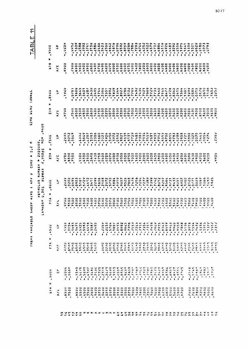
r D O m N N l b h r D O Q & ? . O r o t N O r 3 L I I . ' . a n N r N N n r o O l . . . . . . . . . . , 1 1 1 , i l l

C , >
TABLE 12 - %
N E I N O L U S N U H B E P ' L2OOUOU. L A Y n U A = 0 . O E t ALPHA= * . U L D € G Y O ' , O '
t T 1 : , 4 5 U 0 ETA = . 6 U U U E l k = . / 5 U U
XIE cr a r c


0 0 0 O O O O O O O ~ O o O o O O O O O o O O o o o O O O O O O O O O O C o 0 O C O C 0 0 0 ~ n C n C o C O O ~ C O O O C C o C o C o C C c C c C c ~ C ~ 0 C Y Y ~ ~ Y ~ J P U ~ C C ~ ~ Y C C U ~ ~ C C ~ ~ ~ O C ~ O C ~ C C U ~ ~ ~ C a a m - n-t* N r O O 0 C C C C C O r r . - h n w , n l . - u < w n m G c F ,. C o : o : O O . . . . . . . . . . . . . . . . . . . . . . . . . . . . . . . . . . . . . . .
3 u O D O r N U N N O u O O 0 U m C L C D u ~ W W C ~ h - t - t - t N m T T 6 Y P o c W,IC ~ n ~ n a c . ~ u u ~ ~ ~ n - r c 4 ~ m u r r , o F r r - c ~ r ~ . ~ o m o < r 0 L, 0 . C m h n ~ h c C N c r r u * c W c * r c o r h r a ^ w ~ r C h r " , n o " - . - 0 - o c c c r V r o c c r r ~ ~ ~ ~ n ~ ~ v u u ~ r - l r r v v - ~ m n - c . c c c c n . . . . . . . . . . . . . . . . . . . . . . . . . . . . . . . . . . . . . .
1 1 1 1 1 1 l l I r r l l l l l l l l l l l l l l l , , I l l I I
I,
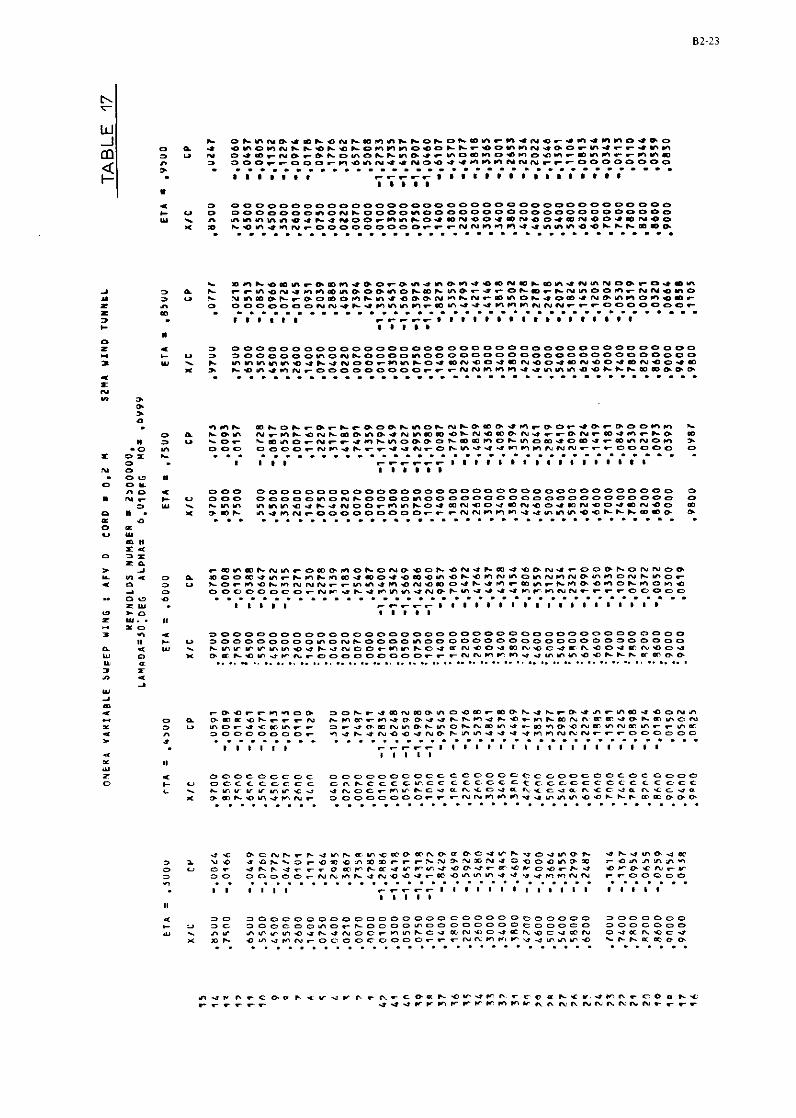
> -I Y V I - 3 P U P 3 "
2 3 - 0 0 0 Z Y .
0 - 0 Z Y . . ,I
< D O O C O O C O C O O O O O O o O C C C o O O O C C C O O 0 ~ O O C O C o o o O t Y O C C L C C C C C ~ ~ C C C C C Y C C C C ~ D C C ~ L C L C C C C L C C C C C C L . C Y Y Y Y m n r . 7 < ~ O C r n Y L C I C h r O ~ - h C c - ~ n r c * 5 5 ~ L - ~ * % m C O m - . n N r a 0 0 0 0 0 0 0 r r r N N m m m " * m m m O O C C C C C C D D . . . . . . . . . . . . . . . . . . . . . . . . . . . . . . . . . . . . . . . .

.E S U F E P U L N G I 4 F V 0 CORD a 0.2 +I SZMA U1NO T U N N t L TABLE 18
ETA ,6000
X I C C P
.97U0 .1U72 : r s o o -.0206 . I 5 0 0 - .on15 :6500 -.1504 :5500 - .2074 :4500 m.2753 :3500 - .2953 ;2600 - .2813 :1400 - .?a76 :0750 -.SO79 :0400 - .4328 :0220 -.SO81 :0070 .1404 : O O O O , 8239 : O l O O - .0958 :a300 - .4542 .OSUU - , J404 :0750 1 .3005 : I 0 0 0 -.2974 : I 4 0 0 -.2921 :lqOO -.7865 :2700 - .2939 :7400 - .7870 :SO00 -.2830 1 3 4 0 0 1.2956 :3800 m.2967 :4200 - .2774 : r a o o *.2666 :SO00 -.2477 :5400 - .2193 : ssoo - . l a 9 6 :b2OO -.1641 ' 6 6 0 0 - . I 4 1 3 f 7 1 0 0 -.1210 :7400 -.0972 :7800 -.0694 : * z o o - .0423 :0400 - .0062 :PO00 .a277 :9400 ,0694
ETA = ,7500 ETA : ETA . .V>OO
X I c C P
. a>ou ,U547
X I C C P

- C C
-tnn ~ n n e e m ~ m c u r r a ~ a o e c ~ + n r ~ ~ ~ n ~ o o ~ o u ~ r m r c o P r n u n ~ n r r o o r o ~ ~ o r ~ m r n ~ ~ n a n - t n n ~ n n n ~ c n n n ~ ~ N
$1 o o 0 0 u C ~ C ~ C ~ ~ C ~ ~ ~ ~ F O ~ - ~ ~ C O ~ ~ ~ ~ P F ~ O C ~ ~ C - ~ ~ N ~ n .c Y - C C r n n r r ~ ~ ~ - t n ~ c o ~ u - t - t u - t r r ~ v n n n h r r r c c c c c r
z C Z C . . . . . . . . . . . . . . . . . . . . . . . . . . . . . . . . . . . . . . . 0 1 1 1 1 1 1 1 1 1 1 l r l l l l l I I I I I I I I 1 I I I I 1 I I
N 0 I . 0" I,
~ 4 n N r G a m , C G m U n N c N r O P m C Q v I U n N r O a O C Q . - -rrrr - t - f + n n ~ m r n ~ , n n r ~ ~ N N N N N N N N N - r r r


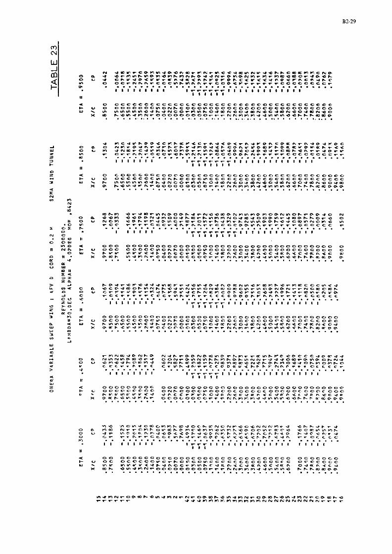
9 0 0 0 0 0 0 0 0 C 0 0 C 0 0 0 0 0 C 0 0 0 0 0 0 0 0 0 0 0 0 0 ~ 0 0 0 0 P + U O o C 1 0 C i C - c O ~ , O N C C O O O m O O C O C o o c ~ c c o o o o c c u o n r c o o Y - C Y Y V I Y V Y < * 4 C C C r w . P . % 0 4 - N r C U D I n W C \ 1 C C < C r t D : n m C U m
x a a r - . o v * v r r r o c - o o o o c c r r r ~ ~ n r n u u m m m m a ~ ~ r ~ ~ e o e . . . . . . . . . . . . . . . . . . . . . . . . . . . . . . . . . . . . . . . .

onn .-OD r r r - F C C . . .
1 I
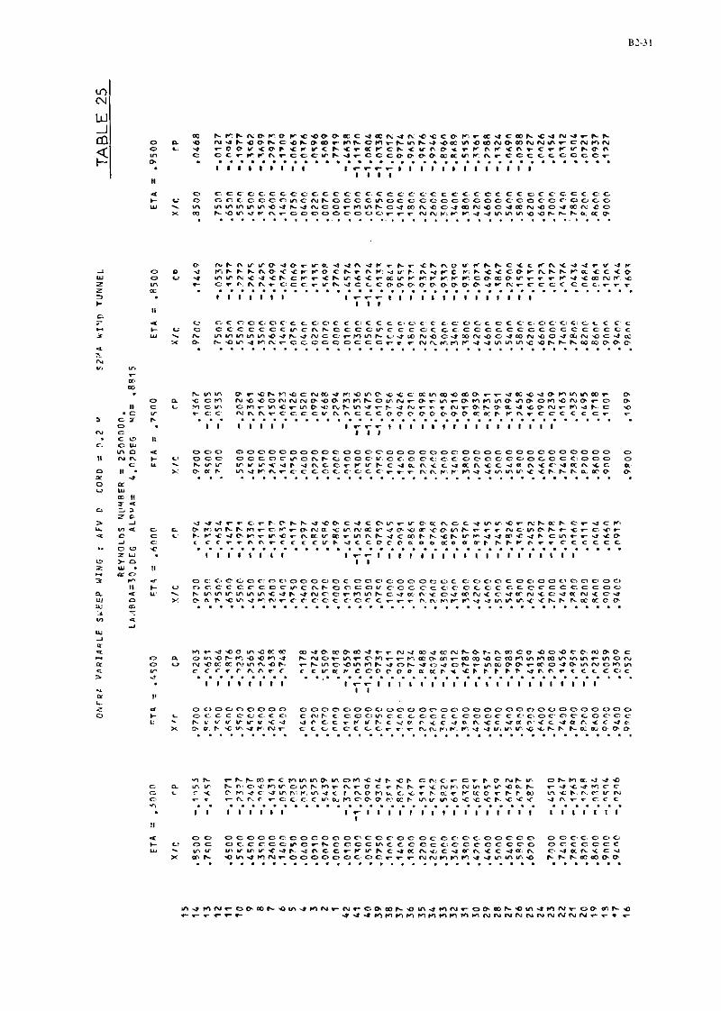
C . - < C C I \Crc.Or r r . , < o C C C C C

,. . ~ N N v n m n O a r m n o m c - N N ~ n m a ~ n r F m n o D u o n a - o o ~ r r o P o o n r ~ u ~ m ~ ~ ~ n r r ~ ~ ~ o ~ u r a ~ ~ m ~ n ~ ~ m m ~ ~ ~ a m o ~ n
I a u -.-a ~ ~ m ~ m ~ ~ n m a u a ~ ~ n u m ~ m a ~ r a m c n ~ ~ c ~ ~ n o ~ ~ * -a m -00 ~ ~ ~ u n n n n ~ n i ~ ~ n * n r m n ~ u r u m u l n a r a n ~ r r o o o o - ....................................... = O I L
0 - 8 1 1 1 1 1 l B I 1 1 1 1 1 1 1 1 1 1 l 1 1 1 1 1 1 1 1 ~ ~ * - - u YI
0 n I -
m z,= z
> 2 N C U ~ n O r r r D r m N O - t N S ~ F D ~ C D t ~ O U O E ~ D D D n U N ~ r ~ D Y w - o P ~ O ~ ~ ~ ~ ~ L D ~ ~ O D C ~ F D ~ O O ~ O ~ ~ ~ ~ O O C ~ V ~ ~ N N N N N E N < O 3 U ~ ~ L D r C L o N O r O C * O L u O N m n m O p . a D N m m r r o * m C C m 3 ~ C
-I o c ~ ~ ~ ~ n u ~ m ~ ) n ~ ~ m ~ u n m m m m n n ~ - t ~ m n w e a a . ~ ~ r ~ ~ ~ w ~ " D O 0 - . - . . . - - . - - - - l - . - . - . - - . - . . . . - . . - - - - . . - - -
Z Y - 1 1 1 1 8 ~ 1 ~ 1 1 1 l l l l t ~ l t l l t e l l I l I l t l I l " > O = Y . Y .. JLO = m e 0 0 0 0 0 0 0 o O O O O O O o o D 0 0 0 O O O ~ o o o O O O D O O O o o o ~ o o I C U D 0 0 0 0 0 0 0 0 n O N C o 0 0 a n 0 0 o o o ~ o O O O O O O O O O D o O 3 o o
L - u . ~ m n ~ u l m m a u ~ - t ~ ~ ~ ~ m n ~ ~ u ~ ~ e ~ - t ~ ~ a o e m ~ ~ o e ~ ~ ~ o ~ W O X 0 0 C O ~ 4 m U C 0 0 0 0 0 0 0 D O r ~ ~ N N ~ m m u - t n m - t e e C C C C ~ D D ......................................... Y m ........................... . . .
r ", * 2
W _I - c r C * C N 0 0 0 * ~ ~ O D N O ~ r ~ U C ~ ~ B N m L L C O O O O U ~ n N J J O O w o L a n a o r o ~ n a ~ C F U ~ O C ) ~ C ~ ~ O ~ N ~ U ~ N ~ . O T ~ Q D ~ U C C C ~ = ~ ~ JL a U P N m N C n * C O r C C ~ ~ O ~ P 0 r U L ~ P N O D n U m Q . J . J . J - t U - t - t r - t - t e n a ~ r n n n u m m n u ~ m 0 u * ~ n n n m n ~ u u u n n n n n n n n ~ ~ 1 ~ 0 0 0 > * ........................................
1 1 1 1 1 1 1 l 1 1 , I , , , I , , , I , I I I I , , , , I I I I - m I YI z 0 0 0 0 0 0 0 0 0 a 0 o C O O O O O O C O O O O O C 0 0 O O O O O D O O 0 C O O O C O O 6 . O O O 0 h : F O C U C Y C C C C C O r O C C C 0 0 C . L D C L C D C C C.
w . Clrn".Y"-na* r n r o - m n c c r m N F s u = . N r c - t o n r c e a N e a u m I ~ m ~ a n u m ~ ~ a o o o o o ~ o r r r ~ ~ ~ v ~ ~ u u m n ~ a a ~ ~ ~ ~ ~ a ~ ~ ........................................

Z 4 C1 O C C O C C C O C C C C - C . C C . C ' C L C P C C C C C C C : C C - E C C C C O C L C C - - C O C O C C 6 C C C ~ 6 h C C C C C ~ C C C ~ ~ C c C C C C C C C C C 0 C C t C C C c 3 Y -. c m ~ m m m ~ u ~ u ~ ~ ~ r n w ~ ~ u m ~ - ~ ~ - f m m . o c - f m ~ . o ~ ~ m ~ . o o - f ~ ~
X a C ~ m * C N - C C C O O O C O C ~ C r r N N C - l C - l C - l u ~ m m Y O C C h C D C m O O O 4 . . . . . . . . . . . . . . . . . . . . . . . . . . . . . . . . . . . . . . . . %~
- -. 1 0
> J ~ C N S ~ ~ ~ < U F O C ~ ~ ~ L ~ ~ D O C ~ ~ ~ " . C ~ ~ P D C ~ D . C C C C ~ - C C ~ Y cn- c p O ~ m w * n ~ ~ s C m L r r n * r D C ~ F o i b * b ~ r j * * r r n ~ * P c o L v * v a : r - c D u ~ v ~ ~ D I c ~ c Y P c c ~ ~ ~ * P ~ ~ ~ ~ c c c ~ ~ ~ ~ ~ ~ D ~ c . c ~ c ~ ~ ~
2 c ~ c ~ ~ ~ - f w n ~ r r r u a ~ ~ ~ * ~ ~ u - f ~ ~ w w ~ ~ ~ ~ ~ ~ ~ ~ . ~ ~ ~ c c .. C Y .(' . . . . . . . . . . . . . . . . . . . . . . . . . . . . . . . . . . . . . . . . = w . 1 1 1 1 1 1 1 l 1 1 1 1 I t l I I I I I I I I I I I I I I 1 1 1 1 1 1 1
3 > 0 Z W . I, .. CLO 3 n = O O C C I C O C O C C I O O C I Z ~ C ~ C ; C . C C , C C I C ~ C ~ ~ O C C I C I C C C C ~ O C U C , C , ~ C
I I c u ~ ~ ~ ~ ~ ~ ~ ~ ~ ~ ~ n r - c c c c : u c c c c c c r c c r c c c c c c . c c c c c c 4 Y . F Y ) I P Y I ~ ~ ~ C V C O N C C ~ ~ ~ C C ~ - ~ D T N < C - ~ O ~ ~ < ~ * c n i c - r r r N < C V
W C x D I C Z V - ~ C ~ \ T C C C C ~ ; < C C C ~ ~ ~ I I ~ C : ~ ~ - ~ - ~ " . ~ ~ C < C . C ~ - ~ : ~ ~ C . . . . . . . . . . . . . . . . . . . . . . . . . . . . . . . . . . . . . . . . i.. a, :<

N 0 . c,L I t 0 C U
m n .s 0 0 0 0 0 0 0 0 0 0 0 0 0 0 0 0 0 0 0 0 0 0 0 0 0 0 0 0 0 0 ~ 0 0 0 0 0 0 0 0
0 N- c u o o o a " o o o ~ o N r - a o c c r o o o a o o o o D o c C o " c o C c o O o o c LL - ~ v m v ~ m ~ ~ ~ ~ ~ ~ ~ r ~ m ~ ~ ~ u ~ ~ ~ \ t u n ~ c ~ O : n ~ ~ u ~ n ~ ~ E
o 0 . x 3 - c m u n ~ ~ ~ ~ o ~ o ~ c ~ i ~ r ~ r n n r ~ w ~ r r r m v ~ m . r . o ~ ~ ~ r r o ; o cr . . . . . . . . . . . . . . . . . . . . . . . . . . . . . . . . . . . . . . . m 0 = " &,
c, ,,
n N O T N n m n r r c < c . . .
I I
.Dco,..-D.m r u n a n n o m u . * r o r n C C C C C C C . . . . . . . 1 1 1 1 1
L Y( . !I - z n x m < 0 c . O ~ 0 0 0 0 C . C 1 0 0 0 0 o c . O O C ~ O o C . " o O C . c > C 1 O C " 0 E 1 0 0 C . O o O o ,, C .J C C C , O ? C C C C w C n C o o C o m o o c . c o ~ ~ r C c C r c C O C O ~ c ~ ~ r m .I w . r - m m m m m m a ~ ~ - t ~ o c r r v , ~ o ~ m ~ . c c ~ m n s o ~ a c ~ c n u p . n ~ c o u Y( e e s r a m * * i ~ - o r c c c r c , c , c r r r r \ ~ r r n - r u m u , m ~ . o ~ r - r c r r c o a . . . . . . . . . . . . . . . . . . . . . . . . . . . . . . . . . . . . . . . . w * - -. m *
,L .- .z 0 C 0 0 0 0 0 0 " ~ O O o O O O O O O O O O O ~ c ~ O O O 0 O O O o O O o o o o o 0 t L. o c o c C~~ c c c n r . o o c c m r c c o c c o c c c . " ~ o c o c . ~ r r o e o c .
c ., P Y w Y Y . w w l . * . * ~ C C C r v ~ ~ ~ y ~ n , c , a n < c u o 0 ~ c + ~ r r . < ~ * a ;. w c c O C C L C C ~ ~ * i ~ . ~ , n r ~ , ~ . t u ~ u v . ~ ~ ~ ~ h ~ a . a ~ . c . o . . . . . . . . . . . . . . . . . . . . . . . . . . . . . . . . . . . . . . . .

." . - 0 11 0 CI I,,
n o u 000 O o O O O O O O O O O O O O O O O O n O 0 " O O O " O O O " O O o o o 0 n N O c u 000 o c c o o n o N C o o o o r c o o r c o o C o C o ~ C C C C C C ~ C ~ o
c Y . CV". Y F m O * C u h c 0 C C Y C C ~ a n ~ 6 * - f n . c C * . c n < r * P n < C C o II . x a a c m ~ n ~ ~ c e c c o c c c c ~ ~ ~ n ~ r r ~ ~ ~ m ~ m ~ . c ~ ~ ~ m r g u a . . . . . . . . . . . . . . . . . . . . . . . . . . . . . . . . . . . . . . . z N 0 E " W *. ,.

8 9 7 0 ' U L L U ' LSLU. S U u 0 ' - f 7 L U ' - L7LO' - 5 6 7 0 ' - L L L 0 ' - Z L 6 U ' - U L L L S - 6 6 L L ' - 'dS5L' - Sfb'L'- S f J d ' - 7 6 6 C ' - 9 6 7 L ' - 7 L Y C ' - U Z Y L ' - 2 L C L ' - 6 L 7 L ' - 5 5 k 5 ' - V 0 7 L e - 5 0 7 6 ' - LL7o.L- 2 S c L - L - LOCO'- L S Y L ' V L L d ' L f Y L . L C L L ' ZULU' 9 0 L U ' - LS l rU ' - 9SYU'- 6 6 7 0 ' - 99CU' - S 1 0 0 '
0 0 0 6 ' 0 0 9 8 ' 0 0 2 8 ' 0 0 8 L ' U 0 7 L ' 0OOL' 0 0 9 9 ' UOZ9' U 0 8 S ' r)O7S' 0 0 0 5 ' 0 0 9 7 ' 0 0 2 7 ' U O U i ' 0 0 7 5 ' OOOE' U 0 9 Z ' UOZZ' 0 0 8 L ' U 0 7 L ' OOOL' U S L J ' u o s o : OOKO' OOLO' 0 0 0 0 ' OLOO' U 2 2 0 ' 0 0 7 0 ' OSLO' UO'IL' 0 0 9 2 ' OOSC' 0 0 5 7 ' OOSS' UOS9' OOSL'
L L S U ' 0 0 8 6 ' L L 7 U ' 0 U 7 6 ' U i f O ' 3 U 0 6 ' YVUU. OU98 ' VULU'- OU28' Y 6 L U a - UUBL ' h L L O a - OU7.L' Y L 9 U ' - SUOL' ZUU0'- J U 9 9 ' 0 5 g b ' - OUZ9' L b O L a - 0 U 8 5 ' L 7 2 L ' - OU7S' Y 2 S L ' - OUOS' L U L L ' - OU97 ' WL8L ' - OUZ7' u o 2 2 ' - O U 8 f ' b L 7 L ' - o U 7 f ' s U 9 L ' - 0 U O f ' L 7 9 2 ' - U U 9 2 ' L 7 L L ' - UUZL ' vucs ' - o u a r . 7 Y S L ' - 5 U 7 L ' L f 8 S ' - OUOL' L L O 8 ' - 3 S L O ' L b Z U ' L - dUS0 ' V C L L ' L - OUEO' U L O L ' L - OULO' b L L 0 ' - 0 0 0 0 ' d d 5 7 ' OLOO' LUSL. OLZO' L 7 S L ' 0 0 7 0 ' ~ L B L ' U S L O ' L L L L ' OU7L ' L L L U ' 0 0 9 2 ' 5 I ILU ' OUSS' b L 0 U ' - LIUS7' c 9 o u . - 3USS' ' 9 9 0 0 ' - J b 5 9 ' ZLOO' GOSL'
9 1 7 0 ' 0 0 L 6 '
d 1 J I X
OOS#' = V13
ZLSO' 0 0 8 6 ' S E L u ' L U 7 6 '
L 6 L O ' 0 0 U 6 ' L S L d ' CU"6' f f 0 U ' - GUYY' L L u U ' - 6 6 ~ 8 ' 6 S L U ' - OULU' 8 9 Z 0 ' - U L L M ' 6 2 S C ' - OUbL' b S 7 U ' - CbbL' L 7 S U ' - 0 0 7 L ' 9 f 9 U ' - " " 7 L . 06LIJ:- OCOL' 9 8 ~ ~ ' - " L Y L ' f b 8 U - OOYY' U 9 6 U ' - GbYY' U 6 L b ' - OOC9' 7 S L b ' - i O 2 9 ' 8 0 7 L ' - OCYS' Z L S b ' - G U S ' 0 6 S b ' - 0 0 7 6 ' b L 9 1 ' - 0 0 7 5 ' 6 0 8 L ' - OOUL' 7 L U b ' - OOPS' 8 6 9 L ' - GDY1' U 2 b d ' - O U y 7 ' 9 9 2 2 ' - OUL?' 6 3 2 L ' - L O Z 7 ' ZS7C'- 00b 'L ' ~ 9 7 ~ ~ - OOML' LO9L ' - 0 0 7 2 ' e f 9 c ' - O U f L ' 9 6 L Z ' - OUUE' Z L Y L s - 0 0 ~ 5 . 2 9 0 ~ ' - Ou'iL' u CUyZ ' L L 2 i ' - GOLC' L CUZZ' Z f S S ' - 0 0 U b ' 5 6 7 L ' - GCbb ' 0 6 0 7 ' - C b 7 b ' L 2 L 7 ' - OO7b' i E Z Y ' - GUDL' b f 7 Y ' - OOUL' 7 OSLu ' L L L U ' - 6 5 ~ 6 . ESZO'L- 0 0 5 U ' L9UU.L- LOSC' 9C60.L - OOLU' Z Z L U ' L - 0 0 i U ' Y 7 0 L ' L - G O I J ' 5 8 L b ' l - 6 0 1 0 ' 9 0 f u ' uUUu ' L 9 O u ' - 0 0 0 3 ' L 6 f 7 ' CLJLI' 5 5 7 7 ' OLOIJ' 6 L f L ' OLLU' S E L L ' OLZU. 8 9 9 C ' OG7U' 2 E 9 L ' 0 IJ70 ' 8 7 6 ~ ' 6 4 L u ' 5 2 0 L ' 65d.U' 8 7 2 L ' 0 0 7 b ' ,LSLL' (IU7L' ~ 7 9 ~ ' D C Y Z ' L ~ L U ' 0 0 9 ~ ' 7 S 2 U ' LGSL ' 9ZEU' OOSS' S fCS ' GOS'I' L7LIU' 3 U S 7 ' f 0 0 0 ' OCSS' Z 6 0 U ' 0 0 5 5 '
SSUU' UUSY' 9 L L O ' 005‘' L 9 L u ' COSL. ELZO' 0 0 5 ~ ' L O L U ' 0 0 5 8 ' 9 f f O ' 0 0 L 6 ' 0 9 7 6 ' OOL6'
d 1 J I X d l I I X
OOSL' = W13 0 0 G 9 ' z V l 3
O O O L ' =ON 9 3 0 ~ 0 ' 9 = V H d l V ~ 3 u . o ~ = w a a w v i ' 000UUSZ = 8dYWflN S U l O N A 3 1
6 S i u ' 0 0 0 0 ' ~ 7 ~ 3 ' o o r o ' O L 3 u ' - OUUO' M0Eu'- O L I Y ~ ' S 5 S u ' - 00 '8 ' . 2 L 0 ' - 0 0 0 ~ ' i 6 6 u ' - 007:' 9 8 L b ' - O U ~ L ' 8 Z S b ' - 30 '19 ' 9 2 S b ' - 0 0 2 9 ' 0 9 L b ' - 0 ~ ~ 5 ' 8 6 OUTS' 7 0 L ~ ' - 0 " U S ' S L ~ L . - OU'97. 8 0 5 2 ' - OUL?' d s 8 d ' - O O b i ' L 0 6 L ' - OGYf ' 0 8 L ~ ' - O O u i ' 6 S 2 i ' - 5CY2 ' 6 2 9 ~ ' - 0 3 6 2 ' 5 0 5 7 ' - 3 0 ~ ~ ' 2 0 0 7 b ' 6 8 7 L ' - OOub' Z9L"- OSrJ ' 7 S L u . L - OO>U' 8 8 9 L . L - 0 3 ~ 0 ' Z Z b i ' 1- 0 0 L 3 ' O f 7 u ' - OOuu' v 7 C V ' 0 ~ ~ 3 ' i 0 2 ~ ' OZ'O' C 6 7 Z ' 0 0 7 3 '
f L 2 b ' O O f L ' 7 9 8 ~ ' OOYZ' 6 8 1 " ' OOSL' 7SOO'- 0 6 > 7 ' 7 6 0 3 ' - 0 0 2 5 ' 7 5 0 0 ' - OG29' f 7 0 0 ' 0 0 s ~ ' 7 8 O u ' Ouhi?' 86211' 0 0 ~ 0 '
d 3 3 1 1
0 0 5 7 ' = V A J
~ 6 u L ' - GULP' 9 L L 2 ' - OOUS' 7 S c L ' - 0 0 7 s ' 9 6 ? < ' - 0OUS' 6 o r L ' - GdY7 ' 9,YL.- 0 0 2 7 ' 9 8 0 2 ' - GOdS' L L L E ' - 0 0 7 s ' 7 7 O O U E ' E25.'- UU92 ' ~ L L E ' - 0 0 2 2 ' Z S L L ' - OUYL. L6LY:- GU7L ' OM97 - 001)L ' 0 3 1 5 ' - OSLO' 7 2 7 6 ' - OOSG' 7 L Y L - L - 0 0 f 0 ' 8 9 b k . L - OJLO' 19.0'- 0 0 0 0 ' S L 2 7 ' OLJO' L U 6 L ' OLCO' L S L ~ ' 0 0 7 0 ' 9 9 i L ' OSLO' L B U L ' GU7L ' S 2 5 0 ' G 0 9 Z ' f L 2 3 ' OO'iE' L a u d ' - 0 0 S 7 ' 6 1 0 0 ' - GOSS' S2UO'- COS9'
3 9 0 5 ' OOSL' OVOO' OOS8'
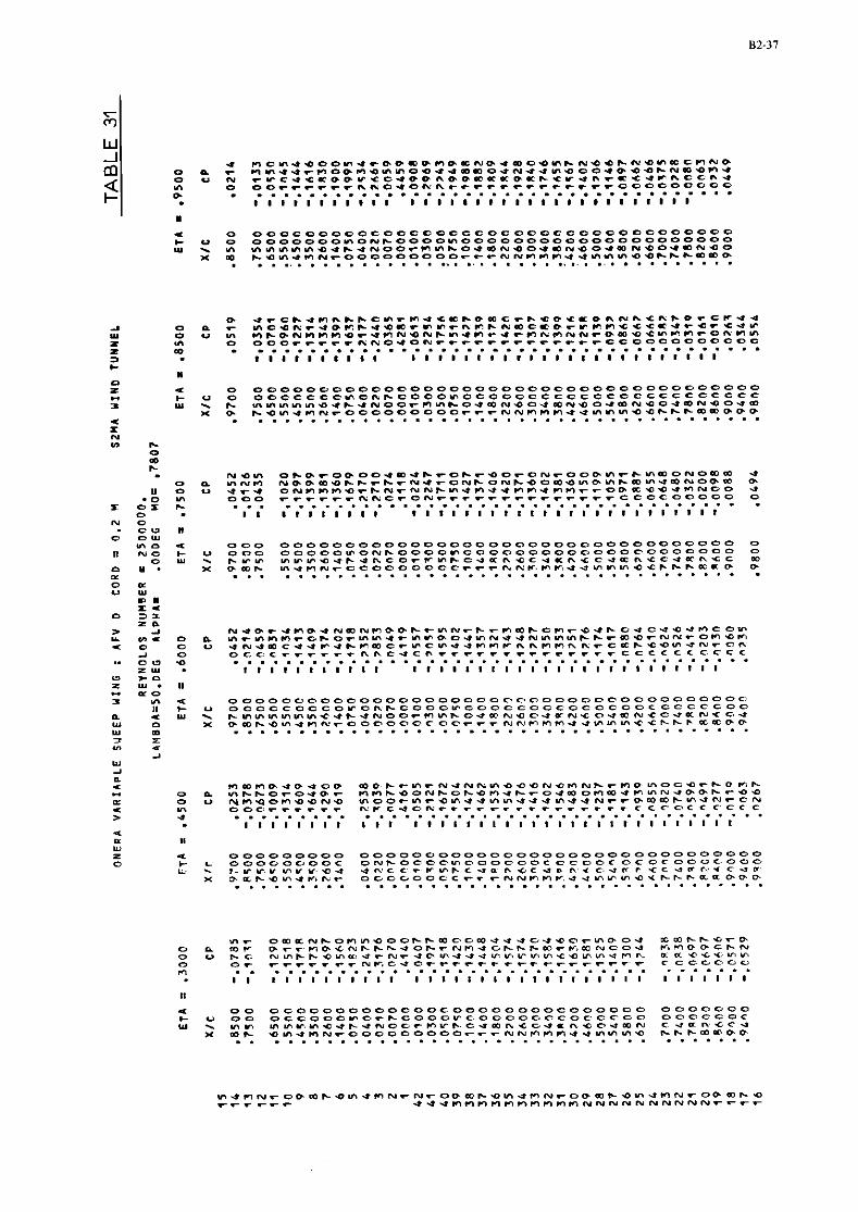
-1 w < 0 i 0 (I Z YI > n Y I . = 0 n

c> O Y 11 C .L. ",O 4 0 0 0 0000000000000000000000000~0"00000~0 0 N r C Y 000 O r 0 0 0 C O N ~ O O O O C O O O C 0 " o O O O O O c C C I C O e o 0 O O o Y - c v c ~ V V ~ ~ C U ~ C C ~ ~ V L C + C ~ C C U O L ~ . L C ~ I C ~ O C U ~ : ~ . L C c
II . X D E C m U n h r O C O O O O C C C r r r N h ~ * . I T U U - t - t L n 2 C C C L p . m D P N . . . . . . . . . . . . . . . . . . . . . . . . . . . . . . . . . . . . . . .
I c m o m m u - . o o m m u r n Y S D P C C C C C L . . . . . . 1 1 1 1 1 1
D w C 0 0 u r r n C C C . . . I

4 O C O C O C O O O O C O C O ~ O O C C ~ 0 0 O O ~ O O " O o o 0 0 0 0 0 0 0 ,- V O r " C C C C " n " r C C O C O C C C O C c C ~ ~ C C c C O C O C E C C C O Y . m u Y I v v < * L * n C C r " ~ C C * ~ n Q ~ V V n 5 c u u n C . , U h * C . ,
Y CGP. ~ n ~ n r \ . ~ c o ~ ~ c o c e o ~ r r r r ~ n n r e ~ n m m ~ C C C C O ~ U . ~ . . . . . . . . . . . . . . . . . . . . . . . . . . . . . . . . . . . .

.- - . 0 - " 0 O W
m o a 0 0 0 0 0 0 0 0 0 0 0 0 0 0 0 c 0 0 0 0 0 0 0 0 C O O O 0 0 0 0 0 0 0 0 0 0 0 0 " Nn C u O C O O f 0 0 0 m 0 h C 0 0 0 0 m O C 0 0 0 0 O O O O O O o O O O O o c O O 0 o Y . r w m m r m ~ ~ e u ~ ~ ~ ~ r m ~ ~ u ~ n a ~ u ~ n . o ~ ~ ~ ~ n ~ ~ ~ a n c c c
D II . x a e r m u n ~ ~ c c c r r ~ o o o ~ ~ ~ ~ ~ m n ~ ~ - t - t m m ~ . ( i r r ~ ~ o o ~ m E . . . . . . . . . . . . . . . . . . . . . . . . . . . . . . . . . . . . . . . 0 E " ",
2 0 ~ ~ O L ~ ~ P C O ~ C ~ C U C C C + U ~ N U D I C ~ ~ ~ O ~ r ~ r n m q w C, L a * Q O P O O ~ F ~ N O O . C C - O W ~ . D C ~ N ~ P m n r ~ ~ ~ a m a a w , u n c - m ? U 3 P m h O . R ~ r . O . & P n C Y . - r . Y 1 m L r a? P C , - D L ' m U h < Y I m O C O P D T I C c. c - r r r r C r . - n w ~ u o h ~ r r r - ~ ~ ~ ~ r r r r r r r r r r c c c c CI . . . . . . . . . . . . . . . . . . . . . . . . . . . . . . . . . . . . . .
I 1 1 1 1 1 1 1 1 1 1 1 l l l l l l l l l l l t l l l l l l 1 1 1 1 1 1 1

u m
- e m o ~ ~ n u r m r r m n ~ o . m u ~ m r o ~ n ( ~ ~ ~ ~ m ~ ~ n m ~ ~ ~ ~ ~ r- o P u m - 0 0 m 0 m m a - u ~ n 0 ~ ~ n 0 ~ o . 0 n ~ ~ u c a m a o n ~ m ~ n ~ i ~ u
t o u - r e ~ o ~ o ~ ~ - o o ~ . ~ c o D L ~ ~ ~ N - ~ o ~ o o * ~ N ~ . o o * ~ ~ ~ v . O m O E O O ~ ~ C C C C O N S ~ ~ U ~ ~ ~ ~ N ~ ~ N ~ ~ ~ ~ ~ ~ ~ ~ C C C O O E O 0
O Z C . . . . . . . . . . . . . . . . . . . . . . . . . . . . . . . . . . . . . . . 0̂ 1 1 1 1 1 1 1 1 1 1 1 1 1 1 1 1 1 1 1 1 1 1 1 1 1 1 1 1 1 1 ) 1 1

- 0 - It " YI LnO < 0 0 0 0 0 0 0 0 0 0 0 0 0 0 0 0 0 0 0 0 0 0 0 0 0 0 0 0 0 0 0 0 0 0 0 0 0 N N C U 0 - 0 O C C O O Y O N C 0 0 0 0 m O C 0 0 0 0 E o O O O C O O O o O O O O O 0
5 Y . C Y W ~ Y ~ ~ U C ~ N C C T ~ ~ C C ~ ~ ~ ~ C ~ ~ ~ ~ C ~ Q Q ~ C ~ O L O L E C a I I . X D L - ~ U * I N r O O O L L O C O C r C C h h I ~ V ~ U - t - t - t Q Q C C C ~ O C O D u . . . . . . . . . . . . . . . . . . . . . . . . . . . . . . . . . . . . . . .
w
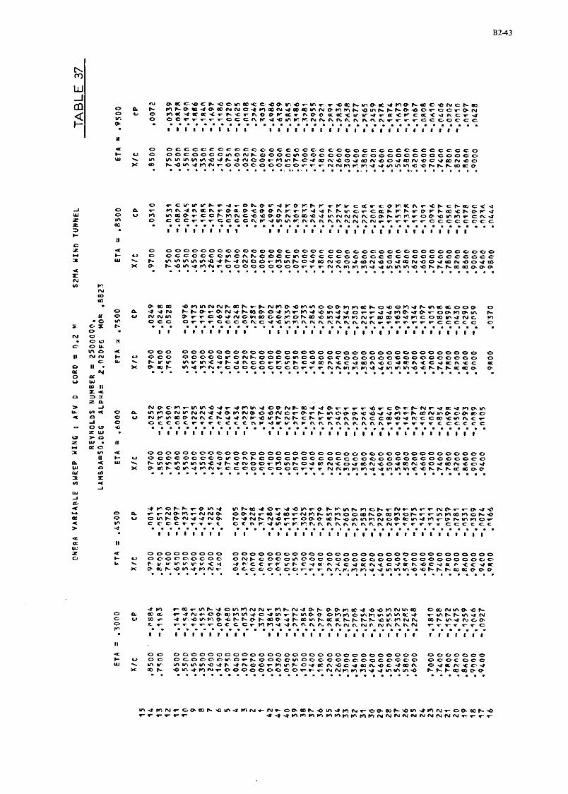
0. - - * C I O C C r O n u n L m ~ O r u a n r a C r n C m O C r N N n V ) T N ( " r r O u a o n C - N O ~ ~ N N O o e ~ r ~ u m r ~ n ~ n n o o m ~ a m n ~ ~ ~ ~ ~ n m n ~ ~ a = 0 u 0 - C C - N U ~ N D C U N L N Q C ~ O O O W F O ~ ~ ~ N ~ O E O O ~ ~ ~ L I C C ~ O ~
u m c c C C C ~ . ~ ~ c ~ n w ~ m v r ~ n . r , n n n n n n n ~ r r r r r ~ c c c c c c > * . . . . . . . . . . . . . . . . . . . . . . . . . . . . . . . . . . . . . . . . u
I I I I I I I I I I 1 1 1 1 1 1 1 1 1 1 1 1 1 1 1 1 1 1 1 1 1 1 1 1 1 1
0: 11

- P - c o n m ~ a r ~ ~ m ~ r r r n o a ~ ~ ~ u ~ ~ m n ~ ~ ~ ~ m ~ n e n ~ r ~ ~ o
o P ~ n m ~ ~ ~ ~ r n ~ ~ ~ n n e m ~ ~ * n ~ c n . t ~ ~ ~ m ~ a ~ ~ u n m ~ m n N H 0 U N r n m O * r n ~ m D c O N m m n o ~ O n 0 e h m * r O D O * r O ( D ( D n N O n .o m o c o ~ ~ ~ ~ c ~ r r r o ~ a m ~ n n ~ n n n n n ~ r r ~ ~ ~ ~ ~ ~ c ~ ~ ~ o o
z c = C . . . . . . . . . . . . . . . . . . . . . . . . . . . . . . . . . . . . . . . 0 * 1 1 I 1 1 1
N O 1 1 r I l l l l l l l r l l 1 l 1 l l l 1 l l l l . C O I,
0 C W m o 4 0 0 0 0 0 0 0 0 0 0 0 0 0 0 0 0 0 0 0 0 0 0 0 0 0 0 0 0 0 0 0 0 0 0 0 0 0 0 0
I N m C U 0 0 0 0 0 0 o C m O N C o O C 0 m 0 0 0 0 0 0 O O O C O C O O O o o O O O O 0 o w - C Y ~ ~ Y ~ S U C U ~ C C - ~ C C S ~ E ~ O C ~ Q ~ ~ C - ~ ~ ~ ~ C - ~ ~ ~ ~ ~ c
0 18 . x D ~ C m ~ n ~ ~ o o o o o ~ ~ ~ ~ ~ r r ~ ~ ~ ~ ~ n u ~ m m m ~ ~ ~ ~ ~ e m ~ o = u . . . . . . . . . . . . . . . . . . . . . . . . . . . . . . . . . . . . . . . 0 D:
Y D O ~ ~ O N ~ ~ ~ C r D C O N C C n O N ~ C C C C N U r - t O r m * C N N U * o c nr N C P ~ ~ O ~ N O N - ~ O P ~ ~ O ~ ~ ~ C ~ D ~ ~ L " ~ ~ ~ ~ o r a * e - a 3 u m e P C C O * C . ~ ~ ~ ~ O ~ C ~ ~ ~ O D ~ ~ C C ~ ~ O ~ , ~ O E ~ r c c h - t r m o c c o o c o r - c ~ ~ ~ n n h ~ ~ - t ~ v n n n n n n * i n ~ ~ r n ~ r d ~ r r r r o CI . . . . . . . . . . . . . . . . . . . . . . . . . . . . . . . . . . . . . .
I # 1 1 1 1 1 l I 1 I I I I I I I I I I I I I I I 1 1 1 1 1 1 1

N N a . o n n ~ o r n r ~ m o a a n ~ m ~ n ~ m ~ m * ~ - m ~ ~ n a - n m ~ n n m a a
o L m ~ m u ~ n ~ ~ ~ o ~ o m ~ n ~ ~ ~ r o o o m n n ~ ~ m ~ m m ~ ~ n ~ n ~ ~ N II o u N ~ O n ~ ~ u ~ a m ~ n ~ m a o m ~ ~ ~ ~ ~ . o ~ c ~ u ~ ~ ~ ~ ~ ~ o t c n u n n n
. O n o c o - ~ r - r C h a O - C n W C r r C r - r - - - C r - r r C C 6 0 C C 5 o . . . . . . . . . . . . . . . . . . . . . . . . . . . . . . . . . . . . . . . = 0 5 C 0 I 1 l t l l l l l l I l l 1 1 1 1 1 1 1 1 1 1 1 1 1 1 1 1 l l t I I I
C N . ~ m ~ ~ n ~ a m ~ c o . t o - ~ ~ m - s ~ n ~ ~ o v , ~ r a ~ e - t r c ~ a o 0 II N N 0 0 N Q m ~ ~ P - m ~ ~ ~ 0 O ~ O o ~ D r ~ O U ~ + C . O C r O Ln*10ODOON 1 Y n o r ~ ~ w r ~ ~ ~ n r o ~ - t ~ ~ ~ r m o o - Y I - ~ ~ - c c . o ~ c m c n u n * . 0 . ir N N N ~ P . I Y O N W O - ~ C N C - C . - N ~ N & - N ~ ~ N & W r r r r r r r F, . . . . . . . . . . . . . . . . . . . . . . . . . . . . . . . . . . . . . .
I I l l l l t l l l l l 1 1 1 l 1 1 1 1 1 1 1 1 1 1 1 1 1 1 1 1 1 1 1 1 1

. 0 n
n o 0 .a n
o r I- 0 0 0 w It 0 I" Y I P I N C ,. u
0 Y \ I . X
N a Y rn I1 I I 3 = z -
-1 '"I 0 0 O U A C 0 0 0 T W . > 0 Y . H a 0
n < Il C U I Y . 0 X m z <
0 0 0 00000000000000000000000000000000000 0 O C O 0 0 0 0 0 n O N C C O 0 0 m C G C S O o o C O 0 O C C C C O O ~ C o c 0 r m - n r r s ~ ~ ~ n r ~ r v n ~ s ~ ~ n ~ c ~ ~ n c ~ ~ m n ~ ~ . ~ ~ h . c c m D O C n ~ n n r o o o o o r o o o r r r n n n r ~ ~ ~ m n n o ~ r ~ r ~ c ~ o . . . . . . . . . . . . . . . . . . . . . . . . . . . . . . . . . . . . . . .
D C N C O O m P n O N m m C r N n n C - C O D C O m N r n N O r C N O * * 0 m n C O . - m n N * N n . - C O r r O r D ~ c ~ v - n u . n r nnnnrr r , n n r . . . . . . . . . . . . . . . . . . . I I 1 1 1 1 1 1 1 1 1 l l l 1 1 1

TABLE 41
WING GEOMETRY
1 :Theoretical wing geometry
2 : Measured wing geometry
TABLE 4 2
FREE STREAM MACH NUMBER VARIATON WITH INCIDENCE DUR~NG FORCE MEASUREMENTS
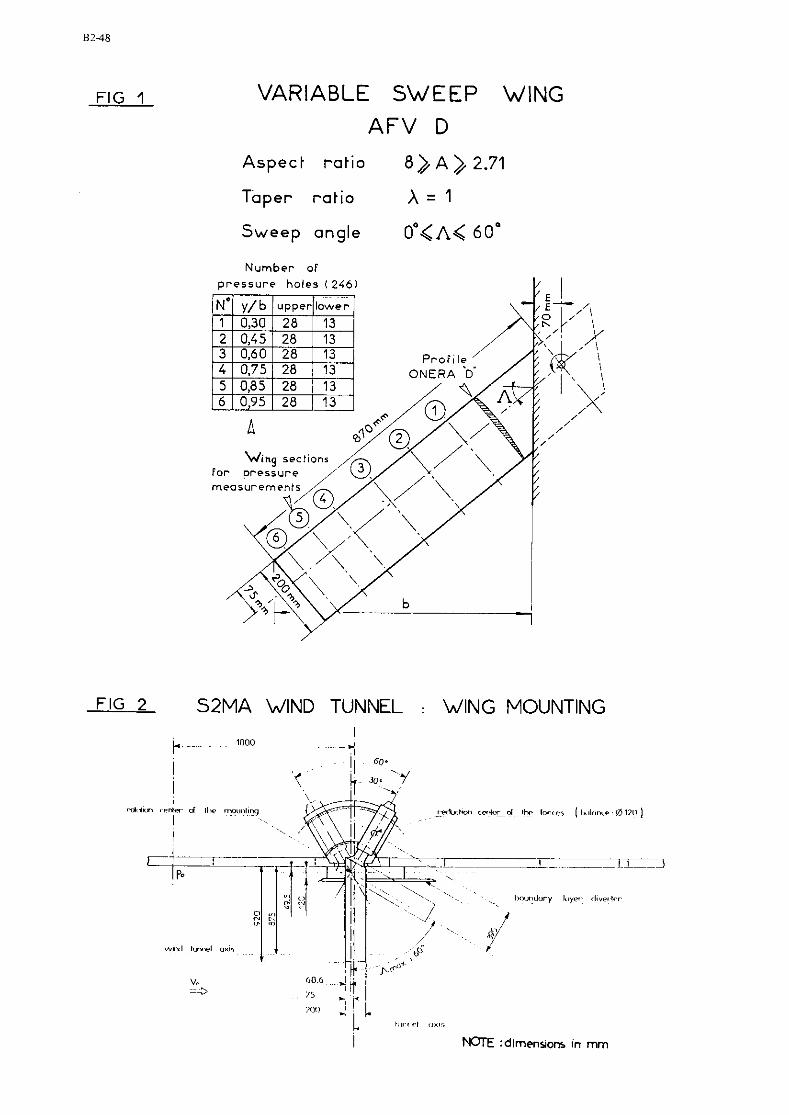
FIG 1 VARIABLE SWEEP WING
AFV D
Aspect rat io 8 > A )/ 2.71
Taper rat io X = l
Sweep angle O",(A< 60"
FIG 2 S2MA WIND TUNNEL : WING MOUNTING

FIG 3
VARIABLE SWEEP WING AFVD
S2MA WIND TUNNEL R e = 2.5.10 6
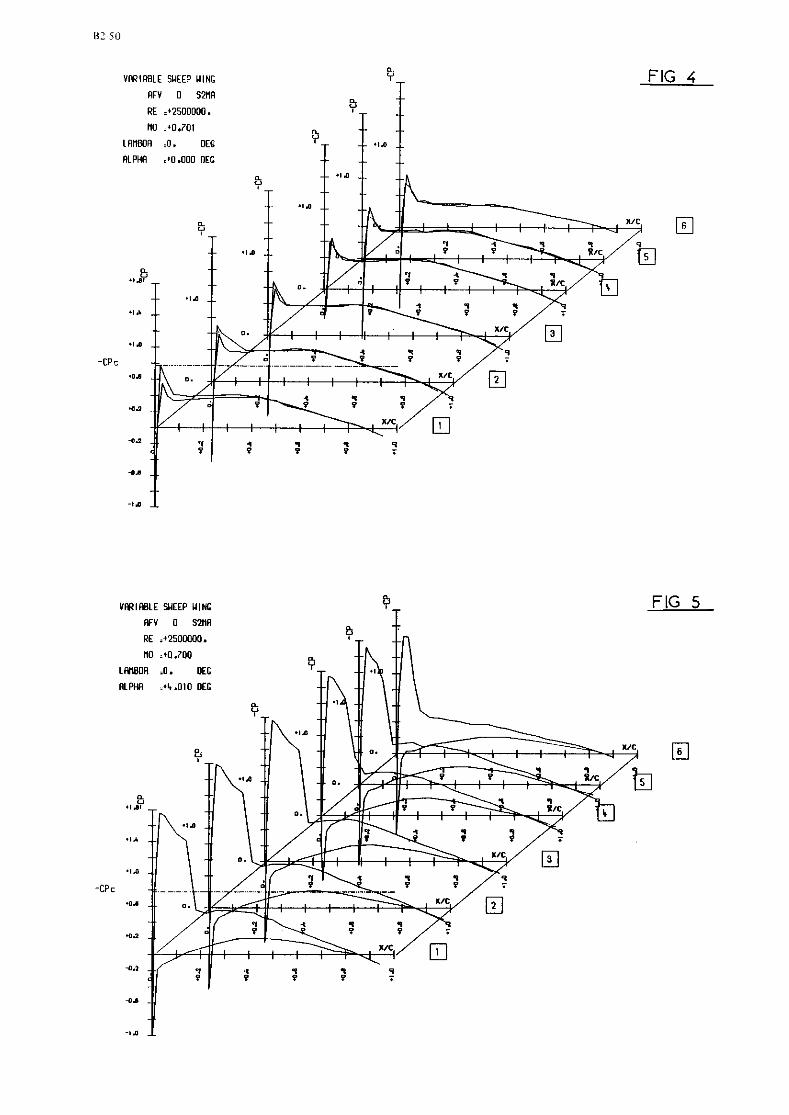
VRRIRBLE SUEE? UlNG 9 AFV 0 S2MR
RE :*2500000.
no ;+o.701
L R ~ E O R ;o. OEG !J RLPHR :+0.000 OEC T
FIG 4

B?-5 I
FIG 6 VARIABLE SUEEP UlNG 4 RFV 0 S2MR
RE .42500000.
MD :+0.782
LRnBOR ;O. OEG
RLPllR .+0.010 OEG
a. .,aY
.I *
.la
.o.r C P c
10.)
*.2
0 s
- 1 1 1
FIG 7

VPRlABLE SUEEP UlNC
WV 0 S2iiR
RE .+2500000.
no :+o.s4a
LMBOA s o . OEC
RLPHR ;*0.020 OEC
D ',,I
.1*
1 1 1
a0.9
-CPc .0.?
4.2
4s
-1 11
FIG 8
FIG 9 VWIRBLE RIEW U I K
f f v 0 sm RE ;+2500000.
no :+O.E~I
LMBOR L!. OEC
RLPHA .+2.010 OEC
8 .,a0
.I*
.,a
.oa
30.9
4.2

VRRlRBLE SUEEP UlNG
RFV 0 S2HR
RE :+2500000.
no :+0.922
LRnEOR :O. OEG
RLPHR :-0.010 OEG
a. ., AY
-1 A
.la
41
.cpc .0.2
4.7
-0.r
-19
FIG fl VRRlRBLE WEEP UlNC
RFV 0 S2NR
RE .+2500000.
no ;+0.920
LRnBOR :O. OEC
RLPHR :+2.030 OEG
a u 1 1 1 '
'I*
.,a
.0..
10.2
*a
Od
-1 10
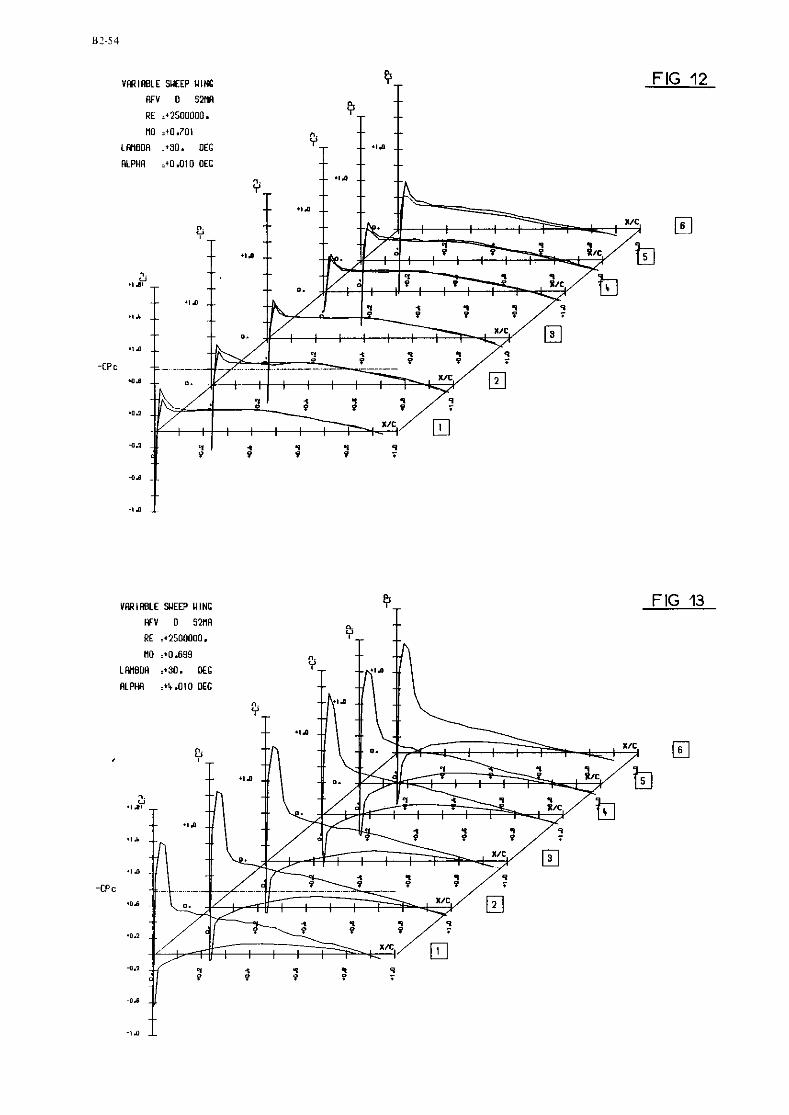
FIG 12 VFRl ABLE SUEEP UlNC
RFV 0 SmR
RE ;*2500000.
HO ;+0.701
LWEOR ;+30. OEG
RLPHR ;+0.010 OEC
-CPc
FIG 13

82-55
FIG 14 YARIRBLE SUEEP UlNC
RFV 0 S2iiR
RE ;+2500000.
NO ;+0.782
LAnEOfl 8 3 0 . OEG
RLPHR ;-0.020 OEG
CP c
FIG 15 a. u VRRIRBLE SUEEP UlNG
RFV 0 S2HR
RE ;12500000.
HO Al .780
LAPl8OR ;+30. OEG
RLPHR ;*& .030 0EG
c. u .Ill
.I*
- 7 a
' P S -CPc
4.1
4.1
*.6
4.0

FIG 16 VRRlfflLE SUEE? UlNC 3 RFV 0 S2nR
RE ;+2500000.
no ;+o.al LWiBOR ;+30. OEG
RLPHA .+0.010 OEC
a. u .1.,1
.I A
.#A
.a*
-CPc 4.2
4.2
- 0 6
-1 a
FIG 17 VRRIRBLE WEEP UINC e RFV 0 S2nA
RE .+2500000.
no .+o.sco LWBOR ;+30. OEG
ALPHA .+2.000 OEG
a. u 11.1
.I A
.,a
'OP
C ? c 10.1

VRRIWLE SUEEP UlNC
R V 0 S2nA
RE ;+2500000.
110 :+0.925
LfflBDfl :+30. OEG
ALPHR .+1.990 0EC
m. u 11.01
. ,A
.I.D
. a 1
.cpc '0.2
-0.1

v m l i w E SUEEP UINC
RFV 0 S2nR
RE .+250WW.
no ;to.7m
LlWOf l ;+SO. OEC
flLPWl :t0.010 OEC
-CP c
VRRIRBIE S E E P UlNC
RFV 0 S2nR
RE :+2500000.
no z+o.700
LAniIOA ;+50. OEG
ALPHR :+K.OIO OEG
FIG 21

VFRIRBLE WEP UlNG
RFV 0 SZnR
RE .+25000W.
no :+o.,a~ L m O R 1150. K G
ALPHR SO. OEC
B2-59
FIG 22
FIG 23 VRRIRBLE SUEEP UIM: 9 AFV 0 S2nR
RE . r z ~ o o ~ o .
MI 80.779
LAnEOR :+SO. OEG
ALPHR :+S.9W OEG
e .,A0
.I*
.,a
.oJ -CPc
*.,
-03
*.,
-1 .a

FIG 25

82-6 1
FIG 26 VflRlRBLE SUEEP UlNC
flFV 0 S2ilR RE .+2500000.
iI0 .+0.323
LflHsOR .+SO. OEC
RLPHR .+O.OSO OEC
VRRlRBLE SUEEP UlNC
w o smn RE .+2500000.
UO .+0.921
LfflBOA :+so. OEG
RLPHR ~t2.000 OEC

3. MBB-AVA Pilot-Model wi th S u p e r c r i t i c a l Wing - Surface Pressure and Force Measurements
H . Ka~ner, W . Loren=-me ye^, A . Heddergott
Deutsche Forschungs- und Versuchsansta l t fiir Luft- und Raumfahrt E.V.
and
A. Eber le
Messerschmitt-Balkow-Blohm GmbH, Miinchen
3 .1 In t roduc t ion
These d a t a con ta in p ressu re and force measurements on t h e MBB-AVA Pilot-Model which is a f i g h t e r t y p e
wing'-body combination wi th a s u p e r c r i t i c a l wing. The a i r f o i l , incorporated i n t h i s wing is MBB-A3, an
a i r f o i l designed by t h e Eber le hodograph-method. Se lec ted exper imental r e s u l t s o f t h i s a i r f o i l a r e given
i n c o n t r i b u t i o n A8.
The measurements have been performed i n t h e DFVLR 1x1 m Transonic Wind-Tunnel GBttingen.
The s e l e c t e d p ressu re d a t a f o r t h i s model con ta in an a sweep a t M = 0.8 and a Mach number sweep f o r
a : 2'. This g ives a c e r t a i n range o f d i f f e r e n t s u p e r c r i t i c a l flow types on t h e wing, inc lud ing f l aws
wi th ex tens ive r e a r s e p a r a t i o n s . Tes t s have shown t h a t s e p a r a t i o n always begins a t t h e t r a i l i n g edge
and f i r s t occurs at t h e wing t i p . Leading edge vor tex shedding has no t been abserved.
1. General Descr ipt ion
1.1 Model Designation o r Name
1.2 Model Type (e .g . , F u l l Span Wing-Body, Semi-Span Wing)
1 . 3 Design Requirements/Conditions
1 .4 Addi t ional Remarks
2. Model Geometry
2 .1 Wing Data
2.1.1 Wing Planform
2.1.2 Aspect Rat io
2.1.3 Leading-Edge Sweep
2.1.4 Trailing-Edge Sweep
2.1.5 Taper Rat io
2.1.6 Twist
2.1.7 Mean Aerodynamic Chord
2.1.8 Span o r Semispan
2.1.9 Number o f A i r f o i l Sec t ions Used t o Define Wing
2.1.10 Spanwise Location o f Reference Sect ion and Sec t ion Coordinates (Note i f Ordinates a r e Design o rAc tua l Measured Values)
2.1.11 Loft ing Procedure Between Reference Sec t ions
2.1.12 Form of Wing-Body F i l l e t , S t r akes
2.1.13 Form of Wing Tip
MBB-AVA Pilot-Model wi th S u p e r c r i t i c a l Wing
F u l l span wing-body
Fighter- type wing-body combination wi th s u p e r c r i t i c a l wing
A i r f o i l s e c t i o n perpendicular t o l ead ing edge is MBB-A3
See f i g . 3 .1
Swept wing (see f i g . 3.1)
4 . 5
35O
14.25'
0.33
-3O
0.11875 m
0.4915 m ( span)
The same a i r f o i l s e c t i o n is used over t h e whole wing, coord ina tes t a b l e 3.1, measured coord ina tes o f wing t a b l e 3.2
S t r a i g h t genera to r s
See f i g . 3.1

2.2 Body Data ( D e t a i l Description o f Body Geometry)
2.3 Wing-Body Combination
2.3.1 Re la t ive Body Diameter (Average Body Diameter at Wing Location Divided by Wing Span)
2.3.2 Re la t ive V e r t i c a l Location of Wing (Height Above o r Below Axis Divided by Average Body Radius a t Wing Location)
2.3.3 Wing S e t t i n g Angle
2.3.4 Dihedral
2.4 Cross Sec t iona l A ~ e a Development
2.5 Fabr ica t ion Tolerances/Waviness
3. Wind Tunnel
3 .1 Designation
3.2 Type of Tunnel
3.2.1 Continuous o r Blowdown. I n d i c a t e Minimum Run Time i f Applicable
3.2.2 Stagnat ion Pressure
3.2.3 Stagnat ion Temperature
3.3 Test Sect ion
3.3.1 Shape o f Test Sect ion
3.3.2 S ize of Test Sect ion (Width, Height, Length)
3.3.3 Type of Tes t Sect ion Walls Closed, Open, S l o t t e d , Pe r fo ra ted)
Open Area Rat io (Give Range if Variable)
Slot/Hole Geometry (e.g., 30-Degree Slanted Holes)
Treatment of Side Wall Boundary Layer
F u l l span models Half-model t e s t i n g
3.4 Flow F i e l d (Empty Test Sec t ion)
3.4.1 Reference S t a t i c Pressure
3.4.2 Flow Angularity
3.4.3 Mach Number Dis t r ibu t ion
3.4.4 Pressure Gradient
3.4.5 Turbulence/Noise Level
3.5 Freestream Mach Number (o r Veloci ty)
3.5.1 Range
3.5.2 Pressure Used t o Determine Mach Number (e .g . , S e t t l i n g Chamber T o t a l Pressure and Plenum Chamber Pressure)
3.5.3 Accuracy of Mach Number Determination (AM)
3.5.4 Maximum Mach Number Varia t ion During a Run
See f i g . 3.1 and 3.2, t a b l e 3.3
2' ( s e e f i g . 3.1)
o0
< 0.15 m, measured coord ina tes a r e given in t a b l e 3.2
DFVLR 1x1 Meter Transonic Tunnel
Continuous, c losed c i r c u i t
Variable between 0.4 and 1.6 b a r
= 305 K
Square
l m x l m with usab le l eng th of 1 . 5 m
Perforated
6 % f i x e d poros i ty
30° s l a n t e d holes
None
Plenum chamber p ressure
f O.OsO
I I I I
Low no i se l e v e l (m < 0.001). Measured on body o f r evo lu t ion NACA R!4 12. Low turbulence l e v e l (measurements are i n p rogress ) .
-
Transonic: M = 0.5 - 1.2 Supersonic: M = 1.33 - 2.2
Transonic range: s e t t l i n g chamber t o t a l pressure/ plenum chamber p ressure
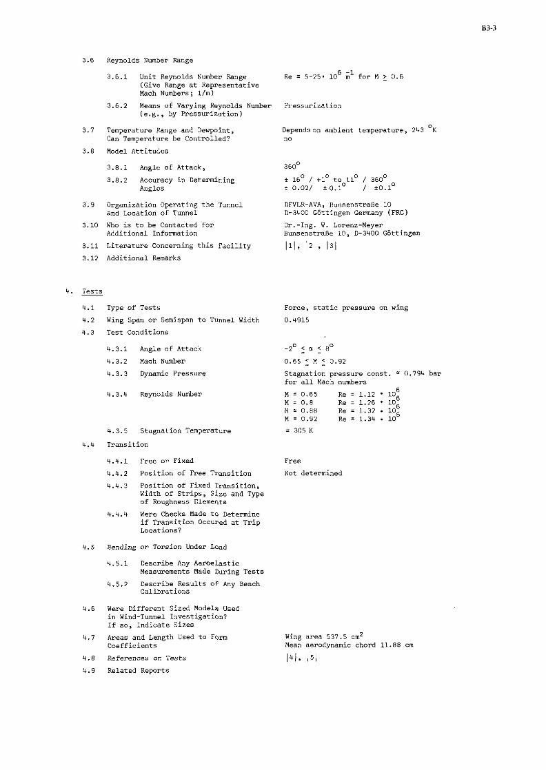
3.6 Reynolds Number Range
3.6.1 Unit Reynolds Number Range (Give Range a t Representa t ive Mach Numbers; l/m)
3.6.2 Means of Varying Reynolds Number ( e . g . , by P r e s s u r i z a t i o n )
3.7 Temperature Range and Dewpoint, Can Temperature be Control led?
3.8 Model A t t i t u d e s
3.8.1 Angle of Attack,
3.8.2 Accuracy i n Determining Angles
3.9 Organizat ion Operating t h e Tunnel and Location o f Tunnel
3.10 Who i s t o be Contacted f o r Addi t ional Information
3.11 L i t e r a t u r e Concerning t h i s F a c i l i t y
3.12 Addi t ional Remarks
4.
4.1 Type o f Tes t s
4.2 Wing Span o r Semispan t o Tunnel Width
4.3 Test Conditions
4.3.1 Angle of Attack
4.3.2 Mach Number
4.3.3 Dynamic Pressu re
4.3.4 Reynolds Number
4.3.5 Stagnat ion Temperature
4.4 Trans i t ion
4 . 1 Free o r Fixed
4 . 4 2 P o s i t i o n of Free Tr,ansition
4.4.3 Pos i t ion of Fixed Trans i t ion , Width o f S t r i p s , S ize and Type of Roughness Elements
4 . 4 Were Checks Made t~ Determine i f T r a n s i t i o n Occured a t T r i p Locations?
4.5 Bending o r Torsion Under Load
q.5.1 Describe Any Aeroe las t i c Measurements Made During T e s t s
4.5.2 Describe Resul ts of Any Bench C a l i b r a t i o n s
4.6 Were Dif fe ren t Sized Models Used i n Wind-Tunnel Inves t iga t ion? I f s o , I n d i c a t e S izes
4.7 Areas and Length Used t o Form C o e f f i c i e n t s
4 .8 References on Tes t s
4 .9 Related Reports
6 -1 Re = 5-25. 10 m fo r M 1 0.6
P ressu r i za t ion
Dependson ambient temperature , 243 OK
no
DFVLR-AVA, BunsenstraRe 10 0-3400 GBttingen Germany (FRG)
Force, s t a t i c p ressu re on wing
0.4915
-2' < u < 8' - .
0.65 2 M I 0 . 9 2
Stagnat ion p ressu re cons t . ' 0.791, b a r f o r a l l Mach numbers
M = 0.65 Re = 1.12 ' l o6 M : 0.8 Re = 1 . 2 6 . l o6 M = 0.88 Re = 1.32. 10; M 3 0.92 Re = 1.34 . 10
= 305 K
Free
Not determined
Wing a r e a 537.5 cm2 Mean aerodynamic chord 11.88 cm
I + / > 151

5. Inst rumentat ion
5 .1 Surface Pressure Measurements
5.1.1 Pressure O r i f i c e s i n Wing. 8 s e c t i o n s , 14 o r i f i c e s f o r each s e c t i o n Location and Number on Upper and on upper s i d e , 10 o r i f i c e s on lower s i d e Lower Surfaces (see f i g . 3 . 1 , t a b l e 3.4)
5.1.2 Pressure O r i f i c e s on Fuselage. Location and Number
5.1.3 Pressure O r i f i c e s on Components, Give Component and O r i f i c e Location
5.1.4 Geometry of O r i f i c e s Ci rcu la r , 0.3 m diameter, some 0.5 m
5.1.5 Type o f P ressure Transducer and CEC 4-312 - 0002 Scanning Devices Used. I n d i c a t e Scanivalve Types d; J; S Range and Accuracy +5 p s i , 10.4 8, T o t a l arrangement f0 .7 %
5.2 Force Measurements
5.2.1 Type and Location of Balance Task 1.5"C. i n t e r n a l balance
5.2.2 Forces and Moments t h a t Can b e N = 2000 Lb Measured. Maximum Loads and X = 130 Lb Accuracy Y = 900 Lb
f0.65 %, t o t a l arrangement f l .O %
5.2.3 Forces and Moments on Components - Type and Location of Balance
Maximum Loads and Accuracy
6.1 .1 Pressure C o e f f i c i e n t s
6.1.2 Aerodynamic Coef f i c ien t s
6 .1 .3 Boundary Layer and Wake Q u a n t i t i e s
6.1.4 Repea tab i l i ty
6.1.5 Addi t ional Remarks
6.2 Wall I n t e r f e r e n c e Correct ions
6 .3 Data Presen ta t ion
6 .3 .1 Aerodynamic Coef f i c ien t s
6.3.2 Surface Pressure Coef f i c ien t s
6 .3 .3 Flow Conditions f o r
+1% assuming t h e worst poss ib le combination of e r r o r s inc lud ing an e r r o r of A M = +0.002 evaluated a t maximum I c I -
P 0.5 % - -
within 1 %
No c o r r e c t i o n s , see 16 1
Table 3.14 Figure 3.12
Tables 3.5 - 3.13 Figures 3.3 - 3.11
- Aerodvnamic c o e f f i c i e n t d a t a ~ o l a r s f o r M = 0.8
- Pressure d a t a
6.3.4 Boundary Layer and/or . Wake Data
6.3.5 Flow Conditions f o r Boundary - Layer and/or Wake Data
6.3.6 Wall In te r fe rence Correct ions Included? No
6.3.7 Aeroe las t i c Correct ions Included? No
6.3.8 Other Correct ions? No
6.3.9 Addi t ional Remarks -

6.4 Were T e s t s Carr ied Out i n Di f fe ren t No F a c i l i t i e s on t h e Current Model? If s o , What F a c i l i t i e s . Are Data Inclluded i n Present Data Base?
7. References
11 Ludwieg, H . Der Transsonische Windkanal d e r Aerodynamischen Versuchsansta l t Lorenz-Meyer, W . Gdttingen. Schneider , W . Jahrbuch derWG1.R 1966,pp. 145-2114.
121 Hot tner , Th. Der Transsonische Windkanal d e r Aerodynamischen Versuchsansta l t Lorenz-Meyer, W . GBttingen (2 . Ausbaustufe).
Jahrbuch d e r DGLR 1968, pp. 235-2114.
13 1 Lo~enz-Meyer, W . Tes t f a c i l i t i e s o f t h e DFVLR i n t h e t r a n s o n i c and hypersonic speed range and main a c t i v i t i e s . DLR-FB 71-86, 1971.
141 E b e r l e , A . Experimentelle Untersuchungen i ibe rk r i t i sche r P r o f i l e und Trag- f l i ige l i m Hochgeschwindigkeitsbe~eich. MBB-Rep. UFE 1153 (1975) and UFE 1153A (1976) .
15 1 Lorenz-Meyer, W . Druckuerteilungs- und 3-Komponentenmessungen an dem AVA-Transsonik- Heddergott , A. Modell m i t i iberkr i t i schem Tragf l i ige lp ro f i l .
DFVLR I B 251-76A19 (1976).
6 1 Lorenz-Meyer, W .
8 . L i s t o f Symbols
x , Y ,
x', 7.'
HS, S1 ... 57
Kanalkorrekturen fiir den Transsonischen Windkanal d e r Aerodynamischen Versuchsansta l t Gdttingen b e i Messungen an 3-dim. Modellen. ZFW 19 (1971), pp. 454-461.
coord ina tes ( f i g . 3 .1)
coord ina tes ad jus ted t o chord l i n e
chord l eng th
ang le of a t t a c k (ve r sus fuse lage cen te r l i n e )
angle of a t t a c k of s e c t i o n (ve r sus fuselage c e n t e r l i n e )
f ree-s t ream Mach number
l o c a l Mach number
Reynolds number (based on mean aerodynamic chord)
p ressu re c o e f f i c i e n t
PPeSSUPe c o e f f i c i e n t a t ML = 1
l i f t c o e f f i c i e n t
drag c o e f f i c i e n t
p i t c h i n g moment c o e f f i c i e n t
frequency func t ion
reduced frequency
des igna t ion o f s e c t i o n s on wing
des igna t ion of s e c t i o n s on fuse lage
Subsc r ip t s
upper s i d e
lower r i d e

Table 3.1: Basic airfoil section (streamwise)
XI i' 1, I X ' Z'
In./ Imml I .. I I I"," I I m m l 1m.1
Table 3.2a: Measured wing contour, left-hand side in flight direction, section HS (aTW = 1.88'). see figure 3.1.
Table 3.2b: Measured wing contour,oleft-hand side in flight direction, section 54 (aTW = 1.26 )

Table 3 . 2 ~ : Measured wing con tour , l e f t -hand s i d e i n f l i g h t d i r e c t i o n , s e c t i o n S7 (a = -0.26')
TW
X ' 1 ' X ' 2 ' X ' Z'
i n l m l l m m l 1m.l l m m l Inl.1 I."l
Table 3.2d: Measured wing contour,oright-hand s i d e i n f l i g h t d i r e c t i o n , s e c t i o n HS (aTW = 1 .91 )
Table 3.2e: Measured wing contour , right-hand s i d e i n f l i g h t d i r e c t i o n , s e c t i o n S4 (aTW = 1.30')

Table 3.2f: Measured wing contour , right-hand s i d e i n f l i g h t d i r e c t i o n , s e c t i o n 57 (aTW = -0.18°)
Sect ion R1
Sect ion R 2
Sect ion R3
Table 3.3: Measured fuse lage contour, see f i g u r e 3.2.

Section RII
15.610
16.227 20.019
21.216 22.234 22.827 tl.071 Z1.098
22.936 Li.65,
2l.'M 19.909
17.IBI 14.678 11.015 7.622
Section
Section R6 Section R7
Section R8 Section R9
Measured fuselage contour
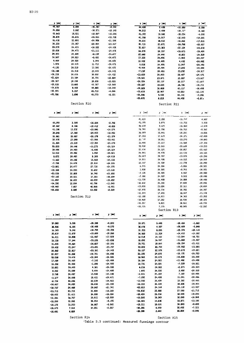
Sect ion R10
2.599 II. LSa 13.232
17.00
20.887
21.U00
23.519
24.116
2 4 . W I...LY
24.481
z..<LY 24.41
24.417
24.093
22.828 20.811
16.13
U . 0 Y 7.157 2 . w
Sect ion
Sect ion R11
2.288 -35.752
1.876 -35.756
9.425 -35.960
12.79b -11.761
15.441 -15.261
17.619 -14.111
19.951 -33.210 21.612 -31.584
23.055 -29.699
24.121, -26.817 24.478 -23.510
14.507 -1'1.626
Z l . 505 -16.211
? r r m - , I . 778
2,. IM -1.956
21.501 -0.711
11.501 4.562 14.102 9.511 24.198 14.088
24.156 11.699
21.024 22.311
20.714 26.781
17.450 10.917 11.811 14.161 12.281 16.930
9.821 18.161
1.175 10 .M5
Section R13
31-1 1 1 b 1
Sect ion R l l i 'Table 3 . 3 continued:
Section R15 Measured fuselage contour

2 1-1 Y 1"l i 1-1 Y I l l
34.353 2.742 -15.332 -7.942
34.116 6.982 -15.035 -12.168
13.121 L0.792 -11.210 -16.312
11.967 11.581 -31.817 -18.901
1 0 . W 18.Wl -29.697 -21.040
21.016 20.345 -27.347 -22.IPS
25.5Sd 22.118 1 4 . 2 8 8 -21.878
22.932 21.850 -20.911 -21.489
19.531 24.311 -16.882 -28.498
14.154 2a.102 -12 .W -24.497
9.811 24.501 -8.157 -26.498
5 . W 2 4 . W -1.9W -24.498
L.211 24.4'16 0.515 -24.697
-3.919 t4.5W 5.601 -24.196
-8.567 24.498 9.9% -21.495
-I1.832 24.495 11.708 .Z:.433
-19.789 21.492 19.209 -24.368
.24.165 23.811 23.191 -21.276
-27.821 22.379 27.2ll -20.979
-10.UI 2 o . w m.170 -17.522
-33.46t 16.181 32.323 -11.760
-%.OM 12.PiI 11.62B -9.618
-35.3OP 7.650 34.251 -5.1%
-35.311 2.248 24.347 -1.116
-35.317 3 .765
Sect ion R16 Sect ion R17
Sect ion R18
Sect ion R21
Sect ion R19 Sect ion R20
Table 3 . 3 cont inued: Measured fuse lage contour
~.~ ~ ~
0.2 I l l g h t d l n i t l o l .
0.1. th. 0rlI1r.s on ih. l a r -id4
6 I 0.648 0.1 01 th. l a f t on.
Table 3 . 4 : Location of pressure o r i f i c e s

Table 3.5: Pressure data ( i l = 0.0 a = -2')
Table 3.6: Pressure data (M = 0.8 a = o O )

Table 3.7: Pressure data (M = 0.8 o = 2')
0.'9Q1 1.1,1? I . . , ,> ,..,*a ! . . , . I ,..01" >.,ha0 1 . 1 1,.
I . I... I.,SL, " . * L l l 0.Q""O 0.1310 0.7.'. O_I.:L
0.0 0 .0150 0 .0 "'I
0 . 0 1 5 0 0.1000 O.,5OU O.?"O" 0.1000 0 . L O l i O 0.5"(10 O."OdO 0.1000 0 . 8 0 0 0 O.P"DO l .OOOO
Table 3.8: Pressure data (M = 0.8 o = 4')

P I C
Table 3.10: Pressure data (M = 0.8 a = 8')

Table 3.11: Pressure data (M = 0.65 a = 2')
Table 3.12: Pressure data (M = 0.88 u = 2' )
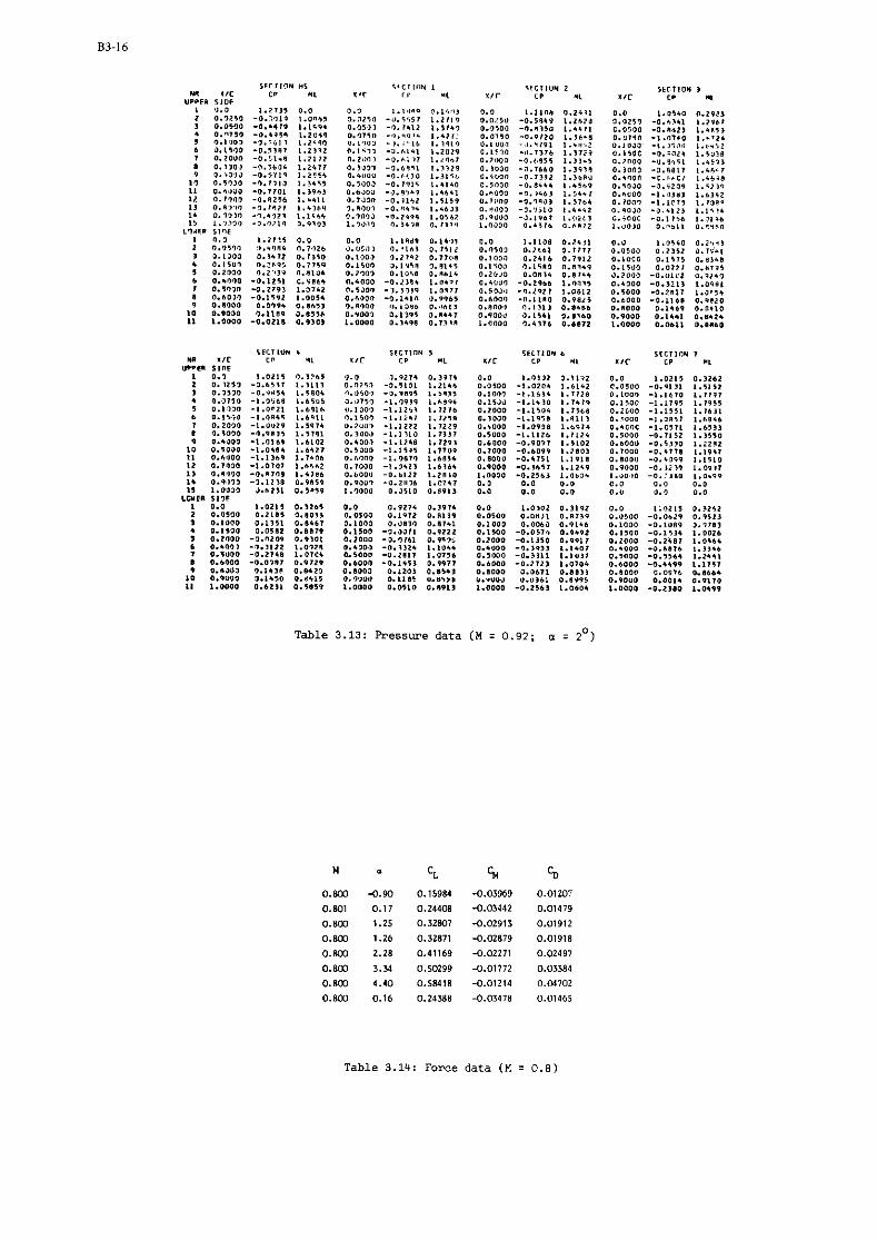
Table 3.13: Pressure data ( M = 0.92: a = 2')
Table 3 .14: Force data (M = 0 . 8 )

- -- I I ,%$.y&-- 6 xs"
I I 1 1I//7SVY ~4wre*n0 o o m lo the r w , a"-- 2:
I prx I I: t 75475 \i
\ I
Fig. 3.1: MBB-AVA-Pilot model wi th s u p e r c r i t i c a l wing
Fig . 3 . 2 : Cross s e c t i o n s of t h e fuselage
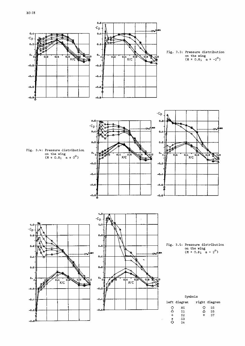
B3-I8
0.6
'CP 0.L 0.L
-c P
0.2 0.2
Fig. 3.3: Pressure d i s t r i b u t i o n 0. 0. on t h e wing
( M = 0.8; a = - 2O)
-0.2 -0.2
-0.6 -0.'
-0.6 -0.6
-0.8 -0.8
Fig. 3.4: Pressure d i s t r i b u t i o n on t h e wing ( M = 0.8; u = 0')
Fig. 3.5: PFessure d i s t r i b u t i o n on t h e wing (M = 0.8; o = 2 O )
Symbols
l e f t diagram r i g h t diagram
0 HS 0 S5 0 S1 D 56 + 52 + S7 X $3 0 s4

Fig. 3.6: Pressure distribution on the wing (M = 0.8; a = 4')
Symbols
left diagram right diagram
0 HS 0 S5 a sl n s6 + 52 f 57 Fig. 3.7: Pressure distribution on the wing (M = 0.8; u = 6') X S 3
0 s4

Fig. 3.8: Pressure dis tr ibut ion on t h e wing (M = 0.8; a = 8')
symbols
l e f t diagram
0 HS A Sl + S 2 X s3 0 s*
r i g h t diagram
0 s5 A 56
+ 57
Fig . 3 . 9 : Ressure d i s tr ibut ion on the wing (M = 0.65; a = 2O)

Fig . 3.10: Pressure d i s t r i b u t i o n
:y"bo1s
l e f t d iagram
0 HS n sl
52 X S3 0 si i
r i g h t d iagram
Fig . 3.11: Pressure d i s t r i b u t i o n on t h e wing (M = 0 . 9 2 ; o : 2')

Fig. 3.12: Polars ( M = 0.8)

4. PRESSURE DISTRIBUTION MEASURED I N THE RAE 8 f t x 6 f t TRANSONIC WIND TUNNEL ON RAE W I N G 'A' I N COMBINATION WITH AN AXI-SYMMETRIC BODY AT MACH NUMBERS OF 0.4, 0.8 AND 0.9
by
D. A. Treadgold, A. F. Jones and K. H. Wilson
Royal A i r c r a f t Establ ishment , Earnborough, Hants, United Kingdom
I . INTRODUCTION
This c o n t r i b u t i o n con ta ins s e l e c t e d d a t a from measurements of s u r f a c e p ressu re d i s t r i b u t i o n s made i n the RAE 8 f t x 6 f t t r anson ic wind tunnel on RAE resea rch wing 'A' i n combination wi th a n axisyormetric body. Wing A i s a wing of simple planform without d ihedra l or t w i s t and i s based on a uncambered RAE 101 aero- f o i l s e c t i o n . The t e s t s were made on a complete model of a s i z e t h a t r enders t h e tunnel j la l l i n t e r f e r e n c e r e l a t i v e l y small. Although t h e t e s t Reynolds number (one m i l l i o n based on the geometric mean chord) i s low, i t r a i s e s no p a r t i c u l a r problems f o r the cases presented he re , s i n c e the adverse p ressu re g r a d i e n t s are mild and boundary-layer t r a n s i t i o n was con t ro l l ed .
Tables and graphs of t h e p ressu re d i s t r i b u t i o n on t h e wing and body are given f o r the cond i t ions given below:
Case number
2. DATA SET
I . General d e s c r i p t i o n
1 . 1 Model des igna t ion or name
Mach number Angle o f incidence
RAE Wing A m u n t e d symmetrically on t h e c y l i n d r i c a l body B2 (WAB2(0)O)
1.2 m d e l type (eg f u l l span wing-body, Full-span wing-body model semi-span wing)
1.3 Design requ i rement s l cand i t lons Wing body made1 of s imple geometric form
1.4 Addi t ional remarks
2. Model geometry
2.1 Wing da ta See F i g 4.1
2.1.1 Wing planform Swept wing with s t r a i g h t l ead ing and t r a i l i n g edges
2.1.2 Aspect r a t i o
2.1.3 Leading-edge sweep
2.1.4 Trai l ing-edge sweep
2.1.5 Taper r a t i o
Gross aspec t r a t i o 6 (g ross planform def ined by t h e s t r a i g h t l i n e ex tens ion of the l ead ing and t r a i l i n g edges t o the body cen t re - l ine )
36.65'
22.34"
113
2.1.6 Twist Zero
2.1.7 Mean aerodynamic chord 152.4 ono (0.5 f t )
2.1.8 Span o r semispan 914.4 ono (3.00 f t ) span
2.1.9 Number of a i r f o i l s e c t i o n s used One t o d e f i n e wing
2.1.10 Spanwise l o c a t i o n a f r e fe rence Root and t i p s e c t i o n and s e c t i o n coord ina tes RAE 101 s e c t i o n th ickness lchord r a t i o 99: (Note i f o r d i n a t e s are des ign or See Table 4.1 a c t u a l measured values)
2.1.11 Lof t ing procedure between re fe rence s e c t i o n s
S t r a i g h t l i n e s between r o o t and t i p s t a t i o n s a t cons tan t x / c
2.1.12 Form of wing-body f i l l e t , s t r a k e s No f i l l e t s o r s t r a k e s f i t t e d
2.1.13 Form of wing t i p Cross-sect ion formed by a r a d i u s of hal f l o c a l wing thickness (see Fig 4.1)

84-2
2.2 Body d a t a ( d e t a i l d e s c r i p t i o n of body geometry)
Axisymmetric body with a nose p r o f i l e g iven by
See P ig 4.1
2.3 Wing-body combination
2.3.1 Rd la t ive body diameter (average body diameter a t wing l o c a t i o n divided by wing span)
Aligned with t h e a x i s of symmetry of t h e body 2.3.2 R e l a t i v e v e r t i c a l l o c a t i o n o f wing (he igh t above or below body a x i s d ivided by average body r a d i u s a t wing l o c a t i o n )
2.3.3 Wing s e t t i n g ang le
2.3.4 Dihedral
2.4 Crass s e c t i o n a l area development
Zero
No 'area-rule ' development - s imple wing wi th a c y l i n d r i c a l body
2.5 F a b r i c a t i o n to leranceslwaviness I n genera l t h e wing i s wi th in t h e s p e c i f i e d manufac- t u r i n g to le rance of $0.05 mm f o r t h e wing o r d i n a t e s and the l i m i t on waviness of 0.05 mm125 m. An inspec t ion r e p o r t i s a v a i l a b l e on reques t
2.6 Addi t ional remarks
3. Wind tunnel
3.1 Designat ion RAE 8 f t x 6 f t t r anson ic wind tunnel
3.2 Type of tunnel
3.2.1 Continuous o r blowdown Continuous, c losed c i r c u i t
2 10 t o 355 kN/m pumping and p ressu re s h e l l l imi ta t ion ; f o r ope ra t iona l l i m i t s due to power o f main d r i v e see s e c t i o n 3.6.1
3.2.2 S tagna t ion p ressu re
3.2.3 S tagna t ion temperature
3.3 Tes t s e c t i o n
Rectangular wi th corner f i l l e t s (160.5 m x 160.5 on0 x 45O)
3.3.1 Shape of t e s t s e c t i o n
3.3.2 S i z e of t e s t s e c t i o n (width, he igh t , length)
2.43 m wide, 1.83 m high, 2.8 m long
3.3.3 Type o f t e s t s e c t i o n w a l l s c losed, open, s l o t t e d , pe r fo ra ted Open area r a t i o (g ive range i f v a r i a b l e ) S l o t l h a l e geometry (eg 30-degree s l a n t e d ho les ) t reatment of s i d e wa l l boundary l a y e r
S l o t s i n a l l four w a l l s f o r th ree dimensional complete model t e s t s . 1 1 % Sharp edged s l o t s : s i x s l o t s i n both roof and f l o o r and f i v e s l o t s i n each s i d e wal l . A l l are vented to a co-n plenum chamber of l a r g e volume
None - F u l l span models Half-model t e s t i n g
3.4 Flow f i e l d (empty t e s t s ec t ion)
3.4.1 Reference s t a t i c p ressu re Plenum chamber
M 0.4 0.8 0.9 flow i0.13' +O. 13' '0 .07~
a n g u l a r i t y
3.4.2 Flaw a n g u l a r i t y

3.4.3 Mach number distribution
3.4.4 Pressure gradient
See Fig 3 of Ref I reproduced as Fig 6.3 in Data Set A6. 3.4.5 Turbulence/noise level
3.4.6 Side wall boundary layer
3.5 Freestream Mach number (or velocity)
3.5.1 Range Mach number 0.40-1.24
A total head measured in the maximum section of the tunnel circuit and a static pressure measured in the plenum chamber
3.5.2 Pressures used to determine Mach number (eg settling chamber total pressure and plenum chamber pressure)
3.5.3 Accuracy of Mach number determination (AM)
3.5.4 Maximum Mach number variation in x, y, z-direction (empty tunnel; specify at what Mach number)
Maximum variation of flow direction
Maximum Mach number variation during a run
3.6 Reynolds number range
3.6.1 Unit Reynolds number range. (Give range at representative Mach numbers; l/m)
3.6.2 Means of varying Reynolds number (eg by pressurisatian)
3.7 Temperature range and dewpoint. Can temperature be controlled?
290 K to 323 K. Absolute humidity <0.003 . Temperature can be controlled manually
3.8 Model attitudes
Calibrated differential screw-jacks giving a range of incidence from -4O to +2Z0. The sting mounting may be rolled through f180°
3.8.1 Angle of attack, yaw, roll
Angle of attack iO.OlO. Roll angle fO.lOO 3.8.2 Accuracy in determining angles
3.9 Organization operating the tunnel and location of tunnel
The Royal Aircraft Establishment, Farnborough, Hants, England
3.10 Who is to be contacted for additional information
Mr D. Pierce, Aerodynamics Department
3.11 Literature concerning this facility
3.12 Additional remarks
4. Tests - 4.1 Type of tests Surface pressure measurements
Spanltunnel width = 0.375 4.2 Wing span of semispan to tunnel width
4.3 Test conditions
4.3.1 Angle of attack 0, lo and 2'
4.3.2 Mach number
4.3.3 Dynamic pressure Dependent on Mach number and temperature to give a constant Reynolds number
4.3.4 Reynolds number 1.0 x lo6 based on the geometric mean chord of the gross wing
4.3.5 Stagnation temperature

4.4 Transition
4.4.1 Freeorfixed
4.4.2 Position of free transition
4.4.3 Position of fixed transition, width of strips, size and type of roughness elements
4.4.4 Were checks made to determine if transition occurred at trip locations?
4.5 Bending or torsion under load
4.5.1 Describe any aeroelastic measurements m d e during tests
4.5.2 Describe results of any bench calibrations
4.6 Were different sized mdels used in wind-tunnel investigation? If so, indicate sizes
4.7 Areas and lengths used to form coefficients
4.8 References on tests
4.9 Related reports
5. Instrumentation
5.1 Surface pressure measurements
5.1.1 Pressure orifices in wing. location and number on upper and lover surfaces
5.1.2 Pressure orifices on fuselage. location and number
5.1.3 Pressure orifices on components, give component and orifice location
5.1.4 Geometry of orifices
5.1.5 Type of pressure transducer and scanning devices used. Indicate range and accuracy
5.2 Force measurements
5.2.1 Type and location of balance
5.2.2 Forces and moments that can be measured. Maximum loads and accuracy
5.2.3 Forces and moments on components
Type and location of balance
Fixed
12.5ZC and on the body nose Ballotini I20 grade 0.13 m to 0.16 mm (0.005 in to 0.0064 in) diameter in a band 2.5 mm (0.1 in) wide
Yes. Acenaphthene sublimition
None made
Bench tests were made and a stiffness matrix determined - see additional remarks under section 6.2.6
NO
Local chord. (The root chord in the case of the body junction.) Local pitching moments are quoted about the local leading edge
- -
206 (see Fig 4.1 and Table 4.2a)
213 (see Fig 4.1 and Table 4.2b)
Depth/ Hole diameter
diameter Location
0.34 rm (0.0135 in) 1.5 to xlc of 0.1 0.34 orm (0.0135 in) 3.0 from xlc 0.15 to 0.90 0.25 orm (0.0100 in) 1.0 for xlc 0.95 and 0.975
Midwood self-balancing capsule manometer 0-1.0 atmosphere. Accuracy '0.03% of full scale
Maximum load and accuracy
5.3 Boundary layer and flow-field measurements
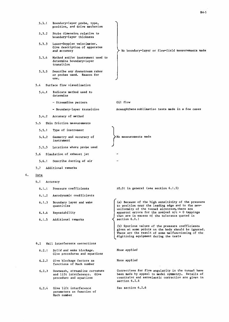
5.3.1 Boundary-layer probe, type, position, and drive mechanism
5.3.2 Probe dimension relative to boundary-layer thickness
5 .3 .3 Laser-Doppler velacimeter. Give description of apparatus and accuracy
5.3.4 Method andlor instrument used to determine boundary-layer transition
5 .3 .5 Describe any domstream rakes or probes used. Reason for Use.
5 .4 Surface flow visualization
5.4.1 Indicate method used to determine
- Streamline pattern - Boundary-layer transition
5.4.2 Accuracy of method
5 .5 Skin friction measurements
5.5.1 Type of instrument
5.5.2 Geometry and accuracy of instrument
5.5.3 Locations where probe used
5 .6 Simulation of exhaust jet
5.6.1 Describe ducting of air
5.7 Additional remarks
6 . Data
6.1 Accuracy
6.1.1 Pressure coefficients
6.1.2 Aerodynamic coefficients
6 .1 .3 Boundary layer and wake quantities
6.1.4 Repeatability
6.1.5 Additional remarks
} No boundary-layer or florfield measurements made
Oil flow
Acenaphthenesublimation tests made in a few cases
A0.01 in general (see section 6.1.5)
(a) Because of the high sensitivity of the pressure to position near the leading edge and to the non- uniformity of the tunnel airstream,there are apparent errors for the nominal xlc = 0 tappings that are in excess of the tolerance quoted in section 6 .1 .1
I (b) Spurious values of the pressure coefficients given at some points on the body should be ignored. These are the result of some malfunctioning of the digitising equipment during the tests
6 . 2 Wall interference corrections
6 .2 .1 Solid and wake blockage. Give procedures and equations
6.2.2 Give blockage factors as functions of Mach number
6 .2 .3 Downwash, streamline curvature and lift interference. Give procedure and equations
6.2.4 Give lift interference parameters as function of Mach number
None applied
None applied
Corrections for flow angularity in the tunnel have been made by appeal to model symmetry. Details of constraint and aeroelastic correction are given in section 6 .2 .6
See section 6.2.6

6.2.5 Reference on wall- interference See Ref 2 cor rec t ions
6.2.6 Additional I remarks The cor rec t ions required f o r a e r o e l a s t i c d i s t o r t i o n of the model and f o r the e f f e c t s of tunnel wall c o n s t r a i n t a r e of a s imi la r order of magnitude. A matr ix of inf luence c o e f f i c i e n t s def ining the s t r u c t u r a l s t i f f n e s s has been derived from the measurement of d e f l e c t i o n under known s t a t i c loads. The a e r o e l a s t i c d i s t o r t i o n has then been calculated using the s t i f f n e s s matrix, together with the aero- dynamic loading obtained by in tegra t ing the measured pressure d i s t r i b u t i o n . Correction f o r tunnel wall c o n s t r a i n t has been derived by in te rpo la t ion with respec t to open area r a t i o 1/(1 + F), between solu- t i o n s of the l i n e a r i s e d formulation f o r the ve loc i ty induced i n the given t e s t sec t ion according to the assumption of (a) f u l l y open, and (b) f u l l y closed, wal l boundary conditions2. Computation of the incremental loading a r i s i n g from d i s t o r t i o n and c o n s t r a i n t confirmed t h a t only spanwise v a r i a t i o n was s i g n i f i c a n t and there fore a l o c a l cor rec t ion t o the nominal incidence of an 'equivalent f l a t wing' was obtained as indicated i n Table 4.3s and 4.3b. The adjusbnents to the measured data have been made by curve- f i t t ing the v a r i a t i o n of s t a t i c pressure c o e f f i c i e n t a t each o r i f i c e with incidence, and i n t e r p o l a t i n g to a corrected nominal incidence
6.3 Data p resen ta t ion
6.3.1 kradynamic c o e f f i c i e n t s Tables h.7 to 4.9 give l o c a l normal f o r c e CN and p i tch ing moment c o e f f i c i e n t CM
6.3.2 Surface pressure c o e f f i c i e n t s Tables 4.4 to 4.9 Figs 4.2 to 4.7 give pressure c o e f f i c i e n t s f o r the wing and body
6.3.3 Flow condit ions f o r
- Aerodynamic c o e f f i c i e n t data Mach numbers 0.4, 0.6 and 0.8 f o r R 1.0 x 10 6
- Pressure da ta
6.3.4 Boundary layer andlor wake da ta
No measurements made
6.3.5 Plow condit ions f o r boundary - l ayer andlor wake da ta
6.3.6 Wall in te r fe rence cor rec t ions See Table 4.3a included?
6.3.7 Aeroelast ic cor rec t ions included?
6.3.8 Other cor rec t ions?
6.3.9 Additional remark.
See sec t ion 6.2.6 and Table 4.3b
6.4 Were t e s t s c a r r i e d o u t i n d i f f e r e n t No f a c i l i t i e s on the cur ren t model? I f so, ,what f a c i l i t i e s . Are da ta included i n present da ta base7
6.5 Were t e s t a c a r r i e d o u t i n d i f f e r e n t No f a c i l i t i e s on the cur ren t model7 I f so, what f a c i l i t i e s . Are data included i n present da ta base7
I D.G. Mabey Boundary-layer t r a n s i t i o n measurements on the AEDC 10' cone i n th ree RAE wind tunnels and t h e i r implications. RAE Technical Report 76077 (1976)
2 H.C. Garner Subsonic wind tunnel wal l correct ions. E.W.E. Rogers AGARDograph 109 (1966) W.E.A. Acum E.C. Maskell

L i s t o f Symbols
local chord
geometric mean chard of the gross wing local pitching momeat
local pitching moment coefficient about the leading edge = 2 2 local normal force 4uv c
local normal farce coefficient =
P - P, 40vLc
pressure coefficient = - 4uv2
d na non-dimensional slotted wall parameter = J-- log casec - , (see Ref 2)
nbh e 2d length of the body
Mach number
local body cross-section radius
Reynolds number based on F
radius of the cylindrical section of the body
semi-span of the gross wing (excluding tip fairing)
free stream velocity
distance measured along the chord from the leading-edge of the wing section
distance measured from the extended nose of the body
distance measured spanwise
distance from the plane of the wing
width of the slots in the tunnel walls
breadth of the tunnel working section
periodic spacing of the slots in the tunnel wall
height of the tunnel working section
length of the profiled portion a f the body
local static pressure
free stream static pressure
angle of incidence
correction applied to the local angle of incidence for wind tunnel wall constraint
correction applied to the local angle of incidence for aeroelastic distortion of the model and deflection of the sting support
YIS non-dimensional spanwise location
density of the free stream
median angle measured from the plane of the wing
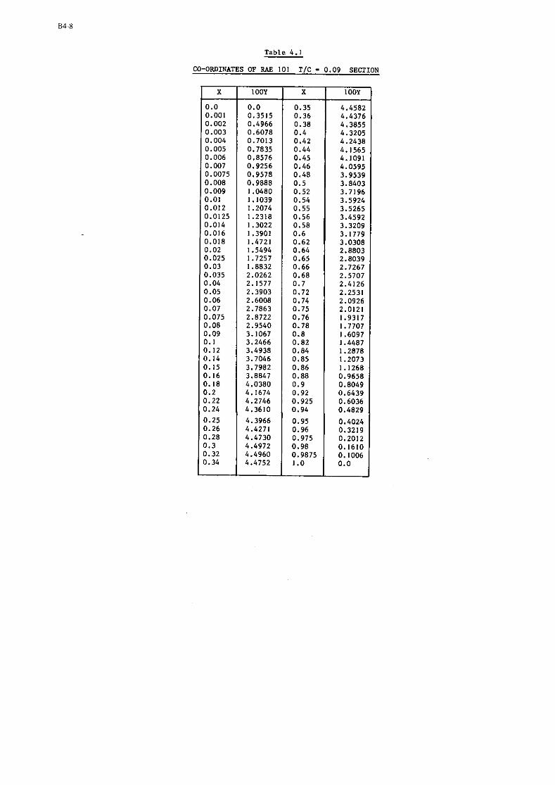
Table 4.1
CO-ORDINATES OF RAE 101 TIC - 0.09 SECTION
X
0.0 0.001 0.002 0.003 0.004 0.005 0.006 0.007 0.0075 0.008 0.009 0.01 0.012 0.0125 0.014 0.016 0.018 0.02 0.025 0.03 0.035 0.04 0.05 0.06 0.07 0.075 0.08 0.09 0. I 0.12 0.14
0.9658 0.8049 0.6439 0.6036 0.4829
4.3966 0.4024 4.4271 0.3219
0.28 0.2012 4.4972 0.1610
0.32 0.34 4.4752
l OOY
0.0 0.3515 0.4966 0.6078 0.7013 0.7835 0.8576 0.9256 0.9578 0.9888 1.0480 1.1039 1.2074 1.2318 1.3022 1.3901 1.4721 1.5494 1.7257 1.8832 2.0262 2.1577 2.3903 2.6008 2.7863 2.8722 2.9540 3.1067 3.2466 3.4938 3.7046
X
0.35 0.36 0.38 0.4 0.42 0.44 0.45 0.46 0.48 0.5 0.52 0.54 0.55 0.56 0.58 0.6 0.62 0.64 0.65 0.66 0.68 0.7 0.72 0.74 0.75 0.76 0.78 0.8 0.82 0.84 0.85
l OOY
4.4582 4.4376 4.3855 4.3205 4.2438 4.1565 4.1091 4.0595 3.9539 3.8403 3.7196 3.5924 3.5265 3.4592 3.3209 3.1779 3.0308 2.8803 2.8039 2.7267 2.5707 2.4126 2.2531 2.0926 2.0121 1.9317 1.7707 1.6097 1.4487 1.2878 1.2073 1 .I268

Table 4.2
(a) Location of the pressure tappings in the wing
(b) Location of the pressure tappings in the wing-body junction
Nominal XIC
0.005 0.010 0.025 0.050 0.075 0.100 0.150 0.200 0.300 0.400 0.500 0.600 0.700 0.800 0.900 0.950 0.975
* X and C appropriate to the normal projection onto the gross wing defined by the straight extension of the leading- and trailing-edges to the centre-line of the body.
ll - Y/S
XIC* X'h ZIL
XIC* 1 Z/L
XIC* X'h ZIL
Table 4.3
(a) Corrections applied to the local angle of incidence for tunnel wall constraint
Acu - Aco(0) + Aco(n)/per degree
0.25
0.005 0.010 0.025 0.051 0.075 0.100 0.151 0.201 0.301 0.401 0.501 0.601 0.701 0.801 0.900 0.950 0.976
(b) Corrections applied to the local angle of incidence for the aero-elaetic deformation of the wing and the deflection of the sting support
Aeo - Aeo (0) + Aem(n)lper degree at Re 1.0 x 10
6
-0.013 0.4817 0
0.200 0.5184 0.00822
0.800 0.6231 0.00356
0.40
0.005 0.010 0.025 0.050 0.075 0.100 0.150 0.200 0.300 0.400 0.500 0.600 0.700 0.800 0.899 0.949 0.974
0.010 0.4856 0.00277
0.250 0.5271 0.00860
0.900 0.6405 0.00226
0.60
- 0.010 0.026 0.051 0.076 0.100 0.150 0.200 0.300 0.400 0.500 0.601 0.701 0.801 0.899 0.949 -
0.025 0.4881 0.00392
0.300 0.5358 0,00876
0.75
- 0.010 0.025 0.050 0.075 0.100 0.150 0.200 0.301 0.401 0.501 0.601 0.701 0.801 0.899 0.950 -
0.050 0.4924 0.00509
0.400 0.5532 0.00840
0.85
- 0.011 0.026 0.052 0.076 0.101 0.150 0.201 0.301 0.401 0.501 0.600 0.701 0.800 0.899 0.949 -
0.925
- 0.011 0.026 0.051 0.076 0.101 0.150 0.200 0.301 0.400 0.500 0.601 0.700 0.800 0.899 0.949 -
0.075 0.4968 0.00585
0.500 0.5707 0.00759
0.100 0.5011 0.00664
0.600 0.5882 0,00639
0.150 0.5097 0.00756
0.700 0.6056 0.00517

Table 4.4
TABULATED DATA
Case No.1 : Mach number 0.40 Angle o f incidence 0
Upperflower surface
Pressures on the wing and a t the wingfbody junct ion
* Nominal value f o r bodyfwing junct ion NB Pressure measured on body, see Table 4.2
Pressures on the body

Table 4 .5
TABULATED DATA
Case No.2 : Mach number 0.80 Angle of incidence 0
Upper/lower surface
Pressures on the wing and at the wing/body junction
n CN=
CM=
X I C 0 . 0 0 0 0 . 5 3 5 0.610 0.025 0 . 3 5 3 0 . 5 7 5 0.1LO
* Nominal value for body/wing junction N B Pressure measured on body, see Table 4 .2
Pressures on the body

Table 4.6
TABULATED DATA
Case No.3 : Mach number 0.90 Angle of incidence 0
Upper/lower surface
Pressures on the wing and a t the wing/body junc t ion
* Nominal value f o r body/wing junc t ion NB Pressure measured on body, see Table 4 .2
Pressures on the body
@ DEG OX f15 i 30 f 4 5 f 60 f 75 f 90

Table 4.7
TABULATED DATA
Case No.4 : Mach number 0.40 Angle of incidence 2.0'
Upper surface
Pressures on the wing and a t the winglbody junc t ion
* Nominal value f o r body/wing junc t ion NB Pressure measured on body, see Table 4 . 2
Pressures on the body
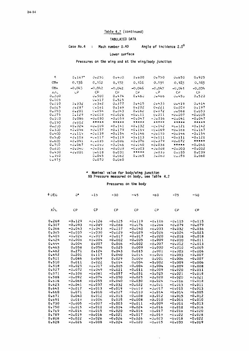
Table 4.7 (continued)
TABULATED DATA
Case No.4 : Mach number 0 .40 Angle of incidence 2.0'
Lower surface
Pressures on the wing and a t the wing/body junc t ion
* Nominal va lue f o r bodylwing junc t ion NB Pressure measured on body, see Table 4.2
Pressures on the body

@ DEG
Table 4.8
TABULATED DATA
Case No.5 : Mach number 0 .80 Angle of incidence 2.0'
Upper surface
Pressures on the wing and a t the winglbody junc t ion
Nominal va lue f o r body/wing junc t ion NB Pressure measured on body, see Table 4.2
Pressures on the body

Table 4.8 (continued)
TABULATED DATA
Case No.5 : Mach number 0.80 Angle o f incidence 2.0'
Lower surface
Pressures on the wing and a t the wing/body junc t ion
* Nominal value for bodylwing junc t ion NB Pressure masured on body. see Table 4.2
Pressures on the body
$ DEG O* -15 -30 -45 - 6 0 -7 5 - 9 0
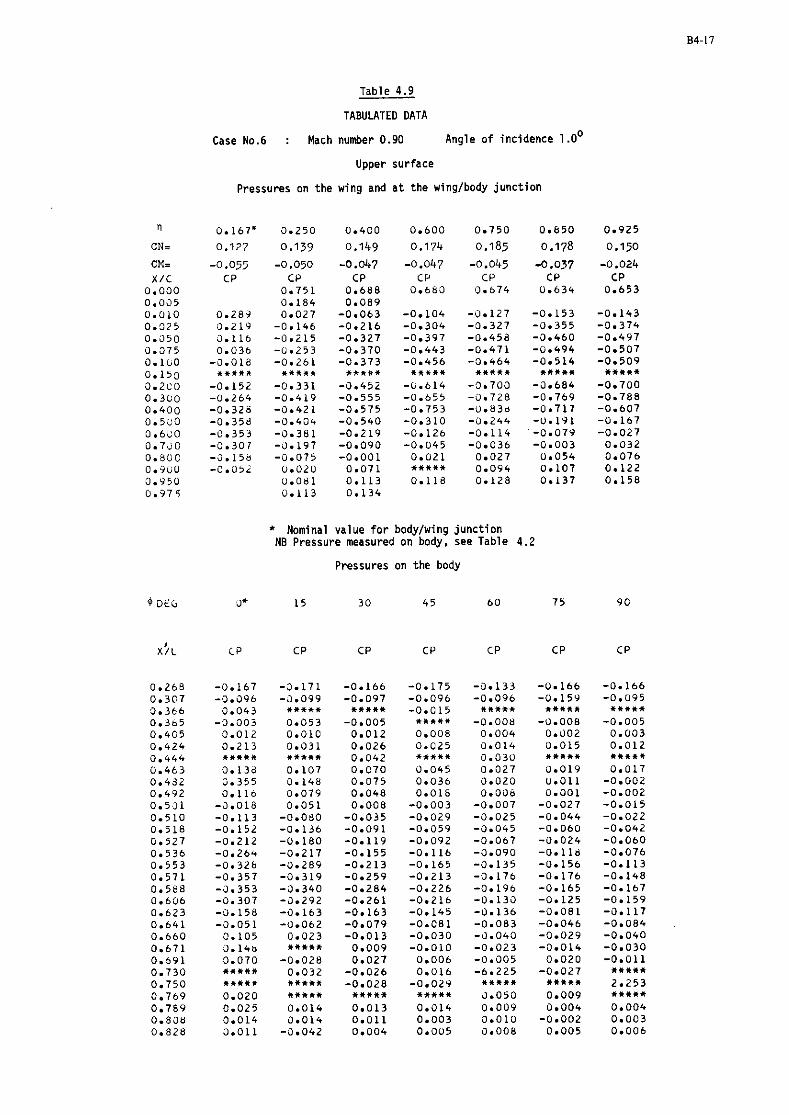
Table 4.9
TABULATED DATA
Case No.6 : Mach number 0.90 Angle o f incidence 1 .oO Upper surface
Pressures on the wing and a t the winglbody junc t ion
* Nominal value f o r bodylwing junc t ion NB Pressure measured on body, see Table 4 .2
Pressures on the body
4 DEG 0* 1 5 3 0 4 5 60 7 5 9 0

Table 4.9 (continued)
TABULATED DATA
Case No.6 : Mach number 0 .90 Angle o f incidence 1 .oO Lower surface
Pressures on the wing and a t the wing/body junc t ion
Nominal value for bodylwing junc t ion NB Pressure measured on body, see Table 4.2
Pressures on the body


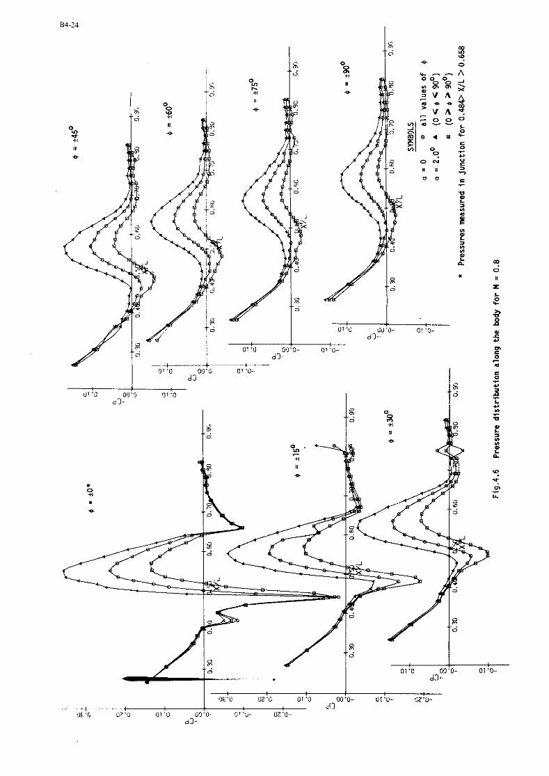
I !If. 'U U Z ' U U1 'U OU'U- 0: .U- UZ'U-
---~t 33 'If. '0 07 '(1 111 'u u 0 '11- f 1 7 ' ~ - UZ'U-.
d2-


5 . PRESSURE DISTRIBUTIONS MEASURED ON AN NASA SUPERCRITICAL-WING RESEARCH AIRPLANE MODEL
by
C. D. Harris and D. 1. Bartlett
National Aeronautics and Space Administration Langley Research Center Hampton, Virginia 23665
5.1 INTRODUCTION
The data presented in this contribution were obtained in the NASA Langley 8-Foot Transonic Pressure Tunnel on a supercritical-wing research airplane to provide a smooth area distribution and consequently a high drag-rise Mach number. Measurements were made with and without area-rule additions; only data for the former are included in this compilation. Tabulated data is given for 5 Mach numbers ranging from 0.50 to 0.99 and for four or five angles of attack at each Mach number.
5.2 DATA SET
1. General Description
1.1 Model Designation or Name TF-8A Supercritical Wing Research Airplane Model
1.2 Model Type (e.g., Full Span Full span wing-body-tail Wing-Body, Semi-span Wing)
1.3 Design Requirements1 Conditions
1.4 Additional Remarks
2. Model Geometry
2.1 Wing Data
2.1.1 Wing Planform
2.1.2 Aspect Ratio
2.1.3 Leading-Edge Sweep
2.1.4 Trailing-Edge Sweep
2.1.5 Taper Ratio
2.1.6 Twist
2.1.7 Mean Aerodynamic Chord
2.1.8 Span or Semispan
2.1.9 Number of Airfoil Sections Used to Define Wing
2.1.10 Spanwise Location of Reference Section and Section Coordinates (Note if Ordinates are Design or Actual Measured Values)
2.1.11 Lofting Procedure Between Reference Sections
2.1.12 Form of Wing-Body Fillet, Strakes
Basic model: M = 1.00 CL = 0.4
Investigation includes measurements with and without area rule additions to sides of fuselage. Only data with area rule additions are included in the present compilation.
See figure 5.1.
6.8 for basic winn (dashed line) - excludes - . L.E. glove, T. E. extension, and tip rounding.
44.34O I quarter chord 4 2 . ~ 4 ~ 35. lo0
-5O root to tip, unloaded. (Included in ordinates of Table I.)
0.1809 m (for basic wing planform)
0.5715 m semispan
17
See Table I. Values given are actual measured values.
Unknown.
See figure 5.2
2.1.13 Form of Wing Tip See figure 5.2

Body Data (Detail Description of Body Geometry)
See figures 5.1 and 5.3.
-0.12 (irregular body).
-1, high wing.
Wing-Body Combination
2.3.1 Relative Bodv Diameter (Average Bod; Diameter at Wing Location Divided by VIing Span)
2.3.2 Relative Vertical Location of Wing (Height Above or Below Body Axis Divided by Average Body Radius at Wing Location)
1.5' (included in ordinates of Table I).
oO See figure 5.4
2.3.3 Wing Setting Angle
2.3.4 Dihedral
Cross Sectional Area Development
Fabrication Tolerances/ Waviness
Waviness not determined. Velues given in Table I are actual measured values.
Additional Remarks Additional details of aileron fairings and vortex generators shown in figure 5.1 are given in figure 5.5.
Tunnel
Designation
Type of Tunnel
8-Foot Transonic Pressure Tunnel
3.2.1 Continuous or Blowdown. Indicate
Continuous
Minimum Run Time if Applicable
Varies from approximately 15 to 68 k ~/m' depending on Mach number and Reynolds
3.2.2 Stagnation Pressure
number
Generally kept at 322 K. 3.2.3 Stagnation Temperature
Test Section
3.3.1 Shape of Test Section Square
2.2 m x 2.2 m x 4.3 m 3.3.2 Size of Test Section (Width, Height, Length)
3.3.3 Type of Test Section Closed, Open, Slotted, Perforated Open Area Ratio (Give Ranee if Variable) Slot/Hole Geometry (e.g.. 30-Degree Slanted Holes) Treatment of Sidewall Boundary Layer
Slotted top and bottom, solid sides. Slotted walls approximately 6% open. Four identical slots of longitudinally varying width in top and bottom walls. See figure 5. fi and 5.7.
Nothing done to sidewall boundary layer.
Full span models I Tunnel has capability for full and half span model testing

3.4 Flow Field (Empty Test Section)
3.4.1 Reference Static Pressure
3.4.2 Flow Angularity
3.4.3 Mach Number Distribution
Plenum chamber.
Generally less than O.1° but may go as high as 0.25O near slots.
3.4.4 Pressure Gradient
3.4.5 ~urbulence/Noise Level Lateral fluctuating velocity components V/Um and %/U, have not been measured. Q/Um varies from 0.002 at IJ = 0.2 to about 0.02 at hiEh Mach numbers.
3.4.6 Sidewall Boundary Layer -
3.5 Freestream Macb Number (or Velocity)
3.5.1 Range 0.2 to 1.3.
3.5.2 Pressures Used to Settling chamber total pressure and Determine Mach Number plenum chamber pressure. (e.g., Settling Chamber Total Pressure and Plenum Chamber Pressure)
3.5.3 Accuracy of Mach AM = +0.003. Number Determination (AM)
3.5.4 Maximum Mach Number Streamwise variations of approximately Variation in x , y, - +0.002 over the Mach number range. z - Direction (Empty Tunnel; Specify at What Mach Number)
Maximum Variation of Flow Direction
Maximum Mach Number Variation During a Run
3.6 Reynolds Number Range
3.6.1 Unit Reynolds Number Range. (Give Range at Representative Mach Numbers; l/m)
3.6.2 Means of Varying Reynolds Number (e.g., by Pressurization)
3.7 Temperature Range and Dewpoint. Can Temperature he Controlled?
3.8 Model Attitudes
3.8.1 Angle of Attack, Yaw, Roll
3.8.2 Accuracy in Determining Angles
3.9 Organization Operating the Tunnel and Location of Tunnel
Generally about 2 millionjm to 18 million/m at most Macb numbers.
Pressurization
~ 6 s t runs made at 322 K stagnation temperature. Temperature and dewpoint both controlled.
0 a = -15' to 25, yaw +7 , roll 360°
a +O.1° at max lift +O. 05O near cruise - Transonic Aerodynamics Branch of the Subsonic-Transonic Aerodynamics nivision, NASA Langley Research Center

3.10 Who is to be Contacted for Additional Information
3.11 Literature Concerning this Facility
3.12 Additional Remarks
4. Tests
4.1 Type Of Tests
4.2 Wing Span or Semispan to Tunnel Width
4.3 Test Conditions
4.3.1 Angle of Attack
4.3.2 Mach Number
4.3.3 Dynamic Pressure
4.3.4 Reynolds Number
4.3.5 Stagnation Temperature
4.4 Transition
4.4.1 Free or Fixed
4.4.2 Position of Free Transition
4.4.3 Position of Fixed Transition, Width of Strips, Size and Type of Roughness Elements
4.4.4 Were Checks Made to Determine if Transition Occurred at h i p Locations?
4.5 Bending or Torsion Under Load
4.5.1 Describe Any Aero- Elastic Measure- ments ~ a d e ~ ~ u r i n g Tests
4.5.2 Describe Results of Any Bench Calibrations
4.6 Were Different Sized Models Used in Wind-Tunnel Invest- igations? If so, Indicate Sizes.
4.7 Areas and Lengths Used to Form Coefficients
4.8 References on Tests
4.9 Related Reports
Head, Transonic Aerodynamics Branch, NASA Langley Research Center
"A Description of the NASA-Langley 8-Foot Transonic Pressure Tunnel'' can be obtained from the above organization.
Surface pressures and force and moment measurements
wing span = ,52 Tunnel width
Varies approximately -5" to +lZO.
I See Table I1 for conditions at which current tests were run.
Fixed.
See figure 5.8 for positions on wing. Strips located at 5% local chord on horizontal and vertical tail, 2.54 cm aft of nose on fuselage. Width of all strips was 0.127 cm. Size and type of roughness elements are given on figure 5.6. Note that No. 100 and 120 carborundum grains average 0.005 in.(0.127 mm) and 0.004 in. (0.102 mm) respectively.
NO.
None
See figure 5.9 for deflections at pressure stations for cruise conditions.
No. But full-scale vehicle was flight tested. See reference list.
All coefficients based on basic wing panel geometry which does & include L. E. glove nor T. E. extension. Moments referenced to 1/4 chord of mean geometric chord (max) of basic wing panel. See figure 5.1.
Area: S = 0.193 m2
MAC : C = 0.1809 m
See references 1, 2, and3.
See references 4 and 5.

5. Instrumentation
5.1 Surface Pressure Measurements
5.1.1 Pressure Orifices in Wing. Location and Nwnber on Upper and Lower Surfaces
5.1.2 Pressure Orifices on Fuselage. Location and Number.
5.1.3 Pressure Orifices on Components, Give Component and Orifice Location
5.1.4 Geometry of Orifices
5.1.5 Type of Pressure Transducer and Scanning Devices Used. Indidate Range and Accuracy
5.2 Force Measurements
5.2.1 Type and Location of Balance
5.2.2 Forces and Moments that Can be Measured. Maximum Loads and Accuracy
5.2.3 Forces and Moments on Components
Type and Location of Balance
Maximum Loads and Accuracy.
5.3 Boundary Layer and Flow-Field Measurements
5.3.1 Boundary-Layer Probe Type, Position, and Drive Mechanism
5.3.2 Probe Dimension Relative to Boundary- Layer Thickness
5.3.3 Laser-Doppler Veloci- meter. Give Descript- ion of Apparatus and Accuracy
5.3.4 Method and/or Instrument Used to Determine Boundary- Layer Transition
See Table 111
See Table IV. Total of 67 orifices.
NO.
Round holes -0.076 cm I.D.
Electronically actuated differential modular scanivalve in model nose.
Upper surface: 103.4 k ~ / m ~ m a x ; 21% max. Lower surface: 82.7 k ~ / m ~ m a x ; 21% max. Fuselage: 17.2 k ~ / m ~ m a x ; 21% max.
Internal strain-gage balance.
6 component force and moment. Normal force: 11 kN; +55.6N Axial force: 890 N; 24.4N Pitching moment: 390 m-N; 22 m-N
None
NO.
5.3.5 Describe any Down- stream Rakes or Probes Used. Reason for Use.

5.4 Surface Flow Visualization
5.4.1 Indicate Method Used to Determine
- Streamline pattern
- Boundary-layer transition
5.4.2 Accuracy of Method
5.5 Skin Friction Measurements
5.5.1 Type of Instrument
5.5.2 Geometry and Accuracy of Instrument
5.5.3 Locations Where Probe Used
5.6 Simulation of Exhaust Jet
5.6.1 Describe Ducting of Air
5.7 Additional Remarks
6. Data
6.1 Accuracy
6.1.1 Pressure Coefficients
6.1.2 Aerodynamic Coefficients
6.1.3 Boundary Layer and Wake Quantities
6.1.4 Repeatability
6.1.5 Additional Remarks
6.2 Wall Interference Corrections
6.2.1 Solid and Wake Blockage. Give Procedures and Equations
6.2.2 Give Blockage Factors as Functions of Mach Number
6.2.3 Downwash, Streamline Curvature and Lift Interference. Give
Not in present experiments. Photographs of fluorescent oil film given for present configuration in references 4 and 5.
Carborundum transition strips.
NO.
There was internal flow through the model which simulated the mass flow ratio of the full-scale airplane.
Variable but < or > 2% of maximum and minimum values, respectively.
Variable but < or > 2% of maximum and minimum values, respectively.
Unknown
None made. Test section sidewall inserts were added and indented in region of model to account for 40% of model cross- sectional area. (See figure 5.7).
An assessment of blockage factors (for fineness ratio 8.2) can perhaps be made from the data contained in:
1. Couch, L. I! . ; and Brooks, C. W., Jr.: Effect of Blockage Ratio on Drag and Pressure Distributions for Bodies of Revolution at Transonic Speeds. NASA TN D-7331, Nov. 1973.
2. Usry, J. W.; and Wallace, J. W.: Drag of a Supercritical Body of Revolution in Free Flight at Transonic Speeds and Comparison With Wind-Tunnel Data. NASA TN D-6580, 1971.
Measured a corrected for induced upwash using procedure outlined in NASA TR R-241 by R. H. Wright and R. L. Barger.
Procedure and Equations.

6.2.4 Give Lift Interference Parameters as Function of Mach Number
6.2.5 Reference on Wall- Interference Correct- ions
6.2.6 Additional Remarks
6.3 Data Presentation
6.3.1 Aerodynamic Coeffic- CL, CD and Cm for wing body, figure 5.10 ients
6.3.2 Surface Pressure
for conditions given in Table V. Local CN and CII, Table VI.
Wing and body Cp distributions, Tables VI, VII and VIII and figure 5.11.
6.::. 3 Flow conditions for
- Aerodynamic CL, CD, and C,,, plots given for Mach coefficient data numbers listed in Table V.
Pressure data Tabulated in Table V
6.3.4 Boundary Layer and/or None Wake Data
6.3.5 Flow Conditions for Boundary Layer and/or Wake Data
6.3.6 Wall Interference No. Corrections Included?
6.3.7 Aeroelastic Correct- No. See 4.5.2 ions Included?
6.3.8 Other Corrections?
6.3.9 Additional Remarks
6.4 Were Tests Carried Out in Yes. Langley 16-Foot Transonic Tunnel. Different Facilities on the See reference 4. Current Model? If so, What Facilities. Are Data Included in Present Data Base?
7. References
1. Harris, C. D.; and Bartlett, D. TI.: Tabulated Pressure Measurements on an NASA Supercritical-Wing Research Airplane Model With and Without Fuselage Area-Rule Additions at Mach 0.25 to 1.00. NASA TM X-2634, Dec. 1972.
2. Bartlett, D. W.; and Harris, C. D.: Aerodynamic Characteristics of an NASA Supercritical-Wing Research Airplane Model With and Without Fuselage Area-Rule Additions at Mach 0.25 to 1.00. NASA TM X-2633, Dec. 1972.
3. Harris, C. D.: Wind-Tunnel Measurements of Aerodynamic Load Distribution on an NASA Supercritical-Research Airplane Configuration. NASA TM X-2469, Feb. 1972.
4. Bartlett, Dennis W. and Re, Richard, J.: Wind-Tunnel Investigation of Basic Aerodynamic Characteristics of a Supercritical-Wing Research Airplane Configuration. NASA TM X-2470, Feb. 1972.
5 . Kelly, T. C.; and Whitcomb, R. T.: Evolution of the F-8 Supercritical Wing Configuration. Supercritical Wing Technology, A Progress Report on Flight Evaluations. NASA SP-301, pp. 35-47, 1972.
6. Montoya, L. C.; and Banner, R. D.: F-8 Supercritical Wing Flight Pressure Boundary Layer and Wake Measurements and Comparison With Wind Tunnel Data. NASA TM X-3544, June 1977.
7. Pyle, J. S.; and Steers, L. L.: Flight Determined Lift and Drag Cbaracter- istics of an F-8 Airplane Modified With a Supercritical Wing With Comparisons to Wind Tunnel Results. NASA TM X-3250, June 1975.
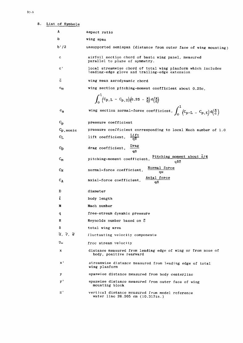
8. List of Symbols
A
b
b7/2
C~
Cp, sonic
CL
aspect ratio
wing span
unsupported semispan (distance from outer face of wing mounting)
airfoil section chord of basic wing panel, measured parallel to plane of symmetry.
local streamwise chord of total wing planform which includes leading-edge glove and trailing-edge extension
wing mean aerodynamic chord
wing section pitching-moment coefficient about 0.25c,
1 j C p , ~ - Cp,u)(0.25 - 5 c) d (E)
Wing section normal-force coefficient,
pressure coefficient
Pressure coefficient corresponding to local Mach number of 1.0
lift coefficient, Lift 7 Drag
drag coefficient, - 9s
Pitching moment about ?i/4 pitcbing-moment coefficient,
qSP
Normal force normal-force coefficient, qs
Axial force axial-force coefficient,
9s
diameter
body length
Mach number
free-stream dynamic pressure
Reynolds number based on E
total wing area
fluctuating velocity components
free stream velocity
distance measured from leading edge of wing or from nose of body, positive rearward
streamwise distance measured from leading edge of total wing planform
spanwise distance measured from body centerline
spanwise distance measured from outer face of wing mounting block
vertical distance measured from model reference water line 26.205 cm (10.317in.)

aaa - wing-twist influence coefficient due to normal load at an c/4 point
wing-twist influence coefficient due to moment about c/4 point
CL angle of attack of wing-body centerline
Aa angle of attack of wing station minus angle of attack of wing-body centerline
6 vertical wing deflection under load
%I horizontal-tail deflection angle referred to a model water line, positive when trailing edge down, deg
i3 circumferential location of pressure orifices on rear of fuselage, deg
4 built-in twist angle
Subscripts:
L lower surf ace
U upper surf ace

TABLE I.- WING COORDINATES ALONG STREAMWISE CHORDS (a) Wing planform coordinate layout @J) = 0.104; c' = 45.839 em (18.047 in.)
bh

- m m m t - t - w m ~ ~ ~ o o r n m w m m m m m t - m o m m o c c c ) m m o n n m O " D n m m 0 " O 0 m m m - u O c ) m O ~ V ) m P N - O m m m NNNNNNNNNNNNN-0000------- ----000 o o o o o o o o o q o o o o o o q q q ~ q ~ q ~ q o q q q q q q . + ; ; : ; ; ; r : , :;;;;;
p g z ~ g ~ ~ s ~ ~ j g g g g ~ ; ~ g $ ~ ~ g g g zgzzs," ~ ~ D D ~ ~ ~ ~ ~ ~ ~ ~ ~ P ~ w ( D v ) Y ) c * ~ ~ ~ o o N N N----" q q q q q q q q q q q q q q q q q q q q q q q q q q q q q q q 0
O I O ~ ~ ~ ~ W ~ ~ ~ ~ ~ . ( Y ~ ~ U ) V ) V ) V ) ( O ~ P - P - N P ) ~ F C ~ F O P I ( D O m r - n o w m n ~ - ( ~ ~ ~ - m m ~ ~ v m w ~ ~ ( ~ ~ EY)WII*UO m r n m m o o o - - ~ ~ m m m o m o e r o n ( ~ m o ~ v ( ~ c m m m o 1?1?5444444451??~?%????0: ??????? 0 -
w I
. . : w I
0
Z 0 2 4
2 + a Z - n E % 0 1 0 - u 2 u 6 Z - I " 2 I - . t- - C
u 9 --I 0)
m 2 a c 2
0
$2 h " ',&
U > N
~ ~ ~ 2 ~ X ~ ~ " o " o N Z 2 2 ~ 2 , " ~ 2 S ~ % N " - - - - - ~ ~ N ~ N N N N N N N N N N N N N N N ZgZZXNO NNNNNN
qqq?q?qqq9?????9??99?9949 9999?? -124'"""""""""""'"""
2: P; 3,
*ti $L? a* 9:
- 1
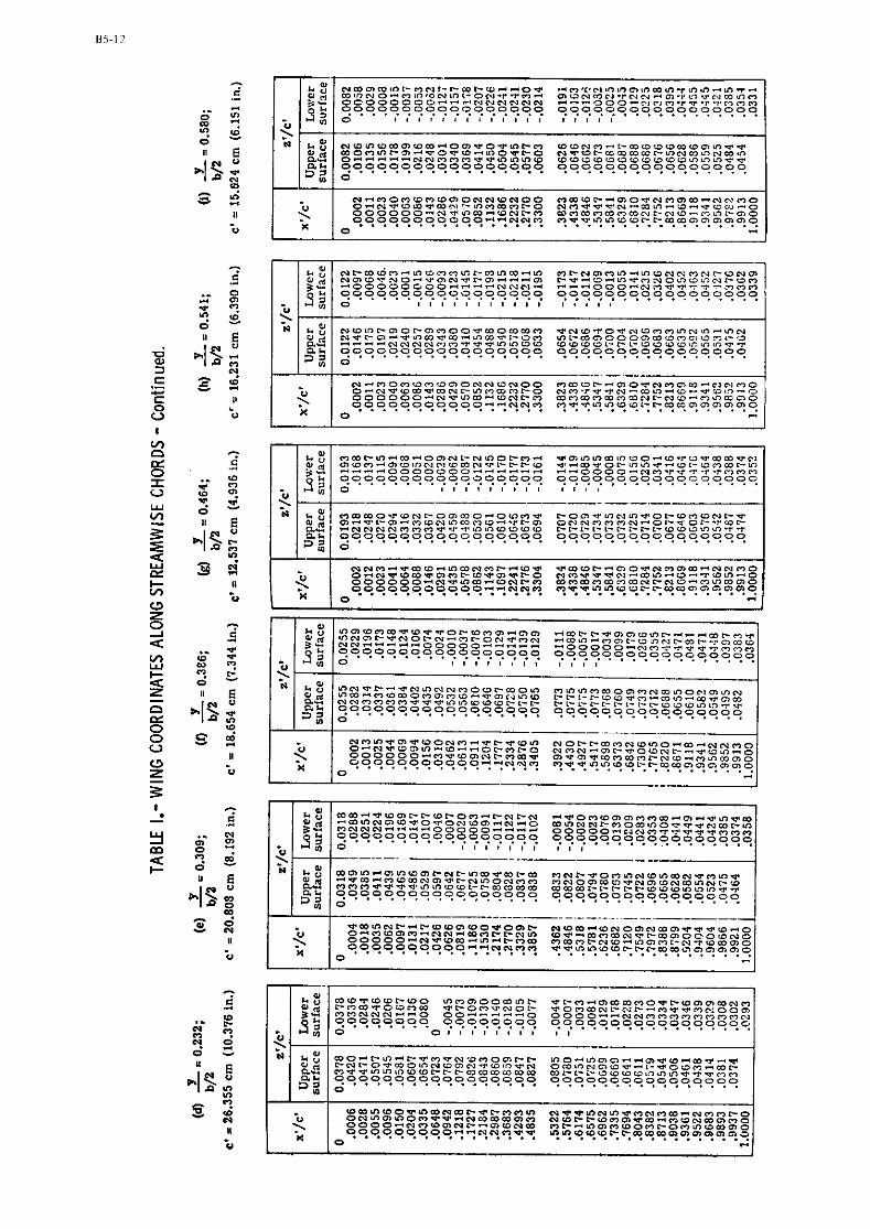
- e' .- .. 0 * m
q 2 - > U
* ' ~2 3 % . 33
~ r m d n - m m o n n t - m m m - m n r - - m o m - m u m o o ~ r o m m "gggggggg2ZfE:::2 CSZ8ZzZz:.$P3$1zz4 qqqqqqqqqqqqqqqqq qqqqqqqqqqqqqqqqq 0 , , , , , , , , , , , , , , , a

- e' .-
(D ;; n " ; 2 - II E
0 h-. c- 1: 0 " 9 $:
II
U
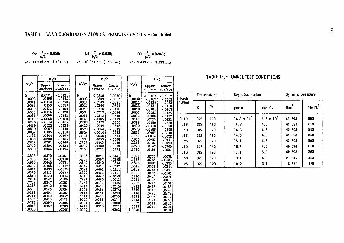
TABLE I.- WING COORDINATES ALONG STREAMWISE CHORDS - Concluded.
-. = 11.382 cm (4.481 in.) c' = 10.051 crn (3.957 in.) c' = 9.467 cm (3.721 in.)
Lower surface
-0.0221 -.0243 -.0210 -.0289 -.0309 -.0328 -.0342 -.0368 -.0405 -.0425 -.0440 -.0458 -.0467 -.0465 1 -.0448 -.0424 -.0394
-.0361 -.0318 -.02i1 -.a211 -.0153 -.0071 .0014 .0109 .0202 .0282 .0334 .0353 .0341 .0329 .0296 .0269 .0246
z'/cT
x'/c' upper l surface
x'/c'
0 .0002 .0011 .0023 .0040 .0063 .0086 .0143 .0286 ,0429 .0510
' .0852 .I132 .I686 2232 .2110 .3330
.3823
.4338
.4846
.5341
.5841 A329 .6810 .I284 .?I52 .8213 .8669 .9118 .9341 .9562 .9852 .9913
1.0000
0 .0002 .0011 .0023
TABLE I 1.- TUNNELTEST CONDITIONS
-0.0221 -.0199 -.01i2 -.0153
Upper surface
-0.0382 -.0362 -.0339 -.0321 -.0301 -.0282 -.0266 -.0235 -.0180 -.0410 -.0108 -.0057 -.0014 .0052 .0102 .0141 .0188
.0230
.0268
.03C3
.0338
.0368
.0395
.0417
.0434
.0446
.0453
.0448
.0425
.0403
.0314
.0322
.0310
Mach number
.
1.00
.99
.98
.97
.95
.90
.80
.50
.25
z1/c8
Lower surface
-0.0382 -.0405 -.0432 -.0450 -.0461 -.0484 -.0491 -.0522 -.0558 -.0580 -.0598 -,0618 -.0632 -.0611 -.0590 -.0560 -.0521
-.0418 -.0428 -.0313 -.0314 -.0241 -.0166 -.0075 .0015 .0101 .Ole5 .0248 .0278 .0214 .0258 .0215 .0203 .0184
.0040 , -.0133
.0063 .0115
.0056 1 1.0099
.0143
.0286
.0429
.0510
.0852
.I132
.I686
.2232
.2110
.3300
I .3823 .4338 .4846 .5341 .5841 .6329 .6810 .7284 .7152 3213 .a669 .9118 .9341 .9562 .9182 .9913
1.0000
Temperature
-.0068 -.0014 .0025 .0051 .0105 .0144 .0208 .0261 .0304 .0344
.0379
.0411
.0440
.0466
.0493
.0513
.0529
.0541
.054i
.0542
.0526
.0494
.0469
.0438
.0391
.0361
K
322
322
322
322
322
322
322
322
322
OF
120
120
120
120
120
120
120
120
120
Reynolds number Dynamic pressure
per m
14.8 x lo6
14.8
14.8
14.8
15.1
15.7
17.1
13.1
10.2
~ / m '
40 698
40 698
40 698
40 698
40 698
40 698
40 698
21 546
8 571
per f t
4.5 x lo6
4.5
4.5
4.5
4.6
4.8
5.2
4.0
3.1
lb / f t2
850
850
850
850
850
850
850
450
179

TABLE 111 . - LOCATION OF PRESSURE ORIFICES ON MODEL
Orifices on wing
in cm (in.]
Orifices on wing
I
LOWER-SURFACE ORIFICES I UFFER-SURFACE ORIFICES I I
0.133 c = 22.614 ( (8.903))
-0.660 -.567 -.452 -.311 -.023 .I33 272 .416 .565 .I13 ,854 ,980 '.074 1.122
-0.660 -.616 -.572 -.462 -329 -.I12 -.030 .I28 .418 .564 .710 .976
1 1.072 :.I10 L . - ___.
Wing orifice
0.307 c = 19.883' ( (7.828))
-0.021 .035 ,105 .I78 .286 .396 ,514 ,618 ,733 .635 .919 ,987
-0.022 ,038 ,101 ,185 ,398 .737
- - . . -
location, :,a1
0.480 /c = 17.160\ \ (6.756)/
Right-u.ing
0.023 ,008 ,134 ,209 .294 .404 ,497 .599 ,700 .a64 ,926 .975
Lclt-wing
0.024 ,075 297 ,400 .GO4 .785 .967 1.000
-
srlnisgan stalion.
0.653 (c = 14.442) \ (5.686),
upprr surface
0.025 ,079 .I33 .214 ,295 ,407 502 ,601 598 ,863 .923 .977
lo\r.er sor fxe
0.025 .074 .I30 ,298 391 ,501 ,603 ,703 ,784 ,868 ,923 .912
X t a f - b/2
0.804
i' e = 12.0i0) , (4.752)
0.022 .075 ,129 ,201 .294 ,391 ,495 ,594 393 ,784 .856 ,926 .917
0.019 .066 .I36 .214 .292 .403 .489 ,594 ,700 ,786 ,858 319 .961
0.933
ic = [j:;;;)) \
0.018 .077 ,129 ,209 .293 ,494 ,590 ,693 .I77 ,861 .918 ,972
0.020 ,076 .I36 221 295 396 ,497 .597 .I02 .T86 .a64 ,912 .985
-

TABLE 1V.- LOCATION OF PRESSURE ORIFICES ON MODEL AREA RULE ADDITIONS
SEE FIGURE 5.3 FOR WATER L I N E DATUM
.,,> .,E, .#,, . , , 8 .,.a
a,,. .,,. -1.3
.I*. .,,, " '0 "6:
.IS .I,. :I:; "'
I Fore fuselage area-rule additton I Aft fusclaze area-rule nddrtion I
Orifice
101 102
104 33.12 105 38.66 106 38.66 101 38.66 108 44.17 109 44.11 110 44.17 111 44.17 112 44.17 113 49.71 114 49.11 115 49.71 116 49.71 117 55.22 53.91 24.74 9.74
118 55.22 53.91 23.42 9.22 119 55.22 120 55.22 121 55.22 122 66.27 123 66.27 124 66.27 125 66.27 126 66.27
MDdel lurclage siationj hladel water line1 , Orifice
cm in. i em
30.92 12.17 i 20.75 33.12 1 13.04 1 22.10
in. I 8.17 : 127
I 8.70 i 128
hlodel l u s c l a ~ e station
cm
103.81 103.81
Model water line
in.
40.87 40.87
cm
22.10 20.75
In.
6.70 8.17

TABLE IV.- LOCATION OF PRESSURE OR IF1 CES ON MODEL - Concluded.
OrUIces on rear of fuselage Orifices on rear of fuselage
Section A-A L*
Orifice
1 2 3 4 5 6
I 8 9 10 11 12
13 14
15 16 11
18 19 20 21 22
0, deg
179.1 119.1 119.1 181.0 180.6 179.8 137.1 137.3 136.6
135.5 135.2 45.1 45.7 45.5 45.2 45.1 8.1 8.2 8.6 9.2 8.6 9.6
Model fuselage
cm
160.45 159.08 151.56 156.13 154.25 152.88 159.16 151.84 156.21
154.61 152.96 159.16 157.63 156.06 154.36 152.38 160.18 159.03
157.56 156.01 154.28 153.01
station
in.
63.11 62.63 62.03 61.41 60.73 60.19 62.66 62.14 61.50
60.87 60.22 62.66 62.06 61.44 60.77
60.19 63.30 62.61 62.03 61.42 60.74 60.24

TABLE V.- TEST CONDITIONS FOR TABULATED DATA *
* ~ n g l e s of at tack s l i g h t l y d i f f erent for s ide- fuse lage pressure data i n Table V I I I .
TABLE VI.- PRESSURE DISTRIBUTIONS OVER WIVG WITH FUSELAGE ADDITIONS;~, , * -2.5
M = 0.50

TABLE V1.- PRESSURE DISTRIBUTIONS OVoER WING WITH FUSELAGE ADDITIONS; s,, '-2.5 - Continued.
M = 0.50
- . b 6 0 .093 -.bLLI . " I 2 - . S T 2 .05t - .462 -014 2 .OOb - . L I Z -.DO, - . 0 3 0 - . o l b .LiB - . O W .4LB - . o l d .5L4 .a26 .110 -111 9 . 2 3 d L.012 .I16 , . ,LO .LI*
CN. .4>P9 L*. .o.Z11

TABLE VI.- PRESSURE DISTRIBUTIONS OVfR WING WITH FUSELAGE ADDITIONS; 8,, - -2.5 - Continued.
M = 0.50
- - 6 6 0 .OUS L O W E R S U I F A C E
- 0 , 345 -.616 .I52
0 .531 .03% . J 3 7 . D l 5
. 3 6 1 -025 .51+ -019 .120 .130 .16P
-020 -503 - .112 - 1 % .LO1 - 2 5 9 - 2 9 7 .I26
-066 .32P .298 . I 1 5
-076 -279 - . * L 2 + 1 3 0 . L B I . L B O .IUD .081 . L a 6 -225
-397 -085 . I 3 6 .I..
- .a29 . L L Y .3P8 -090 .21+ -16, .6OI .YL5 . I 0 1 . 058
.221 .om1 - . I 1 2 ."93 . 7 3 1 . L55 - 7 8 5 .L91
.292 . , I2 , 6 0 3 .OP1
2 9 5 .059 - ."lo .013 .*61 .153
.+03 .C19 .703 . I 1 6
.39. -029 . I 2 8 ."LO L.000 -.0+6 .689 .038
. I S . . I 7 3 .*97 -006
- * I 8 .013 .59I -023 + B 6 B . I 5 8
. I97 -012 .Sf4 .101 . T O 0 .LO,
.P21 -287 -702 .079
. T I 0 . I & > -186 .LOO . 9 7 2 . I 6 6
-7.6 .LIZ .516 . 2 8 3 .a58 .250 -06+ . I 9 7
1.072 . Z J 3 -919 -260 .e l2 .IS7 1.11" .,6, 1 .IPL
LN- - 7 4 9 2 C*. .0859
-.<Lu -.ii, - . 0 2 , - < . 5 , 1 L * P E I SLl l ' aCt -.5LI - . 3 7 1 . C > I - i . L 1 5 ,1123 -I.">< . 0 2 5 - L . 3 6 3
. 'b8 -,.*9, .a22 - . 9 w
. 0 7 q -2.075 -0111 -.SOP
- . + > 2 . . " d b .LU, - , . * a 6 . L 1 4 -.>..5 .01s -1.018 , 1 1 3 - L . O L I - 017 -.SO3
- . 3 i i - . > d , . I 1 8 -.,,, . 2 i Y -,9,i . I 2 9 - . * T O
2 - . 4 2 B . I 2 9 -.$TI
- 2 -..,, . - . 6 3 9 .2** - . L > C .ZPS - . )a+ .2OL -1.020 .209 -*.% - 1 3 3 - . J v : . I l b - . > i d . + C l - . B L i . 4 C ? -.328 .291 -.PP'I .293 -.+21 . ' T i -.,*, .I,* - . 3 5 7
. + * I - . I " , .as7 -1.00,
.5Ul - .28B ..?. -.365
.'.,(I - .11, . * l a - . , u i .)P' - . *94 . + P I -.1110
6 - . 3 1 1 .$PO - . I38
.)L> - . A , " . 7 3 3 - . 2 2 5 . , C O - . h a , . 5 9 I - .842
.6Yd - . 1 5 3 .b93 -.a11
. I ! > -..',, 3 5 -.,,* .Jb* -.e+.c .b9l -.1+6 . 8 < 3 - .>5a 7 -0306
.t:+ ..',, .'.iY - . L C 6 . Y 1 & -.,"I
. I84 -.598 , 9 2 3 -.1UI
.(I61 -.211 . $ u r - . L I I ~ . r e 7 - . ' l a . C 1 1 -.L%t
- 056 - . a 7 1 . P I 7 -.233
.P I8 -..?a. I . Y I I - . L ~ T .PZ6 - .a30 .912 -.219 i . c . 2 -.'"" .PI7 - . I , ,

TABLE VI.- PRESSURE DISTRIBUTIONS OVtR WING WITH FUSELAGE ADDITIONS; s,, = -2.5 - Continued.
I ,480 ST6 . 6 5 3 I T . .am IT. -933 $1. . 1 3 3 A . 3 0 7
* I < T P " / L C P S I C C P X I L C P " I C CP I I L LF

TABLE VI.- PRESSURE DISTRIBl I r IONS OVER WING WITH FUSELAGE ADDITIONS; % . -2.5'- Continued.
M - 0.80 s l l i .113 S I b .307
" I C C Y I / C L P S T b . I S 0 X l C C P
ST. . b S 3 I/< LP
ST. .8OI K I C C P
ST1 .Pa3 X I C CP
-A60 -.oh1 - . I 1 4 UPPER SURFACE - -561 -.2LS .035 -.a12 2 3 -1.251 -025 -1.161
.Ob8 -1.283 . 0 7 5 -.828 -022 -.a79 - .452 - . 3 3 8
.OL8 - . l o 1 . I 0 5 - .e l1 - 1 3 1 - .60L
. I 3 3 - .561 .O75 -.111
-.311 -.>a9 0077 -.I95
-118 - .553 .209 -.+,a . 2 L I -.,+, -129 -.110
-.LIZ3 -.131 .ZBb -.,a3 .20L -.+29 -129 -.+58 -133 - .1*5 2 9 -.411 .195 -.)?a -209 -.151
.a96 -.?PI - 4 0 1 -.153 .+PI - . ) I3 - 2 9 1 -.152 2 2 -.232
-293 -.>PO 5 -.102 .+97 -.32L
.502 -.Wl -397 -.312
1 - . I98 .+95 - . > , I .69* - . I35
.b18 - . 1 7 1 -565 -.IS5 . I 9 1 -.Is2 .601 -.122 -590 -.>,I
.133 -.222 -700 -.IN -698 - .310
-594 -.)I? -113 - . L ~ L
.691 -.Z+3 -835 - . L B O .a64 -.235
.a63 -.277 -693 -.,I5
-85I - .L31 -919 -.Lit .78* -.a10 .771 -0257
.PO0 -.,35 - 9 2 6 -.152 . P 2 3 - .L13 I -.22+
1.07+ - .112 -967 -.031 - 9 7 5 -.0bl .a56 -.283 . e l l - . I82 . 9 l l -.a*, -926 - . I76
1.122 - . 0 5 , -972 -.o*
.977 -.01P
CN- 1140'3 CM- -0328
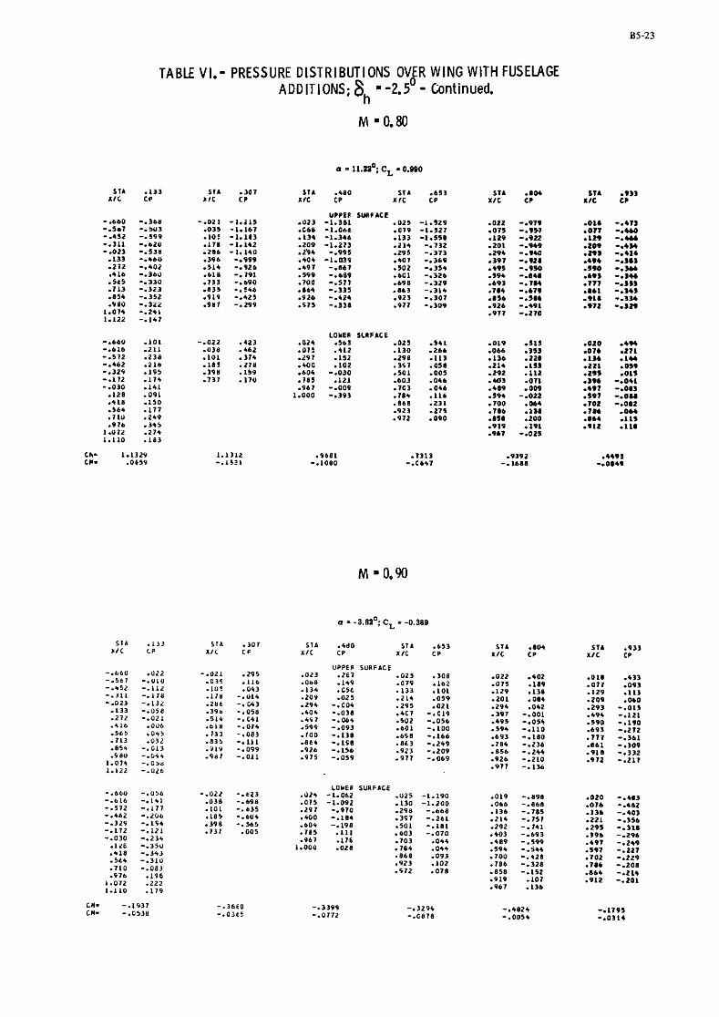

TABLE VI.- PRESSURE DISTRIBUTIONS OVER WING WITH FUSELAGE 0 ADDITIONS;~,, = -2.5 - Continued.
a = o.mO; cL. a.m.
S l l \ .L>3 S r l . 3 U I " / C '6
S I l .<80 I C P
576 .653 *,C C P
SIA .IM X I C C P S I b .P33
" I t CP X I C C I
S l A .LJJ I / C CP
S T # .30l X l C C P
I16 .+SO I l k . 6 5 J X I C CP I CP ST* -804
X I C L P ST1 .Pa3
I I C C P
-.be0 -.Us1 - . 021 - .a06 UPPER SURFbCI
-.st, -.La8 .a23 -.'15L .035 - + I 9 9
5 -.%I .GL6 - 1 . O l t - 0 2 2 -.a23
- 2 - .J3+ . I 0 5 - . L I O - 0 7 9 -L.OJI . 0 1 8 - . I 3 1
. I 3 4 -1.002 . I 3 3 -1.013 -015 -.912
- . 3 1 1 -.+,I - 0 7 7 -.*I6
. I 7 8 -.608 .209 -.Pa3 .LIP -.IIP1 -.021 -.144 . Z L I . I 2 9 - . I 9 5 - 2 8 6 -.566 . I 9 4 -.A75 .20L -. ,A5
.I95 -.5,5 . I09 -.397 . I 3 3 -.273 -396 -.+94 4 -.+Or .+07 - . 2 0 1 - 2 9 4 -.312 - 2 7 2 - .21+
.293 -.,,. .r,* -. ,02 .+PI -.Pa, - 3 9 7 -.100
6 -.213 .b la -.162 .SO2 - . Z 6 T 9 - . t20 . I P S - . I 4 5 .+95 -.a12 5 6 5 - . I 8 8 .733 - .231 .601 - .296
-590 -. I>? . I 00 -..?I9 -698 -.340
. I 9 4 -.3+5 -713 -.I83
1 6 9 3 q . 2 5 5 -835 - . I 1 3 .a64 -.>>a
.a63 - 2 9 , -6'13 -.3+7
- 8 5 1 -.2LP 7 7 -.261
- 9 1 9 - .08J .926 - .LJ2 . P I 3 - . L B O 7 -.311
.9a0 - . , e l .a61 - . I09 . V a l -.OLP .975 -.013 .PI7 -.O51
-1156 - . 2 1 1 1 .074 - . I 3 5
-9111 -.I50 .V26 - . L I P
1 . 2 -.a64 . 9 7 2 - .Olr
.971 -.PI*

TABLE VI.- PRESSURE DISTRIBUTIONS O\ER WING WITH FUSELAGE ADDITIONS; s,, - -2.5 - Continued.
M - 0.90

TABLE VI. - PRESSURE DlSTR I BUT1 ONS OVER WING WITH FUSELAGE ADDITIONS; 4, '-2.5O - Continued.
M = 0.95
e = 3 . ~ 6 ~ ; c, = 0.4S.s
111 .I,> I 1 4 .101 X/L C P
S T A .480 " / C LP "IL LP
ST4 .b53 ST4 .no$ " I C CP
SIA .933 XIC CP X I C CP
- .660 - . O H U P P E R SURFACE
-.021 -.a18 5 -.I+>
,023 -.I89 . a 3 5 -.9,5
.025 -.767 ,068 -.so, .022 -.*Sb
.079 -.a+, .01a -.a20
-.L52 -.21e ,105 - . a 5 1 .LJI - . 8 1 1 .075 -.a22
.L33 -.a56 .017 -.a05
-.111 .I711 -.,be .2OP -.I95 .LIP -.a13
. 2 1 1 -.@12 .I29 -.a22
-.023 - . L b l . I 8 6 - . -Cb .I*+ -.so7 .201 -.a18
.295 -.115 $209 -.790
. I 3 3 -.36O .356 -.43P .4OC -.SO3 .294 -.I57
.+01 -.,., .293 -.,)I .272 -.221 5 -.Be2 .*97 -.$a* .397 -.13
5 -.*,5 .+P* -.so1
. * I6 -.LO5 .b18 - . a d 0 .599 -.+,, .+9Y -.b95 .601 -.*23
-590 .01b . 5 6 5 -.OY8 .133 - . > a 1 .1W -.SO1
.591 -.)LO .698 -.503
-693 -.005 .713 -.I23 .035 - . ) a 3 .86* - . I 9 3
-693 - 2 3 1 ~ 8 6 3 -.I11
r 7 7 7 -.I,¶ . a51 -.207 . 913 -.LBI .92b -.LO2
7 8 -.LO .P23 -.076
.8b l -.I85 . 9 U O - . Z e O . U 8 1 -.061 7 5 -.a71
.85b -.I80 .977 - .012
.P I8 -.I61 1.014 -.309 .92b - . I t ¶ .972 -.OL9 1.112 -.I12 .PI1 .011
-.660 . lLe LOWER SURFLCI -1022 .a12
- .6lb .OBd .02+ .2,9
1038 .116 .025 . I70
.075 .016 .OLP .,.I
0.000 0.000 .020 .2L6
C . 0 0 0 0.000 .IOI .017 2 7 -.LO& .Obb -.076 . I30 -.or1 .076 -.Ole
-.329 -.021 . lB5 -.003 .*W -.Lo, . I 3 6 -.I00 -298 -.LO1
. I 3 6 -.I18 7 -.003 .3C8 -.055 . 6 O 1 -.011+
.I11 -.LO. . 3 P I -.I12
.221 -.I- -.010 -.011 7 3 7 .L31 .IS5 .IT+ .2P2 -.om@
.SOL -.LO+ .295 -.I52
.I># ..I,, -961 .I91 .*03 - 4 5 5
.603 .Of5 -39. -.I29
.+I8 -.012 1.000 -.055 .*89 -.LO3
.TO3 .OI8 . r e 7 -.IIT
.561 .007 .594 -.OW .7e. .L,P -597 -.022
.110 .&I1 .TOO .087 .8b8 .2.'
.TO2 .I10 .97a .293 . I86 .ZOO 2 3 .I97
7 . I 9 1 1.072 +2$1 .858 .271 .8b+ .231 1.110 . I 6 1 .PI9 .296 .PI.? .2$5 0.000 0.000 .P.T . I91
C*. .4'139 C*- -.OX0

TABLE VI.- PRESSURE DISTRIBUTIONS OVER WING WITH FUSELAGE ADDIT IONS;~ , , '-2.5O- Continued.
M = 0.95
S T A .301 I T & .+BO I T A .b5I IT* .80* S I . -933 S T A . I ) , X I L CP X I C CP X I C C P X I C LP " I C CP X I L C P

TABLE VI.- PRESSURE DISTRIBUTIONS OVER WING WITH FUSELAGE 0 ADDITIONS; 4, - -2.5 - Continued.
M -0.99
0 = -0.05'; C,, = -0.004
ST. . L 3 3 STb ,3117 X I L L P
S T 6 .LBO X / L CP
$1, , 6 5 3 "IL LP X I L C P S T 1 . 801 ST, ,913
X l L CP ./C C P
- .66O -.001 - . C 2 L - . O C L UPPER SVRFr(CE
5 -.0,9 .023 -.I05
.a35 - . 2 9 3 5 - . 081
.a68 -.1<8 .022 .OPT
.a79 - . I 75 .018 - 2 2 5
-.452 -.IS7 .I05 - . 2 1 8 1 -.260 .OT5 -.OPT
. I 3 3 - . I 8 6 - 0 7 7 - .037
- . 3 1 1 - . 2 + 5 . I 7 3 - .3CI .ZOP -.Z6L . I 2 9 - . l o b
1 -.L91 . I 2 9 -.OIL
-.a23 -.312 . I 8 6 -.I!* .I% -.2,7 - 2 0 1 -.I10
.295 - . I 1 3 . 209 -.neb . I 1 3 - . 2 $ 7 .39b -.20L .+01 -.,Be
. 294 -.OPE .LOT -.,I5
2 3 - . I 2 8 .212 - . I 8 3 .514 - . I s > .LP l -.201
. 391 -.01+ .502 -.22*
.+9+ -.221 . * I 6 - . i t 1 .b18 - . L P ~ .IPP - . zrg .+95 - . I25 .601 -.263 .)PO -.206 .565 - . O Z a - 7 3 3 - .L91 .TOO - . 2 8 8 . I 9 4 - + I 9 6
.be8 - . I 5 6 - 6 9 3 -.373
,713 - . O L B .a35 -.Z+O .a66 - . I63 .6P3 -.282
.a63 - .322 ~ 7 7 1 - .+TI
.BSL - . 011 .PI9 - . , I 1 .916 -.On6 .TO+ - .361 .921 - . l 6 b
. I 6 1 -.a33 .980 - .118 .Pel .0>2 . + I 5 -.OLz .8Sb -.69L .PI7 . O O L
. P I 8 - .olb 1.074 - . * + I .92b - . I 8 6 . *12 -.011 1.122 -.012 - 9 1 7 -.OSO
- 6 .01D LCWER SURFICE
- . 022 .OlO -.bib -,OZ9
.024 - .>el .038 - . 2 3 J .a75 - .+21 .OZ5 -.+10 .OLV -.516
0.000 0.000 .020 - . I 3 9 0.000 0 .000 , 1 0 1 -.292 .297 - .473 .066 - . I 3 1 . I 3 0 -.L7+ .016 -.691 -.3Z9 -.OPT . I 8 5 -.30C .*on -.4,7
. I 3 6 -.be2 . I 9 8 -.lb+
. I 3 6 -.lob - . I T 2 -.036 .398 - . 3 8 3 .601 -.I13
. 2 1 1 -.563 ,397 -.223
2 2 1 - . l a 2 -.030 -.Lbl .137 .C79 . lo5 ,116 .292 - .301
.so1 -.2,, .295 -.+TO . I 2 8 -.283 .967 .232 .+OJ -.2*7
.603 .008 .39b -.33*
.+La - . 2>8 1.000 .022 .+LIP - . I 1 6 -103 .OP6
.*97 -.z.2 5 6 - .2LL . 5 P 1 -.1P2 .L IT . I 9 7 -.OSP .7 IO - . 0 2 0 . l o 0 .019 .86U +2OL . l o 1 .OSb .976 .220 .1B6 .I00 .P23 . I 1 7 . I 8 6 . I 2 6
1.072 .23O .858 . I 6 8 - 1 6 1 . I 1 3 1.110 . I 8 3 . P I 9 . I 0 1 .9L2 . ,T I 0.000 0.000 7 . L L P
-.bbO .I>. LCWER SURFACE
- . b l $ . O d d -.a22 . l o > .O2C .212 ,038 .OBO
.025 , 1 3 1 0 5 -.020 0.000 0.000 ,019 .0S6 .020 . I 2 0
C.000 0.1100 . L O 1 -.On6 . I 9 7 -.LO6 . I 3 0 -.092 .O66 - . I 1 6 . 076 - . I 5 7
-.om .I85 - .a57 .+00 -.,LO .298 - . L l ? . I 3 6 - . I 2 6 . I 3 6 -.218 - . L I Z .023 . 3 9 U - . 0 6 6 .601 -.011 .J97 -.11T .ZIL - . I 1 0 . I 2 1 -.237 -.a10 - .a81 7 3 .L31 ,785 .I66 .SO1 - .LIZ .292 -.L61 - 2 9 5 - .171
.1<8 - . 201 .Pel . I 9 0 .a03 .036 .LO3 - .Z IT .396 -.20P . ) I 8 - . G I 1 1.000 - . 051 . T O 3 . 056 .LOP -.On5 . b 9 1 -.262 .5b+ - . o w .78' . I 2 1
.59+ - . L W 5 9 - . I 2 9 1 0 .L2. .Ben . d l 8
, 700 .010 .702 .011 . w e .z49
.923 . I 6 3 .TO6 ,159 . I 8 6 . I 1 1
1.0?2 .1.1 .a58 .2311 . 8 b 6 . I 5 5 L. l l0 . i d 1 ,919 .25L . P I 2 . I 7 5 c . 0 ~ 0 0.000 .9b7 . I 2 8

TABLE V1.- PRESSURE D I S T R I B N I O N S OVER WING WITH FUSELAGE 0
ADDITIONS;~,, '-2.5 -Concluded.
M = 0.99
TABLE V I I ,- PRESSURE DISTRIBUTIONS OVER REAR FUSELAGE WITH FUSELAGE AREA-RULE ADDITIONS (SEE TABLE V I FOR ORIFICE LOCATIONS): sh = -2.5O
Fuselage station
on
153.0 154.4 156.1 157.6 159.2 160.8
153.0 154.4 156.1 157.6 159.2 160.8
153.0 154.4 156.1 157.6 159.2 160.8 -
c for
i n .
60.22 60.80 61.46 62.04 62.67 63.30
60.22 60.80 61.46 62.04 62.67 63.30
60.22 60.80 61.46 62.04 62.67 63.30
P
Q = 8 ° ~ 0 = 4 6 0 ~ 0 = 1 3 6 0 ~ ~ = 1 8 0 0
a = -4.08'; CL = -0.339
0.073
.I27
.I45
.058
~ = 8 ° ( ~ = 4 6 0 1 0 = 1 3 6 0 1 Q - 1 8 0 0
a = oO; c = 0.039 L
0.051
.lo8
.I34
.057
0.062 .084 .1M) .lo5 .084
0.042 .066 .087 .lo2 .080
u = 4.00'; CL = 0.396
-0.014 .010 .041 .062 .070
0.041
.lo1
.I24
.061 -
a = 8.00~; CL = 0.730
0.028 .046 .059 .081 .055 .015
0.000 .025 .049 .066 .073
0.020
,085 .I10
.046
0.034 .053 .060 .075 .054 .026
0.025 .054 .080 .093 .074
0.003 .032 .065 ,079 ,060
a - 11.07'; CL - 0.952
0.020 .042 .062 .Om .079
0.053 .067 .076 .092 ,061 .031
0.047 ,057 .075 .084 .087
0.091 ,098 .lo4 .I17 .070 .017
0.004
.078
.I10
.048
0.073 .091 .091 .I03 .OW .018 -
-0.012 .012 .054 .075 .063
0.052 .059 .084 ,088 .090

TABLE V I I.- PRESSURE DISTRIBUTIONS OVER REAR FUSELAGE WITH FUSELAGE 0
AREA-RULE ADDITIONS; 4, - -2.5 - Continued.
Fuselage
cm
153.0 154.4 156.1 157.6 159.2 160.8
153.0 154.4 156.1 157.6 159.2 160.8
153.0 154.4 156.1 157.6 159.2
cp fo r s t a t ion
i n .
60.22 60.80 61.46 62.04 62.67 63.30
60.22 60.80 61.46 62.04 62.67 63.30
60.22 60.80 61.46 62.04 62.67,
160.8
0=8 '1
a = 3.98'; CL = -0.372 -
0.072
.I50
.I75
.071
0=46°10=136010=1800'0=8010=46010=136010=1800
a = 0.03'; CL = -0,034
63.30i .052
0.047
.I23
.I53
.075
.017
0.021 .048 .079 .099 .078 .025
0.061 .090 .I17 .I34 .lo9
0.043 .076 .lo9 .I28 .lo3
a = 4.02'; CL = 0.427
-0.015 .014 ,055 .074 .089
0.037
.I13
.I42
.075
a = 8.14'; CL - 0.792
-0.002 .031 ,062 .078 .090
0.016
. lo3
.I22
.068
0.033 .057 .072 .090 .069 .046
0.026 .062 .097 .I22 .TOO
-0.012 .037 .078 .I10 .086
a - 11.22'; CL = 0.990
0.015 .043 .069 .088 .097
0.052 .070 .085 .I00 .072 .038
0.035 .061 .083 .I00 .I06
-0.014
.087
.I25
0.082 .091 .097 .I22 .073 .030
0.051 .071 .086 .lo4 .I02
-0.036 .018 .057 .090 .082
0.090 .I12 .I14 ,130 ,082

TABLE V I I.- PRESSURE DISTRIBUTIONS OVER REAR FUSELAGE WITH FUSELAGE AREA-RULE ADDITIONS; sh=-2.50 - Concluded.
M = 0.95
[ Fuselage 1 s ta t ion
C fo r P - - - . . . .
cm Q = $10 = 46'1 a = 1 3 6 0 l a = 180°1e = + / 0 = 4,j0 l o = 13601Q = 1 8 0 ~ L
Fuselage s ta t ton
i n . 0 a = -3.97 ; c L 3 -0.440
c for P
an
153.0 154.4 156.1 157.6 159.2 160.8
G = -0.09'; CL = 0.012
in.
60.22 60.80 61.46 62.04 62.67 63.30
0 ~ 1 8 0 ~
153.0 154.4 156.1 157.1 159.2 160.8
~ - , 1 3 6 '
60.22 -0.001 0.046 60.80 .057 .088 61.46 .I45 .lo9 62.04 .I91 .I36 62.67 ,127 63.30 .133 .lo0
-0.016
.I30
.I68
.I34
Q - 4 6 0 O = e O 0 . 8 Q -46'
a = -3.96'; C L = -0.459
-0.075 .056 .I27 .I66 .I55
a = -0.05'; C~ = -0.004
0 0 = 1 3 6
0.091
.203 ,252
.116 -
0.056 .086 .I17 .I41 .I51
0 = 1 8 o O
0.041
.I74
.216
.I32
a . 3.43'; CL = 0.440
-0.083 - .002 ,066 .lo9 .I30
0.057 .lo6 .I51 .I76 .I55
0.095 .I21 .I35 .I60 .I35 .087
a = 7.99'; CL = 0.893
0.012 .048 ,095 .I29 .I45
0.019 .090 .I48 .I76 .I61
-0.052 .026 .078 .I23 ,117 .087
0.027 .069 .lo3 .I29 .I26 .I10


Figure 5 . 2 . - Wing semispan planfom layout w i th model dimensions.
Trail ing-Edge Extension Contour
Fuselage s t a t i o n Senispan s t a t i o n
Inches Centimeters Inches Centimeters
T i p Contour Glove Leading-Edge Contour
xt, In . xt , un yt. I n . yt, at Fuselage s t a t i o n Semispan s t a t i o n
Inches Centimeters Inches Centimeters

Figure 5 . 3 . - Cross-section layout of 0.087-scale model with fuselage area-rule addftions.
Figure 5 . 4 . - Longitudinal progress of cross-section area taken noryal to fuselage centerlfne. Model and fuselage areas include 28.39 n 2 (4.40 in ) of inlet area.

.92-chord l l n e
Model semispan station 43.66(17.19)---------
. . . .
/-.A semlSpan (model center station l i n e )
( a ) Location of ai leron hinge fair ings.
Cross sections (b ) Sketch of typical ai leron hinge fa l r ing .
Wing cross section
I 1.33l.5251
Vortex penerator
I I
(c) Sketch of underwlng leadlng-edge vortex generator.
Figure 5 . 5 - Sketches g iv ing d e t a i l s of a i leron hinge fa i r ings and vortex generator. See Figure 5 . 1 .

Wall ponel Slot edge
I
0 20 40 60 80 100 120 140 160
Distance downstream o f s l o t origin, x , in.
Figure 5 .6 . - Slot geometry for the Langley &Foot Transonic Pressure Tunnel.
Figure 5 . 7 . - Tunnel test section with sidewall inserts,

carborundum grains
'-No. 100 carbarundm grains
No.100 carborundum grains\ /eidrnl i
,,..b,lY),
.a-
% (8) Wing upper surface. M-0.95 to 1.00. &
No. 100 arbarundum grains
No.90 carborundum grains, , , / Z ~ ~ < ~ I . ~ ~ I / /
Side of fuselage
____-IF-
,,.-- A-
(b) Wing lower surface. All Mach numbers.
,122 3.31 I
t ip 571:
i No.120 0% ~ carborundum
Figure 5.8.- Boundary-layer t r i p arrangements. Dimensions a re i n centimeters ( Inches) .

Normal rtolion crn 0 8 16 2 4 32 4d 48 56 64 72
I
Figure 5 . 9 . - Vert ical d e f l e c t l o n of model wing due to aerodynamic loading. M . 0.99; CL = 0.429; 6 6 * 44 193 N/III' (923 l b / s q f t l ; R 3 16.1 x 10 per meter (4.9 x 10 per f o o t ) .
j o t e : Tlp a t normal s t a t i o n 30.

Figure 5.10.- Longitudinal force and moment characteristics for supercritical wing research airplane model.


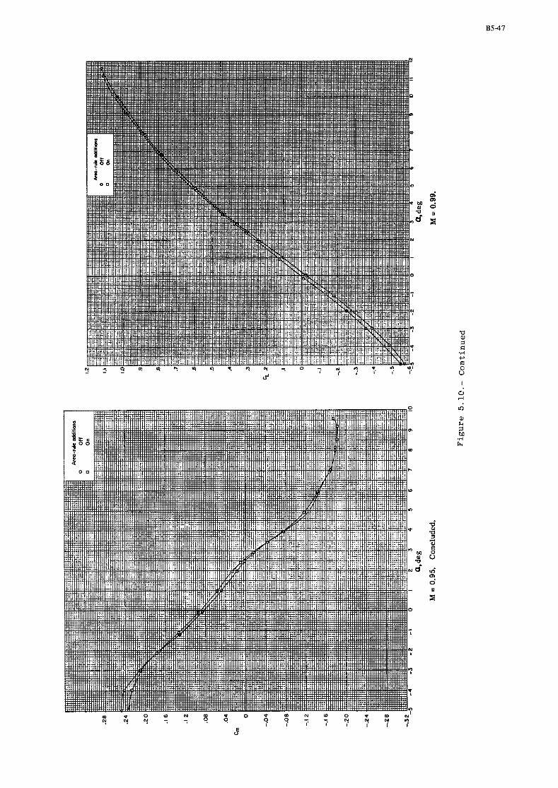


-.6
-.4
Cp -.2
0
.2
.4
- Uppsr wrfon - - - Lower wrtacs
-.8
-.6
-. 4
-.2
CP 0
.2
.4
.6 1=0.933 b/2
1 \ / I I I I I I / I I I I I I .8 0 .I .2 . 3 .4 .5 .6 .7 .8 .9 1.0
x/c
M = 0.99. Concluded.
Figure 5.11.- Concluded

APPENDIX C
BODY-ALONE CONFIGURATIONS
Guide to the Data
The body-alone data are included in the data base to provide data on rather simple three- dimensional (3D) configurations to aid in theory development and program checkout. The configurations include a 1.5-diameter ogive-cylinder - 1 a cubic-cylinder-cubic body (C-2), a 10-degree cone cylinder (C-31, and an equivalent body of the ONERA calibration model (C-4). Pressures along 13 rays and force data were taken on the ogive-cylinder at angles of attack from 0 to 30 degrees and Mach numbers from 0.5 to 1.2. Body and some tunnel wall pressures and force data are given for the cubic-cylinder-cubic model at angles of attack from -3 to 5 degrees and Mach numbers of 0.5, 0.8, 1.0, and 1.2. The cone-cylinder pressure data were taken at zero angle of attack at Mach numbers from 0.9 to 1.4. Pressures along two rays and forebody drag are presented for the ONERA model at zero incidence and Mach numbers from 0.6 to 1.0.
The model and tunnel information format is the same as used for the 3D configurations and includes, in addition to the data, information on the model geom=try, the wind tunnel, test parameters, instrumentation, and data accuracy. This information is provided to assist the user in determining the usefulness of each data set for his application.
As mentioned in Chapter 2 the model-to-tunnel blockage ratios are small enough so that the wall interference effects in the subsonic range are less than 10-2 on the pressure coefficient. However, all of the data obtained at supersonic speeds contain some evi- dence of reflected waves. These disturbances are rather easily discerned at zero inci- dence and do not significantly affect the data upstream of the disturbance. At angle of attack, however, it may be difficult to ascertain if irregular pressure variations are caused by shed vortices and therefore are "legitimate" or are caused by reflected waves and therefore are "illegitimate." It is left to the user to discriminate between the two phenomena.

1. 1. 5 D Ogive - Circu la r Cylinder Body, L I D = 21. 5
K. Hartmann
Deutsche Forschungs- und Versuchsanstalt fiir Luf t - und Raumfahrt
Aerodynamische Versuchsanstalt E. V.
1. 1 Introduction
This paper has been prepared for the Working Group 0 4 of the Fluid Dynamics Panel of AGARD a s
a contribution to the "Experimental Data Base for Computer P rogram Assessment" that i s being
established. This contribution contains selected data from force- and surface p res su re distribution
measurements a s well a s r e su l t s from flow visualization experiments, e. g. smoke and oil now
pictures. The experimental investigations were performed in the DFVLR 1 x l Meter Transonic
Wind Tunnel and in the High-Speed Wind Tunnel of the DFVLR/AVA. Figure 1 . 1 shows the tested
model consisting of a 1. 5 D long c i rcular a r c tangent ogive and a 2 0 D long afterbody of c i r cu la r
c r o s s section (D = 4. 5 c m body diameter) . This body geometry i s typical for most miss i les . The
model was manufactured of s t ee l with a very smooth surface; transition was always f r ee .
0 Two different model supports had to be used since the angle of attack range i s l imited to f 15 .
The model supports a r e shown in Figure 1 . 2 .
The data presented h e r e a r e not correc ted for wall constraints.
At sma l l supersonic Mach numbers the disturbances start ing a t the model nose a r e not completely
cancelled a t the tes t section walls . The effect of the reflected waves on the p res su re distribution
i s , however, c lear ly visible in the respective f igures, e . g. Figure 1.8. The reflection pattern of
the waves i s shown schematically in Fig. 1 . 3.
1 . 2 Data s e t
1 . General Description
1 . 1 Model Designation o r Name B 3 - 2 0 D. 1 . 5 D ogive + 2 0 D circular cylinder
D = body diameter ; Ref. [ I ] , [ 2 ]
1. 2 Model Type (e. g . , Full Span Wing-Body, Semi-span Wing) body of revolution, general body for miss i l e s
2 . Model Geometry
2 . 2 Body Data (Detail Description of Body Geometry) See Figure 1. 1
2 . 5 Fabrication Tolerances/Waviness Manufactured of steel . smooth su r face
3 . Wind Tunnel
3 . 1 Designation 1 x 1 Meter Transonic Wind Tunnel
3 . 2 Type of Tunnel
3.2. 1 Continuous o r Blowdown. Continuous, closed c i rcui t Indicate Minimum Run Time if Applicable
3 . 2 . 2 Stagnation P r e s s u r e 0 . 4 bar up to 1 . 6 ba r
3 . 2 . 3 Stagnation Temperature Ambient
3 . 3 Tes t Section
3 . 3 . 1 Shape of Tes t Section Square
3 . 3 . 2 Size of Tes t Section (Width, Height, Length) 1 me te r . l m e t e r . 3 m e t e r

3. 3. 3 Type of Tes t Section Walls Closed, Open, Slotted, Perforated Open Area Ratio (Give Range i f Variable) Slot/Hole Geometry (e. g . . 30-Degree Slanted Ho1.e~) Treatment of Side Wall Boundary L a y e r
Full span models
Half model test ing
3 .4 Flow Field (Empty T e s t Section)
3 . 4 . 1 Reference Static P r e s s u r e
3 .4 .2 Flow Angularity
3 .4 .3 Mach Number Distribution 3 .4 .4 P r e s s u r e Gradient }
3 .4 .5 Turbulence/Noise Level
3 .4 .6 Side Wall Boundary L a y e r
3. 5 F r e e s t r e a m Mach Number (or Velocity)
3. 5.1 Range
3 .5 .2 P r e s s u r e s Used to Determine Mach Number (e. g., Settling Chamber Total P r e s s u r e and Plenum Chamber P r e s s u r e )
3 .5 .3 Accuracy of Mach Number Determination (AM)
3 .5 .4 Maximum Mach Number Variation in x, y, z-Direction (Empty Tunnel; Specify a t What Mach Number)
Maximum Variation of Flow Direction Maximum Mach Number Variation During a Run
3.6 Reynolds Number Range
3. 6 . 1 Unit Reynolds Number Range. (Give Range a t Representative Mach Numbers; l / m )
3.6.2 Means of Varying Reynolds Number (e. g . . by P r e s s u r - ization)
3.7 Temperature Range and Dewpoint, Can Temperature be Controlled?
3. 8 Model Attitudes 3.8. 1 Angle of Attack, Yaw,
Roll
Perfora ted
30 degree slanted holes, four walls a r e perforated and boundary layer is influenced by plenum suction to adjust f r e e s t r e a m conditions. In case of 2 D and half-model-testing solid end plates (9 0. 57 m) a r e used.
Plenum pressu re , calibrated against side wall s t a - t ic p res su re and lancet-probe [ I ]
A u = A 8 < f 0.05' wedge probe calibration
See Chapter A 5 Fig. 5. 4 and Ref. 151. [6], [ I ] (also s e e 3. 5.4)
Low turbulence level (measurements a r e in p rogress ) [14]
Low noise level (
= 0. 5 0 .8 1. 0 1. 2
6(Pitot p res su re = 0.999 p ) = 8 . 0 7. 4 6. 7 6. 5cm 0
Transonic M = 0. 5 t o 1. 2, supersonic M = 1. 3 m 03
to 2 .0
Transonic range: settling chamber total p r e s s u r e and plenum chamber p res su re . Dependence between plenum pressu re and f r e e s t r e a m s ta t ic p res su re h a s been calibrated by lancet-probe and side-wall. s ta t ic p r e s s u r e [ I ]
A M = i 0.003 m
= 0 . 5 0. 8 1 .0 1.2
AMm(x-direct. ) 0.005 0.003 0.006 0.015
(z-direct. ) 0.003
M m 0 . 5 1 .0 2.0
1.7 . 10 7
1 .8 . 10 1 . 2 . 1 0 7
Remax 0 .27 .10
7 0 .42. 10 0 . 5 . 1 0
7 Remin Pressur iza t ion
To - 305 K (ambient), no
bewpoin t a - 30' C
0 0 2-D and sheared wings: total u = 25 (i 0.02 ) half-models: total u = 25' (i 0 . 0 2 ~ ) complete models: total a = 30°(* 0 . 0 2 ~ ~ -
range can be extended by cranked s t ings

complete models: total yaw 15' (* 0. 1 4 total ro l l 360' (* 0. 1
3.9 Organization Operating the Tunnel and Location of Tunnel
3.10 Who i s t o be Contacted fo r Additional Information
3.11 L i t e ra tu re Concerning th is Facility
4. Tests 4.1 Type of Tes t s
4. 3 Tes t Conditions
4. 3. 1 Angle of Attack
4 .3 .2 Mach Number
4 .3 .3 Dynamic P r e s s u r e
4 . 3 . 4 Reynolds Number
4.3. 5 Stagnation Temperature
4 .4 Transit ion
4.4. 1 F r e e o r Fixed
4 .4 .2 Position of F r e e Transition
4 . 4 . 4 Were Checks Made to Determine if Transit ion Occurred a t T r i p Location?
4. 5 Bending o r Torsion Under Load
4 .6 Were Different Sized Models Used in Wind-Tunnel Investigation? If so. Indicate Sizes
4. 7 Areas and Lengths Used to Form Coefficients
4 . 8 References on Tests
4.9 Related Reports
5. Instrumentation
5 .1 Surface P r e s s u r e Measurements
5.1. 3 P r e s s u r e Ori f ices on Components, Give Component and Orifice
Location
5. 1. 4 Geometry of Orifices
5.1. 5 Type of P r e s s u r e Transducer and Scanning Devices Used. Indicate Range and Accuracy
5 .2 Force Measurements
5.2. 1 Type and Location of Balance
Deutsche Forschungs- und Versuchsanstalt filr Luft- und Raumfahrt E . V. BunsenstraDe 10 D-3400 Gettingen, Germany (FRG)
Dr. -1ng. W. L,orenz-Meyer Address s e e 3.9
Ref. [5] to (111
Force - and moment measurements , surface p res su re distribution and base p res su re measurements , oil now pictures
- 4' to l a 0 (force - measurements)
o0 to 30' (p res su re distribution measurements)
0. 5 t o 1 . 2
0. 16 to 0.43 ba r 5 5
ReDZ4 . 10 to 6. 5 . 10 , based on body diameter
T = 320 K 0
F r e e
Unknown
Unknown
NO
2 = 15.9 c m Area: Body crossection S = - 2
4
Length: Body diameter D = 45 m m
Ref. [ I ] , [21
Ref. [31, (41
Body, see Fig. 1. 1
Holes, 0. 7 m m in d i a m e t e r , 4. 5 m m deep
CEC differential p r e s s u r e t ransducers plus scanivalves. Range: _i 5 psi and * 10 psi Accuracy: + 0 . 3 $ FS Scanning ra t e : 4. 5 sec /or i f ice
Sting mounted internal th ree component s t ra in gauge balance made in DFVLR/AVA, Germany (FRG), located in the middle of the body
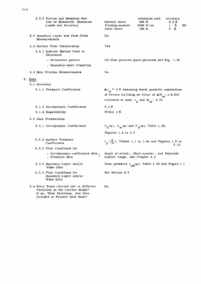
5. 2.2 Forces and Moments that Can be Measured. Maximum Loads and Accuracy
5. 3 Boundary Layer and Flow-Field Measurements
5.4 Surface Flow Visualization
5. 4. 1 Indicate Method Used to Determine
- Streamline pattern
- Boundary-layer transition
5. 5 Skin Friction Measurements
6. Data - 6. 1 Accuracy
6. 1. 1 Pressure Coefficients
6. 1. 2 Aerodynamic Coefficients
6. 1. 4 Repeatability
6. 3 Data Presentation
6. 3. 1 Aerodynamic Coefficients
6. 3.2 Surface Pressure Coefficients
6. 3.3 Flow Conditions for
- Aerodynamic coefficients data - Pressure data 1
6.3.4 Boundary Layer and/or Wake Data
6.3. 5 Flow Conditions for Boundary Layer and/or Wake Data
6.4 Were Tests Carr ied Out in Different Facil i t ies on the Current Model? If so, What Facilities. Are Data Included in Present Data Base?
maximum load accuracy Normal force 300 N 0. 5 $ Pitching moment 4000 N cm 1 $ FS Axial force 100 N 2 $
No
Yes
Oil-flow pictures (paint pictures), see Fig. 1. 16
A c " 1 % assuming worst possible combination P
of e r r o r s including an e r r o r of AM = i 0.002 m
evaluated a t max. c and M = 0.76 P m
0.5%
Within 1 $
C (LI), C m ( a ) and C A ( a ) ; Table 1.45. N
Figures 1.4 to 1.6
X c ( - ) ; Tables 1. 1 to 1.44 and Figures 1.8 to
P D 1. 15
Angle of.attack-, Mach number - and Reynolds number range, see Chapter 4.3
Base pressure c (a); Table 1.45 and Figure 1.7 PB
See Section 4. 3

7. References
[ I ] Hartmann, K.
[2] Hartmann, K.
[3] Esch, H.
[4] Gudmundson, S. E. Torngren, L .
(51 Ludwieg, H. Lorenz-Meyer , W. Schneider, W.
[6] Hottner, Th. Lorenz-Meyer, W.
[ I ] Lorenz-Meyer, W.
[8] Lorenz-Meyer, W.
[9] Mackrodt, P . A.
[ l o ] Lorenz-Meyer, W.
[ l l ] Lorenz-Meyer, W.
[12] Holst, H. Grosche, F. R. Binder. B.
(131 Meier, H. U.
[14] Heddergott, A
[15] Lorenz-Meyer, W.
Aerodynamische Untersuchungen im transsonischen Geschwindigkeitshe- reich. Teil I: Systematische Dreikomponentenmessungen. AVA-Report 67 A 38
Aerodynamische Untersuchungen im transsonischen Geschwindigkeitsbe- reich. Teil 11: Systematische Druckverteilungsmessungen. AVA-Report 69 A 06
1) Untersuchungen an schlanken Rotationskdrpern im Transschall . DFVLR-Report 1 US F 69-1. 2) Kraftmessungen an zylindrischen Rilmpfen im Transschall . DFVLR-Report 1 US F 70-3.
Supersonic and transonic wind tunnel t e s t s on a s lender ogive-cylinder body single and in comhination with cruciform wings and tai ls of dif- ferent s izes . FFA-Report A U - 7 7 2 (1912). Sweden
Der Transsonische Windkanal d e r Aerodvnamischen Versuchsanstalt Giittingen. Jahrbuch WGLR 1966 (1967) pp. 145-155
Der Transsonische Windkanal d e r Aerodynamischen Versuchsanstalt Gdttingen (Zweite Ausbaustufe) Jahrbuch DGLR 1968 (1969) pp. 235-244
Die Strahleigenschaften de r Meestrecke des Transsonischen Windkanals de r AVA. DLR-FB 66-19 (1966)
Tes t - Facil i t ies of the DFVLR in the Transonic and Hypersonic Speed- Range and Main Activities. DLR-FB 11-86 (1971)
Windkanalkorrekturen hei Messungen an zweidimensionalen Profilen i m Transsonischen Windkanal de r Aerodynamischen Versuchsanstalt G6ttingen. ZFW 19 (1971) pp. 449-454
Kanalkorrekturen fur den Transsonischen Windkanal d e r Aerodynami- schen Versuchsanstalt Gdttingen bei Messungen an dreidimensionalen Modellen. ZFW 19 (1911) pp. 454-461
Der Transsonische Windkanal 1 m x 1 m d e r DFVLR-AVA. - Ein Uberblick ilber die Aktivititen von 1963 - 1911 - Festschr i f t zum 65. Gehurtstag von Pro f . Dr. H. Ludwieg, p p . 4 - 1 i 4-54, Gdttingen 1917
Druckschwankungsmessungen im Transsonischen Windkanal d e r DFVLR- AVA GWtingen. DFVLR-AVA-Report 251-15 A 11 (1915)
The Response of Turbulent Boundary L a y e r s to Small Turbulence Leve l s in the External F r e e Stream. ICAS-Paper 76-05 (1976)
Einflufl d e r erh6hten Turbulenz d e r freien Anstriimung auf die Druck- und Kraftbeiwerte e ines superkri t ischen Profi ts . DFVLR-AVA-Report 251-76 A 10 (1971)
Beitrag zur F rage des Vorkdrperwiderstands eines nicht angestellten Rotationskdrpers mi t unterschiedlichen Heckkonfigurationen. DFVLR-AVA-Report 251-74 A 27 (1974)

[16] Aulehla, F. Reynolds-Number Effects on Fore- and Aftbody P r e s s u r e Drag. Besigk, G. AGARD C P 150 No. 12(1974)
[17] Aulehla, F. Fore-and Aftbody Flow Field Interaction with Consideration of Reynolds Besigk, G. Number-Effects.
AGARD C P 208 No. II-F(1975)
[18] Aulehla, F. Grenzen d e r Widerstandsbestimmung schlanker K6rper in transsonischen WindkanBlen. MBB-Report UFE 1315 (0) 1916
1191 Aulehla. F. Drag Measurement in Transonic Wind Tunnels. AGARD Speicialist 's Meeting on Ai rc ra f t Performance Prediction Methods, P a r i s (1977). Pape r No. 7
8. L i s t of Symbols
CN normal - force coefficient. F /q . S n m
'rn pitching - moment coefficient, M/q . S . D m
CA axial - force coefficient. Fa/qm . S (includes base drag)
c p r e s s u r e coefficient, p - p /q P m m
'PB base p res su re coefficient, pB - pm/qm; base p res su re measured with a probe
mounted on st ing within the model 3. 5 D from the base
D body diameter , s e e Fig. 1 . 1
Fa axial - force , positiv against flow direction
F" normal - force
L total body length, L = L + L A , Fig. 1. 1 N
L~ length of nose (ogive), s e e Fig. 1. 1
L~ afterbody length, s e e Fig. 1. 1
M X pitching moment, positive i f increasing a, reference point a t - = 11. 5 D
f r e e - s t r e a m Mach number
Mloc local Mach number
P local, s tat ic p res su re on the body surface
Po stagnation p ressu re
f r e e - s t r e a m s ta t ic p res su re
" B base p res su re
1 f r e e - s t r e a m dynamic p res su re , - 2 qm 2 P a vm
re^ f ree - s t r e a m Reynolds number based on body diameter , pa . Vm . D / k
s 2 reference a r e a , n D /4
vm f ree - s t r e a m velocity
x axial distance from body nose, s e e Fig. 1. 1
a angle of attack
6 boundary layer thickness
0 polar angle, s e e Fig. 1. 1
'bD f r ee - s t r e a m dynamic viscosity of a i r
pm f r e e - s t r e a m density of a i r

0 Table 1 . 1 Experimental pressure coefficients , o = 0
0 Table 1 . 2 Experimental pressure coefficients, o = 0
I Polar angle, 0 , deg. 0 75 90 ( 0 0 C O o r d l ~ t e .
ID Mm- 0 ,70 R.n - 5.2.10) I 0.80 Ren - 5.6.10~ / Mm - 0.90 Rep - 5.9.l~~ 1 "Im- 0.95 ReD - 6 . 0 ' 1 0 ~
0 1 5 90 180 0 15 90 180
I
0 i5 90 180

Table 1 . 3 Experimental pressure coefficients c for o = 5.07', Ma, = 0 . I and ReD = 5. 2 . P
Coordinates Polar nngle. Q . deg. I
Table 1 . 4 Experimental pressure coefficients cp for o = 5 . 0 8 ~ . M- = 0.8 and Re- = 5 . 6 . 10 5

Table 1 . 5 Experimental pressure coefficients c for o = 5 . 0 9 ~ . Mm = 0 . 9 and ReD = 5 . 9 . 10 5 P


0 5 Table 1.14 Experimental pressure coefficients c P f o r o = 10. 28 , Mm = 1.0 and ReD = 6 . 1 ' 10
1
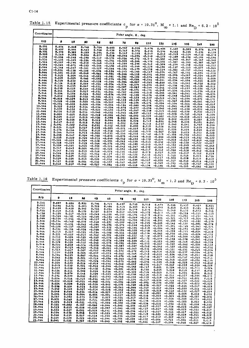
0 Table 1 . 1 6 Experimental pressure coe f f i c i en t s c f o r rr = 1 0 . 3 3 , M_ = 1 . 2 and R e , = 6 . 3 . 10 5 D

0 5 Table 1 .17 Experimental pressure coefficients c for a = 15.31 . Mm = 0 . 7 and ReD = 5. 2 . 10
P I
Coordinates Polar angle. rn , deg.
"10 0 11 so 45 60 13 90 19)
0 M m Z 0 . 8 and R e = 5 . 6 ' 10 5
Table 1.18 Experimental pressure coefficients c for a = 15.38 , P D
I


0 5 Table 1. 21 Experimental pressure coefficients c for o = 15. 53 , Mw = 1 . 0 and Re,, ;- 6 . 1 ' 10
P
i
0 5 Table 1. 22 Experimental pressure coefficients c for or = 15.59 , Mw = 1 . 1 and Re = 6 . 2 ' 10
P D
I

Table 1. 24 Experimental p res su re coefficients c fo r o = 20°. Mm = 0.7 and Re, = 5. 2 . 10 5 n
Table 1.23 Experimental p res su re coefficients c f o r = 15. 650, M m = l . Z and R e D = 6 . 3 . 10 5
Coordinates
XI0
O.?" o.'B2 0'i3L o.9dJ 1.238 1.5a0 L.q4* ' 2 3.'"* ' - * 'e9" ' s"" L.L'4 6.36' 7.CI' 7.9 , . 8.466 # - ? + * 9.C'* 9.'*4
10.*b5 10.>c+ """ ' I?-*** 12.*'+ 13-''4 L3.''' ~ ' .~ '* 16.94+ a5."' L5.'b4 Lb+"' 14.9b0
Lr.911 L8-'** 10.9** lq.b'* 19.9*4 2°.L4' 2J.q'4 21.'''
P
P o l a r m g l e . a. deg.
0 I S )$ 6 0 1 5 9 0 1 0 5 120 3 5 150 1 6 5 l ( 0
I I . 2 3 0.918 0.936 0.845 0.7:3 0.595 0.513 O.III 0.35, 3.331 0.323 o.921 O r 3 2 , 0.7a0 0.762 0.703 O-bZl 0.506 0.391 0.295 0.26' 0.142 0.116 0 . ~ ~ 1 O.oel 0.018 O e S b 8 0.5*b 0.489 0.*Ol 0.301 O.IP* 0.098 O.G>U -0.031 -0.962 -0.065 -0.36z -C.ob2 0.3'3 0.322 0.271 0.196 0.399 0.001 -0.CB1 -0.154 - 0 . 1 ~ ~ -0.210 4 . 1 0 7 -0.1P8 -O.IF1 0.138 0.110 0.074 O.CO7 -0.084 -*.I76 -0.268 -0.3j1 .0.3+3 -0.346 - 0 . ~ ~ 0 -0.318 -O.,l, 0.333 0.320 -0.021 -0.091 -0.172 -0.258 -0.327 - 0 . 3 ~ 3 -o. '<~ -.".3qb -0.36s -0.346 -0.336 0.c57 0.033 -0.012 -0.018 -0.179 -0.271 -0.3+6 -0.3.?3 -0.381 - 0 . ~ 2 1 -0.251 -0.192 -0.172 0.051 0.023 -0.021 -0.100 -0.195 -0.790 -0.365 - 0 . 3 ~ ~ -0.292 -0.182 -o.lo7 -0 -o.050 0.028 c . 0 ~ 3 -0.014 -0.122 -0.220 - 0 . 1 ~ 1 -0 .~00 - C . 3 , 5 -0.176 -O.iL, -O.LL -0.0b6 -0.036 0 .523 0.001 -0.366 -0.135 -0.236 -0.3'3 -0.305 -o. :~z -0.135 -0.128 -fi .L)I .-0.034 O.O1, 0.C12 O-Ulb -0.031 -0-132 -0.232 -0,236 -0.2!+ -0.198 -0.103 -0.123 - 0 . ~ ~ 2 -o.00"10.G,73 0.016 O.o2* -0.0*3 -0.122 -0.150 -0.208 -0.185 - 0 . 1 ~ 6 - 0 . 0 ~ 7 -0.113 -0.126 -O.O1, O.OOl O.ol* 0.013 -0.03* -0.097 -0.169 -0.214 -0.201 - 0 . 1 1 ~ -0.106 -0.113 -0.212 -0.053 -o.a18 0.070 O.05b -0.002 -0.062 -0.117 -0.185 -0.185 -0.116 -0.097 0 . - 0 . 1 5 ~ -0.08 -0.353 0.058 o.G63 0-013 -0.07. -0.135 -0.193 -0.179 -0.091 - 0 . 0 0 ~ - 0 . ~ 6 ~ - 0 . 0 ~ 1 - o . ~ ~ ~ -o.028 0.361 o-C+) -0.006 -0.012 -0.157 -0.113 -0.114 -0.oe.1 -0.075 -5.378 -0.C8, -o.103 -0.078 0.:81 0.548 0.037 -0.061 -0.122 -0.170 -0.157 -0.019 -0.002 -2.:65 -0+0,2 -0.078 -O.O 56 o.Ja9 0.076 0.010 -0.053 -C-135 -0.1S4 -0.110 -0.050 -0.019 - 0 . ~ 5 ~ -0.372 -o .0,5 -o.Cli2 0.35' O.C32 0.013 -0.053 -0.100 -0.157 -0.161 - 0 . ~ ~ 5 -0.056 -0.013 -0.053 -o.056 -o.0,7 0-089 O.Ob2 0.010 -0.059 -0.119 -0.118 -0.13'. -0.012 -0.059 -0.065 -0.068 -0.075 -O.GCB 0.07* 0.073 0 . ~ 2 3 -0.020 -0.110 - 0 . 1 ~ 1 -0.132 -0.5'.1 -0.0,6 -o.Cb2 -0.013 -0.03, 0.378 0.666 0.023 -0.059 -0.116 -0.151 - 0 . 1 ~ 8 - 0 . ~ ~ 9 -0.056 -o.C63 -0.150 -O.O1b -0.0,6 O.oJJ 0.062 0.023 -0.053 -0.116 -0.1s. -0.116 -0.653 - 0 . 0 ~ ~ -o.y+6 .0.050 -O.PIO -01031 0.379 0.06t 9.135
0.027 -0.043 -0.9d* -0.126 -0.100 - o . c ( ~ -0.046 - 3 . 3 -01C30 -C.Oj, 0.081 0.323 -3.027 -0,ITJ - 0 - l * l -0.108 -0.250 -0 .~30 - 0 . 3 ~ 1 - 0 . ~ 1 9 .,0.036 -C.02,
O.G1l 0.05* -0.@5+ -0.C98 -0.04'1 0.000 0.0:8 0.001 0.LO) 0 : 0.C20 C-C,3 D-:PZ 0.095 0.111 o . c n -0.030 -0.07v -0.06- -o.c:,q -o.020 -o.o15 -o.ooa -e.03, -o.o,,, 0.16l 0.1+0 0.075 0 . ~ ~ 3 -C.OM -0.111 -0.100 . -o.n2e . -o.c22 -n.o,r 0 0.104 0.051 -0.931 -0.093 -0.135 -0.111 -0.,%i2 - 0 . 0 ~ 1 -0.3)) -0.,118 -O.O1b -0.027 O . C a l o.08q O.0Iq -0.039 -0.095 -0 . l2 t -0.196 -0.~12 - 0 . 0 ~ 6 - 3 . 0 1 ~ -0.050 -0.C5, -0.039 O.Oal O-C52 -0.001 -0rC58 -0.129 -0.157 -0.IZv -O.:*L -0.051 -0.339 -0.C3P -0.030 -0.017 0.323 0.023 0.023 -0.050 -0.103 -0.131 - 0 . 1 ~ - 0 . o ) ~ -0.051 - O . ~ + + -0.t.14 -O.Oll *.OZ 0.376 0.057 0.03) -0.057 -0.078 -0.105 -0.084 -O.O,,Z - J . o + ~ -o.?+g -O.O,g -5.052 -O.0,1 0.077 O-Ohb 0.020 -0.031 -0.093 -0.114 - 7 1 -0.037 -0.0,,7 -0 .~14 -0.017 -0.057 -0.0,6 0.319 0.076 O.Ca5 -0.039 -0.CbO -0.103 -0.014 - 0 . ~ 4 6 ..3.038 - 0 . ~ 5 ~ -o.052 -.0.051 -0.036 0.07b 0.069 0.029 -0.011 -O.C+? -0.075 -0.!>52 - 0 . ~ 1 5 -0.019 -0.019 - 0 . 0 ~ ~ -0.C25 -0.023 o.Oqr 0.100 0.399 -0.007 -0.C27 -0.063 -0.ohl -0.012 - 0 . 0 1 ~ -0.012 - O . O l l -.O.OIP -O .CL5 0.112 O.090 0.0*3 -0.009 -0.006 0 1 3 2 - 0 . 1 2 -0.058 -0.o11 - 0 . ~ 3 ~ -0.028 -0.02 -0 .0,5 0.3P2 0.071 0 . 0 1 ~ -0-035 -0.133 -0.159 -0.122 -o.a:r -0.252 -o.nr, -0.036 -0 .,,+ -o.04, o.obL O.O1b -0.020 -0.090 -0.121 -0.126 -0.108 -0.665 -0.065 -2.360 - 0 . ~ ~ 2 -0.060 -O.oLO 0 . ~ 5 1 0.012 0 . ~ 7 -0.354 -0.116 - 0 . 1 1 ~ -0.12, -0.3,.6 -0.05, -O.DbO -0.356 -0.C6L -0.058 D . J E a 7 0.016 -0.339 -0.108 -0.108 -0.099 -0.366 - 3 . 0 3 ~ - 0 . 3 ~ 2 -0 .038 -0.033 -0,023 0 . 3 ~ 5 0.08+ 0.075 0.013 - 0 . ~ 6 8 - O . D I ~ -0.052 -0.C)3 -J.02a -0.036 -J.03q -0.0C9 -o.04q O.ob8 0.052 0.023 -0.050 -0.095 -0.137 -0.121 -0.062 -0.0+7 -0.012 -0.C,7 -o.055 -O.Olb 0.J90 0.010 0.024 -0.030 -0.119 -0.111 -0.105 -0.050 -0.011 -C.O++ -0.03q -o.c3L -0.036 3.386 D-OM 0.028 -0.011 -0.070 -0.116 -0 .1~0 -0.116 -0.417 -0.111 -0.0.q -0.C66 -o.060
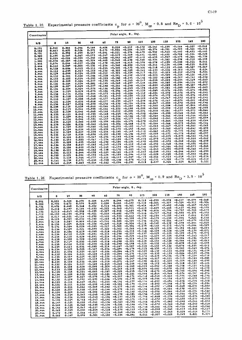
0 Table 1 . 26 Experimental pressure coefficients c for n = 20 , Mco = 0 . 9 and Re,, = 5 . 9 . 10
5
P
1 Polar angle. +.


0 5 Table 1.30 Experimental pressure coefficients c for cz = 20 . Moo = 1. 2 and ReD ' 6 .3 . 10
P
I


0 Table 1.35 Experimental pressure coefficients c fo r a = 25 , Mm = 1.0 and ReD = 6 . 1 . 10 5
P
Cuordfnate. I
0 Table 1 . 3 6 Experimental pressure coefficients c for a : 25 , M = 1 , and Re = 6. . 5
Coord~nates
XI0
0.251 0.482 0.731 O.980 1.238 1.500 1 . 9 ~ 1 2 -4 i4 2.04* 3.464 Y.P+4 *.'16 6-96 . '."* 5-74' 6.'~' 6.qr l ' 7.9'' 0.+" 8.9C* + ' *.'I+$
1 0 . * ~ * 13'q" " ' l'.q'+ 12."' 12.qbG l 3 33.1b* L't.64b l I .946 15.*++ 11.9II ' ' Lb.l+$ 1 7 . w 11 .9~1 1 8 . b ~ 1 18.94+ IP.LII 19.911 23.r.4 z0.911 1 4 4
P w D
Polar angle, 4 , deg.
0 IS 30 45 60 71 90 105 120 135 150 165 I c a
0.560 0.669 0.41) 0.210 0.009 O.+oo -0.128 0.26% -0.031 -3.001 0.02s - o . u I ~ . o ~ ~ o . P ~ + 0.926 o.810 0.640 0.433 0.211 0.019 - a . ~ ~ a -0.13: -0.199 -0.172 -0.14,. -o .~I , 0.758 0.721 0.407 0.449 0.245 0.025 -0.147 -0.231 -0.334 -0.352 -0.315 -0.26) -0.2.8 0.334 0.50" 0.393 0.239 0.051 -0.141 -0.323 -a.*46 -0.513 -0.488 -0.445 -0.37. -0.313 0.338 0.307 0.202 0.055 -0.122 -0.306 -0.+69 -0.586 - 0 . 6 -0.602 -0.148 -0 .~6 : - o .+ ,~ 0.157 0.129 0.031 -0.119 -0.259 -a.hlo -0.576 -0.6a1 -0.730 -0.654 -0.591 -o..ls - 0 . ~ ~ 5 0.237 0.20s 0 . 1 0 ~ - 0 . 0 ~ -c1233 -a.+la -0.602 -0.730 -0.785 -0.553 -0.373 -0 I.> - 0 . 1 ~ 1 0.225 O.l'l5 0.095 -0.061 -0.260 -0.485 -0-664 -0.779 -0.574 -0.618 -01383 -0:lOO -0.521 0.198 0-161 0-O5b -0.lOP -0.299 -0.521 -0.500 -0 .450 -0.458 -0.732 -0.411 -0.011 0.015 0.185 0.150 0.037 -0.125 -0.325 -0.550 -0.604 -0.326 -0.357 -0.599 -0+++1 -0.062 -0.016 0.180 0.141 0.018 -0.152 -0.357 -0.571 -0.404 - 0 . 2 2 -0.296 -0.311 -o.+$o -0.062 -0.016 0.171 O.l2* 0.002 -0.171 -0.317 -0.537 -0.242 -0.229 -0.253 -0.215 -0.273 -0.263 -0.177 0.161 0.120 0.002 -0.183 -0.384 - 0 . 3 2 ~ -0.27. -0.245 -0.199 -0.202 -0.205 -0.211 -0.11~ 0-15s 0.120 -0.014 -0.1.G -0.325 -0.420 -0.113 -0.226 -0 .1s~ -(.189 -0.192 -o.211 -0.2L9 0.291 0.168 0.041 -0.103 -0.292 -0.479 -0.316 -0.216 -0.106 -O.l7(I -0.173 -0.192 -0.206 0.19' 0.15' 0.037 -0.11P -0.29P -0.501 -0.319 -0.200 -0.186 -1.119 -0.163 -0.167 -0.154 0.19% O-L** 0.033 -0.122 -0.295 -0.485 -0.337 -0.16, -0.176 -0.160 -0.160 -0 .13~ -0.14'1 0.196 0.15* 0.033 -0.122 -0.295 -0.185 -0.245 -0.366 -0.110 -0.160 -0.147 -0.11, -0.i31 0-IVO 0.117 0.037 -0.119 -0.305 -0.386 -0.186 - 1 2 1 -0.150 -0.1.4 -0.166 -0.153 -0.111 0.234 0.134 0.031 'Ot12b '0.302 -0.365 -0.199 -0.121 -0.147 1 3 -0.166 -0.166 -0.157 0.158 0.049 -0.106 -0.272 -0.394 -0 225 -0.160 -0.160 -0.167 - 0 . 1 ~ ~ -0.117
o.18* 0.150 0.053 -0.103 -0.249 -0.39. -0:225 -0.117 -C.I+O 0 . 1 -0.137 - 0 . 1 ~ ~ -G.l,4 o . ~ ~ I 0.161 0.051 -0.099 -0.25. -0.394 -0.183 - 0 . 1 ~ s -0.12, -0.126 - 0 . 1 ~ s - 0 . 1 1 ~ -o.cl!2 C.203 0.176 0.066 -0.081 - C . Z I ~ - ~ . 3 3 ~ -o.18v -o.l17 -o.lo. -o.lo, -o.c.l o 'Lq l o.16' 0.055 -0.096 -0.2+8 -0.333 -0.113 - C . l l $ -0.110 -?.I21 -0.132 - 0 . 1 ~ ~ -0.12( 0.178 0.1*5 0.038 -0.111 -0.266 -0.340 -0.196 -0.111 -0.115 -I.:?$ -0.130 -0.13, -3.L13 0.183 O.1** 0.011 -0.113 -0.250 -0.325 -0.161 -0.107 -0.135 -P.LIP -0.125 - 0 . 1 ~ ~ -0.12b 0.16' 0.131 0.023 -0.132 -0.291 -0.285 -0.156 -O.IOI -0.106 -o .~oo -0.117 -o.,07 0.203 O.l+a 0.031 -0.129 -0.249 -0.300 -0.156 - a . ~ a l -0.110 -r.lla -0.135 -o.toi -o.ols 0.205 0.L73 0.063 -0.098 -0.256 -0.315 -0.17, -0.109 -0.670 -1.082 -0.104 -0.07, -c.cps 0.190 0.158 0.066 -a.o7v -0.184 -0.285 -0.122 - 0 . ~ ~ 7 -0.017 -0.,74 -c.0,9 0.221 0.185 0.085 -0.C6b - 0 . 1 9 ~ -0.257 -0.115 -0.051 -0.051 -0.160 -0.061 -O.OTT -0.018 0.251 0.211 0.133 -0.052 -0.209 -0.22. -0.117 - 0 . ~ 7 1 -0.075 -0.079 -0.078 -0.087 -0.07. 0.27* 0.231 a.llr -0.031 -0.164 - c . z e ~ -0.183 -0.101 -0.0P8 -o.0a9 -0.081 0 . 2 0.231 0.134 - 0 . 0 ~ 2 -0.113 -0.328 -0.201 a . -a.l17 -0.109 - c . o ~ ~ -a.102 -0.096 o.231 0.196 0.097 -0.014 -0.194 -0.353 -0.233 -0.138 -0.125 -3.124 - c .~ I ) -0.11) -O.Io, 0.212 0.171 0.071 -0.066 -0.219 -0.378 -O.2+6 -0.116 -0.119 -0.12, -0.122 -0.114 - 0 . 1 ~ 6 0 . ~ 0 2 0.160 0.066 -0.078 -0.231 -0.365 -0.204 -0.109 -0.100 -0.137 -0.105 -0.107 -0.0~. 0.215 0.186 0.076 -o.abv -C .Z>* -0.306 -0.164 -0.112 -O.LOI -0.116 -0.112 -0.12~ - o . ~ ~ ~ 0.236 0.1L9 0.06b -0.183 -0.23B -0.335 -0.Iq8 -0.126 -0.11s -$.I21 -0.127 -0.135 -0.116 0.235 0-17- 0.056 -0.090 -0.256 -0.351 -0.216 -0.136 -0.137 -$.I36 -0.117 -0.147 -3.131 0.171 0.156 0.057 -0.091 -0.256 - 0 . 3 4 ~ -0.221 - o . L + ~ -0.165 -0.152 -0.1~2 -0.15. -0.11s 0 . l b l 0.136 0.031 -6.110 -0.270 -0.160 -0.231 -0.136 -0.117 -0.13L -0.147 -0.1.2 -0.136 0.157 0.137 0.027 -0.110 -0.246 -0.303 -0.214 -C.L26 -0.112 -0.119 -0.137 -0.13, -0.131 o.115 0.138 0.015 -0.108 -0.263 -0.308 -0.2:~ -0.121 -0.109 -3.116 -0 .12~ -0.12; -0.111 O.lI7 0 . 1 ~ 0.0*2 -0.102 -0.154 -C-352 -0.188 -0.C16 -0.043 -0.017 -0.clz - 0 .~23 0.1.6

0 Table 1.37 Experimental pressure coefficients c for a = 25 , Mm = 1 . 2 and ReD = 6 . 3 . 10
5
P
Polar angle. a , deg.
0 = 0.7 and R e = 5 . 2 . 10 5
Table 1. 38 Experimental pressure coefficients cp for 0 = 30 , D
1 Coordinates Polar angle. Q . deg.
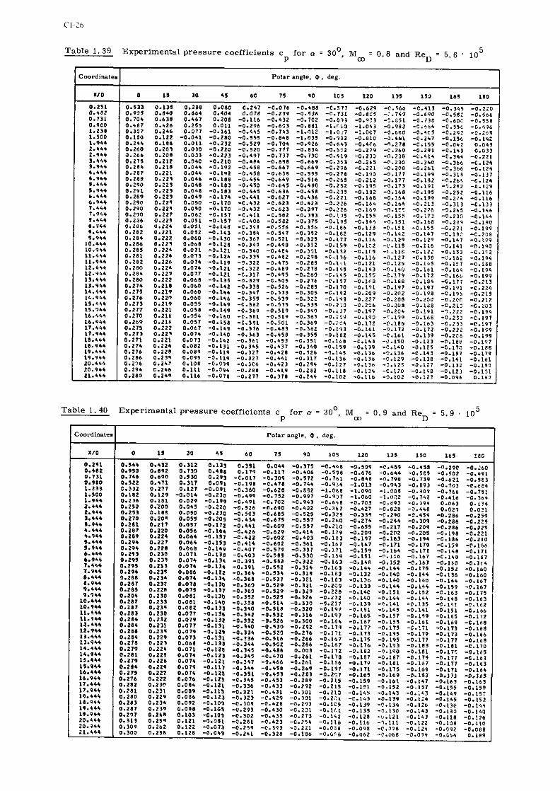
Cl-26
0 Table 1.39 Experimental pressure coefficients c for n = 30 , M m = 0 . 8 a n d R e = 5 . 6 ' 10 5 P D
0 Table 1. 40 Experimental pressure coefficients c for o = 30 . Mm = 0.9 and Re = 5.9 . 10 5 P D
Coordinates
XI0
0.251 0.+82 0.731 0.980 1.238 1.500 1.944 2.*L* 2.PI4 3 . 3.944 6.~11 6.941 3.~11 5 . w ) .+*I b.94+ 1 ?.?'I* 8 . 4 8.1LI
9 . P I I LO.++* LO.*++ Il.C4* 11.914 12.6bi 12.Y4I 1 13.964 1 . 4 1C.q*+ 15.kl+ IS.?** I b . l c + 16.P++ 11.+4b LI.VLI 18.664 18.946 19.446 1 9 . 9 I I 20.664 20.P++ 11.166
P o l a r angle. @ , deg.
0 1 5 30 45 60 75 PO 165 120 135 150 1 5 180
0.533 0.135 0.288 0.080 0.2+l -0.076 -0.688 -0.571 -0.629 -C.56@ -0.413 -0.315 -0.220 0.915 0.840 0.664 0.404 0.078 -0.239 -0.136 -C.731 -0.805 -:.I+? -0.690 -0.59: -0.566 0.704 0.638 0.4b7 0.208 -0.116 -0.132 -0.702 -0.871 -0.033 -C.aEl -0.138 -C.60; -0.558 0.487 0.126 0.255 0.011 -0.296 -0.603 -0.881 -1.rL3 -1+O*3 -0.982 - S . ? L + -C.511 -0., ,76 0.331 0.2*6 0.311 -0.161 -0.+45 -0.763 -1.012 -1.017 -1.007 -0.660 -0.4C5 -0.292 - 2 . 2 6 9 0.180 0.122 -0.041 -0.280 -0.555 -0.848 -1.035 -0.132 -0.010 -0.+61 -0.2+7 -0.156 -0.142 0.2.6 0.188 0.011 -0.232 -0.529 -0.704 -0.Q26 -0.643 -0.4C6 -0.278 -0.155 -0.042 0.013 0.260 0.203 0.030 -0.220 -0.520 -0.177 -0.834 -0.5?2 -0.279 -P.260 -0.291 -0.143 0.033 0.266 0.208 0.033 -0.213 -0.497 -0.737 -0.130 -C.+lP -0.233 -0.238 -0.41, -0.344 -0.221 0.215 0.212 0.010 -0.210 -0.+8+ -0.698 -0.669 -c.353 -0.265 - F . I ~ O - o . ~ + a -0.366 -0.12. 0.284 0.218 0.044 -0.192 -0.458 -0.667 -0.669 -C.71b -0.22, -0.20s -0.261 -P . laa -0.12+ 0.281 0.221 0.046 - 0 . 1 s ~ - 0 . 6 ~ 8 -0.658 -0.555 -0.218 -0.190 -c.17? -0.19s -0.316 -0.137 0.288 0.221 0.046 -0.188 -0.456 -0.669 -0.516 - 0 . ~ 6 5 - 0 . 2 ~ 2 - 0 . ~ 7 - 0 . 1 s ~ - o . P ~ \ -0.124 0.290 0.223 0.048 -0.183 -0.4so a . -o.rsa -0.11~ - 0 . 1 ~ 5 -0.173 -0.191 -7.252 - 0 . 1 2 ~ 0.291 0.223 0.068 -0.18) - 0 . 4 -0.636 -0.458 - 0 . 2 -O.LU -3.168 - 0 . 1 5 -0.251 -0.116 0.269 0.22) 0.019 -0.11* -0.441 -0.621 -0.436 -0.221 -0.168 -0.lb. -0.199 -0.211 -0.116 0.290 0.22' 0.~750 -0.170 -0.632 -0.623 -0.623 -0.226 -0.lbr -0.16, -0.213 -0.313 -0.13j 0.290 0.22- 0.050 -0.170 -0.632 -0.623 -0.397 -0.226 -0.1(,P -0.15: -0.226 -0.265 -0.146 0.210 0.227 0.062 -0.157 -0.411 -0.582 -0.183 - O m ! > ) -9.155 -0.155 -0.i73 -0.233 -0.101 0.236 0.225 0.051 -0.157 -0.406 -0.592 -0.375 -0.135 -0.115 -0.\51 '0.168 -0.237 -0.190 0 . 2 8 6 2 0.051 -0.1+8 -C.353 -0.5S6 -0.356 -0.186 -0.133 -0.151 -0.I55 -0.22, -0.199 0.282 0.221 0.052 -0.1+3 -0.384 -0.517 -0.352 -0.182 -0.129 -0.1C2 -0.117 -0.18: -C.ISa 0.28+ 0.222 0.060 -0.130 -0.361 -0.521 -0.325 -0.177 -0.116 -3.129 -0.12' -0.137 -0.?9? 0.286 0.221 0.068 -0.128 -0.349 -0.498 -0.312 -0.15- -0.LC2 - 1 1 5 - 0 . 1 1 -0.LIl -c.loP 0.285 0.224 0.071 '0.121 -0.3+0 -0.4OI -0.351 -0.132 -O.L<85 -1.118 -0 . l2 i -0.153 -=.LIZ 0.281 0.22. 0.011 -0.124 -0.335 -0.482 -0.29. 4 . 1 3 6 4 . 1 1 6 -0.127 -0.138 -2.162 -0.19+ 0.282 0-226 0.074 -0.119 -1.322 -0.475 -0.285 -0+\ ,11 -0.121 -0.12, -0.1'.5 -0.157 -0.168 0.280 0.224 0.014 '0.121 4 . 3 2 2 -0.489 -0.278 -0.1,+5 -0.163 -0.140 -0.111 -0.164 -0.196 0.28' 0.221 0.017 -0.121 -G.317 -0.495 -0.260 -(.XI5 -0.151 -0.?7P -0.172 - 0 . 6 -0.lPI 0.280 0.222 0.068 -0.135 -0.329 -0.505 -0.276 -C.157 -0.168 -1.160 -C.184 -0.177 -0.l?3 O.27+ 0 2 8 0.0b0 -0.142 -0.338 -0.526 -0.285 -0.170 -0.111 -0.197 -0.197 -0.LYl -0.224 0.275 0.21. 0.060 -0.144 -0.347 -0.533 -0.305 -C.IPZ -0.209 -0.202 -0.198 -0.115 -0.211 0.276 0.22e 0.060 -0.LIL -0.355 -0.539 -0.322 -0.193 -0.221 -0.208 -0.230 -0.2OC -0.211 0.273 0.219 0.055 -0 . l I9 -C.3(12 -0.515 -0.335 -0 .2)3 -0.206 - 0 . 2 0 8 -0.ISa -0.111 - ~ . i 0 3 0.277 0.221 0.058 -0.1+9 -0.36.1 -0.519 -0.340 - 0 . ~ 2 7 -0.197 -0.204 -0 . Iq l -1.222 -0.19% 0.210 0.218 0.05* -0.160 -0.381 -0.519 -0.365 - 0 . 2 ~ -0.190 1 -6.168 -0.233 -0.191 0.269 0.116 0.057 -0.158 -C.331 -0.501 -0.360 - C . i C I -0.172 -0.186 -0.16) -0.231 -0.197 0.275 0.222 0.067 -0.11'1 -0.316 -0.493 -0.362 -0.113 -0.161 -0.112 -0.172 -0.Z22 -0.199 0.273 0 . ~ 2 ' a.ot+ -o.lro -0.363 -o.+5e - 0 . 5 -0.181 -0.165 -0.161 -0.139 -0 .2~6 -0.199 0.271 0 + 2 2 1 0.073 -0.1*2 -0.361 -0.453 -0.351 -C.IO8 -C.I51 -0.150 -0.123 -0.18R -0.197 0.27+ 0.224 0.082 -0.131 -0.315 -0.437 -0.110 -0.159 -0.139 -0.140 -0.125 -C.170 -0.188 0.276 0.220 O-OBP -0.IIP -0.327 -0..21 -0.326 -0.145 -0.136 -0.136 -0.113 -0.157 -0.179 0.286 0.231 0.095 -0.119 - 7 - 0 . 4 - 7 -0.136 -0.156 -0.129 -0.138 -0.141 -0.161 0.276 0.247 0.108 -0.099 -0.3C6 -0.+23 -0.291 -0.127 -0.136 -> . I25 -0.127 -0.132 -0.159 0.29I C.Z*b 0.111 -0.09* -0.288 -0.419 -0.282 -0.118 -0.134 -C.110 -0.148 -0.123 -0.111 0.280 0.24. 0.116 -0.078 -0.211 -0.378 -0.246 -0.102 -0.116 -0.102 -0.123 -0.096 0.152 -
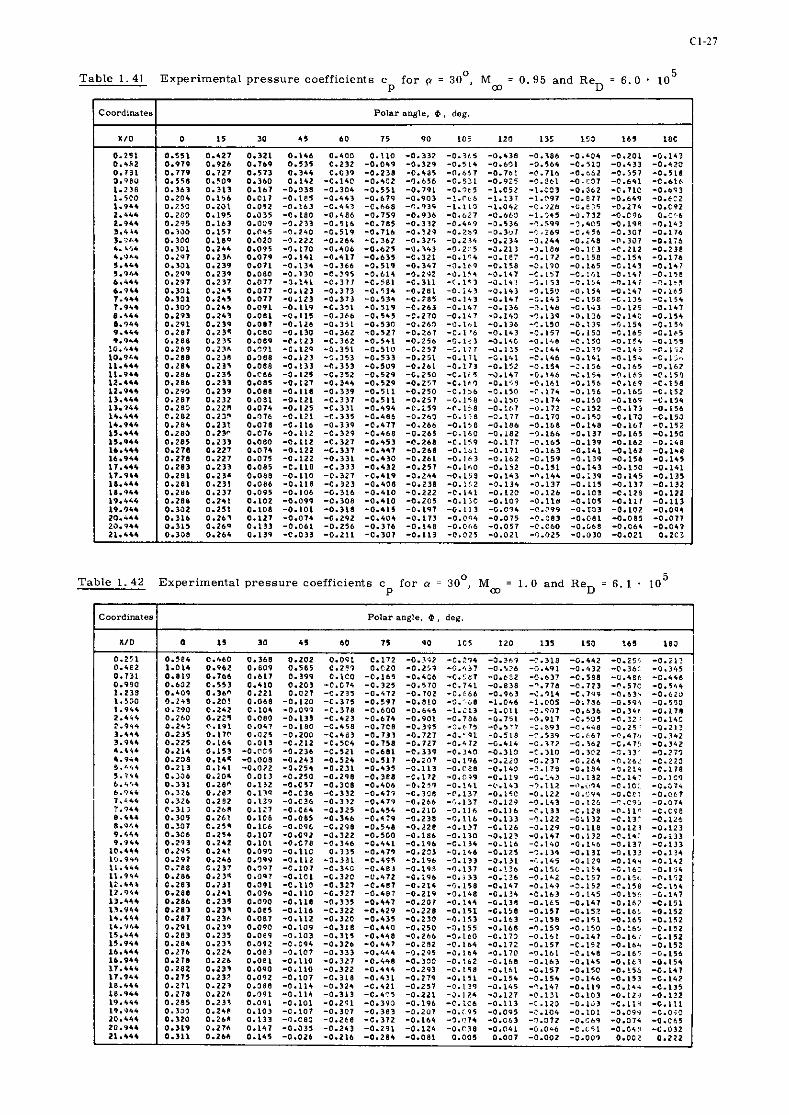
CI-27
0 Table 1. 41 Experimental p res su re coefficients c fo r q = 30 . Mm = 0.95 and Re = 6.0 . 10 5
P D
0 Table 1. 4 2 Experimental p res su re coefficients c for a = 30 , Mm = 1 .0 and Re,, = 6. 1 . 10 5 P
C o o r d i n a t e s
1 1 0
0.251 O.4fi2 0.131 1.P8U 1.238 1.5CO 1.PLI 2.466 2.964 3.6,. 3.l*+ b.rf8+ * . V h I 5 5-94. 6.i.L 6-96) I.*+* 9 8.444 1.14. P.+L+ 9 . ~ ~ 4
! O . C I I lO.9Lq l l .++L 11-9.4 12.4** LZ.*++ 13.++. 13.9LI 1 I4.9I4 15.*+4 15.94. 1*.1** Ib.qr4 11.6+4 I l . P I I l8.+6b 11.91* 19.G46 19.?+$ 20.i44 2J.9M 21.+*+
( c o o r d i n a t e s I P o l a r angle. Q , deg. I
P o l a r angle. a , deg.
0 I 5 30 4 5 60 1 5 90 103 120 135 193 165 18C
0.351 0.421 0.321 0.1.6 0.400 0.110 -0.332 -0.3LS - 0 . + I R -0.186 -0.LO4 -0.201 -0.143 0.979 0.926 0.769 0 . 5 5 0.232 -0.019 -0.329 -0.514 -0.611 -0.564 -0.513 -0.433 -0.420 0.719 0.721 0.573 0.3&+ C.031 -0.238 -O.+a5 -0.661 -0.761 -0.716 -0 .662 -0.551 -0.510 0.558 0.50. 0.360 0.142 -0.110 -0.502 -0.656 -0.831 -0.925 '0.861 -0.C31 -0.6+1 -0.616 0.3b3 0.313 0.161 -0.031 -0.304 -0.551 -0.791 -0.765 -1.051 -1.C03 -0.362 -0.710 -0.693 O.2Ol 0.156 0.017 -0.185 - 0 . 3 -0.679 -0.903 -?.PC6 1 -1 .097 -0.877 -0.649 -0.CC2 0.25O 0.201 0.012 -0 .163 - C . + C l -0.668 -0.719 -1.LI3 -I.O+Z -C.'l26 -Li.t>= -0.274 -0.C92 0.200 0.195 0.035 -0.180 -0.486 -0.759 -0.936 -0.627 -0.660 -1.3.5 -0.732 -0.COb O.C'6 0.295 0.163 0.009 -0.233 -0.516 -0.715 -0.312 -0.CIP -0.536 -1.599 -3.435 -0.19e -0.143 0.300 0.151 O.Oc5 -0.230 -0.519 -0.116 -0.129 -0.211 -0.3uT -9 .269 -5.456 -0.101 -0.176 0.300 0.180 0.020 -0.222 -0.264 -C.362 -0.325 -0.236 -0.236 -0.244 -0.i40 -0.307 -0.176 0.301 0.244 0.095 -0.110 -0.406 - 0 . 5 -o.?r> - 0 . 2 5 -3.21, -3.18.9 - 0 . 1 ~ 3 - C . Z L Z -0.238 0.2'41 0.236 0.079 -0.141 -0.411 -0.635 -0.321 -O.l"4 -U.l87 -0.172 -0.158 -0.154 -0.176 0.331 0.23'1 0.011 -0.13. '0.366 -0.519 -0.341 -3.1t.9 -0.158 -3.170 -0.163 -5.143 -0.147 0.299 0.230 0.080 -0.130 -0 .195 -0.614 -0.292 -0.1'4 -0.147 -5.157 -O.:bl -0.1+7 -0.i5C 0.297 0.231 0.017 -0.141 -0.311 -0.581 -0.311 - < . I 5 1 - 0 . 1 -5.153 -0.154 -0.1,; -r!.l11 0.331 O.:L5 0.017 -0.123 -0.373 -0.514 -0.281 - O . i < l -0.1+3 -0.150 -0.IS. -0.:<7 -0.IO5 0.331 0.245 0.077 -0.123 -0.373 -0.13, -0.785 -0.143 -0.141 - 3 . L C 5 - 0 . I S I - C . 1 3 5 - E . L S I 0.300 0.246 0.091 -0.119 -0.351 -0.519 -0.263 -0.LC7 -0.136 -".I$& -0 . l . i l -0.125 -0.147 0.213 0.2+1 0.081 -0.115 -0.Ibb -0.5'5 -3.270 -O.l<l -0.1$3 -1.139 -0.136 -C.I*C -0.154 0.291 0.23q 0.011 -0.111 -0.351 -0.530 -0.243 -C.lol 1 -S.150 -3.I lF -4.151 -0. l lG 0.281 0.23. 0.080 -0.130 -0.362 -0.527 -0.261 -0.l:b -0.143 -0.157 -G.150 -0.161. -0.lC5 0.288 0.235 0.089 -6.123 -0.362 -0.541 -0 .256 - s . l r > - 0 . 1 ~ -o. lna -c.lso -o.rr+ -o.lsg 0.2111 0 .23L 0.C01 -0.129 -0.351 -0.510 -0.251 - ' r . l i l - 0 . 1 3 5 -0.L4s -3.131 -0.140 -6 . i i2 0.200 0.238 0.008 -0.121 -2.153 -0.533 -0.251 -0.111 -C.lCl -0.116 - 0 . l l i -0 . lS i 'C.15,. O.28* 0.233 0.088 -0.133 -0.353 '0.509 -0.261 -0.171 -0.152 -0 .154 -3.156 - 0 . 5 -0.162 0.286 0.235 0.CL16 -0.125 -0.352 -0.529 -0.250 - 0 . l i 5 -0.L17 -0.1+6 -<.IS. -0.169 -0.158 0.286 0.233 0.085 -0.127 -0.34, -0.529 -0.251 -O.'.r3 -0.LS3 -O. ib l -0.156 [email protected] -(.I58 0.290 0.239 0.000 -0.118 -0.339 -0.511 -0.250 -0.156 -0.150 -P.l7. -0.156 -0.165 -0.152 0.281 0.212 0.081 -0.I21 -0.337 -0.511 -0.251 -0.168 -0.15D -0.114 -0.150 -0.lbS -0.l5'l 0.289 0.228 0.014 -0.125 -0.331 -0.49, - C . i > l -0.158 -0.1t.7 -0.172 -<.I52 -0.113 - 0 . l s b 0.282 0.21" 0.016 -0.121 -E.335 -0.486 -0.2'13 -0.158 -3.117 -0.110 -0.153 -0.173 -0.153 0.28I 0.231 0.010 -0.116 -0.339 -0.471 -0.266 -0.138 -0.186 -0.168 -0.148 -0.1'7 -0.152 0.283 0.23" 0.016 -0.112 -0.329 '0.468 -0.265 -0.160 -3.182 -1.166 -0.131 -0.161 -0.150 0.285 0.233 0.080 -0.1L2 -0.321 - 0 . L S 3 -0.268 -D.l*P -0.177 -0.165 -0.119 -0.162 - O . : * L I 0.210 0.227 0.07+ -0.122 -0.337 -0.141 -0.260 -0 . lo l -0.171 -0.163 -0.1.1 -0.162 -0.1.8 0.118 0.227 0.015 -0.122 -0.331 -0.r30 -0.261 -0.163 -0.162 -=.I59 -0.119 -0.156 -0.115 0.283 0.233 0.085 -0.118 -0.333 -Or*32 -0.257 -0.160 -0.152 -0.151 -0.1$3 -0.150 -0.141 0.281 0.23. 0.080 -0.110 -0.327 -0.4IV -O.2+4 -0.158 -0.1+3 -".L++ -O.:JP -0.1.5 -0.135 0.281 0.231 0.086 -0.118 -0.323 -0.408 -0.230 -0.152 - 0 . l l r -5.131 -0.115 -0.137 -0.132 0.286 0.237 0.OP5 -0.IOb -0.116 -0.410 -0.222 -C.l4L -0.120 -0.126 - 0 . L C 3 -C.I23 -0.122 0.211 0.2.1 0.102 -0.099 -C.108 -0.410 -0.205 -0.130 -0.107 -0.118 -0.105 -0. l i7 -0.113 0.352 0.251 0.108 -0.101 -0.318 -0.415 -0.197 -0.LI3 -0.01, +.a99 -0.133 -0.102 -0.0+1 0.316 0.261 0.127 -0.074 -0.292 -0.404 -0.173 -0.044 -0.015 -0 .C83 -0.081 -0.085 -0.071 0.3LI 0.26P 0.113 -0.061 -0.256 -0.376 -0.118 -0.0<,6 -0.057 -C.000 -0.G6S -0.06' -0.011 0.308 0.264 0.139 -0.033 '0.211 -0.301 -0.113 -0.025 -0.021 -0.025 -0.030 -0.021 O.ZC3

X I 0
0.251 O.CS2 0 . i l l O.'?OY 1.23'1 1.500 1..,46 2.,CC I.;)+& I.',, 3.1.. +.&+'I
4.0". 5.,;1(1 ,..,GI 6.ir+ 6.PI1 7 .414 7.9', El l+ ' 8 . 164 ..,.I 9.q.4
lo.**. 10 .911 11.+1. II.q.* 12.44' 12.9'4 13.464 13.V** 14.,.4 14.91, 15..4* 15.94, Ib..'* 16.9%+ 17.4,. 17.944 18.*4* 18.>'. 19...I 19.964 20.544 20 .944 2 1 . + 4 6
5 Table 1 .43 Experimental pressure coefficients cp for a = 30'. = 1 . 1 and Re,, ' 6 . 2 ' 10
Coordinafea Polar angle, Q . deg.
0 Table 1. 44 Experimental pressure coefficients c for a = 30 , Mm = 1. 2 and ReD = 6 . 3 . 10 5 P
CoordiMtes Polar angle, 4 , deg.

Table 1 . 4 5 Normal-force-, pitching-moment-, axial-force- and base pressure coefficients. Continued.
C A J c 4 , e..

Figure 1.1 Body geometry and coordinates of p res su re orif ices
h ' L N - - . - - LA d ' - ---- , x
- - - - L = 9,575 - - - -
View A - A -A
"0' LN=i.50 D =45mm
LA = 2 0 0 270' Q 90' 0.; ! ?2 Dimeter of pressure orifices 0.5 mm
Coordinates of pressure orifices (constant @ )

Figure 1 . 2 Model supports I and I1
pressure orifices model support I
134 0 ------
. . . - -- . - . -
model support E for oc. = 20: 25' u. 30'
cranked (157 mcdel support ~fcr angles of
M 1:2 -
iqgure 1 . 3 Reflection pattern of model head waves
---------- 7-
,//, . '///// /////////////://////////// /N/ / / / / i ;
1 I - a I I i
H=Height of the test section 6. H = Diagonal of the square test section

Figure 1. 4 Normal-force coefficients Figure 1. 5 Pitching-moment coefficients

Figure 1 . 8 Longitudinal distributions of pressure coefficient
Figure 1 . 9 Longitudinal distributions of pressure coefficient

Figure 1 . 1 0 Longitudinal distributions of pressure coefficients
Figure 1 . 1 1 Longitudinal distributions of pressure coefficient

Figure 1 .12 Longitudinal distributions of pressure coefficient
Figure 1. 13 Longitudinal distributions uf pressure coefficient

Figure 1 . 1 4 Longitudinal distributions of pressure coefficient
Figure 1.15 Longitudinal distributions of pressure coefficient
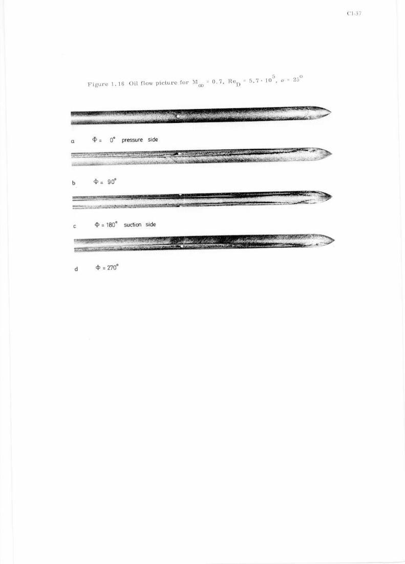

2 . MBB - Body Of R e v o l u t i o n NO. 3
W. Lorenz-Meyer
Deutsche Forschungs- und Versuchsanstalt fiir Luf t - und Raumfahrt E. V.
and
F. Aulehla
Messerschmit t - Balkow - Blohm GmbH, Ottobrunn (Miinchen)
Introduction
The present data s e t contains selected resul ts from surface p res su re and force measurements on
Body No. 3 of 5 parabolic bodies of revolution, which differ only by the shape of their afterbody.
Details of the model geometry a r e given in Fig. 2 - 1 . The presented data were taken during th ree
t e s t phases with the following a ims:
Phase 1: Surface p res su re measurements on 5 parabolic bodies of revolution. Variation of Mach
number, Reynolds number, and incidence; transition f r ee (Results: Table 2 - 4 , 2 -5 )
Phase 2: Surface p res su re measurements on 3 bodies of revolution (No. 1, 3, and 5) with check of repeata-
bility, and chord force measurements. Fur ther , variat ions of Mach number, Reynolds number,
and incidence were made; transit ion was fixed by carborundum(Results:Table 2-6, 2-7, and 2-8).
Phase 3: Forebody d rag force measurements with different aftbody contours. P r e s s u r e measure-
ments on tes t section wall with and without model. Variation of Mach number and Rey-
nolds number; transition fixed by carhorundum (Results: Table 2-9 , 2 - 1 0 ) .
The flow conditions included he re a r e l isted in Table 2 - 1 . In Phase 1 the t e s t s were performed
without fixed transition. In Phase 2 and 3, however, the transition were fixed a t about 5 $ L in
o rde r to have a turbulent boundary layer on the whole surface; moreover , forehody d r a g measure-
ments without fixed transition did not allow significant interpretation.
The included data a r e neither correc ted f o r blockage nor axial p r e s s u r e gradients. But it should he
emphasized that p res su re measurements on the upper and lower tes t section wall have indicated
some possible e r r o r s
a) for the stat ic p res su re p dependent on Mach and Reynolds number m
b) f o r the d rag due to an axial p res su re gradient in the tunnel depending on model, Mach,
and Reynolds number (Reference (141).
However, p res su re measurements on the center-l ine and on the side walls did not indicate any
gradients, except a t Ma = 0. 5. These e r r o r s which probably occur in al l t ransonic windtunnels m
and which usually l ie within the limitations of the measuring equipment a r e not essential f o r stan-
dard fo rce and p ressu re measurements.
1 . General Description
1 . 1 Model Designation o r Name MBB - Body - of Revolution No. 3
1 . 2 Model Type (e. g . , Full Span body of revolution
1. 4 Additional Remarks
2 . Model Geometry
2. 2 Body Data (Detail Description of forebody: x = 0 to x = 0 . 5 L cubic shape; Body Geometry) cylindrical par t : x = 0 , 5 L to 0 . 6875 L ;
aftbody: x = 0 , 6 8 7 5 L t o 0 , 9 6 7 L cubic shape st ing diameter: 3, 0 c m theoretical body length: L = 8 0 c m body diameter : D = 12 c m actual length: 7 7 . 4 cm analytical fo rm: s e e Fig. 2 - 1 [12], 1131

2.4 C r o s s Sectional Area Development
2. 5 Fabrication Tolerances/Waviness
2. 6 Additional Remarks
3. Wind Tunnel
3 .1 Designation
3. 2 Type of Tunnel
3. 2. 1 Continuous o r Blowdown. Indicate Minimum Run Time if Applicable
3.2. 2 Stagnation P r e s s u r e
3.2. 3 Stagnation Temperature
3 .3 Tes t Section
3.3. 1 Shape of T e s t Section
3.3.2 Size of T e s t Section (Width, Height, Length)
3. 3. 3 Type of Tes t Section Walls Closed, Open, Slotted. Perfora ted Open Area Ratio (Give Range if Variable) Slot/Hole Geometry (e. g. , 30-Degree Slanted Holes) Treatment of Side Wall Boundary L a y e r
Full span models Half-model testing
3 .4 Flow Field (Empty Tes t Section)
3 .4 . 1 Reference Static P r e s s u r e
3.4. 2 Flow Angularity
3.4. 3 Mach Number Distribution
3 .4 .4 P r e s s u r e Gradient I 3.4. 5 Turbulence/Noise Level
3.4.6 Side Wall Boundary L a y e r
3 .5 F r e e s t r e a m Mach Number (or Velocity)
3. 5 .1 Range
3 .5 .2 P r e s s u r e s Used to Determine Mach Number (e. g . . Settling Chamber Total P r e s s u r e and Plenum Chamber P r e s s u r e )
3 .5 .3 Accuracy of Mach Number Determination (A Ma)
s e e Fig. 2-1
I x 1 Meter Transonic Wind Tunnel,
continuous, closed c i rcui t
0 .4 ba r up to 1 .6 bar
ambient
squa re
1 me te r , 1 m e t e r , 3 m e t e r
perforated,
30 degree slanted holes, four walls a r e perforated and plenum suction is applied to adjust f ree s t r eam conditions.
In c a s e of 2-D and half-model-testing solid end plates ( q 0. 57 m ) a r e used.
plenum pressu re , calibrated against side wall s ta t ic p r e s s u r e and lancet-probe [3] in the empty tunnel, A u = A 8 < + 0. 05 wedge probe calibration
s e e Chapter A5 Fig. 5.5 and Ref. [ I ] , [Z], 131 a lso s e e 3. 5. 4
transonic Ma = 0. 5 - 1. 2; supersonic Ma = 1. 3 - 2 . 0
transonic range: settling chamber total p r e s s u r e / and plenum chamber p res su re . Dependence between plenum pressu re and f r e e s t r eam s ta t ic p res su re h a s been calibrated by lancet-probe and side-wall stat ic p res su re [3]
AMa = +_ 0.003
low turbulence level (measurements a r e in pro- g r e s s ) [ l o ] low noise level CJnF(n) <0.001) 181
Maximum Variation of Flow t_ n nsO
a
6
- -, -- Direction
Maximum Mach Number A Ma = t 0.001 Variation During a Run
0. 0 .8
8. 7 . 4
1 . 0
6 . 7
1 . 2
6 . 5 c m
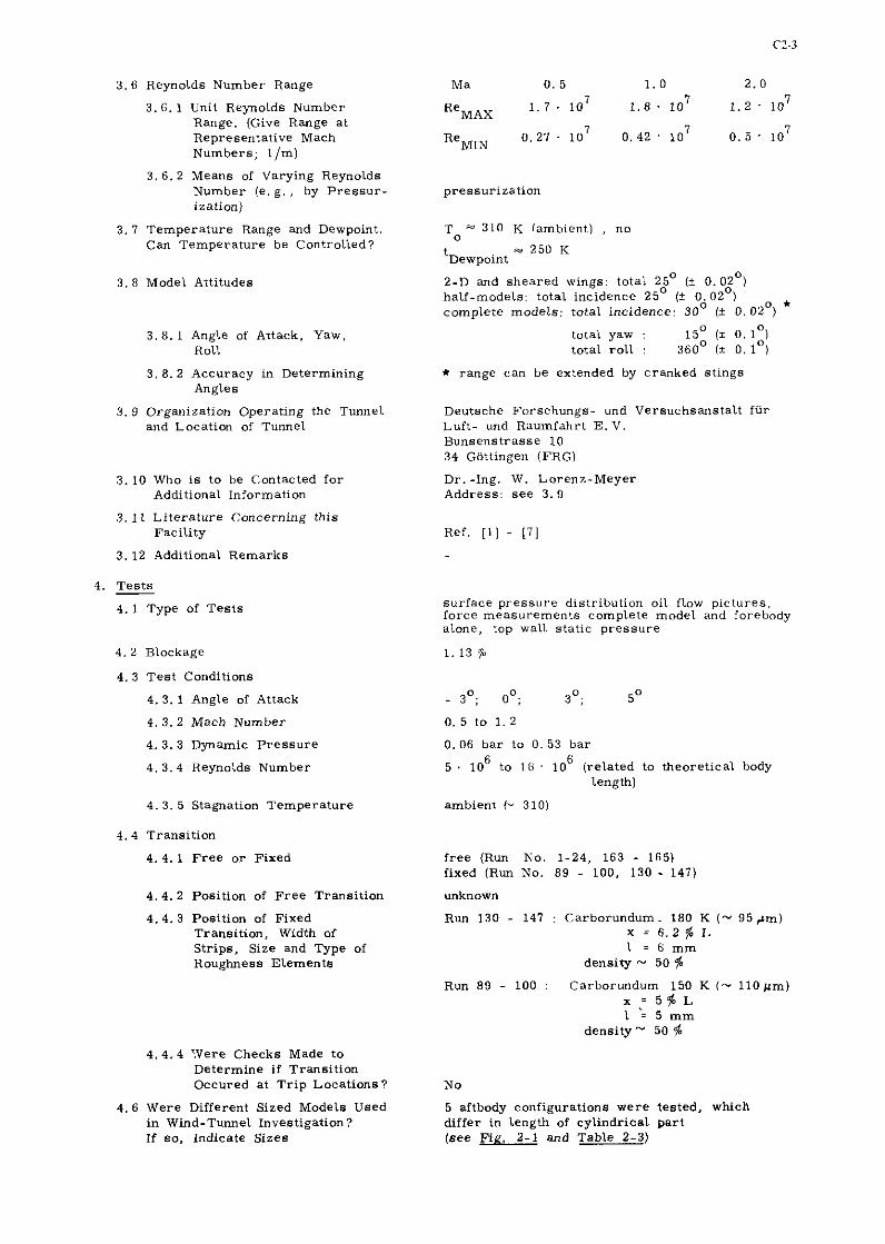
3.6 Reynolds Number Range
3.6. 1 Unit Reynolds Number Range. (Give Range a t Representative Mach Numbers; l / m )
3. 6.2 Means of Varying Reynolds Number (e. g. , by P r e s s u r - ization)
3.7 Temperature Range and Dewpoint. Can Temperature be Controlled?
3 . 8 Model Attitudes
3 .8 . 1 Angle of Attack. Yaw, Roll
3. 8. 2 Accuracy in Determining Angles
3. 9 Organization Operating the Tunnel and Location of Tunnel
3. 10 Who i s to be Contacted f o r Additional Information
3. 11 L i t e ra tu re Concerning this Facility
3.12 Additional Remarks
4. Tests 4. 1 Type of Tes t s
4. 2 Blockage
4. 3 Tes t Conditions
4. 3 . 1 Angle of Attack
4. 3. 2 Mach Number
4 . 3 . 3 Dynamic P r e s s u r e
4 . 3 . 4 Reynolds Number
4. 3. 5 Stagnation Temperature
4.4 Transition
4 .4 .1 F r e e o r Fixed
4 .4 .2 Position of F r e e Transit ion
4.4. 3 Position of Fixed Transit ion, Width of Strips, Size and Type of Roughness Elements
4 . 4 . 4 :Vere Checks Made to Determine if Transition Occured a t T r i p Locations?
4. 6 Were Different Sized Models Used in Wind-Tunnel Investigation? If so, Indicate Sizes
pressurization
To a 310 K (ambient) , no
a 250 K t ~ e w p o i n t
0 0 2-D and sheared wings: total 25 I+ 0.02 )
0 0 half-models: total incidence 25 (+ 0.02 )
0 0 complete models: total incidence: 30 (i 0.02 )
total yaw : 15O (t 0.1:) total ro l l : 360' I t 0. 1 )
* range can be extended by cranked s t ings
Deutsche Forschungs- und Versuchsanstalt fiir Luft- und Raumfahrt E. V . Bunsenstrasse 10 34 GBttingen ( F R G )
Dr. -1ng. W. Lorenz-Meyer Address: s e e 3.9
Ref. [ I ] - [7]
surface pr.es6ur.e distribution oil flow pic tures , force measurements complete model and forebody alone, top wall static p res su re
0 - 3 ; oO; 3O; 5O
0. 5 to 1 .2
0.06 bar to 0. 53 bar 6 6 5 . 10 to 16 . 10 (related to theoretical. body
length)
ambient t- 310)
f r ee (Run No. 1-24, 163 - 165) fixed (Run No. 89 - 100, 130 - 147)
unknown
Run 130 - 147 : Carborundum. 180 K ( - 95 +m) x = 6 . 2 % L 1 = 6 m m
density - 50 % Run 89 - 100 : Carborundum 150 K I - I l O g m )
x - 5 $ L 1 = 5 m m
density" 50 $
5 aftbody configurations were tested, which d i f f e r in length of cylindrical par t ( see Fic. 2-1 and Table 2-3)

4.7 Areas and Lengths Used to Form Coefficients
4.8 References on Tests
4. 9 Related Reports
5. Instrumentation
5.1 Surface Pressure Measurements
5.1.2 Pressure Orifices on Fuselage. Location and Number
5. 1. 4 Geometry of Orifices
5.1. 5 Type of Pressure Transducer and Scanning Devices Used. Indicate Range and Accuracy
5. 2 Force Measurements
5. 2. 1 Type and Location of Balance
5.2.2 Forces and Moments that Can be Measured. Maximum Loads and Accuracy
5.2. 3 Forces and Moments on Components.
Type and Location of Balance
Maximum Loads and Accuracy.
5.4 Surface Flow Visualization
5.4.1 Indicate Method Used to Determine
- Streamline pattern - Boundary-layer transition
6. Data - 6.1 Accuracy
6.1. 1 Pressure Coefficients
6. 1. 2 Aerodynamic Coefficients
6. 1. 4 Repeatability
6.2 Wall Interference Corrections
2 area: c ross section S = n D 14 = 113.09 cm
2
f o r Run No. 130 - 147, 163 - 165 cross section S = 112.81 cm for Run No. 89 - 100 base area: SB = 7. 54 cm 2
length: reference length L = 80 cm
[Ill - [I51 [I11 - [I51
see Fig. 2-2 and Table 2-2, 2-3
0.2 mm in diameter
CEC differential pressure transducers i 5 and i 10 psid; Scanivalve Type MJ 48 accuracy t 0. 3 qb FS
TASK 1.25 MK IV internal balance position see Fig. 2-3 (Run No. 130 - 147) axial force; 340 N; 1 qb FS
Forebody axial force (Run No. 89 - 100)
normal-force spring element, internally mounted (see: Fig. 2-4)
50 N; i 0.02 N
a Titanium dioxyd - oil suspension i s sprayed over the black painted model. Then the model i s exposed for a 10s to the flow of a Free-Jet-Blow-Dom- Facility of 0.75 m x 0.75 m test-section size. This facility i s different from that described in 3.
i 1 qb assuming worst possible combination of e r r o r s an error of A Ma = i 0.002, evaluated at
Ma, - 8 and max. c incLudbn8. t 0.5%
P
within 1 $, compare Run No. 10 and 163; see Ref. [ll]
standard wall corrections were not applied to these tests;
6.2. 5 Reference on Wall- Interference Corrections 151. [el. L141. [I51

6.3 Data Presentation Run No. 130 - 147: axial fo rce , base d r a g co r rec ted d rag of complete body
Run No. 89 - 100: fore body axial force , internal p r e s s u r e fo rce , "forebody"drag
6. 3. 1 Aerodynamic Coefficients Table 2-8, 2-10
6. 3.2 Surface P r e s s u r e Coefficients Fig. 2-5, 2-6, 2-7, 2-8. 2-9 and Table 2-4, 2-5,
2-6, 2-7, 2-9, 2-10
6. 3. 3 Flow Conditions f o r
- Aerodynamic Coefficient data Table 2-1 and P r e s s u r e data
6. 3. 6 Wall Interference Corrections Included? No, but s e e Fig. 2-14, 2-15, 2-16, 2-17, 2-18
6.3.7 Aeroelastic Correct ions No Included ?
6. 3.8 Other Correct ions? s e e Ref. (141, 1151
6. 3.9 Additional Remarks No
6 .4 Were Tes t s Car r i ed Out in Different It i s planned, to rebuild the cu r ren t model f o r Facil i t ies on the Current Model? t e s t s in AEDC 4 T and/or 16T. If so, What Facil i t ies. Are Data Contact: E . R. Thompson, Arnold A i r Force Base, Included in P resen t Data Base? Tullahoma, Tenn. 37389
7. References
[ I ] Ludwieg. H. Der Transsonische Windkanal d e r Aerodynamischen Versuchs- Lorenz-Meyer , W. anstalt Gattingen. Schneider, W. Jahrbuch WGLR 1966 (1967) pp. 145-155.
(21 Hottner, Th. Der Transsonische Windkanal d e r Aerodynamischen Versuchs- Lorenz-Meyer, W. anstalt Gattingen (Zweite Ausbaustufe).
Jahrbuch DGLR 1968 (1969) pp. 235-244.
(31 Lorenz-Meyer , W. Die Strahleigenschaften d e r Meastrecke des Transsonischen Windkanals d e r AVA. DLR-FB 66-19 (1966).
[4] Lorenz-Meyer , W. Tes t - Facil i t ies of the DFVLR in the Transonic and Hypersonic Speed-Range and Main Activities. DLR-FB 71-86 (1971)
[5] Mackrodt, P .A .
[6] Lorenz-Meyer , W.
[ I ] Lorenz-Meyer, W.
[8] Holst, H. Grosche, F. R. Binder, B.
Windkanalkorrekturen bei Messungen an zweidimensionalen P ro - filen im Transsonischen Windkanal de r Aerodynamischen Ver- sucbsanstalt G6ttingen. ZFW 19 (1971) pp. 449.454.
Kanalkorrekturen fiir den Transsonischen Windkanal d e r Aero- dynamischen Versuchsanstalt G6ttingen bei Messungen an d re i - dimensionalen Modellen. ZFW 19 (1971) pp. 454-461.
Der Transsonische Windkanal lm x l m d e r DFVLR - AVA - Ein tlberblick iiber die Aktivitgten von 1963 - 1977 - Festschr i f t zum 65. Geburtstag von Pro f . Dr. H. Ludwieg, pp. 4-1 + 4-54, Gattingen 1977
Druckschwankungsmessungen im Transsonischen Windkanal d e r DFVLR-AVA Gattingen. DFVLR-AVA - Report 251-75 A 17 (1975).

C 2 4
[9] Meier , H.U
[ l o ] Heddergott, A.
[12]Aulehla, F. Besigk, G.
[13]Aulehla. F. Besigk. G.
[IS] Aulehla, F.
8. L i s t of Symbols
The Response of Turbulent Boundary L a y e r s to Small Turbulence Leve l s in the External F r e e St ream. ICAS-Paper 76-05 (1976).
EinfluR d e r erhljhten Turbulenz d e r freien Anstr6mung auf die Druck- und Kraftbeiwerte e ines superkri t ischen Profi ls . DFVLR-AVA Report 251-76 A 10 (1977).
Beitrag zur F rage des Vorkljrperwiderstandes e ines nicht ange- stellten Rotationsk6rpers m i t unterschiedlichen Heckkonfigura- tionen. DFVLR-AVA Report 251-74 A 27 11974).
Reynolds-Number Effects on Fore - and Aftbody P r e s s u r e Drag. AGARD C P 150 No. 12 (1974).
Fore - and Aftbody Flow Field Interaction with Consideration of Reynolds Number-Effects. AGARD C P 208 No. 11-F (1975).
Grenzen d e r Widerstandsbestimmung schlanker Kljrper in t r ans - sonischen Windkanslen. MBB-Report UFE 1315 (0) 1976.
Drag Measurement in Transonic Wind Tunnels. AGARD Specialist 's Meeting on Ai rc ra f t Performance Prediction Methods. P a r i s 11977). Pape r No. 7.
surface p r e s s u r e coefficient on body shape
in ternal p res su re coefficient in the model
su r face p r e s s u r e coefficient on top tes t section wall
measured axial force coefficient
base d rag coefficient
co r rec ted axial force coefficient ei ther by base drag o r by internal p r e s s u r e d rag body diameter I= 12 c m ) measured value of surface p res su re (Volt) theoretical body length ( = 80 c m )
width of carborundum s t r ips (mm)
f r ee s t r eam Mach number
p res su re
dynamic p res su re
Reynolds number based on theoretical body length
2 body face a r e a (= 113.09 o r 112.81 c m Phase 2 o r 3 r eap . )
2 base a rea (= 7.54 c m )
temperature (K)
axial fo rce
axial coordinate f rom apex (cm)
angle of attack
s ide wall boundary layer thickness (pitot p r e s s u r e = 0,999 po)

Indices
0 stagnation condition
m free s t ream
i in the model
W on the wall
B model base
Table: 2-1 Flow Conditions Included in DATA BASE WBB-Body-of-Revolution No. 3)
1 12 ::? 1 iW:z 1 383.21 junction 400.30
u
i a
o
%
Table 2-2 : Position of Pressure Orifices, Forebody
Controll orifices on lower surface
Transition
free "
f r ee
fixed (180K)
fixed (WOK)
fixed 1180K)
fixed (150K)
a Po Ma
['I [mm Hgl
-3 735 0 735 3 735 5 735
0 300 0 1200
-3 135 0 135 3 735
-3 300 0 300
,0°
-3 1160 0 1160 3 1160
Ma Model R e
0.6 empty 0.6 Shape 3
0. 5 0 .6 0.8 0.85 0.90 0.95 0.98 1.05 1.10 1. 20
164 13 11 lO(163) 7 6 5 4 3 2 1
165 8 14 12 9
15 16 17 18 19 24 23 22 21 20
144 139 134 138 143 140 133 137 142 141 135 136
131 130 132
146 145 147
5.0 8 . 0 10.0 14.0
89 90 9 1 9 2 97 98 99 100

Table 2-3 : Position of Pressure Orifices. Aftbody ( 1 to 5)
Measurements on MBB-Body-of-Revolution
Body No. 3
Position of body static pressure orifices re l . to model apex [cm]
2.06 6.06 10.04 14.04 11.03 20.01 23.02 26.03 29.03 32.03 35.03 38.03 42.02 46.03 49.03 51. 54 54.03 56.06 51. 54 59.04 60. 55 62.06 63. 54 64. 54 65. 54 66. 53 67. 51 66. 51 69. 52 70.51 71. 51 72. 50 73. 49 74.48 75. 46 0.00 0.00 2.08 14.04 23.02 60.55 65.54
x-norninr " = I u e
400.0
420.0 460.0
490.0 515.0 540.0 560.0
575.0 590.0 605.0 620.0
635.0 645.0 655.0 665.0 675.0 605.0 695.0
705.0 715.0
725.0 735.0 745.0
755.0 765.0
175.0 end
I
S h s p 1
400.30 420.20
460.30 490.30 515.18
540.24 560.32
575.50 590.30 605.18
620.22
635.20
645.37 655.14 665.32 675.06 685.16
694.86
704.84 714.92 724.82
734.66
758.51
test ( point x/1
Constants & calibration:
Reference area S = 113.094 c m 2
Chord length L = 80 c m
Cal. of pressure pickup EP = 24.11 mm Hg/Volt
Cal . of chord force e l em. EX = 0.183 kp/Volt
junction
13 14
15 16
17 18
19 20 21 22
23 24
25 26
21 28
29 30 31
32 33 4
35 36 37
position
Table 2-4: Calibration and Geometrical Data, Test Phase 1
actual
Shape 2
400.30
420.30 460.30
490.30 515.18 540.30 560.34
575.34 590.36 605.30 620.90
635.30 645.14 655.22 665.20
675.10 685.02 694.96
704.92 714.88
724.92 734.82 744.76
768.96
0.525 0.575 0.6125 0.64175
0.675 0.7 0.71875 0.7375 0.75625
0.775 0.79375 0.80625
0.81875 0.83125
0.84375 0.85625 0.86875 0.88125
0.89375 0.90625
0.91875 0.93125
0.94375 0.95625 0.96875 of shape
value
Shape 3
400.30 420.18
460.34 490.34
515.36, 540.32 560.60
575.36 590.42 605.51 620.56
635.36 645.42
655.30 665.29 675.12 685.10
695.18 705.06 715.01 724.96 734.88
744.76 754.60
714.20
l rn-I
Shape 4
400.30 420.28 461.26
490.30
515.31 540.30 560.20
575.30 590.28 605.26 620.26
635.26 645.24
655.00 664.98 674.88 684.96 694.90 704.82 714.84 724.78
734.84 744.60
754.58 764.42
779.36
Shape s 400.30 420.70 460.50
490.50 515.70 540.50 560.30
575.40 590.30 605.50 620.60 635.60
645.30 655.40 665.80
675.40 605.70 695.40
705.30 715.20 725.10
734.90 744.55 754.30 764.10
774.1 785.03

S O r C - . 0 0 0 4 0 ~ C - - " m N d d d d m m * r n 0 * - 0 O C O O - - m 0 0 0
c- . - - - C 1 O O c m C I - " - o o = - . - - 0 4 - O - m ~ - o - ^ n - r - * m * - - - m . C - - m m h * - O - - - O O C o N o ~ m 001ee,.-*-L0m..00hC
m . Y - C O I O n m ~ 0 m 1 0 0 0 0 0 - O O * ~ ~ o . -*,---.***--DLmOD
m o C N 0 0 - - - - - - 0 0 0 0 0 0 0 0 0 - - * ~ - . * - 0 0 0 0 0 0 0 0 0 1 0 - - 1 . - d d d d d d d d d d d d d d d d d d d d d d d d d d ; d d d ; d d d d d d d d d d 3 t , , , . 0 , , , 8 , , , , a 0 <

m * O n n * 0 - * 0 .
(0 n o o r h - o m . ~ ? S X D L 7 0 E d F t t ; XSt0LS:43S042S$L:
n . : D!E$t$gl:g:::"Es4f2tc2: 00 - "0 * * *0N3*"0*0m
01 0 *hoo- - - - - -ooooooooo-NUoo ::zILSz13:22?081:: . - addadddsaddddd;fdddfdddd d d d d d d d d d d d d d d d d d 0 1 1 1 1 1 1 1 ~ ~ , , 1 4 1 , 1 1 1 , 1 1 1 0 0 . n

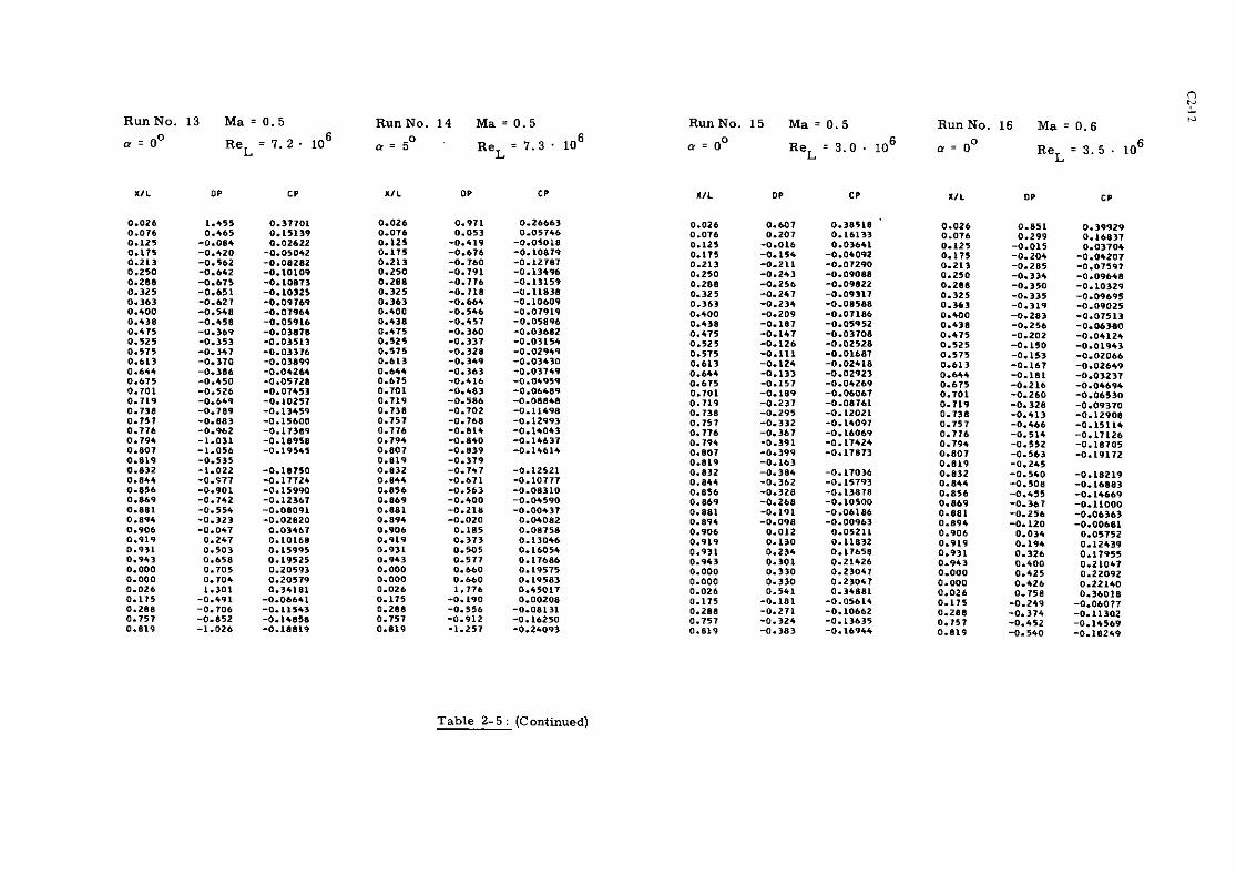
Run No . 13 Ma = 0 . 5 R u n N o . 1 4 M a - 0 . 5 0 a = O ReL = 7 . 2 . 10
6 o a = 5 ReL = 7 . 3 . 10
6
X I L OP C P X I L O P C P
RunNo . 1 5 M a = 0 . 5 RunNo . 16 M a . 0 . 6 0
0 = 0 a - 0 o R e = 3 . 0 . 10 R e = 3 . 5 . 10 6 L L
X I L O P C P X IL OP CP
Table 2 - 5 : (Continued)

(9 0 4
O O O * n O - Q . m O N C Q C * N m a m C . * N O n 0 a - ~ C n . m - a m N C - ~ Q - . - - C Q N C * C D D - O N N O a N a m - o ~ o N z m a w o m * . N - o o . o o
L I O * m d O F a N C m N I - D m O n C N - * - N - m - O C * m O O C - . . D N n O n 0 * u C - C n O m * O N D a - - N N m n C - ~ N ~ - N O - Q D - n - O C a O O m C n N C * N 0 0 - - - ~ ~ 0 0 0 0 0 0 0 0 0 - - N N m m N N - o o O - - - - - - * o - N N + d d d d d d d d d d d d d d d d d d d d d d d d d d d d d d d d d d d d d d d d d O I,
~ ~ ~ ~ , , , , , , I , 1 I , I I , 1 , , I , , , , , , , ,
0
4 ~ n C C O m n ~ O m ~ ~ n m . n - * O ~ o * - ~ h . ~ ~ - * ~ * - - o o ~ C m C * - h r h - - C ~ h O O l - N - - * - O - m n C * o - m * n ~ a O O ~ - . O O ~ O m C ~ 0 0 - - N N N - l . . . n n 0 0 0 - - - - ~ - m m m a ~ m a = ~ O - O O O O ~ N - ~ .
2 6 " d d d d d d d d d d d d d d d d d d d d d d d d d d d d d d d d d d d d d d d d d d
w C-
- - O O - N 4 - 0 m . O 0 C O ~ C I m a a . - - O a O - C . - D - - . r - . . - - * * C h m r N - m m - ~ O , - m m - - C o e n - - h O h C O D 0 0 h - h C O C h - D
D - h m 0 0 n m 0 0 a C h N * O . - m a - - > a * - P m - O m D O C O . , n m - O F N ., . O I . D - N ~ O O L m h N " m e C o C a o N " - * a - C - m C a O O O D Q m C -
m . - 0 0 0 - - - - O C 0 0 0 0 0 0 0 - - - N h n ~ - - - 0 0 0 - - h n ~ * 0 - - r ........................ . d ,o,oo,o,,ooooooooooooooo d d d d d d d d d d d d d d d d d 0 1 1 1 , 1 1 1 , ( 1 1 I , I # # . I I I * I a , ,

C O m - - 0 0 D ~ - a D - * - - m n . ~ - o N h 0 0 a O a 0 0 0 9 D O h . " . C F w ~ ~ . O n * O * O . O - O * . O D C a . - o N O - 0 O ~ . I C 0 a Q O - 0 4 C m N
D a * - C - O C h C - ~ a h N - O . N C N - h ~ - - o h o - o o o o o o o o . . n - Y C n m * m 0 0 0 ~ a Q . * . * C O O O * ~ m O o D a c - O - N O . . D O O . O - * O " " - o o o ~ - - o o ~ o o o o o o o - - - - - h - - - ~ o o o o - ~ N h - o - - ~ . . . . . . . . . . . . . . . . . . . . . . . .
o o o o o o o o o o o o o o o o o o o o o o o o d d d d d d d d d d d d d d d d d 0 , , a , , , a < , 0 , , a , , , , , , 0 0
2:0Zf:C8bt7DPfB:S$2::?2Z8 ZXZ:SPXl:313t:::: 0 O ~ 0 N ~ Q 0 ~ ~ 0 ~ ~ 0 0 1 ~ Q ~ n O m ~ N ~ o r o - ~ n r Q " m O O O r h r r -
c . u - o * ~ D N N - - o - ~ - O O O - - - - O O ~ - - ~ ~ ~ ~ ~ ~ ~ ~ ~ n ~ - ~ - - o ~ ~ c o - - ~ L - o I -D 67
O O q q O O - - - N N N N N - - o o O - C N N h " o - - N . - d d d d d d d d d d d d d d ~ ~ d d d d d d d d d d d d d d d d d d d d d d d d d 0 1 1 . 1 1 1 1 1 1 1 1 1 1 1 . 1 1 1 1 , I , , , , , 0 0 8 ,
O m - 0 . 0 0 n * m h - 0 - - ~ 0 . 0 0 O n n - * C I - n - D * - m O n " a D - O O O Q O O N C O O O O C C h N C N I Q O ~ O . 4 - m C O m - h a . - - N N h C 0 4
m D m C n C . O O O O - O C C m - Q . - O C - n O O 0 - a n o r - h O - O O I O - Q . .l . Y 00*COmn--0.*"m..OON.-.~m ~ " O F Q 0 a . m ~ 0 0 - . 1 0 0
* - 0 0 - - - - - - 0 0 0 0 0 0 0 0 - - N N h N h N - - 0 0 0 - - - h N . O - h N '=? 2 d d d d d d d d d d d d d d d d d d d d d d d d d d d d d d d d d d d d d d d d d 0 1 1 1 , 4 1 1 I I , I J I I I I I I I , , , , , , . a

Measurements on MBB-Body-of-Revolution
Body No. 3
Position of body stat ic p res su re or i f ices r e l . to model apex [cm]
2.08 6 . 0 6 10 .04 1 4 . 0 4 17 .03 20 .01 23 .02 26.03 29.03 32.03 35 .03 38.03 42 .02 46.03 49.03 51.54 54.03 56.06 57. 54 5 9 . 0 4 60. 55 62.06 63. 54 64. 54 65. 54 66. 53 67. 51 68. 51 69. 52 70.51 71. 51 72. 50 73. 49 74. 48 75. 46 0 . 0 0 .0 2.08 14. 0 4 23.02 60. 55 6 5 . 5 4 4.00 8 . 0 0 12 .00 0 . 0
Constants & calibration: 2
Reference a r e a S = 113.094 c m
SB = 7 . 5 4 c m 2
Base a r e a
Chord length L = 80 c m
Cal of p res su re pickup EP = 22.02 mm Hg/Volt
Cal of chord force e lem. EX = 0 .184 kp/Volt
Table 2-6: Calibration and Geometrical Data, Tes t Phase 2
RunNo. 130 Ma = 0 . 8 0
o = 0 Re = 4 . 4 . 10 6 L.
RunNo. 131 Ma = 0 . 8 0
a = -3 R e = 4 . 4 . 10 6
L
Table 2-7: P r e s s u r e Data (Run 130 to 147 , and 163 t o 165), Tes t Phase 2

Run N o . 132 Ma = 0 . 8 RunNo. 133 Ma = 0 . 8 o 6 o a = +3 Re = 4 . 3 . 10 a = 0 Re = 10 ' 10 6
L L
, . ,4 - 3- Run No . 134 Ma = 0 . 8 RunNo . 135 Ma = 0 . 8
0 6 0 a = -3 R e = 1 0 . 10 0 . 3 ReL = 10 . 10 6
L
Table 2-7 : (Continued)
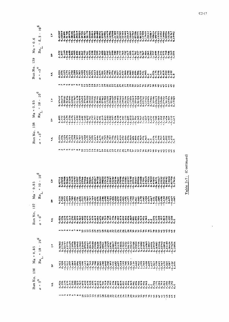

- - C;ZS2EE:8:::11:6ff6:c"Z62K62ZZ:XZ1Zf;~ZZ",ZFgt~Z
D N D O n D m D m l O ~ n D O - I O F I m N O m Q Q C N ~ ~ m ~ ~ ~ ~ ~ N - ~ ~ - N ~ m O a N * U " " ~ " 8 0 0 0 ' . , ~ g C . * r O C n a D I O C a * O L O . C,oo ,,-ooo o o o 6 8 o , , ~ , , ~ - ~ ~ ~ ~ 8 S d Z 2 f : ~ Z E B ~ ~ 0 , ~ Z B Z . P- d d d d d d d d d d d d d d d d d d d d d d d d d d d d d d d d d d d d d d d d d d d d d d
I, I I , , I 4 I J J , I I I I I I , 4 I , I ~ , l l l , , , ! I , I
II .
1Lll"itil"::t3zSf::::::2:z:0,::::::0,2::22:sz::: 3
m. O - . ~ . h h - Q . L C D C . N C - a m m ~ ~ * " ~ * h ~ - O o . ~ ~ . ~ e - m ~ o m ~ u ~ 8 g 8 = 2 " ~ ~ ~ g d 6 8 6 g S ~ g 1 : 2 ~ ~ i : ~ z f g ~ - - s h a - O s h - m * h - N e *
n . 0 0 0 - - - - - * 0 0 - N - 0 0 - . h
0 d d d d d d d d d d d d d d d d d d d d d d d d d d d d d d d d d d d d d d d d d d d d d d
1 1 1 1 1 1 1 1 1 1 1 1 1 1 1 1 ~ I I I I I I I I . I I , , a , 8
d 2 O, e ~ n n m o m c m o m c n n m . c - ~ m - ~ . - o o o o e D ~ ~ a D m * * o r e 0 0 0 c ~ C h C - C m h Q O m . h C - . . C - - * . ~ O O O O ~ O O O O ~ m . h F m m - C o C
a 5 ~o--NhhCC..*~m,,,..~-..OmmmOmmmOO~Oooo~~.mo~~o
(r a d d d d d d d d d d d d d d d d d d d d d d d d d d d d d d d d d d d d d d d d d d d d d d

RunNo . 144 M a C 0 . 5 RunNo . 145 M a . 0 . 8 o 6 o Re = 7 . 4 . 10 a = 0 Re = 15 . 10
6 a = -3 L L
Run No. 146 Ma = 0 . 8 RunNo . 147 M a . 0 . 8 o 6 o ReL = 15 ' 10 a = 3 ReL = 1 5 . 10
6 u = -3
Table 2-7 : (Continued)

Run N o . 163 Ma = 0 . 8 0 4 Run No. 164 Ma = 0 .801 o 6 o
a = 0 ReL = 10 . 10 a = -3 R e = 10 . 10 6
L
Run N o . 165 Ma = 0 . 8 0 0 0
a = 3 Re = 10 . 10 6 L
Table 2-1 : (Concluded)

Table: 2-8 Drag Data for Complete Model (Shape 3) at
Zero Incidence (Test Phase 2)
YE4SUQEYEhlTS ON HP6-d( rOY- , IF -REV3LUTIChl P O S I T I O N OF WALL S T A T l C PRESSURE R E L . T L ~ M'ICEL 4 P E X
Run
130
133
137
140
143
145
163
X R Y ( C H I
-20.73 -18.34 -15.93 -6.32 -3.83 -1.37
5.95 1 9 - 5 8 13.16 22.53 25.57 27.57
?1.88 49.37 41.Rt 51.31 53.75 56 -27
a Ma Po C~ B C
Xcorr
0 0.8 300 0,0623-0,0128 0,0751
0 0,80 735 0,0531 - 0,0133 0,0664
0 0,85 735 0,0541 -0,0129 0,067
0 0,60 735 0,0536 -0.0135 0,0671
0 0.50 735 0,0555 - 0,0135 0,0690
0 0.80 1152 0,0493 -0,0140 0,0633
0 0,804 734 0,0503 -0,0134 0,0637
CflhSTAMTS 6 CAL 1 3 F & T I O N
P F F F H E Y C E 4 1 E 4 S = 112.81 CM**2 CHORD L E N G T H L = 8 2 . ~ 3 ~r
C4L.OF PRESS.TKD. 4 P = 93 .25 MMkS/VOLT CAL.OF CHORD FORCE AX = 0.5868 V O L T I K P
Table 2-9 : Calibration and Geometrical Data, Test Phase 3

RESULTS RUN NO 8 9
4 1 FORCE MEISURFqTS. CX CXC3RR C P I nr REL
0.0 0.80050 0.552F 0 1 0.0 0 .80050 0.552E 0 1
X I L CPULLL
AVERAGE CP4 = 0 . 0 0 7 8 8 PV4R4GE SC4TTEP 4 5 = 0 .00h06
Table 2-10 : Force and Pressure Data. Test Phase 3 (Run 8 9 to 100)
MEISURE*ENTS ON Y 3 B - ~ O O V - l F - k E Y I ~ L ~ J T I J i
PESULTS R i l V YO 9 0
41 FORCE HE4SIIRFMTS. CX CXClPR C P I Ha REL
0.0 0 .80019 O.BI?E 0 1 0.0 3.19989 0.RLIE 3 1
R I STATIC WALL PREISUQE
I I L CPYALL
Table 2-10 : (Continued)

HE4SIIRE*E'ITS 311 ~ ~ R - S O O I - I ) F - f i ~ V ' I L U l I L V
RESULTS RUN NO 9 1
P I FnRCE YEASUREYTS. CX CXClRR < P I V A REL
0.0 0 .88350 0.995E 0 7
0.0 0.80150 0.'+94€ 3 7
H I S T L T I C HALL PRESSURE
X I L CDdALL
PVF f iP tE CPP - 0.001*1 bVL14GE SCLTTEP 4 5 = 5 . 0 0 7 6 0
Table 2-10 : (Continued)
MFbSUREMEMTS ON HRB-BOCV-3F-FEVOLUTILN
RESULTS %\IN NO 9 2
4 ) FORCE HELS'JREHTS. CX CXClRR C P I HA REL
0.0 0.800n3 ( 1 . 1 3 5 ~ O R 0.0 O.RODb5 0.135E 0 8
B I S T P T I C U L L L PRESSURE
X I L CPYALL
LVERPGE CP4 = 0 .00015 PVLRPGE SC4TTEL 4 5 = O.On074
Table 2-10 :(Continued)

WEAS119EYEhTS l h HFB-BODY-IF-REV7LUTILLI
RESULTS RUN NJ 97
b l FnRCE qE4SURFWTS. CX CXCgRR CPI
-0.01205 -0.04295 -0.02911 -0.01209 -0.0+290 -0.02919
D l STATIC HALL PRESSURE
X/L CPUALL
REL
0.543E 0.511E
4VERAGE CPA = 0.00714 4V4RAGE SCATTER 45 = 0.03592
Table 2-10 : (Continued)
*CASUREYENTS 0 " 1 * t . - B ( I O Y - O F - E E V O L ~ T I b ~ ~
PESULTS PUN NO 9 8
41 *EISOREYTS. CX CKCIRL CP I M4 RFL
-0.0bh88 -0.C3619 -0.03OTC 0.89111 O.RZ5F 0 1 -0.06699 -0.03b39 -0.03060 O.8OORO 0.825E 0 7
81 STATIC Y4LL PRESSURE
X/L CPdALL
4VER4tE CPA = 0.00503 bV414GE SCaTTER 45 - 0.03756
Table 2-10 : (Continued)

YE4S11PtYE.TS .lU IU4-83DV-OF-FFV3LUTlCN
RESULTS RUY wc 99
41 FORCE HELSJRFVTS. CX CXC199 COI MP REL
-0.06290 -1.03322 -0.029SR 1.83034 C.IOPE OR -0.06300 -0.03293 -0."3007 0.80950 O.lOmE 3 1
91 STPTIC M I L L PLESSGTE
X I L CPUbLL
4VFRdGE CP4 = 0.00316 bV4R4GF SCATTER AS = 0.00771
Table 2-10 : (Continued:
MELSUREk4EYTS ON MBB-BOOV-OF-REVOLUTIUN
RESIJLTS RUN N0 LOO
41 FORCE MELSIIREHTS. CX CXCORR CP I M4 RE1
-0.05118 -0.02791 -0.0292+ 0.80050 0.14OE 0 8 -0.05683 -0.02806 -0.02877 0.80065 O.l*OE 0 8
B I STATIC WALL PRESSURE
X I1 CPUbLL
Table 2-10 : (Concluded)
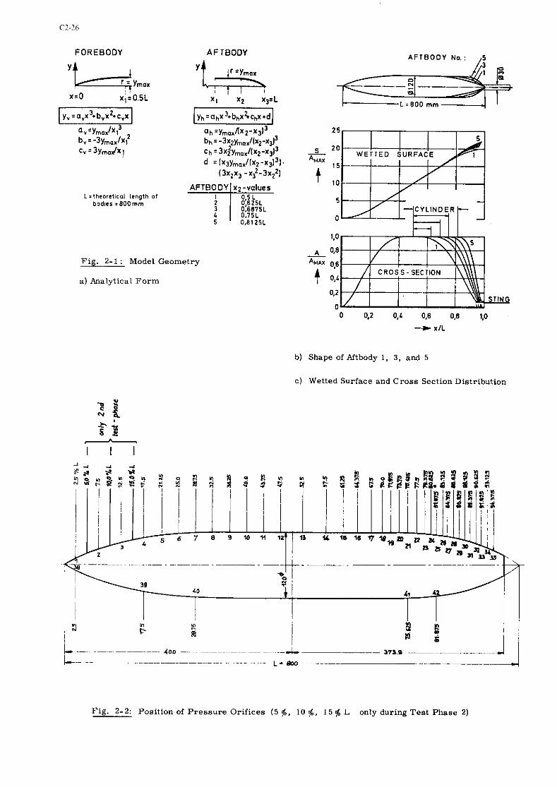
FOREBODY
x.0 x , = 0 . 5 L
L=theoret%coI length o f bodtcr =800rnrn
AFTBODV A F T B O O Y No.:
x , X2 X3.L
Fig. 2 1 : Model Geometry
a) Analytical Form
b) Shape of Aftbody 1, 3, and 5
C ) Wetted Surface and Cross Section Distribution
Fig. 2-2: Position of Pressure Orifices ( 5 $, 10 $, 1 5 $ L only during Test Phase 2)

Fig . 2-3 : Test Setup for Complete Model with Scanivalve, TASK-Balance, and Sting
Fig . 2-4: Forebody Drag Measurement Setup (chord force balance)
F ig . 2-5 : Comparison of Pressure Distribution of Shape 1, 3, and 5 at Ma = 0 .8 , Zero Angle of Attack, and 10 . lo6 Chord Reynolds Number.
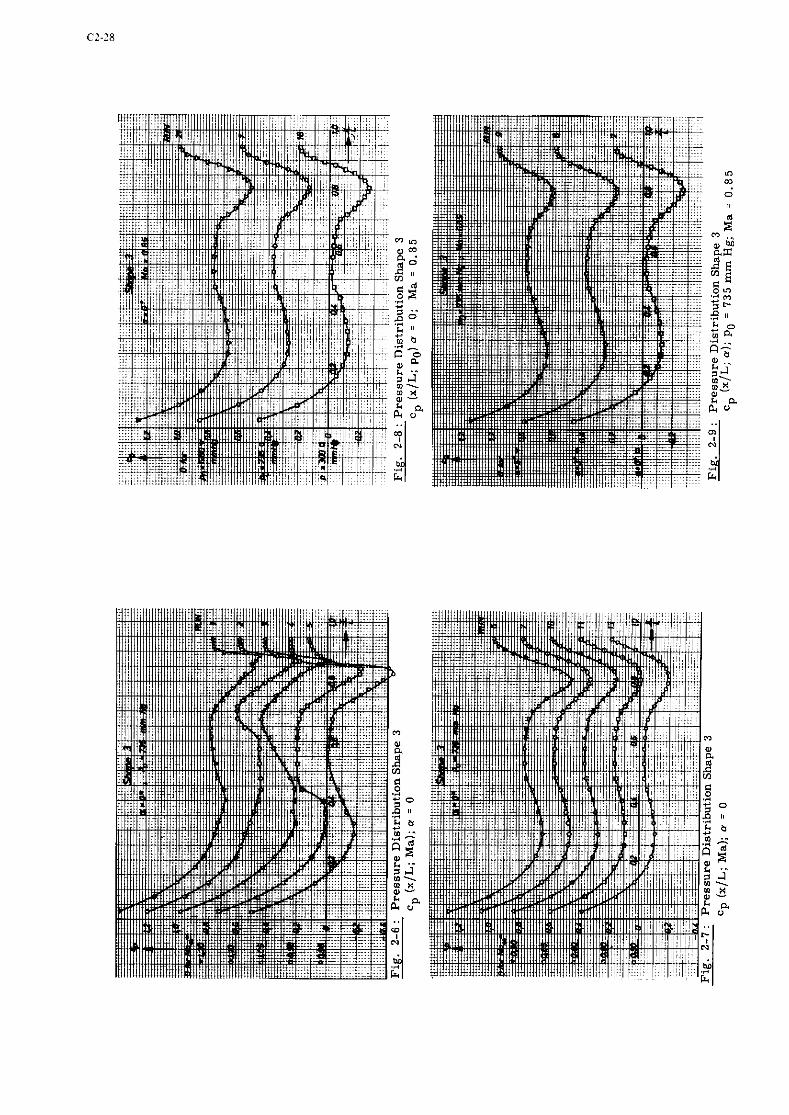


MR - 0.800 KRNRL LEER
ORUCKVERTEILUNGIPRESSURE O I S T R l B U T I O N l
Fig . 2-14 : Sidewall Pressure Distribution at Ma = 0 . 8 , Tunnel Empty; cpwall (x/L; ReL)
F ig . 2 - 1 5 : Sidewall Pres sure Distribution at Ma = 0.8 and Model 3; C
pwall (x/L; ReL)

Fig. 2-16 : Test-Section Wall Pressure, Averaged over all Avavailable Pressure Points c (Ma; pO); Shape 3
pa
0.01
CPo
Fig. 2-17 : Test-Section Wall Pressure. 0.005 Averaged over all Available
Pressure Points c (ReL ; Mode1);Ma = 0.6 pa
0
-0.005
Fig. 2-18 : Test-Section Wall Pressure, Averaged over all Available Pressure Points c (ReL; Model);Mai0.8
pa


C3-I
3. PRESSURE DISTRIBUTION DATA FOR A 10' CONE-CYLINDER
AT ZERO INCIDENCE IN THE MACH NUMBER RANGE 0.91 TO 1.22
submitted by THE HIGH SPEED AERODYNAMICS LABORATORY NAE/NRC
The 10' cone-cylinder is a model configuration, that has become more or less a standard, when determining transonic wind tunnel wall interference characteristics at Mach numbers above, but close to, one. It is also believed that pressure distribution data obtained on a model of such simple geometry will be useful in assessing transonic calculation methods for bodies of revolution. The submitted data were obtained as part of a cali- bration program for the NAE 5ft x 5ft wind tunnel. The data show that for Mach numbers above one the bow shock is effectively eliminated at the wall, but that the expansion wave from the cone-cylinder junction is reflected as a disturbance on the model. The pressure distribution data up to this reflected disturbance should be representative of interference-free, free air data.
1. General Description
1.1 Model designation 01 name NAE calibration model T3
1.2 Model type Cone-cylinder
1.3 Design requirements/conditions
1.4 Additional remarks
2. Model Geometry
2.1 Wing data
2.2 Body data (detail description of Fi ure 3 1 10' half-angle cone with cylindric- body geometry) -e--6 a1 after ody, overall L/D = 12
3. Wind tunnel
3.1 Designation NAE 5-ftx 5-ft trisonic W/T
3.2 Type of tunnel Blowdown
3.2.1 stagnation pressure 1.25 - 4.5 bars, for transonic operations 3.2.2 stagnation temperature 293OK, max drop < 5' during a run
3.2.3 humidity/dew point 0.0002 kg H20/Kg air
3.3 Test section . Square 3.3.1 dimensions 1.52111 x 1.52111 x 4.8m
3.3.2 type of walls perforated 20.5% porosity $ 12.7mm normal holes at 26.4nm spacing
3.4 Flow field (empty test section)
3.4.1 reference static pressure plenum pressure, for transonic operations
3.4.2 flow angularity --0.3O rms for M 20.5
3.4.3 Mach number distribution Fig. 3.2
3.4.4 pressure gradient Fig. 3.2
3.4.5 turbulence/noise level free stream ( A ~ 9 ) = 0.015 at M-= 0.8 3.5 Additional remarks
3.6 References on wind tunnel 1
4. TeStS 4.1 Type of tests Pressure measurements
4.2 Wing span or Semispan to Tunnel Width
4.3 Flow condition
4.3.1 Angle of attack 0'
4.3.2 Mach No. 0.91 - 1.22 4.3.3 Dynamic pressure
4.3.4 Reynolds Number ReD = 4x10⁶
4.3.5 Stagnation temperature To = 290 K
4.4 Transition
4.4.1 Free or fixed Free
4.5 Bending or torsion under load None
4.6 Were different sized models used in No wind tunnel investigation? If so, indicate sizes
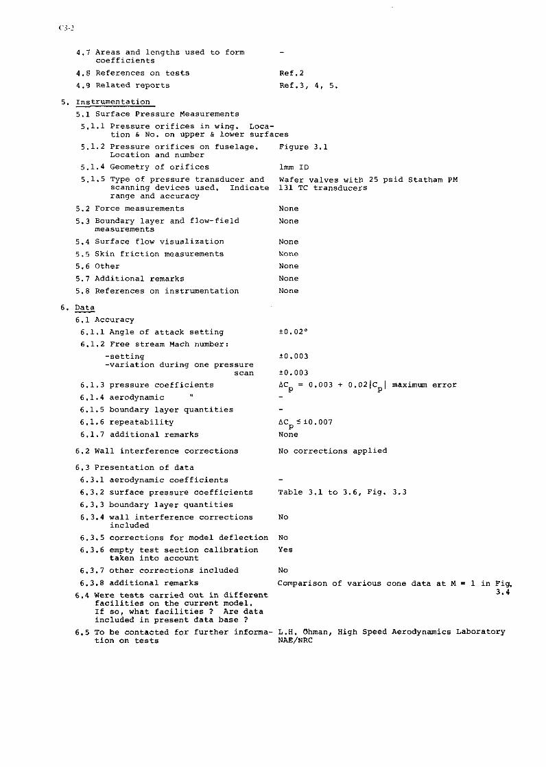
4.7 Areas and lengths used to form - coefficients
4.8 References on tests Ref.2
4.9 Related reports Ref.3, 4, 5.
5. Instrumentation
5.1 Surface Pressure Measurements
5.1.1 Pressure orifices in wing. Loca- tion L No. on upper L lower surfaces
5.1.2 Pressure orifices on fuselage. Figure 3.1 Location and number
5.1.4 Geometry of orifices lmm ID
5.1.5 Type of pressure transducer and Wafer valves with 25 psid Statham PM scanning devices used. Indicate 131 TC transducers range and accuracy
5.2 Force measurements None
5.3 Boundary layer and flow-field None measurements
5.4 Surface flow visualization None
5.5 Skin friction measurements None
5.6 Other None
5.7 Additional remarks None
5.8 References on instrumentation None
6. Data 6.1 Accuracy
6.1.1 Angle of attack setting
6.1.2 Free stream Mach number:
-setting -variation during one pressure
scan
6.1.3 pressure coefficients
6.1.4 aerodynamic
6.1.5 boundary layer quantities
6.1.6 repeatability
6.1.7 additional remarks
30.003
AC = 0.003 + 0.021~ I maximum error - P P
- AC 5i0.007 P
None
6.2 Wall interference corrections No corrections applied
6.3 Presentation of data
6.3.1 aerodynamic coefficients - 6.3.2 surface pressure coefficients Table 3.1 to 3.6, Fig. 3.3
6.3.3 boundary layer quantities
6.3.4 wall interference corrections NO included
6.3.5 corrections for model deflection No
6.3.6 empty test section calibration Yes taken into account
6.3.7 other corrections included NO
6.3.8 additional remarks Comparison of various cone data
6.4 Were tests carried out in different facilities on the current model. If so, what facilities ? Are data included in present data base ?
at M = 1 in Fig. 3.4
6.5 To be contacted for further informa- L.H. Ohman, High Speed Aerodynamics Laboratory ti0n on tests NAE/NRC

8. References
1. Brown, D.
2. Ohman, L.H.
3. Spreiter, J.R.
4. Page, W.A.
5. Eastbrook, B.B.
Information for the users of the National Research Council's 5ft x 5ft blowdown wind tunnel at the National Aeronautical ~stablishment, Second ~dltioni NRC/NAE LTR-HA-6 September, 1970
Calibration of the transonic test section of the NAE 5ft x 5ft wind tunnel. Phase 11 - model measurements. NRC/NAE Data Report 5x5/-018, 1966
Aerodynamics of wings and bodies at transonic speeds J.A.S., August, 1959
Experimental study of the equivalence of transonic flow about slender cone-cvlinders of circular and elliptic cross section. NACA TN 4233, 1958
Wall interference effects on axisymmetric bodies in transonic wind tunnels with perforated wall test sections. AEDC-TR-59-12, 1959.
9. List of Symbols
P local pressure on model
p, plenum chamber pressure = free stream static pressure
Po free stream stagnation pressure
¶ free stream dynamic pressure
P - P, c = - pressure coefficient
q maximum diameter of model
length of model
length of conical nose
free stream Mach number
axial distance from apex of model also upstream distance from rear seal face (exit) of transonic test section.
height = width of transonic test section
re^ Reynolds number based on model diameter D

TABLE 3.1
RUN= 3614, MODEL 13, RUTATE0 0 I O E G R E F S , A V E R A G E :4 I i iF=OO9O9 -- S I X/D l'/PO C P !4IYF P lNF
1 0.400 0.1>5'+ 0.203 0 , 2 1 0 - 18.05 2 0.800 C.644 0.174 0.909 18.08 2 0.800 0.644 0.112 0.90~~H,le 2 0.800 0.644 0.174 0.909 18.08 2 0.800 0.643 0.169 0.909 18,0?- _ 3 1 .200 0.636 0.150 $0.909 1R.08 4 1.600 0.631 0.132 0.908 18.13
-~ ~
5 2.000 9 .611 0;101 0.911 18.08 6 2 . ' 1 c o ~ 6 L ! _ _ 0.059 .- 0.109 1 8 a 7 2.800 0.541 -0.124 0.912 10.05 8 2.855 0.329 -0.758 0.909 18.08 9 3.000 0.357 -0.611 :0.910 1R.05
1 0 3 . 2 0 0 0 . 4 1 9 -0.491 0.909 18.0C I 1 3.600 0 .591 0.023 0.909 18.08 12 4.000 0.587 0.004 0.909 1R.08 13 4.400 0.507 0.003 0.909 18.08 14 4.800 0.586 0.002 0.901 18.08 _ 1 5 5.200 0.587 0.002 0.908 lb.13 16 5.600 0.585 0.002 0.911 1 8 . 0 8 I 7 h .000 0.586 0.002 0.909 18.10 18 b.'tOO 0.584 0.002 0.912 18.05 19 h .800 0.586 0.002 0.909 1R.08 2 0 7.200 - s 2 s 7 0.006 0.910 18.05 2 1 7.600 0.588 0.007 0.109 1R.08 2 2 R.000 0.587 0.004 0.909 lR.08 23 8.400 0 .587 0.004 0.109 19.08 24 8.800 0.587 0.004 0.909 1R.08 25 9.200 0.587 0.004 0.909 18.08 26 9.600 0.5-9 -0.005 0.108 18.13 2 7 10.000 0.585 0.002 0.911 18.08
TABLE 3.2
RlJN= 3699t . f lODFL.T3r R O T A T E D 0 UEGRFES, AVFR&EMINF=0.954 . ._ . .. .. . . S T XI D P/Po C P NINF PINF
.. I 0.400 0 . 6 3 4 0.213 0.954 17.25 2 0.800 0.624 0.1t37 0.953 17.27

TABLE j . 3
3U.V. ~~.~~~~ 3 6 9 l l l C L 3 --.. ~ K O T A ~ F . O ~ _ O ~ _ O I G ~ ~ E _ E S L ~ ~ V _ E . R ~ L . ~ M ~ I ~ ; V F . ~ ~ O P ~ ~ S T X / B I'IPO C P MINF P lNF
TABLE 3.4 . ~
f 'UN= 3679. MUIIEL 7 3 , ROT&!C"-O_DEG!ESI. A.V_EP!_CE ... .~ -~
S T X I 0 P I P 0 C P H lNF P l N F 1 0.!*00. ' L r _ 5 8 9 . 0.245 1.056 ? 5 . 3 ? L 2 0.000 0.585 0.236 1.056 15.33 2 0.80~p-g,~L4_ 0 . 2 3 4 1.056 1 5 . ~ 3 3 2 0.800 0.586 0.237 1.056 15.33 2 0.800 0.584 0.232 -. 1.05.6__ !5_.35 3 1.200 0.581 0.224 1 .056 15.33
1.600 0 , 5 7 6 0.211 1.056 1~5.33.. 4 5 2.000 0.567 0.190 1.057 15.36
-~ 6 2.4'tOO 0 .558 0.166 1 . 0 ~ 5 6 1 5 . 3 6 ~ ~ 7 2.800 0 .521 0,069 1.056 15.36
L i 5 . 6 - 2-1 7 _ _ 10...~6_2_--1-051--E2?_6__6_ 9 3.000 0.337 -0.407 1.056 15.33
10- .... l-?E _4.-370. -0.322 !-05_6_15,L3- 1 1 3.600 0.410 -0.217 1.056 15.33 12 '+.000 . -.- 0.432 ~ - 0 . 1 6 0 l . 0 5 6 1 > . , 3 3 _ 1 3 4.400 0 . 4 5 9 -0 .091 1 .056 15.33
- L L _ _k,aoo- -o .472 . .~Q:0~~. - L P l j b . _ . !5.3F I 5 5 . 2 0 0 0.472 -0.058 1.056 15.33
~ 1 6 .~ 5 . 6 0 0 0.473 - 2 1 . 0 5 7 15,26._ 1 7 6.000 0.495 0.003 1.056 15.36

TABLE 3.5 . .
R U N ~ 3 6 8 . 0 1 M J . 2 E ~ C _ ~ d X A LE P_.O.EE4i34F-SSdV.S9T,E S T XI0 P/PO C P MINF PINF
1 0 . 4 0 - 0,531 _ _O--ZO3 1. 122 1 4 . 1.6 2 0 . 8 0 0 0 .536 0 . 2 0 0 1 .122 14.16
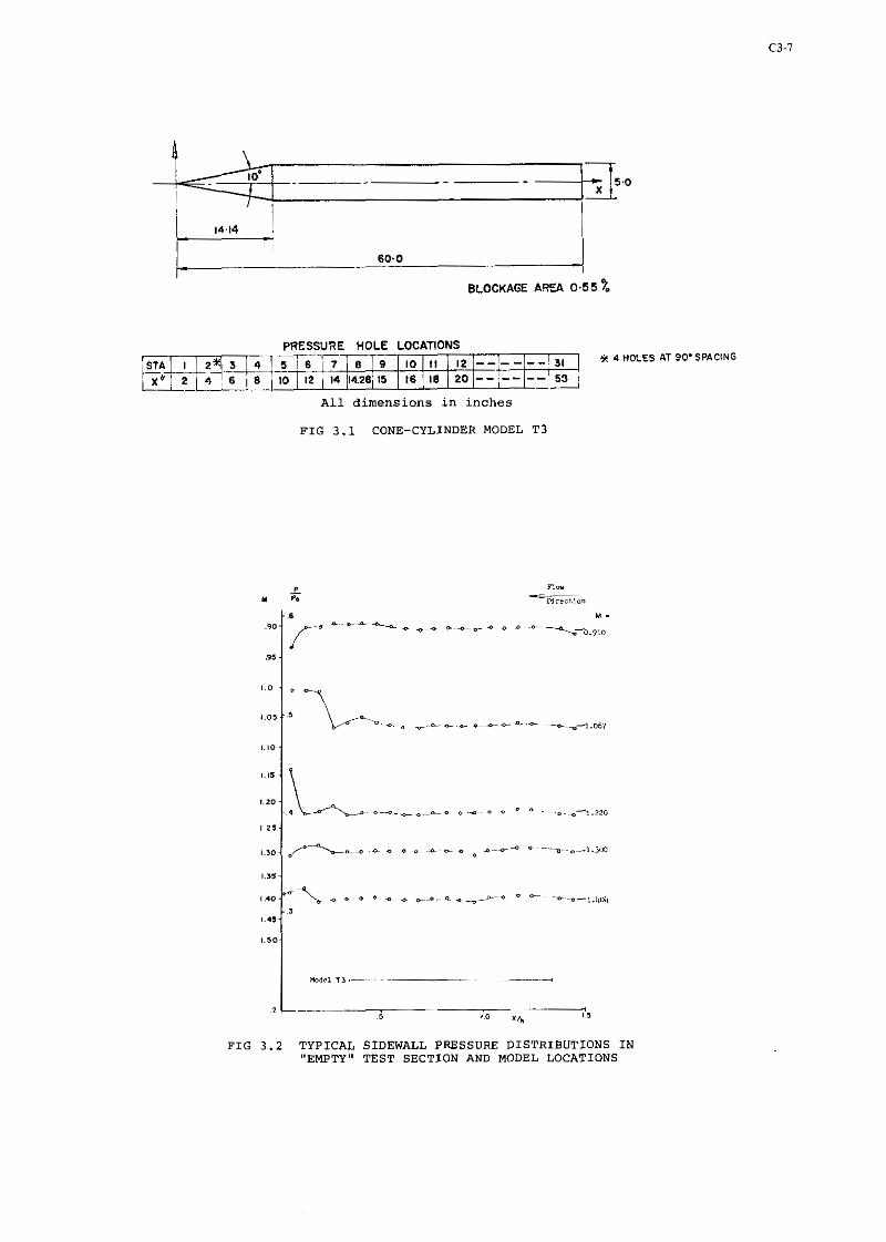
1 60.0 -- I
BLOCKAGE ARC5 0 . 5 5 7-
PRESSURE HOLE LOCATIONS
*'HOLES AT3O'sPAC'NG
All dimensions in inches
FIG 3.1 CONE-CYLINDER MODEL T3
: . - a - ~ o - n *-**-- - ~ - ~ s - >.&Oh
I..,
FIG 3.2 TYPICAL SIDEWALL PRESSURE DISTRIBUTIONS IN "EMPTY" TEST SECTION AND MODEL LOCATIONS

FIG 3.3 PRESSURE DISTRIBUTION FOR MODEL T3
- THEOR" I c r 3 CXP R E I S F IO. l l
/N/ 0 0 ~ - . ! ~ 7 X B L O C I A 0 C
- - - R E F 4 . O O S ~ L O C I I I e E
PRESENT EXP RUNS No 1691.1892
ossX murcrror
FIG 3.4 PRESSURE DISTRIBUTION ON THE NOSE SECTION OF A 10' SEMI-APEX CONE-CYLINDER AT M=1.0

4. ONERA CALIBRATION MODEL C5
by X. Vaucheret
Office National dGtudes et de necherches Aerospatiales 92320 Chatillon - France
4.1 - Introduction A program was initiated in 1969 by ONERA to test a series of similar calibration models representa- tive of a transport aircraft, in various American and European transonic wind-tunnels. The objective of this program was to study wall interference. In relation to this program, blockage effects near Mach number one were separately investigated with bodies of revolutioll havi~ig the same distributions of cross sectional area as the airplane models.
The largest body of revolution tested in the calibration body C5 for which data obteined in the 11 ft NASA-Ames wind tunnel are presented here. The data obtained for the calibration body C5
.in the largest tunnels used, i.e. 16 ft AEDC, 11 ft NASA-Ames and 6 ft 52 MODANE ONERA, practically agree within the data scatter at all Mach numbers up to one.
4.2 - Data set 1 . General Description
1.1. Model Designation ONERA calibration body C5
1.2. Model Type axisymmetrical body
1.3. Design ~equirements/Conditions Comparison of transonic wind-tunnels near Mach 1
1 .4 . Additional Remarks 4 other geometrically similar bodies exist and have been used to study the blockage effect
2. Model Geometry
2.1. Body length 1.0578 m
2.2. Base diameter 0.08516 m
2.3. Maximum diameter 0.15268 m
2.4. Diameter of cylindrical pacts 0.1 242 m
2.5. Fore part ellipsoid
2.6. Model coordinates see table 1
2.7. Fabrication tolerances 0.03 mm
3. Wind Tunnel
3.1. Designation
3.2. Type of Tunnel
3.3. Test Section
3.3.1. Shape of Test Section
3.3.2. Size of Test Section (width, eight) 3.3.3. Type of Test Section Walls
Treatment of Side Wall Boundary Layer
3.4. Flow Field (empty Test section)
3.4.1. Reference Static Pressure
3.4.2. Flow Angularity
3.4.3. Mach Number Distribution
3.4,4. Pressure Gradient
3.4.5. ~urbulence/l~oise Level
3.4.6. Side Wall Boundary Layer
Ames Research Center 11 by 11 ft transonic wind tunnel
continuous-transonic flow
square
11 x 11 ft
baffled slots-open area ratio 5.8 %-constant slot width with 450 "see" baffles with axis of bend normal to the wall
Sidewalls diverged 0.19O
Plenum chamber pressure
2 0.15O at M = 0.6
see 7.5.4
*CQ = 2.2 % at M = 0.6 R.M.S. 2.8 % at M = 0.7
1 . 5 % at M = 1 . 2
3.5. Freestream Mach Number
3.5.1. Range 0.3 to 1.4
3.5.2. Pressures Used to Determine Settling chamber total pressure and plenum chamber Mach Number pressure

3.5.3. Accuracy of Mach Number Determination (AM)
3.5.4. Maximum Mach Number Variation in x , y, z-Direction (~mpty ~unnel)
Maximum Variation of Flow Direction
Maximum k c h Number Variation During a Run
3.6. Reynolds Number Range
3.6.1. Unit Reynolds Number
3.6.2. Means of Varying Reynolds Number
3.7. Temperature Range and Dewpoint
3.8. Model Attitudes
3.8.1. Angle of Attack, Yaw, Roll
3.8.2. Accuracy in Determining Angles
3.9. Organization Operating the Tunnel and Location of Tunnel
3.10. Who is to be Contacted for Additional Information
3.11. Lithrature Concerning this Facility
3.12. Additional Remarks
4. Tests 4.1. Type of Tests
4.2. Blockage
4.3. Test conditions
4.3.1. Angle of Attack
4.3.2. Mach Number
4.3.3. Stagnation Pressure
4.3.4. Reynolds Number
4.3.5. Stagnation Temperature
4.4. Transition
4.4.1. Free or Fixed
4.4.2. Position of Free Transition
4.4.3. Position of Fixed Transition, Width of Strips, Fine and Type of Roughness Elements
4.4.4. Were Checks Made to Determine if Transition Occurred at Trip Locations ?
4.5. Bending or Torsion Under Load
4.6. Were Different Sized Models Used in Wind Tunnel Investigation ?
The standard deviation variation at any given centerline station .001 in Mach number aver pressure range from 172 to 2 atmospheres. Maximum pressure error estimated to be within 1.4 psf for plenum static pressure and f; . Z-direction : .002 difference between ceiling statics and center line at .6 g M & .9 X-direction : f .004 at M = 1.4 * .002 at M = 0.9 optimum model location, optimum tunnel control settings
f 0.15" at M = 0.6
.003, usually within f 0.001
6 6.7 to 32 x 10 per meter
pressurieatian
60 to 120° F depending on M, pi and ambient temperature
f 15O plus bent sting capability and 360° Roll mechanism
Model suppart system calibration and elastic deflections good to .030 or better
Experimental Investigations Branch, Aerodynamics Division, NASA Ames Research Center ; Bldg.227, Moffett Field, California 94035
FRANK STEINLE Jr., Assistant Chief, Exp. Inv. Br. N 227-5 Ames
Ames Research Facilities Summary, 1974 - and NASA CR-1874 "An Inventory of Aeronautical Ground Research Facilities", Vol. 1 - Wind hurnsls - Pirrello & el.
Majority of noise in test section associated with "organ" tones produced by slot-baffles - Research
underway to modify baffles to eliminate organ mode.
steady tests : pressure, drag
0.17 per cent
d= 0 0.6 to 1.0
1.2 to 0.9 bar
RL - 13.8 x 10 6
305 to 307 K
fixed
on the nose at a = 72.7 mm.ballotini (glasa beads) 0.12 ma in diameter.
yes, subliminatian technique
five geometrically similar bodies : body I C1 C2 C3 C4 C5
length 0.31 0.40 0.51 0.66 1.06 (.) I

4.7. Areas and Lengths Used to Form Coefficients
4.8. References on Tests
4.9. Related Reports
5 Instrumentation
5.1. Surface Pressure Measurements
5.1 .l. Pressure Orifices
5.1.2. Geometry of Orifices
5.1.3. Type of Pressure Transducer and Scanning Devices Used
5.2. Force Measurements
5.2.1. Type and Location of Balance
5.2.2. Forces and Moments that Can be Measured. Maximum Loads and Accuracy
6. Data 6.1. Accuracy
6.1.1. Pressure coefficients
6.1.2. Aerodynamic Coefficients
6.2. Wall Interference Corrections
6.3. Data Presentation
6.3.1. Aerodynamic Coefficients
6.3.2. Surface Pressure Coefficients
6.4. Were Tests Carried Out in Different Facilities on the Current Model ? If s o , What Facilities. Are Data Included In Present Data Base ?
7. References 1. X. VAUCEERET
M. BAZIN C. ARMAND
2. T.W. BINION
3. S.E. GUDMUNDSON
8. List of Symbols
C~
L
for the drag coefficient : S = 0.005696 m2 (base area)
44 pressure orifices on vertical generator 40 pressure orifices an horizontal generator 1 base pressure orifice (table 1)
0.6 mm in diameter, perpendicular to body surface
48 pacts scanivalve plus transducer 25 psi
internal balance
6 components balance
none, because of very small blockage (0.17 per cent)
table 2 : drag coefficient
table 2 : local f /Pi figures 1,2 : local Mach number distribution
tests were carried out in 3 transonic wind-tunnels (ref. 1, 2, 3) not included in present data base. The data from these wind-tunnels ( 1 6 ~ AEDC, 11T NASA, 6T 52 ~odane) agree,ercept in rare instances, within the data accuracy at all Mach numbers up to 1.0.
Cornparaison d'essais transsoniques bi et tridimension- nels effectues dans diverses gcandes souffleries. AGUD C.P. no 187 (1975) Tests an the ONERA calibration models in three transonic wind tunnels mnc TR 76-1 33 (1 976)
Comparative tests with ONERA airplane calibration models in FFA transonic wind tunnels EUROMECA 40 Colloquium (1 973)
draf coefficient corrected to zero base drag
pressure coefficient
body length
Mach number (test section)
local Mach number (on the body)
local static pressure (on the body)
stagnation pressure
body radius at x (mm) (table 1)
Reynolds number (based on L)
base area
abscissa along body axis (mm) (table 1) angle of attack

I. I * " rr r , n w 1 .oo w 2 t.00 , ., I L . l l I ' 1 I I , . l o 4. a, 3 ( I . 0 0 4, - 6 2l.IO z. t6 1 31.10 U La I L1.00 52 I 0 T 5,
I 0 1L.50 ,as 11 . , .(I I&.' , I ,O,.PO .I% (1 i t l . 0 0 st, (1 1'1.09 n 9 , $1 1 0 . 1 6 S S U 1. 113.11 1, ,, :: :::::: 2: 3. 112.01 LI 1, 10 I I 6 . 0 0 64 10 21 ,,0.ll un 2 1 191.1, " ' 0 21 II<.II - 4 4 2. 111.1, 0 1 . 2 1 '12.3, U D 2' 111.11 HI, I7 ,.,.'I m" 11 01.1, I. U I. . , I . , , I*.( $1 11..11 we2 11 1IY.II XIC 11 I'..., XO, 11 116.11 1 ) ~ ' I. 3.1.0, V ,L 11 .11.1, 6,s I. .,O.I, 6,- I7 LI1.ll 6, m >I 713 .61 r%%* $0 849.49 I.% LO Ill.', ,SIC '1 ..,.'I IIE 11 I010.1I i t U .I 701I.LI ,.., 11 >I',.', '3 >0,..77
1. ' YI I* I ," a. '6 . I 0 s '8 '7 0 0 1 D1 A8 6.00 In I S A. (,.,I ,< 7, $ 0 ,..OD I. I $1 ll.10 1s.. 51 11.50 ,ow :: ::::: 2: :: ,::::: $: I7 1V8.00 ~ 1 . li ?II.OO y a :: 1:::;: 22 '1 701.00 I IU
:: :::::; 2: 64 211.11 (4 C? 'I 2*..00 GZ 0,
:: ::;::: 2: .I A,..,, 6.3 6. Llr.83 7oaa ID 111.13 1. ;: ;;;:;: gs 71 I18.11 ,a,, 1' 136.85 7.2. 7, ,I,... n*
:: :::::: :::: :: :::::: z:: 10 111.&( 6, U *? 838.43 I." # ? VB,.,, ',%, I, ,."_.I ,I 24 84 ,021.LI 8 , ,aI"_LI ,,
101.11 121.11 I'O.., 11..11 111.1, .,>.,, I,..., 667.89 .O..LI 173.LI I l l . ' , .O,_', .,...I
1013.LI I ~ l O . . ,


0
0 x
0
1 Figure 2