Wiley - The Valuation Handbook (2009) (ATTiCA)

E1FFIRS 09/03/2009 14:19:8 Page 6

E1FFIRS 09/03/2009 14:19:8 Page 1

The ValuationHandbook

E1FFIRS 09/03/2009 14:19:8 Page 2

Founded in 1807, John Wiley & Sons is the oldest independent publishingcompany in the United States. With offices in North America, Europe,Australia, and Asia, Wiley is globally committed to developing and market-ing print and electronic products and services for our customers’ professio-nal and personal knowledge and understanding.

The Wiley Finance series contains books written specifically for financeand investment professionals as well as sophisticated individual investorsand their financial advisors. Book topics range from portfolio managementto e-commerce, risk management, financial engineering, valuation, andfinancial instrument analysis, as well as much more.

For a list of available titles, please visit our Web site at www.WileyFinance.com.

E1FFIRS 09/03/2009 14:19:8 Page 3

Valuation Techniques fromToday’s Top Practitioners

RAWLEY THOMASBENTON E. GUP

John Wiley & Sons, Inc.

The ValuationHandbook

E1FFIRS 09/03/2009 14:19:8 Page 4

Copyright # 2010 by Rawley Thomas and Benton E. Gup. All rights reserved.

Published by John Wiley & Sons, Inc., Hoboken, New Jersey.Published simultaneously in Canada.

No part of this publication may be reproduced, stored in a retrieval system, or transmitted in

any form or by any means, electronic, mechanical, photocopying, recording, scanning, orotherwise, except as permitted under Section 107 or 108 of the 1976 United States Copyright

Act, without either the prior written permission of the Publisher, or authorization through

payment of the appropriate per-copy fee to the Copyright Clearance Center, Inc., 222

Rosewood Drive, Danvers, MA 01923, (978) 750-8400, fax (978) 646-8600, or on the web atwww.copyright.com. Requests to the Publisher for permission should be addressed to the

Permissions Department, John Wiley & Sons, Inc., 111 River Street, Hoboken, NJ 07030,

(201) 748-6011, fax (201) 748-6008, or online at http://www.wiley.com/go/permissions.

Limit of Liability/Disclaimer of Warranty: While the publisher and author have used their best

efforts in preparing this book, they make no representations or warranties with respect to the

accuracy or completeness of the contents of this book and specifically disclaim any implied

warranties of merchantability or fitness for a particular purpose. No warranty may be createdor extended by sales representatives or written sales materials. The advice and strategies

contained herein may not be suitable for your situation. You should consult with a professional

where appropriate. Neither the publisher nor author shall be liable for any loss of profit or anyother commercial damages, including but not limited to special, incidental, consequential, or

other damages.

For general information on our other products and services or for technical support, please

contact our Customer Care Department within the United States at (800) 762-2974, outsidethe United States at (317) 572-3993 or fax (317) 572-4002.

Wiley also publishes its books in a variety of electronic formats. Some content that appears in

print may not be available in electronic books. For more information about Wiley products,visit our web site at www.wiley.com.

Library of Congress Cataloging-in-Publication Data:

Thomas, Rawley, 1946-The valuation handbook : valuation techniques from today’s top practitioners /

Rawley Thomas, Benton E. Gup.

p. cm. – (Wiley finance ; 480)Includes bibliographical references and index.

ISBN 978-0-470-38579-1 (hardback)

1. Corporations–Valuation. 2. Stocks–Prices. I. Gup, Benton E. II. Title.

HG4028.V3.T48 2010332.630221–dc22

2009028345

Printed in the United States of America

10 9 8 7 6 5 4 3 2 1

E1FFIRS 09/03/2009 14:19:8 Page 5

To Jean, Andy, Lincoln, Jeremy, and Carol

—Benton E. Gup

To Carol Ann, John, Alexis, Kim, and Robert

—Rawley Thomas

E1FFIRS 09/03/2009 14:19:8 Page 6

E1FTOC 09/02/2009 16:16:48 Page 7

Contents

Preface xvii

Valuations Are Important xviiValuation Challenges: Which Techniques to Apply xviiContributors xixChapter Summaries xx

CHAPTER 1Two Frameworks for Understanding Valuation Models 1Benton E. Gup

Top-Down/Bottom-Up Analysis 1Life Cycle 6Firms 9Conclusion 10Notes 10

CHAPTER 2The Value Edge: Reap the Advantage of Disciplined Techniques 11William J. Hass and Shepherd G. Pryor IV

Valuation Decisions Are Made Differently by Different People 12Techniques of Communicating Value Can Demonstrate a

Commitment to Value Building 15Analysts Beware: Once-Successful Public Companies Can

Lose Their Way 17Incentive Compensation Techniques Based on Value Are Better 18Valuation Techniques for Private Companies Are Also

More Data Driven 26Estimates of Value May Differ Depending on Data Integrity 27Finance Theory and Corporate Value 31The Value Edge Begins at the Strategic Business Unit Level 33The Waterfall of Value Identifies Value Creators and Destroyers 34Better Valuation Frameworks Provide Discipline 35The Value Journey Has Many Steps along the Way 37

vii

E1FTOC 09/02/2009 16:16:48 Page 8

Acknowledgments 40References 40

CHAPTER 3Applying a Systems Mindset to Stock Valuation 43Bartley J. Madden

Choice 1: A Systems Mindset 43Choice 2: Firms’ Competitive Life Cycle 45Choice 3: Inflation Adjustments and Economic Returns 49Choice 4: Denominator Depends on the Numerator 50Choice 5: Insights and Plausibility Judgments 56Back to the Future 59Searching for Failures and Successes 60Conclusion 63Notes 64References 65

CHAPTER 4Comparing Valuation Models 67Thomas E. Copeland

Literature Review 68Brief Description of the Valuation Models That

Are Compared 69An Expert System That Does Valuation 71Goodness of Fit: Initial Sample (1,395 Valuations,

1993 to 2000) 77Tests of DCF in a Holdout Sample (New Sample 2000–2008) 80Convergence Tests 82Straw Man Horse Races (Comparison of Three Models) 86Convergence 89Conclusion 91Notes 107References 107

CHAPTER 5Developing an Automated Discounted Cash Flow Model 108Robert J. Atra and Rawley Thomas

Models Examined 111Data and Initial Parameterization 114Measurement Principles 114

viii CONTENTS

E1FTOC 09/02/2009 16:16:48 Page 9

Proprietary Models 127Conclusion 130Appendix: Academic Literature 130Notes 132References 133

CHAPTER 6The Essence of Value-Based Finance 135Roy E. Johnson

Introducing Value-Based Finance (a Transition fromAccounting to Economics) 137

Valuation Perspectives: Economic Profit andMarket Value Added 140

Valuation Perspectives: The Magnifier 147Valuation Perspectives: Financial Drivers and

Value Profit Margin 154Value Analysis: The Proper Focus 162Note 171

CHAPTER 7Residual Income and Stock Valuation Techniques:Does It Matter Which One You Use? 172Benton E. Gup and Gary K. Taylor

Economic Value Added (EVA) 173Residual Income Method of Valuation 174Abnormal Earnings Growth Model 175Numerical Example of RI and AEG 176Conclusion 178Notes 180References 181

CHAPTER 8Modern Tools for Valuation: Providing the Investment Communitywith Better Tools for Investment Decisions 182David Trainer

Identifying the Problem 186What Drives Stock Market Valuation? 186Our Valuation Methodology—Providing a Solution 187Theory Meets Practice 191General Notes on Stock Picking 195

Contents ix

E1FTOC 09/02/2009 16:16:48 Page 10

Appendix A: Definitions of Key Terms Used in OurValuation Models 210

Appendix B: How Our Dynamic Discounted CashFlow Model Works 215

Appendix C: Explanation of Risk/Reward Rating System 218Appendix D: NOPAT, Invested Capital, and WACC

Calculations for Accenture 220Notes 224

CHAPTER 9The Economic Profit Approach to Securities Valuation 226James L. Grant

Basics of Economic Profit Valuation 227Economic Profit Models 228Reconciliation of EVA Models 238Cost of Capital Effects 239Pricing Implications 240EVA Accounting Adjustments 241Invested Capital 243EVA Application: JLG Dow Fundamental 245EVA Link to FCF Valuation 246FCF Valuation: Horizon Years 248FCF Valuation: Residual Years 249Summary 251Notes 252Reference 254

CHAPTER 10Valuation for Managers: Closing the Gap betweenTheory and Practice 255Dennis N. Aust

Current Environment 257Alternative Measures of Value Creation: A Quick Review 259Conclusions 270Note 272References 272

CHAPTER 11The LifeCycle Returns Valuation System 273Rawley Thomas and Robert J. Atra

x CONTENTS

E1FTOC 09/02/2009 16:16:48 Page 11

Converting Accounting Information to Economic Returns 274Converting Economic Returns to Intrinsic Values 285Converting Intrinsic Values to Investment Decisions 293Summary 299Appendix: Market Derived Discount Rates and

CAPM Beta Costs of Capital 300Notes 302References 303

CHAPTER 12Morningstar’s Approach to Equity Analysis and SecurityValuation 305Pat Dorsey

Applying Economic Moats to Security Valuation 308Intrinsic Value 317Conclusion 331

CHAPTER 13Valuing Real Options: Insights from Competitive Strategy 334Andrew G. Sutherland and Jeffrey R. Williams

Overview of Option Pricing for Financial Securities 335Basic Option Pricing Applications for Real Assets 345Advanced Option Pricing Applications for Real Assets 351Conclusion and Future Research 365Note 365References 365

CHAPTER 14GRAPES: A Theory of Stock Prices 367Max Zavanelli

A Theory of Stock Prices 367Arbitrage 370The Beginning of All Things 371The Model and System 376GRAPES System for Valuing Companies 378The Pricing of Risk 381Appendix: Examples of McDonald’s and Wal-Mart 383Notes 385References 385

Contents xi

E1FTOC 09/02/2009 16:16:48 Page 12

CHAPTER 15Portfolio Valuation: Challenges and Opportunities Using Automation 386Randall Schostag

Background 386Methods Adoption Implications 387Accounting Pronouncements 389SEC Guidance 390Accounting Pronouncements and the FASB 391XBRL Format 395Emerging Best Practices 395International Standards 397Producing Portfolio Valuations 398Using Automation in Valuations 400Conclusion 411Notes 412References 415

CHAPTER 16The Valuation of Health Care Professional Practices 417Robert James Cimasi and Todd A. Zigrang

Basic Economic Valuation Tenets 417The Value Pyramid 419Buy or Build? Value as Incremental Benefit 420Standard of Value and Premise of Value 420Valuation Adjustments for Risk 424Classification of Assets and Determination of Goodwill 426Impact of Competitive Forces 429Valuation Approaches, Methods, and Techniques 430Analysis of Risk 435Level of Value: Discounts and Premiums 439Conclusion 441Notes 441

CHAPTER 17Valuing Dental Practices 443Stanley L. Pollock

Normalization 445Fixed Asset Appraisal 448Ratio Analysis 450Trend Analysis 451

xii CONTENTS

E1FTOC 09/02/2009 16:16:48 Page 13

USPAP Standards 452Summary 471Notes 472References 473

CHAPTER 18Measures of Discount for Lack of Marketability and Liquidity 474Ashok Abbott

Publicly Traded Equivalent Value 474Discounts for lack of Marketability and Discount for

lack of Liquidity 475Benchmarking Methods 477Empirical Studies 480Liquidity as a Pricing Factor 482Distinction between Holding Period and Liquidation

Period 484Quantitative Approaches based on CAPM and

Time Value 485Historical Market Liquidity Statistics 487Price Pressure and Market failure 489Measuring Asset Liquidity 492Application of Time/Volatility (Option) Models to

Discount for Lack Of Liquidity 495Three Option based Models 497Black-Scholes put (BSP) 497Average Price Asian Put (AAP) 498Look Back Put (LBP) 499Conclusions 504References 505

CHAPTER 19An Economic View of the Impact of Human Capital on FirmPerformance and Valuation 508Mark C. Ubelhart

Creating and Standardizing Metrics 509Predicting Future Financial Results 510Organizational Decomposition 513Mathematical Models Guiding Practical Action 522Note 524Reference 524

Contents xiii

E1FTOC 09/02/2009 16:16:48 Page 14

CHAPTER 20EBITDA: Down but Not Out 525Arjan J. Brouwer and Benton E. Gup

What Is EBITDA? 526Who Uses EBITDA and Why? 527EBITDA in Financial Reporting 531EBITDA in Europe 533Impact on the U.S. Capital Market 537The Reporting Performance Project 538Conclusions 540Notes 540References 542

CHAPTER 21Optimizing the Value of Investor Relations 544William F. Mahoney

Investor Relations as a Service Function 545The Investment Relations Officer as the Resident Investment

Market Expert 547Building Investor Respect as Well 548It’s All about Information of Value 548The Information Advantage 549Working with One Key Investor at a Time 549Working with the Primary Investors 551What It Takes to Do the Job 553Identifying the Information That Determines Intrinsic Value 554Focus on the Value Drivers 555Linking Intrinsic Value to Stock Price 555Numerous Vital Lessons from This Book 556Wrapping It Up 557Note 558References 558

CHAPTER 22Lower Risk and Higher Returns: Linking Stable ParetianDistributions and Discounted Cash Flow 559Rawley Thomas, Dandan Yang, and Robert J. Atra

Background 560Intrinsic Values and Distributions 564Automated Valuation Models 565

xiv CONTENTS

E1FTOC 09/02/2009 16:16:48 Page 15

Research Design and Empirical Results 566Conclusion 573Appendix A: Synthesizing the LifeCycle Framework 575Appendix B: Technical Note—Ranges of Bounded Rationality 577Notes 579References 581

CHAPTER 23Common Themes and Differences: Debates and Associated IssuesFacing the Profession 583Rawley Thomas

Does Intrinsic Value Have Any Meaning? 587Methodologies: Mark to Market, Mark to Model 589Illiquidity Crises and Market Meltdowns: Effect on

Quantitative Strategies 591Discounted Cash Flow Methodologies 592Appendix A: Financial Management Association Practitioner

Demand Driven Academic Research Initiative (FMA PDDARI) 596Appendix B: Examples of Assumptions and Theories

Deserving Debate and Empirical Quantification 598References 601

About the Editors 603

About the Contributors 605

Index 619

Contents xv

E1FTOC 09/02/2009 16:16:48 Page 16

E1FPREF 08/13/2009 17:7:1 Page 17

Preface

VALUATIONS ARE IMPORTANT

Valuations are important simply because they form the basis for makingdecisions involving significant amounts of money or wealth transferredfrom one party to another.

Why do people perform valuations? What are they used for? Thefollowing is a short list, which is by no means complete. Valuations arenormally done to:

& Buy or sell a stock of a publicly held firm.& Buy or sell a privately held business.& Determine how much estate tax is owed the government.& Settle a divorce.& Resolve a dispute with a minority shareholder who wants out.& Give an accounting auditor value basis for reporting.& Determine the amount of compensation for executives, division or busi-

ness unit managers, and employee-owners.& Determine whether to proceed with strategic initiatives and/or major

investment opportunities.& Offer fairness opinions in the purchase or sale of companies.

VALUATION CHALLENGES: WHICH TECHNIQUES TO APPLY

Broadly, valuation techniques may divide into two categories:

1. Those relying on quoted market prices of the specific security.2. Those applying advanced professional knowledge to a set of data.

xvii

E1FPREF 08/13/2009 17:7:1 Page 18

The second category may further divide into three subcategories:

1. Applying a set of comparable company valuations to the subject firm.2. Labor-intensive, expert techniques, such as discounted cash flow.3. Use of multiple regressions or expert systems.

As the chapters in this book suggest, the lines of demarcation betweenthese categories and subcategories blur in actual application. As illustratedin Exhibit P1.1, several possible values exist. They reflect the purpose of thevaluation:

& Minority interests in a nonpublic company incorporate discounts forlack of marketability.

& A sale of a business in its entirety to a strategic buyer includes a premi-um for control that captures a portion of the synergies or restructuringopportunities that the buyer expects.

& The usual case for minority interests in public firms incorporates neitherdiscount nor premium.

Valuation providers are jugglers. They use all available methods—dis-counted cash flow, multiples, and other methods. Ultimately, they employtheir experience on the proper factors to pick a valuation number or a range.

‘‘Valuations Still Part Art’’ is the title of a recent article in the WallStreet Journal. The article began by asking, ‘‘If you invested $100 millionin GMAC LLC in 2006, what would it be worth today? (A) $90 million;(B) $80 million; (C) $75 million; (D) all of the above.’’ The correct answeris all of the above. One reason for three different values is that book valueaccounting was used in 2006, and fair value accounting was adoptedin 2008. Another reason is that three private equity firms using fair valueaccounting valued the assets of GMAC differently.

Why did they derive three different values? Part of the answer is thatthey made different assumptions about the financial data, time horizons,and other factors. Suppose that one of the private equity firms needs five

EXHIBIT P1.1 What is the Purpose of Valuation?

xviii PREFACE

E1FPREF 08/13/2009 17:7:1 Page 19

inputs to estimate an intrinsic value, and it has only five inputs from whichto choose. There is only one possible answer. However, suppose the firmstill needs to choose five inputs, but now has 10 possible choices. Then thereare 252 possible answers. Thus, even if the three firms used the same valua-tion model, they might make different assumptions, so the odds are smallthat they would come up with the same valuation. The problem is compli-cated when different valuation models are used.

So how do professional experts and consulting firms value companies?In theory, valuation is a relatively simple process of discounting a firm’s ex-pected cash flows by investors’ required rates of return. In practice, valua-tion is highly complex because there are numerous valuation models andtechniques. Structures of valuation models often include many assumptionsand parameters. Each valuation model and technique has its own strengthsand weaknesses. Thus, they are not perfect substitutes for each other. Statedotherwise, you must choose the valuation models and techniques that arebest suited for your needs.

The Valuation Handbook differs significantly from other sources of in-formation because the contributors are practitioners representing consultingand investment firms plus academics—all of whom explain how they valuecompanies and other assets. This book provides unique perspectives on howtoday’s leading practitioners and academics value both publicly traded andprivately held companies. Most practitioners agree that, in theory, the valueof a firm is based on the present value of its expected cash flows. However,their applications of the theory vary widely. To some extent, it depends onthe end use of the valuation. Valuing a large number of companies for pur-poses of trading stocks presents different challenges than valuing futuregrowth opportunities within a firm, or valuing a dental practice that is forsale. Thus, the emphasis in this book is on how to value firms rather thanthe theories underlying the valuation process.

This book includes many of the best practitioners in the world on thecore subject of valuation. For the first time, to our knowledge, these toppractitioners have collected their thoughts in one place for you, the read-er, to study. In these times of enormous economic stress, the professionneeds to rethink many of its assumptions and processes involving thecore topic of valuation. This Valuation Handbook may help that processof reevaluation.

CONTRIBUTORS

Contributors to the book include the following individuals. Their biograph-ical information appears in ‘‘About the Contributors.’’

Preface xix

E1FPREF 08/13/2009 17:7:1 Page 20

Abbott, Ashok, University of West Virginia

Atra, Robert J., Lewis University

Aust, Dennis N., CharterMast Partners

Brouwer, Arjan J., University of Amsterdam and PricewaterhouseCoopers

Cimasi, Robert James, Health Capital Consultants

Copeland, Thomas E., Massachusetts Institute of Technology (MIT)

Dorsey, Pat, Morningstar

Grant, James L., JLG Research and University of Massachusetts Boston

Gup, Benton E., University of Alabama

Hass, William J., CTP, TeamWork Technologies, Inc.

Johnson, Roy E., dba Corporate Strategy

Madden, Bartley J., independent researcher, formerly Credit Suisse

Mahoney, William F., Valuation Issues

Pollock, Stanley L., Professional Practice Planners

Pryor, Shepherd G., IV, Board Resources, a Division of TeamWorkTechnologies, Inc.

Schostag, Randall, Minnesota Business Valuation Group

Sutherland, Andrew G., Stern Stewart

Taylor, Gary K., University of Alabama

Thomas, Rawley, LifeCycle Returns, Inc. (LCRT)

Trainer, David, New Constructs

Ubelhart, Mark C., Hewitt Associates

Williams, Jeffrey R., Carnegie-Mellon University

Yang, Dandan, LifeCycle Returns

Zavanelli, Max, ZPR Investment Research

Zigrang, Todd A., Health Capital Consultants

CHAPTER SUMMARIES

Obviously, this book is about valuation—valuation of public companies,private companies, illiquid companies, start-ups, and business units. It cov-ers specific techniques, research processes, and organizational challenges.These insights apply to investment firms where security analysts pick stocks

xx PREFACE

E1FPREF 08/13/2009 17:7:1 Page 21

and managers combine those stocks into diversified portfolios. They alsoapply to corporations where managements try to create shareholder wealthin a highly competitive economy.

The book naturally divides into four groups:

1. Valuation, valued-based management, governance, and drivers.2. Residual income.3. Cash return and net cash flow valuation methods.4. Specialized valuations, liquidity, and other topics.

Benton Gup’s Chapter 1 covers ‘‘Two Frameworks for UnderstandingValuation Models.’’ On the one hand for a small number of firms, the top-down approach examines the major factors influencing the demand for afirm’s products and services. Those factors include the business environ-ment, economic activity, and industry factors, including the life cycle. Theseare factors over which the firm has no control, but they can make or breakthe firm. On the other hand, the bottom-up approach takes advantage oflarge databases and quantitative techniques to estimate intrinsic values.

In Chapter 2, ‘‘The Value Edge: Reap the Advantage of DisciplinedTechniques,’’ Bill Hass and Shep Pryor describe value management fromboth a historical and a strategic point of view. They suggest avoiding sim-plistic solutions and allude to many of the techniques covered in otherchapters.

Bart Madden describes five critical choices that guided the developmentof the CFROI life-cycle valuation model in Chapter 3, ‘‘Applying a SystemsMind-Set to Stock Valuation.’’ This approach emphasizes accuracy in themeasurement of firms’ track records and the assignment of a discount ratethat is dependent on the procedures used to forecast firms’ future cash flows.

The reader may wish to peruse together both Tom Copeland’s Chap-ter 4 on ‘‘Comparing Valuation Models’’ and Bob Atra and Rawley Tho-mas’s Chapter 5 on ‘‘Developing an Automated Discounted Cash FlowModel.’’ Copeland focuses on the important question of how to evaluatevaluation models—suggesting that the convergence of the market price tothe model price is best for portfolio management, and goodness of fit isbest when the objective is for the model price to be as close as possible tothe market fair price. Copeland provides empirical results for a large sam-ple of valuations using an expert system. It is similar to Atra/Thomas’sautomated DCF.

Given the plethora of valuation models, it is a good idea to have a con-sistent methodology to measure their accuracy, effectiveness, and predictivecapability. The computer power available today can be applied against largefundamental databases.

Preface xxi

E1FPREF 08/13/2009 17:7:1 Page 22

Related to Chapters 4 and 5, Randall Schostag in Chapter 15, ‘‘Port-folio Valuation: Challenges and Opportunities Using Automation,’’ cov-ers the history of legal precedent in valuing privately held firms. Randallsuggests that the new possibility of automated approaches can providecost-effective ways to mark to model in addition to marking to market. Infact, the traditional labor-intensive method of valuation becomes simplyimpractical to perform over the large number of securities in portfolios tocomply with FAS 157 at anything close to reasonable cost. Various discus-sions have proposed disclosure of both mark to market and mark to modelas most relevant to investor decision making. Regulatory forbearance ofequity requirements under mark to market may offer a better solution togive banks breathing room than fudging core disclosure for investordecisions.

Roy Johnson’s Chapter 6, ‘‘The Essence of Value-Based Finance,’’ cov-ers the practical realities of employing the value drivers of the models tofocus and simplify management effort. An adjustment should be greaterthan 5 to 10 percent in order to merit inclusion in the effort. Growth addsshareholder value only if returns exceed the cost of capital. In contrast to thetraditional capital budgeting process, Roy also concludes that: ‘‘The majorprogram (for example, an important operational or strategic initiative) isthe absolute lowest level for which value-based analysis should be per-formed.’’ ‘‘For what matters in any system is the performance of thewhole.’’ Forget IRR and DCF analyses on those machines. Concentrate youreffort on strategic initiatives and overlays.

The second group of chapters (Chapters 7 to 9) offers three comple-mentary perspectives on residual income. Benton Gup and Gary Taylor inChapter 7, ‘‘Residual Income and Stock Valuation Techniques: Does ItMatter Which One You Use?’’ conclude that all the methods are mathemati-cally equivalent. Thus, the choice of the model is a matter of individualpreference.

David Trainer in Chapter 8, ‘‘Modern Tools for Valuation,’’ describesin detail the methodologies used at New Constructs to separate most attrac-tive from most dangerous stocks. The methodologies employ comprehen-sive financial data sets to assess true economic earnings, as opposed torelying on reported accounting earnings. In addition, dynamic DCF model-ing enables quantification of expectations for future cash flows that are em-bedded in stock prices. Full transparency and extensive use of footnotescharacterize the framework.

Jim Grant’s Chapter 9, ‘‘The Economic Profit Approach to SecuritiesValuation,’’ provides a highly readable, detailed explanation of economicprofit valuation. The chapter covers both constant and variable growthEVA1 valuation models and provides several numerical examples for

xxii PREFACE

E1FPREF 08/13/2009 17:7:1 Page 23

students and professionals to learn equity valuation concepts and calcula-tions. Jim shows the equivalence of economic profit and free cash flow(FCF) approaches to equity analysis. Importantly, he notes that intrinsic val-uations are highly sensitive to the input assumptions, such as the cost of cap-ital and the length of the economic profit period, and he provides real-worldinsight on the application of economic profit valuation in practice.

Chapters 10 to 12 form the third group, cash flow return and net cashflow valuation models.

Despite widespread lip service to the concept of shareholder value, for-mal value management programs have all too often been rejected, ignored,or abandoned by results-oriented management teams. Dennis Aust’s Chap-ter 10, ‘‘Valuation for Managers: Closing the Gap between Theory andPractice,’’ attributes this to excessive focus on theoretical purity rather thanpractical benefits. He suggests an excellent solution to this conundrum, de-scribing a simplified valuation model that directs management attention to alimited number of key business value drivers: cash profit, depreciating(fixed) assets, and nondepreciating assets. Combining these three drivers im-plicitly incorporates the balance sheet to ensure that the firm achieves re-turns above the cost of capital. Dennis’s solution keeps any complexity ofthe valuation model under the hood, while retaining the accuracy necessaryto drive wealth-creating behavior within the firm’s culture.

The Thomas/Atra Chapter 11 describes ‘‘The LifeCycle Returns Valua-tion System.’’ An appendix compares traditional CAPM costs of capitalwith investor market derived real discount rates.

Pat Dorsey’s Chapter 12, ‘‘Morningstar’s Approach to Equity Analysisand Security Valuation,’’ covers the practical details of valuation employedat one of the premier firms in the profession. The concept of a moat deservesdeep study by students of this book, because it places valuation within thestrategic context of competitive industry dynamics. ‘‘Moat’’ comparesclosely to the ‘‘T’’ horizon concept in Stern Stewart EVA1 and the ‘‘fade’’rates employed by the Callard, Madden offshoots in cash returns.

Specialized valuation, liquidity, and other topics create the basis for thefourth and final group within The Valuation Handbook.

Chapter 13, ‘‘Valuing Real Options: Insights from Competitive Strat-egy,’’ by Andrew Sutherland and Jeffrey Williams, offers a look at an in-creasingly important corporate finance application. This chapter outlines anumber of valuation approaches designed to bring about heightened under-standing of strategic capabilities and limitations of the firm in relation to itsreal option opportunities. By incorporating insights from competitive strat-egy into the valuation exercise and using a variety of approaches to triangu-late on investment values, the real options management process will bebetter informed.

Preface xxiii

E1FPREF 08/13/2009 17:7:1 Page 24

Max Zavanelli’s Chapter 14, ‘‘GRAPES: A Theory of Stock Prices,’’ de-scribes in detail the results and methodology of a highly successful approachto stock selection and portfolio construction. GRAPES stands for GrowthRate Arbitrage Price Equilibrium System. Those interested in quantitativeapproaches to the market should definitely read this chapter. His new theoryof stock prices, the first in 40 years, also applies to asset pricing in generaland the value of private corporations and acquisitions.

Bob Cimasi and Todd Zigrang’s Chapter 16, ‘‘The Valuation of HealthCare Professional Practices,’’ and Stan Pollock’s Chapter 17, ‘‘Valuing Den-tal Practices,’’ cover in astonishingly extensive, professional detail the valu-ation of privately held health care professional service firms. The contrastbetween these labor-intensive, law-compliance-driven, privately held valua-tions and publicly held firms is stark. Bridging these two schools of thoughtand real-world, practical applications should become a long-range goal ofthe profession.

Ashok Abbott’s Chapter 18, ‘‘Measures of Discount for Lack of Mar-ketability and Liquidity,’’ relaxes the traditional academic assumption ofefficient markets by measuring blockage trading discounts. With the melt-down and freeze-up of markets currently occurring worldwide, a deepereconomic understanding of markets has become paramount to practi-tioners, regulators, and politicians.

Everyone knows the importance in today’s information economy ofpeople and intellectual property. However, recognizing its importance isfar different than actually measuring the effects. Mark Ubelhart’s Chapter19, ‘‘An Economic View of the Impact of Human Capital on Firm Per-formance and Valuation,’’ employs Hewitt Associates’ unique proprietarydatabase of 20 million employees in the United States. Hewitt’s researchconfirms that increases in shareholder wealth result from the migration ofpivotal employees from one firm to another. Retention of top performers,who create the intellectual property, therefore becomes a high strategicpriority. Lacking the equivalent of GAAP in human capital reporting, thischapter demonstrates how firms may employ standardized metrics to ad-dress this priority for investors, management, and the board of directorsas well as professional researchers who seek to advance the state of theart of valuation.

Arjan Brouwer and Benton Gup’s Chapter 20, ‘‘EBITDA: Down butNot Out,’’ examines the use of EBITDA by companies from Europe’s largestcapital markets, and discusses the benefits and shortcomings of this meas-ure. This information is relevant for U.S. analysts who must be prepared forthe increased reporting of alternative performance measures like EBITDA,as the International Financial Reporting Standards (IFRS) are gaining moreground in the United States.

xxiv PREFACE

E1FPREF 08/13/2009 17:7:1 Page 25

Bill Mahoney’s Chapter 21, ‘‘Optimizing the Value of Investor Rela-tions,’’ ties many of the chapters together into implications for the commu-nications from firms to their investors. Most important, Bill recommendsthat investor relations professionals transform their role from a simple serv-ice public relation function to being the resident investment market expert.By deeply understanding investor behavior, the market, multifactor quant,and DCF intrinsic value frameworks, investor relations develops the coreskills necessary to bridge between the firm’s shareholder wealth-creating ob-jectives and the investors who provide the capital.

The Thomas/Yang/Atra chapter, Chapter 22, ‘‘Lower Risk and HigherReturns: Linking Stable Paretian Distributions and Discounted Cash Flow,’’combines Benoit Mandelbrot’s research on fat-tailed distributions with Life-Cycle’s DCF. Replacing standard deviation with the stable Paretian ‘‘alphapeakedness parameter’’ as the primary risk measure turns the traditionalconclusions upside down. Lower risk and higher returns result from pur-chasing undervalued stocks and short-selling overvalued stocks. Purchasingfairly valued stock actually increases risk. Consequently, combining Chap-ter 22’s results on new risk measures with Chapter 11’s discussion of marketderived real discount rates creates a possible replacement for traditionalCAPM cost of capital theory.

Now, as you read The Valuation Handbook, consider applying the au-thors’ various insights to your own personal decisions about:

& Your portfolio. Do you employ a passive or an active approach? If ac-tive, do you only analyze price patterns, or do you employ discountedcash flow to measure the intrinsic valuation of each stock you own?

& Your business. What is it worth, if you sell? How can you make yourbusiness worth more?

June 2009 Benton GupRawley Thomas

Preface xxv

E1FPREF 08/13/2009 17:7:1 Page 26

E1C01 08/11/2009 Page 1

CHAPTER 1Two Frameworks for

Understanding Valuation ModelsBenton E. Gup

Chair of Banking University of Alabama

There is a saying that if you don’t know what to look for, you are notgoing to see it. That is especially true for readers of this book who have a

limited background in finance and investments. This chapter provides twoconcepts that will help put the valuation models and concepts presented inthis book in context. The two concepts are top-down/bottom-up analysisand the life cycle.1

TOP -DOWN /BOTTOM-UP ANALYS I S

The traditional approach to analyzing investments is commonly called fun-damental analysis. That approach is represented in Exhibit 1.1 as the top-down analysis of securities. The basic idea of top-down analysis is to startwith a company, such as Microsoft, and then examine the major factorsthat affect the firm now and are likely to affect it in the future. This includesbut is not limited to information about the economic outlook, legislationthat may affect the company, industry information, demographics, andother factors that may be important when estimating a firm’s growth poten-tial. Then analyze the firm and determine its intrinsic value. Intrinsic valueis the theoretical value of a security, and it may differ from the market price.The simplified dividend valuation model is one method of determining in-trinsic value, and it is shown here in equation (1.1). The equation statesthat the price of a stock is equal to expected dividends discounted by therate of return required by investors.

1

E1C01 08/11/2009 Page 2

Because the model is simplified, it applies only to firms that pay cashdividends, and it covers only one time period. Thus, the model is shownhere for purposes of illustration, and it is not known for its accuracy.Nevertheless, the model is useful in explaining fundamental analysis. Forexample, an increasing demand for a firm’s products may lead to higherrevenues and higher dividends. From the equation, it can be seen thathigher dividends result in higher stock prices. Therefore, when consider-ing the fundamental factors that are about to be discussed, think about

TOP-DOWN ANALYSIS(Forward-looking)

Business Environment

Government policiesTechnologyDemographicsOther trends

Economic Activity

Industry

Firm

Data Analysis, Valuation Models, and Intrinsic Value

Arrow weight equals relative importance in the process.

BOTTOM-UP ANALYSIS

(Focuses more on past data)

International conditionsGrowthInterest ratesRegional factors

CompetitionIndustry-specific factors

StrategyManagementFinancial condition

⇓

⇓

⇓

⇓

⇒

⇓

⇓

⇓

⇓

⇓

⇓

EXHIBIT 1.1 Top-Down/Bottom-Up Analysis

2 THE VALUATION HANDBOOK

E1C01 08/11/2009 Page 3

how they affect a firm’s future revenues, its dividends, and the returnsrequired by investors.

P0 ¼ D1

k� gð1:1Þ

where P0 ¼ current price (at time 0)D1 ¼ cash dividend in time period 1k¼ the rate of return required by equity investorsg¼ growth rate of cash dividends

Top-down analysis works well when analyzing a small number of firms.We examine top-down analysis first so that you understand the various fac-tors affecting intrinsic value. Then we are going to reverse the process anddo bottom-up analysis, which is more suitable for investors making exten-sive use of databases containing many firms’ financial data.

Ma j or Fac t ors A f f e c t i ng F i rms Are BeyondThe i r Con tro l

An important insight from top-down analysis is that the major factors af-fecting firms are beyond their control. The major factors affecting the de-mand for firms’ products and services include but are not limited to thebusiness environment, economic activity, industry factors, and other factorssuch as global warming.

Business Environment Government policies, such as defense spending, envi-ronmental controls, and Medicare, will benefit some firms and harm others.By way of illustration, since federal spending is a limited dollar amount, anincrease in spending on submarines will help defense contractors. But whatis spent on submarines cannot be spent on Medicare.

Changes in technology, such as the development of the Internet andwireless communications, are driving the growth of telecommunications,creating new opportunities for e-commerce and new ways to invest funds.

Think about the industries affected by changes in demographics—theaging population, increased immigration, and more females in the laborforce. These changes affect health care, housing, retailers, and many otherindustries.

Economic Activity The states’ domestic and international economic activityaffects the demand for firms’ products and subsequently their revenues. Ifthe economy is strong and growing, firms tend to prosper. When it falters,

Two Frameworks for Understanding Valuation Models 3

E1C01 08/11/2009 Page 4

companies fail. By way of illustration, in 2008, the high costs of fuel causedsome airlines to go bankrupt.

Some products such as automobiles, clothing, and television sets thatwere traditionally made by U.S. firms are increasingly being imported, reflect-ing an increase in globalization. A related factor is that an increasing numberof foreign companies are investing in U.S. firms. For example, India’s SterliteIndustries bought the assets of Tucson-based copper miner Asarco; andFrance’s Vivendi will acquire American video game maker Activision.

Changes in Federal Reserve interest rate policies have both short-runand long-run macroeconomic effects. We know from the dividend valuationmodel shown in equation (1.1) that in the short term an increase in interestrates will adversely affect stock prices. In the long term, it may reduce thedemand for a firm’s products, which would adversely affect its earnings,dividends, and stock price.

While the discussion has focused on global and macroeconomicchanges, some companies are strictly regional. By way of illustration, smalland medium-size banks tend to serve local markets. Thus, the floods in Iowain June 2008 affected local banks, but not banks in California or Florida.Similarly, Hurricane Katrina adversely affected markets in New Orleans,but not markets in Chicago or New York.

Industry It is important to understand the economic structure of industriesbefore investing in them. One type of economic structure is pure competition,with many firms competing and no single firm able to influence the prices.Wheat farming is a classic example of pure competition because no one farmercan influence the price of this standardized commodity. Also consider the res-taurant industry. There are more than 504,000 eating and drinking places inthe United States.2 That is about one eating and drinking place for every 558people, so it is a very competitive market.3 Nevertheless, some firms such asMcDonald’s and Starbucks are able to differentiate their products.

Imperfect competition prevails in markets where various firms try to con-vince you that their products are better than those of competitors. The differ-ences can be real or imagined. The dozens of brands of beer, cereal, shampoo,and toothpaste to choose from are examples of imperfect competition.

Next, there are oligopolies where a few large firms dominate a market.Oligopolies tend to be capital intensive, which means that large dollaramounts are required to produce products such as cars, jet engines, andsteel. The high costs of entry and the complexity of production tend to re-strict the number of firms in such industries.

Finally, there are monopolies where one firm controls the market. Localpublic utilities, such a power companies, have near monopoly power. Be-cause they are government regulated, their monopoly does not guaranteethem excess profits. Also consider the pharmaceutical industry. It consists


E1C01 08/11/2009 Page 5

of a small number of large companies, in part because it costs so much todevelop new prescription drugs. The developmental costs of a new drugmay exceed $1 billion, and the process may take five years or longer. Oncea drug is developed and approved by the government for general use, thepharmaceutical company holding a patent on it has a monopoly on thatdrug for 17 or more years. That may result in large profits, or profits maybe short-lived because other companies can make competing products.Monopolies don’t guarantee profits.

Bo t t om -Up Approaches

The top-down approach works fine when analyzing a small number of com-panies. However, today there are thousands of companies that can beanalyzed in U.S. and foreign markets. The top-down approach is too time-consuming when dealing with large numbers of companies. Because of theavailability of large databases containing financial and other corporate in-formation, high-speed computers, and improved quantitative techniques,many analysts today begin by analyzing the financial data for a large num-ber of companies. Then they make projections about the future prospects ofselected firms. Some of these bottom-up techniques are discussed in theother chapters of this book.

Imp l i c a t i o ns

Grow or Die What are the implications of the factors that we have dis-cussed? First, grow or die. Everybody wants firms to grow and be moreprofitable. The chief executive officer of a firm wants it to make moremoney so that he or she can get a raise. The employees want higher salaries.The shareholders want their stock to appreciate and to receive higher divi-dends. The community and state where the firm is located want more taxrevenue and want the firm to support community activities.

Firms must grow and respond to changes in the market or they will goout of business as competitors take over their markets. A firm can make anexcellent product, be profitable in the short run, and then be driven out ofbusiness because its customers’ preferences shift over time. Consider howcovered wagons were replaced by cars, trains, and planes. Typewriters havebeen largely replaced by computers, and coin-operated telephone booths bywireless phones.

Limited Control Second, firms are limited as to what they can control. Theycannot control the factors in the business environment or economic activitythat were previously discussed. These are some of the most important fac-tors driving the demand for their products and services, and subsequentlytheir revenues.


E1C01 08/11/2009 Page 6

They can control their assets (what they own) and their liabilities (whatthey owe), and can make management decisions (expansion, diversification,marketing, corporate structure, etc.). But such control in and of itself doesnot guarantee success. To paraphrase Charles Darwin, only the fittest firmswill survive.

One key to survival and growth is to have a sustainable competitive ad-vantage over other firms. A sustainable competitive advantage can takemany different forms: Coca-Cola’s and McDonald’s brand names are a sus-tainable competitive advantage. Microsoft’s market power is a sustainablecompetitive advantage. Wal-Mart’s size and distribution system give it anadvantage. Patents provide a competitive advantage.

A sustainable competitive advantage is something that is not easily copiedby other firms. But it is not going to last forever. Oldsmobile was a great brandname for many years, but cars are no longer manufactured under that name.Montgomery Ward and W.T. Grant were two of the leading department storesin the United States; now they are out of business. Polaroid had a monopoly oninstant photographs, but its competitive advantage ended with the develop-ment of one-hour film processing and the growth of digital photography.

The lesson to be learned is that having a well-managed, profitable firmis a necessary, but not sufficient, condition for survival. Markets are dy-namic, and firms must respond effectively and evolve if they are to survive.

L I F E CYC L E

Understanding the life cycle provides unique insights into corporate growth,survival, and financial behavior. All products, firms, and industries evolvethrough stages of development called a life cycle. Exhibit 1.2 illustrates atypical industry life cycle that is divided into four phases: pioneering,expansion, stabilization, and decline.

P i oneer i ng Phase

We begin with a single firm that has one new product line that either will besuccessful or it will fail. The price of the new product is high, and there areno profits in this phase of the life cycle because of low sales volume and highdevelopment and marketing costs. Because there are no profits, there are nodividends to be paid.

The risk to the firm, as measured by beta, is also high. Beta is a measure ofsystematic risk and volatility. Systematic risk is risk that is common to allstocks, and it cannot be eliminated by diversification. The average beta for allstocks is 1. A beta of 1.8 is considered high, and a beta of 0.5 is low. Betas tendto high during the pioneering phase and then diminish as the firms mature.


E1C01 08/11/2009 Page 7

E xpans i on Phase

The expansion phase of the life cycle is characterized by increasing competi-tion, declining product prices, and rising industry profits. If the product issuccessful, other firms enter the market and competition drives the price ofthe product down. For example, the first wireless telephones cost $4,200each when they were introduced in 1984, and now they are given awaywhen you buy telephone service contracts.4 Similarly, handheld calculatorscost $120 when they were introduced in 1970, and now they, too, are givenaway. The point here is that the price of a commodity-type product tends todecline as a result of competition and changes in technology.

As shown in Exhibit 1.2, sales revenues are increasing, but at a decreas-ing rate. Industry profits are increasing as well, and beta is high, but not ashigh as it was during the pioneering phase. As profits rise, the firms begin topay cash dividends.

The expansion phase is a period of spectacular successes and spectacu-lar failures. Only the fittest firms survive. By way of illustration, considerthe automobile industry. During the expansion phase of the life cycle, therewere about 1,500 automobile companies in the United States.5 Today, onlyFord, General Motors, and Chrysler remain, and several foreign-ownedcompanies are producing cars in the United States. The prices of the mass-produced cars are relatively low in real terms. The survivors dominate theindustry in terms of total revenues.

EXHIBIT 1.2 Life Cycle


E1C01 08/11/2009 Page 8

S tab i l i z a t i on Phase

During the stabilization phase of the life cycle, total sales continue to rise,but at a slower pace, while prices decline and industry profits in real terms,though high, begin to fall. The number of firms continues to decline, and thedividend payout ratio (cash dividends/earnings) increases. Beta is about 1.

The surviving firms have the following four characteristics:

1. Sufficient capital to finance their operations.2. Sufficient technology to produce a continuous stream of new products.3. Sufficient scale or size so that the products can be mass-produced at the

lowest possible cost.4. Sufficient marketing and distribution channels to sell, service, and fi-

nance their products.

One way for successful companies to grow is by acquiring other compa-nies. The acquisitions usually occur during the later part of the expansionphase or in the stabilization phase. For example, Cisco Systems and GeneralElectric have acquired large numbers of smaller, faster-growing companies.Strategic alliances are another avenue for expansion. For example, Cit-igroup and Nikko Cordial formed an alliance in order to create one ofJapan’s leading financial services groups and to enable the combined fran-chise to pursue important new growth opportunities.6 Strategic alliancesare sometimes used as precursors to acquisitions.

Another aspect of firms in the stabilization phase of the life cycle is thatthey introduce new products to extend the duration of that phase. Considerthe case of McDonald’s Corporation, which was the innovator of fast-foodrestaurants. Its first product was a hamburger. As shown in Exhibit 1.3, whenthe growth rate of sales of hamburgers slowed, McDonald’s introduced the BigMac. When the growth rate of Big Mac sales slowed, the company introducedEgg McMuffin, Chicken McNuggets, and other new products, and began toenter new markets such as Europe and Asia to increase revenues. The pointhere is that even major brands, such as McDonald’s, must be reinvigoratedwith new products and services if they are to survive. However, not every newproduct is going to be a success. For example, deep-fried zucchini was a loser.

Dec l i n i ng Phase

The declining phase of the life cycle is similar to old age in human beings.The firm or industry is over the hill and on the way out. However, there isone significant difference between humans and firms or industries. Oncehumans have matured, it is unlikely that they can be rejuvenated and beyoung again, but rejuvenation is possible with industries. For example,


E1C01 08/11/2009 Page 9

higher energy costs have contributed to the rejuvenation of the coal indus-try. Similarly, ceiling fans were a common means of cooling homes beforecentral air-conditioning became widespread. Then they went out of style.But when energy prices soared in the late 1970s and early 1980s, peoplesought ways to reduce their energy costs and once again turned to ceilingfans. Note that an external economic factor—higher energy prices—is theforce that is driving the demand for coal and ceiling fans.

Similarly, high oil prices in 2008 increased the demand for hybrid vehi-cles. The use of ethanol in gasoline drove up the price of corn, and subse-quently the price of food. Thus, external factors, such as the cost of energy,oil, and corn, have had a major impact on the demand for selected productsand the companies that produce them.

F I RMS

At the firm level, we need to understand their strategies and current devel-opments. Many firms have web sites that provide access to their annual re-ports, Securities and Exchange Commission (SEC) filings, press releases,news stories, and current research reports. Firms also provide financialguidance. These forward-looking statements include projections about theexpected growth rates, sales forecasts, and other specified financial items.A word of caution is in order. No forward-looking statement can be guar-anteed, and actual results may differ materially from those projected. De-spite these limitations, such information is required reading, and isparticularly useful in monitoring investments.

By way of illustration, Merck & Co., Inc. explains its strategy in its an-nual report, which is available online.7 Simply stated, research and

EXHIBIT 1.3 Extending the Life Cycle of McDonald’s


E1C01 08/11/2009 Page 10

development (R&D) is the key to Merck’s success. Other companies may ormay not be as explicit about their strategies. Merck’s strategy is to discoverimportant new medicines through breakthrough research. Furthermore, itsfinancial goal is to be a top-tier growth company by performing over thelong term in the top quartile of leading health care companies.

We also need to understand the financial condition of the firm, withparticular emphasis on profitability, financial leverage, and other factorsthat are beyond the scope of this chapter.

Finally, we use all of the information obtained in various valuationmodels that are explained in the other chapters of this book. The valuationmodels are used to determine the firm’s intrinsic value.

CONCLUS I ON

Traditional security analysis begins with a particular company in mind. Thetop-down approach then examines the major factors influencing the de-mand for that firm’s products and services. Those factors include the busi-ness environment, economic activity, and industry factors including the lifecycle. These are factors over which the firm has no control, but they canmake or break the firm. Then the firm itself is analyzed. This technique issuitable when analyzing a small number of companies. However, the bot-tom-up approach is better when evaluating a large number of companies.The bottom-up approach takes advantage of large databases and quantita-tive techniques to estimate intrinsic values.

NOTES

1. For additional information on the life cycles, see Benton E. Gup, Investing On-line (Malden, MA: Blackwell Publishing Ltd., 2003).

2. U.S. Bureau of the Census, NAICS 722110, www.census.gov/econ/census02/data/industry/E722110.HTM. Data are for 2002.

3. Data are from the U.S. Bureau of Census, U.S. Census 2000, www.census.gov/main/www/cen2000.html.

4. Juan Enriquez, As the Future Catches You: How Genomics & Other Forces AreChanging Your Life, Work, Health &Wealth (New York: Crown, 2001).

5. Donald L. Kemmerer and C. Clyde Jones, American Economic History(New York: McGraw-Hill, 1959), 325.

6. ‘‘Citigroup and Nikko Cordial Agree on Comprehensive Strategic Alliance,’’Citigroup press release, March 6, 2007.

7. www.merck.com/finance/annualreport/ar2007/pipeline.html.


E1C02 08/25/2009 Page 11

CHAPTER 2The Value Edge

Reap the Advantage ofDisciplined Techniques

William J. HassCEO TeamWork Technologies

Shepherd G. Pryor IVBoard Resources

This chapter traces the evolution of valuation techniques and provides anoverview of the challenges faced by analysts and investors. It includes

advances by academics and practitioners in response to the problems withaccounting based on generally accepted accounting principles (GAAP).Both academics and practitioners have benefited from years of experienceand the availability of better data for model testing. This chapter brieflyreviews the historical development of current financial theory and practice.It exposes many of the myths and simplistic solutions that have been used toexplain the link between corporate intrinsic value and stock price. A reviewof the literature and current practices suggest that discounted cash flow(DCF) models are near a tipping point and are overtaking the frequentlyused shortcuts of accounting-based multiples.

Valuation shortcuts, simplistic solutions, and rules of thumb fail toexplain how value is added at the strategic business unit (SBU) level. Wedescribe how organizations move through a value journey as they gaingreater insights on value building missed by simplistic solutions and popularrules of thumb. A wave of the future is in combining insight on businessfundamentals and organizational culture with the power of DCF models,calibrated with extensive databases of market information.

11

E1C02 08/25/2009 Page 12

In the book The Private Equity Edge: How Private Equity Players andthe World’s Top Companies Build Value and Wealth (Laffer, Hass, andPryor 2009), the authors use private equity firms as the standard for com-parison, because private equity investors’ goal is to manage for value. Thisprovides a meaningful comparison with public companies, because privateequity leaders understand the deficiencies of GAAP accounting, have theirown proven and advanced valuation frameworks, and employ greater disci-pline in measuring value. Private equity investors are action oriented, andcommunicate more frequently with their portfolio companies. This enablesthem to work with management to develop better assumptions about thefuture cash flows than their public peers can develop. As a result, privateequity leaders typically have a strong focus on both capital allocation andthe cash flow generation capability of businesses in which they invest. Mostsophisticated money managers and senior business people understand thebasics behind discounted cash flow (DCF) models. However, far too manystick to more simplistic valuation models, which fail to describe reality.Value-disciplined investors and executives put DCF models to use betterthan others, and more frequently produce above-average returns.

In the following sections we provide insights on the four major steps forembarking on the value journey. We also include a series of questions thatcan help any investor or management team use improved valuation tech-niques to increase the chances of building value.

VALUAT I ON DEC I S I ONS ARE MADE D I F F ER ENTLYBY D I F F ER ENT PEOPL E

We all search for simple solutions in life. However, as we gain experienceand examine the data, simple solutions often become too simplistic to repre-sent reality. The growth of computerized databases has fostered academicresearch and learning on valuation, as well as growing use by practitionerslooking for better models that describe market price levels and movements.Coming from all types of backgrounds, valuation practitioners bring theirexperience and biases with them. Even day traders are influenced by insightson valuation. When we talk about valuation practitioners, however, we aretalking primarily about investors and corporate leaders, both of whom aremore concerned with longer-term intrinsic value than with today’s stockprice. (See Exhibit 2.1.)

Simplistic solutions, shortcuts, personal bias, politics, poor communica-tion, and misdirected incentives make valuations difficult and subject towide variations. There is a fog about how corporate insiders, outside inves-tors, and analysts value companies. Corporate leaders generally receive


E1C02 08/25/2009 Page 13

incentives to build value, but the payments may be heavily weighted onweak value drivers like revenue and GAAP earnings per share (EPS). As onegoes further down the organization, the links between incentive compensa-tion and value creation are even weaker. Rarely does the head of a businessunit in a public company have a sense of ownership of the performance andreporting of the unit. Many performance measures used by public companiesto judge their division heads, such as quarterly sales and earnings growth,are poor replacements for real value-building metrics, such as growth ofcash flow and return on invested capital (ROIC) over the long term.

Both insiders and outsiders are mining databases to make better value-building decisions. Analysts who develop a deep understanding of both thecompany fundamentals and how the company compares to the broader cor-porate universe are on the leading edge of value thinking.

How a public or private company approaches value building is of greatinterest to both the outside analyst and management. There is a growingbody of knowledge dealing with how people influence markets with theirpersonal biases, wishes, hopes, and not-always-rational behavior. Forexample, agency risk and so-called moral hazard play unfortunate roles, asmanagers too frequently find themselves in positions where they can benefitfrom taking inordinate risks, due to asymmetrical payoffs under their com-pensation arrangements.

Valuing a business or a stock from the outside requires masteringinsight in two opposing dimensions. The fact that people participate in mar-kets means that the right-brain creative insights and the left-brain analyticurge to quantify are often at odds. Since analysts and managers are all wireddifferently, it is not surprising that we all have different views on valuationand how the world actually works. People make their own decisions, andoften defy the logic of the best economic model. All too frequently, the care-fully computed numbers effect is completely overwhelmed by the un-anticipated people effect, wreaking havoc on plans and projections, and

EXHIBIT 2.1 Valuation Depends on Perspective and UseSource: Copyright # 2009, Board Resources.

The Value Edge 13

E1C02 08/25/2009 Page 14

occasionally causing bubbles. Because people make decisions in every activ-ity, the people effect has an impact on everything from a divisional projec-tion to overall market efficiency (Thaler and Sustein 2008).

Wise leaders have often repeated, ‘‘What gets measured gets managed!’’Yet we see a wide variety of communication styles and approaches to busi-ness measurement. Regulatory authorities attempt to prescribe how publiccorporations communicate to their investors, with minimum standards forfrequency and disclosure. For years accounting bodies in the United Stateshave been setting standards and rules resulting in the development ofGAAP. Despite their best efforts, GAAP still is an imperfect measurementsystem, and now with globalization it must face international challengesfrom the International Financial Reporting Standards (IFRS). Accountingimprovements and acceptance never seem to keep pace with the creativityof new financial instruments and business models. While most managersand valuation professionals in the United States must rely on GAAP, theyfind it poorly suited to understanding the real economics of a business andestimating intrinsic value. GAAP provides only a starting point, and a dis-torted one at that.

In the growing spirit of improving transparency, many corporateleaders stick to GAAP and EPS-speak, despite its well-known weak-nesses. Yet some more enlightened corporate leaders have gone beyondGAAP to disclose both non-GAAP measures and forecasts of future per-formance. While public companies are reluctant to give forecasts due tofrequent changes in the environment, private-equity-owned businessesare required to provide forecasts and cash budgets to their owners. Thismore disciplined forecasting and planning requirement alone can giveprivate equity fund managers a great advantage over their public com-pany and mutual fund peers.

Because people are different, there will always be a wide variety ofvaluation techniques, from the simple to the most complex. While someanalysts swear by simple multiples, sophisticated managers and privateequity investors dig deeper into the drivers of future cash flow. The bet-ter ones allocate limited capital based on DCF approaches, not account-ing ratios. The more sophisticated analysts, money managers, andcorporate executives use more advanced versions of the basic DCF tech-niques. Because DCF is not a perfect valuation tool, they use it as aframework to adjust for risk, while adding a variety of refinements suchas scenarios, option models, and simulations. The better corporate valuebuilders find ways to communicate these value-building metrics and tech-niques. They use every opportunity to inform everyone both inside andoutside the company that management has a plan and understands thepath to greater value.


E1C02 08/25/2009 Page 15

T ECHN IQUES OF COMMUN ICAT ING VALUECAN DEMONSTRATE A COMMITMENT TOVALUE BU I LD ING

Let’s look at some of the wide differences in disclosures of public compa-nies. Anyone who reviews the annual report of a public company can get afeeling for how the company, its top management, and the people on thefactory floor view the importance of value building. Analysts are likely toget important insights on management’s commitment to value buildingfrom disclosures in required Securities and Exchange Commission (SEC) fil-ings as well as the tone and facts disclosed in presentations to analysts.

According to Karen Dolan, a senior analyst and director of fundanalyses at Morningstar, Inc., ‘‘The best shareholder letters are easy tounderstand, and provide insight into what is working and what is notworking’’ (Jones 2009). John Deere and Best Buy are our poster childrenfor value-based disclosures, underscoring management’s commitment todrive value-based thinking to frontline employees.

For several years running, John Deere has disclosed in its annual reportoperating return on assets (OROA) and shareholder value added (SVA) foreach of its key lines of business. These non-GAAP metrics are relatively sim-ple to compute and disclose in the annual report, but the commitment tomake the disclosures on a consistent multiyear basis is not simplistic. Dis-closure of these value-based metrics says a great deal about Deere’s commit-ment to building a value-creating culture. As we will see later, Deeremanagement puts teeth in its annual report disclosures made to employeesand investors by linking incentive compensation to some of the samekey metrics.

In a similar manner, for several years running, Best Buy’s annual reporthas disclosed return on invested capital (ROIC) on a corporate basis. In ad-dition, Best Buy educates frontline store employees on how they can im-prove the ROIC for their store and department. Our quick sample of publiccorporations found that more companies are disclosing ROIC in theirannual reports. Those that are serious about value building dedicate signifi-cant space to demonstrate how ROIC is computed, and what it means tothe company. Value builders are willing to disclose more than the typicalGAAP one-liners. Simply disclosing ROIC and helping all employees under-stand its importance is one of many reasons Best Buy has outperformedits peers.

The outside and inside analyst will both benefit from the growing num-ber of public companies that are doing a better job of prominently disclos-ing value metrics and talking about intrinsic value. Just take a look at thefollowing sample of better value-building annual reports. These companies

The Value Edge 15

E1C02 08/25/2009 Page 16

go far beyond GAAP revenue and EPS to disclose non-GAAP metrics thatare better measures and drivers of value. These companies demonstrate aconcern for value, and their value-based disclosures are more than one-liners. Warren Buffett’s annual letter to Berkshire Hathaway shareholdersis a value-focused expos�e on the volatility of the market. Buffett describesintrinsic value as a discounted cash flow stream but displays growth in netasset value. Buffett apologizes, as net asset value is a weak surrogate, sinceintrinsic value is likely to be estimated differently by different people.

Other examples of model value-based disclosures follow:

& Best Buy discloses ROIC in an easy-to-understand full page in the an-nual report.

& Corn Products discloses return on capital employed (ROCE), marketcapitalization, and debt to capitalization.

& Chevron discloses cash dividends, ROCE, and debt to enterprise value.& Clorox discloses free cash flow, economic profit, and total shareholder

return.& Hewlett-Packard discloses cash flow from operations and free cash

flow.& General Electric has a great one-page scorecard that discloses total

shareholder return (TSR), average total capital, and cumulative cashflow.

& Manitowoc discloses economic value added (EVA) and market value,tracked over several years with full explanations.

& Temple Inland discloses return on investment (ROI) by sector and saysit has a commitment to ROI first and growth second. Temple Inlandhas sold major divisions to improve focus and returns.

& Whole Foods discloses EVA as a tool for major decisions and incentivesfor 750 senior managers.

Unfortunately, the list of public corporations with a real observablecommitment to value building and better valuation is short relative to thosecommitted to minimum GAAP disclosures. Contrast the disclosures of thelist with the more limiting GAAP or EPS-speak accounting metrics found inthe annual report disclosures of Hospira (a 2004 spin-off of Abbott Labs)and once-great Kodak.

What is a fair return? As disclosed in Hospira’s 2007 annual report,Hospira’s commitment to its shareholders is to safeguard their investmentand provide a ‘‘fair return.’’ Yet while it lists its two key strategies fromday one as ‘‘investing for growth and improving margins and cash flow,’’these metrics are not prominently disclosed, explained in detail, or trended(Hospira 2007). The five-year corporate performance graph required in the


E1C02 08/25/2009 Page 17

proxy shows Hospira outperforming the S&P 500 index and S&P HealthCare Index for the period 2004 to 2007, but the company missed an oppor-tunity to tie these favorable results to performance goals.

Another EPS-speak example is Kodak. The company is having financialand competitive difficulty, so the annual report is nothing more than the10-K. A once-great company known for visuals is now limiting disclosureto EPS-speak and minimum disclosures required by the SEC. Kodak is anexample of value-based reporting and disclosure techniques lost.

ANALYSTS BEWARE : ONCE -SUCCESSFUL PUBL I CCOMPAN I ES CAN LOSE THE I R WAY

Most private equity firms purchase businesses they believe they can im-prove. They seek to earn a high rate of return over a three-to-six-year hori-zon, and then sell. In contrast, public companies are slow to divestunderperforming units. It’s hard to believe that General Motors was oncethe model of the modern corporation. Alfred Sloan was ahead of his timewhen his mandate was for each operating division to earn a return above itscost of capital. As General Motors looked for ways to cut costs, it consoli-dated operations and it lost the clarity of its goal for each division to earn areturn on capital. Eventually, divisions were shuttered, but only after multi-ple attempts to revive them and after years of low or negative returns.

FMC Corporation was an early leader in value-based management, buta change in management in the mid-1990s led to a switch from the 1980sfocus on value building to a greater emphasis on growth. The change re-sulted from requests from operating managers for simpler measures. Man-agers at FMC found the value-based metrics too difficult to manipulate forhigher bonuses. Once one of these operating people assumed a leadershipposition, FMC gave up the more complex value-building metrics in favor ofa simplistic short-term revenue growth goal. Unfortunately, not all revenuegrowth builds value. FMC’s experience underscores the need to balancecomplexity with directionality but also not to give in to simplistic metricsthat do not result in long-term value building.

Don’t be distracted by quarter-to-quarter noise. The more successfulprivate equity investors are likely to separate the noise from the trend be-cause they spend more time monitoring their investments from the groundup and are able to change management when performance falls belowexpectations. Quarter-to-quarter changes can occur because of a wide rangeof factors: timing of expense or revenue recognition, changes in short-termmarketing practices, or even changes in accounting estimates and interpre-tations. None of these guarantee a sustainable change in EPS, yet any could

The Value Edge 17

E1C02 08/25/2009 Page 18

produce changes in EPS that are indistinguishable from a real uptrend. Ef-fective analysts dig deeper than EPS and seek to understand whether the EPSperformance is temporary or signals long-term sustainability in cash flow.They are not usually fooled by changes in GAAP accounting results.

I NC ENT I V E COMPENSAT I ON TECHN IQU ESBASED ON VALUE ARE BETT ER

It is simple but not simplistic to improve annual reports with value-basedmetrics. The annual report and proxy materials can also demonstrate a cor-poration’s commitment to value. This commitment is important to thepockets of the company management and employees, as well as to investors.

Let’s again contrast public company compensation techniques andboard governance with those of private equity. Because private equity firmsbuy businesses with the goal of creating value and high returns over a periodof three to six years, they measure management and provide incentives forcreating value. In contrast, public companies rarely see the value realizedfrom an investment in a new product or division as clearly as a privateequity fund does.

The inability of public companies to measure value created in terms of asale cannot be underestimated. In fact, it is hard for us to believe that thereare still large companies with operating divisions that lack complete incomestatements and balance sheets. Complete financial statements are needed totrack return on investment and improve capital allocation. Without thesebasic tools, division leaders of any company—public or private—simplycannot be measured on value creation.

Compensation discussions are tough for any board of directors, espe-cially when performance is below expectations or market averages. Theboard and CEO need to establish a value-building culture. Too oftenthe culture of the company is focused too much on products or EPS, andvalue is eroded. Consider the U.S. auto industry. Management had a loveaffair with building cars and forgot about making sure every employee inthe organization understood that the company also had to produce a rate ofreturn above the cost of capital for its shareholders.

Bob Lane’s story at Deere demonstrates a case in point and highlightsthe challenges of the value journey. According to Lane, who became CEOof Deere in 2000, most employees at Deere had no idea of the importanceof earning a reasonable return, or why the stock price moved so radicallywith the business cycle. Deere was considered by many investors to be agood company, but it had suffered from the strong economic cycle for farmand construction products, and from a unionized workforce. For years Lane


E1C02 08/25/2009 Page 19

campaigned, appealed, and repeatedly explained to all employees that theyhad great products, but not a great business. He set in place a culture changeprogram designed to get every employee to understand that there was workto do to create a business as great as Deere’s products.

Lane made educating employees on value and economics a top priority.The theme emblazoned on the annual report for six years, and communi-cated to employees, was easy for all to understand: ‘‘Growing a business asgreat as our products.’’ Compensation goals were set based on producingshareholder value added (SVA). This meant earning a minimum target re-turn on capital that was realistic and related to the business cycle. In goodyears of the business cycle the return goal was set at 28 percent, at midcycle20 percent, and at the bottom of the cycle 12 percent. To put greater mean-ing in the goals and make them actionable, every product team at Deeremust have a plan in place to achieve these goals as part of its short-termincentive program. The use of the different goals for different stages of themacroeconomic environment has allowed Deere to achieve higher levels ofreturn at each stage of the cycle because it reflects the reality of the business.

A simple concept with major educational value was to charge each busi-ness unit and division 1 percent per month for capital employed. While sim-ple in concept, the 12 percent per year capital charge was not simplistic. Ithelped everyone in the organization understand that an economic or value-producing profit would not be achieved without covering the cost of capital.According to Bob Lane in a discussion with the authors on December 18,2007, ‘‘the concept of economic profit and how it is applied is understoodby thousands of managers, not by a few financial people at the top.’’

Because of the problems with GAAP accounting, Lane needed to go be-yond the required GAAP disclosures and explain non-GAAP metrics inDeere’s annual report over several years—not just the good years. Deerediscloses and educates investors and employees on OROA of its key productlines. It communicates to Wall Street analysts in its analyst presentationswith value-based concepts like SVA. We see the investor relations presenta-tions at www.JohnDeere.com as examples of what is needed in many publiccompanies.

Absolute gains in economic profit are used as the basis for medium-termincentive bonuses. To avoid bonus boom and bust, the bonus payouts arebased on a four-year moving average. This has resulted in losing bonus dol-lars earned over several good years due to a poor performance in one subse-quent year. As part of Deere’s long-term incentive program, the top 1,000executives are required to own equity. Deere knows that its stock price doesnot always rise in step with creation of value. As a result, it bases its awardof 50 percent stock options and 50 percent restricted stock to the top 40executives on achieving positive SVA, not the more traditional GAAP

The Value Edge 19

E1C02 08/25/2009 Page 20

earnings goals. Deere’s compensation program clearly supports its commit-ment to value building more than most public companies, and mirrors someaspects of the compensation programs of the better-managed top private-equity-owned companies.

Lane considers value-based metrics like SVA to be more effective for itsscoreboard, which has helped change the culture’s focus toward value cre-ation and away from product lines governed by GAAP. With value-basedmetrics Deere gets people to think about the importance of effective use ofcapital.

While time spent by directors is an important factor differentiating pub-lic and private companies, size and complexity also indicate differences incorporate governance. Despite the publicity given the huge private equitybuyouts of large public companies in 2007 and 2008, most private equityinvestments are made in smaller middle-market companies that are easy tounderstand. In contrast, the recent bank bailouts related to the credit crisisdemonstrate the point of complexity in the banking system. In 2009 news-papers opined that the largest banks had so many diverse businesses, an or-dinary director could never master their complexity. Business headlinesquestioned both investors and shareholders: ‘‘Can anyone manage a com-pany as diverse as Citibank?’’

As we have seen, a simple but important technique helps analysts deter-mine a company’s commitment to value building. It requires going beyondthe GAAP metrics found in today’s many financial databases and requires abit of digging into the tone of the annual report and compensation disclo-sures. Consider the following questions that can be asked by any outsideanalyst when refining his or her assumption about a company:

& Does the company have a disciplined strategy and scorecard based onvalue building?& Is the scorecard prominently displayed?& Is it oriented toward value accounting or toward GAAP accounting?

& Does the executive compensation program support the scorecard andpromote value building as an overarching goal?& Are the goals repeated and understood by all employees?& Are the goals linked to a robust market-based valuation technique or

framework?

New Va l ua t i o n Techn i ques Bu i l d onDa t a and Exper i ence

A variety of value-based information providers developed in the 1980s.They launched their products due to the GAAP accounting’s problems and


E1C02 08/25/2009 Page 21

weak linkage to market value, and the growth of modern finance theory.Their proprietary approaches were documented in various articles, andeventually in more complete books with examples. We note some of theseon the Tree of Valuation Methodologies shown in Exhibit 2.2. Most of thenew approaches relied on the simultaneous growth of financial databasesand personal computing power to help both the outside and inside analysts

EXHIBIT 2.2 Tree of Valuation Methodologies (with Major Publication Dates)Source: Copyright # 2009, Board Resources.

The Value Edge 21

E1C02 08/25/2009 Page 22

develop a view of future performance from historical accounting perform-ance. The growth in public company databases allowed comparisons to ac-tual results and helped develop more refined theories and practitionerapproaches to valuation.

Let’s look at some of the roots and branches that have developed overtime. We focus on major publication dates rather than argue about whatwas in use at specific times. Please note that any effort to establish a chro-nology like this is sure to be controversial, so we beg forgiveness in advance.This is only our perception of the many methodologies and insights thathave developed into modern finance and valuation techniques. Publicationdates usually occur years after the initial use.

The roots of valuation are founded in accounting and the theory of thefirm. Luca Pacioli, an Italian monk, was first to publish a detailed descrip-tion of double-entry accounting (his Summa). He collaborated on a laterbook (Divine Proportion) with Leonardo da Vinci. Pacioli described theaccounting system that was in use by Venetian merchants during the Ren-aissance. Pacioli’s Summa was the first scholarly text on accounting. Itspublication in 1494 set the stage for centuries of subsequent refinements(Livio 2002).

Most modern accounting models and multiples go back to the 1920sand 1930s with frameworks like the DuPont model, which related in-come statement and balance sheet ratios to return on assets and returnon equity. Security Analysis by Columbia University professors BenjaminGraham and David Dodd was published in 1934 and still serves asthe bible for value investors such as Warren Buffett and his disciples.Graham is known for refining ‘‘a framework for making people thinkwhat those (financial) numbers really mean’’ (Lowe 1994). The disciplinethat became value investing was grounded in the analysis of factsthat supported what Ben Graham called estimating an ‘‘intrinsic value’’and how it compared to book and market values. Graham and later Buf-fett were known to look for low prices that allowed for a ‘‘margin ofsafety’’ if bad things happened. Interpreting the intrinsic value fromaccounting statements and estimating future earnings was the job of theanalyst. Graham was as critical of the poor corporate accounting disclo-sures and the volatility of ‘‘Mr. Market’’ as investors are today. Grahamlooked to a corporation’s ability to pay cash dividends into the future asa critical element of true measure of value of a security (Lowe 1994;Schroeder 2008).

New insights on the impact of competition and creative destructionfrom Schumpeter (Schumpeter 1942) made models that assumed continu-ous growth in cash dividends like the Gordon growth model (circa 1959)popular but too academic. Corporate cost accounting and capital budgeting


E1C02 08/25/2009 Page 23

were refined in the 1960s and stimulated analyzing the firm as a series ofinvestment projects.

It wasn’t until 1960 when the Center for Research in Security Prices(CRSP) was founded at the University of Chicago Booth School of Businessthat research on security prices could rely on an ever-improving clean data-base of stock prices. The modern concepts of finance took a leap forwardwith the work of Franco Modigliani and Merton Miller (Modigliani andMiller 1961) and the capital asset pricing model (CAPM) of William Sharpe(Sharpe 1964). In 1965 Value Line introduced its five-part timeliness rank-ing of stocks, which it based on its computer valuation models.

About the same time CRSP was developing its database of stock prices,the Profit Impact of Market Strategy (PIMS) Program, based on businessstrategy research at General Electric and later at Harvard University, wasdeveloping a database of nonfinancial and financial business unit data todetermine the drivers of business unit profitability and value. The results ofthe study of over 3,200 business unit experiences was published over a dec-ade later in book form as The PIMS Principles (Buzzel and Gale 1986). Mi-chael Porter, who was a user of the PIMS database at Harvard in the early1970s, produced his landmark book on business strategy setting forth thefive forces framework: Competitive Strategy (Porter 1980). Porter empha-sized that one of management’s key strategy and value-based decisions waschoosing the industries in which to compete. As the PIMS database indi-cated, one of the primary determinants of business unit profitability andvalue was a well-chosen ‘‘served market.’’

The lagging economy of the 1970s and the record inflation of the early1980s caused greater attention to be paid to macroeconomic factors, as fi-nancial statements reflected inadequate information on economic return oninvestments (Callard and Kleinman 1985). The combination of new insightson stock prices and the growing awareness of the link between businessstrategy and profitability led to an explosion of value-based thinking andstrategic planning in the 1980s. Business strategy and valuation became apowerful intertwined pair.

From there, two major branches of financial valuation applications de-veloped. One was heavily based on understanding DCF and the otherfocused on residual income, economic margin, or EVA-related models.Practitioners developed their proprietary models that were used to analyzethe value of the leveraged buyouts (LBOs) and mergers of the 1980s. Manyof these proprietary valuation models found their way into major consultingfirms that promised their clients value-creating strategic improvements andprocesses. Others found their way into the hands of analysts at money man-agement firms. With a number of successful corporate case examplescompleted, the value-based practitioners eventually produced books

The Value Edge 23

E1C02 08/25/2009 Page 24

documenting their calculation techniques and value-building successes.These books were published in the late 1980s and 1990s. The more popularones include:

& Creating Shareholder Value: The New Standard for Business Perform-ance (Rappaport 1986), which documented the problems withaccounting ratios and set forth a discounted cash flow methodology aswell as a reference to modeling software. Rappaport’s software washeavily used at the consulting firm LEK Consulting.

& Valuation: Measuring and Managing the Value of Companies (Cope-land, Koller, and Murrin 1994), which documented McKinsey’s ap-proach to building value with case examples and terrific graphicalpresentations.

& The Quest for Value (Stewart 1991), which set forth the Stern Stewartmodels for computing economic value added (EVA), a term that thefirm later copyrighted. The EVA approach to valuation also becamepopular at a variety of consulting firms and in limited non-GAAP finan-cial statement disclosures.

& CFROI Valuation (Madden 1999), which documented the systematicanalysis of a firm’s accounting data to uncover a real cash flow re-turn on investment. The book was an outgrowth of Madden’s workat Callard Madden Associates (CMA) and HOLT Value Associatesover the prior decades. In 1985, HOLT Planning was founded asHendricks, Olsen, Lipson, and Thomas and separated from CMA.In 1992, Boston Consulting Group (BCG) acquired HOLT Planningas BCG/HOLT to support the growing interest in value-based plan-ning and licensed the intellectual property to HOLT Value Associ-ates. However, in 1995 HOLT Value spun out to permit greaterconcentration on model development and marketing to the invest-ment community. Later HOLT Value was acquired by Credit SuisseFirst Boston (CSFB) in early 2002 to broaden its suite of valuationmethodologies available to its analysts. CFROI-based and other pro-prietary approaches to valuation also became available through suc-cessors of the original CMA firm at Ativo Research, LLC;CharterMast Partners, LLC; LifeCycle Returns (LCRT), LLC; andformer employees of HOLT at the Applied Finance Group (1995).Lafferty Associates also provides CFROI—based valuation products,based on its association with Chuck Callard in the 1980s.

Other firms supplied data to support the need to understand cost ofcapital and analyst estimates. Ibbotson Associates, now part of Morning-star, began to publish the Cost of Capital Annual and Cost of Capital


E1C02 08/25/2009 Page 25

Quarterly in 1995. They were key data sources for cost of capital data usedin DCF valuations of the time. Alternatives to the basic CAPM model, suchas arbitrage pricing theory (APT), also appeared. The APT model was devel-oped by Stephen Ross at Yale University in 1976 to account for systematicrisk in key macroeconomic factors such as interest rate spreads, yieldcurves, inflation, and industrial production. Zacks Investment Research be-gan gathering and distributing analysts’ estimates in 1977. However, theseestimates did not gain widespread usage until the Internet explosion inthe 1990s.

The refinements to valuation models continued in 2001 with publica-tion of Morningstar’s fair value estimates on approximately 500 stocks. Itsmodels incorporate the Buffett strategic concept of an ‘‘economic or com-petitive moat,’’ growth, and return on capital. The estimates further com-bine human analyst insights on competitive strategy with a standardizedDCF framework for over 2,000 stocks. See Pat Dorsey’s more completeexplanation in Chapter 12 of how Morningstar looks at intrinsic value.

The Misbehavior of Markets (Mandelbrot 2004) sets forth the chal-lenges to the basic assumptions of CAPM. The 2008 global economic crisisagain proved returns are not always statistically normal.

Real Options Practitioner’s Guide (Copeland and Antikarov 2001)points out that DCF has some weakness in dealing with sequential invest-ments. However, improvements like real options have not caught on due tothe complexity and assumptions required. Some practitioners believe realoptions will become the primary method for valuing sequential investmentalternatives in the next decade. (See Chapter 13.)

Despite the apparent misbehavior of markets, quant models continue togrow. Some require analyst overrides; some do not. Quantitative Strategiesfor Achieving Alpha (Tortoriello 2009) outlines some of the advances andissues of multifactor models.

Refinements to basic models and techniques like those disclosed in thishandbook will continue to be made as new data becomes available. Spacedoes not permit displaying all new and emerging techniques and methodol-ogies. The top portion of the Tree of Value Methodology contains a selec-tion of these techniques in no specific order. Examples shown at the top ofthe tree include advances in thinking, such as Hewitt Associates’ insights onhuman capital (Mark Ubelhart’s Chapter 19), LifeCycle Returns’ thinkingabout nonnormal distributions (Rawley Thomas’s Chapter 22), and Char-terMast’s thinking on a simple but not simplistic Value Equation (DennisAust’s Chapter 10).

Valuations are focused on the future, and there will be a growing vari-ety of approaches, techniques, and refinements to valuation methodology.Users need to understand the strengths and weaknesses of the proprietary

The Value Edge 25

E1C02 08/25/2009 Page 26

models they use. Probably the best general approach is one used in weatherforecasting. The modern meteorologist looks at a variety of models andthen attaches a range of values to his or her prediction. Many different mod-els are available to today’s modern analyst with the click of a mouse, at In-ternet speed. This has long been the case with technical analysis and isbecoming true with more computer-aided DCF valuation tools. The skilledanalyst looking at the fundamentals can choose the model that best reflectsthe best description of the situation and assure that key assumptions andvalue drivers make sense.

The assumptions behind any of these techniques and models will bechallenged by the passage of time and actual performance under future con-ditions. The main challenge will always involve the inside or outside analystchoosing the right approach for the problem at hand. How the risk of un-known effects on future cash flows and the cost of capital are included inthe model will be the choice of the user. Users will continue to learn whichapproach or combinations of approaches works best for them. Insiders willalways have the edge on the best data about any company, while outsiderswill have the edge on relative market performance and an outsider’s assess-ment of management’s plans and commitment to building value.

VALUAT I ON T ECHN IQUES FOR PR IVATECOMPAN I ES ARE ALSO MORE DATA DR IV EN

While most of the preceding comments on advances in valuation techniquesrelate to public companies, there are advances in the valuation of privatecompanies as well. Guidelines established by the American Institute of Cer-tified Public Accountants (AICPA) and Financial Accounting StandardsBoard (FASB) affect the valuations of both public and private corporations.Shannon Pratt is probably the best-known widely published authority onvaluation of private companies, employee stock ownership plans (ESOPs),and closely held corporations. Several of his books treat the subject of valu-ing privately owned businesses (Pratt 2008).

As spreadsheet valuation models became more popular, major bankssought to automate the loan approval process and financial analysis of po-tential borrowers. The models and databases have grown to include notonly public companies but private corporate borrowers as well. These pro-prietary databases have replaced the books of annual financial statementbenchmarks that became part of the banker’s tool kit in the 1970s and1980s. Several of these private company databases (e.g., Pratt’s Stats, Mer-gerstat) also contain periodically updated valuation information, as well asthe traditional income statement and balance sheet ratios.


E1C02 08/25/2009 Page 27

Industry-specific valuation information is also advancing, as we see inthe valuation of physician and dental practices later in this handbook(Chapters 16 and 17).

EST IMATES OF VALUE MAY D I F F ER DEPEND INGON DATA INT EGR I TY

Ultimately, the highest bidder will win in an acquisition contest. Withoutfull access to the cultural and financial details that affect value, assumptionsabout missing data can prove to be costly. AOL Time Warner’s loss of $54billion in the second quarter of 2002 is a perfect example (Klein 2003 andHu 2005).

Note that where fraud has been involved, estimates of value can bestarkly different. Refco Inc., once the largest independent U.S. futurestrader, was taken public in August 2005, raising $670 million in newlyissued common stock. Two months later, the value was vaporized as thecompany disclosed that it had discovered internal fraud. Refco’s formerchairman, Phillip Bennett, later pleaded guilty to fraud and conspiracy inthis disaster that cost investors $2.4 billion (Glovin and Hurtado 2008).

D i sc i p l i n ed Techn i ques Work Be t t e r ThanS imp l i s t i c So l u t i o ns

Boards of directors and senior management are the custodians of corporatevalue, but they may find themselves rudderless if they cannot agree on a wayto identify and measure corporate value. Corporate leaders must find credi-ble indicators of value. They need enough theory to enable decisions thatare consistent with building corporate value. Value-oriented targets allowthese leaders to move beyond trial-and-error, simplistic solutions and rulesof thumb (Hass and Pryor 2006).

The difficulty of driving long-term corporate value is not an un-recognized problem. In October 2006 the National Association of Corpo-rate Directors (NACD) devoted much of its national conference tofocusing on ‘‘Driving Long-Term Value.’’ Panel members surfaced numer-ous ideas to boost value through better corporate oversight, more strategicfocus, and management accountability for results. At the same time, therewas a pervasive unease with the difficulty of pursuing long-term goals inthe face of mounting pressure to meet short-term targets. See Pryor, Hass,and Aust (2006).

For example, at the conference some corporate leaders feared that in-vestors who are just passing through will demand radical short-term

The Value Edge 27

E1C02 08/25/2009 Page 28

changes. While these changes might grab stockholder attention and causea boost in price in the short term, they may only lead to wreckage in thefuture. By then the short-term investors may have long since dumpedthe company.

Unfortunately, none of these high-level panels clarified how to measurelong-term value or how to differentiate between those strategies and operat-ing programs that would contribute to value and those that would diminishit. In essence, many of the most sophisticated members of the business com-munity who are truly concerned about corporate value and corporate gov-ernance know there is a problem, but lack the tools to solve it.

The problem will continue to rage until corporate leaders realize thatthey lack a functioning definition of long-term or intrinsic value. Until then,they will continue to be victimized by faddish crusades to maximize thewrong variables. Single-minded pursuit of net income, growth in earningsper share (EPS), growth in sales (at the wrong time), stock option value,and even ‘‘funds from operations’’ have all led to disasters in the past. (Con-sider Enron.) Collapses of once-great firms such as Bear Stearns, LehmanBrothers, and American International Group (AIG) can all be traced to deci-sions about value and risk that ignored the broad context in which suchcompanies operate.

Corporate leaders can benefit from frameworks that distinguishbetween actions that build and those that destroy value. To use suchframeworks, they will need to avoid many simplistic solutions that are com-monly used.

First we highlight some of these simplistic solutions and approaches.The next step is to provide some guidance to help corporate leaders betterunderstand corporate value. Finally, we provide methods that can be usefulin pinpointing which business units and activities contribute to or detractfrom corporate value. Using this foundation, corporate leaders can begin toembed value-building approaches into their decision making.

Simplistic Solution—Accounting Accounting values provide lenders withuseful information about assets and cash that can be used to retire debt.However, they are of far less use to investors and management, who needto focus on corporate value and cash flow. Simplistic solutions to clear upinclude the use of EPS growth, price-earnings (P/E) ratios, and multiples ofearnings before interest, taxes, depreciation, and amortization (EBITDA) asproxies for value.

Unfortunately, all of these seemingly innocent variables have turned ontheir users from time to time. In an effort to simplify, boards have agreedon rule-of-thumb goals that could be manipulated by management teams inpursuit of higher compensation. But, beyond that, management teams


E1C02 08/25/2009 Page 29

acting in good faith, but in pursuit of the wrong goals, have driven value outof their companies, all while being congratulated for reaching their goals.For example, the conglomerates of the 1960s and 1970s could produce EPSgrowth virtually on demand by managing the pace of their acquisitions.However, the value of these companies collapsed because their method wasto buy ever-poorer performers. Another example is the use of EBITDA mul-tiples to value or benchmark businesses. Unfortunately, the multiplechanges with capital intensity, nature of the business, and sustainability ofthe cash flow. Like a chain saw, EBITDA should have a warning label say-ing, ‘‘This tool can be dangerous if used improperly.’’

Simplistic Solution—Quarterly Performance Media pundits constantly dis-cuss quarterly performance measures, and the subsequent reaction of thestock market. The false implication is that the market cares only about thisquarter’s EPS.

Hidden under the blast of noise about the quarterly EPS is a comparisonof that earnings number with performance that is expected by outside ana-lysts. Where does this expectation come from? Rarely discussed in detail,these expectations are not just so-called whisper numbers from CFOs. Forcompetent analysts, they have a much deeper meaning. The expectationsare estimates of the long-term sustainable amounts of cash that the com-pany is able to generate from its operations. When these expectations arenot met, the implication is about the long term, not just this quarter. Fur-ther, when a company takes short-term actions to shore up its reportedquarterly performance (such as cutting advertising expenses), perceptive an-alysts see through the move and act accordingly.

Management should never act as though short-term traders run themarket. Even traders have to sell stock to other market participants to real-ize any gain. Unless the market is populated by ‘‘greater fools’’ or followingfalse signals, the trader will not benefit by pressuring a company to focus onshort-term results at the expense of sustainable long-term results.

Boards and management should be wary of pressure from any investorto take actions to produce short-term results at the expense of long-termvalue. The outcome could be the undermining of valuable long-term strate-gies, or hasty announcement of strategic initiatives that the company cannotfulfill. Either way, the market will ultimately see through the misguidedactions and the market value of the company will decline.

Simplistic Solution—Sell, Sell, Sell Sales growth is not a panacea. In fact, itcan kill. When companies consistently earn above their cost of capital andgrow, they create value. However, when a company consistently earns be-low its cost of capital and grows, it actively destroys value.

The Value Edge 29

E1C02 08/25/2009 Page 30

Sometimes in a growing company, directors may sense that manage-ment is ‘‘buying business’’ by cutting margins, but management may pushback with comments about protecting market share or demonstrating thatthe products in question are still ‘‘profitable.’’ However, the directors’ sensethat something is wrong may be on target. This can occur because account-ing profit does not account for the cost of capital.

Growth is sometimes supported by increasing debt loads and leverage.The increasing size of the tax shelter provided by the debt is welcomed as anadditional source of free cash. However, increasing debt raises failure risk,which the market will not ignore. Unfortunately, some managers do ignoreit at their peril.

Directors should beware of what they ask for. Placing high incentiveson growth in sales or using leverage to boost returns on equity may pull theplug on value.

Simplistic Solutions—The Stock Market and Value Many corporate leaders,in frustration, just assume that the market is irrational. There is plenty ofmedia commentary to support this idea, but adopting it is perilous. Themarkets may be more rational than management teams.

The stock market is the mechanism that ultimately pays investors fortheir investments. Thus, the stock price must, over time, approximate ormove around the right measure. However, the level of volatility in stockprices is convincing evidence that the stock price isn’t right every day. Addto this the previous comments regarding quarterly performance measures,and you have recipe for a big misunderstanding between corporate manage-ments and the stock market.

Exhibit 2.3 depicts the flow of information between a company and itsowners: the market as the owner of a public company and, later, privateequity where the company has gone private. For public companies, the over-lap of information is in the published financial statements and such per-formance indicators as EPS. This limited slice of information is never up tothe real task. Investors want to know more about strategy, operations, in-ternal resources, and overall management capability, in order to judge thesustainability and quality of reported earnings and cash flow. The formalityof communication between the CEO and the analysts creates its own prob-lems. The CEO frequently wrongly infers from the conversations that theonly important indicator of performance is the current quarter’s EPS.

In addition, the investors’ perspective is inherently broader than that ofmanagement, and they are perpetually asking themselves whether their in-vestment in any particular company is justified, relative to alternativeinvestments.


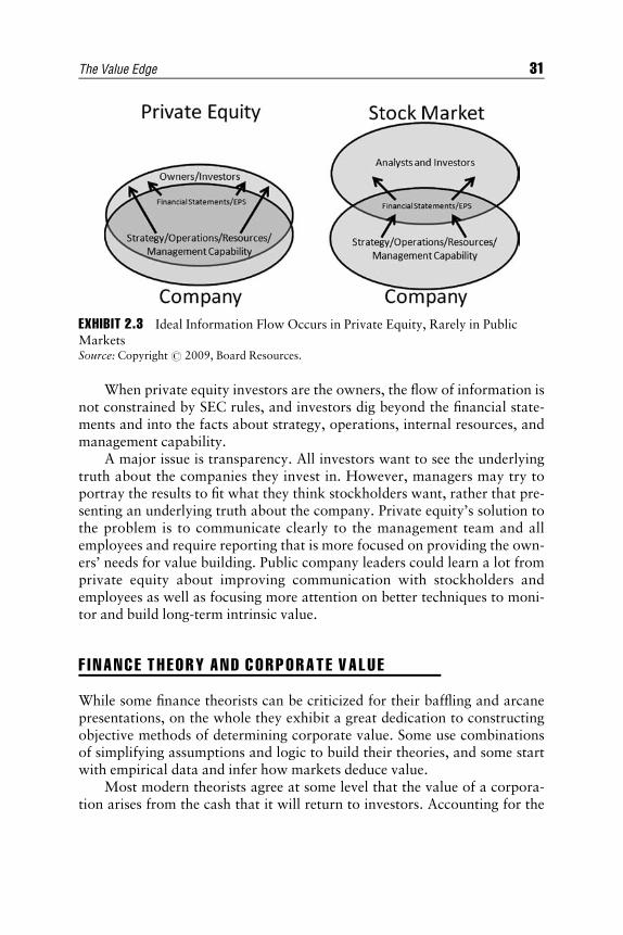
E1C02 08/25/2009 Page 31

When private equity investors are the owners, the flow of information isnot constrained by SEC rules, and investors dig beyond the financial state-ments and into the facts about strategy, operations, internal resources, andmanagement capability.

A major issue is transparency. All investors want to see the underlyingtruth about the companies they invest in. However, managers may try toportray the results to fit what they think stockholders want, rather that pre-senting an underlying truth about the company. Private equity’s solution tothe problem is to communicate clearly to the management team and allemployees and require reporting that is more focused on providing the own-ers’ needs for value building. Public company leaders could learn a lot fromprivate equity about improving communication with stockholders andemployees as well as focusing more attention on better techniques to moni-tor and build long-term intrinsic value.

F I NANCE THEORY AND CORPORATE VALUE

While some finance theorists can be criticized for their baffling and arcanepresentations, on the whole they exhibit a great dedication to constructingobjective methods of determining corporate value. Some use combinationsof simplifying assumptions and logic to build their theories, and some startwith empirical data and infer how markets deduce value.

Most modern theorists agree at some level that the value of a corpora-tion arises from the cash that it will return to investors. Accounting for the

EXHIBIT 2.3 Ideal Information Flow Occurs in Private Equity, Rarely in PublicMarketsSource: Copyright # 2009, Board Resources.

The Value Edge 31

E1C02 08/25/2009 Page 32

timing, they estimate the value by discounting the projected cash. Empiricalstudies have found that the results of these various theories are linked withactual stock market values, with varying amounts of accuracy.

Much of the literature devoted to finance theory is aimed at investorsand portfolio managers. In this arena, a few basis points of return can beworth millions of dollars; hence it is highly worthwhile to focus on nuanceddifferences among the different valuation models. As a result, the invest-ment community has embraced many of the theories and models.

A broad range of valuation models are sufficiently accurate to be usefulfor corporate decision makers. Unfortunately, corporate directors and man-agers are likely to reject portfolio-related theories and models, finding themto be confusing, complicated, incomprehensible, or just not workable if thedetail must be explained to thousands of workers in a large company. Thisis highly unfortunate, for there can be great value in finding a model that isdirectionally correct for use within a company. This standard is far less rig-orous than the standard that a portfolio manager might need to apply inchoosing a valuation model. Valuation Handbook contributor Dennis Austsets forth this distinction with remarkable clarity in Chapter 10 as the‘‘value equation.’’

Still, many senior corporate decision makers continue to sacrifice valuein their pursuit of quarterly EPS targets. These targets do not satisfy the ana-lysts and do not always guarantee value creation. What satisfies the analystsis an uptrend in long-term sustainable cash flow, not reported net income.

There is an undying difference between finance and accounting. Finan-cial values come from expectations about the future, and reported account-ing earnings are all about the past. With a forward-looking numerator and adenominator arising from the past, is it any wonder that price-earnings ra-tios are faulty indicators of value?

To avoid the traps of misusing P/E ratios and EBITDA, financial theo-rists track cash as the wellspring of corporate value. By articulating theirassumptions clearly and describing their logic in mathematical terms, theyset forth their findings with great clarity, to their peers. Unfortunately, fewof their peers sit in corner offices as CEOs or on boards. These decisionmakers use tools they can understand, or those that seem sufficiently acces-sible. As a result, the use of EBITDA and P/E multiples continues, despitepotentially inferior results. These measures do not adequately track value,and their continued use is costly. Companies that shift from performancemeasurement based on accounting to measurement based on value may findthat a third of their prior decisions on capital allocation and value of busi-ness units were just plain wrong (Thomas and Edwards 1993).

Fundamental analysis still has an important place in valuation. In orderto understand the future cash flows of any company, it is important to


E1C02 08/25/2009 Page 33

develop a basic understanding of the economics of key business units in re-lation to industry peers. Ratios too different from those in the industry mayindicate a failure to adopt the best practices of the industry, or worse, thepresence of fraud or creative accounting. Exhibit 2.4 graphically displays asimple (not simplistic) method for visualizing how a company’s financialsand business model compare with industry benchmarks. The analyst ormanager can use this tool and knowledge of the business to examine theimpact of deviations from industry ratios on estimates of corporate value.

THE VALUE EDGE BEG INS AT THESTRATEG I C BUS IN ESS UN I T L EV E L

Large companies are generally built from a number of strategic businessunits (SBUs). Companies have broad latitude in defining these units. De-pending on the nature of the business, the units may be defined by productline, geography, or customer type. Internally, management may have cleardefinitions and goals for individual business units, but the performance ofthe units is frequently blended in some way before issuing public reports.This practice complicates the benchmarking practice discussed earlier.

EXHIBIT 2.4 Basic Graphic to Compare Financial Fundamentals with IndustryBenchmarksSource: Copyright # 2009 Board Resources. Adapted from William J. Hass and Shepherd G.Pryor IV, Building Value through Strategy, Risk Assessment, and Renewal (Chicago: CCH Inc.,

2006).

The Value Edge 33

E1C02 08/25/2009 Page 34

Once management has chosen how to set up the SBUs, tracking andbenchmarking the value of the individual units is a core management princi-ple for building value in the overall company. If the typical board and man-agement team can find a way to determine which units build value andwhich ones detract from overall corporate value, their decision making willbe greatly improved.

THE WATERFAL L O F VALUE I D ENT I F I E S VALUECREATORS AND DESTROYERS

One analysis can be used to compare SBUs, whether they are defined byproduct line, geography, or customer base. The analysis uses a waterfall di-agram, focusing on intrinsic value.

Exhibit 2.5 applies a value analysis to the SBUs of a hypothetical com-pany. What jumps off the page is that some of the units are chugging along,

EXHIBIT 2.5 The Waterfall of SBU Values Highlights Management’s ChallengesSource: Copyright # 2009 Board Resources. Adapted from William J. Hass and Shepherd G.

Pryor IV, Building Value through Strategy, Risk Assessment, and Renewal (Chicago: CCH Inc.,2006).


E1C02 08/25/2009 Page 35

producing value, while others are wasting the corporation’s capital. Thosethat drag down the value do so by returning less than enough to support theunit’s cost of capital. Unfortunately, some of these SBUs are able to reportaccounting profits and favorable budget variances. While the outcome ofthe analysis can be displayed with clarity, the underlying analysis is farfrom simplistic.

The waterfall of SBU values is based on the proposition that the marketcompiles value as a sum of the parts. A common theme is the importance ofa company producing returns in excess of the cost of capital in order tobuild value. The implication for managers is directional. The implicationfor investors seeking the intrinsic value of a company is that they may haveto make further assumptions regarding synergy, covariance, or otheraspects of combined operations.

In the blink of an eye, the waterfall can prompt a director to ask morequestions about a business unit that is reducing the company’s value. Whenthe underlying analysis is undertaken with empirically sound analyticalmethods, many of which are elucidated throughout this book, managementand the board can rely on the waterfall to guide their decision processes. Tobuild the waterfall, varying methods of analysis are available and can bematched with the company’s level of sophistication or budget. For manage-ment, the most important aspect of the model chosen is that it be direction-ally correct, differentiating between the SBUs that add to value and thosethat subtract.

Note that the waterfall focuses on the intrinsic value of a company andits SBUs. A great deal of early research on stock prices focused on pricechanges. While this was mathematically satisfying to the researchers, it didnot translate well into useful principles for corporate decision makers. Ouremphasis on intrinsic value is parallel to newer trends in research on stockprices, which focus on price levels, not just price changes.

BETT ER VALUAT I ON FRAMEWORKSPROV ID E D I SC I P L I N E

Better valuation frameworks and models promote a greater understandingof the cash flows of the business, as well as the underlying strategies thatproduce those cash flows. Exhibits 2.6 and 2.7 provide an example. Theupper portion of Exhibit 2.6 portrays the traditional cash flow forecast in-cluded in a multiyear business plan. The typical financial forecast is drivenby an understanding of the business model and outlook. The lower portion

The Value Edge 35

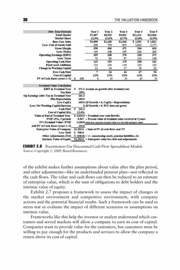
E1C02 08/25/2009 Page 36

of the exhibit makes further assumptions about value after the plan period,and other adjustments—like an underfunded pension plan—not reflected inthe cash flows. The value and cash flows can then be reduced to an estimateof enterprise value, which is the sum of obligations to debt holders and theintrinsic value of equity.

Exhibit 2.7 proposes a framework to assess the impact of changes inthe market environment and competitive environment, with companyactions and the potential financial results. Such a framework can be used tostress test or evaluate the impact of different scenarios or assumptions onintrinsic value.

Frameworks like this help the investor or analyst understand which cus-tomers and served markets will allow a company to earn its cost of capital.Companies want to provide value for the customers, but customers must bewilling to pay enough for the products and services to allow the company areturn above its cost of capital.

EXHIBIT 2.6 Practitioners Use Discounted Cash Flow Spreadsheet ModelsSource: Copyright # 2009, Board Resources.


E1C02 08/25/2009 Page 37

THE VALUE JOURNEY HAS MANY STEPSALONG THE WAY

Just as a company and its management must pursue value buildingthrough a variety of steps, the outside analyst also goes through a similarseries of steps in valuing a company. For the outside analyst it is a choicebetween using simple multiples or more detailed, sophisticated, and ro-bust DCF techniques. On the corporate side, a successful journey towardvalue requires the discipline of tracking progress and making changesalong the way. Conducting an annual valuation and producing thewaterfall for the board along with the annual business plan and budgetis a great first step. An engaged board, guided by a well-constructedvalue analysis, will be in the best position to assist management in refin-ing its strategies, tactics, and resources toward the goal of building cor-porate value.

There are four major steps on the journey to top value builder status.Corporate executives can use them to guide their way. Outside investorsand analysts can evaluate public company management on their progresstoward top value builder status. The steps are:

1. Talking and thinking about value in everything you do, constantly com-municating to the workforce, and providing full disclosure to theshareholders:& This involves setting the right goals and priorities.& This involves communicating verbally and in annual and periodic re-

ports, while changing the culture to ensure all employees understandhow to build value.

2. Implementing metrics that drive cash flow such as return on investedcapital, customer retention and growth, and understanding changingmarkets and market share:

EXHIBIT 2.7 Simple Frameworks Help Identify Key Actions That Create ValueSource: Copyright # 2009, Board Resources.

The Value Edge 37

E1C02 08/25/2009 Page 38

& This includes providing incentive compensation based on value-building metrics.

& This involves going far beyond simplistic EPS-speak metrics.3. Reporting and acting on value and value driver trends on a regular ba-

sis, not just when the trend is positive:& This involves reporting on value-based measures monthly at the op-

erational level and at least quarterly to the board.& This involves developing action plans describing how better results

will be achieved.4. Pushing toward the goal of and achieving top value builder status with

total shareholder returns of 20 percent or more.

Discounted cash flow techniques have been driven to a tipping point bymore sophisticated practitioners. Private equity firms have taken advantageof the discrepancies in valuation of companies to make billions of dollars.They have a stronger focus on future cash flows and value than most ana-lysts, investors, and corporate decision makers.

Public company decision makers can benefit from these advanced DCFtechniques. With the right data at both the macroeconomic and companylevels, better decisions and a better understanding of value are possible.Questions that can help corporate executives and investors build valuealong the value journey are listed with best practices. They are questionsused by many successful private equity players.

& How do we determine which parts of our business build or destroyvalue?& Perform periodic valuations of key business units.& Manage parts of your business as a portfolio.

& How do we assess the macroeconomic environment and the signals itprovides?& Maintain a corporate chart book.& Document the factors and trends that impact operations and value,

such as interest rates, oil prices, and key commodity prices.& How do we ensure management and the board are committed to long-

term value?& Educate the board on value metrics.& Ensure the board has skin in the game.

& How do we effectively identify and track key value drivers?& Make sure each business leader has identified and tracks controllable

and noncontrollable factors.& Adopt an intrinsic value model that uses a broad set of value drivers

appropriate for each of your businesses.


E1C02 08/25/2009 Page 39

& How do we insulate management from forces that might push forshort-term illusory increases in accounting results rather than long-term value?& Adopt an intrinsic value model that uses a broad set of value drivers

appropriate for each of your businesses.& Identify both GAAP and non-GAAP value drivers, but give more

weight to non-GAAP measures.& How can we best communicate that our goal is to improve investor re-

turns through focus on intrinsic value?& Publish and trend goals on value drivers.& Write and talk about intrinsic value drivers at every opportunity, but

especially in employee communications and quarterly and annualreports.

& How do we continue to improve our small but engaged board andensure that they and the management team remain focused on valuecreation?& Make each director responsible for periodically presenting a com-

plete understanding of one or more of the key business units and/orvalue drivers.

& Be sure directors are also investors and have skin in the game.& How do we value the company? How do we best communicate the

value to the rank and file?& Use a simplistic metric like net book value but qualify it with

more robust measures such as adopting use of an intrinsic valuemodel.

& Adopt an intrinsic value model that uses a broad set of value driversappropriate for each of your businesses.

& How do we rank-order our business units by value, and evaluate howthey contribute to our current stock price and intrinsic value?& Adopt an intrinsic value model that uses a broad set of value drivers

appropriate for each of your businesses.& Prepare an annual report with a value waterfall for internal purposes

and the board meetings.& For any unit that supports another, more successful unit, should we be

consolidating those units for reporting purposes?& Ask unit management to run scenarios.& Look at the intrinsic value of the combination.

& What should we do to rectify a situation where a unit is not capable ofearning its cost of capital over the long term and is decreasing the valueof the overall enterprise?& Act sooner than your competitors.& Spin out the unit to a buyer with a better strategic fit.

The Value Edge 39

E1C02 08/25/2009 Page 40

& How can we find ways to improve our insights on value creation?& Experiment with new concepts and valuation approaches.& Involve others in improving the value creation process.

& How do we install a cost of capital discipline into our organization?& Educate all employees in basic finance concepts.& Ensure that key people have an incentive to earn more than their cost

of capital.

ACKNOWLEDGMENTS

We owe a debt of gratitude to several people who assisted in the adaptationby reviewing and providing insights, including Sean Falmer, RawleyThomas, Robert Agnew, Duncan Borne, and many others.

RE F ERENCES

Callard, C., and D. Kleinman. 1985. Inflation-adjusted accounting: Does it matter?Financial Analysts Journal (May–June).

Copeland, T., T. Koller, and J. Murrin. 1994. Valuation: Measuring and managingthe value of companies. 2nd ed. New York: John Wiley & Sons. (Orig. pub.1990 by McKinsey & Co.).

Copeland, T., and V. Antikarov. 2001. Real Options: A practitioner’s guide.New York: Monitor Group.

Glovin, D., and P. Hurtado.Ex-Refco Chief Bennett’s guilty plea may help formerdeputies. Bloomberg.com, February 16, 2008. www.bloomberg.com/apps/news?pid=20601087&sid=aAKxBfxG9fhU&refer=home.

Hass, W., and S. Pryor. 2006. Building value through strategy, risk assessment, andrenewal. Chicago: CCH Inc.

Hospira. 2007. Annual report.Hu, J. 2005. Case accepts blame for AOL-Time Warner debacle. CNET News.com,

published on ZDNet News, January 12, 2005. See also: AOL Time Warner Inc.2002. 10-Q report, second quarter 2002 (August 14), 35: ‘‘Upon adoption ofFAS 142 in the first quarter of 2002, AOL Time Warner recorded a one-time,noncash charge of approximately $54 billion to reduce the carrying value of itsgoodwill.’’ See also: UC Newsroom. 2003. AOL and Time Warner executivesaccused of pocketing nearly $1 billion. www.universityofcalifornia.edu/news/article/5311.

Jones, S. 2009. Sears boss lets loose on a lot: Lampert’s letter ranges far and wide;profit down 55%. Chicago Tribune, February 27, 25.


E1C02 08/25/2009 Page 41

Klein, A. 2003. Stealing time: Steve Case, Jerry Levin, and the collapse of AOL TimeWarner. New York: Simon & Schuster Paperbacks, 68–78.

Laffer, A., W. Hass, and S. Pryor. 2009. The private equity edge: How private equityplayers and the world’s top companies create value and wealth. New York:McGraw-Hill.

Livio, M. 2002. The Golden Ratio: The story of phi, the world’s mostastonishing number. New York: Broadway Books/Random House, 128–137.

Lowe, J. 1994. Benjamin Graham on value investing: Lessons from the dean of WallStreet. Chicago: Dearborn Financial Publishing.

Madden, B. 1999. CFROI valuation: Cash flow return on investment. Woburn, MA:Butterworth-Heinemann. See also: Madden, B. 2007. For better corporate gov-ernance: The shareholder value review. Journal of Applied Corporate Finance19, no. 1 (Winter): 102–114.

Mandelbrot, B., and R. Hudson. 2004. The (Mis)Behavior of Markets: A fractalview of risk, ruin and reward. New York: Basic Books.

Modigliani, F., and M. Miller. 1961. Dividend policy, growth and the valuation ofshares, Journal of Business 34 (October): 411–433.

Porter, Michael. 1980. Competitive strategy. New York: Free Press/Simon & Schus-ter. (Porter received an MBA with high distinction in 1971 from Harvard Busi-ness School, where he was a George F. Baker Scholar, and a PhD in businesseconomics from Harvard University in 1973, during which time he researchedthe PIMS data.)

Pratt, S., and A. Niculita. 2008. Valuing a business: The analysis and appraisal ofclosely held companies. 5th ed. New York: McGraw-Hill. See also: Pratt, S.,R. Reilly, and R. Schweihs. 1998. Valuing small businesses and professionalpractices. 3rd ed. New York: McGraw-Hill.

Pryor, Shepherd, William Hass, and Dennis Aust. 2006. Driving long-term value:What are the next steps? Directors Monthly 30, no. 12 (December): 1.

Rappaport, A. 1986. Creating shareholder value: The new standard for business per-formance. New York: Free Press.

Schroeder, A. 2008. The snowball: Warren Buffett and the business of life. NewYork: Bantam Books. See also: Buffett, W. 1996. An owner’s manual. Omaha,NE: Berkshire Hathaway. Originally produced in June 1996 and updated onwww.berkshirehathaway.com.

Schumpeter, J. 1942. Capitalism, socialism and democracy. New York: Harper &Brothers.

Sharpe, W. 1964. Capital asset prices: A theory of market equilibrium under condi-tions of risk. Journal of Finance 19: 425–442.

Stewart, G. 1991. The quest for value: The EVA1 management guide. New York:HarperBusiness, 40–41. See also: Colvin, G. 2008. A new way to value the mar-ket: The latest technology enables novel analysis of whether stocks are attract-ively priced now. (Hint: They might be.) Fortune, February 21. http://money.cnn.com/2008/02/15/magazines/fortune/investing/colvin_eva.fortune/index.htm.

The Value Edge 41

E1C02 08/25/2009 Page 42

Thaler, R., and C. Sunstein. 2008. Nudge: Improving decisions about health,wealth, and happiness. New Haven, CT: Yale University Press.

Thomas, R., and L. Edwards. 1993. How HOLT methods work: For gooddecisions, determine business value more accurately. Corporate Cashflow(September).

Tortoriello, R. 2009. Quantitative Strategies for Achieving Alpha. New York:McGraw-Hill.


E1C03 09/02/2009 Page 43

CHAPTER 3Applying a Systems Mindset

to Stock ValuationBartley J. Madden

Independent Researcher

Research on the life-cycle valuation model began in 1969 at Callard, Mad-den & Associates in order to improve stock selection and investment re-

turns. Beginning in the mid-1980s, the model was extensively refined andcommercialized by HOLT Value Associates. Today, many institutionalmoney managers use the life-cycle valuation model, as well as relevant datafrom the global database of 20,000 companies in 60 countries provided byCredit Suisse HOLT.

This is a review of the five important choices that guided this 40-yearresearch journey. A systems mindset that stressed intensive measurementand experimentation with variables was especially instrumental to the evo-lution of the life-cycle model. Systems thinking led to distinct departuresfrom mainstream finance practices. For example, the life-cycle model uses adiscount rate that is dependent on the procedure used to forecast a firm’slong-term, net cash receipt (NCR) stream.

Based on this research experience, I offer suggestions about the poten-tial evolution of a new research program to address additional important,practical needs.

CHO IC E 1 : A SYSTEMS M INDSET

Knowledge improvement generally is a product of inquiry, undertaken tobetter understand or solve a perceived problem (Umpleby and Dent 1999).When we are involved in inquiry, we are as much a part of the inquiry as theexternal environment because we have preconceptions that affect what is,

43

E1C03 09/02/2009 Page 44

literally, observed, and the conceptual interpretations of those observations(Madden 1991).

Being constructs of human thought, all theories are actually conditionalstatements subject to tests of their usefulness for solving a problem in itscontext. Users of a theory (or model) want it to reliably serve as a guide fortaking action to achieve an intended goal. This is the ultimate predictabilitytest of a model.

Researchers who have chosen a systems mindset begin with intensiveobservations and trial descriptions of phenomena to uncover both criticallyimportant variables and consequential relationships among them. Forexample, the life-cycle model uses a discount rate that is dependent on theprocedure used to forecast a firm’s long-term, net cash receipt stream. Ingeneral, a systems mindset promotes bottom-up (inductive) thinking that iscrucial to discovering essential but difficult-to-quantify variables, the kindthat might be observed in data as outliers and omitted as anomalies or thatmight be buried in error terms in the construction of econometric models.

However straightforward and commonsense systems thinking is inprinciple, it often times is ignored in practice. For example, many main-stream finance researchers rely heavily on top-down (deductive) theorysuch as market efficiency and the capital asset pricing model (CAPM). Inthe past, the strong pull of this dominant view slowed down experimenta-tion with variables that could jeopardize the market efficiency and CAPMconstructs. For example, note how long it took for behavioral finance toemerge.

An overemphasis on top-down theory can be harmful, as articulated byRobert Haugen (1999, 139, 140):

Finance scholars have long embraced the notion that we advancefaster and better by first creating theories that make predictionsabout the way the world works. Next we turn to the data to see ifthe numbers conform to the predictions. If we find that they donot, we either (a) ‘‘refine’’ the theories, by altering the assumptionsupon which they are based, or (b) ‘‘refine’’ the empirical tests untilthe data speaks in a voice we can appreciate and understand. . . .But most of the major advances in the frontier of human knowl-edge did not follow an arrow running through the theories intothe empirical tests. Rather, most of our greatest triumphs pro-ceeded in the opposite direction from data to theory. The arrowgoes from straightforward empirical observation to the develop-ment of theories which give us the insights to understand what wehave seen. . . . We have two choices. We can advance by develop-ing radically new theories to help us understand what we now see


E1C03 09/02/2009 Page 45

in the data. Or we can go back, denying what is now readily ap-parent to most, bending the data through ever more convolutedeconometric processes, until it screams its compliance with ourpreconceptions. (italics in original)

Modern finance researchers by and large have used CAPM to guidemuch of their work, so much so that Perold (2004) would say it dominatedmodern finance. An elegant explanation of a mathematically logical rela-tionship between expected returns on stocks and risk, CAPM provides ablueprint, given its assumptions, for investors to optimize their portfolios tothe highest expected return for a given level of risk. NotwithstandingCAPM’s poor empirical record of predictability (Fama and French 2004)and its challengeable assumptions, it continues to exert a strong hold onmainstream finance.1

In the past decade or so, behavioral finance researchers have presentedserious challenges to the premises and empirical underpinnings of main-stream finance theory (Thaler 2005). But proponents of the status quo seemlittle concerned about the weaknesses of their theory. Rather, they take theoffensive, asking: Where is the better theory? Believing none has beenoffered yet, they have not significantly changed the core body of knowledgepresented in finance textbooks and taught to finance students. Thus thedominant theory remains intact.

The intended takeaway from this quick sidetrack into the philosophy ofknowing is that empirical work based on innovative formulations of ques-tions/problems and different ways of manipulating and testing variablescan: (1) reveal deeply rooted, but flawed, assumptions, (2) improve the spec-ification of components of an existing model, and (3) lead to new concep-tual advancements—that is, better theory for ‘‘insights to understand whatwe have seen,’’ and for reliably guiding action to achieve a goal.

CHO I C E 2 : F I RMS ’ COMPET I T I V E L I F E CYCL E

Early on in life cycle research, the accepted goal of the research programbecame to better understand levels and changes in company stock prices ona global basis so portfolio managers could make better investment deci-sions. In contrast, mainstream finance was focused on a logically consistentequilibrium model that related risk to expected return—and CAPM becamethe answer. CAPM was not designed to explain the level of firms’ marketprices, but rather the change in prices that drive investor returns.

A dominant academic premise has been that the market is efficient inincorporating all value-relevant information into stock prices. Consequently,

Applying a Systems Mindset to Stock Valuation 45

E1C03 09/02/2009 Page 46

finance academics gave relatively little attention to the process of forecastingfirms’ long-term, net cash receipt (NCR) streams. Why? Because stock priceshave already incorporated these forecasts, and forecasting better than themarket is ruled out by the efficiency assumption.

In contrast, the commercial research program on life cycles wanted a vehi-cle to deal with NCR forecasts so that both levels and changes in stock pricescould be fruitfully studied (without any preconceived beliefs about market ef-ficiency). We chose the firms’ competitive life cycle construct in order to con-nect firms’ economic performance to market valuation in a conceptual waythat incorporates competition, and yet was useful for forecasting NCRs.

Exhibit 3.1 illustrates the firms’ competitive life cycle in four stages cap-tured as patterns of the four key variables that drive a firm’s economic per-formance. The assumed role for competition over time had especially strongempirical support and was aptly stated by George Stigler (1963, 54):

There is no more important proposition in economic theory thanthat, under competition, the rate of return on investment tends towardequality in all industries. Entrepreneurs will seek to leave relativelyunprofitable industries and enter relatively profitable industries.

In the life cycle framework one can observe the effects of Joseph Schum-peter’s (1942, 84) creative destruction at work—the ‘‘kind of competitionwhich counts . . . competition from the new commodity, the new technol-ogy, the new source of supply, the new type of organizations . . . competi-tion which commands a decisive cost or quality advantage and which strikesnot at the margins of the profits and the outputs of the existing firms but attheir foundations and their very lives.’’

EXHIBIT 3.1 Firms’ Competitive Life CycleSource: Madden (2005).


E1C03 09/02/2009 Page 47

The radical competition Schumpeter alludes to often comes from firmsin the High Innovation stage. These firms have satisfied the fundamentalcriterion of wealth creation, namely economic returns clearly in excess ofthe cost of capital. Particularly successful firms exhibit high reinvestmentrates (i.e., growth in operating assets) in order to meet high demand fortheir products or services, and this creates additional wealth.

As competitors attempt to duplicate and improve on the highlydemanded innovative product/service, the Competitive Fade stage (Wigginsand Ruefli 2005) follows. Due to competitive pressure, firms’ economic re-turns fade toward the cost of capital and reinvestment rates fade to lowerlevels (Fama and French 2000).

Next is the Maturity life cycle stage wherein top management is typi-cally lulled into a business-as-usual complacency. Inertia prevails, with abias toward making perceived low-risk investments that incrementallyexpand businesses that were profitable in the past.

A transition to the Failing Business Model stage occurs as profitabilitydeclines, which is consistent with a shortfall, relative to competitors, in pro-viding value to customers. At this stage, purging bureaucratic inefficienciesand downsizing/refocusing are almost always needed in order to restoreprofitability and avoid bankruptcy.

A critical task in the application of the life cycle concept to actualfirms is to estimate economic returns (discussed later). Life cycle track re-cords, based on firms’ reported, or suitably adjusted, accounting data andstock price histories are a valuable tool for better understanding the past,and thereby for making better forecasts of the future. The life cycle trackrecord for Kmart from 1960 to its bankruptcy in 2002 is displayed inExhibit 3.2.

The top panel shows inflation-adjusted (real) economic returns, esti-mated as a cash flow return on investment (CFROI

1

, registered trademarkof Credit Suisse Securities). The panel includes a benchmark, long-term,corporate average CFROI of 6 percent real to approximate the cost ofcapital.2 The middle panel shows real asset growth rates. The bottom panelshows a cumulative index that reflects annual changes in the yearly excess(positive or negative) of the total shareholder return (dividends plus priceappreciation) of the company’s stock relative to the S&P 500. A positiveshare performance versus the S&P 500 is depicted by rising trends in therelative wealth index, and negative performance by falling trends.

Shareholder returns in excess (positive/negative) of the general marketare attributed to firms’ fade rates being more/less favorable than investorsexpected. That is, at the margin, investors were positively/negatively sur-prised. From 1960 to the early 1970s, Kmart’s innovative concept of a dis-count store propelled its CFROIs from barely positive levels to above the


E1C03 09/02/2009 Page 48

EXHIBIT 3.2 Kmart Life Cycle Performance, 1960 to 2002Source: Credit Suisse HOLT ValueSearch global database.


E1C03 09/02/2009 Page 49

cost of capital. This unanticipated upward fade of CFROIs enabled long-term shareholders to outperform the market 36-fold during this period.Then, over the next 20 years, Kmart slightly underperformed the marketwhile CFROIs averaged around 7 percent. From the mid-1990s to bank-ruptcy in 2002, Kmart had four CEOs. Each failed to develop and execute aviable strategy to counteract fierce competition from Wal-Mart.

Let’s turn now to some important technical issues in life cycle research.

CHO IC E 3 : I N F LAT I ON ADJUSTMENTSAND ECONOM IC RETURNS

In the early 1970s, it occurred to me that a project orientation would beuseful for developing the CFROI metric (Larsen and Holland 2008, 119–143). An economic return was specified as the standard return on invest-ment (ROI) measure of a completed project, reflecting each period’s NCRover the full project life. When all outflows and inflows are expressed inmonetary units of equivalent purchasing power, the calculated ROI is aninflation-adjusted, or real, economic return.

A firm was then viewed as a portfolio of ongoing projects (Larsen andHolland 2008, 159–163). The problem facing an analyst using reported fi-nancial statements is to estimate the average economic returns beingachieved on the aggregate of the firm’s ongoing portfolio of projects.

The balance sheet and income statement data provide gross assets, cashflow, nondepreciating assets, and life. These can be arranged as a projectROI with an initial outlay of gross assets, followed by equal cash flows overthe assigned life with a release of nondepreciating assets in the final year.When the ROI calculation uses assets marked up to match the purchasingpower of cash flows, the result is a real CFROI.

I chose not to use a conventional return on net assets (RONA) for threereasons. First, explicit identification of the ROI components helps resolveproblems in adjusting accounting data to match business economics in or-der to more closely approximate economic returns. Second, the productivecapacity of plant and equipment does not decline as rapidly as implied bystraight-line depreciation (Thomas 2002, 2–3), which is wired into mostRONA calculations.

Third, the project emphasis used to construct a CFROI is a useful tie-into the value of existing assets. At any specific point in time, a portfolio ofprojects has different vintages, from the oldest to the most recent projectstarted. The oldest projects have the shortest remaining economic lives, andtypically have the least amount of cash flows remaining, whereas the


E1C03 09/02/2009 Page 50

opposite is true for the newest projects. A project orientation easily trans-lates into a conceptual view of the valuation of existing assets as the wind-down of cash flows as projects meet the ends of their economic lives.

This valuation perspective of the cash flow wind-down of existingassets had more plausibility compared to the conventional, and mathemati-cally convenient, present value of existing assets as a perpetuity (currentearnings divided by the cost of capital). This is particularly evident, forexample, in the use of the wind-down approach when estimating the valueof a firm’s existing oil/gas reserves.

Keep in mind that progress with the task of connecting firms’ economicperformance to market valuation involves learning better ways to approxi-mate important variables such as economic returns and investor expecta-tions. For example, a time series of CFROIs can help one infer the levelof economic returns being earned by the firm, and thus help in making aforecast of ROIs on future investments—a key variable driving long-term NCRs.

Arguably, a prerequisite in working with, and learning from, time seriesdata is that key variables should have the same meaning over time (Madden1999, 17). All of the components of the life-cycle valuation model are realvariables in order to minimize the noise due to fluctuations in monetary unitvalues (different inflation/deflation rates). Consequently, levels of andchanges in CFROIs and discount rates can be meaningfully comparedacross historical time periods and across national borders.

There is a large body of academic work in the accounting literature onthe connection between economic returns and accounting returns (Brief1986). But the research tends to be mathematical exercises, absent track re-cord analyses. Also, researchers have devoted considerable energy to resid-ual-income valuation models (Ohlson 1995; Feltham and Ohlson 1995,1996), which ignore the divergence between true economic returns andaccounting returns such as earnings on book equity. The assumption is thatin forecasting a long-term earnings stream, biases will offset (e.g., a bias oftoo-low book equity would be offset by too-high earnings on book equity).In finessing the flaws in accounting data in this way, the residual incomeproponents shut off a potential learning process, a learning process that isintegral to a systems mindset.

CHO IC E 4 : D ENOM INATOR DEPENDSON THE NUMERATOR

All conceptually sound, discounted cash flow valuation models incorporatesome form of the four fundamental life cycle variables: economic returns,


E1C03 09/02/2009 Page 51

reinvestment rates, competitive fade, and cost of capital (investors’ discountrate). Exhibit 3.3 maps the role of these variables in generating net cashreceipts, which are discounted to a present value (i.e., a warranted valuecontingent on the forecasted variables).

How one specifies operating assets influences the calculated values ofeconomic returns and reinvestment rates. Consequently, the observed his-torical fade rates for economic returns and asset growth rates (proxy forreinvestment rates) also depend on the specification of operating assets. Forexample, the life cycle track record for a typical pharmaceutical companyis significantly different if research and development (R&D) expendituresare capitalized and included in operating assets.

Let’s go another step. Since forecasted fade rates are a key driver ofNCRs (the numerator), discount rates (the denominator) depend on theanalysis of historical fade rates used as the basis for forecasting future faderates. Thus, a less obvious relationship is that the assignment of a company-specific discount rate should be logically consistent with the NCR forecast-ing procedure being used.

Applying systems thinking to discount rates is not an unreasonablepoint of view. Bond investors set market prices for bonds by applying aforward-looking discount rate—their demanded yield to maturity (YTM)—to an expected NCR stream of interest and principal payments. So, too,for common stock investors, although it is far more difficult to estimateexpected NCR streams for business firms. Help in this area came from clientfeedback as part of the commercial research process. Portfolio managersand security analysts, with in-depth knowledge of individual companies,provided a continual stream of problems whose solutions involved newways to better estimate economic returns. This, in turn, helped improveNCR forecasting.

EXHIBIT 3.3 Life-Cycle Valuation ModelSource: Madden (2005).


E1C03 09/02/2009 Page 52

Ne t Cash Rece i p t S t reams , D i s coun t Ra t es ,and Prob l em So l v i n g

First, let’s specify a procedure for forecasting NCRs. Then we’ll discusshow forecasted NCRs are used to calculate a company’s forward-looking(market-derived) cost of capital or discount rate.

NCRs are driven by a forecast life cycle. The present value today ofNCRs from investments made beyond 40 years in the future is quite small,especially when those investments are expected to earn close to cost of capi-tal economic returns. A life cycle forecast period of 40 years (Madden 1999,173) is one practical choice, although the selection of a longer horizon doesnot much impact warranted value calculations.

As today is year T, a near-term fade window from T þ 1 to T þ 5 beginswith a normalized T þ 1 CFROI, which is derived from consensus analystearnings per share (EPS) forecasts for years T, T þ 1, and T þ 2. The fade ofboth CFROIs and reinvestment rates from T þ 1 to T þ 5 is primarily basedon past company CFROI variability and asset growth rates (Madden 1999,165–167). From T þ 5 to T þ 40, CFROIs regress to a long-term corporateaverage CFROI of 6 percent real. And asset growth rates regress to a matureeconomy growth rate at T þ 40. Improved fade forecasts, in particular forthe early part of firms’ future life cycles, continue to be researched andimplemented.

This has been the standard NCR forecast procedure used for manyyears. An argument to add a longer, more favorable near-term fade windowfor certain types of companies hinges on the strength of economic reasonsand empirical data presented to support more customized forecasting proce-dures. Note that the forecast procedures being discussed are standardizedprocedures used to maintain a monitored database of companies.

Company-specific discount rates at points in time are calculated with aregression equation. Given the standard fade forecast for a company keyedto a normalized forecast T þ 1 CFROI, the market-derived discount rate isthe rate that provides a present value of the future NCR stream equal totoday’s known market value.3 This forward-looking discount rate is the de-pendent variable.

There are two independent variables (Madden 1999, 102–104). Be-cause CFROIs include the benefit to cash flows from tax-deductible interestpayments, an offsetting risk differential for financial leverage is called for.That is, higher leverage should result in higher discount rates, all else beingequal. The other independent variable is a liquidity risk differential. That is,all else being equal, less liquid companies involve higher trading costs andshould result in higher demanded returns as compensation. Less liquid com-panies are small companies. As the economic environment becomes better/


E1C03 09/02/2009 Page 53

worse for small companies, this effect will decrease/increase the measuredliquidity risk differential.

In summary, the application of a market-derived process for assigning adiscount rate to a particular company can be compared to estimating theaverage yield to maturity (YTM) for bonds with a particular credit rating.For a sample of bonds, one could assemble data for a regression equationwith YTM as the dependent variable and credit rating as the independentvariable. A regression line for bonds then transforms a credit rating into anexpected YTM. In a similar manner, for stocks, a regression line value for acompany’s discount rate is contingent on its financial leverage and tradingliquidity. Market-derived discount rates serve as an alternative to CAPMcosts of capital.

Market-derived discount rates do not address important CAPM issuessuch as how investors are assumed to handle systematic or market risk inbuilding their portfolios. Rather, market-derived discount rates representthe end result of how investors are currently pricing individual companyrisks in terms of financial leverage and liquidity.

An ability to assign a specific discount rate to a specific firm at aspecific point in time enabled the development of a warranted valuechart. This is the workhorse automated tool for identifying problems. Itis a long-term plotting of both a company’s annual stock price rangesand annual warranted values based on the standardized NCR forecastsusing estimated company-specific discount rates. Systematic overtrackingor undertracking of actual prices compared to warranted values are seenas red flags for possible problems. Other common sources of problemsare when life cycle track record data for a company seems implausiblecompared to industry peers, and/or relative stock price performancedoes not make sense when compared to time series data for CFROIs andreinvestment rates.

Dealing with a problem almost always begins with skepticism abouthow closely accounting data matches business economics. A small sampleof issues includes: capitalization of R&D expenses, operating lease capitali-zation, acquisition intangibles, financial subsidiaries, off-balance-sheetliabilities, special items, stock option expenses, and asset lives. A typical fixfor a problem would entail finding an economically sound reason to adjustaccounting data that not only improves the original company situation, butalso results in similar improvements for other companies that share this eco-nomic characteristic. Improvement is gauged by closer tracking of actualversus warranted values.

The ongoing life-cycle research program leads to insightful ways to ad-just accounting data to better estimate economic returns. Improved NCRforecasts lead to improved discount rates.


E1C03 09/02/2009 Page 54

Taiwan Mystery Resolved A recent experience with Taiwanese companiesserves as an excellent example of the benefit of a systems mindset. In a sys-tems approach, learning is a function of identifying problems and develop-ing solutions by paying attention to interactions among variables. In a 2006Credit Suisse HOLT report, Ng, Jhaveri, and Graziano described a majorimprovement for Taiwanese companies.

Let’s begin with problem recognition. The aggregate market-deriveddiscount rate for Taiwanese companies seemed implausibly high. Also, Tai-wanese companies with low financial leverage had higher discount ratesthan the high-leverage companies—a negative leverage risk differential thatdid not make economic sense.

The root cause of these problems was identified as excessively highCFROIs for the many companies that generously dispensed shares foremployee stock bonuses. From the shareholders’ perspective, this outlaywas clearly an economic expense, although it was ignored in computingaccounting net income.4 This artificially boosted CFROIs, which in turnboosted market-derived discount rates.

Exhibit 3.3 is helpful in understanding this point. Substitute a firm’sknown market value for the warranted value. The market value can bematched by either (1) discounting higher NCRs (boosted by ignoringemployee stock bonuses) at a higher rate or (2) discounting lower NCRs(this is more accurate) at a lower rate.

The solution was to incorporate an appropriate charge, which loweredcash flow used in calculating CFROI. With the new lower CFROIs (betterreflecting business economics), calculated market-derived discount rates de-clined. Interestingly, technology companies were the biggest users of em-ployee stock bonuses, and these companies also tend to have low financialleverage. Thus, the CFROI fix also resolved the mystery of a too-high dis-count rate for low-leverage companies. Finally, there was an across-the-boardimprovement in the tracking of warranted values with actual stock prices.

CAPM Is a Problem CAPM captured and still holds the minds (and hearts?)of finance academics with its elegant mathematics grounded in the neo-classical economic principles of equilibrium, rationality, and efficientmarkets.

In general, finance textbooks (Brealey, Myers, and Allen 2006 is anexample) explain portfolio construction as investors striving to achievehigher expected returns and to reduce risk. CAPM is an integral part of thisexplanation. In this manner, CAPM becomes a foundation for thinkingabout stock prices.

CAPM was brought into discounted cash flow valuation of individualfirms as the basis for assigning a firm’s equity cost of capital. A firm’s equity


E1C03 09/02/2009 Page 55

discount rate equals the risk-free rate plus the product of a stock’s beta (i.e.,volatility) times the risk premium of the overall equity market (i.e., expectedexcess return of the equity market over the risk-free rate). This is the stan-dard method finance students are taught to use for estimating a firm’s costof equity capital.

One objection to market-derived discount rates replacing CAPM ratesis the necessity for maintaining a monitored database and attending to allsorts of issues concerning accounting conventions versus business econom-ics. Fair enough. But increased valuation accuracy through more appropri-ate company-specific discount rates can generate big rewards.

The other major objection is more subtle. This criticism is that the market-derived discount rate methodology can produce illogical discount rates. Forexample, consider a technology company and a food company that haveapproximately the same financial leverage and the same liquidity (companysize). The previously described regression procedure for assigning discountrates would give the same discount rate to both companies. Yet, as criticspoint out, everyone knows that food companies have a lower cost of capitalthan technology companies because food companies have more stable andpredictable cash flows and lower betas than technology companies.

The false perception of illogic only shows the absence of a systemsmindset. The life-cycle valuation model’s standard fade forecast for a typi-cal technology company is much less favorable compared to that of a typi-cal food company. A technology company with above-cost-of-capital, buthighly variable, economic returns and/or high reinvestment rates would beassigned a faster downward fade compared to a food company, which typi-cally has more stable economic returns and slower reinvestment rates. Thelife cycle approach handles the risk difference in the numerator.

There are at least two important reasons to consider for rejecting thestandard CAPM equation in favor of the market-derived approach for usein valuation models. First, application of the CAPM equation requires twoinputs that are notoriously difficult to judge—beta and the equity marketrisk premium over the risk-free rate. These are applied as forward-lookingvariables but they are necessarily estimated from historical data.

Estimates based on historical time periods are especially troublesomewhen tax legislation, such as capital gains tax rates, that affects investors’after-tax returns (and thus their demanded returns) is expected to pass orbecomes law (Madden 1999, 97–99, 250–252). Market-derived discountrates immediately reflect these changes.

Depending on the past time periods selected, a stock’s beta could eas-ily range from, say, 1.2 to 1.5, and the market premium could easily rangefrom, say, 4 percent to 7 percent. Users of CAPM have little to guide themin the selection of these two critical inputs. Combining a risk-free


E1C03 09/02/2009 Page 56

rate of 3 percent with a beta of 1.2 and a 4 percent market premium yieldsa 7.8 percent equity cost of capital. In contrast, substitution of a beta of1.5 and a market premium of 7 percent yields a 13.5 percent equity costof capital.

The valuation impact of using either a 7.8 percent or a 13.5 percentequity cost of capital is enormous. A similar big impact on an economicvalue added (EVA) calculation occurs when the equity cost of capital is esti-mated with the CAPM equation or alternative procedures, such as arbitragepricing theory or the Fama-French three-factor model, which is increasinglybeing used by quantitative portfolio managers (Fabozzi, Focardi, and Jonas2008).

In practice, market-derived discount rates for a sample of companieshave a much smaller range. Particularly important is that these discountrates have a hand-in-glove compatibility fit with the valuation model inwhich the discount rate is applied.

In contrast, two analysts using radically different assumptions for fore-casting long-term fade rates (read as risk adjustments) and using the sameCAPM cost of capital would calculate widely different valuations. But theywould not have a clue about the impact of parachuting into their valuationmodels a discount rate that is totally independent of how NCRs areforecasted.

Another reason for rejecting CAPM equity rates is, as noted earlier, thatthe systems mindset promotes intensive data analysis as part of a process toimprove higher-level understanding. In valuation applications, CAPM userstend to implement theory that arrives on a plate served up by the theorydevelopers. But theory developers don’t analyze firms’ track records, strug-gle with measurement issues, calibrate market expectations, forecast futureNCR streams, and make investment decisions. These activities focus themind on all sorts of important technical issues that have implications forhigher-order model building.

In my opinion, which is echoed by many portfolio managers and ana-lysts who actively work with life cycle data, business risk analysis is mostusefully handled in the numerator and not the denominator.

CHO IC E 5 : I NS I GHTS ANDPLAUS IB I L I TY JUDGMENTS

Mainstream finance, as reflected in standard corporate finance textbooks,has little to say about how the users of valuation models develop their skillin making forecasts. In other words, the users’ forecasting skill is viewed asbeing independent from the model.


E1C03 09/02/2009 Page 57

Not so with the life cycle research program. The three primary researchtools—life cycle track records, warranted value charts, and valuation modelto translate forecast inputs (see Exhibit 3.3) to warranted values—comprisethe product provided to institutional money manager clients. Client userssharpen their forecasting skills by participating in the same learning processas the research staff.

When users employ these tools to investigate a firm, they gain an oppor-tunity to study the causes of a firm’s long-term fade within the unique con-text of an industry and economic environment, and to build up expertise inunderstanding how the market makes forecasts (sets expectations) and re-vises these expectations as new data arrive.

The more experience users accumulate with the application of thesetools, the better prepared they are to analyze a new company. There aretwo main analytical benefits.

First, users can quickly generate insights as to the key valuation issuesfor a particular firm and to the actions management should give top priorityto taking in order to maximize long-term shareholder value. Second, the us-ers’ growing base of experience facilitates plausibility judgments about in-vestor forecasts (expectations), their own forecasts, and the forecasts ofothers. Judging the degree of difficulty in achieving these forecasted levelsof performance is greatly aided by a comparison to the type of companiesthat have historically achieved these same levels of life cycle performance.

As for plausibility judgments and investor expectations, an informativeapplication of the life-cycle model was reported in a September 9, 1996,Forbes article, ‘‘Follow the Cash’’ (Samuels 1996). The article described thelife-cycle framework used by HOLT Value Associates in consulting withinstitutional investors. Forbes pointed out that HOLT had rated Wal-Martas a strong sell five years earlier before it sharply declined, whereas HOLTnow considered Wal-Mart a strong buy. The main point here is not thatthese two recommendations produced returns consistent with the sell-buyrecommendations; rather, the important point being illustrated is the judg-ment process for competitive fade and managerial skill at those two pointsin time versus investor expectations.

Although the Wal-Mart success story is well known, the magnitude ofWal-Mart’s wealth creation achievement is striking when displayed in lifecycle terms as seen in Exhibit 3.4. We see CFROIs rising from 12 percent toabout 15 percent from 1970 to 1990 coupled with enormous real assetgrowth rates. That remarkable performance was continually underesti-mated by investors, and the stock outperformed the S&P 500 100-foldfrom 1970 to 1990.

In 1991, Wal-Mart’s stock price implied no downward competitivefade in both CFROIs and real asset growth rates for the next five years.


E1C03 09/02/2009 Page 58

EXHIBIT 3.4 Wal-Mart Life Cycle Performance, 1970 to 2007Source: Credit Suisse HOLT ValueSearch global database.


E1C03 09/02/2009 Page 59

While possible, our experience suggested that, at its much bigger size rela-tive to the 1970s and 1980s, Wal-Mart was unlikely to meet thoseextremely optimistic investor expectations. The stock subsequently under-performed the market substantially from 1991 to 1996 (see bottom panelof Exhibit 3.4) as CFROIs declined and asset growth sharply fell off.

At the time of the 1996 Forbes article, investor expectations were forWal-Mart’s CFROIs to rapidly fade downward over the next five years to alevel close to the long-term corporate average of 6 percent CFROIs. We feltcomfortable in betting against an expectation that Wal-Mart was on theverge of becoming an average firm. This time, the stock subsequently rosesharply more than the S&P 500 during the next three years as Wal-Marthandily beat the 1996 expectations.

Although it is convenient to distill investor expectations into a singlebest-estimate forecast, more rigorous analysis deals with warranted valueas the expected value of a probability-weighted distribution of scenarios forfuture fade of economic returns and reinvestment rates (Alessandri, Ford,Lander, Leggio, and Taylor 2004).

To illustrate the concept of fade distribution, let’s return to Exhibit 3.4and reflect on the process that produced such extraordinary excess share-holder returns during the 1970s and 1980s. At various times during this pe-riod, I analyzed Wal-Mart and decided not to buy it because I viewed theprobability as low for a scenario in which Wal-Mart would maintain highCFROIs while sustaining an extraordinarily high 25 percent per year or-ganic asset growth rate. I was wrong. My mistake was in not sufficientlyunderstanding Wal-Mart’s business model and exceptional managerial skill,which enabled the firm to perform so spectacularly as to drive its chief com-petitor, Kmart, into bankruptcy.

BACK TO THE FUTURE

The life-cycle model is but one application of discounted cash flow thatspecifies a cause-and-effect relationship for (1) firms’ economic perform-ance, leading to a market valuation, and (2) investor expectations and thefirm’s subsequent economic performance, leading to excess (positive/nega-tive) shareholder returns.

Whatever the life-cycle research program’s contribution to knowledgeis, it is the product of a different way of thinking and going about researchas compared to mainstream practices. The life-cycle research process hasalways been grounded in data observations with a bottom-up, inductivepath for its constructs (e.g., a market-derived discount rate, fade, etc.).


E1C03 09/02/2009 Page 60

Because mainstream theory was not at the foundation of our work, theCAPM never had a top-down, deductive hold on our thinking and doing.

Believers in either CAPM or the life-cycle model can easily lose skepti-cism about what they think they know. The important point is that theorybuilding often makes the most progress when problems are approachedfrom new angles, where a healthy competition exists among alternativemodels, and when commitment is strong enough to actively search for situa-tions where one’s preferred model fails (Carlile and Christensen 2005).These attitudes, I submit, would serve well for the evolution of a powerfulresearch program that could significantly improve our understanding ofhow firms’ strategies, business processes, organizational structures, cul-tures, financing decisions, and the like produce the firms’ long-term, netcash receipt streams—and how this gets reflected in levels and changes instock prices over time.

Empirical testing of a large menu of different valuation models for over-all usefulness would be most fruitful when applied to a broad range of envi-ronmental conditions and user circumstances. Testing valuation modelswith innovative research designs might produce strong-enough evidence toovercome deeply held beliefs (Atra and Thomas 2008).

In this way, theory building would increasingly become part of theprocess in which researchers continually loop through intensive data ob-servations and measurement challenges coupled with ongoing deeperunderstanding of cause and effect. So, how to get from here to there?

Let’s speculate on how finance academics, and both investment andcorporate practitioners, could jointly evolve improved valuation modelsthat better serve the practical needs of users. The foundation for just such ajoint collaboration has already been laid with the Financial ManagementAssociation’s recent start-up of the Practitioner Demand Driven AcademicResearch Initiative (PDDARI).5

PDDARI is coordinating an intellectual marketplace for ideas with thegoal of expediting big advancements in finance theory that are of a highpractical value. A major target is a new theory that integrates both risk/re-turn and the level of firms’ market valuations.

SEARCH ING FOR FA I LURES AND SUCCESSES

Searching for failures as well as successes can be the bridge needed for genu-ine collaboration among finance academics and those who work in thetrenches (Heuer 1999).

As for environmental conditions and user circumstances, one classifica-tion system to consider would be the five categories briefly discussed next.


E1C03 09/02/2009 Page 61

F i rm Ma tur i t y

According to firm size and/or life cycle position, how much can differentvaluation models benefit from analyses of firms’ historical financial data inorder to make most likely or best-estimate forecasts of the input variables ofthe various models?

In addition, how capable are these models in handling risk in the nu-merator? That is, how does accuracy vary when historical data are used aspart of a process for calculating the expected value of a probability-weighted distribution of potential scenarios for a firm’s future profitability?

For example, consider a bullish scenario for an early-stage firm with aspecified level of high economic returns and high reinvestment rates in thefuture. The historical frequency of achieving that level of economic per-formance for early-stage firms could be tabulated after certain milestoneswere delivered. A milestone could be one quarter of 25þ percent organicsales growth, or two back-to-back quarters of 25þ percent growth.This type of information could help assign a probability for a particularearly-stage firm to achieve a bullish scenario. For the same early-stage firm,historical frequencies could be tabulated for a bearish scenario, giving con-sideration to the data on cash balances and product diversification in addi-tion to sales growth. This perspective seems better suited for handlingfirms with low-probability/high-valuation impact scenarios compared to asimple, most likely estimate forecast of future profitability.

I n dus t ry

Users of models employing EVA, CFROI, or other metrics that stress eco-nomic performance accept that valuation accuracy improves after account-ing data are adjusted to more closely mirror business economics. How doesvaluation accuracy vary across industries and across valuation modelsas different types of accounting adjustments are implemented? For a givenindustry, how does valuation model accuracy vary as the estimated propor-tion of intangibles in firms’ economic assets changes and as asset lifechanges?

Mode l Users

Connecting firms’ operating performance to market valuation is clearly im-portant to investors, managements, boards of directors, and accounting rulemakers. How well do models perform to meet the primary needs of eachgroup? Government officials involved with wealth creation issues includemanagements of regulatory agencies as well as politicians and their staffs.


E1C03 09/02/2009 Page 62

Policy decisions about corporate tax rates, personal tax rates, regulation,property rights, and the like impact a society’s ability to create wealth. Inwhat innovative ways can these macroeconomic policy lever variables beconnected via valuation models to levels and changes in aggregate stockprices for countries over longer time periods?

Da t a

Value-relevant data sources include:

& Market prices for ownership claims. At points in time when firmscould easily fall into bankruptcy, does the concurrent market pricebehavior of equity, debt, and options reveal fundamental weaknessesin how valuation models incorporate risk? Another question of in-terest is: Do the fat-tailed distributions of actual stock price changeslead to insights about the environmental (institutional) causes offirms’ economic performance? At the macro level, Baumol (2002)argues convincingly that productive entrepreneurial activity is thedominant source of a society’s wealth generation. Perhaps the condi-tions that favor more/less entrepreneurial activity set the stage forSchumpeter’s creative destruction and result in an increase/decreasein the fat tails of a country’s distribution of long-term shareholderreturns (Fogel, Morck, and Yeung 2006).

& Accounting data. As intangible assets increase in importance (Corrado,Haltiwanger, and Sichel 2005), accounting rule makers and corporateexecutives are grappling with measuring and managing intangibles.Valuation models (including real options) could provide new empiricalangles to help decide if an outlay (e.g., R&D expenditures) should becapitalized as an intangible asset and expensed (Hand and Lev 2003),and how best to do this (Healy, Myers, and Howe 2002). To handlethis extremely difficult challenge, does it not make sense for academicresearchers to join forces with CFOs and their staffs (those closest tothe data)?

& Human capital data. Some intangibles are so soft and qualitative thatthey are not candidates for inclusion in reported accounting data.Many of the long-term benefits of human capital fit this category. Forexample, Toyota’s efficiency seems to result not only from its lean pro-duction techniques, but also from its culture that promotes continuouslearning and problem solving, with every layer of employees deeply in-volved, including top management (Liker and Hoseus 2008). Althoughquite difficult to measure, the effects of human capital improvements ordegradations can be broadly observed in firms’ long-term fade rates.


E1C03 09/02/2009 Page 63

Creativity in developing new measuring sticks is needed. Hewitt Asso-ciates has taken a step in this direction by showing that a measure offirms’ ability to attract and retain higher-grade (pivotal) employees cor-relates with future fade of CFROIs.6

Managemen t Dynam i cs

At any point in time, management could be initiating improvements instrategy, core business processes, or corporate culture, yet the reportedaccounting data usually does not adequately reflect the value change at anearly stage. For example, most valuation models have a component for thepresent value of future investments. But consider, for example, the potentialmisperception during the early stage of a firm’s successful transformation tolean manufacturing. During this period, lean processes free up a great dealof capacity to enable management to pursue new opportunities withouthaving to make the kind of capital outlays customary in its less efficientpast. The resulting decrease in the asset growth rate could easily be misreadas a reduction in new investment opportunities and a concomitant reduc-tion in the warranted value of future investments. Alternatively, manage-ment could be asleep at the switch, as was the case for Kmart for manyyears, yet the reported accounting data did not reflect the extent of share-holder value deterioration. How do different valuation models fare in theirquickness to pick up these big value changes? Given firm maturity and thetype of high-priority initiatives that management has disclosed in the annualreport, what signals are helpful in the early identification of the directionand magnitude of the value change?

CONCLUS I ON

To guide our actions so that we may achieve a goal, we develop modelsabout how the world works. Straightforward as that may seem, any futureknowledge-building process is made difficult by our existing knowledgeassumptions. At any point in time, assumptions representing faulty conceptsimpact how we perceive the world, define problems, explore data, and gen-erate hypotheses to test. Therefore, a significant challenge is to manage thepersonal biases that always exist, even if the researcher is not consciouslyaware of them. Leamer (1983, 36) summarized the challenge:

The econometric art as it is practiced at the computer terminal in-volves fitting many, perhaps thousands, of statistical models. Oneor several that the researcher finds pleasing are selected for


E1C03 09/02/2009 Page 64

reporting purposes. This searching for a model is often well inten-tioned, but there can be no doubt that such a specification searchinvalidates the traditional theories of inference. The concepts ofunbiasedness, consistency, efficiency, maximum likelihood estima-tion, in fact, all the concepts of traditional theory, utterly lose theirmeaning by the time an applied researcher pulls from the brambleof computer output the one thorn of a model he likes best, the onehe chooses to portray as a rose.

The new research program outlined in this chapter, keyed to searchingfor the failures as well as the successes of any model, holds the potential togain knowledge by overcoming our personal biases. A better understandingof cause and effect throughout the wealth creation process will lead to bet-ter decisions for the long-term, mutual benefit of customers, employees, andshareholders.

Most especially, managements and boards of directors need better valu-ation tools in order to make the right long-term decisions. Their decisionsmay, at times, disappoint Wall Street’s myopic fixation on quarterly earn-ings expectations. But managements should finally quit playing WallStreet’s game. Managers should employ an insightful valuation model andvalue-relevant accounting information to make sure their decisions makeeconomic sense (Madden 2007). Then, they need to clearly communicate toinvestors the rationale for their decisions.

NOTES

1. Friedman’s (1953) methodology of positive economics promoted the view thatthe realism of assumptions is immaterial as long as the world behaves as if theassumptions were true. This gave added credibility to mathematical modelssuch as CAPM, and deflected criticism of the use of empirically unsupportedassumptions (Frankfurter and McGoun 1996).

2. For the period 1960 to 1996, aggregate U.S. industrial CFROIs approximated 6percent real, and a market-derived real discount rate (cost of capital) also aver-aged approximately 6 percent real (Madden 1999, 92). For the nonfinancial sec-tor, 1950 to 1996, Fama and French (1999) estimated the real cost of capital at5.95 percent and the return on corporate assets, unadjusted for inflation, at7.38 percent.

3. Especially difficult-to-forecast companies, such as biotech start-ups, should beexcluded from the universe of companies used for the regression.

4. Starting in 2008, Taiwan companies are required to expense the cost ofemployee stock bonuses.

5. See www.fma.org/pddari/pddari.htm.6. See www.evidence-basedmanagement.com/guests/ubelhart_jan07.html.


E1C03 09/02/2009 Page 65

RE F ERENCES

Alessandri, Todd M., David N. Ford, Diane M. Lander, Karyl B. Leggio, and Mari-lyn Taylor. 2004. Managing risk and uncertainty in complex capital projects.Quarterly Review of Economics and Finance 44, no. 5 (December): 751–767.

Atra, Robert J., and Rawley Thomas. 2008. The fundamentals of automated DCFmodeling. www.fma.org/texas/PDDARI/accepts.htm.

Baumol, William J. 2002. The free-market innovation machine: Analyzing thegrowth miracle of capitalism. Princeton, NJ: Princeton University Press.

Brealey, Richard A., Stewart C. Myers, and Franklin Allen. 2006. Principles of cor-porate finance. 8th ed. New York: McGraw-Hill Irwin.

Brief, Richard P., ed. 1986. Estimating the economic rate of return from accountingdata. New York: Garland Publishing.

Carlile, Paul R., and Clayton Christensen. 2005. The cycles of theory building inmanagement research, version 6.0. Harvard Business School Working Paper05-057.

Corrado, Carol, John Haltiwanger, and Daniel Sichel. 2005. Measuring capital inthe new economy. Chicago: University of Chicago Press.

Fabozzi, Frank J., Sergio M. Focardi, and Caroline Jonas. 2008. Challenges in quan-titative equity management. Charlottesville, VA: Research Foundation of CFAInstitute.

Fama, E. F., and K. R. French. 1999. The corporate cost of capital and the return oncorporate investment. Journal of Finance 54, no. 6 (December): 1939–1967.

Fama, E. F., and K. R. French. 2000. Forecasting profitability and earnings. Journalof Business 73, no. 2 (April): 161–175.

Fama, E. F., and K. R. French. 2004. The capital asset pricing model: Theory andevidence. Journal of Economic Perspectives 18, no. 3 (Summer): 25–46.

Feltham, Gerald A., and James A. Ohlson. 1995. Valuation and clean surplusaccounting for operating and financial activities. Contemporary Accounting Re-view 11(Spring): 689–731.

Feltham, Gerald A., and James A. Ohlson. 1996. Uncertainty resolution and thetheory of depreciation measurement. Journal of Accounting Research 34(Autumn): 209–234.

Fogel, Kathy, Randall Morck, and Bernard Yeung. 2006. Big business stability andeconomic growth: Is what’s good for General Motors good for America? NBERWorking Paper 12394.

Frankfurter, George M., and Elton G. McGoun. 1996. Toward finance with mean-ing: The methodology of finance, what it is and what it can be. Greenwich, CT:JAI Press.

Friedman, Milton. 1953. Essays in positive economics. Chicago: University ofChicago Press.

Hand, J., and B. Lev, eds. 2003. Intangible assets: Values, measures, and risks.London: Oxford University Press.

Haugen, Robert A. 1999. The new finance: The case against efficient markets.2nd ed. Upper Saddle River, NJ: Prentice Hall.


E1C03 09/02/2009 Page 66

Healy, Paul M., Stewart C. Myers, and Christopher D. Howe. 2002. R&D account-ing and the tradeoff between relevance and objectivity. Journal of AccountingResearch 40, no. 3 (June): 677–710.

Heuer, Richards J. 1999. Psychology of intelligence analysis. Washington, DC:Government Printing Office. Free download at www.cia.gov/library/center-for-the-study-of-intelligence/csi-publications/books-and-monographs/psychology-of-intelligence-analysis/psychofintelnew.pdf.

Larsen, Tom, and David Holland. 2008. Beyond earnings: A user’s guide to excessreturn models and the HOLT CFROI1 framework. In Equity Valuation: Mod-els from Leading Investment Banks, ed. Jan Viebig, Thorsten Poddig, andArmin Varmaz.West Sussex, England: John Wiley & Sons.

Leamer, Edward E. 1983. Let’s take the con out of econometrics. American Eco-nomic Review 73(1): 31–43.

Liker, Jeffrey K., and Michael Hoseus. 2008. Toyota culture: The heart and soul ofthe Toyota way. New York: McGraw-Hill.

Madden, Bartley J. 1991. A transactional approach to economic research. Journal ofSocio-Economics 20(1): 57–71.

Madden, Bartley J. 1999. CFROI valuation—A total system approach to valuing thefirm. Oxford: Butterworth-Heinemann.

Madden, Bartley J. 2005. Maximizing shareholder value and the greater good.Naperville, IL: LearningWhatWorks, Inc.

Madden, Bartley J. 2007. Guidepost to wealth creation: Value-relevant track re-cords. Journal of Applied Finance 17, no. 2 (Fall/Winter): 102–114.

Ng, Chiew Leng, Viral Jhaveri, and Ron Graziano. 2006. HOLT Taiwan: Account-ing for employee stock bonus. Credit Suisse HOLT, December 5.

Ohlson, James A. 1995. Earnings, book values, and dividends in equity valuation.Contemporary Accounting Research 11 (Spring): 661–687.

Perold, Andre F. 2004. The capital asset pricing model. Journal of Economic Per-spectives 18, no. 3 (Summer): 3–24.

Samuels, Gary, 1996. ‘‘Follow the cash: HOLT Value Associates hated Wal-Mart in1991. Its unique valuation system tells HOLT to love Wal-Mart now,’’ Forbes,September 9.

Schumpeter, Joseph A. 1942. Capitalism, socialism and democracy. New York:Harper & Row.

Stigler, George. 1963. Capital and rates of return in manufacturing industries.Princeton, NJ: Princeton University Press.

Thaler, Richard H. 2005. Advances in behavioral finance. Vol. 2. Princeton, NJ:Princeton University Press.

Thomas, Rawley. 2002. Value management—Past, present, and future. Workingpaper, LifeCycle Returns. www.lcrt.com/value_management_past_present_future_3_19_02.pdf.

Umpleby, Stuart A., and Eric B. Dent. 1999. The origins and purposes of severaltraditions in systems theory and cybernetics. Cybernetics and Systems: An Inter-national Journal 30: 79–103.

Wiggins, R. R., and T. W. Ruefli. 2005. Schumpeter’s ghost: Is hypercompetitionmaking the best of times shorter? Strategic Management Journal 26 (10):887–911.


E1C04 09/03/2009 Page 67

CHAPTER 4Comparing Valuation Models

Thomas E. Copeland, Ph.D.Founder, Copeland Valuation Consultants

Herein I focus attention on a seemingly simple question: ‘‘Which valua-tion model is best?’’1 The marketplace, of course, determines the ac-

tual transaction prices of all types of assets in addition to companies—houses, automobiles, planes, racehorses, gems, artwork, first editions, andso forth. But the current market price can deviate from the fundamentalsin the short run. Valuation models claim to provide equilibrium or intrin-sic value estimates. How does one decide which valuation model is best?

A classic valuation approach has been to find a comparable asset thathas traded recently and to adjust the comparable’s trading price to that ofthe asset being valued by scaling with an alleged value driver such as earn-ings. Unfortunately, while one-carat flawless diamonds are close substitutesto each other, a company in the chemicals industry with $5 billion of annualsales that grows at 4 percent a year may not be even vaguely similar to an-other chemical company with $50 million of sales that has been growing at12 percent, even though their current earnings might be similar. In the past70 years or so, comparables have been replaced with various discountedcash flow (DCF) models. Are they any better than comparables? Howshould one decide?

The measure of the quality of a valuation model depends on its in-tended use. For legal purposes, such as taxation, inheritance, and divisionof property, one may judge the quality of a valuation by the magnitude ofthe difference between the model value and the market (or trading) value ofa company—a measure of the goodness of fit. The smaller the difference,the better the model is. I will use various statistics to put this concept to uselater on in the chapter.

However, for the purpose of investment, I suggest that in order to com-pare valuation models, it does not matter what the difference (or error term)

67

E1C04 09/03/2009 Page 68

is between the model and the market value. In fact, a perfect fit would beuseless for the purpose of investment. Neither does the correlation betweenthe two values make a difference, nor do the slope and intercept of a cross-sectional regression equation. What does make a difference is the time seriesconvergence between them. In particular, does the market price movetoward the model price? If it does, then the model has some economic valid-ity; and, by the way, the market is not instantaneously efficient. The bettermodel provides the more useful information. Said information has valueonly if the set of state-contingent actions that result from its acquisition re-sult in higher payout (or utility) than the next best alternative.

After a brief review of the literature, I describe the discounted cash flowapproach for valuation of a company, and introduce an expert system that Ideveloped in order to supply valuations for sample sets of companymonthly observations that are in the thousands. Its virtue is that it performsdetailed DCF valuations very quickly—in less than five seconds per com-pany. Thereafter, I test the goodness of fit and the time series convergencethat are provided by various valuation approaches, including ratios, simpleformulas, and the DCF model as estimated by the expert system. I find thatthe convergence property of the DCF valuation model is positive and statis-tically significant. It is the best of the models compared in this chapter, butnot by a wide margin.

L I T ERATURE R EV I EW

Very few comparisons of valuation models of companies have been pub-lished. Kaplan and Ruback (1995) used an adjusted present value (APV)model to estimate the market value of 51 highly leveraged transactions(HLTs), then compared the error rates of their APV estimates with the errorrates of valuations derived from multiples of comparable companies. Thisgoodness of fit approach concluded that the APV model valuations haderror rates at least as small as valuations that used multiples. Resultsshowed that the model explained around 70 percent of the cross-sectionalvariation in market price scaled by book value. Bailey (1991) used an optionpricing corporate equity valuation model in a horse race with a discountedcash flow model to see which came closer to explaining the market values ofrubber plantations in Malaysia and Singapore. He reasoned that the planta-tions resembled switching options because when the price of oil was highrelative to natural rubber for the production of close substitutes such aspencil erasers, the rubber plantations would harvest natural rubber fromtheir trees. When the price of oil was low, the rubber plantations were shutdown. It was among the first papers to directly compare the traditional DCF


E1C04 09/03/2009 Page 69

approach with an option-pricing approach to the valuation of companies.Bailey found that the option approach had smaller error terms than theDCF approach. Copeland, Koller, and Murrin (1994) regressed analyst-generated discounted cash flow estimates (in 1988) of the values of a set of35 large industrial companies against their market values and found an r-squared of 94 percent. The regression was repeated in 1999 for 31 survivorsfrom the original set and the r-squared was 92 percent. This is also a type ofgoodness of fit comparison.

This body of evidence is based on relatively small samples, mainly dueto the fact that it is a time-intensive effort to use DCF to value even a singlecompany. For example, in an interview with a top Wall Street analyst, I wastold that an experienced analyst required four to eight hours to complete astandard DCF valuation. An additional problem was that analysts withinthe same securities analysis group often failed to apply the same interpreta-tion of the standard DCF methodology.

A major concern with the publications discussed earlier is that none ofthese comparisons reported time series (or convergence) behavior concern-ing the null hypothesis that the information content of the valuation modelfor the purpose of investment is, in fact, zero. They studied goodness of fitbut not time series behavior. Later in the chapter I show that the standardDCF model exhibits biases in its goodness of fit that are associated with rev-enue growth and stock price volatility. Goodness of fit seems to be margin-ally improved when one uses option pricing parameters to adjust the DCFvaluation. Convergence is also improved if the DCF model bias is corrected.

BR I E F D ESCR I PT I ON OF THE VALUAT I ONMODELS THAT ARE COMPARED

The time-worn and traditional approach to valuation, still used by WallStreet analysts and investment bankers, is a multiples approach that selectsa value driver that is deemed appropriate to the value of a company, thenratios it to the market price of comparable companies. One common exam-ple of a multiple is the average of the comparable’s market price per sharedivided by their earnings before interest, taxes, depreciation, and amortiza-tion (EBITDA):

Market valuet ¼ (EBITDA multiplet)[Et(EBITDAtþ1)] ð4:1Þ

Often EBITDAtþ1 is the expected number for the company being val-ued, denoted in Equation 4.1 as E(EBITDA). Other multiples are the price-earnings ratio, a market-to-book ratio, and a multiple of revenue:

Comparing Valuation Models 69

E1C04 09/03/2009 Page 70

Market value per sharetþ1 ¼ (Price per sharet=Net income per sharet)

�E(Net income per sharetþ1)

¼ (Price per sharet=Book value of equity per sharet)

�E(Per share book value of equitytþ1)

¼ (Price per sharet=Revenue per sharet)

�E(Revenue per sharetþ1)

Sometimes the ratios are industry specific, such as the populationpassed by a length of cable in the telecommunications industry (calledPOPs). All of the aforementioned are referred to as multiples.

For a long time, before the advent of computerized spreadsheets in the1980s, discounted cash flow models were based on simple mathematicalformulas. Two examples are the cash flow perpetuity and the dividendgrowth model. We will use both. The perpetuity model is the present valueof a constant infinite annuity. Implied in it is the assumption that the returnon invested capital and the cost of capital of a company are equal to eachother. Therefore, while earnings may grow, the growth adds nothing to thevalue of the company.

Perpetuity model:

V ¼ E(FCF)=WACC ð4:2Þ

Here, we define V as the value of the entity being valued. The definitionof expected free cash flows is the expectation of earnings before interest andtaxes E(EBIT) multiplied by 1 minus the tax rate that the firm would have ifit had no debt. The weighted average cost of capital (WACC) is theweighted average of the marginal costs of the firm’s debt and equity financ-ing. To convert the entity values of equations (4.2) and (4.3) and the entityDCF value to equity values, I added excess marketable securities, and sub-tracted debt and other liabilities (e.g., unfunded pension plans).

A slightly more sophisticated discounted cash flow formula allows one toaccount for the fact that often cash flows grow and contribute to value be-cause they earn a return on invested capital that exceeds the firm’s WACC. Itis called the Gordon growth model, and it provides higher estimates of value.

Growth model:

V ¼ E(FCF)(1 þ g)=(WACC� g); given that WACC > g ð4:3Þ

Finally, there is the discounted cash flow (DCF) model. It is only slightlymore sophisticated than the perpetuity and growth models. Generally, ituses a spreadsheet model of the expected free cash flows of the firm, givenan explicit forecast for five to ten years, followed by either the perpetuity or


E1C04 09/03/2009 Page 71

growth models that estimate the so-called continuing value (CV) of the firm,which is nothing more than the present value of cash flows from the end ofthe explicit forecast period to infinity. The CV as a percentage of the totalvalue often exceeds 50 percent.

The DCF approach is more sophisticated than the others because: (1) itis founded on cash flows that are derived from both income statement andbalance sheet information, (2) it appropriately accounts for the opportunitycost of capital (debt and equity), and (3) it reflects the timing of cash flowswithin the explicit forecast period.

AN EXPERT SYSTEM THAT DOES VALUAT I ON

All tests of valuation models have had relatively small sample size, and havebeen done by hand. I wanted large sample size. In an attempt to have a toolthat does a complete discounted cash flow valuation quickly, I developed anexpert system. It produces the set of outputs that are illustrated in this chap-ter’s appendix for Intel in 2008. All together there are 14 exhibits on 16pages of output.

1. Market and DCF price history.2. Valuation summary.3. Value driver summary.4. Revenue growth forecast.5. Operating margin forecast.6. Net property, plant, and equipment.7. Operating working capital.8. Weighted average cost of capital.9–10. Income statement.

11–12. Balance sheet.13. NOPLAT and taxes on EBIT.14. Free cash flows and financial flows.15. Invested capital.16. Continuing value.

The data is read in, the calculations are performed, and then output ta-bles are filled—all in less than five seconds per company. It is possible,therefore, to study a large sample of consistently executed DCF valuations.Later in the chapter, I attempt to assess whether the DCFs produced by theexpert system are any good—a separate question.

An expert system is a process that inputs facts and uses rules to producea solution about some particular problem domain. In this case, our system is


E1C04 09/03/2009 Page 72

a consistent set of decision rules that produces an estimate of the marketvalue of a company. The system loads historical company-specific and mar-ket data, performs a historical analysis, estimates a weighted average costof capital, forecasts short-term and long-term free cash flows based on ana-lyst forecasts and extrapolation, and derives a continuing value estimate.The system was developed using data from 1994. Tests were run on out-of-sample data between 1995 and 2000, and separately on a sample from 2000to 2008.

An expert system mimics human expertise at much lower cost. Whiletrue experts are scarce, expensive, and hard to duplicate, an expert systemcan be widely distributed and easily duplicated. An expert system canexceed human capacity in both speed and accuracy. While a living expertspends at least four hours to value a company, an expert system can pro-duce answers with similar accuracy in a few seconds. The expert system isflexible, and one can even use a neural network to train it and solve morecomplicated problems.

As input to the expert system, I used historical accounting statementsand credit ratings from Compustat, estimates of beta (from Compustat andValue Line), market information about the risk-free rate and credit spread(Federal Reserve Board), an estimate of the market risk premium (Ibbot-son), and analyst forecasts of revenue growth, operating margin, and capitalexpenditures—for the current year, the second year of the forecast period,and three to five years out.

I used the DCF model that is found in Valuation: Measuring and Man-aging the Value of Companies, 2nd Edition (1994) by Copeland, Koller, andMurrin. Free cash flows to the entity are defined there as earnings beforeinterest and cash taxes (i.e., the tax the firm would pay if it had no debt),plus depreciation, less capital expenditures and increases in operating work-ing capital. Taxes are assessed at the marginal cash tax rate (i.e., the rate thefirm would pay on its EBIT if it had no debt). The expected free cash flowsof the firm are discounted back to the present using a weighted average costof capital (WACC) based on the capital asset pricing model (CAPM). I usedCompustat or Value Line betas. The risk-free rate was defined as the 10-yearyield to maturity on U.S. Treasuries. The market risk premium was 5.5 per-cent in all years and based on the long-term arithmetic average market riskpremium, less 2 percent survivorship bias. The continuing value formula waschosen by the expert system to be one of the following three formulas:

CV ¼ NOPLAT11(1 � g=ROIC)=(WACC � g) growth formula ð4:4Þ

CV ¼ NOPLAT11=WACC perpetuity formula ð4:5Þ


E1C04 09/03/2009 Page 73

(assumes : ROIC ¼ WACC)

CV ¼ NOPLAT11=kuþ TBþ K(NOPLAT11)N[(ROIC�WACC)=

WACC(1 þWACC) finite supernormal growth formula2ð4:6Þ

The perpetuity formula assumes that the firm’s return on invested capi-tal (ROIC) equals its weighted average cost of capital (WACC) every yearbeyond the explicit forecast period (usually 10 years). Of the three choices,it produces the lowest continuing value estimate. At the opposite extreme isthe ‘‘value driver’’, or growth formula. It assumes that ROIC will perpetu-ally exceed WACC by a constant spread, and that g (growth) is financed byretaining K percent of free cash flows, where K = g/ROIC. The intermediatealternative assumes that the spread between ROIC and WACC closes over aT-year interval. The larger the spread at the end of the explicit forecast pe-riod, the larger is the adjustment interval, T.

The expert system chooses among these three alternatives by examiningreturn on invested capital forecasts. If the forecasted ROIC is greater thanthe weighted average cost of capital by the same margin as in the past, theexpert system assumes that the spread is structural and proceeds to use thevalue driver formula. If the ROIC appears to be trending toward the WACCor to be unsustainable, the expert system uses the finite supernormal ap-proach. Finally, if the ROIC has been and is forecasted to remain close tothe WACC, the expert system uses the perpetuity formula.

Exhibit 4.1 shows a simplified flow chart for the expert system. Itillustrates the inputs to the program, the logic flow, and the outputs. Al-though the expert system is ad hoc, it does reflect the experience of thevaluation expert who built it, and it can be revised after testing to pro-vide better goodness of fit results. There is no harm in efforts to revisethe model so that it provides tighter fits to the actual market data. How-ever, when it comes to efforts to improve the time series relationship be-tween the model and the market, it is important to avoid a specificationsearch. It is improper to test the model on historical data, then retest arevised model on the same data, and to do so iteratively until a successfulmodel is finally found.

The flow of logic in the expert system is quite standard. It beginswith data inputs as described earlier—for example, financial statementsthat go back for at least five and as long as 10 years. The program thenexecutes a series of forecasting routines (called ‘‘forecast engines’’) thatdelve into revenue growth, operating margin, and capital expenditureforecasts whose validity is checked by comparing them with industry me-dian forecasts of their closest industry and with long-term expectationsof economic growth. Next, the weighted average cost of capital and the


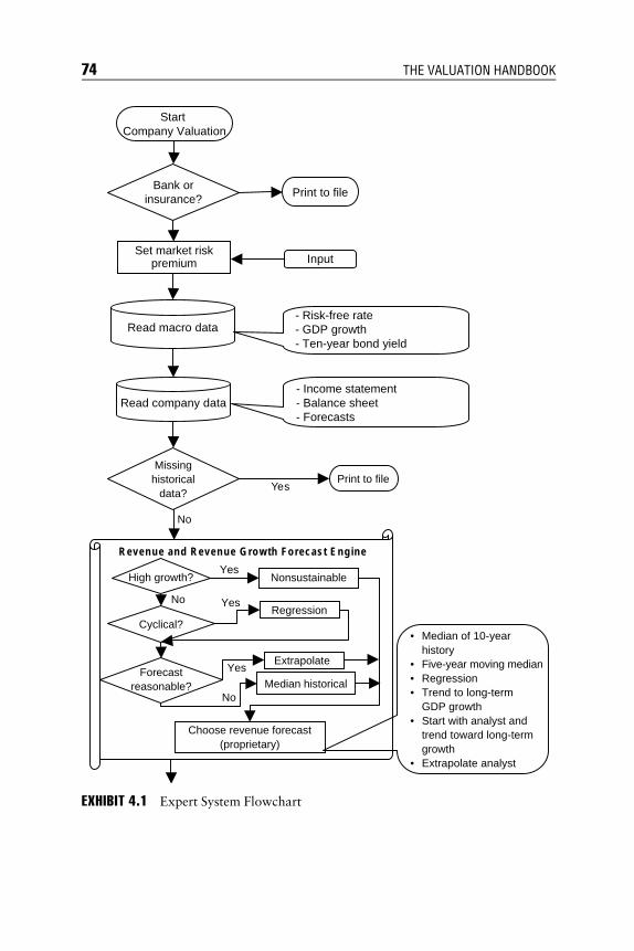
E1C04 09/03/2009 Page 74

- Income statement- Balance sheet- Forecasts

Bank orinsurance?

StartCompany Valuation

- Risk-free rate- GDP growth- Ten-year bond yield

Print to file

Read company data

Set market riskpremium

Read macro data

Input

Revenue and Revenue Growth Forecast Engine

Missinghistorical

data?Print to file

High growth?

Cyclical?

Forecastreasonable?

Yes

No

Choose revenue forecast(proprietary)

• Median of 10-yearhistory

• Five-year moving median• Regression• Trend to long-term

GDP growth• Start with analyst and

trend toward long-termgrowth

• Extrapolate analyst

Nonsustainable

Regression

Extrapolate

Median historical

Yes

No Yes

Yes

No

EXHIBIT 4.1 Expert System Flowchart


E1C04 09/03/2009 Page 75

Record revenue and revenue growthRead historical OM

Read historical SGA/revRead historical COGS/rev

Read historical dep/rev

Operating Margin Forecast Engine

In range?

Reasonable?

Yes

Yes

No

No

Choose OM forecast(proprietary)


• Five-year movingmedian

• Extrapolate analyst

Extrapolate historical

Median

Capital Expenditures Forecast Engine

Turnoverwithin range?

NPPE/revwithin range?

Record OM


• Five-year movingmedian

• First and thirdquartile of history

• Extrapolate analyst• NPPE method

Choose capex forecast(proprietary)

NPPE method

Reasonable?Extrapolate historical

capex/rev

Regression

No

No

No

Yes

Yes

Yes

EXHIBIT 4.1 (Continued)


E1C04 09/03/2009 Page 76

g < WACC?

Determine capital structure

Calculate Kequity, Kdebt, Kpreferred

Record capex forecast

WACC

Record WACC

Yes

No Set long-term growth rate to expectedlong-term nominal GDP growth rate

Perpetuity formula

Determine ROIC usingK (historical)

Is K reasonable?

Value driver formula

Yes

No

Determine entity value as sum of FCF(forecast) and continuing value

Determine equity value

DCF value per share

No

Yes



E1C04 09/03/2009 Page 77

continuing value are estimated. The final step is to estimate the entityvalue of operations, add marketable securities, and subtract the estimatedmarket value of debt in order to derive the final result—an estimate ofthe market value of the firm.

In the test results, we worked hard to search for the expert system thatminimized the percentage error between the live (industry-specific) marketprice as of a given date and the model-estimated price on the same date. Wedid so before testing the portfolio performance of the stocks chosen by themodel. Later, we used out-of-period (i.e., holdout) data.

GOODNESS OF F I T : I N I T I A L SAMPLE(1 ,395 VALUAT I ONS 1993 TO 2000 )

The first of two sample universes was the Standard & Poor’s 500 companiesfrom 1993 to 2000. Exhibit 4.2 shows that companies were excluded be-cause they were financial firms (wrong industry) or utilities (types of compa-nies not handled by the expert system), because there was missing data,because the valuation was out of range (negative equity value), or becausethe book value of equity was negative. These exclusions reduced the samplesize from 4,000 company observations to 1,395. Nevertheless, this sample is26 times the largest sample published to date.

EXHIBIT 4.2 Sample Size, 1993–2000

Year 1993 1994 1995 1996 1997 1998 1999 2000 Total

Originalsample

500 500 500 500 500 500 500 500 4,000

Missingdata

217 212 198 193 176 139 124 121 1,380

Wrongindustry

105 107 114 112 112 117 123 124 914

Out ofrange

31 31 30 29 21 40 48 24 254

Negativebookvalue

10 10 8 6 7 5 7 4 57

Samplesize

137 140 150 160 184 199 198 227 1,395

Percentusable

34% 28% 28% 30% 37% 40% 40% 45% 35%


E1C04 09/03/2009 Page 78

E rror Terms

The error terms are defined in percentages of the market price as:

Errort ¼ (Model price per sharetþ1 � Market price per sharet)=

(Market price per sharet)ð4:7Þ

The distribution of error terms is provided in Exhibit 4.3. This result isencouraging. It can be said that roughly 83 percent of the companies thatwere valued had errors between 0 and plus or minus 50 percent of theirmarket value.

Cross -Sec t i o n Regress i o ns

I applied several different goodness of fit criteria using cross-section data.In addition to the distribution of error terms in Exhibit 4.3, I looked at

EXHIBIT 4.3 Distribution of Error Terms, 1993–2000

Year E�15%15%

<E�25%25%<E�50%

50% <E�100%

100%<E

�200% E>200%

1993 49 42 36 8 1 136% 31% 26% 6% 1% 1%

1994 27 52 53 6 2 019% 37% 38% 4% 1% 0%

1995 41 20 36 28 13 1028% 14% 24% 19% 9% 7%

1996 46 50 47 8 4 229% 32% 30% 5% 3% 1%

1997 49 65 43 9 11 427% 36% 24% 5% 6% 2%

1998 54 44 55 22 15 528% 23% 28% 11% 8% 3%

1999 45 54 67 17 10 223% 28% 34% 9% 5% 1%

2000 54 44 46 31 35 1124% 20% 21% 14% 16% 5%

Averagepercent

27% 28% 28% 9% 6% 3%

Cumulativepercent

27% 55% 83% 92% 98% 100%

The error terms are for the absolute value of (DCF – Market)/Market.


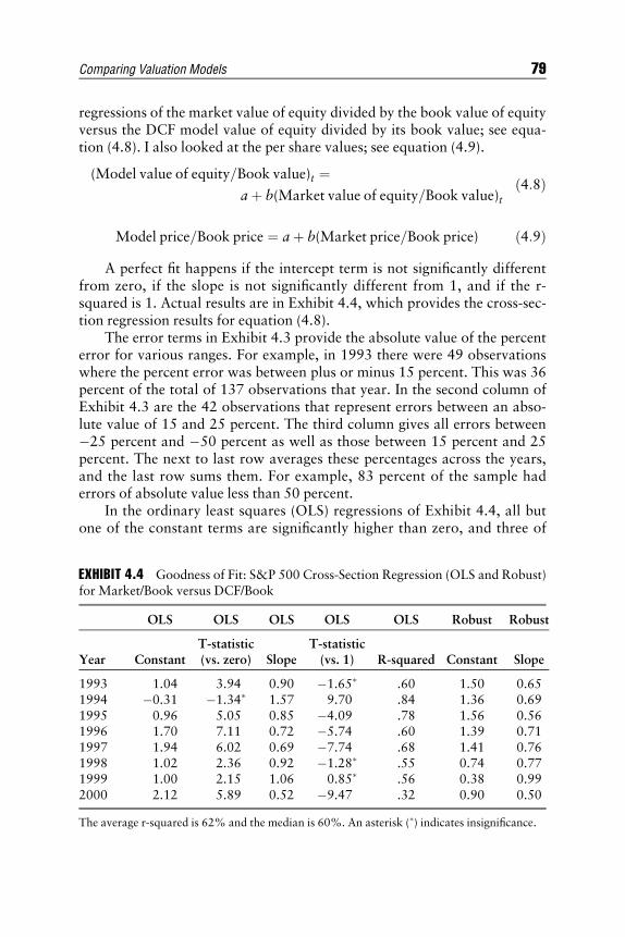
E1C04 09/03/2009 Page 79

regressions of the market value of equity divided by the book value of equityversus the DCF model value of equity divided by its book value; see equa-tion (4.8). I also looked at the per share values; see equation (4.9).

(Model value of equity=Book value)t ¼aþ b(Market value of equity=Book value)t

ð4:8Þ

Model price=Book price ¼ aþ b(Market price=Book price) ð4:9Þ

A perfect fit happens if the intercept term is not significantly differentfrom zero, if the slope is not significantly different from 1, and if the r-squared is 1. Actual results are in Exhibit 4.4, which provides the cross-sec-tion regression results for equation (4.8).

The error terms in Exhibit 4.3 provide the absolute value of the percenterror for various ranges. For example, in 1993 there were 49 observationswhere the percent error was between plus or minus 15 percent. This was 36percent of the total of 137 observations that year. In the second column ofExhibit 4.3 are the 42 observations that represent errors between an abso-lute value of 15 and 25 percent. The third column gives all errors between�25 percent and �50 percent as well as those between 15 percent and 25percent. The next to last row averages these percentages across the years,and the last row sums them. For example, 83 percent of the sample haderrors of absolute value less than 50 percent.

In the ordinary least squares (OLS) regressions of Exhibit 4.4, all butone of the constant terms are significantly higher than zero, and three of

EXHIBIT 4.4 Goodness of Fit: S&P 500 Cross-Section Regression (OLS and Robust)for Market/Book versus DCF/Book

OLS OLS OLS OLS OLS Robust Robust

Year ConstantT-statistic(vs. zero) Slope

T-statistic(vs. 1) R-squared Constant Slope

1993 1.04 3.94 0.90 �1.65� .60 1.50 0.651994 �0.31 �1.34� 1.57 9.70 .84 1.36 0.691995 0.96 5.05 0.85 �4.09 .78 1.56 0.561996 1.70 7.11 0.72 �5.74 .60 1.39 0.711997 1.94 6.02 0.69 �7.74 .68 1.41 0.761998 1.02 2.36 0.92 �1.28� .55 0.74 0.771999 1.00 2.15 1.06 0.85� .56 0.38 0.992000 2.12 5.89 0.52 �9.47 .32 0.90 0.50

The average r-squared is 62% and the median is 60%. An asterisk (�) indicates insignificance.


E1C04 09/03/2009 Page 80

eight of the slope estimates are not statistically different from 1.0. Theseresults are largely corroborated by the robust regressions that are discussednext. This is not good news for the DCF valuations done by the expert sys-tem. Slopes that are too low and intercepts that are too high usually imply amissing variable or an equation misspecification.

A second cross-sectional test was based on robust regression. The moti-vation for so doing was to accept the empirical fact that the distribution ofresiduals in the standard linear regressions is not normally distributed as isassumed when one employs a standard OLS regression. Robust regressionmakes no such distributional assumptions and produces more general re-sults. It is accomplished by randomly selecting pairs of observations fromthe universe of pairs in the data sample. Next, it calculates the slope andintercept of each pair and rank-orders them. The median slope and interceptare then used as asymptotically unbiased estimates of the true intercept andslope for the cross-sectional relationship between the two variables. (SeeExhibit 4.4.) In all eight years, the intercepts were positive, and the slopecoefficients were less than 1.0.

T ESTS OF DCF IN A HOLDOUT SAMPLE(N EW SAMPLE 2000–2008 )

Now I use a second sample, a holdout sample of over 70,000 valuationsdone between January 2000 and July 2008. I wanted to use a holdout sam-ple because the DCF model was developed and tested during the earlier timeinterval (1993–2000), and was not fit to the data in the holdout sample(2000–2008). Consequently, there is no chance of performing a specifica-tion search, where various models are tried on the same data set until agood fit turns up. Before explaining convergence, let’s look at the goodnessof fit for this new sample.

Exhibit 4.5 describes the data set. Starting with a universe of the S&P900, observations were dropped because data was missing, because thecompany was financial (wrong industry), because the DCF was out of range(negative), or because the company had negative book value. From a possi-ble 93,600 observations, the sample actually included 69,429.

Goodness o f F i t

Exhibit 4.6 provides the first goodness of fit statistic, namely the distribu-tion of error terms measured as the DCF value minus the market value, alldivided by the market value. In this case, 51.9 percent of the error terms fell


E1C04 09/03/2009 Page 81

EXHIBIT 4.5 Sample Size, 2000–2008

2000 2001 2002 2003 2004 2005 2006 2007 2008 Total

Originalsample

900 900 900 900 900 900 900 900 900 93,600

Missingdata

201 176 162 151 150 151 153 150 99 16,429

Wrongindustry

25 32 40 43 47 53 56 60 75 4,818

Out ofrange

24 20 22 19 15 16 16 18 23 1,985

Negativebookvalue

9 10 9 15 8 5 7 10 6 939

Samplesize

642 661 667 673 680 674 668 662 696 69,429

Percentusable

71% 73% 74% 75% 76% 75% 74% 74% 77% 74%

The sample size reported for each year is the average monthly sample size during that year.

The total column reports the size of the entire sample in aggregate.

EXHIBIT 4.6 Distribution of Error Terms for DCF Valuations, 2000–2008


E1C04 09/03/2009 Page 82

between plus or minus 50 percent of the market value. Later we comparethis with the error terms of two other valuation methods, namely the mar-ket-to-book ratio and the perpetuity model.

Exhibit 4.7 shows the cross-section regression results, a secondgoodness of fit criterion. The dependent variable is the model price di-vided by the book value, and the independent variable is the marketvalue divided by the book value. All 12 months are pooled each year. Inall but one year, the intercept is significantly different from zero and theslope is significantly different from 1. It was less than 1.0 in three of nineyears. These results would lead one to reject the DCF approach as a rea-sonable fit.

CONVERGENCE TESTS

Convergence tests are of interest because they focus on the predictive abilityof signals generated by the DCF model. Basically, we are interested inwhether the DCF value of the equity of a company is a leading indicator ofthe market value of that company. If no such relationship exists, then themessage that is being transmitted by the DCF valuation model may be agood fit but is valueless.

Equation 4.10 is an OLS regression where the independent variableis the gap between the model DCF value and the actual market valuein the current time period as a percentage of the market value. The

EXHIBIT 4.7 Goodness of Fit: S&P 900 Cross-Section Regression for DCF/Bookversus Market/Book

OLS OLS OLS OLS OLS

Constant

T-statistic

(vs. zero) Slope

T-statistic

(vs. 1) R-squared

2000 3.07 5.59 0.83 �2.86 0.162001 4.26 18.74 0.90 �3.36 0.342002 3.03 17.44 1.18 10.31 0.632003 1.75 14.36 1.20 13.01 0.682004 1.20 12.42 1.08 5.55 0.652005 2.27 36.26 0.73 �32.37 0.712006 0.06 0.86� 1.23 23.55 0.832007 �0.77 �7.67 1.48 55.09 0.892008 1.07 7.14 1.43 23.41 0.76

An asterisk(�) indicates insignificance.


E1C04 09/03/2009 Page 83

dependent variable is the closure of the gap by movement in the actualmarket value a time period later, scaled by the market value at the startof the period.

(Closure at t þ 1)=(Market at t) ¼ aþ b(Gap at t)=(Market at t) ð4:10Þ

where Gap at t¼ Model at t � Market at tClosure at t þ 1 ¼ Market at t þ 1 � Market at t

We expect that if the intercept, a, is equal to zero and the slope, b, isequal to 1, the market price is adjusting toward the model price perfectlywithin one time period. The simple algebra is:

(Market at t þ 1 � Market at t)=(Market at t)

¼ aþ b(Model at t � Market at t)=(Market at t)

and if a ¼ 0 and b ¼ 1, then:

Market at t þ 1 ¼ Model at t

In other words, the market price adjusts during the period toward themodel price at the beginning of the period. If the intercept a is significantlydifferent from 0.0, there is bias in the estimated regression equation. If thecoefficient of closure is between zero and one (0 < b < 1), then there is par-tial adjustment during the time period, and if the slope b is significantlygreater than zero, the adjustment is statistically significant.

One often hears the comment that convergence is nothing morethan a proxy for the rate of return. Nothing could be further from thetruth. Return is the change in the market price (plus dividends) over atime period divided by the starting market price. If the price goes up,the return is positive; and if it goes down, the return is negative. Con-vergence is the adjustment in the market price toward the DCF estimateat the beginning of the period. For example, if the market price startsthe period higher than the DCF estimate at the beginning of the period,then falls toward it, there is convergence, and the rate of return is alsopositive because downward convergence is accompanied by a short po-sition. Thus, while convergence of the market price toward the modelprice is always a good thing, it is not the same thing as the realizedrate of return from a long-only position.

A more extensive form of equation (4.10) uses a multiple regression withup to six closure intervals (i.e., up to six months). See Exhibit 4.8, Panel B.

Exhibit 4.8 is the summary of over 800 individual company regres-sions run on data spanning one, two, and up to six months, for the timeinterval between January 2000 and July 2008. Panel A shows the


E1C04 09/03/2009 Page 84

EXHIBIT 4.8 Convergence of the DCF Model

Panel A: Regressions over a Single Time Period (1, 2, . . . , 6 Months)

Time

Interval

Number of

Observations

% of

b < 0

% of

b > 0

% of bwith

t-stat> 2.0

% of

a > 0

% of awith

t-stat > 2.0

One month 928 21.1% 78.9% 21.4% 58.5% 12.5%Two months 897 29.4% 70.6% 16.0% 46.8% 6.4%Three months 893 31.1% 68.9% 17.4% 52.7% 6.2%Four months 890 31.3% 68.7% 14.4% 55.4% 7.3%Five months 882 31.1% 68.9% 16.3% 55.0% 7.2%Six months 879 30.7% 69.3% 14.4% 54.6% 7.5%

Panel B: Regressions over Multiple One-Month Time Periods

Months

Number of

Observations

% of

b < 0

% of

b > 0

% of bwith

t-stat > 2.0

% of

a > 0

% of awith

t-stat > 2.0

1–2/mo. 1st mo. 897 29.4% 70.6% 16.0% 60.3% 11.8%1–2/mo. 2nd mo. 47.3% 52.7% 6.4%

1–3/mo. 1st mo. 893 31.1% 68.9% 17.4% 59.9% 12.9%1–3/mo. 2nd mo. 47.3% 52.7% 6.2%1–3/mo. 3rd mo. 59.2% 40.8% 4.4%

1–4/mo. 1st 890 31.1% 68.7% 14.4% 58.2% 12.7%1–4/mo. 2nd 44.6% 55.4% 7.3%1–4/mo. 3rd 59.9% 40.1% 4.8%1–4/mo. 4th 46.0% 54.0% 9.6%

1–5/mo. 1st 882 31.1% 68.9% 16.3% 57.4% 11.7%1–5/mo. 2nd 45.0% 55.0% 7.2%1–5/mo. 3rd 58.6% 41.4% 3.6%1–5/mo. 4th 49.2% 50.8% 7.6%1–5/mo. 5th 44.7% 55.3% 8.2%

1–6/mo. 1st 879 30.7% 69.3% 14.4% 57.0% 10.0%1–6/mo. 2nd 45.4% 54.6% 7.5%1–6/mo. 3rd 59.3% 40.7% 4.5%1–6/mo. 4th 48.0% 52.0% 7.4%1–6/mo. 5th 50.5% 49.5% 6.7%1–6/mo. 6th 45.3% 54.7% 7.1%


E1C04 09/03/2009 Page 85

magnitude of the intercept and the slope coefficient that measures thespeed of adjustment in closing the gap between the beginning of periodmodel value and the market value. The fourth column is the percentageof the regressions with positive measures of b, the coefficient of conver-gence in equation (4.10). Convergence between zero and 1.0 indicatesthat the market price moves toward the model price over the period,but only partially. A coefficient of 1.0 indicates full adjustment, and ifgreater than 1.0, it indicates overadjustment. Note, however, that coef-ficients greater than 1.0 are rare. In Panel A, 78.9 percent of the con-vergence coefficients are positive during the first month and 21.4percent of them are significantly greater than zero, where one wouldexpect only 5 percent to be significant by chance. Note also, that thepercentage of positive convergence coefficients is greatest for onemonth, then declines as the time interval lengthens, until for a six-month adjustment interval only 69.3 percent of the adjustment coeffi-cients are positive, and of those 14.4 percent have t-statistics greaterthan 2.0. The majority (58.5 percent) of the intercept terms are positive(Panel A, column 6), and 12.5 percent are significantly greater thanzero. One may conclude from the test of convergence in Exhibit 4.8,Panel A, that the market price does, in fact, adjust to the model price.Therefore, the model is not without value, and the market (before con-sidering transaction costs) is not instantaneously efficient.

Panel B of Table 4.8 looks at the convergence differently because it is amultiple regression with a separate one-month interval of adjustment foreach set of months from two to six.

First, note that the percent of positive convergence coefficients formonth 1 is no less than 68.7 percent and no more than 70.6 percent, regard-less of the number of adjustment terms in the multiple regression—a narrowrange. Furthermore, this one-month convergence is statistically significantin no less than 14.4 percent and no more than 17.4 percent of the regres-sions, where by chance one would expect it to be significantly positive 5percent of the time. Finally, the intercept terms in Panel B are positive in themultiple regressions between 57.0 percent and 60.3 percent of the time, andare significantly positive in between 10.0 percent and 12.9 percent of theregressions—again, statistically significant.

In sum, the empirical test of convergence of market prices towardthe DCF estimated by an expert system indicates that convergence is statisti-cally significant, although biased. In a world without costly information ortransaction costs, this result would imply market inefficiency. I cannotmake such a claim in this chapter, because I have not introduced either costinto my tests of the model.


E1C04 09/03/2009 Page 86

STRAW MAN HORSE RACES (COMPAR ISONOF THRE E MODELS )

I have no DCF model other than the standard methodology foundembedded in the aforementioned expert system; therefore, I develop twostraw men to illustrate how models may be compared with each other usinggoodness of fit and convergence as criteria. It turns out that goodness of fitand convergence are quite different among the various approaches tovaluation.

Defin i n g t he S t raw Men

The first straw man, and the most naive, is the value estimate that re-sults when the sector median market-price-to-book-value (M/B) ratio ismultiplied by the current book value of a given company to estimate itsmarket value.

The second straw man uses the perpetuity version of the continuingvalue formula from the DCF model as of the current year. There is no at-tempt to forecast cash flows during an explicit forecast period. Instead, Ifeed the relevant valuation parameters into the perpetuity model. Those pa-rameters are (1) earnings before interest and taxes next year times 1 minusthe corporate cash tax rate and (2) the weighted average cost of capital. I donot use the value driver formula because too many observations are lost dueto the requirement that the company’s weighted average cost of capitalmust be higher than its growth rate.

Goodness o f F i t

To test their goodness of fit, I produced histograms of the error rates of allthree methods that are competing in the statistics horse race. See Exhibit 4.9and Exhibit 4.10, where the results are summarized. In Exhibit 4.11, I pro-vide the results of cross-section regressions of the model/book versus themarket/book.

If the distribution of errors were the only relevant criterion, then wemight conclude that the market-to-book ratio is the model that has themost estimates close to the market value. It has 69.4 percent within plus orminus 50 percent of the market value, while the DCF model has only 52 per-cent and the perpetuity model has only 18.6 percent. However, if webroaden the relevant range to plus or minus 100 percent, the ranking of thethree models changes. Although the market/book model still has the highestpercent in range (91.5 percent), the second best is the perpetuity model


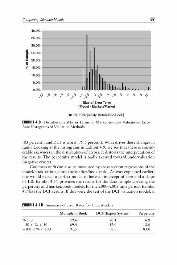
E1C04 09/03/2009 Page 87

(83 percent), and DCF is worst (79.5 percent). What drives these changes inrank? Looking at the histograms in Exhibit 4.9, we see that there is consid-erable skewness in the distribution of errors. It distorts the interpretation ofthe results. The perpetuity model is badly skewed toward undervaluation(negative errors).

Goodness of fit can also be measured by cross-section regressions of themodel/book ratio against the market/book ratio. As was explained earlier,one would expect a perfect model to have an intercept of zero and a slopeof 1.0. Exhibit 4.11 provides the results for the data sample covering theperpetuity and market/book models for the 2000–2008 time period. Exhibit4.7 has the DCF results. If this were the test of the DCF valuation model, it

EXHIBIT 4.9 Distributions of Error Terms for Market-to-Book Valuations: ErrorRate Histograms of Valuation Methods

EXHIBIT 4.10 Summary of Error Rates for Three Models

Multiple of Book DCF (Expert System) Perpetuity

% > 0 29.6 50.1 6.9�50 < % < 50 69.4 52.0 18.6�100 < % < 100 91.5 79.5 83.0


E1C04 09/03/2009 Page 88

would do better than the other two models, primarily because its slope coef-ficients are closer to one.

Panel A of Exhibit 4.11 shows the cross-section regressions that are ameasure of goodness of fit of the perpetuity model. The slopes should aver-age 1.0, but they are all significantly less than 1.0. Furthermore, the inter-cepts should be equal to 0.0, and all are significantly different.

Panel B provides the results of an OLS regression of the sector market/book versus the actual equity value divided by the book value. It has resultsthat are even worse than the perpetuity model’s results.

EXHIBIT 4.11 Goodness of Fit, Cross-Section Regressions

Panel A: Perpetuity Mode/Book. versus Market/Book 2000–2008

OLS OLS OLS OLS OLS

ConstantT-statistic(vs. zero) Slope

T-statistic(vs. 1) R-squared

2000 1.19 50.43 0.12 �351.74 0.492001 0.63 21.29 0.33 �173.51 0.712002 0.82 28.85 0.30 �244.98 0.782003 0.91 32.07 0.29 �196.82 0.702004 0.19 9.51 0.41 �195.31 0.852005 �1.10 �27.02 0.79 �39.32 0.862006 �0.01 �0.64 0.47 �173.52 0.872007 0.22 9.08 0.40 �283.33 0.902008 0.53 14.87 0.44 �121.49 0.82

Panel B: Sector Market/Book prior period versus Market/Book current period,

2000–2008

OLS OLS OLS OLS OLS

ConstantT-statistic(vs. zero) Slope

T-statistic(vs. 1) R-squared

2000 2.95 63.05 0.24 �152.98 0.492001 3.10 108.07 0.11 �237.90 0.342002 2.88 135.96 0.04 �444.41 0.232003 2.75 145.51 0.06 �394.29 0.272004 2.96 155.98 0.07 �323.99 0.282005 2.49 78.83 0.21 �187.44 0.492006 2.90 104.51 0.11 �236.37 0.312007 3.05 60.77 0.11 �205.72 0.282008 2.64 74.29 0.08 �200.19 0.26


E1C04 09/03/2009 Page 89

The DCF model results that were given in Exhibit 4.7 at least showslope coefficients that are distributed around 1.0, and are therefore less bi-ased than either of the two straw men.

CONVERGENCE

Exhibit 4.12, Panel A, provides the convergence coefficients for all three ofthe competing valuation models. Referring to the bottom row in Panel A,the DCF model using the expert system has good convergence properties;79 percent of the regressions have positive adjustment coefficients, indicat-ing that the market price moves toward the DCF price that was calculatedat the beginning of the year. The perpetuity model, however, is slightly bet-ter, having 81 percent positive convergence coefficients, and the sector mar-ket/book is third, having 76 percent of its coefficients positive.

Panel B uses as an additional comparison the percentage of slopeterms that are significant compared to the percentage that one wouldexpect by chance. For example, one would expect that roughly 15 percentof the equations would have t-tests greater than an absolute value of 1.5just by chance. The expert system has 30.7 percent of its slope terms thatare significant at this level (t-test greater than 1.5), versus 15 percent if theobservations were random. This is good, but the results for the perpetuityare slightly better and the market/book model is only slightly worse with31.9 and 26.3 percent respectively. The percentage of intercept terms thatare significantly different from zero is also of interest (see Exhibit 4.12,Panel B). The expert system has roughly the same number of significantintercept terms as would have occurred by chance (13.7 percent), the per-petuity has too many significantly positive intercept terms (33.8 percent),and the Market/Book approach is roughly random (16.8 percent).

Taking the evidence on goodness of fit and on convergence to-gether, one gets the impression that the perpetuity model tends toundervalue stocks, a fact that is apparent from the distribution of errorterms in Exhibit 4.10 that indicates only 6.9 percent of the error termsare greater than zero. Consistent with this is the observation fromExhibit 4.12 that convergence is somewhat greater (i.e., slope coeffi-cients that measure convergence are more frequent) in the 0.1 < b < 0.4range, while they are less frequent in the 0.0 < b < 0.1 range. Thisappears to happen because the perpetuity value gap is greater than theexpert system DCF value gap; therefore, the perpetuity model showsgreater convergence because it has further to go. Regardless of whichmodel wins in the statistics horse race, there appears to be strong supportfor convergence of the market value toward the model value.


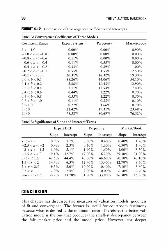
E1C04 09/03/2009 Page 90

CONCLUS I ON

This chapter has discussed two measures of valuation models: goodnessof fit and convergence. The former is useful for courtroom testimonybecause what is desired is the minimum error. Therefore, the better val-uation model is the one that produces the smallest discrepancy betweenthe fair market price and the model price. However, for deeper

EXHIBIT 4.12 Comparison of Convergence Coefficients and Intercepts

Panel A: Convergence Coefficients of Three Models

Coefficient Range Expert System Perpetuity Market/Book

b < �1.0 0.00% 0.00% 0.90%�1.0 < b < �0.8 0.00% 0.00% 0.00%�0.8 < b < �0.6 0.11% 0.00% 0.00%�0.6 < b < �0.4 0.11% 0.55% 0.00%�0.4 < b < �0.2 0.33% 0.89% 1.00%�0.2 < b < �0.1 0.55% 1.55% 2.50%�0.1 < b < 0.0 20.31% 16.32% 19.30%0.0 < b < 0.1 68.26% 44.06% 54.10%0.1 < b < 0.2 5.88% 16.43% 12.90%0.2 < b < 0.4 3.11% 13.54% 7.40%0.4 < b < 0.6 0.44% 3.22% 0.70%0.6 < b < 0.8 0.55% 1.22% 0.50%0.8 < b < 1.0 0.11% 0.55% 0.10%b > 1.0 0.22% 1.66% 0.70%b < 0 21.42% 19.31% 23.68%b � 0 78.58% 80.69% 76.32%

Panel B: Significance of Slope and Intercept Terms

Expert DCF Perpetuity Market/Book

Slope Intercept Slope Intercept Slope Intercept

x < �2.5 0.9% 1.7% 0.30% 0.40% 0.40% 1.70%�2.5 < x < �2 0.4% 2.3% 0.60% 1.30% 0.90% 1.90%�2 < x < �1.5 1.0% 5.1% 1.40% 1.60% 1.00% 5.30%�1.5 < x < 0 19.1% 32.7% 17.00% 16.20% 29.30% 31.20%0 < x < 1.5 47.6% 44.4% 48.80% 46.60% 50.10% 43.10%1.5 < x < 2 14.4% 6.3% 12.90% 13.40% 12.70% 8.50%2 < x < 2.5 9.3% 5.0% 10.00% 10.40% 7.10% 5.60%2.5 < x 7.0% 2.4% 9.00% 10.00% 6.50% 2.70%Percent > 1.5 30.7% 13.70% 31.90% 33.80% 26.30% 16.80%


E1C04 09/03/2009 Page 91

questions of market efficiency and portfolio performance, the goodnessof fit criterion is not helpful. A superior measure is one that measuresthe convergence between the price determined by the model and themarket price. Specifically, the market price must converge to the modelprice and not vice versa.

To illustrate a comparison of valuation models, I chose three commonlyused models—the DCF model, the market/book ratio, and the perpetuitymodel. The data were valuations done for each company, each month be-tween January 2000 and July 2008. The final sample consisted of nearly70,000 valuations of each type.

The goodness of fit criterion seemed to favor the DCF model for tworeasons: First, its error terms were more symmetrical, and second, althoughit did a poor job in a cross-section regression against the market/book value,it did better than the other two measures.

The crucial convergence criterion favored the perpetuity modelslightly over the DCF approach. It had more companies whose marketvalues adjusted toward the beginning-of-period DCF value (80.7 per-cent) than either of the other two models, and more of these adjust-ment coefficients were statistically significant than could have occurredby chance. The major drawback of the perpetuity model was that thepercentage of the intercept terms coefficients that were statistically sig-nificant was much higher than can be expected to occur randomly—anundesirable result.

In the final analysis, however, one must test the actual return perform-ance of the alternative valuation models by using a back-test procedure.Goodness of fit and convergence are tools that are useful, but they do nottell the whole story.


E1C04 09/03/2009 Page 92

EXHIBIT 4A.1 Market and DCF Price History

EXHIBIT 4A.2 Valuation Summary


E1C04 09/03/2009 Page 93

EXHIBIT4A

.3V

alu

eD

river

Sum

mary

93

E1C04 09/03/2009 Page 94

EXHIBIT4A

.4R

even

ue

Gro

wth

Fore

cast

94

E1C04 09/03/2009 Page 95

EXHIBIT4A

.5O

per

ati

ng

Marg

inFore

cast

95

E1C04 09/03/2009 Page 96

EXHIBIT4A

.6N

etPro

per

ty,Pla

nt,

and

Equip

men

t

96

E1C04 09/03/2009 Page 97

EXHIBIT4A

.7O

per

ati

ng

Work

ing

Capit

al

97

E1C04 09/03/2009 Page 98

EXHIBIT 4A.8 Weighted Average Cost of Capital


E1C04 09/03/2009 Page 99

EXHIBIT4A

.9In

com

eSta

tem

ent

99

E1C04 09/03/2009 Page 100

EXHIBIT4A

.9(C

ontinued

)

100

E1C04 09/03/2009 Page 101

EXHIBIT4A

.10

Bala

nce

Shee

t

101

E1C04 09/03/2009 Page 102

EXHIBIT4A

.10

(Continued

)

102

E1C04 09/03/2009 Page 103

EXHIBIT4A

.11

NO

PL

AT

and

Taxes

on

EB

IT

103

E1C04 09/03/2009 Page 104

EXHIBIT4A

.12

Inves

ted

Capit

al

104

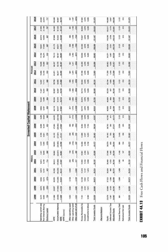
E1C04 09/03/2009 Page 105

EXHIBIT4A

.13

Fre

eC

ash

Flo

ws

and

Fin

anci

alFlo

ws

105

E1C04 09/03/2009 Page 106

EXHIBIT4A

.14

Conti

nuin

gV

alu

e

106

E1C04 09/03/2009 Page 107

NOTES

1. I would like to thank Chris Cha for programming assistance.2. This uses a linear approximation of the growth term in the finite supernormal

growth formula. The approximation holds as long as g is reasonably close toWACC and N is small.

RE F ERENCES

Bailey, W. 1991. Valuing agricultural firms: An examination of the contingentclaims approach to pricing real options. Journal of Economic Dynamics andControl 15: 771–791.

Copeland, T., T. Koller, and J. Murrin. 1994. Valuation: Measuring and managingthe value of companies. 2nd ed. New York: John Wiley & Sons.

Kaplan, S., and R. Ruback. 1995. The valuation of cash flow forecasts: An empiricalanalysis. Journal of Finance 50 (4): 1059–1093.


E1C05 08/25/2009 Page 108

CHAPTER 5Developing an Automated

Discounted Cash Flow ModelRobert J. Atra

Chair of the Finance Department, Lewis University

Rawley ThomasPresident, LifeCycle Returns, Inc.

Intrinsic value is the investment concept on which our views ofsecurity analysis are founded. Without some defined standards ofvalue for judging whether securities are over- or underpriced in themarketplace, the analyst is a potential victim of the tides of pessi-mism and euphoria which sweep the security markets.

—Cottle, Murray, and Block (Graham and Dodd’s SecurityAnalysis, 5th Edition, 1988)

D iscounted cash flow (DCF) forms the core of finance. While its basicstructure has existed for many years, DCF valuation now takes many

forms, from the simplistic, such as the Gordon model, to the extraordinarilysophisticated, such as proprietary free cash flow models. Though professio-nals may employ other methods of valuation, such as relative valuation andthe contingent claims approach, DCF forms the basis for all other valuation(Damodaran 2002).

Underscoring the importance of DCF valuation is the fact that it pro-vides a linchpin to link various fields of finance. Security analysts shouldvalue stocks in much the same manner as corporate managers value proj-ects. In the case of a project, managers estimate cash flows and discountthem back to the present. They then net the present value of those cash

108

E1C05 08/25/2009 Page 109

flows against the cost of the project and decide whether to accept or rejectthe project. Since, conceptually, an investor can view any firm as simply abundle of projects, security valuation should be similar to project valuation.

This chapter will examine how best to develop a subset of valuationmodels, namely those related to equity valuation. Analysts typically refer tothe results of such models as ‘‘intrinsic values’’ of the equity, which they cancompare to actual market prices to determine to what extent current stockprices are under- or overvalued. That information provides the basis forbuy/sell recommendations.

Models producing intrinsic values are of value not only to security ana-lysts and portfolio managers but to corporate managers as well. As firmscompensate managers based on stock performance to eliminate agencyproblems, intrinsic valuation provides a valuable tool to judge their per-formance (Madden 2007). Of course, market prices provide a metric tojudge managerial skill, but factors not under the control of managers ofteninfluence market prices. Furthermore, market noise obfuscates the ability totell whether a movement in market price is genuinely due to managerial de-cisions. Consequently, even principles of finance textbooks are now empha-sizing the need for managers to maximize intrinsic value as opposed tocurrent market price (Brigham and Houston 2007).

Despite the historical importance of DCF valuation, security analysisand portfolio management research seems to be trending away from DCFand toward statistical methods such as multifactor analysis.1 We find thistrend unfortunate, since DCF may provide insights that are simply notavailable with pure statistical approaches to security selection. The DCF ap-proach models price level as opposed to price change, and thus can helpexplain the price formation process of how market participants actually de-termine market prices. Understanding how the market values securities iscritical to both external valuation professionals as well as managers.

For example, once an analyst has developed an accurate valuationmodel, the model can provide valuable information to the managers onhow to increase the intrinsic value (and ultimately the market price) of theirstock. Finding the economic value drivers is an essential result of developinga DCF model. Note that determining value drivers is not a benefit fromother types of security valuation and portfolio management techniques suchas multifactor models. For instance, if research determines that low price-to-book ratios predict future returns, of what value is that relationship to acorporate manager’s decision-making process?

A common—and certainly justified—criticism of discounted cash flowvaluation is that it is often performed on a case-by-case basis, with littleempirical support for the results—especially the structure of the terminalvalue. Kaplan and Ruback (1995) emphasize this point: ‘‘Most economists

Developing an Automated Discounted Cash Flow Model 109

E1C05 08/25/2009 Page 110

readily accept the concept of estimating market value by calculating the dis-counted value of the relevant cash flows. However, little empirical evidenceexists to show that discounted cash flows provide a reliable estimate of mar-ket value.’’ One possible explanation for this conclusion is that researchersview DCF models as rather ad hoc, primarily driven by subjective inputs byanalysts. (See Thomas Copeland’s Chapter 4 and Randy Schostag’s Chapter15 for related material.) This subjectivity in the traditional analyst’s processapparently makes a widespread evaluation of models difficult to examine.We disagree. We assert that valuation professionals can develop and testDCF models through a rigorous, formal process, improving both the under-standing of valuation and the enhancement of investment performance.

Specifically, this chapter focuses on providing guidance in developingautomated DCF models with no analyst intervention. An automated DCFmodel defined a priori yields many benefits. An automated model can covera much larger universe of stocks than one that requires analysts’ judgmentand input. In fact, the automated model can value literally thousands ofstocks, increasing the scope of possible investments when an investor wishesto both diversify broadly and still engage in a fundamental analysis strat-egy.2 Models with good dispersion across industries promise better diversifi-cation than ones concentrated in particular industries. The large number ofstocks covered by an automated model allows the model to be empiricallyvalidated in that the developer can quantitatively analyze and statisticallytest the model. Automated models should be free from anecdotal evidenceand perform well over a substantial portion of the investable universe.

Covering such a large universe may be critical, for example, if portfoliomanagers seek to develop an index portfolio based not on market values buton company fundamentals. Arnott, Hsu, and Moore (2005) contend thatportfolio managers should not weight index portfolios by market valuessince noise will result in overvalued stocks being overweighted and under-valued stocks being underweighted. Instead of market weights, they recom-mend fundamentally weighting an index by the ‘‘economic footprint’’ of thecompany. An intrinsic value is the model’s determination of the economicfootprint of a company’s stock and, therefore, becomes the appropriateweight in a fundamentally indexed portfolio.

An automated system may also diminish the influence of emotion andherd behaviors in determining intrinsic prices and hence buy/sell recommen-dations. If widely used, an accurate automated DCF model should be able todetect systematic over- or undervaluation of stocks and provide a naturaltether on current security prices, thus avoiding pricing bubbles. Finally, oncebuilt, automated DCF models should achieve substantial economies of scale,since the cost of the model is spread over perhaps thousands of securities. Incontrast, security analysts may be able to cover only 15 to 20 securities.


E1C05 08/25/2009 Page 111

Despite the advantages, automated DCF models do not preclude analystinput. In fact, developers may create models flexible enough to allow for an-alysts’ input when expert analysis adds value. In such a case, the automatedDCF model does most of the heavy lifting by quantifying how value is deter-mined, and the analyst fine-tunes the model by changing particular inputs.For example, an analyst who has superior insight regarding the return onequity of a firm can override the normal automated process of estimatingreturn on equity, and the model can determine an adjusted intrinsic valuebased on the analyst’s insight. Naturally, this process allows an effectiveway to judge an analyst’s recommendations, as the onus is now on the ana-lyst to show that overriding the model has added value. The model’s intrinsicvalues thus become a benchmark to monitor and evaluate analysts’ opinions.This process should also point analysts to areas where their information ad-vantage is the greatest, such as adjusting recent accounting information orforecasting near-term events, and make off limits areas where analyst inter-vention may simply add noise, such as changing distant terminal values.3

Ultimately, researchers should develop and evaluate an automated DCFmodel based on the following measurement principles:

& Robustness. What area of the universe of possible investments can themodel reasonably value?

& Accuracy. Does the model’s intrinsic values yield results that are closeto actual prices?

& Unbiasedness. Does the model avoid systematically under- or overvalu-ing the securities in its scope and against its economic drivers?

& Predictability. Does the model actually forecast stock returns as op-posed to simply estimating current prices?

A fundamentally sound automated DCF model does not use these asisolated features of the model, but rather as part of an integrated modelbuilding process. We present evidence that shows the most robust, accurate,and unbiased models are also the most predictive. Some valuation practi-tioners’ primary interest lies in establishing an accurate value for a firm,while others focus on valuation in order to make investment recommenda-tions. This range of professionals should find solace in knowing that a well-developed automated DCF model can achieve both objectives.

MODELS EXAM INED

In order to demonstrate the model development process, we examine severalversions of dividend discount models (DDMs). DDMs have several


E1C05 08/25/2009 Page 112

advantages over other models. First, they are commonly accepted and exam-ined in both academic and practitioner literature. Second, they represent ac-tual cash flows received by investors and do not depend on the calculationof a hypothetical dividend that may be a source of controversy and error.Finally, DDMs represent an excellent choice to demonstrate model develop-ment since they need only a small number of inputs. The tractable numberof inputs enables us to examine the model-building process without oversha-dowing the process with the sheer number of inputs used, parameters esti-mated, or complex theory expounded on in building the valuation model.

Using DDMs possesses disadvantages as well. They are not nearly asrobust as other models, as they can only apply to dividend-paying firms.Models with strict assumptions, such as the Gordon model, are even lessrobust given that they assume a constant growth rate. Furthermore, someDDMs, such as the ROPE4 model discussed later, require that companieshave positive earnings in order to estimate future dividends. We examinethe importance of this issue in the section on robustness.

Additionally, DDMs that allow for a fading of the dividend still dependon a terminal value. Intrinsic values produced by the DDM may exhibitextreme sensitivity to the terminal value, which can represent a large por-tion of the total present value and can be difficult to estimate. Finally, someresearch concludes that DDMs produce biased estimators of actual stockvalues (Bethke and Boyd 1983) and are, therefore, inherently inaccurate.Later, we address the issues of accuracy and bias as well as how best to han-dle those two issues in the process of building a DCF model.

Because this chapter primarily focuses on building an automated DCFmodel, our process does not rely on analysts’ estimates, but simply extrap-olates historical data to compute intrinsic values. We therefore avoid look-ahead bias—such as when analysts may infer future terminal values fromcurrent prices—in our automated process.

We demonstrate our process using three particular DDMs: (1) the con-stant growth or Gordon model, (2) a DDM based on the fading growth rateof the dividend, termed the GROW5 model, and (3) a DDM based on a fadingreturn on equity and an increasing payout ratio, termed the ROPE model.6

The Gordon model (Gordon 1962) assumes a constant growth rate andtakes on the following form:

P0 ¼ D1

K�Gð5:1Þ

where D1 is the dividend received one year from the point of the presentvalue calculation, K is the equity discount rate, and G is the growth rate inthe dividend, which is assumed to be constant. As applied in our work, weestimate the parameters and the resulting P0 becomes the model’s estimate


E1C05 08/25/2009 Page 113

for the intrinsic value of the stock price. We refer to the Gordon model as a‘‘one-phase model’’ in that it assumes a constant growth rate and, therefore,assumes the company is in the last phase of its life cycle (i.e., the company ismature).

We refer to the GROW and ROPE models as ‘‘multistage’’ or ‘‘multi-phase’’ DDMs. Both models usually assume an initial stage when divi-dends grow at a high rate (phase 1), a fade period or regression toward themean where the dividend growth rate declines (phase 2), and a terminalperiod in which the dividend growth rate becomes constant (phase 3). Themodels’ flexibility stems from the fact that the model builder can adjustthe three stages based on experience, judgment, and empirical evidence.Both the GROW and ROPE models discount all cash flows at a constantdiscount rate.

The primary difference between the GROW and ROPE models relatesto the way the growth rate of the dividend fades. In the GROW formula-tion, the growth rate simply fades linearly to the terminal growth rateaccording to the following formula:7

DG ¼ Gt �G1

N2ð5:2Þ

where DG represents the annual change in the growth rate, Gt representsthe growth rate in phase 3 (terminal growth rate), G1 represents the initialgrowth rate in phase 1, and N2 is the number of years in phase 2. Analystsmust estimate both the growth rates and the phase lengths. Once phase2 ends, the Gordon model can compute the terminal value for the GROWmodel where Gt would serve as the constant growth rate.

The ROPE model does not assume that the growth rate fades in such asimple fashion, but instead uses the sustainable growth framework to con-struct the fade. In the sustainable growth framework, the dividend equalsthe product of the initial book value for the period, the return on equity(ROE) for the period, and 1 minus the retention rate (RR). As the ROE andRR fade, the dividend changes (not necessarily decreases) and the result im-plies a growth rate in the dividend. In the ROPE model, we assume the ROEand RR fade in the same linear manner as the growth rate in dividends inthe GROW model and, therefore, compute the change as:

DROE ¼ ROEt � ROE1

N2ð5:3Þ

DRR ¼ RRt � RR1

N2ð5:4Þ


E1C05 08/25/2009 Page 114

where we define the time subscripts as in equation (5.2). As with theGROW model, once phase 2 ends, the terminal value for the ROPE modelcomputes according to equation (5.1).

Depending on the relative fade rates of the ROE and RR, the dividendgrowth rate may actually increase during the fade period due to the domi-nant effect of a fading RR. The previous research of Rozeff (1990) and ourown experience suggest this increase in dividend growth rates may be a moreaccurate representation of the dividend pattern of maturing companies.

DATA AND IN I T I A L PARAMETER I ZAT I ON

The data for our example are from Ipreo and, in all, include over 5,000companies from January 1, 1996, through the second quarter of 2007,which results in over 48,000 company years of data. We chose not to limitthe span of sectors examined but rather to truly stress test the models byexamining how they perform over the entire universe.

To compare our models, we must choose some initial parameters. Inselecting those parameters for the three models, we recognize the fact thatprevious research has indicated a consistent bias in DDMs to tend to under-estimate intrinsic values. We therefore choose initial parameters that tend toincrease the intrinsic values, though we will adjust those later in an attemptto improve the model. For each firm, we begin by estimating a capital assetpricing model (CAPM) discount rate, using the long-term Treasury bondrate, the firm’s median industry beta, and an equity risk premium of 3 per-cent. Though the estimate of the risk premium may seem low compared tohistorical risk premiums, that premium represents just an initial parameter-ization that yields generally unbiased estimates of intrinsic values relative tostock prices according to DDMs.8 We estimate 5 percent terminal growthrates for the three models.9 Finally, we assume the simplest fade model, onethat immediately starts fading the growth rate, which, in essence, turnsthe GROW and ROPE into two-phase models. Note that we chose these asthe initial inputs, which serve as a first step in the model-building process.After testing the models based on the initial parameterization, we proposeways to improve them.

MEASUREMENT PR INC I P L ES

All valuation models are estimations of the actual underlying valuation pro-cess.10 Mathematical constructions of the models will limit the allowableinputs and, therefore, restrict the model from valuing all possible


E1C05 08/25/2009 Page 115

investments. For example, the Gordon model with its constant growth as-sumption can value only firms where the expected growth rate of the divi-dend is less than the discount rate—a very strict limitation indeed.However, even those DDMs that incorporate a fading growth rate have lim-itations. The GROW model can value only firms where D > 0 since it relieson a base dividend to determine the next period’s dividend. In contrast, theROPE model does not rely on a base dividend since it allows for an initialRR of 1. As the RR fades from 1, dividends commence and the model be-comes able to value the stock. Despite the advantage of not relying on abase dividend, the ROPE model cannot value every stock. Since the ROPEmodel uses sustainable growth, it does require positive earnings to generatea meaningful retention rate.

Robus t ness

Robustness is our term for how many of the stocks in the universe the modelis able to value. We measure robustness as the number of company yearswhere a model produces meaningful values for stocks in the universe asa percentage of the total number of company years in the data set.Exhibit 5.1 gives results for the entire period, which has a maximum of48,299 company years.

As indicated in the table, the Gordon model is the least robust, and theROPE model performs the best in terms of robustness, covering almost 50percent of the universe. The robustness information indicates that of thetwo models with a fading growth rate, the ROPE model covers almost twicethe number of stocks that the GROW model covers. Clearly, the ROPEmodel offers analysts the most opportunity in terms of the number of securi-ties that they can value via an automated valuation model.

Naturally, models exist that cover a greater percentage of the universethan those presented here. The preceding analysis does point out, however,that the model builder must present robustness as a critical feature of anyvaluation model. Even models with very similar characteristics—both theGROW and the ROPE are dividend models incorporating fading growthrates—possess very different degrees of robustness.

EXHIBIT 5.1 1996–2007 Results

Gordon GROW ROPE

Period Stocks % of Total Stocks % of Total Stocks % of Total

1996–2007 5,004 10.4% 12,104 25.1% 23,999 49.7%


E1C05 08/25/2009 Page 116

Accuracy

An intuitively attractive feature of any valuation model is whether it pro-duces results consistent with actual market prices. While nobody expects amodel to be perfectly accurate, models that produce intrinsic values farfrom actual prices are suspect. In general, analysts can measure the accuracyof a model by examining a pricing error, computed as:

Error ¼ IVit � Pit

Pitð5:5Þ

where Pit is the market price of security i at time t and IVit is the intrinsicvalue produced by the respective model for security i at time t. The smallerthe pricing errors produced by the model, the more accurate the model. Onecan consider errors in absolute value if one is only concerned about accu-racy or, as defined earlier, if one is primarily concerned about systematicbias (overall under- or overvaluation of the securities).

Our definition of pricing error has intuitive appeal for later use in pre-dicting returns. Since we view intrinsic value as the true price, we wouldexpect the market price to migrate toward the intrinsic value.11 In such acase, our definition of pricing error produces the return from purchasingthe stock and having the price move to the intrinsic value. Furthermore, thedefinition in equation (5.5) gives the correct ordering of stock values—themost undervalued would exhibit the largest positive errors, while the mostovervalued would have the largest negative errors.

Because the pricing errors are not likely to be normally distributed, themean pricing error likely misleads. For example, consider the intrinsic val-ues produced by the Gordon model. The model produces values from nearzero (for stocks with small dividends, small growth rates, and large discountrates) to values tending toward infinity (for stocks where the growth rateapproaches the discount rate). Clearly, the model will lead to skewed pric-ing errors. Thus, the median pricing error in these cases may yield a bettermeasure of central tendency, which we present later.

Exhibit 5.2 presents the absolute values of percentage pricing errors forthe 40th, 50th (median), and 60th percentiles for the Gordon, GROW, andROPE models. The errors are extremely large, indicating that the modelsoverall are not very accurate, though the Gordon and ROPE perform muchbetter than the GROW model, exhibiting not only a smaller median but amuch smaller range between the 40th and 60th percentiles. The large errorsmay indicate a poorly specified model—one where the analyst could moreaccurately estimate the discount rate or growth rates. A large part of ourwork will demonstrate how to improve the accuracy of the model.

While the percentiles contain valuable information, we believe thatexamining the entire distribution of pricing errors is the easiest way to


E1C05 08/25/2009 Page 117

evaluate the accuracy of a model. The plot of the cumulative distributionfunction (CDF) of the absolute errors provides a convenient way to in-stantly assess accuracy. Tracking of the model’s accuracy by the CDF alsoallows the model builder to visualize accuracy across models. We present ahypothetical example of a CDF for accuracy in Exhibit 5.3. The more accu-rate model’s sharply steep curve on the left side of the CDF horizontal scaleimplies lower errors and a tighter distribution of errors. The less accuratemodel has a flatter CDF. The flatter CDF in the figure reveals that the mod-el’s errors have more variability and are of greater magnitude. The mostaccurate models, therefore, will plot up and to the left.

Comb i n i ng Accuracy and Robus t ness

Examining only accuracy or robustness may misrepresent a model’s truevalue. For example, examine the percentage errors in Exhibit 5.2. The tableclearly demonstrates that the Gordon model and ROPE model exhibit supe-rior accuracy when compared to the GROW model, but are close in

EXHIBIT 5.2 Absolute Percentage Pricing Errors of Three DDMs

Percentile Gordon GROW ROPE

40th 54.205 110.031 76.64150th 67.079 208.961 120.73260th 78.617 321.304 238.906

EXHIBIT 5.3 Comparing the Accuracy of Models


E1C05 08/25/2009 Page 118

accuracy when compared to each other. Which one, therefore, should ana-lysts considered superior? The problem is that we are not comparing themodels on an equal basis. Recall from Exhibit 5.1 that the ROPE model,despite similar accuracy to the Gordon model, values over five times thenumber of securities! The Gordon model handles only mature companies,which may be considerably easier to value, whereas the ROPE model’sscope encompasses all firms with positive earnings, making the model amuch more fruitful candidate for refinement.

One way to visualize the value of a model in terms of both robustnessand accuracy is to use a CDF-type diagram, but adjust the vertical scale bythe percentage of stocks of the entire universe that the model can value.Exhibit 5.4 represents a diagram that compares three hypothetical modelson the principles of robustness and accuracy. The first model not onlyexhibits accuracy as evidenced by its steep slope but it also rises high on thevertical axis. The height of the curve demonstrates its robustness, as it isable to cover over 80 percent of the universe. The second model in our dia-gram demonstrates accuracy—it has a steep slope toward the left of the hor-izontal scale—but scores low on robustness, covering less than 20 percent ofthe universe. The final hypothetical model displays neither accuracy nor ro-bustness. The line is relatively flat, indicating errors are substantial and var-ied. Furthermore, the model only covers between 15 percent and 20 percentof the stocks in the universe. With one diagram, an investment manager can

EXHIBIT 5.4 Comparing the Accuracy and Robustness of Models


E1C05 08/25/2009 Page 119

directly compare several models on two fundamental principles of valua-tion—accuracy and robustness.

Exhibit 5.4 also yields great practical insight as to what direction a firmshould take when it comes to allocating its resources. Take, for example,the accurate and robust model in the diagram. Clearly, the model providesaccurate valuations on a large number of securities. Analyst input regardingstocks covered by that model is likely to have only incremental benefits. In-stead, firms should direct resources and analyst skill toward the approxi-mate 20 percent of the universe that the model does not cover. For themodel that displays accuracy but not robustness, firms should invest moreresources in model improvement to allow for a greater breadth of coverage.

Now let us examine the combined accuracy and robustness of DDMs.As discussed earlier, the diagram plots the percentage of the universe thatthe model covers on the vertical axis and the absolute value of errors on thehorizontal axis. The scale on the vertical axis is set to log base 2 for easiervisualization. Exhibit 5.5 shows that the Gordon model performs relativelypoorly, particularly in terms of robustness, as it covers only a small portionof the universe. Exhibit 5.6 includes the GROW model, which although notvery accurate, does display increased robustness resulting in a vertical in-crease over the Gordon model. Finally, Exhibit 5.7 includes all three mod-els. Clearly, the ROPE model performs much better than the Gordon orGROW models, rising more quickly and to a greater vertical distance thanthe other models.

EXHIBIT 5.5 Accuracy and Robustness of Gordon Model


E1C05 08/25/2009 Page 120

EXHIBIT 5.6 Accuracy and Robustness of Gordon and GROW Models

EXHIBIT 5.7 Accuracy and Robustness of Gordon, GROW and ROPE Models


E1C05 08/25/2009 Page 121

Unb i a sedness

Bias, as we use the term, refers to the tendency of a model to systematicallyover- or undervalue securities. We view an unbiased model as one where 50percent of securities are overvalued and 50 percent are undervalued againstintrinsic values.12 Clearly, a relationship should exist between bias and ac-curacy—a model that systematically places too low or too high intrinsic val-ues on securities becomes unlikely to produce accurate estimates.Unbiasedness, therefore, represents a most desirable feature of a model.Valuation practitioners will not find models that consistently recommendall buy or all sell signals very beneficial.

As evidence of the connection between unbiasedness and accuracy, weexamine the signed errors for the models under consideration. Exhibit 5.8presents the signed errors for the three models for the 30th through 70thpercentiles. The data indicate that the GROW and ROPE exhibit the leastbias, with the Gordon model biased toward overvaluation. While neither isperfectly unbiased, each demonstrates a change from overvaluing to under-valuing securities within one decile of the median. In contrast, the Gordonmodel tends to overvalue securities, as evidenced by the negative errors thatdo not turn positive until above the 60th percentile.

A second type of bias not commonly researched in the valuation litera-ture relates to the bias caused by a particular parameter. Examining thistype of bias becomes particularly useful in improving a model’s perform-ance. A subsequent section covers in detail reducing parameter model biasto improve model performance.

Pred i c t i v e Capab i l i t y

Ultimately, the value of the measurement principles of robustness, accuracy,and unbiasedness to practitioners lies in their ability to produce superiorinvestment decisions. Unlike much of the previous academic work, whichhas tended to focus on whether models are replicating the true underlying

EXHIBIT 5.8 Signed Percentage Pricing Errors of Three DDMs

Percentile Gordon GROW ROPE

30th �58.495 �37.551 �26.66440th �45.364 �20.805 �12.05250th �29.521 �1.528 3.22260th �11.676 19.627 19.21070th 14.119 43.783 37.996


E1C05 08/25/2009 Page 122

valuation process, we intend to show that the most robust, accurate, andunbiased models also become the most predictive. We will concentrate onan intermodel comparison and not attempt to show that any of the DDMsbeat the market. Our experience with both these simplistic models and inthe development of the LifeCycle Returns proprietary models (Chapter 11)finds that models with the best opportunity to earn superior returns alsoperform well on the measurement principles of accuracy, robustness, andunbiasedness.

Some people may find it ironic that an accurate model—one that com-putes intrinsic values close to actual market prices—becomes best suited toearn excess returns. Indeed, a perfectly accurate model makes no recom-mendations as to which securities are under- or overvalued. Our view positsthat market prices represent errors around intrinsic values.13 Thus, the un-der- or overvaluation indicated by the model predicts the direction of futurestock prices. The migration of prices toward intrinsic values produces thereturn from the under- or overvaluation. In that migration sense, we agreewith Lee (2001), who makes the analogy that the market is moving towardefficiency like ‘‘the ocean is constantly trying to become flat.’’ The marketmay not be instantaneously efficient, but it is trying to correct pricing errors.Inaccurate models do not produce theoretically correct intrinsic values and,therefore, provide inaccurate signals on the future movements of stockprices.

To test whether models that perform well on the previously discussedmeasurement principles demonstrate more predictive capability, we divideeach model’s intrinsic values into deciles at the beginning of the year, rank-ing intrinsic values from the most overvalued to most undervalued. Sinceannual accounting information is not available at the beginning of the year,we allow for a disclosure lag by subsequently tracking the performance ofthe decile portfolios over the following 3 to 15 months. In addition, weoversample the tails, tracking the performance of the top and bottom 1 per-cent and 5 percent of the over- and undervaluations. Oversampling the tailsis a convenient way to test the extreme results of the model. We repeat ourportfolio procedure for the entire period from 1996 to 2007 and computeaverage returns. For models that perform well on our predictive capabilitycriterion, the most overvalued portfolios should perform the worst, whilethe most undervalued portfolios should perform the best.

Empirical results for our models’ portfolios sorted on over- and under-valuations appear in Exhibit 5.9. For clarity, we present the empirical re-sults for only the ROPE model in Exhibit 5.10. As the reader may see, themodels do not perform exceptionally well. However, with the exception ofthe bottom 30 percent of more overvalued securities, the ROPE does exhibitsome predictive ability by producing increasing returns in the range


E1C05 08/25/2009 Page 123

between the 30th and 100th percentiles. Of course, we obtained these re-sults with a first pass of the model-building process. Since this chapterfocuses on model development, not just model selection, we need to demon-strate how to improve the models.

Parame ter B i a s and Mode l Improvemen t

Thus far, we have presented limited information that more robust, accurate,and unbiased models are also the most predictive. Model builders need,

EXHIBIT 5.9 Median Returns for Dividend Discount Models

EXHIBIT 5.10 Median Returns for ROPE Model


E1C05 08/25/2009 Page 124

however, a systematic way to improve the accuracy of their models, whichshould lead to better predictive ability. To detect where the greatest im-provements are likely to occur, we use a parameter bias-detecting proce-dure. This procedure determines if any particular input is systematicallyrelated to the under- or overvaluations produced by the model. If so, remov-ing the bias will increase the accuracy of the model.

To demonstrate our procedure, we concentrate on the discount rate asdetermined by the CAPM. Recall that we first estimated our models byusing the median industry beta to determine the discount rate. There are, ofcourse, alternatives. Numerous studies have employed various discount ratespecifications such as firm-specific betas, industry betas, and uniform dis-count rates.

Since we have several models from which to choose, we opt to concen-trate on the one with the most promise, the ROPE model. Because the errorsare not likely to be normally distributed, we test for parameter bias by run-ning a regression of the fractional ranks of the over-/undervaluation errorsproduced by the ROPE model against the fractional ranks of the corre-sponding firms’ betas (estimated by the firms’ median industry betas).14 Sta-tistical programs compute fractional ranks by ranking the data of interestfrom low to high and assigning a value to each rank. If the regression showsa relationship between the fractional ranks of the parameter values and theunder-/overvaluations, the model is likely to be improved by removing theeffect of that relationship bias.

Our results from the fractional rank regression appear in Exhibit 5.11.The figure shows a clear negative relationship between the fractional rankof the median industry beta and the under-/overvaluations. Since the verti-cal scale in the figure runs from over- to undervaluation, the regression indi-cates that the model tends to overvalue securities with high median industrybetas, while it tends to undervalue those with low median industry betas. Inother words, beta produces too large an impact on the valuation estimate.Beta drives down the intrinsic values of the high-beta securities to the pointwhere the securities become overvalued. Conversely, the undervaluation re-sults from the too-low discount rate associated with low-beta securities.

To remove the bias associated with the beta, we simply set the beta to1 for all securities, resulting in a uniform discount rate. Better valuation re-sults with uniform discount rates are not uncommon in academic literature.See Kaplan and Ruback (1995) and Sougiannis and Yaekura (2001) forexamples of uniform discount rates.

After removing the bias due to the discount rate, we retest the modelusing our fundamental measurement principles. Using the scaled CDF graph,we see the improvements in the accuracy of the model in Exhibit 5.12. Theslope of the ROPE model with a beta of 1 rises more rapidly compared to


E1C05 08/25/2009 Page 125

EXHIBIT 5.11 Relationship Between Under (over) Valuation and Beta

EXHIBIT 5.12 Accuracy and Robustness with Different Beta Specifications


E1C05 08/25/2009 Page 126

the ROPE model with the median industry beta. For comparison, we alsoinclude the scaled CDF of the ROPE model incorporating a firm-specific (fis-cal year) beta, which demonstrates poorer performance than the other twoROPE specifications. Our results not only agree with Kaplan and Ruback(1995) and Sougiannis and Yaekura (2001), but are also in the same spirit asFama and French (1992)—beta, as computed here, is not useful in valuingthe securities in our sample.

What effect does the increase in accuracy have on the predictive capa-bility? To examine that issue, we revisit the diagram from our decile analy-sis, but now with a comparison between various specifications of the betafor the ROPE model. As Exhibit 5.13 illustrates, the ROPE model with thebeta bias removed performs substantially better. Unlike the returns for theROPE formulation with firm-specific or median industry betas, the ROPEmodel with a beta of 1 shows a steady increase from the bottom 1 percent(most overvalued) to the top 1 percent (most undervalued). Though thereturns were generally positive for the market during this period, the spreadbetween the top and bottom 1 percent is extraordinarily large for theimproved ROPE model. The other model specifications seem to have muchmore difficulty with securities in the tails, showing very large returns forovervalued securities as defined by the model.

As a check, we also revisit the Gordon and GROW models’ perform-ance with a beta equal to 1 to determine if they outperform the ROPE.Comparing across models in Exhibit 5.14, we see that the most promisingmodel, the ROPE, exhibits superior performance, while the other two mod-els fail to demonstrate the consistency of the ROPE model across the deciles.

EXHIBIT 5.13 Median Returns for ROPE Model with Different Beta Specfications


E1C05 08/25/2009 Page 127

We provide additional support for the hypothesis that removingthe bias improves the model’s peformance by constructing portfolios withthe under- and overvalued securities as indicated by the three models inExhibit 5.14. Since analysts focus primarily on the most under- or overval-ued securities, we construct four portfolios: (1) a portfolio consisting of the20 percent most undervalued securities, (2) a portfolio consisting of the 10percent most undervalued securities, (3) a long/short portfolio that investslong in the 20 percent most undervalued and shorts the 20 percent mostovervalued securities, and (4) a long/short portfolio that invests long in the10 percent most undervalued and shorts the 10 percent most overvaluedsecurities.

Results for our portfolios appear in Exhibit 5.15. Since the market wasgenerally up, the long-only portfolios perform much better, but in all casesthe adjusted ROPE—the ROPE with a beta equal to 1—outperforms theother ROPE models. The removal of the bias results in increased perform-ance for the adjusted ROPE model above the initial ROPE specifications forall of the portfolio constructions. The increase in portfolio returns due tothe removal of the bias ranges from about 6 percent for the 20/20 long/shortportfolio to about 10 percent for the other portfolios.

PROPR I E TARY MODELS

Dividend discount models represent relatively simple and straightforwardvaluation models. Their simplicity, however, limits the model builder.More sophisticated models, such as those that estimate a firm’s free cash

EXHIBIT 5.14 Median Returns for Three Dividend Models, Beta ¼ 1


E1C05 08/25/2009 Page 128

flow, contain more levers the analyst can pull in order to create a model thatperforms better as measured by robustness, accuracy, unbiasedness, andpredictive capability. How does a more sophisticated model compare to asimpler construction? We answer that question by presenting results fromthe LifeCycle models.15

Recall from our earlier discussion that both the Gordon and GROWmodels were restricted to performing valuations on stocks that pay divi-dends. Furthermore, the Gordon model was only able to value firms whoseexpected growth rate was less than the discount rate. Consequently, valua-tion models that estimate future cash flows independent of dividends mayobtain a significant advantage in terms of robustness. The ROPE model, incontrast, did not assume an initial dividend, but estimated a dividend basedon earnings and retention rates. However, what if earnings are not positive?Once again, a model able to handle the difficulty of firms with negativeearnings will obtain a large advantage over simpler models in terms ofrobustness.

More sophisticated models should also possess greater accuracy due tothe additional amount of information they pull into the valuation process.For instance, dividend models generally do not incorporate the balancesheet in establishing firm value. The ROPE model does include return on

EXHIBIT 5.15 Portfolio Results for Three ROPE Model Specifications

Portfolio Portfolio Percentage Return

Long Only (Top 20% Undervalued)ROPE DDM Beta ¼ 1 38.88ROPE DDM Median industry beta 29.89ROPE DDM Fiscal year beta 27.35

Long Only (Top 10% Undervalued)

ROPE DDM Beta ¼ 1 50.45ROPE DDM Median industry beta 40.83ROPE DDM Fiscal year beta 26.73

Long/Short (20% Undervalued/20% Overvalued)ROPE DDM Beta ¼ 1 14.52ROPE DDM Median industry beta 8.35ROPE DDM Fiscal year beta 0.25

Long/Short (10% Undervalued/10% Overvalued)ROPE DDM Beta ¼ 1 20.30ROPE DDM Median industry beta 10.08ROPE DDM Fiscal year beta (0.06)


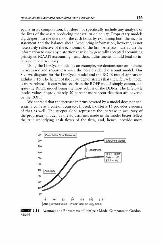
E1C05 08/25/2009 Page 129

equity in its computation, but does not specifically include any analysis ofthe lives of the assets producing that return on equity. Proprietary modelsdig deeper into the drivers of the cash flows by examining both the incomestatement and the balance sheet. Accounting information, however, is notnecessarily reflective of the economics of the firm. Analysts must adjust theinformation to cure any distortions caused by generally accepted accountingprinciples (GAAP) accounting—and those adjustments should lead to in-creased model accuracy.

Using the LifeCycle model as an example, we demonstrate an increasein accuracy and robustness over the best dividend discount model. OurS-curve diagram for the LifeCycle model and the ROPE model appears inExhibit 5.16. The height of the curve demonstrates that the LifeCycle modelis more robust—it can value securities the ROPE model simply cannot, de-spite the ROPE model being the most robust of the DDMs. The LifeCyclemodel values approximately 50 percent more securities than are coveredby the ROPE.

We contend that the increase in firms covered by a model does not nec-essarily come at a cost of accuracy. Indeed, Exhibit 5.16 provides evidenceof that as well. The steeper slope represents the increase in accuracy ofthe proprietary model, as the adjustments made in the model better reflectthe true underlying cash flows of the firm, and, hence, provide more

EXHIBIT 5.16 Accuracy and Robustness of LifeCycle Model Compared to GordonModel


E1C05 08/25/2009 Page 130

accurate valuations. Despite covering much more difficult firms to value—those with negative earnings, such as start-ups—the LifeCycle model doesso with more accuracy. While a complete analysis of proprietary modelsversus commonly accepted models, such as the DDMs, is beyond the scopeof this chapter, the evidence in Exhibit 5.16 should console analysts thattrade-offs between the number of securities covered and accuracy are not aforegone conclusion. Developers may, indeed, build superior models onboth accuracy and robustness!

CONCLUS I ON

Using dividend discount models as examples, we have demonstrated how toevaluate and improve automated discounted cash flow models. Our resultsfrom this sample suggest that the fundamental measurement principles ofrobustness, accuracy, unbiasedness, and predictive capability are not sepa-rate concepts but part of an integrated model-building process. Further-more, we showed in our sample how to improve the model with respect toaccuracy and predictive capability once we remove the bias influence from aparticular parameter.

Despite the simplistic models used, the results are consistent with ourbasic premise that models can achieve superior robustness, accuracy,unbiasedness, and predictive capability. Moreover, builders can improveeven the best of a subset of models in some systematic fashion. Our initialresults should encourage model builders that choosing between models doesnot necessarily involve trade-offs between the measurement principles. Fol-lowing our process, they may indeed develop dominant proprietary models,leading to improved investment decisions and portfolio performance.

APPEND IX : ACADEM IC L I T ERATURE

There exists a substantial and growing body of literature investigating theperformance of valuation models. In the academic literature, researchersare primarily concerned about the ability of valuation models to provideaccurate and unbiased estimates of market prices. Rozeff produced one ofthe earlier works on the topic (1990), where he analyzes the performance oftwo different three-phase dividend discount models—one that fades the div-idend growth rate and another that fades the return on equity and retentionrate in a linear fashion. Our chapter revisited those two models as an exam-ple of our model-building process. Central to Rozeff’s evaluation of the div-idend discount models is the analysis of pricing errors, defined as


E1C05 08/25/2009 Page 131

(Vit � Pit)=Pit, where Vit is the value predicted by the model for stock i attime t and Pit is the corresponding market price. Researchers consider mod-els that lead to lower pricing errors superior in terms of estimating how themarket sets prices.

Numerous other studies have utilized a similar criterion for evaluatingand comparing valuation models. Francis, Olsson, and Oswald (2001) use apricing error definition as in Rozeff to compare the accuracy of dividend,free cash flow, and abnormal earnings models and later to compare mechan-ical earnings and residual income models. Penman and Sougiannis (1998)define a valuation error as (Pit � Vit)=Pit to compare dividend, free cashflow, and earnings models; and Sougiannis and Yaekura (2001) use thesame definition of valuation error to compute the accuracy of analysts’ earn-ings forecasts. More recently, Bakshi and Chen (2005) define a valuationerror similarly in evaluating the accuracy of a stochastic valuation model.

Downs (1991) employs an ‘‘overvalue ratio’’ as Pit/Vit to evaluate anasset-based valuation model. Alternatively, Frankel and Lee (1998) use theinverse of Downs’s overvalue ratio to research an analyst-based valuationmodel, and Kaplan and Ruback (1995) use the natural log of Vit/Pit to de-termine if DCF models accurately value highly leveraged transactions.Courteau, Kao, O’Keefe, and Richardson (2003) compute mean squaredpricing errors and interpercentile ranges in their comparison of direct valua-tion and multiplier approaches.

In addition to accuracy, most studies also examine the issue of theirmodels’ biases. Rozeff explicitly factors bias in his models by adjusting themodels so that the pricing errors average out to zero, thus making the mod-els unbiased by that definition. Others such as Francis, Olsson, and Oswald(2000) examine the sign of the median pricing errors. Kaplan and Ruback(1995), Sougiannis and Yaekura (2001), and Courteau, Kao, and Richard-son (2001) use linear regression to test for bias by regressing some form ofprices on model values. If model values are unbiased, the regression shouldyield an intercept of zero and slope of one. The regression analysis simulta-neously tests for accuracy since models that produce values close to theiractual prices will result in regressions with a high r-squared.

In addition, some previous research has investigated another type ofbias that relates pricing errors to various subsets of the data or systematicfactors. Francis, Olsson, and Oswald (2000), for instance, test whethermodel accuracy is different between high and low accrual firms or betweenfirms with varying degrees of research and development spending. Bakshiand Chen (2005), based on their observation that pricing errors are contem-poraneously correlated across stocks, test whether factors such as defaultspreads, term spreads, size premiums, and value premiums can explain pric-ing errors.


E1C05 08/25/2009 Page 132

In examining accuracy and bias, many studies also investigate the distri-bution of pricing or valuation errors. Bakshi and Chen, for example, exam-ine standard deviation of the pricing errors, while Rozeff presents quartilesof the pricing errors. Kaplan and Ruback display the actual distribution ofpricing errors for their DCF models. The consensus of previous work con-cludes that researchers should employ both the central tendency and the dis-persion of pricing errors in evaluating models.

Compared to the issues of accuracy and bias, fewer studies have exam-ined whether accurate models are more predictive. Rozeff alludes to the is-sue by stating that a more accurate model is more likely to be successful.Courteau, Kao, and Richardson (2001) recommend that future researchmove beyond an assumption of market efficiency and test whether differentmodels have varying predictive capability. Frankel and Lee (1998) test theconcept of predictive capability and find the Vit/Pit ratio produced by theirresidual income model to be correlated with long-term future returns. Simi-larly, Francis et al. find the Vit/Pit ratio to be predictive of returns in excessof those relative to CAPM but not relative to a three-factor model.

With increasing frequency, academic researchers are investigating themeasurement principles of accuracy, bias, predictive capability, and, to alesser extent, robustness. Previous academic literature, however, primarilyhas presented the principles as evaluation techniques rather than tools tosystematically improve models. We believe our chapter help fills that gap ofsystematic model improvement in the literature.

NOTES

1. For example, DCF and valuation research primarily appears in accounting jour-nals as opposed to journals strictly related to finance.

2. A recent study by Domian, Louton, and Racine (2007) suggests that the numberof stocks needed to adequately diversify is well in excess of 100.

3. It is possible that analysts will have insight regarding terminal values. In such acase, that insight should become part of the normal model-building process toensure the terminal value adjustments are empirically validated.

4. Rozeff never specifies precisely what the ‘‘ROPE’’ acronym means. Atra andThomas guess from its context and calculations that ‘‘ROPE’’ may mean‘‘Return on Payout and Return on Equity.’’

5. Rozeff never specifies precisely what the ‘‘GROW’’ acronym means. From itscontext and calculations, ‘‘GROW’’ may mean the specified, multi-stage‘‘growth’’ model.

6. These terms are found in academic literature such as Rozeff (1990).7. In our description, we assume the fade is linear. Other fade patterns are possible

as well. For instance, the model may employ an exponential fade pattern as in


E1C05 08/25/2009 Page 133

Bernstein, Kirschner, and Lui (2002). Numerical examples of the fading pat-terns appear in Rozeff.

8. Both theoretical literature (Cornell 1999) and some practitioner literature(Lawson 2002) suggest a lower equity risk premium than historically observed.

9. Since the ROPE model requires estimates of both ROE and RR, we estimatethese to be 8.33 percent and 60 percent, respectively, to achieve the same5 percent growth rate.

10. We present a review of the academic literature related to the measurement prin-ciples in the chapter’s appendix.

11. The authors acknowledge a discussion with Tom Copeland in 2004 regardingthis point.

12. There may be a theoretical reason for an overall under- or overvaluation of se-curities. For example, an accurate macroeconomic model may suggest at a givenpoint in time that the entire market is over- or undervalued, and that model maytherefore be useful in asset allocation. Since the models of concern in this chap-ter primarily concentrate on practitioner security selection, we leave the issue ofintegrating a macroeconomic model with a security selection model for futureresearch.

13. Our view, therefore, contrasts with the traditional view of market efficiency,which assumes that intrinsic values represent errors around the (true) marketprice.

14. Our (unreported) tests of normality of the errors confirm that they are not nor-mal but instead fat-tailed.

15. Chapter 11 provides details of the computations in the LifeCycle models.

RE F ERENCES

Arnott, R., J. Hsu, and P. Moore. 2005. Fundamental indexation. Financial AnalystsJournal 61 (March/April): 83–99.

Bakshi, G., and Z. Chen. 2005. Stock valuation in dynamic economies. Journal ofFinancial Markets 8 (May): 111–151.

Bernstein, R., L. Kirschner, and K. Lui. 2002. Quantitative primer: A guide to con-cepts, models, and techniques. Merrill Lynch Global Securities Research andEconomics Group (September).

Bethke, W., and S. Boyd. 1983. Should dividend discount models be yield-tilted?Journal of Portfolio Management 9 (Spring): 23–27.

Brigham, E., and J. Houston. 2007. Fundamentals of financial management.11th ed. Mason, OH: Thomson-Southwestern, 8–11.

Cornell, B. 1999. The equity risk premium. New York: John Wiley & Sons, 126–157.Cottle, S., R. Murray, and F. Block. 1988. Graham and Dodd’s Security Analysis.

5th ed. New York: McGraw-Hill, 41.Courteau, L., J. Kao, T. O’Keefe, and G. Richardson. 2003. Gains to valuation accu-

racy of direct valuation over industry multiplier approaches. (April 4) Availableat SSRN: http://ssrn.com/abstract=393120.


E1C05 08/25/2009 Page 134

Courteau, L., J. Kao, and G. Richardson. 2001. Equity valuation employing theideal versus ad hoc terminal value expressions. Contemporary AccountingResearch 18 (Winter): 625–661.

Damodaran, A. 2002. Investment valuation: Tools and techniques for determiningthe value of any asset. 2nd ed. New York: John Wiley & Sons, 11–25.

Domian, D., D. Louton, and M. Racine. 2007. Diversification in portfolios of indi-vidual stocks: 100 stocks are not enough. Financial Review 42 (November):557–570.

Downs, T. 1991. An alternative approach to fundamental analysis: The asset side ofthe equation. Journal of Portfolio Management (Winter): 6–16.

Fama, E., and K. French. 1992. The cross-section of expected returns. Journal ofFinance 43: 153–194.

Francis, J., P. Olsson, and D. Oswald. 2000. Comparing the accuracy and explain-ability of dividend, free cash flow, and abnormal earnings equity value esti-mates. Journal of Accounting Research 38 (Spring): 45–69.

Francis, J., P. Olsson, and D. Oswald. 2001. Using mechanical earnings and residualincome forecasts in equity valuation. Working paper (April): 1–36.

Frankel, R., and C. Lee. 1998. Accounting valuation, market expectation, and cross-sectional stock returns. Journal of Accounting and Economics 25: 283–319.

Gordon, M. 1962. The investment, financing and valuation of the corporation.Homewood, IL: Irwin.

Kaplan, S., and R. Ruback. 1995. The valuation of cash flow forecasts: An empiricalanalysis. Journal of Finance 50 (September): 1059–1093.

Lawson, S. 2002. The equity risk premium: It’s lower than you think. GoldmanSachs CEO Confidential 14 (November).

Lee, C. 2001. Market efficiency and accounting research. Journal of Accounting andEconomics 31: 233–253.

Madden, B. 2007. For better corporate governance, the shareholder value review.Journal of Applied Corporate Finance 19(1): 102–114.

Penman, S., and T. Sougiannis. 1998. A comparison of dividend, cash flow, andearnings approaches to equity valuation. Contemporary Accounting Research15 (Fall): 343–383.

Rozeff, M. 1990. The three-phase dividend discount model and the ROPE model.Journal of Portfolio Management (Winter): 36–42.

Sougiannis, T., and T. Yaekura. 2001. The accuracy and bias of equity values in-ferred from analysts’ earnings forecasts. Journal of Accounting, Auditing, andFinance 16: 331–362.


E1C06 09/03/2009 Page 135

CHAPTER 6The Essence of Value-Based

FinanceRoy E. Johnson

Co-Founder, Vanguard Partners; Currently D/B/A Corporate Strategy

The material in this chapter incorporates a process and set of analytic tech-niques that delve into the true economic characteristics and performance

of companies, as well as business units within companies. There are two ma-jor building blocks of value-based finance (VBF) that will be explored:

1. Indicators of shareholder value creation, neutrality, or destruction.2. Measurements of actual or potential value created, maintained, or

destroyed.

The chapter is divided into the following segments:

& Introducing Value-Based Finance (a Transition from Accounting toEconomics). An example is given to display the potential differencesbetween accounting and economic returns, along with implications.

& Valuation Perspectives: Economic Profit (EP) and Market Value Added(MVA). EP is the primary indicator of value creation and at the core ofmany value-based performance systems implemented by leading-edgecompanies. MVA is a key measure of shareholder value creation, repre-senting a spread between what financial markets (or investors) judge abusiness to be worth and what has been invested. This section explainsand explores both.

& Valuation Perspectives: The Magnifier. This segment illustrates thevalue-creating impact of growth, which works in positive and negativedirections.

135

E1C06 09/03/2009 Page 136

& Valuation Perspectives: Financial Drivers and Value Profit Margin(VPM). This segment lays out a template of high-level metrics that areat the heart of many well-known ratios used in measuring financial per-formance, and then provides a simple and insightful profit margin thatlinks to return on investment.

& Value Analysis: The Proper Focus. Many companies spend a lot of timeestablishing the ingredients of a value-based system, but then misapplythem—analyzing stand-alone projects (which are usually part of alarger endeavor) instead of major strategies and investment programs.This misapplication can waste time by performing irrelevant evalua-tions, confuse management as to what’s really important, and, at theextreme, lead to bad investment decisions.

This material provides useful concepts and tools for financial and oper-ating professionals and managers in major corporations, plus owners andkey managers of privately held businesses. The reader is taken through aprocess of:

& Making a transition from traditional accounting-based perspectives andmeasures to those focused on business economics—centered around theconcepts of economic profit, return on investment, and cash flow.

& Developing a template of financial drivers—a set of measures that helpbusiness managers and owners instill value creation as a discipline—along with an understanding of how value is created from a financialpoint of view.

& Establishing analytic tools and techniques to evaluate and measurevalue creation.

& Focusing all the concepts, tools, techniques, and metrics for the mosteffective utilization—demonstrating how to avoid common mis-application traps.

Knowledge of this subject is essential for those who work in corporateAmerica, because the value of any for-profit enterprise is linked to its under-lying economics and cash flow, which can differ from what is reportedthrough an accounting-based financial system. Virtually all research onpublic stock markets supports this premise, and knowledgeable investorsin privately owned firms employ economic principles in their valuationsand decisions about buying and selling businesses.

For anyone involved in commercial or investment banking, the materialwill provide insight into how to evaluate the performance of client busi-nesses, which should impact the nature of relationships and financing pol-icy, along with financing alternatives and opportunities. This material


E1C06 09/03/2009 Page 137

should enhance the expertise and professionalism of bankers in the area ofcorporate finance—part of the world their clients live in. For those in mer-chant banking or equity financing, the material should provide a solid foun-dation for business valuations and investment selections.

INTRODUCING VALUE-BASED FINANCE(A TRANSITION FROM ACCOUNTING TO ECONOMICS)

The movement from accounting to economic metrics is at the core of value-based finance (VBF)—driven by the fact that the real profitability of a busi-ness is not always reflected in the traditional accounting measures that focuson net earnings. An example using a hypothetical firm—Growthstar Inc.—will illustrate the dilemma. The company has a core business, expandedthree years ago by the acquisition of Newco. The purchase price was$55 million, financed with excess cash and new debt. Off-balance-sheetleases of $15 million were assumed. Thus, the total investment was$70 million, none of which impacted the book value of Growthstar Inc.stockholders’ equity. Financial highlights of the three most recent historicalyears plus the current year will be presented, to provide a comparison of theaccounting versus economic framework.

Exhibit 6.1 gives a summary for the accounting scenario, noting thatyear 3 is the most distant and year 1 is the most recent historical period.The Newco deal was closed at the end of year 3. Thus, it had no effect onthe company’s operations for year 3.

Has this acquisition benefited Growthstar’s shareholders? Based on theaccounting scenario, the answer would seem to be a resounding yes! Reve-nue has doubled and net income has grown nearly fourfold—using year 3 asa base—through the current year. Return on equity has almost doubled,from 12 percent to 22 percent, during this time period.

Under an economic framework, however, the key indicators paint asomewhat different picture. The economic scenario entails some importantadjustments:

& Interest expense is eliminated from the profit and loss (P&L) statementand is factored into a weighted average cost of capital (WACC). Thus,the P&L is focused on operating profit.

& The acquisition reserve in year 3 (accounting write-off of the ‘‘pur-chased R&D’’ portion of goodwill) is reversed—added back to boththe P&L and the balance sheet—reflecting the sunk cost nature ofacquisition investments. Write-offs reduce acquisition prices onthe books.

The Essence of Value-Based Finance 137

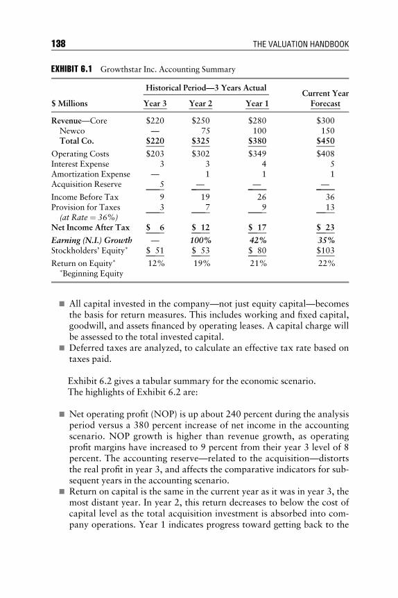
E1C06 09/03/2009 Page 138

& All capital invested in the company—not just equity capital—becomesthe basis for return measures. This includes working and fixed capital,goodwill, and assets financed by operating leases. A capital charge willbe assessed to the total invested capital.

& Deferred taxes are analyzed, to calculate an effective tax rate based ontaxes paid.

Exhibit 6.2 gives a tabular summary for the economic scenario.The highlights of Exhibit 6.2 are:

& Net operating profit (NOP) is up about 240 percent during the analysisperiod versus a 380 percent increase of net income in the accountingscenario. NOP growth is higher than revenue growth, as operatingprofit margins have increased to 9 percent from their year 3 level of 8percent. The accounting reserve—related to the acquisition—distortsthe real profit in year 3, and affects the comparative indicators for sub-sequent years in the accounting scenario.

& Return on capital is the same in the current year as it was in year 3, themost distant year. In year 2, this return decreases to below the cost ofcapital level as the total acquisition investment is absorbed into com-pany operations. Year 1 indicates progress toward getting back to the

EXHIBIT 6.1 Growthstar Inc. Accounting Summary

Historical Period—3 Years ActualCurrent Year

$ Millions Year 3 Year 2 Year 1 Forecast

Revenue—Core $220 $250 $280 $300Newco — 75 100 150Total Co. $220 $325 $380 $450

Operating Costs $203 $302 $349 $408Interest Expense 3 3 4 5Amortization Expense — 1 1 1Acquisition Reserve 5 — — —

Income Before Tax 9 19 26 36Provision for Taxes(at Rate ¼ 36%)

3 7 9 13

Net Income After Tax $ 6 $ 12 $ 17 $ 23

Earning (N.I.) Growth — 100% 42% 35%Stockholders’ Equity� $ 51 $ 53 $ 80 $103

Return on Equity� 12% 19% 21% 22%�Beginning Equity


E1C06 09/03/2009 Page 139

year 3 return. The message here is that the company is now no better orworse off than it was before it made the acquisition. This is quite a con-trast to the return on equity results from Exhibit 6.1, influenced byaccounting entries and only the equity portion of invested capital incor-porated into the return metric.

& Economic profit goes from positive in year 3 to negative in year 2, andthen rebounds as the firm moves through year 1 and the current year.As with NOP, the current year is a bit more than double the year 3level, versus a fourfold increase of net income.

Whether the shareholders will benefit long-term from this acquisitionwill depend on the strategy and future profitability of Newco. This year’seconomic profit is a good sign.

To conclude, accounting metrics often do not provide good shareholdervalue indicators. Thus, much of the business world is turning to economicsfor value analysis. Exhibit 6.3 gives a graphic portrayal of profit growth

EXHIBIT 6.2 Growthstar Inc. Economic Summary

Historical Period—3 Years ActualCurrent Year

$ Millions Year 3 Year 2 Year 1 Forecast

Revenue-Total $220 $325 $380 $450Operating Costs 302 302 349 408Interest—Eliminate — — — —

EBITAa 17 23 31 42Cash Taxes—Rate 25% 26% 26% 26%Amount 4 6 8 11

Net Operating Profit $ 13 $ 17 $ 23 $ 31

Profit (NOP) Growth — 31% 35% 35%Invested Capital (IC)� $ 90 $170 $190 $220

Return on Capital� 14% 10% 12% 14%Return on Equity� 12% 19% 21% 22%Economic ProfitNet Operating Profit $ 13 $ 17 $ 23 $ 31Capital Chargeb (10) (19) (21) (24)

Economic Profit $ 3 $ (2) $ 2 $ 7�Beginning Equity

aEarnings before interest, taxes and amortization.bThe capital charge is based on a weighted cost of capital of 11% for this company and is

charged against IC for each year. This charge is an indicator of whether NOP is sufficient to


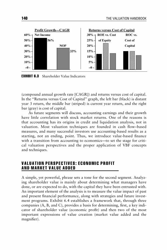
E1C06 09/03/2009 Page 140

(compound annual growth rate [CAGR]) and returns versus cost of capital.In the ‘‘Returns versus Cost of Capital’’ graph, the left bar (black) is distantyear 3 return, the middle bar (striped) is current year return, and the rightbar (gray) is cost of capital.

As future segments will discuss, accounting earnings and their growthhave little correlation with stock market returns. One of the reasons isthat accounting has its origins in credit and liquidation analysis, not invaluation. Most valuation techniques are founded in cash flow–basedmeasures, and many successful investors use accounting-based results as astarting, not an ending, point. Thus, we introduce value-based financewith a transition from accounting to economics—to set the stage for criti-cal valuation perspectives and the proper application of VBF conceptsand techniques.

VALUAT I ON PERSPECT I V ES : ECONOM IC PROF I TAND MARKET VALUE ADDED

A simple, yet powerful, phrase sets a tone for the second segment. Analyz-ing shareholder value is mainly about determining what managers havedone, or are expected to do, with the capital they have been entrusted with.An important element of the analysis is to measure the value impact of pastand present financial performance, along with strategies and future invest-ment programs. Exhibit 6.4 establishes a framework that, through threecompanies (A, B, and C), provides a basis for determining, first, a key indi-cator of shareholder value (economic profit) and then two of the mostimportant expressions of value creation (market value added and themagnifier).

EXHIBIT 6.3 Shareholder Value Indicators


E1C06 09/03/2009 Page 141

Economic profit (EP) is a concept right out of basic economics—thecourse many people took in college. EP is what any business owner (share-holder) should be concerned with, since it takes into account the cost of allthe capital invested in the business. EP is the residual (what’s left over) afterall the costs of running a business have been accounted for and the suppliersof capital have been provided with a fair return on their investment. A prob-lem with accounting profit—most commonly expressed as net income orearnings per share (EPS)—is that it only includes a charge for debt financ-ing; thus it misses a cost for equity capital, the most expensive and prevalentform of capital for a typical industrial company. The cost of equity capital iswhat a common shareholder expects to earn annually as a rate of return oninvestment. The cost of equity capital formula adds a premium to the cur-rent return on a long-term risk-free security, such as a 10-year U.S. govern-ment bond.

Because of this condition and another important one—the gap betweenaccounting profit and cash flow—there is virtually no correlation betweennet income and/or EPS growth and key stock market indicators (e.g., mar-ket-to-book ratios).

As stated earlier, economic profit (EP) is a residual—the amount ofprofit available after all suppliers of capital have been given a fair return fortheir investment. The example in Exhibit 6.4 shows how three companies,all with the same accounting profit, can have significantly different eco-nomic profits.

If we start with the upper portion of Exhibit 6.4, we have the essenceof the accounting profit model, reflecting the traditional P&L summaryshown here:

EXHIBIT 6.4 Economic Profit Example

Base Period Company A Company B Company C

Revenue (Sales) $1,000 $1,000 $1,000Net Operating Profit (NOP) $ 100 $ 100 $ 100

10% 10% 10%

Invested Capital (IC) $ 600 $ 800 $1,000Cost of Capital (CCAP) 12% 12% 12%

Economic ProfitNOP (from above) $ 100 $ 100 $ 100Capital Charge (CCAP) (72) (96) (120)

Economic Profit (EP) $ 28 $ 4 $ (20)


E1C06 09/03/2009 Page 142


Revenue (Sales) $1,000 $1,000 $1,000Net Operating Profit

– $ $ 100 $ 100 $ 100– % 10% 10% 10%

Historically, this is what Wall Street has published and what most com-panies have geared themselves to. The questions to ask are: What is differ-ent about these companies? Can you make any type of investment decisionbased on this information?

Two critical factors are missing, from a financial perspective, to beginto make shareholder value judgments. These two factors get at the heart ofthe shortcomings of using the traditional accounting profit model, based onnet income or earnings per share as the key determinant for stock prices.Using earnings alone as a proxy for value misses the following:

& The risk of the earnings.& The capital needed to generate the earnings.

Economic profit begins the same as accounting profit—that is, with rev-enue (or sales). All the operating-related expenses and taxes are then sub-tracted to arrive at net operating profit (NOP). The EP model, in itsunending quest to get close to the economics of the business, makes someadjustments to the typical accounting P&L, as follows:

& Nonoperating charges such as restructuring and other one-time or extra-ordinary expenses (often not related to cash flow) are usually reversed.

& Expenditures for advertising and/or R&D may be capitalized, depend-ing on how such treatment affects the cash flow characteristics ofthe business. The determining factor (rule of thumb) is whether capital-ization/amortization versus expensing affects the calculation of EP bymore than 10 percent, on average, over a multiyear period. If so, capi-talize. If not, keep the more simple expensing treatment.

& Taxes are based on actual/projected cash payments rather thanaccounting provisions for statutory tax rates.

& The charge for debt financing (interest expense) is excluded, since thiswill be picked up in the overall corporate cost of capital (CCAP), whichis 12 percent in the example.


E1C06 09/03/2009 Page 143

The rule for making adjustments is very straightforward and is based onthe concept of simplicity with integrity. If an adjustment is needed to main-tain the economic integrity of the performance measure, then make it. Ifnot, use information as reported.

A major enhancement in the EP model is the explicit recognition ofbalance sheet investment. The major categories are working capital (re-ceivables, inventory, payables, etc.) and fixed capital (property, plant,and equipment). In some companies, goodwill and intangibles are im-portant investments and so are included in the invested capital. Anotherimportant item, ignored in the accounting model, is one found in thefootnotes: operating leases. This off-balance-sheet item accounts forassets leased—thus, a financial obligation similar to other secureddebt—but falling below an arbitrary hurdle defined by a generally ac-cepted accounting principles (GAAP) formula to determine whether anasset should appear on the balance sheet. In some companies, operatingleases represent a significant portion of assets and debt. A rule of thumbis: If the present value of operating leases comprises more than 10 per-cent of invested capital, then they should be included. If less than 10percent, they are not material and can be left out of the calculation ofEP—again, simplicity with integrity.

Charging a cost for the capital invested in a business approximatesthe desires of investors. What this means is that the capital charge(CCAP)—12 percent in our example—is the minimum annual return thatinvestors, in the aggregate, expect from each of these three companies.(As a note, some refer to this return as the weighted average cost of capi-tal—WACC.) Thus, the closest we can come to replicating the capitalmarket perspective is to assess profitability after charging for this (mini-mum) return on capital requirement. The term hurdle rate is used widelywith respect to the analysis of capital investments. CCAP is the hurdlefor these three firms. In this case, it is expressed as a dollar amount, butcan also be a percentage. While not perfect, this approach captures theexpectations of the financial markets.

As seen in Exhibit 6.4, all the firms are not profitable from an eco-nomic, or rate of return, perspective. In fact, only Company A is trulyprofitable, with an EP of $28 million. Note the EP of $4 million (justabove break-even) in the Company B column and the negative EP of$(20) million in the Company C column. A variation on this format, inwhich the minimum return is expressed as a percentage, rather than adollar amount, and the comparison is to a percentage CCAP, can beillustrated as follows:


E1C06 09/03/2009 Page 144


EP Expressed as returnon capital (%)

Net Operating Profit (NOP) $100 $100 $100Invested Capital (IC) $600 $800 $1,000Return on Capital (ROC) 17% 12.5% 10%Cost of Capital (CCAP) 12% 12.0% 12%

Spread: ROC minus CCAP 5% .5% �2%

The point for now is that, conceptually, virtually all economic measuresare based on the notion of ascribing a cost (minimum rate of return) to thecapital invested in a business. While companies produce a balance sheetwhen the books are closed, most people don’t evaluate it thoroughly, nordo they make the balance sheet a focus of their analysis.

The EP status of a business positions it as a value creator (Company A)or destroyer (Company C)—or, as with Company B, being value neutral.This has major implications for what growth will produce in terms of share-holder value. If we apply a growth scenario, with a very limited number ofassumptions, to the three firms (A, B, and C), we can begin to get an appre-ciation of why EP is so important in the value creation process.

Marke t Va l u e Added

The simple scenario that follows provides a useful foundation for lookinginto the future for a business.

Market Value Added—Sample ScenarioValuation Summary: Assumptions

& All companies maintain the same invested capital-to-revenue ratio.& All companies continue to earn the same profit margin on revenue.& All companies increase revenue by 10 percent per year for four years.

The assumptions in this scenario, while simple and few in number, arerepresentative of a forward-looking financial model, which investors use tovalue companies and businesses within companies. They are also indicativeof the type of thinking necessary to value strategies. The value we’re de-scribing here—market value added (MVA)—is what the market is addingto or subtracting from what has been invested in the company, based on itsevaluation of past/present financial performance and its perception about


E1C06 09/03/2009 Page 145

where the company is going in the future. A goal of any for-profit business isto increase the spread between what has been invested and what the marketfeels is warranted based on performance. So, both EP and MVA are spreadsor residuals.

We could expand these assumptions into a more robust scenario, butthe ones given will suffice to illustrate the concept: a numerical expressionof these assumptions for our three companies—A, B, and C. Exhibit 6.5provides an illustration.

Company A increases its EP throughout the forecast period—in thiscase, four years. If you think about the consistency of performance im-plied in the assumptions (which, again, are probably oversimplified) youshould understand the EP forecast results for Company A—EP increaseseach year at the 10 percent growth rate for revenue—$31 million infuture year 1 to $41 million in future year 4. The ‘‘Years 5 on residual’’is a typical way that the years after the forecast horizon are treated,which capitalizes the year 4 EP at the CCAP rate (in this case, 12 per-cent). This assumes that the plan can produce no incremental EP even ifthe business continues to grow, which is equivalent to saying that, afteryear 4, the company will just earn its cost of capital on new investment.The MVA for this growth scenario is the sum of the EPs for the four-year growth period plus the residual value.

The example is oversimplified, at this point, in that it doesn’t (yet) ac-count for discounting of the future values. However, it does show thatCompany A is creating shareholder value with its growth plan. Therefore,the total warranted market value of Company A (again, before discountingthe future year EPs) is the base period invested capital (IC) of $600 million(from Exhibit 6.4) plus the MVA of $485 million—for a total of nearly$1.1 billion. Obviously, the real MVA and total warranted value for Com-

EXHIBIT 6.5 Market Value Added Example (10 Percent Growth, $ Millions)

Pro Forma Company A Company B Company C

EP—value impactYear 1 $ 31 $ 4 $ (22)Year 2 34 5 (24)Year 3 37 5 (27)Year 4 41 6 (29)

Subtotal (4 years) 143 20 (102)Years 5 on residual 342 50 (242)Sum of EPs þ residual

before discounting$485 $70 $(344)


E1C06 09/03/2009 Page 146

pany A will be less when we apply the 12 percent discount rate to futureyear EP and residual values, but for now we can see that Company A shouldcommand a premium over its invested capital when valued in the financialmarkets. Why? Because management is earning more than the cost of capi-tal and is growing the business. You should be able to visualize that if Com-pany A can increase its revenue growth, then it will generate more MVA—and, thus, should experience a greater warranted total market value.

One of the interesting features of this analysis is that we get approxi-mately the same MVA result as we would with the traditional free cashflow (FCF) approach. Once we factor in an appropriate discount rate—which we will do after we get through with this nondiscounted example—MVA (under the EP approach) is about the same as the net present value(NPV) calculated using the free cash flow (FCF) technique. One reason thatthe EP model is receiving widespread application in corporations and thefinancial institutions that invest large sums in the equity markets is that it isthe conceptual equivalent to the FCF approach, with the result (MVA)equal or very close to the NPV. Further, with the EP approach, we can de-termine meaningful period-by-period financial results—indicative of valuecreation, destruction, or neutrality—which is usually not possible with thefree cash flow technique. The FCF model provides a credible value-basedend result, but is typically not very useful in assessing value creation prog-ress along the way.

Company B presents a somewhat different scenario. Even though itgrows and maintains its 10 percent after-tax profit margin, the companydoes not produce any significant future year EPs. By now this should be ap-parent, since Company B just earns its CCAP. Company B may get bigger,but it doesn’t get much better, at least in terms of shareholder value cre-ation. Notice the very modest $70 million MVA, which is less than 10 per-cent of its $800 million invested capital. This is noteworthy because itindicates that B-type companies should be valued (in the financial markets)fairly close to their economic book value. They simply don’t return muchmore to the shareholders than what was invested in the first place—and arenot expected to do much more with new investment.

Company C is truly a problem. It cannot grow out of its dilemma ofearning a return below the cost of capital without radically changing theway it conducts its business. Yet the business world is littered with C-typecompanies and businesses, thinking that they can grow and be successfulwithout changing their fundamental structures. This is a very serious situa-tion in corporate America since a significant percentage (in excess of 25 per-cent according to some research) of publicly traded companies in the UnitedStates fall into the C category. Whatever assumptions we may make, the


E1C06 09/03/2009 Page 147

impact is clear—growth destroys shareholder value for C-types—and moregrowth means more value destruction!

The next segment presents an example to illustrate the value-creatingpotential for A-type companies and businesses, along with how C-types de-stroy shareholder value.

VALUAT I ON PERSPECT I V ES : TH E MAGN I F I E R

One of the most powerful concepts in value-based finance is the Magnifier.Whereas previous topics give good indications of shareholder value creationor destruction, the magnifier provides a ‘‘more bang for the buck’’ type ofevaluation—especially regarding the impact of growth, which is still themost important determinant of share price movement.

The focus of this analysis will be on Company A and Company C fromthe previous segment since value-neutral firms, such as Company B essen-tially run in place and really don’t go anywhere from a shareholder valueperspective. The point to be illustrated is that the EP position of a businesshelps to dictate what its future actions should be if the objective is to createshareholder value.

Company A has a positive EP and a return on capital higher than itscost of capital. With these positive indicators, the following gives an over-view of what Company A should do.

How to Increase Shareholder Value for Company A

& Invest capital in growth-oriented strategies/programs, with high returnpotential.& Go for growth. Instill growth as a driving force throughout the

organization.& Emphasize staying close to existing margins and capital intensity,

with room for some deterioration if the opportunity is significant.& Growth adds value. Bigger is better!

This set of directive actions says a lot. Growth is what most companieswant. You just have to make sure that the business is in the A category interms of its sustainable economic profit. If not there now, then the near andlonger-term strategy has to get it into an A position before embarking on agrowth strategy.

The potential for shareholder value creation of this ‘‘go for growth’’goal for Company A can be illustrated in Exhibit 6.6.


E1C06 09/03/2009 Page 148

Exhibit 6.6 needs careful explanation. We start with the horizontalaxis, which plots annual compound growth rates (CGRs) for revenue andnet earnings. These are the same, since we’re assuming a steady profit mar-gin (10 percent). The growth rate scenarios over a four-year future time ho-rizon are in increments of five percentage points—from 0 percent (nogrowth) to 20 percent. These are annual CGRs.

Next, the vertical axis plots MVA in millions of dollars. The MVA isthe net present value (NPV) of the various growth scenarios, based on theassumptions for invested capital intensity (ICI)—the capital needed for eachnew revenue dollar—and the NOP margin. Thus, MVA measures share-holder value created—the NPV for each growth plan.

The magnifier effect is the impact on MVA (shareholder value) forthe selected revenue growth rates. Starting with the no growth (0 per-cent) scenario, if the business stays at its base period level of revenueand earnings, it will create $233 million of MVA. This results from thecompany (A) generating an economic profit (EP) of $28 million. Under ano growth scenario, this level of EP would continue forever. MVA(equivalent to the shareholder value added) is simply the EP capitalizedat the 12 percent cost of capital. Finally, $28 million divided by 12 per-cent is approximately $233 million. What this means is that managementhas created a warranted MVA of $233 million. This is the amount ofmarket value that management has added to the economic book value of$600 million.

EXHIBIT 6.6 The Magnifier Effect for Company A


E1C06 09/03/2009 Page 149

Now, let’s assume that a 5 percent growth plan is communicated tothe investors. With the assumptions we have made, this 5 percentgrowth in revenue and earnings translates into a 10 percent increase inMVA. In essence, growth in revenue and earnings is magnified into in-creasingly higher growth rates for MVA. As we continue along the hori-zontal axis, to higher growth rates for revenue and earnings, look atwhat happens to the height of the (vertical) MVA bars. They rise ateven higher rates—again, in a magnified fashion. At the peak of thisexample, a 20 percent CGR for sales and earnings over a four-year fu-ture time period produces a 75 percent increase in shareholder value.Extending the time horizon or further increasing the growth rate wouldmagnify the situation even further.

Many CEOs and business unit heads have had this intuitive feelingabout the impact of growth. However, many think it’s driven by earningsper share (EPS). What this example shows is that value creation is depen-dent on EP (drop the S from EPS) and profitable growth—beating the costof capital with old and new investments. This example also explains whysome of the great names we know in business have produced incrediblegains in their stock prices. They generated positive economic profit—whichtranslates into a high return on their invested capital (well in excess of theircost of capital)—and they grew rapidly!

A picture is often worth a thousand words, and Exhibit 6.6 gives apicture that people at all levels in a business should embed into theirminds. In order not to interrupt the discussion flow, two tables placed atthe end of this segment show the key calculations for the 15 percent and20 percent growth cases—this, after all the major scenarios have beenpresented.

The situation for Company B can be covered rather quickly, per thefollowing:

Company B

& Earn more operating profit with the same capital.& Squeeze additional profit from the existing capital base (selective

pricing and/or cost cutting).& Emphasize margin improvement.

& Growth is secondary, as it adds minimal value!

Company B needs to become more efficient, not bigger. Its predica-ment is rather straightforward. Many of the conglomerates are in the Bcategory. They buy firms that are sometimes in different businesses, withvery little in the way of common marketing, distribution, or other


E1C06 09/03/2009 Page 150

functions. They are running what amounts to a portfolio of companies—in essence, a miniature mutual fund. What they fail to realize are someimportant shortcomings. First, most institutional investors want to con-struct their own portfolios, not one that a CEO or management grouphas chosen. Second, focus—not diversification—has usually produced thehighest total shareholder returns (TSRs) in the stock market. This ispartly due to the management complexity that conglomerates or diversi-fied companies are subject to. It’s very difficult to be an expert at every-thing! Finally, growth by acquisition alone creates obstacles to valuecreation in that it’s hard to avoid the ‘‘transfer of wealth’’ phenome-non—the payment of a premium to gain control of another companythrough a purchase. Unless an acquisition target has been mismanagedand a turnaround opportunity exists, or a truly synergistic combinationcan be implemented, or the seller is not very astute (a rare situationtoday with the involvement of boards of directors and shareholder acti-vists), it is hard to hit a home run with acquisitions. Companies may domuch better with internally developed products and/or services, new mar-keting channels, distribution methods, manufacturing techniques, and soon. Therefore, without greater efficiency (thus, higher EP) many B-typefirms will continue to tread water. They may grow, but they won’t addmuch value if they don’t become more efficient with the capital they cur-rently employ.

A real challenge for business is outlined as follows.

Company C

& Reduce the level of capital employed.& Streamline/re-engineer/re-structure operations.& Validate capital invested in major lines of business.

. . . Noting that Growth destroys value!C-type firms or businesses can not grow and create value without a fun-

damental—perhaps radical—change in the way they manage their investedcapital. The points noted previously are clear. The C businesses are thosewhere major restructuring or reengineering efforts have the potential for abig payoff.

For our example, Exhibit 6.7 quantifies the impact of growth withoutany change in the operating dynamics for a C-type business.

This illustration conveys a powerful and cautionary message forgrowth-minded executives. Since the structure of this chart is somewhat dif-ferent from the magnifier effect for Company A (as illustrated in Exhibit6.6), the elements require an explanation.


E1C06 09/03/2009 Page 151

The growth rate scenarios for revenue and net earnings are plotted in anupward direction in the top portion of the vertical axis. The diagonallysloped line with points of intersection at 5 percent growth rate incrementsrepresent the traditional picture of rising revenue and earnings, the implica-tion being that shareholder value and stock prices rise accordingly. It’s fairto say that this is probably the view of many, since the earnings growthmodel has driven many valuations, or at least valuation perceptions, for along time.

However, as the bottom portion of the chart indicates, this is not thecase. What’s happening is that every percentage point of compound growthwill cost Company C more in a capital charge (CCAP) than it will producein net operating profit (NOP), thus eroding EP. This is despite the fact thatCompany C is generating a profit—at least in the traditional accountingmethod of calculation. As we saw in Exhibit 6.5, however, Company C isactually producing an economic loss. If firms with this performance charac-teristic signal to the financial markets that the pattern (that is, too muchcapital) will continue, then the markets should, in theory, respond with val-uations that would follow the progression of the MVA bars in the lowerportion of the graph.

Let’s take them one at a time. In the no growth scenario, the negativeEP of �$20 million (the real bottom line from Exhibit 6.4) would be

EXHIBIT 6.7 The Magnifier Effect for Company C


E1C06 09/03/2009 Page 152

capitalized at negative $167 million. That’s �$20 million divided by 12 per-cent (CCAP). This management has got some fixing to do before thinkingabout growth. You may have seen some firms that have actually contracted(gotten smaller) and created value. Well, this is why!

Now, assume that management communicates a 5 percent growthplan to investors, maintaining the same NOP margin and invested capitalintensity (ICI) as in the base period. The investors should respond by shav-ing an additional $16 million from the firm’s economic book value. Thus,negative MVA grows (how’s that for misuse of a word?) by 10 percent to�$183 million. The magnifier effect is now working in reverse.

Follow the progression of scenarios to the 20 percent growth levelfor revenue and earnings. MVA (shareholder value) has been destroyedby 75 percent. By now, the message should be clear: Regardless of theiraccounting earnings, C-type businesses will destroy value as they grow, andthe more they grow, the more value they will destroy!

EXHIBIT 6.8 Fifteen Percent Growth for Company A

Valuation via Economic Profit (EP)

($ Millions,Except ICI) Base Year 1 Year 2 Year 3 Year 4 Residual

Revenue 1,000 1,150 1,323 1,521 1,749Investedcapital (IC)

600 690 794 913 1,049

Economic Profit (EP)NOP 100 115 132 152 175Capital charge(CCAP)

(72) (83) (95) (110) (126)

Economic Profit(EP)

28 32 37 43 49 49

Valuation

TotalMarketValue Base IC

MVA – Base +Growth�

Net presentvalue (NPV)

951 600 351

�Discounted (EPs þ Residual)

Assumptions:Annual growth rate (CGR) ¼ 15%

Annual profit (NOP) margin ¼ 10%Invested capital intensity (ICI) ¼ $0.60

Cost of capital (CCAP)¼ 12%


E1C06 09/03/2009 Page 153

Before ending this discussion, we should briefly address start-up busi-nesses. Generally, they should be placed in a special category (A-prime).They may technically be C-type businesses, based on start-up losses, but theexpectation is to become an A. These (start-up) businesses have to be valuedtotally on future prospects with an attempt made to establish a base-levelEP and set of financial drivers—margins, investment requirements, and soforth that will carry them into the future.

In conclusion, the following highlights what has been presented anddiscussed:

& Economic profit incorporates the income statement, balance sheet in-vestments, and a capital cost, making it more robust than accountingearnings.

& A firm’s EP category (A, B, or C) provides an important indicator forwhat a value-creating strategy should focus on and encompass.

& Economic profit translates into market value added through a futureoutlook.

EXHIBIT 6.9 20 Percent Growth for Company A

Valuation via Economic Profit (EP)

($ Millions,

Except ICI) Base Year 1 Year 2 Year 3 Year 4 Residual

Revenue 1,000 1,200 1,440 1,728 2,074Invested capital(IC)

600 720 864 1,037 1,244

Economic Profit (EP)NOP 100 120 144 173 207Capital charge(CCAP)

(72) (86) (104) (124) (149)

Economic Profit(EP)

28 34 40 48 58 58

Valuation

TotalMarket

Value Base IC

MVA – Base

þþþ Growth�

Net presentvalue (NPV)

1,008 600 408

�Discounted (EPs + Residual)Assumptions:Annual growth rate (CGR) ¼ 20%

Annual profit (NOP) margin¼ 10%Invested capital intensity (ICI) ¼ $0.60

Cost of capital (CCAP) ¼ 12%


E1C06 09/03/2009 Page 154

& Growth magnifies value creation positively or negatively, depending onwhether economic returns are above or below the cost of capital.

Exhibits 6.8 and 6.9 provide pertinent details for the MVA/NPV calcula-tions in Exhibit 6.6, regarding the higher-growth scenarios for Company A.

VALUAT I ON PERSPECT I V ES : F I NANC IA L DR I V ERSAND VALUE PROF I T MARG IN

This segment begins with a perception many people in publicly owned com-panies and investment firms embrace—that steadily rising earnings (definedas net income or earnings per share [EPS]) will produce stock price gainsand improved valuation ratios and indexes (for example, price-earnings ra-tio and/or market-to-book ratio). While pervasive, these beliefs are, in fact,not true. The following two charts are indicative of a vast amount of re-search that disputes and disproves the emphasis on EPS and growth (alone)as key drivers of stock market performance.

For those who may be a bit rusty on statistics, Exhibit 6.10 is referred toas a scatter diagram—the plots are all over the place and there is no correla-tion for the variables. In this case, there is no correlation of increasing EPSgrowth rates and market-to-book ratios for the companies in the research.A great deal of analysis produced by some of the best-known investment

EXHIBIT 6.10 Accounting Profit—Stock Market TestSource: Credit Suisse First Boston.


E1C06 09/03/2009 Page 155

research firms during the past 20 or so years yields results similar to what isdisplayed in Exhibit 6.10. Note that MV/IC is market-to-book.

Exhibit 6.11 presents a similar conclusion from a slightly differentperspective.

The key message from Exhibit 6.11 is that revenue growth alone doesnot create shareholder value. There must also be a return on capital.

To highlight the table, the average market multiples inside the matrixthat are italicized and greater than 1.0 indicate a market value greater thanbook value (thus creating value for investors). Numbers equal to 1.0 indi-cate a market value that is equal to book value (call this being value neu-tral). Numbers less than 1.0 portray a shareholder’s nightmare—a marketvalue below the firm’s book value, which can be translated as destroyingvalue.

Looking into the matrix, it is apparent that, except for a few outliers(two 1.1 multiple rapid-growth groups and two 1.1 multiple negative-growth categories with returns below the cost of capital), the pattern forthe value-creating firms—those italicized and >1.0—is consistent in thatthe return on capital exceeds the cost of capital. This is where we see a pay-off for growth in terms of market multiple. In terms of the 1.1 multiple out-liers, it’s possible that the stocks are being priced on the expectation ofhigher returns—two resulting from growth and two from shrinking thebusiness and using capital more effectively. Most of the firms in the twocolumns on the left side of the matrix—those with returns below the cost ofcapital—have either a <1.0 or a 1.0 number for a market multiple. Themarket is astute and looks beyond growth to the return that a company gen-erates on the capital that has already been invested and also the new capitalexpected for the future.

EXHIBIT 6.11 Accounting Profit—Stock Market Test (Revenue Growth, ROISpreads, and Market Multiples)

Revenue CGR (%) Average Market Multiples—S&P Industrials

>16% 0.7 1.1 2.1 2.2 4.212% to 16% 0.9 1.1 1.5 1.5 2.58% to 12% 1.0 0.9 1.2 1.7 3.24% to 8% 0.7 0.9 1.2 1.7 3.11% to 4% 0.7 1.0 1.0 1.4 2.2<1% 0.9 1.1 1.1 1.2 1.6

<�4% �4% to �2% �2% to 2% 2% to 4% >4%

Return on Investment ‘‘Spread’’ . . . ROI less Cost of Capital

Source: Hewitt Associates.


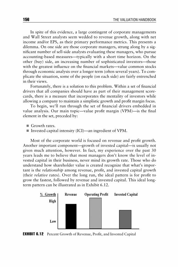
E1C06 09/03/2009 Page 156

In spite of this evidence, a large contingent of corporate managementsand Wall Street analysts seem wedded to revenue growth, along with netincome and/or EPS, as their primary performance metrics. This presents adilemma. On one side are those corporate managers, strung along by a sig-nificant number of sell-side analysts evaluating these managers, who pursueaccounting-based measures—typically with a short time horizon. On theother (buy) side, an increasing number of sophisticated investors—thosewith the greatest influence on the financial markets—value common stocksthrough economic analysis over a longer term (often several years). To com-plicate the situation, some of the people (on each side) are fairly entrenchedin their views.

Fortunately, there is a solution to this problem. Within a set of financialdrivers that all companies should have as part of their management score-cards, there is a measure that incorporates the mentality of investors whileallowing a company to maintain a simplistic growth and profit margin focus.

To begin, we’ll run through the set of financial drivers embedded invalue analysis. Our main topic—value profit margin (VPM)—is the finalelement in the set, preceded by:

& Growth rates.& Invested capital intensity (ICI)—an ingredient of VPM.

Most of the corporate world is focused on revenue and profit growth.Another important component—growth of invested capital—is usually notgiven much attention, however. In fact, my experience over the past 30years leads me to believe that most managers don’t know the level of in-vested capital in their business, never mind its growth rate. Those who dounderstand how shareholder value is created recognize that what’s impor-tant is the relationship among revenue, profit, and invested capital growth(their relative rates). Over the long run, the ideal pattern is for profit togrow the fastest, followed by revenue and invested capital. This ideal long-term pattern can be illustrated as in Exhibit 6.12.

EXHIBIT 6.12 Percent Growth of Revenue, Profit, and Invested Capital


E1C06 09/03/2009 Page 157

The rationale is straightforward. If operating income (profit) growsfaster than revenue, then profit margin will increase. If both revenueand operating profit grow faster than invested capital, then the returnon capital—by any of the well-known calculations—will increase. Asthe previously cited research indicates, higher returns on capital com-bined with revenue growth are usually rewarded in the financial mar-kets through increased measures of performance (e.g., market-to-bookratios). While the pattern illustrated is ideal for the long run, a businessstrategy may dictate a different pattern in the short or near term. Sucha strategy needs to be tested to see when it will produce the optimalpattern. If the recent history of a business produces a different pattern,then management needs to determine when they will get on track withthe optimal pattern.

Growth is an important issue in most firms, and is often overanalyzed.The problem with much of the traditional analysis, however, is that itexcludes or deemphasizes the invested capital element. The type of analysisdiscussed, and illustrated in Exhibit 6.12, is the only one that can translategrowth into shareholder value impact.

Corporate managements need to communicate this message. Lendersand other capital suppliers should understand the performance of their cli-ents. Sophisticated investors look for signals that profit margin expectationswill be at, below, or above historical levels, and estimate the pattern of fu-ture investment—especially as related to the past few years.

The second element in the set of financial drivers—a very useful tool infinancial analysis and planning—is the ratio of invested capital to revenue.This indicator is focused on how much capital is required (or expected) togenerate one dollar (or other currency unit) of revenue. Invested capital in-tensity (ICI) is the inverse of the well-known turnover ratio.

One application is to compare business units of different size on a stan-dard basis. Another is to estimate capital needs for new business ventures,acquisitions, and other corporate development programs. ICI is looked atin the aggregate and also, as appropriate, by discrete categories (e.g., work-ing and fixed capital). As we’ll discuss later, ICI is a key input to the valueprofit margin.

Companies growing by acquisition need to consider goodwill andintangibles in addition to the traditional hard assets, since these items canhave investment and credit rating implications. Obtaining credible ICI indi-cators may involve detailed evaluations. One important element of the anal-ysis is to determine which investments move in a trend line versus a steppattern. Further, a given investment category (such as inventory or physicalplant space) may exhibit different patterns as the business moves along agrowth curve (or alternatively, as it contracts). The insights derived from


E1C06 09/03/2009 Page 158

this type of analysis are helpful in assessing the financial impact of a strategyor an acquisition. Since the more sophisticated investors use ICI, it shouldbe part of management’s tool kit.

Having highlighted growth and balance sheet drivers, we can nowbring them together and provide an earnings performance measure linkedto value creation. This measure is the value profit margin (VPM). Theoverriding thought here is that if operating managers are going to haveprofit targets, let’s give them one or two that correlate to value creation.There is a ‘‘pre’’ and ‘‘post’’ tax profit margin that, for any business, isa minimum requirement for the creation of shareholder value. We incorpo-rate key perspectives from the notion of earning a return on capital thatexceeds the cost of capital in a way that expresses the result in a traditionalprofit margin on sales (revenue). The good news is that it’s not difficultto calculate.

The value profit margin (VPM) is derived by integrating:

& Invested capital intensity (ICI).& Cost of capital (CCAP).& The effective (or cash) tax rate.

Multiplying ICI by the cost of capital (CCAP) and then dividing by 1minus the cash tax rate (some use the expression 1 – T for this rate) pro-duces a pretax operating income (EBIT, EBITA, or EBITDA) margin thatwill sustain the value of the business, but not increase it. On an after-taxbasis, multiplying ICI by CCAP calculates the value net operating profit(NOP) margin. Margins above the VPM level will increase value, whilemargins below this level are destructive. Why? Because margins below theVPM level do not cover the cost of capital employed in the business.

Invested capital intensity has been previously discussed. Cost of capitalis the weighted (or blended) cost of debt and equity, the basis for the capitalcharge in economic profit measures. Think of CCAP as the average annualrate of return that you, as an investor, would expect to earn on capital youprovided to a business or invested into a portfolio of common stocks, mu-tual funds, and bonds. Cash tax rates incorporate deferrals and may differfrom accounting (book) provisions found on the income statement. Mostpublic companies disclose this effective cash tax rate in the footnotes totheir financial statements in 10-K and annual reports. Some analysis may beinvolved in calculating these capital cost and tax rates, a normal part of anyvalue-based approach to planning and performance review.

The following table—incorporating data presented earlier in the seg-ment on valuation perspectives (EP and MVA) and referred to in the discus-sion of the magnifier—establishes a framework that allows us to work


E1C06 09/03/2009 Page 159

through the individual financial drivers and then arrive at the value profitmargin (VPM):


Revenue (Sales) $1,000 $1,000 $1,000Net Operating Profit (NOP)$ $ 100 $ 100 $ 100% 10% 10% 10%Invested Capital (IC) $ 600 $ 800 $1,000Cost of Capital (CCAP) 12% 12% 12%

NOP (from above) $ 100 $ 100 $ 100Capital Charge (CCAP) (72) (96) (120)Economic Profit (EP) $ 28 $ 4 $ (20)

To reiterate what was stated in an earlier segment, economic profit(EP) is a concept from basic economics taught in college. EP is whatany business owner (shareholder) should be concerned with, since ittakes into account the cost of all the capital invested in the business.EP is the residual (what’s left over) after all the costs of running a busi-ness have been accounted for and the suppliers of capital have beenprovided with a fair return on their investment. A problem withaccounting profit—most commonly expressed as net income or earningsper share (EPS)—is that it includes only a charge for debt financing;thus, it misses a cost for equity capital, the most expensive and preva-lent form of capital for a typical industrial company. The cost of equitycapital is what a common shareholder expects to earn annually as arate of return on investment. The cost of equity capital formula adds apremium to the current return on a long-term risk-free (or close to risk-free) security, such as a 10-year U.S. government bond.

Because of this condition and another important one—the gap betweenaccounting profit and cash flow—there is virtually no correlation betweennet income and/or EPS growth and key stock market indicators, as illus-trated in Exhibit 6.10.

The preceding information can be used to delve into the key financialdrivers.

It’s important in any business to get a handle on invested capital inten-sity (ICI). Using the numbers shown in the following table (for the A, B, andC firms), we can see the differences in the amount of fuel needed to maintainand drive the businesses forward:


E1C06 09/03/2009 Page 160


Revenue (Sales) $1,000 $1,000 $1,000Invested Capital (IC) $ 600 $ 800 $1,000Invested CapitalIntensity (ICI)�

$ 0.60 $ 0.80 $ 1.00

�ICI is expressed as cents per dollar; in this case, cents per sales dollar.

This analysis yields an important dynamic regarding the value-creatingperformance for these three companies, which is that Company A requiresthe least amount of capital and Company C needs the most. This knowledgeis useful in this example, and essential when we’re dealing with businessesof different sizes, since it is sometimes the only way we can make compari-sons and arrive at meaningful perceptions about the use of capital. So, allthings being equal, Company C needs to produce a higher profit margin ver-sus both Company A and Company B to generate the same return on capi-tal. As illustrated next, this is not the case and results in Company Cproducing an unacceptable return on invested capital—resulting in negativeEP—and, thus, being classified as a value destroyer.

Now, let’s see how we get to the same conclusion using the value profitmargin (VPM) technique, beginning with a summary of its definition andusefulness.

Value Profit Margin (VPM)

& What is it?& A minimum profit margin—in essence, a beginning point for value

creation.& A pre- and/or posttax financial performance benchmark.

& Why use it?& Allows for profitability comparisons for businesses of different sizes.& Is simple to calculate and easy to communicate, especially to operat-

ing managers.& Provides managers with a threshold; generating a positive spread cre-

ates shareholder value.& Is effective for planning—strategies, acquisitions, major investments.& Provides an earnings measure linked to value creation.

We can refer back to Company A in the economic profit example earlierin this chapter to illustrate the derivation of the value profit margin. Thecalculations are:


E1C06 09/03/2009 Page 161

& Pretax basis: Multiply ICI by CCAP; then divide by 1 minus the effec-tive tax rate.

& After-tax basis: Multiply ICI by CCAP.

Example—Company A

Revenue (Sales) ¼ $1,000

IC ¼ $600 (ICI ¼ $.60)

CCAP ¼ 12%

Effective tax rate ¼ 30%

& VPM: Pretax basis:.60 � 12% ¼ 7.2%/70% ¼ 10.3%

& VPM: After-tax basis:.60 � 12% ¼ 7.2% (vs. actual NOP ¼ 10.0%)

Multiplying ICI by the cost of capital and then dividing by 1 minus thecash tax rate produces an operating income (EBIT, EBITA, or EBITDA)margin that will sustain the value of the business. On an after-tax basis,multiplying ICI by CCAP calculates the value profit margin on a net operat-ing profit basis. Margins above the VPM will increase value, while marginsbelow this level are destructive. Why? Because margins above VPM beatCCAP, while those below VPM do not cover the cost for the capitalemployed in the business. Profit margins at the VPM level maintain the cur-rent level of shareholder value.

Invested capital intensity has been discussed. Cost of capital is theweighted (or blended) cost of debt and equity, the basis for the capital chargein the economic profit (EP) measures. ‘‘Cash’’ tax rates incorporate deferralsand, as we have noted, may differ from accounting (‘‘book’’) provisions.

There is a direct connection of VPM to EP which makes this measureparticularly useful. Referring back to Exhibit 6.5, notice that EP for‘‘Company A’’ is $28 million . . . derived as NOP of $100 million minusCCAP of $72 million. If we compare the VPM for ‘‘Company A’’ (7.2 per-cent) with the actual NOP margin (10.0 percent), a positive spread of 2.8percentage points is the result. Multiplying the 2.8 percentage points spreadby the $100 million revenue for ‘‘Company A’’ equals $28 million of EP –the same result as when calculated under the traditional method.

We can make the same calculation for ‘‘Company C’’. Under the tradi-tional EP calculation, NOP of $100 million minus CCAP of $120 millionyields a negative ($20) million. VPM for ‘‘Company C’’ is calculated asfollows:


E1C06 09/03/2009 Page 162

Example—Company C

Revenue (Sales) ¼ $1,000

IC ¼ $1,000 (ICI ¼ $1.00)

CCAP ¼ 12%

Effective tax rate ¼ 30%

& VPM: Pretax basis:1.00 � 12% ¼ 12.0%/70% ¼ 17.1%

& VPM: After-tax basis:1.00 � 12% ¼ 12.0% (vs. actual NOP ¼ 10.0%)Spread: 10.0% actual minus 12.0% VPM ¼ (2.0)% (negative)

& EP: $100 million revenue times (2.0)% ¼ $(20) million (negative)

This connection is very important, since it demonstrates the value-driven nature of this metric, and enables us to construct an earnings type ofmeasure that is linked to shareholder value creation. This should be an op-erating manager’s dream—a P&L metric that’s basically a percent-to-salesratio—with key drivers of value creation supporting and standing behind it.

The value profit margin (VPM) is thus one of the most powerful, yet sim-ple, measures for management focus and communication to investors. WhenVPM is combined with growth, we have the key ingredients of a value-drivenmeasurement system for almost any business. Further, we can work within theP&L (i.e., the earnings framework that people seem fixated on) despite all theevidence (cited earlier) about little or no correlation to stock market value.

To conclude, VPM is the P&L (earnings) measure indicating share-holder value creation or destruction. In fact, it is the only P&L metric witha direct link to value creation! The benefit of developing the VPM input andimplementing the technique is well worth the effort, since no other P&Lmetric has such a direct link to shareholder value.

VALUE ANALYS I S : TH E PROPER FOCUS

The final segment explores the unfortunate fact that, in the world of corpo-rate finance, few activities are more entrenched than capital project evalua-tions. This focus on individual projects often comes at the expense ofidentifying and analyzing major programs, the building blocks of a strategy.Valuing the strategy itself, the ultimate indicator of future business success,can also be overlooked in the pursuit of net present value (NPV) or internalrate of return (IRR) calculations for individual investments. Project evalua-tion keeps countless financial analysts hard at work (I have memories of my


E1C06 09/03/2009 Page 163

early years in finance) and consumes a significant amount of time for corpo-rate managers and directors—much of which is nonproductive. Taken to anextreme, bad decisions can result.

A review of project analysis and what it accomplishes, in light of what’sreally going on in any business, can be revealing. In this appraisal, we need tobe willing to raise some candid questions about certain traditions in finance.

Do we really need to be assured that, say, a $750,000 machining centerfor a $3 billion (in sales) manufacturing company is economically viable?Or that a $300,000 computer-aided design/manufacturing (CAD/CAM)system for the engineering department will have a payoff? When such smallinvestments are put in their proper context, capital project evaluations canappear virtually meaningless—as, in reality, they usually are.

Is this an exaggerated claim? Let’s assume that our $3 billion companyhas three business units (BUs), each with approximately $1 billion of sales.Further, assume that the machining center and CAD/CAM projects are inBU 1, which has a strategy of growing at 15 percent per year and offering acombination of high product quality and competitive cost. BU 1, therefore,plans to grow sales by approximately $150 million next year. Its currentyear balance sheet reflects the following for fixed assets:

Gross fixed assets $300 millionAccumulated depreciation ($100) millionNet fixed assets $200 million

Comparing the gross fixed assets (GFA) and net fixed assets (NFA)amounts to sales, we can calculate the following ratios:

GFA: $300 million (assets) divided by $1 billion (sales) equals $0.30, or30 percent.

NFA: $200 million (assets) divided by $1 billion (sales) equals $0.20, or20 percent.

The GFA and NFA ratios reflect capital intensity—that is, how muchcapital is required to generate each dollar of sales. If we determine that thegrowth strategy will be in line with past experience, then BU 1 will need toinvest about $45 million next year—30 percent of its new sales. After depre-ciation, the net new investment will be approximately $30 million (20 per-cent of $150 million) if the strategy replicates recent investment patterns.

Even if the strategy can leverage the existing assets and require less newcapital, on a relative basis, we’re still dealing with annual investments of


E1C06 09/03/2009 Page 164

many millions of dollars to support the strategy. Since strategies usually re-quire more than one year to execute, the aggregate amount of new capitalover the next few years, necessary for BU 1 to grow and prosper, could be$100 million or more.

So what is the point of financially justifying the investment in themachining center or the CAD/CAM system? Why drive people crazy by re-quiring elaborate evaluations on relatively small projects that have no pur-pose or life of their own, and are only pieces of a much larger puzzle?

The job of management is to put the puzzle together, not to place eachpiece under a microscope. I’d be willing to bet that many companies per-forming extensive capital project evaluations have not quantified the share-holder value impact (that is, the NPV/IRR) of their overall strategy. The keypoints are: If a strategy has value, then the individual projects should havevalue, since they are part of the strategy; and further, these projects cannot,and should not, be separated out for purposes of analysis.

The purpose of value-based analysis, regardless of which metric youprefer (since they are all extensions of NPV/IRR), is to determine value cre-ation at appropriate levels in the business hierarchy—the company, businessunit, strategy, and major program. The major program (for example, an im-portant operational or strategic initiative) is the absolute lowest level forwhich value-based analysis should be performed.

The strategy for BU 1 may encompass growth via high quality andcompetitive cost. A supporting program might be one to enhance productquality and, at the same time, contain or reduce costs. This type of initia-tive would seem logical; in fact, it may be an essential program. Let’s as-sume that this program encompasses 10 machining centers averaging $1million each plus a CAD/CAM system. At this level, value analysis can bemeaningful, as it may well represent a building block of the strategy oroperating plan, or both. As we present a numerical example, we will high-light the impact of focusing on the program versus the 10 individualmachining center projects. It is my belief that too many companies stillconcentrate on the individual investments, rather than grasping a larger,and more important, link of value to either a strategic or an operationalobjective. Accepting or rejecting investments are big decisions involvinglarge sums of money.

A walk through the numbers can demonstrate the valuation hierarchy.Let’s start with the project. Assume that the $750,000 machining center,mentioned earlier, reduces cost, but does not have the throughput capabilityto increase sales beyond the current level. Therefore, this project is pre-sented as a classic cost-reduction investment. Due to this myopic perspec-tive, we miss the point that the strategy is for growth, through enhancedproduct quality features, along with competitive cost. Exhibit 6.13


E1C06 09/03/2009 Page 165

EXHIBIT6.13

Pro

ject

Analy

sis

Investin

a$750,000N/C

Machine

Centerto

SaveCosts($000sOmitted)

Rates/Factors

Year1

Year2

Year3

Year4

Year5

Capit

alIn

ves

tmen

t(o

utl

ay)

$(7

50)

AnnualC

ost

Savin

gs

(pre

tax)

$150

200

200

200

200

Taxes

@C

orp

ora

teT

ax

Rate

¼33%

$(5

0)

(67)

(67)

(67)

(67)

Tax

Shie

ldre

:D

epre

ciati

on:

AnnualD

epre

ciati

on—

Lif

e(y

ears

)¼

10

$75

75

75

75

75

Tax

Shie

ld@

Rate

¼33%

$25

25

25

25

25

Fre

eC

ash

Flo

w/P

rofit

Aft

erT

ax

(FC

F/P

AT

)$(6

25)

158

158

158

158

Rates/Factors

Year6

Year7

Year8

Year9

Year10

AnnualC

ost

Savin

gs

(pre

tax)

$200

200

200

200

200

Taxes

@C

orp

.T

ax

Rate

¼33%

$(6

7)

(67)

(67)

(67)

(67)

Tax

Shie

ldre

:D

epre

ciati

on:

AnnualD

epre

ciati

on—

Lif

e(y

ears

)¼

10

$75

75

75

75

75

Tax

Shie

ld@

Rate

¼33%

$25

25

25

25

25

Fre

eC

ash

Flo

w/P

rofit

Aft

erT

ax

(FC

F/P

AT

)$

158

158

158

158

158

Cost

of

Capit

al(C

CA

P)¼

11%

..

.W

eighte

dco

stof

equit

yand

deb

t

Net

PresentValueof10-yearFCF/PAT

�InitialCashOutlay

$227

Internal

RateofReturn

(IRR)

21%

165

E1C06 09/03/2009 Page 166

illustrates a typical cost savings analysis to justify spending $750,000. If wetake this approach to a ridiculous extreme, we could conceivably have 10separate evaluations, some growth, some cost reduction, and some maybecombining the two. What a potential nightmare! For some companies,though, this is their analytic world.

Oh, good, we have a winner—at least by some standards. We have pro-duced an analysis that yields a positive net present value (NPV) and a stronginternal rate of return (IRR). So what? How can anyone seriously getexcited by an NPV of $227,000 in a billion-dollar business? Is this what wewant management and the board to concentrate on? Or is there somethingmore important, in terms of achieving the primary goal of any for-profitenterprise—that is, to execute the strategy in order to maximize the value ofthe total investment that shareholders have made, and will continue tomake, in the business? By the way, in one recent research study of institu-tional investors, strategy execution was one of the most important factorsin their investment decision for a particular company; and strategy execu-tion is two levels above project returns.

When we elevate our analysis to the program level, we can start tograsp the strategy for this business. The capital investment program alludedto in a previous paragraph is illustrated in Exhibit 6.14.

The highlights of this program are:

& Ten machining centers are to be purchased over a two-year investmentperiod.

& The average investment per machine is $1 million.& The machining centers have an average useful life of 10 years.& CAD/CAM systems are to be purchased in years 1 and 6, noting that

these systems have a useful life of five years. The first CAD/CAM costs$300,000, and the second is estimated to cost $500,000 in year 6.

& The investment program generates cost savings plus the capability toproduce new sales, albeit at a lower throughput ratio. BU 1 gener-ates about $3 of sales for each $1 of gross fixed asset. This equip-ment reduces manufacturing cost and generates 50 percent of theoverall asset base throughput ratio—or $1.50 of sales for each $1 ofnew capital.

Is there any question as to what is the more relevant message for seniormanagement and the board—the program value of $5.3 million or the proj-ect value of $227,000? The project is narrow in scope and presents only avery limited perspective of the goals for the business. The program getscloser to the strategic intent for the business.


E1C06 09/03/2009 Page 167

EXHIBIT6.14

Pro

gra

mA

naly

sis

Investin

a$10.8

MillionCostSavings/Quality

Program

($000sOmitted)

Rates/Factors

Year1

Year2

Year3

Year4

Year5

Aver

age

Cost

per

N/C

Mach

ine

Cen

ter

$1,0

00

1,0

00

1,0

00

1,0

00

1,0

00

Num

ber

of

N/C

Mach

ine

Cen

ters

55

——

—T

ota

lC

apit

alIn

ves

tmen

t(o

utl

ay)

Incl

udin

g1

CA

D/C

AM

inY

ear

1$

(5,3

00)

(5,0

00)

——

—

Incr

emen

talSale

s@

per

Mach

ine¼

$1,5

00

$—

7,5

00

15,0

00

15,0

00

15,0

00

Incr

emen

talPro

fit

@M

arg

in¼

12%

$—

900

1,8

00

1,8

00

1,8

00

Cost

Savin

gs

(use

per

-mach

ine

impact

from

Exhib

it6.1

3)

$750

1,7

50

2,0

00

2,0

00

2,0

00

Tota

lPro

fit

Impact

$750

2,6

50

3,8

00

3,8

00

3,8

00

Dep

reci

ati

on—

N/C

Mach

ines

10

$(5

00)

(1,0

00)

(1,0

00)

(1,0

00)

(1,0

00)

(#yea

rs)

CA

D/C

AM

5$

(60)

(60)

(60)

(60)

(60)

Net

Taxes

@R

ate

¼33%

$(6

3)

(529)

(912)

(912)

(912)

Fre

eC

ash

Flo

w/P

rofit

Aft

erT

ax

(FC

F/P

AT

)$

(4,6

13)

(2,8

79)

2,8

88

2,8

88

2,8

88

Year6

Year7

Year8

Year9

Year10

Fre

eC

ash

Flo

w/P

rofit

Aft

erT

ax

(FC

F/P

AT

)Y

ear

5Ste

ady

Sta

te$

2,8

88

2,8

88

2,8

88

2,8

88

2,8

88

Adju

sted

for

Add’l

CA

D/C

AM

inY

ear

6$

(500)

Fre

eC

ash

Flo

w/P

rofit

Aft

erT

ax

(FC

F/P

AT

)$

2,3

88

2,8

88

2,8

88

2,8

88

2,8

88

Net

PresentValueof10-yearFCF/PAT

Net

ofInitialCashOutlay

s$5,3

00

Internal

RateofReturn

(IRR)

28%

167

E1C06 09/03/2009 Page 168

To appreciate the real value potential for the business, the analysishas to be elevated to a higher level—that of the business strategy itself.This evaluation level is one of the most productive (also, one of themost difficult) for management to work through, because it forces man-agers to think about their most critical financial drivers and rationalizewhy they will stay the same or change based on the strategy. Thesedrivers help determine the value potential for the strategy and, ulti-mately, the entire business.

Exhibit 6.15 gives an example of the financial expectation for BU 1’sstrategy. It assumes that:

& The business will grow by 15 percent annually for the next four years,maintaining its recent operating profit margin of 12 percent.

& The historical capital intensity ratio will be reduced, from $0.30 grossand $0.20 net to $0.27 and $0.17, respectively, as a ratio to sales, dueto the ability to leverage prior years’ investment in plant and equipment.

& Detailed assumptions for pricing and cost structure are assumed to beembedded in the summary results presented in Exhibit 6.15.

If you add up the net new fixed capital investments (this is after depreci-ation) anticipated for the next four years to execute the strategy, you willcalculate an amount of slightly over $125 million. How can anyone focustheir attention on analyzing each $1 million project when the businessunit may need to invest $125 million (net) over the next four years? That’snot to say we shouldn’t control the expenditures for capital projects, butwe need to move away from evaluating them, because they do not providea meaningful basis or perspective for value analysis. Control systems can,and should be, detailed and specific, but evaluation systems need to befocused at a higher level. To repeat, the major program is the lowest levelfor value analysis.

Look at what we miss if our attention is at the project versus theprogram or strategy level. BU 1 appears to have a strategy with a verystrong value-creating potential, to the tune of over $40 million NPVand total business return (similar to IRR) of nearly 25 percent. And weshould be losing sleep over a $750,000 machining center to help exe-cute a major cost-containment objective? Can you imagine going to theboard with the capital project and not presenting the value analysis forthe strategy? Management needs to know what the strategy is contribu-ting to the overall value (stock price) of the enterprise, and then whatthe key building blocks (programs) of the strategy are. Major programsare necessary to ensure that the strategy has substance. They also pro-vide a mechanism to prioritize investments and track progress toward


E1C06 09/03/2009 Page 169

EXHIBIT6.15

Str

ate

gy

Analy

sis

Enhance

Product

Quality

andControl

Coststo

Grow

SalesandM

aintain

Margins

($M

illionsOmitted,ExceptRatios)

Rates/Factors;

Also,Base

#’s

Year1

Year2

Year3

Year4

Residual

Sale

s—T

ota

l1,0

00

$1,1

50

1,3

23

1,5

21

1,7

49

New

Sale

s@

AnnualG

row

th¼

15%

$150

323

521

749

New

Oper

ati

ng

Pro

fit

(pre

tax)

120

$18

39

63

90

@O

PM

arg

in¼

12%

New

Taxes

@R

ate

¼33%

$(6

)(1

3)

(21)

(30)

New

Net

Oper

ati

ng

Pro

fit

(NO

P)

$12

26

42

60

254

Net

New

Fix

edIn

ves

tmen

t@

Capit

alIn

tensi

tyR

ati

o¼

$0.1

7$

(26)

(29)

(34)

(39)

New

Work

ing

Capit

al@

Rati

o¼

$0.2

0$

(30)

(35)

(40)

(46)

Fre

eC

ash

Flo

wfo

rth

eStr

ate

gy

$(4

3)

(38)

(32)

(24)

254

Net

PresentValueof4-YearFCF

plusResidual

Value

$41

Thestrategy

has

apresentva

lueof$40+million,

assumingaresidual

that

continues

year

3NOPfor6

more

years(10-yeartotaltimefram

eforan

alysis).

TotalBusinessReturn

(TBR)

24%

Equivalentto

IRRforthestrategy

169

E1C06 09/03/2009 Page 170

achieving key success elements of a strategy. Projects are a basis forcash control, but provide no foundation for meaningful analysis. Fur-ther, project analysis can actually confuse people as to what isreally going on in the business. Therefore, project evaluations should bescrapped and replaced with value analysis focused at the level wherevalue creation occurs!

A quote from one of the most respected experts on corporate man-agement in the twentieth century will help to drive home the point.Many readers have heard of Peter Drucker. This quote is from one ofhis books.

There is one fundamental insight underlying all management sci-ence. It is that the business enterprise is a system of the highest or-der. And one thing characterizes all genuine systems, whether theybe mechanical like the control of a missile, biological like a tree, orsocial like the business enterprise: it is interdependence. The wholeof a system is not necessarily improved if one particular function orpart is improved or made more efficient. In fact, the system maywell be damaged thereby, or even destroyed. In some cases, thebest way to strengthen the system may be to weaken a part—tomake it less precise or less efficient. For what matters in any systemis the performance of the whole; this is the result of growth anddynamic balance, adjustment and integration rather than of meretechnical efficiency.1

Drucker talks about ‘‘interdependence’’ and ‘‘performance of thewhole’’ as key to the functioning of any system. Since financial approachesneed to support a company’s overall business system, it is hoped that we cancome to grips with the notion that financial evaluations have to be done at alevel that encompasses the important interdependencies that exist in a busi-ness. Think of Drucker’s comment about the ‘‘performance of the whole’’ asit might be applied to shareholder value of the whole, in terms of whatneeds to be accomplished with value-based analysis and performance. Thekey message here is that managers can do a great job of selecting an overallmetric such as EP and all the supporting financial drivers—and then botchthe implementation through misapplication. Value analysis must be per-formed in a logical hierarchy that fits with the way that value is actuallycreated in a business.

We conclude with a summary of which metric(s) to apply at the variouslevels in the hierarchy.


E1C06 09/03/2009 Page 171

Value-Based Analysis Valuation Hierarchy

Total company/operating units/strategic business units

Full value analysis: EP� and MVAy

Analysis over time Financial drivers��

Business strategies MVAy and financial drivers��

Annual operating plans EP� and financial drivers��

Major programs/strategic MVAy (linked to a strategy, over anappropriate life cycle)

Major programs/operational Financial drivers��

Capital projects No value analysis; focus is on controlof appropriations and/orexpenditures, part of a program

�EP—Economic profit (similar to economic value added): focus on historical versusfuture patterns and progression.yMVA—Market value added (similar to shareholder value creation): focus on anappropriate future growth time horizon.��Financial drivers—Support (underlying) metrics for EP and MVA.

NOTE

1. Peter F. Drucker, Management: Tasks, Responsibilities, Practices (New York:Harper & Row, 1974), 508.


E1C07 08/14/2009 Page 172

CHAPTER 7Residual Income and Stock

Valuation TechniquesDoes It Matter Which One You Use?

Benton E. GupChair of Banking, University of Alabama

Gary K. TaylorAssociate Professor, University of Alabama

Common stockholders are the residual claimants of corporations. It fol-lows that whatever cash flows remain after creditors have been paid are

residual cash flows.1 In essence, all discounted cash flow (including divi-dends) stock valuation models could be considered residual income valua-tion models. However, advocates of economic value added (EVA), residualincome (RI), and abnormal earnings growth (AEG) valuation methods havea specific definition in mind when using the term residual income. For thesethree models, RI represents earnings above or below normal earnings. Nor-mal earnings are those earnings generated by multiplying the required rateof return by the book value of equity.2

All three of these valuation techniques are used on Wall Street andtaught in business schools. By way of illustration, consider Stowe et al.,Analysis of Equity Investments: Valuation (2002). The chapter on residualincome valuation states that EVA is a commercial implementation of theresidual income ‘‘concept.’’ Similarly, Hirst and Hopkins, in Earnings:Measurement, Disclosure, and the Impact on Equity Valuation (2000),show that EVA is a specific version of the RI valuation model. However,EVA, RI, and AEG methods of valuation are quite different in their imple-mentation. This chapter clarifies the differences in the use of residual

172

E1C07 08/14/2009 Page 173

income in the EVA, RI, and AEG methods of valuation. It also calculatesintrinsic value using the residual income and abnormal earnings growthvaluation models.

The remainder of this chapter is divided into four parts. The first threeexamine the EVA, RI, and AEG methods, respectively. The last sectionprovides a numerical example of the RI and AEG method of determiningintrinsic value.

ECONOM IC VALUE ADDED ( EVA )

EVA is trademarked by Stern Stewart & Company. Joel Stern (1998, xi)and G. Bennett Stewart (1991, 742) state that EVA is the residual incomethat remains after operating profits cover the cost of capital. Stern explainsthat for debt and equity investors to earn an adequate rate of return, thereturn must be large enough to compensate them for risk. If the residualincome (i.e., EVA) is zero, a firm’s operating return is just equal to the re-turn that investors require for the risk they are taking. Thus, EVA is definedby Stewart (1991) and Ehrbar (1998) as:

EVA ¼ NOPAT � C%(TC)

where NOPAT ¼ net operating profits after taxesC% ¼ cost of capitalTC ¼ total capital

Based on the EVA model, the value of a firm is equal to the valueof its total capital plus the sum of the present value of its projectedEVA.3 Thus, there are three inputs into the EVA model: total capital,net operating profits after taxes, and the cost of capital. The true costof capital is unobservable but can be estimated from observable data.Stewart (1991, 744) defines TC as total assets less non-interest-bearingcurrent liabilities. However, Stewart suggests the following three adjust-ments to capital in order to undo the accounting and arrive at a truelevel of capital: (1) subtract marketable securities; (2) increase property,plant, and equipment by the present value of noncapitalized leases; and(3) increase assets by certain accounting reserves, such as allowancefor bad debts, last in, first out (LIFO) reserve, and capitalization ofresearch and development expense. Adjusting TC also requires adjust-ments to NOPAT. For example, Goldman, Sachs & Company (1997) sug-gests several adjustments to reported accounting numbers when usingEVA. The primary purpose of these adjustments is to calculate a true TCand NOPAT.

Residual Income and Stock Valuation Techniques 173

E1C07 08/14/2009 Page 174

Such adjustments to capital and NOPAT require a sophisticatedknowledge of accounting rules and procedures in order to performthe necessary adjustments. For example, if not done correctly, theseadjustments may eliminate the self-correcting nature of accounting,thereby eliminating one of the advantages of these valuation models.In all three models, overestimating the value of equity causes an over-estimation of normal earnings, causing a simultaneous reduction inresidual earnings.

RES I DUAL INCOME METHOD OF VALUAT I ON

Hirst and Hopkins (2000) highlight the benefits of using the RI model, pri-marily that the RI model is derived from the discounted dividend model andthat the model focuses on the creation of value rather than the distributionof value (as in the discounted dividend model). Focusing on the creation ofvalue allows for the RI model to be used as a valuation model and as a toolfor determining where business growth will come from and its sustainabilityvia DuPont analysis.4

The RI model assumes that future earnings belong to the current share-holders. However, Ohlson (2003) notes that stock options and share buy-backs may undermine that assumption.

Penman (2004) shows how the RI model can be used for a parsimo-nious valuation model. The RI model estimates the intrinsic value ofstock by using both the current-period book value of equity on the bal-ance sheet and forecasted earnings. In the RI model, the total equity ofthe firm is a function of the book value of equity and the sum of thepresent value of residual income. Residual income is the difference be-tween forecasted accounting earnings and normal earnings. Normalearnings are calculated from the book value of equity at the beginning ofthe period and the cost of capital. Thus, two of the three inputs to the RImodel are observable (again, the firm’s true cost of equity capital is un-observable but can be estimated by the analyst) and do not require arbi-trary adjustments by the analyst.

Formally, residual income is defined as the accounting earnings abovenormal earnings. Normal earnings are the earnings that would be earnedgiven the cost of capital and beginning-of-the-period book value of equity;and the number is calculated by multiplying the book value of equity at thebeginning of the period (Bt�1) by the firm’s cost of equity capital (Ce). Theresidual income for period t is (FEPSt � Ce Bt�1), where FEPSt is the fore-casted earnings for period t. An important assumption in the RI model isclean surplus accounting.


E1C07 08/14/2009 Page 175

The mathematical relationship between the price of a share of stock,forecasted earnings, and book value is:

V0 ¼ B0 þX

1 þ Ceð Þ�t FEPSt � Ce Bt�1ð Þ� �

where V0 ¼ current intrinsic value of a share of stockB0 ¼ book value of a share of stockCe¼ cost of equity capital

FEPS¼ forecasted earnings per share

As seen by the formulations, the EVA and RI models are similar. In fact,the EVA model is a special case of the more general RI model. Both modelshave an anchor, total capital in the EVA model and the book value of equityin the RI model. Both models have a residual income component—that is,earnings above what should have been earned by the firm given the bookvalue of equity (total capital in the EVA model) and the cost of capital. Thedifference between the two models rests in the book value and earnings thatare used. The EVA model takes reported accounting numbers and makesseveral adjustments. These adjustments are based on assumptions made byanalysts from reading the financial statements. In essence, the EVA model istrying to undo parts of the accrual accounting process. This then forces theanalyst to impose subjective assumptions onto the valuation model. In con-trast, the RI model starts with the accounting numbers and recognizes thatif the book value of equity is under- or overstated (relative to a true value ofequity, which is what the EVA model attempts to calculate) this period,then, due to the nature of double-entry accounting, future earnings will beover- or understated relative to true earnings. This relationship betweenbook and earnings eliminates the effects of conservative or aggressiveaccounting on firm valuation as long as forecasted earnings are consistentwith the firm’s accounting choices.

In other words, the RI model utilizes double-entry accounting to ad-dress the measurement error associated with the conservative accountingprocess rather than forcing analysts to undo the effects of the selectedaccounting policies. Using the RI model allows analysts to focus on predict-ing future patterns of earnings rather than trying to identify how accountingmethod selection affects the components of future earnings and the currentbook value of equity.

ABNORMAL EARN INGS GROWTH MODEL

The abnormal earnings growth (AEG) model is another accounting-basedvaluation model. The AEG model utilizes capitalized forward earnings as


E1C07 08/14/2009 Page 176

the valuation anchor instead of the book value of equity that is used in theRI model.

V0 ¼ 1=Cð Þ FEPS1 þX

1 þ Cð Þ�t G� Cð Þ � FEPSt�1

h i

where V0 ¼ current intrinsic value of a share of stockC¼ cost of capital

FEPS¼ forecasted earnings per shareG¼ cum-dividend earnings growth rate

The phrase (G � C) � FEPSt�1 represents abnormal earnings growth,which is the growth in accounting earnings above the cost of capital. In theAEG model, normal earnings represent the earnings growth at the cost ofcapital. There is no abnormal earnings growth if G is equal to the cost ofcapital. Similar to the RI model, the addition of value comes only from earn-ings above normal earnings. Also similar to the RI model, the AEG modelallows the analyst to use forecasted earnings rather than an analyst-adjustedearnings number, and focusing on forecasted earnings rather than the indi-vidual adjustments to earnings allows the analyst to focus on the growth ofearnings. Penman (2004) shows that the RI and AEG models will give thesame valuations as long as the inputs (book value of equity, earnings, anddividends) are the same. While the AEG valuation model will yield the samevaluations as the RI model, it does not readily lend itself to the financialstatement (DuPont) analysis and determination of the creation of firm value.

NUMER ICAL EXAMPLE OF R I AND AEG

In this section we calculate Wal-Mart’s intrinsic value as of January 1986using both the RI and AEG valuation models.5 Wal-Mart is widely used asan example, and has been used extensively in Penman (2004). We assumedthat net income is identically equal to comprehensive income, and that real-ized net income and dividends are identically equal to forecasted net incomeand dividends. Book value of equity is calculated as the book value of equityat the beginning of the period plus forecasted net income less dividends.Normal earnings are calculated as the cost of capital multiplied by the be-ginning-of-the-period book value of equity, while residual earnings are thedifference between forecasted earnings per share and normal earnings pershare. For simplicity we assume that 2002 forecasted earnings will be a per-petuity (see Exhibit 7.1).6

Based on this information, Wal-Mart’s intrinsic value per share of$5.80 is calculated as the sum of beginning-of-the-period book value of


E1C07 08/14/2009 Page 177

EXHIBIT7.1

Wal-

Mart

Calc

ula

tion

of

Com

ponen

tsof

Res

idualIn

com

eM

odel

EarningsandDividendForecast($)

1987

1988

1989

1990

1991

1992

1993

1994

1995

1996

1997

1998

1999

2000

2001

2002

Earn

ings

per

Share

0.2

70.3

60.4

70.5

60.7

00.8

71.0

11.1

71.1

91.3

31.5

31.9

32.3

42.7

42.9

0

Div

iden

ds

per

Share

0.0

30.0

40.0

50.0

70.0

80.1

00.1

30.1

70.2

00.2

10.2

70.3

00.3

90.4

70.5

4

Book

Valu

eof

Equit

yper

Shar

e0.7

30.9

71.2

91.7

12.2

02.8

23.5

94.4

75.4

76.4

67.5

88.8

410.4

712.4

214.6

917.0

5

Norm

alE

arn

ings

0.0

90.1

20.1

50.2

10.2

60.3

40.4

30.5

40.6

60.7

80.9

11.0

61.2

61.4

91.7

6

Res

idualE

arn

ings

0.1

80.2

40.3

20.3

50.4

40.5

30.5

80.6

30.5

30.5

50.6

20.8

71.0

81.2

51.1

4

Dis

count

Fact

or

1.1

21.2

54

1.4

05

1.5

74

1.7

62

1.9

74

2.2

11

2.4

76

2.7

73

3.1

06

3.4

79

3.9

04.3

63

4.8

87

5.4

74

Pre

sent

Valu

eof

Res

idualIn

com

e

0.1

60.1

90.2

20.2

30.2

50.2

70.2

60.2

60.1

90.1

80.1

80.2

20.2

50.2

60.2

1

177

E1C07 08/14/2009 Page 178

equity ($0.73), the sum of the present value of residual income ($3.33), andthe present value of the continuing value: [($1.14/0.12)/5.474] = $1.74.7

Exhibit 7.2 provides the inputs for calculating Wal-Mart’s intrinsicvalue using the AEG model. In this example, we assume that abnormalearnings growth will be zero after 2002. The intrinsic value based on theAEG valuation model is $5.87.8 Cum-dividend earnings are defined as earn-ings after reinvesting the previous period’s dividends. In the AEG model,normal earnings are defined as the previous period’s earnings growing atthe cost of capital. Abnormal earnings growth is the difference betweencum-dividend earnings and normal earnings.

As seen in Penman (2004), the RI valuation model allows analysts toforecast those investing activities that will generate value. The AEG valua-tion model does not lend itself to this type of analysis. However, the AEGvaluation model embodies the notion that a firm’s intrinsic value is derivedfrom its earnings.

The three models are compared in Exhibit 7.3. As discussed previously,EVA, RI, and AEG valuation models are all derived from the discountedcash flow (including dividends) model. EVA is the residual income modelwith adjustments to undo the conservative accounting policies of GAAP.The RI model relies on double-entry accounting to adjust for the effect ofaccounting policies on the reported and forecasted numbers. In other words,if the book value of equity is understated this period relative to a true bookvalue of equity (i.e., not enough earnings have been recorded in previous pe-riods), then forecasted earnings will be higher than true earnings. The AEGmodel is closer to the concepts discussed on Wall Street, such as the P/Eratio. All three valuation models have an anchor (book value of equity ortotal capital as in the RI and EVA valuation models, and capitalized earningsin the AEG valuation model) and a residual income component (forecastedearnings above normal earnings). The RI and EVA valuation models allowfor financial statement (DuPont) analysis to determine where future growthwill arise. The AEG model does not permit this type of analysis.

CONCLUS I ON

Every stock valuation model that employs discounted cash flows can beconsidered a residual income model. The EVA model includes analystassumptions about the book value of equity and future earnings that maynot coincide with clean surplus accounting. This process requires analyststo undo the accounting and maintain the clean surplus relationship. In con-trast to the EVA model, the RI and AEG models utilize observables (currentperiod book value per share, dividends, and forecasted earnings) and allow


E1C07 08/14/2009 Page 179

EXHIBIT7.2

Wal-

Mart

Calc

ula

tion

of

Com

ponen

tsof

Abnorm

alE

arn

ings

Gro

wth

Model

EarningsandDividendForecast($)

1988

1989

1990

1991

1992

1993

1994

1995

1996

1997

1998

1999

2000

2001

2002

Div

iden

ds

per

Shar

e0.0

30.0

40.0

50.0

70.0

80.1

00.1

30.1

70.2

00.2

10.2

70.3

00.3

90.4

70.5

4

Earn

ings

per

Share

0.2

70.3

60.4

70.5

60.7

00.8

71.0

11.1

71.1

91.3

31.5

31.9

32.3

42.7

42.9

0

Rei

nves

ted

Div

iden

ds

(12%

)0.0

04

0.0

05

0.0

06

0.0

08

0.0

10

0.0

12

0.0

16

0.0

20

0.0

24

0.0

25

0.0

32

0.0

36

0.0

47

0.0

56

Cum

-Div

iden

dE

arn

ings

0.3

64

0.4

75

0.5

66

0.7

08

0.8

80

1.0

22

1.1

86

1.2

10

1.3

54

1.5

55

1.9

62

2.3

76

2.7

87

2.9

56

Norm

alE

arn

ings

0.3

02

0.4

14

0.5

26

0.6

27

0.7

84

0.9

74

1.1

31

1.3

10

1.3

33

1.4

90

1.7

14

2.1

62

2.6

21

3.0

69

Abnorm

alE

arn

ings

Gro

wth

0.0

72

0.0

61

0.0

40

0.0

81

0.0

96

0.0

48

0.0

55

�0.1

00

0.0

21

0.0

65

0.2

48

0.2

14

0.1

66

�0.1

33

Pre

sent

Valu

eof

AE

G0.0

64

0.0

84

0.0

28

0.0

51

0.0

54

0.0

24

0.0

25

�0.0

41

0.0

08

0.0

21

0.0

71

0.0

55

0.0

38

�0.0

23

179

E1C07 08/14/2009 Page 180

the analyst to focus on financial statement analysis to identify growth inearnings rather than undoing the accounting. Having said that, does itmake any difference which model is used? The answer appears to be no,because if forecasted earnings and dividends are the same, then the RI andAEG models should yield the same valuation results. The difference be-tween the two models is due to rounding errors. Thus, the choice of themodel is a matter of individual preference.

NOTES

1. Damodaran (2001).2. In the accounting literature, residual earnings have also been called abnormal

earnings. See Palepu et al. (1996), Chapter 7.3. See Stewart (1991), page 320, for further details.4. See Ohlson (1995) and Feltham and Ohlson (1995) for the detailed explanation

of the theoretical formulation of the RI model. See Penman and Sougiannis

EXHIBIT 7.3 Comparison of EVA, RI, and AEG Valuation Models

EVA RI AEG

Theoretically derivedfrom discounteddividend model

Yes Yes Yes

Can be used if thefirm does not paydividends

Yes Yes Yes

Uses an estimatedcost of capital

Yes Yes Yes

Uses realizedaccounting dataand forecasts

No—Requiresanalyst to adjustforecasts andaccountingdata to attemptto arrive at a truetotal capital andearnings forecast

Yes Yes

Can be used if futurecash flows arenegative

Yes Yes Yes

On average, the terminalor continuing valuemakes up a significantportion of theintrinsic value.

No—Total capitalis used as theanchor

No—Bookvalue ofequity isused as theanchor

No—Capitalizedearnings areused as theanchor


E1C07 08/14/2009 Page 181

(1998) for a comparison of the discounted dividend, free cash flow, and RImodels.

5. We use realized earnings and dividends as a forecast for earnings and dividends.We obtained this information from Wal-Mart’s published annual reports. Wehave assumed that there were 2,300 million shares outstanding from 1987 to2002. We have also assumed a 12 percent cost of capital.

6. See Taylor, Samson, and Gup (2001) for a discussion of how changes in thecontinuing value will change the intrinsic value calculations.

7. The purpose of this example is to show how to utilize the RI and AEG models incalculating intrinsic value. Obviously, different earnings forecasts will yield dif-ferent intrinsic values. This example is not intended to discuss market efficien-cies and/or the information available to analysts at a point in time.

8. The difference between the two models is due to rounding errors.

RE F ERENCES

Damodaran, Aswath. 2001. The dark side of valuation. Upper Saddle River, NJ:Prentice Hall PTR.

Ehrbar, Al. 1998. EVA: The real key to creating value. New York: John Wiley & Sons.Feltham, G. A., and J. A. Ohlson. 1995. Valuation and clean surplus accounting for

operating and financial activities. Contemporary Accounting Research 11(2):689–731.

Goldman, Sachs & Company. 1997. EVA: A primer. September 10.Hirst, D. Eric, and Patrick E. Hopkins. 2000. Earnings: Measurement, disclosure,

and the impact on equity valuation. Charlottesville, VA: Research Foundationof AIMR and Blackwell Series in Finance.

Ohlson, J. A. 1995. Earnings, book values, and dividends in equity valuation. Con-temporary Accounting Research 11(2): 661–687.

Ohlson, J. A. 2003. On accounting-based valuation formulae. Working paper.Palepu, Krishna G., Victor L. Bernar, and Paul M. Healy. 1996. Business analysis &

valuation. Cincinnati, OH: South-Western Publishing.Penman, Stephen H. 2004. Financial statement analysis and security valuation.

2nd ed. New York: McGraw-Hill.Penman, S. H., and T. Sougiannis. 1998. A comparison of dividend, cash flow, and

earnings approaches to equity valuation. Contemporary Accounting Research15(3): 343–383.

Stern, Joel M. 1998. Foreword. In Ehrbar (1998).Stewart, G. Bennett, III. 1991. The quest for value: A guide for senior managers.

New York: HarperCollins.Stowe, John D., Thomas R. Robinson, Jerald E. Pinto, and Dennis W. McLeavey.

2002. Analysis of equity investments: Valuation. Charlottesville, VA: Associa-tion for Investment Management and Research.

Taylor, Gary, William Samson, and Benton Gup. 2001. Questrom vs. Federated De-partment Stores, Inc.: A question of equity value. Issues in Accounting Educa-tion 16, no. 2 (May): 223–256.


E1C08 09/02/2009 Page 182

CHAPTER 8Modern Tools for ValuationProviding the Investment Community

with Better Tools for Investment Decisions

David TrainerCEO, NEW CONSTRUCTS, LLC

This chapter presents the New Constructs analytical approach for pickingstocks. While many firms have claimed to execute similar analytical

approaches, no other firm rivals the scale and analytical rigor of New Con-structs’ research and analytical platform. By removing the accounting dis-tortions found in published financial statements, our methodology enablesus to analyze the true economic profitability of businesses. In turn, we de-mystify stock market valuation by explicitly quantifying the future eco-nomic performance that must be attained to justify stock prices.

The founding purpose for New Constructs is to bring more integrity tothe function of the capital markets. We fulfill this purpose by delivering toinvestors more accurate information on the profitability and valuation ofstocks. Nevertheless, we cannot accomplish this goal by ourselves. Investorsmust use the better information, and, for the most part, they do not. Afterhundreds of meetings, we can report that the analytical rigor of the profes-sional money management community is deplorable. Most of them do notbelieve they need to understand true economic profits of the business inwhich they invest. There are three reasons that investors have been success-ful without conducting their due diligence:

1. They are too rich to care, and believe there is no need for the extrawork. Picking stocks has been easy when the market had been going upso much.

182

E1C08 09/02/2009 Page 183

2. As interest rates have declined for most of the past 20 years, the rise inthe valuation tide has lifted almost all stocks. More of the improvementin valuations has come from lower interest rates than from improvedprofits. Over time, investors have given less weight to the importance ofprofitability than of valuation. Until recently, the market has proventhem right. I would like to reference the ‘‘Sources of Return’’ slide fromthe Epoch Investment Partners web site. It shows that the majority ofgains in stocks over the past 20 years come from price-earnings (P/E)multiple expansion, not earnings growth or dividends. The point is thatvaluations have expanded more because of the prosperous economicenvironment in which we have lived than because the economics ofbusiness are better.

3. Most investors do not care much about performance and are closet in-dexers. (See Exhibit 8.1.)

Perhaps the most alarming reason why more investors do not embraceour research is because they have forgotten the difference between an inves-tor and a speculator. The following quotes define the chasm between theactivity of speculating and investing:

If you are a speculator, your decision to buy or sell is based on whatyou believe about the near-term direction of price.

—Benjamin Graham

Speculation is the activity of forecasting the psychology of the market.

—John Maynard Keynes

If you are an investor, your decision to buy or sell is based on theunderlying economics of the stock you own.

—Benjamin Graham

EXHIBIT 8.1 Very Few Investors Are Dedicated Investors

Institutional Investor Category Percentage Breakdown

Quasi-indexers 61%Transients 31%Dedicated 8%Total 100%

Source: Brian Bushee, ‘‘Identifying and Attracting the ‘Right’ Investors: Evidence

on the Behavior of Institutional Investors,’’ Journal of Applied CorporateFinance 16, no. 4 (Fall 2004), 28–35.

Modern Tools for Valuation 183

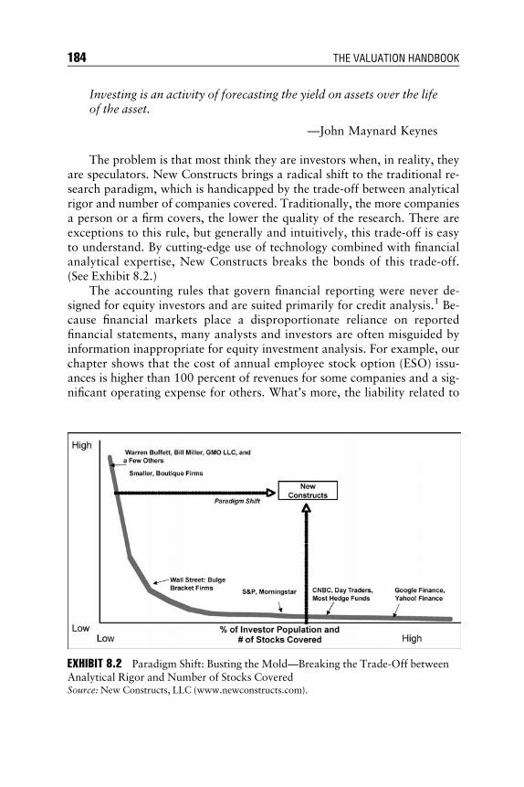
E1C08 09/02/2009 Page 184

Investing is an activity of forecasting the yield on assets over the lifeof the asset.

—John Maynard Keynes

The problem is that most think they are investors when, in reality, theyare speculators. New Constructs brings a radical shift to the traditional re-search paradigm, which is handicapped by the trade-off between analyticalrigor and number of companies covered. Traditionally, the more companiesa person or a firm covers, the lower the quality of the research. There areexceptions to this rule, but generally and intuitively, this trade-off is easyto understand. By cutting-edge use of technology combined with financialanalytical expertise, New Constructs breaks the bonds of this trade-off.(See Exhibit 8.2.)

The accounting rules that govern financial reporting were never de-signed for equity investors and are suited primarily for credit analysis.1 Be-cause financial markets place a disproportionate reliance on reportedfinancial statements, many analysts and investors are often misguided byinformation inappropriate for equity investment analysis. For example, ourchapter shows that the cost of annual employee stock option (ESO) issu-ances is higher than 100 percent of revenues for some companies and a sig-nificant operating expense for others. What’s more, the liability related to

EXHIBIT 8.2 Paradigm Shift: Busting the Mold—Breaking the Trade-Off betweenAnalytical Rigor and Number of Stocks CoveredSource: New Constructs, LLC (www.newconstructs.com).


E1C08 09/02/2009 Page 185

outstanding ESOs claims as much as 10 percent of the market value of thecompanies analyzed in our chapter. Unearthing critical financial informa-tion buried deep within 10-Q and 10-K filings, we are able to translateaccounting statements into economic statements that perform apples-to-apples analysis of the true profitability of businesses despite the accountingpolicies different businesses may employ.

Folding these economic statements into a valuation frameworkallows precise quantification of the future economic cash flows requiredto justify stock prices. We present the stock market’s expectations for thefuture financial performance of the companies in this chapter using intui-tive terms.

We do not suggest that basic elements of the investment decision pro-cess have changed. We do not present a black box or crystal ball that canpredict stock price performance. Our goal is to present analytical tech-niques that help investors assess the profitability and value of businesseswith more reliability and accuracy.

For example, here are some of the key insights presented in our chapteron these companies:

Avalon Bay Communities (AVB)

& The market has high expectations. To justify the current market priceof $99.45, the company will have to grow its profits by over 6 percentcompounded annually for each of the next 45 years.

& Lifting the accounting veil. The true profitability of AVB’s business issignificantly worse than the company’s reported financials indicate.Our research shows misleading earnings, which means reported net in-come is positive and rising while the economic profits of the businessare negative and declining.

Accenture Ltd (ACN)

& Low valuation means low expectations. To justify the current marketprice of $36.63, the company need not grow profits at all. The currentvaluation implies that ACN will never grow its profits above the cur-rent level.

& Strong economics. Accenture has a top-quintile return on invested capi-tal (ROIC). Over the past five years, the company’s ROIC has been ris-ing even while the company grows revenue at a double-digit pace. ACNgenerates a lot of economic value.

The remainder of this chapter explains how we arrive at our conclu-sions and presents the detailed information that led us to them.


E1C08 09/02/2009 Page 186

I D ENT I FY ING THE PROBL EM

‘‘We still don’t know how to value companies.’’2

The problem with popular valuation techniques such as price-to-earn-ings, price-to-revenues, and EBITDA ratios is twofold: They are shortcutsthat fail in their attempt to supplant proper discounted cash flow (DCF)analysis, and they are entirely based on reported accounting data. Toomany analysts and investors rely on the face value of reported financialstatements and base valuations on those numbers. Financial statementswere never designed for equity investors. They were created for accountantsand creditors, who have different financial priorities than equity investors.For this reason, it is not unusual that companies with excellent credit ratingsare poor stocks.

WHAT DR IV ES STOCK MARKET VALUAT I ON?

‘‘The value of any asset equals the discounted present value of itscash flows.’’

As far back as the 1950s, Professors Merton Miller and Franco Modi-gliani showed that the stock market equates the value of a firm to the pres-ent value of the future cash flows available to the firm’s owners. This recipefor valuation seems quite simple, but its execution can be difficult. Althoughthe reported financial statements (e.g., the income statement, balance sheet,and cash flow statement) do not capture the full picture of a company’s truefinancial performance, all of the necessary information is available. Thenotes to the financial statements found in the 10-K and 10-Q documentsprovide important disclosures that affect the interpretation of the reportedfinancial statements.

Why haven’t more investors followed Warren Buffett’s example orMiller and Modigliani’s proof? Here are some of the principal reasons:

& The process of removing distortions in accounting statements and ar-riving at the accurate cash flows of a business is a complex task requir-ing knowledge of both accounting rules and economic principles.

& Discounting long-term streams of cash flow is computationally cum-bersome, even without the additional burden of repeating the processfor sensitivity analyses.

& Long before Miller, Modigliani, and Buffett, the large majority of WallStreet analysts and investors had already established a variety of short-cuts, such as price-to-earnings and price-to-revenues ratios, to simplifythe information computation process.


E1C08 09/02/2009 Page 187

& There has previously been little incentive to modify the practices thathave led to unusually high analyst compensation and to investmentbanks’ large share of capital market profits.

OUR VALUAT I ON METHODOLOGY—PROV ID INGA SOLUT I ON

After reviewing and extracting key data from company filings, we performtwo key tasks: (1) translation of accounting data from company filings intoeconomic statements that enable an assessment of the economic profitabilityof the business and (2) quantification of the future financial performancerequired to justify stock values in terms of revenue growth, cash profits, andsustainability of cash profits.

Trans l a t i ng Accoun t i n g Da t a i n t oEconom i c S t a t emen t s

In our view, the true profitability of a business can be derived from the cal-culation of three key values:

1. Net operating profit after tax (NOPAT). This is the after-tax operatingcash generated by the business, excluding nonrecurring losses andgains, financing costs, and goodwill amortization and including thecompensation cost of employee stock options (ESOs). See Appendix Afor a detailed explanation of how we calculate this value.

2. Invested capital. This is the sum of all cash that has been invested in acompany’s net assets over its life without regard to financing form oraccounting name. It is the total of investments in the business fromwhich revenue is derived. Common adjustments to this value includethe addition of accumulated goodwill amortization, unrecorded good-will, asset write-offs, unrealized gains and losses in investment securi-ties, loan loss reserves, and capitalizing operating leases. See AppendixA for a detailed explanation of how we calculate this value.

3. Weighted average cost of capital (WACC). Weighted average cost ofcapital (WACC) is the average of debt and equity capital costs that allpublicly traded companies with debt and equity stakeholders incur as acost of operating. The cost of debt capital is equal to the long-term mar-ginal borrowing rate of the business. The cost of equity is calculatedusing the capital asset pricing model (CAPM). Though there are manyother more complicated approaches for arriving at a firm’s cost ofequity, we do not feel their additional complexity offers commensurate


E1C08 09/02/2009 Page 188

accuracy. CAPM is simple, gets us close enough, and is easy to imple-ment consistently across all companies we analyze. See Appendix A fora detailed explanation of how we calculate this value.

Samples of these calculations are available in the research section of ourweb site (www.newconstructs.com). Look for the free snapshot reports.

These three value drivers encompass the comprehensive financial pic-ture of a business and are the foundation for an economic assessment of theprofitability of any business. From them we are able to generate the follow-ing metrics:

& Free cash flow. Free cash flow reflects the amount of cash free for distri-bution to both debt and equity shareholders. It is calculated by sub-tracting the change in invested capital from NOPAT.

& Return on invested capital (ROIC). This is the best measure of a busi-ness’s cash return on cash invested. It represents the cash flow derivedfrom all capital invested in the business. It is equal to NOPAT dividedby invested capital.

& Economic profit margin. ROIC minus WACC equals the truest mea-sure of a business’s profitability. This metric accounts for the cash flowreturns adjusted for the risk associated with the business modelemployed to achieve those returns. Economic profit margins preciselymeasure a firm’s ability to create value for its stakeholders.

& Economic profit. This metric quantifies the amount of shareholdervalue a company creates or destroys. It can be calculated two mathe-matically equivalent ways:1. Residual income approach: (ROIC – WACC) � Invested capital ¼

Economic profit.2. Refined earnings approach: NOPAT – (Invested capital � WACC)

¼ Economic profit.

These metrics provide investors with insight critical to assessing themerits of business models. Understanding the true economic performanceof businesses is the first step in valuing any business model or strategy.

Cash I s K i n g

Our methodology is based on the view that that economic cash flow is themost important driver of asset value.3 In Exhibit 8.3, we use our discountedcash flow framework to show how ROIC is the key valuation driver value asmeasured by a price-earnings (P/E) multiple. The results from the 20 differentearnings growth and ROIC scenarios show that a company must achieveROIC greater than the WACC for growth to contribute to the value of a


E1C08 09/02/2009 Page 189

business. Growth has no impact on value if the business’s ROIC is equal to itsWACC. Growing a business that earns an ROIC below the WACC increasesthe rate of value destruction. Just left of the middle, the chart shows that whenthe ROIC equals 10 percent, the same as the WACC, the value of the businessdoes not change no matter how much the company grows. This result stemsfrom the fact that a business with an ROIC equal to its WACC neither createsnor destroys value. Looking toward the left, the chart illustrates that growthfrom companies not earning ROIC above their WACC destroy value. Thefaster a business with ROIC less than WACC grows, the more value it de-stroys, resulting in a lower, eventually negative, P/E multiple. Looking towardthe right side of the chart reveals that a company with high revenue growthand an ROIC above its WACC can be very valuable. The takeaway for inves-tors is that understanding the economics of a business is more important thanmeasuring its growth.

Demystifying Stock Market Valuation: Linking Valuation to Fundamentals Oncethe economic profitability of a business has been accurately evaluated, onecan build financial models grounded in bedrock financial theory to computethe value of a business. Exhibit 8.4 illustrates the overall process we employto value a company’s stock.

EXHIBIT 8.3 P/E Ratios That Result from ROIC and Earnings Growth Scenarios

Earnings Growth ROIC 5% 10% 15% 20%

2% 8.1 10.0 10.6 11.010% �7.3 10.0 15.8 18.615% �29.8 10.0 23.3 29.920% �74.5 10.0 38.2 52.235% �661.5 10.0 233.8 345.8

Assumptions: WACC is 10 percent and the growth appreciation period or DCF forecast

horizon is 20 years.

Source: New Constructs, LLC (www.newconstructs.com).

EXHIBIT 8.4 Analytical Process for Equity ValuationSource: New Constructs, LLC (www.newconstructs.com).


E1C08 09/02/2009 Page 190

The Basic Valuation Recipe: Same for Every Asset Exhibit 8.5 shows how theproper approach to value every type of asset is the same. In Exhibit 8.5, wecompare bond valuation with stock valuation to show how the relevantterms correspond to each other. Equity cash flows, for example, mirrorfixed-income coupon payments. The growth appreciation period (GAP)4

for stocks is analogous to the maturity date for bonds. Market risk for bondinvestors comes from interest rate fluctuation. Market risk for equity inves-tors is quantified by the weighted average cost of capital (WACC), whichquantifies the risk assigned to the stream of cash flows. Hence, the main keydifference between bond and equity valuation is that equity value driversare based on expectations rather than defined by debt covenants.

We can extend the framework to demonstrate more detailed financialanalysis. Exhibit 8.6 shows how business cash flows can be broken downinto more intuitive financial terms like revenue growth and return on in-vested capital (ROIC).

Using Intuitive Terms We can replace the cash flow variable and focuson the three variables with which investors are most familiar. (SeeExhibit 8.7.) We can use these three terms (defined in the next section) toquantify the specific financial performance required to justify stock pricesfor all companies:

EXHIBIT 8.5 The Basic Valuation RecipeSource: New Constructs, LLC (www.newconstructs.com).

EXHIBIT 8.6 Key Ingredients of the Valuation RecipeSource: New Constructs, LLC (www.newconstructs.com).


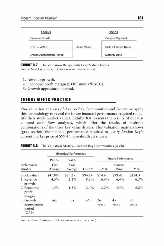
E1C08 09/02/2009 Page 191

1. Revenue growth.2. Economic profit margin (ROIC minus WACC).3. Growth appreciation period.

THEORY MEETS PRACT I C E

Our valuation analyses of Avalon Bay Communities and Accenture applythis methodology to reveal the future financial performance required to jus-tify their stock market values. Exhibit 8.8 presents the results of our dis-counted cash flow analyses, which offer the results of multiplecombinations of the three key value drivers. This valuation matrix shows(gray section) the financial performance required to justify Avalon Bay’scurrent market price of $99.45. Specifically, it shows:

EXHIBIT 8.8 The Valuation Matrix—Avalon Bay Communities (AVB)

Historical Performance

Past 5- Past 3-Future Performance

Performance

Hurdles

Year

Average

Year

Average Last FY �25%

Current

Price 25%

Stock values $47.80 $89.25 $94.14 $74.6 $99.45 $124.31. Revenue

growth4.3% 2.1% 8.8% 6.4% 6.4% 6.5%

2. Economicprofitmargin

�1.4% �1.5% �2.4% 2.2% 5.4% 8.8%

3. Growthappreciationperiod(GAP)

n/a n/a n/a 26years

45years

75years


EXHIBIT 8.7 The Valuation Recipe with Core Value DriversSource: New Constructs, LLC (www.newconstructs.com).


E1C08 09/02/2009 Page 192

1. Revenue growth—the compounded annual growth rate (CAGR) forrevenues that must be achieved over the growth appreciation period(GAP—see definition). For the current stock price of $99.45, this hurdleis 6.4 percent.

2. Economic profit margin—the excess returns on capital that must beachieved over the growth appreciation period. Note that this number isthe average return level during the entire GAP and not the actual levelof returns at the end of the GAP. For this reason, the length of the GAPcan drive results from this calculation up significantly for longer GAPsand it might seem unusually low for short GAPs. For the current stockprice of $99.45, this hurdle is 5.4 percent.

3. Growth appreciation period (GAP)—the number of years over whichthe company must sustain the aforementioned hurdles. For the currentstock price, this hurdle is 45 years. We arrive at this number by extend-ing the forecast of our discounted cash flow model as far into the futureas needed to calculate a value equal to the current market price.

To the left of the future financial performance required to justify mar-ket expectations, we provide a summary of the historical performance of therelevant value drivers.

Exhibit 8.8 also shows the financial performance hurdles required tojustify prices 25 percent above and below the current price. All of these cal-culations are based on market expectations from consensus estimates forrevenue. We use this matrix in our valuation analysis of all the companiesin this chapter. It is designed to present the reader with a streamlined sum-mary of the financial hurdles the business must meet to justify the marketprice, or must exceed to drive price appreciation.

Buy Low Expec t ed Cash F l ows ;Se l l H i gh E xpec t ed Cash F l ows

Material changes in the present value of expected cash flows are the keydriver of material changes in a stock price. Accordingly, determining theinvestment merit of a given stock boils down to identifying gaps betweenthe investor’s expectations for future financial performance and the mar-ket’s expectations. Our methodology focuses on comparing the valuationimpact of multiple forecast scenarios and measuring the different valuationimpacts they create. We offer investors the ability to identify those stockswhere the market’s expectations are significantly different from their ownwith greater accuracy and reliability.

We do not see any relevance to the distinction between ‘‘growth’’ and‘‘value’’ investment strategies. Growth without profit (i.e., value) offers no


E1C08 09/02/2009 Page 193

investment merit. At the same time, value without growth offers littleupside incentive for investing in a company. We encourage investors to in-corporate the assessment of both the growth and the value of a business intotheir investment decision-making process.

Providing Context Juxtaposing the historical performance with the requiredfuture performance shows how much the expected future performance mayor may not diverge from historical performance. The historical informationprovides insightful context for investors to assess the likelihood of meeting,beating, or underperforming market expectations. In the next section of thischapter, we build on this matrix by adding the results of scenario analysesbased on expectations different from those implied by consensus estimates.These scenario analyses enable investors to assess the valuation sensitivitythat different companies have to the three key value drivers. Appendix Bprovides a detailed explanation of how our discounted cash flow model cal-culates the values in our valuation matrix.

‘‘Better to Be Vaguely Right Than Precisely Wrong’’5 We do not assert thatwe can define the exact combination of value drivers implied by stock prices.Nevertheless, we attempt to present cogent combinations while offeringmultiple scenarios that, at the very least, enable investors to calibrate theirvaluation analyses with greater accuracy and transparency than traditionaltools.

Mos t A t t r ac t i v e S t ocks : Me t hodo l o gy

Stocks make our ‘‘Most Attractive Stocks’’ list because they have:

& High-quality earnings based on:& Returns on invested capital are rising.& Economic earnings/cash flows are positive.

& Cheap valuations based on:& Two-year average free cash flow yields6 are positive.& Price-to-economic book value (EBV)7 ratios are relatively low.& Growth appreciation periods (GAPs)8 are relatively short.

These characteristics also qualify stocks for a Very Attractive or At-tractive rating, according to our risk/reward rating system. Exhibit 8.9shows our risk/reward rating analysis, which we apply to the 3,000þ com-panies that we cover. Stocks get a grade of 1 to 5 for each criterion, 5 beingthe worst and 1 being the best score. The overall score is based on the aver-age score of all five criteria. Stocks must get an average score of 1.4 or better


E1C08 09/02/2009 Page 194

to be rated Very Attractive. For the most part, only Very Attractive stocksqualify for our ‘‘Most Attractive Stocks’’ lists.

Please see our website (www.newconstructs.com) for a free sample ofour Most Attractive Stocks for any given month since July 2004.

Mos t Dangerous S t ocks : Me t hodo l ogy

Stocks make our ‘‘Most Dangerous Stocks’’ list because they have:

& Poor-quality earnings based on:& Misleading earnings: rising and positive GAAP earnings while eco-

nomic profits are negative and falling.& Low returns on invested capital (ROIC).

& Expensive valuations, based on:& Two-year average free cash flow yields9 that are very low or

negative.& Price-to-economic book value (EBV)10 ratios that are relatively high.& Growth appreciation periods (GAP)11 that are relatively long.

These characteristics also qualify stocks for a Very Dangerous or Dan-gerous rating, according to our risk/reward rating system. Exhibit 8.10shows our risk/reward rating analysis, which we apply to the 3,000þ

EXHIBIT 8.9 New Constructs Risk/Reward Rating for Stocks—Very Attractive

Quality of Earnings Valuation

OverallRisk/

RewardRating

Economicvs.

ReportedEPS

Return onInvested

Capital(ROIC)

FCFYield

2-YearAverage

Price-

to-EBVRatio

Growth

AppreciationPeriod (Years)

Verydangerous

Misleadingtrend

Bottomquintile

��5% �3.5 or�1 to 0

�50

Dangerous Falsepositive

4th quintile �5% to�1%

2.4 to3.5 or��1

20 to 50

Neutral Neutral 3rd quintile �1% to3%

1.6 to2.4

10 to 20

Attractive Positive EP 2nd quintile 3% to10%

1.1 to1.6

3 to 10

Veryattractive

Rising EP Top quintile >10% 0 to 1.1 0 to 3



E1C08 09/02/2009 Page 195

companies that we cover. Stocks get a grade of 1 to 5 for each criterion, 5being the worst and 1 being the best score. The overall score is based on theaverage score of all five criteria. Stocks must get an average score of 4.25 ormore to be rated Very Dangerous. For the most part, only Very Dangerousstocks qualify for our ‘‘Most Dangerous Stocks’’ list.

Please see our website (www.newconstructs.com) for a free sample ofour Most Dangerous Stocks for any given month since July 2004.

GENERAL NOTES ON STOCK P ICK ING

We do not hesitate to admit that our approaches to measuring economicprofits and the expectations embedded in stock prices are not novel. Weadd value, as highlighted in Exhibit 8.2, by not sacrificing any anlyticalrigor when applying the approaches consistently to a virtually unlimitednumber of publicly-traded stocks. New Constructs’ ability to gather andapply data from the notes to the financial statements when calculating eco-nomic profit gives our clients unprecedented insights into the true profitabil-ity and valuation of companies. In our opinion, we are simply applying theproper methodologies for measuring corporate profitability and quantifyingmarket expectations with scale. Our goal is to give investors quick and easyaccess to better information for making investment deicsions. Despite the

EXHIBIT 8.10 New Constructs Risk/Reward Rating for Stocks—Very Dangerous


OverallRisk/

RewardRating

Economicvs.

ReportedEPS

Return onInvested

Capital(ROIC)

FCFYield

2-YearAverage

Price-

to-EBVRatio

Growth


Verydangerous

Misleadingtrend

Bottomquintile

��5% �3.5 or�1 to 0

�50



2.4 to3.5 or��1

20 to 50


1.6 to2.4

10 to 20


1.1 to1.6

3 to 10

Veryattractive




E1C08 09/02/2009 Page 196

rigor and insights delivered by our research, intelligent investing remains adifficult task.

Unders t and i ng Our L im i t a t i o ns

Few have articulated the tenets of a sound valuation philosophy as well asMartin Liebowitz:

At the very most, the modeled result should be taken as delineatingthe region beyond which the analyst must rely on imagination andintuition.

. . . the results of any equity valuation model should beviewed only as a first step in a truly comprehensive assessment offirm value.

. . . analyzing a firm’s future is akin to assessing the value of acontinually unfinished game in which the rules themselves drift on atide of uncertainty.12

Our research does not attempt to predict the future performance ofbusinesses or stock prices. Our focus is to present a methodology thatempowers investors with information essential to assessing the true profit-ability and value of companies.

Our models perform no subjective strategic analysis. Instead, we pro-vide the financial context critical to performing subjective analysis more ef-fectively. We offer a methodology that provides a better understanding ofthe economics of businesses. We hope investors can use these insights toperform a more accurate strategic analysis in order to determine whether abusiness can exceed the market’s implied expectations for future financialperformance.

A Good Barga i n I s Hard t o F i nd

We underscore that finding undervalued stocks (i.e., good investment op-portunities) is not a simple task. Finding overvalued stocks can be simple;however, finding good stocks to short is much more difficult. The market isa very robust pricing mechanism. Consistently finding inappropriately val-ued stocks is a challenge that few professional investors meet.13 Indeed,Warren Buffett, one of the most successful contemporary investors, employsan investment strategy that reflects this fact.14 He has often noted that find-ing undervalued stocks is difficult, especially at the market heights. Accord-ingly, his investment strategy focuses on making large investments in thefew stocks he considers attractive. The purpose of this chapter is to present


E1C08 09/02/2009 Page 197

a methodology that we believe will help investors more systematically iden-tify those few, rare potential bargains as well as avoid the stocks most likelyto decline in value.

Da t a Sources

There are four sources for the data inputs required to develop a model oneach of the companies we analyzed. (1) Companies’ 10-K filings are the pri-mary source, and provide all the information required to perform historicalanalyses. (2) We reference consensus estimates to forecast market expecta-tions where data was available, which primarily includes revenues for twoto three years into the future. (3) We extrapolated estimates into futureyears beyond where consensus provided actual data. (4) In some cases weentered a separate set of forecasts that provide a point of comparison tomarket expectations. The results of these forecasts demonstrate our abilityto perform scenario analyses with our model.

Backup Da t a

In Appendix D, we provide an example of the NOPAT, invested capital,and weighted average cost of capital (WACC) calculations. We provide freesamples of our NOPAT, invested capital, and WACC calculations on ourweb site: www.newconstructs.com. These backup calculations provide thedetails behind the calculations that drive our conclusions. Combined withthe methodology overview earlier in the chapter, the Appendixes providereaders with additional explanations of how we arrived at all of our results.

One o f t h e 40 Mos t Dangerous S t ocks f orSep t ember 2008 : Ava l on Bay Commun i t i e s—Poor Bus i n ess Econom i cs w i t h a R i c h Va l u a t i on

Every month since July 2004, New Constructs publishes its list of the 40Most Dangerous Stocks comprised of 20 large cap stocks and 20 small capstocks. All of the reports are available on our website (www.newconstructs.com) along with reports tracking the performance of our Most Attractiveand Most Dangerous Stocks as a long/short portfolio and as independentportfolios.

Very Dangerous Risk/Reward Rating15

& Avalon Bay Communities (AVB) has an overall risk/reward rating ofVery Dangerous because the stock offers much more downside riskthan upside potential, in our opinion.


E1C08 09/02/2009 Page 198

& Exhibit 8.11 summarizes the five factors that drive our overall risk/re-ward rating for AVB. Each factor offers insights into the profitabilityand valuation of AVB.

& ‘‘Misleading trend’’ means that reported EPS is positive and risingwhile economic EPS is negative and falling.

& The two biggest adjustments that lower economic EPS and are not cap-tured in reported EPS are reported net assets and off-balance-sheet op-erating leases.

& The combination of negative economic EPS with a rich stock valuationdrives a risk/reward rating of Very Dangerous for AVB.

& Our risk/reward rating system identifies disconnects between the mar-ket’s expectations for future cash flows and current cash flows.

& This chapter provides a detailed explanation of each diagnostic crite-rion and each rating for AVB. Appendix C offers an explanation ofhow our risk/reward rating system works.

Economic versus Reported Earnings: Why Economic profits Matter Economicprofits are almost always meaningfully different from GAAP earnings.Economic profits are informative because they provide a truer measureof underlying economic profitability and shareholder value creation

EXHIBIT 8.11 AVB Risk/Reward Rating


Overall

Risk/RewardRating

Economic

vs.Reported

EPS

Return on

InvestedCapital(ROIC)

FCF

Yield2-YearAverage

Price-to-EBVRatio

GrowthAppreciationPeriod (Years)

Verydangerous

Misleadingtrend

Bottomquintile

��5% �3.5 or�1 to 0

�50



2.4 to3.5 or��1

20 to 50


1.6 to2.4

10 to 20


1.1 to1.6

3 to 10

Veryattractive


Actualvalues

�$2.12 vs.$4.38

6.0% �3.8% 6.2 47

Source: New Constructs, LLC (www.newconstructs.com) and company filings.


E1C08 09/02/2009 Page 199

than offered by GAAP earnings. Beware of stocks whose economicprofits are declining while reported earnings are increasing. Beware ofcompanies whose economic profits differ meaningfully from theiraccounting earnings.

The Most Attractive stocks have positive economic profits and their re-turns on capital are increasing. The Most Dangerous stocks have negativeeconomic profits that are declining while reported GAAP earnings are posi-tive and rising.

Exhibit 8.12 highlights the differences between the reported and eco-nomic profits for AVB.

Note the misleading trend caused by the company reporting positiveand rising GAAP profits while the economics of its business are in decline.

During the past fiscal year, the two biggest drivers of the difference be-tween reported and economic EPS are reported net assets and off-balance-sheet operating leases.

Economic profits and return on capital metrics are significantlymore accurate when as-reported financial statements have been adjustedto reverse accounting distortions. The majority of the data required toreverse accounting distortions is available only in the notes to the finan-cial statements, which we analyze rigorously. Our core competency isgathering and analyzing all relevant financial data (from financial state-ments and the notes) so that we can deliver earnings analyses that bestrepresent the true profitability of businesses. Following is a list of theadjustments we make to a company’s reported GAAP profits in order toreverse accounting distortions and arrive at a better measure of a firm’sprofits:

EXHIBIT 8.12 AVB: Accounting Perception versus Economic RealitySource: New Constructs, LLC (www.newconstructs.com) and company filings.


E1C08 09/02/2009 Page 200

& Employee stock options.& Off-balance-sheet financing.& Pension over-/underfunding.& LIFO reserve.& Excess cash.& Unrealized gains/losses.& Restructuring charges.& Goodwill amortization.& Pooling goodwill.& Unconsolidated subsidiaries.& Minority interests.& Capitalized expenses.

Exhibit 8.13 compares AVB’s return on invested capital (ROIC) to itsweighted average cost of capital (WACC). This company’s ROIC during itslast fiscal year ranks in the 4th quintile.

How We Measure Economic profits The metrics we use to measure the eco-nomic performance of companies are economic profit margin and economicprofits. The economic profit margin for a company equals its return on in-vested capital (ROIC) minus its weighted average cost of capital (WACC).The economic profits of a company equal its economic profit margin multi-plied by its invested capital.

We believe our measures of economic performance to be substantiallymore accurate than accounting metrics because we make adjustments forall the issues listed in Exhibit 8.5.

EXHIBIT 8.13 AVB Economic Profit Margin: Return on Invested Capital versusWeighted Average Cost of CapitalSource: New Constructs, LLC (www.newconstructs.com) and company filings.


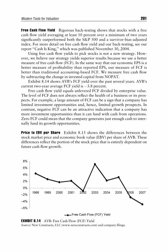
E1C08 09/02/2009 Page 201

Free Cash Flow Yield Rigorous back-testing shows that stocks with a freecash flow yield averaging at least 10 percent over a minimum of two yearssignificantly outperformed both the S&P 500 and a survivor-bias-adjustedindex. For more detail on free cash flow yield and our back-testing, see ourreport ‘‘Cash Is King,’’ which was published November 30, 2004.

Using free cash flow yields to pick stocks is not a new strategy. How-ever, we believe our strategy yields superior results because we use a bettermeasure of free cash flow (FCF). In the same way that our economic EPS is abetter measure of profitability than reported EPS, our measure of FCF isbetter than traditional accounting-based FCF. We measure free cash flowby subtracting the change in invested capital from NOPAT.

Exhibit 8.14 shows AVB’s FCF yield over the past several years. AVB’scurrent two-year average FCF yield is �3.8 percent.

Free cash flow yield equals unlevered FCF divided by enterprise value.The level of FCF does not always reflect the health of a business or its pros-pects. For example, a large amount of FCF can be a sign that a company haslimited investment opportunities and, hence, limited growth prospects. Incontrast, negative FCF can be an attractive indication that a company hasmore investment opportunities than it can fund with cash from operations.Zero FCF could mean that the company generates just enough cash to inter-nally fund its growth opportunities.

Price to EBV per Share Exhibit 8.15 shows the differences between thestock market price and economic book value (EBV) per share of AVB. Thesedifferences reflect the portion of the stock price that is entirely dependent onfuture cash flow growth.

EXHIBIT 8.14 AVB: Free Cash Flow (FCF) YieldSource: New Constructs, LLC (www.newconstructs.com) and company filings.


E1C08 09/02/2009 Page 202

When stock prices are much higher than EBVs, the market predictsthat the economic profitability (as distinct from accounting profitability)of the company will meaningfully increase. When stock prices are muchlower than EBVs, the market predicts that the economic profitability ofthe company will meaningfully decrease. If the stock price equals theEBV, the market predicts the company’s economic profitability will notchange.

EBV measures the no-growth value of the company based on the cur-rent economic cash flows generated by the business. It is also known as theprestrategy value of the company because it ignores the value attributable tofuture cash flows, which are, in theory, what business strategies should aimto improve.

The formula for EBV is: (NOPAT/WACC) + Excess cash – Debt (in-cluding operating leases) – Value of outstanding stock options – Minorityinterests � Over-/underfunded pensions. EBV per share equals EBV dividedby basic shares outstanding.

Quantifying Market Expectations We believe this stock has a Very Danger-ous risk/reward rating because there is a relatively large difference betweenthe expected financial performance implied by its market price and the com-pany’s historical performance.

Exhibit 8.16 compares the future performance required to justify thecompany’s stock market price to its historical performance. Specifically,Exhibit 8.16 shows that to justify the current stock price of $99.45, AVBmust grow revenues at 6.4 percent and maintain a 5.4 percent economicprofit margin for 45 years.

EXHIBIT 8.15 AVB: Stock Price versus Economic Book Value (EBV) per ShareSource: New Constructs, LLC (www.newconstructs.com) and company filings.


E1C08 09/02/2009 Page 203

Historically, AVB has generated revenue growth of 4.3 percent, 2.1percent, and 8.8 percent, and economic profit margins of –1.4 percent,–1.5 percent, and –2.4 percent over the past five years, three years, andone year. For the future, the market expects AVB will achieve revenuegrowth of 6.4 percent and economic profit margins of 5.4 percent for45 years.

GAP measures the number of years implied by the stock price duringwhich the company must maintain an edge over its current and future com-petitors. Specifically, GAP measures the number of years a company willearn returns on invested capital greater than its cost of capital on new in-vestments. The law of competition dictates that a company can only growits economic profits for the finite period over which it can maintain a com-petitive advantage.

GAP analysis comes from our dynamic discounted cash flow model, amultistage DCF model that values companies across multiple forecast hori-zons. Each forecast horizon (i.e., growth appreciation period) assumes thecompany cannot grow profits beyond the GAP. Our model exclusively usesno-growth terminal value assumptions for calculating the value of the stockfor each GAP.

The forecast drivers for our DCF model are: (1) revenue growth,(2) Net Operating Profit Before Tax (NOPBT) margin (i.e., EBIT mar-gin with adjustments), (3) cash tax rate, and (4) incremental net work-ing and fixed capital needs. Our MaxVal models value stocks based onthe present value of expected free cash flow, with that free cash flowmeasured according to our economic (as distinct from conventional

EXHIBIT 8.16 AVB: Future Performance Required to Justify Valuation

Avalon BayCommunities(AVB)

Historical Performance FuturePerformance

PerformanceHurdles

Past 5-YearAverage

Past 3-YearAverage Last FY

CurrentPrice

Stock values $47.80 $89.25 $94.14 $99.451. Revenue growth 4.3% 2.1% 8.8% 6.4%2. Economic profit

margin�1.4% �1.5% �2.4% 5.4%

3. Growthappreciation period(GAP)

n/a n/a n/a 45 years



E1C08 09/02/2009 Page 204

accounting) methodology. MaxVal subscribers forecast economic freecash flow by assigning estimates to three value drivers:

1. Revenue growth—compounded over the indicated time frame.2. Economic profit margin—the return on invested capital minus the

weighted average cost of capital.3. Growth appreciation period—number of years the company can earn a

positive economic profit margin on incremental investments (i.e., thenumber of years it can create economic value).

An alternative way to conceptualize the three value drivers is:

1. ‘‘How fast will the company grow?’’2. ‘‘How profitable will the company be?’’3. ‘‘For how many years will the company grow economic profits or create

incremental value?’’

One o f t h e 40 Mos t A t t r ac t i v e S t ocks f orSep t ember 2008 : Accen t ure L t d—Strong CashEconom i cs w i t h a Low Va l ua t i o n

Every month since July 2004, New Constructs publishes its list of the 40Most Attractive Stocks comprised of 20 large cap stocks and 20 small capstocks. All of the reports are available on our website (www.newconstructs.com) along with reports tracking the performance of our Most Attractiveand Most Dangerous Stocks as a long/short portfolio and as independentportfolios.

Very Attractive Risk/Reward Rating16

& ACN has an overall risk/reward rating of Very Attractive because thestock offers much more upside potential than downside risk, in ouropinion.

& Exhibit 8.17 summarizes the five factors that drive our overall risk/re-ward rating for ACN. Each factor offers insights into the profitabilityand valuation of ACN.

& Rising EP means that economic EPS are positive, the company’s ROICis greater than WACC, and ROIC is rising.

& The biggest adjustment that lowers economic EPS and is not capturedin reported EPS is reported net assets.

& The combination of positive and rising economic EPS with a cheapstock valuation drives a risk/reward rating of Very Attractivefor ACN.


E1C08 09/02/2009 Page 205

& Our risk/reward rating system identifies disconnects between the mar-ket’s expectations for future cash flows and current cash flows.

& This chapter provides a detailed explanation of each diagnostic crite-rion and each rating for ACN. Appendix C offers an explanation ofhow our risk/reward rating system works.

Economic versus Reported Earnings: Why Economic profits Matter Economicprofits are almost always meaningfully different from GAAP earnings.Economic profits are informative because they provide a truer measureof underlying economic profitability and shareholder value creation thanis offered by GAAP earnings. Beware of stocks whose economic profitsare declining while reported earnings are increasing. Beware of compa-nies whose economic profits differ meaningfully from their accountingearnings.

The Most Attractive stocks have positive economic profits and their re-turns on capital are increasing. The Most Dangerous stocks have negativeeconomic profits that are declining while reported GAAP earnings are posi-tive and rising.

Exhibit 8.18 highlights the differences between the reported and eco-nomic profits for ACN. ACN is one of the few companies in our coverage

EXHIBIT 8.17 ACN: Risk/Reward Rating


OverallRisk/

RewardRating

Economicvs.

ReportedEPS

Return onInvested

Capital(ROIC)

FCFYield

2-YearAverage

Price-

to-EBVRatio

Growth


Verydangerous

Misleadingtrend

Bottomquintile

��5% �3.5 or�1 to 0

�50



2.4 to3.5 or��1

20 to 50


1.6 to2.4

10 to 20


1.1 to1.6

3 to 10

Veryattractive


Actualvalues

$2.35 vs.$1.44

50.0% 17.7% 1.0 <1 year



E1C08 09/02/2009 Page 206

universe of over 3,000 companies whose economic profits exceed theiraccounting earnings. During the past fiscal year, the two biggest drivers ofthe difference between reported and economic EPS are reported net assetsand off-balance-sheet operating leases.

Economic profits and return on capital metrics are significantly moreaccurate when as-reported financial statements have been adjusted to re-verse accounting distortions. The majority of the data required to reverseaccounting distortions is available only in the notes to the financial state-ments, which we analyze rigorously. Our core competency is gathering andanalyzing all relevant financial data (from financial statements and thenotes) so that we can deliver earnings analyses that best represent the trueprofitability of businesses. Following is a list of the adjustments we make toa company’s reported GAAP profits in order to reverse accounting distor-tions and arrive at a better measure of a firm’s profits:

& Employee stock options& Off-balance-sheet financing.& Pension over-/underfunding.& LIFO reserve.& Excess cash.& Unrealized gains/losses.& Restructuring charges.& Goodwill amortization.& Pooling goodwill.

EXHIBIT 8.18 ACN: Accounting Perception versus Economic RealitySource: New Constructs, LLC (www.newconstructs.com) and company filings.


E1C08 09/02/2009 Page 207

& Unconsolidated subsidiaries.& Minority interests.& Capitalized expenses.

Exhibit 8.19 compares ACN’s return on invested capital (ROIC) to itsweighted average cost of capital (WACC). This company’s ROIC during itslast fiscal year ranks in the 1st quintile.

How We Measure Economic profits The metrics we use to measure the eco-nomic performance of companies are economic profit margin and economicprofits. The economic profit margin for a company equals its return on in-vested capital (ROIC) minus its weighted average cost of capital (WACC).The economic profits of a company equal its economic profit margin multi-plied by its invested capital.

We believe our measures of economic performance to be substantiallymore accurate than accounting metrics because we make adjustments forall the issues listed in Exhibit 8.5.

Free Cash Flow Yield Rigorous back-testing shows that stocks with a freecash flow yield averaging at least 10 percent over a minimum of two yearssignificantly outperformed both the S&P 500 and a survivor-bias-adjustedindex. For more detail on free cash flow yield and our back-testing, see ourreport ‘‘Cash Is King,’’ which was published November 30, 2004.

EXHIBIT 8.19 ACN: Economic Profit Margin—Return on Invested Capital versusWeighted Average Cost of CapitalSource: New Constructs, LLC (www.newconstructs.com) and company filings.


E1C08 09/02/2009 Page 208

Using free cash flow yields to pick stocks is not a new strategy. How-ever, we believe our strategy yields superior results because we use a bettermeasure of free cash flow (FCF). In the same way that our economic EPS is abetter measure of profitability than reported EPS, our measure of FCF isbetter than traditional accounting-based FCF. We measure free cash flowby subtracting the change in invested capital from NOPAT.

Exhibit 8.20 shows ACN’s FCF yield over the past several years. ACN’scurrent two-year average FCF yield is 9.5 percent.

Free cash flow yield equals unlevered FCF divided by enterprise value.The level of FCF does not always reflect the health of a business or its pros-pects. For example, a large amount of FCF can be a sign that a company haslimited investment opportunities and, hence, limited growth prospects. Incontrast, negative FCF can be an attractive indication that a company hasmore investment opportunities than it can fund with cash from operations.Zero FCF could mean that the company generates just enough cash to inter-nally fund its growth opportunities.

Price to EBV per Share Exhibit 8.21 shows the differences between thestock market price and economic book value (EBV) per share of ACN.These differences reflect the portion of the stock price that is entirely depen-dent on future cash flow growth.

When stock prices are much higher than EBVs, the market predictsthat the economic profitability (as distinct from accounting profitability)of the company will meaningfully increase. When stock prices are muchlower than EBVs, the market predicts that the economic profitability ofthe company will meaningfully decrease. If the stock price equals the

EXHIBIT 8.20 ACN: Free Cash Flow (FCF) YieldSource: New Constructs, LLC (www.newconstructs.com) and company filings.


E1C08 09/02/2009 Page 209

EBV, the market predicts that the company’s economic profitability willnot change.

EBV measures the no-growth value of the company based on the cur-rent economic cash flows generated by the business. It is also known as theprestrategy value of the company because it ignores the value attributable tofuture cash flows, which are, in theory, what business strategies should aimto improve.

The formula for EBV is: (NOPAT/WACC) þ Excess cash – Debt (in-cluding operating leases) – Value of outstanding stock options – Minorityinterests � Over-/underfunded pensions. EBV per share equals EBV dividedby basic shares outstanding.

Quantifying Market Expectations We believe this stock has a Very Danger-ous risk/reward rating, because there is a relatively large difference betweenthe expected financial performance implied by its market price and the com-pany’s historical performance.

Exhibit 8.22 compares the future performance required to justify thecompany’s stock market price to its historical performance. Specifically, thetable shows that to justify the current stock price of $36.63, ACN need notgrow its profits at all. In other words, the current stock price implies noprofit growth. This finding correlates with our preceding price to economicbook value analysis, which shows that ACN’s stock price equals its eco-nomic book value.

Historically, ACN has generated revenue growth of 12.5 percent,12.0 percent, and 17.7 percent, and economic profit margins of 30.9 percent,35.0 percent, and 43.9 percent over the past five years, three years, and oneyear. For the future, the market expects ACN will achieve no profit growth.

EXHIBIT 8.21 ACN: Stock Price versus Economic Book Value (EBV) Per ShareSource: New Constructs, LLC (www.newconstructs.com) and company filings.


E1C08 09/02/2009 Page 210

APPEND IX A : D E F I N I T I ONS OF KEY TERMSUSED IN OUR VALUAT I ON MODE LS

We did not invent any of the terms or definitions below. We add value byimplementing these calculations with high analytical rigor for a virtuallyunlimited number of publicly-traded companies.

I n v es t ed Cap i t a l

Invested capital is the sum of all cash that has been invested in a companyover its life without regard to financing form or accounting name. It is thetotal of investments in the business from which revenue is derived. It can becalculated two mathematically equivalent ways:

Operating Financing

Current Assets Short-Term Debt– NIBCLs* þ Long-Term DebtNet Working Capital þ All Leasesþ Tangible Assetsy Total Debt and Leasesþ Intangible Assets þ Equity Equivalentsþ Other Assets þ Common EquityInvested Capital Invested Capital

�NIBCLS stands for non-interest-bearing current liabilities.yIncludes leased assets.

Source:New Constructs, LLC (www.newconstructs.com).

EXHIBIT 8.22 ACN: Future Performance Required to Justify Valuation

Accenture Ltd (ACN) Historical Performance

PerformanceHurdles

Past 5-YearAverage

Past 3-YearAverage Last FY

Future

PerformanceCurrentPrice

Stock values $21.16 $24.40 $41.21 $36.631. Revenue growth 12.5% 12.0% 17.7% —2. Economic profit

margin30.9% 35.0% 43.9% —

3. Growth appreciationperiod (GAP)

n/a n/a n/a < 1 year



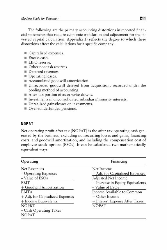
E1C08 09/02/2009 Page 211

The following are the primary accounting distortions in reported finan-cial statements that require economic translation and adjustment for the in-vested capital calculation. Appendix D reflects the degree to which thesedistortions affect the calculations for a specific company.

& Capitalized expenses.& Excess cash.& LIFO reserve.& Other noncash reserves.& Deferred revenues.& Operating leases.& Accumulated goodwill amortization.& Unrecorded goodwill derived from acquisitions recorded under the

pooling method of accounting.& After-tax portion of asset write-downs.& Investments in unconsolidated subsidiary/minority interests.& Unrealized gains/losses on investments.& Over-/underfunded pensions.

NOPAT

Net operating profit after tax (NOPAT) is the after-tax operating cash gen-erated by the business, excluding nonrecurring losses and gains, financingcosts, and goodwill amortization, and including the compensation cost ofemployee stock options (ESOs). It can be calculated two mathematicallyequivalent ways:

Operating Financing

Net Revenues Net Income– Operating Expenses þ Adj. for Capitalized Expenses– Value of ESOs Adjusted Net IncomeEBIT þ Increase in Equity Equivalentsþ Goodwill Amortization – Value of ESOsEBITA Income Available to Commonþ Adj. for Capitalized Expenses þ Other Incomeþ Income Equivalents þ Interest Expense After TaxesNOPBT NOPAT– Cash Operating TaxesNOPAT


E1C08 09/02/2009 Page 212

The following are the primary accounting distortions in reported finan-cial statements that require economic translation and adjustment for theNOPAT calculation. Appendix D reflects the degree to which these distor-tions affect the calculations for a specific company.

& Capitalized expenses.& Income from unconsolidated subsidiaries.& Restructuring/nonrecurring charges.& All nonoperating items are below EBIT.& All after-tax items.& Value of employee stock options (ESOs) issued in a given year.& Operating leases.& Over-/underfunded pensions.

Free Cash F l ow

Free cash flow (FCF) reflects the amount of cash free for distribution to bothdebt and equity shareholders. It is calculated by subtracting the change ininvested capital from NOPAT.

RO I C

Return on invested capital (ROIC) is the true measure of a business’soperating profitability. It represents the cash flow derived from all capi-tal invested in the business. It is equal to NOPAT divided by investedcapital.

WACC

Weighted average cost of capital (WACC) is the average of debt and equitycapital costs that all publicly traded companies with debt and equity stake-holders incur as a cost of operating. We provide the details behind ourWACC calculations:

Cost of Equity

& Our cost of equity calculation is based on the capital asset pricingmodel methodology.

& Though there are many other more complicated approaches for arriv-ing at a firm’s cost of equity, we do not feel their additional complexityoffers commensurate accuracy. CAPM is simple, gets us close enough,and is easy to implement consistently across all companies we analyze.


E1C08 09/02/2009 Page 213

& The market value of equity is used when calculating the debt to totalmarket capital ratio that is used in the cost of equity calculation.

& The equity risk premium is based on a forward-looking dividend dis-count model.

& Beta can come from many sources (Value Line, Ibbotson, Yahoo! Finance,etc.). We try to use fairly consistent estimates for beta to avoid this varia-ble having an inappropriately large impact on WACC calculation.

Cost of Debt

& The cost of debt capital is equal to a business’s long-term marginal bor-rowing rate.

& The risk-free rate (RFR) is approximated by the 30-year Treasurybond.

& To the RFR, we add the debt spread associated with the debt rating onthe company’s long-term debt.

& The resulting pretax cost of debt is then multiplied by (1 – Marginal taxrate17)

& Debt rating, as per Moody’s or S&P.

Formula for Weighted Average Cost of Capital (WACC)

WACC ¼ Ke � (1 �D=TC) þ [Kd � (1 � T)] � (D=TC)

where Ke¼ cost of equity

D/TC¼ debt to total adjusted market capital ratioKd¼ cost of debtT¼ tax rate

E conom i c Profi t Marg i n

ROIC minus WACC equals the truest measure of a business’s profitability.This metric measures the net cash flow returns to shareholders adjusted forthe risk associated with the business model employed to achieve those re-turns. In essence, economic profit margins directly measure a firm’s abilityto create actual value for its shareholders.

Growth Apprec i a t i on Per i o d (GAP )

The growth appreciation period is the amount of time (usually expressed inyears) that a business can be expected to earn positive economic profit mar-gins (ROIC greater than WACC) on new investments. Put simply, GAP isthe amount of time a business can grow its economic cash flow. After theGAP, it is assumed that incremental investments by the business earn ROIC


E1C08 09/02/2009 Page 214

equal to WACC. Warren Buffett refers to GAP as the moat around a com-pany’s castle. It is also known as the competitive advantage period (CAP)and the forecast growth horizon.

Our dynamic DCF model calculates share prices attributable to multi-ple GAP scenarios.

For example, the value of the company with a 20-year forecast horizonassumes the company will enjoy a 20-year GAP. Without a model thatencompasses this long-term approach, we may not be able to capture themarket’s true expectations for many companies.

Growth Deprec i a t i o n Per i o d (GDP )

GDP is the amount of time a business destroys value by allocating capital toprojects that earn negative economic profit margins (ROIC below WACC).

Marke t - Imp l i e d GAP

The market-implied growth appreciation period (MIGAP) is the number ofyears that a company’s stock market price implies it will earn ROIC greaterthan WACC on incremental investments.

Provided that the estimates entered on the forecast page are based onconsensus projections, the MIGAP represents the forecast horizon neededin a DCF model to arrive at a value equal to the current market price.

E conom i c Profi t or Econom i c Cash F l ow

Economic profit quantifies the amount of shareholder value a company cre-ates or destroys. It can be calculated two mathematically equivalent ways:

Residual income approach:

Economic profit ¼ (ROIC � WACC) � Invested capital

Refined earnings approach:

Economic profit ¼ NOPAT � (Invested capital � WACC)

Cons i s t e ncy and I n t e gr i t y f o r A l l K eyCa l cu l a t i o ns

It is important to note that our model ensures consistent treatment of alladjustments, especially the calculations of NOPAT, invested capital, andWACC. In other words, the model guarantees that any adjustment made toNOPAT is properly reflected in the calculation of invested capital. Forexample, when goodwill expense is removed from NOPAT, the relatedaccumulated goodwill amortization is added to invested capital. This


E1C08 09/02/2009 Page 215

methodology ensures that no adjustment to the financial statements is dou-ble-counted and that the ROIC calculation has maximum integrity.

APPEND IX B : HOW OUR DYNAM IC D I SCOUNTEDCASH F LOW MODEL WORKS

Dynamic DCF modeling compares closely to the ‘‘T’’ horizon concept inStern Stewart EVA1 and the ‘‘fade’’ rates employed by the Callard, Mad-den offshoots in cash returns. We did not invent the Dynamic DiscountedCash flow model, but we are among the first to apply this valuation tech-nique to more than five thousand publicly-traded companies.

S t a t e - o f - t h e - Ar t D i s coun t ed Cash F l ow Ana l ys i s

Our discounted cash flow model calculates the value attributable to stockprices based on the forecasted financial performance entered into the model.

In turn, the model harnesses state-of-the-art computing power to calcu-late a value per share for every year up to 100 years into the future. Nota-bly, we do not believe that we can forecast the future performance of acompany into the future with any special accuracy. Our model focuses onthe market’s expectations for future financial performance by matching themarket price of a stock with values calculated by the DCF model. In turn,we leverage our model to tease out of the stock price the stock market’sexpectations for the future financial performance of a company. This insightenables investors to calibrate their valuation assessment around the market’sexpectations. The burden of predicting the specific performance of the corevalue drivers shifts to the market. Investors are positioned to determine onlyif they feel market expectations are too high, too low, or about right.

Calculating the Value of the Business

Free Cash Flows

Cumulative free cash flow generated during the business’s GAP dis-counted by WACC to present value

Plus:

Perpetuity value of free cash flows generated at end of the business’sGAP discounted by WACC to present value.

Basic formula:Present value of free cash flow during GAPþ Residual value of free cash flows at end of GAP¼ Present value of the business’s total cash profits


E1C08 09/02/2009 Page 216

Economic Profits

Cumulative economic profits generated during the business’s GAP dis-counted by WACC to present value

Plus:

Perpetuity value of economic profits generated at end of the business’sGAP discounted by WACC to present value

Plus:

All capital invested in the business prior to the creation of future eco-nomic profits.

Basic formula:Present value of economic profits during GAPþ Residual value of economic profits at end of GAPþ Beginning invested capital¼ Present value of the business’s total cash profits

Cons i s t e ncy and I n t e gr i t y i n Our Va l u a t i on Mode l

To ensure absolute consistency and maximum integrity in our valuationmodel, we calculate the present value of the business’s total cash profits byboth the free cash flow and economic profit methods. In theory these calcu-lations should provide identical results. In our model they always matchperfectly, giving us high confidence in both the consistency and the integrityof our calculations. In addition, they provide the analyst with a choice be-tween metrics and enhance the clarity of model assumptions.

De t erm i n i n g t he Va l u e A t t r i b u t ab l et o Shareho l d ers

Once the model calculates the present value of the business’s total cashflows, we know the present value of cash flows available to all stakeholders.The next step, detailed as follows, is to determine the value available toshareholders by adding the value of any nonoperating assets and deductingthe value of any senior claims to the cash flows. Remember that value at-tributable to equity investors is residual to that available to creditors andminority interests. In addition, we must account for the value of outstand-ing options attributable to employees to determine the net value for currentor prospective shareholders.

Present value of the business’s total cash profits

þ Excess cash


E1C08 09/02/2009 Page 217

þ Current value of unconsolidated subsidiaries

– Current value of preferred stock

– Current value of total debt owed creditors

– Current value of minority interests

– Current value of outstanding employee stock options

¼ Shareholder value

Divide shareholder value by current number of basic shares outstanding

¼ Value per share in the business

See Exhibit 8A.1 for a graphic representation of how our model’s dy-namic discounted cash flow analysis calculates the value of a business andthe attendant value available to shareholders for multiple growth apprecia-tion periods. This chart shows how the value of the company analyzed inthis example rises as its GAP increases. The market-implied growth appreci-ation period (MIGAP) is the GAP as implied by the current market price.Our model calculates the MIGAP by matching the current stock price withthe year that the DCF value matches that of the current stock price. Forexample, the MIGAP for the company in Exhibit 8A.1 is 45 years. Ourmodel can also calculate the GAP implied for target prices as well as anyother stock prices no matter how great or small they may be. The analysis

EXHIBIT 8A.1 Results of the Dynamic Discounted Cash Flow CalculationsSource: New Constructs, LLC (www.newconstructs.com).


E1C08 09/02/2009 Page 218

in Exhibit 8A.1 shows DCF values for only 50 years, though the model canvalue companies over an indefinite time period.

Exhibit 8A.2 provides a more numerical summary of our dynamic DCFanalysis of Avalon Bay Communities. This table shows the specific growthrates and profitability levels required to justify the current stock price andprices 25 percent higher or lower than the current stock price. Specifically,the table shows that AVB must grow revenues at 6.4 percent and achieve aneconomic profit margin of 5.4 percent for 45 years to justify the currentstock price of $99.45. To justify a stock price of $74.60, the company mustgrow revenues at 6.4 percent and achieve an economic profit margin of 2.2percent for 26 years. To justify a stock price of $124.30, the company mustgrow revenues at 6.5 percent and achieve an economic profit margin of 8.8percent for 75 years. Note that Exhibit 8A.2 is the same as Exhibit 8.8 ear-lier in the chapter.

APPEND I X C : EXPLANAT I ON OF R I SK /R EWARDRAT ING SYSTEM

Our risk/reward rating system assigns a rating to every stock under ourcoverage according to what we believe are the five most important crite-ria for assessing the risk versus reward profile of stocks. See Exhibit 8A.3for details.

EXHIBIT 8A.2 The Valuation Matrix—Avalon Bay Communities (AVB)

Historical Performance

Past Past Future Performance

PerformanceHurdles

5-YearAverage

3-YearAverage Last FY �25%

CurrentPrice 25%

Stock values $47.80 $89.25 $94.14 $74.60 $99.45 $124.301. Revenue

growth4.3% 2.1% 8.8% 6.4% 6.4% 6.5%

2. Economicprofitmargin

�1.4% �1.5% �2.4% 2.2% 5.4% 8.8%

3. Growthappreciationperiod(GAP)

n/a n/a n/a 26years

45years

75years

Source: New Constructs, LLC (www.newconstructs.com)


E1C08 09/02/2009 Page 219

EXHIBIT 8A.3 New Constructs’ Risk/Reward Rating System

Overall Risk/RewardRanking

The overall risk/reward ranking provides a final ratingbased on the equal-weighted average rating of eachcriterion.

Very Dangerous Two-year average FCF yield is not included in theaverage.

Dangerous Two-year average FCF yield is not included in theaverage.

Neutral All criteria are equal-weighted in the averagecalculation.

Attractive All criteria are equal-weighted in the averagecalculation.

Very Attractive All criteria are equal-weighted in the averagecalculation.

Economic versusReported EPS

Rates stocks based on how their economic earningscompare to their reported earnings. Values are basedon latest fiscal year.

Very Dangerous Negative and declining economic profits despite positiveand rising reported earnings.

Dangerous Same as above except reported earnings are not rising orreported earnings are not positive.

Neutral Negative economic and reported earnings.Attractive Economic earnings are positive.Very Attractive Economic earnings are positive and rising.

Return on InvestedCapital (ROIC)

Rates stocks based on their ROICs. Values are based onlatest fiscal year.

Bottom Quintile Very Dangerous = in the bottom 20 percent of allcompanies.

4th Quintile Dangerous ¼ in the bottom 40 percent of all companies.3rd Quintile Neutral ¼ in the middle 20 percent of all companies.2nd Quintile Attractive ¼ in the top 40 percent of all companies.Top Quintile Very Attractive ¼ in the top 20 percent of all companies.

FCF Yield Two-Year Average

Rates stocks based on their two-year average free cashflow yield. Values are based on latest closing stockprice and latest fiscal year.

��5% Very Dangerous ¼ less than or equal to �5%.�5% to �1% Dangerous ¼ more than �5% but less than or equal to

�1%.�1% to 3% Neutral ¼ more than �1% but less than or equal to

þ3%.3% to 10% Attractive¼ more thanþ3% but less than or equal to

þ10%.

(Continued )


E1C08 09/02/2009 Page 220

APPEND IX D : NOPAT , I NVESTED CAP I TA L , ANDWACC CALCULAT I ONS FOR ACCENTURE

Exhibits 8A.4, 8A.5, and 8A.6 provide examples of calculations forAccenture. Note that readers can access more examples of our NOPAT,invested capital, and WACC calculations on our web site: www.newconstructs.com.

>10% Very Attractive ¼ more than þ10%.

Price-to-EBV Ratio Rates stocks based on their price-to-economic bookvalue ratio. Values are based on latest closing stockprice and latest fiscal year.

�3.5 or �1 to 0 Very Dangerous ¼ greater than or equal to 3.5 or lessthan 0 but greater than �1.

2.4 to 3.5 or ��1 Dangerous ¼ greater than or equal to 2.4 but less than3.5 or less than or equal to �1.

1.6 to 2.4 Neutral ¼ greater than or equal to 1.6 but less than 2.4.1.1 to 1.6 Attractive ¼ greater than or equal to 1.1 but less

than 1.6.0 to 1.1 Very Attractive ¼ greater than or equal to 0 but less

than 1.1.

Growth AppreciationPeriod (Years)

Rates stocks based on their market-implied growthappreciation period. Values are based on latest closingstock price and default forecast scenario.

�50 Very Dangerous ¼ greater than or equal to 50 years.20 to 50 Dangerous ¼ at least 20 years but less than 50.10 to 20 Neutral ¼ at least 10 years but less than 20.3 to 10 Attractive ¼ at least 3 years but less than 10.0 to 3 Very Attractive ¼ less than 3 years.

EXHIBIT 8A.3 (Continued )


E1C08 09/02/2009 Page 221

EXHIBIT 8A.4 Accenture’s NOPAT ($ Millions)

2005 2006 2007

Operating RevenuesNet Sales Revenue $15,547.03 $16,646.39 $19,695.81Other Revenue $ 1,547.40 $ 1,582.00 $ 1,756.90Total Operating Revenue $17,094.42 $18,228.37 $21,452.75

Operating ExpensesCost of Sales $12,002.22 $13,234.33 $13,654.34Cost of Licensing Revenue — — —Cost of Service Revenue — — —Other Cost of Revenue — — $ 1,756.90

Total Cost of Sales $12,002.22 $13,234.33 $15,411.27Gross Profit $ 5,092.20 $ 4,994.04 $ 6,041.47Gross Margin 29.80% 27.40% 28.20%General and Administrative $ 1,511.95 $ 1,492.69 $ 1,618.50Sales and Marketing $ 1,558.30 $ 1,708.30 $ 1,904.00Losses from UnconsolidatedSubsidiaries (Operating)

— — —

Other Operating Expense — — —

Total Operating Expense $15,072.44 $16,435.27 $ 18,933.76EBIT $ 2,021.98 $ 1,793.09 $ 2,518.98

AdjustmentsGoodwill Amortization — — —EBITA $ 2,021.98 $ 1,793.09 $ 2,518.98(ESO) Expense Employee Stock

Options$ 208.30 — —

ESO Expense as % of Revenue 1.20% 0.00% 0.00%Adjusted EBITA $ 1,813.66 $ 1,793.09 $ 2,518.98Change in Total Reserves $ 0.00 $ 0.00 $ 0.00Implied Interest for PV of Operating

Leases$ 68.40 $ 68.60 $ 64.70

Capitalized Items Net Adjustment $ 68.42 $ 68.59 $ 64.73Net Operating Profit Before Tax

(NOPBT)$ 1,882.08 $ 1,861.68 $ 2,583.72

NOPBT Margin 11.00% 10.20% 12.00%Taxes

Income Tax Provision $ 697.10 $ 490.53 $ 895.86ESO Tax Shield $ 65.80 $ 0 $ 0Net Nonoperating Expense Tax

Impact($ 58.20) ($ 33.30) ($ 34.20)

Implied Interest for PV of OperatingLeases Tax Impact

$ 21.60 $ 17.50 $ 22.10

(Continued )


E1C08 09/02/2009 Page 222

Normalized Change in DeferredTaxes

($ 32.10) ($ 32.10) ($ 32.10)

Cash Operating Tax $ 626.82 $ 506.81 $ 915.90NOPAT (Net Operating Profit

After Tax)$ 1,255.26 $ 1,354.87 $ 1,667.81


EXHIBIT 8A.5 Accenture’s Invested Capital ($ Millions)

2005 2006 2007

Current Assets

Cash and Equivalents(Nonoperating)

$ 2,483.99 $3,066.99 $ 3,314.40

Short-Term Investments(Nonoperating)

$ 463.50 $ 353.00 $ 231.30

Long-Term Investments(Nonoperating)

$ 262.90 $ 125.10 $ 81.90

Company-Owned Life Insurance(Nonoperating)

— — —

Total Cash and Investments $ 3,210.32 $3,545.06 $ 3,627.61Required Cash as % of Revenue 5.00% 5.00% 5.00%Excess Cash $42,355.60 $2,633.60 $ 2,555.00Required Cash $ 854.70 $ 911.40 $ 1,072.60Restricted Cash — — —Accounts Receivable $ 1,752.90 $1,916.40 $ 2,409.30Inventory — — —Current Deferred Taxes $ 121.40 $ 187.70 $ 318.20LIFO Reserves — — —Other Receivables — — —Other Current or Investment Assets $ 1,863.50 1,829.70 $ 1,698.00Total Current Assets (adjusted) $ 4,592.54 $4,845.30 $ 5,498.14

Current LiabilitiesAccounts Payable $ 807.32 $ 856.09 $ 985.07Accrued Expenses — — —Accrued Compensation $ 1,431.00 $1,693.80 $ 2,274.10Accrued Other Taxes — — —Income Taxes Payable $ 831.40 $ 722.10 $ 942.30Deferred Income Taxes $ 42.60 $ 49.90 $ 39.10Accrued Restructuring Charges — — —Current Deferred Revenue $ 1,284.30 $1,511.30 $ 1,785.30

EXHIBIT 8A.4

2005 2006 2007

(Continued )


E1C08 09/02/2009 Page 223

2005 2006 2007

Other NIBCL or InvestmentLiabilities

$ 434.70 $ 958.60 $ 913.00

Non-Interest-Bearing CurrentLiabilities (NIBCL)

$ 4,831.32 $5,791.69 $ 6,938.82

Net Working Capital ($ 238.78) ($ 946.39) ($1,440.68)Fixed Assets

Property, Plant, and Equipment (PPE) $ 693.71 $ 727.69 $ 808.07Net Goodwill $ 378.50 $ 527.60 $ 643.70Net Combined Intangibles — — —Deferred Tax Assets $ 291.00 $ 392.20 $ 389.90Unconsolidated Subsidiary Assets

(Operating)— — —

Other Fixed Assets $ 646 $ 291.60 $ 852.40Off-Balance-Sheet Operating Leases $2,123.90 $1,837.50 $1,952.10Asset Write-Offs After Tax 97.30 $ 121.50 $ 136.20Accumulated Unrecorded Goodwill 0 0 0Accumulated Goodwill

Amortization0 0 0

Accumulated OCI (OtherComprehensive Income)

$ 232.50 $ 26.50 ($ 84.20)

Total Adjusted Fixed Assets $4,462.84 $3,924.71 $4,698.18

Invested Capital $4,224.07 $2,978.32 $3,257.50


EXHIBIT 8A.6 Accenture’s Weighted Average Cost of Capital ($ Millions)

2005 2006 2007CurrentValues

Cost of Equity Capital According to the Capital Asset Pricing Model (CAPM)Risk-Free Rate

(10-Year Treasury)4.2% 4.7% 4.7% 4.0%

Beta Adjusted 77.0% 77.0% 77.0% 77.0%Expected Market

Return8.5% 8.5% 8.5% 8.5%

Equity Risk Premium 4.3% 3.8% 3.8% 4.5%Cost of Equity 7.5% 7.6% 7.6% 7.4%Market Value of Basic

Equity$14,359.50 $17,472.70 $24,896.20 $22,099.00

Equity per TotalAdjusted Capital

86.7% 90.2% 92.6% 91.6%

Weighted Cost ofEquity Capital

6.5% 6.9% 7.1% 6.8%

(Continued )


E1C08 09/02/2009 Page 224

NOTES

1. A number of books have been written on the deficiencies of accounting metricswhen it comes to equity valuation, for example: A. Rappaport, Creating Share-holder Value (New York: Free Press, 1986); B. Stewart, The Quest for Value(New York: HarperCollins, 1991); T. Copeland, T. Koller, and J. Murrin, Val-uation: Measuring and Managing the Value of Companies (New York: JohnWiley & Sons, 1994).

2. Matthew Bishop, senior writer for the Economist, in a television interview onCNNfn on May 17, 2002.

Cost of Debt CapitalRisk-Free Rate

(10-Year Treasury)4.2% 4.7% 4.7% 4.0%

Debt Spread Adjusted 0.5% 0.3% 0.3% 0.3%Income Tax Rate 31.6% 25.5% 34.2% 34.2%Cost of Debt After

Tax3.2% 3.7% 3.3% 2.8%

Adjusted Total Debt $2,199.00 $1,889.40 $1,978.50 $2,025.10Debt Per Total

Adjusted MarketCapital

13.3% 9.8% 7.4% 8.4%

Weighted Cost ofDebt After Tax

0.4% 0.4% 0.2% 0.2%

Cost of Preferred CapitalPreferred Dividends — — — —Preferred Capital — — — —Cost of Preferred

Capital0.0% 0.0% 0.0% 0.0%

Preferred Capital/Total AdjustedMarket Capital

0.0% 0.0% 0.0% 0.0%

Weighted Cost ofPreferred Capital

0.0% 0.0% 0.0% 0.0%

Weighted AverageCost of Capital

(WACC)

6.9% 7.2% 7.3% 7.1%

Source: New Constructs, LLC (www.newconstructs.com), CSI Data, and Standard & Poor’s.

EXHIBIT 8A.6

2005 2006 2007CurrentValues

(Continued )


E1C08 09/02/2009 Page 225

3. We offer additional information on this topic in the reports, interviews, and ar-ticle on our web site at www.newwconstructs.com.

4. The growth appreciation period (GAP) refers to the number of years into thefuture that a business can increase its economic profits or free cash flow. In fi-nancial terms, it equals the amount of time during which a business can investin projects that earn ROIC greater than WACC. It also represents the length ofthe forecast horizon used in a discounted cash flow model.

5. John Maynard Keynes.6. Free cash flow yields measure the percentage of the total value of the firm for

which the free cash flows of the firm account. The formula is (FCFt þ FCFt–1)/(Current enterprise value þ Enterprise valuet–1), where t is the latest fiscal year.

7. Economic book value (EBV) measures the no-growth value of the businessbased on its annual after-tax cash flow. The formula for EBV is: (NOPAT/WACC) þ Excess cash þ Nonoperating assets – Debt (including operatingleases) – Value of outstanding stock options – Minority interests.

8. The growth appreciation period measures the number of years, implied by themarket price, that a company will grow its economic profits. This measureassigns a numerical value to the width of the moat around a firm’s business.

9. Free cash flow yields measure the percentage of the total value of the firm forwhich the free cash flows of the firm account. The formula is (FCFt + FCFt–1)/(Current enterprise value þ Enterprise valuet–1), where t is the latest fiscal year.

10. Economic book value (EBV) measures the no-growth value of the businessbased on its annual after-tax cash flow. The formula for EBV is: (NOPAT/WACC) þ Excess cash þ Nonoperating assets – Debt (including operatingleases) – Value of outstanding stock options – Minority interests.

11. The growth appreciation period measures the number of years, implied by themarket price, that a company will grow its economic profits. This measureassigns a numerical value to the width of the moat around a firm’s business.

12. Martin L. Leibowitz, Sales-Driven Franchise Value (Charlottesville, VA: Re-search Foundation of the Institute of Chartered Financial Analysts, 1997), 5.

13. Many empirical studies show that the majority of professional money managersearn returns below those of market benchmarks like the S&P 500, which arepassively managed.

14. ‘‘ . . . principles of limited diversification hold only for well-chosen commonstocks that carry a margin of safety between price paid and the reasonable valueestimated. For those, Buffett believes finding between 5 and 10 stocks would besensible.’’—L. Cunningham, How to Think Like Benjamin Graham and InvestLike Warren Buffett (New York: McGraw-Hill, 2001).

15. Data in this chapter based on 10-Ks and last closing stock price as of 09/11/2008: $99.45.

16. Data in this chapter based on 10-Ks and last closing stock price as of 09/11/2008: $36.63.

17. In some cases, applying the effective tax rate may be more appropriate.


E1C09 08/13/2009 Page 226

CHAPTER 9The Economic Profit Approach to

Securities ValuationJames L. Grant

JLG Research and Professor of Finance, University of Massachusetts Boston

This chapter provides a foundation on the economic profit (EVA11) ap-proach to securities valuation. The EVA model differs from other well-

known approaches to securities valuation such as the dividend discountmodel (DDM) and the free cash flow (FCF) model because it provides adirect measure of the value added to invested capital.2 In financial terms,the wealth added to invested capital is called the firm’s net present value(NPV). Assuming market efficiency, the firm’s market value added (MVA)will be equal to the intrinsic value added measured by its net present value.As shown by Grant (2003), the firm’s NPV is equal to the present value ofthe anticipated future economic profit stream.3

In turn, the question of whether economic profit is positive or negativeis of interest to corporate managers and securities analysts, as it relates tothe period in which a company can actually generate a return on capital(ROC) that exceeds the opportunity weighted average cost of capital(WACC). Common assumptions about economic profit beyond a forecastperiod are that (1) EVA is zero due to competitive forces, (2) EVA decaysover time to zero, (3) EVA is perpetuity, or (4) EVA is growing at somelong-term rate that is less than WACC.

In the next sections, we will look at several economic profit valuationmodels with the goal of assessing the firm’s NPV, corporate value, and theintrinsic value of common stock. During our economic profit journey wewill look at similarities and differences of EVA valuation to the traditionalfree cash flow (FCF) model. We will also look at the sensitivity of economicprofit valuation to changes in economic profit assumptions (the so-callednumerator effects) and the risky discount rate (the so-called denominatoreffects). We will also discuss how to estimate EVA with standard

226

E1C09 08/13/2009 Page 227

accounting adjustments, and we’ll apply the EVA valuation model to com-panies that populate a well-known stock market index.

BAS I CS OF ECONOM IC PROF I T VALUAT I ON

In the economic profit approach to securities valuation, the firm’s enterprisevalue can be expressed as:

V ¼ Cþ NPV

In this expression, V is enterprise value, C is net invested capital,4 andNPV is net present value. As shown by Grant (2003), the firm’s NPV can beexpressed as a discounted stream of economic profit according to:

NPV ¼ Present value of EVA¼P

EVAt=(1 þ WACC)t (t ¼ 1 to 1)

In turn, EVA is the estimated economic profit at time period t, andWACC is the familiar weighted average cost of debt and equity capital.

In practice, EVA is expressed in two forms: in NOPAT form and inEVA spread form according to:

EVA ¼ NOPAT � WACC � Capital¼ (ROC � WACC) � Capital

In the first expression, EVA is equal to NOPAT (net operating profit aftertax) less the dollar cost of capital. In the second expression, EVA is equal tothe EVA spread (after-tax return on capital less the cost of capital) times theamount of invested capital.

Assuming other things the same,5 we see that managers create wealthby making discounted positive economic profit—positive NPV—decisions.They destroy wealth by making discounted negative EVA—negativeNPV—decisions. Moreover, the firm’s economic profit is positive when theestimated after-tax return on capital, ROC, exceeds the cost of capital,WACC. That is, EVA is positive when the EVA spread is positive. However,economic profit—and its discounted NPV equivalent—is negative whencorporate managers invest in assets (both tangible and intangible) havingan after-tax return that falls short of the WACC.

For example, if we assume a NOPAT of $14.95, initial (net6) capital of$40, and a cost of capital of 10 percent, we see that the firm’s assessed eco-nomic profit is $10.95:7

EVA ¼ NOPAT � WACC � C¼ $14:95 � 0:10 � $40:00 ¼ $10:95

The Economic Profit Approach to Securities Valuation 227

E1C09 08/13/2009 Page 228

We can also express the EVA of $10.95 in terms of a return on capital of37.38 percent ($14.95/$40), a cost of capital of 10 percent, and the assumedinvested capital of $40 (noted as C):

EVA ¼ (ROC � WACC) � C¼ (NOPAT=C� WACC) � C¼ (14:95=40 � 0:10) � 40¼ (0:3738 � 0:10) � 40 ¼ $10:95

We will use this EVA figure as a one-step-ahead forecast in the follow-ing discussion of the constant growth EVA valuation model and the variablegrowth EVA valuation model. In the latter valuation model, we look atEVA valuation with forecast and residual value periods, whereby EVA isforecasted during a horizon period and a residual period.

ECONOM IC PROF I T MODELS

Like any discounted cash flow (DCF) model, there are several ways ofexpressing the EVA valuation model. In this section, we discuss and applyfour conventional EVA valuation models:

1. Constant growth EVA model.2. Variable growth EVA model.3. Forecast EVA valuation model.4. T-period EVA model.

We also look at reconciliation of EVA valuation models. Followingthat, we see how EVA valuation relates to the traditional free cash flowmodel. We also discuss how to estimate EVA with standard account-ing adjustments, and we apply EVA valuation to a well-known stockmarket index.

Cons t an t Growth EVA Mode l

We will begin our EVA valuation journey with the constant growth EVAvaluation model. Rather than estimating the annual economic profit duringforecast and residual periods, EVA growth models are used as a convenientway to simplify the discounted cash flow process. There are two well-known EVA growth models that are used in practice: (1) the constantgrowth EVA valuation model (a variation of the classic Gordon model) and(2) the variable growth EVA valuation model. We begin with the constantgrowth EVA model.


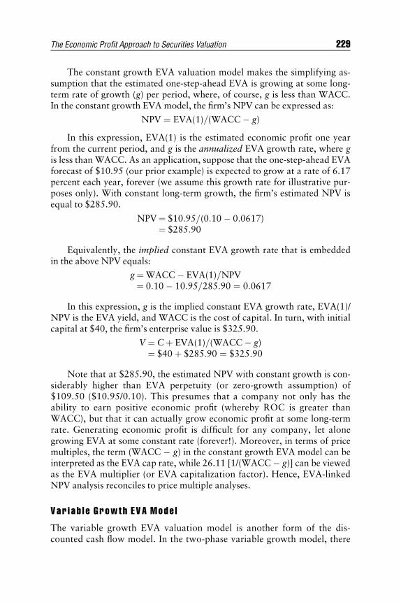
E1C09 08/13/2009 Page 229

The constant growth EVA valuation model makes the simplifying as-sumption that the estimated one-step-ahead EVA is growing at some long-term rate of growth (g) per period, where, of course, g is less than WACC.In the constant growth EVA model, the firm’s NPV can be expressed as:

NPV ¼ EVA(1)=(WACC � g)

In this expression, EVA(1) is the estimated economic profit one yearfrom the current period, and g is the annualized EVA growth rate, where gis less than WACC. As an application, suppose that the one-step-ahead EVAforecast of $10.95 (our prior example) is expected to grow at a rate of 6.17percent each year, forever (we assume this growth rate for illustrative pur-poses only). With constant long-term growth, the firm’s estimated NPV isequal to $285.90.

NPV ¼ $10:95=(0:10 � 0:0617)¼ $285:90

Equivalently, the implied constant EVA growth rate that is embeddedin the above NPV equals:

g¼ WACC � EVA(1)=NPV¼ 0:10 � 10:95=285:90 ¼ 0:0617

In this expression, g is the implied constant EVA growth rate, EVA(1)/NPV is the EVA yield, and WACC is the cost of capital. In turn, with initialcapital at $40, the firm’s enterprise value is $325.90.

V ¼ Cþ EVA(1)=(WACC � g)¼ $40 þ $285:90 ¼ $325:90

Note that at $285.90, the estimated NPV with constant growth is con-siderably higher than EVA perpetuity (or zero-growth assumption) of$109.50 ($10.95/0.10). This presumes that a company not only has theability to earn positive economic profit (whereby ROC is greater thanWACC), but that it can actually grow economic profit at some long-termrate. Generating economic profit is difficult for any company, let alonegrowing EVA at some constant rate (forever!). Moreover, in terms of pricemultiples, the term (WACC � g) in the constant growth EVA model can beinterpreted as the EVA cap rate, while 26.11 [1/(WACC � g)] can be viewedas the EVA multiplier (or EVA capitalization factor). Hence, EVA-linkedNPV analysis reconciles to price multiple analyses.

Var i a b l e Growth EVA Mode l

The variable growth EVA valuation model is another form of the dis-counted cash flow model. In the two-phase variable growth model, there


E1C09 08/13/2009 Page 230

are two growth rates that serve to capture the pattern of EVA flows duringhorizon and residual periods. In this context, it is common to assume thatEVA is growing at a relatively high rate during the horizon years (due tocompetitive or comparative advantages) while EVA growth settles down toeither zero or a mature growth rate during the residual years.8 We can makea simple change to the EVA assumption in the previous constant growthexample to see how this model works.

Specifically, suppose that a company’s one-step-ahead economic profit,EVA(1) of $10.95, is expected to grow at 7.5 percent for just one year, fol-lowed by a long-term or mature growth rate of 6.17 percent. In this case,there are two steps to estimating the firm’s NPV (and enterprise value) withvariable growth assumptions:

Step 1: Calculate the present value of the estimated EVA generated dur-ing the first growth phase—we’ll interpret this result as the NPVgenerated during the horizon period (forecast period), NPV-HV.

Step 2: Calculate the present value of the EVA earned during the maturegrowth phase. We’ll express this value as NPV-RV. Then, calculatethe present value of the firm’s residual (or terminal) NPV value.

With variable growth, the present value of EVA during the horizonyears can be expressed as:

NPV�HV ¼ PEVAt � (1 þ gNT)t�1=(1 þ WACC)t

(t ¼ 1 to N)

In this expression, EVAt is the estimated economic profit at period t,gNT is the near-term growth rate in EVA during the horizon period, andWACC is the discount rate or cost of capital. With just two periods (N = 2)during the horizon period, we can express the NPV horizon value as:

NPV � HV ¼ EVA(1)=(1 þ WACC) þ EVA(2)=(1 þ WACC)2

¼ EVA(1)=(1 þ WACC) þ EVA(1)(1 þ gNT)=(1 þ WACC)2

The net present value of the estimated EVA flow for the two-year hori-zon period is $19.68:

NPV � HV ¼ $10:95=(1:10) þ $10:95(1:075)=(1:10)2

¼ $9:95 þ $11:77=1:21¼ $9:95 þ $9:73¼ $19:68

In turn, the firm’s residual NPV at the end of period 2, NPV-RV(2), canbe calculated by noting that (1) the EVA forecast for period 3 can be viewedas EVA(2) growing at the long-term EVA growth rate, and that (2) the one-


E1C09 08/13/2009 Page 231

step-ahead forecast for period 3 is growing at the mature or competitivegrowth rate, gLT. With these assumptions, the three-step-ahead economicprofit, EVA(3), can be estimated according to:

EV(3) ¼ EVA(2)(1 þ gLT)¼ EVA(1)(1 þ gNT)(1 þ gLT)¼ $10:95(1:075)(1:0617) ¼ $12:50

With constant EVA growth for the residual period, the firm’s residualNPV value at the end of the two-year horizon period can be expressed as:

NPV � RV(2) ¼ EVA(3)=(WACC � gLT)

Upon substituting the estimated EVA for period 3, EVA(3) of $12.50,into the preceding expression yields NPV-RV(2), at $326.37:

RV(2) ¼ $12:50=(0:10 � 0:0617)¼ $12:50=0:0383¼ $326:37

Moreover, upon combining the NPV results for horizon and (dis-counted) residual periods, we obtain the total NPV, at $289.41:

NPV ¼ NPV � HV þ PV of NPV � RV(2)¼ $19:68 þ NPV � RV(2)=(1 þ WACC)2

¼ $19:68 þ $326:37=(1 þ 0:10)2

¼ $19:68 þ $326:37=1:21¼ $19:68 þ $269:73¼ $289:41

Notice that the variable growth NPV of $289.41 differs by a smallamount from the 6.17 percent constant growth EVA model result of$285.90.9 This minor difference in net present value results because we as-sumed only a 7.5 percent rate of growth in EVA for year 2. All other EVAvalues were assumed to be growing at 6.17 percent, as in the previous con-stant growth example. With initial capital of $40, the firm’s estimatedenterprise value is $329.41.

F orecas t EVA Va l u a t i o n Mode l

In practice, corporate managers and securities analysts like to forecast theannual economic profit over some discrete time period, say five or ten years.They then assess the residual value of economic profit based on varyingassumptions about EVA during the so-called out years, particularly in lightof the firm’s presumed competitive or comparative advantages, if any. Asbefore, the NPV of economic profit over the horizon years plus the present


E1C09 08/13/2009 Page 232

value of the residual NPV determines the firm’s overall net present value—or net creation of wealth. The firm’s enterprise value is equal to investedcapital plus the present value of all future EVA (which is NPV).

To illustrate the forecast EVA valuation model, we use the EVA esti-mates (NOPAT, capital, and WACC) obtained from a revenue forecastingmodel described by Grant (2003). Later on, we will look at the details ofeconomic profit estimation with standard accounting adjustments. Fornow, let’s see how economic profit estimates during a forecast period getrolled up into the firm’s enterprise value and intrinsic value of commonstock. In this context, Exhibit 9.1 shows EVA estimates over a 10-year fore-cast or horizon period. As before, with NOPAT(1) at $14.95, initial capitalof $40, and a cost of capital of 10 percent, the firm’s assessed economicprofit for year 1 is $10.95:10

EVA(1) ¼ NOPAT(1) � WACC � C(0)¼ $14:95 � 0:10 � $40:00 ¼ $10:95

Likewise, economic profit for year 2, at $12.74, is just NOPAT less thecapital charge on invested capital at the end of year 1 (or BOY capital at year 2).

EVA(2) ¼ NOPAT(2) � WACC � C(1)¼ $17:19 � 0:10 � $44:50 ¼ $12:74

At $44.50, the capital at the start of year 2 is a reflection of the initialcapital, C(0) of $40, plus the net investment in capital (including physicaland intangible capital) of $4.50 that occurred during year 1.

EXHIBIT 9.1 Forecasting Economic Profit (EVA)

Year

Yearly Net

Investment

Total Net

Capital NOPAT

Capital

Charge�Economic

Profit

0 40.001 4.50 44.50 14.95 4.00 10.952 5.18 49.68 17.19 4.45 12.743 5.95 55.63 19.77 4.97 14.804 6.84 62.47 22.74 5.56 17.185 7.87 70.34 26.15 6.25 19.906 9.05 79.39 30.07 7.03 23.047 10.41 89.80 34.58 7.94 26.648 11.97 101.77 39.77 8.98 30.799 13.77 115.54 45.73 10.18 35.5510 15.83 131.37 52.59 11.55 41.0411 Plus 54.17 13.13 41.04

�WACC = 10 percent.


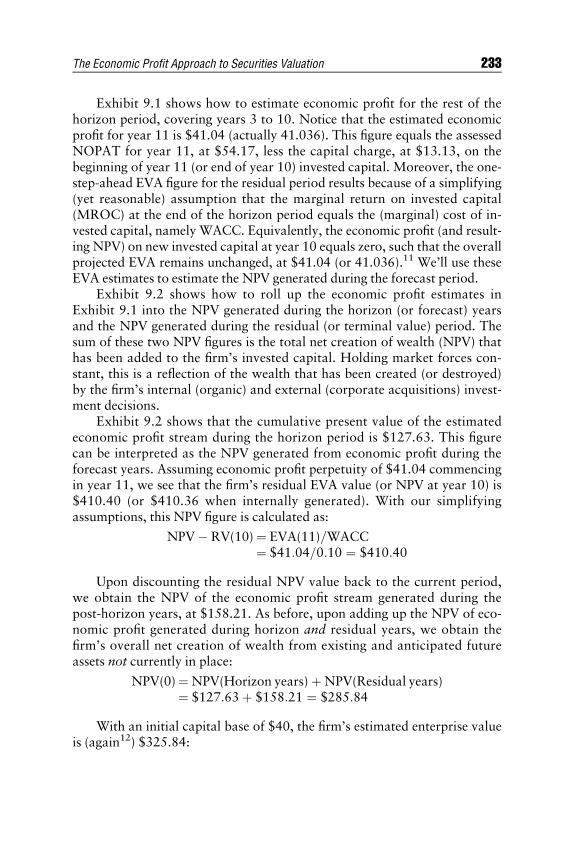
E1C09 08/13/2009 Page 233

Exhibit 9.1 shows how to estimate economic profit for the rest of thehorizon period, covering years 3 to 10. Notice that the estimated economicprofit for year 11 is $41.04 (actually 41.036). This figure equals the assessedNOPAT for year 11, at $54.17, less the capital charge, at $13.13, on thebeginning of year 11 (or end of year 10) invested capital. Moreover, the one-step-ahead EVA figure for the residual period results because of a simplifying(yet reasonable) assumption that the marginal return on invested capital(MROC) at the end of the horizon period equals the (marginal) cost of in-vested capital, namely WACC. Equivalently, the economic profit (and result-ing NPV) on new invested capital at year 10 equals zero, such that the overallprojected EVA remains unchanged, at $41.04 (or 41.036).11 We’ll use theseEVA estimates to estimate the NPV generated during the forecast period.

Exhibit 9.2 shows how to roll up the economic profit estimates inExhibit 9.1 into the NPV generated during the horizon (or forecast) yearsand the NPV generated during the residual (or terminal value) period. Thesum of these two NPV figures is the total net creation of wealth (NPV) thathas been added to the firm’s invested capital. Holding market forces con-stant, this is a reflection of the wealth that has been created (or destroyed)by the firm’s internal (organic) and external (corporate acquisitions) invest-ment decisions.

Exhibit 9.2 shows that the cumulative present value of the estimatedeconomic profit stream during the horizon period is $127.63. This figurecan be interpreted as the NPV generated from economic profit during theforecast years. Assuming economic profit perpetuity of $41.04 commencingin year 11, we see that the firm’s residual EVA value (or NPV at year 10) is$410.40 (or $410.36 when internally generated). With our simplifyingassumptions, this NPV figure is calculated as:

NPV � RV(10) ¼ EVA(11)=WACC¼ $41:04=0:10 ¼ $410:40

Upon discounting the residual NPV value back to the current period,we obtain the NPV of the economic profit stream generated during thepost-horizon years, at $158.21. As before, upon adding up the NPV of eco-nomic profit generated during horizon and residual years, we obtain thefirm’s overall net creation of wealth from existing and anticipated futureassets not currently in place:

NPV(0) ¼ NPV(Horizon years) þ NPV(Residual years)¼ $127:63 þ $158:21 ¼ $285:84

With an initial capital base of $40, the firm’s estimated enterprise valueis (again12) $325.84:


E1C09 08/13/2009 Page 234

EV ¼ Cþ NPV¼ $40:00 þ $285:84 ¼ $325:84

Moreover, with debt at say $12 and five shares of common stock out-standing, the firm’s intrinsic stock price is:

Intrinsic stock price ¼ (EV � Debt)=Shares¼ ($325:84 � 12)=5 ¼ $62:77

As explained earlier, the EVA approach to enterprise valuation pro-vides managers and investors with a direct assessment of the wealth that isbeing added—via discounted economic profit on existing and anticipatedfuture growth assets—to the firm’s invested capital. As we will see later, theenterprise value and the intrinsic stock price are the same figures that wouldbe obtained using the traditional free cash flow approach to securitiesvaluation.

EXHIBIT 9.2 Valuation of Economic Profit

Year EVA Present Value� Cumulative PV(0)

1 10.95 9.95 9.952 12.74 10.53 20.483 14.80 11.12 31.604 17.18 11.73 43.345 19.90 12.36 55.696 23.04 13.00 68.707 26.64 13.67 82.378 30.79 14.36 96.739 35.55 15.08 111.8110 41.04 15.82 127.63Residual Value 410.36

(at year 10)158.21

NPV 285.84Capital 40.00Corporate Value 325.84

Long-Term Debt 12.00Equity 313.84Shares Outstanding 5.00Price 62.77



E1C09 08/13/2009 Page 235

I n ves tmen t Oppor t un i t i e s and t he T -Per i o dEVA Mode l

In the EVA valuation model, the firm’s enterprise value is defined as investedcapital plus aggregate net present value. With a simple rearrangement, wecan see the part of the firm’s enterprise value that is attributed to economicprofit generated by existing assets and the EVA contribution due to futureinvestment (or growth) opportunities. Taken together, the two economicprofit sources determine the firm’s total net present value.

In this context, the firm’s enterprise value can be split into two compo-nents: (1) the present value of a NOPAT perpetuity generated by existingassets, NOPAT/WACC, and (2) the net present value of the firm’s antici-pated investment opportunities, Gf, according to:13

V ¼ NOPAT=WACC þGf

The obvious question at this point is how to estimate the NPV contribu-tion of the firm’s anticipated investment opportunities, Gf. While severalDCF approaches exist to estimate the market value of future investment op-portunities, we will estimate growth opportunities with a simplified versionof the T-period EVA model.14

Growth Oppor t un i t i e s and t he T - P er i o d EVA Mode l

In the T-period EVA model, the investor makes an assessment of the num-ber of periods that the firm can generate positive economic profit on itsanticipated future assets. This boils down to an estimate of the number ofpositive EVA periods (if any) that managers and investors perceive that thefirm can invest in real assets having an after-tax return on capital (ROC)that exceeds the opportunity weighted average cost of capital, WACC.Whether or not a company can actually earn positive (or negative) EVA inthe residual years (or out years) is determined by the competitive nature ofthe industry as it relates to the firm’s potential competitive or comparativeadvantage. We will assume that the length of the economic profit period,T, is greater than zero, at least for illustrating how this EVA valuationmodel works.

In formal terms, the T-period economic profit model can be expressed as:

Gf ¼ [Avg: EVA(Future)=WACC � T] � 1=(1 þ WACC)

In this expression, Avg. EVA(Future) is an economic profit perpetu-ity generated on new investment opportunities, T is the number of peri-ods that a firm can realistically earn positive economic profit on future


E1C09 08/13/2009 Page 236

investments, and WACC is the cost of capital, assuming risk constancyof future cash flows.

To illustrate the T-period EVA model,15 we make the simplifyingassumption that economic profit earned during the horizon years isattributed entirely to existing assets,16 while any economic profit gener-ated during the residual period is due to future assets not currently inplace. Also, we will make the simple assumption that the estimated eco-nomic profit for year 11, at $41.04, can be used to proxy the averageeconomic profit generated during the residual years. Based on these sim-plifications, the T-period EVA model suggests that a large portion of thefirm’s NPV and enterprise value can be determined by estimating thenumber of periods that it can generate positive economic profit duringthe residual years.

For example, with no restriction on the number of years that the firmcan earn economic profit of $41.04 during the residual period, we foundthat the firm’s estimated NPV at year 10 was $410.40 [$41.04/0.10]. Thisresidual EVA value has a current NPV of $158.21. Notice, too, that in theabsence of economic profit growth during the residual years the NPV of$158.21 is the maximum current value of the firm’s estimated EVA streamduring the post-horizon years. This, in turn, sets upper limit values on boththe firm’s aggregate NPV and its intrinsic enterprise value. Drawing valuesfrom before, we have $285.84 and $325.84, respectively.

In general, the T-period EVA model assumes that a firm’s opportu-nity to earn positive economic profit during the residual period is limitedby technological obsolescence and/or competition in the market forgoods and services. In this model, managers and investors must make anassessment of the number of periods that a company can realistically earnpositive economic profit for the future. By implication, we can say thatinvestors will not pay for negative EVA generated during the residual pe-riod covering years T þ1 to infinity. Moreover, if the return on futureinvestment opportunities is equal to the cost of capital, then growth op-portunities per se make no contribution whatsoever to the firm’s overallNPV. In this case the firm’s NPV is solely driven by the EVA generatedon its existing assets.

In lieu of these restrictions, Exhibit 9.3 shows how the NPV of thefirm’s future growth opportunities varies as the number of positive EVAperiods goes from (say) 5 to 100 years. At $410.40 (rounded), theexhibit shows the upper limit value of the economic profit stream gener-ated during the residual period. Notice how the residual value changesas T varies from 5 to 100 years of positive economic profit. Basedon present value dynamics, we see that the residual value function, RV(T), asymptotically approaches a line that represents the value of anEVA perpetuity.


E1C09 08/13/2009 Page 237

Exhibit 9.3 shows that with just five years of positive EVA in post-hori-zon years, the NPV of future EVA opportunities is only $59.97. Whenexpressed in terms of the firm’s enterprise value and its warranted stockprice, we obtain $227.61 and $43.12, respectively. In contrast, with 20 and30 years of positive economic profit during the residual period, the NPVvalues of future EVA opportunities are $134.69 and $149.14. The exhibitalso shows that with T of 20 and 30 years, the firm’s enterprise values are$302.33 and $316.78. Also, the corresponding stock price estimates are$58.07 and $60.96, respectively.

With unlimited positive economic profit in the residual years, we seethat the firm’s estimated enterprise value is $325.84 and its intrinsic stockprice is $62.77. These are the values that we obtained before. Notice thatwith five years of positive EVA in residual years that the estimated stockprice is only 69 percent ($43.12/$62.77) of the price obtained with un-limited positive economic profit. With 20 and 30 years of positive economicprofit in post-horizon years, the intrinsic stock prices are 93 percent and 97percent, respectively, of the price obtained with unlimited positive economicprofit.17 Thus, managers and investors must make an accurate assessmentof the number of periods that a company can earn economic profit for thefuture in order to have a realistic view of enterprise value and stock price.

Marke t - Imp l i ed I nves tmen t Per i o d

In practice, the T-period EVA model can be rearranged to solve for the mar-ket-implied number of years of positive economic profit on future

EXHIBIT 9.3 T-Period EVA Model

ResidualPeriod Annuity RV(T) RV(0)

NPV(0)� EV

StockPrice

PriceRatio %

5 41.04 155.56 59.97 187.61 227.61 43.12 68.7010 41.04 252.15 97.21 224.85 264.85 50.57 80.5620 41.04 349.36 134.69 262.33 302.33 58.07 92.5130 41.04 386.84 149.14 276.78 316.78 60.96 97.1140 41.04 401.29 154.72 282.35 322.35 62.07 98.8950 41.04 406.86 156.86 284.50 324.50 62.50 99.5760 41.04 409.01 157.69 285.32 325.32 62.66 99.8370 41.04 409.84 158.01 285.64 325.64 62.73 99.9480 41.04 410.16 158.13 285.77 325.77 62.75 99.9890 41.04 410.28 158.18 285.81 325.81 62.76 99.99100 41.04 410.33 158.20 285.83 325.83 62.77 100.00Infinite 41.04 410.36 158.21 285.84 325.84 62.77 100.00

WACC = 10 percent; horizon years = 10.�NPV(0) reflects present value of EVA during horizon and residual years.


E1C09 08/13/2009 Page 238

investment opportunities. The following inputs are required to solvefor market-implied T that is embedded in a firm’s NPV and enterprisevalue:

& Enterprise value (outstanding debt plus equity values18).& NOPAT perpetuity (or annualized equivalent of periodic NOPAT on

existing assets).& Average economic profit on new investments.& Cost of capital (WACC).

Upon solving for the market-implied number of growth periods, T, thatthe firm expects to earn positive economic profit, we obtain:

T ¼ [Gf � WACC � (1 þ WACC)]=Avg: EVA (future)

Upon calculating market-implied T, managers and investors can assesswhether this figure is consistent with a company’s intrinsic number of peri-ods to earn positive economic profit on future investments.

Based on our previous illustration, if the actual number of positive EVAperiods were, say, 10 years rather than 30 years, then the firm’s enterprisevalue and stock price would be overvalued in the capital market. Based onthe figures supplied before, the firm’s stock price would fall over time from$60.96 to $50.57—unless of course the firm’s managers could preempt thedecline by surprising investors positively about the number of periods thatfirm could earn positive economic profit on its investment opportunities.Conversely, a company’s stock would be undervalued if investors in-correctly perceived that the number of positive EVA periods was, say, 10years when in fact the intrinsic EVA period was longer.

RECONC I L I A T I ON OF EVA MODELS

While examining the EVA model, we focused on two general formulationsof the firm’s enterprise value. In this context, we said that the firm’s enter-prise value is equal to (1) invested capital, C, plus aggregate NPV and (2)the present value of a NOPAT perpetuity on existing assets plus the NPV ofall future investment opportunities—as captured by Gf. We can reconcilethese EVA valuation models for the firm’s enterprise value as follows.

To begin, note that NOPAT can be expressed as a capital charge earnedon the firm’s existing assets plus the EVA generated by existing assets al-ready in place. From this, we see why the firm’s enterprise value is equal toinvested capital, C, plus the NPV of all future economic profit arising


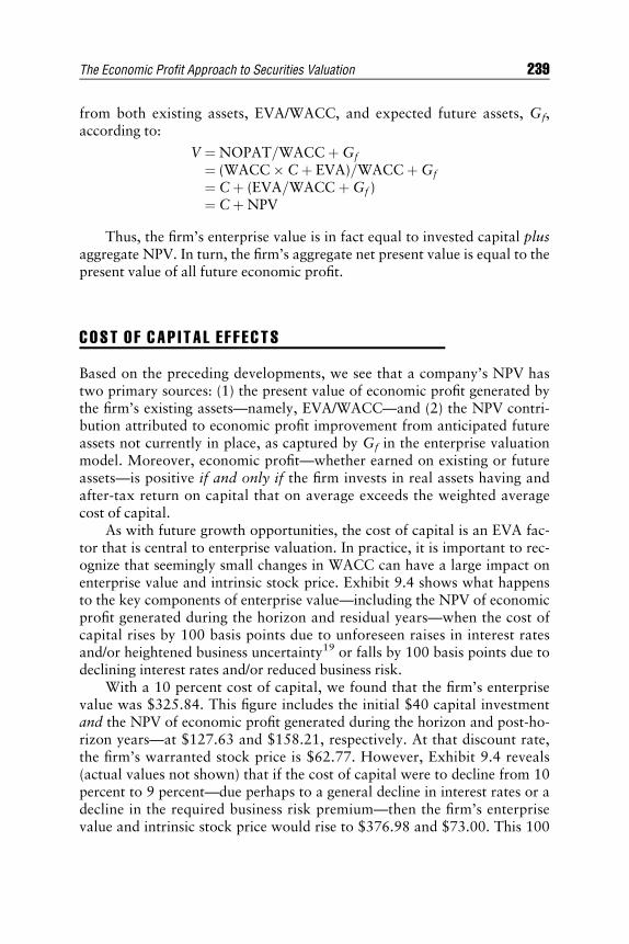
E1C09 08/13/2009 Page 239

from both existing assets, EVA/WACC, and expected future assets, Gf,according to:

V ¼ NOPAT=WACC þGf

¼ (WACC � Cþ EVA)=WACC þGf

¼ Cþ (EVA=WACC þGf )¼ Cþ NPV

Thus, the firm’s enterprise value is in fact equal to invested capital plusaggregate NPV. In turn, the firm’s aggregate net present value is equal to thepresent value of all future economic profit.

COST OF CAP I TA L E F F ECTS

Based on the preceding developments, we see that a company’s NPV hastwo primary sources: (1) the present value of economic profit generated bythe firm’s existing assets—namely, EVA/WACC—and (2) the NPV contri-bution attributed to economic profit improvement from anticipated futureassets not currently in place, as captured by Gf in the enterprise valuationmodel. Moreover, economic profit—whether earned on existing or futureassets—is positive if and only if the firm invests in real assets having andafter-tax return on capital that on average exceeds the weighted averagecost of capital.

As with future growth opportunities, the cost of capital is an EVA fac-tor that is central to enterprise valuation. In practice, it is important to rec-ognize that seemingly small changes in WACC can have a large impact onenterprise value and intrinsic stock price. Exhibit 9.4 shows what happensto the key components of enterprise value—including the NPV of economicprofit generated during the horizon and residual years—when the cost ofcapital rises by 100 basis points due to unforeseen raises in interest ratesand/or heightened business uncertainty19 or falls by 100 basis points due todeclining interest rates and/or reduced business risk.

With a 10 percent cost of capital, we found that the firm’s enterprisevalue was $325.84. This figure includes the initial $40 capital investmentand the NPV of economic profit generated during the horizon and post-ho-rizon years—at $127.63 and $158.21, respectively. At that discount rate,the firm’s warranted stock price is $62.77. However, Exhibit 9.4 reveals(actual values not shown) that if the cost of capital were to decline from 10percent to 9 percent—due perhaps to a general decline in interest rates or adecline in the required business risk premium—then the firm’s enterprisevalue and intrinsic stock price would rise to $376.98 and $73.00. This 100


E1C09 08/13/2009 Page 240

basis point change in WACC translates into a 15.69 percent rise in thefirm’s enterprise value.

However, if the firm’s cost of capital were to rise by 100 basis points—from 10 percent to 11 percent—then Exhibit 9.4 shows that the firm’s enter-prise value and intrinsic stock price would decline to $284.92 and $54.58,respectively. This in turn represents a 12.56 percent decline in the firm’swarranted enterprise value. As with the present value impact of changes ina company’s future investment opportunities, we see that enterprise valueand intrinsic stock price are impacted in a nonlinear way by fluctuations inthe firm’s cost of capital. This valuation result is the essence of equity dura-tion when viewed through an economic profit lens.

PR IC ING IMPL I CAT I ONS

The investment opportunities and cost of capital illustrations provide somestrategic pricing insight for managers and investors. Specifically, we see thatuncertainty about the number of years that a firm can generate positive eco-nomic profit on new investments and/or uncertainty about the firm’s truecost of capital can have a material impact on both its enterprise value andits intrinsic stock price. These valuation effects arise from so-called numera-tor and denominator effects. Moreover, there are changes in T and WACCthat can produce the same impact on the price of any company’s stock. For

EXHIBIT 9.4 Enterprise Value and the Cost of Capital: EVA Model


E1C09 08/13/2009 Page 241

example, the intrinsic stock price—see Exhibits 9.3 and 9.4, respectively—drops from $62.77 to about $51 when T declines to 10 years or the cost ofcapital, WACC, rises to 11.5 percent.20 Hence, anything that managers cando to increase the positive EVA investment period and/or decrease the op-portunity weighted average cost of capital will surprise investors positivelyand have a meaningful impact on both enterprise value and stock price.

EVA ACCOUNT ING ADJUSTMENTS

In practice, there are several value-based accounting adjustments that canbe made to calculate economic profit. While a detailed treatment of VBMaccounting adjustments is beyond the scope of this chapter, there are severalstandard accounting adjustments that are often made by corporate manag-ers and securities analysts when estimating economic profit. In this context,Exhibit 9.5 shows the standard income statement adjustments that aremade to basic NOPAT (tax-adjusted operating earnings), while Exhibit 9.6shows the corresponding balance sheet adjustments that are made to basicEVA capital (balance sheet debt and equity capital).21 As shown, there areequivalent top-down and bottom-up approaches to estimating NOPAT,while there are equivalent assets and financing approaches to estimatingEVA capital.

NOPAT Es t ima t i o n

Exhibit 9.5 shows the bottom-up approach to estimating NOPAT. In thisapproach, the analyst begins with net operating profit before taxes. This isjust the familiar earnings before interest and taxes (EBIT) figure on a com-pany’s income statement.22 To this amount, several value-based accountingadjustments are made to move toward a better representation of the firm’spretax cash operating profit. For example, the increase in LIFO reserve ac-count is added back to operating profit to adjust for the overstatement ofcost of goods sold (COGS)—due to an overstatement of product costing—in a period of rising prices (inflation), while the net increase in research anddevelopment expenditures is added back to pretax operating profit to recog-nize that R&D expenditures should be capitalized (meaning put on the EVAbalance sheet), as they presumably generate a future stream of economicbenefits.23

Likewise, the increase in accumulated intangibles amortization is addedback to pretax cash operating profit to reflect the fact that intangibles (pat-ents, copyrights, etc.) are a form of capital investment that need to earn acost of capital return just like expenditures on physical capital. The net


E1C09 08/13/2009 Page 242

increase in bad debt reserve is added back to pretax operating profit to moreaccurately reflect a company’s expected default experience. In addition, theimplied interest expense on operating leases is added back to operating re-sults to remove the effects of debt-related financing decisions. Moreover,the rise in reengineering and restructuring expenditures is added back topretax operating profit because these expenditures are viewed in the value-based realm as reengineering or restructuring investments.

Exhibit 9.5 also shows the top-down approach to estimating NOPAT.In this approach, the manager or investor begins with net sales and thenadds the increase in several equity reserve accounts, including the LIFOreserve and accumulated intangibles accounts, the bad debt reserve ac-count, and the rise in other equity reserve accounts noted earlier. As withthe bottom-up approach to estimating NOPAT, the implied interestexpense on operating leases is added to the EVA-based income statement.Information on LIFO (and other) reserve and leasing accounts is generally

EXHIBIT 9.5 Calculation of NOPAT from Financial Statement Data

A. Bottom-up approach

Begin: Operating profit after depreciation and amortization (EBIT)Add: Implied interest expense on operating leases

Increase (decrease) in equity reserve accounts, including:Increase in LIFO reserveIncrease in accumulated intangibles amortizationIncrease in bad debt reserveIncrease in capitalized research and developmentIncrease in cumulative write-offs of special items

Equals: Adjusted operating profit before taxesSubtract: Cash operating taxesEquals: NOPAT

B. Top-down approach

Begin: Net salesSubtract: Cost of goods sold

Selling, general, and administrative expensesDepreciation

Add: Implied interest expense on operating leasesIncrease (decrease) in equity reserve accounts (see listing above)Other operating income

Equals: Adjusted operating profit before taxesSubtract: Cash operating taxesEquals: NOPAT


E1C09 08/13/2009 Page 243

found in the footnotes to financial statements. In the top-down approach,the manager or investor subtracts from net sales the usual accounting in-come statement items such as cost of goods sold (COGS); selling, general,and administrative expenses (SG&A); and depreciation. Also, other oper-ating income (if any) shown on the income statement is included in thecalculation of pretax cash operating profit while other nonoperating in-come is excluded.

In the EVA tax calculation, the manager or investor begins withreported income tax expense on the income statement. To this amount, onesubtracts (or adds) the increase (or decrease) in the deferred income taxaccount obtained from the balance sheet. The tax benefit received from in-terest expense (tax rate � interest expense) and the tax benefit received fromimplied interest expense on operating leases is added to the reported incometax figure to remove the tax benefit obtained from debt-related financingdecisions. Also, taxes on nonoperating income (or tax benefits receivedfrom nonoperating expenses) must be subtracted from (or added to)reported income taxes to obtain an accurate measure of cash operatingtaxes. Upon subtracting cash operating taxes from pretax net operatingprofit (from either the bottom-up or the top-down approach), one obtainsnet operating profit after taxes (NOPAT).

I NV ESTED CAP I TA L

Exhibit 9.6 shows the EVA accounting adjustments that are necessary in theequivalent asset and financing approaches to estimating invested capital. Inthe assets approach, the manager or investor begins with net short-term op-erating assets (basically, net working capital). This reflects moneys tied upin current assets like accounts receivables and inventories as well as a nor-mal amount of cash needed for operations.24 Current liabilities such asaccounts payable, accrued expenses, and income taxes payable are of coursenetted from the short-term operating asset accounts. Short-term notes pay-able (a current liability account) are excluded because they represent asource of debt financing. Interest-bearing debt is reflected in the sources offinancing approach, and the debt-interest tax subsidy is reflected in the cal-culation of a company’s (dollar) cost of capital.

Cap i t a l E s t ima t i o n

Net plant, property, and equipment; goodwill; and other assets are thenadded to net short-term operating assets. As shown in Exhibit 9.6, severalequity reserve accounts are added to basic invested capital, including LIFO


E1C09 08/13/2009 Page 244

reserve, accumulated intangibles amortization (from patents, copyrights,etc), net capitalized research and development, cumulative bad debt reserve,and the cumulative write-off of special items like reengineering and restruc-turing costs. Also, the present value of operating leases (shown as leasedoperating assets) is added back to arrive at invested capital on the EVA bal-ance sheet.

In the sources of financing approach (Exhibit 9.6), the manager or in-vestor begins with the book value of common equity. This is just the famil-iar common at par, capital surplus, and retained earnings amounts on thebalance sheet net of treasury stock (if any). To this sum, one adds severalequity equivalent accounts, including those already listed on a company’s

EXHIBIT 9.6 Calculation of Capital from Financial Statement Data

A. Asset approach

Begin: Net short-term operating assetsAdd: Net plant, property, and equipment

Other assetsGoodwill (net)Equity reserve accounts, including:LIFO reserveAccumulated intangibles amortizationBad-debt reserveCapitalized research and developmentCumulative write-offs of special itemsLeased operating assets (Present value of operatingleases from debt equivalents)

Equals: Capital

B. Sources of financing approach

Begin: Book value of common equityAdd other equity and equivalents: Preferred stock

Minority interestDeferred income taxEquity reserve accounts (see listing above)

Add debt and debt equivalents: Interest bearing short-term debtCurrent portion of long-term debt dueLong-term debtOther liabilitiesCapitalized lease obligationsPresent value of operating leases

Equals: Capital


E1C09 08/13/2009 Page 245

balance sheet—such as preferred stock, minority interest, and deferred in-come taxes—as well as the companion equity reserve accounts mentionedin the assets approach to estimating invested capital—namely, LIFO re-serve, accumulated intangibles amortization, net capitalized research anddevelopment, bad debt reserve, and the cumulative write-offs of specialitems.

Debt and debt equivalents are then added to arrive at an EVA-basedfigure for invested capital. These debt-related accounts include those listedon the balance sheet—including interest-bearing short-term debt, long-termdebt, other liabilities, and capitalized lease obligations—and off-balance-sheet debt items25 such as the present value of operating leases. With theengagement of several EVA accounting adjustments, we see that the assetand financing approaches to estimating invested capital produce a robustmeasure (compared with basic EVA capital, or on-balance sheet capital) ofeconomic capital that is actually tied up in a business.

EVA APPL I CAT I ON : J LG DOW FUNDAMENTAL

To illustrate the results of an EVA valuation in practice, Exhibit 9.7 shows asnapshot of the JLG Dow Fundamental26 versus the Dow Jones IndustrialAverage (DJIA) from February 20 to May 1, 2008. The JLG Dow Funda-mental provides a bottom-up, EVA-based assessment of where the marketshould be trading based on underlying economic profit and risk character-istics. While past performance is not indicative of future returns, the JLG

EXHIBIT 9.7 JLG Dow Fundamental versus Dow Actual


E1C09 08/13/2009 Page 246

Dow Fundamental during the reporting period was a leading fundamentalindicator of stock market performance.

Specifically, Exhibit 9.7 shows convergence between the Dow Jones In-dustrial Average and the JLG Dow Fundamental. In terms of valuation sta-tistics, the estimated cost of capital for the Dow Industrials was 7.77percent, while the EVA-based future growth component of NPV for themarket index was 36 percent. This suggests that 64 percent of estimatedNPV was due to economic profit generated by existing assets while the bal-ance of intrinsic value added was due to the presumed EVA generated fromfuture growth opportunities (NPV from assets not currently in place). As ofApril 25, 2008, there were 10 active buy opportunities and 10 active sell orshort-sell opportunities within the JLG Dow Fundamental.

Due to the onset of the global financial crisis, stock market performancein the summer and fall of 2008 was impacted negatively by several adversefinancial events, as reflected in an unprecedented rise in the base equity riskpremium to an all-time high of 9.0 percent.27 As of January 12, 2009, theJLG Dow Fundamental stood at 8736, some 3% higher than the quotedvalue of the Dow Jones Industrial Average, at 8474. However, due to thelingering effects of the global financial crisis the market continued to abateuntil reaching the lows of early March 2009, and did not reach the Januaryvalue indicated by the JLG Dow Fundamental until June 1, 2009.

EVA L INK TO FC F VALUAT I ON

Given the preceding developments on EVA, it is helpful for managers andinvestors to know how EVA valuation relates to other DCF approachessuch as the free cash flow model. There are a couple of things to keep inmind regarding the similarities and differences between economic profit val-uation and, say, free cash flow valuation. The first observation is obvious—namely, that EVA and FCF valuation models (as well as DDM models forthat matter) must produce the same intrinsic value of the firm and its com-mon stock. That is, the value of the firm is driven by the present value of acash flow stream generated by the firm’s existing assets and its futuregrowth opportunities (assets not current in place). Having said that, it isworth emphasizing that EVA valuation provides managers and investorswith a direct measure of how the firm creates or destroys shareholder valueas reflected in NPV.

The second observation about EVA versus FCF valuation pertains tothe capital charge on invested capital. Specifically, in the economic profitapproach to securities valuation an explicit charge on the beginning of year(BOY) capital is assessed each year and deducted from NOPAT. In contrast,


E1C09 08/13/2009 Page 247

in free cash flow model, the present value of the capital charge on the firm’speriodic investment is implicitly recognized in the year that the capitalexpenditure is incurred. To see this, suppose that a company spends $4.50in capital improvement during a particular year. In the free cash flowmodel, the entire net investment would be subtracted from the net operatingprofit (NOPAT) in the year incurred. As mentioned, this is equivalent torecognizing the present value of the yearly capital charge that would be as-sessed in the EVA model. Assuming the capital charge can be expressed asperpetuity, this yields:

Net investment (year 1) ¼ $4:50¼ ($4:50 � WACC)=WACC ¼ $4:50

Hence, the free cash flow model subtracts the entire investment of$4.50 from NOPAT. In the EVA approach, the periodic capital charge of$0.45 (assuming a 10 percent cost of capital) would be deducted from eachyear’s NOPAT, beginning in the first year following the capital expenditure.Of course, the investment expenditure (assumed at $4.50) is added to theend of year 1 capital base to arrive at beginning of year (BOY) capital forthe second year.

Free Cash F l ow Va l u a t i o n

For comparative purposes, let’s take a look at free cash flow valuation.28 Inthis widely used model, the enterprise value of the firm can be expressed asthe present value of the anticipated cash flow stream generated by the firm’sexisting assets and its expected future growth assets not currently in place.In general, the FCF model is expressed as:

V ¼PFCFt=(1 þ WACC) t (t ¼ 1 to 1)

In this expression, V is the firm’s enterprise or corporate value, FCFt isthe assessed free cash flow for year t, and WACC is the weighted averagecost of debt and equity capital. In turn, the firm’s assessed free cash flow atyear t, FCFt, can be viewed as the anticipated net operating profit after tax,NOPAT, less the annual net investment, INV, to support the firm’s growth.

If, as before, NOPAT is $14.95 and the net investment is $4.50, thenthe one-step-ahead FCF is $10.45.

FCF(1) ¼ NOPAT(1) � INV(1)¼ $14:95 � $4:50 ¼ $10:45

Note that net investment refers to gross capital expenditures at year tless the required maintenance expenditures (measured by economic depreci-ation) on the firm’s existing assets. As with gross investment, net investment


E1C09 08/13/2009 Page 248

includes the required change in working capital (measured by the year-over-year change in operating current assets less the associated change in operat-ing current liabilities) to support a growing revenue and earnings stream.

FC F VALUAT I ON : HOR I ZON YEARS

To illustrate FCF valuation, we’ll use the 10-year stream of free cash flowestimates produced by the revenue-forecasting model used by Grant (2003).Exhibit 9.8 shows how to roll up the 10 years of free cash flow estimates forthe horizon years. The exhibit reports NOPAT, net annual investment, freecash flow, the present value of free cash flow for any given year, and thecumulative present value of the free cash flow estimates over the horizonperiod. Using a cost of capital (discount rate) of 10 percent, we see that the$10.45 free cash flow estimate for year 1 has a currently assessed marketvalue of $9.50.

Upon calculating the present value of the 10 years of free cash flow esti-mates and cumulating these values, we see that the firm’s horizon value is$116.98. However, stopping here in the enterprise valuation process wouldbe unduly conservative because it presumes that the firm is unable to gener-ate discounted positive free cash flow beyond the horizon period. Such anunfortunate state of affairs might exist for a company’s shareholders if (1)the firm’s existing capital assets at that time (year-end 10 in our case) werecompletely obsolete, and if (2) the NPV on all future investments were zero;since the EVA on future investment opportunities is zero when the marginalreturn on future investments equals the cost of capital.

EXHIBIT 9.8 FCF Valuation: Horizon Years

Year NOPAT Net Investment FCF Present Value� Cumulative PV

1 14.95 4.50 10.45 9.50 9.502 17.19 5.18 12.01 9.93 19.433 19.77 5.95 13.82 10.38 29.814 22.74 6.84 15.90 10.86 40.675 26.15 7.87 18.28 11.35 52.026 30.07 9.05 21.02 11.87 63.887 34.58 10.41 24.17 12.40 76.298 39.77 11.97 27.80 12.97 89.269 45.73 13.77 31.96 13.55 102.8110 52.59 15.83 36.76 14.17 116.9811 Plus� 54.17



E1C09 08/13/2009 Page 249

FC F VALUAT I ON : R ES I DUAL YEARS

While several assumptions can be made about free cash flow generationduring the post-horizon years,29 we’ll make the simplifying (and economi-cally consistent) assumption that the marginal return on the net investmentat end of the horizon period earns a cost of capital return. This is tanta-mount to saying that (1) free cash flow for post-horizon years is equal tothe one-period-ahead estimate of NOPAT, and (2) that economic profit gen-erated by the end-of-horizon period net investment (and the EVA on anyfuture investment) is equal to zero. With this zero-NPV assumption, thefirm’s residual (or continuing) value at year T can be expressed in simpleterms as:

VT ¼ NOPATTþ1=WACC

While the resulting perpetuity is a convenient way out of a complex ter-minal value pricing process, we still need to estimate the one-step-aheadNOPAT as of the end of the horizon period. Fortunately, we can obtain thisforecast with knowledge of (1) the firm’s plow-back or net investment-to-NOPAT ratio, and (2) the marginal return on invested capital (MROC).With this information, we can express the firm’s growth in NOPAT, gN, as:

gN ¼ PBR � MROC

In this expression, gN is the estimated year-over-year growth rate inNOPAT from the end of the horizon period, PBR is the plowback ratio,measured by net investment during the last year of the horizon period overthe end-of-horizon period net operating profit after tax, NOPATT.30

Assuming that the investment at year 10, at $15.83 (again, Exhibit 9.8),earns a cost of capital return, we obtain an estimated NOPAT growth ratefor the residual or continuing period of 3 percent.

gN ¼ ($15:83=$52:59) � 0:10¼ 0:3010 � 0:10 ¼ 0:0301 (or 3:01%)

It is now a simple matter to estimate the one-step-ahead NOPATaccording to:

NOPAT11 ¼ NOPAT10 � (1 þ gN)¼ $52:59 � (1:0301) ¼ $54:17

Note that this is the same continuing value for NOPAT as indicated inExhibits 9.1 and 9.8. Thus, the firm’s residual value at year 10 is equal to$541.73. This is obtained by discounting the one-step-ahead NOPAT per-petuity by the 10 percent cost of capital. Equivalently, this residual value


E1C09 08/13/2009 Page 250

figure is obtained by multiplying the estimated NOPAT perpetuity of$54.17 by a price-to-NOPAT multiplier of 10 (equal to 1/WACC).

V10 ¼ $54:17=0:10¼ $54:17 � 10 ¼ $541:73

Moreover, upon discounting the residual value back 10 periods, we ob-tain the intrinsic value, at $208.86, of the free cash flow generated duringthe residual or continuing years. As summarized in Exhibit 9.9, we see thatthe enterprise value of the firm is $325.84. This value consists of $116.98 inhorizon value plus $208.86 of current residual value. With long-term debtat $12, and five shares of common stock outstanding, the warranted stockprice is $62.77. Not surprisingly, the firm’s enterprise value of $325.84 andits intrinsic stock price of $62.77 are the same values that we obtained inthe EVA valuation model.

EXHIBIT 9.9 FCF Valuation: Residual Years

Year NOPATNet

Investment FCFPresentValue�

CumulativePV

1 14.95 4.50 10.45 9.50 9.502 17.19 5.18 12.01 9.93 19.433 19.77 5.95 13.82 10.38 29.814 22.74 6.84 15.90 10.86 40.675 26.15 7.87 18.28 11.35 52.026 30.07 9.05 21.02 11.87 63.887 34.58 10.41 24.17 12.40 76.298 39.77 11.97 27.80 12.97 89.269 45.73 13.77 31.96 13.55 102.8110 52.59 15.83 36.76 14.17 116.9811 Plus 54.17Residual

Value541.73

(at year 10)208.86

CorporateValue

325.84

Long-TermDebt

12.00

Equity 313.84Shares

Outstanding5.00

Price 62.77



E1C09 08/13/2009 Page 251

Before concluding, it is interesting to see that the current residual value,at $208.86, makes up some 64 percent of the firm’s warranted corporatevalue. This large residual value impact is a common finding among dis-counted cash flow approaches—whether dividend discount model (DDM),free cash flow (FCF), or economic profit approaches—to estimate enterprisevalue and stock price. In practice, the residual value (or terminal value) im-pact is especially pronounced for growth-oriented companies.31 Examplesinclude companies operating in the technology and health care sectors ofthe economy since most of their enterprise value comes from distant—andoften very difficult to predict—free cash flow and EVA generated on currentand future R&D investments.

SUMMARY

Like any DCF model, the EVA valuation model has both attractive featuresand some limitations. On the positive side, the economic profit model pro-vides a direct means by which managers and investors can assess the NPVcontribution from existing assets as well as future growth opportunities. Inthis context, the firm’s wealth creation—as measured by its NPV—is equalto the present value of all future economic profit generated by existing assetsand anticipated future assets (growth opportunities) not currently in place.With discounted positive economic profit, a company is a wealth creator,while with discounted negative economic profit a company is—un-fortunately–a wealth destroyer.

While EVA valuation is intuitively appealing, managers and investorsneed to realize that the resulting estimates of enterprise value and intrin-sic stock price are highly sensitive to the model inputs. We found that aseemingly small change in the length of the firm’s economic profit period(T) and/or its cost of capital (WACC) via equity duration effects can havea meaningful impact on the value of the firm and its outstanding shares.With uncertainty about model inputs, it is clear that managers must doeverything within their responsibility and control to (honestly!) surpriseinvestors positively about key economic profit drivers such as the returnon capital, the cost of capital, and the length of the economic profitperiod.

We recognized several value-based accounting adjustments that shouldbe taken into consideration when estimating economic profit. We also pro-vided an application of EVA valuation in the context of the JLG Dow Fun-damental. Finally, we argued that EVA valuation must reconcile to otherwell-known discounted cash flow approaches such as the dividend discountmodel and the traditional free cash flow model.


E1C09 08/13/2009 Page 252

NOTES

1. EVA1 is a registered trademark of Stern Stewart & Co.2. However, this does not mean that the EVA approach to securities valuation

gives a better answer than that obtained from other valuation models.3. Grant (2003).4. As explained later, invested capital or EVA capital can be obtained using an

equivalent assets or financing approach.5. When evaluating companies, investors must be keenly aware of economic profit

influences from industry, sector, and general market effects.6. Since NOPAT is net of depreciation on the EVA income statement, we must use

net (of accumulated depreciation) operating assets on the EVA balance sheet.Equivalently, we could use gross operating profit after tax (GOPAT) and grossinvestment to obtain the same EVA results.

7. The dollar units assumed in the EVA illustration are a matter of detail ratherthan substance.

8. Some investors use a three-stage EVA growth model, with transitional or decayrate of cash flow growth between horizon and residual stages. The so-called‘‘H (or half-life)’’ model is popular in this regard.

9. A variable-growth EVA model can produce an answer that is substantially dif-ferent from that obtained with a constant-growth model. The goal here is toshow that the present value dynamics of a variable-growth model are differentfrom those of a constant-growth model.

10. Again, the dollar units assumed in the illustration are a matter of detail ratherthan substance.

11. In other words, if MROC equals WACC, then the change in EVA from period Tto T + 1 is zero because the change in NOPAT, at $1.58, is equal to the dollarcapital charge on the end-of-horizon-period net investment of $15.83.

12. With long-term growth of precisely 6.1692 percent in the constant-growth EVAmodel, we obtain the same value—at $285.84—as that shown in the two-stagevariable-growth model. This NPV value is marginally different from the$285.90 figure that we obtained before with the assumed constant EVA growthrate of 6.17 percent.

13. The enterprise valuation model presented here is based on the classic ‘‘invest-ment opportunities approach to valuation’’ described by Fama and Miller—seeEugene F. Fama and Merton H. Miller, The Theory of Finance (New York:Holt, Rinehart & Winston, 1972).

14. For an insightful discussion of the T-period EVA model, see G. Bennett StewartIII, The Quest for Value (New York: HarperCollins, 1991).

15. In the previous EVA illustration, we assumed no future investment opportuni-ties beyond the horizon period. While we utilize the same numbers in theT-period EVA illustration that follows, the goal here is to shed basic insight onEVA investment opportunities (or periods) without getting bogged down indetailed formulas that model the firm’s investment opportunities.


E1C09 08/13/2009 Page 253

16. This simplification presumes that the firm’s existing capital is worthless at theend of the 10-year horizon period.

17. Notice, too, that with 50 years of positive EVA during residual years the stockprice is virtually the same as the perpetuity result, at $62.77. While wealth-creating managers should focus on long-term EVA rather than just short-termEVA, this sheds some interesting light on how long is ‘‘long.’’

18. In practical application of enterprise valuation models, long-term debt is oftenmeasured at book value while equity capitalization—number of shares of stockoutstanding times stock price—is used for the common stock.

19. As a real-world example, one would expect a significant rise in the equityrisk premium (a component of the cost of equity) due to the tragic eventsof September 11, 2001. If correct, this would go a long way in helping toexplain the sharp decline in stock prices that occurred in the aftermath of9/11.

20. Specifically, if T falls from infinity to 10 years, or WACC rises from 10 percentto 11.5 percent, then the stock price declines from $62.77 to about $51—actually, the price is $50.57 with T at 10 years, and $51.09 with WACC at11.5 percent, separately.

21. See JLG Research at www.jlgresearch.com for software that calculates EVAwith standard value-based accounting adjustments.

22. Net operating profit before taxes (EBIT) is also the same as operating profitafter depreciation and amortization.

23. R&D expenditures should be capitalized and amortized over a useful timeperiod such as five years, rather than expensed on the current year income state-ment as if these expenditures have no future cash flow benefit.

24. Estimates of a normal amount of cash required for operations vary by indus-try—such as 0.5 percent to 2 percent of net sales. Also, one can make a distinc-tion between invested capital and operating capital. Operating capital isgenerally viewed as invested capital net of excess cash and marketable securitiesand goodwill arising from premiums paid in corporate acquisitions

25. The EVA recognition of all forms of debt including off-balance-sheet debt isimportant. While EVA accounting uses information that is deemed accuratefrom a company’s published financial reports, EVA cannot possibly reflect off-balance-sheet debts arising from hidden liabilities or fraudulent accountingtransactions as in the notorious case of Enron.

26. See www.jlgresearch.com for equity valuation software and updates on the JLGDow Fundamental.

27. For explanation of the base equity risk premium on an ‘‘approximately-certainty-earnings (ACE) portfolio,’’ see Abate, Grant, and Rowberry, ‘‘Under-standing the Required Return under New Uncertainty,’’ Journal of PortfolioManagement, Fall 2006.

28. See Alfred Rappaport, ‘‘Strategic Analysis for More Profitable Acquisitions,’’Harvard Business Review (July/August 1979) for a pioneering application ofthe free cash flow model.


E1C09 08/13/2009 Page 254

29. Such possibilities include constant growth in free cash flow during the residualyears (at a growth rate less than WACC) and some form of competitive decay inthe estimated free cash flow during post-horizon years.

30. The growth in NOPAT, gN, can be expressed as the product of the net invest-ment plow-back ratio (PBR) times the marginal return on net invested capital,MROC, because (1) PBR measures net investment over NOPAT (at end of thehorizon period), and (2) MROC equals the change in NOPAT over netinvestment.

31. The term growth-oriented companies is taken to mean companies that can earnsubstantially positive EVA on future investment opportunities. They do sobecause the estimated after-tax rate of return on future investment opportuni-ties widely exceeds the WACC.

RE F ER ENCE

Grant, James L. Foundations of economic value added. 2nd ed. Hoboken, NJ:John Wiley & Sons, 2003.


E1C10 09/03/2009 Page 255

CHAPTER 10Valuation for Managers

Closing the Gap betweenTheory and Practice

Dennis N. AustManaging Director, CharterMast Partners

Over the past three decades, creating shareholder value has been widelyadopted as a principal objective for publicly held corporations, at least

in theory.1 In practice, the results have been mixed. The long-term secularincrease in corporate sector profits is consistent with the image of hard-nosed corporate executives diligently working to increase shareholdervalue. Yet a continuing stream of corporate miscues suggests otherwise.Whether because of overpriced acquisitions and bad strategic decisions, orbecause of flagrant, Tyco-type abuses, a significant number of major firmsstill fail to create value for their shareholders. Numerous benchmarks docu-ment this consistent underperformance over both long-term and short-termhorizons. For example, during 2007, even though the S&P 500 index in-creased by 3.5 percent, nearly half of the firms in the index (249 firms,according to statistics provided by Ativo Research LLC) ended the yearwith their stock prices lower than when they started.

Of course, there are numerous reasons for falling stock prices. Externalfactors such as adverse business cycles, market dynamics, and sector rota-tion regularly drive down stock prices in any given year. Even when execu-tives diligently work to create value for shareholders, they can still beundermined by competitors that push back, staff who fail to execute, and

255

E1C10 09/03/2009 Page 256

business conditions that move against them. And yet, while these mayseem like reasonable excuses, there’s much more to this story of why somany firms perform so poorly.

This chapter asserts that value management experts, whether externalconsultants or internal financial executives, have unintentionallysabotaged their causes. These experts have provided senior executiveswith increasingly sophisticated, but ultimately unworkable shareholdervalue enhancement solutions. These solutions almost always produceone of two results. One type of firm, ambitious and aggressive, initiallyadopts the best, most sophisticated metrics and methodologies. However,most such ambitious initiatives eventually fail, as the difficulty of imple-menting an overly complex approach undermines its usefulness and ac-ceptance throughout the organization. The other type of firm, cautiousand practical, sticks with a tried-and-true approach that is more easilyunderstood, but ultimately proves inadequate for the task. Executivesin these firms diligently execute to meet their targets, but fail to delivershareholder results because the performance metrics and targets employedare flawed.

From the corporate management perspective, the challenge for valua-tion experts is not so much to devise a methodology that correlates perfectlywith the market, but rather to apply a framework that provides reason-ably accurate insights and guidance within the framework of an easilyunderstood package. We, as experts, need to know when to say, ‘‘That’sgood enough.’’

This doesn’t mean we should simply discard the powerful (but com-plex) models linking operating performance to stock prices, particularlywhen the alternatives are simplistic rules of thumb with marginal linksto value creation. Rather, the challenge is to rework or streamline thesesophisticated valuation models so that they become more accessible andpractical to executives and managers at all levels of an organization.Carefully paring back complexity while preserving (or substituting) corecapabilities can produce valuation models that retain sufficient marketlinkages, while still providing useful insights and incentives for corpo-rate management. It is often difficult, even painful, to leave out sophis-ticated adjustments and nuances that are supported both by financialtheory and empirical evidence. However, in the long run, leaving outnuances is often a better decision. This is particularly true if the ulti-mate choice is between a near-perfect methodology that is eventuallydiscarded and a reasonably good approximation with the staying powerto provide long-term, market-linked discipline and insights.


E1C10 09/03/2009 Page 257

CURRENT ENV I RONMENT

Consider this contrast between theory and reality:

Any expert in business strategy must have a superior understandingof what drives financial value creation in the first place. Such a strat-egy expert must thoroughly understand the differences and nuancesbetween relative valuations and discounted cash flow analyses. . . .In short, he or she must be an expert in business valuations.

Littman, J. and Frigo, M. (2004)

In the classroom, value-based management (VBM) programs soundseductively simple. Theoretically, they involve just two steps. First,adopt an economic profit metric, such as Stern Stewart’s EconomicValue Added (EVA), as a key measure of performance. Second, tiecompensation to agreed-upon improvement targets in that metric.For large companies with flagging share prices, this looks like amiracle cure. All they have to do to boost their market value is callin consultants to revamp their accounting system, install the newmeasure of performance, align their incentive systems, and voil�a!Managers and employees will march along like good foot soldiersand start making all kinds of value-creating decisions.

If only it were that easy. As recent reports in the press indicate,almost half the companies that have adopted a VBM metric havemet with mediocre success. Some have even abandoned the systemaltogether after three to five years, reverting to traditional perform-ance measures such as earnings per share.

Haspeslagh, Noda, and Boulos (2001)

Haspeslagh, Noda, and Boulos conclude that effective value manage-ment isn’t so much about numbers and metrics, but rather is centered oncultural change. At one point they quote Cadbury Schweppes CEO JohnSunderland: ‘‘Managing for value is 20% about the numbers and 80%about the people . . . because people create value.’’ Successful VBM adopt-ers build on existing accounting systems, avoid complexity, and adoptmethodologies that can be widely understood and embraced throughout theorganization.

Unfortunately, as valuation experts we have often embraced a differentperspective.

Valuation for Managers 257

E1C10 09/03/2009 Page 258

Of course, a highly precise and nuanced approach to valuation is im-portant in certain contexts. A few percentage points in investment returnscan make the difference between success and failure for institutional port-folio managers, so they employ highly trained financial specialists who usethe most sophisticated models in an attempt to realize as much alpha aspossible from each portfolio. Highly sophisticated models are also justifiedin mergers, acquisitions, divestitures, and related financial transactions,where 1 percent of improved accuracy on a $10 billion deal is worth $100million. Even so, the success of most acquisitions depends more on under-standing the business, getting the forecast right, effectively executing thepostmerger integration, and having the confidence and judgment to walkaway from a bad deal. Having a sound valuation model is undoubtedly im-portant and appropriate. The risk increases when that model becomes socomplex that it diverts attention from more critical issues.

The key challenge when choosing a valuation model/methodology is tomatch the tool to the objective. Institutional portfolio managers can profitfrom highly complex models. Executives making major deals can gaininsights from sophisticated analysis. But for ongoing corporate performancemanagement and value creation, the objectives are considerably different.Does the model provide managers with directionally accurate incentivesand insights so that they make the right decisions? Is it relevant to manag-ers’ day-to-day activities and responsibilities? Is it sufficiently clear andstraightforward that it can be implemented throughout the organization?

In his 1996 Chairman’s Letter, Warren Buffett described BerkshireHathaway’s key principles for executive compensation: ‘‘Goals should be(1) tailored to the economics of the specific operating business; (2) simple incharacter so that the degree to which they are being realized can be easilymeasured; and (3) directly related to the daily activities of plan partici-pants.’’ (Buffett 1996) If one slightly rephrases the first principle as ‘‘tail-ored to the economics of how the specific operating business creates value,’’then these principles provide excellent guidance for the corporate executiveseeking to implement a value creation framework throughout his organiza-tion. Buffett also cautioned against arrangements that are ‘‘totally out of thecontrol of the person whose behavior we would like to affect,’’ observingthat such schemes ‘‘may actually discourage the focused behavior we valuein managers.’’ For example, consider the all-too-common situation whenthe valuation framework leads operating managers into extended debatesabout intricacies such as alternative cost of capital estimates. There is abso-lutely no question that operating managers need to know that capital has acost, and they need to know approximately what that cost is. But most op-erating managers have effectively zero control over their cost of capital. Aslong as they have an answer that is approximately right, effort dedicated to


E1C10 09/03/2009 Page 259

refining the estimate is effort diverted from running the business. (One par-ticularly savvy client addressed this problem by stating cost of capital as a3 percentage point range. Operating units and projects that were above thisrange were clearly exceeding the cost of capital, while those below thisrange were clearly underperforming. For those within the range, a seniorexecutive observed that he was satisfied that the operation was ‘‘closeenough’’ to meeting the cost of capital, and the operating manager’s timewould best be spent on improving operating performance rather than tryingto justify a lower cost-of-capital estimate.)

From a managerial perspective, the purpose of valuation is to provideproper insights, incentives, and control processes. For managers, valuation isconcerned with change. If I choose among actions X, Y, and Z, the issueis which will increase value and which will destroy value. Once I have mademy choice, how do I evaluate whether the financial results provide the share-holder value impact I expected? Valuation is also about relative value, and itsdirection. It is important to know which business units add value, which areneutral, and which destroy value, as well as how these relationships arechanging over time.

ALT ERNAT I V E MEASURES OF VALUE CREAT I ON :A QU I CK REV I EW

So, if the goal is to create value, what should you measure?Stock price, or more precisely total shareholder return (TSR), is the gold

standard. By definition, TSR is the return actually earned by shareholders.Unfortunately, TSR is affected by many factors, including broader marketmovements, investor sentiment, rumors, and so on that have little or nothingto do with what management accomplishes in running the business. TSRmeasures expectations, not results. It also provides an unclear link betweenmanagement actions and objectives. Although management might budget asales or profit increase of, say, 20 percent, with some degree of confidence,budgeting a stock price increase of 20 percent is considerably riskier. Fur-thermore, compensation based on stock price has directly led to many of theexcesses of the past decade. First, stock options paid off exorbitantly duringthe technology bubble, even when completely unjustified by firm-specific fi-nancial performance. Then, when the bubble burst, firms turned to backdat-ing and repricing options, an attempt to salvage returns for hardworkingexecutives as a falling market slammed both good and bad companies alike.Corporate cultures emerged where employees had one eye on their work andthe other on the stock ticker, watching to see how quickly their ‘‘lotterytickets,’’ otherwise known as stock options, would make them rich.


E1C10 09/03/2009 Page 260

Another traditional measure is discounted cash flow (DCF) valuation.The key problem with DCF is its dependence on projections, which makesit an inherently subjective measure. Also, DCF (as normally implemented) isa point-in-time measure. A manager typically constructs a detailed cashflow forecast, which is then discounted back to determine a specific netpresent value of the business unit (or project) as of some specific point intime. Rarely do managers construct a time series of DCF estimates showinghow business value has changed over extended multiyear time periods.(Although Thomas and Atra describe a creative methodology for automatedDCF valuations in Chapter 11 of this book, such techniques have not yetbeen widely adopted.) In current practice DCF remains primarily a point-in-time calculation, so it doesn’t show how value is being created ordestroyed. In cases when a time series of actual market values is available(e.g., historical stock prices for publicly traded firms), using a single point-in-time DCF value misses an important opportunity to confirm that thetrend in calculated value is consistent with the trend in actual value.

Other traditional metrics (sales growth, earnings per share (EPS)growth, etc.) are relatively simple, but empirically unrelated to value cre-ation. Earnings before interest, taxes, depreciation, and amortization(EBITDA), for example, is widely used. It reflects the cash-generating per-formance of a business, but not the investment required to support thatcash generation. Although EBITDA multiples are used to relate EBITDA tovaluation, multiples vary widely between firms over time. EBITDA multi-ples implicitly recognize the importance of cash generation, but don’t incor-porate the assets required to generate that cash flow.

Residual income metrics, such as economic value added (EVA), whichhave been adopted by a significant number of firms, have both advantagesand disadvantages. An explicit capital charge reflects the impact of manag-ing assets, and the structure of the metric addresses issues such as scale andleverage. The biggest disadvantage is that residual income is not directlycomparable to stock price, so it can be difficult or impossible to confirmhow reliably operating changes impact valuation. Although the metric itselfis reasonably straightforward, we’ve seen clients who have abandoned themetric because too many complex adjustments undermined its usefulness.Consistent with the theme of this chapter, firms using residual income needto focus on practical utility rather than theoretical purity.

Return metrics (sometimes flippantly characterized as ‘‘return on what-ever’’) provide only a partial answer at best. In our experience, when such ametric comes closer to representing the underlying cash flow economics, itdoes relate more closely to value creation. A traditional accounting metriclike return on equity is computed using two synthetic and often suspectinputs, net income and equity, so it isn’t surprising that return on equity has


E1C10 09/03/2009 Page 261

little relation to value creation. Return metrics that focus on cash generationand total investment are more closely linked to value creation. One highlysophisticated measure was developed at Callard, Madden & Associates inthe 1970s. Using an internal rate of return format, cash flow return on invest-ment (CFROI) balances inflation-adjusted assets against cash generation tocompute the economic rate of return actually earned by any firm or business.Various organizations have introduced refinements and variations on thismetric, but Bart Madden provides a thorough description of the basic con-cept and calculation in his book on CFROI valuation (Madden 1999).

Even though carefully constructed metrics like cash flow return on in-vestment provide powerful insights when examining trends or comparingdifferent firms, like all ‘‘return on’’ metrics, they can prove a treacherousfoundation for making decisions about value creation. Jensen (2001) suc-cinctly explains the problem of using return and ratio measures:

Here I can be blunt: Don’t do it. Using ratios, such as sales marginor return on assets, inevitably produces gaming. That’s becausemanagers can increase the measure in two ways: by increasing thenumerator or decreasing the denominator. If, for example, a com-pany tracks performance according to margin as a percentage ofsales, managers can increase their pay by simply cutting back sales(selling only the highest margin products) instead of working to in-crease the margins on all products. The result: Total dollars ofprofit fall, and company value erodes.

Using a return measure as a surrogate for value creation inevitably in-troduces a bias to reduce assets. Although focusing growth on high-returnbusinesses is a powerful value-creation strategy, and redeploying underper-forming assets often does make economic sense, arbitrarily shedding assets(or underinvesting) to boost returns can easily diminish the long-term cashflow, ultimately destroying value.

The underlying problem with return metrics is that they simply fallshort of the ultimate goal, which is value creation. Over the years, we haveobserved a number of firms embracing goals such as earning a return oninvestment (however measured) in the top quartile (or top quintile, or topthird) of the S&P. These goals usually tie to some incentive compensationframework that links specific payouts to some range of performance, but aslong as the firm meets its overall return on investment goal, managementearns a substantial bonus. That problem is that return on investment isn’tthe same thing as value created for shareholders. For many slow-growing,mature firms, what drives value creation isn’t the level of returns, but thetrend in returns. Even if management continues to meet its top quartile


E1C10 09/03/2009 Page 262

target and earns a hefty bonus, flat returns translate to minimal value cre-ation, and eroding returns destroy value. (In fact, firms with subpar returnsregularly create substantial value, and are often more attractive investmentsthan consistent high-return firms. They create value by improving return oninvestment, as successful turnaround specialists have demonstrated overand over. But once the turnaround is accomplished, maintaining the samerate of improvement becomes significantly more difficult.)

Measuring return on investment is not the same as measuring valuecreation. If the objective is to increase the value of a company or businessunit, rather than focusing on surrogates like return on investment, theideal metric should be some reasonably direct measure of value. If it isused as a performance measure, it should measure actual achieved per-formance, rather than forecasts. And it should be routinely and consis-tently computed over time, because value creation is defined as change invalue. One such framework is described in the Valuation Equation Solu-tion section. Cash flow ROI models project a stream of cash flows, whichare then discounted back to present value. The cash flow profile is ad-justed based on projected asset growth rates and standardized hold/fadeparameters. The original model was developed at Callard, Madden &Associates in the 1970s, then heavily promoted by HOLT Planning Asso-ciates, formed by departing Callard, Madden employees in 1985. SinceMadden documented the methodology (Madden 1999), variations of thesemodels have been developed and promoted by various offshoots of theCallard and HOLT organizations.

Cash flow ROI models have been accepted by a large number of institu-tional investors, but have been less widely adopted in the general businesscommunity. Adherents (including the author) believe these models have avery strong link to value, and therefore can serve as powerful tools for theoperating manager seeking to increase the value of the firm.

One particular advantage of this type of valuation model is its ability toproduce a stream of point-in-time value estimates. Exhibit 10.1 shows howthe Ativo/CharterMast valuation model produces annual value estimatesfor United Technologies Corporation. Many practitioners (see Chapters 2and 7, Hass, Pryor 2006) believe this type of chart is essential for the sys-tematic implementation of any valuation model. There are two majoradvantages. First is the ability to identify value creation trends (or valuedestruction trends). Second is the ability to assess how well the model com-pares to market value. This is not to imply that the values generated by anyvaluation model should always mirror stock prices. Stock prices contain asignificant amount of noise, and can depart from intrinsic value forextended periods of time. But significant and extended discrepancies doidentify the need for a closer look at valuation details.


E1C10 09/03/2009 Page 263

The major problem with cash flow ROI models, and return-driven valu-ation models in general, has been a level of complexity that impedes widercorporate-sector adoption. While finance specialists are often comfortablerunning and interpreting such models, the fact that someone even needs torun the model introduces an extra step into decision making and manage-ment. Unfortunately, running the model has almost always been a require-ment, because the internal calculations are extremely detailed, with cashflow projections reflecting asset growth, asset replacement, and carefullysculpted fades to ROI and growth rates over a period of 30 to 50 years, oreven longer. In addition, these models are built in such a way that they oftenrequire numerous inputs, so the linkage to operating results can be indirectand obscure. In our experience, the learning curve has been extremely steep,requiring significant effort before a manager starts to develop an intuitivefeeling for how operating performance drives value.

The Va l ue Equa t i on So l u t i on

It is unfortunate, but not surprising, that the complexity issue has preventedwider usage of sophisticated valuation models in corporate performancemanagement. Executives and managers need clear performance measuresthat can be understood throughout an organization, so they have generallysettled for traditional metrics and ratios that are inferior measures of valuecreation. The ideal solution would be to implement a value-based frame-work that clearly links operating performance to value creation, doing so ina direct manner so that managers at any level of an organization can easilyunderstand their contribution to value without having to consult the financedepartment wizards.

One method of solving the complexity problem with cash flow ROImodels is to rearrange the cash flow projection equations to compute

EXHIBIT 10.1 United Technologies Corporation Intrinsic Equity Value with AnnualTrading Range (Bars)


E1C10 09/03/2009 Page 264

functionally equivalent results in a streamlined and conceptually straight-forward manner. CharterMast uses a simple three-factor Value Equationthat, in everyday usage, provides results equivalent to the complete (but in-tricate) cash flow projection model:

Value ¼ F1 � Cash profit þ F2 � Depreciating assets

þ F3 � Nondepreciating assets

In practice, the three major operating inputs are specified with a levelof precision appropriate to the application and to the economic character-istics of the business. For example, cash profit can be defined as EBITDA(or operating income before depreciation) minus cash taxes. If operatingmanagement doesn’t have visibility into cash tax payments (which dependon year-end tax filings, and may not be available until several months af-ter the fiscal year closes), it often makes sense to substitute a normalizedtax provision based on long-run cash tax rates, or to use reported taxexpense. Depreciating assets include gross property, plant, and equipment.Nondepreciating assets include net working capital plus other long-termassets (including intangibles and investments but excluding goodwill). Thethree multiples, F1, F2, and F3, which are equivalent to present value mul-tiples adjusted to reflect the growth/hold/fade profile, are computed by thevaluation model.

Exhibit 10.2 shows details of how the simplified Value Equation appliesto United Technologies Corporation.

In addition to providing a straightforward value derivation, the ValueEquation framework also provides a direct linkage showing how changes inthe three main inputs affect enterprise value. In this particular example, adollar of incremental tax profit is worth $17 in enterprise value, while adollar of working capital reduces enterprise value by 20 cents. Adding theValue Equation calculation into a financial reporting system provides on-going visibility into the value contribution of any business unit. Incorporat-ing the Value Equation into a DuPont-style financial model is a quick wayto show the linkage between value creation and basic inputs such as pricing,volumes, margins, and other financial variables. In order to support a cor-porate-wide value creation program, the Value Equation can be applied atany level of an organization, as long as basic income statements and balancesheets are available.

Although changes to the discount rate and long-term growth rate willaffect the three multiples, these multiples are not affected by changes to thethree main operating inputs. This is a critical observation for operating pur-poses. To a large degree, the discount rate is an external variable beyond thedirect control of operating management. Although the long-term growth


E1C10 09/03/2009 Page 265

rate is certainly influenced by management, changing it is a long-term pro-cess: Over periods of a few years, holding long-term growth constant (ab-sent a compelling demonstration to the contrary) is usually a reasonableassumption. The other input that changes the three multiples is the averagelife of depreciating assets. Significant asset life changes are often associatedwith changes to the business model (outsourcing manufacturing, for exam-ple) or technological overhaul. Asset life changes are more often incremen-tal, since replacing the existing stock of assets for most businesses is aprocess that can take a decade or more.

This formulation separates operating considerations from strategic con-siderations. The three operating inputs to the value (cash profit, depreciat-ing assets, and nondepreciating assets) are predominately (although notcompletely) under the influence of operating management. Changes in thesevariables represent the levers operating management can pull to change the

EXHIBIT 10.2 United Technologies Corporation ($ Millions)

2005 2006 2007

Operating Profit Before Depreciation 6,217 7,165 8,178� Taxes �1,253 �1,494 �1,836¼ Cash Profit 4,964 5,671 6,342� Cash Multiple 3 17 3 17 3 17¼ Value Impact of Cash Profit (A) 84,388 96,407 107,814

Working Capital plus Other Assets(Excluding Goodwill)

14,255 12,956 15,823

� Nondepreciating Asset Multiple � �0.2 � �0.2 � �0.2¼ Value Impact of Working Capital (B) �2,851 �2,591 �3,165

Gross Property, Plant, and Equipment 13,328 13,738 14,877� Fixed Asset Multiple 3 �1.4 3 �1.4 3 �1.4¼ Value Impact of Fixed Assets (C) �18,659 �19,233 �20,828

Enterprise Value (Sum of A + B + C) 62,878 74,583 83,822� Debt �8,240 �7,931 �9,148¼ Equity Value 54,638 66,652 74,674

Divided by Shares Outstanding 1,014 996 984¼ Value per Share 54 67 76

Actual Calendar Year High Price 58.89 67.47 82.50Actual Calendar Year Low Price 48.42 54.20 61.85

Source Data: Ativo Research LLC, company reports.


E1C10 09/03/2009 Page 266

value of the firm. The three multiples are less directly influenced by manage-ment, being more closely related to long-term and strategic drivers such aslong-term growth, the business model, and market characteristics. Exhibit10.3 summarizes some of these relationships.

The Value Equation provides a powerful way to focus management’sattention on managing three key operating drivers that directly determinethe value of the firm—cash profit, working capital, and fixed assets. Theresult of the equation is a direct measure of value, so if the goal (for exam-ple) is to increase the value of the business by $100 million, it is a straight-forward task to calculate the combination of cash profitability, workingcapital, and fixed asset changes required to accomplish that change.Although the computations behind the Value Equation incorporate the fullpower of the cash flow ROI model, the Value Equation itself requires nomath beyond multiplication and addition (or subtraction).

For practical purposes, the Value Equation gives the same answers asthe full cash flow ROI model. From a study of 1,249 nonfinancial firms inthe S&P 1500, the result calculated by the Value Equation is within � 2percent of the value calculated by the full cash flow type model for 95 per-cent of firms. (It is within � 1 percent for 86 percent of firms.) Of theremaining 5 percent of firms where the Value Equation differed by morethan 2 percent, four out of five were extremely low-return firms (cash flowROI less than 4 percent), which are typically priced as turnarounds, usingalternative valuation methodologies.

The specific multiples vary by firm, depending on current discountrates, long-term growth, and asset mix. As a benchmark, multiples for anaverage firm with typical growth rates would be between 10 and 25 timescash profit, between �1.0 and �3.0 times gross fixed assets, and between

EXHIBIT 10.3 Operating Drivers versus Strategic Drivers


E1C10 09/03/2009 Page 267

þ0.4 and �0.4 times nondepreciating assets (working capital and otherinvestments, excluding goodwill). Exhibits 10.4, 10.5, and 10.6 show howeach of the multiples changes with respect to real (inflation-adjusted)growth and discount rates.

The response to changing assumptions is consistent with financial the-ory. The multiples decrease as discount rates rise, reflecting that both posi-tive and negative future cash flows have smaller present values at higherdiscount rates. The absolute value of the multiples increases with growthrates, reflecting the proportionally greater importance of future cash flowsat higher compound growth rates.

In certain respects, the Value Equation framework is highly similar towidely used EBITDA multiples. Both approaches recognize that the primarysource of value is the ability to generate cash from ongoing operations. The

EXHIBIT 10.4 Relationship between Cash Profit Multiple and Growth, DiscountRate

EXHIBIT 10.5 Relationship between Fixed Assets Multiple and Growth, DiscountRate


E1C10 09/03/2009 Page 268

Value Equation framework refines this principle by recognizing that thepositive value of cash generation is offset by the assets required to supportthe business. For any given level of cash profit or EBITDA, firms that arehighly asset intensive have lower EBITDA multiples reflecting lower returnon investment. The EBITDA approach also ignores the effect of taxes, con-sistent with their wide use in restructuring analysis, where tax rates arehighly variable in response to changing financial structures. Even so, onemight observe that EBITDA multiples are just another form of Value Equa-tion (as long as you are willing to ignore the balance sheet and tax return!).

Another important difference between the Value Equation andEBITDA multiples is that EBITDA multiples are typically descriptive, whilethe Value Equation is designed to be predictive. In other words, EBITDAmultiples are typically obtained by calculation based on the current marketvalue and estimated EBITDA for a given firm, or for a set of comparablefirms. In contrast, the Value Equation is derived from a systematic cashflow valuation model, explicitly incorporating important value driverssuch as growth, investments, and the discount rate. As a result, while onecan observe a given firm’s EBITDA multiples at any given point in time, theValue Equation framework allows the manager to predict how the variousmultiples will change under different sets of assumptions.

Examining the Value Equation for various firms yields some usefulinsights. For example, working capital, by itself, contributes little to value.This is consistent with conventional business wisdom. Working capital isan investment with some optimal level required to generate cash profit,and higher levels generate additional costs, such as warehousing, obsoles-cence, and write-offs, which depress cash profits. But a dollar of workingcapital (including cash) on the balance sheet almost always contributes con-siderably less than a dollar to enterprise value, so it makes sense to

EXHIBIT 10.6 Relationship between Nondepreciating Assets Multiple and Growth,Discount Rate


E1C10 09/03/2009 Page 269

aggressively manage working capital to generate cash for debt reduction,dividends, or alternative investments. The key insight comes when consider-ing trade-offs.

One of our clients was recently under pressure from a very large cus-tomer to provide extended payment terms. The client’s direct competitorswere subsidiaries of large firms that were highly resistant to suchextended payment terms, while the client had both financial and manage-ment flexibility to adjust terms to some degree. This framework allowedthe client to directly and easily calculate the trade-off between the incre-mental investment required and the impact of incremental sales andprofits on the client’s stock price. A conventional focus on cash flowmanagement would have discouraged any flexibility, as evidenced byhow the client’s competitors reacted. A sales- or profit-driven strategywould have provided the opposite incentive. The Value Equation quantif-ied the trade-off, so that the client could balance the incremental cashprofit realized against the required investment. Understanding the dimen-sions of this relationship helped the client exploit a profitable growthopportunity it would have otherwise missed.

Measur i n g Va l u e Crea t i on

A good framework for measuring value is essential, but one final input isneeded to measure value creation. Understanding value creation requiresunderstanding the incremental investment (or incremental cash released) inconjunction with the change in value. Consider a mutual fund account. Sim-ply comparing the opening and closing balance doesn’t give an accurate pic-ture of performance. You also need to incorporate any interim investmentsinto or disbursements from the account. An account balance that increasesfrom $10,000 to $11,000 appears to indicate a 10 percent positive return,but only if there were no interim transactions. If the investor added $2,000to the account in the interim, the apparent 10 percent gain masks an actual10 percent loss.

Such a refinement may seem obvious, but is overlooked by a surprisingnumber of professionals who focus simply on change in enterprise value.Just as in the mutual fund example, true performance is more than just thedifference between opening and closing value. To get an accurate measureof value creation, it is essential to incorporate any net cash invested in orreleased by the business. The end result provides a valuation measure di-rectly comparable to total shareholder return, representing the true eco-nomic return provided by the business.

One additional benefit of measuring value creation is that a focuson change in value reduces the impact of nonoperating inputs that


E1C10 09/03/2009 Page 270

frequently present unjustified distractions for managers. For example,the discount rate (cost of capital) is a critical valuation input. Managerswho want to justify a higher (or lower) business valuation frequentlydispute the choice of discount rate as one more way of achieving theirgoal. Yet, if the focus is on change in value, the specific discount rateused is not highly significant. Consider one hypothetical example of abusiness earning slightly improving returns averaging 7.5 percent (infla-tion-adjusted). If the inflation-adjusted discount rate is 7 percent, thenthe business is exceeding its hurdle, but if the discount rate is 8 percent,the business is falling short. At a 7 percent discount rate, the value ofthe business increases from $691 million to $750 million, or 8.6 per-cent. If we keep all inputs exactly the same but use an 8 percent dis-count rate, the value of the business increases from $630 million to$684 million, for the same 8.6 percent increase. A similar result holdsfor other non-operating inputs, such as long-term growth rate. As longas nonoperating inputs are constant over the measurement period, theyhave little impact on the calculation. Unlike other measurement frame-works where there is often an incentive to game the system, manage-ment focus is right where it should be, on improving operatingperformance.

In a Harvard Business Review article, Jensen (2001) describes the per-vasive problems of management attempting to circumvent incentive sys-tems. If good performance is defined as hitting the budget, managerssandbag their projections so that they are assigned a lower budget target. Incontrast, measuring value creation performance as a percentage return fromone period to the next provides a metric that is directly comparable to themarket. The process of setting targets becomes less an issue of subjectivenegotiation, and more a matter of objectively determining what rate ofvalue increase is required for the stock to hold its own relative to the mar-ket. In practice, linking the targeted value creation percentage to the firm’scost of capital provides an objective and market-based method for settingperformance objectives.

CONCLUS I ONS

Running a business is difficult. Stockholders demand results, yet by defini-tion, 50 percent of firms underperform the average. Executives and manag-ers at all levels of an organization need to balance conflicting demandsand challenges from customers, shareholders, suppliers, competitors,and employees. Creating value requires simultaneous success in severaldimensions:


E1C10 09/03/2009 Page 271

& Correctly identifying industries/segments with the potential for signifi-cant value creation.

& Developing effective strategies for achieving and sustaining competitivesuperiority.

& Keeping attention focused on effective execution for value creation.& Employing value creation metrics that provide accurate and actionable

insights on a timely basis.

Expecting busy executives to master the minutiae of an overly complexvalue management process significantly increases the risk that such a pro-cess will ultimately fail. Yet valuation is a complex and sophisticated topic,and overly simplistic approaches will also fail (for different reasons).

The fundamental objective in establishing value creation goals and met-rics is to increase the value of the firm. Highly sophisticated frameworks failwhen they are too complex to be effectively implemented throughout theorganization. Simplistic frameworks that provide inaccurate insights and in-centives fail because they give the wrong answer. Either way, having thewrong incentives leads to substantial amounts of value destruction.

For value management, successful execution requires keeping theframework sufficiently straightforward that it can be broadly deployed andembraced throughout the organization as a long-term tool. Simultaneously,it must be sophisticated enough to provide accurate insights, support rea-sonable and productive goals, and provide a measurement system that sup-ports the achievement of these goals.

An effective value management expert needs to carefully balance theseconflicting demands. But it doesn’t have to be an either/or decision. Ratherthan choosing between the complexity and simplicity, the optimal answer isto manage the complexity, so that the sophisticated solution becomes work-able and comprehensible.

In the earliest days of the twentieth century, automobiles were so proneto breakdown that any driver who ventured far from home needed a tool kitand collection of spare parts. Today’s automobiles are considerably morecomplex, yet the complexity has been packaged in such a way that thedriver needs only the most basic knowledge to master the fundamentals ofoperating a motorcar. He or she still needs to visit the mechanic on a sched-uled basis to keep the car in top operating condition, but the day-to-dayfocus of driving is how to get from point A to point B, rather than how tokeep the car running.

The challenge for the valuation expert is to keep the value creationengine running smoothly, so that executives and managers throughout theorganization can focus on moving the business forward. The Value Equa-tion provides a particularly effective framework for meeting this challenge,


E1C10 09/03/2009 Page 272

providing a mechanism that effectively links operating performance tovalue creation. Implemented properly, it provides executives with a power-ful tool to measure progress in creating shareholder value, while keepingtheir attention focused on running the business. And that’s the way toempower managers for long-term value creation.

NOTE

1. The author wishes to thank Ativo Capital Management LLC (Ricardo Bekin,chief investment officer, and Ram Gopal Gandikota, senior financial analyst)for their assistance and insights in preparing this paper.

RE F ERENCES

Buffett, W. 1996. Chairman’s letter, Berkshire Hathaway annual report.Haspeslagh, P., T. Noda, and F. Boulos. 2001. Managing for value: It’s not just

about the numbers. Harvard Business Review (July-August).Hass, W., and S. Pryor. 2006. Building value through strategy, risk assessment, and

renewal. Chicago, IL: CCH, Inc.Jensen, M. 2001. Corporate budgeting is broken—Let’s fix it. Harvard Business

Review (November).Littman, J. and M. Frigo.‘‘When Strategy and Value Meet,’’ Strategic Finance

(August 2004).Madden, B. 1999. CFROI Valuation—A total system approach to valuing the firm.

Woburn, MA: Butterworth-Heinemann.


E1C11 08/25/2009 Page 273

CHAPTER 11The LifeCycle Returns Valuation

SystemRawley Thomas

President, LifeCycle Returns, Inc.

Robert J. AtraChair of the Finance Department, Lewis University

I t’s simple,’’ exclaimed an academic at a recent conference. ‘‘The valueof a firm is the present value of the firm’s cash flows.’’ Practitioners,

however, understand that valuing a firm is anything but simple. Thoughmost would agree with the soundness of valuing a firm by a discounted cashflow (DCF) methodology, the details of the process become a source ofmuch debate. Consider, for instance, the issue of computing what cashflows to discount. Ask a dozen valuation experts what the firm’s future cashflows are and those experts will likely reveal a dozen different answers.

This chapter presents an overview of the LifeCycle Returns system forcomputing valuations. We say ‘‘system’’ for several reasons. First, systemrefers to the process by which a builder develops and improves a model. Wedo not expound on that process since Chapter 3 presents that procedure indetail.

Second, system also refers to the way LifeCycle considers theory andpractice to interact.1 Traditionally, theories are developed and then tested.When theories fail empirically, theoreticians develop substitute theories andthe testing process begins once again. LifeCycle’s research system treats ob-servations of actual data as the starting point of the system, not the initia-tion of an untested theory. Once the model builder observes a phenomenon,the builder initiates a pragmatic solution while offering consistently soundeconomic explanations. For example, we observed that models employingtraditional theory could not value start-ups effectively. Consequently, wedeveloped a special fade function for start-ups to solve the problem. Option

‘‘

273

E1C11 08/25/2009 Page 274

theory provided both the economic explanation and the adjusted fade func-tion to produce more accurate valuations for start-ups. This chapter illus-trates that fade function later.

Finally, system refers to the reality that valuation becomes just a part ofa process that begins with information and ends with decisions by invest-ment or corporate professionals. We portray that process as follows:

Accounting information!Economic returns! Intrinsic values!Decisions

Each part of the process represents a critical element of the LifeCyclevaluation system. Though the following sections sequentially present theconcepts in the arrow diagram, the modeling process does not follow astrictly linear path. As the model builder compares intrinsic values to actualmarket prices for accuracy, the builder revises the model. Excellent modelscan always be improved. Encouraging models to learn from their own out-put forms a core philosophy of the LifeCycle valuation system. We beginwhere most analysts must start—by restating the accounting statements towhat, we think, represents the true economic performance of the firm.

CONVERT ING ACCOUNT ING IN FORMAT IONTO ECONOM IC RETURNS


Ultimately, the value of any asset derives from the economic returns ofthat asset. An analyst first forecasts the cash flows and then discounts thoseflows at an appropriate discount rate to produce a value for the asset. Forexample, assume a firm considers purchasing a machine to fabricate a prod-uct. Once it is purchased at a known initial cost, the firm expects the ma-chine to produce less certain positive cash flows over a finite life. A diagramrepresenting those cash flows appears in Exhibit 11.1. Note that the downarrow represents a cash outflow and the up arrows represent cash inflows. Atypical capital budgeting analysis nets the present value of the inflowsagainst the cash outflow, resulting in a net present value (NPV). Tradition-ally, if the NPV exceeds zero, the firm funds the project. Alternatively, theanalysis can rely on an internal rate of return (IRR) where a rate is foundthat will equate the present value of the cash inflows and the cash outflow.The company then compares the IRR to its cost of capital and decideswhether to accept the project, accepting the project if the IRR is at least asgreat as the cost of capital.

Analysts should follow a similar approach when valuing a firm. Ofcourse, the plot thickens when valuing a firm, since, unlike the machine, the


E1C11 08/25/2009 Page 275

firm does not necessarily have a finite life. One way an analyst can handlethe complication of a firm with an infinite life is to assume that the firm is astring of projects, whereby the firm purchases new machines when the oldmachines wear out—a process that could go on perpetually. Valuing thestring of projects is not so simple, though. If a machine is valuable, otherfirms are likely to enter the market by purchasing similar machines. Compe-tition for the equipment will cause firms to invest larger initial outlays inthe replacement machines. Furthermore, the cash inflows produced by thereplacement machines are likely to decrease as firms reduce prices to gainmarket share. In other words, returns from the replacement machines willtend to fade due to competition—an issue we address in detail later.

Another complication that analysts encounter when valuing firms isthat firms do not operate a single string of projects but simultaneouslymanage many projects. Exhibit 11.2 represents the cash flows from severalprojects. The firm now becomes a nexus of cash flows as it invests in,

EXHIBIT 11.2 The firm’s cash flows from several projects

EXHIBIT 11.1 Corporate Investment

The LifeCycle Returns Valuation System 275

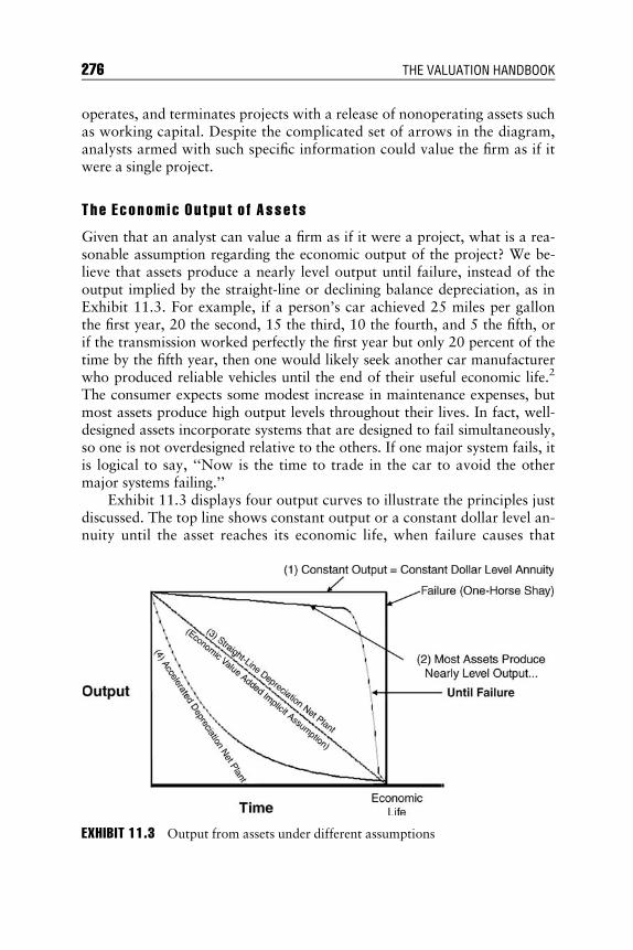
E1C11 08/25/2009 Page 276

operates, and terminates projects with a release of nonoperating assets suchas working capital. Despite the complicated set of arrows in the diagram,analysts armed with such specific information could value the firm as if itwere a single project.

The Econom i c Ou t pu t o f Asse t s

Given that an analyst can value a firm as if it were a project, what is a rea-sonable assumption regarding the economic output of the project? We be-lieve that assets produce a nearly level output until failure, instead of theoutput implied by the straight-line or declining balance depreciation, as inExhibit 11.3. For example, if a person’s car achieved 25 miles per gallonthe first year, 20 the second, 15 the third, 10 the fourth, and 5 the fifth, orif the transmission worked perfectly the first year but only 20 percent of thetime by the fifth year, then one would likely seek another car manufacturerwho produced reliable vehicles until the end of their useful economic life.2

The consumer expects some modest increase in maintenance expenses, butmost assets produce high output levels throughout their lives. In fact, well-designed assets incorporate systems that are designed to fail simultaneously,so one is not overdesigned relative to the others. If one major system fails, itis logical to say, ‘‘Now is the time to trade in the car to avoid the othermajor systems failing.’’

Exhibit 11.3 displays four output curves to illustrate the principles justdiscussed. The top line shows constant output or a constant dollar level an-nuity until the asset reaches its economic life, when failure causes that

EXHIBIT 11.3 Output from assets under different assumptions


E1C11 08/25/2009 Page 277

output to fall immediately to zero, as in the classic one-horse shay example.The second line down from the top displays the high output for most assetsuntil failure at the end of their economic lives. The third line, a diagonalfrom the upper left to the lower right, exhibits the net plant under straight-line depreciation. Economic value added (EVA) models implicitly assumethis line of output, unless they adjust each asset’s depreciation schedulefrom the one reported. The fourth line, curved from the upper left to thelower right, reveals the net plant under declining-balance accelerated depre-ciation. Of course, not all assets produce constant output, equivalent to aconstant dollar level annuity; however, their output line (2) more closelyresembles line (1) than the depreciated net plant line (3). Therefore, the con-stant output assumption is closer to reality than the depreciated net plantoutput assumption.

Little research exists on output curves, although an abundance of re-search on optimum asset replacement policy appears in the literature.3 Asmentioned before, substantially complicating the analysis is competitive re-action. Most new assets produce higher output and have less down timethan older assets. Some face declining prices. The relevant issue is howmuch of the higher output, less down time, and lower prices flow throughto investors and how much flows through to customers in the form of lowerprices and margins from competitive pressures.

For example, consider the output curves of personal computers. Con-sistent with the previous example, the output produced by the PC remainsconstant as it ages. Despite increased capacity and speed with lower prices,no one purchases a new computer each month. Even computers have a de-sign life, reflecting the amortization of their costs with benefits given theusage application and over which output is reasonably stable. Some pur-chase new computers every 12 to 18 months, if speed and capacity are criti-cal. The rest make do with replacements every three to five years.

Future research will likely investigate asset output, lives, and competitiveprice reaction, as the importance of this field and data becomes more obviousand relevant to economic performance measurement. Of particular impor-tance will be how these principles apply to capitalizing expenses associatedwith creating intellectual intangible property—software, customer acquisi-tion, employee training, advertising, and R&D—all critical to the propereconomic performance measurement in service industries. All businesses fol-low this fundamental cash-out, cash-in project pattern with a finite life of thedepreciating or amortizable assets. The challenge is identifying the funda-mental underlying projects and properly accounting for them so measuringcash economic returns becomes possible. As business continues the shiftfrom hard assets to intangible assets in a more service-oriented economy, themore important solutions to these measurement issues will become.


E1C11 08/25/2009 Page 278

Unfortunately for practitioners, companies generally do not provide in-formation for specific projects, only for the firm overall. Therefore, the chal-lenge presented to the analyst is how best to convert information providedby the financial statements into cash flows as if they arose from the under-lying projects. In terms of our system approach, this is the idea of convertingaccounting information to economic returns.

Accounting statements provide information, not valuation. Accountingacademics have known for many years that annual accounting rates of re-turn—return on equity (ROE), return on net assets (RONA), return on capi-tal employed (ROCE), and return on assets (ROA)—do not reflect theeconomic or internal rate of return of necessary for the valuation of theunderlying projects. Ezra Solomon (1966), Gerald Salamon (1982), andRichard Brief (1986) wrote some of the classic articles on the problem ofrelating economic to accounting returns. The difference between theaccounting returns and economic returns relates to the pattern of cash flowswithin the project, the depreciation method, the growth rate of the projects,the project life, and inflation, making the problem almost insolvable. But, ifone can make the simplifying assumption that most assets produce constantoutput and follow a constant dollar level annuity, one can create an annualperformance measure—gross cash flow return on gross assets with a finitelife—which precisely equals the economic or internal rate of return of allthe underlying projects. Then one need only apply Ijiri’s (1980) insight onthe proper method for accounting for inflation: simply to translate all cashflows from the income statement and balance sheet into units of the sameconstant dollar purchasing power. This appropriate treatment relates to in-vestors’ objectives to receive a return for their investment, all expressed inthe same purchasing units. The type of assets or their replacement cost mat-ters little to investor rate of return objectives.

To illustrate these principles, consider a project consisting of a depreci-ating asset costing $10,000, which produces cash flows of $1,740 for eightyears with no salvage value. This project produces an internal rate of return(IRR) of 8 percent. Assume for the moment no inflation. Exhibit 11.4 dis-plays the project and the accounting for each year. The income is constant,but the net plant declines from $8,750 in year 1 to zero in year 8. The returnon net assets (RONA ¼ Net income � Net plant) begins at 5.71 percentin year 1, rises to 40 percent in year 7, and becomes infinite in year 8. Onlyin year 3 does the RONA precisely equal the 8 percent IRR economic rate ofreturn, known for the project. With inflation, the RONA bias becomesworse, as cash flows tend to rise with the price level, while the historicaldollar net plant declines with depreciation accounting.

The annual performance measure, the cash economic return (CER),explained in detail in the following section, precisely equals the 8 percent


E1C11 08/25/2009 Page 279

EXHIBIT11

.4A

nnualPer

form

ance

Mea

sure

of

Pro

ject

Year

12

34

56

78

Inco

me

$500

$500

$500

$500

$500

$500

$500

$500

Dep

reci

ati

on

1,2

50

1,2

50

1,2

50

1,2

50

1,2

50

1,2

50

1,2

50

1,2

50

Gro

ssC

ash

Flo

w1,7

50

1,7

50

1,7

50

1,7

50

1,7

50

1,7

50

1,7

50

1,7

50

Gro

ssPla

nt

10,0

00

10,0

00

10,0

00

10,0

00

10,0

00

10,0

00

10,0

00

10,0

00

Acc

um

ula

ted

Dep

reci

ati

on

1,2

50

2,5

00

3,7

50

5,0

00

6,2

50

7,5

00

8,7

50

10,0

00

Net

Pla

nt

$8,7

50

$7,5

00

$6,2

50

$5,0

00

$3,7

50

$2,5

00

$1,2

50

$0

Ret

urn

on

Net

Ass

ets

(RO

NA

)¼

Inco

me/

Net

Pla

nt

5.7

1%

6.6

7%

8.0

0%

10.0

0%

13.3

3%

20.0

0%

40.0

0%

1

Cash

Eco

nom

icR

eturn

(CE

R)

8.0

0%

8.0

0%

8.0

0%

8.0

0%

8.0

0%

8.0

0%

8.0

0%

8.0

0%

Dif

fere

nce

�2.2

9%

�1.3

3%

0.0

0%

2.0

0%

5.3

3%

12.0

0%

32.0

0%

1

Ret

urn

on

Gro

ssA

sset

s17.5

0%

17.5

0%

17.5

0%

17.5

0%

17.5

0%

17.5

0%

17.5

0%

17.5

0%

279

E1C11 08/25/2009 Page 280

economic return each and every year, because it relates the gross cash flowto the gross assets over the eight-year life as an IRR calculation. Anothersimplified annual performance measure, return on gross assets (ROGA ¼Gross cash flow � Gross plant) remains constant at 17.5 percent and avoidsthe upward bias of RONA.

Any performance measure that relies on an accounting return of net in-come divided by net assets after depreciation suffers from the same biases.Only where output declines with depreciated net plant does the annualRONA approximate the project IRR.4

It is possible that new projects counterbalance old projects, so RONAsaverage out. While true directionally, this hypothesis is not supported byclient work or empirical work with company financial statements. In thelate 1980s, unpublished research by Rawley Thomas sought to quantifyhow frequently the accounting returns provided the wrong strategic direc-tion for the company compared to the economic returns. The answer was30 percent. Thirty percent of the time, accounting RONAs exceeded theircost of capital hurdle while the economic returns fell below the investor’srequired real returns or vice versa.

Examples of the failure to address the material differences betweenaccounting returns and cash economic returns (CERs) abound in academicresearch studies. For instance, some observed level to declining returns onassets during the 1990s. Actually, economic returns increased significantlyduring the 1990s because of declining inflation and more noncash chargesfor amortization of goodwill. The increase in economic returns helps toexplain superior stock price performance; the nominal accounting returns donot. Most academic researchers should pay much closer attention to the ma-terial differences between CERs and accounting returns. Insights on marketperformance arise from understanding these differences in depth; however,these insights are not available from calculating simple accounting returns.

The following paragraphs describe corporate planning applications.Referring to case B in Exhibit 11.5, ponder the chemical company, underinvestor pressure, that sold its new plants because they showed the lowestreturns on net assets, while retaining the older, inefficient plants with higherRONAs. Or consider the tire company, case A, whose strategic plan showedincreasing RONAs barely reaching the cost of capital as the company let itsplants age, while the economic returns remained substantially underwater.A management group, who realized complacency was not an option, ac-quired the tire company in an unfriendly takeover. Dramatic restructuringwould be required.

Examine case C in the diagram, where the credit operation was ac-quired for its very high returns and then starved by the board of directorsbecause its low RONAs, including goodwill, were not making the cost of


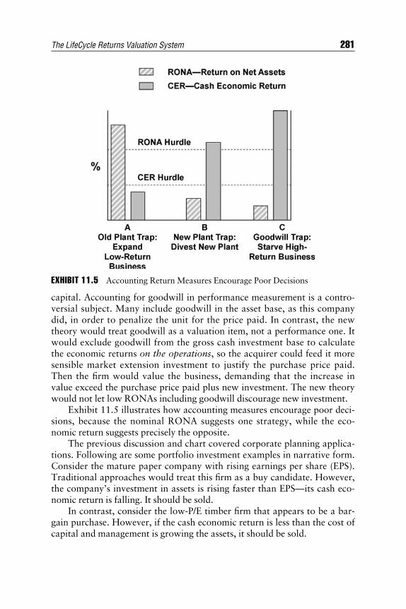
E1C11 08/25/2009 Page 281

capital. Accounting for goodwill in performance measurement is a contro-versial subject. Many include goodwill in the asset base, as this companydid, in order to penalize the unit for the price paid. In contrast, the newtheory would treat goodwill as a valuation item, not a performance one. Itwould exclude goodwill from the gross cash investment base to calculatethe economic returns on the operations, so the acquirer could feed it moresensible market extension investment to justify the purchase price paid.Then the firm would value the business, demanding that the increase invalue exceed the purchase price paid plus new investment. The new theorywould not let low RONAs including goodwill discourage new investment.

Exhibit 11.5 illustrates how accounting measures encourage poor deci-sions, because the nominal RONA suggests one strategy, while the eco-nomic return suggests precisely the opposite.

The previous discussion and chart covered corporate planning applica-tions. Following are some portfolio investment examples in narrative form.Consider the mature paper company with rising earnings per share (EPS).Traditional approaches would treat this firm as a buy candidate. However,the company’s investment in assets is rising faster than EPS—its cash eco-nomic return is falling. It should be sold.

In contrast, consider the low-P/E timber firm that appears to be a bar-gain purchase. However, if the cash economic return is less than the cost ofcapital and management is growing the assets, it should be sold.

EXHIBIT 11.5 Accounting Return Measures Encourage Poor Decisions


E1C11 08/25/2009 Page 282

Last, reflect on the aerospace company with level EPS, whose stock in-vestors normally avoid. Nevertheless, if the management is restructuring theasset base by eliminating unprofitable operations and the cash economicreturn is rising, the company should be a buy candidate.

Compu t i n g a Cash Econom ic Re turn

As demonstrated in the preceding paragraphs, accounting information maynot always provide an accurate picture of the economic condition of a firm.The problem is not just a theoretical one. The examples show how bothcorporate and investment managers could make erroneous decisions basedon the accounting information alone.

Traditionally, analysts adjust the information from the financial state-ments to better reflect the economics of the firm. This is the first step towardderiving a value. We cannot provide here an exhaustive set of adjustmentsused by LifeCycle, but will present a nice sample along with some economicintuition. The key to understanding the adjustments used by LifeCycle isthat we are attempting to create a ‘‘cash on cash’’ or cash economic return(CER) from the financial statement information. As with cash flows gener-ated by projects, the return on an investment in a company can be computedas cash flows returned to the firm (gross cash flow) divided by the capitalinvestment in the firm (gross investment). We now turn to a particularexample of the computation of CER.

Exhibit 11.6 displays the details of the cash economic return for Super-Valu, a major grocery store chain, in 2001.5 The method transforms the$206 million of income and $5,825 million of assets into $781 million ofgross cash flow and $5,704 million of gross cash investment, all expressedin the same units of investor purchasing power—2001 current dollars. De-tails on the computations follow:

A: To income, LifeCycle Returns adds $33 million in extraordinaryitems after tax and subtracts $16 million in nonoperating expenses.To assets, LifeCycle subtracts $137 million of nonoperating assetsand $1,531 million of purchase goodwill. These two adjustmentsfocus the results on the operations.

B: Noncash charges of $333 million in the numerator consist of depreci-ation, amortization, and changes to the allowance for doubtfulaccounts. In turn, adding back reserves for receivables, LIFO (inven-tory), and accumulated depreciation—$23 million, $141 million,and $1,580 million respectively—returns to the original investorcash investment in the denominator assets.


E1C11 08/25/2009 Page 283

C: To reflect inflation and restate all historical dollars to 2001 dollars,LifeCycle computes a $14 million gain on nonfixed assets in thenumerator (GDP deflator change � nonfixed assets—payables andother nondebt liabilities for SuperValu exceed assets of receivables,operating cash, inventories, and other assets) and a $249 millionadjustment to land, gross plant, and deferred taxes to the denomi-nator. Using the plant life and age enables approximate restatementof historical cost for plant to 2001 dollars without knowing inter-nal company records.6 When tested against internal companyrecords from selected clients, the algorithm is accurate within 5 to10 percent, unless capital expenditures have been extremely large inthe past one to two years.

D: Capitalizing $1,202 million of operating leases in the denominatorand adding back $134 million of after-tax interest on debt andleases along with the $77 million principal portion of rental pay-ments to the numerator make the measure independent of financialleverage.

E: If SuperValu disclosed advertising and research and development(R&D), those elements would be capitalized in the denominator,while adding back the after-corporate-tax effect in the numerator.

F: Last, LifeCycle subtracts $1,648 million of non-interest-bearingliabilities, in order to effectively reconcile to the cash investmentmade by all the equity holders, debt holders, and landlords.

The ratio of $781 million gross cash flow to $5,704 million is not yet aproper return measure, because it erroneously assumes the assets will lastforever. To reflect the finite life of depreciating assets, LifeCycle transformsthe CER into a project 9.09 percent internal rate of return (IRR) format,according to Exhibit 11.7. The $5,704 million down arrow reflects the cur-rent-dollar investor gross cash investment expressed in 2001 dollars. The11.55 years up arrows of $781 million reflect the current-dollar annual grosscash flow available to all the investors and to the business for reinvestment.

Life equals a weighted average of the operating leased asset life of 15years and the plant life from gross plant/depreciation. Of all the estimates,plant life merits the greatest scrutiny in client assignments to ensure it re-flects the economic life over which the assets produce cash flows until fail-ure and to ensure the proper fixed asset inflation adjustment.

The capability to relate annual performance measures derived fromaccounting data to capital budgeting project internal rates of return repre-sents an extremely powerful way of monitoring firm economic perform-ance. This capability enables comparison of economic performance across


E1C11 08/25/2009 Page 284

EXHIBIT11

.6C

ash

Eco

nom

icR

eturn

Exam

ple

:A

ccounti

ng

toC

ash

—Super

Valu

,2001

($M

illi

ons)

Income

$206

A:EliminateNonoperating

Spec

ialE

xtr

aord

inary

Item

sA

fter

Tax

33

Item

s(–

)N

on-o

per

ati

ng

Expen

seA

fter

Tax

(16)

B:Translateto

Cash

Nonca

shC

harg

es333

C:Restate

forInflation

Inflati

on

Gain

on

Nonfixed

Ass

ets

14

D:EliminateLeverag

eA

fter

-Tax

Inte

rest

(Deb

tand

Oper

ati

ng

Lea

ses)

134

$781

$206

Ren

tals

—Pri

nci

palPaym

ents

77

Curr

ent-

Doll

ar

Inco

me

E:Cap

italizeExpenses

(–)

Adver

tisi

ng

and

R&

DA

fter

Tax

(0)

Gro

ssC

ash

Flo

w______

��!

__________________________________________________

��!

______________

Ass

ets

Tota

lA

sset

s$9,8

25

Curr

ent-

Doll

ar

$5,8

25

A:EliminateNonoperating

(–)

Nonoper

ati

ng

Ass

ets

(137)

Inves

tor

Gro

ssItem

s(–

)Purc

hase

Goodw

ill

(1,5

31)

Cash

Rec

eivable

sR

eser

ve

23

Inves

tmen

tB:Translateto

CashInvest.

LIF

OR

eser

ve

141

$5,7

04

Acc

um

ula

ted

Dep

reci

ati

on

1,5

80

C:Restate

forInflation

Inflati

on

Adju

stm

ents

toL

and,G

ross

Pla

nt,

and

Def

erre

dT

axes

249

D:EliminateLeverag

eG

ross

Lea

sed

Pro

per

tyfr

om

Oper

ati

ng

Lea

ses

1,2

02

E:Cap

italizeExpenses

Capit

ali

zed

Adver

tisi

ng,R

&D

0F:Cap

ital

Owner

CashInvest.

(–)

Oper

ati

ng

Non-I

nte

rest

-Bea

ring

Lia

bil

itie

s(1

,648)

Source:

Raw

data

from

Sta

ndard

&Poor’

sC

om

pust

at;

inflati

on

adju

stm

ents

from

Lif

eCycl

eR

eturn

s,In

c.

284

E1C11 08/25/2009 Page 285

firms through time, without the cash distortions arising from accountingconventions, depreciation, purchase goodwill, or varying inflation. Is it per-fect? No. Is it much better than other performance measures, such asaccounting returns or EPS growth? Yes.

The CER represents a practical method for translating accounting in-formation to economic real internal rates of return with imperfect, noisydata. Critics who take issue with the constant dollar level annuity assump-tion bear the responsibility, if not the obligation, to propose a better, practi-cal alternative applicable to real-world company data, which is equallycorrect theoretically.

CONVERT ING ECONOM IC RETURNSTO INTR INS I C VALUES


Once LifeCycle converts accounting information to an economicallymeaningful form, the next step is to convert the CER to an intrinsic valuefor the firm of interest. Two key elements play a role in converting the CERto an intrinsic value. The first is how the cash economic returns appear onthe time line as cash flows. Recall that the value of a firm is the present valueof all the cash flows received in the future by that firm. Critical to the valua-tion process is the timing of the expected cash flows and their duration,since, theoretically, the firm may live forever but also attempts to survivea competitive environment. The second key element is the rate used to

EXHIBIT 11.7 Cash Economic Return Example: Cash to Economics—SuperValu,2001 ($ Millions)


E1C11 08/25/2009 Page 286

discount the cash flows. We address timing of the cash flows first and thediscount rate computation later.

F rom Econom i c Re t urns t o F i rm Cash F l ows

Intuitively, the cash flows a company is able to generate are a function of itsasset base and the rate of return on those assets. In LifeCycle terms, a com-pany will produce cash flows consistent with its gross assets and its CER.In forecasting CERs and asset growth, one thing is certain—neither is im-mune from competition. Competition will cause firms to decrease prices,thus reducing CERs. Competition will also cause market saturation, trim-ming asset growth in attractive industries. The manner in which LifeCyclefactors in competitive effects is a process called fade. Academics oftendescribe a very similar concept: regression toward the mean.

Research confirms that CERs and asset growth rates regress over timetoward the mean of all companies. Exactly how the CER and asset growthrates fade is an empirical question. LifeCycle recomputes fade parameterseach year so that 50 percent of the firms in the universe are overvalued and50 percent are undervalued. Exhibit 11.8 shows fade patterns representativeof those that appear in the LifeCycle model for CERs.

A couple of key points stand out in the exhibit. First, our research re-veals that fade patterns differ by firm size. Larger firms, whose CERs tendto fall in a narrower band, have less extreme adjustments, while smallerfirms experience greater adjustments as their extreme returns move towardthe average for all companies. Second, firms currently earning low returnsshould actually expect their returns to fade up; that is, the poor returns willnot persist forever. A peculiar case is the small firm that has a low return.

EXHIBIT 11.8 Fade Patterns


E1C11 08/25/2009 Page 287

Small start-up firms are an exception in that the market prices those firms asthough the average survivors will achieve superior returns above the aver-age. Effectively, investors purchasing small start-ups are buying an optionon economic performance, where the initial public offering (IPO) cash in-vested in operating assets is the premium.

The numerical example in Exhibit 11.9 illustrates an example of a fadeprocedure used for both asset growth and CER. Assume a firm in 2004employs constant dollar gross investment of $21.779 billion. Furthermore,assume the firm’s sustainable growth rate is 5.67 percent. LifeCycle computesthe sustainable growth rate using a proprietary model that factors in histori-cal data on asset size, capital expenditures, and dividend payments. Fadingthe growth rate toward the 3 percent economy growth rate at an assumed80 percent rate results in a 3.54 percent growth rate for the following year.The calculation is as follows: (5.67% � 3.00%) � .80 þ 3.00% ¼ 3.54%.

The calculated growth rate applies each year to the expected growth inassets to determine the required amount of new annual asset investment andthe resultant total gross investment. Therefore, by applying the 3.54 percentasset growth rate in 2005, the model anticipates that the $21.779 billion2004 investment will grow to $22.549 billion in 2005. The growth rateresults in new asset investment of $770. The fading of asset growth contin-ues in the LifeCycle model for 50 years, at which point the remaining assetswind down and are not replaced. The life of a firm, therefore, in the Life-Cycle model is 50 years plus the life of the assets at that time—firms do notcontinue into perpetuity.

The second fade adjustment made by the model is to the CER. Assumethe company achieves a CER of 20.17 percent in 2004. Also, assume themodel fades the CER toward, but not all the way to, the universe average of8 percent at a 50 percent rate. Instead, assume this particular firm fades to arate of 12.57 percent.7 The computation of the CER for 2005 is: (20.17% –12.57%) � .50 þ 12.57% ¼ 16.56%. The faded CER results in a constantdollar gross cash flow of $5,977 for 2005, demonstrated in Exhibit 11.10.

To arrive at constant dollar net free cash flow—the cash flow availableto investors—we need to deduct replacement investments and growthinvestments as shown in Exhibit 11.11.

EXHIBIT 11.9 Fade Procedure for Asset growth

Year Future Growth Rate Constant Dollar Gross Investment

2004 5.67% 21,7792005 3.54% 22,549Increase 770


E1C11 08/25/2009 Page 288

The model repeats this procedure for each year in the future, assuminga life for the firm of 50 years plus the life of the assets in place at the time.The present values of the 50þ years of cash flows determine the firm’s in-trinsic value.

The Marke t Der i v ed D i s coun t Ra t e

Financial theory dictates that the value of an asset is the present value of thecash flows discounted at an appropriate rate. Traditionally, valuation bookssuggest a weighted average discount rate based on the capital asset pricingmodel (CAPM) for equity and an after-tax cost of debt. The weighted aver-age cost of capital (WACC) represents the appropriate discount rate to useto discount cash flows available to the entire firm. Equity values result bysubtracting the value of the debt from the total firm value.

Although elegant, using the CAPM presents theoretical and practicalproblems. We will focus here on the practical issues and address the theoret-ical problems of the CAPM in this chapter’s appendix. The CAPM accountsfor risk, for example, via its use of the systematic risk measure beta. Com-puting beta, however, presents a valuation conundrum for the analyst. Theprimary practical problem facing the use of beta as a risk measure is a tim-ing problem—the analyst must estimate beta based on historical data, whilethe discount rate determines the present value of future cash flows. The betacomputed from historical data may not be consistent with the risk of futurecash flows.

Another CAPM problem arises when estimating the market risk pre-mium. Most estimates from historical data have relied on Ibbotson data of1926 to the present.8 The geometric mean of large company returns less

EXHIBIT 11.11 Constant Dollar Net Free Cash Flow

Gross cash flow þ$5,977Replacement investments �$1,973Growth investments �$ 770Constant dollar net free cash flow þ$3,234

EXHIBIT 11.10 Fade Procedure for Cash Economic Return

YearConstant DollarGross Investment

Cash EconomicReturn

Constant DollarGross Cash Flow

2004 $21,779 20.17% $6,4622005 $22,549 16.56% $5,977


E1C11 08/25/2009 Page 289

long-term government securities from 1926 to 2007 was 4.90 percent and6.70 percent over Treasury bills. Large company returns over long-termgovernment securities over the past 20 years averaged 2.54 percent whileover the past 10 years they averaged –1.35 percent. The run-up in stockprices during the 1990s caused the measured equity risk premium toincrease, while, in contrast, financial theory suggests prices increase withdeclining costs of capital. The theory’s application appears inconsistent.

Contrast these historical equity risk premium numbers generally in the5 to 7 percent range with those forward-looking ones derived recently fromdividend discount models, which lie in the 2 to 3 percent range. The premi-ums derived from dividend discount models generally rely on finding theequity discount rate that equates the price to the present value of a perpet-ual stream of dividends, growing at various growth rates to reflect recenttrends.9

It behooves analysts to find a forward-looking discount rate that cap-tures investors’ required rates of returns given the current investment envi-ronment. Actually, forward-looking rates are common. Take, for example,the WACC discussed earlier. Practitioners almost universally determine acost of debt by estimating a yield to maturity on the company’s currentdebt, where the yield to maturity is the discount rate that equates the futurecash flows from the debt to its current price. In other words, yields to matu-rity are forward-looking discount rates.

Can one compute costs of equity similarly? Peruse a corporate financetext and it generally makes several suggestions to compute a cost of equity(discount rate). For example, Brigham and Houston (2007) present threeapproaches to estimating the cost of equity: (1) CAPM, (2) dividend discountmodel (DDM), and (3) bond yield plus a premium. The DDM approachtakes the familiar Gordon constant growth model of P0 ¼ D1/(ke � g)and solves for the cost of equity, ke ¼ D1/P0 þ g. The bond yield plus a pre-mium approach adds a premium of 3 to 5 percent to the yield to maturityof the bonds of the firm. The constant growth approach uses future divi-dends and growth rates, and the bond yield approach uses future bondcash flows. Indeed, two of the three methods suggested are forward-lookingdiscount rates!

As with the DDM approach and bond yield approach, we consider aforward-looking discount rate the appropriate way to determine the dis-count rate. The DDM approach, however, is limited since many firms payeither no dividends or arbitrarily low dividends. Furthermore, dividends areonly flows to equity. Instead, LifeCycle uses cash flows estimated from theearlier section as the first step in determining the discount rate. As previ-ously explained, the model computes cash flows to firms from the CER, as-set base, and fade patterns. Once LifeCycle estimates cash flows for all firms


E1C11 08/25/2009 Page 290

in the universe, the model iteratively selects a discount rate to equate thepresent value of cash flows to the current values of debt and equity. Criticsmay claim that the discount rate procedure just described is circular. Thosecritics would be correct if the model computed a separate discount rate inthis fashion for each company in every year. The model, however, uses asingle discount rate for all companies after appropriately adjusting for risk,which is the topic we turn to next.

Bart Madden, author of Chapter 3, once offered a keen insight on valu-ation models. Traditionalists place risk dimensions in the denominator dis-count rate of present value calculations, but more insights arise fromplacing those same effects in the model’s numerator cash flow descriptions.For example, yield to maturity measures on bonds assume investors receiveall the cash interest and principal payments. They do not—some bonds de-fault. A model including 1 minus the probability of default times the interestand principal payments would enable the comparison of the realized yieldbetween bonds of differing credit quality. Similarly for stocks, some modelsassume no default. A more insightful model, however, would incorporatethe probability of dropout from acquisition or bankruptcy and the capitalreleased at the dropout date. The no-default models would have to incorpo-rate equity risk premiums for leverage, but the more complete dropoutmodels would not. LifeCycle Returns’ research process places more andmore of the traditional risk effects into the cash flow model, so the costs ofcapital remain within a very narrow range across companies. Tests of suc-cessful refinements require reduced errors between actual prices and DCFmodel values. Tests also require reduced ranges of costs of capital betweencompanies and industries.

In contrast to the research process just described with one unifiedmodel, many would prefer separate parameters for each industry. Addingadditional degrees of freedom can increase apparent accuracy, but often atthe expense of conceptual soundness. Ijiri (1980) had this insight: Investorsshould not focus on what assets (or markets) the corporation invests in,only the gross investor cash outlays and gross cash flows generated, allexpressed in the same units of purchasing power.10 The industry shouldnot make any difference to the investor, unless the distribution of potentialreturns is fundamentally different from other industries.

Definitely following differing fundamental distributions are the three sec-tors: financial firms, unregulated firms, and regulated firms (utilities, tele-phones, railroads, and to a lesser extent oils and autos). Regulation tendsto narrow the economic rate of return distribution of companies. Conse-quently, we treat the three sectors of financials, regulated utilities, andunregulated firms fundamentally differently—with different cash economicreturn distributions and different market derived discount rates applied to


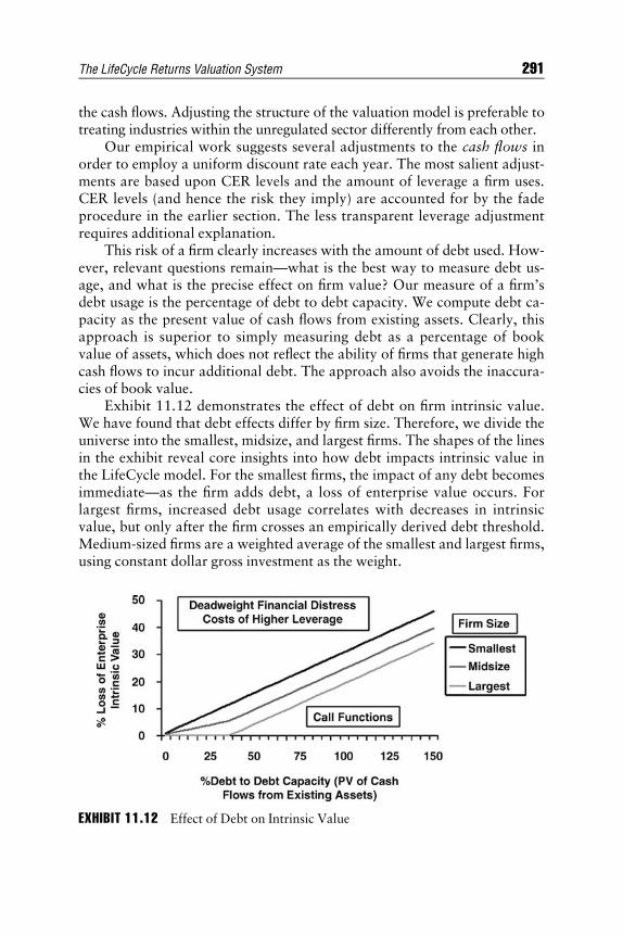
E1C11 08/25/2009 Page 291

the cash flows. Adjusting the structure of the valuation model is preferable totreating industries within the unregulated sector differently from each other.

Our empirical work suggests several adjustments to the cash flows inorder to employ a uniform discount rate each year. The most salient adjust-ments are based upon CER levels and the amount of leverage a firm uses.CER levels (and hence the risk they imply) are accounted for by the fadeprocedure in the earlier section. The less transparent leverage adjustmentrequires additional explanation.

This risk of a firm clearly increases with the amount of debt used. How-ever, relevant questions remain—what is the best way to measure debt us-age, and what is the precise effect on firm value? Our measure of a firm’sdebt usage is the percentage of debt to debt capacity. We compute debt ca-pacity as the present value of cash flows from existing assets. Clearly, thisapproach is superior to simply measuring debt as a percentage of bookvalue of assets, which does not reflect the ability of firms that generate highcash flows to incur additional debt. The approach also avoids the inaccura-cies of book value.

Exhibit 11.12 demonstrates the effect of debt on firm intrinsic value.We have found that debt effects differ by firm size. Therefore, we divide theuniverse into the smallest, midsize, and largest firms. The shapes of the linesin the exhibit reveal core insights into how debt impacts intrinsic value inthe LifeCycle model. For the smallest firms, the impact of any debt becomesimmediate—as the firm adds debt, a loss of enterprise value occurs. Forlargest firms, increased debt usage correlates with decreases in intrinsicvalue, but only after the firm crosses an empirically derived debt threshold.Medium-sized firms are a weighted average of the smallest and largest firms,using constant dollar gross investment as the weight.

EXHIBIT 11.12 Effect of Debt on Intrinsic Value


E1C11 08/25/2009 Page 292

In summary, LifeCycle bridges the gap between price matching intrinsicvalue and accounting information in a structured, empirically supportedsystem. Starting with adjustments to balance sheet and income statementaccounts to reflect cash economics, the LifeCycle model computes anexpected cash economic return on the firm’s assets. Because our philosophyassumes that ‘‘competition does not wait,’’ both CERs and asset growthrates fade toward sector averages depending on whether the firm is in thefinancial sector, a regulated sector, or an unregulated sector. The combina-tion of CERs and expected gross assets produces expected cash flows, whichthe model discounts at a uniform rate for each sector to present value, re-sulting in an enterprise value. The equity intrinsic value results from deduct-ing debt and adding net nonoperating assets to the present value of the cashflows. In practice, the model does not stop with the computation of intrinsicvalue. LifeCycle continually updates both the structures and the informa-tion contained in the models to improve their performance. Chapter 5 de-scribes the process we follow for analyzing and improving the models. Inthat sense, the model never rests. The following list summarizes LifeCycle’sentire process of converting accounting information to intrinsic values.

Step 1: Adjust accounting information to treat the firm as a series ofprojects.

Step 2: Place gross cash flows on a time line for the expected life ofassets, including a cash flow expected from the release of non-operating assets at the end of time line.

Step 3: Compute a cash economic return by finding the internal rate ofreturn for the time line.

Step 4: Create expected cash flows for the firm by taking the product ofcash economic return and gross assets, both of which are assumedto be fading toward economy-wide averages.

Step 5: Compute a market derived discount rate from the expected cashflows computed in step 4 for the financial, regulated, and un-regulated sectors.

Step 6: Using the market derived discount rate, compute the presentvalue of the cash flows, and make appropriate adjustments to theindividual firms’ intrinsic values based on the risk analysis, such asleverage. To the adjusted enterprise value, add nonoperating assetsand subtract debt. The result is a risk-adjusted intrinsic equity valuefor each firm.

Step 7: Analyze the performance of the model by comparing intrinsicvalues to actual market prices. Repeat the process, making


E1C11 08/25/2009 Page 293

adjustments to both the model structure and its parameterization asnecessary to improve its accuracy.

CONVERT ING INTR INS I C VALUESTO INVESTMENT DEC I S I ONS


To many practitioners, intrinsic values represent the beginning, not theend of a process. Security analysts, portfolio managers, corporate execu-tives, and regulators, among others, can benefit from the information pro-vided by the intrinsic values produced from LifeCycle models. This sectionfocuses on how investment professionals and corporate managers can usethe results in their decisions. Investment professionals may find that in-vesting in securities where the price is lower than intrinsic value will pro-duce that often-elusive combination of lower risk and higher returns.Corporate managers may use the models to better understand the trueunderlying value drivers of their stock, irrespective of the noise that cloudsthe information in market prices.

Exhibit 11.13 illustrates one of the most powerful tools in the LifeCyclevaluation system—value charts. Value Line introduced value charts in the1930s to display the capitalization of its cash flow model. Later, Callard,Madden and Associates (CMA) employed the value chart to demonstrate

EXHIBIT 11.13 Value Chart Example


E1C11 08/25/2009 Page 294

its model’s results. Subsequently, HOLT Planning, HOLT Value, the Bos-ton Consulting Group, and others illustrated their models with value charts.In 2001, we began using value charts to illustrate the results of multiplemodels.

The value chart represented in Exhibit 11.13 incorporates bars repre-senting the trading range for fiscal year prices, small circles representing theclosing price at the end of the fiscal year plus three months (allowing for adisclosure lag), and a solid line connecting the intrinsic values determinedby the valuation model. The value chart serves two core purposes. First, thechart represents a convenient visual way to determine the relative positionof prices to the intrinsic value. Analysts can easily determine the under- orovervaluation of the security and how the relative positions behaved overtime. Consider, for instance, the example in Exhibit 11.13. In the earlyyears of the chart, the actual prices and intrinsic values remain relativelyclose, suggesting that the market fairly valued the stock. In the middle years,the price rises substantially above the intrinsic value, indicating the stockbecame overvalued. Supporting this overvaluation signal is that the intrinsicvalue tracks not only below the current stock price but also at the low endof the trading range. In later years, both the stock and intrinsic values beginto drop, though the market valuation appears generally fair. In the finalyear, once again the price and intrinsic value diverge, but this time the valuechart indicates an undervaluation, portending future stock price increases.

The second core purpose of the value chart is to examine the effective-ness of the model itself—or even compare the effectiveness of several mod-els, as LifeCycle does. Let’s assume the value chart indicates that the priceremains consistently very distant from the intrinsic value for a particularsecurity. Under- or overvaluation signals from that model for that securitymay be suspect, since the model appears to lack accuracy in tracking theactual price. While one would never expect a model to perfectly track allmarket prices, a model that produces intrinsic values that are never close tothe actual price is most likely facing serious trouble valuing that particularsecurity. Exhibit 11.14 demonstrates the use of a value chart to comparemultiple valuation models. In the exhibit, the LifeCycle (LCRT) model pro-duces intrinsic values much closer to actual market prices than the othertwo models, one based on a simple rule of eight times EBITDA and anotherbased on net free cash flow. Both non-LifeCycle models consistently under-estimate the market price, suggesting that they are misspecified and there-fore would not likely lead to accurate, wealth-producing decisions.11

A model that consistently under- or overvalues firms in the universe isbiased. Dividend discount models, for example, tend to produce intrinsicvalues that are consistently too low when using typical assumptions aboutdiscount rates. LifeCycle continually examines its intrinsic values to ensure


E1C11 08/25/2009 Page 295

they are, on average,12 unbiased and accurate. A most important analystrole, however, addresses situations where the automated model fails totrack prices well in order to investigate why the breakdown occurs.

In contrast to security analysts, portfolio managers seek to selectcombinations of securities to produce the best risk/return trade-off. Life-Cycle back-tests the model’s predictive ability by ranking the securitiesaccording to their under-/overvaluation in order to construct decile port-folios. Portfolio managers expect the top decile (most undervalued) tooutperform the bottom decile (most overvalued) if the model is function-ing properly. Though the back-test is no guarantee of future performance,Exhibit 11.15 presents a sample. In this sample, the model works well, as

EXHIBIT 11.15 Sample Back-Test: Undervalued Stocks, Overvalued Stocks, andS&P 500

EXHIBIT 11.14 Value Chart with Three Models


E1C11 08/25/2009 Page 296

undervalued stocks greatly outperform the overvalued stocks as well asthe S&P 500.

Two complications arise in examining portfolios constructed from amodel’s intrinsic values. First, some of the most under- or overvalued firmsmay not possess sufficient trading liquidity to enter a portfolio. Portfoliomanagers should filter out illiquid firms prior to back-testing. In this exam-ple, we included only firms with greater than $1 billion market capitaliza-tion and prices greater than $10 per share. Second, since no model isperfect, some of the model under- or overvaluations may result from modelerror instead of market mispricing. To avoid securities where the modelmay not perform well, LifeCycle filters out securities where the firm’s track-ing error is high. Tracking error is the absolute percentage value of the dif-ference between the intrinsic value and the stock price. On average, if thattracking error exceeds 40 percent, the model is not performing well enoughto include those securities in the back-test.

For investment analysts and portfolio managers who would like to peekunder the hood, LifeCycle also examines the key value drivers for any firm,the CER and asset growth rates. Utilizing Hewlett-Packard as an example,Exhibit 11.16 presents key information on exactly why a firm’s intrinsicvalue may be increasing or decreasing. The top chart in the exhibit com-pares Hewlett-Packard’s CER with the market derived discount rate dis-cussed earlier. The CER exceeds the discount rate for the entire period—

EXHIBIT 11.16 Economic Drivers: Hewlett-Packard Co. CER and Asset Growth


E1C11 08/25/2009 Page 297

substantially so in the later years. Will the excess of the CER above the dis-count rate lead to a substantial increase in intrinsic value? Not necessarily,as the bottom of the exhibit reveals. Since cash flows are a product of theCER and asset base, we must consider the growth in assets as well. In thiscase, the asset base is growing far below what the firm could sustain andtherefore restrains increases in intrinsic value. The firm is finding profitableproduct niches, but fewer than the number supportable from its sustainablecash flow.

Exhibit 11.16 presents the economic drivers of the intrinsic values com-puted by the model. We can easily see that the intrinsic values for Hewlett-Packard respond significantly to the jump in CER in 2003. Furthermore,though the asset growth rate is small, there was a substantial change from2002 to 2003, rising from a negative rate to a small positive one. Nowexamine the data in 2003 and 2004. Hewlett-Packard experienced an evenstronger CER in 2004, yet the intrinsic value rose only slightly. Why? Onceagain, the asset growth did not justify a large increase in intrinsic value asthe rate dropped back to approximately zero in 2004. Despite the flatteningof the intrinsic values during that 2003–2004 period, the market still under-valued the stock, according to the LifeCycle model. (That undervaluationquickly evaporated, though, as the stock steadily rose in 2005 and 2006.)The example demonstrates how effective charts, such as the value chart andeconomic driver chart, complete a model. They provide the user with easy-to-access information on pricing and economic performance.

Despite the fact that the LifeCycle platform is fully automated, the sys-tem encourages analyst input. In fact, an analyst with superior insight subs-tantially improves the predictive results through an override procedure. Forexample, assume the analyst correctly believes that the firm will experienceabove-average sales due to a new product introduction. The LifeCyclemodel encourages the analyst to override the automated computations withthis forecasted data. The analyst’s short-term insight should lead to a moreaccurate intrinsic value than one estimated purely from the automated pro-cess based purely on historical data. In our opinion, though, certain areas ofthe model should remain off limits to the analyst. Extensive empirical anal-ysis, for example, underlies the fade procedure built into the model. Theanalyst is not likely to add much value in that fade area of the model. Otherareas, such as incorporating information from the footnote data, may provemuch more fertile ground for analysts. Also, recall that the LifeCyclemodel—or any other model—cannot value every security accurately. Thosesecurities not tracking well, such as heavily leveraged firms or those in fi-nancial distress, may provide the greatest opportunity for analyst interven-tion and subsequent superior risk/return portfolio performance.


E1C11 08/25/2009 Page 298

Understanding their firm’s economic performance and the resultingintrinsic values should appeal to corporate managers as well. While aninvestment manager may want to peek under the hood, the corporatemanager lives under the hood. Investors expect their agent corporatemanagers to pull the correct levers to maximize shareholder value inthe long run. These valuation models now provide a laboratory in whichthe manager can examine the impact of corporate investment and operat-ing decisions on the firm’s intrinsic value. What is the likely impact onstock value from a reduction in accounts receivable? What effect will anincrease in leverage have on firm value? A well-functioning, empiricallyvalidated, automated model should assist the manager in answering thosequestions instantly.

A valuation model can also provide additional benefits to corporatemanagers on compensation issues. Stock-related compensation helps cureone of the stickiest problems associated with the corporate form of businessownership, the agency problem. Stock compensation based on a noisy (andpossibly manipulated) stock price produces the primary difficulty. An accu-rate model offers an alternative to the noisy stock price in the form ofan intrinsic value. Compensation tied to the economic drivers of a model’svaluation encourages managers to pull the right levers to increase share-holder value since they directly benefit from their actions with higher com-pensation. To accomplish shareholder value creation, however, requiresempirical validation of theoretically sound models and deep managerunderstanding of the strategic economic drivers of those models.

Of course, the actual change in stock price, not the change in intrinsicvalue, compensates shareholders, so examining whether a model has explan-atory power in addition to predictive capability becomes critical. The differ-ence between those two concepts relates to timing. Predictive capabilityimplies that the model’s calculations of under- and overvaluation forecastchanges in future stock prices. Explanatory power means that the model’sintrinsic values correlate with movements in current stock prices. In otherwords, if a manager takes an action that increases intrinsic value, on averagethat action should also increase stock price. Without that correlation, the useof a valuation model for compensation purposes remains dubious.

Determining compensation from a complete analysis of valuation mod-els extends beyond the scope of this chapter. Our brief discussion here,however, highlights the role of the valuation model as an integral part of asystem as opposed to simply producing valuations as a product or manualprocess. The LifeCycle valuation system processes accounting informationin a mathematically rigorous and empirically supported program to providetools for managers—from Wall Street investment firms to corporate board-rooms, all the way down to the shop floor—to make better decisions.


E1C11 08/25/2009 Page 299

SUMMARY

This chapter presented an introduction to the LifeCycle Returns valuationsystem. We refer to it as a system as opposed to simply a model, since itprovides a comprehensive, automated way to:

& Translate data from accounting statements into economic returns.& Compute an intrinsic value based on those economic returns and exten-

sively empirically validate the intrinsic values against actual stockprices.

& Present the information to decision makers in simple charts and graphsthat are easy to digest.

The LifeCycle Research platform also possesses a systems mind-set,whereby it observes valuation phenomena to develop solutions that profes-sionals can pragmatically implement in a robust fashion—that is, one appli-cable to a wide variety of securities within the universe.

The LifeCycle system employs publicly available financial data to cre-ate economically sound adjustments to avoid much of the distortions in-herent in financial statements. The financial data converts to a casheconomic return—a return similar in concept to an internal rate of returnon a project. Then the model forecasts that return and the associated cashflows for the life of the company. Companies naturally face competitivepressures. To reflect competition, LifeCycle uses its proprietary computa-tions of fade, which trend both the cash economic return and asset growthtoward economy averages. The fade process is not arbitrary, but ratheran empirically researched method designed to ensure that the model, onaverage, produces valuations consistent with actual market prices in anunbiased way.

LifeCycle employs a market derived discount rate to determine the pres-ent value of cash flows produced by the model. The LifeCycle system itera-tively determines the uniform market derived discount rate across sectors byequating cash flows produced by the model to current prices. The systemadjusts individual securities’ values for risk, such as leverage, by modifyingthe expected cash flows instead of the discount rate.

Analysts and portfolio managers utilize the intrinsic values in securityselection and portfolio construction. Based on its evidence that marketprices tend to migrate toward intrinsic values, under- and overvaluationssignaled by the LifeCycle model present an opportunity to reduce risk whileincreasing return. Value-based corporate managers can incorporate themodel into an analysis of the economic drivers impacting their shareholders’value. In addition, targeting intrinsic values for executive compensation


E1C11 08/25/2009 Page 300

avoids the serious problems of noisy prices when measuring how muchvalue managers actually added.

An estimate of value can come from conjecture or be derived fromempirical analysis. Our philosophy represents an approach to determinevalue in an empirical and structured way. We hope the chapter providedinsights into the process of LifeCycle’s system. Though not simple, the auto-mated system produces intrinsic values on thousands of securities at thetouch of a ticker symbol. In addition, it provides numerous tools for deci-sion makers to whom the concept of value proves critical.

APPEND IX : MARKET DER I V ED D I SCOUNT RATESAND CAPM BETA COSTS OF CAP I TA L

All discounted cash flow (DCF) models require a discount rate or cost ofcapital to discount the cash flows to present value. Determining the bestrate to use, however, can be challenging, in part because the issue is fairlycomplex and in part because competing theories exist on how best to dealwith these complexities. Two theories in use are the well-known capital as-set pricing model (CAPM) and the much less known market derived dis-count rates.

All knowledgeable finance professionals know that a CAPM total costof capital arises from a weighted average of debt and equity. The nominalequity rate derives from multiplying a beta times an equity risk premiumand adding a risk-free rate.

While at Callard, Madden (CMA) in the early 1980s, author Thomasfirst experienced the benefits of replacing a CAPM cost of total capital witha market derived discount rate. The market derived discount rate appliesto both stock valuation and corporate finance for capital projects. Italso extends to business unit valuation in value-based strategic planningapplications.

All CMA offshoots chose the road less traveled between CAPM andmarket derived discount rates. All chose a market derived discount rate13

because we wanted the rate to be derived from the cash flow model itself,using a system mind-set to assure internally consistent assumptions. Al-though it is less frequently employed, the finance and investment profes-sions do use market derived discount rates. For one example, marketderived discount rates represent the only method commonly accepted forcalculating yields to maturity on bonds from the price, the coupon cashflows, and the principal repayments. For a second example, some financeprofessionals reverse the Gordon dividend discount model to calculatea market derived cost of equity: Price ¼ Dividend/(Equity discount


E1C11 08/25/2009 Page 301

rate � Growth rate), so Equity discount rate ¼ Dividend/Price þ Growth.Utility rate-making cases often use this reversal approach to estimate therequired rate of return.

We found zero empirical correlations between market derived equityrates from the cash flow models and CAPM betas. Zero! The accompanyingAtra-Thomas Chapter 5 empirically found a beta of 1 produced more accu-rate and more predictive dividend discount rate models than traditional be-tas. Consequently, incorporating non-1 actual betas added noise to both themodels’ accuracy for price level and their predictive capability for futureprice change. (Refer to Chapter 5.)

With these two strong empirical results, a system mind-set and soundtheory testing require reevaluating the assumptions of these two choices fordiscounting.

A market derived discount rate assumes:

& A methodology based on price level, not price change.& A structure of a discounted cash flow model equating price to the pres-

ent value of cash flows.& Risks may be incorporated into either the discount rate or the cash

flows. For one example, the discount rate may measure the price effectof financial leverage risk. For another example, the cash flow modelspecification may capture the risk of competitive fade of the firm’s op-erating returns on capital employed toward a corporate average.

From our perspective, a CAPM beta cost of capital relies on six assump-tions—either explicitly or implicitly. Following are those six assumptionsand our observations on each. Unfortunately, marrying CAPM beta dis-count rates with automated discounted cash flow models—both dividenddiscount models and Callard, Madden offshoot enterprise DCF modelsbased on constant dollar real cash flows—produces less accurate and lesspredictive results than market derived discount rates. These empirical fail-ures to explain actual price levels caused us to question the assumptionsunderlying the CAPM beta cost of capital by building on the shoulders ofnon-CAPM giants in the profession.

CAPM Assumptions

1. A methodology based on price change, not price level. In simple practi-tioner terms, although CAPM theoretically looks forward, its estimatestraditionally rely on backward data to calculate risk measures based onprice change. In contrast, market derived discount rates look forward tocalculate risk measures based on price levels, not price changes.


E1C11 08/25/2009 Page 302

2. Investors seek to avoid stock price variability relative to market varia-bility. Thaler (1987) and others suggest loss aversion as more appropri-ate than variability aversion.

3. A risk-free rate exists to form one anchor. Since even Treasury index-linked bonds vary in price and can therefore lose money in the shortterm, no risk-free asset exists in real terms. Recall that Treasury billslost 18 to 20 percent of their purchasing power in 1946–1947 with theunexpected inflation resulting from relaxing price controls after WorldWar II. Consequently, T-bills were not a risk-free asset.

4. A portfolio of assets exists to form the other anchor, so the capital mar-ket line can be drawn between the two (Sharpe 1970). Richard Roll(1977) questions the existence of the market portfolio to form the otheranchor to the risk-free asset in the CAPM.

5. Investors are indifferent between the loss and gain tails of the price dis-tribution, as implied by the variance statistic. Variance treats both tailsof the price change distribution as equally undesirable. Markowitz him-self (1959) recognized that this assumption may not reflect investorbehavior.

6. Firm stock price changes follow lognormal distributions with finite var-iances, so co-variances with the market can be calculated with confi-dence. Mandelbrot and Hudson (2004), McCulloch (1986), andThomas (2006) all demonstrated that price changes follow stable Pare-tian distributions with infinite variances, so the statistical measurementsassumed in the CAPM fail to exist.

Cracks in CAPM began to appear after publication of Fama andFrench’s 1992 paper.

For our own continuing empirical research and personal portfolio in-vestments, we choose to marry market derived discount rates with the cashflows instead of CAPM-based discount rates, in order to assure a systemsmind-set of internal consistency between the price level and the cash flows.This marriage with market derived discount rates creates more accurateand predictive DCF models. Consequently, these models prove more usefulto portfolio manager clients of all Callard, Madden’s offshoots for stockselection decisions than employing CAPM beta. For consistency, these dis-count rates should also apply to corporate capital projects and businessunit valuations.

NOTES

1. We owe this insight to Bart Madden, who presents the concept in Chapter 3.


E1C11 08/25/2009 Page 303

2. See Oliver Wendell Holmes’s poem, ‘‘The Deacon’s Masterpiece or, the Won-derful ‘One-Hoss Shay’: A Logical Story’’ (Holmes 1895). The ‘‘one-hoss shay’’was designed to last precisely a hundred years to the day, on which day it fellapart to dust.

3. A classic is Terborgh (1958).4. Using beginning-of-year assets eliminates this RONA/IRR difference.5. Source: Raw data from Standard & Poor’s Compustat; inflation adjustments

from LifeCycle Returns, Inc.6. Lewis, Stelter, Casata, and Reiter (1994).7. Although the exact computation of the 12.57 percent is beyond the scope of this

section, recall from Exhibit 11.8 that the fade patterns indicate that high-CERfirms fade, but they fade to a higher than average level. Low-CER firms mayfade to a lower than average level of CER.

8. Ibbotson Associates (2008). For a longer time horizon, see Siegel (1992).9. Arnott and Bernstein (2002), Fama and French (2002), and Lawson (2002). The

last article employs the dividend discount model and surveys of portfolio man-agers and chief investment officers.

10. Ijiri (1980).11. The numbers in parentheses in the exhibit represent the models’ tracking

error—a statistical measure for how well the model is performing. Models withlower tracking errors produce better results, as discussed in Chapter 5.

12. By ‘‘on average’’ we mean 50 percent of the firms are undervalued and 50 per-cent are overvalued. That is, the median firm is valued correctly by the market.

13. This market derived discount rate is a weighted average cost of debt and equity,since the valuation is based on the enterprise, not the equity. Consequently, themarket derived rate may be decomposed into its debt and equity components,unlike the CAPM, which provides only the cost of equity component for thecost of capital.

RE F ERENCES

Arnott, R., and P. Bernstein. 2002. What risk premium is ‘‘normal’’? Financial Ana-lysts Journal (March/April): 64–84.

Brief, Richard P. 1986. Estimating the economic rate of return from accountingdata, New York and London, Garland Publishing, Inc.

Brigham, E., and J. Houston. 2007. Fundamentals of financial management.11th ed. Mason, OH: Thomson-Southwestern, 335–340.

Fama, E., and K. French. 1992. The cross section of expected returns. Journal ofFinance 43: 153–194.

Fama, E., and K. French. 2002. The equity premium. Journal of Finance (April):637–659.

Holmes, O. 1895. The complete poetical works of Oliver Wendell Holmes. Boston:Houghton Mifflin. http://rpo.library.utoronto.ca/poem/1028.html.


E1C11 08/25/2009 Page 304

Ibbotson Associates. 2008. 2008 Ibbotson stocks, bonds, bills, and inflation classicyearbook. Chicago, IL: Morningstar.

Ijiri, Y. 1980. Recovery rate and cash flow accounting. Financial Executive (March):54–60.

Lawson, S. 2002. The equity risk premium: It’s lower than you think. GoldmanSachs CEO Confidential 14 (November).

Lewis, T., D. Stelter, T. Casata, and M. Reiter. 1994. Steigerung des unternehamens-wertes (Total value management). Landsberg am Lech, Germany: Verlag Mo-derne Industrie, 244–247.

Mandelbrot, B., and R. Hudson. 2004. The (mis)behavior of markets: A fractal viewof risk, ruin, and reward. New York: Basic Books.

Markowitz, H. 1959. Portfolio selection: Efficient diversification of investments.New Haven, CT: Cowles Foundation, 94.

McCulloch, J. 1986. Simple consistent estimators of stable distribution parameters.Communications in Statistics Simulation and Computation 15(4): 1109–1136.

Roll, R. 1977. A critique of the asset pricing theory’s tests. Part 1: On past and po-tential testability of the theory. Journal of Financial Economics 4: 129–176.

Salamon, Gerald L. 1982. Cash recovery rates and measures of firm profitability,The Accounting Review, April, 292–302.

Soloman, Ezra 1966. Return on investment: the relation of book yield to true yield,research in accounting measurement, American Accounting Association,232–244.

Sharpe, W. 1970. Portfolio theory and capital markets. New York: McGraw-Hill,83.

Siegel, J. 1992. The equity premium: Stock and bond returns since 1802. FinancialAnalysts Journal (January-February): 28–46.

Terborgh, G. 1958. Business investment policy: A MAPI study and manual. Wash-ington, DC: Machinery and Allied Products Institute and Council for Techno-logical Investment. 1958.

Thaler, R. 1987. The psychology of choice and the assumptions of economics. InLaboratory Experimentation in Economics: Six Points of View, ed. Alvin Roth,99–130, especially 106. New York: Cambridge University Press.

Thomas, R. 2006. Advanced DCF valuation measurement methodology: Predictivecapability, accuracy, and robustness. Presented at the Midwest Finance Associ-ation Annual Meeting. www.LCRT.com. Slides 33–36.


E1C12 08/14/2009 Page 305

CHAPTER 12Morningstar’s Approach

to Equity Analysis andSecurity Valuation

Pat DorseyDirector of Equity Research, Morningstar

A t Morningstar, we take an unusual perspective toward equity analysis,relative to much of the industry. Instead of setting price targets and

guessing what others might pay for a stock 12 months hence, we forecastcash flows and value businesses. In fact, our estimates of intrinsic value arethe anchor for the five-star rating system we use for equities. If a company’sshare price is roughly in line with our estimate of its intrinsic value, thestock receives a three-star rating—essentially a ‘‘neutral’’ or ‘‘hold.’’ Whenshare prices diverge markedly from our estimates of intrinsic value, our rat-ings become more bullish or bearish.

We focus on intrinsic—rather than relative—valuation because it cen-ters our thinking on the business that we are analyzing, as opposed to themarket’s current opinion of that business. We use a discounted cash flow(DCF) approach to arrive at our intrinsic value estimates because it allowsus to separate economic reality from accounting-based noise. Also, we be-lieve that shareholder value creation is a more complex process than simplyincreasing earnings per share, and a cash flow–based approach lets us un-pack concepts like growth, investment, and returns on capital.

By modeling the relationships between these three concepts, DCFallows our analysts to better understand the value drivers for the companiesthat we cover. We can quickly isolate the variables most likely to have alarge impact on a company’s intrinsic value, in addition to gaining insighton the effect of corporate capital allocation. If, for example, slower growth

305

E1C12 08/14/2009 Page 306

and less internal reinvestment would actually increase shareholder value, aDCF model will reveal this fact more clearly than an earnings-based model.

We use a standardized DCF model at Morningstar, which has a numberof advantages relative to using individually customized models. It ensuresconsistency across our analyst staff, which means we’re always treating var-ious line items and calculations in the same way. Having a standardizedmodel also gives our analyst staff a common language, which makes inter-nal debate more efficient as we are able to discuss what matters—our cashflow assumptions—rather than wasting time understanding the vagaries ofindividualized models. Finally, standardized models make it relatively easyto roll up our data by sector or industry, which allows us to ensure that ourbottom-up forecasts make sense in the aggregate.

Of course, our models are standardized only to a certain extent, since itwould be silly to attempt to forecast sales for a retailer in the same way thatyou would forecast sales for a large pharmaceutical firm. So, our analystsbuild company-specific front-end models to help them forecast sales andmargins, and then link the output to our standardized model. Essentially,it’s as if all of our analysts drive cars with V-6 engines, but the cars maylook quite different from the outside. We think this process gives the bestbalance of company-specific flexibility and across-the-board consistency.

Intrinsic value is the first pillar of our investment approach. The secondis margin of safety—we always look for a material discount from our intrin-sic value estimates before we recommend a security, as an insurance policyagainst being wrong. The size of that discount varies depending on howconfident we are in the accuracy of our cash flow forecasts, since it’s mucheasier to bound the intrinsic value of some companies than others. Thegreater the spread of likely future outcomes, the larger the margin of safetywe demand before recommending a stock.

We try to think about the valuation of companies as points along a con-tinuum of possible outcomes, rather than as definitive point estimates. So,we employ scenario analysis as a way of gauging how large a margin ofsafety we should attach to the companies that we follow. If we can plausiblyenvision scenarios in which a company could be worth one-half or twotimes our base case scenario, we’d look for a reasonably large discount toour intrinsic value estimate before recommending the shares. (Imagine asmall biotech company, or a levered auto-parts company.) By contrast, ifthe range of reasonably likely outcomes is fairly narrow, we can have somedegree of confidence that investors purchasing the shares at even a modestdiscount are likely to have a good expected return.

The third concept around which we organize our research is competi-tive analysis. In any reasonably unregulated capitalist economy, capitalseeks the area of highest prospective return, which forces down above-


E1C12 08/14/2009 Page 307

average returns on invested capital over time. Our valuation frameworkexplicitly assumes that firms with high return on invested capital (ROIC)eventually revert to their cost of capital. We think this assumption is criticalto disciplined valuation—trees don’t grow to the sky, and the natural hu-man tendency is to extrapolate recent trends too far into the future. Goodvaluation requires a framework that is strict enough to rein in the poten-tially overly enthusiastic analyst, but flexible enough to encompass a widevariety of companies.

Of course, it’s an empirical fact that some firms post supranormalROICs for very short periods of time before returning to terra firma, whileothers manage to maintain high returns on capital for many decades. Butwhich is which? We think that we can add a lot of value to the analyticalprocess by prospectively sorting companies into groups based on their eco-nomic moat or competitive advantage.

We divide our coverage universe into three groups—wide moat, narrowmoat, and no moat—depending on our assessment of the strength of thecompany’s competitive advantage. Exhibit 12.1 shows some summary sta-tistics from our coverage universe. As you can see, we think that companieswith very strong competitive advantages—wide economic moats—are quiterare, accounting for less than 10 percent of our coverage universe. We thinkthis is consistent with both the lessons of economic history and the assump-tion of excess returns regressing to the mean over time.

In our view, the wider a company’s economic moat—that is, the stron-ger its competitive advantage—the longer it will be able to keep competitorsat bay and post high returns on capital. And if returns on capital regress tocost of capital at a slower pace, a company has the potential to create moreeconomic value for shareholders over time.

Given that moat analysis is central to how we value companies and isalso the most unique aspect of our valuation process at Morningstar, we’llfirst dig further into that topic. We’ll then circle back to the details of howand why we use discounted cash flow analysis at Morningstar—and whenwe think DCF is less useful than alternative valuation techniques. Finally,we’ll discuss how we attempt to systematically incorporate uncertainty and

EXHIBIT 12.1 Economic Moats in Morningstar’s Coverage Universe

Type of

Moat

Number

Covered

As % of Total

Coverage

Average

ROIC

Median

ROIC

None 1,116 52% 9% 9%Narrow 835 39% 18% 13%Wide 183 9% 27% 19%

Morningstar’s Approach to Equity Analysis and Security Valuation 307

E1C12 08/14/2009 Page 308

scenario analysis into our margin of safety process, and then conclude withsome lessons that we’ve learned from several years of applying DCF analysisin a real-world setting.

APPLY ING ECONOM IC MOATS TOSECUR I TY VALUAT I ON

We think that identifying economic moats is an important part of the ana-lytical process for several reasons, chief among them the simple fact thatmoats add intrinsic value. After all, a company that has a high likelihood ofgenerating returns above its cost of capital for many years will create moreeconomic value in the future than a company that has a high likelihood ofshort-lived excess returns.

Schematically, this is shown in Exhibit 12.2, which places time on thex-axis and return on invested capital on the y-axis. Here, we assume threecompanies with equal starting ROICs, but with different levels of competi-tive advantage. ROIC declines linearly in all three examples, but does soover a longer time frame for the wide-moat business than for the no-moatbusiness. A slower rate of decline leads to a higher level of economic valuecreation, which is represented by the areas of the three triangles.

When comparing two businesses with similar growth rates, returns oncapital, and reinvestment needs, the business with the moat should have ahigher intrinsic value. From an investment perspective, this has two impor-tant implications: First, underestimating a moat can result in opportunitycost, because the investor will assume a shorter competitive advantage pe-riod than actually comes to pass, and may not estimate an intrinsic valuehigh enough to make the security appear attractively priced. After all, ifexcess returns are likely to persist, and a business can reinvest capital at ahigh rate of return for a substantial period of time, what looks expensivemay actually be quite a bargain.

EXHIBIT 12.2 Schematic Illustration of the Value Created by Economic Moats


E1C12 08/14/2009 Page 309

Bob Goldfarb, co-manager of the famed Sequoia Fund, summarizedthis concept nicely at the 2004 Sequoia shareholder meeting: ‘‘Time is thefriend of the wonderful business, affording it the opportunity to reinvestcapital at favorable rates and increase the value of the enterprise. Overtime, the price you paid for a terrific company looks cheaper and cheaper.For the inferior business at the cheap price, time may turn out to be the felldestroyer.’’

The second important implication of the notion that moats add intrinsicvalue is that overestimating a moat can result in capital loss or investmentunderperformance, since the investor pays up for sustained value creationthat fails to materialize. Given that moats add value only over time, whileinvestors can become overexcited about securities for all kinds of transientreasons—such as a hot product or a celebrity CEO—we can see how thinkingabout economic moats can be valuable by enforcing investment discipline.

After all, high returns on capital will always be competed away eventu-ally, and for most companies—and their investors—the regression to themean is fast and painful. Economic moats give us a systematic frameworkfor thinking about which businesses have a reasonable probability ofsustaining high returns, and which do not.

F i nd i n g Moa t s

Morningstar’s process for identifying economic moats is both qualitativeand quantitative. We begin with a strong belief that sustainable competitiveadvantage should be demonstrated in excess returns on capital—to para-phrase Jerry Maguire, ‘‘Show us the money.’’ Corporate managers may tella good story about a company’s strong market share, well-regarded brandname, or superior strategy, but we take these blandishments with a largegrain of salt if there is not accompanying financial evidence.

Yet even businesses that have posted high returns on capital in the pastdo not necessarily have a moat. A hot product may enable a company togenerate substantial returns on capital for a time, but such sudden popular-ity is rarely enduring—as investors in one-hit wonders from Iomega toKrispy Kreme to Crocs all discovered to their chagrin.

So, what is a moat? In our view, an economic moat is a structural busi-ness characteristic that allows a firm to generate excess economic returns foran extended period of time. Moats must be structural because the basic eco-nomics of businesses do not tend to change quickly, so we can more confi-dently forecast sustained excess returns if they can be tied to some structuralattribute of the business.

We’re skeptical that smart managers and good strategies constitute sus-tainable competitive advantages, simply because we cannot predict their


E1C12 08/14/2009 Page 310

future with a high degree of confidence. Managers can come and go, whilestrategies can be implemented, tweaked, or abandoned.

Moreover, managers in structurally disadvantaged companies fight anuphill battle. Certainly, some succeed against the odds, and these cases getplenty of attention (how many books have been written about HerbKelleher and Southwest Airlines?). But investing is all about stacking theodds in one’s favor, and we believe that while it is easy to anchor on theexceptions—such as Southwest—the hard truth is that companies with eco-nomic moats and undistinguished managers are more likely to post excessreturns on capital than companies with poor economics and savvy manag-ers. As Warren Buffett has famously said, ‘‘When a management team witha reputation for brilliance meets a business with a reputation for badeconomics, it is the reputation of the business that remains intact.’’

Make no mistake—we are not blind to the value that can be createdthrough intelligent capital allocation by a skilled team of managers, and wefully recognize that some strategies are more likely to succeed than others.Management and strategy do matter. However, they matter less than mostmanagers think, since some businesses are simply better (that is, more likelyto post sustainable excess economic returns) than others.

We would also argue that managerial skill and strategic success are eas-ier to recognize ex post than ex ante. Smart managers are generally laudedonly in hindsight, and strategies that may work well in one competitiveenvironment can easily fail in another. Structural advantages, by contrast,can be identified prospectively with greater confidence because they are lesssubject to change.

Types o f Moa t s

At Morningstar, we categorize economic moats into four groups: intangibleassets, customer switching costs, the network effect, and cost advantages.

Intangible Assets In this group, we look specifically for brands, patents,and regulatory approvals, all of which typically confer some kind of sustain-able advantage on their owners.

Brands are an interesting case study. Those that are well-known don’tnecessarily confer competitive advantage on their owners. Brands are valu-able only if they increase a consumer’s willingness to pay (think Tiffany) orif they reduce a consumer’s search costs by delivering a predictable experi-ence (think McDonald’s).

Sony, for example, has a very well-known brand, but it fails both tests.Consumer electronics is a cutthroat business, and even if Sony cancommand a small premium over a second-tier brand such as Goldstar, that


E1C12 08/14/2009 Page 311

premium is not large enough to offset the company’s enormous investmentin maintaining its brand through extensive advertising and expensive show-case stores. Moreover, consumers do not buy electronics frequently enoughto need to rely on a brand name to reduce the time they spend decidingwhich product to buy; instead, they compare features, consult experts suchas Consumer Reports, and then make their purchase decision.

Now contrast Sony with Tiffany, which can charge substantially higherprices for virtually the same products as competing jewelers. Or Bayer aspi-rin, which is the exact same chemical formulation as other aspirins, butwhich costs twice as much as generic aspirin. These brands confer competi-tive advantage because they enable the company to charge more for a goodwith reasonably similar production costs, leading to higher returns on in-vested capital.

Brands attached to goods and services with a high frequency of con-sumption may not necessarily have pricing power (McDonald’s does notcharge more than Burger King), but they can create customer loyalty by deliv-ering a highly consistent experience. This reduces consumer search costs,leading to habitual purchase behavior that drives sales volumes. Most peopledon’t compare the price of Colgate and Crest when they’re out of toothpaste.They simply buy the product they have previously used and enjoyed.

Brands can create powerful economic moats, but they are subject toconstant threat, and need to be prudently managed if they are to last. Kraftused to dominate the market for processed cheese, but overplayed its handon price, allowing private labels to show consumers that Kraft processedcheese didn’t taste any different than store brands. Tommy Hilfiger used tocharge premium prices for its preppy designer clothing, until the companyflooded department stores with too much product that had to be dis-counted, damaging the brand’s high-end image.

Patents can create obvious economic advantages—potential competi-tors are legally enjoined from selling identical products. However, patentshave finite life spans and are frequently subject to challenge, so we thinkcarefully about a company’s entire patent portfolio before deciding whetherit has an economic moat. We find that companies with a long track recordof producing valuable intellectual property, and whose revenues are welldiversified across many patents (3M, for example, qualifies on both counts),have stronger competitive advantages than companies that are too relianton a small number of patents.

Regulatory approvals, like patents, can increase the scarcity of a goodor service by limiting the number of companies that can provide it. Theseare also vulnerable to challenge, though usually through a political processrather than a legal one. However, a company with a durable regulatory ap-proval can nonetheless often extract high economic rents.


E1C12 08/14/2009 Page 312

Consider, for example, the pedestrian but profitable industries of wastehauling and aggregate production. In both cases, the key economic asset—alandfill or gravel quarry—requires municipal approval, and municipalitiestypically are not eager to hand out licenses for new landfills or quarries, be-cause they reduce adjacent property values. Customers in any given areathus have fewer choices than they would otherwise, so they wind up payinghigher prices.

This pricing power is enhanced by the low value-to-weight character-istics of waste and gravel. The further one has to travel to a landfill, or froma quarry, the more transport costs eat into profit margins, giving customersa strong incentive to use the closest landfill or quarry. This combination canlead to quasi-monopolies within a certain geographic radius.

Of course, regulatory approvals can be withdrawn, but the incentivesare such that this is less common with regulatory approvals than with pat-ents. Smart lawyers have incentives to challenge profitable patents, andcourts can often find consumer benefits by leveling the playing field. But amunicipality has little incentive to approve a new landfill close to a popula-tion center—precisely where it would be most valuable—because doing socould harm neighboring property values.

The caveat to regulatory approvals is that they’re most valuable whenoutput is regulated, via licenses, but pricing is not. Utilities, for example,must get reams of approvals to build new power plants and transmissionlines, but pricing is regulated precisely to cap the economic returns availableto shareholders. Monopolies are best for shareholders when they’re not reg-ulated like monopolies.

Switching Costs The second broad category of competitive advantage thatwe look for when assigning economic moats is customer switching costs,which can increase pricing power. If the cost for a consumer to switch fromone company’s products or services to those of a competitor is greater thanthe benefit from doing so, odds are good that the company will be able tocharge higher prices and earn excess profits.

We frequently see this type of economic moat in the software industry,which can lock in customers by requiring them to invest substantialamounts of time to become proficient in a particular program. New entrantswould need to induce users to discard months or years of hard-won exper-tise with the incumbent platform, and then invest still more time learningthe new software. This can happen, but we have found it’s more the excep-tion than the rule.

Adobe’s Photoshop image-management software and Autodesk’sAutoCAD computer-aided design software are perfect examples of thisphenomenon. Designers and engineers are often trained on these two


E1C12 08/14/2009 Page 313

platforms in college, so employers would need to bear the cost ofretraining and at least a temporary loss in productivity if they chose touse different software. Of course, if a new entrant offered image-man-agement or CAD software that was tremendously better than Photoshopor AutoCAD, companies might be induced to move away from the in-cumbent—but the new software would need to offer benefits that com-pensated for the high switching costs.

A similar phenomenon can occur when the cost of switching is rela-tively low, but the perceived benefit from switching is even lower. Intuit’sTurboTax is not terribly complicated, and it’s not markedly better thancompeting products. Yet Intuit has maintained a high level of market sharein the tax-prep software market simply because users don’t see very largebenefits to switching. As long as TurboTax is good enough, that’s all mostusers need.

Switching costs are not limited to the software industry, of course.Companies that provide back-office data-processing services to financialinstitutions—like Fiserv, DST, and Jack Henry—often benefit from thesame economic moat. Their services are so vital to the smooth operation oftheir customers’ businesses that renewal rates of 90 percent to 95 percentare quite common, since switching to a competitor would incur knownmonetary and labor costs to manage the change, as well as unknown costsin the form of potential business disruption. (How do you put a price onyour customers receiving accurate account statements every month?) In thisindustry, the challenge is not making money—data processors tend to bephenomenally profitable—but wisely allocating the resulting free cash flow.

Finally, switching costs needn’t be explicit and burdensome in order tocreate an economic moat. The explicit cost for consumers to move theiraccounts from one asset manager to another is quite low; competing manag-ers even offer to do most of the legwork for a new customer. Yet consumersroutinely leave their money parked in funds that have high costs or abysmalperformance.

The reason for this seemingly odd consumer behavior is that, while thecost of switching may be relatively low, the benefit of switching is highly un-certain. Maybe the new mutual fund will perform better—but maybe itwon’t. Moreover, selling shares in an underperforming fund and investingthe proceeds elsewhere requires the consumer to admit a mistake and possiblyrecognize taxable gains, something most people are loath to do. So, assets inthe fund industry—especially for funds that are sold through financialadvisers—tend to be sticky, and high returns on capital are the industry norm.

Network Effects The third type of economic moat we look for is in someways a type of switching cost, but it’s powerful enough that we think it


E1C12 08/14/2009 Page 314

merits a separate category. Network effects occur when the value of a prod-uct or service increases with the number of users, and broaching a moatbased on network effects can be very difficult, making it a very robust typeof competitive advantage.

Credit cards are a perfect network-effect industry. More cardholdersmean more businesses are likely to be persuaded to accept the card, andhigher merchant acceptance makes consumers more likely to own a card.Given these dynamics, it’s not hard to understand why 85 percent of allcredit card transactions in the United States pass through just four creditcard networks—Visa, MasterCard, American Express, and Discover.There’s little incentive for merchants or consumers to bear the additionalhassle of marginal cards, so transaction volume naturally concentratesaround a few networks.

To get an idea of how powerful this competitive advantage can be,imagine that a large venture capitalist offers you substantial funding to starta new credit card brand. With no consumers, how would you convince mer-chants to accept the card? And even if you could convince a few largemerchants to accept your new card by offering them attractive pricing, howwould you convince consumers to use it? Perhaps you offer below-marketinterest rates for a time, but what would prevent customers from dumpingyour card as soon as you raised rates to an economically sustainable level?

Any business that benefits consumers by providing a pool of liquiditycan be a strong candidate for network effects, which is why financialexchanges tend to have economic moats. The strength of that moat, how-ever, can vary tremendously depending on how captive the liquidity pool isto a particular network.

For example, contrast the New York Stock Exchange (NYSE) and theChicago Mercantile Exchange. While the NYSE still has a very profitablebusiness collecting listing fees, it makes far less from bread-and-butterequity trading than it did 20 years ago. Competitors like Archipelago cre-ated lower-cost businesses that stole volume and reduced pricing, whichwas possible because equities are fungible across different exchanges—there’s nothing to prevent an investor from purchasing a share on exchangeA and selling it on exchange B.

Futures are quite different. Since futures contracts require settlement incash or in kind, users require a clearing agent to reduce counterparty risk; somost futures exchanges have in-house clearing operations. A futures con-tract must be closed on the same exchange on which it was opened, makingcustomers captive to a particular exchange and giving the exchange muchgreater pricing power. Pricing, profit margins, and returns on capital forfutures exchanges like the Chicago Merc are far higher than those forequity-based exchanges.


E1C12 08/14/2009 Page 315

Network effects, though rare, are not limited to financial services firms,of course. Think about Adobe’s Acrobat Reader software, which is installedon over 600 million PCs and has become the industry standard for creatingportable documents. The more PCs that have Reader installed, the more at-tractive it becomes to create documents in Adobe’s PDF format, because thecreator has a high level of confidence that the recipient will be able to readthe file. Network effects based around industry standards are certainly sub-ject to technological disruption (getting a royalty on VHS tapes isn’t muchgood if everyone is buying DVDs), but they can provide a strong competi-tive advantage nonetheless.

Cost Advantages The fourth and final group of moats we look for atMorningstar are structural cost advantages, but we think it’s vital to ana-lyze the source of a company’s cost advantage when assessing the durabilityof this competitive advantage. We sort these sources into better processes,advantageous locations, access to unique assets, and/or traditional econo-mies of scale.

Process advantages are the least durable type of cost advantage, sincerivals or new entrants are generally able to replicate a given process withtime. However, this type of advantage can last longer than one might ini-tially expect. When we analyze process-based cost advantages we considernot just the theoretical feasibility of replication, but the practical likelihood.Most incumbents are typically skeptical of radical departures from businessas usual, which also slows their competitive response.

Dell and Southwest are both good examples of process-based costadvantages that enabled each company to generate high returns on investedcapital for surprisingly long periods. In both cases, processes that deliveredproducts or services at a markedly lower cost were neither secretnor patented, but competitors would have had to throw away their existingbusiness models in order to copy them. In Dell’s case, selling directwould have required other computer manufacturers to anger their largestdistribution partners. Southwest’s competitors faced capital costs that wereprohibitively high to standardize on a single plane type, and junking thehub-and-spoke model would have risked losing lucrative international traffic.

It may be inevitable that process-based advantages will be replicatedgiven enough time, but the competitive advantage period may last longerthan one would initially suppose.

Location can also serve as the basis for a sustainable cost advantage,most commonly in commodity industries with high weight-to-value ratios,for which transportation is a large component of the final cost to the con-sumer. The aggregate quarries mentioned earlier, as well as cement plants,often enjoy mini-monopolies in the areas close to the facility, because a


E1C12 08/14/2009 Page 316

competing supplier further away simply can’t overcome the higher trans-port costs and still be price competitive. The numbers for aggregate quarriesin particular are quite powerful. Transporting a truckload of stone, sand, orgravel 10 miles from the quarry site in mid-2007 would increase the cost tothe end user by 15 percent to 20 percent. If one quarry is 10 miles from aconstruction site and another is 20 miles away, the former has a 20 percentpricing advantage right off the bat.

Another type of cost advantage that we see mainly in commodity indus-tries is access to a unique, world-class asset. If a company has access to nat-ural resource deposit that is markedly cheaper to extract—located closer tolow-cost transportation, or composed of a richer grade that is cheaper torefine—it can have a sustainable edge. Granted, this competitive advantageis subject to disruption if a deposit is discovered lower on the cost curve, butlow-cost deposits are not discovered every day, and the high weight-to-value nature of many commodities makes transport costs a big factor.

Finally, we come to the fourth type of cost advantage—scale—which isoften the most durable and the most applicable across a wide swath of in-dustries. Manufacturing scale (spreading fixed costs across a large volumeof widgets) is the type of scale that we’re most familiar with from Econ101. However, it’s also the most vulnerable to a globalized economy thatconstantly incorporates newer, cheaper pools of labor. Size alone cannotgenerate excess profitability (just ask General Motors).

By contrast, scale advantages based on large or dense distribution net-works can be very durable. Although the cost to establish a sizable distribu-tion network is high, the marginal cost of delivering an extra package onthat network is quite low. If an incumbent has built out a distribution sys-tem which covers its fixed costs, it’s likely earning large incremental profitsas volumes increase, making it very difficult for a competitor to scale upprofitably. And because these advantages are geographically defined, they’reless vulnerable than manufacturing scale to foreign competition.

We see this phenomenon with package delivery in the United States,which is essentially a duopoly between UPS and FedEx. In the medicalwaste disposal industry, Stericycle is 15 times larger than its closest compet-itor, giving it unrivaled route density. More stops per route leads to moreprofitable routes and higher overall returns on capital—in addition to theability to underprice a potential competitor, should one emerge. In food dis-tribution, Sysco exhibits similar characteristics, and in uniform rental, Cin-tas has far lower costs than its peers due to a larger delivery network.

The final type of cost advantage that we look for is single-scale effi-ciency, which occurs when a company dominates a market that is too smallfor competitors to justify the cost of competing. We see this advantage inniche providers of software solutions, such as Blackbaud, which dominates


E1C12 08/14/2009 Page 317

the market for fund-raising software used by nonprofit organizations. Thisis a relatively small market, so large competitors like Oracle or Salesforce.com pass it by, and Blackbaud is entrenched enough that a new entrantwould need to incur large losses before establishing itself as a credibleplayer. Moreover, the new entrant would then need to split a relativelysmall profit pool with Blackbaud, reducing its potential return oninvestment.

I N TR INS I C VALUE

Given that legions of investors rely solely on multiple-based and compara-ble-company valuation to make their decisions, what is it about intrinsicvalue that we find useful?

To start, it’s important to note that we don’t view discounted cash flowanalysis as a magic bullet. Poor assumptions fed into a DCF model will pro-duce results just as inaccurate as will assigning a too-high or too-low price-earnings (P/E) ratio to an accurately estimated earnings stream. And in fact,the complexity of DCF models relative to multiple-based analysis can leadto a false sense of analytical confidence, since it is easy for analysts to con-flate more detail with greater accuracy.

Why DCF?

However, we do think DCF modeling is valuable for a number of reasons.First, the end result is an intrinsic value that’s not dependent on comparisonwith a benchmark. For example, if you know that a stock trades for $20 pershare and has a P/E of 15, you’re still in the dark, since that P/E means verylittle in a vacuum. Fifteen times earnings might be wildly expensive for adeeply cyclical steel company that can barely earn its cost of capital over acycle, but it could be the bargain of an investing lifetime for a company withlow capital needs, high returns on capital, and ample opportunities to re-invest future earnings. You need to know more about the business—or at aminimum, you need to know the multiples of comparable companies—inorder to make an informed decision about valuation.

But if you know that a stock trades for $20 and its intrinsic value isestimated to be $30, you can reasonably say that the shares are underval-ued, especially if that intrinsic value has been estimated using a model thatincorporates factors like the value-creating potential of a high ROIC. More-over, you’ve estimated the value of the business based on the cash it cangenerate, rather than estimating the potential price of the business basedon what other market participants might pay for it. This last point is


E1C12 08/14/2009 Page 318

important, and underscores a key difference between DCF valuation andmultiple-based valuation. DCF relies on accurately forecasting the econom-ics of a business, while multiple-based valuation frequently relies on accu-rately predicting changes in market opinion.

Forecasting the economics of a business, in fact, is the second reason weuse DCF. Modeling the intrinsic value of a company forces the analyst tothink through the cash economics of a business—a valuable process regard-less of the result.

For example, DCF allows the analyst to better appreciate the inflectionpoints brought on by operating leverage—when an average-seeming busi-ness suddenly starts gushing cash, or vice versa. When MasterCard wentpublic in mid-2006, it looked like a solid business, with good margins andreasonable growth prospects. However, it was also a business that shouldhave had extremely high operating leverage, since the cost of managing aglobal payment-processing network is relatively fixed. Using DCF, we wereable to model the effect of rapidly increasing margins, and initiate coveragewith an intrinsic value roughly twice the offering price.

DCF disaggregates cash flow from generally accepted accounting prin-ciples (GAAP) earnings, and requires the practitioner to clearly understandhow money flows in and out of the business to create value for shareholders.This process can be overlooked when an analyst simply forecasts year-ahead earnings per share and assigns a multiple.

We also think that DCF is valuable because it incorporates the empiri-cal relationship between growth and return on capital. As Warren Buffettsaid in another context, ‘‘Growth is always a component in the calculationof value, constituting a variable whose importance can range from negligi-ble to enormous and whose impact can be negative as well as positive.’’Growth is valuable only if a company earns a return on capital greater thanits cost of capital, and it can in fact subtract value if ROIC is below cost ofcapital. Redeploying shareholder capital into a low-ROIC business to in-crease earnings per share is the height of economic lunacy, yet it can pro-duce the growth so prized by Wall Street.

DCF also enables the user to perform diagnostics on the intrinsic value.Because you’re forecasting full pro forma financial statements, you can ana-lyze forward operating ratios to ensure that the revenue growth you’re fore-casting is actually feasible given the economics of the business. Ratiooutputs allow for quick sanity checks that would be more difficult with arough-and-ready multiple analysis.

Fourth, DCF modeling enables the analyst to reverse-engineer marketexpectations in a detailed fashion. We often find ourselves asking: Whatrevenue growth or margin assumptions do we have to plug into our DCFmodels in order to arrive at the current market price? And do those


E1C12 08/14/2009 Page 319

assumptions seem reasonable? From an investment perspective, making areasonable estimate of intrinsic value by forecasting cash flows is just onepart of making an accurate stock call. Understanding the expectations im-plied by the current market price is also important, since it can help gaugehow rational or irrational those expectations may be.

DCF modeling also facilitates scenario analysis, enabling an expected-value approach to security valuation. We’ll discuss the importance of sce-nario analysis later in this chapter, but we think DCF is tailor-made forthinking about the future in a probabilistic fashion, since the analyst caneasily change a large number of variables to see which has the largest impacton valuation.

Finally, DCF modeling provides consumers of our research—both in-ternal and external—an easy way to see how we derive our intrinsicvalue estimates. This facilitates conversation with clients, for example,since the discussion can zero in on why we’re making certain operatingassumptions, versus spending time going over exactly what those assump-tions are.

Nu ts and Bo l t s

The mechanics of Morningstar’s DCF model are conceptually quite simple,though we have bolted on a number of bells and whistles that we’ll describehere. At the end of the day, we think we can add more analytical value byclosely following the companies we cover, and developing greater insightinto their competitive positions and ability to generate cash, than we can bydeveloping a better DCF mousetrap.

We use a free cash flow to the firm approach because is allows us tofocus on the cash flows generated by operations without the noise of capitalstructure movement in our analysis. We think it’s simpler to subtract outdebt at the end of the analysis, rather than attempting to forecast interestexpense. Granted, this simplification can cause problems when a firm’s cap-ital structure is not currently at a steady state, but we can accommodatethese cases by forecasting a long-run capital structure. For example, if afirm is sold to the public by a leveraged buyout firm with a large slug ofdebt and plans to quickly delever, we will estimate a reasonable long-runmix of debt to equity and use that in our model.

Our model has three stages: an explicit forecast period, a ‘‘moat value’’period, and a perpetuity period. In the first stage, we make explicit financialforecasts for a wide variety of variables—sales, margins, working capitalefficiency, capex, and so forth—typically for five years. We extend thelength of the first stage if we think that a company is unlikely to reach some-thing approaching a steady state by year 5.


E1C12 08/14/2009 Page 320

For example, a company may have a very long product cycle. Boeingwould be a good example of this case—the commercial aerospace cycle istypically longer than five years, and the company may carry two to threeyears of fairly firm backlog on its books at any given time. We’ll also extendour stage 1 forecast horizon for pharmaceutical companies, for which wemay need to forecast patent expirations and new drug approvals beyondyear 5. Biotech firms would fall into the same category, since they may haveonly marginal cash flows until approval of their first product, which couldbe many years in the future.

Finally, if we think a fast-growing company with a large addressablemarket is likely to continue generating profits at supranormal rates pastyear 5, we’ll extend our explicit forecast horizon. Chipotle would be a goodcurrent example; we think the firm has a very long runway ahead of it, andeven though we project growth to slow after year 5, we think margins willcontinue to expand as the firm gains scale.

The second stage of our model is straightforward in some respects; forexample, we assume that marginal returns on invested capital—the returnof a new dollar invested in the business—converge to the company’s cost ofcapital during this stage, consistent with the observation that high ROICsattract competition. However, we differ from some other three-stage mod-els in one important manner, which is that we tie the length of the secondstage of our model to the analyst’s assessment of the company’s economicmoat. Wide-moat firms can defend their franchises against competitivethreats, so we assume a lengthy ROIC-WACC convergence period. Firmswithout competitive advantages should see their high returns on capitalquickly competed away, so we assume that marginal ROIC declines toWACC very soon after year 5 of our explicit forecast.

We use a variable-length second stage for a number of reasons. Firstand foremost, we think it reflects reality—some companies are able to main-tain high returns on capital in the face of strong competition, many are not,and the distinction is usually company-specific. The second reason is thatwe can explicitly value the company’s moat. By changing the length of thesecond stage from zero to, say, 20 years, we can see just how much of thecompany’s current intrinsic value hinges on its ability to successfully main-tain high returns on capital for an extended time.

There are a few main drivers to our second stage: a starting growth ratefor earnings before interest (EBI), an investment rate taken from the initialforecast stage, and an incremental ROIC in the first year of the second stage.The values of these drivers can vary across our coverage universe dependingon an analyst’s perception of the company’s growth prospects, profitability,operating leverage, and capital intensity. Exhibit 12.3 shows values forthese three drivers for three industrial companies.


E1C12 08/14/2009 Page 321

A mature company like Waste Management may have a startinggrowth rate for EBI in the middle single digits, while a young, fast-growingfirm like Fastenal could see a level well north of this, perhaps in the mid-teens. An asset-light firm like logistics services company Landstar, which isessentially a broker for truck cargo, would have a very low investment rateof perhaps 5 percent, while a manufacturing company like Boeing would beplowing back a much higher percentage of its EBI into investment.

During the second stage, the investment rate and marginal ROIC de-cline until a firm’s marginal ROIC hits its real cost of capital (WACC minusinflation). At this point, we apply a standard perpetuity formula, assumingthat the firm will no longer be able to invest in projects that earn a profitgreater than its cost of capital. However, because the perpetuity value isessentially unknowable (how do you forecast forever with any accuracy?)we simply assume that all companies grow at 3 percent, and don’t spendmuch time thinking about company-by-company tweaks to that value.

Our model outputs a table that summarizes the present value of each ofthe three stages, which is helpful for understanding the model’s mechanics.You can see in Exhibits 12.4, 12.5, and 12.6 the distribution of values be-tween stages for a variety of companies. Expeditors International is an as-set-light logistics company that we think has a wide economic moat, so oursecond stage—during which we assume that marginal returns on capitalconverge to cost of capital—is quite long. As a result, the present value ofcash flows from the second stage of our model accounts for a substantialproportion of the company’s total estimated intrinsic value. So, if we’reright about the moat, we’re likely going to be at least roughly on targetwith our valuation.

EXHIBIT 12.3 Second-Stage Value Drivers

Waste Management Landstar Boeing

Growth of earnings before interest 5% 9% 5%Investment rate 10% 5% 19%Incremental ROIC 25% 130% 13%

EXHIBIT 12.4 Expeditors International

Present value of future cash flows:Present value of years 1 to 5 $ 875,178Present value of years 6 through the perpetuity $3,425,042Present value of the perpetuity $3,808,638Total value $8,109,856


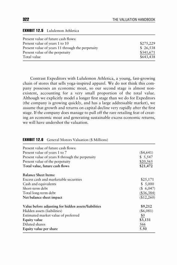
E1C12 08/14/2009 Page 322

Contrast Expeditors with Lululemon Athletica, a young, fast-growingchain of stores that sells yoga-inspired apparel. We do not think this com-pany possesses an economic moat, so our second stage is almost non-existent, accounting for a very small proportion of the total value.Although we explicitly model a longer first stage than we do for Expeditors(the company is growing quickly, and has a large addressable market), weassume that growth and returns on capital decline very rapidly after the firststage. If the company does manage to pull off the rare retailing feat of creat-ing an economic moat and generating sustainable excess economic returns,we will have undershot the valuation.

EXHIBIT 12.5 Lululemon Athletica

Present value of future cash flows:Present value of years 1 to 10 $275,229Present value of years 11 through the perpetuity $ 26,538Present value of the perpetuity $341,671Total value $643,438

EXHIBIT 12.6 General Motors Valuation ($ Millions)

Present value of future cash flows:Present value of years 1 to 7 ($4,641)Present value of years 8 through the perpetuity $ 5,547Present value of the perpetuity $20,565Total value, future cash flows $21,472

Balance Sheet Items:Excess cash and marketable securities $25,171Cash and equivalents $ 5,000Short-term debt ($ 6,047)Total long-term debt ($36,384)Net balance sheet impact ($12,260)

Value before adjusting for hidden assets/liabilities $9,212

Hidden assets (liabilities) ($6,081)Estimated market value of preferred $0Equity value $3,131Diluted shares 566Equity value per share 5.50


E1C12 08/14/2009 Page 323

Ad j u s tmen t s t o t he DCF Va l ue

Once we have forecasted cash flows and arrived at a base intrinsic value forthe business, we then adjust that value for hidden assets and liabilities, suchas pensions and stock options. Although the amount of value being sub-tracted by options is less today than it was a few years ago (options issuancedeclined once companies actually had to recognize the expense), it’s still ameaningful deduction to our valuation for some companies.

We start with the premise that options are a potential transfer of eco-nomic value away from existing shareholders to holders of the options. Al-though one can model this value loss by diluting the stake of currentshareholders, we think it’s more intuitive to quantify the dollar value beingtransferred. This approach also better matches companies’ actual behavior,since most firms use cash to buy back shares in an effort to mitigate—ornegate—option-driven dilution.

In valuing options, we assume that all options already issued with exer-cise prices below our fair value are in the money, and that the shares issuedupon exercise are immediately repurchased by the company with cash. Op-tions with strikes well above our fair value do not impact valuation, as theyare unlikely to be exercised. We also adjust for the cash received by thecompany as proceeds from the options, the tax benefits of the grants, and adiscount factor for buybacks that take place in future years.

Until recently, this was the easy part of our options adjustment; we alsohad to estimate the cost of options not yet granted, which was a tricky exer-cise given that companies did not have to expense them on the income state-ment. Now that options are expensed, we generally assume options are afixed percentage of expenses going forward, and incorporate that assump-tion into our forecasts for sales, general & administrative costs, or cost ofgoods sold when we project cash flows.

Compared with stock options, our pension adjustment is relatively sim-ple. We take the present value of all future pension payouts, and comparethem with the assets set aside to pay for them. We do the same with otherpostemployment benefits (OPEBs) such as health care, since this liabilitycan often dwarf the pension liability for companies with a large number ofretirees and a relatively small number of active workers.

We also make adjustments for companies that lease a material portionof their operating assets to reflect the economic reality of leasing transac-tions. Long-term contractual leases are in many ways economically equiva-lent to a purchase of the underlying asset, so we want to reflect them as suchto get a more accurate picture of companies’ true financial health. So, weoften remove the lease payments associated with these contractual arrange-ments from the income statement and replace them with the corresponding


E1C12 08/14/2009 Page 324

interest and depreciation component of rent expense that would have beencreated if the leased assets were financed with debt and purchased outrightin the first place. This adjustment tends to boost free cash flow to the firm(FCFF) because a key component of operating expenses (rent) is now inter-est expense, which is not removed from the FCFF calculation. However, be-cause the capitalized lease obligations are deducted from the firm’s equityvalue (similar to debt), and the cost of capital is modified to reflect both theadjusted capital structure and the cost of leases, the valuation impact couldvary depending on the company.

We also adjust for off-balance-sheet debt such as special purpose enti-ties, as well as potential legal liabilities. The latter are often eye-opening,since the huge numbers thrown around by the popular press in the wake ofa high-profile story (think Vioxx) are generally paid out over a lengthy timeperiod, rather than as an immediate lump sum. When you take a reasonableestimate of potential liability, adjust it for time, and then factor in a proba-bility that a jury will reduce the award, the actual economic impact can besurprisingly small.

For example, when the Vioxx news broke in November 2004, we esti-mated a total legal liability of about $15 billion. We based this estimate onWyeth’s phen-fen settlement of $375,000 per patient, multiplied by a roughnumber of potential Vioxx claimants, which yielded an estimate of $10 bil-lion. We then added an additional $5 billion in possible liability to accountfor uncertainty, and assumed that the payments would occur in 2006–2008after legal wrangling was completed. At the time, the present value of that$15 billion liability was only about $7.5 billion, which was the amount wededucted from our intrinsic value estimate.

We adjusted this liability estimate as new information became availa-ble regarding Food and Drug Administration (FDA) decisions and theunfolding legal picture, finally knocking it down to just $600 million inMarch 2008 once most claimants had signed on to a proposed settlement.It’s interesting to note that although we initially overestimated the even-tual legal liability, we were on target with our assumption that paymentswould not take place for some time after the news broke; in fact, Merckmade its first payments in August 2008. Also, despite our (in hindsight)draconian liability estimates, the stock market assumed things would beeven worse.

We finish out this section with an example of a company for which ourcash flow–based fair value was overwhelmed by adjustments: General Mo-tors. (Note that this example is from late summer, 2008, just before thecompany went off a cliff. By early November, our intrinsic value estimatefor GM was less than a dollar.) You can see in Exhibit 12.6 that our first-stage DCF value is actually negative—a wonderful industry, automobiles—


E1C12 08/14/2009 Page 325

and our total cash flow–based value is about $21 billion. After adding in$30 billion in cash and securities and netting out $42 billion in debt, we’releft with about $9 billion in value.

That’s before we adjust for hidden assets and liabilities, however—andas you can see in Exhibit 12.7, those make quite a difference. The pensionplan is overfunded by about $8 billion, but the company owes far moremoney to retirees in the form of health care and other benefits than it hasassets to pay for those benefits, which knocks over $21 billion off of enter-prise value. Then we have about $3 billion in net operating losses (NOLs),about $1.5 billion attributable to the company’s financing arm, and about$2 billion in cash that the company expects to receive from some asset sales.It’s an interesting commentary on General Motors that estimating howmany cars it will sell and for what prices is only a small part of the wholestory when valuing the company.

When DCF Fa i l s

No valuation method is perfect, of course, and there are times when we findthat DCF modeling needs to be set aside in favor of other tools. We thinkDCF works very well in most cases, but we’re aware of its limitations.

The most common reason that we turn to alternative valuation tools iswhen a company’s survival is at risk. We’ve found that relying on a DCFmodel for these types of companies frequently results in an overestimationof the company’s worth, because implicit in a DCF is the assumption of aperpetuity, which generally comprises a large chunk of the total intrinsic

EXHIBIT 12.7 General Motors’ Hidden Assets and Liabilities

Pensions:Fair value of plan assets less projected benefit obligation $ 8,348Fair value of OPEB� plan assets less accumulated OPEB ($21,022)Total pension + OPEB value ($12,674)

Other Adjustments to Enterprise Value:Present value of net operating losses (NOLs) $ 3,06849% of GMAC’s book value at P/B multiple of 0.2 $ 1,525Cash for Hummer and other asset sales $ 2,000

Balance sheet impact $ 6,593Net hidden assets (liabilities) ( $ 6,081)

�OPEB = Other postretirement employee benefits.


E1C12 08/14/2009 Page 326

value. Needless to say, the value of perpetuity is completely moot if a com-pany is at risk of going belly-up.

In these cases—usually brought on by a liquidity crunch—we run vari-ous scenarios focused on two questions: What are the odds that the com-pany will survive? And what is it worth if it does? Generally, this meansdetailed analysis of capital ratios, debt covenants, and a look at whetherparties high in the capital structure have a vested interest in survival versusfailure. (As the saying goes, if you owe the bank $10,000, it’s your problem;if you owe the bank $10 billion, it’s the bank’s problem.)

We also shift our focus from long-run to short-term operational per-formance. We have a long-term focus at Morningstar, and one of thethings we like about DCF valuation is that it matches that focus, sincewe have to project several years of financial results and estimate thelength of a company’s competitive advantage period. But when a com-pany’s survival may be determined by its ability to generate cash or parelosses over the next several quarters, its long-term prospects becomemuch less relevant.

We also use alternative valuation tools when a company is being bro-ken up, or when it has placed itself on the auction block. In this case ofbreakups, we may not have enough financial information to perform a DCFvaluation, so we’ll look at industry multiples, recent transactions, and soforth. When a company has either put itself up for sale or is in play as apotential target, we will typically blend an upside scenario based on a take-out price with DCF-derived scenarios that value the company on a stand-alone basis.

There are many cases in which a company’s value to an acquirer can belegitimately higher than its value as an independent firm—perhaps due tothe acquirer’s ability to leverage a larger distribution platform, for exam-ple—and we take this into account when estimating our upside scenario.For example, we cover a small medical device company called Insulet,which makes a novel type of insulin pump that is selling very quickly. Un-fortunately, Insulet is competing with giants like Medtronic and Johnson &Johnson with vastly greater resources.

So, in valuing the company, we blend three scenarios: one based on aDCF model that assumes the company is successful as a stand-alone entity,one that assumes that the competition rolls out a better insulin pump anddrives Insulet’s equity value to zero, and one that assumes the company ispurchased at a premium by a larger competitor. The diabetes device fieldhas undergone a lot of recent consolidation, and buyouts are fairly com-mon, so we’re comfortable with the assumption that this is a plausiblescenario.


E1C12 08/14/2009 Page 327

Uncer t a i n t y and Marg i n o f Sa f e t y

Physicist Niels Bohr once said, ‘‘Making predictions is hard, especiallyabout the future.’’ We’re very cognizant of Bohr’s words at Morningstar,and we recognize that any forward-looking estimate of intrinsic value is re-ally better thought of as a range of possible outcomes. For this reason, wetry to look at the future in a probabilistic way as much as possible.

After all, the future of any company can follow a number of differentpaths. In estimating an intrinsic value, we think the analyst’s job is to assesswhich of those paths have some likelihood of occurring, assign reasonableprobabilities to the least implausible scenarios, and thus reach an expectedintrinsic value for the company’s shares.

Practically, this means we encourage our analysts to spend time think-ing about the range of possible outcomes for the companies that we value,even though the fair values we publish are, of necessity, point estimates. Forexample, we use scenario analysis and other tools to estimate a variety offair values given different combinations of plausible future events.

Why do we think it’s so important to consider a range of possible futurefair values, rather than a single most likely fair value? Although it’s veryeasy to think about the future in a linear fashion, in reality events rarelyplay out in such a neat and orderly manner. Major structural changes inan industry or a company are inherently hard to predict, but thinkingabout the future probabilistically allows us to at least open our minds to thepossibility of outcomes that, though unlikely, can have a huge impact onfair values.

A second reason we believe it’s important to think about fair valuesas points along a distribution of potential outcomes is that it improves thedecision-making process. If you think about only a single fair value, you’veanchored yourself to a particular outcome and the pathway that leads to it,which means you’re likely to discount new information that doesn’t supportthe answer to which you have already mentally committed. However, if youconsider a range of possible outcomes, you essentially commit to the possi-bility that the future could play out in a wide variety of ways, so you’remore likely to assess new information in a less biased fashion.

Our scenario analysis typically focuses on a few key value drivers thatare often company-specific. For example, we cover a small company calledFuel-Tech that manufactures a product that makes coal-burning powerplants much more efficient. As far as we can tell, it has minimal competitionand offers a compelling return on investment to utilities that use it. How-ever, Fuel-Tech is a small company with a limited sales force, and the pur-chasing decisions of utilities are often hard to forecast because they’re soheavily regulated. So, our scenarios range from a low of $14 to a high of


E1C12 08/14/2009 Page 328

$92 depending on what share of various markets the company is able to get.Exhibit 12.8 shows these scenarios.

Because Fuel-Tech is such a young company, estimating its eventualmarket share is the best way to tackle various scenarios. For a companyoperating in a long-cycle market like Boeing, the key variables may be howlong the current cycle lasts and what kind of cost efficiencies can beachieved. So for Boeing, we forecast sales of different key products, rollthem up into an overall estimate of aircraft deliveries, and forecast cost ofgoods sold (COGS) as a percentage of sales. Exhibit 12.9 shows our possi-ble scenarios for Boeing, with the current commercial aircraft cycle peakingin 2009, 2010, or 2012, depending on the level of optimism.

We believe that thinking about what could happen is just as useful asthinking simply about what is most likely to happen—or perhaps more so.This is why we believe it’s very useful to embed multipath thinking in ananalytical tool kit. To reflect this aspect of our research process, we have afair value uncertainty rating on every stock that we cover, assessing eachcompany’s uncertainty as low, medium, high, very high, or extreme. In as-signing the rating, we ask ourselves, ‘‘How tightly can we bound the fairvalue of this company? With what level of confidence can we estimate itsfuture cash flows?’’ What we’re essentially attempting to do is to estimatethe size of the confidence interval for the values of the companies weanalyze.

For example, a small biotech company with a promising drug in clinicaltrials could plausibly be worth anywhere from $50 (if the drug is approvedand gains a reasonable amount of market share) all the way down to $2 (ifthings do not pan out and the company is left with nothing but the cash onits balance sheet and some interesting research ideas). Such a companywould land squarely in our very high uncertainty bucket.

EXHIBIT 12.8 Valuation Scenarios for Fuel-Tech

Scenario Base Pessimistic Optimistic

Air Pollution Control annual growth rate 20% 8% 25%Share of addressable U.S. coal-fired market 35% 10% 50%Share of addressable China coal-fired market 33% 3% 50%Share of addressable India coal-fired market 20% 3% 50%Share of addressable EU coal-fired market 15% 2% 50%Share of addressable Russian coal-fired market 10% 0% 50%Total 8-year revenue CAGR 33% 14% 41%Total 8-year EBIT CAGR 44% 20% 48%Fair value estimate $55 $14 $92


E1C12 08/14/2009 Page 329

EXHIBIT12

.9V

alu

ati

on

Sce

nari

os

for

Boei

ng

(Num

ber

of

pla

nes

del

iver

ed.)

2008

2009

2010

2011

2012

2013

2014

2015

2016

2017

Expec

ted

case

,valu

e¼

$84

Com

mer

cialdel

iver

ies

475

502

523

518

498

486

481

421

391

$386

CO

GS,as

%of

sale

s79.9

%81.6

%82.2

%83.9

%83.2

%83.0

%83.8

%85.0

%84.8

%84.5

%

Wors

tca

se,

valu

e¼

$56

Com

mer

cialdel

iver

ies

475

502

444

414

399

389

385

337

313

$309

CO

GS,as

%of

sale

s79.9

%81.6

%84.7

%86.4

%85.7

%85.5

%86.3

%87.5

%87.3

%87.0

%

Bes

tca

se,

valu

e¼

$124

Com

mer

cialdel

iver

ies

$477

$502

$549

$571

$597

$583

$577

$505

$469

$463

CO

GS,as

%of

sale

s79.9

%81.6

%78.7

%80.4

%79.7

%79.5

%80.3

%81.5

%81.3

%81.0

%

329

E1C12 08/14/2009 Page 330

For example, we cover a small biotechnology company called Mann-Kind that is developing a form of insulin that can be inhaled, rather thaninjected. This could potentially be a blockbuster product, but the high-pro-file failure of a competing product early in 2008 could also cause physiciansto be wary of recommending it without data from further studies, whichwould be both expensive and time-consuming for MannKind. Or, despitethe promising data that has been released so far, the company’s applicationfor approval could simply be rejected by the FDA. It should come as no sur-prise, then, that the company could be worth anywhere from zero to $12per share, as you can see in Exhibit 12.10.

At the other end of the spectrum, consider a company like McCormick,which dominates the spice and seasoning industry. The spice market neithergrows nor shrinks very much over time, and McCormick’s strong brandsgive it pricing power that no competitor can match. Unless Americans sud-denly shift their tastes en masse to desire much more heavily flavored ormuch blander food, there’s not a very wide range of plausible outcomes forthe fair value, so McCormick would get a low uncertainty rating.

Of course, precisely quantifying uncertainty is an almost oxymoroni-cally difficult process. So what we do is try to look at a standardized set offactors, all of which affect the dispersion of possible fair values.

For example, we estimate the likely range of sales for a company. Somebusinesses—such as grocery stores or consumer product companies—havefairly predictable sales, while many others have revenue lines that can swingaround quite a bit. A closely related step is thinking about a company’s op-erating leverage. What percentage of each incremental dollar of sales be-comes income? The key to this question is often the mix of variablesrelative to fixed costs at a company.

We also take financial leverage into account, because high levels of debtcan amplify equity values in both directions, and we consider whether a spe-cific event in the future, such as a product approval or legal decision, couldradically change a company’s value.

EXHIBIT 12.10 Valuation Scenarios for MannKind

Probability DescriptionFair ValueEstimate

20% Drug on market in 2010 with 10%peak share in 2020

On track $12.00

40% Drug on market in 2012, with 5%peak share in 2020

Additionalstudies

$ 7.00

40% Failure Rejected $ 0$ 5.00


E1C12 08/14/2009 Page 331

Finally, we are cognizant of how these factors interact. For example,sales variability and operating leverage work together. A company withsales that don’t fluctuate very much, but which has high fixed costs—suchas a grocery store—might have the same level of uncertainty as a companywith more variable sales but costs that can ebb and flow with the business,such as a consulting firm.

We use these uncertainty ratings to set our margins of safety. A com-pany with a wide range of plausible outcomes and a very high uncertaintyrating would need to trade at a very large discount to our estimate of intrin-sic value before we would recommend the stock to investors. The reasoningbehind this is simple. Although the central tendency of the range of possibleintrinsic values may be $30, our confidence in that point estimate is not ter-ribly high, so we look for a large margin of safety as an insurance policy ofsorts.

Empirical research into decision making has shown that people are notterribly good at accurately estimating probabilities, and so some may criti-cize our emphasis on scenario analysis on these grounds. We agree that esti-mating the likely probabilities of various future scenarios is difficult andimprecise. However, we think that a process that embraces uncertainty andincorporates scenario analysis is more representative of reality than a finelytuned point estimate that considers only a single set of potential outcomes.

Moreover, we think that scenario analysis can improve the decision-making process inside a large research organization when new informationneeds to be incorporated into an intrinsic value estimate, or when conflictarises over what a company’s future may look like. When only one intrinsicvalue has been estimated, the conversation centers on whether that estimateis right or wrong, and a discussion framed in such terms can lead to in-appropriate anchoring on the previous opinion. However, if multiple sce-narios were forecasted initially, then the discussion centers on thedistribution of probabilities among various scenarios, as well as the appro-priate level of optimism/pessimism for upside and downside cases. This canlead to a much healthier debate, in addition to less anchoring.

CONCLUS I ON

After applying DCF modeling to literally thousands of companies fromscores of industries and dozens of companies over several years, we thinkwe have learned a few lessons.

& It’s better to be approximately right than precisely wrong. The com-plexity of DCF models can cause the user to spend too much time


E1C12 08/14/2009 Page 332

making assumptions that have a relatively minor impact on valua-tion. DCF valuation works best when the user steps back and asks,‘‘How does this company make money? What assumptions are likelyto move the needle, and which are not?’’ before plunging head firstinto Excel. Greater complexity and greater accuracy are not neces-sarily joined at the hip; in fact, more complex modeling may causethe analyst to lose sight of the issues likely to have the largest impacton intrinsic value.

& Look for diminishing returns in the valuation process, since somethings either are unknowable or would require too much effort withouta corresponding payback in increased accuracy. For example, the rightlevel of capex for a software firm is not going to move the valuationneedle relative to the right values for research and development or salesand marketing. Tie the time you spend on each assumption to its likelyimpact on the firm’s overall valuation.

& Be aware that how you model can affect what you model. For example,if your assumptions are based on growth rates and margin percent-ages—as most models are—it’s very easy to misestimate operatingleverage, because operating margins that increase from, say, 20 percentto 30 percent over a few years look unreasonable. Avoid this mentaltrap by thinking carefully about how much additional capital a com-pany actually needs to spend to generate an incremental dollar of sales,and by modeling results in absolute dollar terms. Once this process iscomplete, see what margins are implied by your incremental-cost esti-mates. The results may surprise you.

& A corollary to the preceding lesson is that underestimating operatingleverage—positive and negative—is one of the most common mistakesanalysts can make. Thinking creatively and carefully about a com-pany’s cost structure is one of the most fruitful avenues for uncoveringcompanies with intrinsic values that are dramatically higher or lowerthan the current market price.

& Don’t forget the importance of checks and balances. About three-quar-ters of Morningstar’s DCF model is devoted to ratios, pro forma finan-cial statements, and other output meant to provide context and gutchecks to our analysts. This output is tremendously helpful in pinpoint-ing where a model may be too optimistic, too pessimistic, or simplyinconsistent. Even more importantly, it helps us have confidence invalue estimates that seem too high or too low, but which are actuallylikely to be reasonable estimates of the future.

We’ve performed detailed DCF valuations on something close to 3,000stocks over the past eight years, and our experience has been that DCF


E1C12 08/14/2009 Page 333

works well in the vast majority of cases, however tempting it might be toopt for a shortcut. At the end of the day, the value of an asset is dependenton the cash it can generate in the future, and DCF is generally the best toolavailable for forecasting and valuing those cash flows. Of course, no valua-tion tool is perfect, and there are times when we eschew DCF in favor ofother approaches.

Finally, we think it’s vital to remember that any valuation approach isonly as good as its inputs, and even the most complex or cutting-edge valua-tion tool cannot compensate for a poor understanding of the asset beingvalued. We spend a great deal of time understanding the companies that wecover so we can attempt to forecast their future cash flows with an appro-priate level of confidence, and we think any user of DCF should do thesame. Understanding your valuation tool kit is important, but understand-ing the assets you’re valuing is paramount.


E1C13 08/25/2009 Page 334

CHAPTER 13Valuing Real Options

Insights from Competitive Strategy

Andrew G. SutherlandVice President, Stern Stewart & Co.

Jeffrey R. WilliamsProfessor of Business Strategy, Tepper School of Business at Carnegie Mellon

Growth opportunities and future strategies can comprise a significant pro-portion of a firm’s valuation. At the end of 2006, the median companies

in the S&P 500 and the Russell 3000 had 25 percent and 40 percent of theirvaluations, respectively, attributed to Future Growth Value (FGV1), thecapitalized value of future profit growth.1 Acquisition premiums can alsobe interpreted as estimates of value creation attributed to new tactics andoperational improvements under a new regime. Unfortunately, managersoften find static net present value (NPV) tools and trading multiples to betoo rigid to evaluate the contingent nature of strategic decisions and thecash flow recovery profiles associated with possible outcomes. For example,Microsoft was willing to develop its Xbox platform at a loss because itexpected subsequent game and peripheral offerings linked to it to generatesignificant profits. Similarly, commodities producers frequently choose todelay extraction until output prices swing in their favor. Academics andpractitioners have recognized the similarities of payoff functions betweensuch contingent decisions about real assets, classic examples of so-calledreal options, and those of financial securities whose values are derived fromthe price of something else. The Black-Scholes model and binomial latticeshave emerged as the most frequently prescribed and used tools for evaluat-ing real options within both capital budgeting and enterprise valuation con-texts. With the classic real option decision growing increasingly complex,

334

E1C13 08/25/2009 Page 335

and managers becoming more sophisticated, a frank assessment of modernvaluation tools is timely.

The first section provides an overview of commonly used approachesfor pricing contingent claims on financial securities. We then review howpractitioners and academics have extended these approaches to the basicapplication of real option pricing. The next section, the core focus of thischapter, scrutinizes the assumptions made in the extension of models builtfor financial securities to real projects. A number of refinements are pre-sented that attempt to better address the strategic realities of the firm and,in doing so, generate a more robust valuation. A summary and discussion ofareas of future research conclude the chapter.

OVERV I EW OF OPT I ON PR IC ING FORF INANC IA L SECUR I T I ES

Options give an investor the right, but not the obligation, to buy or sell asecurity according to predetermined terms during some period or at somespecific point. Stock option contracts can be divided into two categories:calls and puts. A call option gives the holder the right to purchase (call)stock from a counterparty at a fixed exercise price at or before a specificdate. A put option gives the holder the right to sell (put) stock to a counter-party at a fixed exercise price at or before a specific date. At contract expiry,the call holder makes money when the price of the underlying is above theexercise price, while the opposite holds for the put holder. When the exer-cise is only permitted upon option contract expiry, it is termed European;when exercise is permitted at any point up to and upon expiry, it is termedAmerican. Exhibit 13.1 depicts the payoff function for call and put optionpositions where the exercise price is $100.

Stock options can serve three important purposes:

1. Given their low price relative to the underlying stock, call and put op-tions can be used to make a leveraged bet on future returns. For thesame up-front cost as a single stock, a number of call options can bepurchased, resulting in more than a dollar-for-dollar change in wealthfor each dollar change in stock price.

2. Call and put options can provide an inexpensive way to hedge positionsin firms with similar exposures, or holdings in the stock itself. An inves-tor locked into a long position in a stock can purchase insurance on theposition by purchasing a put option.

3. Finally, call options are instruments frequently used in executive com-pensation to align the long-term interests of management and the firm.

Valuing Real Options 335

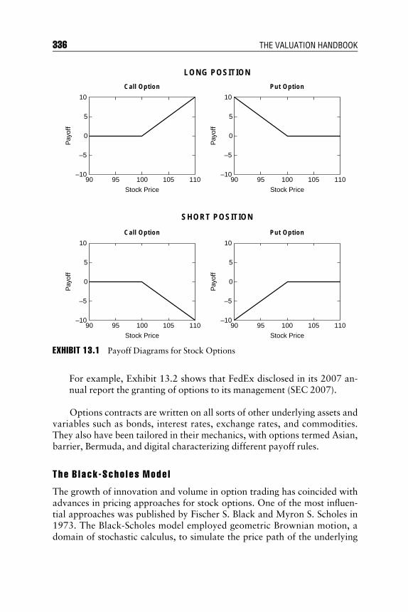
E1C13 08/25/2009 Page 336

For example, Exhibit 13.2 shows that FedEx disclosed in its 2007 an-nual report the granting of options to its management (SEC 2007).

Options contracts are written on all sorts of other underlying assets andvariables such as bonds, interest rates, exchange rates, and commodities.They also have been tailored in their mechanics, with options termed Asian,barrier, Bermuda, and digital characterizing different payoff rules.

The B l a ck - Scho l es Mode l

The growth of innovation and volume in option trading has coincided withadvances in pricing approaches for stock options. One of the most influen-tial approaches was published by Fischer S. Black and Myron S. Scholes in1973. The Black-Scholes model employed geometric Brownian motion, adomain of stochastic calculus, to simulate the price path of the underlying

10

Call Option

5

0

Pay

off

–5

–1090 95 100

Stock Price

105 110

10

Put Option

LONG POSITION

SHORT POSITION

5

0

Pay

off

–5

–1090 95 100

Stock Price

105 110

10

Call Option

5

0

Pay

off

–5

–1090 95 100

Stock Price

105 110

10

Put Option

5

0

Pay

off

–5

–1090 95 100

Stock Price

105 110

EXHIBIT 13.1 Payoff Diagrams for Stock Options


E1C13 08/25/2009 Page 337

stock. Options had been traded on exchanges as far back as the seventeenthcentury, but it wasn’t until the Black-Scholes model and equally importantresearch by Robert C. Merton (1973) was published that the market trulytook off. (See Exhibit 13.3.)

The Black-Scholes model prices stock options with five variables:

& The price of the underlying (S).& The exercise (strike) price (X).

EXHIBIT 13.2 FedEx Option Grants

2007 2006 2005

Expected lives 5 years 5 years 4 yearsExpected volatility 22% 25% 27%Risk-free interest rate 4.869% 3.794% 3.559%Dividend yield 0.3023% 0.3229% 0.3215%

The weighted-average Black-Scholes value of our stock option grantsusing the assumptions indicated above was $31.60 per option in 2007,$25.78 per option in 2006 and $20.37 per option in 2005. The intrinsicvalue of options exercised was $145 million in 2007, $191 million in 2006and $126 million in 2005.

The following table summarizes information about stock option activ-ity for the year ended May 31, 2007:

Stock Options

Shares

Weighted-Average

Exercise Price

Weighted-AverageRemaining

Contractual Term

AggregateIntrinsic Value

(in Millions)

Outstandingat June 1,2006

17,099,526 $ 60.82

Granted 2,094,873 110.25Exercised (2,333,845) 49.55Forfeited (270,153) 89.12Outstandingat May31, 2007

16,590,401 $ 68.22 5.9 years $696

Exercisable 10,418,072 $ 54.75 4.6 years $577Expected to vest 5,678,543 $ 90.97 8.0 years $109


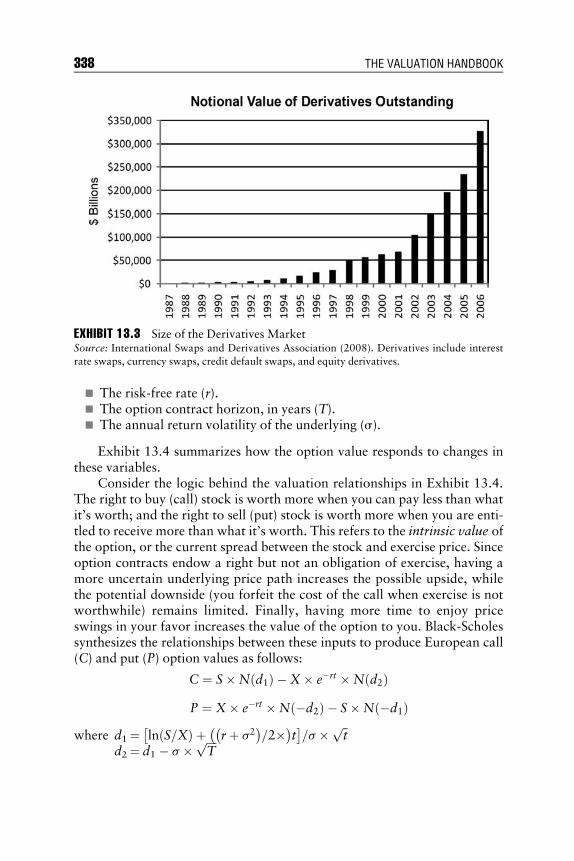
E1C13 08/25/2009 Page 338

& The risk-free rate (r).& The option contract horizon, in years (T).& The annual return volatility of the underlying (s).

Exhibit 13.4 summarizes how the option value responds to changes inthese variables.

Consider the logic behind the valuation relationships in Exhibit 13.4.The right to buy (call) stock is worth more when you can pay less than whatit’s worth; and the right to sell (put) stock is worth more when you are enti-tled to receive more than what it’s worth. This refers to the intrinsic value ofthe option, or the current spread between the stock and exercise price. Sinceoption contracts endow a right but not an obligation of exercise, having amore uncertain underlying price path increases the possible upside, whilethe potential downside (you forfeit the cost of the call when exercise is notworthwhile) remains limited. Finally, having more time to enjoy priceswings in your favor increases the value of the option to you. Black-Scholessynthesizes the relationships between these inputs to produce European call(C) and put (P) option values as follows:

C ¼ S�N d1ð Þ �X� e�rt �N d2ð ÞP ¼ X� e�rt �N �d2ð Þ � S�N �d1ð Þ

where d1 ¼ ln S=Xð Þ þ rþ s2� �

=2�� t

� �=s � ffiffi

tp

d2 ¼ d1 � s � ffiffiffiffiT

p

EXHIBIT 13.3 Size of the Derivatives MarketSource: International Swaps and Derivatives Association (2008). Derivatives include interest

rate swaps, currency swaps, credit default swaps, and equity derivatives.


E1C13 08/25/2009 Page 339

One significant finding of Black and Scholes is that there is a relation-ship between the option value, the current value of the underlying stock,and the return on a risk-free security. The put-call parity relationship is:

CþX� e�rt ¼ Pþ S

Exercise 1

1. Price a European call option issued on stock with an exercise price of$15, value of $13, annual return volatility of 25 percent, and horizonof one year. Assume the risk-free rate is 5 percent.

2. Use the put-call parity relationship to price a put option on the samestock.

3. Another one-year European call issued on a different stock is priced at$1.20. It has an exercise price of $20 and a current value of $17, andthe risk-free rate is still 5 percent. Use the Black-Scholes model to calcu-late the annual return volatility implied by the current price.

Solutions

1. $0.812. $2.083. 28.74 percent

EXHIBIT 13.4 Drivers of Option Value


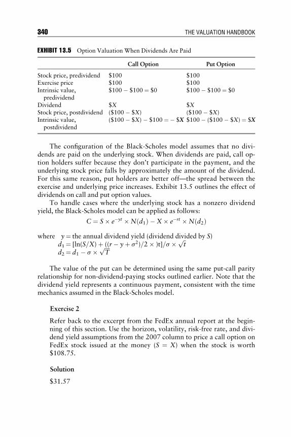
E1C13 08/25/2009 Page 340

The configuration of the Black-Scholes model assumes that no divi-dends are paid on the underlying stock. When dividends are paid, call op-tion holders suffer because they don’t participate in the payment, and theunderlying stock price falls by approximately the amount of the dividend.For this same reason, put holders are better off—the spread between theexercise and underlying price increases. Exhibit 13.5 outlines the effect ofdividends on call and put option values.

To handle cases where the underlying stock has a nonzero dividendyield, the Black-Scholes model can be applied as follows:

C ¼ S� e�yt �N d1ð Þ �X� e�rt �N d2ð Þ

where y¼ the annual dividend yield (dividend divided by S)d1 ¼ [ln(S=X) þ ((r� yþ s2)=2 � )t]=s � ffiffi

tp

d2 ¼ d1 � s � ffiffiffiffiT

p

The value of the put can be determined using the same put-call parityrelationship for non-dividend-paying stocks outlined earlier. Note that thedividend yield represents a continuous payment, consistent with the timemechanics assumed in the Black-Scholes model.

Exercise 2

Refer back to the excerpt from the FedEx annual report at the begin-ning of this section. Use the horizon, volatility, risk-free rate, and divi-dend yield assumptions from the 2007 column to price a call option onFedEx stock issued at the money (S ¼ X) when the stock is worth$108.75.

Solution

$31.57

EXHIBIT 13.5 Option Valuation When Dividends Are Paid

Call Option Put Option

Stock price, predividend $100 $100Exercise price $100 $100Intrinsic value,

predividend$100 � $100 ¼ $0 $100 � $100 ¼ $0

Dividend $X $XStock price, postdividend ($100 � $X) ($100 � $X)Intrinsic value,

postdividend($100 � $X) � $100 ¼ � $X $100 � ($100 � $X) ¼ $X


E1C13 08/25/2009 Page 341

B i nom i a l L a t t i c es

Whereas the Black-Scholes model applies continuous time dynamics, bino-mial lattices use discrete time dynamics. This approach, developed by Cox,Ross, and Rubinstein (1979), is particularly useful for analyzing the effectson option values of one-time events such as bankruptcies or mergers andrecurring events such as quarterly dividends, in addition to modeling theAmerican option exercise. The same five variables (price of the underlying,strike price, risk-free rate, option contract horizon, and return volatility ofthe underlying) play a role in valuing the option. In fact, as the binomiallattice is geared with smaller and smaller time increments, the option pricewill converge to the Black-Scholes value.

A binomial lattice works as follows. The period leading up to optionexpiration is split into subperiods, marked by nodes. Price discovery for theunderlying occurs at each node—the stock rises or falls by a specific amountdepending on its return volatility. The stock increase scalar ‘‘u’’ that sets themagnitude of the price rise is equal to es

ffiffit

pand the stock decrease scalar ‘‘d’’

equals 1/u. Readers familiar with decision trees will recognize the mechan-ics of this framework, presented in Exhibit 13.6.

Exercise 3

Using the volatility assumptions of Exercise 1.1, model the price path ofthe stock for one year using a binomial lattice with nodes everythree months.

S

Su

Today Period 1 Period 2

Sd

Sd2

Sud

Su2

EXHIBIT 13.6 Simple Binomial Lattice for Stock


E1C13 08/25/2009 Page 342

Solution

Once the price path of the underlying has been simulated, the op-tion can be valued at each ending node.

For the call option, the value is the greater of 0 and S-X: for the putoption, the value is the greater of 0 and X-S.

The option value today is then estimated by working recursivelythrough the tree, assuming risk neutrality. This means that future payoffsare discounted at the risk-free rate, where the probability of a ‘‘u’’ step inthe underlying is:


E1C13 08/25/2009 Page 343

pu ¼ e(r�y) � dh i

= u� dð Þ

And the probability of a ‘‘d’’ step is simply 1 � pu.The value of the options at each of the second-to-last nodes can be

calculated:

For each node prior to the second-to-last node, using the same recursiveapproach:

$21.43$6.43

$18.91$4.10

$16.69 $16.69$2.51 $1.69

$14.73 $14.73$1.50 $0.87

$13.00 $13.00 $13.00$0.88 $0.44 $0.00

$11.47 $11.47$0.23 $0.00

$10.12 $10.12$0.00 $0.00

$8.93$0.00

$7.88$0.00


E1C13 08/25/2009 Page 344

When the stock pays a discrete dividend (as the vast majority of divi-dends are paid in practice), it can be modeled in the lattice by simply sub-tracting the dividend from the underlying when it is paid.

Exercise 4

1. The stock from Exercise 3 pays a dividend of $0.10 at the end of eachquarter. Recalculate the price path of the stock using the binomial lat-tice approach.

2. How does the new price path change the value of the call option?

Solutions

1.

2.

The call is worth $0.13 less.

Su4 30.12$04.$-

Su3 16.81$03.$-

Su2-$.20 Su3 94.61$04.$-d $16.29

Su-$.10 Su2d-$.30 $14.63 $14.43

02.$-duSS Su2d2-$.40 $13.00 $12.80 $12.60

Sd-$.10 Sud2 71.11$73.11$03.$-

Sd2-$.20 Sud3 27.9$29.9$04.$-

Sd3-$.30 $8.63

Sd4-$.40 $7.48

$21.03$6.03

$18.61$3.71

$16.49 $16.29$2.21 $1.29

$14.63 $14.43$1.30 $0.66

$13.00 $12.80 $12.60$0.75 $0.34 $0.00

$11.37 $11.17$0.17 $0.00

$9.92 $9.72$0.00 $0.00

$8.63$0.00

$7.48$0.00


E1C13 08/25/2009 Page 345

BAS IC OPT I ON PR I C ING APPL I CAT I ONS FORREAL ASSETS

The pricing tools for call and put options have been extended to the valua-tion of all sorts of other contracts, including interest rate derivatives, futurescontracts, and exotic variations of vanilla calls and puts. Largely because ofthe explicit modeling of state-dependent decisions, they have also provenuseful for evaluating real options, where the firm holds the right but not theobligation to make some business decision. Traditional valuationapproaches such as NPV and internal rate of return (IRR) are useful for ap-plication to the as-is perspective of the firm. However, the total worth of afirm comprises not just the value of the current operations, but also the valuederived from the ability to expand projects progressing successfully; aban-don ones revealing themselves to be unsuccessful; and take advantage of thelearning, information, and market position gained in both scenarios. Netpresent value (NPV) and internal rate of return (IRR) analyses often are toorigid to maneuver the dynamic and flexible nature of such strategic options.

The classic capital budgeting exercise involves discounting expectedcash flows at an appropriate risk-adjusted rate. When only point estimatesof the most likely scenario are used in valuation and the payoffs from dy-namic and flexible strategies are ignored or improperly measured, the valua-tion exercise is incomplete (Myers 1977, 1984). How can the ability toexpand, abandon, and collect information be priced? What is the concep-tual connection to the options framework?

Produc t i o n F l e x i b i l i t y and P l a t f o rm I nves tmen t s

Let’s start with a call option. There are many situations where possessingthe right, but not the obligation, to make a production or investment deci-sion creates value for the firm. Consider the investment and extraction op-portunities of an oil company. While spot (current) market prices are amajor determinant of project valuation, the possibility of delaying produc-tion until prices may be higher can be a material source of value as well. Thegreater the uncertainty in the output market, the more the right to delay isworth. The value of this flexibility, combined with the present value of theproject in current conditions, can be compared to the fixed investment cost.A manufacturer may look at its capacity decisions with a similar perspec-tive. Maintaining excess capacity or inventory can allow the firm to captureenormous profits during periods of peak demand that more than offsetholding costs and the opportunity cost of the capital tied up.

Yet another analogy can be made to companies that invest significantamounts in intangible assets. Much of their focus is on searching for growth


E1C13 08/25/2009 Page 346

opportunities where platform investments, often developed at considerableexpense, spawn profitable offspring. For example, Microsoft’s ownership ofthe Windows platform allowed it to develop follow-on products such as theOffice software, the MSN Messenger application, and subsequent versionsof Windows. Had Microsoft overlooked the value of follow-on productsand made the decision to develop the first Windows product based solely onits stand-alone profits, the company might not have invested so heavily orplaced so much faith in the development of what would be one of the richestreal-option platforms in history. Note that Microsoft succeeded with an-other platform investment in the Xbox video game system, sold at a consid-erable loss (as described in Exhibit 13.7), expecting to more than recoverthrough the sale of games and hardware that are linked exclusively to thesystem (Ivan 2007).

EXHIBIT 13.7 Xbox’s Real Options

‘‘There are three ways to make money on an Xbox. Generally it’s not on thehardware itself: we’ll probably be gross margin neutral on that over the lifecycle of the product and try to break even on that. The second thing you tryto do is you make money on the games themselves, and there are two mod-els there. One is first-party games that Microsoft produces. The other isgames that Electronic Arts or an Activision produces, and we get paid aroyalty on those games. The third place you make money is on Live, andwhere we actually have a very nice service that’s scaling very well, and thatis a business model that’s subscription, ad-based, and download-based. Itkind of has the full gamut of business models associated with it, and I thinkyou’re going to continue to see that grow. And then the final place you makemoney is on peripherals, so game controllers, cameras, steering wheels, awhole other set of things.’’

—Robbie Back, President of Microsoft’s Entertainmentand Devices Division

Estimates of Microsoft’s development spending on the system varied,but the company recorded significant operating losses in its Home andEntertainment segment, comprised primarily of Xbox offerings, leading upto its release:

Home andEntertainment(In millions,

exceptpercentages) 2006 2005 2004

PercentChange2006

versus2005

PercentChange2005

versus2004

Revenue $ 4,256 $ 3,140 $ 2,737 36% 15%Operating loss $ (1,262) $ (485) $ (1,337) (160%) 64%


E1C13 08/25/2009 Page 347

I n f o rma t i on and Organ i z a t i ona l L earn i ng

There are scenarios in which the information revealed or the organizationallearning following a decision can be used to maximize the potential of plat-form investments. Sometimes the uncertainty surrounding the future successof a new product release can be managed in such a way to make even thebiggest Hail Mary offerings worth taking on. A film studio can phase itsinvestments in advertising, distribution, and development of sequels for amovie by staging its expenditures pending the reaction of critics and otherviewers at early screenings. While new releases tend to have a low probabil-ity of success, successful releases generate vast payoffs not just from screen-ing revenues, but from DVDs, merchandise, and sequels. Therefore, beingable to accelerate or decelerate spending after the results of early screeningsare known is like letting the studio participate in a real options lottery, andkeeping the cost of their participation at a minimum. Exhibit 13.8 providesa hypothetical investment-decision road map for film studios.

The investments made by a pharmaceutical company can be thought ofin terms of embedded real options as well. Like the film studio, it can simi-larly stage the research and development of drugs pending clinical trialsand regulatory approval. Furthermore, it attaches value to learning, oftenfirm-specific and proprietary, that occurs even when a given product failsto make it to market. The research and development for one project maygenerate knowledge and capabilities useful for others that would not havenecessarily been enjoyed had the initial project not been carried out. Break-throughs and patents spawned from a losing effort can be applied to sup-port related projects, and mistakes made in previous trials can be avoided.

Test Audiences,Critical Reviews

Pitch toDirectors

Today

WriteScript

Produce$50M

Abandon$0

Cost of option exercise in italics

Low Budget$10M

High Marketing.Distribution Budget

$100M

No Sequel$0M

Write, ProduceSequel$80M

6 Months 18 Months(Film Release)

30 Months

Merchandise,DVD, Ticket Sales

EXHIBIT 13.8 Real Options Embedded in a Film Project


E1C13 08/25/2009 Page 348

Pro j e c t Abandonmen t as an Op t i on

The right to abandon or scale back an investment is also worth somethingto the firm, and this is what typifies the put variety of real options. Take aminerals company that gets hit with an extended period of declining pricesfor its output. Rather than continue to operate at a loss, it can sell its prop-erty and equipment, and use the proceeds to invest elsewhere. There aremany analogous situations in which shutting down a business that runs intohard times is a much better alternative to letting it ride.

Each of the aforementioned investment scenarios can be characterizedby a common element. Being able to make or unwind an investment at afuture date, pending the realization of some event, is a valuable right. Whenrelating the realization to the price path of the underlying security for a callor put option, the analogy between the real investment and the financialderivative, for the purpose of real option pricing, is complete. To the extentone can model the variables that determine the value of the investment—beit the price path of oil, the popularity of a movie, or the success of follow-onprojects—either the Black-Scholes or the binomial lattice framework can beapplied. The remainder of this section demonstrates how the trade-offs be-tween the benefits and costs of investment flexibility and information arequantified in each of these frameworks.

Us i ng t he B l ack - Scho l e s Mode l t o Va l ueRea l Asse t s

Recall the example of the oil company that possesses reserves, and thinksabout market price volatility in timing extraction. This situation natu-rally extends itself to Black-Scholes valuation. The inputs originally takenfrom the opportunity to invest in a financial security can be drawn fromthe characteristics of the real investment opportunity as illustrated inExhibit 13.9.

The option values (calls and puts) are added to the static NPV in deter-mining the total worth of the investment.

Exercise 5

1. Consider an oil company with 400,000 barrels of known reserves. Thecompany can extract and produce the reserves at a cost of $25 per bar-rel over the next five years. Oil is priced in the market today at $100 abarrel, and the contribution margin averages 45 percent. The risk-freerate is 5 percent, and volatility of oil prices—believed to be the onlysource of uncertainty influencing the value of the reserves—is estimatedat 25 percent per year. What is the value of producing the oil today?


E1C13 08/25/2009 Page 349

2. Use the Black-Scholes framework to estimate the value of the reserves.3. How much is the ability to delay production worth to the company?

Solutions

1. $8,000,0002. $18,401,1393. $10,401,139

Exercise 6

1. Consider a company that is bidding on a mine. For various reasons, thecompany cannot delay or ramp up production given the evolution ofcommodity prices in the market, but it can abandon the investment inthree years by selling off the property and equipment for $5 million. Itestimates the value of the mine today to be $10 million. The risk-freerate is 5 percent, and the volatility of commodities prices—believed tobe the only source of uncertainty influencing the value of the reserves—is estimated at 20 percent per year. Use the Black-Scholes framework toestimate the maximum acceptable bid for the mine.

2. How much is the ability to abandon worth to the company?

Solutions

1. $10,405,3522. $405,352

EXHIBIT 13.9 Real Option Valuation Drivers Using Black-Scholes

Black-ScholesInput Stock Option Real Option

S Stock price Value of reserves today, given quantity andprice of oil, and variable cost structure

X Exercise price Fixed cost of extraction and production(no variable costs counted here)

r Risk-free rate Risk-free rateT Contract horizon Investment option horizon, given

maintenance costs, depletion, andcompetitive forces

d Return volatility Return volatility resulting from future priceuncertainty, reserve uncertainty, etc.


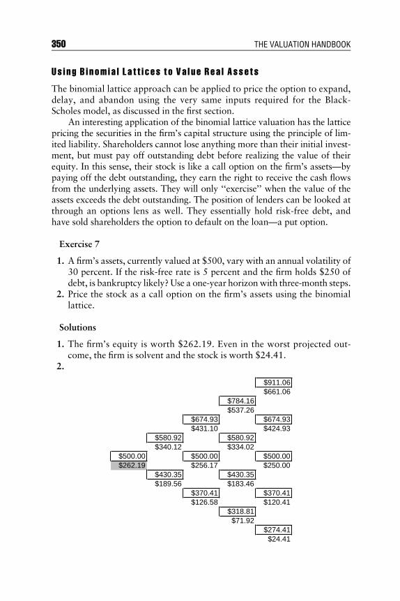
E1C13 08/25/2009 Page 350

Us i ng B i n om i a l L a t t i c es t o Va l ue Rea l Asse t s

The binomial lattice approach can be applied to price the option to expand,delay, and abandon using the very same inputs required for the Black-Scholes model, as discussed in the first section.

An interesting application of the binomial lattice valuation has the latticepricing the securities in the firm’s capital structure using the principle of lim-ited liability. Shareholders cannot lose anything more than their initial invest-ment, but must pay off outstanding debt before realizing the value of theirequity. In this sense, their stock is like a call option on the firm’s assets—bypaying off the debt outstanding, they earn the right to receive the cash flowsfrom the underlying assets. They will only ‘‘exercise’’ when the value of theassets exceeds the debt outstanding. The position of lenders can be looked atthrough an options lens as well. They essentially hold risk-free debt, andhave sold shareholders the option to default on the loan—a put option.

Exercise 7

1. A firm’s assets, currently valued at $500, vary with an annual volatility of30 percent. If the risk-free rate is 5 percent and the firm holds $250 ofdebt, is bankruptcy likely? Use a one-year horizon with three-month steps.

2. Price the stock as a call option on the firm’s assets using the binomiallattice.

Solutions

1. The firm’s equity is worth $262.19. Even in the worst projected out-come, the firm is solvent and the stock is worth $24.41.

2.

$911.06$661.06

$784.16$537.26

$674.93 $674.93$431.10 $424.93

$580.92 $580.92$340.12 $334.02

$500.00 $500.00 $500.00$262.19 $256.17 $250.00

$430.35 $430.35$189.56 $183.46

$370.41 $370.41$126.58 $120.41

$318.81$71.92

$274.41$24.41


E1C13 08/25/2009 Page 351

ADVANCED OPT I ON PR I C ING APPL I CAT I ONSFOR REAL ASSETS

Academic research continues to advance the quantitative techniques forpricing contingent claims on financial and real assets alike, but the use ofsuch techniques remains found within a very small, sophisticated audience.A 2003 CFO magazine survey found that just 9 to 11 percent of senior exec-utives are using the valuation technique, and a large proportion of earlyadopters have abandoned it (Teach 2003). The well-publicized demise ofEnron, once considered to be championing the integration of real-optiondecision making into the twenty-first century, has only served to build anaura of distrust around the field.

While such preconceptions will wane over time, there are bona fide ob-jections to refocusing the strategic investment process that will need to beovercome. The most significant of these is the divide between what manyperceive to be the worth of their investment opportunities and what the ba-sic application of pricing models tells them. This often results when theassumptions underlying the financial pricing techniques do not hold in acorporate investment setting. The intent is not to critique the extension ofpricing financial derivatives to real options, but rather to understand wherethe underlying conditions differ and to adjust pricing models as well as pos-sible. This section provides commentary on the critical strategic and eco-nomic considerations surrounding investment opportunities—areas wheremuch of the existing literature has been agnostic. The aim is to equip stu-dents and practitioners with a set of approaches that address the discrepan-cies between financial market and corporate investment settings. The mostrelevant discrepancies include:

& The manner in which volatility is estimated.& The act of option exercise.& The legal right to option payoffs.

Vo l a t i l i t y

According to the Black-Scholes model, the value of a financial option isinfluenced by the uncertainty of returns on the underlying stock. Eventhough many systematic and nonsystematic factors influence returns, areasonable estimate of volatility for the purposes of computing the op-tion value can be calculated by simply measuring the variation in histori-cal returns on the traded stock. Techniques for doing this may vary, butthe volatility implied by call or put prices set in a competitive financialmarket is most likely going to reflect some reasonable estimate of future


E1C13 08/25/2009 Page 352

return volatility. However, there is no market exchange for real optionopportunities that can be referenced to produce an implied volatility.Though some models of estimating volatility using certainty equivalentshave been proposed (Copeland and Antikarov 2005), there is no widelyaccepted technique that captures the systematic and nonsystematic risksaffecting the cash flows of real investments. The lack of a simple, practi-cal method for getting the volatility input makes price estimates morelikely to drift from their economic value to the firm, and therefore beless credible.

E xerc i s e

Financial investors can exercise options almost instantaneously by callingtheir broker or using an online trading account. Real investment opportuni-ties can be much more complex and time- consuming to act on. The invest-ment decisions we identified earlier—extracting a commodity from a mine;ramping investment in advertising and research; and releasing follow-onproducts—all involve a certain level of time and resources to followthrough. Companies, for many reasons, maintain varying degrees of agilityor control; and this will affect their ability to exercise and capture the op-tion payoffs from their project.

Cap t ur i n g Op t i o n Payo f f s

A related and equally important distinction between financial and real in-vestment settings rests in the ownership of option payoffs. Whereas finan-cial investors hold legal rights to the profits on their options, the sameprotection does not exist for firms in competitive corporate markets. Firmscan converge on one another’s markets with little or no recourse for theloser. This can be prevented in markets where physical property rights (thecommodities seller owns its mine) or intellectual property rights (the phar-maceutical company files patents) exist and are enforced but, in many cases,the information and competitive setting are available for all rivals to capi-talize on. While employees are being mobilized, marketing programslaunched, and distribution channels filled during the exercise process, rivalsare reacting and new information is arriving in ways that make the originaloption value estimate meaningless.

Intel’s initial processor releases surely generated demand for fastersubsequent releases, but the company ended up sharing much of the prof-its from these future releases with Advanced Micro Devices and others.The risk of such convergence happening is especially high when there areweak isolating mechanisms, and competitors have varying degrees of


E1C13 08/25/2009 Page 353

agility to act on their investment opportunities. Another competitive fac-tor that heavily influences option payoffs is the extent to which a firm cancope with the very uncertainty that drives (at least mathematically) optionvalues (Williams 2006). Those such as Wal-Mart and McDonald’s thatcompete on the basis of scale are more likely to see risk as disruptiverather than as a source of value creation within their process-driven orga-nizations. In light of these more prominent discrepancies, we haveattempted to modify and expand upon traditional models to better cap-ture the strategic realities of the firm.

B l ack -Scho l e s Mode l : D i v i d end Y i e l d Ad j u s tmen t

In many settings, possessing a first mover or organizational learning advan-tage may enhance the value of future projects. Then, as barriers to entrydecline and competing firms enter the market, the profitability of these proj-ects becomes less secure and more uncertain. Extreme forms of convergenceto commodity status of products and services occur in so-called fast-cyclemarkets, where cash flow half-life is on the order of one year or less(Williams 1999). Examples include microchips (Intel), hard drives for com-puters (Seagate), cell phones (Nokia), the fashion industry (Benetton), andinnovation-driven sports markets such as golf (Callaway). These marketsexperience high marginal utility of early adoption, but simultaneously arecharacterized by weak isolating mechanisms, with the result that considera-ble profit can be made for companies that move quickly. At the same time,delays in production or distribution are typically very costly, as competitorsquickly enter first mover markets with look-alike products at a fraction ofthe first mover’s price.

One way to model the trajectories of such fast-cycle option payoffs is toassess a dividend yield that erodes the value of the expected underlying cashflows (Damodaran n.d.). In a similar sense that dividend payments representforgone income for the financial call option holder, the assessed dividendyield captures the economic cost of having to share option payoffs withfast-following competitors.

Exercise 8

Future releases for a microchip manufacturer are expected to be worth$25 million, with development costs of $25 million, a two-year invest-ment horizon, and an annual volatility of returns on the investment of25 percent. Competitors are likely to follow the releases with lower-quality, knock-off products in an attempt to capture market share.What do various dividend yields imply about option values?


E1C13 08/25/2009 Page 354

Solution

While assessing a dividend yield on a real asset may seem opaque,to the extent investment value erosion can be estimated, the approachcan be informative. Estimates may be drawn from projections of excessreturns or monopoly profits available during the competitive advantageperiod, consumer demand and price forecasts, and past investmentexperience.

S t ochas t i c Var i ab l e s

For many financial derivatives, market conditions evolve by a sufficientmargin to justify modeling the inputs to the pricing model dynamically.Volatility can increase over time, or vary with the price of the underlyingsecurity. The underlying may tend to exhibit mean reversion—common ininterest rate derivatives—or experience random shocks from time to time,as in energy markets. Traders have reverse-engineered the Black-Scholesmodel, stripping out the assumed static volatility and geometric Brownianmotion assumptions and recalibrating their models for assumptions morerelevant to the given security.

The variables that drive real option value may change over time as well.An excellent example of this in the context of real options is the tipping ofthe high-definition video storage market toward the Blu-ray Disc platform,where the HD DVD Optical Disc platform ultimately lost out. Preceding therelease of the machines, both Sony and Toshiba invested heavily in researchand development and spent significant time courting movie studios and dis-tributors for exclusivity deals. The money spent on these endeavors wasexpected to be more than recovered on the discs that would be sold in thefuture and used on the platform. Given the high stakes and uncertainty for

0%

20%

40%

60%

80%

100%

120%

15%10%7%5%3%0%

Dividend Yield

% o

f V

alu

e vs

. No

Div

iden

d Y

ield

Option Value Erosion via Dividend Yield


E1C13 08/25/2009 Page 355

both Sony and Toshiba at this stage, their development options were bothlikely in the money. However, the subsequent events—the rate of consumeradoption and the level of success in landing exclusivity deals—would deter-mine the ultimate payoffs. The degree of uncertainty would decrease asthese events were to unfold, and one competitor would surpass the other.However, managers at Sony or Toshiba don’t have a crystal ball, and mustex ante do their best to capture the possibilities and state-dependent out-comes in their decision tools. To the extent they are equipped with quantita-tive approaches rooted in dynamic rather than static settings, they will bemaking more informed decisions.

Quan t i t a t i v e Approaches

Monte Carlo simulations have proven to be a popular and useful tool forconducting scenario analysis for investment decisions. The tool allows for awide variety of variables to be modeled with a distribution, and the range ofoption payoffs are produced over hundreds or thousands of trials. Manag-ers may be adept at forecasting the cash flow drivers of their businesses, butthere are further adjustments to the underlying price process and volatilityassumptions worth incorporating into the simulations.

Recall that the Black-Scholes model assumes stock prices are governedby geometric Brownian motion, a form of continuous-time stochastic pro-cess. In order to look at the option in a binomial lattice or assign a differentstochastic process to the underlying, the continuous price path must be con-verted into a discrete step-by-step model. The Euler discretization allows forthe price changes to be simulated in small time increments as follows:

dSt ¼ mStdt þ sStdwt

where dSt¼ the change in value of the underlying from one period to thenext

m¼ the annualized mean returndt¼ the time increments ¼ the annualized standard deviation of returnsSt¼ the present value of the underlying at time t

dwt¼ the instantaneous increment to a Wiener process, which cap-tures the random arrival of information

Exercise 9

1. Model the price path over 12 months of a stock with m 8 percent, dt ofone month, initial price of $24, and annual s of 20 percent using thefollowing random numbers generated from a normal distribution:


E1C13 08/25/2009 Page 356

2. The strike price on a 12-month call option is $23.50. Assuming theunderlying stock follows the path from Exercise 9.1, determine thevalue of the option at expiration.

Solutions

1.

2. Max 0; S�Xð Þ ¼ $10:83

There are alternative processes that can be modeled for situationswhere a normally distributed return process or constant volatility does notapply.

A Markov Ito price process allows for changing annual returns and het-eroscedasticity by:

dSt ¼ m St; tð ÞStdt þ v St; tð ÞStdwt

where v¼ the annual variance of returns

An Ornstein-Uhlenbeck process allows for mean reversion by:

dSt ¼ a u� Stð Þdt þ sdwt

where a¼ the parameter denoting the speed of mean reversionu¼ the mean

Exercise 10

1. A mining company has 10,000 tons of XYZ deposits that it can bring tomarket at any point. The current market price per ton is $650, andprices tend to mean revert with properties a ¼ .005 and u ¼ $580. Ifthe annual price volatility is 20 percent, model the price path using one-month steps with the following randomly generated numbers:

Period 1 2 3 4 5 6 7 8 9 10 11 12

Random Normal 0.2369 2.3593 1.1456 –1.0193 0.1606 1.8706 –0.8572 0.3757 –1.9000 0.8581 0.9516 0.9795

Period 0 1 2 3 4 5 6 7 8 9 10 11 12

Price $24.00 $24.45 $28.16 $30.24 $28.65 $29.06 $32.54 $31.13 $31.97 $28.79 $30.40 $32.28 $34.33

Period 1 2 3 4 5 6 7 8 9 10 11 12

Random Normal 0.4990 0.5115 –1.5999 1.1199 –0.7580 1.0363 –1.0604 –0.0068 1.9674 0.5088 –0.5629 –1.1259


E1C13 08/25/2009 Page 357

2. Assuming that the contribution margin is 60 percent and the fixedcost of extraction per ton is $300, value the opportunity to bringthe metals to market at the end of 12 months using the price path inExercise 10.1.

Solutions

1.

2.Max 0; S�Xð Þ ¼ Max 0; 10; 000 � $509:81 � 0:60ð Þ � $300½ � ¼ $58; 844

A stochastic variance model allows for variance to evolve according tosome specified relationship:

dSt ¼ m St; tð ÞStdt þ v St; ht; tð ÞStdwt

where ht¼ secondary volatility factor where heteroscedasticity is notdriven by t or St

A Poisson jump diffusion process allows for spikes and regressions inprice path:

dSt ¼ m St; tð ÞStdt þ v St; tð ÞStdwt þ AtStdqt

where At¼ the variable accounting for random jumpsdqt¼ the change in the level of a Poisson process, which is either

1 or 0

Managers can configure their business case simulation with the appro-priate statistical underpinnings and evolving decision rules or payoff func-tions that reflect competitive dynamics. For example, the achievement of acertain level of customer adoption can serve as the market tipping point,where volatility and the risk of competitive convergence severely dissipate.Such a payoff rule resembles that of a barrier option in financial markets,where payoffs kick in only when a predetermined threshold has beenreached.

Introducing even the most basic forms of scenario analysis requires train-ing and planning process redesign. Yet despite the negative sentiment sur-rounding real options expressed in senior executive surveys, some promisingtrends have emerged. The use of sensitivity analysis and scenario analysis iswidespread, appearing in 85 percent and 67 percent of companies,

Period 0 1 2 3 4 5 6 7 8 9 10 11 12

Price $650.00 $697.58 $735.78 $500.72 $647.46 $540.96 $676.46 $525.63 $536.94 $810.22 $814.97 $660.28 $509.81


E1C13 08/25/2009 Page 358

respectively, in the aforementioned CFO magazine survey (Teach 2003).While managers may perceive real option pricing exercises to be occurring inblack boxes, they may soon realize that, by incorporating sensitivity analysisand scenario analysis into the decision process, they are indirectly assigninga value to the firm’s real options. We hope the approaches outlined in thissection bring them closer to embracing more explicit assessments of realoptions.

Advanced B i nom i a l L a t t i c e Approach—Cos to f De l a y

For some firms, it is particularly important to be able to maintain flexibilityto ramp and shutter operations, because the goal is to match productioncapacity of the firm to rapidly shifting changes in supply and demand. Thecase of Pulse Engineering is illustrative here. In 1982, Pulse became a com-ponent supplier to IBM in the rapidly growing personal computer industry,and could build delay lines at a rate of 15,000 units a week. But demandquickly jumped to 35,000 units per week, leaving Pulse unable to meet de-mand. Management responded with investment to increase available capac-ity until late 1984 when demand shrunk to 6,000 units per week, requiringPulse to lay off much of its production force and take large inventory write-offs. Then, in 1986, demand for a second-generation PC component rosefrom 20,000 units per week to 120,000 units per week over a nine-monthperiod, only to fall off in demand by 1988 in a pattern similar towhat occurred in 1984. Yet during this period spanning rapid growth andvolume decline, Pulse Engineering enjoyed several years of profits, due inno small part to its ability to rapidly adjust its capacity to changing marketdemand.

In situations like these, rather than using Monte Carlo simulations tosimulate the underlying price path and payoffs, managers can explicitlymodel decision-triggering events in a binomial lattice. This technique is par-ticularly useful for estimating the cost of delayed exercise, and provides auseful visual road map for tracking the life of the investment. The criticalstep of this approach is to distinguish between the exercise decision pointand when the exercise actually happens. The decision point occurs whenthe organization commits to following through with investment. Exercisecan be defined as the point at which the firm has made the necessary re-source allocations to make the investment possible, as discussed earlier inthis section. The wider the gap between decision and exercise, the greaterthe expected option value lost because of the firm’s inability to react quicklyand capture payoffs before competitors do.


E1C13 08/25/2009 Page 359

Exercise 11

1. A mobile phone maker has the option of releasing an extension of anexisting model with new Web browsing and music applications. Fixeddevelopment costs are $1 billion, and the present value of expected cashflows from the extension is $850 million, with annual volatility of 35percent. The applications and features built into the phone are antici-pated to be popular for 15 months before future releases make themodel obsolete. Price the option using a binomial lattice, assuming therisk-free rate is 5 percent.

2. Now assume that the company plans on making its exercise decisionthree months from now, but will only have the wherewithal to mobilizeon the decision in nine months. It expects to have forgone income of$300 million at the six-month point, and an additional $115 million atthe nine-month point due to missing out on sales to early adopters. Re-trace the project value through the binomial lattice.

3. What is the cost of delay to the firm?

Solutions

1.


E1C13 08/25/2009 Page 360

2. The forgone income can be subtracted from the project value at the six-month and nine-month nodes, similar to the dividend yield treatment inExercise 4 (8th lattice).

3. The cost of delay is $82.93 million.

Advanced B i nom i a l L a t t i c e Approach—Cos to f Commi tmen t

Firms in many industries face competitive situations where it is necessary tocommit to a course of action over extended periods. In his pioneering workon commitment, Ghemawat (1991) shows how the strategies of firms have atendency to persist over time. In the case of Boeing, for example, the com-pany was fully committed to the development of the 747 because of the highlevels of investment that precluded the company from developing other air-craft over the period. In the case of Reynolds Aluminum, a decision to shutdown a facility precluded the company from ever starting up that facilityagain because the high costs of restarting exceeded the costs of a newer fa-cility. In the case of Coors, the company’s decision to move from regional tonational distribution would take a full decade to be fully realized due to lagsin marketing, market penetration, and large-scale facilities start-up.

During these periods of inertia and irreversibility, decision making iscomplicated by changing levels of uncertainty, the arrival of new informa-tion, competitive behavior, and compounding exit barriers associated withdecisions over time. As Ghemawat (1991) makes clear, an important factorover periods of commitment is the degree to which investment decisions can


E1C13 08/25/2009 Page 361

be reversed. If, during the gap between decision and exercise, informationarrives that makes the investment no longer worthwhile (or worthwhileescalating), option value can be recovered only when the firm can act on thenew information. The ex ante difference between the traditional optionprice and the price accounting for exercise and decision reversal constraintscan be interpreted as the cost of commitment.

Exercise 12

1. A pharmaceutical company has the right to develop a drug at any pointover the next two and a half years. The present value of expected cashflows and the exercise price related to development are both $200 mil-lion, the annual volatility of expected cash flows is 20 percent, and therisk-free rate is 5 percent. Price the option.

2. Now assume the company plans to make a decision on option exercise,and stick with it six months from now. In what scenarios will the firmwish it had made a different decision, and how (qualitatively) will thisaffect the real option value?

3. What is the cost of commitment to the firm?

Solutions

1.

NORMAL CONDITIONS$405.62

$205.62$352.13$157.07

$305.69 $305.69$115.45 $105.69

$265.38 $265.38$82.00 $70.32

$230.38 $230.38 $230.38$56.59 $45.13 $30.38

$200.00 $200.00 $200.00$38.11 $28.24 $16.41

$173.62 $173.62 $173.62$17.34 $8.87 $0.00

$150.73 $150.73$4.79 $0.00

$130.85 $130.85$0.00 $0.00

$113.59$0.00

$98.61$0.00


E1C13 08/25/2009 Page 362

2. When decisions can’t be reversed, the firm will regret exercising whensubsequent information is unfavorable, and not exercising when subse-quent information is favorable. The inability to act on new informationmakes the possibility of development less valuable to the firm (10thlattice).

3. The cost of commitment is $16.56 million.

The scale orchestration constraints common in oligopolistic industriesserve to decrease much of the appeal of real option investments. Such a con-trol-oriented focus may lead firms to be unable to quickly react to favorabledevelopments, or to abandon investments that subsequently turn for theworse. Furthermore, to the extent the organization’s culture discouragesrisk taking and innovation, real option thinking may be discouraged.

Vo l a t i l i t y E s t ima t i o n Approaches

Both external and internal sources can be tapped for the volatility input re-quired for Black-Scholes and binomial lattice valuation. If a given invest-ment or strategic decision is typical for the firm, such as the developmentopportunities of a pharmaceutical company, the standard deviation of theenterprise value can be used. When the company is privately held, a peer setof firms with comparable assets and activities can be constructed, and vola-tility can be similarly estimated. The variation in cash flows of past projectsmay also be a good indicator of the risk of future projects, as would theimplied variation from Monte Carlo simulations. When there are multiplesources of project risk that can be readily identified and estimated, a

26.504$26.504$

31.253$31.253$

96.503$96.503$96.503$96.503$

83.562$83.562$83.562$83.562$

83.032$83.032$83.032$83.032$83.032$83.032$

00.002$00.002$00.002$00.002$00.002$00.002$

26.371$26.371$26.371$26.371$26.371$26.371$

37.051$37.051$37.051$37.051$

58.031$58.031$58.031$58.031$

95.311$95.311$

16.89$16.89$

Decision at 6 Months:Exercise

Price Paths of Regret

Decision at 6 Months:Don't Exercise

Price Paths of Regret


E1C13 08/25/2009 Page 363

TN

EM

TS

UJD

A T

NE

MTI

MM

OC

SN

OITI

DN

OC

LA

MR

ON

26.504$26.504$ $2

05.6

2$2

05.6

2$3

52.1

3$3

52.1

3$1

57.0

7$1

57.0

796.503$

96.503$96.503$

96.503$ $115

.45

$105

.69

$115

.45

$105

.69

$265

.38

$265

.38

$265

.38

$265

.38

$82.

00$7

0.32

$79.

83$7

0.32

83.032$83.032$

83.032$83.032$

$230

.38

$230

.38

$56.

59$4

5.13

$30.

38$4

9.41

$40.

14$3

0.38

$200

.00

$200

.00

$200

.00

$200

.00

$200

.00

$200

.00

$38.

11$2

8.24

$16.

41$2

3.50

$14.

45$4

.94

26.371$26.371$

26.371$26.371$

$173

.62

$173

.62

$17.

34$8

.87

$0.0

0-$

7.34

-$16

.62

($26

.38)

$150

.73

$150

.73

$150

.73

$150

.73

$4.7

9$0

.00

-$34

.82

-$44

.33

58.031$58.031$

58.031$58.031$

$0.0

0$0

.00

-$59

.40

($69

.15)

$113

.59

$113

.59

$0.0

0-$

81.4

716.89$

16.89$ $0.0

0($

101.

39)

363

E1C13 08/25/2009 Page 364

portfolio variance model can be introduced to estimate volatility:

s2p ¼

XNi¼1

w2i s

2i þ

XNi¼1

XNj¼1

wiwjsijsjrij

where sp¼ the project volatilitysi¼ the volatility of factor iwi¼ the weighting of volatility factor irij¼ the correlation between factors i and j

Do A l l I n ves tmen t s Have Embedded Op t i ons?

The bulk of this section highlights investment opportunities where real op-tion pricing tools focus and empower valuation exercises. When can thesesame tools be misleading or inappropriate to apply? One of the biggest cred-ibility barriers preventing real options valuation from being adopted on awidespread basis is the notion that any project can be justified by supple-menting the stand-alone NPV with the option value for an unlimited num-ber of projects. While part of embracing real option thinking is looking forsources of project value outside of the expected course of action, somewarnings are in order:

& Favorable market settings alone do not necessarily mean a given invest-ment has option value. If a company is unwilling to pursue a new strat-egy regardless of the potential payoffs, that strategy has no value to it.Similarly, if a firm lacks the agility or competence to capture potentialoption payoffs available, no option value exists. Retail chains with sub-stantial real estate investments such as McDonald’s should not be in-cluding the option value of selling underlying property if prices risewhen they have no intention or capability of relocating or leasing.

& Premeditated strategic moves do not count as options. When a firm hasdedicated itself to escalating or unwinding an investment, the very rightto react to new information that characterizes real options does notexist. This situation resembles the commitment setting discussed ear-lier, with the important difference that with commitment it isn’t optionexercise that is certain, but rather the follow-through if exercise occurs.Premeditated moves should be evaluated with NPV analysis of mostlikely outcomes and Monte Carlo simulations, but not options analysis.

Being skilled at identifying when not to apply real options valuationtools will help prevent managers from attempting to justify unprofitableprojects, and prevent investors from overvaluing shares.


E1C13 08/25/2009 Page 365

CONCLUS I ON AND FUTURE RESEARCH

Advances in pricing methods for financial securities have served to benefitmanagers in the valuation of the strategic options of their firms. Research inasset pricing is rapidly evolving, and the development of valuation modelsdriven by quantitative software platforms is transforming the capital mar-kets. There is great potential for leveraging asset pricing technology to theevaluation of real investments, and for helping managers make capital allo-cation decisions, value their businesses, and assess performance. Pricing realoptions arguably involves as much art as science, and the application of tra-ditional models can produce misleading output. This chapter has outlined anumber of valuation approaches designed to bring about heightened under-standing of strategic capabilities and limitations of the firm in relation to itsreal option opportunities. By incorporating insights from competitive strat-egy into the valuation exercise and by using a variety of approaches to trian-gulate on investment values, the real options management process will bebetter informed.

NOTE

1. FGV is calculated as Enterprise value – Capital in place – Current year’s EVA1/WACC. S&P data for the 2006 year-end was downloaded from Bloomberg;and Russell 3000 and WACC data was pulled from the 2007 Russell 3000EVA/MVA Annual Ranking Database (Russell 2007).

RE F ERENCES

Black, F., and M. Scholes. 1973. The pricing of options and corporate liabilities.Journal of Political Economy 81(3): 637–654.

Copeland, T., and V. Antikarov. 2005. Real options: Meeting the Georgetown chal-lenge. Journal of Applied Corporate Finance 17(2): 32–51.

Cox, J, S. Ross, and M. Rubenstein. 1979. Option pricing: A simplified approach.Journal of Financial Economics (7): 229–263.

Damodaran, A. N.d.The promise and peril of real options. http://pages.stern.nyu.edu/�adamodar.

Ghemawat, P. 1991. Commitment: The dynamic of strategy. New York: Free Press.International Swaps and Derivatives Association. 2008. ISDA market survey results,

1987-present.Ivan, T. 2007. The Xbox turnaround. BusinessWeek, May 7. www.businessweek

.com/innovate/content/may2007/id20070507_071106.htm?chan=search.Merton, R. 1973. Theory of rational option pricing. Bell Journal of Economics and

Management Science 4(1): 141–183.


E1C13 08/25/2009 Page 366

Myers, S. 1977. Determinants of corporate borrowing. Journal of Financial Eco-nomics 5: 147–175.

Myers, S. 1984. Finance theory and financial strategy. Interfaces 14(January-February): 126–137.

Russell. 2007. EVA dimensions: The 2007 Russell 3000 EVA/MVA annual rankingdatabase.

SEC. 2007. Annual report on Form 10-K for FedEx Corporation. Commission FileNumber 1-15829, United States Securities and Exchange Commission,Washington, D.C.

Teach, E. 2003. Will real options take root? CFO.Williams, J. 1999. Renewable advantage: Crafting strategy through economic time.

New York: Free Press, 46–47.Williams, J., and A. Sutherland. 2006. Options pricing of dynamic strategies. Tepper

Working Paper 2006-E20. http://business.tepper.cmu.edu/facultyAdmin/upload/wpaper_27770882620405_2006-E20.pdf.

United States Securities and Exchange Commission. 2006. Annual Report on Form10-K for Microsoft Corporation (Commission File Number 0-14278),Washington, D.C.


E1C14 08/25/2009 Page 367

CHAPTER 14GRAPES

A Theory of Stock Prices

Max ZavanelliPresident, ZPR Investment Research, Inc.

Max Zavanelli developed the Growth Rate Arbitrage Price EquilibriumSystem (GRAPES) theory of stock prices in 1986. ZPR Investment

Management, Inc. has since recorded what may be the best performanceof any diversified U.S. equity manager from 1988 to 2007 with an 1897percent return net of fees measured according to the Global InvestmentPerformance Standards (GIPS1). From 2001, the audited returns are shownin Exhibit 14.1.

Since 2001, ZPR also has had a global investment product (see Exhibit14.2), which is also audited, net of fees, and according to GIPS. (Full detailsof the composites can be found on the company’s web site www.zprim.com.)

Both investment products set a record for the most consecutive times(12) on Morningstar’s top 10 managers list for the categories of WorldStock and U.S. Value for the trailing five years.

ZPR Investment Research, Inc. provides quantitative research tomutual fund families and institutional investors. Over $21 billion investedin U.S. equities uses its databases and models.

A NEW THEORY OF ASSET PR I C ES

The field of microeconomics has established the theory for a price of a good.It is the intersection of supply and demand. This is further overlaid withutility preference theory related to consumption. In the field of investments,we use risk and expected returns instead of demand and supply. Utility

367

E1C14 08/25/2009 Page 368

preference is based on our tolerance for risk and the trade-off with return. Anew dimension is advanced with the concept of diversification. We can mini-mize risk and maximize return per Harry Markowitz’s optimizations and hisfamous 1950 book defining the efficient frontier. This began modern port-folio theory (MPT) and greatly eclipsed the thinking of Benjamin Grahamand David Dodd, the fundamentalists, who argued for value but were folksyin their philosophy; they set guidelines, not theory or mathematics, for whatvalue was; but they were at least concerned about the price.

The next great leap forward was the capital asset pricing model andtheory by William Sharpe, also approached in another way by EugeneFama, who championed efficient market theory. These expositions werebrilliant and insightful, but completely missed the most important ingredi-ent (price), resulting in a pizza without cheese, a hamburger without beef.We simply assume that in equilibrium all prices are efficient. You buy themarket portfolio (index), as you can’t beat the market. The price at any

EXHIBIT 14.2 ZPR Investment Management, Inc. Global EquityPerformance Analysis

Year Global Equity S&P 500 MSCI-EAFE

2001 18.62% �11.88% �21.21%2002 28.46% �22.10% �15.66%2003 55.34% 28.68% 39.17%2004 11.78% 10.88% 20.70%2005 9.48% 4.92% 14.02%2006 27.69% 15.80% 26.86%2007 9.29% 5.49% 11.62%Compounded 304.25% 25.53% 80.22%Annualized 22.09% 3.30% 8.78%

EXHIBIT 14.1 ZPR Investment Management, Inc. Small Cap ValuePerformance Analysis

Year ZPR Small Cap Value Russell 2000 S&P 500

2001 28.02% 2.49% �11.88%2002 33.67% �20.48% �22.10%2003 55.36% 47.25% 28.68%2004 17.32% 18.32% 10.88%2005 16.47% 4.55% 4.92%2006 29.87% 18.37% 15.80%2007 3.35% �1.57% 5.49%Compounded 387.65% 72.95% 25.53%Annualized 25.40% 8.14% 3.30%


E1C14 08/25/2009 Page 369

time reflects all expectations, so price doesn’t matter: extraordinary andremarkable logic.

As a result, we have stock prices built on air. You can pay anything andbe right. No wonder many have gone back to Graham and Dodd, followsquiggly lines on charts, are concerned about astrology (alignment of theprices), or follow waves, cycle vibrations, and the like. The investmentworld at large has been left to its own arcane devices. Every universityacross the land in its undergrad, MBA, and PhD programs fails to clearlyexplain two basic elements: value and price. What should we pay for a stocktoday? Next year? Is there any wonder investors react nervously to changesin price when academia has failed to build a theory on the foundation ofprice? The United States completed a wild bubble in the year 2000 withextreme swings in style. Before that there was also the stock market crashof 1987 caused by MPT and portfolio insurance. If we don’t know whatsomething is worth, we are left to our emotions of panic and greed, or thebigger fool theory. We hope to find someone else to sell to at a higher price.

We need a real theory of price using the best concepts of efficient mar-kets and of Franco Modigliani and Merton Miller (cost of capital theoryand value of the firm). We can borrow from the bond market mechanics,where we indeed have an excellent idea of the relationships of price.

The first task is to establish normative theory—what would be underperfect conditions. The second task is to establish positive theory—how itworks in practice given the rest of the world’s behavior. This is the adaptiveand applicative form of the theory. The application has many variants andexceptions and must fit reality and behavior to be useful for our investing.It would take many pages to expound upon the application, and the variantscan be subject to improvement, debate, substitution, and continuing discov-eries of investor behavior. That behavior itself may be dynamic and adaptiveover time. Our normative theory is different. It must be built like geometry,like the calculation of the circumference of a circle or the sides of a triangle.

Its foundation must be made in granite to withstand all challenge. Ourtheory must stand for a thousand years. We present it here.

As we are writing this to a general audience, we need to establish somebasic concepts and definitions so everyone can follow.

Concept of Value and Price

Existing modern portfolio theory (MPT) uses only expected return. It ismissing one of the most important elements and the first investmentrule, which is: return of my money (not return on my money).

(MPT handles this indirectly by assuming a principal payment atthe end, or it is incorporated into risk.)

GRAPES 369

E1C14 08/25/2009 Page 370

The stock market is a tug-of-war between two classes of investors:growth and value. Growth investors follow the income statement—salesand earnings. Value investors follow the balance sheet—book value, cash,and tangible assets.

There is a third group of investors that we will call ‘‘hope’’ (hype?).They are the group that follows tech and biotech stocks without earnings orassets. They don’t pay attention to the balance sheet or the income state-ment, but are only interested in product and research developmentannouncements. This speculative class has grown over time to become amajor one and can dominate the market. It is the main cause of volatilityand bubbles. For now, we will ignore this very important group. They areakin to the Mongols and Huns of old who only want to pillage, burn, andplunder. They are out for the quick buck and care not for civilized investing.Risk has a completely different meaning for them, as does casino risk versusinvestment risk.

We first define our theory for traditional growth and value investing.Our theory must link the income statement to the balance sheet and bridgethese two classes of investors. It must find the hidden equilibrium price.

ARB I TRAGE

Our key tool for mathematical proof of our tenets will be arbitrage. Whatdo we mean by growth rate arbitrage? (Recall that GRAPES stands forGrowth Rate Arbitrage Price Equilibrium System.)

Assume that you have two identical companies except for price-earn-ings (P/E) ratio.

Company A 25% growth 10 P/ECompany B 25% growth 15 P/E

Everything else is equal. Which company’s shares do you buy?Everyone will keep buying A (and selling B) until the prices are thesame, which is what we call equilibrium. Here the P/E would be 12.5—proof by arbitrage.

But P/E is a spurious measure. It has mathematical holes and disconti-nuities. How do you evaluate a negative P/E, zero earnings, or the compa-nies with only pennies for earnings? (Note that we didn’t define growth.Growth of what?) If we use historical or current P/E, we have violatedefficient market theory, which implies that historical earnings have lessinfluence on today’s prices as it is an expectational market.


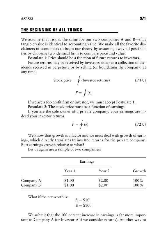
E1C14 08/25/2009 Page 371

THE BEG INN ING OF AL L TH INGS

We assume that risk is the same for our two companies A and B—thattangible value is identical to accounting value. We make all the favorite dis-claimers of economists to begin our theory by assuming away all possibili-ties by choosing two identical firms to compare price and value.

Postulate 1: Price should be a function of future returns to investors.Future returns may be received by investors either as a collection of div-

idends received in perpetuity or by selling (or liquidating the company) atany time.

Stock price ¼I

(Investor returns) ðP1:0Þ

P ¼I

(r)

If we are a for-profit firm or investor, we must accept Postulate 1.Postulate 2: The stock price must be a function of earnings.If you are the sole owner of a private company, your earnings are in-

deed your investor returns.

P ¼I

(e) ðP2:0Þ

We know that growth is a factor and we must deal with growth of earn-ings, which directly translates to investor returns for the private company.But: earnings growth relative to what?

Let us again use a sample of two companies:

Earnings

Year 1 Year 2 Growth

Company A $1.00 $2.00 100%Company B $1.00 $2.00 100%

What if the net worth is:A ¼ $10

B ¼ $100

We submit that the 100 percent increase in earnings is far more impor-tant to Company A (or Investor A if we consider returns). Another way to

GRAPES 371

E1C14 08/25/2009 Page 372

look at it is that an extra dollar means more to a poor man than to a richman. We cannot simply look at earnings growth. It must be relative to thesize of the investment—the net worth of our investment. We must introducea scaling factor.

We define net worth as book value. (Our actual investment as an inves-tor needs the stock price; here we are first trying to establish the value of thecompany and its relationship to what we will pay for it.) So we have earn-ings scaled by book value, which happens to also be the definition of returnon equity (ROE).

Definition 1.0

ROE ¼ Earnings

Book valueðD1:0Þ

where book value is simply assets – liabilities ¼ equity. (We can assumeno liabilities. Then assets ¼ equity.) We can further define this as commonequity.

For a private firm, book value is the sum of all paid–in capital and re-tained earnings.

We can express both earnings and book value in per-share terms since:Definition 2.0

Price � Shares outstanding ¼ Book value ¼ Capitalization

for a private company ðD2:0Þ

For a partnership, we would use percentage ownership instead ofshares. As a sole owner of several companies, I was legally required to issueshares according to the paid-in value of the start-up capital and issue addi-tional shares for when additional capital is added. (Otherwise it is consid-ered a loan.)

Now that we have shares, we have Postulate 2.1:

Stock price ¼I

(Earnings per share) ðP 2:1Þ

And now we will divide both sides of the equation by book value (BKV)per share to get the relative importance of size.

Postulate 3

Price

BKV per share¼

IEarnings per share

BKV per share

� �ðP 3:0Þ

We can also assume there is only one share if you wish.


E1C14 08/25/2009 Page 373

The right-hand equation is also the definition for ROE—equation(D1.0). So our equation is now:

P=BKV ¼I

(ROE) ðP3:1Þ

But the stock market is built on expectations, so this should be futurereturn on equity (FROE).

P=BKV ¼I

(FROE) ðP3:2Þ

Note that we can at any time convert this to per-share values by multi-plying the equation by BKV. To demonstrate:

Price

BKV(BKV) ¼

I(FROE)(BKV)

Price

BKV(BKV) ¼

IFuture earnings

BKV

� �(BKV)

and since BKV/BKV ¼ 1, we get back to:

Price ¼ Future earnings

BKV(BKV)

which becomes:

P ¼I

(Earnings)

which is Postulate 2.Our equation so far is mathematically granite. But prices in the stock

market are relative to each other. We introduce one more concept that iscritical and the solution to the long-standing riddle.

Let us take any asset. Let us use the example of a $1,000 Treasurybond. When this bond was first issued (the original investment), this bondhad a coupon of 10 percent.

It was issued at par, and the expected market return was 10 percentat that time. (Bond prices are quoted in a unique way, as the last figureis dropped. This bond would be considered having a price of 100.) Let us

Price Income Return$1,000 $100 10%

GRAPES 373

E1C14 08/25/2009 Page 374

assume this bond has infinite maturity, as does the legal life of a corporationand its common stock. (Bond mechanics are such that a 100-year maturityapproaches infinite maturity and a 30-year bond mathematically app-roaches 100 years when issued, so any asset with a long life approaches theinfinite case. (Continuously compounding interest acts similarly.)

Now assume that one day later the rate on new bonds issued of thesame risk class, everything else being equal, falls to 5 percent.

Why buy a new bond at par ($1,000) yielding 5 percent when we canbuy the old bond at 10 percent? To be sure, no one will buy the new bond ifthey are rational1 and aware of the first bond until both are in equilibrium,which occurs only when the price of the old bond doubles.

The market requires the rate of return of 5 percent. We use (MRRET)to represent the Market Required Rate of Return. And if on the next day,rates suddenly go to 20 percent and new bonds are again issued at par, theprice of our first bond will plunge to be in equilibrium with the new bondsince you will sell it and buy the new bond to double your income at 20percent.

It is not the firm’s cost of capital that determines the stock price; it is therequired market rate of return! We will also call this the investor’s cost ofcapital.

Prices therefore can swing wildly while the underlying asset, company,and structure (return on equity, earnings and book value, etc.) remain fixed.

To be sure this is the case for Treasury bonds as every professional in-vestor including myself will step in and arbitrage for profit until the oppor-tunity on the old bond is gone. Note that the value and coupon when issueddo indeed affect the nominal price, so prices cannot be the only function offuture returns. Our bond analogy takes us a quantum leap forward to un-derstand market valuation levels.

Postulate 4: The required rate of return by the market directly affectsthe price of the stock.

Price Coupon Income MRRETNew bond #1 $1,000 5% $ 50 5%Old bond $2,000 10% $100 5%

Price Coupon Income MRRETNew bond #2 $1,000 20% $200 20%Old bond $ 500 10% $100 20%


E1C14 08/25/2009 Page 375

We define the required rate of return as KOC: the investor’s cost ofcapital.

From equation (P 3.2):

P=BKV ¼I

(FROE)

We insert KOC to give comparative meaning to FROE:

P=BKV ¼I

(FROE=KOC) ðP4:1Þ

Proof: the arbitrage of bond prices and interest rates; and after multi-plying both sides by BKV we get:

P ¼I

(FROE=KOC)BKV ðP4:2Þ

which is the normative GRAPES model.If an investment is expected to earn twice the required rate of return, it

should sell for twice its book value. If it can’t make the required rate ofreturn, it should sell at a discount exactly like a bond that has a lower cou-pon or a higher coupon.

The positive theoretical version will introduce behavioral risk and dif-ferent risk classes of the firm and deal with two period outcomes. (Assumedin the normative model is that the same FROE continues forever.) The nor-mative model captures all the key elements but risk. Risk is subject to indi-vidual preference.

We have assumed a riskless asset. We can extend this to securities of thesame risk class, which allows us to do a comparative evaluation.

We present Postulate 4.2 as the correct theory of price—to withstandall time. It establishes the true value of the firm. It adjusts to market condi-tions. It captures future expectations. It connects and gives meaning to valueand growth. It shows that the firm’s structure (book value) is still important.It explains huge premiums to book value and discounts. It explains the roleof interest rates and their competing influence on cost of capital of investors.It explains volatility of the markets, contraction and expansion of P/E rates,and levels of market valuation. It removes the confusion over the firm’s costof capital, which is merely a latent determinant of the profitability of thefirm and its earnings.

Summary o f The Theory

Academia has addressed well the issue of risk and return, but it has all butignored concepts of value and price. Yes, there are dividend discount

GRAPES 375

E1C14 08/25/2009 Page 376

models, but they lie outside MPT and cannot tell us what the price shouldbe today even under a host of assumptions. What is an asset worth?

We have solved the problem for three of the four elements; value, price,and return. We sidestep the issue of risk by assuming a riskless security, orsecurities of the same risk class. Academia provides no useful basis for rela-tive evaluation of securities—except for security market line (SML)—inrisk/return space by saying all prices are efficient. Specific risk can be diver-sified away, so only systematic risk (beta) is important. It is a very cleverand diabolical argument signifying nothing about the price and value of anasset.

We want a theory that will tell us what we should pay for a company ina rational context. When we begin to overlay the characteristics of investorbehavior (the most dangerous form of risk is how investors react to greedand fear), we get very close to explaining today’s stock price. Knowingwhat the price should be gives us an awesome tool for turning GRAPESinto fine wine. It is one major reason why we have had the best performancein the world the past seven years. It is also why we think we will continue tohave exceptional performance. Of course we are subject to the usualextreme style swings and moods of the general investing public. And wemust add the mandatory disclaimer that past performance is not an indica-tor of future performance (just in case Big Brother is watching).

But we can invest with great confidence that we know what the priceshould be given all publicly available information and that we will not over-pay for anything. That gives us an advantage over thousands of other in-vestment managers who are essentially clueless.

GRAPES is a simple equation, like E ¼ mc2. It is elegant, and a theoryof relativity for investing that will stand the test of time.

THE MODEL AND SYSTEM

The GRAPES model is a sophisticated, dynamic, and powerful investmentmanagement tool. It addresses both value and growth of an investment byrelating the earnings growth with the size of the firm and cost of capital. Inso doing, it resolves the controversy of having to make a choice betweenvalue and growth. In reality a stock price is affected by both the company’sbalance sheet and its earnings potential. The GRAPES theory makes thisimportant link by integrating the two. The model, driven by the theory, be-comes the practical application of identifying the efficient price of a stock.

The value of a firm has to be linked to some general cost of capital, andthe concepts of capital budgeting theory should apply to investor decisionsas well as to projects. Price should be a function of future returns to


E1C14 08/25/2009 Page 377

investors. We would pay a premium for a company if returns were aboveaverage and a discount if returns were below average. Earnings of a com-pany are viewed by investors as being earnings available to the owners orshareholders. We assume that stock price is a function of earnings.

The efficient market hypothesis states that consensus expectations andhistorical information are fully reflected in stock prices. Historical earningshave no significant influence on stock prices except as a potential aid forforecasting future earnings patterns. Also, an important piece of nonexpec-tational data is the immediate liquidation value of the firm. If an investmentfails to earn its cost of capital, the investment will sell at a discount to itsbook value or liquidation value. If it earns more than its cost of capital, itwill sell at a premium to its book value.

Price

Book value¼ Forecasted return on equity

Cost of capital

A particular company’s unique cost of capital is considered irrelevant toan investor’s decision to buy or sell with the exception of the implicit effectof that unique cost of capital on calculating future return on equity. Inves-tors determine stock prices and it is their cost of capital that is important. Ifthe cost of capital of investors change, they would be able to raise more orless funds. They would now take advantage of more profitable situations orbe forced to sell positions that are no longer profitable. All new opportuni-ties created by a change in the cost of capital will be exploited until a newmarket equilibrium is reached.

In capital market theory, a key of price equilibrium is the security mar-ket line (SML), shown in Exhibit 14.3. In equilibrium, an asset’s expectedreturn is a positive linear function of its covariance of returns with the mar-ket. Every individual security’s expected return and risk will be on thisSML. Proof is by arbitrage. If we assume that all securities are of the samerisk class, by proof of arbitrage all stock prices will be on the SML in orderof expected return on equity after scaling for the size of the firm.

P/BKV

KOC FROE

SML

1.0

EXHIBIT 14.3 GRAPES Security Market Line (SML)

GRAPES 377

E1C14 08/25/2009 Page 378

The SML slope coefficient or regression coefficient is a measure of sys-tematic risk, universally known as beta. The slope coefficient of theGRAPES SML is defined as the ratio of the future return on equity and thecost of capital. We will call this the GRAPES coefficient multiplier (GCM).When GCM is 1, the company is expected to earn exactly the cost of capitaland will sell at book value. To find the theoretical price of a stock on theSML, we multiply both sides of our relationship by book value:

Price

Book value¼ Forecasted return on equity

Cost of capital

Price

Book value(Book value) ¼ FROE

KOC(Book value)

Price ¼ FROE

KOC(Book value)

where KOC is the investor’s cost of capital and FROE is the theoretical re-turn on equity.

In summary, the GRAPES theory links the balance sheet with the earn-ings statement of a firm, the size of the firm, and the cost of capital in themarketplace. The model adjusts for investor’s perceptions and risk prefer-ences. The model is:

Price ¼ Zeta(f )FROE

KOC(BKV) þ Chinese wall

Zeta is the investor’s preference function that is a transformation to theGRAPES Coefficient Multiplier (GCM). The Zeta function accommodatesnot only high-growth stocks but also speculation in turnaround cases andeven bankruptcy situations. The Chinese wall is a nonparametric itemthat we add to our model; it reflects the investor time horizon. We use theChinese wall concept (there are two: current wall and future wall) toexplain and understand stock prices that are temporarily much lower thanthe theoretical price per investor behavior. They are not used in the actualcalculation of theoretical price or the adjusted theoretical price, and theyare considered temporary behavioral anomalies.

GRAPES SYSTEM FOR VALU ING COMPAN I ES

This is the practical data you need to apply the theory.


E1C14 08/25/2009 Page 379

Definitions

KOC ¼ Cost of capital ¼ Long-term government bond yield

FY1 ¼ Consensus EPS estimate for current fiscal year

BKVPS ¼ Book value per share (one year ago from FY1 date)2

FROE ¼ Forecast ROE ¼ FY1/BKVPS

ZETA ¼ [(1þ FROE)2 � (1þ FROE)]=KOC

GRAPES ¼ GRAPES company value ¼ ZETA � BKVPS

Special Situations

& If FROE < KOC, use the following GRAPES calculation:

GRAPES ¼ BKVPS � [1 � (KOC � FROE)]

& When no forecast for EPS (FY1) is available:BKVPS–1 ¼ Year ago book value per share ¼ Latest book value per

share – Latest EPS12 þ Dividends/share throughout theyear (EPS12 ¼ trailing 12 months earnings per share)

ROE ¼ Latest EPS12/BKVPS–1

ZETA ¼ [(1 þ ROE)2 � (1 þ ROE)]=KOCGRAPES ¼ GRAPES company value ¼ ZETA � BKVPS–1

GRAPES Ad j us tmen t s

This section not only handles extreme cases, but deals with financial compa-nies – especially banks.

For Excessive Risk of Default or Bankruptcy In our model and theory, weassume there is no long-term debt. These companies are debt free. Compa-nies that are highly leveraged will obtain a high return on a small level ofequity, but have greater risk. For companies in a normal risk range, wedon’t need a special adjustment. However, the following can be used for allcompanies – especially financial companies.

GRAPES Long-term debt coefficient (GLT) is:

GLT ¼ 1:0 � Long term debt

Common equity� 0:10

� �

a limit of � 0:50j

GRAPES 379

E1C14 08/25/2009 Page 380

Some foreign banks do not report long-term debt. The ratio to use forthese banks is:

GLT ¼ 1:0 � Loans to customers

Current account deposits� 0:10

� �

a limit of � 0:50j

So if long-term debt is equal to common equity, we discount theGRAPES price by 10 percent. If long-term debt exceeds common equity bydouble, then it is 20 percent. This adjustment should also be used with thenext one:

GRAPES current liabilities coefficient (GCL) is:

GCL ¼ 1:0 � Current liabilities

Common equity� 0:10

� �

a limit of � 0:50jSo if current liabilities are equal to common equity, there is a 10 percent

discount. Note that almost all companies have some current liabilities, andwe may add a condition that if current liabilities are at some minimal per-cent we can ignore them. Note that this measure penalizes low-margin com-panies, as it should. We also stay away from using current assets since thiswould use inventories, and unsold bloated inventory is often a cause ofbankruptcy.

Adjusted formula for the GRAPES price (GP) is:

GP ¼ [Zeta f (ROE=KOC) � BKV] � GLT � GCL

For Extreme ROEs from Tiny Book Values When a company has losses, itsbook value can approach zero (still positive) or go from negative to positivewhen turning around. This can create infinite ROE mathematically, and weneed to fix this.

Conditions:

& If book value is �1.00 and EPS12 is > than half of BKV (50% ROE),then substitute total assets instead of common equity for the ROEcalculation (ROA instead).

& If book value >1.00 and < 10.00 and ROE >100%, and book value is< .20 of total assets, also substitute ROA.

& If you use ROA, do not use GLT and GCL adjustments.

Special Cases There are two other special cases that create mathematicalproblems:


E1C14 08/25/2009 Page 381

1. Negative book value and positive earnings.2. Negative book value and negative earnings.

These have a more complicated solution using the analyst’s long-termgrowth rate forecast and assets. For extreme negative cases, one can substi-tute the Black-Scholes option pricing model to come up with a price thatreflects speculation without any underlying value. For simplicity, we suggestexcluding these cases when solving for KOC treating them as N/A or notappropriate.

Class Stock To reflect your true ownership, you need to adjust class stocksfor their true voting power.

Grapes Procedure for Handling Class Stocks All class stocks (over 10% ofall companies) need to be manually investigated by looking up their sharesoutstanding for both classes and the voting rights from each company’s 10-K or 10-Q and proxy statement (DEF-14A).

Then FY1 or EPS12 needs to be manually reduced before doingGRAPES theoretical price calculation.

The ratio by which FY1 or EPS12 need to be multiplied is:

Total number of shares for both classes/Total number of votes

Illustrated by example:

Richardson Electronics, Ltd.

Common stock 14.865 million shares Entitled to one voteClass B stock 3.048 million shares Entitled to 10 votes

Adjustment ratio to FY1 or EPS12:

14:865 þ 3:048 ¼ 17:913 million total shares available3:048 � 10 ¼ 30:48 þ 14:865 ¼ 45:345 million votes availableTotal number of shares/Total number of votes ¼ 0.40

The company’s FY1 or EPS12 needs to be multiplied by 0.40 beforedoing the GRAPES calculation.

THE PR I C I NG OF R I SK

While the CAPM is totally concerned with risk to the extent there isno price, there is no direct pricing of risk in the GRAPES model. The

GRAPES 381

E1C14 08/25/2009 Page 382

GRAPES model best applies to securities of the same risk class. Stocksthat lie outside the normal range of leverage, including financials, havetheir own variants of measurement. There should be some further dis-count or premium for quality, stability, or reliability, perhaps in accord-ance with bond ratings. However, bond ratings are badly skewed tomarket capitalization.

There is no evidence that a large company with a stable business willsurvive longer than a small company with a stable business. In fact, theremay be evidence to the contrary. Nevertheless the larger, more politicallypowerful company will get a substantially higher credit rating although theproducts that got it there are more likely to become obsolete and are undergreater competition, more cyclical influence, and less sustainable growth bythe very nature of its size.

Another issue is the use of consensus forecasted earnings when agree-ment could be either unanimous or wide among analysts. The size of theforecast error, the correlation of future errors, and the behavior of analystsare more important than agreement.

In the commodities market, risk is often not priced. The future pricesnormally trade at less than the spot price or close to the spot price. Oil, forexample, rarely has a futures premium where it pays to store current oil forfuture delivery even though there are always high geopolitical risks. Basiccrops such as corn and wheat are at high risk to the weather, which tends tohave many extremes, yet future prices often seem to only reflect that the sunis always shining.

The investors’ required cost of capital can change rapidly, and this, too,should be a risk (gain or loss), but like forecasting the stock market, perhapsthe most practical forecast is today’s price as the best guess for the future(at least according to efficient market theory), so we don’t need to furtheradjust the prices for general risk. You can solve for KOC at any point intime across the market since that is the only unknown variable in theGRAPES model. Prices are set by marginal sellers and buyers—in some waylinked to those of an auction where the highest bid wins or the most extremeopinion generates a buy or sell. The pricing of risk will be a function ofinvestment behavior affected by fear, greed, and overreaction. Such an over-lay function will explain the differences between the GRAPES theoreticalprice and the actual price.

The model does an excellent job of explaining most stock prices. LikeAdam Smith’s Wealth of Nations, the market invisibly finds its equilibrium.GRAPES goes a very long way in clearly explaining and understanding thisinvisible process.


E1C14 08/25/2009 Page 383

APPEND IX : E XAMPLES OF MCDONALD ’ S ANDWAL -MART

GRAPES System for Valuing Companies McDonald’s Corp. (MCD)

Cost of Capital ¼ 2/28/2008 Corporate AAA Bond Yield

KOC ¼ 5.55%

Consensus EPS Estimate for Current Fiscal Year

FY1 ¼ $3.18

Book Value per Share One Year Prior to FY1 Date�

BKVPS ¼ $13.11

Forecast ROE ¼ FY1/BKVPS

FROE ¼ 0.2425

Zeta ¼ [(1 þ FROE)2 � (1 þ FROE)]/KOC

Zeta ¼ 5.43

GRAPES Company Value = Zeta � Full Year Ago BKVPS

GRAPES ¼ $71.19

GRAPES Adjustments:

GLT ¼ 1:0 � Long-Term DebtCommon Equity � 0:10

� �

Long-Term Debt ¼ $7,310 (million)

Common Equity ¼ $15,280 (million)

GLT ¼ 0.95

GCL ¼ 1:0 � Current LiabilitiesCommon Equity � 0:10

� �

Current Liabilities ¼ $4,499 (million)


GCL ¼ 0.97

GRAPES Price ¼ $65.79

Last Price ¼ $53.16 (3/3/2008)GRAPES Return ¼ 23.76%

*FY1 is for fiscal year ending 12/31/2008; book value per share is as of 12/31/2007.

On December 12, 2007, McDonald’s was at $63.69 (almost its GRAPES price)when the stock market began a sharp decline.

GRAPES 383

E1C14 08/25/2009 Page 384

GRAPES System for Valuing Companies Wal-Mart Stores Inc. (WMT)

Cost of Capital ¼ 2/28/2008 Corporate AAA Bond Yield

KOC ¼ 5.55%

Consensus EPS Estimate for Current Fiscal Year

FY1 ¼ $3.40

Book Value per Share One Year Prior to FY1 Date�

BKVPS ¼ $16.18

Forecast ROE ¼ FY1/BKVPS

FROE ¼ 0.2101

Zeta ¼ [(1 þ FROE)2 � (1 þ FROE)]/KOC

Zeta ¼ 4.58

GRAPES Company Value ¼ Zeta � Full Year Ago BKVPS

GRAPES ¼ $74.13

GRAPES Adjustments:

GLT ¼ 1:0 � Long-Term DebtCommon Equity � 0:10

� �

Long-Term Debt ¼ $29,799 (million)


GLT ¼ 0.95

GCL ¼ 1:0 � Current LiabilitiesCommon Equity � 0:10

� �

Current Liabilities ¼ $58,153 (million)


GCL ¼ 0.91

GRAPES Price ¼ $64.35

Last Price ¼ $49.89 (3/3/2008)GRAPES Return ¼ 28.98%

�FY1 is for fiscal year ending 1/31/2009; book value per share is as of 1/31/2008.

Wal-Mart made a new 52-week high of $51.57 on February 27, 2008, as it hasdefied a sharply declining stock market.


E1C14 08/25/2009 Page 385

NOTES

1. In practice, bond salespeople do indeed manage to sell new bonds to Joe Inves-tor when better opportunities from older bonds can be purchased directly in themarket.

2. Example: If FY1 is for fiscal year ending 12/31/2009, book value per shareshould be as of 12/31/2008. Similarly, for fiscal years not ending in December,book value per share should be one year back from the FY1 date.

RE F ER ENCE

See any investment textbook for the existing Capital Asset Pricing Theory, the CapitalAsset Pricing Model (CAPM), and dividend discount models.

GRAPES 385

E1C15 08/14/2009 Page 386

CHAPTER 15Portfolio Valuation

Challenges and OpportunitiesUsing Automation

Randall SchostagPresident, Minnesota Business Valuation Group,

LLC. Olsen Thielen & Co., Ltd. subsidiary

Business development companies, hedge funds, and other fund managersface new, intensive scrutiny over periodic valuations of portfolio securi-

ties. From a funds management/compliance standpoint, it is essential to havereliable sources for this security valuation, especially with privately ownedholdings. For multiple reasons, business valuators who value these fundsmust simultaneously value numerous securities rapidly. To accomplish thislaborious task may require the employment of new types of technologicaltools. Automating aspects of the process might offer a new solution.

Divided into two major groups of topics, this chapter explores the vari-ous aspects of partial automation. The first segment summarizes backgroundrules and procedures currently developing for portfolio valuation. Includedis a detailed history that reviews how valuation evolved from a narrow do-mestic focus to an international application. This segment concludes withthe effect of these events on appraisers and their portfolio valuations. Thechapter then reviews the application of the evolving portfolio valuation reg-ulations. Finally, it concludes by proposing that current methods may alsoneed to evolve to be timely, cost effective, and (most important) defensible.

BACKGROUND

Changes in the value of underlying securities from one period to the next notonly determine the net asset value of holdings, but in addition measure

386

E1C15 08/14/2009 Page 387

portfolio managers’ performance. Further, the valuation and periodic reviewof a portfolio should also provide information about risk to the investor.

Accurate security valuation becomes significant because open-end mu-tual funds must buy and sell shares daily. Unlike other industries, where di-rectors may be conservative and simply mark down a security, mutual funddirectors don’t have that alternative (Investment Company Institute 2001).

The most important contributors to U.S. portfolio valuation theory in-clude the Securities and Exchange Commission (SEC), the FinancialAccounting Standards Board, the Investment Company Institute, and thePrivate Equity Investment Guidelines Group (PEIGG).1 The Chartered Fi-nancial Analysts Institute (formerly the Association for Investment Manage-ment and Research) has been the most visible contributor of valuationissues from valuation practitioners.2

The task of fulfilling new best practices and regulations will eventuallybecome the responsibility of certified valuators and appraisers who performthe work. Client companies and valuation specialists will be the ones whomay be sanctioned for failing to comply with new directives.

Valuation practitioners have the knowledge, skill, and experience to ap-praise company securities for multiple purposes. The resulting appraisalsprovided a primary source of case law, creating legal precedent of acceptedmethods and procedures. Courts examine appraisers using the FederalRules of Evidence for admissibility of expert testimony, test their methods,subject them to peer review, and determine if the methods are acceptedwithin the valuation community.

Appraisers understand that the most problematic securities are thosethat are not publicly traded or where trading prices do not reflect true value.Certified business appraisers specialize in valuing private business. The cer-tifying bodies have adopted standards, developed over time, to assure com-plete work product.3

Business appraisal experts can benefit from emerging recommendedpractice. A partial listing includes addressing acceptable modeling/methods,portfolio holdings liquidity, and economical/timely reporting. Althoughemerging procedures consider acceptable modeling/methods, later in the ar-ticle a closer inspection reveals that the enumerated procedures may fail inreal-world application.

METHODS ADOPT I ON IMPL I CAT I ONS

Accurate reporting by registered funds is paramount. Failure to provide de-fensible portfolio valuations can have significant consequences. In August2007 the SEC issued a cease and desist order4 against Allied Capital

Portfolio Valuation 387

E1C15 08/14/2009 Page 388

Corporation in determining the fair value of specific portfolio securities forwhich market quotations were not readily available (SEC 2007). Internalpersonnel completed the appraisals instead of engaging an independent thirdparty.5

Registered fund organizations are not the only ones sanctioned. InSeptember 1998, the SEC issued a cease and desist order after establishingan aiding and abetting violation against certain individuals who did not useappropriate methods to determine the fair value of certain holdings(SEC 1998).

Portfolio management, as defined in the United States, is the manage-ment of funds for fees or commissions. Managers decide on investmentsand earn fees based on the size and/or overall performance of the portfolio.Participants include managers of trusts, mutual funds, pension funds, andother portfolios.6

About 90 percent of the portfolios are managed by organizations orpersons registered with the SEC under the Investment Company Act of1940 (ASA 2003). Such professionals have at least minimum standards ofperiodic reporting. However, in the past 10 years, hedge funds have demon-strated blistering growth. Consequently these funds receive little oversightor have few reporting requirements. Unregistered investment pools (venturecapital funds/private equity funds/commodity pools) and registered funds/hedge funds are all often referred to as hedge funds. Some regard businessdevelopment companies as part of registered investment companies, al-though the primary accounting challenge remains valuation.

For funds registered under the 1940 Act, IBISWorld estimated thatabout $10.4 trillion existed in assets under management at the end of 2006.Of the totals, institutions invested about $3.06 million and individuals in-vested about $7.35 trillion. Growth averages about 9.1 percent a year, in-creasing from $7.1 trillion at the end of 2002 to about $11 trillion by theend of 2007.

Funds management is a fragmented industry. IBISWorld estimates thefour largest managers of registered funds comprise about 20 percent of themarket. IBIS assessed that there are approximately 1,170 enterprises and12,300 establishments in the registered funds industry, which employ212,000 individuals (IBISWorld 2007).

Hedge funds grew rapidly and consequently became virtually un-regulated. No universally accepted definition of hedge fund exists. It typi-cally refers to an entity that holds a pool of securities (and/or other assets)that is not sold in a registered public offering. Also key to the definition isthat the fund is not registered as an investment company. In 2003 the SECdetermined that approximately 6,000 to 7,000 hedge funds and funds ofhedge funds (FOHFs) existed in the United States, managing assets of $600


E1C15 08/14/2009 Page 389

billion to $650 billion. The SEC expected hedge fund assets to exceed $1trillion by 2008 (Implications 2003). By 2007 the hedge fund industry hadincreased to nearly 9,000 companies (Hedge 2007).

The SEC report and resulting actions focused on (1) an increase inhedge fund enforcement, (2) limited ability to obtain basic information, (3)emergence of FOHFs that do register but hold securities that are not regis-tered, (4) hedge fund disclosure/marketing practices, (5) valuation practices,and (6) conflicts of interest.

The Financial Services Authority in 20057 issued a discussion paper inwhich it listed valuation weaknesses in hedge fund methods. It assigned theweaknesses to skill shortages and potential conflicts of interest that createdsignificant potential for ill-informed investment decisions and harm to mar-ket confidence (Financial Services Authority 2005).

Several groups attempted efforts to set up guidelines and standards forfunds as a result of rising investor, regulator, accountant, and other stake-holder concerns.

ACCOUNT ING PRONOUNCEMENTS

The pivot point for valuing investments is the Financial Accounting Stan-dards Board (FASB). On one side are the certified public accountants(CPAs) who must sign off on the audit and the appraisers who must sign offon the values. By issuance and enforcement of new requirements, the SEC ison the other side.

The Investment Company Act of 1940 drives the SEC. The 1940 Actdetermines policy encouraging the SEC to take certain positions thathave had significant influence on how the FASB determined its definitionof fair value. The SEC influenced many of the FASB’s decisions by refer-ring to the 1940 Act. Auditors and appraisers have had much lessinfluence.

Begun in 1924, mutual funds were quickly and extensively accepted byinvestors. Just five and a half years later the stock market crashed. To renewmarket confidence, Congress enacted the Securities Act of 1933 and the Se-curities Exchange Act of 1934 to regulate the securities industry.

Investment companies were still new in 1940. To give investors confi-dence in this unique offering, Congress passed the 1940 Act to regulate con-flicts of interest between investment companies and securities exchanges.Furthermore, it protected the public by requiring disclosure of material de-tails about the investment companies.

The 1940 Act applies to all investment companies, but exempts severaltypes of investment companies from coverage. Sections 3(c)(1) and 3(c)(7)


E1C15 08/14/2009 Page 390

contain the most common exceptions and include hedge funds. The Act (asamended) requires open-end investment companies to sell and redeem theirshares at a price based on ‘‘current net asset value,’’ defined as the amountthat reflects calculations made substantially as follows:

& Managers must value portfolio securities for which market quotationsare readily available at current market value.

& Managers must value at fair value other securities and assets for whichmarket quotations are not readily available, and the board of directorsmust determine fair value in good faith.

& Managers must reflect changes in portfolio holdings by the first busi-ness day following the trade date.

The 1940 Act did not define ‘‘readily available market quotations,’’‘‘fair value’’ or ‘‘good faith’’ for valuation (Ake and Hays 2007). As thegatekeeper responsible for enforcing the 1940 Act, the SEC became respon-sible for oversight and made interpretations.

SEC GU IDANCE

Issues may arise even if market quotations are readily available on a specificsecurity. For example, restricted securities differ materially from un-restricted securities, so the market-quoted price is not applicable. The fol-lowing chronology summarizes important SEC guidance, starting with thequestion of restricted securities and then addressing fair value considera-tions and overall supervision by fund boards of directors (Ake andHays 2007).

1969. Accounting Series Release No. 113 (October 21, 1969) providesguidance on fair valuation determinations for restricted securities.It defines fair value as ‘‘the amount which the owner might reason-ably expect to receive for [the securities] on their current sale.’’ Al-though there can be no ‘‘automatic formula’’ by which aninvestment company can value restricted securities, ASR 113 re-quires that a fund’s board of directors consider all relevant factors.These factors include the operations of the issuer, changes in gen-eral market conditions, and the extent to which the inherent valueof the securities may have changed.

1970. In ASR No. 118 (December 23, 1970), the SEC sought to providemore general guidance regarding how funds should value portfoliosecurities. Where market quotations are not readily available,


E1C15 08/14/2009 Page 391

including where existing quotations are unreliable or invalid, afund must price its securities at fair value. ASR 118 describes sev-eral nonexclusive methods of valuation a board may use to valuesecurities: a multiple of earnings, a discount from the market priceof a similar freely traded security, a yield to maturity for debtissues, or a combination of these principles. In addition, a fund’sboard of directors should consider several general reasons whenchoosing a valuation method, including (1) the fundamental andanalytical data about the investment, (2) the nature and durationof any limits on disposition of the securities, and (3) an evaluationof the forces that influence the market in which the securities arepurchased and sold.

1999. The staff issued an interpretative letter to the Investment Com-pany Institute (December 8, 1999). The letter was an effort to clar-ify and provide more guidance on pricing issues in an emergency orother unusual situations.

2001. A second interpretative letter (April 30, 2001) supplemented ad-vice in the 1999 letter about valuing foreign securities. Paraphras-ing, ‘‘where a fund board knows or has reason to believe that itsfair value determination does not reflect the amount the fund mightreasonably expect to receive for the security upon its current sale,or where a board acts with reckless neglect about its fair value de-termination, a fund board would not be judged to have acted ingood faith.’’

2003. The SEC adopted Investment Company Act Rule 38a-1 (ICA Rel.No. 26299, December 17, 2003), which requires invested compa-nies to adopt, and boards of directors approve, written compliancepolicies and procedures, including procedures covering the pricingof portfolio securities.

The preceding SEC directives explain how the SEC’s interpretations fol-lowing implementation of the 1940 Act have expanded what investmentcompanies and appraisers must now consider when making fair value deter-minations. These directives have become part of generally acceptedaccounting principles (GAAP) through the FASB.

ACCOUNT ING PRONOUNCEMENTS AND THE FASB

The SEC has statutory authority to establish financial accounting andreporting standards for publicly held companies under the Securities


E1C15 08/14/2009 Page 392

Exchange Act of 1934. Throughout its history, the SEC relied on the pri-vate-sector FASB for this role.

Created in 1973, FASB is independent of all other business and profes-sional organizations. Before FASB, the Committee on Accounting Proce-dure of the American Institute of Certified Public Accountants (AICPA)(1936–1959), and then the Accounting Principles Board, also a part of theAICPA (1959–1973), set up the financial accounting and reportingstandards.

The standards and interpretations rendered by FASB are considered au-thoritative not only for the SEC, but for AICPA as well, where GAAP rulesapply to all audits, reviews, and compilations, regardless of whether thecompanies are public or private, unless otherwise stipulated. For example,through the Uniform Accountancy Act the FASB has encouraged these rulesto be broadly adopted (AICPA 2007).

The FASB’s mission is ‘‘to establish and improve standards of financialaccounting and reporting for the guidance and education of the public, in-cluding issuers, auditors, and users of financial information.’’ It is a seven-member, independent board consisting of accounting professionals in a pri-vate, not-for-profit organization.

FASB standards (GAAP) govern the preparation of corporate financialreports. The Financial Accounting Foundation (FAF) funds, oversees,administers, and decides governance issues at the FASB, including determin-ing the criteria for a sufficient majority for adopting new rules (FinancialAccounting Foundation 2002). FAF is also responsible for the Governmen-tal Accounting Standards Board (GASB) and advisory councils for bothFASB and GASB. Founded in 1972, FAF consists of 16 trustees (FinancialAccounting Foundation 2006). The following organizations determine whois on the FAF Board of Trustees:

& American Accounting Association.& American Institute of Certified Public Accountants.& CFA Institute.& Financial Executives International.& Government Finance Officers Association.& Institute of Management Accountants.& National Association of State Auditors, Comptrollers and Treasurers.& Securities Industry Association.

As part of its role in providing guidelines for U.S. accounting, FASBparticipates in a convergence project with the International AccountingStandards Board (IASB). The project’s goal is to move toward inter-continental uniformity in financial statements. Therefore, U.S and


E1C15 08/14/2009 Page 393

international companies would no longer need to complete separate fi-nancial statements. Another vital element of the convergence project forthe FASB was to begin to transition from the principle of historical costto fair value.

The 1940 Act referred to fair value, and the SEC’s history of enforce-ment has in part involved evaluating methods to get fair value. IASB alsoincorporated language and set forth definitions using fair value and hasbeen moving toward substituting fair value for historical cost accounting.Although there are many places that referred to fair value within pastaccounting statements and interpretations,8 FASB did not assemble to re-solve these various pronouncements about fair value until 2006.

Effective November 15, 2007, FASB’s Statement of Financial Account-ing Standard (SFAS) 157 became effective. It defines fair value andaddresses fair value measurement protocols, financial statement disclosure,and measurement techniques. With the market melt-down in 2008, theFASB has been under pressure to revise the SFAS 157. Modest changes weremade in interpretations in 2008-2009, mostly relating to securitized debtholdings, not equity.

Auditors must use the SFAS when examining financial statements, in-cluding those funds that hold multiple securities.9 Because the SEC consid-ers this work authoritative, it references the new statement and integratesthe SFAS into its requirements. Consequently, for registered funds or otheraudited reporting entities, SFAS 157 is a critical determinant in howappraisers should value funds and report to users.

The FASB history, composition, and principle mandate highlights itsfocus on politics and its concentration on fulfilling requirements for theSEC, the 1940 Act, and publicly traded securities. There is less evidence ofcontributions from the private valuation community (although the FASBvaluation resource group seems to offer some broader perspective). Courtdecisions also differ in some respects from that considered important topublic companies.

Forbidding the application of a blockage discount when valuing a largeposition in an unrestricted security represents one troublesome feature pro-posed by SFAS 157. This prohibition fails to recognize that the valuationcommunity and courts accept the blockage discount concept.10 Strongempirical evidence exists for the effect of blockage discounts. Many nowbelieve appraisers should divide the traditional idea of a ‘‘discount for lackof marketability’’ into a ‘‘discount for lack of marketability’’ and a ‘‘dis-count for lack of liquidity.’’ Lack of liquidity effects represent the essence ofa blockage discount (Abbott 2004).

Investors who trade thinly traded public stocks (or who own a propor-tionately large position in a stock that otherwise has reasonable trading


E1C15 08/14/2009 Page 394

activity) recognize the difficulty of selling blocks of stock in a timely man-ner. Most experience a discount or must conduct a costly secondary regis-tration (Pratt 1996). The failure to provide a discount for liquidity oflarge block holdings thus potentially rewards portfolio managers whoacquire thinly traded equities. The portfolio manager’s buys may increasethe quoted price of the stock, while also failing to describe to fund investorsthe potential risk of selling stock.

The FASB’s proposed position reflects positions upheld in the past bythe SEC. In SEC Accounting Series Release (ASR) 118 (SEC 1970) the Com-mission stated that for securities listed or traded on a national securitiesexchange, market value is the last quoted sales price on the valuation effec-tive date. In that ASR, modification for commissions (other sellingexpenses) or for other adjustments (liquidity) was not provided.

The SFAS uses ‘‘exit price’’ and has thus avoided the question of com-missions or selling costs. It uses the bid price of a security, when available,rather than its offer or last selling price. The writing of SFAS 157 caused adebate. Some became concerned about using the bid price rather than theask price or other measure (e.g., an average of the bid and ask). The Invest-ment Company Institute expressed apprehension that this ‘‘could causefunds to undervalue their shares, to the detriment of shareholders’’ (Invest-ment Company Institute 2000). The 1940 Act established the ASR rules.The ASR requires, where market quotations are available, that securities bevalued at market value, and all other securities be valued at fair value. Thefund’s board of directors estimates fair value ‘‘in good faith.’’

The SFAS 157 established a three-tiered fair value hierarchy, which pri-oritizes techniques for valuing the portfolio securities. It facilitates a moreuniform interpretation of ‘‘good faith’’:

& Level 1 uses quoted prices in active markets of the subject securi-ties. FASB considers active markets those where transactions occurwith sufficient frequency and volume to provide reliable pricinginformation.

& Level 2 are prices other than those quoted in Level 1 that are observ-able either directly or indirectly. Included are prices for similar invest-ments in active markets, quoted prices for identical or similar assets inmarkets that are not active, or drawn from or corroborated by observ-able market data.

& Level 3 pricing considers unobservable inputs (entity inputs). Includesprojections used for discounted cash flow analyses.

Understanding the escalating levels is essential because they affect notonly the methods used but the documentation auditors require for working


E1C15 08/14/2009 Page 395

papers/disclosure footnotes to financial statements. The cost of auditing andvaluation progressively increases from the first to the third level.

Although appraisers still need more clarification, the SFAS 157 recog-nizes that a market quote in a thinly traded or inactive stock may not reflectfair value. Therefore, it may need more analyses before simply marking theprice to market.

XBRL FORMAT

Another linkage between the FASB and the SEC has been their recent advo-cacy of eXtensible Business Reporting Language (XBRL), an XML-based,standards-based format to define and exchange business and financial infor-mation.11 Metadata defines these communications set out in taxonomies.Taxonomies define individual reporting concepts as well as the relationshipsbetween concepts.

An international consortium, XBRL International, governs and marketsthe XBRL format. The consortium consists of about 600 organizations thatencompass companies, regulators, government agencies, ‘‘infomediaries,’’and software vendors. The consortium promotes the format to transferbusiness information from paper-based/proprietary electronic formats toInternet-oriented processes.12

Availability of financial and other information through XBRL in the fu-ture will have a significant impact on use of public company information foranalysts as the SEC reporting adopts its use.

EMERG ING BEST PRACT I C ES

Regulation and accounting history are equally vital to understanding howvaluing portfolios best practices evolved. Because those establishing thestandards expect findings of value to be used in the context of the 1940 Act,the standards have been created for public company reporting. Theappraiser must rethink the kinds of methods and procedures to use andhow to report such findings.

The American Society of Appraisers (ASA) College of Fellows in 1989(Opinion 1989) stressed defining the standard of value pertinent to a spe-cific valuation. The Fellows noted there are many different standards ofvalue, including fair market value, fair value (which now has two defini-tions, as one relates to shareholder oppression and dissenting rights), intrin-sic value, and investment value. Also, the standard of value may varyamong legal jurisdictions, such as in matters of divorce where states maydepart from the standards of other states. It is important to know that when


E1C15 08/14/2009 Page 396

we appraisers apply a different standard of value, it may produce a differentfinal value in the security.

Issued in 1959, the seminal standards work is IRS Revenue Ruling 59-60. It remains the most important reference for valuing ownership interestsin closely held businesses (Lieberman and Anderson 2008). RR 59-60applies to federal gift, income, and estate tax valuations, and the U.S. De-partment of Labor has incorporated it into requirements for employee stockownership plans. Matrimonial dissolution is an example of another valua-tion standard that has referenced RR 59-60.

In 2006 the IRS issued general business valuation standards, applicableto all Internal Revenue Service (IRS) employees and to those who provide orreview valuation services valuations for the IRS. Revenue Ruling 59-60’scontinuing influence is also obvious in the comprehensive business valua-tion standards that began to appear in the late 1980s. The most importantof these was the Uniform Standards of Professional Appraisal Practice(USPAP), issued by the Appraisal Foundation in 1987, followed by stan-dards from professional associations such as the American Society ofAppraisers (ASA) in 1992, the Institute of Business Appraisers (IBA) in1993, and the National Association of Certified Valuation Analysts(NACVA).

These appraisal associations have a history of developing valuation as aprofession. This effort is independent of accounting/analyses of public secu-rities, and establishing accepted methods/procedures for work. The valua-tion profession includes certification to ensure members possess uniformstandards of knowledge, skill, and experience to enhance public confidencein work product. To complete the requirements, each association offers ed-ucation/continuing education programs to obtain and maintain certifica-tion. The AICPA formally recognized the existence of business valuationand embraced it in 1996 by establishing the accredited business valuatordesignation.

The Appraisal Foundation and USPAP are outgrowths of fraudulentand poor real estate appraisals that ended with several savings and loan fail-ures. The first edition of USPAP appeared in 1987 and the most recent edi-tion for 2008–2009 was effective January 1, 2008.

The several business valuation standards have much in common, in-cluding the dependence on Revenue Ruling 59-60, which discusses eightfactors to consider in valuations. USPAP Standard Rule 9-4 incorporatesthe eight factors from Revenue Ruling 59-60, and this USPAP StandardRule remains essentially unchanged from its first issuance. The eight factorsfrom RR 59-60 also appear in ASA Standard I–iii, IBA Standards sec-tion 5.3, and NACVA’s Development Standards 3.4, as well as in the IRSStandards under ‘‘Analyzing.’’


E1C15 08/14/2009 Page 397

Although the SEC and FASB do not directly cite the ASA, IBA, orNACVA, FASB issued a new standard, effective January 1, 2008. It reflects,in part, this body of knowledge. The Statement on Standards for ValuationServices No. 1 has incorporated most of these established principles. Sincethe FASB’s directives are authoritative to the SEC, industry organizationsare now integrating the new standards into the analyses of publiccompanies.

I N T ERNAT I ONAL STANDARDS

The FASB’s influence extends to the international community. In coordinat-ing with the IASB, its guidelines become part of the broader discussion; in-creasingly parties are originating or holding portfolios outside the UnitedStates. While GAAP are the rules issued within this country, the IASB’s In-ternational Financial Reporting Standards (IFRS) are the ones now most ac-cepted outside the United States.13

In 2002, the FASB and the IASB agreed to integrate their standards inthe Norwalk Agreement. The first paragraph of the Norwalk Agreementreads: ‘‘At their joint meeting in Norwalk, Connecticut, USA, on September18, 2002, the FASB and the IASB each acknowledged their commitment tothe development of high-quality, compatible accounting standards thatcould be used for both domestic and cross-border financial reporting.’’ Atthat meeting, the FASB and the IASB pledged to use their best efforts to (1)make their existing financial reporting standards fully compatible as soon asis practicable, and (2) coordinate their future work programs to ensure thatonce achieved, compatibility is maintained.

Before finalizing SFAS 157 in January 2007, the FASB formed a val-uation resource group (VRG) to provide the FASB with input for clarify-ing the guidance related to the application of the principles in SFAS 157.The VRG is comprised of a cross section of constituents in addition tomajor accounting firms. Representatives from the valuation communityinclude:

& American Appraisal.& Duff & Phelps.& Financial Reporting Advisors.& FVG International.& Houlihan Lokey.

Users who are participating include the CFA Institute and Moody’s,along with regulators. Standard setters include: AICPA, Appraisal


E1C15 08/14/2009 Page 398

Foundation, International Valuation Standards Council (IVSC),Public Company Accounting Oversight Board (PCAOB), SEC, andIASB.

Simultaneous to the joint efforts by the IASB (IVSC) and the FASB(with its VRG), several other international groups have emerged and arenow engaging. Many reflect the U.S. concerns about hedge funds. Valuingprivate security holdings and other difficult-to-value securities (e.g., deriva-tives) is a universal concern.

In October 2007, the International Organization of Securities Commis-sions issued its Policy Statement on Hedge Fund Valuation, Principles forthe Valuation of Hedge Fund Portfolios. The Association Francaise desInvestisseurs en Capital, the British Venture Capital Association, and theEuropean Private Equity and Venture Capital Association produced Inter-national Private Equity and Venture Capital Valuation Guidelines to reflectthe need for greater comparability across the industry and for consistencywith IFRS and U.S. GAAP. In March 2007 the Private Equity IndustryGuidelines Group issued its Updated U.S. Private Equity ValuationGuidelines.

Far from inclusive, the foregoing list demonstrates a global understand-ing of the changes in GAAP applicable to portfolio valuation. A deluge ofideas and preferences on valuing private securities exists. Formulating suchrules is political. The rules must address the multiple international stake-holders. Additional interpretations and associated changes will likely occurwithin the next few years as FASB, the SEC, the IASB, and others balancethe political concerns.

The domestic valuation community, which deals only with privatelyheld companies, may possibly never appraise hedge funds or other passiveinvestor portfolios. Appraisers and their clients will, however, experiencethe impact of decisions in this arena.

PRODUC ING PORTFOL I O VALUAT I ONS

Producing portfolio valuations requires a deep understanding of the back-ground of SFAS 157. This knowledge provides a clearer basis for fair valueand the wide-ranging impact on both domestic and international communi-ties. Business appraisers must apply their acquired knowledge, skill, andexperience. However, the SEC and diverse international groups will becomeincreasingly significant in establishing focus/standards for a broad spectrumof financial valuation assessments and, more specifically, for portfoliovaluations.


E1C15 08/14/2009 Page 399

Prac t i t i o ner Cons i d era t i o ns

A thoughtful review of the requirements of the various organizations indi-cates that political compromising may have overlooked 10 very real consid-erations that will directly affect the business appraiser:

1. In some practical cases, the definition of fair value departs significantlyfrom fair market value (a critical basis for U.S. business valuations).

2. Apart from its tax purposes, the use of fair market value was influentialin formulating much of U.S. case law.

3. The business valuation community has become much more reliant onusing methods other than the market approach for much of its work.The use of a discounted cash flow analysis, for example, has becomemuch more common with the advent of digital technology. Models canbe thoroughly constructed. Back-tested models become more visuallydramatic and require less explanation compared to using potentiallyproblematic public guideline companies.

4. A typical valuation for a valuation engagement (AICPA definition of acomplete valuation) may cost from $8,000 to $50,000 or more. There-fore, for a fund with multiple securities, a high cost to obtain defensiblevalues may likely result.

5. An ordinary valuation for a typical valuation engagement may take amonth or more for each security analyzed. For a fund with multiple se-curities, this process creates a significant delay between the effectivedate of a valuation and the delivery of findings. Given the use of thesefindings for pricing and compliance reporting, such delays will fail tomeet investor needs.

6. The valuation community has traditionally employed capital markettheory in a modified form to build portfolio risk from individual secu-rity risk. When performing portfolio valuations, should the appraisermeasure the diversification effect of the interaction of securities to de-termine portfolio risk and aggregate valuation?

7. In addition to other investments, hedge funds (and other funds) notonly hold private common stocks, but also hold private debt, realestate, specialized equipment for leasing, derivatives, and hybrid securi-ties. Often valuing these various securities requires unique, specializedskills. These skill requirements raise another management issue fordelivering high-quality and timely reports from potentially multiplesources of expertise.

8. Practically, the time/cost factors for valuation confirm the need for au-tomated systems use. However, automation becomes antithetical to thehands-on analysis that currently represents the greatest strength of


E1C15 08/14/2009 Page 400

business valuation. One essential reservation remains: how can auto-mated tools be evaluated to ensure new standards compliance?

9. The hierarchy levels set forth in SFAS 157 increase the need for docu-mentation and support for both appraiser and auditor as the methodsshift from Level 1 through Level 3. For cost and timely reporting pur-poses, avoiding Level 3 with its substantial analyst intervention andsubjective judgment becomes likely. Given the ‘‘implied lower credibil-ity’’ (FASB language), investors may be less confident if analysts use‘‘unobservable’’ data (e.g., discounted estimated future cash flows). An-alysts may therefore favor one method over another, because the con-clusions retain more support from the rule makers.

10. The AICPA Statement of Standards for Valuation Services No. 1 liststwo forms for valuation services: a full valuation engagement or a valu-ation calculation. Using the market approach for portfolio securitiesmay technically represent only a calculation and therefore not reflectthorough due diligence. A valuation calculation retains much lessweight than a full valuation engagement.

In summary, the following topics were reviewed:

& Background on the expanding rules and regulations.& Protocols for portfolio valuation.& Shift in focus from domestic to international applications.& Ongoing debate among the stakeholders concerning the appropriate

procedures to use in portfolio valuation.

US ING AUTOMAT ION IN VALUAT I ONS

The remainder of the discussion examines how technology might minimizeanalyst intervention to solve the issues of valuing multiple securities withina rigid time constraint for compliance applications. Finding a solution istimely in light of mark-to-market concerns expressed by the Federal Reservechairman, the insurance industry, and others.14 This chapter now explores‘‘marking to model.’’

The Financial Accounting Standards Board (FASB) issued Statement ofFinancial Accounting Standard 157 (effective after November 15, 2007) onfair value, which defines what auditors must now evaluate to acceptappraisals of securities in portfolios. The international community, throughthe International Accounting Standards Board (IASB), accepts the FASBleadership on the fair value definition. The standard remains consistentwith accounting series releases from the SEC to fulfill its responsibility for


E1C15 08/14/2009 Page 401

supervision over the Investment Company Act of 1940. The FASB has de-layed some interpretations for financial assets. However, appraisers, portfo-lio managers, and auditors can no longer use simple cost or rule of thumb tovalue securities in portfolios for audit and compliance purposes.

I s sues

For compliance purposes, significant, multiple issues will impact valuingportfolio securities. Appraisers must plan the work or anticipate problemswhen reviewed by auditors. To avoid audit difficulties, the work planshould address the following issues:

& Business appraisers consider three approaches to value: the market ap-proach, the asset-based approach, and the income approach. A robustappraisal should evaluate all three. In contrast, the FASB defines athree-level hierarchy in valuing securities. Each higher tier—frombucket 1 to bucket 3—requires more auditors’ footnotes.

& Each advanced level consumes more time, is more expensive, and ismore vulnerable to rejection by an examiner. Since both the appraiserand the auditor need greater certainty, appraisers will want to achievevalues for private securities by using Level 2 methods whenever possi-ble, thereby avoiding Level 3.

& The FASB may reconsider whether publicly traded securities’ pricesshould be reevaluated based on size of blocks relative to trading vol-ume. At present, however, appraisers utilize a publicly traded pricequote as the safest measure, despite the potential failure of the currentprice to reflect true value.

& The FASB and prior SEC accounting series releases stress prices quotedin public markets. Focusing on price remains consistent with the IRS.Historically, the IRS encouraged using the market approach, while dis-couraging other methods.

& Using publicly traded securities to benchmark the values of private se-curities only amplifies the problem of the mark-to-market approach,which fails to consider intrinsic value.

& The business appraisal community uses methods other than the marketapproach for much of its work. Appraisers face problems identifyingwhat, if any, public companies are comparable. Consequently, subjec-tive, discretionary selection of guideline public companies occurs.

& Managers of private equity and those engaged in mergers and acquisi-tions use discounted cash flow analysis. Sophisticated computer soft-ware calculates values that are transparent and easier to evaluate thanprevious methods.


E1C15 08/14/2009 Page 402

& Given the implied lower credibility for Level 3 analyses, investors maybe less confident if the valuation uses ‘‘unobservable’’ data, such as dis-counted estimated future cash flows from analysts. Consequently,appraisers may favor a Level 2 method, even if the findings are less cer-tain, because the conclusions receive more support from the rulemakers.

& A valuation engagement (AICPA definition of a complete valuation)may cost $8,000 to $50,000 or more. For a fund with multiple securi-ties, significant costs exist to obtain defensible values.

& A valuation engagement could take a month or more for each securityanalyzed. For multiple securities, substantial delay occurs between theeffective date of a valuation and the delivery of findings. Given the usefor compliance reporting, such delays fail to meet stated requirements.

& The AICPA Statement of Standards for Valuation Services No. 1 liststwo forms for appraisal services: a full valuation engagement or a valu-ation calculation. Using the market approach for portfolio securitiesmay technically represent only a calculation and therefore not reflectthorough due diligence. A valuation calculation holds much less credi-bility than a valuation with thorough due diligence to users.

THREE-LEVEL HIERARCHY FOR FAIR VALUE

SFAS 157 set up a ‘‘fair value hierarchy’’ of three levels, which priori-tizes valuation techniques for valuing portfolio securities. It promotesthe understanding of ‘‘good faith’’:

Level 1 uses quoted prices in active markets of the subject securi-

ties. The FASB considers active markets those where transac-

tions occur with enough frequency and volume to provide

reliable pricing information.

Level 2 uses prices other than those quoted in Level 1 that are

observable either directly or indirectly. It includes prices for

similar investments in active markets, quoted prices for simi-

lar assets in markets that are not active, or drawn from or

corroborated by observable market data.

Level 3 pricing considers unobservable inputs (entity inputs). This

includes projections used for discounted cash flow analyses.


E1C15 08/14/2009 Page 403

& Appraisers use capital market theory in an adjusted form to build port-folio risk derived from individual securities. Although the SEC and theFASB prescribe approaches for valuing individual securities, the SFAS157 and the SEC fail to address the interaction of securities within aportfolio. Portfolio construction, however, has a proven effect on therisk and value of a portfolio.

Prom i s i ng So l u t i on s

The time and cost for delivering valuations, coupled with advancing tech-nology and data availability, indicate the potential use of automated orsemiautomated work flow. However, automation is antithetical to thehands-on analysis that currently is the greatest strength of business valua-tors. Appraisers and rule makers should assess how to evaluate automationtools to conduct defensible work to comply with the new standards for mul-tiple-securities valuations.

Various sellers offer software to value businesses, but the programs relyon subjective input by analysts for appraising nonpublic securities. Mostsoftware solutions do cash flow projections and analyses, producing a dis-counted present value. Although discounted cash flow (DCF) evaluationgives intrinsic value estimates, thus marking to model rather than markingto market, a human analyst must estimate various inputs. These inputs in-clude growth rate, capital structure, risk, and other factors. A few, such asthe Automated Valuation Service (AVS) of the National Association of In-surance Commissioners Securities Valuation Office, keep a computerizeddatabase for members only.15 The database updates securities prices for in-surance company portfolios, but only for traded bonds and preferredstocks—namely, securities that are filing-exempt.16

To establish the inputs, analysts use a labor-intensive process to selectspecific data and models. This analyst process incorporates personal bias.The process also increases cost and delays opinion delivery time. Most im-portant, findings based on analyst intervention escalate the valuation toLevel 3 (SFAS 157). Therefore, the findings are subject to the misgivingsand costs associated with Level 3. Maximizing automation to minimize an-alyst intervention may save time and cost. Therefore, partial automationcould become an ideal solution. Using publicly traded guideline companiesto set parameters for public companies cash flow projections to apply to aprivate company combines the best attributes of the market approach andthe DCF income approach models. Such automation may also shift findingsfrom Level 3 to Level 2 if the conclusions result from observable data andreplicable models.


E1C15 08/14/2009 Page 404

Marke t and I n come Approaches

Certified appraisers now value private companies with a mark-to-model ap-proach to valuation. They continue to evaluate the market approach, butalso consider the income approach. The asset-based approach is usually re-served only for holding companies or companies with minimal value addedfrom management. Because the income approach employs so many assump-tions not observable in the market, its conclusions rely on Level 3 inputs,requiring substantial documentation.

Designing an automated model with minimal analyst intervention forbusiness valuation first raises the question of what is state-of-the-art andhow models have developed. Aswath Damodaran17 stated that ‘‘the re-search into valuation models and metrics in finance is surprisingly spotty,with some aspects of valuation, such as risk assessment, being deeply ana-lyzed and others, such as how best to estimate cash flows and reconcilingdifferent versions of models, not receiving the attention that they deserve’’(Damodaran 2006). Yet Damodaran argues that DCF forms the basis for allother valuation.

Susan Mangiero, CFA, AVA, MBA, FRM, has said that ‘‘model-relatedissues are relevant as never before. Anyone using a financial model must beprepared to defend it, warts and all. No one can afford to look at outputalone. Valuation professionals will be under even more pressure to explainwhat goes into the black box, how it gets assembled, and whether the out-put makes sense.’’18

An automated model needs to incorporate SEC, FASB, AICPA, andUSPAP, as well as valuation certifying body rules. Therefore, an ideal modelshould:

& Use accurate and replicable data relevant to the effective date.& Be sufficiently transparent so users can effortlessly interpret and justify

conclusions.& Select comparable public guideline companies based on quantitative

criteria without subjective input to avoid cherry-picking.& Select a sufficient sample of companies to reduce unique influence.& Apply accepted methods within the academic and practitioner commu-

nities to function as a model for both.& Focus on the market approach, using information from publicly traded

companies to benchmark the value of private companies. Applicationincludes thinly traded firms because their quoted prices may not repre-sent intrinsic value.

& Incorporate an income approach solution, which can be applied to asubject company with minimal or no user intervention.


E1C15 08/14/2009 Page 405

& Incorporate past inflation and future economic growth based on quan-titative, nonsubjective input.

& Measure risk based on quantitative reasons gained from the publicmarket to lessen analyst judgment and bias.19

& Provide a conclusion of value to reported equity (asset-based approach)for a reasonableness assessment and evaluation of intangible assets.

& Conduct back-testing to estimate an error rate in findings.

The preceding depicts minimum obstacles for any software answer toovercome. Focusing on those criteria, these should be goals for any auto-mated solutions:

& Base identifying comparable guideline public companies on economicsrather than arbitrary industry and size filters.20

& Compare companies even if in different industries. Many companieswithin the same industry are not comparable, depending on capitalstructure and operating differences.

& Understand the tools’ strengths and limitations. This includes the re-quired amount and distribution of data when developing value andconfidence measures.21 The data, for example, might not be normallydistributed.22

& Base the income approach method, if developed, on information gainedfrom the guideline public companies and applied to unique quantitativeinformation pertinent to the subject company. A measure of incomeshould be determined (earnings, gross cash flow, net free cash flow, orcash economic return) that can be used across multiple industries(Schostag and Thomas 2006).

& Normalize company financial statements to a common standard. Forinstance, make capital investment adjustments to normalize fixed assetsand make excess cash adjustments (Schostag and Thomas 2006, 37).

& Test model measurement conclusions against the public guideline com-panies historically to demonstrate how well the model’s intrinsic valuecompares with historical pricing. Back-tests should allow the analyst togain an error estimate for findings.

In a working paper presented at the Financial Management Associationconference in Texas in October 2008, authors Robert J. Atra and RawleyThomas23 describe a system for developing and evaluating an automatedDCF model based on the fundamental measurement principles of robust-ness, accuracy, minimum bias, and predictability.

‘‘Finding the ‘economic drivers’ is an essential result of developing aDCF model,’’ the authors write. A well-specified DCF model can avoid the


E1C15 08/14/2009 Page 406

criticisms of other models, including data mining. ‘‘Since the model of pricelevel has a foundation of DCF at its base, there is a built-in economicexplanation of why different inputs alter the intrinsic value. Theoreticiansshould be more comfortable with a process that begins with an economicmodel as opposed to one that is an artifact of massive statistical analysis’’(Atra and Thomas 2008).

To test existing computerized models of publicly traded common stock,Atra and Thomas used proven statistical techniques to assess whether mod-els were robust, accurate, unbiased, and predictive. Basing the work on theassumption that market prices of publicly traded common stock representerrors around intrinsic values, the intrinsic values determined by the variousmodels were then compared to actual market prices. Models that produceintrinsic values close to actual prices are deemed more accurate.

Atra and Thomas investigated several versions of dividend discountmodels for the study, as those models represented actual cash flows receivedby investors. The three particular models were the Gordon model, theGROW model, and the ROPE model. The Gordon model is a one-phasemodel, not considering future changes in payout. The GROW and ROPEmodels are multiphase, where growth regresses toward a mean over time.

The Atra and Thomas study results demonstrated that models differsignificantly in terms of accuracy. Model accuracy can be improved in asystematic manner, however. For instance, the authors found that includingfirm-specific betas actually created a bias in the models, reducing accuracy.Removing bias by incorporating a uniform beta of 1 actually improved theaccuracy of the model. The more accurate models also predicted future re-turns, as prices migrate toward intrinsic values. In other words, undervaluedsecurities from the model provided greater returns than overvalued firms.

Atra and Thomas concluded that models can be built that are accurateand predictive. However, they also stated that models require developers tosystematically remove bias arising from the model’s economic drivers.

Da t a Sources

Business valuation professionals are fortunate to have high-quality publiclytraded company information—both pricing and fundamental data. Unlikedata for real estate specialists, the data available are not only high-qualitybut consistent nationwide as well.

There are several sellers that supply historical public company informa-tion, both pricing and financial. Some important vendors are:

& Hemscott Data24: fundamental and pricing data.& Center for Research in Security Prices (CRSP)25: pricing data.


E1C15 08/14/2009 Page 407

& Compustat26: fundamental data; a joint venture of CRSP and Comput-stat27 combines fundamental and pricing data.

& EDGAR Online: pricing and fundamental information.28

The SEC’s EDGAR is a primary source of information. EDGAR Onlineand other vendors use the reported information directly from EDGAR,while sellers like Compustat adjust the reported information. EDGAR isavailable because the SEC mandates that reporting companies, including allexchange-traded firms, file financial statements in accordance with its Regu-lation SX, which governs the actual form and content of financial state-ments of publicly traded securities.29 Since 1972, the SEC requirescompanies that report to it to use Regulation SX formatting.30 However,many provisions of Regulation SX have since been modified by RegulationS-T, which governs the preparation and submission of documents in elec-tronic format. Subsequently, Regulation S-T is currently undergoing modifi-cations with new and future provisions to mandate substantial newmethods by which companies submit the data, thus making it easier to uti-lize the information.

Among those changes, in February 2008 the SEC launched on its website the Financial Explorer to help investors rapidly and more easily analyzefinancial results of public companies. Users can examine corporate perform-ance by viewing diagrams and charts. They can use the financial informa-tion provided to the SEC as interactive data in eXtensible BusinessReporting Language (XBRL).

Many expect the SEC’s mandate for using XBRL in financial reportingwill encourage more uniform charts of accounts and, therefore, ensure con-sistency among reported financial statements. EDGAR Online partneredwith XBRL and has a database that is now consistent with the reporting(and downloading) of the new format.

Va l u a t i o n Au t oma t i o n H i s t ory

Real estate appraisal use of automated valuation technology provides someinsight into challenges and opportunities for business appraisal. Automatedvaluation models (AVMs) have been one answer for property assessors, in-surance underwriters, and lenders to obtain timely and economical values.Acceptance of the models has encountered conflict.

After a 30+-year history, a regulator in late 2006 noted, ‘‘While AVMtechnology can augment the appraisal process, it is not a substitute for an ap-praisal or independent valuation.’’ Later the regulator states, ‘‘The appraisalrule contemplates the involvement of an experienced, disinterested individualwho prepares the written estimate of value.’’31 In this case, the regulator


E1C15 08/14/2009 Page 408

subsequently backed away from the first tough stance. In early 2007 the regu-lator wrote that AVM use is acceptable in ‘‘conjunction with review by a loanofficer or an individual with knowledge, training, and experience in the realestate market where the loan is being made.’’32 The regulator referred to alegal opinion necessitating human involvement in the valuation work for taxassessment (National Credit Union Administration 1994).

The correspondence on automated real estate valuations does not relateto the FASB or the SEC. However, it illustrates concern about automatedmodels and insists on continuing professional oversight. The critical take-away from this example remains that even if automation is developed forsecurities analyses, a continuing need exists for certified professionals toexercise strict oversight.

AVM technology is an outgrowth of multiple regression analysis(O’Rourke 1998). Many econometric models use multiple regression analy-sis to identify statistically significant variables and, therefore, predictors.

In statistics, regression analysis epitomizes a method for explaining oc-currences and predicting future events. Multivariate regression analysis usesmany variables to predict some unknown variable. It produces a methodnot only to measure the correlation between variables but also to assess con-fidence in those findings. For real estate, the variables may include squarefootage, lot size, age, quality, and other measures (O’Rourke 1998).

After identifying statistically significant measures (square footage, lotsize, etc.), the real estate appraiser may use an adjustment grid to set forththe variables. The appraiser then adjusts for a specific subject property(Gordon n.d.). An analyst who feels that growth rate, debt to equity, oryield of a stock might be useful in predicting a price-earnings ratio may usemultiple linear regressions and produce a range of possible price-earningsratios (Multiple n.d.). Business appraisers also use grids, often for assessingfactors, when comparing a subject company to public guideline companiesor private transactions.

Access to a reliable database is essential to AVM to produce real estatevalues. The Federal Home Loan Mortgage Corporation and the Federal Na-tional Mortgage Association, for example, use their proprietary internaldatabases for pricing.33 Vendors that build databases rely chiefly on publicrecords from those states making disclosure of information. If unavailable,tax assessment information (adjusted for percent of market value consid-ered in locations) and Multiple Listing Service data may also be used forbenchmarking.

Many vendors use multiple sources and methods for confirmation.However, some states, for example, do not make tax assessment informa-tion available. Often in rural areas no data is available. When required in-formation is not available, the real estate appraiser is unable to use AVM.


E1C15 08/14/2009 Page 409

Au t oma ted Va l u a t i on Mode l L essons

The Uniform Standards of Professional Appraisal Practice (USPAP)34 listsfive critical questions the real estate appraiser should answer affirmativelybefore using AVM in an engagement for valuing real estate.35 Appraiserswho can give positive answers to the following questions are likely compe-tent to perform an appraisal using AVM:

1. Does the appraiser have a basic concept of how the AVM functions?2. Can the appraiser operate the AVM appropriately?3. Are the AVM and the data it uses suitable given the intended use of

assignment results?4. Is the AVM output credible?5. Is the AVM output sufficiently reliable for use in the assignment?

Further, according to the USPAP advisory opinion, the appraiser mustspecify if the scope of work is to:

& Perform an appraisal.& Conduct an appraisal review.& Provide appraisal consulting service.& Supply AVM findings only.

This real estate appraisal criterion is consistent with the AICPA State-ment of Standards for Valuation Services No. 1 (effective January 1, 2008)for business appraisal to define if the work is a valuation engagement or avaluation calculation.

Past historical examples reveal why the appraiser prefers the market ap-proach; the SEC, FASB, and IRS all support it. Therefore, the analyst shouldfirst ascertain if an automated solution exists to expedite the valuation andreduce cost. Second, the appraiser should try to either locate or develop anautomated solution. Third, and finally, the appraiser must comprehensivelylearn the model to assure reliable, defensible determinations of value.

Bus i n ess Va l ua t i on So f tware

For appraisal solutions not related to real estate, software developers thatcreate software to discover the intrinsic value of publicly traded companiesfor investor buy/sell decisions should be one source of possible programs. AnInternet search of ‘‘business valuation software’’ produced the following:

& Business ValuExpress.36

& Business Valuation Model (BizPrep).


E1C15 08/14/2009 Page 410

& ValuSource Pro (MBAWare).& BizPricer (Business Book Express).& DealSense Plus (MoneySoft).& Business Valuation Specialist (Thompson).& Business Valuation Manager Pro (the National Association of Valua-

tion Analysts).& Business Valuation (Ball Park).& VALUware (Deal Maker’s Resource Center).& Business valuation software (PriceYourBusiness.com, Value Adder,

Business Valuer, Urgent Business Forms).& Numerous programs to run on Excel (available as shareware or

freeware).

In the institutional investor market, the following products approachminimal analyst intervention criteria:

& Stock Screener by Credit Suisse: analysis by sector, market, momen-tum, price to earnings, return on equity, price to book, dividend yield,and other measures.

& Value Line Investment Survey products.& Programs from Zacks, Schaeffer’s Research, StockTrak, Haugen Cus-

tom Financial Systems.& DeMarche Associates ranking system.& Numerous other valuation software sellers.

First, all available software listed, however, contains a universal flaw:The user must make numerous subjective decisions concerning which fac-tors to input. User judgments include growth and margin forecasts forexpected future performance using the income approach. Second, the fewsoftware packages that include the market approach require analyst screen-ing to select public guideline companies for market comparables. Third,none of the various models currently available contains back-testing to sup-ply confidence intervals of statistical reliability. Finally, none of the listedmodels apply the findings for use against private securities for an enhancedmarket approach method.

Software can be designed to follow accepted valuation methods for:

& Fitting standards.& Eliminating mathematical errors.& Avoiding information after the valuation effective date.& Discovering objectively capitalization rates and long-term growth

capacity.


E1C15 08/14/2009 Page 411

& Avoiding subjective use of comparable company data.& Giving consistent analyses across different companies and industries.

The aforementioned type of solution remains weak, however, relyingonly on numbers. For example, the automated software solution excludescompany visits. These limitations must be fully disclosed. Procedures mustcontain sufficient information so the conclusion of value can rise above thelimitations. Any reporting must contain adequate information so results canbe reproduced by another analyst. A certified appraiser must remain respon-sible for a review and sign the conclusion. Output and reporting with anautomated model implies peers within the professional community shouldbe able to test and endorse a model. Certifying organizations like the Na-tional Association of Certified Valuation Analysts (publisher of the ValueExaminer) should establish a certification program for appraisers.

CONCLUS I ON

Compliance reporting research confirms the central importance of valua-tion. Mark-to-market and mark-to-model approaches represent core issuesfacing the profession today. The growing concern of the SEC, FASB, IASB,and domestic/international private equity groups for consistent, indepen-dent valuation of portfolio securities has created opportunities within thebusiness valuation community. Strict new rules necessitate increased ap-praisal quality in financial and regulatory reporting.

Believers of instantaneous, strong-form efficient markets always de-mand a mark-to-market approach. However, both behavioral finance andautomated DCF research confirm the noise of market overreaction thatoccurs around intrinsic valuation as the anchor. Heretofore, the ability ofany empirically validated model to separate with confidence the effects ofanchor and noise has been inadequate. However, valuation professionalsshould no longer assume that DCF refers only to the labor-intensive ap-proach of one company at a time for the current year.

Historically, valuing companies has evolved from an art based solely onanalyst assumptions to an increasing reliance on scientific methods. Per-sonal computers with sophisticated software have dramatically revolution-ized the world, including our very own profession. Digital informationabout publicly traded companies is now readily available. Accessibilitymakes in-depth research and analysis much more cost-effective. Today’scomprehensive programs should surmount the difficulties of solely markingto model. Companies must disclose both mark-to-market capability (whena market exists) and mark-to-model capability while describing the


E1C15 08/14/2009 Page 412

empirical validation of their model(s). Empirical validation needs to incor-porate the measurement principles of:

& Robustness or percentage of total company years for which model(s)calculates.

& Lack of bias on driver variables of under or over intrinsic valuation.& Accuracy of intrinsic valuations relative to achieving market prices.

Software exists today to value public securities to assist investors in se-lecting publicly traded common stocks to buy and sell. The foundation nowexists to transform the use of these software programs into sophisticatedmodels for a market approach. Based on empirical data that can minimizeanalyst intervention and produce robust values for privately held commonstock, the next generation of software has the potential for revolutionizingvaluation employed in the business world.

NOTES

1. PEIGG was formed in February 2002 and is comprised of a volunteer group ofindustry-wide representatives (www.peigg.org).

2. The CFA Institute contribution is most noteworthy for its Global InvestmentPerformance Standards.

3. The Appraisal Standards Board of the Appraisal Foundation has been autho-rized by the U.S. Congress as the source of appraisal standards and appraisalqualifications with respect to certain appraisal for government purposes. TheASB issues these standards in the Uniform Standards of Professional AppraisalPractice (USPAP), the most current edition of which is effective from January 1,2008, through December 31, 2009. At present the only certifying organizationthat requires adherence to USPAP is the ASA. All of the certifying organizations,however, have standards; the most recent issuance was by the AICPA throughthe Statement of Standards for Valuation Services, No. 1, effective January 1,2008, which is consistent with USPAP but in greater detail for business valua-tion. The other certifying body standards contain provisions that are similar tothose issued by the AICPA.

4. If the SEC finds, after notice and opportunity for hearing, that any person isviolating, has violated, or is about to violate any provision of Section 21C, theCommission may publish its findings and enter an order requiring such person,and any other person that is, was, or would be a cause of the violation, due toan act or omission the person knew or should have known would contribute tosuch violation, to cease and desist from committing or causing such violationand any future violation of the same provision, rule, or regulation.

5. See also ‘‘An Analysis of Allied Capital: Questions of Valuation Technique,’’Greenlight Capital, June 17, 2002.


E1C15 08/14/2009 Page 413

6. This activity is generally reported under North American Industry Classification52392.

7. The FSA is an independent United Kingdom nongovernmental body, given stat-utory powers by the Financial Services and Markets Act of 2000, limited byguarantee and financed by the financial services industry.

8. Jim Hitchner, ‘‘Fair Value Measurement: Understanding and Applying SFAS157, 141, & 142,’’ 7th Annual MNCPA Business Valuation Conference, Octo-ber 17, 2007, said that SFAS 157 amends 28 Opinions, Statements, Interpreta-tions, and other official pronouncements of FASB and applies to another 39pieces of accounting literature.

9. Although effective in late 2007, the FASB has delayed implementing many ofthe portions that treat financial assets.

10. See, for example, Edwin A. Gallun, 1974, 33 T.C.M. 1316.11. See Wikipedia discussion regarding XBRL at http://en.wikipedia.org/wiki/XBRL.12. Besides the SEC, the U.S. Federal Deposit Insurance Corporation, in coordina-

tion with the Federal Reserve Board and the Office of the Comptroller of theCurrency, launched an XBRL project in October 2005.

13. Many of the standards forming part of IFRS are known by the older name ofInternational Accounting Standards, which were issued between 1973 and2001 by the board of the International Accounting Standards Committee.

14. See www.ft.com and other articles for discussion of Fed Chairman Bernanke’sCongressional testimony. See also ‘‘Liquidity and Leverage’’ (2007) by TobiasAdrian, Federal Reserve Bank New York, and Hyun Song Shiin, Princeton Uni-versity, for argument that the mark-to-market approach is procyclical and failsto give evidence of value.

15. See ‘‘Automated Valuation Service User’s Manual,’’ www.naic.org/documents/svo_AVS_user_guide.pdf.

16. The securities should be SEC-registered for reporting and have Committee onUniform Securities Identification Procedures (CUSIP) identification. The CUSIPnumber identifies most securities, including stocks of all registered U.S. and Ca-nadian companies and U.S. government and municipal bonds. CUSIP is ownedby the American Bankers Association and operated by Standard & Poor’s tofacilitate the clearing and settlement process of securities.

17. Aswath Damodaran is a professor of finance at the Stern School of Business atNew York University, where he teaches corporate finance and equity valuation.He is best known as the author of several widely used academic texts on valua-tion, corporate finance, and investment management.

18. Susan Mangiero, ‘‘Model Risk and Valuation,’’ Valuation Strategies, RIAThompson, March/April 2003, 37. Mangiero is president of Business ValuationAnalytics, LLC, and the author of Risk Management for Pensions, Endow-ments, and Foundations (Hoboken, NJ: John Wiley & Sons, 2005).

19. Ibid. See discussion about using certainty equivalent cash flows versus a risk-adjusted discount rate, beginning page 6.

20. This extends the concept of comparables as described in Gilbert E. Matthews’spresentation titled ‘‘Fairness Opinions,’’ April 2, 2001. (Estate of Gallo v.Commissioner, T.C. Memo, 1985-363 [July 22, 1985])


E1C15 08/14/2009 Page 414

21. See Fat-Tailed and Skewed Asset Return Distributions: Implications for RiskManagement, Portfolio Selection, and Option Pricing, by Svetlozar T. Rachev,Christian Menn, and Frank J. Fabozzi (Hoboken, NJ: Wiley Finance, 2005).

22. See discussion of Paretian versus Gaussian distributions in ‘‘Valuing ForeignCurrency Options with the Paretian Stable Option Pricing Model,’’ by StanleyJ. Hales, Price Waterhouse, LLP, October 3, 1997.

23. Robert J. Atra, PhD, is professor and chair of the finance department, LewisUniversity. Rawley Thomas is co-founder and president of LifeCycle Returns,Inc.

24. Hemscott databases offer historical financial data and stock price informationon U.S., Canadian, and international publicly traded companies, 215 industrygroups, and major equity markets. Most time series data in the database beginsin the early 1970s. It was formed in 2003 from Media General Financial Ser-vices and was acquired by Morningstar in early 2008. Morningstar acquiredIbbotson Associates in 2006 and the Standard & Poor’s fund data business inMarch 2007.

25. CRSP is an integral part of the University of Chicago’s Graduate School of Busi-ness. With a grant of $300,000 from Merrill Lynch, CRSP was established in1960.

26. Standard & Poor’s started Compustat in 1962. Compustat provides un-matched company history back to 1950, providing key restated and unre-stated data for back-testing. S&P’s Compustat data is standardized to ensurecomparability among similar types of data items, as well as financial resultsin current and prior time frames. Compustat notes that there is much latitudeamong companies and industries regarding reporting, presentation, and dis-closure methods and alleges that its manual adjustments present better datafor modeling.

27. See www.crsp.com/products/ccm.htm.28. EDGAR Online, Inc. makes its information and a variety of analytical tools

available via online subscriptions and licensing agreements (www.edgaronline.com/company/about.aspx).

29. All companies, foreign and domestic, are required to file registration statements,periodic reports, and other forms electronically through EDGAR.

30. See www.law.uc.edu/CCL/regS-X/SX1-01.html#history.31. Letter dated October 31, 2006, to Infinity Federal Credit Union, Westbrook,

Maine, from National Credit Union Administration associate general counselSheila Albin regarding use of automated valuation models. NCUA is the federalagency that charters and supervises federal credit unions and insures savings infederal and most state-chartered credit unions.

32. Letter dated January 19, 2007, to Infinity Federal Credit Union from NCUA,regarding ‘‘Additional Guidance on Using Automated Valuation Methods.’’

33. See Econbrowser, www.econbrowser.com/archives/2007/03/fannie_freddie.html for discussion of Freddie Mac and Fannie Mae business of holding largemortgage portfolios.


E1C15 08/14/2009 Page 415

34. USPAP, 2008–2009 Edition, effective January 1, 2008 through December 31,2009, Appraisal Standards Board, Appraisal Foundation. See Advisory Opinion18 (AO 18), A-45.

35. This discussion does not pertain to mass appraisal, but to the appraisal of a spe-cific real property. Mass appraisal generally describes a procedure that defines agroup of properties with characteristics sufficiently similar so that one modelmay be applied to all.

36. Business ValuExpress is owned by Mike Adhikari, a principal of the MinnesotaBusiness Valuation Group, LLC.

RE F ERENCES

Abbott, A. 2004. Role of liquidity in asset pricing. West Virginia University.AICPA. 2007. Standards for regulation, including substantial equivalency. Uniform

Accountancy Act. New York: AICPA (July).Ake, J., and M. Hays. 2007. Regulatory and accounting standards on the valuation

of portfolio securities. Wall Street Lawyer (January).ASA College of Fellows. 1989. Opinion of the College on defining standards of

value. American Society of Appraisers (June).Atra, R., and R. Thomas. The fundamentals of automated DCF modeling. Financial

Management Association Annual Conference, Dallas, Texas, October 10,2008.

Damodaran, A. 2006. Valuation approaches and metrics: A survey of the theory andevidence. Stern School of Business, New York University (November).

Financial Accounting Foundation. 2002. Financial Accounting Foundation changesFinancial Accounting Standards Board’s voting to increase efficiency. FinancialAccounting Foundation press release, Norwalk, CT, April 24.

Financial Accounting Foundation. 2006. Annual report.Financial Services Authority. 2005. Briefing note BN008/2005. FSA (June 23).

www.fsa.gov.uk/pages/about/media/notes/bn008.shtml.Gordon, W. N.d. Appraisers, buyers and adjustment grids. www.aicanada.ca/e/

articles/appraisal_principles_related_to_market_value_and_injurious_affection.cfm.Hedge fund management. 2007. First Research, Quarterly Update (November 12).IBISWorld. 2007. Portfolio management in the US: 52392 (July 30).Implications of the growth of hedge funds. 2003. Staff report to the United States

Securities and Exchange Commission (September).Investment Company Institute. 2000. Comment letter ICI Director-Operations/

Compliance & Fund Accounting to FASB. ICI (May 31).Investment Company Institute. 2001. Valuation issues for mutual fund directors. In-

vestment Directors Conference.Lieberman, M., and D. Anderson. 2008. Will the real business valuation standards

please stand up? New York Society of CPAs (January).Multiple linear regression. N.d. www.trade10.com/Linear_Regression.html.


E1C15 08/14/2009 Page 416

National Credit Union Administration. 1994. NCUA Office of General CounselOpinion 94-0909 (October 7).

Initiation Chair Responsibility. Volume 34, No. 2.

O’Rourke, A. 1998. Automated valuation models—Threat and opportunity. Ap-praisal Today. www.appraisaltoday.com/avms.htm.

Pratt, S. 1996. Valuing a business. Chicago, IL: Irwin Professional Publishing, 324.Reilly, R. 2000. Handbook of advanced business valuation. New York: McGraw-

Hill, 140.Schostag, R., and R. Thomas. 2006. Discounted cash flow method, using new model-

ing to test reasonableness. Valuation Strategies, Thompson RIA (September/October), 24–41.

SEC. 1970. Investment Company Act Release No. 6295, December 23.SEC. 1998. Administrative Proceeding File No. 3-9317. In the matter of: Parnassus

Investments, Jerome L. Dodson, Marilyn Chou, and David L. Gibbon; andWestern Asset Management Co. & Legg Mason Fund Advisor, Inc., IAA No.1980, September 28, 2001; and Hammes (ICA Rel. No. 26290), December 11,2003.

SEC. 2007. Administrative Proceeding File No. 3-12661; Securities Exchange Act of1934 Release No. 55931; and Accounting and Auditing Enforcement Release2618.


E1C16 08/14/2009 Page 417

CHAPTER 16The Valuation of Health Care

Professional PracticesRobert James Cimasi

President, Health Capital Consultants

Todd A. ZigrangSenior Vice President, Health Capital Consultants

The valuation of professional practices, such as medical practices, requiresan understanding of the economic and market forces—that is, the reim-

bursement and regulatory environment in which the professional practiceoperates. Specifically, this chapter discusses the selection and application ofthe methodologies and approaches utilized in the valuation of professionalpractice enterprises.

The valuation of professional practices can be examined within theframework of the four pillars: regulation, reimbursement, competition, andtechnology. (See Exhibit 16.1.)

BAS IC ECONOM IC VALUAT I ON TENETS

Market perceptions of the value of an enterprise are based on investors’knowledge of the historical and current status, but more important, the fu-ture trends of the industry and transactional/capital marketplace withinwhich the subject professional practice operates. An understanding of theimportance of future trends to the valuation process is illustrated by the fol-lowing basic valuation tenets:

& All value is the expectation of future benefit; therefore, value is for-ward-looking.

& The best indicator of future performance is usually the performance ofthe immediate past.

417

E1C16 08/14/2009 Page 418

& Historical accounting and other data are useful primarily as a road mapto the future.

Traditional professional practice valuation methodologies have reliedon the analysis of historical accounting and other data as predictive of fu-ture performance and value. However, circumstances surrounding the spe-cific industry in which the professional practice operates may have thepotential to make the historical past a less reliable indicator of the futurefinancial performance of the practice. For example, in the case of a medicalpractice, the turbulent status of the health care industry over the past threedecades has introduced intervening events and circumstances that may havea dramatic effect on the revenue or benefit stream of the subject medicalpractice. In that event, the road map of historical performance becomes lesspredictive of future performance. An example of how events may changethe prediction of future performance for a subject medical practice is setforth in Exhibit 16.2.

EXHIBIT 16.1 The Four Pillars of Valuing Professional Practice Enterprises

(5) (5)(4) (4)(3) (3)(2) (2)(1) (1)PAST

“AS OF” DATE

Price to Earnings

Q: HOW USEFUL IS PAST IN DETERMINING VALUE?

FUTURE

Traditional Fee for Service Provider Delivery System

Reliatively Stable Regulatory andReimbursement Environment

Reimbursementincreased forcertain outpatientservices

Physicianprofessional feereimbursementdocreases

Managed carebalanced billinginitiatives

Lab, diagnostic, andother outpatientrevenue deniedthrough ban onself-referral

Increasedtechnology allowsmore procedure inan outpatient,ambulatory setting

Aging baby-boomerpopulation createsadditional demandfor services

EXHIBIT 16.2 Reliance on Historical Data


E1C16 08/14/2009 Page 419

THE VALUE PYRAM ID

Key value drivers of professional practice enterprises may be viewed withinthe context of the Value Pyramid; that is, the process related to the financialvaluation of these enterprises can generally be discussed within the contextof two determinants: ‘‘I,’’ the determination of the appropriate income/earnings/benefit stream for the subject enterprise, and ‘‘R,’’ the develop-ment and selection of the appropriate risk-adjusted required rate of return,typically expressed as a discount rate, capitalization rate, or multiple, to ap-ply to the income stream selected. (See Exhibit 16.3.)

When assessing the amount of risk associated with the given profes-sional practice enterprise being valued, it is important for the valuator tokeep the following items in mind:

& Since uncertainty breeds the perception of risk, under which circum-stances a higher rate of return is demanded by potential purchasers,even high-quality, risk-averse, stable-growth, highly profitable andeminently transferable professional practices may have the potential tobe ‘‘tar-brushed’’ by the perception of overall market uncertainty, aswell as risk related to the particular subject enterprise’s industry sector.

& Other market motivating factors often drive transactional pricing mul-tiples; for example, investors’ fear of being shut out of their ability tolegally maintain or sell their investment represents an undue stimulus

EXHIBIT 16.3 The Value Pyramid

The Valuation of Health Care Professional Practices 419

E1C16 08/14/2009 Page 420

or special motivation and synergy that may drive the deal, resulting inprices below or above value.

& The selection of risk-adjusted rates to capitalize an earnings or benefitstream into value requires more than just a cursory analysis of under-lying data related to market systematic risk, as a nonsystematic, subjectenterprise risk adjustment may also be appropriate.

The valuation expert must be aware that the assessment of risk by in-vestors is related to both the actualities and (perhaps more substantially)the perceptions of the market; it is related to external economic, demo-graphic, and industry conditions, as well as aspects of the specific subjectprofessional practice and the prospective transaction.

BUY OR BU I LD? VALUE ASINCREMENTAL BENE F I T

Another important value concept is driven by the economic principle of sub-stitution, which states that the cost of an equally desirable substitute (or oneof equivalent utility) tends to set the ceiling of value; that is, it is the maxi-mum price that a knowledgeable buyer would be willing to pay for a givenasset or property. As applied to the professional practice valuation process,this concept is embodied in selecting and applying valuation methods in amanner that recognize that the fair market value of a professional practice(e.g., a medical practice) is the aggregate present value of the total of allfuture benefits of ownership to be derived, in excess of (incremental to) thelevel of net economic benefits that may be projected to accrue from an alter-native, hypothetical, start-up entity of the same type, setting, format, andlocation. This benefit of buying rather than building is referred to as theincremental benefit. (See Exhibit 16.4.)

The equally desirable substitute that is required by the principle of sub-stitution is more difficult to hypothecate or project at a time when historicaltrends and assumptions may no longer be deemed valid by prospective pur-chasers or investors. Measuring the depth of the marketplace’s perceptionof the probability of success for start-ups being diminished by reimburse-ment and regulatory pressures is subject to similar uncertainties.

STANDARD OF VALUE AND PREM IS E O F VALUE

At the outset of each valuation engagement, it is important to appropriatelydefine the standard of value, which defines the type of value to be


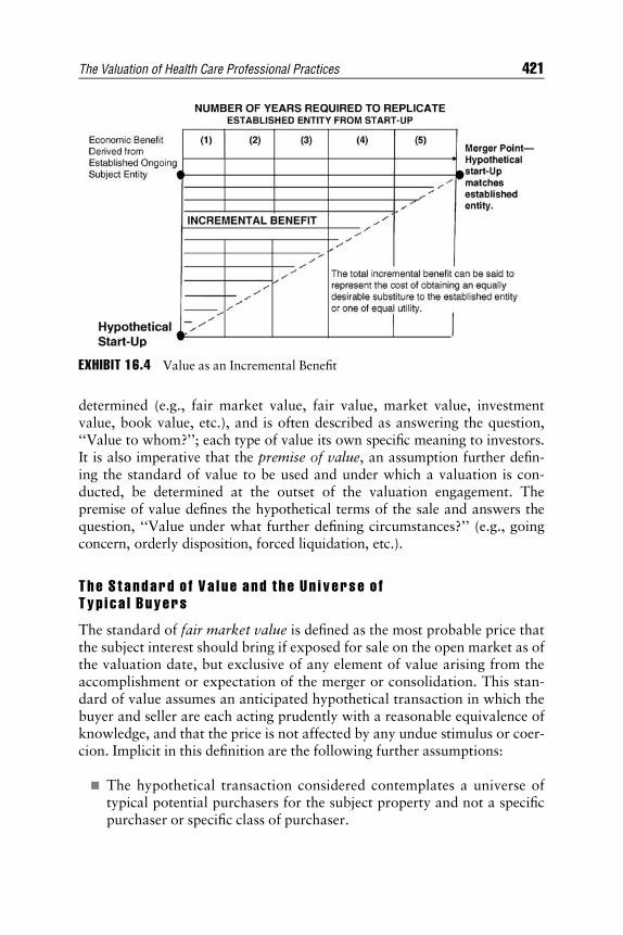
E1C16 08/14/2009 Page 421

determined (e.g., fair market value, fair value, market value, investmentvalue, book value, etc.), and is often described as answering the question,‘‘Value to whom?’’; each type of value its own specific meaning to investors.It is also imperative that the premise of value, an assumption further defin-ing the standard of value to be used and under which a valuation is con-ducted, be determined at the outset of the valuation engagement. Thepremise of value defines the hypothetical terms of the sale and answers thequestion, ‘‘Value under what further defining circumstances?’’ (e.g., goingconcern, orderly disposition, forced liquidation, etc.).

The S t andard o f Va l ue and t he Un i v erse o fTyp i ca l Buyers

The standard of fair market value is defined as the most probable price thatthe subject interest should bring if exposed for sale on the open market as ofthe valuation date, but exclusive of any element of value arising from theaccomplishment or expectation of the merger or consolidation. This stan-dard of value assumes an anticipated hypothetical transaction in which thebuyer and seller are each acting prudently with a reasonable equivalence ofknowledge, and that the price is not affected by any undue stimulus or coer-cion. Implicit in this definition are the following further assumptions:

& The hypothetical transaction considered contemplates a universe oftypical potential purchasers for the subject property and not a specificpurchaser or specific class of purchaser.

EXHIBIT 16.4 Value as an Incremental Benefit


E1C16 08/14/2009 Page 422

& Buyer and seller are typically motivated.& Both parties are well informed and acting in their respective rational

economic self-interests.& Both parties are professionally advised, and the hypothetical transac-

tion is assumed to be closed with the typical legal protections in placeto safeguard the transfer of ownership of the legal bundle of rights thatdefine and encompass the transacted property or interest.

& A sufficiently reasonable amount of time is allowed for exposure in theopen market.

& Payment is made in cash or its equivalent.

When the professional practice being valued operates in an industrythat is subject to further regulatory restraints defining what is meant byfair market value, other assumptions may also apply that the valuatorshould be aware of: For example, in the case of a medical practice, thefollowing assumptions implicit in the definition of fair market valuealso apply:

& The anticipated hypothetical transaction would be conducted in com-pliance with Stark I and II legislation prohibiting physicians from mak-ing referrals for ‘‘designated health services’’ reimbursable underMedicare or Medicaid to an entity with which the referring physicianhas a financial relationship.1 Stark II defines fair market value as the‘‘value in arm’s-length transactions, consistent with the general marketvalue.’’2 The transaction falls within Stark II’s specific exception for‘‘isolated financial transactions’’ when the amount of the remunerationunder the employment (1) is consistent with fair market value of theservices, (2) is not determined in a manner that takes into account (di-rectly or indirectly) the volume or value of any referrals by the referringphysician, and (3) is provided pursuant to an agreement that would becommercially reasonable even if no referrals were made to theemployer; and (4) the transaction meets such other requirements as theSecretary [of the Department of Health and Human Services] may im-pose by regulation as needed to protect against program or patientabuse.3

& The anticipated hypothetical transaction would be conducted in com-pliance with the Medicare Anti-Kickback Statute making it illegal toknowingly pay or receive any remuneration in return for referrals.4

The Medicare Anti-Kickback Statute requires the payment of ‘‘fairmarket value in arm’s-length transactions . . . [and that any compensa-tion is] not determined in a manner that takes into account the volumeor value of any referrals or business otherwise generated between the


E1C16 08/14/2009 Page 423

parties for which payment may be made in whole or in part underMedicare, Medicaid or other Federal health care programs.’’5

& Related to the aforementioned, the following definitions of terms ap-ply. ‘‘In an excess benefit transaction, the general rule for the valuationof property, including the right to use property, is fair market value.’’6

‘‘A disqualified person, regarding any transaction, is any person whowas in a position to exercise substantial influence over the affairs of theapplicable tax-exempt organization at any time during [a five-year pe-riod ending on the date of the transaction].’’7 An ‘‘excess benefit trans-action’’ is a ‘‘transaction in which an economic benefit is provided byan applicable tax-exempt organization, directly or indirectly, to or forthe use of a disqualified person, and the value of the economic benefitprovided by the organization exceeds the value of the consideration re-ceived by the organization.’’8

The Prem ise o f Va l u e and t he I nves tmen tT ime Hor i z o n

The premise of value under which a valuation is conducted is an assumptionfurther defining the standard of value to be used. The premise of value de-fines the hypothetical terms of the sale and answers the question, ‘‘Valueunder what further defining circumstances?’’ Two general concepts relateto the consideration and selection of the premise of value: value in use andvalue in exchange.

Value in Use Value in use is that premise of value that assumes that theassets will continue to be used as part of an ongoing business enterprise,producing profits as a benefit of ownership. For example, in valuing theassets of a surgical hospital, the valuator must determine whether it is ap-propriate to value simply the tangible assets or to consider the enterprise asa going concern and incorporate the potential value of intangible assets. Or-derly liquidation value involves assuming that the equipment is sold, per-haps separately, over a reasonable period of time. Forced liquidationassumes that the equipment is sold as quickly as possible to the first bidder.

Value in Exchange Value in exchange describes an orderly disposition of amass assemblage of the assets in place, but not as a going concern enter-prise. While value in exchange is often referred to as liquidation value, theliquidation can be either on the basis of an orderly disposition of the assetswhere more extensive marketing efforts are made and sufficient time is per-mitted to achieve the best price for all assets, or on the basis of forced liqui-dation where assets are sold immediately and without concern for obtaining


E1C16 08/14/2009 Page 424

the best price. Costs of liquidation should be considered in the value esti-mate when using this premise of value. Shortening the investment timehorizon may have a deleterious effect on the valuation of the subject entity,as it presents a restriction on the available pool of buyers and investorsand the level of physician ownership, as required under the standard offair market value.

VALUAT I ON ADJUSTMENTS FOR R I SK

The selection of the appropriate risk adjustment to market-derived requiredrates of return utilized in the development of selected discount rates, capi-talization rates, and/or market multiples in health care valuation requires athorough understanding of several underlying investment concepts. In de-veloping a discount/capitalization rate to be applied in income approachmethods, the following should be considered:

& Investors in professional practices have alternative investments availa-ble to them. Therefore, the investment justification for a given profes-sional practice should be considered in comparison to rates of returnavailable from a broader array of other types of investments.

& High-risk factors are considered to have a greater than average chanceof negatively affecting the enterprise’s earning power, while low-riskfactors are considered less likely to reduce the enterprise’s ability togenerate profits and cash flow as a future benefit of ownership; accord-ingly, elements that increase risk decrease the value of the enterprise,and conversely, elements that decrease risk increase value.

& Knowledgeable investors in a professional practice with an accompany-ing high degree of risk should require a greater return on investment tocompensate for the greater risk.

& There will be differences of opinion as to how much risk is representedby any single characteristic of the professional practice, and the risktolerance of each individual investor is, to a large extent, dependentupon the return on investment required to compensate for the per-ceived level of risk.

In addition to informed consideration (i.e., consideration of the fourpillars) of the effect of what may be volatile market changes on the percep-tion of risk and resulting adjustment to the required rate of return for in-vestment, the most probable income/earnings/benefit stream that isforecasted to be available for return to the subject practice’s investorsshould also be carefully analyzed to determine appropriate adjustments to


E1C16 08/14/2009 Page 425

reported results derived from historical performance, in order to reflect themost accurate and appropriate information available on the valuation dateof the most probable future performance, often referred to as normalizedearnings. To arrive at an estimate of the normalized earnings for the subjectenterprise, the adjustments considered should include, but not necessarilybe limited to:

& Actual or expected increase(s)/decrease(s) in fees and reimbursementsfor services by regulatory edict or competitive market pressures.

& Projected increase(s)/decrease(s) in operating expenses based on newoperating parameters and market realities (e.g., provider taxes and dis-closure requirements).

& Expectations of the future stability and growth of the revenue streamsand the sustainability of the subject practice’s earnings within the con-text of what may be an ever-changing industry and marketplace.

In the final analysis, both the valuator’s assessment of an appropriaterisk-adjusted required rate of return for investment and the forecast of themost probable income/earnings/benefit stream are inexorably related to,should be based on, and must be carefully correlated to an informed, realis-tic, and unsparing assessment of a universe of typical buyers’ current per-ceptions of the market as to the future performance of the subjectenterprise, as well the market’s assessment of risk related to an investmentin such an enterprise.

D i scoun t f o r Lack o f Con t ro l

While a control premium is an increase to the pro rata share of the value ofthe business that reflects the impact on value inherent in the managementand financial power that can be exercised by the holders of a control interestof the business, usually the majority holders, a discount for lack of control(DLOC) or minority discount is the reduction from the pro rata share of thevalue of the business as a whole that reflects the impact on value of the ab-sence or diminution of control that can be exercised by the holders of a sub-ject interest.

D i scoun t f o r Lack o f Marke t ab i l i t y

There are inherent risks relative to the liquidity of investments in closelyheld, nonpublic companies in that investors in closely held companies donot have the ability to dispose of an invested interest quickly if the situationis called for (e.g., forecasted unfavorable industry conditions or the


E1C16 08/14/2009 Page 426

investor’s personal immediate need for cash). This relative lack of liquidityof ownership in a closely held company is accompanied by risks and costsassociated with the selling of an interest of a closely held company (i.e.,locating a buyer, negotiation of terms, adviser/broker fees, risk of exposureto the market, etc.). Thus, a discount may be applicable to the value ofclosely held company due to both the inherent illiquidity of the investmentas well as the transactional costs related to its disposition. Such discountsare commonly referred to as discounts for lack of marketability.

CLASS I F I CAT I ON OF ASSETS ANDDET ERM INAT I ON OF GOODW I L L

The valuator must be careful to define the professional practice entity andinterest being valued. The definition and description of the entity should in-clude identification of legal structure, legal name, trade name, address ofrecord, and other descriptors (e.g., type of company), as well as the specificdefinition and description of the type and size of the interest in the entitybeing appraised in the engagement (e.g., ‘‘100 percent interest in the com-mon shareholders’ equity’’ or ‘‘100 percent interest in the total invested cap-ital/assets’’).

Once the subject entity and interest have been defined, the appropriateclassification of assets and the goodwill related to the professional practiceis critical to the valuation process. The classification of assets may be initi-ated by condensing of the existing assets within the context of two catego-ries, tangible and intangible assets. See Exhibit 16.5 for a representativeclassification of tangible and intangible assets in the context of a profes-sional medical practice.

In the context of the valuation of medical professional practices, thetypical focus of the classification of assets begins with determining the exis-tence and quantifiability of intangible assets. Once that existence is estab-lished, one type of intangible asset that is often subsequently found iscommonly called goodwill. This term may appropriately be defined as thepropensity of clients/customers (and the revenue stream thereof) to returnto the practice. Keep in mind that goodwill is only one of several intangibleassets that may be found, not a catchall moniker for all intangible assets inthe aggregate.

Intangible assets that may be classified as goodwill and patient-relatedinclude custody of client charts and records, as well as both personal/profes-sional and practice/commercial goodwill. The custody of client charts andrecords may create the background that supports the propensity for the con-tinued client-provider relationship, which constitutes goodwill.


E1C16 08/14/2009 Page 427

There are numerous sources for information related to the definition ofthe often-misused valuation term goodwill. The following is the definitionof ‘‘Good Will’’ [sic] from Black’s Law Dictionary:

The favor which the management of a business wins from the pub-lic. Seneca Hotel Co. V. U.S., Ct.C.., 42 F.2d. 343, 344. The fixedand favorable consideration of customers arising from establishedand well-conducted business. Colton v. Duvall, 254 Mich. 346,237 N.W. 48, 49. The favorable consideration shown by the pur-chasing public to goods known to emanate from a particularsource. White Tower System v. White Castle System of EatingHouses Corporation, C.C.A.Mich., 90 F.2d 67, 69. Goodwill is anintangible asset. Something in business which gives reasonableexpectancy of preference in race of competition. In re Witkind’sEstate, 167 Misc. 885, 4 N.Y.S.2d 933, 947. The custom or patron-age of any established trade or business; the benefit or advantage ofhaving established a business and secured its patronage by thepublic. The advantage or benefit which is acquired by an establish-ment, beyond the mere value of the capital, stocks, funds, or prop-erty employed therein, in consequence of the general publicpatronage and encouragement which it receives from constant or

EXHIBIT 16.5 Classification of Tangible and Intangible Assets of ProfessionalEnterprise Practices


E1C16 08/14/2009 Page 428

habitual customers, on account of its local position, or commoncelebrity, or reputation for skill or affluence or punctuality, orfrom other accidental circumstances or necessities, or even from an-cient partialities or prejudices. And as property incident to businesssold, favor vendor has won from public, and probability that allcustomers will continue their patronage. It means every advantage,every positive advantage, that has been acquired by a proprietor incarrying on his business, whether connected with the premises inwhich the business is conducted, or with the name under which it ismanaged, or with any other matter carrying with it the benefit ofthe business.9

D i s t i ngu i s h i ng be tween Pro f ess i o na l / P ersona land Prac t i ce / Commerc i a l G oodw i l l

Sources for guidance as to the definition of goodwill can be found in IRSRevenue Ruling 59-60 and established judicial opinions from valuation-related case law. In the event that the valuation consultant determines,first, the existence of intangible asset value in the subject practice and, sec-ond, the existence of goodwill as one of the intangible assets existing, thenthe next step is to identify, distinguish, disaggregate, and allocate the rele-vant potion of the existing goodwill to either professional/personal goodwillor practice/commercial goodwill.

Professional/Personal Goodwill Professional goodwill results from thecharisma, knowledge, skill, and reputation of a specific practitioner.Professional/personal goodwill is generated by the reputation and per-sonal attributes of the physician that accrue to that individual physi-cian. Professional/personal goodwill may include such characteristics as‘‘(1) lacks transferability, (2) specialized knowledge, (3) personalizedname, (4) inbound referrals, (5) personal reputation, (6) personal staff,(7) age, health, and work habits, and (8) knowledge of end user.’’10

Since these attributes go to the grave with that specific individual physi-cian and therefore can’t be sold, they have no economic value.

Professional/personal goodwill is not, as a practical matter, transfer-able. Even with long transition periods of introduction for a new acquiringphysician-owner, the charisma, skills, reputation, and personal attributes ofthe seller cannot, by definition, be transferred. It is often stated that withassisted transfer (i.e., an extended transition period), a large portion of pro-fessional/personal goodwill may be transferred; however, the transferabilitysuggested is in conflict with the definition of professional or personalgoodwill.


E1C16 08/14/2009 Page 429

Practice/Commercial Goodwill Practice/commercial goodwill should bedefined in a medical services enterprise that includes a practice componentas ‘‘the propensity of patients (and the revenue stream thereof) to return tothe practice in the future.’’ That portion of goodwill that may be transferredshould be appropriately characterized as practice (or commercial) goodwillas described next. Practice/commercial goodwill may include such charac-teristics as ‘‘(1) number of offices, (2) business location, (3) multiple serviceproviders, (4) enterprise staff, (5) systems, (6) years in business, (7) out-bound referrals, and (8) marketing.’’11

Practice/commercial goodwill, as distinguished from professional/per-sonal goodwill, is transferred frequently, and may be described as the un-identified, unspecified, residual attributes of the practice as an operatingenterprise that contribute to the propensity of patients (and the revenuestream thereof) to return to the practice in the future. There are several sig-nificant factors to consider in determining the existence and quantity ofpractice/commercial goodwill related value.

There are several significant factors to consider in determining the exis-tence and quantity of practice goodwill related value. In litigation related tovaluation engagements, there may be significant legal precedents related toestablishing evidence as to goodwill in a specific legal venue or court juris-diction. The valuator should consult with the attorney in the case to clearlyunderstand these definitional requirements. Also, significant practice trans-fer activity in the market area can result in marginal practices attaining sig-nificant goodwill value.

IMPACT OF COMPET I T I V E FORCES

The competitive environment in which the subject professional practice op-erates is a significant factor to be addressed by the valuator in performingthe valuation analysis.

Harvard professor Michael Porter12 is considered by many to be one ofthe world’s leading authorities on competitive strategy and internationalcompetitiveness. In his 1980 book Competitive Strategy: Techniques forAnalyzing Industries and Competitors13 he argues that all businesses mustrespond to five competitive forces, shown in Exhibit 16.6.

1. Threat of new market entrants. This force may be defined as the risk ofa similar company entering your marketplace and winning business.There are many barriers to entry of new market entrants in health care,including the high cost of equipment, licensure, requirements for physi-cians and other highly trained technicians, development of physician


E1C16 08/14/2009 Page 430

referral networks and provider contracts, and other significant regula-tory requirements.

2. Bargaining power of suppliers. A supplier can be defined as any businessrelationship you rely on to deliver your product, service, or outcome.

3. Threats from substitute products or services. Substitute products or ser-vices are those that are sufficiently equivalent in function or utility tooffer consumers an alternate choice of product or service.

4. Bargaining power of buyers. This force is the degree of negotiatingleverage of an industry’s buyers or customers.

5. Rivalry among existing firms. This is ongoing competition betweenexisting firms without consideration of the other competitive forcesthat define industries.

VALUAT I ON APPROACHES , METHODS ,AND TECHN IQUES

There are numerous generally accepted health care valuation approaches,methods, and procedures. The choice of approaches or methods dependsprimarily on the purpose of the valuation report and the specific character-istics of the entity to be appraised. The objective and purpose of the valua-tion engagement, the standard of value, the premise of value, and theavailability and reliability of data must all be considered by the valuator inthe selection of applicable approaches and methods

Michael Porter’sFive Forces

DrivingIndustry

Competition

SUPPLIERS BUYERS

INDUSTRYCOMPETITORS

Rivalry amongExisting Firms

Threat of SubstituteProducts or Services

Bargaining Powerof Suppliers

Bargaining Powerof Buyers

Treat ofNew Entrants

POTENTIALENTRANTS

SUBSTITUTES

EXHIBIT 16.6 Five Forces of CompetitionSource: Michael Porter, Competitive Strategy: Techniques for Analyzing Industries and Com-petitors (New York: Free Press, 1980), 4.


E1C16 08/14/2009 Page 431

Revenue Ru l i ng 59 -60

Among the wide array of sources of guidance with which business valuationconsultants should be familiar to conduct an accurate business valuation,the pronouncements of the IRS may be most widely cited. The IRS providesinsights regarding its positions on business valuation issues through variousmediums: the Internal Revenue Code, the Treasury Regulations to theCode, Technical Advice Memorandums, Private Letter Rulings, and variousRevenue Rulings. Revenue Ruling 59-60 (RR 59-60) has been a significanttopic of discussion in the valuation community, as it provides basic guid-ance for the valuation of closely held common stocks. RR 59-60 provides ageneral outline and review of ‘‘the approach, methods, and factors to beconsidered in valuing shares of the capital stock of closely held corporationsfor estate tax and gift tax purposes.’’14

In the valuation of the stock of closely held corporations or corporatestock that lacks market quotations, all available financial data along withsignificant factors impacting the fair market value should be considered.

The following contains fundamental factors that require vigilant analy-sis in each business valuation:

& The nature of the business and the history of the enterprise from itsinception.

& The economic outlook in general and the condition and outlook of thespecific industry in particular.

& The book value of the stock and the financial condition of the business.& The earnings capacity of the company.& The dividend-paying capacity.& Whether or not the enterprise has goodwill or other intangible value.& Sales of stock and the size of the block of stock to be valued.& The market price of stocks of corporations engaged in the same or simi-

lar line of business having their stocks actively traded in a free and openmarket, either on an exchange or over the counter.15

The choice of methodology depends primarily on the purpose of thevaluation report and the specific characteristics of the professional practice.For example, the standard of value to be estimated in a divorce case is oftenfair market value; however, the standard may be different from state tostate; that is, some states set a standard of fair value that is either judiciallyor legislatively defined. For example, the state of Michigan has developed aconcept known as the holder’s interest theory of value. The value to theholder concept is most often associated, although not frequently articulated,with investment or intrinsic value. Application of this standard of value


E1C16 08/14/2009 Page 432

contemplates value to the holder (or particular buyer) rather than value to apotential hypothetical buyer; that is, investment value is distinguished fromfair market value in that investment value provides a going concern value tothe current owner and thereby identifies assets that have an intrinsic worthto the owner, which may not be transferable to another person.16

It is also important that the valuation consultant determine the premiseof value. For example, value in use considers the subject practice on the ba-sis of an ongoing professional practice enterprise. Value in exchange de-notes a liquidation of the practice on either an orderly or a forced basis.

Once the valuation consultant clearly understands the purpose of theappraisal assignment, has determined the standard of value and the premiseof value, and has determined the availability and reliability of data, he orshe must select one or more applicable methods. These methods can be clas-sified by three major valuation approaches: income, cost, and market.

I n c ome Approaches

The following methods may be utilized under the income approach.

Discounted Cash Flow Method The discounted cash flow method is based ona multiperiod discounting income approach that estimates the present valueof normalized expected cash flows distributable to the owners of the entitybeing appraised, with a residual or terminal value ascribed to all periodsbeyond the projection.

The value of an investment in an operating company is often consideredto be equal to the present value of all its expected future cash flows. There-fore, when selecting the discounted cash flow method (an income approachmethod), the valuation consultant recognizes that the fair market value of amedical practice is the aggregate present value of the total of all cash flowslikely to be achieved from the practice in the future.

The net present value is calculated by applying a weighted average costof capital (WACC) or a risk-adjusted built-up discount rate to the total netcash flow generated by the practice.

This total net cash flow is the gross collected revenues of the practiceless all noncash and non-owner/officer-compensation-related expenses ad-justed for depreciation, capital expenditures, and working capital. This rep-resents the real cash flow of the practice.

These cash flows are then discounted over the selected years of the pro-jection at the risk-adjusted discount rate. All cash flows from the final yearof the projection through infinity are accounted for in the terminal periodand calculated by utilizing the adjusted cash flow of the final year capital-ized at the selected capitalization rate (discount rate less growth rate) and


E1C16 08/14/2009 Page 433

then discounted at the selected risk-adjusted discount rate to arrive at thepresent value of all of these future terminal-period cash flows. The totalpresent value of all the cash flows will be equal to the estimated fair marketvalue of the practice under this method.

As the discounted net cash flow method results in a C corporationequivalent level of value due to both the tax structure typically used in pro-jections as well as the use of a buildup method to develop a discount ratederived from empirical market transactional data of publicly traded C cor-poration interests, an adjustment to reflect a pass-through entity level ofvalue may be appropriate. An adjustment to reflect the additional incremen-tal net economic benefits derived from an entity’s pass-through status mayalso be applicable to the indicated results derived from other methods, in-cluding the guideline public company method and the direct market compa-rable transactions method, discussed further later.

Single-Period Capitalization Method The single-period capitalization methodestimates the present value of the entity being appraised by capitalizing asingle year of benefits.

Cos t Approaches

The following methods may be utilized under the cost approach.

Asset Accumulation Method In valuation engagements where there is no sig-nificant income stream to capitalize, a cost approach method such as theasset accumulation method is often used. This method identifies, distin-guishes, disaggregates, and appraises each of the component assets, bothtangible and intangible, within the practice.

Challenges with this method include determining which assets can le-gally be sold and to whom; determining fair market value of goodwill andother intangible assets requires the use of some type of capitalization ofearnings method, with the same difficulties noted earlier.

Liquidation Value Methods Liquidation methods, either by orderly disposi-tion or by forced liquidation, estimate the value of an entity by determiningthe present value of the net proceeds from liquidating the company’s assetsand paying off liabilities. The orderly method describes a situation in whichthe sell-off process is conducted in an organized and systematic fashion un-der a reasonable time line constructed by the seller. In this scenario a lesserdegree of urgency exists. Under the forced method the seller no longer is in asituation to proceed at his or her own discretion. All, or the majority, of theassets will be sold at approximately the same time in a relatively quick


E1C16 08/14/2009 Page 434

fashion. Generally, the orderly liquidation method value will be greaterthan the forced liquidation value.

Excess Earnings Method The excess earnings method, also called the trea-sury method or the IRS formula method based on Revenue Ruling 68-609,does not fit neatly into any of the three approaches. This method is consid-ered by many valuators to be a hybrid method, combining elements of theasset-/cost-based approach with elements of income approach methods.

The excess earnings method first values the intangible assets of theentity being appraised utilizing a residual technique, whereby a portionof the benefit stream (e.g., net free cash flow or net income) is firstattributed to a return on net tangible assets utilizing a market-derivedcost of capital for similar tangible assets; second, an appropriate por-tion of the benefit stream is attributed to the fair market value of thereplacement cost of services provided by the owner as owner compensa-tion; and finally, the dollar amount of the benefit that remains after thededuction of these two amounts (the residual) is then presumed to beattributable to the intangible assets. This amount of the benefit stream,which has been determined to be attributable to the intangible assets ofthe subject entity, is then capitalized using a risk-adjusted equity rate ofreturn and the resulting indicated value of the intangible assets is thencombined with (added to) the value of the tangible assets of the entitybeing appraised to arrive at an estimate of overall asset value for thesubject entity as a going concern.

Marke t Approaches

The following methods may be utilized under the market approach.

Direct Market Comparable Transactions Method The direct market compa-rable transactions method, also known as the market data comparableor analysis of transactional data method, is often selected because con-ceptually an analysis of actual transactions of comparable health carepractices and a comparison in the aggregate to the practice make goodsense.

However, because of the developing and unreliable nature of reportedcomparable transactional data for health care practices and the significantand substantive dissimilarity and individual uniqueness of health care prac-tices (which tend to be unique enterprises lacking easily disaggregatable,homogenous units for comparison), the abstraction of useful and valid datais problematic.


E1C16 08/14/2009 Page 435

The lack of publicly traded physician practice management company(PPMC) purchasers has reduced the number of reported sales.

Guideline Publicly Traded Company Approach This method compares pub-licly traded companies in the same industry and line of business as the sub-ject practice. Comparable companies for medical practices are physicianpractice management companies (PPMCs) that contract with practiceswithin the same medical specialty as the subject practice. The current price-to-revenue and price-to-earnings ratios of these guideline companies areused in the computation of an estimated fair market value for the practice.Because these guideline companies are publicly traded on the variousexchanges, these two ratios represent a minority-marketable position oftheir investors, as compared to a controlling-interest closely held, nonmar-ketable position of the subject practice. Therefore, appropriate adjustmentsneed to be made before calculating the indicated value.

Previous Subject Practice Transactions Previous sales of the subject prac-tice, whether partially in its entirety, can provide a very good estimate ofvalue. However, depending on how long ago the practice sold, market andpractice changes may discount the validity of such data.

ANALYS I S OF R I SK

As discussed earlier, it is important to first analyze and reach a supportableconclusion as to the relationship between risk and return for a specific typeof practice investment that is characteristic of the specific dynamics of themarket in which it operates at any point in time, before selecting a discount/capitalization rate.

It should be kept in mind that while this estimate of investor-perceivedrisk is, in the end, necessarily based, to a great degree, on the subjectivejudgment of the valuation consultant, objective methods and teachings areavailable and will be employed to the extent possible to arrive at a valid andsupportable discount/capitalization rate. The assessment of risk is inexora-bly related to and should be based on an informed consideration of the mostprobable expectations and perceptions of a universe of typical buyers as tothe future performance of the subject entity, as well as material changes insubstantive value drivers.

In the final analysis, the assessment of risk must be carefully correlatedto an informed, realistic, and unsparing assessment of current buyer percep-tions in the market.


E1C16 08/14/2009 Page 436

Compara t i ve F i n anc i a l Da t a and Deve l o pmen t o fD i s coun t Ra t es

Information used to compare the subject practice’s financial statementswith industry averages is available through a variety of industry studies.Some of the standard sources that cover all industry categories includeRMA Annual Statement Studies, published by the Risk Management As-sociation; Financial Studies of the Small Business, published by FinancialResearch Associates; and Statistics of Income: Partnership Source Bookand Statistics of Income: Sole Proprietor Source Book, available throughthe IRS. Other sources of this data include trade associations and variousindustry studies.

Benchmarking techniques are often used to determine the degree towhich the subject entity varies from comparable health care industrynorms, as well as to provide vital information regarding its trends in in-ternal operational performance and financial status. An appropriate andsuccessful application of benchmarking techniques generally reveals bothfavorable and unfavorable areas of the business operation of the subjectentity, which may in turn require further examination to determine cau-sality and the effect, if any, on the subject entity’s value. Thus, bench-marking often assists valuators not only in identifying the existence ofnonstandard performance and anomalies in costs, levels of productivity,and financial ratios, but also in discovering the underlying causes of theseanomalies. When the causes for aberration from the norm are identified,they should be further investigated and assessed as to the potential weak-nesses and risk factors (as well as the potential strengths) they pose forthe subject entity.

As illustrated by the preceding discussion, the benchmarking process isnot only essential for internal managers seeking to adjust business methodsto optimize performance, but is also an invaluable tool for valuators andfinancial analysts. Common methods of applying the results of benchmark-ing analysis include:

& Adjusting operating expense and capital items, as well as capital struc-ture, to industry norms (when valuing a control position).

& Adjusting the indication of a discount rate or cost of equity as derivedfrom the market (subject entity specific risk premium).

& Selecting the appropriate financial multiples or ratios (e.g., price-earn-ings, price-to-revenue, price-to-EBITDA, etc.).

& Selecting the appropriate discounts and premiums, based on the level ofvalue sought (e.g., discount for lack of marketability, control premium,discount for lack of control, etc.).


E1C16 08/14/2009 Page 437

Re t urn on I nves tmen t : D i s coun t Ra t e /Cos t o f E qu i t y

The discount rate, at which the measured expected future stream of eco-nomic benefit of ownership is discounted to present value, is selected by thevaluation consultant to represent the rate of return a typical investor in theprofessional practice would require in discounting the expected stream ofthe economic benefits of equity ownership of the subject professional prac-tice, given the systematic risk of the market, as well as the unsystematic riskof investment in the subject professional practice. In contrast, the capitaliza-tion rate is the rate by which a single estimate of benefit is divided to deter-mine value. Inherent in this single-period capitalization formula is theassumption of continuity of the benefit stream in perpetuity. Typically, thecapitalization rate is calculated by deducting the projected annual long-termgrowth rate of the subject medical practice from the selected discount rate:

Discount rate � Growth rate ¼ Capitalization (cap) rate

As mentioned earlier, the discount rate is a measure of return requiredof an equity investor, thus, in effect, is the cost of equity of a specific busi-ness enterprise. The cost of equity, combined with the cost of debt, com-prise the weighted average cost of capital (WACC) of a specific businessenterprise, which is utilized when estimating the return on investment oftotal invested capital (both equity and debt).

The discount rate or cost of equity, selected by the valuation consultantmay be developed by building up the aggregate elements of several rates andrisk adjustments as illustrated in Exhibit 16.7.

R i sk - F ree Ra t e

The starting point for developing an appropriate discount rate is the alter-native investment opportunities in risk free or relatively risk-free

EXHIBIT 16.7 Determination of the Discount Rate

Discount Rate/Cost of Equity Components Rate

1 Risk-free rate 3.05%2 Investment alternative (equity risk premium) 6.05%3 Health care risk premium adjustment �0.79%4 Size premium 5.82%5 Subject enterprise company-specific risk premium 5.00%6 Total discount rate/cost of equity 19.13%


E1C16 08/14/2009 Page 438

investments. The interest paid by U.S. government securities are the closestsubstitute or proxy available for a risk-free rate.

I n v es tmen t A l t e rna t i v e ( E qu i t y R i sk Prem i um )

This adjustment reflects the extra return, or premium, that is expected bythe typical equity investor in large company stocks in excess of the returnon a riskless asset. Ibbotson has studied and estimated the historical (since1926) realized equity risk premium (ERP) associated with the risk of invest-ment in common stock in its Stocks, Bonds, Bills and Inflation Yearbook(SBBI).

According to several recent published articles and papers in the val-uation profession, the realized returns on equity reported by Ibbotson,as mentioned earlier, have been overstated as compared to the ERP thatmust have been expected by investors given the underlying economics ofthe economy (i.e., expected growth in gross domestic product) and theunderlying economics of public companies (i.e., expected growth inearnings and/or dividends). These studies suggest that investors wouldnot reasonably have expected as large an ERP as what was actually re-alized, and it may be appropriate to adjust downward a historical real-ized ERP to estimate an expected ERP,17 based on the aforementionedstudies and recent research.

Company -Spec i fic R i s k Prem i um

The combination of the risk-free rate and the equity risk premium estimatesthe return required by the investor in large company stocks. Ibbotson mea-sures the additional return of small company stocks over the market as awhole.

This adjustment is somewhat more subjective in that it reflects the valu-ation consultant’s informed assessment of the various risk factors that areinherent and specific to the subject professional practice. Additional riskfactors specific to a subject medical practice include but are not limited to:operational performance, market/competition, technological obsolescence,revenue stream, risk related to key persons, and depth of management.

Research challenges related to determining the appropriate discountrate/cost of equity include: (1) finding research to support the quantificationof subject medical practice risk premiums, (2) obtaining size premium datafor small companies, and (3) determining industry risk adjustments for cer-tain professional practice industry subsectors.

Keith Pinkerton and Peter Butler have released a calculator to measuretotal cost of equity and public company-specific risk.18 It provides empirical


E1C16 08/14/2009 Page 439

benchmarks for selecting the correct company-specific risk premium (CSRP)for the subject entity, mixing subjective and objective techniques. This pro-cess begins by reviewing the public company’s form 10-K to understand thedisclosures related to company-specific factors. The valuator can then placethe private company within, above, or below the calculated benchmarksbased on the degree to which the private company faces the same risks asthe public company. Also, while Pinkerton and Butler do not recommendusing the NASDAQ index as a proxy, it is available in their calculator. Thecalculator can only be used to calculate implicit volatilities exactly match-ing the private company’s total cost of equities (TCOE). Canadian publiccompanies can also be used in the calculator. If the companies are publiclytraded in the United States, pricing data will be available. Otherwise, histor-ical data must be utilized. The calculator pulls indexes’ closing prices, andcan handle pricing either adjusted for dividends or not. Data is available forthe previous five years or 261 weeks, and the creators recommend using atleast the past three years when calculating beta. Also, selecting public com-pany comparables in the model using the calculator does not differ fromselecting them for the market approach.

One of the most innovative abilities of the calculator is the way it pullsthe prior 261 days of closing prices for a particular company. For example,if the effective date is Monday, the calculator will return 261 Mondays ofclosing prices. The technique has not been reviewed by the SEC or IRS.

Pinkerton and Butler were questioned about the necessity of havinggood public company comparables when using the calculator for a $40 mil-lion entity when the opposing party valued it at $90 million. Theyresponded by explaining that the calculator has empirical data whereasalternatives to calculating company-specific risk (CSR) lack this type ofdata. While the calculator may have ‘‘not so great guidelines,’’ the compo-nent observation method offers no empirical data. Since the calculator com-putes the CSR from the same publicly traded companies as the incomeapproach, it should not be thrown out when there are no good guidelinecompanies to use, since the income approach is not abandoned when thisoccurs.19

L EV E L O F VALUE : D I SCOUNTS AND PREM IUMS

With each method utilized, certain adjustments should be considered basedon the specific requirements of each engagement and the inherent indicationof value (i.e., the level of value that results from each method).

When a closely held level of value (in contrast to a freely traded, mar-ketable, or publicly traded level) is sought, the valuation consultant may


E1C16 08/14/2009 Page 440

need to make adjustments to the indicated valuation results. There are in-herent risks relative to the liquidity of investments in closely held, nonpubliccompanies that are not relevant to the investment in companies whoseshares are publicly traded (freely traded). Investors in closely held compa-nies do not have the ability to dispose of an invested interest quickly if thesituation is called for (e.g., forecasted unfavorable industry conditions orthe investor’s personal immediate need for cash). This relative lack of li-quidity of ownership in a closely held company is accompanied by risks andcosts associated with the selling of an interest of a closely held company(i.e., locating a buyer, negotiation of terms, adviser/broker fees, risk ofexposure to the market, etc.). By contrast, investors in the stock market aremost often able to sell their interests in a publicly traded company withinhours and receive cash proceeds in a few days. Accordingly, a discount maybe applicable to the value of a closely held company due to the inherentilliquidity of the investment. Such a discount is commonly referred to as adiscount for lack of marketability.

Over the years, there have been several empirical studies performed at-tempting to quantify a discount for lack of marketability, typically in threecategories: (1) transactions involving restricted stock of publicly tradedcompanies, (2) private transactions of companies prior to their initial publicofferings (IPOs), and (3) an analysis and comparison of the price-earnings(P/E) ratios of acquisitions of public and private companies published in theMergerstat Review study.

With a noncontrolling interest, in which the holder cannot solely autho-rize and cannot solely prevent corporate actions (in contrast to a controllinginterest), a discount for lack of control (DLOC) may be appropriate. In con-trast, a control premium may be applicable to a controlling interest. While acontrol premium is an increase to the pro rata share of the value of the busi-ness that reflects the impact on value inherent in the management and finan-cial power that can be exercised by the holders of a control interest of thebusiness, usually the majority holders, a discount for lack of control is thereduction from the pro rata share of the value of the business that reflectsthe impact on value of the absence or diminution of control that can beexercised by the holders of the minority interest.

Several empirical studies have been done to attempt to quantify DLOCsfrom their antithesis, control premiums. The studies include the MergerstatReview,20 an annual series study of the premium paid by investors for con-trolling interest in publicly traded stock, and the Control Premium Study,21

a quarterly series study that compiles control premiums of publicly tradedstocks by attempting to eliminate the possible distortion caused by specula-tion of a deal.


E1C16 08/14/2009 Page 441

CONCLUS I ON

There is no single approach or method, or combination thereof, that is uni-versally correct or that applies to every engagement. Each case must be con-sidered as a unique exercise of informed judgment, based on careful analysisand supported by documented evidence and reasoned argument. All the so-phisticated arithmetic and brilliant theoretical constructs in the valuationworld will not support a credible valuation if the appraiser does not have athorough understanding of the market sector within which the subjectentity exists and operates (i.e., the four pillars). In addition, the valuatorshould remember to question everything and everyone, but be prepared toutilize reasoned, informed professional judgment to review the valuation re-port. In the end, in arriving at your opinion of value, remember to ‘‘loveeveryone, trust no one, and paddle your own canoe!’’

NOTES

1. 42 U.S.C.A. 1395nn(a); Social Security Act 1877(a).2. 42 U.S.C.A. 1395nn(h)(3); Social Security Act 1877(h)(3).3. 42 U.S.C.A. 1395nn(e)(6); Social Security Act 1877(e)(6).4. 42 U.S.C.A. 1320a-7b(b).5. 42 C.F.R. 1001.952(d)(5).6. ‘‘Intermediate Sanctions—Excess Benefit Transactions,’’ Internal Revenue Ser-

vice, www.irs.gov/charities/charitable/article/0,id=123303,00.html (accessed 9/2/08).

7. ‘‘Disqualified Person,’’ Internal Revenue Service, www.irs.gov/charities/charita-ble/article/0,id=154667,00.html (accessed 9/2/08); ‘‘Lookback Period,’’ Inter-nal Revenue Service, www.irs.gov/charities/charitable/article/0,id=154670,00.html (accessed 9/2/08).

8. ‘‘Intermediate Sanctions—Excess Benefit Transactions,’’ Internal Revenue Ser-vice, www.irs.gov/charities/charitable/article/0,id=123303,00.html (accessed9/2/08).

9. Black’s Law Dictionary, 5th ed. (St. Paul, MN: West, 1979), 625.10. In re Marriage of Alexander, 368 Ill.App.3d 192, 199 (2006).11. Ibid.12. Michael Porter is the recipient of the Wells Prize in Economics, the Adam Smith

Award, three McKinsey Awards, and honorary doctorates from the StockholmSchool of Economics and six other universities. He is also the author of 14books, including Competitive Advantage, The Competitive Advantage of Na-tions, and Cases in Competitive Strategy.

13. Michael Porter, Competitive Strategy: Techniques for Analyzing Industries andCompetitors (New York: Free Press, 1980), 4.


E1C16 08/14/2009 Page 442

14. Shannon P. Pratt, Robert F. Reilly, and Robert P. Schweihs, Valuing a Business(New York: McGraw-Hill, 2000), 585.

15. Ibid.16. J. Fishman et al., Standards of Value: Theory and Applications (Hoboken, NJ:

John Wiley & Sons, 2007), 167, 181.17. Roger J. Grabowski, ‘‘Equity Risk Premium: What Valuation Consultants Need

to Know About Recent Research,’’ Valuation Strategies (September/October2003).

18. Keith Pinkerton and Peter Butler, ‘‘Using the Butler Pinkerton Model—TotalCost of Equity and Public Company Specific Risk Calculator,’’ Business Valua-tion Resources (March 6, 2008).

19. ‘‘Butler/Pinkerton Update Questions on Comparables,’’ BVUpdate, March 5,2008, www.bvlibrary.com.

20. Published by FactSet Mergerstat, LLC.21. Compiled by Mergerstat/Shannon Pratt’s Business Valuation Resources.


E1C17 08/26/2009 Page 443

CHAPTER 17Valuing Dental Practices

Stanley L. PollockProfessional Practice Planners, Inc.

Over the past decades, the appraisal of dental practices has become popu-lar and the number of appraisers involved in dental practice appraisal

has increased greatly. During the decades, dental practice appraisal has de-veloped from a rather crude, formula-driven art form into a mature, multi-method process. By way of example, in the 1970s and 1980s dentalpractices were valued and sold at 100 percent of the latest 12 months equalsgross revenues. In the 1990s, values of dental practices continued upwardand sold at inflated numbers. Shortly thereafter, the dental practice bubblebegan to leak. Cox (1995) reported on the subject; as a rule, dental practicessold at around 65 percent of collected revenues, which was the price/grossratio. After extensive research, I reported in the 2006 and 2007 supplementsof Valuing Professional Practices & Licenses (Pollock 2006, 2007) that gen-eral dental practices sold in arm’s-length deals at 57 percent of the latestgross revenues. Gross revenues, of course, were higher than in previous dec-ades, and operating expenses were creeping up; certain pockets across theUnited States were not affected to any great extent, while other pocketswere greatly affected.

What became apparent during the decades was that certain appraiserswere still seeking simple guideline formulas while other more studious onesgained a great deal of relevant and applicable appraisal information. Manyappraisers maintained a great deal of local data. Data banks, most notablythose of the Institute of Business Appraisers (IBA),1 Pratt’s Stats,2 the Good-will Registry, the American Dental Association,3 the National Society ofProfessional Business Healthcare Consultants, and the Risk ManagementAssociation, gathered and published a great deal of important data, whichbecame available for astute and eager dental practice appraisers to use. TheAppraisal Foundation published the Uniform Standards of Professional

443

E1C17 08/26/2009 Page 444

Appraisal Practice (USPAP 2008), which certain appraisal societies andindividuals recognized; certain others proudly declared they would not, butconscientious appraisers do follow them (far too many unconscientiousones do not).

What also became apparent during the decades is that dental practices,especially specialty practices, have turned into large business organizations.Although professional practices generally are not thought of or classified assmall businesses, they are, nevertheless, generating gross and net revenues insix and seven figures. For appraisal and business matters and all intents,dental practices are and must be treated as not-so-small businesses.

Appraisers value practices differently depending on the purpose andfunction of the valuation; their training, experience, style, and integrity; thelocation of the subject practice; the size and type of practice; the businessform of the practice; and other reasons. Despite being not-so-small busi-nesses, dental practices and their valuations pose many differences fromother businesses and even from other professions. This chapter addressesdifferences that have transpired over the past few decades and includes myand others’ relevant suggestions and comments. The first few are:

Over the years multiple organizations have seen the value and applica-bility of accumulating data. Foremost is the data bank of the Institute ofBusiness Appraisers located in Plantation, Florida. Other significant databanks for dental practices are Pratt’s Stats of Business Valuation Resourcesin Portland, Oregon, and the Goodwill Registry in Plymouth Meeting,Pennsylvania. Raymond C. Miles, ASA, FIBA, one of the founders and themainstay of the Institute of Business Appraisers and its vast market databank, promulgated the direct market data method (DMDM). The DMDMhas become a highly relevant standard to assist appraisers in implementingthe market approach, especially for dental practices. At this time the IBAdata bank has accumulated data on close to 3,000 transactions of generaland specialty dental practices. Interestingly, the category of dental practicesis the second largest category of transactions in the IBA data bank (noneth-nic restaurants are number one). The following are important data pointsfor the appraiser of dental practices to have as background in today’s dentalpractice environment:

& Dental practices are heavily involved and controlled by third-party,managed care, and government sources.

& Certain practices participate in managed care and other programs com-pletely or partially, while others do not.

& Although corporate ownership of dental practices is possible andencouraged, the actual care of patients is limited to licensed dentists.

& There is a major decreasing supply of dentists.


E1C17 08/26/2009 Page 445

& Within certain limits, there are few barriers in dentistry to free marketcompetition. Professional or personal and practice or entrepreneurialgoodwill, as well as noncompetitive covenants, play a large part in thevaluation and transition processes.

& Acquiring a dental education and advanced training is long-term andextremely expensive.

& The cost of starting a dental practice is extremely expensive.& The cost of operating a dental practice is very high.& Technology plays a large part in dental practices.& Efficient management, more than ever, is required to operate a dental

practice.& The average dental practice staff today consists of four to five skilled

individuals per dentist.

NORMAL I ZAT I ON

Normalization is the adjustment of financial statements for items that arenot representative of the present going-concern status of the practice. Nor-malization addresses and characterizes unusual, over- or understated, andnonrecurring items. In other words, normalization brings reasonablenessand consistency into the valuation process. Adjusting financial statementsis one of the first steps an appraiser of a dental practice addresses. The sour-ces of the data are the latest three to five years’ tax reports, financial state-ments, depreciation, amortization, and Section 179 schedules.

First, of course, are gross receipts or collections (which are not produc-tion). Both are important, but the practitioner can’t spend money that is notyet collected and deposited. Also, comparing collections to production pro-vides an initial and meaningful way to see if the practice is operating effi-ciently. The collection ratio (collections divided by production) is crucial tothe financial health and security of a dental practice and should run in themid 90 percent range. Practices heavily involved and reliant upon third-party and Medicaid participation will have a lower percent. It is importantto know how much the practice is producing and actually collecting. Cer-tain write-offs and discounts are normal, but they must be controlled andthey affect bottom lines and valuations.

A major normalization is in owners’ or professional compensation. Forvaluation purposes, all practice or professional income should be classifiedas compensation, that is, income of officers, associates, independent con-tractors, employees, hygienists, and others. The appraiser is looking for theprofessional income and its sources that the practice entity provides. Fre-quently, the appraiser has to search for this income, especially if associates,

Valuing Dental Practices 445

E1C17 08/26/2009 Page 446

employees, and independent contractors are involved. Obtaining the com-plete revenue stream is crucial. A major difference between most dentalpractices and regular businesses is that most dental practices will balanceout at the end of the year and will show little or no profit or taxable income.

In regard to the matter of compensation, the appraiser must question ifthere are family members or others on the payroll who are nonproductiveemployees. In such hiring matters, family education, Social Security, retire-ment, and other funding show up and require appropriate adjustment. Mar-keting, advertising, promotion, meals, club memberships, andentertainment are major and legitimate factors in a dental practice today.However, a great deal of such expenses are personal, which can run from50 to 75 percent of the deductions. Many appraisers automatically adjustout 100 percent for professional continuing education. Today, in all statesand in many professional organizations, continuing education is requiredand is very expensive. Therefore, appraisers should allow a reasonableamount for legitimate continuing education, for meetings and travel, andfor personal allocation, and 50 percent, generally, is reasonable (but canrun higher). Vehicles and vehicle expenses can be quite large for many prac-titioners, and deductions may be difficult to substantiate. However, forthose practitioners with multiple facilities, hospital privileges, and reasonsto attend professional meetings and visit accountants and consultants,banks, referrers, and laboratories, vehicle expenses are legitimate and canrun around 50 percent of the listed expenses.

Cash and cash equivalents normally (but not always) are not included inmost dental practice appraisals. Accounts receivable and payable and liabil-ities may or may not be included. In most practice sales, they are not; in di-vorce matters and associate buy-ins and buyouts they are. In mergers andacquisitions, they may or not be included yet play an important role. Mostof the time, they are handled separately. If handled separately or included inan appraisal, accounts receivable and payable should be properly adjusted oraged. A reasonable approach to such aging of accounts receivable is:

Up to 30 days 92%31–60 days 85%61–90 days 75%91–120 days 65%120þ days 25% or more

Beyond 120 days, collection usually drops off rapidly.For accounts payable, unless specifically listed, 50 percent of one month’s

true operating expenses is reasonable. Current or short- and long-term


E1C17 08/26/2009 Page 447

liabilities should be those listed in the financial reports. Orthodonticpractices have an added current asset to address—contracts receivable, theamount that the orthodontist and patient or patient’s family have con-tracted for services that have not been completed but that are still undercontract to be paid. They are tricky to calculate. Mr. William Sutton,4 aseasoned appraiser of orthodontic practices (located in Highpoint, NorthCarolina), developed a method to value contracts receivable and has givenme permission to include his practical method and example in this chapter.

Total amount of contracts receivable $650,000Less normal overhead (62%) �$403,000Less cost of professional to complete at 30% �$195,000Value of contracts receivable $ 52,000

Over the decades, normal operating overhead expenses in a dental prac-tice have increased considerably and today run between 50 percent (special-ists) to 65 percent (generalists). Staff expenses range from 15 percent to 30percent plus 31

2 percent for benefits of gross collected revenues depending ontype of practice and staff longevity. Normal rent and occupancy costs runaround 7 percent of gross collected revenues. Laboratory expenses are criti-cal in a general dental practice and run around 7 percent also. In dentalpractices today, the amount paid for normal operating supplies is quitelarge and can run from 8 percent to 12 percent of gross revenues. A reason-able method of determining the value of such expenses, considered inven-tory, is to calculate the amount actually paid during the past 12 months anddivide by 6, which is the equivalent of two months’ inventory. Appraiserscan reasonably vary this amount from one to three months’ supply. If apractice has a large inventory of implant materials, precious metals, costlyinjectibles, and medications or other specialty items, an actual count may bein order.

Rent is a major expense in most professional practices, and normallyruns from 3 to 6 percent of gross receipts. Rent is a frequent cause for ad-justment, particularly for owners of the property or facility. Solo practition-ers frequently do not charge their practices for rent; rather they allocate andinclude mortgage payments, taxes, interest, and other expenses. Other own-ers will charge their corporation or limited liability company an excessiverental. Both cases require adjustments to the area’s fair market rental,which sometimes is difficult (but necessary) to obtain.

It is essential that the valuator be aware of nonrecurring expenses, espe-cially in divorce and employment and professional liability situations. Insuch situations, dental practices not infrequently exhibit strange and


E1C17 08/26/2009 Page 448

exceptional legal and other expenses and practice trends, which theappraiser must recognize and accommodate.

Not only are many types of insurance necessary in a dental practice, butalso they usually need to be adjusted. Most of the time practices lump all ofthe practice’s insurance into one category. The appraiser, then, must exam-ine the grouping and make appropriate business, fringe, and personal de-ductions. Generally, life and buyout insurance is not deductible. Disabilityincome insurance may or not be deductible depending on the accountant’sand doctor’s inclinations. The professional’s health care, although deduct-ible most of the time, can still be considered a fringe benefit and theappraiser should adjust it appropriately.

A final adjustment that I do not see very often but that I feel is note-worthy is an allowance for future replacement of equipment and furniture.In modern dental practice today, equipment, especially computer systemsand other technology assets, instruments, furniture, and furnishings requirefrequent replacement and updating, which are terribly expensive. There-fore, it is best to include an allocation and adjustment for them in normaliz-ing financial statements. Reviewing the depreciation schedule and beingaware of today’s cost of equipment and furnishings provides a good startingpoint and, generally, $10,000 to $30,000 per year is reasonable.

It is obvious and absolutely necessary, then, that the appraiser mustmeticulously review and adjust the financial statements. This painstakingactivity reveals a great deal about the practice and practitioner and, nor-mally, makes a considerable impact on the valuation process and finalestimate of value. It is, to a large extent, a matter of being perceptive,reasonable, and realistic.

F I X ED ASSET APPRA ISAL

For years, appraisers utilized simple methods to come up with the value ofthe tangible assets of the practice for an appraisal. A few are: (1) calculatingbook values shown on the balance sheet (original costs less accumulateddepreciation) and adding one-half of the accumulated depreciation to thebook value, (2) calculating the major equipment on a 10-year depreciationschedule and the furniture and furnishings on a five-year depreciationschedule rather than the more rapid accountant’s depreciation or economicschedule, and (3) engaging the services of a dental supply company orequipment dealer to determine the value of the tangible assets. It is impera-tive that the doctor or appraiser explain the purpose of the engagement,what is and is not included, and what she or he needs and expects. Alltoo often, the equipment dealer values only those items that the dealer


E1C17 08/26/2009 Page 449

originally sold or that are obvious in the office but overlooks the expensivecomputer, telephone, communication, technology, anesthesia, vacuum andother systems, cabinetry, certain leasehold improvements, and the expen-sive office and digital equipment. It is imperative that all major and minortangible assets are included in the fixed asset appraisal.

Computer systems and office equipment fall into a five-year deprecia-tion schedule. Dental practices have a great deal of so-called minor equip-ment, including hand instruments, handpieces, implant systems, bloodpressure apparatus, forceps, typewriters, television and stereophonic sys-tems, and others that are exceedingly expensive, which must be included ina comprehensive valuation and which are overlooked most of the time. Ifthe practice appraiser or tangible asset appraiser cannot determine detailedor specific valuations, the appraiser can determine their values at 15 to 20percent of the value of the major items, which can be a reasonable estima-tion to include in the normalized balance sheet. Be aware that with the rapidand large Section 179 write-offs today, many major items do not appear onthe balance sheets but should be included in the fixed asset appraisals. Gen-uine antiques, certain artwork, and special and personal items are generallynot included, and are valued at original cost or have to be valued by a com-petent personal property appraiser.

In dental practices, leasehold improvements are extensive, expensive,and amortized over 30 years. For normalization, however, a 15-year amor-tization write-off is appropriate. Additionally, reviewing the depreciationand amortization schedules provides the appraiser an opportunity to deter-mine the age, condition, and obsolescence of the various tangible assets andif replacement may be indicated.

However, like dental and professional practice appraisal, the appraisalof tangible assets has progressed, has become specialized, and has risen toa higher level. Comprehensive dental practice valuation includes a detailedtangible asset valuation. John Harris, president and founder of theNational Equipment and Business Brokers Institute (NEBB Institute) inWichita, Kansas, has been a leader, advocate, and instrumental proponentin training professional appraisers in the specialized field of machineryand equipment appraisal, which certainly is appropriate in a comprehen-sive valuation of a dental practice. NEBB Institute training is particul-arly valuable for appraisers experienced in business appraisals. TheAmerican Society of Appraisers in northern Virginia also trains andcertifies machinery and equipment appraisers.

The NEBB Institute addresses the appraisal of dental equipment. NEBBInstitute trains, certifies, and supports certified machinery and equipmentappraisers (CMEAs). CMEAs prepare and deliver comprehensive anddetailed Certified Appraisal Reports consistent with the ethics and


E1C17 08/26/2009 Page 450

guidelines mandated by the Uniform Standards of Professional AppraisalPractice (USPAP 2008). USPAP, promulgated by Congress and the Ap-praisal Foundation, is the leading authoritative source for appraisals andappraisers. Many appraisal assignments may be solely tangible assetappraisals. A USPAP-compliant Certified Appraisal Report includes, but isnot limited to:

& Purpose, function, and type of appraisal.& Scope of services, including economic factors that affect property.& Data research.& Type and extent of analysis applied in arriving at opinions and

conclusions.& Onside inspection and its depth.& Highest and best use.& Statement of limiting conditions.& Definitions.& Methods of valuation.& Additional and special considerations.& Final value summary and reconciliation.& Appraiser’s certification and qualification.& Additional.

RAT I O ANALYS I S

Ratio analysis involves establishing a relationship between specific pairs offigures found in financial statements. Ratios reveal trends, comparisons,strengths, and weaknesses of the practice and provide an additional guideto assist in establishing an estimate of value. Many ratios are available toassist the appraiser. A few of the more important and applicable ratios for adental practice are:

& Liquidity ratios. Liquidity ratios indicate the practice’s ability to payits current bills and liabilities, including unexpected ones. The cur-rent ratio (total current assets divided by current liabilities) indi-cates solvency of the practice. The quick ratio (total current assetsless inventory and supplies) indicates liquidity or the ability of thepractice to pay off short-term obligations and, similarly, indicatesits solvency. The ratios show the liquid assets available to coverevery dollar of current debt.

& Profitability ratio. The profitability ratio is net cash flow divided by to-tal revenues; it indicates how effectively the practice has been managed,


E1C17 08/26/2009 Page 451

the relative amount of net cash flow that the practice has generated,and how much profit had been made on every dollar earned. Today,profitability ratios range from 35 percent (generalists) to 50þ percent(specialists), indicating that dental practices earn 35 to 50 cents forevery dollar collected.

& Debt to net worth ratio. The debt to net worth ratio is total liabilitiesdivided by tangible net worth; it indicates the debt structure or marginof safety and the long-term solvency of a practice. This leverage ratioindicates the practice’s ability to deal with financial problems and op-portunities as they arise, and indicates whether a practice has a favor-able debt structure.

TREND ANALYS I S

After completing normalization; reviewing and analyzing the tax returns, fi-nancial statements, and other data over a number of years; and conductingratio analysis, an appraiser observes certain trends. By way of example, arethe collected revenues, cash flows, and overhead increasing? Or are they de-creasing? By how much or by what percentage? Are they ahead of or belowthe consumer price index (CPI), inflation, and those of other similar practi-tioners? It is imperative that the appraiser comprehend fully the financial sta-tus of the practice, what the practice has or has not accomplished financially,and what it is expected to do in the future. After the appraiser has thoroughlyreviewed and analyzed the data and has a knowledgeable and comfortableimpression of the practice, the appraiser can contact the owner to arrangethat central, personal, confidential on-site inspection and interview.

Exhibit 17.1 is an outline to assist in the revealing trend analysis, whichillustrates:

& Gross revenues and net cash flows of an oral and maxillofacial surgeon(OMFS) compared to an average surgeon across the country.

& Dollar differentials between the two.& Percent differentials between the two.& Annual increase and averages in gross revenues and net cash flows for

most recent years.

Exhibit 17.1 shows that the practice and practitioner have gross reve-nues 41 percent greater and net cash flows 43 percent greater than the aver-age oral and maxillofacial surgeon across the country. It also demonstratesthat average annual gross revenues increased 5 percent and the net cashflows increased 10.5 percent annually.


E1C17 08/26/2009 Page 452

USPAP STANDARDS

The Uniform Standards of Professional Appraisal Practice (USPAP) Stan-dards Rule 9-4 states: ‘‘In developing an appraisal of an interest in a busi-ness enterprise or intangible asset, (a) an appraiser must develop valueopinion(s) and conclusion(s) by use of one or more approaches that are nec-essary for credible assignment results.’’ Nowhere is this rule more appropri-ate than in the valuation of a dental practice. Proficient practice appraisersfollow USPAP 9-4(a) and its multi-approach edict. At this time there arespecific differences or variations in the performance and application of theapproaches and methods in valuing dental practices.

EXHIBIT 17.1 Differentials

Oral and Maxillofacial Surgeon—Gross Revenues

2007 2006 2005 Total

Gross Revenues $1,309,506 $1,257,165 $1,183,059 $3,749,729Average OMFS �$943,554 �$881,826 �$839,834 �$2,665,214Differential $365,952 $187,670 $343,225 $896,847

Differential % 41%

Annual Increase/Decrease

2006/2007 2005/2006 Average

þ4% þ6% þ5%

Oral and Maxillofacial Surgeon—Net Cash Flows

2007 2006 2005 Total

Net Cash Flow $669,031 $588,549 $557,277 $1,814,857Average OMFS �$453,180 �$421,563 �$392,141 �$1,266,884Differential $215,851 $166,986 $165,136 $547,973

Differential % 43%

Annual Increase/Decrease

2006/2007 2005/2006 Average

14% þ7% þ10.5%

Source: National Society of Certified Healthcare Business Consultants.


E1C17 08/26/2009 Page 453

Cap i t a l i z a t i o n o f I n come Me thod

In this method, also called the capitalized economic income method, capi-talization of benefits method, cash flow method, and other names, grossand net revenues, overhead, and benefits play a large part in the valuationof a dental practice and require exquisite adjusting. For most businessappraisals in this single-period method, the appraiser reviews and analyzesthree to five years of financial statements. In dental practice valuations to-day, more particularly because of the accelerated changes in the dentalhealth care environment, three years of financial statements generally areappropriate and sufficient. The six-step outline of the method is:

1. Gross revenues: In applying the methodology, the latest year’s grossrevenues are reasonably projected based on the previous years’ increaseor decrease and other business and economic factors.

2. (Less) true operational expenses: Expenses and adjustments to expensesare highly pertinent in the valuation of dental practices and are, to somedegree, substitutes for income and dividends. In additional to theadjustments mentioned before, others are depreciation, amortization,retirement and profit-sharing contributions, certain insurance, tele-phones, and loans to and for shareholders. Interest still is optional, andthe inclination is to allocate it as an operating expense and not as a per-sonal adjustment.

3. (Less) professional compensation: Appraisers are frequently lookingfor reasonable professional compensation, which is the amount thepractice would have to pay a professional or professionals to producethe intended gross revenues of the practice. Data derived from thePractice Valuation Study Group, a national group of professionalpractice valuators, the American Dental Association, and other reli-able sources indicate that reasonable professional compensation formost dental practices today is around 35 percent of gross revenuesplus certain fringe benefits. By using this realistic percentage or mod-est variations, the appraiser does not have to spend a great deal oftime, and sometimes money, in attempting to procure so-called rea-sonable professional compensation. This is also case-specific as com-pared to researching the various data from certain organizations. Toemphasize, dental practices pay out most of the practice earnings assalaries, benefits and perquisites; and all professional compensation—that is, owners’, associates’, and employed professionals’ compensa-tion—must be included. In surveys of dental and other professionalpractices, owners’ compensation is and must be considered net profitor income.


E1C17 08/26/2009 Page 454

4. Equals profit: Simply, then, gross revenues minus true operationalexpenses, minus reasonable compensation, equals pretax profit.

5. Capitalization rate determination: Capitalization rate deserves specialattention. Besides being the bane of many appraisers, determining thecapitalization rate is extremely important. The buildup method is mostfrequently used in dental practice valuations and deserves a few com-ments. The first element is the long-term government or 20-year bondrate, and the next two elements are the common study equity and thesmall stock equity derived from the Ibbotson Associates annual reports(Ibbotson 2008) or the latest Duff & Phelps data. Since the multiple riskfactors in a dental practice are large, the risk premium is large andranges from 5 to 10 or more percent. Finally, in the buildup capitaliza-tion rate, usually there should be an amount for management burden,which can range from 4 to 10 percent. Capitalization rates, then, formodern dental practices and their pretax profits generally run between25 and 30 percent. Depending on the uniqueness of each practice andpractice situation, however, the appraiser must build up a realistic,workable capitalization rate.

James A. Schilit, editor of Business Valuation Review, listed anddescribed guidelines for risk management premiums, classified busi-nesses into categories, and assigned risk premiums (Schilit 1987). Hiscategory 5, ‘‘small businesses of a personal service nature,’’ has a riskpremium (capitalization rate) of 26 percent to 30 percent and is appli-cable today.

6. Profit divided by capitalization rate equals practice value: In this invest-ment value appraisal method, the appraiser converts the determinedprofit into value. The value reflects a broad interpretation of the impor-tant principle of substitution, which simply states that the value of apractice is determined by the cost of an equally desirable practice orthe cost of starting a new one. The process of capitalization is theconversion of this profit into value and involves dividing the profitby the determined capitalization rate (Profit � Capitalization rate =Practice value).

D i scoun t ed Fu t ure Cash F l ow Me thod

For many years, courts were skeptical about an appraiser’s use of thismethod regardless of the purpose of appraisal, but they have recently showna major inclination for its use. At the same time, this method has becomepopular and applicable in the valuation of dental practices. The concept ofthe method is that the value of a dental practice is the value of its sum ofexpected future economic income or cash flows discounted to present


E1C17 08/26/2009 Page 455

values. The discount rate generally is the previously determined capitaliza-tion rate plus an allowance for growth (the growth rate), which is usually 5percent. Conversely, the capitalization rate is the determined discount rateless the growth rate.

In dental practice valuation, the problems in this method are (1) thedetermination of the discount rate, (2) the number of years to project thecash flows, and (3) the so-called terminal, residual, or perpetuity value. Anappraiser can build up a reasonable discount rate as described earlier. Fordental practices, five years is a reasonable projection time. Many years ago,Robert J. Cimasi5 of Health Capital Consultants in St. Louis taught that notonly was five years a normal time frame for purchases, buy-ins, and payoutsfor dental practices and dental practice valuations, but also that including aterminal or residual value unrealistically increases the estimate of value.Further, the five-year time frame eliminates the necessity to add the un-realistic terminal value. Mark Dietrich,6 a noted health care consultant andvaluator, has suggested that the time frame for medical practices currentlycould even be two to three years.

I have found that the five-year time frame without the terminal value isexceedingly applicable. I apply this excellent method and find it useful toassist in the determination of value in most dental practice valuations. Ihave found abuse in its use when certain valuators have extended the timeframe for an inordinate number of years. Going beyond five years is un-reasonable in most cases, and including a terminal or residual value is im-practical almost all of the time in dental practice valuation.

E xcess Earn i ngs Me thod

For whatever reasons, some appraisers will not use this method, whileothers (and I am one) find it very useful and applicable. This so-called for-mula method is considered a hybrid method by many appraisers; it origi-nated in the 1920s, pronounced in Revenue Ruling 68-609, and, like otherappraisal and business factors, it is entitled to current revision. The applica-ble concept of this method is that the goodwill of a dental practice entity isdetermined by capitalizing the net earnings of the entity over the fair rate ofreturn on its tangible assets. Determining goodwill of a dental practice iscrucial in that goodwill normally is the largest single asset in the valuationof the practice. The difficulties lie in interpreting the IRS’s 1968 definitionof tangible assets, fair rate of return, and the capitalization rate.

The value of the tangible assets should be the actual, realistic deter-mined values of the major and minor equipment, furniture and furnishings,and other assets that the appraiser prepared and presented from the ad-justed balance sheet and is simply labeled the tangible asset value (TAV).


E1C17 08/26/2009 Page 456

This is another important reason for a highly competent tangible asset valu-ation. The TAV can command a 10 percent rate of return. Assets such ascash, accounts receivable, supplies, and leasehold improvements less allliabilities simply cannot and should not command a 10 percent assessmentand should not be included. As mentioned earlier, dental practices are gen-erating large net cash flows today, especially after appropriate adjustments.The net cash flows are quite large relative to the tangible assets of the prac-tices. Therefore, it should not be necessary or appropriate to capitalize theexcess earnings, which saves the agony of trying to determine another capi-talization rate and negates an unrealistic final estimate of value. By way ofexample, the following is close to an actual valuation:

Latest year’s net cash flows $2,400,000Tangible asset value (TAV) $ 475,000Reasonable rate of return � 10%Return on investment $ 47,500Excess earnings $2,352,500þ Net tangible asset value (adjusted balance sheet) $ 775,000Practice value $3,127,500

Revenue Rule 68-609 states that ‘‘the formula approach may be used indetermining the fair market value of intangible assets of a business (or prac-tice) only if there is no better basis available for making the determination.’’Strangely, the IRS issued this ruling in 1968 when no (or few) data banksexisted so that it would have been extremely difficult to value the goodwillof a professional practice by any method other than simple rules of thumbor formulas. Notwithstanding the goodwill factor, the excess earningsmethod is an excellent method to assist the appraiser in the valuation of adental practice, especially as modified.

Ad j us t ed Ne t Asse t Me t hod

In simple terms, the value of a dental practice should be the current fairmarket value of the tangible and intangible assets of the practice. The val-uation of the tangible assets is not simple and requires the expertise of anindividual skilled in the valuation of dental practice tangible assets. Thisleaves the appraiser with the important determination of the intangiblevalue, which consists of personal and entity goodwill, going concern, andother values.

When the appraiser procures the two values, she or he adds them andderives the value of the practice.


E1C17 08/26/2009 Page 457

Marke t Approach

Although there have been many, the greatest difference over the years in thevaluation of dental practices is in the market approach. Fortunately, multi-ple organizations have seen the value and applicability of accumulatingdata. Foremost was the data bank of the Institute of Business Appraisers.(See Exhibit 17.2.) Significant data points from this data bank are annualgross revenues and earnings, owner’s compensation, sale price, price togross revenues, price to earnings, and year/month of sale.

Many years ago, Dr. Shannon P. Pratt believed that accumulating andrecording certain transaction data was imperative to assist appraisers intheir application of the market approach in the valuation of businessesand professional practices. Dr. Pratt founded Pratt’s Stats. Dental practicedata comprise a large portion of Pratt’s Stats. This excellent data bankencompasses income data, asset data, transaction data, and relevant addi-tional data. (See Exhibit 17.3.) Income data includes net sales, cost ofgoods sold, gross profit, operating and other expenses, owner’s compensa-tion, earnings before taxes, and net income. Asset data is listed accordingto purchase price allocations, which include current assets of cash equiva-lents, accounts receivable, inventory and fixed assets, real estate, intan-gibles and nonrecurring assets, liabilities, and stockholder’s equity.Pertinent transactions data include sale and asking price, business form ofentity, amount of down payment, whether stock or asset sale, detailsabout employment/consulting agreement, leases, and others. The form fur-ther lists certain information in regard to valuation multiples and financialratios. With 88 data points, Pratt’s Stats is a reliable, major source of per-tinent data that greatly assists today’s appraisers in the valuation of dentalpractices.

Raymond C. Miles, a founder and the mainstay of the Institute of Busi-ness Appraisers and its vast market data bank, promulgated the direct mar-ket data method (DMDM). The DMDM has become a highly relevantstandard to assist appraisers in implementing the market approach, espe-cially for dental practices. At this time the IBA data bank has accumulateddata on close to 3,000 transactions of general and specialty dental practices.In contrast to the aforementioned guideline methods, which strive to usefive to ten comparable transactions, the DMDM stresses, uses, and thriveson data from many transactions. Interestingly, the category of dental prac-tices is the second largest category of transactions in the IBA data bank(nonethnic restaurants are number one).

With the accumulation and availability of data from the multiple databanks over the decades, the use of the market approach in valuing dentalpractices has become extremely meaningful. The market approach to


E1C17 08/26/2009 Page 458

EXHIBIT17

.2M

ark

etC

om

pari

son

Data

—IB

AD

ata

Bank,Sam

ple

Form

SIC

CODE:

8021

Notice:Thisinform

ationisto

beusedonly

withtheDirectM

arket

Data

Methodorasimilarmethodofappraisingclosely

held

businesses.Itisnotto

beusedwiththeGuidelineCompanyM

ethod.

The

info

rmati

on

bel

ow

issu

ppli

edin

resp

onse

toyour

reques

tfo

rdata

tobe

use

din

apply

ing

the

‘‘M

ark

etD

ata

Appro

ach

’’to

busi

nes

sappra

isal.

Bec

ause

of

the

natu

reof

sourc

esfr

om

whic

hth

ein

form

ati

on

isobta

ined

,w

eare

not

able

toguara

nte

eit

sacc

ura

cy.N

eith

erdo

we

make

any

repre

senta

tion

as

toth

eappli

cabil

ity

of

the

info

rmati

on

toany

spec

ific

appra

isalsi

tuati

on.

The

foll

ow

ing

isan

expla

nati

on

of

the

entr

ies

inth

edata

table

:

Busi

nes

sT

ype

Pri

nci

palli

ne

of

busi

nes

s.SIC

CO

DE

Pri

nci

palSta

ndard

Indust

rialC

lass

ifica

tion

num

ber

appli

cable

toth

ebusi

nes

sso

ld.

AnnualG

ross

Rep

ort

edannualsa

les

volu

me

of

busi

nes

sso

ld.

Dis

cret

ionary

Earn

ings

Rep

ort

edannualea

rnin

gs,

excl

udin

gow

ner

’sco

mpen

sati

on

and

bef

ore

inte

rest

and

taxes

.O

wner

’sC

om

p.

Rep

ort

edow

ner

’sco

mpen

sati

on.

Sale

Pri

ceT

ota

lre

port

edco

nsi

der

ati

on;i.

e.ca

sh,li

abil

itie

sass

um

ed,et

c.ex

cludin

gre

ales

tate

.Pri

ce/G

ross

Rati

oof

tota

lco

nsi

der

ati

on

tore

port

edannualgro

ss.

Pri

ce/E

arn

ings

Rati

oof

tota

lco

nsi

der

ati

on

tore

port

edannualea

rnin

gs.

Yr/

Mo

of

Sale

Yea

rand

month

duri

ng

whic

htr

ansa

ctio

nw

as

consu

mm

ate

d.

458

E1C17 08/26/2009 Page 459

BusinessType

AnnualGross

$000’s

Discretionary

Earnings$000’s

Owner’s

Comp.$000’s

SalePrice

$000’s

Price/

Gross

Price/

Earnings

Geographic

Year/M

onth

ofSale

Den

tist

,G

ener

al

276

125

210

0.7

6PA

97/1

2

Den

tist

,G

ener

al

237

157

95

0.4

0W

V97/1

2

Ped

edonta

l587

300

500

0.8

5PA

97/0

8

Den

tist

,G

ener

al

135

25

35

0.2

6PA

97/1

0

Ora

lSurg

eon

1,1

00

610

600

0.5

5C

A97/1

0

Ora

lSurg

eon

1,0

00

485

500

0.5

0N

C97/0

1D

enti

st,

Gen

eral

256

105

145

0.5

7PA

97/0

8

Ort

hodonti

a1,0

96

535

700

0.6

4PA

97/1

0

Ora

lSurg

ery

780

442

600

0.7

7M

A97/0

9

Ora

lSurg

ery

721

423

600

0.8

3M

A97/0

9O

ralSurg

ery

1,9

18

978

1400

0.7

3PA

97/0

9

Ora

lSurg

ery

460

215

300

0.6

5M

D97/0

8

Ora

lSurg

ery

738

341

500

0.6

8ID

98/0

1O

ralSurg

ery

925

373

500

0.5

4K

S97/1

1

Ora

lSurg

ery

250

204

265

1.0

6N

C97/1

2

Ora

lSurg

ery

1,0

24

591

550

0.5

4N

C97/1

1

Ort

hodonti

a265

126

175

0.6

6PA

97/0

9

(Continued

)

459

E1C17 08/26/2009 Page 460

Den

tist

,G

ener

al

732

258

400

0.5

5PA

97/0

2

Ora

lSurg

ery

1,3

61

700

1000

0.7

3M

I97/1

2

Ora

lSurg

ery

310

140

175

0.5

6N

C97/0

6O

ralSurg

ery

776

417

550

0.7

1PA

97/0

7

Ora

lSurg

ery

1,6

20

1042

1200

0.7

4M

I97/1

0

Ora

lSurg

ery

1,1

10

562

700

0.6

3ID

97/1

0

Ora

lSurg

ery

2,5

00

1500

2000

0.8

0O

H97/0

3D

enti

st,

Gen

eral

238

108

150

0.6

3PA

97/0

5

Ora

lSurg

ery

605

320

440

0.7

3FL

97/0

9

Ora

lSurg

ery

766

430

500

0.6

5C

O97/0

5

Source:

Inst

itute

of

Busi

nes

sA

ppra

iser

s.

EXHIBIT17

.2

BusinessType

AnnualGross

$000’s

Discretionary

Earnings$000’s

Owner’s

Comp.$000’s

SalePrice

$000’s

Price/

Gross

Price/

Earnings

Geographic

Year/M

onth

ofSale

(Continued

)

460

E1C17 08/26/2009 Page 461

valuing dental practices is powerful in that the compilation and organiza-tion of accumulated data permit comparison of prices at which similar prac-tices have actually exchanged hands at arm’s length.7 Courts, appraisers,buyers, sellers, brokers, lenders, and others rely on this method a great deal.Revenue Ruling 59-60 and IRS Code Section 2031(b) emphasize the use ofthe market approach, especially in estate, income, and gift tax cases.

EXHIBIT 17.3 Pratt’s Stats, Sample FormSource: Pratt’s Stats.


E1C17 08/26/2009 Page 462

In comprehensive appraisal practice, the market approach comprisesmultiple methods—the market value multiple method, the guideline mergedand acquired company method, and the guideline public company method.The market value multiple method is based on multiples derived from pub-licly traded security prices and transactions. The appraiser obtains, com-putes, and applies the multiples of public companies to multiples of thesubject company. The two basic categories of multiples are equity multiplesand invested capital multiples, and the most commonly used market valuesare price to earnings, price to gross cash flow, and price to pretax income.After organizing the pertinent multiples, the appraiser computes and appliesthe multiples of the public companies to multiples of the subject company.Such data is normally not available or applicable for dental practice apprais-als despite dental practices today being considered not-too-small businesses.

Today, there are many dental practice mergers and acquisitions. In thebusiness world, particularly, the guideline merged and acquired companymethod is a relatively popular market appraisal method. However, withmergers and acquisitions, there is little or no organized trading of shares,reporting of data, or accessibility of multiples, especially in dental practices.For dental and other professional practices, the guideline merged and ac-quired company method is not applicable. It is used in a variety of generalbusiness appraisals, especially large ones, but I have not seen or read of itsbeing used in the appraisal of dental practices. Similarly, there is little to nodata available for dental practices.

The guideline public multiple method deals with public companies thatare similar to the subject company that trade daily and actively in the publicenvironment. In this method, the appraiser is working with data of major andlarge companies in comparing certain relationships and analyzing smallernonlisted companies. The object of the guideline public multiple method is todevelop multiples that are applicable to the subject company. This method isused extensively in the valuation of almost all types of businesses but, like themarket value multiple method and guideline merged and acquired companymethod, it is hardly ever used in the valuation of dental practices.

All methods are used in a variety of general business appraisals, espe-cially midsize to large ones, but have not been used to any great extent inthe appraisal of dental practices. The comparability between dental prac-tices, even ones with large gross and net revenues that are publicly tradedcompanies, is just too vast to be meaningful.

D i rec t Marke t Da t a Me thod (DMDM)

This method, developed, promulgated, and advanced by Raymond C.Miles, has become a highly relevant standard to help appraisers to


E1C17 08/26/2009 Page 463

determine values of small and midsize businesses and professions, moreparticularly in their application of the market approach. In the DMDM,all transactions for which market data are available are considered as astatistical ensemble that defines the market for businesses and profes-sions of the same general type and classifies them under their StandardIndustrial Classification (SIC) codes. Dental practices are classified un-der SIC 8021 or the North American Industrial Classification System(NAICS) 621210.

The appraiser determines by conventional means the economic,industry, financial ratios, and other analyses and the desirability ofthe subject practice relative to the overall market and specific situation.The appraiser further determines whether the practice is more or lessdesirable than the typical market transaction and by approximately howmuch. This provides useful insight into the practice and its value. Theappraiser then estimates the market value of the target practice from theprices for which other similar practices or practice entities have been soldat arm’s length.

The DMDM’s use of a statistical ensemble is representative of the entiremarket instead of a limited number of publicly traded similar practices forwhich there is little data available. This is a major difference between thedirect market data method and other market valuation methods. Whileother methods based on comparison are about practices, the DMDM isabout markets. (See Exhibit 17.4.)

EXHIBIT 17.4 Outline of the DMDM Method

1. Gather data on large number of actual, arm’s-length sales and transactions—SIC 8021, NAICA 621210.

2. Select performance measure—usually, price to gross revenues.3. Analyze the transactional data:

A. Number of transactions. D. Gross revenues.B. Mean (average) ratio. E. Net profit and cash flow.C. Median ratio. F. Additional.

4. Compare the subject practice and data to the transacted practices and data.5. Estimate the fair market value of the practice:

A. Apply all appropriate methods from the three approaches—income, assets,and market.

B. Weight the methods.

6. Justify the value estimate.

Source: IBA Tutorial, Institute of Business Appraisers, P.O. Box 1741, Plantation, FL 33318.


E1C17 08/26/2009 Page 464

Pr i ce t o Earn i ngs (P / E )

In the valuation of most dental practices, earnings are central and criticaland the price-earnings (P/E) ratio is highly relevant. Results gleaned fromthe IBA transactional data bank revealed that (1) practical problems in datagathering and interpretation limited the usefulness of the P/E ratio as a mea-sure of market performance, and (2) the most implausible number from aneconomic perspective on the financial statements of a closely held businessis net income or profit. The same is true of dental practices.

Pr i ce t o Gross Revenues (P / G )

Empirical data from the IBA transactional data bank indicate that in thevaluation of dental practices, price to gross revenues (P/G) is the most sig-nificant ratio. Mr. Miles calls the P/G a ‘‘significant surrogate.’’ He statesthat ‘‘the selling price to gross sales is a more reliable measure of marketvalue than is price to earnings.’’ The DMDM considers the data a statisticalensemble that defines the market for businesses and professions. TheDMDM’s use of the statistical ensemble is representative of the entire mar-ket instead of a limited number of publicly traded same or similar businessesor practices. This is the major difference between the DMDM and othervaluation market methods.

Once the appraiser selects the large number of transactions and deter-mines the price-to-gross ratio, the appraiser simply multiplies the ratiotimes the latest gross revenues of the practice. This, then, calculates thevalue of the practice. If the data in the data bank does not include accountsreceivable and payable and liabilities—which most of the time it does not—and if it is indicated, the appraiser must include this determined amount toarrive at the estimate of value. The formula is:

Gross revenues � P=G ratio þ Accounts receivable � Liabilities

¼ Practice value

Significant facts in the direct market data method are:

& The appraisal effective date is the key date for an appraisal.& Price to gross revenues and net earnings of sales of dental practices are

not influenced by the dates of the transactions.& Events occurring after the appraisal effective date should not be consid-

ered in the estimated value of the dental practice.& Fair market value defined in Revenue Ruling 59-60 and the Internal

Revenue Service’s Business Valuation Guidelines is the value normallydetermined and used in dental practice valuations.


E1C17 08/26/2009 Page 465

& The DMDM employs as many transactions as possible to assist in thedetermination of value; other methods use a relatively small number oftransactions.

& The DMDM is about ranges; other methods are about individualtransactions.

& With fewer than five transactions, regardless of source, an appraisershould not or cannot properly draw upon the market approach.

& Dental practices are unique and most are not average, althoughappraisers and others refer to and like to use the term average. Averageis difficult to define.

& Correlation between Price/Revenue ratios and down payment is verylow to negligible.

& DMDM transactions and applications are relatively inexpensive toacquire.

& DMDM transactions and applications are relatively simple to explainto individuals not trained or experienced in the appraisal process.

& Finally and importantly, the best evidence of the market value is directobservation of the marketplace.

Empirical data from the IBA data bank indicate that in the valuation ofa dental practice, price to gross revenues (P/G) is the most significant ratio.I have assessed the IBA dental data and have come up with the followingpertinent price to gross revenue statistics in 2008.

Type of Practice Price/GrossGeneral dentistry 61%Oral and maxillofacial surgery 65%Orthodontics 63%

The data indicate that the average of these practices actually sold atarm’s length for the listed price-to-gross ratio. It does not mean that everypractice is worth or should sell for such average, but it is a significant guide-line. Each practice and each appraisal must stand on its own merits. Notonly is the direct market data method an excellent market method, but alsoits resultant P/G ratio can serve as a reasonable checkpoint or guidelinewhen an appraiser attempts to justify a final estimate of value. The resultsserve as excellent aids to the perceptive appraiser.

Many appraisers who value dental practices for multiple reasons andpractice brokers maintain their own market data banks. This is excellent asdifferent communities, areas, and portions of states have indigenous marketcharacteristics that deserve specific recognition. Western Pennsylvania,


E1C17 08/26/2009 Page 466

where I practice, falls into this pattern, and the price to gross revenues andsale prices, like many factors in the region, are lower than national aver-ages. Following the pattern of simply multiplying previous or weighted netincome by some percent has been popular with many dental practiceappraisers in the past and currently. Regrettably, the source of this percentis self-determined, and unprincipled appraisers use their sources in a self-serving manner to arrive at an unsubstantiated conclusion of value.

Revenue Mu l t i p l i e r Me thod

Another method under the market approach is the revenue multipliermethod. In this method, the appraiser multiplies the latest gross revenues ofthe practice by a goodwill factor. In most cases, intangible asset value isimportant and generally is the largest asset in the valuation of a dental prac-tice. In divorces cases in certain states, personal goodwill is not a maritalasset, while enterprise goodwill may be. Many appraisers have accumulateddata of actual arm’s-length transactions, while others look for reliable databanks of accumulated data. The Goodwill Registry, located in PlymouthMeeting, Pennsylvania, has accumulated data contributed by appraisers,certified public accountants, business and practice brokers, attorneys, andothers who have submitted data for many years. The Goodwill Registry re-cords the reason for the valuation—sale/purchase of the practice, divorce,buy-sell arrangement and agreement, and reevaluation. It also lists the stateand practice location as urban, suburban, or rural. Interestingly, this databank actually lists the methods that the appraiser used in determining theestimate of value. The methods listed are the comparable sales market,gross revenue multiplier, discounted cash flow, excess earnings capitaliza-tion, and capitalization of earnings/income methods. In its annual survey,the Goodwill Registry requests and tabulates:

& Gross revenues— the practice’s cash-basis gross receipts for the past 12months.

& Overhead percent— the overhead rate, excluding doctors’ compensa-tion and benefits.

& Practice price— the total value/sales price for 100 percent of the prac-tice, normally without accounts receivable.

& Goodwill value— allocated as the portion of the total value/salesprice, including charts, patient lists, records, restrictive covenants, andso on.

& The simple formula is:

Goodwill value � Gross revenues ¼ Goodwill percent


E1C17 08/26/2009 Page 467

In its copyrighted 2008 edition, the Goodwill Registry lists the signifi-cant data shown in Exhibit 17.5.

The accumulation of reliable data and the sources of such data over theyears have made the foremost difference in the valuing of dental practicesduring the past decades. There are multiple excellent data banks availabletoday, three of which I have addressed. The vast data bank of the Instituteof Business Appraisers, the respected Pratt’s Stats, and the long-term Good-will Registry are outstanding sources and provide outstanding data. Eachhas its major and appropriate data points and, some appraisers believe,weaknesses; yet each greatly assists appraisers in their approaches to esti-mating the value of dental practices. Each data bank is relatively easy andinexpensive to access. The data banks encourage participants to contributedata, and by submitting sufficient data, participants have free access to thedata banks. Access to and proper use of data from the multiple collectionsources provide appraisers with a tremendous tool in the appraisal of dentalpractices.

Buy -Se l l A greemen t Me t hod

Around 15 percent of general dentists and 65 percent of specialists are inmultiperson practices. Over the years, and especially recently, there havebeen frequent and numerous buy-in and payout transactions in this large

EXHIBIT 17.5 Cumulative Goodwill Statistics, 1998–2007

Goodwill as a Percentageof Gross Revenues

GoodwillNo

Goodwill� Mean Median Low High

Endodontia 24 1 (4%) 50.05% 52.63% 16.00% 69.49%Generaldentistry

1,857 23 (1%) 44.48% 45.62% 0.06% 163.50%

Oral andmaxillofacialsurgery

301 4 (1%) 43.24% 42.86% 2.35% 100.00%

Orthodontia 63 2 (3%) 45.61% 43.19% 4.41% 76.52%Pedodontia 30 1 (3%) 49.21% 49.93% 15.52% 69.98%Periodontia 44 1 (2%) 37.67% 38.18% 6.19% 67.24%Prosthodontia 4 0 (0%) 37.73% 34.45% 27.82% 54.18%Total/Average 2,323 32 (1%) 44.33% 45.34% 0.06% 163.50%

Copyright # 2008 The Health Care Group. All Rights Reserved.�Includes instances of negative goodwill.


E1C17 08/26/2009 Page 468

number of practices. In the case of group practices, buy-sell agreements arecrucial. No multiperson practice should be without one. The terms of theagreements should be reasonable, realistic, and fair to all parties and, ofcourse, committed to writing. The agreements should be reviewed and, ifappropriate, revised annually. Valuing dental practices today is commonand necessary for buy-sell transactions, and the terms of buy-sell transitionsare highly relevant. The terms can be considered a form of market method.However, not all buy-sell agreements include a value or a method to valuethe practice and intangible assets. Many actually state that there is no in-tangible asset value, which may cause a problem in certain contentious val-uation cases. It is imperative that the appraiser request informationconcerning whether there have been previous sales, principally recent ones,and the terms of them. Having realistic data available from practice buy-selltransactions in general and the subject practice particularly goes a long wayin the valuation process regardless of the purpose and function of theappraisal.

Corporate-owned insurance plays a large part in funding buy-sell agree-ments. As a matter of fact, it is the major source of funding of the agree-ments. Death and other benefits and cash values are highly relative to thefunding process. The planned steps in case of premature death and perma-nent disability are: (1) The corporation owns the policies. (2) Tragedy setsin. (3) The corporation arranges to collect the benefits. (4) The corporationcollects the benefits. (5) Money is deposited into the corporation’s account.(6) The corporation pays the deceased or disabled partner’s estate or benefi-ciary the entitled benefits. (7) The corporation owns additional stockor units.

There is a flaw in this process, however, which professional partnersand appraisers must be aware of and address. Recently, there have beenproblems in certain cases. When the corporation receives and depositsthe benefits (steps 4 and 5), the corporation then actually adds hundredsof thousands of dollars to its bank accounts and balance sheet eventhough this may (or may not) be on a short-term basis. However, twomajor conditions now exist: (1) If the corporation owes any debts orother payables, in most cases the lenders and creditors have first lien onthe collected benefits and the corporation legally cannot distribute thebeneficiary’s intended funds until the liabilities are satisfied or the lendersand creditors give permission to do so. (2) Importantly, certain individu-als, more particularly the heirs and their attorneys, may conclude thatthe value of the corporation may have increased considerably and theheirs are entitled to a larger payout. Any amount collected that is greaterthan the amount that will be paid to the beneficiaries is another factor.Timing of the insurance collection, the payout, and the appraisal is


E1C17 08/26/2009 Page 469

pertinent. Therefore, what we are seeing and suggesting is that the par-ties insert a clause in their buy-sell and other agreements such as: ‘‘Thedeath benefits of a deceased or permanently disabled Shareholder whichthe Corporation shall receive shall not in any manner affect nor alter thetotal value of the Company.’’

Relative to sales today, there are two types of dental practices—soloand group practices. A dentist in a solo practice may plan and want toretire, and the practice on paper has considerable value; but there are nobuyers and the departing doctor cannot sell the practice. This is mainlydue to the tremendous shortage of dentists. Potential buyers of both gen-eral and specialty practices feel that although goodwill and other in-tangible assets may be present, they simply are not going to pay for them.Buyers may explain their reasons for perceiving no intangible value,whereas others will simply refuse to pay for it. Modern technology, equip-ment, and techniques are extensive and expensive in dental practices to-day, and many seasoned, financially rewarding practices have not caughtup with them. Modern dentists believe they cannot practice without them.Taking these crucial points one step further and in pointed contrast, grouppractices definitely have a great deal of valuable intangible assets. Wiseseasoned and neophyte practitioners alike and astute appraisers must be-come aware of these recent practice phenomena and appropriately con-sider and accommodate them in practice buy-ins, payouts, transactions,and appraisals.

D i scoun t s and Prem i ums

Discounts and premiums are frequently applicable and used in determiningthe final estimate of value in businesses. Similarly, they should be used inselected dental practice cases to determine the final estimate of value, espe-cially specialty and group practices. Common discounts are for lack of mar-ketability and lack of control. Having and maintaining control can be areason for a premium. When applicable, discounts and premiums widelyrun from 10 to 50 percent. Marketability refers to (1) the market of individ-uals or practice entities available to purchase a practice or practice interestand (2) the ability to convert the value of a dental practice into cash in ashort time (also known as liquidity). Today, more than ever, most dentalpractices are highly illiquid. The typical time involved in the sale of a dentalpractice has increased and runs between 8 and 12 or more months, if a saleoccurs at all.

Control simply refers to the power and ability to have power over theoperation, decisions, and management of the practice entity. Most dentistsare frightfully aware of control and abhor losing it, which can considerably


E1C17 08/26/2009 Page 470

affect the true value of noncontrolling dentists. Some group practice entitieshave voting and nonvoting stock or units that handle control, compensa-tion, and other matters. Very few valuators tack on a premium for control,although they may find an occasion where it is indicated. Conversely, it isentirely appropriate in valuations and sales of a minority interest in a dentalpractice to apply a discount for lack of control as well as lack of marketabil-ity. The purpose and function of the appraisal play a large part in the deci-sion for the application.

Discounts for lack of marketability are more common and appropri-ate in valuations and sales of solo and group dental practices. Over theyears there have been multiple studies, much disagreement, and a greatdeal of authorship on marketability, control, and other discounts, moreparticularly the lack of them. Therefore, in aptly applying discounts orpremiums, appraisers must be able to justify and document adequatelytheir basis for determination of either. The appraiser may apply the appro-priate discount or premium to the final estimate of value and not to se-lected methods only.

We igh t i n g

Section 7 of RR 59-60 states that ‘‘no useful purpose is served by taking anaverage of several factors and basing the valuation on the result. Such a pro-cess excludes active consideration of other factors, and the end result cannotbe supported by a realistic application of the significant facts in the caseexcept by mere change.’’

In each appraisal method, present and future earnings and market com-parables are significant. Like appraising in general, weighting is subjective,is not always exact, and may change over time. Weighting is presented inmathematical terms to assist in determining the relevance of the differentmethods.

Earnings-based methods are significant and proper methods for the val-uation of a dental practice. The capitalization of income method, to a greatextent, is dependent on the built-up capitalization rate and certain projec-tions. The result, advantageously, incorporates both tangible and intangiblevalues. This method is a well-established and relied-upon appraisal method.The discounted cash flow method is dependent on reasonable cash flow pro-jections for a number of years with allowances for taxes and future replace-ment of tangible assets and the built-up discount rate. This method is ahighly recognized and acceptable method in today’s appraisal environmentof dental practices.

Derived from IRS Revenue Ruling 68-609, the IRS and certain apprais-ers use this method to calculate goodwill and to value closely held


E1C17 08/26/2009 Page 471

businesses and health care entities. The basic concept is to determine in-tangible value as a reasonable return on invested tangible assets subtractedfrom net cash flow or earnings of the practice, the excess earnings, which isthen added to the value of the adjusted balance sheet or net tangible assetvalue. The ruling states that modification permits application for the valua-tion of a dental practice. This is a reliable method to assist an appraiser inthe estimation of value of a dental practice.

The comparable market sales method is meaningful and addresses thefacts of the marketplace, that is, the actual prices at which dental practiceshave changed hands at arm’s length. Having data available from the Insti-tute of Business Appraisers, Pratt’s Stats, and other reliable data banks ena-bles an appraiser to estimate the value of a dental practice in a realistic andreasonable manner.

The revenue multiplier method multiplies previous gross revenues by anintangible factor to determine the intangible asset value. The resultantintangible or goodwill value is added to the adjusted balance sheet or nettangible asset value, which calculates the estimated value of the practice.

There are other recognized and unrecognized valuation methods availa-ble and used today. After reviewing the calculated results of all methods anddetermining which are applicable and which are not, appraisers have to callupon their meticulous skill and experience to determine the various weightsof the accepted methods.

SUMMARY

During the past few decades, dental practice appraisal has developed fromsimple formulas and rules of thumb. Glenn Desmond’s 1987 Handbook ofSmall Business Valuation Formulas and Rules of Thumb was a classic. Hisformulas were based on monthly net revenues (MNRs) for tangibles andintangibles, which ranged widely from 50 percent to 100 percent. Today,appraisers have many training and educational programs leading to variouscertifications. Continuing education is a must for current-day appraisers.Most important, multiple organizations have accumulated and made avail-able extensive and significant data.

Dental practice appraising has become a mature, established, business-like, skillful art. Appraisers apply modern appraisal techniques derivedfrom a plethora of methods and follow established guidelines. Attorneys,courts, lenders, the Internal Revenue Service, and other interested partiesare aware of and look for appraisals that are properly prepared, adequatelydocumented, reasonable, and realistic, and the examine the methodologyapplied in achieving the results. They are aware of, understand, and expect


E1C17 08/26/2009 Page 472

reliable, comprehensive appraising that includes application of the threeapproaches and multiple methods, whether or not they eventually end up inthe final estimate of value. In cases where bias, unreasonableness, and un-realistic estimates appear, appraisers and their appraisals will be legiti-mately challenged.

In this chapter, relevant to the valuation of general and specialty dentalpractices, I have shown the overall enormity of the appraisal specialty ofdental practices; the development, importance, and uniqueness of the spe-cial field; and its relationship with, differences from, and similarities to busi-ness and other appraising. I pointed out the important guidelines forresponsible appraisers of the Uniform Standards of Professional AppraisalPractice (USPAP). I pointed out today’s importance, reliability, and availa-bility of certified machinery and equipment appraisers and their importancein tangible asset appraisals. I showed the method and the applicability ofthe direct market data method.

There are, however, major and important differences between the valu-ation of dental practices and other businesses. I pointed out such pertinentdifferences in the recognized and most commonly used appraisal methods—the capitalization of income method, the discounted future cash flowmethod, the excess earnings method, the comparable market data method,and the revenue multiplier method. I presented general and specific guide-lines that may provide appraisers of dental practices with additional infor-mation, data, and suggestions, which, I hope, will be helpful to appraiserswho already apply sound appraisal techniques.

Although each appraiser, each appraisal, each dental practice, and eachdental practitioner is elegantly unique, with proper application of the basicand unique characteristics, each appraiser will be able to prepare, publish,and defend his of her professional appraisal.

NOTES

1. Institute of Business Appraisers, P.O. Box 1741, Plantation, FL 33318.2. Pratt’s Stats, Business Valuation Resources, 7412 SW Beaverton Hillsdale High-

way, Portland, OR 97225.3. American Dental Association, 211 East Chicago Avenue, Chicago, IL 60611.4. William Sutton, 3 McAllister Place, Greensboro, NY 27455.5. Robert J. Cimasi, MHA, ASA, CBA, AVA, CM&AA, CMP, Health Capital

Consultants, LLC, 9666 Olive Blvd., St. Louis, MO 63132.6. Mark O. Dietrich, CPA, ABV, 801 Water Street, Framingham, MA 01701.7. Arm’s length transaction—a transaction negotiated by unrelated parties each

acting in his or her self interest; a good faith transaction. A basis for fair marketvalue determination. (Black’s Law Dictionary).


E1C17 08/26/2009 Page 473

RE F ERENCES

Cox, H.A., 1995. Are you prepared to retire? Dental Economics 85(7): 36–45.Ibbotson. 2008. Stocks, bonds, bills & inflation: 2008 yearbook. Chicago, IL: Ibbot-

son Associates.Pollock, Stanley L. 2006, 2007. Valuing professional practices & licenses: A guide

for the matrimonial practitioner. 3rd ed., supplements. Ed. Ronald L. Brown.Austin, TX: Wolters Kluwer.

Schilit, James H. 1987. Relevance of financial analysis to standard appraisal meth-odology. Business Valuation Review (September): 110.

USPAP. 2008. Uniform standards of professional appraisal practice, 2008–2009 edi-tion. Washington, DC: Appraisal Standards Board, Appraisal Foundation.


E1C18 08/25/2009 Page 474

CHAPTER 18Measures of Discount for Lackof Marketability and Liquidity

Ashok Abbott, Ph.D.Associate Professor of Finance, West Virginia University

Fair market value is defined as the price at which an asset will changehands between a willing buyer and a willing seller, neither party being

under compulsion to buy or sell, and both having reasonable knowledge ofrelevant facts. It is generally accepted that equity interests in small, closelyheld businesses are not readily marketable and may be relatively illiquid.Estimating the loss in value due to lack of marketability and liquidity is notmerely an academic issue. Investors, owners of small businesses, and taxauthorities frequently need to make an estimate of realizable value in thecase of a willing buyer not being readily available.

In fact, a better theoretically sound, empirically validated model frame-work on illiquidity effects can provide immense economic understanding ofthe recent market turmoil induced by the freeze-up and meltdown of mar-kets. This chapter addresses this model framework.

PUBL I C LY TRADED EQU I VAL ENT VALUE

Public markets based approaches in business valuation practice are designedto convert a stream of anticipated cash flows from ownership of a closelyheld business to a present value. This conversion can be achieved by using amultiple, such as a price-to-sales ratio, or a more sophisticated, but func-tionally equivalent, application of capitalizing a cash flow stream using arequired rate of return. These multiples or required rates of return are fre-quently calculated using public markets based data. The steps involved aresimple; after selecting a risk-free rate and an appropriate risk premium, re-quired rate of return for the subject company being valued is determined. A

474

E1C18 08/25/2009 Page 475

variety of approaches are used to develop the appropriate risk premium.These may include estimates based on the capital asset pricing model(CAPM) beta or a buildup method where premiums based on different risk,size, industry, or other parameters are added to the risk-free rate to estimatethe required rate of return. This approach results in an income approachestimating the publicly traded equivalent value (PTEV) of the privately heldcompany.

D ISCOUNTS FOR LACK OF MARKETAB I L I TY ANDD ISCOUNT FOR LACK OF L I QU I D I TY

The issues of discounts for lack of marketability (DLOM) and liquidity(DLOL), therefore, need to be identified and addressed in the valuationanalysis. PTEV assumes inherently that the interests in closely held busi-nesses being priced are freely tradable in open-outcry liquid markets. In re-ality, nothing could be further from the truth. Even in the public markets forfreely traded stocks, liquidity is not always available. Smaller market valuestocks suffer from significant lack of liquidity and the observed high buy-and-hold returns may be masking considerable transaction costs that an in-vestor desiring liquidity would face. Loeb (1983), for example, documentsthat the total cost of trading (the spread plus price concessions and broker-age commissions) increases significantly as the size of the firm decreases andthe block size increases. ‘‘The roundtrip trading cost on a $5,000 block ofsmall capitalization issues (under $10 million) will consume 17.3 per cent ofthe price; the spread/price cost for an equivalent block of large capitaliza-tion issues (over $1.5 billion) will be 1.1 per cent.’’ These results suggestthat it would be unreasonable to ignore the role of liquidity in asset pricing.

Pratt (2009) suggests that understanding the difference between market-ability (legal ability to sell an asset) and liquidity (ability to sell an asset with-out delay or loss of value) is critical to identifying the appropriate level ofapplicable discounts. Emory (2003) defines a ‘‘gold standard’’ of marketabil-ity for stock as ‘‘being actively traded on a public market, where an investorcan receive a predictable amount of cash three business days after deciding tosell, with minimal transaction costs.’’ Such acceptance provides a simplestarting point where any price differences between this ‘‘gold standard’’ andthe price of the unregistered/restricted security is accepted as a measurementof the discount for lack of marketability. In practice this distinction appearsto have been largely ignored. Liquidity is different for different classes ofassets and can change relatively quickly in response to market conditions.Recent events in the financial markets have amply illustrated how much thefinancial system depends on the ability to trade assets continuously. Even

Measures of Discount for Lack of Marketability and Liquidity 475

E1C18 08/25/2009 Page 476

though traditional business valuation literature has used marketability andliquidity interchangeably, it is important for us to make clear the importantdistinction between the two concepts. While the concepts of marketabilityand liquidity are closely aligned, they are quite separate and distinct, and thepresence of one does not automatically confer the other.

Marketability, as defined by Pratt, denotes the ability to sell a block ofsecurities in an established and efficient public capital market, whereas li-quidity denotes the ability to sell an asset within a reasonable time, withrelatively low transaction costs, and with minimal effect on that asset’s pub-lic market price. Liquidity denotes the ability to convert an asset into cash.Marketability is discrete with well-defined different stages, whereas liquid-ity is a continuous and varying spectrum. A block with high liquidity willhave low transaction costs, a short liquidation period, and minimal dis-counts (e.g., bid-ask spread). A block with low liquidity will have oppositecharacteristics. In summary, marketability relates to the right to sell some-thing, whereas liquidity refers to the speed with which an asset may be con-verted to cash without diminishing its value.

Marketability and liquidity vary across a fairly wide range. There arevarying degrees of marketability as well as liquidity. Registering a security,incurring a defined registration cost, can cure lack of marketability, allow-ing the original holders to offer the security in public capital markets. Li-quidity, however, is a function of multiple factors, at least some of whichare outside the control of the management. As marketability and liquidityget impaired, larger value adjustments need to be made. For example, mar-ketability may be ranked from highest to lowest in the following order.

1. Registered stock in an exchange-listed publicly traded firm capable ofbeing transferred without any limitations.

2. Registered stock in an exchange-listed publicly traded firm subject toRegulation 144 or similar contractual restrictions.

3. Unregistered stock in an exchange-listed publicly traded firm.4. Unregistered stock in a closely held unlisted large firm (potential to go

public).5. Unregistered stock in a closely held unlisted small firm.

Each of these marketability stages after the first one will require deeperdiscounts for lack of marketability. Further, liquidity can differ significantlywithin each marketability class, based on the attributes of the asset. Forexample, a significant block of a large stock may be liquidated relativelyeasily, whereas stock of a small over-the-counter (OTC) firm may find fewbuyers in the short run without offering significant discounts.


E1C18 08/25/2009 Page 477

Prior business valuation literature has focused on the lack of market-ability, without making an explicit effort to identify and address the cost ofliquidity, which is the focus of our analysis in this chapter.

BENCHMARK ING METHODS

It has been suggested that the length of expected holding period is a criti-cal variable in determining an appropriate discount for lack of liquidity.The observed changes in price differentials for recent studies of restrictedstocks issued after reduction of holding period by the Securities andExchange Commission (SEC) have been ascribed to the new shorter hold-ing period. Similarly, a growing body of initial public offering (IPO)underpricing studies suggests that the observed underpricing is explained,at least in part, by the level of expected post-IPO liquidity. Therefore, theresults from publicly traded firm data may be helpful in explaining theliquidity behavior of unlisted closely held firms. Pratt (2009) provides asummary of research suggesting the importance of expected holding pe-riod in explaining observed discounts for restricted stock. The threegroups of empirical studies identified by Pratt are:

1. Studies comparing private placements of restricted securities with pub-licly traded securities of the same company, known as restricted stockstudies.

2. Studies comparing prices received in sales of closely held stock withsubsequent initial public offerings, known as pre-IPO studies.

3. Studies measuring equity returns around events causing increase inliquidity

The business valuation community has generally used results of re-stricted stock valuation studies and pre-IPO studies as benchmarks for esti-mating discounts for lack of marketability. A myriad of studies, rangingfrom comparing pre- and post-IPO prices, observed discounts in privateplacements of registered and unregistered stocks, and differences betweenprices of restricted and unrestricted securities of the same issuer, have beenconducted and published. There are two problems with this benchmark ap-proach. The mean or median of observed sample discounts appears to havebeen used as an estimate of the general discount for lack of marketability(DLOM), without exploring causal relationship between the observed dis-count and the characteristics of the subject company. The second problemarises from the failure to distinguish between the returns attributable to


E1C18 08/25/2009 Page 478

changes in liquidity and the combined effects of market conditions andother confounding factors.

Restricted stock studies compare the prices observed in placement ofrestricted stock issued to corporate insiders during an initial public offeringor to company executives as a result of exercising incentive stock options.Restricted stocks of publicly traded companies are identical to their freelytradable counterpart securities except that they are restricted from publictrading. Under SEC Rule 144 a holder of restricted stock is allowed to selllimited quantities of stock in any three-month period (the greater of 1 per-cent of the then outstanding shares of the company or an average of theprior four weeks’ trading volume) after an initial period that has been grad-ually reduced over time. These restrictions on free reselling of restrictedstock were originally set to expire two years after initial acquisition. In Feb-ruary 1997 these guidelines were revised to reduce the period of trading re-strictions to one year. Further changes in applicable restrictions occurred inFebruary 2008, reducing the period of the initial no-trading restriction tosix months for registered reporting companies.

Since restricted stocks are not freely tradable, they suffer from a relativelack of marketability when compared with the equivalent publicly tradablestock of the same firm. The relative price difference between a trade of re-stricted and unrestricted stock in a similar time frame has been used to pro-vide a measure of DLOM. The mean and median discounts for most ofthese studies fall between 30 percent and 35 percent. The mean discountsfrom these studies have been widely used by the business appraisal profes-sion as an indication of applicable DLOM. This analysis does not usuallydistinguish between the characteristics of the individual firms, and thesamples show wide variation in observed discounts, reducing statisticalsignificance of these results. This variation indicates a need for further inves-tigation of causal factors.

Empirical analysis of the price differences between restricted stocks andtheir tradable counterparts provides an indication of the significant discountfor lack of trading ability. Wruck (1989) reports an average discount of 14percent in a sample of 83 sales of New York Stock Exchange (NYSE) andAmerican Stock Exchange (AMEX) firms making private sales of restrictedshares between July 1979 and December 1985. In contrast, a sample of 45sales of registered securities during the same period reveals a premium of 4percent. This paper does not provide any analysis of systematic differences inthe characteristics of firms issuing registered and restricted shares. A regres-sion model developed by Silber (1991) analyzes a sample of 69 private place-ments. The average discount for restricted stocks analyzed in this study was33.75 percent. The sample analysis indicates that the firm revenue, relativesize of the restricted block, firm profitability, and the buyer’s relationship


E1C18 08/25/2009 Page 479

with the selling firm are significant in explaining the level of the observeddiscount, which ranged from 84 percent to a premium of 12.7 percent.

The estimated regression is:

LN (RPRS) ¼ 4:33 þ 0:036 LN (REV) � 0:142 LN (RBRT)

þ 0:174 DERN � 0:332 DCUST

where LN (RPRS) is natural logarithm of the relative price of restrictedstock expressed in percentage terms [(p�/p) � 100]. The explanatory varia-bles are LN (REV), the natural logarithm of the firm’s revenues (inmillions); LN (RBRT), the natural logarithm of the restricted block relativeto total common stock (in percent); DERN, a dummy variable equal to 1 ifthe firm’s earnings are positive and equal to zero otherwise; and DCUST, adummy variable equal to 1 if there is a customer relationship between theinvestor and the firm issuing the restricted stock and zero otherwise.

Hertzel and Smith (1993) analyze a sample of 106 private placementsmade between January 1980 and May 1987 and find that firm size, fractionplaced, financial distress, book to market equity, restricted shares, single in-vestor, and management buyer are all significant in explaining the amountof discount observed in private placements. Their results indicate that firmsin financial distress and engaged in speculative development of new prod-ucts are more likely to place equity privately, and that observed discountstend to be higher for these types of firms. In their opinion, discounts are notcaused solely by the lack of marketability, but also may be caused by thesefactors. After controlling for nonmarketability determinants of privateplacement discounts in a multivariate regression framework, the observedmean discount for restricted shares in the Hertzel-Smith study was 20.14percent and the median discount was13.25 percent.

Bajaj et al. (2001) also provides empirical analysis of data sets involv-ing restricted stock placements for identifying factors influencing the levelof discounts related to lack of marketability. This study analyzed a sampleof 88 private placements occurring between January 1, 1990, and Decem-ber 31, 1995. In conformity with prior literature, the size of the block,financial condition, and riskiness of the firm’s cash flows were found tobe significant. This regression also tested a dummy variable for the regis-tration status of the issue and found a significant effect. The estimatedregression is:

Discount ¼ aþ 0:40 � Fraction of shares issued � 0:08 � Z-Score þ 3:13

� Standard deviation of returns þ b4 � Registration indicator

The coefficients are as expected and significant. Every percentage pointby which the block size increases (relative to the total shares after the issue)


E1C18 08/25/2009 Page 480

is accompanied by an increase in the discount by 0.40 percent. Similarly, forevery unit increase in the Z-Score (indicating better financial health), thediscount decreases by 0.08 percent. For every percent by which the standarddeviation of monthly returns increases, indicating greater business risk inthe issuer, the discount increases by 3.13 percent. Lack of registration in-creases the discount by 7 percent.

These models present a significant theoretical advance in understandingthe causal nature of the discount for lack of marketability. The results pro-vide a theoretical justification for the observed discount and are appealingas a relatively simple approach for quantifying DLOM for a specific firm.While the models provide an explanation for the observed discounts andidentify causal factors that may explain the level of discount, the estimatedcoefficients may be time-sensitive, as underlying economic conditions arenot accounted for in the model specification. In addition, any model thatseeks to explain gross returns from an event may suffer from confoundingevents. More recently, FMV Opinions, Inc. has started providing FMV Re-stricted Stock StudyTM, a database of transactions involving stock restrictedunder SEC Rule 144 that can be used to create a customized study to deter-mine discounts for lack of marketability (DLOM).

Pre-IPO studies have been used to provide another set of benchmarksfor DLOM adopted by the business valuation community. These studiescompare prices received in sales of closely held stock with subsequent initialpublic offerings. SEC rules require all firms registering their stock to discloseall transactions in the stock as a private company for a period of three yearsprior to the registration. A comparison of the pre-offering transfer priceswith the IPO price has been used as an estimate of the marketability dis-count. Two series of such studies have been published. Robert W. Baird &Co., Inc. studies compare transaction prices up to five months before theIPO. These studies are regularly updated by Emory Business ValuationLLC. Willamette Management Associates studies compare transactionprices up to three years prior to the IPO with the IPO prices. These studiesare also updated periodically. Valuation Advisors, LLC published anotherpre-IPO study in 2000. These studies have shown mean and median dis-counts in the range of 42 percent to 46 percent. The discounts reported inthe Valuation Advisors study were considerably higher, reaching 77 percentfor transactions dated one year and more prior to the date of the IPO.

EMP IR I CAL STUD I ES

Academic empirical studies are inconclusive about the effects of listing onshareholder wealth. Such studies disagree about whether prelisting gains


E1C18 08/25/2009 Page 481

offset postlisting losses. Sanger and McConnell (1986) and Edelman andBaker (1993) find abnormally positive returns before listing, especially duringthe interval between application and listing, but abnormally negative returnsimmediately afterward. Researchers often attribute the positive reaction tolisting announcements to expectations of increased liquidity and to signal-ing effects. Long-run post-IPO performance has been studied, and the after-market stock and operating performances are found to be negative, fallingshort of initial expectations. The extent of the actual postissue growth waslower than the ex ante estimations by financial analysts, whose valuationswere systematically upwardly biased. Affiliated analysts are found not to bemore overly optimistic than the unaffiliated analysts (e.g., Paleari 2007).

A corollary to pre-IPO studies is to study the change in value when apublic stock is delisted. Such an event allows us to directly observe the valuelost as a result of the lost access to public markets. Abbott (2004) analyzeddelisting events specifying lack of liquidity as the reason for delisting duringthe years from 1982 to 2001. NASDAQ listing rules require active partici-pation of a minimum number of market makers to ensure liquidity for thelisted stocks. If the number of active market makers falls below the requiredminimum (two active market makers for smaller firms and four active mar-ket makers for larger firms), the firm receives a notice of deficiency. If thefirm fails to cure this deficiency within a period of 90 days, the firm isdelisted from NASDAQ. The data sample consists of a total verified sampleof 324 delistings due to lack of liquidity and a smaller sample of 179 delist-ings due to lack of liquidity without any confounding events occurring dur-ing the year leading to delisting. This selection procedure resulted in a finalsample of 175 firms for which adequate information is available. The meanobserved cumulative negative excess returns during the period of delistingwere 22.75 percent, ranging from a loss of 86.67 percent of value to a gainof 64.25 percent of value.

The mean market value of the firms on the day of the delisting an-nouncement was $3.08 million and values ranged from $115,000 to $65million. The firms included in this sample had a mean annual stock turnoverof 1.27 times, ranging from firms that were practically not traded during thepreceding year to highly liquid firms with a stock turnover of 18 times peryear. The firms in the sample had trailed the market by an average of 18.29percent during the year leading to delisting announcement. The averagevalue of transactions during the year leading to the delisting was $4 million,and ranged from $14,000 to $7 million. A clear pattern emerges when wecompare the observed variables across different size categories. The excessnegative returns observed during the period of delisting are largest for thesmallest firms, with the lowest quartile showing a mean of 39.9 percent,reducing to 28.56 percent for the second quartile, 17.51 percent for the


E1C18 08/25/2009 Page 482

third quartile, and becoming an insignificant 4.19 percent for the largestfirms in the sample. The firm performance relative to the market alsochanges with size. The average annual total transactions value for the firmsalso changes with the firm size. The observed variables are all statisticallysignificantly different from zero, with the exception of the observed excessreturns for the period of delisting for the firms in the largest quartile.

Discount for lack of marketability is found to be a function of marketvalue of the firm, firm performance relative to the market, and the level ofliquidity measured by the annual turnover of the stock.

The estimated model equation for DLOM according to this model is:

DLOM ¼ �0:22220 þ 0:39571 � Cumexret þ 1:146

� Cap90X10^ � 5 þ 0:02491 � Turnover

The results indicate that DLOM gets smaller as the firm becomes largerand more profitable, and the volume of trades taking place during the yearincreases as less market value is lost by delisting. For highly profitable andheavily traded firms, there may not be appreciable loss of value due todelisting, as buyers are likely to be available for such firms. Conversely,smaller firms with performance trailing the market and a small number oftransactions or no transactions would suffer a larger loss in value as a resultof the delisting event.

More recently, Macey, O’Hara, and Pompilio (2008), analyzing a sam-ple of stocks delisted from the NYSE in 2002, report that share prices fall byhalf, percentage spreads on average triple, and volatility almost doubles atthe announcement of delisting.

L I QU I D I TY AS A PR IC ING FACTOR

The role of liquidity has not been explicitly empirically recognized in busi-ness valuation literature. One common feature of all of the restricted stockand pre-IPO studies is that liquidity is presumed to exist for all degrees ofmarketability. A review of this literature suggests that the assumption ofunlimited instantaneous liquidity for all registered marketable securities hasbeen accepted without question. This omission is not surprising since thevast majority of equilibrium asset pricing models do not consider tradingand thus ignore the time and cost of transforming cash into financial assetsor vice versa. We can get considerable help from prior academic finance re-search, which, in contrast, has concentrated on the issue of liquidity and itscost for publicly traded equity securities. Since the data from publiclytraded markets have been used, the marketability assumption has been sat-isfied in the data used for this research.


E1C18 08/25/2009 Page 483

A small but growing body of market microstructure finance literatureexplores the relationship among liquidity, marketability, and the bid-askspread. Various empirical and theoretical studies, such as Amihud andMendelson (1986, 1991) and, more recently, Garvey (2000), have arguedand documented that the yield to maturity, or investment returns, on lessliquid financial instruments might be higher compared to their identicalliquid counterparts. Studies measuring equity returns around events caus-ing increase in liquidity (e.g., inclusion in the S&P 500 index, or switch-ing registration between different exchanges) generally report a gain fromthis increase. Liquidity pricing is also evident in event studies analyzingchanges in liquidity as a result of exchange migration or inclusion in anindex. For example, the studies on additions to the S&P 500 (e.g., Harrisand Gurel 1986; Shleifer 1986) find a 2 percent to 3 percent excess returnwhen a stock is added to the S&P 500 index. Other recent studies, suchas Beneish and Whaley (1996, 2002) and Lynch and Mendenhall (1997),establish that there is a permanent excess return when a stock enters theheavily traded S&P 500 list. Furthermore, these studies show that thispermanent increase in value is closely related to improvements in thestock’s liquidity. Exchange migration listings of NASDAQ stocks provideanother opportunity for monitoring the effects of a major liquidity event.Studies such as Kadlec and McConnell (1994) find an average excess re-turn of approximately 5 percent to 6 percent when a stock listing movesfrom NASDAQ to the NYSE. Kadlec and McConnell further claim thatthis excess return is weakly associated with the reduction in the bid-askspread that follows the listing.

Academic finance literature recognizes four dimensions of liquidity:

1. Width (availability of a large number of buyers).2. Depth (ability to absorb large volume).3. Immediacy (ability to complete the transaction quickly).4. Resiliency (ability to absorb a large volume of trades without moving

the price).

The market for small firms suffers from lack of liquidity in each ofthese four dimensions. A small number of potential buyers decreases thecompetition inherent in an auction market; therefore, lack of depth andresiliency force a higher price impact of trading. Consequently, theseller has to choose between a long liquidation period (lack of immedi-acy) with attendant price risk and the immediate price pressure attribut-able to lack of depth and the attendant likelihood of market failure. Itis important to note that price risk is not only the risk of a decline inselling price, but also the risk of not being able to realize the higher


E1C18 08/25/2009 Page 484

prices that might occur during the period of liquidation. The two com-ponents of the discount for lack of liquidity can, thus, be identified asthe price pressure caused by additional supply of the stock and the pricerisk faced by the holder as a result of the long liquidation period. Theoptimal trading strategy for a seller is to minimize the total cost of theprice pressure and the price risk by selecting an appropriate level oftrade size and frequency over the anticipated liquidation period.

D IST INCT I ON BETWEEN HOLD ING PER I OD ANDL I QU I DAT I ON PER I OD

At this point it is useful to make a clear distinction between holding periodand liquidation period. A holding period is discretionary; investors elect tohold an asset for a certain period based on their investment preferences andexpected returns. In contrast, a liquidation period is the time needed to liq-uidate a position in a manner that minimizes the total cost of the price pres-sure and price risk faced by the seller in response to the prevailing marketconditions. The price concession offered by the seller (discount for lack ofliquidity) is therefore determined by the liquidation period faced by theseller, and not the intended holding period of the buyer. This externally de-termined constraint is a major factor for determining the discount for lackof liquidity. The second piece of the DLOL puzzle is the variability of assetreturns, which creates the price risk faced by the investor during the periodof liquidation. Since this risk consists of both the risk of decline in value aswell as the inability to realize the gains from an increase in value, it is appro-priate to use a path-dependent option (look-back put) to capture the entirevalue of the price risk, as opposed to a Black-Scholes put option, whichcaptures only the risk of the decline in value during the liquidation period.Longstaff (1995) provides an expectations form of the look-back putthat uses only two inputs, the variance of asset returns and the liquidationperiod, to determine the discount for lack of liquidity.

Translating these concepts to the business valuation arena requiressubstantial adjustments. Business valuation assignments typically dealwith negotiated transactions for significant blocks between a very smallnumber of potential buyers and sellers for a particular business. In con-trast, public trading involves markets where minuscule interests in rela-tively large firms are traded among a very large number of potentialbuyers and sellers. Using rates of return derived from small at-the-markettransactions of high-trading-volume public securities approaching imme-diate execution to price transactions in the closely held business market-place induces large distortions that need to be corrected.


E1C18 08/25/2009 Page 485

QUANT I TAT I V E APPROACHES BASED ONCAPM AND T IME VALUE

One approach used in business valuation literature to account for delayedvalue realization has been to adapt the traditional CAPM-based discountedcash flow models. Four notable discounted cash flow models commonly rec-ognized in business valuation literature are:

1. Quantitative Model of Discount for Marketability (QMDM) proposedby Z. Christopher Mercer and Travis W. Harms (1997).

2. Time Value Model proposed by John J. Stockdale (2006).3. CAPM-based approach to calculating illiquidity discounts that deals

with lack of diversification proposed by David I. Tabak. (2002)4. Meulbroek model for cost of lack of diversification proposed by Lisa K.

Meulbroek (2002).

The primary mechanism for the first two papers is to adjust the param-eters of present value calculation by varying the required rate of return andthe anticipated period of liquidation. The second set of papers incorporatesthe notion of lack of diversification in addition to the time dimension ofdelayed liquidation and consequent ability to diversify.

The QMDM was the first model to attempt to identify the parametersfor the discussion of marketability discounts. This model introduced somespecificity to the rather murky qualitative benchmarking practices of thetime. An additional advantage of this framework is to make explicit the im-plicit (and unspecified) assumptions used by practitioners. The model esti-mates a difference in value if immediately realizable versus the presentvalue of the expected delayed realization. The parameters used are:

Expected holding period (HP).

Expected distribution yield (D%)

Expected growth in distributions (GD%).

Projected terminal value.

When appraisers use a DCF model to value an enterprise, they forecastexpected enterprise cash flows and estimate an appropriate discount rate, in-clusive of specific risks attributable to the enterprise not otherwise accountedfor by their CAPM-related discount rates. The enterprise value is the sum ofthe forecasted cash flows discounted to the present at the estimated discountrate. The role of the discount rate in the QMDM is no different from in anyother DCF model. Any increase in the discount rate is accompanied by a de-crease in the present value and therefore a higher DLOM. QMDM has been


E1C18 08/25/2009 Page 486

criticized by some practitioners for the sensitivity of the estimated DLOM tothe input parameters. This sensitivity, however, is not unique to QMDM.Any equation will change its value when the inputs are changed. QMDMapplication provides a midrange DLOM value as well as a range of valueswith an analysis of the anticipated changes in DLOM when the requiredrates of return and period of liquidation are varied.

The Stockdale model was published in 2006 and presents an additionallevel of flexibility. The model’s major contribution is that it explicitly incor-porates the inherent uncertainty in the estimated liquidation period. Whilethe paper assumes a linear liquidation probability, the model is flexibleenough to accommodate any selected probability distribution. It also allowsfor the starting point for the period of liquidation to be any time in the futurerather than the present time period. This makes it easy to incorporate theinitial delays in liquidation mandated by the Regulation 144 requirements orlockout periods provided in restricted stock and IPO allotments.

The CAPM-based model proposed by David Tabak treats the stock-holder restricted from selling the security interest as an undiversified inves-tor subject to an increased risk due to the lack of diversification and treatsthis incremental cost of lack of diversification as a proxy for the cost ofmarketability.

The model is simple and relatively easily computed:

DLOM ¼ 1 � e^ s2S=s

2m

� �� RP � T

where the equity risk premium is multiplied by the ratio of variance of theasset’s returns with the variance of the market and the time to anticipatedliquidation.

Thus, the discount is a function of the total risk of the security to marketrisk, the market risk premium, and the time at which the security would be sold.

The Meulbroek model is similar in concept, except it uses the differencebetween the asset beta and the ratio of standard deviation of returns for theasset and the market as a measure of the incremental risk taken by the undi-versified holder during the period of restricted marketability:

DLOM ¼ 1 � 1=(1 þ R)n½ �where R is the product of the market risk premium multiplied by the differ-ence between the asset’s beta and the ratio of standard deviation of returnsfor the asset and the market, a measure of incremental risk.

Both of these models assume that the total wealth of the holder is tied upin the undiversified asset. Kahl, Liu, and Longstaff (2001) present a similarmodel in which the value of restricted stock is a function of stock volatility,beta, the holder’s risk aversion coefficient, fraction of illiquid wealth to totalwealth, and time to hold the stock. The model is not easy to implement.


E1C18 08/25/2009 Page 487

H ISTOR I CAL MARKET L I QU I D I TY STAT I ST I CS

It has been suggested that the length of expected holding period is a criti-cal variable in determining an appropriate discount for lack of liquidity.Theoretical underpinnings of the QMDM model, for example, hinge onthe notion of an estimated holding period. A longer holding periodimplies the existence of a larger discount for lack of liquidity. It is impor-tant to note that all of these present value models use a specific time tosale as one input into the model. As Stockdale (2006) points out, this as-sumption results in neglecting the uncertainty as to future time of saleand suggests that each of these models should be used in connection witha time probability distribution when used to compute a DLOM. The ob-served changes in price differentials for recent studies of restricted stocksissued after reduction of holding period by the SEC has been ascribed tothe new shorter holding period. Similarly, a growing body of IPO under-pricing studies suggests that the observed underpricing is explained, atleast in part, by the level of expected post-IPO liquidity. Further, theliquidity characteristics of securities pre- and post-IPO have been shownto be comparable. Therefore the results from publicly traded firm datamay be helpful in explaining the liquidity behavior of unlisted closelyheld firms. Pratt (2009) provides a summary of research suggesting theimportance of expected holding period in explaining observed discountsfor restricted stock.

Market data show a very striking difference between the observedliquidity for large and small stocks. Large stocks, defined as the largest mar-ket value decile, exhibit a high degree of liquidity, as shown in Exhibit 18.1.

The largest decile stocks (median market value $15 billion) trade on aregular basis, the mean bid ask spread is less than 0.1 percent,, and the costof trading as measured by the difference between the buy-and-hold and buy-and-sell returns is less than one- percent. Positive returns dominate negative

EXHIBIT 18.1 Measures of Liquidity for Large Market Capitalization Stocks

Variable Minimum Maximum Mean Median t Pr > jtjMarket

Value

’000

4,833,845 25,967,708 14,299,716 15,263,634 31.61 <.0001

Trading

Cost

0.02% 2.61% 0.77% 0.94% 18.17 <.0001

No Trade

Days

0.00% 0.30% 0.08% 0.05% 12.17 <.0001

Spread 0.000753 0.0127176 0.0074236 0.0093479 6.02 <.0001


E1C18 08/25/2009 Page 488

returns, and even after factoring in trading costs there is not a significantdifference between the likelihood of positive and negative returns.

Small stocks, defined as the smallest market value decile, (median mar-ket value $6.75 million) exhibit a very low degree of liquidity, as shown inExhibit 18.2.

The small stocks do not trade frequentlymean bid ask spread, while ithas declined significantly from the very high levels of early 1990s, is stillmore than 10 percent,, and the cost of trading as measured by the differencebetween the buy-and-hold and buy-and-sell returns is more than 9 percent.A very large part of the incremental small stock returns can be explained bythe higher trading costs. Negative returns dominate positive returns, and

EXHIBIT 18.2 Measures of Liquidity for Small Market Capitalization Stocks

Variable Minimum Maximum Mean Median t Pr > jtjMarket Value

’0003,783 21,467 9,144 6,751 24.95 <.0001

Trading Cost 1.38% 19.62% 9.11% 9.33% 25.46 <.0001No Trade

Days8.47% 41.85% 21.44% 21.20% 35.53 <.0001

Spread 2.24% 19.25% 10.18% 10.32% 6.97 <.0001

Buy and Hold vs. Buy and Sell rerurns

0

0.1

0.2

0.3

0.4

0.5

0.6

0.7

0.8

0.9

16151413121110987654321

Years 1993-2008

Pro

po

rtio

n o

f D

aily

Ret

urn

s

retpos retneg tretpos tretneg


E1C18 08/25/2009 Page 489

this difference is exaggerated after factoring in trading costs as there is avery significant difference between the likelihood of positive and negativereturns.

PR IC E PRESSURE AND MARKET FA I LURE

Small stocks are very susceptible to price pressure. We calculate incrementalprice pressure by regressing trading costs over volume, and find that increas-ing volume is accompanied by increasing trading costs. Exhibit 18.3 pres-ents the incremental price pressure calculated for increasing block sizesduring 1993–2007.

We find that the incremental price pressure can reduce the bid price tozero for a substantial number of cases. Exhibit 18.4 presents the likelihoodof market failure for small firms during the 1993–2007 period.

It is therefore unlikely that large blocks of small market value firms canbe sold as such. It would be necessary to dribble out even unrestricted securi-ties over extended periods of time, exposing the holders to considerable pricerisk. Such a high level of trading cost indicates that the market for small,publicly listed (marketable) firms is not quite liquid and the commonlyreported small stock premium may be a reflection of this liquidity cost.

Market prices are formed in a dynamic equilibrium between supply anddemand. The observed trading price is the market clearing price for the

Daily Returns Buy and Hold v. Buy and Sell

0

0.2

0.4

0.6

0.8

1

1.2

16151413121110987654321

Years 1993-2008

Ret

urn

s F

req

uen

cy

retpos retneg tretpos tretneg

EXHIBIT 18-2-A Market Liquidity Changes over Time


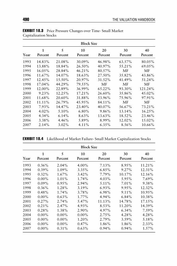
E1C18 08/25/2009 Page 490

EXHIBIT 18.3 Price Pressure Changes over Time- Small MarketCapitalization Stocks

Block Size

Year

1

Percent

5

Percent

10

Percent

20

Percent

30

Percent

40

Percent

1993 14.83% 21.08% 30.09% 46.98% 63.57% 80.05%1994 13.88% 18.84% 26.50% 40.97% 55.21% 69.05%1995 16.05% 28.84% 46.21% 80.57% MF MF1996 11.67% 14.07% 18.63% 27.50% 35.82% 43.86%1997 12.45% 15.50% 20.97% 31.52% 41.49% 51.24%1998 17.04% 44.29% 79.55% MF MF MF1999 12.00% 22.89% 36.99% 65.22% 93.30% 121.24%2000 9.23% 12.25% 17.21% 26.60% 35.86% 45.02%2001 11.68% 20.60% 31.88% 53.96% 75.96% 97.91%2002 11.11% 26.79% 45.95% 84.11% MF MF2003 7.93% 14.47% 23.40% 40.07% 56.67% 73.21%2004 4.02% 5.10% 6.80% 9.86% 13.14% 16.25%2005 4.34% 6.14% 8.63% 13.63% 18.52% 23.46%2006 3.38% 4.46% 5.89% 8.99% 12.02% 15.02%2007 2.14% 3.02% 4.11% 6.35% 8.56% 10.66%

EXHIBIT 18.4 Likelihood of Market Failure- Small Market Capitalization Stocks

Block Size

Year1

Percent5

Percent10

Percent20

Percent30

Percent40

Percent

1993 0.36% 2.04% 4.00% 7.13% 8.95% 11.21%1994 0.39% 1.09% 3.35% 6.85% 9.27% 12.31%1995 0.32% 1.67% 3.42% 7.79% 10.17% 12.16%1996 0.00% 1.01% 1.74% 4.03% 5.95% 7.69%1997 0.09% 0.95% 2.94% 5.11% 7.01% 9.38%1998 0.36% 1.28% 3.19% 6.93% 9.95% 12.32%1999 0.48% 1.74% 3.78% 6.98% 9.11% 10.95%2000 0.00% 0.63% 1.77% 4.94% 6.84% 10.38%2001 0.27% 2.74% 5.47% 11.13% 14.78% 17.15%2002 0.21% 2.47% 4.93% 8.53% 11.20% 14.39%2003 0.28% 1.38% 2.90% 4.97% 6.34% 7.59%2004 0.00% 0.00% 0.00% 2.75% 4.28% 4.28%2005 0.00% 0.00% 1.20% 2.79% 3.59% 5.18%2006 0.00% 0.00% 0.47% 1.86% 1.86% 2.33%2007 0.00% 0.31% 0.63% 0.94% 0.94% 1.57%


E1C18 08/25/2009 Page 491

stock. That is, the current volume of stock traded represents the totalmatched demand and supply at the prevailing price. Market makers postbid (price available to the seller) and ask (price payable by the buyer) quotesfor small trading lots and revise these quotes frequently, and without cost,in response to changes in demand (buy orders) and supply (sell orders) ofthe stock. An examination of the trade and quote data from NYSE showsthat while the bid-ask spread for single-lot quotes (100 shares) is usuallysmall, it increases rapidly for larger blocks and is very sensitive to changesin trading volume. As additional supply enters the market, it increases thevolume that needs to be traded and the price decreases to stimulate demand.Conversely, if additional demand enters the marketplace, increasing the vol-ume that needs to be traded, the price increases to stimulate supply. There isconsiderable empirical evidence that large block trades tend to occur out-side the posted bid-ask spread.

Using a variety of liquidity measures, finance researchers have demon-strated that generally less liquid stocks have higher average returns (lowerprices). Amihud and Mendelson (1986), Constantinides (1986), Heaton andLucas (1996), Vayanos (1998), and Lo, Mamaysky, and Wang (2001),among others, explore the relationship between liquidity and asset prices andshow that significant price discounts exist for less liquid but otherwise com-parable assets. While liquidity has many facets, existing measures of liquiditytypically focus on one dimension of liquidity. For example, the bid-askspread measure used in Amihud and Mendelson (1986) relates to the tradingcost dimension; the turnover measure of Datar, Naik, and Radcliffe (1998)captures the trading quantity dimension; and Amihud (2002) and Pastor andStambaugh (2003) construct their measures based on the concept of price im-pact to capture the price reaction to trading volume. Abbott (2006) extendsthis research to develop a continuous time model for measuring liquidity.This approach provides a measure of liquidity that is based on two observ-able variables—the quantity of outstanding stock and the observed tradingvolume at the current quoted bid-ask spread. This measure allows us todirectly estimate the liquidation period for a specific block of stock that isspecific to the asset class, size, and prevailing market conditions.

There is a general consensus regarding the positive relationship betweenliquidity and observed asset prices, but the precise measurement of liquidityand, by extension, measurement of an appropriate discount for lack ofliquidity have posed a problem for valuation practitioners.

Any analysis of liquidity and its impact on the asset needs to considercurrent conditions surrounding the asset. An alternative mechanism fordetermining the expected liquidation period is proposed in Abbott (2006).Follwing, the proposed direct measure of liquidity is defined.


E1C18 08/25/2009 Page 492

MEASUR ING ASSET L I QU I D I TY

Given:

The stock holding at time t is St.

Volume for one time period time t is Vt.

The stock holding at time t þ 1 is Stþ1 = St � Vt.

Assuming that the rate of deal flow is constant l

at time t

Stþ1 ¼ Ste�l

Or lLogn Stð Þ � Logn St þ 1ð Þl is a measure of the observed level of liquidity, with higher levels signifyingthat the current order flow in the market can absorb larger volumes of trad-ing without impacting prices. An additional advantage of this specificationof l is that the expected half-life or average holding period can be calcu-lated directly by dividing the value of lognormal (2) by the calculated valueof l. If 50 percent of the stock changes hands over a period n,

Logn Stð Þ � Logn Stþnð Þ is Logn St=0:5 Stð Þ ¼ Logn (2)

The observed liquidity levels for different market value deciles are sig-nificantly different from each other and vary across time, indicating that thelevel of liquidity and consequently the time to liquidation are variable andshould be estimated for the period of analysis. Using a sample of 715,785firm-month observations spanning all listed securities for the three equitymarkets (NYSE, AMEX, and NASDAQ) for January 1993 to December2007, we find that the observed average holding period (half-life) for listedsecurities is much longer than the standard of instantaneous liquidity as-sumed in existing literature. Market-level liquidity varies over time, and theaverage holding period for individual stocks is significantly influenced bythe size of the firm, the level of holding period returns, and the systematicliquidity of the markets. It has been suggested by Chordia, Roll, and Sub-rahmanyam (2000) that market index moves are accompanied by corre-sponding changes in market liquidity.

Prior finance literature suggests that larger firms tend to be more liquidas a result of enhanced analyst following and institutional portfolio invest-ment. A similar market capitalization effect appears to be significant inexplaining the observed liquidity for listed firms. The average holding pe-riod appears to decrease as market capitalization increases. Each month thefirms in the sample are partitioned into 10 equal (decile) groups, ranked bythe size of market capitalization. Mean, median minimum, and maximum


E1C18 08/25/2009 Page 493

holding periods are calculated for each of the decile portfolios. Summaryannual results for the smallest and largest deciles are presented in Exhibit18.5 and 18.6. While each decile portfolio shows a wide dispersion from alow of less than one day to 20 years or beyond, the mean holding perioddecreases from a high of 47 months for smaller firms to 14 months for thelargest firms in 2005. Abbott’s (2006) results confirm this relationship. InExhibit 18.5 it is seen that market liquidity increased and the holding period

EXHIBIT 18.5 Observed Half Life (Average Holding period) in Months- SmallMarket Capitalization Stocks

Year N Minimum Maximum Mean Median t Pr > jtj1993 8240 0.106626 27039.32 146.0706 28.72826 19.31 <.0001

1994 9091 0.15011 23559.73 135.8086 24.63378 18.64 <.0001

1995 9381 0.143805 23746.88 98.47306 20.57023 18.84 <.0001

1996 9857 0.138335 14347.8 81.9523 17.6965 19.43 <.0001

1997 10258 0.113984 19754.35 67.58244 14.64149 15.76 <.0001

1998 10014 0.119041 11117.73 45.75571 12.90686 16.86 <.0001

1999 9229 0.124116 45587.94 54.11297 14.30336 8.65 <.0001

2000 8574 0.109128 7624.27 49.17992 14.0678 17.89 <.0001

2001 7011 0.146613 14472.57 94.74068 28.28889 18.65 <.0001

2002 6701 0.161453 13301.15 89.23909 31.83736 21.27 <.0001

2003 6128 0.15791 34518.38 83.63157 26.45441 11.95 <.0001

2004 5724 0.128788 6407.8 52.11892 19.31529 21.61 <.0001

2005 5374 0.13232 8078.28 46.74653 18.60425 20.54 <.0001

EXHIBIT 18.6 Observed Half Life (Average Holding period) in Months- LargeMarket Capitalization Stocks

Year N Minimum Maximum Mean Median t Pr > jtj1993 8645 0.277218 100134 38.36299 13.66489 3.29 0.001

1994 9498 0.197619 75479.22 51.45356 13.07885 4.89 <.0001

1995 9669 0.169446 15095.57 35.17457 11.98269 12.37 <.0001

1996 10187 0.140644 8247.97 30.85015 11.17565 15.92 <.0001

1997 10527 0.175407 3323.83 21.88812 10.36773 24.18 <.0001

1998 10158 0.195504 462097.8 67.84834 9.585681 1.49 0.136

1999 9269 0.132759 74999.48 34.85971 8.190064 4.16 <.0001

2000 8360 0.1055 8119.22 24.13534 5.902787 11.15 <.0001

2001 7641 0.101258 10146.86 17.45331 5.805328 10.74 <.0001

2002 7771 0.087806 3478.91 14.3471 5.666866 16.15 <.0001

2003 7125 0.151554 1264.35 14.035 5.93147 21.09 <.0001

2004 6830 0.13616 3162.24 16.00685 6.370044 14.65 <.0001

2005 6720 0.138856 3450.34 14.06328 5.851912 12.79 <.0001


E1C18 08/25/2009 Page 494

decreased during the monetary expansion from 1994 to 2000, and there-after market liquidity sharply declined in 2001 in response to market condi-tions, recovering somewhat in 2004.

Penny stocks have been anecdotally linked with low liquidity. The re-sults show that there is a significant difference between observed liquidityfor the stocks priced at less than $1 per share (penny stocks, not eligible forcontinued listing), priced between $1 and $5 per share (small-cap market),and shares priced at $5 or above (see Exhibit 18.7).

These results are in line with the prior studies of liquidity behavior forstocks. The next step is to estimate a predictive equation for calculating theaverage holding period faced by the holders of a publicly traded stock.Using a standard multivariate ordinary least squares procedure, the coeffi-cients for the hypothesized variables are tested for significance. Economictheory suggests that the individual security liquidity is a function of the sys-tematic liquidity and security-specific attributes.

Prior literature suggests the following security attributes as significantfactors:

EXHIBIT 18.7 Observed Half Life (Average Holding period) in Months—PennyStocks

Price per Share N Min Max Mean

Less than $1 27,033 0.064274 551.0211 32.11198Price between $1 and $5 164,337 0.05721 552.1212 27.09066Price greater than $5 524,415 0.057029 562.1384 21.94253


E1C18 08/25/2009 Page 495

& Market liquidity: equally weighted average of holding period for allsecurities in the sample during the estimation month.

& Stock returns, excluding dividends: proxy for expected growth in value.& Dividend distributions: proxy for cash distributions received.& Market capitalization: proxy for relative size.& Stock price per share: proxy for continued listing ability.

The regression results show that all of the hypothesized variables arehighly significant, and the regression equation is also significant in explain-ing the observed holding period.

The estimation equation for the average holding period in months for asecurity is given by:

Estimated half-life ¼ 3:67 þ 0:95 � Market average holding period � 6:42

� Returns excluding dividends (%) þ 202:23

� Dividend returns (%) � 0:00000121

� Market capitalization ($’000) � 0:10

� Price per share ($)

The expected holding period for individual stocks rises and falls with theobserved average market (systematic) levels, and decreases as the stock priceand size of the firm increase and as the firm provides higher returns. How-ever, as the level of dividends paid by the firm increases, willingness to holdthe firm stock for longer periods rises sharply. (See Exhibits 18.6 and 18.7.)

These results provide an interesting insight for valuation practitioners.Markets appear to be relatively illiquid, especially for smaller firms,

and the prior assumption of costless unlimited trading does not appear tohold even for relatively large firms. These results suggest that applying abenchmark discount for lack of liquidity based on restricted stock studiesassuming a holding period of 12 or even 24 months for stocks in smallfirms may be a serious underestimation of the true discount for lack ofliquidity applicable for smaller illiquid firms with much longer holdingperiods. In the next section we present an introduction to three empiri-cally sound option based methods for determining the applicable discountfor lack of liquidity.

APPL I CAT I ON OF T IME /VOLAT I L I TY (OPT I ON )MODE LS TO D I SCOUNT FOR LACK OF L I QU I D I TY

Business valuation profession is moving toward a consensus that develop-ment and application of empirically rigorous methods for determining and


E1C18 08/25/2009 Page 496

defending discounts and premiums is warranted. Increased availability ofaffordable good-quality public markets data has contributed to this movetoward empirical analysis. Time/volatility models use options theory toestimate the appropriate discounts for lack of liquidity, are conceptuallyeasy to understand, and are relatively simple computationally. The param-eters are directly observable from market data, making them easy to de-fend. This following section presents three major put option models andillustrates their applications for estimating appropriate discounts for lackof liquidity.

The ‘‘gold standard’’ for liquidity is cash in hand. When the holder ofan illiquid asset wants to exchange the asset for cash in hand, the intend-ing buyer offers a cash price and by implication an option to liquidate theasset. The price of this option is the difference between the seller’s askingprice for the asset as if liquid and the buyer’s offered price recognizing therelative illiquidity of the asset. The buyer assesses the potential illiquidity ofthe asset and seeks compensation for the potential discount that may haveto be offered if and when the buyer in turn needs to liquidate the asset.

It is important to identify the two components of the price risk facedby the buyer due to the lack of liquidity. If the price of the asset goesdown during the period of illiquidity and the realized price is lower thanthe price at which the asset was purchased, there is a realized loss. This isthe first component, and is well understood (Loss I). Potentially, a secondand much larger component of the price risk is the opportunity loss thatoccurs when the asset increases in price during the period of illiquidity,and then declines to a lower value by the time the asset can be liquidated(Loss II). Thousands of dot-com paper millionaires faced the tax night-mare when they had to treat the value of restricted securities granted dur-ing the year as taxable compensation based on the post-IPO pricesreached. Subsequently, as the bubble burst, the stocks become worthlessand these grantees ended up with tax liabilities on the phantom gains thatwere never realizable by them.

Valuing the option to liquidate the asset is an important and interestingissue for valuation practitioners. Option-based models are being increas-ingly employed by practitioners to measure the price risk associated withlack of liquidity. The value of an option premium, estimating the cost ofliquidity, is frequently presented as the discount for lack of liquidity.Neglecting to convert from the option premium to the applicable discountmay create the illusion that the estimated discounts are greater than 100percent, an impossible solution. Stockdale (2008) makes an importantpoint: ‘‘Models providing results that equal or exceed 100 percent mayhave a theoretical problem because it seems logical that a discount wouldnot reduce a value to zero or less.’’ It appears that this conclusion may have


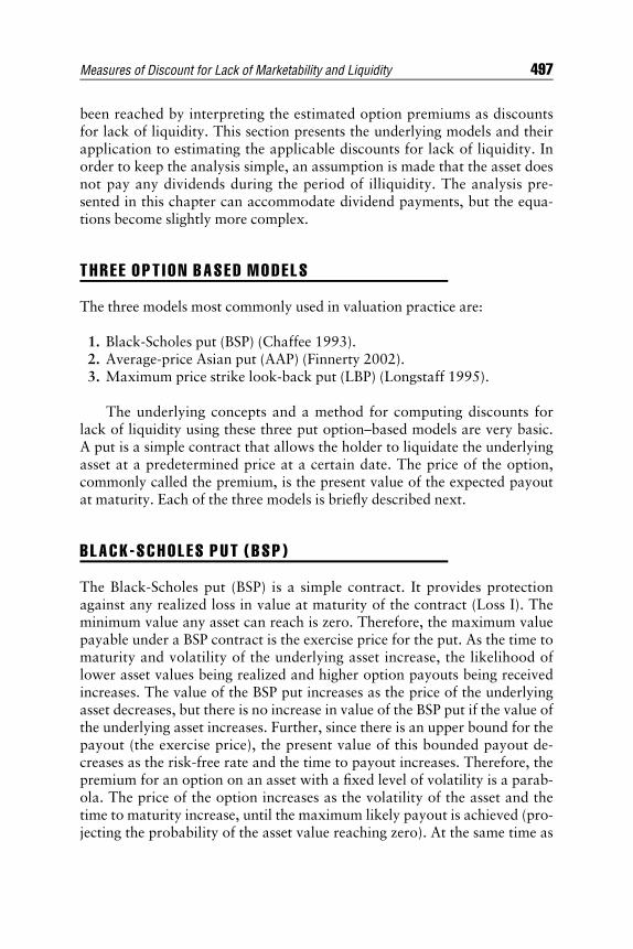
E1C18 08/25/2009 Page 497

been reached by interpreting the estimated option premiums as discountsfor lack of liquidity. This section presents the underlying models and theirapplication to estimating the applicable discounts for lack of liquidity. Inorder to keep the analysis simple, an assumption is made that the asset doesnot pay any dividends during the period of illiquidity. The analysis pre-sented in this chapter can accommodate dividend payments, but the equa-tions become slightly more complex.

THRE E OPT I ON BASED MODELS

The three models most commonly used in valuation practice are:

1. Black-Scholes put (BSP) (Chaffee 1993).2. Average-price Asian put (AAP) (Finnerty 2002).3. Maximum price strike look-back put (LBP) (Longstaff 1995).

The underlying concepts and a method for computing discounts forlack of liquidity using these three put option–based models are very basic.A put is a simple contract that allows the holder to liquidate the underlyingasset at a predetermined price at a certain date. The price of the option,commonly called the premium, is the present value of the expected payoutat maturity. Each of the three models is briefly described next.

BLACK -SCHOL ES PUT (BSP )

The Black-Scholes put (BSP) is a simple contract. It provides protectionagainst any realized loss in value at maturity of the contract (Loss I). Theminimum value any asset can reach is zero. Therefore, the maximum valuepayable under a BSP contract is the exercise price for the put. As the time tomaturity and volatility of the underlying asset increase, the likelihood oflower asset values being realized and higher option payouts being receivedincreases. The value of the BSP put increases as the price of the underlyingasset decreases, but there is no increase in value of the BSP put if the value ofthe underlying asset increases. Further, since there is an upper bound for thepayout (the exercise price), the present value of this bounded payout de-creases as the risk-free rate and the time to payout increases. Therefore, thepremium for an option on an asset with a fixed level of volatility is a parab-ola. The price of the option increases as the volatility of the asset and thetime to maturity increase, until the maximum likely payout is achieved (pro-jecting the probability of the asset value reaching zero). At the same time as


E1C18 08/25/2009 Page 498

the time to maturity and the risk-free rate increase, the present value of thispayout starts declining. BSP provides protection against a decline in value ofthe asset as compared to the current price, but does not address the oppor-tunity cost of not being able to liquidate the asset at the intermediate highprice reached but not realized (Loss II).

The underlying equation for the price of a BSP put option is:

P(S;T) ¼ K e�rT N �d2ð Þ � S N �d1ð Þ

where S¼ the current asset priceK¼ the exercise priceT¼ the time to maturity (for our purpose, time to

liquidation)r¼ the risk-free ratee¼ the natural constant, approximately 2.71828s¼ the standard deviation for the returns com-

puted for the samed1 ¼ lognormal(S=K) þ rþ s2=2

� �T

� �=s

ffiffiffiffiT

pd2 ¼ d1 � s

ffiffiffiffiT

pN(�d1) and N(�d2) ¼ the normal cumulative distribution

probabilities

Setting the exercise price K to be the same as the current asset price Sand assuming S ¼ K ¼ 1, we can compute the option premium as a fractionof the current asset price.

The BSP put option premium equation collapses to

P(T) ¼ e�rT N �d2ð Þ �N �d1ð Þ

where d1 ¼ rþ s2=2� �

T� �

=sffiffiffiffiT

pd2 ¼ d1 � s

ffiffiffiffiT

p

Thus an asset selling for a price of 1, if liquid would sell for 1 þ P(T). Theestimated BSP discount for lack of liquidity then becomes P(T)/[1 þ P(T)].

AVERAGE PR I C E AS I AN PUT (AAP )

The Finnerty model is an application of the average-price Asian put (AAP).This contract provides a payout based on the average price achieved for theasset during the life of the option. The price of the option increases as thevolatility of the underlying asset and the time to maturity increase. Initially,the value of an AAP is lower than the corresponding BSP, as the payout is


E1C18 08/25/2009 Page 499

based on the average of gains and losses. It increases slowly with volatility, asthe likelihood of achieving lower values and higher values is symmetric. Oncethe lower bound for negative returns (�100 percent) is reached, the entireincrease in value comes from the potential increase in the value of the under-lying asset. For larger values of the asset volatility and the time to maturity,the potential increase in value of the underlying asset dominates the growthin value. An Asian put option provides partial coverage of the opportunitycost for not being able to liquidate it at the higher prices reached during thelife of the option by averaging it with the potential losses.

The equation for an Asian put premium for a non-dividend-paying assetis:

D(T) ¼ V ert N r=yffiffiffiffiT

pþ y

ffiffiffiffiT

p=2

� ��N r=y

ffiffiffiffiT

p� y

ffiffiffiffiT

p=2

� �h i

and

y2 ¼ s2 T þ Ln 2 es2T � s2 T � 1� �� 2 Ln es2T � 1

� �

Once again setting V to 1, D(T) becomes:

ert N r=yffiffiffiffiT

pþ y

ffiffiffiffiffiffiffiffiffiT=2

p� ��N r=y

ffiffiffiffiT

p� y

ffiffiffiffiffiffiffiffiffiT=2

p� �

and the corresponding discount for lack of liquidity becomes:

D(T)=1 þD(T)

LOOK BACK PUT ( LBP )

The Longstaff model is an application of the look-back put (LBP), a contractthat pays out based on the highest value for the underlying asset achievedover the lifetime of the option. The price of the option increases as the vola-tility of the underlying asset and the time to maturity increase. An LBP optionaddresses the risk of loss in value of the asset as well as providing full cover-age of the opportunity cost for not being able to liquidate at the highest pricereached during the life of the option. From the perspective of a buyer of anasset, the price risk is the value given up by buying an asset that cannot beliquidated over a defined period of time. An LBP is the ultimate no-regretcontract, as it fully compensates the buyer for the inability to sell during theperiod of the contract protecting against a realized loss in value, as well asthe opportunity cost of not being able to sell at the intermediate high pricereached (Loss I þ Loss II). This property makes it highly desirable for thebuyer to demand a discount that fully compensates for the lack of liquidity.


E1C18 08/25/2009 Page 500

The simplified estimation equation for an LBP involves only twoparameters: T, the time to liquidation, and s, the standard deviation ofreturns. The equation defines the potential maximum value reached duringthe period to liquidation as:

V 2 þ s2T=2ð ÞNffiffiffiffiffiffis2

pT=2

� �þ V

ffiffiffiffiffiffiffiffiffiffiffiffiffiffiffiffiffiffiffiffiffiffiffiffiffiffiffiffiffiffiffiffiffiffiffiffiffiffiffiffiffiffiffiffiffiffiffiffis2T=2

Y� �e(�s2T=8)

r

where V¼ the current value of the assetT¼ the time to liquidations2 ¼ the variance of returns on the asset

N(�) ¼ the cumulative normal distribution

The LBP put option premium becomes:

F(V;T) ¼ V 2 þ s2T=2ð ÞNffiffiffiffiffiffis2

pT=2

� �þ V

ffiffiffiffiffiffiffiffiffiffiffiffiffiffiffiffiffiffiffiffiffiffiffiffiffiffiffiffiffiffiffiffiffiffiffiffiffiffiffiffiffiffiffiffiffiffiffiffis2T=2

Y� �e(�s2T=8)

r� V

Again, since we are interested in computing a proportional discount forlack of liquidity, we can set V to 1, the LBP option premium becomes:

F(T) ¼ 2 þ s2T=2ð ÞNffiffiffiffiffiffis2

pT=2

� �þ

ffiffiffiffiffiffiffiffiffiffiffiffiffiffiffiffiffiffiffiffiffiffiffiffiffiffiffiffiffiffiffiffiffiffiffiffiffiffiffiffiffiffiffiffiffiffiffiffiffiffiffiffiffiffiffiffis2T=2

Y� �e(�s2T=8) � 1

r

The corresponding LBP discount for lack of liquidity becomes:

F(T) ¼ (2 þ s2T=2)Nffiffiffiffiffiffis2

pT=2

� �þ

ffiffiffiffiffiffiffiffiffiffiffiffiffiffiffiffiffiffiffiffiffiffiffiffiffiffiffiffiffiffiffiffiffiffiffiffiffiffiffiffiffiffiffiffiffiffiffiffiffiffiffis2T=2

Y� �e �s2T=8ð Þ

r

These theoretical models indicate that for low values of volatility, BSPdiscounts will dominate AAP discounts as the holder of an AAP contractshares in the lower as well as higher prices achieved during the period ofilliquidity. However, as volatility increases, AAP discounts will becomelarger than BSP discounts. LBP will dominate both AAP and BSP as theexercise price of the put is set to the highest value achieved during the pe-riod of illiquidity, compensating the holder for both Loss I and Loss II, de-fined earlier. In negotiated sales, BSP and AAP represent the discountoffered by the seller, and LBP represents the discount demanded by thebuyer. Seller-initiated transactions would likely occur at a price incorporat-ing the LBP discount, whereas buyer-initiated offers are likely to be made atprices incorporating the larger of the BSP or AAP discount. The negotiateddiscount is likely to be in between these bounds based on the relative moti-vation of the buyer and seller.

Estimated lack of liquidity discounts for a range of inputs using each ofthe three option based methods are presented in Exhibits 18.8 to 18.10. Acomparison of the three subsets, based on volatility, risk-free rates, and time


E1C18 08/25/2009 Page 501

EXHIBIT 18.8 Estimated DLOL for Low Volatility (Annual s 0.10–0.30), LowRisk-Free Rate (3%), Short Duration (1 Year)

Annual Standard Deviation BSP LBP AAP

0.10 2.56% 7.61% 4.00%0.11 2.92% 8.33% 4.19%0.12 3.27% 9.04% 4.38%0.13 3.63% 9.75% 4.58%0.14 3.98% 10.45% 4.77%0.15 4.33% 11.14% 4.97%0.16 4.68% 11.83% 5.17%0.17 5.03% 12.51% 5.37%0.18 5.38% 13.19% 5.56%0.19 5.72% 13.86% 5.76%0.20 6.07% 14.52% 5.96%0.21 6.41% 15.17% 6.16%0.22 6.74% 15.82% 6.35%0.23 7.08% 16.47% 6.55%0.24 7.41% 17.10% 6.75%0.25 7.74% 17.74% 6.94%0.26 8.07% 18.36% 7.14%0.27 8.40% 18.98% 7.33%0.28 8.72% 19.60% 7.52%0.29 9.04% 20.20% 7.71%0.30 9.36% 20.81% 7.90%

EXHIBIT 18.9 Estimated DLOL for Midrange Volatility (Annual s 0.40–0.60),Medium Risk-Free Rate (6%), Medium Duration (5 Years)

Standard Deviation BSP LBP AAP

0.40 15.72% 48.38% 33.79%0.41 16.18% 49.16% 34.22%0.42 16.64% 49.92% 34.64%0.43 17.09% 50.68% 35.06%0.44 17.53% 51.41% 35.46%0.45 17.97% 52.14% 35.86%0.46 18.40% 52.85% 36.25%0.47 18.83% 53.55% 36.63%0.48 19.25% 54.23% 37.00%0.49 19.66% 54.90% 37.36%0.50 20.07% 55.56% 37.70%0.51 20.47% 56.21% 38.04%0.52 20.87% 56.84% 38.37%0.53 21.26% 57.47% 38.69%

(Continued)


E1C18 08/25/2009 Page 502

period for illiquidity confirms our theoretical results for ranking of the esti-mated discounts. Exhibit 18.11 illustrates the mean calculated Look BackPut discounts for block sizes of five, ten, and twenty percent during theyears 1993–2005. The discounts track closely the prevailing levels of liquid-ity and volatility and illustrate the difference between the behavior of thelarge and small stocks.

EXHIBIT 18.9


0.54 21.64% 58.08% 39.00%0.55 22.02% 58.68% 39.30%0.56 22.39% 59.27% 39.58%0.57 22.76% 59.85% 39.86%0.58 23.12% 60.42% 40.13%0.59 23.47% 60.97% 40.39%0.60 23.82% 61.52% 40.64%

EXHIBIT 18.10 Estimated DLOL for High Volatility (Annual s 0.70–0.90), HighRisk-Free Rate (9%), Long Duration (10 Years)


0.70 19.56% 76.91% 59.57%0.71 19.81% 77.30% 59.57%0.72 20.07% 77.69% 59.58%0.73 20.31% 78.06% 59.59%0.74 20.55% 78.43% 59.59%0.75 20.79% 78.79% 59.60%0.76 21.02% 79.14% 59.60%0.77 21.24% 79.48% 59.60%0.78 21.46% 79.81% 59.61%0.79 21.68% 80.14% 59.61%0.80 21.89% 80.46% 59.61%0.81 22.09% 80.78% 59.62%0.82 22.29% 81.08% 59.62%0.83 22.49% 81.38% 59.62%0.84 22.68% 81.68% 59.62%0.85 22.86% 81.97% 59.62%0.86 23.04% 82.25% 59.63%0.87 23.22% 82.52% 59.63%0.88 23.39% 82.79% 59.63%0.89 23.56% 83.06% 59.63%0.90 23.72% 83.32% 59.63%

(Continued)


E1C18 08/25/2009 Page 503

Discount for Lack of Liquidity

0.00%

10.00%

20.00%

30.00%

40.00%

50.00%

60.00%

156

151

146

141

136

131

126

121

116

111

106

10196918681767166615651464136312621161161

Dis

cou

nt

Per

cen

tag

e

Total Sample 1993–2005

5% Block 10% Block 20% Block

Discount for Lack of Liquidity for Large Firms

0.00%

2.00%

4.00%

6.00%

8.00%

10.00%

12.00%

14.00%

16.00%

Time

Dis

cou

nt

Per

cen

tag

e

Large Firms 1993–2005

1993 1993 2003


EXHIBIT 18.11 Look Back Put Discounts for Lack of Liquidity Changes over Time


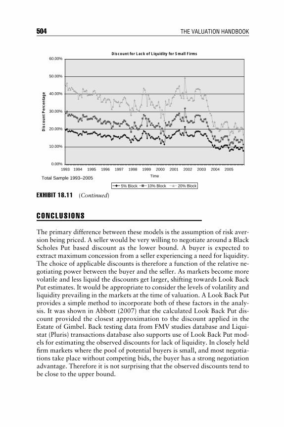
E1C18 08/25/2009 Page 504

CONCLUS I ONS

The primary difference between these models is the assumption of risk aver-sion being priced. A seller would be very willing to negotiate around a BlackScholes Put based discount as the lower bound. A buyer is expected toextract maximum concession from a seller experiencing a need for liquidity.The choice of applicable discounts is therefore a function of the relative ne-gotiating power between the buyer and the seller. As markets become morevolatile and less liquid the discounts get larger, shifting towards Look BackPut estimates. It would be appropriate to consider the levels of volatility andliquidity prevailing in the markets at the time of valuation. A Look Back Putprovides a simple method to incorporate both of these factors in the analy-sis. It was shown in Abbott (2007) that the calculated Look Back Put dis-count provided the closest approximation to the discount applied in theEstate of Gimbel. Back testing data from FMV studies database and Liqui-stat (Pluris) transactions database also supports use of Look Back Put mod-els for estimating the observed discounts for lack of liquidity. In closely heldfirm markets where the pool of potential buyers is small, and most negotia-tions take place without competing bids, the buyer has a strong negotiationadvantage. Therefore it is not surprising that the observed discounts tend tobe close to the upper bound.

Discount for Lack of Liquidity for Small Firms

0.00%

10.00%

20.00%

30.00%

40.00%

50.00%

60.00%

Dis

cou

nt

Per

cen

tag

e


Total Sample 1993–2005 Time

1993 1994 1995 1996 1997 1998 1999 2000 2001 2002 2003 2004 2005



E1C18 08/25/2009 Page 505

These option based models are conceptually sound, rely on observableempirical data, and are replicable. Therefore they meet the requirements ofscientific method for determining the applicable discounts for lack of liquid-ity. It is expected that their increasing usage will allow the valuation practi-tioners to have a greater degree of confidence in their discount estimates.

Lastly, these Look Back Put Option based models provide a theoreti-cally and empirically validated foundation for better economic understand-ing of the recent melt-down in markets induced by liquidity crises.

RE F ERENCES

Abbott, A. 2004. Estimating the holding period for listed securities. Valuation Strat-egies 8 (September–October).

Abbott, A. 2006. Role of liquidity in asset pricing. Conference Proceedings CAFI.December 2006, Hyderabad, India.

Abbott, A. 2007. A quantitative measure of discount for lack of liquidity. BusinessValuation Review, April 2007.

Amihud, Yakov. 2002. Illiquidity and stock returns. Journal of Financial Markets,5:31–56.

Amihud, Yakov, and Haim Mendelson. 1986. Asset pricing and the bid-ask spread.Journal of Financial Economics 17 (December): 223–249.

Amihud, Yakov, and Haim Mendelson. 1991. Liquidity, maturity, and the yields onU.S. Treasury securities. Journal of Finance 46, issue 4 (September): 1411–1425.

Bajaj, Mukesh, David J. Denis, Stephen P. Ferris, and Atulya Sarin. 2001. Firm valueand marketability discounts. (February 26). Available at SSRN: http://ssrn.com/abstract¼262198 or DOI: 10.2139/ssrn.262198.

Beneish, Messod D., and Robert E. Whaley. 1996. An anatomy of the ‘‘S&P Game’’:The effects of changing the rules. Journal of Finance 51, issue 5 (December):1909.

Beneish, Messod D., and Robert E. Whaley. 2002. S&P 500 index replacements.Journal of Portfolio Management 29, no. 1 (Fall): 51–60.

Chaffee, David B.H., II. 1993. Option pricing as a proxy for discount for lack ofmarketability in private company valuations. Business Valuation Review(December).

Chordia, Tarun, Richard Roll, and Avanidhar Subrahmanyam. 2000. Commonalityin liquidity. Journal of Financial Economics 56 (April): 3–28.

Constantinides, George M. 1986. Capital market equilibrium with transaction costs.Journal of Political Economy 94 (August): 842–862.

Datar, Vinay T., Narayan Y. Naik, and Robert Radcliffe. 1998. Liquidity and stockreturns: An alternative test. Journal of Financial Markets 1 (August): 203–219.

Edelman, Richard B., and H. Kent Baker. 1993. The impact of company pre-listingattributes on the market reaction to NYSE listings. Financial Review 28, no. 3(August): 431–448.


E1C18 08/25/2009 Page 506

Emory, John D. 2003. Business valuation discounts for lack of marketability indivorce. American Journal of Family Law 17, issue 3 (Fall).

Finnerty, John D. 2002. The impact of transfer restrictions on stock prices. Pre-sented at AFA 2003 Washington DC meetings, October 2002.

Garvey, Gerald T., and Todd T Milbourn. 2000. EVA versus earnings: Does it mat-ter which is more highly correlated with stock returns? Journal of AccountingResearch 38.

Harris, Lawrence, and Eitan Gurel. 1986. Price and volume effects associated withchanges in the S&P 500 list: New evidence for the existence of price pressures.Journal of Finance 41, issue 4 (September): 815.

Heaton, John, and Deborah J. Lucas. 1996. Evaluating the effects of incompletemarkets on risk sharing and asset pricing. Journal of Political Economy104 (June): 443–487.

Hertzel, Michael, and Richard L. Smith. 1993. Market discounts and shareholdergains for placing equity privately. Journal of Finance 48, issue 2 (June): 459.

Kadlec, Gregory B., and John J. McConnell. 1994. The effect of market segmenta-tion and illiquidity on asset prices: Evidence from exchange listings. Journal ofFinance 49, no. 2 (June): 611–636.

Kahl, Matthias, Jun Liu, and Francis A. Longstaff. 2003. Paper millionaires: howvaluable is stock to a stockholder who is restricted from selling it? Journal ofFinancial Economics 67, 385410.

Lo, Andrew W., Harry Mamaysky, and Jiang Wang. 2001. Asset prices and tradingvolume under fixed transactions costs. (May). EFA 2001 Barcelona meetings;Yale ICF Working Paper 00-35. Available at SSRN: http://ssrn.com/abstract=270733.

Loeb, Thomas F. 1983. Trading cost: The critical link between investment informa-tion and results. Financial Analysts Journal 39, issue 3 (May/June): 39.

Longstaff, Francis A. 1995. How much can marketability affect security values?Journal of Finance 50, issue 5 (December): 1767.

Lynch, Anthony W., and Richard R. Mendenhall. 1997. New evidence on stockprice effects associated with changes in the S&P 500 index. Journal of Business70, issue 3 (July): 351.

Macey, Jonathan, Maureen O’Hara, and David Pompilio. 2008. Down and out inthe stock market: The law and economics of the delisting process. Journal ofLaw and Economics 51, issue 4 (November): 68.

Mercer, Z. Christopher, and Travis W. Harms. 1997. Quantifying marketability dis-counts. Memphis, TN: Peabody Publishing LP.

Paleari, Stefano, and Silvio Vismara. 2007. Over-optimism when pricing IPOs. Man-agerial Finance 33(6): 352–367.

Pastor, L., and Robert F. Stambaugh. 2003. Liquidity risk and expected stock re-turns. Journal of Political Economy 111:642–685.

Pratt, Shannon P. 2001. Business valuation discounts and premiums. New York:John Wiley & Sons.

Pratt, Shannon P., and Alina V. Niculta. 2009. Valuing a business. New York:McGraw-Hill.


E1C18 08/25/2009 Page 507

Sanger, Gary C., and John J. McConnell. 1986. Stock exchange listings, firm value,and security market efficiency: The impact of NASDAQ. Journal of Financial &Quantitative Analysis 21, issue 1 (March): 1.

Shleifer, Andrei. 1986. Do demand curves for stocks slope down? Journal of Finance41, issue 3 (July): 579.

Silber, William L. 1991. Discounts on restricted stock: The impact of illiquidity onstock prices. Financial Analysts Journal 47, issue 4 (July/August): 60.

Stockdale, John J. 2006. Time is of the essence: A proposed model for computing thediscount for lack of marketability. Business Valuation Review (Fall).

Stockdale, John J. 2008. A test of DLOM computational models. Business ValuationReview (December).

Tabak, David. 2002. A CAPM-based approach to calculating illiquidity discounts.NERA working Paper 11, November 2002.

Vayanos, Dimitri. 1998. Transaction costs and asset prices: A dynamic equilibriummodel. Review of Financial Studies 11 (Spring): 1–58.

Wruck, Karen Hopper. 1989. Equity ownership concentration and firm value: Evi-dence from private equity financings. Journal of Financial Economics 23, issue1 (June): 3.


E1C19 08/25/2009 Page 508

CHAPTER 19An Economic View of the Impact

of Human Capital on FirmPerformance and Valuation

Mark C. UbelhartPractice Leader, Value-Based Management, and Architect,

Human Capital Foresight, Hewitt Associates

Everyone knows that human capital and intellectual property form thecore drivers of our global economic growth today. Consequently, how

best to measure these driver effects become paramount to shareholderwealth creation. This chapter explains the measurement of the movementof pivotal employees between firms and their effect on shareholder valuereturn.

In order to examine business valuation implications from a human cap-ital standpoint, cross-company, longitudinal data becomes essential. Whilemaking use of such data forms the empirical underpinnings of modern cor-porate finance, that usage is new to human resources (HR) as a function;consequently, it is unavailable to investors in general.

Of course, investors can obtain a glimpse of the highest-level pay prac-tices from proxy disclosures, but see virtually nothing below or beyondthose disclosures. Hewitt possesses an exceptionally rich database. Thatdatabase includes well over 1,000 companies and 20 million employees de-rived from compensation and benefit surveys. It also includes the out-sourced administration of many HR activities to Hewitt Associates as well.For our research, we gathered and used all the data possible, while carefullypreserving company confidentiality and individual privacy. Our intent mir-rored accomplishments using data and associated measurements in otherdisciplines like marketing and finance.

508

E1C19 08/25/2009 Page 509

CREAT ING AND STANDARD I Z I NG METR I CS

Once we de-identified individual data covering the 20 million employees bygiving them unique numbers, we discovered that some employees in onecompany one day arose in another company the next. In other words, theychanged jobs. We could observe the workings of a microcosm of the U.S.labor market, as employees transitioned between companies.

Knowing we now had the capability to measure the flow of employeesinto and out of organizations, our next step was to devise a metric—calledthe Talent QuotientTM (TQTM). TQ quantified these employee transitionsby measuring the relative proportion of employees leaving or joining thecompany who are pivotal employees. Simply put, pivotal employees pro-duce a disproportionate impact on the business. TQ reveals the propor-tional magnitude of pivotal employees leaving the organization who arecritical to the firm’s success.

The standardized definition of pivotal employees relies on incremen-tal investment measured by percentage pay progression, adjusted for age,pay, and tenure. This definition captures management decisions regard-ing individual employees in a systematic manner applicable to cross-company analysis and linkage to business performance and valuecreation. The top quartile percentage pay progressors are identified aspivotal. Consequently, a standard TQ score of 100 means 25 out ofevery 100 departing employees were considered pivotal—equal to thepercentage of total employees so defined within the company. A higherscore means fewer than 25 out of 100 departing employees were piv-otal—that is, a better retention rate for such critical employees—and thereverse, that a lower score means less retention of them. The TQ score iscompensation-dollar weighted so that a lower-paid departing person hasless impact in the calculation. It is not a head-counting turnover statisticbut a financial one.

Of course, one can take issue with the definition; for example:

& What if pay decisions are made poorly such that those so identified aspivotals really are not? The law of large numbers helps out, as somelevel of poor pay decisions or other anomalies characterize most com-panies, but with many companies and over time, an element of self-correction occurs. In some cases, we went back 10 years in applyingthis definition, and for all companies in our database we went back atleast five years.

& And even if these pay decisions are poorly made, what does it say abouta company where the people receiving the highest pay increases areleaving?

An Economic View of the Impact of Human Capital 509

E1C19 08/25/2009 Page 510

Certainly some companies may have separate internal lists of highpotentials and people with the highest performance ratings, but these listsare not available in cross-company data and are not consistently developed.Moreover, in our piloting process, clients encouraged us to rely on pay pro-gression rather than internal lists because they believed their own internallists were suspect.

PRED I CT ING FUTURE F I NANC IA L R ESULTS

With a measure of the flow of pivotal employees in and out of a company,testing its relationship to business value creation became possible. Well-per-forming companies are likely to retain more of their pivotal employees, andat the same time the retention of more pivotal employees is likely to contrib-ute to subsequent financial performance and value creation. We had to sep-arate these effects. We removed reverse casualty by handicapping companyperformance—that is, whether a company was performing well was takeninto account at the start of the time period analyzed, which used prior-period TQs together with subsequent performance. The process used is il-lustrated in Exhibit 19.1, and greater detail is available in the article

EXHIBIT 19.1 Linkage to Business Results and Cash Flow Return on Investment(CFROI)


E1C19 08/25/2009 Page 511

‘‘Optimizing Human Capital Investments for Superior Shareholder Re-turns’’ by Samir Raza (Valuation Issues, February 2006).

Most readers of this publication will be at least somewhat familiarwith cash flow return on investment (CFROI

11) and variations of it. Forthose less familiar, please refer to Rawley Thomas and Robert Atra’sChapter 11, ‘‘The LifeCycle Returns Valuation System.’’ Also, refer toBartley Madden’s book (Madden 1999) and his Chapter 3, ‘‘Applying aSystems Mind-Set to Stock Valuation.’’ We incorporated CFROI into theanalysis because of its measurement advantages—both over time and acrossindustry. CFROI’s conceptual validity as an economic return measure ofbusiness performance and the prevalence of its use by analysts and inventorsadd to its advantages.

Research suggests that stock price level links to CFROI level, whilestock price change correlates to the market’s expectations of CFROIchange.

Exhibits 19.2 and 19.3 summarize the results, namely that a 10-pointdifference in TQ predicts a 0.7 percent and 1.6 percent difference in CFROIfor standard industrial companies and financial services, respectively.

Exhibit 19.4 shows a more dramatic picture by comparing the bestto worst in TQ and their subsequent financial results on measures otherthan CFROI.

Two individual company case studies are represented in Exhibits 19.5and 19.6, to complement and reinforce the results found in the multicom-pany analysis.

EXHIBIT 19.2 What Is the Impact of Loss or Gain of Talent on Future BusinessPerformance?


E1C19 08/25/2009 Page 512

D i agnos t i c Benchmark i ng

A crucial characteristic of financial reporting is its standardization throughgenerally accepted accounting principles (GAAP). Credit Suisse HOLT andLifeCycle Returns go beyond conventional reporting to recast results so thatthey are much more reflective of economic cash flow performance and moreaccurate for comparison over time and company to company. No suchequivalent exists in the domain of human capital. This fact alone stifles ac-countability and reporting, and that, in turn, stifles HR’s use of data in adecision science framework, as there are no external anchors creating pres-sures on firms to more effectively manage their pivotal employees.

In fact, the development of TQ is a step in the direction of measuringand managing pivotal employees, as any company can report it in thestandardized manner used in our analysis. At the same time, any com-pany can compute its own customized TQ, using its own internally

EXHIBIT 19.4 TQ Impacts Business Results—Cross-Industry Study

Average2004TQ

Sales Growth 3Years Annualized(Ending 7/07)

Total Return 3years Annualized(Ending 7/07)

Price toBook (at7/07)

Worst10 inTQ

84 Median 5.8% 7.1% 1.8

Best10 inTQ

141 Median 8.0% 13.2% 2.9

EXHIBIT 19.3 Is There a Greater Talent Leverage in Industries That Are RelativelyMore Dependent on Human and Intellectual Capital?


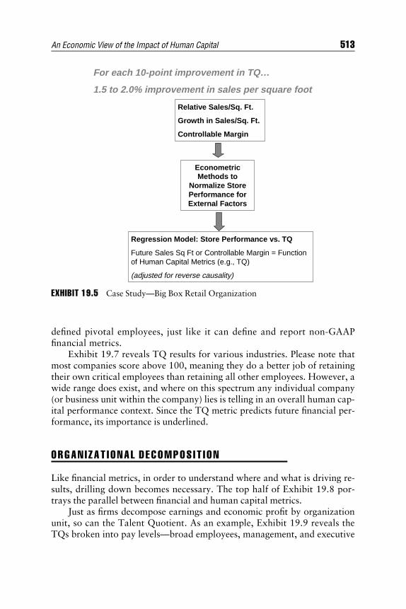
E1C19 08/25/2009 Page 513

defined pivotal employees, just like it can define and report non-GAAPfinancial metrics.

Exhibit 19.7 reveals TQ results for various industries. Please note thatmost companies score above 100, meaning they do a better job of retainingtheir own critical employees than retaining all other employees. However, awide range does exist, and where on this spectrum any individual company(or business unit within the company) lies is telling in an overall human cap-ital performance context. Since the TQ metric predicts future financial per-formance, its importance is underlined.

ORGAN I ZAT I ONAL DECOMPOS I T I ON

Like financial metrics, in order to understand where and what is driving re-sults, drilling down becomes necessary. The top half of Exhibit 19.8 por-trays the parallel between financial and human capital metrics.

Just as firms decompose earnings and economic profit by organizationunit, so can the Talent Quotient. As an example, Exhibit 19.9 reveals theTQs broken into pay levels—broad employees, management, and executive

Relative Sales/Sq. Ft.

Growth in Sales/Sq. Ft.

Controllable Margin

Econometric Methods to

Normalize Store Performance for External Factors

Regression Model: Store Performance vs. TQ

Future Sales Sq Ft or Controllable Margin = Function of Human Capital Metrics (e.g., TQ)

(adjusted for reverse causality)

For each 10-point improvement in TQ…

1.5 to 2.0% improvement in sales per square foot

EXHIBIT 19.5 Case Study—Big Box Retail Organization


E1C19 08/25/2009 Page 514

Clinical Trials—A Business Case for TQTo determine if the flow of talent matters for a particular pharmaceutical sales force, a detailed analysis was undertaken to measure the impact of TQ on sales performance across 22 sales units over four years. A two-step econometric model was developed to first capture the effect of past sales results on TQ, and then measure the impact of TQ on future sales performance. Not only arethe results consistent with the intuition of seasoned HR professionals, but for the first time, this landmark effort quantifies what was previously unmeasurable.

KEY FINDINGS

• TQ reliably predicts future sales performance. In other words, retainingcritical talent is a leading indicator ofhigher sales, and vice versa.

• A 10-point increase in TQ within this salesforce translates into approximately $40–$110 million per year in additional pretax operating income.

• Sales unit TQs were startlingly different,making a compelling business case tomanage TQ.

EXHIBIT 19.6 Case Study—Major Pharmaceutical Company

TQ retention values are typically over 100, but vary widely fromcompany to company

14013012011010090807060

Consumer Discretionary

Energy

Financials

Health Care

Industrials

Information Technology

TQ100

= Interquartile range: 25th–75th percentile= Median for industry

EXHIBIT 19.7 Industry TQ Retention Ranges


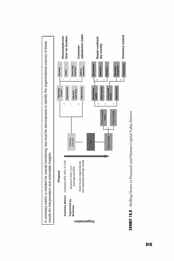
E1C19 08/25/2009 Page 515

Su

mm

ary

Met

rics

Com

pany

EP

S, R

OI,

or C

VA

Bus

ines

s U

nits

1,2

,3…

Ear

ning

s an

d R

OI

Dow

n to

any

org

aniz

atio

nal

unit

repo

rtin

g ea

rnin

gs r

esul

ts

Seg

men

ted

by

Bu

sin

ess

Organization

CV

A

Dep

reci

atio

n

Ad

just

edca

shta

xes

Ad

just

men

ts

Net

wo

rkin

gca

pit

al

Oth

eras

sets

Gro

ssfi

xed

asse

ts

Ad

just

men

ts

Rev

enu

e

CO

GS

Dir

ect

fiel

dex

pen

ses

Ind

irec

tex

pen

ses

Rec

eiva

ble

s

Inve

nto

ry

Pay

able

s

Mo

veab

leeq

uip

men

t

Fix

edas

sets

Gro

ssin

vest

edca

pita

l

Cos

tofc

apita

l

Cap

ital c

harg

e

Ope

ratin

gca

sh fl

ow

Rev

enu

e/p

erso

nh

ou

r o

n lo

cati

on

Cu

sto

mer

sati

sfac

tio

n in

dex

Rep

air

cost

/un

it(b

y m

on

th)

Inve

nto

ry c

on

tro

l

+ +–

– – – –

+ + +

+ +

Op

erat

ing

inco

me

Fin

ance

A s

umm

ary

met

ric is

nee

ded

for

over

all m

onito

ring,

but

mus

t be

deco

mpo

sed

to id

entif

y th

e or

gani

zatio

nal s

ourc

es o

f the

sere

sults

for

inte

rpre

tatio

n an

d ac

tiona

ble

insi

ghts

.

EXHIBIT19

.8D

rill

ing

Dow

nto

Fin

anci

aland

Hum

an

Capit

alV

alu

eD

river

s

515

E1C19 08/25/2009 Page 516

Value Drivers

Com

pany

TQ

and

TS

Bus

ines

s U

nits

1, 2

, 3…

TQ

and

TS

Dow

n to

any

gro

up o

f peo

ple

TQ

*

Co

mp

ensa

tio

n

Lea

der

ship

Ben

efit

s

Car

eer

Op

po

rtu

nit

ies

Org

aniz

atio

nD

esig

n

Rec

ruit

men

t

En

gag

emen

t

Per

form

ance

Man

agem

ent

Pay

atR

isk

Bo

nu

sP

ayo

ut

%T

arg

etN

orm

aliz

edA

ctu

alB

on

us

No

rmal

ized

Tar

get

Bo

nu

sC

om

pen

sati

on

/Rev

enu

e

Per

cen

tag

eo

f“S

ho

oti

ng

Sta

rs”

inP

ayB

and

s

Per

cep

tio

no

fR

eco

gn

itio

nan

dG

row

thO

pp

ort

un

itie

sG

ini-

Pay

Pro

gre

ssio

nG

ini-

Pay

Gin

i-B

on

us

Pay

ou

t%

Tar

get

Ben

efit

Ind

exB

enef

its

No

w/A

llB

enef

its

Per

cep

tio

no

fM

eeti

ng

Nee

ds

Per

cen

tag

eo

fH

igh

Pai

ds

Wit

hL

on

gS

ervi

ce

Per

cep

tio

no

fB

usi

nes

sA

cum

eno

fL

ead

ers

Rep

ort

ing

Rel

atio

nsh

ipH

iera

rch

y

Say

,Sta

y,an

dS

triv

e

Per

cen

tag

eo

f“S

ho

oti

ng

Sta

rs”

Am

on

gN

ewH

ires

Per

cep

tio

no

fQ

ual

ity

of

New

Hir

es

Per

cep

tio

ns

of

Pay

Per

cep

tio

no

fR

ewar

dfo

rE

ffo

rt

Par

ticul

ar d

river

s of

the

over

all r

esul

ts, e

spec

ially

thos

e th

at c

an b

e m

anag

ed, s

uch

as in

vent

ory

cont

rolin

the

finan

cial

dom

ain

and

perf

orm

ance

man

agem

ent i

n hu

man

cap

ital,

also

nee

d de

term

inat

ion.

Hu

man

Cap

ital

*And

pre

dict

ed T

Q b

ased

on

Tal

ent

Gua

rdia

n R

eten

tion

Ris

k S

core

s

EXHIBIT19

.8(C

ontinued

)

516

E1C19 08/25/2009 Page 517

groups. Here the particular company is assessed as being deficient in benchstrength, as it is disproportionately losing pivotal employees at the level justbelow executives.

Interestingly, analysts’ comments about this particular company raisethe same issue by conjecturing that it may not be able to grow organically—but only by acquisition—as it lacks internal management depth. Humancapital metrics can be decomposed in many ways, such as according to thedemographics of age, pay, tenure, location, ethnicity, and gender. They canalso be grouped in categories, such as those who participate in certain train-ing programs or other initiatives and those who do not.

Prescr i p t i v e I n s i g h t s

Once TQ is recognized as a linchpin metric that predicts future financialresults, stepping back to examine what drives TQ becomes not only possiblebut essential to decision making in the human capital arena. All of the di-mensions depicted in the octagon in Exhibit 19.8, and many more, can belinked to TQ using data available internally within a company or cross-company information where it exists.

The fundamental building block of such analysis is retention risk at theindividual level, as illustrated in Exhibit 19.10.

Each individual is assigned a score representing the risk of leaving theorganization within the next 12 months. These proprietary calculations uti-lize a neural network model continuously trained on:

TQ

TQ RETAIN

BROAD($50K–$125K)

MANAGEMENT($125K–$200K)

EXECUTIVE($200K+)

TOTAL($50K+)

120

110

90

100

80

100102

83

106

Example of Talent Quotient Retain by pay level, highlighting critical futureleadership gap for this company

TQ> 100RETAINING

PIVOTALEMPLOYEES

TQ< 100LOSINGPIVOTAL

EMPLOYEES

EXHIBIT 19.9 Organizational TQ Retention


E1C19 08/25/2009 Page 518

& Human capital data on the behavior of participants.& Employee demographics such as age, tenure, and gender.& Employee history, including pay progression and performance.& Company history of hiring and attrition.& National economic data such as housing statistics and price inflation or

deflation.& General labor market data such as regional unemployment.& Local market data such as household income and hiring trends.

This is precisely the methodology used to detect credit card fraud andstop transactions before they occur. It also utilizes concepts applied to de-velop FICO credit scores, which range from 0 to 800. In this case (as op-posed to FICO scores), a higher number means greater risk. Exhibit 19.11shows the probability that an individual employee with a particular reten-tion risk score will leave the company during the coming year.

Exhibit 19.12 employs the same individual scoring methodology toidentify prominent risk clusters of people and their characteristics. Such in-formation can inform talent management strategies to:

& Identify and target at-risk talent.& Target segments of risk for group interventions.& Discover retention performance differences across units.& Inform talent sourcing strategies.& Benchmark the company.

Jeff Singh

Anand Gupta

Carol Yu

Jim Smith

Employee

280

462

610

726

Retention Risk Score

Yes

No

Yes

Yes

Critical Talent

8002 1QerocS ksiR noitneteRIT Department: Terry Brown

HighestRisk

To help companies understand and manage their critical talent risk,the basic building block is the individual retention risk score.

Risk of leaving the organization in the next 12 months

Scores range from 0 to 800

EXHIBIT 19.10 Individual Retention Risk Score


E1C19 08/25/2009 Page 519

A Por t f o l i o V i ew

Mitigating risk is a good thing, but not if it costs too much. The cost ofintiatives aimed at improving retention rates can be compared to the result-ing improvement in TQ and its estimated financial benefit.

Exhibit 19.13 shows a portfolio view of retention risk incorporating thescoring methodology just described, applied to 75 companies in HewittAssociates’ database. It displays two different charts. The one on the leftsimply counts people, while the one on the right is compensation-dollarweighted and illustrates greater human capital risk. From the standpoints

EXHIBIT 19.11 Attrition Probabilities

Retention Risk ScoreProbability of Attrition(within 12 Months)

800 95%700 85%620 65%520 32%455 16%400 8%345 4%300 2%

“Builders”1% of population

1% of compensation investment

• Young, perhaps first job• Modest pay• Skewed toward Business Unit A• Tend to live in suburban-like

areas

“Hired Young Guns”3% of population


• Young, though likely not first job• High performing, relatively high pay• Tend to live in suburban-like areas

(educated, mid-to-high income, homeowners, married with children)

“Reaching for More”3% of population


• Average performers• Recently changed roles/

promoted, but with relatively small pay increase

• Tend to live in economically depressed areas

“Solid Opportunists”2.5% of population


• Average performing• Tend to move between roles• Have relatively high pay• Tend to live in suburban-like

areas

“Midcareer Misfires”3.5% of population


• Not first job• Low performers, slow pay

progression• Tend to live in low-income,

relatively uneducated areas

“Struggling Starters”2.5% of population


• Young, likely first job out of school

• Average to modest performers• Likely living in relatively

low-income areas

Most ConcernPivotal/Key Talent Concentration

Secondary Concern Modest Concern

RRS480

RRS500

RRS450

RRS470

RRS490

RRS460

EXHIBIT 19.12 Talent GuardianTM—Actual Client, Prominent Risk Clusters


E1C19 08/25/2009 Page 520

of both business valuation and the board of directors’ fiduciary responsibil-ity to manage the risk of pivotal employee loss, these retention assessmentsmatter to shareholders.

C l amor f or D i s c l o sure

No one denies the impact that human capital has on business valuation. De-spite its obvious importance, the absence of commonly accepted measure-ment and reporting standards creates a vacuum on the availability ofhuman capital metrics that matter. As mentioned previously, that same vac-uum inhibits a groundswell of external pressure from focusing its energy onchanging these conditions. A perfect storm is gathering and inevitable.Exhibit 19.14 represents just one indication.

In answer to the question posed during a live webcast by the HumanCapital Institute, 76 percent of the respondents stated they believed stan-dardized human capital metrics are coming within five years.

Another indication occurred in May 2008 at the joint Credit Suisse/Hewitt Associates conference—the first-ever joint conference of investmentprofessionals and corporate managements focused on human capital and itsimpact on valuation.

The Impact of Human Capital on Investment CapitalTuesday Evening, May 13, 2008

Hewitt and HOLT: Examining human capital metrics thatdrive corporate performance

Please accept this invitation for this joint conference of HewittAssociates and Credit Suisse HOLT. This program offers new

Number of People

Low Risk57%

High Risk22%

In Between

21%

Investment in People

Low Risk47%

High Risk24%

In Between

29%

EXHIBIT 19.13 Retention Risk Complexion Benchmarks


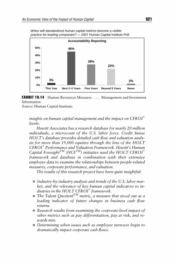
E1C19 08/25/2009 Page 521

insights on human capital management and the impact on CFROI1

levels.Hewitt Associates has a research database for nearly 20 million

individuals, a microcosm of the U.S. labor force. Credit SuisseHOLT’s database provides detailed cash flow and valuation analy-sis for more than 19,000 equities through the lens of the HOLTCFROI

1

Performance and Valuation Framework. Hewitt’s HumanCapital ForesightTM (HCFTM) initiative used the HOLT CFROI

1

framework and database in combination with their extensiveemployee data to examine the relationships between people-relatedmeasures, corporate performance, and valuation.

The results of this research project have been quite insightful:

& Industry-by-industry analysis and trends of the U.S. labor mar-ket, and the relevance of key human capital indicators to in-dustries in the HOLT CFROI

1

framework.& The Talent QuotientTM metric, a measure that stood out as a

leading indicator of future changes in business cash flowreturns.

& Research results from examining the corporate-level impact ofother metrics such as pay differentiation, pay at risk, and re-wards mix.

& Determining when issues such as employee turnover begin todramatically impact corporate cash flows.

When will standardized human capital metrics become a visiblepractice for leading companies? — 2007 Human Capital Institute Poll:

Accountability Reporting

28%

3% 2%

22%

45%

0%

10%

20%

30%

40%

50%

NeverBeyond 5 YearsFive YearsNext 2–3 YearsThis Year

EXHIBIT 19.14 Human Resources Measures . . . Management and InvestmentInformationSource: Human Capital Institute.


E1C19 08/25/2009 Page 522

& What companies are beginning to monitor internally, whatactions can they take as a result, and what investors may beginrequesting from management teams.

This program provides insights from two perspectives: Fromthe point of view of the investor analyzing company fundamentalswith an eye on stock price and from the planning and actions ofmanagement looking to improve business performance andvaluation.

The goal of business strategy is clear—to invest capital in a waythat maximizes shareholder value. Traditional capital budgetingand financial planning frameworks offer very little to guide humancapital investment decisions; yet pay and benefits typically consti-tute 30% to 70% of operating expenses. Hewitt’s Human CapitalForesightTM offers factual analysis grounded in data representingmore than 20 million people—in effect, a microcosm of the U.S.labor market.

The research based on this data has yielded HR metrics andinsights quantitatively linked to business results.

Credit Suisse Conference Center, 11 Madison Avenue, Level2B, The Club Room, New York, NY 10010

There are two sides to this story. Certainly, investors are clamoring formore disclosure. They seek an enhanced ability to both understand andvalue the human capital risks and associated circumstances of companies inwhich they invest. At the same time, managements—particularly leading-edge human resources (HR) functions—seek to apply decision scienceframeworks to the vast amount of data now available. They know that HRdata will provide their firms with a competitive advantage and they wel-come the external pressure that will reinforce their efforts.

MATHEMAT I CAL MODE LS GU I D I NGPRACT I CAL ACT I ON

At the core of Talent GuardianTM is a mathematical model that predicts thelikelihood an individual employee will quit within a specified time. Hewittdesigned the rest of Talent Guardian to achieve the greatest practical benefitfrom this basic insight of quitting behavior.

Predicting individual human behavior with a computer represents a no-toriously difficult challenge. The Human Capital Foresight team at HewittAssociates and partner Global Analytics overcame this challenge by a


E1C19 08/25/2009 Page 523

flanking attack: Rather than write a program to mimic the complexity ofhuman decisions, the Talent Guardian team developed a program—a math-ematical model—that learns by example from exhaustive trial and error tobehave as humans actually do in millions of actual employment histories inHewitt databases and in histories from subscribing employers.

To capture the complexity of human actions, Global Analytics andHewitt constructed Talent Guardian models using a proprietary, evolvedneural network structure. This approach differs from more traditionalmodel structures like those used in regression models. The model-buildingprocess analyzes the impact of both individual variables and the many com-binations of variables interacting with one another thereby changing eachother’s impact on a final outcome. The resulting models recognize complexpatterns of behavior and their most probable outcomes.

By dealing directly with the complex relationships in employment deci-sions, these models avoid misleading, oversimplified, single-cause explana-tions for complex human outcomes. As a consequence, their predictiveperformance is superior. (Models for each client vary in technical perform-ance, but are usually in the high 20s to low 30s on the Komogorov-Smirnov—K-S—test statistic.) Exhibit 19.15, based on real-world examplesfor over 200,000 employees, shows that Talent Guardian retention riskscores accurately predict subsequent actual attrition.

EXHIBIT 19.15 Predicted Retention Risk Scores versus Subsequent Actual Attrition


E1C19 08/25/2009 Page 524

Talent Guardian not only locates attrition risk in employee popula-tions, it also differentiates between those risks due to employee character-istics and those due to employer actions or policies. It guides interventionby identifying high-risk groups with common characteristics and by accu-rately monitoring the retention impact of specific interventions and policyactions.

Talent Guardian avoids the guesswork on whether retention successesor problems are due to employee characteristics or to employer actions;whether a group’s retention problems are inherent or created; or whetherapparent patterns across similar employees are real or random.

Talent Guardian is the most sensitive way to identify retention risks. Itrepresents the best tool to help overcome those risks.

Global Analytics supplies Talent Guardian’s predictive analytics. Glob-al’s management includes the inventor of neural network fraud detectionfor bank payment systems and other pioneers in the application of advancedanalytics to financial services. One pioneering executive became most re-sponsible for the widespread adoption of consumer credit scores and theway financial services firms manage consumer credit accounts today. Learnmore about Global Analytics at www.global-analytics.com.

NOTE

1. CFROI1

is a registered trademark in the United States and other countries(excluding the United Kingdom) of Credit Suisse or its affiliates. Credit SuisseHOLT is a division of Credit Suisse. CFROI is adjusted for asset age/life/mix,and allows for comparisons across companies.

RE F ER ENCE

Madden, Bartley J. 1999. CFROI valuation: Cash flow return on investment—Atotal system approach to valuing the firm. Woburn, MA: Butterworth-Heinemann.


E1C20 08/14/2009 Page 525

CHAPTER 20EBITDA

Down but Not Out

Arjan J. BrouwerUniversity of Amsterdam and PricewaterhouseCoopers

Benton E. GupChair of Banking, University of Alabama

On June 12, 2008, Belgian-Brazilian InBev S.A. published the terms of itsinitial unsolicited bid for Anheuser-Busch Company of the United States.

InBev wanted to pay $47.5 billion, which ‘‘represents 12� Anheuser-Busch’s 2007 EBITDA.’’1 On July 14, 2008, Anheuser-Busch agreed to betaken over for $70 per share in cash. InBev presented the transaction valueas $62 billion and stated that the implied enterprise value/earnings beforeinterest, taxes, depreciation, and amortization (EV/EBITDA) multipleof 12.4 was in line with comparable transactions in the industry.2 InBevfinanced the transaction primarily with borrowed funds that will be repaidlargely from the divestiture of noncore assets from both companies and bytemporarily reducing cash dividends. The noncore assets include theAnheuser-Busch theme parks—Busch Gardens, SeaWorld, and others.3

This transaction is interesting from many perspectives. Not only doesthe combination of the two firms result in the world’s largest beer companyand the third largest consumer products company after Procter & Gambleand Nestl�e, but the transaction is one of the examples of the increasinginvolvement of other economies (Europe, Asia, Middle East) in the U.S.capital market. Companies from these countries bring their own governance,business, and valuation practices and reporting behavior into the U.S.market. Since 2007, the Securities and Exchange Commission (SEC) hasallowed foreign companies with a U.S. listing (foreign private issuers) to filetheir International Financial Reporting Standards (IFRS) financial statements

525

E1C20 08/14/2009 Page 526

without additional U.S. generally accepted accounting principles (GAAP) in-formation. This will also affect the financial analyst’s job to analyze financialinformation that is reported into the market. Except for the United States, allother major capital markets have already implemented IFRS (for exampleEurope and Australia) or are in the process of converting to IFRS (for exam-ple Japan and Canada), and the influence of IFRS on the U.S. capitalmarkets cannot be ignored. Even the SEC has started talking about whetherU.S. public companies should be granted the option of using the IFRS.

Differences in valuation and reporting behavior are also reflected in theInBev–Anheuser-Busch transaction where it appears that InBev placedsignificant weight on Anheuser-Busch’s EBITDA in the valuation of thecompany. EBITDA is a non-GAAP measure that lost significant ground inthe United States after the implementation of the Sarbanes-Oxley Act(SOX) and related SEC regulations, but is still popular in Europe, partlydriven by the fact that IFRS allows significant flexibility in the presentationof a company’s income statement. The EBITDA acronym was, for example,found 64 times in InBev’s 2007 financial statements, whereas it was notfound at all in the Anheuser-Busch 2007 10-K.

The EBITDA measure can serve many useful purposes, but if nothandled with care it also has the potential to lead the analyst to incorrectconclusions. Therefore, this paper discusses EBITDA, its benefits and short-comings, and developments in the use thereof in the three largest non-U.S.capital markets that have implemented IFRS: the United Kingdom, France,and Germany.

WHAT IS EB I TDA?

As mentioned, EBITDA4 is the acronym for earnings before interest, taxes,depreciation, and amortization. Some analysts consider EBITDA a measureof operating income. The logic behind this method is that the analystsdeducted interest expenses and taxes from a firm’s income because theywanted to use their own calculations to determine the costs. They also de-ducted depreciation and amortization because those do not reflect currentcash outlays. The operating income excluded the value of investment activi-ties such as investments in securities, including minority interests in othercompanies. More will be said about this exclusion in connection with theInBev–Anheuser-Busch merger.

Moody’s5 explains how EBITDA became popular in the mid-1980samong leveraged buyout sponsors and bankers to evaluate cash flow andcalculate multiples for companies in a near-bankruptcy state. The idea wasthat if large-scale capital expenditure programs would not be necessary in


E1C20 08/14/2009 Page 527

the foreseeable future, the noncash depreciation and amortization chargesshould be available to service debt. At that time EBITDA was thus mainlyused in the context of companies’ debt and interest (re)payment capacity.

During the dot-com bubble era of the mid-1990s to 2001,6 EBITDAbecame a widely used and widely abused measure of profitability andperformance. Multiples of EBITDA were used to calculate the enterprisevalue of companies. Some firms manipulated their financial data in order toinflate their revenues and EBITDAs. WorldCom, a large communicationscompany, capitalized many items that might have been expensed. By‘‘improperly manipulating WorldCom’s reported revenue, expenses, netincome, earnings before interest, taxes, depreciation and amortization(EBITDA), and earnings per share . . . [WorldCom] materially overstatedthe income it reported in its financial statements by at least $9 billion.’’7

The manipulation of its earnings contributed to its bankruptcy in July2002. The $103.9 billion bankruptcy was the largest in U.S. history.8

Vivendi Universal, S.A., a media and environmental services conglom-erate, is another example of the misuse of EBITDA. The Securities andExchange Commission (SEC) settled civil fraud action against Vivendi thatthe company ‘‘at the direction of its senior executives, made improperadjustments that raised Vivendi’s EBITDA by approximately $59 millionduring the second quarter of 2001 and by at least $10 million during thethird quarter of 2001. These adjustments were made so that Vivendi couldmeet ambitious earnings targets that it had communicated to the market.’’9

However, during the boom part of the dot-com era, Internet and tech-nology stocks soared. Many of the new initial public offerings (IPOs) werenot profitable, and were never going to make a profit. Companies, regula-tors, and investors found out that excessive emphasis on non-GAAPmeasures like EBITDA may not draw the complete picture that is necessaryto make well-substantiated investment decisions, also refer to the sectionEBITDA in financial reporting. This does not, however, mean that EBITDAis completely gone. As we will see later in this chapter, EBITDA as aperformance measure is still widely used in Europe. In addition, EBITDAis often used for valuation purposes, like in the InBev–Anheuser-Busch transaction.

WHO USES EB I TDA AND WHY?

EBITDA became a widely used profitability measure in the 1980s and 1990sbecause it is easy to understand and it is not complicated by differentmethods of depreciation and taxation. As part of its initial research intoperformance reporting, the Financial Accounting Standards Board (FASB)

EBITDA 527

E1C20 08/14/2009 Page 528

interviewed 56 analysts and other users, the results of which were reportedin 2002. According to the FASB, ‘‘most analysts interviewed focus primarilyon operating cash flow/free cash flow or operating earnings. EBITDA,EBIT, return on investment, and measures of leverage or liquidity and reve-nue growth or market share were among the key metrics.’’10

Also as a basis for the valuation of companies, EBITDA is often referredto as a relevant measure. Camblain (2008) presented the results of an Ernst& Young 2005 survey of 142 European brokers, 88 companies, and 15investment banks. The survey found that 55 percent of the respondentsused EBITDA valuation multiples. In their International Private Equity andVenture Capital Valuation Guidelines (AFIC, BVCA, and ECVA 2006), aninternational group of private/venture capital associations describe howEBIT- and EBITDA-based multiples are commonly used to estimate thevalue of an entity. They, however, also note that the particular multipleused should be appropriate for the business being valued, and they warnthat if EBITDA multiples are used without sufficient care, ‘‘the valuer mayfail to recognize that business decisions to spend heavily on fixed assets or togrow by acquisition . . . do have real costs associated with them whichshould be reflected in the value attributed to the business in question.’’ Thisindicates that EBITDA multiples are less appropriate for businesses wheresignificant investments are required to grow. In the PricewaterhouseCoop-ers Outlook (2007) PricewaterhouseCoopers used EBITDA multiples to de-scribe market values and valuation opportunities in the United States andstated that ‘‘The average middle market EBITDA multiple for the lasttwelve months, as of October 15, 2007, was 10.3�, up from 8.6� for thesame period in 2006.’’ The PwC data was provided by Thomson Reuters, acompany with employees in 19 countries that provides intelligent informa-tion for businesses and professionals.11 Its databases contain EBITDAmultiples and other data. The point here is that data about EBITDA isreadily available to analysts and investors worldwide.

The references just mentioned indicate that many consider EBITDA arelevant measure to assess a company’s performance and as a basis for thevaluation of a company. But why would an analyst or a valuator be inter-ested in this measure? Damodaran (2001, 317) states that EBITDA acquiredadherents among analysts because:

1. There are fewer firms with negative EBITDAs than negative earningsper share.

2. Differences in depreciation methods across firms will not affectEBITDA.

3. It is easy to compare the EBITDA multiples across firms with differentdegrees of financial leverage.


E1C20 08/14/2009 Page 529

Williams (2002), a strategist for Goldman Sachs, stated that analystscan use enterprise value (EV)/EBITDA or EV/sales for looking at a largenumber of companies ‘‘because these measures tend to be less distorted byaccounting differences than measures further down the P&L (profit andloss) statement. . . . We have found EV/sales and EV/EBITDA to be supe-rior to both P/E (price/earnings) and required cash flow measures.’’ He alsopoints out that the use of EBITDA ‘‘does not solve the problem of how tolook at differences in balance sheet measurements.’’

EBITDA multiples are thus still widely used since they allow com-parison between companies that use different depreciation methods orhave different degrees of financial leverage. When assessing management’sperformance, EBITDA also has the potential to exclude expenses that aremore or less outside the control of current management since depreciationand amortization often follow from capital expenditures made by priormanagement in the past, and interest expenses largely follow from financingdecisions made in the past as well. In addition, from a valuation perspective,the fact that EBITDA is positive more often than net profit is an advantagebecause application of a multiple to a negative amount will not result inmeaningful results. However, it ignores relevant costs that must be paid tocontinue doing business (interest, taxes) or to grow the business (capitalexpenditures), which brings us to some of the shortcomings of EBITDA.

Shor t com ings o f EB I TDA

Although EBITDA can be a useful measure to assess a company’s perform-ance, it has a number of shortcomings that should not be ignored whenusing it, including, but not limited to, the following:

& EBITDA represents debt-free firms, which is not the case for mostcompanies. EBITDA can be helpful for valuation purposes since it canbe used to estimate the enterprise value, which is less variable to acompany’s financing policy. In addition, it can be used to determine acompany’s ability to repay debt and interest when worst comes toworst. However, when assessing a company’s performance it ignores atrue cost that must be paid on a regular basis and will result in a cashoutflow.

& EBITDA also ignores tax payments, which profitable firms cannot, orcannot always, avoid. Again, EBITDA can be useful in a stress test toassess what room the company has to pay debt holders when resultsdecrease to a break-even point (and taxes are not likely to be paid), butit overestimates a company’s capacity to generate future cash flows forprofitable firms that generally have to pay their taxes.

EBITDA 529

E1C20 08/14/2009 Page 530

& It does not take into account firms with different capital investments,and the depreciation that comes with them. A capital-intensive andgrowing company may have large depreciation charges but will alsohave to incur large capital expenditures to continue as a going concernor grow the business as intended, and this cost cannot be ignored whenvaluing the company. A measure like free cash flow (operating cashflow less capital expenditures) seems more appropriate to estimate rele-vant future cash flows for these companies. On the contrary, companieswith higher depreciation and tax deductions will have smaller tax bur-dens and higher cash flows.

& EBITDA does not exclude all noncash items such as the allowancesfor bad debts and inventory write-downs as well as the impact of in-vestments in working capital. It is therefore questionable whether animperfect measure of cash flows would give more meaningful informa-tion to predict future cash flows than the current cash flow itself.

Warren Buffett told Berkshire Hathaway, Inc. shareholders in his 2002annual letter that:

Trumpeting EBITDA . . . is a particularly pernicious practice.Doing so implies that depreciation is not truly an expense, giventhat it is a ‘‘non-cash’’ charge. That’s nonsense. In truth, deprecia-tion is a particularly unattractive expense because the cash outlay itrepresents is paid up front, before the asset acquired has deliveredany benefits to the business. Imagine, if you will, that at the begin-ning of this year a company paid all of its employees for the nextten years of their service (in the way they would lay out cash for afixed asset to be useful for ten years). In the following nine years,compensation would be a ‘‘non-cash’’ expense—a reduction of aprepaid compensation asset established this year. Would anyonecare to argue that the recording of the expense in years two throughten would be simply a bookkeeping formality?12

Another shortcoming of EBITDA is illustrated in the InBev–Anheuser-Busch transaction. As indicated before, InBev wanted to pay $47.5 billion,which ‘‘represents 12� Anheuser-Busch’s 2007 EBITDA.’’13 However,EBITDA excludes the value of investments in securities, including minorityinterests in other companies. This includes Anheuser-Busch’s income from its50 percent stake in Groupo Modelo SA, a Mexican beer company, and its 27percent stake in Tsingtao, a Chinese beer company.14 The 2007 Anheuser-Busch balance sheet revealed that investments in affiliated companies totaled$4.012 billion, or 23 percent of total assets. Income from affiliates where


E1C20 08/14/2009 Page 531

there is not sufficient ownership to consider them as subsidiaries is listed as‘‘equity income.’’ Equity income is not part of operating income that is thebasis of EBITDA. In 2007, equity income net of taxes was $662.4 million,about 23 percent of operating income.15 Anheuser-Busch noted that the eco-nomic benefit from Modelo also could be measured in terms of its fair mar-ket value of the investment over its cost. The excess was $8.7 billion.16 Thus,a valuation measure based on Anheuser-Busch’s operating income underval-ued the enterprise value because there is substantial equity income.

EB I TDA IN F INANC I A L REPORT ING

One of the objectives of general-purpose financial statements is to provideinformation about the performance of the entity. As stated by both theFinancial Accounting Standards Board (FASB) and the InternationalAccounting Standards Board (IASB), this information is primarily providedin the income statement. In the income statement, the company’s earningsand its components are reported; these numbers are frequently used as ameasure of performance or as the basis for other measures.

According to both the FASB’s Statements of Financial AccountingConcepts (CON) 2 and the IASB’s Framework for the Preparation andPresentation of Financial Statements, the information that is reported inthe financial statements should be relevant. Both consider informationrelevant when it assists users in their economic decision making by help-ing them evaluate past, present, or future events, or confirm or correcttheir past evaluations.

In this context and given that many analysts and valuators indicate theyfind EBITDA a helpful measure, one might conclude that to adhere to thesequalitative characteristics a company should disclose its EBITDA explicitly.A question that is difficult to answer, however, is: ‘‘Which came first, thechicken or the egg?’’ Did companies start reporting EBITDA because theusers of their financial statements asked for this as a relevant measure, ordid the users start looking at this measure because the companies could notstop talking about it?

Many have objected to the use of these so-called non-GAAP measures.The Securities and Exchange Commission (SEC) and the InternationalOrganization of Securities Commissions (IOSCO) are among them. At theend of the previous century and the start of this century, the SEC debatedthis subject in many comment letters that were sent to companies usingsuch measures.17 In May 2002, the IOSCO also cautioned issuers, investors,and other users of financial information to use care when presenting andinterpreting non-GAAP results measures.18

EBITDA 531

E1C20 08/14/2009 Page 532

Following the passage of the Sarbanes-Oxley Act of 2002, the SECadopted new rules concerning public companies’ disclosure of financial in-formation that is not based on GAAP.19 Because EBITDA is not anaccepted measure under GAAP, firms registering securities with the SEC arerequired to justify its use and to reconcile it to the most directly comparableGAAP financial measure, such as net income. For example, if EBITDA ispresented as a performance measure, it should be reconciled to net incomeas presented in the statement of operations under GAAP. ‘‘Operatingincome would not be considered the most directly comparable GAAP finan-cial measure because EBIT and EBITDA make adjustments for items thatare not included in operating income.’’20

The use and misuse of EBITDA in the United States declined sharply inthe post-dot-com era. As shown in the following list, many books that dealtwith valuation and were published in the United States after 2000 had littleor nothing to say about EBITDA valuation multiples.

Valuation Books Post-2000

Arzac, Enrique R., Valuation for Mergers, Buyouts, and Restructuring(Hoboken, NJ: John Wiley & Sons, 2005). EBITDA is notmentioned.

Damodaran, Aswath, The Dark Side of Valuation (Upper Saddle River,NJ: Prentice Hall, 2001). Offers favorable comments for compar-ing firms with different degrees of financial leverage. EBITDA’suses may be industry/sector specific. EBITDA valuation multiplesare discussed.

Damodaran, Aswath, Investment Valuation, 2nd ed. (New York: JohnWiley & Sons, 2002). EBITDA is mentioned as one of several mea-sures of relative valuation. EBITDA valuation multiples arediscussed.

Fern�andez, Pablo, Valuation Methods and Shareholder Value Creation(San Diego, CA: Academic Press, 2002). States that EBITDA is awidely used valuation model. EBITDA valuation multiples arediscussed.

Ferris, Kenneth R., and Barbara S. P�echerot Petitt, Valuation: Avoidingthe Winner’s Curse (Upper Saddle River, NJ: Prentice Hall, 2002).EBITDA is briefly mentioned.

Koller, Tim, Mark Goedhart, and David Wessels, Valuation: Measur-ing and Managing the Value of Companies, University Edition(New York: McKinsey & Co./John Wiley & Sons, 2005). Brieflydiscusses both EBITA and EBITDA measures of valuation.


E1C20 08/14/2009 Page 533

Lundholm, Russell, and Richard Sloan, Equity Valuation & Analysiswith eVal (New York: McGraw-Hill, 2004). EBITDA is barelymentioned.

Stowe, John D., Thomas R. Robinson, Jerald E. Pinto, and Dennis W.McLeavey, Analysis of Equity Investments: Valuation (Charlottes-ville, VA: AIMR, 2002). Is critical of EBITDA as a substitute forfree cash flow. It does not mention EBITDA valuation multiples.

EB I TDA IN EUROPE

Until 2004, European Union (EU) companies were subject to local account-ing laws and regulations. The national laws regarding financial reportingare based on the fourth and seventh EU directives, which contain detailedformats for the presentation of the income statement. An entity had to applyone of the mandatory formats for the income statement, including the lineitems as indicated, and in the prescribed format.

Since 2005, all (with a few exceptions) EU listed companies have toapply IFRS in their consolidated financial statements, and EU law is nolonger applicable to this part of their financial reporting. IFRS does not givea detailed format for the presentation of the income statement, but givessignificant flexibility to managers to present the income statement in whatthey believe is a relevant and understandable format. In addition, a signifi-cant portion of the financial information that is communicated to the mar-ket through the financial statements is included in parts other than theincome statement itself. The narrative review sections (management’sdiscussion and analysis) are used by management to further explain the de-velopment of the results and performance and the drivers behind thesedevelopments. IFRS does not yet provide guidance with regard to thesenarrative review sections. In October 2005, the IASB issued a discussionpaper, and an exposure draft is tentatively planned for 2009. The contentof these parts is therefore subject to local legislation, which is generally lim-ited. The fourth EU directive only requires that the narrative section givea fair review of the development of the company’s business and of its posi-tion, an indication of any important events that have occurred since the endof the financial year, and likely future developments and activities in thefield of research and development. In addition, the narrative sections out-side the audited financial statements are generally not subject to auditrequirements. As a result, companies have a large degree of freedom in thepresentation of their performance in these sections. Many companies reportalternative performance measures in these sections, and these alternativemeasures seem to become increasingly important.

EBITDA 533

E1C20 08/14/2009 Page 534

The relative freedom under IFRS gives management the possibility toprovide understandable, relevant, and reliable information to stakeholdersbased on the company-specific situation. However, it also creates an oppor-tunity to present the financial information, and additional performance mea-sures, in such a way that a more positive picture is drawn of the company’sperformance than would be appropriate under the circumstances.

Although EBITDA fell out of favor in the United States, the messagesand warnings about its shortcomings do not seem to have had an impact onthe reporting of it by European companies. To gain insight in this matter,we have reviewed the use of EBITDA and similar measures in the financialstatements of a large set of companies from the three largest capital marketsin Europe—France, Germany, and the United Kingdom—over the period1999–2005. The study covers the sample of financial statements shown inExhibit 20.1.

As indicated in Exhibit 20.2, a large portion of the European companiesdo report EBITDA or a similar measure (like EBITA or profit before depre-ciation and amortization). After a sharp increase in the use of EBITDA until2002, the use stabilizes after that. There is a slight decline between 2003and 2005, but Exhibit 20.3 indicates that this is primarily due to the groupof European companies with a U.S. listing.

The results in Exhibit 20.2 indicate that there are significant cross-country differences in the extent to which companies report EBITDA intheir financial statements. In the United Kingdom, the use is fairly low at 31

EXHIBIT 20.1 Number of Financial Statements per Country and Year in the Sample

1999 2000 2001 2002 2003 2004 2005 Total

France 100 136 163 169 167 169 130 1,034Germany 233 351 386 378 370 363 325 2,406United Kingdom 341 538 663 704 723 723 660 4,352Total 674 1,025 1,212 1,251 1,260 1,255 1,115 7,792

EXHIBIT 20.2 Percentage of Financial Statements That Include EBITDA andSimilar Measures

1999 2000 2001 2002 2003 2004 2005 Total

France 33% 32% 37% 45% 44% 43% 42% 40%Germany 32% 51% 58% 65% 66% 65% 63% 59%United Kingdom 16% 22% 27% 31% 30% 30% 31% 28%Total 24% 33% 38% 43% 43% 42% 41% 39%


E1C20 08/14/2009 Page 535

percent in 2005, whereas in Germany as much as 63 percent of the compa-nies in our sample report this measure. This is likely driven by the fact thatthe German economy has historically been more bank driven than theUnited Kingdom’s economy, which is much more shareholder driven, com-parable to the United States. This is in line with the notion that EBITDA ismore suitable as a debt service ratio than as a performance measurefor shareholders.

Brouwer et. al (2007)21 also reviewed the income statements inthe 2005 year-end financial statements of 250 companies from eightEuropean countries in order to examine EBITDA and similar incomemeasures they used beyond the minimum required by International Fi-nancial Reporting Standards (IFRS). The study included companies fromBelgium, Denmark, France, Germany, Italy, the Netherlands, Spain, andthe United Kingdom. Also in this area, the study found significant na-tional differences. In the Netherlands, EBITDA is rarely reported on theface of the income statement, whereas this is very common in Denmark,Italy, and Spain. These results should be taken with care, though, sincesample sizes were small.

This does not, however, mean that the use of EBITDA or other alterna-tive performance measures is without debate in Europe. Already in 2001, forexample, the Dutch Accounting Standards Board prohibited the use ofEBITDA and EBITA on the face of the income statement. Early in 2004, boththe Dutch Institute for Auditors (NIVRA) and the security exchange regula-tor—Netherlands Authority for the Financial Markets (AFM)—expressedtheir concerns regarding the use of these measures in financial information.

EXHIBIT 20.3 Percentage of Financial Statements That Include AlternativePerformance Measures for EU Companies with and without a U.S. Listing

EBITDA 535

E1C20 08/14/2009 Page 536

The introduction of IFRS in 2005 further led to discussions regardinginconsistencies in the presentation of various performance measures.Several parties have expressed their concerns that the introduction of IFRSwill not result in the high level of transparency and comparability of finan-cial reporting from all publicly traded EU companies that was the primaryobjective of this introduction. The IASB, for example, started its perform-ance-reporting project because it regarded the increased use of alternativeperformance measures as increasingly problematic, but also acknowledgedthat the bottom-line (comprehensive) income was not sufficiently useful forthe users of the financial statements (Newberry 2003). Parties like the Com-mittee of European Securities Regulators (CESR)22 and the EuropeanFinancial Reporting Advisory Group (EFRAG)23 argue that comparabilitycould even decrease as a result of the lack of detailed guidance regardingthe presentation of the result of the entity in the income statement and otherparts of the financial statements. In the 2006 European Economic Associa-tion Congress plenary opening session, M. Hoogendoorn24 stated that com-parability under IFRS is significantly impeded by the lack of standardizationof income statement formats and considers this a step backwards comparedto the EU directives. He believes that income statements will be prepared ina variety of formats, using a variety of pro forma revenue, cost, and profitmeasures that will cause great difficulty for analysts attempting to comparefinancial statements. Newberry (2003), Barker (2004), and Marseille andVergoossen (2005) have expressed similar concerns.

In October 2005, the Committee of European Securities Regulators(CESR) issued recommendations to encourage European companies toensure that alternative performance measures are reported in a way that isappropriate and useful for investors’ decision making. CESR recommended,among other things, that alternative performance measures be clearlydefined, used consistently, and reconciled to defined measures, and that com-panies explain why alternative performance measures are presented and howthey are used internally. The recommendation does not, however, prescribeor forbid the use of certain performance measures and does not have a legalstatus. As a result, European companies rarely consider these recommenda-tions when preparing their financial statements. This was also noted byEuropean regulators, like the UK, the French, and the Dutch regulator.

Exhibit 20.3 shows the trend in the use of EBITDA by the Europeancompanies with (approximately 10 percent of the sample) and without aU.S. listing. It appears that initially EBITDA and similar performance mea-sures were more popular with the companies that were more influenced bythe U.S. capital market due to their U.S. listings. In 2002, approximately60 percent of the U.S.-listed companies reported EBITDA, whereas this wasdone by approximately 40 percent of the companies with an EU listing


E1C20 08/14/2009 Page 537

only. However, from that moment on, the implementation of RegulationG in 2002 clearly had an impact on EBITDA reporting by the U.S.-listedcompanies whereas the non-U.S.-listed companies were not affected by thisevent. The CESR recommendation in 2005 does not seem to have affectedeither group. As a result, the levels of EBITDA reporting by both the U.S.-listed and non-U.S.-listed companies were at almost the same level in 2005,slightly above 40 percent.

IMPACT ON THE U . S . CAP I TA L MARKET

As discussed earlier in the chapter, the impact of IFRS as well as otherelements of financial reporting behavior in Europe and other economies onthe U.S. capital markets is expected to increase. This means that financialanalysts will have to be aware of the consequences thereof. These conse-quences are widespread and affect elements of recognition and valuation,but certainly also the presentation of financial information. Prior researchhas indicated that format, emphasis, and transparency in the presentationof financial information do affect investors’ decision making. See for exam-ple Hirst and Hopkins (1998), and Maines and McDaniel (2000) who studythe impact of comprehensive income disclosure formats and Fredericksonand Miller (2004) and Elliott (2006) who study disclosure of alternativeperformance measures in experimental settings. This means that analystsshould be aware that their conclusions might be affected simply by manage-ment decisions about the format in which information is presented and thedecision whether to report certain alternative performance measures.

Should we expect an explicit ban on EBITDA reporting by the U.S.regulators once IFRS is widely accepted in the U.S. market? The first indica-tions are that this will not be the case. In their summary observationsfrom their review of 2006 IFRS financial statements filed by foreign privateissuers, the SEC, for example, noted the following:

We found that companies based in the same jurisdiction and com-panies in the same industries sometimes used different incomestatement formats. IAS 1 provides general guidance of minimumline items a company must include and requires a company to pres-ent other items, captions and subtotals ‘‘relevant to an understand-ing of the entity’s financial performance.’’ We asked a number ofcompanies to:

& rename income statement subtotals so it was clear what eachsubtotal represented;

EBITDA 537

E1C20 08/14/2009 Page 538

& explain the accounting policies they followed in determiningwhat items to exclude from the income statement subtotals, in-cluding what elements constituted operating income; and

& disclose how they calculated additional voluntary per sharemeasures and how they reconciled these measures to the in-come statement.

It is important to note that while we sought further explanation ofthe relevance of an item a company presented on the face of itsincome statement or in footnotes, we did not request any companyto remove any measure that we would consider a non-GAAPmeasure under U.S. GAAP.

www.sec.gov/divisions/corpfin/ifrs_staffobservations.htm

This communication, as well as other communications made by theSEC so far related to the acceptance of IFRS, indicates that the SEC is likelyto accept IFRS as it stands, including all the options and judgmental areasthat come with it.

THE REPORT ING PERFORMANCE PROJECT

Discussions about alternative performance measures used and reportedcannot be seen separately from the fact that the FASB and IASB do in factnot explicitly state how they define performance other than stating thatinformation about performance is primarily provided in the income state-ment. The widespread use of alternative performance measures indicatesthat the current reporting model may not fit very well to the actual informa-tion needs of analysts and other users of financial information.

After publication of the reports ‘‘Reporting Financial Performance:Current Developments and Future Directions’’ and ‘‘Reporting FinancialPerformance: Proposals for Change’’ in 1998 and 1999, already in 2001both the FASB and the IASB had started their ‘‘Performance Reporting’’projects, which they combined in 2004 and later renamed (or narrowed inscope) into ‘‘Financial Statement Presentation.’’ The project should result innew standards for the presentation of information in annual accounts, in-cluding classification, aggregation, and display that improve the usefulnessof that information in assessing the financial performance of a company. InOctober 2008, a Discussion Paper (‘‘Preliminary Views on Financial State-ment Presentation’’) was issued. The Discussion Paper proposes a new fi-nancial statements format which ‘‘portrays a cohesive financial picture ofan entity’s activities’’ and ‘‘disaggregates information so that it is useful in


E1C20 08/14/2009 Page 539

predicting an entity’s future cash flows’’. The Discussion Paper proposes topresent an entity’s financial position, financial performance (comprehensiveincome) and cash flows in three statements which are consistently disaggre-gated in comparable categories:

Statement of FinancialPosition

Statement ofComprehensive Income

Statement of CashFlows

Business

& Operating assets andliabilities

& Investing assets andliabilities

Business

& Operating incomeand expenses

& Investment incomeand expenses

Business

& Operating cashflows

& Investing cashflows

Financing

& Financing assets& Financing liabilities

Financing

& Financing assetincome

& Financing liabilityexpenses

Financing

& Financingasset cash flows

& Financingliability cashflows

Income taxes Income taxes oncontinuing operations(business and financing)

Income taxes

Discontinued operations DiscontinuedOperations, net of tax

Discontinuedoperations

Other comprehensiveincome, net of tax

Equity Equity

Although the Boards initiated the joint project to address users’concerns that existing requirements permit too many alternative types ofpresentation and that information in financial statements is highly aggre-gated and inconsistently presented, the Discussion Paper does not proposeto include additional detailed guidance on the presentation of items withinor between the categories presented above. In fact, the Discussion paperproposes a ‘‘management approach’’ which will follow management’s clas-sification rationale based on how management views and manages theentity and its resources. This rationale would be presented in the notes tofinancial statements as part of the accounting policy discussion. The Discus-sion Paper is silent about the use of EBITDA and similar measures.

EBITDA 539

E1C20 08/14/2009 Page 540

This means that both in the current situation and in the expected futuresituation, analysts and valuators must ensure that they fully understand thedefinition, relevance and shortcomings of performance measures reportedby an entity’s management before they use it as the basis for their assess-ment of an entity’s performance or valuation.

CONCLUS I ONS

The worldwide adoption of IFRS seems unavoidable and the influences ofIFRS, as well as other reporting behavior from outside the United States, arenoticeable already in the U.S. capital markets. Given the current IFRS require-ments and the proposed direction for a new standard about financial state-ments presentation, this is expected to result in a larger variety of presentationformats and increased use of what under U.S. GAAP would be considered non-GAAP measures. Many of the measures, including EBITDA, can be very rele-vant when assessing a company’s performance. However, there is no companyin the world whose performance can be captured in one single measure. Andfor different companies the relevant measures can be different. For a telecomcompany the performance may be best explained by number of customers,churn, and average revenue per user (ARPU); for an oil company, by the devel-opment of its oil reserves; and for a biotech company, by the development ofits R&D pipeline. Therefore, it is not likely that there will ever be a standardthat will make reporting of alternative performance measures disappear.

It is the analyst’s responsibility to assess and summarize a company’sperformance as fairly and comprehensively as possible using all the relevantperformance measures. For many companies it is very well possible thatEBITDA is one of them. In that case, the analyst should use it to cover theareas where EBITDA is relevant and beneficial for the analysis, but shouldnot shut his or her eyes for the shortcomings that are discussed in this chap-ter. In addition, the analyst should determine which measures are relevantgiven the fundamentals of the company, irrespective of the reportingchoices made by the company’s management.

History has, however, shown that people may easily forget about theshortcomings of EBITDA. Let’s make sure that history does not repeat itself!

NOTES

1. ‘‘Proposed Combination with Anheuser-Busch: Creating the Global Leader inBeer with Flagship Brand Budweiser,’’ June 12, 2008, www.inbev.com/pdf/Investor_Presentation_080612.pdf.


E1C20 08/14/2009 Page 541

2. ‘‘Anheuser-Busch InBev, Creating the Global Leader in Beer,’’ July 14, 2008,www.inbev.com/pdf/Final_Investor_Presentation.pdf. Data were based on I/B/E/S 2008E EBITDA consensus estimate from Bloomberg.

3. ‘‘InBev May Sell US Theme Parks,’’ CNNMoney.com, July 18, 2008, http://money.cnn.com/news/newsfeeds/articles/apwire/200359aad711f3f3f669e21c8bb737df.htm.

4. Pronounced E-bit-dah.5. Moody’s Investors Service, Inc. Putting EBITDA in Perspective: 10 Critical

Failings of EBITDA as the Principal Determinant of Cash Flow (New York:Moody’s Investors Service, 2000).

6. The NASDAQ Composite index peaked at an intraday high of 5,132.52 onMarch 10, 2000. Subsequently, the dot-com bubble burst.

7. ‘‘SEC Charges Scott D. Sullivan, WorldCom’s Former Chief Financial Officer,with Engaging in Multi-Billion Dollar Financial Fraud,’’ U.S. Securities andExchange Commission, Press Release 2004-25, March 2, 2004.

8. ‘‘Largest Bankruptcies, 1980–Present,’’ Infoplease.com, 2008, www.infoplease.com/toptens/bankruptcies.html.

9. ‘‘SEC Files Settled Civil Fraud Action against Vivendi Universal, SA,’’ SECNews Digest, issue 2003-244, Enforcement Proceedings, December 2003, 24.

10. Financial Accounting Standards Board (FASB), ‘‘Summary of User Interviews—Reporting Financial Performance by Business Enterprises,’’ 2002.

11. www.thomsonreuters.com/about/.12. Berkshire Hathaway, Inc., Shareholder Letters, 2002, 21. www.berkshirehath

away.com/letters/2002pdf.pdf.13. ‘‘Proposed Combination with Anheuser-Busch: Creating the Global Leader in

Beer with Flagship Brand Budweiser,’’ June 12, 2008, www.inbev.com/pdf/Investor_Presentation_080612.pdf.

14. David Kesmodel and Matthew Karnitschnig, ‘‘Anheuser to Slash 1,000 Jobs,Raise Prices,’’ Wall Street Journal, June 28–29, 2008, B6.

15. Anheuser-Busch, 2007 Annual Report, 44.16. Ibid., 40.17. See, among others: Securities and Exchange Commission (SEC), Division of

Corporation Finance, ‘‘Frequently Requested Accounting and Financial Report-ing Interpretations and Guidance,’’ March 31, 2001.

18. IOSCO Technical Committee, ‘‘Cautionary Statement Regarding Non-GAAPResults Measures,’’ May 2002.

19. SEC, ‘‘Final Rule: Conditions for Use of Non-GAAP Financial Measures,’’Release No. 47226 (2003); also see: 17 CFR Parts 228, 229, 244, and 249.

20. SEC, ‘‘Frequently Asked Questions Regarding the Use of Non-GAAP FinancialMeasures,’’ June 13, 2003, http://sec.gov/divisions/corpfin/faqs/nongaapfaq.htm#ebit.

21. Brouwer’s study (Presentation of Income under IFRS: Flexibility and Consist-ency Explored) was funded and reported by PricewaterhouseCoopers (PwC).

22. Committee of European Securities Regulators (CESR) press release, 2005.CESR consults on recommendations on the use of alternative performance

EBITDA 541

E1C20 08/14/2009 Page 542

measures to ensure best practices by companies in the information preparedfor investors.

23. European Financial Reporting Advisory Group (EFRAG), ‘‘Pro-ActiveAccounting Activities in Europe—Discussion Paper 2: The Performance Report-ing Debate—What (If Anything) Is Wrong with the Good Old Income State-ment,’’ 2006.

24. M. Hoogendoorn, ‘‘International Accounting Regulation and IFRS Implemen-tation in Europe and Beyond—Experiences with First-Time Adoption inEurope,’’ European Economic Association Congress Plenary OpeningSession, 2006.

RE F ERENCES

AFIC, BVCA and EVCA (2006), International Private Equity And Venture CapitalValuation Guidelines.

Barker, R. 2004. Reporting financial performance. Accounting Horizons 18(2):157–172.

Brouwer, Arjan, Leandrovan Dam and Ian Wright. 2007. Presentation ofincome under IFRS: Flexibility and consistency explored. New York:PricewaterhouseCoopers.

Camblain, Edouard. 2008. Valuation tricks and traps. Microsoft PowerPoint,presented at the Association des EDHEC Business School, Lille-Nice, France,January 15. http://planete.edhec.com/servlet/com.univ.collaboratif.utils.LectureFichiergw?ID_FICHIER=9700-.

Continued EBITDA margin expansion in a tough quarter. 2007. InBev press release,November 8. www.inbev.com/press_releases/20071108_1_e.pdf.

Damodaran, Aswath. 2001. The dark side of valuation. Upper Saddle River, NJ:Prentice Hall.

Elliot, W.B. (2006), Are Investors Influenced by Pro Forma Emphasis and Reconcili-ations in Earnings Announcements, in: The Accounting Review, Vol. 81, No.1,pp. 113–133.

Frederickson, J.R. and Miller, J.S. (2004), The Effects of Pro Forma Earnings Disclo-sures on Analysts’ and Nonprofessional Investors’ Equity Valuation Judgments,in: The Accounting Review, Vol. 79, No.3, pp. 667–686.

Hirst E.D. and Hopkins P.E. (1998), Comprehensive Income Reporting and Ana-lysts’ Valuation Judgments, in: Journal of Accounting Research, Vol. 36,pp. 47–75.

International Accounting Standards Board (2008), Piscussion Paper PreliminaryViews on Financial Statement Presentation, October.

Johnson, Jeffrey J. 2002. FASB works with IASB toward global convergence. FASBreport, November 27.

Maines, L.A., and McDaniel, L.S. (2000), Effects of Comprehensive-Income Char-acteristics on Nonprofessional Investors’ Judgments: The Role of Financial-


E1C20 08/14/2009 Page 543

Statement Presentation Format, in: The Accounting Review, Vol. 75, No. 2, pp.179–207.

Marseille, E. A., and R. G. A. Vergoossen. 2005. Het gebruik van alternatievefinanci€ele prestatie-indicatoren in persberichten. Maandblad voor Accountancyen Bedrijfseconomie 79(5): 196–204.

Newberry, S. 2003. Reporting performance: Comprehensive income and its compo-nents. Abacus 39(3): 325–339.

PricewaterhouseCoopers Outlook. 2007. Disruption in the US credit markets tocreate some favorable valuation opportunities in 2008. (December 12).

Williams, Neil. 2002. Valuation models for cross-border analysis. AIMR Confer-ence Proceedings, Equity Research and Valuation Techniques, August, 26–36.

EBITDA 543

E1C21 08/13/2009 Page 544

CHAPTER 21Optimizing the Valueof Investor Relations

William F. MahoneyEditor, Valuation Issues

The primary purpose of investor relations (IR) is to optimize the under-standing of the company by the investment community.Given the popularity of multifactor models among professional inves-

tors, we can think of a good investor relations program as being one ofthose factors. In this way, an effective IR function contributes to the valueof a company.

In this case, value doesn’t mean that IR adds to revenues or cash flow ormargins or other operating drivers. It means that the IR help is being pro-vided by enabling investors to price the stock at its fair value.

That contribution, of course, isn’t limited to users of multifactor mod-els. There is a productive role for IR to play for every investor using an ac-tive modeling approach, whether it emphasizes earnings or cash, andwhether it is built on multiple factors or other approaches. Even indexersand other users of quantitative methods benefit from inputting the best in-formation possible into their models. A really good IR program delivers thebest information.

We believe that corporate managements and professional investorshave served to limit the role and value of IR. Investor relations people aswell can do a better job of educating these two primary audiences on thereal value of the function. Stock analysts and fund/portfolio managers stillcan be heard calling IR ‘‘PR’’ (public relations), and company executivesmainly think of it as a service function.

544

E1C21 08/13/2009 Page 545

I NV ESTOR RE LAT I ONS AS A SERV I C E FUNCT I ON

Indeed, investor relations can be divided into two broad categories of activi-ties: (1) service and (2) in an enhanced capacity, value fulfillment.

CEOs, presidents, operating division heads, and CFOs have enough todo. Hire the best IRO you can find and have him or her lead the value fulfill-ment team.

As we say, still today most managements view IR as a service function,and thus most corporate IR programs essentially provide service to share-holders, analysts, brokers, and institutional and individual investors. Thus,unfortunately, the function continues to accomplish less than it can.

So, let’s divide the IR function into its two primary components—service and value fulfillment. Basic service functions are familiar to all prac-ticing IROs as well as CFOs and CEOs. Essentially they consist of six majoractivities:

1. Produce or participate with the finance and legal groups in preparingdisclosure materials and filings. These include the proxy materials,10-K, 10-Q, 8-K, and similar documents.

2. Prepare news releases, covering both material and nonmaterial infor-mation. Quarterly/annual results, dividend declarations, executive andboard elections, mergers and acquisitions and divestitures, new facili-ties, and significant operational and product/service offerings head thelist.

3. Lead or participate in preparing the annual report, fact book, and othermaterials geared for the investment community.

4. Answer requests for information from shareholders, analysts, brokers,prospects among these groups, and maybe the media and other influen-tial parties—by phone, mail, e-mail, and Internet.

5. Maintain the IR web site.6. Provide information about the investment market to management and

the board of directors. Typically, these include analysts’ reports and com-ments, investment market attitudes toward the company, media cover-age, and identities of leading analyst and institutional investor prospects.

Frequently, IR programs extend beyond these activities, incorporating anumber of proactive efforts in reaching out to the market. Managementshave come to consider these as leading activities, conducted primarily bythe investor relations office:

& Enable the CEO, CFO, and other top executives to address analyst andinstitutional groups, typically professional investment societies

Optimizing the Value of Investor Relations 545

E1C21 08/13/2009 Page 546

and splinter groups and organizations created to bring investment andcorporate players together. There also exist today similar opportunitiesto meet with individual investors, hopefully most times those with largeportfolios.

& Encourage analysts and investors to meet with senior management,either in small groups or individually, and arrange these sessions. IRdepartments score points with management by being able to attractleading portfolio managers to meet with the CEO and CFO. Likewise,IROs gain credibility when they can get the CEO to take the time tomeet with certain fund managers and analysts.

& Prepare presentations for the top executives to give to these audiences.This work by IROs also includes anticipating and preparing answers toquestions most likely to be asked during these sessions.

& Expand and upgrade the communications flow through the frequencyand quality of the content of such materials as releases, fact books, pre-sentations, phone conversations, e-mails, and the company’s web site.Striving to improve the quality of information should be an ongoingobjective.

& Run the meetings and give the presentations to analyst and investorgroups. At an extensive number of companies, the IRO is the chiefspokesperson to the investment community, making the presenta-tions and answering questions. In one way, this is an expansion ofthe ongoing role of IR pros in handling telephone conversations andInternet contact. Filling this role means management is comfortablewith letting the IRO be the prime source of information and confi-dent that he or she is fully able to satisfy investors’ informationdesires.

Confidence that the IRO speaks well for the company is the rightattitude for management. But, unfortunately, there are some seniorexecutives who are only too glad to pass along the job to the IRO orCFO for the wrong reasons. There are CEOs who feel they are toobusy, or it isn’t worth their time, or they fear making mistakes or sayingthe wrong thing, or they simply are shy and afraid to take on a publicpersona. That’s not good. The market needs to know the people incharge; it is a fundamental piece of analyzing the qualities ofmanagement.

& Advise management and the board of directors on analyst and investorattitudes toward the company, its fundamentals and prospects to grow.Feedback from the IR department can be very helpful in understandinghow the market views the company, and it can impact managementstrategies and decisions. Plus (this is very important), it is critical forthat feedback to be on the mark.


E1C21 08/13/2009 Page 547

THE INVESTMENT RE LAT I ONS OF F I C ER ASTHE RES I D ENT INVESTMENT MARKET EXPERT

This last function creates a bridge between investor relations operating as aservice function and being vital in the value fulfillment process. Now we aremoving into that second and most vital role, that of leading the way inhaving the investment market price its stock at the level of the company’sintrinsic value.

This process starts with understanding the investment market as fully aspossible. Your path to achieving fair value begins with having a deep under-standing of how this collective group of investors called the equity marketgoes about its business.

It is logical for the investor relations officer to be the company’s resi-dent expert on the investment marketplace. Filling this role is a big and im-portant job, and it isn’t easy to be wholly knowledgeable. It can take intensestudy—indeed, study that never ends. The market is highly complex, incor-porating a myriad of macro and micro factors, bringing together an array ofinvestment processes, continually refining models, constantly changing.

It should be a fundamental requirement for the IRO to have investmentmarket expertise and to be steadily growing it. It should be the foundationof his or her work. It makes sense that the leader of the value fulfillmentteam be the person in the company who best understands market dynamicsand the investment process. He or she should be viewed that way by theentire management group. Each member should be totally comfortable con-sulting with the IRO on matters of the stock and bond markets. That highlevel of respect should exist.

Some IROs today have work to do to reach that level of knowledge andrespect. Get to work if you need to. Make the time to be a student of themarket to the extent necessary to build your expertise. It should be an inte-gral part of your job description, more so than anyone else in the company.

In taking the chief responsibility for being the resident market expert,the IRO also may have to work at winning management acceptance. In-deed, winning that acceptance can be the hardest part of the job for IROs.Many CEOs and CFOs consider themselves to be the ultimate implementerof the shareholder value mandate.

These executives need to distinguish between the two responsibilities.Managements create shareholder value; investor relations teams see to itthat the company’s full value is recognized by the investment community.Enlightened managements understand the role of investor relations in grow-ing shareholder value.

The best way for IROs to win the acceptance of senior management andthe board is through execution. Prove your market knowledge every day


E1C21 08/13/2009 Page 548

and perform the key parts of carrying out the service function and leadingthe value fulfillment effort at the highest level.

Going full circle, ideally, the investor relations program effectivelycombines the service function with the pursuit of value fulfillment.

BU I LD ING INVESTOR RESPECT AS WEL L

It’s a two-way street. To lead the value fulfillment effort, the investor rela-tions officer must be trusted to successfully handle and manage the role byboth the executive team and the investment community. The IRO truly isthe bridge between the two vital groups.

Security analysts, institutional fund and portfolio managers, institu-tional and retail brokers, individual investors—all the players need to becomfortable and trustful of the effectiveness of the IR team. The IRO andkey members of the staff have to prove themselves to the market throughtheir daily performance.

Once that trust is established, managers and investors are in a positionto literally work together to achieve the fair value of the company’s securi-ties, working through all the daily market nuances. Wouldn’t it be great toreach that high point of progress, multiplied by all the companies in the in-vestment universe!

I T ’ S A L L ABOUT IN FORMAT ION OF VALUE

As indicated earlier and is obvious anyway, information is the key ingredi-ent in this recipe for fairly valuing a company’s securities. The quality ofinformation is what matters. It is information of the highest quality andvalue that leads analysts and investors first to the knowledge and then tothe insights that enhance the accuracy of their decisions.

What each analyst and investor seeks is an information advantage. Pro-fessionals in the market work hard to gain that information advantage,recognizing its benefits in the practical process of making investment recom-mendations and decisions. An information advantage has even become afactor in the models of many investors.

Highest-quality information is elusive—certainly elusive enough to makegaining an information advantage a real factor in understanding a company.

Companies and their IR teams can make an important difference inproviding valuable information across the investment market spectrum.Clearly, it should be the goal of every public company to deliver informa-tion of the highest value in both their required disclosure filings and their


E1C21 08/13/2009 Page 549

voluntary communications efforts, seeking to reach the widest investmentaudience effectively.

In reality, there is a huge spread in the range of the quality and value ofinformation made available by companies. Part of the reason for this differ-ential across the spectrum of companies is a lack of professionalism in recog-nizing the information investors need to make good decisions. The other partis intentional; management prefers to hold back information, usually fromfear it might benefit competitors or reveal too much to such interested audi-ences as investors, the media, government, and others. How many times havewe heard a CEO say, ‘‘It’s none of their damn business!’’ Well, in fact, it is.

THE IN FORMAT ION ADVANTAGE

As hard as we might try and as effective as we might be, there always willbe a limit on the ability of IR departments to extend the information advan-tage to everyone. It just can’t happen; it just isn’t human nature; and thenthere wouldn’t be any information advantage.

In fact, building an information advantage is a complex effort, bringingtogether the willingness and capability of the company and its IR depart-ment to provide quality information with the efforts of analysts and inves-tors to gather, analyze, and deeply understand the information and its value.

For the investor, that effort includes a commitment of a significantamount of time and energy involved in processing the information fully.Vital in this commitment: spending time with the IRO and asking probingquestions.

Those discussions and questions and answers likely deliver the differ-ence in being able to gain an information advantage. This assumes that theIRO (or CFO or CEO) is fully forthcoming, just short of crossing the line inmaking sure that no material information is being given selectively.

A word about selective material disclosure: Clearly, IROs have to bevery careful about not violating the rules, which require disseminating in-formation that likely will cause any or many investors to make buy/hold/sell decisions to the entire marketplace. Providing such material informa-tion to one person or a group of people can send an IRO, CFO, CEO, oranyone else to jail.

WORK ING W ITH ONE KEY INVESTOR AT A T IME

At this point, it is becoming clear that effective investor relations programsinvolve a considerable amount of one-on-one relationship building.


E1C21 08/13/2009 Page 550

Thus, overall, the investor relations function is practiced simulta-neously on two levels—reaching the investment audience broadly andworking with investors and analysts selectively.

The task of building professional, personal relationships with dozens tohundreds of portfolio managers and analysts is formidable, if not im-possible. Most corporate IR staffs consist of anywhere from one to a hand-ful of professionals, limiting the number of relationships that can benefitboth parties. Perhaps the size of the IR staff should be larger; the mission isimportant enough to deserve more firepower.

A certain amount of selectivity takes place somewhat naturally. Com-patibility impacts decisions by research analysts on which companies tocover, primarily companies within the sector and industry each is assignedor chooses. To some extent, fund and portfolio managers focus on evaluat-ing companies that fit the parameters of their models, such as growth, value,growth at a reasonable price (GARP), and other styles. The models them-selves are much more precise in their requirements when evaluating invest-ment prospects.

Thus, selectivity applies on both sides of the equation. Investors andanalysts pursue certain companies; investor relations professionals shouldbe about the work of finding them.

For sure, targeting has been a practice of IR departments for a couple ofdecades now. Most companies use the various targeting services available,and that’s okay. These services offer names of institutional investors, iden-tify the specific funds within the investment firm, describe the fundamentalcompatibility with the company, and give names of managers and analysts,size of holdings, amounts invested in the sector and industry, competitors,and much more information. Collectively, the services range from fairly ba-sic in their analysis of compatibility and detail of data to fairly sophisticated.

By showing levels of compatibility, IROs can better understand the rea-sons certain institutions and funds currently are shareholders. They can seehow the financial and operating characteristics of their companies match upwith the factors important in an institution’s investing model. Indeed, theelements may indicate a positive or negative match now or could suggestthey will turn more positive or negative as strategies and initiatives roll outin the coming months and years. IROs can gauge whether an institution islikely to buy more shares or sell shares as these realities unfold. They cananticipate more buying or selling.

This same information can be used to identify institutions likely to be-come interested in the company going forward. In this way, targeting is atool to begin contact and dialogue with these investors.

Collectively, institutional managers have a wide range of models attheir disposal. The range of multifactor models, for example, is quite


E1C21 08/13/2009 Page 551

extensive.1 Models are described in chapters of this book. In every case, themanager is pursuing highest returns; they call it alpha, captured well in thebook by Richard Tortoriello (2009), Quantitative Strategies for AchievingAlpha.

Understanding the reasons for investing helps the IRO, CFO, CEO, andother spokespersons in the company determine and focus on the informa-tion that matters in driving the institution’s investing model. This serves asa vital step in being able to provide highest-quality information in helpingdeliver an information advantage to the investor.

Certainly, institutional and research analyst targeting is worthwhile. Italso is a starting point and should be viewed that way. The main problem isthat it is working at a superficial level. Its value probably comes more fromgaining some limited intelligence on the reasons institutional investors areholding the stock. There likely is some connection between the investor’smodel and company performance and outlook.

Using the targeting lists, however, companies have found that many ofthe institutions being contacted have no interest in investing or talking withmanagement at the time. Or their models have driven them to the stock andthey are content to apply the data from readily available sources and maketheir decisions. The latter is especially true among quant investors.

WORK ING W ITH THE PR IMARY INVESTORS

The key for IROs is to help build an information advantage for those insti-tutions that are having and will have the greatest influence on determiningthe company’s value as measured by stock price.

Given the wide scope of the shareholder base of most companies,these institutions assuredly encompass an extensive collection of investingstyles and models. They are active investors, applying growth or value orsimilar styles and using earnings or cash as a leading measure, versus pas-sive investors, using quantitative and indexing models, even though thesequants certainly influence rising/falling stock pricing trends as they areoccurring.

We want to focus on active investors who put a high value on having aninformation advantage. We are far less likely to get audiences with andexert much influence over the multifactor quants.

Ideally, our dialogue centers on the intrinsic value of the company. Weshould strive for a relationship with each investor and analyst that encour-ages discussion around intrinsic value. In these discussions, we can sharethe findings of our models as intrinsic value is calculated and determined.We can talk about how the investor’s model calculates intrinsic value and


E1C21 08/13/2009 Page 552

the primary drivers in that process. We can compare that model with ourcompany model.

Perhaps the investor’s model is mainly driven by earnings. Or it is amultifactor model, incorporating a number of vital inputs. That’s fine. Wehave lots of information to contribute in working these models. We happento have a bias toward cash flow modeling. Our model focuses on cash eco-nomic return. We want to understand the real cash being generated by thebusiness, how it is being used, and how future cash investments will con-tinue to grow operating performance and intrinsic value.

If the portfolio manager doesn’t want to go so far as to share his or hermodel, okay. You still can discuss the primary inputs and contribute tomaking the model of the investor or analyst more accurate. You can dis-cuss the company’s model. Clearly, it is a successful relationship when theIRO is providing information that enables an investor to run an accuratemodel in calculating intrinsic value. Accuracy is what every investor wants.You can gain more insight into understanding the work of modeling andthe information that’s most valuable by reading Chapter 4, ‘‘ComparingValuation Models,’’ by Thomas Copeland, and Chapter 5, ‘‘Developing anAutomated Discounted Cash Flow Model,’’ by Robert Atra and RawleyThomas.

Are these discussions in which material information is being pro-vided selectively? We don’t believe so. Or at least they don’t have to be.Certainly, these conversations can be meaningful without divulging non-public material information. Sharing and describing models is not inher-ently a material discussion. Certain inputs can be material. Know whatthey are. Be careful.

Building dialogue around intrinsic value modeling enables investorsand analysts to do a better job of identifying the inflection points. These arethe key events and developments that begin to change the company’s intrin-sic value or begin to move the investment market toward its fair value. In-vestors who recognize the inflection point early can begin buying sharesbefore the price starts to rise or begin selling shares before the price starts tofall. An excellent primer on recognizing inflection points is provided inRawley Thomas, Dandan Yang, and Robert Atra’s Chapter 22, ‘‘LowerRisk and Higher Returns: Linking Stable Paretian Distributions and Dis-counted Cash Flow.’’ Refer to that chapter’s Appendix B on ranges ofbounded rationality.

The goal of a company and its IR professionals is to be engaged in effec-tive relationship building with the highest number of those powerful inves-tors driving valuation.

Identifying those investors requires a considerable amount of hardwork and energy.


E1C21 08/13/2009 Page 553

WHAT I T TAKES TO DO THE JOB

That’s why IR professionals need to be students of the investment marketand process, learning everything possible, academically and operationally.It’s a challenge, requiring substantial intellectual effort to understand themarket and all its nuances, combined with hands-on learning of the manyinvestment approaches, styles, and models at work. Add the challenge ofmaintaining that high level of expertise in a dynamic, always changing in-vestment marketplace.

Success also depends on having a strong personal interest and goodskills in growing relationships. The focus here is on conversation. The realunderstanding of an investor’s model results from discussion and demon-stration. The portfolio manager needs to be confident that sharing at thislevel will benefit him or her.

As the company’s leading investor relations officer, are you up to thetask? Or are you content to fill the various service functions and reach outto shareholders and targeted investors by giving presentations, answeringtheir questions, and lining up sessions with senior management?

Another way of looking at it: To what extent is the investor relationsfunction passive and active? Is IR primarily a response function? Is it 75percent response and 25 percent proactive?

How time is used is critical in expanding the value of investor relations.Time is limited, especially in one-person and small staffs. Emphasize timemanagement. Be thoughtful about it and plan time usage carefully. Con-ducting all the service and standard proactive activities should take up lessthan half of the time available, leaving the bulk of it for the value fulfillmentthrust.

Get help if necessary in completing the other activities. It is good tohave people inside or outside writing the press releases, annual reports, andother materials and watching over the web site. For sure, be involved inthese activities, but don’t perform them. They can be distracting.

Also, investor relations professionals need to guard against gettingcaught up in related functions, key ones being public relations and corpo-rate governance. These are important functions, best left to others havingor growing their credentials in these fields. To wit: Let the corporate secre-tary be the governance guru. Let the PR officer be the media representative.

A footnote: Reducing risk is a big part of every investor’s proposi-tion. The investor relations function helps reduce risk for both the inves-tor and the company through the flow of the most valuable informationavailable.

Result: Investors and analysts are confident of the quality and value ofthe information being inputted into their models. Managements are


E1C21 08/13/2009 Page 554

confident of their ability to fashion a more knowledgeable shareholder basethat will retain some loyalty and hold their positions. It is good to have afoundation of longer-term shareholders.

It can be argued that reducing risk is what investor relations is allabout.

I D ENT I FY ING THE IN FORMAT ION THATDET ERM INES INTR INS I C VALUE

Now we come to the information that isn’t necessarily obvious in the disclo-sure documents that can make the difference in fully understanding thevalue of a company. Of course, a considerable amount of it is in the disclo-sure filings, with some of it speaking for itself and some benefiting fromfurther explanation and interpretation.

Information is an integral ingredient of the value creation process.Information leads to understanding a company’s intrinsic value. Whilestrategies and initiatives and programs successfully implemented createvalue, information makes those activities understood.

The decision-driving information is unique to each company. We read-ily can organize all the information into three categories: macro, sector/in-dustry, and company-specific, the latter mainly financial and operational,encompassing physical assets, intangible attributes, and more.

We can put all this information into an intrinsic value context. What isa company’s intrinsic value? It is the calculated worth of all the company’sassets, incorporating physical and intangible assets.

Thus, intrinsic value is based on calculating a value for plant, property,and equipment; talents of management and employees; scientific and tech-nological capabilities; patents and licenses; products and services and theircompetitive positions; new products being launched and products in thepipeline; production and administration efficiencies; partnerships; qualityand effectiveness of strategies; levels of creativity and leadership; social andenvironmental leadership; and the list goes on.

Efforts have been growing for years now to put values on intangibleassets, especially those included in the preceding grouping.

Add calculating an intrinsic value for revenue generation, cash flowgeneration, profit margin, and cash available to invest.

We believe that investors are better off seeking an economic number,namely based on cash flow rather than earnings.

Our intrinsic value calculation proposition also must take into accountrealities that subtract from value. These can include lawsuits, regulatoryissues, environmental/social issues, declining competitive positions, product


E1C21 08/13/2009 Page 555

and plant obsolescence, fading markets, and rising and new competition.Add your own.

FOCUS ON THE VALUE DR I V ERS

Prioritizing the information leads companies and investors to focus on thevalue drivers. These constitute the half-dozen (more or less) of the realdeterminants of a company’s intrinsic value. They likely encompass a com-bination of outside macro/sector/industry drivers and inside operating/financial/intangible drivers.

Availability and cost of a critical raw material may be a macro driver.Being part of a fading or growing industry is another. A sizable and strongnew product pipeline can be an inside value driver, and so can running amodern, highly efficient production system, or having a sizable cash reserveto make strategic acquisitions and expand into new markets at highly ad-vantageous times.

There is much to be gained in having the investment market price thestock at levels of intrinsic value. For this to happen, it helps to have manage-ment and investors agree on the value drivers. Investor relations professio-nals have a key role to play in making this happen. Dialogue usually bringsit about. Investors have their convictions on which drivers matter the most,and so does management.

Good discussion can be enlightening in enabling the two groups to de-termine together the primary value drivers and probably even rank andquantify their relative contributions.

In the process, management is gaining a better understanding of inves-tor views on the company and its value drivers, and investors gain impor-tant insights into executive thinking.

An ongoing solid communications program detailing the primary driv-ers of value reaching an ever widening audience can significantly expand thenumber of investors using an information advantage to make decisions.

Also important, efforts to focus investors and analysts on the mostuseful information can reduce the amount of the least useful informationfloating through the marketplace. Superfluous noise distracts investors.

L I NK ING INTR INS I C VALUE TO STOCK PR IC E

As indicated, understanding a company’s intrinsic value is the basis forknowing whether its stock at the moment is underpriced, overpriced, orfairly priced. Studies by LifeCycle Returns, Inc. (LCRT), a consultancy that


E1C21 08/13/2009 Page 556

has won high praise for its work to understand investment behavior, showthat about half the firms in its 6,000-company universe are overvalued andhalf are undervalued. By their actions, investors comprising the marketmove those prices toward fair value. Using their intrinsic value models, in-vestors gain an advantage by identifying the inflection points early that willstart the price movement up or down accordingly.

The lesson for managements and their IR officers is to understandwhere the company stands; compare the current price with your calculationof intrinsic value.

In leading the value fulfillment team, the investor relations officershould focus information and communication on the drivers of value whilealso providing the other information most important to investors and ana-lysts, and advising and preparing management for what is likely to happento stock price—higher if the market perceives the stock to be underpricedand lower if the market perceives the stock to be overpriced.

Management must be working always to create more value, especiallywhen the stock is seen as fairly priced.

NUMEROUS V I TA L L ESSONS FROM TH IS BOOK

Investor relations officers, CFOs, CEOs, boards of directors, and otherexecutives reading this book can benefit greatly from studying the chaptersand work of the authors describing how the stock market functions, theo-ries, and practices of academics and professional investors that have grownand evolved through the years, insights into investment process and investorbehavior, and especially the new thinking that is emerging.

To wit, there is the systems mind-set to investing that is described inChapter 3, ‘‘Applying a Systems Mind-Set to Stock Valuation,’’ by BartleyJ. Madden, an author and a principal in HOLT Value Associates, lateracquired by Credit Suisse. Bart describes how knowledge and understand-ing grow from inquiry aimed at identifying problems and developing solu-tions, incorporating solid analysis of the ‘‘interactions among variables’’and intense use and analysis of data to enhance understanding.

Chapters in the book describe in detail the range of valuation models be-ing employed by the investment community, covering the variations of eco-nomic and cash-based models. To gain insight into these various approaches,suggested reading include, in addition to Bart Madden’s chapter: Chapter 4,‘‘Comparing Valuation Models,’’ by Thomas E. Copeland, author, consul-tant, and senior lecturer at MIT; Chapter 5, ‘‘Developing an AutomatedDiscounted Cash Flow Model,’’ by Robert J. Atra, professor and chair ofthe department of finance at Lewis University, and Rawley Thomas,


E1C21 08/13/2009 Page 557

president and co-founder of LifeCycle Returns, Inc. (LCRT); Chapter 6,‘‘The Essence of Value-Based Finance,’’ by Roy Johnson, author, consul-tant, and educator; and Chapter 9, ‘‘The Economic Profit Approach to Se-curities Valuation,’’ by James Grant, author, president of JLG Research,anda finance professor at the University of Massachusetts–Boston.

Rawley Thomas envisions a future when DCF and multifactor model-ing will be brought together by these and other brilliant minds, forming anew and better standard for investing. For those investors, says Thomas,the ability to ‘‘harness the combined power of lower-risk automated DCFfor higher returns and multifactor models combined with incorporatinganalysts’ insights will create a durable competitive advantage.’’

The references here highlight just a handful of the gems and opportu-nity to gain wisdom from thoroughly reading this book.

For corporate executives, another quote from Bart Madden’s chapterwarrants serious thought.

Referring to continuing new research to overcome current personalbias, he writes, ‘‘A better understanding of cause and effect throughout thewealth creation process will lead to better decisions for the long-term, mu-tual benefit of customers, employees, and shareholders.

‘‘Most especially,’’ continues Madden, ‘‘managements and boards ofdirectors need better valuation tools in order to make the right long-termdecisions. Their decisions may, at times, disappoint Wall Street’s myopicfixation on quarterly earnings expectations. But managements shouldfinally quit playing Wall Street’s game. Managers should employ an insight-ful valuation model and value-relevant accounting information to makesure their decisions make economic sense. Then, they need to clearly com-municate to investors the rationale for their decisions.’’

Now that hits at the essence of investor relations.

WRAPP ING I T UP

A quick summary: The service role of the investor relations office is beingconducted very professionally with sufficient disclosure of good informa-tion taking place; the IRO and management are reaching out to the invest-ment community, offering valuable additional information. Thus, the IRfunction is being performed quite well. This is the case today at numerouscompanies across the world.

Then, we add the vital dimension of working toward achieving valuefulfillment by enabling the investors who matter to build an informationadvantage and drive the stock price to match the company’s intrinsic value.Job well done.


E1C21 08/13/2009 Page 558

NOTE

1. For a description of the Schwab multifactor approach with very good perform-ance, see Racanelli (2006).

RE F ERENCES

Racanelli, Vito J. 2006. The Schwab advantage. Barron’s, November 27, 22 ff.Tortoriello, Richard. 2009. Quantitative strategies for achieving alpha. New York:

McGraw-Hill.


E1C22 08/25/2009 Page 559

CHAPTER 22Lower Risk and Higher ReturnsLinking Stable Paretian Distributions and

Discounted Cash Flow


Dandan YangPresident’s Research Associate, LifeCycle Returns, Inc.

Robert J. AtraChair of the Finance Department, Lewis University

The nonnormality of security returns has reemerged due to the recent crisisin the financial markets. In just October 2008, the Dow Jones Industrial

Average experienced five days where the average moved more than �5 per-cent. Given a daily standard deviation of around 1 percent, these returnsshould be extraordinarily rare, if not impossible, assuming the normal distri-bution (De Grauwe, Iania, Rovira, and Kaltwasser 2008). These rare eventstraditionally predicted by the normal distribution are not nearly rare enough.

October 2008 is not an isolated event. The crash of October 1987 wasapproximately a 20 standard deviation event. The 1987 event should neverhave occurred, not only in our lifetime but in the universe’s lifetime, assum-ing normality. Furthermore, international borders do not confine theseextraordinary episodes. The 1987 crash, as well as the recent crisis, repre-sents a worldwide phenomenon. As disastrous as October 1987 was for theU.S. stock market, in reality it performed the fifth best of the 23 major coun-try markets (Roll 1989) during that depressing month.

Given the doubt cast upon applications of the normal distribution infinance, two questions arise: (1) What is an accurate assumption regardingthe distribution of security returns? and (2) What does the assumption

559

E1C22 08/25/2009 Page 560

imply for practitioners, especially those in the field of security valuation andportfolio management?

Due to the current economic turmoil, considerable academic researchand debate has reignited interest in answering the first question. While acomplete analysis of the topic extends well beyond the scope of this chapter,a brief literature review in the next section represents some of the financialresearch key insights on the distribution of security returns. Academics haveexpended great effort in researching the first question, but rigorous researchhas virtually ignored the second question. Therefore, we anticipate that theinsights in this empirical research chapter represent a significant contribu-tion to the valuation literature. This chapter endeavors also to provide guid-ance for practitioners, while revealing the crucial link between valuationand portfolio construction.

Clearly, portfolio managers’ beliefs about distributions of security re-turns closely impact their decisions. For example, consider portfolio manag-ers analyzing the value at risk (VaR) of their portfolios. An individual’sbelief about risk depends almost entirely on one’s assumptions about theleft tail of the distribution. If returns are normal, risk is much less than ifreturns are fat-tailed. Consequently, portfolio managers express keen inter-est in return distributions and related risk management research. Value atrisk (VaR) becomes problematic if it assumes Gaussian normality. If theportfolio manager relies on VaR as a primary risk control tool, assumingnormality understates the risk in any fat tails.

Securities do not just magically appear in a portfolio, but typically enterthrough a security analysis selection process. Admittedly, that process canbe passive, as in the case of indexing, but it often follows an active ap-proach. LifeCycle’s research focuses on how active security selection influ-ences the distribution of returns.1 Active selection processes affect not onlylocation (expected return) but also shape, including tail thickness. The re-search concludes that superior security selection may effectively lead to nor-mally distributed returns, placing less of the portfolio at risk.2

Security selection traditionally is a labor-intensive process, and, there-fore, most challenging to assess empirically. We employ, however, an auto-mated process in identifying over- and undervalued securities, explainedbriefly in a later section.3 This automated process produces valuation esti-mates for thousands of stocks, allowing for diversified portfolios of substan-tially under- or overvalued securities.

BACKGROUND

Beginning with the Bachelier’s (1900) work on modeling Brownian motionof security prices, finance has evolved into a mathematical discipline.


E1C22 08/25/2009 Page 561

Markowitz (1952) extended mathematical concepts to portfolio construc-tion by quantitatively incorporating risk into the process. Prior to Marko-witz, both academic and industry publications presented risk primarily in aqualitative way.

Markowitz’s theory assumed that investors desired to achieve a highmean return but with little variation in that return. Markowitz, therefore,employed variance as an appropriate measure of risk.4 The use of varianceas a risk measure later led to the development of the capital asset pricingmodel (CAPM) by Sharpe (1964), Lintner (1965), and Mossin (1966).

Huang and Litzenberger (1988) observed that the Markowitz mean-variance model, however, is not a general model of asset choice. Theoreticalsupport for the model derives from either an assumption of quadratic utilityor normally distributed asset returns. Quadratic utility provides motivationfor the mean-variance model, because investors define utility over only thefirst two moments. In other words, investors with quadratic utility consideronly mean and variance when choosing investments. Quadratic utility,however, becomes counterintuitive since it implies satiation and increasingabsolute risk aversion. These undesirable facts reduce its application in the-oretically supporting the mean-variance model.5

Despite quadratic utility limitations, investors may accept the mean-variance paradigm if asset returns follow Gaussian distributions, becausethe mean and variance completely define the normal distribution. The Mar-kowitz model centers on the assumption of normality. Therefore, if thatnormality assumption is incorrect, the mean-variance model and all of itsderivative theories become subject to question.

Originally, Markowitz conceded the questionability of the normalityassumption. Later, Mandelbrot (1963, 1997, and 2004) investigated thenormality assumption in depth. Primarily, Mandelbrot contended thatrandom security return processes do not empirically conform to thenormal distribution, but to a stable Paretian distribution. Stable Paretiandistributions represent a class of distributions of which the normal distri-bution is a limiting case. Such distributions retain the attractive featurethat they are stable in the sense that the distribution of returns does notdepend on the time period over which those returns are measured. Inother words, stability of scale and location means that daily returns pos-sess the same distribution as weekly returns, monthly returns, annualreturns, and so on.6

In contrast to the normal distribution, stable Paretian distributions mayhave more or less ‘‘thick’’ or ‘‘fat’’ tails. As the anecdotal evidence in theintroduction stated, extreme stock returns occur with much higher fre-quency than predictions of the normal distribution. The stable Paretian dis-tribution fat tails better model the extreme behavior of security returns.

The following parameters characterize a stable Paretian distribution:

Lower Risk and Higher Returns 561

E1C22 08/25/2009 Page 562

& a, which determines the peakedness and thickness of the tails, falls inthe range 0 � a � 2, where 2 is the limiting case of the normaldistribution.

& b determines the skewness.& ‘‘c’’ determines the scale (dispersion).& d determines the location.

For the limiting normal case, a is 2 and b is zero. The s and m parame-ters then become the standard deviation and mean of the distribution. As astable distribution departs from normality, the lower a implies relativelyfatter tails and a more peaked distribution.

Stable distributions pose one extremely serious problem: For an a lessthan 2, any moment of order greater than a is not defined, thus renderingtheories relying on variance not useful.7 Therefore, testing whether a set ofsecurities possesses an a peakedness parameter significantly less than 2 pro-duces useful information about the possibility of extreme returns and thebenefits of diversification corresponding to that set.

An undefined variance does not imply that the concept of diversifica-tion with greater numbers of securities becomes meaningless. For an aabove 1, diversification produces benefits by reducing the dispersion ofreturns, even if that dispersion is not the variance per se. As the a param-eter approaches 1, however, diversification becomes more difficult, withgreater numbers of securities required to achieve a certain level of disper-sion. Diversification ceases to be meaningful for a peakedness equal to 1,as adding securities no longer reduces dispersion. In the extreme case,when a is less than 1, adding securities to a portfolio actually increasesdispersion.8

Given the preceding discussion, the key question becomes: What is thea of a particular set of security returns? Early work by Fama (1965) indi-cated that the a parameter of large American companies ranges between1.7 to 1.9—perhaps close enough to normal to make the concept of Marko-witz diversification operational, if not theoretically airtight.

Campbell, Lo, and MacKinlay (1997) computed sample statistics forindividual and aggregate stock returns over the period 1962–1994. Whilenot specifically computing the stable Paretian parameters, they did computeexcess kurtosis. For daily returns, they found statistically significant excesskurtosis for both stock indexes and individual stocks. While the monthlyreturns still exhibited excess kurtosis, they were not statistically significantin most cases.

Stoyanov et al. (2005) performed an extensive analysis of daily returnsof stocks in the S&P 500 over a 12-year time period beginning in 1992. Inaddition to an unconditional model assuming independent and identically


E1C22 08/25/2009 Page 563

distributed (IID) returns, Stoyanov et al. modeled returns according to anautoregressive moving average-generalized autoregressive conditional het-eroskedasticity (ARMA-GARCH) process, thus allowing for clustering ofvolatility of the returns. Although the ARMA-GARCH model producedmore normally distributed returns, returns for both models were closer to astable Paretian than normal distribution as measured by the Kolmogorovdistance statistic. For the unconditional model, every stock in the samplehad an a less than 2, with the majority falling between 1.5 and 2. TheARMA-GARCH formulation produced a parameters closer to 2, withmost falling above 1.7. In both models, returns were almost universally pos-itively skewed.

The research on the fat-tailed tendency of security returns is too vast tocompletely address here. Numerous studies have documented the aforemen-tioned phenomenon; the incidents and applications are wide-ranging. Theearly work of Mandelbrot (1963) focused on commodity prices. Rachev,Schwartz, and Khindanova (2003) document fat-tailed returns for Treasuryand corporate bonds, while Fabozzi, Racheva-Iotova, and Stoyanov (2005)examined fat-tailed returns and value at risk in the mortgage-backed securi-ties market. Stable Paretian distributions also apply in researching optionpricing. For example, McCulloch (1986), Carr and Wu (2003), and Hales(1997) found that a stable Paretian model better explains pricing of far out-of-the-money options in order to avoid the ‘‘volatility smile’’ anomaly.

Rietz (1988) and Barro (2005) present yet another interesting applica-tion of fat-tailed distributions in analyzing the equity risk premium puzzle.Historically, stocks yield a return too high compared to risk-free invest-ments given standard financial theory. However, if catastrophic events(wars, depressions, etc.) occur with more frequency than predicted by thenormal distribution, required returns on risky securities, such as equities,should reflect the possibility of catastrophe in their expected returns.

Despite the plethora of research indicating nonnormal security returns,researchers are not unanimous that the stable Paretian is the only distribu-tion to model the fat tails. Cootner (1964) critiqued Mandelbrot’s stableParetian distribution security return evidence as too casual. More recently,Campbell, Lo, and MacKinlay (1997) criticized stable Paretian distribu-tions use from both a theoretical and an empirical perspective. Much of thedevelopment of modern financial theory requires finite higher moments (orat least a finite second moment). As those moments are not defined for thestable Paretian distributions, developing financial theory from them couldbe extremely challenging. The second criticism relates to stock returnempirical behavior that is inconsistent with stable Paretian theory of con-stant alpha peakedness and beta skewness over different time periods. Forexample, stable distribution theory predicts that short-term returns would


E1C22 08/25/2009 Page 564

be as nonnormal as long-term returns. Yet empirical work reveals that long-term returns may be less skewed and kurtotic than short-term returns.

Do alternatives to stable Paretian distributions exist to explain stockreturns? The t-distribution, gamma distributions, and mixtures of normaldistributions all present alternatives to the stable Paretian because they cancontain more mass in the tails than the normal distribution. None of them,however, has the desirable mathematical property of stability. We thereforeexamined data using the stable Paretian distribution.

I N TR INS I C VALUES AND D ISTR I BUT I ONS

Much of the research on distributions of returns has focused on indexes ofassets or subsets of those indexes, such as the individual stocks of the S&P500. Research to measure the benefit of stock selection in finding securitieswith less fat-tailed distributions has been virtually nonexistent, to ourknowledge. If avoiding extreme events increases investor utility, then deter-mining which stocks have less thickness in the tails of their return distribu-tions should represent at least a side benefit, if not a primary objective, ofsecurity selection.

Historically, security analysts attempt to find stocks that are not prop-erly valued by the market. Stocks that analysts deem to have a greater valuethan their market price are undervalued and are likely candidates for ‘‘buy’’recommendations, whereas overvalued stocks would receive ‘‘sell’’recommendations.

If analysts can accurately determine which stocks are under- and over-valued, then portfolios constructed with undervalued stocks should experi-ence relatively higher returns. Intuitively, not only should undervaluedstocks possess different average returns than overvalued stocks, but the dis-tributions of their returns should differ as well. If an empirically validatedprocess can detect undervalued securities, then the left tail of the return dis-tribution may become thinner. A thinner left tail results, since the analystnaturally expects a reduction in the probability of an already undervaluedstock dropping dramatically.

One key impediment to the distribution of under- and overvalued secu-rities centers on the current labor-intensive process of security valuation.Security analysts most often perform valuation on a company-by-companybasis for the current year. Assembling value estimates of a vast number ofstocks becomes virtually impossible given the analyst’s current suite oftools. One could use crude value measures—such as dividend yields andprice-earnings ratios—but as Chen and Zhang (1998) observe, value mea-sures may be more indicative of firms in financial distress than mispricing.


E1C22 08/25/2009 Page 565

AUTOMATED VALUAT I ON MODELS

To assist analysts in processing the values of thousands of securities, Life-Cycle Returns created unique automated valuation models. Model buildersspecify automated models a priori and, therefore, can provide empirical val-idation of the model. Numerous valuation methods appear in the literaturefor valuing securities. These models include dividend discount models(Rozeff 1990; Penman and Sougiannis 1998); free cash flow models (Fran-cis, Olsson, and Oswald 2000); and earnings-based models (Sougiannis andYaekura 2001). Most of the research utilizing automated models tends tofocus on the model’s accuracy. Very few analyze the distributions of returnsfrom portfolios constructed from the automated models. None, to ourknowledge, performs a stable Paretian analysis of the portfolio returns,except LifeCycle.

Discounted cash flow (DCF) concepts form the basis for LifeCycle’smodels. These models were based on a concept termed ‘‘cash economic re-turn’’ formulated by LifeCycle to extend current constructs.9 For the ana-lyst, LifeCycle’s system10 of computing intrinsic values transformsaccounting information into valuation. This transformation occurs througha series of empirically validated adjustments and discounted cash flowmodeling. First, LifeCycle’s system converts raw accounting data into acash return by adjusting generally accepted accounting principles (GAAP)accounting. One adjustment adds back depreciation while another trans-lates investment in assets into constant dollars. Second, the model convertsthe cash-on-cash return to an economically meaningful performance mea-sure. This measure estimates the consolidated internal rate of return of allthe current projects in which the firm invests.

Third, LifeCycle’s system subsequently translates, for the analyst, thefirm’s real internal rate of return to a lifetime net cash flow stream by utiliz-ing option pricing and regression toward the mean. In valuation terms,company returns fade as returns and growth rates trend toward a long-termaverage. Fourth, LifeCycle’s system estimates the firm’s intrinsic value bydiscounting the cash flow stream at a single, forward-looking ‘‘real marketderived discount rate.’’ This rate for valuing firms is analogous to the yieldto maturity on bonds. Fifth, the automated LifeCycle system examines theintrinsic values for accuracy to provide feedback to the model for refine-ment. In-house research documents that the cash economic return model issuperior to other tested models based on two core measurements. The twocore measures relate to accuracy (how closely the intrinsic values approxi-mate market prices) and robustness (the percentage of the stock universe forwhich the model can produce reasonable values).11 A third core measurerelates to unbiasedness (does the model produce intrinsic value estimates


E1C22 08/25/2009 Page 566

where 50 percent of the firms are undervalued and 50 percent are overval-ued across all the model’s drivers?).12 The fourth core measure is predictivecapability (can the model predict future returns as prices migrate towardintrinsic values?).

The ‘‘intrinsic values’’ of the securities represent the valuations pro-duced by LifeCycle’s models. LifeCycle hypothesizes that intrinsic valuesproduced by a well-functioning model provide an anchor to which marketprices migrate. We therefore assume that the market is not instantaneouslyefficient. Consequently, the market moves toward efficiency as prices thatstray too far from their intrinsic values tend to move back over time towardthose intrinsic values. Exactly how far is ‘‘too far,’’ LifeCycle thinks, is anempirical question. A practical description of ‘‘too far’’ follows in the nextsection.

RESEARCH DES I GN AND EMP IR I CA L RESULTS

To examine the normality of stock returns on the total industrial universe,LifeCycle’s initial automated research computed annual returns on 5,500industrial firms from 1994 to 2003.13 The natural log of 1 plus the totalshareholder return transforms the distribution of logged returns. Over thistransformed return data, we superimposed both a normal and a stable dis-tribution. The histogram data and distributions appear in Exhibit 22.1.

As demonstrated in the left chart, the normal distribution cannot ac-count for the high peak or the thicker tails of the shareholder returns. Insharp contrast, the stable distribution demonstrates a very close fit, due to

EXHIBIT 22.1 Distributions of Stock Returns


E1C22 08/25/2009 Page 567

its peakedness and thicker tails. The exhibit also clearly illustrates where themass that creates the peak and fatter tails arises. The normal distributionreveals a significant gap between the hypothetical distribution and theempirical distribution in the shoulder area, perhaps most significant aroundone standard deviation.

Based on the data, LifeCycle’s system computed the statistics inExhibit 22.2 for the four stable Paretian parameters. All four parametersconfirm the nonnormality of the data. The peakedness of the data is readilyobvious from the alpha parameter. The data is also negatively skewed andmore dispersed than the normal distribution would imply. Statistically, eachand every parameter is significantly different from the normal distributionparameters. These statistical results effectively refute Cootner’s (1964) con-structive criticism of Mandelbrot’s research as ‘‘too casual.’’

The analysis confirms that the normality assumption is likely a flawedone for portfolio management. The analysis is not, however, normative.It only describes to security analysts and portfolio managers what the dis-tribution is. It does not describe how they may apply these insights.LifeCycle’s research recommends avenues in which both analystsand portfolio managers may avoid fat-tailed returns by more effective se-curity selection.

Using Morningstar’s raw data from 2002 to 2006, LifeCycle’s systemsegregates stocks into under- and overvalued stocks via the proprietary Life-Cycle automated discounted cash flow models. In order to ensure that themodels analyze investable securities, we apply a market capitalization filterto the universe. Selected stocks are greater than the 40th percentile of mar-ket capitalization, thereby avoiding thinly traded stocks and the associatedliquidity issues.14 Applying the market capitalization filter reduces the num-ber of securities from the approximately 5,500 in the initial universe to ap-proximately 3,300 firms.

EXHIBIT 22.2 Stable Paretian Parameters of Stock Returns

Results Value Standard Error t-Statistic

a (peakedness) 1.48 0.01 43.41 Difference from 2.00b (skewness) �0.31 0.02 �17.55 Difference from 0.00‘‘c’’ (dispersion) 0.39 0.01 50.60 Difference from 0.00d (location or average) �0.16 0.02 �7.32 Difference from 0.00

Sources: 5,500 industrial firms, 1994–2003, total shareholder return (TSR) from FY þ3 to þ15

months relative to S&P 500, Hemscott Data, LCRT platform calculations; J. HustonMcCulloch, ‘‘Simple Consistent Estimators of Stable Distribution Parameters,’’ Communica-tions in Statistics—Simulation and Computation 15, no. 4 (1986): 1109–1136.


E1C22 08/25/2009 Page 568

Beyond the market capitalization filter, we chose several other criteriato avoid firms that either do not report clean accounting data or are finan-cially distressed. The resulting filter includes firms with plant life between 4and 50 years. The plant life filter eliminates firms with suspect fixed assetsaccounting data. We also eliminated firms with debt in excess of 85 percentof debt capacity.15 Applying the Miller and Modigliani (1961) insight, Life-Cycle’s system computes debt capacity as the ‘‘present value of estimatedcash flows from existing assets.’’16 This definition avoids using a flawedbook value debt measurement. Firms that exceed the 85 percent debt filterare likely either start-up firms or those that have experienced recent largelosses and are therefore not likely candidates for the typical investmentmanager’s portfolio. Finally, to avoid liquidity and related excessivetrading costs, the analysis includes only firms that have a share price greaterthan $5.

As with any valuation model, LifeCycle’s System may not be able tovalue every firm in the universe. For instance, a Gordon dividend discountmodel could not value stocks that do not pay dividends. While the modelsare cash flow based and therefore able to value a substantial portion of theuniverse, LifeCycle’s system utilizes a statistic termed tracking error. Lowtracking errors ensure that the analysis employs the model for stocks likelyto outperform the market. The tracking error statistic measures how closelythe model’s intrinsic values compare to actual market prices. LifeCycle’ssystem computes a geometric average of 1 plus the absolute percentage dif-ferences between the intrinsic values and market prices. Specifically, Life-Cycle’s system weights recent annual results more heavily than distantresults with a sum-of-the-years digits method. The sample includes stockswith weighted average tracking errors of less than 45 percent. The afore-mentioned filters result in a final total sample size of between 500 and1,000 securities.17 This filtered universe is between 25 times and 50 timesthe 15 to 20 stocks currently evaluated by most individual security analysts.Therefore, automation could significantly facilitate analysts’ efficiencyand effectiveness.

Intrinsic values represent a model’s estimate of the value of a security.However, concentrating solely on a point estimate of value could prove un-wise. Examining a likely range of prices around intrinsic value as the anchoris much more beneficial. We utilize the behavioral finance technique knownas ‘‘ranges of bounded rationality.’’ These ranges provide reasonable esti-mates of where the price of a security could likely fall. Separately for eachfirm-year, LifeCycle’s system applies the economic drivers that influence thedispersion of intrinsic values (size, economic returns, and trading volume)to provide a range of the estimates—a low end and a high end.18 Consistentwith the work of Thaler (1987) on loss aversion, LifeCycle’s system uses


E1C22 08/25/2009 Page 569

the lower end of the range to estimate intrinsic values for portfolio construc-tion purposes.

The LifeCycle system first computes intrinsic values. It then ranks thesampled stocks by the percent difference between the current price and thelow end of the range of bounded rationality. The ranking assigns stocks todeciles in order to track the deciles’ performance over the subsequent quar-ter. We rebalance at the beginning of each quarter based on the stocks’ in-trinsic value ranking. The LifeCycle ranking system contains a subtlety: Theintrinsic values base themselves only on annual data19 (after a three-monthdisclosure lag). Therefore, while this procedure rebalances quarterly, thatrebalancing occurs due to price fluctuations rather than changes in intrinsicvalues. Later, we address this issue again in the analysis of panel data. Afterranking the securities, we weight each decile portfolio by market capitaliza-tion, thus avoiding small stock bias. Finally, for simplicity, the analysisassumes no transaction or price impact costs.

Exhibit 22.3 represents the return performance of over- and underval-ued portfolios. As the chart reveals, the most overvalued securities (on theleft-hand side of the horizontal scale) produce a quarterly mean return ofapproximately –0.5 percent while the most undervalued yield a mean quar-terly return of about 4.5 percent. Throughout the entire range of all valua-tions, returns positively correlate with the degree of undervaluation.

How do returns from the undervalued securities compare to their risk?We first answered that question by reviewing the traditional risk measure,standard deviation. Exhibit 22.4 summarizes the standard deviation of the

EXHIBIT 22.3 Returns of Overvalued and Undervalued Securities—QuarterlyRebalancing


E1C22 08/25/2009 Page 570

decile portfolios as somewhat of a U shape. The overvalued stocks experi-ence the highest standard deviation while the most undervalued stocksshow a standard deviation slightly higher than those in the middle deciles.The results exhibit inconsistency with the higher risk and higher returnstory, as the portfolios with the poorest return performance display thehighest standard deviations. The chart does suggest, however, that trying toearn higher returns from undervalued securities may come only by takingon additional risk, if indeed standard deviation represents a reliable and ap-propriate measure of risk.

Standard deviation may not be meaningful if the stable Paretian distri-bution is representative of the portfolio returns. Therefore, Exhibit 22.5presents stable Paretian alpha parameters for each portfolio decile to assistin determining the shape of the distribution for the over- and undervaluedportfolios. According to the (inverted) vertical scale, the returns for themost undervalued securities exhibit returns distributed more normally intheir tails. If the thinner tails of the normal distributions represent lowerportfolio risk, the most undervalued securities do display the ideal combina-tion of lower risk and higher return. Exhibit 22.6 documents the statisticsfor the alpha peakedness parameters. Small sample sizes produce quite largestandard errors. Nonetheless, two a peakedness parameters achieve signifi-cance at the 5 percent and one does at the 10 percent level.

Two major disadvantages to the quarterly rebalancing design exist.First, quarterly data may not produce enough data points to enable robuststatistical testing. Second, the limitation of the quarterly analysis relates to

EXHIBIT 22.4 Standard Deviation of Returns of Overvalued and UndervaluedSecurities—Quarterly Rebalancing


E1C22 08/25/2009 Page 571

LifeCycle models computing intrinsic values only annually. Thus, whenLifeCycle’s system rebalances, the adjustments relate solely to price changesas opposed to changes in intrinsic value.

To surmount these limitations, a second test creates a panel of dataeach year by ranking the securities based on their intrinsic values. The testthen collects the data across all the years for every security to compute riskand return measures. Each security, therefore, represents one data point ofover- or undervaluation to compare to the associated annual return.

EXHIBIT 22.5 Alpha Peakedness Parameters of Overvalued and UndervaluedSecurities—Quarterly Rebalancing

EXHIBIT 22.6 Alpha Peakedness Parameters—Quarterly Rebalancing

MostOvervalued Percentiles Most

UndervaluedBottom

5% 10% 15% 20%

20–

80% 80% 85% 90% Top 5%

Alphapeakedness

1.19 1.41 1.37 1.49 1.25 1.39 1.28 1.79 2.00

t-Statistic 1.54 1.23 1.05 0.86 1.74 1.43 1.88 0.29 0.00

Underlined t-statistics are significant at the 10% level.Quarterly returns on portfolios 2002–2006; 4 < plant life < 50; debt/debt capacity < 85%;

price > $5; tracking error < 45%; market capitalization weights > 40th percentile.

Source: Financial statement and price data from Morningstar; calculations from LifeCycleReturns.


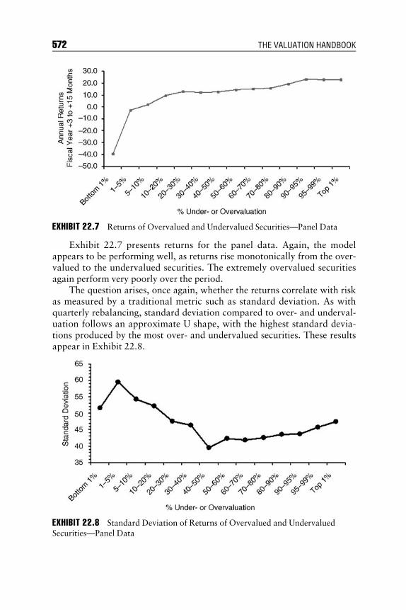
E1C22 08/25/2009 Page 572

Exhibit 22.7 presents returns for the panel data. Again, the modelappears to be performing well, as returns rise monotonically from the over-valued to the undervalued securities. The extremely overvalued securitiesagain perform very poorly over the period.

The question arises, once again, whether the returns correlate with riskas measured by a traditional metric such as standard deviation. As withquarterly rebalancing, standard deviation compared to over- and underval-uation follows an approximate U shape, with the highest standard devia-tions produced by the most over- and undervalued securities. These resultsappear in Exhibit 22.8.

EXHIBIT 22.7 Returns of Overvalued and Undervalued Securities—Panel Data

EXHIBIT 22.8 Standard Deviation of Returns of Overvalued and UndervaluedSecurities—Panel Data


E1C22 08/25/2009 Page 573

In contrast to standard deviation, Exhibit 22.9 displays risk, as meas-ured by the alpha peakedness parameter, as an inverted U when measuredacross over- and undervaluations. Consequently, the panel data confirmthat managers may lessen exposure to extreme events by investing in securi-ties that are extremely over- or undervalued—ironically, the very same secu-rities that possess a very high standard deviation of returns. Therefore,according to the annual data, investment managers may experience higherreturns and lower risk (as measured by the normality of the returns) byeither going long in undervalued securities or shorting the most extremelyovervalued securities.

Statistics for the panel data appear Exhibit 22.10. The t-statistics revealthat securities that are neither extremely overvalued nor undervalued havealpha parameters significantly different from 2. Therefore, the test cannotreject normality for securities that have an intrinsic value very differentfrom market value. However, extensive stable Paretian distribution analysisconfirms that fairly valued securities may actually become more risky thanextremely over- or undervalued ones.

CONCLUS I ON

LifeCycle’s linkage of automated DCF with the stable Paretian alphapeakedness parameter aligns the security selection process with portfolioconstruction. As extreme returns in the fat tails of distributions are

EXHIBIT 22.9 Alpha Peakedness Parameters of Overvalued and UndervaluedSecurities—Panel Data


E1C22 08/25/2009 Page 574

EXHIBIT22

.10

Alp

ha

Pea

ked

nes

sPara

met

ers—

Panel

Data

Most

Overvalued

Percentiles

Most

Bottom

1%

1–

5%

5–

10%

10–

20%

20–

30%

30–

40%

40–

50%

50–

60%

60–

70%

70–

80%

80–

90%

90–

95%

95–

99%

Undervalued

Top1%

Alp

ha

pea

ked

nes

s2.0

01.9

81.7

81.5

41.5

71.5

51.7

21.5

21.5

51.5

91.5

71.6

01.7

62.0

0

t-st

ati

stic

0.0

00.0

91.1

74.54

4.17

4.76

2.18

4.86

4.60

4.00

3.98

2.33

1.1

30.0

0

Underlined

bold

t-statistics

are

significantatthe5%

level.

Quarterlyreturnsonportfolios2002–2006;4<

plantlife

<50;debt/debtcapacity<

85%

;price

>$5;trackingerror<

45%

;market

capitalizationweights

>40th

percentile.

Source:

Fin

anci

al

state

men

tand

pri

cedata

from

Morn

ingst

ar;

calc

ula

tions

from

Lif

eCyc

leR

eturn

s.

574

E1C22 08/25/2009 Page 575

becoming an increasingly recognized significant risk, managers may try tofind securities that produce returns that are more normally distributed whilesimultaneously attempting to enhance returns. This study’s targeted resultsreveal that an automated discounted cash flow model may well produce theonce elusive combination of higher returns and lower risk given that the al-pha peakedness parameter evolves as an appropriate risk measure.

Clearly, the importance of the topic warrants additional research.Researchers can easily extend the time frame represented in this chapter todetermine whether the results are consistent. A longer time frame wouldenable analysts to examine the data over subperiods to determine if possibleshifts in the hypothesized distributions occur over time.

Another extension of this research would employ various valuationmodels to rank the securities. While the chapter presented results from theproprietary LifeCycle model, many valuation models appear in the financeand accounting literature. Academics could use these other models to testthis chapter’s conclusions. Practitioners may wish to employ their own pro-prietary models with the framework provided in this chapter.

Finally, researchers may need to develop additional risk measures. Thischapter’s analysis provided some introductory evidence by concentrating onthe alpha peakedness parameter of stable Paretian distributions, but othersmay prove to be appropriate as well. Even for distributions where the vari-ance is not defined, measures of skewness and dispersion exist. Conse-quently, those measures may provide valuable insight into how risk andreturn may be measured in a fat-tailed world.

APPEND IX A : SYNTHES I Z I NG THEL I F ECYCL E FRAMEWORK

Three chapters (5, 11, and 22) in this Handbook embody LifeCycle’s valua-tion philosophy. They represent a unique, integrated examination of the se-curity analysis and portfolio construction process to enhance client benefit,in contrast to current organization structures. LifeCycle’s framework bestutilizes the strengths of traditional security analysts’ insights, the power ofstatistical testing, and the resulting implications for redefining portfolioconstruction risk.

A quick glance through Graham and Dodd’s (1962) Security Analysisand Campbell, Lo, and MacKinlay’s (1997) Econometrics of Financial Mar-kets reveals the stark differences between traditional security analysis andanalyses steeped in econometrics. The strength of traditional security analy-sis lies in its ability to analyze accounting data to examine the role of corpo-rate decision making in shareholder value creation. The ability to subject


E1C22 08/25/2009 Page 576

large quantities of financial market data to rigorous statistical testing repre-sents the forte of quantitative approaches. Unfortunately, within an organi-zation, security analysts and econometricians may never totally integratetheir separate skill sets, which results in a broken bridge that we term thesilo effect.

The LifeCycle framework can synergistically bridge across silos. As de-scribed in Chapter 11, LifeCycle’s system first translates accounting data toeconomic returns and then derives an intrinsic value through automated dis-counted cash flow models. While still producing thousands of intrinsic valueestimates, star analysts with exceptional insights can significantly contrib-ute to the process along three critical dimensions:

1. Produce more accurate decade-long intrinsic value baselines fromwhich to forecast by:& Adding missing value-relevant data to the analysis.& Overriding plant lives and other variables from GAAP data that do

not reflect the economics of the business.& Testing empirically analysts’ terminal value assumptions with supe-

rior model structures. (See Chapter 5 for related measurements andmethodologies.)

2. Enhance the automated models with their near-term forecasts based onthe deep understanding necessary to accurately model industry compet-itive conditions.

3. Tackle the formidable task of valuing those firms most difficult to value,such as start-ups or companies in financial distress.

Due to the vast amount of data arising from the process, portfolio man-agers can now statistically construct portfolios with the best risk and returntrade-offs.

Of course, risk will remain elusive to define comprehensively for everyindividual investor. Building on the pioneering work of Mandelbrot in thecurrent chapter, LifeCycle links the security selection process and an inno-vative way to evaluate portfolio risk. Thus, we compiled in three chapters aprocess that transforms raw accounting data to eventually produce path-breaking portfolio risk measurement.

Periodically, ‘‘disruptive technologies’’ emerge which change the wayfirms within industries must compete. Christensen (1997) cites numerousexamples, while documenting how large firms often miss disruptive technol-ogies until too late to change. We consider the LifeCycle process disruptivebecause investment firms must bridge traditional silos to reexamine the in-teraction among security valuation, quantitative analysis, and portfolioconstruction. As the three chapters document, the resulting processes could


E1C22 08/25/2009 Page 577

then combine the greatest strengths of any investment organization to sig-nificantly increase customer security and benefit.

APPEND IX B : T ECHN ICAL NOTE—RANGESOF BOUNDED RAT I ONAL I TY

Intrinsic values represent an estimate of the true value of a security. As such,investors best think of them as a point in a range of reasonable estimates forthe underlying value. LifeCycle derives this range by examining the disper-sion of actual prices over a period and applying a dispersion adjustment tothe intrinsic value. Academics call the dispersion around intrinsic valuations‘‘the range of bounded rationality.’’

Two schools of thought impacted the concept of LifeCycle’s ranges ofbounded rationality. The first school relates to behavioral finance observa-tions. These observations revealed that dispersions around reasonable esti-mates of intrinsic valuation were far too wide to support the concept ofinstantaneous, strong-form market efficiency. Consequently, the marketoverreacts. Price does not always equal intrinsic value. See Shiller (1981)for dispersion research on the U.S. market around dividend discount modelestimates of intrinsic valuation. Also, see Smith (1986) for supporting evi-dence in a controlled economic laboratory of overreaction by individualsaround a dividend discount model intrinsic value as the anchor.

The second school of thought relates to technical analysis, which triesto measure market sentiment or market overreaction of prices. For example,see Bollinger (2002). LifeCycle adapted these two concepts to create modelsof ranges of bounded rationality. Instead of employing Bollinger’s �1.5standard errors around the 200-day moving average of stock prices, Life-Cycle developed a model of dispersion that relies on the fundamental eco-nomic drivers of size, cash economic return, and trading volume.

Exhibit 22B.1 illustrates the ranges of bounded rationality results witha value chart. The bars represent the fiscal year high/low prices. The darkline in the middle exhibits the intrinsic value. The white line on top and thegray line on the bottom display the high and low ranges of bounded ratio-nality, respectively. The star in the current year represents the latest price.Since the star falls on the lower bound, the stock becomes undervalued.Consequently, the analyst should issue a buy recommendation.

To measure relative dispersion, LifeCycle’s system first divides the fiscalyear high price for the stock by the fiscal year high value for the S&P 500 todetermine a relative high value for the stock. It also computes a relative lowvalue for the stock by the same procedure. Second, LifeCycle’s system calcu-lates a geometric mean of the relative highs and lows. Third, taking the


E1C22 08/25/2009 Page 578

relative high value for the stock divided by the geometric mean then be-comes LifeCycle’s measure of dispersion for the security. Fourth and last,LifeCycle utilizes that measure as a data point in determining the relation-ship between dispersion and fundamental drivers across all firms.

LifeCycle’s empirical research documents that three fundamental driv-ers determine dispersions around stock prices: size, economic performance,and liquidity. To measure the underlying empirical relationship, LifeCycleregresses the dispersion measure against proprietary nonlinear functions ofconstant dollar gross investment (size), cash economic return (economicperformance), and trading volume (liquidity). Directionally, all three varia-bles should negatively correlate with dispersion. As firms grow larger,achieve higher economic performance, and trade more deeply, analysts andinvestors possess more certainty about where the true value of the securityshould lie.

LifeCycle’s system then applies the mathematical relationship deter-mined through the regression to the individual firm’s dispersion by enteringthe fundamentals as independent variables. The result from the regressionbecomes the dispersion applied to that individual firm. Multiplying themeasure of dispersion by the intrinsic value produces a high estimate ofvalue, while dividing the intrinsic value by the dispersion measures pro-duces the low-end estimate of intrinsic value.

LifeCycle documented that the low-end value predicts inflection pointsin security pricing far more effectively than the high-end value does.

80

60

40

25

15

10

5

‘98 ‘99 ‘00 ‘01 ‘02 ‘03 ‘04 ‘05 ‘06 ‘07 ‘08

80

60

40

25

15

10

5

Production Ranges

EXHIBIT 22B.1 Ranges of Bounded Rationality


E1C22 08/25/2009 Page 579

LifeCycle’s empirical research reveals that stocks that drift from their intrin-sic values tend to bounce off the low-end value. From there, they migrateback toward the intrinsic value, thus providing a return to the theoreticallyundervalued investment. Prices also bounce off the high-end value as theybecome overvalued. We expected that the low-end value would becomemore predictive for buys, while the high-end value would become more pre-dictive for sells. Counter intuitively, the empirical evidence did not supportour expectations. In fact, the low-end was more predictive for both the buysand the sells. We interpret these empirical results to suggest that investorsimplicitly sort on the lower-end value to avoid risk (Thaler 1987), becausetheir risk avoidance is asymmetrical. They strongly prefer to avoid lossesthan achieve gains of the same magnitude.

NOTES

1. Technically, this research employs panel data, which includes both cross-sec-tional and time series results. LifeCycle utilizes panel data in order to study thesignificance of effects at the extreme tails of the distributions where few datapoints exist in time series data.

2. For example, Fabozzi, Focardi, and Jonas (2008, 16) state, ‘‘If a modeler is suc-cessful in rendering errors truly Gaussian with small variance and also seriallyindependent, the model should be safe.’’ Although that monograph refers toFama/French multifactor modelers, this chapter applies the same concept ofnormality to the riskiness of DCF models.

3. A complete description of developing an automated discounted cash flow modelfor security valuation appears in Chapter 5.

4. Markowitz (1959) extensively discusses other risk measures besides variance.These measures include semivariance, expected value of loss, expected absolutedeviation, probability of loss, and maximum loss. Most academic developmentafter Markowitz, however, focuses on mean variance.

5. Satiation means that an increase in wealth beyond some point will actually de-crease utility. Increasing absolute risk aversion implies that risky assets are in-ferior goods. Theoreticians can assume the point of satiation occurs very farout, thus negating the satiation criticism. However, increasing absolute riskaversion remains a major impediment to using quadratic utility.

6. For an accessible but more complete explanation of stability, please see Rachev,Menn, and Fabozzi (2005).

7. The LifeCycle system does not rely on any mean-variance calculations in deter-mining its intrinsic valuations. Consequently, the system remains consistentwith the non-Gaussian methodology of this chapter.

8. If adding securities actually increases risk, it may be wise to follow Warren Buf-fett’s philosophy of putting fewer eggs in your basket, but watching them veryclosely.


E1C22 08/25/2009 Page 580

9. For a complete description of the LifeCycle Returns valuation system, see Chapter11. Callard, Madden and Associates (CMA) first began computing economic per-formance measures in the 1960s. Calculating an IRR measure of gross cash flowagainst an inflation adjusted gross investment began with CMA’s DCF ROI.HOLT Planning Associates used the term CFROI1 to describe this concept in1985. HOLT Value Associates registered the CFROI term. The Boston ConsultingGroup may also use the CFROI term. CMA spawned several offshoots. AppliedFinancial Group (AFG) utilizes a similar concept, calling it economic margin.LifeCycle’s name for this concept is cash economic return. Callard, Maddenlater became Callard Research and then Ativo Research and CharterMast.

10. For an excellent discussion of applying a systems mind-set to the creation ofvaluation models, please see Bart Madden’s Chapter 3, ‘‘Applying a SystemsMind-Set to Stock Valuation.’’

11. Since we are using a proprietary model, LifeCycle permits independent verifica-tion of our results by interested parties.

12. For a discussion of unbiasedness, see Atra and Thomas’s Chapter 5, ‘‘Develop-ing an Automated Discounted Cash Flow Model.’’

13. Technically, we computed our annual returns from month 3 through 15 in or-der to allow for a disclosure lag. While not all firms would fit into this windowto account for the disclosure lag, our research indicates that it would accuratelyrepresent the lag for about 90 percent of firms.

14. Tiny start-up firms tend to possess alpha peakedness parameters close to 1.00 oreven less than 1.00.

15. High-leverage firms tend to possess alpha peakedness parameters approaching1.00 or even less than 1.00.

16. Page 345 states: ‘‘ . . . the worth of an enterprise, as such, will depend only on:(a) the ‘normal’ rate of return he can earn by investing his capital in securitiesheld by the firms; (b) the earning power of the physical assets current held by thefirm; and (c) the opportunities, if any, that the firm offers for making additionalinvestments in real assets what will yield more than the ‘normal’ (market) rateof return.’’ Callard, Madden offshoots (see note 9) define (b) as the presentvalue of cash flows from existing assets and (c) as the present value of futureinvestments; (a) is the real investors’ market derived discount rate. LifeCycleuses (b) as its measure of the firm’s debt capacity.

17. LifeCycle’s use of the tracking filter does not mean investment firms must ignorethe portion of the universe eliminated by the filter. The filter only means that theautomated valuation process is not valuing those firms accurately. In fact, secu-rity analysts, using firm-specific knowledge and insight, should focus their at-tention on the securities not covered by the automated model.

18. This chapter’s Appendix B presents some of the technical details of computingthese ranges of bounded rationality.

19. Some make the case that annual information contains more accurate auditeddata on cash flows than quarterly data, which may contain suspect accruals tomatch analysts’ interim earnings per share (EPS) expectations and lacks thefootnote data included in annual statements.


E1C22 08/25/2009 Page 581

RE F ERENCES

Bachelier, Louis. 1900. Theorie de la speculation. Doctoral dissertation, AnnalesScientifiques de l’Ecole Normale Superieure. Trans. Cootner, 1964.

Barro, Robert J. 2005. Rare events and the equity premium. Working paper, Har-vard University.

Bollinger, John. 2002. Bollinger on Bollinger bands. New York: McGraw-Hill.Campbell, J. Y., A. W. Lo, and A. C. MacKinlay, 1997. The econometrics of finan-

cial markets. Princeton, NJ: Princeton University Press.Carr, P., and L. Wu. 2003. The finite moment log stable process and option pricing.

Journal of Finance 58: 753–778.Chen, Nai-fu, and Feng Zhang. 1998. Risk and return of value stocks.Christensen, Clayton M. 1997. The innovator’s dilemma. Boston: Harvard Business

School Press; HarperBusiness, 2000; Harper Business Essentials, 2003; CollinsBusiness Essentials, 2006.

Cootner, Paul,ed. 1964. The random character of stock prices. Cambridge, MA:MIT Press, 333.

De Grauwe, Paul, Leonardo Iania, and Pablo Rovira Kaltwasser. 2008. How abnor-mal was the stock market in October 2008? Euro Intelligence. www.eurointel-ligence.com/article.581+M5f21b8d26a3.0.html.

Fabozzi, Frank J., Sergio M. Focardi, and Caroline Jonas. 2008. Challenges in quan-titative equity management. Charlottesville, VA: CFA Institute.

Fabozzi, Frank J., B. Racheva-Iotova, and S. Stoyanov. 2005. An empirical examina-tion of the return distribution characteristics of agency mortgage pass throughsecurities. Reported in Rachev, Menn, and Fabozzi (2005).

Fama, Eugene. 1965. Portfolio analysis in a stable Paretian market. ManagementScience 11: 404–419.

Francis, J., P. Olsson, and D. Oswald. 2000. Comparing the accuracy and explain-ability of dividend, free cash flow, and abnormal earnings equity value esti-mates. Journal of Accounting Research 38: 45–69.

Graham, Benjamin, David L. Dodd, Sidney Cottle, and Charles Tatham. 1962. Secu-rity analysis: Principles and techniques. New York: McGraw-Hill.

Hales, Stanley. 1997. Valuing foreign currency options with the Paretian stable op-tion pricing model. Working paper, Price Waterhouse, LLP.

Huang, Chi-fu, and R. Litzenberger, 1988. Foundations for financial economics. Up-per Saddle River, NJ: Prentice Hall.

Lintner, John. 1965. The valuation of risk assets and the selection of risky invest-ments in stock portfolios and capital budgets. Review of Economics and Statis-tics 47: 13–37.

Mandelbrot, Benoit B. 1963. The variation of certain speculative prices. Journal ofBusiness 36: 394–419.

Mandelbrot, Benoit B. 1997. Fractals and Sealing in Finance: Discontinuity, Con-centration, Risk. New York: Springer.

Mandelbrot, Benoit B. and Richard L, Hudson. 2004. The (Mis)Behavior of Mar-kets: A Fractal View of Risk, Ruin, and Reward. New York: Basic Books.


E1C22 08/25/2009 Page 582

Markowitz, Harry. 1952. Portfolio selection. Journal of Finance 7: 77–91.Markowitz, Harry. 1959. Portfolio selection: Efficient diversification of investments.

The Cowles Foundation, Utility Functions and Measures of Risk, pp. 286–297.McCulloch, J. Huston. 1986. Simple consistent estimators of stable distribution pa-

rameters. Communications in Statistics—Simulation and Computation 15(4):1109–1136.

Miller, Merton H., and Franco Modigliani. 1961. Dividend policy, growth, and thevaluation of shares. Journal of Business 34, no. 4 (October): 411–433.Reprinted in Stephen H. Archer and Charles A. D’Ambrosio, The Theory ofBusiness Finance: A Book of Readings (New York: Macmillan, 1967).

Mossin, Jan. 1966. Equilibrium in a capital asset market. Econometrica 35: 768–783.

Penman, S., and T. Sougiannis. 1998. A comparison of dividend, cash flow, andearnings approaches to equity valuation. Contemporary Accounting Research15: 343–383.

Rachev, Svetlozar T., Christian Menn, and Frank J. Fabozzi. 2005. Fat-tailed andskewed asset return distributions: Implications for risk management, portfolioselection and option pricing. Hoboken, NJ: John Wiley & Sons.

Rachev, Svetlozar, T. E. Schwartz, and I. Khindanove. 2003. Stable modeling ofcredit risk. In Handbook of Heavy Tailed Distributions in Finance, ed. S.Rachev,249–328. Amsterdam: North Holland. Reported in Rachev, Menn, andFabozzi (2005).

Rietz, T. A. 1988. The equity risk premium: A solution. Journal of Monetary Eco-nomics 23: 117–131.

Roll, Richard. 1989. The international crash of October 1987. In Black Monday andthe Future of Financial Markets, ed. Kamphuis, Kormendi, and Watson,35–70.Chicago: MAI.

Rozeff, Michael. 1990. The three-phase dividend discount model and the ROPEmodel. Journal of Portfolio Management (Winter): 36–42.

Sharpe, William. 1964. Capital asset prices: A theory of capital market equilibriumunder conditions of risk. Journal of Finance 19: 425–442.

Shiller, Robert J. 1981. Do stock prices move too much to be justified by subsequentchanges in dividends. American Economic Review 71, no. 3 (June): 421–436.

Smith, Vernon, 1986. Experimental methods in the political economy of exchange.Science 234, no. 10 (October): 167–173.

Sougiannis, T., and T. Yaekura. 2001. The accuracy and bias of equity values in-ferred from analysts’ earnings forecasts. Journal of Accounting, Auditing, andFinance 16: 331–362.

Stoyanov, S., S. Rachev, A. Biglova, and F. Fabozzi. 2005. An empirical examinationof daily stock return distributions for U.S. stocks. Data Analysis and DecisionSupport, Springer Series in Studies in Classification, Data Analysis, and Knowl-edge Organization. Reported in Rachev, Menn, and Fabozzi (2005).

Thaler, Richard. 1987. The psychology of choice and the assumptions of economics.In Laboratory Experimentation in Economics: Six Points of View, ed. Alvin E.Roth,99–130. New York: Cambridge University Press.


E1C23 09/02/2009 Page 583

CHAPTER 23Common Themes and Differences

Debates and Associated IssuesFacing the Profession


The Preface suggested that valuations are important simply because theyform the basis for making decisions involving significant amounts of

money or wealth transferred from one party to another.The following partial list covers many decision applications for valua-

tion. Valuations are normally done to:

& Buy or sell publicly held stock.& Buy or sell a privately held business.& Determine how much estate tax is owed the government.& Settle a divorce.& Resolve a dispute with a minority shareholder who wants to receive full

value for his or her stock.& Give a value basis to accounting auditors.& Determine the compensation amount for executives, division or busi-

ness unit managers, or employee-owners.& Determine to proceed (or not) with strategic initiatives and/or major

investment opportunities.& Offer fairness opinions in the purchase or sale of companies.

The Valuation Handbook has provided the unique perspectives frommany of today’s top practitioners. Some authors covered labor-intensivetechniques, in which expert analyst judgment is paramount. Other authorsproposed expert or automated systems with minimal analyst judgment.Some described the valuation of publicly held firms. Others displayed

583

E1C23 09/02/2009 Page 584

techniques utilized on privately held firms to satisfy compliance standardsof law and legal precedents. Clearly, the techniques to be used rely on thedecisions to be made. The reader now has in one location a compendiumfrom some of the best minds in the world.

With the 2007–2008 market meltdowns, the profession has begun amost healthy debate on the theories, assumptions, and associated practicesin valuation. Intrinsic valuations work best when liquid markets are trad-ing. Without liquid markets, no standard of prices exists against which tocompare intrinsic valuations. When markets freeze or function much lessperfectly, what are decision makers to do? To what extent should intrinsicvaluations substitute for prices in frozen or illiquid markets? In addition,how may insights from all the various theories and associated techniques bemerged into better ones?

Exhibit 23.1 compares dimensions of efficient markets with inefficientmarkets. Any effort to establish a comparison like this is destined to be

E xh i b i t 23 .1 Comparison of Efficient and Inefficient Markets

Efficient Markets Inefficient Markets

Theories CAPM, modern portfoliotheory

Behavioral finance,discounted cash flow(DCF)

Distributions Gaussian normal Fat-tailed: stable Paretianand others

Key contributors Markowitz, Sharpe,Fama, French, Grinold,Kahn

Graham and Dodd,Mandelbrot, Shiller,Smith, McCulloch,Nolan, Copeland, SternStewart, CallardMadden offshoots

Philosophy of knowing(Madden’s Chapter3—first three pages)

Deductive: Theory )empirical testing

Inductive: Data(observations) )patterns ) economictheories ) anomaliesfrom observations )modified theory

Results—key beliefs Markets are strong-form,instantaneouslyefficient, reflecting allcurrent information; noexcess returns after

Markets are efficientwithin ranges ofbounded rationality;sometimes markets failto function due toilliquidity or uncertainty;


E1C23 09/02/2009 Page 585

price impact costs canbe achieved

excess returns (alpha)can be achieved withinformation advantagesor better modeling

Primary assumptionsdeserving debate

Homogeneous investors;homogeneousexpectations; costless orvery low-costinformation; rationalinvestors; adaptivelearning

Heterogeneous investorsand expectations;information and modeldevelopment costly;investors possessirrational biases, don’talways learn from theirmistakes

Primary quantitativemethods

Price change regressionsagainst factors (mayproduce excess returnfrom informationadvantage)

Price levels from DCF orregressions fromeconomic drivers

Risk implications Higher returns requiremore risk taking

Lower risk and higherreturns may not bemutually exclusive

Corporate finance costsof capital

Based on beta and pricevariability

Based on fundamentaleconomic drivers likefinancial leverage oruniform discount rate,with risks placed incertainty-equivalent cashflows

Portfolio constructionimplications

Indexation based onmarket cap: no benefitto stock selection

Fundamental (size)indexation or intrinsicvalue weights

Existence of intrinsicvalues

Prices are close to intrinsicvalues

Prices may differsubstantially fromintrinsic values; intrinsicvalues exist; excessreturns can be obtained

Implications of beliefsabout intrinsic valuesto disclosure

Mark to market Mark to model

Traditional dichotomy(Fabozzi et al.,Challenges inQuantitative EquityManagement)

Quant models on pricechange

Labor-intensive securityanalysis on price level

E xh i b i t 23 . 1 (Continued )


(Continued )

Common Themes and Differences 585

E1C23 09/02/2009 Page 586

controversial, so I beg forgiveness in advance. This table represents only myperception of the many dimensions of two competing theories of financeand investments. The demarcation between the two columns is far fromcrisp. For example, some who believe in a degree of market inefficiency alsoemploy capital asset pricing model (CAPM) costs of capital, originally aris-ing from the efficient markets literature. I hope this table will encourageadditional productive debate within the profession.

Fabozzi, Focardi, and Jonas (2008) wrote an outstanding research piecefor the CFA Institute on current issues facing the profession. Many of thequant models (‘‘children of Fama/French,’’ page vii) failed during thefreeze-up of markets during 2007–2008 as quants headed for the exits all atonce with very similar models, causing a reassessment of investment pro-cesses. One result from their extensive survey research was the conclusionthat many investment organizations were seeking better ways to combinetraditional fundamental security analysis with quantitative approaches.Linking their research with this Valuation Handbook resulted in my assess-ment summary in Exhibit 23.1.

For the other side of the debate of efficient versus inefficient markets,please see Fama (2009). Fama is very eloquent in how he articulates thecase for efficient markets.

Alternatives arisingfrom dichotomy

DCF intrinsic value addedas addition factor

Security analysts useautomated DCF modelstructures for theirterminal valuations

Speculation onevolution

Probabilistic priceformation models basedon intrinsic valuation asthe core, with ranges ofbounded rationality,price momentum, EPSsurprises of marketoverreaction, and otherinformation effectsmodeled withMandelbrot-typefractional Brownianmotion generatingfunctions with memory

E xh i b i t 23 .1 (Continued )



E1C23 09/02/2009 Page 587

In the last row of Exhibit 23.1, I speculate that the profession maycombine insights from both schools of thought in order to relax the as-sumption of Brownian motion and independent draws from distribu-tions in order to create price formation models. These price formationmodels may incorporate Mandelbrot’s research of fractional Brownianmotion (Mandelbrot (2002) with memory, linked to DCF with rangesof bounded rationality around intrinsic value as the anchor and insightsfrom multi-factor research of short term price effects (EPS surprises,etc.). Stay tuned.

Using the valuation perspectives from The Valuation Handbook, thenext four sections outline several debates facing the profession. Certainly,other debates exist.

1. Does intrinsic value have any meaning?2. ‘‘Mark to market’’ versus ‘‘mark to model.’’3. Illiquidity crises and market meltdowns: effect on quantitative

strategies.4. Residual income versus cash flow return on investment models.

DOES INTR INS I C VALUE HAVE ANY MEAN ING?

Some say, ‘‘No one knows what the intrinsic value is, anyway.’’ I suspectthat the authors in this Valuation Handbook, who have spent their profes-sional careers on the subject of valuation, would strongly disagree. Aswith any effective debate, trying to identify the underlying assumption(expressed, implied, or unstated) proves useful to understanding the beliefsof the participants. Why do valuation experts say that intrinsic value can beestimated with the techniques illustrated in this book? Why do some indus-try experts say that intrinsic value has no meaning? While I cannot defini-tively answer the questions, I can offer some possible reasons for this veryfundamental disagreement.

From the mutual fund and other academic empirical evidence, let’s saythat I believe in perfectly instantaneously efficient markets. Almost by defi-nition in this world of perfect market efficiency, price always preciselyequals the intrinsic value derived from all information available to the mar-ket. As outlined in Exhibit 23.1, I may assume that the market consists ofhomogeneous investors with homogeneous expectations, who rapidly learnfrom their mistakes. Consequently, I may logically conclude that pricealways equals the intrinsic valuation of all the participants in the market.If price changes, that change represents the change in intrinsic valuationderived from those participants.


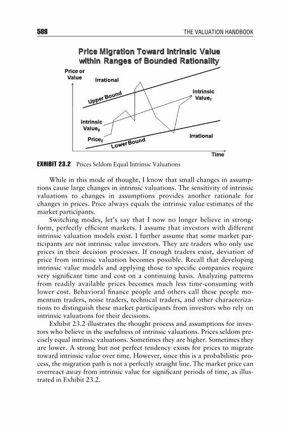
E1C23 09/02/2009 Page 588

While in this mode of thought, I know that small changes in assump-tions cause large changes in intrinsic valuations. The sensitivity of intrinsicvaluations to changes in assumptions provides another rationale forchanges in prices. Price always equals the intrinsic value estimates of themarket participants.

Switching modes, let’s say that I now no longer believe in strong-form, perfectly efficient markets. I assume that investors with differentintrinsic valuation models exist. I further assume that some market par-ticipants are not intrinsic value investors. They are traders who only useprices in their decision processes. If enough traders exist, deviation ofprice from intrinsic valuation becomes possible. Recall that developingintrinsic value models and applying those to specific companies requirevery significant time and cost on a continuing basis. Analyzing patternsfrom readily available prices becomes much less time-consuming withlower cost. Behavioral finance people and others call these people mo-mentum traders, noise traders, technical traders, and other characteriza-tions to distinguish these market participants from investors who rely onintrinsic valuations for their decisions.

Exhibit 23.2 illustrates the thought process and assumptions for inves-tors who believe in the usefulness of intrinsic valuations. Prices seldom pre-cisely equal intrinsic valuations. Sometimes they are higher. Sometimes theyare lower. A strong but not perfect tendency exists for prices to migratetoward intrinsic value over time. However, since this is a probabilistic pro-cess, the migration path is not a perfectly straight line. The market price canoverreact away from intrinsic value for significant periods of time, as illus-trated in Exhibit 23.2.

EXHIBIT 23.2 Prices Seldom Equal Intrinsic Valuations


E1C23 09/02/2009 Page 589

Just to add richness to the process as illustrated in this Valuation Hand-book, intrinsic valuations can be calculated purely from historical data orcalculated from a cash flow forecast and a terminal value. They can be auto-mated or hand calculated through a labor-intensive security analysis processone company at a time for the current year. I think that how one combinesautomated or expert-system DCF with analysts’ input from history andforecast insights becomes a most critical aspect of the stock selection pro-cess. This probabilistic process flows from relaxing the assumptions of ho-mogeneous investors and homogeneous expectations.

Exhibit 23.2 adds another behavioral finance/technical/sentiment di-mension to the debate: upper and lower bounds of rationality. Thesebounds measure market overreaction. Models of these bounds of rationalitymay derive from standard errors around moving price averages or funda-mental dispersion models around intrinsic valuations as the anchors (seeAppendix B in Chapter 22). Since I assume markets are not perfectly effi-cient, prices can exceed the bounds periodically.

Which set of assumptions do you believe? What thought mode are youin? Logically, if you believe in highly efficient markets, you may decide toinvest in passive index funds to avoid management fees and price impactcosts. If you believe in inefficient markets, you may take a more active ap-proach to your investment strategy. I recommend that you examine yourbeliefs, your assumptions, and the empirical evidence to decide your stockselection strategy—passive or active. This Valuation Handbook providesadditional information for your assessment and decisions.

METHODOLOG I ES : MARK TO MARKET ,MARK TO MODEL

What methodologies apply? Randall Schostag’s Chapter 15, ‘‘PortfolioValuation: Challenges and Opportunities Using Automation,’’ providesan extensive history of the field. Generally, the courts accept threemethodologies:

1. Market price.2. Comparables.3. Earnings or discounted cash flow approach.

With current meltdowns and freeze-ups of several markets, the profes-sion is exploring and debating new approaches. How can anyone establish avalue if no one is trading the security? Or some trading is occurring, but notenough to provide confidence that the trades are representative of the true


E1C23 09/02/2009 Page 590

underlying intrinsic valuation. Or the trades occurred several days, weeks,or months ago.

‘‘Mark to market’’ seems deceptively simple. However, I suggest thatmark to market may rely on two assumptions—often unstated or implicit:

1. The market is perfectly, instantaneously, strong-form efficient at eachmoment in time.

2. The market can absorb any amount of volume on either the buy side orthe sell side without changing the price.

Suppose we relax both these assumptions. Under these relaxed condi-tions, price does not equal intrinsic value at all times. Sometimes it is higher.Sometimes it is lower. And trading from noise traders can push the pricefurther away from intrinsic value—at least temporarily.

Several theoretical reasons exist for prices to diverge from intrinsic val-ues. We need to relax the assumption that the market consists of homoge-neous investors. In addition to fundamental investors who rely onestimating intrinsic valuations from financial statements, other investortypes exist. Momentum traders follow the trend in market prices, with nostudy of the fundamentals. Noise traders may employ concepts like Bollin-ger bands to determine likely inflection points in prices, again with no refer-ence to financial statements. Vultures purchase stock from those needingimmediate liquidity. Overlaps among investor types clearly exist. However,if every investor used the identical intrinsic valuation model and traded ononly that information, no trading would occur. The fact that trading doesoccur and that ranges of bounded rationality around reasonable estimatesof intrinsic valuations place limits on prices does suggest that various classesof market participants are active in the market.

With price no longer representing intrinsic value during every momentin time, our concrete foundation of efficient markets and the superiority ofprice as the primary determinant of intrinsic valuation cracks. Not usingprice exclusively creates a huge problem in valuation, because we have lostour anchor. We need to find a replacement.

For example, within the financial sector, many banks don’t want markto market, because the lower valuations of actual trades may wipe out theirequity to make them insolvent. These banks argue, ‘‘Just wait a while; themarket will come back. These nontraded securities are worth much morethan stale market prices. Their intrinsic valuations are much higher thantheir traded prices.’’

No one wants to see markets continue their freeze up, causing immenseeconomic hardship throughout the world. To stimulate debate, permit me


E1C23 09/02/2009 Page 591

to offer one solution of many possible ones, arising from FMA PDDARIdiscussions at the CFA Society of Chicago. (See Appendix A of this chapterfor a description of FMA PDDARI.)

& Disclose both mark to market and mark to model (DCF) so investorshave the information they need for decisions.

& Solvency tests continue to rely on mark to market, but:& While the markets continue to malfunction, regulators forbear some in-

solvent banks, depending on the degree of insolvency.

Consequently, this proposal suggests that GAAP still forces mark tomarket, but mark to model may be footnoted. (Disclosure could functionthe other way around: mark to model occurs on the financial statements,while mark to market occurs in a footnote.) During periods of extreme mar-ket distress, regulators may employ the footnote information on mark tomodel instead of the market information for regulatory compliance ofequity capital requirements. By demanding empirical evidence to supportthe models consistent with measurements proposed in this Valuation Hand-book, regulators may increase their confidence in the validity of mark tomodel for compliance purposes.

I L L I QU I D I TY CR I S ES AND MARKET MELTDOWNS :E F F ECT ON QUANT I TAT I V E STRATEG I ES

After the 2007 meltdown, Fabozzi, Focardi, and Jonas (2008) extensivelysurveyed the profession to unearth how portfolio managers were reactingto the market freeze-ups and illiquidities, primarily during August 2007when the ‘‘quants rushed for the exit to sell with largely similar models.’’ Ingeneral, the ‘‘children of Fama/French’’ were attempting to identify the bestways to overlay traditional, labor-intensive DCF security analyst valuationsover their multifactor models of price change. In contrast, no mention wasmade of the expert/automated approaches to DCF prevalent in this Valua-tion Handbook. Combining insights from the Fabozzi et al. research withthis book raises some interesting and potentially useful possibilities. In myview, the two core questions are:

1. Should security analysts and portfolio managers start with discountedcash flow and then overlay multifactor quantitative strategies? or

2. Should they start with multifactor quantitative strategies and add in-trinsic valuation as one additional factor?


E1C23 09/02/2009 Page 592

With these questions, I am suggesting that DCF form the core of valua-tions. After all, DCF represents not just another factor, but a true long-termestimate of value—especially when markets fail to trade or are illiquid in theshort term. However, reduced-form traditional Fama/French correlations ofthe factors driving price change may supplement the understanding of theprice formation process through time.

What measurement criteria should researchers employ to measure theempirical results to these two alternative approaches? Chapter 4 (TomCopeland: ‘‘Comparing Valuation Models’’), Chapter 5 (Atra/Thomas:‘‘Developing an Automated Discounted Cash Flow Model), and Chapter22 (Thomas/Yang/Atra: ‘‘Lower Risk and Higher Returns: Linking StableParetian Distributions and Discounted Cash Flow’’) offer measurementmethodologies to address the two core questions. These measurement crite-ria include robustness, accuracy, unbiasedness, predictive capability, andrisk. Empirical results from Chapter 22 suggest that more accurate unbiasedvaluation models are more predictive, with lower risk at the tails.

Related to these two core questions is the debate between Fama andMandelbrot—two giants in the field of finance and investments. Do re-turns follow lognormal distributions or stable Paretian ones? What arethe best measures of risk? And, since this is The Valuation Handbook,how best to combine discounted cash flow valuation methodologieswith the Fama/French/Grinold/Kahn multifactor approach or the Man-delbrot approach?

My own admittedly biased view is that DCF should form the core,while the multifactor approach should help model the price formation pro-cess around the core. Additionally, stable Paretian generating functionswith memory should relax the traditional independent and identically dis-tributed (IID) random draw assumptions found in traditional modeling.However, let the debates rage on.

D ISCOUNTED CASH F LOW METHODOLOG I ES

Once we agree that discounted cash flow should be an integral part of anyinvestment process, the question arises: how? Traditionally, discounted cashflow has been a largely manual process to value one firm at a time for thecurrent period. However, Chapters 3 to 5, 8, 11, 12, and 15 raise the potentialof expert systems or automated approaches. Should the profession employ:

& The traditional largely manual process& The automated approach?& Some combination of both—if so, how?


E1C23 09/02/2009 Page 593

Again, my admittedly biased view is to combine the best of both, as out-lined in Chapter 22. However, these are central issues to the theory andpractice of finance and investments. Consequently, they deserve muchdebate and empirically validating research.

Which discounted cash flow approach should analysts utilize? Twomajor schools of thought for valuation exist:

1. The residual income school.2. The cash return school.

The Valuation Handbook covers both schools in much detail from the dif-ferent perspectives of top practitioners. Both schools think that achievingreturns above the cost of capital forms the most important strategic coreof finance and investment. Meeting analysts’ EPS expectations for the currentquarter and Fama/French multifactor models fail to fulfill this most importantstrategic core. Exhibit 23.3 compares the residual income and cash returnschools of thought. A review of the table reveals three primary differences:

E xh i b i t 23 . 3 Residual Income and Cash Return Schools of Thought

Similarities Residual Income Cash Return

Return on investment More important to long-term shareholderwealth creation thanquarterly

EPS relative to marketexpectations

Same

Operating income Exclude nonoperatingincome/expense

Same

Operating assets minusnondebt liabilities

Exclude nonoperatingassets/nondebtliabilities

Same

Return on investmentless cost of capital

Core operating metric Same

Capitalize expenseswith economic liveslonger than one year(e.g., R&D,advertising, training,software, etc.)

Important to calculatereturns comparable tocost of capital

Same

Capitalize operatingleases

Yes Yes

(Continued )


E1C23 09/02/2009 Page 594

Treatment ofdepreciation,amortization, andaccumulateddepreciation

Subtracted to determinenet operating income

Added back to after-taxoperating income toproduce gross cash flow

Treatment of inflation Employs GAAP historicalcost

Inflation adjusts grossplant with GDP deflator

Goodwill intangibles Included in asset base Some include in asset base;others exclude

Return measure Net operating profit/netoperating assets

IRR of gross cash flowover current dollar grossinvestment or gross cashflow – sinking funddepreciation/grossinvestment

Implicit assumption tomake return measurecomparable to cost ofcapital

Output declines withincrease in accumulateddepreciation

Output is constant overeconomic life of assets(one-horse shay)

Correction to makeabove assumptionmore realistic

Subtract economicdepreciation instead ofGAAP depreciation soRONA ¼ IRR returnon investment

Proprietary function toincrease/decreaseintrinsic value for assetlife effects

Cost of capital or realinvestor discount rate

CAPM nominal weightedaverage cost of capital

Market derived discountrate using the valuationmodel to establish therate that equates thepresent value of cashflows less debt tomarket value of equity;some adjust discountrate for leverage andsize effects (CSFBHOLT, etc.); LCRTadjusts certaintyequivalent cash flowsin intrinsic value forsize and leverageeffects

E xh i b i t 23 .3 (Continued )

Differences Residual Income Cash Return


E1C23 09/02/2009 Page 595

1. Residual income employs operating net income and operating invest-ment net of accumulated depreciation. The cash return school usesgross cash flow and gross investment, by adding back depreciation andamortization and accumulated depreciation, respectively.

2. Residual income bases itself on historical cost, whereas cash returnadjusts the data for inflation.

3. Residual income generally employs CAPM costs of capital, whereascash return utilizes market derived discount rates.

Based on the chapters in this Valuation Handbook, the reader may de-cide which approach to follow.

Thank you for choosing The Valuation Handbook. We anticipate manyviews on what constitutes accurate valuations, and hope that our effortsproduce more informed, in-depth discussions that result in more accuratedecisions.

While discounted cash flow predates modern portfolio theory (MPT),MPT provided considerable insight into risk measurement and diversifiedportfolio construction. However, by focusing on price change, MPT strayedfrom the fundamental DCF roots of price level in finance. The ValuationHandbook authors suggest ways to integrate the fundamental soundness ofDCF with evolving innovative thinking of twenty-first-century global fi-nance. We intend that the integration promises to expand theory andmodeling into a much more robust price formation process, using state-of-the-art methodologies and applications for decisions.

Excess returns Continue for T timeperiod

Exponentially competedaway

Valuation of start-ups Requires analyst cashflow forecast

Same or option pricingfunction on gross capitaland likely returns

Thought leaders Tom Copeland, Bart Madden,Joel Stern, Chuck Callard,Bennett Stewart, Rawley Thomas,Jim Grant, Ricardo Bekin,Roy Johnson Dennis Aust,

Rafe Resendes,Dan O’Brycki

E xh i b i t 23 . 3 (Continued )

Differences Residual Income Cash Return


E1C23 09/02/2009 Page 596

Based on studying The Valuation Handbook, what investment strategydo you choose–passive or active? To continue the dialogue, contact [email protected].

APPEND IX A : F I NANC IA L MANAGEMENTASSOC IAT I ON PRACT I T I ONER DEMAND DR IV ENACADEM IC RESEARCH IN I T I AT I V E ( FMA PDDAR I )

Because collaboration and effective communication have become critical tocreativity in the information age, several paths exist for practitioners andresearchers to join to improve practice, research, and teaching. These in-clude facilitating communications among those who teach, who perform re-search, and who are in the finance business:

& Residence programs.& Investment firms that hire academics.& Conferences that mix academic and practitioner speakers.& Special sessions at the Financial Management Association annual meet-

ings that mix speakers.& Firms that hire academics as consultants.

A recent effort that shows promise is the Financial Management Associ-ation Practitioner Demand Driven Academic Research Initiative (FMAPDDARI).

The PDDAR I P l a t f o rm

PDDARI facilitates a unique format for dialogue between academics andpractitioners to debate pivotal finance challenges articulated from practi-tioners’ perspectives. PDDARI engages ‘‘thought partners’’ in interactivediscussions that seek genuinely new, even breakthrough ideas. Examples ofthe types of challenges that can be addressed include:

& A better theory than the capital asset pricing model for dealing with lev-els and changes in stock prices plus the associated measurement of risk.

& Improved valuation and communication tools to help managementundertaking wealth-creating investments that may depress short-termquarterly earnings.

& Ideas for improving or replacing conventional discounted cash flow meth-odology derived from empirical findings in behavioral finance and ad-vanced quantitative tools used by leading-edge quant portfolio managers.


E1C23 09/02/2009 Page 597

An all-encompassing theme of PDDARI is to create avenues for practi-tioners to share with academic partners as well as fellow practitioners, thetypes of real-life problems encountered when making or implementing deci-sions. In other words, PDDARI strives to create a climate in which practi-tioners and academics can collaboratively address the current challenges inthe field. The current and conventional practice reflects practitioners and aca-demics functioning independently to address practical decision applicationsfrom their unique, individual perspectives. While the conventional practiceproduces results, it represents a silo: an isolated and uncoordinated system tounderstand and offer resolutions to practical day-to-day financial issues.

The immediate benefits of PDDARI provide a platform to increaseplanned, effective communication between practitioners and academics. Itoffers a centralized marketplace in which practitioners and academics mayinteract equally under established guidelines of full disclosure of commer-cial interests. Academics can discover which issues practitioners feel arecentral and can express their thoughts and knowledge in a proactive, effi-cient manner. Ultimately, PDDARI fervently desires that academics collab-orate closely with practitioner thought partners on application topics todirect documented research in order to more effectively facilitate globalpractice.

In addition, PPDARI’s long-term benefits offer:

& Thought partners to collaborate with academics on real-life practicalproblems.

Strong incentives exist for practitioners to interchange with aca-demics. Many practitioner thought partners perform advanced researchthemselves. Therefore, they are current on academic literature as well aspractitioner research. Consequently, practitioners remain keenly awareof both theoretical and empirical issues involved in great research.

& Opportunities to engage practitioners and academics.The PDDARI has organized forums on the PDDARI web site (www

.fma.org/PDDARI/PDDARI.htm), face-to-face meetings, and specialsessions at the FMA annual meeting. PDDARI’s coordinated effort pro-vides for an interchange that is both planned and multifaceted. In addi-tion, PDDARI plans to meet the needs of a continually evolvingprofession in the twenty-first century.

& Access to databases.Many practitioners may be willing to contribute access to proprie-

tary databases to assist academics with relevant research projects, be-cause meeting these challenges is most important to them.

& Publishing opportunities.


E1C23 09/02/2009 Page 598

Because it addresses important issues in financial practice,PDDARI-initiated research should be attractive to leading research out-lets. PDDARI’s collaborative and respectful problem-solving climatealso has the potential to change financial practice in meaningful andbeneficial ways.

One example of how FMA PDDARI seems to be succeeding in bringingacademics and practitioners together is the PDDARI working group sup-ported jointly by FMA and the CFA Society of Chicago. This workinggroup meets the third Thursday of each month to keep joint practitioner/academic research on track to solve problems relevant to the profession.Groups in other cities are in the formative stages.

Appendix B represents another FMA PDDARI example of a collabora-tive industry effort. It offers a list of the assumptions and theories deservingdebate and empirical quantification. The new information age demandscritical thinking to question these assumptions and theories in order to findcreative solutions to the problems plaguing the profession.

In the new information age, students need to apply critical thinking toeven the most classic articles. Often assumptions are unstated or implicit,instead of explicit. For instance, the articles by Nobel Prize-winning Millerand Modigliani assumed earnings are a good enough proxy for cash flow,without discussing the implicit assumption that capex equals historical dol-lar depreciation. Statisticians assume, often implicitly, that the upper mo-ments of independent variables exist, so the central limit theorem applies. IfMandelbrot is correct that the upper moments do not exist, what shouldpractitioners use instead?

Identifying the explicit assumptions and the implicit unstated assump-tions in each of the chapters of this Valuation Handbook might prove to bea very useful exercise for students.

APPEND IX B : EXAMPLES OF ASSUMPT IONS ANDTHEOR I ES DESERV ING D EBATE AND EMP IR I CA LQUANT I F I CAT I ON

PDDARI seeks to bridge gaps in understanding by adopting two workingassumptions to confirm mutual respect between the academic and practi-tioner silos:

1. Many practitioners perform theoretically sound and empirically validresearch.


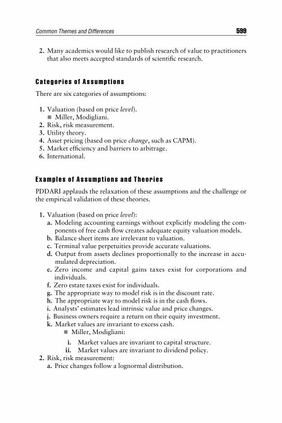
E1C23 09/02/2009 Page 599

2. Many academics would like to publish research of value to practitionersthat also meets accepted standards of scientific research.

Ca t egor i e s o f Assump t i ons

There are six categories of assumptions:

1. Valuation (based on price level).& Miller, Modigliani.

2. Risk, risk measurement.3. Utility theory.4. Asset pricing (based on price change, such as CAPM).5. Market efficiency and barriers to arbitrage.6. International.

E xamp l es o f Assump t i ons and Theor i es

PDDARI applauds the relaxation of these assumptions and the challenge orthe empirical validation of these theories.

1. Valuation (based on price level):a. Modeling accounting earnings without explicitly modeling the com-

ponents of free cash flow creates adequate equity valuation models.b. Balance sheet items are irrelevant to valuation.c. Terminal value perpetuities provide accurate valuations.d. Output from assets declines proportionally to the increase in accu-

mulated depreciation.e. Zero income and capital gains taxes exist for corporations and

individuals.f. Zero estate taxes exist for individuals.g. The appropriate way to model risk is in the discount rate.h. The appropriate way to model risk is in the cash flows.i. Analysts’ estimates lead intrinsic value and price changes.j. Business owners require a return on their equity investment.k. Market values are invariant to excess cash.

& Miller, Modigliani:

i. Market values are invariant to capital structure.ii. Market values are invariant to dividend policy.

2. Risk, risk measurement:a. Price changes follow a lognormal distribution.


E1C23 09/02/2009 Page 600

b. Upper moments in distributions exist.c. The mean in distributions exists.d. Distributions are symmetrical.e. Draws from distributions are independent from prior draws.f. The error terms in regression models follow normal distributions

with finite variances.g. The conditions hold that are needed for the central limit theorem to

apply.3. Utility theory:

a. Approximating expected utility by a function of expected return andstandard deviation is adequate for making investment decisions.

b. Expected utility theory is an adequate model for how investors makedecisions under uncertainty.

4. Asset pricing (based on price change, such as CAPM):a. Investors possess homogeneous expectations for risk and return.b. The CAPM beta and standard deviation, which relate to price

changes, are adequate measures of risk for both portfolio and corpo-rate investment decision making.

5. Market efficiency and barriers to arbitrage:a. Markets are so efficient that no reliable ways exist to exploit any

inefficiencies.b. In the aggregate, perfect arbitrage exists between the corporate re-

turns on operating assets and the costs of capital available in the cap-ital markets.

c. Dispersions of prices around intrinsic valuations are zero.d. No noise or market sentiment exists.e. Markets do not overreact.f. Markets remain perfectly liquid with zero price impact costs.

6. International:a. Purchasing power parity holds.b. In the aggregate, cost of capital parity holds between countries.

As an illustration, some academics may simplify assumption 5 to say:‘‘Is the market efficient?’’ In response, some practitioners may reframe thequestion: ‘‘How inefficient is the market?’’

Both framings display bias of the authors. However, the practitioners’framing demands empirical quantification in order to measure the effect ofthe assumptions on practitioner high-stakes decisions with available infor-mation. It may also foster a most lively debate on the theories and bestempirical research to address the applications.


E1C23 09/02/2009 Page 601

RE F ERENCES

Fabozzi, Frank J., Sergio M. Focardi, and Caroline Jonas. 2008. Challenges in quan-titative equity management. Charlottesville, VA: CFA Institute.

Fama, Eugene. 2009. Eugene Fama revisits efficient market hypothesis. 57th AnnualManagement Conference 2009, Friday May 29, 2009. http://chicagobooth.edu/mc/2009/2009coverage.aspx?video=special

Mandelbrot, Benoit B. 2002. Gaussian Self-Affinity and Fractals. New York:Springer-Verlag. 254-282 from Fractional Brownian motions, fractional noisesand applications, Siam Review, 10, 1968, 422-437.


E1C23 09/02/2009 Page 602

E1BOTH01 08/25/2009 17:21:46 Page 603

About the Editors

Benton E. Gup has a broad background in finance. His undergraduate andgraduate degrees are from the University of Cincinnati. After receiving hisPhD in economics, he served as a staff economist for the Federal ReserveBank of Cleveland. He currently holds the Robert Hunt Cochrane/AlabamaBankers Association Chair of Banking at the University of Alabama, Tusca-loosa. He also held banking chairs at the University of Virginia and the Uni-versity of Tulsa. He worked in bank research for the Office of theComptroller of the Currency while on sabbatical.

Dr. Gup is the author or editor of 28 books. His articles on financialsubjects have appeared in the Journal of Finance, the Journal of Financialand Quantitative Analysis, the Journal of Money, Credit, and Banking, Fi-nancial Management, the Journal of Banking and Finance, Financial Ana-lysts Journal, and elsewhere. He is an internationally known lecturer inexecutive development and graduate programs in Australia (University ofMelbourne; University of Technology, Sydney; Monash University, Mel-bourne); New Zealand (University of Auckland); Peru (University of Lima);and South Africa (Graduate School of Business Leadership). He has been avisiting researcher at the Bank of Japan and at Macquarie University, Syd-ney, Australia. He lectured in Austria, Brazil, Greece, Morocco, and Tunisiafor the U.S. Department of State on current economic issues, and served as aconsultant to the International Monetary Fund (IMF) in Uruguay.

Rawley Thomas is president of LifeCycle Returns, Inc. (LCRT) in St.Charles, Illinois. He served as assistant treasurer of SuperValu Stores, joinedCallard, Madden in 1981, co-founded HOLT Planning in 1985, and di-rected value management research for the Boston Consulting Group for 11years. Credit Suisse First Boston acquired the successor to HOLT Planning,HOLT Value, in early 2002. Mr. Thomas is vice president of practitionerservices for the Financial Management Association International (FMA)and is chairman of the FMA Practitioner Demand Driven Academic Re-search Initiative (PDDARI) Advisory Committee. Currently, he serves onthe Northern Illinois Accountancy Board and chairs the FMA PDDARI,supported by the CFA Society of Chicago. The objective of PDDARI is tofacilitate the development of cutting-edge research useful to practitioners,

603

E1BOTH01 08/25/2009 17:21:46 Page 604

their firms, and the profession. Through this research initiative the FMAhopes to encourage academic research that addresses practitioner needs andto encourage interaction between the practitioner and academic communi-ties. LifeCycle Returns supports investment funds, consulting firms, and in-vestment banks with process consulting and licensed platforms to createworld-class capabilities in their use of value management principles.

ED I TOR CONTACT IN FORMAT ION

Benton Gup, Chair of Banking, University of AlabamaBox 870224, 200 Alston HallTuscaloosa, AL [email protected]

Rawley Thomas, President, LifeCycle Returns, Inc.

7N238 Barb Hill DriveSt. Charles, IL [email protected]

604 ABOUT THE EDITORS

E1BOTH02 09/02/2009 17:39:6 Page 605

About the Contributors

Ashok Abbott received his MBA in finance from Virginia Polytechnic Insti-tute and State University (VPI), Blacksburg, Virginia, in 1984, followed by aPhD in finance, also at VPI, in 1987. His PhD dissertation title was ‘‘TheValuation Effects of Tax Legislation in Corporate Sell-Offs.’’

His areas of focus are blockage discount, discount for lack of market-ability/liquidity, control premiums, securities, active/passive appreciation indivorce, and event studies. He has also taught at the Graduate School ofCredit and Financial Management held at Dartmouth College and StanfordUniversity, and is now an associate professor of finance at West VirginiaUniversity.

Professor Abbott provides technical and econometric support for valua-tion firms with Business Valuation LLC. Recent clients include divisions ofStandard & Poor’s, Duff & Phelps, Willamette Management Associates,Houlihan Valuation Advisors, Anchin Block & Anchin, and members ofnational business valuation groups.

Professor Abbott has published extensively in scholarly research journalsand made presentations at national and international conferences. He hasalso written a weekly column on small business issues. This pro bono servicehas been recognized by the Small Business Administration by designatingProfessor Abbott as the Small Business Advocate-Journalist for the year2002. He has received frequent recognition and awards for his teaching.

Robert J. Atra is professor and chair of the department of finance at LewisUniversity in Romeoville, Illinois. Dr. Atra is also affiliated with LifeCycleReturns, Inc. of St. Charles, Illinois, where he researches automated dis-counted cash flow models. Prior to entering academia, he was a projectfinance officer for Mitsubishi Bank, where he valued numerous real estateand industrial projects. He has also held the position of senior businessappraiser for a major accounting firm, responsible for valuing securitiesof privately held firms. His publications include articles in the Journal ofFinancial Planning and International Review of Financial Analysis.

Dr. Atra has consulted with businesses ranging from start-ups seekingprivate equity funding to Fortune 500 companies in the areas of valuation,financial modeling, performance analysis, managerial training, and critical

605

E1BOTH02 09/02/2009 17:39:7 Page 606

thinking. He holds a PhD in finance from the University of Illinois–Chicago,an MS in finance from Northern Illinois University, and a BA in businessfrom the College of the Ozarks. In addition, he holds the Chartered Finan-cial Analyst designation from the CFA Institute.

Dennis N. Aust has spent nearly 30 years developing and implementingvalue creation strategies, frameworks, and tools for Fortune 500 andmid-cap firms in a variety of industries. His first major assignment wasthe successful turnaround/restructuring effort at FMC Corporation inthe early 1980s, where he led the financial analysis effort for corporatedevelopment and developed the value creation framework that sup-ported the turnaround effort throughout the firm. Following FMC, hejoined Callard, Madden and Associates (CMA), where the CFROI valu-ation framework was originally developed in the 1970s. His focus atCMA was twofold: helping major industrial firms develop and imple-ment strategies for value creation, and continuing to push the bounda-ries of the value creation discipline by developing approaches that weresimultaneously more powerful yet significantly simpler to implementthan first-generation approaches. During the 1990s he was an indepen-dent consultant, started and sold an online strategy journal, taught fi-nancial modeling (Purdue University North Central), and joined thestrategy consulting practice at CSC. In 2001, he renewed his associationwith CMA to found CharterMast Partners LLC, which is dedicated toproviding public and privately held companies guidance, support, andinsights for developing and implementing best-in-class strategies forvalue creation.

Mr. Aust’s articles covering strategic analysis, consulting, financialmanagement, and innovation have appeared in the Journal of PrivateEquity, Director’s Monthly (NACD),. ‘‘Managing Innovation in the NewMillennium’’ (ICFAI, 2002) and ‘‘Stock Options—An Introduction’’(ICFAI, 2005). He has spoken at conferences of the National Association ofAccountants and the American Management Association. He holds an un-dergraduate degree in business and an MBA in management science fromthe University of Chicago Graduate Booth School of Business.

Arjan J. Brouwer is senior manager in the Accounting and Valuation Advis-ory Services group of PricewaterhouseCoopers in the Netherlands. Headvises various listed and nonlisted companies on the application of Inter-national Financial Reporting Standards (IFRS), including the reporting ofalternative performance measures. He teaches accounting at the Universityof Amsterdam and is working on a PhD on the use of alternative perform-ance measures in the European Union.

606 ABOUT THE CONTRIBUTORS

E1BOTH02 09/02/2009 17:39:7 Page 607

Robert James Cimasi, MHA, ASA, CBA, AVA, CM&AA is president ofHealth Capital Consultants, a nationally recognized health care financialand economic consulting firm. With over 25 years of experience in serv-ing clients in 49 states, his professional focus is on the financial and eco-nomic aspects of health care service sector entities, including valuationconsulting; litigation support and expert testimony; business intermedi-ary and capital formatting services; certificate-of-need and other regula-tory and policy planning consulting; and health care industrytransactions, including joint ventures, sales, mergers, acquisitions, anddivestitures. Mr. Cimasi holds a Master’s in Health Administration fromthe University of Maryland, the Accredited Senior Appraiser (ASA) desig-nation in Business Valuation, as well as the Certified Business Appraiser(CBA), Accredited Valuation Analyst (AVA), and Certified Merger &Acquisition Advisor (CM&AA). He is a nationally known speaker onhealth care industry topics. He has been certified and has served as anexpert witness on cases in numerous states, and has provided testimonybefore federal and state legislative committees. In 2006, Mr. Cimasi washonored with the prestigious Shannon Pratt Award in Business Valuationconferred by the Institute of Business Appraisers.

Thomas E. Copeland is the co-founder of Copeland Valuation Consul-tants. Measured by the number of citations over a 25 year period, he isamong the top 100 (out of 12,000) authors in finance. His six books havebeen translated into 14 languages and sold around 1 million copies. Finan-cial Theory and Corporate Policy has been continuously in print since1979, and Valuation: Measuring and Managing the Value of Companieshas sold over 350,000 copies. He has authored 60 articles in corporatefinance, security market micro-structure, and experimental economics.Mr. Copeland earned his BS in economics from Johns Hopkins University,his MBA from Wharton where he graduated second in his class, and hisPhD from the University of Pennsylvania. He taught at UCLA for 14 yearswhere he was a tenured full professor, at NYU for 9 years, at HarvardBusiness School as visiting professor for 1 year, and as senior lecturer atMIT for 5 years. He won the best teacher award at UCLA and at NYU.For 11 years he was co-leader of McKinsey’s worldwide corporate financepractice, and for 7 years he was managing director of Monitor’s financegroup. Recognized as a world-class authority on company valuation,he has twice testified before the World Court. He has consulted forroughly 200 companies in 40 countries.

Pat Dorsey is the director of equity research for Morningstar. He is theauthor of The Five Rules for Successful Stock Investing: Morningstar’s


E1BOTH02 09/02/2009 17:39:7 Page 608

Guide to Building Wealth and Winning in the Market and The LittleBook That Builds Wealth: The Knockout Formula for Finding GreatInvestments. He is responsible for the overall direction of Morningstar’sequity research, as well as for communicating Morningstar’s ideas tothe media and to clients.

Mr. Dorsey holds a master’s degree from Northwestern University anda bachelor’s degree from Wesleyan University. He also holds the CharteredFinancial Analyst (CFA) designation. He appears weekly on the Bulls &Bears show on the Fox News Channel, writes a monthly column on in-vesting for Money magazine, and has been quoted in publications such asthe Wall Street Journal, Fortune, the New York Times, and BusinessWeek.

James L. Grant is president of JLG Research and a finance professor at theUniversity of Massachusetts Boston. He has served as advisory analyst atmajor Wall Street firms, including Credit Suisse Asset Management andGlobal Asset Management. Dr. Grant holds a PhD in business from the Uni-versity of Chicago Booth School of Business and has been a featured speakerat industry conferences on value-based metrics. He serves on the editorialadvisory boards of the Journal of Portfolio Management and Journal of In-vesting. Dr. Gant has published several articles in finance and investmentjournals and has contributed chapters to investment books. He is the authorof Foundations of Economic Value Added, the co-author of Focus onValue: A Corporate and Investor Guide to Wealth Creation, and co-authorand co-editor (with Frank J. Fabozzi) of Equity Portfolio Management andValue-Based Metrics: Foundations and Practice. His writings (with JamesAbate) on the value-based metrics approach to securities analysis have beenadopted by the CFA Institute.

William J. Hass is CEO of TeamWork Technologies, Inc., a consultingpractice in Northbrook, Illinois. Bill specializes in value-building strategy,performance improvement, board governance, and effectiveness and com-munication for boards and senior management teams. He has consultedwith both large public companies and small private clients and reviewedhundreds of business plans. He is a co-author of Building Value throughStrategy, Risk Assessment and Renewal (CCH, 2006) and of The PrivateEquity Edge: How Private Equity Players and the World’s Top CompaniesBuild Wealth and Value (McGraw-Hill 2009).

Mr. Hass was a partner at Ernst & Young, where he led the MidwestStrategy Practice and was involved in numerous restructurings. He is a Cer-tified Turnaround Professional (CTP) and is a past national chairman of the8,000-member Turnaround Management Association. Mr. Hass receivedhis MBA in finance from the University of Chicago Booth School of


E1BOTH02 09/02/2009 17:39:7 Page 609

Business (1971) and has an undergraduate degree in engineering from theUniversity of Illinois–Chicago. He has also served as a member and chair-man of the Industrial Advisory Board of the UIC College of Engineering.

Roy E. Johnson has nearly 40 years of work experience encompassing cor-porate financial management, business consulting, entrepreneurship, educa-tion, and writing. His corporate accomplishments include implementingcompany-wide capital appropriation and financial planning systems alongwith shareholder value-based performance measurements at Pitney BowesInc. Prior to this company, he held financial positions at General Foods Cor-poration, W.R. Grace & Company, and The Hertz Corporation. He was afounding shareholder, board member, and financial adviser for a medicaldevice company from 1988 through 2001.

Currently, he is an independent consultant and educator based inRidgefield, Connecticut. From 1993 through 2008, he was a partner withVanguard Partners, a management consulting firm that he co-founded. Heco-founded another consulting firm, Corporate Strategy Inc., in the mid-1980s. His consulting work has been broad-based in strategy and finance,and includes linking value-based financial metrics to business strategy andoperations. His work accomplishments and writings have been featured inCFO and Shareholder Value magazines plus other publications. Mr. John-son has spoken on the subject of economic value-based financial perform-ance at conferences and seminars across the United States during the pastdecade. He has taught economics and finance at the college and graduateschool level at four institutions, and has facilitated corporate educationworkshops on business performance management and value-based finance.His book, Shareholder Value—A Business Experience, was published inOctober 2001 by Butterworth-Heinemann. Publicly owned consulting cli-ents include Baldwin Technology Company, FMC Corporation, First DataCorporation, Hewitt Associates, Monsanto, Merrill Lynch, Penn TreatyAmerican Corporation, Pitney Bowes, and Valmont Industries. Privatelyowned clients include DFB Pharmaceuticals, Pamida, Synchronoss Technol-ogies, the Army & Air Force Exchange Service (AAFES), and several smallowner/manager firms.

He holds a bachelor of arts degree from Upsala College and a master ofbusiness administration from Rutgers University School of Business.

Bartley J. Madden in the early 1970s at Callard, Madden & Associates wasinstrumental in developing the CFROI valuation model now used by institu-tional money managers worldwide. Since he retired as a managing director ofCredit Suisse in 2003, his writings on public policy issues have been publishedas journal articles and monographs. This work has focused on freedom of


E1BOTH02 09/02/2009 17:39:7 Page 610

choice for not-yet-approved therapeutic drugs, more effective corporate gov-ernance, and the valuation challenges posed by intangible assets. A selectionof his work is available at his web site at www.LearningWhatWorks.com.Mr. Madden’s current major project is a book, Wealth Creation, scheduledfor publication in 2010 by John Wiley & Sons. It will focus on the role ofbusiness firms in creating wealth and a rising standard of living.

William F. Mahoney is a veteran investor relations practitioner, journalist,and author. He spent 20 years as a communications and investor relationsprofessional with such companies as Motorola, Scott Paper, and Esmark,and 25 years as an editor of investor relations and corporate governancepublications, including Update, which is the official publication of the Na-tional Investor Relations Institute; Shareholder Value magazine; and thenewsletter Valuation Issues. He has written a half-dozen books on investorrelations and corporate governance. He began his career as a reporter forthe Ft. Wayne News-Sentinel after graduating from Marquette University.

Stanley L. Pollock earned his doctor of dental medicine (DMD) degree fromthe School of Dental Medicine of the University of Pittsburgh. After years ofadvanced specialty training, military service, and specialty board certifica-tion, he practiced oral and maxillofacial surgery in western Pennsylvania.He returned to academia and earned bachelor of science and PhD degreesin business and hospital science administration, and a juris doctor (JD) de-gree. He became interested in business appraisal and became a CertifiedBusiness Appraiser. The Institute of Business Appraisers raised Dr. Pollockto be a Master Certified Business Appraiser. He continued advanced studiesand became a Business Valuator Accredited in Litigation Support (BVAL),Appraiser Accredited In Business Appraisal Review and a Certified Machin-ery & Equipment Appraiser. Specializing in professional practices, Dr. Pol-lock has valued professional practices and served as an expert witnessacross the country, and has presented seminars in his multiple fields of ad-vanced expertise. He is the author of over 90 publications.

Shepherd G. Pryor IV is a managing director of Board Resources, a divisionof TeamWork Technologies, Inc. He focuses on board governance, finance,and director training. He serves on the board of Taylor Capital Group, abank holding company, as chairman of the corporate governance commit-tee, lead director, and member of the audit committee. In the past he hasserved on the boards of HCI Direct, a manufacturer and direct response re-tailer; Petrolane, Inc., a propane distribution company; and ArchibaldCandy Corporation, a manufacturer and retailer. He is a co-author ofBuilding Value through Strategy, Risk Assessment and Renewal (CCH,


E1BOTH02 09/02/2009 17:39:7 Page 611

2006) and of The Private Equity Edge: How Private Equity Players and theWorld’s Top Companies Build Wealth and Value (McGraw-Hill 2009).

Mr. Pryor is a member of the senior faculty at Keller Graduate Schoolof Management, in Chicago, where he teaches finance courses, includingmergers and acquisitions (M&A) and international finance. In addition, heserves as an expert witness, consultant, and member of nonprofit boards.He was formerly deputy group head for corporate banking at Wells FargoBank. Mr. Pryor received his MBA in finance from the University ofChicago Booth School of Business and his AB (cum laude) in economicsfrom Princeton University.

Randall Schostag has conducted business analysis, valuations, and dealstructuring for more than 35 years. He is the founder and president of Min-nesota Business Valuation Group, LLC. He is a Chartered Financial Analyst(CFA) (Association for Investment Management and Research—AIMR), aCertified Business Appraiser (CBA) (Institute of Business Appraisers—IBA)further certified as a Master (MCBA), and an Accredited Senior Appraiser(ASA) (American Society of Appraisers—ASA). Randall has also earned thedesignation of Accredited Valuation Analyst (AVA) from the National As-sociation of Certified Valuation Analysts (NACVA) and the designation ofBusiness Valuator Accredited for Litigation (BVAL) from the IBA. He wasa principal of a small, regional valuation firm (Hawthorne Company), andhe has also been director of research and corporate finance for two regionalinvestment banking firms. Mr. Schostag has published a weekly investmentnewsletter; provided analytical support for retail brokers, traders, and man-agement; conducted underwriting due diligence; and prepared business valu-ations, fairness opinions, and solvency reviews. He has been a vice presidentand general manager of a commercial bank and a venture capital firm, andhe was a co-founder of a national retail children’s clothing manufacturingcompany. Mr. Schostag has provided litigation support on valuation mat-ters, including working with court panels, bench report submissions, andexpert testimony, and has also been a plaintiff in a valuation damages mat-ter that required mediation, arbitration, federal district court proceedings,and appeals. He has completed valuation/consulting engagements for estatesettlements and gift transactions, employee stock ownership plans, buy/sellagreements, merger/acquisition transactions, shareholder oppression, man-agement buyouts, options, technology, goodwill impairment, purchase priceallocation, intangible assets, and early-stage companies.

Andrew G. Sutherland is a vice president with Stern Stewart & Companyin New York City. He has advised a wide range of public and private corpo-rations on valuation, the cost of capital, mergers and acquisitions, capital


E1BOTH02 09/02/2009 17:39:7 Page 612

budgeting, financial policy, and performance measurement. He graduatedwith University Honors from the Tepper School of Business at CarnegieMellon University with an MBA in finance, strategy, and quantitative anal-ysis; and summa cum laude with a bachelor’s degree in accounting fromYork University.

Gary K. Taylor graduated from Ohio University with a bachelor’s degree inaccounting. In 1996, he earned a PhD in accounting from Ohio State Uni-versity. He is a certified public accountant (Ohio) and is currently an associ-ate professor in the Culverhouse School of Accountancy at the University ofAlabama. Dr. Taylor is a PricewaterhouseCoopers Faculty Fellow and di-rector of the accounting PhD program for the Culverhouse School ofAccountancy. He has also served as the director of the Garner Center Work-shop Series. He has published in several academic journals, including theJournal of Accounting Research; Journal of Accounting, Auditing and Fi-nance; Issues in Accounting Education; Review of Accounting Studies, andInternational Journal of Auditing. In 2003 Dr. Taylor was a winner of theUniversity of Alabama Alumni Teaching Award.

David Trainer is CEO of New Constructs, LLC, an independent equity re-search firm, and managing partner at Novo Capital Management, LLC, anadviser to a hedge fund. A veteran investment strategist and corporate fi-nance expert, Mr. Trainer specializes in divining the true economic profit-ability of businesses and its impact on valuation.

Institutional Investor magazine highlighted New Constructs for beingranked #1 for stock picking among all research firms. CNBC’s Squawk onthe Street and the Fox Business Network often cover the monthly releaseof the Most Attractive and Most Dangerous Stocks. Forbes magazine, theWall Street Journal, the New York Times, Fortune, CBS MarketWatch,and BusinessWeek often reference New Construct’s expertise on topicsranging from forensic accounting to options expense, valuation, qualityof earnings, and interpretation of accounting rules and the notes to thefinancial statements.

Mr. Trainer has been a guest lecturer in the finance and investing classesat Columbia Business School, the Graduate School of Business at Universityof Chicago, and Vanderbilt’s Owen Graduate School of Management. He isa member of the CFA Institute’s Distinguished Speakers Lecture Series. Mr.Trainer also serves on the FASB and IASB special working group for review-ing changes to accounting rules regarding operating leases.

Mark C. Ubelhart’s title at Hewitt Associates is ‘‘Architect, Human Capi-tal Foresight, and Practice Leader, Value-Based Management.’’ He


E1BOTH02 09/02/2009 17:39:7 Page 613

consults in the fields of executive compensation and value-based manage-ment. This encompasses linking the principles of corporate finance andbusiness valuation to a broad range of people management topics relatedto attracting, motivating, and retaining talent; employee engagement;business education; performance measurement; and goal setting. It alsoinvolves leading Hewitt’s efforts to work with financial professionals,academics, and corporate management on human capital issues and re-search. Mr. Ubelhart is the architect of Hewitt’s Human Capital Fore-sightTM methodology linking fact-based data and metrics, predictiveanalytics, and business results.

He has written several articles, including ‘‘Business Strategy, Perform-ance Measurement, and Compensation,’’ ‘‘Case Studies of ShareholderValue Incentives,’’ and ‘‘Measuring the Immeasurable,’’ which appeared intwo summer 2001 issues of Shareholder Value magazine.

Before joining Hewitt Associates, Mr. Ubelhart was a vice presidentand division administrator of a money center bank’s Corporate FinancialConsulting Division. Under his leadership, this division conducted numer-ous consulting engagements for clients in areas of financial strategy, valua-tion of debt and equity securities, recapitalizations, mergers andacquisitions, and cost of capital-based target rates of return. He has 30years of consulting experience in his fields.

Mr. Ubelhart has a BA in economics from Dartmouth College (Phi BetaKappa) and an MBA in finance from the University of Chicago.

Jeffrey R. Williams is professor of business strategy at the Tepper Schoolof Business at Carnegie Mellon University, and author of the award-win-ning method, ‘‘Sustainability Analysis,’’ which guides managers throughtheir most crucial challenge, ‘‘How do we best renew our competitiveadvantage?’’ His study of renewal centers on 50 markets ranging acrossmanufacturing, service, high technology, and software industries, and isthe focus of his critically acclaimed book, Renewable Advantage: Craft-ing Strategy through Economic Time. He is the author of 40 studies onbusiness strategy, including works for the National Science Foundation,the Federal Trade Commission, the Sloan Foundation, and the Journal ofLaw and Economics, as well as the influential book, Fundamental Issuesin Strategy.

He has served on the editorial board of the Strategic Management Jour-nal and has received the California Management Review Pacific TelesisAward for best new thinking in management. His clients have includedAT&T, IBM, McKinsey, Bristol-Myers Squibb, Southwestern Bell, West-inghouse, National Semiconductor, Mellon Bank, United Technologies,Goodyear, Bell Labs, and Seagate Technologies.


E1BOTH02 09/02/2009 17:39:7 Page 614

Dandan Yang is the LifeCycle Returns (LCRT) president’s research associ-ate. She performed the advanced SPSS/Excel research that formed the basisfor Chapter 22, ‘‘Lower Risk and Higher Returns: Linking Stable ParetianDistributions and Discounted Cash Flow.’’ This pathbreaking work onportfolio construction became the basis for her presentation to the FMA2007 Annual Meeting in Dallas, Texas.

She has reviewed papers for the Financial Management Association(FMA) and actively participated in the FMA Practitioner Demand DrivenAcademic Research Initiative (PDDARI).

Prior to these activities, Ms. Yang earned a master of science in financefrom the University of Texas at San Antonio and a bachelor’s degree in me-chanical engineering from Dalian University of Technology. She is a CFALevel III candidate.

Max Zavanelli founded Zavanelli Portfolio Research (ZPR) in 1979. Due tothe success of his research for professional money managers, there was ademand for ZPR to manage discretionary accounts. In 1982, Mr. Zavanellistarted managing discretionary accounts directly. In 1994, ZPR becamethree corporations and legal entities: ZPR Investment Management Inc.,ZPR Investment Research Inc., and ZPR International Inc. ZPR InvestmentManagement Inc. became the successor company for U.S. investmentmanagement.

Prior to founding ZPR, Mr. Zavanelli was an investment strategist atAmerican National Bank in Chicago and a senior financial analyst at Mel-lon Bank. From 1990 to 1994 he held the position of Distinguished GeorgeProfessor, chair of applied investments and research at Stetson University inDeLand, Florida. He was also a visiting professor of the Stetson Universityfrom 1983 to 1986 and was a board member of the School of Business from1997 to 2006.

In 2000, Mr. Zavanelli founded the first mutual fund in Lithuania, theNSEL 30 Index Fund, which is a national index fund of the 30 largest floatadjusted market cap Lithuanian stocks. Mr. Zavanelli is a chairman of thesupervisory board of this fund. In April 2004, the ZPR U.S Small Cap ValueMutual Fund was started.

Todd A. Zigrang, MHA, MBA, CHE is a senior vice president at HealthCapital Consultants (HCC). Mr. Zigrang has over 12 years’ experiencein providing valuation, financial analysis, and provider integration ser-vices to HCC’s clients nationwide. He has developed and implementedhospital- and physician-driven MSOs and networks involving a widerange of specialties; developed a physician-owned ambulatory surgery


E1BOTH02 09/02/2009 17:39:7 Page 615

center; participated in the evaluation and negotiation of managed carecontracts; performed valuations of a wide array of health care entities;participated in numerous litigation support engagements; created proforma financials; written business plans and feasibility analyses; con-ducted comprehensive industry research; completed due diligence analy-sis; and overseen the selection process for vendors, contractors, andarchitects. Mr. Zigrang holds a master’s in business administration anda Master of Science in Health Administration from the University ofMissouri at Columbia. He holds the Certified Healthcare Executive(CHE) designation from and is a diplomate of the American Collegeof Healthcare Executives and is a member of the Healthcare FinancialManagement Association.

CONTR I BUTOR CONTACT IN FORMAT I ON

Ashok Abbott, Associate Professor of Finance, West Virginia University217 College of Business & Economics1601 University AvenueMorgantown, WV [email protected]

Robert J. Atra, Chair, Finance Department, Lewis UniversityOne University ParkwayRomeoville, IL [email protected]

Dennis N. Aust, Managing Director and Founder, CharterMast PartnersAtivo Capital Management LLC11 South LaSalle Street, Suite 820Chicago, IL [email protected]

Arjan J. Brouwer, Senior Manager, PricewaterhouseCoopers AccountantsN.V./University of AmsterdamN.V. (KvK 34180285)Thomas R. Malthusstraat 51066 JR, Postbus 903511006 BJ, Amsterdam, [email protected]


E1BOTH02 09/02/2009 17:39:7 Page 616

Robert James Cimasi, Health Capital Consultants, LLC9666 Olive BoulevardSt. Louis, MO [email protected]

Thomas E. Copeland, Founder, Copeland Valuation Consultants, andSenior Lecturer, MIT2541 Via ViestaLa Jolla, CA [email protected], [email protected]

Pat Dorsey, Director of Equity Research, Morningstar22 W Washington StChicago, IL [email protected]

James L. Grant, JLG Research, and Professor of Finance, University ofMassachusetts—[email protected]

William J. Hass, Managing Director, Hass Associates andTeamWork Technologies4121 Rutgers LaneNorthbrook, IL [email protected]

Roy E. Johnson, Vanguard PartnersP.O. Box 109814 Hobby DriveRidgefield, CT [email protected]

Bartley J. Madden, Independent Researcher520 South Washington Street, Unit PH-2Naperville, IL [email protected]

William F. Mahoney, Editor, Valuation Issues716 South Brandywine StreetWest Chester, PA [email protected]


E1BOTH02 09/02/2009 17:39:7 Page 617

Stanley L. Pollock, Professional Practice Planners, Inc.332 Fifth Avenue, #213McKeesport, PA 15132

Shepherd G. Pryor IV, Managing Director, Haas Associates andTeamWork Technologies975 North AvenueHighland Park, IL 60035

Randall Schostag, President, Minnesota Business Valuation Group, LLC,a subsidiary of Olsen Thielen & Co., Ltd2675 Long Lake RoadSt. Paul, MN [email protected]

Andrew G. Sutherland, Associate, Stern Stewart & Company111 Broadway, Suite 1402New York, NY [email protected]

Gary K. Taylor, Associate Professor, University of AlabamaBox 870220, Room 326 Alston HallTuscaloosa, AL [email protected]

David Trainer, President, New Constructs, LLC282 Spencer Creek RoadFranklin, TN [email protected]

Mark C. Ubelhart, Architect, Human Capital Foresight, and PracticeLeader, Value-Based Management, Hewitt Associates100 Half Day RoadLincolnshire, IL [email protected]@global-analytics.com

Jeffrey R. Williams, Professor of Business Strategy, Tepper School of Busi-ness at Carnegie Mellon University5000 Forbes AvenuePittsburgh, PA [email protected]


E1BOTH02 09/02/2009 17:39:7 Page 618

Dandan Yang, LifeCycle Returns7N238 Barb Hill DriveSt. Charles, IL 60175-6804

Max Zavanelli, President, ZPR Investment Research, Inc.1642 North Volusia AvenueOrange City, FL [email protected]

Todd A. Zigrang, MBA, MHA, CHE. Health Capital Consultants, LLC9666 Olive Boulevard, Suite 375St. Louis, MO [email protected]


E1BINDEX 09/02/2009 19:6:52 Page 619

Index

Abbott, A., 481, 491, 493

Abnormal earnings growth (AEG) model, 172,

175–176

Wal-Mart example, 176–180

Accenture Ltd (ACN):

New Constructs analytic approach, 185, 204–210

NOPAT, invested capital, WACC calculations,

220–224

Accounting:

building versus destroying value and, 28–29

data sources and, 62

differs from finance, 32

economic profit calculations and, 241–244

financial drivers and value-based finance,

154–157

LifeCycle system and converting information to

economic returns, 274–285

New Constructs analytic approach, 187–188

value-based finance shift to economics from,

137–140

Accounting Principles Board, 392

Accounting Series Release (ASR) 118, of SEC, 394

Accuracy, of automated DCF models, 116–120

Acquisitions, life cycle of companies and, 8

Adjusted net asset method, USPAP standards and

dental practices, 456

Adjusted present value (APV) model, 68

Allied Capital Corporation, 387–388

American Dental Association, 443–444

American Institute of Certified Public Accountants

(AICPA), 392, 397, 400, 402, 409

American options, defined, 335

American Society of Appraisers (ASA), 395, 396

Amihud, Yakov, 483, 491

Analysis of Equity Investments: Valuation (Stowe),

172

Anheuser-Busch, 525–526, 530–531

Appraisal Foundation, 396, 397–398, 443–444

Arbitrage. See Growth Rate Arbitrage Price

Equilibrium System (GRAPES) theory

Arbitrage pricing theory (APT), 25

Arnott, R., 110

Asset-based approach:

dental practice valuation, 448–450

health care practice valuation, 426–429

portfolio valuation, 401

Assets, economic output of, 276–282

Atra, Robert J., 405–406, 511

Automated Valuation Service (AVS), 403

Automation, using in valuations, 400–411. See also

Discounted cash flow (DCF) model, automated

model development

data sources, 403, 406–407

history and lessons of, 407–409

LifeCycle Returns valuation system, 565–575

market and income approaches, 404–406

software for, 403, 409–411, 412

work plan issues, 401–403

Autoregressive moving average-generalized autore-

gressive conditional heteroskedasticity

(ARMA-GARCH) process, 562–563

Avalon Bay Communities (AVB), 218–219

New Constructs analytic approach, 185,

191–192, 197–204

Average Price Asian Put (AAP), 498–499,

500

Bachelier, Louis, 560

Back, Robbie, 346

Bailey, W., 68–69

Bajaj, Mukesh, 479

Baker, H. Kent, 481

Bakshi, G., 131, 132

Bankruptcy, GRAPES theory and, 379–380

Barker, R., 536

Barro, Robert J., 563

Benchmarking:

company versus industry fundamentals,

32–33

discount for lack of liquidity and marketability,

477–480

health care practice risk assessment, 435

human capital and, 512–513

Beneish, Messod D., 483

Bennett, Phillip, 27

Best Buy, 15

Beta, life cycle of companies and, 6

Bid-ask spread, 491

619

E1BINDEX 09/02/2009 19:6:52 Page 620

Binomial lattices, options valuation and, 341–344

cost of commitment, 360–362

cost of delay, 358–360

using, 250

Black, Fischer, S., 336

Black-Scholes option pricing model, 336–340

dividend yield adjustment and, 353–354

using, 348–349

Black-Scholes Put (BSP), 497–498

Black’s Law Dictionary, on goodwill, 427–428

Blockage discount, 393–394. See also Discount for

lack of liquidity

Boeing, 328–329

Bollinger, John, 577

Bond prices, 373–374

Book value, in GRAPES equation, 377–384

Boston Consulting Group, 293

Bottom-up analysis. See Top-down/bottom-up

analysis

Boulos, F., 257

Bounded rationality, ranges of, 568, 577–579

Brands, as Morningstar moats, 310–311

Brief, Richard, 278

Brigham, E., 289

Brouwer, Arjan, 535

Buffett, Warren, 16, 22, 186, 196, 214, 258, 310,

318, 530

Business environment, top-down analysis and, 3

Business units:

value-based finance and, 163–170

Value Equation and visibility of contributions,

265

Business valuation profession, 396. See also

Professional debates and issues

Butler, Peter, 438–439

Buy-sell agreement method, USPAP standards and

dental practices, 467–469

Callard, Madden & Associates, 260–261, 262, 293,

300, 301, 302

Call options. See Real options valuation

Camblain, Edouard, 528

Campbell, J. Y., 562, 563, 575

Capital, economic profit and, 143

Capital asset pricing model (CAPM), 23

CFROI and, 54–56

discount for lack of liquidity and, 485,

486

financial theory and, 45

market derived discount rates and, 288–292,

299–302


risk and return, 561

Capital charge (CCAP), economic profit and,

143–144, 145

Capital estimation, EVAj and, 244–245

Capitalization of income method, USPAP standards

and dental practices, 453–454

Capitalization rate, dental practice valuation, 454

Capital market theory, 376

Carr, P, 563

Cash economic return (CER), 278, 280

computing of, 282–285

firm cash flows and, 285–287

market derived discount rates and, 290–291

in Morningstar DCF analysis, 318

Cash flow return on investment. See CFROITM

life-cycle valuation model

Cash profit, valuations for managers and, 263–269

Cash tax rate, value-based finance and, 158–162

Center for Research in Security Prices (CRSP), 23

Certified machinery and equipment appraisers

(CMEAs), 449–450

CFROIj life-cycle valuation model, 43–66

capital asset pricing model and, 54–56

failures and successes, 60–63

firm’s competitive life cycle, 45–49


inflation adjustments and economic returns,

49–50

insights and plausibility judgments, 56–59

net cash receipts and discount rate calculations,

50–56

systems mind-set, 43–45

CFROI Valuation (Madden), 24

Chartered Financial Analysts Institute, 387

Chen, Nai-fu, 564

Chen, Z., 131, 132

Chordia, Tarun, 492

Christensen, Clayton M., 576

Cimasi, Robert J., 455

Class stock, GRAPES theory and, 381

Committee of European Securities Regulators

(CESR), 536–537

Commodities, GRAPES theory and, 382

Company-specific risk premium (CSRP), health care

practice valuation, 438–439

Competition:

bottom-up analysis and sustainable advantage,

6

top-down analysis and types of, 4–5

Competitive analysis, used by Morningstar,

306–307, 309

Competitive Strategy: Techniques for Analyzing In-

dustries and Competitors (Porter), 23, 429–430

Constant growth EVAj model, 228–229

Constantinides, George M., 491

Continuing education, dental practice valuation

and, 446

Continuing value (CV) model, 71

Control. See Discount for lack of control

Control Premium Study, 440

620 INDEX

E1BINDEX 09/02/2009 19:6:53 Page 621

Convergence:

model comparisons and, 68, 89–91

tests of, 82–86

Cootner, Paul, 563, 567

Copeland, T., 69, 72

Cost advantages, as Morningstar moats, 315–317

Cost approaches, health care practice valuation,

433–434

Cost of capital (CCAP):

estimates and value of manager’s time, 258

EVAj and, 236–240

GRAPES theory and, 377–384


Cost of Capital Annual /Cost of Capital Quarterly

(Ibbotson Associates), 24–25

Cost of equity, health care practice valuation, 437

Courteau, L., 131, 132

Cox, H. A., 443

Cox, J., 341

Creating Shareholder Value: The New Standard for

Business Performance (Rappaport), 24

Creative destruction, 46–47

Credit Suisse Securities, 47

Damodaran, Aswath, 404, 528

Data:

bottom-up analysis and, 5

dental practice valuation, 443–444, 457

new valuation techniques and, 20–27

portfolio analysis, 403, 406–407

relevant sources for life cycle model, 62–63

value management and, 13

Datar, Vinay T., 491

Debt:

debt to net worth ratio, dental practices, 451

EBITDA and, 529

effect on intrinsic value, 290–291

GRAPES theory and, 379–380

off-balance sheet, in Morningstar analysis, 324

Declining phase, of life cycle, 8–9

Default risk, GRAPES theory and, 379–380

Delisting of stock, discount for lack of liquidity and,

481–482

Dental practices, 443–473

fixed asset appraisal, 448–450

normalization, 445–448

ratio analysis, 450–451

trend analysis, 451–452

USPAP standards, 452–471

Depreciation:

dental practice valuation, 448

EBITDA and, 530

economic output of assets and, 276–282

valuations for managers and, 263–269

Desmond, Glenn, 471

Dietrich, Mark, 455

Direct market comparable transactions method,


Direct market data method (DMDM), dental

practice valuation and, 444, 457, 462–465

Disclosure:


value-based, 15–17

Discounted cash flow (DCF) model, 38

advantages of, 108–110

convergence, 89–91

goodness of fit, 87–89, 91


holding and liquidity periods, 485–486

model comparisons and, 70–73, 80–82, 91


professional debates and issues, 592–595

time required for, 69

traditional valuation by manager and, 259–260

USPAP standards and dental practices, 454–455

value management and, 12, 14

Discounted cash flow (DCF) model, automated

model development, 108–134

advantages of using, 110–111

data and initial parameterization, 114

dividend discount models examined, 111–114

literature review, 130–132

measurement principles, 114–127

proprietary models, 127–130

Discounted cash flow (DCF) model, used by

Morningstar, 317–331

adjustments to, 323–325

alternatives to, 325–326

benefits of, 305–306

reasons for use, 317–319

stages of model, 319–323

standardization and, 306

uncertainty and margin of safety, 327–331

Discount for lack of control (DLOC):


health care practices, 425, 440

Discount for lack of liquidity (DLOL), 474–507

benchmarking methods, 477–480

empirical studies, 480–482

historical liquidity statistics, 487–489

holding period distinguished from liquidation

period, 484

liquidity as pricing factor, 482–484

marketability contrasted with liquidity,

475–477

measuring asset liquidity, 492–495

option-based models, 497–505

price pressure and market failure, 489–491

publically traded equivalent value, 474–475

quantitative approaches based on CAPM and

time value, 485–486

time/volatility models applied to, 495–497

Index 621

E1BINDEX 09/02/2009 19:6:53 Page 622

Discount for lack of marketability (DLOM):


health care practices, 425–426, 440

marketability contrasted with liquidity, 475–477

Discount rates:

health care practice valuation, 437

life cycle and, 50–56

Discounts and premiums, USPAP standards and


Dividend discount models. See Gordon growth

model; GROW model; ROPE model

Dividends:

dividend payout ratio, 8

options and, 340

dividend valuation model, 1–3

DLOC. See Discount for lack of control

DLOL. See Discount for lack of liquidity

DLOM. See Discount for lack of marketability

Dodd, David, 22, 368, 575

Dolan, Karen, 15

Downs, T., 131

Earnings before interest (EBI), in Morningstar DCF

analysis, 320–321

Earnings: Measurement, Disclosure, and the Impact

on Equity Valuation (Hirst and Hopkins),

172

Earnings per share (EPS):

financial drivers and, 154–157

value-based finance and, 141

value management and disclosure, 13–17

EBITDA, 525–543

building versus destroying value, 29

decline in use of, 532–533

in Europe, 525–526, 533–537

FASB and, 527, 531, 538–540

in financial reporting, 531–533

impact on U.S. capital market, 537–538

misuses of, 32, 526–527

‘‘Performance Reporting’’ projects, 538–540

shortcomings of, 529–531

traditional valuation by manager and, 260

uses of, 527–529

Value Equation and, 268–269

Econometrics of Financial Markets (Campbell, Lo,

MacKinlay), 575

Economic activity, top-down analysis and, 3–4

Economic book value (EBV):

New Constructs analytic approach and ACN,

209–210

New Constructs analytic approach and AVB,

202

Economic profit (EP):

common assumptions about, 226

Magnifier and, 148–153

MVA and, 145–147

New Constructs analytic approach, 188–192,

204–208, 214, 215

value-based finance and, 141–144, 159

Economic profit (EVAj) approach, 24, 226–254

accounting adjustment to calculate, 241–244

basics of, 227–228

capital estimation, 244–245

constant growth EVAj model, 228–229

cost of capital effects, 239–240

depreciation and, 277

forecast EVAj valuation model, 231–234

free cash flow link to, 246–251

JLG Dow Fundamental example, 245–246

pricing implications, 240–241

reconciliation of models, 238–239

residual income method of valuation, 172–174,

175

T-period EVAj model, 235–238

traditional valuation by manager and, 260

variable growth EVAj model, 229–231

Economic returns:

CFROI and, 49–50

LifeCycle system and converting accounting

information to, 274–285

LifeCycle system and converting to intrinsic

values, 285–292

Economic value added (EVAj). See Economic

profit (EVAj) approach

Edelman, Richard B., 481

Efficient markets, compared with inefficient

markets, 584–585

Efficient market theory, 368, 377

Ehrbar, Al, 173

Elliott, W. B., 537

Emory, John D., 475

Emory Business Valuation, LLC, 480

Employees. See Human capital, impact of

Employee stock options (ESOs), 184–185

EP. See Economic profit

Equity risk premium (ERP), health care practice

valuation, 438

Europe, EBITDA in, 525–526, 533–537

European options, defined, 335

EVAj. See Economic profit (EVAj) approach

Excess earnings method:



Exercise of options, 352

Expansion phase, of life cycle, 7

Expenses, normalization of dental practice,

446–448, 453

eXtensible Business Reporting Language (XBRL),

395, 407

Fabozzi, Frank J., 563, 586, 590–591

Fade patterns, 275, 286–287, 299

622 INDEX

E1BINDEX 09/02/2009 19:6:53 Page 623

Fair market value, health care practices,

421–423

Fair value, SFAS 157 hierarchy for, 394, 402

Fama, Eugene, 126, 561, 562, 586

Finance theory, value management and, 31–34

Financial Accounting Foundation (FAF),

392

Financial Accounting Standards Board (FASB),

387, 397, 400. See also Statement of Financial

Accounting Standard (SFAS)

accounting pronouncements, 389, 391–395

EBITDA and, 527, 531, 538–540

international standards, 397

valuation resource group, 397–398

Financial drivers, value-based finance and,

154–157

Financial firms, LifeCycle system and, 290,

291

Financial Management Association Practitioner

Demand Driven Academic Research Initiative

(FMA PDDARI), 60, 590, 595–597

Financial Services Authority, 389

Financial Studies of the Small Business (Financial

Research Associates), 436

Fixed asset appraisal, dental practice valuation,

448–450

Fixed capital, economic profit and, 143

FMC Corporation, 17

FMV Opinions, Inc., 480

Focardi, Sergio M., 586, 590–591

‘‘Follow the Cash’’ (Forbes), 57

Forecast EVAj valuation model, 231–234

Forward-looking statements, 9–10, 204

Francis, J., 131, 132

Frankel, R., 131, 132

Frederickson, J. R., 537

Free cash flow (FCF):

EVAj link to, 246–251

in Morningstar DCF analysis, 319, 324

MVA and, 146


201–202, 208–209, 212

French, K., 126

Frigo, M., 256–257

Fundamental analysis (top-down/bottom-up), 1–6,

10

GAAP (Generally Accepted Accounting Principles):

as imperfect measurement system, 14

value management and disclosure, 13–17

Garvey, Gerald T., 483

General Motors, 17, 324–325

Ghemawat, P., 360–361

Goldfarb, Bob, 309

Goodness of fit model, 67, 69, 91

in holdout sample, 80–82

in initial sample, 77–80

model comparisons and, 87–89

Goodwill:

economic profit and, 143


Goodwill Registry, 443–444, 466–467

Gordon growth model, 70, 112–113, 289. See also

Constant growth EVAj model


tests of accuracy, 406

Governmental Accounting standards Board

(GASB), 392

Graham, Benjamin, 22, 183, 368, 575

GRAPES. See Growth Rate Arbitrage Price

Equilibrium System (GRAPES) theory

Graziano, Ron, 54

GROW model, 112–114



Growth:


building versus destroying value, 29–30

in Morningstar DCF analysis, 318

value-based finance and Magnifier,

147–153

Growth appreciation period (GAP)

market-implied GAP, 214


204, 214

Growth depreciation period (GDP), New

Constructs analytic approach, 214

Growth investors, 370

Growth Rate Arbitrage Price Equilibrium System

(GRAPES) theory, 367–385

arbitrage in, 370–371

data in, 378–381

McDonald’s and Wal-Mart examples,

383–384

model and system, 376–378

postulates of, 371–375

pricing of risk in, 381–382

summarized, 375–376

theory of prices, 367–368

value, price and, 368–369

Guideline publicly traded company approach,


Gurel, Eitan, 483

Hales, Stanley, 563

Handbook of Small-Business Valuation Formulas

and Rules of Thumb (Desmond), 471

Harms, Travis W., 485–486

Harris, John, 449

Harris, Lawrence, 483

Haspeslagh, P., 257

Haugen, Robert, 44–45

Index 623

E1BINDEX 09/02/2009 19:6:54 Page 624

Health care practices, 417–442. See also Dental

practices

adjustments for risk, 424–426

analysis of risk, 435–439

approaches/methods/techniques, 430–435

classification of assets/determination of goodwill,

426–429

competitive forces impact, 429–430

discounts and premiums, 439–440

pillars of valuation, 417, 441

standard of value/premise of value, 420–424

valuation tenets and future trends, 417–418

value as incremental benefit, 420–421

value pyramid, 419–420

Heaton, John, 491

Hedge funds, valuation standards, 388–389, 390,

398

Hertzel, Michael, 479

Hewitt Associates, human capital impact and,

508–524

Hewlett-Packard, 295–296

Hirst, D. Eric, 172, 173, 537

Holding period, DLOL and, 477–480, 484, 487–489

HOLT Planning Associates, 24, 262, 293

Hoogendoorn, M., 536

Hopkins, Patrick E., 172, 173, 537

Hospira, 16–17

Houston, J., 289

Hsu, J., 110

Huang, Chi-fu, 561

Hudson, R., 302

Human capital, impact of, 508–524

future results predicted, 510–513

life cycle models and data, 62–63

mathematical models, 522–524

metrics and, 509

organizational decomposition and, 513–522

Hurdle rate, 143

Ibbotson Associates, 24–25, 438, 454

IBISWorld, 388

Ijiri, Y., 278, 290

Illiquidity. See Discount for lack of liquidity

Imperfect competition, 4

InBev S.A., 525–526, 530–531

Incentive compensation:

Buffett on, 258

value management and, 13, 18–20

Income approach:

dental practice valuation, 445–446, 453


portfolio valuation, 401, 404–406

Incremental benefit, 420–421

Industry economic structure:

life cycle models and, 61

top-down analysis and, 4–5

Inflation adjustments, CFROI and, 49–50

Information, option pricing and, 347

Initial public offerings, benchmarking and DLOM,

477–480

Institute of Business Appraisers (IBA), 443–444,

457, 467

Insurance, dental practice valuation and,

448

Intangible assets. See also Goodwill

economic output of assets and, 277

economic profit and, 143


as Morningstar moats, 310–312

options pricing and, 345–346

Intel, market and model price history, 92–100

Internal Revenue Service, Revenue Ruling 59-60,

396


health care practice valuation, 428, 431–432

Internal Revenue Service, Revenue Ruling 68-609,

455–456, 470–471

International Accounting Standards Board (IASB),

392–393, 397

automation and, 400–401

EBITDA and, 531, 536, 538–540

International Financial Reporting Standards (IFRS),

397

EBITDA and, 525–526, 533–538, 540

International Organization of Securities Commis-

sions (IOSCO), 531

International valuation standards, 397–398

International Valuation Standards Council (IVSC),

398

Intrinsic value:

defined, 1

distribution of returns and, 564

investor relations and, 552, 554–555

LifeCycle and converting economic returns to,

285–292

LifeCycle and converting to investment decisions,

292–298

professional debates and issues, 586–588

used by Morningstar, 305, 317–331

Invested capital:

calculated for Accenture, 222–223



Invested capital intensity (ICI):

Magnifier and, 148


Investment Company Act of 1940, 388, 389–390

Investment Company Institute (ICI), 387, 394

Investment opportunities:

LifeCycle and converting to intrinsic value to

investment decisions, 292–298

T-period EVAj model and, 235–238

624 INDEX

E1BINDEX 09/02/2009 19:6:54 Page 625

Investor relations, 544–558

intrinsic value and, 552, 554–555

job skills, 553–554

one-on-one relationships, 549–551

primary investors and, 551–552

service function tasks, 545–546

value fulfillment tasks, 547–549

Investors:

versus speculators, 183–184

types of, 370

typical lack of information, 182–183

Jensen, M., 261, 270

Jhaveri, Viral, 54

JLG Dow Fundamental, 245–246

John Deere, 15, 18–20

Jonas, Caroline, 586, 590–591

Kadlec, Gregory B., 483

Kahl, Matthias, 486

Kao, J., 131, 132

Kaplan, S., 68, 109–110, 124, 126, 131, 132

Keynes, John Maynard, 183, 184

Khindanova, I., 563

Kmart, life cycle performance, 47–49

Kodak, 17

Koller, T., 69, 72

Lane, Bob, 18–20

Leamer, Edward E., 63–64

Leasehold improvements, dental practice valuation,

449

Leasing, in Morningstar DCF analysis, 323–324

Lee, C., 122, 131, 132

Liebowitz, Martin, 196

Life cycle, of business, 6–10

LifeCycle Returns valuation system, 273–304,

555–556

automated valuation, 565–575

basics of, 565–566

converting accounting information to economic

returns, 274–285

converting economic returns to intrinsic values,

285–292

converting intrinsic values to investment

decisions, 292–298

framework synthesized, 575–577

market derived discount rates and CAPM beta

costs of capital, 299–302


Limited control, bottom-up analysis and, 5–6

Lintner, John, 561

Liquidation value method, health care practice

valuation, 433–434

Liquidity. See also Discount for lack of liquidity

four dimensions of, 483

illiquidity crises and quantitative strategies,

590–592

in Morningstar DCF analysis, 325–326

ratio analysis in dental practices, 450

Littman, J., 256–257

Litzenberger, R., 561

Liu, Jun, 486

Lo, Andrew W., 491, 562, 563, 575

Location, as Morningstar moat, 315–316

Loeb, Thomas F., 475

Longstaff, Francis A., 484, 486

Look Back Put (LBP), 499–505

Lucas, Deborah J., 491

Lynch, Anthony W., 483

Macey, Jonathan, 482

MacKinlay, A. C., 562, 563, 575

Madden, Bartley, 260–261, 289, 511, 555–556

Magnifier, value-based finance and, 147–153

Maines, L. A., 537

Mamaysky, Harry, 491

Management dynamics, life cycle models and, 63

Managers, valuations for, 255–272

current theory and reality contrasts, 256–259

moats and economics of business, 310

value creation, alternative measures, 259–263

value creation, measuring of, 269–270

Value Equation’s advantages, 263–269

Mandelbrot, B., 302, 561, 563, 586

Mangiero, Susan, 404

MannKind, 330

Margin of safety, in Morningstar’s DCF analysis,

327–331

Marketability. See Discount for lack of

marketability

Market approach:


portfolio valuation, 401, 404–406


Market derived discount rate, 288–292

CAPM beta costs of capital and, 299–302

Market expectations:

Morningstar’s reverse engineering of, 318–319

New Constructs analytic approach and ACN,

210

New Constructs analytic approach and AVB,

203–204

Market failure, DLOL and price pressure, 489–491

Market-implied GAP (MIGAP), 214, 217

Market-implied investment period, 235–238

Market prices, life cycle models and, 62

Market-price-to-book-value (M/B) ratio, 86, 91



Markets, comparison of efficient and inefficient,

584–585

Index 625

E1BINDEX 09/02/2009 19:6:54 Page 626

Market value added (MVA), 144–147


Markowitz, H., 301, 561

Mark to market, versus mark to model, 589–590.

See also Automation, using in valuations;

Portfolio valuation

Marseille, E. A., 536

Maturity of firm, life cycle models and, 61

McConnell, John J., 481, 483

McCormick and Company, Inc., 330

McCulloch, J., 302, 561–562, 563

McDaniel, L. S., 537

McDonald’s, GRAPES theory and, 383

Medicare/Medicaid:



Mendelson, Haim, 483, 491

Mendenhall, Richard R., 483

Mercer, Christopher, 485–486

Merck, 9–10

Mergerstat Review, 440

Meulbroek, Lisa K., 485

Meulbroek model, DLOL and, 485, 486

Microsoft, 346

Miles, Raymond C., 444, 457, 462, 464

Miller, J. S., 537

Miller, Merton, 23, 186, 369, 568

Minority discount. See Discount for lack of control

Misbehavior of Markets, The (Mandelbrot), 25

Moats, of Buffett, 214

Moats, used by Morningstar, 307–317

finding of, 309–310

types of, 310–317

Model users, life cycle models and, 61–62

Modern portfolio theory (MPT), 368, 369

Modigliani, Franco, 23, 186, 369, 568

Monopolies, 4–5

Monte Carlo simulations, 355–358

Moore, P., 110

Morningstar approach, to analysis and valuation,

305–333. See also Discounted cash flow (DCF)

model, used by Morningstar

economic moats and, 307–317

fair value estimates, 25

lessons of, 331–333

Mossin, Jan, 561

Multiples valuation approach, 69–70

contrasted to DCF, 317–318

Murrin, J., 69, 72

MVA. See Market value added

Naik, Marayan Y., 491

National Association of Certified Valuation

Analysts (NACVA), 396

National Association of Corporate Directors

(NACD), 27–28

National Equipment and Business Brokers Institute,

449

Net cash receipts (NCRs), life cycle and, 46, 50–56

Net operating profit (NOP), economic profit and,

142–143

Net operating profit after tax (NOPAT), 25, 173


EVAj and, 227–228, 241–244, 246–251


Net operating profit before tax (NOBIT) margin, 204

Net present value (NPV), economic profit ands,

229–239

Network effects, as Morningstar moats, 313–315

Net worth, in GRAPES theory, 372

Newberry, S., 536


cash flow and methodology, 188–191, 192–193,

215–219

drivers of stock market valuation, 186–187

key terms defined, 210–215

most attractive stocks and methodology,

193–194, 204–210, 220–224

most dangerous stocks and methodology,

194–195, 197–204

risk/reward rating system and, 219–220

stock-picking notes, 195–197

translating accounting data into economic

statements and methodology, 187–188,

190–191

Ng, Chiew Leng, 54

Noda, T., 257

Nondepreciating assets, valuations for managers

and, 263–269

NOPAT. See Net operating profit after tax

Normal distribution, doubts about, 559–560

Normalization financial statements, dental practice

valuation, 445–448

Normalized earnings, in health care practice, 425

Off-balance sheet debt, in Morningstar DCF

analysis, 324

O’Hara, Maureen, 482

Ohlson, J. A., 174

O’Keefe, T., 131, 132

Oligopolies, 4

Olsson, P., 131, 132

Operating leases, economic profit and, 143

Options. See Real options valuation

Organizational learning, option pricing and, 347

Orthodontic practices, 447

Oswald, D., 131, 132

Pacioli, Luca, 22

Parameter bias and model improvement, of

automated DCF models, 123–127

Pastor, L., 491

626 INDEX

E1BINDEX 09/02/2009 19:6:54 Page 627

Patents, as Morningstar moats, 311

PDDARI. See Practitioner Demand Driven

Academic Research Initiative

Penman, S., 131, 174, 176, 179

Penny stocks, 494

Pensions, in Morningstar DCF analysis, 323

Perold, Andre F., 45

Perpetuity model, 70, 73, 86–87, 91



PIMS Principles, The (Buzzel and Gale), 23

Pinkerton, Keith, 438–439

Pioneering phase, of life cycle, 6–7

Pivotal employees. See Human capital, impact of

Platform investments, option pricing and, 345–347

Pompilo, David, 482

Porter, Michael, 23, 429–430

Portfolio construction. See Security selection, with

lower risk and higher returns

Portfolio valuation, 386–416

accounting pronouncements, 389–390

automation uses in, 400–411

background, 386–389

emerging best practices, 395–397

FASB accounting pronouncements, 391–395

international standards, 397–398

practitioner considerations, 398–400

SEC guidance, 390–391

xBRL format, 395

Practice/commercial goodwill, health care practice

valuation, 429

Practitioner Demand Driven Academic Research

Initiative (PDDARI), 60, 590, 595–597

Pratt, Shannon P., 26, 457, 475–476, 477, 487

Pratt’s Stats, 443–444, 457, 461

Predictive capability, of automated DCF models,

121–123

Premise of value, health care practice valuation,

421, 423–424

Previous subject practice transactions, health care

practice valuation, 435

Prices:

DLOL, pressure, and market failure, 489–491

DLOL and risk, 496

in GRAPE equation, 377–384

liquidity as factor, 482–484

Price to earnings (P/E) ratio:


misuse of, 32

Price to gross revenues, dental practice valuation,

464–466

PricewaterhouseCoopers, 528

Principle of substitution, 420

Private Equity Edge: How Private Equity Players

and the World’s Top Companies Build Value

andWealth, The (Laffer, Hass, Pryor), 12

Private Equity Investment Guidelines Group

(PEIGG), 387

Process-based cost advantages, as Morningstar

moat, 315

Production flexibility, option pricing and, 345–347

Professional debates and issues, 583–600

assumptions and theories needing quantification,

597–599

discounted cash flow methodologies, 592–595

efficient and inefficient markets, 584–585

illiquidity crises and quantitative strategies,

590–592

intrinsic value’s meaning, 586–588

mark to market versus mark to model, 589–590

Practitioner Demand Driven Academic Research

Initiative, 590, 595–597

Professional/personal goodwill, health care practice

valuation, 428

Profitability ratio, dental practices, 450–451

Profit Impact of Market Strategy (PIMS) Program,

23

Project abandonment, option pricing and, 348

Publically traded equivalent value (PTEV), 474–475

Public Company Accounting Oversight Board

(PCAOB), 398

Pulse Engineering, 358

Pure competition, 4

Put options. See Real options valuation

Quadratic utility, mean-variance model and, 561

Quantitative analysis:


option pricing and, 355–358

Quantitative Model for Discount for Marketability

(QMDM), 485–486

Quantitative Strategies for Achieving Alpha

(Tortoriello), 25, 551

Quant models, 25

Quest for Value, The (Stewart), 24

Rachev, Svetlozar, 563

Racheva-Iotova, B., 563

Radcliffe, Robert, 491

Ranges of bounded rationality, 568, 577–579

Ratio analysis, in dental practice valuation,

450–451

Raza, Samir, 511

Real estate industry, valuation automation history,

407–480

Real Options Practitioner’s Guide (Copeland and

Antikarov), 25

Real options valuation, 334–366

advanced applications, 351–364

basic applications, 345–350

calls and puts defined, 335–336

option-based models and DLOL, 496

Index 627

E1BINDEX 09/02/2009 19:6:54 Page 628

Real options valuation (Continued )

option payoffs, capturing, 352–354

option pricing corporate equity valuation model,

68–69

pricing methods, 336–344

warnings about, 364

Refco, Inc., 27

Regressed analyst-generated discounted cash flow,

69

Regulated firms, LifeCycle system and, 290, 291

Regulatory approvals, as Morningstar moats,

311–312

Rejuvenation, in life cycle, 8–9

Residual income (RI), 172–181

abnormal earnings growth model, 172, 175–176

defined, 174

economic value added and, 172–174

residual income method of valuation, 174–175

Wal-Mart example of, 176–180

Restricted stocks, lack of marketability and,

477–480

Return on capital (ROC), EVAj and, 226–228

Return on equity (ROE), in GRAPES equation,

377–384

Return on invested capital (ROIC):

in Morningstar DCF analysis, 307, 320–321


212–213

Return on investment (ROI):


traditional valuation by manager and, 260–263

Return on net assets (RONA), accounting versus

economics and, 278–282

Revenue growth, New Constructs analytic

approach, 191–192, 204

Revenue multiplier method, USPAP standards and


Richardson, G., 131, 132

Rietz, T. A., 563

Risk, GRAPES theory and, 379–380, 381–382

Risk assessment, health care practices, 419–420

analysis methods, 435–439

valuation adjustments for, 424–426

Risk/reward rating system, of New Constructs,

219–220

RMA Annual Statement Studies (Risk Management

Association), 436

Robert W. Baird & Co., Inc., 480

Robustness, of automated DCF models, 115,

117–120

Roll, Richard, 301, 492

ROPE model, 112–114



Ross, S., 341

Rozeff, M., 130–132

Ruback, R., 68, 109–110, 124, 126, 131, 132

Rubinstein, M., 341

Salamon, Gerald, 278

Sale of company, in Morningstar DCF analysis,

325–326

Sales growth. See Growth

Sanger, Gary C., 481

Sarbanes-Oxley Act of 2002, 526, 532

SBUs. See Strategic business units

Scale, as Morningstar moat, 316

Scenario analysis, used by Morningstar, 306, 319,

331

Schilit, James A., 454

Scholes, Myron, 336

Schumpeter, Joseph, 46–47

Schwartz, T. E., 563

Securities and Exchange Commission (SEC),

387–388, 393

Accounting Series Release 118, 394

automation and, 401–403

EBITDA and, 531–532, 537–538

EDGAR, 407

hedge funds and, 388–389

IFRS and, 525–526

Rule 144, 478, 480

valuation guidance, 390–391

Security Acts of 1933 and 1934, 389

Security Analysis (Graham and Dodd), 22, 575

Security market line (SML), 376, 377–378

Security selection, with lower risk and higher

returns, 559–582

intrinsic values and, 564

LifeCycle Returns automated valuation models,

565–575

LifeCycle Returns framework, 575–577

ranges of bounded rationality, 577–579

stable Paretian distribution and, 560–564

Shareholder value added (SVA). See Managers,

valuations for

Sharpe, William, 23, 368, 561

Shiller, Robert J., 577

Shleifer, Andrei, 483

Silber, William L., 478

Single-period capitalization method, health care

valuation and, 433

Single-scale efficiency, as Morningstar moat,

316–317

Smith, Richard L., 479

Smith, Vernon, 577

Software, for business valuation, 403, 409–411,

412

Solomon, Ezra, 278

Sony, 354–355

Sougiannis, T., 124, 126, 131

Speculators:

628 INDEX

E1BINDEX 09/02/2009 19:6:54 Page 629

contrasted to investors, 183–184

volatility and, 370

Stabilization phase, of life cycle, 8–9

Stable Paretian distribution, 560–564

in LifeCycle automated valuation models, 565–575

parameters of, 561–562

Stambaugh, Robert F., 491

Standard of value, health care practice valuation,

420–423

Start-up businesses, Magnifier and, 152–153

Statement of Financial Accounting Standard (SFAS)

157, 393–395, 400

automation and, 400, 401–403

three-level hierarchy for fair value, 394, 402

Statistics of Income: Partnership Source Book and

Statistics of Income: Sole Proprietor Source

Book, 436

Stern, Joel, 173

Stewart, G. Bennett, 173

Stigler, George, 46

Stochastic variables, option pricing and, 354–355

Stockdale, John J., 485, 486, 487, 496

Stock market, building versus destroying value,

30–31

Stock options, in Morningstar DCF analysis, 323

Stocks, Bonds, Bills and Inflation Yearbook (SBBI),

438

Stowe, John D., 172

Stoyanov, S., 562–563

Strategic alliances, life cycle and, 8

Strategic business units (SBUs):

value management and, 33–34

Waterfall of SBU values, 34–35

Subrahmanyam, Avanidhar, 492

Substitution, principal of, 420

Summa (Pacioli), 22

Sunderland, John, 257

Sustainable competitive advantage, 6

Sutton, William, 447

Switching costs, as Morningstar moats, 312–313

Systematic risk, life cycle and, 6

Systems mind-set. See CFROITM life-cycle valuation

model

Tabak, David, 485

Taiwanese companies, CFROI and, 54

Talent GuardianTM, 522–524

Talent QuotientTM, 509–519

Tangible assets, dental practice valuation, 455–456

Taxes, cash tax rate, 158–163. See also EBITDA;

NOPAT

10-K and 10-Q documents, New Constructs

analysis and, 185, 186

Thaler, Richard, 301, 579

Thomas, Rawley, 300, 302, 405–406, 511, 555–556

Thomson Reuters, 528

Time series convergence. See Convergence

Time Value Model, 485, 486

Time/volatility option models, DLOL and, 495–497

Top-down/bottom-up analysis, 1–6, 10, 44

Tortoriello, Richard, 551

Toshiba, 354–355

Total shareholder return (TSR), 259

T-period EVAj model, 235–238

Transparency, communicating with stockholders

and, 31

Tree of Valuation Methodologies, 20–26

Trend analysis, in dental practice valuation, 451–452

Unbiasedness, of automated DCF models, 121

Uncertainty, Morningstar’s handling in DCF

analysis, 327–331

Uniform discount rates, 124, 126

Uniform Standards of Professional Appraisal

Practice (USPAP), 396, 409

Uniform Standards of Professional Appraisal

Practice (USPAP), dental practices and, 450,

452–471

adjusted net asset method, 456

buy-sell agreement method, 467–469

capitalization of income method, 453–454

direct market data method, 462–465

discounted future cash flow method, 454–455

discounts and premiums, 469–470

excess earnings method, 455–456

market approach, 457–462

price to earnings, 464

price to gross revenues, 464–466

revenue multiplier method, 466–467

weighting, 470–471

Unique asset, as Morningstar moat, 316

United Technologies Corporation, 262, 264

Unregulated firms, LifeCycle system and, 290, 291

Valuation Advisors, LLC, 480

Valuation hierarchy, 164–170

Valuation: Measuring and Managing the Value of

Companies (Copeland, Koller, Murrin), 24

Valuation model frameworks:

life cycle, 6–10

top-down/bottom-up analysis, 1–6, 10

Valuation models, comparisons of, 67–107. See also

Portfolio valuation

compared models described, 69–71

convergence, models compared, 89–91

convergence tests, 82–86

expert system for valuation, 71–77

goodness of fit, initial sample, 77–80

Intel history charts, 92–100

literature review, 68–69

models compared, 86–89

tests of DCF in holdout sample, 80–82

Index 629

E1BINDEX 09/02/2009 19:6:55 Page 630

Valuations:

possible techniques for, xvii–xviii

reasons for, xvii, 583

Value at risk (VaR), 560

Value-based finance (VBF), 135–171

accounting to economics transition, 137–140

economic profit and, 141–144

financial drivers and, 154–157

importance of, 136–137


market value added and, 144–147

project analysis focus and, 162–170

value profit margin and, 157–162

Value charts, 293–294

‘‘Value equation,’’ 32

Value in exchange, health care practice, 423–424

Value in use, health care practice, 423

Value investors, 370

Value Line, 23, 293

Value management, 11–42

company’s losing way, 17–18

compensation and, 18–20

discipline and better valuation frameworks,

35–37

disciplined versus simplistic approaches, 27–31

disclosures and, 15–17

finance theory and, 31–34

new valuation techniques and databases, 20–27

steps to building value, 37–40

varying perspectives on, 12–14


Value profit margin (VPM), 157–162

Valuing Professional Practices & Licenses

(Pollock), 443

Variable growth EVAj model, 229–231

Vayanos, Dimitri, 491

Vergoossen, R. G. A., 536

Vioxx, 324

Vivendi Universal S.A., 527

Volatility, options pricing and, 351–352,

362–364

WACC. See Weighted average cost of capital

Wal-Mart:

GRAPES theory and, 384

life cycle performance, 57–59

residual income and abnormal earning growth

models, 176–180

Wang, Jiang, 491


Weighted average cost of capital (WACC)


economic profit and, 229–239

EVAj and, 226–228

market derived discount rates and, 288–292


213–214


Whaley, Robert E., 483

Williamette Management Associates, 480

Williams, Neil, 529

Working capital, economic profit and, 143

WorldCom, 527

Wruck, Karen Hopper, 478

Wu, L., 563

Xbox video game, 346

Yaekura, T., 124, 126, 131

Zacks Investment Research, 25

Zavanelli, Max, 367

Zhang, Feng, 564

ZPR Investment Management, Inc., 367–368

630 INDEX

Rawley Thomas Benton E. Gup

ValuationHandbook

The Valuation Handbook

The

VA LUAT ION T EC H N IQU E S F ROM

TODAY ’ S TOP PR AC T I T ION E R S

$85.00 USA/$102.00 CAN

In theory, valuation is a relatively simple pro-cess of discounting a fi rm’s expected cash fl ows by investors’ required rates of return.

In practice, valuation is highly complex because there are numerous valuation models and tech-niques. So, how can fi nancial professionals and consulting fi rms effectively value companies? They must choose the valuation models and techniques that are best suited for the situation at hand.

Given the extreme volatility of today’s mar-kets and the continuing economic uncertainty, valuation is a critical issue for analysts, inves-tors, and businesses. That’s why you need The Valuation Handbook. Filled with in-depth in-sights and expert advice, this reliable resource touches upon the essential aspects of this fi eld, including the valuation of public companies, private companies, illiquid companies, start-ups, and business units. It also covers the spe-cifi c tools and techniques needed to excel at this endeavor, rather than focusing on the underlying theories associated with the valuation process. The information found here applies equally to investment fi rms where security analysts pick stocks and managers combine those stocks into diversifi ed portfolios, as well as corporations where management seeks to create shareholder wealth in a highly competitive economy.

Written with the serious fi nancial professional in mind, this book details a variety of important issues you must become familiar with, including:

• Valuation, valued-based management, governance, and drivers

• Residual income• Cash return and net cash fl ow valuation

methods• Specialized valuations and liquidity• And much more

The Valuation Handbook differs signifi cantly from other sources of information on this sub-ject because the contributors to this guide are practitioners representing consulting and invest-ment fi rms, plus academics—all who explain how they value companies and other assets. Along the way, these leading practitioners and academics provide a unique perspective on how to value both publicly traded and privately held companies.

In these times of enormous economic stress, the fi nancial profession needs to rethink many of its assumptions and processes involving the core topic of valuation. The Valuation Handbook will help you achieve this goal and put you in a better position to make more informed valua-tion decisions.

RAWLEY THOMAS is President of LifeCycle Returns, Inc. He is Vice President of Practitioner Services for the Financial Management Associa-tion International (FMA) and Chairman of the FMA PDDARI (Practitioner Demand Driven Academic Research Initiative) Advisory Com-mittee. Currently, Thomas serves on the North-ern Illinois Accountancy Board and chairs the FMA PDDARI as supported by the CFA Society of Chicago.

BENTON E. GUP, PHD, has served as a staff economist for the Federal Reserve Bank of Cleveland and currently holds the Robert Hunt Cochrane/Alabama Bankers Association Chair of Banking at the University of Alabama. Gup worked in bank research for the Offi ce of the Comptroller of the Currency while on sabbati-cal in 1997. He is also the author or editor of a number of books in the area of fi nance.

Thomas Gup

VA

LU

AT

ION

TE

CH

NIQ

UE

S FRO

M T

OD

AY

’S TO

P PRA

CT

ITIO

NE

RS

(continued on back flap)

(continued from front flap)

“Given the large and increasing supply of books available about valuing investments and businesses, I was initially skeptical of a market need for The Valuation Handbook. However, during my reading of the book’s chapters, I encountered numerous useful and unique perspectives for both students and teachers of business valuation. The Valuation Handbook offers readers an interesting overview of different issues confronted by the professional (or amateur) valuation practitioner.”

—Daniel A. Rogers, Associate Professor of Finance, Portland State University

“Anybody who teaches or practices valuation should defi nitely consider this handbook because it includes a wide range of approaches to company and stock valuation including interesting new models as well as new insights related to widely accepted models.”

—Frank K. Reilly, Bernard J. Hank Professor of Finance, Mendoza College of Business, University of Notre Dame

“There is an old phrase about knowing the price of everything, and the value of nothing. That phrase unfortunately encompassed the global investment markets leading to 2008. If ever there was a time for improving techniques and perspectives on valuation, it is now, and this book delivers.”

—Michael Falk, CFA, VP and Chief Investment Offi cer, ProManage, LLC

“This is a great, insightful book for the newly minded analyst to veterans in the trenches. It broaches some new areas that have not been discussed within our industry.”

—Mitch Abeyta, Managing Director, Capital IQ–Compustat

Valuation HandbookThe

Jacket Illustration: Jupiter Images

wileyfi nance.com

Pra i s e For

Wiley - The Valuation Handbook (2009) (ATTiCA)

Documents

Transcript of Wiley - The Valuation Handbook (2009) (ATTiCA)