Whole-brain anatomical networks: Does the choice of nodes matter?
21
Whole-Brain Anatomical Networks: Does the choice of nodes matter? Andrew Zalesky, Alex Fornito, Ian H. Harding, Luca Cocchi, Murat Y¨ ucel, Christos Pantelis, Ed T. Bullmore Abstract Whole-brain anatomical connectivity in living humans can be modeled as a network with diffusion-MRI and trac- tography. Network nodes are associated with distinct grey-matter regions, while white-matter fiber bundles serve as interconnecting network links. However, the lack of a gold standard for regional parcellation in brain MRI makes the definition of nodes arbitrary, meaning that network nodes are defined using templates employing either random or anatomical parcellation criteria. Consequently, the number of nodes included in networks studied by different authors has varied considerably, from less than 100 up to more than 10 4 . Here, we systematically and quantitatively assess the behavior, structure and topological attributes of whole-brain anatomical networks over a wide range of nodal scales, a variety of grey-matter parcellations as well as different diffusion-MRI acquisition protocols. We show that simple bi- nary decisions about network organization, such as whether small-worldness or scale-freeness is evident, are unaffected by spatial scale, and that the estimates of various organizational parameters (e.g. small-worldness, clustering, path length, and efficiency) are consistent across different parcellation scales at the same resolution (i.e. the same number of nodes). However, these parameters vary considerably as a function of spatial scale; for example small-worldness exhibited a difference of 95% between the widely-used automated anatomical labeling (AAL) template (∼ 100 nodes) and a 4000-node random parcellation (σAAL =1.9 vs. σ4000 = 53.6 ± 2.2). These findings indicate that any comparison of network parameters across studies must be made with reference to the spatial scale of the nodal parcellation. 1. Introduction Modeling the whole human brain as a network, the so-called human connectome (Sporns et al., 2005), has gained significant interest in the last few years. Two distinct types of whole brain networks have now been empirically mapped using different mag- netic resonance imaging (MRI) modalities: anatom- ical networks and functional networks. An anatomical brain network is derived from diffusion-MRI (d-MRI) and models the axonal fiber bundles that support information transfer between spatially isolated grey-matter regions. Structural connectivity is therefore often referred to as anatom- ical or physical connectivity and can be mapped in vivo with tractographic methods. On the other hand, a functional brain network is typically de- rived from measures of functional connectivity; in particular, correlated activity between regions over time, assessed using either resting-state functional- MRI (rs-fMRI), magnetoencephalography (MEG) or electroencephalography (EEG). Efforts have been devoted to elucidating the topo- logical properties of human brain networks in both health and disease. A summary of some studies is shown in Table 1. Topological properties can be mathematically an- alyzed by characterizing the brain as an undirected graph, where each region-of-interest composing a grey-matter parcellation serves as a node and each link represents some statistical measure of associa- tion, such as correlations in physiological time se- ries; interconnecting axonal fiber pathways; or inter- regional covariance in anatomical parameters such as cortical thickness (Bullmore et al., 2009). The two most ubiquitous topological proper- Preprint submitted to Elsevier 11 December 2009
Transcript of Whole-brain anatomical networks: Does the choice of nodes matter?

Whole-Brain Anatomical Networks: Does the choice of nodes matter?
Andrew Zalesky, Alex Fornito, Ian H. Harding, Luca Cocchi, Murat Yucel,
Christos Pantelis, Ed T. Bullmore
Abstract
Whole-brain anatomical connectivity in living humans can be modeled as a network with diffusion-MRI and trac-tography. Network nodes are associated with distinct grey-matter regions, while white-matter fiber bundles serve asinterconnecting network links. However, the lack of a gold standard for regional parcellation in brain MRI makes thedefinition of nodes arbitrary, meaning that network nodes are defined using templates employing either random oranatomical parcellation criteria. Consequently, the number of nodes included in networks studied by different authorshas varied considerably, from less than 100 up to more than 104. Here, we systematically and quantitatively assess thebehavior, structure and topological attributes of whole-brain anatomical networks over a wide range of nodal scales, avariety of grey-matter parcellations as well as different diffusion-MRI acquisition protocols. We show that simple bi-nary decisions about network organization, such as whether small-worldness or scale-freeness is evident, are unaffectedby spatial scale, and that the estimates of various organizational parameters (e.g. small-worldness, clustering, pathlength, and efficiency) are consistent across different parcellation scales at the same resolution (i.e. the same numberof nodes). However, these parameters vary considerably as a function of spatial scale; for example small-worldnessexhibited a difference of 95% between the widely-used automated anatomical labeling (AAL) template (∼ 100 nodes)and a 4000-node random parcellation (σAAL = 1.9 vs. σ4000 = 53.6±2.2). These findings indicate that any comparisonof network parameters across studies must be made with reference to the spatial scale of the nodal parcellation.
1. Introduction
Modeling the whole human brain as a network, theso-called human connectome (Sporns et al., 2005),has gained significant interest in the last few years.Two distinct types of whole brain networks havenow been empirically mapped using different mag-netic resonance imaging (MRI) modalities: anatom-
ical networks and functional networks.An anatomical brain network is derived from
diffusion-MRI (d-MRI) and models the axonal fiberbundles that support information transfer betweenspatially isolated grey-matter regions. Structuralconnectivity is therefore often referred to as anatom-ical or physical connectivity and can be mappedin vivo with tractographic methods. On the otherhand, a functional brain network is typically de-rived from measures of functional connectivity; in
particular, correlated activity between regions overtime, assessed using either resting-state functional-MRI (rs-fMRI), magnetoencephalography (MEG)or electroencephalography (EEG).
Efforts have been devoted to elucidating the topo-logical properties of human brain networks in bothhealth and disease. A summary of some studies isshown in Table 1.
Topological properties can be mathematically an-alyzed by characterizing the brain as an undirectedgraph, where each region-of-interest composing agrey-matter parcellation serves as a node and eachlink represents some statistical measure of associa-tion, such as correlations in physiological time se-ries; interconnecting axonal fiber pathways; or inter-regional covariance in anatomical parameters suchas cortical thickness (Bullmore et al., 2009).
The two most ubiquitous topological proper-
Preprint submitted to Elsevier 11 December 2009
Node 1
Node2
Node3
Node 2N1
Grey-matter
Streamlines(Axons)
Graphical Model
1 25
4
1 3
2
4
5
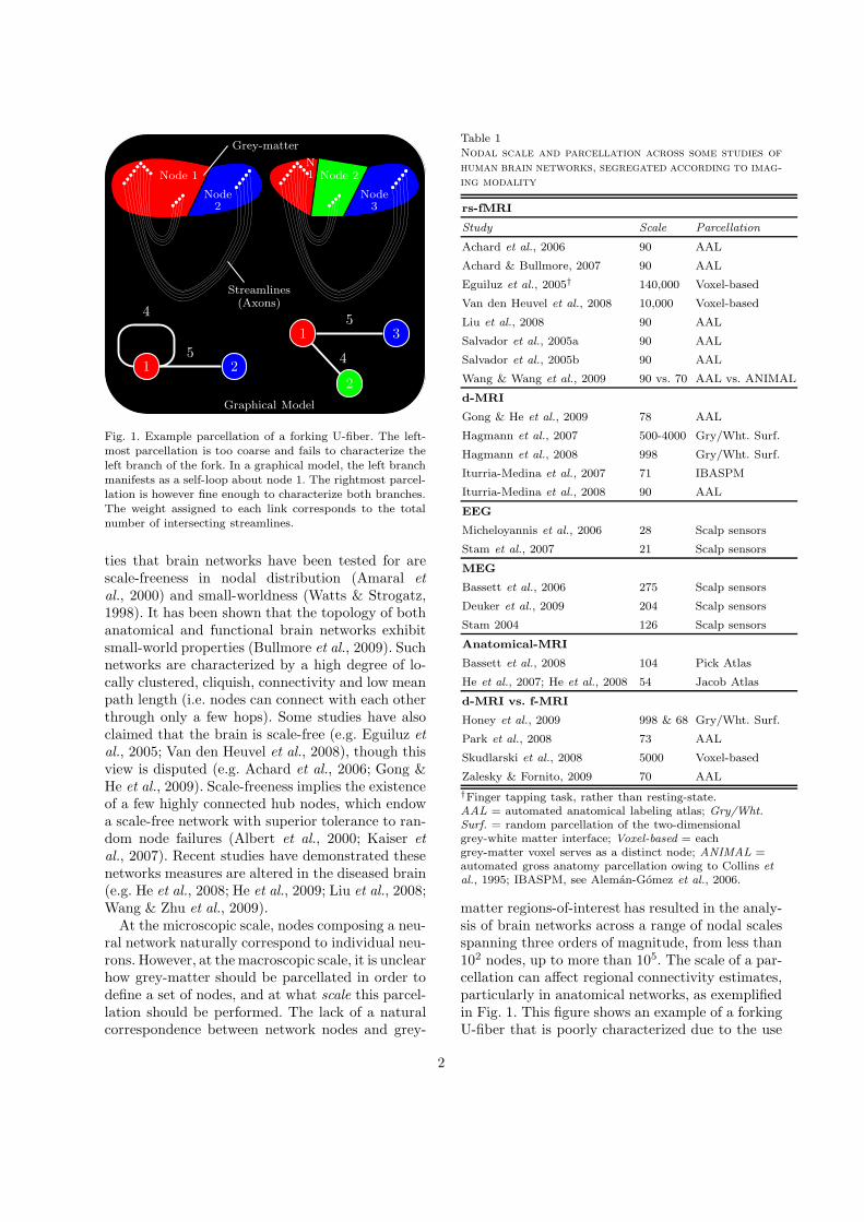
Fig. 1. Example parcellation of a forking U-fiber. The left-most parcellation is too coarse and fails to characterize theleft branch of the fork. In a graphical model, the left branchmanifests as a self-loop about node 1. The rightmost parcel-lation is however fine enough to characterize both branches.The weight assigned to each link corresponds to the totalnumber of intersecting streamlines.
ties that brain networks have been tested for arescale-freeness in nodal distribution (Amaral et
al., 2000) and small-worldness (Watts & Strogatz,1998). It has been shown that the topology of bothanatomical and functional brain networks exhibitsmall-world properties (Bullmore et al., 2009). Suchnetworks are characterized by a high degree of lo-cally clustered, cliquish, connectivity and low meanpath length (i.e. nodes can connect with each otherthrough only a few hops). Some studies have alsoclaimed that the brain is scale-free (e.g. Eguiluz et
al., 2005; Van den Heuvel et al., 2008), though thisview is disputed (e.g. Achard et al., 2006; Gong &He et al., 2009). Scale-freeness implies the existenceof a few highly connected hub nodes, which endowa scale-free network with superior tolerance to ran-dom node failures (Albert et al., 2000; Kaiser et
al., 2007). Recent studies have demonstrated thesenetworks measures are altered in the diseased brain(e.g. He et al., 2008; He et al., 2009; Liu et al., 2008;Wang & Zhu et al., 2009).
At the microscopic scale, nodes composing a neu-ral network naturally correspond to individual neu-rons. However, at the macroscopic scale, it is unclearhow grey-matter should be parcellated in order todefine a set of nodes, and at what scale this parcel-lation should be performed. The lack of a naturalcorrespondence between network nodes and grey-
Table 1Nodal scale and parcellation across some studies of
human brain networks, segregated according to imag-ing modality
rs-fMRI
Study Scale Parcellation
Achard et al., 2006 90 AAL
Achard & Bullmore, 2007 90 AAL
Eguiluz et al., 2005† 140,000 Voxel-based
Van den Heuvel et al., 2008 10,000 Voxel-based
Liu et al., 2008 90 AAL
Salvador et al., 2005a 90 AAL
Salvador et al., 2005b 90 AAL
Wang & Wang et al., 2009 90 vs. 70 AAL vs. ANIMAL
d-MRI
Gong & He et al., 2009 78 AAL
Hagmann et al., 2007 500-4000 Gry/Wht. Surf.
Hagmann et al., 2008 998 Gry/Wht. Surf.
Iturria-Medina et al., 2007 71 IBASPM
Iturria-Medina et al., 2008 90 AAL
EEG
Micheloyannis et al., 2006 28 Scalp sensors
Stam et al., 2007 21 Scalp sensors
MEG
Bassett et al., 2006 275 Scalp sensors
Deuker et al., 2009 204 Scalp sensors
Stam 2004 126 Scalp sensors
Anatomical-MRI
Bassett et al., 2008 104 Pick Atlas
He et al., 2007; He et al., 2008 54 Jacob Atlas
d-MRI vs. f-MRI
Honey et al., 2009 998 & 68 Gry/Wht. Surf.
Park et al., 2008 73 AAL
Skudlarski et al., 2008 5000 Voxel-based
Zalesky & Fornito, 2009 70 AAL
†Finger tapping task, rather than resting-state.AAL = automated anatomical labeling atlas; Gry/Wht.Surf. = random parcellation of the two-dimensionalgrey-white matter interface; Voxel-based = eachgrey-matter voxel serves as a distinct node; ANIMAL =automated gross anatomy parcellation owing to Collins etal., 1995; IBASPM, see Aleman-Gomez et al., 2006.
matter regions-of-interest has resulted in the analy-sis of brain networks across a range of nodal scalesspanning three orders of magnitude, from less than102 nodes, up to more than 105. The scale of a par-cellation can affect regional connectivity estimates,particularly in anatomical networks, as exemplifiedin Fig. 1. This figure shows an example of a forkingU-fiber that is poorly characterized due to the use
2
of a too coarse parcellation.Most studies have utilized a subset of the 90 non-
cerebellar regions-of-interest composing the auto-mated anatomical labeling (AAL) parcellation at-las (Tzourio-Mazoyer et al., 2002) to serve as nodes(see Table 1). In the case of functional connectiv-ity, Wang & Wang et al., 2009 statistically testeddifferences in the topological properties of an AAL-based network with a network based on an 70-nodeparcellation. While both networks exhibited robustsmall-world attributes and an exponentially trun-cated power law degree distribution, several topo-logical parameters were found to exhibit significantvariations across the two networks.
The substantial disparity in parcellation scalesacross different studies raises a question: Does scale
matter? Since an underlying neuronal/axonal net-work is not necessarily endowed with the same prop-erties as its macroscopic approximation, do claimsof the form “human brain network shown to exhibittopological property X” need to be interpreted withrespect to scale? For example, the discrepancy be-tween Eguiluz et al., 2005; Van den Heuvel et al.,2008 versus Achard et al., 2006; Gong & He et al.,2009 (i.e. power law nodal distribution versus expo-nentially truncated power law) may be attributableto the orders of magnitude difference in scales con-sidered.
This paper seeks to systematically evaluate thedependence of whole-brain anatomical networksover a range of nodal scales, a variety of grey-matterparcellations as well as different diffusion-MRI ac-quisition protocols. To this end, networks were ana-lyzed across scales ranging from 100 to 4000 nodes.For each scale, 100 random parcellations of grey-matter were generated. Two distinct tractographicmethods were then used to determine which pairsof nodes were anatomically connected.
A variety of local and global topological propertieswere computed for each of the 100 networks, includ-ing small-worldness, path length, clustering coeffi-cient, nodal degree distribution, efficiency and be-tweenness centrality. The variation of each topolog-ical parameter across the 100 networks was then as-sessed to evaluate the discrepancy in parameter es-timates that can be solely attributable to the choiceof parcellation. Quantifying parcellation-driven dis-crepancies is important because the choice of par-cellation is usually arbitrary or random.
It was found that topological properties varymarkedly with scale. For example, if one experi-menter uses the AAL template, while another uses
a random 4000-node template, the value of small-worldness measured by the two experimenters willbe discrepant by approximately 95% (σAAL = 1.9vs. σ4000 = 53.6 ± 2.2). Although small-world at-tributes were found at all scales, the extent of small-worldness was found to increase as scale is madefiner, resulting from a large increase in clustering.Exponential nodal degree distributions were alsofound at all scales. These findings suggest scale doesnot matter if the experimenter simply seeks a yes/nodetermination about whether or not a network issmall-world or scale-free, but scale does matter ifthe experimenter seeks to quantify the extent towhich the network exhibits these topological prop-erties. The variation in topological properties fornetworks of the same scale, but with different nodalparcellations was found to be more subtle (< 3%).
2. Methods
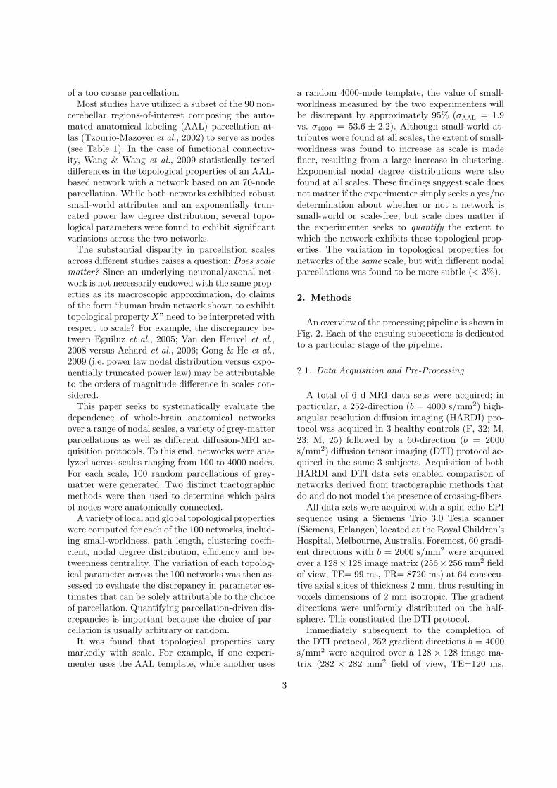
An overview of the processing pipeline is shown inFig. 2. Each of the ensuing subsections is dedicatedto a particular stage of the pipeline.
2.1. Data Acquisition and Pre-Processing
A total of 6 d-MRI data sets were acquired; inparticular, a 252-direction (b = 4000 s/mm2) high-angular resolution diffusion imaging (HARDI) pro-tocol was acquired in 3 healthy controls (F, 32; M,23; M, 25) followed by a 60-direction (b = 2000s/mm2) diffusion tensor imaging (DTI) protocol ac-quired in the same 3 subjects. Acquisition of bothHARDI and DTI data sets enabled comparison ofnetworks derived from tractographic methods thatdo and do not model the presence of crossing-fibers.
All data sets were acquired with a spin-echo EPIsequence using a Siemens Trio 3.0 Tesla scanner(Siemens, Erlangen) located at the Royal Children’sHospital, Melbourne, Australia. Foremost, 60 gradi-ent directions with b = 2000 s/mm2 were acquiredover a 128× 128 image matrix (256× 256 mm2 fieldof view, TE= 99 ms, TR= 8720 ms) at 64 consecu-tive axial slices of thickness 2 mm, thus resulting invoxels dimensions of 2 mm isotropic. The gradientdirections were uniformly distributed on the half-sphere. This constituted the DTI protocol.
Immediately subsequent to the completion ofthe DTI protocol, 252 gradient directions b = 4000s/mm2 were acquired over a 128 × 128 image ma-trix (282 × 282 mm2 field of view, TE=120 ms,
3
N-node parcellationN × N connectivity
matrixBinarize
Whole-braintractography
bb
bb
bb
bb
bb
bb
bbbb
bb b
b
bb
bb
bb
bb
bb
bb
bb
bb
bbbb
bb
bb
bb
bb
bb bb
bb
bb bb
bb
bb
bb
bb bb
bb
bbbbbb
bb bbbb
bb
bb
bb
bb
Whole brain network
DTI
HARDI
1: do whole-brain tractography2: for Subject = 1, 2, 3 do
3: for N = 82(AAL), 100, 500, 1000, 2000, 3000, 4000 do
4: for 100 random parcellations do
5: 1. Generate N-node parcellation6: 2. Populate N × N connectivity matrix7: 3. Threshold and binarize8: 4. Compute network metrics9: end for
10: end for
11: end for
Fig. 2. An overview of the processing pipeline. The example network shown corresponds to DTI tractography in subject 1 andthe 82-node AAL parcellation. The adjacency matrix is ordered such that all left-hemisphere nodes occupy the first 41 rows.Therefore, the two strongly connected sub-blocks along the diagonal exclusively correspond to intra-hemispheric connectivity,while the two off-diagonal blocks correspond to inter-hemispheric connectivity.
TR=7550ms) at 48 consecutive axial slices of thick-ness 2.2 mm, thus resulting in voxel dimensionsof 2.2 mm isotropic. The gradient directions wereobtained from the vertices of a fivefold tesselatedicosahedron projected onto the sphere. This consti-tuted the HARDI protocol, which was modeled onthe protocol developed in Tuch, 2004.
Several T2 non-diffusion weighted images were ac-quired at regular intervals during both protocols.The total time of acquisition per subject was approx-imately 40 mins. The mean SNR of the diffusion-weighted images was 27.6± 0.8 for the DTI acquisi-tion and 14.3± 0.4 for HARDI, where the standarddeviation was computed over all diffusion weightedimages.
To correct for slight head motion, each diffusionweighted image was registered to a representative T2
image using a rigid-body transform. Each represen-tative T2 image was then registered to MNI space us-ing a 12-parameter affine transform, and the trans-form was stored for later use. The diffusion weightedimages remained in native space. Registration wasperformed using the algorithm in Jenkinson et al.,2002.
2.2. Parcellation
Grey-matter was randomly parcellated into Ncontiguous regions-of-interest using a simple parcel-lation algorithm that was particularly developed forthis purpose. Each region-of-interest was requiredto serve as a distinct node (vertex) in a graphicalbrain model.
The parcellation algorithm was developed to min-imize the variation in nodal volume and was per-formed at voxel resolution. The value of N and abinary grey-matter mask (binarized AAL template)was provided as input to the algorithm.
The algorithm operates as follows: N grey-matterseed voxels are chosen at random, each of which cor-responds to the first voxel to be classified as belong-ing to each of the N nodes. All other grey-mattervoxels remain unclassified. The strategy is to incre-mentally ‘grow’ each node voxel-by-voxel until ev-ery grey-matter matter voxel has been assigned toexactly one node. At each iteration of the growthphase, a new voxel is assigned to the node with thesmallest volume. If two or more nodes are of equally
4
All Streamlines Culled Streamlines Usable Streamlines
HA
RD
ID
TI
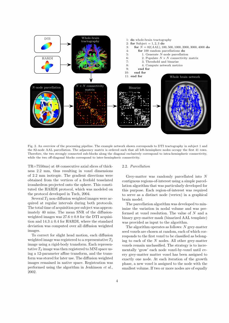
Fig. 3. The set of all, culled and usable streamlines. Streamlines representing the cortico-spinal tract and cerebellum wereculled. Streamlines less than 5 mm in length (prevalent in HARDI) were considered spurious and also culled. The set ofusable streamlines characterize cortico-cortical connectivity. Axial orientation: bottom of page is posterior. Coronal orientation:coming out of page is anterior.
small volume, one is chosen randomly. The new voxelthat is assigned at each iteration is selected so thatthe surface area (i.e. voxel faces) between it and thechosen node is maximal. A voxel cannot be assignedto a node with which it shares no surface area. Iftwo or more voxels are equally strong neighbors, thevoxel that is closest in distance to the current cen-ter of mass of the node is chosen. Any further tiesbetween voxels are broken randomly. Note that thegrowth of a node may be stunted if all the voxelswith which it shares a surface have already been as-signed to other nodes.
Akin to Hagmann et al., 2007, each node wasconstrained to lie within the periphery of one andonly one AAL region-of-interest. This constraintprecluded the formation of nonsensical nodes, suchas nodes that encompass both hemispheres. To en-force this constraint, the parcellation algorithm wasinvoked separately for each AAL region-of-interest.In particular, the proportion of streamline end-points residing in each AAL region-of-interest wasfirst tallied. An AAL region-of-interest comprising
a proportion p of the total number of endpoints wasthen parcellated into pN nodes. This ensured morenodes were assigned to regions-of-interest at whichmany axonal pathways terminate. See Appendix forpseudocode of the entire parcellation algorithm.
To serve as a grey-matter mask, an 82-nodeversion of the AAL template was binarized (i.e.subcortical nuclei and cerebellum were omitted).The standard AAL template comprises 116 nodes;however, all cerebellar and sub-cortical regions-of-interest were omitted because the HARDI acquisi-tion yielded only partial coverage of the cerebellum,and accurate grey-matter segmentation in subcor-tical regions can be problematic. Since the AALincorporates significant portions of white-matter,this template was contracted by a few voxels inregions where excessive non-cortical coverage wasevident. This contracted AAL-based binary grey-matter mask was registered to native space usingthe inverse of the transforms stored during the pre-processing stage. Since the aim herein is to charac-terize topological attributes as a distribution across
5

all random parcellations of a fixed scale, N , it wasnot necessary to ensure the same nodal parcellationwas used for each subject. It was therefore possibleto perform parcellation in native space.
2.3. Tractography
For each DTI acquisition, a tensor was fitted toeach voxel using weighted linear least squares (Sal-vador et al., 2005). The orientation of the eigen-vector with largest eigenvalue was assumed to cor-respond to the local orientation of any underlyingaxonal fiber bundle. While this assumption is en-trenched in DTI studies, it is known to yield erro-neous orientations in the case of crossing fibers (Hesset al., 2006). The eigenvector with largest eigenvalueis henceforth referred to as the principal eigenvector.
For each white-matter voxel, a streamline was ini-tialized from each of the two opposing directions ofthe principal eigenvector. Each streamline was prop-agated in fixed increments of 1 mm using the FACTalgorithm (Mori et al., 1999). Propagation was ter-minated if either a minimum angle threshold of 50◦
was violated or if a voxel was encountered with frac-tional anisotropy below 0.2. At each increment, thedirection of propagation was parallel to the orienta-tion of the eigenvector closest to the current stream-line endpoint. In subsequent analysis, the two oppos-ing streamlines initialized from each white-mattervoxel were joined at their point of initialization andconsidered to be a single streamline. The coordinatesof each streamline were stored for later use.
For each HARDI acquisition, the higher angularresolution and higher gradient strength enabled fit-ting an orientation distribution function (ODF) toeach voxel. Fitting an ODF can potentially capturethe presence of multiple fiber orientations. An ODFwas analytically fitted to each voxel using q-ballreconstruction with spherical harmonic basis func-tions (Hess et al., 2006). The appeal of q-ball recon-struction (Tuch, 2004) relative to alternative ODFreconstruction techniques such as spherical decon-volution (Tournier et al., 2004) is that q-ball is modelfree and thus does not require estimation of a re-sponse function.
For tractographic purposes, each ODF was dis-cretized along 181 directions spanning the half-sphere, yielding an angular sampling resolution of10.85◦ ± 0.97◦. Local maxima of each discretizedODF were then computed and assumed to corre-spond to the local orientation of any underlying
axonal fiber bundles. For each white-matter voxel,a streamline was initialized from each of the two op-posing directions of each local maxima. Streamlineswere propagated using precisely the same algorithmand termination criteria used for DTI tractography.In cases of multiple local maxima, the direction ofpropagation was chosen to proceed parallel to theparticular local maximum which was most closelyaligned with the current streamline direction. Theclaimed advantage of this tractographic approach(e.g. Hagmann et al., 2007) relative to conventionalDTI tractography is that streamlines can accuratelynavigate through fiber intersections and other com-plex fiber geometries that are poorly modeled witha single compartment fit.
While several alternative tractographic methodshave been customized to network mapping (e.g.Hagmann et al., 2007; Jbabdi et al., 2007; Iturria-Medina et al., 2007; Zalesky, 2008; Zalesky & For-nito, 2009), this study utilized the DTI and HARDIversions of FACT streamline tracking (Mori et al.,1999) described above. Local greediness is a keydisadvantage of streamline tracking that has beenshown to obstruct the reconstruction of long fiberbundles (e.g. transcallosal pathways) due to noisecorruption (Zalesky, 2008). While globally opti-mal approaches address this disadvantage, they aremore computationally demanding.
Tractographic maps were viewed with TrackVis
(http://www.trackvis.org).
2.4. Graph Construction
Graph construction involved utilizing tracto-graphic results and an N -node parcellation as inputto populate an N × N connectivity matrix, for-mally known as an adjacency matrix. An adjacencymatrix completely specifies the structure of a graphand is denoted herein as A.
A streamline was considered usable if and only if itintersected grey-matter. Any unusable streamlineswere culled from the set of all streamlines and givenno further consideration. Specifically, any stream-line that was wholly constrained to white-matter,the sub-cortex, the cerebellum or a combinationthereof was culled. Culling is a necessary step toeliminate spurious streamlines that do not intercon-nect distinct grey-matter regions. Streamlines thatwere less than 5 mm in length were also culled. Fig.3 shows the set of all, culled and usable streamlines.
Table 2 shows that while HARDI tractography
6
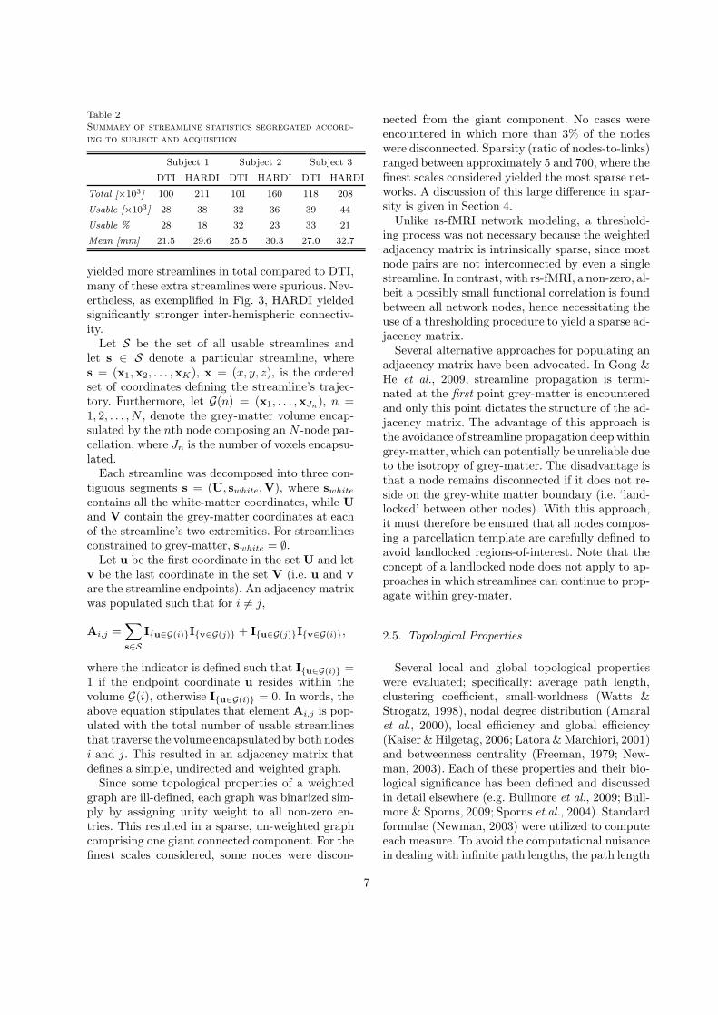
Table 2Summary of streamline statistics segregated accord-
ing to subject and acquisition
Subject 1 Subject 2 Subject 3
DTI HARDI DTI HARDI DTI HARDI
Total [×103] 100 211 101 160 118 208
Usable [×103] 28 38 32 36 39 44
Usable % 28 18 32 23 33 21
Mean [mm] 21.5 29.6 25.5 30.3 27.0 32.7
yielded more streamlines in total compared to DTI,many of these extra streamlines were spurious. Nev-ertheless, as exemplified in Fig. 3, HARDI yieldedsignificantly stronger inter-hemispheric connectiv-ity.
Let S be the set of all usable streamlines andlet s ∈ S denote a particular streamline, wheres = (x1,x2, . . . ,xK), x = (x, y, z), is the orderedset of coordinates defining the streamline’s trajec-tory. Furthermore, let G(n) = (x1, . . . ,xJn
), n =1, 2, . . . , N , denote the grey-matter volume encap-sulated by the nth node composing an N -node par-cellation, where Jn is the number of voxels encapsu-lated.
Each streamline was decomposed into three con-tiguous segments s = (U, swhite,V), where swhite
contains all the white-matter coordinates, while U
and V contain the grey-matter coordinates at eachof the streamline’s two extremities. For streamlinesconstrained to grey-matter, swhite = ∅.
Let u be the first coordinate in the set U and letv be the last coordinate in the set V (i.e. u and v
are the streamline endpoints). An adjacency matrixwas populated such that for i 6= j,
Ai,j =∑
s∈S
I{u∈G(i)}I{v∈G(j)} + I{u∈G(j)}I{v∈G(i)},
where the indicator is defined such that I{u∈G(i)} =1 if the endpoint coordinate u resides within thevolume G(i), otherwise I{u∈G(i)} = 0. In words, theabove equation stipulates that element Ai,j is pop-ulated with the total number of usable streamlinesthat traverse the volume encapsulated by both nodesi and j. This resulted in an adjacency matrix thatdefines a simple, undirected and weighted graph.
Since some topological properties of a weightedgraph are ill-defined, each graph was binarized sim-ply by assigning unity weight to all non-zero en-tries. This resulted in a sparse, un-weighted graphcomprising one giant connected component. For thefinest scales considered, some nodes were discon-
nected from the giant component. No cases wereencountered in which more than 3% of the nodeswere disconnected. Sparsity (ratio of nodes-to-links)ranged between approximately 5 and 700, where thefinest scales considered yielded the most sparse net-works. A discussion of this large difference in spar-sity is given in Section 4.
Unlike rs-fMRI network modeling, a threshold-ing process was not necessary because the weightedadjacency matrix is intrinsically sparse, since mostnode pairs are not interconnected by even a singlestreamline. In contrast, with rs-fMRI, a non-zero, al-beit a possibly small functional correlation is foundbetween all network nodes, hence necessitating theuse of a thresholding procedure to yield a sparse ad-jacency matrix.
Several alternative approaches for populating anadjacency matrix have been advocated. In Gong &He et al., 2009, streamline propagation is termi-nated at the first point grey-matter is encounteredand only this point dictates the structure of the ad-jacency matrix. The advantage of this approach isthe avoidance of streamline propagation deep withingrey-matter, which can potentially be unreliable dueto the isotropy of grey-matter. The disadvantage isthat a node remains disconnected if it does not re-side on the grey-white matter boundary (i.e. ‘land-locked’ between other nodes). With this approach,it must therefore be ensured that all nodes compos-ing a parcellation template are carefully defined toavoid landlocked regions-of-interest. Note that theconcept of a landlocked node does not apply to ap-proaches in which streamlines can continue to prop-agate within grey-mater.
2.5. Topological Properties
Several local and global topological propertieswere evaluated; specifically: average path length,clustering coefficient, small-worldness (Watts &Strogatz, 1998), nodal degree distribution (Amaralet al., 2000), local efficiency and global efficiency(Kaiser & Hilgetag, 2006; Latora & Marchiori, 2001)and betweenness centrality (Freeman, 1979; New-man, 2003). Each of these properties and their bio-logical significance has been defined and discussedin detail elsewhere (e.g. Bullmore et al., 2009; Bull-more & Sporns, 2009; Sporns et al., 2004). Standardformulae (Newman, 2003) were utilized to computeeach measure. To avoid the computational nuisancein dealing with infinite path lengths, the path length
7
of any node that was disconnected from the giantcomponent was set to the maximum path lengthbetween any pair of nodes in the giant component.
Let cG denote the average clustering coefficientand let lG denote the average path length of a graphG. To test for small-worldness of G, the σ-ratio, σ =γ/λ was evaluated, where γ = cG/cR, λ = lG/lRandR represents a ‘random’ graph that is equivalentto G. According to the σ-ratio, G was diagnosed assmall-world if γ > 1 and λ ≈ 1. These two conditionswere abbreviated to the single test σ > 1.
In many studies, a random graph R was consid-ered equivalent to G if and only if R and G exhibitan identical nodal degree distribution. To com-pute a random graph R satisfying this equivalencecriterion, the iterative randomization algorithmpresented in Maslov & Sneppen, 2002 or the se-quential algorithm in Bayati et al., 2007 can beinvoked. In Achard et al., 2006; Van den Heuvel et
al., 2008; Liu et al., 2008, the algorithm in Maslov &Sneppen, 2002 was reinvoked M times to computeM random graphs R1, . . . ,RM equivalent to G,thereby affording the Monte-Carlo approximationcR = 〈cR1
, . . . , cRM〉 and lR = 〈lR1
, . . . , lRM〉.
Approximating cR and lR as such was intractablefor the large graphs that were considered herein. In-stead, well-known analytical results for an equiva-lent Erdos-Renyi random graph; namely, cR = d/Nand lR = log N/ log d were used, where d denotesaverage nodal degree. The disadvantage of this ana-lytical approach is that it was necessary to relax thedefinition of equivalence between G and R; specif-ically, it was no longer insisted that G and R ex-hibit an identical nodal degree distribution, but onlyidentical average nodal degree.
We assessed the consequence of matching averagenodal degree instead of the entire degree distribu-tion by estimating the σ-ratio for a few computa-tionally tractable cases using the randomization al-gorithm devised in Bayati et al., 2007 to generate500 random graphs. This algorithm yields normaliz-ing graphs that are matched in degree distribution.It was found that matching the average nodal de-gree (i.e. Erdos-Renyi normalization) yielded a moreconservative estimate of the σ-ratio compared tomatching the entire degree distribution. Specifically,in the case of the AAL, Erdos-Renyi normalizationyielded σ = 2.6, 2.5 and 2.5 for each of the threesubjects (DTI acquisition), while matching the fulldegree distribution yielded σ = 3.0 ± 0.2, 2.9 ± 0.1and 2.7±0.1. This suggests Erdos-Renyi normaliza-tion yields a stricter definition of small-worldness.
To test for scale-freeness of a graph comprisingN nodes, the degree of each node was ranked from1, . . . , N such that the node with highest degree wasranked with the index 1 and and the node with thelowest degree was ranked with the index N . Nodalrank as a function of degree was then plotted ona set of doubly logarithmic axes. A roughly linearrank-degree plot is indicative of a scale-free degreedistribution, since a scale-free degree distribution di
is defined such that di = cy−αi , where yi is the rank
of di, and c and α are constants. Since log(di) =log(c) − α log(yi), plotting rank versus degree ondoubly logarithmic axes yields a line of slope −α.Rank-degree plots were opted for in favor of the morecommon frequency-degree plots utilized in Achardet al., 2006; Gong & He et al., 2009; Hagmann et al.,2007; Van den Heuvel et al., 2008.This is because thebinning process involved in generating a frequency-degree plot has been shown to introduce artifacts(see Liu et al., 2005).
2.6. Evaluation
The processes detailed in Sections 2.2-2.5 wererepeated 100 times for parcellations of scale N =82 (AAL), 100, 500, 1000, 2000, 3000, 4000 and foreach of the 6 acquisitions (3 HARDI and 3 DTI).Therefore, a total of 100 × 6 × 6 = 3600 networkswere mapped, represented as a graph and evaluatedfor the presence of several topological properties.
For each nodal scale, N , and for each subject, themean and standard deviation of each measure wascomputed across the 100 networks (i.e. 100 randomparcellations of the same scale). In this way, eachtopological attribute was characterized as a distri-bution across all parcellations of a fixed scale N .This distribution represents the variation of a mea-sure across different parcellations of the same scale.
Of equal importance was the variation of a mea-sure across parcellation templates of different scale.This kind of variation is useful in determining thecompatibility of the results reported in studies utiliz-ing significantly different scales, for example, Skud-larski et al., 2008 (5000-node) versus Gong & He et
al., 2009 (78-node AAL). To this end, the above de-scribed mean and standard deviation was plotted foreach global measure as a function of scale. To avoidcluttering, rather than plotting a trace for each sub-ject, the means and standard deviations were aver-aged across the 3 DTI acquisitions and separatelyacross the 3 HARDI acquisitions, thereby yielding
8
two distinct traces that enable explicit comparisonof HARDI and DTI. This across subject averagingalso assists in suppressing the effects of variation ow-ing to individual anatomical differences.
The distribution of relative error between twodistinct parcellations of the same scale was com-puted for each global measure and the mean ofthis distribution was tabulated. The distribution ofrelative error was constructed by enumerating all(
1002
)
= 4950 pairs of parcellations from the poolof 100 and computing the relative error betweeneach pair for the particular measure of interest.The mean of this distribution was then computedacross the 4950 pairs to yield the expected relativeerror at a given scale. This enables quantitativeevaluation of questions of the form: if an experi-menter computes small-worldness with respect toa particular N -node parcellation, while a secondexperimenter performs the same computation withrespect to an alternative N -node parcellation, whatis the expected difference (relative error) betweenthe values of small-worldness computed by bothexperimenters?
3. Results
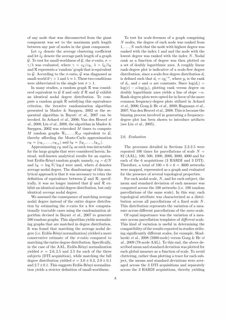
The first topological property considered wassmall-worldness, σ = γ/λ. Fig. 4 shows small-worldness plotted as a function of the number ofnetwork nodes. A distinct trace is shown for HARDI(blue) and DTI (red). The dashed lines correspondto 95% confidence intervals. Fig. 4 also shows asagittal representation of some arbitrarily chosenparcellations of varying scale.
The variability in the σ-ratio is rather small acrossparcellations of the same scale which can be assessedby the tightness of the the confidence intervals inFig. 4. In contrast, the σ-ratio exhibits a marked in-crease as nodal scale is made finer. This means finerparcellations give rise to ‘stronger’ small-world at-tributes. For example, in the case of HARDI, the σ-ratio is approximately 95% greater for a 4000-nodetemplate (σ = 53.6 ± 2.2) compared to the AAL(σ = 1.9). Therefore, a σ-ratio should be reportedand compared across studies with respect to a par-cellation scale.
For each nodal scale, the null hypothesis σDTI =σHARDI was tested using a two-tailed Student’s t-test. The standard deviations used to constructthis t-test accounted for the variation of the σ-ratioacross different parcellations of the same scale. The
Nodes (Parcellation Scale)
Small-W
orldness
,σ
DTI
HARDI
b b 95% C.I.
82 n. (AAL)
500 nodes
1000 nodes
2000 nodes
3000 nodes
4000 n.
0
10
20
30
40
50
60
70
0 1000 2000 3000 4000
bb
b
b
b
b
b
bb
b
b
b
b
b
82 nodes (AAL) 500 nodes 1000 nodes
2000 nodes 3000 nodes 4000 nodes
Fig. 4. Small-worldness (σ-ratio) as a function of the num-ber of nodes. Each data point was computed as follows: foreach acquisition and for each of 100 random parcellations,a brain network was constructed and its σ-ratio computed.The mean and standard deviation of the 100 σ-ratios wascomputed separately for each of the 6 acquisitions (3 HARDIand 3 DTI), thereby yielding 6 means and 6 standard de-
viations. Finally, the means and standard deviations wereaveraged across the 3 DTI acquisitions and separately acrossthe 3 HARDI acquisitions, thereby yielding two data points(blue and red) for each nodal scale. The null hypothesisσDTI = σHARDI was rejected with p < 10−8 for all nodalscales considered. Also shown is a sagittal representation ofsome arbitrarily chosen parcellations of varying scale.
null hypothesis σDTI = σHARDI was rejected withp < 10−8 for all nodal scales considered. Note thatthe null hypothesis was not tested for the AAL(N = 82), since there is no parcellation variation in
9
this case.Fig. 4 shows that networks owing to DTI derived
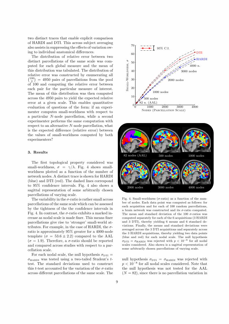
tractographic maps exhibited stronger small-worldattributes than their HARDI counterparts; in par-ticular, a relatively consistent difference of approx-imately 8.5 was evident in the σ-ratio for all scalesconsidered beyond 1000 nodes. Was this due to ahigher clustering coefficient, γ, or a shorter averagepath length λ? (Since σ = γ/λ, stronger small-worldattributes can be owing either to an increase in clus-tering, a decrease in path length or a combinationof both.) To address this question, the normalizedpath length, λ = lG/lR, and the average normal-ized clustering coefficient, γ = cG/cR, were plottedas function of the number of nodes in Fig. 5(a) and5(b), respectively. These two figures adhere to pre-cisely the same format as the plot presented in Fig.4.
To understand the effect of normalization, the‘raw’ (i.e. non-normalized) clustering coefficient, cG ,and the raw path length, lG , was also plotted inFig. 5. In this way, the raw clustering coefficient wasexplicitly decoupled from the analytically derivedcoefficient of the normalizing Erdos-Renyi randomgraph model.
Consideration of Fig. 5 shows path lengths aremarginally longer in DTI relative to HARDI, how-ever, this difference in path length is overshadowedby a significantly higher clustering clustering coef-ficient in DTI. Hence, the net effect is an increasein the σ-ratio for DTI. In other words, DTI-derivednetworks exhibit slightly longer path lengths, butsignificantly greater clustering. Therefore, withHARDI, only a few links (streamlines) need to betraversed to travel a long distance, whereas withDTI, the presence of many short links yields highclustering but also means many links must be tra-versed to travel a commensurate distance. Thisexplanation is further supported by Fig. 6, whichshows the distribution of streamline lengths forHARDI is skewed towards longer streamlines rela-tive to DTI.
It is important to remark that the expression ofstronger small-world attributes does not suggestDTI has yielded a biologically truer network modelof anatomical connectivity. The purpose herein isnot to determine which choice yields a truer networkmodel, but rather to draw attention to the fact thattopological properties can indeed vary markedlyacross different tractographic methods, acquisitionprotocols, and parcellation scales and templates.
For coarse parcellation scales, the discrepancy in
Nodes
Clust
erin
gC
oeffic
ient
DTI
HARDI
RawcG
Equivalent
RandomGraph cR
Normalizedγ = cG/cR
10-3
10-2
10-1
100
101
102
0 1000 2000 3000 4000
bb
b
b
b
bb
bbb
b
b
bb
bb
b
b
b
bb
bbb
b
b
bbb
b
b
b
b
b
b
bb
b
b
b
b
b
(a) Clustering Coefficient
Nodes
Path
Length
HARDI
DTIRawlG
EquivalentRandomGraph lR
Normalizedλ = lG/lR
0
1
2
3
4
5
6
7
8
9
10
0 1000 2000 3000 4000
bbb b b b b
bb
b
b
b
b
b
bbb b b b b
bb
b
b
b
b
b
bb
b
b
b
b
b
bb
b
b
b
b
b
(b) Path Length
Fig. 5. Average clustering coefficient and path length (raw,G, equivalent random graph, R, and normalized value). Nor-malization is with respect to an equivalent Erdos-Renyi ran-dom graph with the same number of nodes and same aver-age nodal degree. Confidence intervals were suppressed forthe intervals were too small to distinguish in most cases.The discrepancy between HARDI and DTI was statisticallysignificant with p < 10−4 for both the raw and normalizedvalues of l and c, and for all the scales considered.
clustering and path length between DTI and HARDIis negligible, however, for a 4000-node scale, this dis-crepancy is approximately 31% with respect to nor-malized clustering (111.7±4.8 versus 77.5±2.9) andapproximately 19% with respect to normalized pathlength (1.8±0.04versus 1.4±0.03). Fig. 5 shows thatin the case of HARDI, clustering and path length is
10
Streamline Length [mm]
Cumulativ
eD
istrib
utio
nFunctio
n
DTI
HARDI
0
0.2
0.4
0.6
0.8
1.0
0 20 40 60 80 100 120 140
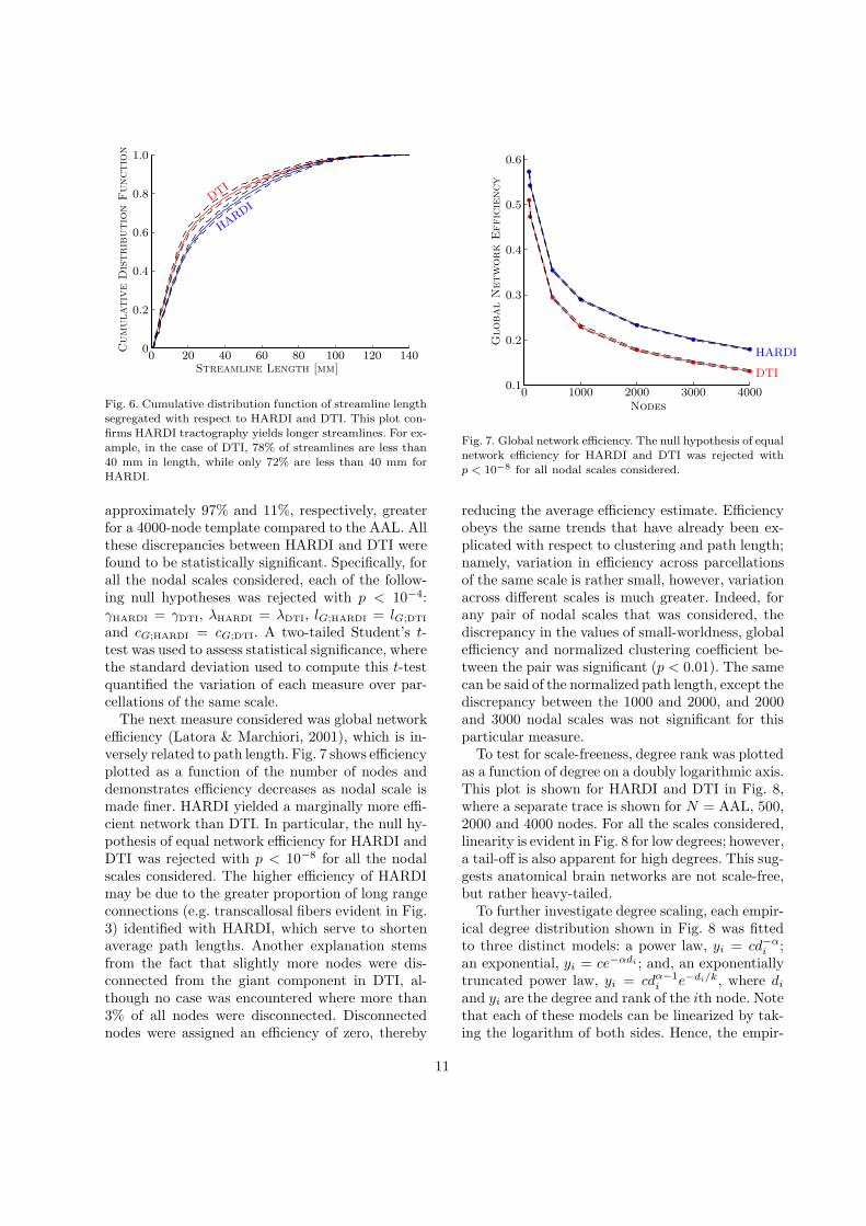
Fig. 6. Cumulative distribution function of streamline lengthsegregated with respect to HARDI and DTI. This plot con-firms HARDI tractography yields longer streamlines. For ex-ample, in the case of DTI, 78% of streamlines are less than40 mm in length, while only 72% are less than 40 mm forHARDI.
approximately 97% and 11%, respectively, greaterfor a 4000-node template compared to the AAL. Allthese discrepancies between HARDI and DTI werefound to be statistically significant. Specifically, forall the nodal scales considered, each of the follow-ing null hypotheses was rejected with p < 10−4:γHARDI = γDTI, λHARDI = λDTI, lG;HARDI = lG;DTI
and cG;HARDI = cG;DTI. A two-tailed Student’s t-test was used to assess statistical significance, wherethe standard deviation used to compute this t-testquantified the variation of each measure over par-cellations of the same scale.
The next measure considered was global networkefficiency (Latora & Marchiori, 2001), which is in-versely related to path length. Fig. 7 shows efficiencyplotted as a function of the number of nodes anddemonstrates efficiency decreases as nodal scale ismade finer. HARDI yielded a marginally more effi-cient network than DTI. In particular, the null hy-pothesis of equal network efficiency for HARDI andDTI was rejected with p < 10−8 for all the nodalscales considered. The higher efficiency of HARDImay be due to the greater proportion of long rangeconnections (e.g. transcallosal fibers evident in Fig.3) identified with HARDI, which serve to shortenaverage path lengths. Another explanation stemsfrom the fact that slightly more nodes were dis-connected from the giant component in DTI, al-though no case was encountered where more than3% of all nodes were disconnected. Disconnectednodes were assigned an efficiency of zero, thereby
Nodes
Global
Netw
ork
Effic
iency
DTI
HARDI
0.1
0.2
0.3
0.4
0.5
0.6
0 1000 2000 3000 4000
b
b
b
b
b
b
b
b
b
b
b
b
b
b
Fig. 7. Global network efficiency. The null hypothesis of equalnetwork efficiency for HARDI and DTI was rejected withp < 10−8 for all nodal scales considered.
reducing the average efficiency estimate. Efficiencyobeys the same trends that have already been ex-plicated with respect to clustering and path length;namely, variation in efficiency across parcellationsof the same scale is rather small, however, variationacross different scales is much greater. Indeed, forany pair of nodal scales that was considered, thediscrepancy in the values of small-worldness, globalefficiency and normalized clustering coefficient be-tween the pair was significant (p < 0.01). The samecan be said of the normalized path length, except thediscrepancy between the 1000 and 2000, and 2000and 3000 nodal scales was not significant for thisparticular measure.
To test for scale-freeness, degree rank was plottedas a function of degree on a doubly logarithmic axis.This plot is shown for HARDI and DTI in Fig. 8,where a separate trace is shown for N = AAL, 500,2000 and 4000 nodes. For all the scales considered,linearity is evident in Fig. 8 for low degrees; however,a tail-off is also apparent for high degrees. This sug-gests anatomical brain networks are not scale-free,but rather heavy-tailed.
To further investigate degree scaling, each empir-ical degree distribution shown in Fig. 8 was fittedto three distinct models: a power law, yi = cd−α
i ;an exponential, yi = ce−αdi ; and, an exponentiallytruncated power law, yi = cdα−1
i e−di/k, where di
and yi are the degree and rank of the ith node. Notethat each of these models can be linearized by tak-ing the logarithm of both sides. Hence, the empir-
11
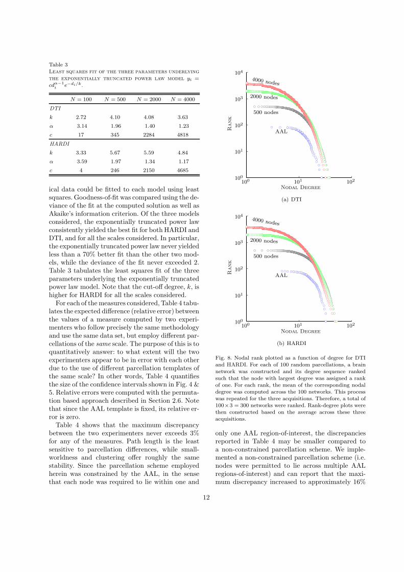
Table 3Least squares fit of the three parameters underlying
the exponentially truncated power law model yi =cdα−1
i e−di/k.
N = 100 N = 500 N = 2000 N = 4000
DTI
k 2.72 4.10 4.08 3.63
α 3.14 1.96 1.40 1.23
c 17 345 2284 4818
HARDI
k 3.33 5.67 5.59 4.84
α 3.59 1.97 1.34 1.17
c 4 246 2150 4685
ical data could be fitted to each model using leastsquares. Goodness-of-fit was compared using the de-viance of the fit at the computed solution as well asAkaike’s information criterion. Of the three modelsconsidered, the exponentially truncated power lawconsistently yielded the best fit for both HARDI andDTI, and for all the scales considered. In particular,the exponentially truncated power law never yieldedless than a 70% better fit than the other two mod-els, while the deviance of the fit never exceeded 2.Table 3 tabulates the least squares fit of the threeparameters underlying the exponentially truncatedpower law model. Note that the cut-off degree, k, ishigher for HARDI for all the scales considered.
For each of the measures considered, Table 4 tabu-lates the expected difference (relative error) betweenthe values of a measure computed by two experi-menters who follow precisely the same methodologyand use the same data set, but employ different par-cellations of the same scale. The purpose of this is toquantitatively answer: to what extent will the twoexperimenters appear to be in error with each otherdue to the use of different parcellation templates ofthe same scale? In other words, Table 4 quantifiesthe size of the confidence intervals shown in Fig. 4 &5. Relative errors were computed with the permuta-tion based approach described in Section 2.6. Notethat since the AAL template is fixed, its relative er-ror is zero.
Table 4 shows that the maximum discrepancybetween the two experimenters never exceeds 3%for any of the measures. Path length is the leastsensitive to parcellation differences, while small-worldness and clustering offer roughly the samestability. Since the parcellation scheme employedherein was constrained by the AAL, in the sensethat each node was required to lie within one and
Nodal Degree
Rank
AAL
500 nodes
2000 nodes
4000 nodes
100
101
102
103
104
100 101 102
bc
bc
bc
bcbcbcbcbcbcbcbcbcbcbcbcbcbcbcbcbcbcbcbcbcbcbcbcbcbcbcbcbcbcbcbcbcbcbcbcbcbcbcbcbcbcbcbcbcbcbcbcbcbcbc
bcbcbcbcbcbcbcbcbcbcbcbc
bcbcbcbcbcbcbcbcbcbcbcbcbcbc
bcbc
bc
bc
bc
bcbcbcbcbcbcbcbcbcbcbcbcbcbcbcbcbcbcbcbcbcbcbcbcbcbcbcbcbcbcbcbcbcbcbcbcbcbcbcbcbcbcbcbcbcbcbcbcbcbcbcbcbcbcbcbcbcbcbcbcbcbcbcbcbcbcbcbcbcbcbcbcbcbcbcbcbcbcbcbcbcbcbcbcbcbcbcbcbcbcbcbcbcbcbcbcbcbcbcbcbcbcbcbcbcbcbcbcbcbcbcbcbcbcbcbcbcbcbcbcbcbcbcbcbcbcbcbcbcbcbcbcbcbcbcbcbcbcbcbcbcbcbcbcbcbcbcbcbcbcbcbcbcbcbcbcbcbcbcbcbcbcbcbcbcbcbcbcbcbcbcbcbcbcbcbcbcbcbcbcbcbcbcbcbcbcbcbcbcbcbcbcbcbcbcbcbcbcbcbcbcbcbcbcbcbcbcbcbcbcbcbcbcbcbcbcbcbcbcbcbcbcbcbcbcbcbcbcbcbcbcbcbcbcbcbcbcbcbcbcbcbcbcbcbcbcbcbcbcbcbcbcbcbcbcbcbcbcbcbcbcbcbcbcbcbcbcbcbcbcbcbcbcbcbcbcbcbcbcbcbcbcbcbcbcbcbcbcbcbcbcbcbcbcbcbcbcbcbcbcbcbcbcbcbcbcbcbcbcbcbcbcbcbcbcbcbcbcbcbcbcbcbcbcbcbcbcbcbcbcbcbcbcbcbcbcbcbcbcbcbcbcbcbcbcbcbcbcbcbcbcbcbcbcbc
bcbcbcbcbcbcbcbcbcbcbcbcbcbcbcbcbcbcbcbcbcbcbcbcbcbcbcbcbcbcbcbcbcbcbcbcbcbcbcbcbcbcbcbcbcbcbcbcbcbcbcbcbcbcbcbcbcbcbcbcbcbcbcbcbcbcbcbcbcbcbcbcbc
bcbcbcbcbcbcbcbcbcbcbcbcbcbcbcbcbcbcbcbcbcbcbcbcbcbcbcbcbcbcbcbcbcbcbcbcbcbcbcbcbcbcbcbcbcbcbcbcbcbcbcbcbcbcbcbcbcbcbcbcbcbcbcbcbcbcbcbc
bc
bc
bc
bcbcbcbcbcbcbcbcbcbcbcbcbcbcbcbcbcbcbcbcbcbcbcbcbcbcbcbcbcbcbcbcbcbcbcbcbcbcbcbcbcbcbcbcbcbcbcbcbcbcbcbcbcbcbcbcbcbcbcbcbcbcbcbcbcbcbcbcbcbcbcbcbcbcbcbcbcbcbcbcbcbcbcbcbcbcbcbcbcbcbcbcbcbcbcbcbcbcbcbcbcbcbcbcbcbcbcbcbcbcbcbcbcbcbcbcbcbcbcbcbcbcbcbcbcbcbcbcbcbcbcbcbcbcbcbcbcbcbcbcbcbcbcbcbcbcbcbcbcbcbcbcbcbcbcbcbcbcbcbcbcbcbcbcbcbcbcbcbcbcbcbcbcbcbcbcbcbcbcbcbcbcbcbcbcbcbcbcbcbcbcbcbcbcbcbcbcbcbcbcbcbcbcbcbcbcbcbcbcbcbcbcbcbcbcbcbcbcbcbcbcbcbcbcbcbcbcbcbcbcbcbcbcbcbcbcbcbcbcbcbcbcbcbcbcbcbcbcbcbcbcbcbcbcbcbcbcbcbcbcbcbcbcbcbcbcbcbcbcbcbcbcbcbcbcbcbcbcbcbcbcbcbcbcbcbcbcbcbcbcbcbcbcbcbcbcbcbcbcbcbcbcbcbcbcbcbcbcbcbcbcbcbcbcbcbcbcbcbcbcbcbcbcbcbcbcbcbcbcbcbcbcbcbcbcbcbcbcbcbcbcbcbcbcbcbcbcbcbcbcbcbcbcbcbcbcbcbcbcbcbcbcbcbcbcbcbcbcbcbcbcbcbcbcbcbcbcbcbcbcbcbcbcbcbcbcbcbcbcbcbcbcbcbcbcbcbcbcbcbcbcbcbcbcbcbcbcbcbcbcbcbcbcbcbcbcbcbcbcbcbcbcbcbcbcbcbcbcbcbcbcbcbcbcbcbcbcbcbcbcbcbcbcbcbcbcbcbcbcbcbcbcbcbcbcbcbcbcbcbcbcbcbcbcbcbcbcbcbcbcbcbcbcbcbcbcbcbcbcbcbcbcbcbcbcbcbcbcbcbcbcbcbcbcbcbcbcbcbcbcbcbcbcbcbcbcbcbcbcbcbcbcbcbcbcbcbcbcbcbcbcbcbcbcbcbcbcbcbcbcbcbcbcbcbcbcbcbcbcbcbcbcbcbcbcbcbcbcbcbcbcbcbcbcbcbcbcbcbcbcbcbcbcbcbcbcbc
bcbcbcbcbcbcbcbcbcbcbcbcbcbcbcbcbcbcbcbcbcbcbcbcbcbcbcbcbcbcbcbcbcbcbcbcbcbcbcbcbcbcbcbcbcbcbcbcbcbcbcbcbcbcbcbcbcbcbcbcbcbcbcbcbcbcbcbcbcbcbcbcbcbcbcbcbcbcbcbcbcbcbcbcbcbcbcbcbcbcbcbcbcbcbcbcbcbcbcbcbcbcbcbcbcbcbcbcbcbcbcbcbcbcbcbcbcbcbcbcbcbcbcbcbcbcbcbcbcbcbcbcbcbcbcbcbcbcbcbcbcbcbcbcbcbcbcbcbcbcbcbcbcbcbcbcbcbcbcbcbcbcbcbcbcbcbcbcbcbcbcbcbcbcbcbcbcbcbcbcbcbcbcbcbcbcbcbcbcbcbcbcbcbcbcbcbcbcbcbcbcbcbcbcbcbcbcbcbcbcbcbcbcbcbcbcbcbcbcbcbcbcbcbcbcbcbcbcbcbcbcbcbcbcbcbcbcbcbcbcbcbcbcbcbcbcbcbcbcbcbcbcbcbcbcbcbcbcbcbcbcbcbcbcbcbcbcbcbcbcbcbcbcbcbcbcbcbcbcbcbcbcbcbcbcbcbcbcbcbcbcbcbcbcbcbcbcbcbcbcbcbcbcbcbcbcbcbcbcbcbcbcbcbcbcbcbcbcbcbcbcbcbcbcbcbcbcbcbcbcbcbcbcbcbcbcbcbcbcbcbcbcbcbcbcbcbcbcbcbcbcbcbcbcbcbcbcbcbcbcbcbcbcbcbcbcbcbcbcbcbcbcbcbcbcbcbcbcbcbcbcbcbcbcbcbcbcbcbcbcbcbcbcbcbcbcbcbcbcbcbcbcbcbcbcbcbcbcbcbcbcbcbcbcbcbcbcbcbcbcbcbcbcbcbc
bcbcbcbcbcbcbcbcbcbcbcbcbcbcbcbcbcbcbcbcbcbcbcbcbcbcbcbcbcbcbcbcbcbcbcbcbcbcbcbcbcbcbcbcbcbcbcbcbcbcbcbcbcbcbcbcbcbcbcbcbcbcbcbcbcbcbcbcbcbcbcbcbcbcbcbcbcbcbcbcbcbcbcbcbcbcbcbcbcbcbcbcbcbcbcbcbcbcbcbcbcbcbcbcbcbcbcbcbcbcbcbcbcbcbcbcbcbcbcbcbcbcbcbcbcbcbcbcbcbcbcbcbcbcbcbcbcbcbcbcbcbcbcbcbcbcbcbcbcbcbcbcbcbcbcbcbcbcbcbcbcbcbcbcbcbcbcbcbcbcbcbcbcbcbcbcbcbcbcbcbcbcbcbcbcbcbcbcbcbcbcbcbcbcbcbcbcbcbcbcbcbcbcbcbcbcbcbcbcbcbcbcbcbcbcbcbcbcbcbcbcbcbcbcbcbcbcbcbcbcbcbcbcbcbcbcbcbcbcbcbcbcbcbcbcbcbcbcbcbcbcbcbcbcbcbcbcbcbcbcbcbcbcbcbcbcbcbcbcbcbcbcbcbcbcbcbcbcbcbcbcbcbcbcbcbcbcbcbcbcbcbcbcbcbcbcbcbcbcbcbcbcbcbcbcbcbcbcbcbcbcbcbcbcbcbcbcbcbcbc
bcbcbcbcbcbcbcbcbcbcbcbcbcbcbcbcbcbcbcbcbcbcbcbcbcbcbcbcbcbcbcbcbcbcbcbcbcbcbcbcbcbcbcbcbcbcbcbcbcbcbcbcbcbcbcbcbcbcbcbcbcbcbcbcbcbcbcbcbcbcbcbcbcbcbcbcbcbcbcbcbcbcbcbcbcbcbcbcbcbcbcbcbcbcbcbcbcbcbcbcbcbcbcbcbcbcbcbcbcbcbcbcbcbcbcbcbcbcbcbcbcbcbcbcbcbcbcbcbcbcbcbcbcbcbcbcbcbcbcbcbcbcbcbcbcbcbcbcbcbcbcbcbcbcbcbcbcbcbcbcbcbcbcbcbcbcbcbcbcbcbcbcbcbcbcbcbcbcbcbcbcbcbcbcbcbcbcbcbcbcbcbcbcbcbcbcbcbcbcbcbcbcbcbcbcbcbcbcbcbcbcbcbcbcbcbcbcbcbcbcbcbcbcbcbcbcbcbcbcbcbcbcbcbcbcbcbcbcbcbcbcbcbcbcbcbcbcbcbcbcbcbcbcbcbcbcbcbcbcbcbcbcbcbcbcbcbcbc
bcbcbcbcbcbcbcbcbcbcbcbcbcbcbcbcbcbcbcbcbcbcbcbcbcbcbcbcbcbcbcbcbcbcbcbcbcbcbcbcbcbcbcbcbcbcbcbcbcbcbcbcbcbcbcbcbcbcbcbcbcbcbcbcbcbcbcbcbcbcbcbcbcbcbcbcbcbcbcbcbcbcbcbcbcbcbcbcbcbcbcbcbcbcbcbcbcbcbcbcbcbcbcbcbcbcbcbcbcbcbcbcbcbcbcbcbcbcbcbcbcbcbcbcbcbcbcbcbcbcbcbcbcbcbcbcbcbcbcbcbcbcbcbcbcbcbcbcbcbcbcbcbcbcbcbcbcbcbcbcbcbcbcbcbcbcbcbcbcbcbcbcbcbcbcbcbcbcbcbcbcbcbcbcbcbcbcbcbcbcbcbcbcbcbcbcbcbcbcbcbcbcbcbcbcbcbcbcbcbcbcbcbcbcbcbcbcbcbcbcbcbcbcbcbcbcbcbcbcbcbcbcbcbcbcbcbcbcbcbcbcbcbcbcbcbcbcbcbcbcbcbcbcbcbcbcbcbcbcbcbcbcbcbcbcbcbcbcbcbcbcbcbcbcbcbcbcbcbcbcbcbcbcbcbcbcbcbcbcbcbcbcbcbcbcbcbcbcbcbcbcbcbcbcbcbcbcbcbcbcbcbcbcbcbcbcbcbcbcbcbcbcbc
bcbcbcbcbcbcbcbcbcbcbcbcbcbcbcbcbcbcbcbcbcbcbcbcbcbcbcbcbcbcbcbcbcbcbcbcbcbcbcbcbcbcbcbcbcbcbcbcbcbcbcbcbcbcbcbcbcbcbcbcbcbcbcbcbcbcbcbcbcbcbc
bc
bc
bc
bcbcbcbcbcbcbcbcbcbcbcbcbcbcbcbcbcbcbcbcbcbcbcbcbcbcbcbcbcbcbcbcbcbcbcbcbcbcbcbcbcbcbcbcbcbcbcbcbcbcbcbcbcbcbcbcbcbcbcbcbcbcbcbcbcbcbcbcbcbcbcbcbcbcbcbcbcbcbcbcbcbcbcbcbcbcbcbcbcbcbcbcbcbcbcbcbcbcbcbcbcbcbcbcbcbcbcbcbcbcbcbcbcbcbcbcbcbcbcbcbcbcbcbcbcbcbcbcbcbcbcbcbcbcbcbcbcbcbcbcbcbcbcbcbcbcbcbcbcbcbcbcbcbcbcbcbcbcbcbcbcbcbcbcbcbcbcbcbcbcbcbcbcbcbcbcbcbcbcbcbcbcbcbcbcbcbcbcbcbcbcbcbcbcbcbcbcbcbcbcbcbcbcbcbcbcbcbcbcbcbcbcbcbcbcbcbcbcbcbcbcbcbcbcbcbcbcbcbcbcbcbcbcbcbcbcbcbcbcbcbcbcbcbcbcbcbcbcbcbcbcbcbcbcbcbcbcbcbcbcbcbcbcbcbcbcbcbcbcbcbcbcbcbcbcbcbcbcbcbcbcbcbcbcbcbcbcbcbcbcbcbcbcbcbcbcbcbcbcbcbcbcbcbcbcbcbcbcbcbcbcbcbcbcbcbcbcbcbcbcbcbcbcbcbcbcbcbcbcbcbcbcbcbcbcbcbcbcbcbcbcbcbcbcbcbcbcbcbcbcbcbcbcbcbcbcbcbcbcbcbcbcbcbcbcbcbcbcbcbcbcbcbcbcbcbcbcbcbcbcbcbcbcbcbcbcbcbcbcbcbcbcbcbcbcbcbcbcbcbcbcbcbcbcbcbcbcbcbcbcbcbcbcbcbcbcbcbcbcbcbcbcbcbcbcbcbcbcbcbcbcbcbcbcbcbcbcbcbcbcbcbcbcbcbcbcbcbcbcbcbcbcbcbcbcbcbcbcbcbcbcbcbcbcbcbcbcbcbcbcbcbcbcbcbcbcbcbcbcbcbcbcbcbcbcbcbcbcbcbcbcbcbcbcbcbcbcbcbcbcbcbcbcbcbcbcbcbcbcbcbcbcbcbcbcbcbcbcbcbcbcbcbcbcbcbcbcbcbcbcbcbcbcbcbcbcbcbcbcbcbcbcbcbcbcbcbcbcbcbcbcbcbcbcbcbcbcbcbcbcbcbcbcbcbcbcbcbcbcbcbcbcbcbcbcbcbcbcbcbcbcbcbcbcbcbcbcbcbcbcbcbcbcbcbcbcbcbcbcbcbcbcbcbcbcbcbcbcbcbcbcbcbcbcbcbcbcbcbcbcbcbcbcbcbcbcbcbcbcbcbcbcbcbcbcbcbcbcbcbcbcbcbcbcbcbcbcbcbcbcbcbcbcbcbcbcbcbcbcbcbcbcbcbcbcbcbcbcbcbcbcbcbcbcbcbcbcbcbcbcbcbcbcbcbcbcbcbcbcbcbcbcbcbcbcbcbcbcbcbcbcbcbcbcbcbcbcbcbcbcbcbcbcbcbcbcbcbcbcbcbcbcbcbcbcbcbcbcbcbcbcbcbcbcbcbcbcbcbcbcbcbcbcbcbcbcbcbcbcbcbcbcbcbcbcbcbcbcbcbcbcbcbcbcbcbcbcbcbcbcbcbcbcbcbcbcbcbcbcbcbcbcbcbcbcbcbcbcbcbcbcbcbcbcbcbcbcbcbcbcbcbcbcbcbcbcbcbcbcbcbcbcbcbcbcbcbcbcbcbcbcbcbcbcbcbcbcbcbcbcbcbcbcbcbcbcbcbcbcbcbcbcbcbcbcbcbcbcbcbcbcbcbcbcbcbcbcbcbcbcbcbcbcbcbcbcbcbcbcbcbcbcbcbcbcbcbcbcbcbcbcbcbcbcbcbcbcbcbcbcbcbcbcbcbcbcbcbcbcbcbcbcbcbcbcbcbcbcbcbcbcbcbcbcbcbcbcbcbcbcbcbcbcbcbcbcbcbcbcbcbcbcbcbcbcbcbcbcbcbcbcbcbcbcbcbcbcbcbcbcbcbcbcbcbcbcbcbcbcbcbcbcbcbcbcbcbcbcbcbcbcbcbcbcbcbcbcbcbcbcbcbcbcbcbcbcbcbcbcbcbcbcbcbcbcbcbcbcbcbcbcbcbcbcbcbcbcbcbcbcbcbcbcbcbcbcbcbcbcbcbcbcbcbcbcbcbcbcbcbcbcbcbcbcbcbcbcbcbcbcbcbcbcbcbcbcbcbcbcbcbcbcbcbcbcbcbcbcbcbcbcbcbcbcbcbcbcbcbcbcbcbcbcbcbcbcbcbcbcbcbcbcbcbcbcbcbcbcbcbcbcbcbcbcbcbcbcbcbcbcbcbcbcbcbcbcbcbcbcbcbcbcbcbcbcbcbcbcbcbcbcbcbcbcbcbcbcbcbcbcbcbcbcbcbcbcbcbcbcbcbcbcbcbcbcbcbcbcbcbcbcbcbcbcbcbcbcbcbcbcbcbcbcbcbcbcbcbcbcbcbcbcbcbcbcbcbcbcbcbcbcbcbcbcbcbcbcbcbcbcbcbcbcbcbcbcbcbcbcbcbcbcbcbcbcbcbcbcbcbcbcbcbcbcbcbcbcbcbcbcbcbcbcbcbcbcbcbcbcbcbcbcbcbcbcbcbcbcbcbcbcbcbcbcbcbcbcbcbcbcbcbcbcbcbcbcbcbcbcbcbcbcbcbcbcbcbcbcbcbcbcbcbcbcbcbcbcbcbcbcbcbcbcbcbcbcbcbcbcbcbcbcbcbcbcbcbcbcbcbcbcbcbcbcbcbcbcbcbcbcbcbcbcbcbcbcbcbcbcbcbcbcbcbcbcbcbcbcbcbcbcbcbcbcbcbcbcbcbcbcbcbcbcbcbcbcbcbcbcbcbcbcbcbcbcbcbcbcbcbcbcbcbcbcbcbcbcbcbcbcbcbcbcbcbcbcbcbcbcbcbcbcbcbcbcbcbcbcbcbcbcbcbcbcbcbcbcbcbcbcbcbcbcbcbcbcbcbcbcbcbcbcbcbcbcbcbcbcbcbcbcbcbcbcbcbcbcbcbcbcbcbcbcbcbcbcbcbcbcbc
bcbcbcbcbcbcbcbcbcbcbcbcbcbcbcbcbcbcbcbcbcbcbcbcbcbcbcbcbcbcbcbcbcbcbcbcbcbcbcbcbcbcbcbcbcbcbcbcbcbcbcbcbcbcbcbcbcbcbcbcbcbcbcbcbcbcbcbcbcbcbcbcbcbcbcbcbcbcbcbcbcbcbcbcbcbcbcbcbcbcbcbcbcbcbcbcbcbcbcbcbcbcbcbcbcbcbcbcbcbcbcbcbcbcbcbcbcbcbcbcbcbcbcbcbcbcbcbcbcbcbcbcbcbcbcbcbcbcbcbcbcbcbcbcbcbcbcbcbcbcbcbcbcbcbcbcbcbcbcbcbcbcbcbcbcbcbcbcbcbcbcbcbcbcbcbcbcbcbcbcbcbcbcbcbcbcbcbcbcbcbcbcbcbcbcbcbcbcbcbcbcbcbcbcbcbcbcbcbcbcbcbcbcbcbcbcbcbcbcbcbcbcbcbcbcbcbcbcbcbcbcbcbcbcbcbcbcbcbcbcbcbcbcbcbcbcbcbcbcbcbcbcbcbcbcbcbcbcbcbcbcbcbcbcbcbcbcbcbcbcbcbcbcbcbcbcbcbcbcbcbcbcbcbcbcbcbcbcbcbcbcbcbcbcbcbcbcbcbcbcbcbcbcbcbcbcbcbcbcbcbcbcbcbcbcbcbcbcbcbcbcbcbcbcbcbcbcbcbcbcbcbcbcbcbcbcbcbcbcbcbcbcbcbcbcbcbcbcbcbcbcbcbcbcbcbcbcbcbcbcbcbcbcbcbcbcbcbcbcbcbcbcbcbcbcbcbcbcbcbcbcbcbcbcbcbcbcbcbcbcbcbcbcbcbcbcbcbcbcbcbcbcbcbcbcbcbcbcbcbcbcbcbcbcbcbcbcbcbcbcbcbcbcbcbcbcbcbcbcbcbcbcbcbcbcbcbcbcbcbcbcbcbcbcbcbcbcbcbcbcbcbcbcbcbcbcbcbcbcbcbcbcbc
bcbcbcbcbcbcbcbcbcbcbcbcbcbcbcbcbcbcbcbcbcbcbcbcbcbcbcbcbcbcbcbcbcbcbcbcbcbcbcbcbcbcbcbcbcbcbcbcbcbcbcbcbcbcbcbcbcbcbcbcbcbcbcbcbcbcbcbcbcbcbcbcbcbcbcbcbcbcbcbcbcbcbcbcbcbcbcbcbcbcbcbcbcbcbcbcbcbcbcbcbcbcbcbcbcbcbcbcbcbcbcbcbcbcbcbcbcbcbcbcbcbcbcbcbcbcbcbcbcbcbcbcbcbcbcbcbcbcbcbcbcbcbcbcbcbcbcbcbcbcbcbcbcbcbcbcbcbcbcbcbcbcbcbcbcbcbcbcbcbcbcbcbcbcbcbcbcbcbcbcbcbcbcbcbcbcbcbcbcbcbcbcbcbcbcbcbcbcbcbcbcbcbcbcbcbcbcbcbcbcbcbcbcbcbcbcbcbcbcbcbcbcbcbcbcbcbcbcbcbcbcbcbcbcbcbcbcbcbcbcbcbcbcbcbcbcbcbcbcbcbcbcbcbcbcbcbcbcbcbcbcbcbcbcbcbcbcbcbcbcbcbcbcbcbcbcbcbcbcbcbcbcbcbcbcbcbcbcbcbcbcbcbcbcbcbcbcbcbcbcbcbcbcbcbcbcbcbcbcbcbcbcbcbcbcbcbcbcbcbcbcbcbcbcbcbcbcbcbcbcbcbcbcbcbcbcbcbcbcbcbcbcbcbcbcbcbcbcbcbcbcbcbcbcbcbcbcbcbcbcbcbcbcbcbcbcbcbcbcbcbcbcbcbcbcbcbcbcbcbcbcbcbcbcbcbcbcbcbc
bcbcbcbcbcbcbcbcbcbcbcbcbcbcbcbcbcbcbcbcbcbcbcbcbcbcbcbcbcbcbcbcbcbcbcbcbcbcbcbcbcbcbcbcbcbcbcbcbcbcbcbcbcbcbcbcbcbcbcbcbcbcbcbcbcbcbcbcbcbcbcbcbcbcbcbcbcbcbcbcbcbcbcbcbcbcbcbcbcbcbcbcbcbcbcbcbcbcbcbcbcbcbcbcbcbcbcbcbcbcbcbcbcbcbcbcbcbcbcbcbcbcbcbcbcbcbcbcbcbcbcbcbcbcbcbcbcbcbcbcbcbcbcbcbcbcbcbcbcbcbcbcbcbcbcbcbcbcbcbcbcbcbcbcbcbcbcbcbcbcbcbcbcbcbcbcbcbcbcbcbcbcbcbcbcbcbcbcbcbcbcbcbcbcbcbcbcbcbcbcbcbcbcbcbcbcbcbcbcbcbcbcbcbcbcbcbcbcbcbcbcbcbcbcbcbcbcbcbcbcbcbcbcbcbcbcbcbcbcbcbcbcbcbcbcbcbcbcbcbcbcbcbcbcbcbcbcbcbcbcbcbcbcbcbcbcbcbcbcbcbcbcbcbcbcbcbcbcbcbcbcbcbcbcbcbcbcbcbcbcbcbcbcbcbcbcbcbcbcbcbcbcbcbcbcbcbcbcbcbcbcbcbcbcbcbcbcbcbcbcbcbcbcbcbcbcbcbcbcbcbcbcbcbcbcbcbcbcbcbcbcbcbcbcbcbcbcbcbcbcbcbcbcbcbcbcbcbcbcbcbcbcbcbcbcbcbcbcbcbcbcbcbcbcbcbcbcbcbcbcbcbcbcbcbcbcbcbcbcbcbcbcbcbcbcbcbcbcbcbcbcbcbcbcbcbcbcbcbcbcbcbcbcbcbcbcbcbcbcbcbcbcbcbcbcbcbcbcbcbcbcbcbcbcbcbcbcbcbcbcbcbcbcbcbcbcbcbcbcbcbcbcbcbcbcbcbcbcbcbcbcbcbcbcbcbcbcbc
bcbcbcbcbcbcbcbcbcbcbcbcbcbcbcbcbcbcbcbcbcbcbcbcbcbcbcbcbcbcbcbcbcbcbcbcbcbcbcbcbcbcbcbcbcbcbcbcbcbcbcbcbcbcbcbcbcbcbcbcbcbcbcbcbcbcbcbcbcbcbcbcbcbcbcbcbcbcbcbcbcbcbcbcbcbcbcbcbcbcbcbcbcbcbcbcbcbcbcbcbcbcbcbcbcbcbcbcbcbcbcbcbcbcbcbcbcbcbcbcbcbcbcbcbcbcbcbcbcbcbcbcbcbcbcbcbcbcbcbcbcbcbcbcbcbcbcbcbcbcbcbcbcbcbcbcbcbcbcbcbcbcbcbcbcbcbcbcbcbcbcbcbcbcbcbcbcbcbcbcbcbcbcbcbcbcbcbcbcbcbcbcbcbcbcbcbcbcbcbcbcbcbcbcbcbcbcbcbcbcbcbcbcbcbcbcbcbcbcbcbcbcbcbcbcbcbcbcbcbcbcbcbcbcbcbcbcbcbcbcbcbcbcbcbcbcbcbcbcbcbcbcbcbcbcbcbcbcbcbcbcbcbcbcbcbcbcbcbcbcbcbcbcbcbcbcbcbcbcbcbcbcbcbcbcbcbcbcbcbcbcbcbcbcbcbcbcbcbcbcbcbcbcbcbcbcbcbcbcbcbcbcbcbcbcbcbcbcbcbcbcbcbcbcbcbcbcbcbcbcbcbcbcbcbcbcbcbcbcbcbcbcbcbcbcbcbcbcbcbcbcbcbcbcbcbcbcbcbcbcbcbcbcbcbcbcbcbcbcbcbcbcbcbcbcbcbcbcbcbcbcbcbcbcbcbcbcbcbcbcbcbcbcbcbcbcbcbcbcbcbcbcbcbcbcbcbcbcbcbcbcbcbcbcbcbcbcbcbcbcbcbcbcbcbcbcbcbcbcbcbcbcbcbcbcbcbcbcbcbcbcbcbcbcbcbcbcbcbcbcbcbcbcbcbcbcbcbcbcbcbcbcbcbcbcbcbcbcbcbcbcbcbcbcbcbcbcbcbcbcbcbcbcbcbcbcbcbcbcbcbcbcbcbcbcbcbcbcbcbcbcbcbcbcbcbcbcbcbcbcbcbcbcbcbcbcbcbcbcbcbcbcbcbcbcbcbcbcbcbcbcbcbcbcbcbcbcbcbcbcbcbcbcbcbcbcbcbcbcbcbcbcbcbcbcbcbcbcbcbcbcbcbcbc
bcbcbcbcbcbcbcbcbcbcbcbcbcbcbcbcbcbcbcbcbcbcbcbcbcbcbcbcbcbcbcbcbcbcbcbcbcbcbcbcbcbcbcbcbcbcbcbcbcbcbcbcbcbcbcbcbcbcbcbcbcbcbcbcbcbcbcbcbcbcbcbcbcbcbcbcbcbcbcbcbcbcbcbcbcbcbcbcbcbcbcbcbcbcbcbcbcbcbcbcbcbcbcbcbcbcbcbcbcbcbcbcbcbcbcbcbcbcbcbcbcbcbcbcbcbcbcbcbcbcbcbcbcbcbcbcbcbcbcbcbcbcbcbcbcbcbcbcbcbcbcbcbcbcbcbcbcbcbcbcbcbcbcbcbcbcbcbcbcbcbcbcbcbcbcbcbcbcbcbcbcbcbcbcbcbcbcbcbcbcbcbcbcbcbcbcbcbcbcbcbcbcbcbcbcbcbcbcbcbcbcbcbcbcbcbcbcbcbcbcbcbcbcbcbcbcbcbcbcbcbcbcbcbcbcbcbcbcbcbcbcbcbcbcbcbcbcbcbcbcbcbcbcbcbcbcbcbcbcbcbcbcbcbcbcbcbcbcbcbcbcbcbcbcbcbcbcbcbcbcbcbcbcbcbcbcbcbcbcbcbcbcbcbcbcbcbcbcbcbcbcbcbcbcbcbcbcbcbcbcbcbcbcbcbcbcbcbcbcbcbcbcbcbcbcbcbcbcbcbcbcbcbcbcbcbcbcbcbcbcbcbcbcbcbcbcbcbcbcbcbcbcbcbcbcbcbcbcbcbcbcbcbcbcbcbcbcbcbcbcbcbcbcbcbcbcbcbcbcbcbcbcbcbcbcbcbcbcbcbcbcbcbcbcbcbcbcbcbcbcbcbcbcbcbcbcbcbcbcbcbcbcbcbcbcbcbcbcbcbcbcbcbcbcbcbcbcbcbcbcbcbcbcbcbcbcbcbcbcbcbcbcbcbcbcbcbcbcbcbcbcbcbcbcbcbcbcbcbcbcbcbcbcbcbcbcbcbcbcbcbcbcbcbcbcbcbcbcbcbcbcbcbcbcbcbcbcbcbcbcbcbcbcbcbcbcbcbcbcbcbcbcbcbcbcbcbcbcbcbcbcbcbcbcbcbcbcbcbcbcbcbcbcbcbcbcbcbcbcbcbcbcbcbcbcbcbcbcbcbcbcbcbcbcbcbcbcbcbcbcbcbcbcbcbcbcbcbcbcbcbcbcbcbcbcbcbcbcbcbcbcbcbcbcbcbcbcbcbcbcbcbcbcbcbcbcbcbcbcbcbcbcbcbcbcbcbcbcbcbcbcbcbcbcbc
(a) DTI
Nodal Degree
Rank
AAL
500 nodes
2000 nodes
4000 nodes
100
101
102
103
104
100 101 102
bc
bc
bc
bcbcbcbcbcbcbcbcbcbcbcbcbcbcbcbcbcbcbcbcbcbcbcbcbcbcbcbcbcbcbcbcbcbcbcbcbcbcbcbcbcbcbcbcbcbcbcbcbcbcbcbcbcbcbcbcbcbcbcbcbcbcbc
bcbcbcbcbcbcbcbcbcbcbcbcbcbcbcbc
bc
bc
bc
bcbcbcbcbcbcbcbcbcbcbcbcbcbcbcbcbcbcbcbcbcbcbcbcbcbcbcbcbcbcbcbcbcbcbcbcbcbcbcbcbcbcbcbcbcbcbcbcbcbcbcbcbcbcbcbcbcbcbcbcbcbcbcbcbcbcbcbcbcbcbcbcbcbcbcbcbcbcbcbcbcbcbcbcbcbcbcbcbcbcbcbcbcbcbcbcbcbcbcbcbcbcbcbcbcbcbcbcbcbcbcbcbcbcbcbcbcbcbcbcbcbcbcbcbcbcbcbcbcbcbcbcbcbcbcbcbcbcbcbcbcbcbcbcbcbcbcbcbcbcbcbcbcbcbcbcbcbcbcbcbcbcbcbcbcbcbcbcbcbcbcbcbcbcbcbcbcbcbcbcbcbcbcbcbcbcbcbcbcbcbcbcbcbcbcbcbcbcbcbcbcbcbcbcbcbcbcbcbcbcbcbcbcbcbcbcbcbcbcbcbcbcbcbcbcbcbcbcbcbcbcbcbcbcbcbcbcbcbcbcbcbcbcbcbcbcbcbcbcbcbcbcbcbcbcbcbcbcbcbcbcbcbcbcbcbcbcbcbcbcbcbcbcbcbcbcbcbcbcbcbcbcbcbcbcbcbcbcbcbcbcbcbcbcbcbcbcbcbcbcbcbcbcbcbcbcbcbcbcbcbcbcbcbcbcbcbcbcbcbcbcbcbc
bcbcbcbcbcbcbcbcbcbcbcbcbcbcbcbcbcbcbcbcbcbcbcbcbcbcbcbcbcbcbcbcbcbcbcbcbcbcbcbcbcbcbcbcbcbcbcbcbcbcbcbcbcbcbcbcbcbcbcbcbcbcbcbcbcbcbc
bcbcbcbcbcbcbcbcbcbcbcbcbcbcbcbcbcbcbcbcbcbcbcbcbcbcbcbcbcbcbcbcbcbcbcbcbcbcbcbcbcbcbcbcbcbcbcbcbcbcbcbcbcbcbcbcbcbcbcbcbcbcbcbcbcbcbcbcbcbcbcbcbcbcbcbcbcbcbcbc
bcbcbcbcbcbcbcbcbcbcbcbcbcbcbcbcbcbcbcbcbcbcbcbcbcbcbc
bc
bc
bc
bcbcbcbcbcbcbcbcbcbcbcbcbcbcbcbcbcbcbcbcbcbcbcbcbcbcbcbcbcbcbcbcbcbcbcbcbcbcbcbcbcbcbcbcbcbcbcbcbcbcbcbcbcbcbcbcbcbcbcbcbcbcbcbcbcbcbcbcbcbcbcbcbcbcbcbcbcbcbcbcbcbcbcbcbcbcbcbcbcbcbcbcbcbcbcbcbcbcbcbcbcbcbcbcbcbcbcbcbcbcbcbcbcbcbcbcbcbcbcbcbcbcbcbcbcbcbcbcbcbcbcbcbcbcbcbcbcbcbcbcbcbcbcbcbcbcbcbcbcbcbcbcbcbcbcbcbcbcbcbcbcbcbcbcbcbcbcbcbcbcbcbcbcbcbcbcbcbcbcbcbcbcbcbcbcbcbcbcbcbcbcbcbcbcbcbcbcbcbcbcbcbcbcbcbcbcbcbcbcbcbcbcbcbcbcbcbcbcbcbcbcbcbcbcbcbcbcbcbcbcbcbcbcbcbcbcbcbcbcbcbcbcbcbcbcbcbcbcbcbcbcbcbcbcbcbcbcbcbcbcbcbcbcbcbcbcbcbcbcbcbcbcbcbcbcbcbcbcbcbcbcbcbcbcbcbcbcbcbcbcbcbcbcbcbcbcbcbcbcbcbcbcbcbcbcbcbcbcbcbcbcbcbcbcbcbcbcbcbcbcbcbcbcbcbcbcbcbcbcbcbcbcbcbcbcbcbcbcbcbcbcbcbcbcbcbcbcbcbcbcbcbcbcbcbcbcbcbcbcbcbcbcbcbcbcbcbcbcbcbcbcbcbcbcbcbcbcbcbcbcbcbcbcbcbcbcbcbcbcbcbcbcbcbcbcbcbcbcbcbcbcbcbcbcbcbcbcbcbcbcbcbcbcbcbcbcbcbcbcbcbcbcbcbcbcbcbcbcbcbcbcbcbcbcbcbcbcbcbcbcbcbcbcbcbcbcbcbcbcbcbcbcbcbcbcbcbcbcbcbcbcbcbcbcbcbcbcbcbcbcbcbcbcbcbcbcbcbcbcbcbcbcbcbcbcbcbcbcbcbcbcbcbcbcbcbcbcbcbcbcbcbcbcbcbcbcbcbcbcbcbcbcbcbcbcbcbcbcbcbcbcbcbcbcbcbcbcbcbcbcbcbcbcbcbcbcbcbcbcbcbcbcbcbcbcbcbcbcbcbcbcbcbcbcbcbcbcbcbcbcbcbcbcbcbcbcbcbcbcbcbcbcbcbcbcbcbcbcbcbcbcbcbcbcbcbcbcbcbcbcbcbcbcbcbcbcbcbcbcbcbcbcbcbcbcbcbcbcbcbcbcbcbcbcbcbcbcbcbcbcbcbcbcbcbcbcbcbcbcbcbcbcbcbcbcbcbcbcbcbcbcbcbcbcbcbcbcbcbcbcbcbcbcbcbcbcbcbcbcbcbcbcbcbcbcbcbcbcbcbcbcbcbcbcbcbcbcbcbcbcbcbcbcbcbcbcbcbcbcbcbcbcbcbcbcbcbcbcbcbcbcbcbcbcbcbcbcbcbcbcbcbcbcbcbcbcbcbcbcbcbcbcbcbcbcbcbcbcbcbcbcbcbcbcbcbcbcbcbcbcbcbcbcbcbcbcbcbcbcbcbcbcbcbcbcbcbcbcbcbcbcbcbcbcbcbcbcbcbcbcbcbcbcbcbcbcbcbcbcbcbcbcbcbcbcbcbcbcbcbcbcbcbcbcbcbcbcbcbcbcbcbcbcbcbcbcbcbcbcbcbcbcbcbcbcbcbcbcbcbcbcbcbcbcbcbcbcbcbcbcbcbcbcbcbcbcbcbcbcbcbcbcbcbcbcbcbcbcbcbcbcbcbcbcbcbcbcbcbcbcbcbcbcbcbcbcbcbcbcbcbcbcbcbcbcbcbcbcbcbcbcbcbcbcbcbcbcbcbcbcbcbcbcbcbcbcbcbcbcbcbcbcbcbcbcbcbcbcbcbcbcbcbcbcbcbcbcbcbcbcbcbcbcbcbcbcbcbcbcbcbcbcbcbcbcbcbcbcbcbcbcbcbcbcbcbcbcbcbcbcbcbcbcbcbcbcbcbcbcbcbcbcbcbcbcbcbcbcbcbcbcbcbcbcbcbcbcbcbcbcbcbcbcbcbcbcbcbcbcbcbcbcbcbcbcbcbcbcbcbcbcbcbcbcbcbcbcbcbcbcbcbcbcbcbcbcbcbcbcbcbcbcbcbcbcbcbcbcbcbcbcbcbcbcbcbcbcbcbcbcbcbcbcbcbcbcbcbcbcbcbcbcbcbcbcbcbcbcbcbcbcbcbcbcbcbcbcbcbcbcbcbcbcbcbcbcbcbcbcbcbcbcbcbcbcbcbcbcbc
bcbcbcbcbcbcbcbcbcbcbcbcbcbcbcbcbcbcbcbcbcbcbcbcbcbcbcbcbcbcbcbcbcbcbcbcbcbcbcbcbcbcbcbcbcbcbcbcbcbcbcbcbcbcbcbcbcbcbcbcbcbcbcbcbcbcbcbcbcbcbcbcbcbcbcbcbcbcbcbcbcbcbcbcbcbcbcbcbcbcbcbcbcbcbcbcbcbcbcbcbcbcbcbcbcbcbcbcbcbcbcbcbcbcbcbcbcbcbcbcbcbcbcbcbcbcbcbcbcbcbcbcbcbcbcbcbcbcbcbcbcbcbcbcbcbcbcbcbcbcbcbcbcbcbcbcbcbcbcbcbcbcbcbcbcbcbcbcbcbcbcbcbcbcbcbcbcbcbcbcbcbcbcbcbcbcbcbcbcbcbcbcbcbcbcbcbcbcbcbcbcbcbcbcbcbcbcbcbcbcbcbcbcbcbcbcbcbcbcbcbcbcbc
bcbcbcbcbcbcbcbcbcbcbcbcbcbcbcbcbcbcbcbcbcbcbcbcbcbcbcbcbcbcbcbcbcbcbcbcbcbcbcbcbcbcbcbcbcbcbcbcbcbcbcbcbcbcbcbcbcbcbcbcbcbcbcbcbcbcbcbcbcbcbcbcbcbcbcbcbcbcbcbcbcbcbcbcbcbcbcbcbcbcbcbcbcbcbcbcbcbcbcbcbcbcbcbcbcbcbcbcbcbcbcbcbcbcbcbcbcbcbcbcbcbcbcbcbcbcbcbcbcbcbcbcbcbcbcbcbcbcbcbcbcbcbcbcbcbcbcbcbcbcbcbcbcbcbcbcbcbcbcbcbcbcbcbcbcbcbcbcbcbcbcbcbcbcbcbcbcbcbcbcbcbcbcbcbcbcbcbcbcbcbcbcbcbcbcbcbcbcbcbcbcbcbcbcbcbcbcbcbcbcbcbcbcbcbcbcbcbcbcbcbcbcbcbcbcbcbcbcbcbcbcbcbcbcbcbcbcbcbcbcbcbcbcbcbcbcbcbcbcbcbcbcbcbcbcbcbcbcbcbcbcbcbcbcbcbcbcbc
bcbcbcbcbcbcbcbcbcbcbcbcbcbcbcbcbcbcbcbcbcbcbcbcbcbcbcbcbcbcbcbcbcbcbcbcbcbcbcbcbcbcbcbcbcbcbcbcbcbcbcbcbcbcbcbcbcbcbcbcbcbcbcbcbcbcbcbcbcbcbcbcbcbcbcbcbcbcbcbcbcbcbcbcbcbcbcbcbcbcbcbcbcbcbcbcbcbcbcbcbcbcbcbcbcbcbcbcbcbcbcbcbcbcbcbcbcbcbcbcbcbcbcbcbcbcbcbcbcbcbcbcbcbcbcbcbcbcbcbcbcbcbcbcbcbcbcbcbcbcbcbcbcbcbcbcbcbcbcbcbcbcbcbcbcbcbcbcbcbcbcbcbcbcbcbcbcbcbcbcbcbcbcbcbcbcbcbcbcbcbcbcbcbcbcbcbcbcbcbcbcbcbcbcbcbcbcbcbcbcbcbcbcbcbcbcbcbcbcbcbcbcbcbcbcbcbcbcbcbcbcbcbcbcbcbcbcbcbcbcbcbcbcbcbcbcbcbcbcbcbcbcbcbcbcbcbcbcbcbcbcbcbcbcbcbcbcbcbcbcbcbcbcbcbcbcbcbcbcbcbcbcbcbcbcbcbcbcbcbcbcbcbcbcbcbcbcbcbcbcbcbcbcbcbcbcbcbcbcbcbcbcbcbcbcbcbcbcbcbcbcbcbc
bcbcbcbcbcbcbcbcbcbcbcbcbcbcbcbcbcbcbcbcbcbcbcbcbcbcbcbcbcbcbcbcbcbcbcbcbcbcbcbcbcbcbcbcbcbcbcbcbcbcbcbcbcbcbcbcbcbcbcbcbcbcbcbcbcbcbcbcbcbcbcbcbcbcbcbcbcbcbcbcbcbcbcbc
bc
bc
bc
bcbcbcbcbcbcbcbcbcbcbcbcbcbcbcbcbcbcbcbcbcbcbcbcbcbcbcbcbcbcbcbcbcbcbcbcbcbcbcbcbcbcbcbcbcbcbcbcbcbcbcbcbcbcbcbcbcbcbcbcbcbcbcbcbcbcbcbcbcbcbcbcbcbcbcbcbcbcbcbcbcbcbcbcbcbcbcbcbcbcbcbcbcbcbcbcbcbcbcbcbcbcbcbcbcbcbcbcbcbcbcbcbcbcbcbcbcbcbcbcbcbcbcbcbcbcbcbcbcbcbcbcbcbcbcbcbcbcbcbcbcbcbcbcbcbcbcbcbcbcbcbcbcbcbcbcbcbcbcbcbcbcbcbcbcbcbcbcbcbcbcbcbcbcbcbcbcbcbcbcbcbcbcbcbcbcbcbcbcbcbcbcbcbcbcbcbcbcbcbcbcbcbcbcbcbcbcbcbcbcbcbcbcbcbcbcbcbcbcbcbcbcbcbcbcbcbcbcbcbcbcbcbcbcbcbcbcbcbcbcbcbcbcbcbcbcbcbcbcbcbcbcbcbcbcbcbcbcbcbcbcbcbcbcbcbcbcbcbcbcbcbcbcbcbcbcbcbcbcbcbcbcbcbcbcbcbcbcbcbcbcbcbcbcbcbcbcbcbcbcbcbcbcbcbcbcbcbcbcbcbcbcbcbcbcbcbcbcbcbcbcbcbcbcbcbcbcbcbcbcbcbcbcbcbcbcbcbcbcbcbcbcbcbcbcbcbcbcbcbcbcbcbcbcbcbcbcbcbcbcbcbcbcbcbcbcbcbcbcbcbcbcbcbcbcbcbcbcbcbcbcbcbcbcbcbcbcbcbcbcbcbcbcbcbcbcbcbcbcbcbcbcbcbcbcbcbcbcbcbcbcbcbcbcbcbcbcbcbcbcbcbcbcbcbcbcbcbcbcbcbcbcbcbcbcbcbcbcbcbcbcbcbcbcbcbcbcbcbcbcbcbcbcbcbcbcbcbcbcbcbcbcbcbcbcbcbcbcbcbcbcbcbcbcbcbcbcbcbcbcbcbcbcbcbcbcbcbcbcbcbcbcbcbcbcbcbcbcbcbcbcbcbcbcbcbcbcbcbcbcbcbcbcbcbcbcbcbcbcbcbcbcbcbcbcbcbcbcbcbcbcbcbcbcbcbcbcbcbcbcbcbcbcbcbcbcbcbcbcbcbcbcbcbcbcbcbcbcbcbcbcbcbcbcbcbcbcbcbcbcbcbcbcbcbcbcbcbcbcbcbcbcbcbcbcbcbcbcbcbcbcbcbcbcbcbcbcbcbcbcbcbcbcbcbcbcbcbcbcbcbcbcbcbcbcbcbcbcbcbcbcbcbcbcbcbcbcbcbcbcbcbcbcbcbcbcbcbcbcbcbcbcbcbcbcbcbcbcbcbcbcbcbcbcbcbcbcbcbcbcbcbcbcbcbcbcbcbcbcbcbcbcbcbcbcbcbcbcbcbcbcbcbcbcbcbcbcbcbcbcbcbcbcbcbcbcbcbcbcbcbcbcbcbcbcbcbcbcbcbcbcbcbcbcbcbcbcbcbcbcbcbcbcbcbcbcbcbcbcbcbcbcbcbcbcbcbcbcbcbcbcbcbcbcbcbcbcbcbcbcbcbcbcbcbcbcbcbcbcbcbcbcbcbcbcbcbcbcbcbcbcbcbcbcbcbcbcbcbcbcbcbcbcbcbcbcbcbcbcbcbcbcbcbcbcbcbcbcbcbcbcbcbcbcbcbcbcbcbcbcbcbcbcbcbcbcbcbcbcbcbcbcbcbcbcbcbcbcbcbcbcbcbcbcbcbcbcbcbcbcbcbcbcbcbcbcbcbcbcbcbcbcbcbcbcbcbcbcbcbcbcbcbcbcbcbcbcbcbcbcbcbcbcbcbcbcbcbcbcbcbcbcbcbcbcbcbcbcbcbcbcbcbcbcbcbcbcbcbcbcbcbcbcbcbcbcbcbcbcbcbcbcbcbcbcbcbcbcbcbcbcbcbcbcbcbcbcbcbcbcbcbcbcbcbcbcbcbcbcbcbcbcbcbcbcbcbcbcbcbcbcbcbcbcbcbcbcbcbcbcbcbcbcbcbcbcbcbcbcbcbcbcbcbcbcbcbcbcbcbcbcbcbcbcbcbcbcbcbcbcbcbcbcbcbcbcbcbcbcbcbcbcbcbcbcbcbcbcbcbcbcbcbcbcbcbcbcbcbcbcbcbcbcbcbcbcbcbcbcbcbcbcbcbcbcbcbcbcbcbcbcbcbcbcbcbcbcbcbcbcbcbcbcbcbcbcbcbcbcbcbcbcbcbcbcbcbcbcbcbcbcbcbcbcbcbcbcbcbcbcbcbcbcbcbcbcbcbcbcbcbcbcbcbcbcbcbcbcbcbcbcbcbcbcbcbcbcbcbcbcbcbcbcbcbcbcbcbcbcbcbcbcbcbcbcbcbcbcbcbcbcbcbcbcbcbcbcbcbcbcbcbcbcbcbcbcbcbcbcbcbcbcbcbcbcbcbcbcbcbcbcbcbcbcbcbcbcbcbcbcbcbcbcbcbcbcbcbcbcbcbcbcbcbcbcbcbcbcbcbcbcbcbcbcbcbcbcbcbcbcbcbcbcbcbcbcbcbcbcbcbcbcbcbcbcbcbcbcbcbcbcbcbcbcbcbcbcbcbcbcbcbcbcbcbcbcbcbcbcbcbcbcbcbcbcbcbcbcbcbcbcbcbcbcbcbcbcbcbcbcbcbcbcbcbcbcbcbcbcbcbcbcbcbcbcbcbcbcbcbcbcbcbcbcbcbcbcbcbcbcbcbcbcbcbcbcbcbcbcbcbcbcbcbcbcbcbcbcbcbcbcbcbcbcbcbcbcbcbcbcbcbcbcbcbcbcbcbcbcbcbcbcbcbcbcbcbcbcbcbcbcbcbcbcbcbcbcbcbcbcbcbcbcbcbcbcbcbcbcbcbcbcbcbcbcbcbcbcbcbcbcbcbcbcbcbcbcbcbcbcbcbcbcbcbcbcbcbcbcbcbcbcbcbcbcbcbcbcbcbcbcbcbcbcbcbcbcbcbcbcbcbcbcbcbcbcbcbcbcbcbcbcbcbcbcbcbcbcbcbcbcbcbcbcbcbcbcbcbcbcbcbcbcbcbcbcbcbcbcbcbcbcbcbcbcbcbcbcbcbcbcbcbcbcbcbcbcbcbcbcbcbcbcbcbcbcbcbcbcbcbcbcbcbcbcbcbcbcbcbcbcbcbcbcbcbcbcbcbcbcbcbcbcbcbcbcbcbcbcbcbcbcbcbcbcbcbcbcbcbcbcbcbcbcbcbcbcbcbcbcbcbcbcbcbcbcbcbcbcbcbcbcbcbcbcbcbcbcbcbcbcbcbcbcbcbcbcbcbcbcbcbcbcbcbcbcbcbcbcbcbcbcbcbcbcbcbcbcbcbcbcbcbcbcbcbcbcbcbcbcbcbcbcbcbcbcbcbcbcbcbcbcbcbcbcbcbcbcbcbcbcbcbcbcbcbcbcbcbcbcbcbcbcbcbcbcbcbcbcbcbcbcbcbcbcbcbcbcbcbcbcbcbcbcbcbcbcbcbcbcbcbcbcbcbcbcbcbcbcbcbcbcbcbcbcbcbcbcbcbcbcbcbcbcbcbcbcbcbcbcbcbcbcbcbcbcbcbcbcbcbcbcbcbcbcbcbcbcbcbcbcbcbcbcbcbcbcbcbcbcbcbcbcbcbcbcbcbcbcbcbcbcbcbcbcbcbcbcbcbcbcbcbcbcbcbcbcbcbcbcbcbcbcbcbcbcbcbcbcbcbcbcbcbcbcbcbcbcbcbcbcbcbcbcbcbcbcbcbcbcbcbcbcbcbcbcbcbcbcbcbcbcbcbcbcbcbcbcbcbcbcbcbcbcbcbcbcbcbcbcbcbcbcbcbcbcbcbcbcbcbcbcbcbcbcbcbcbcbcbcbcbcbcbcbcbcbcbcbcbcbcbcbcbcbcbcbcbcbcbcbcbcbcbcbcbcbcbcbcbcbcbcbcbcbcbcbcbcbcbcbcbcbcbcbcbcbcbcbcbcbcbcbcbcbcbcbcbcbcbcbcbcbcbcbcbcbcbcbcbcbcbcbcbcbcbcbcbcbcbcbcbcbc
bcbcbcbcbcbcbcbcbcbcbcbcbcbcbcbcbcbcbcbcbcbcbcbcbcbcbcbcbcbcbcbcbcbcbcbcbcbcbcbcbcbcbcbcbcbcbcbcbcbcbcbcbcbcbcbcbcbcbcbcbcbcbcbcbcbcbcbcbcbcbcbcbcbcbcbcbcbcbcbcbcbcbcbcbcbcbcbcbcbcbcbcbcbcbcbcbcbcbcbcbcbcbcbcbcbcbcbcbcbcbcbcbcbcbcbcbcbcbcbcbcbcbcbcbcbcbcbcbcbcbcbcbcbcbcbcbcbcbcbcbcbcbcbcbcbcbcbcbcbcbcbcbcbcbcbcbcbcbcbcbcbcbcbcbcbcbcbcbcbcbcbcbcbcbcbcbcbcbcbcbcbcbcbcbcbcbcbcbcbcbcbcbcbcbcbcbcbcbcbcbcbcbcbcbcbcbcbcbcbcbcbcbcbcbcbcbcbcbcbcbcbcbcbcbcbcbcbcbcbcbcbcbcbcbcbcbcbcbcbcbcbcbcbcbcbcbcbcbcbcbcbcbcbcbcbcbcbcbcbcbcbcbcbcbcbcbcbcbcbcbcbcbcbcbcbcbcbcbcbcbcbcbcbcbcbcbcbcbcbcbcbcbcbcbcbcbcbcbcbcbcbcbcbcbcbcbcbcbcbcbcbcbcbcbcbcbcbcbcbcbcbcbcbcbcbcbcbcbcbcbcbcbcbcbcbcbcbcbcbcbcbcbcbcbcbcbcbcbcbcbcbcbcbcbcbcbcbcbcbcbcbcbcbcbcbcbcbcbcbcbcbcbcbcbcbcbcbcbcbcbcbcbcbcbcbcbcbcbc
bcbcbcbcbcbcbcbcbcbcbcbcbcbcbcbcbcbcbcbcbcbcbcbcbcbcbcbcbcbcbcbcbcbcbcbcbcbcbcbcbcbcbcbcbcbcbcbcbcbcbcbcbcbcbcbcbcbcbcbcbcbcbcbcbcbcbcbcbcbcbcbcbcbcbcbcbcbcbcbcbcbcbcbcbcbcbcbcbcbcbcbcbcbcbcbcbcbcbcbcbcbcbcbcbcbcbcbcbcbcbcbcbcbcbcbcbcbcbcbcbcbcbcbcbcbcbcbcbcbcbcbcbcbcbcbcbcbcbcbcbcbcbcbcbcbcbcbcbcbcbcbcbcbcbcbcbcbcbcbcbcbcbcbcbcbcbcbcbcbcbcbcbcbcbcbcbcbcbcbcbcbcbcbcbcbcbcbcbcbcbcbcbcbcbcbcbcbcbcbcbcbcbcbcbcbcbcbcbcbcbcbcbcbcbcbcbcbcbcbcbcbcbcbcbcbcbcbcbcbcbcbcbcbcbcbcbcbcbcbcbcbcbcbcbcbcbcbcbcbcbcbcbcbcbcbcbcbcbcbcbcbcbcbcbcbcbcbcbcbcbcbcbcbcbcbcbcbcbcbcbcbcbcbcbcbcbcbcbcbcbcbcbcbcbcbcbcbcbcbcbcbcbcbcbcbcbcbcbcbcbcbcbcbcbcbcbcbcbcbcbcbcbcbcbcbcbcbcbcbcbcbcbcbcbcbcbcbcbcbcbcbcbcbcbcbcbcbcbcbcbcbcbcbcbcbcbcbcbcbcbcbcbcbcbcbcbcbcbcbcbcbcbcbcbcbcbcbcbcbcbcbcbcbcbcbcbcbcbcbcbcbcbcbcbcbcbcbcbcbcbcbcbcbcbcbcbcbcbcbcbcbcbcbcbcbcbcbcbcbcbcbcbcbcbcbcbcbcbcbcbcbcbcbcbcbcbcbcbcbcbcbcbcbcbcbcbcbcbcbcbcbcbcbcbcbcbcbcbcbcbcbcbcbcbcbcbcbc
bcbcbcbcbcbcbcbcbcbcbcbcbcbcbcbcbcbcbcbcbcbcbcbcbcbcbcbcbcbcbcbcbcbcbcbcbcbcbcbcbcbcbcbcbcbcbcbcbcbcbcbcbcbcbcbcbcbcbcbcbcbcbcbcbcbcbcbcbcbcbcbcbcbcbcbcbcbcbcbcbcbcbcbcbcbcbcbcbcbcbcbcbcbcbcbcbcbcbcbcbcbcbcbcbcbcbcbcbcbcbcbcbcbcbcbcbcbcbcbcbcbcbcbcbcbcbcbcbcbcbcbcbcbcbcbcbcbcbcbcbcbcbcbcbcbcbcbcbcbcbcbcbcbcbcbcbcbcbcbcbcbcbcbcbcbcbcbcbcbcbcbcbcbcbcbcbcbcbcbcbcbcbcbcbcbcbcbcbcbcbcbcbcbcbcbcbcbcbcbcbcbcbcbcbcbcbcbcbcbcbcbcbcbcbcbcbcbcbcbcbcbcbcbcbcbcbcbcbcbcbcbcbcbcbcbcbcbcbcbcbcbcbcbcbcbcbcbcbcbcbcbcbcbcbcbcbcbcbcbcbcbcbcbcbcbcbcbcbcbcbcbcbcbcbcbcbcbcbcbcbcbcbcbcbcbcbcbcbcbcbcbcbcbcbcbcbcbcbcbcbcbcbcbcbcbcbcbcbcbcbcbcbcbcbcbcbcbcbcbcbcbcbcbcbcbcbcbcbcbcbcbcbcbcbcbcbcbcbcbcbcbcbcbcbcbcbcbcbcbcbcbcbcbcbcbcbcbcbcbcbcbcbcbcbcbcbcbcbcbcbcbcbcbcbcbcbcbcbcbcbcbcbcbcbcbcbcbcbcbcbcbcbcbcbcbcbcbcbcbcbcbcbcbcbcbcbcbcbcbcbcbcbcbcbcbcbcbcbcbcbcbcbcbcbcbcbcbcbcbcbcbcbcbcbcbcbcbcbcbcbcbcbcbcbcbcbcbcbcbcbcbcbcbcbcbcbcbcbcbcbcbcbcbcbcbcbcbcbcbcbcbcbcbcbcbcbcbcbcbcbcbcbcbcbcbcbcbcbcbcbcbcbcbcbcbcbcbcbcbcbcbcbcbcbcbcbcbcbcbcbcbcbcbcbcbcbcbcbcbcbcbcbcbcbcbcbcbcbcbcbcbcbcbcbcbcbcbcbcbcbcbcbcbcbcbcbcbcbcbcbcbcbcbcbcbcbcbcbcbcbcbcbcbc
bcbcbcbcbcbcbcbcbcbcbcbcbcbcbcbcbcbcbcbcbcbcbcbcbcbcbcbcbcbcbcbcbcbcbcbcbcbcbcbcbcbcbcbcbcbcbcbcbcbcbcbcbcbcbcbcbcbcbcbcbcbcbcbcbcbcbcbcbcbcbcbcbcbcbcbcbcbcbcbcbcbcbcbcbcbcbcbcbcbcbcbcbcbcbcbcbcbcbcbcbcbcbcbcbcbcbcbcbcbcbcbcbcbcbcbcbcbcbcbcbcbcbcbcbcbcbcbcbcbcbcbcbcbcbcbcbcbcbcbcbcbcbcbcbcbcbcbcbcbcbcbcbcbcbcbcbcbcbcbcbcbcbcbcbcbcbcbcbcbcbcbcbcbcbcbcbcbcbcbcbcbcbcbcbcbcbcbcbcbcbcbcbcbcbcbcbcbcbcbcbcbcbcbcbcbcbcbcbcbcbcbcbcbcbcbcbcbcbcbcbcbcbcbcbcbcbcbcbcbcbcbcbcbcbcbcbcbcbcbcbcbcbcbcbcbcbcbcbcbcbcbcbcbcbcbcbcbcbcbcbcbcbcbcbcbcbcbcbcbcbcbcbcbcbcbcbcbcbcbcbcbcbcbcbcbcbcbcbcbcbcbcbcbcbcbcbcbcbcbcbcbcbcbcbcbcbcbcbcbcbcbcbcbcbcbcbcbcbcbcbcbcbcbcbcbcbcbcbcbcbcbcbcbcbcbcbcbcbcbcbcbcbcbcbcbcbcbcbcbcbcbcbcbcbcbcbcbcbcbcbcbcbcbcbcbcbcbcbcbcbcbcbcbcbcbcbcbcbcbcbcbcbcbcbcbcbcbcbcbcbcbcbcbcbcbcbcbcbcbcbcbcbcbcbcbcbcbcbcbcbcbcbcbcbcbcbcbcbcbcbcbcbcbcbcbcbcbcbcbcbcbcbcbcbcbcbcbcbcbcbcbcbcbcbcbcbcbcbcbcbcbcbcbcbcbcbcbcbcbcbcbcbcbcbcbcbcbcbcbcbcbcbcbcbcbcbcbcbcbcbcbcbcbcbcbcbcbcbcbcbcbcbcbcbcbcbcbcbcbcbcbcbcbcbcbcbcbcbcbcbcbcbcbcbcbcbcbcbcbcbcbcbcbcbcbcbcbcbcbcbcbcbcbcbcbcbcbcbcbcbcbcbcbcbcbcbcbcbcbcbcbcbcbcbcbcbcbcbcbcbcbcbcbcbcbcbcbcbcbcbcbcbcbcbcbcbcbcbcbcbcbcbcbcbcbcbcbcbcbcbcbcbcbcbcbcbcbcbcbcbcbcbcbcbcbcbcbcbcbcbcbcbcbcbcbcbcbcbcbcbcbcbcbcbcbcbcbcbcbcbc
(b) HARDI
Fig. 8. Nodal rank plotted as a function of degree for DTIand HARDI. For each of 100 random parcellations, a brain
network was constructed and its degree sequence rankedsuch that the node with largest degree was assigned a rankof one. For each rank, the mean of the corresponding nodaldegree was computed across the 100 networks. This processwas repeated for the three acquisitions. Therefore, a total of100×3 = 300 networks were ranked. Rank-degree plots werethen constructed based on the average across these threeacquisitions.
only one AAL region-of-interest, the discrepanciesreported in Table 4 may be smaller compared toa non-constrained parcellation scheme. We imple-mented a non-constrained parcellation scheme (i.e.nodes were permitted to lie across multiple AALregions-of-interest) and can report that the maxi-mum discrepancy increased to approximately 16%
12

MaxDegree
MinDegree
DTI HARDI DTI HARDI DTI HARDI
AverageSubject 1 Subject 2 Subject 3500
nodes
100
nodes
AA
L3000
nodes
Fig. 9. Nodal degree (x = 4 mm MNI)
Table 4Relative error, |x−y|/max(x, y), in the value of small-worldness, σ, normalized clustering coefficient, γ,and normalized path length, λ, computed across ran-dom parcellations of the same scale. Values averagedacross the three DTI acquisitions.
# Nodes Small-Worldness Clustering Path Length
82 (AAL) 0 0 0
100 1.4 ± 1.1% 1.3 ± 1.0% 0.3 ± 0.2%
500 1.9 ± 1.5% 1.7 ± 1.3% 0.7 ± 0.6%
1000 2.3 ± 1.9% 2.0 ± 1.6% 0.8 ± 0.6%
2000 2.3 ± 1.7% 2.1 ± 1.6% 0.9 ± 0.7%
3000 2.7 ± 2.0% 2.2 ± 1.6% 1.2 ± 1.0%
4000 2.5 ± 2.1% 2.3 ± 1.8% 1.2 ± 1.0%
for small-worldness and clustering, and approxi-mately 4% for path length.
Finally, some local measures were considered;namely, nodal degree and betweenness centrality.The presentation and interpretation of a local mea-sure is more intricate because a separate value mustbe considered for each of possibly thousands ofnodes.
Fig. 9 shows a sagittal representation of nodal de-gree at slice x = 4 mm of MNI space. The four rows
correspond to parcellations of scale 82 (AAL), 500,1000 and 3000 nodes. Each of the 6 acquisitions (DTIand HARDI in each of 3 subjects) is represented by aseparate column, while the last column correspondsto the average over all acquisitions. For each of thenon-AAL cases, each slice is the average over 100random parcellations. For example, the slice shownin row 2, column 1, corresponds to the average over100 random parcellations of scale N = 500 for DTIin subject 1, while the slice shown in row 2, column7, corresponds to the grand average over each of the6 acquisitions and over each of the 100 random par-cellations for each of the 6 acquisitions.
Fig. 9 reveals that the nodes of highest degree arelocated in the cingulate cortex and to a lesser extentin the parietal/occipital lobe. Previous diffusion-MRI studies have also reported strong anatomicalconnectedness of the cingulate. For example, Beck-mann et al., 2009 segmented the cingulate cortexinto 9 subregions based on its connectivity profilewith 11 target regions, including the hippocampus,amygdala, orbitofrontal, parietal, precentral andprefrontal cortex.
In Fig. 9, the strong connectedness of the cin-gulate is most apparent for the 500 and 1000-node
13
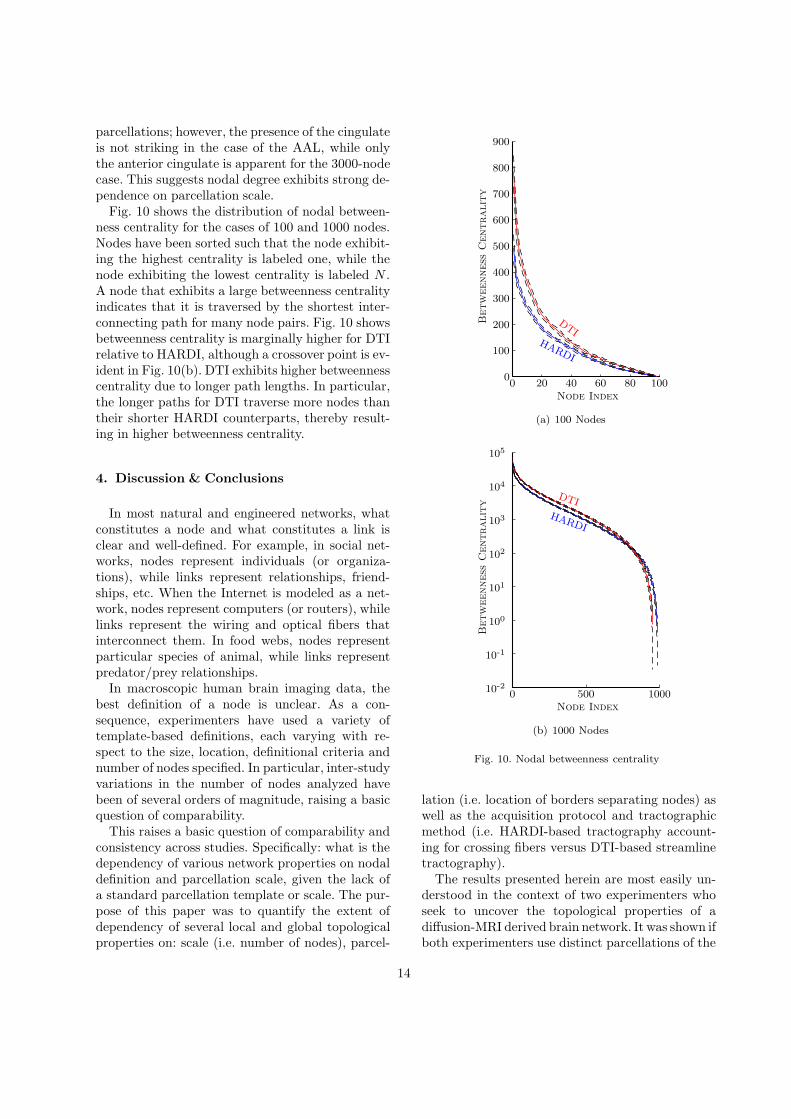
parcellations; however, the presence of the cingulateis not striking in the case of the AAL, while onlythe anterior cingulate is apparent for the 3000-nodecase. This suggests nodal degree exhibits strong de-pendence on parcellation scale.
Fig. 10 shows the distribution of nodal between-ness centrality for the cases of 100 and 1000 nodes.Nodes have been sorted such that the node exhibit-ing the highest centrality is labeled one, while thenode exhibiting the lowest centrality is labeled N .A node that exhibits a large betweenness centralityindicates that it is traversed by the shortest inter-connecting path for many node pairs. Fig. 10 showsbetweenness centrality is marginally higher for DTIrelative to HARDI, although a crossover point is ev-ident in Fig. 10(b). DTI exhibits higher betweennesscentrality due to longer path lengths. In particular,the longer paths for DTI traverse more nodes thantheir shorter HARDI counterparts, thereby result-ing in higher betweenness centrality.
4. Discussion & Conclusions
In most natural and engineered networks, whatconstitutes a node and what constitutes a link isclear and well-defined. For example, in social net-works, nodes represent individuals (or organiza-tions), while links represent relationships, friend-ships, etc. When the Internet is modeled as a net-work, nodes represent computers (or routers), whilelinks represent the wiring and optical fibers thatinterconnect them. In food webs, nodes representparticular species of animal, while links representpredator/prey relationships.
In macroscopic human brain imaging data, thebest definition of a node is unclear. As a con-sequence, experimenters have used a variety oftemplate-based definitions, each varying with re-spect to the size, location, definitional criteria andnumber of nodes specified. In particular, inter-studyvariations in the number of nodes analyzed havebeen of several orders of magnitude, raising a basicquestion of comparability.
This raises a basic question of comparability andconsistency across studies. Specifically: what is thedependency of various network properties on nodaldefinition and parcellation scale, given the lack ofa standard parcellation template or scale. The pur-pose of this paper was to quantify the extent ofdependency of several local and global topologicalproperties on: scale (i.e. number of nodes), parcel-
Node Index
Betw
eenness
Centralit
y
DTIHARDI
0
100
200
300
400
500
600
700
800
900
0 20 40 60 80 100
(a) 100 Nodes
Node Index
Betw
eenness
Centralit
y
DTI
HARDI
10-2
10-1
100
101
102
103
104
105
0 500 1000
(b) 1000 Nodes
Fig. 10. Nodal betweenness centrality
lation (i.e. location of borders separating nodes) aswell as the acquisition protocol and tractographicmethod (i.e. HARDI-based tractography account-ing for crossing fibers versus DTI-based streamlinetractography).
The results presented herein are most easily un-derstood in the context of two experimenters whoseek to uncover the topological properties of adiffusion-MRI derived brain network. It was shown ifboth experimenters use distinct parcellations of the
14
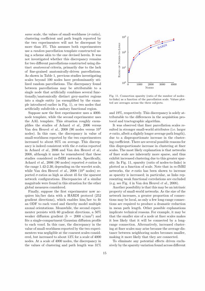
same scale, the values of small-worldness (σ-ratio),clustering coefficient and path length reported bythe two experimenters will not be discrepant bymore than 3%. This assumes both experimentersuse a random parcellation template constructed us-ing a scheme akin to the one devised herein. It wasnot investigated whether this discrepancy remainsfor two different parcellations constructed using dis-tinct anatomical criteria, primarily due to the lackof fine-grained anatomically-driven parcellations.As shown in Table 1, previous studies investigatingscales beyond 100 nodes have predominantly uti-lized random parcellations. The discrepancy foundbetween parcellations may be attributable to asingle node that artificially combines several func-tionally/anatomically distinct grey-matter regionsinto a single entity (as exemplified by the exam-ple introduced earlier in Fig. 1), or two nodes thatartificially subdivide a unitary functional region.
Suppose now the first experimenter uses a 4000-node template, while the second experimenter usesthe AAL template. This situation roughly exem-plifies the studies of Achard et al., 2006 versusVan den Heuvel et al., 2008 (90 nodes versus 104
nodes). In this case, the discrepancy in value ofsmall-worldness reported by the two experimentersincreased to about 95% on average. This discrep-ancy is indeed consistent with the σ-ratios reportedin Achard et al., 2006 and Van den Heuvel et al.,2008, although it must be remembered that thesestudies considered rs-fMRI networks. Specifically,Achard et al., 2006 (90 nodes) reported σ-ratios inthe range 1.42-2.30, depending on the wavelet scale,while Van den Heuvel et al., 2008 (104 nodes) re-ported σ-ratios as high as about 45 for the sparsestnetwork configurations. Discrepancies of a similarmagnitude were found in this situation for the otherglobal measures considered.
Finally, suppose the first experimenter now ac-quires his/her data with a HARDI protocol (252gradient directions), which enables him/her to fitan ODF to each voxel and thereby model multipleaxonal orientations. Meanwhile, the second experi-menter persists with 60 gradient directions, a 50%weaker diffusion gradient (b = 2000 s/mm2) andfits a single-compartment Gaussian diffusion profileto each voxel. In this case, the discrepancy in thevalue of small-worldness reported by the two experi-menters was negligible at the coarsest scales consid-ered, but increased to about 13% for a scale of 4000nodes. At a scale of 4000 nodes, the discrepancy inthe values of clustering and path length was 31%
Nodes
Ratio
of
Nodes-
to-L
inks DTI
HARDI
100
101
102
103
0 1000 2000 3000 4000
bb
b
b
b
b
b
b
b
b
b
b
b
b
Fig. 11. Connection sparsity (ratio of the number of nodes–to-links) as a function of the parcellation scale. Values plot-ted are averages across the three subjects.
and 19%, respectively. This discrepancy is solely at-tributable to the differences in the acquisition pro-tocol and tractographic algorithm.
It was observed that finer parcellation scales re-sulted in stronger small-world attributes (i.e. largerσ-ratio, albeit a slightly longer average path length),due to a disproportionate increase in the cluster-ing coefficient. There are several possible reasons forthis disproportionate increase in clustering at finerscales. The most likely explanation is that networksof finer scale are inherently more sparse, and thusexhibit increased clustering due to this greater spar-sity. In Fig. 11, sparsity (ratio of nodes-to-links) isplotted as a function of scale. Note that in rs-fMRInetworks, the σ-ratio has been shown to increaseas sparsity is increased; in particular, as links rep-resenting weak functional correlations are excluded(e.g. see Fig. 4 in Van den Heuvel et al., 2008).
Another possibility is that this may be an intrinsicproperty of small-world networks. As the size of thenetwork increases, a greater proportion of connec-tions may be local, as only a few long-range connec-tions are required to produce a dramatic reductionin mean path length. Other possible explanationsimplicate technical reasons. For example, it may bethat the smaller size of a node at finer scales makesit less likely that it will be connected by a long-range connection. Alternatively, increased cluster-ing at finer scales may arise because the average dis-tance between neighboring nodes becomes smaller,making it more likely that they are connected.
To eliminate any potential effects driven exclu-sively by the sparsity variation found across different
15
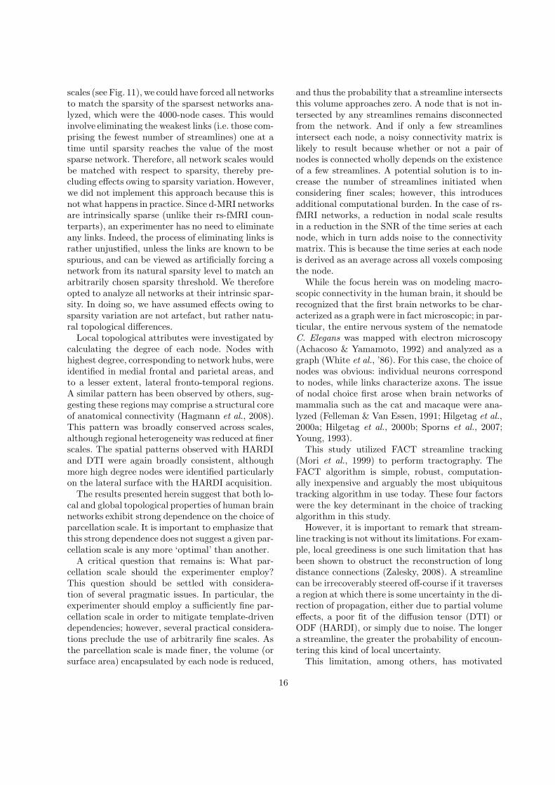
scales (see Fig. 11), we could have forced all networksto match the sparsity of the sparsest networks ana-lyzed, which were the 4000-node cases. This wouldinvolve eliminating the weakest links (i.e. those com-prising the fewest number of streamlines) one at atime until sparsity reaches the value of the mostsparse network. Therefore, all network scales wouldbe matched with respect to sparsity, thereby pre-cluding effects owing to sparsity variation. However,we did not implement this approach because this isnot what happens in practice. Since d-MRI networksare intrinsically sparse (unlike their rs-fMRI coun-terparts), an experimenter has no need to eliminateany links. Indeed, the process of eliminating links israther unjustified, unless the links are known to bespurious, and can be viewed as artificially forcing anetwork from its natural sparsity level to match anarbitrarily chosen sparsity threshold. We thereforeopted to analyze all networks at their intrinsic spar-sity. In doing so, we have assumed effects owing tosparsity variation are not artefact, but rather natu-ral topological differences.
Local topological attributes were investigated bycalculating the degree of each node. Nodes withhighest degree, corresponding to network hubs, wereidentified in medial frontal and parietal areas, andto a lesser extent, lateral fronto-temporal regions.A similar pattern has been observed by others, sug-gesting these regions may comprise a structural coreof anatomical connectivity (Hagmann et al., 2008).This pattern was broadly conserved across scales,although regional heterogeneity was reduced at finerscales. The spatial patterns observed with HARDIand DTI were again broadly consistent, althoughmore high degree nodes were identified particularlyon the lateral surface with the HARDI acquisition.
The results presented herein suggest that both lo-cal and global topological properties of human brainnetworks exhibit strong dependence on the choice ofparcellation scale. It is important to emphasize thatthis strong dependence does not suggest a given par-cellation scale is any more ‘optimal’ than another.
A critical question that remains is: What par-cellation scale should the experimenter employ?This question should be settled with considera-tion of several pragmatic issues. In particular, theexperimenter should employ a sufficiently fine par-cellation scale in order to mitigate template-drivendependencies; however, several practical considera-tions preclude the use of arbitrarily fine scales. Asthe parcellation scale is made finer, the volume (orsurface area) encapsulated by each node is reduced,
and thus the probability that a streamline intersectsthis volume approaches zero. A node that is not in-tersected by any streamlines remains disconnectedfrom the network. And if only a few streamlinesintersect each node, a noisy connectivity matrix islikely to result because whether or not a pair ofnodes is connected wholly depends on the existenceof a few streamlines. A potential solution is to in-crease the number of streamlines initiated whenconsidering finer scales; however, this introducesadditional computational burden. In the case of rs-fMRI networks, a reduction in nodal scale resultsin a reduction in the SNR of the time series at eachnode, which in turn adds noise to the connectivitymatrix. This is because the time series at each nodeis derived as an average across all voxels composingthe node.
While the focus herein was on modeling macro-scopic connectivity in the human brain, it should berecognized that the first brain networks to be char-acterized as a graph were in fact microscopic; in par-ticular, the entire nervous system of the nematodeC. Elegans was mapped with electron microscopy(Achacoso & Yamamoto, 1992) and analyzed as agraph (White et al., ’86). For this case, the choice ofnodes was obvious: individual neurons correspondto nodes, while links characterize axons. The issueof nodal choice first arose when brain networks ofmammalia such as the cat and macaque were ana-lyzed (Felleman & Van Essen, 1991; Hilgetag et al.,2000a; Hilgetag et al., 2000b; Sporns et al., 2007;Young, 1993).
This study utilized FACT streamline tracking(Mori et al., 1999) to perform tractography. TheFACT algorithm is simple, robust, computation-ally inexpensive and arguably the most ubiquitoustracking algorithm in use today. These four factorswere the key determinant in the choice of trackingalgorithm in this study.
However, it is important to remark that stream-line tracking is not without its limitations. For exam-ple, local greediness is one such limitation that hasbeen shown to obstruct the reconstruction of longdistance connections (Zalesky, 2008). A streamlinecan be irrecoverably steered off-course if it traversesa region at which there is some uncertainty in the di-rection of propagation, either due to partial volumeeffects, a poor fit of the diffusion tensor (DTI) orODF (HARDI), or simply due to noise. The longera streamline, the greater the probability of encoun-tering this kind of local uncertainty.
This limitation, among others, has motivated
16
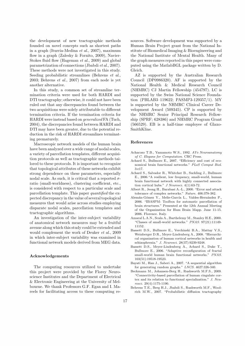
the development of new tractographic methodsfounded on novel concepts such as shortest pathsin a graph (Iturria-Medina et al., 2007), maximumflow in a graph (Zalesky & Fornito, 2009), Navier-Stokes fluid flow (Hageman et al., 2009) and globalparametrization of connections (Jbabdi et al., 2007).These methods were not investigated in this study.Seeding probabilistic streamlines (Behrens et al.,2003; Behrens et al., 2007) from each node is yetanother alternative.
In this study, a common set of streamline ter-mination criteria were used for both HARDI andDTI tractography; otherwise, it could not have beenruled out that any discrepancies found between thetwo acquisitions were solely attributable to differenttermination criteria. If the termination criteria forHARDI were instead based on generalized FA (Tuch,2004), the discrepancies found between HARDI andDTI may have been greater, due to the potential re-duction in the risk of HARDI streamlines terminat-ing prematurely.
Macroscopic network models of the human brainhave been analyzed over a wide range of nodal scales,a variety of parcellation templates, different acquisi-tion protocols as well as tractographic methods tai-lored to these protocols. It is important to recognizethat topological attributes of these networks exhibitstrong dependence on these parameters, especiallynodal scale. As such, it is critical that a reported σ-ratio (small-worldness), clustering coefficient, etc.,is considered with respect to a particular scale andparcellation template. This paper quantified the ex-pected discrepancy in the value of several topologicalmeasures that would arise across studies employingdisparate nodal scales, parcellation templates andtractographic algorithms.
An investigation of the inter-subject variabilityof anatomical network measures may be a fruitfulavenue along which this study could be extended andwould complement the work of Deuker et al., 2009in which inter-subject variability was examined infunctional network models derived from MEG data.
Acknowledgements
The computing resources utilized to undertakethis project were provided by the Florey Neuro-science Institutes and the Department of Electrical& Electronic Engineering at the University of Mel-bourne. We thank Professors G.F. Egan and I. Ma-reels for facilitating access to these computing re-
sources. Software development was supported by aHuman Brain Project grant from the National In-stitute of Biomedical Imaging & Bioengineering andthe National Institute of Mental Health. Many ofthe graph measures reported in this paper were com-puted using the MatlabBGL package written by D.Gleich.
AZ is supported by the Australian ResearchCouncil (DP0986320). AF is supported by theNational Health & Medical Research Council(NHMRC) CJ Martin Fellowship (454797). LC issupported by the Swiss National Science Founda-tion (PBLAB3–119622; PASMP3-129357/1). MYis supported by the NHMRC Clinical Career De-velopment Award (509345). CP is supported bythe NHMRC Senior Principal Research Fellow-ship (SPRF; 628386) and NHMRC Program Grant(566529). EB is a half-time employee of Glaxo-SmithKline.
References
Achacoso T.B., Yamamoto W.S., 1992. AYs Neuroanatomyof C. Elegans for Computation. CRC Press.
Achard S., Bullmore E., 2007. “Efficiency and cost of eco-nomical brain functional networks.” PLoS Comput Biol.3:e17.
Achard S., Salvador R., Whitcher B., Suckling J., BullmoreE., 2006.“A resilient, low frequency, small-world, humanbrain functional network with highly connected associa-tion cortical hubs.” J Neurosci. 4(1):63-72.
Albert R., Jeong H., Barabasi A.-L., 2000. “Error and attacktolerance of complex networks.” Nature. 406:378-382.
Aleman-Gomez Y., Melie-Garcıa L., Valdes-Hernandez P.,2006. “IBASPM: Toolbox for automatic parcellation ofbrain structures.” Presented at the 12th Annual Meetingof the Organization for Hum Brain Mapp. June 11-15.2006. Florence. Italy.
Amaral L.A.N., Scala A., Barthelemy M., Stanley H.E., 2000.“Classes of small-world networks.” PNAS. 97(21):11149-11152.
Bassett D.S., Bullmore E., Verchinski B.A., Mattay V.S.,Weinberger D.R., Meyer-Lindenberg A., 2008. “Hierarchi-cal organization of human cortical networks in health andschizophrenia.” J. Neurosci. 28(37):9239-9248.
Bassett D.S., Meyer-Lindenberg A., Achard S., Duke T.,Bullmore E., 2006. “Adaptive reconfiguration of fractalsmall-world human brain functional networks.” PNAS.103(51):19518-19523.
Bayati M., Han J., Saberi A., 2007. “A sequential algorithmfor generating random graphs.” LNCS. 4627:326-340.
Beckmann M., Johansen-Berg H., Rushworth M.F.S., 2009.“Connectivity-based parcellation of human cingulate cor-tex and its relation to functional specialization.” J. Neu-rosci. 29(4):1175-1190.
Behrens T.E., Berg H.J., Jbabdi S., Rushworth M.F., Wool-rich M.W., 2007. “Probabilistic diffusion tractography
17
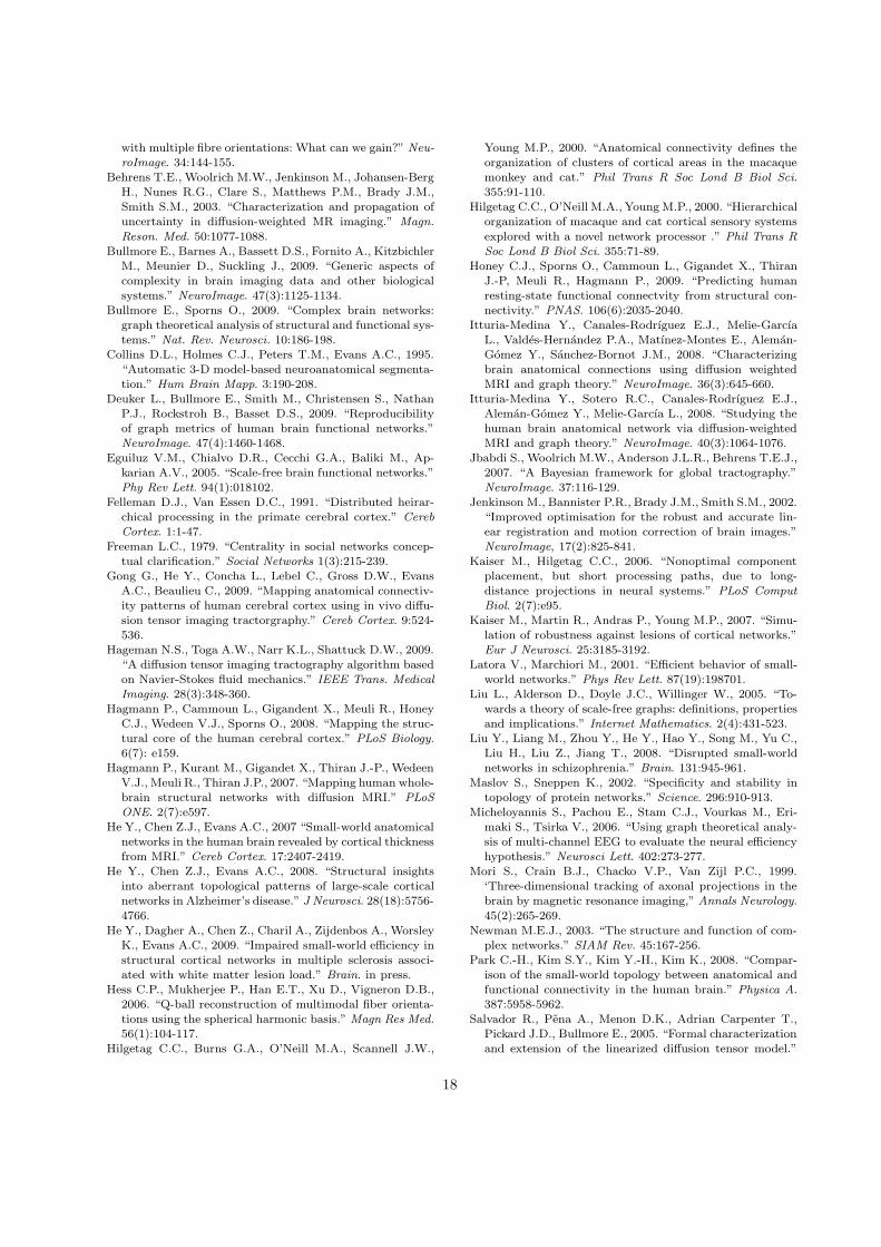
with multiple fibre orientations: What can we gain?” Neu-roImage. 34:144-155.
Behrens T.E., Woolrich M.W., Jenkinson M., Johansen-BergH., Nunes R.G., Clare S., Matthews P.M., Brady J.M.,Smith S.M., 2003. “Characterization and propagation ofuncertainty in diffusion-weighted MR imaging.” Magn.
Reson. Med. 50:1077-1088.Bullmore E., Barnes A., Bassett D.S., Fornito A., Kitzbichler
M., Meunier D., Suckling J., 2009. “Generic aspects ofcomplexity in brain imaging data and other biologicalsystems.” NeuroImage. 47(3):1125-1134.
Bullmore E., Sporns O., 2009. “Complex brain networks:graph theoretical analysis of structural and functional sys-tems.” Nat. Rev. Neurosci. 10:186-198.
Collins D.L., Holmes C.J., Peters T.M., Evans A.C., 1995.“Automatic 3-D model-based neuroanatomical segmenta-tion.” Hum Brain Mapp. 3:190-208.
Deuker L., Bullmore E., Smith M., Christensen S., NathanP.J., Rockstroh B., Basset D.S., 2009. “Reproducibilityof graph metrics of human brain functional networks.”NeuroImage. 47(4):1460-1468.
Eguiluz V.M., Chialvo D.R., Cecchi G.A., Baliki M., Ap-karian A.V., 2005. “Scale-free brain functional networks.”Phy Rev Lett. 94(1):018102.
Felleman D.J., Van Essen D.C., 1991. “Distributed heirar-chical processing in the primate cerebral cortex.” CerebCortex. 1:1-47.
Freeman L.C., 1979. “Centrality in social networks concep-tual clarification.” Social Networks 1(3):215-239.
Gong G., He Y., Concha L., Lebel C., Gross D.W., EvansA.C., Beaulieu C., 2009. “Mapping anatomical connectiv-ity patterns of human cerebral cortex using in vivo diffu-sion tensor imaging tractorgraphy.” Cereb Cortex. 9:524-536.
Hageman N.S., Toga A.W., Narr K.L., Shattuck D.W., 2009.“A diffusion tensor imaging tractography algorithm basedon Navier-Stokes fluid mechanics.” IEEE Trans. MedicalImaging. 28(3):348-360.
Hagmann P., Cammoun L., Gigandent X., Meuli R., HoneyC.J., Wedeen V.J., Sporns O., 2008. “Mapping the struc-tural core of the human cerebral cortex.” PLoS Biology.6(7): e159.
Hagmann P., Kurant M., Gigandet X., Thiran J.-P., WedeenV.J., Meuli R., Thiran J.P., 2007. “Mapping human whole-brain structural networks with diffusion MRI.” PLoSONE. 2(7):e597.
He Y., Chen Z.J., Evans A.C., 2007 “Small-world anatomicalnetworks in the human brain revealed by cortical thicknessfrom MRI.” Cereb Cortex. 17:2407-2419.
He Y., Chen Z.J., Evans A.C., 2008. “Structural insightsinto aberrant topological patterns of large-scale corticalnetworks in Alzheimer’s disease.” J Neurosci. 28(18):5756-
4766.He Y., Dagher A., Chen Z., Charil A., Zijdenbos A., Worsley
K., Evans A.C., 2009. “Impaired small-world efficiency instructural cortical networks in multiple sclerosis associ-ated with white matter lesion load.” Brain. in press.
Hess C.P., Mukherjee P., Han E.T., Xu D., Vigneron D.B.,2006. “Q-ball reconstruction of multimodal fiber orienta-tions using the spherical harmonic basis.” Magn Res Med.56(1):104-117.
Hilgetag C.C., Burns G.A., O’Neill M.A., Scannell J.W.,
Young M.P., 2000. “Anatomical connectivity defines theorganization of clusters of cortical areas in the macaquemonkey and cat.” Phil Trans R Soc Lond B Biol Sci.355:91-110.
Hilgetag C.C., O’Neill M.A., Young M.P., 2000. “Hierarchicalorganization of macaque and cat cortical sensory systems
explored with a novel network processor .” Phil Trans RSoc Lond B Biol Sci. 355:71-89.
Honey C.J., Sporns O., Cammoun L., Gigandet X., ThiranJ.-P, Meuli R., Hagmann P., 2009. “Predicting humanresting-state functional connectvity from structural con-nectivity.” PNAS. 106(6):2035-2040.
Itturia-Medina Y., Canales-Rodrıguez E.J., Melie-GarcıaL., Valdes-Hernandez P.A., Matınez-Montes E., Aleman-Gomez Y., Sanchez-Bornot J.M., 2008. “Characterizingbrain anatomical connections using diffusion weightedMRI and graph theory.” NeuroImage. 36(3):645-660.
Itturia-Medina Y., Sotero R.C., Canales-Rodrıguez E.J.,Aleman-Gomez Y., Melie-Garcıa L., 2008. “Studying thehuman brain anatomical network via diffusion-weightedMRI and graph theory.” NeuroImage. 40(3):1064-1076.
Jbabdi S., Woolrich M.W., Anderson J.L.R., Behrens T.E.J.,2007. “A Bayesian framework for global tractography.”NeuroImage. 37:116-129.
Jenkinson M., Bannister P.R., Brady J.M., Smith S.M., 2002.“Improved optimisation for the robust and accurate lin-ear registration and motion correction of brain images.”NeuroImage, 17(2):825-841.
Kaiser M., Hilgetag C.C., 2006. “Nonoptimal componentplacement, but short processing paths, due to long-distance projections in neural systems.” PLoS ComputBiol. 2(7):e95.
Kaiser M., Martin R., Andras P., Young M.P., 2007. “Simu-lation of robustness against lesions of cortical networks.”Eur J Neurosci. 25:3185-3192.
Latora V., Marchiori M., 2001. “Efficient behavior of small-world networks.” Phys Rev Lett. 87(19):198701.
Liu L., Alderson D., Doyle J.C., Willinger W., 2005. “To-wards a theory of scale-free graphs: definitions, propertiesand implications.” Internet Mathematics. 2(4):431-523.
Liu Y., Liang M., Zhou Y., He Y., Hao Y., Song M., Yu C.,Liu H., Liu Z., Jiang T., 2008. “Disrupted small-worldnetworks in schizophrenia.” Brain. 131:945-961.
Maslov S., Sneppen K., 2002. “Specificity and stability intopology of protein networks.” Science. 296:910-913.
Micheloyannis S., Pachou E., Stam C.J., Vourkas M., Eri-maki S., Tsirka V., 2006. “Using graph theoretical analy-sis of multi-channel EEG to evaluate the neural efficiencyhypothesis.” Neurosci Lett. 402:273-277.
Mori S., Crain B.J., Chacko V.P., Van Zijl P.C., 1999.‘Three-dimensional tracking of axonal projections in thebrain by magnetic resonance imaging,” Annals Neurology.
45(2):265-269.Newman M.E.J., 2003. “The structure and function of com-
plex networks.” SIAM Rev. 45:167-256.Park C.-H., Kim S.Y., Kim Y.-H., Kim K., 2008. “Compar-
ison of the small-world topology between anatomical andfunctional connectivity in the human brain.” Physica A.387:5958-5962.
Salvador R., Pena A., Menon D.K., Adrian Carpenter T.,Pickard J.D., Bullmore E., 2005. “Formal characterizationand extension of the linearized diffusion tensor model.”
18
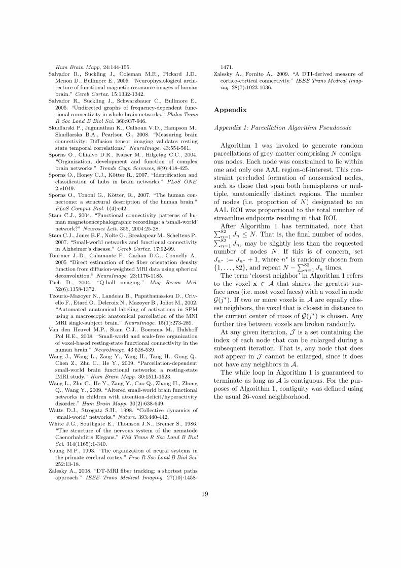
Hum Brain Mapp, 24:144-155.Salvador R., Suckling J., Coleman M.R., Pickard J.D.,
Menon D., Bullmore E., 2005. “Neurophysiological archi-tecture of functional magnetic resonance images of humanbrain.” Cereb Cortex. 15:1332-1342.
Salvador R., Suckling J., Schwarzbauer C., Bullmore E.,
2005. “Undirected graphs of frequency-dependent func-tional connectivity in whole-brain networks.” Philos TransR Soc Lond B Biol Sci. 360:937-946.
Skudlarski P., Jagnnathan K., Calhoun V.D., Hampson M.,Skudlarska B.A., Pearlson G., 2008. “Measuring brainconnectivity: Diffusion tensor imaging validates restingstate temporal correlations.” NeuroImage. 43:554-561.
Sporns O., Chialvo D.R., Kaiser M., Hilgetag C.C., 2004.“Organization, development and function of complexbrain networks.” Trends Cogn Sciences, 8(9):418-425.
Sporns O., Honey C.J., Kotter R., 2007. “Identification andclassification of hubs in brain networks.” PLoS ONE.2:e1049.
Sporns O., Tononi G., Kotter, R., 2007. “The human con-nectome: a structural description of the human brain.”PLoS Comput Biol. 1(4):e42.
Stam C.J., 2004. “Functional connectivity patterns of hu-man magnetoencephalographic recordings: a ‘small-world’network?” Neurosci Lett. 355, 2004:25-28.
Stam C.J., Jones B.F., Nolte G., Breakspear M., Scheltens P.,2007. “Small-world networks and functional connectivityin Alzheimer’s disease.” Cereb Cortex. 17:92-99.
Tournier J.-D., Calamante F., Gadian D.G., Connelly A.,2005 “Direct estimation of the fiber orientation densityfunction from diffusion-weighted MRI data using sphericaldeconvolution.” NeuroImage. 23:1176-1185.
Tuch D., 2004. “Q-ball imaging.” Mag Reson Med.52(6):1358-1372.
Tzourio-Mazoyer N., Landeau B., Papathanassiou D., Criv-ello F., Etard O., Delcroix N., Mazoyer B., Joliot M., 2002.“Automated anatomical labeling of activations in SPMusing a macroscopic anatomical parcellation of the MNIMRI single-subject brain.” NeuroImage. 15(1):273-289.
Van den Heuvel M.P., Stam C.J., Boersma M., HulshoffPol H.E., 2008. “Small-world and scale-free organizationof voxel-based resting-state functional connectivity in thehuman brain.” NeuroImage. 43:528-539.
Wang J., Wang L., Zang Y., Yang H., Tang H., Gong Q.,Chen Z., Zhu C., He Y., 2009. “Parcellation-dependentsmall-world brain functional networks: a resting-statefMRI study.” Hum Brain Mapp. 30:1511-1523.
Wang L., Zhu C., He Y., Zang Y., Cao Q., Zhang H., ZhongQ., Wang Y., 2009. “Altered small-world brain functionalnetworks in children with attention-deficit/hyperactivitydisorder.” Hum Brain Mapp. 30(2):638-649.
Watts D.J., Strogatz S.H., 1998. “Collective dynamics of
‘small-world’ networks.” Nature. 393:440-442.White J.G., Southgate E., Thomson J.N., Bremer S., 1986.
“The structure of the nervous system of the nematodeCaenorhabditis Elegans.” Phil Trans R Soc Lond B BiolSci. 314(1165):1-340.
Young M.P., 1993. “The organization of neural systems inthe primate cerebral cortex.” Proc R Soc Lond B Biol Sci.252:13-18.
Zalesky A., 2008. “DT-MRI fiber tracking: a shortest pathsapproach.” IEEE Trans Medical Imaging. 27(10):1458-
1471.Zalesky A., Fornito A., 2009. “A DTI-derived measure of
cortico-cortical connectivity.” IEEE Trans Medical Imag-ing. 28(7):1023-1036.
Appendix
Appendix 1: Parcellation Algorithm Pseudocode
Algorithm 1 was invoked to generate randomparcellations of grey-matter comprising N contigu-ous nodes. Each node was constrained to lie withinone and only one AAL region-of-interest. This con-straint precluded formation of nonsensical nodes,such as those that span both hemispheres or mul-tiple, anatomically distinct regions. The numberof nodes (i.e. proportion of N) designated to anAAL ROI was proportional to the total number ofstreamline endpoints residing in that ROI.
After Algorithm 1 has terminated, note that∑82
n=1 Jn ≤ N . That is, the final number of nodes,∑82
n=1 Jn, may be slightly less than the requestednumber of nodes N . If this is of concern, setJn∗ := Jn∗ + 1, where n∗ is randomly chosen from{1, . . . , 82}, and repeat N −
∑82n=1 Jn times.
The term ‘closest neighbor’ in Algorithm 1 refersto the voxel x ∈ A that shares the greatest sur-face area (i.e. most voxel faces) with a voxel in nodeG(j∗). If two or more voxels in A are equally clos-est neighbors, the voxel that is closest in distance tothe current center of mass of G(j∗) is chosen. Anyfurther ties between voxels are broken randomly.
At any given iteration, J is a set containing theindex of each node that can be enlarged during asubsequent iteration. That is, any node that doesnot appear in J cannot be enlarged, since it doesnot have any neighbors in A.
The while loop in Algorithm 1 is guaranteed toterminate as long as A is contiguous. For the pur-poses of Algorithm 1, contiguity was defined usingthe usual 26-voxel neighborhood.
19
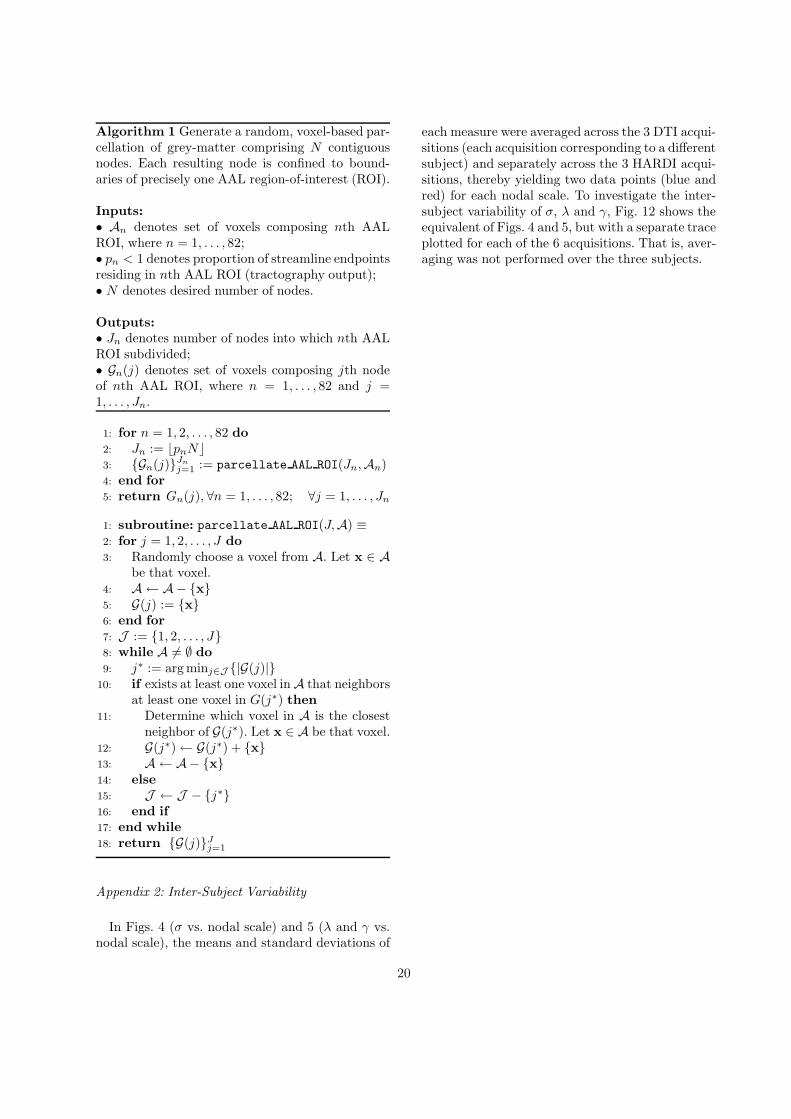
Algorithm 1 Generate a random, voxel-based par-cellation of grey-matter comprising N contiguousnodes. Each resulting node is confined to bound-aries of precisely one AAL region-of-interest (ROI).
Inputs:
• An denotes set of voxels composing nth AALROI, where n = 1, . . . , 82;• pn < 1 denotes proportion of streamline endpointsresiding in nth AAL ROI (tractography output);• N denotes desired number of nodes.
Outputs:
• Jn denotes number of nodes into which nth AALROI subdivided;• Gn(j) denotes set of voxels composing jth nodeof nth AAL ROI, where n = 1, . . . , 82 and j =1, . . . , Jn.
1: for n = 1, 2, . . . , 82 do
2: Jn := ⌊pnN⌋3: {Gn(j)}Jn
j=1 := parcellate AAL ROI(Jn,An)4: end for
5: return Gn(j), ∀n = 1, . . . , 82; ∀j = 1, . . . , Jn
1: subroutine: parcellate AAL ROI(J,A) ≡2: for j = 1, 2, . . . , J do
3: Randomly choose a voxel from A. Let x ∈ Abe that voxel.
4: A ← A− {x}5: G(j) := {x}6: end for
7: J := {1, 2, . . . , J}8: while A 6= ∅ do
9: j∗ := arg minj∈J {|G(j)|}10: if exists at least one voxel inA that neighbors
at least one voxel in G(j∗) then
11: Determine which voxel in A is the closestneighbor of G(j∗). Let x ∈ A be that voxel.
12: G(j∗)← G(j∗) + {x}13: A ← A− {x}14: else
15: J ← J − {j∗}16: end if
17: end while
18: return {G(j)}Jj=1
Appendix 2: Inter-Subject Variability
In Figs. 4 (σ vs. nodal scale) and 5 (λ and γ vs.nodal scale), the means and standard deviations of
each measure were averaged across the 3 DTI acqui-sitions (each acquisition corresponding to a differentsubject) and separately across the 3 HARDI acqui-sitions, thereby yielding two data points (blue andred) for each nodal scale. To investigate the inter-subject variability of σ, λ and γ, Fig. 12 shows theequivalent of Figs. 4 and 5, but with a separate traceplotted for each of the 6 acquisitions. That is, aver-aging was not performed over the three subjects.
20
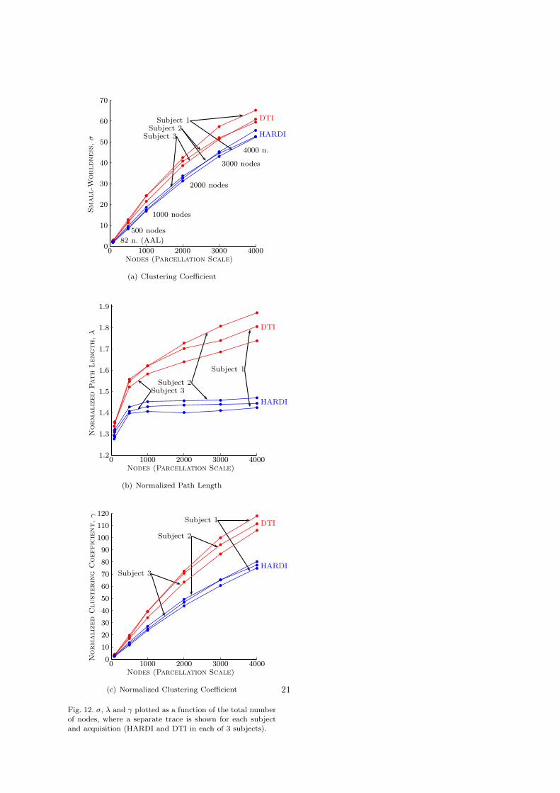
Nodes (Parcellation Scale)
Small-W
orldness
,σ
DTI
HARDI
82 n. (AAL)
500 nodes
1000 nodes
2000 nodes
3000 nodes
4000 n.
Subject 1Subject 2
Subject 3
0
10
20
30
40
50
60
70
0 1000 2000 3000 4000
bb
b
b
b
b
b
bb
b
b
b
b
b
bb
b
b
b
b
b
bb
b
b
b
b
b
bb
b
b
b
b
b
bb
b
b
b
b
b
(a) Clustering Coefficient
Nodes (Parcellation Scale)
Normaliz
ed
Path
Length,
λ
DTI
HARDI
Subject 1
Subject 2Subject 3
1.2
1.3
1.4
1.5
1.6
1.7
1.8
1.9
0 1000 2000 3000 4000
b
b
b
b
b
b
b
b
b
b
b
b
b
b
b
b
b
b
b
b
b
bb
bb b
bb
b
b
b
b b bb
b
b
b
bb b b
(b) Normalized Path Length
Nodes (Parcellation Scale)
Normaliz
ed
Clust
erin
gC
oeffic
ient,
γ
DTI
HARDI
Subject 1
Subject 2
Subject 3
0
10
20
30
40
50
60
70
80
90
100
110
120
0 1000 2000 3000 4000
bb
b
b
b
b
b
bb
b
b
b
b
b
bb
b
b
b
b
b
bb
b
b
b
b
b
bb
b
b
b
b
b
bb
b
b
b
b
b
(c) Normalized Clustering Coefficient
Fig. 12. σ, λ and γ plotted as a function of the total numberof nodes, where a separate trace is shown for each subjectand acquisition (HARDI and DTI in each of 3 subjects).
21