8 Upscaling Water Productivity in Irrigated Agriculture Using Remote-sensing and GIS Technologies
Upload
khangminh22Category
view
0download
0
39 MM3 NN08201 40951 1999-09-30 ?bj>c>
'etland Methane Fluxes
Upscaling
from Kinetics
via a Single Root
and
a Soil Layer
to the Plot
Reinoud Segers

Wetland Methane Fluxes: Upscaling from Kinetics
via a Single Root and a Soil Layer to the Plot

promotor: dr. ir. R. Rabbinge hoogleraar in de plantaardige productiesystemen
co-promotor: dr. ir. P. A. Leffelaar universitair hoofddocent bij de leerstoelgroep plantaardige productiesystemen
Wetland Methane Fluxes: Upscaling from Kinetics
via a Single Root and a Soil Layer to the Plot
Reinoud Segers
Proefschrift
ter verkrijging van de graad van doctor
op gezag van de rector magnificus
van de Wageningen Universiteit,
dr. C. M. Karssen,
in het openbaar te verdedigen
op woensdag 13 oktober 1999
des namiddags te vier uur in de Aula

Segers, Reinoud, 1999.
Wetland Methane Fluxes: Upscaling from Kinetics via a Single Root and a Soil Layer to the Plot. Ph. D. Thesis, Wageningen University. -With summary in Dutch.
ISBN: 90-5808-123-0
This study was part of 'the integrated CH4 grassland project' and 'the integrated N ,0 and CH4 grassland project'. Both these projects were partially financed by the Dutch National Research Programme on Global Air Pollution and Climate Change
Abstract
The aim of this thesis was to increase the understanding of plot scale relations between CH4 fluxes and environmental variables in wetlands. Theories of microbial and chemical conversions were taken as starting point, as a literature review showed that it is hard to relate methane production and oxidation directly to environmental variables. These theories only apply under homogeneous conditions at the kinetic scale (here about 1 mm) and were linked to plot scale CH4 fluxes by stepwise scaling up.
At the kinetic scale a CH4 production model was developed, comprising anaerobic C-mineralisation, electron acceptor reduction, methanogenesis and methanogenic growth, of which the last process is probably not important in wetland soil. Application of this model to anaerobic incubation experiments with peat soil suggested that organic peat may act as terminal electron acceptor, using a substantial amount of anaerobically mineralised C.
At the single root scale CH4 dynamics were explained with coupled reaction-diffusion equations for CH4, oxygen (O2), molecular nitrogen, carbon dioxide and an electron acceptor in oxidised and reduced form. Included conversions were: aerobic respiration, C-mineralisation, CH4 production and oxidation, electron acceptor reduction and re-oxidation. Root gas transport was described with first order gas exchange over the root surface. Bubble formation was modelled with simultaneous liquid-gas equilibria of all gases and bubble export with a descriptive relation with bubble volume. The model was simplified by assuming quasi steady-state for O2 and by spatially averaging the other compounds. These simplifications had little effect on simulated CH4 dynamics and therefore the simplified model was used at the next higher level.
At the soil layer scale the CH4 dynamics were calculated with a weighed set of single root systems with different distances to the next root. These weights were calculated from the root architecture, conserving the probability density function of the distance to the nearest root. The model was simplified by averaging over the single root systems. This had some effect on CH4 production and CH4 transport, but little on CH4 emissions.
At the plot scale, temporal water unsaturation was accounted for with Richards' equation. The soil layer models were extended to the plot scale by incorporating vertical transport of the compounds by diffusion and mass flow. Simulated CH4 fluxes were of the same order of magnitude as measured fluxes. They were sensitive to several uncertain parameters, indicating that predictive process modelling of CH4 fluxes is not possible yet. Heterogeneities within a soil layer seem to be less important than heterogeneities between soil layers. This may be explained by a weaker effect on the O2 input into the soil.
CH4 fluxes result from the electron donor input minus the electron acceptor input and changes in storage of electron donors, electron acceptors and CH4 in the soil. The developed models showed that the changes in storage are the result of a number of uncertain processes. Hence, the most stable relationships between CH4 fluxes and environmental variables may exist at larger time scales.
To conclude, a coherent set of models was developed that explicitly relates processes at the kinetic, single root and soil layer scale to methane fluxes at the plot scale.
Segers, R. Wetland Methane Fluxes: Upscaling from Kinetics via a Single Root and a Soil Layer to the Plot, Ph. D. Thesis, Wageningen University, 1999.
Contents
Abstract 5
Voorwoord 9
Chapter 1: General introduction 11
Chapter 2: Methane production and methane consumption: a review of processes
underlying wetland methane fluxes 17
Chapter 3: Methane production as a function of anaerobic carbon mineralisation: a process model 37
Chapter 4: Modelling methane fluxes in wetlands with gas transporting plants: 1. single root scale 53
Chapter 5: Modelling methane fluxes in wetlands with gas transporting plants: 2. soil layer scale 87
Chapter 6: Modelling methane fluxes in wetlands with gas transporting plants:
3. plot scale 115
Chapter 7: General discussion 151
Samenvatting 157
References 163
Curriculum vitae 179

Voorwoord
Dit boekje heeft het meeste bloed, zweet en tranen gekost van ondergetekende, maar zonder de hulp van vele anderen zou het mij niet gelukt zijn. Daarom wil ik hen graag bedanken. Allereerst natuurlijk Peter Leffelaar, de co-promotor. Hij heeft indertijd (1992) een belangrijke rol gespeeld bij het formuleren van het projectvoorstel (het gemtegreerde CH4 graslandproject), het continueren van de financiering en bij het grondidee van dit proefschrift: het gebruiken van kennis van basisprocessen om methaanfluxen te begrijpen. Daarnaast heeft hij vele manuscripten en zelfs de computercode doorgenomen om mij zo de gelegenheid te geven vele fouten, onduidelijkheden en andere onvolkomenheden te elimineren. Rudy Rabbinge, de promotor, stimuleerde mij bij het vinden van de grote lijn.
Binnen het project heb ik prettig samengewerkt. Agnes van den Pol - van Dasselaar heeft mij ongeveer lx per jaar meegenomen naar het veld om mij te laten zien hoe dat nou werkt, methaanfluxen meten. Daarbij en daarnaast heb ik vele nuttige discussies met haar gevoerd over de materie en het vertrouwen gekregen dat mijn theoretische ideeen interessant kunnen zijn voor praktijkmensen. Met Serve Kengen heb ik zijn incubatie-proefjes bediscussieerd, wat uiteindelijk geresulteerd heeft in een gezamelijk artikel.
Kees Rappoldt hielp mij met zijn methode om ingewikkelde geometrien eenvoudig te representeren. Op alle e-mailtjes had ik spoedig een antwoord waarmee ik verder kon. Hugo Denier van der Gon, Fons Stams en de leden van het AlO-groepje van de C.T. de Wit Onderzoeksschool Produktiecologie gaven nuttig commentaar op mijn conceptartikelen. I am greatful to Anu Kettunen for discovering two mistakes in my articles, just before publishing. Elisa D' Angelo provided me with a submitted manuscript, enabling me to simplify one of the models.
De laatste jaren was de methaan-onderzoeksgroep op de vakgroep uitgebreid met Peter van Bodegom. Zijn commentaar op mijn ideeen en schrijfsels waren vaak zeer verhelderend en to the point. Net als mijn andere kamergenoten, Marcos Bernardes, Sanderine Nonhebel en Huub Klein Gunnewiek was hij bereid mijn dagelijkse teleurstellinkjes en vreugdetjes met mij te delen.
De computerinfrastructuur werkte meestal voorbeeldig dankzij Rob Dierkx, Frank Vergeldt (Moleculaire Fysica), TUPEA en de Kezen van IenD, evenals de service van de veschillende bibliotheken. Bijna elk artikel wat ik wilde lezen had ik binnen korte tijd te pakken.
Het gaat niet alleen om de inhoud, maar het oog wil 00k wat. Gon van Laar en Jacco Wallinga hebben mij geholpen met de lay-out en Anne Marie van Dam met de voorkant.
Evenals mijn kamergenoten op mijn werk waren mijn huisgenoten bereid pieken en dalen in het onderzoek te delen. Daarnaast waren ze een prettige basis voor mijn Wageningse leven buiten het proefschrift en de vakgroep. Cor, Anne Marie, Inge, Leonie, Han, Piter, Rodney, Guido, Carla, Gerda, Jos, Janneke, Rutger, Remko, Dorte, Stephen, Mark, Evy, Noortje, Nuray, allemaal bedankt!
Segers, R. Wetland Methane Fluxes: Upscaling from Kinetics via a Single Root and a Soil Layer to the
Plot, Ph. D. Thesis, Wageningen University, 1999.
II
Chapter 1
General introduction
Methane emissions from soils
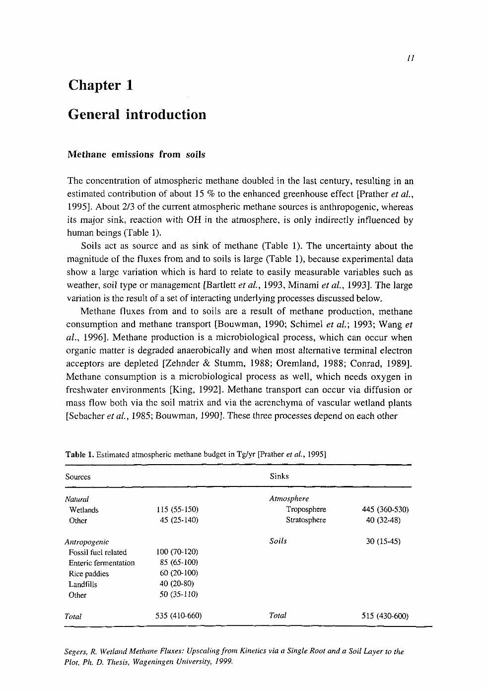
The concentration of atmospheric methane doubled in the last century, resulting in an estimated contribution of about 15 % to the enhanced greenhouse effect [Prather et aL, 1995]. About 2/3 of the current atmospheric methane sources is anthropogenic, whereas its major sink, reaction with OH in the atmosphere, is only indirectly influenced by human beings (Table 1).
Soils act as source and as sink of methane (Table 1). The uncertainty about the magnitude of the fluxes from and to soils is large (Table 1), because experimental data show a large variation which is hard to relate to easily measurable variables such as weather, soil type or management [Bartlett et ah, 1993, Minami et ah, 1993]. The large variation is the result of a set of interacting underlying processes discussed below.
Methane fluxes from and to soils are a result of methane production, methane consumption and methane transport [Bouwman, 1990; Schimel et al.\ 1993; Wang et al., 1996]. Methane production is a microbiological process, which can occur when organic matter is degraded anaerobically and when most alternative terminal electron acceptors are depleted [Zehnder & Stumm, 1988; Oremland, 1988; Conrad, 1989]. Methane consumption is a microbiological process as well, which needs oxygen in freshwater environments [King, 1992]. Methane transport can occur via diffusion or mass flow both via the soil matrix and via the aerenchyma of vascular wetland plants [Sebacher et ah, 1985; Bouwman, 1990]. These three processes depend on each other
Table 1. Estimated atmospheric methane budget in Tg/yr [Prather et al., 1995]
Sources Sinks
Natural Wetlands Other
Antropogenic Fossil fuel related Enteric fermentation
Rice paddies Landfills Other
Total
115(55-150) 45 (25-140)
100(70-120) 85 (65-100) 60(20-100) 40 (20-80) 50(35-110)
535 (410-660)
Atmosphere Troposphere Stratosphere
Soils
Total
445 (360-530) 40 (32-48)
30 (15-45)
515(430-600)
Segers, R. Wetland Methane Fluxes: Upscaling from Kinetics via a Single Root and a Soil Layer to the Plot, Ph. D. Thesis, Wageningen University, 1999.
12 Chapter 1
and on a number of other interacting processes: transport of gas, water and heat and dynamics of soil carbon, alternative electron acceptors (like SO42" or Fe3+) and vegetation [Hines et al, 1989; Bouwman, 1990; Schimel et al; 1993; Wang et al, 1996; Kim etal, 1999].
Despite these complex interactions it is possible to distinguish two soil groups with respect to methane emissions: wetland soils, in which the top soil is water saturated for at least some time of the year and non-wetland soils, which are not or only shortly water saturated. Non-wetlands soils generally consume a small amount of methane, in the order of magnitude of 1 mg nrr2 d'1 [Minami et al, 1993], with a few exceptions in tropical soils (uptake about 10 mg m~2 &~l [Singh et al, 1997, 1998]), which received little attention sofar. By contrast, methane emissions from wetland soils, which cover about 10% of the earth [Bouwman, 1990], are typically in the order of magnitude of 100 mg vcr2 d"1, though variation is large [Bartlett et al., 1993],
In non-wetland soils the rate of methane uptake is mainly determined by the methanotrophic activity and the diffusion of methane from the atmosphere to the methanotrophs [King, 1997]. As a result, methane consuming bacteria in non-wetlands soils have to cope with methane concentrations which are similar to the methane concentration in the atmosphere («2 ppmv, [Prather et al, 1995]). In the water phase this corresponds to «3 nM, which is very low from a microbial energetic point of view [Conrad, 1984]. This explains why it is hard to explain the effects of various factors, such as depth or ammonium concentration, on methanotrophic activity at atmospheric methane concentrations [Dunfield et al, 1999].
In wetland soils different processes govern methane exchange between soil and atmosphere. Water saturated periods are long enough to allow substantial methane production. Methane production is fuelled by anaerobic carbon mineralisation, which varies strongly with depth near the surface. Therefore, fluctuations of the water table near the soil surface (within 30 cm) often have a large influence on methane emissions [Moore and Knowles, 1989; Moore and Roulet, 1993]. Here, also the sensitivity of methane oxidation for oxygen availability, controlled by the water table, plays a role. Furthermore, temperature [Hogan, 1993] and vegetation ([Bouwman, 1990; Schimel et air, 1993; Wang et al, 1996], Figure 1) are important. High methane emissions are often observed in wetlands with gas transporting plants (such as sedges, reed and rice) [Shannon and White, 1996; Waddington et al, 1996; Bellisario et al, 1999; Nykanen, et al, 1998]. This may be caused by root exudation or root turn-over, promoting methane production, [Whiting et al, 1991] or by the provision of an efficient escape route of methane to the atmosphere [Verville et al, 1998]. However, gas transporting plants may also have a negative influence on methane emissions, because oxygen released by the roots [Armstrong, 1967] may lead to methane oxidation [de Bont et al, 1978] or suppress methane production directly or indirectly via the re-oxidation of electron acceptors [van der Nat and Middelburg, 1998a].

General Introduction 13
llllll aerobic
anaerobic
Figure 1. Flows of carbon and methane in wetlands with gas transporting plants.
The integrated CH4 grassland project
In 1992 the integrated CH4 grassland project (described by Segers and Van Dasselaar, [1995]) was set up. The aim of the project was to understand and quantify methane fluxes from grasslands on peat soil, using knowledge at different integration levels.
The integrated CH4 grassland project comprised four subprojects (Figure 2). In the experimental field project [van den Pol - van Dasselaar, 1998] methane fluxes and major environmental variables, like water table and temperature, were monitored. Methane production [Kengen and Stams, 1995] and consumption [Heipieper and De Bont, 1997] were studied in two separate microbiological subprojects. This thesis is the result of the fourth subproject, which aims to integrate the knowledge of underlying processes by mathematical modelling. As a case study two peat soils were investigated: a drained, cultivated grassland at an experimental farm and a grassland in a nature preserve with a controlled water table near the surface. With respect to methane fluxes from peat soils these two sites represent two extremes. The first site is relatively dry and the second is relatively wet.
At the start of the project the drained peat soils were considered a substantial source of
methane, with an average emission of about 60 mg m - 2 d"1 contributing about 5% to the Dutch methane emissions [van Amstel et ai, 1993], However, soon it was discovered that methane emission from drained peat soils (average water table = 30 cm) are low (<1 mg m - 2 d -1) or even negative, both by measurements at our site [van den Pol - van Dasselaar et ai, 1997] and at other sites [Martikainen et al, 1992; 1995; Roulet et al, 1993; Glenn et al, 1993]. These field results were supported by anaerobic incubation studies, which showed that prolonged anaerobic periods (a few weeks) are needed before substantial methane production starts [Kengen and Stams, 1995; van den Pol - van
14 Chapter 1
experimental: NMI, Soil Sciences Plant Nutrition, WAU
methane fluxes
environmental factors
methane production
T
experimental: Microbiology, WAU
modelling: Theoretical Production Ecology, WAU
laboratory
experimental: Industrial Microbiology, WAU
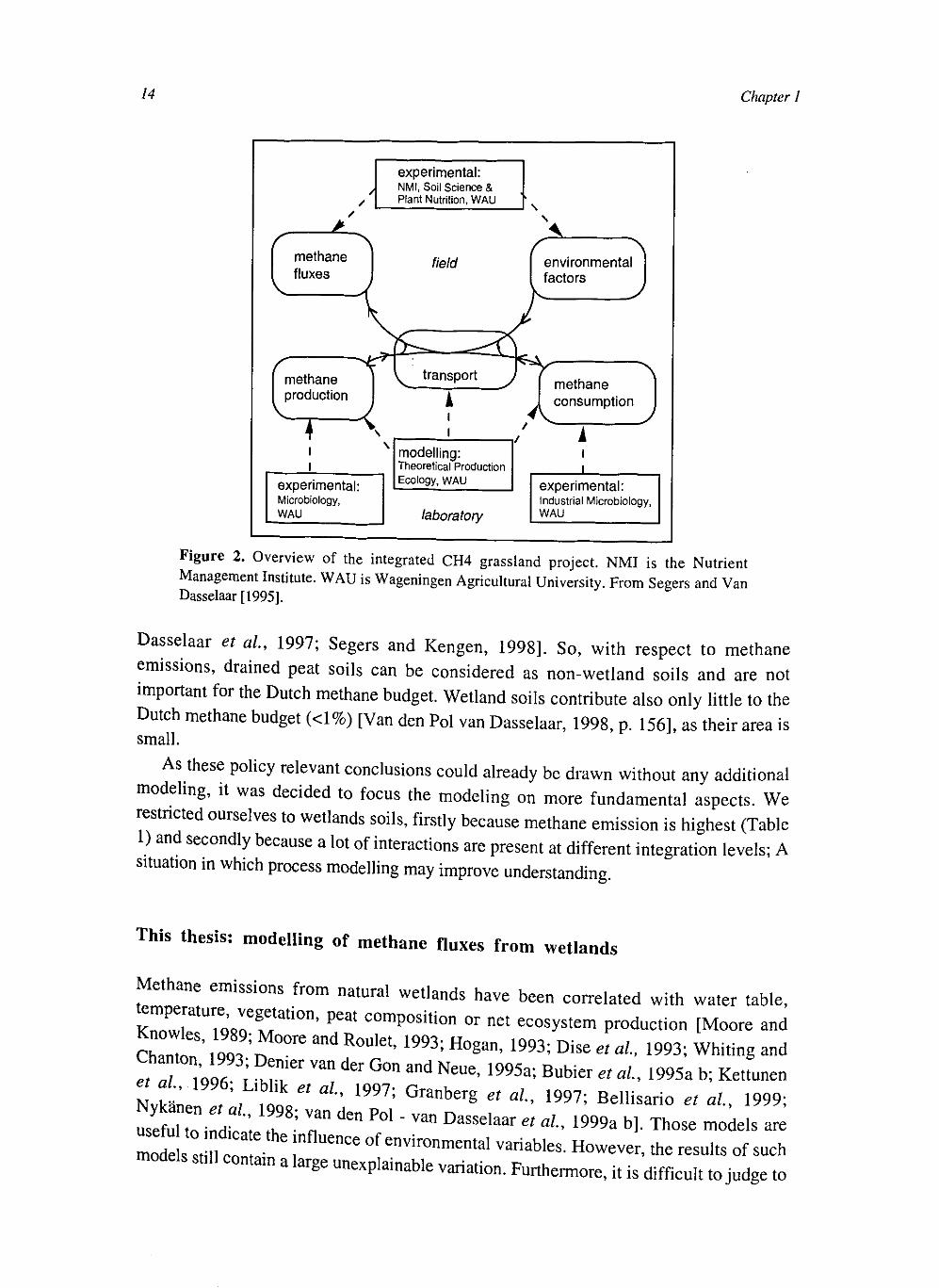
Figure 2. Overview of the integrated CH4 grassland project. NMI is the Nutrient Management Institute. WAU is Wageningen Agricultural University. From Segers and Van Dasselaar [1995].
Dasselaar et al., 1997; Segers and Kengen, 1998]. So, with respect to methane emissions, drained peat soils can be considered as non-wetland soils and are not important for the Dutch methane budget. Wetland soils contribute also only little to the Dutch methane budget (<1%) [Van den Pol van Dasselaar, 1998, p. 156], as their area is small.
As these policy relevant conclusions could already be drawn without any additional modeling, it was decided to focus the modeling on more fundamental aspects. We restricted ourselves to wetlands soils, firstly because methane emission is highest (Table 1) and secondly because a lot of interactions are present at different integration levels; A situation in which process modelling may improve understanding.
This thesis: modelling of methane fluxes from wetlands
Methane emissions from natural wetlands have been correlated with water table,
^le,^atU,ieQfiVoef,tati0n, P C a t C ° m P° s i t i o n o r n * ecosystem production [Moore and
Chant ! ' 99, n ° ° r e "* ^ ^ " ^ ^ D i s e «<*• ^ Whiting and
etal 1 oof J J r Van ° ° n ^ NeU6' 1995a; Bubier «<*•> 1995a b; Kettunen NvkL t , , £ / ' ' 199?: ° r a n b e r g et aL' 1997> B e l l i s a r i ° et al, 1999; S Z i d, t T- T ^ P 0 1 " ^ D a S S d a a r et < 1 9 9 9 a »>]. Those models are I e 1 I CnCe ° f e n V i r ° n m e n t a l V a r i a b l e s ' H o w e v e r • *e results of such models still contain a large unexplainable variation. F u r t h e r , it is difficult to judge to

General Introduction J5
what extent results of such models can be extrapolated, because quantitative understanding of underlying processes is poor in such models.
To understand methane fluxes from wetland systems it is necessary to look for stable relationships, which can only be found to some extent in theory of microbial and chemical transformations and physical transport processes. In this thesis knowledge of these basic processes is related to methane fluxes and it is investigated what can be gained by doing so in terms of understanding the relation between plot scale environmental variables and methane fluxes.
These theories can only be directly applied in homogeneous systems, which makes their application to soils difficult, as these are generally heterogeneous at various scales. However, at small scales, when mixing is faster than the conversions, heterogeneities tend to be resolved. This scale is of the order of magnitude of 1 mm for the conversions relevant for methane emissions[Chapter 4], which is smaller than typical distances between roots [Chapter 4]. Hence, heterogeneities around gas transporting roots, caused by relatively fast gas exchange of gases with the atmosphere, are not resolved and have to be considered. Also at the profile scale (dm) important heterogeneities exist: a fluctuating water table and a decreasing organic matter availability. To cope with these scale differences a stepwise scaling up procedure is used (Figure 3).
driving variables
• weather • vegetation • soil type • hydrology
scale
t water content soil temperature root density
• distance to next root root radius root mass transfer mineralisation
* mineralisation aeration
target variables
• C H 4 flux
t flux through plants [CH4 ]
net CH4 production
• • CH4 f luxto root
• net CH 4 production
• [CH4]
I • CH 4 production • CH 4 consumption
• [CH4]
Figure 3. Organisation of levels of scale in relating methane kinetics to methane fluxes in wetlands with gas transporting roots (from chapter 4). The full lines represent existing, conservative, relationships. The dashed lines represent relationships to be investigated.

16 Chapter I
First the kinetic knowledge on methane production and methane oxidation is summarised (Chapter 2) and extended for methane production in peat soils (Chapter 3). In Chapter 4 the kinetic knowledge is integrated with diffusion around a single gas transporting root in a reaction-diffusion model. Subsequently, this model is simplified in such a way that the details at the kinetic scale are not considered explicitly any more, while maintaining the same functional behaviour at the single root scale. In the next steps (Chapter 5 and Chapter 6) the same procedure is repeated at consecutively higher integration levels. In this way it is possible to understand the extent to which knowledge at the kinetic scale influences methane fluxes at the plot scale.
17
Chapter 2
Methane production and methane consumption: a review of processes underlying wetland methane fluxes
Segers, R. Biogeochemistry, 41, 23-51, 1998
Abstract
Potential rates of both methane production and methane consumption vary over three orders of magnitude and their distribution is skew. These rates are weakly correlated with ecosystem type, incubation temperature, in situ aeration, latitude, depth and distance to oxic/anoxic interface. Anaerobic carbon mineralisation is a major control of methane production. The large range in anaerobic CH4:C02 production rates indicate that a large part of the anaerobically mineralised carbon is used for reduction of electron acceptors, and, hence, is not available for methanogenesis. Consequently, cycling of electron acceptors needs to be studied to understand methane production. Methane and oxygen half saturation constants for methane oxidation vary about one order of magnitude. Potential methane oxidation seems to be correlated with methanotrophic biomass. Therefore, variation in potential methane oxidation could be related to site characteristics with a model for methanotrophic biomass.
Introduction
Methane contributes to the enhanced greenhouse effect. Wetlands, including rice paddies, contribute between 15 and 45% of global methane emissions [Prather et ah, 1995]. Methane emissions from wetlands show a large variation [Bartlett and Harris, 1993] which can only partly be described by correlations with environmental variables [Moore and Knowles, 1989; Moore and Roulet, 1993; Dise et a/., 1993; Hogan, 1993; Whiting and Chanton, 1993; Bubier et al, 1995ab; Kettunen et ai, 1996; Denier van der Gon and Neue, 1995a]. This limits the accuracy of estimates of both current and future global emissions, the latter being the result of possibly changed conditions due to a changed climate or changed soil management. Insight in the underlying processes could improve this situation.
Methane fluxes from or to soils result from the interaction of several biological and physical processes in the soil [Hogan, 1993; Schimel et ah, 1993; Conrad, 1989; Cicerone and Oremland, 1988; Bouwman, 1990; Wang et ah, 1996]; Methane
Segers, R. Wetland Methane Fluxes: Upscaling from Kinetics via a Single Root and a Soil Layer to the Plot, Ph. D. Thesis, Wageningen University, 1999.
jg chapter 2
production is a microbiological process, which is predominantly controlled by the absence of oxygen and the amount of easily degradable carbon. Methane consumption is also a microbiological process. Major controls are soil oxygen and soil methane concentrations. Gas transport influences aeration and determines the rate of methane release from the soil. Gas transport occurs via the soil matrix and via the vegetation. In the first case it is controlled by soil water and in the second case it is sometimes influenced by weather conditions. The vegetation also influences the amount of easily degradable carbon. All these processes are affected by temperature, and thus by heat transport.
In the last decade, knowledge of methane production and methane consumption has increased considerably. This increased knowledge has been used to support the descriptive models mentioned above and to develop process models [Cao et aL, 1995; 1996; Walter et al, 1996; Watson et al, 1997]. However, these process models require fit procedures or intensive on site measurement of parameters which are as variable as methane fluxes, which limits their applicability for understanding and developing general relationships between methane fluxes and environmental variables. To improve the process models in this respect the knowledge of methane production and methane consumption is reviewed and it is investigated how this knowledge could be used to establish quantitative relations between the rates of both processes and environmental variables.
Two pathways are followed. Firstly, potential, laboratory rates, collected from a large number of studies, are related directly to environmental variables with statistical methods. Secondly, the process knowledge underlying these relations is summarised. Methane production and consumption are driven by organic matter mineralisation, soil aeration and heat transport. For understanding the relation between environmental variables and methane kinetics, these driving processes have to be understood as well. However, these processes are not reviewed here to limit the size of the paper.
Methane production
Methane production in soils can occur when organic matter is degraded anaerobically [Oremland, 1988; Svensson and Sundh, 1992; Conrad, 1989]. Several bacteria that degrade organic material via a complex food web are needed to perform this process. The final step is performed by methanogens, methane producing bacteria. Methanogenic bacteria can use a limited number of substrates, of which acetate and hydrogen are considered the most important ones in fresh water systems [Peters and Conrad, 1996;
fubs I" T \W87; ^ ^ "' KIUg' 1983; YaVkt and L^< »*»• °*" ZZTonT TT A" Sh°Wn t 0 bC r e S P ° n S i b l e f ° r — *»» 5 % °f ^ e methane m a t t Zm T Q S I J d r 0 g e n " ^ ^ b y S ta t ion from hydrolysed organic S . ^ f • J ^ d e C t r 0 n a C C C p t 0 r S SUPPrCSS - t h a n e production, which is most easily understood from thermodynamics [Zehnder and Stumm 1988]
review of methane production and consumption 19
Potential methane production correlated to environmental variables
Potential methane production, PMP, is the methane production by an anaerobically incubated soil sample. Rates of PMP have been determined in a large number of studies in various natural wetlands and rice paddies. Here, it is investigated whether general applicable relations emerge when all data are put together. To do so, the following assumptions were made: Zero rates in tables were assigned values equal to half of the detection limit, which was, when not specified, equal to half of the lowest value. Zero rates in graphs were assigned a value of 1/20 of the smallest unit. All rates were converted to volumetric units, because both the ultimate controls (primary production and oxygen influx) and the quantity to be explained (methane fluxes) are on an area basis, which is more closely related to volumetric rates than to gravimetric rates. Consequently, all rates which were originally expressed on a soil weight basis had to be multiplied with soil density. In case the soil density was not given, wet bulk densities of peat were 1 g cm-3, dry bulk densities of peat varied between 0.04 and 0.11 g cirr3, depending on depth and
v
0.8 4-
CD O
Q. 0.4 +
0.2 4-
0 -3
potential methane ~ ^
production
j potential methane
cpo-.
oxidation
-2 -1 0 1
log rate (rate in umol m s~ )
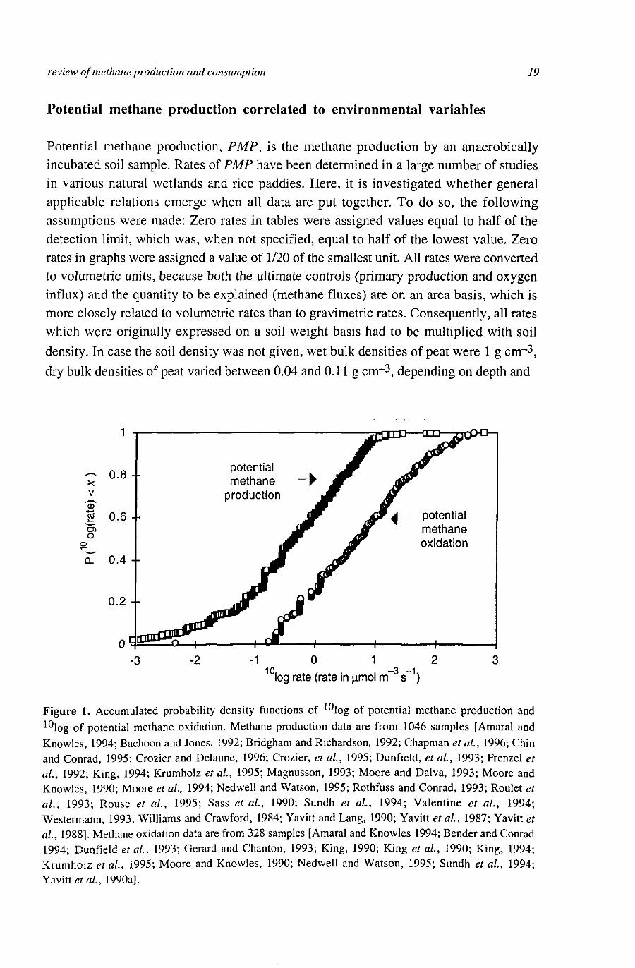
Figure 1. Accumulated probability density functions of I0Iog of potential methane production and 10log of potential methane oxidation. Methane production data are from 1046 samples [Amaral and Knowles, 1994; Bachoon and Jones, 1992; Bridgham and Richardson, 1992; Chapman et al., 1996; Chin and Conrad, 1995; Crozier and Delaune, 1996; Crozier, et al., 1995; Dunfield, et al, 1993; Frenzel et al., 1992; King, 1994; Krumhoiz et al, 1995; Magnusson, 1993; Moore and Dalva, 1993; Moore and Knowles, 1990; Moore et al, 1994; Nedwell and Watson, 1995; Rothfuss and Conrad, 1993; Roulet et al, 1993; Rouse et al, 1995; Sass et al, 1990; Sundh et al, 1994; Valentine et al, 1994; Westermann, 1993; Williams and Crawford, 1984; Yavitt and Lang, 1990; Yavitt et al, 1987; Yavitt et al, 1988]. Methane oxidation data are from 328 samples [Amaral and Knowles 1994; Bender and Conrad 1994; Dunfield et al, 1993; Gerard and Chanton, 1993; King, 1990; King et al, 1990; King, 1994; Krumhoiz et al, 1995; Moore and Knowles, 1990; Nedwell and Watson, 1995; Sundh et al, 1994; Yavitt etal, 1990a].
20 c/tapter 2
soil type [Minkinnen and Laine, 1996] and dry bulk densities of mineral soils were 1.5 g cm - 3 [Koorevaar et al, 1983]. For roots a dry bulk density of 0.08 g cm - 3 was calculated, assuming a water content of 90% and a porosity of 20% [Crawford, 1983]. To improve future comparisons of rates in any unit it is recommended to measure bulk density and soil moisture contents in addition to the biogeochemical rates.
The distribution of PMP rates is skew and variation is large (Figure 1), as is for methane fluxes in the field [Bubier et al, 1995a b, Dise et al, 1993, Panikov, 1994]. Typical PMP rates vary from 10~2 to 101 mmol nr-3 s"1. An exception are the very high values of around 103 mmol m~3 s"1 found by Bachoon and Jones [1992]. This may be attributed to their relatively high incubation temperature (30 °C) and the high concentration of available organic matter, as they sampled only the upper 2 cm of subtropical minerotrophic wetland.
Evaluation of experimental methods
No standard procedure exists for measuring PMP, though the effect of the experimental procedure on measured rates could be large. Hall et al. [1996] observed that small periods of aerobiosis (5 min.) decreased PMP in peat soil samples 10 to 70 %. Sorrell and Boon [1992] reported that rigorously mixing of a sediment decreased methane production by an order of magnitude. By contrast, Kengen and Stams [1995] found higher production of both methane and carbon dioxide in slurried samples compared to unslurried samples of a drained peat soil. Valentine et al [1994] suggested that slurrying could decrease methane production as a result of inhibition by a flush of fatty acid production. Kelly and Chynoweth [1980] could stimulate methane production in deep fresh water sediments (3-20 cm) by stirring. By contrast, in the top sediment (0-3 cm) they could not do so. So, the effect of measurement procedure on methane production is highly uncertain, which was also concluded by Sundh et al [1994]. Knowledge of the effect of sampling procedure on the processes underlying methane production is needed to improve this situation. Recently, Dannenberg et al [1997] made considerable progress in this area by showing that acetoclastic methanogens in paddy soils are seriously affected by stirring and moderately by gently shaking.
The effect of sampling procedures on the conclusion drawn in this paper may be limited by the large number (19) of used data sets. Due to the wide variety in experimental methods it was not possible to investigate the effect of sampling procedures with statistical methods.
In situ aeration, ecosystem type and latitude
In situ aeration affects PMP significantly (Table la). Mean ™\og(PMP) of samples
trom aerobic sites was more than one order of magnitude less than the mean ™\og{PMP)

review of methane production and consumption 21
of samples from anaerobic sites, probably caused by higher concentration of electron acceptors and/or lower concentrations of methanogenic biomass.
PMP in samples from oligotrophic natural wetlands is lower than methane production in samples from minerotrophic natural wetlands (Table la), possibly because of the lower amount of fresh organic material as a result of lower primary production. In contrast, Moore and Knowles [1990] did not find any correlation between trophic status of the soil and PMP, This difference can only partly be explained by the difference in units used, because also when the data of this paper are converted to the gravimetric units of Moore and Knowles [1990], PMP in oligotrophic wetlands is relatively low. PMP in soil samples from paddy soil is higher than PMP in samples from natural wetlands. The
Table la. Statistics of potential methane production (PMP). Data are the same as in Fig. 1. SED is the standard error of the mean and SD is the standard deviation. Aerobic samples were taken from >5 cm above the water table, intermediate samples from within 5 cm of the water table and anaerobic samples were taken from >5 cm below the water table. In submerged soils the aeration of the first cm was considered intermediate, deeper layers were considered anaerobic. Values with the same letter are not significantly different from each other (p=0.05).
qualitative variables
10log (PMP) (PMP in /xmol m"3 s"1)
mean SEM SD
in situ aeration
aerobic
intermediate
anaerobic
ecosystem type
minerotrophic natural wetland
oligotrophic natural wetland
rice paddy
-1.7a
-0.42b
-0.42b
-0.47a
-0.9 lb
0.09c
0.1 0.06
0.04
0.05
0.06
0.05
0.8 1.0 1.1
1.2 0.8 0.7
39 268 621
657 176 210
Table lb. Linear regressions for potential methane production (PMP). T\nc is the incubation
temperature (°C), lat is the latitude (°N) and depth is the depth below the soil surface (cm). /0i,
(oligotrophic) /pad (paddy) and / a e r (aerobic) are dummy variables, used to combine qualitative and
quantitative variables. /0li=l if soil type is oligotrophic and /oli=0 for the other soil types, ect..
Standard errors of coefficients are between brackets.
PMP in ^mol m 3 s I ^adj
10log(/>Af/>) = -1.8(0.1) + 0.069(0.005)*rinc
l0log(PMP) = 1.3(0.1) - 0.040(0.003)-/af X0\og(PMP) = -0.28(0.04) - 0.008(0.001)vfep//i
10log(PMP) = -0.2(0.2) + 0.069(0.006)«7jnc -
0.026(0.003)«/a/ - O.39(0.08)»/Oii - 0.7 (0.1)*/pad
- 1.2 (0.2)»/aer-0.012(0.002Wepryi
0.16
0.20
0.03
973 1001
1042
0.36 926

22 chapter 2
minus sign in the summary relation for the /paci (Table la) suggests, that this is caused by more anaerobic conditions, higher temperature, and lower latitude.
The relatively high PMP at lower latitudes (Table lb) can be explained the higher incubation temperatures and by the higher primary production (resulting in more easily
degradable carbon).
Temperature
Incubation temperature could describe part of variation in the 10log PMP (Table 1). <2l0 of all samples together was 4.1(±0.4). Alternatively, <2l0 values have been determined in incubation experiments with temperature as single varying factor, resulting in a range from 1.5 to 28 (Table 2). To explain this large range Qjo, values of underlying processes are listed as well. Q\Q of anaerobic C-mineralisation is between 1 and 4 and methanogenic bacteria have Qio values up to 12, which is still not high enough to explain the highest end of the Q\Q values for methane production. A possible explanation for the high GlO values for methane production is the interaction of several processes: An increasing temperature increases rates of electron acceptor reduction, which results in lower electron acceptor concentrations which has an additional positive effect on methane
Table 2. Temperature dependence of methane production and sub processes responsible for methane production.
Sample source, process or organism Q j Q
Methane production, soil sample scale
minerotrophic peat4 '5-6 '1 3 '1 5 '1 9 1.5-6.4
oligotrophic p e a t 6 ' 1 0 ' 1 3 ' 1 4 ' 1 5 2-28
paddy1-8'17 2.1-16
Methanogenesis of pure cultures
acetotrophic3- *6 '2 0 ' ] 8 2.9-9.0
hydrogenotrophic1 '3 1.3-12.3 growth of M. soehngenii^^O 2.1
Processes related to anaerobic carbon mineralisation
anaerobic CO2 production in peat6 '14 1.5
total anaerobic C -mineralisation in paddy soil17 0.9-1.8
anaerobic hydrolysis of particulate organic matter2 1.9
acetate production from various substrates11 1.7-3.6
^chutz et al. [1990], 2Imhoff and Fair [1956], 3Westermann et al. [1989], 4Westermann and Ahring [1987], 5Westermann [1993], 6Updegraff et al. [1995], 8Sass et al. [1991], 10Nedwell and Watson [1995], nKotsyurbenko^fl/. [1993], 13Valentine et al. [1994], 14Bridgham and Richardson [1992], I5Dunfield et al. [1993], 16Huser et al. [1982], 17Tsutsuki and Ponnamperuma [1987], 18van den Berg et al. [1976], 19Williams and Crawford [1984], 20Gujer and Zehnder [1983]
review of methane production and consumption 23
production. This mechanism could explain the high QlO values of Updegraff et al[1995] and Tsutsuki and Ponnamperuma [1987] in their long term (>several weeks) experiments in which methane production increased with time. However, for the shorter term experiments (a few days) of Dunfield et al [1993] and Nedwell and Watson [1995] this explanation is not applicable as methane production was more or less constant over the incubation time [R. Knowles pers. comm.; A. Watson pers. comm.], indicating that depletion of an inhibiting electron acceptor did not occur during the incubation experiment.
In summary, variation in reported £>10 values of methane production is large. This could be due to the anomalous temperature behaviour of the methanogens themselves and due to the interaction of the underlying processes.
PH
Most known methanogenic bacteria have their optimum pH at 7. However, anaerobic bacteria with lower optima have been isolated from acidic peats [Williams and Crawford, 1985; Goodwin and Zeikus, 1987]. Mostly, increasing pH in incubated samples increases PMP [Dunfield et al, 1993; Yavitt et al, 1987; Valentine et al, 1994]. A correlation between pH and PMP was found in most samples by Valentine et ah, [1994], but not by Moore and Knowles [1990]. Dunfield et al [1993] observed that optimum pH was 0-2 units above field pH for peat samples from five different acidic sites. So, the adaption to in situ pH of the microorganisms controlling methane production is variable.
Root-associated methane production
Roots can affect methane production both positively and negatively, because root oxygen transport suppresses methane production, whereas root decay and root exudation promote methane production. King [1994] reported methane production in roots and rhizomes of anaerobically incubated Calamogrostis canadensis, and Typha latifolia, which were washed aerobically. The conversion time of photosynthesised 13C to emitted methane was sometimes less than 1 day in a rice paddy [Minoda and Kimura, 1994; Minoda et al, 1996]. These two observations point at methane production inside, at, or near roots. Apparently, aeration of roots and rhizosphere is not complete, as follows also from the observation of organic acids within waterlogged plants [Ernst, 1990], a root oxygen diffusion model of Armstrong and Beckett [1987] and rhizosphere oxygen measurements [Conlin and Crowder, 1988; Flessa and Fischer, 1992].
The relative contribution of root-associated methane production to methane emissions could be important in a rice paddies, as it varied between 4 and 52 % in a case study of Minoda et al [1996]. Also in natural wetlands the contribution of root-associated methane production to methane emissions could be large, because removing above ground vegetation decreased methane emissions considerably (up to more than a factor
2A chapter 2
10) without a concurrent decrease of stored methane in the soil [Waddington et al, 1996;
Whiting and Chanton, 1992].
Inhibitory compounds
Under anaerobiosis, compounds can be formed that are toxic to plants [Drew and Lynch, 1980] and possibly also to bacteria involved in methane production. Some volatile compounds may inhibit methanogenesis [Williams and Crawford, 1984] and anaerobic carbon dioxide production [Magnusson, 1993], as flushing with N2 resulted in an increase in gas production in anaerobic incubation experiments. It is not known what kind compounds are involved and whether this effect is important under in situ conditions.
Fatty acids can inhibit anaerobic bacteria when its undissociated concentrations are too high [Wolin et al, 1969]. Consequently, especially acid environments are sensitive for this inhibition. Fukuzaki et a/.[1990] found that two methanogens had distinct optimum undissociated acetate concentrations (140 and 900 |iM) for acetate consumption. Also in laboratory incubations experiments with acid soil samples, acetate inhibited methane production [Yavitt et al, 1987, Williams and Crawford, 1984] and glucose decomposition [Kilham and Alexander, 1984]. By contrast, van den Berg et al. [1976] obtained a methanogenic enrichment culture for a waste digestor, in which acetate uptake was independent of acetate concentration between 0.2 and 200 mM.
Also sulfide can inhibit methane production. Cappenberg [1975] found a total inhibition of methane formation at 0.1 mM, and no inhibition at 0.001 mM, but in methanogenic enrichment cultures from a waste digestor there was no inhibition of methanogenesis below approximately 1 mM [van den Berg et al, 1976; Maillacheruvu and Parkin, 1996].
Explanation of methane production via the underlying processes.
Substrate, organic matter
Once anaerobiosis is established, organic substrate is considered as the major limiting factor for methane production; Firstly, both the addition of direct methanogenic substrates, like hydrogen or acetate, and the addition of indirect substrates, like glucose and leaf leachate, enhanced methane production in anaerobically incubated soil samples [Williams and Crawford, 1984; Valentine et al, 1994; Amaral and Knowles, 1994; Bachoon and Jones, 1992]. Yavitt and Lang [1990], however, did not find substrate limitation in some of their soil samples. Secondly, Denier van der Gon and Neue [1995a] found a positive correlation between methane emission and organic matter input at 11 rice paddy sites. Thirdly, Whiting and Chanton [1993] and Chanton et al [1993] found a
review of methane production and consumption 25
relation between carbon dioxide fixation and methane emission in flooded wetlands, though this could also be a consequence of a larger vegetational transport capacity. Fourthly, root-associated methane production could contribute to methane emissions (see above). Fifthly, methane production measured in laboratory incubations of soil samples often decreases with depth, when taken from below the water table [Sundh et al, 1994; Williams and Crawford, 1984; Yavitt et aL, 1987], as does the availability of organic matter. Sixthly, the 14C fraction of emitted methane was near the 14C fraction of atmospheric carbon dioxide [Chanton et ah, 1995], indicating that the methane was mainly derived from recently fixed carbon. And seventhly, often there is a correlation between organic matter quality parameters and methane production: (i) Crozier et ah [1995] found a good correlation between aerobic carbon dioxide production and anaerobic methane production in dried and fresh undisturbed peat cores, (ii) Yavitt and Lang [1990] found positive correlations with total organic matter and acid-soluble organic matter, though no correlations were found with dissolved organic matter and hot water-soluble organic matter and a negative correlation was found with acid-insoluble organic matter, (iii) Valentine et al. [1994] found positive correlations with carbohydrate content. Correlations with C;N and lignin:N content were not consistent, however, (iv) Nilsson [1992] successfully correlated methane production to infrared spectra of peat samples, suggesting that the organic composition of the peat samples was a major determinant of methane production.
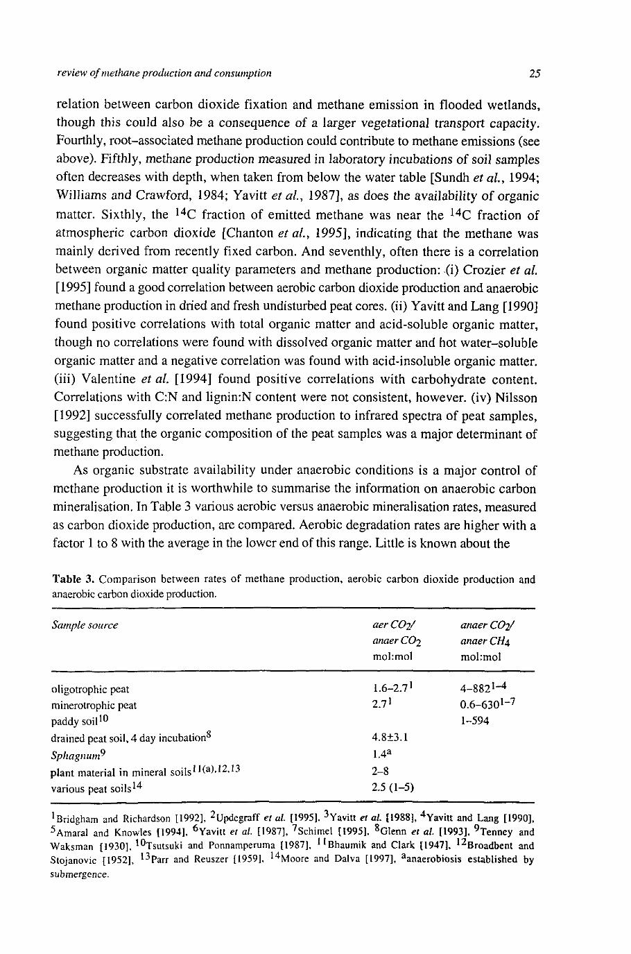
As organic substrate availability under anaerobic conditions is a major control of methane production it is worthwhile to summarise the information on anaerobic carbon mineralisation. In Table 3 various aerobic versus anaerobic mineralisation rates, measured as carbon dioxide production, are compared. Aerobic degradation rates are higher with a factor 1 to 8 with the average in the lower end of this range. Little is known about the
Table 3. Comparison between rates of methane production, aerobic carbon dioxide production and anaerobic carbon dioxide production.
Sample source
oligotrophy peat
minerotrophic peat
paddy soil10
drained peat soil, 4 day incubation8
Sphagnum^
plant material in mineral soils1 Ha),12,13
various peat soils14
^ridgham and Richardson [1992], 2Updegraff et al. [1995], 3Yavitt et al [1988], 4Yavttt and Lang [1990], 5Amaral and Knowles [1994], 6Yavitt et al. [1987], 7Schimel [1995], 8GIenn et al. [1993], 9Tenney and Waksman [1930], 10Tsutsuki and Ponnamperuma [1987], nBhaumik and Clark [1947], 12Broadbent and Stojanovic [1952], 13Parr and Reuszer [1959], 14Moore and Dalva [1997], aanaerobiosis established by submergence.
aer COi/ anaer CO2 mol:mol
1.6-2.7!
2.7 *
4.8±3.1 1.4a
2-8 2.5(1-5)
anaer CO2/ anaer CH4
mol:mol
4-8821"4
0.6-6301"7
1-594

26 chapter 2
causes of this variation, which limits the accuracy of soil carbon models with respect to anaerobic carbon mineralisation.
Microbial biomass
Limitation of methane production by microbial biomass occurs when microbial uptake capacity does not meet substrate supply. In principle, it can be a result of (i) periodical damage to bacteria due to poisoning or starvation, (ii) nutrient stress of the bacteria and (iii) an increase of substrate supply that is larger than the growth rate of the bacteria. Methanogenic bacteria are more likely to limit methane production than fermenting bacteria for several reasons. Firstly, their relative growth rate is relatively low [Pavlosthatis and Giraldo-Gomez, 1991] and secondly, accumulation of substrates for fermenting bacteria, like sugars, has never been observed, whereas accumulation of substrates for methanogenic bacteria, especially acetate, did occur at low temperatures [Shannon and White, 1996; Drake et a/., 1996] and upon anaerobic incubation of non-wetland soils [Peters and Conrad, 1996, Kusel and Drake, 1995, Wagner et al, 1996].
Damage to a methanogenic population could be the result of aerobiosis, either directly by poisoning or indirectly by C-starvation due to competition for substrates with aerobic microorganisms. If damage occurs during aerobiosis the methanogenic population needs time to recover when anaerobiosis returns, especially because relative growth rates of methanogenic bacteria are low, typically 0.4 d"l at 35 °C [Pavlostathis and Giraldo-Gomez, 1991]. Shannon and White [1994] attributed the reduction of methane emission from a bog in the year following a dry year to this mechanism. By contrast, in rice paddies methane emission can develop quickly after inundation [Holzapfel-Pschorn and Seiler, 1986], which can be explained by the good oxygen survival abilities of methanogenic bacteria in paddy soil [Mayer and Conrad, 1990; Joulian et al, 1996]. These differences in the onset of methane emission after aerobiosis can explained by (i) differences in kind and concentration of electron acceptors that suppress production, which are formed during an aerobic period [Freeman et al.t 1994], by (ii) differences in temperature causing differences in rates of electron acceptor reduction and differences in rates of bacterial growth and by (iii) differences in oxygen survival times of methanogenic bacteria, ranging from a few hours to several months [Kiener and Leisinger, 1983; Fetzer et „/., 1993; Huser et aU 1982; Huser, 1981]. The latter explanation is not so likely, as, from an ecolog1Cal point of view, it is likely that methanogenic bacteria in sites with a fluctuating aeration have good oxygen survival characteristics.
N or P limitation for the methanogenic consortium does not seem to occur, as N or P
! 1 ! l g e n e r a 1 1 : d ° n 0 t S t i m u l a t e m*hane production [Bridgham and Richardson, 992 wilhams and Crawford, 1984, Bachoon and Jones, 1992]. Additionally, Williams
I Craw ord [1984] found no reaction of methane production on the addition of yeast extract and vitamins in samples from an acid bog. Yavitt and Lang [1990] suggested that

review of methane production and consumption 27
in rain water fed mires nickel could be limiting, as explanation why they could not enhance methane production by adding various substrates. For Methanothrix concilii optimum Ni2+ concentration was about 0.1 JJM [Patel et ai, 1988]. Apart from the concentration of Ni2+ also the form of Ni2+ (chelated or not) could be relevant [Nozoe and Yoshida, 1992].
Flushes of substrate are not a likely cause of biomass limitation, because plant decay, which is the major source of labile organic matter, is a rather stable process. Even the application of organic material in agricultural ecosystems is not a likely cause of biomass limitation, because normally it is managed in such a way that fatty acids do not accumulate, as they are toxic.
Electron acceptors
Alternative electron acceptors, like NO3-, Fe3+, Mn4+, S042~ and possibly humic acids [Lovley et ai, 1996] suppress methanogenesis, because reduction of alternative electron acceptors supplies more energy than methanogenesis [Zehnder and Stumm, 1988]. Three mechanisms, that could operate at the same time, could be responsible for this effect. Firstly, reduction of electron acceptors could reduce substrate concentrations to a value which is too low for methanogenesis [Achtnich etai, 1995; Peters and Conrad, 1996; Kristjansson et ai, 1982; Schonheit et aL, 1982]. Secondly, the presence of electron acceptors could result in a redox potential which is too high for methanogenesis [Wang et ai, 1993; Peters and Conrad, 1996; Jakobsen et al, 1981]. Thirdly, electron acceptors could be toxic for methanogens [Jakobsen et ai 1981].
The large range of anaerobic C02:CH4 production rates (Table 3) indicate that reduction of terminal alternative electron acceptors uses a large and variable part of the anaerobically mineralised carbon, provided that no substantial accumulation of fermentation products occurs, which has never been observed in the C02:CH4 measurements. Consequently, cycling of electron acceptors is probably a major process in controlling methane production.
Reduction of electron acceptors requires organic matter. Consequently, anaerobic carbon mineralisation influences methane production not only directly, but also indirectly, via the rate of electron acceptor depletion. A dynamic process model centered around this relation was developed [chapter 3].
Summary
The knowledge of the processes underlying methane production can be summarised in a simple equation [Segers and Leffelaar, 1996]:
MP^ICF, (1)

28 chapter 2
where MP is the methane production rate, / is an aeration inhibition function, which is one under anaerobiosis and zero under aerobiosis, C is the anaerobic C-mineralisation rate and F is the fraction of the anaerobically mineralised C, which is transformed into methane. When PMP rates are considered / is equal to one. A basic assumption underlying equation (1) is that availability of organic matter is a major control of methane production. Variation in F is caused by a varying contribution of the reduction of terminal electron acceptors. Therefore, to explain variation in F, cycling of electron acceptors should be considered.
Methane consumption
In contrast with methane production, methane consumption in wetlands is considered to be mainly performed mainly by a single class of microorganisms: a methanotroph [Cicerone and Oremland, 1988; King, 1992]. Methane consumption is essential for understanding methane emission. Although the methods for determining in situ methane oxidation on the field scale are under debate [Denier van der Gon and Neue, 1996; Frenzel and Bosse, 1996; King, 1996; Lombardi et al, 1997], it is likely that a large and a varying part (1-90%) of the produced methane could be consumed again, either in the oxic top layer or in the oxic rhizosphere [de Bont et aL, 1978; Holzapfel Pschorn and Seiler, 1986; Schiitz et a/., 1989; Sass et a/., 1990; Fechner and Hemond, 1992; Oremland and Culbertson, 1992; Happell etal, 1993; Epp and Chanton, 1993; Kelley et aL, 1995; King, 1996; Denier van der Gon and Neue, 1996; Schipper and Reddy, 1996; Lombardi et al, 1997]. This large variation could be explained by knowledge of methane oxidation on the soil sample scale, which is reviewed below.
High affinity and low affinity methane oxidation
It is convenient to distinguish two kinds of methanotrophic activity: high affinity (low, atmospheric, methane concentrations) and low affinity (high methane concentrations). The essential difference is that growth and ammonium inhibition of high affinity activity is barely understood [Roslev et al, 1997; Gulledge et al 1997], while the basic kinetics of low affinity methane oxidation are relatively well established [King, 1992]. The transition point between high and low affinity oxidation is somewhere between 100 and 1000 ppm methane (gas phase) [Bender and Conrad, 1992, 1995, Nesbit and Breitenbeck 1992, Schnell and King, 1995; King and Schnell, 1994]. When soil methane concentrations are in the range of high affinity methane oxidation, methane emission can only be relatively small for wetlands. A closer study of (high affinity) methane oxidation will not change that picture. Therefore, the peculiarities of high affinity methane oxidation are not considered in this article, which is restricted to wetlands.

review of methane production and consumption 29
Aerobic methane oxidation
Aerobic methane oxidation, MO, requires both oxygen and methane. So, in principle, both substrates could be limiting. The following double Monod expression describes this double substrate dependence:
MO = PMO [CH4] [02 ]
[ C H ^ + ^ o ^ [02] + ^mp 2
(2)
Potential methane oxidation, PMO, is typically between 0.1 and 100 /imol m - 3 s_1
(Figure 1). This is about one order of magnitude larger than PMP. Km,cH4. and ATm>02 vary about one order of magnitude (Table 4). In experiments with pure cultures the higher values for ^m,CH4 could have been too high, because in those experiments MO was determined as the oxygen uptake rate, while methane concentrations were assumed to be constant [Joergensen and Degn, 1983]. However, this reasoning does not hold for the experiments with peat soils, because in those cases £"m,CH4 values were determined by monitoring the decrease of methane concentration in the headspace above continuously stirred samples. Therefore, the large variation in Km values may be an intrinsic property of methanotrophic bacteria.
There are two strategies to find predictive relations for PMO. Firstly, by using descriptive relations between PMO and soil environmental variables, like water table.
Table 4. Half saturation constants for methane oxidation.
Organism or sample source ^m,CH4 ^m,02 uM
Wetland soils
fresh water sediment
sediment free roots
natural peat soils
agricultural peat
paddy soil
Other methanotrophic environments
various methanotrophs
deep lake sediments
landfill soils
2.2-3.7' 3-62
1-453'5'6-7
66.24
88 'a
0.8-489"15
4.1-1016.18
1.6-31.719-20
200a'7
374
0.3-1.3".1* 201 8 ,<181 7
'King [1990], 2King [1994], 3Yavitt et al. [1988], 4Megraw and Knowles [1987], 5Dunfield et al. [1993], 6Nedwell and Watson [1995], 7Yavitt et al [1990a], 8Bender and Conrad [1992], 9Linton and Buckee [1977], 10Lamb and Garver [1980], uJoergensen [1985], 12Nagai et al [1973], 13Harrison [1973], 140'Neill and Wilkinson [1977], 15Ferenci et al [1975]. I6Bucholz et al [1995], 17Frenzel et al. [1990], 18Lidstrom and Somers [1984] I9Kightley et al [1995], 20Whalen et al [1990], aupper limit, as obtained in unshaken samples.

30 chapter 2
Secondly, by using a model for methanotrophic biomass, because PMO appears, logically, to be correlated with methanotrophic biomass [Bender and Conrad, 1994 and Sundh etaU 1995b].
Anaerobic methane oxidation
Thermodynamically, it is possible to oxidise methane anaerobically with the alternative electron acceptors that inhibit methane production. However, bacteria that perform this process have never been isolated. Nevertheless, for anaerobic methane oxidation by sulphate in marine systems fairly strong evidence is present [Cicerone and Oremland, 1988; King, 1992]. In freshwater systems indications were obtained at sulphate concentrations from 0.5 mM, but not at concentrations below 0.2 mM [Panganiban, 1979; Nedwell and Watson, 1995; Yavitt et al, 1988]. Panganiban [1979] could not find any anaerobic methane oxidation at any nitrate concentration. Ferrous iron [Miura et al, 1992] and sulphate [Murase and Kimura, 1994b] may be involved in anaerobic methane oxidation in paddy soil (with about 1 mM sulphate and 2.5% of free iron), with an upper
limit of about 3 |imol m - 3 s_1 (calculated from Miura et al. [1992] and Murase and Kimura [1994a b]). This upper limit is of the same order of magnitude as typical rates of PMO in paddy rice (Table 5a).
Concluding, anaerobic methane oxidation in freshwater systems could be possible from sulphate concentrations of about 1 mM, which is relatively high for natural freshwater wetlands. Also anaerobic methane oxidation by iron may occur, while very little is known about the other alternative electron acceptors. However, it has never been shown that anaerobic methane oxidation is relevant for the total soil methane budget in a freshwater system. In a case study of Murase and Kimura [1996] anaerobic methane oxidation in the subsoil of a rice paddy was below 5% of the methane emission during the whole growth period. Therefore, and because little more is known, for the remaining part of this article anaerobic methane oxidation is not considered.
Table 5a. Statistics of potential methane oxidation (PMO). Data are the same as in Figure 2, but without the marl samples of King et al. (1990). Values with the same letter are not significantly different from each other (p=0.05).
, . 10log(PA/O) {PMO in nmol m"3 s"1) (eco)system type mem s m ^
minerotrophic natural wetland oligotrophic natural wetland rice paddy roots of wetland plants
0.75a
0.74a
0.48a
0.91a
0.07
0.11
0.14
0.11
0.9
1.0
0.5
0.9
159 77 11 65
review of methane production and consumption 31
Potential methane oxidation correlated to environmental variables.
Effects of experimental methods on potential methane oxidation
In contrast with PMP, there are no reports on large effects of experimental methods on PMO. The main precaution of experimentalists seems to be the avoidance of mass transfer limitation. This is necessary, because, when molecular diffusion is the only mass transfer process, the characteristic length scale is typically only 1 mm (calculated by
——i -L QcciiTinina A4D— 1 0 / / m n l m ~ 3 c— 1
MO , assuming MO- 10 jUmol m~3 s_1, [CH4]aq=10 /iM, and a diffusion
constant, Daq, of 2«10~9 m2 s_1) So, to avoid mass transfer limitation samples should be dry, shallow (<1 mm) or shaken.
To measure a true PMO the methane concentration in the soil solution should be
above the half saturation constant. Taking a typical half saturation constant of 10 /JM, this implies that, at 15 °C, the methane concentration in a head space with atmospheric pressure should be at least 6000 ppmv. Therefore, in this paper, PMO rates obtained below 2000 ppmv were not used and rates obtained between 2000 and 10,0000 ppmv were only used when there was a linear decrease in methane concentration with time. It is recommended to use at least 10,000 ppmv in future determinations of PMO.
Distance to oxic/anoxic interface
Highest PMO is expected near oxic/anoxic interfaces, because substrates from the aerobic zone (oxygen) and the anaerobic zone (methane) are needed for this process.
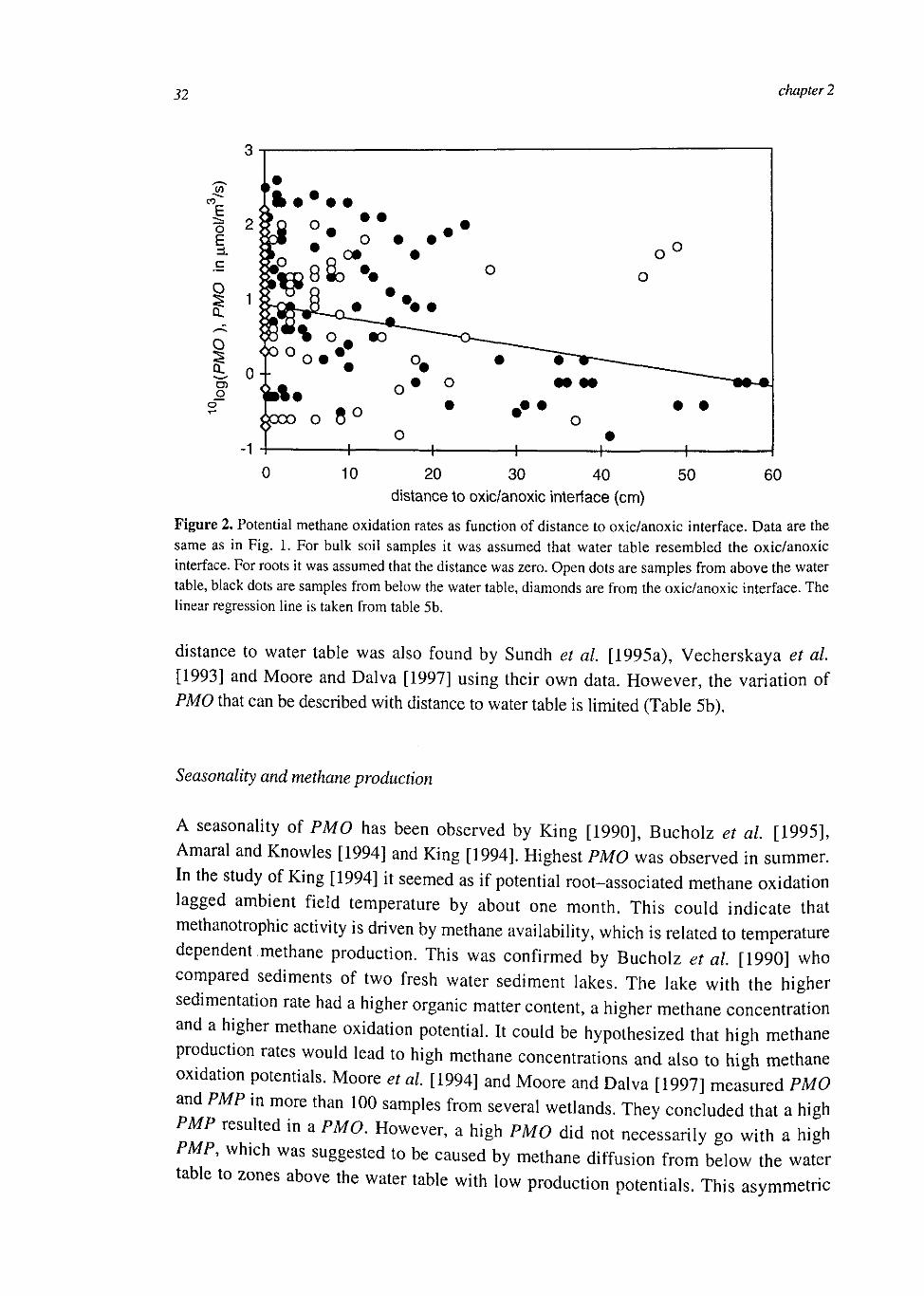
Indeed, all high values of PMO (> 50 /imol m - 3 s-1) were found within 25 cm of the anoxic/oxic interface (Figure 2). At the anoxic site of the aerobic/anaerobic interface potential rates are higher than at the oxic site. This reflects the better survival abilities of methanotrophs under anaerobic circumstances compared to aerobic circumstances [Roslev and King, 1994, 1995]. The negative correlation relation between PMO with (absolute)
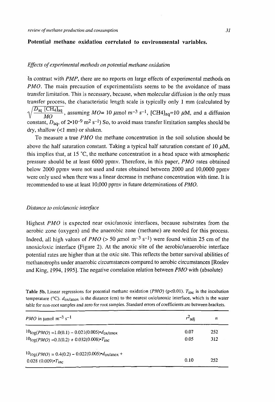
Table 5b. Linear regressions for potential methane oxidation {PMO) (p<0.01). Tmc is the incubation temperature (°C). ^0x/anox is the distance (cm) to the nearest oxic/anoxic interface, which is the water table for non-root samples and zero for root samples. Standard errors of coefficients are between brackets.
PMO in umol m~3 s_I / adj n
l0\og(PMO) =1.0(0.1) - 0.021(0.005Wox/anox 0.07 252 ]0\og(PMO) =0.1(0.2) + 0.032(0.008)-rinc 0.05 312
X0\og(PMO) = 0.4(0.2) - 0.022(0.005)-rfOx/anox + 0.028 (0.009)*rinc 0.10 252
32 chapter 2
(/) o
1 2 E
c
O
1 o
0
-1
' ! • • • •
$a °« •* &I . • o • • • <*^ • 0# •
fa83-..
8o*% o m act" ----o-f o 0 . * : o.
i%. o» ° Go o 8° Y ° -1 1 1
o
• • ~Tr—•—
• • • •
• • • w o • H 1
o° o
• •
1 0 10 50 60 20 30 40
distance to oxic/anoxic interface (cm)
Figure 2. Potential methane oxidation rates as function of distance to oxic/anoxic interface. Data are the same as in Fig. 1. For bulk soil samples it was assumed that water table resembled the oxic/anoxic interface. For roots it was assumed that the distance was zero. Open dots are samples from above the water table, black dots are samples from below the water table, diamonds are from the oxic/anoxic interface. The linear regression line is taken from table 5b.
distance to water table was also found by Sundh et al [1995a), Vecherskaya et at. [1993] and Moore and Dalva [1997] using their own data. However, the variation of PMO that can be described with distance to water table is limited (Table 5b).
Seasonality and methane production
A seasonality of PMO has been observed by King [1990], Bucholz et al [1995], Amaral and Knowles [1994] and King [1994]. Highest PMO was observed in summer. In the study of King [1994] it seemed as if potential root-associated methane oxidation lagged ambient field temperature by about one month. This could indicate that methanotrophic activity is driven by methane availability, which is related to temperature dependent methane production. This was confirmed by Bucholz et al [1990] who compared sediments of two fresh water sediment lakes. The lake with the higher sedimentation rate had a higher organic matter content, a higher methane concentration and a higher methane oxidation potential. It could be hypothesized that high methane production rates would lead to high methane concentrations and also to high methane oxidation potentials. Moore et al [1994] and Moore and Dalva [1997] measured PMO and PMP in more than 100 samples from several wetlands. They concluded that a high PMP resulted in a PMO. However, a high PMO did not necessarily go with a high 7 W h l c h w a s suSgested to be caused by methane diffusion from below the water table to zones above the water table with low production potentials. This asymmetric
review of methane production and consumption 33
relation may also be caused by temporal inhibition of PMP due to the presence of electron acceptors or damage to the methanogenic population as a result of in situ aerobiosis.
Soil type, root-associated methane oxidation, pH, temperature and salinity
There is no difference between PMO at minerotrophic and ombotrophic natural wetlands (Table 5a). At roots, PMO is relatively high, though the difference is not significant. This is reflected by the relatively high number of methanotrophic bacteria in rhizospheric soil [de Bont et al, 1978; Gilbert and Frenzel, 1995], Root-associated methane oxidation depends on plant type and may be controlled by root oxygen release [Calhoun and King, 1997]. Gerard and Chanton [1993] found zero methane oxidation in stems and most rhizomes of several wetland plants. King et al. [1990] could not find methanotrophic activity in a subtropical marl sediment, in contrast with a peat sediment with a similar vegetation.
Dunfield et al. [1993] found that the pH optimum for PMO was 0-1 pH units above the in situ pH, which varied between 4 and 6. No trend between optimum pH and PMO was observed. So, pH does not seem to be a discriminating factor for methane oxidation at different sites.
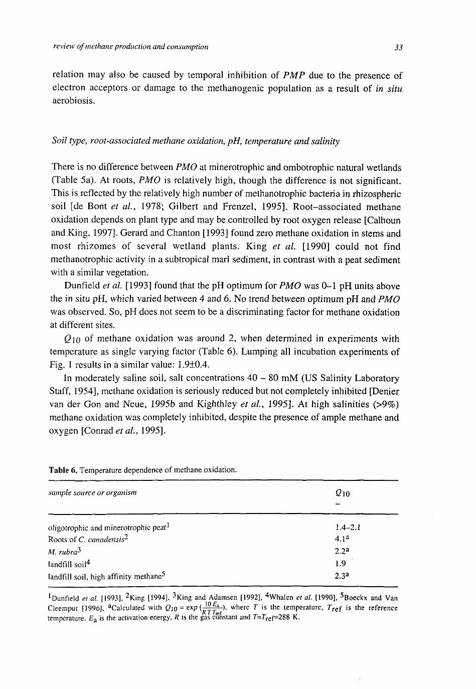
Qio of methane oxidation was around 2, when determined in experiments with temperature as single varying factor (Table 6). Lumping all incubation experiments of Fig. 1 results in a similar value: 1.9±0.4.
In moderately saline soil, salt concentrations 40 - 80 mM (US Salinity Laboratory Staff, 1954], methane oxidation is seriously reduced but not completely inhibited [Denier van der Gon and Neue, 1995b and Kighthley et al, 1995]. At high salinities (>9%) methane oxidation was completely inhibited, despite the presence of ample methane and oxygen [Conrad et al, 1995].
Table 6. Temperature dependence of methane oxidation.
sample source or organism Q \ Q
oligotrophic and minerotrophic peat1 1.4-2.1
Roots of C. canadensis^ 4. l a
M. rubra2* 2.2a
landfill soil4 1.9
landfill soil, high affinity methane5 2.3a
!Dunfield et al. [1993], 2King [1994]. 3King and Adamsen [1992], 4WhaIen et al. [1990], 5Boeckx and Van 10 F
Cleemput [1996], Calculated with Qio = exp ( '" a ), where T is the temperature, r r e f is the reference temperature. £ a is the activation energy, R is the gas constant and 7"=rref=288 K.
54 chapter 2
Summary
Rates of PMO are skewly distributed and vary three orders of magnitude. Only a very limited part (r2=0.10) of this variation can be described with well established variables: distance to average water table and incubation temperature (Table 5b). Possibly, the descriptive relations can be improved by adding correlations with methane and oxygen concentrations, time averaged over a certain period, possibly a month. In this way, seasonal variation and the good survival characteristics of methanotrophs are incorporated.
A methanotrophic biomass model to explain variation in potential methane oxidation
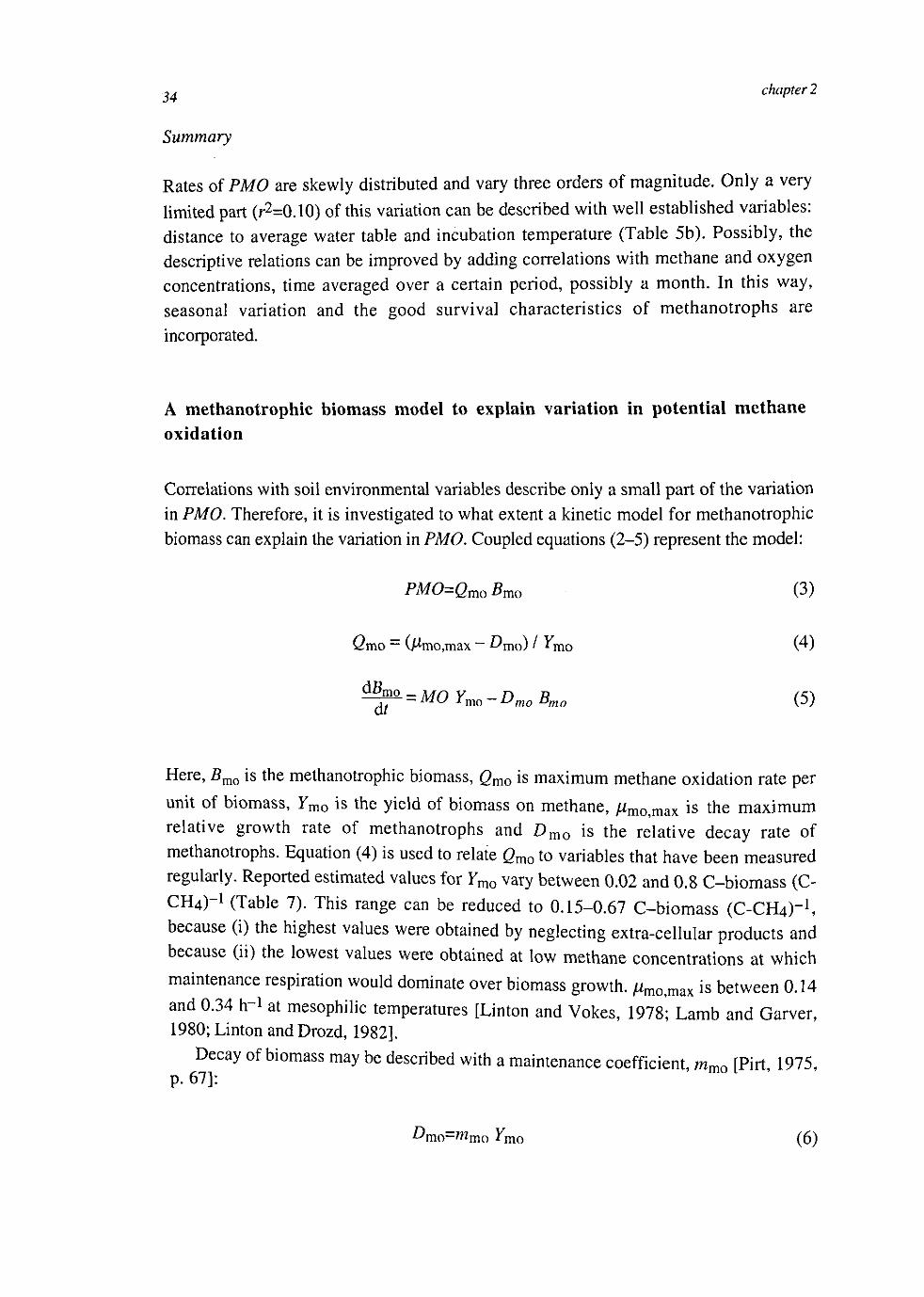
Correlations with soil environmental variables describe only a small part of the variation in PMO. Therefore, it is investigated to what extent a kinetic model for methanotrophic biomass can explain the variation in PMO. Coupled equations (2-5) represent the model:
PMO=Qmo Bmo (3)
2mo = (Mmo,max — ^mo) / ^mo (4)
dBt
6t mo _ yif) Y - D B (5)
Here, Smo is the methanotrophic biomass, Qmo is maximum methane oxidation rate per unit of biomass, Ymo is the yield of biomass on methane, ,um o m a x i s the maximum relative growth rate of methanotrophs and Dmo is the relative decay rate of methanotrophs. Equation (4) is used to relate Qmo to variables that have been measured regularly. Reported estimated values for Ymo vary between 0.02 and 0.8 C-biomass (C-CH4)~ (Table 7). This range can be reduced to 0.15-0.67 C-biomass (C-CH4K because (,) the highest values were obtained by neglecting extra-cellular products and because („) the lowest values were obtained at low methane concentrations at which maintenance respiration would dominate over biomass growth. ^mo>max i s between 0.14
! f *" at mesophilic temperatures [Linton and Yokes, 1978; Lamb and Garver, 1980; Linton and Drozd, 1982].
p. 6 7 r a y ^ b i ° m a S S may ^ deSCribed Wlth 3 maintenance coefficient, mmo [Pirt, 1975,
£>mo=mmo 7m o ^

review of methane production and consumption 35
Table 7. Carbon partitioning of methane consumed by methanotrophs
Organism or sample source
drained peat1
tundra soil2
various methanotrophic bacteria-*'^'"'1^
M. trichosporium OB3b^
Mthylococcus capsulatu'
fresh water sediment°°
landfill soil5
high affinity conditions9 '10,11
CH4 limited
O2 limited
0.02--0.6
Yield (Ymo) Extra
C-biomass/C-CH4
0.77a
0.5b
0.19-0.67
0.80a
0.66
0.25
0.15-0.61
0.69b
cellular product
C/C-CH4
0-0.48 c
0C
0.7C
!Megraw and Knowles [1987], 2Vecherskaya [1993], 3Nagai et al [1973], 4Nagai et al. [1973] from data of Sheehan and Johnson [1971], 5Whalen et al. [1990], 6Ivanova and Nesterov [1988], 7Hardwood and Pirt [1972], 8Bucholz et al. [1995], 9Lidstrom and Somers [1984], 10Yavitt et al. [1990a], UYavitt et al. [1990b] 12Linton and Drozd [1982] Calculated as CH4 consumption - CO2 production, bC in biomass + organic compounds, Calculated as CH4 added - (CO2 produced + C incorporated in biomass).
Taking mm0 and Ymo from Nagai et al. [1973] and Sheehan and Johnson [1971], who measured these under optimal and sub optimal growth conditions, leads to Dmo ~ 1 d_l, which is substantially higher than the aerobic and anaerobic C-starvation rates of methanotrophs, which were about 0.1 d -1 [Roslev and King, 1994]. Apparently, methanotrophs are able to decrease their maintenance requirements under conditions of C-starvation. So, the maintenance coefficient at (sub) optimal growth conditions cannot be used to describe the starvation of methanotrophs. A solution may be the introduction of an extra state variable, representing the physiological state of the micro-organism [Panikov, 1995, p. 203], in combination with experimental data of starvation kinetics of methanotrophs [King and Roslev, 1994].
So, it is possible to model PMO via a model for methanotrophic biomass, although predictability of the model will be limited, because of a large variation in parameters which is hard to explain.
Concluding remarks
Like methane fluxes, rates of potential methane production (PMP) and potential methane oxidation (PMO) are skewly distributed and vary three orders of magnitude. In relating (potential) rates of methane production and methane consumption to environmental variables, like weather, soil and vegetation data, two lines were followed. Firstly, potential rates collected from a large number of studies were statistically analysed. 34 %
36 chapter 2
of the variation in the 10log of PMP and 10% of the variation in the 10Iog of PMO could be described with correlations with environmental variables. Secondly, the knowledge of the processes underlying methane production and oxidation was reviewed and summarised in explanatory models. For a quantitative evaluation of these models they need to be integrated in a framework that provides the dynamics of water, heat and gas transport, carbon and vegetation dynamics on a sufficiently small scale. Given the large unexplainable variation in the descriptive models it is worthwhile to do so, although expectations for predictive modelling should not be too high, as the variation in parameters of the process models is large. Anyhow, such an integrating effort would provide a lot of insight in the dynamic, non-linear, interactions between processes and in the causes of the large variations in methane fluxes.

37
Chapter 3
Soil methane production as a function of anaerobic carbon mineralisation: a process model
Segers, R. and S. W. M. Kengen, Soil Biol. Biochem., 30, 1107-1117, 1998
Abstract
Anaerobic carbon mineralisation is a major regulator of soil methane production, but the relation between these processes is variable. To explain the dynamics of this relation a model was developed, which comprises the dynamics of alternative electron acceptors, of acetate and of methanogenic biomass. Major assumptions are: (i) alternative electron acceptors suppress methanogenesis and (ii) the rate of electron acceptor reduction is controlled by anaerobic carbon mineralisation. The model was applied to anaerobic incubation experiments with slurried soil samples from a drained and an undrained peat soil in the Netherlands to test the model and to further interpret the data. Three parameters were fitted with a Monte Carlo method, using experimentally determined time series of methane, carbon dioxide and acetate. The fitted parameters were the initial concentration of electron acceptors, the initial concentration of methanogenic biomass and the maximum relative growth rate of methanogenic biomass. Simulated and measured time courses of methane corresponded reasonably well. The model as such stresses the importance of alternative electron acceptors. At the drained site initial alternative electron acceptor concentrations were between 0.3 and 0.8 mol electron equivalents (el. eqv.) kg"1 dw soil, whereas at the undrained site they were between 0.0 and 0.3 mol el. eqv. kg"-1 dw soil, depending on the experimental treatments. The sum of measured NO3" and SO42"* concentrations and
estimated maximum Fe3 + and Mn4+ concentrations was much lower than the fitted concentrations of alternative electron acceptors. Apparently, reduction of unknown electron acceptors consumed a large part of anaerobically mineralised carbon which, therefore, was not available for methanogenesis.
Introduction
The increase of atmospheric methane from 0.7 to 1.7 ppmv is estimated to be responsible for about of 15% of the enhanced greenhouse effect [Houghton et al, 1995]. Wetland soils, including rice paddies, contribute between 15 and 45 % to the methane source of the atmosphere, whereas non-wetland soils contribute between 3 and 10% to the methane sink of the atmosphere [Prather et al.y 1995]. Current flux estimates contain a large uncertainty and the effects of soil management and climate on fluxes are difficult to estimate, because the conditions, scales and processes that control methane emissions are not well known. Methane fluxes from or to soils are a result of the interaction of several
Segers, R. Wetland Methane Fluxes: Up scaling from Kinetics via a Single Root and a Soil Layer to the Plot, Ph. D. Thesis, Wageningen University, 1999.
38 Chapter 3
biological and physical processes and factors in the soil [Schimel et al.,1993; Wang et al, 1996]. This paper, specifically focuses on the dependence of methane production on anaerobic carbon mineralisation. § The available literature indicates that, at least on a small scale, a simple relation
between both processes does not exist. For instance, the ratio of anaerobic CO2/CH4 formation in peat samples was found to vary by as much as two to three orders of magnitude [Amaral and Knowles, 1994; Yavitt et al, 1987; Yavitt and Lang, 1990]. Similarly, potential methane production rates were shown to vary by several orders of magnitude [e.g. Moore et al, 1994], whereas anaerobic carbon mineralisation varied only by one to two orders of magnitude [Amaral and Knowles, 1994; Magnusson, 1993; Yavitt et al, 1987; Yavitt and Lang, 1990].
Because the relation between methane production and anaerobic carbon mineralisation is complex, knowledge of the underlying controlling processes is required to derive it. Soil methane production is the result of anaerobic degradation of organic matter via several interdependent microbiological reactions [Oremland, 1988]. This paper presents a model that explains the dependence of the time course of methane production on the time course of anaerobic carbon mineralisation and integrates current knowledge of the underlying controlling processes.
The model should be suitable to simulate field scale methane production. For this it should be integrated with models on soil aeration, soil mineralisation and electron acceptor re-oxidation. Consequently, the accuracy of the methane production submodel (presented in this paper) should be in balance with the accuracy of the models for these other processes. Therefore, we tried to reduce as much as possible the number of parameters that are both sensitive and uncertain. Only after scaling up it is possible to judge whether refinement of the kinetic model is useful for understanding field scale methane production.
Material and methods
Main structure of model
Methane is produced according to the reaction (Figure 1, box 1):
acetate —> methane + carbon dioxide + methanogenic biomass 0 )
t methanogenic biomass
We assumed that acetate is the only substrate for methanogenesis and that acetate • production can be directly coupled to anaerobic carbon mineralisation. The rate of reaction (1) depends on the simulated concentrations of acetate and methanogenic biomass. Acetate

Methane production model 39
anaerobic carbon mineralisation
acetate
oxidised electron acceptors
methano-genesis
electron 2 acceptor reduction
electron 3 acceptor re-oxidation
methanogenic biomass
reduced electron acceptors
Figure 1. Material flow diagram for the methane production model. The upper part concerns the carbon flow, the lower part concerns the electron acceptor cycling. Rectangular boxes represent material, rounded boxes represent processes. The thicknesses of the lines qualitatively represent typical sizes of the flows. The size of the flows vary with time.
is also consumed by the reduction of an arbitrary alternative electron acceptor (Figure 1, box 2):
acetate + electron acceptor —> carbon dioxide + reduced electron acceptor (2)
The rate of this reaction depends on the concentrations of acetate and the alternative electron acceptors. In contrast with methanogenesis, the concentration of biomass is not included as controlling factor in reaction (2). During aerobiosis alternative electron acceptors are re-oxidised (Figure 1, box 3), acetate is oxidised and methanogenic biomass decays. These processes are not included in the model, however, as it is restricted to anaerobic conditions.
In an earlier version of this model [Segers and Leffelaar, 1995] retardation of the onset of methane production by electron acceptors was simply described by a lag time. With the present model it is possible to account for this lag by the time it takes to reduce alternative electron acceptors. Lovley and Klug [1986] have used a comparable model to explain competition between sulphate reduction and methanogenesis in an anaerobic freshwater sediment in steady state. Our model is a generalisation of their model, because (i) it is designed for alternative electron acceptors other than sulphate as well, (ii) acetate production is directly coupled to anaerobic organic matter mineralisation and (iii) dynamic situations are considered.

40 Chapter 3
Assumption I: The inclusion of methanogenic bacteria
Often it is assumed that methanogenic bacteria do not limit methane production in wetland soils, because (i) additions of substrates like acetate, hydrogen or glucose often stimulate methane production [Williams and Crawford, 1984; Amaral and Knowles, 1994; and Bachoon and Jones, 1992], (ii) some methanogenic bacteria survive aeration for periods from several hours to at least several months [Mayer and Conrad, 1990; Fetzer et aL, 1993, Huser, 1981] and (iii) methane emissions can start quickly after inundation of rice paddies [Holzapfel Pshorn and Seiler, 1986]. However, limitation of methane production by methanogenic biomass probably does occur in wetland soils under low temperatures [Shannon and White, 1996 and Drake et al, 1996] and in non wetland soils upon anaerobic incubation (this study; Peters and Conrad, 1996; Kusel and Drake, 1995; Wagner et ah, 1996], as acetate accumulation was observed under these conditions. To account for a large range of conditions, including the incubation study used in this paper, methanogenic biomass was included in the model.
Assumption II: The exclusion of electron acceptor reducing bacteria
The concentration of electron acceptor reducing biomass was not considered, as it is not likely to limit electron acceptor reduction. There are two reasons for this assumption: (i) Iron and nitrate reducing bacteria are facultative anaerobic [Sikora and Keenet, 1983] and sulphate reducing bacteria can survive aerobiosis [Le Gall and Xavier, 1996], so periods of aerobiosis would not severely affect the population, (ii) If a biomass limitation would occur, organic substrate (e.g. acetate) accumulation would occur in the presence of ample electron acceptors. Thus far, this has only been observed in anaerobically incubated upland soils [Peters and Conrad, 1996]. However, in upland soils, in situ methane production is likely to be small, as anaerobic periods are generally short.
Assumption III: Acetate as single methanogenic substrate
We assume that acetate is the sole substrate for the methanogens. Other possible substrates like hydrogen or formate are thus not included explicitly. There are two reasons for this. Firstly, in several case studies with wetland soils acetate was the precursor of about 70% of the produced methane [Goodwin and Zeikus, 1987; Cappenberg and Prins, 1974; Drake et aL, 1996]. Secondly, including other substrates would not change the trend of the dependence of methane production on anaerobic organic matter mineralisation, because alternative electron acceptors would also suppress methanogenesis from other substrates for thermodynamic reasons. This is reflected in the model by a low sensitivity of simulated methane production for substrate specific parameters (see subsection on parameter estimation). So, when other substrates are relevant, the acetate in this model can be taken as representing other substrates as well.

Methane production model 41
The relative unimportance of the kind of the substrate was also found by Lovley and Klug [1986] when they replaced acetate by hydrogen in their model for sulphate reduction and methanogenesis.
Assumption IV: No intermediate fermentation reactions included
Acetate production is assumed to be directly coupled to anaerobic organic matter mineralisation. This implies that all intermediate fermentation reactions and hydrolysis are not explicitly taken into account. If intermediate fermentation reactions controlled acetate production, significant accumulation of other intermediates should occur. This has only been observed when acetate accumulates as well, which indicates that other intermediates only accumulate when acetate itself inhibits the conversion of those intermediates. When such an inhibition is resolved these compounds would be converted to acetate. In soils this conversion is not often observed, but it could be rather slow [Chin and Conrad, 1995], in which case fermentation reactions would limit methane production. This situation is not considered in the model, because (i) the few measurements of small
concentrations of propionate and lactate in field soils (<100 /iM) [Rothfuss and Conrad, 1993; Amaral and Knowles, 1994] do not point at significant accumulation, (ii) accumulation of acetate implies limitation of methane production by methanogenic biomass, which does not seem to occur often (see above), (iii) lack of information required to model these fermentation reactions without additional measurements.
Assumption V: Electron acceptors suppress methanogenesis
An unspecified alternative terminal electron acceptor that suppresses methane production plays a central role in the model. Apart from the inorganic electron acceptors (NO3", SO42-, Fe3+ and Mn4+) [Zehnder and Stumm, 1988] organic peat material may also act as terminal electron acceptor [Lovley et aL, 1996] and suppress methanogenesis. In the model it is assumed that the reduction of electron acceptors lowers the acetate concentration to a value that is too low for methanogenesis. Alternatively, the suppressing effect of electron acceptors can be explained via their influence on the redox potential. It is not clear which mechanism is closest to reality [Peters and Conrad, 1996]. In fact, both could operate at the same time. Incorporating the alternative mechanism in a model would mostly result in a similar functional relation between anaerobic carbon mineralisation and methane production, because also with the alternative mechanism the depletion rate of electron acceptors will be mostly controlled by anaerobic carbon mineralisation (see assumption II).
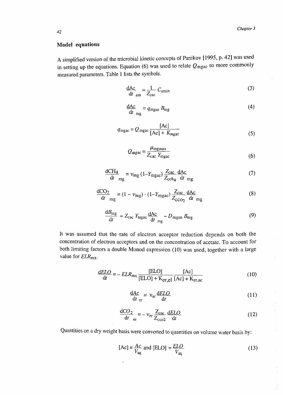
Chapter 3
Model equations
A simplified version of the microbial kinetic concepts of Panikov [1995, p. 42] was used in setting up the equations. Equation (6) was used to relate Gmgac to more commonly measured parameters. Table 1 lists the symbols.
dAc - J _ r (3) ~T~ ~~ y wmin v /
C" am ^ c a c
dAc - n ft (4) Cu mg
Q -o ^JM fegac-ymgac[Ac]+^gac
k?mgac ^cac *mgac (6)
dCKU = v , j _ y v Zcac dAc (7)
u^ mg ^cch4 d/ mg
"* mg ^CC02 ^ mg
d ^ m g _ 7 Y dAc n n (en i — ^cac -*mgac , ^mgan % g v-v
Cu Cu m g
It was assumed that the rate of electron acceptor reduction depends on both the concentration of electron acceptors and on the concentration of acetate. To account for both limiting factors a double Monod expression (10) was used, together with a large value for ELRmx.
dELQ = „ E L R [ELO] [Ac] dr mx [ELO] + Ker,el [Ac] + Ker,ac
(10)
6M = V e r d£LO ( 1 1 )
at er dt
^22 = _ V e r Z^dEML ( i 2 ) ^ er Z c c o 2 dt
Quantities on a dry weight basis were converted to quantities on volume water basis by:
[Ac] = Ac. a n d p^Q] = ELO. (13) *aq ^aq
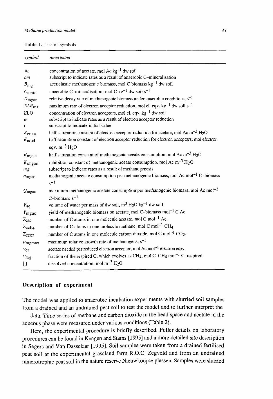
Methane production model 43
Table 1. List of symbols.
symbol description
Ac am Bmg
Camin
^mgan
ELO er i
^er,ac
^er,el
mgac K
^imgac mg
<7mgac
Q mgac
"aq
^mgac
Zcac
Zcch4
^cco2
/^mgmax
Ver
[]
concentration of acetate, mol Ac kg * dw soil subscript to indicate rates as a result of anaerobic C-mineralisation
aceticlastic methanogenic biomass, mol C biomass kg - 1 dw soil
anaerobic C-mineralisation, mol C kg-* dw soil s - 1
relative decay rate of methanogenic biomass under anaerobic conditions, s_1
maximum rate of electron acceptor reduction, mol el. eqv. kg - 1 dw soil s_ 1
concentration of electron acceptors, mol el. eqv. kg"1 dw soil subscript to indicate rates as a result of electron acceptor reduction subscript to indicate initial value
half saturation constant of electron acceptor reduction for acetate, mol Ac m - 3 H2O
half saturation constant of electron acceptor reduction for electron acceptors, mol electron
eqv. m~3 H2O
half saturation constant of methanogenic aceate consumption, mol Ac m~3 H2O
inhibition constant of methanogenic aceate consumption, mol Ac m~3 H2O subscript to indicate rates as a result of methanogenesis
methanogenic acetate consumption per methanogenic biomass, mol Ac mol - 1 C-biomass
s-1
maximum methanogenic acetate consumption per methanogenic biomass, mol Ac mol"1
C-biomass s - 1
volume of water per mass of dw soil, m3 H2O kg - 1 dw soil
yield of methanogenic biomass on acetate^ mol C-biomass mol -1 C Ac
number of C atoms in one molecule acetate, mol C mol"1 Ac.
number of C atoms in one molecule methane, mol C mol"1 CH4
number of C atoms in one molecule carbon dioxide, mol C mol"1 CO2.
maximum relative growth rate of methanogens, s - 1
acetate needed per reduced electron acceptor, mol Ac mol"1 electron eqv.
fraction of the respired C, which evolves as CH4, mol C-CH4 mol -1 C-respired
dissolved concentration, mol m~3 H2O
Description of experiment
The model was applied to anaerobic incubation experiments with slurried soil samples from a drained and an undrained peat soil to test the model and to further interpret the
data. Time series of methane and carbon dioxide in the head space and acetate in the aqueous phase were measured under various conditions (Table 2).
Here, the experimental procedure is briefly described. Fuller details on laboratory procedures can be found in Kengen and Stams [1995] and a more detailed site description in Segers and Van Dasselaar [1995], Soil samples were taken from a drained fertilised peat soil at the experimental grassland farm R.O.C. Zegveld and from an undrained minerotrophic peat soil in the nature reserve Nieuwkoopse plassen. Samples were slurried
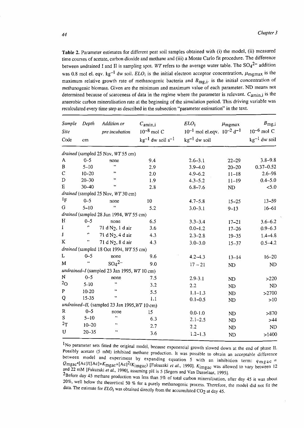
44 Chapter 3
Table 2. Parameter estimates for different peat soil samples obtained with (i) the model, (ii) measured
time courses of acetate, carbon dioxide and methane and (iii) a Monte Carlo fit procedure. The difference
between undrained I and II is sampling spot. WT refers to the average water table. The S 0 4 2 - addition
was 0.8 mol el. eqv. kg - 1 dw soil. ELO\ is the initial electron acceptor concentration, //mgmax ls t n e
maximum relative growth rate of methanogenic bacteria and Bmg.i- ls the initial concentration of
methanogenic biomass. Given are the minimum and maximum value of each parameter. ND means not
determined because of scarceness of data in the regime where the parameter is relevant. Camin,i1S t n e
anaerobic carbon mineralisation rate at the beginning of the simulation period. This driving variable was
recalculated every time step as described in the subsection "parameter estimation" in the text.
Sample Depth Addition or Camin,i
Site pre incubation 10~8 mol C
Code cm kg - 1 dw soil s"1
ELOi /%igmax B mg,i 10"1 mol el.eqv. 10"2 d"1 10~6 mol C
kg - 1 dw soil kg - 1 dw soil
drained (sampled 25 Nov, WT55 cm) A B C D E
0-5 5-10 10-20 20-30 30-40
none 9.4 2.9 2.0 1.9 2.8
drained (sampled 25 Nov, WT 30 cm)
*F 0-5 none 10
G 5-10 " 5.2 drained (sampled 28 Jun 1994, WT55 cm) H 0-5 none 6.5 I " 71dN2, I d air 3.6 J " 7 1 d N 2 , 4 d a i r 4.3
K " 71dN2 ,8da i r 4.3
drained (sampled 18 Oct 1994, HT55 cm) L 0-5 none 9.6
M " SO4 2 - 9.0
undrained-l (sampled 23 Jan 1995, WT 10 cm) N 0-5 none 7.5 2 0 5-10 " 3.2
P 10-20 " 5.5 Q 15-35 " 1.1 undrained-U, (sampled 23 Jan 1995.HT 10 cm) R 0-5 none 15 S 5-10 " 6.3 2T 10-20 " 2.7
U 20-35 " 3.6
2.6-3.1 3.9-4.0 4.9-6.2 4.3-5.2 6.8-7.6
4.7-5.8
3.0-3.1
3.3-3.4
0.0-1.2
2.3-2.8
3.0-3.0
4.2-4.3
1 7 - 2 1
2.9-3.1
2.2
1.1-1.3 0.1-0.5
0.0-1.0
2.1-2.5
2.2
1.2-1.3
22-29 20-20 11-18 11-19 ND
15-25 9-13
17-21 17-26 19-35 15-37
13-14
ND
ND ND ND ND
ND ND ND ND
3.8-9.8 0.37-0.52
2.6-98 0.4-5.0
<5.0
13-59 16-61
3.6-6.2 0.9-6.3 1.4-4.8 0.5-4.2
16-20
ND
>220 ND
>2700 >10
>870 >44 ND
>1400
i ~ 1 i r r ' m0del' beC3USe e X P ° n e n t i a l g r ° w t h sIowed d ™ n at the end of phase ... be we „ mode, T m e ' h a n e P r ° d U C t i 0 n - " WaS P ° S S i b l e t 0 o b t a i n *> ^ P " * " ^ n c e C f A c m t u r ^ r l T ' ^ e X P a n d l n g e q U a t i ° n 5 w i t h a " inhibition term: 9 m g a c =
fndg2a2 M F 1 ^ T / C + ^ img3C) [FUkUZakJ « "'" 1990]' ™ a "°- d '° "* b ™ '2
2 R e f l H Y< u " ° ] ' a S S U m m g P H iS 5 [ S e S e r s a n d V a " ttaselaar. 1995]. 20% we! L l w T h e r T ? ™ T ' "* *"" ™ ° f ^ ™b0n """^isation. after day 45 it was about
«I Th s ™ I o £LO , ° ; a P U r e 'y m e t h a n o g - c P — s . Therefore, the mode, did not fit the oata. ine est.mate for ELOi was obtained d.rectly from the accumulated C02 at day 45.
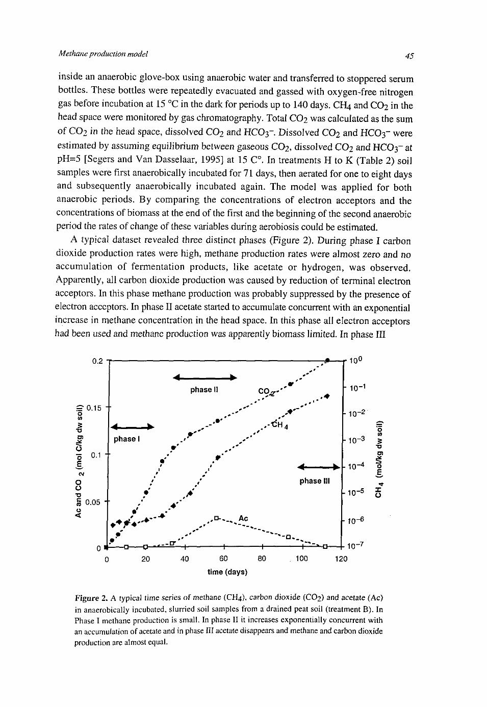
Methane production model 45
inside an anaerobic glove-box using anaerobic water and transferred to stoppered serum bottles. These bottles were repeatedly evacuated and gassed with oxygen-free nitrogen gas before incubation at 15 °C in the dark for periods up to 140 days. CH4 and CO2 in the head space were monitored by gas chromatography. Total CO2 was calculated as the sum of CO2 in the head space, dissolved CO2 and HCO3-. Dissolved CO2 and HCO3- were estimated by assuming equilibrium between gaseous CO2, dissolved CO2 and HCO3- at pH=5 [Segers and Van Dasselaar, 1995] at 15 C°. In treatments H to K (Table 2) soil samples were first anaerobically incubated for 71 days, then aerated for one to eight days and subsequently anaerobically incubated again. The model was applied for both anaerobic periods. By comparing the concentrations of electron acceptors and the concentrations of biomass at the end of the first and the beginning of the second anaerobic period the rates of change of these variables during aerobiosis could be estimated.
A typical dataset revealed three distinct phases (Figure 2). During phase I carbon dioxide production rates were high, methane production rates were almost zero and no accumulation of fermentation products, like acetate or hydrogen, was observed. Apparently, all carbon dioxide production was caused by reduction of terminal electron acceptors. In this phase methane production was probably suppressed by the presence of electron acceptors. In phase II acetate started to accumulate concurrent with an exponential increase in methane concentration in the head space. In this phase all electron acceptors had been used and methane production was apparently biomass limited. In phase III
0.2 T
phase II
•=0.15 •• o » •o
O
o °-1 + CM
O U S 0.05 -• o <
CO^-
A'
,.-t5H4
.+
phase I
r10°
phase III
> V
w : g
..*-** Ac
* '
20 -\ 1 1-40 60 80
time (days)
— i — » -
-10 - 1
L 1 0 - 2
o - 1 0 " 3 5
•o
i no-4 1
1-10-5 g
- 1 0 " 6
10-7
100 120
Figure 2. A typical time series of methane (CH4), carbon dioxide (CO2) and acetate (Ac) in anaerobically incubated, slurried soil samples from a drained peat soil (treatment B). In Phase I methane production is small. In phase II it increases exponentially concurrent with an accumulation of acetate and in phase III acetate disappears and methane and carbon dioxide production are almost equal.
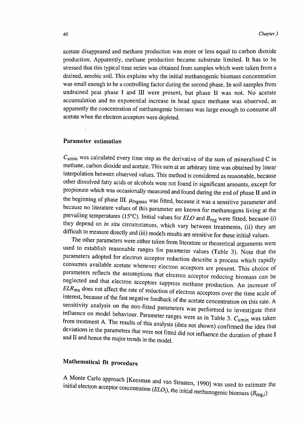
46 Chapter 3
acetate disappeared and methane production was more or less equal to carbon dioxide production. Apparently, methane production became substrate limited. It has to be stressed that this typical time series was obtained from samples which were taken from a drained, aerobic soil. This explains why the initial methanogenic biomass concentration was small enough to be a controlling factor during the second phase. In soil samples from undrained peat phase I and III were present, but phase II was not. No acetate accumulation and no exponential increase in head space methane was observed, as apparently the concentration of methanogenic biomass was large enough to consume all acetate when the electron acceptors were depleted.
Parameter estimation
Camin w a s calculated every time step as the derivative of the sum of mineralised C in methane, carbon dioxide and acetate. This sum at an arbitrary time was obtained by linear interpolation between observed values. This method is considered as reasonable, because other dissolved fatty acids or alcohols were not found in significant amounts, except for propionate which was occasionally measured and found during the end of phase II and in the beginning of phase III. nmgmax was fitted, because it was a sensitive parameter and because no literature values of this parameter are known for methanogens living at the prevailing temperatures (15°C). Initial values for ELO and Bm g were fitted, because (i) they depend on in situ circumstances, which vary between treatments, (ii) they are difficult to measure directly and (iii) models results are sensitive for these initial values.
The other parameters were either taken from literature or theoretical arguments were used to establish reasonable ranges for parameter values (Table 3). Note that the parameters adopted for electron acceptor reduction describe a process which rapidly consumes available acetate whenever electron acceptors are present. This choice of parameters reflects the assumptions that electron acceptor reducing biomass can be neglected and that electron acceptors suppress methane production. An increase of ELRm does not a feet the rate of reduction of electron acceptors over the time scale of interest, because of the fast negative feedback of the acetate concentration on this rate. A sensmvity analysis on the non-fitted parameters was performed to investigate their mfluence on model behaviour. Parameter ranges were as in Table 3. Camin was taken d e l l " I u ° f t h l S 3 n a , y S i S ^ n 0 t S h 0 w ") confirmed the idea that
iTltand Ic t r 1 1 1 6 1" 1 ™ *"* «* " * ^ ™ the Nation of l and 11 and hence the major trends in the model.
Mathematical fit procedure
electron a c c e p . o , ^ ^ ^ ^ . ^ ^ ^ ^ ^

Methane production model 47
Table 3. Parameter values which were not fitted, but otherwise estimated.
param.
ELRmx
^mgan
^er,el
^er,ac
^mgac
^mgac
^cac
^ch4
^co2
Ver
vmg
value
10"5
0.01
10
0.01
0.1
0.04
2
1
1
0.125
0.5
unit
mol el. eqv. kg - 1 dw soil s - 1
d-1
mM
mM
mM
mol C biomass mol - 1 C-Ac
mol C-Ac mol -1 Ac
mol C-CH4 mol"1 CH4
mol C-CO2 mol - 1 CO2
mol Ac mol -1 el. ace. (el. eqv.)
mol C-CH4 mol - 1 C-resp.
by methanogens
range
i 0 " 6 - 10-4
0 - 0.02
1-100
0.001 - 0 . 1
0.01 - 0.3
0.01 -0 .05
ND
ND
ND
ND
ND
comment
>wmin'(v'er'A;ac)
Pavlosthatis and Gomez [1991]
< initial [ELO]
< Kmg a c
Fukuzakie?a/.,[1990], taking pH=5, Segers and Van Dasselaar, 1995]
Pavlosthatis and Gomez [1991]
molecular constant
molecular constant
molecular constant
stoichiometric constant in
electron acceptor reduction
stoichiometric constant in
methanogenesis
and the maximum relative growth rate of methanogenic biomass Gumgmax) • The result of the procedure was not a single set of optimal parameters, but multiple sets of acceptable parameters. We used this method, because (i) no linearisations have to be performed, (ii) the method is suitable for situations with little data and (iii) the acceptable-non-acceptable criterium allows to use problem dependent information in a straight forward and explicit way.
The following constraints were imposed to discriminate between acceptable and non-acceptable parameter sets: Phase I (Ac < 0.1 mM): CH4 < CH4 at transition phase I/II;
Phase II (Ac> 0.1 mM): |logio (CH4, meas / CH4, sim)| < 0.25; Phase III when phase II present: no constraints on CH4; Phase III when phase II not present: jlogio (CH4, meas / CH4, s i m ) | < 0.25; All Phases: logio (Ac meas / Ac sjm) < 0.5. In the defined constraints focus is on parameters which control the main trends of methane production. Therefore, in phase I the restriction on methane is that the concentration is absolutely small. In the second phase, we elected a logarithmic comparison of measured with simulated methane, because an exponential increase is characteristic for this phase. In phase II the model predicts a very low carbon dioxide production, because a still low methane production is the only carbon dioxide source in this phase. However, in experiments some carbon dioxide production is observed. Via Camin this carbon dioxide production results in an overestimated acetate production. To account for this structural difference between model and reality the constraint on acetate was weak, implying that only the trend in the time course of acetate had to be predicted for acceptable model behaviour. As a consequence of the high simulated acetate concentrations also methane concentrations directly after phase II were simulated too high. Therefore, no constraints were put on CH4 in phase III when
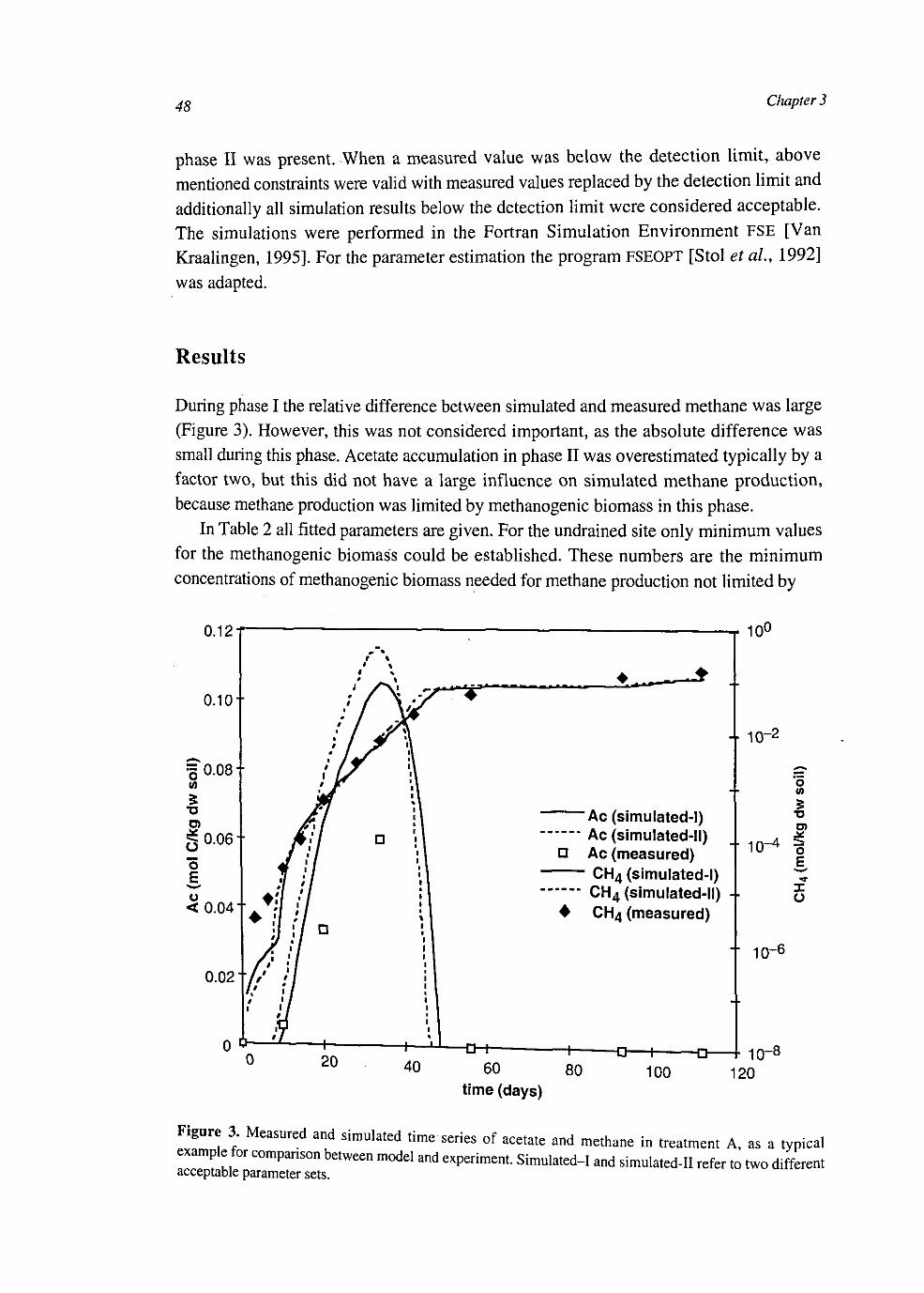
48 Chapter 3
phase II was present. When a measured value was below the detection limit, above mentioned constraints were valid with measured values replaced by the detection limit and additionally all simulation results below the detection limit were considered acceptable. The simulations were performed in the Fortran Simulation Environment FSE [Van Kraalingen, 1995]. For the parameter estimation the program FSEOPT [Stol et aL, 1992] was adapted.
Results
During phase I the relative difference between simulated and measured methane was large (Figure 3). However, this was not considered important, as the absolute difference was small during this phase. Acetate accumulation in phase II was overestimated typically by a factor two, but this did not have a large influence on simulated methane production, because methane production was limited by methanogenic biomass in this phase.
In Table 2 all fitted parameters are given. For the undrained site only minimum values for the methanogenic biomass could be established. These numbers are the minimum concentrations of methanogenic biomass needed for methane production not limited by
0.12
0.10 +
0.08 + o W
3
J*
D o E < 0.04
0.06 +
0.02 +
4 10-2
Ac (simulated-l) Ac (simulated-ll) Ac (measured) CH4 (simulated-l) CH4 (simulated-ll) CH4 (measured)
10°
o 5
10-4 |
X
o
I 10-6
60 time (days)
Figure 3 Measured and simulated time series of acetate and methane in treatment A as a tvmcal
Methane production model 49
methanogenic biomass. The low value for initial methanogenic biomass in treatment Q can be explained by the low anaerobic C-mineralisation rate.
At the drained site initial concentrations of electron acceptors were larger and initial concentrations of methanogenic biomass were smaller than at the undrained site. This is probably the cause of the higher in situ aeration at the drained site. At greater depths concentrations of electron acceptors were not larger than at the surface. The lower aeration of the deeper layers may be compensated by the greater reducing power of the top layer due to the higher anaerobic carbon mineralisation in the top layer. In this respect it is interesting to note that Amaral and Knowles [1994] found increasing sulphate concentrations with depth (from 15 cm) in a peat soil.
The addition of 0.8 mol electron equivalents (el. eqv.) SO42" kg -1 dw soil (treatment M) resulted in a comparable increase in concentration of initial electron acceptors. In this treatment during the last part of phase I, acetate concentration was more or less stable for some period at 0.1 mM (the same order of magnitude as typical half saturation constants for methanogenic acetate consumption), concurrent with an increase in methane production, which was less than the increases in phase II in the other treatments. Apparently sulphate at ~ 5 mM [Kengen and Stams, 1995] did not inhibit aceticlastic methanogenesis completely.
A period of aerobiosis affected both the electron acceptor concentration and the methanogenic biomass (Table 2, treatment H - K). After 71 days of anaerobiosis the simulated methanogenic biomass was above 10~3 mol C-biomass kg -1 dw soil. A single day of aerobiosis was sufficient to reduce the fitted methanogenic biomass to below 10~5
mol C-biomass kg -1 dw soil. Apparently the methanogens which grew during the 71 days anaerobic incubation period were not able to survive aerobiosis. Electron acceptor re-oxidation was slower than the loss of activity of methanogenic biomass. After eight days of aerobiosis the concentration of electron acceptors was back to its initial concentration. Using the estimates of ELO\ in treatment F and G an electron acceptor re-oxidation rate was about 0.05 mol el. eqv. kg-1 dw soil d*1.
Discussion
Except for two cases the model was able to describe the experimental data according to the criteria in the subsection "mathematical fit procedure". Therefore, we conclude that the model captures the underlying processes accurately enough to explain the major trends of methane production in our case study.
Electron acceptors
From the sulphate addition experiment it became clear that sulphate did not suppress methane production completely. This was also found by others [e.g. Yavitt et al, 1987]
rn Chapter 3
and is understandable as thermodynamically sulphate reduction favours methanogenesis
only slightly [Zehnder and Stumm, 1988]. Apparent initial electron acceptor concentrations amounted to 0.8 mol el. eqv. kg"1 dw
soil in the drained soil. This was considerably more than the sum of the estimated inorganic electron acceptors as calculated below. Nitrate was not observed, neither was the production of nitrogen and nitrous oxide [Kengen and Stams, 1995]. A typical sulphate concentration was 0.3 mM [Kengen and Stams, 1995] which corresponds to 0.024 mol el. eqv. kg-1 dw soil, taking for our case (slurried soil) a typical water content of 0.01 m3 kg"1 dw soil. Typical maximum Fe3+ and Mn4+ concentrations in peat waters are about 40 mg Fe2C>3 L"1 and 7 mg Mn02 L"1 [Shotyk, 1987]. This corresponds to 0.008 mol el. eqv. kg'1 dw soil, assuming a water saturated peat soil with a porosity of 95 % and a solid phase density of 1300 kg m~3. So, reduction of inorganic electron acceptors cannot explain the observed carbon dioxide production during phase I. Theoretically, net production of hydrogen, ethanol or propionate also results in a net production of carbon dioxide [Thauer et al, 1977]. However, accumulation of these fermentation products was not observed. Therefore, these kind of fermentation reactions cannot explain the observed carbon dioxide production. Solubility of carbon dioxide depends on pH and, therefore, changes in pH could cause changes of carbon dioxide in the head space. However, pH (=5) and volumetric liquid:gas ratios (=0.2) were so small that only a small fraction (=0.2) of carbon dioxide was in the liquid phase. As a result, changes in pH cannot explain the observed carbon dioxide production.
In anaerobic incubation studies of Yavitt and Lang [1990] and Amaral and Knowles [1994] carbon dioxide production that was not explained by methanogenesis or sulphate reduction was equivalent to (-0.2 to 12) mol el. eqv. m~3 peat slurry d"1. Assuming that this production lasts for five days and assuming a water saturated peat soil with a porosity of 95 % and a solid phase density of 1300 kg m~3, this corresponds to (-0.02 to 0.9) mol el. eqv. kg-1 dw soil. Values of this study fall within this range. Amaral and Knowles [1994] found little H2 production. Yavitt and Lang [1990] observed one of the highest unexplained carbon dioxide production rates in a low pH (3.8) sample. Therefore, though the evidence is less strong compared to this study, also in the studies of Yavitt and Lang [1990] and Amaral and Knowles [1994] unknown terminal alternative electron acceptors may have been active. By contrast, in two mineral rice paddy soils methane production and inorganic electron acceptor reduction were able to explain a large part of the carbon dioxide production [Inubushi etal, 1984].
In conclusion, commonly used arguments cannot explain the observed carbon dioxide production during phase I. Therefore, it is hypothesised that peat material acts as terminal electron acceptor. This hypothesis is supported by recent findings of Lovley et al [1996], who demonstrated that humic acids could act as terminal electron acceptor. Alternatively, the assumed dissolved concentrations of NO3- S042- Fe3+ and Mn4+
may not represent the amounts of these compounds that are available for reduction, because a large part of the reducible inorganic electron acceptors may be bound to peat material in some way. Humic acids may shuttle electrons to relatively inaccessible electron

Methane production model 5 /
acceptors [Lovley et al.9 1996]. Okruszko [1993] reports total Fe2C>3 concentrations in drained peat soils are typically 1.5 % (mass) of the dry matter, which corresponds to 0.2 el. eqv. kg -1 dw soil.
Methanogenic biomass
The relative growth rate of the methanogens was about 0.2 d_1. This value is relatively high considering the temperature (15°C), because it is within the range of rates found for aceticlastic methanogens that live at 35°C (0.1-0.7 d"1) [Pavlosthatis and Gomez, 1991]. Apparently methanogens from this environment are adapted to sub mesophilic temperatures, which was also found by Svensson [1984] for a Swedish peat soil.
Effect of aerobiosis
The rate of electron acceptor re-oxidation (0.05 mol el. eqv. kg - 1 dw soil d~*) is comparable to the oxygen consumption of soil samples from this site under aerobic conditions, which were about 0.03 mol el. eqv. kg -1 dw soil d_1 at 15.5°C [Otten, 1985] or 0.04 mol el. eqv. kg -1 dw soil d"1 at 20°C [C. A. Langeveld, pers. comm.] under different incubation conditions. The data are too limited to say anything about the controls of electron acceptor re-oxidation.
Conclusions
The model explains the large variation in observed anaerobic CO2/CH4 production ratios with a varying contribution of reduction of electron acceptors to total anaerobic C turnover. The rate of depletion of electron acceptors depends on the anaerobic carbon mineralisation. As a result the relation between methane production and anaerobic carbon mineralisation is dynamic and non-linear, at least on small time scales (days or weeks). The model as such stresses the importance of alternative electron acceptors. In our case study and probably also in the studies of Amaral and Knowles [1994] and Yavitt and Lang [1990] reduction of unknown electron acceptors consumed a large part of anaerobically mineralised carbon, which, therefore, was not available for methanogenesis. Identification and quantification of these electron acceptors deserves attention in research directed at understanding the relation between methane production and anaerobic C-mineralisation.
53
Chapter 4
Modelling methane fluxes in wetlands with gas transporting plants: 1. Single root scale
Segers, R.
Abstract
Methane fluxes were related to the first principles of transport and kinetics (microbial and chemical conversions). The difference between the kinetic scale and the smallest flux scale, the plot scale, is large. A stepwise scaling up procedure was therefore used in a series of three papers. This paper treats kinetics and diffusion around a single gas transporting root. Kinetic processes include: methane production, methane oxidation, electron acceptor reduction, acceptor re-oxidation and aerobic respiration. This is the minimum number of processes needed to relate net methane production to the main driving variables: carbon availability and oxygen inflow. Kinetics were integrated with diffusion, leading to a set of partial differential equations. This set was solved directly and also after simplification to a set of spatially averaged ordinary differential equations. Results of the simplified model closely resembled results of the unsimplified (full) model, which implies that the simplified model covers the main interactions of the full model and is suitable for further scaling up. Model results showed that reduction of methane emission after 100% specific inhibition of methane oxidation may not result an reliable estimate of methane oxidation, firstly because of changes in the oxygen dynamics, directly or indirectly affecting methane production, and secondly because of transient effects.
Introduction
Methane fluxes from wetlands are highly variable. This variation is not well understood and can only be partly described by correlations with environmental variables, such as water table, temperature, vegetation and net carbon dioxide flux [Moore and Roulet, 1993; Bartlett and Harris, 1993; Whiting and Chanton, 1993; Bubier et ah, 1995a b; Liblik et al, 1997; Nykanen et a/., 1998]. High methane fluxes are often found in wetlands with plants that can transport gases, like rice paddies or sedge fens [Prather et a/., 1995; Nykanen et al, 1998; Bellisario et al, 1999; van den Pol - van Dasselaar et a/., 1999b]. Therefore, these systems get special interest. Gas transporting plants affect methane fluxes in three ways: Firstly they provide organic substrates (via root decay and root exudation), which promotes (i) methane production, (ii) electron acceptor reduction and (iii) oxygen consumption by aerobic respiration. Secondly they provide an escape route of methane to the atmosphere. Thirdly they allow oxygen penetration into the soil, resulting in (i) enhanced methane oxidation, (ii) enhanced electron acceptor re-oxidation and (iii) reduced methane production [Wang et al.t 1996].
Segers, R. Wetland Methane Fluxes: Upscaling from Kinetics via a Single Root and a Soil Layer to the Plot, Ph. D. Thesis, Wageningen University, 1999.

54 Chapter 4
Given these complex interactions, it is not surprising that no simple relation are found yet to account for the influence of gas transporting plants on methane fluxes. For example, estimated percentages of methane oxidation in the rhizosphere range from 10 to 90 % [e.g. Epp and Chanton, 1993; Schipper and Reddy, 1996; Lombardi et al., 1997] and removing vascular vegetation may lead to an increase, but also to a decrease in soil methane concentrations [e.g. Waddington et al, 1996; Verville et al, 1998]. Consequently, to understand methane fluxes from these systems it is necessary to look for stable relationships, which can only be found to some extent in theory of microbial and chemical transformations.
These theories can only be directly applied in homogenous systems. This makes their application in soils difficult, as these are generally heterogeneous. However, at small scales, when mixing is faster than the conversions, heterogeneities tend to be resolved. The spatial scale, at which the system can be considered homogeneous, is defined as the kinetic scale, Lk. As molecular diffusion in the aqueous phase is the dominant small scale mixing process, an estimate for Lk is:
^k = V £>aq *k (1)
Table 1 lists the symbols. A lower limit of Tk, the characteristic time of the kinetic processes, was obtained by considering a fast kinetic process: oxygen consumption. Dividing the concentration (=0.3 mol m-3 in equilibrium with atmosphere) by the consumption (100 /imol m-3 s~l as a typical large value (Table 2, equation 16)), results m a -^ of 1 hour and Lk * 3 mm. Direct application of the kinetic knowledge on scales larger than Lk is not correct, because spatial micro variation may affect calculated rates, due tc> non-linear relationships. This implies that gradients around gas transporting roots should be considered, as typical distances between roots are 0.5 to 10 mm (equations A10). A spatially explicit treatment of a soil root system would be most accurate. However, this has also disadvantages: Firstly, the accuracy may be lost in the uncertainties on parameters. Secondly, without any further analysis of intermediate scales it would not provide much insight. Thirdly, computer hardware may be limiting
Therefore, a stepwise scaling up procedure is introduced (Figure 1). At each scale the aim ,s to deduce conservative relationships that can be understood from the lower level. In
m^ t" P t0,traC: h ° W ( i n f 0 i m a t i ° n ° n ) thC Physica1' b i o l °g i c a l and chemical tad 11™5 r ^ Pl0t SCalC rdati0nShipS fOT methane * — E-h step is discussed in a separate paper.
d i f f ^ l ( f o b l T I t 8 " I " " 0 k n ° W l e d g e iS S U m m a r i s e d a n d i n t ^ a t e d with Turtl IT™?"* r e a C t i ° n - d i f f u s i o n equ-tions for methan! dynamics
ZZlnZ £To T 7 n g r°0t' WhlCh " " ^ t0 gai" i n ^ h t in the "tenons between processes. On the basis of insight in the order of magnitude of parameters and driving variables this (full) model is .imniifi.H , • , 8 l u a e o r Parameters and the root' The simnlifil! simplified, resolving the spatial variable 'distance to and M, m ^ 1
S , m p h f l C a t l ° n S «* ^ e d by comparison of model output of the simplified
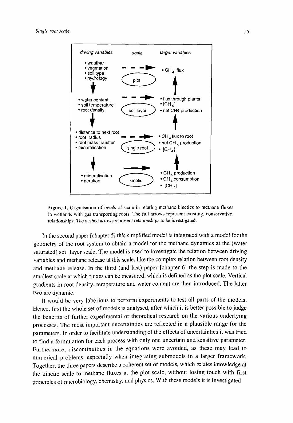
Single root scale 55
driving variables
• weather • vegetation • soil type • hydrology
scale
t plot
water content soil temperature root density
• distance to next root root radius root mass transfer mineralisation
1 mineralisation aeration
target variables
• C H 4 flux
• • flux through plants • [CH 4 ]
• net CH4 production
• CH4f luxto root net CH 4 production [CH4]
• • C H 4 production • C H 4 consumption • [CH4]
Figure 1. Organisation of levels of scale in relating methane kinetics to methane fluxes in wetlands with gas transporting roots. The full arrows represent existing, conservative, relationships. The dashed arrows represent relationships to be investigated.
In the second paper [chapter 5] this simplified model is integrated with a model for the geometry of the root system to obtain a model for the methane dynamics at the (water saturated) soil layer scale. The model is used to investigate the relation between driving variables and methane release at this scale, like the complex relation between root density and methane release. In the third (and last) paper [chapter 6] the step is made to the smallest scale at which fluxes can be measured, which is defined as the plot scale. Vertical gradients in root density, temperature and water content are then introduced. The latter
two are dynamic. It would be very laborious to perform experiments to test all parts of the models.
Hence, first the whole set of models is analysed, after which it is better possible to judge the benefits of further experimental or theoretical research on the various underlying processes. The most important uncertainties are reflected in a plausible range for the parameters. In order to facilitate understanding of the effects of uncertainties it was tried to find a formulation for each process with only one uncertain and sensitive parameter. Furthermore, discontinuities in the equations were avoided, as these may lead to numerical problems, especially when integrating submodels in a larger framework. Together, the three papers describe a coherent set of models, which relates knowledge at the kinetic scale to methane fluxes at the plot scale, without losing touch with first principles of microbiology, chemistry, and physics. With these models it is investigated

Chapter 4 56
Table 1. List of Symbols
ATt surface area of root, m2 soil b rate of change due to bubble transport, mol m - 3 soil s"1
c concentration in soil, mol m~3 soil c' dimensionless oxygen concentration at root surface c\ integration constant, mol m"3 H 2 0 (equation 43a) or mol m"3 H2O m soil (equation 43b)
C2 integration constant, mol n r 3 H2O
c r t root density, kg dw m~3 soil
c s a t saturated aqueous gas concentration, mol m*""3 H2O
curv curvature of equation for bubble release, m3 soil m~3 gas
Dg io gaseous molecular diffusion coefficient, m2 gas s - 1
Daq molecular aqueous diffusion coefficient, m2 H2O s - 1
Daq<eff effective aqueous diffusion coefficient, m3 H2O m"1 soil s"1
/ a e r aeration factor / a n relative reduction of C-mineralisation under anaerobiosis
/d,rt diffusion reduction factor in roots, m gas m - 1 soil / e o factor to account for the concentration of electron acceptors
/jat mass fraction of lateral roots, kg dw lateral root kg"1 dw total root
/prim m a s s fraction of primary roots, kg dw primary root kg - 1 dw total root
kr0 electron acceptor re-oxidation constant, s - 1
kx\ effective root surface gas transport coefficient, m3 H2O m"2 soil s_1
Kpj half saturation constant of process p and compound /, mol m~3 H2O /rt length of root, m soil Z-k characteristic length of kinetic processes, m soil
Z, t o t root length density, m root m~ 3 soil
iVtot root tip density, m~ 3 soil p air pressure, Pa q transport of gas via plant, mol i r r 3 soil s - 1
4rt root respiration, mol O2 kg"1 dw total root s_ 1
^rt" root respiration, mol O2 m""2 active area s_ 1
r spatial coordinate, distance to centre of root, m soil tfaer distance to centre of root to which the soil is aerated, m soil rt, relative rate of bubble release, s - 1
r\yymx maximum relative rate of bubble release, s~*
/q effective root gas transport coefficient, m3 H2O m"3 soil s~!
/"n root radius, m soil R half the distance between a root and the next root, m soil ^gas gas constant, J mol - 1 K_1
ROL root oxygen loss, mol kg - 1 dw root s - 1
s net production of a compound, mol m~3 soil s - 1
SA RA specific active root area, m2 active root kg - 1 dw total root SRL specific root length, m kg - 1 dw t time, s T temperature, K v probability density of R, m_ 1 soil vbub velocity of bubbles, m3 gas m - 2 soil s"1
Vmp,i maximum rate of process p and compound /, mol m - 3 s~!

Single root scale $y
^tot volume of model system, m3 soil
a solubility, m3 gas m~3 H2O
P ratio of time constants of O2 sink in the soil and root O2 transport y ratio of time constants of transport in root and transport just around a root r gamma function ^*lat distance between the bases of the lateral root at the primary roots, m soil Az thickness of soil layer, m soil £aq,rt volumetric water content of non-aerenchymatous root tissues, m3 H2O m~3 root
£bub bubble volume, m3 gas m~3 soil
£Cr critical gas filled pore space for bubble release, m3 gas m~3 soil
£g,rt gas filled pore space of roots, m3 gas m~3 root £solid volumetric solid phase, m3 solid m~3 soil £ partitioning factor for anaerobic C-mineralisation 7] carbon sink strength of electron acceptor reduction relative to methanogenes is T]Q T) under electron acceptor saturation
9 volumetric moisture content, m3 H2O m~3 soil K root O2 release relative to the O2 demand for aerobic respiration
v stoichiometric constant, mol mol - 1
Prt density of root, kg dw m~3
pS)rt solid phase density of root, kg dw m~3
% characteristic time of kinetic processes, s
0" flux density of gas through root surface, mol m*~2 soil s - 1
(0 O2 sink relative to O2 sink for aerobic respiration.
Compounds cs carbon substrate eo oxidised electron acceptor er reduced electron acceptor e t o t sum of oxidised and reduced electron acceptors
Subscripts acm anaerobic C-mineralisation ae aerobic respiration aq aqueous phase eq equilibrium c in the cylindrical geometry g gas phase i index of compound lat lateral root mo methane oxidation mg methanogenesis mx maximum ro re-oxidation (of electron acceptors) id reduction (of electron acceptors) rt root rem reference C-mineralisation s in the spherical geometry
other symbols ~ spatially averaged at the single root level. * normalised with equilibrium CH4 production when O2 inflow is zero
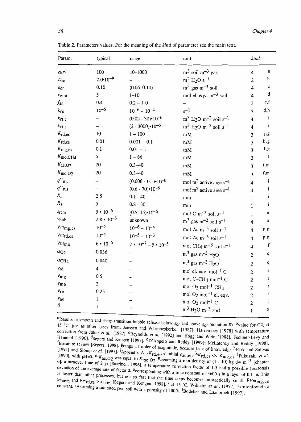
58 Chapter 4
Table 2. Parameters values. For the meaning of the kind of parameter see the main text.
Param. typical range unit kind
curv
^aq £cr cetot
/an
*ro
*rttc
*rt,s
^rd,eo
^rd.cs
^mg,cs
^mo,CH4
^ae,02
^mo,02
<Trt,c
<?"rt,s
* c
*s
rcm
Vbub
* wmg,cs
W"rd(cs
Vmmo
«02
«CH4
Vrd vmg
Vmo
Vro
Vae 0
100
2.0-10"9
0.10
5
0.4
10"5
10
0.01
0.1
5
20
20
2.5
5
5 • 10~6
2.8 • 10"5
10-5
10"4
6 • 10"6
0.036
0.040
4
0.5
2
0.25
1
1
10-1000
(0.06-0.14)
1-10
0 .2 -1 .0
1 0 " 6 - 10"4
(0.02- 30)-10~6
(2-3000WO-6
1-100
0.001-0.1
0.01 - 1
1 -66
0.3-40
0.3^*0
(0.006 - 0.1 MO"6
(0.6-70HQ-6
0.1-40
0.8 - 30
(0.5-15)* 10~6
unknown
1 0 " 6 - lO-4
1 0 ~ 5 - 10~3
7 • 10~7 - 5 • 10~5
m3 soil m 3 gas
m2 H2O s -1
1 3 soil m J gas m mol el. eqv. m - 3 soil
s-1
m3 H2O m - 2 soil s_ 1
m3 H2O m - 2 soil s_ 1
mM
mM
mM
mM
mM
mM
mol m2 active area s_1
mol m2 active area s"1
mm
mm
mol C m"-3 soil s"1
m3 gas m - 2 soil s"1
mol Ac m - 3 soil s_1
mol Ac m - 3 soil s""1
mol CH4 m - 3 soil s"1
m3 gas i r r 3 H2O
m3 gas m~3 H2O
mol el. eqv. mol - 1 C
mol C-CH4 mol"1 C
mol O2 mol - 1 CH4
mol O2 mol - 1 el. eqv.
mol O2 mol - 1 C
m3 H 2 0 m"3 soil
4
2
4
4
3
3
4
4
3
3
3
3
3
3
4
4
1
1
1
4
4
4
4
2
2
2
2
2
2
2
1
a
b
c
d
e,f
d,h
i
i
j .g
k,g
l.g
f
t,m
f,m
n
0
P.g
P.g
f
q
q
r
r
r
r
r
s
' ^ r ^ ^ r t : bubb,e/wase beiow E« and above e« ^^ « > • b ^ ** ™> -c o r r e c t f r o m ^OL^^IT^ST IT" " " * ^ ^ ^ " ^ Hemond [1996]. dsegers a n d K e n l ( Z n , [ ] ^ H ° S g M d W e i n I1 9 8 8! ' Fechner-Levy and 'literature review [S g e" i S ? . * "* ^ [ 1 M 9 ] : M c U t e h e > a n d R e d d ^ l ^ ] . [1994] and S . o m p . T ^ M p di A t ^ ^ *"""^ °f k™ , e d« e hKirk ™« ^ [1990], with pH=5. m^ae 0 - was equal to K „ n° < ^ ^ ^ * r d ' c s « K m ^ s - ' F u k u z a k i " al
6], a turnover time of 2 yr fsaa^ nen 9 9 6 f T , ' 0 2 ' ^ * " ^ ^ ° f (1 " 10> ^ d w m ~ 3 IchaP t e r
deviation of the average rate of factor 2 o ' e T e r a t U r e e o r r e c t i™ factor of 1.5 and a possible (seasonal) is faster than other proc ses b „ot 7 ? ° , "f w i t h a t i m e —tant of 3600 s in a layer of 0.1 m. This >*acm and v„ r d , c s I ^ ^ 1 ^ ^ / t « — — c a l l y small, constant. sA s s u m i n g . „ p e a ( ^ ^ / ^ ^ , ^ ^ ^ ^ ^ ^ , 0 ^
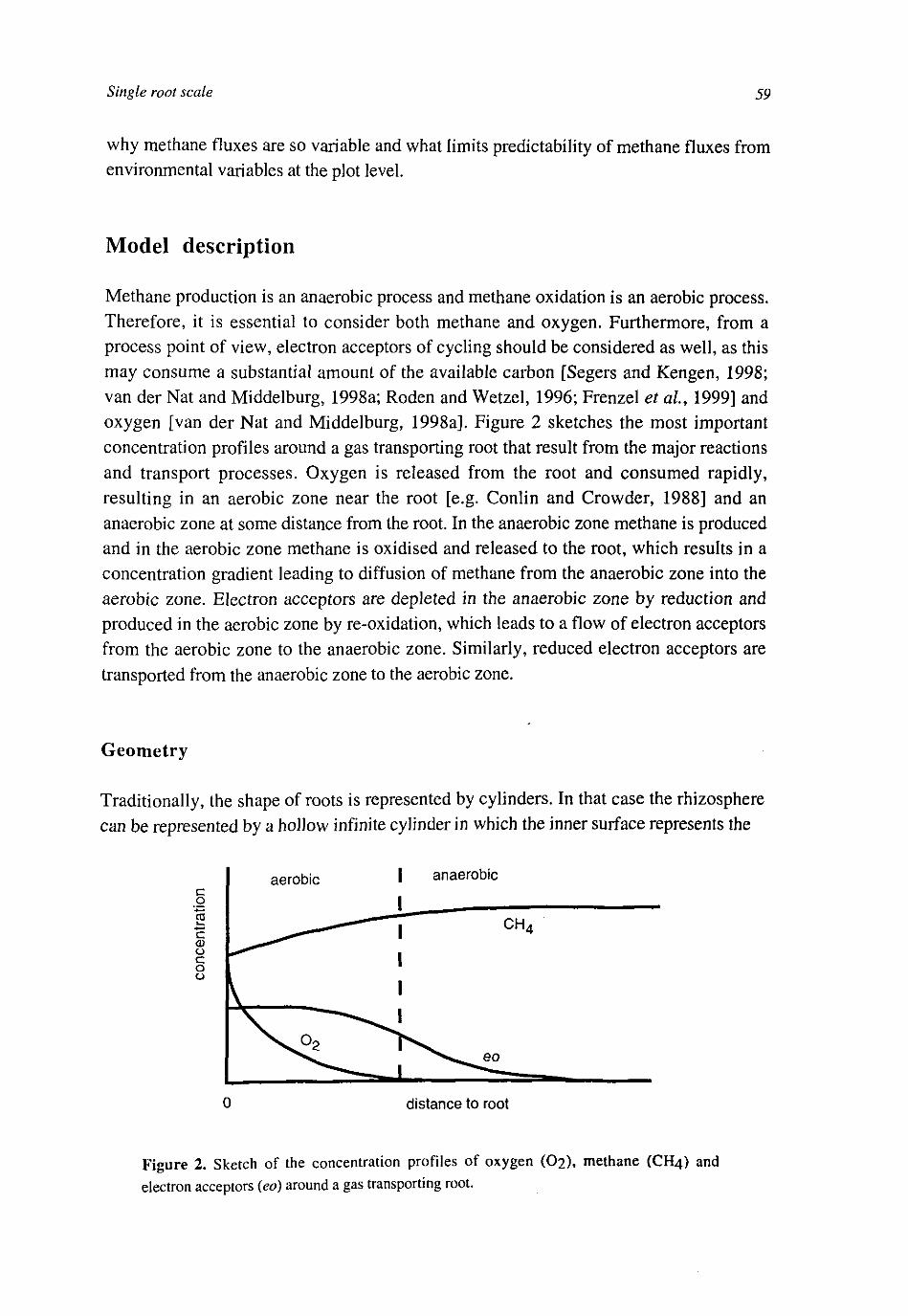
Single root scale 59
why methane fluxes are so variable and what limits predictability of methane fluxes from environmental variables at the plot level.
Model description
Methane production is an anaerobic process and methane oxidation is an aerobic process. Therefore, it is essential to consider both methane and oxygen. Furthermore, from a process point of view, electron acceptors of cycling should be considered as well, as this may consume a substantial amount of the available carbon [Segers and Kengen, 1998; van der Nat and Middelburg, 1998a; Roden and Wetzel, 1996; Frenzel et a/., 1999] and oxygen [van der Nat and Middelburg, 1998a]. Figure 2 sketches the most important concentration profiles around a gas transporting root that result from the major reactions and transport processes. Oxygen is released from the root and consumed rapidly, resulting in an aerobic zone near the root [e.g. Conlin and Crowder, 1988] and an anaerobic zone at some distance from the root. In the anaerobic zone methane is produced and in the aerobic zone methane is oxidised and released to the root, which results in a concentration gradient leading to diffusion of methane from the anaerobic zone into the aerobic zone. Electron acceptors are depleted in the anaerobic zone by reduction and produced in the aerobic zone by re-oxidation, which leads to a flow of electron acceptors from the aerobic zone to the anaerobic zone. Similarly, reduced electron acceptors are transported from the anaerobic zone to the aerobic zone.
Geometry
Traditionally, the shape of roots is represented by cylinders. In that case the rhizosphere can be represented by a hollow infinite cylinder in which the inner surface represents the
c o TO
•*—•
c <D O c o o
C
aerobic
\Oa
>
| anaerobic
— j C H 4
^ * * w _ eo 1 ^ —
distance to root
Figure 2. Sketch of the concentration profiles of oxygen (O2), methane (CH4) and electron acceptors (eo) around a gas transporting root.
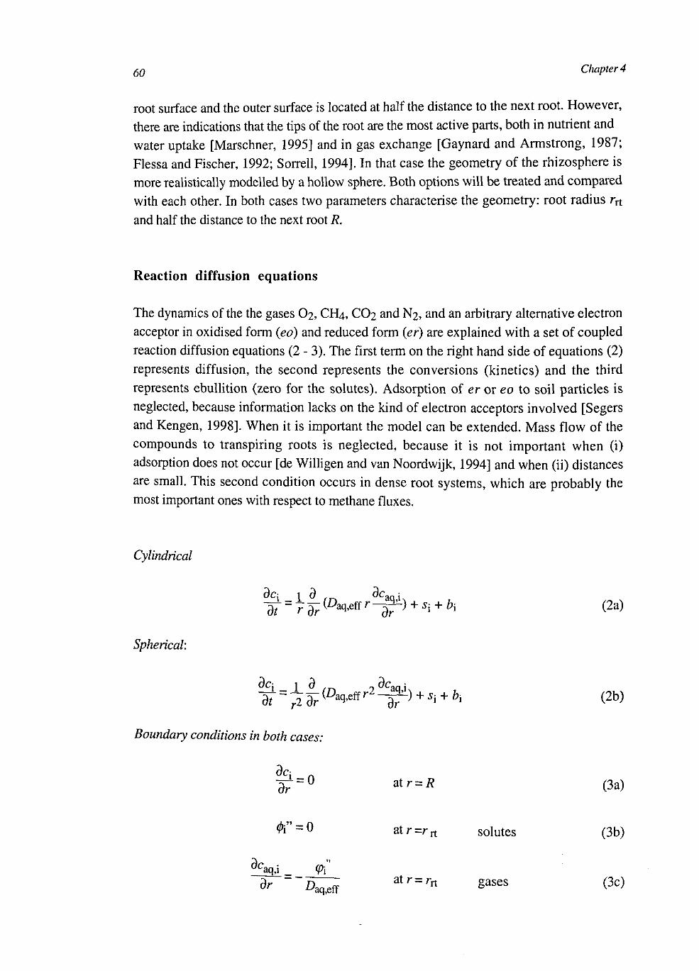
$0 Chapter 4
root surface and the outer surface is located at half the distance to the next root. However, there are indications that the tips of the root are the most active parts, both in nutrient and water uptake [Marschner, 1995] and in gas exchange [Gaynard and Armstrong, 1987; Flessa and Fischer, 1992; Sorrell, 1994]. In that case the geometry of the rhizosphere is more realistically modelled by a hollow sphere. Both options will be treated and compared with each other. In both cases two parameters characterise the geometry: root radius rrt
and half the distance to the next root R.
Reaction diffusion equations
The dynamics of the the gases O2, CH4, CO2 and N2, and an arbitrary alternative electron acceptor in oxidised form (eo) and reduced form (er) are explained with a set of coupled reaction diffusion equations (2 - 3). The first term on the right hand side of equations (2) represents diffusion, the second represents the conversions (kinetics) and the third represents ebullition (zero for the solutes). Adsorption of er or eo to soil particles is neglected, because information lacks on the kind of electron acceptors involved [Segers and Kengen, 1998]. When it is important the model can be extended. Mass flow of the compounds to transpiring roots is neglected, because it is not important when (i) adsorption does not occur [de Willigen and van Noordwijk, 1994] and when (ii) distances are small. This second condition occurs in dense root systems, which are probably the most important ones with respect to methane fluxes.
Cylindrical
Spherical:
dc\ 1 3 ._ «dcaa\
-di = Tr{D^f{r 2 ^ f ) + *i + foi (2b)
Boundary conditions in both cases:
• ^ T = 0 a t r = K (3a)
#' = 0 at r=r r t solutes (3b)
^ a q j _ (Pi dr ~~ A ^ f f a t r = r r t gases (3c)
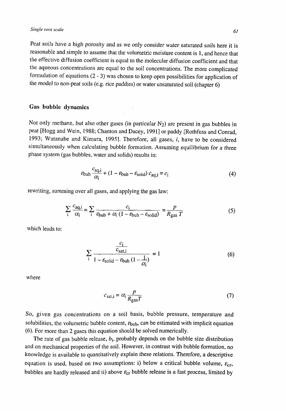
Single root scale *.i
Peat soils have a high porosity and as we only consider water saturated soils here it is reasonable and simple to assume that the volumetric moisture content is 1, and hence that the effective diffusion coefficient is equal to the molecular diffusion coefficient and that the aqueous concentrations are equal to the soil concentrations. The more complicated formulation of equations (2 - 3) was chosen to keep open possibilities for application of the model to non-peat soils (e.g. rice paddies) or water unsaturated soil (chapter 6)
Gas bubble dynamics
Not only methane, but also other gases (in particular N2) are present in gas bubbles in peat [Hogg and Wein, 1988; Chanton and Dacey, 1991] or paddy [Rothfuss and Conrad, 1993; Watanabe and Kimura, 1995]. Therefore, all gases, 1, have to be considered simultaneously when calculating bubble formation. Assuming equilibrium for a three phase system (gas bubbles, water and solids) results in:
£bub ~ + (1 - £bub - Ssolid) caq,i = q (4)
rewriting, summing over all gases, and applying the gas law:
2 ^ = £ Q , P i CC[ i £fcub + CC{ ( 1 - £bub _ ^solid) ^gas T
(5)
which leads to:
c\ csat,i
1 l-£solid-£bub(l-;J-) = 1 (6)
where
= a i -^F (7) sat,l "~ ^ 1 ~n T AgasJ
So, given gas concentrations on a soil basis, bubble pressure, temperature and
solubilities, the volumetric bubble content, £bub> c a n t>e estimated with implicit equation (6). For more than 2 gases this equation should be solved numerically.
The rate of gas bubble release, b\, probably depends on the bubble size distribution and on mechanical properties of the soil. However, in contrast with bubble formation, no knowledge is available to quantitatively explain these relations. Therefore, a descriptive equation is used, based on two assumptions: i) below a critical bubble volume, ecr, bubbles are hardly released and ii) above ecr bubble release is a fast process, limited by

(52 Cliapter 4
bubble rise velocity, vt,ut>. The second assumption is based on the suggestion that ebullition may be triggered by small disturbances [Bartlett et al, 1988; Shurpali et al, 1993] and results in a high value of vt>ub (Table 2). To obtain a continuous transition between (i) and (ii) the expolinear equation [Goudriaan and Monteith, 1990] is used:
*i = -1b £bubcg,i (8a)
rb = ~T~ ln(l+exp(c«rv (£bub - «cr))) (8b)
1,,mx = - ^ ^ (80 Az £bub
Root gas transport
Depending on plant species, root gas transport is influenced by anatomy of roots [Armstrong and Beckett, 1987], anatomy of the root/shoot interface [Butterbach-Bahl et al, 1997], soil temperature [Hosono and Nouchi, 1997] and/or through-flow mechanisms that depend on weather [Armstrong et al, 1996; Chanton et al 1993; Morrissey et al, 1993; Grosse et al, 1996a; Brix et al, 1996; van der Nat tf al, 1998]. It would be possible to formulate a model to summarize and integrate (part of) these insights, using Luxmoore et al. [1970], Armstrong and Beckett [1987], Armstrong et al [1990], Kirk [1993] and Sorrell [1994]. However, such a model would be complex and would contain many uncertainties, which would complicate understanding of the processes in the rhizosphere, on which this paper focuses. Instead, an effective root surface gas transport coefficient, kn, is introduced (equation 9) which represents the overall transport resistance.
K - ** ((«. c M - ^ . Caq,ru) = kn {a {CM (1 _ ^ j l _ ) _ (9)
b e c a r r ' """J f T 0 0 T CmSUm^0n is * t he 8» changing root surface, firstly
Becke 9 e8 ; r?Z°S PH 1 " ^ "* ^ m ° S t aCtiVC r ° 0 t ^ ^™* ^
as a d t r tSeC°n, Y C3USe * enaWeS 3 deSCripti0n of root o x V g - consumption
s ctted Z " 3 m ° S P " C ° X y 8 e n C O n C e n t r a t i o" (^cond part of equation 9). Root o t m e t n T HPr t i a l T™ ^ ^ * °n'y ^ h^than vo.umetric esu a r e vo \ lnfSOil [SegerS'1998] and the V0lume ° f - t s is probably o lo r tn t an 7 ^ ^ ^ ^ «« f° r ™*™ » P^b ly not o o J a l o n t e ; 7 t0 bC Z e r °- N ° t e ' h ° W e V e r ' t h a t m e t h a n e -Nation near the ons m e 7 : ^ ( e q U a t l 0 n S
f * * "* ^ «« fm °^e" 1S »<* neglected as it can q Z n 9) a m ° U n t ^ ° X y g e n t r a n S P ° r t e d * " » * " the Plant (Table Al and
Single root scale 63
Kinetics
Net methane production is the result of methane production and methane oxidation (equation 10). Net production of electron acceptors in oxidised and reduced form are described similarly (equations 11-12). Oxygen consumption is the sum of aerobic respiration, methane oxidation and electron acceptor re-oxidation (equation 13). Carbon dioxide production is the result of aerobic respiration, methane oxidation, methane production and electron acceptor reduction(equation 14). Molecular nitrogen is inert (equation 15).
^CH4 = %ig,CH4 + Smo,CH4 (10)
seo = %),eo + 5rd,eo (11)
Ser = sro,tr + %i,er (12)
^02 = Sae,02 + ^ m o ^ + sro,Oi (13)
SCO2 ~ 5ae,C02 + %io,C02 + %ig,C02 + 5rd,C02 ( 1 4 )
^N2 = 0 (15)
C-mineralisation
As the simplest approach in a partially aerobic environment it is assumed that aerobic respiration (=aerobic C-mineralisation) only depends on the oxygen concentration (equations 16-18). Under anaerobic conditions C-mineralisation proceeds slower than under aerobic conditions which is described by equation (19).
5ae,02 = " ^ae/aer 5rcm (16)
Sae,C02 = /aer ^rcm ( 1 ' )
/aer = - ^ J ^ _ (18) Caq,02
+ ^ae,02
•Sacm = (l-^aer)jan ^rcm (1")
The reduction factor for anaerobic-mineralisation,/an> probably depends not [D'Angelo and Reddy, 1999] or only weakly [McLatchey and Reddy, 1998] on the kind of alternative electron acceptor and hence is assumed to be constant.
64 Chapter 4
methane production
The relation between anaerobic C-mineralisation and methane production is dominated by the influence of electron acceptors [Segers, 1998]. Van Cappellen and Wang [1996] developed and parameterised a comprehensive model on methanogenesis and cycling of nitrogen, iron, manganese and sulfur. However, including all this knowledge would be in imbalance with the complexity and accuracy of the model for root gas transport. Moreover, in peat soils also organic electron acceptors may be active, which suppress methane production just like the inorganic alternative electron acceptors [Segers and Kengen, 1998; Lovley et aL, 1996; Coates et al, 1998]. Therefore, all individual electron acceptors were lumped into one generalised electron acceptor pool, following Segers and Kengen [1998]. Furthermore, in wetlands it is likely that methanogenic biomass does not limit methane production [Segers, 1998]. Therefore, the methane production model of Segers and Kengen [1998] is further simplified with a quasi steady state assumption for acetate leading to:
5mg,CH4 = vmg bmg ^acm \^)
Smg,C02 = (1 - vm g) fmg sacm (21)
•Srd,eo = - Vrd (1 - Cmg) acm (22)
%J,C02 = (1 - Crng) sacm (23)
Here, £mg is a partitioning factor for anaerobically mineralised carbon, which depends on a set of kinetic parameters and the concentration of electron acceptors (equations 24 -27).
?m* - ^ T (24)
V =/eo VO (25)
*rd,cs Vmm g ,c s (26>
f = caq,eo
^rd,eo +c a q , e o ( 2 7 )
0*,™""°"'k I' r e a S ° n a b , e t 0 3 S S U m e t h a t t h e P r e s e " c e o f e l e^ron acceptors ompletely suppresses methane production [Segers and Kengen, 1998], which .implies
rio » 1 and, hence, that Cmg « 1 when electron acceptors are present and £ng -
Single root scale 65
1 when electron acceptors are depleted. A process based refinement of this picture is difficult as five independent kinetic parameters (Vm and K) are involved [van Cappellen and Wang, 1996].
Electron acceptor re-oxidation
Under aerobic conditions reduced electron acceptors are re-oxidised, which can occur both biologically and chemically [van Cappellen and Wang, 1996]. Chemical re-oxidation is probably best described with a second order equation and biological re-oxidation is probably best described with Monod equations. In the low substrate range, which is not unlikely in reality [van Cappellen and Wang, 1996], both formulations result in the same behaviour, namely proportional to the substrate concentrations. Therefore, and because in general little is known about the re-oxidation process, the simplest formulation is chosen: an oxygen dependence similar to aerobic respiration and a first order dependence on the concentration of reduced electron acceptors:
•?ro,er = ~/aer &ro 0 Caq,er (28)
•Sro,eo = — %),er (~9)
Sro,02 = vro %),er (30)
Methane oxidation
In freshwater wetlands, aerobic methane oxidation is probably more important than anaerobic methane oxidation and is mainly controlled by the availability of methane and oxygen [Segers, 1998]. To account for both controlling factors a double Monod expression is used:
T/ <?aq,CH4 . caq,Q2 f 3 n
J m 0 ' C H 4 " " V m m 0 C a q . C H 4 + ^ m o , C H 4 *aq,02 + W > 2 *
Smo,02 = vmo Smo,CH4 (32)
Smo,C02 - - Smo,CH4 ( 3 3 )
As typical values for ^ m o ,o 2 a r e i n t h e s a m e r a n S e a s lW{cd!i v a I u e s f o r K*&&2 tSeSers>
1998; Bodelier and Laanbroek, 1997] it is reasonable (and simple) to assume that both values are the same, which leads to the replacement of the third factor in equation (31) by
/aer (equation 18).
66 Chapter 4
Simplification of the reaction diffusion equations
Equations (2-33) form the Jull model, which was solved numerically. However, using information on the order of magnitude of various parameters, also a simplified model was deduced to improve insight in the interactions and to speed up calculations. The simplifying procedure consists of two steps. First, a quasi steady state condition for oxygen is applied and subsequently the differential equations for the other compounds are spatially averaged. As a result the distance to the root, r, is resolved as independent variable.
Rewriting the equations for the oxygen consuming processes
Main drivers of the system are root oxygen release (electron acceptor input) and carbon mineralisation (electron donor input). Therefore, as first step, methane oxidation, electron acceptor re-oxidation and total oxygen consumption are normalised with oxygen consumption by aerobic respiration:
W™ " S ? = W ™.™ ^ (34) S™>°2 Caq,CH4 + K m o , C H 4 W
^ ^ ^ n i o ( 3 5 )
^ae ^rcm
s M - Aro,C>2 <?aa er n, = ^ = f l , r o - n « r 9 £ L (36)
ae,o2 caq,e to t
v
fljb>mx = ^ j k ^ f a A o t vae ^rcm
^ae ^rcm
(37)
(38)
S°2 ^ ^ ^ ' ^ o + ^ o (39)
and thus
s02 - W/aer Vae srcm ^
rs;irmc;r:p,i:is propor,ionai * "*~ <«-»«—. ** „«» *,«<,,,

Single root scale 67
Analytical approximation of radial oxygen release
In principle, root oxygen loss depends on both the mass transfer characteristics of the root and on the strength of the oxygen sink in the soil. As the relation between the oxygen consumption by the soil and the oxygen concentration is non-linear, there is no analytical solution of equations (2, 3, 9, 18, 40) for oxygen and an approximation has to be made. Such an approximation is trivial when either root transport capacity or the soil oxygen sink is limiting. However, a reasonable approximation can also be found when both the root and the rhizosphere influence root oxygen release; In that case the concentration gradient will be divided between root and rhizosphere and the oxygen concentration at the root surface will be about 0.15 mol rn~3 H2O (50% of the equilibrium with atmosphere). This is one order of magnitude larger than the half saturation constants for the oxygen consumption processes which are about 0.01 mol m~3 H2O (Table 2). As a result, the interaction between oxygen in root and rhizosphere needs only to be investigated in the zero order regime of rhizospheric oxygen consumption (/*aer = 1).
The oxygen sinks strength depends on the r dependent concentrations of methane and reduced electron acceptors. However, as the oxygen consumption zone is thin, it is likely that gradients of these concentrations will be small and, therefore, these gradients are neglected. Furthermore, it is assumed that the oxygen sink strength in the oxygenated rhizosphere is equal to the spatially averaged (indicated by a single bar) sink strength, co. For methane oxidation, this is reasonable, because methane concentrations are mostly above ^mo,CH4 (e-g- [Shannon and White, 1996; van den Pol - van Dasselaar et a/., 1999a]; Table 2). For re-oxidation of electron acceptors this assumption is probably less good, though the slow reduction of electron acceptors has a spatially smoothening effect on the electron acceptor dynamics. So, equation (40) is further simplified into (41), resulting in a linear partial differential equation for oxygen (equation 2 and 41a) with boundary conditions (3c, 9) and (42). From these equations /?aer can be solved as well, due to the extra condition at r = 7?aer-
so2 = - Vae CO srcm r < 7?aer (41a)
502 = 0 r>/?aer (41b)
^ 2 . = 0 and c02 = 0 r = /?aer (42) or
As oxygen consumption is a fast process, with time constants typically less than 1 day, only steady state conditions for the oxygen profiles are considered, which, for r < i?aer, leads to [Carslaw and Jaeger, 1959, p. 191]:
= Vaefl>frcm. r2 + c \n (r) + c2 (cylinder) (43a) q ' 2 4Daq,eff

6g Chapter 4
and (straight forward integration):
caq,02 = y j r o m r2 + £L + c2 (sphere) (43b)
Now equations (3c, 9,42 and 43) form two systems of five equations and five unknowns (integration constants c\ and Q , <P"C>2'
crt,02 anc* ^aer)> which result in single closed equations for the dimensionless oxygen concentration at root surface, c':
2 /? v+ 2 Bc'd-tf 2/?y(l - c ' ) + r = l n (2 0 d - c '>+ D (cylinder) (44a)
c' + ^ ( ( l + 3 j 3 ( l - c ' ) ) 2 / 3 - 2 ) 3 ( l - c ' ) - l ) = 0 (sphere) (44b) 2/3
with
r'
B,aun,U2 /, /Crt
vae fi> ^rcm rn
y - *rt >Yt
Aiq,eff
caq,02,rt
P = -^£L- (45)
(46)
(47) etc _ #rt w cg,atm k rt
/? and y can be interpreted as ratios of characteristic times of three processes: external mass transfer (0r r t/* r t), mass transfer around the root (6 rrt2/(Daq,eff)) and reaction (0 («< :a tm-? r t " /* r , ) / (v a e a )5 r c m ) . In the field of transport phenomena y is called the Biot number [Janssen and Warmoeskerken, 1987], Numerical solutions for equations (44) (Figure 3) are used to calculate 7?aer:
( % L ) 2 = 1 + 2 ^ 1 - ' ) cylinder (48a)
( % L ) 3 = 1 + 3 ^ 1 - ' ) sphere (48b)
Surface c ^ b e t t , 5 0 1 ! '"^«* a e r a t e d a " d ^ °*ygen concentration at the root u t l t to , ox" ^ m tHe C ° n C e n t r a t i 0 n d i f f - n c e over the root needed to
sustain me total oxygen consumption:

Single root scale 69
100 10000 1000000
P
Figure 3. Dimensionless oxygen concentration at the root surface, c \ as function of dimensionless number ft, for several values of the dimensionless number y. The full line refers to the cylindrical geometry, the dashed line refers to the spherical geometry. The graph is obtained from numerical solutions of equations (44).
1 ( *2 - r r t
2 .
2 P rrt2 c'=l--M-—^-) cylinder (49a)
c'= 1 - 1 ( f i 3 - ^
3 P rrt3
sphere (49b)
Spatially averaging methane kinetics
Using the analytical approximation for total oxygen release, spatially averaged equations for the other processes can be found. Under the quasi steady state condition, oxygen inflow is equal to oxygen consumption:
An 0"O2 JVtot
f astir) vae co sTcm dV (50)
From equation (19) average anaerobic carbon mineralisation is:
(1 -/aerW)/an srcm dV *?acm — T/ " to t
(51)
% ot
Substitution of a re-written form of equation (50) into equation (51) leads to:
•?acm -/an %;m (* ^ (52)
with

70 Chapter 4
K _ nj^i cylinder (53a) Vae^rcmCtf ->Yt2)
3 rrt2 <p"o2
K = r t ^ _ j s p h e r e ( 5 3 b ) V a e 5 r c m ( ^ - r r t
3 )
K is the total oxygen inflow divided by the maximum oxygen consumption by aerobic respiration. Hence, it is a kind of aeration factor.
As reduction of electron acceptors is slower than diffusion, it is assumed that the average concentration prevails in the whole volume, in which case the mean carbon
partitioning, £ factors can be calculated from the mean values of the concentrations of electron acceptors:
%ig,CH4 = vmg £mg sacm (54)
*rd,eo = " Vrd (1 - Cmg) ^acm (55)
Now, the only two processes which are explicitly dependent on r are methane oxidation and electron acceptor re-oxidation. To resolve this it was assumed that the volume averaged partitioning of the oxygen over the three oxygen sinks could be calculated from the volume averaged sink strengths:
Sae,02 = ~K 4vae srcm (56) ft) v '
^mo,CH4 = - ^ ^ ^ , r c m ( 5 7 )
ft) vmo v
%),eo- —K ^ % m (5g) vro 0) v
In case the electron acceptors are in equilibrium (?er,eo = W ) , w h i c h w o u l d h a p p e n
after prolonged flooded conditions and a relatively stable root system, normalised net methane production, sCHr can be calculated with:
vmg/an*rcm afm ' ( 5 9 )
producti^ ^H ^ C a l C U l a t e d d i r C C t l y f r ° m t h e d i f f e r e n C e b e t w e e n elytron donor
mTthanrol l r " ^ " ^ ^ ^ S ° ' U n d e r t h e s e c o"d i t i<™' " e t
methane products ,s only dependent on soil mineralisation and overall oxygen
Single root scale 7J
dynamics. Information about methane oxidation and electron acceptor cycling is only
relevant via their influence on the total oxygen demand, co.
Simplification of plant mediated transport of methane
Like the kinetics and the oxygen dynamics also the plant mediated transport of methane, #CH4> is summarised at the single root scale, using two assumptions. Firstly, net methane production rate does not depend on distance to the root, r, because the aerated zone is often small and because reduction of electron acceptors is slow. Secondly, net methane
production ( r= residence time in soil ~ days to weeks [Moore et aL, 1990; Liblik et
aL, 1998]) is slower than methane transport to the root (r~ 1 day, with distances of ~ 1 cm). These two assumptions lead to a first order equation (appendix B):
#CH4 = - rq,CH4 (Caq,CH4 - «CH4 ^g,atm,CH4) ( 6 0 )
with
rq,CH4 = (f)2 l ; j - cylinder (61a) r* R (l+7cH4ln(f)) ^n*
rn r H = A*ri (3t)3 1 sphere q'CH4 'k V (1+7CH4)
(61b)
The other two gases (N2 and CO2) only have effect on methane emissions via ebullition, which is probably not so strong. Therefore, plant mediated transport of these gases is modelled similar to methane.
Simplification of bubble transport
The formation of bubbles is mainly governed by the concentration of methane. In line with the assumptions above it is assumed that average methane concentration can be used to estimate the bubble volume.
Simplified model in transition directly after an aerobic period
In the simplified model it is assumed that quasi-steady state conditions prevail for oxygen, which implies that the supply of oxygen is equal to the sink. However, directly after an aerobic period there is a stock of oxygen which has to be consumed before the steady state condition is realistic. Therefore, during such an initial, transition phase, oxygen is maintained as state variable until its concentration is below 10% of the equilibrium with
72 Chapter 4
the atmosphere. In this phase, the system is not dominated by the gas transporting root, and hence, gradients with distance to the root are neglected. As a first approach in this generally short phase also oxygen exchange with the atmosphere is described with ^q,02'(equations 61).
Parameterisation
Four kinds of parameters are distinguished (Table 2). The first kind are driving variables, representing external factors, which will be resolved when the model is integrated in a large framework [chapter 5]. For this paper it is sufficient to get an idea over which range these parameters vary. The second kind are physical or chemical constants, like solubilities or stoichiometric constants. Accurate, generally valid estimates of these parameters are available. The third kind are biological constants, such as Km or the anaerobic reduction factor, /an. Often it is assumed that these parameters are similar across sites and situations. However, quite some variation may be present [e.g. Segers, 1998] due to biological variation which is often poorly understood. The fourth kind are biological variables which, intrinsically, vary across sites and in time, like Vm (potential activity on a soil basis) or kn (root surface gas transport resistance). Often these parameters are the weakest point of a model, as ground for extrapolation is poor.
In the formulated model, nine parameters of the fourth kind are present. Of these, V/»mg,cs and Vm^cs are not sensitive, which is a consequence of the assumption that electron acceptors suppress methane production completely [Segers and Kengen, 1998]. Furthermore, for reasons of simplicity, situations where bubble transport is important are avoided. This leaves Vmmo, Etot, ktt, qn and r r t as the most problemat ic ones. Together with R and sIcm and the geometry eight sources of uncertainty are present wh,ch should be considered. To catch as efficient as possible this space of uncertainty 32 parameter sets were chosen in such a way that key dimensionless numbers (como mx. " V m x , A y , K) varied over a large range in several combinations (Table 3). Initial values of the gas concentrations were equal to equilibrium with the atmosphere. The electron acceptors were set at 50% in oxidised form and 50% in reduced form
Numerical t echniques
mtH hi h e Were sed according t0 the control v o l»™ ™thod ^ a " k a r ' t toTh " SUreS C T T l m ° f m a S S - T h e 8 a S e X c h a " S e b e t — the roo and shel.
he t a v 3 J " Ca]Tl U S i n § t h e a n a l y t k a l S O l u t i ° " f o r - inert gas in the first a i b s 7 ( l S m a " I*" 8 - N U m e r i C a l S 0 l u t i 0 " s o f the full mode, (with state
Z v ^ a b £ H - ' ^ ]' ^ ^ a n d C ° 2 ( " » 3 n d t h e simplified model (with E £ ^ J £ ^ ~ *> e * t . y solving the equations w.th
avoid problems with discontinuities. Spatial discretisation was taken
Single root scale 73
so small that the influence on the results was negligible. For the temporal discretisation the explicit Euler method was used with a dynamic time step. For each state at each time step, a maximum time step was estimated as a fraction of the inverse of the relative rate of change. The smallest of these maximum steps was used for integration of all states. The fraction was chosen so small (0.1) that the simulation results were not affected by its value. Equations (6 and 44) are solved with the ZBRENT module of Press et al [1987], To check the numerical code mass balances are calculated of the individual species and of total carbon. The Fortran programme was run on a Alpha machine (model 600, 333 MHz, open VMS). Typical computer time was 17 seconds per simulated day for the full model and about 100 times less for the simplified model. The code containing the integrated models of the three papers is available upon request.
Model Analysis
General
Both the full and the simplified model were run several times after varying a few sensitive parameters, leading to a representative range of the controlling dimensionless parameters,
j3, y and o) (Table 3). j3 was always larger than 1, which implies that the gas transport capacity of the plant is large enough to supply the rhizosphere with oxygen over
distances of at least the radius of the root. When the relative aeration, K, was below 0.2, 0) approached its maximum value, indicating a highly reduced environment, producing considerable amounts of methane. When /cwas above 0.5 methane production was very small. Furthermore, it is interesting to see that K did not depend on ca, which implies that the oxygen sink strength in the rhizosphere is always in the saturation regime. Time coefficients for the release of methane, 0/rq, vary from 0.3 to 30 days, which corresponds to experimental values for rice [Sass et al, 1991; Byrnes et al, 1995; Watanabe and Kimura, 1995] and for sedge wetlands [Moore et al, 1990; Liblik et al,
1998].
Simplified and full model
Agreement between the two models was good, though in some cases net methane production was somewhat lower in the simplified model, because the aeration was higher, due to the higher oxygen sink strength. Methane flux through the plant was slightly lower in the simplified model, because of (i) the steady state assumption of the methane profiles and (ii) the assumption of a homogeneous net methane production. Both assumptions lead to a lower methane concentration near the root surface.
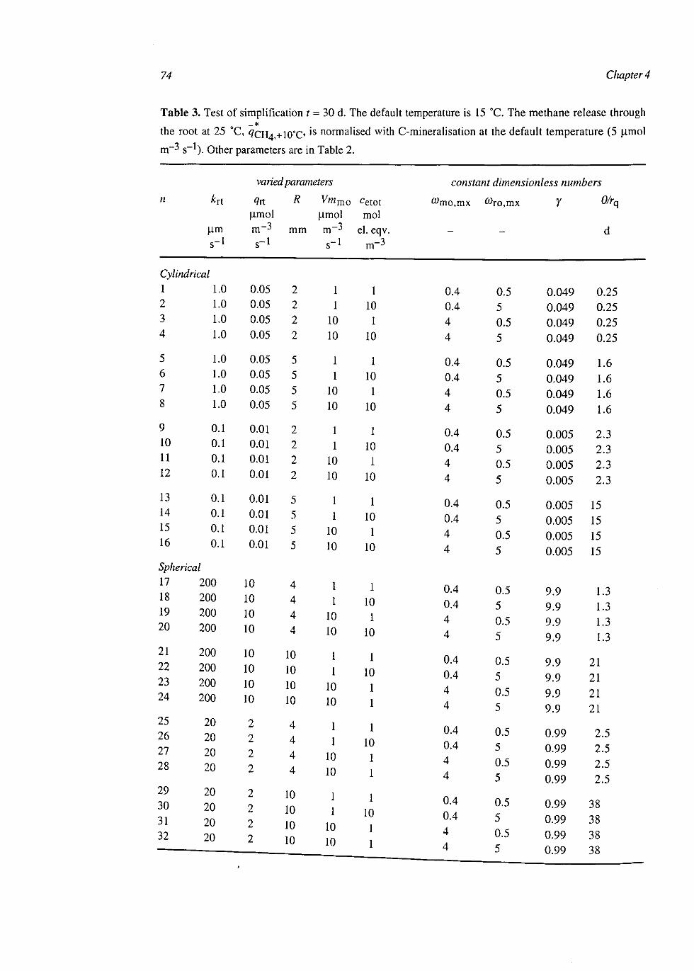
74 Chapter 4
Table 3. Test of simplification t = 30 d. The default temperature is 15 °C. The methane release through _*
the root at 25 °C, <7cH4+10°O ls normalised with C-mineralisation at the default temperature (5 imol
m-3 s-l) other parameters are in Table 2.
n *rt
(i,m s-1
Cylindrical 1 2 3 4
5
6 7 8
9
10 11 12
13
14 15 16
1.0 1.0 1.0 1.0
1.0
1.0 1.0 1.0
0.1
0.1 0.1 0.1
0.1
0.1 0.1 0.1
Spherical 17 18 19 20
21 22 23 24
25 26 27 28
29 30 31 32
200 200 200 200
200 200 200 200
20 20 20 20
20 20 20 20
varied parameters
<7rt (imol m~3
H
0.05 0.05 0.05 0.05
0.05 0.05 0.05 0.05
0.01
0.01 0.01 0.01
0.01
0.01 0.01 0.01
10 10 10 10
10 10 10 10
2 2 2 2
2 2 2 2
R
mm
2 2 2 2
5 5 5 5
2 2 2 2
5 5 5 5
4 4 4
4
10 10 10 10
4 4
4 4
10 10 10 10
Vmmo
u,mol m-3
s-1
1 1
10 10
1 1
10 10
1 1
10 10
1 1
10 10
1 1
10 10
1 1
10 J. \J
10 M. \J
1 1
10 10 1 \J
1 1
10 10
cetot mol
el. eqv. m-3
1 10 1
10
1 10
1 10
1 10 1
10
1 10
1 10
1 10
1 10
1 10 1 1
1 10 1 1
1 10 1 1
constant dimensionless numbers
%o,mx
—
0.4 0.4 4 4
0.4 0.4 4 4
0.4 0.4 4 4
0.4 0.4 4 4
0.4 0.4
A
4 4 f\ A
0.4 0.4 A
4 4
0.4
0.4
4 A
4
0.4 0.4
A
4 4
^ro.mx
—
0.5 5 0.5 5
0.5 5 0.5 5
0.5 5 0.5 5
0.5 5 0.5 5
0.5 5
0.5 5
0.5 5
0.5 5
0.5 5
0.5 5
0.5 5
0.5 5
7
0.049 0.049 0.049 0.049
0.049 0.049 0.049 0.049
0.005 0.005 0.005 0.005
0.005 0.005 0.005 0.005
9.9 9.9
9.9 9.9
9.9 9.9
9.9 9.9
0.99 0.99 0.99 0.99
0.99 0.99 0.99 0.99
e/rq
d
0.25 0.25 0.25 0.25
1.6 1.6 1.6 1.6
2.3 2.3 2.3 2.3
15 15 15 15
1.3 1.3
1.3
1.3
21 21 21 21
2.5 2.5 2.5 2.5
38 38 38 38

Single root scale 75
Table 3. (Continued) s refers to the simplified model , / to the full model and a to the analytical
steady state solution (equation 59). app refers to the apparent percentage of oxidation, which is defined as
the reduction of plant methane flux after setting Vmmo to zero.
dynamic dimensionless quantities 1
s
0)
/
Cylindrical 1.1 1.1 1.1 1.1
1.8 5.3 4.9 5.6
1.9 6.3 5.3 9.8
1.9 6.4 5.5 10.0
1.1 1.1 1.1 1.1
1.9 5.5 5.0 6.0
1,9 6.3 5.3 9.8
1.9 6.5 5.5
10.0
Spherical 1.8 3.5 3.4 3.5
1.9 6.4 5.5 10.0
1.9 6.4 5.4 9.8
1.9 6.4 5.5 10.0
1.8 3.6 3.7 3.6
1.9 6.5 5.5
10.1a
1.9 6.4 5.4 9.8
1.9 6.5 5.5
10. l a
59 31 31 30'
57' 17-20-11«
4.6' 1.4-1.6-0.9-
P s
510 509 509 509
290 101 109 96
23 7 8 4
23 7 8 4
•103
•103
•103
•103
•103
•103
>103
>103
>103
•103
103
>103
4.6-103
1.4-103
1.6-103
0.9» 103
s
0.93 0.93 0.93 0.93
0.36 0.37 0.37 0.37
0.20 0.20 0.20 0.21
0.03 0.03 0.03 0.03
0.46 0.47 0.47 0.47
0.03 0.03 0.03 0.03
0.20 0.20 0.20 0.21
0.01 0.01 0.01 0.01
K
f
0.93 0.93 0.93 0.93
0.35 0.36 0.36 0.36
0.20 0.20 0.20 0.20
0.03 0.03 0.03 0.03
0.45 0.46 0.46 0.46
0.03 0.03 0.03 0.03
0.20 0.20 0.20 0.20
0.01 0.01 0.01 0.01
s
0.00 0.00 0.00 0.00
0.39 0.03 0.19 0.00
0.65 0.54 0.55 0.52
0.94 0.93 0.93 0.92
0.22 0.01 0.03 0.00
0.95 0.93 0.93 0.93
0.66 0.54 0.55 0.51
0.98 0.97 0.97 0.97
—* •?CH4
/
0.00 0.00 0.00 0.00
0.41 0.04 0.21 0.01
0.66 0.54 0.55 0.52
0.94 0.93 0.93 0.92
0.24 0.01 0.03 0.00
0.95 0.93 0.93 0.93
0.66 0.54 0.55 0.52
0.98 0.97 0.97 0.97
a
0.00 0.00 0.00 0.00
0.39 0.18 0.19 0.17
0.65 0.54 0.55 0.52
0.94 0.90 0.93 0.92
0.22 0.03 0.03 0.02
0.95 0.93 0.93 0.93
0.66 0.54 0.55 0.51
0.98 0.97 0.97 0.97
s
-
0.00 0.00 0.00 0.00
0.39 0.02 0.19 0.00
0.65 0.54 0.55 0.52
0.62 0.56 0.61 0.56
0.22 0.01 0.03 0.00
0.39 0.35 0.39 0.35
0.66 0.53 0.55 0.51
0.27 0.24 0.27 0.24
- * <7CH4
/
-
0.00 0.00 0.00 0.00
0.41 0.03 0.21 0.00
0.66 0.54 0.55 0.52
0.63 0.57 0.62 0.57
0.24 0.01 0.03 0.00
0.40 0.36 0.41 0.36
0.66 0.54 0.55 0.52
0.28 0.25 0.27 0.25
s +10 °C
0.02 0.00 0.00 0.00
1.56 1.42 1.44 1.40
1.74 1.71 1.72 1.71
0.67 0.66 0.67 0.66
1.35 0.99
1.13 0.97
0.49 0.47 0.48 0.47
1.70 1.66 1.66 1.65
0.29 0.28 0.29 0.28
*&oxid,s real ^
82 86
105 114
32 53 77 94
14 5
40 28
2 1 6 3
50 78 96 98
2 1 6 3
14 5
40 28
1 0 2 1
app. ^
82 86 99
103
17 70 60 97
6 1
21 4
5 9 6 9
31 78 91 98
6 11 7
11
6 1
22 5
7 11 7
11
aw>ft)mx, because of bubble formation, which decreases 0, leading to an increase in [cerL leading to
^erXUer.mx* which is calculated with 0 = 1 .
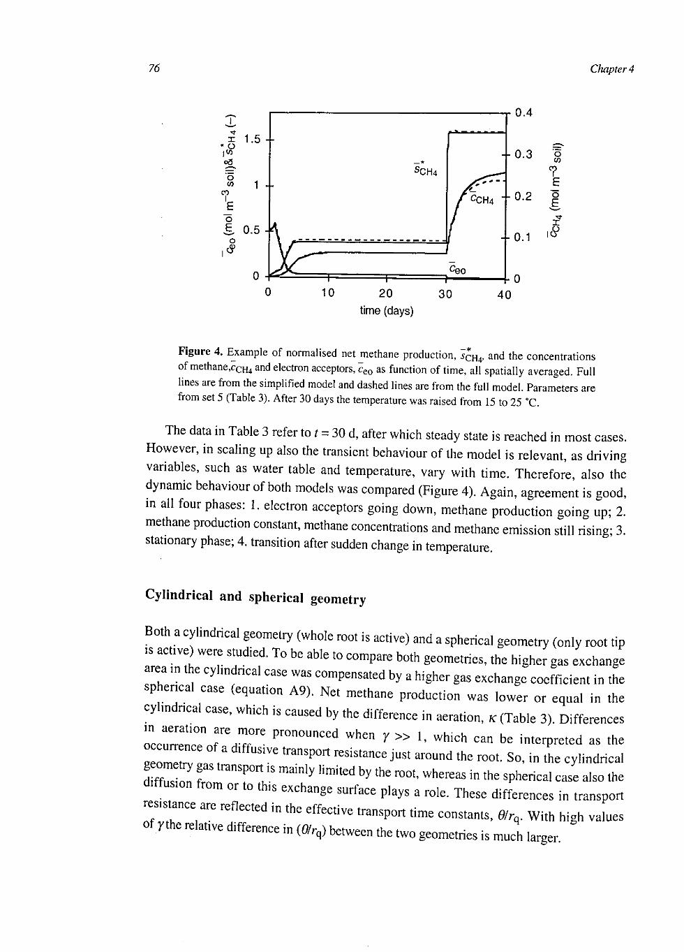
76 Cfiapter 4
10 20 time (days)
30 40
o </> ? E o E, £
16*
Figure 4. Example of normalised net methane production, SQH4, and the concentrations of methane,ccH4 ant* electron acceptors, ceo as function of time, all spatially averaged. Full lines are from the simplified model and dashed lines are from the full model. Parameters are from set 5 (Table 3). After 30 days the temperature was raised from 15 to 25 °C.
The data in Table 3 refer to t - 30 d, after which steady state is reached in most cases. However, in scaling up also the transient behaviour of the model is relevant, as driving variables, such as water table and temperature, vary with time. Therefore, also the dynamic behaviour of both models was compared (Figure 4). Again, agreement is good, in all four phases: 1. electron acceptors going down, methane production going up; 2. methane production constant, methane concentrations and methane emission still rising; 3. stationary phase; 4. transition after sudden change in temperature.
Cylindrical and spherical geometry
Both a cylindrical geometry (whole root is active) and a spherical geometry (only root tip is active were studied. To be able to compare both geometries, the higher gas exchange area in the cylindrical case was compensated by a higher gas exchange coefficient in the spherical case (equation A9). Net methane production was lower or equal in the cylindrical case, which is caused by the difference in aeration, K (Table 3). Differences
1ZZT T H T 6 P r ° n 0 U n C e d W h C n Y » *' W h i c h c a n b e interpreted as the 1 Z rv t r a n S P ° r t rCSiS tanCe jUSt a r ° U n d t h e raot- S o ' i n ^ e cylindrical d Z on f P ° ? m i n l y l i m U e d b y t h e r ° 0 t ' W h e r e a s i n ^ sitoical case also the diffusion from or to this exchange surface plays a role. These differences in transport
resistance are reflected in the effective transport time constants, 0!rq. With high values
of ythe relative difference in (Gfrq) between the two geometries is much larger

Single root scale 77
Analytical expression for methane production in equilibrium situation
- * i CD -I + fan
fi>/s (59)
an
Simulation results confirmed that equation (59) is the steady state of the simplified model (Table 3). This means that in steady state situations (typically a month in water saturated soil with no rapid changes in the root system) this equation can be used to summarise the full model and to find the key interactions.
In the limiting cases (co = 1) or (/*an =1) the factor (co - 1 +/an)/fi)/an is equal to 1 and in the other cases the factor is larger than 1. This means that methane oxidation and electron acceptor cycling influence net methane production only if/an < 1> which can be explained by considering the electron donor production. If / a n = 1 methane oxidation and electron acceptor cycling do not affect the total electron donor production, which is equal to C-mineralisation. If/an < 1> these processes reduce electron donor production, as less oxygen is available for C-mineralisation, increasing the proportion of anaerobic C-mineralisation and thus decreasing total C-mineralisation and electron donor production. Similarly, it can be understood why electron acceptor cycling and methane oxidation
influence methane production in the same way, via co.
From equation (59) it may seem as if the relation between relative aeration, K, and
methane production is simple. However, as co depends on K, this is not the case (Figure
5). co plays an important role in the model. Therefore, it is useful to note that the
estimated plausible range for wmo,mx (1-10) is similar to a measured range [Watson et
al., 1997].
1 1
X
# :
0.5 -
0 -
h
i_
C
— i —
* >
* *
+ * + - * -
• full OsimpI
— 1 1 t — —iO—
0 0.5 K (-) 1
-# Figure 5. Relation between normalised net methane production, SQH^ and relative aeration, K.
Model reliability
The assumptions for the simplification procedure were tested under a wide range of conditions. Therefore, the weakest points are in the assumptions for the full model. It is

75 Chapter 4
very difficult to test a model by experiments at the single root level. Instead, the reliability of the full model is based on the use of first principles of kinetics and transport. A lot of uncertainty is already reflected in the uncertainty of the parameters. However, there are also some implicit assumptions: Firstly, reference C-mineralisation and potential methane oxidation are assumed to be constant and independent on the distance to the root and secondly a constant, first order behaviour of the gas exchange between root and rhizosphere is assumed. In principle, the full model is open for refinement to test the implications of these assumptions. However, priority was given to scaling up the information at this scale to plot scale [chapter 5 and 6]. After doing so, it will be better possible to judge the benefits of refinements at the single root scale for understanding methane fluxes at the plot scale.
Model Applications
Effect of temperature
Methane fluxes exhibit a highly variable temperature response. This may be due to the anomalous temperature response of the methanogens [Gujer and Zehnder, 1983; Huser, 981], but also due to the interactions between the different processes. Van Hulzen et al.
Impress] demonstrated that already at the kinetic level the interaction between electron acceptor reduction and methane production could result in high overall gio values, assuming modest d o values of the individual biological processes. Here, in addition to he interactions between biological processes, we also investigated the interactions with transport processes, which generally have a modest temperature response
Solubilities decrease - 20% with an increase of 10 °C in temperature [Wilhelm et al,
temnif Se°m- "/ir C° e f f i d e n t S ^ ^ ~ 5% With an increase <* 10 °C in emperature [Hirschfelder et al, 1964] and aqueous diffusion coefficients increase -
30% with an increase of 10 °C in temperature [Jahne et al, 1987]. For the biological
zzz:^ an increase of ioo% with an ° f io * * z k n e f c t m be 1 " ' " ; Ht0 t emPera tUre ' " " gCnera l l k t l e i s k n o w " a n d a s temperature l^ZorZT^ t 0 C O r T e , a t i ° n W h h d i f f U s i ° " C O e f f i c ^ s or pressurised d « S l T ^ J 0 COrrelati°n WitH S ° 1 U b i l i t y ) - Th£ Sta"dard s i ™ l a t i o " as
CVI 4) Wth 10 ^ aftCr a SUdde" inCreaSe in t e mP™re of 10
(TaMe 3 ^ / 2 Z T T ? " ^ ^ ^ ^ ^ t h e root w a s h i ^ variable w ^ ^ T i 1
d , T a ^ C (rClat iVe) CffeCtS °CCUITCd w h e " « - a l l methane emission
linel d d f T ^ mCreaSe ' ^ ^ b e e X p l a i n e d COnsideri"S the non-linear dependence of methane production on the aeration, K(Figure 5)
Dmnia. variations in methane fluxes are the result of the e f f L of diurnal variations in

Single root scale 79
temperature or plant activity on the processes that underly methane production [Chanton et al.y 1993; Thomas et ai, 1996]. The model covers the major underlying processes and the effects of temperature. However, it is not suited to analyse the diurnal variations, because it was assumed that gas transport in the plant is constant and infinitely fast, while in reality it may depend on weather and has a time constant of a probably one to a few hours [Chanton et a/., 1993; Thomas et ah, 1996; Sebacher et al, 1985; Whiting and Chanton, 1996; Yavitt and Knapp, 1995]. To analyse diurnal variations the model should be extended with a plant gas compartment that exchanges with the atmosphere with a (possibly weather dependent) time constant of about a few hours.
Effect of inhibitor of methane oxidation
Methane oxidation was often measured in undisturbed soil with inhibitors for methanotrophs such as, acetylene [e.g. de Bont et ah, 1978], 100% N2 [e.g. Holzapfel-Pschorn et al9 1986], Methyl Fluoride [e.g. Oremland and Culbertson, 1992] or 1-AIlyl-2-thiourea [Calhoun and King, 1997]. However, the inhibitors may not be specific, affecting methanogens as well [Denier van der Gon and Neue; 1996; Frenzel and Bosse, 1996; King, 1996]. Furthermore, the inhibitors may affect other processes than methane oxidation indirectly, via the role of methane oxidation in the oxygen dynamics [suggested by J. Arah in a mini symposium on" methane fluxes from soils and sediments", Wageningen, June 1996]. This last mechanism is investigated with the simulation model.
After 30 days methane oxidation was numerically inhibited by setting Vmmo to zero, mimicking an idealised inhibition experiment. In all cases net methane production and methane efflux increased (Table 3). In case equilibrium of the emission was not reached yet (small rq), the apparent oxidation was higher than the real oxidation, because the soil methane concentration continued to increase. In contrast, when equilibrium was reached (high /-q, Figure 6), the apparent methane oxidation was lower than the real oxidation, because of the promotion of electron acceptor re-oxidation and the decrease of anaerobic C-mineralisation. Moreover, the effect of the inhibitor is dynamic (Figure 6).
In conclusion, at the single root level, the percentage of methane oxidation depends on specific conditions. Furthermore, interpretation of experiments with specific inhibitors for methane oxidation is not straight forward, because of indirect effects of the inhibitors, which could lead to both an underestimation and to an overestimation of methane oxidation.

80 Chapter 4
0
SCH4 C -
CCH4 — i i ~
0.15
- •0 .05
'eo J^~ 0
20 time (days) 4 0
o
7
E
x
_* Figure 6. Example of normalised net methane production, SCR^ and the concentrations of methane, cCH4 and electron acceptors, ceo as function of time, all spatially averaged. Full lines are from the simplified model and dashed lines are from the full model. Parameters are from set 5 (Table 3). After 30 days potential methane oxidation was set to zero, mimicking an idealised inhibition experiment.
Concluding remarks
Methane dynamics around a single gas transporting root was investigated with a mathematical model consisting of reaction diffusion equations for oxygen, methane and oxidised and reduced electron acceptors. The model shows that, given the uncertainty and natural variation in parameters, several interactions are possible at the times of days to weeks, resulting in diverse responses of the system to external influences, such as changes in temperature or inhibition of methane oxidation. At long times methane emissions are determined by the balance between electron donor input (C-mineralisation) and electron acceptor inflow (oxygen). This balance is mainly determined by the root gas transport capacity, the root oxygen consumption and the carbon availability in the system. The overall effect of electron acceptor cycling and methane oxidation is to decrease net methane production by decreasing aerobic C-mineralisation (electron donor input) via a faster depletion of oxygen.
To support the process analysis and in view of future scaling up a simplified model was deduced, resolving oxygen as state variable and distance to the root as independent variable. This simplified model produced almost the same results as the original full model. In this way driving variables at the single root level are directly related to target variables at the single root level (Figure 1), using knowledge on the kinetic level.

Single root scale gj
Appendix A: Parameter estimation
Root gas transfer coefficient and root oxygen consumption
In principle, the resistance for gas transfer in the plant, \lk^ is the sum of the resistances in the leaves, in the stem, in the root/shoot transition, and in the rhizomes or in the roots [Armstrong, 1979]. For many plants the resistance in the above ground part is probably low [Armstrong, 1979, Denier van der Gon and van Breemen, 1993; Kelker and Chanton, 1997]. The shoot/root transition could limit gas transport in rice [Butterbach-Bahl et al, 1997], though in general little is known about this resistance [Armstrong, 1979]. Long rhizomes could limit gas transfer under weather conditions that are unfavorable for pressurised ventilation of the rhizomes [Armstrong et al, 1996]. Large concentration differences of methane between plant and rhizosphere [Sebacher et al, 1985; Chanton and Dacey, 1991; Sorrell and Boon, 1994; Frye et al, 1994; Yavitt and Knapp, 1995] and the theoretical considerations of Armstrong et al, [1996] suggest a substantial resistance between root and rhizosphere. An additional complication in predicting jtrt is the possibility of adaptation of plant roots to redox conditions in the soil [Kludze et al, 1993; Kludze and Delaune, 1995a b,1996), temperature [Hosono and Nouchi, 1997] or plant development (Hines et al, 1989; Hosono and Nouchi, 1997; Kim et al, 1999]. So, knowledge to predict krt is scarce. However, from a process point of view kn cannot be ignored. Therefore, information from literature was used to come to a reasonable estimate for the range of plausible values for kn.
The root system of sedges, reed and several other gas transporting wetland plants can
be divided into rhizomes, primary (course) roots (typical radius 0.5 mm [Armstrong et
al 1996; Metsavainio, 1931]) and lateral (secondary, fine) roots (typical radius 0.1 mm
[Armstrong et al, 1996; Metsavainio, 1931]). Probably, gas exchange with the soil
occurs mainly at the surfaces of the lateral roots [Conlin and Crowder, 1988; Armstrong
et al, 1992, 1996], which can be understood from the relatively large root length (m n r 3
soil) [Metsavainio, 1931; Wallen, 1986; Sjors, 1991; Saarinen, 1996] and the relatively
high root wall permeability [Armstrong et al, 1990] of the lateral roots. Therefore, the
lateral roots were taken as starting point for estimating in-
Calculating fcrtfrom physical root properties
In non-rhizome roots (where no convection occurs), molecular diffusion is probably the main transport process [Beckett et al, 1988; Armstrong et al, 1996], resulting in:
2 n r r t /rt,Iat *rt (a cg,atm - ^aq,rt) <
n rrt2 Art 2>gfo (cg,atm - <fcrt) / 0.5 Zrtjat cylinder (Ala)
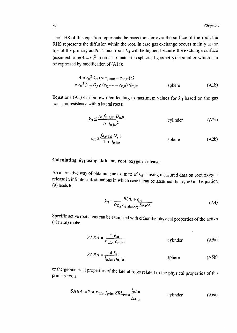
82 Chapter 4
The LHS of this equation represents the mass transfer over the surface of the root, the RHS represents the diffusion within the root. In case gas exchange occurs mainly at the tips of the primary and/or lateral roots krt will be higher, because the exchange surface
(assumed to be 4 7rrrt2 in order to match the spherical geometry) is smaller which can
be expressed by modification of (Ala):
4 n rn2 !cn (a cgMm - caq,rt) <
n rn2Jd,rt £>g,0 (cg,atm - cg,rt) UnM sphere (Alb)
Equations (Al) can be rewritten leading to maximum values for kn based on the gas transport resistance within lateral roots:
^ r r t / d , r t , l a t f l g , 0 c y i . n d e r ( A 2 a )
a htMt
. ^/d,rt,lat £>g,0 r t d rv / . . sphere (A2b) 4a I rtjat
Calculating krt using data on root oxygen release
An alternative way of obtaining an estimate of *rt is using measured data on root oxygen release in infinite sink situations in which case it can be assumed that crt=0 and equation (9)leads to:
. ROL + qn a02
cg,atm,02 SARA ^ ;
Specific active root areas can be estimated with either the physical properties of the active (=lateral) roots:
SARA =—^kt ,- , ,A~, ^,atPrt,lat ^ ^ ( A 5 a )
SARA = — A / k _ /rt,lat Prt,lat S P h e r e < A 5 b )
or the geometrical properties of the lateral roots related to the physical properties of the primary roots: ^ ^
SARA = 2 71 rrt i,. f ?I?T rt,lat rrt,iat/pnm A/Oprim cylinder (A6a)
Axiat
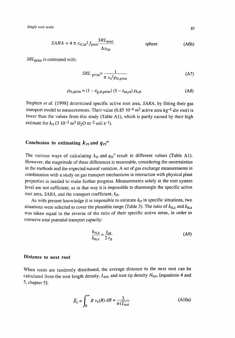
Single root scale ^
SARA = 4 n r r t , l a t2/p r i m^PliE s p h e r e ( A 6 b )
Axiat
SRLpr{m is estimated with:
SRL Prim= ~ (A7) TC rrtPrt,prim
Prt,prim - (1 - eg,rt,prim) (1 - eaq,rt) Ps,rt (A8)
Stephen et al. [1998] determined specific active root area, SARA, by fitting their gas transport model to measurements. Their value (0.85 10-4 m2 active area kg-1 dw root) is lower than the values from this study (Table Al), which is partly caused by their high estimate for kTt (3 10"3 m3 H2O n r 2 soil s"1).
Conclusion in estimating krt and #rt"
The various ways of calculating kTt and qx" result in different values (Table Al). However, the magnitude of these differences is reasonable, considering the uncertainties in the methods and the expected natural variation. A set of gas exchange measurements in combination with a study on gas transport mechanisms in interaction with physical plant properties is needed to make further progress. Measurements solely at the root system level are not sufficient, as in that way it is impossible to disentangle the specific active root area, SARA, and the transport coefficient, kTt.
As with present knowledge it is impossible to estimate &rt in specific situations, two situations were selected to cover the plausible range (Table 3). The ratio of /rrt,c and fcrttS
was taken equal to the inverse of the ratio of their specific active areas, in order to conserve total potential transport capacity:
*rt,s _ l\ at
>rttc ^ ' r t 2/V (A9)
Distance to next root
When roots are randomly distributed, the average distance to the next root can be calculated from the root length density, LioU and root tip density Nioh [equations 4 and 5, chapter 5]:

84 Chapter 4
Table Al. Parameters and variables for the estimates of the root surface mass transfer coefficient, £rt
and root surface oxygen consumption, qx{\ Between brackets is the considered range. Lowercase letters
refer to the foodnotes, uppercase letters combined with figures refer to the equations in the appendix.
Subscripts c and s in root properties refer to the cylindrical and spherical geometry respectively.
root property
%o /d,rt rrt,lat rrt,prim £aq,rt £g,rt,lat eg,rt,prim
Ps.rt
'rt,lat A*lat
A&t /prim
^ ^ p r i m SARAC
SARAS
SARAC
SARAS
SARASt bog bean
"^several plants
Qn, sedges
H rt,c,sedges 11
H rt,s,sedges
*rt,c
*rt,s
*rt,c
*rt,s
*rt>s
value
2.0 10"5
£g,rt 0.1 (0.05-0.1)
1.0(0.3- 1)
0.9 (0.85 - 0.95)
0.014(0.01 -0.03)
0.3 (0.02 - 0.45)
1000
40(10- 100)
2 ( 0 . 5 - 5 )
0.67 (0.50 - 0.85)
0.22 (0.06 - 0.39)
4.5 (2 - 100W03
130(70-700)
0.7(0.1 -7)
12 (0.08 - 6000)
0.06(0.0008- 10)
0.9 -10"4
(0.07-56)-10-*
(4-7)»10-6
(0.006 -0.1)-10"6
(0.6-70)-10"6
<2(0.1 - 3 0 H 0 ~ 6
<200(IO-3000)*10"6
(0.02 - 3) • 10"6
(2. - 2000) • 10-6
3 10"3
unit
m 2 gas s"1
m gas m"1 root
mm root
mm root
m3 H2O m~3 non aerenchymatus root
m3 gas m~3 root
m3 gas m~3 root
kg dw solid root m - 3 solid root
mm root
mm root
kg dw lateral root kg"1 dw total root
kg dw primary root kg"1 dw total root
m kg"1 dw primary root
m2 active area kg - 1 dw total root
m2 active area kg"1 dw total root
m2 active area kg"1 dw total root
m2 active area kg"1 dw total root
m2 active area kg"1 dw total root
mol kg"1 dw (total root?) s"1
mol kg"1 dw total root s"1
mol m2 active area s"1
mol m^ active area s"1
m3 H2O m~2 soil s"1
m3 H2O m"2 soil s"1
m3 H2O n r 2 soil s"1
m3 H 2 0 m"2 soil s"1
m3 H 2 0 m"2 soil s"1
source
a
b
c,d
c,d
g
c,e
c,f
g
c,d,h
c,d,h
i i
A7
A5a
A5b
A6a,A7,A8
A6b,A7,A8
J k
1
m
m
A2a
A2b
A4,A5a
A4,A5b n
a02 in N2 at 15 °C [Hirschfelder et al, 1964; Leffelaar, 1987]. Armstrong [1979]. cArmstrong et at. [1996]. dMetsavainio [1931]. erange estimated. fCrawford [1983]. Sguessed. "Conlin and Crowder [1988]. 'Wallen [1986], Sjors [1991] and Saarinen [1996]. JStephen et al. [1998]. kSorrell and Armstrong [1994] assuming that the authors made a factor 10 mistake in their Table 1, Kludze and Delaune [1996], Kludze et al. [1994] and Jespersen et al. [1998]. 'van der Werf et al. [1988] and Bouma et al. [1996]. ^Calculated from qri and SARA (A5). "Assumption of Stephen et al. [1998], at depth 0.1 m.
R< JO
Rvs(R)dR=33 V ~ . 0 . ? 4
V n Mot Vtf
These root density parameters are estimated with:
(AlOb) tot
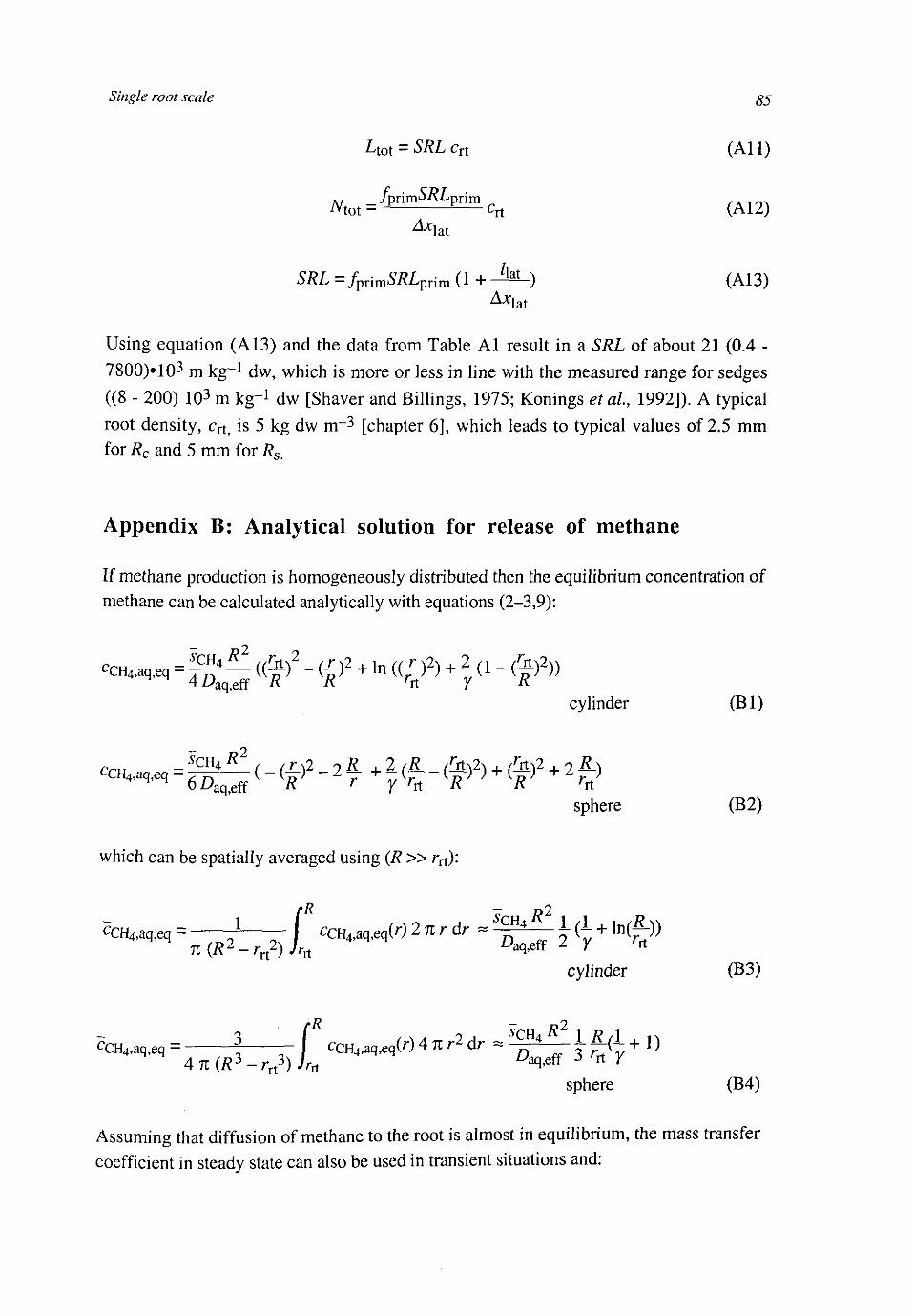
Single root scale 55
Lm = SRLcn (All)
A'tot = ~ ~ cn (A12)
SRL =fPrimSRLprim (1 + -4sL) (A13) A*Iat
Using equation (A13) and the data from Table Al result in a SRL of about 21 (0.4 -7800)* 103 m kg-1 dw, which is more or less in line with the measured range for sedges ((8 - 200) 103 m kg-1 dw [Shaver and Billings, 1975; Konings et al, 1992]). A typical root density, crt, is 5 kg dw irr3 [chapter 6], which leads to typical values of 2.5 mm for Rc and 5 mm for Rs.
Appendix B: Analytical solution for release of methane
If methane production is homogeneously distributed then the equilibrium concentration of methane can be calculated analytically with equations (2-3,9):
c c " « - = f t S <(«)2 - («)2 +'" "&> +r ( 1" («'2))
cylinder (Bl)
sphere (B2)
which can be spatially averaged using (R » rrt):
taum = } . I -CH4,aq,eq(r) 2 u r dr - ^ ^ 1 ( I + ln<£)) 7l(i?2-rrt
2);/-rt ^q,eff * Y rt cylinder (B3)
'CH4,aq,eq = f — J CCH4,aq,eqW 4 * r* dr ~ *gk^L W + 1) 4Tc(/?3-rrt
3)Art ^ V f f J rt ' sphere (B4)
Assuming that diffusion of methane to the root is almost in equilibrium, the mass transfer coefficient in steady state can also be used in transient situations and:

86 Chapter 4
qcn4 = - ^ - (f)2 l—— (cCH4,aq - a cCH4,g,atm) cylinder (B4) rrt R 1 + 7 In (£-)
4CH4 = - ^ f " (^) 3 J ^ ( CH4,aq - « CH4,g,atm) sphere (B5)
This can be rewritten into equations (60 - 61). The calculated first order constant for methane release in the cylindrical case differs slightly with the constant for a solute uptake in the limited single root system of [Baldwin et ah, 1973]: in the logarithm of their expression a factor 1.65 is present. This is caused by a different steady state profile: In contrast with this paper, Baldwin et <a/., [1973] use a single root system with a zero source/sink and an influx at the boundary, R.

87
Chapter 5
Modelling methane fluxes in wetlands with gas transporting plants: 2. soil layer scale
Segers, R. and Rappoldt, C.
Abstract
Methane dynamics in a water saturated soil layer with gas transporting roots is modelled with a weighted set of single root model systems. Each model system consists of a soil cylinder with a gas transporting root along its axis or a soil sphere with a gas transporting root at its centre. The weights associated with different cylinder or sphere radius were deduced from root architecture. Methane dynamics in each single root model system are calculated using a single root model from the previous paper. From this full model a simplified model was deduced consisting of an oxygen saturated and an oxygen unsaturated model system. An even more simplified model was deduced, called the kinetic model. In this model the concentrations are homogeneous in the whole soil layer. Simulation results of the simplified model are closer to the simulation results of the full model than the simulation results of the kinetic model. The overall effect of the simplifications on simulated methane emissions are small, though the underlying processes are affected more severely, depending on simulation time and parameters. At high root densities and at large times, under stationary conditions, root density is proportional to simulated methane fluxes, provided that carbon availability is proportional to root density. Sensitivity analysis shows that lack of knowledge on root gas transport is an important limitation for the predictability of methane fluxes via the processes at the kinetic level.
Introduction
Wetland soils with gas transporting plants are an important source of methane [Prather et al., 1995; Nykanen et al., 1998; Bellisario et al, 1999]. Variation in methane fluxes from these systems is large and difficult to understand due to the dynamic, non-linear interactions between underlying processes [Conrad, 1993; Wang, 1996; Segers, 1998]. This paper is the second in a series of three, which aims to unravel these interactions by explicitly relating knowledge at the kinetic level to methane fluxes at the plot level.
In the preceding paper [chapter 4] the interactions between the kinetic and diffusion processes around a single gas transporting root were investigated by developing, simplifying and testing a reaction-diffusion model. In this paper this model is scaled up from a single root to a soil layer. In the next paper [chapter 6] the step is made to a model for methane fluxes at the plot scale, allowing vertical gradients and temporarily water unsaturation. At the (discretised) soil layer scale, studied in this paper, it is assumed that root density, water content and temperature are constant. Furthermore, in this paper only
Segers, R. Wetland Methane Fluxes: Upscaling from Kinetics via a Single Root and a Soil Layer to the Plot, Ph. D. Thesis, Wageningen University, 1999.

0 0 Chapter 5
water saturated soil is considered in which gas exchange with the atmosphere occurs via the plant roots and ebullition. Hence, focus is on the role of a system of gas transporting roots in methane dynamics.
Model description
A single root model system
Starting point of the analysis is a single root model system [chapter 4]. The soil is represented by a hollow infinite cylinder or a hollow sphere. The inner surface represents the root surface via which gas exchange with the atmosphere is possible. The outer surface, at distance R from the centre, is half the distance to the next root at which fluxes are zero. Within this system methane, oxygen, carbon dioxide, molecular nitrogen and an arbitrary alternative terminal electron acceptor in reduced and oxidised form react and diffuse. These processes cause the oxygen concentration to decrease with distance to the root. Near the root aerobic processes occur: aerobic respiration, methane oxidation and electron acceptor re-oxidation. Far from the root anaerobic processes occur: methane production and electron acceptor reduction. The system as a whole imports oxygen and exports methane via the root. Both a cylindrical and a spherical geometry are studied. The cylindrical geometry represents a situation where the whole root is active, while the cylindrical geometry represents a situation where only the root tip is active. In the previous paper [chapter 4] reaction-diffusion equations for the six compounds were numerically solved to study the behaviour of this system. Using insight in the order of magnitude of parameters this full single root model was simplified by a quasi steady state assumption for oxygen and by spatially averaging the equations for the other compounds. The resulting simplified single root model produced almost the same results as the full model and is therefore used in this paper. The derivation of this simplified model in [chapter 4] is rather long. Therefore, a shorter description of this simplified model is added (Appendix A) to make this paper easier to read.
A soil layer with a root system: a weighted set of single root systems with different radii.
The interaction between diffusion and reactions is mainly determined by surface-area-to volume-ratios and not by the exact geometry [Bird et al., I960]. The surface-area-to volume-ratio is closely related to the distance of a point in soil to the gas exchanging surface. Using this insight Rappoldt [1990,1992] developed an algorithm to represent the geometry of a complex medium by a weighed set of simple geometric forms. The basic idea is that the probability density distribution, PDF, of the distance to the nearest gas
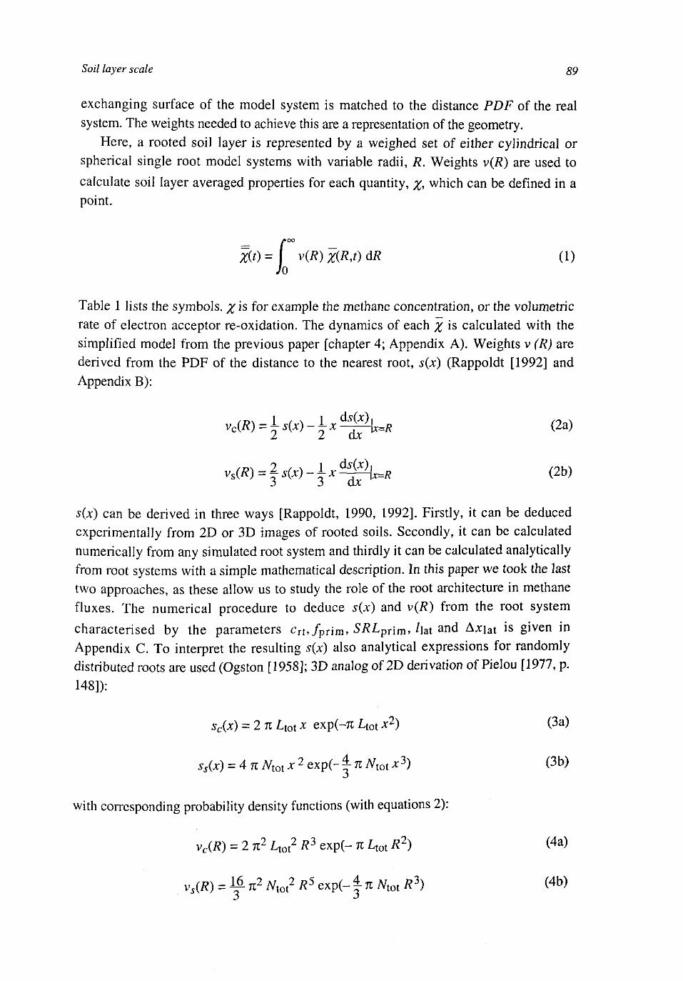
Soil layer scale gg
exchanging surface of the model system is matched to the distance PDF of the real system. The weights needed to achieve this are a representation of the geometry.
Here, a rooted soil layer is represented by a weighed set of either cylindrical or spherical single root model systems with variable radii, R. Weights v(R) are used to
calculate soil layer averaged properties for each quantity, %, which can be defined in a point.
-i X(t)=l v(R)x(R,t)dR (1) JO
Table 1 lists the symbols. % is for example the methane concentration, or the volumetric rate of electron acceptor re-oxidation. The dynamics of each % is calculated with the simplified model from the previous paper [chapter 4; Appendix A). Weights v (R) are derived from the PDF of the distance to the nearest root, s(x) (Rappoldt [1992] and Appendix B):
vc(/?) = W - ^ ^ U i ? (2a)
Vs(R) = js(x)-±x^\x=R (2b)
s(x) can be derived in three ways [Rappoldt, 1990, 1992]. Firstly, it can be deduced experimentally from 2D or 3D images of rooted soils. Secondly, it can be calculated numerically from any simulated root system and thirdly it can be calculated analytically from root systems with a simple mathematical description. In this paper we took the last two approaches, as these allow us to study the role of the root architecture in methane fluxes. The numerical procedure to deduce s(x) and v(R) from the root system characterised by the parameters crt,/Prim» SRLpT[m, /iat and Axjat is given in Appendix C. To interpret the resulting s(x) also analytical expressions for randomly distributed roots are used (Ogston [1958]; 3D analog of 2D derivation of Pielou [1977, p. 148]):
sc(x) = 2 n Ltot x exp(-7t Ltot x2) (3a)
ss(x) = 4nNt0[x2 exp(-1 n Nioix
3) (3b)
with corresponding probability density functions (with equations 2):
vc(R) = 2n2 Ltot2 R3 exp(- n Ltot R
2) (4a)
vs(R) = &K2 Ntot2 R5 exp(-171 Mot * 3 ) <4b>
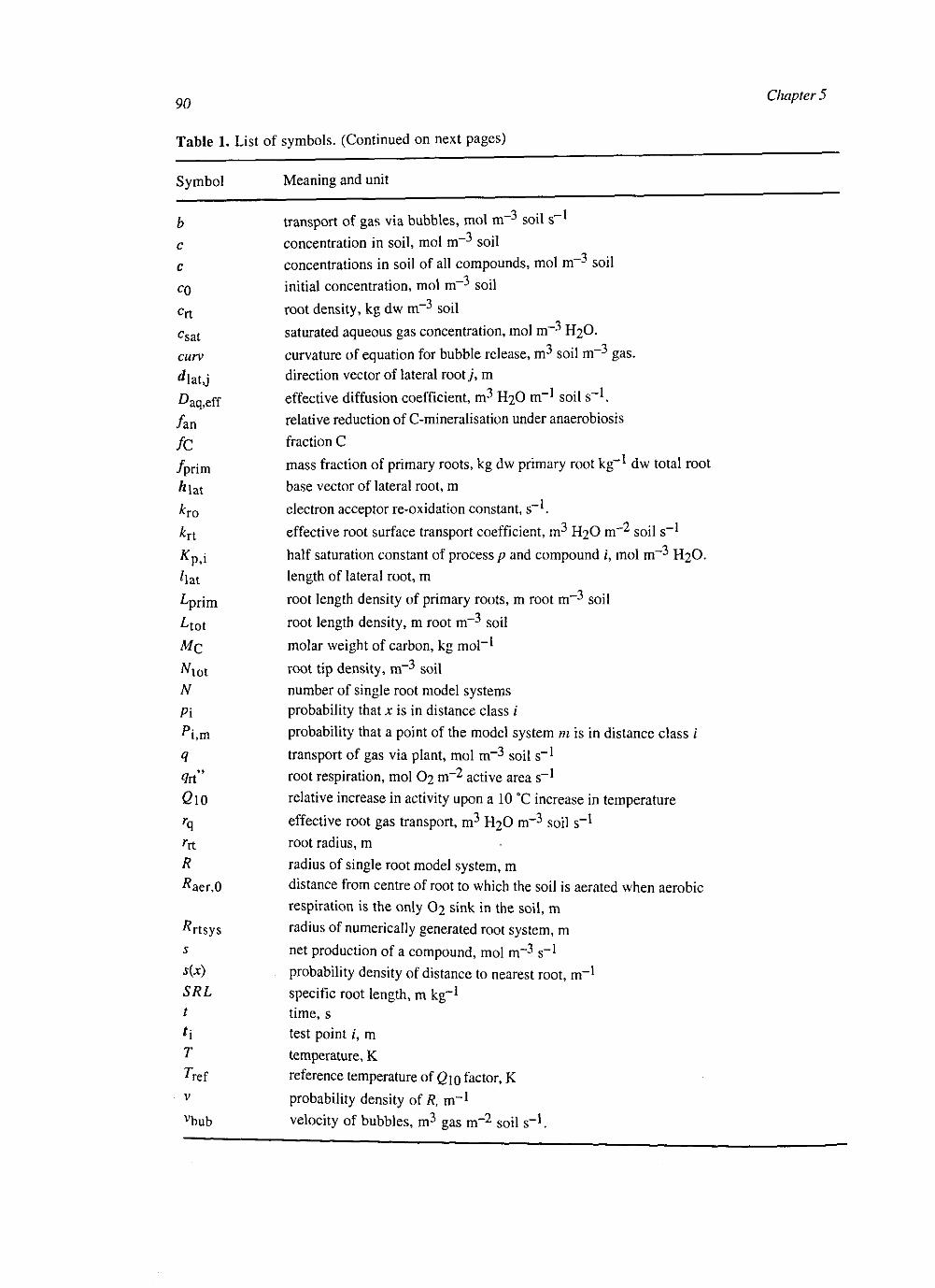
90 Chapter 5
Table 1. List of symbols. (Continued on next pages)
Symbol Meaning and unit
b
c
c
CQ
Crt
^sat curv rflatJ
£>aq,eff
/an
/c /prim
^lat
*ro
*rt ^p,i
'lat
^prim
^tot MC
"tot N
Pi
^i,m
q
<7r t "
do rq 'it
R
#aer,0
"rtsys
• * ( * )
SRL t
*\ T
?ref v vbub
transport of gas via bubbles, mol m~3 soil s - 1
concentration in soil, mol m~3 soil
concentrations in soil of all compounds, mol m~3 soil
initial concentration, mol m - 3 soil
root density, kg dw m~3 soil
saturated aqueous gas concentration, mol m~3 H2O.
curvature of equation for bubble release, m3 soil m~3 gas. direction vector of lateral root;', m
effective diffusion coefficient, m3 H2O m - 1 soil s_1.
relative reduction of C-mineralisation under anaerobiosis
fraction C
mass fraction of primary roots, kg dw primary root kg"1 dw total root
base vector of lateral root, m
electron acceptor re-oxidation constant, s .
effective root surface transport coefficient, m3 H2O m~2 soil s~*
half saturation constant of process p and compound 1, mol m~3 H2O.
length of lateral root, m
root length density of primary roots, m root m~3 soil
root length density, m root m ' 3 soil
molar weight of carbon, kg mol-*
root tip density, m~3 soil
number of single root model systems
probability that x is in distance class i
probability that a point of the model system m is in distance class i
transport of gas via plant, mol m~3 soil s - 1
root respiration, mol O2 m~2 active area s"1
relative increase in activity upon a 10 °C increase in temperature
effective root gas transport, m3 H2O rrr3 soil s"1
root radius, m
radius of single root model system, m
distance from centre of root to which the soil is aerated when aerobic
respiration is the only O2 sink in the soil, m
radius of numerically generated root system, m
net production of a compound, mol m~3 s_1
probability density of distance to nearest root, m"1
specific root length, m kg"1
time, s test point /, m
temperature, K
reference temperature of Q\Q factor, K
probability density of R, m~l
velocity of bubbles, m3 gas m"2 soil s - 1 .

Soil layer scale 91
Table 1. (Continued)
Symbol
Vm
wm
x
pa
i.J a P
A) r
4*lat
Az
£bub ecr £solid
? 7?aer
e K
v
rq
*rt
0)
Meaning and unit
maximum rate of process p and compound /, mol m~3 s~*.
weight of single root model system m
distance to nearest root, m vector between test point i and lateral rooty, m
solubility, m3 gas m~3 H2O.
dimensionless number, ratio of time constants of O2 sink in the soil and root O2
transport P when aerobic respiration is the only O2 sink in soil
dimensionless number, ratio of resistances for gas transport in root and transport just around a root distance between the bases of the lateral root on the primary roots, m
thickness of soil layer, m
gas filled pore space of bubbles, m3 gas m - 3 soil.
critical gas filled pore space for bubble release, m3 gas m~3 soil.
volumetric solid phase, m3 solid m"3 soil.
partitioning factor for anaerobic C-mineralisation. fraction of single root model systems, which is completely aerated
volumetric moisture content, m3 H2O m - 3 soil.
root O2 release relative to the O2 demand for aerobic respiration
distance between x y and /*iatj> m
stoichiometric constant, mol mol . time constant of transport via plant, s time constant of root turnover, s
arbitrary quantity O2 sink relative to O2 sink for aerobic respiration.
compounds eo er etot
electron acceptor reduced electron acceptor sum of oxidised and reduced electron acceptors
subscripts acm atm c
g i
J ae lat m mg mo mx prim
anaerobic C-minera!isation atmospheric cylindrical gas phase index of compound, index of distance class index of lateral root aerobic respiration lateral root index of single root model system methanogenesis. methanotrophic maximum primary root

Chapter 5 92 ^
Table 1. (Continued)
Symbol Meaning and unit
subscripts (continued) rem reference C-mineralisation id reduction of electron acceptors ro re-oxidation of electron acceptors
rt root s spherical
other symbols bold vector ~~ spatially averaged at the single root level
~~ spatially averaged at the soil layer level. * normalised with equilibrium CH4 production when O2 inflow is zero
# single root systems that are completely aerated X single root systems that are not completely aerated
Simplified soil layer model
In analogy to the single root level, a simplified model is formulated at the soil layer level by aggregating over the single root model systems, to arrive at state variables, concentrations c, at the soil layer level (Figure 1). Each concentration, c/, changes as a result of ebullition, b{, kinetics, 57, and plant mediated transport, #/.
^ = * i ( c ) + Ji(c) + (c) (5)
The dynamics of the simplified model are governed by the oxygen dynamics, a key factor. First, the distance to the root at which the soil is aerated is estimated from some dimensionless numbers consisting of ratios between kinetic and transport parameters [chapter 4, equations 44-48]:
#aer,o,c = V2 £0 (1-C) rrt (6a)
^aer,0,s = V 3 / 3 0 ( l - O r r t (6b)
where @Q is P with co= 1. Subsequently, the single root model systems are divided into two fractions: (i) oxygen saturated single root model systems with R < tfaer,0 with symbol "#" and fraction rjaer and (ii) oxygen unsaturated single root model systems with # > #aer,o, with symbol "f' and fraction (1 - r?aer)- Weight function v(R) is used to calculate rjaer:
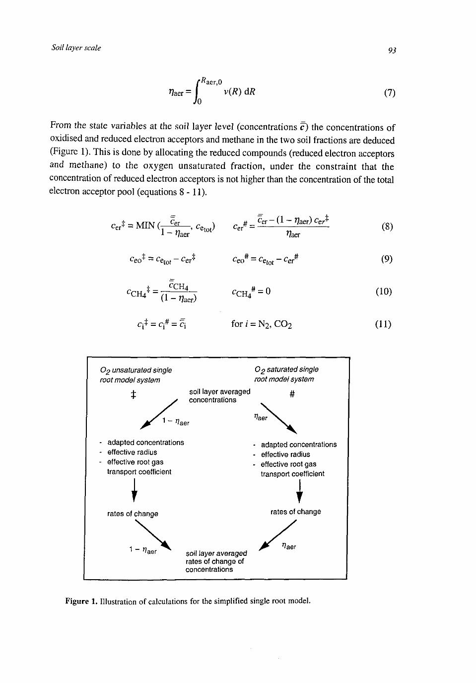
Soil layer scale 93
'^aer,0 f?aer = I v(R) dR -i (7)
From the state variables at the soil layer level (concentrations c) the concentrations of oxidised and reduced electron acceptors and methane in the two soil fractions are deduced (Figure 1). This is done by allocating the reduced compounds (reduced electron acceptors and methane) to the oxygen unsaturated fraction, under the constraint that the concentration of reduced electron acceptors is not higher than the concentration of the total electron acceptor pool (equations 8-11).
Cert = MIN(-fe-,cetot) cj = 1 ~ '/aer
Cer-(l-f?aer)Cer*
n aer (8)
cecr - Cetot"~ cer* # — # ceo — ce t ot - cer
(9)
CCH4
%= CCH4
(1 - %») ecu/ = 0 (10)
q* = q # = q for i = N2, C0 2 (11)
O2 unsaturated single root model system
1 - *
soil layer averaged concentrations
O2 saturated single root model system
#
aer
adapted concentrations effective radius effective root gas transport coefficient
\
adapted concentrations effective radius effective root gas transport coefficient
I rates of change rates of change
1-*? n aer soil layer averaged
rates of change of concentrations
aer
Figure 1. Illustration of calculations for the simplified single root model.
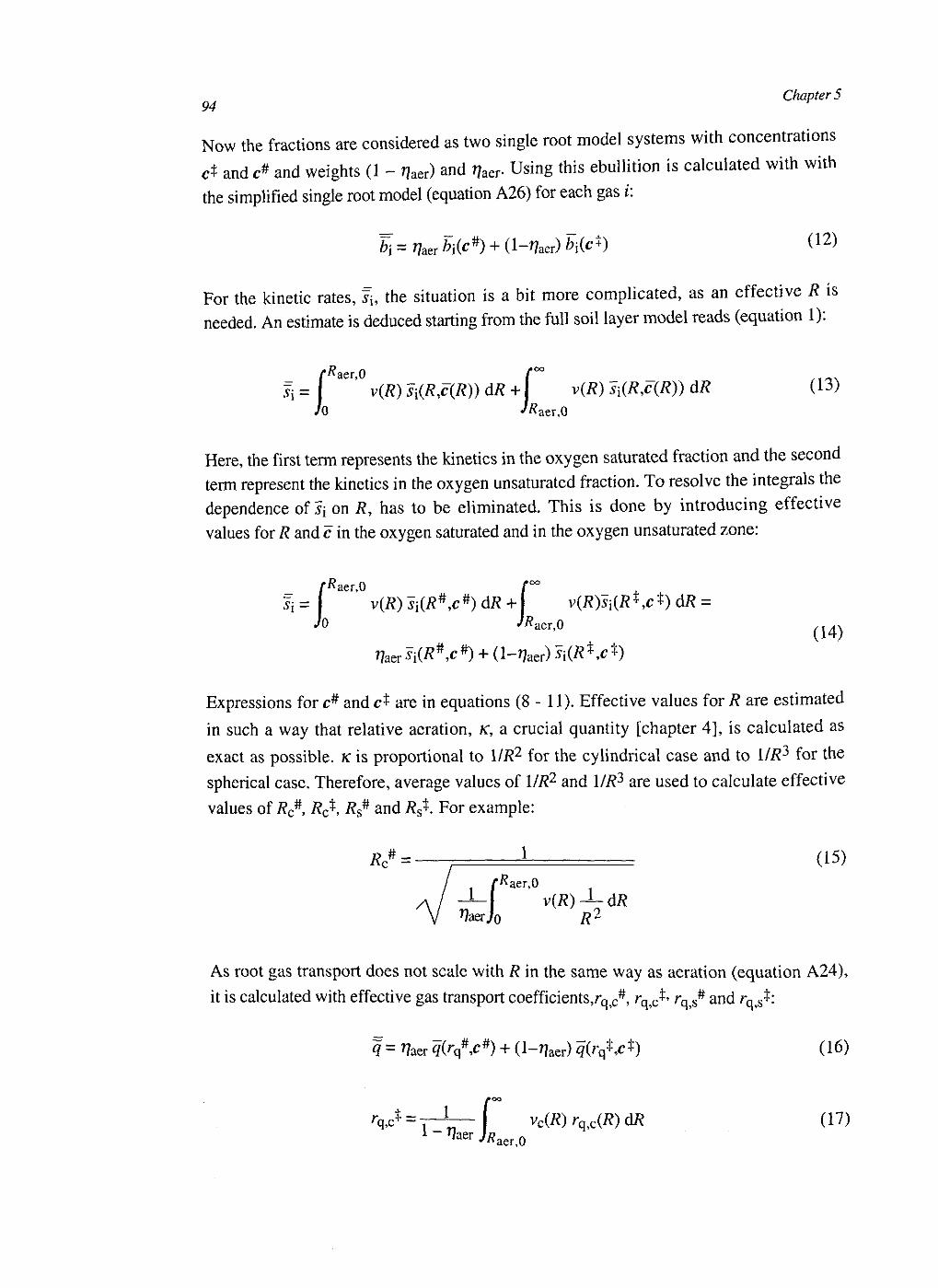
Chapter 5
Now the fractions are considered as two single root model systems with concentrations
c$ and c# and weights (1 - 7]aeT) and w Using this ebullition is calculated with with
the simplified single root model (equation A26) for each gas i:
¥i=r]aerbi(c#) + (l-t1aQr)bi(c$) (12)
For the kinetic rates, s{, the situation is a bit more complicated, as an effective R is needed. An estimate is deduced starting from the full soil layer model reads (equation 1):
s\ = I v(R) JiiR^R)) d* +1 v(R) s\(RAR)) d* (13> JO ^aer,0
Here, the first term represents the kinetics in the oxygen saturated fraction and the second term represent the kinetics in the oxygen unsaturated fraction. To resolve the integrals the dependence of Jj on R, has to be eliminated. This is done by introducing effective values for R and c in the oxygen saturated and in the oxygen unsaturated zone:
v(R) Si(R#,c#) dR + l v(R)s1(R^Jct) dR = JR^T n
l^aer,0
to ^aer.O (14)
Expressions for c# and c$ are in equations (8-11). Effective values for R are estimated
in such a way that relative aeration, K a crucial quantity [chapter 4], is calculated as
exact as possible, K is proportional to \IR2 for the cylindrical case and to \IR^ for the
spherical case. Therefore, average values of l/R2 and \IR? are used to calculate effective
values of Rc#, Rc$, R$# and Rs$. For example:
*c# = * (15) '#aei\0 , paer,0
- L v(R)±~dR 7/aery0 Rl
As root gas transport does not scale with R in the same way as aeration (equation A24),
it is calculated with effective gas transport coefficients,rqiC#, rq,c£* rq^ and rqfS$:
q= %er ?(>q* c # ) + (Maer) ^ q M ) (16)
rqJ = — 1 — J vc(R) %C(R) dR (17) 1 " ^aer JR Q
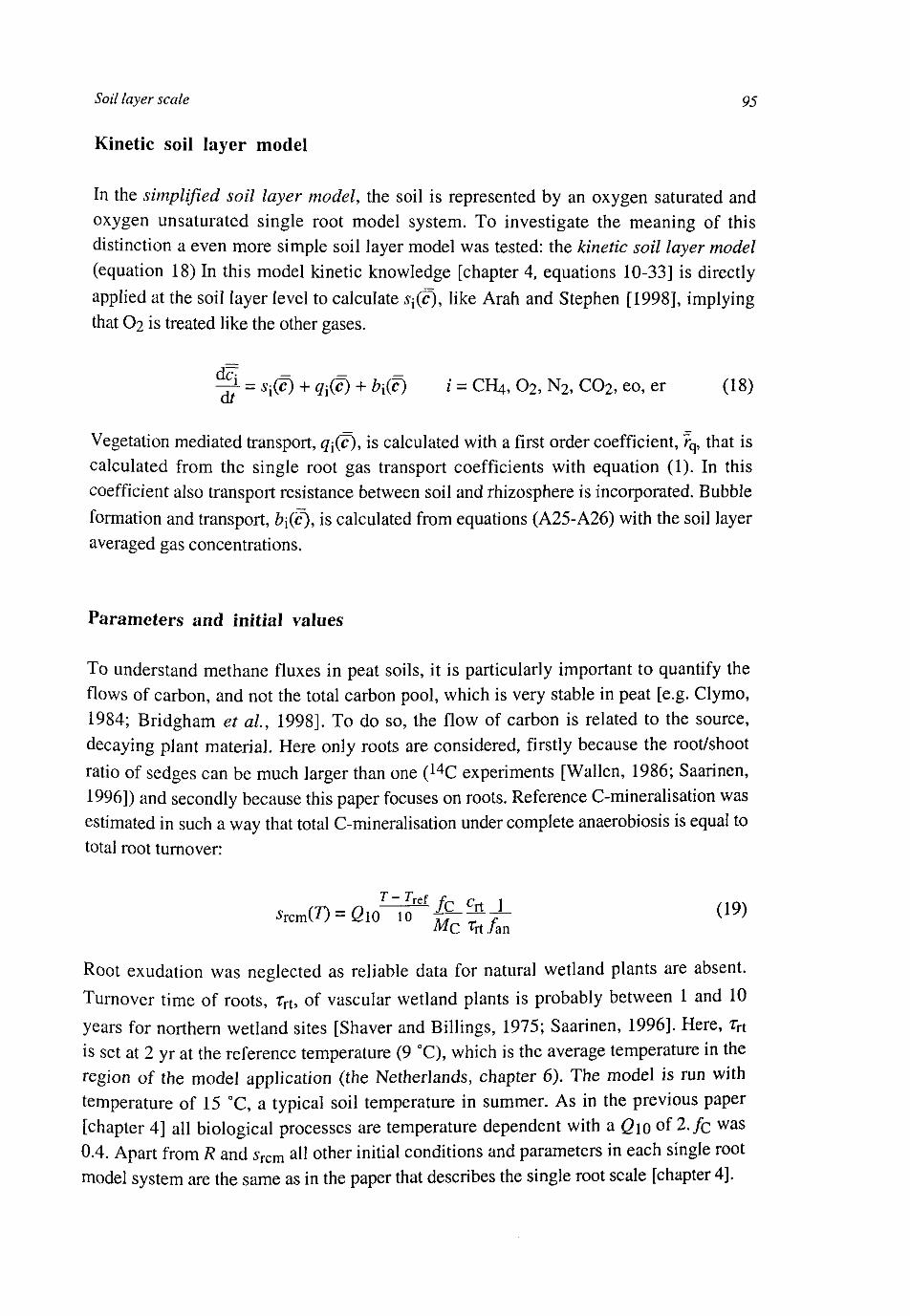
Soil layer scale 95
Kinetic soil layer model
In the simplified soil layer model, the soil is represented by an oxygen saturated and oxygen unsaturated single root model system. To investigate the meaning of this distinction a even more simple soil layer model was tested: the kinetic soil layer model (equation 18) In this model kinetic knowledge [chapter 4, equations 10-33] is directly applied at the soil layer level to calculate s0), like Arah and Stephen [1998], implying that O2 is treated like the other gases.
^ = s-0) + qx{c) + b{(c) i = CH4, O2, N2, C02 , eo, er (18)
Vegetation mediated transport, q\(c), is calculated with a first order coefficient, rq, that is calculated from the single root gas transport coefficients with equation (1). In this coefficient also transport resistance between soil and rhizosphere is incorporated. Bubble formation and transport, b{(c), is calculated from equations (A25-A26) with the soil layer averaged gas concentrations.
Parameters and initial values
To understand methane fluxes in peat soils, it is particularly important to quantify the flows of carbon, and not the total carbon pool, which is very stable in peat [e.g. Clymo, 1984; Bridgham et a/., 1998]. To do so, the flow of carbon is related to the source, decaying plant material. Here only roots are considered, firstly because the root/shoot ratio of sedges can be much larger than one (14C experiments [Wallen, 1986; Saarinen, 1996]) and secondly because this paper focuses on roots. Reference C-mineralisation was estimated in such a way that total C-mineralisation under complete anaerobiosis is equal to total root turnover:
srcmm = Qio^£rcfr- (19)
Root exudation was neglected as reliable data for natural wetland plants are absent. Turnover time of roots, rrt, of vascular wetland plants is probably between 1 and 10 years for northern wetland sites [Shaver and Billings, 1975; Saarinen, 1996]. Here, rrt
is set at 2 yr at the reference temperature (9 °C), which is the average temperature in the region of the model application (the Netherlands, chapter 6). The model is run with temperature of 15 °C, a typical soil temperature in summer. As in the previous paper [chapter 4] all biological processes are temperature dependent with a Qlu of 2./c w a s
0.4. Apart from R and srcm all other initial conditions and parameters in each single root model system are the same as in the paper that describes the single root scale [chapter 4].
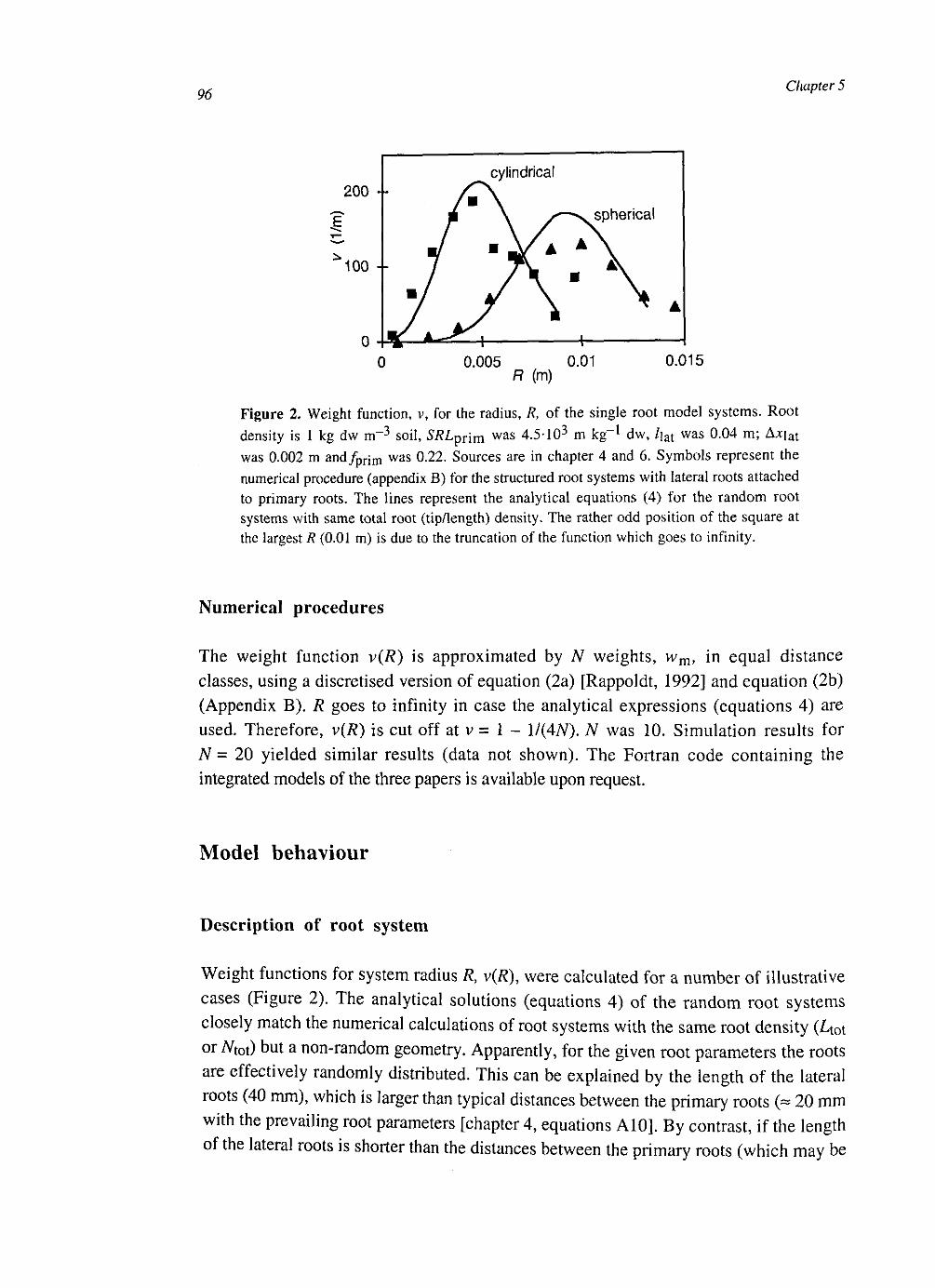
96 Chapter 5
200 •
100 -
0 •
• /
y A~-
cylindrical
/ • \ I \ y—N. spherical
7\- A. / \ " \
/ \ ^ A
z—\ 1 0 0.005
R (m) 0.01 0.015
Figure 2. Weight function, v, for the radius, R, of the single root model systems. Root density is 1 kg dw m~3 soil, SRLpT\m was 4.5-103 m kg -1 dw, l\at was 0.04 m; A*iat was 0.002 m and/prjm was 0.22. Sources are in chapter 4 and 6. Symbols represent the numerical procedure (appendix B) for the structured root systems with lateral roots attached to primary roots. The lines represent the analytical equations (4) for the random root systems with same total root (tip/length) density. The rather odd position of the square at the largest R (0.01 m) is due to the truncation of the function which goes to infinity.
Numerical procedures
The weight function v(R) is approximated by N weights, vvm, in equal distance classes, using a discretised version of equation (2a) [Rappoldt, 1992] and equation (2b) (Appendix B). R goes to infinity in case the analytical expressions (equations 4) are used. Therefore, v(R) is cut off at v = 1 - 1/(4A0- N was 10. Simulation results for N = 20 yielded similar results (data not shown). The Fortran code containing the integrated models of the three papers is available upon request.
Model behaviour
Description of root system
Weight functions for system radius R, v(R), were calculated for a number of illustrative cases (Figure 2). The analytical solutions (equations 4) of the random root systems closely match the numerical calculations of root systems with the same root density (Ltot or A tot) but a non-random geometry. Apparently, for the given root parameters the roots are effectively randomly distributed. This can be explained by the length of the lateral roots (40 mm), which is larger than typical distances between the primary roots (= 20 mm with the prevailing root parameters [chapter 4, equations A10]. By contrast, if the length of the lateral roots is shorter than the distances between the primary roots (which may be

Soil layer scale 97
the case in reed, for example) than the root system is clustered and the distance probability density distribution gets wider than the distribution of the randomly distributed roots (data not shown). As in our case the difference between the two methods for estimating v(R) is small, we used the fastest and simplest method, the analytical expression, in the remainder of the paper.
Full, simplified and kinetic model at the soil layer level
The complete soil layer model with TV weighted single root model systems is called the full soil layer model (equation 1). In the simplified soil layer model (equations 5-17), the rates are calculated in two single root model systems: an oxygen unsaturated single root model system and an oxygen saturated single root model system. To investigate the meaning of the single root details of these models also an even more simple soil layer model was tested: the kinetic soil layer model. In this model kinetic knowledge is directly applied at the soil layer level.
Simulations of relative aeration, /c, are little affected by the assumptions in the simplified soil layer model, but the kinetic soil layer model results in a higher aeration than the two other models (Figure 3a) due to the absence of the influence of oxygen saturated single root model systems. This means that in the full and the simplified model
0 0.1 0.2 full
Figure 3a-3e. Comparison of simplified (open squares) and kinetic (plusses) model with full model after 30 days for 32 different parameter sets. Parameter values are in chapter 4 and in the subsection on parameterisation. (a) O2 supply/ O2 demand, K, b) net normalised
—* — methane production, $CH4» (c) time coefficient for methane release via plant fqciU' (<0
=* normalised methane released via ebullition, bcwA and (e) total normalised methane release, =* ^*
CH4 + <7CH4- Methane production and methane release are normalised with / a n vm g
•Srcm* the maximum (equilibrium) methane production if no oxygen enters the system. The dashed line is the 1 to 1 line.
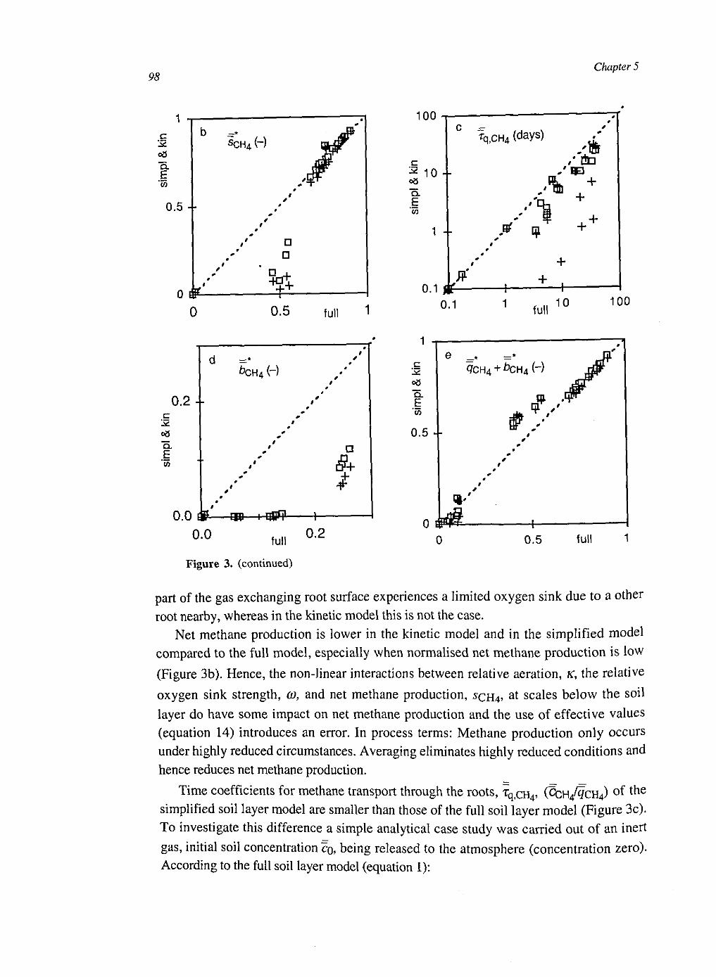
98 Chapter 5
c
"5. E
0.5 --
o m-o
SCH4 H
• D
D
0.5 full
100
^ 10 +
E
rq,cH4 (days) .-/ f t
/ dm %h +
' +
0.1 # 0.1
tf
rf * + +
+
full 10 100
full
Figure 3. (continued)
c
Q.
E CO
0.5 •-
QCH4 + bCH^(')
o ^ £ 0 0.5 full
part of the gas exchanging root surface experiences a limited oxygen sink due to a other root nearby, whereas in the kinetic model this is not the case.
Net methane production is lower in the kinetic model and in the simplified model compared to the full model, especially when normalised net methane production is low (Figure 3b). Hence, the non-linear interactions between relative aeration, K, the relative oxygen sink strength, co, and net methane production, scH4> a t s c a l e s below the soil layer do have some impact on net methane production and the use of effective values (equation 14) introduces an error. In process terms: Methane production only occurs under highly reduced circumstances. Averaging eliminates highly reduced conditions and hence reduces net methane production.
Time coefficients for methane transport through the roots, Tq,cH4> (^H 4 /^CH 4) of the simplified soil layer model are smaller than those of the full soil layer model (Figure 3c). To investigate this difference a simple analytical case study was carried out of an inert gas, initial soil concentration co, being released to the atmosphere (concentration zero). According to the full soil layer model (equation 1):
Soil layer scale 99
c(t) = co [ v(R) exp(- -j-) dR (20) Jo W
where r^ is the time coefficient of a single root model system (increasing with R, equations A24). From equation (20) it is clear that the contribution to the total concentration of the single root model systems with the largest radius increases in time. These single root model systems could be seen as dead zones that exchange gases slowly with atmosphere. By introducing an averaging procedure, these dead zones are artificially mixed with the remainder of the system, enhancing total transport and preventing the overall time coefficient, ?q, to increase in time. Therefore, plant mediated transport is faster in the simplified models compared to the full model.
So, a fundamental problem with methane release from the soil on the root system scale is that one needs to know the spatial micro distribution of methane, which depends on the history and which cannot be estimated from the actual average concentrations only. Consequently, gas transport experiments with plants in a mixed culture solution [Nouchi, 1994, Hosono and Nouchi, 1997; Butterbach-Bahl et al, 1997] cannot be directly extrapolated to the soil and the first order models [Nouchi et al, 1994; Hosono and Nouchi, 1997; Stephen et a/., 1998; Walter et al. 1996] have to be interpreted with care.
Similar to methane plant transport, averaging reduces rates of bubbles release (Figure 3d), firstly due to the non-linear relation between bubble volume and bubble release (equation A26) and secondly due to the lower methane concentrations as a result of the higher plant mediated transport. As the errors introduced by the assumptions on net methane production and methane transport partly cancel, the difference in simulated normalised methane flux by the full and the simplified model is surprisingly small (Figure 3e).
In the analysis above (Figures 3) variables were analysed after 30 days, under constant driving variables. However, differences between the three models depend on simulation time (Figure 4). In situ driving variables, like temperature and aeration (water table) will fluctuate on all kinds of time scales. Consequently, it is difficult to judge how large the difference between the kinetic, simplified and full model will be when incorporated in a model for fluxes at the plot scale. Therefore, in the next paper [chapter 6], which will address this scale, all three models will be used. In the remaining part of this paper only the full soil layer model is used.
Cylindrical and spherical geometry
Two models for root and rhizosphere geometry were used: a cylindrical and spherical. The cylindrical model represents a situation where the whole root surface exchanges gases. The spherical model reflects the situation where only root tips are active. To compare both models, k« and qj' are taken in such a way that total root activity per
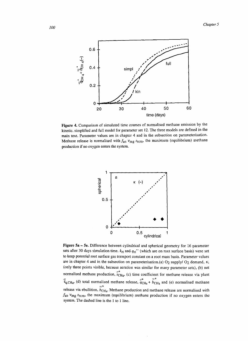
100 Chapter 5
20 30 40 50 time (days)
Figure 4. Comparison of simulated time courses of normalised methane emission by the kinetic, simplified and full model for parameter set 12. The three models are defined in the main text. Parameter values are in chapter 4 and in the subsection on parameterisation. Methane release is normalised with/ a n v m g $ r c m , the maximum (equilibrium) methane production if no oxygen enters the system.
CO
a> x: Q . C/3
0.5 --
0 0.5 1 cylindrical
Figure 5a - 5e. Difference between cylindrical and spherical geometry for 16 parameter sets after 30 days simulation time. kn and qx{" (which are on root surface basis) were set to keep potential root surface gas transport constant on a root mass basis. Parameter values are in chapter 4 and in the subsection on parameterisation.(a) O2 supply/ O2 demand, K,
(only three points visible, because aeration was similar for many parameter sets), (b) net - *
normalised methane production, SQH4, (C) time coefficient for methane release via plant — _=r* = * Tq,CH4» (d) t o t a* normalised methane release, #CH4 + ^CH4 a n d (e) normalised methane
= *
release via ebullition, £cH4- Methane production and methane release are normalised with /an vmg rcm* the maximum (equilibrium) methane production if no oxygen enters the system. The dashed line is the 1 to 1 line.
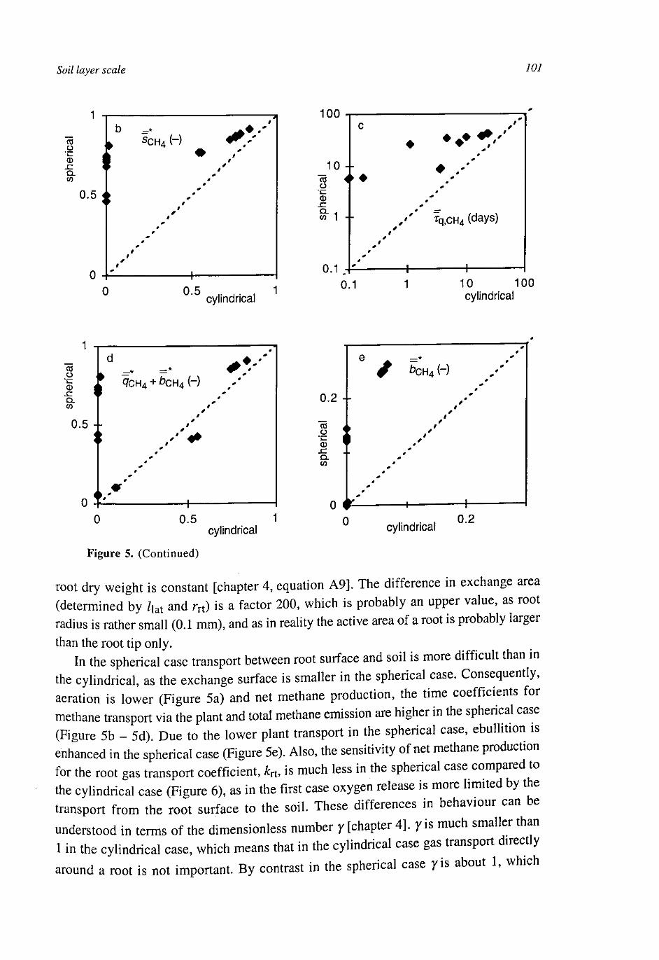
Soil layer scale 101
0 cylindrical
100
10 + 8 * • CD
f 1 4-
0.1 0.1
• • •• r<
, ' ' 7q,CH4 (days)
10 100 cylindrical
0 0.5 1 cylindrical
Figure 5. (Continued)
cylindrical
root dry weight is constant [chapter 4, equation A9]. The difference in exchange area (determined by Ziat and rrt) is a factor 200, which is probably an upper value, as root radius is rather small (0.1 mm), and as in reality the active area of a root is probably larger
than the root tip only. In the spherical case transport between root surface and soil is more difficult than in
the cylindrical, as the exchange surface is smaller in the spherical case. Consequently, aeration is lower (Figure 5a) and net methane production, the time coefficients for methane transport via the plant and total methane emission are higher in the spherical case (Figure 5b - 5d). Due to the lower plant transport in the spherical case, ebullition is enhanced in the spherical case (Figure 5e). Also, the sensitivity of net methane production for the root gas transport coefficient, kn, is much less in the spherical case compared to the cylindrical case (Figure 6), as in the first case oxygen release is more limited by the transport from the root surface to the soil. These differences in behaviour can be understood in terms of the dimensionless number y [chapter 4]. y is much smaller than 1 in the cylindrical case, which means that in the cylindrical case gas transport directly around a root is not important. By contrast in the spherical case / i s about 1, which

102 Chapter 5
means that gas transport around a root is approximately as important as gas transport
within a root.
Model Applications
Relation of methane flux with root gas transport coefficient
The root surface gas transport coefficient, kn> has been varied over two orders of magnitude within the plausible range as estimated in chapter 4. Net methane production was very sensitive for &rt, especially in the cylindrical case (Figure 6). The extreme range in relative net methane production is not unrealistic as redox values in water saturated soils with gas transporting plants may vary between -200 and +300 [Holzapfel-Pschorn et a/., 1986; Chen and Barko, 1988; Grosse et a/., 1996b; Frenzel et a/., 1999].
Furthermore, it is interesting to note that kn may both be positively or negatively correlated with methane emissions. By contrast, Arah and Stephen [1998] found a consistently negative correlation between methane emissions and &rt, because they considered the steady state of the system, whereas we evaluated emissions after 30 days simulation time. In our simulations, net methane production, which is equal to net methane emission in steady state, was consistently negatively correlated with k^ (data not shown). In reality all kinds of times are relevant, especially when a fluctuating water table is present. So, it is hard to draw general conclusion about the sensitivity of methane emissions for kr{.
+
\3 0.5 -•
cylindrical
0 1.E-08
'*»5, :**
! s s s B . ;
spherical
1.E-06 1.E-04
kn (m3H20 m 2soil s 1)
—* Figure 6. Normalised methane release, ^CH4+ £CH4, as function of root gas transport coefficient, £rt> for 8 different parameter sets after 30 days of simulation. Parameter values are in chapter 4 and in the subsection on parameterisation. Methane release is normalised w i t n /an vmg sTcm> the maximum (equilibrium) methane production if no oxygen enters the system.
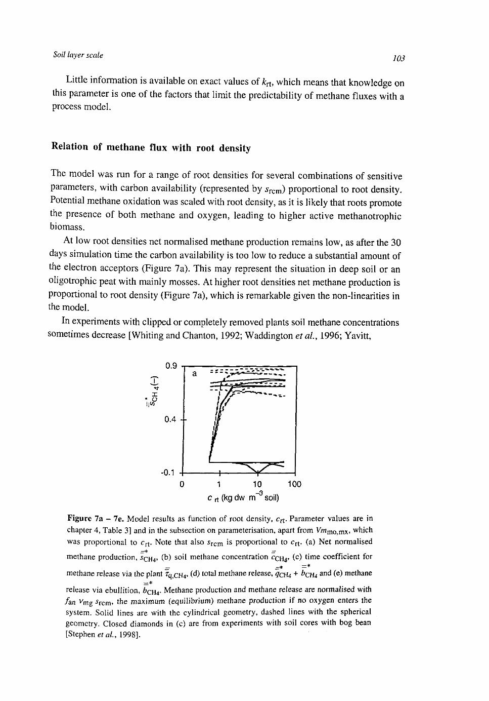
Soil layer scale 103
Little information is available on exact values of jfcrt, which means that knowledge on this parameter is one of the factors that limit the predictability of methane fluxes with a process model.
Relation of methane flux with root density
The model was run for a range of root densities for several combinations of sensitive parameters, with carbon availability (represented by sTcm) proportional to root density. Potential methane oxidation was scaled with root density, as it is likely that roots promote the presence of both methane and oxygen, leading to higher active methanotrophic biomass.
At low root densities net normalised methane production remains low, as after the 30 days simulation time the carbon availability is too low to reduce a substantial amount of the electron acceptors (Figure 7a). This may represent the situation in deep soil or an oligotrophic peat with mainly mosses. At higher root densities net methane production is proportional to root density (Figure 7a), which is remarkable given the non-linearities in the model.
In experiments with clipped or completely removed plants soil methane concentrations sometimes decrease [Whiting and Chanton, 1992; Waddington et al„ 1996; Yavitt,
0 1 10 100
c rt (kg dw m soil)
Figure 7a - 7e. Model results as function of root density, cTi- Parameter values are in chapter 4, Table 3] and in the subsection on parameterisation, apart from Vmm0)mx, which was proportional to crt. Note that also sTcm is proportional to crt. (a) Net normalised
- * -methane production, SQH4, (b) soil methane concentration CQH4, (C) time coefficient for
methane release via the plant Tq cH^ (d) t o t a l methane release, <7cH4 + CH4 ancl (e) methane =*
release via ebullition, fccH4- Methane production and methane release are normalised with /an vm g s r cm , the maximum (equilibrium) methane production if no oxygen enters the system. Solid lines are with the cylindrical geometry, dashed lines with the spherical geometry. Closed diamonds in (c) are from experiments with soil cores with bog bean [Stephen etai, 1998].

104 Chapter 5
100
100 -3
c rt (kg dw m soii) 100
- 3 crt (kg dw m soil)
0.2 -
T
0 -
e
• ••J 100
-3 c rt (kg dw m soil)
0.1 1 -3
100
o rt(kgdwm soil)
Figure 7. (continued)
1997] and sometimes increase [Yavitt, 1997; Verville et al, 1998; King et al, 1998]. These manipulations may be seen as an artificial decrease of root density. In the model, decreasing root density consistently decreases soil methane concentrations (Figure 7b). This discrepancy between model and experiment may be due to a difference in the dependence o carbon mineralisation on root density. In the model this dependence is assumed to be linear. However, in the experiments the dependence may be less than linear over th e c d e r e d ^ ^ ^ ^ ^ ^ . ^ . ^ ^ ^ ^ ^ ^
vegetation of the near past. Hence, information on soil carbon flows is needed to properly interpret vegetation removal experiments.
the IxhnpdePenfe,nre ? t h £ t i m C C ° n S t a m ° f r ° 0 t g a S t r a n s P° r t o n r o o t ^nsity is similar to
oot d e n ^ r 1 §S f ° r b ° g bea" (FigUrC ?C)- The Simulat i0ns >how that at higher onfinT T 6 e m i S S i ° n " P r 0 P 0 I t i 0 n a l t 0 r 0 0 t d e n s i * ( R g " - *»• which rimarvI!6 7 ™ ' * ^ f ° U n d " " ^ r e l a t i 0 n S b e t w e e " ™*™ A-xes and net
ZZZZn [ g et al-1991; Chanton et <1993] and bi—s ° f g — and sedges [Whit.ng et al, 1991; van den Pol - van Dasselaar, 1999b? The
Soil layer scale *05
disproportionate relation at lower root densities can be explained by (i) the effective time coefficient of plant gas transport being larger than the simulation time at low root densities (Figure 7c) and by (ii) the onset of ebullition at high root densities (Figure 7e) when methane concentrations are high enough.
Possible model extensions
The knowledge from the single root level is scaled up to the soil layer level by a probability density distribution for R. By contrast, other system parameters are assumed to be constant within a soil layer. However, it is likely that, apart from R, also kn and •Srcm vary within a soil layer, as parts of the roots will be more effectively connected to the atmosphere than other parts and as hot spots will be present in which carbon is preferentially available. It would be possible to assume probability density distributions for kn and srcm as well. However, this would make interpretation of results more complex without an increase in predictability on the field scale, as information on average or effective values of jfcrt and sTcm is scarce, let alone information on the variation in these parameters.
In the model and the sensitivity analysis it was assumed that most parameters are independent. Only wmo ,mx was scaled with crt. However, also other parameters are probably correlated to each other. If redox decreases, plants tend to increase their gas transport capacity by increasing root oxygen release to prevent damage by toxic compounds [Drew and Lynch, 1980; Kludze et al, 1993; Kludze and Delaune, 1996]. So, probably high q"n and cn are correlated to high values of kn. Principally, it would be possible to dynamically model such an adaptation mechanism by relating the rate of change of kn to, for example, the oxygen concentration at the root surface. But practically, this would be difficult as quantitative information on such relations is absent. A functional relation, assuming sufficient adaptation, is also not feasible, as the actual redox conditions in rooted water saturated soil may vary largely [Chen and Barko, 1988; Holzapfel-Pschorn et al, 1986; Grosse et al, 1996b]. So, quantitative research on plant mediated transport and its' regulating mechanisms [Jackson and Armstrong, 1999] is needed to be able to predict kn under various circumstances.
As a first approach it was assumed that the root system is static. Given the large time coefficient of root turnover this may seem realistic. However, in reality root growth and inactivation of root oxygen loss may occur in short time intervals (a month, [Hines, et aU 1989; Behaeghe, 1979]) in the season. Fast root dynamics may have two implications. Firstly, the probability density function of the model systems will be dynamic and, secondly, a kind of mixing will occur, as aerobic spots (new roots) will emerge at anaerobic spots and aerobic spots (decaying roots) will emerge in anaerobic spots. This mixing may be described with an exchange between the different single root model systems or an exchange between the shells of different single root model systems.

J06 Chapter 5
Concluding remarks
In this paper we scaled up from the single root scale to the soil layer scale. The simulation results demonstrate that methane emission may be limited by as several processes (oxygen transport via vegetation, root oxygen consumption, methane transport via vegetation, reduction of electron acceptors, soil carbon mineralisation). The relative importance of these processes depends on the conditions.For example, at high root densities, under continuous water saturation and at longer times, methane emission is proportional with carbon availability, and hence with net primary production.

Soil layer scale 107
Appendix A: Overview of simplified single root model
The simplified single root model was derived from the full single root model which is a coupled set of root reaction-diffusion equations for methane, oxygen, molecular nitrogen, carbon dioxide and electron acceptors in oxidised (eo) and reduced (er) form [chapter 4, equations 2-33]. The equations were simplified in two steps: 1. quasi-steady state assumption for oxygen, 2. spatially averaging the equations for the other state variables. The result of this procedure is a set of coupled ordinary differential equations for the mean concentrations, c:
^ = S C H 4 + ?CH4 + FC H 4 (AD
=^co2 + <7co2 + ^co2 ( A 2 ) d/
dcCo2 _-z
dc
^ = «N2 + H ( A 3 )
eo _
dc
=seo (A4)
dt er _ =*er ( A 5 )
Here, s are the spatially averaged kinetic rates, q is the spatially averaged gas transport via
the plant b is the spatially averaged gas transport via bubbles.
Net methane production is the result of methane production (mg) and methane oxidation (mo):
SCH4 =Smg,CH4 + Smo,CH4 (A6)
Electron acceptor cycling is the result of electron acceptor reduction (rd) and electron
acceptor re-oxidation (ro).
Se0 =%i,eo + ^ro,eo *•
%- =%j,er + *o,er ( A 8 )
And carbon dioxide production is the result of aerobic respiration (ae), methane oxidation, electron acceptor reduction and methane production:
^C02 =Sae,C02 + ^mo,C02 + ^rd,C02 + 5mg,C02
(A9)
IQg Chapters
Two groups of processes are distinguished: aerobic processes and anaerobic processes. To compare the different processes, all rates were normalised with carbon mineralisation under optimal aeration or with the oxygen demand for this process.
aerobic processes
The aerobic processes (aerobic respiration, methane oxidation and electron acceptor re-oxidation) are determined by the total oxygen consumption, SQ2, and the relative oxygen
sink strengths, co, of each process:
*ae,02 = ^ 0 2 (A10) CO
smo,o2 = ^so2 (All) co l
sro,o2 = ^so2 (A12) 0)
By definition, co is the oxygen sink relative to the oxygen sink for aerobic respiration:
ft)=ft^e + < mo + ^-o (A13)
ft>ae = 1 (A14)
Smo,lWV%o = £aq£H4 ( A l 5 )
Vae^rcm caq,CH4 + ^mo,CH4
Et0 = -mkmed«!* (A16)
The total oxygen consumption rate SQ2 i s calculated from steady state solution of the
reaction-diffusion equation for oxygen, assuming a zero order behaviour. The essential functional property of the procedure is that root oxygen release (equal to total oxygen consumption) depends on only two dimensionless numbers:
Q M a c g , a t m , 0 2 - ^ ) P = &L_ (A17)
vae 0) srcm rn
r ^ (M8) Aiq,eff
Soil layer scale 109
In both numbers kvt appears which is the root surface transport coefficient for gases, used as boundary condition at the root surface in the original reaction-diffusion equation:
f = Art (« Cg.atm (1 - , * « " ) - Caq,rt) (A19)
Here a cg)atm is the aqueous gas concentration in equilibrium with the atmosphere, [crt] is the gas concentration at the root surface and <?rt" is the oxygen consumption at the root surface. The aerobic rates of change in methane, carbon dioxide and electron acceptors are related to the oxygen consumption rates (equations A10-A12) via stoichiometric factors (relations not shown).
anaerobic processes
Both anaerobic processes (methane production and electron acceptor reduction) are determined by anaerobic C-mineralisation, Jacm.
^mg,CH4 = vmg Cmg ^acm ( A 2 0 >
%i,eo = " ^ rd (1 - Cmg) ^acm ( A 2 1 >
The partitioning factor for anaerobically mineralised carbon, £mg, depends on the kinetic constants and the concentration of electron acceptors. If ample electron acceptors are
present methane production is low and £mg approaches zero. When the electron acceptors
get depleted, £mg will rise until one. Anaerobic production of C0 2 and reduced electron acceptors depend on equations (A20-A21) via stoichiometric relations.
Anaerobic C-mineralisation could be related to the aerobic processes, for which
expressions are above:
- _/• «. t\ J°2 N (A22)
Here,/an is a factor which describes the slow down of C-mineralisation under anaerobic
conditions.
root gas transport of gases other than oxygen
Plant mediated transport of gases other than 0 2 was modelled with a first order relation:
n* • err •) ( A 2 3 >
jjfj Chapter 5
where cg,atm,i is the gas concentration in the atmosphere of gas i, The constants rqj are taken from the steady state solution of the reaction-diffusion equation with methane production constant in time and space.
r . = 2At At )2 1 (A24a)
' r t
. = 3fet / k ) 3 _ J _ (A24b) r W rrt V (l+M)
bubble transport
Ebullition is calculated in two steps. First the bubble volume, £t>ub> is calculated from the equilibrium equations between the gas and aqueous phase for all gases:
c\ 'sat,i
1 1 - fisolid - fibiib (1 —~ ' )
= 1 (A25)
Subsequently, bubble release was assumed to rise sharply after a critical bubble volume
£cr, using an expolinear equation:
bx = ^ub in(i+exp(cwrv (^u b - %))) c^{ (A26) Azcurv %
Appendix B: Weight functions for the spherical case
In analogy with the derivations of Rappoldt [1992, eq. 7.1] for a cylinder, the distribution of the distance to the gas exchanging surface in single sphere with radius R is equal to the surface to volume ratio:
*s (*,*)= Anx2 = £ 0<X<R 4/3 nR3 R3
(Bl) ss(Rf x) = 0 x > R
Then, the distance probability distribution for a set of spheres with weight function vs(R) becomes (in analogy with Rappoldt [1992, eq. 7.5]):

Soil layer scale HI
»oo ^ o o i»oo
s&(x) = ss(R, x) vs(R) dR=\ 2 ^ v s ( R ) d R = 3 x2 -\vs(R) d R (B2) h Jx R3 Jx R3
Substitution of equation (B2) into the derivative of equation (B2) with respect to x leads to an expression of vs as function of ss(x):
v8(i?) = | ^ ) - l j t ^ U (B3)
To find a discretised form of equation (B3), the starting point is the discretised equivalent
of equation (B2):
nm
Pi = I Pi,m Ws,m <B4) m=l
where p{ is the probability that x is in distance class i and Pi,m is the probability that a point of the model system with radius Rm is in distance class L If there are N equal distance classes and if the model systems consists of N spheres with radii equal to the upper bounds of the distance classes, then, in analogy with [Rappoldt, 1992, eq. 7.22 and 7.25]:
P i m = I 3 x 2 ^ = * i 3 -* i - l 3 - 3 ^ l J i ± i i < m (B5a) i,m - I
Ai_i Rm3 Rm3 w 3
i >m (B5b)
Combining equations (B4) and (B5) leads via backsubstitution [Press et at, 1987, p. 30]
to:
A'3 „ (B6a) ws N = — , ^N * 3N2-3N+l
s,m - — J — (pm - flm* - 3m+l). Z ^ wSii m < N (B6b) 3m2-3m+l 1=m+1 <3
Wc m = m

jj2 Chapter 5
Appendix C: PDF of distance to nearest root of root system with lateral roots attached to randomly distributed primary roots
Lateral roots constitute the largest part of the root length density and it is likely that these roots release the largest part of the oxygen. Therefore, an adequate description of the geometry of lateral roots is needed to obtain a realistic model of rhizosphere aeration. Lateral roots are not randomly distributed, as they are attached to primary roots. To study this an artificial 3D root system was generated.
To represent'the primary roots, a set of random lines is generated in sphere (radius 7?rtsys) with root length density Lprim, using Rappoldt [1993, eq. 9-11]. tfrtsys was 10 times the length scale of the primary root system (1/VLprim)- At each Ax\at lateral roots with constant length l\ai are attached to the primary roots. Each lateral root is represented by a base vector, h\a^ which lies on a primary root, and a direction vector d\at, which lies in the plane perpendicular to the primary root. The orientation in the plane is random.
Subsequently, random test points, th are generated within the sphere. The number of test points was so high (10,000) that the results were not affected by further increasing this number. x\ j is the vector between test point t\ and the nearest point on the line j defined by /*iatj and rfiat,j (Figure CI). ;qj and d\at,j are perpendicular:
*ij*<*latj=0 (CI)
and the sum of the vectors of the triangle in Figure CI is zero:
t\ - Ajatj + xy - Ajj </iat j = 0 (C2)
fi " ^latj
latj ^latj
J
Figure CI. Illustration for the calculation of the distance between test point t[ and the lateral root, characterised by a base vector A latj, a direction vector d\^ and a length l\at
(not in the graph), XJJ is the vector between test point t\ and the nearest point on the (dashed) line,/.

Soil layer scale 113
where Ay is distance between /*iat,j and the end of x\j. Here, note that the length of direction vector d is 1. Taking the inproduct with diay for all the terms of equation 02 and using equation CI results in:
Ai,j = (*i-/MatjWlat,j (C3)
The lateral root is present at only part of the line;. If Ay < 0, then the nearest point of
the lateral root to the test point is at the base of the lateral root and, hence, the distance of
test point t\ to the lateral root; is |*i -ftiatjl- If >kj i s between 0 and /iat> then the
distance of test point t\ is equal to |*i - (/*iat,j + Ajj </iat,j)|, otherwise it is equal to |fj
-( f tlat,j + 'latrflat,j)|.

115
Chapter 6
Modelling methane fluxes in wetlands with gas transporting plants: 3. Plot scale
Segers, R. and Leffelaar, P. A.
Abstract
A comprehensive process model was developed for methane fluxes from wetlands with gas transporting plants and a fluctuating water table. Water dynamics are modelled with the ID Richards' equation. For temperature a standard diffusion equation is used. The depth dependent dynamics of methane, oxygen, molecular nitrogen, carbon dioxide, soil carbon, electron acceptors in oxidised and in reduced form are affected by transport processes and kinetic processes. Modelled transport processes are convection and diffusion in the soil matrix, ebullition and plant mediated gas transport. Modelled kinetic processes are carbon mineralisation, aerobic respiration, methane production, methane oxidation, electron acceptor reduction and electron acceptor re-oxidation. Concentration gradients around gas transporting roots in water saturated soil are accounted for by the models from the two previous papers, ensuring an explicit connection between process knowledge at the kinetic level (mm scale) and methane fluxes at the plot scale. We applied the model to a fen and without any fitting simulated methane fluxes are within one order of magnitude of measured methane fluxes. The seasonal variations, however, are much weaker in the simulations compared to the measurements. Simulated methane fluxes are sensitive to several uncertain parameters such as the distribution over depth of carbon mineralisation, the total pool size of reduced and oxidised electron acceptors and the root-shoot ratio. Due to the process based character of the model it is likely that these sensitivities are present in reality as well, which explains why the measured variability is usually very high. Interestingly, heterogeneities within a root soil layer seem to be less important than heterogeneities between different soil layers. This is due to the strong influence of the interaction between water table and profile scale processes on the oxygen input to the system, and hence on net methane production. Other existing process models are discussed and compared with the present model.
Introduction
High methane fluxes are often measured from wetlands with aerenchymateous plants that transport gases, like rice paddies or sedge dominated fens [Prather et ai, 1995; Nykanen et aU 1998; Bellisario et aU 1999]. Gas transporting plants can affect methane fluxes both positively, by an escape route of methane to the atmosphere and by carbon substrates via root turn-over or root exudation, or negatively, by allowing oxygen penetration into the soil [Conrad, 1993; Wang et aU 1996]. Given these complex interactions it is not surprising that there is a large unexplained variation in methane fluxes
Segers, R. Wetland Methane Fluxes: Up scaling from Kinetics via a Single Root and a Soil Uyer to the
Plot, Ph. D. Thesis, Wageningen University, 1999.
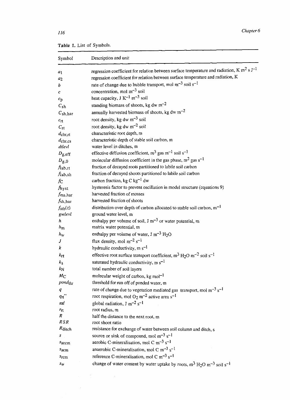
116 Chapter 6
Table 1. List of Symbols.
Symbol Description and unit
b
c
cp
Csh
C"sh,har
crt
C r t
^chr.rt
"chr.cs dtlevl Dg,eff
% 0
/lab,rt
/lab,sh
/C
Ayst
/ms,har
/sh,har
/stbU) gwlevl
h
hw
J
k
*rt
*s
*N
MC
ponder
q
<7rt"
mi
'it
R RSR
^ditch s
^aecm
^acm
^rcm
regression coefficient for relation between surface temperature and radiation, K mz s J"
regression coefficient for relation between surface temperature and radiation, K
rate of change due to bubble transport, mol m"~3 soil s - 1
concentration, mol mT3 soil
heat capacity, J K"1 m~3 soil
standing biomass of shoots, kg dw m~2
annually harvested biomass of shoots, kg dw m~2
root density, kg dw m~3 soil
root density, kg dw m~2 soil
characteristic root depth, m
characteristic depth of stable soil carbon, m
water level in ditches, m
effective diffusion coefficient, m3 gas m~* soil s - '
molecular diffusion coefficient in the gas phase, m2 gas s - 1
fraction of decayed roots partitioned to labile soil carbon
fraction of decayed shoots partitioned to labile soil carbon
carbon fraction, kg C kg - 1 dw
hysteresis factor to prevent oscillation in model structure (equations 9)
harvested fraction of mosses
harvested fraction of shoots
distribution over depth of carbon allocated to stable soil carbon, m - 1
ground water level, m
enthalpy per volume of soil, J m~3 or water potential, m
matrix water potential, m
enthalpy per volume of water, J m~3 H2O
flux density, mol m~2 s - 1
hydraulic conductivity, m s~*
effective root surface transport coefficient, m3 H2O trT2 soil s"1
saturated hydraulic conductivity, m s - 1
total number of soil layers
molecular weight of carbon, kg mol -1
threshold for run off of ponded water, m -3C-1 rate of change due to vegetation mediated gas transport, mol m~3 s
root respiration, mol O2 m~2 active area s -1
- 2 . - 1 global radiation, J m~2 s root radius, m
half the distance to the next root, m root shoot ratio
resistance for exchange of water between soil column and ditch, s
source or sink of compound, mol m~3 s"1
aerobic C-mineralisation, mol C m~3 s"1
anaerobic C-mineralisation, mol C m"3 s~*
reference C-mineralisation, mol C m~3 s"1
change of water content by water uptake by roots, m3 H2O m~3 soil s"1
Plot scale 117
t T
Ts
vw
Vmmo
w z
ziittr a
P Az
Azp
h £g,cr 6
Os K
Vae
Smix,sj
P Tc|ab Tcstb
Trt Tsh CO
rate of change due to vertical convection and diffusion, mol m~3 s_1
time, s temperature, K temperature at soil surface, K
water flow, m3 H2O m~2 soil s"*1
potential methane oxidation, mol m - 3 s_1
weight function for half the distance to the next root, m - 1
spatial coordinate depth, m maximum depth of litter allocation, m
solubility, m3 gas m~3 H2O
dimensionless parameter thickness of a soil layer, m distance to the grid point in the next higher soil layer, m
distance to the grid point in the next deeper soil layer, m
gas filled pore space, m3 gas m - 3 soil
gas filled pore space above which convection may occur, m3 gas m~3 soil
volumetric moisture content, m3 H2O m~3 soil
saturated volumetric moisture content, m3 H2O m~3 soil root O2 release relative to the O2 demand for aerobic respiration
thermal conductivity, J m_ 1 K - 1 s _ 1
stoichiometric constant for aerobic respiration
apparent mixing coefficient due to vertical transport, s~*
bulk density, kg dw m~3 soil
time constant of turnover of labile soil carbon, s
time constant of turnover of stable soil carbon, s
time constant of root turnover, s time constant of shoot turnover, s total oxygen sink relative to oxygen sink for aerobic respiration
compounds eo er clab cstb
electron acceptor reduced electron acceptor labile soil carbon stable soil carbon
subscripts
atm
IWl
m
aqueous phase atmosphere index of compound gas index of discretised soil layer index of deepest gas continuous discretised soil layer index of discretised soil layer soil layer below the deepest water unsaturated soil layer
single root model system
other symbols
averaged over single root model system
averaeed over soil layer
j jg Chapter 6
[Moore and Roulet, 1993; Bartlett and Harris, 1993; Nykanen et al, 1998; Bellisario et a/., 1999] and the underlying processes [Segers, 1998]. Therefore, a more fundamental understanding of methane fluxes is desirable, using knowledge which is generally applicable: the theories of microbial and chemical conversions and physical transport processes. The scale at which this knowledge applies is called the kinetic scale, with a typical size of a few mm [chapter 4].
This paper is the last paper in a series of three which aim to explicitly connect the knowledge at the kinetic level to methane fluxes at the plot scale. Mathematical modelling is used, as this is the most efficient way to integrate knowledge of several interacting processes across various spatial and temporal scales. In the first paper [chapter 4] the overall approach is discussed and a reaction-diffusion model was developed for processes around a single gas transporting root. This model was successfully simplified by assuming a quasi steady state for oxygen and by spatially averaging the other compounds. In the second paper [chapter 5], methane dynamics are simulated in a water saturated soil layer with gas transporting roots. Here, root architecture is described by a weight function for half the distance to the next root [Rappoldt, 1990,1992]. Spatially averaging at this scale had a small effect on net methane emission, but a substantial effect on net methane production and methane transport.
In this third paper we scale up to the plot scale. At this scale the gas transporting roots are not the only determinants of methane fluxes, but also temperature and water table [Moore and Roulet, 1993; Bartlett and Harris, 1993; Nykanen et aL, 1998; Bellisario et a/., 1999]. Therefore, the model is extended with modules for vertical transport of heat, water and compounds. Furthermore, depth is introduced as independent variable, as water content, temperature, root density and decomposable organic matter vary with depth. As a result of quasi-steady state assumptions for some processes with characteristic times of a few hours [chapter 4], the smallest time scale of interpretation is 1 day. First, we describe the model and summarise information from literature which is used for parameterisation. Subsequently, we compare simulated methane fluxes with measured methane fluxes from an intensively monitored fen in the Netherlands [van den Pol - van Dasselaar et a/., 1999a, b]. Effects of uncertainty in the parameters on simulated emissions are investigated by a sensitivity analysis. In addition, we tested the effects of model structure at the soil layer level [chapter 5] on methane fluxes. Finally, we discuss the difference between our model and other process models for methane fluxes.
Model description and non site specific parameterisation
The core of the model is a set of coupled partial differential equations for water, heat, and species (CH4, 0 2 , N2, C02 , labile soil carbon (q a b) , stable soil carbon (cstb), and electron acceptors in oxidised form (eo) and reduced form (er) with time and depth as independent variables. Table 1 lists the symbols.
Plot scale U9
Water
Water plays a crucial role in the aeration of the soil. As a first approximation one might assume that above the water table the soil is aerobic and below the water table the soil is anaerobic. However, reality is often more complicated. Firstly, the border between the oxic and anoxic soil may be somewhat above the water table, especially in dense soil (deeper peat layers with higher water retention) (Tables 2 and 3). Secondly, upward and downward flow of water may affect methane fluxes by aqueous convective transport of methane and electron acceptors [Romanowicz et al, 1993; Waddington and Roulet, 1997]. Thirdly, understanding of the episodic emissions of stored methane after a drop of the water table [Windsor et al, 1992; Shurpali et al 1993] may require accurate information on the dynamics of gas filled pore space to calculate the balance between methane release and methane oxidation regulated by oxygen inflow. To investigate these phenomena, a model is needed that simulates depth dependent water content and bidirectional flow, driven by evapotranspiration and external hydrological conditions. Therefore, we used the one-dimensional Richards' equation [Richards, 1931].
To use Richards' equation soil k-h-G relationships are needed. These vary strongly for peat (Boelter [1969]; Table 2 and 3). Surface soil tends to be highly porous, with low bulk density, low water retention, and high hydraulic conductivity, whereas deeper soil and anthropogenically drained peat soil tends to have a higher bulk density, high water retention and low hydraulic conductivity [e.g. Silins and Rothwell, 1998]. As first
Table 2. Water content, 0, (m3 H 2 0 m ' 3 soil) as function of water potential and dry bulk density, p
(kg m"3) for peat soils [Paivanen, 1973; Okruszko and Szymanowksi, 1992; Loxham and Burghardt,
1986; Silins and Rothwell, 1998]. Standard deviations are between parenthesis.
p<50 5 0 - 1 0 0 100-150 150-250
pF
0 0.96 (0.03) 0.92 (0.04) 0.91 (0.02) 0.88 (0.03) 1 0.46 (0.29) 0.74 (0.20) 0.79 (0.11) 0.82 (0.04) 2 0.21 (0.12) 0.40 (0.15) 0.69 (0.08) 0.67 (0.06) 3 0.13 (0.08) 0.24 (0.07) 0.31 (0.10) 0.39 (0.05)
Table 3. Coefficients, c{ and c2 , for regression equations of the logarithm of saturated hydraulic
conductivity, * s , in relation to bulk density, p , in peat (10!og(*s/*s,r) = c\ + c2 p)- *s,r « the
reference value of kc which is 1 m s Ls,
c i ( - ) c 2 ( m 3 k g - 1 ) n i2 source
_ 3 6 _0 016 <119 0.54 Boelter [1969] 4.2 -0.0098 1280 0.22 Paivanen [1973]
-2.0 -0.027 80 0.73 Silins and Rothwell [1998]
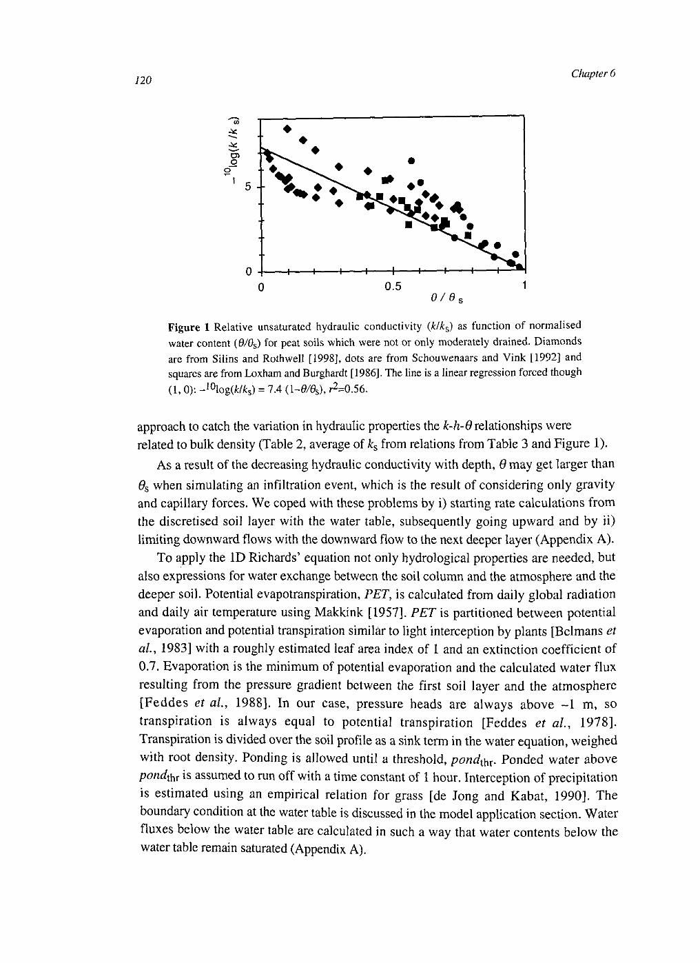
120 Chapter 6
v>
o
Figure 1 Relative unsaturated hydraulic conductivity (k/ks) as function of normalised water content (9/6s) for peat soils which were not or only moderately drained. Diamonds are from Silins and Rothwell [1998], dots are from Schouwenaars and Vink [1992] and squares are from Loxham and Burghardt [1986]. The line is a linear regression forced though (1, 0): -10log(£Ms) = 7.4 (1-0/ft), ^=0.56.
approach to catch the variation in hydraulic properties the k-h-0relationships were related to bulk density (Table 2, average of ks from relations from Table 3 and Figure 1).
As a result of the decreasing hydraulic conductivity with depth, 6 may get larger than 0S when simulating an infiltration event, which is the result of considering only gravity and capillary forces. We coped with these problems by i) starting rate calculations from the discretised soil layer with the water table, subsequently going upward and by ii) limiting downward flows with the downward flow to the next deeper layer (Appendix A).
To apply the ID Richards' equation not only hydrological properties are needed, but also expressions for water exchange between the soil column and the atmosphere and the deeper soil. Potential evapotranspiration, PET, is calculated from daily global radiation and daily air temperature using Makkink [1957]. PET is partitioned between potential evaporation and potential transpiration similar to light interception by plants [Belmans et al, 1983] with a roughly estimated leaf area index of 1 and an extinction coefficient of 0.7. Evaporation is the minimum of potential evaporation and the calculated water flux resulting from the pressure gradient between the first soil layer and the atmosphere [Feddes et al, 1988]. In our case, pressure heads are always above -1 m, so transpiration is always equal to potential transpiration [Feddes et al, 1978]. Transpiration is divided over the soil profile as a sink term in the water equation, weighed with root density. Ponding is allowed until a threshold, pond^. Ponded water above ponder is assumed to run off with a time constant of 1 hour. Interception of precipitation is estimated using an empirical relation for grass [de Jong and Kabat, 1990]. The boundary condition at the water table is discussed in the model application section. Water fluxes below the water table are calculated in such a way that water contents below the water table remain saturated (Appendix A).

Plot scale
Temperature
As simplest process based approach, soil temperature could be modelled with a diffusion
equation for temperature [e.g. Koorevaar et al, 1983]:
9r = AA3Z; (1) at dzcpdz
in which the heat conductivity, Ah, and volumetric heat capacity, cp, are related to the volumetric soil composition [Frolking and Crill, 1994]. The lower boundary is set at such a depth (4 m) that a zero gradient in temperature can be assumed (preliminary simulations and Puranen et al. [1999]). At the surface, it is most simple to assume that soil temperature is equal to air temperature from weather data.
This simple approach is tested by considering more refined formulations for several parts of this model. The first refinement is to include the geometric arrangement of the soil components on Ah [de Vries, 1963; ten Berge, 1990, p. 26]. The second is to include the effect of radiation on surface temperature (see model application section). The third is to include convection of heat, which may play a role in fens [van Wirdum, 1991]. This last process is modelled by using enthalpy, h (J m-3 soil) as state variable, instead of temperature, keeping open the possibilities to extend the model with phase transitions (e.g. freezing), staying as close as possible to the underlying physics:
dA_^adjm) + div^l + Svjhw (2a) 3t dz dz dz
7W = £ (2b)
Species dynamics
The species CH4, 0 2 , C02 , N2, electron acceptors in reduced form and oxidised form and two soil carbon pools are modelled as function of time and depth. In soil parts in which gas transport is dominated by gas transporting plants the gradients around gas transporting roots are also considered, using models of the previous papers [chapter 4 and
5].
Soil carbon and roots
To obtain a rough explanatory model for the depth distribution .of soil carbon mineralisation three plant related sources of soil carbon are distinguished. Firstly,
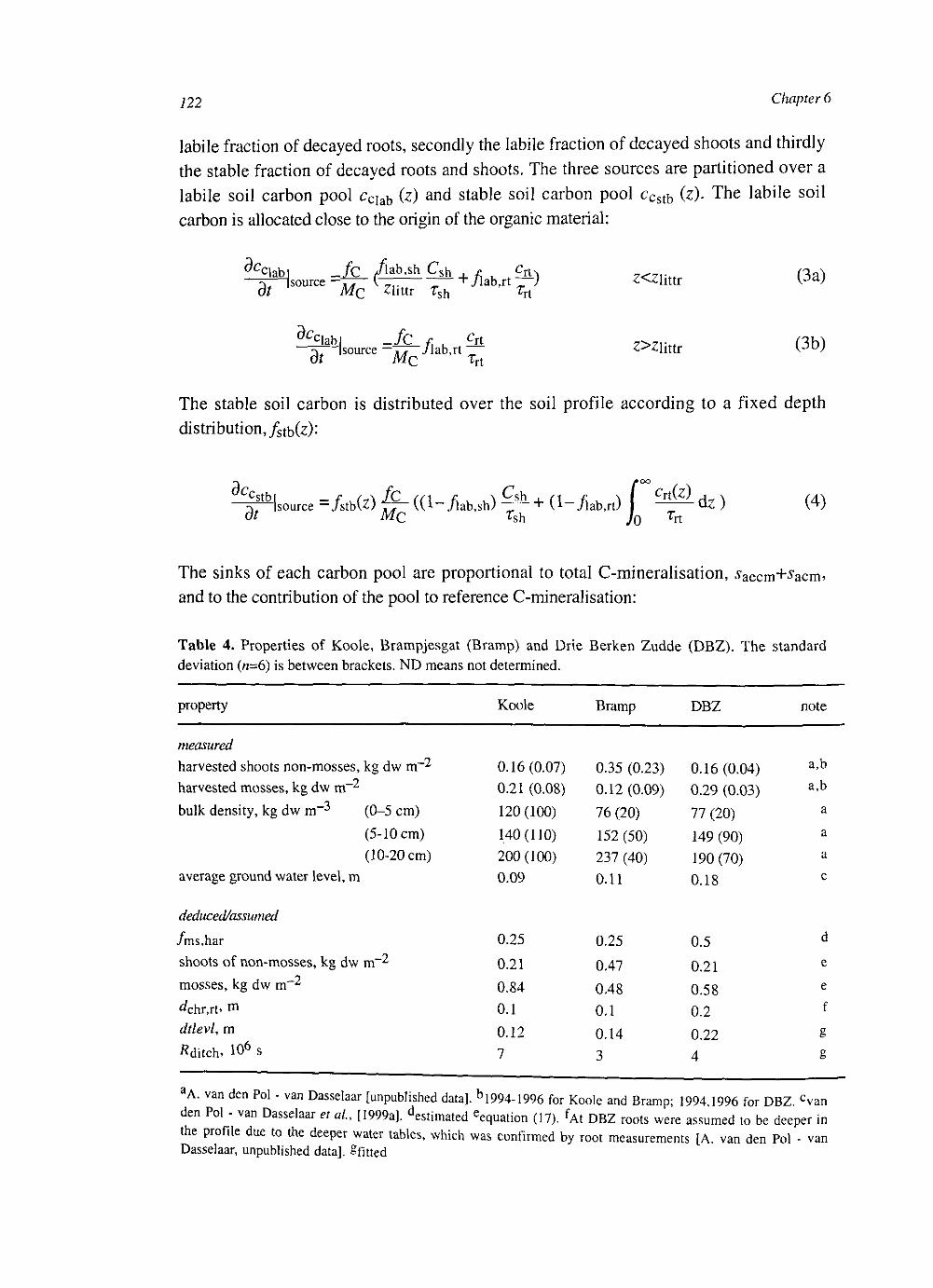
122 Chapter 6
labile fraction of decayed roots, secondly the labile fraction of decayed shoots and thirdly the stable fraction of decayed roots and shoots. The three sources are partitioned over a labile soil carbon pool cciab (z) and stable soil carbon pool cCstb (z). The labile soil carbon is allocated close to the origin of the organic material:
da ciabi - / c / l a b ' s h Csh , r CrtN =r (source -7~T~ \~Z7. ~ wlab,rt „ ) dt MQ Zlittr r s h
Z<Zlittr (3a) rt
3c, ciabl _ / c r L £rt }, Isource — ,*- 71ab,rt _ 3r MC *rt
Z>Zlittr (3b)
The stable soil carbon is distributed over the soil profile according to a fixed depth
distribution,/stb(z):
^ I s o u r c e = /stbfe) §~ ( ( W l a b , s h ) ^ + (1-^ab.r t ) f ^ dz (4)
The sinks of each carbon pool are proportional to total C-mineralisation, ^aecm+^acm. and to the contribution of the pool to reference C-mineralisation:
Table 4. Properties of Koole, Brampjesgat (Bramp) and Drie Berken Zudde (DBZ). The standard deviation («=6) is between brackets. ND means not determined.
property
measured
harvested shoots non-mosses, kg dw m~2
harvested mosses, kg dw m~2
bulk density, kg dw m~^ (0-5 cm)
(5-10 cm)
(10-20 cm) average ground water level, m
deduced/assumed
/ms.har
shoots of non-mosses, kg dw m~2
mosses, kg dw m~2
^chr,rt> rn ddevl, m
Kditch* 106 s
Koole
0.16(0.07)
0.21 (0.08)
120 (100)
140(110)
200(100)
0.09
0.25
0.21
0.84
0.1
0.12
7
Bramp
0.35 (0.23)
0.12(0.09)
76 (20)
152 (50)
237 (40)
0.11
0.25
0.47
0.48
0.1
0.14
3
DBZ
0.16 (0.04)
0.29 (0.03)
77 (20)
149 (90)
190(70)
0.18
0.5
0.21
0.58
0.2
0.22
4
note
a,b
a.b
a
a
a
c
d
e
e
f
g
g
aA. van den Pol - van Dasselaar [unpublished data]. b1994-1996 for Koole and Bramp; 1994,1996 for DBZ. cvan den Pol - van Dasselaar et aL [1999a]. Estimated Equation (17). fAt DBZ roots were assumed to be deeper in the profile due to the deeper water tables, which was confirmed by root measurements [A. van den Pol - van Dasselaar, unpublished data], gfitted
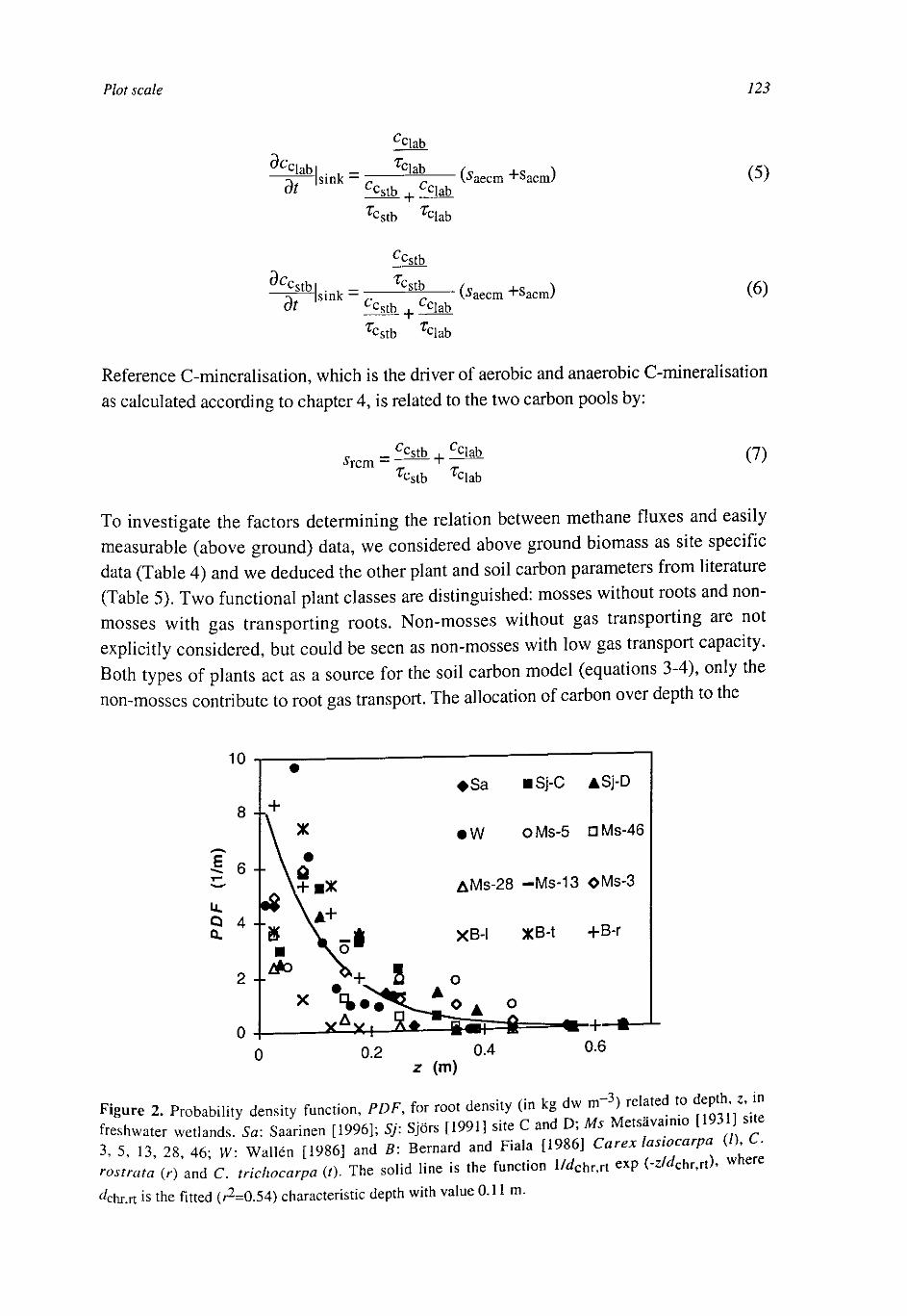
Plot scale 123
dcC[
dt ab
sink —
Cciab rciab
cc s tb | Cclab Tcstb
(Aaecm ~*~Sacm) (5)
'Clab
dc Cstb dt
sink —
Ccstb Tcstb
cc stb | CcIab Tcstb
Tciab
(s aecm """Sacm/ (6)
Reference C-mineralisation, which is the driver of aerobic and anaerobic C-mineralisation as calculated according to chapter 4, is related to the two carbon pools by:
srcm — ccstb rcstb
+ •ciab rciab
(7)
To investigate the factors determining the relation between methane fluxes and easily measurable (above ground) data, we considered above ground biomass as site specific data (Table 4) and we deduced the other plant and soil carbon parameters from literature (Table 5). Two functional plant classes are distinguished: mosses without roots and non-mosses with gas transporting roots. Non-mosses without gas transporting are not explicitly considered, but could be seen as non-mosses with low gas transport capacity. Both types of plants act as a source for the soil carbon model (equations 3-4), only the non-mosses contribute to root gas transport. The allocation of carbon over depth to the
•Sa HSj-C ASj-D
• W OMs-5 DMs-46
AMs-28 -Ms-13 OMs-3
XB-I XB-t +B-r
0.2 0.4 z (m)
Figure 2. Probability density function, PDF, for root density (in kg dw nr*) related to depth z in
freshwater wetlands. Sa: Saarinen [1996]; Sj: Sjors [1991] site C and D; Ms Metsavam.o [1931 sue
3, 5, 13, 28, 46; IV: Wailen [1986] and B: Bernard and Fiala [1986] Caret tastocarpa </) C.
rostrata (r) and C. trichocarpa (r). The solid line is the function l/</chr.rt exp (-z/</chr,rt). w h e r e
^chr.n is the fitted (#2=0.54) characteristic depth with value 0.11 m.

124 Chapter 6
stable carbon pool, /stb(z)» i s t a k e n a s a n exponential function with a characteristic depth, </chr,cs- T u r n o v e r of s o i l carbon and vegetation are assumed to depend on temperature with a £>10 of 2 and with reference temperature at average air temperature. Generally, roots do not penetrate deeply in freshwater wetlands, though quite some variation is present (Figure 2). Little is known about the causes of this variation. Miller et aL [1982] suggested that root depth in peats is controlled by nutrient availability. Metsavainio [1931] found a much higher percentage of dead roots below the water table than above, indicating that, despite the adaption mechanisms, roots of wetland plants are hampered under anoxic conditions. As default we assumed that root density, crt, decreases exponentially with a characteristic depth, /chr,rt of 0.1 m:
Cn = C rt
^chr,rt exp(-
^chr,rt (8)
Table 5, Default non-site specific parameters. Investigated range in sensitivity analysis is between brackets.
parameter value source
/sh.har
Zlittr. m
"chr.cs* m
RSR
yiab,sh
/iab,ms
*rt. s
Tclab> s
Tcstb' s
rhizosphere geometry
&rt, m3 H2O m~2 soil s"1
#rt"t mol O2 m~2 active root s - 1
^etot» m 0 ' el- eciv- m~3 soil Vmm0f mol m~3 soil s_ 1
kinetics
root architecture
bubble transport ,3 ,,„„ ^ - 3
0.75
0.05 (0.05-10)
0.2(0.1-0.5)
1 (0.2-10)
0.5
0.2
3.2 107
6.3 107
6.4 107
3.2 109
cylindrical (spherical)
10-^(10-6-10"7)
10~8 (10-8-5-10"8)
50(5-100)
10"5 ( lO^- lO- 4 ) 1
m
1
0.05
k
1
m
£g>cr> m J gas m"J soil
aestimated bfitted by eye (Figure 7). c[Brinson et aL, 1981; Shaver and Chapin, 1991; Wallen, 1986; Sjors, 1991; Saarinen, 1996; Bernard et aL, 1988; Wieder, in prcp].dTypha, Phragmites, Scolocloa, Scirpus [Wrubleski et aL, 1997]. e[Johnson and Damman, 1993]. fCarex rostrata [Saarinen, 1996] gSzumigalski and Bayley [1996], Thorman and Bayley [1997] and Wrubleski et aL, [1997]. ntaken much larger than the scale of experiments. Combination of rhizosphere geometry, kn and qn" leading to an intermediate exchange between rhizosphere and atmosphere [chapter 5]. JSomewhat higher than [Segers and Kengen, 1998], because they only considered electron acceptors in oxidised form. kAverage of wetlands [Segers, 1998] and few measurements at Koole [Heipieper and de Bom, 1997]. Chapter 4. mchapter 5. "sandy loam [Leffelaar. 1988].

Plot scale 125
Homogeneous concentrations in water unsaturated soil and heterogeneous concentrations in water saturated soil
In water saturated soil gas exchange is dominated by transport via the roots and aqueous diffusion around the roots. This diffusion process is slower than several reactions, resulting in heterogeneous concentrations of several species at a certain depth [chapter 4]. In the oxic, water unsaturated soil gas exchange is dominated by transport via the gaseous pores and diffusion through water films around soil particles. In non-aggregated or dry soils these water films will be thin, resulting in fast diffusion processes and in homogeneous species concentrations at each depth. In aggregated moist soil the aqueous volumes may be so large that diffusion is slower than reaction, resulting in heterogeneous species concentrations (e.g. partial anaerobiosis). In the top soil of undrained peat, water retention is low and no clear aggregation is present. Therefore, as first approach it is assumed that in the water unsaturated surface soil the concentrations are homogeneous at each depth. As a result of the different behaviour in the two zones of the soil we applied different models for each zone (Figure 3).
The functional difference between the homogeneous and the heterogeneous zone, as defined above, is reflected in the oxygen behaviour. In the water unsaturated zone oxygen is amply available and supplied by vertical transport via the soil matrix and in the water saturated zone it is scarce and supplied by gas transporting plants. Therefore, the differences between the two regimes is not directly governed by the water table, but by three conditions, related to gas transport and aeration, for heterogeneous soil:
0 m . soil
concentrations^ s u r f a c e
homogeneous 1 at each depth/ interface bewteen dominating gas
H „ • ^ exchange mechanisms. Above: diffusion aynamic ly:|:j:j:;:;:;:j^ in g a s phase. Below: plant mediated
dynamicTPi:J:s^ ground water """]:l!!ir!:!:!i!:l:!!l:l!!:!ilil:l:l:i:lil:l:l± l e v e l
|:|:i:|:|:|^oncentrations j:j:::!:::|: !:l:!:l:l:i heterogeneous 1|:|:|:|:I:|: Sjiiiivat each depth/!;!:!:!:!:;; j:|r|:|:|:|:|r|:|:|;|:|:|:|r|:|:|:|:|:|:|:|:|r|:|:|r|:|r|:|:|:|: bottum of profile
2 m ^:=:=^:=:=:=:=:^:^:j:j:!:|:j:j:|:|:|:|;iHl'!ij: for gases, soil carbon and solutes
_ _ _ — — — — bottum of profile 4 m for water and
heat
Figure 3. Overview of the model structure. For explanation and discussion see text.
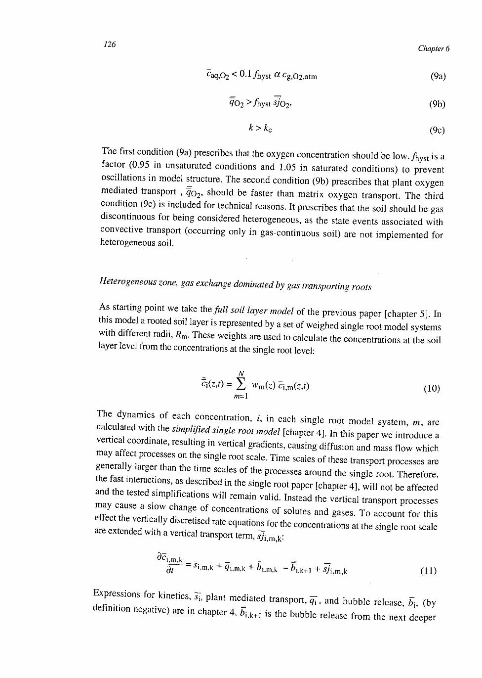
j2/j Cliapter6
Caq,02 < 0-1 Ayst a Cg,02,atm (9a)
qo2> Ay st sjo2> (9b^
Jfc > Jfcc (9c)
The first condition (9a) prescribes that the oxygen concentration should be low./hyst is a factor (0.95 in unsaturated condit ions and 1.05 in saturated condi t ions) to prevent oscillations in model structure. The second condition (9b) prescribes that plant oxygen mediated transport , qo2, should be faster than matrix oxygen t ransport . T h e third condition (9c) is included for technical reasons. It prescribes that the soil should be gas discontinuous for being considered heterogeneous, as the state events associated with convective transport (occurring only in gas-continuous soil) are not implemen ted for heterogeneous soil.
Heterogeneous zone, gas exchange dominated by gas transporting roots
As starting point we take the full soil layer model of the previous paper [chapter 5 ] . In this model a rooted soil layer is represented by a set of weighed single root model systems with different radii, R m . These weights are used to calculate the concentrations at the soil layer level from the concentrations at the single root level:
N
The dynamics of each concentra t ion, /, in each single root mode l sys tem, m , are calculated with the simplified single root model [chapter 4 ] . In this paper we introduce a vertical coordinate, resulting in vertical gradients, causing diffusion and mass flow which may affect processes on the single root scale. Time scales of these transport processes are generally larger than the time scales of the processes around the single root. Therefore, the fast interactions, as described in the single root paper [chapter 4 ] , will not be affected and the tested simplifications will remain valid. Instead the vertical transport processes may cause a slow change of concentrations of solutes and gases. T o account for this effect the vertically discretised rate equations for the concentrations at the single root scale are extended with a vertical transport term, sji^my.
dQ m k __ _ = _ — ^ ~ - i,m,k + 4i.m,k + 6i,m,k - Z?jik+1 + S/j,m,k (1 0
Expressions for kinetics, si, plant mediated transport, q[, and bubble release, b\, (by
definition negative) are in chapter 4. Fiik+i is the bubble release from the next deeper
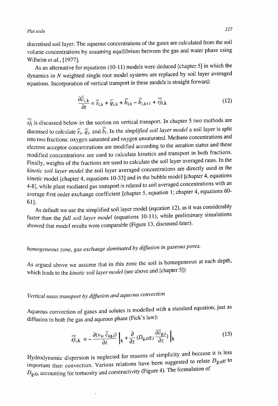
Plot scale I27
discretised soil layer. The aqueous concentrations of the gases are calculated from the soil volume concentrations by assuming equilibrium between the gas and water phase using Wilhelmera/., [1977].
As an alternative for equations (10-11) models were deduced [chapter 5] in which the dynamics in TV weighted single root model systems are replaced by soil layer averaged equations. Incorporation of vertical transport in these models is straight forward:
~\= _ —.
- ^ = *i,k + «i.k + *i.k - *»i.k+l + tfi,k (1 2> at
sji is discussed below in the section on vertical transport. In chapter 5 two methods are discussed to calculate sit q{, and b{. In the simplified soil layer model a soil layer is split into two fractions: oxygen saturated and oxygen unsaturated. Methane concentrations and electron acceptor concentrations are modified according to the aeration status and these modified concentrations are used to calculate kinetics and transport in both fractions. Finally, weights of the fractions are used to calculate the soil layer averaged rates. In the kinetic soil layer model the soil layer averaged concentrations are directly used in the kinetic model [chapter 4, equations 10-33] and in the bubble model [chapter 4, equations 4-8], while plant mediated gas transport is related to soil averaged concentrations with an average first order exchange coefficient [chapter 5, equation 1; chapter 4, equations 60-61].
As default we use the simplified soil layer model (equation 12), as it was considerably faster than the full soil layer model (equations 10-11), while preliminary simulations showed that model results were comparable (Figure 13, discussed later).
homogeneous zone, gas exchange dominated by diffusion in gaseous pores.
As argued above we assume that in this zone the soil is homogeneous at each depth,
which leads to the kinetic soil layer model (see above and [chapter 5])
Vertical mass transport by diffusion and aqueous convection
Aqueous convection of gases and solutes is modelled with a standard equation, just as
diffusion in both the gas and aqueous phase (Fick's law):
= _ 9(vW Caq,i) «/i,k - - dz k + 3i- (Dg-eff- ,"ar ) (13)
Hydrodynamic dispersion is neglected for reasons of simplicity and because jt important than convection. Various relations have been suggested to relate Z>g,eff t Dg,0, accounting for tortuosity and constructive (Figure 4). The formulat.on of
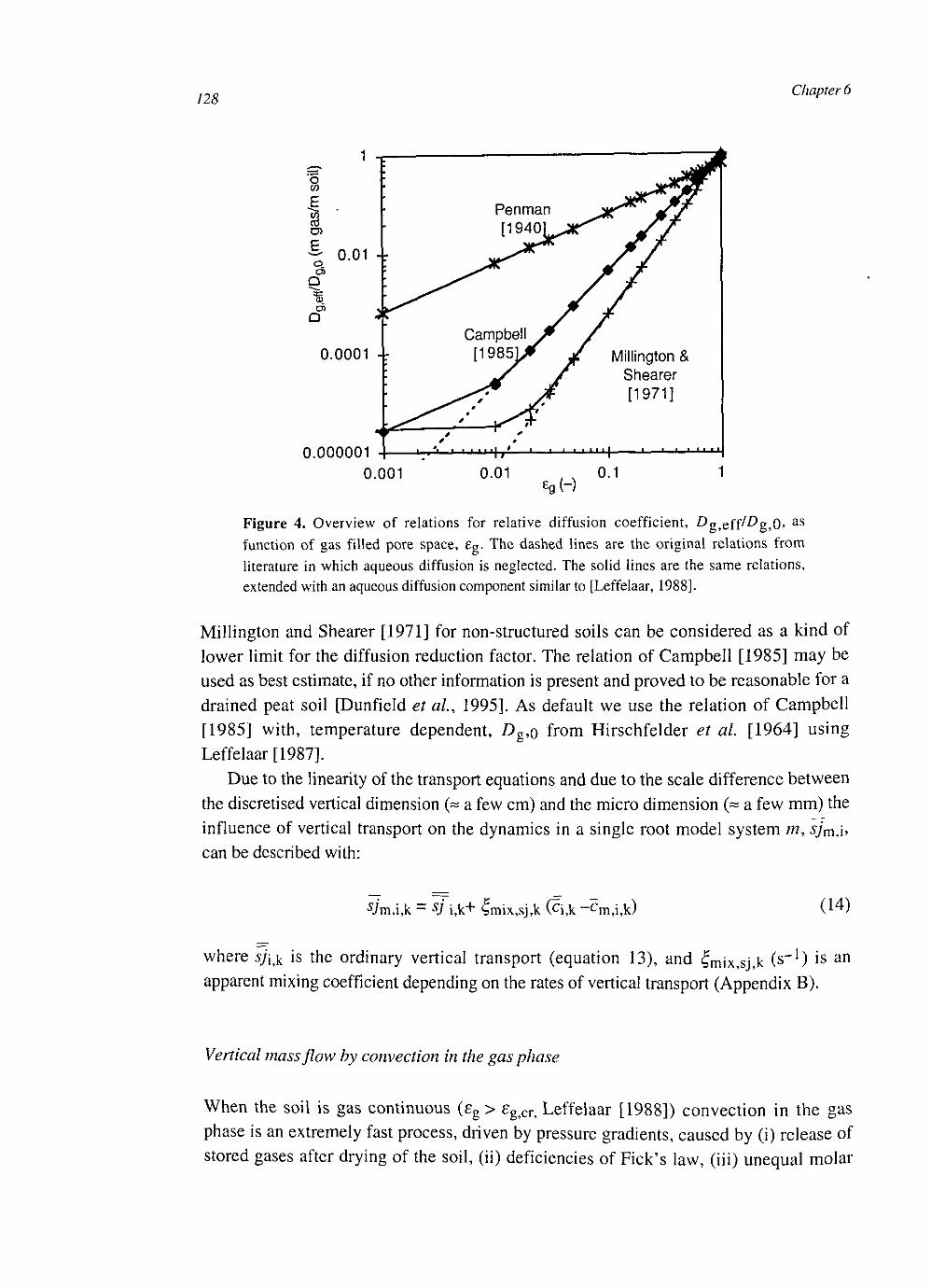
128 Chapter 6
1 -c
O w
ro
o Q
O
Penman [1
0.01 -r
0.0001 -:
0.000001
Millington & Shearer [1971]
0.001
Figure 4. Overview of relations for relative diffusion coefficient, £>g,eff^g,0» a s
function of gas filled pore space, £g. The dashed lines are the original relations from literature in which aqueous diffusion is neglected. The solid lines are the same relations, extended with an aqueous diffusion component similar to [Leffelaar, 1988].
Millington and Shearer [1971] for non-structured soils can be considered as a kind of lower limit for the diffusion reduction factor. The relation of Campbell [1985] may be used as best estimate, if no other information is present and proved to be reasonable for a drained peat soil [Dunfield et al, 1995]. As default we use the relation of Campbell [1985] with, temperature dependent, Z>g,n from Hirschfelder et al [1964] using Leffelaar [1987].
Due to the linearity of the transport equations and due to the scale difference between the discretised vertical dimension (~ a few cm) and the micro dimension (~ a few mm) the influence of vertical transport on the dynamics in a single root model system m, s/m,i> can be described with:
tym,i,k — SJ i,k+ bmix,sj,k \c'\,k ~cm,i,k) (14)
where sj\^ is the ordinary vertical transport (equation 13), and £mjx,sj,k (s -1) is an apparent mixing coefficient depending on the rates of vertical transport (Appendix B).
Vertical mass flow by convection in the gas phase
When the soil is gas continuous (eg > egjCn Leffelaar [1988]) convection in the gas phase is an extremely fast process, driven by pressure gradients, caused by (i) release of stored gases after drying of the soil, (ii) deficiencies of Fick's law, (iii) unequal molar

Plot scale 129
production/consumption of gases [Leffelaar, 1988] and (iv) unequal gas solubilities in water. Time-explicit simulation of gas continuous convection results in unpractically small time steps. Therefore, we modelled this process as a state event, following [Leffelaar, 1988, equation 14], occurring when the pressure difference between soil and atmosphere is larger than 0.1%.
Boundary conditions and initial values
For water and temperature the lower boundary was set at 4 m (see section on temperature). For the other compounds it was set at 2 m. At this boundary the sum of the electron acceptors in reduced and oxidised status was the same as in the bulk of the soil with 95% in reduced status. Both at the bottom of the profile and at the soil surface the gases were in equilibrium with the atmosphere, except for CQ2 at the bottom, which was set zero. Gas composition in precipitation was in equilibrium with the atmosphere, while electron acceptor concentrations were assumed to be zero.
To reduce the effect of initial conditions on results, simulations were always started in spring about 0.75 year before interpretation of the data. This is sufficient for most processes, as they have characteristic times less than 1 year. As soil carbon dynamics are much slower, we used equilibrium values as initial conditions. These were analytically estimated with, depth dependent, 3 year averaged aeration from preliminary simulations.
Computational considerations
Spatial discretisation is according to the control volume method [Patankar, 1980], ensuring conservation of mass. For convection we used an upwind scheme. Differences with the more accurate hybrid upwind/central scheme [Patankar, 1980] were investigated and are small (data not shown). For the vertical discretisation we used 15 soil layers (6 x 0.02, 0.03, 3 x 0.05, 2 x 0.1, 0.5, 1 and 2 m thick). A finer grid results in similar simulation results (average differences in flux < 1 %), apart from some peaks in methane fluxes which differ in magnitude (up to 300 %) when plotted once a day. The problem is minimised by analysing daily averaged methane fluxes, which are much less sensitive to the spatial discretisation (differences in peaks of methane fluxes < 30 %) than the fluxes at
a point in time. , • •• « For the temporal discretisation we used the explicit Euler method with a dynamic t.me
step. For each state at each time step, a maximum time step was estimated as a fract.on o the inverse of the relative rate of change. This fraction was different for the water, heat and gas state variables and set at the largest value which did not affect nmulation resu ts Integration of all the states was performed with the smallest maximum t.me step. As the water model requires the smallest time steps, but relatively only a few - l c u l » e
time step, this sub model was run separately and its output was used as input for the heat
and gas model.
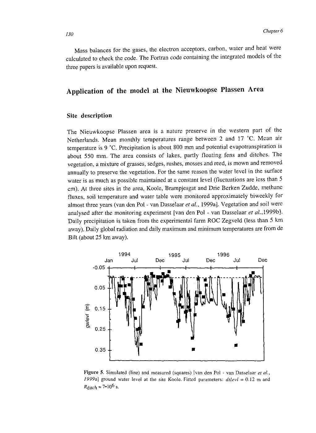
130 Chapter 6
Mass balances for the gases, the electron acceptors, carbon, water and heat were calculated to check the code. The Fortran code containing the integrated models of the three papers is available upon request.
Application of the model at the Nieuwkoopse Plassen Area
Site description
The Nieuwkoopse Plassen area is a nature preserve in the western part of the Netherlands. Mean monthly temperatures range between 2 and 17 °C. Mean air temperature is 9 °C. Precipitation is about 800 mm and potential evapotranspiration is about 550 mm. The area consists of lakes, partly floating fens and ditches. The vegetation, a mixture of grasses, sedges, rushes, mosses and reed, is mown and removed annually to preserve the vegetation. For the same reason the water level in the surface water is as much as possible maintained at a constant level (fluctuations are less than 5 cm). At three sites in the area, Koole, Brampjesgat and Drie Berken Zudde, methane fluxes, soil temperature and water table were monitored approximately biweekly for almost three years (van den Pol - van Dasselaar et ah, 1999a]. Vegetation and soil were analysed after the monitoring experiment [van den Pol - van Dasselaar et ah, 1999b]. Daily precipitation is taken from the experimental farm ROC Zegveld (less than 5 km away). Daily global radiation and daily maximum and minimum temperatures are from de Bilt (about 25 km away).
1994 Jan Jul
-0.05
0.05 --
M, 0.15 --
0.25 --
0.35 --
1995 1996 Dec Jul Dec Jul Dec
Figure 5. Simulated (line) and measured (squares) [van den Pol - van Dasselaar et aL, 1999a] ground water level at the site Koole. Fitted parameters: dtlevl = 0.12 m and *ditch = >10 6s .
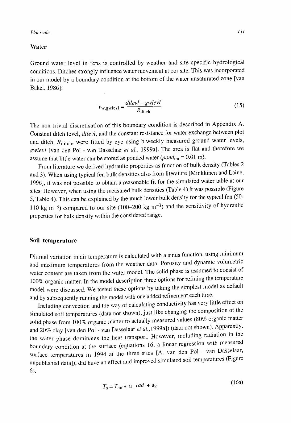
Plot scale yjy
Water
Ground water level in fens is controlled by weather and site specific hydrological conditions. Ditches strongly influence water movement at our site. This was incorporated in our model by a boundary condition at the bottom of the water unsaturated zone [van Bakel, 1986]:
dtlevl - gwlevl . _. vw,gwievl = ~ (15)
^ditch
The non trivial discretisation of this boundary condition is described in Appendix A. Constant ditch level, dtlevl, and the constant resistance for water exchange between plot and ditch, #ditch> were fitted by eye using biweekly measured ground water levels, gwlevl [van den Pol - van Dasselaar et al, 1999a]. The area is flat and therefore we assume that little water can be stored as ponded water (pondfa = 0.01 m).
From literature we derived hydraulic properties as function of bulk density (Tables 2 and 3). When using typical fen bulk densities also from literature [Minkkinen and Laine, 1996], it was not possible to obtain a reasonable fit for the simulated water table at our sites. However, when using the measured bulk densities (Table 4) it was possible (Figure 5, Table 4). This can be explained by the much lower bulk density for the typical fen (50-110 kg m"3) compared to our site (100-200 kg m~3) and the sensitivity of hydraulic properties for bulk density within the considered range.
Soil temperature
Diurnal variation in air temperature is calculated with a sinus function, using minimum and maximum temperatures from the weather data. Porosity and dynamic volumetric water content are taken from the water model. The solid phase is assumed to consist of 100% organic matter. In the model description three options for refining the temperature model were discussed. We tested these options by taking the simplest model as default and by subsequently running the model with one added refinement each time.
Including convection and the way of calculating conductivity has very little effect on simulated soil temperatures (data not shown), just like changing the composition of the solid phase from 100% organic matter to actually measured values (80% organic matter and 20% clay [van den Pol - van Dasselaar et a/., 1999a]) (data not shown). Apparently, the water phase dominates the heat transport. However, including radiation in the boundary condition at the surface (equations 16, a linear regression with measured surface temperatures in 1994 at the three sites [A. van den Pol - van Dasselaar, unpublished data]), did have an effect and improved simulated soil temperatures (Figure 6).
r s = rair + ai/w/ +a2 ( 1 6 a )
132 Chapter 6
Jan Jul Dec Jul Dec Jul
1994 1995 1996
Dec
Figure 6. Simulated (lines) and measured (symbols) [A. van den Pol - van Dasselaar, unpublished data] soil temperatures at 0.3 m depth at Koole. The thin line is the result from the temperature diffusion equation (1) with surface temperature equal to air temperature. The thick line is the result from the same model with a different boundary condition at the surface (equations 16).
a i=0 .015Km 2 s J - 1 (16b)
a2 = - 0.4 K (16c)
Therefore, in the remaining part of the paper we used the simplest soil temperature model (equation 1) with boundary conditions (16).
Soil carbon dynamics
The soil carbon model (equations 3 - 8 ) requires standing biomass as site specific input. In 1994 and 1995 the vegetation was cut at about 5 cm above the soil surface in summer, similar to the usual nature management at our site. In 1996 it was cut at the surface. Dry weights of the cut vegetation [van den Pol van Dasselaar et ai, 1999b] averaged over 1994-1996, and estimated harvested fraction were used to estimate standing biomass:
Csh = ^sh.har
7sh,har (17)
Furthermore, the input to the soil carbon pools from the shoots (equations 3a and 4) is reduced by a factor (l-/sh,har). For the short mosses/sh5har is estimated at 0.25 and for longer shoots it is estimated at 0.75. To estimate the initial size of the carbon pools, time averaged depth dependent aeration (oxygen supply/oxygen demand) was used (see subsection on boundary conditions and initialisation). Preliminary simulations showed
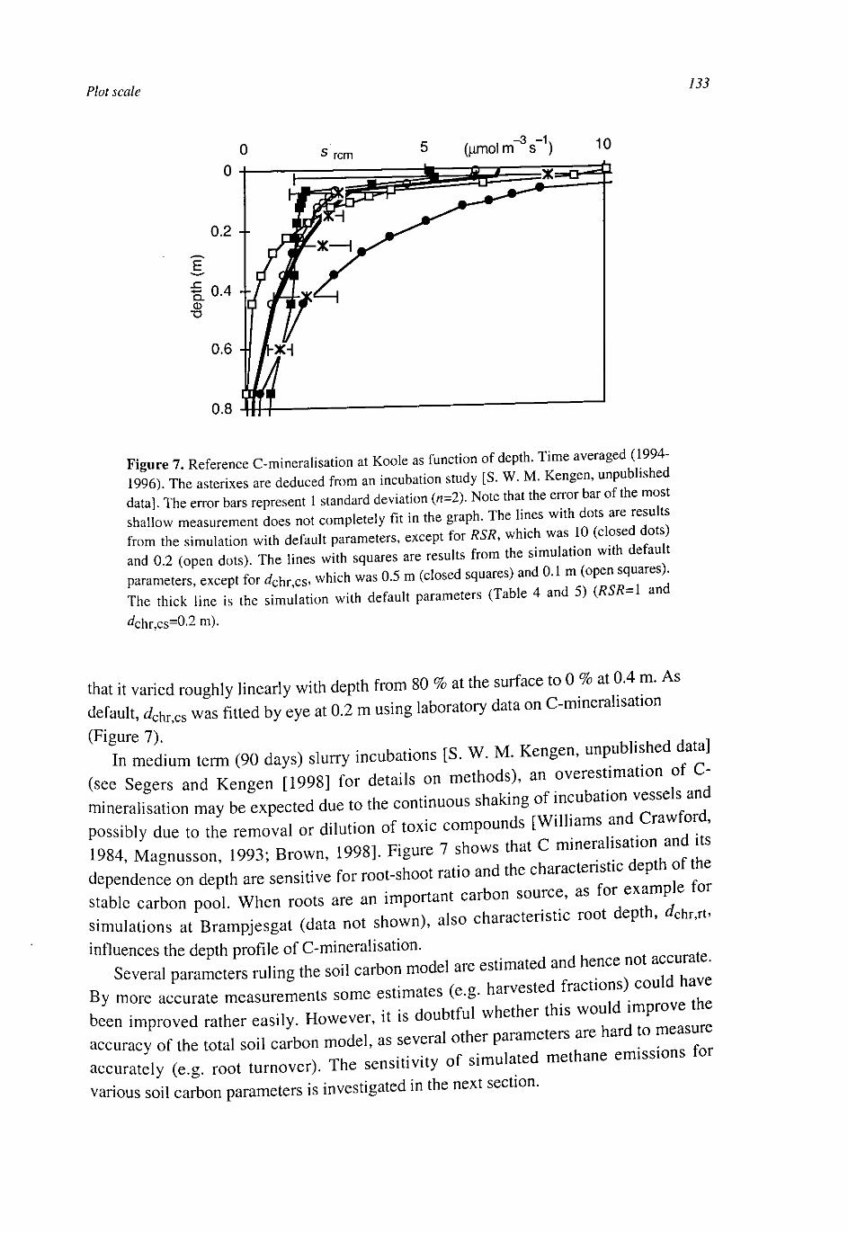
Plot scale 133
0
Q . CD •o
0
0.2 4-
0.4 +
0.6
0.8
rem (umol m s ) 10
Figure 7. Reference C-mineralisation at Koole as function of depth. Time averaged (1994-1996). The asterixes are deduced from an incubation study [S. W. M. Kengen, unpublished data]. The error bars represent 1 standard deviation (n=2). Note that the error bar of the most shallow measurement does not completely fit in the graph. The lines with dots are results from the simulation with default parameters, except for RSR, which was 10 (closed dots and 0.2 (open dots). The lines with squares are results from the simulation with defau t parameters, except for J c h r , c s , which was 0.5 m (closed squares) and 0.1 m (openi squares). The thick line is the simulation with default parameters (Table 4 and 5) (RSR-l and ^chr,cs=0.2m).
that it varied roughly linearly with depth from 80 % at the surface to 0 % at 0.4 m. As default, Jchr,cs was fitted by eye at 0.2 m using laboratory data on C-mineralisation
(Figure 7). t .. , , , . -, In medium term (90 days) slurry incubations [S. W. M. Kengen, unpubhshed data]
(see Segers and Kengen [1998] for details on methods), an overestimate of C-mineralisation may be expected due to the continuous shaking of incubation vessels and possibly due to the removal or dilution of toxic compounds [Williams and Crawford 1984, Magnusson, 1993; Brown, 1998]. Figure 7 shows that C ^ ^ ° ^ ^ dependence on depth are sensitive for root-shoot ratio and the characteristic depth of the stable carbon pool. When roots are an important carbon source, as for-example simulations at Brampjesgat (data not shown), also characteristic root depth, rfchr,r„ influences the depth profile of C-mineralisation. ,^,„ r f l tP
Several parameters ruling the soil carbon model are estimated and hence not a cur t . By more accurate measurements some estimates (e.g. harvested ^ ™ S > . C 0 U J ^ been improved rather easily. However, it is doubtful whether this would improve the accuracy of the total soil carbon model, as several other parameters are hard to measu* accurately (e.g. root turnover). The sensitivity of simulated methane em.ss.ons various soil carbon parameters is investigated in the next section.
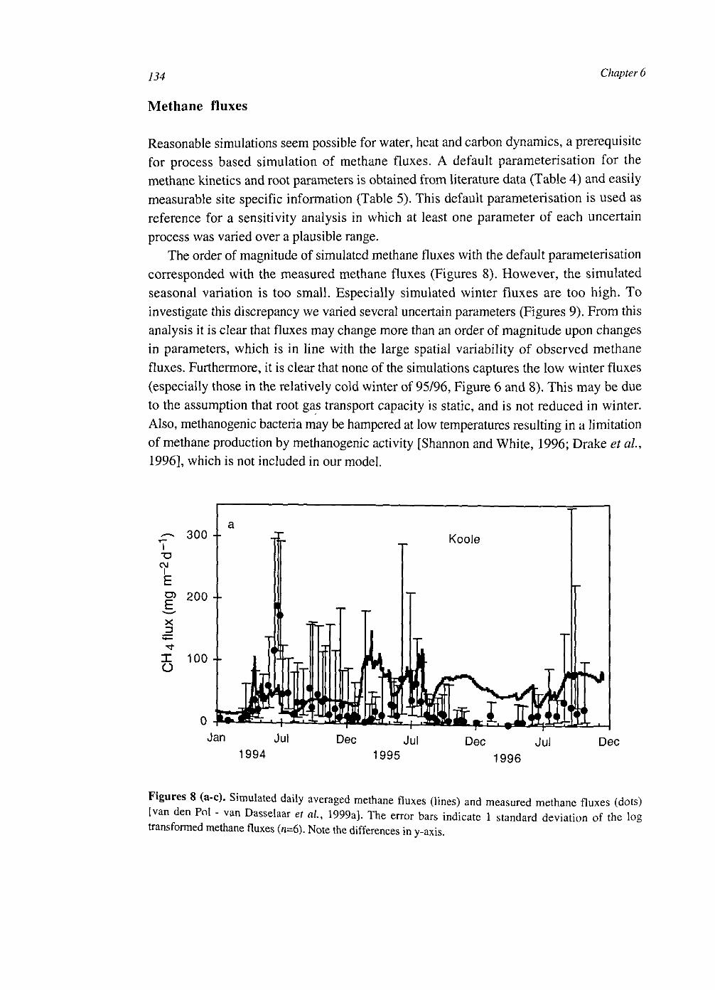
134 Chapter 6
Methane fluxes
Reasonable simulations seem possible for water, heat and carbon dynamics, a prerequisite for process based simulation of methane fluxes. A default parameterisation for the methane kinetics and root parameters is obtained from literature data (Table 4) and easily measurable site specific information (Table 5). This default parameterisation is used as reference for a sensitivity analysis in which at least one parameter of each uncertain process was varied over a plausible range.
The order of magnitude of simulated methane fluxes with the default parameterisation corresponded with the measured methane fluxes (Figures 8). However, the simulated seasonal variation is too small. Especially simulated winter fluxes are too high. To investigate this discrepancy we varied several uncertain parameters (Figures 9). From this analysis it is clear that fluxes may change more than an order of magnitude upon changes in parameters, which is in line with the large spatial variability of observed methane fluxes. Furthermore, it is clear that none of the simulations captures the low winter fluxes (especially those in the relatively cold winter of 95/96, Figure 6 and 8). This may be due to the assumption that root gas transport capacity is static, and is not reduced in winter. Also, methanogenic bacteria may be hampered at low temperatures resulting in a limitation of methane production by methanogenic activity [Shannon and White, 1996; Drake et al, 1996], which is not included in our model.
1994 Dec Jul Dec Jul
1995 1 9 9 6
Dec
Figures 8 (a-c). Simulated daily averaged methane fluxes (lines) and measured methane fluxes (dots) [van den Pol - van Dasselaar et aL, 1999a]. The error bars indicate 1 standard deviation of the log transformed methane fluxes (n=6). Note the differences in y-axis.
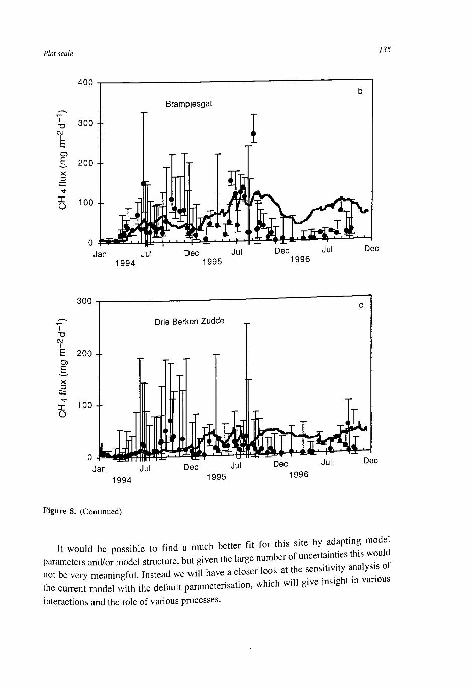
Plot scale 135
400
"D C\J
I
£
E x
X o
300 4-
200 4-
100 +
0 Jan Jul
1994 Dec Jul
1995 Dec Dec
1996
I
CM
X o
300
E 200 4-
X 3
100 4-
Drie Berken Zudde
0 Dec Jan
1994 1995 1996
Figure 8. (Continued)
It would be possible to find a much better fit for this site by adapting mod 1 parameters and/or model structure, but given the large number of uncertainties th would not be very meaningful. Instead we will have a closer look at the sensitivity analy*o the current model with the default parameterisation, which will g.ve insight ,„ interactions and the role of various processes.
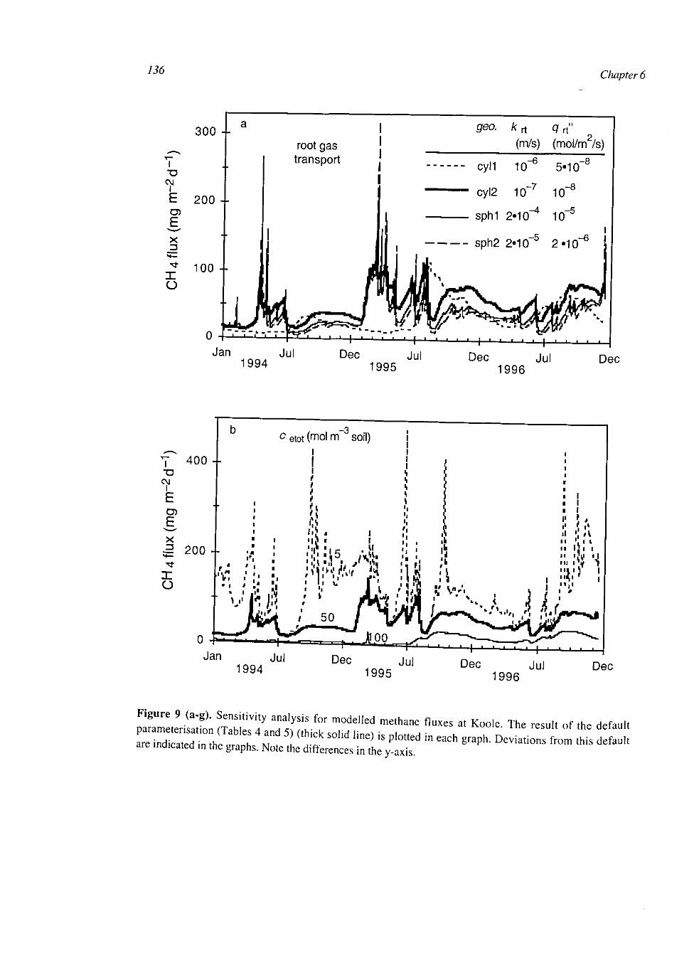
136 Chapter 6
I •O
05 E X
X o
300 4-
200 4-
100 4-
0
geo. kn q rt'
root gas transport
(m/s) (mol/m /s)
Jan Jul 1994
Dec Jul 1995
Dec Jul 1996
* — i — ' i i i — i i i i i .
Dec
Jan Jul 1994
Dec Jul 1995
Dec Jul 1996
Dec
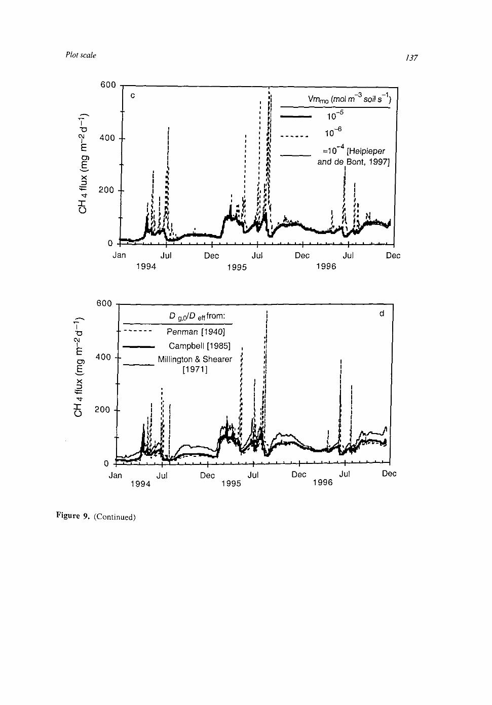
Plot scale 137
I • D
C\J
E X
X o
600
400 --
200 --
0
l . i
%
; !
I i
—3 —1 Vmmo (mol m soil s )
_*«
i i i i - 1 .1—i__i
10 - 5
1Cf6
- 4
=10 [Heipieper and de Bont, 1997]
i i i t t\ t»
)i 5
Jan Jul 1994
Dec 1995
Jul Dec Jul 1996
Dec
CM
E X
•< f r
X O
600
400 --
200 --
0
2g,o/Defffrom:
Penman [1940]
Campbell [1985]
ington & Shearer [1971
Jan Jul 1994
Dec Dec 1995 1996
Figure 9. (Continued)
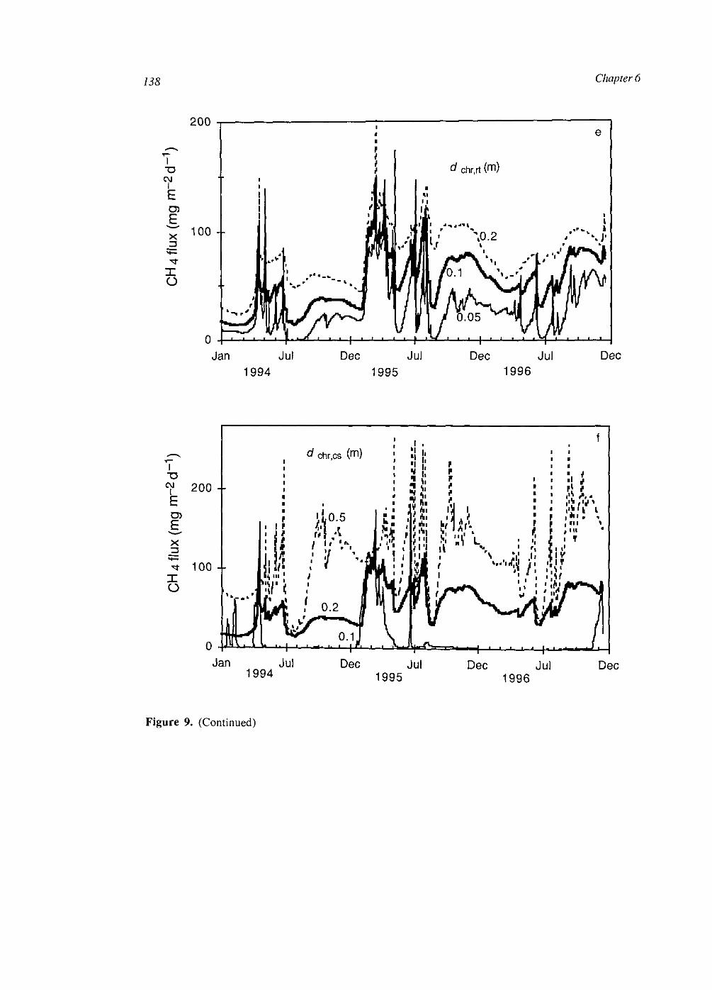
138 Chapter 6
200
E X
**—
X o
100
0
d chr.rt (m)
Jan Jul 1994
Dec Jul 1995
Dec Jul 1996
Dec
^ 1994 J U l ° e C J u ' i y y 4 1995
Dec Jul Dec 1996
Figure 9. (Continued)
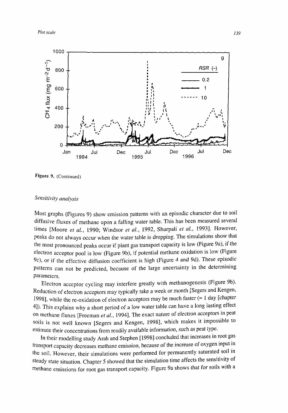
Plot scale 139
T3
1000
800 4-
I O
600 +
400 4-
200 4-
0 Jan
1994 Dec Jul
1995 Dec Jul
1996 Dec
Figure 9. (Continued)
Sensitivity analysis
Most graphs (Figure 9) show emission patterns with an episodic character due tc, soil diffusfve fluxes of methane upon a falling water table. This has been measured sev 1 time. [Moore et al, 1990; Windsor et al, 1992, Shurpali^ al, 1993] Howe er, peaks do not always occur when the water table is dropping. The s,mu aUon sh w t a the most pronounced peaks occur if plant gas transport capacity ,s low (Figu^ 9aX f th electron acceptor poo, is low (Figure 9b), if potential methane ° » < ^ ^ ^ 9c), or if the effective diffusion coefficient is high (Figure 4 and ^ ^ Z t l patterns can not be predicted, because of the large uncertainty ,n the determining
" n acceptor cycling may interfere greatly with methanogenesis (Figure 9b) Reduction of electron acceptors may typically take a week or mon h Seger and Keng 1998], while the re-oxidat,on of electron acceptors may be much faste - 1 a [cha^ 4]). Th,s explains why a short period of a low water table can ^ ^ ^
j ino/n THP exact nature of electron accepiuia ^ on methane fluxes [Freeman et a/., 1994]. lhe exact naiu ;mnnssible to A ir^napn 19981 which makes it impossiDie iu soils is not well known [Segers and Kengen, lyvoj, c l W t v n e
estimate their concentrations from readily ^ j — ^ ^ ' n root gas In their modelling study Arah and Stephen [1998] coneluded t ^
transport capacity decreases methane emission Jbecause of the m c - s of yg ^ ^ the soil. However, their simulations were performed for permanently steady state situation. Chapter 5 showed that the simulation time affe » ^ ^ methane emissions for root gas transport capacity. Figure 9a shows that for soils
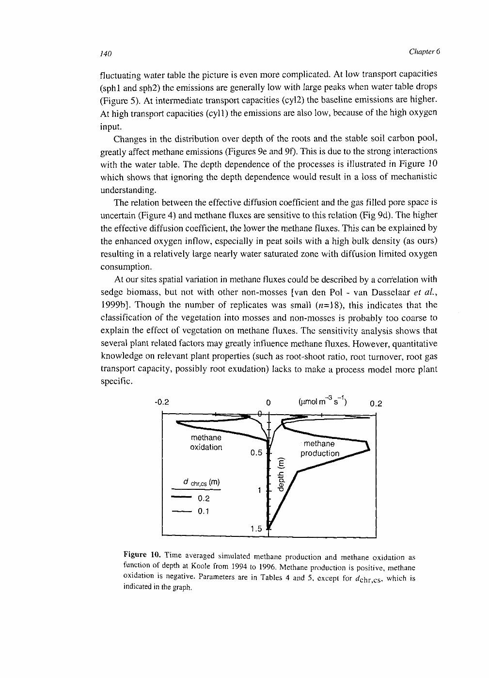
140 Chapter 6
fluctuating water table the picture is even more complicated. At low transport capacities (sphl and sph2) the emissions are generally low with large peaks when water table drops (Figure 5). At intermediate transport capacities (cyl2) the baseline emissions are higher. At high transport capacities (cyll) the emissions are also low, because of the high oxygen input.
Changes in the distribution over depth of the roots and the stable soil carbon pool, greatly affect methane emissions (Figures 9e and 9f). This is due to the strong interactions with the water table. The depth dependence of the processes is illustrated in Figure 10 which shows that ignoring the depth dependence would result in a loss of mechanistic understanding.
The relation between the effective diffusion coefficient and the gas filled pore space is uncertain (Figure 4) and methane fluxes are sensitive to this relation (Fig 9d). The higher the effective diffusion coefficient, the lower the methane fluxes. This can be explained by the enhanced oxygen inflow, especially in peat soils with a high bulk density (as ours) resulting in a relatively large nearly water saturated zone with diffusion limited oxygen consumption.
At our sites spatial variation in methane fluxes could be described by a correlation with sedge biomass, but not with other non-mosses [van den Pol - van Dasselaar et al.y
1999b]. Though the number of replicates was small («=18), this indicates that the classification of the vegetation into mosses and non-mosses is probably too coarse to explain the effect of vegetation on methane fluxes. The sensitivity analysis shows that several plant related factors may greatly influence methane fluxes. However, quantitative knowledge on relevant plant properties (such as root-shoot ratio, root turnover, root gas transport capacity, possibly root exudation) lacks to make a process model more plant specific.
-0.2 0 (umolm s ) o.2
1.5
Figure 10. Time averaged simulated methane production and methane oxidation as function of depth at Koole from 1994 to 1996. Methane production is positive, methane oxidation is negative. Parameters are in Tables 4 and 5, except for </chr,cs* which is indicated in the graph.
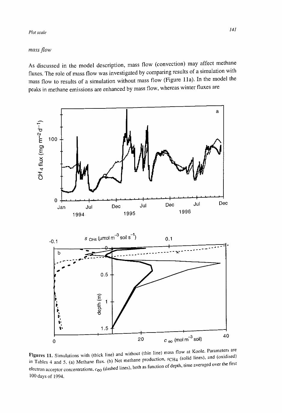
Plot scale 141
mass flow
As discussed in the model description, mass flow (convection) may affect methane fluxes. The role of mass flow was investigated by comparing results of a simulation with mass flow to results of a simulation without mass flow (Figure 11a). In the model the peaks in methane emissions are enhanced by mass flow, whereas winter fluxes are
i n
C\J
i E O)
E x
_D s—
X o
100 +
0
Jan Dec
1994 1995 1996
-0.1 -3 ., -1v
S CH4 (M m o 1 m S O l i S '
0 20 -3 c eo (mol m soil)
Figures 11. S.mulations with (thick line) and without (thin line) mass flow a Koo • P - -
in Tables 4 and 5. (a) Methane flux, (b) Net methane producfon, *CH 4 M * >"->• " ^ T J
electron acceptor concentrations, c e 0 (dashed line.), both as function of depth, t,me averaged over
100 days of 1994.
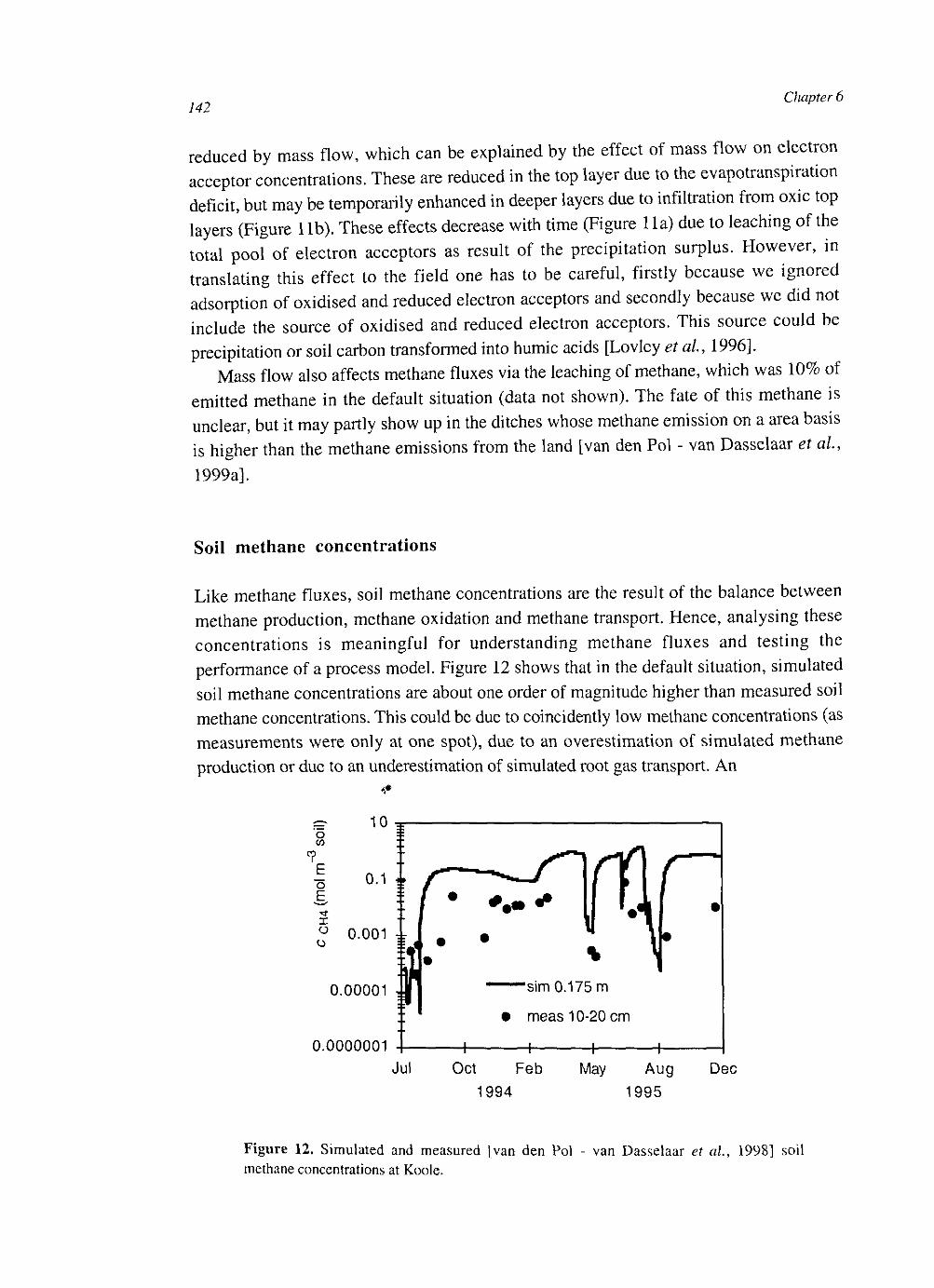
142 Chapter 6
reduced by mass flow, which can be explained by the effect of mass flow on electron acceptor concentrations. These are reduced in the top layer due to the evapotranspiration deficit, but may be temporarily enhanced in deeper layers due to infiltration from oxic top layers (Figure lib). These effects decrease with time (Figure 11a) due to leaching of the total pool of electron acceptors as result of the precipitation surplus. However, in translating this effect to the field one has to be careful, firstly because we ignored adsorption of oxidised and reduced electron acceptors and secondly because we did not include the source of oxidised and reduced electron acceptors. This source could be precipitation or soil carbon transformed into humic acids [Lovley et al, 1996].
Mass flow also affects methane fluxes via the leaching of methane, which was 10% of emitted methane in the default situation (data not shown). The fate of this methane is unclear, but it may partly show up in the ditches whose methane emission on a area basis is higher than the methane emissions from the land [van den Pol - van Dasselaar et a/., 1999a].
Soil methane concentrations
Like methane fluxes, soil methane concentrations are the result of the balance between methane production, methane oxidation and methane transport. Hence, analysing these concentrations is meaningful for understanding methane fluxes and testing the performance of a process model. Figure 12 shows that in the default situation, simulated soil methane concentrations are about one order of magnitude higher than measured soil methane concentrations. This could be due to coincidently low methane concentrations (as measurements were only at one spot), due to an overestimation of simulated methane production or due to an underestimation of simulated root gas transport. An
10 -o to
<? 0.1 i> o
E,
° 0.001 4
0.00001
0.0000001
'sim 0.175 m
meas 10-20 cm
Jul Oct Feb
1994 May Aug
1995 Dec
Figure 12. Simulated and measured [van den Pol - van Dasselaar et al., 1998] soil methane concentrations at Koole.
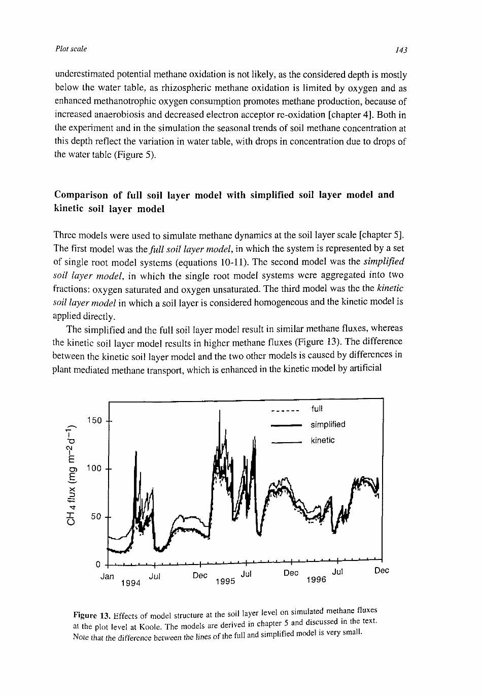
Plot scale 143
underestimated potential methane oxidation is not likely, as the considered depth is mostly below the water table, as rhizospheric methane oxidation is limited by oxygen and as enhanced methanotrophic oxygen consumption promotes methane production, because of increased anaerobiosis and decreased electron acceptor re-oxidation [chapter 4], Both in the experiment and in the simulation the seasonal trends of soil methane concentration at this depth reflect the variation in water table, with drops in concentration due to drops of the water table (Figure 5).
Comparison of full soil layer model with simplified soil layer model and kinetic soil layer model
Three models were used to simulate methane dynamics at the soil layer scale [chapter 5]. The first model was the full soil layer model, in which the system is represented by a set of single root model systems (equations 10-11). The second model was the simplified soil layer model, in which the single root model systems were aggregated into two fractions: oxygen saturated and oxygen unsaturated. The third model was the the kinetic soil layer model in which a soil layer is considered homogeneous and the kinetic model is applied directly.
The simplified and the full soil layer model result in similar methane fluxes, whereas the kinetic soil layer model results in higher methane fluxes (Figure 13). The difference between the kinetic soil layer model and the two other models is caused by differences in plant mediated methane transport, which is enhanced in the kinetic model by artificial
•o CM
i £ E x _D »*-
X o
150 --
100 --
50 --
0 Jan Dec
1994 1995 1996
Figure 13. Effects of model structure at the soil layer level on simulated methane fluxes at the plot level at Koole. The models are derived in chapter 5 and discussed in the text. Note that the difference between the lines of the full and simplified model is very small.

l44 Chapter 6
mixing [chapter 5]. Aeration and net methane production are almost the same for the three models (data not shown), because in all cases the aeration is mainly controlled by thewater content profile. In the studied case (Koole) roots contribute little to aeration, because the zone with a high root density (top soil) is often aerated via the water unsaturated soil matrix.
The differences in methane fluxes between the kinetic and the full model are small relative to the differences in methane fluxes between various values for dchr,cs a n d ^chr,rt (Figure 9e and f). Hence, the considered heterogeneities at the profile scale seem to be more important than the considered heterogeneities within a soil layer. The strong influence of these profile scale parameters can be understood in terms of their influence on the electron balance, via the oxygen input. With low values of dchr,cs and <ichr,rt the oxygen sink in the surface layers increases, which leads to a higher oxygen input into the system, as in the surface layers oxygen uptake is often not limited by oxygen transport. Moreover, fewer roots in deeper layers hamper methane export and increase methane oxidation (=oxygen input) when the water table drops.
Comparison with other models
Our comprehensive process model for methane fluxes from wetlands with gas transporting roots enables a discussion of the assumptions in other models from a process point of view. We will discuss other models in decreasing order of (spatial) detail.
Soil layer models
In soil layer models [Walter et al.9 1996; Arah and Stephen, 1998] the soil is divided in several layers to explicitly account for vertical gradients. Each soil layer is considered as homogeneous. The model of Arah and Stephen [1998] comes closest to our model, as they use both oxygen, methane and, in an extension, electron acceptors as state variables, whereas Walter et aLy [1996] use only methane as state variable. The omission of oxygen as state variable seems attractive as methane oxidation can be estimated as a fraction of emitted methane, using the frequently applied technique of specifically inhibiting methanotrophs. However, reported oxidation fractions are highly variable [Epp and Chanton, 1993; King, 1996; van der Nat and Middelburg, 1998b] and, furthermore, there may be methodological problems due to effects of the inhibitor on other processes than methane oxidation, directly [Frenzel and Bosse, 1996; Lombardi et al, 1997] or indirectly [chapter 4].
Our sensitivity analysis shows that the parameter!sation of a methane flux model is crucial for the model results. Arah and Stephen [1998] used a detailed set of experiments on methane production, methane oxidation and gas transport [Nedwell and Watson, 1995; Stephen et al, 1998] and one fit parameter to parameterise their model and succeeded well in describing methane fluxes for a short period (10 days) from the investigated,
Plot scale 145
permanently saturated, peat core. This success supports the soil layer approach. However it is still hard to transfer their model to other sites without the same amount of measurements, as laboratory methane production and oxidation rates are very hard to relate to environmental variables [Segers, 1998]. By contrast, Walter et al. [1996] parameterised their model with a set of assumed parameters, in combination with two fit parameters and dynamic soil methane concentrations and methane fluxes. With this method they achieved a close correspondence between simulated and measured methane fluxes. However, they analysed the sensitivity for only part of the assumed parameters and not all parameter values can be traced in their paper, which makes it hard to compare their model with ours.
Ecosystem models
In ecosystem models [Cao et al, 1996; Potter, 1997; Christensen et al, 1996] the soil is considered as a whole and vertical gradients in the soil are ignored or implicitly accounted for. In all these models methane production is connected somehow to net primary production (NPP), which enables extrapolation via NPP models.
From a process point of view one of the crucial factors in ecosystem models is the incorporation of the effect of water table. Both Cao et al [1996] and Potter [1997] multiply methane production with an empirical factor which decreases with lower water tables. Qualitatively this is reasonable, but quantitatively it is questionable whether a conservative relationship exists, as this relationship depends on the (depth distribution of) C-mineralisation and the presence of electron acceptors. For parametensat.on of the relation between water table and methane production data on the relation between water table and methane emission from the field [Cao et al, 1996] or cores [Potter, 1997] were used. This is rather crude, as in these emission data also methane oxidation and transport is included. Furthermore, in both papers the large variation in the relation between water table and methane emission is ignored.
In all ecosystems models methane is not present as state variable, implicitly assuming a small delay between methane production and emission (less than the time scale o interpretation). As the time scale of root mediated gas transport is typically larger than day [Stephen et al, 1998, Liblik et al, 1997, chapter 5] one has to be careful in interpreting these kind of models on daily basis.
Christensen et al. [1996] ignored water table effects and assumed that methane ITux was a fraction (3 ± 2%, based on literature) of aerobic respiration, the latter being, almo similar to net primary production on an annual basis. So, on an annual basis, the r mode basically comes down to a proportional relation between methane flux and simulated ne pnmary production. They also simulated monthly methane emissions, bj.assuming h they depend on temperature in the same way as aerobic respiration, but did not tes th, assumption, nor the simulated monthly methane fluxes. So, given present know,e^^ h model of Christensen et al [1996] may be suited for estimation of methane em.ssion
146 Chapter 6
over large areas on an annual time scale, but is not likely to represent the underlying processes.
Concluding remarks
In this paper we completed a thorough exercise in process modelling of methane fluxes from wetlands with gas transporting plants and a fluctuating water table. Four scales were connected in three steps: the kinetic scale, the single root scale, the soil layer scale and the plot scale. At all scales the factors that determine the total redox balance (carbon input -oxygen input) are crucial. These factors are scale dependent. For example, at the single root level, root oxygen release and carbon mineralisation are important and the total pool of electron acceptors is not so important, as it has only little influence on the oxygen input. However, at the plot scale the pool of re-oxidisable electron acceptors determines how much oxygen is captured after a drop of the water table, and, hence, may greatly influence methane fluxes.
The sensitivity analysis in this paper showed that current process knowledge is insufficient to mechanistically predict relations between methane fluxes and above ground vegetation, water table and temperature. For example, little is known about root gas transport capacities and the distribution of the various carbon pools over depth, while these factors have a large influence on methane fluxes. Furthermore, heterogeneities around gas transporting roots seem to be less important than vertical gradients in the soil column. This implies that averaging kinetic processes at the soil layer scale is sensible.
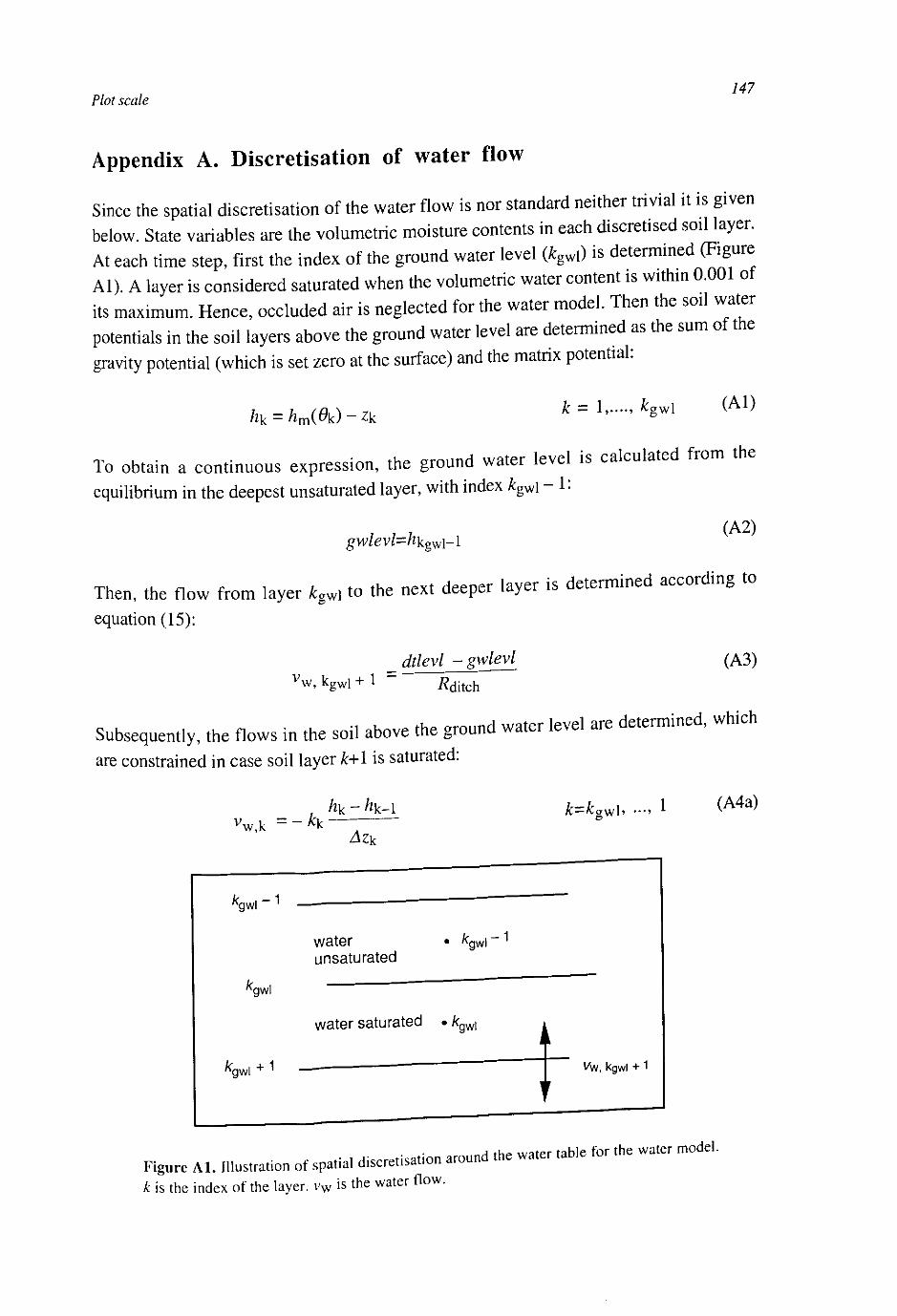
Plot scale 147
Appendix A. Discretisation of water flow
Since the spatial discretisation of the water flow is nor standard neither trivial it is given below. State variables are the volumetric moisture contents in each discretised sod layer. At each time step, first the index of the ground water level (*gwi) is determined (Figure Al). A layer is considered saturated when the volumetric water content is within 0.001 of its maximum. Hence, occluded air is neglected for the water model. Then the soil water potentials in the soil layers above the ground water level are determined as the sum of the gravity potential (which is set zero at the surface) and the matrix potential:
K = M#k) - k k — 1,...., Kgwl (Al)
To obtain a continuous expression, the ground water level is calculated from the
equilibrium in the deepest unsaturated layer, with index &gwl - 1:
(A2) gwlevl=hkgVj\-l
Then, the flow from layer *gw, to the next deeper layer is determined according to
equation (15):
v w, kgwi + 1
dtlevl -gwlevl
^ditch
(A3)
Subsequently, the flows in the soil above the ground water level are determined, which
are constrained in case soil layer k+l is saturated:
v w,k = - * k ftk - frk-1
^gwl " 1
water unsaturated
fgwi
^gwl + 1
• ^gwl 1
water saturated . /c( gwi
&=&gwl> •••» *
i
7 VW, kgwl + 1
(A4a)
Figure Al . Illustration of spatial discretisation
k is the index of the layer. vw is the water flow
around the water table for the water model.
148 Chapter 6
vw,k,max = vw,k+l - ^w,k M : in case 9k saturated (A4b)
Note that equations (A4) require that the calculations start at the deepest soil layer. Finally, the flow below the water table is calculated in such a way that the water contents below the water table are constant:
vw,k = vw,k-l + sw,k-l ^Zk-1 * = £gwl+l, ». % (A5)
Appendix B: Incorporation of profile scale transport processes in the single root models.
At the soil layer level it was assumed that gas exchange in water saturated soil only occurs via the plants and via ebullition [chapter 5]. However, at the plot scale also vertical diffusion and convection occurs. Especially just below the water table and in deep layers (with large distances between roots) this could be relevant. This vertical transport was incorporated in the model by adding an extra term, sjiXm, to the rate equations for the concentrations (equation 11) in each discretised soil layer k9 for each component i, in each single root model system m. sjiXm is equal to the discretised gradient of the flux density:
*Vi,k,m - ( B l )
The length scale of the structures within a discretised soil layer (a few mm in densely rooted top soil, a few cm in deeper soil) is smaller than the discretised soil layer thicknesses (a few cm in the top and a few dm deeper in the profile). Consequently, a point near a root does not preferentially exchanges gases or solutes with points near a root in the next upper or next deeper discretised soil layer. Therefore, and because diffusion and convection are linear with concentrations, it is assumed that the flux densities only depend on the averages of the next upper and next deeper discretised soil layer:
4,k,m = MAX(vWik, 0) caq.j.k.! + MIN(vWfk, 0) c a q , u , m - Dg ,e f f ,u C g.U.m - Cg,i,k-^
^ m , k (B2a)
Ak+l,m = MAX(vaq(k+1, 0) c a q M , m + MIN(vaq)k+1, 0) ^aq,i)k+1 -(B2b)
D « • , , cg^»k+1 ~^g,i,ktm x-'g,eff,i,k+l — s
^ P , k
149 Plot scale
Using equations (Bl - B2) the soil layer averaged component can be isolated by
introducing an apparent mixing term:
— ^i,k - ^i,k+l , c ., (= . _ ~.. ) (B3) SJiXm = + Smix,sj,i,k Kcuk ^iXm) *> J
Here, the first term represents ordinary, soil layer averaged, profile scale transport, which
is the same for all model systems m. The second term represents apparent mixing
between the single root model system within a discretised soil layer. From equations (BI
BS) mixing rate, £mix,sj,i,k, can be expressed with:
^ e f f j j c | ^g.eff.i.k+l)
_ ahk (- MIN(vaq,k,0) + MAX(vaq,k+bQ)l M __&zm± Az£k ( B 4 )
5 miX,SJ,i'k " ~" (%k + a u f l ^ k A^k <*g,k + «i,k ^w,k)
Here, the first term represents upwind discretised convection [Patankar, 1980], the
second discretised diffusion. At the boundaries, £mix,sj,i,k, is calculated in a similar way
resulting in slightly different expressions (not shown). The extra oxygen transport term
reduces the oxygen sink for the roots, resulting in adaptation of the expressions for the
dimensionless numbers p and K: [equations 45 and 53 in chapter 4].
*rt Ka cg,atm,02 h } / B 5) Six.
_ J r t (VaQ0) ^rcm-^02)rrt
_ 2 rrt <p"02 +_jQl_ cylinder (B6a)
Vae %;m (P2 ~ rrt2)
3 r r t V o 2 + SJ02 sphere (B6b)
Vae *rcm (^ - rrt )
In this way the other equations of the simplified single root model [chapter 4] remain
unchanged.
151
Chapter 7
General discussion
The aim of this thesis is to increase understanding of plot scale relations between methane fluxes and environmental variables. The approach taken contains two related aspects: 1. including knowledge at the kinetic level and 2. stepwise scaling up. First, both aspects will be addressed. Subsequently, the concept of an electron balance will be used to further analyse and integrate results and to facilitate discussion of this work with respect to large scale emissions estimates.
Including knowledge at the kinetic level
The inclusion of kinetic knowledge implies that the dynamics of various compounds (methane, oxygen, soil carbon, electron acceptors in oxidised and reduced status) are explicitly treated with chemical or microbiological knowledge obtained under homogeneous conditions. An alternative is a soil system approach in which methane production is directly related to carbon input [Christensen et al, 1996] and water table [Cao et al, 1996; Potter, 1997], and in which methane oxidation is a constant percentage of methane production [Cao et al, 1996; Walter et al, 1996, Potter, 1997]. The advantage of the soil system approach is that it is easier to use. However, the used relations are often empirical and originate from one or a few sites. Consequently, the reliability of extrapolations is hard to judge.
The kinetic approach is more complex, but the advantage is that dynamic and spatial aspects are included more mechanistically. Consequently, conclusions are more generally applicable and causes of uncertainty are revealed more explicitly. For example, from kinetic knowledge it followed that the relation between methane production and water table depends on water table history, C-mineralisation and alternative electron acceptors. As these factors will vary in time and in place a constant relation between water table and methane production is not likely, and can only be used for the conditions under which it has been measured.
Stepwise scaling up
Stepwise scaling up explicitly considers intermediate scales. The opposite would be to neglect spatial micro variation and to consider the soil as one box An > « d . a t e solution would be to consider the soil as a vertically stratified system. The introducuon, of these intermediate levels increases complexity, but the advantage is that accuracy of the
Segers. R. Wetland Methane Fluxes: Upscaling frotn Kinetics via a Single Root and a Soil Uyer to the
Plot, Ph. D. Thesis, Wageningen University, 1999.
152 Chapter 7
scaling up is improved [chapter 4] and that the sensitivities for smaller scale heterogeneities are made explicit.
Meso scale [Rappoldt, 1992] heterogeneities within a discretised soil layer caused by gas transporting roots are of relatively little importance (chapter 6), as ignoring these heterogeneities resulted in small changes in simulated methane fluxes, compared to the changes in methane fluxes upon variation in several uncertain parameters. This is in contrast with the macro scale heterogeneities between different soil layers, as shown by the sensitivity to characteristic depths of soil carbon mineralisation and rooting depth (chapter 6). Below, the causes of different sensitivity of heterogeneities at different scales will be discussed using the concept of an electron donor/acceptor balance.
The sensitivity to heterogeneities between soil layers and the relative insensitivity to heterogeneities within soil layers support process modelling to start at this scale [Walter etal, 1996; Arah and Stephen, 1998]. Sub soil layer heterogeneities in C-mineralisation, in potential methane oxidation and in root gas transport capacity were not investigated yet and may influence the methane dynamics at the soil layer scale. So, one still has to be careful in using kinetic knowledge directly at the soil layer scale.
Unifying concept: electron donor/acceptor balance
The formulated models for methane fluxes comprise many processes at various scales. Therefore, also simplified models were developed at intermediate scales. Here, the concept for a summary model at the plot level is introduced; As all soil reactions governing methane emissions are redox reactions, methane fluxes can be obtained from an electron (e.) donor/ acceptor balance over the soil:
CH4 emission = e. donor input - e. acceptor input - rate of change in stored e. donor + rate of change in stored e. acceptor - rate of change in stored CH4 (1)
Here, 1 mol CH4 corresponds to 8 electron equivalents. Excluding particulate soil carbon from the soil system, the e. donor input is carbon mineralisation and root exudation. The e. acceptor input is mainly oxygen, e. donor output, in the form of leached dissolved carbon, is neglected. The increase in stored electron donors, the third RHS term, could be accumulation of intermediates such as acetate. In chapters 4 to 6 it is assumed that this term is zero. The increase in stored electron acceptors could be re-oxidation of reduced electron acceptors, as oxygen itself probably does not accumulate, because of its fast consumption rates. The advantage of equation (1) above the more conventional methane balance (methane production, methane consumption and methane storage [Roulet and Reeburgh, 1993] is that it is closer to the environmental variables at the plot scale.
Any process model can be evaluated in terms of its capability of simulating each of the terms in equation (1). For example, the inclusion of intermediates in the anaerobic degradation chain is only needed if their net accumulation is equal or larger than the
153 General discussion
methane emission. Or, it does not matter whether depletion of Fe3+ suppresses net methane emission by anaerobic methane oxidation [Cicerone and Oremland, 1988], by iron reduction/sulphide oxidation [Elsgaard and J0rgensen, 1992] followed by sulphate reduction/acetate oxidation [Zehnder and Stumm, 1988], or by iron reduction/acetate
oxidation [Zehnder and Stumm, 1988]. The electron balance can also be used to understand why heterogeneities at the sub
soil layer scale seem to have relatively little influence on methane fluxes. Ignoring the heterogeneities is equivalent to using the kinetic soil layer model (chapter 5). This leads to a complete elimination of the few situations that the roots experience an oxygen saturated soil and hence this leads to only a small difference in simulated oxygen input (Figure 3a in chapter 5), especially when root oxygen release is small compared to total C-mineralisation. Due to the small effect on aeration, also the C-mineralisation is little affected by ignoring heterogeneities at the sub soil layer scale. The largest effect of ignoring these heterogeneities is the enhanced gas transport via the plants, because methane in dead zones is artificially mixed (Figure 3c in chapter 5). This leads to a more negative rate of change in stored methane (equation 1) and hence to higher methane emission (Figure 13 in Chapter 6). In addition, less methane will be stored in the so 1 and be available for extra oxygen input by methane oxidation after drops of the wa er tab e However, these transient effects are small when compared to the effects ofpro fik.scale heterogeneities, such as the different profile of C-availability, which constantly effects the oxygen input in the gas-continuous top soil.
At longer time scales (a few days in top soil in summer, about a year in d p so D the
last three terms of the electron balance (equation 1) will be small compared to the first two
terms. Therefore, and because climate change issues ultimately concern large time scales,
it is most crucial to study the first two terms:
e. donor input = aerobic carbon mineralisation + anaerobic carbon mineralisation + root exudation
e. acceptor input = aerobic respiration + methane oxidation + ^ electron acceptor re-oxidation
Assuming that all aerobically mineralised carbon is used for aerobic respiration this leads
with equation (1) to:
C H 4 emission = anaerobic carbon mineralisation + roo, exudates no,,oxidised by 0 2
- 0 2 used for methane oxtdation - 0 2 used for electron acceptor re-ox,d,,,on
Anaerobic carbon mineraiisation is determined by < " ^ < ^ Z ? ^ anaerobic conditions. As t r a d a b l e carbon tsrno* * £ £ ^ £ £ ( L j b | i k a
explains why methane emissions are often sensmve to the aver g
« , , w N y k a „ e „ « « , » * : : : : * : i ; : : ; : „, j « ^ methane emissions, because of a decrease in SLUIC

/54 Chapter 7
time scales drops in water table will reduce methane emission, because each time it is lowered, re-oxidation of electron acceptors and methane oxidation may consume a lot of oxygen (equation 3). However, it cannot be concluded that variation in water table reduces average methane emission, because of the often non-linear variation of carbon availability with depth.
The effect of root gas transport on the long term electron balance is ambiguous. On the one hand, root gas transport increases oxygen input in the system, which can be used for methane oxidation and electron acceptor re-oxidation. On the other hand, it may serve as a bypass for produced methane, avoiding methane oxidation, especially during a draw down of the water table, as rhizospheric methane oxidation is often oxygen limited (chapter 4).
For predicting large scale methane emission, it can be related to the driver of carbon mineralisation: net primary production [Whiting and Chanton, 1993]. Within the framework of the electron balance this connection can be made by including particulate soil carbon in the system, which leads, for larger time scales, to:
CH4 emission + C-accumulation = net primary production - O2 input (4)
From equation (4) it is evident that, at large time scales, both CH4 emissions and C accumulation are the result of the same balance. As the terms at the left hand side (LHS) are typically much less than net primary production [e. g. Christensen et ah, 1996] the O2 input will be almost the same as the net primary production. Consequently, the terms at the right hand side should be known accurately to be able to quantify the left hand side. Equation (4) also highlights why carbon accumulation (peat formation) and high CH4 emission often occur in similar systems: wet soils in which O2 input is hampered. However, the partitioning between the two factors at the LHS is not constant, as fens often have a higher CH4 emission than bogs [Nykanen, 1998; Moore and Knowles, 1990, Bellisario et aL, 1999], but a lower carbon accumulation rate [Tolonen and Turunen, 1996]. It is not possible to understand this partitioning with the simple anaerobic mineralisation model (a fixed fraction (0.4) of aerobic C-mineralisation) used in this thesis (chapter 4). Probably, the more resistant character of bog peat has to be accounted for.
Methane emission at large spatial and time scales
For the questions concerning policy and global climate it is not strictly needed to understand the relations between methane fluxes and environmental variables. It is needed to be able to predict methane fluxes from environmental variables, as with predictive knowledge it is possible to obtain more reliable emission estimates over large areas, at present, in the past and in the future. In chapter 1 it was argued that current regression models for the relations between methane fluxes and environmental variables are of
155 General discussion
limited predictive value, because they are site specific and contain large undescribed variability, and in chapter 2 and 6 it was argued that other process models require either site specific calibration or intensive site specific soil sampling. With a d « * use of he process model from this thesis it is not possible to obtain better predictions Firs ly because sensitivity analysis shows that methane fluxes are sensitive for quite ai mHnberof not well known parameters [Chapter 6] and secondly, because simulated season pattern in methane fluxes differ from measured seasonal patterns. However, the aim of the mode was not to predict methane fluxes, but to increase understanding of * ° processes at the kinetic level. The use of this understanding in view of predictive models
is discussed below. A1 . n ™ p n t Given the large uncertainty in sensitive process parameters chapter 6 ^ t F sent
models predicting methane emissions should be calibrated and tested.vntom ha emission data. The models should have few parameters which are simu t neou y uncertain and sensitive. Hence, the global application of the model o f O n e « ^ probably not very reliable. Furthermore, to allow extrapolations, the m a m P r s should be caught As the terms representing changes in storage in equat.n 1) a sensitive to several uncertain parameters, predictive modes may * m ^ ^ ™ operating at a time scale larger than these changes (probably a month or season), thoug this requires long term field data for calibration and testing
Starting from equation (3), anaerobic carbon mineralisation ^ ^ ^ ^ methane oxidation and electron acceptor re-oxidation have to be q u a ^ ; ^ carbon m.neralisation depends on the w a t e r ^ b . . so• ^ ^ » m a i n l y
distribution of the available carbon over depth. Soil carbon i ] a b l e
determined by primary production. Assuming that the ^ ^ ^ I Z n be carbon is onfy influenced by the water table, anaerobic ^ Z T a Z Z ^ o r related to water table and net primary production. Methane o » ^ ^ ° ^ re-oxidation depend on vegetation (for plant mediated oxygen input) fluctuations, leading to:
, M a~A H P P . /(time averaged water table) time averaged methane emission = time ™™^ * w a t e r t a b l e fluctuations) (5) - time averaged NPP -/(vegetation type) -/(time average
where/are arb.trary functions, with one or ^ ^ ^ ^ ^ Z ^ the last two terms are not important or cannot be deduced
case, the best solution would be to omit the terms. „ e r i _. t e s the best method is So, currently, for large scale wetland methane emission — * ; ^
to develop .argely descnptive models « ^ » ^ " j S n g up from the kinetic to scale up from the plot to the region. This may ^ ^ ^ ^ p r e s e n t ,„ scale to the plot scale, as spatial process interactions a g ^ ^ ^ . ^ ^ ^ jn
water dynamics. However, optimal use of possibly corr^ ^ ^ ^ ^ submitted\.
combination with a non-linear model is far from m™l , flux estimates. A. presen, ,« ,s „„• c,e, r *» W - U - — ^ n c e r t a i n l y ,„ OT,ss,on
Therefore, the development and use of formal memo
156 Chapter 7
estimates would be useful. In that way it would be possible to re-asses the global methane upscaling estimates of Bartlett et al. [1993] and to have maximum benefit from comparison [Denier van der Gon et al, submitted] of upscaling estimates with estimates obtained from inverse atmospheric modelling [Fung et al, 1991; Hein et al, 1997].
In the long run process research on various topics may help to obtain more explanatory, predictive plot scale relations between wetland methane fluxes and environmental variables. Results from this thesis may help to focus this research. The first question to be adresssed is whether it is possible to develop a simplified process model at large time scales. Starting point could be equation (3). To obtain a process based implementation of this equation the following questions need to be answered: Are the events of water table drops important in terms of the total oxygen consumed for electron acceptor re-oxidation and methane oxidation? How important is root oxygen release and root exudation? What is the distribution of C-availability over depth in various wetlands soils?
If it turns out to be hard to develop a process model for large time scales, it is necessary to go back to the short time scales. Then, all sensitive uncertainties in the process model of chapter 6 have to be addressed: 1. identification of alternative electron acceptors (chapter 3), 2. a dynamic model for methanotrophic biomass, to explain variation in potential methane oxidation (chapter 2), 3. measuring effective diffusion coefficients in various peat types, 4. distribution over depth of C-mineralisation and roots, 5. root gas transport properties as function of plant type and season, 6. root exudation [Wieder and Yavitt, 1994; Wieder et al, in prep.], 7. limitations of methanogens at low temperatures.
Concluding remarks
The sensitivity analysis in chapter 6 showed that it will be hard to develop explanatory, predictive models for methane fluxes, but further progress in that direction can be made by focused experiments followed by further model development. Presently, the best method for predicting methane emissions from environmental variables is to use simple, calibrated, models that relate methane fluxes to water table, primary production and possibly vegetation type. The sensitivity of the change in storage terms of the electron balance (equation 1) for several uncertain processes (chapter 6) suggests that the most reliable relations can be obtained at large time scales.
In this thesis an explicit connection was made between biogeochemical processes at the kinetic scale, in which microbiological and chemical laws apply, and the plot scale, at which fluxes are measured. This was accomplished by introducing two intermediate levels of scale, the single root level and the soil layer level and by formulating a coherent set of models to connect the scales. In this way the influence on methane fluxes of all kinds of processes between the kinetic and the plot scale could be quantitatively analysed.

157
Samenvatting
Inleiding
De concentratie van methaan in de atmosfeer is de afgelopen eeuw verdubbeld Daarmee draagt methaan ongeveer 15% bij aan het veronderstelde versterkte broeikaseffect. Bodems zijn zowel een belangrijke bron als een belangrijke put voor methaan. Methaanemissies uit bodems zijn het resultaat van methaanproduktie, methaanconsumpt.e en methaantransport. Methaanproduktie is een microbiologisch proces wat kan optreden wanneer organische stof wordt afgebroken onder anaerobe omstandigheden en wanneer er geen of weinig alternatieve electron acceptoren voorhanden zijn. Methaanconsumpt.e ook een microbiologisch process wat in zoetwatersystemen een aeroob proces is. Gas (zuurstof) transport in natte bodems ('wetlands') is veel langzamer dan in met natte bodems. Natte bodems zijn daarom vaak anaeroob en niet natte bodems vaak aerooK Dit verklaart waarom natte bodems meestal methaan uitstoten en droge bodems methaan
De variatie in gemeten methaanfluxen is vaak groot en slecht begrepen. Daarom is n 1993 het geintegreerde CH4 grasland project gestart. Dit project bestond u vier deelprojecten. In de eerste twee deelprojecten zijn de microbiologische aspecten van methaanproduktie en methaanconsumptie onderzocht. In het derde project zyn methaanfluxen gemeten in het veld, tezamen met belangrijke ° ^ ^ v ™ ^ m ™ proefschrift beschrijft het vierde deelproject, welk tot doel had het verkla «^ van methaanfluxen vanuit de (basis)processen. In het geintegreerde CH* & f ^ ^ twee Nederlandse bodems bestudeerd: een gedraineerde veengrond (pro f t , ^ R.O.C. Zegveld) en een natuurlijke veengrond (Nieuwkoopse Plassen). In het b ^ g ™ het projec werd verondersteld dat beide gronden een belangnjke b r » vanm h an zouden kunnen zijn. Echter, al gauw bleek uit metingen dat de onderzoch* 6 * ^ £ veengraslanden geen methaan uitstoten, maar eerder een heel klein ^ ° ^ ^ literatuur bleek dit ook het geval was voor gedraineerde veengraslande n and*lan*m Dat was een belangrijke reden om het onderzoek in dit vierde deelproject geheel te op het begrijpen van de methaanemissies uit natte bodems Plantenwortels
Planten spelen een speciale rol bij methaanem.ssies uit natte bodems. .v hebben zuurstof nodig om te overleven en om de anaerobe vorming ™™£%Z tegen te gaan. Zuurstof kan nauwehjks worden * ^ ™ ™ £ ^ L t bodemmatrix. Daarom kunnen vele waterplanten (zoals net z e g g e n J aanpassen (o.a. door de vorming van aerenchym), zodat ze via de p n ^ « ^
de atmosfeer naar de wortei en ^ ^ ^ 2 ^ ^ ™ via een negatieve invloed op methaanem.ssie via een remm g ^ . ^ ^
stimulans van methaanoxidatie en ^ ™ * C C ^ ° * ^ O p deze manier hebben zuurstof de bodem mkomt, kan ^ ^ ^ S ^ - i - ^amaast gastransporterende waterplanten een positieve inv.u v
S,n,„., « «*,„ n«:»-"«/«» — » - ' SUt" "~"""' " """" "" Plot, Ph. D. Thesis, Wageningen University, 1999.
158
kunnen ze de methaanemissies ook positief bei'nvloeden door het uitscheiden van koolstofexudaten of door het afsterven van plantenresten. Beide processen stimuleren de methaanproduktie en de zuurstofconsumptie en remmen daardoor weer de methaanoxidatie. Kortom, het effect van planten is complex doordat er vele interacterende processen tegelijk spelen. In zo'n situatie is een mathematisch procesmodel een geschikt onderzoeksinstrument. Dit was een tweede reden om het theoretisch procesonderzoek geheel te richten op natte bodems.
Methaanemissies uit natte bodems zijn vaak gecorreleerd aan allerlei omgevingsvariabelen, zoals de grondwaterspiegel, de temperatuur, de samenstelling van het veen, de vegetatie en de netto primaire produktie. Echter, de correlatiecoefficienten zijn vaak laag en het is meestal lastig om te beoordelen in hoeverre de gevonden correlatieve verbanden geextrapoleerd kunnen worden. Om de verbanden tussen methaanemissies en omgevingsvariabelen te begrijpen zijn stabiele relaties nodig, welke gevonden kunnen worden in de theorien van microbiologische en chemische omzettingen en van fysische transportverschijnselen. Deze theorien zijn van toepassing in homogene systemen terwijl bodems heterogeen zijn. Echter, op kleine schaal, als de menging door transport sneller is dan de omzettingen, kan de bodem homogeen verondersteld worden. Voor de omzettingen en transportprocessen welke van belang zijn voor methaanemissies is deze schaal ongeveer 1 mm.
De afstanden tussen de wortels van planten is vaak ongeveer 1 cm, Dit betekent dat de heterogeniteiten in bodem welke veroorzaakt worden door gastransportende planten belangrijk kunnen zijn. Ook op de bodemprofielschaal kunnen belangrijke heterogeniteiten ontstaan als gevolg van de interactie tussen de waterspiegel en de met de diepte afnemende beschikbaarheid van organisch materiaal. Om deze heterogeniteiten expliciet mee te kunnen nemen werd in dit proefschrift een stapsgewijze opschalingsprocedure gehanteerd. Achtereenvolgens werden beschouwd: de schaal van de kinetiek, de schaal van een enkelvoudige wortel, de schaal van een bodemlaag en de schaal van een plot.
De schaal van de kinetiek
Uit integratie van literatuurgegevens volgde dat de correlaties tussen laboratorium-snelheden van methaanproduktie en -consumptie en omgevingsvariabelen zwak zijn. Om netto methaanproduktie te koppelen aan omgevingsvariabelen is het dus noodzakelijk om de onderliggende processen te beschouwen. De aan omgevingsvariabelen gerelateeerde drijvende krachten achter netto methaanproduktie op kinetische schaal zijn de koolstofmineralisatie en aeratie. Alle processen die de relatie tussen netto methaanproduktie en deze drijvende krachten bepalen dienen te worden meegenomen. Reductie van electronacceptoren en re-oxidatie van gereduceerde electronacceptoren (zoals Fe3+/Fe2+ of S042~/S2~) kunnen een belangrijk deel van gemineraliseerd koolstof of

159 Samenvatting
beschikbaar zuurstof consumeren. Deze processen zijn dus belangrijk voor het begrijpen van de relatie tussen methaanfluxen en omgevingsvariabelen.
Anaerobe incubatieproeven van een van de partners in het geintegreerde CH4 grasland project lieten zien dat methanogenese en de reductie van anorganische electronacceptoren (NO3-, Mn4+, Fe3+ en SO42-) niet de geproduceerde hoeveelheid C02 kunnen verklaren. Daarom zou in veengronden organisch materiaal kunnen optreden als electronacceptor. Deze suggestie werd ondersteund door een Amerikaanse groep, die aantoonde dat humuszuren als electronacceptor op kunnen treden en dat er micro-organismen zijn die kunnen groeien op acetaat en humuszuren als enig electrondonor/acceptor koppel. Omdat electronacceptoren belangrijk zijn, maar omdat vaak niet bekend is welke electronacceptor in welke hoeveelheid aanwezig is, werd voor het model uitgegaan van een willekeunge, niet nader gespecificeerde, electronacceptor, wiens reductie methanogenese onderdrukt. Naast methaanproduktie, methaanconsumptie, electronacceptor reductie en re-oxidatie werd 00k heterotrofe respiratie beschouwd, vanwege de belangrijke rol in de zuurstof- en koolstofhuishouding.
De schaal van een enkelvoudige wortel
De bodem rondom een wortel werd gerepresenteerd door een holle oneindige lange cilinder of door een holle bol. Het binnenoppervlak stelde dan het gas-transporterende worteloppervlak voor wat in verbinding staat met de atmosfeer. Het buitenoppervlak lag op de halve afstand tot de volgende wortel. De twee geometries representee twee uiterste aannamen over de fractie van het worteloppervlak dat actief is in gastransport. De cylindrische geometrie stelt een situatie voor waarbij de hele wortel actief is en de bolvormige geometrie stelt een situatie voor waarbij alleen de wortelpunt actief is. De gasuitwisseling bij het worteloppervlak werd beschreven met een le orde v e n d i n g -Als gevolg van deze gasuitwisseling ontstaan gradienten in concentnjt.es rondom, een wortel, welke leiden tot diffusie. Een geintegreerde beschouwing van het g e h e sy tern werd verkregen door middel van een stelsel gekoppelde reactie-diffusievergehjkrogen voor methaan, zuurstof, koolstofdioxide en stikstof (N2) en een ^ " ^ ^ J geoxideerde en gereduceerde toestand. Koolstofdioxide en stikstof werfe ^ook meegenomen, omdat deze stoffen een rol spelen bij de vorming van ^ l e r u w e l t e berekend werd uit het simultane gas-vloeistof evenwicht ^ f ^ T ^ Z verder weinig van bekend is, werd de ontsnapsnelheid van de bellen beschreven met
empirische relatie met het belvolume. ^^nWeliiken Om het begrip van het systeem te vergroten en om het opscha en te - ^ k k
werd de wiskundige beschrijving van het systeem vereenvoudigd op ba.s va « h u n de relatieve snelheden van de verschillende processen. ^ { « ™ ^ a ™ * ™ _ proces. Daarom werd de t o e s t a n d s v e r g e ^ n g J ^ ^ ^ Z ^ en steady state vergelijking. De converses van de andere stotten zij d
daarom werd aangenomen dat hun concentraties homogeen zijn. Een uitzondenng w
160
hierbij gemaakt voor het transportproces naar de wortel toe, omdat de transportweerstand rondom een kleine wortelpunt belangrijk kan zijn.
De aannames voor het vereenvoudigde model werden getest door simulatieresultaten te vergelijken met simulatieresultaten van het niet vereenvoudigde model. De verschillen tussen beide simulaties waren zeer gering, wat betekende dat het vereenvoudigde model geschikt was om verder te gebruiken in de opschalingsprocedure.
De schaal van een bodemlaag
Een bodemlaag werd gedefinieerd als een laag in de bodem met homogene macroscopische eigenschappen zoals watergehalte, temperatuur, worteldichtheid en C-mineralisatie. Dit is dus een andere definitie dan zoals die vaak in de bodemkunde wordt gehanteerd waarbij men uitgaat van min of meer statische bodemeigenschappen, zoals textuur of organisch stof gehalte. In eerste instantie werden alleen waterverzadigde bodemlagen bekeken, om zo alle aandacht te richten op de interactie van de processen met de wortels.
Een bewortelde bodemlaag werd gerepresenteerd door een gewogen verzameling van enkelvoudige wortelsystemen welke verschillen in halve afstand tot de volgende wortel. Deze gewichten werden zodanig gekozen dat de kansdichtheidsverdeling van de afstand tot de dichtsbijzijnde wortel van de verzameling gelijk is aan dezelfde verdeling van het werkelijke wortelsystem, beschreven door een aantal wortelarchictectuur parameters. De gedachtenhang achter deze al bestaande methode is dat in systemen waar diffusie belangrijk is vooral deze afstanden van belang zijn en niet de exacte geometric
In analogie met het vorige schaalniveau werden ook vereenvoudigde modellen op bodemlaagniveau afgeleid en getest, met als toestandvariabelen concentraties gemiddeld over een bodemlaag. Het effect van deze vereenvoudigingen was een wat hogere methaantransportsnelheid via de plant en een wat lagere methaanproduktie. Het totale effect op de methaanemissies was daardoor vrij klein. Dit betekent dat de vereenvoudigde modellen op een hoger schaalnivau gebruikt konden worden, mits tevens getest ten opzichte van het originele, niet vereenvoudigde model.
Variatie van worteldichtheid liet zien dat de methaanemissie evenredig is met de worteldichtheid als aangenomen wordt dat de koolstofmineralisatie evenredig is met de worteldichtheid en mits de beschouwde tijdschaal langer is dan de tijdschaal van electron acceptor reductie en de tijdschaal van methaanemissie via de plant. Het effect van variaties in de wortelgastransportcoefficient op gesimuleerde methaanemissies was divers. Soms was er nauwelijks een effect, soms nemen de emissies toe en soms nemen ze af. Het was dus onmogelijk om algemene uitspraken te doen over de effecten van gastransport door de wortels op methaanemissies.
Samenvatting
De schaal van een plot
Op dit schaalniveau spelen naast de dynamica van de gassen en opgeloste stoffen ook de water en temperatuurhuishouding een belangrijke rol. De waterhuishouding werd gemodelleerd met Richards' vergelijking. Voor temperatuur werd een standaard diffusievergelijking gebruikt. Binnen een bodemlaag werden de dynamica van de gassen en opgeloste stoffen gesimuleerd zoals hierboven beschreven. Transport tussen de bodemlagen werd beschreven door middel van diffusie en convectie.
Het model werd toegepast voor een laagveen in Nederland. Gesimuleerde methaanemissies waren van dezelfde ordegrootte als gemeten methaanemissies. De gemeten seizoensdynamiek in methaanfluxen was echter sterker dan de gesimuleerde. Oorzaken voor deze discrepantie is waarschijnlijk het ontbreken van emge seizoensdynamiek in de gemodelleerde vegetatie en mogelijk ook de limitatie van methaanproduktie door methanogene aktiviteit bij lage temperaturen welke limitatie met in
het model was opgenomen. Gesimuleerde methaanfluxen waren gevoelig voor een groot aantal onzekere
parameters, zoals de verdeling van koolstofmineralisatie over de diepte, de som van de aanwezige electronacceptoren en gereduceerde electronacceptoren en de wortel-spruitverhouding van de aanwezige vegetatie. Vanwege het procesmatige karakter van het model zijn deze gevoeligheden waarschijnlijk ook aanwezig in de praktijk, wat een verklaring is voor de grote lastig verklaarbare variatie in methaanfluxen, zoals die vaak
gemeten is. , Het bodemlaag model waarin heterogeniteiten binnen een bodemlaag werden
genegeerd resulteerde in hogere methaanfluxen dan het bodemlaagmodel waarin deze heterogeniteiten werden meegenomen. Echter, de verschillen tussen de bodemlaagmodellen waren klein vergeleken met de gevoeligheden voor parameters die de heterogeniteiten tussen bodemlagen karakteriseren. Een verklaring hiervoor>da heterogeniteiten op profielschaal een groter invloed hebben op de zuurstof input in systeem dan heterogeniteiten binnen een bodemlaag.
Algemene discussie
Het doe. van dit proefschrift was het verklaren van de relatie tussen ° ^ n * ^ ^ en methaanfluxen De gebmikte methode bevatte twee, met elkaar verbonden kernpurnem ten eerste het gebruik van theorien op kinetisch niveau en ten tweed h e » ^ g ^ oPscha.en. Het gebruik van theorien op kinetisch niveau had t o t g e v o ^ gedaan konden worden zonder al te afhankelijk te zijn van p l a a s - ^ ^ waamemingen. Oorzaken van onzekerheden kwamen ^ f ^ ^ l T L de stapsgewi, opscnalen ^ £ ^ % Z ^ ^ * *
verschUlende schaalniveau's doorwerken in methaanfluxen en hoe
162
verantwoorde wijze vereenvoudigd kan worden zonder verlies van verklarende en andere functionele eigenschappen.
De geformuleerde modellen zijn over het algemeen vrij complex. Omdat alle omzettingen redox-reacties zijn, kan een electronenbalans helpen om de modellen op verschillende niveau's te analyseren. Voordeel van het gebruik van electronenbalans boven een analyse in termen van methaanproduktie, methaanconsumptie en methaantransport is dat de electronenbalans dichter aangrijpt op de drijvende krachten op plot schaal.
Uit de electronenbalans op plotschaal blijkt dat methaanemissies het resultaat zijn van electrondonor input min de electronacceptor input en de veranderingen in de bodemvoorraden aan electrondonoren, electronacceptoren en methaan. Als vast koolstof niet wordt meegenomen in het systeem dan is de belangrijkste electrondonor input koolstofmineralisatie en de belangrijkste electronacceptor input zuurstof.
Gevoeligheden van gesimuleerde methaanfluxen voor modelstructuur of modelparameters kunnen begrepen worden in termen van hun invloed op de koolstofmineralisatie en de zuurstof input. Zo leidt bijvoorbeeld een verschuiving van afbreekbaar koolstof naar het bodemoppervlak tot een flinke lagere methaanemissie, omdat zo de zuurstofpname wordt gestimuleerd, daar deze in het bovenste, meestal wateronverzadigde gedeelte van de bodem minder wordt geremd door transport.
Op kortere tijdschalen (uren tot maanden) kunnen de veranderingen in bodemvoorraden van electrondonoren, electronacceptoren en methaan belangrijk zijn. De simulaties lieten echterzien dat deze veranderingen lastig te voorspellen zijn. Daarom lijkt het beter om te streven naar simulatiemodellen welke opereren op een grote tijdschaal. Gezien de grote onzekerheid in proceskennis is het daarbij verstandig om voor voorspellende studies deze modellen te calibreren met methaanemissiegegevens, wat impliceert dat de gebruikte modellen tevens weinig onzekere parameters of aannames dienen te bevatten.
Samenvattend, in dit proefschrift een expliciet verband gelegd tussen processen op kinetisch, enkelvoudige wortel- en bodemlaagschaal en methaanfluxen op plotschaal. Daarmee is duidelijk geworden wat de kennis op deze schaalniveau's betekent voor het begrijpen van methaanfluxen.

163
References
Achtnich C , F. Bak, and R. Conrad, Competition for electron donors among nitrate reducers, ferric iron reducers, sulphate reducers, and methanogens in anoxic paddy soil, Biol. Fertil. Soils, 19, 65-72, 1995.
Amaral J. A., and R. Knowles, Methane metabolism in a temperate swamp, Appl. Environ. Microbiol., 60, 3945-3951, 1994.
Arah, J. R. M., and K. D. Stephen, A model of the processes leading to methane emission from peatland, Atmos. Environ., 32, 3257-3264, 1998.
Armstrong, W., The oxidizing activity of roots in waterlogged soils, Physiologia Planatarum, 20, 920-
926, 1967. Armstrong, W., Aeration in higher plants, in Advances in Botanical Research, edited by H. W.
Woolhouse, pp. 225-332, Academic Press, London, 1979. Armstrong, W., and P. M. Beckett, Internal aeration and the development of stelar anoxia in submerged
roots, New Phytol., 105, 221-245, 1987. Armstrong, W., J. Armstrong, and P. M. Beckett, Measurement and modelling oxygen release from roots
of Phragmites Australis, in The Use of Constructed Wetland in Water Pollution Control, edited by P.
Cooper, pp. 41-51, Pergamon, Oxford, 1990. Armstrong, J., W. Armstrong, and P.M. Beckett, Phragmites australis: Venturi- and humidity-induced
pressure flows enhance rhizome aeration and rhizosphere oxidation, New Phytol., 120, 197-207, 1992. Armstrong, J., W. Armstrong, P. M. Beckett, J. E. Haider, S. Lythe, R. Holt, and A. Sinclair, Pathways
of aeration and the mechanisms and beneficial effects of humidity- and Venturi-induced convections in Phragmites australis (Cav.) Trin. ex Steud., Aquat. Bot., 54, 177-197, 1996.
Bachoon, D., and R. D. Jones, Potential rates of methanogenesis in sawgrass marshes with peat and marl soils in the Everglades, Soil Biol. Biochem., 24, 21-27, 1992.
Baldwin, J. P., P. H. Nye., P. B. Tinker, Uptake of solutes by multiple root systems from soil. 111. A model for calculating the solute uptake by a randomly dispersed root system developing in a Unite
volume soil, Plant Soil, 38, 621-635, 1973. , T w w , i \K *U - fi..v Bartlett, K. B., P. M. Crill, D. I. Sebacher, R. C. Harris, J. O. Wilson, and J. M Melack, Methane flux
from the central Amazonian floodplain, J. Geophys. Res., 93, 1571-1582, 1988. Bartlett, K. B., and R. C. Harris, Review and assessment of methane emissions from wetlands,
Chemosphere, 26,261-320, 1993. t , . . . „ * Beckett, P.M., W. Armstrong, S. H. F. W. Justin, and J. Armstrong, On ^ ^ " ^ ^ ° f
convective and diffusive gas-flows in plant aeration, New Phytol., 110, 463-4b», i y 5 ° ; Behaeghe, T. J., De seizoensvariatie in de grasgroei, in Dutch, Fakulteit van ^ ^ ^ ^ L ^
Laboratorium voor Landbouwplantenteelt en Herbologie, Rijksumversiteit Gent, Be g urn £ / * . Bellisario, L. M., J. L. Bubier, T R. Moore, and J. P. Chanton, Controls on CH4 emissions from a
northern peatland, Global Biogeochem. Cycles, 13, 81-91, 1999. f r r o n D e d
Belmans, C. J. G. Wesseling, and R. A. Feddes, Simulation model of the water balance of a cropped
soil: SWATRE, J. Hydrol., 63, 271-286, 1983. Qmhient , i r and or Bender, M., and R. Conrad, Kinetics of methane oxidation in oxic soils exposed to ambient air and
high CH4 mixing ratios, FEMS Microbiol. Ecol., 101, 261-270 1992. Q p d i m e n t s . Bender, M., and R. Conrad, Methane oxidation activity in various soils and tehw^ s e d —
occurrence, characteristics, vertical profiles, and distribution on grain size fractions, J. Geopnys
B ^ S ^ T c S . Effects of the CH4 concentrations and soil conditions on the induction of
CH4 oxidation activity, Soil. Biol. Biochem, 27, 1517-1527, 1995. Bernard, J. M., and K. Fiala, Distribution and standing crop of living and dead roots in three wetland
Carex species, Bulletin of the Torrey Botanical Club, 113 1-5, 19M>. . . A t
Bernard, J M., D. Solander, and J. Kvet, Production and nutrient dynamics in Carex wetlands, Aq
Bot., 30, 125-147, 1988. . rtWnlnffira| actjvitv Soil Sci. Soc. Am. Bhaumik, H. D., and F. E. Clark, Soil moisture tension and m.crobiolog.cal activity,
Proc, 12,234-238, 1947. n, ^MQ 7 o 0 nn Wilev New York, Bird, R. B., W. E. Stewart, and E. N. Lightfoot, Transport Phenomena, 780 pp., Wiley, Ne
1 9 6 0 ' rt MVP kinetics of Pseudomonas chlorororaphis grown Bodelier, P. L. E., and Laanbroek, H. J., Oxygen uptake kinetic\o\ rse ^ m _ ^ m i
in glucose- or glutamate-limited continuous cultures, Arch. Mic
164
Boeckx P., and O. van Cleemput, Methane oxidation in a neutral landfill cover soil: Influence of moisture content, temperature, and nitrogen-turnover, J. Environ. Quality, 25, 178-183, 1996.
Boelter, D. H., Physical properties of peats as related to degree of decomposition, Soil Sci. Soc. Am. Proc, 33, 606-609, 1969.
Bouma, T. J., A. G. M. Broekhuysen, and B. W. Veen, Analysis of root respiration of Solanum tuberosum as related to growth, ion uptake and maintenance of biomass, Plant Physiol. Biochem., 34, 795-806, 1996.
Bouwman, A. F., Soils and the Greenhouse Effect, Wiley, Chichester, UK, 1990. Bridgham, S. D., and C. J. Richardson, Mechanisms controlling soil respiration (CO2 and CH4) in
southern peatlands, Soil Biol. Biochem., 24, 1089-1099, 1992. Bridgham, S. D., K. Updegraff, and J. Pastor, Carbon, nitrogen, and phosphorus mineralization in
northern wetlands, Ecology, 79, 1545-1561, 1998. Brinson, M. M., A. E. Lugo, and S. Brown, Primary productivity decomposition and consumer activity
in freshwater wetlands, Annu. Rev. Ecol. Syst., 12, 123-161, 1981. Brix, H., B. K. Sorrell, and H. H. Schierup, Gas fluxes achieved by in situ convective flow in
Phragmites australis, Aquat. Bot., 54, 151-163, 1996. Broadbent, F. E., abd B. F. Stojanovic, The effect of partial pressure of oxygen on some soil nitrogen
transformations, Soil Sci. Soc. Am. Proc, 16, 359-363, 1952. Brown, D. A., Gas production from an ombotrophic bog - Effect of climate change on microbial ecology,
d i m . Change, 40, 277-284, 1998. Bubier, J. L., T. R. Moore, L. Bellisario, N. T. Comer, and P. M. Crill, Ecological controls on methane
emissions from a northern peatland complex in the zone of discontinuous permafrost, Manitoba, Canada, Global Biogeochem. Cycles, 9, 455-470, 1995a.
Bubier, J. L., T. R. Moore, and S. Juggins, Predicting methane emission from bryophyte distribution in northern Canadian peatlands, Ecology, 76, 677-693, 1995b.
Bucholz L. A., J. V. Klump , M. L. P. Collins, C. A. Brantner, and C. C. Remsen, Activity of methanotrophic bacteria in Green Bay sediments, FEMS Microbiol. Ecol., 16, 1-8, 1995.
Butterbach Bahl, K, H. Papen, and H. Rennenberg, Impact of gas transport through rice cultivars on methane emission from rice paddy fields, Plant Cell Environ., 20, 1175-1183, 1997.
Byrnes, B. H., E. R. Austin, and B. K. Tays, Methane emissions from flooded rice soils and plants under controlled conditions, Soil Biol. Biochem., 27, 331-339, 1995.
Calhoun, A, and G. M. King, Regulation of root-associated methanotrophy by oxygen availability in the rhizosphere of two aquatic macrophytes, Appl. Environ. Microbiol. 63, 3051-3058, 1997.
Campbell, G. S., Soil Physics with Basic. Transport models for soil plant systems, 150 pp., Elsevier, Amsterdam, 1985.
Cao M. K., J. B. Dent, and O. W. Heal, Modelling methane emissions from rice paddies, Global Biogeochem. Cycles, 9, 183-195, 1995.
Cao, M. K., S. Marshall, and K. Gregson, Global carbon exchange and methane emissions from natural wetlands: Application of a process-based model, J. Geophys. Res., 101, 14,399-14,414, 1996.
Cappenberg, Th. E., and R. A. Prins, Interrelations between sulphate-reducing and methane-producing bacteria in bottum deposits of a fresh water lake, Antonie van Leeuwenhoek, 40, 457-469, 1974.
Cappenberg, Th. E., A study of mixed continues cultures of sulfate-reducing and methane-producing bacteria. Microb. Ecol., 2, 60-72, 1975.
Carslaw, H. S., and J. C. Jaeger, Heat Conduction in Solids, 510 pp., Oxford University Press, London, 1959.
Chanton, J. P., and J. W. H. Dacey, Effects of vegetation on methane flux, reservoirs, and carbon isotopic composition, in Trace Gas Emissions by Plants, edited by T. D. Sharkey, E. A. Holland and H. A. Mooney, pp. 65-92, Academic Press, San Diego, 1991.
Chanton, J. P., G.J. Whiting, J. D. Happell, and G. Gerard, Contrasting rates and diurnal patterns of methane emission from emergent aquatic macrophytes, Aquat. Bot., 46, 111-128, 1993.
Chanton, J. P., J. E. Bauer, P. A. Giaser, D. I. Siegel, C. A. Kelley, S. C. Tyler, E. H. Romanowicz, and A. Lazrus, Radiocarbon evidence for the substrates supporting methane formation within northern Minnesota peatlands. Geochim. Cosmochim. Acta 59, 3663-3668, 1995.
Chapman, S. J., K. Kanda, H. Tsuruta, and K. Minami, Influence of temperature and oxygen availability on the flux of methane and carbon dioxide from wetlands: A comparison of peat and paddy soils, Soil Sci. Plant Nutr., 42, 269-277, 1996.
References *®5
Chen, R. L., and J. W. Barko, Effects of microphytes on freshwater ecology, J. Freshw. Ecol., 4, 279-289, 1988.
Chin, K. J., and R. Conrad, Intermediary metabolism in methanogenic paddy soil and the influence of temperature, FEMS Microbiol. Ecol., 18, 85-102, 1995.
Christensen, T. R., I. C. Prentice, J. Kaplan, A. Haxeltine, and S. Sitch, Methane flux from northern wetlands and tundra - an ecosystem source modelling approach, Tellus Ser. B, 48, 652-661,1996.
Cicerone, R. J., and R. S. Oremland, Biogeochemical aspects of atmospheric methane, Global
Biogeochem. Cycles, 2, 299-327, 1988. Clymo, R. S., The limits to peat bog growth, Phil. Trans. R. Soc. Lond. B., 303, 605-654, 1984. Coates, J. D., D. J. Ellis, E. L. Blunt-Harris, C. V. Gaw, E. E. Roden, and D. R. Lovley, Recovery of
humic-reducing bacteria from a diversity of environments, Appl. Environ. Microbiol. 64, 1504-1509,
1998. Conlin, T. S., and A. A. Crowder, Location of radial oxygen loss and zones of potential iron uptake m a
grass and two nongrass emergent species, Can. J. Bot. 67, 717-722, 1988. Conrad, R., Capacity of aerobic microorganisms to utilize and grow on atmospheric trace gases, in
Perspectives in Microbial Ecology, edited by M. J. Klug and C. A. Reddy, pp. 461-467, 1984. Conrad, R., Control of methane production in terrestrial ecosystems, in Exchange of Trace Gases between
Terrestrial Ecosystems and the Atmosphere, edited by M. O. Andrea and D. S. Schimel, pp. 39-58,
Wiley, New York, 1989. . f
Conrad, R., Mechanisms controlling methane emission from wetland rice fields, in Biogeochemistry or Global Change, edited by R. S. Oremland, pp. 317-335, Chapman, London, 1993.
Conrad, R., P. Frenzel, and Y. Cohen, Methane emission from hypersaline microbial mats: Lack ot aerobic methane oxidation activity, FEMS Microbiol. Ecol., 16, 297-305, 1995.
Crawford, R. M. M., Root survival in flooded soils, in Ecosystems of the World 4A. Mires: swamp, Bog, Fen and Moor, edited by A. J. P. Gore, pp. 257-283, Elsevier, Amsterdam, 1983.
Crozier, C. R., and I. Devai, R. D. Delaune, Methane and reduced sulfur gas production by fresh and dried
wetland soils, Soil Sci. Soc. Am. J., 59, 277-284,1995 _ Crozier, C. R., and R. D. Delaune, Methane production by soils from different Louisiana marsh
vegetation types, Wetlands, 16, 121-126, 1996. D' Angelo, E. M , and K. R. Reddy, Regulators of heterotrophic microbial potentials in wetland soils,
Soil Biol. Biochem., 31,815-830, 1999. tWnnmnce Dannenberg, S., J. Wudler, and R. Conrad, Agitation of anoxic paddy soil slurries affects the performance
of the methanogenic microbial community, FEMS Microbiol. Ecol., 22, 257-2W. de Bont, J. A. M., K. K. Lee, and D. F. Bouldin, Bacterial methane oxidation m rice paddy, Ecol. Bull.,
de Jong, R., 'and P. Kabat, Modeling water balance and grass production, Soil Sci. Soc. Am. J., 54,
Den!™^ to atmosphere as mediated by rice plants, Biogeochemistry, 21 177-190, uy' .
Denier van der Gon, H. A. C. and H. U. Neue, Influence of organic matter incorporation on methane
emission from wetland rice field, Global Biogeochem. Cycles 9, ^ . afffected by Denier van der Gon, H. A. C. and H. U. Neue, Methane emission from a wetland rice field y
salinity, Plant Soil, 170,307-313, 1995b. . ru:„rtC„hprp of rice plants. Denier van der Gon, H. A. C , and H. U. Neue, Oxidation of methane in the rrnzosphere of pla
Biol, and Fertil. Soils, 22, 359-366, 1996. d N Breemen, Denier van der Gon, H. A.C., P. M. van Bodegom, S. Houwemg P. H y ^ ; ™ . ^ , s c a l e ,
Upscaling and downscaling of methane emissions from wetland nee fields to the reg.onal
d e v S S A., Thermal properties of soils, ,n Physics of Plant Environment, edited by
* p^« r!: r " ^ r s x z«. -»*. *,-*-»• - •»—" zero-sink uptake II. Zero Sink Uptake, Soil Sci., 157, 171-175, 19 • m p r h a n e emissions from
Dise, N. B., E Gorham, and E. S. Verry, E n v i r o n m e n t a l f a c t o r s > ™ ^ ™ f ™ ^ peatlands in northern Minnesota, J. Geophys. Res., 98, w^~1^ 7 p h n d e r DD 417-468, Wiley,
Dolfing, J., Acetogenesis, in Anaerobic Microbiology, edited by A. J. B. Zehnder, pp.
New York, 1988. ^ . , m o r „ n H M Schmittroth, Anaerobic Drake, H. L„ N. G Aumen., C. Kuhner, C. Wagner, A. Gnesshammer, and M. Scnrmttr
166
microflora of Everglades sediments: effects of nutrients on population profiles and activities, Appl. Environ. Microbiol., 62, 486-493, 1996.
Drew, M. C , and J. M. Lynch, Soil anaerobioisis, microorganisms, and root function, Annu. Rev. Phytopathol., 18, 37-66, 1980.
Dunfield, P., R. Knowles, R. Dumont, and T. R., Moore, Methane production and consumption in temperate and subarctic peat soils: response to temperature and pH, Soil Biol. Biochem., 25, 321-326, 1993.
Dunfield, P. R, E. Topp, C. Archambault, and R. Knowles, Effect of nitrogen fertilizers and moisture content on CH4 and N2O fluxes in a humisol: measurements in the field and intact soil cores,
Biogeochemistry, 29, 199-222, 1995. Dunfield, P.F., W. Liesack, T. Henckel, R. Knowles, R. Conrad, High-affinity methane oxidation by a
soil enrichment culture containing a type II methanotroph, Appl. Environ. Microbiol., 65, 1009-1014, 1999.
Elsgaard, L., and B. B. J0rgensen, Anoxic transformations if radiolabeled hydrogen sulfide in marine and freshwater sediments, Geochim. Cosmochim. Acta, 56, 2425-2435.
Epp, M. E., and J. P. Chanton, Rhizospheric methane oxidation via the methyl fluoride inhibition technique, J. Geophys. Res., 98, 18, 413-18, 1993.
Ernst ,W. H. O., Ecophysiology of plants in waterlogged and flooded environments. Aquat. Bot., 38, 73-90, 1990.
Fechner, E. J., and H. F. Hemond, Methane transport and oxidation in the unsatuarated zone of a Sphagnum peatland, Global Biogeochem. Cycles, 6, 33-44, 1992.
Fechner-Levy, E. J., and H. F. Hemond,Trapped methane volume and potential effects on methane ebullition in a northern peatland, Limnol. Oceanogr., 41, 1375-1383, 1996.
Feddes, R. A., P. J. Kowalik, and H. Zaradny, Simulation of Field Water Use and Crop Yield, pp. 189, PUDOC, Wageningen, 1978.
Feddes, R. A., P. Kabat, P. J. T van Bakel., J. J. B Bronswijk, and J. Halbertsma, Modelling soil water dynamics in the unsaturated zone - state of the art, J. Hydrol., 100, 69-111, 1988.
Ferenci T., Strom T., and J. R. Quayle, Oxidation of carbon monoxide and methane by Pseudomonas methanica, J. Gen. Microbiol., 91, 79-91, 1975.
Fetzer, S., F. Bak, and R. Conrad, Sensitivity of methanogenic bacteria from paddy soil to oxygen and desiccation, FEMS Microbiol. Ecol., 12, 107-115, 1993.
Flessa, H., and W. R. Fischer, Plant induced changes in the redox potentials of rice rhizospheres, Plant Soil, 143, 55-60, 1992.
Freeman, C , J. Hudson, M. A. Lock, B. Reynolds, and C. Swanson, A possible role of sulphate in the suppression of wetland methane fluxes following drought, Soil Biol. Biochem., 26, 1439-1442, 1994.
Frenzel, P., B. Thebrath, and R. Conrad, Oxidation of methane in the oxic surface layer of a deep lake sediment (Lake Constance), FEMS Microbiol. Ecol., 73, 149-158, 1990.
Frenzel, P., F. Rothfuss, and R. Conrad, Oxidation profiles and methane turnover in a flooded rice microcosm, Biol. Fert. Soils, 14, 84-89, 1992.
Frenzel, P., and U. Bosse, Methyl fluoride, an inhibitor of methane oxidation and methane production, FEMS Microbiol. Ecol., 21, 25-36, 1996.
Frenzel, P., U. Bosse, and P. H. Janssen, Rice roots and methanogenesis in a paddy soil: ferric iron as an alternative electron acceptor in the rooted soil, Soil Biol. Biochem., 31, 421-430, 1999.
Frolking, S., and P. Crill, Climate controls on temporal variability of methane flux from a poor fen in southeastern New Hampshire: measurement and modeling, Global Biogeochem. Cycles, 8, 385-397, 1994.
Frye, J.P., L. A. Mills, and W. E. Odum, Methane flux in Peltandra Virginica (Aracaeae) wetlands: Comparison of field data with a mathematical model, Am. J. Bot., 81, 407-413, 1994.
Fukuzaki ,S., N. Nishio, and S. Nagai, Kinetics of the methanogenic fermentation of acetate, Appl. Environ. Microbiol. 56, 3158-3163, 1990.
Fung, I., J. John, J. Lerner, E. Matthews, M. Prather, L. P. Steele, and P. J. Fraser, Three dimensional model synthesis of the global methane cycle, J. Geophys. Res., 96, 13,034-13,065, 1991.
Gaynard, T. J., and W. Armstrong, Some aspects of internal plant aeration in amphibious habitats, in Plant Life in Aquatic and Amphibious Habitats, edited by R. M. M. Crawford, pp. 303-320, Blackwell, Oxford, 1987.

References 167
Gerard, G., and J. Chanton, Quantification of methane oxidation in the rhizosphere of emergent aquatic macrophytes: defining upper limits, Biogeochemistry, 23, 79-97, 1993.
Gilbert, B, and P. Frenzel, Methanotrophic bacteria in the rhizosphere of rice microcosms and their effect on porewater methane concentration and methane emission, Biol. Fertil. Soils, 20, 93-100, 1995.
Glenn, S., A. Heyes, and T. M. Moore, Carbon dioxide and methane emissions from drained peatland soils, southern Quebec, Global Biogeochem. Cycles, 7, 247-258, 1993.
Goodwin, S., and J. G. Zeikus, Ecophysiological adaptations of anaerobic bacteria to low pH: analysis of anaerobic digestion in acidic bog sediments, Appl. Environ. Microbiol., 53, 57-64, 1987.
Goudriaan, J., and J. L. Monteith, A mathematical function for crop growth based on light interception and leaf area expansion, Ann. Bot., 66, 696-701, 1990.
Granberg, G., C. Mikkela, I. Sundh, B. H. Svensson, and M. Nilsson, Sources of spatial variation in methane emission from mires in northern Sweden: a mechanistic approach in statistical modeling, Global Biogeochem. Cycles, 11, 135-150, 1997.
Grosse, W., J. Armstrong, and W. Armstrong, A history of pressurised gas-flow studies in plants, Aquat.
Bot., 54, 87-100, 1996a. Grosse, W., K. Jovy, and H. Tiebel, Influence of plants on redox potential and methane production in
water-saturated soil, Hydrobiologia, 340, 93-99, 1996b. Gujer, W., and A. J. B. Zehnder, Conversion processes in anaerobic digestion, Water Sci. TechnoL, 15,
127-167, 1983. Gulledge J., A. P. Doyle, J. P. Schimel, Different NH4+-inhibition patterns of soil CH4 consumption: a
result of distinct CH4 oxidiser populations across sites?, Soil Biol. Biochem. 29, 13-21, 1997. Hall, G.H., B. M. Simon, and R. W. Pickup, CH4 production in blanket bog peat: A procedure for
sampling, sectioning and incubating samples whilst maintaining anaerobic conditions, Soil Biol.
Biochem., 28, 9-15, 1996. Happell J. D., J. P. Chanton, G. J. Whiting, and W. J. Showers, Stable isotopes as tracers of methane
dynamics in Everglades marshes with and without active populations of methane oxidizing bacteria, J.
Geophys. Res. 98, 14771-14782, 1993. . Hardwood, J. H., and S. J. Pirt, Quantitative aspects of the growth of the methane oxidising bacterium
Mythylococcus capsulatus on methane in shake flasks and continuous chemostat culture, J. Appl.
Bacterid., 35,597-607, 1972. . . Harrison, D. E. F., Studies on the affinity of methanol- and methane-utilising bacteria for their carbon
substrates, J. Appl. Bacteriol., 36, 301-308, 1973. Harremoes, P., Biofilm kinetics, in Water Pollution Microbiology vol. 2, edited by R. Mitchell, pp.
109, Wiley, New York, 1978. . . , K I Hein, R., P. J. Crutzen, and M. Heimann, An inverse modeling approach to investigate the global
atmospheric methane cycle, Global Biogeochem. Cycles, 1997; I I , 43-76, 1997. Heipieper, H. J., and J. A. M. De Bont, Methane oxidation by Dutch grassland and peat soil microflora,
Chemosphere, 35, 3025-3037, 1997. Hines, M. E., Knollmeyer, L. S., and Tugel, J. B., Sulfate reduction and other ^ m e n t a r y
biogeochemistry in a northern New England salt marsh, Limnol. Oceanogr., *^l*™*™-Hirschfelder, J. O., C. F. Curtiss, and R. B. Bird, Molecular Theory of Gases and Liquids, 124; pp.,
Wiley, New York, 1964 TTO ^ . m _ , Hogan, K. B., Current and Future Methane Emissions from Natural Sources, US Environmental
Protection Agency, Office of Air and Radiation, Washington, 1993. Hogg, E. H., and R. W. Wein, Seasonal change in gas content and buoyancy of floating Typha mats, J.
Ecol., 76, 1055-1068, 1988. . , , m on TtaIi j in r i c e
Holzapfel-Pschorn, A., and W. Seller, Methane emission during a cultivation period from an Italian paddy, J. Geophys. Res., 91, 11,803-11,814, 1986. . n f m-thane from
HoLpfel-Pschorn, A., R. Conrad, and W. Seller, Effects of vegetation on the emission of methane from submerged paddy soil, Plant Soil, 92, 223-233, 1986.
Hosono, T., and Nouchi, I., The dependence of methane transport in nee plants on the root zone
temperature, Plant Soil, 191, 233-240, 1997. r u -t w of l rPu *nd K H o u g l n , T. . L. G. Meira F.lho, , Bruce, l i U e . ^ ^ ^ ^ ^ ^ ^ t t
Maskell K, Climate change 1994. Radiative Forcing of Climate Change ana a IPCC IS92 emissions scenarios, Cambridge University Press, Cambridge, i m

168
Hulzen, H., R. Segers, P. W. M. van Bodegom, and P. A. Leffelaar, Explaining the temperature effect on methane production, Soil Biol. Biochem., in press.
Huser, B. A., Methanbildung aus Acetat: Isolierung eines neuen Archaebakteriums, PhD Thesis (in German), Eidgenossischen Technischen Hochschule, Zurich, 1981.
Huser, B. A., K. Wuhrmann, and A. J. B. Zehnder, Methanothrix soehngenii gen. sp. nov., a new acetotrophic non-hydrogen-oxidizing methane bacterium, Arch. Microbiol., 132, 1-9, 1982.
Imhoff, K., and G. M. Fair GM, Sewage Treatment, Wiley, New York, 1956. Inubushi, K., H. Wada, and Y. Tahai, Easily decomposable organic matter in paddy soil. IV. Relationship
between reduction process and organic matter decomposition, Soil Sci. Plant Nutr., 30, 189-198, 1984. Ivanova, T. I., and A. I. Nesterov, Production of organic exometabolites by diverse cultures of obligate
methanoptrophs, Microbiol., 57, 486-491, 1988. Jackson, R. B., J. Canadell, J. R. Ehleringer, H. A. Mooney, O. E. Sala, and E. D. Schulze, A global
analysis of root distributions for terrestrial biomes, Oecologia, 108, 389-411, 1996. Jackson, M. B., and W. Armstrong, Formation of Aerenchyma and the processes of plant ventilation in
relation to soil flooding and submergence, Plant Biol., 1, 274-287, 1999. Jahne, B., G. Heinz, and W. Dietrich, Measurement of diffusion coefficients of sparingly soluble gases in
water, J. Geophys. Res., 92, 10,767-10,766, 1987. Jakobsen, P., W. H. Patrick Jr, and B. G. Williams, Sulfide and methane formation in soils and
sediments, Soil Sci., 132, 279-287, 1981. Janssen, L. B. P. M., and M. M. C. G. Warmoeskerken, Transport Phenomena Data Companion, 160
pp., DUM, Delft, 1987. Jespersen, D.N., B. K. Sorrell, and H. Brix, Growth and root oxygen release by Typha Latifolia and its
effects on sediment methanogenesis, Aquat. Bot., 61, 165-180, 1998. Joergensen, L., and H. Degn, Mass sectrometric measurements of methane and oxygen utilization by
methanotrophic bacteria, FEMS Microbiol. Lett., 20, 331-335, 1983. Joergensen, L., The methane mono-oxygenase reaction systen studied in vivo by membrane inlet mass
spectrometry, Biochem. J., 225, 441-448, 1985. Johnson, L. C., and A. W. H. Damman, Decay and its regulation in Sphagnum peatlands, Adv. Bryol.,
5, 249-296., 1993. Joulian, C., B. Ollivier, H. U. Neue, and P. A. Roger, Microbiological aspects of methane emission by a
ricefield soil from the Camargue (France): 1. Methanogenesis and related microflora, Eur. J. Soil Biol. 32, 61-70, 1996.
Keesman, K., and G. van Straten, Set membership approach to identification and prediction of lake eutrophication, Water Resour. Res., 26, 2643-2652, 1990.
Kelley, C. A., C. S. Martens, and W. Ussier, Methane dynamics across a tidally flooded riverbank margin, Limnol. Oceanogr. 40, 1112-1119, 1995.
Kelly, C. A., and D. P. Chynoweth, Comparison of in situ and in vitro rates of methane release in freshwater sediments, Appl. Environ. Microbiol., 40, 287-293, 1980.
Kelker, D., and J. Chanton, The effect of clipping on" methane emissions from Carex, Biogeochemistry, 9, 37-44, 1997.
Kengen, S. W. M., and A. J. M. Stams, Methane formation by anaerobic consortia in organic grassland soils, Dept. of Microbiology, Wageningen Agricultural University, Wageningen, The Netherlands, 1995.
Kettunen, A., V. Kaitala, J. Aim, J. Silvola, H. Nykanen, and P. J. Martikainen, Cross-correlation analysis of the dynamics of methane emissions from a boreal peatland. Global Biogeochem. Cycles, 10,457-471, 1996.
Kiener, A., and T. Leisinger, Oxygen sensitivity of methanogenic bacteria, System Appl. Microbiol. 4, 305-312, 1983.
Kightley, D., D. B. Nedwell, and M. Cooper, Capacity for methane oxidation in landfill cover soils measured in laboratory-scale soil microcosms, Appl. Environ. Microbiol., 61, 592-601, 1995.
Kilham, O. W., and M. Alexander, A basis for organic matter accumulation in soils under anaerobiosis, Soil Sci., 137,419-427, 1984.
Kim, J., S. B. Verma, and D. P. Billesbach, Seasonal variation in methane emission from a temperate Phragmites-domimted marsh: effect of growth stage and plant-mediated transport, Global Chanee Biol., 5, 433-440, 1999.
References 169
King, G. MM P. Roslev, and H. Skovgaard, Distribution and rate of methane oxidation in sediments of the Florida Everglades, Appl. Environ. Microbiol., 56, 2902-2911, 1990.
King, G. M., Dynamics and controls of methane oxidation in a Danish wetland sediment, FEMS Microbiol. Ecol., 74, 309-323, 1990.
King, G. M., Ecological aspects of methane consumption, a key determinant of global methane dynamics, Adv. Microb. Ecol., 12, 431-468, 1992.
King, G. M., and A. P. S. Adamsen, Effects of temperature on methane oxidation in a forest soil and in pure cultures of the methanotroph Methylomonsas rubra, Appl. Environ. Microbiol., 58, 2758-2763,
1992. King, G. M., Associations of methanotrophs with the roots and rhizomes of aquatic vegetation, Appl.
Environ. Microbiol., 60, 3220-3227, 1994. King, G. M., and S. Schnell, Effects of Increasing atmospheric methane concentration on ammonium
inhibition of soil methane consumption, Nature, 379, 282-284, 1994. King, G. M., In situ analysis of methane oxidation associated with roots and rhizomes of a Bur Reed,
Sparganium eurycarpum, in a Maine Wetland, Appl. Environ. Microbiol, 62, 4548-4555, 1996. King, G. M., Responses of atmospheric methane consumption by soils to global climate change, Global
Change Biol., 3, 351-362, 1997. King J. Y., W. S. Reeburgh, and S. K. Regli, Methane emission and transport by arctic sedges in Alaska:
Results of a vegetation removal experiment, J. Geophys. Res., 103, 29,083-29,092, 1998. Kirk, G. J. D., Root ventilation, rhizosphere modification, and nutrient uptake by rice, Systems
approaches for agricultural development, in Systems Approaches for Agricultural Development, edited by F. W. T. Penning de Vries., P. S. Teng. and K. Metselaar, pp. 221-232, Kluwer, Dordrecht, 1993.
Kirk, G. J. D., and J. L. Solivas, Coupled diffusion and oxidation of ferrous iron in soils: III. Further development of the model and experimental testing, Eur. J. Soil Sci., 45, 369-378, 1994.
Kludze, H. K., R. D. DeLaune, and W. H. Patrick, Aerenchyma formation and methane and oxygen exchange in rice, Soil Sci. Soc. Am. J., 57, 386-391, 1993.
Kludze, H. K., and R. D. Delaune, Straw application effects on methane and oxygen exchange and growth
in rice, Soil Sci. Soc. Am. J., 59, 824-830, 1995. Kludze, R. D., and H. K. Delaune, Gaseous exchange and wetland plant response to soil redox intensity
and capacity, Soil Sci. Soc. Am. J., 59, 939-945, 1995. rtf„flttn:i Kludze, H. K., and R. D. Delaune, Soil redox intensity effects on oxygen exchange and growth of cattail
and sawgrass, Soil Sci. Soc. Am. J., 60, 616-621, 1996. Kludze, H. R., S. R. Pezeshki, and R. D. Delaune, Evaluation of root oxygenation and growth in
baldcypress in response to short-term soil hypoxia, Can. J. Forest Res., 24 ^ ^ ' ^ Konings, H., J. T. A Verhoeven, and R. De Groot, Growth characteristics and seasonal ' ~
patterns of biomass and nutrients in Carex species growing in floating fens, Plant Soil, 147, 183 196,
K o Z a a r , P., G. Mene.ik, and C. Dirksen, Elements of Soil Physics, pp. 230, Elsevier, Amsterdam,
Ko!s9y8urbenko, O. R., A. N. Nozhevnikova, and G. A. Zavarzin, » ^ ^ ° f " ^ matter by anaerobic bacteria at low temperature, Chemosphere, 27, /45 > methanoeenic
Kristjansson, J. K., P. Schonheit, and R. K. Thauer, Different Ks v a l u ^ f ° ^ b y
bacteria and sulfate reducing bacteria: an explanation for the apparent mhibit.on of methanogenes.s by
sulfate, Arch. Microbiol., 131, 278-282, 1982. ^ ^ n n c ^ n e s i s and Krumholz, L.R., J. L. Hollenback, S. J. Roskes, and D. B. R ' ^ ^ ^ ^ f ^ S
methanotrophy within a Sphagnum peatland, FEMS M i c r o b l o ln ^
Kusel, K., and. H. L. Drake, Effects of environmental parameters on the formation
by forest soils, Appl. Environ. Microbiol., 61, 3667-3675, 199 . Biotechnol. Lamb, S. C , and J. C Garver, Interspecific interactions in a methane-utilizing mixed
Bioeng., 22, 2119-2135, 1980. . . . t „oi l S o i i Sci., 143, 79-Leffelaar P. A., Dynamic simulation of multinary diffusion problems related to soil,
L e S S . " A., Dynamics of partial anaerobiosis, denitrification, and water in a soil aggregate:
simulation, Soil Sci., 146, 427-444, 1988. sulphate-reducing bacteria, Anaerobe, 2, le Gall J., and A. V. Xavier, Anaerobes response to oxygen. The sulphate g
1-9, 1996.
170
Liblik, L. K., T. R. Moore, J. L. Bubier, and S. D. Robinson, Methane emissions from wetlands in the zone of discontinuous permafrost: Fort Simpson, Northwest Territories, Canada, Global Biogeochem. Cycles, 11,485-494, 1997.
Lidstrom, M. E., and L. Somers, Seasonal study of methane oxidation by in Lake Washington, Appl. Environ. Microbiol., 47, 1255-1260, 1984.
Linton, J. D., and J. C. Buckee, Interaction in a methane-utilising mixed bacterial culture in a chemostat, J. Gen. Microbiol., 101, 219-225, 1977.
Linton J. D., and J. Vokes, Growth of the methane utilising-bacterium Mythylococcus NCIB 11083 in mineral salts medium with methanol as the sole source of carbon, FEMS Microbiol. Lett., 4., 125-128, 1978.
Linton, J. D., and J. W. Drozd, Microbial interactions and communities in biotechnology, in Microbial Interactions and Communities, edited by A. T. Bull and J. H. Slater, pp. 357-406, 1982.
Lombardi, J. E., M. A. Epp, and J. P. Chanton, Investigation of the methyl fluoride technique for determining rhizospheric methane oxidation, Biogeochemistry, 36, 153-172, 1997
Lovley, D. R., and R. J. Klug, Methanogenesis from methanol and methylamines and acetogenesis from hydrogen and carbon dioxide in sediments of an eutrophic lake, Appl. Environ. Microbiol., 45, 1310-1315, 1983.
Lovley, D. R., and R. J. Klug, Model for the distribution of sulphate reduction and methanogenesis in freshwater sediments, Geochim. Cosmochim. Acta, 50, 11-18, 1986.
Lovley, D. R., J. D. Coates, E. L. Blunt-Harris, E. J. P. Phillips, and J. C. Woodward, Humic substances as electron acceptors for microbial respiration, Nature, 382, 445-448, 1996.
Loxham, M., and W. Burghardt, Saturated and unsaturated perrmeabilities of North German peats, in Peat and Water, edited by C. H. Fuchsman, pp. 37-59, Elsevier, London, 1986.
Luxmoore, R. J., L. H., Stolzy, and J. Letey, Oxygen diffusion in the soil-plant system I. A model, Agron. J., 62, 317-322, 1970.
Magnusson, T., Carbon dioxide and methane formation in forest mineral and peat soils during aerobic and anaerobic incubations, Soil Biol. Biochem., 25, 877-883, 1993.
Maillacheruvu, K. Y., G. F. Parkin, Kinetics of growth, substrate utilization and sulfide toxicity for proprionate, acetate, and hydrogen utilizers in anaerobic systems, Water Environ. Res., 68, 1099-1106, 1996.
Makkink, G. F., Testing the penman formula by means of lysimeters, Int. J. Water Eng., 11, 277-288, 1957.
Marschner, H., Mineral Nutrition of Higher Plants, 889 pp., Academic Press, London, 1995. Martikainen, P. J., H. Nykanen, P. Crill, and J. Silvola, The effect of changing water table on methane
fluxes at two Finnish mire sites, Suo, 43, 237-240, 1992. Martikainen, P. L, H. Nykanen, J. Aim, and J. Silvola, Change in fluxes of carbon dioxide, methane and
nitrous oxide due to forest drainage of mire sites of different trophy, Plant Soil, 169, 571-577, 1995. Mayer H. P., and R. Conrad, Factors influencing the population of methanogenic bacteria and initiation
of methane production upon flooding of paddy soil, FEMS Microbiol. Ecol., 73, 103-112, 1990. McLatchey, G. P., and K. R. Reddy, Regulation of organic matter decomposition and nutrient release in a
wetland soil, J. Environ. Qual., 27, 1268-1274, 1998. Megraw, S. R., and R. Knowles, Methane production and consumption in a cultivated humisol, Biol.
Fertil. Soils, 5, 56-60, 1987. Metsavainio, K., Untersuchungen uberdas Wurzelsystem der Moorpflanzen, Annales Botanici Societas
Zoologicae Fennicae Vanamo, 1, 1-419, 1931. Miller, P. C , R. Mangan, and J. Kummerow, Vertical distribution of organic mattter in eight vegetation
types near Eagle Summit, Alaska, Holarct. Ecol., 5, 117-124, 1982. Millington, R. J., and R. J. Shearer, Diffusion in aggregated porous media, Soil Sci., 111, 372-378,
1971. Minami, K., J. Goudriaan, E. A. Lantinga, T. Kimura, Significance of grasslands in emissions and
absorptions of greenhouse gases, in Grasslands for our World, edited by M. J. Baker, pp. 1231-1238, SIR, Wellington, 1993.
Minkinnen, K., and J. Laine, Effect of forest drainage on peat bulk density and carbon stores of Finnish mires, in Northern Peatlands in Global Climatic Change, edited by R. Laiho, J. Laine and H. Vasander, pp. 236-241, Edita, Helsinki, 1996.
References * '*
Minoda, T., and M. Kimura, Contribution of photosynthesized carbon to the methane emitted from paddy fields, Geophys. Re.s Lett., 21, 2007-2010, 1994.
Minoda, T., Kimura, M., and E. Wada, Photosynthates as dominant source of CH4 and CO2 in soil water and CH4 emitted to the atmosphere from paddy fields, J. Geophys. Res., 101, 21091-21097, 1996.
Miura, Y., A. Watnabe, J. Murase, and M. Kimura, Methane production and its fate in paddy fields, Soil
Sci. Plant. Nutr., 38, 673-679, 1992. Moore, T. R., and R. Knowles, The influence of water table levels on methane and carbon dioxide
emissions from peatland soils, Can. J. Soil Sci., 69, 33-38, 1989. Moore, T. R., and R. Knowles, Methane emissions from fen, bog and swamp peatlands in Quebec,
Biogeochemistry, 11,45-61, 1990. Moore, T. R., N. T. Roulet, R. Knowles, Spatial and temporal variations of methane flux from
Subarctic/Northern boreal fens, Global Biogeochem. Cycles, 4, 29-46, 1990. Moore, T. R., and M. Dalva, The influence of temperature and water table position on carbon dioxide and
methane emissions from laboratory columns of peatland soils, J. Soil Sci., 44, 651-664, 1993. Moore, T. R., and N. T. Roulet, Methane flux: water table relations in northern wetlands, Geophys. Res.
Lett., 20, 587-590, 1993. Moore, T. R., A. Heyes, and N. T. Roulet, Methane emissions from wetlands, southern Hudson bay
lowland, J. Geophys. Res., 99, 1455-1467, 1994. Moore, T. R., and M. Dalva, Methane and carbon dioxide exchange potentials of peat soils in aerobic and
anaerobic laboratory incubations, Soil Biol. Biochem., 29, 1157-1164, 1997. Morrissey, L. A., D. B. Zobel, and G. P. Livingston, Significance of stomatal control on methane release
from Carex dominated wetlands, Chemosphere, 26, 339-355, 1993. Murase, J., and M. Kimura, Methane production and its fate in paddy fields. 6. anaerobic oxidation ol
methane in plow layer soil, Soil Sci., Plant Nutr., 40, 505-514, 1994a. Murase, J., and M. Kimura, Methane production and its fate in paddy fields. 7. Electron^epters
responsible for anaerobic methane oxidation, Soil Sci. Plant Nutr., 40 647-654 U94b. Murase, J., and M. Kimura, Methane production and its fate in paddy fieIds 9. Me hane flux jstiAudon
and decomposition of methane in the subsoil during the growth period of rice plants, Soil Sci.
Nutr., 42, 187-190, 1996. , .,. . , . • i n mfifhane-Nagai, S., T. Mori, and S. Aiba, Investigation of the energetics of metha^utihzing bacteria in methane
and oxygen limited chemostat cultures, J. Appl. Chem. Biotechnol 23, 5 4 * ^ £ ^ . Nedwell, D B., and A. Watson, CH4 production, oxidation and emission in a UK ombotrophic peat bog.
influence of SO4 from acid rain, Soil Biol. Biochem., 27, 893-903, 1995. Nesbit, S. P., and G. A. Breitenbeck, A laboratory study of the factors influencing methane uptake by
soils, Agric. Ecosys. Environ., 41, 39-54, 1992. n n c i f i n n elemental - and Nilsson, M , Methane production from peat, regulated by organic chemical " £ £ " ^ 7 ^ 3>
anion concentrations, pH and depth, in Proceedings of the 9. International Peat Congress, volume
edited by D. Frederikson, pp. 125-133, IPS, Helsinki. 1992. ^ ^ E m i s s i o n s
Nouchi, I., Mechanisms of methane transport through rice plants, in CH4 2 • and Controls from Rice Fields and Other Agricultural and Industrial Sources, edited by K. Minami,
Mosier and R. Sass., pp. 87-104, NIAES, Tokyo, 1994. d i e s
Nouchi, I., T. Hosc.no, K. Aoki, and K. Minami, Seasonal variation ' ™ * ™ ™ ^ , t s m 0P
d e l l i n g , associated with methane concentration in soil water, rice b.omass and temperature,
Plant Soil, 161, 195-208., 1994. n f volatile fatty acids in paddy soil, Soil Nozoe, T. and K. Yoshida, Effect of Ni-EDTA on production of volatile tatty
Sci. Plant Nutr., 38, 763-766, 1992. . M p t h „ n e f i u x e s o n boreal peatlands of Nykanen, H., J. Aim, J. Si.vola, K. Tolonen, P. J. ^ ^ ^ ^ r table on L rates,
different fertility and the effect of long-term experimental lowering Global Biogeochem. Cycles, 12, 53-69, 1998. d SoCi> 54, 1754.
Ogston, A. G., The spaces in a uniform random suspension of fibres, rans. 1 7 5 7 , 1 9 5 8 ' • u , ,„ hulk density and water holding capacity of
Okruszko, H., and Szymanowski, M., Correlation between bulk aens y Frederikson,
fen-peats, in Proceedings of the 9. International Peat Congress, volume 3,
pp. 106-115, IPS, Helsinki, 1992. draining Zeszyty Problemowe Okruszko, H., Transformation of fen-peat soils under the impact of draining, A
Postepow Nauk Rolniczyc, 406, 3-73, 1993.

172
O'Neill, J.G., and J. F. & Wilkinson, Oxidation of ammonia by methane-oxidizing bacteria and effects of ammonia on methane oxidation, J. Gen. Microbiol, 100, 407-412, 1977.
Oremland, R. S., Biogeochemistry of methanogenic bacteria, in Anaerobic Microbiology, edited by A. J. B. Zehnder, pp. 641-705, Wiley, New York, 1988.
Oremland, R. S., and W. C. Culbertson, Importance of methane-oxidizing bacteria in the methane budget as revealed by the use of a specific inhibitor, Nature, 356, 421-423, 1992.
Otten, W., Nader onderzoek naar oxydatie van veengronden, literatuuroverzicht en metingen aan veenmonsters, ICW, Wageningen, in Dutch, 1985.
Paivanen, J., Hydraulic conductivity and water retention in peat soils, Acta Forestalia Fennica, 129, 1-70, 1973.
Panganiban Jr., A.T., T. E. Patt, W. Hart, and R. S. Hanson, Oxidation of methane in the absence of oxygen in lake water samples, Appl. Environ. Microbiol., 37, 303-309, 1979.
Panikov, N.S., CH4 and CO2 emission from northern wetlands of Russia: source strength and controlling mechanisms, in Proceedings of the International Symposium on Global Cycles of Atmospheric Greenhouse Gases, pp. 100-112, Tohuku University, Sendai, Japan, 1994.
Panikov, N. S., Microbial Growth Kinetics, Chapman and Hall, London, 1995. Parr, J. F., and H. W. Reuszer, Organic matter decomposition as influenced by oxygen level and method
of application to soil, Soil Sci.Soc. Am. Proc, 23, 214-216, 1959. Patel, G.B., C. Baudet, B. J. Agnew, Nutritional requirements for growth of Methanothrix concilii, Can.
J. Microbiol., 34, 73-77, 1988. Patankar, S. V., Numerical heat transfer and fluid flow, pp. 197, Hemisphere, New York, 1980. Pavlostathis, S. G., and E. Giraldo-Gomez, Kinetics of anaerobic treatment, Water Sci. Technol., 24, 35-
59, 1991. Penman, H. L., Gas and vapor movements in soil: I. The diffusion of vapors through porous solids, J.
Agric. Sci., 30,437-461, 1940. Peters, V., and R. Conrad, Sequential reduction processes and initiation of CH4 production upon flooding
of oxic upland soils, Soil Biol. Biochem., 28, 371-382, 1996. Pielou, E. C , Mathematical Ecology, 385 pp., Wiley, New York, 1977. Pirt, S. J., Principles of Microbe and Cell Cultivation, Blackwell, Oxford, 1975. Potter, C. S., An ecosystem simulation model for methane production and emission from wetlands,
Global Biogeochem. Cycles, 11, 495-506, 1997. Prather, M., R. Derwent, D. Ehhalt, P. Fraser, E. Sanhueza, and X. Zhou, Other trace gases and
atmospheric chemistry, in Climate change 1994. Radiative Forcing of Climate Change and an Evaluation of the IPCC IS92 Emissions Scenarios, edited by J. T. Houghton, L. G. Meira Filho, J. Bruce, Hoesung Lee, B A. Callander. E. Haites, and K. Maskell, pp. 73-126, Cambridge University Press, Cambridge, 1995.
Press, W. H., B. P. Flannery; S. A. Teukolsky, and W. T. Vetterling, Numerical Recipes, The Art of Scientific Computing, 3.rd. ed., 818 pp., Cambridge University Press, USA, 1987.
Puranen, R, M. Makila, and H. Saavuori, Electric conductivity and temperature variations within a raised bog in Finland: implications for bog development, Holocene, 9, 13-24, 1999.
Rappoldt, C , The application of diffusion models to an aggregated soil, Soil Sci., 150, 645-661, 1990. Rappoldt, C Diffusion in Aggregated Soil, Ph.D. Thesis, Wageningen Agricultural University,
Wageningen, 1992.
Rappoldt, C , Modelling the geometry of a worm burrow system in relation with oxygen diffusion, Geoderma, 57, 69-88, 1993.
Reynolds, W. D., D. A. Brown, S. P. Mathur, and R. P. Overend, Effect of in situ gas accumulation on the hydraulic conductivity of peat, Soil Sci., 153, 397-408, 1992.
Richards, L. A., Capillary conduction of liquids through porous mediums, Physics, 1, 318-333, 1931. Roden, E., E., R., and G. Wetzel, Organic carbon oxidation and suppression of methane production by
microbial Fe(III) oxide reduction in vegetated and unvegetated freshwater wetland sediments, Limnol. Oceanogr.,41, 1733-1748, 1996.
Romanowicz, E. A., D. A. Siegel, and P. H. Glaser, Hydraulic reversals and episodic methane emissions during drought cycles, Geology, 21, 231-234, 1993.
Roslev, P., and G. M. King, Survival and recovery of methanotrophic bacteria starved under oxic and anoxic conditions, Appl. Environ. Microbiol., 60, 2602-2608, 1994.
References 173
Roslev, P., and G. M. King, Aerobic and anaerobic starvation metabolism in methanotrophic bacteria, Appl. Environ. Microbiol., 61, 1563-1570, 1995.
Roslev, P., Iversen, N., and K. Henriksen, Oxidation and assimilation of atmospheric methane by soil methane oxidisers, Appl. Environ. Microbiol., 63, 874-880, 1997.
Rothfuss, F., and R. Conrad, Vertical profiles of CH4 concentrations, dissolved substrates and processes involved in CH4 production in a flooded Italian rice field, Biogeochemistry, 18, 137-152, 1993.
Roulet, N. T., R. Ash, W. Quinton, and T. R. Moore, Methane flux from drained northern peatlands: effect of a persistent water table lowering on flux, Global Biogeochem. Cycles, 7, 749-769, 1993.
Roulet, N. T., and W. S. Reeburgh, Formation and consumption of methane, in Atmospheric Methane: Sources, Sinks, and Role in Global Change, edited by M. A. K. Khalil, pp. 128-137, Springer, Berlin,
1993. Rouse, W- R., S. Holland, and T. R. Moore, Variability in methane emissions from wetlands at northern
treeline near Churchill, Manitoba, Canada, Arct. Alp. Res., 27, 146-156, 1995. Saarinen, T., Biomass and production of two vascular plants in a boreal mesotrophic fen, Can. J. Bot.,
74,934-938, 1996. Sass, R. L., F. M. Fisher, P. A. Harcombe, F. T. Turner, Methane production and emission in a Texas
rice field, Global Biogochem. Cycles, 4,47-68, 1990. Sass, R. L., F. M. Fisher, F. T. Turner, and M. F. Jund, Methane emissions from nee fields as
influenced by solar radiation, temperature, and straw incorporation, Global Biogeochem. Cycles, 5,
335-350, 1991. Schimel, J.P., E. A. Holland, and D. Valentine, Controls on methane flux from terrestrial ecosystems, in
Agricultural Ecosystem Effects on Trace Gases and Global Climate Change, edited by L. A. Harper, A. R. Mosier, J. M. Duxbury and D. E. Rolston, pp. 167-182, American Society of Agronomy,
Madison, USA, 1993. Schimel, J. P., Plant transport and methane production as controls on methane flux from arctic wet
meadow tundra, Biogeochemistry, 28, 183-200, 1995. *?•„•» Schipper, L. A., and K. R. Reddy, Determination of methane oxidation in the rmzosphere of Sagittana
lancifolia using methyl fluoride, Soil Sci. Soc. Am. J., 60, 611-616, 1996. Schnell, S., and G. M. King, Stability of methane oxidation capacity to variations in methane and
nutrient concentrations, FEMS Microbiol. Ecol., 17, 285-294, 1995. Schonheit, P., J. K. Kristhansson , and R. K. Thauer, Kinetic ™ c h a m s ^
reducers to out-compete methanogens for acetate, Arch. Microbiol., 132, 2K>--«8, i ^ z . Schouwenaars, J. M., and J. P. M. Vink, Hydrophysical properties of peat relicts in a former bog and
S c f f £ ^ of soil temperature on methane emission from rice paddy
fields, Biogeochemistry, 11, 77-95, 1990. ,,mr,<;nhere through aquatic plants, Sebacher, D.I., R.C. Harris, K. B. Bartlett, Methane em.ss.ons to the atmosphere g
J. Environ. Qual., 14, 40-46, 1985. a ra«land on a peat soil: modelling Segers, R., and P. A. Leffelaar, Methane fluxes from and to a d™medJ™~™^ e d i t e d by S.
methane production, in Climate Change Research, Evaluation and Policy mpl cat.on Zwerver R. S. A. R. Van Rompaey, M. T. J. Kok and M. M. Berk, pp. 585-590,
Amsterdam, 1995. , . t >trnt, mherence and site Segers, R„ and A. van Dasselaar, The integrated CH4 ^ f ^ ^ ^ Z Z S. Zwerver, R.
description, in Climate Change Research, Evaluation and Po hey mphc no ; e d J , ^ 1 9 9 5 . S. A. R. Van Rompaey, M. T. J. Kok and M. M. Berk, pP 573-576 E sev e ^ ^
Segers, R. and P. A. Leffelaar, On explaining methane fluxes from weather so.l and g }
the underlying processes, in Northern Peatlands in Global ClunaU C t e f 9
Laine, and H. Vasander, pp. 326-241, The ^ ^ J ^ t ^ ^ "**** ***** Segers, R., Methane production and methane consumption, a review o p
methane fluxes, Biogeochemistry, 41, 23-51, 1998. n f anaerobic carbon mineralisation: a Segers, R., and S. W. M. Kengen, Methane production as function of anaerob.c
process model, Soil Biol. Biochem., 30, l 1 0 7 "* 1 1 7 ' , m e t n a n e emissions from two Shannon, R. D., and J. R. White, A three-year study of controls
Michigan peatlands, Biogeochemistry, 27, 35-60, 19J •

174
Shannon, R. D., and J. R. White, The effects of spatial and temporal variations in acetate and sulfate on methane cycling in two Michigan peatlands, Limnol. Oceanogr., 41, 435-443, 1996.
Shaver, G. R., and W. D. Billings, Root production and root turnover in a wet tundra ecosystem, Barrow, Alaska, Ecology, 56, 401-410, 1975.
Shaver, G. R., and F. S. Chapin III, Production: biomass relationships and element cycling in contrasting arctic vegetation types, Ecol. Monogr., 61, 1-31, 1991.
Sheehan, B. T., and M. J. Johnson, Production of bacterial cells from methane, Appl. Microbiol., 21, 511-515, 1971.
Shotyk, W., Review of the inorganic geochemistry of peats and peatland waters, Earth Sci., Rev., 25, 95-176, 1988.
Shurpali, N. J, S. B. Vernma, R. J. Clement, and D. P. Billesbach, Seasonal distribution of methane flux in a Minnesota peatland measured by eddy correlation, J.Geophys. Res., 98, 20,649-20,655, 1993.
Sikora, L. J., and D. R. Keenet, Further aspects of soil chemistry under anaerobic conditions, in Ecosystems of the World 4A. Mires: swamp, Bog, Fen and Moor, edited by A. J. P. Gore, pp. 247-256. Elsevier, Amsterdam, 1983.
Silins, U, and R. L. Rothwell, Forest peatland drainage and subsidence affect soil water retention and transport properties in an Alberta peatland, Siol Sci. Soc. Am. J., 62, 1048-1056, 1998.
Singh, J. S., S. Singh, A. S. Raghubanshi, S. Singh, A. K. Kashyap, and V. S. Reddy, Effect of soil nitrogen, carbon and moisture on methane uptake by dry tropical forest soils, Plant Soil, 196, 115-121, 1997.
Singh, J. S., A. S. Raghubanshi, V. S. Reddy, S. Singh, A. K. Kashyap, Methane flux from irrigated paddy and dryland rice fields, and from seasonally dry tropical forest and savanna soils of India, Soil Biol. Biochem., 30, 135-139, 1998.
Sjors, H., Phyto- and necromass above and below ground in a fen, Holarct. Ecol., 14, 208-218, 1991. Slomp, C. P., J. F. P. Malschaert, L. Lohse, and W. van Raaphorst, Iron and manganese cycling in
different sedimentary environments on the North Sea continental margin, Continental Shelf Res., 17, 1083-1117, 1997.
Sorrell, B.K., and P. J. Boon, Biogeochemistry of Billabong sediments, II seasonal variation in methane prodcution, Freshw. Biol., 27, 435-445, 1992.
Sorrell, B. K., Airspace structure and mathematical modelling of oxygen diffusion, aeration and anoxia in Eleocharis spacelata R. Br. Roots, Aust. J. Mar. Freshw. R., 45, 1529-1541, 1994.
Sorrell, B. K., and W. Armstrong, On the difficulties of measuring oxygen release by root systems of wetland plants, J. Ecol., 82, 177-183, 1994.
Sorrell, B. K., and P.I., Boon, Convective gas flow in Eleocharis Sphacelata R Br - methane transport and release from wetlands, Aquat. Bot., 47, 197-212, 1994.
Stephen, K. D., J. R. M. Arah, W. Daulat, and R. S. Clymo, Root-mediated gas transport in peat determined by argon diffusion, Siol Biol. Biochem., 30, 501-508, 1998.
Stol W., D. I. Rouse, D. W. G. Kraalingen, O. and Klepper, FSEOPT a FORTRAN Program for Calibration and Uncertainty Analysis of Simulation Models, DLO Research Institute for Agrobiology and Soil Fertility, the Netherlands and Department of Theoretical Production Ecology, Wageningen Agricultural University, the Netherlands, pp. 24, 1992.
Sundh I., M. Nilsson, G. Granberg, B. H. Svensson, Depth distribution of microbial production and oxidation of methane in northern boreal peatlands, Microb. Ecol., 27, 253-265, 1994.
Sundh, I., C. Mikkela, M. Nilsson, and B. H. Svensson, Potential aerobic methane oxidation in a Sphagnum-dominated peatland - Controlling factors and relation to methane emission, Soil Biol. Biochem., 27, 829-837, 1995a.
Sundh, I., P. Borga, M. Nilsson, and B. H. Svensson, Estimation of cell numbers of methanotrophic bacteria in boreal peatlands based on analysis of specific phospholipid fatty acids, FEMS Microbiol. Ecol., 18, 103-112, 1995b.
Svensson, B. H., Different temperature optima for methane formation when enrichments from acid peat are supplemented with acetate or hydrogen, Appl. Environ. Microbiol., 48, 389-394, 1984.
Svensson, B. H., and I. Sundh, Factors affecting methane production in peat soils, Suo 43, 183-190, 1992.
Szumigalski, A. R., and S. E. Bayley, Decomposition along a bog to rich fen gradient is central Alberta, Canada, Can. J. Bot., 74, 573-581, 1996.
ten Berge, H. F. M., Heat and Water Transfer in Bare Topsoil and the Lower Atmosphere, pp. 207, Pudoc, Wageningen, 1990.
References 175
Tenney, F.G., and S. A. Waksman, Composition of natural organic materials and their decomposition in the soil: V. Decomposition of various chemical constitituents in plant materials, under anaerobic conditions, Soil Sci., 30, 143-160, 1930.
Thauer, R. K., K. Jungermann, and K. Decker, Energy conservation in chemotrophic anaerobic bacteria, Bacteriol. Rev., 41, 100-180, 1977.
Thomas, K. L., J., Benstead, K. L. Davies, and D. Lloyd, Role of wetland plants in the diurnal control of CH4 and C02 fluxes in peat, Soil Biol. Biochem., 28, 17-23, 1996.
Thormann, M. N., and S. E. Bayley, Decomposition along a moderate rich fen marsh peatland gradient in boreal Alberta, Canada, Wetlands, 17, 123-137, 1997.
Tolonen, K., and J. Turunen, Accumulation rates of carbon in mires in Finland and implications for climate change, Holocene, 6, 171-178, 1996.
Tsutsuki, K. and F. N. Ponnamperruma, Behaviour of anaerobic decomposition products in submerged soils, Soil Sci. Plant Nutr., 33, 13-33, 1987.
Updegraff, K., J. Pastor, S. D. Bridgham, C. A. Johnston, Environmental and substrate controls over carbon and nitrogen mineralization in northern wetlands, Ecol. Appl., 5, 151-163, 1995.
U.S. Salinity Laboratory Staff, Diagnosis and Improvement of Saline and Alkali Soils. USA Department
of Agriculture, Washington DC, 1954. Valentine, D. W., E. A. Holland, and D. S. Schimel, Ecosystem and physiological controls over methane
production in northern wetlands, J. Geophys. Res., 99, 1563-1571, 1994. van Amstel, A. R., R. J. Swart, M. S. Krol, J. P. Beck, A. F. Bouwman, and K.W. van der Hoek,
Methane, the Other Greenhouse Gas, Research and Policy in the Netherlands, National Institute of Public Health and Environmental Protection (RIVM), the Netherlands, 1993.
van Bakel, P. J. T., A Systematic Approach to Improve the Planning, Design and Operation of Surface Water Management Systems: a Case Study, Report 13, ICW, Wageningen, The Netherlands, 1986.
van Bodegom, P. M., P. H. Verburg, A. Stein,; S. Adriningsih, and H. A. C. Demer van der Gon, Effects of interpolation and data resolution on methane emission estimates from rice paddies,
submitted, van den Berg L., G. B. Patel, D. S. Clark, and C. P. Lentz, Factors affecting rate of methane format.on
from acetic acid by enriched methanogenic cultures, Can. J. Microbiol., 22, 1312-1319, 1976. van Cappellen, P., and Y.F. Wang, Cycling of iron and manganese in surface sediments: A general theory
for the coupled transport and reaction of carbon, oxygen, nitrogen, sulfur, iron, and manganese, Am. J.
vanden Pol'- Ian D a s a S A., M. L. van Beusichem, and O. Oenema, Effects °f grassland management on the emission of methane from intensively managed grasslands on peat soil. Plant Soil, 189, i-*,
1997 van den Pol - van Dasselaar, A., Methane Emissions from Grasslands, Ph.D. thesis, Wageningen
Agricultural University, Wageningen, 1998. a™;Cci™ fmm wet van den Pol - van Dasselaar, A., M. L. van Beusichem, and O. Oenema Methane emission from wet
grasslands on peat soil in a nature preserve, Biogeochemistry, 44, 205-ZZU, i w a . van den Pol - van Dasselaar, A., M. L. van Beusichem, and O. Oenema, Determ.nan of spatial
variability of methane emission from wet grasslands on peat soil in a nature preser ,
Biogeochemistry, 44, 221-237, 1999b. methane van der Nat, F. J. W. A., and J. J. Middelburg, Effects of two common macrophy.es on methane
dynamics in freshwater sediments, Biogeochemistry, 43,79-104 a van der Nat, F. J. W. A., and J. J. Middelburg, Seasonal variation ^ f ^ ^ 0 ^
rhizosphere of Phragmites australis and Scirpus lacustns, Aquat. c> ., , • ^ . ^ van der Nat-F. J. W. A. J.J. Middelburg, D. van Meteren, and A. w ™ k e r * ' U
2 m&
patterns from Scrpus lacustris and Phragmites australis, ^ ^ ^ c o s / s f o r t h e
van der Werf, A., A. Kooiman, R. Welschen, and H. Lambers, ^ " J j Carex acutiformis, maintenance of biomass, for growth and ion uptake m roots of Carex daindra
Physiol. Plant ,72, 438-491, 1988. 2 { D L 0 Research Institute van Kraalingen D. W. G., The FSE System for Crop Simulation vers . ^ p r o d u c t i o n Ecology.
for Agrobiology and Soil Fertility, the Netherlands and Department of Theoretica Wageningen Agricultural University, the Netherlands, 1995^ Datawyse, Maastricht, 1991.
van Wirdum, G., Vegetation and Hydrology of Floating Rich Fens, pp. 310, Datawy
176
Vecherskaya, M. S., V. F. Galchenko, E. N. Sokolova, and V. A. Samarkin, Activity and species composition of aerobic methanotrophic communities in tundra soils, Curr. Microbiol., 27, 181-184, 1993.
Verville, J. H., S. E. Hobbie, F. S. Chapin, and D. U. Hooper, Response of tundra CH4 and CO2 flux to manipulation of temperature and vegetation, Biogeochemistry, 41, 215-235, 1998.
Waddington, J. M., N. T. Roulet, and R. V. Swanson, Water table control of CH4 emission enhancement by vascular plants in boreal peatlands, J. Geophys. Res., 101, 22,775-22,785, 1996.
Waddington, J. M, and N. T. Roulet, Groundwater flow and dissolved carbon movement in a boreal peatland, J. Hydrol., 191, 122-138, 1997.
Wagner, C , A. Griesshammer, and H. L. Drake, Acetogenic capacities and the anaerobic turnover of carbon in a Kansas prairie soil, Appl. Environ. Microbiol., 62, 494-500, 1996.
Wallen, B., Above and below ground dry mass of the three main vascular plants on hummocks on a subarctic bog, Oikos, 46, 51-56, 1986.
Walter, B. P., M. Heimann, R. D. Shannon, and J. R White, A process-based model to derive methane emissions from natural wetlands, Geophys. Res. Lett., 23, 3731-3734, 1996.
Wang, Z. P., C. W. Lindau, R. D. Delaune, and W. H. Patrick Jr., Methane emissions and entrapment in flooded rice soils as affected by soil properties, Biol. Fertil. Soils, 16, 163-168, 1993.
Wang, Z. P., D. Zeng, and W.H. Patrick, Methane emissions from natural wetlands, Environ. Monit. Assess., 42, 143-161, 1996.
Watanabe, A., and Kimura. M., Methane production and its fate in paddy fields .8. Seasonal variations in the amount of methane retained in soil, Soil Sci. Plant Nutr., 41, 225-233, 1995.
Watson, A., K., D. Stephen, D. B. Nedwell, and J. R. M. Arah, Oxidation of methane in peat: kinetics of CH4 and 02 removal and the role of plant roots, Soil Biol. Biochem., 29, 1257-1267, 1997.
Westermann, P., and B. K. Ahring, Dynamics of methane production, sulfate reduction and denitrification in a permanently waterlogged alder swamp, Appl. Environ. Microbiol., 53, 2554-2559, 1987.
Westermann, P., B. K. Ahring, and R. A. Mah, Temperature compensation in Methanosarcina barkeri by modulation of hydrogen and acetate affinity, Appl. Environ. Microbiol., 55, 1262-1266, 1989.
Westermann, P., Temperature regulation of methanogenis in wetlands, Chemosphere, 26, 321-328, 1993. Whalen, S. C, W. S. Reeburgh, and K. A. Sandbeck, Rapid methane oxidation in a landfill cover soil,
Appl. Environ. Microbiol., 56, 3405-3411, 1990. Whiting, G. J., J. P. Chanton, D. S. Bartlett, and J. D. Happell, Relationships between CH4 emission,
biomass, and CO2 exchange in a subtropical grassland, J.Geophys. Res., 96, 13,067-13,071, 1991. Whiting, G. J., and J. P. Chanton, Plant dependent CH4 emission in a subartic Canadian fen, Global
Biogeochem. Cycles, 1992; 6, 225-231, 1992. Whiting, G. J., and J. P. Chanton, Primary production control of methane emission from wetlands,
Nature, 364, 794-795, 1993. Whiting, G. J., and J. P. Chanton, Control of the diurnal pattern of methane emission from emergent
aquatic macrophytes by gas transport mechanisms, Aquat. Bot., 54, 237-253, 1996. Wieder, R. K-, and J. B. Yavitt, Peatlands and global climate change: insights from comparative studies
of sites situated along a latitudinal gradient, Wetlands, 14, 229-238, 1994. Wilhelm, E., R. Battino, and RJ. Wilcock, Low-pressure solubility of gases in liquid water, Chem.
Rev., 77, 219-262, 1977. Williams, R. J., and R. L. Crawford, Methane production in Minnesota peatlands, Appl. Environ.
Microbiol., 47, 1266-1271, 1984. Williams R. J., and R. L. Crawford, Methanogenic bacteria, including an acid-tolerant strain, from
peatlands, Appl. Environ. Microbiol., 50, 1542-1544, 1985. Windsor, J., T. R. Moore, N. T. Roulet, Episodic fluxes of methane from subarctic fens, Can. J. Soil
Sci., 72, 441-452, 1992. Woiin, M. J., Volatile fatty acids and the inhibition of Escherichia coli growth by rumen fluid, Appl.
Microbiol., 17, 83-87, 1969. Wrubleski, D. A., H. R. Murkin, A. G. van der Valk, and J. W. Nelson, Decomposition of emergent
macrophyte roots and rhizomes in a northern prairie marsh, Aquat. Bot. 58, 121-134, 1997. Yavitt, J. B., G. E. Lang, and R. K. Wieder, Control of carbon mineralization to CH4 and CO2 in
anaerobic Sphagnum-derived peat from Big Run Bog, West Virginia, Biogeochemistry, 4, 141-157, 1987.
References 177
Yavitt, J. B., Lang G. E., and D. M. Downey, Potential methane production and methane oxidation rates in peatland ecosystems of the Appalachian Mountains, United States. Global Biogeochem. Cycles, 2, 253-268, 1988.
Yavitt, J. B., and G. E. Lang, Methane production in contrasting wetland sites: response to organic-chemical components of peat and to sulfate reduction, Geomicrobiol. J., 8, 27-46, 1990.
Yavitt, J. B., D. M. Downey, E. Lancester, and G. E. Lang, Methane consumption in decomposing Sphagnum-derived peat, Soil Biol. Biochem., 22, 441-447, 1990a.
Yavitt, Y.B., D. M. Downey, G. E. Lang, and A. J. Sextone, Methane consumption in two temperate forest soils, Biogeochemistry, 9, 39-52, 1990b.
Yavitt, J. B., and A. K. Knapp, Methane emission to the atmosphere through emergent cattail (Typha latifolia L) plants, Tellus Ser. B, 47, 521-534, 1995.
Yavitt, J. B., Methane and carbon dioxide dynamics in Typha latifolia (L) wetlands in central New York State, Wetlands, 17, 394-406, 1997.
Zehnder, A. J. B., and W. Stumm, Geochemistry and biogeochemistry of anaerobic habitats, in Anaerobic Microbiology, edited by A. J. B. Zehnder, pp. 1-38, Wiley, New York, 1988.
779
Curriculum vitae
Reinoud Segers werd op 7 augustus 1969 geboren te Schiedam. In juni 1987 haalde hij zijn VWO diploma op het Coornhert Gymnasium te Gouda. Daarna studeerde hij Technische Natuurkunde aan de TU Delft. Hij afstudeerde af in September 1993 bij de sectie Warmtetransport op het numeriek modelleren van eendimensionale laminaire aardgasvlammen. Aansluitend was hij vier jaar aangesteld als AIO bij de vakgroep Theoretische Produktie Ecologie aan de Landbouwuniversiteit om te werken aan het promotieproject dat resulteerde in dit proefschrift. Van november 1997 tot augustus 1998 was hij toegevoegd docent bij dezelfde vakgroep met als taak het vernieuwen van het computerondersteunend onderwijs bij het vak Grondslagen Plantaardige Produktie. In September 1999 is hij begonnen als statistisch onderzoeker bij het Centraal Bureau voor de Statistiek (CBS).

Stellingen
1. In vccn is organische stof ccn bclangrijkcrc electron acceptor dan nitraat, sulfaat. ijzer (III) en mangaan (IV). Segers and Kcngcn. Soil Biol. Biochem., 30. 1107-1117. 1998.
2. Ecn verdubbcling van hct areaal naac vccngraslandcn in Nedcrland Icidt tot ccn vcrlaging van de Nederlandsc broeikasgasuitstoot met 1 tot 4 %<. Langeveld ct al.. J. European Agron., 7, 35*42, 1997.
3. E)c eerste orde reacticconstante van gasconsumptie in geVncubeerdc bodemmonstcrs wordt vaak uitgedrukt in s**1 <a> of kg-1 dw soil s -1 <b>. Een betere eenhcid is kg-1 dw soil s*1 m3
gas <c>. a Adamsen and King. Appl. Env. Microbiol., 59.585-490.1993; Kosschorrcck and Conrad, Global
Biogcochcm. Cylces. 7. 109-121. 1993. b Crill ct al. Soil Biol. Biochem.. 26. 1331-1339. 1994; Shorter
et al.. Nature. 377,717-719.1995.c Bender and Conrad, Chemosphere, 26.687-696.1993.
4. Simulaties zonder gevoeligheidsanalyse zijn als experimenten zonder foutcnanalysc.
5. In de biogeochemie is dc fysica zoek.
6. Onderzoeksinstellingen die hun bronmateriaal afschermen zijn niet wetenschappelijk-
7. IntuYtie is in de wetenschap en bij schaken een onderschatte factor.
8. Na rcorganisaties gaat het altijd eerst slcchter, daarna misschicn bcter. Telefontite van KPN - Telecom.
9. Europesc subsidieprogramma*s staan vaak zo ver van dc praktijk dat de doelstellingen hct dichtst benaderd kunnen worden met enige fraude.
10. Er bestaat geen natuurwetenschappelijke grootheid om de toestand van het milieu uit te dmkken.
11. De ongelijke verdeling van welvaart is een groter problem voor het welzijn van de mens dan het versterkte broeikaseffect
Stellingen bij het proefschrift "Wetland Methane Fluxes: Up&caltng from Kinetic* via a Single Root and a Soil
L a w to the Plot" van Resnoud Segers.
Wageningen. 13 oktooer 1999.
Copyright © 2022 FDOKUMEN