Wetland Change Assessment on the Kafue Flats, Zambia
339
University of Stirling Department of Environmental Science Wetland Change Assessment on the Kafue Flats, Zambia: A Remote Sensing Approach Submitted for the degree of Doctor of Philosophy (Ph.D.) by Christopher Munyati 1997
-
Upload
khangminh22 -
Category
Documents
-
view
1 -
download
0
Transcript of Wetland Change Assessment on the Kafue Flats, Zambia

University of StirlingDepartment of Environmental Science
Wetland Change Assessment on the Kafue Flats, Zambia:A Remote Sensing Approach
Submitted for the degree ofDoctor of Philosophy (Ph.D.)
byChristopher Munyati
1997

DECLARATION
I declare that this thesis has been composed by me and that the work which itembodies has been done by me and has not been included in another thesis. Where datafrom secondary sources have been used, they have all been duly acknowledged.
Signed: ----~-:---~~-~~~~,j:-~~~----Christopher Munyati
J_ ~ ~ '1,-~\"'\_1991Date: --------------- --------~- ---------

DEDICATION
To father, Mwenda Munyati, whose endurance of odds was the inspiration which sawme through some trying moments during the study

ABSTRACT
The Kafue Flats floodplain wetland system in southern Zambia is under increasing
climate and human pressures. Firstly, drought episodes appear more prevalent in recent
years in the region and secondly, two dams were built on the lower and upper ends of
the wetland in 1972 and 1978, respectively, across the Kafue River which flows
through the wetland. The study uses multi-temporal remote sensing to assess change in
extent and vigour of green vegetation, and extent of water bodies and dry land cover
on the Kafue Flats. The change detection's management value is assessed. Four
normalised, co-registered digital Landsat images from 24 September 1984,
3 September 1988, 12 September 1991 and 20 September 1994 were used. The main
change detection method used was comparison of classifications, supplemented by
Normalised Difference Vegetation Index (NDVI) and Principal Component Analysis
(PCA) change detection. Ancillary land use and environmental data were used in
interpreting the change in the context of cause and effect.
The results indicate inconsistent trends in the changes of most land cover classes, as a
result of manipulation of the wetland by man through annual variations in the timing
and magnitude of regulated flows into the wetland, as well as burning. However, the
results also show spatial reduction in the wetland's dry season dense green reed-grass
vegetation in upstream sections which are not affected by the water backing-up above
of the lower dam. Sparse green vegetation is replacing the dense green vegetation in
these upstream areas. It is inferred that this dry season degradation of the wetland
threatens bird species which may use the reeds for dry season nesting. It is proposed
that ground surveying and monitoring work at the micro-habitat level is necessary to
ascertain the implications of the losses. It is concluded that, in spite of difficulties,
multi-temporal remote sensing has a potential role in wetland change assessment on the
Kafue Flats at the community level, but that it needs to be supplemented by targeted,
micro-habitat level ground surveys.
iv

ACKNOWLEDGEMENTS
Thanks are due to all who made this work possible. Sincere gratitude goes to the BeitTrust, without whose financial support I would not have been able to study at StirlingUniversity. The British Council is thanked for providing a return ticket which enabledmy field work in Zambia.
Staff in the Department of Environmental Science, University of Stirling, are thankedfor their hospitality. Professor M.F. Thomas and Dr. R.G. Bryant made manycomments and suggestions. Thanks are due to Mr. John MacArthur for his remotesensing and GIS technical support.
Thanks also go to the University of Zambia for providing transport during field work.Dr. P.S.M. Phiri of the Department of Biology, University of Zambia helped in theidentification of plant samples, for which I am very grateful. Lastly, I thank my familyfor their understanding during our long period of separation while I was carrying outthis work.
v

CONTENTS
Declaration .Dedication .Abstract ·· .Acknowledgments .Contents ············································ ...List of Figures .List of Tables ..
Chapter 1 INTRODUCTION ·..··..·..·· ·..· .1.1 Statement of the Problem ..1.2 Scope of the Study ·· · ··..·· · · .1.3 Rationale of the Study ..1.4 An Overview of Digital Image Processing in Remote Sensing and
Relationship to Thesis Structure ····················· ..1.5 Characteristics of Images from Major Imaging Systems .1.6 General Spectral Reflectance Characteristics of Water, Vegetation and
Soil ···························· .1.7 General Characteristics, Function and Monitoring of Wetland
Environments ···················································· .1.8 Structure of the Thesis ·········································
Chapter 2 THE STUDY AREA ..2.1 Introduction .2.2 Climate ······················ .2.2.1 Recent Climatological Trends .2.3 Hydrology · · ·· ·· ····..·· ·· ··..· .2.3.1 The Kafue Basin · · · ·· ··..·· ·..2.3.1.1 The Upper and Mid Kafue ·2.3.1.2 The Lower Kafue and the Kafue Flats ..2.3.2 Recent Hydrological Trends · · · · · .2.4 Geology, Soils and Relief.. ·2.5 Vegetation · · ·..··..·· ·..····..·· ..2.6 Wildlife · ·· ·..· ·· ·..··..·..· .2.7 Land Use and Commercial Pressures on Wetland Stability on the Kafue
Flats ····························································· ...2.7.1 Hydroelectric Power Generation ·2.7.2 Sugar Cane Irrigation ..2.7.3 Nature Conservation · · · ·..··..·..··· · ·· .2.7.4 Other Uses ··········· .2.8 Summary ·························· .
Chapter 3 LITERATURE REVIEW ··..··· ·..·····..·····3.1 Introduction · · · ··..· · · ·..· .3.2 Change Detection in Remote Sensing ..3.2.1 Potential Sources of Change Detection Inaccuracy and their Prior
vi
Page11
111
IV
V
VI
X
XIll
II45
69
14
1824
262626313940404243505460
687173777880
838384

Elimination · .3.2.1.1 Radiometric Factors and Atmospheric Correction Methods ..3.2.1.1.1 Dark Object Subtraction Method ..3.2.1.1.2 Regression Adjustment Method ..3.2.1.1.3 Radiance to Reflectance Conversion Method ..3.2.1.1.4 Atmospheric Modeling Methods · ·3.2.1.1.5 Sensor Aberrations and Sensor System Factors ..3.2.1.2 Temporal Factors ·..·· ·..· ··· ·..·..· ··..·· .3.2.1.3 Spatial Aspects ·..· ·..·..· ··..·· · · ..3.2.1.4 Spatial Registration Aspects · ..3.2.2 Change Detection Techniques ·..· ·..···3.2.2.1 Transparency Compositing ·..· · ·· ··..· ·3.2.2.2 Image Differencing ·· ····· · ·..·..·· ..3.2.2.3 Image Ratioing .3.2.2.4 Classification Comparisons ·..· ·..· ..3.2.2.5 Image Enhancement Techniques for Change Detection ..3.2.2.6 Other Methods · ··..· ·· ·..·..· · ·..·..·· .3.2.2.7 Comparison of Use and Evaluation of the Change Detection
Techniques .3.3 Recent Wetland Change Studies by Remote Sensing ..3.4 Studies of the Kafue Flats · ·..· ·..· ·3.4.1 Change Prediction and Verification Studies · ·..·..3.4.1.1 Hydrological Changes · ..3.4.1.2 Vegetation changes · ·..···· ··3.4.1.3 Fishery Output Changes · ·..·3.4.1.4 Wildlife Changes ·..··· ·..·· ·..·3.4.2 Remote Sensing Studies ..3.4.3 The Current Study in Relation to Previous Studies of the Kafue Flats ..
Chapter 4 METHODOLOGY · ·· · ··..·· · ..4.1 Introduction · ..4.2 Image Data Selection ·..· ·······························4.3 Image Data Acquisition .4.4 Image Pre-processing .4.4.1 Image Quality Assessment .4.4.2 Atmospheric Correction .4.4.3 Image Co-registration and Resampling ..4.4.4 Image Normalisation · · · · · · ·· ·· ..4.5 Preparation of Reference Image for Field Work ·..· ..4.6 Field Work · · ··..·..· · ·..··· · ··..·· · .4.6.1 Ground Truthing Organisation and Procedure ..4.6.2 Ground Truthing Traverses · ·····..····· ·..·..··· ·· ····· ..4.6.3 Land Cover Classes Identified in the Field , , , ..4.7 Change Detection Method ..4.9 Creation of Vector Maps for Image Rectification ··················
Chapter 5 IMAGE INTERPRETATION AND THEMATICINFORMATION EXTRACTION ··..··..·..··..···..··..···..··
vii
Page8484858686878990929293939495969799
99104106106107108110III113114
116116116121126126134137139143148148153156156161
166

5.1 Introduction .5.2 Image Interpretation Classes .5.3 Assessment of Classification Accuracy .5.3.1 Classification Accuracy Assessment Statistics .5.3.2 Significance of the Classification Accuracy Assessment Procedure
and Results ·············· .
Chapter 6 CHANGE DETECTION RESULTS ··6.1 Introduction ······ .6.2 Land Cover Trends in the Whole Study Area .6.3 Land Cover Trends in Sub-Sections of the Study Area .6.3.1 Trends in Blue Lagoon West.. ········· .6.3.2 Trends at Lochinvar. · ·..···..··..·· .6.3.3 Trends in the Blue Lagoon Area ..6.3.4 Trends in Mazabuka West ···..· · ·..···..·· ··..···..·..6.3.5 Trends at Large Lagoons · .6.4 Change Detection Using Spectral Enhancement Techniques .6.4.1 Normalised Difference Vegetation Index (NOV!) Changes ..6.4.2 Principal Component Analysis · ·..6.5 Summary ·..·..· ..
Chapter 7 DISCUSSION ·..··..···..· ··..····· · .7. I Introduction ·..·· ··..···..·· ·..·..··..··..· ···..·..····..···7.2 Significance and Possible Causes of the Observed Land Cover Changes .7.2.1 Changes in the Whole Study Area ·7.2.2 Changes in the Blue Lagoon West Area ..7.2.3 Changes at Lochinvar. .7.2.4 Changes in the Blue Lagoon Area ·7.2.5 Changes in Mazabuka West.. ··· ·· ··..···..··..····..··..··..···7.2.6 Changes at Large Lagoons ··..·..···· ··..·· ·..··7.2.7 Predictions for the Future using Observed Trends .7.3 Evaluation of Methodological Procedures and the Error Factor .7.3.1 Design of the Study in Relation to Climatic and Hydrological Cycles .7.3.2 Appropriateness of Images Used · ··.. ·7.3.3 Atmospheric Correction · ·..· ··· ·..· ·..·· ·· .7.3.4 Image Co-registration and Resampling ..7.3.5 Image Normalisation · ·..··..·· ·..· ·..··..·· ..7.3.6 Field Work · · · ·..· ···..· ·· · ·..· ···..·· .7.3.7 Change Detection Techniques · · ·· ··..·7.4 The Potential Role of Remote Sensing in Conservation and Planning of
Water use on the Kafue Flats .
Chapter 8 CONCLUSIONS AND RECOMMENDATIONS ·8.1 Introduction ·..· ·· · ·· ····· ·..· ..8.2 Conclusions ······················· .8.3 Recommendations ··..· ·..·..·····..··..·..· ·..· .
Vlll
Page166166181183
187
191191191199201203207210212215216224234
239239240247255256257257258258262262264268269273275276
277
281281281285

PageAPPENDICES................................................................................................. 287Appendix I Summary of Soil Sampling Results from the Kafue Flats..... 288Appendix 2 Class Spectral Signature Statistics................................................. 291Appendix 3 Comparison of Image and Ground Cover Classes........ 293
REFERENCES................................................................................................ 319
lX

LIST OF FIGURES
Figure1.1 Location of the Kafue Flats in Zambia .1.2 Digital image processing considerations in remote sensing ..1.3 Spectral reflectance characteristics of clear water, vegetation and soil. .2.1 Geographical and land use setting of the study area on the Kafue Flats .2.2 Monthly rainfall at Kafue Polder on the Kafue Flats in the 1992/93 season ..2.3 Mean monthly temperature at Kafue Polder in 1993 ····2.4 The Kafue River catchment area ································· .2.5 Long term seasonal rainfall trends on the Kafue basin .2.6 June and October temperature trends on the Kafue basin .2.7 Profile of the Kafue River. ········ .. ······ .. ·.. ··.. ·.. ······ .. ··· ..2.8 Relationship between middle basin river discharge and upper basin rainfall
on the Kafue basin ···· .2.9 Kafue River levels at Nyimba and opposite Pumping Station 1,
Nakambala, in April 1983 ··.···································· .2.10 Year to year variations in monthly discharge into the Kafue Flats at
Itezhi-tezhi , .2.11 Hydrological trends at Kafue Hook, 1973 - 1994 ·.. ·2.12 Hydrological trends at Itezhi-tezhi, 1976 - 1994 ·.. ·.. ·..2.13 Hydrological trends at Nyimba (1962 - 1986) and Pumping Station I
opposite Nakambala Sugar Estate (1983 - 1994) ······2.14 Geology of the Kafue Flats ··· .. ·.. ··.. ······ .. ·.. ··.. ·············· ..2.15 Floodplain relief on the Kafue Flats ···························· ..2.16 Dense Acacia po[yacantha woodland on the northern fringes of the Kafue
Flats ···································· .2.17 A sparse stand of woodland on the northern Kafue Flats .2.18 The termitaria zone on the Kafue Flats · · · ..2.19 Ungrazed floodplain grassland on the Kafue Flats ..2.20 A dense stand of water reeds and water fringe vegetation on the Kafue
Flats ··································· .2.21 Hydrophytic vegetation on the Kafue Flats ·············· .2.22 Zebra in the heavily grazed grassland on the Kafue Flats .2.23 A flock of egrets on the fringe of Luwato Lagoon ·····2.24 Distribution of Kafue lechwe ······································ .,.2.25 Part of the Nakambala Sugar Estate on the edge of the Kafue Flats ..2.26 The water abstraction point at the end of the gravity canal diverting water
from the Kafue River to Pumping Station 1, Nakambala Sugar Estate,Mazabuka ································ .
2.27 The discharge at Pumping Station 1, Nakambala Sugar Estate ·2.28 Trends in water abstraction from the Kafue River for irrigation at
Nakambala Sugar Estate ···· .. ············· .. ··.. ················ .. ··· ..2.29 Lechwe grazing on the edge of Chunga Lagoon, Lochinvar National
Park ······························· .2.30 Cattle grazing in the wetland areas surrounded by dry grassland on the
Kafue Flats ························································· ..·
x
Page271527292932333740
41
44
454647
495154
56565859
616264666974
7575
77
79
80

Figure Page4.1 A Landsat Thematic Mapper (TM) quick-look false colour image of the
study area... . .. . .. . .. . . . .. .. . .. . . .. . .. . .. .. I 194.2 The 20 September 1994 Landsat TM image........ . . .. . . . .. . 1224.3 The 12 September 1991 Landsat TM image..................................... 1234.4 The 3 September 1988 Landsat MSS image..................................... 1244.5 The 24 September 1984 Landsat MSS image................................... 1254.6 Flow diagram of methodological procedures.................................... 1274.7 The 20 September 1994 Landsat TM image after atmospheric correction.. 1364.8 Water surface conditions on a lagoon on the Kafue Flats...................... 1384.9 An irrigation water storage reservoir on the Nakambala Sugar Estate,
used as a normalisation target. . . . . . . . . . . . . . . . . . . . . . . . . . . . . . . . . . . . . . . . . . . . . . . . . . . .. 1404.10 The 12 September 1991 Landsat TM image after normalisation with
the atmospherically corrected 20 September 1994 Landsat TMreference image ······················ 144
4.11 The 3 September 1988 Landsat MSS image after normalisation withthe atmospherically corrected 20 September 1994 Landsat TMreference image ·· ···················· 145
4.12 The 24 September 1984 Landsat MSS image after normalisation withthe atmospherically corrected 20 September 1994 Landsat TMreference image. . . . . . . . . . . . . . . . . . . . . . . . . . . . . . . . . . . . . . . . . . . . . . . . . . . . . . . . . . . . . . . . . . . . . 146
4.13 Location and distribution of field sampling sites ······· 1524.14 Ground truthing traverses undertaken on the Kafue Flats ,. . 1544.15 The classified 20 September 1994 TM (reference) image, rectified to the
UTM map projection · ·.. ··.. ·.. · · 1624.16 The classified 12 September 1991 TM image, rectified to the UTM map
projection................................................ 1634. 17 The classified 3 September 1988 MSS image, rectified to the UTM map
projection , . .. . . . .. .. .. . 1644.18 The classified 24 September 1984 MSS image, rectified to the UTM map
projection. . . . . . . . . . . . . . . . . . . . . . . . . . . . . . . . . . . . . . . . . . . . . . . . . . . . . . . . . . . . . . . . . . . . . . . . . . . . 1655.1 Plots of class spectral signature means ······ ·· 1685.2 Dense, very vigorous Typha domingensis reeds in a marsh on the Kafue
Flats................................................................................... 1705.3 Less dense and sparse wetland reeds on the Kafue Flats ···· 1715.4 Mixed woodland in spring among dry grass in Blue Lagoon National
Park , 1735.5 Partly submerged Polygonum senegalense, sedges, Typha domingensis
reeds and floating small plants on Luwato Lagoon..................... 1755.6 Examples of colour variations in dry grassland on the Kafue Flats........ 1765.7 Game trampled, compacted soil land cover types in Lochinvar National
Park ,. 1785.8 Examples of land cover types created by fire on the Kafue Flats............. 1806.1 Trends in area of recoded land cover classes on the Kafue Flats:
24 September 1984, 3 September 1988, 12 September 1991 and20 September 1994 ······························· .. , 194
6.2 A change detection map of September dense green vegetation on theKafue Flats · ··································· 196
6.3 A change detection map of September sparse green vegetation on the
XI

Kafue FIats ·.·· ········· 1976.4 Subsections into which the images were divided for separate analysis of
change ································ .6.5 Trends in area of recoded land cover classes in the Blue Lagoon West 200
Subsection of the Kafue Flats: 24 September 1984, 3 September 1988,12 September 1991 and 20 September 1994 .
2046.6 Trends in area of recoded land cover classes in the Lochinvar Subsection
of the Kafue Flats: 24 September 1984, 3 September 1988, 12 September1991 and 20 September 1994 · ················· 207
6.7 Trends in area of recoded land cover classes in the Blue LagoonSubsection of the Kafue Flats: 24 September 1984, 3 September 1988,12 September 1991 and 20 September 1994 ·· 210
6.8 Trends in area of recoded land cover classes in the Mazabuka WestSubsection of the Kafue Flats: 24 September 1984, 3 September 1988,12 September 1991 and 20 September 1994 ··· 213
6.9 An NDVI image of the wetland area northwest of Nyimba................ ... 2176.10 Frequencies of Normalised Difference Vegetation Index (NDVI) values
on the 24 September 1984 MSS, 3 September 1988 MSS, 12 September1991 TM and 20 September 1994 TM images of the Kafue Flats... 218
6.11 Trends in NDVI values at representative dense green vegetation and drysoil sites on the Kafue Flats: 24 September 1984, 3 September 1988,12 September 1991 and 20 September 1994............... 223
6.12 An illustration of principal component analysis ··· 2266.13 A colour composite image of PCA eigen images 3 (red), 2 (green) and
1 (blue) showing the changes in the outline of Shalwembe Lagoon.......... 2357. I Comparison of the distribution of rainfall in the rain season preceding the
image acquisition dates ·.. ·.. ···························· 2497.2 Comparison of discharges from Itezhi-tezhi dam into the Kafue Flats in
the periods preceding the image acquisition dates ···· 2527.3 Comparison of histograms of image band data for the reference
(20 September 1994) TM image before and after atmospheric correctionusing the dark object subtraction (zero minimum) method.................... 270
xu

LIST OF TABLES
Table1.1 Characteristics of Landsat MSS bands ········1.2 Characteristics of Landsat TM bands , .1.3 Characteristics of NOAA AVHRR channels .....................................1.4 SPOT sensor system characteristics ···.··········1.5 Classification of wetlands by system, location, water properties and
vegetation .1.6 Measures of wetland structure and function ····1.7 Comparison of potential ability of imaging systems to monitor wetland
changes, based on temporal resolution ·· ·········2.1 Rainfall statistics at three stations on the Kafue basin, 1950-1994 .2.2 Differences in frequency of below average rain seasons at Kafue Polder,
1957 - 1977 versus 1978 - 1993 ································2.3 Major vegetation zones on the Kafue Flats ···········2.4 Bird populations on the Kafue Flats ··························2.5 Kafue lechwe population trends ·······························4.1 Digital image data used .4.2 Image data univariate statistics , , ..4.3 Correlation matrices of image data , .. , .4.4 Atmospheric correction equations used to correct reference image .4.5 Image co-registration and resampling error. .4.6 Image normalisation targets used , ., , .4.7 Image normalisation regression equations used ·············4.8 Theoretically derived preliminary classes on the reference image prior to
field work , , .4.9 Summary of ground truthing procedure ·····················4. 10 Field defined land cover classes on the Kafue Flats .4.11 Image interpretation classes used · , .. , .5.1 Magnitude of error in rectifying classified images to the UTM map
projection ·.······················································ ..5.2 Classification error matrix for reference (1994) TM image , .6. 1 Area of land cover classes on the Kafue Flats: 24 September 1984,
3 September 1988, 12 September 1991 and 20 September 1994 .6.2 Recoded land cover class categories .6.3 Regression analysis of changes in land cover classes on the Kafue Flats:
September 1984, 1988, 1991 and 1994 ······················6.4 Area and trends in area of land cover classes in the Blue Lagoon
West subsection of the Kafue Flats: 24 September 1984, 3 September1988,12 September 1991 and 20 September 1994 ·············
6.5 Area and trends in area of land cover classes in the Lochinvarsubsection of the Kafue Flats: 24 September 1984, 3 September 1988,12 September 1991 and 20 September 1994 ····················
6.6 Area and trends in area of land cover classes in the Blue Lagoonsubsection of the Kafue Flats: 24 September 1984, 3 September 1988,12 September 1991 and 20 September 1994 ························
XlIl
Page10111213
1922
2434
37556670118128131135139141142
147149157160
182186
192193
198
202
205
208

Table Page6.7 Area and trends in area of land cover classes in the Mazabuka West
subsection of the Kafue Flats: 24 September 1984, 3 September 1988,12 September 1991 and 20 September 1994.................................... 21 1
6.8 Area and trends in area of land cover classes around ChungaLagoon on the Kafue Flats: 24 September 1984, 3 September 1988,12 September 1991 and 20 September 1994.................................... 214
6.9 Area and trends in area of land cover classes around ShalwembeLagoon on the Kafue Flats: 24 September 1984, 3 September 1988,12 September 1991 and 20 September 1994.................................... 215
6.10 NDVI values at representative dense green vegetation and dry sites...... 2226.11 Principal component analysis characteristics of raw image data used........ 2286.12 Eigen vectors and eigen values of principal components of merged image
data set....... . . .. . . . .. .. .. .. 2337.1 Magnitudes of potential wetland change cause and effect variables on the
Kafue Flats ····················· 2427.2 Correlation of potential wetland change cause and response variables on
the Kafue Flats ························· 2437.3 Comparison of the timing of rainfall and hydrological events on the Kafue
Flats prior to the image acquisition dates · · 2487.4 Performance of a possible predictive equation for dry season discharges
into the Kafue Flats from Itezhi-tezhi.......... .. 2617.5 Comparison of spectral resolutions of image band data used................. 265
xiv
Chapter 1
INTRODUCTION
I. I Statement of the Problem
Concern about change in the size and quality of many of the world's wetland systems
has been increasing as more and more wetlands are being converted to agricultural or
urban use and by natural factors like and drought (Williams, 1990; Markham et al,
1993; Jensen et ai, 1995; Ringrose et al, 1988; Mackey, 1993; Haack, 1996). Wetlands
are important natural habitats which must be conserved (Williams, 1990). As a prelude
to their conservation it is necessary to map them, determine whether or not they have
changed over specified time periods, and quantify the changes, if any (Jensen et al,
1993). This task often may require timely and synoptic data collection and analysis.
Remote sensing techniques can be helpful in such wetland studies and this study is an
investigation into wetland change on a section of the Kafue Flats wetland area in
Zambia (Figure 1.1), by remote sensing.
The simplest definition of a wetland is a land with soils that are periodically flooded
(Williams, 1990). The Kafue Flats are flooded annually and, therefore, qualify to be
placed in the wetland category. A general reduction in the amount and reliability of
rainfall received in Zambia during the 1980s and early 1990s has been observed (Daka,
1995; Muchinda, 1988; Kruss, 1992; Sakaida, 1994). The reduction has generally
resulted in an increase in the pressure on the ecological stability of river and wetland
systems like the Kafue Flats, from enhanced human use of the water resource. Under
this increased climatic and human pressure regime the underground and surface water

24° 32°E28°
ZAMBIA
L. Kariba
o 100 200 300 400
Km
Figure 1.1 Location of the Kafue Flats in Zambia (modified from Rees, 1978).
2

Chapter 1 Introduction
recharge may not be sufficiently rapid to sustain a dense and vigorous green vegetation
cover on the Kafue Flats. Assessing the trends in land cover characteristics of the
Kafue Flats during the period 1984 - 1994 was the focus of the investigation that was
undertaken. The study was restricted to the period 1984 - 1994 by the high cost and
availability of digital images out with this period.
Being a wetland system under the threat of economic exploitation of its water
resources, the Kafue FIats area has attracted a lot of research interest in the past.
Zambia's largest hydroelectric scheme has been developed by damming the Kafue
River which flows through the FIats. The country's largest irrigation scheme is also
located on the Kafue Flats. The wetland, therefore, is of vital strategic importance to
the Zambian economy in terms of energy and water supply. The wetland's importance
as a habitat is underscored by the fact that it is home to a large variety of birds and
mammals, including the endemic Kafue lechwe (Kobus leche kafuensis), a semi-aquatic
antelope. Intercontinental migratory birds use the Kafue Flats on route to and from
northern hemisphere areas during their escape from the northern hemisphere winter
(rain season and summer on the Kafue Flats) (Douthwaite, 1978). Among the birds
which live on the Kafue Flats is the wattled crane (Crus carunculatus) which was once
said to be endangered (Douthwaite, 1974).
The combination of climatic and anthropogenic pressures by way of droughts,
irrigation and dam storage, respectively, have led to speculation about land use change
on the Kafue Flats. Investigating whether or not change had occurred in this study is
undertaken primarily by multi-temporal remote sensing data analysis in a geographic
3

Chapter J Introduction
information system (GIS) framework. Details about the environment and the climatic
and anthropogenic pressures on the Kafue Flats are given in Chapter 2.
1.2 Scope of the Study
The study investigated the applicability of remote sensing to wetland change
assessment on the Kafue Flats, and had the following hypothesis and objectives:
Research Hypothesis
• As a wetland habitat, the Kafue Flats are undergoing a trend of land cover
degradation as a result of reduced amounts of water received. Multi-temporal,
multi-spectral remote sensing can help in the identification, characterisation and
quantification of the change.
Research Objectives
To test the hypothesis, the research objectives were:-
1. To assess the Kafue Flats vegetation regime for change in terms of vigour and
spatial extent of cover, using multi-temporal remote sensing data.
2. To assess the Kafue Flats for other land cover changes, especially areal extent
of water bodies and dry land, using multi-temporal remote sensing data.
3. To assess the wildlife habitat implications and usefulness of the changes detected,
and methodology developed, for nature conservation and planning future use of the
water resources on the Kafue Flats, in conjunction with ancillary land use and
environmental data.
4

Chapter 1Introduction
A review of the literature (Chapter 3) revealed that no comparable work had been
done for the Kafue Flats, although Turner (1982) attempted a flood monitoring study
by manually overlaying Landsat Multi-Spectral Scanner (MSS) image transparencies,
with limited success. In addition, the World Wide Fund for Nature (WWF) Wetlands
Project in Zambia used NOAA AVHRR Channel 2 data to monitor the extent of the
annual flood on the Kafue Flats, until about 1994/1995, using IDRISI GIS software
(WWF-Zambia, 1995, pers. comm.).
1.3 Rationale of the Study
The study was undertaken against the background of predictions about the ecological
and hydrological changes on the Kafue Flats likely to result from dam operations which
were made by many researchers (e.g. Chabwela and Ellenbroek, 1990; Douthwaite,
1974; Douthwaite, 1978; Howard and Aspinwall, 1984; Muyanga and Chipundu,
1978; Rees, 1976; Rees, 1978; Sayer and van Lavieren, 1975; Schuster, 1980; Sheppe,
1985; Turner, 1982). In general, verifying whether or not any of the predicted changes
have occurred is important.
The methodology used for monitoring any of the predicted changes on the Kafue Flats
will depend on factors like period of monitoring, the size of the area to be monitored,
accessibility of ground sites to be monitored and the particular environmental aspect
being monitored (e.g. wildlife numbers, water quality, vegetation). Changes relating to
site specific phenomena in accessible parts of the Kafue Flats can be determined by
ground surveys, even when the time scale is as long as ten years. Monitoring spatial
phenomena like vegetation cover, extent of water bodies and other land cover
phenomena, however, is more problematic. This is especially so, when it is being done
5
Chapter 1Introduction
over a long period of time, given the inaccessibility of some wetland areas, the large
spatial extent of the area to be monitored and the lack of up to date maps. Remote
sensing techniques may be more appropriate in this case because:
• Compared to ground surveying, remote sensing has the advantage of a synoptic
coverage at any given time.
• Remote sensing techniques give more timely answers.
• The danger posed by wetland hazards like water accidents and encounters with
dangerous animals (e.g. snakes and crocodiles) on the ground is reduced when
remote sensing techniques are used (Jensen et al, 1986).
The main disadvantage of undertaking a study of land cover change on the Kafue Flats
by remote sensing, in addition to other technical problems, is that subtle, gradual
vegetation and other changes may not be detected at all. This is a general disadvantage
of satellite imagery, because gradual deterioration in vegetation cover associated with
drought or overgrazing occurs without distinct boundaries. This type of change is
characterised by only a slight change in the spectral reflectance of large areas and is
usually more difficult to detect on satellite imagery (Milne, 1988).
lA An Overview of Digital Image Processing in Remote Sensing andRelationship to Thesis Structure
The process of digital image processing in remote sensing typically involves some or all
of the steps shown in Figure 1.2, as outlined by Jensen (1986). First, the nature of the
problem is defined and all objectives and methods necessary to accept or reject
research hypotheses defined. In this study the problem was wetland change assessment
as outlined in Section 1.2, which, it was hypothesized, warranted a remote sensing
approach (Section 1.3). Acquisition of alternative forms of remotely sensed digital data
6

Chapter 1 Introduction
STATEMENT OF THE PROBLEM.Formulate hypothesis.Identify criteria
DATA ACQUISITION.Digitise data, or.Collect or purchase digital data
IMAGE PROCESSING SYSTEM
INITIAL STATISTICS EXTRACTION.Compute univariate or multivariate statisticsto assess image quality
INITIAL DISPLA Y.Video or hard copy display to assess imagequality
PREPROCESSING.Radiometric correction.Geometric correction
IMAGE ENHANCEMENT.For visual analysis.For further digital analysis
THEM ATIC INFORMATIONEXTRACTION
.Identify criteria
.Perform supervised or unsupervisedclassification.Evaluate accuracy
GEOGRAPHIC INFORMATION SYSTEM.Place thematic information in raster or polygonbased GIS.Ask appropriate questions
SOLVE PROBLEMS
Figure 1.2 Digital image processing considerations in remote sensing(After Jensen, 1986).
7

Chapter 1Introduction
must then be evaluated, for example digitising existing aerial photographs or obtaining
already digital images. In this study, data already in digital form were purchased. Then,
if the analysis is to be performed digitally, an appropriate digital image processing
system is obtained. In this case the work was carried out using the Earth Resources
Data Analysis System (ERDAS) image processing software.
Fundamental univariate and multivariate statistics used to display the raw digital data
(mean, median, mode, minimum, maximum, standard deviation, correlation) are then
computed. These and the initial display help assess the image quality. This and the rest
of the steps in Figure 1.2 are outlined in Chapters 4 to 8. Based on the initial statistics
and display the imagery is then pre-processed to reduce environmental and/or remote
sensor system distortions in the data, usually by both radiometric and geometric
correction.
Various image enhancements may then be applied to the corrected data for improved
visual analysis or as input to further digital image processing. Then important thematic
information is extracted from the imagery using either supervised (human assisted) or
unsupervised techniques. For some problems, research answers may result from this
stage, but for others, as in this study, placing the thematic information in a geographic
information system may improve its usefulness. Chapters 7 and 8 consider the
usefulness of remote sensing in solving the problem of wetland change assessment on
the Kafue Flats.
8

Chapter J Introduction
1.5 Characteristics of Images from Major Imaging Systems
Images (defined as pictorial representations of features under investigation) can be
photographic or non - photographic. Photographs are images detected on film and
recorded as photographic prints (Lillesand and Kiefer, 1994). Non - photographic
images are detected electronically and recorded on magnetic tape. Satellite images are
mainly non - photographic. The major satellite imaging systems available for civilian
use in earth resource studies are Landsat Multi-Spectral Scanner (MSS), Landsat
Thematic Mapper (TM), NOAA AVHRR (National Oceanic and Atmospheric
Administration Advanced Very High Resolution Radiometer) and SPOT (Systeme
Pour I'Observation de la Terre). Their characteristics will be summarised.
Landsat MSS and TM images have been acquired by the Landsat 1-5 senes of
satellites. Landsat 1 operated from 23 July 1972 to 6 January 1978 (with MSS),
Landsat 2 from 22 January 1975 to 5 November 1979 and again from 6 June 1980 to
27 July 1983 (with MSS), Landsat 3 from 5 March 1978 to 7 September 1983 (with
MSS and Return Beam Vidicon (REV) camera), Landsat 4 from 16 July 1982 onwards
(with MSS and TM), and Landsat 5 from 1 March 1984 onwards (with MSS and TM)
(Lillesand and Kiefer, 1994; Jensen, 1986). Landsats 1-3 orbited the earth at
approximately 919 km in near polar, sun synchronous orbits, crossing the equator at
9:30 to 10:00 a.m. local time at an angle approximately 9° from normal, with 14 orbits
per day, and returning to a given spot every 18 days. The orbits of Landsats 4 and 5
are also near polar and sun synchronous but the altitude is 705 km. This lower orbit
produces an earth coverage cycle of 16 days. The sensors on board the Landsat
satellites have included the Multi-Spectral Scanner (MSS), Thematic Mapper (TM),
and the Return Beam Vidicon (RE V) camera.
9

Chapter 1Introduction
The characteristics of the Landsat MSS and REV bands are summarised in Table 1.1.
MSS bands 4, 5, 6 and 7 were renumbered as bands 1, 2, 3 and 4, respectively, on
Landsats 4 and 5 (Jensen, 1986; Lillesand and Kiefer, 1994) and will subsequently be
called bands 1, 2, 3 and 4 hence forth in this thesis. Each MSS image covers a scene of
185 x 185 km in size (I85 x 178 km on Landsats 1-3; Jensen, 1986) and each picture
element (pixel) covered 79 x 79 m on Landsats 1-3, 82 x 82 m on Landsats 4 and 5
(Lillesand and Kiefer, 1994). These are the smallest ground areas that can be distinctly
recorded by the MSS sensor, known as the sensor's spatial resolution.
Table 1.1 Characteristics of Landsat MSS Bands
Band (sensor) Wavelength (11m) Electromagnetic spectrumregion
I (RBV) 0.475 - 0.575 green
2 (RBV) 0.580 - 0.680 red
3 (RBV) 0.690 - 0.830 near infrared
4 (MSS)* 0.5 - 0.6 green
5 (MSS)* 0.6 - 0.7 red
6 (MSS)* 0.7 - 0.8 near infrared
7 (MSS)* 0.8-1.1 near infrared
*Numbering of MSS bands 4, 5, 6 and 7 later I, 2, 3 and 4, respectively; see text. RBVrefers to Return Beam Vidicon. (Summarised from Lillesand and Kiefer, 1994; Jensen,
1986).
The characteristics of Landsat TM bands are summarised in Table 1.2. With seven
spectral bands compared to 4 bands in MSS, and finer spectral regions In
the equivalent bands, TM has a higher spectral resolution than MSS. The TM spatial
10

Chapter l introduction
Table 1.2 Characteristics of Landsat TM Bands
Band Wavelength(urn)
Electromagnetic Major ApplicationsSpectrum Region
0.45 - 0.52 blue-green Designed for water body penetration. Uses:--coastal water mapping-soil/vegetation differentiation-forest type mapping. e.g. deciduous/coniferousdifferentiation-cultural feature identification
2 0.52 - 0.60
3 0.63 - 0.69
4 0.76 - 0.90
5 1.55 - 1.75
6 10.4 - 12.5
7 2.08 - 2.35
green Designed to measure visible green reflectance peak ofvegetation. Uses:--healthy growth estimation-cultural feature identification
red A chlorophyll absorption band. Uses:--plant species differentiation-cultural feature identification
near infrared For determining biomass content and delineating waterbodies. Uses:--biomass surveys-water body delineation-soil moisture discrimination
mid infrared Indicative of vegetation and soil moisture content.Uses>-vegetation moisture measurement
thermal infrared For use in vegetation stress (temperature) analysis, soilmoisture discrimination. Uses:--plant heat stress management-other thermal mapping
mid infrared For discriminating rock types. Uses:--mineral and petroleum geology-hydrothermal mapping
(Summarised from LiIlesand and Kiefer, 1994)
II

Chapter 1Introduction
resolution is also higher, having a 30 x 30m pixel size compared to 79 x 79m or
82 x 82m in MSS. Each TM scene covers 185 x 185 km, the same as an MSS image.
The Advanced Very High Resolution Radiometer (AVHRR) has 5 channels (Table
1.3), some of which overlap with some TM bands but one (Channel 3) covers a region
of the electromagnetic spectrum that is not covered by TM bands. Each pixel covers
1.1 x 1.1 km and a scene covers 3000 - 4000 km north-south, and 1000 km east-west.
Therefore, AVHRR data are of coarser spatial resolution than either Landsat MSS or
TM data. AVHRR images of an area can be obtained every 12 hours (Lillesand and
Kiefer, 1994), which is a higher temporal resolution than either Landsats 1-3 (18 days)
or Landsats 4 and 5 (16 days).
Table 1.3 Characteristics of NOAA AVHRR Channels
NOAA Satellites Channel Wavelength (11m) ElectromagneticSpectrum Region
I 0.58 - 0.68 red
2 0.72 - 1.10 near infrared
3 3.55 - 3.93 thermal infrared
4 10.50 - 11.50 thermal infrared
5 10.50 - 11.50 thermal infrared
0.58 - 0.68 red
2 0.72 - 1.10 near infrared
3 3.55 - 3.93 thermal infrared
4 10.30 - 11.30 thermal infrared
5 11.50 - 12.50 thermal infrared
6,8, to, 12
7,9,11
(Summarised from Lillesand and Kiefer, 1994)
NOAA AVHRR images are acquired by a number of satellites in the NOAA
programme: NOAA's 6, 7, 8, 9, 10, 11 and 12. Their launch dates were 27 June 1979
12

Chapter 1Introduction
(NOAA 6), 23 June 1981 (NOAA 7), 28 March 1983 (NOAA 8), 12 December 1984
(NOAA 9), 17 September 1986 (NOAA 10), 24 September 1988 (NOAA 11) and
14 May 1991 (NOAA 12). Images are acquired in north- or south-bound orbits whose
crossing times at the Equator are 7:30 p.m. and 7:30 a.m., respectively. The satellites
orbit the earth at an altitude of 833 km (Lillesand and Kiefer, 1994). AVHRR data are
suitable for environmental applications such as vegetation monitoring of large areas
(Lillesand and Kiefer, 1994).
SPOT images have been acquired by the SPOT -1, 2, and 3 series of satellites with
sun-synchronous, near polar-orbits. SPOT -1 was launched on 21 February 1986 and
retired from service on 31 December 1990. SPOT -2 was launched on 21 January 1990
and SPOT -3 on 25 September 1993. The sensors on SPOT satellites include High
Resolution Visible (HRV) imaging systems designed to operate in either panchromatic
(P; black and white) or multi-spectral (XS) mode, as summarised in Table 1.4.
Table 1.4 SPOT Sensor System Characteristics
Characteristics of the HRV sensorsMulti-spectral mode Panchromatic mode
Spectral bandsXS I:0.50-0.59 11m (green) 0.51-0.73 11m (green-red)XS2:0.61-0.68 11m (red)XS3:0.79-0.89 11m (near infrared)
Spatial resolutionGround swath width at nadir (image size)Satellite orbit repeat cycleSatellite equatorial crossing timeSatellite orbit altitude
20m60km
10m60km
26 days10:30 a.m.832 km
(Summarised from Jensen. 1986; Lillesand and Kiefer. 1994)
13

Chapter 1 Introduction
With only three channels, SPOT images have lower spectral resolution than either
Landsat MSS or TM images but they have higher spatial resolution. The temporal
resolution is also less in SPOT (26 days compared to 16 or 18 days in Landsat) but
images of off-nadir areas can be acquired by SPOT (Lillesand and Kiefer, 1994;
Jensen, 1986).
Aerial photographs can be panchromatic black and white, infrared black and white,
true colour or infrared false colour. Panchromatic black and white photographs are
produced from film recorded in the visible region of the electromagnetic spectrum
(ranging from 0.4 - 0.7 urn in wavelength, i.e. blue to red) in shades ranging from
black through grey to white. True colour photographs are produced from film
depicting the true (visible) colour of objects. Infrared photographs are produced from
film recorded in the green, red and the 0.7-0.9 urn near infrared portion of the
electromagnetic spectrum. In false colour infrared photographs, features reflecting
green energy appear blue, those reflecting red appear green, and those reflecting near
infrared energy appear red. Black and white infrared photographs depict these same
features in shades ranging from black to grey. The size of the ground covered by each
photograph (and hence the scale) varies depending on the flying height above ground
and the focal length of the camera lens used.
1.6 General Spectral Reflectance Characteristics of Water, Vegetation and Soil
Typical (average) reflectance characteristics for clear water, healthy green vegetation,
dead or senescent vegetation and dry (grey-brown loam) soil are shown in Figure 1.3,
together with the spectral ranges of Landsat Multi-Spectral Scanner (MSS) and
Thematic Mapper (TM) bands. Water which is deep and free of suspended sediments
14

10
60 MSS1 MSS2 MSS3
(GREEN) (RED)MSS4
• (NEAR INFRARED) (NEAR INFRARED)~ ~~ .TM2 TM4
50(GREEN) TM3 (RED) (NEAR INFRARED). .
20
-_ ..-----------------Cl)
g 40CIlU~~C 30Cl)
~Cl)o,
DEADGRAS~ ......• ....··-......../ -----: ----*""-
...." _/---DRY SOIL, --,,' .>......v" ..- ~.~ .
..................~,:,,.",.~'-"---;,",........
---_------------
. .o .-~,_ -r ~------------~----------~~J0.4 0.5 0.6 0.7 0.8
Wavelength (micrometers)
(a) Typical reflectance characteristics for clear water, healthy green grass, dead or senescing grass and drybare soil in the 0.4 _ 1.1 micrometer region (modified from Jensen, 1986). Arrows indicate the spectralrange of coverage of equivalent MSS and TM bands (Tables 1.1 and 1.2).
60
50..... .... Soil......
40 _,........--,-....
~30 ./
~Cl) ./o ./CCIl / Vigorous vegetationU 20 /~ ....Qi /et: ./
10 ,, Water,
-,
0 1.5 2.30.3 0.5 0.7 0.9 1.1 1.3 1.7 1.9 2.1
Wavelength (micrometers)
(b) Spectral reflectance curve for vigorous vegetation, soil and water in the 0.3 - 2.3 micrometer region
(after Mather, 1987).
Figure 1.3 Spectral reflectance characteristics of clear water, vegetation and soil.
15

Chapter 1 Introduction
or plants has very little infrared reflectance. The peak reflectance of clear water is in
the blue-green (0.4 - 0.6 J.1m)region of the electromagnetic spectrum. Healthy green
vegetation generally reflects 40 to 50% of the incident near infrared energy (0.7-1.1
J.1m),with the chlorophyll absorbing approximately 80 to 90% of the incident energy
in the visible (0.4 - 0.7 J.1m)part of the spectrum (Jensen, 1986), especially at about
0.45J.1m(blue) and 0.67 J.1m(red) (Lilies and and Kiefer, 1994).
Plant reflectance in the range 0.7 to 1.3 11mresults primarily from the internal structure
of plant leaves. Because this structure is highly variable between species, reflectance
measurements in this range often permit species differentiation. Many plant stresses
alter the reflectance in this region, and sensors operating in this range are often used
for vegetation stress detection. Beyond 1.3 J.1m, leaf reflectance is approximately
inversely related to the total water present in a leaf, as a function of both the moisture
content and the thickness of the leaf (Lillesand and Kiefer, 1994). There are dips in the
green vegetation reflectance curve at 1.4, 1.9 and 2.7 J.1m(Figure 1.3b) due to the fact
that water absorbs strongly at these wavelengths.
Dead or senescent vegetation reflects a greater amount of energy than healthy green
vegetation throughout the visible spectrum (0.4 - 0.7 J.1ID).Conversely, it reflects less
than green vegetation in the near infrared region. Dry soil generally has higher
reflectance than green vegetation and lower reflectance than dead vegetation in the
visible region, whereas in the near infrared, dry soil generally has lower reflectance
than green or senescent vegetation (Jensen, 1986). Beyond the wavelength of 1.3
J.1m,dry soil has higher reflectance than green vegetation (Figure 1.3b). The factors
16

Chapter 1 Introduction
that influence soil reflectance include moisture content, soil texture, surface roughness,
presence of iron oxide, and organic matter content (LiIlesand and Kiefer, 1994). These
factors are complex. variable and interrelated. Because they act over less specific
spectral bands, the dry soil reflectance curve shows considerably less peak-and-valley
variation than the green vegetation curve. Soil moisture content is strongly related to
the texture of a soil (in the absence of over-riding hydrological controls): coarse, sandy
soils are usually well drained, resulting in low moisture content and relatively high
reflectance; poorly drained fine textured soils will generally have lower reflectance
(Lillesand and Kiefer, 1994).
These generalised spectral reflectance characteristics can help in the interpretation of
reflectance remote sensing images. However, an inherent problem in remote sensing is
the lack of unique spectral signatures for many features (Liliesand and Kiefer, 1994).
Several, different features could have the same spectral signatures, making
interpretation of images of the features difficult. For example, different vegetation
species could have the same near infrared or visible spectral signatures, depending on
their vigour, density, colour and leaf type. In general, though, broad leaved plant
species have higher near infrared reflectance than narrow leaved species (Liliesand and
Kiefer, 1994), for a given vegetation density and stage of growth. There are frequent
departures from the idealised reflectance curves in Figure 1.3. If, for example, water is
turbid, very shallow or contains emergent vegetation or is rich in chlorophyll due to
eutrophication, it acquires some of the reflectance characteristics of the suspended
sediments, the stream/river bed material, or vegetation, respectively. If soil is wet, its
reflectance generally decreases, especially in the water absorbing bands at about 1.4,
1.9 and 2.7 urn,
17

Chapter l Introduction
1.7 General Characteristics, Function and Monitoring of Wetland Environments
Wetlands have been defined in various ways, depending upon cumulative experience
and personal needs (Williams, 1990; Kent, 1994a). They defy a unifying functional
definition, and each wetland is unique with respect to its size, shape, hydrology, soils,
vegetation and position in the landscape (Kent, 1994a; Jensen et al, 1993). There are,
therefore, various types of wetland, as shown in Table 1.5. By consensus, however,
there are three characteristics (parameters) that distinguish all wetlands (Tammi,
1994):
I. Presence of (surface) water, typically from a surface or ground water source.
2. Presence of unique (hydric) soils which are diagnostic of wetland conditions.
The soils display properties which indicate anaerobic conditions in the root
zone resulting from prolonged saturation or inundation.
3. Presence of wetland vegetation which possesses morphological adaptations
that enable it to tolerate frequent root zone saturation or inundation, and
anaerobic conditions (i.e. hydrophytic vegetation).
These three main parameters of wetlands are interlinked. Permanent or periodic
inundation or saturation of the root zone during the growing season results in the
development of anaerobic conditions, which is one of the determinants of hydric soil
conditions. Root zone saturation is in turn responsible for the occurrence and
distribution of hydrophytic vegetation, which can withstand these conditions.
Hydrophytic vegetation is the most visible and easily recognisable diagnostic feature of
wetlands (Tammi, 1994). It may, therefore, be the most recognisable diagnostic feature
of wetland change, from a remote sensing perspective. However, wetland hydrology is
18

Chapter 1 Introduction
Table 1.5 Classification of Wetlands by System, Location, Water Properties and Vegetation
(after Orme, 1990)
System Location Water regime Water Vegetation typechemistr *
Coastal wetlandsMarine Open coast Supratidal Euhaline- Shrub wetland
mixohalineIntertidal Euhaline Salt marsh, mangroveSubtidal Euhaline Sea grass, algae
Estuarine Coastal sabkha Supratidal Hyperhaline- Algae, barren sabkhamixohaline
Estuaries Supratidal Mixohaline- Brackish-freshwater
deltas fresh marsh, shrub wetland
lagoons Intertidal Euhaline- Salt marsh, mangrovemixohaline
Subtidal Euhaline Sea grass, algae
Interior wetlandsRiverine River channels Perennial Fresh Aquatics, algae
Intermittent Aquatics, emergentwetland
Ephemeral Aquatics, emergentwetland
Flood plains Ephemeral or Fresh Emergent wetland,
stagnant shruband forest wetland
Lacustrine Lakes Perennial Fresh Aquatics, algae
lake deltas >2 m deep limneticPerennial- Fresh Aquatics,
intermi ttent littoral emergent wetland,
<2 mdeep shrub/forest wetland
Sabkhas Ephemeral Hypersaline- Algae, barren sabkha,mixosaline some phreatophytes
Palustrine Ponds Perennial Fresh Aquatics, algaelittoral
Turloughs Intermittent Fresh Aquatics, emergentwetland
Lowland mires High water Fresh Aquatics, Sphagnumtables moss, bog plants,
emergent wetland
Upland mires Perennial to shrub wetland,
ephemeral forest wetland
surface water
* Halinity refers to ocean-derivedsalts and salinity to land-derivedsalts. The prefixesare defined in terms of parts per thousand saltsas follows: hyper, >40°/00• eu, 30 - 40°100• mixo, 0.5 - 3001CK) (brackish); fresh. <O.So/CK).
the single greatest impetus driving wetlands because it drives the development and
distribution of the other two parameters of wetlands (Tammi, 1994). Wetland
19

Chapter 1 Introduction
hydrology is characterised by permanent, temporary, periodic, seasonal or tidally
influenced inundation or soil saturation within the root zone. A wetland's net
hydroperiod (duration and depth of surface water cover) can be represented by the
following equation (Tammi, 1994):
!1V = Pn + Si + Gi - Et - So - Go +/- T (1.1 )
Where:V = Volume of water storage
AV = Change in volume of water storagePn = Net precipitationSi = Surface inflowGi = Ground water inflowEt = EvapotranspirationSo = Surface outflowGo = Ground water outflowT = Tidal inflow (+) or outflow (-)
Wetlands have both functions and values. Wetland functions is the collective term for
the physical, chemical and biological interactions within wetlands, while characteristics
of wetlands that are beneficial to society are considered as wetland values (Reimold,
1994). Examples of wetland biological functions are the provision of habitats for
animal reproduction, feeding and resting. Physical functions of wetlands include flood
attenuation, ground water recharge and sediment entrapment, and chemical functions
include nutrient removal and toxins decontamination (Reimold, 1994; Jensen et al,
1993). Examples of wetland values are production of peat, fishing, supply of water,
maintenance of species diversity, and aesthetics.
As habitats, however, wetlands are transitional in the sense that they are neither
terrestrial nor aquatic, but exhibit characteristics of both. Their boundaries are part of a
20

Chapter 1Introduction
continuum of physical and functional characters, and may expand or contract over time
depending upon factors such as average annual precipitation, evapotranspiration,
modifications to the watershed and presence of non-persistent (plant) species (Kent,
1994a; Jensen et al, 1993). The transitional nature of wetland characteristics, and the
shifting of wetland boundaries, renders precise identification of wetland boundaries
difficult, if not impossible (Kent, 1994a). Wetlands, therefore, playa crucial role in the
survival of numerous fauna and flora living within, as well as fauna and flora living
adjacent to them. Their functions are frequently based on vegetation (species,
coverage, survival), fauna (species, density and habitat quality), sanctuary refuge value
for fish, wildlife and waterfowl, and food chain production export to adjacent
ecosystems (Reimold, 1994).
Changes in wetland functions and values are concepts used in monitoring and
managing wetlands (Reimold, 1994). Since hydrology is the main parameter driving
wetlands formation (Tammi, 1994), factors that induce changes in a wetland's water
content will cause wetland changes (e.g. in plant communities; Wilcox, 1995). From
Equation I. 1, net precipitation, surface inflow, ground water inflow and tidal inflow
add water to a wetland and, therefore, increases in these factors will increase the
wetland's water content, and vice versa. Evapotranspiration, surface outflow, ground
water outflow and tidal outflow subtract water from the wetland and increases in these
factors will reduce the wetland's water content. The changes in water content result in
changes to a number of wetland characteristics which can be monitored (Table 1.6).
Two broad approaches are available for monitoring wetlands: remote (i.e. remote
sensing) and contact (i.e. ground surveys) (Kent, I994b; Wilcox, 1995). All of the
21

Chapter 1 Introduction
Table 1.6 Measures of wetland structure and function(After Kent, 1994b)
Properties of Individual PlantsBasal AreaBiomassCanopy DiameterCover
Properties of Vegetation CommunitiesBasal CoverBiomassCover
Landform PropertiesAccessibilityDispersion
Properties of SoilClassificationMoisture
Hydrologic and Hydraulic PropertiesFlood Storage VolumeFrequency of FloodingGroundwater DepthGroundwater Recharge
Aquatic Physical/Chemical PropertiesBiological Oxygen
DemandChlorophyllTurbidityDissolved Salts
Organismal PropertiesBehaviourBioaccumulationGrowth andDevelopment
Growth RateProducti vi tyStem DiameterSurvival
Cover TypeDensityEvenness
RichnessSurvivalStratification
Heterogenei tyIsolation
InteractionShapeSize
Organic ContentTexture
Surface Water DepthSurface Water AreaSurface Water VelocitySurface Water Width
pHSalinityTemperatureToxicantsNutrients
MetabolismReproductionTissue Health
Properties of Individual Wildlife and Fish SpeciesAbundance Age StructureAssociation Density
Properties of Wildlife CommunitiesAbundanceBiomassDensity
MortalityPresence/Absence
EvennessNiche OverlapRichness
measures in Table 1.6 can be monitored by ground surveys, where practical. For
example, field studies of vegetation can provide information on plant community
22

Chapter 1Introduction
changes by repeated sampling of quadrats over time, gradient analyses, or sampling
along topographic or bathymetric contours that reflect significant water level events
(Wilcox, 1995). Routine water level measurements over time from staff gauges or
shallow, hand driven wells can help indicate hydrologic changes (Wilcox, 1995). When
the level of spatial and temporal sampling is impractical with contact techniques,
remote sensing can be used. Because remote sensing data are available at large and
synoptic scales, large scale wetland patterns can be discerned and large scale processes
measured (Kent, 1994b). This study employs this approach in monitoring the Kafue
Flats wetland, as justified in Section 1.3. The vegetation cover and density (which fall
under the 'Properties of vegetation communities' category in Table 1.6) are the main
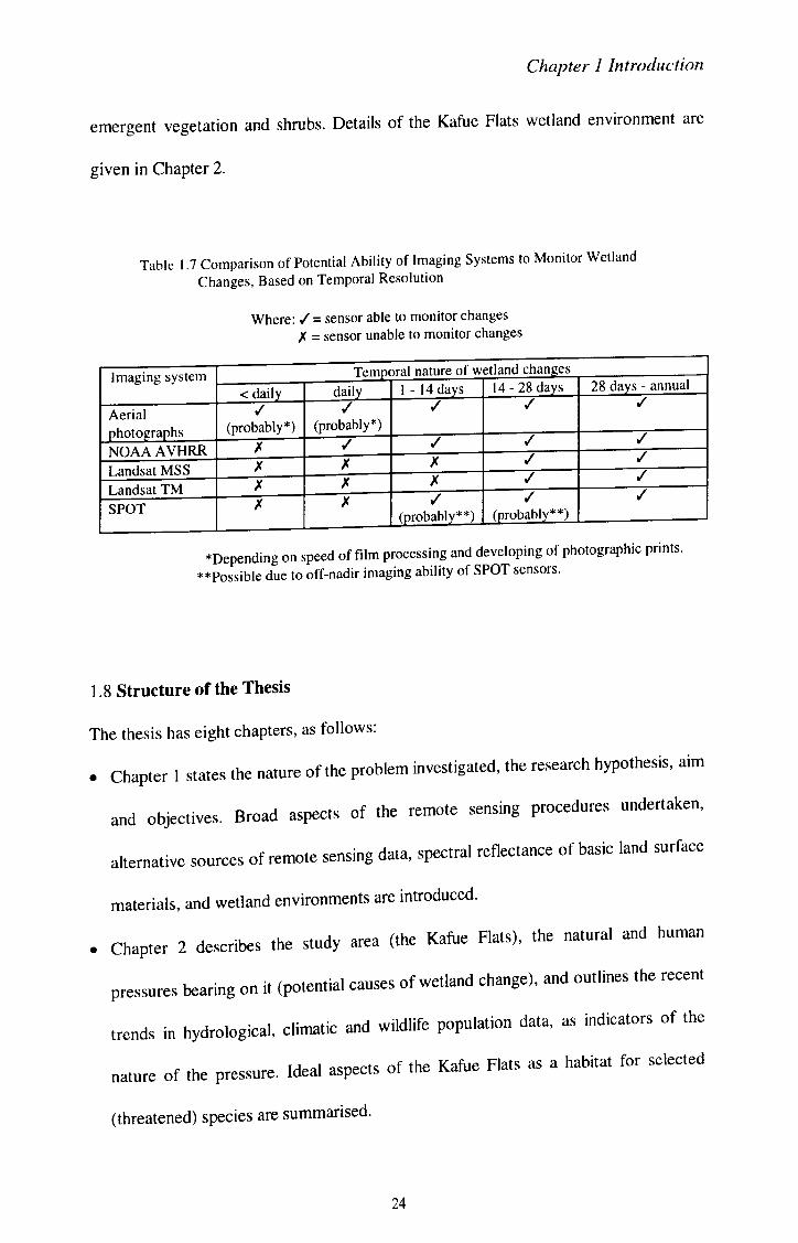
wetland characteristics being monitored. As shown in Table 1.7, the temporal nature of
wetland changes that can be monitored depends on the imaging system from which the
remote sensing data are obtained. However, spatial resolution, spectral resolution and
cost are important considerations. For example, the National Wetlands Inventory
(NW!) in the USA periodically (every 10 years) maps wetlands (type and extent)
mainly by high altitude colour infrared aerial photographs (Hefner and Storrs, 1994).
This is probably because colour infrared aerial photographs have high spatial
resolution.
Using the classification system in Table 1.5, the Kafue Flats wetland falls under the
Interior Wetlands, Riverine category, with both river channel and floodplain wetland
characteristics. The river channel (Kafue River) is perennial, while floodplain wetland
locations are both ephemeral and perennial, with stagnant water in some depressions.
The wetland's water is fresh, and the vegetation includes aquatic vegetation, algae,
23
Chapter 1 Introduction
emergent vegetation and shrubs. Details of the Kafue Flats wetland environment are
given in Chapter 2.
Table 1.7 Comparison of Potential Ability of Imaging Systems to Monitor WetlandChanges, Based on Temporal Resolution
Where: ./ = sensor able to monitor changesX = sensor unable to monitor changes
Imaging system Temporal nature of wetland changes
< daily daily 1 - 14 days 14 - 28 days 28 days - annual
Aerial ./ ./ ./ ./ ./
photographs (probably*) (probably*)
NOAA AVHRR X ./ ./ ./ ./
Landsat MSS X X X ./ ./
Landsat TM X X X ./ ./
SPOT X X ./ ./ ./(probably**) (probably**)
*Depending on speed of film processing and developing of photographic prints.**Possible due to off-nadir imaging ability of SPOT sensors.
1.8 Structure of the Thesis
The thesis has eight chapters, as follows:
• Chapter 1 states the nature of the problem investigated, the research hypothesis, aim
and objectives. Broad aspects of the remote sensing procedures undertaken,
alternative sources of remote sensing data, spectral reflectance of basic land surface
materials, and wetland environments are introduced.
• Chapter 2 describes the study area (the Kafue Fiats), the natural and human
pressures bearing on it (potential causes of wetland change), and outlines the recent
trends in hydrological, climatic and wildlife population data, as indicators of the
nature of the pressure. Ideal aspects of the Kafue Flats as a habitat for selected
(threatened) species are summarised.
24

Chapter J Introduction
• Chapter 3 summarises material from literature concerning methodological aspects of
the use of remote sensing in change detection, the error factor involved and how to
minimise it, as well as predictions of change that have been made for the Kafue
Flats.
• Chapter 4 details the methodology employed in conducting the research.
• Chapter 5 describes the criteria and organisation of the process of extracting
thematic information from the multi-temporal remote sensing data, as well as the
significance of the procedures.
• Chapter 6 details the change detection results.
• In Chapter 7, the methodological procedures are appraised and the significance of
the results in relation to the original objectives is evaluated.
• Chapter 8 outlines the conclusions arising from the study, with recommendations
for future work.
25

Chapter 2
THE STUDY AREA
2.1 Introduction
This chapter summarises the physical environment and land use characteristics of the
study area, a section of the Kafue FIats wetland area in southern Zambia (Figures 1.1
and 2.1) between latitudes 15°30' to 15050'S and longitudes 27°00' to 27°50'E (about
90 km x 50 km). The main focus of the chapter is on the aspects of land use and the
physical environment which are causing increased pressure on the stability of the
wetland in terms of input and output of water, and vegetation cover. It was pointed
out in Chapter 1 that a wetland's hydrological regime is the single greatest impetus
driving the other wetland attributes like hydric soils and hydrophytic vegetation.
Changes in the Kafue Flats' water input and output may, therefore, result in changes in
the flora and fauna. Within the constraints of data availability, trends in climate, river
discharge and water levels at hydrological stations, populations of animal species and
human use of water on the Kafue Flats are outlined in this chapter.
2.2 Climate
According to the Koppen Classification System, Zambia lies almost entirely in the
Cwa-Zone, "C (standing) for warm climate (coldest month 18 to -3°C) with sufficient
heat and precipitation for forest vegetation, w for winter dry season and a for
temperature of the warmest month over 22°C" (Ellenbroek, 1987, p.lO). Rainfall and
temperature are more prominent in dictating the rhythm of life on the Kafue Flats as an
26

""T1te·eCDf'-'....
OJ G) 0
(j) Cl>0 0
<0""T1 iiite· -0 I\)e :T 0
CD 1':;-
f'" ~Ql::Ja. +>ill
0
::Ja.cr.n
0>Cl> 0r.n ACl> 3;:;::J<0g_......:TCl>r.nc-a.-cQl....Cl>Ql
5·....Cl>o5i::J<0
2:0::J
s:Cl>
Aetc<1>""T1ill......r.n
3' 'r ID0 I :. :a. ' :~ : ;co· c;oJJl:l: m JJa. g~5·~. ~ m...... :J~ 0:::::1 fJ) "Tl.... 0.0) -'"""'1 0 m0 00,< (3 ~ :J JJ3 -< ~a.~ mzI 0" 0Ql 0 m
0.::J (1)a. 0.
0" IIICil_m III.... g_
c.o A-..,j III
~ 2'(1)
"TlCJ) DJCl> 1iiCl>

Chapter 2 The Study Area
ecosystem compared to the other climatic parameters like wind velocity, sunshine
hours and relative humidity.
There is a distinct ramy season in the study area, coinciding with the southward
migration of the Inter Tropical Convergence Zone (lTCZ). The rainy season is
normally from November to March/April. It is followed by a cool, dry season from
May to July/August, and a hot, dry season from August/September to November.
Ellenbroek (1987) has divided the seasons as follows:
I. The cool, dry season from April to August
2. The hot, dry season from August to November
3. The warm, wet season from November to April.
Handlos (1978) gives a similar division: cool, dry season from April/May to
July/August, hot, dry season from September to October, and wet season from
November to March.
In normal years, rainfall averages at about 800 mm per year in the area of the Flats
(Handlos, 1978; Douthwaite, 1974). According to the Zambia Meteorology
Department, mean annual rainfall at Kafue Polder (Nanga) and Mazabuka (for
location, see Figure 2.1) is 771 mm (period of measurement unspecified). Seasons with
less than 771 mm could, therefore, be classified as having below normal rainfall. Within
a given year the rains are usually distributed as shown in Figure 2.2, although there are
considerable year to year variations. The temperature pattern in a year is such that June
is usually the coldest month (average 16°C) and October (average 24 - 27°C) the
hottest (Figure 2.3). Unlike rainfall, mean monthly temperatures do not fluctuate very
28

Chapter 2 The Study Area
~~---------------------------------------------------
250 +--------------
E200 +---------gco'E 150 +--------.~
co(5..... 100 4--------
50 4--------
Sep Oct Nov Dec Jan Feb Mar Apr May Jun Jul AugMonth
Figure 2.2 Monthly rainfall at Kafue Polder on the Kafue Flats in the 1992/93 season (Sep. 1992 -Aug. 1993). Data: Meteorology Department, Lusaka (See also Figure 2.5).
~.-----------------------------25+---------------------------~~
~~+-------\-----------------f------~~.ai~+-----~~----------------------~r-----------~E.!cm21 +- ~--------.~~--f---------~~
Jan Feb Mar Apr May Jun Jul Aug Sep Oct Nov DecMonth
Figure 2.3 Mean monthly temperature at Kafue Polder in 1993 (see also Figure 2.6a).Data: Meteorology Department, Lusaka.

Chapter 2 The Study Area
much from year to year in the area, but years with poor or late rains (therefore with
less cloud cover) have highest temperatures in the period November to January. Winds
are generally of low velocity in the area, the maximum average being l.Zms'
(Ellenbroek, 1987). A lot of sunshine is received, up to 10 hours per day at the height
of the dry season in September but as few as 4 or 5 during the rainy season due to
cloud cover. On average, a total of 2 810 hours of sunshine are received per year
(Ellenbroek, 1987). Relative humidity ranged from daily means as high as 99% in the
rainy season to 20% in the dry season in 1993 at Kafue Polder (Zambia Meteorology
Department data).
Weather data show annual pan evaporation for the area of the Kafue Flats to be about
2 200mm but Penman calculations of potential evapotranspiration show about 1 700 to
1 800mm; both figures being greater than the annual rainfall in the area (Handlos,
1978). The actual evapotranspiration changes from month to month as the height,
density, species composition and stomatal activity of the vegetation, winds, light and
temperature change from month to month. Using the Penman equation, Ellenbroek
(1987) determined average monthly values of the reference crop evapotranspiration
(ET 0), defined as 'the rate of evapotranspiration from an extended surface of 8 to
15cm tall green grass cover of uniform height, actively growing, completely shading
the ground and not short of water'. Between September 1978 and May 1981, the
values (in mm per day) ranged from 4.1 (lowest, in June) to 7.4 (highest, in October).
The form of the Penman equation used in estimating these values was:
ETo =W.Rn + (I -W).f(u).(ea - ed)
Where:ETo = reference crop evapotranspiration in mm.d'
(2.1 )
30

Chapter 2 The Study Area
W = the temperature and altitude related weighting factorRn = the net radiation in equivalent evaporation in mm.d'f(u) = the wind related function
(ea - ed) = the difference between the saturation vapour pressure atmean air temperature and the mean actual pressure of theair in mbar
The factors affecting evapotranspiration are many and may interact with one another in
a complex fashion. Although average estimates give some indication, the real situation
is beyond our own capabilities to measure accurately (Handlos, 1978).
2.2.1 Recent Climatological Trends
Long term daily climate data from the Zambia Meteorology Department were
statistically analysed in order to determine trends. The data selected constituted daily
temperature and rainfall records for Ndola, Lusaka and Kafue Polder, representing the
upper, middle and lower portions of the Kafue River basin respectively (Figure 2.4).
The records were from 1950 - 1994 for Ndola and Lusaka, and 1957 - 1994 for Kafue
Polder. No records outside these periods were available.
The rainfall fluctuations from year to year at the stations analysed (Figure 2.5a), appear
to show wet and dry phases. Examining the graphs in Figure 2.5a reveals these phases,
which have been arbitrarily delineated from the trends in the graphs and summarised in
Table 2.1. Eight year moving average trend analysis of Kafue Polder rainfall data
reveals this cyclic nature of the rainfall (Figure 2.5b). The rainfall in each of the periods
is characterised by very high variability (Table 2.1a). Although there have been
alternating wet and dry phases in the period analysed, the declining trend in seasonal
rainfall from 1978 _ 1993 (Period III in Table 2.1a) seems to be longer than
any previous dry period. This has led to debates about whether or not the climate is
31

Scale 1 : 3 000 000 (approx.)
Figure 2.4 The Kafue River catchment area (modified from Burke, 1994). Hydrological stations arenumbered as follows: 1. Kafue Hook, 2. Itezhi-tezhi, 3. Nyimba, 4. Kafue Polder
32

Chapter 2 The Study Area
Figure 2.5(a)
1~t-----------------------------------~
E1200~rf~ilf-r-t--;~~J-+~~~~~~--I~~~~i~I~~..s~ 1~if~ __~~--x---_L--~+-·~tM--l~~--~~~~--~j__J'i!J~~~ ~~~~--~~----I~l~~-~~~~
--Kafue Polder
Lusaka---Ndola
2OOT-----------------------------------~O+----+----r---~--~----~---+----+---~--~1950 1960 1970 1980
Rain season (1950/51,1951/52, etc)1990
Figure 2.5(b)
1400,-------------------------------------~
1200+-~------------------------------------~
Actualiii- BOOc'(ij...iii-0t- 600
Moving average
400+---------------------------------------~
200+---~----~----~---+----+---~----~--~1955 1960 1965 1970 1975 19BO 1985 1990 1995
Rain season (1957/58, 1958/59, etc)
Figure 2.5 Long term seasonal rainfall trends on the Kafue basin(a) Long term seasonal rainfall fluctuations at Kafue polder (1957 - 1994), Lusaka
(1950-1994) and Ndola (1950-1994). Data: Meteorology Department, Lusaka (1968-
1972 Lusaka data missing).(b) Eight year moving average seasonal rainfall trends at Kafue Polder, 1957 - 1994.

Chapter 2 The Study Area
Table 2.1 Rainfall Statistics at Three Stations on the Kafue Basin, 1950 - 1994.(a) Apparent wet and dry phases
Station Period Seasons Mean Seasonal Seasonal RainfallSeasonal Rainfall's TrendRainfall Coefficient(mm) of
Variation(%)
Kafue Polder 1957 - 1969 781 20.10 declining
II 1970 - 1977 838 20.29 rising, then peak
III 1978 - 1993 714 24.51 declining
IV 1957 - 1977 803 19.93 declining, then rising
Lusaka 1950 - 1967 788 18.27 declining
II 1973 - 1977* 1083 30.56 peak
III 1978 - 1993 768 27.86 declining
IV 1950 - 1977 855 26.90 declining, then peak
Ndola 1950 - 1961 1205 23.65 rising
II 1962 - 1977 1 228 22.07 mixed/rising
III 1978 - 1993 1 177 18.52 declining
IV 1950 - 1977 I 218 22.33 rising/mixed
* 1968 - 1972 data missing
changing under the influence of global warming. According to these data there is no
significant difference in mean rainfall between this latter period and either the wet or
the dry period before (Table 2.1b).
Another trend that is apparent is increasing frequency of seasons with below average
total rainfall from 1978 to 1993 (Period III in Table 2.1) compared to the period 1950
_ 1977 (Period IV in Table 2.1). For the Kafue Flats area the mean seasonal rainfall
is 771 mm at Mazabuka and Kafue Polder, according to the Zambia Meteorology
Department. Years with total seasonal rainfall less than 771mm could, therefore, be
34

Chapter 2 The Study Area
Table 2.1 Rainfall Statistics at Three Stations on the Kafue Basin, 1950 - 1994.(b) Differences between rainfall means of wet and dry phases
Station periods rainfaIl means. No. of
00'0'
s t Probability Significance
compared compared (mm) years (P)
(see part (mm) (n)
(a) of tableabove)
Kafue IV 803 160 21 1.58 0.12 not significant
Polder III 714 175 16
II 838 170 8 1.67 0.12 not significant
III 714 175 16
781 157 13 1.08 0.29 not significant
III 714 175 16
Lusaka IV 855 230 22 1.21 0.24 not significant
III 768 214 16
II 1083 331 5 2.00 0.10 not significant
III 768 214 16
788 144 17 0.32 0.75 not significant
III 768 214 16
NdolaIV 1218 272 28 0.55 0.58 not significant
III 1177 218 16
II 1228 271 16 0.59 0.56 not significant
III 1177 218 16
I 1205 285 12 0.29 0.78 not significant
III 1177 218 16
considered as below average rainfall years. Statistically, there is no significant
difference in frequency of below average rain seasons between the period 1978 - 1993
• Standard deviation.. Student's t statistic.. , Using 5% level of probability to determine significance
35

Chapter 2 The Study Area
and the period 1950 - 1977 for Kafue Polder (Table 2.2). The cold season versus dry
season temperature difference at the three stations seems to be changing. October is
normally the hottest month of the year and June the coldest. From the records
available, June has been getting warmer while October has been getting cooler (Figure
2.6). This is likely to have resulted in increased evaporation and evapotranspiration
losses in June and possibly reduced losses in October.
It is difficult to make conclusive statements about the latest climate trends in the area ,
given the short record available (1950 - 1994 only). It remains to be seen how long the
latest trend (since 1978) will last. Staff at the Zambia Meteorology Department urge
similar caution about the issue, adding that what is certain is that rainfall has become
erratic and very unpredictable (in terms of beginning and end of rain season, as well as
amount of rain) lately, and that the rains have been consistently poor in the 7 years
before 1995 (Daka, 1995 and pers. comm.; Muchinda, 1988 and pers. comm.) I.
Sakaida (1994) and Kruss (1992)2 made a similar observation of reduced rainfall in
Zambia in the 1980s, with the 1991192 rain season being the driest on record. A WWF
commissioned report on climate change in the southern Africa (Hulme, 1996) states
that rainfall in the region is variable from year to year and droughts have occurred from
time to time. However, the report states, the last twenty years have seen a trend
towards reduced rainfall. The decade 1986-1995, as well as being the warmest this
century, has also been the driest, according to the report. The observed rate of
warming in southern Africa during the present century - about 0.05°C per decade - is
IMuchinda was Chief Meteorologist (Agronomy) and Daka was Meteorologist at Zambia
Meteorology Department in 1995.2 Kruss was working at Zambia Meteorology Department in 1993 and previously at the World
Meteorology Organisation, Geneva, Switzerland.
36

Chapter 2 The Study Area
Table 2.2 Differences in frequency of below average rain seasons at Kafue Polder, 1957 -1977
versus 1978 - 1993
Seasonal rainfall class(mm)*
1957 - 1977 (periodIV)** frequency
1978 - 1993 (periodIII)** frequency
Total (No. of years inclass)
<771~771Total (No. of years inperiod)
91221
11516
201737
,t = 2.451, P = 0.118 (not significant at 5%)
*Mean rainfall is 771mm (Zambia Meteorology Department)**See Table 2.l(a)
(a) Kafue Polder
28
26
24
022 -If-
'-'e June
~20 -----~ October
E~ 18
16
14
121955 1965 1975 1985 1995
Year
Figure 2.6 June and October temperature trends on the Kafue basin (a) Kafue Polder, 1957-1994.

Chapter 2 The Study Area
(b) Lusaka
26
24
22
~20CD....:Jiii18Q;a.~ 16I-
14
12
101955 1965 1975
Year1985
(c) Ndola
26~--------------------------------------------~
020+---------------------------------------------~::_...
~:Jiii18+---------------------------------~-~-A~~'~~8.~16+-~----~C--~-p~-4~~~-~~~~r~------------~I-
12+---------------------------------------------~
10+---~~--~----+---~-----r----+---~----~----,1950 1960 1970
Year1980 1990
Figure 2.6 (continued) June and October temperature trends on the Kafue basin(b) Lusaka, 1967-1994.(c) Ndola, 1950- 1994.
(Data: Zambia Meteorology Department, Lusaka).
June--October
1995
June
----October

Chapter 2 The Study Area
similar to the global rate (Hulme, 1996). In the region, the rainfall fluctuations have
been observed to correlate with sea surface temperature and pressure changes
(Matarira, 1990; Mason, 1995; Daka, 1995b). In particular, the phenomena of El Nino
and the Southern Oscillation (SO) have been identified as being influential. El Nino
refers to the anomalous warm sea-surface temperatures over the east Equatorial
Pacific, while the Southern Oscillation is the term describing the planetary scale
phenomenon involving a sea-saw in surface pressure between Indonesia and the south-
east Pacific (Matarira, 1990). In wet years, there is higher pressure on the sea surface
than on the Southern Africa land surface. There are also warmer inland temperatures
and, consequently, an influx of moist air. In dry years, the opposite of this occurs
(Matarira, 1990).
2.3 Hydrology
The study area is set in the floodplain of the Kafue River. Flowing eastwards across the
study area, the river discharges into the Zambezi (see Figure 2.4) and starts in the
border area between Zambia and Zaire. A profile of the Kafue River from source to
mouth shows that it has very low gradient in the area of the Kafue Flats (Figure 2.7).
On the Flats, the meandering river has a channel length of 450km from Itezhi-tezhi to
Kafue Gorge Reservoir, compared to the straight distance of 255km. It falls only 10m
in that distance (Ellenbroek, 1987), giving a gradient of about 1 in 25 500. Over the
years the river has cut across its meanders, leaving numerous ox-bow lakes in the
stranded former channels. These former channels form an integral part of the wetland
system (Ellenbroek, 1987).
39

Chapter 2 The Study Area
Height (m)above sealevel 1380
Zambezi cont1uence ~
1200 Itezhi- KafucGorgedam
J,
900
600
300~----------~r-----------~------------~------------400 800 1200
Distance (km) from source
Figure 2.7 Profile of the Kafue River (after Handlos, 1978). Hydrological stations are numbered asfollows: 1. Kafue Hook, 2. Itezhi-tezhi, 3. Nyimba, 4. Pumping Station 1 (opposite
Nakambala, Figure 2.1).
2.3.1 The Kafue Basin
The Kafue River basin (Figure 2.4) covers an area of 154 OOOkm2(Ellenbroek, 1987)
and can be divided into two sections: (1) the upper and mid Kafue (2) the lower Kafue
and Kafue Flats.
2.3.1.1 The Upper and Mid Kafue
The water level in the upper Kafue starts to nse with the onset of the rains in
November in the northern part of the basin, having been at its lowest in October. The
level continues to rise as the rainy season progresses until maximum discharges are
reached at the height of the rains in January/February (Figure 2.8). The flood proceeds
40
1600

Chapter 2 The Study Area
50+---
(a) Kafue River hydrograph at KafueHook, 1993/94 hydrological year
~~----------------------------------------------,
e~~i--------------f---------\------------------------~E~~t---------------.~------------\------------------------~,£.~~T--------------r--------------~----------------------~IVs:o~~+- ~L-------------------\~------------------~cIV~1oot---------~t-----------------------~~~~~--------~
Oct Nov Dec Jan Feb Mar Apr May Jun Jul Aug SepMonth
(b) Monthly rainfall at Ndola, upperKafue basin, 1993/94 rain season
~.-----------------------------------------------------~~-+-----
250-+-----
E.: zoo -+-------~~150+----~I-
100 +----
o +---+-Oct Nov Dec Jan Feb Mar Apr May Jun Jul Aug SepMonth
Figure 2.8 Relationship between middle basin river discharge and upper basin rainfall on the Kafuebasin. Data: (a) ZESCO, Lusaka (b) Meteorology Department, Lusaka (April data
missing).

Chapter 2 The Study Area
quickly down to Itezhi-tezhi, where maximum water levels are reached in March. At
Itezhi-tezhi, the flood used to be held back by a constriction of the valley, but at
present the main regulating factor is an artificial one - the Itezhi-tezhi dam (Figure 2.7).
There are a number of swamp and floodplain areas in the upper Kafue, two of which
are the Busanga and Lukanga Swamps (Figure 2.4). The Lufupa flows through the
Busanga plain where large quantities of water are lost through evaporation, its outflow
into the Kafue being slow. This swamp acts as a natural, temporary storage basin. The
Lukanga swamp, however, sometimes actually causes withdrawal of water from the
Kafue River because in times of high flood flow in the Kafue, water spills over into the
swamp (Ellenbroek, 1987).
2.3.1.2 The Lower Kafue and the Kafue Flats
Downstream of Itezhi-tezhi, the Kafue River enters the Kafue Flats whose area is
about 45 OOOkm2•The local catchment of the Kafue Flats is quite small compared to
the upper Kafue and the rains are lower (compare Figures 2.2 and 2.8b). This causes
the water balance of the Kafue Flats to be largely dependent on the discharges at
Itezhi-tezhi (Ellenbroek, 1987). The channel capacity of the Kafue in the Kafue Flats
area is small, approximately 170m3s·1, and consequently when discharges at Itezhi-tezhi
are over this amount, flooding occurs - i.e. floodplain areas around the river are
inundated (Ellenbroek, 1987).
Before damming at Itezhi-tezhi, the flood normally used to reach Lochinvar (Figure
2.1) in April and Kafue Gorge late in May, although there was considerable variation in
timing and scale (Douthwaite, 1974). Since damming at Itezhi-tezhi, the regulated
42

Chapter 2 The Study Area
flood progresses slowly to the Kafue Gorge Reservoir where it arrives between June
and August (Ellenbroek, 1987). There is a lag in the timing of the flood between upper
and lower sections of the Kafue Flats in any given year (Figure 2.9; see also Figure
4.1 ).
As a result of damming at Itezhi-tezhi, the total area flooded, flood level, duration and
timing of flooding on the Kafue Flats all depend on the discharge from Itezhi-tezhi
dam. The regulation of the discharge at Itezhi-tezhi is targeted primarily at satisfying
reservoir level needs for generating electricity at Kafue Gorge (as will be described in
Section 2.7.1), which means that there are annual differences in flood pattern and
timing depending on the rainfall received (Figure 2.10). When there is high total
seasonal rainfall, there is wider flooding on the floodplain.
2.3.2 Recent Hydrological Trends
Long term daily discharge and river level data from four stations in the Kafue basin
were obtained from the Zambia Electricity Supply Corporation (ZESCO) and the
Zambia Sugar Company (ZSC). The stations were: (1) Kafue Hook, (2) Itezhi-tezhi
and (3) Nyimba (ZESCO data), and (4) Pumping Station I opposite Nakambala (ZSC
data) (Figure 2.4) for the periods 1973-1994, 1976-1994, 1962-1986 and 1983-1994,
respectively. The data for Nyimba were incomplete between 1977 and 1986 because
the station was in a state of disrepair. No records outside of these periods or from
other stations were available from ZESCO or ZSc. Kafue Hook is up stream of the
dam at Itezhi-tezhi (Figure 2.7) and, therefore, served as a control.
43

Chapter 2 The Study Area
980.18
980.16
1(II 980.14$Q).8 980.12(II
:§: 980.1
~J!l 980.08...~~ 980.06
~ 980.04
980.02
976.05
j 975.95(II
I 975.9
-ai~ 975.85...~~ 975.8
.~O!: 975.75
(a) Kafue River levels at Nyimba,April 1983
980. 2
AJ ,--
.W/-~
~
~
\ ./~~
I I
Figure 2.9 Kafue River levels (a) at Nyimba (b) Opposite Pumping Station 1, Nakambala in April1983. The flood started to raise the river level at Nyimba (upstream) before 1 April, butonly arrived opposite Mazabuka at Pumping Station 1 on 16 April. Data (a) ZESCO,
Lusaka, (b) Zambia Sugar Company, Mazabuka.
980 1 2 3 4 5 6 7 8 91011121314151617181920212223242526272829Date in April 1983
(b) River levels at Pumping Station 1opposite Nakambala Estate, April 1983
976.1
7l~j- --
--!- - - - _1~~--~~ ~ '\_7--- ~
LI
I I
T T T , T-, T , T T
976
975.7 1 234 567 8 91011121314151617181920212223242526272829Date in April 1983

Chapter 2 The Study Area
1600~--------------------------------------~
---1978179---B---....
CDCL
i1000t----------------,~--f-4r~----------------~CDEo~ 800t-----------7.r~~~--~--~~--------------~~
1979/80---1980/81-e-1984/85)(-
CDCl(ij 600s:s'6c:III 400CD~
1986/87---s;;z-
1989/90_._1994/95
0~+--4---+--1_--~-4--~--+---~-+--~--~Oct Nov Dec Jan Feb Mar Apr May Jun Jut Aug Sep
Month
Figure 2.10 Year to rear variation in monthly discharge into the Kafue Flats at Itezhi-tezhi. Thehydrological year starts in October each year and ends in September the following year.The peak discharges were generally higher in the late 1970' s and early eighties. High,long duration peak discharges in March-June result in wider spatial inundation (flooding)of the Kafue Flats for a long time, and vice versa. Widespread, long lasting flooding ofthe Flats is important for its ecology. By September, the discharge is almost similar fromyear to year. See also Figures 2.5 and 2.12b. Data: ZESCO, Lusaka.
Apparently as a consequence of the declining seasonal rainfall since 1978 (Section
2.2.1), the mean annual discharge of the Kafue River at Kafue Hook and the minimum
(dry season) and maximum (rainy season) river levels have been declining since about
1978 (Figure 2.11), although there were annual fluctuations in the period. A similar
trend has occurred in the mean annual discharge at Itezhi-tezhi dam (Figure 2.12b).
Since the completion of the dam in 1978, the minimum and maximum water levels in
the re ervoir have been maintained at fairly constant levels (Figure 2.12a; maximum

Chapter 2 The Study Area
7
6
0Q;~5Cl~roCl
~4 ---0
Maximum.0ro
:[3-§-
Qj
Minimum
>~lP2>er
~ 800....8-I!!~ 600E0:0::J~Q) 400Cl....ros:~'5c 200m~
(a) Maximum and minimum river levels
O+-4-~4-~4-4-4-4-4-4-4-4-4-4-4-4-4-4-4-4-4-~1m1m1m1m1~1m1~1_1~1m1m1~
Hydro-year (1973174,1974175,etc)
(b) Mean annual discharge
1~'---------------------------------------------------~
o+-~-+~ __~+-4--r-+~--r-+--r-r-+~r-+-~-r-+-4--r-~1~ 1~ 1~ 1m 1~ 1~ 1~ 1~ 1~ 1_ 1~ 1*
Year
Figure 2.11 Hydrological trends at Kafue Hook, 1973 - 1994.

Chapter 2 The Study Area
(a) Maximum and minimum reservoirwater levels
1~~--------------------------------------~11030t----~=-~F9r=-=~---~=-~~~~~~---~=-~~IV
~10~~-r--T_--------~---f---------~~----t~~
jIV51010+-----t-----------------------------~~--~
~~1000+-~--r---------------------------------------.~
i ~+_--~--------------------------------------~er
----Maximum~Minimum
~+-+-~~~~,-~,-~-r-r-r~~~~-r~-r~1~ 1~ 1~ 1~ 1~ 1~ 1~ 1~ 1~ 1~ 1~
Hydro-year (1976m, 1977f78, etc)
(b) Mean annual discharge
700,----------------------------------------------------,~600+--------------------------------------------------------j3l!~+-----~------------------------------------------~iE~+-----------~-------------------------------------------j:M::J~300+-------------+---------------------------------------~~IVor;~~+------------=~--~~----~---=~--------'L---~~'0CIV~100+-------------------------------------------------------
O+_-+--+--r--~-r~~~~--+--+--+--r--r--r~--4-~--+-~1976 1978 1980 1982 1984 1986 1988 1~ 1992 1994
Hydro-year (1976m, 1977f78, etc)
Figure 2.12 Hydrological trends at Itezhi-tezhi, 1976 - 1994.

Chapter 2 The Study Area
capacity of reservoir is at 1029.5m level), although they have fallen occasionally in
coincidence with very low rainfall years (around 1982 and 1991; Figures 2.5a and
2.12a).
The fact that discharge through Itezhi-tezhi has been declining since 1978 implies that
the amount of water entering the Kafue Flats from the upper Kafue basin has also been
declining. Added to the fact that the local rains on the Flats have also been declining
since 1978 (Figure 2.5b; Tables 2.1 and 2.2), it is likely that water supply pressure on
the wetland has also been increasing since 1978. The effect of rising June temperatures
(Figure 2.6a), which is the approximate period of maximum flood (May-July), is
difficult to ascertain but evaporation losses from the wetland are likely to have
increased too. No data on recent evapotranspiration trends were available.
The effect of damming at Kafue Gorge in 1972 (damming will be described Section
2.7.1) seems to have been to raise the maximum and minimum river levels as far
upstream as Nyimba, as can be seen from the long term data for Nyimba (Figure
2.13a). ZESCO confirmed that the influence of Kafue Gorge dam reaches as far
upstream as Nyimba. In fact the whole section of the river from Nyimba to the Kafue
Gorge dam (Figure 2.1) is regarded by ZESCO as the 'Kafue Gorge Reservoir'. The
lower rains since 1978, however, seem to have been reducing even these dam induced
high river levels at Nyimba (Figure 2.13a). Nyimba data records from 1977-1994 are
not continuous (the station was in a state of disrepair), but the data from ZSC for
Pumping Station 1 (1983 - 1994; Figure 2.13b) may partly compensate for this since
both stations are in the section of the Kafue River between the dams (Figure 2.7).
48

Chapter 2 The Study Area
(a) Maximum and minimum river leveltrends at Nyimba, 1962-1986
~~----------------------------------------
~+----------------------------------------
98
980
~978~~ 976VIQ)
~ 974.0(lI
--972.5~970~:u 968iii~ 966Q)
.~0::: 964
972+-+-+-~~-+-+~1-+-+-~~-+~~~+-+-~-4-+~~1~1~1~1~1~1m1m1m1m1m1~1~1~1E
Hydro-year (1962163, 1963/64, etc)
(b) Maximum and minimum river leveltrends at Pumping Station 1, 1983-1994
2
~~- ...._ ~ __ / _;::-.<« ~ -r'" 'X
,962
96019821983198419851986198719881989199019911992 19931994 1995
Hydro-year (1983/84, 1984185, etc)
Maximum
Minimum
Figure 2.13 Hydrological trends at Nyimba (1962-1986) and Pumping Station 1 opposite Nakambala
Sugar Estate (1983-1994).
---Maximum_._Minimum

Chapter 2 The Study Area
There is no appreciable trend for the data from Pumping Station 1, although there is a
slight declining trend in the minimum levels of the river.
2.4 Geology, Soils and Relief
The underlying lithology over much of the area is complex Katangan sediments
(gneisses, schists, marbles) of upper Pre-Cambrian age (Handlos, 1978; Turner, 1982).
Most of the Kafue Flats is carpeted by a layer of alluvial material (sands, gravel and
clay; see Figure 2.14) (Handlos, 1978; Burke, 1994; Turner, 1982; Rees, 1978) dating
back to the Tertiary (Handlos,1978). Turner (1982) has described the geological
setting of the area, stating that the geological structure of the Kafue Flats is an east-
west to east north east - west south west trough, in part down warped but mainly
down faulted, filled with Karroo sedimentary rocks which outcrop occasionally from
beneath the alluvium. The rocks on each side of the trough, and around its eastern end,
are Precambrian gneisses, schists and marbles. Thus the Kafue Flats are contained
within, and partly coincide with, a Karroo age rift valley, with a drainage barrier of
Tertiary-Quaternary sands in the south west (Figure 2.14a).
Soil samples from the Kafue Flats collected and analysed for texture and organic
carbon content revealed that the soils are generally highly organic, dark and clays (see
Appendix 1; also Figure 4.13 for sample site locations). The samples represented all
the zones of the Kafue Flats (described in Section 2.5) and the results indicate that
generally in the floodplain zone the soils are clays while the more peripheral soils are
loams (sand-silt-c1ay loams). Similar descriptions have been given by other workers
(e.g. Handlos, 1978; Turner, 1982; Rees, 1978; Ellenbroek, 1987; FAO, 1968 Vol. II).
50

10 9 \0 go ~o 10 ~Okm
LEGEND
ALLUVIUM
DSILTetC.
KALAHARI~ SAND, SANDSTONE,b.2:J LIMESTONE AND SILCRETE
KARROO
BASALT
•
MUDSTONE, SANDSTONECARBONACEOUS BEDS WITHCOAL SEAMS
~A
BASEMENT
fT\\:l SANDSTONE, GRIT~ AND MARL
GNEISSES, SCHISTS AND MAGMATITES
IGNEOUS ROCKS
[~ : Ij GRANITE
____ FAULT
Figure 2.14 Geology of the Kafue Flats(a) Geology map of the Kafue Flats and surrounding areas (modified from
Ellenbroek, 1987). The map shows that the Kafue Flats (centre of map) areunderlain mainly by alluvial material.
51

Chapter 2 The Study Area
Figure 2.14 (continued) Geology of the Kafue Flats(b) Alluvial and rock layering in a well on the Kafue Flats floodplain (just north of
Luwato Lagoon, UTM grid 35 558829E, 8294452N, 27 September 1995). The soilhorizon textures in the profile (from top to bottom) are:
o - 35cm: dark clay35 - 60cm: clay sand60cm - 1.15m: sand1.15 - 1.56m: gravel1.56 - 6.00m: rock (water table at 6m)
52

Chapter 2 The Study Area
Handlos (1978) has described the trend in soil distribution on the Kafue Flats, stating
that a transition of soils occurs depending on the local relief and the parent material.
The more peripheral soils are clays and loams, while, on the Flats, those areas that are
flooded consist of clay soils rich in carbon, giving a dark black colour. Turner (1982)
gives a similar description, stating that the soils of the floodplain are dark margallitic
clays, very heavy and sticky when wet, but cracking when dry. At the margins of the
floodplain, these may give way abruptly to sandy loam 'upland' soils, or there may be a
gradual or patchy transition to clay-loam.
Departures from this general trend in the soils analysed (Appendix 1) may be attributed
to local site conditions such as presence of old, flattened termite mounds or the action
of local plants in trapping wind borne silt particles, or variations in sediment deposition
resulting from site flood characteristics.
The area is generally very flat (Figure 2.15), with very little macro-relief variation. It
has an average elevation of 900m above sea level (Howard, 1985). Only in the
woodland zone (which will be described in Section 2.5) do relief differences in the land
begin to be noticeable. There is notable micro-relief on the Kafue Flats which results
from the contraction, expansion or drying up of the clay soils. The montmorillonitic
(smectite) clays expand when wet and contract when dry. Such expansion and
contraction gives rise to what is termed gilgai micro relief (2-6 m wide and up to 50
cm high; Rees, 1978). Deep cracks in the clay result when the clay soils dry up in the
dry season and are a prominent feature of the micro relief of the area in the dry season.
53

Chapter 2 The Study Area
Figure 2.15 Floodplain relief on the Kafue Flats (north east of Shalwembe Lagoon, UTM grid35521087£, 8280058N, looking south east, 25 September 1995, afternoon). This areais heavily grazed by zebra and lechwe. Green shoots of Vossia cuspidata grass can
be seen. See also Figure 2.22.
2.5 Vegetation
There is distinct zonation in the distribution of vegetation on the Kafue Flats. The
major vegetation zones are woodland, termitaria zone and floodplain zone (Table 2.3).
In between the zones are sharp or gradual ecotones. From Table 2.3 it can be inferred
that the zones are largely controIled by hydrology and soil spatial variations.
The woodland zone is on the periphery. The major woodland types are munga
woodland (mainly Acacia species), miombo woodland (mainly Brachystegia species),
and mopane woodland (mainly Colophospermum species) (Ellenbroek, 1987). Some
stretches of woodland consist largely of dense stands of a particular species (e.g. see
54

Chapter 2 The Study Area
Table 2.3. Major Vegetation Zones of the Kafue Flats
Zone
Woodland
Termitaria zone
Description Major vegetation types
Floodplain
Located on the fringes, soils mainlyclays and loams.
(i) Munga woodland -mainly Acacia species
(ii) Miombo woodland -mainly Brachystegiaspecies
(iii)Mopane woodland -mainly Colophospermumspecies
Figure 2.16), but most of the woodland is mixed and open. In the open spaces between
Located between woodland andfloodplain proper, characterised bytermite mounds of different sizes andtypes, waterlogged in wet season,mainly grey clay soils.
Grasses (e.g. Acrocerosmacrum, Panicum species)and shrubs associated withoccasional flooding, occasionaltrees (Acacia) on termitemounds.
the trees grow a variety of grass species, most of which are of the genera Hyparrhenia,
Generally impervious soils, subject toseasonal inundation.
Major plant species are waterlilies (Nymphaea), hippo grass(Vossia cuspidata), water grass(Echinochloa stagnina),Ph ragmites mauritianus andAeschynomene fluitans; otherspecies are abundant in localisedsections of the floodplain; thereare up to 28 species of grasses.
Setaria, Brachiaria, Echinochloa and Panicum. The grasses are mostly perennial,
(Summarised from Howard, 1985, and Handlos, 1978).
being senescent in the dry season. The woodland species are mostly deciduous, losing
their leaves in June/July and re-growing them in September/October (southern
hemisphere spring time). Where substantial cutting of trees by man has been sustained,
55

Chapter 2 The Study Area
Figure 2. I6 Dense Acacia poLyacantha woodland on the northern fringes of the Kafue Flats (nearNangoma River, just west of Muchabi School, UTM grid 35 529706E, 8292732N,looking west 25 September 1995, morning).
Figure 2.17 A sparse stand of woodland tAlbizia harveyi in the center) on the northern Kafue Flats(in the former village areas south of Muchabi, UTM grid 35 527592E, 8289917N,looking east, 25 September 1995, morning). The trees are in spring.
56

Chapter 2 The Study Area
the woodland will degenerate into shrubs, and regenerating woodland areas appear as
coppiced areas. Albizia harveyi (in munga woodland; Figure 2.17) is favoured for
wood and Colophospennum mopane (in mopane woodland) is favoured for house
building by the local people. Close to human settlement areas, these trees are coppiced
(Figure 2.17).
Woodland gradually gives way to the termitaria zone (e.g. Figure 2.1S) which has
termite mounds of different sizes, built by different termite species. Macrotennis
species build large mounds (about 1.5 - 2m tall), Odontotermis species build rounded,
medium sized mounds (about SOcm - Im tall) and Cubitennis species build very small
mounds (about 30cm tall) (FAO, 1965, Vol. IV). Grasses grow between the termite
mounds, and in some areas isolated shrubs of woodland tree species can be found (see
Figure 2.1Sb). The grasses include Setaria sphacelata, Vitiveria nigritana and Setaria
eylesii.
The lower limit of the termitaria zone roughly marks the edge of the upper limit of
flooding (Ellenbroek, 1987; Turner, 1982). On the floodplain are vast areas of
grassland, either largely with stands of a particular dominant species or with mixtures
of grass species (e.g. Figure 2.19). In areas with wildlife or cattle, the floodplain
grasses are grazed (see Figures 2.15 and 2.22). The timing and duration of the flood
(see Section 2.3.1.2) determines the nature of floodplain vegetation, and as a result (of
annual flood variations) annual changes in the species composition of the floodplain
grassland community are common (Ellenbroek, 1987).
57

Chapter 2 The Study Area
Cb)Figure 2.18 The Termitaria zone on the Kafue Flats.
(a) woodland-termitaria (macrotermis) mixture, with Vitiveria nigritana grass inthe foreground (south of Nachaba, UTM grid 35 563446E, 8256978N, looking south
east, 21 September 1995, noon).(b) termitaria (odontotermis)-grassland mixture, with isolated Acacia shrubs (south of
Nachaba, UTM grid 35 564184E, 8250996N. looking east, 8 September J 995,afternoon). The grass still has faint greenness in lower portions.
58

Chapter 2 The Study Area
Figure 2.19 nuruzcd floodplain gras land on the Kafue Flats(a) Just s uth 01 am tu i village. outh bank (UTM grid 35 536530E, 8256867N,
loo 109 east, 1 cptember 1995, noon).(b) H. parrllm/Cl rufu (fight and background) gras land, north bank and south of Muchabi
( 'rid 35 52 02 . 2824 7 ,looking southeast, 25 September 1995, afternoon).In th central tore- rr und is a mi ture of Eragrotis lappula and Setaria sphacelata.
9
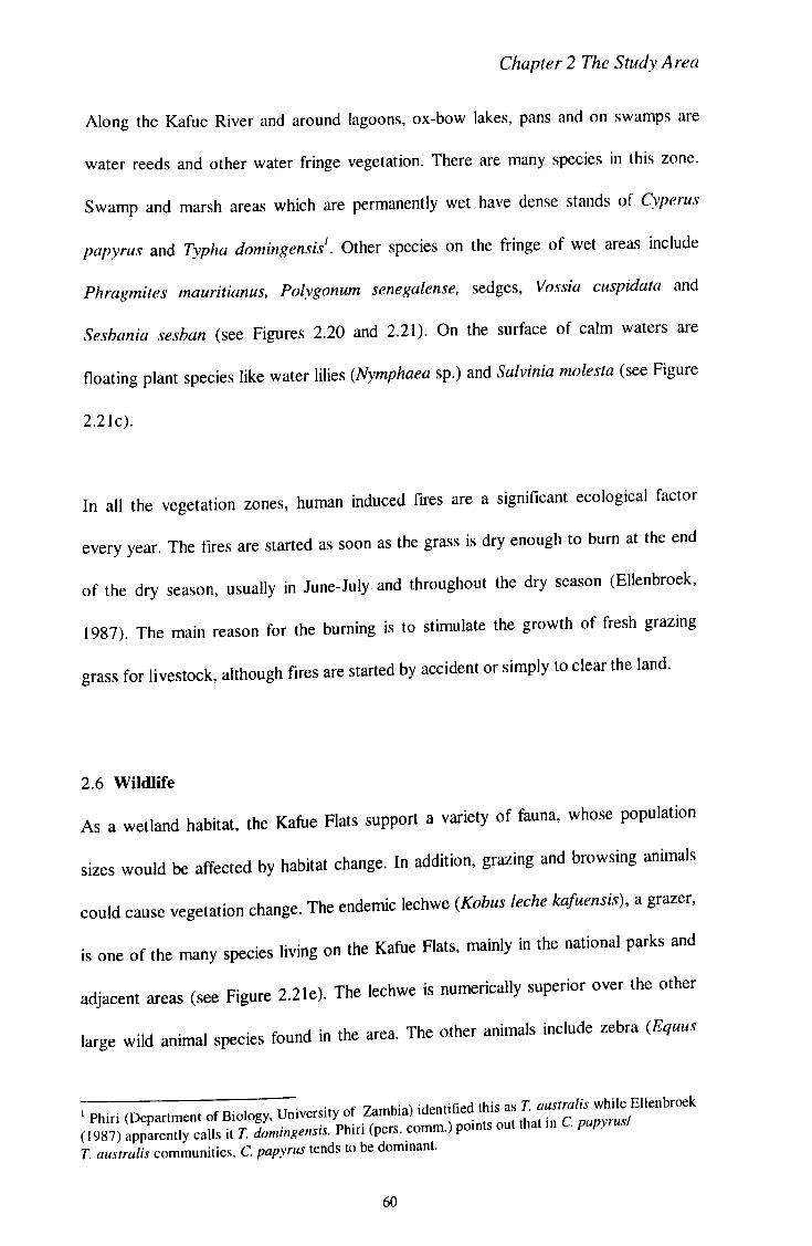
Chapter 2 The Study Area
Along the Kafue River and around lagoons, ox-bow lakes, pans and on swamps are
water reeds and other water fringe vegetation. There are many species in this zone.
Swamp and marsh areas which are permanently wet have dense stands of Cyperus
papyrus and Typha domingensis', Other species on the fringe of wet areas include
Phragmites mauritianus, Polygonum senegalense, sedges, Vossia cuspidata and
Sesbania sesban (see Figures 2.20 and 2.21). On the surface of calm waters are
floating plant species like water lilies (Nymphaea sp.) and Salvinia molesta (see Figure
2.21 c).
In all the vegetation zones, human induced fires are a significant ecological factor
every year. The fires are started as soon as the grass is dry enough to burn at the end
of the dry season, usually in June-July and throughout the dry season (Ellenbroek,
1987). The main reason for the burning is to stimulate the growth of fresh grazing
grass for livestock, although fires are started by accident or simply to clear the land.
2.6 Wildlife
As a wetland habitat, the Kafue Flats support a variety of fauna, whose population
sizes would be affected by habitat change. In addition, grazing and browsing animals
could cause vegetation change. The endemic lechwe (Kobus leche kafuensisy, a grazer,
is one of the many species living on the Kafue Flats, mainly in the national parks and
adjacent areas (see Figure 2.21e). The lechwe is numerically superior over the other
large wild animal species found in the area. The other animals include zebra (Equus
I Phiri (Department of Biology, University of Zambia) identified this as T. australis while Ellenbroek(1987) apparently calls it T. domingensis. Phiri (pers. comm.) points out that in C. papyrus/T. australis communities, C. papyrus tends to be dominant.
60

Chapter 2 The Study Area
burchelli)(Figure 2.22) - second most abundant after lechwe (El1enbroek, 1987),
wildebeest (Connochaetus taurinus) - the next most numerous although much fewer,
buffalo (Syncerus caffer), oribi (Ourebi ourebi), reedbuck (Redunca arundinum) and
kudu (Tragelaphus strepsiceros). Most of these animals are found in Lochinvar
National Park (Figure 2.1) on the Flats and adjacent wooded areas. Buffaloes are rare
in Blue Lagoon National Park, although the other herbivores listed above (excluding
buffalo) were seen there aloin 1995.
Figure 2.20 A dense stand of water reeds and water fringe vegetation on the Kafue Flats (bor~eringthe eastern edge of Shalwembe Lagoon, UTM grid 35 517618~, 8279633N, ~OOklng
h 25 S b 1995 mid afternoon). In the foreground IS polygonum senegalense.nort , eptem er , . . 0 •
coo the top right and top left corners and Phragmltes mauritianus ISyperus papyrus IS In '
in the middle of the background.
61

Chapter 2 The Study Area
Figure 2.21 Hydrophytic vegetation on the Kafue Flats
(a) Polygonum senegalense and water grass mixture (foreground, right bank), withon the banks of the Kafue River at Banachibwembwe (UTM grid 35 533451 E, 8260878N, lookingeast,7 September 1995, afternoon). Across the river (background) are dense Cyperus papyrus andTvpha doniingensis reeds and a herd of cattle is grazing on the right
(b) Dense Yossia cuspidata along the banks of the Kafue River at Banachibwembwe (UTM grid35 533451 E. 8260878N. looking north, 7 September 1995, afternoon). Across the river(hackground) is a dense. vigorous stand of Typha domingensis.
62

Chapter 2 The Study Area
Figure 2.21 (continued) Hydrophytic vegetation on the Kafue Flats
(c) A dense stand of Vossia cuspidata on the south bank of the Kafue River at Kabwe village justnorth or Lochinvar (UTM grid 35 532500E, 8259412N, looking west, 7 September 1995, midafternoon). In the lower portion of the picture, behind the grass, is floating Salvinia molesta.
(d) A dense stand of Cyperus papyrus and water grass on the banks of the Kafue at Shakapinka(UTM grid 35 567256E. 8264201N, looking west from south bank. 8 September 1995. noon).
63

Chapter 2 The Study Area
Figure 2.21 (continued) Hydrophytic vegetation on the Kafue Flats
(e) Sesbania sesban shrubs stranded by the retreating water line in a depression north east ofChunga Lagoon, just outside Lochinvar National Park (UTM grid 35 532717E, 8255682N,looking cast, 7 September 1995, morning). Notice the lechwe (in middle) and zebra (background).
igure 2.22 Zebra in the heavily grazed floodplain grassland of the Kafue Flats (north east ofhalwembe Lagoon, just outside Blue Lagoon National Park, UTM grid 35 518150E,8279705N,lo king northeast, 25 September 1995, mid afternoon).
64

Chapter 2 The Study Area
Large carnivores such as lions (Pantheras leo), leopards (Pantheras pardus), wild
dogs (Lycan pictus) and cheetah (Acynonix jubatus) are absent because they were
systematically exterminated when the parks were cattle ranches, but, according to
Ellenbroek (1987), the spotted hyena (Cracuta crocuta), serval (Felis serval) and side
striped jackal (Canis adustisi are still permanent residents. Primates such as vervet
monkeys and baboons (Papio ursinus) are also present in the woodland zone. The
hippopotamus (Hippopotamus amphibius) occurs in small herds in most parts of the
Kafue Flats (river and other deep water areas) while sitatunga (Tragelaphus spekei), a
true aquatic ungulate confined to Papyrus and reed marshes, has also been observed
locally (Ellenbroek, 1987).
Over 400 species of birds are listed for the Kafue Flats (Handlos, 1978; Douthwaite,
1974), about 125 of which are water birds (Sheppe, 1985). Some of the birds are
migrants and come to the Flats to breed in the wet season (northern hemisphere
winter). The birds found on the Flats include ducks, cormorants, darters, pelicans,
herons, king fishers, fish eagles, storks, geese, spoon bills, red billed teal, ibises and
wattled cranes. Most of the birds live on or around water bodies (e.g. see Figure 2.23).
Concern about the plight of some of these birds prompted ornithologists, including the
International Waterfowl and Wetlands Research Bureau (IWRB), to conduct bird
counts (especially of wattled cranes) on the Kafue Flats. The figures (e.g. as in Table
2.4), however, are incomplete and unreliable (Dodman I, 1995, pers. comm., confirmed
this with respect to the wattled crane). Studies of birds on the Kafue Flats were started
I Tim Dodman was Technical Advisor, Africa Programme at IWRB in 1995.
65

Chapter 2 The Study Area
Figure 2.23 A Flock of egrets (center of picture on water fringe) on the fringe of Luwato Lagoon(UTM grid 35 560401E, 8290070N, looking south from north bank, 27 September1995)
Table 2.4 Bird Populations on the Kafue Flats
Date Bird population Source
June 1972 wattled crane 1601 Douthwaite, 1974
November 1972 wattled crane 2932 Douthwaite, 1974
May 1973 wattled crane 3085 Douthwaite, 1974
August 1973 wattled crane 2336 Douthwaite, 1974
21 - 24 May 1982 wattled crane 3282 Howard andAspinwall, 1984
66

Chapter 2 The Study Area
as early as 1970 (Douthwaite, 1974). There have not been many (published) recent
quantitative studies of bird populations but numbers seem to be on a declining trend as
a result the regulation of flooding due to dam operations (Sheppe, 1985).
The habitat requirements of most wildlife species on the Kafue Flats all center around
the availability of water and green or other fresh vegetation. The wattled crane (Grus
carunculatus) breeds in the grass left by the retreating flood and even in shallow flood
water areas. More wattled cranes breed when there is extensive flooding. Its diet
consists of grass seeds and insects sometimes, but mainly rhizomes which it digs out
of soft clay soils (Douthwaite, 1974). The availability of an extensive, shallow flood is,
therefore, very important to the wattled crane, whose distribution around the year
follows the flood water line. Wattled cranes occur elsewhere in Africa but as far as is
known, the largest concentration of these birds in Africa occurs on the Kafue Flats in
the latter half of the dry season (Douthwaite, 1974). For fish eating birds, whatever
affects fish numbers affects their populations in the long term. Low dry season water
levels increase both natural and fishing (by birds and man) induced mortality of fish
(Dudley and Scully, 1980).
The habitat requirements of the semi aquatic lechwe are also related to water (i.e.
hydrological availability). Handlos (1978), Rees (1978) and Sayer and van Lavieren
(1975) have described the habitat requirements and distribution around the year of the
Kafue lechwe. During the early dry season (April-June) the grasses of the termitaria
zone (especially Oryza longistaminata. Sporobolus festivus, Brachiaria rugulosa,
Vossia cusp ida ta, Yitiveria nigritana (see Figure 2.18a), Cynodon dactylon) form the
largest part of the diet. In all up to 30 species of grass and two dicotyledons have been
67

Chapter 2 The Study Area
identified as lechwe food, from lechwe lumen studies (Handlos, 1978; Rees, 1978;
Sayer and van Lavieren, 1975). In general, vegetation species of the woodland are not
utilized by lechwe because the lechwe normally do not spend much of their time there,
although on occasion some animals may graze in the area. Like that of the wattled
crane, the distribution of lechwe follows the flood (see Figure 2.24).
Currently lechwe are confined to the vicinity of Lochinvar and BIue Lagoon national
parks and the area between (Sheppe, 1985). Interest in animal counting on the Kafue
Flats has mainly focused on the lechwe which was said to be endangered. Recent
recovery in lechwe numbers (Table 2.5) has been attributed to a number of factors,
including the involvement of the local people in wetland management (Jeffrey and
Chooye, 1991), which has reduced poaching. Poaching is the lechwe's key mortality
factor, although over population induced stresses and diseases also cause lechwe
mortality (Schuster, 1980).
2.7 Land Use and Commercial Pressures on Wetland Stability on the Kafue Flats
Being an important source of water in the semi-arid environment, the Kafue River
which flows through the Kafue Flats has attracted conflicting demands for the
utilisation of the water. The main demands for the use of the area and its water are:
1. hydroelectricity power generation,2. sugar cane irrigation,3. nature conservation,4. fishing,5. cattle grazing,6. municipal water supply.
68

Line
2TOO'
Flood
Line
s,National;Park
• Lechwe distribution
Figure 2.24 Distribution of Kafue Lechwe: A. 17-22 June, 1971 (during peak flood period).B. 2-14 September, 1971 (during low flood period).
(After Sayer and van Lavieren, 1975)
69

Chapter 2 The Study Area
Table 2.5 Kafue Lechwe Population Trends
Year Lechwe Population Source
before 1971 94000 (stable) Sayer and van Lavieren, 1975
1972197319741975 80000 Sheppe, 1985; Schuster, 1980
1976
1977 70000 Schuster, 1980
1978
1979 50000 Schuster, 1980
1980
1981 45000 Sheppe, 198545867 Chooye, 1996, pers. comm. I
1982 41000 Sheppe, 198541345 Chooye, 1996, pers. comm.
1983 41000 Sheppe, 198541 155 Chooye, 1996, pers. comm.
1984198519861987 50715 Chooye, 1996, pers. comm.
1988 65000 Jeffrey and Chooye, 1991
1989 47145 Chooye, 1996, pers. comm.
1990 44538 Chooye, 1996, pers. comm.
1991 68872 Chooye, 1996, pers. comm.
1992
1993 64940 Chooye, 1996, pers. comm.
(Where - = nO data available)
I Chooye was working at the WWF-Zambian Government administered Wetlands Project and had
records of aerial censuses of Kafue lechwe.
70

Chapter 2 The Study Area
These will be addressed in tum. Very little arable farming is done as a result of soil and
flooding constraints.
2.7.1 Hydroelectric Power Generation
The Zambia Electricity Supply Corporation (ZESCO) has implemented a three stage
scheme for hydroelectric power generation on the Kafue Flats (Balasubrahmanyam and
Abou-Zeid, 1978b). In Stage I, completed in 1972, a 45m dam was built across the
Kafue River at Kafue Gorge (Figure 2.1) to utilize a 400m drop of the river in a 14km
reach. This resulted in the 800 million m' capacity Kafue Gorge Reservoir whose
influence in river water levels reaches as far upstream as Nyimba (Figure 2.1) opposite
Lochinvar National Park. ZESCO considers the whole section of the Kafue River
between Nyimba and Kafue Gorge dam as the Kafue Gorge Reservoir and has water
rights for it (Mwasile, 1995, pers. cornm.)'. A IOkm head race tunnel was built to
transport water to the underground power station with four units of 150MW each
(with provision for two more similar machines in stage II), with a 4km tail race tunnel
and vertical penstocks, one for each machine. The Kafue Gorge Reservoir makes
available a firm regulated release of 62m\-I. With the four machines from Stage I, the
firm output from the Kafue Gorge Power Station was about 1 800GWh
(Balasubrahmanyam and Abou-Zeid, 1978b).
Stage II of the scheme aimed at the creation of back up water storage (upstream) at
Itezhi-tezhi (Figure 2.1) and the installation of two more 150MW units in the Kafue
Gorge Power Station. Backing storage was essential to ensure a constant steady
'Mwasile was ZESCO's Chief Engineer. Hydrology, in 1995.
71

Chapter 2 The Study Area
supply of water to the power station. The stage, completed in 1978, involved
construction of a 65m dam across the river at Itezhi-tezhi, resulting in a reservoir with
a gross capacity of 5 700 million m'. This capacity, together with that at Kafue Gorge
Reservoir, was sufficient to ensure a firm output of just over 5 000 GWh annually from
the six machines installed (Balasubrahmanyam and Abou-Zeid, 1978b). In addition, the
Itezhi-tezhi reservoir capacity included in it a capacity for the assured flooding of the
Kafue Flats (a previous natural annual event; see Section 2.3.1.2) for four weeks, even
in the driest years (Balasubrahmanyam and Abou-Zeid, 1978b).
In Stage III of the scheme, a dam site power station is due to be constructed at Itezhi-
tezhi to utilize the head created by the dam and the regulation resulting from the
operation of the Itezhi-tezhi and Kafue Gorge reservoirs (Balasubrahmanyam and
Abou-zeid, 1978b). A component of Stage III which was envisaged was to exploit the
200m drop between the tail race of the Kafue Gorge Power Station and the confluence
of the Kafue with the Zambezi (see Figure 2.7). The Kafue Gorge Lower Development
Corporation, a private company, has sought investors in a plan to build a $450 million,
600MW power station on the Kafue River to earn $220 million a year exporting power
to South Africa (News From Zambia, No. 667, 1996). In January 1996, ZESCO
signed agreements with the US government and its aid agencies to build a power
station at Itezhi-tezhi (News From Zambia, No. 667, 1996).
The electricity generated from the scheme accounts for most of Zambia's industrial
energy requirements, especially the mining industry on the Zambian Copperbelt which
has for a long time been the back bone of the Zambian economy (providing over 90%
of Zambia's foreign exchange earnings; News From Zambia, No. 667,1996). The only
72

Chapter 2 The Study Area
other large hydroelectric power plant which Zambia has is the Kariba North Bank on
the Zambia-Zimbabwe border, which is not solely owned by Zambia because
Zimbabwe owns the south bank facility on the same dam and reservoir at Lake Kariba
(Figure 2.14a) (Mwasile, 1995, pers. cornrn.)'. The Kafue Flats are, therefore, a vital,
strategically important energy source for Zambia.
The recent climate pressure (Section 2.2.1) is inevitably influencing the discharge of
water (timing, duration) through Itezhi-tezhi by the Zambia Electricity Supply
Corporation. The company's priority is to use the water available to generate
electricity, the ecology of the area being only a secondary consideration (Mwasile,
pers. comm.).
2.7.2 Sugar Cane Irrigation
On the southern edge of the Kafue Hats at Mazabuka (Figure 2.1) is Zambia's largest
irrigation scheme (Nang'omba, 1995, pers. comm.r', growing sugar cane on the
15 OOOhaNakambala Sugar Estate (see Figure 2.25). The estate is owned by the
Zambia Sugar Company (ZSC) and managed by Tate and Lyle, a British sugar
company (Njobvu, 1990). Sugar cane is grown all year round; in the dry season
(defined in Section 2.2) this is accomplished solely by the use of irrigation, while in the
rainy season irrigation is used as a supplement to the rainfall (Nang'omba, 1995, pers.
comm.). From planting to harvesting the cane requires approximately 2000mm of
water, 750mm of which may come from rain and 1250mm from irrigation (Pike, 1978).
I Mwasilc was ZESCO's Chief Engineer, Hydrology, in 1995.2 Nang' omba was Irrigation Manager at Nakambala Sugar Estate in 1995.
73

Chapter 2 The Study Area
The sugar estate draws its water from the Kafue River. A diversion channel was built
from the river, through which the water flows by gravity for about 200m to a pumping
station (see Figures 2.26 and 2.27) from which it is pumped to a series of storage dams
around the estate. The sugar company has water rights for use of the Kafue River's
water (Nang'omba, 1995, pers. comm.). The estate has been growing in size since its
inception in 1964, from about 2 849ha to over 10 OOOhain 1978 (Pike, 1978).
Figure 2.25 Part of the Nakarnbala Sugar Estate on the edge of the Kafue Flats (UTM grid35 573891 E, 8245457N, looking west from behind Kaleya, 21 September 1995,
morning).
74
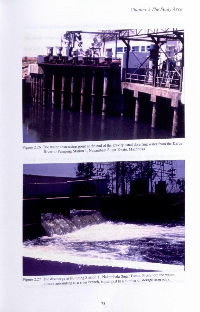
Chapter 2 The Study Area
Figure 2.26 The water abstraction point at the end of the gravity canal diverting water from the KafueRiver LO Pumping Station I, Nakambala Sugar Estate, Mazabuka.
Figure 2.27 The discharge at Pumping Station I. NakambaJa Sugar Estate. From here the water,almost amounting to a river branch. is pumped to a number ot' storage reservoirs.
75

Chapter 2 The Study Area
A cane factory was commissioned on the estate in 1968. In addition to cane grown by
the sugar company, a number of commercial farmers and "small holders" grow cane
and sell it to the sugar company, which, by agreement, supplies them with irrigation
water (Nang'omba, 1995, pers. comm.). The small holder land size was about 1885ha
in 198911990 (Njobvu, 1990). Projections were that the estate would grow to
17 OOOha,including cane farmers and small holders (Pike, 1978). In 1995 it was about
15 OOOhaincluding cane farmers and small holders (Nang'omba, 1995, pers. comm.).
Expansion to 17 OOOhawould, among other things, depend on the availability of the
extra water required (Pike, 1978). The 1978 water rights allowed the estate 12 262ha
(including farmers), after which further water rights would be required.
Virtually all of Zambia's sugar is produced from cane grown on the Nakambala estate
(Nang'omba, pers. comm.). In 1978 some 40 000 tonnes of sugar were produced
(Pike, 1978) and over 116 000 tonnes were grown in 1982 (Howard, 1985). Presently
about 164 000 tonnes per year are produced (News From Zambia, No. 665, 1996).
Production of sugar cane is another strategically important use of part of the Kafue
Flats to the Zambian economy.
The recent trends in rainfall (and to an extent temperature; Section 2.2.1) seem to have
exerted pressure on the management of the water resources of the Kafue Flats, as
indicated by the fact that the Zambia Sugar Company has had to pump more water
each year out of the Kafue River for irrigation of sugar cane (Figure 2.28). From
Figure 2.28, the lowest total abstraction (in the 1980/81 hydrological year) translates
into a consumption of 3.41m's' and the highest (1991192) translates into 6.14mJs-
1,
representing 2.0% and 3.1%, respectively, of the channel capacity of the Kafue River
76

Chapter 2 The Study Area
on the Kafue Flats, which is 170m\-1 (Ellenbroek, 1987)_ Increased abstraction of
water for irrigation is one indication of rainfall stress, but it could be due to a
combination of the climate pressure and the expansion of the sugar estate.
200~------------------------------------------------~
c: 150 +------------------o
~t)
~~V>wc:Qi g 100E=u:::E:c~:::J~wE:::J(5> 50
o 197919801981198219831984198519861987198819891990 1991 199219931994Year
Figure 2.28 Trends in water abstraction from the Kafue River for irrigation at Nakambala SugarEstate. Data: Zambia Sugar Company, Mazabuka.
2.7.3 Nature Conservation
A variety of birds and large mammals live on the Kafue Flats (as outlined in Section
2.6). In an attempt to conserve them, two small national parks have been established:
Lochinvar (1972) and Blue Lagoon (1973) National Parks (see Figure 2.1). Both were
cattle ranches previously, from which carnivores were systematically exterminated.
Conservation of the biodiversity on the Kafue Flats is an important component of
biodiversity conservation in Zambia.
77

Chapter 2 The Study Area
Tourism is a small industry in the national parks and a few wild animals are taken by
safari hunters. Poaching is a persistent problem. The World Wide Fund for Nature
(WWF) included the Kafue Flats in its Wetlands Project, which was handed over to the
Zambian government's Department of National Parks and Wildlife Services in 1995
(WWF-Zambia, 1995, pers. comm.). The project encourages the involvement of the
local people in conservation and wetland management, and has largely been successful
in doing so (Jeffrey and Chooye, 1991).
The endangered status assigned to the Kafue lechwe (Kobus leche kafuensis)
(Ellenbroek, 1987; Sayer and van Lavieren, 1975; Schuster, 1980; Chabwela and
Ellenbroek, 1990) has meant that most conservation concerns on the Kafue Flats have
been about this species. The animal, which is an antelope, is endemic to the Kafue
Flats. It lives a semi aquatic way of life and can graze the emergent vegetation in
shallow water up to 50cm deep (see Figure 2.29) (Ellenbroek, 1987; Rees, 1978; Sayer
and van Lavieren, 1975). It is, therefore, highly influenced by the nature (extent and
duration) of flooding on the Kafue Flats (described in Section 2.3.1.2).
2.7.4 Other Uses
The Kafue River on the Kafue Flats is one of Zambia's commercial fisheries. About 67
species of fish have been listed for the Kafue River system (Handlos, 1978). The
fishery is one of the most productive in Zambia, its catches providing about 18% of the
national total in 1976 (Muyanga and Chipundu, 1978). Traditional inhabitants (the
Twa people) and migrant fishermen sell their fish to middle men who transport the fish
(mainly Tilapia) to urban markets. In 1982 at least 7 400 tonnes of fish were caught in
78
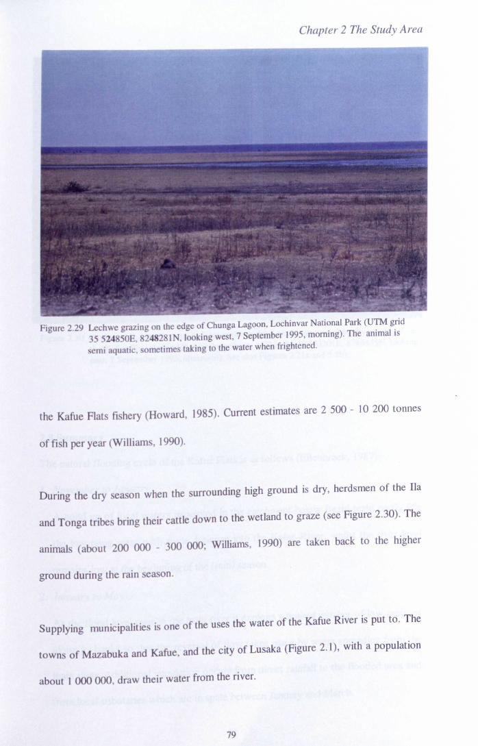
Chapter 2 The Study Area
Figure 2.29 Lechwe grazing on the edge of Chunga Lagoon, Lochinvar National Park (UTM grid35 524850E, 8248281N, looking west, 7 September 1995, morning). The animal issemi aquatic, sometimes taking to the water when frightened.
the Kafue Flats fishery (Howard, 1985). Current estimates are 2 500 - 10 200 tonnes
of fi h per year (Williams, 1990).
During the dry season when the surrounding high ground is dry, herdsmen of the IIa
and Tonga tribes bring their cattle down to the wetland to graze (see Figure 2.30). The
animals (about 200 000 - 300 000; Williams, 1990) are taken back to the higher
ground during the rain eason.
Supplying municipalities is one of the uses the water of the Kafue River is put to. The
towns of Mazabuka and Kafue, and the city of Lusaka (Figure 2.1), with a population
about 1 000000, draw their water from the river.
79

Chapter 2 The Study Area
Figure 2.30 Callie grazing (back ground, right) in the wetland areas surrounded by dry grassland onthe Kafue Flats (behind Banachibwembwe, UTM grid 35 533201E, 8260455N, lookingeast,7 September 1995, afternoon). See also Figures 2.21a and 5.3b).
2.8 Summary
The natura] flooding cycle of the Kafue Flats is as follows (Ellenbroek, 1987):
l,November to January
A build up of local waters deposited in the catchment below Itezhi-tezhi partly fills
the low lying areas with orne drainage into the Kafue River, whilst the river level
remain low at the beginning of the (rain) season.
2. January to May
As the flood level ri e in the main river it exploits a limited number of low sections
along it bank 0 that the reversal of flow takes place by water spreading from the
main river. Additional inundation occurs from direct rainfall to the flooded area and
from local tributaries which are in spate between January and March.
80

Chapter 2 The Study Area
3. May to October
As the river level falls again, drainage from the inundated areas will resume but not
all the available free water finds its way back to the main river. Large volumes are
retained in depressions and are lost by evaporation during the dry season.
Since about 1978, the area has been receiving more unpredictable, erratic and
frequently below average seasonal rainfall compared to the period before. Statistically,
however, these rains do not significantly differ from those before 1978 in terms of
either seasonal totals or frequency of below average rainfall. As a consequence of the
reducing seasonal rainfall and the operation of dams, river discharges have been
declining. This, in tum, is likely to have resulted in change in wetland attributes.
The potential causes of wetland change on the Kafue Flats (in order of potential
magnitude of impact) are fluctuations in:
I. Discharges at Itezhi-tezhi dam (magnitude, duration, timing).2. Local rainfall (magnitude, duration, timing).3. Abstraction of water for irrigation of sugar cane on the Nakambala Sugar
Estate.4. Burning (human induced).5. Grazing pressure (from wildlife and cattle).
The factors influencing the Kafue River's discharge and water levels on the Kafue Flats
are:
I. Discharges through Itezhi-tezhi dam (timing, magnitude, duration).2. Rainfall (timing, magnitude, length of season).3. Abstractions for irrigation at Nakambala Sugar Estate.4. Evapotranspiration.5. Ground water outflow.
Whereas data exist for the first three factors, factors (4) and (5) have scarcely been
quantified. There is also a lack of data on the potential indicators (measures) of
81
Chapter 2 The Study Area
wetland change listed in Table 1.6. These measures range from properties of plants,
vegetation communities, landform, soil, hydrologic and hydraulic properties, aquatic
physical and chemical properties, organismal properties, properties of individual
wildlife and fish species, to properties of wildlife communities. For wetland change
assessment purposes, these attributes would have had to be monitored over time, a
very time consuming process. The paucity of data indicates the difficulty of using
ground monitoring as a method of assessing long term wetland change. In the case of
spatial wetland properties, remote sensing would be a more appropriate approach if
historical images are available, because of synoptic coverage of large areas.
The human uses of the Kafue Flats wetland's water are often in conflict with its role as
a wetland habitat for many animals and birds. The human use of the area has resulted in
increased pressure on the stability of the wetland, in conjunction with climatic
pressures. However, because of the economic importance of these human uses, their
impact on the wetland is likely to increase, rather than reduce, in the foreseeable
future. Striking a balance between resource use and conservation is difficult since the
country is under-developed but vitally important, particularly given the role of wildlife
in promoting the tourism industry.
82

Chapter 3
LITERATURE REVIEW
3. I Introduction
It was shown in Chapter 2 that there have been environmental stresses on the Kafue
Flats, in terms of inflow and outflow of water and land use, which could have resulted
in wetland changes. The precise nature of these changes can be determined by ground
monitoring, remote sensing, or by both approaches. This chapter outlines and
summarises material from literature concerning the methodological aspects of change
detection by remote sensing, and field-based studies about change on the Kafue Flats.
The first part of the chapter reviews the change detection procedures, methods and
factors that must be addressed prior to change detection by remote sensing in order to
make it more accurate. The strengths and weaknesses of the change detection methods
are outlined and examples of wetland studies and land cover change detection studies
in southern Africa by remote sensing are pointed out.
The second part of the chapter outlines the results and predictions of change studies of
the Kafue Flats. Many studies anticipated and predicted adverse hydrological,
vegetation, wildlife and fishery output changes on the Kafue Flats, primarily to result
from damming and regulation of discharges into and from the Flats for hydroelectric
power generation as outlined in Sections 2.3.1.2 and 2.7.1. These studies and those
concerning remote sensing of the Kafue Flats are reviewed.
83

Chapter 3 Literature Review
3.2 Change Detection in Remote Sensing
Change detection involves the selection of a minimum of two images of an area. Prior
to change detection analysis of the images, it is important to ensure that any changes
detected are the result of change in the land surface target under investigation and not
due to any other factors. The other factors that may result in apparent inter image
change have been explored by Milne (1988), Jensen (1986) and Mouat et al (1993).
They are addressed below.
3.2.1 Potential Sources of Change Detection Inaccuracy and Their PriorElimination
The potential sources of change detection inaccuracy in remote sensing can be grouped
into four categories (Milne, 1988):
I. Radiometric factors2. Temporal factors3. Spatial aspects4. Spatial registration aspects
These will be addressed in turn, together with methods of eliminating them or
minimising their magnitude.
3.2.1.1 Radiometric Factors and Atmospheric Correction Methods
Differences in the composition of the atmosphere at the time of image acquisition, such
as water vapour, aerosols, dust and cloud cover differences, can add to or reduce the
apparent reflectance from unchanged ground targets as a result of differences in
atmospheric scattering, absorption and reflection of the electromagnetic energy. These
factors necessitate radiometric and atmospheric correction before images are used in
change detection analysis.
84

Chapter 3 Literature Review
There are four main techniques that can be used to correct images for atmospheric
effects (Jensen, 1986; ERDAS Inc., 1994):
1. Dark object subtraction (or zero minimumJhistogram adjustment method)2. Regression adjustment3. Radiance to reflectance conversion4. Atmospheric modeling
The methods are reviewed below.
3.2.1.1.1 Dark Object Subtraction Method
In the dark object subtraction method, it is assumed that the pixel of lowest digital
number in each band should really be zero and hence its radiometric value is the result
of atmospheric induced additive factors. Potential targets that can have zero readings
are cloud or mountain shadows, dark rocks or volcanic soils in the visible; cloud or
mountain shadows, clear and deep water surfaces or burnt areas in the near infrared
(Gonima, 1993). The bands are adjusted to have zero as the minimum value, and all the
other pixel values are reduced by the same respective amounts as were used to reduce
each minimum to zero. The problem with this method is that there may not really be a
pixel with zero readings on the image (Crippen, 1987). Work has shown that instead of
improving image quality, this method may actually degrade images (ERDAS Inc.,
1994). Subtracting a constant value from the entire digital image assumes a constant
atmospheric additive effect throughout the entire image, which is often not the case
(Chavez, 1988). The method, however, does accomplish first order correction, which
is usually better than no correction at all (Chavez, 1988).
85

Chapter 3 Literature Review
3.2. I. 1.2 Regression Adjustment Method
In the regression adjustment method, an area either in shadow or in homogenous deep,
non-turbid water is chosen and then for each pixel in the area, the brightness values of
a visible band are plotted against the corresponding values in an infrared band at the
same location (Jensen, 1986). If there are no atmospheric effects this plot should pass
through the origin. Any shift away from the origin (the x - intercept, called bias)
represents atmospheric effects and should be subtracted from all the original data in the
visible band concerned. This technique requires many more passes through the digital
data than when using the zero minimum method (in the latter method only the band
minima are determined). There is no guarantee, however, that it will provide superior
results (Jensen, 1986; Crippen, 1987). Although it has a strong statistical footing in
that it uses several pixels of various illumination intensities, it provides only relative
(not absolute) results (Crippen, 1987).
3.2. I. 1.3 Radiance to Reflectance Conversion Method
In the radiance to reflectance conversion method, on-site reflectance measurements or
standard tables that list the standard reflectance of known targets such as particular soil
types, road surfaces or rock types, are used to obtain the true ground reflectance
values. The image digital numbers over these known targets are then adjusted to
conform to these values, thereby eliminating the atmospheric effects. Use of reflectance
tables for standard materials involves assumptions about the targets in the image
(ERDAS Inc., 1994) which may not always hold. There is also the disadvantage of the
logistical impracticality of ground measurements (Crippen, 1987) because the
measurements may have to be made simultaneously at the time of image acquisition.
86

Chapter 3 Literature Review
3.2.1. 1.4 Atmospheric Modeling Methods
In atmospheric modeling methods (e.g. LOWTRAN or MODTRAN - Kneizys et al,
1988), knowledge of the meteorological conditions at the time of satellite overpass,
such as aerosol composition, water vapour content, temperature, ozone and pressure,
are used to model the path radiance and atmospheric transmission. Though accurate
results may result if this information is available, these methods are very complex
(ERDAS Inc., 1994). However, the required meteorological information is not always
available for a given area, is very expensive to acquire, and is point data and therefore
site specific and not necessarily representative of the atmospheric conditions over the
entire image (Milne, 1988). Assumptions are often involved which may not always
hold.
Work has been done to improve the atmospheric correction methods (e.g. Switzer et
al, 1981; Chavez, 1988; Crippen, 1987; Kaufmann and Sendra, 1988; Richter, 1990;
Gonima, 1993). These improvements may still need further testing and research. The
best atmospheric correction method is that which uses in situ data from the field at the
time of satellite overpass (Chavez, 1988). According to Kaufmann and Sendra (1988),
lack of such information means that the only operational use of atmospheric
corrections today is that for the ocean colour where the very low reflectance of the
water in the red allows a relatively easier correction. Cracknell and Hayes (199 I)
summarise atmospheric correction by stating that there are several approaches that one
can take to the question of applying atmospheric correction to satellite remote sensing
data for the extraction of geophysical parameters:
87

Chapter 3 Literature Review
I. Ignore the atmospheric effects completely. There are some applications for which
this is often a perfectly acceptable approach, according to Cracknell and Hayes
( 1991). Ignoring atmospheric effects would probably be acceptable when mapping a
phenomenon at a single time, but for change detection purposes, atmospheric
effects have to be addressed in order to minimise change detection errors.
2. Calibration with in situ measurements of geophysical parameters (the Radiance to
Reflectance Conversion Method in Section 3.2.1.1.3).
3. The use of a model atmosphere with parameters determined from historic data.
4. The use of a model atmosphere with parameters determined from simultaneous
meteorological data (called Atmospheric Modeling Methods in this section).
5. The elimination of, or compensation for, atmospheric effects on a pixel-by-pixel
basis (e.g. the Dark Object Subtraction and Regression Adjustment Methods In
Sections 3.2.1.1.1 and 3.2.1.1.2).
The selection of the appropriate option will be governed by considerations both of the
sensor that is used to gather the data and the problem to which the data are being
applied (Cracknell and Hayes, 1991). Due to problems with these methods, it has been
more common in the past to attempt to standardise one data set to another rather than
to try and apply the complex modeling that is required to correct for variations in
atmospheric transmission and path radiance (Milne, 1988). One technique for
standardising image data sets is normalisation (described in Section 3.2.1.2) (Schott et
al, 1988; Eckhardt et al. 1990; Hall et al, 1991; Jensen et al, 1995; Lee and Marsh,
1995).
88

Chapter 3 Literature Review
3.2.1.1.5 Sensor Aberrations and Sensor System Factors
Differences in sensors and sensor systems used to capture the images can also cause
apparent changes in the appearance of unchanged ground targets. The sensor and
sensor system factors that can cause radiometric differences are principally due to
fluctuations in the orbital parameters of the satellite platform and variations in the
sensitivity of the sensors to the detection and recording of incoming energy levels
(radiometric resolution). One way of dealing with the problem of differences in
radiometric resolution is to convert the digital numbers in the data sets to actual
reflectance values using standard tables or formulae (Milne, 1988; Lee and Marsh,
1995; Robinove, 1982). Fluctuations in the orbital and platform attitudes of the
spacecraft are known and the necessary geometric corrections can be applied in the
early stages of the pre-processing of the data, usually by the ground station receiving
the raw data from the satellite (Milne, 1988).
Detector response errors (aberrations) also cause change detection inaccuracy and
must be corrected. They can be either due to line dropout, striping (banding) or line
start problems (Jensen, 1986). Line dropout results if one of the detectors on a sensor
fails to function during a scan, resulting in zero values for every pixel in the particular
line, or if it is temporarily saturated along a scan, resulting in very high or maximum
values in the scan. To correct the data, estimated values can be used in each bad line by
averaging the values of the pixels above or below the bad scan line. If a detector goes
out of adjustment, for example if it provides readings twice as great as the other
detectors for the same band, the problem is referred to as n-line striping or banding
(Jensen, 1986). One way to identify the bad scan lines is to compute a histogram of the
values for each of the detectors over a homogenous area such as a water body. If one
89

Chapter 3 Literature Review
detector's mean or median is significantly different from the others, it is possible that
this detector is out of adjustment and may require a bias (additive or subtractive)
correction or a more severe gain (multiplicative) correction (Jensen, 1986). If a
scanning system fails to collect data at the beginning of a scan line, this is called a line
start problem. A detector may abruptly stop collecting data somewhere along a scan
line and produce results similar to line dropout. Data not recorded by the detector in
this way can never be restored (Jensen, 1986).
3.2.1.2 Temporal Factors
Diurnal and seasonal differences can cause the appearance of change in unchanged
surface conditions between two image dates. These differences result in change in the
sun angle and the vegetation (phenological changes) which in turn will result in
apparent change on the images. If phenological change is not the subject of the change
analysis, selecting data collected on anniversary or near anniversary dates will help
eliminate its effects (Milne, 1988; Jensen, 1986; Jensen et al, 1995; Eckhardt et al,
1990).
Differences in sun angle result in differences in the intensity of radiation received and
hence reflected to a sensor by a ground target. These differences, as well as those
resulting from differences in atmospheric composition, can be minimised by
standardising the data sets using the technique of normalisation (Schott et al, 1988;
Eckhardt et al. 1990; Hall et al, 1991; Jensen et al, 1995; Lee and Marsh, 1995). The
technique attempts to make each spectral band (from the different dates) appear as
though imaged through the same sensor, under similar illumination conditions and the
same atmosphere for each image. Targets that are common to the images in the image
90

Chapter 3 Literature Review
set and are considered to be constant reflectors over time (i.e. their reflectance remains
unchanged over time) are selected. For these normalisation targets any changes in their
digital numbers between dates will be attributed to detector calibration, atmospheric,
astronomic and phase angle (sun-target-sensor geometry) differences. After the
removal of these variations, changes in digital numbers may be related to changes in
surface conditions. Potential normalisation targets should have the characteristics in
Box 3.1.
Potential normalisation targets should have the following characteristics:
I. The target should be at approximately the same elevation as the other land within thescene. Selecting a mountain top normalisation target would be of little use in estimatingatmospheric conditions near sea level because most aerosols in the atmosphere occurwithin the lowest tDOOm.
2. The target should contain only minimal amounts of vegetation. Vegetation spectralreflectance can change over time due to environmental stresses and plant phenology.
3. The target must be in a relatively flat area so that incremental changes in sun angle fromdate to date will have the same proportional increase or decrease in direct beam sunlightfor all normalisation targets.
4. When viewed on the image display screen, the patterns seen on the normalisation targetsshould not change over time. Changing patterns indicate variability within the targetswhich could mean that the reflectance of the target as a whole may not be constant overtime. For example, a mottled pattern on what had previously been a continuous tone drylake bed may indicate changing surface moisture conditions, which might eliminate thedry lake bed from consideration as a normalisation target.
Box 3.t Ideal Characteristics of Potential Normalisation Targets (after Eckhardt et al, 1990).
Targets that qualify to be potential normalisation targets are wet (water) and dry (e.g.
unvegetated bare soil) sites. Where these natural targets are lacking artificial features
like car parks, roads and buildings may be used (Schott et al, 1988; Hall et al, 1991).
91

Chapter 3 Literature Review
The targets used need not be the same throughout the multitemporal data set (Schott
et al, 1988; Hall et al. 1991).
Once the targets have been chosen, their brightness values in the respective image
bands (e.g. green, red, infrared) on one image are regressed against their
corresponding values in the corresponding bands on the other image. A reference
image is chosen, whose brightness values in a given band are placed on the y-axis while
those for the image to be normalised are placed on the x-axis, The regression model
developed is then used to transform the band brightness values of the image to be
normalised into values that they would have been had the image been acquired under
scene conditions like those when the reference image was acquired. This technique
may be helpful in vegetation change detection in semi-arid areas (Mouat et al, 1993). It
can, however, be criticised for adding an additional, unstandardised 'treatment' and
therefore further uncertainty into a study (Stow et al, 1990).
3.2.1.3 Spatial Aspects
The spatial resolution of the sensors used will determine the nature and scale of the
changes that can be identified between images dates (Jensen, 1986; Milne, 1988). For
example, if Landsat MSS with a spatial resolution of 80m is used, land surface changes
at a (spatially small) rate of (for example) 1.5m per year may not be detected (Milne,
1988).
3.2.1.4 Spatial Registration Aspects
Accurate spatial registration of at least two images is essential for digital change
detection (Jensen, 1986). In order to accurately measure the difference in brightness
92

Chapter 3 Literature Review
values between images of different dates, the images need to be registered together to
within an accuracy (root mean square error - RMSE) of 0.25 to 0.5 of a pixel (Jensen,
1986) or one pixel at the most (Milne, 1988). The task necessitates the use of
geometric rectification algorithms that register the images to each other or to a
standard map projection, by using common ground control points in the image set. The
algorithm performs a rotational adjustment and resampling of one image to another so
that ground features appear in the same place on each of the images (Milne, 1988).
Without accurate co-registration, registration errors could potentially be interpreted as
land cover change (Mouat et ai, 1993).
3.2.2 Change Detection Techniques
A number of change detection techniques in remote sensing are described In the
literature. They can be grouped as:
I.Transparency Compositing2. Image Differencing3. Image Ratioing4. Classification Comparisons5. Image Enhancement techniques to facilitate change detection
Within these broad groups are sub categories of change detection techniques and each
of the techniques has its own merits and demerits, as outlined below.
3.2.2.1 Transparency Compositing
This method involves assigning a different colour to the same band for images from
different dates such that when the bands are overlaid, a colour composite transparency
is produced. If positive film transparencies of one infrared band are used for two image
93

Chapter 3 Literature Review
dates for example, and red is used for the first date and blue for the second, unchanged
areas will appear purple and areas of positive or negative change will appear red or
blue, respectively (Turner, 1982). MSS Band 5 (renamed band 2, see Table 1.1)
images have been used in this manner for change detection, for example using red for
one date and blue for another (Jensen, 1986). An alternative approach is to use a
negative transparency for the first date and a positive one for the second (Crapper and
Hynson. 1983). When the two are overlaid, areas that have not changed between the
dates will appear neutral to grey and those that have changed will appear either light or
dark depending on the type of change that occurred between the two dates. The
method relies on visual interpretation of the imagery and may not be sensitive enough
to pick up general environmental degradation (Milne, 1988), especially if the change is
very subtle.
3.2.2.2 Image Differencing
With this technique (also called Delta Change Detection), changes in radiance between
two co-registered image data sets are determined by pixel-by-pixel subtraction of the
digital values of one image from those of another (Muchoney and Haack, 1994; Price
et al, 1992; Jensen, 1986; Dale et al, 1996). The subtraction (differencing) produces an
image data set where positive and negative values represent areas of change and values
equal or close to zero indicate areas that remain relatively unchanged. The potential
range of values that can result from the differencing is -255 to 255 if an 8 - bit analysis
with pixel values ranging from 0 to 255 is used (Jensen, 1986). The results are often
transformed into positive values by adding a constant (e.g. 255) and a threshold
boundary is established to define change and no change. After differencing, change
maps can be created.
94

Chapter 3 Literature Review
In their studies using image differencing for change detection, Price et al (1992) and
Muchoney and Haack (1994) recoded the output difference values to numbers ranging
from 0 to 255. A value of 127 was assigned to areas where there was no change in
reflectance (127 is the median between 0 and 255). A value greater than 127 indicated
higher reflectance in the later image and a value less than 127 indicated higher
reflectance in the earlier image.
Similar to Image Differencing is the technique called Albedo Differencing (Mouat et al,
1993) in which digital image data from two dates are converted to reflectance or
radiance values which are then compared to detect changes.
3.2.2.3 Image Ratioing
Ratio images result from the division of digital number values in one spectral band by
the corresponding values in another and have the major advantage that they convey the
spectral or colour characteristics of image features regardless of variations in scene
illumination conditions like shadow or sun angle differences (Lillesand and Kiefer,
1994; Jensen, 1986). They are especially useful for change detection when several
dates of imagery are used in an analysis because they can reduce the effect of
environmental and system multiplicative factors present (Jensen, 1986) and are often
useful for discriminating subtle spectral variations in images from individual spectral
bands or in standard colour composites (Lillesand and Kiefer, 1994).
If, for example, near infrared band data for the dates under comparison are divided
(date I divided by date 2), unchanged areas will have a ratio of 1 while changed areas
95

Chapter 3 Literature Review
will have values greater than 1 if near infrared reflectance was higher at date 1 than at
date 2, or less than I if it was higher at date 2.
3.2.2.4 Classification Comparisons
Change detection can also be undertaken by evaluating land cover classifications
produced either from each separate date of imagery or from the two dates of imagery
as a set, by post classification comparison or spectraVtemporal change classification,
respectively (Jensen, 1986; Lillesand and Kiefer, 1994). Provided good ground
information or some baseline classification is available against which the final
information classes can be compared and interpreted, multidate classifications can be
used to show changed areas. Otherwise unsatisfactory classification may compound
classification and registration errors present in individual classes (Milne, 1988).
In post classification comparison (or post classification change detection differencing -
Muchoney and Haack, 1994), change is identified by comparing two independently
produced classifications on a pixel-by-pixel or polygon-by-polygon basis (Jensen,
1986; Muchoney and Haack, 1994). An algorithm compares class pairs specified by the
analyst in the comparison and, by properly coding the classification results for date I
and date 2, the analyst can produce maps that show a complete matrix of changes. This
enables not only the identification of pixels that have changed but also the nature of
that change (Howarth and Wickware, 1981).
Where classifications are being compared from an image (or images) with a higher
spatial resolution than the other(s), Jakubauskas et al (1990) advise that 'common
ground' be reached between the data sets of differing spatial resolution. They advise
96

Chapter 3 Literature Review
that the comparison will be valid provided that it is made after classification, that it is
made at a land cover classification level no finer than could be accurately determined
by the lowest resolution sensor, and that appropriate generalisation of the finer
resolution data is carried out (i.e. the higher resolution sensor classes are made more
general).
Spectral/temporal classification detects change by performing a single classification on
a multidate data set. Change classes should have significantly different statistics from
non-change classes. Though appealing because it requires only a single classification,
the method uses a very complex classification. If, for example, the 4 bands of Landsat
MSS are used from each image from two dates, 8 bands will have to be used in the
classification, some of which will be redundant in information content (because of
similarity of spectral range of coverage as is the case with the near infrared bands).
Also, if clustering is performed during the classification, the cluster labeling (assigning
class names) is usually difficult (Jensen, 1986) because of the large volume of spectral
information from which the resulting clusters are derived.
3.2.2.5 Image Enhancement Techniques for Change Detection
Before using the techniques described in Sections 3.2.2.1 - 3.2.2.4, pre-processing the
remote sensing data by low frequency filtering, high frequency filtering, texture
transformations or principal component analysis may be done (Jensen, 1986).
In low frequency filtering the image is smoothed using a spatial moving average filter
of a given size (e.g. 3x3 pixels) which enhances areas of homogeneity at the expense of
97

Chapter 3 Literature Review
high frequency detail. High frequency filtering enhances high frequency detail,
producing a sharp visual image which, however, contains more noise than the original
(Jensen, 1986).
With texture transformations, the images to be compared are pre-processed to yield
multiple date texture images which can then be analysed using any of the change
detection procedures in Sections 3.2.2.1 - 3.2.2.4 (Jensen, 1986).
Muchoney and Haack (1994) describe principal component analysis (PCA) in the
context of change detection. The technique is a multivariate statistical one in which the
data sets are rotated into principal axes, or components, that maximise the data
variance. The original data are then transformed to the new principal axes (components
or eigen images). In this manner correlated data sets can be represented by a smaller
number of axes, while maintaining most of the variation of the original data. For
change detection purposes the authors divide PCA into two categories:
(a) independent data transformation analysis,
(b) merged data transformation analysis.
Independent transformations, they point out, are subsets of post classification change
detection that employ PCA independently on co-registered multitemporal data pairs as
a prelude to post classification comparisons, while merged data transformations are
those that rely upon PCA of combined multitemporal data sets to isolate inter image
change (prelude to spectraVtemporal change detection). They point out that the
premise for this analysis is that multitemporal data sets are highly correlated and that
PCA can be used to highlight differences attributable to change. Changes are enhanced
98

Chapter 3 Literature Review
in medium to higher order eigen images, whereas unchanged areas dominate the
redundant temporal information in the lower order eigen image(s) (Stow et al, 1990).
3.2.2.6 Other Methods
Some studies have used change in vegetation indices (like the Normalised Difference
Vegetation Index (NDVI), near infrared to red ratio (NIRfR), and Tasseled Cap
(greenness, brightness, wetness) transformation as indicators of change (Mouat et al,
1993). For example, Mikkola (1996) compared NDVI values from different years to
analyse vegetation damage around smelters in Russia, in addition to change detection
by comparing classifications.
Jensen (1986) describes a detection method called Change Vector Analysis. In this
method, if two spectral variables are measured for an area both before and after change
occurs and then are plotted on the same graph, the vector describing the direction and
magnitude of the change from the first to the second date indicates the type and
magnitude of spectral change.
Milne (1988) lists spectral change pattern analysis, logical pattern change detection
(,classification routine techniques') and regression analysis as methods for detecting
land cover change, in addition to other techniques which seem to be just other names
for the same techniques described in Sections 3.2.2.1 - 3.2.2.5.
3.2.2.7 Comparison of Use and Evaluation of the Change Detection Techniques
Regardless of the technique used, the success of change detection will depend on the
nature of the change involved - whether it is abrupt or gradual. Milne (1988) stresses
that provided the areas involved in the change are large enough, changes are relatively
easy to detect and measure on imagery, but that more subtle changes like gradual
99

Chapter 3 Literature Review
deterioration in vegetation cover associated with drought or overgrazing are more
difficult to detect.
Muchoney and Haack (1994) compared principal component analysis (PCA), image
differencing, spectral-temporal change classification and post classification comparison
change detection techniques in their study of gypsy moth induced forest defoliation,
using multitemporal SPOT data. They found that the defoliation was best determined
by image differencing and PCA. The four techniques resulted in significantly different
accuracies at 95% level of probability. The authors pointed out that PCA and image
differencing are generally more complex than post classification change detection
because the data no longer represent actual sensor data values, and classification
involves identifying change, rather than cover, classes. They concluded that PCA and
image differencing are simpler than post classification approaches, which require
independent classification prior to change detection. No corrections for atmospheric
effects were done because, according to the authors, the imprecision of a scattering
model might influence change detection results. Geocoding and rectification (RMSE
approximately 1 pixel) were done.
Price et at (1992) found the image differencing technique useful for detecting areas of
shrub die back between 1975 and 1988 in a semi arid environment. Significant
reduction in reflectance was, however, observed both in die back and non die back
areas, and the authors suggest that the reduction could be related to calibration
differences between the sensors used (Landsat MSS images from Landsats I, 3, 5), or
to large scale environmental differences such as surface soil moisture or vegetation
composition. No atmospheric correction or scene normalisation was done. Therefore
100

Chapter 3 Literature Review
these authors ignored the pre-change detection considerations outlined in Section
3.2.1.
From a study of vegetation change resulting from fire, lakubauskas et al (1990) report
successful use of post classification comparison for vegetation change detection,
advising that the technique can be used for vegetation change detection within the
context of GIS analysis. The images used were from Landsat I (1973 MSS), Landsat 2
(1980 MSS) and Landsat 4 (1982 TM). A 3x3 majority class filter was applied to the
classified TM data set to generalise the data to the level of the MSS. No normalisation
of the images or atmospheric correction was done.
Stow et al (1990) compared image ratioing with principal component analysis in a
change detection study involving multitemporal, multispectral imagery of varying
spatial resolution (October 1976 MSS, October 1986 TM, November 1986 SPOT
HRV XS) which were co-registered. Following change detection mapping with the
two techniques, a 5x5 pixel majority filter was passed across each image in an attempt
to minimise extraneous errors. No atmospheric correction or image normalisation was
done and the authors argue that normalising the multisensor data would have meant an
additional, unstandardised treatment that would have added further uncertainty into the
study. They found that ratioing produced higher change detection accuracies than did
PCA. Applying a majority moving window filter whose size approximated a minimum
mapping unit of I hectare increased change detection accuracies by 1-3% and reduced
commission errors by 10-25%, according to the authors.
Baumgartner and Price (1993) argue that although a non-enhancement technique such
as classification comparison can provide information on all changes occurring in a
101

Chapter 3 Literature Review
study area (while enhancement techniques only distinguish change from no change),
the accuracy of a change map produced with this technique may be poor. The authors
point out that the accuracy of a change map produced from two classifications is
similar to the product of the two classification accuracies, such that two classifications
with 80% accuracy may produce a map that is 64% accurate. The integration of
enhancement and non enhancement techniques using Landsat TM data was employed
in the authors' study which aimed at accurate detection and measurement of the spatial
extent of non urban land cover change, as well as deriving categorical change
information between 1982 and 1990. The techniques used were vegetation index
differencing with the near infrared/red ratio (TM4fTM3 (date 1) - TM4fTM3 (date 2)
plus a constant), image differencing (TM4 (date I) - TM4 (date 2) + a constant (255»,
principal component analysis (combining 6 TM bands from 1982 with 6 TM bands
from 1990) and post classification comparison. Image registration (RMSE +/- 10m),
atmospheric correction with an improved dark object subtraction technique, and image
normalisation were undertaken.
Tao et al (1993) introduce a change detection technique employing what they term
'three dimensional temporal feature space' which they used to analyse wetland change
in coastal Louisiana using single band (Band 4) Landsat TM data (2 December 1984,
28 January 1988, I November 1990). The technique is, in effect, a kind of
transparency compositing because a different primary colour was assigned to the band
4 images from the three respective dates, which were then overlaid to create a colour
composite. The colour composite was then analysed for indications of change using the
resulting colours (white or black indicating no change; red, green, blue, yellow,
magenta and cyan indicating a specific type of change between the dates). The authors
102

Chapter 3 Literature Review
outline the advantages of using the technique: first, that there is data efficiency and
saving on data processing time since only one band of data for each of three dates is
used (thereby avoiding the complex and intensive labour/computer process of
classifying large data sets); and second, that it is possible to perform change detection
analysis for three periods simultaneously. However they pay little attention to the effect
that temporal differences between the two imaging dates might have on the change
results.
From the literature, therefore, there is no consensus on which change detection
technique(s) is (are) best or worst. The decision of which technique to use seems to
depend on the judgement of the researcher. The enhancement techniques and
vegetation indices seem to be widely used, and image differencing and classification
comparisons are common. Image ratioing seems to be rarely used solely, and there are
very few recent studies using transparency compositing. However, methods which
involve a direct comparison of digital (reflectance) values, such as image differencing,
image ratioing and vegetation indices, are highly susceptible to radiometric errors (see
Section 3.2.1.1) in the original digital image data. Because classification uses a range
of values in arriving at classes, it avoids this reliance on comparing the values directly
and may, therefore, be a more useful change detection technique if the classification is
accurate. Image ratioing and differencing techniques compare only two equivalent
bands at a time and may, therefore, not be useful if change detection is required on
more than two images simultaneously. Classification can use one or more bands per
date, and the resulting classified images (more than two at a time) can be manipulated
in a GIS framework to enable a range of change detection queries. Enhancement
techniques will be accurate if they adequately enhance the feature(s) under study but
103

Chapter 3 Literature Review
have the disadvantage that they modify the original image data, which may complicate
further processing of the image.
3.3 Recent Wetland Change Studies by Remote Sensing
No recent work on tropical, Southern African wetland change assessment by remote
sensing was found in the literature. However, monitoring and change detection work
has been done for the arid lands of Botswana using Landsat images (Ringrose et al,
1990), for a forest area in Zaire using Landsat images (Massart et al, 1995), for
woodland areas around Lusaka in Zambia (Cheattle, 1994) and for the Central and
Southern region of Zambia using AVHRR images (Azzali, 1991).
In East Africa, Haack (1996) used a GIS overlay of Landsat MSS near infrared (band
4) black and white film positives at a scale of 1:1 000 000 to monitor changes in the
Omo Delta wetland (Kenya). The image dates were 1 February 1973, 1 January 1979
and I March 1989. The delta appeared to have grown in the time period, with much of
the new delta growth being green vegetation. The data used could not differentiate
categories within the green vegetation. Haack (1996) attributes the growth of the delta
to a decrease in levels of the lake (Lake Turkana) into which the Omo discharges,
which in turn may be a result of increased aridity and/or a decreased flow into the lake.
Both a decrease in precipitation within the catchment basin and an increase in
temperature could have been contributing factors (Haack, 1996). Upstream diversion
of water for small scale irrigation are also likely to have caused the decline in lake level
(Haack, 1996).
104

Chapter 3 Literature Review
Three wetland studies in the USA, by Jensen et al (1995), Mackey (1993) and
Williams and Lyon (1991), give comparative procedural frameworks for wetland
change detection work. Jensen et at (1995) used a combination of Landsat MSS, TM
and SPOT images from the period 1973 - 1991 (6 in total), which were resampled to
the 20 x 20 m resolution of SPOT, normalised and co-registered to a common map
projection (UTM), to produce a wetland change map following post classification
comparison in a GIS framework. No atmospheric correction was undertaken. Mackey
(1993) used fifteen dates of spring time SPOT HRV data along with near-concurrent
vertical aerial photographic and phenological data from Spring 1987 through Spring
1992 to monitor trends in wetland community changes. No atmospheric correction or
scene normalisation was undertaken. Post-classification comparison was used for
change detection. Williams and Lyon (1991) used a digital data base constructed by
photo interpretation, mapping and digitising seven dates of aerial photography on the
St. Mary's River, USA, to examine historical changes in wetland area in a GIS
framework. The photos were from 1939, 1953, 1964, 1978, 1984 and 1985. The
results indicated that there was greatest variation in areas of emergent wetland and
shrub wetland, which appeared to be responding primarily to changes in water level.
In Australia, Dale et al (1996) used digitised colour infrared photographs from May
1982, May 1987 and June 1991 to evaluate change in the Moretan Bay inter-tidal
wetland, which was modified in 1985 for purposes of managing a mosquito breeding
programme. Green, red and near infrared bands were used. Change detection was
undertaken by image subtraction and classification comparison techniques. The results
indicated that the wetland had become wetter as a result of increased tidal flushing,
105

Chapter 3 Literature Review
indicated by reduced spectral values. Mangroves had increased in size and spatial
extent, and generally had increased spectral values.
3.4 Studies of the Kafue Flats
Studies involving surveying and describing specific aspects of the Kafue Flats
environment prior to the establishment of hydroelectric and irrigation schemes (see
Sections 2.7.1 and 2.7.2) are many and have been listed by Turner (1983). These
studies were mainly undertaken in order to understand better the area and to assess its
potential for economic development. In spite of these studies, understanding of the
Kafue basin is still inadequate for satisfactory protection and management of its
resources; and the little that is known has had little effect on policy decisions (Sheppe,
1985; Burke, 1994).
After the implementation of the hydroelectric scheme in 1972 considerable research
attention focused on predicting and monitoring the impacts of the scheme on the Kafue
Flats environment. Interest in studying change in the area has, therefore, been strong.
The University of Zambia had, until the late eighties, the Kafue Basin Research Project
(KBRP) which coordinated the various research interests on the Kafue Flats and basin
(KBRP publications include Howard and WiIliams, 1977; Turner, 1983).
3.4.1 Change Prediction and Verification Studies
Predictions have been made about the likely hydrological, vegetation, fishery output
and wildlife populations changes to result from the hydroelectric scheme. Climate
pressure was largely ignored as a cause of change in some of these studies, perhaps
because the recent low rainfall trend (see Section 2.2.1) had just began.
106

Chapter 3 Literature Review
3.4.1.1 Hydrological Changes
It was widely predicted that the effect of the Kafue Gorge dam (hydroelectric scheme
Phase I; see Section 2.7.1) would result in the maintenance of higher than normal
minimum river levels in the dry season. with the result that the area under permanent
water would increase. Several studies have emphasized this (e.g. Schuster, 1980;
Howard. 1985: Sheppe, 1985; Rees, 1978; Turner, 1982; Douthwaite, 1974;
Douthwaite. 1978) and pointed out that Chunga Lagoon at Lochinvar (Figure 4.14) is
a direct consequence of this because it did not exist before 1972.
As pointed out in Section 2.5. the timing and duration of the flood on the Kafue Flats
determines the nature of floodplain vegetation in terms of vigour and density.
Widespread. long lasting flooding is ecologically more beneficial to the wetland in this
respect. Therefore. any alteration of the flooding pattern in such a way that flooding
starts late. is spatially less widespread and lasts only a short time, is detrimental. The
predicted impact of damming at Itezhi-tezhi in 1978 (hydroelectric scheme Phase II)
and the consequent regulation of discharges for generation of electricity would be to
decrease the size of the area flooded. as well as the duration of the flood, a situation
which would be worse in dry years (Balasubrahmanyam and Abou-Zeid, 1978a;
Sheppe. 1985; Douthwaite. 1974; Schuster. 1980) when the peak flood in March
would be lower than it was under natural conditions. With regulated flow, river levels
would be higher than normal in the dry season and the flood would start later than
normal and fall more slowly (Douthwaite. 1974).
Balasubrahmanyam and Abou-Zeid (1978a) state that measures were incorporated in
the design of Phase II of the hydroelectric scheme to ensure flooding of the Flats even
)07

Chapter 3 Literature Review
in dry years, by way of releasing at least 300mJs-' in March of every year. The Itezhi-
tezhi Reservoir's capacity was designed to ensure that this happened so that ecological
requirements would not be overridden by those of power generation. Only aerated
water would be discharged from the reservoir. Compared to natural conditions, the
authors point out, this controlled flooding would ensure higher river levels than would
otherwise be the case in dry years and in the dry season, which would be beneficial. In
wet or normal years the dam would have no adverse effect on the Flats. Sheppe (1985)
argues that the 300m3s-' discharge would be small compared to the former March
discharge of 1400m3s-'. Douthwaite (1978) predicted that even with the 300m3f' in
March in dry years, there was unlikely to be any extensive flooding.
3.4.1.2 Vegetation Changes
As a result of reduced flood extent, disrupted flood timing, and the maintenance of
permanent water in seasonally inundated areas (see Section 3.4.1.1) vegetation
changes were foreseen. Plants that thrive in wet areas, such as Cyperus papyrus and
Typha domingensis (see Figures 2.20, 2.21a, 2.21b, 2.21d), would occupy
permanently flooded areas that previously had floodplain grassland species, and those
sections of the floodplain that were no longer flooded would be invaded by woody
plant species.
Sheppe (1985) compared a portion of the floodplain at Lochinvar in 1983 with what it
was in 1967. Whereas in May 1967 the portion was covered by a dense growth of
emergent grasses reaching the horizon and hiding the flood water, in May 1983 there
was permanent open water (Chunga Lagoon). The very productive vegetation that had
depended on annual flooding had largely been replaced by aquatic plants in the open
108

Chapter 3 Literature Review
water, while the former floodplain had a sparse cover of low grasses and was being
invaded by woody plants. He further observed that where permanent water had been
established on the former floodplain, floodplain grassland had died out and thickets of
Cyperus papyrus, Typha domingensis and other water loving plants were becoming
established along the shore of the new water bodies. The reduction in flooding had
reduced the productivity of the remaining floodplain grasses and permitted the invasion
of the floodplain by woody plants (mainly Mimosa pigra and to a lesser extent
Hibiscus diversifolius) that formerly were suppressed by the floods. Although only a
small portion of the floodplain was as yet occupied by such plants, Sheppe (1985)
states, they were spreading.
Prior to dam buildings, there existed natural (rainfall and flooding induced) variability
in the distribution of vegetation on the Kafue Flats from month to month and year to
year (Turner, 1994, pers. comm.; Sheppe, 1985; Howard, 1985; Ellenbroek, 1987),
which makes it difficult to draw precise conclusions about the effects of human
interference (Sheppe, 1985), but some of the recent changes in floodplain vegetation
distribution have been caused by the altered flooding regime (Howard, 1985). Howard
(1985) made observations about vegetation change at Lochinvar similar to those by
Sheppe (1985). He observed that high water levels at Chunga Lagoon from 1976-1981
resulted in the appearance of Cyperus papyrus, Typha domingensis and Hibiscus
diversifolius vivularis (in contrast to Sheppe, 1985, who attributed the presence of
H. d. vivularis to reduced flooding), and that in the same period, floating and emergent
grasses and water lilies disappeared from the lagoon. The 1981/82 and 1982/83
droughts, Howard (1985) states, resulted in partial drying of the lagoon and in April
1983 the lilies and emergent grasses reappeared; C. papyrus, T. domingensis and
109

Chapter 3 Literature Review
H. d. vivularis had almost completely disappeared from the part of Chunga Lagoon
that dried out. The emergence of C. papyrus in former floodplain grassland areas was
also observed by Schuster (1980).
3.4.1.3 Fishery Output Changes
It was predicted that after river impoundment, the resulting higher than normal dry
season minimum river levels (Section 3.4.1.1) would reduce fish mortality from fishing
by man and birds and, therefore, increase fish abundance. Post and pre-impoundment
comparison studies have yielded no real evidence of increased fish abundance after
impoundment.
Dudley and Scully (1980), from experimental catches at Chunga (lagoon site), Nyimba
(flowing river sites) and in a lagoon north of Nyimba (Figure 4.14) found that in the
raised water level regime, there was no increased fish abundance; the proportion of
Sarotherodon, a commercially important fish genus, may have actually decreased after
impoundment in 1972.
Muyanga and Chipundu (1978), in a study of 19 commercially important fish species,
observed a decline in catches of Sarotherodon machrochir, Tilapia rendalli and
Tilapia sparrmanii after damming in 1972 compared to the period before. They
attribute the decline to the increase in the area of open water which may have forced
the fish to marginal habitats, thus exposing them to predators. There was a significant
increase in the abundance of four predatory fish species and little change in twelve
others.
110

Chapter 3 Literature Review
Sheppe (1985) predicted unspecified effects on the fish populations, stating that "the
dams altered the flooding schedule and the vegetation - undoubtedly with effects on
the fish population".
3.4.1.4 Wildlife Changes
Wildlife populations, especially those of water birds and lechwe, were generally
predicted to reduce as a result of damming and alteration of the flooding pattern.
Douthwaite (1978) predicted threats to regional and intercontinental migratory birds
which visit the wetland. He stated that birds from the Kafue Flats, like red-billed teal,
fulvous whistling ducks, open billed storks, grey herons and little stints, visit other
regional wetlands (in Namibia, Botswana, South Africa, Kenya and Sudan) while
palaearctic waders from Arctic Russia and Northern Europe visit the area at the end of
the dry season on their way south and at the end of the rains as they return north.
The altered flooding regime was seen by Douthwaite (1974 & 1978) and Howard and
Aspinwall (1984) as being disruptive to the wattled crane's ecology. With reduced
flooding as predicted (see Section 3.4.1.1), suitable breeding and feeding grounds of
the crane would become more restricted and in this situation it was likely that the
wattled crane population would diminish unless flood levels at Nyimba regularly
exceed 5 meters' depth (Douthwaite, 1974 & 1978). Referring to their wattled crane
population estimate of 3 282 in May 1982 compared to Douthwaite's (1974) estimate
of 3 085 in May 1973 (see Table 2.4), Howard and Aspinwall (1984) suggest that
numbers may have increased since t 973 because their study did not include areas to
the west which Douthwaite's did. However, they suggest that it is also possible that
seasonal flocking areas had moved in response to changes in the flooding patterns.
111

Chapter 3 Literature Review
Also many other external factors which affect bird population numbers could have
been responsible.
Water birds in general were identified to be threatened by the flooding alterations.
Douthwaite (1978) predicted that they would disappear. Howard and Aspinwall ( 1984)
state that the extent of the effects of changed flooding patterns were still unknown and
may prove deleterious to floodplain birds. According to observations by Sheppe
(1985), the populations of both fish and fish eating birds had been reduced after the
implementation of the hydroelectric scheme, there were fewer populations of
herbivorous snails and of open billed storks that fed on them, and a reduction in
herbivorous insects had also led to there being smaller numbers of Jacanas and other
insect eating birds. Successful nesting of water birds like yellow billed storks and
others could be eliminated, largely via interfering with their food supply.
Relatively more attention has been paid to the likely consequences of flood alteration
on the lechwe. Many studies predicted a bleak future for the lechwe (e.g. Chabwela
and Ellenbroek, 1990; Rees, 1978; Schuster, 1980; Sheppe, 1985; Douthwaite, 1978;
Sayer and van Lavieren, 1975; Rees, 1976), stating that the lechwe's ecology is highly
influenced by the flood. Douthwaite (1978) points out that persistently high minimum
water levels (see Section 3.4.1.1) since 1974 due to retention of water by the Kafue
Gorge dam had, in 1978, probably led to decline in Vossia grassland in the Chung a
Lagoon area (Vossia was formerly the most important fodder grass for lechwe in the
dry season) (see Figures 2.15, 2.22 and 2.29).
Schuster (1980) suggests that changes in the flooding cycle threatened to disrupt the
lechwe's breeding behaviour and social organisation. The lechwe rut was mainly in the
112

Chapter 3 Literature Review
dry season when leks (mating grounds) were established. Males were in peak condition
then (highest body weight). In the new flooding regime, coarser tussock grasses were
expected to replace lechwe' s favoured and more nutritious floodplain species in areas
that receive less flooding. The resultant scarcity of good grazing in the late dry season
where formerly great quantities were exposed by the falling flood waters might mean
few males reach prime condition for the rut, resulting in disrupted lekking behaviour.
Schuster (1980) points out that the lechwe can also mate, though less successfully, by
way of solitary males defending larger territories than those in the crowded leks.
Contrary to this prediction of disappearing lekking behaviour, the lek system still
existed in 1990 and was studied by Nedft (1992).
Sheppe (1985) sums up the expected changes in wildlife populations in predicting
general decline in lechwe and other wildlife populations, with the result that the rich
variety of communities that once occurred would be destroyed. One reason for this
would be because flow regulation would reduce year to year variability, which IS
important for species abundance in any ecosystem, according to Sheppe (1985).
3.4.2 Remote Sensing Studies
The World Wide Fund for Nature (WWF) has recently (about 1993-1994) used NOAA
AVHRR Channel 2 data to monitor the extent of the flooding on the Kafue Flats
(WWF-Zambia, 1995, pers. comm.). Map updating and reservoir mapping have been
done by the Zambian government's Survey Department and by ZESCO, respectively,
using aerial photographs (Turner, 1982).
Work was underway (in the early 1980s) to monitor and quantify the observed and
predicted land cover changes (see Sections 3.4.1.1 - 3.4.1.4) by the University of
113

Chapter 3 Literature Review
Zambia's Kafue Basin Research Project using maps, aerial photographs and records,
with plans to use Landsat (paper print) imagery for the same purpose (Howard, 1985).
In this regard, Turner (1982) undertook a flood extent monitoring study of the Kafue
Flats using positive Landsat image transparencies from 1972, 1980 and 1981, which
were overlaid manually. Turner concludes that MSS Band 7 (renamed Band 4, see
Table 1.1) is useful for mapping open water because it appears black. There is no
simple relationship between measured river levels and the area of flooding, Turner
(1982) states, and further monitoring by Landsat was needed before the extent of
flooding could be accurately predicted. The reason for the lack of a simple relationship
between measured river levels and area of flooding is the fact that the spreading of
flood water on the plain is influenced by the filling up of old river channels, ox-bow
lakes and lagoons, as well as being slowed down by mats of dense aquatic vegetation,
all of which are complex and unquantified, according to Turner's observations. A
further conclusion was that for mapping seasonal changes, Landsat has great
advantages over conventional aerial photography (Turner, 1982).
3.4.3 The Current Study in Relation to Previous Studies of the Kafue Flats
Most of the previous studies predicting changes to the wetland were done mainly in the
context of human interference through flood regulation. This study adds climate
pressure to human interference as the context of wetland change assessment. The
previous studies were mainly speculative about future change. This study came about
10 years after these predictions were made, which was an opportunity to see if some of
the predicted changes had occurred, especially spatial and vegetation changes
114

Chapter 3 Literature Review
detectable by remote sensing. In addition, most field observations of change were
localised at Lochinvar.
This chapter has shown that there have been field observations of some of the effects
of the environmental stresses outlined in Chapter 2. The changes on the Kafue Flats
range from inherent seasonal and year to year variations to long-term trends which are
not inherent and may be a result of long-term environmental stresses. However, there
is very little work on quantification of the changes, especially in terms of their spatial
extents. Long-term trends in vegetation changes, in terms of vigour, density and spatial
extent of cover, could be identified, quantified and mapped using some of the remote
sensing change detection methods outlined in this chapter. This would enable an
assessment of the effects of the long-term environmental stresses. Chapter 4 gives
details of how this approach was employed in conducting this study.
115
Chapter 4
METHODOLOGY
4. 1 Introduction
This chapter details the methodology employed in conducting the study usmg the
remote sensing approach. The first part of the chapter outlines the digital image pre-
processing that was done prior to change detection on the images. Pre-processing was
necessary in order to make the change detection more accurate (see Section 3.2.1).
Then the field work undertaken is described. The final part of the chapter describes the
remote sensing change detection technique used.
4.2 Image Data Selection
The criteria used when selecting the image data to be used (within the constraints of
affordability) were:
1. Coverage dating back as far as possible
2. High spatial resolution
3. Appropriateness of season of coverage (in relation to cloud interference,
plant phenology differences and presence or absence of flooding on the
Kafue Flats).
The original, ideal plan was to obtain as many historical images of the Kafue Flats as
possible, going back to the period just before the implementation of Phase I of the
116

Chapter 4 Methodology
hydroelectric scheme in 1972 (see Section 2.7.1). This was not possible both because
of lack of coverage of the area by the major satellite sensor systems and because of the
expenses involved. The Landsat satellite programme started operating in 1972 (see
Section 1.5) but there are no images of the Kafue Flats before 1980 except one or two
scenes from 1972 and 1973 due to lack of demand and also due to technical problems
(Turner, 1982), as is common for many places. The 1972 and 1973 Landsat images,
however, have line striping problems and considerable cloud cover. Because of their
poor quality, they were of little use. The other imaging systems like NOAA AVHRR
and SPOT started operating in 1979 and 1986, respectively.
Landsat images seemed to be more appropriate than AVHRR images because of higher
spatial resolution (80m and 30m for MSS and TM, respectively) and coverage dating
back to 1972, although TM images are only available for the period after 16 July 1982
and their cost was relatively high. Four Landsat images were selected. The images
were from September 1984, 1988, 1991 and 1994 (Table 4.1). An attempt was made
to spread the dates of images used evenly over the period after 1980 when Landsat
images of the area are available. The latest trend of reducing annual rainfall started
around 1978 (see Figures 2.5a and 2.5b, also Tables 2.1 and 2.2), almost coincidentally
with the completion of the dam at Itezhi-tezhi (see Section 2.7.1). There was,
however, no cloud free September image before 1981 available from the earth
receiving station in South Africa and in some years after 1981, no cloud free images
were acquired in September by the Landsat imaging system.
For a number of reasons, dry season (September) images were chosen. The wetland
system stands out from the surrounding dry land then, which permits differentiation
of a larger number of land cover classes than on wet season images. In the wet season
117

Chapter 4 Methodology
Table 4. I Digital Image Data Used
Image Date Landsat Pre-processing Level Other
Sensor
24 September MSS 5 - with radiometric correction. Acquired by Landsat: 5
1984 Geometric correction both in the World Reference System: In17 Iacross and along scan directions. Acquisition time at centre: ---
Corrected to a map projection but Sun elevation at centre: ---
orientation not changed. Sun azimuth at centre: ---
(where --- = information notavailable)
3 September MSS 5 - with radiometric correction. Acquired by Landsat: 5
1988 Geometric correction both in the World Reference System: In17 I
across and along scan directions. Acquisition time at centre: 7:43 am
Corrected to a map projection but Sun elevation at centre: 47.27°
orientation not changed. Sun azimuth at centre: 60. 16()
12 September1991
TM 4 - with radiometric correction.Geometric correction in the alongscan direction only. Not correctedto a map projection.
Acquired by Landsat: 5WorId Reference System: In17 IAcquisition time at centre: 7:35 amSun elevation at centre: 48.29°Sun azimuth at centre: 64.12°
20 September1994
TM 4 - with radiometric correction.Geometric correction in the alongscan direction only. Not correctedto a map projection.
Acquired by Landsat: 5WorId Reference System: 172171Acquisition time at centre: 7:28 amSun elevation at centre: 48.81 °Sun azimuth at centre: 69.13°
the surrounding land also has green vegetation and is moist, while in the cold season
there is usually a rising or receding flood on the floodplain (Figure 4.1; see also
Section 2.3.1.2). The wetland system is at its weakest in the dry season and it was
118

Chapter 4 Methodology
Figure 4.1. A Landsat Thematic Mapper (TM) quick-look false colour image of the study area (Red =Band 4 (Near Infrared), Green = Band 3 (visible Red), Blue = Band 2 (Green». The scene, 90 x 90km in size, is the northwestern quadrant (Ql) of Landsat 5 Path 172, Row 071, on 31 July 1993. Thegreen grass and reed vegetation on the Kafue Flats floodplain in the lower (southern) half is highlyreflective in the Near Infrared because of chlorophyll content and, therefore, appears red, clearlystanding out from the dry, wooded upland in the north whose reddish/brown dry soil and grass appeargreen in the false colour image. The sugar cane on the Nakarnbala Sugar Estate at Mazabuka, alsorich in chlorophyll, is in the lower right corner. Downstream parts of the floodplain, immediatelynorth and northwcst of Mazabuka, are still flooded (appearing dark/black because of low visible andnear infrared reflectance from the water). [Image supplied by Satellite Applications Centre, South
Africa].
119

Chapter 4 Methodology
anticipated that any trends in wetland size and quality could best be detected then. In
addition, dry season images are largely cloud free (Cheattle, 1994). Starting from
October when early rains commence, (Figure 2.2), rain clouds increase the problem of
cloud interference. To minimise change detection errors arising from temporal
differences (vegetation phenology cycle), images from September of the years under
consideration (near anniversary dates; see Section 3.2.1.2) were used (Table 4.1).
Change detection errors arising from sensor differences (see Section 3.2.1.1.5) were
partly minimised by sticking to one satellite system (Landsat) and partly by image
normalisation (see Section 3.2.1.2).
The cost of digital image data was generally very high and imposed limits on the
number of images that could be used I. The need for a lot of spatial detail made it
necessary to purchase at least one Landsat TM image (with high spatial resolution),
although Landsat MSS images were cheaper. SPOT images, although they have a high
spatial resolution of 20m x 20m (in multispectral mode), were not used because the
area under study (about 90km x 50km in size) would have required the use of more
than one scene from different, adjacent orbital tracks per date (each SPOT image
covers 60km x 60km _ see Table 1.4). This would have introduced further costs. In
addition, archive lists of SPOT images of the area revealed that there were no same
date multispectral images of the area from adjacent orbital tracks to enable change
analysis between 1986 (the SPOT launch year) and 1994 when the study was started.
AVHRR images were considered but no long term archive was available.
Only an archive dating back to 1991 was found at Frascati in Italy. Their coarse spatial
I A Landsat TM quarter scene digital image (all bands) cost US$2 600, a full scene MSS digital imagecost US$200, a NOAA AVHRR image cost 100 ECU (about £ 118), and multispectral SPOT imagescost FFr 12 300 (ahout US$2 724) for I990s data, FFr7 000 (about US$I 500) for 1980s data.
120

Chapter 4 Methodology
resolution (1.1 km x 1.1km) and large size of scene coverage made them largely
unsuitable for this relatively small area (size 90km x 50km compared to the 3000-
4000km x IOOOkm of one AVHRR scene). AVHRR images have been (more)
extensively used for vegetation monitoring of large areas (Lillesand and Kiefer, 1994).
4.3 Image Data Acquisition
Based on the considerations in Section 4.2, the four digital images (Figures 4.2, 4.3,
4.4 and 4.5) were obtained, three directly from the earth receiving station in South
Africa, one (the 1984 image) via an individual source. All images were on computer
compatible tape, except the 1991 image which was on compact disk read only memory
(CDROM). All were already radiometrically corrected and cloud free. The MSS
images were geometrically corrected both in the along and across scan directions and
corrected to a map projection (unspecified by the earth receiving station). The ™images were geometrically corrected in the along scan direction only. This level of pre-
processing was cheaper for the TM images than level 5 with both along and across
scan geometric corrections. MSS images were only available at level 5.
With prior radiometric and geometric corrections, therefore, the images did not have
errors arising from fluctuations in orbital and platform attitudes of the satellites (see
Section 3.2.1.1.5) but could have had non land surface change differences arising from
differing atmospheric compositions, detector response errors, spectral and spatial
resolutions (see Section 1.5) and sensor calibration (Landsat 5 MSS and TM captured
the images, see Table 4.1). For the TM images, quarter scenes (northwestern
quadrants) covering the area under study (see Figures 2.1 and 4.1) were obtained from
121


II
~!,


Chapter 4 Methodology
the full scene of Landsat 5 reference (rrack/frame) 172171. For the MSS images only
full scenes (same reference) could be bought from the earth receiving station in South
Africa, from which the northwestern quadrant was subset. The thermal infrared TM
band (Band 6, see Table 1.2) was not available on the 1994 image due to a technical
problem. All MSS bands were available.
For use in the field, May-June 1991 panchromatic aerial photographs (the latest
available) from three subsections of the study area (described in Section 4.6.1) were
purchased. However, the photographs were found to convey too little variation in
spectral information to be useful in land cover assessment. In addition they were from a
different time of year (May-June) compared to the September satellite images, making
them not directly comparable. The ensuing methodological procedures after the
acquisition of the image data, and the interrelationships among them, are as
summarised in Figure 4.6 (compare framework in Figure 4.6 with that in Figure 1.2).
Details of the procedures are outlined in the sections below.
4.4 Image Pre-processing
Pre-processing of the images involved (I) image quality assessment, (2) atmospheric
correction, (3) image co-registration, and (4) image normalisation. These will be
addressed in turn below.
4.4.1 Image Quality Assessment
Initial univariate statistics were extracted for all the images using the image processing
software. They are shown in Table 4.2. The more the scatter of values in a band (i.e.
the higher the standard deviation and range), the more differentiation there is (Jensen,
1986). All the images were cloud free.
126

Chapter 4 Methodologv
Definition of problem(= change detection)
.Formulation of hypothesis
.Statement of objectives
tDigital image data acquisition Assessment of image quality
.24 September 1984 Landsat MSS image .Minimum, maximum, mean, median, mode and3 September 1988 Landsat MSS image ~ standard deviation statistics
.12 September 1991 Landsat TM image .Band correlation statistics
.20 September 1994 Landsat TM image
•Selection of referenceimage (1994 TM)
r Preparation of referenceimage for field work
First order (haze) atmospheric correction of reference ~ .Classifyimage (dark object subtraction/zero minimum method) .Colour print
¥Ground truthing of reference image Acquisition of
(September 1995) May/June 1991.Survey of vegetation, soil and other panchromatic aerialland cover characteristics photographs
+Registration of all images with geometry ofreference image
•Normalisation of all images withradiometric characteristics of reference ~ Classification of all images, for post
image classification change detection (eachimage separately, same procedures on eachimage)
....Numeric analysis of change - Digitise UTM maps into I-.Assess trends in class area vector file
~,
[Rectify classified images to UTM projection [.NDVI change analysis.PCA assessment of
-,change GIS analysis of change
.Recodc classes
.Overlay recoded classes
.Produce UTM projection change maps
•IAnalyse results, draw conclusions, make recommendationsI
Figure 4.6 Flow diagram of methodological procedures.

Chapter 4 Methodology
Table 4.2 Image Data Univariate Statistics*
Image Band Minimum Maximum Mean Median Mode Standarddeviation
20 September 1994 I 85 174 108.426 108 109 6.119
Landsat TM 2 31 82 43.739 44 44 4.401
3 29 124 54.861 55 55 9.632
4 15 132 53.040 52 47 15.088
5 I 255 101.464 103 101 32.949
7 0 255 61.862 64 66 20.643
12 September 1991 83 145 98.212 98 98 4.584
Landsat TM 2 29 76 40.842 40 39 3.984
3 31 118 53.561 53 49 9.031
4 15 123 48.741 47 43 12.943
5 6 255 94.787 95 91 29.390
6 125 183 159.417 162 164 9.837
7 0 255 52.264 54 56 16.581
3 September 1988Landsat MSS
I234
312112o
105 56.964110 54.866144 74.852157 76.154
56547577
56538176
8.14411.71018.00322.007
24 September 1984Landsat MSS
I234
1051112
105 61.655131 64.866155 70.484157 67.169
61636764
61586262
6.95612.76317.88520.377
*All statistics refer to reflectance, on a scale of 0-255 levels (8 bits).
Each image was examined for radiometric errors arising from sensor aberrations such
as line dropout, line striping or line start problems (see Section 3.2.1.1.5). These
problems were investigated visually on the digital image display screen.
128

Chapter 4 Methodology
(i) Quality of 20 September 1994 TM Image
There was one large fire on the ground at the time of image acquisition (near Luwato
Lagoon, see Figure 2.1 for location) and two isolated smaller ones elsewhere in the
image area. The large fire produced a plume of smoke which drifted across the area to
the west as far as Lochinvar (see Figure 4.2). The smoke and generally high
atmospheric scattering caused a high maximum value in TM band 1 (the Blue-Green
band), while the fires caused the flame induced maximum possible readings of 255 (i.e.
saturation) in bands 5 and 7 (mid infrared bands) (see Table 4.2). There was, therefore,
temporary line dropout along scan lines just after fires in bands 5 and 7. In spite of
these isolated cases the image was of good visual quality. It had a near normal
distribution of values in bands 1, 2, and 3 (mean::::median:==mode),and large standard
deviations in bands 5 and 7 because of the fire. There were no line start or line striping
radiometric errors identified in any of the bands.
(ii) Quality of 12 September 1991 TM Image
As in the case of the 20 September 1994 TM image, this image had a flame induced
maximum possible reading of 255 in bands 5 and 7 (mid infrared). There was,
however, less smoke in the image scene, hence the lower maximum and minimum
values in band I. The fire was smaller and there were no line start, striping or dropout
problems. Bands 1 and 2 had near normal distributions of data (mean::::median::::mode).
The other bands had slightly skewed distributions but overall the image was of good
quality.
129

Chapter 4 Methodology
(iii) Quality of 3 September 1988 MSS Image
The image was of good visual quality in spite of there being faint smoke over (Chunga
Lagoon; Figure 4.4). It had near normal distribution of values in bands I, 2 and 4
(where meanvmcdian=mode) but a slightly skewed distribution in Band 3 (where
mean=median=mode ).
(iv) Quality of 24 September 1984MSS Image
The image was of good visual quality and had no smoke interference, line start, line
dropout or line striping problems. However, the distribution of values was slightly
skewed in all the bands except for band 1 (where meanemedian=mode).
Multivariate statistics for all the images were computed and are shown in Table 4.3.
Highly correlated bands usually carry redundant information, and using one of such
bands instead of both may reduce the volume of data and save computation space and
time (e.g. in classification). The lower the correlation between two bands the more
independent they are (Jensen, 1986).
On the 1994 TM image, the visible bands 2 and 3 are, as expected, very highly
correlated (r = 0.936). Bands 1 and 2, and 1 and 3 (also visible bands) are highly
correlated too, but to a lesser degree (r = 0.834 and 0.735, respectively). In the visible
region of the electromagnetic spectrum, therefore, band 1 is slightly independent of
bands 2 and 3 (i.e. it contains information which is slightly independent of the contents
of bands 2 and 3). Infrared bands 5 and 7 are very highly correlated (r = 0.894) but
band 4 is slightly independent of bands 5 and 7. The infrared bands (4, 5 and 7)
are slightly independent of the visible bands (1, 2 and 3), as expected, but the high
130

Chapter 4 Methodology
Table 4.3 Correlation Matrices of Image Data
(a) Correlation Matrix of 20 September 1994 TM Image Bands
TMI TM2 TM3 TM4 TM5 TM7
TMI 1.000
TM2 0.834 1.000
TM3 0.735 0.936 1.000
TM4 0.428 0.703 0.651 1.000
TM5 0.606 0.807 0.864 0.679 1.000
TM7 0.555 0.684 0.767 0.368 0.894 1.000
(b) Correlation Matrix of 12 September 1991 TM Image Bands
TMI TM2 TM3 TM4 TM5 TM6 TM7
TMI 1.000
TM2 0.897 1.000
TM3 0.894 0.960 1.000
TM4 0.647 0.811 0.781 1.000
TM5 0.797 0.839 0.871 0.719 1.000
TM6 0.053 -0.046 0.022 -0.292 0.212 1.000
TM7 0.659 0.625 0.670 0.382 0.882 0.527 1.000
131

Chapter 4 Methodology
Table 4.3 continued - Correlation Matrices of Image Data
(c) Correlation Matrix of 3 September 1988 MSS Image Bands
MSSI
MSS2
MSS3
MSS4
MSSI
1.000
0.919
0.755
0.689
MSS2 MSS3 MSS4
1.000
0.725
0.661
1.000
0.981 1.000
(d) Correlation Matrix of 24 September 1984 MSS Image Bands
MSSI
MSS2
MSS3
MSS4
MSSI
1.000
0.949
0.823
0.760
MSS2 MSS3 MSS4
1.000
0.806
0.738
1.000
0.981 1.000
correlation (r = 0.864) between bands 5 (mid infrared) and 3 (visible red) is surprising.
It could be due to the dry nature of the land surrounding the wetland. The dry land is
reddish-brown in colour (giving it high visible red reflectance) (see Figures 2.15, 2.18,
2.19, 2.22) and bare in some places (resulting in high mid infrared reflectance, from dry
soil), which could have resulted in the high correlation between bands 3 and 5.
132

Chapter 4 Methodology
As on the 1994 TM image, the visible bands 2 and 3 on the 1991 TM image are very
highly correlated, as expected (r = 0.960). Band 1 correlates highly with bands 2 and 3
(r = 0.897 and 0.894, respectively) and is less independent of the other visible bands
than is the case on the 1994 TM image. The mid infrared bands 5 and 7 are highly
correlated (r = 0.882), while the near infrared band 4 is independent of band 7
(r = 0.382) but less independent of band 5 (r = 0.719). There is a surprising high
correlation between mid infrared band 5 and visible bands 1, 2 and 3 (r = 0.797, 0.839
and 0.871, respectively). The same explanation (i.e. predominance of reddish/yellowish
dry land) proposed for the high correlation between bands 5 and 3 on the 1994 TM
image can help explain this high correlation. The thermal infrared TM band (band 6)
correlates negatively with TM2 (green) and TM4 (near infrared), possibly because at
sites with healthy, green vegetation (and, therefore, high green and near infrared
reflectance), shade cools the land, resulting in less thermal emission. The band has a
low correlation with the other bands.
On the 1988 and 1984 MSS images, visible bands 1 and 2, and near infrared bands 3
and 4 are highly correlated (r = 0.919 and 0.981, respectively, on the 1981 image;
0.949 and 0.981, respectively, on the 1984 image), as expected. The near infrared
bands 4 and 3 are generally independent of the visible bands 1 and 2, as expected.
There are generally higher correlation values for the 1984 MSS image than for the
1988 MSS image, perhaps because on the latter image there was flood water (with low
visible and infrared reflectance) in lower sections of the floodplain near Mazabuka
(Figure 4.4).
133

Chapter 4 Methodology
4.4.2 Atmospheric Correction
The four general methods of atmospheric correction (Section 3.2.1.1) were considered
for use, initially on the 1994 TM image (taken as the reference image), but atmospheric
correction of the reference image was done using the dark object subtraction method.
Because of the presence of freshly burnt grassland in the image scene (Figure 4.2), it
was assumed that the reflectance from such areas should have been zero in visible and
near infrared bands and hence the actual digital values over the burnt grassland were
the result of atmospheric induced additive factors, especially haze. Using the image
processing software, a model which subtracted the minimum value (Table 4.2) from
each pixel's digital value in the respective band was built and used to produce a raster
image, for the band, whose minimum value was zero. The values subtracted from the
reference 1994 TM image bands are as shown in Table 4.4a. Bands 5 and 7 are not
affected by haze (Jensen, 1986) and were, therefore, not corrected using this method.
However, band 7 already had a minimum value of zero, and band 5 had a minimum
value of 1, which is close to zero (see Table 4.2). The results of the atmospheric
correction show that the haze was eliminated, as shown in Figure 4.7.
There were no targets whose ground reflectance was known to enable use of the
radiance to reflectance conversion method, because no field work had been undertaken
concurrently with the satellite overpass. Therefore, the radiance to reflectance
conversion method was not used. Similarly, modeling methods would have required
data on the meteorological and atmospheric conditions over the Kafue Flats at the time
of data acquisition, such as aerosol composition, water vapour content, temperature,
134

Chapter 4 Methodology
Table 4.4 Atmospheric Correction Equations used to Correct Reference Image
(a) Dark Object Subtraction Method
TMBand Subtraction from Band Pixel Values
TMl - 85
2 TM2 - 31
3 TM3 - 29
4 TM4 - 15
5 None
7 None
(b) Regression Adjustment Method (attempted)
Water Bands Regression Equation r2(%) x-Body Regressed
intercept(Bias)
Chinuka Pan TM7. TMI TM7 = -4.30 + 0.106TMI 3.2 40.566
TM7. TM2 TM7 = 1.45 + 0.130TM2 1.1 -11.154
TM7. TM3 TM7 = 2.10 + O.llOTM3 0.7 -19.091
TMS. TMI TM5 = 19.3 - 0.088TMI 1.9 218.573
TM5. TM2 TM5 = 20.6 - 0.28STM2 4.7 72.281
TM5. TM3 TM5 = 5.80 + 0.148TM3 1.0 -39.189
TM4. TMI TM4 = 10.4 + 0.076TMI 2.5 -137.384
TM4. TM2 TM4 = 12.2 + 0.159TM2 2.7 -76.730
TM4. TM3 TM4 = 12.5 + O.149TM3 1.9 -83.893
Shalwembe TM7. TMI TM7 = 1.55 + 0.031TMI 0.2 -49.679
Lagoon TM7. TM2 TM7 = 5.04 - 0.004TM2 0.0 1172.099
TM7. TM3 TM7 = -6.06 + 0.276TM3 4.7 21.957
TMS. TMI TM5 = 12.5 - 0.033TMI 0.2 377.640
TM5. TM2 TMS = 9.69 - 0.020TM2 0.0 484.500
TMS. TM3 TM5 = 0.91 + 0.203TM3 2.0 -4.480
TM4. TMI TM4 = 21.5 - 0.019TMI 0.4 -1155.914
TM4. TM2 TM4 = 19.7 - 0.00STM2 0.0 3788.462
TM4. TM3 TM4 = 15.2 + 0.108TM3 3.8 -144.741
Chunga TM7. TMI TM7= 10.7 - 0.070TMI 0.8 151.989
Lagoon TM7. TM2 TM7= 7.01 - 0.092TM2 0.3 76.196
TM7, TM3 TM7 = 7.87 - 0.127TM3 1.8 61.968
TM5. TMI TM5 = 6.80 + 0.008TM I 0.0 -850.000
TM5, TM2 TM5 = 6.38 - 0.037TM2 0.0 -172.430
TM5. TM3 TM5 = 8.09 - 0.018TM3 0.0 449.440
TM4, TMI TM4 = -13.5 + 0.138TMI 7.3 97.830
TM4. TM2 TM4 = -27.6 + 1.380TM2 33.8 20.000
TM4, TM3 TM4 = -10.1 + 0.890TM3 39.6 11.348
135


Chapter 4 Methodology
humidity, pressure, and ozone content over each pixel location. These data were not
available and consequently the method was not used.
The regression adjustment method was attempted, using the TM near and mid-infrared
bands (Bands 4, 5 and 7) readings at three large water bodies in the study area
(Chunga Lagoon, Shalwembe Lagoon and Chinuka Pan- see Figure 4.14 for location).
The infrared band digital numbers for pixels on the water bodies were plotted against
the corresponding visible band readings (Bands 1, 2 and 3) at the same pixels, one
band pair at a time, to see which pairs gave the best results for use in atmospheric
correction. The procedure was repeated for all three water bodies, 100 random pixels
per water body. All the regression models were not significant (see Table 4.4b). The
coefficients of determination (r2) were all less than 0.5, meaning that more than 50% of
the variation in the infrared band values was not accounted for by their regressions on
the visible bands. The main reason for the poor regression results could have been
because the lagoons are shallow and their surfaces have emergent and floating
vegetation (e.g. water lilies and hyacinths; see Figure 4.8). Therefore, instead of having
no infrared reflectance, the water bodies have infrared reflectance from the vegetation
and bottom sediments. Due to the poor regression results the method was abandoned.
Having corrected the reference image for first order atmospheric effects, the other
images were indirectly corrected by the technique of image normalisation, as outlined
in Section 4.4.4.
4.4.3 Image Co·Registration and Resampling
Accurate co-registration was needed to facilitate change detection and minimise
change detection errors (see Section 3.2.1.4). A number of ground control targets
137

Chapter 4Methodology
were used to regi ter all the other images to the geometry of the 1994 reference image.
These included road junctions and river bends distributed in all sections of the scene.
The results are summarised in Table 4.5. A nearest neighbour resampling algorithm
was then used to re ample the MSS images to a 30m x 30m pixel size like that of the
TM images. The results show that the error (RMSE) was 0.43 of a pixel at the most
(l2.9m).
Figure 4.8 Water surface conditions on a lagoon on the Kafue Flats (on Luwato Lagoon, UTM grid 3556040 IE 8290070N looking southwest from north bank, 27 September ]995, noon. In the back
'. '. fr ti fi . the water fringe vegetation zone). See alsoground (top right corner) IS smoke om an ac ive Ire to
Figure 5.5.
138

Chapter 4 Methodology
Table 4.5 Image Co-registration and Resampling Error
1984 MSS, 1994 TM
Number of Ground Output Pixel Size Root Mean square
Control Points Error (RMSE)
9 30m 0.35
10 30m 0.43
16 30m 0.28
Images Co-registered
1988 MSS, 1994TM
1991 TM, 1994 TM
4.4.4 Image Normalisation
The most recent image (20 September 1994) was chosen as the reference image
because ground truthing was undertaken for this image. The radiometric characteristics
of all the other images (in equivalent bands) were normalised to this image to minimise
change detection errors arising from differences in atmospheric composition,
illumination conditions, detector calibration (MSS versus TM), and astronomic and
phase angle conditions (see Section 3.2.1.2) at the times of image acquisition on the
five dates. The reference image was acquired at 07:28am local time, with a sun
elevation angle of 48.81° and sun azimuth of 69.13° at the center (Table 4.1). The
other images were acquired at slightly different times and sun angles (see Table 4.1),
resulting in slightly different illumination conditions. Normalisation was undertaken to
minimise any such differences (Schott et al. 1988; Eckhardt et al, 1990; Hall et al,
1991; Jensen et al, 1995; Lee and Marsh, 1995). Being near anniversary dates (Table
4.1), phenological differences were minimised. However, soil moisture conditions are
also likely to have been different on the four dates as a result of annual variations in
seasonal flooding (timing, duration, extent) and rainfall (see Figures 2.5 and 2.10).
139

Chapter 4 Methodology
Wet and dry normalisation targets (Table 4.6) were selected in accordance with the
criteria outlined by Eckhardt et al (1990) (see Box 3.1). One of the wet normalisation
targets is shown in Figure 4.9. The reflectance from the targets was considered to be
non-changing and, therefore, any change in digital value between images was due to
non target difference (e.g. atmospheric composition, illumination conditions, detector
calibration, astronomic and phase angle differences). The assumption of no change is
justified because irrigation reservoirs are maintained at near constant levels and the
water is not stagnant. Artificial structures like concrete structures in Mazabuka are
similarly non changing in reflectance.
Figure 4.9 An irrigation water storage reservoir on the Nakambala Sugar Estate, used ~s anormalisation target (UTM grid 35 574784E, 8246200N, looking west, 21 September 1995, morning).
The reservoir is about 100m x 100m in size.
140

Chapter 4Methodology
Table 4.6 Image Normalisation Targets Used
Target 20 September 1994 12 September 1991 3 September 1988 MSS 24 September 19X4MSS
TM band values" TM band values band values band values
TM2 TM3 TM4 TM2 TM3 TM4 MSSI MSS2 MSS4 MSSI MSS2 MSS4
1. Irrigation 13 18 ID 40 45 27 54 50 30 63 61
reservoir I
29
2. Irrigation II 16 ID 41 45 29 55 43 32 65 56
reservoir 2
34
3. Irrigation 5 6 6 not covered by image 49 35 25 61 50 26
reservoir 3
4. Irrigation 10 13 8 28 41 28 65 54 47 57 51 30
reservoir 4
5. Brightartificialfeature I 44 77 69 71 102 83 93 99 98
(concrete at
85 102 95
maize storagedepot)
6. Brightartificialfeature 2 28 60 67 60 93 86 78 88 108 85 107 115
(village area)
7. Irrigation 7 9 8 not covered by image 55 42 35 61 58 34
reservoir 5
8. Irrigation 9 14 8 not covered by image 56 46 34 60 58 30
reservoir 6
9. Irrigation II 15 9 39 43 27 51 45 26 61 57 25
reservoir 7
10. Brightartificialfeature 3 33 64 66 not covered by image 88 92 95 94 113 103
(urbanroofing)
II. Bright 24 50 68 not covered by image 74 82 us 83 97 liS
artificialfeature 4
12. Irrigation II 16 22 39 42 28 54 45 48 61 58 43
reservoir 8
13. Irrigation 9 12 13 37 40 33 56 46 40 65 58 38
reservoir 9
14. Brizht feature 29 55 58 58 59 77 not clear not clear
IS. Irrigation 8 13 13 38 41 30 not clear not clear
reservoir 10
16. Irrigation 13 21 21 41 45 31 not clear not clear
reservoir I I
*1994 TM values presented are averages from a 4 or 6 pixel area at target concerned on the atmospherically corrected image.Absolute values used in developing the equations in Table 4.7 differed from image to image according to pixel correspondence after
co-registration. All values refer to reflectance on a scale of 0-255 levels (8 bits).
141

Chapter 4 Methodology
The targets' brightness values in the Green, Red and Near Infrared bands, which were
present in both MSS and TM images (MSS 1, 2, 4; TM2, 3, 4, respectively), were
taken. The average value from a four pixel square per target (or 6 pixels for large
targets) were used in the regression of the bands of the reference TM image (y-axis)
against the equivalent MSS bands to be normalised (x-axis). Some of the targets were
sometimes eliminated in order to get more significant regressions statistically (see
Table 4.7). Therefore, not the same targets were used for each resulting equation.
Table 4.7 Image Nonnalisation Regression Equations Used
Image normalised Regression Equations Coefficient of Targets
with thedetermination (r') eliminated in
20 September 1994 (%) deriving
TM reference imageequation (seeTable 4.6)
12 September 1991 1994 TM2 = -28.5 + 1.00 1991TM2 99.1 4
TM 1994 TM3 = -28.8 + 1.02 1991TM3 99.9 5,14,16
1994 TM4 = -21.2 + 1.09 199ITM4 99.8 12,14,16
3 September 1988MSS
TM2 = -32.2 + 0.764MSS1TM3 = -25.8 + 0.892MSS2TM4 = -15.4 + 0.786MSS4
90.798.898.4
None4,5,64,5,10
24 September 1984MSS
TM2 = -37.5 + 0.77IMSSITM3 = -39.2 + 0.939MSS2TM4 = -13.7 + 0.758MSS4
92.697.598.3
5,65,65,6
Once the regression equations were determined, each of the bands on the respective
dates was adjusted using the relevant equation to simulate the atmospherically
corrected reference image and the conditions when the 1994 TM image was acquired.
142

Chapter 4 Methodology
A model was built which applied the regression equations on each pixel value in the
respective band, to produce a raster image with adjusted values simulating those on the
equivalent band on the reference image. The images resulting from the application of
the normalisation equations in Table 4.7 are shown in Figures 4.1D, 4.11 and 4.12.
In each equation, the subtraction component corrects for the difference in atmospheric
path radiance (haze) between the dates, and the multiplication term corrects for the
difference in detector calibration, sun angle, earth/sun distance, atmospheric
attenuation, and phase angle between the dates (Jensen et al, 1995).
4.5 Preparation of Reference Image for Field Work
All pre-processing and further work concentrated on the southern 90 x 50 km subset
of the quarter scenes, excluding the wooded upland area to the north (see Figure 4.2).
Prior to field work, a supervised maximum likelihood classification of a Bands 4, 3, 2
(red, green, blue) false colour composite of the 1994 TM image (reference image) was
performed using the spectral characteristics of the ground features for feature
identification and training area selection (e.g. black areas for water, red for
healthy/vigorous vegetation, etc.). The nomenclature of the classes was a modification
of that used by Ringrose et al (1988) for the Okavango Delta, Botswana, which is a
similar wetland system in southern Africa. Ten classes were used in this preliminary
classification (Table 4.8) of the southern subset. The classified image was printed in
colour at 1:178 000 for the 90 km x 50 km area, for use during ground truthing. This
theoretical use of the comparative Okavango Delta wetland land cover classes in the
preliminary classification was later found to have produced a lot of classification errors
143


Chapter 4 Methodology
after field verification. Because of the large error factor this preliminary classification
has not been reproduced in this report. More relevant classes which were specific to
the Kafue Flats were defined after field work and used in all ensuing classifications.
These more accurate classified images wiIl be illustrated in Section 4.7.
Table 4.8 Theoretically Derived Preliminary Classes on the Reference Image Prior to Field Work*
ClassDescription
I.Open waterLagoons, river, ox-bow lakes
2. Waterlogged dark soilClay, wet dark soil
3. Dry, dark soilClay, dry, bare dark soil
4. Actively growing riparian zone vegetationRiver fringe, healthy vegetation including sugar
cane
5. Less actively growing riparian zone vegetation River fringe, stunted vegetation including sugarcane
6. Mixed vegetation in floodplain zoneVaried vegetation stands in floodplain, stunted bywater shortage
7. Land based green vegetationWoodland on fringe of wetland/floodplain
8. Other dry landUndefined dry land
9. Sparse/dying vegetationVery sparse, water stressed vegetation
10. Dry/dead vegetationMainly dry grass
*Names derived from comparative wetland work on the Okavango Delta, Botswana, by Ringrose et
al, 1988.
147

Chapter 4 Methodology
4.6 Field Work
Field work was undertaken in September 1995, one year after the acquisition of the
reference image. It was expected that the September 1995 conditions would not be
exactly like those in September 1994 but it was anticipated that field work then would
yield knowledge of the ground features being analysed. This knowledge would then be
used when analysing archival images of the area by using known 1994 ground features
to identify similar features on the archival images.
4.6.1 Ground Truthing Organisation and Procedure
The ground truthing was done in two stages, as summarised in Table 4.9. The first
stage was reconnaissance surveying of the area covered by the image, on a four wheel
drive vehicle, to examine the relationship between the satellite image classes (Table
4.8) and the land cover characteristics. Sites representative of most of the image
classes were visited, mainly on the south bank floodplain of the Kafue River.
Stage two of the ground truthing survey involved semi-detailed surveying of the image
area to generate details about the land cover characteristics. The important activities
which needed to be undertaken in the field were:
I. Identifying land cover types
2. Determining vegetation density and speciation
3. Determining image classes that would relate to the land cover types.
Three geographical regions were chosen for the work: (1) Lochinvar, (2) northwest
of Mazabuka, and (3) the area around Blue Lagoon National Park (Figure 4.13). The
148

Chapter 4 Methodolog»
Table 4.9 Summary of Ground Truthing Procedure
Stage Activities (September 1995)
Reconnaissance surveying of area covered by image, on 4-wheel-drive vehicle, to examinerelationship between classes on classified 20 September 1994 image and ground cover classes.
2 More detailed surveying:
I. Choose three geographical locations for the semi-detailed work
ii. Carry out traverse/transect, on 4-wheel-drive vehicle. Stop at sites typical of the land coverclass, visually identified in the field, within the given image class.
iii. Attempt generation of quantitative land cover information at each site using tape extendedin 30-60m radius (extend further if necessary). In 4 main compass bearings (90
0apart)
record ground cover characteristics for given distance from site centre. Repeat if necessaryuntil typical scene is characterised. Summarize land cover types from distance ranges intopercentages. Technique was found to be too laborious, had only limited success and wassubstituted for by qualitative approach of mere description of visually identified land cover
category (see vi. below).
iv. Record location of site using GPS. Mark the site on 1:50 000 map and on 1:30 000 air
photo if identified.
v. Use air photos to "extend the view" beyond where traverse/transect was done (by stereophoto interpretation later in the laboratory).
vi. At site record (as appropriate):
a) Datek) Fire damage
b) Site no.lGPS positionI) Ecotone (sharp or transitional?)
c) Sample/slide/photo no. m) Termite mounds (type)
d) Satellite image class n) Soil sample no.
e) dominant (visually identified)ground cover class
0) Plant sample no.
t) Tree height (estimated by tangetcomputation of height, fromclinometer angle reading)
g) Tree leaf type
h) Grass height (estimate)
i) Grass leaf type
j) Grazinglbrowsing intensity(Iow~moderate~high~intense )
149

Chapter 4 Methodology
choice of the areas was dictated by accessibility (roads) and availability of lodging
facilities - the two most important factors in the vast wilderness of the Kafue Flats. In
each of the areas traverses were carried out on a four wheel drive vehicle. Stops were
made at sites typical of the observed (field defined) land cover classes irrespective of
which satellite class the site corresponded to. At the sites an attempt was made at
generating quantitative as opposed to qualitative vegetation description data (to avoid
subjective descriptions - Treitz et al, 1992) using a 30m tape. The tape was extended
in four compass directions (900 apart) to record the vegetation variation with distance
along the tape in the first 30m and the radius was widened to 60m where necessary
(TM resolution is 30m except in band 6)1. The procedure was repeated if necessary in
an attempt to characterise the typical scene in the given land cover types. The
technique had limited success because of the large variations within given land cover
types. For example there was no 'typical' woodland scene (examine Figures 2.16,
2.17). The qualitative approach of placing each site in a descriptive aspect of the broad
land cover zone in which it occurred was more practical (woodland, termitaria zone,
grassland, etc., - see Table 2.3 and Figures 2.15, 2.16, 2.17, 2.18, 2.19, 2.20,2.21).
The location of each site where a stop was made was recorded using a Global
Positioning System (GPS) with a potential accuracy of 12m when there is no selective
availability (SA) military interference, or an error of 100m at the most when there is
SA interference (according to the product's manufacturer)' . The site location was
marked on the appropriatel:50 000 topographic map and, if identified, on
accompanying 1:30 000 May-June 1991 aerial photographs for stereo- and
I Bryant, (1995) pers. comm., Department of Environmental Science, University of Stirling .
• Actual field accuracy about 42m.
150

Chapter 4 Methodology
monoscopic laboratory analysis later. It was hoped that the aerial photographs would
'extend the view' beyond where the traverse observations were made.
The traverses were undertaken mainly parallel to bicycle and ox-cart paths used hy
fishermen to transport fish from the Kafue River fishery. Colour print and slide
photographs were taken at most of the sites for future reference. At sites with notahle
soil exposure, lOcm surface soil samples were taken (using a hand spade) for
laboratory analysis to determine the texture and organic matter content in order to
obtain a general indication of the likely reflectance characteristics of the soil. A total of
29 samples were collected, code labeled, stored in air tight plastic sample bags and
analysed in the Department of Soil Science of the University of Zambia, three weeks
later. The results are summarised in Appendix 1. Soil colour was recorded on site
using Munsell Colour Charts. The dominant (visually identified) plant species at the
site was named using accompanying photographs prepared by the FAO (1968, Vol.
IV). Where field identification was not possible or doubted, plant samples were
collected, code labeled, placed in a paper press for storage, and (three weeks later)
given to a plant taxonomist in the Department of Biology, University of Zambia for
identification.
The other site detail recorded is as shown in Table 4.9. The information was recorded
in order to understand better the environmental setting of the site. Eighty two sites
from all the traverses were described in detail (Figure 4.13). The descriptions are
summarised in Appendix 1 and Column 2 of Appendix 3. It soon became apparent that
the pattern of land cover classes was similar in both south and north bank areas. This
limited the number of sites described in detail because no distinctly new land cover
types were emerging.
lSI

•
Figure 4.13 Location and distribution of field sampling sites
8~5_ I r 1 T 1 1 T T f 1 I 1 T I ,
MuchabiW2
t jkW22·SLW23jllW24
,pLWI2,LWII
lIlW4
,LW!jLW28
jLW25jLW:l2..Bl,.W~6
BLW~3e'LWi7
,pLWU
.t1ZWII.t1ZW10W:W9.MZ)'V2
.t1lW20 11m
Grids repre ent the UTM coordinate system41 (Zone 35; northings have prefix 82-, eastings
ha e prefix 35 5-). YeUow lines represent roads2]9_ railway, paths and tracks; Blu line repre 'ent'
water cour '.
~7-
cv-,N
,-:t
,cc ,
NN....
00N.,..
,or"l....
, I
\D 00I~ I~
I
00V'"
C11"..,..
I
C"IV'l.,..
I~V'l."
I00
.,..V'l
I
C"I\C."
I00\C....
-.... v- -.... -.... -."

Chapter 4 Methodology
4.6.2 Ground Truthing Traverses
Traverses were made both in the north and south banks sides of the Kafue River (as
shown in Figure 4.14). Traverses A and B in Lochinvar attempted to follow the flight
path during the acquisition of the accompanying 1991 air photographs. Because of the
flat nature of the floodplain (see Figures 2.19a and 2.29), it was possible to drive
eastwards from Chunga (Traverse A) and Hippo Corner (Traverse B) across the
lechwe and zebra grazed grassland. Traverse A could not be extended farther east
because of the obstacle presented by dense Sesbania reeds (e.g. see Figure 2.2Ie) in
the periodically watered water course. East of Hippo Corner (Traverse B), a straight
course could not be maintained due to a large active grassland fire at the time of
traversing. This traverse diverted northeast to Namatusi fishing village (Figure 4.14).
A combined reconnaissance and semi detailed survey visit was made towards
Banachibwembwe fishing village prior to undertaking Traverses A and B (see Figures
2.21 a, 2.21 b, 2.21c and 2.30). Traverse C aimed at avoiding the obstacle of the water
in Chunga Lagoon so as to make observations in the west. Most of the traverse fell
outside the image area and, therefore, no site recording was undertaken along it except
on the edge of the lagoon (Site LV20 in Figure 4.13). Traversing farther west proved
to be difficult due to the vastness of the lagoon (see Figure 2.29).
North west of Mazabuka and in the Blue Lagoon area there is woodland (e.g. see
Figures 2.16 and 2.17) which opens up into the termitaria zone (e.g. see Figure 2.18)
before the floodplain grassland (e.g. see Figure 2.19) and then the river (e.g. see Figure
2.21 d). The inaccessibility of the (thorny) mixed woodland to vehicles prevented the
153

/1II,'1
. II..... /1/1
. I :". "I.t: :.I ....'"/ H
, Pumping~ Station IG~
.,1../ "\._.-
£.".>,,~,:~t \su6~~ \
\ ..~e..<1,'":
...........\.
.: ' floOd.' ....
.' .... : 0 10
Track
Km
-....-~
Traverse course _._._ ......... Boundary
---_ .
Main tarred roadOther rood
Path
6=?3- - - -
.i:. * *. Periodically water.d course
Lagoon/water body ':»>
Swamp
River I stream---_ .
............... Rail'ltay
•Figure 4.14 Ground truthing traverses undertaken on the Kafue Flats

Chapter 4 Methodology
use of straight traverses. The traversing undertaken, therefore, followed paths and
tracks entering the floodplain.
Traverse D went through the woodland from Mazabuka towards the settled and
cultivated area at Hebe, on route to the floodplain and fishing villages at Kampalwe,
Maamba, Chimwaikila and back to Mazabuka (Figure 4.14). Similar zonation was
encountered along Traverse E towards Shakapinka, Garden and Nachaba fishing
villages. Traverse F headed towards the settled and cultivated area at Kabanje,
terminating at the swamp north of Kabanje. Traverse G passed through the cane fields
on the Nakambala Sugar Estate (see Figure 2.25) towards the irrigation water
Pumping Stations 1 and 2, terminating at Pumping Station 1 (see Figures 2.26 and
2.27).
In the Blue Lagoon area there was a more limited number of access paths and tracks
across the woodland into the floodplain. Traverse H started at the settled and
cultivated area of Muchabi, turning west on the floodplain (see Figures 2.15, 2.16,
2.17, 2.19(b), and 2.22) towards Shalwembe Lagoon (see Figure 2.20). Similar
zonation as that in Traverse D was observed along Traverse I when moving from
Muchabi along Nangoma River towards the beginning of Luwato lagoon on the zebra
and lechwe grazing areas of the floodplain. Observations were made parallel to the
main road between Muchabi and Blue Lagoon Lodge, across Blue Lagoon National
Park. Traverse J headed southwards from the lodge to Luwato Lagoon (see Figures
2.23 and 4.8) and Traverse K terminated where Luwato lagoon begins to 'turn south
east, having started near the main gravel road to Lusaka.
155

Chapter 4 Methodology
4.6.3 Land Cover Classes Identified in the Field
Representative sites for most of the classes into which the 1994 image was
preliminarily classified (Table 4.8) were visited for verification and re-definition of the
classes. The main problem was in pin pointing exactly where on the classified image
print (I: 178 000) a particular site was. Care was taken to visit representative sites of
all the classes in all the three geographical areas (see Section 4.6.1) where the ground
truthing was undertaken. After field verification of the initial classes, it was found that
the more appropriate classes should be as shown in Table 4.10. The classes in Table
4.10 are a summary of the land cover characteristics observed in the field (see column
2 of Appendix 3). The woodland categories refer to woodland either in full leaf or in
various stages of spring leafing.
4.7 Change Detection Method
The principal change detection technique used was Classification Comparisons (see
Section 3.2.2.4) (Lillesand and Kiefer, 1994; Jensen, 1986; Milne, 1988; Muchoney
and Haack, 1994; Howarth and Wickware, 1981; Jakubauskas et al, 1990; Dale et al,
1996). The normalised and co-registered 3-band images from the four dates (see
Sections 4.4.3 - 4.4.4) were classified separately. The Classifications Comparisons
method was preferred to the other change detection techniques outlined in Section
3.2.2 because it not only indicates where change has occurred but also the nature of
the change (i.e. from one specified land cover category to another). Techniques like
Image Differencing and Image Ratioing can show where change has occurred in terms
of increased or decreased reflectance but this change still has to be related
to the ground cover categories producing it, which requires some form of land cover
156

Chapter 4 Methodology
Table 4.10 Field Defined Land Cover Classes on the Kafue Flats
Class Sub classes
I. Open water I. deep, without plant cover (river, ox-bow lakes, lagoons)
ii. deep/shallow, with floating or partly submerged plants(mainly lagoons and ox-bow lakes)
iii. shallow (lagoons, ox-bow lakes)
2. Water reeds and water fringevegetation
i. dense, vigorously growing
ii. less dense, disturbed by fire, cattle grazing or water stress
3. Dry stream, lagoon or pan bed
4. Grassland i. open, dry/green, intensively grazed grassland
ii. open, dry, moderately grazed or grazing free grassland
111. tall, redlbrown dry reeds
5. Sparse green floodplain vegetation i. drought resistant, ungrazed
ii. emerging after heavy grazing or burning
6. Termitaria zone i. grassland termitaria with isolated shrubs
ii. tree termitaria with dry grass
iii. termitaria without trees or grass
7. Burnt areas i. old burning with little black ash and with bare soil
ii. recent burning with a lot of black ash
8. Exposed dry soil (with or withoutshort grass)
I. associated with human settlement /cultivation areas
ii. associated with game/cattle trampling, browsing/grazing
9. Woodland i. degraded, mixed, with short shrubs
ii. dense mixed woodland with dry grass
iii. sparse mixed woodland with dry grass
iv. Acacia woodland/thicket with dry grass
v. Albizia woodland with dry grass
vi. Mopane woodland with dry grass
157

Chapter 4 Methodology
categorisation. In addition, since they rely solely on a comparison of reflectance values
at each pixel, they are highly susceptible to the radiometric and geometric errors
outlined in Section 3.2.1. Other techniques such as change in vegetation indices
(NDVI, PCA, Tasseled Cap change) also still require that the change be interpreted in
terms of the land cover characteristics causing it, which requires some form of land
cover categorisation. They can indicate where change has occurred, but interpreting
this change still has to be undertaken with respect to the land cover types causing it. If
these land cover types are not known, the interpretation becomes difficult. Change
detection using the NDVI and PCA spectral enhancement techniques was, however,
undertaken as a supplement.
In the classification process, each image was subjected to the same classification
procedures. A supervised maximum likelihood classifier was used on each image, and
the same number of classes used in each case. The initial gathering of signatures was
done using an unsupervised classification technique because using the field sampling
sites as supervised classification training sites resulted in more classification errors than
when signature clustering was done in an unsupervised way. The clusters (signatures)
generated were later edited by collecting signatures at selected training areas for the
clusters, depending on the amount of error in the unsupervised classification. The class
signature statistics used in the classification process were the minimum, maximum,
mean and standard deviation values. Each respective unsupervised classification (to
gather signatures) on each of the five images was set to 20 maximum iterations, to stop
at 0.999 convergence threshold (i.e. 99.9% convergence). This means that as soon as
99.9% or more of the pixels stay in the same cluster between one iteration and the
next, the utility should stop processing. In other words, as soon as O. I% or fewer of
158
Chapter 4 Methodology
the pixels change clusters between iterations, the utility should stop processing, which
prevented it from running indefinitely (ERDAS Inc., 1994).
Image classification is inherently an iterative process, so starting with a trial run of 9
classes per image (to try and depict the main field-defined classes shown in Table
4.10), the number of classes per classification trial was progressively increased. It was
found that 15 classes produced more meaningful variation in the vegetation cover
classes, nearly as much variation as on the original image (see Figures 4.15, 4.16, 4.17
and 4.18; compare with Figures 4.7, 4.10, 4.11 and 4.12, respectively). Compared to
the wetland classes derived from work by Ringrose et al (1988) on the Okavango
Delta (Table 4.8), the classes were more relevant to the Kafue Flats. The 15 classes
resulted from the 9 main field defined classes because some of the subclasses in Table
4. 10 were delineated by the classification procedures. They depict a hierarchy of
vegetation density and vigour (and therefore wetness/dryness). Dense (hydrophytic)
wetland vegetation is the clearest wetland diagnostic feature (Tammi, 1994; Section
I.7). Table 4.11 summarises the resulting 15 classes used, but details of the reflectance
characteristics of the 15 classes are outlined in Chapter 5. Beyond 15 classes there
were too many dry land cover classes for meaningful interpretation because of the
difficulty of assigning meaningful class names.
The combination of supervised and unsupervised signature gathering techniques was
found to be more accurate in reproducing the variation on the original images than
either technique alone. The convergence levels reached to produce the 15 classes were
0.991 for the 1984 MSS image, 0.987 for the 1988 TM, 0.984 for the 1991 TM, and
0.990 for the 1994 TM image.
159

Chapter 4 Methodology
Table 4.11 Image Interpretation Classes Used
Class Land cover characteristics
I. Open water
2. Dense, very vigorous water reeds/water fringe vegetation
3. Dense, vigorous water reeds/water fringe vegetation
4. Less dense, stressed water reeds/water fringe vegetation
5. Sparse, stressed water reeds/water fringe vegetation
6. Mixed green grassland!woodland vegetation
7. Sparse green grassland!woodland vegetation
8. Very sparse green grassland/woodland vegetation
9. Very sparse green vegetation!termitaria with isolated trees
10. Emergent vegetation in shallowwater or after burning
II. Dry grassland and termitariazone without trees
12. Dry land with leafless plantstructures (woodland/grassland)
13. Exposed, trampled dry soil withsurface debris
14. Bare, compacted dry soil
15. Burnt area or muddy, darksurface
Water without plant cover (in river, lagoons, ox-bowlakes)
Dense, very vigorous wetland vegetation (grass,reeds, shrubs)
Dense, vigorous wetland vegetation (grass, reeds,shrubs)
Medium to low density/vigour wetland vegetation(grass, reeds, shrubs); dense woodland in full leaf
Sparse or low vigour wetland vegetation (grass, reeds,shrubs); moderately dense woodland in full leaf
Mixture of sparse green and dry grass, and/or drygrass with sparse trees in leaf
Mixture of sparse green and dry grass, and!or drygrass with scattered trees in full or emerging springleaf
Mixture of very sparse green and dry grass, and/ordry grass with very scattered trees in full or emergingspring leaf
Mainly dry grass with very scattered trees in full orpartial spring leaf in termitaria zone; also grasslandwith very faint greenness
Emergent vegetation in shallow water (especially inlagoons and water body fringes); new grass flushamong (old) black soot in burnt areas
Dry grassland (with little soil exposure); mixture oftreeless termitaria zone (termite mounds) and drygrass
Leafless woodland, with bare soil and dry grasspatches
Exposed, dry greyish/brown soil with plant litter
Exposed, dry greyish/brown soil
Freshly burnt areas (with black soot), dark wet clay(on fringes of water bodies or mud in drying up
areas)
160

Chapter 4 Methodology
The area covered by each of the classes on each of the images was calculated and
trends in the classes evaluated. The original classes were later regrouped into fewer
classes, some of which were overlaid and mapped in a GIS framework to assess spatial
changes.
4.8 Creation of Vector Maps for Image Rectification
For use in image rectification, 1:50 000 topographic maps of the study area, produced
by the Survey Department of the Government of Zambia (Sheets 1527C 1, I527C2,
1527C3, 1527C4, 152701, 152703) were digitised and a vector file created for use in
locating the field sites described in the field and for which GPS readings were taken
(Figure 4.13). The maps were in UTM (Universal Transverse Mercator) projection,
Zone 35 (south of equator). Only processed images were rectified to this projection, to
avoid the introduction of further errors on the original images (unrectified images are
more spectrally correct than rectified ones; ERDAS Inc., 1994). The classified,
rectified images are shown in Figures 4.15, 4.16, 4.17 and 4.18.
161

Figure 4.15 The classified 20 September 1994 TM (reference) image, rectified to the UTMmap projection. Prior to classification, the image was atmosphericallycorrected. Compare with Figure 4.7.
Scale10 o 10 20
Legend
Open water Very sparse green vegetation/termitaria with isolated treesEmergent vegetation in shallow water or after burningDry grassland and termitaria zone without treesDry land with leafless plant str ctures (woodland/grassland)
_ Exposed, trampled, dry soil with surface debrisBare, compacted dry soilBurnt area or muddy, dark surfaca
Dense, very vigorous water reeds/water fringe vegetationDense, vigorous water reeds/water fringe vegetationLess dense, stressed water reeds/water fringe vegetationSparse, stressed water reeds/water fringe vegetationMixed, green grassland/woodland vegetationSparse, green qrassland/woodland vegetationVery sparse, green grassland/woodland vegetation •

10
Figure 4.16 The classified 12 September 1991 TM image, rectified to the UTM mapprojection. Prior to classification, the image was normalised and registeredwith the reference (20 September 1994 TM) image. Compare with Figure.10.
Scaleo 10 Kilometers
20
Legend-------------------------------- Very sparse green vegetation/ter.mitaria with isolated green treesEmergent vegetation in shallow water or after burning
II1II Dry grassland and termitaria zone without treesDry land with leafless plant structures (woodland/grassland)
II1II Exposed, trampled dry soil with surface debrisc===J Bare, compacted dry soil
Burnt area or muddy, dark surface
Open waterDense, very vigorous water reeds/water fringo vegetation
..... Dense, vigorous water reeds/water fringe vegetationLess dense, stressed water reeds/water fringe vegetationSparse, stressed water reeds/water fringe vegetationMixed green grassland/woodland vegetationSparse, green grassland/woodland vegetationVery sparse green grassland/woodland vegetatjon

Figure 4.17 The classified 3 September 1988 MSS image, rectifiedto the UTM map projection. Prior to classificationthe image was registered and normalised with the 'reference (20 September 1994 TM) image. White areason water bodies are unclassified (error) pixels. Comparewith Figure 4.11.
Scalela o 10 Kilometers
20
Legend
Open water
Dense, very vigorous water re.ds/water fringe vegetationDense, vigorous water reeds/water fringe vegetationLess dense, stressed water reeds/water frinqe vegetationSparse, stressed water reeds/water fringe vt~getationMixed, green grassland/woodland vegetationSparse, green grassland/woodland vegetationVery sparse, green grassland/woodland veqet tion
Very sparse, gre~ veqetation/termitaria with isolated treesEmergent vegetation in shallow water or after burningDry grassland and termitaria zone without treesDry land with leafless plant structures (woodland/grassland)
II1II Exposed, trampled dry soil with sur;ace debrisBare, compacted dry soil
II1II Burnt area or muddy, dark surface
•

Figure 4 18 The classified 24 September 1984 NBS image, rectifiedto the UTM map projection. Prior to classification theimage was registered and normalised with the reference(20 september 1994 TN) image. Compare with Figure 4.12.
Scale10 o Kilometers10 20
Legend
Open water Very sparse, green grassland/woodland vegetationVery sparse, green vegetation/termitaria with isolated trees
II1II Emergent vegetation in shallow water or after burningII1II Dry grassland and termitaria zone without treesII1II Dryland with leafless plant structures (woodland/grassland)..... Exposed, trampled dry soil with surface debris
Bare, compacted dry soilBurnt area or muddy, dark surface
Dense, very vigorous water reeds/water frinqe vegetationDense, viqorous water reeds/water fringe veqctationLess dense, stressed water reeds/water fringfl vegetationSparss, stressed water reeds/water fringe v~fetationMixed, qreen qrassland/woodland vegetationSpars., qreen qrassland/woodland veqatation
•

Chapter 5
IMAGE INTERPRETATION AND THEMATIC INFORMATIONEXTRACTION
5.1 Introduction
This chapter details the characteristics of the digital image interpretation categories
resulting from the classification of the normalised and co-registered images as
described in Section 4.7. The significance of the accuracy of the image classification
results is briefly assessed.
5.2 Image Interpretation Classes
On each image, 15 classes were used in the classification (Table 4.11), starting with the
reference image (1994 TM). It was assumed that the 15 classes existed on the earlier
images as well, although in different relative sizes and spatial location. This means that
there was no new land cover class in 1994 that did not exist in 1984, and that all the
land cover classes that existed in 1984 still existed in 1994 in some form
(qualitative/quantitative). The characteristics of the 15 classes are outlined below. The
wetness (and, consequently, green vegetation content) decreases from Class 1 to Class
15. The class spectral signatures (see Figure 5.1 and Appendix 2) on the other images
were compared to those on the reference image to find their equivalent. The names of
the classes were derived from the descriptions of the field sites whose GPS positions
were recorded (see Appendix 3) and located on classified images rectified to the UTM
projection (see Section 4.8).
166

Chapter 5 Image Interpretation and Thematic Information Extraction
Class 1 - Open Water
The class included deep or shallow water largely free from vegetation cover, in the
main river, lagoons, oxbow lakes and pans (see Figures 2.21a, 2.21b, 2.21c, 2.21d,
2.29 and 4.8). The class spectral signature was characterised by low green, red and
near infrared reflectance (see Figure 5.1 and Appendix 2; also Figure 1.3).
Class 2 - Dense, Very Vigorous Water ReedslWater Fringe Vegetation
Included in this class were stands of dense, very vigorous vegetation that thrives in
very wet conditions, like Cyperus papyrus, Typha domingensis, Polygonum
senegalense, Vossia cuspidata, Phragmites mauritianus and sugar cane (see Figure
5.2; also Figures 2.20, 2.2la, 2.2lb, 2.21c, 2.21d and 2.25). The spectral signature of
the class was characterised by very high near infrared reflectance and relatively low red
and green reflectance (see Figure 5.1 and Appendix 2).
Class 3 _Dense, Vigorous Water Reeds/Water Fringe Vegetation
This class was like Class 2 but the vegetation reflected less near infrared radiation
either because it was in less than prime growth stage or because of stress due to less
water or physical disturbances like grazing (see Figure 5.2).
Class 4 _Less Dense, Stressed Water Reeds/Water Fringe Vegetation
This class was like Class 3 but the vegetation had less near infrared reflectance. Dense
woodland in some stands fell in this class. The water reeds and water fringe vegetation
in this class was more stressed either by less water or more severe disturbance by
grazing or even fire (see Figure 5.3).
167

Chapter 5 Image Interpretation and Thematic Information Extraction
(a) Plot of Class SignatureMeans, 1994 TM Image --- _._
Class1 CII.. 15
--9-
CIIn2
-+-a... 3-a-a.••••..l[-••
CIa•• 5
-B-
C1ass e-A-
Class 7
--ffi-
a.••a-M-
CIa.. 9
-a-CIa.. 10...*..Class '1-+-a... 12
Clan 13
---CIa .. ,.
80T----------------------------T----~
~~60t---------------------------~~~----~1a~40T_--------------~~~~~~~~~--~
iI:
~20t-----~~~~~--~~~=--=~~----~
TM2 (green) TM3 (red)Band
TM4 (NIR)
(b) Plot of Class SignatureMeans, 1991 TM Image --- ---eta•• 1 Cia .. 1.
--9- _._etan2 Class 15
-+-Cia •• 3
-e-a. ...
---a.ooS
.....-ClaMS
-&-
CIa .. 7
--ffi-
Closs 8
-M-
Class ~
-a-eta .. 10
...•...CIa•• ll
-+-CIa .. 12
CIIl.. 13
80+-------------------------------------------~
I:J~t_---c~~~~~f=~~====~---l
TM2 (green) TM3 (red)Band
TM4 (NIR)
Figure 5.1 Plots of class spectral signature means (see text for class descriptions). For TM images,green = TM2 (O.52-O.60}lll1), red == TM3 (O.63-O.69).Lm), near infrared = 'JM4 (0. 76-0. 9OJ.LID).ForMSS images, green = MSSI (0.50-O.60).LID), red =MSS2 (O.60-O.70}lll1), near infrared (NIR) = MSS4
(O.80-1.1).LID).

Chapter 5Image Interpretation and Thematic Information Extraction
(c) Plot of Class SignatureMeans, 1988 MSS Image
OO~--------------------------------~
c
~20t-----g7~~~~~~~~----------~
MSS1 (green) MSS2(red)Band
MSS4(NIR)
~ •Clan1 Clan14
-9- _._CIoss2 CIon15
--1-
a...3-&-
a...4_._ClHs5
--H-Clan8
-6-
0Iu07
-es-Closs a~CtnoD
-El-
CIooI10
·--A--·
CIoss11
--1-
CIoss12
CIoss13
(d) Plot of Class SignatureMeans, 1984 MSS Image
80 +-----------------------------------~
~060+-----------------------~~~r-----~1~~40+-----------~--~~~~~~--~
ic~20+-----~~~~~~~~~~~~------~
ol_--~====~---.~~==~~--~MSS2(red)Band
MSS1 (green) MSS4(NIR)
~ ---Clan1 Closs 14
-9- _._CIoss2 CIna 15
--1-
a...3-&-
Clna4_._CIooI5
--H-a...e-6-
Clna7
-fB-
Closs a-)(-
Clnall
-El-
ClHs10
·--A--
a...11--1-
Clan12
CIon13
Figure 5.1 (continued) Plots of class spectral signature means (see text for class descriptions). For1M images, green = 1M2 (0.52-O.60JUll), red = TM3 (O.63-O.69JUll), near infrared = 1M4 (0.76-0.90J.UIl). For MSS images, green = MSSI (O.50-O.60.,un), red = MSS2 (O.60-O.70J.UIl),near infrared
(NIR) = MSS4 (O.80-l.1.,un).

Chapter 5 Image Interpretation and Thematic Information Extraction
Figure 5.2 Dense, very vigorous Typha Domingensis reeds in a marsh on the Kafue Flats (UTM grid35 571744E, 8254536N; at Kabanje just Northwest of Mazabuka, looking Northwest, 9 September1995 in the morning). On the margins of the marsh the reeds are less dense, disturbed by cattlegrazing and fire
Class 5 - Sparse, Stressed Water Reeds/Water Fringe Vegetation
The vegetation in this class was like that in Class 4 but with increased red and green
reflectance (see Figure 5.1 and Appendix 2) from the dry grass and exposed dry soil
among the par e vegetation. The higher proportion of dry soil in Class 5 resulted in
170

Chapter 5 Image Interpretation and Thematic Information Extraction
(b)
Figure 5.3 Less den e and sparse wetland reeds on the Kafue Flats (a) Sparse Typha domingensisreeds bordering Luwato Lagoon CUTM grid 35 560401E, 8290070N looking west, 27 September 1995at noon}. The reeds are near a fishing camp and are annuaJly opened up by cutting and burning byman ( .ee also Figures 4.8 and 5.8b). (b) Less dense Typha domingensis reeds bordering a lagoon atNamatusi ( TM grid 15 538523E, 8259102N. looking east, 19 September 1995 at noon).
171

Chapter 5 Image Interpretation and Thematic Information Extraction
higher near infrared reflectance. Woodland stands which were not reflecting enough
near infrared radiation to be included in Class 4 were included in this class.
Class 6· Mixed Green Grassland/Woodland Vegetation
This class mainly included green floodplain grassland vegetation growing in the moist
floodplain left by the retreating flood, and also woodland in leaf (see Figure 5.4). The
vegetation in the class had less near infrared or more red reflectance than that in Class
5, either because it was not dense enough (especially in the case of woodland) or
because of water stress (especially in the case of grasses, water reeds and other water
fringe vegetation) or high grazing pressure (in the case of grasses and reeds eaten by
cattle and game). Very young sugar cane also fell in this class.
Class 7· Sparse, Green Grassland/Woodland Vegetation
This class had composition similar to Class 6 but with higher visible red reflectance
(see Figures 5.1 and 5.4, also Appendix 2) because of a higher proportion of dry
reddishlbrown grass and exposed dry soil. The high red reflectance is especially
highlighted by the MSS images.
Class 8. Very Sparse Green Grassland/Woodland Vegetation
The land cover included in this class had more dry grass, dry trees and exposed dry
land (among the little green vegetation) than that in Class 7. The spectral signature was
characterised by higher red reflectance (and slightly more green) than in Class 7 (see
Figure 5.1 and Appendix 2), coming from the dry reddishlbrown features and soil (see
Figure 5.4).
172

___ Chapter 5 Image Interpretation and Thematic Information Extraction
Figure 5.4 Mixed woodland in spring among dry grass in Blue Lagoon National Park (a) Near BlueLagoon Lodge (UTM grid 35 549043E, 8291808N looking south, 28 September 1995 in theafternoon) (b) At UTM grid 35 541141E, 8294348N looking Northwest, 26 September 1995,07:30 am. Depending on the retlectance characteristics as detected by the MSS and TM sensor, suchwoodland was classified into either class 6, 7, 8 or 9 together with grass or reed stands with similarspectral signatures, Site (a) was placed in Class 6 while Site (b) was placed in Class 8. Comparecolours with those in Figures 2.15, 2.16, 2.17, 2.18 and 2.22.
173

Chapter 5 Image Interpretation and Thematic Information Extraction
Class 9· Very Sparse Green Vegetationffermitaria With Isolated Trees
This class included drying grass in the floodplain as well as the dry grass-isolated
green trees combination in the termitaria and woodland zones. The spectral signature
was therefore characterised by higher visible red and green reflectance, from the
reddishlbrown dry grass and leaves, than in Class 8 (see Figure 5.1 and Appendix 2).
Class 10· Emergent Vegetation in Shallow Water or After Burning
This class included sparse vegetation (grass, sedges, reeds) in shallow water (flood
water, lagoons, ox-bow lakes or river edges) as well as the fresh, scanty vegetation
shoots in dry grass stands subjected to early burning (June/July), resulting in the
growth of fresh grass in the period leading up to the image acquisition time in
September (spring). These two land cover types were spectrally similar because water,
like the black soot in burnt areas, has low reflectance in the near infrared and visible
regions of the electromagnetic spectrum. The similarity was enhanced by the shallow
nature of some of the water bodies (except river), whose water was laden with
suspended clay particles similar in reflectance characteristics to the exposed soil in
burnt areas (compare Figures 5.5 and S.8a). With the green, red and near infrared
bands used in the time series (see Section 4.4.4), emergent vegetation in shallow water
(see Figure 5.5) was difficult to separate from that emerging after burning (see Figure
5.8a).
174

Chapter 5 Image Interpretation and Thematic Information Extraction
Figure 5.5 Partly submerged Polygonum senega/elise (foreground, right), sedges, Typha domingensisreeds (background, top right corner) and floating small plants on Luwato Lagoon (UTM grid 35560401E, 8290070N, 27 September 1995 at noon).
Class 11 . Dry Grassland and Termitaria Zone Without Trees
This class included dry, tall (20cm - l.5m) unburnt reddish brown and yellow grass
either in the floodplain or termitaria-grassland zone where green vegetation was absent
or too scanty to be included in Class 9 (see Figure 5.6). Some woodland stands with
dry leaves (among dry grass) and with dry reddish brown structures, such as dry seed
pods (see Figure 5.4b), also fell in this class.
175

Chapter 5 Image Interpretation and Thematic Information Extraction
(a)
(b)
Figure 5.6 xamples of colour variation in dry grassland on the Kafue Flats (a) Red coloured,un grazed dry floodplain grass south of Namatusi (UTM grid 35 538542E, 8257918N, 19 September1995, noon, looking east) (b) Brown/yellowish grass (predominantly Setaria sphacelatat in thetreeless termitaria zone south of Muchabi (UTM grid 35 524962E, 8284342N, 25 September 1995,
afternoon, looking south west). See also Figure 2.19.
176
Chapter 5 Image Interpretation and Thematic Information Extraction
Class 12 . Dry Land With Leafless Plant Structures (Grassland/Woodland)
This class included dry areas not distinctly reddishlbrown enough to be included in
Class 11. Leafless woodland in areas with exposed dark clay bare patches, as well as
scanty tall grasses in similar areas, tended to fall in this class. The interaction of
shadows from the tall, leafless woodland trees (or grass reeds) with the dark clay bare
patches probably made this class spectrally distinct from either Class 11 or Class 13.
Class 13 . Exposed, Trampled Dry Soil With Surface Debris
This class included dry, bare soil surfaces with scanty, dry grass and tree cover (see
Figure 5.7). The land cover type occurred either in game and cattle grazing areas or in
human settlement areas. The interaction of surface debris and greyishlbrownish clay-
loam soils made the surfaces have a predominantly light green colour which appeared
light bluish on a Red-Green-Blue false colour composite image (where red represents
near infrared, green represents red and blue represents green reflectance).
Class 14 . Bare, Compacted Dry Soil
This class was spectrally distinct from either Class 11, 12 or 13 because it had high
reflectance in the near infrared, red and green regions of the electromagnetic spectrum,
which made it appear white on a false colour composite image. It was clearly dry with
no apparent green vegetation cover (compare this interpretation with the ret1ectance
curves in Figure 1.3). Its dry grass was too short and scanty to be in class 11, but the
surface was too bare to be included in Class 13. This resulted in high visible (red +
177

Chapter 5 Image Interpretation and Thematic Information Extraction
Figure 5.7 Game trampled, compacted soil land cover types in Lochinvar National Park (a) Withthorny Acacia trees, near Chunga Lagoon (UTM grid 35 525699E, 8250254N looking south east, 18September 1995, morning) (b) Bare, with scanty. ungrazed drying herbs, just east of Chunga Lagoon(UTM grid 35 526544E, 82S0392N, looking east, 18 September 1995, morning). Both sites in the
photos are heavily trampled by lechwe.
178

Chapter 5 Image Interpretation and Thematic Information Extraction
green) and near infrared reflectance, from the dry soil surface. About this 'white zone',
Turner (1982) points out that the land cover class was at first interpreted as grass
whose leaves and inflorescence had turned brown but still maintained a high infrared
reflectance because the stem remains green, adding that the zone moves downslope
during the dry season and has a grass cover which is eventually burnt over. Turner
(1982) adds that the white colour may be partly due to a growth of algae developed
after the grass has began to die down and the soil is exposed. It was thought that this
would increase the infrared reflectance, while the visible appearance is light coloured
because of the light yellow leaves of the grass. When the algae die the infrared
reflectance again declines, and then the area is usually burnt but it was noted that the
burning always stops at the edge of the white area, showing that the grasses are too
green to burn. According to Turner (1982) this explanation is not entirely satisfactory
because the new growth of algae would probably reduce the reflectance in the visible
bands, but instead both visible and infrared are extremely high in the white zone.
Another possibility is that as the soil dries out, its infrared reflectance increases due to
the presence of certain minerals such as Calcium Carbonate and Gypsum (Turner,
1982).
Class 15 - Burnt Area Or Muddy, Dark Surface
This class included primarily burnt areas not old enough to have the characteristics of
Class 10 because of a black soot cover. Areas in this class (see Figure 5.8) appeared
black on the false colour composite image, but less so than water (Class 1). It was
sometimes difficult to separate burnt areas from water, especially deep, open water
which has a nearly similar spectral signature (see Figure 5.1 and Appendix 2). When it
179

Chapter 5 Image Interpretation and Thematic Information Extraction
o»Figure 5.8 Examples of land cover types created by fire on the Kafue Flats (a) Compositae herbamong unburnt grass stems in the terrnitaria-floodplain transition zone south of Muchabi (UTM grid35 523417E, 8282027N, 25 September 1995 ). The herb is quite frequent per unit area in some places(b) Burnt Typha domingensis reeds in Blue Lagoon National Park (UTM grid 35 553490E, 8290044Nlooking Southeast, 28 September 1995, mid morning). Such burnt reeds could be classified as drygrass (Class I I or Class 12) but may not have been present at this site at image acquisition time.
180

Chapter 5 Image Interpretation and Thematic Information Extraction
occurred on the periphery of water bodies where the water would not be expected to
be deep, this class characterised muddy, dark clay surfaces without vegetation cover.
5.3 Assessment of Classification Accuracy
Following rectification of the classified reference (20 September 1994 TM) image to
the UTM projection, a digital UTM vector file (created as described in Section 4.8)
with 82 field sampling sites (Figure 4.13) was draped over the image to investigate the
accuracy of the classification of the field sites. Because there is usually some geometric
error during rectification, not one but four pixels at each digitised site were
investigated to see the classification. The reference image was rectified to the UTM
projection with Root Mean Square Error (RMSE) of 0.48 (Table 5.1), which means
that each pixel in the rectified image was 0.48 of a pixel (14.4m) away from its true
UTM position. In addition, the GPS accuracy was potentially 12m at best (see Section
4.6.1) but about 42m in the field I,making the total possible deviation of each site from
its true UTM position at least 56m (nearly two pixels), hence the need to investigate
the four pixels around the site.
The results, summarised in Appendix 3, show that 75 of the 80 'error free sites" were
placed in classes whose names characterised the site field descriptions (i.e. all except
LV9, LVlO, MZW22, BLW6 and BLW16), giving a classification accuracy of 93.7%.
When determining whether or not the class assigned to a site was acceptable, the site
I The estimated actual accuracy of the GPS in the field was 42m because it gave the UTM co-ordinatesof Site MZWI in Appendix 3 (a road junction site which is clear on a 1:50000 map) as 65782E,44851 N (excluding the UTM easting and northing prefixes). On a 1:50000 map the site is at6575E, 4480N. This deviation is about 32m (easting) and 51m (northing), an average of 41.5m (or
42m).2 After image rectification, some of the sites described in the field turned out to be just outside the
reference image's cover by a few hundred meters.
181

Chapter 5 Image Interpretation and Thematic Information Extraction
Table 5.1 Magnitude of Error in Rectifying Classified Images to the UTM Map Projection
Classified Pixel size after Total Root Mean
image rectification Square Error
1994TM 30m 0.48
1991 TM 30m 0.75
1988 MSS 30m 0.38
1984 MSS 30m 0.95
description (column 2 in Appendix 3) was related to the vegetation/aridity hierarchy of
the classes as described in Section 5.2. See the 'Comments' column in Appendix 3 for
specific justification for acceptance or rejection of an assigned class for each site. This
assessment was not undertaken for the other images because no ground truthing
information was available. However, the classification technique (see Section 4.7)
demonstrated enough accuracy to be reliable (see Figures 4.15 - 4.18). Although
unable to assign each site to its absolute ground cover zone (without confusing
floodplain with woodland green vegetation for example), the classification was able to
cluster areas with similar density (and/or vigour) of green vegetation cover or dry land
types (an inherent problem in remote sensing is lack of unique spectral signatures -
Lillesand and Kiefer, 1994). This was done by analysing their reflectance statistics
using a maximum likelihood classifier which assigns a pixel to the class it is most likely
to belong to using class signature mean, standard deviation, minimum and maximum
value statistics (Jensen, 1986; ERDAS Inc., 1994). The classifier is the most accurate
182

Chapter 5 Image Interpretation and Thematic Information Extraction
and requires that the data be normally distributed (ERDAS Inc., 1994). The class
signature data in this case were normally distributed except for Classes I (Open water)
and 15 (Burnt area or muddy, dark surface). Although the field site descriptions were
mainly qualitative rather than quantitative (see Table 4.9 and Appendix 3), there was
broad agreement between field site descriptions and image cover classes for the sites.
5.3.1 Classification Accuracy Assessment Statistics
In order to assess the classification accuracy of features other than the field sample
sites, and to assess the accuracy of each of the 15 classes, 255 random pixels
(equalised per class, i.e. 17 per class) on the reference (1994) classified image were
examined. Ideally these should have been points for which there was known ground
cover information for reference (ERDAS Inc., 1994), but inaccessibility of the study
area, costs and lack of up to date aerial photographs or maps meant that the reference
information was mainly the points' reflectance characteristics as depicted on the
original false colour composite image (compared to class signatures) and also the
context of their location and the knowledge of the area derived from ground traverses
(see Figure 4.14). The May-June 1991 panchromatic aerial photographs (the latest
available) were of little use as surrogate ground truth reference data because:
• The contrast of features was too poor for detailed land cover interpretation. Colour
photographs would have been more useful for this.
• The photographs covered only sections, and not all, of the area. Only the sections of
the Kafue Flats where ground truthing was undertaken (see Section 4.6.]) were
covered by the photographs, but the random points generated were from all over
183

Chapter 5 Image Interpretation and Thematic Information Extraction
the image area. This made the photographs inadequate as reference data for the 255
random points.
• The photographs were taken in 1991, 3 years before the reference image was
acquired. In addition, there was still flood water on the flood plain at the time of
photo acquisition. The two facts meant that the difference between the features as
they were on the image and photo acquisition dates was large.
The random points were generated using 3x3 pixel windows and, for each window,
when a clear majority of 6 class values existed, the class value with the majority was
taken as the centre pixel. Therefore the random points were at homogenous sites.
The error matrix generated is shown in Table 5.2, together with the classification
accuracy estimates. Congalton (1991) has defined the classification accuracy
assessment techniques used as follows (see also Box 5.1):
1. Producer's accuracy indicates the probability of a reference pixel being correctly
classified and is a measure of omission error. It is called producer's accuracy
because the producer of the classification is interested in how well a certain area can
be classified.
2. User's accuracy on the other hand indicates the probability that a pixel classified on
the image actually represents that class on the ground, and is a measure of
commission error. It can, therefore, be called Class accuracy.
The overall accuracy from the error matrix generated (see Table 5.2) was 72.55%. The
source of the majority of classification inaccuracy was Classes 10, 11, 12, 13 and 14;
with accuracies of 59%,47%,65%,59% and 59% respectively. In Class 10 (emergent
184

Chapter 5 Image Interpretation and Thematic Information Extraction
(i) Overall Accuracy = total (correctly) classified pixelstotal number of pixels in error matrix
(ii) Producer's Accuracy = total (correctly) classified pixels in classtotal number of pixels in the class as derived from the referencedata (i.e. column total)
(iii) User's Accuracy = total (correctly) classified pixels intotal number of pixels that were classified in the class
(iv) Kappa Coefficient
KAPPA is a discrete multivariate technique of use in accuracy assessment. The result of performing aKAPPA analysis is a KHAT statistic, which is a measure of agreement or disagreement. KHAT is
computed as follows>
r r
N LXii - L (Xi + *X + i)i=1 i=1KHAT =
r
N2 _ L(x, + *x + r)i=1
Where:-
r is the number of rows in the matrixXii is the number of observations in row i and column i, respectivelyXi+ and X+i are the marginal totals of row i and column i, respectivelyN is the total number of observations
From Table 5.2:
KHAT = [(255 x185) - 4335] + (255)2 - 4335 = 0.7059
Box 5.1 Definitions of Classification Accuracy Assessment Statistics (After Congalton, 1991).
vegetation in shallow water or after burning) there was some confusion with Classes
8 and 9 (sparse green vegetation classes), which can be expected because some
emerging vegetation in shallow water or in burnt patches begins to have the reflectance
185
class
(5.1 )

Chapter 5 Image Interpretation and Thematic Information Extraction
Table 5.2 Classification Error Matrix for Reference (1994) TM Image
(Rows refer to classified pixels, columns refer to reference pixels. See text for class names anddescriptions, and Box 5.1 for definition of statistics).
Class I 2 3 4 5 6 7 8 9 10 II 12 13 14 15 class classtotal (user's)
accuracy(%)
I 16 0 0 0 0 0 0 0 0 0 0 0 0 0 I 17 94
2 0 14 3 0 0 0 0 0 0 0 0 0 0 0 0 17 82
3 0 3 12 2 0 0 0 0 0 0 0 0 0 0 0 J7 71
4 0 0 3 13 I 0 0 0 0 0 0 0 0 0 0 17 76
5 0 0 0 I 14 0 0 0 2 0 0 0 0 0 0 17 82
6 0 0 0 I 3 12 0 I 0 0 0 0 0 0 0 17 71
7 0 0 0 0 I 2 14 0 0 0 0 0 0 0 0 17 82
8 0 0 0 0 0 0 0 15 0 I I 0 0 0 0 17 88
9 0 0 0 0 I 0 I 0 13 0 0 I I 0 0 17 76
10 I 0 0 0 0 0 I 2 2 10 0 I 0 0 0 17 59
II 0 0 0 0 0 4 I I 2 0 8 I 0 0 0 J7 47
12 0 0 0 0 0 0 0 0 3 0 2 11 I 0 0 17 65
13 0 0 0 0 3 0 0 0 3 0 I 0 10 0 0 17 59
14 0 0 0 0 3 0 0 0 I 0 0 0 3 10 0 17 59
15 I 0 0 0 0 0 0 0 0 3 0 0 0 0 13 17 76
column 18 17 18 17 26 18 17 19 26 14 12 14 15 10 14 255
total(pixels)
producer's 89 82 67 76 54 67 82 79 50 71 67 79 67 100 93
accuracy(%)
Overall accuracy = 1851255 = 72.55%Adjusted overall accuracy (see text) = 80%Overall accuracy for field sites = 93.7%Mean class (user's) accuracy = 72.47%KHAT (Kappa coefficient) overall = 0.7059 (i.e. 70.59%)
186

Chapter 5 Image Interpretation and Thematic Information Extraction
characteristics of sparse vegetation (there is slight overlap in the range of their
signature values in some bands - see Appendix 2). For Classes II, 12, 13 and 14, the
main source of inaccuracy was faint smoke (in localised, small areas, see Figures 4.7
and 4.8) from at least three active fires at the time of acquisition of the 1994 image.
The smoke could not be eliminated by the atmospheric correction performed (see
Section 4.4.2; Figures 4.7 and 4.11). When the smoke occurred over sparse green
vegetation (Classes 5, 6, 7 or 8), the pixels were classified either as Class 11, 12, 13 or
14 depending on the intensity of visible (red or green) reflectance. If Classes 10, 11,
12, 13 and 14 are excluded, the overall classification accuracy using the error matrix in
Table 5.2 becomes 80%. The classification technique was, therefore, accurate in terms
of the reflectance from the pixels affected by faint smoke, and can, therefore, be said to
have been reliable. The other classes all had user's accuracies greater than 70%.
There was some confusion, in many of the classes, between one class and those
immediately bordering it in the wetness/greenness hierarchy, as can be expected when
there is slight overlap in the ranges of values in the class signatures (see Appendix 2).
The overall Kappa coefficient of 0.7059 means that the classification process was
avoiding 70.59% of the errors that a completely random classification would generate.
5.3.2 Significance of the Accuracy Assessment Procedure and Results
Congalton (1991) points out that a critical assumption of classification accuracy
assessment techniques is that the error matrix is truly representative of the entire
classification. He stresses four issues for consideration when generating the error
matrix:
1. Ground (reference) data should be available.
187

Chapter 5 Image Interpretation and Thematic Information Extraction
2. The classification scheme should have the following provisions:-
(a) any area to be classified should fall into one and only one category.(b) every area should be included in the classification.(c) a hierarchical nature.
3. The sample size should be statistical, but what is statistically sound should be
balanced with what is practical.
4. Whether the sample used is random, stratified random or equalised random.
The 255 pixels (points) used to generate the error matrix in Table 5.2 were truly
representative of the entire classification because they were an equalised random
sample, 17 points per class. Although ground data were not available for all of them
due to the constraints of inaccessibility, high costs of generating ground data and lack
of up to date maps or aerial photographs, the context in which the points occurred,
their reflectance characteristics compared to class signatures, and knowledge of the
area from the ground truthing traverses served as surrogate reference data. The errors
of omission were largest for Classes 9 and 5 (see Table 5.2), meaning that the
surrogate data were not adequate for distinguishing sparse, stressed water reeds/water
fringe vegetation from very sparse green vegetationltermitaria with isolated trees. For
the other classes, producer accuracy was greater than 66%, making the surrogate data
fairly adequate for distinguishing these classes.
The classification scheme used assigned each area to one and only one class and,
except for very deep, clear water pixels with zero readings in all the three bands used
(green, red, near infrared), all pixels were classified (e.g. see Figure 4.17). Zero value
pixels were not classified because they were like the image background zeros.
Classifying the zeros would have resulted in classifying the image background as well,
thereby introducing more errors. However, the 15 classes used (see Section 5.2) were
188

Chapter 5 Image Interpretation and Thematic Information Extraction
in a wetness/greenness hierarchy. The error matrix generated is, therefore, valid from
the view points of Congalton' s (1991) considerations (I), (2) and (4).
The requirement that a statistical sample size be used was more difficult to satisfy.
Congalton (1991) advises that a good rule of thumb is to collect at least 50 samples for
each vegetation and land use category in the error matrix, and if the matrix has more
than 12 classes, at least 75-100 samples per class should be used. This would have
meant using up to 100 sample points per class, or a total of 1500 points for the 15
classes. This sample size was overwhelming in practice. Jensen (1986) reports the use
of the following equation, determined from the formulas for the binomial probability
theorem, to calculate the ideal number of sample points:-
(5.2)
where: p is the expected percent accuracy
q- is the difference between 100 and p
E is the allowable error
N is the number of points to be sampled
With an expected overall classification accuracy of 85% and an allowable error of 5%,
the number of sample points for reliable results, from this formula, should have been
204. The 255 random points are, therefore, acceptable for reliable results, according to
this formula.
Acceptable overall classification accuracy depends on predetermined criteria depending
on the phenomena being studied (Congalton, 1991; Jensen, 1986). For example, the
overall accuracy of land use maps for earth resource management should generally be
85%, and the accuracy must be approximately equal for most categories (Jensen,
189

Chapter 5 Image Interpretation and Thematic Information Extraction
1986). From Table 5.2, the overall accuracy of 73% (adjusted to 80%) is close to this
and probably acceptable for purposes of mapping the green vegetation content and
dryness of the Kafue Flats. With the exception of dry land classes (Classes 10, 11, 12,
13, 14), class accuracy was over 70%. Green vegetation was recognised as green
vegetation by the classifier, with slight confusion of the density/vigour status due to
slight overlap in the signature value ranges (see Appendix 2) and the presence of faint
plumes of smoke at the time of acquisition of the image.
The overall accuracy of 73-80% (and KHAT value of 70.59%) is similar to values
reported by other workers. Jensen et al (1995) report 81% (with KHAT 73.5%), and
Sader et al (1991) report 70%. Comparing quantitative (TWINSP AN) to qualitative
(subjective) field data gathering techniques and their resulting classification accuracies,
Treitz et al (1992) report overall accuracies of 70-76% (KHAT 71-77%) from
subjective techniques, and 55-61 % (KHAT 53.1-58.6%) from quantitative techniques.
They conclude that generally applied, objective quantitative analysis of field plot
vegetation does not presently offer any advantages over subjective field-plot
information for classification of remotely sensed data because the data needed take
longer to collect but do not give superior validation accuracies. Sader et al (1991)
comment that 100% accuracy is unrealistic, and that 70% at regional level could be
good enough in the context of cost of alternative ground surveys.
The accuracy assessment performed, therefore, adequately estimates the accuracy of
classification and the omission and commission errors in classifying the four images.
The errors vary among the four images because the environment was not 100% similar
on the five dates but normalisation and using near anniversary dates attempted to
minimise temporal differences.
190

Chapter 6
CHANGE DETECTION RESULTS
6.1 Introduction
This chapter presents the results of the change detection analysis performed on the
multi-temporal image data. The first part of the chapter outlines the results from the
Classification Comparisons change detection method. In the second part of the chapter
supplementary change detection results from the Normalised Difference Vegetation
Index (NDVI) and Principal Component Analysis (PCA) techniques are outlined.
6.2 Land Cover Trends in the Whole Study Area
The sizes of the areas covered by each of the land cover classes into which the images
were classified for change detection analysis (Section 5.2) are shown in Table 6.1,
together with percentages of change in each of the respective classes between
successive image dates. The largest area of the Kafue Flats and nearby woodland
common to all images was used, because the images were co-registered.
From Table 6.1. the classes fluctuated in size between successive image dates. with no
class showing a consistent trend of either increasing or reducing in area of coverage on
the ground. The figures for Classes 1 and 15 are unreliable because of non uniqueness
of spectral signatures of deep. open water and freshly burnt areas on one hand, and
some stands of emergent vegetation in water and fresh shoots or unburnt green
vegetation in burnt areas on the other (see Sections 5.2 and 5.3).
191

Chapter 6 Change Detection Results
Table 6.1 Area of Land Cover Classes on the Kafue Flats: 24 September 1984, 3 September 1988,12 September 1991 and 20 September 1994.
Area covered by class (ha) %Change between successive image[Area = (No. pixels x 30m x 30m) + 10 000m2ha·l] dates
24 3 12 20Class September September September September 1984-1988 1988-1991 1991-1994
1984 1988 1991 1994
1 9556.9 7690.2 8247.6 6564.9 -19.5 7.2 -20.4
2 4994.9 11 915.7 4280.2 4959.5 138.6 -64.1 15.9
3 17153.7 13 684.1 12934.5 15305.3 -20.2 -5.5 18.3
4 13 690.0 23741.2 18150.8 19564.8 73.4 -23.5 7.8
5 20207.4 27996.3 17501.1 30429.5 38.5 -37.5 73.9
6 24 236.7 35294.1 48776.9 35849.9 45.6 38.2 -26.5
7 30823.4 36794.1 45521.0 31514.5 19.4 23.7 -30.8
8 37392.4 27419.4 45592.7 38839.0 -26.7 66.3 -14.8
9 45588.9 39746.2 35559.4 38288.1 -12.8 -10.5 7.7
10 86767.9 52804.5 48204.1 62345.9 -39.1 -8.7 29.3
11 39267.0 41 772.2 37039.1 45915.1 6.4 -11.3 24.0
12 40368.2 38254.3 45784.0 39159.4 -5.2 19.7 -14.5
13 31760.8 27484.7 28099.5 34 401.3 -13.5 2.2 22.4
14 14763.3 21289.3 13156.9 19463.2 44.2 -38.2 47.9
15 18710.3 29394.5 26433.0 12680.4 57.1 ·10.0 -52.0
Total 435280.8 435280.8 435280.8 435280.8
Where:Class I = Open waterClass 2 = Dense, very vigorous water reeds/water fringe vegetation
Class 3 = Dense, vigorous water reeds/water fringe vegetation
Class 4 = Less dense, stressed water reeds/water fringe vegetation
Class 5 = Sparse, stressed water reeds/water fringe vegetation
Class 6 =Mixed green grassland/woodland vegetation
Class 7 = Sparse green grassland/woodland vegetation
Class 8 = Very sparse green grassland/woodland vegetationClass 9 = Very sparse green vegetationltermitaria with isolated treesClass 10 = Emergent vegetation in shallow water or after burningClass 11 = Dry grassland and termitaria zone without treesClass 12 = Dry land with leafless plant structures (woodland/grassland)Class 13 = Exposed, trampled dry soil with surface debrisClass 14 = Bare, compacted dry soilClass 15 = Burnt area or muddy, dark surface
192

Chapter 6 Change Detection Results
The classes shown in Table 6.1 were regrouped and recoded as shown in Table 6.2, in
order to see if consistent trends would emerge and for analysis of any emerging trends
in a GIS frame work. Determining trends was necessary in order to establish whether
or not the large inter image changes observed (Table 6. I) fitted in a particular long
term pattern and, therefore, whether or not the wetland was undergoing a degradation
trend. The new land cover categories are broader, with more distinct spectral
signatures. For example, there was very little confusion between pixels in classes
assigned to the dense green vegetation category and those in the dry grassland,
woodland and exposed soil category (see Table 5.2).
Table 6.2 Recoded Land Cover Class Categories
(a) New class categories
Category Old classes included(see Table 6.1)
I Open water2 Dense green vegetation3 Sparse green vegetation4 Very sparse green vegetation5 Dry grassland, woodland, exposed soil6 Burnt or muddy area
I2,3,45,6,78,9,1011,12,13,1415
(b) Size of area covered by new class categories: September 1984, 1988, 1991 and 1994
Area covered by class (hectares) % Change between successive
[Area = (No. pixels x 30m x 30m) + 10OOOmlha']j image dates
20 Sept. 3 Sept. 12 Sept. 20 Sept. 1984- 1988- 1991-
Cat!.8o!l1984 1988 1991 1994 1988 1991 1994
Open water 9556.9 7690.2 8247.6 6564.9 -19.5 7.2 -20.4
2 Dense green vegetation 35838.6 49341.0 35365.5 39829.6 37.7 -28.3 12.6
3 Sparse green vegetation 75267.5 100084.5 111799.0 97793.9 33.0 n.7 -12.5
4 Very sparse green 139473.0 -29.3 7.8 7.8vegetation 169749.2 119970.1 129356.2
5 Dry grassland, 138939.0 2.10 -3.7 12.0woodland, exposed soil 126159.3 128 SOO.5 124079.5
6 Burnt or muddy area IS 710.3 29394.5 26433.0 12 6S0.4 57.1 -10.1 -52.0
Total 435280.S 435280.8 435280.8 435280.8
193

Chapter 6 Change Detection Results
From Table 6.2, the sizes of the new land cover categories do not show consistent
increasing or decreasing trends either, as illustrated in Figure 6.1.
20000 0
~
r=f- I---
$8 1= = F
F=~
t- - 1=t-
~I=" ~f-r= ~I ~
I---
=~~ ~
~I~
~r- ~FI" -
IXI
150000
50000
o1988 1991 1994
1984Year
• Dense green vegetationmVery sparse green vegetation
~ Bumt or muddy area
E Open water
§ Sparse green vegetation
[Ill] Dry grassland, woodland, exposed soil
Figure 6.1 Trends in area of recoded land cover classes on the Kafue Flats: 24 September1984, 3 September 1988, 12 September 1991 and 20 September 1994.
During the time of the year when the images were acquired (dry season), a distinct
characteristic of the Kafue Flats which distinguishes the area as a wetland is the dense,
green vegetation which the surrounding upland does not have except in isolated
woodland stands (sparse green vegetation found on the flood plain is also present in
the surrounding woodland). To see where spatial extent of this category of land cover
was changing, dense green vegetation (see Table 6.2a) from the 1984, 1988, 1991 and
194

Chapter 6 Change Detection Results
1994 images was recoded as 1, 2, 3 and 4, respectively, and all other classes on the
respective images recoded to zero. These unique codes enabled overlaying of the maps
of dense green vegetation from the respective years in a GIS framework to produce a
change map. The resulting change map (Figure 6.2) shows that there was loss of dense
green vegetation in upstream parts of the study area west and north-west of Nyimba.
Areas downstream of Nyimba are affected by backing up of water from the Kafue
Gorge dam (see Section 2.7.1) and appear to have undergone very little change.
Sparse green vegetation on the images was recoded as 5, 6, 7 and 8 for 1984, 1988,
1991 and 1994 images, respectively, to enable overlaying of the raster images in a GIS
framework. The resulting change map for sparse vegetation (Figure 6.3) shows that
areas from which 24 September 1984 dense green vegetation was lost (Figure 6.2)
were covered by sparse green vegetation on 20 September 1994. Most of this
degradation of dense green vegetation occurred upstream of Nyimba. Very sparse
green vegetation appears to have increased consistently from 1988 to 1994, whereas
burnt land reduced consistently in the same period (Table 6.2b, Figure 6.1). The area
covered by dry grassland, woodland and exposed soil was highest in 1994, and, with
the exception of a slight reduction in 1991, was increasing in the period leading up to
1994.
Statistically, however, these trends are not significantly linear (Table 6.3). The
equation for Class I (Open water) has a high coefficient of determination (r2) but is
unreliable because of confusion of spectral signature of water with that of burnt land
(see Section 5.2).
195

Figure 6 2 A change detection map of September dense greenvegetation on the Kafue Flats. The map is an overlayof dElnSe green veqetation thematic files from the24 September 1984, 3 September 1988, 12 September 1991and 20 September 1994 imaqes.
". ,tl,.~ . ."
..
," r.~ • ,::' '••e ' - \-
~ t~ ~f.t,J \0"~"~ ~ H,
.7>~ ,'Blue.Laqb'onNationalPark
• 'Tt,.. '
, "
.'., .
..~.Itebe "........,~...
--.. ...... 1;
LochinvarNationalPark
Scale10
Kilometerso 10
Legend
1984198819911994

Figure 6.3 A change detection map of September sparse greenvegetation on the Kafue Flats. The map is an overlayof sparse green vegetation thematic files from the24 September 1984, 3 September 1988, 12 SeptembEr1991 and 20 September 1994 images.
LochinvarNationalPark
Scale10
Kilometerso 10
Legend
1984198819911994

Chapter 6 Change Detection Results
Table 6.3 Regression Analysis of Changes in Land Cover Classes on the Kafue Flats: September IlJH4,1988,1991 and 1994
(a) Original Classes
Coefficient ofRegression Equation Determination (r2) Probability Significance (at
(%) 5% level)"
Class I 522 664 - 259 Year. 79.0- 0.111 not significant
Class 2 = 372 420 - 184 Year 04.8 0.782 not significant
Class 3 = 444465 - 216 Year 24.3 0.507 not significant
Class 4 = -822 249 + 423 Year 19.0 0.564 not significant
Class 5 = -1214312 + 623 Year 18.6 0.568 not significant
Class 6 = -3026349 + 1539 Year 42.9 0.345 not significant
Class 7 = -746467 + 393 Year 06.1 0.752 not significant
Class 8 = -I 186683 + 615 Year 12.3 0.650 not significant
Class 9 = I 672 145 - 821 Year 68.5 0.172 not significant
Class 10 = 5 186880 - 2576 Year 40.9 0.360 not significant
Class II = -850 916 + 448 Year 25.3 0.497 not significant
Class 12=-190835+ 116Year 02.2 0.853 not significant
Class 13 = -386 684 + 210 Year 07.6 0.724 not significant
Class 14 = -395 425 + 207 Year 05.3 0.769 not significant
Class 15 = I 056 670 - 520 Year. 08.6 0.706 not significant
Where:Class I = Open waterClass 2 = Dense, very vigorous water reeds/water fringe vegetationClass 3 = Dense, vigorous water reeds/water fringe vegetationClass 4 = Less dense, stressed water reeds/water fringe vegetationClass 5 = Sparse, stressed water reeds/water fringe vegetationClass 6 = Mixed green grassland/woodland vegetationClass 7 = Sparse green grassland/woodland vegetationClass 8 = Very sparse green grassland/woodland vegetationClass 9 = Very sparse green vegetationltermitaria with isolated treesClass 10 = Emergent vegetation in shallow water or after burningClass II = Dry grassland and terrnitaria zone without treesClass 12 = Dry land with leafless plant structures (woodland/grassland)Class 13 = Exposed, trampled dry soil with surface debrisClass 14 = Bare, compacted dry soilClass 15 = Burnt area or muddy, dark surface
) The null hypothesis is that the slope of the regression is not significantly different from zero (i.c. theregression is not significantly linear). If the calculated probability (of this being true) is greater than5% (0.05), the null hypothesis is accepted and it is concluded that the regression's slope does notsignificantly differ from zero and, therefore, the regression equation is not statistically significant at5%. If the calculated probability is less than 5%, the null hypothesis is rejected .
• Unreliable due to confusion of spectral signature between freshly burnt areas and deep, cIear water
pixels
198

Chapter 6 Change Detection Results
Table 6.3 Regression Analysis of Changes in Land Cover Classes on the Katuc Flats. September 19X4.1988. 1991 and 1994
(b) Recoded Classes (see Table 6.2)
Coefficient ofRegression Equation Determination (r2) (%) Probability Significance (at
5% level)'
Category 2 - -5371 + 23 Year 0Category 3 = -4 987 134 + 2 555 Year 51.1Category 4 = 5672 326 - 2 781 Year 30.3Category 5 = -1 823 874 + 982 Year 40.6
0.9850.2850.4500.363
not significantnot significantnot significantnot significant
(Equations for Categories 1 and 6 as in Table 6.3a for Classes I and 15. respectively).
Where:Category 1 = Open waterCategory 2 = Dense green vegetationCategory 3 = Sparse green vegetationCategory 4 = Very sparse green vegetationCategory 5 = Dry grassland. woodland. exposed soilCategory 6 = Burnt or muddy area
6.3 Land Cover Trends in Subsections of the Study Area
The lack of significant trends in land cover change in the entire study area (Section 6.2)
may have been because of offsets by way of losses in a particular land cover class in
one part of the study area and gains in the class in other parts. To see if there were any
consistent trends in localised sections, the images were divided into four contiguous
subsections (Figure 6.4) which were analysed separately. The subsections were:
I. Blue Lagoon West, chosen in order to isolate the upstream area which showed the
largest losses in dense green vegetation (Figure 6.2).
2. Blue Lagoon, chosen in order to isolate Blue Lagoon National Park and
surrounding grazing land.
I See Footnote Ion the previous page.
199


Chapter 6 Change Detection Results
3. Lochinvar, chosen in order to isolate Lochinvar National Park and the surrounding
grazing land.
4. Mazabuka West, chosen in order to isolate a predominantly woodland area.
The results of the separate analyses of change, for the subsections, will be presented in
turn.
6.3.1 Trends in Blue Lagoon West
This subsection included the area west and north-west of Nyimba (Figure 6.4) which
revealed losses in dense green vegetation and gains in sparse green vegetation (Figures
6.2 and 6.3). The area covered by the original and recoded land cover classes (Table
6.2a) on the image dates is as shown in Table 6.4. As in the case of the entire study
area, the original land cover classes in this subsection do not show consistent
increasing or decreasing trends between successive image dates (Table 6.4a).
The areas of the recoded classes are as shown in Table 6.4b. Very sparse green
vegetation shows a consistent decreasing trend between 1984 and 1994. The other
classes underwent mixed trends. However, compared to 19 493.2 hectares of dense
green vegetation in 1984, there were only 16 899.7 hectares in 1994, a total loss of
2 593.5 (13.3%) in spite of gains in the intervening period. This is the approximate
amount of dense green vegetation lost in the area west and north-west of Nyimba as
shown in Figure 6.2. The fact that the area from which the loss occurred was still
without dense green vegetation in 1994 in spite of gains in the intervening period
indicates that the gains were in downstream areas, perhaps in lagoons with falling
water levels, leaving sufficiently moist areas for dense vegetation to thrive in. Sparse
201

Chapter 6 Change Detection Results
green vegetation increased by 3 879.4 hectares (18.7%) from 20 767.4 hectares in
1984 to 24 646.8 hectares in 1994, following increases and decreases in the intervening
period. The Changes are illustrated in Figure 6.5.
Table 6.4 Area and Trends in Area of Land Cover Classes in the Blue Lagoon West Subsection or theKafue Flats: 24 September 1984, 3 September J 988, 12 September 1991 and 20 September
1994.
(a) Original Land Cover Classes
Area covered by class (ha) % Change between successive image dates
[Area = (No. pixels x 30m x 30m) + 10 000m2ha·
t]
24 Sept. 3 Sept. 12 Sept. 20 Sept.
Class 1984 1988 1991 1994 1984-1988 1988- 1991 1991-1994
1 1372.7 20.5 110.3 560.2 -98.5 438.2 407.7
2 1606.5 6834.6 989.2 1361.5 235.4 -85.5 37.6
3 10020.7 606.0 5238.8 8154.1 -94.0 764.5 55.6
4 7866.0 829.7 3372.7 7384.1 -89.5 306.5 118.9
5 5945.0 1260.6 5026.1 9569.6 -78.8 298.7 90.4
6 6570.2 9558.8 9964.7 7888.6 45.5 4.2 -20.8
7 8252.2 17112.1 9418.1 7188.8 107.4 -45.0 -23.7
8 5091.6 14097.2 8328.3 4793.6 176.9 -40.9 -42.4
9 4040.1 2972.7 4353.1 2469.6 -26.4 46.4 -43.3
10 13525.2 4562.2 8402.9 11517.8 -66.3 84.2 37.1
11 3732.3 2934.6 8170.7 4408.0 -21.4 178.4 -46.1
12 6036.1 3878.0 7328.8 3197.3 -35.8 89.0 -56.4
13 2954.5 4423.5 3733.7 5848.0 49.7 -15.6 56.6
14 2380.5 9498.6 2832.5 3484.2 299.0 -70.2 23.0
15 2247.6 3052.1 4371.3 3815.8 35.8 43.2 -12.7
Total 81641.2 81641.2 81641.2 81641.2
Where:Class I = Open waterClass 2 = Dense, very vigorous water reeds/water fringe vegetationClass 3 = Dense, vigorous water reeds/water fringe vegetationClass 4 = Less dense, stressed water reeds/water fringe vegetationClass 5 = Sparse, stressed water reeds/water fringe vegetationClass 6 = Mixed green grassland/woodland vegetationClass 7 = Sparse green grassland/woodland vegetationClass 8 = Very sparse green grassland/woodland vegetationClass 9 = Very sparse green vegetation/termitaria with isolated treesClass 10= Emergent vegetation in shallow water or after burningClass II = Dry grassland and termitaria zone without treesClass 12 = Dry land with leafless plant structures (woodland/grassland)Class 13 = Exposed, trampled dry soil with surface debrisClass 14 = Bare, compacted dry soilClass 15 = Burnt area or muddy, dark surface
202

Chapter 6 Change Detection Results
Table 6.4 Area and Trends in Area of Land Cover Classes in the Blue Lagoon Wesl Subsection of theKafue Flats: 24 September 1984,3 September 1988, 12 September 1991 and 20 September1994.
(b) Recoded Land Cover Classes
Area covered by class (hectares) % Change between successive image dates[Area = (No. pixels x 30m x 30m) + 10OOOrnzha·tI
24 Sept. 3Sept. 12Sept. 20 Sept.Category 1984 1988 1991 1994 1984·1988 1988-1991 1991-1994
1 Open water 1372.7 20.5 110.3 560.2 -98.5 438.2 407.7
2 Dense greenvegetation 19493.2 8270.3 9600.7 16899.7 -57.6 16.1 76.0
3 Sparse greenvegetation 20767.4 27931.5 24409.0 24646.8 34.5 -12.6 1.0
4 Very sparsegreen 22656.9 21632.1 21084.3 18781.2 -4.5 -2.5 -10.9
vegetation
5 Drygrassland,woodland, 15 103.4 20734.7 22065.6 16937.5 37.3 6.4 -23.2
exposed soil
6 Burnt ormuddy area 2247.6 3052.1 4371.3 3815.8 35.8 43.2 -12.7
Total 81641.2 81641.2 81641.2 81641.2
6.3.2 Trends at Lochinvar
The Lochinvar subsection included Chunga Lagoon, the lagoon and river fringe dense
reeds immediately north (near Nyimba) and west, and the floodplain area to the east of
Chunga Lagoon but west of Hebe (Figure 6.4). The area covered by the land cover
classes is as shown in Table 6.5.
203

Chapter 6 Change Detection Results
3000 0
FII:: r-
e I
I
~....
- I---
I~ ~
.....~~ r---
m.~...
m ~ ~w ~ I
L I_l t I"'I"
25000
¥ 20000coUQ)_c
-;; 15000~«<Jlsn810000
5000
o1988 1991 19941984
Year
§lEI Open water • Dense green vegetation1:::::.:::1 Sparse green vegetation mVery sparse green vegetationIJII] Dry grassland. woodland. exposed soil ~ Burnt or muddy area
Figure 6.5 Trends in area of recoded land cover classes in the Blue Lagoon West subsection of theKafue Flats: 24 September 1984, 3 September 1988. 12 September 1991 and 20 September
1994.
The area covered by the land cover classes fluctuated from year to year. The 1988
image showed faint smoke over Chunga Lagoon (see Figure 4.11), which resulted in
the spectral signature of the water being distorted towards that of features highly
reflective in the visible region of the electromagnetic spectrum and, consequently, very
little water was delineated. The spectral signature of the flood plain west and east of
the lagoon was similarly distorted into non-vegetated categories (dry grassland,
woodland, exposed soil), even though there was sparse green vegetation (compare
Figures 4.17 and 4.11).
204

Chapter 6 ChUl1KC Detection Results
Table 6.5 Area and Trends in Area of Land Cover Classes in the Lochinvar Subsection of the KalucFlats: 24 September 1984, 3 September 1988, 12 Septemher 1991 and 20 September 1(1)4.
(a) Original Land Cover Classes
Area covered by class (ha) % Change between successive dates[Area = (No. pixels x 30m x 30m) + 10 000m2ha·l]24 Sept. 3 Sept. 12 Sept. 20 Sept. 1984·1988 1988- 1991 1991-1994
Class 1984 1988 1991 1994
1 5504.0 *6.7 4394.6 3524.3 *-99.9 * -19.8
2 212.0 428.2 69.4 39.3 102.0 -83.8 -43.1
3 1694.0 302.0 856.1 487.4 -82.2 183.5 -39.9
4 1554.6 300.5 1942.4 1264.4 ·80.7 546.4 -34.9
5 1830.8 527.7 579.1 2091.6 ·71.2 9.7 261.2
6 1928.9 2310.5 3465.1 3159.3 19.8 50.0 -8.8
7 1971.9 5021.9 2925.4 4942.4 154.7 -41.7 68.9
8 2147.0 6579.0 3396.2 2403.7 206.4 -43.4 -29.2
9 3203.4 763.8 2863.5 2102.6 -76.2 274.9 -26.6
10 6722.7 7829.2 3447.4 11912.6 16.5 -56.0 245.6
11 2016.8 1252.4 3604.6 1520.4 ·37.9 187.8 -57.8
12 1745.9 2488.8 3733.0 678.2 42.6 50.0 ·81.1!
13 4273.3 7821.7 3122.1 3297.9 83.0 ·60.1 5.6
14 3224.2 6834.2 3186.5 2801.3 112.0 -53.4 -12.1
15 4355.6 206.5 4392.8 1980.1 ·95.3 2027 -54.9
0 10743.2 10455.2 11150.0 10922.8
Total 53128.3 53128.3 53128.3 53128.3
(*unreliable - see text)
Where:Class 1 = Open waterClass 2 = Dense, very vigorous water reeds/water fringe vegetationClass 3 = Dense, vigorous water reeds/water fringe vegetationClass 4 = Less dense, stressed water reeds/water fringe vegetationClass 5 = Sparse, stressed water reeds/water fringe vegetationClass 6 =Mixed green grassland/woodland vegetationClass 7 = Sparse green grassland/woodland vegetationClass 8 = Very sparse green grassland/woodland vegetationClass 9 = Very sparse green vegetation/termitaria with isolated treesClass 10 = Emergent vegetation in shallow water or after burningClass 11 = Dry grassland and termitaria zone without treesClass 12 = Dry land with leafless plant structures (woodland/grassland)Class 13 = Exposed, trampled dry soil with surface debrisClass 14 = Bare, compacted dry soilClass 15 = Burnt area or muddy, dark surfaceClass 0 = Image background and Zero value pixels in burnt areas
205
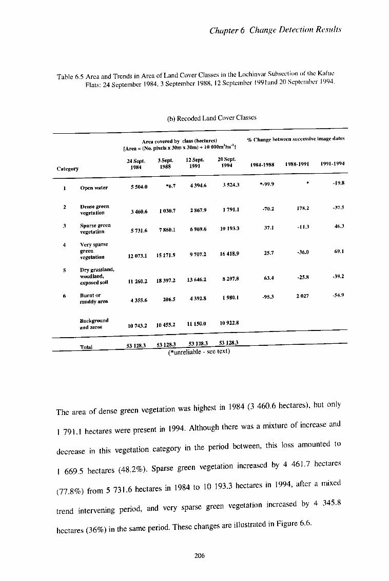
Chapter 6 Change Detection Results
Table 6.5 Area and Trends in Area of Land Cover Classes in the Lochinvar Subsection of the KafucFlats: 24 September 1984,3 September 1988, 12 September 1991and 20 September 1<)<)4.
(b) Recoded Land Cover Classes
Area covered by class (hectares) % Change hetween successive image dates
[Area = (No. pixels x 30m x 30m) + 10 OOOm1ha·IJ
24 Sept. 3 Sept. 12 Sept. 20 Sept.
Category 1984 1988 1991 1994 1984-19811 19811-1991 1991-1994
1 Open water 5504.0 *6.7 4394.6 3524.3 *-99.9 * -19.11
2 Dense greenvegetation 3460.6 1030.7 2867.9 1791.1 -70.2 178.2 -37.5
3 Sparse greenvegetation 5731.6 7860.1 6969.6 10193.3 37.1 -11.3 46.3
4 Very sparsegreenvegetation 12073.1 15171.9 9707.2 16418.9 25.7 -36.0 69.1
5 Dry grassland,woodland,exposed soil 11260.2 18397.2 13646.2 8297.8 63.4 -25.8 -39.2
6 Burnt ormuddy area 4355.6 206.5 4392.8 1980.1 -95.3 2027 -54.9
Backgroundand zeros 10743.2 10455.2 11150.0 10922.8
Total 53128.3 53128.3 53128.3 53128.3
(*unreliable - see text)
The area of dense green vegetation was highest in 1984 (3 460.6 hectares), but only
I 791.1 hectares were present in 1994. Although there was a mixture of increase and
decrease in this vegetation category in the period between, this loss amounted to
I 669.5 hectares (48.2%). Sparse green vegetation increased by 4 461.7 hectares
(77.8%) from 5 731.6 hectares in 1984 to 10 193.3 hectares in 1994, after a mixed
trend intervening period, and very sparse green vegetation increased by 4 345.8
hectares (36%) in the same period. These changes are illustrated in Figure 6.6.
206

Chapter 6 Change Detection Results
20000~---------------------------------------------'
15000+-------------------~ r----------------------~~--~Ui!!?
~..c-;10000+------001!!?«(/)
~o5000-+---I+I--l
mOpen water
[::::::::]Sparse green vegetation
DID Dry grassland, woodland, exposed soil
• Dense green vegetationm Very sparse green vegetation
~ Burnt or muddy area
cg:
I-~r:
~1"".
r- ~I-- ~-- ~ ~ ...~.....
~....~
~..-.ra M .. _
T1984 1988 1991 1994
Year
Figure 6.6 Trends in area of recoded land cover classes in the Lochinvar Subsection of the KalucFlats: 24 September 1984, 3 September 1988, 12 September 1991 and 20 September 1994.
6.3.3 Trends in the Blue Lagoon Area
The Blue Lagoon subsection stretched from the woodland area just south of Muchabi,
across the flood plain and dense water fringe vegetation zone around Luwato Lagoon
in the east, across the flood plain down to Shakapinka (north-west of Mazabuka) and
west in the river and lagoon zone east of Nyimba (Figure 6.4). The area of cover of
each of the land cover classes is shown in Table 6.6.
207
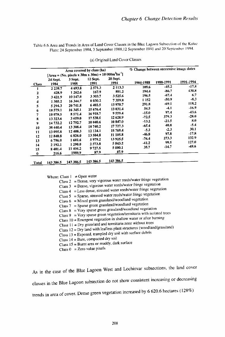
Chapter 6 Change Detection Results
Table 6.6 Area and Trends in Area of Land Cover Classes in the Blue Lagoon Subsection of the KatucFlats: 24 September 1984, 3 September 1988,12 September 1l)9 I and 20 September 1994.
(a) Original Land Cover Classes
Area covered by class (ha) % Change between successive image dates[Area = (No. pixels x 30m x 30m) + 10 000m2ha'IJ24 Sept. 3 Sept. 12 Sept. 20 Sept.
Class 1984 1988 1991 1994 1984-1988 ]988-199] ]99] -1994
1 2239.7 4693.8 2571.3 2113.3 109.6 -45.2 -17.8
2 428.9 1262.6 167.9 891.2 194.4 -86.7 430.8
3 3421.9 10147.0 3303.7 3525.6 196.5 -67.4 6.7
4 1305.2 16344.7 8030.2 7359.8 ] 152 -50.9 -8.3
5 5294.3 20741.8 6402.5 13 970.7 291.8 -69.1 118.2
6 10579.1 16345.1 15676.4 13 031.4 54.5 -4.1 -16.9
7 10078.5 8571.4 16918.7 9559.4 -15.0 97.4 -43.6
8 13323.6 3659.0 17538.0 12628.9 -72.5 379.3 -28.0
9 14732.2 12792.7 10040.6 10847.0 -13.2 -21.5 H.O
10 38440.4 13308.4 18740.2 17727.3 -65.4 40.8 -5.4
11 13 095.8 12408.3 12124.1 15769.4 -5.2 -2.3 30.1
12 12840.8 6826.0 13504.8 11105.8 -46.8 97.8 -17.8
13 6796.0 1601.6 5979.2 13925.5 -76.4 273.3 132.9
14 2192.1 1290.0 2573.8 5843.2 -41.2 99.5 127.0
15 8401.4 11404.2 9727.5 5000.1 35.7 -14.7 -48.6
0 216.6 1989.9 87.9 87.9
Total 143386.5 143386.5 143386.5 143386.5
Where: Class 1 = Open waterClass 2 = Dense, very vigorous water reeds/water fringe vegetationClass 3 = Dense, vigorous water reeds/water fringe vegetationClass 4 = Less dense, stressed water reeds/water fringe vegetationClass 5 = Sparse, stressed water reeds/water fringe vegetationClass 6 = Mixed green grassland/woodland vegetationClass 7 = Sparse green grassland/woodland vegetationClass 8 = Very sparse green grassland/woodland vegetationClass 9 = Very sparse green vegetation/termitaria with isolated treesClass 10 = Emergent vegetation in shallow water or after burningClass 11 = Dry grassland and termitaria zone without treesClass 12 = Dry land with leafless plant structures (woodland/grassland)Class 13 = Exposed, trampled dry soil with surface debrisClass 14 = Bare, compacted dry soilClass 15 = Burnt area or muddy, dark surfaceClass 0 = Zero value pixels
As in the case of the Blue Lagoon West and Lochinvar subsections, the land cover
classes in the Blue Lagoon subsection do not show consistent increasing or decreasing
trends in area of cover. Dense green vegetation increased by 6 620.6 hectares (128%)
208

Chapter 6 Change Detection Results
Table 6.6 Area and Trends in Area of Land Cover Classes in the Blue Lagoon Subsection of the Kahil:Flats: 24 September 1984,3 September 1988, 12 Septemher 1991 and 20 September 1994.
(b) Recoded Land Cover Classes
Area covered by class (hectares) % Change between successive IIIIII~C dates[Area = (No. pixels x 30m x 30m) + 10OOOmlho·'j
24 Sept. 3Sept. 12Sept. 20 Sept.Category 1984 1988 1991 1994 1984·19811 191111-1991 1991-1994
I Open water 2239.7 4693.8 2571.3 2113.3 109.6 -45.2 -17.11
2 Dense greenvegetation 5156.0 27754.3 11 501.8 11 776.6 4311.9 -511.6 2.4
3 Sparse greenvegetation 25951.9 456511.3 38997.6 36561.5 75.9 ·14.6 ·6.2
4 Very sparsegreenvegetation 66495.6 29760.1 46318.5 41203.2 ·55.2 55.6 ·11.0
5 Dry grassland,woodland,exposed soil
34925.3 22125.9 34181.9 46643.5 ·36.6 55.5 36.5
6 Burnt ormuddy area 8401.4 11 404.2 9727.5 5000.5 35.7 ·14.7 ·411.6
Backgroundand zeros 216.6 1989.9 87.9 87.9
Total 143386.5 143386.5 143386.5 143386.5
from 5 156 hectares in 1984 to 11 776.6 hectares in 1994, while sparse green
vegetation increased by 10 609.6 hectares (40.9%) from 25951.9 to 36 561.5 hectares
(Table 6.6b). The main decrease in the same time period was in very sparse green
vegetation which covered 66 495.6 hectares in 1984 but 41 203.2 hectares in 1994, a
reduction of 25 292.4 hectares (38%). In the intervening period the area covered by
the classes underwent both an increase and a decrease (Figure 6.7).
209

Chapter 6 Change Detection Results
70000
60000
50000UlCl)
r-: ~~
..~.
40000 ....~ ~ "'"Cl)
....~......~
I----
E.-M ••••
CIS.MO •• :::@] C
~ 88_.
30000-_. ....- I:
« _M"
...... f--
(J)
_ ...
(J) 1 --CIS
_'M' "'-'
U.-
20000_.- •• 'M_
::::: ._.- -.--.-.-._. • •• M.
-••• M.
--_-~10000 _", -- ,._ ..
--_ ... -
~
-~rJ····· ..-
-.- ff -...... ..._.
~_.IJ:l [J
0, _. ..._-._.
1984 1988 1991 1994Year
§Rl Open water • Dense green vegetation
L:::::J Sparse green vegetation mVery sparse green vegetation
[DJ Dry grassland. woodland. exposed soil ~ Burnt or muddy area
Figure 6.7 Trends in area of recoded land cover classes in the Blue Lagoon subsection of the KafucFlats: 24 September 1984, 3 September 1988, 12 September 1991 and 20 September 1994.
6.3.4 Trends in Mazabuka West
The Mazabuka West subsection mainly included the woodland area from Hebe to just
west of the Nakambala Sugar Estate and part of the flood plain to the north, as far as
the river and water fringe vegetation zone around Maamba (Figure 6.4). The area
covered by the land cover classes is as shown in Table 6.7.
The lack of consistent trends of either increase or decrease in the area of cover.
observed for predominantly flood plain areas (Sections 6.3.1 - 6.3.3) is noticeahle for
210

Chapter 6 Change Detection Results
this subsection predominantly consisting of woodland in early spring leaf but with dry
grass (Figure 6.8).
Table 6.7 Area and Trends in Area of Land Cover Classes in the Mazabuka West Subsection of theKafue Flats: 24 September 1984, 3 September 1988, 12 September 1991 and 20 Sept em her1994.
(a) Original Land Cover Classes
27.4 43.9 29.425.6 201.8 53.2
243.5 556.8 311.8341.0 442.4 337.5594.7 598.1 478.6822.8 1529.3 4399.6
1548.2 1709.2 4887.24029.4 1982.4 5289.95987.8 4186.6 3327.28009.9 6179.0 4228.43841.3 4707.3 5344.93715.6 7421.8 3943.16139.3 5199.5 3962.72805.5 2478.5 1238.63208.4 4101.2 3474.4
92.3 94.7 126.5
% Change between successive image dates
1984·1988 1988· 1991 1991·199460.2 ·33.0 ·1l1.7
688.3 ·73.6 ·41.6128.7 ·44.0 ·41.629.7 ·23.7 ·1l1.50.6 ·20.0 26.6
85.9 187.7 ·72.210.4 185.9 ·64.9·50.8 166.8 ·9.6·30.1 ·20.5 76.6·22.9 ·31.6 47.222.5 13.5 28.099.7 ·46.9 97.1·15.3 ·23.8 ·24.6·11.7 ·50.0 61.8927.8 ·15.3 ·77.9
Area covered by class (ha)[Area = (No. pixels x 30m x 30m) + 10 000m2ha·l]24 Sept. 3 Sept. 12 Sept. 20 Sept.
Class 1984 1988 1991 1994
Total 41433.0 41433.0 41433.0 41433.0
Where:Class I = Open waterClass 2 = Dense, very vigorous water reeds/water fringe vegetationClass 3 = Dense, vigorous water reeds/water fringe vegetationClass 4 = Less dense, stressed water reeds/water fringe vegetationClass 5 = Sparse, stressed water reeds/water fringe vegetationClass 6 = Mixed green grassland/woodland vegetationClass 7 = Sparse green grassland/woodland vegetationClass 8 = Very sparse green grassland/woodland vegetationClass 9 = Very sparse green vegetation/termitaria with isolated treesClass 10 = Emergent vegetation in shallow water or after burningClass II = Dry grassland and termitaria zone without treesClass 12 = Dry land with leafless plant structures (woodland/grassland)Class 13 = Exposed, trampled dry soil with surface debrisClass 14 = Bare, compacted dry soilClass 15 = Burnt area or muddy, dark surfaceClass 0 = Image background and Zero value pixels in burnt areas
211

Chapter 6 Change Detection Results
Table 6.7 Area and Trends in Area of Land Cover Classes in the Mazabuka West Subsection of theKafue Flats: 24 September 1984, 3 September 1988, 12 September IY9 I and 20 September
1994.
(b) Recoded Land Cover Classes
Area covered by class (hectares) % Change between successive image[Area = (No. pixels x 30m x 30m) + 10000mlha·1j dates
24 Sept. 3 Sept. 12 Sept. 20 Sept.
Category 1984 1988 1991 1994 1984·1988 1988·1991 1991·1994
Open water 27.4 43.9 29.4 23.9 60.2 ·33.0 ·1!!.7
2 Dense greenvegetation 610.1 1201.0 702.5 497.3 98.9 ·41.5 ·29.2
3 Sparse greenvegetation 2965.7 3836.6 9765.4 3540.6 29.4 154.5 .63.7
4 Very sparsegreenvegetation 18027.4 12348.5 12 845.5 16888.6 ·31.5 4.0 31.5
5 Dry grassland,woodland,exposed soil 16501.7 19807.1 14489.3 19607.6 20.0 ·26.8 35.3
6 Burnt ormuddy area 3208.4 4101.2 3474.4 769.4 27.8 ·15.3 ·77.9
Backgroundand zeros 92.3 94.7 126.5 105.6
Total 41433.0 41433.0 41433.0 41433.0
6.3.5 Trends at Large lagoons
Square areas enclosing Chung a and Shalwembe Lagoons (Figure 6.4), the biggest
lagoons on the Kafue Flats, were examined for land cover changes. The results are
summarised in Tables 6.8 and 6.9.
212

Chapter 6 Change Detection Results
20000
150001
-
(i)1
~<Ut5Cl)
.c:-; 10000 ;::;;; I---
~<{
•• H ••
rJJ
_M'O'
rJJ
•• H ••
<U ~(3 B8 ~ ••• H •
5000•• H •• -
=~
_ .... RIiII
r.: I- •••• H
~c:::__
----
~..._. - --_-
~_.- .._ ..
~ J~ • I-t?l
0I ::::~ _::::
1984 1988 1991 1994Year
EEm Open water • Dense green vegetation
[::==1 Sparse green vegetation m Very sparse green vegetation
ITID Dry grassland, woodland, exposed soil ~ Burnt or muddy area
Figure 6.8 Trends in area of recoded land cover classes in the Mazabuka West subsection of the KalucFlats: 24 September 1984, 3 September 1988, 12 September 1991 and 20 September 1994.
Apart from the 3 September 1988 image conditions (when there was smoke over the
lagoon and surrounding dry ground - see Figure 4.11) the amount of water in Chunga
lagoon seems to have been reducing between 1984 and 1994 (see Table 6.8). There
appears to have been reduction in dense, very vigorous water reeds/water fringe
vegetation (Class 2) and an increase in emergent vegetation in shallow water (Class
10). The pattern at Shalwembe Lagoon is not clear but the lagoon had less water and
surrounding dense, very vigorous green vegetation (Class 2) in September 1994 than it
did in September 1984 (see Table 6.9). The amount of water reeds and water fringe
vegetation categories (Classes 3 and 4) also seems to have increased in the same
period.
213

Chapter 6 Change Detection Results
Table 6.8 Area and Trends in Area of Land Cover Classes around Chunga Lagoon on the Kafuc Flats:24 September 1984, 3 September 1988, 12 September 1991 and 20 Scptcrnhcr 1994.
Area covered by class (ha) % Change between successive image dates[Area = (No. pixels x 30m x 30m) + 10 000m2ha·1]24 Sept. 3 Sept. 12 Sept. 20 Sept.
Class 1984 1988 1991 1994 1984-1988 1988- 1991 1991-1994
1 5525.3 *0.0 4357.1 3496.4 *-100 *00 -19.S
2 292.7 638.7 126.8 93.5 118.2 -80.1 -26.3
3 1825.7 6.8 1149.4 739.5 -99.6 16803 -35.7
4 2150.2 151.3 1947.4 1262.1 -93.0 I 187 -35.2
5 1 143.0 107.4 497.2 756.8 -90.6 362.9 52.2
6 965.7 554.1 688.7 847.0 -42.6 24.3 23.0
7 457.1 1791.3 576.6 1328.9 292.0 -67.8 130.5
8 95.0 2022.1 345.9 370.0 2029 -82.9 7.0
9 1013.8 484.4 898.1 933.1 -52.2 85.4 3.9
10 609.4 *7566.8 1480.9 7544.6 ·1142 -80.4 409.5
11 490.0 710.0 325.9 260.4 44.9 -54.1 -20.1
12 244.5 1142.5 796.7 201.1 367.3 -30.3 -74.8
13 1054.1 3832.2 1394.6 1021.1 263.6 -63.6 -26.8
14 1249.5 2306.9 2557.2 984.1 84.6 10.9 -61.5
15 4166.6 62.7 4016.7 1372.3 -98.5 6306 -65.8
0 930.3 835.7 1053.7 1002.0
Total 22212.9 22212.9 22212.9 22212.9
(*unreliable - see Section 6.3.2)
Where:
Class I = Open waterClass 2 = Dense, very vigorous water reeds/water fringe vegetationClass 3 = Dense, vigorous water reeds/water fringe vegetationClass 4 = Less dense, stressed water reeds/water fringe vegetationClass 5 = Sparse, stressed water reeds/water fringe vegetationClass 6 =Mixed green grassland/woodland vegetationClass 7 = Sparse green grassland/woodland vegetationClass 8 = Very sparse green grassland/woodland vegetationClass 9 = Very sparse green vegetationlterrnitaria with isolated treesClass 10 = Emergent vegetation in shallow water or after burningClass II = Dry grassland and terrnitaria zone without treesClass 12 = Dry land with leafless plant structures (woodland/grassland)Class 15 = Burnt area or muddy, dark surfaceClass 13 = Exposed, trampled dry soil with surface debrisClass 14 = Bare, compacted dry soilClass 0 = Image background and zero value pixels
214

Chapter 6 Change Detection Results
Table 6.9 Area and Trends in Area of Land Cover Classes around Shalwcmbc Lagoon on the KutucFlats: 24 September 1984. 3 September 1988. 12 September 1991 and 20 September 1994.
Area covered by class (ha) % Change between successive image dates
[Area = (No. pixels x 30m x 30m) + 10 000m2ha·l]
Class 1984 1988 1991 1994 1984-1988 1988- 1991 1991-1994
1 1140.9 0.0 31.8 402.8 -100 00 1 167
2 735.8 2026.7 555.8 504.2 175.4 -72.6 -9.3
3 943.9 157.0 1659.8 1885.7 -83.4 957.2 13.6
4 743.6 505.5 835.9 1411.4 -32.0 65.4 61tH
5 112.2 103.3 408.6 343.0 -7.9 295.5 -16.1
6 192.0 363.3 223.2 117.2 89.2 -38.6 -47.5
7 40.4 740.1 206.7 411.3 1732 -72.1 99.0
8 1.6 187.1 65.3 7.2 11594 -65.1 -H9.1
9 21.9 12.5 51.3 0.6 -42.9 309.6 -91tH
10 33.8 51.8 531.5 142.8 53.3 926.1 -73.1
11 23.4 5.4 62.6 5.9 -76.9 1059.3 -90.6
12 12.8 4.7 141.4 0.4 -63.3 2908.5 -99.7
13 31.3 4.5 128.7 26.6 -85.6 2760.0 -79.3
14 47.3 48.2 181.9 114.8 1.9 277.4 -36.9
15 1569.3 1527.6 653.2 362.1 -2.7 -57.2 -44.6
0 87.5 0.0 0.0 1.7
Total 5737.7 5737.7 5737.7 5737.7
Where:
Class I = Open waterClass 2 = Dense. very vigorous water reeds/water fringe vegetationClass 3 = Dense. vigorous water reeds/water fringe vegetationClass 4 = Less dense. stressed water reeds/water fringe vegetationClass 5 = Sparse. stressed water reeds/water fringe vegetationClass 6 = Mixed green grassland/woodland vegetationClass 7 = Sparse green grassland/woodland vegetationClass 8 = Very sparse green grassland/woodland vegetationClass 9 = Very sparse green vegetationltermitaria with isolated treesClass 10 = Emergent vegetation in shallow water or after burningClass II = Dry grassland and termitaria zone without treesClass 12 = Dry land with leafless plant structures (woodland/grassland)Class 15 = Burnt area or muddy. dark surfaceClass 13 = Exposed. trampled dry soil with surface debrisClass 14 = Bare. compacted dry soilClass 0 = Zero value pixels
6.4 Change Detection Using Spectral Enhancement Techniques
Inter-image changes in the spectral characteristics of the image series were examined
using the Normalised Difference Vegetation Index (NDVI) and Principal Component
Analysis (PCA) spectral enhancement techniques. The results are presented in tum.
215

Chapter 6 Change Detection Results
6.4.1 Normalised Difference Vegetation Index (NDVI) Changes
The Normalised Difference Vegetation Index (NDVI) compares the amount of infrared
with visible red reflectance as follows:
NDVI = Near Infrared - Red or MSS4 - MSS2 or TM4 - TM3 (6.1)
Near Infrared + Red MSS4 +MSS2 TM4 +TM3
NDVI values range between 1 and -1. Values greater than one indicate a predominance
of near-infrared reflecting features (mainly healthy, green vegetation but also dry grass
and soil - see Figure 1.3) over visible red reflectors (for example, reddish/brown dry
grass and dry soil). Values less than one indicate a predominance of visible red
reflectors and zero values indicate equal near-infrared and visible red reflectance
(Lillesand and Kiefer, 1994; Jensen, 1986; ERDAS Inc., 1994). Figure 6.9 illustrates
the use of the NDVI spectral enhancement technique in highlighting areas, and
assessing vigour, of green vegetation cover. Many studies have used the NDVI for
vegetation monitoring (e.g. Townshend and Justice, 1986; Hielkema et ai, 1986;
Justice et al. 1986; Justice and Hiernaux, 1986). The frequencies of NDVI values from
each of the normalised images are shown in Figure 6.10. On the 24 September 1984
image most of the NDVI values were above 1, with a peak frequency around 0.25
(Figure 6.1Oa). There was a similar pattern on the 3 September 1988 image but the
number of pixels at the peak frequency of 0.25 is less than that for the 1984 image
216

Figure 6.9 An NOVI image of the wetland area north west of Nyimba (theBlue Lagoon west subsection in Figure 6.4). The image wasderived from the atmospherically corrected 20 September1994 TN image. The NDVI values, ranging from -1.000 to0.992, have been colour coded (density sliced) such thatyellow represents the lowest value (-1.000) and redrepresents the highest (0.992). The colour hierarchy is inthe order red (highest NOVI), blue, green, yellow (lowestNOVI). Dense, vigorous vegetation appears red (high NDVI)but there is some confusion with dry soil/dry grass on themargin of the wetland north of Shalwembe Lagoon (comparewith Figure 6.4 or 4.15). Dry land appears blue while waterand burnt areas (with very low NDVI) appear green/yellow.

Chapter 6 Change Detection Results
(a) 1984 NDVI Frequencies
1000000
I.
-l' ~~l.o&
o-0.25 0 0.25
NOVI Value0.5 0.75
-1 -0.75 -0.5
(b) 1988 NDVI Frequencies
1000000
r--:
Q) 800000::l(ij>f;.§.!!J. 6OClOOO~.Q.'0o 400000~>-0cQ)::J
W 200000u,
0-
-1 -0.75 -0.5 -0.25 0 0.25NOVI Value
0.5 0.75
Figure 6.10 Frequency of Normalised Difference Vegetation Index (NDV!) values on the24 September 1984 MSS, 3 September 1988 MSS, 12 September 1991 TM and20 September 1994 TM images of the Kafue Flats.

Chapter 6 Change Detection Results
(c) 1991 NDVI Frequencies
1~~---------------------'--------------------~
Q) 800000:J(ij>£i.~III 600000Cii.esQ.
'00 400000~>-0cQ)Js 200000...u,
0-1
0.75-0.75 -0.5 -0.25 0 0.25NDVI Value
0.5
(d) 1994 NDVI Frequencies
1~~------------------------'-----------------------~
Q) 800000J(ij>
~.!!l 600000Q).i!SQ.
'00 400000~>-0cQ)Jg 200000...u,
0-1 -0.25 0 0.25
NDVI Value0.5 0.75
-0.75 -0.5
Figure 6.10 (continued) Frequency of NormaIised Difference Vegetation Index (NDVJ) values on the24 September 1984 MSS, 3 September 1988 MSS, 12 September 1991 TM and 20 September
1994 TM images of the Kafue Flats.

Chapter 6 Change Detection Results
(Figure 6. lOb), indicating a predominance of near-infrared reflectors on both images
(healthy green vegetation but also dry grass and dry soil - see Figure 1.3). However,
because on the 1988 image there was still a flood in lower floodplain sections, there
was less dry grass and dry soil; hence the lower number of pixels on the 1988 image's
graph.
The peak frequencies on the 12 September 1991 and 20 September 1994 TM images
are about zero, although there was a predominance of near-infrared reflectance on both
images (Figures 6.lOc and 6.lOd). However, on both the 1991 and 1994 images there
were more NOVI values which were less than zero than on either the 1988 or the 1984
images, indicating the presence of more visible red reflectors on the 1991 and 1994
images (especially dry, reddishlbrown grassland and other dry plant structures). This
means that the Kafue Flats were drier on 12 September 1991 and 20 September 1994
than either on 24 September 1984 or on 3 September 1988. From the images used, the
area was driest on 12 September 1991, indicated by the higher number of pixels with
NDVI values between 0 and -0.125 on the 12 September 1991 than on the 20
September 1994 image.
Although NOVI changes indicated the relative proportion of near-infrared and red
reflectance, and although inferences can be made about the possible ground cover
features from which the reflectance was coming, mapping the change between two
NDVI images by pixel by pixel subtraction of NDVI values between the respective
images resulted in images predominantly with zero values. Other resulting values were
more difficult to interpret. For example, a pixel with an NOVI value of I on the second
NOVI image and a value of 0.5 on the first, results in a difference of 0.5 on the NOVI
220

Chapter 6 Change Detection Results
change image (i.e. 1 - 0.5 = 0.5), exactly the same as the difference between a 0.75
value on the second and a 0.25 value on the first (0.75- 0.25 = 0.5), which would make
the resulting value of 0.5 on the NDVI change image difficult to interpret. For this
reason the classification comparison technique was found to be a more useful change
detection method, from the image data set used.
To obtain an indication of NDVI trends at specific dense green vegetation sites over
the period covered by the images, NDVI values at specific points were examined.
Dense green vegetation (because of presence of water) is the main characteristic
distinguishing the Kafue Flats as a wetland in the dry season. A site was chosen ncar
Shalwembe Lagoon in the area that showed spatial losses of dense green vegetation
between 1984 and 1994 (Figure 6.2). Two sites opposite the Nakambala Sugar Estate
in the area showing no losses were chosen for comparison, and, as a control, three dry
sites were examined. Because the images were geometrically co-registered (see Section
4.4.3) it was possible to locate the same site on all the images. The sites and their
NDVI characteristics are listed in Table 6.10 and the NDVI trends at the sites arc as
shown in Figure 6.11.
Figure 6.11 shows that for the area that underwent degradation in dense green
vegetation around Shalwembe Lagoon (Figure 6.2), represented by site Dense green 3,
the vegetation was also undergoing a reduction in vigour because the NDVI was
reducing. This means that the vegetation was possibly reflecting less near-infrared
radiation, resulting in a smaller difference between the amount of red and near-infrared
reflectance and, therefore, reduced NDVI. However, the reducing NDVI could also he
because the density of the vegetation had reduced, thereby opening up the canopy and
221

Chapter 6 Change Detection Results
Table 6.10 NOV I Values at Representative Dense Green Vegetation and Dry Sites
NDVI Values
Site Characteristics 24 3 12 20
(setting) September September September September1984 1988 1991 1994
Dense In area notgreen 1 undergoing
spatial loss of 1.000 0.634 0.483 0.773
dense greenvegetation
Dense In area notgreen 2 undergoing
spatial loss ofdense green 0.846 0.829 0.559 0.624
vegetation;oppositeirrigation estate
Dense In areagreen 3 undergoing
spatial loss ofdense green 0.736 0.443 0.341 0.425
vegetation; nearShalwembeLagoon
Dry soil 1 Dry bare surfacein human 0.061 0.105 0.031 0.036
settlement area
Dry soil 2 Dry bare surfacein human 0.080 0.149 0.034 0.096
settlement area
Dry soil Dry area inwith debris national park 0.094 0.088 0.040 0.011
222

Chapter 6 Change Detection Results
1t---~~------------------------------------~
0.75Q):J(ij>:>
0.50z
0.25 t-------------------------
Year
Figure 6.11 Trends in NDVI values at representative dense green vegetation and dry soil sites on theKafue Flats: 24 September 1984, 3 September 1988,12 September 1991 and20 September 1994. There is a general reduction in NDVI values over time, possiblyindicating reduced green vegetation vigour, opening up of green vegetation canopy anddrying up at the sites.
___ Dense green 1
-7r- Dry soil 1
....- Dense green 2
--*- Dry soil 2
--e-- Dense green 3___ Dry soil with debris
increasing the amount of red reflectance from the soil and dry under storey plant
structures. The trend is similar for the other two dense green vegetation sites (Dense
green 1 and 2 in Figure 6.11) representing the down stream section of the Kafue Flats
which appeared not to have had spatia1loss of dense green vegetation between 1984
and 1994 (Figure 6.2). Site Dense green 1 was in a dark/muddy or water land cover
type on 24 September 1984 (with zero visible red reflectance), hence the NDV! value
of 1.000. The dry (control) sites experienced a small lowering of NDV! values,
indicating a possible drying up or increased soil exposure trend between 1984 and

Chapter 6 C}UI11RC Detection Results
1994. This could have resulted in more visible red reflectance from the soil and dry
plant structures, hence the reduced NDVI values.
6.4.2 Principal Component Analysis
Principal component analysis (PCA), a spectral enhancement technique often used as a
method of compressing data, may be used as a change detection technique (Jensen,
1986). PCA enables the compression of multi-band remote sensing data into fewer
bands. The data are rotated into a new co-ordinate system associated with the
maximum amount of variance in the scatter of the points. The major and minor axes of
the ellipsoid of points are called the principal components (see Box 6.1). The first
principal component contains the majority of the variance in the data, and the second.
third, fourth and nth principal components (n = total number of components) contain
decreasing amounts of the variance (Figure 6.12). The direction of a principal
component is the eigen vector, and its length is the eigen value. An image produced
from a principal component is an eigen image (Figure 6.12).
Eigen values and eigen vector characteristics of the raw (un-normalised) image data set
used are shown in Table 6.11. The first and second principal components of the
24 September 1984 MSS image contain a total of 98.28% of the variance in the data
(Table 6.11a). This is mainly from the contents of the near-infrared bands (bands 3 and
4), because the two bands have the largest vector values, 0.591 and 0.614 respectively.
in component I, and 0.174 and 0.532, respectively, in component 2. Component
3 is made up largely of MSS band 1 reflectance (eigen vector value of 0.786 in Table
224

X2
112
X1
A
X2 X2'
A scatterplot of data points collected from two remotely sensedbands labeled Xl and X2 with the means of the distributionlabeled III and 112.
X1'
A new coordinate system is created by shifting the axes to an X'system. The values for the new data points are found by therelationship Xl' = X1 - III and X2' = X2 - 112.
B
c
X1
The X' axis system is then rotated about its origin (111,112)so that PC1 is projected through the semimajor axis of thedistribution of points and that the variance of PC2 is a maximum.PC2 must be perpendicular to PC1. The PC axes are the principalcomponents of this two-dimensional data space. Component 1usually accounts for approximately 90% of the variance,with component 2 accounting for approximately 5%.
Box 6.1 An illustration of principal component analysis: Diagrammatic representation of the spatialrelationship between the first two principal components (modified from Jensen, 1986).
225

Cb) An eigen image of principal Component 2, containing 4.83% of the data varianceand, consequently, less clear than the Principal Component 1 image.
Figure 6.12 An illustration of principal component analysis: Eigen imagesfrom a subset of the raw 3 september 1988 NSS data, around Shalwembe Lagoon.

(c) An eigen image of principal component 4, containing 0.33% of the data variance,mainly noise. The eigen image from principal Component 3 (with 0.49% of thedata variance) was empty of raster information. Therefore from the original 4bands, the data over this area could be compressed into these 3 principalcomponents. The eigen vector characteristics for the subset were as follows:
component 1 2 3 4
Band MSSl 0.168 0.371 -0.348 0.884MSS2 0.243 0.871 0.292 -0.311MSS3 0.598 -0.067 -0.703 -0.379MSS4 0.745 -0.314 0.548 0.216
Eigen value 1019.270 52.223 5.312 3.524
Figure 6.12 (continued) An illustration of principal component analysis:Eigen images from a subset of the raw 3 September 1988 MSS data,around Shalwembe Lagoon.

Chapter 6 Change ne/cc/ion Results
Table 6.11 Principal Component Analysis Characteristics of Raw Image Data Used
(a) Eigen Vectors and Eigen Values of Principal Components or24 September 1984 MSS Image
Band IBand 2Band 3Band4
Component2 3 4
0.286 -0.543 0.786 o.on0.439 -0.626 -0.611 0.208
0.591 0.174 -0.022 -0.788
0.614 0.532 0.092 0.575
948.197 71.390 11.646 6.142Eigen value ofcomponent
Percentage ofdata variancein component
91.40 6.88 1.12 0.59
(b) Eigen Vectors and Eigen Values of Principal Components of3 September 1988 MSS Image
Component2 3 4
Band I 0.337 -0.560 0.697 0.294
Band 2 0.377 -0.626 -0.682 -0.007
Band 3 0.580 0.164 0.179 -0.777
Band4 0.638 0.517 -0.127 0.556
Eigen value of 1539.627 99.849 13.638 6.348
component
Percentage ofdata variance 92.78 6.02 0.82 0.38
in component
228

Chapter 6 Change Detection Results
Table 6.//(continued) Principal Component Analysis Characteristics ofRaw /111(/~(,
Data Used
(c) Eigen Vectors and Eigen Values of Principal Components of 12 September 199 I TM Image
Component2 3 4 5 () 7
Band I 0.393 -0.236 -0.666 -O.4XO 0.117 -O.M6 (),2lX
Band 2 0.171 -0.029 -0,169 -0.234 (l.115 O,m5 -O,lJl4
Band 3 0.239 0.087 -0.238 -0.534 (l.095 0.720 0,256
Band 4 0.223 0.195 -0.672 0.557 0.382 0.020 0,0(15
Band 5 0.489 0.682 0.085 0.033 -0.523 -0.114 -0,024
Band 6 0.631 -0.595 0,227 0.343 -0.176 0.21X -0.007
Band 7 0.269 0.279 0.578 -0.002 0.717 -0.036 0,023
Eigen value ofcomponent 5433.109 627.957 152.827 20.293 9.727 6.3X2 0,721
Percentage ofdata variance incomponent 86.92 10.05 2.44 0.32 0.16 0.10 0.01
(d) Eigen Vectors and Eigen Values of Principal Components of 20 Septemoer 1994 TM Image
Component
2 3 4 5 6
Band I 0.393 -0.768 0.280 0.207 0.308 0.203
Band 2 0.183 -0.244 0.027 -0.096 -0.196 -0.927
Band 3 0.275 -0.164 0.013 -0.137 -O.8X8 0.300
Band4 0.289 -0.163 -0.783 -0.477 0.209 0.OX2
Band 5 0.696 0.444 -0.159 0.538 0.033 -0.047
Band 6 * * * * * *
Band 7 0.410 0.316 0.531 -0.642 0.IX9 0.040
Eigen value of 15.645component 3097.669 337.747 159.174 18.957 1.262
Percentage ofdata variance incomponent 85.32 9.30 4.38 0.52 0.43 0.03
(*Band 6 unavailable due to technical problem on Landsat)
229

Chapter 6 Change Detection Results
6.11 a), and component 4 is largely made up of MSS band 4 reflectance (eigen vector
value of 0.575). Therefore, most of the variance in the 24 September 1984 MSS scene
is bands 3 and 4, the near infra red bands (equivalent to TM band 4; sec Tahles 1.1 and
1.2).
On the 3 September 1988 MSS image principal component I also consists mainly of
near-infrared reflectance because bands 4 and 3 have the largest eigen vector values of
0.638 and 0.S80, respectively (Table 6.11 b). Component 2 is largely band 4 (near-
infrared) reflectance (eigen vector value 0.517 from the band is the largest in the
component) and some reflectance from band 3 (vector value 0.164). Therefore, nearly
all of the data variance (98.80%) in the scene is from near-infrared reflectance (bands 3
and 4). Component 3 is largely from green (band I) reflectance but accounts for only
0.82% of the data variance. Component 4 is largely band 4 reflectance.
The large contribution of infrared bands to the overall image data variance is observed
for the TM images as well (Tables 6.11c and 6.11 d). On the 12 September 1991 ™image (Table 6.11c), principal component 1 is largely made up of TM6 (thermal
infrared), with a vector value of 0.631, TMS (mid-infrared) with a vector value of
0.489, and, to a lesser extent, TM1 (blue-green) with a vector value of 0.393 (of all
TM bands this band has the largest haze interference factor). Component 2 consists
largely of TMS (mid-infrared) reflectance (vector value 0.682). Component 3 is largely
TM7 (mid-infrared) reflectance (vector value 0.578). These first three components
account for 99.41 % of the data variance. Therefore, TM bands 5, 6 and 7 account for
most of the variance in the image data. Components 4, 5 and 6 are largely TM4, TM7
and TM3 reflectance, respectively, and together account for only 0.S8% of the total
230

Chapter 6 Change Detection Results
variance. Component 7 is difficult to interpret but TM3 has the largest vector value
(0.256).
The first principal component on the 20 September 1994 TM image consists largely of
TM5 (mid-infrared) reflectance with a vector value of 0.696, TM7 (mid-infrared) with
a vector value of 0.410 and TMI (blue-green with largest haze interference) with a
vector value of 0.393 (Table 6.11d). Component 2 is largely TM5 and TM7 reflectance
as well (vector values 0.444 and 0.316, respectively) while component 3 is largely
TM7 reflectance (vector value 0.531). These first three components account for 99%
of the data variance. Components 4, 5 and 6 are largely TM5, TM I and TM3
reflectance, respectively, with respective vector values of 0.538,0.308 and 0.300.
Therefore, for the MSS images the near-infrared bands (MSS3 and MSS4, equivalent
to TM4) contain most of the data variance, while for the TM images, most of the data
variance is in the mid-infrared bands which MSS images do not contain (see Tables 1.1
and 1.2). The reason for the predominance of infrared reflectance is because most of
the area in the image scene is dry. Dry soil and dry grass reflect highly in the near-
infrared but to a lesser extent than healthy green vegetation (Figure 1.3). The
combination of near-infrared reflectance from dry soil, dry grass and healthy green
vegetation explains the fact that most of the MSS image variance is in near-infrared
bands (see Figure l.3a). The same explanation accounts for the large variance of the
data in mid-infrared TM bands. There was high mid-infrared reflectance from the
combination of healthy green vegetation and dry soil and grass, though to varying
degrees depending on moisture content. In addition the presence of fire resulted in high
231

Chapter 6 Change Detection Results
mid-infrared (TM5,TM7) and thermal infrared (TM6) reflectance and, therefore. high
variance (see Table 4.2).
For change detection purposes using PCA, the lack of directly equivalent ncar and
mid-infrared bands between TM and MSS images, in which most of the data variance
was, prevented the direct use of the raw data set. The only equivalent infrared bands
between TM and MSS are MSS4 and TM4 (see Tables 1.1 and 1.2). There are two
ways in which PCA can be used in change detection (Muchoney and Haack, 1994;
Jensen, 1986):-
(1) Independent data transformation analysis - in which multitemporal image
data sets area spectraJly enhanced separately using PCA. Each image is then
separately classified for use in post classification change detection.
(2) Merged data transformations - in which all the bands from the n -
dimensional multitemporal image data set are registered and treated as a
single N-dimensional data set as input to the PCA (where n is the number
of bands per image, N = n x the number of image dates).
Enhancement by PCA prior to post classification change detection was not done in
order to avoid the introduction of further classification errors. For example, in an eigen
image from the first principal component consisting of near-infrared reflectance it
would be even more difficult to separate dry grass from dry soil if they both reflected
equal amounts of near-infrared energy, but additional use of visible bands in the
original images would probably separate dry grass from dry soil if they have different
visible colours. Merged data transformation was done using the normalised, co-
232

Chapter 6 Change Detection Results
registered 3 band images used in the post classification comparison change detection
technique. The bands were MSS 1, MSS2, MSS4 from the 1984 and 1988 images,
TM2, TM3 and TM4 from the 1991 and 1994 images; resulting in a merged 12 band
image. The merged 12 band data set was processed into principal components, whose
resulting eigen value and eigen vector characteristics are as shown in Table 6.12.
Table 6.12 Eigen Vectors and Eigen Values of Principal Components of Merged Data Set
BandComponent
2 3 4 5 6 7 8 9 10 11 12
1984 MSSI 0.114 0.077 ·0.152 0.163 0.089 0.168 0.129 ·0.014 .0.202 0.893 0.173 11.105
1984 MSS2 0.254 0.187 .0.349 0.393 0.273 0.568 0.305 ·0.106 .0.003 ·0.341 ·0.078 11.1136
1984 MSS4 0.419 0.150 ·0.356 0.464 ·0.442 ·0.426 .0.264 0.101 0.044 ·0.037 0.000 1I.(HI6
1988 MSS1 0.121 ·0.190 ·0.101 ·0.060 0.200 .0.321 0.243 0.122 .0.780 ·0.227 11.234 -11.058
1988 MSS2 0.222 ·0.303 ·0.201 .0.060 0.478 ·0.447 0.346 0.031 0.491 0.(199 ·0.122 0.019
1988 MSS4 0.463 .0.711 .0.066 .0.219 .0.198 0.353 .0.238 .0.085 .0.018 0.014 0.002 1I.(Hl9
1991 TM2 0.120 0.134 ·0.031 ·0.155 0.104 0.024 ·0.106 0.226 ·11.111 0.104 ·O.l1M 0.912
1991 TM3 0.266 0.301 ·0.078 .0.341 0.272 0.133 .0.321 0.627 0.070 ·0.042 0.049 -0.346
1991 TM4 0.421 0.435 .0.006 ·0.544 ·0.190 .0.084 0.230 .0.488 .0.011 ·0.1M17 O.IMII -0.042
1994TM2 0.104 0.019 0.164 0.092 0.186 ·0.076 ·0.190 ·0.128 -0.292 0.099 ·0.860 .0.162
1994TM3 0.214 0.072 0.334 0.220 0.484 ·0.093 .0.487 ·0.406 0.1123 ·0.044 0.371 0.()60
1994TM4 0.386 0.1HI9 0.727 0.236 .0.158 0.037 0.381 0.302 0.062 ·0.001 0.022 O.(HlM
Eigen valueof component 685.1 274.9 257.3 243.1 115.5 26.8 18.9 14.2 3.9 2.1 i.s (1.11
Percentage ofdata variance 41.67 16.72 15.65 14.79 7.02 1.63 J.lS 0.86 0.24 0.13 0.09 0.05
in comEonent
The large contribution of the near-infrared bands (1984 MSS4, 1988 MSS4, 1991
TM4 and 1994 TM4) can be seen from the fact that their vector values in component
1 are the largest (0.419, 0.463, 0.421 and 0.386, respectively; Table 6.12). Visible red
( 1984 MSS2, 1988 MSS2, 1991 TM3, 1994 TM3) and then green (1984 MSS 1, 1988
MSS 1, 1991 TM2, 1994 TM2) contribute the next largest and least variance,
respectively, in component 1 (Table 6.12). Component 2 is largely made up of 1991
TM4 and 1991 TM3 reflectance (vector values 0.435 and 0.301, respectively).
233

Chapter 6 Change Detection Results
Component 3 consists largely of 1994 TM4 and 1994 TM3 reflectance (vector values
0.727 and 0.334, respectively) and component 4 consists of 1984 MSS4, 19H4MSS2.
1994 TM4, 1994 TM3 and 1984 MSSI reflectance (vector values 0.464, 0.393, 0.236,
0.220 and 0.163, respectively). Eigen images of components I, 2, 3, 4, 5 and 6, which
account for a total of 97.48% of the total variance, were produced. These highlighted
the change areas, where as the other components contained non changed areas or
redundant information. It was then possible to identify change areas (e.g. see Figure
6.13). However, it was difficult to interpret the change without examining the changed
area on each of the original images to see what the change was. Fung and LeDrew
(1987) caution that, even though it is a powerful data reducing technique, PCA should
be used only with a thorough understanding of the characteristics of the study area to
avoid drawing any faulty conclusions. Therefore, although change detection by PCA is
possible, interpreting the changes is more complex than in post classification change
detection.
6.5 Summary
The following points emerge as the main results of the investigation:-
1. When the area common to all the images used (24 September 1984,
3 September 1988, 12 September 1991, 20 September 1994) was considered, the
post classification change detection technique showed that there were inconsistent
trends in the change of the area of land cover classes on the Kafue Flats. Substantial
losses in, for example, amounts of dense, vigorous green vegetation or water
between two images dates were followed by gains, or vice versa. The same is true
of dry land categories, sparse green vegetation and burnt land. No significant Iincar
regression equation, therefore, could be fitted to the changes.
234

Figure 6.13 A colour composite image of PCA eigen images 3 (red),2 (green) and 1 (blue) showinq the changes in the outlineof Shalwembe Lagoon (in middle of picture). The eiqenimages were produced from the merged data set of all theimages used (see Table 6.12). The lagoon has been gettingsmaller. The 24 September 1984 outline ia the out rmostred zone, the 3 September 1988 outline is in yellow, the12 September 1991 outline i. the red Eone enclosed by theyelloW Eone, and the 20 September 1994 outline is thecentral dark zon•. Around the lagoon on the floodplain areother (difficult to interpret) change. shown in differentcolour •. Se•• lso Table 6.9.

Chapter 6 Change Detection Results
However, separate mapping of dense green and sparse vegetation and overlay
analysis in a GIS framework revealed that upstream areas (approximately upstream
of Nyimba), in western and north-western parts of the area common to all images, lost
dense green vegetation between 24 September 1984 and 20 September 1994. Some
areas under dense green vegetation on 24 September 1984 were under sparse green
vegetation on 20 September 1994. This dense green vegetation, the main
characteristic distinguishing the Kafue Flats as a wetland at the time of the year of the
study (September, dry season), was being lost around lagoons, especially Shalwembe
lagoon. In spite of the upstream losses, there was more total dense green vegetation on
20 September 1994 than on 24 September 1984, possibly indicating gains in dense
green vegetation in downstream areas affected by backing up of water from the lower
dam at Kafue Gorge.
2. When subsections of the area common to all images used (24 September 1984,
3 September 1988, 12 September 1991, 20 September 1994) were considered, the
post classification change detection technique revealed that there were inconsistent
trends in the change of the amount (area) of land cover classes, like in the case of
the whole study area. However, the subsections examined - Blue Lagoon West,
Lochinvar, Mazabuka West and Blue Lagoon - each showed localised, different
fluctuations in the land cover categories, indicating different magnitudes of causes
of change for each subsection. The Blue Lagoon West subsection, largely covering
the upstream area showing losses in dense green vegetation and gains in sparse
green vegetation, revealed that approximately 2 593.5hectares of dense green
vegetation were lost between 24 September 1984 and 20 September 1994, with a
236
Chapter 6 Change Detection Results
gain of approximately 3 879.4 hectares of sparse green vegetation in the same
period. Large lagoons fluctuated in water content but no consistent trend emerged.
3. Analysis of NOV I (Normalised Difference Vegetation Index) change for the entire
area common to all the images used revealed potential of the technique to indicate
how dry (or wet) the area was on the date of image acquisition. NDVI change
analysis of the four images revealed that the area was driest on 12 September 1991,
coinciding with the date with the lowest amount (area) of dense green vegetation
detected by the post classification comparison change detection technique.
NDVI change analysis for specific dense green vegetation sites on the four image
dates revealed a decline in NDVI in both upstream (near Shalwembe Lagoon) and
downstream (near Mazabuka) sites, although NDVI values were generally higher
for downstream sites. Dry soil sites revealed a smaller decline. The changes indicate
possible reduced dense green vegetation vigour, opening up of the dense green
vegetation canopy and general drying up.
4. Principal Component Analysis (peA) of a merged co-registered image data set
consisting of normalised green, visible red and near-infrared bands from each of the
four images from the four dates revealed potential use of PCA in indicating where
change had occurred. However, interpretation of the change was more difficult than
in post classification comparison of the image data without PCA transformations.
The technique is generally more complex.
5. Post classification change detection was found to be a very useful change detection
technique provided errors in classification are minimised. Principal component
237

Chapter 6 Change Detection Results
analysis of a merged multi-temporal image data set was found to he an accurate
change detection technique but it provided less interpretahle information on the
nature of the change compared to post classification change detection. As a change
detection technique. changes in the normalised difference vegetation index (NDVI)
were found not to be a very reliable technique because there was douht about what
ground cover features were causing increases or decreases in red or near-infrared
reflectance in the landscape with a mixture of dry land and healthy green vegetation.
238

Chapter 7
DISCUSSION
7. I Introduction
This chapter examines the results of the study in terms of ecological significance.
possible causes and land management implications. It was established in Chapter 2 that
the potential causes of any wetland change on the Kafue Flats are (in order of potential
magnitude of impact):
1. Discharges at Itezhi-tezhi dam (magnitude, duration, timing).
2. Local rainfall (magnitude, duration, timing).
3. Abstraction of water for irrigation of sugar cane on the Nakambala Sugar
Estate.
4. Burning (human induced).
5. Grazing pressure (from wildlife and cattle).
The results of the study (Chapter 6) indicate that the main wetland change response
variable is the spatial extent (and, to an extent, vigour) of green water reeds and water
fringe vegetation (referred to as dense green vegetation in Chapter 6). This vegetation
category is a mixture of mainly Cyperus papyrus, Typha domingensis, PO/.VWJflWlI
senegalense, vossia cuspidata, Phragmites mauritianus, Sesbania sesban, sedges and
other grasses (see Section 5.2). Therefore, the land cover categories that potentially
could best show the largest change in response to the potential change causative
factors are:
239

Chapter Z'Discussion
1. Dense green vegetation, with the sub - categories of (i) Dense, very
vigorous- (ii) Dense, vigorous - (iii) Less dense, stressed - , and (iv) Sparse,
stressed water reeds/water fringe vegetation.
2. Amount of dry land.
These land cover categories will be examined for their relationship with potential
wetland change causative factors. Potentially, they would all be affected by changes in
the wetland's water content and changes in magnitude of the causative factors.
Turner (1982) has observed that there is no simple relation between measured river
levels and area of flooding on the Kafue Flats. Because of incomplete data from the
Nyimba gauge station (Figure 2.1, Section 2.3.2), which is the only centrally located
monitoring station in the area covered by the images, this response variable will not he
used analytically as one of the potential change indicative variables. River level data
opposite the Nakambala Sugar Estate are complete between 1983 and 1994 (Figure
2.13 b) but the river levels in this section of the Kafue Flats are highly influenced by the
backing up effect of the lower dam at Kafue Gorge and are, therefore. artificial and
unreliable as change response indicative data. Human induced burning is a random
event and. therefore, analysis of trends in burning is not very useful as a variable of
study on only one day of each of the years under study. Its timing. however, has impact
on nearly all the vegetation cover classes.
7.2 Significance and Possible Causes of the Observed Land Cover Changes
The magnitudes of the potential causes and response of wetland change over time arc
listed in Table 7.1 and their correlations are listed in Table 7.2. The correlation table
240
Chapter Z'Discussio«
(Table 7.2) lists both the correlations of the causative variables among themselves and
with the response variables, and the correlations of the response variables among
themselves.
Interpretation of the correlation in the context of cause-and-effect shou Id be
undertaken with caution because there may be high correlations between variables
when they really represent two measurements, each quite closely related to some third
variable, and not to one another directly. The low number of observations also limits
the confidence with which conclusions can be made. However. the resulting
correlations do point to possibilities of cause-and-effect. Correlation coefficients (r)
which were greater than those (in statistical tables) at the 5% level of probability were
taken to be significant. The null hypothesis was that the correlation coefficient (r) was
zero, in order to test whether or not the calculated r (positive or negative) was
significantly different from zero.
There is an almost significant positive correlation between total local seasonal rainfall
(at Kafue Polder, Figure 2.4) on the Kafue Flats and the peak discharge into the Flats
at Itezhi-tezhi dam (r = 0.463, P = 0.071; Table 7.2). The peak discharge (called
'freshet') takes place towards the end of the rain season (around February - April). is a
simulation of the previously natural event prior to damming (see Section 2.7.1) and its
magnitude, timing and duration are very important to the wetland's ecology (sec
Section 2.3.1.2) because they determine how wet the wetland stays in the dry season.
The almost significant positive correlation between local rainfall and the peak discharge
at Itezhi-tezhi dam suggests that peak discharges through the dam, regulated by the
241

Chapter 7 /);.\'('/1.\'.\';011
Table 7.1 Magnitudes of Potential Wetland Change Cause and Effect Variables on the Kaluc Flals
(a) Potential Wetland Change Causes
Image Rain Season a Total local b Peak mean b Lowest mean ' Total
Date and Hydro- rainfall, at monthly discharge monthly ahstraction
logical year Kafue Polder at Itezhi-tezhi discharge at for sugar cane
(preceding (mm) (rrr's') Itezhi-tezhi irrigation
image date) (rrr's') (1111 )
1977178 1080.2 ----------
1978179 788.1 1386 204 ----------
1979/80 *693.2 931 126 122 SXX61S
1980/81 1 047.4 1466 145 107642 X92
1981/82 817.3 481 132 143 X79 :n4
1982/83 *549.7 296 115 Ill) 24X xm24/9/84 1983/84 *460.1 285 133 141024440
1984/85 *639.7 480 135 13S 766 on1985/86 *764.7 588 118 15549120X
1986/87 *644.4 356 121 146 76X S92
03/9188 1987/88 *586.8 645 97 189709 161
1988/89 1045.3 411 97 IXX613064
1989/90 904.7 428 108 180 XOI 422
12/9/91 1990/91 *638.0 304 106 IX5 291224
1991/92 *509.2 203 120 193 7XO6S1
1992/93 *749.8 755 83 144735326
20/9/94 1993/94 *585.4 844 65 ISO059 917
* Below average (771 mm) seasonal rainfalla Data: Zambia Meteorology Department, Lusaka.b Data: Zambia Electricity Supply Corporation (ZESCO), Lusaka.C Data: Zambia Sugar Company, Mazabuka. Graphed in Figure 2.28.
(b) Potential Wetland Change Effect Variables
Variable
Area on image date (see Tables 6.1 and 6.2)24 Sep. 1984 3 Sep. 1988 12 Sep. 1991 20 Sep. 1994
Class 2Class 3Class 4Class 5Total dense greenTotal dry land
4994.9 ha 11915.7 ha 4280.2 ha 4959.5 ha
17153.7ha 13684.1 ha 12934.5 ha IS 30S.3 ha
13690.0 ha 23741.2 ha 18 150.8 ha 19 564.X ha
20207.4 ha 27996.3 ha 17501.1 ha 30429.5 ha
35838.6 ha 49341.0 ha 35365.5 ha 39 829.6 ha
126159.3 ha 128800.5 ha 124079.5 ha 13X939.0 ha
Where:Class 2 = Dense, very vigorous water reedslwater fringe vegetationClass 3 = Dense, vigorous water reedslwater fringe vegetationClass 4 = Less dense, stressed water reeds/water fringe vegetationClass 5 = Sparse, stressed water reeds/water fringe vegetationTotal dense green = total area under Classes 2, 3, and 4Total dry land = total area under dry land classes (see Table 6.2)
242

Chapter Z'Discussion
Table 7.2 Correlation of Potential Wetland Change Cause and Response Variahles Oil the Kahle Flats
Variable
2 3 4 5 6 7 X (J
Var-iablc
2 r = 0.463P = 0.071 NS
3 r=0.146 r = 0.427P = 0.590 NS P =0.099 NS
4 r= ·0046 r = ·0.529 r = ·0.432P= 0.870 NS P = 0.042" P = 0.107 NS
5 r=O.IOO r = 0.344 r=·0.082 r= 0.556
P = 0.900 NS P=0.656 NS P=0.916NS P=O.444NS
6 r = ·0.933 r = -0.082 r = 0.331 r = ·0.936 r = -0.307
P = 0.067 NS P=0.918NS P=0.669 NS P = 0.064" P= 0.693NS
7 r= 0.650 r = 0.652 r = ·0.614 r =0.720 r = 0.775 r= -0.685
p = 0350 NS P = 0.348 NS P =0.386 NS p= 0.280 P = 0.225 P=0.315NS NS NS
8 r=O.IOI r = 0.969 r = -0.774 r =-0.085 r = 0.479 r = 0.058 r = 0.6.,0
P = 0.899 NS P=0.031" P=0.226NS P=0.915 P= 0.521 P = 0.942 P=OJ70
NS NS NS NS
9 r = 0.202 r =0.586 r= -0.343 r = 0.499 r = 0.962 r= -0.320 r = 0.872 r=O.6X5
P = 0.798 NS P =0.416 NS P=0.657NS P= 0.501 P = 0.038" P =0.680 P=Il.12K 1'=(UI5
NS NS NS NS
10 r= 0.088 r = 0.916 r = ·0.850 r = -0.388 r=-0.018 r=0.211 r = 0.297 r= 0.869 r = () 241
P=0.912NS P =0.084 NS P =0.150 NS P=0.612 P = 0.982 P =0789 P = 0.703 P=0.131 I' = 075')
NS NS NS NS NS NS
Where:
= Pearson's correlation coefficientP = Probability of correlation coefficient being zeroNS = correlation coefficient not significant at 5%* = correlation coefficient significant at 5% (significant and almost significant correlation
coefficients are highlighted)
Variable I -Total local rainfallVariable 2 - Peak discharge at Itezhi-tezhi damVariable 3 - Lowest discharge at Itezhi-tezhi damVariable 4 - Abstraction for sugar cane irrigationVariable 5 - Dense, very vigorous water reeds/water fringe vegetationVariable 6 _ Dense, vigorous water reeds/water fringe vegetationVariable 7 _ Less dense, stressed water reeds/water fringe vegetationVariable 8 _ Sparse, stressed water reeds/water fringe vegetationVariable 9 - Total water reeds/water fringe vegetationVariable 10 - Total dry land
243

Chapter 7 Discussion
Zambia Electricity Supply Corporation (ZESCO), are high when there is a lot of
rainfall (and, therefore, high reservoir water levels and excess water in the reservoir).
It, therefore, means that in below average rain seasons when there is no excess water in
the reservoir, the wetland will receive less water than would be the case naturally
because water from upper parts of the basin will be held back by the dam at Itczhi-
tezhi - the inlet for upper basin flood water (Sections 2.3.1.1 and 2.3.1.2). The data in
Table 7.1 confirm this. Normal (average) rainfall on the Kafue Flats at Mazabuka and
Kafue Polder is 771 mm (Zambia Meteorology Department, see Section 2.2), and
ZESCO assured a freshet of at least 300 m's' for four weeks, even in dry years
(Section 3.4.1.1). A number of the rain seasons listed in Table 7.1 had below average
rains (droughts)'. In 3 out of 11 of these drought years, ZESCO barely discharged the
assured 300 m's' freshet, and this was in seasons with some of the lowest total rainfall,
i.e. 1982/83 (549.7 mm total rainfall, 296 m's' peak discharge), 1983/84 (460.1 mm
total rainfall, 285 m's' peak discharge), and 1991192 (509.2 mm total rainfall, 203m\-'
peak discharge, the lowest ever). In the other drought seasons thc peak discharges
were higher than the 300 m's' assured freshet, perhaps due to other reasons like
surges in demand for electricity generated at Kafue Gorge. The low peak discharges in
dry years confirm predictions made in the 1970's and early 1980's (Section 3.4.1.1).
The reductions in maximum reservoir water levels in the 1983/84 and 1991/92
hydrological years (Figure 2.12a) coincide with the droughts in these seasons, and
minimum reservoir water levels respond to droughts with an approximately I - year
time lag, during which reservoir water is depleted and recovery is a year later (Figure
I These were 1979/80, 1982/83, 1983/84, 1984/85,1985/86,1986/87,1987/88,1990/91,1991/92,1992/93 and 1993/94 rain seasons. The corresponding peak discharges at [tezhi-tezhi during these
1 _I 1 -I 285 3 -I 480 3 -I 588 3 -I 356 3,·1 645 .1,·1 'l()4 .1,·1seasons were 931 ms ,296 ms. ms, ms, ms, ms, m SI' .1 ms,201 rrr's' 755 m's' and 844 rrr's'. respectively, which were low compared to 1466 m S·I in the~ ..-19S0/SI season (Table 7.1).
244

Chapter 7 Discussion
2.l2a). The fluctuations in peak discharge shown in Table 7.1 arc approximately
synchronous with the fluctuations in mean annual discharges at Itezhi-tezhi shown in
Figure 2.l2b).
The almost significant negative correlation between total local rainfall and amounts of
dense, vigorous water reeds/water fringe vegetation (r = -0.933, P = 0.067; Table 7.2)
might be accidental since only 4 values were used. Alternatively it might be a result of
the fact that with high total rainfall and, consequently, high discharge at Itezhi-tezhi, a
wider area of the Kafue Flats is flooded. This results in more vegetation under the less
dense, stressed category by September (image acquisition time) when it is stressed
(stranded) by the retreated flood. There is a high, positive correlation between total
local rainfall and less dense, stressed water reeds/water fringe vegetation, which seems
to support this suggestion (r = 0.650, P = 0.350, not significant; Table 7.2).
There is an almost significant positive correlation between peak and lowest discharges
through Itezhi-tezhi dam (r = 0.427, P = 0.099; Table 7.2), suggesting that when peak
discharges are high (in water surplus rain seasons), ZESCO can afford to allow more
water out of the reservoir in the dry season. Peak discharges at Itezhi-tezhi show
significant negative correlation with abstractions of water for irrigation of sugar cane
by the Zambia Sugar Company (ZSC) (r = -0.529, P = 0.042; Table 7.2). It is difficult
to ascertain the reason for this, especially because ZESCO and ZSC respond to
dissimilar levels of demand for the electricity and sugar products, respectively, in their
levels of operation. However, the negative correlation might be because when there is
normal or surplus seasonal rainfall (and, therefore, high peak discharge at Itezhi-tezhi).
there is less need for irrigating the sugar cane in the rain season, resulting in less
245

Chapter 7 Discussion
abstraction of water for irrigation and hence the negative correlation. As pointed out in
Section 2.7.2, cane irrigation in the rainy season is used as a supplement to the rainfall,
according to the Estate's Irrigation Manager'. The total abstractions in the below
average rainfall seasons (1979/80, 1982/83, 1983/84, 1984/85, 1985/86, I986/S7 ,
1987/88, 1990191, 1991/92, 1992/93 and 1993/94) are, however, difficult to compare
with the normal rainfall years in terms of whether or not there was higher total
abstraction for irrigation in the corresponding hydrological years because there has
been a general increase in annual total abstractions by ZSC since 1979 (Figure 2.28),
perhaps due to the expansion of the sugar estate (Section 2.7.2).
Significant positive correlation (r = 0.969, P = 0.031; Table 7.2) between peak
discharge at Itezhi-tezhi and the amount of sparse, stressed water reeds/water fringe
vegetation might be because higher peak discharges result in wider flooding (spatially),
leaving more sparse, stressed water reeds/water fringe vegetation by September (image
acquisition time) when the flood has receded. It is difficult to account for the high
(nearly significant) positive correlation (r = 0.916, P = 0.084; Table 7.2) between peak
Itezhi-tezhi discharges and the total amount of dry land but perhaps it is because with
high peak discharge, the resulting wider flooding maintains more green vegetation for
longer periods, which prevents early burning. By September (image acquisition time),
this vegetation is dry in sections of the outer most areas of the floodplain where it may
still be unburnt. Lowest discharges through Itezhi-tezhi show nearly significant
negative correlation with total amounts of dry land (r = -0.850, P = 0.150), meaning
that there is more dry land with lower minimum discharges through Itezhi-tezhi dam.
This is likely to be because lower minimum discharges in the dry season sustain less
1 Nang' omba, pers. comm. (as Irrigation Manager, 1995).
246

Chapter 7 Discussion
green vegetation on the floodplain. Lowest discharges through Itezhi-tezhi dam also
show nearly significant negative correlation with abstractions of water for irrigation of
sugar cane (r = -0.432, P = 0.107; Table 7.2). This is perhaps because when the
discharges are lower (in the dry season and after below average rains), there is more
need for irrigation and, therefore, abstractions are higher.
The almost significant and high negative correlation between abstractions for sugar
cane irrigation and amounts of dense, vigorous water reeds/water fringe vegetation
(r = -0.936, P = 0.064; Table 7.2) is difficult to account for but it might mean that
with higher amounts of abstraction of water, less water is left upstream to sustain
dense, vigorous water reeds/water fringe vegetation on the wetland in the dry season.
The amount of vegetation in the dense, very vigorous water reeds/water fringe
vegetation and the less dense, stressed water reeds/water fringe vegetation categories
shows positive correlation with the total amount of green water reeds/water fringe
vegetation. For these respective variables, r = 0.962 (P = 0.038, significant) and
r = 0.872 (P = 0.128, not significant; Table 7.2). Perhaps these classes could serve as
indicators of the plight of green water reeds/water fringe vegetation. Amounts of
sparse, stressed water reeds/water fringe vegetation show almost significant positive
correlation (r = 0.869, P = 0.131; Table 7.2) with amount of dry land, perhaps because
they occur in close proximity, i.e. as more sparse, stressed water reeds/water fringe
vegetation dries out, more dry land results.
7.2.1 Changes in the Whole Study Area
The total rainfall received by the Kafue Flats shows nearly significant positive
correlation with discharges into the Kafue Flats from Itezhi-tezhi dam (r = 0.463, P =
247

Chapter 7/)iscusS;0l1
0.071). It is the main influence on the discharges into the Kafue Flats from Itezhi-tezhi
dam, which in turn are the main influence on the wetness and green vegetation content
of the Flats in the dry season (Table 7.2; Section 7.2). The rainfall and hydrological
conditions in the periods leading up to the image acquisition dates are as shown in
Table 7.3. The conditions could help to account for the changes observed for the study
area taken as a whole (Tables 6.1 and 6.2; Figure 6.1). The total seasonal rainfall prior
to the image dates decreases in the image date order 12 September 1991, 3 September
1988, 20 September 1994 and 24 September 1984. However, differences in the timing,
distribution and amount of the local rainfall in the preceding season probably have little
effect on the inter-image changes because the months May, June, July and August are
similar prior to all the image acquisition dates because they were dry (Figure 7.1).
Table 7.3 Comparison of the Timing of Rainfall and Hydrological Events on the Kafue Flats Prior to
the Image Acquisition Dates
Image Preced- Kafue Date of Date of Length Peak Lowest Peak Lowest
date ing rain Polder first rains, last of rain mean mean dischar- dischar-
season total and rains, season month- monthly ge ge
and rainfall amount of and (no. of Iy dischar- month month
hydrol- (mm) ** rain ** amount months) dischar- ge at *** ***
ogical of rain ge at Itezhi-
year * ** Itezhi- tezhitezhi (m's·I)(m3s·l) ******
24.9.84 1983/84 460.1 15.10.S3 1.4.S4 7 2S5 133 Mar. 'S4 Scpo ' !l4
(lO.Smm) (7.9mm)
3.9.!lS 19871S8 5!16.S 2.10.S7 21.4.S8 7 645 97 Mar. '!lK Jan. '!I!I
(22.4mm) (1.7mm)
12.9.91 1990/91 63S.0 16.11.90 7.4.91 6 304 106 Apr. '91 ~'cb.'91
(0.3mm) (S.5mm)
1993/94 5S5.4 5.11.93 23.4.94 6 844 65 .'eb. '94 Jul. '94
20.9.94 (13.0 mm) (9.0mm)
* Rain season is from October/November in the previous calendar year to March/April in the calendar yearconcerned. Hydrological year is from October in the previous calendar year to September in the calendar year
concerned.**Data: Zambia Meteorology Department***Data: Zambia Electricity Supply Corporation
248

Chapter 7Discussion
(a) 1983/84 Rain Season
250~--------------------------------------------~
2o0T-----------------------------------------------~
1150t-------------------------------------------------~~.~
~100+--------------t-
50+--------------
04----1- Feb Mar Apr May Jun Jul AugMonth
Sep
(b) 1987/88 Rain Season
250.-------------------------------------------------~
200+-------------------------------------------------~
1150 +--------------~.~
~100+--------------t-
50+--------------
0-1----1-Sep Oct Nov Dec Jan Feb Mar Apr May Jun Jul AugMonth
Figure 7.1 Comparison of the distribution of rainfall in the rain season preceding the imageacquisition dates: (a) Preceding the 24 September 1984 image (b) Preceding the 3 September 1988image. The rain season started in October/November in the preceding year, ended in the April beforethe respective September image acquisition dates. (Data: Zambia Meteorology Department, Lusaka]

Chapter 7Discussion
(c) 1990/91 Rain Season
250~------------------------------------------~
200+----------
I150+--------~c.~~100+--------I-
50+--------
0+---+---+Sep Oct Nov Dec Jan Feb Mar Apr May Jun Jul AugMonth
(d) 1993/94 Rain Season
250,--------------------------------------------------
200+------------------------------------------------~
1150+---------
~ 100-f---------I-
50+---------
Sep Oct Nov Dec Jan Feb Mar Apr May Jun Jul AugMonth
o +---+---+-
Figure 7.1 (continued) Comparison of the distribution of rainfall in the rain season preceding theimage acquisition dates: (c) Preceding the 12 September 1991 image (d) Preceding the 20 September1994 image. The rain season started in OctoberlNovember in the preceding year, ended in the Aprilbefore the respective September image acquisition dates. [Data: Zambia Meteorology Department,
Lusaka].

Chapter 7Discussion
The peak discharge through Itezhi-tezhi dam prior to the image acquisition dates
decreases in the image date order 20 September 1994, 3 September 19XX,
12 September 1991 and 24 September 1984 (Table 7.3). The total amount of dense
green vegetation would, consequently, be expected to decrease in the same order if
magnitude of peak discharges had the largest influence on the amount of this
vegetation category. But the total area under dense green vegetation was highest on
3 September 1988, followed by 20 September 1994, then 24 September 1984 and least
on 12 September 1991 (Table 7.1). Therefore, magnitudes of peak discharges alone do
not seem to account for the inter-image changes in dense green vegetation. An
important factor seems to be how long low discharges last in the months leading up to
September (June, July and August). Discharges prior to the 3 September 1988 image
suddenly rose in June 1988 and continued to do so until September 1988 (Figure 7.2).
The image showed the existence of a flood opposite and north-west of Mazabuka (see
Figure 4.4). The rise in discharges at Itezhi-tezhi in June 1988 seems to explain the late
flood and, therefore, why the amount of dense green vegetation was highest on
3 September 1988. There was an almost similar rise in discharge in July 1994 prior to
the 20 September 1994 image, probably explaining why this image had the next highest
amount of dense green vegetation.
The 24 September 1984 image probably had more dense green vegetation than the
12 September 1991 image because of the fact that although the magnitude of the peak
discharge was higher in the 1990/91 than in the 1983/84 hydrological year (Table 7.3),
a higher discharge was sustained in the months May, June and July 1984 than in the
same months in 1991 (Figure 7.2). NDVI change analysis was, therefore, correct in
251

Chapter 7Discussion
detecting that on the images used, the area was driest on 12 September 1991 and
wettest on 3 September 1988 (see Figure 6.10; Section 6.4.1).
1000.-------------------------------------------------~
~ 800t-------------------f-~-----------------------------j(/)....Q)a.e~ 600t-----------------·r----~J~~~--------------------~E.~.0:::J~
0~1---~---+---+--~----~--+---+---4---~--~---4~Oct Nov Dec Jan Feb Mar Apr May Jun Jul Aug Sep
Month
...... 1983/84 (preceding 1984 image) ~ 1987/88 (preceding 1988 image)
-ft- 1990/91 (preceding 1991 image) -e- 1993/94 (preceding 1994 image)
Figure 7.2 Comparison of discharges from Itezhi-tezhi dam into the Kafue Flats in the periodspreceding the image acquisition dates. The hydrological year started in October of the preceding yearand ended in September, the month of acquisition of the respective images. In the legend, 1983/84refers to the 1983/84 hydrological year which preceded the 24 September 1984 image, 1987/88 refersto the 1987/88 hydrological year which preceded the 3 September 1988 image, 1990/91 refers to the1990/91 hydrological year which preceded the 12 September 1991 image, and 1993/94 refers to the1993/94 hydrological year which preceded the 20 September 1994 image. No actual daily data wereavailable for comparison. [Data: ZESCO, Lusaka]
It is difficult to account for site specific NDVI changes (Figure 6.11) because site
specific conditions on the day of image acquisition, such as presence or absence of
water, prior burning or grazing, and opening up of the vegetation canopy by cattle,

Chapter 7 Discussion
might have been responsible. No ground visits to these sites on the image acquisition
dates were made.
As discharges at Itezhi-tezhi (upon which the dry season wetness and greenness of the
wetland largely depend) fluctuate in a controlled manner, the wetland's dense green
vegetation land cover classes change in inconsistent trends. This could probably
explain the lack of consistency in the changes observed in Section 6.2. The reason for
the loss of dense green vegetation in upstream areas of the area studied (Figure 6.2),
and the loss of less amounts of this vegetation in downstream areas, is likely to be
because downstream areas are affected by the backing up effect of the lower dam at
Kafue Gorge, which might entail that enough water is held back for the vegetation
downstream. There are probably quantitative offsets in downstream areas for the
upstream losses by way of gains in dense green vegetation, depending on the discharge
characteristics in the period leading up to September (May, June, July and August).
This might be the reason why there was more dense green vegetation on 20 September
1994 than on 24 September 1984 (Table 6.2) in spite of the upstream losses.
It is likely that the dry season losses in dense green vegetation in the upstream areas
have had ecological effects. Pin pointing exactly what the effects have been needs
detailed field surveys and monitoring of both plant and animal species, which would
yield information on what plant or animal species has become more abundant or rare.
The lack of unique spectral signatures from each of the many plant species means that
the satellite borne remote sensing images used are unable to distinguish the reflectance
from the different plant species if they have, for example, the same leaf type, colour,
density of stands and stage (vigour) of growth. The green vegetation which has been
253

Chapter 7 Discussion
lost includes reeds (e.g. Cyperus papyrus, Typha domingensis, Polygonum
senegalense, Phragmites mauritianus, Sesbania sesban) and many grass species (e.g.
Vossia cuspidata, other grasses) and sedges (see Figures 2.20 and 2.21). As a habitat,
field observations indicated that such dense reeds are not favoured by large grazers like
zebra (Equus burchellii, wildebeest (Connochaetus taurinusi and antelopes like
lechwe (Kobus leche kafuensis). However, Sitatunga (Tragelaphus spekeii are directly
at threat because, as aquatic ungulates, their habitat is dense reed marshes (EIIenbroek,
1987). Also, cattle graze in such dense reed areas (e.g. see Figures 5.2 and 5.3b). To
other grazers such as lechwe and wildebeest, shorter but green vegetation stands
(categorised as sparse and very sparse green vegetation in Table 6.2) seem to be more
important at the time of the year of the study in September (see Figures 2.22 and 2.29).
These do not seem to be reducing, at least in quantity (Figure 6.1), although spatial
location and species mayor may not stiIl be ideal. For example, the abundance of
drought resistant, unpalatable herbs (e.g. see Figure 5.8a) may be on the increase but
the herbs are largely ungrazed by large wildlife species and cattle and are, therefore,
probably of little benefit to them. Some bird species (e.g. weaver birds) were seen to
be utilising the reed vegetation as perches and, possibly, as nesting sites. Invertebrates,
amphibians and reptiles are also likely inhabitants of such vegetation. In addition to
sitatunga it is, therefore, small birds, reptiles and amphibians which face possible direct
adverse effects from losses of dense green vegetation in the dry season. However, the
edge of this reed vegetation habitat is of relevance to grazers as well and its retreat in
upstream areas could have some effect on them too.
What is probably a consolation, in spite of these dry season ecosystem stresses, is that
the wetland does recover to varying degrees each year at the height of the rain season.
254

Chapter 7 Discussion
This is usually around January - March, during which period the Kafue Flats become a
veritable vast shallow lake with emergent vegetation as far up the floodplain as the
termitaria zone. A delay in the onset of the rain season after September postpones the
beginning of this recovery and, therefore, if the rains start as late as November (as was
the case in the 1990/91 and 1993/94 seasons - Table 7.3), the ecosystem stresses are
prolonged and worsened. It is comforting to note that the population of the endemic
Kafue lechwe (Kobus leche kafuensis), which was once said to be endangered, seems
to be recovering from its earlier downward trend (see Table 2.5). The recovery has
been attributed to the involvement of the local people in conservation and wetland
management, which has reduced poaching (Jeffrey and Chooye, 1991). No reliable
source of population data for the wattled crane (Grus carunculatus), which was also
once said to be endangered, was available (see Table 2.4).
7.2.2 Changes in the Blue Lagoon West Area
This subsection included the area west and north-west of Nyimba (Figure 6.4), which
revealed the largest losses in dense green vegetation and gains in sparse green
vegetation in Figure 6.2. The biggest lagoon in the area (Shalwembe Lagoon) and
other smaller outlying lagoons seem to have been shrinking in size (see Figure 6.13),
leaving behind some green vegetation and mud. This seems to explain the steady
increase in dense green vegetation from 1988 to 1991 and then onto 1994, following a
large reduction between 1984 and 1988 (Table 6.4; Figure 6.5) due to losses north-
west of the lagoon (Figure 6.2).
The fluctuations in the other land cover classes are perhaps due to year to year
differences in discharge characteristics at Itezhi-tezhi in the months prior to the image
255

Chapte r 7Discussion
acquisition dates as explained in Section 7.2.1. Early burning is likely to have randomly
affected the vegetation classes too. Very sparse green vegetation shows a consistent
declining trend, perhaps due to general drying up because dry land categories largely
increased consistently between 1984 and 1991(Figure 6.5). This loss of sparse green
vegetation potentially threatens wildlife grazers as the area's floodplain was seen to be
grazed by lechwe and zebra (see Figure 2.22).
7.2.3 Changes at Lochinvar
The most notable cause of dry season change in the Lochinvar area (besides wetness
characteristics in the preceding hydrological year) seems to be burning of the grassland
started in the human settlement area at Itebe (Figure 6.4). This is illustrated by the fact
that when there was very little burnt land on the 3 September 1988 image, the total
amount of dry land was highest (Figure 6.6; Table 6.5). However, this image was
unreliable for the Lochinvar area due to the presence of smoke which caused the
spectral signatures of features to acquire more dry land characteristics (Figures 4. t t
and 4.17). Burning also determines the amount of sparse green vegetation, as fresh
grass shoots will have emerged by September after early (May/June/July) burning.
Thus, when there was very little land under dry cover classes on the 1994 image (due
to evident burning), very sparse green vegetation (including new shoots after burning)
was the largest land cover class (Figure 6.6) due to a large amount of land under Class
10 (emergent vegetation in shallow water or after burning in Table 6.Sa). The exact
implications of the burning (positive or negative) on the availability of grazing areas in
the national park need detailed, species specific investigation in the field. The amount
of open water and dense green vegetation classes varied probably due to May, June,
July and August discharge characteristics at Itezhi-tezhi as explained in Section 7.2.1.
256

Chapte r 7 Discussion
7.2.4 Changes in the Blue Lagoon Area
This subsection included sparse woodland areas but the majority of it included the
floodplain (see Figure 6.4). Like in the Lochinvar subsection, the larger the size of land
which has been burnt, the lower the amount of dry land (under grassland) that remains.
Early burning (in May, June, July) also results in sparse green vegetation by
September. There is likely to have been early burning in 1984, which resulted in a large
amount of land under Class 10 (emergent vegetation in shallow water or after burning,
Table 6.6a), hence the large amount of land under the very sparse green vegetation
category in Figure 6.7. The amount of water seems to have remained the same in the
subsection (Figure 6.7). The changes in dense green vegetation are likely to have been
due to the discharge characteristics at Itezhi-tezhi during the months May, June, July
and August as explained in Section 7.2.1. For example, the large amount of dense
green vegetation on 3 September 1988 was due to the presence of a late flood (see
Figure 4.4).
7.2.5 Changes in Mazabuka West
The subsection largely consisted of the woodland area west of Mazabuka (see Figure
6.4). The observed changes in the subsection are very likely to be due to timing of
burning as well as stages in the woodland spring leafing cycle. September is spring time
and the later in September the image date is, the more green vegetation resulting from
woodland spring leaf there is. This probably explains why the 3 September 1988 image
had the least vegetation under the 'very sparse green' category, followed by the
12 September 1991 image, then the 20 September 1994 image and then the 24
September 1984 image which had the most sparse green vegetation (Figure 6.8; Table
6.7). The 1988 image probably had the largest amount of dry land for the same reason
257

Chapter 7Discussion
(woodland having been largely still leafless, in early stages of spring). The amount of
dense green vegetation stayed largely the same on the four dates (except for a small
increase in 1988 due to the late flood) because the area is in the zone affected by
backing up from the lower dam. The changes in sparse green vegetation were probably
due to differences in timing of burning.
7.2.6 Changes at Large Lagoons
Of the two large lagoons examined (see Tables 6.8 and 6.9), Shalwembe Lagoon
showed the more definite trend of drying up and being replaced by dense green
vegetation as the water line retreats (see Figure 6.13). The trends in this lagoon
indicate the possibility that the dry season underground water table in the upstream
parts of the section of the Kafue Flats studied was falling. Chunga Lagoon is just
opposite Nyimba, the approximate upstream limit of the backing up effect of the lower
dam at Kafue Gorge. In spite of this, Chung a Lagoon also showed a declining trend in
water content (Table 6.8).
7.2.7 Predictions for the Future Using Observed Trends
As was established in Section 7.2, the total local rainfall received is the main factor
influencing the discharges into the Kafue Flats from Itezhi-tezhi dam. The magnitude
and timing of the discharges are in tum the main influencing factor on the dry season
wetness and dense green vegetation content of the floodplain wetland.
High peak discharges are ecologically more beneficial to the wetland (Sections 2.3.1.2,
2.5 and 2.6), but statistics show that the Zambia Electricity Supply Corporation
(ZESCO), which regulates the discharges, is most likely to allow high peak discharges
258

Chapter 7 Discussion
through the dam if there is normal or above average rainfall (Table 7.2). This conflict
between ecology and development is likely to continue, and it is likely that national
energy requirements will override ecological considerations. From the wetland
conservationist's view, it might be important to predict the peak discharges through
Itezhi-tezhi dam given a certain forecast amount of total seasonal rainfall. This would
probably enable the conservationist to expect certain effects on the wetland, such as
duration and extent of the annual flood, and the maintenance of the greenness of the
floodplain. This is not an easy task, given the observed unpredictable nature of the
rains recently (Section 2.2.1). Using the observed rainfall and peak discharges between
1978 and 1994 (Table 7.1), the regression relationship between the two variables is:
Dmax = 1.0 (TR) - 98(7.1 )
[r2 = 21.4%; F = 3.81, P = 0.071]
Where: Dmlu = Highest peak mean discharge (m's')TR = Total local seasonal rainfall at Kafue Polder (mm)F = the variance ratio statisticP = Probability of regression not being significant (i.e. probability of slope of
regression line being zero).
The regression equation is not significant. The discharge (and rainfall) values from the
1978179 hydrological year might be unreliable because the dam at Itezhi-tezhi had just
been completed and, therefore, discharges had not yet fitted into the long term pattern.
If they are eliminated, the equation becomes:
Dmax = 0.879 (TR) - 58(7.2)
[r2 = 23.1%; F = 3.91, P = 0.070]
(Where Dma.n TR, F and P as in Equation 7.J).
259

Chapter 7 Discussion
Equation 7.2 is slightly a better regression fit than Equation 7. I but it is not significant.
As a predictive equation, its accuracy is as shown in Table 7.4, which shows that in its
original form, Equation 7.2 is very inaccurate due to large prediction errors. The
equation's average error, calculated using the absolute values of the prediction errors
(i.e. ignoring positive or negative nature) is 228.6 m1s-1 (Table 7.4). Adding and
subtracting the average error to and from the predicted mean peak discharge,
respectively, yields a predicted range in which the actual peak discharge is likely to be
(column 6 in Table 7.4), given a certain amount of total seasonal rainfall. This
operation can be summarised as:
Dmax = [0.879 (TR) - 58] +/_ 228.6(7.3)
(WhereDmll.n and TR as in Equation 7.1).
The resulting predicted ranges encompass the actual peak mean monthly discharges
observed at Itezhi-tezhi for all below average rainfall (drought) years. Equation 7.3,
therefore, accurately predicts the range of peak discharges to be expected for a given
lower than normal rainfall year's forecast sum of seasonal rainfall at Kafue Polder. This
is only with the exception of the seasons before and including 1980/81, perhaps
because during these seasons the discharge pattern at Itezhi-tezhi dam was not yet
settled. Unfortunately this equation cannot accurately be used to predict the peak
discharges from a given lower than normal rainfall year's seasonal rainfall forecast
from the Zambia Meteorology Department, assuming that ZESCO is unwilling to
reveal their discharge plans. The peak discharges significantly correlate statistically
with some wetland change cause and response variables such as abstraction of water
for irrigation at Nakambala and amount of sparse, stressed water reeds/water fringe
260

Chapter 7 Discussion
Table 7.4 Performance of a Possible Predictive Equation for Dry Season Discharges into the KafucFlats from Itezhi-tezhi
Rain Season Total Actual peak Equation Equation Predicted range of
and Hydro- local mean 7.2's 7.2's mean monthly
logical year rainfall, monthly prediction of Prediction discharge at Itezhi-
at Kafue discharge at peak mean error (m's I) h' ( I -I) .tez I In'S using
Polder Itezhi-tezhi monthly Equation 7.3
(mm) (rrr's") discharge atItezhi-tezhi(rrr's')
1977178 1080.21978179 788.1 I 3861979/80 693.2 931 551.3 -379.7 322.7 - 779.9
* 1980/81 I 047.4 1466 862.7 -603.3 634.1 -1091.3
* 1981/82 817.3 481 660.4 179.4 431.8 - 889.0
1982/83 549.7 296 425.2 129.2 196.6 - 653.8
1983/84 460.1 285 346.4 61.4 117.8 - 575.0
1984/85 639.7 480 504.3 24.3 275.7 - 732.9
1985/86 764.7 588 614.2 26.2 385.6 - 842.8
1986/87 644.4 356 508.4 152.4 279.8 - 737.0
1987/88 586.8 645 457.8 -187.2 229.2 - 686.4
*1988/89 1045.3 411 860.8 449.8 632.2 -1089.4
*1989/90 904.7 428 737.2 309.2 508.6 - 965.8
1990/91 638.0 304 502.8 198.8 274.2 - 731.4
1991/92 509.2 203 389.6 186.6 161.0-618.2
1992/93 749.8 755 601.1 -153.9 372.5 - 829.7
1993/94 585.4 844 456.6 -387.4 228.0 - 685.2
Mean= 228.6
( * Not below average rainfall year)
vegetation. They show nearly significant correlation with the amount of dry land. If an
accurate equation was developed, it may then be possible to draw out a range of
consequences on the wetland, given an expected range of peak discharge, possibly
enabling planning of conservation strategies.
It is impossible to predict future trends accurately, though. The seasonal rainfall at
Kafue Polder seems to be going through wet and dry cycles (Figure 2.5b). From Figure
2.5b, the early 1990's seem to be the beginning of a wet phase in recovery from the dry
261

Chapter 7 Discussion
phase which began around 1978. If this is the case, the wetland could become wetter in
the dry season than was the case from 1981 to the mid 1990' s. The situation is,
however, complicated by plans to increase the electricity and sugar cane production
activities on the Kafue Flats (see Sections 2.7.1 and 2.7.2).
7.3 Evaluation of Methodological Procedures and the Error Factor
Care was taken to minimise the error factor during each step of the methodological
procedures. The inherent, unavoidable errors in the process will in turn be evaluated
for their overall bearing on the results.
7.3.1 Design of the Study in Relation to Climatic and Hydrological Cycles
The design of the study is outlined in Section 4.2. The observed changes (Chapter 6)
would be most meaningful if the environment, on each of the dates being compared,
was similar (i.e. near anniversary dates, see Section 3.2.1.2). On the Kafue Flats,
seasonal and river hydrological (flow) characteristics could result in inter-image land
cover differences. These differences could in turn make interpretation of long term
change difficult.
The images used (from 24 September 1984, 3 September 1988, 12 September 1991,
and 20 September 1994) are from the same season and, therefore, vegetation
phenology stage differences were minimised. However, the phenology stages were not
exactly the same. Being September images (Southern Hemisphere spring time), there
were differences in the stages of growth of the spring leaf. In the three weeks between
the earliest September date (3 September) and the latest (24 September), some plant
species could change from a leafless state to full spring leaf, with the result that the late
262

Chapter 7Discussion
September image could have more near infrared reflectance from vegetation than the
early September one. Very little could be done to minimise such errors because no
'same September date' images were available in archive at the earth receiving station in
South Africa. These differences were, however, only applicable to deciduous woodland
and floodplain herb and shrub plant species which respond to seasonal temperature
differences in their leafing cycle. Wetland species such as water meadows (e.g.
Acroceros macrum), water lilies (e.g. Nymphaea spp.), Aeschynomene fluitans,
Cyperus papyrus, Typha domingensis, Polygonum senegaiense, Vossia cuspidata,
Phragmites mauritianus and Sesbania sesban depend more on the presence or absence
of surface or near subsurface water for their leafing and vigour status, as the most
important factor determining the vegetation on the floodplain is the timing and
duration of the flooding (Ellenbroek, 1987).
As much of the peripheral woodland zone as possible was excluded from the study (see
Section 4.5). However, the floodplain could not be accurately delineated and isolated
for study, mainly because, as is the case with wetlands in general (Kent, 1994a), its
boundary is not clear (Turner, 1982). Therefore, analyses of dense green vegetation
were correct because dense green vegetation is largely absent from the higher ground
in the dry season and is mostly found on the wetland. The dense green vegetation
multi-temporal mapping in Figure 6.2 is, therefore, reliable. Analyses of sparse green
vegetation were, however, more susceptible to errors introduced by differences in
September vegetation phenology stages. These errors were worsened by differences in
timing of burning. If burning is early (MayfJune/July), fresh shoots of some grass
species will have grown by September.
263

Chapter 7 Discussion
A possible solution to avoid spring phenology stage errors would be to use late
October or November images when the growth of spring leaves is complete. However,
by then the first rains will have fallen (Table 7.3). The rains will have triggered grass
seed germination, thereby introducing further inter-image sparse vegetation change
errors. Also by then, increased cloud cover due to rain clouds will have introduced
more interference of the reflectance from the ground cover classes. Therefore, the best
time of study of long term change on the Kafue Flats seems to be just after the cold
season (August/September). The wetland is weakest then because discharges into it are
approaching their dry season lowest stage. Any trends could best show then.
Hydrological differences from year to year are smallest in August and September, in
terms of discharges into the wetland from Itezhi-tezhi (see Figures 2.10 and 7.2),
although differences in discharges from Itezhi-tezhi in the period May/June/July seem
to be very influential on the late dry season greenness of the wetland (Section 7.2.1 ).
The results of the study are, therefore, reliable in indicating the plight of the Kafue
Flats wetland under the climatic and human stresses. It could be argued that the best
design of such a study would be to use images from the same day of the month for
each of the years. The discharge characteristics into the wetland, weather on the dates
and in the preceding period, and the timing of any prior burning should, ideally, be the
same. It is, however, unlikely that all of these (human and natural) factors can be
exactly the same on dates which are years apart.
7.3.2 Appropriateness of Images Used
It was important to use images which were similar in terms of spectral resolution and
region of the electromagnetic spectrum covered. On the images used, MSS band I
264

Chapter 7 Discussion
(green, 0.5 - 0.6f.lm) was equivalent to TM band 2 (green, 0.52 - 0.60f.lm), MSS band
2 (visible red, 0.6 - 0.7f.lm) was equivalent to TM band 3 (visible red, 0.63 - 0.69f.lm),
and MSS band 4 (near infrared, 0.8 - l.Iurn) was equivalent to TM band 4 (near
infrared, 0.76 _ 0.90f.lm). Although equivalent, the bands differed by very fine regions
of the electromagnetic spectrum, mostly present on MSS bands (which have lower
spectral resolution) but absent from equivalent TM bands (Table 7.5).
Table 7.5 Comparison of Spectral Resolutions of Image Band Data Used
Equivalent bands Regions of electromagnetic spectrumcovered by equivalent bands
Difference between equivalentbands: Region of the electro-magnetic spectrum covered by oneband and not the other
MSSl, TM2 MSS 1: 0.50 - 0.60Jlm (green)TM2: 0.52 - 0.60Jlm (green)
0.50 - 0.52Jlm, covered by MSS Ibut not TM2
MSS2, TM3 MSS2: 0.60 - 0.70Jlm (red)TM3: 0.63 - 0.69Jlm (red)
0.60 - 0.63Jlm, 0.69 - 0.70Jlm,covered by MSS2 but not TM2
MSS4, TM4 MSS4: 0.80 - 1.lOJlm (near infrared)TM4: 0.76 - 0.90Jlm (near infrared)
0.76 - O.80Jlm covered by TM4 butnot MSS4; 0.90 - 1.1Oum coveredby MSS4 but not TM4
The fine spectral regions absent from one MSS or TM band but present in the
equivalent band may have led to differences in the amount of soil and vegetation
reflectance between the bands due to the presence or absence of reflectance from a
spectral region in which either vegetation or soil reflects highly (see Figure 1.3).
Field measurements of soil reflectance (bi-directional reflectance factor) from tropical
(Brazilian) and US soils showed that soils having high (> 2%) organic matter content
265

Chapter 7 Discussion
and fine texture (like the majority of those on the Kafue Flats - see Appendix I)
generally have a bi-directional reflectance factor of approximately 18-20% in the
0.60 _ 0.63Jlm region of the electromagnetic spectrum, about 21.5 - 22.5% in the
0.69 _ 0.70Jlm region, approximately 26 - 27.5% in the 0.76 - 0.80f..lm region, and
approximately 29 _ 35% in the 0.90 - 1.10Jlm region (Irons et al, 1989). In these
regions of the electromagnetic spectrum, the images used differ, although the bands
used were equivalent (Table 7.5). The authors do not report the soil bi-directional
reflectance factor for the 0.50 - 0.52Jlm region. Because the regions 0.60 - 0.63Jlm and
0.69 _ 0.70f..lm are covered by MSS2 (red) but not TM2 (red), there could,
respectively, have been 18 - 20% and 21.5 - 22.5% more reflectance from soil detected
by MSS images than by TM images. The MSS images could also have had 29 - 35%
more reflectance from soil because the region 0.90 - 1.10Jlm is covered by MSS4 but
not by TM4. The TM images on the other hand could have had 26 - 27.5% more soil
reflectance than the MSS images because the near infrared region 0.76 - 0.80Jlm is
covered by TM4 but not MSS4.
In theory, MSS images could have had more near infrared and visible red reflectance
than TM images. This is probably the reason why dry soil sites had higher NDVI
values in 1984 (MSS image) and 1988 (MSS image) than in 1991 (TM image) and
1994 (TM image) (see Figure 6.11) It could also be the reason why Class 7 (sparse
green grassland/woodland vegetation) had more near infrared reflectance than Class 6
(mixed green grassland/woodland vegetation) on the MSS images but not on the ™images (Figure 5.1). In terms of delineation of dry soil during the classification process
(which enabled post classification change detection), the differences are likely to have
266

Chapter 7 Discussion
had little effect because the maximum likelihood classifier which was used (see Section
4.7) is likely to have correctly classified dry soil either in Class 13 (exposed, trampled
dry soil) or Class 14 (bare, compacted dry soil), using class signature statistics. This
was done by comparing the green, red and near infrared reflectance values from the
soil with those in class signatures and then, using class signature mean, minimum,
maximum and standard deviation statistics, assigning the soil pixels to the class they
were most likely to belong to. The assigned class was unlikely to be vegetated, burnt,
water, muddy or dry grass classes because these were largely spectrally different from
bare soil signatures (see Appendix 2 and Figure 5.1).
There may also have been inter-image differences in the detection of vegetation
reflectance, possibly arising from the fine spectral region differences between
equivalent bands. The vegetation reflectance curve, represented by green grass, has a
small peak (II%) between 0.5 - 0.6J,1m(green) and a very high peak (48%) in the near
infrared region of the electromagnetic spectrum between 0.8 - 1.1J,1m(Figure 1.3). The
absence of the 0.50 _ 0.52J,1mregion from TM2' s coverage, and its presence in MSS I,
might have meant that slightly less green reflectance was detected by the TM images.
TM4 includes the region 0.76 - 0.80J,1m, coinciding with the beginning of the near
infrared peak reflectance on the green grass reflectance curve. Its equivalent, MSS4,
does not include this region. However, MSS4 covers the region 0.90 - 1.1OJ,1m,while
TM4 does not. In this region, green grass reflectance is almost at peak (47%).
Probably the absence, from MSS4, of reflectance in the 0.76 - 0.80J,1m region was
compensated for by the reflectance in the region 0.90 - 1.1OJ,1m(in terms of total
quantities) but in terms of reflectance from various types of green vegetation, the two
267

Chapter 7 Discussion
bands could have slightly differed in information content. However, the bands overlap
in the region 0.80 - 0.90llm, enough to make their reflectance content comparable.
Very little can be done to minimise these system design differences but enough multi-
spectral information was available in the three bands that were equivalent on all the
images to make the images appropriate for the change detection work. In terms of
spatial resolution, the 30m resolution of TM was among the highest available in the
multi-spectral mode of satellite images and was, therefore, appropriate. The other
images were resampled to this resolution. The effect of the errors in the resampling
process is discussed in Section 7.3.4.
7.3.3 Atmospheric Correction
The atmospheric correction technique used to correct the reference (1994 TM) image
was the dark object subtraction (zero minimum) method (see Sections 4.4.2 and
3.2.1.1.1). The radiometric characteristics of the other images were normalised with
the atmospherically corrected reference image. It was necessary to undertake
atmospheric correction because the images were evidently hazy (Figures 4.2 - 4.5).
The technique used can be criticised because subtracting a constant value from the
entire digital image assumes a constant atmospheric additive effect throughout the
entire image, which is often not the case (Chavez, 1988).
The technique was used instead of the regression adjustment, radiance to reflectance
conversion or atmospheric modelling methods (see Sections 3.2.1.1.2, 3.2.1.1.3 and
3.2.1.1.4) because it was the only one that worked (see Section 4.4.2), and the results
of the correction were better than no correction at all (compare Figures 4.7 and 4.2).
268

Chapter 7Discussion
Judging the merits and demerits of correcting or not correcting the reference image
using the zero minimum method should take into consideration the relative radiometric
errors in the image data without and after correction for haze. Atmospheric induced
reflectance additive factors cause the apparent detection of more reflectance from a
target ground pixel than is really corning from the pixel, especially in short wavelength
bands (e.g. MSS I, TM 1, TM2). Subtracting this extra atmospheric induced reflectance
reduces this effect and, therefore, the radiometric errors. However, assuming that this
additive effect is constant throughout the image is, in theory, erroneous because there
may be pixels above which the haze effect is very small. For such pixels the subtraction
will actually reduce the genuine reflectance from the ground, which is an error. Judging
from the histograms of the reference image data before and after the correction, this
error was minimal because the shapes of the original histograms were largely
maintained (Figure 7.3).
7.3.4 Image Co-registration and Resampling
The original MSS images with a spatial resolution of 80m were resampled to the 30m
resolution of the TM images. The total root mean square error in the process was
between 0.28 and 0.43 of a pixel (Table 4.5). This means that the error in spatial co-
registration for a given pixel was a ground distance of 12.9m at the most. The root
mean square error was within the advisable range of 0.25 to 0.5 of a pixel (Jensen,
1986), or one pixel at the most (Milne, 1988).
It could be argued that instead of 'upgrading' the 80m resolution MSS images to
produce the spatial detail of the 30m resolution TM images, the TM images should
269

Chapter 7 Discussion
TM2 histo ram before atmos hcric correction
QN';'-:'II .\ I I'", r
.1_"1 "ion
1h26--l(),
2- J li"«1( ,)lJ!l!
I~ I ;_:(I
'jl)t,hll
II' 'I''I
64 128 IlI2u
TM~ histogram after atmos hcric correction
I,i (",nl
II
II
If I I 'I'
o 64 128 192
TMJ histogram before .umosphcric correction
II ','rrnl
I
I
I'",
'I' I I'
o 64 128 In
Figure 7.J Comparison of histograms of band data for the reference (20 September 1994) TM imagebefore and after atmospheric correction using the dark object subtraction (zero minimum) method.Only hands 2. J and 4 were used because they had equivalent MSS bands. On the X - axis isreflectance (brightness) digital number values on a scale of 0 - 255. The Y-axis shows how manypixels had a gi vcn digital number value. The computation of the mean values shown in the histogramsincluded the zero (background) values surrounding the images. The computation of the means shownin Table 4.2 did not include image background zeros and for this reason the mean values in Table 4.2are higher than the ones shown in the histograms in this figure.
270

Chapter 7 Discussion
Figure 7.3 continued
TM3 histogram after atmospheric correction
( ',)IWI
" ', ,
o 128 192
Ti\I-t histogram before aunosphcric correction
,'I' " '
192o 64 12K
Tl\I-t histogram after atlllosphenc correction
:1()(1 '\'!.J I ~L '(,
~ '-l.-ll Ii I
~.-::'~I )
, - f141!
l .iunt
, I ~....(,i \
';:,1,"\,";11
'I, , , 1
64 128 192 255
0
771

Chapter 7Discussion
have been degraded to the 80m resolution during resampling. However, the nature of
the problem under study (wetland land cover changes) required as much spatial detail
as possible. lakubauskas et al (1990) advise that when images with different spatial
resolutions are used, post classification change detection (which was used in this study)
should be done at a land cover classification level no finer than could be accurately
determined by the lowest resolution sensor (MSS in this case). The classes used in this
study (see Section 5.2) were broad enough to be determined on the MSS images,
especially because they covered large (more than 80m) areas on the ground (except for
Open water in sections of the Kafue River where the river was less than 80m wide).
Figures 4.11 and 4.12 give an indication of how effective resampling the MSS images
to a 30m pixel size was, compared to the original pixel sizes in Figures 4.4 and 4.5,
respectively.
The 30m spatial detail was created from the original 80m MSS resolution by using the
nearest neighbour interpolation (resampling) algorithm. In the interpolation process,
after the creation of a 30m x 30m pixel grid from the original 80 x 80m MSS pixel
grid, brightness (reflectance) values for pixel locations in the new grid at which there
was no value in the original grid were derived by assigning the values of the nearest
neighbouring pixels. Nearest neighbour interpolation is a computationally efficient
procedure, favoured by many workers because it does not alter the pixel brightness
values during resampling, whereas other interpolation techniques like bilinear
interpolation and cubic convolution use averages to compute the new brightness
values, often removing valuable spectral information (Jensen, 1986; ERDAS Inc.,
1994). Preserving the spectral integrity of the original images is important because it is
272
Chapter 7 Discussion
often the very subtle changes in brightness (reflectance) value that make all the
difference when discriminating between one type of vegetation and another.
The processed (classified) images were rectified to the UTM projection by co-
registering them with a UTM vector map created as described in Section 4.8. The total
root mean square error in this case was much higher (0.38 - 0.95 of a pixel; Table 5.1)
but still within the acceptable limit of one pixel at the most (Milne, 1988). It means that
the ground error between the classified, rectified images and the UTM map was I1.4 -
28.5m. This error was higher than was the case with image-to-image co-registration
(where maximum error was 12.9m) because, firstly, whereas they were sharp on the
vector file, the ground control points used (mostly river bends and confluences) were
not always clear due to vegetation cover on some images. Secondly, the maps used to
create the UTM vector map were drawn using very old aerial photographs (taken in
May 1970, according to the Survey Department of the Government of Zambia). The
maps were the latest, largest scale (1:50 000) topographic maps available at the Survey
Department. Between May 1970 and the latest image date (20 September 1994), these
river bend and river confluence ground control points could have changed slightly in
location, due to river erosion and deposition activities. It is, therefore, possible that
spatial extent changes less than 11.4m were not delineated in the change maps (Figures
6.2 and 6.3).
7.3.5 Image Normalisation
Normalisation of the images was necessary in order to minimise non-ground cover
differences between images, such as differences in sun angle, atmospheric composition,
detector calibration and astronomic differences (see Section 3.2.1.2), which could have
273

Chapter 7 Discussion
caused change detection errors. The acquisition time, sensor, sun angle and radiometric
differences among the original images are summarised in Tables 4. I and 4.2. The
normalisation of the images with the atmospherically corrected reference image was
performed as described in Section 4.4.4., and the equations used for the linear
transformations are listed in Table 4.7. The correlation between equivalent bands was
best between the TM images (r2 was 99.1 - 99.9%), as expected. The correlation
between equivalent MSS and TM bands was best between TM4 and MSS4 (near
infrared), followed by TM3 versus MSS2 (red), and least between TM2 and MSS 1
(green). All correlation coefficients were, however, over 95% (and r2 greater than
90%), which is quite satisfactory.
The lowest r2 value was 90.7% (in the green band), meaning that a maximum of 9.3%
of non-ground surface (target) differences were maintained. This, however, was in the
green band in which there was very little difference among all the spectral signatures
(see Figure 5.1). There was more class signature difference in the red and near infrared
bands (see Figure 5.1) in which a maximum of only 2.5% of non-ground surface
differences were maintained after normalisation (minimum r2 value was 97.5%,
between 1984 MSS2 and reference image's TM3 - see Table 4.7). Therefore,
normalisation satisfactorily kept non-target inter image differences as low as possible,
meaning that the inter image changes detected were really largely due to land cover
changes and not due to other factors like differences in atmospheric composition, sun
angle, detector calibration and astronomic differences. The error introduced by
phenological differences is discussed in Section 7.3.1. For the bands used,
normalisation largely retained the inter-band correlation shown in Table 4.3.
274

Chapter 7 Discussion
7.3.6 Field Work
Although the field work undertaken (Sections 4.5 - 4.6.3) enabled the acquisition of
general knowledge of the area covered by the images, the best timing of the field work
would have been to coincide it with the time of acquisition of one of the images,
especially the reference (20 September 1994 TM) image. The following activities
should then have been undertaken at the time of image acquisition:
1. Measurement of on site (in situ) reflectance from specific target features
which are large enough (e.g. more than 30 x 30m in size), using
spectroscopic measurement devices (e.g. spectro-radiometer). Examples of
suitable target features are bare soil and dry grassland sites. Knowledge of
the reflectance from these sites would have enabled more accurate
atmospheric correction of the reference image, using the radiance to
reflectance conversion method (Section 3.2.1.1.3).
2. Vegetation surveys to determine the dominant species at selected sites. The
qualitative approach employed in this study (see Sections 4.6.1 and 4.6.2)
would still have been appropriate, but the surveys should have been done
within a few days of the satellite overpass at the latest. In this study the field
work was done one year after the acquisition of the reference image, which
limited the confidence with which land cover classes could be named. As a
result, broad names were used to describe the classes (see Section 5.2)
instead of more specific ones.
275

Chapter 7Discussion
Coinciding the field work with the time of satellite overpass requires making
arrangements with the satellite imaging company, and foresight is needed to determine
whether or not on the date arranged the weather will be suitable, and whether or not
the area will be cloud free. Lack of such ideal conditions would have meant postponing
the field work date until an ideal date was arranged. Its is not possible to be
everywhere, simultaneously in the area covered by the image at the time of satellite
overpass, which necessitates the use of sample plots. It has been suggested that the
ideal amount of ground work is at least 50 pixels per class (Watson, 1995, pers.
comm .. )' .
7.3.7 Change Detection Techniques
The main change detection technique employed in the study was post classification
comparisons (see Sections 3.2.2.4 and 4.7). The technique was favoured over other
digital image change detection techniques like image differencing, image ratioing and
image enhancement techniques (see Sections 3.2.2.2, 3.2.2.3 and 3.2.2.5) because it
provided more meaningful change analysis in terms of interpretation of change (Le.
from a specified class to another). Differencing and ratioing techniques rely too much
on the comparison of brightness (reflectance) numbers, with the implication that if
there are radiometric errors, wrong change detection results will be yielded. According
to Jensen (1986), image differencing and ratioing of spectral data is practical but may
be too simple to identify the variety of change in a complex scene.
Classification comparison methods are only useful if accurate classifications can be
obtained (Jensen, 1986). The classification accuracies in this study were in the range 73
I Lecturer in Remote Sensing until 1995
276

Chapter 7 Discussion
_ 80% (see Section 5.3.1) and, as discussed in Section 5.3.2, this level of accuracy is
comparable with those reported by other workers (e.g. Jensen et al, 1995; Sader et al,
1991; Treitz et al, 1992). Although 100% accuracy is desirable, it is unrealistic (Sader
et ai, 1991) because even the original raw images usually have some degree of
radiometric error.
Post classification comparison was important as the main change detection technique
because it facilitated interpretation and quantification of the changes in a GIS
framework. However, additional change information was obtained when the technique
was supplemented by NDVI and PCA change analysis (Sections 6.4.1 and 6.4.2).
7.3.8 The Potential Role of Remote Sensing in Conservation and Planning ofWater Use on the Kafue Flats
As was established in Sections 2.7.1 - 2.7.4, the major economic activities which are
supported by the water resource on the Kafue Flats are hydroelectric power
generation, irrigation, wildlife utilisation (including tourism and hunting), fishing,
livestock grazing and municipal water supply. There are, therefore, conflicting
demands for the use of the water, between human use and nature conservation. In
recognition of the importance of conserving the wetland's natural resources and
enhancing their natural productivity, the World Wide Fund for Nature (WWF) included
the Kafue Flats in its Wetlands Project in Zambia (Jeffrey and Chooye, 1991). The
Wetlands Project also aims at improving the standards of living of the wetland's local
communities through the sustainable utilisation of natural resources.
277

Chapter 7Discussion
This study has shown possibilities for using remote sensing in conservation of nature
and planning of water use on the Kafue Flats, in conjunction with ancillary
environment and land use data. It was shown in Section 7.2 that land cover data from
remote sensing can be used in a statistical analysis with ancillary data to determine the
relationships between level of use of the water resource, climate and impact on the
wetland's quality. Thus abstraction of water for irrigation of sugar cane was shown to
have a negative impact on quantities (and possibly quality) of dense green vegetation.
The regulation of discharges of water into the wetland was shown to be very influential
on the dry season greenness of the wetland, as well as being related to abstractions of
water for irrigation.
There is, therefore, potential for using multi-temporal, multi-spectral remote sensing as
a synoptic source of data on trends in the quality and quantity of the wetland's land
cover classes resulting from the use of the water resource. To enable planning of future
use of the water using observed trends, ancillary data would be needed. The ancillary
data needed would be discharge data into the wetland (from the Zambia Electricity
Supply Corporation), abstractions for irrigation (from the Zambia Sugar Company),
abstractions for municipal water supply (from the relevant municipal authorities, at
Kafue, Mazabuka and Lusaka), climate data (from the Zambian government's
Meteorology Department), Kafue River hydrological data (from the Zambian
government's Water Affairs Department), and ecological data (possibly from the
Zambian government's Department of National Parks and Wildlife Services or from
WWF _ Zambia). The concerned parties would need to state the critical water
requirements needed for the sustainability of their operations on the Kafue Flats, and
278

Chapter 7Discussion
long term remote sensing data would help indicate the wetland land cover
consequences of the various demands, in a statistical or mapping framework.
Remote sensing has already been used by WWF to monitor the extent of the annual
flood on the Kafue Flats (WWF - Zambia, 1995, pers. comm.). This has been done
using Channel 2 AVHRR images, which were available free of charge at the Zambia
Meteorology Department. AVHRR images, however, have the disadvantage of having
low spatial resolution. Selected AVHRR data are recorded at the full AVHRR
resolution of 1.1 km, referred to as local area coverage (LAC), and all of the data are
sampled down to a nominal resolution of 4 km, referred to as global area coverage
(GAC) (Lillesand and Kiefer, 1994). Such resolutions are too coarse to generate the
kind of land cover detail that resulted from this study because small features like the
river and other small features less than 1.1km in size would not be distinct. More
spatial and spectral detail can be obtained from digital Landsat TM and SPOT images
(also Landsat MSS) but these are very expensive (see Section 4.2) and probably too
expensive for regular use. Though inferior in terms of spatial resolution, AVHRR
images are of higher temporal resolution than Landsat or SPOT images because they
can be acquired every 12 hours compared to 16 - 26 days in the case of Landsat and
SPOT images (although off-nadir SPOT images can be acquired).
Therefore, the role of remote sensing on the Kafue Flats will depend on the particular
detail of the information that is required. The amount of detail will indicate the spatial
resolution of imagery needed, the frequency of acquisition of the imagery and the
spectral resolution necessary (Le. whether only one band or several bands are needed).
Large scale mapping, for example, only needs aerial photographs, perhaps every five
279

Chapter 7 Discussion
years. Animal counting has also been done from the air (e.g. Howard and Aspinwall,
1984). Satellite imaging provides synoptic, multi-spectral and repetitive coverage of
large areas. The most serious hindrance to its use are the image costs and the costs of
the necessary image processing hardware and software.
280

Chapter 8
CONCLUSIONS AND RECOMMENDATIONS
8.1 Introduction
This chapter presents the conclusions arising from the study and some
recommendations for future work. The first part of the chapter states the conclusions
emerging from the study. The discussion in Chapter 7 highlighted some unforeseen
shortcomings in methodological procedures which pointed to the fact that the study
was not exhaustive. In the second part of the chapter, recommendations for future
work are stated and justified.
8.2 Conclusions
The study set out to investigate the applicability of remote sensing to wetland change
assessment on the Kafue Flats. The hypothesis of the work was that, as a wetland
habitat, the Kafue Flats were undergoing a trend of land cover degradation as a result
of reduced amounts of water received, and that multi-temporal, multi-spectral remote
sensing could help in the identification, characterisation and quantification of the
change. Three objectives were used in testing this hypothesis. The conclusions of the
study wiIl be stated in tum against each of the objectives.
1. The first objective of the study was to assess the Kafue Flats vegetation regime for
change in terms of vigour and spatial extent of cover, using multi-temporal remote
sensing data.
281

Chapter 8 Conclusions and Recommendations
Taking dense green vegetation as the main characteristic of the wetland in the dry
season, it can be concluded that in the dry season there were losses of dense green
vegetation (amounting to about 2 593.5 hectares) between September 1984 and
September 1994. Spatial mapping revealed that the losses were in upstream areas of
the Kafue Flats, which are not affected by the backing-up effect of the lower dam at
Kafue Gorge. Though not significantly linear from the four images used, these losses
indicate a gradual lowering of the late dry season water level and reduction in soil
moisture in the upstream areas of the wetland.
Some lagoons in upstream areas were contracting in size and with this contraction the
dense green vegetation around the lagoons was contracting in terms of spatial extent of
cover. In some locations in the upstream zone, less vigorous, sparse vegetation was
replacing the dense green vegetation. Downstream areas appeared not to be losing any
dense green vegetation but the situation was complicated by the timing of dry season
high discharges into the wetland, which are regulated. There were inconsistent trends
in dry season vegetation cover as a result. Due to time lags in the withdrawal of the
regulated high discharge events, downstream areas tended to be wetter and upstream
areas drier in the late dry season (September) when the wetland was studied. However,
the wetland recovers in the rain season each year, to varying degrees. It is likely that
there were changes in the dry season relative abundance of vegetation species over the
time period but the lack of known, unique (species specific) spectral signatures for the
many wetland plant species meant that remote sensing was unable to determine the
changes in the species regime over time.
282

Chapter 8 Conclusions and Recommendations
2. The second objective of the study was to assess the Kafue Flats for other land cover
changes, especially areal extent of water bodies and dry land, using multi-temporal
remote sensing data.
Apart from green vegetation cover, the other land cover changes that could be
assessed by multi-temporal, multi-spectral remote sensing were changes in area of open
water, dry land and burnt land. From an assessment on only one day in September of
the years 1984, 1988, 1991 and 1994, there were inconsistent year to year trends in the
amount of open water, dry land and burnt land. The nature of the fluctuations points to
the large human influence on the wetland by way of year to year differences in the
timing of the regulated river discharges and burning, which have influence on the
amount of dry land left. Many water courses (especially the Kafue River) stayed largely
unchanged. Some upstream lagoons, notably Shalwembe Lagoon, were evidently
reducing in size gradually.
3. The third objective of the study was to assess the wildlife habitat implications and
usefulness of the land cover changes detected, and methodology developed, for
nature conservation and planning future use of the water resources on the Kafue
Flats, in conjunction with ancillary land use and environmental data.
Without knowledge of the specific plant species that changed in spatial and relative
abundance, and without knowledge of which wildlife species are consequently at risk,
only general rather than specific statements can be made about the effects of the
observed land cover changes on wildlife habitats. Spatial reductions in dry season
dense green vegetation in upstream areas of the Kafue Flats pose a threat to avian
species which use the dense reed vegetation for nesting and as perches. They also
threaten sitatunga (Tragelaphus spekei), an aquatic ungulate whose habitat are the
283

Chapter 8 Conclusions and Recommendations
dense reed marshes. There is possibly a threat to amphibian and reptile species as well.
Grazing species like lechwe (Kobus leche kafuensisi and zebra iEquus hurchelli) may
not immediately be threatened because, with the exception of the shy sitatunga
(Tragelaphus spekei), they prefer the more open, short green vegetation areas for
grazing. The year to year fluctuations in dry season amounts of water, dense green
vegetation, sparse green vegetation, dry and burnt land might mean that non-migratory
wildlife species are subjected to an unstable habitat by man's manipulation of their
wetland habitat in the dry season. This is likely to cause them ecological stresses
through overcrowding in dwindling suitable habitats and relocation to escape non ideal
habitat, perhaps in the same dry season.
The study has demonstrated that multi-temporal remote sensing data are a useful
synoptic record of the historic land cover characteristics of the Kafue Flats. Long term
ancillary environment and land use data can be used in a statistical framework with the
remote sensing data to assess cause and effect characteristics on the wetland habitat.
Such assessments can then be used to plan conservation and water use strategies.
However, this can only be possible if adequate and reliable ancillary data are available,
appropriate and affordable imagery and image processing software and hardware are
available, errors in remote sensing image processing and interpretation are minimised,
and adequate and reliable information about the ground cover characteristics is
available for use in remote sensing image processing and interpretation procedures.
Remote sensing, therefore, can only be a source of supplementary and synoptic data
but not solely a substitute for ground surveys in assessing change on the Kafue Flats.
As demonstrated by this study, appropriate change detection algorithms and
geographic information systems can help in the identification, characterisation and
284

Chapter 8 Conclusions and Recommendations
quantification of community level changes on the Kafue Flats wetland, in a quicker and
planimetrically more accurate manner than can ground surveying. However, changes at
the micro-habitat level are more difficult to detect by remote sensing without detailed,
targeted surveys on the ground.
With any change detection algorithm, a lot of attention has to be paid to possible
sources of change detection error and how to minimise them. Familiarity with the
ground cover characteristics being remotely sensed is vital in the process. In view of
this, post classification change detection was found to be a very useful change
detection technique provided errors in classification are minimised. Principal
component analysis of a merged multi-temporal image data set was found to be an
accurate change detection technique but it provided less interpretable information on
the nature of the change compared to post classification change detection. As a change
detection technique, changes in the normalised difference vegetation index (NDVI)
were found not to be a very reliable technique because there was doubt about what
ground cover features were causing increases or decreases in red or near infrared
reflectance in the landscape with a mixture of dry land and healthy green vegetation.
8.2 Recommendations
The study only provided preliminary insight into the problem of wetland change
assessment by remote sensing on the Kafue Flats. There is scope for adopting a
different design by using different imagery or purposely acquired aerial photographs,
and using a different time frame in assessing change on the wetland in future. Specific
suggestions for future work are as follows:
285

Chapter 8 Conclusions and Recommendations
I. More images need to be used. This study used only four images from September
1984, 1988, 1991 and 1994. More statistically reliable trends would probably
emerge if an annual, anniversary or near anniversary image set was used. Ground
survey work should be done concurrently with the acquisition of at least one of the
images.
2. Ground monitoring ecological work to determine trends in wetland species
composition (plant or animal species) needs to be initiated at the micro-habitat level
in the context of cause and effect of change. This work should determine possible
wetland change indicator (plant) species for long term monitoring. The most
suitable location for such work is in upstream parts of the wetland.
3. There is scope for use of purposely acquired anniversary or near anniversary
airborne imagery with high spatial and spectral resolution, such as airborne thematic
mapper (ATM) imagery. This, however, would involve chartering a company to fly
aerial photographic missions and may be too expensive. Airborne Thematic Mapper
images have higher spatial and spectral resolution than the Landsat TM and MSS
images used in this study. Their spatial resolution is I - 10 meters compared to
30 and 120 meters for Landsat TM images, and 80 meters for Landsat MSS images.
They have 11 spectral bands in the 0.42 - 12.5 urn region of the electromagnetic
spectrum compared to the 7 bands of Landsat TM or the 4 bands of Landsat MSS
in the region 0.45 - 12.5 urn. Therefore, more spatial and spectral wetland change
detail could be obtained with ATM imagery.
286

APPENDICES
287

APPENDIX I
SUMMARY OF SOIL SAMPLING RESULTS FROM THE KAFUE FLATS
(a) Lochinvar Area
Sample Field land cover type Soil colour Soil texture %(%S.md. %Clay. %Silt) organic
matter
LVI Acacia thicket (on edge of very dark greyish sandy clay loam 4.66
Chunga lagoon) brown (I OYR 3/2) (56.74.23.08. 1552)
LV2 isolated termitaria with bare soil dark greyish brown clay 2.:n
(game trampled) (2.5Y 4/2) (29.28.53.24.15.15)
LV5 edge of periodically watered black (2.5Y 2.5/1) clay 5.28
course, with tall Sesbania reeds(11.52.54.90.28.29)
LVII bare soil with isolated termitaria dark grey clay 3.18
in floodplain (game trampled) (lOYR 4/1) (25.75.51.64. 19.42)
LVl21l3 sparse, green ungrazed herbs in very dark grey loam 7.07
floodplain zone (game trampled) (lOYR 3/1) 03.96.23.67.3530)
LVIS Hyparrhenia rufa grassland with black (I OYR 211) loam 7.22
patches of bare soil, in floodplain(40.18. 17.25.35.35)
(cattle grazed)
LV20 edge of Chunga lagoon, very dark greyish loam 7.11
periodically under water (intense brown (I OYR 312) (36.05. 17.22.39.62)
game browsing on Polygonumherbs, game droppings abundant)
288

Appendix J continued - Summary of Soil Sampling Results from the Kafue Flats
(b) Mazabuka West
Sample Field land cover type Soil colour Soil texture % organic matter(%Sand. %Clay, %Silt)
MZWI annually cultivated light olive brown sandy clay loam 1.55land (bare soil) (2.5Y 5/6) (57.00,24.38, 17.(7)
MZW9 regenerating Acacia dark greyish clay 3.03
mixed woodland brown (2.5Y 4/2) (28.08,49.50, 19.39)
(former settlementarea)
MZWI2 Acacia gerrardii mixed dark greyish clay 2.95
woodland with Setaria brown (lOYR 4/2) (26.16,53.58,17.31)
sp. grasses
MZWI3 seasonally watered very dark grey clay loam 4.43
depression in woodland (IOYR 3/1) (38.23, 31.39, 25.95)
zone
MZWI7 termitaria grassland brown (I0YR 4/3) sandy loam 1.44
(Yitiveria sp.) in(69.34,12.17.17.04)
floodplain zone
MZWI8 termitaria grassland in very dark grey clay 2.60
floodplain zone (lOYR 3/1) (22.65,53.39, 2136)
MZW22 termitaria grassland dark greyish clay 4.12
(Setaria sp.) pocket in brown (lOYR 4/2) (5.36,73.00,17.52)
termitaria- woodlandtransition zone
MZW23 termitaria zone with dark grey clay 6,91
short grass, transition (lOYR 4/1) (12.74.64.45, 15.90)
to floodplain proper(cattle trampled)
MZW25 sparse green floodplain black (lOYR 2/1) loam 7.22
zone herbs (emerging(33.71.25.87.33.20)
after burning,ungrazed, Vernoniasp.)
289

Appendix 1 continued - Summary of Soil Sampling Resultsfrom the Kafue Flats
(c) Blue Lagoon Area
Sample Field land cover type Soil colour Soil texture % organic(%Sand, %Clay, 'Y,,sill) matter
BLW2 depression area with Setaria sp. black (IOYR 2/1) clay 7.IR
grass, near thick Acacia albida (12.23,47.40, 33.19}
woodland
BLW3 regenerating mixed woodland greyish brown silty clay 2.56
(former settlement area) (IOYR 5/2) (5146, 18.4X, 27.50)
BLW5 termitaria grassland (Setaria dark grey loam 3.73
sp.) with isolated trees (IOYR 4/1) (43.51,20.77. 31.99)
BLW6 termitaria grassland with black (IOYR 2/1) clay 2.RO
isolated trees(l6.13.59.67,21.40)
BLW7 ungrazed, tall floodplain black (I0YR 2/1) silty clay/silty clay 4.62
grassland (Hyparrhenia rufa, loam
Eragrostis sp.)(56.80,20.97,17.6I)
BLWIO edge of Shalwembe lagoon, black (N2.5) sandy loam 6.87
seasonally under water, tall(47.17.17.18,28.78)
water fringe reeds
BLWI8 termitaria grassland (Brachiaria black (lOYR 2/1) clay 4.70
sp.)(23.11,54.56, 17.63)
BLWI9 Sorghum versicolor reeds in very dark grey loam 4.74
floodplain zone (lOYR3/1) (37.74,27.29,30.23)
BLW21 sparse green floodplain grass very dark grey loam 6.83
(Vossia cuspidata), emerging (N3) (42.94, 10.73,39.50)
after heavy grazing
BLW22 grassland in woodland- light greyish brown sandy loam 1.09
floodplain transition zone (lOYR 6/2) (79.90,8.09, 10.92)
BLW25 sparse, green floodplain grass black (lOYR 2/1) sandy clay loam 6.99
(Vossia cuspidata), grazed(40.54, 32.25, 20.22)
BLW33 dry floodplain grassland, short black (lOYR 2/1) clay 7.IR
grass affected by burning(792,64.65,20.25)
BLW34 sparse, green emerging black (lOYR 2/1) clay 7.11
floodplain grass after burning(10.21,49.52,33.16)
(Vossia cuspidate)
290

APPENDIX2CLASS SPECTRAL SIGNATURE STATISTICS
min = minimum digital band reading for class signature in bandmax = maximum digital band reading for class signature in bandmean = mean digital band reading for class signature in bandst. dev = standard deviation of digital band readings for class signature in band
[mage Band Stati- Class
stic I 2 3 4 5 6 7 8 9 10 II 12 13 14 15
1994 green min. 0 5 4 2 8 5 2 5 10 I 6 8 12 13 I
TM (2)
max. 4 24 22 19 25 22 17 21 35 16 24 28 40 96 7
mean 2.1 14 13 10 15 13 9.4 11 17 8.2 13 15 19 22 3.1
st.dev 0.7 3.1 2.2 2.0 1.6 1.4 1.7 1.4 2.0 1.6 15 1.7 2.2 4.2 1.2
red 0) min. 0 5 5 4 22 18 I 16 28 3 20 25 31 31 1
max. 6 42 34 25 37 32 24 29 49 22 32 40 55 98 10
mean 3.7 21 21 18 30 26 18 22 36 16 26 31 40 45 5.2
st.dev 1.0 5.7 4.9 3.5 2.9 2.6 3.1 2.0 2.8 2.5 1.8 1.9 3.6 6.3 1.8
ncar min. 0 71 54 42 46 37 29 13 33 14 22 23 41 48 3
infra- max. 12 117 71 61 63 48 41 31 49 31 36 41 63 112 20
red (4) mean 3.2 80 62 49 52 42 34 26 43 23 32 36 54 64 11
st.dev 1.2 8.3 4.0 3.9 3.5 2.7 3.1 2.9 2.5 2.7 2.2 2.2 3.9 S.I :u
1991 green min. I 4 4 3 8 7 4 S 10 2 7 9 12 14 2
TM (2)
max. 5 22 19 15 20 21 15 15 23 14 20 21 27 47 H
mean 3.0 14 11 10 14 12 10 10 16 8.1 12 14 19 23 5.0
st.dev 0.8 2.7 2.0 1.6 1.4 1.2 1.0 0.9 1.4 1.1 1.0 1.1 1.9 3.0 0.9
red (3) min. 3.0 5.0 5.0 5.0 22 19 9 II 29 5 22 24 :U 36 6
max. 9 40 33 26 37 33 26 26 44 23 33 37 S3 91 17
mean 5.6 22 21 19 29 26 22 20 36 17 26 30 42 52 10
st.dev 0.8 5.1 4.1 3.4 2.9 2.1 1.8 1.3 2.3 1.8 1.3 1.9 3.3 6.S 2.1
ncar min. 0 66 47 31 42 28 21 13 34 II 19 30 42 51 4
infra- max. II 112 67 49 61 37 32 28 48 30 28 40 67 106 16
red (4) mean 2.2 76 55 41 48 32 25 21 43 19 27 36 52 66 11.6
st.dev 1.1 7.7 4.7 4.3 3.9 1.5 1.9 1.3 2.6 1.9 1.3 2.2 4.1 7.6 1.7
291

Appendix 2 continued - Class Signature Statistics
Image Band Statis- Class
tic I 2 3 4 5 6 7 8 9 10 II 12 13 14 15
19S8 green min. 0 0 0 0 0 3 5 9 2 0 4 6 10 13 0
MSS (I)
max. 2 22 14 12 17 20 23 27 26 26 26 28 36 48 6
mean 0.1 12 5.4 3.0 6.8 10 13 18 9.3 8.4 11 14 19 24 1.3
st. dey. 0.3 3.1 2.6 2.0 2.1 2.1 2.3 2.5 2.1 3.5 2.1 2.4 3.2 3.7 U
red (2) min. 0 0 0 0 2 13 14 24 12 9 IS 23 27 J3 0
max. 4 33 19 16 22 29 34 44 33 32 36 41 53 72 15
mean 0.5 19 11 8.0 15 21 25 34 21 18 26 31 37 44 7.3
st. dey. 0.9 5.0 4.1 3.4 3.3 30 35 3.1 2.8 2.8 25 2.7 3.9 4.6 2.6
near min. 0 67 48 26 37 46 54 61 24 II 27 34 42 56 3
infra- max. 13 107 75 47 51 60 70 83 40 33 48 57 64 108 34
red (4) mean 1.6 77 58 35 44 53 61 68 34 26 41 49 57 73 14
st.dev. H 6.4 5.3 4.7 3.2 2.9 3.4 3.9 2.5 3.6 2.7 3.1 3.4 5.8 4.0
1984 gn ..'en min. 0 0 0 4 3 0 0 0 7 0 6 4 9 12 0
MSS (I)
max. 4 19 13 19 16 13 14 16 24 16 20 18 32 43 3
mean 1.4 7.9 6.5 12 10 5.7 8.2 8.5 15 5.9 13 10 18 21 0.2
st. dey. 1.2 2.6 2.4 2.4 1.8 1.9 1.5 1.5 2.0 1.5 1.7 1.6 2.4 3.0 05
red (2) min. 0 0 0 14 14 0 10 15 26 6 24 20 31 33 0
max. 3 33 19 37 28 19 25 28 45 24 39 34 56 In 5
mean 0.6 11 10 24 22 13 19 19 34 14 29 24 41 50 0.5
st. dey. 0.9 5.2 4.3 5.4 3.2 4.2 1.8 1.8 2.7 2.1 2.3 1.9 3.8 5.9 1.1
near min. 0 66 42 54 41 28 32 16 39 12 31 27 46 52 5
infra- max. 9 105 66 84 54 42 43 32 57 28 47 41 70 103 13
red (4) mean 2.1 78 54 63 46 32 35 29 48 24 42 36 56 68 8.4
st. dey. 1.3 8.3 5.9 5.1 3.3 3.0 2.4 2.0 2.9 2.0 2.4 2 ..'1 3.7 6.8 1.8
292

APPENDIX 3COMPARISON OF IMAGE AND GROUND COVER CLASSES
SITE SEPTEMBER 1995 20 SEPTEMBER 1994 COMMENTS
GROUND COVER IMAGE CLASSCHARACTERISTICS
LVI On 18 September 13 - Exposed, trampled Acceptable
UTM grid 35 525699E, 1995: Leafless Acacia dry soil with surface classification since
X250254N thicket (=50%) with debris trees leafless. Presence
bare, trampled, very of classes 9 (Vcry
dark greyish brown sparse green
sandy clay loam soil vegetationltcrmitaria
(4.66% organic with isolated green
matter). Acacia trees 3- trees) and 14 (Bare,
5m tall, with 4.5-6m compacted dry soil)
canopies. Groundaround correctly
largely bare, intensedepicts the variation on
grazing by lechwe, soil the ground.
trampled andcompacted. FewOdontotermis andCubitermis termitemounds among trees.
(see Figure 5.7a)
LV2 On 18 September 13 - Exposed, trampled Correct classification.
UTM grid 35 526544E, 1995: Bare, dark dry soil with surface
8250392N greyish brown clay soil debris(2.33% organic matter)with isolated termitemounds. No trees.Heavy grazing andtrampling, grasscropped to the groundexcept for herbsunpalatable to game,many animaldroppings.
(see Figure 5.7b)
LV3 On 18 September 9 - Very sparse green Acceptable class
UTM grid 35 530 I24E, 1995: Open dry vegetationltermitaria because area is in
8249422N floodplain grassland with isolated trees floodplain zone and,
without termitetherefore, grass may
mounds. Grass =20cmhave been sparsely
tall, complete groundgreen in 1994 because
cover, no trees orflood timing varies
shrubs. Little grazingfrom year to year.
but animal trackspresent.
293

Appendix 3 continued - Comparison of Image and Ground Cover Classes
SITE SEPTEMBER 1995 20 SEPTEMBER 1994 COMMENTS
GROUND COVER IMAGE CLASS
CHARACTERISTICS
LV4 On 18 September Outside image area Site fell just outside
UTM grid 35 532652E, 1995: Open dry image cover area hy
8247464N floodplain grassland about 500m. It was
without trees. Grass difficult to determine
about 1m tall, mainly this in the field before
Hyparrhenia rufa, image rectification.
ungrazed but animaltracks present
LVS On 18 September 5 - Sparse, stressed Correct classification
UTM grid 35 537574E, 1995: Tall water fringe water reeds/water since classified image
8249606N reeds/shrubs, mainly fringe vegetation has gradation inwards
Sesbania sesban.from Class 5 (Sparse,
Reeds/shrubs about Srn stressed-) to 4 (Less
tall, in leaf, canopies dense, stressed-) to 3
small but almost(Dense, vigorous-) to 2
closed, stems with(Dense, very vigorous
climbers, making areawater reeds/water
almost impenetrable,fringe vegetation).
although vegetationopened up bycattle/animal tracks.Fire damage evident.Sparse green grassaround, water atcentre. Black clay soil(5.28% organic matter)
LV6 On 18 September 9 - Very sparse green Correct classification,
UTM grid 35 528390E, 1995: Termitaria zone, vegetationltermitaria ground cover variation
8249128N isolated Acacia with isolated trees reproduced.
trees/bushes, dry grass &
and ungrazed green (nearby)
Compositae herb 13 - Exposed, trampled
(Vernonia species; an dry soil with surface
annual grass debris
dicotelydon (Rees,1978a - see Figure5.8a). Acacia bushesabout 2m tall, canopies2m wide, emergingleaves (spring). Highgrazing pressure,ground cropped bareexcept for Compositaeherbs, dark greyishbrown clay soilexposed betweenbushes and herbs.
294

Appendix 3 continued - Comparison of Image and Ground Cover Classes
SITE SEPTEMBER 1995 20 SEPTEMBER 1994 COMMENTS
GROUND COVER IMAGE CLASSCHARACTERISTICS
LV7 On 7 September 1995: 10 - Emergent Acceptable
UTM grid 35 532717E, Shallow, periodically vegetation in shallow classification because
8255682N watered depression in water or after burning of possibility of
floodplain zone, with existence of damp,
water at the centre and dark clay + green herbs
isolated thickets of mixture at time of
Sesbania sesban image acquisition.
stranded by retreating Water in depression's
water line. Where dry, centre and surrounding
depression bed has reeds/thicket clearly
cracked clay, covered demarcated as Class I
by green herbaceous (Open water) and Class
plants. 5 (Sparse, stressedwater reeds/water
(see Figure 2.21e) fringe vegetation),respectively.
LV8 On 7 September 1995: 6 - Mixed green Because of dry grass
UTM grid 35 53320 IE. Scattered depressions grassland/woodland patches around,
8260455N with water and reeds vegetation grazing and small sizes
and grass on of the depressions,
peripheries; water fringe vegetation
surrounded by dry not prominent. Class 7
grass areas which are (Sparse, green
trampled by cattle. grassland/woodland
Depressions typically vegetation) farther east
::30m x 80m, probably and the water (Class I)
former river channels, delineated, correctly
then ox-bow lakes, now reproducing ground
diminished in size. cover variation.
(see Figure 2.30)
LV9 On 7 September 1995: 10 - Emergent Wrong class. Narrow
UTM grid 35 533451 E. Kafue River channel. vegetation in shallow nature of river open
8260878N River ::20-25m wide, water or after burning water width probably
with water fringemade it difficult to
grass/reeds (mainlyseparate it as open
Vossia cuspidata.water (Class 1) without
polygonumthe inaccuracy of old
senegalense) on banks.burning areas with new
Near south bank isshoots of vegetation
village(Class 10) being
(Banachibwembwe)classified as burnt(Class 15) and freshly
(see Figures 2.21a andburnt areas in
2.21b).woodland andfloodplain zones beingclassified as Openwater (Class I).
295

Appendix 3 continued - Comparison of Image and Ground Cover Classes
SITE SEPTEMBER 1995 20 SEPTEMBER 1994 COMMENTS
GROUND COVER IMAGE CLASSCHARACTERISTICS
LVIO On 7 September 1995: 10 - Emergent Wrong class. Narrow
UTM grid 35 532500E, Kafue River channel. vegetation in shallow nature of river open
8259412N River= 20-25m wide, water or after burning water width prohahly
grass (mainly Vossia made it difficult to
cuspidata) and floating separate it as open
water hyacinth water (Class I) without
tSalvinia molesta) on the inaccuracy of old
bank. Farther from burning areas with new
bank (east) are open, shoots of vegetation
dry spaces used as (Class 10) being
cattle kraals and classified as burnt
milking areas. Site(Class 15) and freshly
close to villageburnt areas in
(Kabwe).woodland andfloodplain zones being
(see Figure 2.2Ic)classified as Openwater (Class I). Sparsewater fringe vegetationon banks of riverfarther south detectedas Class 5 (Sparse,stressed-). Farther east,the cattle patchescorrectly classified asClass 13 (Exposed,trampled dry soil withsurface debris).
LVII On 19 September 13 - Exposed, trampled Correct classification.
UTM grid 35 526782E, 1995: Bare, dark grey dry soil with surface Class 9 (Vcry sparse
8251770N clay soil (3.18% debris green vegetation/
organic matter), verytermitaria with isolated
isolated Acacia bushestrees) present around,
('" l.5m tall) in partialcorrectly reproducing
spring leaf, isolatedground cover variation.
Odontotermis termitemounds. Area intenselygrazed and trampled bygame animals. End oftermitaria-f1oodplainecotone.
LVI2 Isolated Acacia 6 - Mixed green, Correct classification.
UTM grid 35 52890SE, polycacantha tree grassland/woodland Pocket of trees too
8254724N stand (::::20x30m) in vegetation small to be separated
floodplain zone. Treesfrom LV 13 cover. Site
about 7m tall, in leaf,visited on same day as
with Sesbania bushesLVI3.
(in leaf) between trees.Cover around treepocket as at LVI3.
296

Appendix 3 continued - Comparison of Image and Ground Cover Classes
SITE SEPTEMBER 1995 20 SEPTEMBER 1994 COMMENTSGROUND COVER IMAGE CLASS
CHARACTERISTICS
LVl3 On 19 September 6 - Mixed, green Correct classification.
UTM grid 35 529013E, 1995: Bare, very dark grassland/woodland
8254752N grey, loam soil (7.07% vegetationorganic matter) withungrazed, apparentlyunpalatable greenCompositae herbs(Grangeamaderaspatana) (20-30cm tali). Herbs about40% of cover, the restbare dark soil.
LVI4 On 19 September 9 - Very sparse green Correct identification
UTM grid 35 532111E, 1995: Shallow, small vegetationltermitaria of sparse greenness.
8254724N stream draining large with isolated trees Stream too small to be
lagoon (Chunga). delineated (less than
Stream about 2m wide pixel (30m) in size).
but with belt of sparse,green Compositaeherbs (Grangeamaderaspatana)around it. Beyond thisbelt are dry. gametrampled grass stemswith sparse Grangeamaderaspatana herbs.
LVI5 On 19 September 8 - Very sparse green Acceptable class. Area
UTM grid 35 534729E, 1995: Dry, open grassland/woodland may have had sparse
8256600N floodplain grassland vegetation) greenness in 1994,
(mainly Hyparrhenia depending on timing
rufa). grass ::::Im tall,and duration of flood
almost completerecession, as clearly
ground cover butshown by vegetation
intermittent, ::::15-20cm reflectance
wide patches ofcharacteristics on
exposed black, loam image.
soil (7.22% organicmatter). Moderategrazing by cattle,mainly as transit zone.
297

Appendix 3 continued - Comparison of Image and Ground Cover Classes
SITE SEPTEMBER 1995 20 SEPTEMBER 1994 COMMENTS
GROUND COVER IMAGE CLASSCHARACTERISTICS
LV16 On 19 September 7 - Sparse green Acceptable class. Area
UTM grid 35 536530E, 1995: Dry, open grassland/woodland may have had sparse
X256867N floodplain grassland, vegetation greenness in 1994,
little soil exposure, depending on timing
grass about 40cm tall, and duration of flood
very little grazing, recession, as clearly
mainly cattle zone, shown by vegetation
outside national park. reflectance
Dry brown grass. characteristics (moreintense than at LV 15)
(see Figure 2.19a) on image.
LVl7 On 19 September 7 - Sparse green Acceptable class. Area
UTM grid 35 538542E, 1995: Short, reddish, grassland/woodland may have had sparse
X257918N semi-dry floodplain vegetation greenness in 1994,
grassland. Grass depending on timing
=20cm tall. Almostand duration of tlood
complete cover, butrecession, as clearly
about 30% soilshown by vegetation
exposure. Very little retlectance
grazing, mainly cattlecharacteristics (more
zone, outside nationalintense than at LV 15)
park.on image.
(see Figure 5.6a)
LVI8 On 19 September I-Open water Classification
UTM grid 35 538523E, 1995: Open water body & reproduced the
X259102N (small lagoon) with 10 - Emergent variation in land cover
green grass and water vegetation in shallow characteristics around
reeds on fringes. Near water or after burning, the lagoon. Class 15
village, grass grazed by (with 15 (Burn t area or (burnt area or muddy,
cattle. muddy, dark surface) dark surface) referred
around) to dark, wet clay
(see Figure 5.3b)around lagoon in thiscase.
298

Asppendix 3 continued - Comparison of Image and Ground Cover Classes
SITE SEPTEMBER 1995 20 SEPTEMBER 1994 COMMENTSGROUND COVER IMAGE CLASS
CHARACTERISTICS
LVl9 On 19 September 6 - Mixed green AcceptableUTM grid 35 532464E. 1995: Pocket of green grassland/woodland classification.
S254385N herbaceous shrubs vegetation(Gomphocarpusrostratusi, ",,30x60m.Shrubs I .5- I .6m tall.with I-1.5m canopies,constituting about 50%of site cover, the rest isdry grass mat atground level (",,45%)and small number (",,7)of young Acaciapolyacantha trees (5%)in leaf. Grass IO-I5cmtall, Acacia trees 2-3mtall. Pocket surroundedby dry, heavily grazedtloodplain grassland.
LV20 On 20 September Outside image area Site fell just outside
UTM grid 35 5178I5E, 1995: Lagoon fringe image cover area by
82503I8N (Chunga Lagoon). about 600m. It was
Open water on one difficult to determine
side, periodically this in the field before
inundated heavily image rectification.
grazed ground around. Open water in lagoon
Heavily grazed. to the north, however.
periodically inundated correctly c1assified
ground has Polygonum (Class I).
species cropped to theground. Beyond areungrazed greenGrangeamaderaspatana herbsamong dry, trampledvery dark greyishbrown loam soil(7. I I% organic matter)
LV21 On 7 September 1995: 12- Dry land with Class should probably
UTM grid 35 531704E. Dry tloodplain twigs leatless plant structures have been II (Dry
S251SIIN (=40%) among dark (woodland/grass land) grassland and
clay soil patches. termitaria zone without
Twigs yellowish, trees) but tall nature of
=80cm tall. Notwigs among dark clay
grazing, but transitsoil patches probably
area for animals. Sitemakes Class 12
just outside national acceptable.
park.
299

Appendix 3 continued - Comparison of Image and Ground Cover Classes
SITE SEPTEMBER 1995 20 SEPTEMBER 1994 COMMENTS
GROUND COVER IMAGE CLASSCHARACTERISTICS
MZWI On 8 September 1995: 13 - Exposed, trampled Acceptable
UTM grid 35 565782E, Crop fields in dry dry soil with surface classification. Class 14
8244851N season fallow after debris. (Bare, compacted dry
harvesting and clearing soil) and sparse green
of debris. Isolated vegetation classes also
green shrubs in some. distinguished, correctly
Dry, bare soil with reproducing the
scanty dry grass cover, variation on the
light olive brown sandy ground.
clay loam soil (1.55%organic matter).Isolated trees betweenfields.
MZW2 On 8 September 1995: 9 - Very sparse green Error: coordinates not
reference 15050'35"S, Mixed broad leaved vegetationltermi tari a recorded as UTM.
27°35·43'"E. bushes + bare ground with isolated trees. Class acceptable.
MZW3 On 8 September 1995: 12 - Dry land with Acceptable class given
UTM grid 35 563446E, Depression in leafless plant structures non-contiguous nature
8256978N termitaria zone with (woodland/grassland) of tall grass cover and
tall grass (0.5-1 m) in the large termite
non-contiguous tuft mounds among the
stands, mainly grass tufts.
Yitiveria nigritana.Large (Macrotermis)termite mounds ('" 1.5mtall). Ecotone:transition zonebetween tree termitariazone and floodplaingrassland.(see Figure 2. I8a)
MZW4 On 8 September 1995: I I - Dry grassland and Acceptable class.
UTM grid 35 564l84E, Drying grassland termitaria zone without
8250996N (about 30% moist, treesmainly in lower stemand leaf portions), withfrequent termitemounds (Microtermisand flattenedOdontotermis mounds)and isolated Acaciabushes. Grass 20-50cmtall, yellowish brown incolour.(see Figure 2.18b)
300

Appendix 3 continued - Comparison of Image and Ground Cover Classes
SITE SEPTEMBER 1995 20 SEPTEMBER 1994 COMMENTS
GROUND COVER IMAGE CLASSCHARACTERISTICS
MZW5 On 8 September 1995: I - Open water Correct reproduction of
UTM grid 35 567256E, Kafue River channel. & the varied nature of the
8264201N River about 40-50m 3 - Dense, vigorous land cover
wide but open water water reeds/water characteristics
section only about 30m fringe vegetationwide due to water (farther south of riverfringe vegetation bank; II -Dry(Vossia cuspidata. grassland andCyperus papyrus). termitaria zone withoutFarther from bank trees)(south) are open, dryspaces used as cattlekraals and milkingareas, with dryinggrass (40-50cm tall)farther south. Site isclose to village(Shakapinka).
(see Figure 2.2Id)
MZW6 On 8 September 1995: 9 - Very sparse green Correct class.
UTM grid 35 564380E. Acacia trees (3-5m tall, vegetationltermitaria
826150lN 3.5-5m canopies) in with isolated trees.
spring leaf, amongshort, dry grass andOdontotermis termitemounds.
MZW7 On 9 September 1995: 4 - Less dense, stressed Water reed
UTM grid 35 571744E, Wetland, apparently water reeds/water vigour/density classes
R254536N perennial marsh, with fringe vegetation increase inwards from
extensive and denseperiphery of marsh.
Typha domingensis & Class 2 - Dense, very
reed cover. Reedvigorous- delineated
density increasing 3 - Dense, vigorous inwards. Correct
inwards, peripheral water reeds/water classification.
areas disturbed by fringe vegetation
burning and cattlegrazing. Village area(Kabanje) just south,dry grass to the westwith frequentlyoccurring Acaciabushes and isolatedtermite mounds.
(see Figure 5.2)
301

Appendix 3 continued - Comparison of Image and Ground Cover Classes
SITE SEPTEMBER 1995 20 SEPTEMBER 1994 COMMENTS
GROUND COVER IMAGE CLASSCHARACTERISTICS
MZW8 On 21 September 13 - Exposed, trampled Correct class.
UTM grid 35 564085E, 1995: Bare ground dry soil with surface
824767lN with light olive brown debris.soil (75%) and mixedspecies, scattered greenshrubs. Groundcompacted and dry,scattered dry grasspatches at groundlevel. Shrubs I-3m tall,with 1-4m canopies,some in leaf. Nearvillages, cattletrampling evident.Shrub species includeAlbizia, Combretumand Acacia.
MZW9 On 21 September 12 - Dry land with Correct class since
UTM grid 35 563561 E, 1995: Mixed leafless plant structures woodland not in leaf.
8248780N woodland, tree species (woodland/grassland)
include Combretum,Albizia. Acacia.Largely leafless, sometrees in early spring(especially Combretumand A. po!yacantha).Site =48% covered byleafless trees, 37% byshort grass, 6% baredark greyish brownclay soil (3.03%organic matter), 9%dead leaf debris onground. Tree height1.5-8m, canopies up to10 wide, closed insome places.Woodland recoveringfrom degraded state,area evidently formerhuman settlement.
302

Appendix 3 continued - Comparison of Image and Ground Cover Classes
SITE SEPTEMBER 1995GROUND COVER
CHARACTERISTICS
MZWIOUTM grid 35 562984.8249535N
On 21 September1995: Mixedwoodland, not in leaf,mainly Acaciapolyacantha treesespecially in area justsouth between site andMZW9. Area coppicedin places due toprevious humansettlement. Tall (:::40-9Ocm) grass betweentrees. Cattle grazingevident but not intense.
MZWIIUTM grid 35 562635E.8250496N
On 21 September1995: Woodlandlargely not in leaf,mainly Acaciagerrardii with drygrass (mainly Setariasphacelata) betweentrees. About 40% treecover, 32% dry grasscover, and 4% bare,dark clay soil. Inaddition toA. gerrardii, areCombretum andAlbizia trees. Treeheight 8-15m, canopies5-6m, some in earlyspring leaf.
On 21 September1995: Mixed woodlandin early spring, withAcacia gerrardii,Colophospermummopane. Albiziaharveyi and mixedcomposition thicketson Odontotermismounds, includingEuphorbia species. Drygrass and dark greyishbrown soil (2.95%organic matter)between trees. Trees upto 20m tall.
MZWl2UTM grid 35 562776E.8252100W
20 SEPTEMBER 1994IMAGE CLASS
12 - Dry land withleafless plant structures(woodland/grassland)
12 - Dry land withleafless plant structures(woodland/grassland)
9 - Very sparse greenvegetati onltermi tari awith isolated trees
303
COMMENTS
Correct classification.Classes II (Drygrassland andtermitaria zone withouttrees), 9 (Verysparse, greenvegetation/termitariawith isolated trees),and 6 (Mixed greengrassland/woodlandvegetation) delineatedaround site, correctlyreproducing groundcover variation.
Correct classification.Classes 9 (Very sparse,green vegetation/termitaria with isolatedtrees), and 6 (Mixedgreen grassland!woodland vegetation)delineated around site.correctly reproducingground cover variation.as some trees hadleaves.
Correct detection ofsparse greenness. Moregreen than MZW I I .Classes 12 (Dry landwith leafless plantstructures) and II (Drygrassland andtermitaria zone withouttrees) alsodistinguished aroundsite, correctlyreproducing groundcover variation.

Asppendix 3 continued - Comparison of Image and Ground Cover Classes
SITE SEPTEMBER 1995 20 SEPTEMBER 1994 COMMENTS
GROUND COVER IMAGE CLASSCHARACTERISTICS
MZWI3 On 21 September 9 - Very sparse green Correct depiction of
UTM grid 35 563463E. 1995: Depression in vegetation/termi taria sparse ground cover
H255286N woodland zone, with with isolated trees greenness. Classes 12
bare, loose, very dark (Dry land with leafless
grey. clay loam soil plant structures) and
(4.43% organic II (Dry grassland and
matter), intermittent termitaria zone without
tussocks of dry, brown trees) also
grass (Setaria sp.), distinguished around
Acacia thickets in leaf site, correctly
on Macrotermis reproducing ground
termite mounds ( 5 cover variation.
mounds in 30x30marea). Depressionroughly 500m north-south, and 200m east-west. Acacia gerrardii;Albizia harveyi andAcacia polyacanthatreeslbushes in springaround depression. Tothe south betweenMZW12 and MZW13is predominantlyA. harvevi, leaflesswoodland with trees upto 20m tall.
MZWI4 On 21 September 12 - Dry land with With Class 9 (Very
UTM grid 35 563440E, 1995: Woodland- leafless plant structures sparse green
H256887N termitaria transition (woodland/grassland) vegetation/termitaria
(with grassland), about with isolated trees),
88% dry grass (mainly ground variation
Vitiveria nigritana), reproduced by
12% isolated trees on classification.
Macrotermis termitemounds, some trees inleaf. Mixed woodlandaround.
MZWI5 On 21 September 12 - Dry land with Correct class. Site
UTM grid 35 563446E, 1995: Termitaria zone leafless plant structures actually very nearly
8256978N with isolated Acacia (woodland/grassland) MZW3, the two visited
trees/bushes, with tallon separate dates.
dry grass (mainlyVitiveria nigritana,",60cm-Im).Trees/bushes 3-6m tall.
304

Appendix 3 continued - Comparison of Image and Ground Cover Classes
SITE SEPTEMBER 1995 20 SEPTEMBER 1994 COMMENTSGROUND COVER IMAGE CLASS
CHARACTERISTICS
MZWl6 On 21 September 9 - Very sparse green Correct class. Classes
UTM grid 35 564373E, 1995: Termitaria zone vegetationltermitaria 12 (Dry land with
g260470N with Acacia trees in with isolated trees leafless plantleaf between termite structures) and II (Dry
mounds, and dry, grassland and
brown Hyparrhenia termitaria zone without
rufa and Setaria eylesii trees) also
grass. Tree height 2.5- distinguished around
10m. site, correctlyreproducing groundcover variation.
MZWl7 On 21 September 9 - Very sparse green Correct reproduction of
UTM grid 35 563997E, 1995: Dry floodplain vegetationftermitaria ground cover variation.
8261968N grassland, mainly with isolated trees Moisture (and
Hyparrhenia rufa, greenness) status could
Vitiveria nigritana & have been different in
brown in colour. Very 1994 because of
isolated Acacia bushes 12 - Dry land with variation in flood
in leaf. Intermittent leafless plant structures timing from year to
exposure of brown year.
sandy loam soil (1.44%organic matter). Grass40-60cm tall. FewCubitermis termitemounds.
MZWl8 On 21 September II - Dry grassland and Correct classification.
UTM grid 35 562693E. 1995: Open dry termitaria zone without
8264349N floodplain grassland, treesmainly Hyparrheniarufa, almost no treesexcept for very isolated-1.5m tall bushes.Grass 1-1.6m tall,almost completelycovering the very darkgrey clay soil (2.60%organic matter). Littlegrazing but cattletracks present.
305

Appendix 3 continued - Comparison of Image and Ground Cover Classes
SITE SEPTEMBER 1995 20 SEPTEMBER 1994 COMMENTS
GROUND COVER IMAGE CLASSCHARACTERISTICS
MZWI9 On 21 September 8 - Very sparse green Correct classes. Sparse
UTM grid 35 560932E, 1995: Open dry grassland/woodland greenness from the
8266338N tloodplain grassland, vegetation grass stems, trampled
predominantly Setaria soil due to cattleevlesii grass, stems still & activity. Close hy isgreen, 40-50cm tall, Class II (Dryhigh cattle grazing 13 - Exposed, trampled grassland and
pressure. Near fishing dry soil with surface termitaria zone without
village (Nachaba). debris trees). Correctreproduction ofvariation in groundcover types.
MZW20 On 22 September 6 - Mixed green Correct class. Different
UTM grid 35 561419E, 1995: Dense Acacia grassland/woodland grades of woodland
8247299N albida woodland. Tall vegetation greenness at site
trees (IS-20m height) distinguished,
with thickets and dry including Less dense,
grass and leaf debris at stressed - (Class 4)
tree bases. very little where trees densest.
soil exposure. Trees in Therefore correct
full leaf. In southeast reflection of ground
land opens up into cover variation.
human settlement andcrop fields in dryseason fallow belowlarge A. albida trees.
MZW21 On 22 September 6 - Mixed green Correct class. Different
UTM grid 35 559858E, 1995: Acacia mixed grassland/woodland grades of woodland
8248677N woodland with dry vegetation greenness at site
grass (mainly distinguished,
Hyparrhenia rufa and including Less dense,
Setaria sp.) between stressed -(Class 4)
trees. Odontotermis where trees densest.
termite mounds amongtrees. Trees in leaf, 2-15m tall. Very littlebare soil exposure,grass between trees;=60% grass, 40% trees.Most common trees:Acacia polyacantha inleaf. Open, dry grassspaces nearby. Formersettlement andcultivation areas.
306

Appendix 3 continued - Comparison of Image and Ground Cover Classes
SITE SEPTEMBER 1995 20 SEPTEMBER 1994 COMMENTSGROUND COVER IMAGE CLASS
CHARACTERISTICS
MZW22 On 22 September 12 - Dry land with Should probably have
UTM grid 35 557263E, 1995: Grassland leafless plant structures been more correctly
R249720N depression with (woodland/grass Iand) classified as Class IIOdontotermis termite (Dry grassland and
mounds, surrounded by termitaria zone withoutscanty green tree cover trees).and human settlement.Grass mainly dry,yellowish grey Setariasphacelata, ""Im tall,no grazing pressure.Setting is transitionzone betweenwoodland andtermitaria zones. Verylittle exposure of darkgreyish brown clay soil(4.12% organicmatter).
MZW23 On 22 September 11 - Dry grassland and Classification probably
UTM grid 35 550978E, 1995: Termitaria termitaria zone without correct state of
8255209N (Odontotermis sp.) trees. floodplain grass at time
with dry, short grass, of image acquisition
trampled dark greyclay soil (6.91 %organic matter). Notrees or shrubs. Intensecattle grazing, area justinside floodplain zonebut close to humansettlements. Burningevidently used topromote fresh flush ofgrass.
MZW24 On 22 September 10 - Emergent Correct class. Early
UTM grid 35 547768E, 1995: Burnt floodplain vegetation in shallow burning to promote
8257833N grassland with water or after burning fresh flush for cattle
emerging flush of grazing likely to be
grass.annually practiced,hence the similaritybetween 1994 and1995.
307
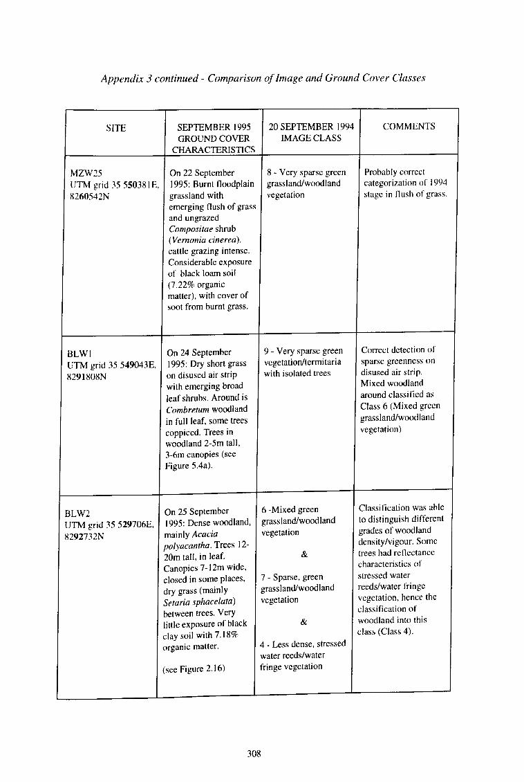
Appendix 3 continued - Comparison of Image and Ground Cover Classes
SITE SEPTEMBER 1995 20 SEPTEMBER 1994 COMMENTSGROUND COVER IMAGE CLASS
CHARACTERISTICS
MZW25 On 22 September 8 - Very sparse green Probably correctUTM grid 35 550381 E, 1995: Burnt floodplain grass land/wood Iand categorization of 1994
X260542N grassland with vegetation stage in tlush of grass.emerging flush of grassand ungrazedCompositae shrub(Vernonia cinerea).cattle grazing intense.Considerable exposureof black loam soil(7.22% organicmatter), with cover ofsoot from burnt grass.
BLWI On 24 September 9 - Very sparse green Correct detection of
UTM grid 35 549043E, 1995: Dry short grass vegetati onltermi tari a sparse greenness on
X291XOXN on disused air strip with isolated trees disused air strip.
with emerging broad Mixed woodland
leaf shrubs. Around is around classified as
Combretum woodland Class 6 (Mixed green
in full leaf, some trees grassland/woodland
coppiced. Trees in vegetation)
woodland 2-5m tall,3-6m canopies (seeFigure 5.4a).
BLW2 On 25 September 6 -Mixed green Classification was able
UTM grid 35 529706E, 1995: Dense woodland, grassland/woodland to distinguish different
X292732N mainly Acacia vegetation grades of woodland
polyacantha. Trees 12- density/vigour. Some
20m tall, in leaf. & trees had reflectance
Canopies 7-l2m wide, characteristics of
closed in some places, 7 - Sparse, green stressed water
dry grass (mainly grassland/woodland reeds/water fringe
Setaria sphacelata) vegetation vegetation, hence the
between trees. Very classification of
little exposure of black & woodland into this
clay soil with 7.18% class (Class 4).
organic matter. 4 - Less dense, stressedwater reeds/water
(see Figure 2.16) fringe vegetation
308

Appendix 3 continued - Comparison of Image and Ground Cover Classes
SITE SEPTEMBER 1995GROUND COVER
CHARACTERISTICS
BLW~UTM grid 35 527592E.H289917N
On 25 September1995: Mixed, degradedwoodland (30%) in latespring stage of leaf re-growth ( almost fullleaf), with bare soil(709c). Former humansettlement area,woodland regenerating.Trees/bushes 1.5-4mtall, species includeAlbizia harveyi,Piliostigma thonningei,Combretum ghasalenseand Acacia species.Exposed soil is brown,silty clay. IsolatedOdontotermis termitemounds.(see Figure 2.17)
BLW4UTM grid 35 527159E.X289156N
On 25 September1995: Tree and bushgrassland. Dry grass,mainly Hyparrheniarufa, scattered Acaciatrees in leaf. Areaformer humansettlement, treesregenerating, transitionzone from woodland innorth to rermitariazone south.
On 25 September1995: Grasslandtermitaria with isolatedbushes (Albizia,Piliostigma.Combretum andAcacia sp.). Bushes 2-4m tall, with 1-1.5mcanopies, in leaf. Grassdry, mainly Setariasphacelata). Nograzing. Occasionalexposure of dark greyloam soil (3.73%organic matter)
BLW5UTM grid 35 525883E,8285780N
COMMENTS20 SEPTEMBER 1994IMAGE CLASS
9 - Very sparse greenvegetationltermitariawith isolated trees.
Probably correctcategory for site'sgreenness. Otherclasses around are 6(Mixed greengrassland/woodlandvegetation), 11 (Drygrassland andtermitaria zone withouttrees) and 12 (Dry landwith leafless plantstructures(woodland/grassland».Classification correctlyreproduced groundcover variation.
9 - Very sparse greenvegetati onltermi tari awith isolated trees.
Correct class.
9 - Very sparse greenvegetationltermitariawith isolated trees.
Acceptable category forsite's greenness.
309

Appendix 3 continued - Comparison of Image and Ground Cover Classes
SITE SEPTEMBER 1995 20 SEPTEMBER 1994 COMMENTSGROUND COVER IMAGE CLASS
CHARACTERISTICS
BLW6 On 25 September 12 - Dry land with Correct class should
UTM grid Y; 524962E. 1995: Termitaria leatless plant structures probably have been
X284342N grassland with very (woodland/grassland) Class I I (Dryisolated trees/shrubs in grassland andleaf. Odontotermis termitaria zone withouttermite mounds. Grass trees). Perhaps becausedry. yellowish grass was tall and castbrown/grey in colour. shadows just likemainly Setaria leafless woodland. thesphacelata, 60cm-1 m site was classified the
tall. not grazed. same as leafless
Transition zone to woodland.floodplain grassland.Black clay soil (with2.80% organic matter).
(see Figure 5.6b)
BLW7 On 25 September II - Dry grassland and Correct class.
UTM grid 35 523802E. 1995: Open. dry termitaria zone without
8282487N grassland with very treesisolated Cubitermistermite mounds.Predominant grassspecies Hvparrheniarufa. Eragrostislapp II la, Seteria sp.Grass yellowish brown.50cm-2m tall. notgrazed. almostcompletely coveringblack sandyloam/sandy clay loamsoil.
(see Figure 2.19b)
BLW8 On 25 September 8 - Very sparse green Correct classification
UTM grid 35 523417E. 1995: Open. dry grassland/woodland because of green herbs.
8282027N floodplain grassland. vegetation Around site are classes
ungrazed. grass 20- II (Dry grassland and
30cm tall. occasional termitaria zone without
green Compositae trees) and 12 (Dry land
herbs among dry grass. with leatless plantstructures
(see Figure 5.8a) (woodland/grassland»
310

Appendix 3 continued - Comparison of Image and Ground Cover Classes
SITE COMMENTS
BLW9UTM grid 35 521087E.8280058N
BLWIOUTM grid 35 517618E.8279633N
(see Figure 2.15)
Around site arc classesII (Dry grassland andtermitaria zone withouttrees) and 12 (Dry landwith leafless plantstructures(woodland/grassland)),a correct reproductionof ground covervariation.
SEPTEMBER 1995GROUND COVER
CHARACTERISTICS
20 SEPTEMBER 1994IMAGE CLASS
On 25 September1995: Open, heavilygrazed floodplaingrassland. Grasscropped to the ground,new shoots emerging,debris of old grassstems trampled andbroken. Intensegrazing by lechwe andzebra. Evidence ofearly burning.
15 - Burnt area ormuddy, dark surface
Was burnt in 1994.Correct class (butunlikely to have beenmuddy)
On 25 September1995: Dense waterfringe vegetation(species includingCyperus papyrus,Typha domingensis,Polygonumsenegalense,Phragmitesmauritianus),2-4mtall, density increasinginwards towards largelagoon. Cattle grazingevident. Soil black(gley) sandy loam.
3 - Dense, vigorouswater reeds/waterfringe vegetation
Correct classification.Inwards from site areClasses 2 (Dense, veryvigorous-) and 4 (Lessdense, stressed waterreeds/water fringevegetation), a correctreproduction of theground cover variation.
(see Figure 2.20)
BLWIIUTM grid 35 541l41E,8294348N
On 26 September1995: Mixed woodlandwith concentration ofplant with reddish drypods (especially Acaciaand Albina species).Some trees in leaf,others in early spring.Open spaces with baresoil between trees.Trees 3-20m tall, with4-8m canopies. Nograzing but in Nationalpark (see Figure 5.4b).
8 - Very sparse greengrassland/woodlandvegetation
311

Appendix 3 continued - Comparison of Image and Ground Cover Classes
SITE SEPTEMBER 1995 20 SEPTEMBER 1994 COMMENTSGROUND COVER IMAGE CLASS
CHARACTERISTICS
BLWl2 On 26 September 9 - Very sparse green Correct category of
UTM grid 35 529062E, 1995: Degraded mixed vegetati onltermi tari a site's greenness
~Q90X56N woodland (mainly with isolated trees.Acacia andCombretum species) informer humansettlement area, denserwoodland immediatelyeast across stream.Trees 2.5-6m tall('" IOm in nearbywoodland), in springleaf, canopies 2-1Omwide. About 60% ofcover dry grass).
BLWI3 On 26 September 6 -Mixed green Correct classification.
UTM grid 35 530l65E, 1995: Mixed grassland/woodland Other classes of
X289256N woodland. Tall trees vegetation woodland around are
( IO-15m height), Class 4 (Less dense,
canopies (8-lOm wide) stressed-), Class 5
not touching. Many (Sparse, stressed water
trees in leaf. Large reeds/water fringe
(Macrotermis) termite vegetation), a correct
mounds among trees. reproduction of
Short (=20cm), dry woodland variation on
grass where open the ground. Some trees
spaces occur. had reflectancecharacteristics ofstressed waterreeds/water fringevegetation, hence theclassification ofwoodland into theseclasses.
BLWI4 On 26 September 12 - Dry land with Correct depiction of
UTM grid 35 530769E, 1995: Degraded mixed leafless plant structures dry state.
X288355N woodland in human (woodland/grassland) )
settlement area. Treesin leaf (Acacia.Piliostigma sp.),2-2.5m tall, canopies1-1.5m wide. Short drygrass between trees,also crop fields in dryseason fallow (with drygrass and old cropdebris).
312

Appendix 3 continued - Comparison of Image and Ground Cover Classes
SITE COMMENTSSEPTEMBER 1995GROUND COVER
CHARACTERISTICS
20 SEPTEMBER 1994IMAGE CLASS
BLWIXUTM grid 35 531774E.X279696N
Pockets of: Correct reproduction ofground cover variation.Other classes aroundsite are Class 13(Exposed. trampled drysoil with surfacedebris) and Class 7(Sparse, greengrassland/woodlandvegetation)
BLWI5UTM grid 35 530521 E.S28773XN
On 26 September1995: Dry grassland(mainly Hyparrheniatufa) among thicketson Macrotermistermite mounds. Grassabout 60% of cover.Trees 6-l2m tall. with6m wide canopies. inspring leaf. Grass I-2mtall.
Class I1- Drygrassland andtermitaria zone withouttrees
Class 6 - Mixed greengrassland/woodlandvegetation
BLWI6UTM grid 35 531091E.X283005N
On 26 September1995: Termitariagrassland. dry browngrass. isolated trees.Transition zonebetween woodland andfloodplain-grasslandzone. Odontotermistermite mounds. Nograzing.
II -Dry grassland andtermitaria zone withouttrees
Should probably havebeen more accuratelyclassified in a sparsegreen vegetation class.However, Class 8(Very sparse greengrassland/woodlandvegetation) presentaround.
BLW 17UTM grid 35 531519E.X280240N
On 26 September1995: Open. dryfloodplain grassland.Grass 20cm-1 m tall.Mixed. with variouscoarse twigs. Area is indelta of seasonallyflowing tributary of theKafue, whichdisappears infloodplain. No grazing.
II -Dry grassland andtermitaria zone withouttrees
Acceptable class.Ground cover variationreproduced byclassification. Class 12( Dry land with leaflessplant structures(woodland/grassland))also delineated nearsite.
Must have had earlyburning in 1994,resulting in new shootsof grass.
On 26 September1995: Open floodplaingrassland. very fewsmall (Cubitermis)termite mounds. Grassdrying. faintly green inlower portions. Maingrass speciesBrachiaria brizantha.not grazed. Area is indelta of seasonallyflowing tributary of theKafue. whichdisappears infloodplain.
10 - Emergentvegetation in shallowwater or after burning
313

Appendix 3 continued - Comparison of Image and Ground Cover Classes
SITE SEPTEMBER 1995 20 SEPTEMBER 1994 COMMENTSGROUND COVER IMAGE CLASS
CHARACTERISTICS
BLWl9 On 26 September II -Dry grassland and Acceptable class.
l'TM grid 35 532215E. 1995: Tall. dry. brown termitaria zone without
X277X93]1.; Sorghum versicolor treesreeds in tloodplainzone. Stand over70x70m in size. Reedsover 2m tall. Shortergrass species betweenreeds. Very littleexposure of loam, verydark grey soil (4.74%organic matter). Reedsform isolated pocketstands to the cast ofsite. the rest beingshorter grass.
BLW20 On 26 September 5 - Sparse, stressed Acceptable class. Grass
UTM grid 35 532219E. 1995: Open floodplain water reeds/water may have been in this
X2740lXN grassland. Heavily fringe vegetation state at time of image
grazed by lechwe and acquisition.
zebra. grass cropped toground level. Debris ofold grass stemstrampled and broken.New shoots of grassemerging.
BLW21 On 26 September 13 - Exposed, trampled Maybe correct class
UTM grid Vi 532914E. 1995: Open floodplain dry soil with surface assuming that there
X271lJ7XN grassland. Intensely debris was more trampling
grazed by lechwe andand blowing of debris
zebra, grass cropped to by wind in 1994,
ground level. Debris of leaving exposed soil.
old grass stemstrampled and broken.Evidence of earlyburning. New shoots ofgrass emerging.Exposed loam, verydark grey soil (6.83%organic matter) inplaces. with coveringof soot from burning.
314

Appendix 3 continued - Comparison of Image and Ground Cover Classes
SITE SEPTEMBER 1995 20 SEPTEMBER 1994 COMMENTS
GROUND COVER IMAGE CLASSCHARACTERISTICS
BLW22 On 27 September 9 - Very sparse green With Class 13
UTM grid 35 558798E, 1995: Dry grassland vegetationltermitaria (Exposed, trampled dry
8294972N with isolated shrubs, with isolated trees soil with surface
bushes and trees, few debris) near site,
termite mounds acceptable
(Ondontotermis sp.). categorization of state
Site close to human of greenness.
settlement. Trees,bushes and shrubsI-15m tall, canopies1.5-10m wide, many inleaf. Grass dry,brownish, ungrazed,40cm-1 m tall. Littleexposure of lightgreyish brown sandyloam soil (1.09%organic matter)
BLW23 On 27 September II -Dry grassland and Acceptable, possible
UTM grid 35 558829E, 1995: Open floodplain termitaria zone without cover class in 1994.
8294452N grassland. Grass dry in trees
upper portions, freshshoots in lowerportions. Low grazingpressure. Fire damageevident.
BLW24 On 27 September 10 - Emergent Acceptable class.
UTM grid 35 558579E, 1995: Open floodplain vegetation in shallow Could have been hurnt
8293469N grassland. Grass dry in water or after burning in 1994.
upper portions, freshshoots in lowerportions, about 15cmtall. Higher grazingpressure than BLW23,mainly cattle grazing.
BLW25 On 27 September 5 - Sparse, stressed May be correct
UTM grid 35 558524E, 1995: Open floodplain water reeds/water category for state of
8291892N grassland largely dry fringe vegetation floodplain at site in
but with emerging1994.
green shoots. Moretrampled by cattle thanBLW24, moreexposure of blacksandy clay loam soil.
315

Appendix 3 continued - Comparison of Image and Ground Cover Classes
SITE SEPTEMBER 1995 20 SEPTEMBER 1994 COMMENTSGROUND COVER IMAGE CLASS
CHARACTERISTICS
BLW26 On 27 September 4 - Less dense, stressed Correct class.
UTM grid 35 5591 07E, 1995: Depression in water reeds/water
8291325N floodplain zone, fringe vegetation.periodically watered,wi th water reeds(mainly Typhadomingensis). Smallstreams leading intodepression. Not underwater at time but verymoist. Cattle grazingevident.
BLW27 On 27 September I - Open water Correct classification
UTM grid 35 56040 IE, 1995: Open lagoon
8290070N water (Luwato &Lagoon). Lagoon 60-80m wide. Same 4 - Less dense, stressed
lagoon as BLW36. water reeds/water
Water reeds and water fringe vegetation
fringe vegetation onlagoon banks (Typhadomingensis on northbank, T. domingensisand Polygonumsenegalense on southbank).
(see Figures 2.23, 4.8,5.3a and 5.5)
BLW28 On 28 September 9 - Very sparse green With Class 12 (Dry
UTM grid 35 549838E 1995: Termitaria vegetationltermitaria land with leafless plant
8291164N grassland bordering with isolated trees structures
floodplain grassland.(woodland/grassland)
Very isolated, mainlyncar site, ground cover
Acacia shrubs 1-4mvariation reproduced
tall. Odontotermisby classification.
termite moundscommon. Dry,yellowish brown grass(mainly Graminaespecies), up to 1m tall,ungrazed.
316

Appendix 3 continued - Comparison of Image and Ground Cover Classes
SITE SEPTEMBER 1995 20 SEPTEMBER 1994 COMMENTS
GROUND COVER IMAGE CLASSCHARACTERISTICS
BLW29 On 28 September II - Dry grassland and With Classes 12 (Dry
UTM grid 35 551310E. 1995: Open. dry termitaria zone without land with leatless plant
8289929N grassland on edge of trees structures (woodland/
floodplain. very grassland) and 9 (Very
isolated Odontotermis sparse green
termite mounds. Fewer vegetationltermitaria
shrubs than at BLW28. with isolated trees)
No grazing. Grass as at near site, ground cover
BLW28. variation reproducedby classification
BLW30 On 28 September 9 - Very sparse green With Classes 12 (Dry
UTM grid 35 551957E. 1995: Dry, open vegetationltermitaria land with leafless plant
8287834N floodplain grassland, with isolated trees structures (woodland/
mainly ungrazed darkgrassland), 6 (mixed
brown twigs (mainlygreen grassland/
Vernonia sp.). Somewoodland vegetation),
twigs in leaf butand 5 (Sparse, stressed
ungrazed. Height ofwater reeds/water
twigs 30-5Ocm, almostfringe vegetation),
complete ground coverground cover variation
but interrupted byreproduced hy
game tracks.c1assification
BLW31 On 28 September 4 - Less dense, stressed At time of image
UTM grid 35 553490E, 1995: Typha water reeds/water acquisition in 1994,
8290044N domingensis water fringe vegetation reeds very likely to
reeds, next to open,have been unhurnt.
heavily grazed & Classification
floodplain grasslandreproduced variation in
(grazing by 5 - Sparse, stressed reed density/vigour.
lechwelzebra). Fire water reeds/water
disturbance of reeds fringe vegetation
evident at time of visit.
(see Figure 5.8b)
BLW32 On 28 September 4 - Less dense, stressed Correct classification.
UTM grid 35 556865E. 1995: Water reed zone, water reeds/water
8291003N mainly Typha fringe vegetation
domingensis in shallowseasonally inundateddepression. Firedisturbance evident.Low grazing pressure.
317
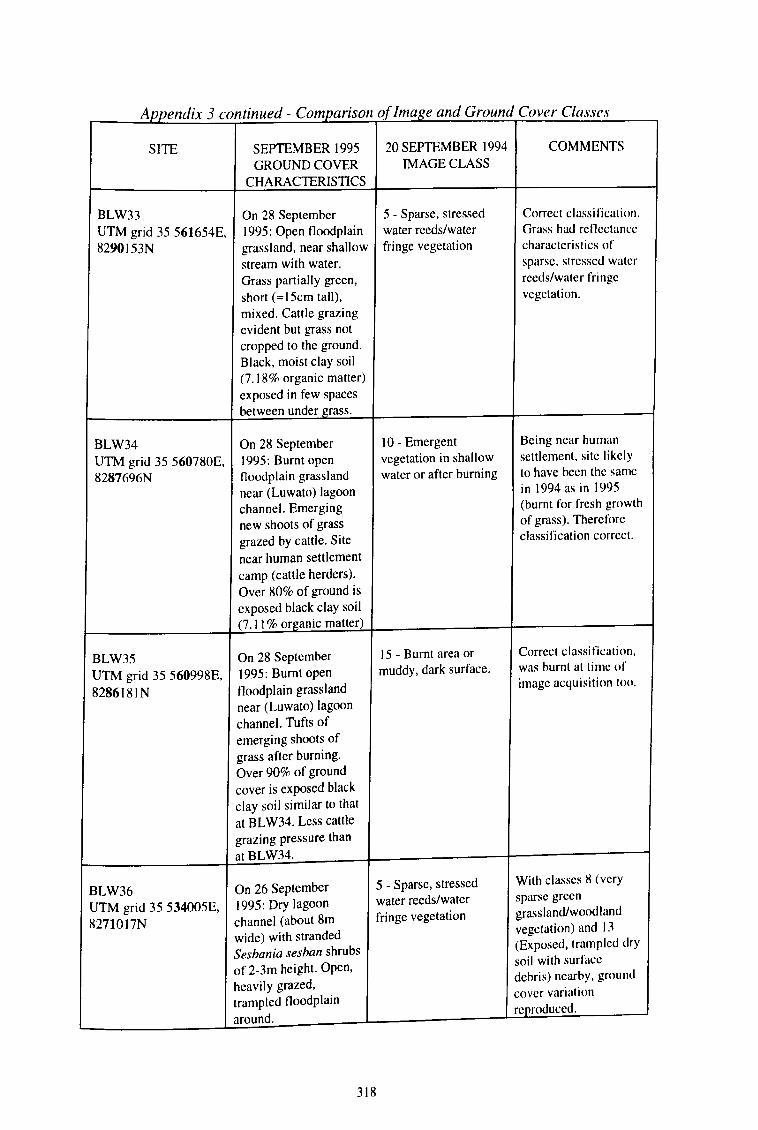
Avppendix 3 continued - Comparison of Image and Ground Cover Classes
SITE SEPTEMBER 1995 20 SEPTEMBER 1994 COMMENTSGROUND COVER IMAGE CLASS
CHARACTERISTICS
BLW33 On 28 September 5 - Sparse, stressed Correct classification.UTM grid 35 561654E, 1995: Open floodplain water reeds/water Grass had reflectance
8290l53N grassland, near shallow fringe vegetation characteristics ofstream with water. sparse, stressed waterGrass partially green, reeds/water fringeshort (=:l5cm tall), vegetation.mixed. Cattle grazingevident but grass notcropped to the ground.Black, moist clay soil(7.18% organic matter)exposed in few spacesbetween under grass.
BLW34 On 28 September 10 - Emergent Being near human
UTM grid 35 560780E, 1995: Burnt open vegetation in shallow settlement. site likely
8287696N floodplain grassland water or after burning to have been the same
near (Luwato) lagoon in 1994 as in 1995
channel. Emerging (burnt for fresh growth
new shoots of grass of grass). Therefore
grazed by cattle. Site classification correct.
near human settlementcamp (cattle herders).Over 80% of ground isexposed black clay soil(7.11 % organic matter)
BLW35 On 28 September 15 - Burnt area or Correct classi fication,
UTM grid 35 560998E. 1995: Burnt open muddy, dark surface. was burnt at time of
8286181N floodplain grassland image acquisition too.
near (Luwato) lagoonchannel. Tufts ofemerging shoots ofgrass after burning.Over 90% of groundcover is exposed blackclay soil similar to thatat BLW34. Less cattlegrazing pressure thanatBLW34.
BLW36 On 26 September 5 - Sparse, stressed With classes H (very
UTM grid 35 534005E, 1995: Dry lagoon water reeds/water sparse green
8271017N channel (about 8m fringe vegetation grassland/woodland
wide) with strandedvegetation) and J 3
Sesbania sesban shrubs(Exposed. trampled dry
of 2-3m height. Open,soil with surface
heavily grazed.debris) nearby. ground
trampled floodplaincover variation
around.reproduced.
318

References
REFERENCES
Azzali, S., 1991, Interpretation of crop growth patterns by means of NDVI-time seriesin Zambia, Geocarto International, 6(3): 15-26.
Balasubrahmanyam, S. and Abou-Zeid, S.M., 1978(a), Post Itezhi-tezhi flow pattern ofthe Kafue in the Kafue Flats region, in: Howard, G.W. and Williams, GJ. (eds.),Proceedings of the National Seminar on Environment and Change: the Consequencesof Hydroelectric Power Development on the Utilization of the Kafue Flats, Lusaka,April 1978, pp. 63-67, Kafue Basin Research Committee, University of Zambia,Lusaka, Zambia.
Balasubrahmanyam, S. and Abou-Zeid, S.M., 1978(b), The Kafue River hydroelectricdevelopment, in: Howard, G.W. and Williams, GJ. (eds.), Proceedings of the NationalSeminar on Environment and Change: the Consequences of Hydroelectric PowerDevelopment on the Utilization of the Kafue Flats, Lusaka, April 1978, pp. 31-33,Kafue Basin Research Committee, University of Zambia, Lusaka, Zambia.
Baumgartner, D.W. and Price, KP., 1993, An integrative approach to changedetection in an agricultural environment, in: Lewis, AJ. (ed.), Looking to the FutureWith an Eye on the Past: ACSMIASPRS Convention, New Orleans, February 15-/8,1993, Volume 2, pp. 2-10, American Society for Photogrammetry and Remote Sensingand American Congress on Surveying and Mapping, Bethesda, USA
Burke, 1.1., 1994, Approaches to integrated water resources development andmanagement: the Kafue basin, Zambia, Natural Resources Forum, 18(3): 181-192.
Chabwela, H.N. and Ellenbroek, G.A, 1990, The impact of hydroelectricdevelopments on the lechwe and its feeding grounds at Kafue Flats, Zambia, in:Whigham, D.F. et al (eds.), Wetland Ecology and Management, pp. 95-101, Kluwer;Tasks for Vegetation Science, 25.
Chavez, P.S. Jr., 1988, An improved dark-object subtraction technique foratmospheric scattering correction of multispectral data, Remote Sensing ofEnvironment, 24(3):459-479.
Cheatle, M.E., 1994, A preliminary evaluation of Landsat imagery for detectingindigenous woodland and monitoring changes in the hinterland of Lusaka, Zambia, in:Stone, le. (ed.), Maps and Africa, Proceedings of Colloquium, Aberdeen, /993, pp.245-252, Aberdeen University African Studies Group, Aberdeen, Scotland.
Congalton, R., 1991, A review of assessing the accuracy of classifications of remotelysensed data, Remote Sensing of Environment, 37(1 ):35-46.
Cracknell, AP. and Hayes, L.W.B., 1991, Introduction to Remote Sensing, Taylor and
Francis, London, UK.
319

References
Crapper, P. and Hynson, K., 1983, Change detection using Landsat photographicImagery, Remote Sensing of Environment, 13(4):291-300.
Crippen, RE., 1987, The regression interaction method of adjusting image data forband ratioing, International Journal of Remote Sensing, 8(2); 137-155.
Daka, AN., I995(a), A review of seasonal forecast model performance in Zambia,Pers. Comm. (unpublished/draft paper).
Daka, AN., I995(b), Rainfall variability and its impact on maize production in Zambia,Pers. Comm. (unpublished/draft paper).
Dale, P.E.R, Chandica, AL. and Evans, M., 1996, Using image subtraction andclassification to evaluate change in subtropical intertidal wetlands, InternationalJournal of Remote Sensing, 17(4):703-719.
Douthwaite, RJ., 1974, An endangered population of wattled cranes (Gruscarunculatus), Biological Conservation, 6(2): 134-142.
Douthwaite, R.J., 1978, Water birds: their ecology and future on the Kafue Flats, in:Howard, G.W. and Williams, G.J. (eds.), Proceedings of the National Seminar onEnvironment and Change: the Consequences of Hydroelectric Power Development onthe Utilization of the Kafue Flats, Lusaka, April 1978, pp. 137-140, Kafue BasinResearch Committee, University of Zambia, Lusaka, Zambia.
Dudley, RG. and Scully, R.T., 1980, Changes in experimental gill net catches from theKafue floodplain, Zambia, since construction of the Kafue Gorge Dam, Journal of Fish
Biology, 16:521-537.
Eckhardt, D.W., Verdin, lP. and Lyford, G.R., 1990, Automated update of anirrigation lands GIS using SPOT HRV imagery, Photogrammetric Engineering andRemote Sensing, 56(11):1515-1522.
Ellenbroek, G.A, 1987, Ecology and Productivity of an African Wetland System: theKafue Flats, Zambia, Dr. W. Junk Publishers, Dordrecht, Netherlands.
ERDAS Inc., 1994, Field Guide, ERDAS Systems Incorporated, Atlanta, Georgia,
USA
FAO, 1968, Multipurpose Survey of the Kafue Basin, Zambia, Volume Il-Soil Survey;Volume IV-Ecology of the Kafue Flats Part 3, Photographs; Part 5, Drawings,
FAO/SF:35/ZAM, Rome, Italy.
Fung, T. and LeDrew, E., 1987, Application of principal component analysis to changedetection, Photogrammetric Engineering and Remote Sensing, 53( 12): 1649-1658.
Gonima, L., 1993, Simple algorithm for the atmospheric correction of reflectanceimages, International Journal of Remote Sensing, 14(6): 1179-1187.
Haack, B., 1996, Monitoring wetland changes with remote sensing: an East Africanexample, Environmental Management, 20(3):411 -4 19.
320

References
Hall, EG., Strebel, D.E., Nickeson, J.E. and Goetz, S.1., 1991, Radiometricrectification: toward a common radiometric response among multidate, multisensorimages, Remote Sensing of Environment, 35( I): I 1-27.
Handlos, W.L., 1978, Introduction to the ecology of the Kafue Flats, in: Howard,G.W. and Williams, G.J. (eds.), Proceedings of the National Seminar on Environmentand Change: the Consequences of Hydroelectric Power Development on theUtilization of the Kafue Flats, Lusaka, April 1978, pp. 5-29, Kafue Basin ResearchCommittee, University of Zambia, Lusaka, Zambia.
Hefner, lM. and Storrs, e.G., 1994, Classification and inventory of wetlands in theSouthern Appalachian region, Water, Air and Soil Pollution, 77(3):209-219.
Hielkema, S.D., Prince, S.D. and Astle, W.L., 1986, Rainfall and vegetationmonitoring in the savanna zone of the Democratic Republic of Sudan using the NOAAAdvanced Very High Resolution Radiometer, International Journal of RemoteSensing, 7(11): 1499-15 I3.
Howard, G.W., 1985, The Kafue Flats of Zambia: a wetland system comparable withfloodplain areas of northern Australia, Proceedings of the Ecological Society ofAustralia, 13:293-306.
Howard, G.W. and Aspinwall, D.R., 1984, Aerial censuses of shoebills, saddlebilledstorks and wattled cranes at the Bangweulu Swamps and Kafue Flats, Zambia, Ostrich,55(4):207-212.
Howard, G.W. and Williams, GJ. (eds.), 1977, Development in the Lower KafueBasin in the Nineteen Seventies, Kafue Basin Research Committee, University ofZambia, Lusaka, Zambia.
Howarth, P.1. and Wickware, G.M., 1981, Procedures for change detection usmgLandsat digital data, International Journal of Remote Sensing; 2(3):277-291.
Hulme, M., 1996 (ed.), Climate Change and Southern Africa: an exploration of somepotential impacts and implications in the SADC region, Climate Research Unit,University of East Anglia, Norwich, UK / WWF-International, CH-1196 Gland,
Switzerland.
Irons, lR., Weismiller, R.A. and Petersen, G.W., 1989, Soil Reflectance, in: Asrar, G.(ed.), Theory and Applications of Optical Remote Sensing, pp. 66-106, Wiley, New
York, USA.
Jakubauskas, M.E., Lulla, K.P. and Mausel, P.W., 1990, Assessment of vegetationchange in a fire altered landscape, Photogrammetric Engtneering and Remote Sensing,
56(3):371-377.
Jeffrey, R.C.V. and Chooye, P.N., 1991, The people's role in wetlands management:the Zambian initiative, Landscape and Urban Planning, 20(1-3):73-79.
Jensen, J.R., 1986, Introductory Digital Image Processing: A Remote SensingPerspective, Prentice Hall, Eagle Wood Cliffs, New Jersey, USA.
321

References
Jens~n, J.R, Hodgson, M.E., Christensen, E.J., Mackey, H.E., Tinney, L.R andShantz, R., 1986, Remote sensing inland wetlands: a multispectral approach,Photogrammetric Engineering and Remote Sensing, 52(1) :87- 100.
Jensen, 1.R, Narumalani, S., Weatherbee, O. and Mackey, 1.R. Jr., 1993,Measurement of seasonal and yearly cattail and waterIily changes using multi dateSPOT panchromatic data, Photogrammetric Engineering and Remote Sensing,59(4):519-525.
Jensen, J.R, Rutchey, K., Koch, M.S. and Narumalani, S., 1995, Inland wetlandchange detection in the Everglades Water Conservation Area 2A using a time series ofnormalised remotely sensed data, Photogrammetric Engineering and Remote Sensing,61 (2): 199-209.
Justice, e.O. and Hiernaux, P.H. Y., 1986, Monitoring the grasslands of the sahel usingNOAA AVHRR data: Niger 1983, International Journal of Remote Sensing,7(11):1475-1497.
Justice, e.O., Holben, RN. and Gwynne, M.D., 1986, Monitoring East Africanvegetation using AVHRR data, International Journal of Remote Sensing, 7( 11): 1453-
1474.
Kaufman, Y.1. and Sendra, C., 1988, Algorithm for automatic atmospheric correctionsto visible and near infrared satellite imagery, International Journal of Remote Sensing,9(8): 1357-1381.
Kent, D.M., 1994(a), Introduction, in: Kent, D.M.,(ed.), Applied Wetlands Scienceand Technology, pp. 1-11, Lewis Publishers, London, UK.
Kent, D.M., 1994(b), Monitoring of wetlands, in: Kent, D.M.,(ed.), Applied WetlandsScience and Technology, pp. 193-219, Lewis Publishers, London, UK.
Kneizys et al. 1988, User's Guide to LOWTRAN 7, Hanscom AFB, Massachusetts:Airforce Geophysics Laboratory.
Kruss, P.D., 1992, Drought and climate change in Zambia, the last 100 years, (Pers.
Comm./Extended Draught Abstract).
Lee, CT. and Marsh, S.E., 1995, The use of archival Landsat MSS and ancillary datain a GIS environment to map historical change in an urban riparian habitat,Photogrammetric Engineering and Remote Sensing, 61(8):999-1008.
Lillesand, T.M. and Kiefer, RW., 1994, Remote Sensing and Image Interpretation,
Wiley, Chichester, USA.
Mackey, H.E. Jr., 1993, Six years of monitoring annual changes in a fresh water marshwith SPOT HRV data, in: Lewis, A.J. (ed.), Looking to the Future With an Eye on thePast: ACSMIASPRS Convention. New Orleans. February 15-18. 1993, Volume 2, pp.222-229, American Society for Photogrammetry and Remote Sensing and AmericanCongress on Surveying and Mapping, Bethesda, USA.
322

References
Markham, A, Dudley, N. and Stolton, S., 1993, Some Like it Hot: Climate Change,Biodiversity and the Survival of Species, WWF International, Gland, Switzerland.
Mason, S.l., 1995, Sea surface temperature-South African rainfall associations, 1910-1989, International Journal of Climatology, 15(2): 119-135.
Massart, M., Petillon, M. and Wollf, E., 1995, The impact of an agriculturaldevelopment on a tropical forest: the case of Shaba (Zaire), PhotogrammetricEngineering and Remote Sensing, 61(9): 1153-1158.
Matarira, CH., 1990, Drought over Zimbabwe in a regional and global context,International Journal of Climatology, 10(6):609-625.
Mather, P.M., 1987, Computer Processing of Remotely Sensed Images: AnIntroduction, Wiley, New York, USA
Mikkola, K., 1996, A remote sensing analysis of vegetation damage around smelters inthe Kola Peninsula, Russia, International Journal of Remote Sensing, 17(18):3675-3690.
Milne, AK., 1988, Change detection analysis using Landsat imagery: a review ofmethodology, Proceedings of IGARSS '88 Symposium, Edinburgh, Scotland, /3-/6September /988, pp. 541-544, ESA publications Division.
Mouat, D.A, Mahin, G.G. and Lancaster, 1., 1993, Remote sensing techniques in theanalysis of change detection, Geocarto International, 2(1):39-50.
Muchinda, M.R, 1988, The reliability of annual rainfall in Zambia,Hydrometeorological Report No. 1/, Meteorology Department, Lusaka, Zambia.
Muchoney, D.M. and Haack, RN., 1994, Change detection for monitoring forestdefoliation, Photogrammetric Engineering and Remote Sensing, 60( I0): 1243-1251.
Muyanga, E.D. and Chipundu, P.M., 1978, A short review of the Kafue Flats fishery,from 1968 to 1978, in: Howard, G.W. and Williams, GJ. (eds.), Proceedings of theNational Seminar on Environment and Change: the Consequences of HydroelectricPower Development on the Utilization of the Kafue Flats, Lusaka, April /978, pp.105-113, Kafue Basin Research Committee, University of Zambia, Lusaka, Zambia.
Nedft, RT.1., 1992, Lekking Behaviour in Kafue Lechwe, PhD thesis, University of
Cambridge, Darwin College, Cambridge, UK.
News From Zambia, (compiled from the Zambian press and distributed from the officeof) The Zambia Society, Zimco House, 16-28 Tabernacle Street, London EC2A 4BN.
Njobvu, S.L., 1990, The problems of running an efficient irrigation system on a smallholder project, Agricultural Water Management, 17(1-3):319-321.
Orme, AR, 1990, Wetland morphology, hydrodynamics and sedimentation, in:Williams, M. (ed.), Wetlands: A Threatened Landscape, pp. 42-94, Blackwell, Oxford,
UK.
323

References
Pike, V.R, 1978, Nakambala and the Kafue Flats, in: Howard, G.W. and Williams.G.J. (eds.), Proceedings of the National Seminar on Environment and Change: theConsequences of Hydroelectric Power Development on the Utilization o] the KafucFlats, Lusaka, April 1978, pp. 75-79, Kafue Basin Research Committee, University ofZambia, Lusaka, Zambia.
Price, P.K., Pyke, D.A. and Mendes, L., 1992, Shrub die back in a semi aridecosystem: the integration of remote sensing and geographic information systems fordetecting vegetation change, Photogrammetric Engineering and Remote Sensing.58(4):455-463.
Rees, W.A., 1976, The ecology of the lechwe, Kobus leche kafuensis Haltenorth, inLochinvar National Park, Zambia as affected by the Kafue Gorge hydroelectricscheme: herbage digestibility in free living antelope, East African Wildl~t'e journal,14:59-66.
Rees, W.A., 1978, The ecology of the Kafue lechwe, journal of Applied Ecology,15:163-217.
Reimold, RJ., 1994, Wetlands functions and values, in: Kent, D.M.,(ed.), AppliedWetlands Science and Technology, pp. 55-78, Lewis Publishers, London, UK.
Richter, R, 1990, A fast atmospheric correction algorithm applied to Landsat TMimages, International journal of Remote Sensing, II (I): 159-166.
Ringrose, S., Matheson, W. and Boyle, T., 1988, Differentiation of ecological zones inthe Okavango Delta, Botswana, by classification and contextual analyses of LandsatMSS data, Photogrammetric Engineering and Remote Sensing, 54(5):601-608.
Ringrose, S., Matheson, W., Tempest, F. and Boyle, T., 1990, The development andcauses of range degradation features in Southeast Botswana using multi-temporalLandsat MSS imagery, Photogrammetric Engineering and Remote Sensing,56(9): 1253-1262.
Robinove, Ci.l., 1982, Computation with physical values from Landsat digital data,Photogrammetric Engineering and Remote Sensing, 48(5):781-784.
Sader, S.A., Powell, G.V.N. and Rappole, 1.H., 1991, Migratory bird habitatmonitoring through remote sensing, International journal of Remote Sensing.12(3):363-372.
Sakaida, K., 1994, Rainfall changes and their effects on maize production in Zambia,Science Reports, 43( I): 13-25, Tohoku University, Japan.
Sayer, l.A. and van Lavieren, L.P., 1975, The ecology of the Kafue lechwe before theoperation of hydroelectric dams on the Kafue River, East African Wildlife journal,13(1):9-38.
Schott, 1., Salvaggio, C. and Volchok, W., 1988, Radiometric scene normalisationusing pseudo invariant features, Remote Sensing of Environment, 26( 1): 1-16.
324

References
Schuster, R.H., 1980, Will the Kafue lechwe survive the Kafue dams? Oryx, 15:476-489.
Sheppe, W.A, 1985, Effects of human activities on Zambia's Kafue Flats ecosystems,Environmental Conservation, 12(I):49-57.
Stow, D.A, Collins, D. and Mckinsey, D., 1990, Land use change detection based onmultidate imagery from different satellite sensors, Geocarto International, 3( 1):3-12.
Switzer, P., Kowalik, W. and Lyon, R., 1981, Estimation of atmospheric path radianceby the covariance matrix method, Photogrammetric Engineering and Remote Sensing,47( 10): 1469-1474.
Tammi, e.E., 1994, Onsite identification and delineation of wetlands, in: Kent,D.M.,(ed.), Applied Wetlands Science and Technology, pp. 35-54, Lewis Publishers,London, UK.
Tao, Q., Lewis, AJ. and Braud, D.H. Jr., 1993, Change detection using multitemporalfeature space with digital TM data, in: Lewis, Al (ed.), Looking to the Future Withan Eye on the Past: ACSMIASPRS Convention, New Orleans, February 15-18, 1993,Volume 2, pp. 364-373, American Society for Photogrammetry and Remote Sensingand American Congress on Surveying and Mapping, Bethesda, USA
Townshend, J.R.G. and Justice, e.O., 1986, Analysis of the dynamics of Africanvegetation using the normalised difference vegetation index, International Journal o]Remote Sensing, 7(1 1):1435-1445.
Treitz, P.M., Howarth, PJ., Suftling, R'C. and Smith, P., 1992, Application of detailedground information to vegetation mapping with high spatial resolution digital imagery,Remote Sensing of Environment, 42( I):65-82.
Turner, B., 1982, Use of Landsat imagery in mapping the flooding of the Kafue Flats,Zambia, in: Williams, GJ. and Wood, AP. (eds.), Geographical Perspectives onDevelopment in Southern Africa: Papers from the Regional Conference of theCommonwealth Geographical Bureau, Lusaka, 9-J5th June 1982, pp. 45-54,Commonwealth Geographical Bureau, James Cook University, Queensland, Australia.
Turner, B. 1983, Bibliography of the Kafue Flats, Kafue Basin Research Committee,University of Zambia, Lusaka, Zambia.
Wilcox, D.A, 1995, Wetland and aquatic macrophytes as indicators of anthropogenichydrologic disturbance, Natural Areas Journal, 15(3):240-248.
Williams, D.e. and Lyon, lG., 1991, Use of a Geographic Informationn System database to measure and evaluate wetland changes in the St. Mary's River, Michigan,
Hydrobiologia,219:83-95.
Williams, M. 1990, Protection and Retrospection, in: Williams, M. (ed.), Wetlands: AThreatened Landscape, pp. 325-353, Blackwell, Oxford, UK.
325