Wax deposition analysis for oil andgas multiphase flow in pipelines

Aalborg University EsbjergOil and Gas Technology

Master’s Thesis

Fernando MonteroK10-OG-2-F20

Supervisor:Rudi Nielsen

June 10, 2020

Contents

Abstract III

Nomenclature IV

1 Introduction 11.1 Background . . . . . . . . . . . . . . . . . . . . . . . . . . . . . . . . . . . . 11.2 Problem statement . . . . . . . . . . . . . . . . . . . . . . . . . . . . . . . . 2

2 Wax 32.1 Wax appearance . . . . . . . . . . . . . . . . . . . . . . . . . . . . . . . . . . 3

2.1.1 Wax appearance temperature . . . . . . . . . . . . . . . . . . . . . . 32.1.2 Pour point . . . . . . . . . . . . . . . . . . . . . . . . . . . . . . . . . 42.1.3 Wax content . . . . . . . . . . . . . . . . . . . . . . . . . . . . . . . . 4

2.2 Wax chemistry . . . . . . . . . . . . . . . . . . . . . . . . . . . . . . . . . . . 4

3 Wax formation thermodynamics 63.1 Phase equilibrium . . . . . . . . . . . . . . . . . . . . . . . . . . . . . . . . . 63.2 Thermodynamic models . . . . . . . . . . . . . . . . . . . . . . . . . . . . . 7

4 Wax deposition via molecular diffusion 9

5 Multiphase flow 115.1 Multiphase flow fundamentals . . . . . . . . . . . . . . . . . . . . . . . . . 115.2 Wax deposition in two phase flow . . . . . . . . . . . . . . . . . . . . . . . 12

6 Wax deposition Matzain model 14

7 Wax deposition modeling and simulation 17

8 Entry Data 198.1 Fluids characterization . . . . . . . . . . . . . . . . . . . . . . . . . . . . . . 198.2 Physical properties correlations . . . . . . . . . . . . . . . . . . . . . . . . . 208.3 Wax precipitation curve . . . . . . . . . . . . . . . . . . . . . . . . . . . . . 208.4 Process conditions and pipeline characteristics . . . . . . . . . . . . . . . . 218.5 Study cases . . . . . . . . . . . . . . . . . . . . . . . . . . . . . . . . . . . . . 21

9 Wax deposition using OLGA R© 239.1 Entry data treatment . . . . . . . . . . . . . . . . . . . . . . . . . . . . . . . 23

9.1.1 Fluid characterization . . . . . . . . . . . . . . . . . . . . . . . . . . 239.1.2 Pipeline characteristics . . . . . . . . . . . . . . . . . . . . . . . . . . 299.1.3 Process conditions . . . . . . . . . . . . . . . . . . . . . . . . . . . . 30

I

9.2 Wax deposition simulation setup . . . . . . . . . . . . . . . . . . . . . . . . 309.2.1 Discretization independence analysis . . . . . . . . . . . . . . . . . 319.2.2 Stability analysis . . . . . . . . . . . . . . . . . . . . . . . . . . . . . 31

10 Wax deposition using Matlab R© 3210.1 Entry data treatment . . . . . . . . . . . . . . . . . . . . . . . . . . . . . . . 3210.2 Modeling setup . . . . . . . . . . . . . . . . . . . . . . . . . . . . . . . . . . 33

10.2.1 Heat transfer calculations . . . . . . . . . . . . . . . . . . . . . . . . 3310.2.2 Hydrodynamic calculations . . . . . . . . . . . . . . . . . . . . . . . 3410.2.3 Thermodynamic calculations . . . . . . . . . . . . . . . . . . . . . . 3610.2.4 Wax deposition calculations . . . . . . . . . . . . . . . . . . . . . . . 3610.2.5 Discretization independence analysis . . . . . . . . . . . . . . . . . 3710.2.6 Stability analysis . . . . . . . . . . . . . . . . . . . . . . . . . . . . . 3710.2.7 Modeling flow chart . . . . . . . . . . . . . . . . . . . . . . . . . . . 38

11 Results 4011.1 Heat transfer and fluid mechanics along the pipeline . . . . . . . . . . . . 40

11.1.1 Bulk and wall temperatures . . . . . . . . . . . . . . . . . . . . . . . 4011.1.2 Pressure drop profile . . . . . . . . . . . . . . . . . . . . . . . . . . . 4411.1.3 Superficial velocities . . . . . . . . . . . . . . . . . . . . . . . . . . . 4511.1.4 Flow pattern prediction . . . . . . . . . . . . . . . . . . . . . . . . . 46

11.2 Wax precipitation along the pipeline . . . . . . . . . . . . . . . . . . . . . . 4711.3 Wax deposition . . . . . . . . . . . . . . . . . . . . . . . . . . . . . . . . . . 49

11.3.1 Wax deposition profile . . . . . . . . . . . . . . . . . . . . . . . . . . 5011.3.2 Wax deposition evolution through time . . . . . . . . . . . . . . . . 54

12 Conclusions 58

13 Future work 59

Bibliography 60

Appendix A

Abstract

Wax deposition has been a big challenge for the Oil & Gas industry, and the current en-ergy demand has driven the oil production to remote environments where subsea facil-ities present low-temperature environments that represent potential financial losses dueto wax deposition. Some techniques have been developed to deal with wax formationor deposition problems; however, its modeling and simulation present some limitationsrelated to accurate predictions of wax deposit thickness and location. The closed interre-lation of wax deposition process with aspects referring to thermodynamics, heat & masstransfer and fluid mechanics brings additional complexity to wax deposition analysis.

This work consists in a comparative study of modeling and simulation of a subsea hor-izontal pipeline section transporting a multiphase flow. The analysis is done using acommercial software and a self developed code, which are used to evaluate the predic-tion of wax deposition using a non-compositional model; always pursuing a better un-derstanding of the wax deposition process, multiphase flow, transport phenomena, andtheir mathematical models and simulation tools.

Four main cases of analysis are considered in this project in which different gas and liq-uid mass flow rates are evaluated. Moreover, these four cases are expanded to 16 studycases to include different paraffin characterization and deposition times into the waxdeposition analysis. Experimental data available in open literature is used for fluid char-acterization in both commercial simulator and self developed code.

The results demonstrate the high sensitivity of the wax deposition prediction to the ac-curacy of the calculation of the inner wall temperature as well as the influence of thethermodynamic approach used in the wax formation analysis.

The wax deposition process is modeled based on the non-compositional Matzain Modelthrough the commercial software OLGA R© (by Schlumberger) and a code developed inMatlab R©.

III

Nomenclature

Abbreviations and Initials

API American Petroleum InstituteASTM American Society for Testing and MaterialsCapEx Capital expenditureCPA Cubic plus associationCPM Cross-polarized microscopyDSC Differential scanning calorimetryEoS Equation of stateFT-IR Fourier-transform infrared spectroscopyGUTS Grand Universal Thermodynamic SimulatorOHTC Overall heat transfer coefficientOpEx Operational expenditureSRK Soave-Redlich-Kwong equation of stateUOP Universal Oil Products companyVLSE Vapor-Liquid-Solid equilibriumWAT Wax appearance temperature

IV

1 Introduction

1.1 Background

Petroleum reservoir fluids are complex mixtures which contain primarily a wide rangeof hydrocarbons. Most of these fluids contain heavy paraffins which can precipitate andbe deposited as a solid-like material namely wax [1].

Wax deposition has been a big challenge for the Oil & Gas industry since its inception;additionally, the current global demand of energy has driven the oil exploration andproduction to remote environments where avoiding wax deposition requires innovativesolutions for cooler and deeper scenarios [2, 3].

Subsea facilities and pipelines are more susceptible to present wax deposition problemsduring petroleum production due to low-temperature environments and higher heattransfer capacity of these systems surrounded by water [4]. Pipeline operation presents ahigh risk associated to wax plugging, which worst-case scenario compliance the replace-ment of a pipe-section or even the abandonment of the production facilities representinghigh financial losses and environmental problems [5]. In this context, pipeline restart-ing flow after a programmed or emergency shutdown presents additional attention andchallenges related to blockage by gelled waxy crude oil [6, 7, 8].

Pipeline isolation and heating, pipe-in-pipe, wax-repellent surfaces, chemical and bi-ological treatments, mechanical scraping and cold-flow are some techniques useful todeal with wax formation or removal; however, wax deposition modeling and simulationpresent some limitations related to accurate predictions of wax deposit thickness, loca-tion and composition. Indeed, these limitations are frequently observed when real fieldcases are simulated due to the absence of adequate experimental field data and a strongsensitivity presented by the wax deposition models [9, 10, 11, 12, 13, 14].

The wax deposition process is closely interrelated to other phenomena making difficultits prediction through models and simulations; in other words, factors as the amount, lo-cation, composition and hardness of the wax deposited on the inner surface of a pipelinedepend on aspects related to thermodynamics, heat & mass transfer and fluid mechan-ics. Multiphase flow brings additional complexity to wax deposition analysis becauseparameters as flow regime and superficial phase velocities should be considered [11, 15].

Few studies of wax deposition in multiphase flow have been conducted. Nevertheless,accurate wax deposition predictions are needed to develop reliable and economical so-lutions to avoid this problem in current more challenging scenarios. Therefore, a goodknowledge of the wax deposition process, multiphase flow and transport phenomena in-volved leads to a better understanding about mathematical models, simulation tools andtheir optimal setting for real case wax deposition predictions [15, 16].

1

2

1.2 Problem statement

The aim of this work is to simulate a horizontal section of a subsea pipeline transportinga multiphase flow from wellhead to offshore production facilities understanding the waxdeposition phenomenon. To achieve this objective, the commercial software OLGA R©

(by Schlumberger) and a self developed code are used to evaluate the prediction of waxdeposition using a non-compositional model.

For this project, experimental data available in open literature is used. The experimentaldata related to wax deposition projects considering multiphase flow serves to character-ize the fluid for both simulations, acquiring a better knowledge about the interrelationbetween fluid characterization and wax deposition per se. The model used for the pre-diction of wax deposition corresponds, in both codes, to the Matzain model.

After model buildup and simulation, a comparative analysis of results is done in order toevaluate the different modules of the code developed in Matlab R© regarding heat transfer,fluid mechanics and wax deposition.

2 Wax

Basic and general concepts for wax deposition are needed to have a good understatingof the fundamentals linked to this phenomenon. The most important concepts related towax appearance and its chemistry are presented in this section.

2.1 Wax appearance

Three important concept should be well understood to have an comprehensive knowl-edge about wax appearance and related issues. Wax appearance temperature, pour pointand wax content give a fundamental basis for wax deposition studies.

2.1.1 Wax appearance temperature

Wax precipitation occurs if paraffin petroleum reservoir fluid is cooled down to the waxappearance temperature (WAT), which is defined as the highest temperature where solidwax molecules start to appear in the reservoir fluid. The term cloud point is also applied,based in a standardized procedure to determine WAT [1, 16, 17].

Different measurement methodologies can be used to determine WAT, but all those giveslightly different result due to the applied technique. Some WAT determination examplesare the following [1, 18]:

• Microscopic technique is based on the observation of the wax crystals formation,which increase the opacity of the fluid, giving the idea of a cloud appearing into thefluid. Standard testing methods, as ASTM-D2500 and ASTM-D3117, can be usedfor this visual analysis. The cross-polarized microscopy (CPM) uses cross-polarizedlight to allow the visualization of solid particle in dark oil samples increasing thesensitivity of the standard microscopic technique.

• Differential scanning calorimetry (DSC) is associated to the measurement of heatreleased by the crystallization wax process. The standard method ASTM-D4419-90was developed for WAT determination through DSC.

• Fourier-Transform Infrared Spectroscopy (FT-IR) measures the WAT of oil samplesbased on the distinct IR absorbance of solid wax particles in comparison with theone of liquid oil.

• Wax molecules increase the apparent viscosity of the fluid, so viscometry can beused to determine WAT.

CPM and FT-IR provide the closest values to the exact thermodynamic WAT, whereasDSC and viscosity measure usually result in an estimation of temperature below WAT,

3

4

where severe wax precipitation could occur. Regardless the WAT measurement tech-nique, its determination is very important to know under which conditions the wax pre-cipitation stars.

2.1.2 Pour point

The pour point is the lowest temperature at which the oil flows freely under its ownweight. This is measured under specific test conditions established by the ASTM D-97standard. The pour point is considerably lower than the WAT, and crude oils that havesignificant paraffin content usually present high pour points. During shutdown periods,the temperature can drop below the pour point, making the flow restarting a challengingtask. The pour point analysis should be combined with viscosity and yield stress mea-surements to perform a good rheological fluid evaluation; however, it is a useful roughindicator of flow behavior [1, 19].

2.1.3 Wax content

In a wax precipitation curve (Fig.2.1), the highest temperature represents the wax appear-ance temperature, where the crystallization of waxy component starts due to cooling. Atlow temperatures, the precipitation curve usually has an asymptotic trend, which repre-sents the total wax content in oil. The total wax content in an oil can be measured usingstandards, such as UOP46-64 or UOP46-85 [18].These standards were developed by theUniversal Oil Products company, now Honeywell UOP.

Figure 2.1: Wax precipitation curve [18].

The WAT and wax content are the first two parameters to be checked to determine if waxdeposition can be a problem during the production of certain well. Practically speaking,crude oils with more than 2% of wax content and a WAT higher than the subsea floortemperature, which commonly is around 4 ◦C, can present wax deposition problems [18].

2.2 Wax chemistry

Wax particles are mainly constituted by normal paraffins, but slightly branched paraffins(iso-paraffins) and cycle paraffins (naphthenes) with long paraffinic chains can be foundas part of the deposited wax material [1, 16, 17]. Common wax-forming molecules arepresented in Fig.2.2.

5

Figure 2.2: Typical wax forming molecules [1].

Regarding wax formation in petroleum reservoir fluids, two types of waxes are definedfor crude oils: macro and micro-crystalline wax. Straight-chain n-paraffins in a carbonrange from C20 to C50 are mainly present in macro-crystalline wax deposits; on the otherhand, branched paraffins and naphthenes in a carbon range from C30 to C60 are domi-nant in micro-crystalline wax composition. In a fraction with a carbon range higher thanapproximately C60 the degree of branching is high, making it less likely to be part of thesolid structure [1, 17, 20].

Wax deposits related to flow assurance problems consist of around 40-60% of macro-crystalline waxes and less than 10% of micro-crystalline waxes. Additionally, the com-position of the deposit varies through time considering that fresh wax deposits present asignificant fraction of oil. However, this oil fraction decreases through time making thedeposit more solid or harder [17].

The volumetric fraction of the entrapped oil in the deposit is called wax porosity. In thisconcept is assumed that the waxy components are only present in the solid phase andthe entrapped oil only consists of on non-waxy ones [18]. Porosity is important for bothpractical and modeling aspects. Through wax porosity analysis the wax removal methodto be applied and its frequency can be estimated. In wax deposition modeling, the waxporosity is a parameter which affects wax physical properties and the deposition thick-ness per se. A common range for wax porosity is from 60 to 90 mass %, corresponding tohard and soft wax deposits, respectively [2, 10, 16, 18, 21].

The wax porosity is also affected by the cooling rate. Higher cooling rates produce softerdeposits because the wax is formed and deposited rapidly, entrapping higher oil frac-tions; on the contrary, lower cooling rates produce harder deposits [16].

3 Wax formation thermodynamics

Wax thermodynamics knowledge is a fundamental part of wax deposition process notonly to identify the viability of wax formation but also to determine how severe the de-position could be. However, wax formation analysis is a hard task because the reservoirfluids are complex mixtures, even wax is composed of n-paraffins of different carbonnumber [18]. A representative phase diagram of waxy oils is presented in Fig.3.1.

Temperature

Pre

ss

ure

VLE

Wax

Figure 3.1: Typical phase diagram of waxy crude oil.

3.1 Phase equilibrium

Vapor-Liquid-Solid equilibria are useful to determine the quantity of paraffins dissolvedin the liquid hydrocarbon. Describing wax thermodynamics for vapor-liquid equilib-rium implies the use of equations of state, as Peng-Robinson, SRK or CPA; however,liquid-solid analysis requires a different approach based on fugacity and Gibbs free en-ergy change [17, 18].

The fugacity of a component i, which represents the tendency of component i to escapefrom one phase to another. In a Vapor-Liquid-Solid equilibrium (VLSE) the fugacity ofcomponent i must be equal in each phase [1, 17, 18]. The fugacity fi is a function ofpressure (P ), temperature (T ) and molar composition of the different phases (yi, xi, si).

fVi (T, P, y1, y2, ..., yn) = fLi (T, P, x1, x2, ..., xn) = fSi (T, P, s1, s2, ..., sn) (3.1)

The phase equilibrium equations (Eq.3.1) together with mass balance (Eq.3.2) and con-stitutive equations (Eq.3.3) are solved simultaneously to determine the amount of each

6

7

phase (nV , nL, nS) and its molar composition (yi, xi, si).

nV yi + nLxi + nSsi = nFi (3.2)

N∑i

yi = 1;N∑i

xi = 1;N∑i

si = 1 (3.3)

3.2 Thermodynamic models

Thermodynamic models are useful tools to predict the solubility of wax components,their fractions in the fluid and the wax concentration [21].

Fugacity and the Gibbs free energy change of a pure liquid compound are used to esti-mate the corresponding variables for the pure solid. Essentially, the various wax modelsdiffer in the way how liquid and solid (wax) fugacities are estimated. Different thermo-dynamic approaches are used to analyze these non-idealities and calculate the activitycoefficients. A general expression which relates fugacity and Gibbs free energy change isshown in Eq.3.4. Depending of the theoretical approach of the analysis, the mathematicalform of this equation can vary [1, 18].

lnfSifLi

= −∆Hf

i

RT

(1− T

T fi

)− 1

RT

∫ T fi

T∆CPidT +

1

RT

∫ T fi

T

∆CPi

TdT +

∫ P

Po

∆ViRT

dp (3.4)

Where ∆Hfi is the enthalpy of fusion, T f

i is the melting temperature of component i,∆CPi is the difference between solid and liquid state heat capacities at constant pressurefor component i, ∆Vi is the difference between the solid and liquid phase molar volumeof component i and R is the ideal gas constant.

In addition to non-idealities, two aspects related to phase change from liquid to solidof n-paraffins should be considered. The secondary phase transition, which states that theenthalpy for the estimation of the Gibbs free energy, used in Eq.3.4, equals the enthalpy offusion plus the enthalpy of the secondary phase transition, which is an intermediate stageobserved in the solidification phenomenon of n-paraffins. The equilibrium between multiplesolid phases establishes the coexistence of wax solid phases with different structures (eg.hexagonal and orthorombic) [18].

Some thermodynamic models have been developed to handle wax formation. Differentapproaches are considered for each model as is shown in Table3.1.

According to literature, Coutinho’s model is the most thermodynamically complete methodfor wax deposition modeling because, in addition to non-idealities for liquid and solidphases, it includes secondary phase transition and multiple solid phases equilibrium [18].This approach gives to Coutinho’s wax model a high accuracy considering experimentaldata, as is observed in Fig.3.2.One of the main outputs of thermodynamic analysis of wax deposition is the predictionof the wax solubility curve (Fig.3.3) which can be built inverting the wax precipitationcurve. This construction is based on the fact that the amount of dissolved wax is equal tothe total amount of wax minus the precipitated one [18].Considering the radial temperature profile, the corresponding concentrations could beestimated using the wax solubility curve.

8

Table 3.1: Different thermodynamic models (based on Huang et. al [18])

Model Liquid Solid Multiple Secondary Commercialnon-ideality non-ideality solid phases transition software

Conoco – – Yes – GUTS / LedaFlowWon’s Yes Yes – – –Pedersen’s Yes Yes – – PVTsim by CalsepLira-Galeana’s Yes – Yes – –Coutinho’s Yes Yes Yes Yes Multiflash by KBC

Figure 3.2: Thermodynamic models comparison. "Reprinted with permission from [21]. Copyright 2020American Chemical Society."

Figure 3.3: Wax solubility curve [18].

4 Wax deposition via moleculardiffusion

In a general way, wax deposition occurs in pipeline systems if the temperature of thesystem is below the WAT, a negative radial temperature gradient is presented by theflow and the surface roughness is large enough to retain the wax crystals [11, 22].

According to literature, the following four wax deposition mechanisms have been pro-posed: molecular diffusion of the dissolved wax molecules, which form waxy componentson the inner wall surface; shear dispersion of the precipitated waxy particles on the innersurface; Brownian diffusion of the precipitated waxy particles on the wall through Brow-nian motion and gravity settling of the precipitated waxy particles towards the bottom ofthe pipeline. However, as result of several experimental studies, it is widely accepted thatmolecular diffusion is the dominant mechanism for the wax deposition process; the othermentioned mechanisms have a negligible impact in the wax deposition phenomenon[2, 10, 11, 3, 18].

The wax deposition process throughout molecular diffusion can be explained based onthe following description [10, 11, 18]. A scheme of the wax deposition mechanism throughmolecular diffusion is presented in Fig.4.1.

• Step 1: Precipitation of dissolved wax

At temperature values lower than WAT the dissolved wax molecules precipitateforming crystals. This precipitation occurs indistinctly on the bulk of the fluid oron the pipe wall if the local temperature is lower than WAT, but an incipient depositwax layer is formed on the inner pipe surface.

• Step 2: Generation of radial concentration gradient

In normal cooling conditions a negative radial temperature gradient is observed,in other words, the inner wall surface presents a lower temperature than the bulkoil. This makes greater the degree of precipitation on the wall than in the bulksurroundings. Consequently, the concentration of dissolved waxy components ishigher in the bulk than on the wall, which is the driving force for the diffusion ofwax molecules from the fluid bulk to the inner wall.

• Step 3: Deposition of waxy components

The dissolved waxy components that arrive to the wall vicinity precipitate, butnow on the surface of the existing deposit increasing its thickness. The moleculardiffusion continues if the flow through the pipeline continues as well, resulting inthe deposit buildup.

9

10

• Step 4: Deposit aging

The deposit aging is a phenomenon in which the solid fraction of wax into the de-posit increases, and two main steps describe this phenomenon. The internal diffu-sion of wax molecules inside the deposit layer increasing the solid wax fraction andthe counter diffusion of de-waxed oil out of the deposit, reducing the wax poros-ity and making harder the remain solid wax layer. However, the aging presentshigher rates when the wax deposition process starts because the internal direct andcounter diffusion have less resistances in a tinny layer; on the other, the aging pro-cess presents an asymptotic trend through the time.

Figure 4.1: Wax deposition through molecular diffusion [18].

Molecular diffusion, described by Fick’s Law, can be used as a basis to predict wax depo-sition rate and tendency [2, 4, 18]. This law can be expressed as a function of the radialtemperature gradient as is shown in Eq.4.1.

dmw

dt= −ρoDwoAi

dCw

dr= −ρoDwoAi

dCw

dT

dT

dr(4.1)

Where mw is the mass of wax, ρo is the density of oil, Dwo is the diffusion coefficient ofwax in oil, Ai is the inner surface area, Cw is the concentration of wax in oil (weight %),T is the temperature and r is the radial distance (m). .

Nevertheless, Fick’s Law cannot solely and correctly predict the wax deposition phe-nomenon because the wax is a combination of many hydrocarbons and it is not formedby a single component [2].

5 Multiphase flow

Multiphase flow is a common way to transport fluids in the Oil & Gas industry. As waspreviously stated, petroleum reservoir fluids are complex mixtures which contain a widerange of hydrocarbons. While this fluid is extracted and transported from the reservoir tothe surface, the pressure is reduced by the progressive diminution of hydro-static columnin vertical pipeline sections and friction losses in horizontal ones. This change in pressuremay lead to the appearance of a second phase in the produced fluid [23].

Some concepts have to be defined for a better understanding of the wax deposition pro-cess in multiphase flow. Horizontal two-phase flow is reviewed in this section consider-ing that wax deposition models have been developed only based on two-phase flow.

5.1 Multiphase flow fundamentals

The appearance of deformable interfaces is the main characteristic of two-phase flows;and the interfacial distribution is used to classify this flow. Regarding multiphase trans-port, horizontal flows present more complexity than vertical ones because the grav-ity tends to segregate the fluid according to density differences [24]. Multiphase flowregimes in horizontal pipelines are commonly divided into stratified, stratified wavy,slug, dispersed bubble and annular flow. A schematic representation is shown in Fig.5.1.

Figure 5.1: Horizontal two-phase flow regimes

In multiphase flow, the portion of area occupied by a particular phase varies in space andtime, meaning that the flow is no longer proportional to velocity [23]; however, the super-ficial velocity concept can be applied when dealing with multiphase flow. The followingexpressions (Eq.5.1) are used to estimate superficial velocities in two-phase flow.

11

12

usl =Ql

A; usg =

Qg

A(5.1)

Where usl and usg are the liquid oil and gas superficial velocities (m/s),Ql andQg are theliquid oil and gas volumetric flows (m3/s) and A is the pipe cross-sectional area (m2).

The superficial velocities are useful to predict the flow regime of a multiphase flow underspecific conditions. The gas and liquid superficial velocities are plotted along horizontaland vertical axes respectively, creating a flow regime map which help us to identify underwhich multiphase flow regime the fluid is transported.

An additional parameter to be defined in multiphase flow is the liquid holdup (E), whichis the fraction of the area occupied by the liquid phase to the total cross-sectional area ofthe pipeline.

Several multiphase flow maps have been developed to determine the flow regime basedon different parameters. Figure 5.2 shows the flow map presented by Mandhane et al.[25]

Figure 5.2: Phase flow map - Mandhane [25].

The determination of the flow regime is an important parameter for an accurate predic-tion of fluid mechanics, heat transfer and even wax deposition phenomena.

5.2 Wax deposition in two phase flow

Wax deposition itself is a complex process which depends on some physical phenomena,making its analysis and prediction a hard task; in addition, when multiphase flow isconsidered, the number of variables which affect the wax deposition and the processcomplexity increase.

The multiphase flow regime and phase velocities affect the wax deposit thickness, hard-ness and profile. For horizontal pipelines, the deposition pattern and thickness varies

13

according to the flow regime as is shown in Fig.5.3. Wax deposition occurs only in areaswhere the waxy oil has contact with the surface of the pipeline inner wall [3, 26, 27].

Figure 5.3: Wax deposit distribution - horizontal pipes [3].

Stratified flow presents wax deposition on the lower section of the pipe with a decreasingthickness from the bottom to upward positions. This decreasing behavior is produceddue to higher heat transfer rates in the bottom of the pipeline rater than in upward points.The stratified wavy flow deposit has a thicker section along the interface because thewaves increase the heat transfer rate. The intermittent flow (slug and bubble) induceshigher shear stress on the bottom of the pipeline, resulting in a thinner deposit section onthe lower part of the pipe. The annular regime presents a uniform deposition around thepipe if the oil is uniformly distributed over all the pipeline circumference [3, 26, 27].

The deposit hardness is also affected by the flow regime. Stratified and stratified waxyflow present soft deposits at the bottom of the pipe and harder ones on the phase inter-face. Slug and bubble flow have hard deposits around the pipeline circumference withan increasing hardness trend from the top to the bottom of the pipe. The annular flowpresents very hard deposits on all inner surface of the pipe if the oil is uniformly dis-tributed [3, 26, 27].

General observations, made by Matzain et al [27], are shown in Fig.5.4. For horizontalflow the deposit thickness decreases but its hardness increases if the superficial liquidvelocity increases. In stratified flow patterns, increasing superficial gas velocity increasesthe deposit hardness. Under intermittent flow regimes, at higher superficial gas veloc-ity the deposit thickness is increased and its hardness decreased. In the change fromintermittent to annular flow regime, only the thickness of the deposit increases [28].

Figure 5.4: Observations in wax deposit - horizontal pipes [26]

Hardness is directly linked to wax deposition management techniques. In other words,the wax removal technique, and its application frequency in pipelines, is mainly estab-lished based on the hardness of the deposit.

6 Wax deposition Matzain model

An accurate and reliable prediction of the wax deposition process is required in the Oil &Gas industry to reduce the risk of pipeline plugs and optimize the facilities characteristicsand operational procedure in order to reduce expenses related to CapEx and OpEx. So,several mathematical models have been developed through time.

Table 6.1 presents some wax deposition models which are available in commercial soft-ware as well in academic programs.

Table 6.1: Different thermodynamic models (based on Huang et. al [18])

Deposition modelsMatzain, Lindeloff Edmonds Hernandez HuangRygg and and et al. et al. et al.

Heat Analogy KrejbjergSoftware OLGA R© DepoWax FloWaxTM TUWAX MWP

implementation by SLB PVTsimTM by KBC by University by Universityby Calsep of Tulsa of Michigan

The models presented in Table 6.1 have the capability to model wax deposition undermultiphase conditions. OLGA R© is the most common transient multiphase simulator inthe Oil & Gas industry. TUWAX and MWP are the main academic models which havebeen developed after decades of research in this flow assurance issue [18].

The following literature review includes the non-compositional Matzain model, which isused in the present project.

The Matzain model is a one-dimensional semi-empirical model based on the molecu-lar diffusion theory, which can be applied to multiphase (gas-oil) flow in pipelines andwellbores. This model incorporates the shear stripping mechanism making possible itsapplication under turbulent and multiphase conditions, where wax removal by shearforces becomes important for an accurate wax deposition prediction [2, 11, 3].

The wax deposition approach for single-phase flow, described in Eq.4.1, is used as a firstapproximation for wax deposition prediction under multiphase environments. Addi-tionally, this model considers that all the wax that is moved to the wall via moleculardiffusion mechanism is deposited on the wall surface. [2].

The net deposition rate is calculated using an empirical modification of Fick’s Law (Eq.6.1)

dδ

dt= − π1

1 + π2Dwo

(dCw

dT

dT

dr

)(6.1)

14

15

Where δ is the thickness of wax deposited on the inner pipeline surface (m), Cw is theconcentration of wax in oil (weight %) and r is the radial distance (m).

Dwo, the diffusion coefficient (m2/s), presented in Eq.6.1, is calculated using the Wilke-Chang correlation (Eq.6.2) [10, 11, 18, 29, 30, 26].

Dwo = BWC(φoMo)

0.5T

µoV 0.6wax

(6.2)

Where BWC = 7.4 × 10−12, φo is the oil association parameter (assumed equal to 1), Mo

is the oil molecular weight (g/mol), T is the fluid temperature (K), µo is the oil viscosity(cP ) and Vwax is the average molar volume cm3/mol.

The empirical relation π1 (Eq.6.3) is related to the rate enhancement due to trapped oiland also accounts for any positive rate not considered by the diffusion constant as turbu-lent mass diffusion. On the other hand, π2 (Eq.6.4) accounts for the rate reduction due toshear stripping.

π1 =C1

1− Coil100

; Coil = 100

(1−

N0.15RE,f

8

), (6.3)

π2 = C2NC3SR (6.4)

Matzian considers that the diffusion coefficient calculated using Wilke-Chang correla-tion (Eq.6.2) underpredicts the wax deposition phenomenon. C1, C2 and C3 are threeempirical constants which correlate the wax deposition phenomenon between single andmultiphase flow. These constants were found to be: C1 = 15.0, C2 = 0.055 and C3 = 1.4

[26].

The empirical constant C1 attempts to correct the offset in wax deposition prediction con-sidering that flow turbulence enhances the diffusion process via turbulent eddies effect.The empirical constants C2 and C3 affect the wax removal due to shear stripping; how-ever, considering that the age of the deposit increases its hardness making more difficultthe wax removal, the constants C2 and C3 should be changed through time. This fea-ture is not implemented in this model due to the limited understanding about how waxdeposit evolves with time [26].

The dimensionless parameter NRE,f (Eq.6.5) is a function of the effective inside diameterrelated to the wax buildup. In addition, the dimensionless parameter NSR accounts forthe limiting deposition effect due to shear stripping, and their expressions were derivedfor different flow regimes as follows: Eq.6.6 for single-phase flow, Eq.6.7 for stratifiedand wavy flow, Eq.6.8 for bubble and slug flow and Eq.6.9 for annular flow. All these di-mensionless variables are expressed in form of flow regime dependent Reynolds number[26].

NRE,f =ρo(vsl)dwax

µo(6.5)

NSR =ρo(vo)δ

µo(6.6)

NSR =ρo(vslE

)δ

µo(6.7)

16

NSR =ρm(vslE

)δ

µo(6.8)

NSR =

√ρmρo

(vslE

)δ

µo(6.9)

Where ρo and ρm are the densities of the oil and oil-gas mixture (kg/m3) respectively,vo and vsl are the oil and liquid superficial velocities (m/s) respectively, E is the liquidholdup, dwax is the inside diameter as a result of the wax buildup (m), δ is the thicknessof the wax layer (m) and µo is the oil viscosity (kg/(ms)).

The shear stripping effect is modeled as a function of the deposit thickness, flow condi-tions and fluid properties, as is shown by all equations developed to estimate the dimen-sionless parameter NSR (Eqs.6.6, 6.7, 6.8 and 6.9) [11, 29].

The Matzain model calculates the thermal gradient through the laminar sub-layer fordeposition by applying Eq.6.10.

dT

dr=Tb − Tws

kohwall (6.10)

Where Tb and Tws are the bulk fluid and wax deposit surface temperature (K) respec-tively, ko is the oil thermal conductivity (W/(mK)) and hwall is the inner wall heat trans-fer coefficient (W/(m2K)).

An apparent weakness of the Matzain model lies on that all the experimental work de-veloped for its construction only uses oil from South Pelto block. However, many studiesrecognized this model as the most accurate one for wax deposition prediction after anadequate tuning [10, 11, 12, 29, 31].

7 Wax deposition modeling andsimulation

Wax deposition analysis in the Oil & Gas industry requires different input sources dueto its complexity, for instance laboratory analyses, experimental and field data, to obtainadequate management strategies to face wax deposition issues.

As seen in Fig.7.1, experimental data regarding wax formation is a useful tool to tune thethermodynamic wax deposition model. A valuable output of this model is the solubilitycurve, which at the same time, is an input of the wax deposition modeling. Commonly,wax deposition modeling needs experimental data, required to obtain an accurate predic-tion of this phenomenon. As a result of a correct wax deposition modeling, an accurateprediction of wax deposition growth considering field conditions can be used to havegood management strategies [18].

It is important to notice that high-quality and specialized experimental data is neededto match the results of the modeling with the real field data, and consequently, obtainaccurate predictions [10, 11, 12, 13, 14].

Figure 7.1: General overview of wax modeling [18].

Regarding specifically to wax deposition modeling, Fig.7.2 summarizes a general algo-rithm, from where it is easy to see that wax deposition is coupling of multiphase fluid

17

18

flow, VLSE thermodynamics, multiphase heat transfer and mass transfer [2].

For the hydrodynamic and heat transfer calculations, operating conditions, pipeline char-acteristics and fluid properties are needed, obtaining the bulk temperature profile of thepipeline and the corresponding pipe wall temperatures. These profiles along with thewax solubility curve are used as input for the mass transfer module (wax depositionmechanism). Altogether, the algorithm results in the determination of the wax depositgrowth [18].

Figure 7.2: General algorithm for wax deposition modeling [18].

The deposit buildup, not only reduces the effective diameter of the pipe, but also in-creases the heat transfer insulation; thus, heat transfer and hydrodynamic calculationsmust be continuously updated for the application of the algorithm.

This project is divided into two main analyses. The first one simulates and modelsthe wax deposition phenomenon using OLGA R© which is a commercial code owned bySchlumberger. The second approach corresponds to the use of a simplified code devel-oped in Matlab R© to simulate wax deposition to further perform a comparative analysis.Both analyses use the same fluid-related data available in open literature to evaluate thewax deposition phenomenon.

8 Entry Data

This section shows the experimental data regarding pipeline characteristics, fluid com-position and properties and special input data needed for wax deposition modeling.

The aim of this work is to get a better understanding regarding wax deposition phe-nomenon and its modeling. For this reason, simulations using OLGA R© and Matlab R© areperformed based on experimental data available in literature.

The experimental data for the present work is sourced from Chi [15] and Rittirong [28],both projects from Tulsa University. The information available in the cited works is usedfor fluid characterization while some process conditions and pipeline characteristics aretaken from some typical industry values presented by Gudmundsson [17] and Bai [4].

8.1 Fluids characterization

Tables 8.1, 8.2 and 8.3 show the entry data related to the liquid phase, which correspondsto Garden Banks condensate (GBC) production.

Table 8.1: General properties of GBC [15]

Parameter Symbol Units ValueWax content − wt% 4.3API gravity − oAPI 42.1

Wax appearance temperature WAT oC 35.55

Table 8.2: Single carbon number composition of GBC [15, 28]

Component wt %

C5 0.43C6 1.43C7 3.40C8 5.88C9 6.11C10 5.80C11 5.44C12 4.47C13 4.80C14 5.17C15 3.40

Component wt %

C16 4.14C17 2.96C18 3.37C19 3.74C20 2.58C21 2.46C22 2.31C23 2.17C24 1.92C25 1.76C26 1.71

Component wt %

C27 1.49C28 1.45C29 1.48C30 1.34C31 1.23C32 1.45C33 1.30C34 0.70C35 0.95C36 0.91C37 0.74

Component wt %

C38 0.90C39 0.63C40 0.84C41 0.56C42 0.52C43 0.47C44 0.51C45 0.94C46 0.26C47 1.05

C48+ 4.81

19

20

Table 8.3: n-alkane analysis for GBC [15, 28]

Component wt %

C5 0.2036C6 0.7285C7 1.2544C8 1.4204C9 1.3588C10 1.2131C11 1.0843C12 0.9457C13 0.8632C14 0.7275C15 0.7886

Component wt %

C16 0.6019C17 0.4992C18 0.4290C19 0.4694C20 0.3521C21 0.2905C22 0.2464C23 0.1839C24 0.1808C25 0.1825C26 0.1143

Component wt %

C27 0.0976C28 0.0678C29 0.0630C30 0.0642C31 0.0562C32 0.0488C33 0.0398C34 0.0376C35 0.0306C36 0.0225C37 0.0188

Component wt %

C38 0.0124C39 0.0120C40 0.0099C41 0.0121C42 0.0073C43 0.0088C44 0.0098C45 0.0090C46 0.0037C47 0.0039

Table 8.4 shows the entry data related to the gas phase, which corresponds to natural gasprovided by Oklahoma Natural Gas Company (ONG). The average molecular weight ofthe gas phase (MWg) is 17.68 [15, 28].

Table 8.4: Natural gas composition [15, 28]

Compound wt %

Methane 84.5Ethane 6.5

Propane 4.0Butane 2.5Pentane 1.5Hexane 0.5

CO2 0.5

8.2 Physical properties correlations

Some physical properties are estimated using given specific correlations as function oftemperature (Table 8.5), according to the information provided by Chi and Rittirong [15,28]. Note that temperature is expressed in degree Fahrenheit (oF) in the aforementionedcorrelations, and the gas density correlation corresponds to pressure values of 2.51 MPa,which is the operating pressure used by Chi and Rittirong.

8.3 Wax precipitation curve

The wax precipitation curve represents the amount of solids precipitated from the fluidmixture as a function of temperature. Figure 8.1 presents the experimental data regardingwax formation collected by differential scanning calorimetry (DSC) as well as the waxprecipitation curve estimated through Erickson’s thermodynamic model according to theinformation provided by Rittirong [28].

21

Table 8.5: Physical properties correlations [15, 28]

Parameter Symbol Units CorrelationLiquid oil

Density ρo kg/m3 ρo = −3.9630E − 01(T ) + 8.5861E + 02

Thermal conductivity ko W/(mK) ko = −2.9980E − 04(T ) + 2.0954E − 01

Heat capacity Cpo J/(kgK) Cpo = 2.0819(T ) + 1885.8

Interfacial tension σ mN/m σ = −0.0157(T ) + 17.6660

GasDensity @ 2.51 MPa ρg kg/m3 ρg = −4.30023E − 02(T ) + 2.23029E + 01

Thermal conductivity kg W/(mK) kg = 5.9630E − 05(T ) + 3.2221E − 02

Heat capacity Cpg J/(kgK) Cpg = 0.8298(T ) + 2282.2

0 5 10 15 20 25 30 35 40

Temperature [°C]

0

0.2

0.4

0.6

0.8

1

1.2

Wax m

ass [w

t.%

]

Experimental data

Erickson model

Figure 8.1: Wax weight fraction (based on [28])

8.4 Process conditions and pipeline characteristics

The main characteristics of the pipeline as well as the conditions of the process used forthe modeling and simulation of wax deposition phenomena are shown in Table 8.6.

The wax deposition analysis for this section uses typical values for process and pipelinecharacteristics, which are reported by Gudmundsson [17] and Bai [4].

8.5 Study cases

Based on the experimental data, four main cases are analyzed using OLGA R© and Matlab R©,as presented in Table 8.7. These cases are defined considering different liquid and gasmass flows, according to some study cases presented by Chi and Rittirong [15, 28]. Theaforementioned cases are also used to validate the multiphase flow pattern predictionmodule developed in Matlab R©.

In order to evaluate the effect of time in the wax deposition phenomenon, each case is runconsidering two deposition times: 10 and 30 days, obtaining in total 8 cases of analysis. In

22

Table 8.6: Pipeline characteristics [4, 17]

Parameter Symbol Units ValueProcess parameters

Inlet temperature TinoC 60

Ambient temperature TamboC 5

Oulet pressure Pout MPa 2.51Pipeline characteristics

Nominal pipe diameter d in 40Pipe wall thickness − in 1Inner pipe material − − Carbon Steel

Pipe thermal conductivity k W/(mK) 45Pipe roughness ε m 4.572E − 5

Pipe length for evaluation L km 20

the name of each case, E stands for experimental data that is used in the present project.

Table 8.7: Main study cases based on experimental data [15, 28]

CaseLiquid flow Gas flow

kg/s kg/s

1E 32.49 11.142E 32.49 22.293E 591.35 11.144E 591.35 44.58

9 Wax deposition using OLGA R©

This section presents the methodology used in the entry data treatment and simulationsetup for wax deposition analysis using OLGA R©.

9.1 Entry data treatment

The important parameters required as input data for OLGA R© simulator are fluid charac-terization, process conditions and pipeline characteristics.

9.1.1 Fluid characterization

The fluid characterization is done through Multiflash R©, which is a tool available in OLGA R©.Multiflash R© works as a fluid characterization environment, where different files are gen-erated. Such files are later read by OLGA R© to determine the properties of the fluidsinvolved in the simulation.

The information available in the work done by Rittirong [28] is used in the fluid charac-terization made in Multiflash R©. The oil API density, single carbon number (SCN) compo-sition of the oil and n-alkane analysis, presented in Tables 8.1, 8.2 and 8.3, are introducedin the Single Fluid and N-Paraffins (STO) characterization option of the PVT Analysismodule as basic information needed for Multiflash R© to perform the fluid characteriza-tion. Figure 9.4, presented ahead in this section, represents the workflow followed for theoil characterization in Multiflash R©.

The carbon number distribution obtained through Multiflash R© is presented in Fig.9.1.The trend followed by the calculated carbon number distributions looks acceptable con-sidering the experimental data scatter according to the plot presented in Fig.9.1.

It is important to note that Multiflash R© generates tables for flash calculations and wax for-mation considering fluid characterization, equation of state, thermodynamic wax modeland pressure-temperature conditions. These tables are used in the calculation of wax de-position simulations performed by OLGA R©. However, the wax appearance temperature(WAT) estimated by Multiflash R© can be done considering two possible analyses: CPMand DCS with 0.045 wt% and 0.3 wt% of wax as the minimum precipitation criterion todetermine the WAT, respectively. On the other hand, OLGA R© takes the first point of thewax precipitation curve, which corresponds to a criterion of 0.0 wt% of wax, as the WATof the fluid. A lower wax precipitation criterion results in a higher WAT; in other words,the WAT used by OLGA R© is higher than the WAT calculated by Multiflash R©. This dif-ference leads to analyze an additional characterization in which the paraffin compositionhas been modified in order to match the experimental fluid WAT (35.5 oC) and the valuereported by OLGA R©.

23

24

0 20 40 60 80 100 120

Single carbon number

0

1

2

3

4

5

6

7

Mass [w

t.%

]

Experimental n-paraffin

Experimental SCN

Calculated n-paraffin

Calculated SCN

Figure 9.1: Fluid characterization performed in Multiflash R©

Therefore, the four main cases presented in Table 8.7 are expanded to 16 cases, which areshown in Table 9.5, considering that each case is run for two deposition times (10 and 30days); and additionally, each case is analyzed using two paraffin compositions, the firstone using the information presented in Table 8.3, and the second one based on a modifiedwax composition done to match the WAT of 35.5 oC (308.65 K) in OLGA R©.

Modified wax compositionThe wax composition of the fluid presented in Table 8.3 is modified by maintaining con-stant the total mass of wax. In addition, the model presented by Pedersen et. al [1](Eqs.9.1 and 9.2) for plus fraction characterization is used for the wax composition mod-ification.

SCN = A+B ln(zSCN ) (9.1)

The constant coefficients A and B are obtained through a linear regression of SCN andthe logarithm of the corresponding composition.

The mass balance must be closed, which means the summations of wax composition ofeach carbon number must be equal to the total wax reported in the original n-alkanescomposition (14.77 wt%), as is presented in Eq.9.2.

zW =

Cmax∑i=Co

zi (9.2)

The aim of this modification is based on obtaining a wax composition that presents awax appearance temperature (WAT) of 35.5 oC in OLGA R©; for this, a reduction in thewax content of heavy fractions is needed. Thus, a trial and error analysis is done split-ting the original composition in three sections (C11-C22, C23-C34, C35-C47). Eq.9.1 isapplied to each section, obtaining a new wax composition; always verifying that the totalamount of wax be equal to the original amount (14.77 wt%). The initial value of eachsection presents the corresponding value of the original composition. Table 9.1 showsthe constant coefficients (A and B) for each section.

25

Table 9.1: Constant coefficient for modified wax composition

Section A BC11 - C22 -6.90 12.33C23 - C34 -6.13 12.61C35 - C47 -4.00 21.06

The modified wax composition, which presents a total wax value of 14.77%, is presentedin Table 9.2.

Table 9.2: n-alkane modified composition

Component wt %

C5 0.2036C6 0.7285C7 1.2544C8 1.4204C9 1.3588C10 1.2131C11 1.2131C12 1.0495C13 0.9079C14 0.7854C15 0.6795

Component wt %

C16 0.5878C17 0.5085C18 0.4399C19 0.3806C20 0.3292C21 0.2848C22 0.2464C23 0.1839C24 0.1562C25 0.1327C26 0.1128

Component wt %

C27 0.0958C28 0.0814C29 0.0691C30 0.0587C31 0.0499C32 0.0424C33 0.0360C34 0.0306C35 0.0306C36 0.0238C37 0.0186

Component wt %

C38 0.0144C39 0.0112C40 0.0088C41 0.0068C42 0.0053C43 0.0041C44 0.0032C45 0.0025C46 0.0020C47 0.0015

A comparison of the original and modified wax compositions is presented in Fig.9.2. Themodified composition presents slightly higher wax content for lower carbon numbersand smaller wax composition values for higher carbon numbers, as intended.

5 10 15 20 25 30 35 40 45 50

Single carbon number

0

0.5

1

1.5

Para

ffin

mass [w

t.%

]

Original composition

Modified composition

Figure 9.2: Original and modified paraffin compositions

26

Both compositions present an acceptable match considering the wax content, making itpossible to use both wax compositions to describe the wax deposition process analyzedin the present work.

It is important to mention that only the n-alkane composition is modified, while the sin-gle carbon number composition of the oil (red line in Fig.9.1) remains the same for allcharacterizations.

After doing the oil characterization in Multiflash R©, based on the SCN composition andthe n-alkanes compositions (original and modified), an equation of state (EoS) and waxmodel have to be selected to generate the information needed by OLGA R©. The waxmodel used in this project, which is the only one available in Multiflash R©, is the Coutinho’smodel. When the wax model is selected, the Cubic Plus Association (CPA) EoS is auto-matically used by Multiflash R© to perform flash calculations considering gas, oil and waxphases. Thus, the CPA-EoS is used in the present project.If other EoS is required to describe the behavior of the fluid, a standalone file of flashcalculations can be generated without including the wax fraction; this does not have asignificant effect on the fluid properties [32].

Using the Multiflash R© components option, the gas phase is directly characterized basedon the information presented in Table 8.4. Liquid and gas characterizations are com-pared with values of physical properties calculated using the expressions reported byRittirong[28] and Chi[15] (see Table 8.5) in order to validate the fluid characterizationperformed in Multiflash R©. Table 9.3 shows the above mentioned comparison. It is im-portant to mention that the properties of the oil are not affected by the characterizationof the wax (original or modified); so, the oil properties presented in Table 9.3 are repre-sentative for both characterizations (original and modified).

Table 9.3: Validation of fluid characterization

ParameterReference Value Error (%) Reference Value Error (%)

5.00 oC 45.00 oCOil properties

Density 842.36 818.46 2.84 813.83 799.50 1.76Thermal conductivity 0.20 0.15 24.68 0.18 0.14 17.66

Heat capacity 1.97 1.84 6.44 2.12 2.05 2.99Viscosity 6.10 6.67 9.30 2.10 2.73 30.05

Gas propertiesDensity 20.54 20.87 1.60 17.44 17.67 1.32

Thermal conductivity 0.03 0.03 3.49 0.4 0.4 2.27Heat capacity 2.32 2.31 0.16 2.12 2.35 10.94

Viscosity 0.01 0.01 5.50 0.01 0.01 6.17Units: density-kg/m3, thermal conductivity-W/(mK), heat capacity-kJ/(kgK), viscosity-cP

The gas characterization done in Multiflash R© presents closer results regarding fluid prop-erties than oil characterization. However, both are considered acceptable based on thepremise that the fluid property expressions reported by Rittirong[28] and Chi[15] werecalculated using a different EoS (SRK).

27

After the validation of the oil characterization the WAT is checked. Table 9.4 presentsthe WAT values obtained in Multiflash R© and OLGA R© for the oil characterizations doneusing the original wax composition and the modified one.

Table 9.4: WAT for characterized oils

CharacterizationWAT (oC) - Multiflash R© WAT (oC) - OLGA R© WAT (oC) - DSC0.045 wt% 0.3 wt% 0.0 wt% Experimental

Original 29.77 10.53 46.5435.5

Modified 25.83 7.91 35.32

The values of WAT estimated by Multiflash R© differ considerably from the experimentalvalue (35.5 oC); however, Multiflash R© has an additional option for tuning the wax model,which produces results closer to the experimental WAT value. To use this option, theinformation provided by Rittirong[28] and Chi[15], regarding wax precipitation curve,could be used to tune the model. However, this tuning option is not applied in the presentwork due to higher discrepancies obtained between the estimated and the experimentalWAT, since the first point of the wax precipitation curve (0.0 wt%) is moved at highertemperature values when the model is tuned in Multiflash R©. In other words, when theMultiflash R© tuning option is applied, the WAT reported by OLGA R© is even higher, whichis an undesired result.

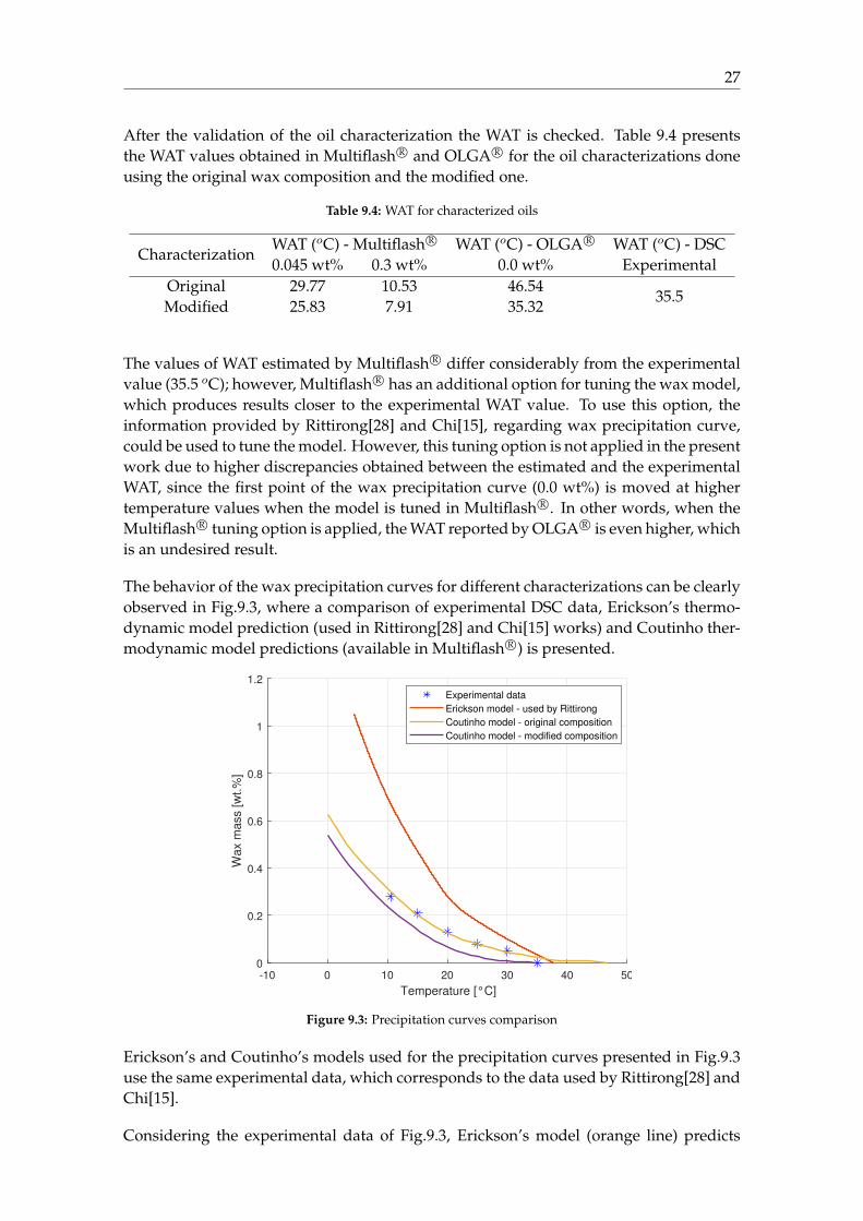
The behavior of the wax precipitation curves for different characterizations can be clearlyobserved in Fig.9.3, where a comparison of experimental DSC data, Erickson’s thermo-dynamic model prediction (used in Rittirong[28] and Chi[15] works) and Coutinho ther-modynamic model predictions (available in Multiflash R©) is presented.

-10 0 10 20 30 40 50

Temperature [°C]

0

0.2

0.4

0.6

0.8

1

1.2

Wax m

ass [w

t.%

]

Experimental data

Erickson model - used by Rittirong

Coutinho model - original composition

Coutinho model - modified composition

Figure 9.3: Precipitation curves comparison

Erickson’s and Coutinho’s models used for the precipitation curves presented in Fig.9.3use the same experimental data, which corresponds to the data used by Rittirong[28] andChi[15].

Considering the experimental data of Fig.9.3, Erickson’s model (orange line) predicts

28

higher values for wax precipitation; on the other hand, Coutinho’s model (yellow line)fits better to the wax experimental values. Such result was expected and agrees with theinformation presented in Fig.3.2. As can be seen in Fig.9.3, the prediction based on thewax original composition (yellow line) has a better match than the prediction made us-ing the modified wax composition (violet line); however, the first point of the curve (0.0wt% of wax) for the original wax composition appears at 46.54 oC while the first pointof the modified composition appears at 35.32 oC. These two temperatures are the corre-sponding wax appearance temperatures, for original and modified wax composition thatOLGA R© takes to perform wax deposition calculations. The same two values of WAT areused also in the Matlab R© runs for comparison of results.

After the oil and gas characterizations, the fluid blending process is done using the blendfluid option available in Multiflash R©. The corresponding amounts of oil and gas are usedaccording to the information presented in Table 8.7.

The last step in Multiflash R© corresponds to the generation of PVT and WAX tables,which are used by OLGA R© as simulation inputs. These tables are generated in the Im-port/Export option presented by Multiflash R© for pressure and temperature ranges of0.10 - 3.44 MPa and -10 - 80 oC, respectively.

The flow chart presented in Fig.9.4 shows the process followed in Multiflash R© to charac-terize the fluid considering three phases (oil, gas and wax).

Figure 9.4: Precipitation curves comparison

A summary of the 16 study cases are presented in Table 9.5. The liquid and gas massflows for each group of cases are based on the information presented in Table 8.7. Simi-

29

larly, E stands for the experimental data used in the present project and m for modifiedwax characterization.

Table 9.5: Study cases for analysis based on experimental data

Main cases Study cases1E 1E-10d 1E-30d 1Em-10d 1Em-30d2E 2E-10d 2E-30d 2Em-10d 2Em-30d3E 3E-10d 3E-30d 3Em-10d 3Em-30d4E 4E-10d 4E-30d 4Em-10d 4Em-30d

As an example, considering the first main case 1E, the four study cases related to thismain case are:

• 1E-10d, where the fluid characterization is done based on the information presentedin Tables 8.1,8.2,8.3 and 8.4, which corresponds to the original information providedby Rittirong and Chi [28, 15]. This study case is analyzed for a deposition time of10 days.

• 1E-30d, this study case uses the same fluid characterization described for the case1E-10d. The present case differs in the deposition time considered for analysiswhich is equal to 30 days.

• 1Em-10d, where the fluid characterization is done based on the information pre-sented in Tables 8.1,8.2 and 8.4, which corresponds to the original information pro-vided by Rittirong and Chi [28, 15]; however, the n-alkane composition used in thisstudy case is a modified version that is presented in Table 9.2. This study case isanalyzed for a deposition time of 10 days.

• 1Em-30d, this study case uses the same fluid characterization described for the case1Em-10d. The present case differs in the deposition time considered for analysiswhich is equal to 30 days.

It is important to note that these 16 study cases are analyzed in OLGA R© and Matlab R©,and their comparative results will be presented in corresponding section (Chapter 11).

9.1.2 Pipeline characteristics

In this section all characteristics used in OLGA R© regarding pipeline are presented.

Properties of the pipeline material corresponds to steel with a heat capacity of 500 J/(kgoC),heat conductivity of 45 W/(mK) and density of 7850 kg/m3. These properties are in-cluded in the software library regarding structural-material properties. In the same li-brary, the pipeline thickness is defined according to the information presented in Table8.6.

When the pipeline is created in the software interface, pipe length and roughness areestablished based on the information provided in Table 8.6. Finally, the number of sec-tions in which the pipeline is split to increase the accuracy of the calculation is set. Inthe present project, 300 sections are used in the OLGA R© simulation, according to theindependence analysis presented in section 9.2.1.

30

9.1.3 Process conditions

This section includes the conditions considered in the simulations performed in OLGA R©

using experimental data.

In addition to the pipeline components, an inlet source and outlet nodes are created inthe software interface. In these components the inlet temperature, fluid mass flow andoutlet pressure are set according to the information presented in Tables 8.6 and 8.7.

When wax deposition process is analyzed in OLGA R©, heat transfer calculations cannotbe performed based on a given overall heat transfer coefficient - OHTC (U ). Instead ofthis, the inner wall and ambient heat transfer convective coefficients (hinwall, hamb) canbe provided to the software in order to run wax deposition simulations. Thus, trying tomaintain the same conditions between OLGA R© and Matlab R© simulations, and consid-ering that the code developed in Matlab R© uses a constant value of OHTC equal to 20W/(m2K), a trial and error analysis is done varying the hamb to find an OHTC closer to20 W/(m2K), as is seen in Table 9.6 . In all scenarios, the inner convective coefficienthinwall is maintained constant and equal to 20 W/(m2K).

Table 9.6: Heat transfer coefficients used in OLGA R© simulation

Main casehamb U

W/(m2K) W/(m2K)

1E 24.5 18.6 - 20.82E 22.0 19.1 - 20.83E 21.5 19.8 - 20.24E 21.9 19.9 - 20.1

The range of OHTC values presented in Table 9.6 varies around the constant OHTC valueused in Matlab R© (20 W/(m2K)); this approach provides a similar heat transfer scenariofor wax deposition evaluation.

The values presented in Table 9.6 apply for the corresponding study cases (4 for eachmain case).

9.2 Wax deposition simulation setup

The setup of the simulation for wax deposition analyses is shown in the present sectionconsidering simulation based on experimental data.

The wax deposition option must be included in the simulation to run this kind of analy-ses. Such option is defined under the option FA-models (flow assurance models), whichare available in OLGA R© [32].

After the activation of the wax deposition module in the simulation environment, theMatzain model available in OLGA R© is selected. The empirical constants C2 and C3

(Eq.6.4), which are related to the wax removal due to shear stripping, are defined ac-cording to the values provided by Matzain which are 0.055 and 1.4, respectively [26]. Theempirical constantC1 = 15, which attempts to correct the offset in wax deposition predic-tion considering that flow turbulence enhances the diffusion process via turbulent eddies

31

effect, is included directly inside the software code, and it cannot be modified; however,OLGA R© presents a diffusion coefficient multiplier which modifies directly the values ofthe diffusion coefficient calculated by the wax deposition model [33]. According to Lep-orini et al. [11] the diffusion coefficient multiplier is the most important tuning value forwax deposition evaluations when Matzain model is used in OLGA R©. All the simulationcases of the present project use a diffusion coefficient multiplier equal to 1.

9.2.1 Discretization independence analysis

The independence analyses are performed in order to define the best number of sectionsin which the pipeline should be divided in order to obtain a balance between accuracyand computation cost.

For the independence analysis performed based on experimental data, pressure dropand outlet temperature are analyzed considering different number of pipeline sections.Figure 9.5 presents the results for the independence analysis made for the study case 3E-10d. It is important to note that all cases present the same trend shown in the followingfigure.

0 50 100 150 200 250 300 350 400 450 500

Number of cells

150

151

152

153

154

155

156

157

Pre

ssu

re d

rop

[kP

a]

(a) Pressure drop

0 50 100 150 200 250 300 350 400 450 500

Number of cells

25.2

25.3

25.4

25.5

25.6

25.7

25.8

25.9

Flu

id tem

pera

ture

[°

C]

(b) Temperature outlet

Figure 9.5: Discretization independence analysis OLGA

As expected, the pressure drop increases when the number of sections is increased, butan asymptotic trend is observed at a value around 200 sections. In addition, the fluidtemperature outlet decreases when the number of pipeline sections is increased, showingalmost constant temperature values around 300 sections. Thus, a number of 300 sectionsis considered adequate for having a balance between accuracy and computation cost.

The variations of pressure drop and temperature presented in Fig.9.5 are small and canbe considered as a non-significant; however, this kind of study should be visualized as atrend evaluation analysis in order to select an acceptable simulation balance.

9.2.2 Stability analysis

Regarding the time step for wax deposition calculations, OLGA R© uses a time step of 3600s approximately, regardless the input parameters provided. This is not a constant timestep, it varies around this value giving the idea that the software calculates the time stepbased on other unknown parameters.

10 Wax deposition using Matlab R©

This section presents the methodology used in the entry data treatment and modelingsetup for wax deposition analysis using Matlab R©. It is important to note that this isa very simplified modeling for wax deposition phenomenon; thus, many assumptionsare made during the model development. This methodology applies for the experimen-tal data considering horizontal pipelines, and it is based on the Matzain model for waxdeposition. The appendix of this document shows the code developed for the currentproject.

10.1 Entry data treatment

The entry data treatment shows some simplifications done for different parameters re-quired as input data in the code developed in Matlab R© in order to perform a simplebut representative modeling of wax deposition phenomenon. Average values for flu-ids properties and other process characteristics are included in this section considering afluid temperature of 32.5 oC. This temperature corresponds to the average value between60 oC and 5 oC which are the inlet and expected outlet fluid temperatures, respectively,considering the entire pipe length.

Oil and gas properties are estimated using the equations presented in Table 8.5 consider-ing the average fluid temperature of 32.5 oC. Additionally, Table 10.1 presents the averageproperties used in the Matlab R© code.

Table 10.1: Fluid properties used in Matlab R© [15, 28]

Parameter Symbol Units ValueOil average properties

Density ρo kg/m3 822.74Thermal conductivity ko W/(mK) 0.18

Heat capacity Cpo J/(kgK) 2074.21Viscosity µo cP 3.00

Interfacial tension σ mN/m 16.25Gas average properties

Density ρg kg/m3 18.41Thermal conductivity kg W/(mK) 0.04

Heat capacity Cpg J/(kgK) 2357.30Viscosity µg cP 0.011

In addition, typical values for wax density and molecular weight, presented in Table 10.2,are used as part of the Matlab R© entry data needed for wax deposition analysis.

32

33

Table 10.2: Wax properties used in Matlab R© [34, 35, 36]

Parameter Symbol Units ValueDensity ρw kg/m3 900

Molecular weight MWw g/mol 475

The code developed in Matlab R© uses a constant overall heat transfer coefficient (OHTC)which is equal to 20 W/(m2K). This value is taken as an average of the typical OHTCvalues reported by Bai [4] and Gudmundsson [17] for bare steel pipes, which oscillatefrom 15 to 25 W/(m2K).

The process conditions and pipeline characteristics used in the Matlab R© code correspondto the values presented in Table 8.6.

In addition, the Matlab R© code is run for the 16 study cases presented and explained inTable 9.5. As input data, this code requires the wax appearance temperature (WAT) ofeach study case; thus, 46.5 oC is used as WAT for the cases that use original n-alkanecomposition, and 35.5 oC as the WAT for modified composition cases.

Finally, as entry data for Matzain wax deposition model the constants C1 = 15.0, C2 =

0.055 and C3 = 1.4 are used as stated in the model description (section 6).

10.2 Modeling setup

Using the input data the wax deposition phenomenon is modeled through the code de-veloped in Matlab R©. The following methodology is applied to accomplish the wax de-position prediction.

10.2.1 Heat transfer calculations

Considering the heat transfer calculation the bulk and inner wall temperatures are esti-mated. These two temperatures are calculated in a steady-state scenario, and are usefulfor the wax deposition analysis [17].

The bulk temperature is calculated through Eq.10.1.

T2 = Tamb + (T1 − Tamb)exp

[−UπdmCp

]L (10.1)

Where T1, T2 and Tamb are the pipe section inlet, outlet and ambient temperatures (K)

respectively, U is the overall heat transfer coefficient - OHTC (W/(m2K)), d is the pipeinner diameter (m), m is the total mass flow rate (kg/s), Cp is the fluid heat capacity(kJ/(kgK)) and L is the pipe section length (m).

The internal convection coefficient is estimated from the Nusselt dimensionless numberwhich is found applying the Sieder and Tate correlation (Eq.10.2) for laminar flow, andDittus-Boelter (Eq.10.3), Sieder and Tate (Eq.10.4) and Whitaker (Eq.10.5) correlations forturbulent flow. Each correlation applies to different ranges of Reynolds and Prandtl num-bers as indicated in the corresponding equations. In these correlations, the effect of theviscosity ratio is neglected because the Matlab R© code does not consider the viscosity as a

34

function of temperature. Then, the general heat flux equation or Newton’s Law of Cool-ing (Eq.10.6) is used to determine the inner wall temperature [17, 37].

It is important to mention that in the calculation approach used to determine the innerwall temperature, the fluid is considered as a homogeneous flow, not as multiphase fluidflow. This assumption has a direct impact on the Reynolds number calculation.

Nu = 1.86(RePr(d/L)

)1/3 (10.2)

For 13 ≤ Re ≤ 2030 0.48 ≤ Re ≤ 16700

Nu = 0.023Re0.8Pr0.3 (10.3)

For Re ≥ 10000 0.7 ≤ Re ≤ 160

Nu = 0.027Re4/5Pr1/3 (10.4)

For Re ≥ 10000 0.7 ≤ Re ≤ 16700

Nu = 0.015Re0.83Pr0.42 (10.5)

For 2300 ≤ Re ≤ 100000 0.48 ≤ Re ≤ 592

Where Nu, Re and Pr are the Nusselt, Reynolds and Prandlt dimensionless numbersrespectively, d is the internal diameter (m) and L is the pipe length (m).

q

A=

(Ti − To)R

(10.6)

Where q/A is the heat flux (W/m2), Ti and To are the inner and outer temperatures,respectively (K) and R is the heat transfer resistance (m2K/W ).

10.2.2 Hydrodynamic calculations

The hydrodynamic calculations are constituted by two main parts: pressure drop calcu-lations and multiphase flow regime determination, both considering no-changes in pipeelevation and diameter.

Pressure drop

The pressure drop estimations are performed based on one-phase pressure drop analy-sis considering all fluid as liquid. Moreover, Gudmundsson states that the multiphasepressure drop is typically ten times greater that single-phase pressure drop [17]; thus, theprevious results are multiplied by ten in order to obtain a more realistic value of multi-phase pressure drop in pipelines.

For flow in horizontal pipelines without changes in inner diameter, the pressure droponly corresponds to looses due to friction calculated through Darcy-Weisbach Equation,where the friction factor determination plays a main role.

35

The friction factor for laminar flow (Re < 2100) is calculated by Eq.10.7. When the flowis turbulent (Re > 4000) the friction factor is computed applying Haaland Equation forliquids (Eq.10.8). For flows that obey to transition regime (2100 < Re < 4000) an averageof laminar and turbulent friction factors is used for pressure drop calculation.

f =64

Re(10.7)

Where f is the Darcy’s friction factor√1

f= −1.8 log

[6.9

Re+

(ε

3.75d

)1.11](10.8)

Where ε is the pipeline roughness (m) and d is the pipe inner diameter (m).

Flow pattern map

The flow regime is determined through Mandhane et al. two-phase regime map (Fig.5.2), which was published in the work: A flow pattern map for gas-liquid flow in horizontalpipes [25].

Mandhane et al. two-phase regime map uses liquid and gas superficial velocities (Eq.5.1)to determine the flow pattern.

According to Mandhane et al. their map presents a small effect of the physical fluidproperties. So, it can be used for several fluids without any map correction [25].

In the present project the Mandhane et al. two-phase regime map is slightly modified inorder to predict flow patterns useful for wax deposition Matzain model [26]. The codedflow map predicts stratified & wavy and bubble & slug as two flow regimes instead offour separated flow regimes, as is presented in the Mandhane et al. two-phase regimemap. The reason for this modification is based on the fact that Matzain model uses Eq.6.7to estimate the Reynolds number to account the limiting deposition effect due to shearstripping for stratified & wavy flow and Eq.6.8 for bubble & slug flow, which makesunnecessary the identification of four different flow patterns.

Table 10.3 shows the transition boundaries used in the Matlab R© code to determine thedifferent flow regimes.

Among other variables, the multiphase flow regime and liquid holdup (E) are neededin the determination of the Matzain constant (π2) regarding wax removal due to shearstripping. The liquid holdup is estimated through Eq.10.9 [38].

E =1

1 +(

uM8.66

)1.39 (10.9)

Where uM is the mixture velocity and is equal to the sum of the gas and liquid superficialvelocities.

36

Table 10.3: Coordinates for transition boundaries

Boundaryusg usl

(ft/s) (ft/s)

Stratified & Wavyto Slug & Bubble

0.1 0.55.0 0.57.5 0.340.0 0.3

Stratified & Wavyto Annular

40.0 0.370.0 0.01

Slug & Bubble toAnnular

40.0 0.3230 14

Slug & Bubble toDispersed

0.1 14230 14

Dispersed toAnnular

230 14269 30

10.2.3 Thermodynamic calculations

The thermodynamic analysis developed in the Matlab R© code has a simple approachwhich only considers the wax precipitation curve. In other words, the equations thatdescribe the behavior of the precipitation curves presented in Figure 9.3, for original andmodified wax compositions, are used to estimate the wax weight fraction as a functionof temperature.

The behavior observed in the precipitation curves is described under the cubic equations(Eqs.10.10 and 10.11) for original and modified wax composition, respectively. As ex-plained in the Entry data treatment (section 10.1), the WAT for original and modifiedn-alkanes composition are 46.5 and 35.5 oC, respectively.

wpf = −6.618E − 8 ∗ T 3 + 6.290E − 5 ∗ T 2 − 1.994E − 2 ∗ T + 2.109 (10.10)

wpf = −6.92E − 8 ∗ T 3 + 6.589E − 5 ∗ T 2 − 2.090E − 2 ∗ T + 2.208 (10.11)

Where wpf is the wax precipitated fraction and T is the temperature, expressed in K.

The wpf is calculated for two temperatures (bulk and wall ones). Finally, each wpf issubtracted from the total content of wax, which is equal to 4.3% (Table 8.1), resulting inthe fraction of wax that is still available and dissolved in the hydrocarbon fluid.

The derivative of Eqs.10.10 and 10.11 are used in the wax deposition calculation pre-sented in the following section.

10.2.4 Wax deposition calculations

The wax deposition calculations are performed applying the Matzain model describedin section 6. All the equations presented in the mentioned section (Eqs from 6.1 to 6.10)are used to perform wax deposition estimations considering deposit through length anddeposition evolution over time.

37

It is important to mention that the wax deposition modeling using Matlab R© consists inan iterative computation process which includes heat transfer, hydrodynamic and waxdeposition calculations considering that each time step means an increment in the waxdeposit layer and consequently a variation in the heat transfer, hydrodynamic and waxdeposition phenomena mainly due to a continuous reduction in the inner diameter.

10.2.5 Discretization independence analysis

The pipeline is discretized in a certain number of sections in order to obtain accurateresults when the different modules are run in the code.

The effect of different number of pipe sections on pressure drop and temperature outletis evaluated in this independence analysis, as is shown in Fig.10.1.

0 50 100 150 200 250 300 350 400 450 500

Number of cells

225.4342

225.4344

225.4346

225.4348

225.4350

225.4352

Pre

ssure

dro

p [kP

a]

(a) Pressure drop

0 50 100 150 200 250 300 350 400 450 500

Number of cells

24.9380

24.9385

24.9390

24.9395

24.9400

24.9405

Flu

id tem

pera

ture

[°

C]

(b) Temperature outlet

Figure 10.1: Discretization independence analysis Matlab

Even though the variations of pressure drop and temperature values for different numberof cells are almost negligible, a stable behavior is observed when 300 cells are consideredfor running the Matlab R© code. This number of cells presents an acceptable balance be-tween pressure drop behavior and computational cost.

The small variations in pressure drop and temperature could be attributed to the assump-tion of constant fluid properties used in the code developed in Matlab R©.

10.2.6 Stability analysis

A stability analysis regarding the size of the time step for wax deposition calculations ispresented in this section.

The effect of different time steps on the deposit thickness is evaluated, as is shown inFig.10.2. The study case 1E-10d is considered in the present analysis.

Small variations in wax thickness is observed for different time steps; however, a stabletrend is shown for time steps lower than 1000 s. Thus, in order to maintain a good balancebetween simulation accuracy and computational cost a time step of 1000 s is consideredin all wax deposition simulations performed in Matlab R©.

38

0 1000 2000 3000 4000 5000 6000 7000 8000 9000 10000

Time step [s]

5.77

5.78

5.79

5.8

5.81

5.82

5.83

De

po

sit t

hic

kn

ess [

mm

]

Figure 10.2: Time step stability analysis

10.2.7 Modeling flow chart

The Matlab R© routine used for modeling the wax deposition process is summarized inFig. 10.3 where a general overview of all modules coded in Matlab R© is presented.

39

Figure 10.3: Wax deposition through molecular diffusion.

11 Results

This section presents the results obtained based on the experimental data using OLGA R©

and Matlab R© code.

The 16 study cases presented in Table 9.5 were run in OLGA R© and Matlab R©; however,some results can be considered as representative of the four study cases correspondingto a main case. For instance, results regarding bulk temperature calculation for cases 1E-10d, 1E-30d, 1Em-10d and 1Em-30d are well represented by the results of only one of thiscases, which is presented as the main case 1E.

These representative results are used in the interpretation of data resulting from the anal-ysis of the following variables:

• Bulk and wall temperatures

• Pressure drop

• Superficial velocities

• Flow pattern prediction

• Wax precipitation

On the other hand, the wax deposition analyses show the results of the 16 cases run inOLGA R© and Matlab R©.

11.1 Heat transfer and fluid mechanics along the pipeline

Results regarding heat transfer and fluid mechanics analysis are presented in this sec-tion. As previously stated, this section presents representative results for each main casenamely 1E, 2E, 3E and 4E. This means that the differences in fluid characterization (orig-inal and modified wax composition) as well as wax deposition times (10 and 30 days) donot present a significant effect over the variables presented in this section.

11.1.1 Bulk and wall temperatures

This section presents the results regarding bulk and wall temperature profiles along thepipeline length. The results for main cases 1E and 2E as well as for main cases 3E and 4Eare shown in Figs.11.1 and 11.2, respectively.Bulk temperature profiles for main cases 1E and 2E, calculated using OLGA R© and Matlab R©

code, present similar behavior along the pipeline with close temperature values result-ing of both codes. The system fluid-pipeline reaches the ambient temperature at 8 and10 km for main cases 1E and 2E, respectively. These distances are found similar in the

40

41

0 2 4 6 8 10 12 14 16 18 20

Pipeline length [km]

0

10

20

30

40

50

60

70T

em

pera

ture

[°

C] WAT 46.5 °C

WAT 35.5 °C

Matlab code - Bulk

OLGA - Bulk

Matlab code - Wall

OLGA - Wall

(a) Case 1E

0 2 4 6 8 10 12 14 16 18 20

Pipeline length [km]

0

10

20

30

40

50

60

70

Tem

pera

ture

[°

C] WAT 46.5 °C

WAT 35.5 °C

Matlab code - Bulk

OLGA - Bulk

Matlab code - Wall

OLGA - Wall

(b) Case 2E

Figure 11.1: Bulk and wall temperature profile - Cases 1&2 E/Em

results obtained by OLGA R© and Matlab R© simulations. These results let infer that themodel used for bulk temperature prediction in Matlab R© is appropriate and works welleven considering a homogeneous fluid flow.

In main cases 1E and 2E, the wall temperature profiles obtained through OLGA R© andMatlab R© show a significant difference which can be attributed to the different heat trans-fer calculation approach used in both codes. OLGA R© considers a multiphase heat trans-fer approach together with fluid properties variation with temperature, while the codedeveloped in Matlab R© uses a homogeneous fluid approach in addition to constant fluidproperties. Thus, the calculation of the film heat transfer resistance (R - Eq.10.6) is af-fected by Reynolds and Prandtl number determinations.Moreover, the fluid velocity used in the calculation of Reynolds number (Eqs. from 10.2to 10.5) has an important effect on the wall temperature determination. In fact, Lindeloffmentions about some difficulties regarding this calculation algorithm due to the highsensitivity related to the determination of the film heat transfer coefficient [39].

Table 11.1 shows the position in the pipeline at which the WAT is reached considering thebulk temperature.

Table 11.1: Pipeline length where WAT is reached - 1&2 E Bulk temperature

Main casesWAT = 46.5 oC WAT = 35.5 oC

OLGA R© Matlab R© OLGA R© Matlab R©

1E 0.46 0.50 0.93 0.962E 0.60 0.56 1.13 1.20

All values in this table are expressed in km

As was observed in Fig.11.1, the bulk temperature results present similar values consid-ering the OLGA R© and Matlab R© simulations. These results agree with the positions atwhich the bulk temperatures of the fluids reach the corresponding WAT. Considering themain case 1E, the WAT of 46.5 oC is reached around 0.48 km; on the other hand, at around0.95 km the WAT of 35.5 oC is attained. This means the pipe position at which wax forma-tion and deposition begin for cases 1E (original wax characterization) and 1Em (modified

42

wax characterization) is located at 0.48 and 0.95 km, respectively. Doing a similar analy-sis for cases 2E (original wax characterization) and 2Em (modified wax characterization)the starting points for wax formation and deposition are located at 0.58 and 1.16 km, re-spectively. Generally speaking, the wax appearance of main case 2E is slightly further inpipe length in comparison with main case 1E due to the higher mass flow of the case 2E.

Table 11.2 presents the position in the pipeline at which the WAT is reached consideringthe wall temperature.

Table 11.2: Pipeline length where WAT is reached - 1&2 E Wall temperature

Main casesWAT = 46.5 oC WAT = 35.5 oC

OLGA R© Matlab R© OLGA R© Matlab R©

1E 0.10 N/A 0.50 N/A2E 0.30 N/A 0.90 N/A

All values in this table are expressed in km

The high difference regarding wall temperature calculations observed in Fig.11.1 consid-ering OLGA R© and Matlab R© simulations is also appreciable when the starting point forwax formation and deposition using wall temperature is performed. In main cases 1Eand 2E, Matlab R© results cannot be estimated because the initial wall temperatures calcu-lated using this code present lower values than the corresponding WATs; in other words,based on the wall temperature, the wax formation and deposition process should beginbefore the fluid entering into the pipeline.Considering the results obtained through OLGA R©, the pipe position at which wax for-mation and deposition begin for cases 1E (original wax characterization-WAT 46.5 oC)and 1Em (modified wax characterization-WAT 35.5 oC) are located at 0.10 and 0.50 km,respectively. Doing a similar analysis, for cases 2E (original wax characterization) and2Em (modified wax characterization) the starting points for wax formation and deposi-tion are located at 0.30 and 0.90 km, respectively.

Figure 11.2 shows the results of bulk and wall temperatures related to main cases 3E and4E calculated using OLGA R© and Matlab R© code. Both temperature profiles present simi-lar behavior along the pipeline with close temperature values resulting of both codes. Inthe main cases 3E and 4E, the system fluid-pipeline does not reach the ambient tempera-ture since the mass flows considered are higher than the flows for main cases 1E and 2E.

In main cases 3E and 4E, the wall temperature profiles obtained through OLGA R© andMatlab R© show a similar behavior in contrast to the results obtained for main cases 1Eand 2E. The closer resultant values can be explained considering a higher accuracy ofthe Matlab R© wall temperature prediction. The liquid mass fractions presented by thesetwo cases (3E and 4E - Table 8.7) are higher than 0.90; thus, fluid velocity presented bythe multiphase flow in OLGA R© has a better similitude with the one-phase and homo-geneous fluid flow approach used in the Matlab R© code. At the end, the different heattransfer approaches used in both codes do not suffer significant differences when walltemperature results are estimated.

Table 11.3 shows the position in the pipeline at which the WAT is reached considering thebulk temperature.

43

0 2 4 6 8 10 12 14 16 18 20

Pipeline length [km]

20

25

30

35

40

45

50

55

60

65T

em

pera

ture

[°

C]

WAT 46.5 °C

WAT 35.5 °C

Matlab code - Bulk

OLGA - Bulk

Matlab code - Wall

OLGA - Wall

(a) Case 3E

0 2 4 6 8 10 12 14 16 18 20

Pipeline length [km]

20

25

30

35

40

45

50

55

60

65

Tem

pera

ture

[°

C]

WAT 46.5 °C

WAT 35.5 °C

Matlab code - Bulk

OLGA - Bulk

Matlab code - Wall

OLGA - Wall

(b) Case 4E

Figure 11.2: Bulk and wall temperature profile - Cases 3&4 E/Em

Table 11.3: Pipeline length where WAT is reached - 3&4 E Bulk temperature

Main casesWAT = 46.5 oC WAT = 35.5 oC

OLGA R© Matlab R© OLGA R© Matlab R©

3E 5.60 5.70 11.73 11.904E 6.00 6.10 12.46 12.70

All values in this table are expressed in km

As was observed in Fig.11.2, the bulk temperature results present similar values consid-ering the OLGA R© and Matlab R© simulations. This agrees with the positions at which thebulk temperatures of the fluids reach the corresponding WAT. Considering the main case3E, the WAT of 46.5 oC is reached around 5.65 km; on the other hand, at around 11.81km the WAT of 35.5 oC is reached. This means the pipe position at which wax formationand deposition begin for cases 3E (original wax characterization) and 3Em (modified waxcharacterization) are located at 5.65 and 11.81 km, respectively. Doing a similar analysis,for cases 4E (original wax characterization) and 4Em (modified wax characterization) thestarting points for wax formation and deposition are located at 6.05 and 12.58 km, respec-tively. In general, the wax appearance of main case 4E is slightly further in pipe length incomparison with main case 3E due to the higher mass flow of the case 4E.

Table 11.4 presents the position in the pipeline where the WAT is reached considering thewall temperature.

Table 11.4: Pipeline length where WAT is reached - 3&4 E Wall temperature

Main casesWAT = 46.5 oC WAT = 35.5 oC

OLGA R© Matlab R© OLGA R© Matlab R©

3E 3.93 3.96 10.06 9.594E 4.20 4.16 10.80 10.03

All values in this table are expressed in km

According to the information presented in Table 11.4 the positions at which the wall tem-peratures of the fluids reach the corresponding WAT for main cases 3E and 4E are similar

44

for the simulations performed in OLGA R© and Matlab R©. The pipe position at which waxformation and deposition begin for cases 3E (original wax characterization-WAT 46.5 oC)and 3Em (modified wax characterization-WAT 35.5 oC) are located at 3.95 and 9.82 km,respectively. Doing a similar analysis, for cases 4E (original wax characterization) and4Em (modified wax characterization) the starting points for wax formation and deposi-tion are located at 4.18 and 10.42 km, respectively.

The points 3.95 and 4.18 km for cases 3E and 4E respectively can be observed as smallchanges in the trends followed by the wall temperatures estimated through OLGA R© sim-ulations (Fig.11.2).

11.1.2 Pressure drop profile

This section presents the results regarding pressure drop along the pipeline. The resultsfor main cases 1E and 2E as well as for main cases 3E and 4E are shown in Figs.11.3 and11.4, respectively.

0 2 4 6 8 10 12 14 16 18 20

Pipeline length [km]

0

0.5

1

1.5

2

2.5

3

3.5

4

Pre

ssu

re [

kP

a]

Matlab code

OLGA

(a) Case 1E

0 2 4 6 8 10 12 14 16 18 20

Pipeline length [km]

0

1

2

3

4

5

6

7

8

9

10

Pre

ssure

[kP

a]

Matlab code

OLGA

(b) Case 2E

Figure 11.3: Pressure drop profile - Cases 1&2 E/Em

Pressure drop profiles for main cases 1E and 2E, calculated using OLGA R© and Matlab R©

code, present similar behavior along the pipeline with close pressure drop values result-ing of both codes. The total pressure drop observed for main case 1E is around 3.5 and2.0 kPa using OLGA R© and Matlab R© simulations, respectively. Additionally, the totalpressure drop observed for main case 2E is around 9.0 and 3.0 kPa using OLGA R© andMatlab R© simulations, respectively.

Generally speaking, the pressure drop calculation based on the criterion presented byGudmundsson [17], which states that the multiphase pressure drop is ten times biggerthan the liquid pressure drop, produces results with high similarities considering themain cases 1E and 2E.

The pressure drop predictions for main cases 3E and 4E are presented in Fig.11.4.Likewise, the pressure drop profiles for main cases 3E and 4E, calculated using OLGA R©

and Matlab R© code, present similar behavior along the pipeline with close pressure dropvalues resulting of both codes. The total pressure drop observed for main case 3E isaround 150 and 210 kPa using OLGA R© and Matlab R© simulations, respectively. Addi-tionally, the total pressure drop observed for main case 4E is around 350 and 240 kPausing OLGA R© and Matlab R© simulations, respectively.

45

0 2 4 6 8 10 12 14 16 18 20

Pipeline length [km]

0

50

100

150

200

250P

ressure

[kP

a]

Matlab code

OLGA

(a) Case 3E

0 2 4 6 8 10 12 14 16 18 20

Pipeline length [km]

0

50

100

150

200

250

300

350

400

Pre

ssure

[kP

a]

Matlab code

OLGA

(b) Case 4E

Figure 11.4: Pressure drop profile - Cases 3&4 E/Em

For case 3E, contrary to the behavior observed in the rest of the main cases (1E, 2E and4E), calculations with Matlab R© present a higher pressure drop than the one obtainedwith OLGA R©. This behavior might be related to the pressure drop observed at higherliquid fractions (98%) for multiphase flow, which is slightly smaller than the criterion ofGudmundsson. In other words, for main case 3E, the multiphase flow pressure drop isseven times bigger than the one-phase pressure drop (considering all the fluid amount asliquid.) Nevertheless, Gudmundsson criterion seems acceptable for all main cases.

11.1.3 Superficial velocities

This section presents the results regarding superficial velocities profiles. The results formain cases 1E and 2E as well as for main cases 3E and 4E are shown in Figs.11.5 and 11.6,respectively.

0 2 4 6 8 10 12 14 16 18 20

Pipeline length [km]

0.00

0.02

0.04

0.06

0.08

0.10

0.12

0.14

0.16

0.18

0.20

Liq

uid

su

pe

rfic

ial ve

locity [

m/s

]

0.30

0.40

0.50

0.60

0.70

0.80

0.90

1.00

Ga

s s

up

erf

icia

l ve

locity [

m/s

]

Matlab code - usG

OLGA - usG

Matlab code - usL

OLGA - usL

(a) Case 1E

0 2 4 6 8 10 12 14 16 18 20

Pipeline length [km]

0.03

0.04

0.05

0.06

0.07

0.08

0.09

0.10

Liq

uid

su

pe

rfic

ial ve

locity [

m/s

]

0.80

1.00

1.20

1.40

1.60

1.80

2.00G

as s

up

erf

icia

l ve

locity [

m/s

]Matlab code - usG

OLGA - usG

Matlab code - usL

OLGA - usL

(b) Case 2E

Figure 11.5: Superficial velocities - Cases 1&2 E/Em

Superficial velocities for main cases 1E and 2E, calculated using OLGA R© and Matlab R©

code, present similar behaviors along the pipeline with close superficial velocity valuesresulting of both codes. The average fluid velocity for main case 1E is around 0.75 m/sfor the gas phase and 0.05 m/s for the liquid phase. Considering the main case 2E, theaverage fluid velocities are around 1.50 m/s for the gas phase and 0.05 m/s for the liquidphase.

46

The divergence presented in the first section of the pipeline for gas superficial veloci-ties between the results from OLGA R© and Matlab R© can be attributed to the significantchange of bulk temperature observed in such first sections, affecting the density of thegas phase, which is correlated to the gas superficial velocity.

The predictions for superficial velocities for main cases 3E and 4E are presented in Fig.11.6.

0 2 4 6 8 10 12 14 16 18 20

Pipeline length [km]

0.5

0.6

0.7

0.8

0.9

1.0

1.1

1.2

Liq

uid

su

pe

rfic

ial ve

locity [

m/s

]

0.5

0.6

0.7

0.8

0.9

1.0

1.1

1.2

1.3

Ga

s s

up

erf

icia

l ve

locity [

m/s

]

Matlab code - usG

OLGA - usG

Matlab code - usL

OLGA - usL

(a) Case 3E

0 2 4 6 8 10 12 14 16 18 20

Pipeline length [km]

0.7

0.8

0.9

1.0

1.1

1.2

1.3

1.4

1.5

Liq

uid

su

pe

rfic

ial ve

locity [

m/s

]

2.2

2.4

2.6

2.8

3.0

3.2

3.4

Ga

s s

up

erf

icia

l ve

locity [

m/s

]

Matlab code - usG

OLGA - usG

Matlab code - usL

OLGA - usL

(b) Case 4E

Figure 11.6: Superficial velocities - Cases 3&4 E/Em

Analogous to main cases 1E and 2E, superficial velocities for main cases 3E and 4E, cal-culated using OLGA R© and Matlab R© code, present similar behaviors along the pipelinewith close superficial velocity values resulting of both codes. The average fluid velocityfor main case 3E is around 0.75 m/s for the gas phase and 0.95 m/s for the liquid phase.Considering the main case 4E, the average fluid velocities are around 3.00 m/s for thegas phase and 0.95 m/s for the liquid phase.

In general, the observed differences in superficial velocities might be a consequence ofdifferent physical properties of the fluids as a result of the characterization approachused in OLGA R© and the constant fluid properties consideration applied in Matlab R©.

11.1.4 Flow pattern prediction

This section presents the results regarding multiphase flow pattern predictions. Table11.5 shows the results obtained through OLGA R©. These agree with the flow patternpresented in the works done by Chi and Rittirong [15, 28].

Table 11.5: Flow pattern predictions

Case Flow pattern1E & 1Em Stratified2E & 2Em Stratified3E & 3Em Slug4E & 4Em Slug

Main cases 1E and 2E present a stratified flow pattern while main cases 3E and 4E aredefined as slug flows, according to the flow prediction made by OLGA R©.

The flow pattern predictions performed by the Matlab R© code, for main cases 1E and 2Eas well as for main cases 3E and 4E are shown in Figs.11.7 and 11.8, respectively.

47

10-1 100 101 102

Superficial gas velocity (m/s)

10-2

10-1

100

101S

uperf

icia

l Liq

uid

velo

city (

m/s

)

Stratified & Wavy

Annular

Dispersed

Slug & Bubble

(a) Case 1E

10-1 100 101 102

Superficial gas velocity (m/s)

10-2

10-1

100

101

Superf

icia

l Liq

uid

velo

city (

m/s

)

Stratified & Wavy

Annular

Dispersed

Slug & Bubble

(b) Case 2E

Figure 11.7: Flow pattern map - Cases 1&2 E/Em

Figure 11.7 shows a stratified & wavy flow pattern for main cases 1E and 2E. These resultsare in agreement with the flow pattern predictions done in OLGA R©.

10-1 100 101 102

Superficial gas velocity (m/s)

10-2

10-1

100

101

Superf

icia

l Liq

uid

velo

city (

m/s

)

Stratified & Wavy

Annular

Dispersed

Slug & Bubble

(a) Case 3E

10-1 100 101 102

Superficial gas velocity (m/s)

10-2

10-1

100

101

Superf

icia

l Liq

uid

velo

city (

m/s

)

Stratified & Wavy

Annular

Dispersed

Slug & Bubble

(b) Case 4E

Figure 11.8: Flow pattern map - Cases 3&4 E/Em

Similarly, Fig.11.8 shows a slug & bubble flow pattern for main cases 3E and 4E. Theseresults are in agreement with the flow pattern predictions done in OLGA R©.

These results demonstrate as well that the flow pattern prediction module in Matlab R© isaccurately developed, obtaining valid results.

11.2 Wax precipitation along the pipeline

This section presents the results regarding wax precipitation profiles obtained in Matlab R©.The results for main cases 1E and 2E as well as for main cases 3E and 4E are shown inFigs.11.9 and 11.10, respectively. For each main case, the wax precipitation profile con-sidering bulk and wall temperatures are shown for original wax characterization (WAT46.5 oC) and modified wax characterization (WAT 35.5 oC).

Even though the wax precipitation profiles are calculated considering bulk and wall tem-peratures, the condition to begin with the wax precipitation calculations in the Matlab R©

48

model states that the bulk temperature should be lower than the corresponding WATvalue. This condition is considered based on the uncertainties related to wall tempera-ture calculations presented in section 11.1.

0 2 4 6 8 10 12 14 16 18 20

Pipeline length [km]

0

0.05

0.1

0.15

0.2

0.25

0.3

0.35

0.4

0.45

0.5

Concentr

ation [%

]

Bulk - WAT 46.5°C

Wall - WAT 46.5°C

Bulk - WAT 35.5°C

Wall - WAT 35.5°C

(a) Case 1E

0 2 4 6 8 10 12 14 16 18 20

Pipeline length [km]

0

0.05

0.1

0.15

0.2

0.25

0.3

0.35

0.4

0.45

0.5

Concentr

ation [%

]

Bulk - WAT 46.5°C

Wall - WAT 46.5°C

Bulk - WAT 35.5°C

Wall - WAT 35.5°C

(b) Case 2E

Figure 11.9: Wax precipitation curve - Cases 1&2 E/Em

The information provided by Fig.11.9 is closely related to Table 11.1 which presents thelength of the pipeline where the WAT values are reached considering the two wax ap-pearance temperatures (46.5 and 35.5 oC) analyzed in this project.

The trend followed by the wax precipitation profiles in both wax characterization sce-narios is similar for cases 1E and 2E. The starting point for the formation of wax concurswith the length at which the bulk temperature reaches the corresponding WAT value (seeTable 11.1). Similarly, the precipitation profiles for bulk and wall temperatures presentan equal and asymptotic trend when the thermal equilibrium is reached at around 8 and10 km for case 1E and 2E, respectively.The concentration of wax obtained for the original wax characterization scenario presentshigher values than the concentration regarding the modified wax characterization. Thisbehavior is related to the two different equations used to calculate the wax precipitation(Eqs.10.10 and 10.11) when the original and modified wax characterization are used.

The shape presented by the precipitation curves obtained for bulk and wall temperaturesis an important parameter to consider because the wax deposition phenomenon is mainlydriven by the concentration gradient of the wax dissolved in oil in the bulk liquid and thewall surroundings. Generally speaking, for cases 1E and 2E, considering the original andmodified wax composition, the difference between the concentration of precipitated waxobtained in the bulk liquid and the one obtained in the wall surroundings first increasesreaching a maximum difference and then such difference decreases until it is equal tozero in the corresponding asymptote of the curve. Considering that the dissolved wax isobtained subtracting the precipitated wax from the wax content value (4.3% - Table 8.1)a similar behavior is followed by the difference between the dissolved wax at bulk andwall surroundings.

Figure 11.10 shows the results of bulk and wall wax precipitation profile related to cases3E and 4E, considering the original (WAT 46.5 oC) and modified (WAT 35.5 oC) wax char-acterization.

49

0 2 4 6 8 10 12 14 16 18 20

Pipeline length [km]

0

0.05

0.1

0.15C

oncentr

ation [%

]Bulk - WAT 46.5°C

Wall - WAT 46.5°C

Bulk - WAT 35.5°C

Wall - WAT 35.5°C

(a) Case 3E

0 2 4 6 8 10 12 14 16 18 20

Pipeline length [km]

0

0.02

0.04

0.06

0.08

0.1

0.12

0.14

Concentr

ation [%

]

Bulk - WAT 46.5°C

Wall - WAT 46.5°C

Bulk - WAT 35.5°C

Wall - WAT 35.5°C

(b) Case 4E

Figure 11.10: Wax precipitation curve - Cases 3&4 E/Em

The information provided by Fig.11.10 is closely related to Table 11.3 which presents thepoints where the WAT values are reached considering the two wax appearance tempera-tures (46.5 and 35.5 oC) analyzed in this project.

The trend followed by the wax precipitation profiles in both wax characterization sce-narios is similar for cases 3E and 4E. The starting point for the formation of wax concurswith the length at which the bulk temperature reaches the corresponding WAT value (seeTable 11.3).Likewise to cases 1E and 2E, the concentration of wax obtained for the original wax char-acterization scenario presents higher values than the concentration regarding the modi-fied wax characterization. This behavior is related to the two different equations used tocalculate the wax precipitation (Eqs.10.10 and 10.11) when the original and modified waxcharacterization are used.

It is important to mention that for cases 3E and 4E, considering only the original waxcomposition, the difference between bulk and wall concentrations of precipitated waxfirst slightly decreases presenting a minimum difference, but then such difference in-creases along the pipeline. Similarly, the difference of the dissolved wax at bulk and wallsurroundings follows the same trend. On the contrary, for the modified wax composi-tion, the difference between bulk and wall concentrations of precipitated wax increasesalong the pipeline since its appearance.

Note that these calculations represent a very simplistic approach considered in Matlab R©

to model the thermodynamic process of wax formation. On the other hand, OLGA R©

uses Multiflash R© to perform these computations through flash calculations and wax for-mation models.

11.3 Wax deposition

A comparative analysis of the results obtained in the commercial simulator OLGA R© withthe results of the code developed in Matlab R© allows to have a better understanding ofthe wax deposition process and its prediction through mathematical models.

This section presents the results regarding wax deposition thickness along the pipeline

50

as well as its evolution through time considering the 16 study cases run in OLGA R© andMatlab R© code.

11.3.1 Wax deposition profile

This section presents the results regarding wax deposition thickness along the pipelinefor the 16 study cases run in OLGA R© and Matlab R© code.

Figure 11.11 and Table 11.6 show the results of wax deposition thickness along the pipelinefor the four study cases related to main case 1E.

0 2 4 6 8 10 12 14 16 18 20

Pipeline length [km]

0

1

2

3

4

5

6

7

Wax d

epositio

n [m

m]

Matlab code - WAT 46°C

OLGA - WAT 46°C

Matlab code - WAT 35°C

OLGA - WAT 35°C

(a) 10 days

0 2 4 6 8 10 12 14 16 18 20

Pipeline length [km]

0

2

4

6

8

10

12

14

16

18

20

Wax d

epositio

n [m

m]

Matlab code - WAT 46°C

OLGA - WAT 46°C

Matlab code - WAT 35°C

OLGA - WAT 35°C

(b) 30 days

Figure 11.11: Wax deposition profile - Cases 1E & 1Em

Table 11.6: Wax deposition max. thickness and location - Cases 1E & 1Em

Study cases10 days 30 days

Max. thickness Location Max. thickness Location1E-OLGA R© 0.91 0.17 1.38 0.171E-Matlab R© 5.82 1.33 17.26 1.33

1Em-OLGA R© 0.82 0.70 1.28 0.701Em-Matlab R© 5.16 1.51 15.32 1.53

Max. thickness is expressed in mm and Location in km

In general, OLGA R© predicts the first point for the wax deposition when the WAT isreached by the wall temperature. On the other hand, Matlab R©, as coded, presents itsfirst point for wax deposition when the WAT is reached by the bulk temperature. Due tothe uncertainties observed in wall temperature calculations in Matlab R©, the bulk temper-ature was selected as parameter for estimation of the wax formation point through theWAT. However, for the current case, both codes present similar starting points for waxdeposition. Similarly, comparing the original and modified wax characterization, theinitial points for wax deposition do not present significant differences; in other words,for the main case 1E the modified characterization can be used in the simulation of waxdeposition presenting results closely similar to the ones obtained with the original waxcharacterization regarding the position in the pipeline where wax deposition appears.

51

Overall, the modified characterization presents slightly lower results regarding wax de-position thickness in OLGA R© and Matlab R©; thus, the modified characterization can beused instead of the original one without major differences in the results of wax depositionthickness.

Matlab R© over predicts the thickness of the wax deposited around five to ten times for 10and 30 days respectively, compared to the results obtained through OLGA R©. This overprediction is mainly due to the higher difference between bulk and wall temperaturethat Matlab R© presents instead of OLGA R©. Additionally, OLGA R© calculates an overallheat transfer coefficient (OHTC) that changes as a consequence of the increment in thethickness of the wax precipitation layer reducing the driven force of the wax depositionphenomenon regarding temperature gradient. As noted before, the code in Matlab R©

considers the OHTC constant for all the calculations. From another perspective, whenthe two wax characterizations are used in the same simulation tool, either OLGA R© orMatlab R©, the results do not present significant differences between each other.

OLGA R© presents a maximum wax deposition thickness at the beginning of the wax layer,which agrees with the highest temperature difference between the bulk and wall temper-atures presented in the first sections of the pipeline. Such temperature difference de-creases until becoming zero when the thermal equilibrium is reached. The same decreas-ing trend is presented by the wax deposit profile as expected, which is shown in OLGA R©

results. However, the Matlab R© code presents a first big wax thickness at the beginningof the layer, then the wax profile increases until a maximum value is reached and later itreduces progressively to zero. This behavior is explained in section 11.2 for the differencefor dissolved wax between the bulk liquid and the wall surroundings which seems to bethe responsible for the shape presented by the deposit wax layer. Overall, this behavioris an additional factor for the wax thickness over prediction obtained with Matlab R©.

Figure 11.12 and Table 11.7 show the results of wax deposition thickness along the pipelinefor the four study cases related to main case 2E.

0 2 4 6 8 10 12 14 16 18 20

Pipeline length [km]

0

1

2

3

4

5

6

Wax d

epositio

n [m

m]

Matlab code - WAT 46°C

OLGA - WAT 46°C

Matlab code - WAT 35°C

OLGA - WAT 35°C

(a) 10 day

0 2 4 6 8 10 12 14 16 18 20

Pipeline length [km]

0

2

4

6

8

10

12

14

16

18

Wax d

epositio

n [m

m]

Matlab code - WAT 46°C

OLGA - WAT 46°C

Matlab code - WAT 35°C

OLGA - WAT 35°C

(b) 30 days

Figure 11.12: Wax deposition profile - Cases 2E & 2Em

As observed, a behavior similar to the main case 1E is obtained for the main case 2E.Thus, the discussion previously developed for the main case 1E correctly applies to theresults of main case 2E. Consequently, it might be appropriate to consider that the waxdeposition behavior when the fluid follows a stratified flow pattern results in the profile

52

Table 11.7: Wax deposition max. thickness and location - Cases 2E & 2Em

Study cases10 days 30 days

Max. thickness Location Max. thickness Location2E-OLGA R© 0.61 0.37 0.92 0.372E-Matlab R© 5.26 1.87 15.66 1.87

2Em-OLGA R© 0.56 1.10 0.86 1.102Em-Matlab R© 4.67 2.13 13.93 2.13

Max. thickness is expressed in mm and Location in km

presented in cases 1E and 2E, if the heat transfer phenomenon presents strong similaritieswith the one observed in the present project for the corresponding cases.

Additionally, in OLGA R© as well as Matlab R©, it is observed that the maximum thicknessof the wax deposition layer decreases as the gas mass flow increases. It is possible to inferthat the increased mass flow reduces the temperature difference between bulk and walltemperatures, and consequently reduces the concentration difference of wax dissolvedin the liquid bulk and the wall surroundings producing a lower driven force for the waxdeposition phenomenon.

Figure 11.13 and Table 11.8 show the results of wax deposition thickness along the pipelinefor the four study cases related to main case 3E.

0 2 4 6 8 10 12 14 16 18 20

Pipeline length [km]

0

0.5

1

1.5

2

2.5

Wa

x d

ep

ositio

n [

mm

]

Matlab code - WAT 46°C

OLGA - WAT 46°C

Matlab code - WAT 35°C

OLGA - WAT 35°C

(a) 10 day

0 2 4 6 8 10 12 14 16 18 20

Pipeline length [km]

0

1

2

3

4

5

6

7

Wax d

epositio

n [m

m]

Matlab code - WAT 46°C

OLGA - WAT 46°C

Matlab code - WAT 35°C

OLGA - WAT 35°C

(b) 30 days

Figure 11.13: Wax deposition profile - Cases 3E & 3Em

Table 11.8: Front wax deposition thickness and location - Cases 3E & 3Em

Study cases10 days 30 days

Front thickness Location Front thickness Location3E-OLGA R© 0.31 4.03 0.46 4.033E-Matlab R© 0.74 5.60 2.21 5.06

3Em-OLGA R© 0.30 10.63 0.45 10.633Em-Matlab R© 0.38 11.60 1.12 11.60

Front thickness is expressed in mm and Location in km

53

In general, OLGA R© predicts the first point for the wax deposition when the WAT isreached by the wall temperature. On the other hand, Matlab R©, as coded, presents itsfirst point for wax deposition when the WAT is reached by the bulk temperature; as aconsequence, the wax deposit predicted by OLGA R© appears first in the pipeline. Ad-ditionally, comparing the original and modified wax characterization, the initial pointsfor wax deposition change drastically using both simulation tools; in other words, underconditions of main case 3E the modified and the original wax characterization cannot beused interchangeably because a difference around 6 km is presented in the appearance ofthe wax layer.

Overall, the modified characterization presents lower results regarding wax depositionthickness in Matlab R© while the wax deposition thickness in OLGA R© is practically thesame; thus, the modified characterization can be used instead of the original one withoutmajor differences in the results of wax deposition thickness when using OLGA R©.

Matlab R© over predicts the thickness of the wax deposited in ratios lower than 6 timesfor 10 days and 13 times for 30 days. This over prediction is mainly due to the shapepresented by the difference between the concentration of the wax dissolved in the bulkliquid and the wall surroundings, as explained in section 11.2, which is the responsiblefor the shape presented by the deposit wax layer. These results let us understand thehigh sensitivity of the Matlab R© code to the equation used to describe the thermodynam-ics of the wax formation. On the other hand, OLGA R© uses flash calculations and waxmodels to perform in an accurate way the thermodynamics regarding wax precipitationphenomenon.From another perspective, when the two wax characterizations are used in the same sim-ulation tool, either OLGA R© or Matlab R©, the results do not present significant differencesbetween each other regarding wax thickness predictions; however, the modified and theoriginal wax characterization cannot be used interchangeably for predictions of the waxdeposit position in the pipeline.

OLGA R© presents a constant wax deposition thickness along the entire length of the waxlayer, which agrees with the almost constant temperature difference between the bulkand wall temperatures presented along all sections of the pipeline. Thus, it is expectedthat this constant temperature difference should be translated to a constant concentrationdifference of dissolved wax between the bulk fluid and the wall surrounding, which atthe end results in a constant deposited wax layer. However, considering the original waxcharacterization, the Matlab R© code presents a first front of wax thickness at the beginningof the layer, then the wax profile decreases until a minimum value is reached and later itincreases progressively along the pipeline. On the other hand, considering the modifiedwax characterization, the Matlab R© code presents an increasing profile along the pipelinefrom the wax layer appearance. These behaviors are explained in section 11.2 for thedifference of dissolved wax between the bulk liquid and the wall surroundings whichseems to be the responsible for the shape presented by the deposit wax layer.

Figure 11.14 and Table 11.9 show the results of wax deposition thickness along the pipelinefor the four study cases related to main case 4E.

As observed, a behavior similar to the main case 3E is obtained for the main case 4E.Thus, the discussion previously developed for the main case 3E correctly applies to theresults of main case 4E. Consequently, it might be appropriate to consider that the wax

54

0 2 4 6 8 10 12 14 16 18 20

Pipeline length [km]

0

0.5

1

1.5

2

2.5W

ax d

ep

ositio

n [

mm

]

Matlab code - WAT 46°C

OLGA - WAT 46°C

Matlab code - WAT 35°C

OLGA - WAT 35°C

(a) 10 day

0 2 4 6 8 10 12 14 16 18 20

Pipeline length [km]

0

1

2

3

4

5

6

7

Wax d

epositio

n [m

m]

Matlab code - WAT 46°C

OLGA - WAT 46°C

Matlab code - WAT 35°C

OLGA - WAT 35°C

(b) 30 days

Figure 11.14: Wax deposition profile - Cases 4E & 4Em

Table 11.9: Front wax deposition max. thickness and location - Cases 4E & 4Em

Study cases10 days 30 days

Front thickness Location Front thickness Location4E-OLGA R© 0.39 4.23 0.56 4.304E-Matlab R© 0.75 5.93 2.22 5.93

4Em-OLGA R© 0.37 11.43 0.55 11.504Em-Matlab R© 0.38 12.30 1.13 12.40

Front thickness is expressed in mm and Location in km

deposition behavior when the fluid follows a slug flow pattern results in the profile pre-sented in cases 3E and 4E, if the heat transfer phenomenon presents strong similaritieswith the one observed in the present project for the corresponding cases.

Additionally, in OLGA R© as well as Matlab R© comparing cases 3E and 4E, it is observedthat the starting point of the appearance of the wax layer is moved further in the pipelinewhen the gas mass flow increases. This can be explained considering that WAT is reachedby the fluid temperature further in the pipeline for cases 4E.

Generally speaking, comparing the wax deposition behavior for study cases which presentstratified flow (1E & 2E) with study cases that show a slug pattern flow (3E & 4E), an im-portant difference is observed regarding the thickness of the deposited wax layer. Thelatter cases present notorious lower thickness of the wax layer due to smaller tempera-ture difference and consequently wax concentration differences between the bulk fluidand wall surroundings; additionally, the stripping effect on the wax deposition thicknessdue to the slug flow causes a reduction of the thickness of the wax deposit layer.

11.3.2 Wax deposition evolution through time

This section presents the results regarding wax deposition thickness trend through timefor the 16 study cases run in OLGA R© and Matlab R© code.

In the study cases related to main cases 1E and 2E, the analyses of the wax depositionevolution through time are performed considering the maximum layer thickness point,

55

according to information presented in Tables 11.6 and 11.7. On the other hand, for studycases related to main cases 3E and 4E, the wax evolution analyses are done for the frontor first point where the wax deposition appears, as presented in Tables 11.8 and 11.9.

Figure 11.15 shows the results of wax deposition thickness evolution for the four studycases related to main case 1E.

0 2 4 6 8 10 12

Time [d]

0

1

2

3

4

5

6

7

Wax d

epositio

n [m

m]

Matlab code - WAT 46°C

OLGA - WAT 46°C

Matlab code - WAT 35°C

OLGA - WAT 35°C

(a) 10 days

0 5 10 15 20 25 30 35

Time [d]

0

2

4

6

8

10

12

14

16

18

20

Wax d

epositio

n [m

m]

Matlab code - WAT 46°C

OLGA - WAT 46°C

Matlab code - WAT 35°C

OLGA - WAT 35°C

(b) 30 days

Figure 11.15: Wax deposition trend - Case 1E & 1Em

In general, OLGA R© presents an exponential-like trend for wax deposition growing in thepoint that shows the maximum wax layer thickness. This behavior is related to the con-stant changes experienced by the heat transfer phenomenon through time. These changesare related to the fact that wax is continuously deposited on the inner surface of the pipeaffecting the overall heat transfer coefficient (OHCT) and consequently reducing the dif-ference between the bulk and wall temperatures. Moreover, it is important to understandthat a new inner wax layer covers the wall surface and the previously deposited layersproducing a thermal isolating effect. So, this reduces the temperature difference betweenthe bulk and the new inner surface of the pipeline producing a reduction in the drivenforce of the wax deposition phenomena.

The aforementioned exponential-like trend followed by OLGA R© can be easily visualizedin the results regarding 30 days of deposition time because the growing trend presents astronger asymptotic behavior after 10 days of deposition.

On the other hand, the Matlab R© code considers a constant OHTC values. This consider-ation produces deposit trends that follow a linear-like pattern.

The deposited layer thickness over prediction resulting of the Matlab R© code, which isdiscussed in section 11.3, is well observed in Fig.11.15.

Figure 11.16 shows the results of wax deposition thickness evolution for the four studycases related to main case 2E.

As observed, a behavior similar to the main case 1E is obtained for the main case 2E.Thus, the discussion previously developed for the main case 1E correctly applies to theresults of main case 2E.

56

0 2 4 6 8 10 12

Time [d]

0

1

2

3

4

5

6W

ax d

epositio

n [m

m]

Matlab code - WAT 46°C

OLGA - WAT 46°C

Matlab code - WAT 35°C

OLGA - WAT 35°C

(a) 10 days

0 5 10 15 20 25 30 35

Time [d]

0

2

4

6

8

10

12

14

16

18

Wax d

epositio

n [m

m]

Matlab code - WAT 46°C

OLGA - WAT 46°C

Matlab code - WAT 35°C

OLGA - WAT 35°C

(b) 30 days

Figure 11.16: Wax deposition trend- Case 2E & 2Em

As previously stated, in OLGA R© as well as Matlab R©, it is observed that the maximumthickness of the wax deposition layer decreases as the gas mass flow increases.

Figure 11.17 shows the results of wax deposition thickness evolution for the four studycases related to main case 3E.

0 2 4 6 8 10 12

Time [d]

0

0.1

0.2

0.3

0.4

0.5

0.6

0.7

0.8

0.9

1

Wa

x d

ep

ositio

n [

mm

]

Matlab code - WAT 46°C

OLGA - WAT 46°C

Matlab code - WAT 35°C

OLGA - WAT 35°C

(a) 10 days

0 5 10 15 20 25 30 35

Time [d]

0

0.5

1

1.5

2

2.5

3

Wa

x d

ep

ositio

n [

mm

]

Matlab code - WAT 46°C

OLGA - WAT 46°C

Matlab code - WAT 35°C

OLGA - WAT 35°C

(b) 30 days

Figure 11.17: Wax deposition trend- Case 3E & 3Em

The analysis presented for the study cases related to the main case 3E considers the grow-ing behavior of the point where the wax layer starts to appear in the pipeline or the frontof the wax deposition layer. Using this approach, the results obtained from OLGA R© andMatlab R© are compared considering that the increasing wax deposition shape obeys tothe simplistic thermodynamic information provided to the Matlab R© code.

As observed, a behavior similar to the main cases 1E and 2E is obtained for the main case3E. Thus, the discussion previously developed for the main cases 1E and 2E correctlyapplies to the results of main case 3E. However, in case 3E the over prediction of thedeposited layer thickness resulting of the Matlab R© code, observed in Fig.11.17, is lowerand presents closer values to OLGA R© results.

Figure 11.18 shows the results of wax deposition thickness evolution for the four study

57

cases related to main case 4E.

0 2 4 6 8 10 12

Time [d]

0

0.1

0.2

0.3

0.4

0.5

0.6

0.7

0.8

Wa

x d

ep

ositio

n [

mm

]

Matlab code - WAT 46°C

OLGA - WAT 46°C

Matlab code - WAT 35°C

OLGA - WAT 35°C

(a) 10 days

0 5 10 15 20 25 30 35

Time [d]

0

0.5

1

1.5

2

2.5

Wa

x d

ep

ositio

n [

mm

]

Matlab code - WAT 46°C

OLGA - WAT 46°C

Matlab code - WAT 35°C

OLGA - WAT 35°C

(b) 30 days

Figure 11.18: Wax deposition trend- Case 4E & 4Em

As observed, a behavior similar to the main case 3E is obtained for the main case 4E.Thus, the discussion previously developed for the main case 3E correctly applies to theresults of main case 4E.

12 Conclusions

The Matlab R© self developed code over predicts the thickness of the wax deposited layeraround five to ten times compared to the results obtained through OLGA R©. This overprediction can be attributed to the higher difference between values of bulk and walltemperature when the flow presents a stratified pattern, and the trend followed by thedifference of the concentration of the dissolved wax between the bulk fluid and the wallsurroundings when the flow presents a slug pattern.

Even with the wax thickness over prediction the results can be considered acceptable asa first approximation of the wax deposition phenomenon based on the fact that moreconservative results are obtained through the Matlab R© self developed code.

An accurate heat transfer modeling, which includes the wall temperature calculationsconsidering the multiphase characteristic of the fluid as well as an updating OHTC esti-mation that considers every new wax layer deposited in the inner surface of the pipeline,plays a critical role in the wax deposition simulation for multiphase flow in pipelines.

The thermodynamic approach used for the analysis of the wax deposition formation is abasic parameter to accurately calculate the dissolved wax concentration avoiding wrongpredictions of wax deposition.

A representative wax characterization regarding wax appearance temperature is directlylinked with the prediction of wax deposition and consequently with the location of thedeposited wax layer.

58

13 Future work

Future projects can be developed considering as a starting point the present work.

A multiphase heat transfer module together with a wax deposition thermodynamic mod-ule can be implemented in order to increase the accuracy of the self developed wax de-position model.

Additionally, to run real case scenarios, a pressure drop determination module as well asa multiphase flow pattern module for vertical pipelines can be implemented in the selfdeveloped code built in the present project.

A better understanding of the WAT determination for waxy oils can be done throughan experimental study using the different techniques to estimate the wax appearancetemperature.

59

Bibliography

[1] K. Pedersen, P. Christensen, and J. Shaikh, Phase Behavior of Petroleum Reservoir Fluid.CRC Press, 2015. ISBN 13: 978-1-4398-5227-9.

[2] M. S. Apte, A. Matzain, H. Q. Zhang, M. Volk, J. P. Brill, and J. L. Creek, “Investiga-tion of paraffin deposition during multiphase flow in pipelines and wellbores - Part2: Modeling,” SPE Reprint Series, vol. 123, no. 58, pp. 171–178, 2004.

[3] A. Aiyejina, D. P. Chakrabarti, A. Pilgrim, and M. K. Sastry, “Wax formation in oilpipelines: A critical review,” International Journal of Multiphase Flow, vol. 37, no. 7,pp. 671–694, 2011.

[4] Y. Bai and Q. Bai, Subsea pipelines and risers. Elsevier, 2005. ISBN: 0-080-4456-67.

[5] R. Venkatesan, N. Nagarajan, K. Paso, Y.-B. Yi, A. Sastry, and H. Fogler, “Thestrength of paraffin gels formed under static and flow conditions,” Chemical Engi-neering Science, vol. 60, no. 13, pp. 3587 – 3598, 2005.

[6] O. Skjæraasen, H. J. Oschmann, K. Paso, and J. Sjöblom, “Accurate assessment ofpipeline restart behavior at subsea conditions for a highly waxy crude oil employ-ing advanced computational pressure wave modeling,” Industrial and EngineeringChemistry Research, vol. 54, no. 16, pp. 4429–4440, 2015.

[7] J. J. Barrera Escobedo, A. O. Nieckele, and L. F. A. Azevedo, “Analysis of the Tran-sient Cooldown of Sub-Sea Pipelines,” vol. Volume 1: Project Management; Designand Construction; Environmental Issues; GIS/Database Development; InnovativeProjects and Emerging Issues; Operations and Maintenance; Pipelining in NorthernEnvironments; Standards and Regulations, pp. 845–853, 09 2006.

[8] C. Van Der Geest, V. C. Guersoni, and A. C. Bannwart, “Experimental study of thetime to restart the flow of a gelled waxy crude in rheometer and pipeline,” Journal ofPetroleum Science and Engineering, vol. 181, no. July, p. 106247, 2019.

[9] R. Bagatin, C. Carniani, S. Correra, M. Margarone, and C. Busto, “Wax modeling:There is need for alternatives,” 2008. SPE-115184-MS.

[10] G. Giacchetta, B. Marchetti, M. Leporini, A. Terenzi, D. Dall’Acqua, L. Capece, andR. Cocci Grifoni, “Pipeline wax deposition modeling: A sensitivity study on twocommercial software,” Petroleum, vol. 5, no. 2, pp. 206–213, 2019.

[11] M. Leporini, A. Terenzi, B. Marchetti, G. Giacchetta, and F. Corvaro, “Experiencesin numerical simulation of wax deposition in oil and multiphase pipelines: Theoryversus reality,” Journal of Petroleum Science and Engineering, vol. 174, no. February2018, pp. 997–1008, 2019.

60

61

[12] I. Noville and L. Naveira, “Comparison between real field data and the results ofwax deposition simulation,” 2012. SPE-152575-MS.

[13] C. Labes-Carrier, H. P. Rønningsen, J. Kolnes, and E. Leporcher, “Wax deposition innorth sea gas condensate and oil systems: Comparison between operational experi-ence and model prediction,” 2002. SPE-77573-MS.

[14] A. Singh, H. S. Lee, P. Singh, and C. Sarica, “Flow Assurance: Validation of WaxDeposition Models Using Field Data from a Subsea Pipeline,” 2011.

[15] Y. Chi, “Wax deposition under two-phase gas-oil stratified flow,” 2019. PhD Thesis.

[16] K. Døble, “Wax deposition as a function of flow,” 2018. Master’s Thesis.

[17] J. S. Gudmundsson, Flow Assurance Solids in Oil and Gas Production. CRC Press, 2018.ISBN: 978-1-138-73784-6.

[18] Z. Huang, S. Zheng, and H. S. Fogler, Wax Deposition - Experimental Characterizations,Theoretical Modeling, and Field Practices. CRC Press, 2015. ISBN 13: 978-1-4665-6767-2.

[19] H. P. Roenningsen, B. Bjoerndal, A. Baltzer Hansen, and W. Batsberg Pedersen, “Waxprecipitation from north sea crude oils: 1. crystallization and dissolution tempera-tures, and newtonian and non-newtonian flow properties,” Energy & Fuels, vol. 5,no. 6, pp. 895–908, 1991.

[20] D. Tiwary and A. K. Mehrotra, “Phase transformation and rheological behaviourof highly paraffinic “waxy” mixtures,” The Canadian Journal of Chemical Engineering,vol. 82, no. 1, pp. 162–174, 2004.

[21] B. Edmonds, T. Moorwood, R. Szczepanski, and X. Zhang, “Simulating wax depo-sition in pipelines for flow assurance,” Energy & Fuels, vol. 22, no. 2, pp. 729–741,2008.

[22] J. A. Svendsen, “Mathematical modeling of wax deposition in oil pipeline systems,”AIChE Journal, vol. 39, no. 8, pp. 1377–1388, 1993.

[23] O. Bratland, Multi-phase Flow Assurance - Pipe Flow 2. 2013. ISBN: 978-616-335-926-1.

[24] G. Yadigaroglu and G. F.Hewitt, Introduction to Multiphase Flow - Basic Concepts, Ap-plication and Modelling. Springer, 2018. ISBN: 978-3-319-58718-9.

[25] J. Mandhane, G. Gregory, and K. Aziz, “A flow pattern map for gas—liquid flow inhorizontal pipes,” International Journal of Multiphase Flow, vol. 1, no. 4, pp. 537 – 553,1974.

[26] A. Matzain, “Multiphase flow paraffin deposition modeling,” 1999. PhD Thesis.

[27] A. Matzain, M. S. Apte, H.-Q. Zhang, M. Volk, J. P. Brill, and J. L. Creek, “In-vestigation of Paraffin Deposition During Multiphase Flow in Pipelines and Well-bores—Part 1: Experiments ,” Journal of Energy Resources Technology, vol. 124,pp. 180–186, 08 2002.

[28] A. Rittirong, “Paraffin deposition under two-phase gas-oil slug flow in horizontalpipes,” 2014. PhD Thesis.

[29] K. Rosvold, “Wax deposition models,” 2008. Master’s Thesis.

62

[30] C. R. Wilke and P. Chang, “Correlation of diffusion coefficients in dilute solutions,”AIChE Journal, vol. 1, no. 2, pp. 264–270, 1955.

[31] K. K. Botne, “Modeling wax thickness in single-phase turbulent flow,” 2012. Mas-ter’s Thesis.

[32] Schlumberger, “Olga user manual,” 2019.

[33] Schlumberger, “Olga user manual,” 2016. Version 2016.2.

[34] B. J. Musser and P. K. Kilpatrick, “Molecular characterization of wax isolated from avariety of crude oils,” Energy & Fuels, vol. 12, no. 4, pp. 715–725, 1998.

[35] H. M. B. Veiga, F. P. Fleming, and L. F. A. Azevedo, “Wax deposit thermal con-ductivity measurements under flowing conditions,” Energy & Fuels, vol. 31, no. 11,pp. 11532–11547, 2017.

[36] M. M. El-Dalatony, B.-H. Jeon, E.-S. Salama, M. Eraky, W. B. Kim, J. Wang, andT. Ahn, “Occurrence and characterization of paraffin wax formed in developingwells and pipelines,” Energies - MDPI.

[37] I. Tosun, Modeling in Transport Phenomena: A Conceptual Approach. Elsevier ScienceB.V., 2007.

[38] L. C. Maley and W. P. Jepson, “Liquid holdup in large diameter horizontal multi-phase pipelines,” The American Society of Mechanical Engineers - Petroleum Division.

[39] N. Lindeloff and K. Krejbjerg, “A compositional model simulating wax depositionin pipeline systems,” American Chemical Society - Energy and Fuels.

Appendix

Code developed in Matlab R© for wax deposition analysis

A

MAIN CODE

clear allclose allclc

Inputs

%---------------------- Fluid flow and Properties -------------------------CpL = 2.074; %[kJ/kg-K] - Heat capacity of liquid fractionrhoL = 822.74; %[kg/m3] - Liquid densitymuL = 0.003; %[Pa.s] - Dynamic viscositysigmaL = 0.01625; %[N/m] - Liquid surface tensiontkL = 0.18; %[W/m-K] - Liquid thermal conductivity

CpG = 2.357; %[kJ/kg-K] - Heat capacity of vapor fractionrhoG = 18.41; %[kg/m3] - Gas densitymuG = 0.000012; %[Pa.s] - Dynamic viscositytkG = 0.04; %[W/m-K] - Liquid thermal conductivity

mwW = 475; %[g/mol] - Wax molecular weightrhoW = 0.9; %[g/cm3] - Wax density 900[kg/m3]

%---------------------- Temperature and pressure --------------------------T_amb = 5; %[C] - Ambient temperatureT_in = 60; %[C] - Inlet temperatureP_out = 2204254; %[Pa] - Inlet pressure

%------------------- Process and pipe characteristics ---------------------U = 20; %[W/m2-K] - System overall heat transfer coeff

d_0 = 1; %[m] - Pipe inner diameterL = 20000; %[m] - Pipe lengthk = 4.572E-5; %[m] - Pipe roughnesstkW = 45; %[W/m-K] - Pipe thermal conductivity

%++++++++++++++++++++++++++++ VARIBLE INPUTS ++++++++++++++++++++++++++++++mL = 591.35; %[kg/s] - Liquid mass flowmG = 11.14; %[kg/s] - Gas mass flowni = 300; %[-] - Number of pipeline segments

WAT_0 = 46.5; %[C] - Wax Appearance Temperature% WAT_0 = 35.5; %[C] - Wax Appearance Temperature

%---------------------- Wax deposition parameters -------------------------C1 = 15; %[-] - Enhancement due to wax porosityC2 = 0.055; %[-] - Reduction due to shear strippingC3 = 1.4; %[-] - Reduction due to shear stripping

t_final = 10 ; %[d] - Final time for wax evaluation

time_step = 1000 ; %[s] - Time step for wax deposition evaluationdeltaW_0 = 0; %[mm] - Value for initial deposition

%----------------------------- Precalculation ----------------------------[m_tot,alphaL,WAT,d,CpM,rhoM,muM,tkM,dx,x,t_end,nj,deltaW,nq,timeWAX,...timeCOOLING] = Precalc(mL,mG,WAT_0,d_0,CpL,CpG,rhoL,rhoG,muL,muG,...tkL,tkG,ni,L,t_final,deltaW_0,time_step,cool_time,cool_step);

%--------------------------- Calling functions ----------------------------

for j = 1:nj%-------------------------- Bulk temperature -----------------------------[Tb] = BulkTemp(T_in, T_amb, U, d, m_tot, CpM, dx, x, ni);

%---------------------------- Pressure drop ------------------------------[DeltaPres,v] = PDrop(rhoL,m_tot,d,muL,k,x,P_out,ni);

%---------------- Multiphase regime determination - Mandhane ------------[regimeMan,usL,usG,regM,alertM] = FlowRegMan(rhoL,rhoG,alphaL,m_tot,d,ni);

%----------------------- Multiphase regime map Mandh ---------------------[usG3,usG5,usG6,usG7,usL1,usL2,usL3,usL4,usL5,usL6,usL7,usG1_1,usG1_2,...usG2_1,usG2_2,usG4_1,usG4_2] = RegMapMan(usL,usG);

%-------------------------- Wall temperature -----------------------------[Twi,Two,ReL,alertRe,PrL,alertPr,h_in] = WallTemp(Tb,T_amb,U,rhoM,muM,...CpM,tkM,tkW,usG,usL,d,ni,L,alphaL,m_tot);

%----------------------- Wax solubility calculation ---------------------[SolBulk,SolWall,SolubDiff,ConcGrad] = Solubility(Tb,Twi,WAT,ni,WCont);

%----------------------- Wax deposition calculation ---------------------[deltaWnew,dnew] = WaxDepo(mwW,rhoW,rhoL,muL,usL,usG,Tb,Twi,SolubDiff,...h_in,tkL,d,regimeMan,time_step,C1,C2,C3,deltaW,rhoM,ni,ConcGrad);

d = dnew;deltaW = deltaWnew ;

end

PRE-CALCULATIONS

function [m_tot,alphaL,WAT,d,CpM,rhoM,muM,tkM,dx,x,t_end,nj,deltaW...,nq,timeWAX,timeCOOLING] = Precalc(mL,mG,WAT_0,d_0,CpL,CpG,rhoL,...rhoG,muL,muG,tkL,tkG,ni,L,t_final,deltaW_0,time_step,...cool_time,cool_step)

%---------------------- Total mass and fractions --------------------------m_tot = mL + mG; %[kg/s] - Liquid mass percentajealphaL = mL/(mL+mG); %[%] - Liquid mass percentaje

%--------------------------- WAT as vector -------------------------------WAT = (WAT_0 + 273.15)*ones(1,ni+1);

%------------------------- Diameter as vector -----------------------------d = d_0*ones(1,ni+1);

%---------------------- First wax depo as vector --------------------------deltaW = deltaW_0*ones(1,ni+1);

%------------------------- Mixture properties -----------------------------CpM = alphaL*CpL + (1-alphaL)*CpG;rhoM = alphaL*rhoL + (1-alphaL)*rhoG;muM = alphaL*muL + (1-alphaL)*muG;tkM = alphaL*tkL + (1-alphaL)*tkG;

%-------------------------- Defining the grid -----------------------------dx = L/ni; %[m] - Segment lengthx = 0:dx:L; %[-] - Grid points

%---------------------- Pseudo Steady State INPUTS ------------------------t_end = t_final*3600*24 ; %[s] - Final time for wax evaluationnj = t_end/time_step ; %[-] - Number of evaluation throug timetimeWAX = 1:time_step:t_end;

end

BULK TEMPERATURE

function [Tb] = BulkTemp(T_in,T_amb,U,d,m_tot,CpM,dx,x,ni)%--------------------- Changing values to SI ------------------------------T_amb = T_amb + 273.15; %[K]T_in = T_in + 273.15; %[K]CpM = CpM*1000; %[J/kg-K] - Mixture heat capacity

%--------------------- Initializating the grid ----------------------------T1 = zeros(1, ni); %[-] - Temperature grid pointsT2 = zeros(1, ni); %[-] - Temperature grid points

%-------------------- Setting inlet temperature ---------------------------T1(1,1) = T_in;T2(1,1) = T_amb + (T1(1:1) - T_amb)*exp((-U*pi*d(1,2)*dx)/(m_tot*CpM));

%---------------------------- Calculating ---------------------------------for i=2:niT1(1,i) = T2(1,i-1) ;T2 = T_amb + (T1-T_amb)*exp((-U*pi*d(1,i)*dx)/(m_tot*CpM));end

Tb = zeros(1,length(x));Tb(1,1) = T1(1,1);Tb(1,2:length(x)) = T2;end

WALL TEMPERATURE

function [Twi,Two,ReL,alertRe,PrL,alertPr,h_in] = WallTemp(Tb,T_amb,U,...rhoM,muM,CpM,tkM,tkW,m_tot,d,ni,L)%---------------------- Changing values to SI -----------------------------T_amb = T_amb + 273.15; %[K]CpM = CpM*1000; %[J/kg-K] - Heat capacity

%---------------------- Previous calculations -----------------------------% Considernig one homogeneous phase onlyA = pi/4*d.^2; %[m2] - Cross sectional areaQM = m_tot/rhoM; %[m3/s] - Volume flow for one homogeneous mixturevM = QM./A ; %[m/s] - Velocity for one homogeneous mixture

%---------------------------- Calculating ---------------------------------ReL = rhoM*vM.*d./muM;PrL = CpM*muM/tkM;

for i=1:ni+1if ReL(i) < 2030NuL = 1.86*(ReL(i).*PrL*d/L)^(1/3);elseif ReL(i) >= 2300 && ReL(i) < 10000 && PrL <= 592NuL = 0.0015*ReL(i).^0.83*PrL^0.42; %Whitakerelseif ReL(i) >= 10000 && PrL <= 160NuL = 0.023*ReL(i).^0.8*PrL^0.3; %Dittus-Boelter

elseif ReL(i) >= 10000 && PrL <= 16700 && PrL >= 160NuL = 0.027*ReL(i).^(4/5)*PrL^(1/3); %Sieder-Tateendendendend

% Internal transfer coeff-resistanceh_in = NuL.*tkM./d;R_in = 1./h_in;

%------------------ Wall temperatures calculations -----------------------HeatFlux = U*(Tb-T_amb);Twi = Tb - HeatFlux.*R_in;

R_W = d./(2*tkW)* log((d.*1000/2+d.*39.37)/(d.*1000/2));Two = Twi - HeatFlux.*R_W;

%-------------------- Dittus-Boelter verification ------------------------for i=1:ni+1if ReL(i) < 10000

alertR= ’Dittus-Boelter error’;elsealertR = ’OK’;endend

alertRe =[’Reynolds alert:’,alertR];

if PrL >= 0.7 && PrL <= 160alertP= ’OK’;elsealertP = ’Dittus-Boelter error’;endalertPr =[’Prandlt alert:’,alertP];

end

PRESSURE DROP

function [DeltaPres,v] = PDrop(rhoL,m_tot,d,muL,k,x,P_out,ni)% Pressure drop considering all mass flow as liquid single phase.% Considering only pressure drop due to friction. Gravity and acceleration% are not included.

%---------------------- Previous calculations -----------------------------A = pi/4*d.^2; %[m2] - Pipe inner areaQ = m_tot/rhoL; %[m3/s] - Volume flow for one-phase (liquid)v = Q./A ; %[m/s] - Velocity for one-phase (liquid)

%---------------------------- Calculating ---------------------------------ReL = rhoL*v.*d./muL;

for i=1:ni+1

if ReL(i) <= 2100f = 64./ReL;elseif ReL(i) >= 4000

f = 1./((-1.8*log((6.9./ReL) + (k./(3.75.*d)).^(1.11))).^2);

elseif ReL(i) > 2100 && ReL(i) < 4000

f = 1/2*(64./ReL + 1./((-1.8*log((6.9./ReL) +...(k./(3.75.*d)).^(1.11))).^2) );endendend

DeltaP = 1/2.*f.*rhoL.*v.^2.*x./d; %Pressure drop for single phaseP_out = P_out*ones(1,length(x));DeltaPres = 10.*DeltaP; %10times to multiphase flow

end

FLOW REGIME

function [regimeMan, usL, usG, regM, alertM] = FlowRegMan(rhoL,rhoG,...alphaL,m_tot,d,ni)

%------------------------ NOTE: REGIME FORMAT -----------------------------% NOTE: REGIME FORMAT% Stratified & Wavy = 1% Slug & Bubble = 2% Annular = 3% Dispersed = 4%--------------------------------------------------------------------------

%------------------ Changing values to English Units ----------------------% Calculating Superficial VelocitiesusGo = (1-alphaL)* m_tot./ (rhoG*(pi/4.*d.^2));usG = usGo /0.3048;usLo = alphaL* m_tot./ (rhoL*(pi/4.*d.^2));usL = usLo /0.3048;

%---------------- Estimating parameters to comparison ---------------------X = 1; %Esxtimation without correction factorsY = 1;

usL1 = 10^(1.1461)*Y;usL2 = 10^(-0.301)*1/Y;usL3 = 10.^(-1.2599.*log10(usG)+0.5796)*X;usL4 = 10^(-0.5229)*Y;usL5 = 10.^(-6.0777.*log10(usG)+9.214)*X;usL6 = 10.^(2.197.*log10(usG)-4.0425)*X;usL7 = 10.^(4.8658.*log10(usG)-10.346)*X;

usG1 = 10^(1/1.2599* (0.301/(X*Y) + 0.5796));usG2 = 10^(1/1.2599* (0.5229*Y/X + 0.5796));usG3 = 10^(1/6.0777* (0.5229*Y/X + 9.214));usG4 = 10^(1/6.0777* (9.214-(log10(0.01)/X)));usG5 = 10^(1/2.197* (1.1461*Y/X + 4.0425));

%---------------------------- Calculating ---------------------------------regimeMan = zeros(1,ni+1);

for i=1:ni+1if usG(i) <= usG1if usL(i) <= usL2regimeMan(i) = 1;elseif usL(i) >= usL2 && usL(i) <= usL1regimeMan(i) = 2;else

regimeMan(i) = 4;endendelseif usG(i) >= usG1 && usG(i) <= usG2if usL(i) <= usL3regimeMan(i) = 1;elseif usL(i) >= usL3 && usL(i) <= usL1regimeMan(i) = 2;elseregimeMan(i) = 4;endendelseif usG(i) >= usG2 && usG(i) <= usG3if usL(i) <= usL4regimeMan(i) = 1;elseif usL(i) >= usL4 && usL(i) <= usL1regimeMan(i) = 2;elseregimeMan(i) = 4;endendelseif usG(i) >= usG3 && usG(i) <= usG4if usL(i) <= usL5regimeMan(i) = 1;elseif usL(i) >= usL5 && usL(i) <= usL6regimeMan(i) = 3;elseif usL(i) >= usL6 && usL(i) <= usL1regimeMan(i) = 2;elseregimeMan(i) = 4;endendendelseif usG(i) >= usG4 && usG(i) <= usG5if usL(i) <= usL6regimeMan(i) = 3;elseif usL(i) >= usL6 && usL(i) <= usL1regimeMan(i) = 2;elseregimeMan(i) = 4;

endendelseif usL(i) <= usL7regimeMan(i) = 3;elseregimeMan(i) = 4;endendendendendendend

if regimeMan == 1regimeManTxt = ’Stratified & Wavy’;elseif regimeMan == 2regimeManTxt = ’Slug & Bubble’;elseif regimeMan == 3regimeManTxt = ’Annular’;elseif regimeMan == 4regimeManTxt = ’Dispersed’;endendend

regM =[’Mandhane regime:’,regimeManTxt];

for i=1:ni+1if usG(i) > 270 || usL(i) > 30alertMan = ’Out of range’;elsealertMan = ’OK’;endend

alertM =[’Mandhane alert:’,alertMan];

end

FLOW REGIME MAP

function[usG3,usG5,usG6,usG7,usL1,usL2,usL3,usL4,usL5,usL6,usL7,...usG1_1,usG1_2,usG2_1,usG2_2,usG4_1,usG4_2] = RegMapMan(usL,usG)

X=1;Y=1;

% DATA FOR PLOTTINGusG1_1 = 0.1;usG1_2 = 10^(1/2.197* (1.1461*Y/X + 4.0425));usL1 = 10^(1.1461)*Y;

usG2_1 = 0.1;usG2_2 = 10^(1/1.2599* (0.301/(X*Y) + 0.5796));usL2 = 10^(-0.301)*1/Y;

usG3_1 = usG2_2;usG3_2 = 10^(1/1.2599* (0.5229*Y/X + 0.5796));usG3 = usG3_1:0.1:usG3_2;usL3 = 10.^(-1.2599*log10(usG3)+0.5796)*X;

usG4_1 = usG3_2;usG4_2 = 10^(1/6.0777* (0.5229*Y/X + 9.214));usL4 = 10^(-0.5229)*Y;

usG5_1 = usG4_2;usG5_2 = 10^(1/6.0777* (9.214-(log10(0.01)/X)));usG5 = usG5_1:0.1:usG5_2;usL5 = 10.^(-6.0777*log10(usG5)+9.214)*X;

usG6_1 = usG4_2;usG6_2 = usG1_2;usG6 = usG6_1:0.1:usG6_2;usL6 = 10.^(2.197*log10(usG6)-4.0425)*X;

usG7_1 = usG1_2;usG7_2 = 10^(1/4.8658* (10.346+(log10(30)/X)));usG7 = usG7_1:0.1:usG7_2;usL7 = 10.^(4.8658*log10(usG7)-10.346)*X;

end

SOLUBILITY

function [SolBulk,SolWall,SolubDiff,ConcGrad] = Solubility(Tb,Twi,WAT,ni)

------------- Calculating based on precipitation curve ------------for i=1:ni+1if Tb(i) <= WAT(i)

%OLGA equation at ^3 WAT 42 CBulkSol(i) = -6.618E-8*Tb(i).^3 + 6.290E-5*Tb(i).^2 -...1.994E-2*Tb(i) + 2.109 ;WallSol(i) = -6.618E-8*Twi(i).^3 + 6.290E-5*Twi(i).^2 -...1.994E-2*Twi(i) + 2.109 ;Grad(i) = -3*6.618E-8*Tb(i).^2 + 2*6.290E-5*Tb(i) - 1.994E-2 ;

% %OLGA equation modified at ^3 WAT 35.5 C% BulkSol(i) = -6.92E-8*Tb(i).^3 + 6.589E-5*Tb(i).^2 -...2.090E-2*Tb(i) + 2.208 ;

% WallSol(i) = -6.92E-8*Twi(i).^3 + 6.589E-5*Twi(i).^2 -...2.090E-2*Twi(i) + 2.208 ;

% Grad(i) = -3*6.92E-8*Tb(i).^2 + 2*6.589E-5*Tb(i) - 2.090E-2 ;

------------------ Changing to solublity curve ------------------

BulkSol(i) = 0.043 - BulkSol(i) ;WallSol(i) = 0.043 - WallSol(i) ;GradSol(i) = Grad(i);

elseBulkSol(i) = 0.043;WallSol(i) = 0.043;endend

SolBulk = BulkSol ;SolWall = WallSol ;SolubDiff = WallSol - BulkSol;ConcGrad = GradSol ;

end

WAX DEPOSITION

function [deltaWnew,dnew] = WaxDepo(mwW,rhoW,rhoL,muL,usL,usG,Tb,Twi,...SolubDiff,h_in,tkL,d,regimeMan,time_step,C1,C2,C3,deltaW,rhoM,ni,ConcGrad)

%---------------------- Previous calculations -----------------------------volW = mwW/rhoW;deltaW_old = deltaW;dwax = d ;muL = muL*1000 ;

%------------------- Calculating diffusion coefficient --------------------Bwc = 7.4e-12;Dwo = Bwc*mwW^0.5*Tb./(muL*volW^0.6);

%------------------ Accounting the wax porosity effect --------------------Ref = rhoL*usL.*dwax./muL;Coil = 100*(1-(Ref.^0.15)/8);Phi1 = C1./(1-Coil./100);

%--------------------- Accounting the rate reduction ---------------------usL = usL*0.3048;usG = usG*0.3048;

uM = usL + usG;E = 1./(1+(uM/8.66).^1.39);

%------------- Calculating Res using Baker map flow regime ----------------%------------------------ NOTE: REGIME FORMAT -----------------------------% NOTE: REGIME FORMAT% Stratified & Wavy = 1% Slug & Bubble = 2% Annular = 3% Dispersed = 4%--------------------------------------------------------------------------

Res=zeros(1,ni+1);

for i=1:ni+1if regimeMan(i) == 1Res(i) = rhoL.*usL(i).*deltaW(i)./(E(i).*muL);elseif regimeMan(i) == 2Res(i) = rhoM.*usL(i).*deltaW(i)./(E(i)*muL);elseif regimeMan(i) == 3Res(i) = ((rhoL*rhoM)^0.5).*usL(i).*deltaW(i)./(E(i).*muL);elseif regimeMan(i) == 4Res(i) = 0;

endendendend

Phi2 = C2.*Res.^C3;

%CTG = SolubDiff./(Tb-Twi);CTG = ConcGrad

TRG = (Tb - Twi).*h_in./tkL ;

deltaW = Phi1./(1+Phi2).*Dwo.*CTG.*TRG*time_step;deltaWnew = deltaW + deltaW_old;dnew = d-2*deltaW ;

end