biblio.ugent.be

The UGent Institutional Repository is the electronic archiving and dissemination platform for all UGent research publications. Ghent University has implemented a mandate stipulating that all academic publications of UGent researchers should be deposited and archived in this repository. Except for items where current copyright restrictions apply, these papers are available in Open Access.

This item is the archived peer‐reviewed author‐version of:

Title: Water Management In An Alkaline Fuel Cell

Authors: Ivan Verhaert, Sebastian Verhelst, Griet Janssen, Grietus Mulder, Michel De Paepe

In: International Journal of Hydrogen Energy, Volume 36, pages 11011‐11024, 2011.

Optional: http://dx.doi.org/10.1016/j.ijhydene.2011.05.172

To refer to or to cite this work, please use the citation to the published version:

Authors (year). Title. journal Volume(Issue) page‐page. doi

Water management in an alkaline fuel cell

Ivan Verhaerta,b,c,∗, Sebastian Verhelsta, Griet Janssenb, Grietus Mulderc,Michel De Paepea

aDepartment of Flow, Heat and Combustion Mechanics, Ghent University - UGent,Sint-Pietersnieuwstraat 41, 9000 Gent, Belgium

bKHKempen, University College, Kleinhoefstraat 4, 2440 Geel, BelgiumcVITO, Flemish Institute for Technological Research, Boeretang 200, 2400 Mol, Belgium

Abstract

Alkaline fuel cells are low temperature fuel cells for which stationary applica-

tions, like cogeneration in buildings, are a promising market. To guarantee a

long life, water and thermal management has to be controlled in a careful way.

To understand the water, alkali and thermal flows, a model for an alkaline fuel

cell module is developed using a control volume approach. Special attention

is given to the physical flow of hydrogen, water and air in the system and the

diffusion laws are used to gain insight in the water management. The model is

validated on the prediction of the electrical performance and thermal behaviour.

The positive impact of temperature on fuel cell performance is shown. New in

this model is the inclusion of the water management, for which an extra vali-

dation is performed. The model shows that a minimum temperature has to be

reached to maintain the electrolyte concentration. Increasing temperature for

better performance without reducing the electrolyte concentration is possible

with humidified hot air.

Key words: Alkaline Fuel Cell, Model, Heat Management, Water

Management, Cogeneration, Performance

∗Corresponding Author:Email addresses: ivan.verhaert@khk.be (Ivan Verhaert )

Preprint submitted to Elsevier May 24, 2011

Nomenclature

(hA) overall conductance (W/K)

A effective area of the fuel cell (m2)

D Diffusion constant(m2/s)

ENernst thermodynamic potential (V)

F molar flow rate (kmol/hr)

Far constant of Faraday (C/mol)

G Gibbs free energy (GJ/kmol)

h total enthalpy (GJ/kmol)

I load current (A)

Ni molar flux (mol/m2 · s)

pI (partial) pressure of flow I(bar)

P power (W)

Q heat (W)

R universal gas constant (J/mol.K)

T temperature (C)

U voltage (V)

v velocity (m/s)

yi molar fraction of species i(-)

z 1-dimensional coordinate of location in the diffusion layer (m)

Re Reynolds number (-)

Nu Nusselt number (-)

cj coefficient j for the electrochemical model (*)

α transfers coefficient (-)

η overvoltage (V)

Subscripts

an anode

cat cathode

FCB fuel cell body

e electrical

el electrolyte

surr surroundings

w water/water vapour

A,B,... identification of flow

2

1. Introduction

In a changing climate of energy supply and demand, distributed generation

will play a significant role in our energy market [1]. Despite efforts in improved

insulation and air tightness, building heating is still responsible for a large part

of energy use in the world. In this prospect micro combined heat and power

(micro-CHP) systems for building applications are getting more attention [2, 3].

Compared to other technologies fuel cell based systems offer a high power to heat

ratio even at small sizes, because they are modularly built. Therefore, fuel cell

based micro-CHP have the potential to reduce gas emissions and primary energy

use in residential dwellings or buildings with a relatively low heat demand [4, 5,

6]. Four prominent fuel cell technologies are suitable as micro-CHP for building

applications: solid oxide fuel cells (SOFC), proton exchange membrane fuel cells

(PEMFC), phosphoric acid fuel cells (PAFC) and alkaline fuel cells (AFC) [7].

This last one is often forgotten since the surge of interest in PEMFC and SOFC

[8]. Despite a lower amount of research and development activities, the AFC

shows some interesting prospects such as cheaper construction, as it can be

produced by relatively standard materials and does not require precious metals

[8, 9]. The perceived disadvantage of carbon dioxide intolerance was found to

be a minor problem. Next to several cost-effective solutions for carbon dioxide

removal [5], in recent publications also a carbon dioxide tolerance of the AFC

was found [8, 10]. This led to renewed interest in AFC technology [5, 9]. Next to

lifetime improvements and handling degradation, the biggest advancements and

reduction in total environmental impact are to be expected in reducing catalyst

loading and optimising the overall system [5]. To optimise the overall system

of an AFC-based micro-CHP for buildings it is necessary to understand the

complete thermodynamic behaviour of the fuel cell. In previous work a model

of an alkaline fuel cell was built in Aspen Custom Modeller [11]. The model

combined prediction of electrical performance and thermal behaviour, but had

no interest in water management, since re-concentrating the electrolyte solution

can be easily implemented into the AFC-system, compared to the complex water

3

management within PEMFC [10]. However, if a more compact system design

is desired to reduce material cost, the electrolyte concentration needs to stay

within limitations for a longer period of time, to allow implementation of a

smaller buffer tank. For this an understanding of the water management is

necessary.

The objective of this study is to build a model which provides insight in the

water management of the fuel cell and to study new control strategies for an

AFC system.

2. Model development

2.1. Review of previous models

2.1.1. General operation of an alkaline fuel cell

An overview of the general operation of an AFC system is given in [12]. As

shown in Figure 1 an AFC operates by introducing hydrogen at the anode and

oxygen/air at the cathode.

• At the hydrogen inlet a gas mixture of water vapour and hydrogen enters

the gas chamber of the fuel cell. The hydrogen diffuses out of the gas

chamber into the working area of the anode.

• At the oxygen inlet CO2-free air or pure oxygen arrives in the gas chamber.

The oxygen diffuses into the working area of the cathode to take part in

the reaction.

Both electrodes, anode and cathode, are separated by a circulating electrolyte,

a 6M potassium hydroxide solution (Fig.1).

[Figure 1 about here.]

At the anode hydrogen reacts with hydroxyl ions into water and free electrons,

Eq. (1):

H2 + 2(OH)− −→ 2H2O + 2e− (1)

4

Within the electrolyte, the water is transported from the anode to the cathode.

An external electric circuit leads the electrons to the cathode. At the cathode

oxygen reacts with water and electrons into hydroxyl ions, Eq. (2):

H2O +12O2 + 2e− −→ 2(OH)− (2)

These ions flow from cathode to anode through the electrolyte, to sustain the

total electrochemical reaction. Combining both reactions the overall reaction,

Eq. (3), shows that the end product is water, which can be removed in one or

both gas streams or in the electrolyte, depending on the fuel cell configuration.

H2 +12O2 + 2e− −→ H2O (3)

The overall reaction is exo-energetic. This energy has an electric part, which is

transferred in the external electric circuit, and a thermal part, which results in

a temperature rise inside the fuel cell. To maintain the overall fuel cell temper-

ature, heat is removed by outlet mass flows or by losses to the environment.

2.1.2. Overview of AFC models

In order to improve fuel cell performance, mathematical models were devel-

oped which were able to predict electrical power. In the early nineties Kimble

and White proposed a model for a complete fuel cell, where they take into ac-

count the polarization and physical phenomena going on in the solid, liquid

and gaseous phase of both anode, separator and cathode regions, assuming a

macro homogeneous, three-phase porous electrode structure [13]. The model

divides the fuel cell in five layers, a gas diffusion layer and reaction layer for

both anode and cathode and a separator, containing the electrolyte. In 1999

this model was the basis for the model of Jo and Yi, where they corrected some

invalid correlations and parameters e.g. in the open-circuit potential and the

liquid diffusion parameters [14]. Both Kimble and White and Jo and Yi used

immobilized or re-circulating electrolyte and removed water in the gas streams.

In 2006 Duerr et al. translated the model of Jo and Yi to a stack-model in a

Matlab/Simulink environment and added dynamics to the electrical part of the

5

model [15]. Few details were given on the calculation method and the estimation

method of some physical parameters. These models are all meant to predict the

polarization curve or electric response of the fuel cell. In 1998 Rowshanzamir

et al. studied the mass balance and water management in the AFC [16] by only

applying mass balances and diffusion laws (Stefan-Maxwell) for the gas diffu-

sion layer. However, their model does not provide any prediction on fuel cell

performance. In earlier work a model was presented predicting both electrical

performance and thermal behaviour [11]. This model will be used as a starting

point to include the water management of the fuel cell.

In all the previous models the water was assumed to be disposed into the gas

streams, either into one or into both. This assumption was the consequence

of the used alkaline fuel cell type, with or without circulating electrolyte, the

desired working point and/or the scope of the model. The fuel cell (system) in

our research removes water by both exhaust gases and electrolyte flow. After

the fuel cell, all these streams are collected in one reservoir, where eventually

at nominal working point, the air flow is responsible for the disposal of water

(vapour). Therefore in a first approach the water removal is modelled to happen

in the gas streams [11].

In this work, the possibility of water disposal into the electrolyte, is included,

in order to predict the water management within the stack allowing to generate

intelligent control strategies in the future.

2.2. General equation and model assumptions

The model is divided into 5 areas, each with their own physical and thermo-

dynamic behaviour. For each control volume the mass and energy balance are

posed. Next to this, the following assumptions were made:

• Dynamic pressure losses within the fuel cell are neglected. In this way the

total pressure can be assumed constant over the entire fuel cell. The same

approach is used for a PEM fuel cell in [17], which is more critical than

AFC to pressure drops, because it has no liquid electrolyte.

6

• The temperature is assumed to be uniform in each control volume and all

output flows have this temperature, which is similar to the approach in

[11, 17].

• The partial pressures within the gas chambers are the mean (partial) pres-

sures of the input and output flow in the direction of the gas channels.

• The heat losses from the gas chambers to the environment are neglected,

because the heat transfer surface is relatively small. All heat losses to the

environment are therefore modelled as heat losses of the fuel cell body to

the environment.

The five parts which are considered in the control volume model, are the anode

and cathode gas chambers (AGC and CGC), the anode and cathode gas diffusion

layers (AGDF and CGDF) and the fuel cell body (FCB), where the reaction

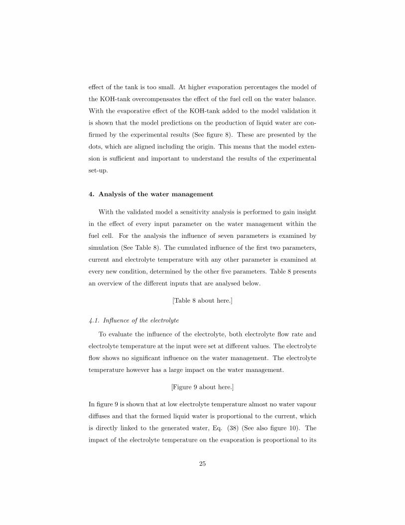
takes place (See Fig.2). The model is modularly built. In this way a more

detailed model can be obtained by serially connecting several individual models.

Table 1 gives an overview of the molar and energy flows shown in figure 2. New

elements in this model, compared to earlier work [11] are

• that the hydrogen and oxygen consumption and the water vapour removal

of the fuel cell model is based upon diffusion laws. The diffusion is de-

scribed by the Stefan-Maxwell equation, Eq.(4):

dyi

dz=RT

P·∑

j

yi ·Nj − yj ·Ni

Dij(4)

In this equation, the z-coordinate represents the dimension in which the

diffusion occurs.

• that the water vapour in the fuel cell body is assumed to be saturated. In

this way a direct relation between cell temperature and partial pressure

of water vapour can be posed, Eq.(5):

p = f(T ) (5)

7

[Figure 2 about here.]

[Table 1 about here.]

8

2.3. Model Variables

Each molar flow shown on the figure 2 is determined by 8 variables (See

Table 2 ). Next to the molar flows five other variables are shown on Fig.2

and described in table 2, the three heat fluxes and the electric power output,

determined by voltage and current. The goal of the model is to predict the

output flows (B, H and N), the generated electric power and the heat loss to the

environment based upon the input flows (A, G and M). The other variables are

intermediate stages which provide more understanding of the physical behaviour

of the fuel cell. Based upon Fig. 2 all variables within the model are defined.

The model exists out of 14 mass flows and 4 energy flows. Each mass flow exists

out of 8 variables which describe the state of the flow (See Table 2). The energy

flows are heat or electricity. The electric power is characterised by current and

voltage.

[Table 2 about here.]

2.4. Model equations

For each control volume a mass and energy balance is used. The energy

balances are closed by heat fluxes between neighbouring control volumes or

between a control volume and the environment. This heat flux is modelled

as a convective heat flux. Next to heat and mass transfer between control

volumes, also electric energy, generated in the fuel cell body is transferred to

the environment. An electrochemical model is used to describe the electric

behaviour of the fuel cell. Finally the gas diffusion equations are used to relate

the gas flows to the partial pressure of water vapour, which is assumed to be

saturated in the fuel cell body.

2.4.1. Variables reduction

Since the intermediate flows are defined as component specific flows and

based upon the nature of the inlet flows a number of molar fractions can be

predefined, which will reduce the number of equations in the following model

description.

9

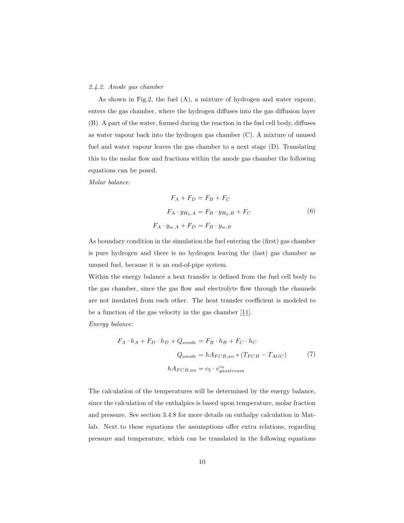
2.4.2. Anode gas chamber

As shown in Fig.2, the fuel (A), a mixture of hydrogen and water vapour,

enters the gas chamber, where the hydrogen diffuses into the gas diffusion layer

(B). A part of the water, formed during the reaction in the fuel cell body, diffuses

as water vapour back into the hydrogen gas chamber (C). A mixture of unused

fuel and water vapour leaves the gas chamber to a next stage (D). Translating

this to the molar flow and fractions within the anode gas chamber the following

equations can be posed.

Molar balance:

FA + FD = FB + FC

FA · yH2,A = FB · yH2,B + FC

FA · yw,A + FD = FB · yw,B

(6)

As boundary condition in the simulation the fuel entering the (first) gas chamber

is pure hydrogen and there is no hydrogen leaving the (last) gas chamber as

unused fuel, because it is an end-of-pipe system.

Within the energy balance a heat transfer is defined from the fuel cell body to

the gas chamber, since the gas flow and electrolyte flow through the channels

are not insulated from each other. The heat transfer coefficient is modeled to

be a function of the gas velocity in the gas chamber [11].

Energy balance:

FA · hA + FD · hD +Qanode = FB · hB + FC · hC

Qanode = hAFCB,an ∗ (TFCB − TAGC)

hAFCB,an = c5 · vc6gasstream

(7)

The calculation of the temperatures will be determined by the energy balance,

since the calculation of the enthalpies is based upon temperature, molar fraction

and pressure. See section 3.4.8 for more details on enthalpy calculation in Mat-

lab. Next to these equations the assumptions offer extra relations, regarding

pressure and temperature, which can be translated in the following equations

10

for the anode gas chamber.

Temperatures and pressures:

Tanode = TB = TC

pA = pB

pC =pA · (FA · yH2,A) + pB · (FB · yH2,B)

FA + FB

pD =pA · (FA · yw,A) + pB · (FB · yw,B)

FA + FB

(8)

2.4.3. Cathode gas chamber

The entering air contains oxygen, nitrogen and water vapour. There is a

large excess of air because air is used to remove water vapour from the cathode.

While oxygen diffuses to the fuel cell body, water vapour diffuses into the gas

stream. The same remarks regarding heat transfer in the energy balance which

were made for the anode are valid for the cathode.

Molar balance:

FL + FM = FK + FN

FM · yO2,M = FK + FN · yO2,N

FL + FM · yw,M = FN · yw,N

FM · yN2,M = FN · yN2,N

(9)

Energy balance:

FL · hL + FM · hM +Qcathode = FK · hK + FN · hN

Qcathode = hAFCB,cat · (TFCB − TCGC)

hAFCB,cat = c5 · vc6gasstream

(10)

11

Temperatures and pressures:

Tcathode = TK

Tcathode = TN

pM = pN

pK =pM · (FM · yO2,M ) + pN · (FN · yO2,N )

FM + FN

pL =pM · (FM · yw,M ) + pN · (FN · yw,N )

FM + FN

(11)

The cathode outlet temperature is one of the main parameters on which the

model is validated.

2.4.4. Anode gas diffusion layer

Between gas chamber and active surface a layer can be defined in which the

diffusion or migration of the gases towards the reaction zone takes place. Since

molar fractions are fixed the molar balance is very simple. The energy balance is

built in the same way as the gas chambers. Temperatures are calculated similar

to the gas chambers.

Molar balance:

FC = FE

FD = FF

(12)

Energy balance:

FC · hC + FF · hF = FD · hD + FE · hE (13)

Temperature :

TD = TE (14)

Diffusion equations and pressures:

In absence of a global pressure drop between the gas chamber and fuel cell

12

body, the driving force behind this migration is the concentration difference of

the gases between the gas chamber and the boundary of the fuel cell body. This

concentration difference is captured in the partial pressure difference between

fuel cell body and gas chamber. The pressure of the intermediate flows in the

model are in fact partial pressures. E.g. pC is the partial pressure of hydrogen

in the anode gas chamber and pE will be the partial pressure of hydrogen at the

boundary with the fuel cell body. The total pressure at each boundary is the

sum of the pressure of the flows passing this boundary, since only water vapour

and hydrogen are present at the anode side.

pC + pD = pE + pF (15)

yw + yH2 = 1 (16)

Taking this into account the Stefan-Maxwell equation (4) results in one inde-

pendent differential equation, describing the diffusion and the lack of global

pressure drop between the two boundaries (one of the assumptions, mentioned

above).

dyH2

dz=RT

P· yH2 ·Nw − yw ·NH2

DHw

with:

Nw = −a1 · FD

NH2 = a1 · FC

a1 =1

nstack · nparallel ·Acell

(17)

The resulting differential equation is a first order (18)

dyH2

dz=RT

P· yH2 · (Nw +NH2)−NH2

DHw(18)

13

Since the diffusion occurs between the two boundaries, each boundary can be

represented by a z-coordinate. As boundary condition the molar fraction in the

gas chamber is set equal to a weighted mean of input and output flow, which

was also the case for the (partial) pressure. Therefore at the anode side the

following conditions have to be fulfilled.

yH2 · ptot = pC

yw · ptot = pD

z = 0

(19)

Since these partial pressures are a function of the molar flow, within the diffusion

equations, an extra boundary condition is needed. This boundary condition is

found at the side of the fuel cell body, which can be defined by the thickness of

the diffusion layer, LGDF . At this side, it is assumed that the partial pressure

of the water vapour is equal to the saturation pressure in the fuel cell body, as a

result of the earlier mentioned model assumptions. This results in the following

equations:

yH2 · ptot = pE

yw · ptot = pF

pF = psaturation,FCB

z = LGDF

(20)

2.4.5. Cathode gas diffusion layer

Similar to the anode gas chamber, at the cathode side a gas diffusion layer

can be defined. Instead of diffusion of hydrogen and water vapour, at the

cathode side there is a net diffusion of oxygen and water vapour.

Molar balance:

FI = FK

FJ = FL

(21)

14

Energy balance:

FK · hK + FJ · hJ = FI · hI + FL · hL (22)

Temperature :

TI = TL (23)

Diffusion equations and pressures

Next to oxygen and water vapour also nitrogen exists in the cathode gas diffusion

layer. Since nitrogen does not react in the fuel cell body there is no net nitrogen

consumption of the fuel cell body and therefore no net transport of nitrogen

over the diffusion layer. However the presence of nitrogen has an impact on the

complexity of the formulation of the diffusion. The Stefan-Maxwell equation is

used to formulate the diffusion equations.

dyi

dz=RT

P· Σj

yi ·Nj − yj ·Ni

Dij(24)

which results in the following equations for oxygen, nitrogen and water vapour

dyO

dz=RT

P· yO ·NN − yN ·NO

DON+RT

P· yO ·Nw − yw ·NO

DOw(25)

dyw

dz=RT

P· yw ·NN − yN ·Nw

DwN− RT

P· yO ·Nw − yw ·NO

DOw(26)

dyN

dz= −RT

P· yO ·NN − yN ·NO

DON− RT

P· yw ·NN − yN ·Nw

DwN(27)

with

NO2 = −a1 · FK = −a1 · FI

Nw = a1 · FL = a1 · FJ

(28)

Since no net nitrogen flow is assumed in the model, NN can be set to zero. Next

to that the sum of the molar fractions is always one.

NN = 0 (29)

yN = 1− yO − yw (30)

dyN

dz= −dyO

dz− dyw

dz(31)

15

Combining and deriving these equations results in a differential equation of the

second degree for yO. This results in the following differential equation which

can be solved using similar boundary conditions as formulated for the anode

diffusion.

At the side of the fuel cell body:

z = 0 (32)

yw,FCB =pJ

ptot(33)

pJ = psaturation,FCB (34)

At the side of the gas chamber:

z = LGDF (35)

yw,CGC =pL

ptot(36)

yO2,CGC =pK

ptot(37)

2.4.6. Fuel cell body

Within the fuel cell body, the driving electrochemical reaction takes place.

The mass and molar balance relates the hydrogen and oxygen consumption to

the generation of water and electric current. The current is linked to the molar

flows by Faraday’s law.

Molar Balance:

FG +Iref · nseries

2Far= FH + FF + FJ

FE =Iref · nseries

2Far

FI =Iref · nseries

4Far

(38)

Energy balance:

Within the fuel cell body the catalytic and separator layer are enclosed [13, 14,

15]. Although different layers exist in the fuel cell, in this paper the properties

of the electrolyte/separator are taken to define the thermodynamic behaviour

16

of the fuel cell body. The mass flows between fuel cell body and gas chamber

however will only consist of gas in accordance to the boundary conditions of

the gas diffusion layers. This will affect the enthalpy of these streams and will

limit the mass or molar flow, because the partial pressure cannot exceed the

saturation pressure.

FG · hG + FE · hE + FI · hI =

FH · hH + FF · hF + FJ · hJ +QFCB + Pe

QFCB = QFCB,sur +QFCB,cat +QFCB,an

QFCB,surr = hAFCB,surr.(TFCB − Tsurr)

hF = hJ

(39)

The energy balance of the fuel cell body consists not only of incoming and

outgoing mass streams and heat flows, but also of an electric power output.

This output is more detailed in the electrochemical model.

2.4.7. Electrochemical model

The electrochemical model, presented in [11], is used. Since a few parameters

were adapted within the model the used equations are summarized.

Pe =U · I (40)

U =ENernst − ηact − ηres − ηdiff (41)

ENernst = −∆G0

2Far+RTcell

2Far

[ln (pH2) +

12ln (pO2)

](42)

ηact =R · T

α · n · Farln

(Icell

A

j0

)(43)

ηres = Re · Icell (44)

ηdiff =R · T

α · n · Farln

(jL

jL − Icell

A

)(45)

j0 = c1 · exp(−c2Tcell

)(46)

Re = c3 − c4 · Tcell (47)

17

2.4.8. Discussion on parameter estimation

[Table 3 about here.]

Table 3 contains all used semi-empiric parameters, which were used to tune

the model. Since the new model is built upon the base of the model in [11],

the same values were used in a first approach. Due to the extra layer at each

side the parameters regarding the heat transfer coefficient towards anode and

cathode will be different. This difference is found in c5. Its value is reduced,

since part of the heat transfer from the electrolyte into the gas stream is already

included in the energy balance of the diffusion layer. Next to this difference a

new parameter is introduced, namely LGDF . To determine an acceptable range

for LGDF a comparison was made with Jo et al.[23]. In this paper values from

0.05 to 0.55mm were found to be representative for the thickness of the gas

diffusion layer. These variations however had no significant influence on per-

formance. Since the model, presented in this paper, has a gas diffusion layer,

but no catalyst layer, the gas diffusion layer is chosen to be thicker to include

the diffusion resistance of the catalyst layer. The catalyst layer is 2 to 5 times

thinner than the diffusion layer and the diffusion coefficients are 10 to 100 times

larger for gas diffusion compared to diffusion through liquid [14]. Therefore, in

this model a value between 0.05 and 1cm is acceptable.

2.5. Implementation of the model in Matlab

For the implementation of the model, Matlab is chosen. Originally the model

was built in Aspen Custom Modeler [11]. Aspen Custom Modeler however

isn’t built to deal with complex mathematical problems, which are sensitive to

small distortions. The diffusion equations lead to an increased complexity and

therefore Matlab is chosen, which is more apprioriate for the scope of our work.

As a consequence the libraries of Aspen aren’t available anymore to calculate all

the necessary physical properties. As a solution, the different thermodynamic

properties of Aspen Custom Modeller are translated into constants or linear

18

functions so they could be implemented in Matlab. For the gasses hydrogen,

nitrogen and oxygen this is acceptable, since they are considered to be ideal. For

the enthalpy and Gibbs free energy calculations of water (vapour) a published

Matlab function by Magnus Holmgren [24] is used. Table 4 presents an overview

of the used constants in the linear expression (48) to calculate enthalpy.

hgas = cgas · T (C) + bgas (48)

[Table 4 about here.]

Also the diffusion constants in the Stefan-Maxwell equations need to be im-

ported. In a first approach they were imported as a constant from the libraries

of Aspen Custom Modeller. However, because the diffusion is a function of tem-

perature, already mentioned by Jo et all(2000) [23], this correlation is included

into the model, Eq. (49).

D(T ) = D0 · T 2,334 (49)

3. Model validation

The model is validated using experimental data which were generated with

the AFC system described in detail in [11, 25]. Part of these experimental

results were discussed in [11]. Further data analysis is performed to evaluate

the new element in the model, i.e. the water management.

3.1. Experimental set-up

[Figure 3 about here.]

Figure 3 shows a schematic view of the experimental set-up. Table 5 gives a

brief description of the main operating parameters, marked on Fig.3.

[Table 5 about here.]

19

For a detailed description of the parameters a to h in the experimental set-up we

refer to earlier work, where the same experimental data were used to validate

a previous model [11]. Next to the already discussed parameters the level of

electrolyte is measured (point i). The measurement however is not that precise,

because the water surface is not stable. This is caused by the KOH-pump which

switches between working steps and by the output air flow which passes over

the electrolyte tank. Only an evaluation of the water level - with consideration

of changes in electrolyte flow (point e) - over a long period of time will indicate

when there is a net evaporation of water (electrolyte) or when there is a net

formation of liquid water during this period of time.

3.2. Model validation

Current - which is directly proportional to the input hydrogen flow - input

air flow rate, input electrolyte flow rate and input electrolyte temperature are

used as input parameters for model validation. The model is used to predict

electrical performance, thermal behaviour and water management. The model

will be validated on these three aspects, which can be characterized by voltage,

output temperatures for both electrolyte and air and by output flow rate of the

liquid electrolyte. The validation is performed in two stages.

• First the model is compared with the previous model [11] and validated

regarding the prediction on voltage and thermal behaviour, using a selec-

tion of experimental data shown in Table 6. The selection of these working

points is described in [11].

• Secondly the water management is validated by selecting a long period in

which the fuel cell is relatively stable and the electrolyte level is monitored.

3.2.1. Validation with existing experimental data

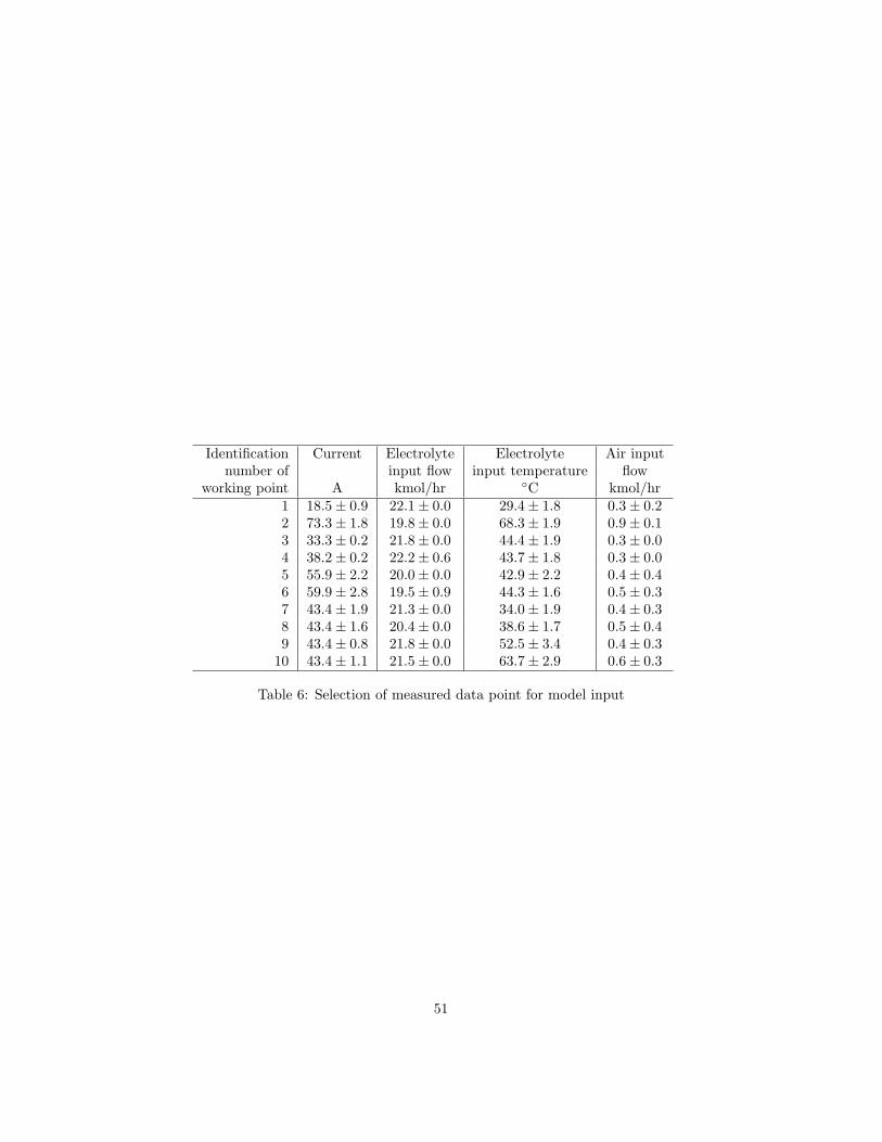
[Table 6 about here.]

As described in ref. [11], all measured parameters are subject to uncertainties.

Data analysis led to a data set of 50 working points. The measured parameters,

20

which are used as model input, are illustrated by a representative selection of

data points. This selection, shown in Table 6, is based on current and electrolyte

temperature, the two most determining input parameters. The first two working

points are representative for the range in which the data were obtained: the first

one represents the lower bound and the second one the upper bound for both

current and electrolyte temperature. The next four data points are all measured

at the same average current, over a wide range of electrolyte temperatures. The

last four are all measured at about the same average electrolyte temperature

over a wide range of currents. The measured and modeled output parameters of

these ten data points are shown in figures 4, 5 and 6. A complete data set with

all 50 measured and modelled data points will be held available by the authors.

In each of these figures the experimental data are compared to the model also

ref. [11] and to this new model, described in this paper.

• The experimental output is represented by dots with error bars, which

represent the instability on the measurement, similar to the variation in

the input value, shown in Table 6.

• The output of the model is represented by a floating bar. The line in the

middle of this bar represents the modeled output of the mean input pa-

rameters listed in Table 6. To include the measurement error on the model

input a set of model experiments were executed. In this set all possible

combinations of extreme input values for each input parameter were used

as input for the model, based upon the mean values and measurement

errors, listed in Table 6. In the end, the maximum and minimum result

were considered to be the upper and lower bound of the model output.

• The model in [11] is represented with a circle. For this model the mea-

surement error on the input parameters was not taken into account.

Electrical performance, voltage:

[Figure 4 about here.]

21

In Figure 4 the prediction on electric performance is shown. The data is arranged

by ascending current and electrolyte temperature, in case of similar currents

(data points 7 to 10). The model shows a better performance on prediction

of the voltage, compared to [11]. For two data points no overlap is found

between the experimental and the modeled voltage. This is however acceptable

because in the complete set of 50 data points these are indeed the only two

points, where no overlap is found. In these points the new model has a smaller

deviation than the previous model. Next to this, both for the experimental as

for the modelled voltage, a similar influence of the current is shown in Fig.4.

The same result is shown regarding the positive influence of the electrolyte

temperature (data point: 7 to 10) on the electrical performance or total voltage.

The model is therefore representative in predicting the voltage, including the

effect of temperature and current on electrical performance.

Thermal behaviour, electrolyte temperature:

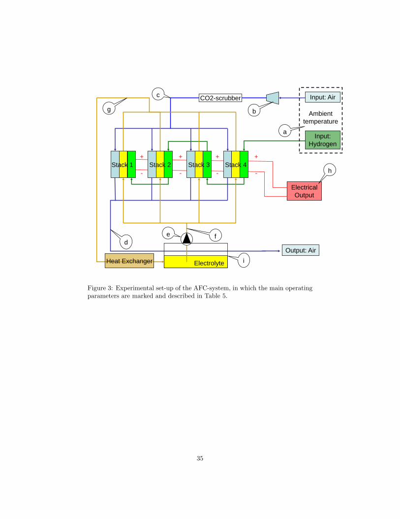
[Figure 5 about here.]

In Figures 5 and 6 the thermal behaviour is shown. Figure 5 shows the prediction

of the output electrolyte temperature. The model has comparable results to

[11], in predicting the electrolyte temperature. For two data points there is

no overlap. In the complete data set three working points show no overlap.

The deviation however is limited to a few degrees. The higher the electrolyte

temperature, the higher the output electrolyte temperature. This is visible both

in the experimental as in the modeled results. In the discussion on experimental

results in [11] was already mentioned that the temperature rise in the electrolyte

grows with higher current. This effect is visible in the modeled output, but is

not very clear in the shown experimental results (data points 3 to 6).

Thermal behaviour, air temperature:

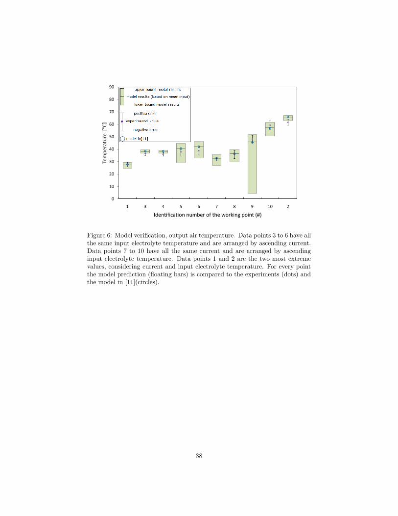
[Figure 6 about here.]

Figure 6 shows the prediction of the output air temperature. For all 50 working

points there is an overlap. Next to that, the relation with the electrolyte tem-

perature is noticeable, both in the measurements as in the model. Therefore,

22

the model is acceptable to predict thermal behaviour. Still the prediction of

the air temperature is sensitive to the air flow, the parameter with the highest

error range. As a result the modelled output shows a large difference between

upper and lower boundary. The most remarkable result is the lower bound in

working point 9. This represents an impossible situation, due to the high stan-

dard deviation in the measured air flow. The point however shows one of the

limitations of the model, since it is assumed that the air flow is controlled to

be at least sufficient to compensate the hydrogen input in Faraday’s law. This

assumption is not fulfilled in point 9, so the model cannot be used with those

input conditions.

3.2.2. Validation on the water management

[Figure 7 about here.]

[Table 7 about here.]

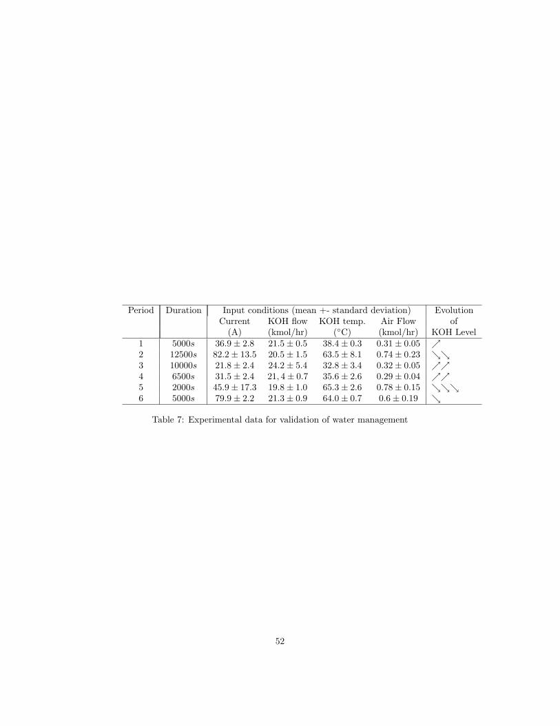
To validate the model regarding the water management, the level of the elec-

trolyte in the KOH-tank is monitored in time over the duration of the exper-

iments (Fig.7). In this time period it was possible to determine 6 periods in

which the electrolyte level shows a clear and steady change and in which the

variation on the inlet conditions was relatively stable (Table 7). These condi-

tions were used as input data for our model to predict the water production in

the electrolyte flow, which will result in a rise (or reduction) of the electrolyte

level in the KOH-tank. If the model is representative to reflect the measure-

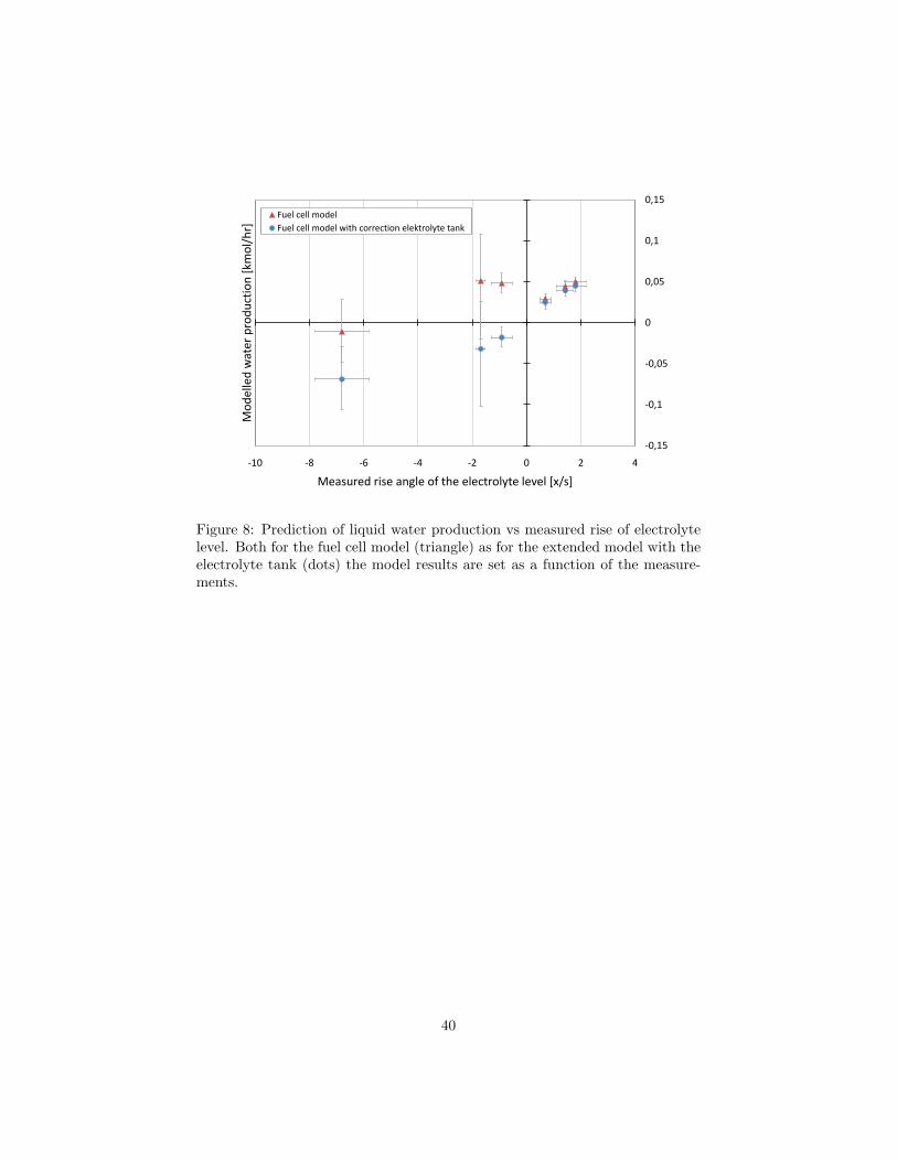
ments, the modeled water production is directly proportional to the speed at

which the measured electrolyte level rises. In Figure 8 the model results for the

formation of liquid water in the electrolyte flow (Y-axis) are set as a function

of the measured rise per unit of time of the electrolyte level in the KOH-tank

(X-axis). These data sets are represented by the triangles, which are expected

to be in a straight line through the origin. However, when the electrolyte level

drops (periods 2.5 and 6 in Table 7), the model overestimates the formation of

liquid water in the electrolyte.

23

[Figure 8 about here.]

At high currents (periods 2 and 6 in Table 7) the model predicts a rise in elec-

trolyte level due to the high water production. The measurements show however

a drop in electrolyte level. Table 7 shows that the positive effect of the current

on the water formation is almost neglectable compared to the negative effect of

the air flow and electrolyte temperature. According to the measurements, air

flow rate and temperature are the most determining parameters regarding rise

or decrease of the electrolyte level. This could be due to the fact that the output

air, which is not saturated, passes the tank. Assuming that this passage will

result in an increased relative humidity (RH%) of the output air, more water

will be evaporated at higher air flow rate and higher temperature, resulting in

a lower electrolyte level.

3.2.3. Model extension for electrolyte tank

To verify this the evaporation in the electrolyte tank is modelled as a function

of the following parameters:

• electrolyte temperature

• electrolyte flow

• air flow

• air temperature

• relative humidity of air

• percentage of evaporation: 0 means no evaporation - 100 means that the

air is completely saturated

Only this last parameter could be fitted to the results. Since it is reasonable that

the KOH tank has an influence, but complete saturation will not be reached, the

parameter will be higher than 0 and lower than 100. A best fit could be found at

about 40%. Taking the error bars into account, the model already shows good

results for an evaporation percentage of 30% to 65%. At lower percentages the

24

effect of the tank is too small. At higher evaporation percentages the model of

the KOH-tank overcompensates the effect of the fuel cell on the water balance.

With the evaporative effect of the KOH-tank added to the model validation it

is shown that the model predictions on the production of liquid water are con-

firmed by the experimental results (See figure 8). These are presented by the

dots, which are aligned including the origin. This means that the model exten-

sion is sufficient and important to understand the results of the experimental

set-up.

4. Analysis of the water management

With the validated model a sensitivity analysis is performed to gain insight

in the effect of every input parameter on the water management within the

fuel cell. For the analysis the influence of seven parameters is examined by

simulation (See Table 8). The cumulated influence of the first two parameters,

current and electrolyte temperature with any other parameter is examined at

every new condition, determined by the other five parameters. Table 8 presents

an overview of the different inputs that are analysed below.

[Table 8 about here.]

4.1. Influence of the electrolyte

To evaluate the influence of the electrolyte, both electrolyte flow rate and

electrolyte temperature at the input were set at different values. The electrolyte

flow shows no significant influence on the water management. The electrolyte

temperature however has a large impact on the water management.

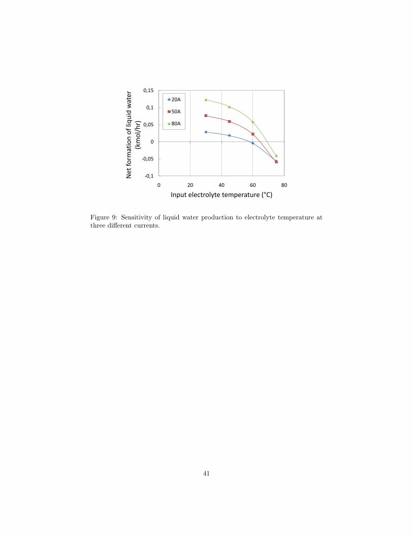
[Figure 9 about here.]

In figure 9 is shown that at low electrolyte temperature almost no water vapour

diffuses and that the formed liquid water is proportional to the current, which

is directly linked to the generated water, Eq. (38) (See also figure 10). The

impact of the electrolyte temperature on the evaporation is proportional to its

25

impact on the saturation pressure. At least a temperature of about 55C has

to be reached to avoid net rise of liquid water in the electrolyte flow. At lower

temperatures the saturation pressure drops rapidly. Because of this the driving

force for the water vapour diffusion is strongly reduced. As a result liquid water

builds up due to the formation of water, which is not transported out of the fuel

cell by diffusion. For the same reason, but now in the opposite direction, there

is a net evaporation at temperatures higher than 75C, at least for currents

within nominal working range (20A to 80A). To avoid dry out of the fuel cell,

75C is to be set as a maximum temperature when working with dry or cold air.

This will limit the electric efficiency since this is higher at higher temperature

[11].

4.2. Influence of current

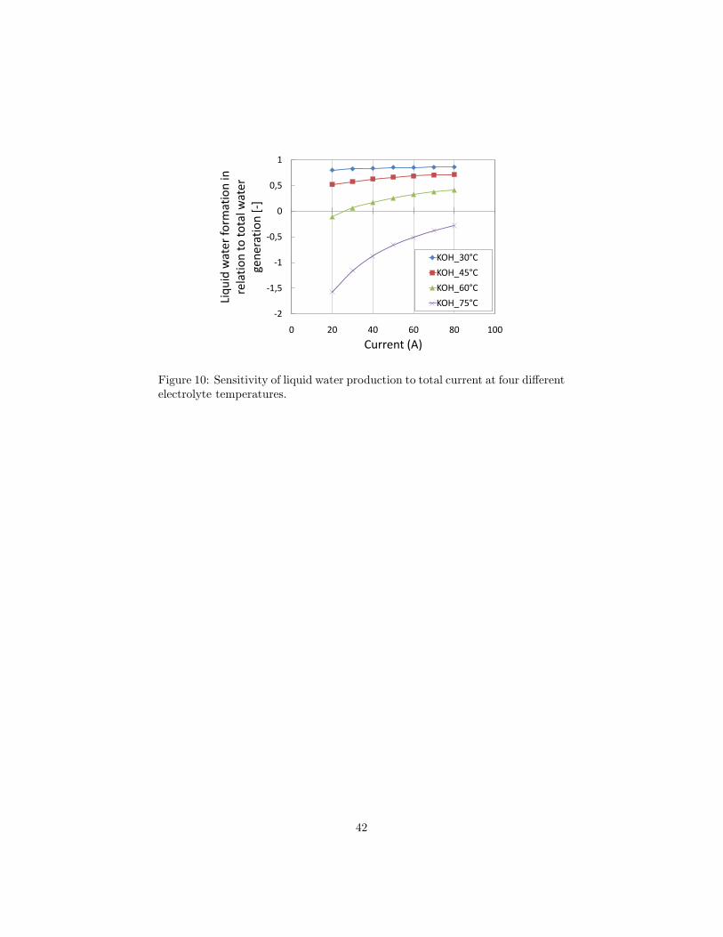
[Figure 10 about here.]

At low temperature current has no significant influence and all formed water will

end up in the electrolyte flow. Figure 10 shows that for every input electrolyte

temperature higher than the minimum value (about 55C, See Section 4.1) a

current can be found at which all formed water is evaporated and diffuses into

the gas streams. This is interesting regarding steady state working points.

4.3. Influence of the input air

To understand the influence of the air stream, three parameters were evalu-

ated:

• the air ratio or the actual air flow in relation to the necessary air flow

• the relative humidity

• the air temperature

[Figure 11 about here.]

[Figure 12 about here.]

26

Figure 11 shows that a higher air ratio has a negative effect on the net forma-

tion of liquid water. The relative impact of an increased air ratio reduces after

a ratio of 2,5 to 4 (See Fig. 11). Naturally, the impact of the air ratio on the

evaporation of the electrolyte tank is directly related, as shown in the model

extension for the electrolyte tank (See Section 3.2.2). The air ratio can be used

as a control parameter for the water management within a small range within

the stack itself (1 - 2,5). If the output air passes over the electrolyte tank, as in

the used experimental set-up of the AFC-system, the air ratio can be a useful

control paramater in a much wider range.

Next to the air ratio, the temperature and relative humidity will be of impor-

tance. Their effect however, is relatively low. If the input air is dry, the air

temperature has only a very small positive effect on the diffusion, which results

in a lower net liquid water formation. The relative humidity only has a large

impact at high input air temperature (See Fig. 12). At lower temperature the

water vapour content of saturated air is a lot lower and will have no signifi-

cant influence on the water vapour content of the heated output air stream. As

discussed earlier(See Section 4.1), to avoid dry out of the fuel cell a maximum

temperature of the electrolyte has to be respected. However, this statement was

posed using dry and cold air as inlet for the cathode. In Fig. 12 is shown that

at higher electrolyte temperature it is still possible to maintain water content

of the electrolyte flow, if hot humidified air is used as input for the fuel cell. Be-

cause electrolyte temperature has a positive effect on the fuel cell performance

[11], this could increase the efficiency of the fuel cell.

27

5. Conclusion

A model of an alkaline fuel cell is created in Matlab. The model predicts

the thermodynamic behaviour and water management of the fuel cell and is

validated with experimental data from a system designed for CHP-applications.

The influence of the input parameters on the water management is investigated.

• To maintain the concentrations within the electrolyte, a minimum elec-

trolyte temperature has to be reached (about 55C) to operate at low

current.

• Higher currents will require higher input temperatures of the electrolyte

to maintain the electrolyte concentration.

• The electrolyte temperature at a given current can be increased without

dry out using hot humidified air.

• An air ratio higher than 2.5 is no more effective as a control paramater to

maintain electrolyte concentration within the fuel cell.

Acknowledgements

The authors would like to thank VITO and KHLim for use of their equip-

ment.

References

[1] M. Pehnt, Environmental impacts of distributed energy systems-The case of

micro cogeneration, Environmental science and policy II (2008),25-37.

[2] M. De Paepe, P. D’Herdt, D. Mertens, Micro-CHP systems for residential

applications, Energy Conversion and Management, Volume 47, Issues 18-19,

November 2006, Pages 3435-3446.

[3] K. Alanne, A. Saari, Sustainable small-scale CHP technologies for buildings:

the basis for multi-perspective decision-making, Renewable and Sustainable

Energy Reviews,Volume 8, Issue 5 (October 2004) Pages 401-431

28

[4] A.D. Hawkes, D.J.L. Brett, N.P. Brandon, Fuel cell micro-CHP techno-

economics, International Journal of Hydrogen Energy 34(2009)9545-9557.

[5] I. Staffell, A. Ingram, Life cycle assessment of an alkaline fuel cell CHP

system, International Journal of Hydrogen 35(2010) 2491-2505.

[6] H.I. Onovwiona, V.I. Ugursal, Residential cogeneration systems: review of

the current technology, Renewable and Sustainable Energy reviews 10 (2006)

389-431.

[7] I. Staffell, A review of small stationary fuel cell performance , http :

//wogone.com/iq/reviewoffuelcellperformance.pdf (2009) [cited Decem-

ber 2010].

[8] G.F. Mclean,T. Niet,S. Prince-Richard,N. Djilali, An assessment of alkaline

fuel cell technology, International Journal of Hydrogen Energy 275(2002)507-

526.

[9] E. Gulzow, J.K. Nor, P.K. Nor and M. Schulze, A renaissance for alkaline

fuel cells The fuel cell review, Volume 3 Issue 1 (2006).

[10] E. Gulzow,M. Schulze, U. Gerke, Bipolar concept for alkaline fuel cells

International Journal of Power Sources 156(2006)1-7.

[11] I. Verhaert, M. De Paepe, G. Mulder, Thermodynamic Model for an Alka-

line Fuel Cell, Journal of Power Sources 193(1) (2009); 193(1) 233-240.

[12] G. Mulder, Alkaline Fuel Cells - Overview, Encyclopedia of Electrochemical

Power Sources (2009), Pages 321-328.

[13] M.C. Kimble and R.E. White, A Mathematical Model of a Hydrogen/Oygen

Alkaline Fuel Cell, J. Electrochem. Soc., Vol. 138, No. 11, (November

1991)3370-3382.

[14] J.-H. Jo, S.-C. Yi, A computational simulation of an alkaline fuel cell,

Journal of Power Sources 84 (1999) 87-106.

29

[15] M. Duerr, S. Gair, A. Cruden, J. McDonald, Dynamic electrochemical

model of an alkaline fuel cell stack, Journal of Power Sources, Volume 171,

Issue 2, (27 September 2007) 1023-1032.

[16] S. Rowshanzamir, M. Kazemeini and M.K. Isfahani. Mass balance and

water management for hydrogen-air fuel cells, Journal of Hydrogen Energy,

Volume 23, Issue 6 (June 1998) 499-506.

[17] H.Huisseune, A. Willockx, M. De Paepe, Semi-empirical along-the-channel

model for a proton exchange membrane fuel cell International Journal of

Hydrogen Energy, Volume 33, Issue 21 (November 2008)6270-6280.

[18] J.Wu, X.Z. Yuan, H. Wang, M. Blanco, J.J. Martin, J. Zhang, Diagnostic

tools in PEM fuel cell research: Part I Electrochemical techniques, Interna-

tional Journal of Hydrogen Energy 33 (2008)1735-1746.

[19] B.Y.S. Lin, D.W. Kirk, S.J. Thorpe, Performance of alkaline fuel cells:

A possible future energy system?, Journal of Power Sources 161 (2006).

474-483.

[20] R. O’Hayre, S.-W. Cha, W. Colella and F.B. Prinz, Fuel Cell Fundamentals,

Chapter 6: Fuel Cell Modelling, (2006) pp 169-192.

[21] J.C. Amphlett, R.F. Mann, B.A. Peppley, P.R. Robergy, A. Rodrigues, A

model predicting transient responses of proton exchange membrane fuel cell,

Journal of Power Sources 1996; 61(1-2) 183-188.

[22] C. Depcik, D. Assanis A universal heat transfer correlation for intake and

exhaust flows in an spark-ignition internal combustion engine, SAE Paper

2002-01-0372.

[23] J.H. Jo, S.-K. Moon and S.-C. Yi, Simulation of influences of layer

thickness in an alkaline fuel cell, Journal of Applied Electrochemistry 30

(2000),1023-1031.

[24] M. Holmgren, Matlab function: X STEAM, www.x-eng.com (2006-01-20).

30

[25] G. Mulder, P. Coenen, A. Martens, J. Spaepen, The development of a 6

kW fuel cell generator based on alkaline fuel cell technology, International

Journal of Hydrogen Energy, Volume 33, Issue 12 (June 2008) 3220-3382.

31

List of Figures

1 Working Principle of an Alkaline Fuel Cell . . . . . . . . . . . . 332 Lay-out of the alkaline fuel cell model (See Table 1 for a detailed

description). . . . . . . . . . . . . . . . . . . . . . . . . . . . . . 343 Experimental set-up of the AFC-system, in which the main op-

erating parameters are marked and described in Table 5. . . . . . 354 Model verification on electric performance (voltage) with the

working points (See Table 6) arranged by ascending current andtemperature in case of equal current (points 7 to 10). For ev-ery point the model prediction (floating bars) is compared to theexperiments (dots) and the model in [11](circles). . . . . . . . . 36

5 Model verification, output electrolyte temperature. Data points3 to 6 have all the same input electrolyte temperature and arearranged by ascending current. Data points 7 to 10 have all thesame current and are arranged by ascending input electrolytetemperature. Data points 1 and 2 are the two most extreme val-ues, considering current and input electrolyte temperature. Forevery point the model prediction (floating bars) is compared tothe experiments (dots) and the model in [11](circles). . . . . . . . 37

6 Model verification, output air temperature. Data points 3 to 6have all the same input electrolyte temperature and are arrangedby ascending current. Data points 7 to 10 have all the same cur-rent and are arranged by ascending input electrolyte temperature.Data points 1 and 2 are the two most extreme values, consideringcurrent and input electrolyte temperature. For every point themodel prediction (floating bars) is compared to the experiments(dots) and the model in [11](circles). . . . . . . . . . . . . . . . . 38

7 Measured fluctuation of the electrolyte level in the KOH-tankduring time of the experiments. Six periods are selected in whichthe input parameters are relatively stable and marked on thefigure. These 6 periods are described in Table 5 . . . . . . . . . . 39

8 Prediction of liquid water production vs measured rise of elec-trolyte level. Both for the fuel cell model (triangle) as for theextended model with the electrolyte tank (dots) the model re-sults are set as a function of the measurements. . . . . . . . . . 40

9 Sensitivity of liquid water production to electrolyte temperatureat three different currents. . . . . . . . . . . . . . . . . . . . . . 41

10 Sensitivity of liquid water production to total current at fourdifferent electrolyte temperatures. . . . . . . . . . . . . . . . . . 42

11 Sensitivity of liquid water production to air ratio. . . . . . . . . 4312 Sensitivity of liquid water production to relative humidity and

air temperature. For 8 different combinations of currents (20Aor 80A), electrolyte temperature (30C or 75C) and air temper-ature (20C or 50C) the net formation of liquid water is set asa function of the relative humidity of the input air. . . . . . . . 44

32

Figure 1: Working Principle of an Alkaline Fuel Cell

33

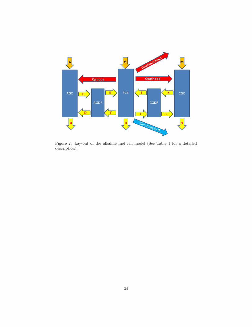
Figure 2: Lay-out of the alkaline fuel cell model (See Table 1 for a detaileddescription).

34

CO2-scrubber Input: Air

Input:

Hydrogen

Output: Air

Heat Exchanger Electrolyte

c

d

e

g b

f

Electrical

Output

+

-

+ + +

--- h

Ambient

temperature

a

Stack 1 Stack 2 Stack 3 Stack 4

i

Figure 3: Experimental set-up of the AFC-system, in which the main operatingparameters are marked and described in Table 5.

35

65

67

69

71

73

75

77

1 3 4 7 8 9 10 5 6 2

Tota

l vo

ltag

e (V

)

Identification number of the working point (#)

Figure 4: Model verification on electric performance (voltage) with the workingpoints (See Table 6) arranged by ascending current and temperature in case ofequal current (points 7 to 10). For every point the model prediction (floatingbars) is compared to the experiments (dots) and the model in [11](circles).

36

25

30

35

40

45

50

55

60

65

70

75

1 3 4 5 6 7 8 9 10 2

Tem

per

atu

re [

°C]

Identification number of the working point (#)

Figure 5: Model verification, output electrolyte temperature. Data points 3 to 6have all the same input electrolyte temperature and are arranged by ascendingcurrent. Data points 7 to 10 have all the same current and are arranged byascending input electrolyte temperature. Data points 1 and 2 are the two mostextreme values, considering current and input electrolyte temperature. Forevery point the model prediction (floating bars) is compared to the experiments(dots) and the model in [11](circles).

37

0

10

20

30

40

50

60

70

80

90

1 3 4 5 6 7 8 9 10 2

Tem

per

atu

re [

°C]

Identification number of the working point (#)

Figure 6: Model verification, output air temperature. Data points 3 to 6 have allthe same input electrolyte temperature and are arranged by ascending current.Data points 7 to 10 have all the same current and are arranged by ascendinginput electrolyte temperature. Data points 1 and 2 are the two most extremevalues, considering current and input electrolyte temperature. For every pointthe model prediction (floating bars) is compared to the experiments (dots) andthe model in [11](circles).

38

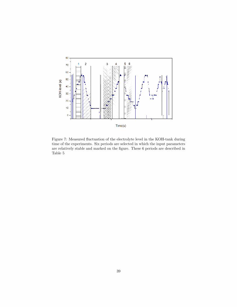
Figure 7: Measured fluctuation of the electrolyte level in the KOH-tank duringtime of the experiments. Six periods are selected in which the input parametersare relatively stable and marked on the figure. These 6 periods are described inTable 5

39

-0,15

-0,1

-0,05

0

0,05

0,1

0,15

-10 -8 -6 -4 -2 0 2 4

Mo

del

led

wat

er p

rod

uct

ion

[km

ol/

hr]

Measured rise angle of the electrolyte level [x/s]

Fuel cell model

Fuel cell model with correction elektrolyte tank

Figure 8: Prediction of liquid water production vs measured rise of electrolytelevel. Both for the fuel cell model (triangle) as for the extended model with theelectrolyte tank (dots) the model results are set as a function of the measure-ments.

40

-0,1

-0,05

0

0,05

0,1

0,15

0 20 40 60 80

Net

fo

rmat

ion

of

liqu

id w

ater

(k

mo

l/h

r)

Input electrolyte temperature (°C)

20A

50A

80A

Figure 9: Sensitivity of liquid water production to electrolyte temperature atthree different currents.

41

-2

-1,5

-1

-0,5

0

0,5

1

0 20 40 60 80 100

Liq

uid

wat

er f

orm

atio

n in

re

lati

on

to

to

tal w

ater

ge

ner

atio

n [

-]

Current (A)

KOH_30°C

KOH_45°C

KOH_60°C

KOH_75°C

Figure 10: Sensitivity of liquid water production to total current at four differentelectrolyte temperatures.

42

-0,2

-0,1

0

0,1

0,2

0 2 4 6 8

Net

fo

rmat

ion

of

liqu

id w

ater

(k

mo

l/h

r)

Air ratio (-)

80A_KOH_75°C 80A_KOH_30°C

20A_KOH_75°C 20A_KOH_30°C

Figure 11: Sensitivity of liquid water production to air ratio.

43

-2

-1

0

1

2

3

0 50 100

Liq

uid

wat

er f

orm

atio

n in

re

lati

on

to

to

tal w

ater

ge

ner

atio

n [

-]

Relative humidity air (%)

80A_KOH75°C_Air20°C 80A_KOH30°C_Air20°C20A_KOH75°C_Air20°C 20A_KOH30°C_Air20°C80A_KOH75°C_Air50°C 80A_KOH30°C_Air50°C20A_KOH75°C_Air50°C 20A_KOH30°C_Air50°C

Figure 12: Sensitivity of liquid water production to relative humidity and airtemperature. For 8 different combinations of currents (20A or 80A), electrolytetemperature (30C or 75C) and air temperature (20C or 50C) the net for-mation of liquid water is set as a function of the relative humidity of the inputair.

44

List of Tables

1 Description of the control volumes and the molar and energy flowsin Fig.2 . . . . . . . . . . . . . . . . . . . . . . . . . . . . . . . . 46

2 List of variables in each mass (molar) stream . . . . . . . . . . . 473 List of the used semi-empiric parameters . . . . . . . . . . . . . 484 Constants for enthalpy calculation . . . . . . . . . . . . . . . . . 495 List of operating parameters of the AFC-system, marked on Fig.3 506 Selection of measured data point for model input . . . . . . . . . 517 Experimental data for validation of water management . . . . . 528 Description of the sensitivity analysis . . . . . . . . . . . . . . . 53

45

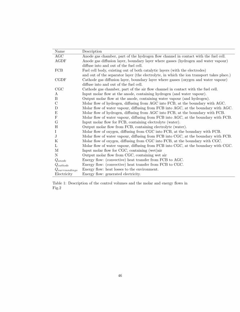
Name DescriptionAGC Anode gas chamber, part of the hydrogen flow channel in contact with the fuel cell.AGDF Anode gas diffusion layer, boundary layer where gasses (hydrogen and water vapour)

diffuse into and out of the fuel cell.FCB Fuel cell body, existing out of both catalytic layers (with the electrodes)

and out of the separator layer (the electrolyte, in which the ion transport takes place.)CGDF Cathode gas diffusion layer, boundary layer where gasses (oxygen and water vapour)

diffuse into and out of the fuel cell.CGC Cathode gas chamber, part of the air flow channel in contact with the fuel cell.A Input molar flow at the anode, containing hydrogen (and water vapour).B Output molar flow at the anode, containing water vapour (and hydrogen).C Molar flow of hydrogen, diffusing from AGC into FCB, at the boundary with AGC.D Molar flow of water vapour, diffusing from FCB into AGC, at the boundary with AGC.E Molar flow of hydrogen, diffusing from AGC into FCB, at the boundary with FCB.F Molar flow of water vapour, diffusing from FCB into AGC, at the boundary with FCB.G Input molar flow for FCB, containing electrolyte (water).H Output molar flow from FCB, containing electrolyte (water).I Molar flow of oxygen, diffusing from CGC into FCB, at the boundary with FCB.J Molar flow of water vapour, diffusing from FCB into CGC, at the boundary with FCB.K Molar flow of oxygen, diffusing from CGC into FCB, at the boundary with CGC.L Molar flow of water vapour, diffusing from FCB into CGC, at the boundary with CGC.M Input molar flow for CGC, containing (wet)airN Output molar flow from CGC, containing wet airQanode Energy flow: (convective) heat transfer from FCB to AGC.Qcathode Energy flow: (convective) heat transfer from FCB to CGC.Qsurroundings Energy flow: heat losses to the environment.Electricity Energy flow: generated electricity.

Table 1: Description of the control volumes and the molar and energy flows inFig.2

46

Variables Symbol Unit

Molar Flow F kmol/hrTemperature T CPressure p barEnthalpy h GJ/kmolMolar Fraction Hydrogen yH2

Molar Fraction Oxygen yO2

Molar Fraction Water(Vapour) yw

Molar Fraction Nitrogen yN2

Table 2: List of variables in each mass (molar) stream

47

Parameter Value [11] New Model

jL 2000A/m2 2000A/m2

α 0.1668 0.1668c1 174512A/m2 174512A/m)

c2 5485K 5485Kc3 0.0045Ω 0.0045Ωc4 5.9e− 5Ω/K 5.9e− 6Ω/Kc5 3.375e− 3 1.5e− 3c6 1.5 1.5hAsur 51.2W/K 51.2W/KLGDF 0.2cm

Table 3: List of the used semi-empiric parameters

48

Gas b [GJ/kmol] c [GJ/(kmol · C)]

Hydrogen −7.22573286 · 10−4 2.89388143 · 10−5

Nitrogen −7.28014 · 10−4 2.91195 · 10−5

Oxygen −7.32343 · 10−4 2.92833 · 10−5

Table 4: Constants for enthalpy calculation

49

Parameter Description Measuring method

a Ambient temperature Direct(input temperature for air and hydrogen supply)

b Air flow Indirectc Air temperature Estimatedd Output air temperature Directe Electrolyte flow Indirectf Input electrolyte temperature Directg Output electrolyte temperature Directh Total voltage, Current, cell voltages Directi Level of the electrolyte in the tank Direct

Table 5: List of operating parameters of the AFC-system, marked on Fig.3

50

Identification Current Electrolyte Electrolyte Air inputnumber of input flow input temperature flow

working point A kmol/hr C kmol/hr1 18.5± 0.9 22.1± 0.0 29.4± 1.8 0.3± 0.22 73.3± 1.8 19.8± 0.0 68.3± 1.9 0.9± 0.13 33.3± 0.2 21.8± 0.0 44.4± 1.9 0.3± 0.04 38.2± 0.2 22.2± 0.6 43.7± 1.8 0.3± 0.05 55.9± 2.2 20.0± 0.0 42.9± 2.2 0.4± 0.46 59.9± 2.8 19.5± 0.9 44.3± 1.6 0.5± 0.37 43.4± 1.9 21.3± 0.0 34.0± 1.9 0.4± 0.38 43.4± 1.6 20.4± 0.0 38.6± 1.7 0.5± 0.49 43.4± 0.8 21.8± 0.0 52.5± 3.4 0.4± 0.3

10 43.4± 1.1 21.5± 0.0 63.7± 2.9 0.6± 0.3

Table 6: Selection of measured data point for model input

51

Period Duration Input conditions (mean +- standard deviation) EvolutionCurrent KOH flow KOH temp. Air Flow of

(A) (kmol/hr) (C) (kmol/hr) KOH Level1 5000s 36.9± 2.8 21.5± 0.5 38.4± 0.3 0.31± 0.05 2 12500s 82.2± 13.5 20.5± 1.5 63.5± 8.1 0.74± 0.23 3 10000s 21.8± 2.4 24.2± 5.4 32.8± 3.4 0.32± 0.05 4 6500s 31.5± 2.4 21, 4± 0.7 35.6± 2.6 0.29± 0.04 5 2000s 45.9± 17.3 19.8± 1.0 65.3± 2.6 0.78± 0.15 6 5000s 79.9± 2.2 21.3± 0.9 64.0± 0.7 0.6± 0.19

Table 7: Experimental data for validation of water management

52

Parameter average minimum maximum step sizeCurrent 20A-80A 20A 80A 10A

Input electrolyte temperature 30C-75C 30C 75C 15CInput air temp 20C 5C 65C 15CInput air RV% 0 0% 100% 50%

Input air flow (air ratio) 2.5 1 8 1.5Input electrolyte flow 20.5 kmol/hr 19 22 1.5 kmol/hr

Temperature surroundings 20 -10C 50C 15C

Table 8: Description of the sensitivity analysis

53