Water and Development - in a Himalayan Watershed - IDRC ...
281
Too Little and Too Much: Water and Development in a Himalayan Watershed Editors Hans Schreier Sandra Brown Jennifer Rae MacDonald
-
Upload
khangminh22 -
Category
Documents
-
view
0 -
download
0
Transcript of Water and Development - in a Himalayan Watershed - IDRC ...

Too Little and Too Much: Water and Development
in a Himalayan Watershed
Editors Hans Schreier Sandra Brown
Jennifer Rae MacDonald

Too Little and Too Much
Water and Development in a Himalayan Watershed
Editors
Hans Schreier Sandra Brown
Jennifer Rae MacDonald
Institute for Resources and Environment University of British Columbia
August 2006
RIMSD
Text Box
This report is presented as received by IDRC from project recipient(s). It has not been subjected to peer review or other review processes. This work is used with the permission of University of British Columbia. © 2006, University of British Columbia.

Copyright @ 2006 Institute for Resources and Environment (IRES)
Publisher: IRES-Press, 2202 Main Mall, Vancouver, B.C. V6T 1Z4, Canada
Printed in Canada Allegra Print & Imaging 211 W 2nd Ave. Vancouver, B.C. V5Y 3V5 Canada
The views and interpretations in this publication are those of the authors. They are not attributable to IRES or the granting agencies (IDRC or SDC) or ICIMOD. Product named does not imply promotion or legal endorsement.

ni
Acknowledgements
We would like to thank the many people who made a major contribution to the Jhikhu Khola watershed project. These include our Nepali team members and field staff, the farmers, all national and international students and various different organizations that provided valuable input and assistance.
A major recognition goes to the International Development Research Centre (IDRC, Ottawa) which in 1989 provided the initiative financial support and continued their support throughout the length of the project. Over the 16 year span we collaborated with the following IDRC project officers: Ken Riley, N. Mateo, M. Beaussart, E. Rached, Joachim Voss, Ronnie Vernooy, John, Graham, and Liz Fabjer. They all made a special effort to help us through good and bad times but a special thank you goes to John Graham who was our true supporter, advisor, and friend over the entire length the project.
In 1996 the Swiss Agency for Development and Cooperation (SDC-Bern) became the principal donor as part of the expanded PARDYP project. We would like to thank Peter Maag, Christine Grieder, Carmen Thonnissen, Felix van Sury and Karl Schuler for their support and assistance.
Initially the project was housed in the HMG Topographie Survey Branch and 1994 ICIMOD became the home base for the project. While it was not easy being a field-based research project in an institution that focuses primarily on information dissemination, we benefited significantly from being associated with an international institution.
We would like to thank for following individuals for their collaboration and assistance. They all made a major contribution to the project and enriched our experience:
Richard Allen and his successor Roger White, the PARDYP project coordinators 1996-2006 The leader for the other PARDYP watershed teams J. Xu (China), H. Shah (Pakistan), P.B. Kothiary and S. Bhuchar (India) Our Swiss colleages from the University of Bern particularly: Jurg Merz, Bruno Messerli, Rolf Weingartner and Eve Wymann Brian Carson (Roberts Creek, B.C. previously LRMP)
A special thank-you goes to the original Nepali team. Without their enthusiasm and dedication the project would never have succeeded. P.B Shah was our inspirational leader. Without his integrity, dedication, enthusiasm, local knowledge, and organizational capacity this project would have never survived the political, logistical and management difficulties encountered over the years. Gopal Nakarni engineered the production of all

iv
infrastructure and was the committed organizer of field based activities. Bhuban Shrestha has been incredibly loyal as our database / GIS / multi- media creator and manager, and excelled in all field and office tasks. Pathak was instrumental in helping us in the early stages to get hydrometric and erosion monitoring off the ground. All four were dedicated and delightful people to work with, and they all enriched our lives.
Jurg Merz played a pivitol role in keeping the research program alive during the political conflict.
Words are insufficient to measure the contribution and enthusiastic support provided by Sandra Brown. The final thank you goes to Jennifer MacDonald for lier valiant effort in editing and producing the book.
Vancouver, BC. August 1, 2006

V
TABLE OF CONTENTS
Acknowledgements ............................................................................................ iii
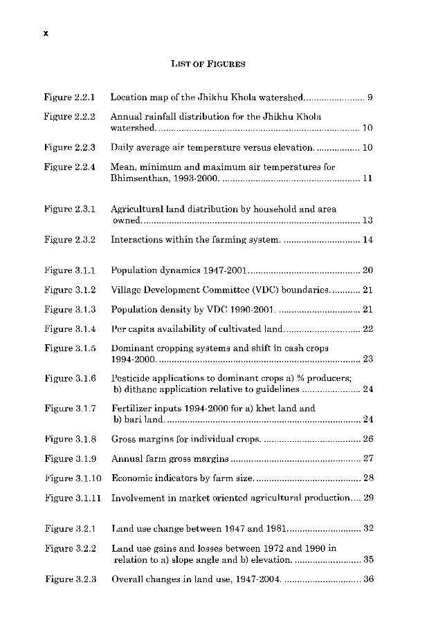
List of Figures ......................................................................................................x
List of Tables .................................................................................................... xvi
List of Plates .................................................................................................... xxi
CHAPTER 1: OVERVIEW OF THE PROJECT
1.1 A Historic Perspective .................................................................1
1.2 Introduction and Objectives ....................................................... 3
CHAPTER 2: AN INTEGRATED APPROACH TO WATERSHED MANAGEMENT IN THE HIMALAYAS
2.1 Why a Watershed Approach ....................................................... 7
2.2 Biophysical Setting ..................................................................... 8
2.2.1 Geology and Soils ............................................................................... 8 2.2.2 Climatic Conditions ............................................................................ 9 2.2.3 Land Use ........................................................................................... 11
2.3 The Socio-Economic Characteristics of the Watershed........... 11
2.3.1 People ................................................................................................ 11 2.3.2 Land .................................................................................................. 12 2.3.3 Livelihoods ........................................................................................ 13 2.3.4 Interrelationships: People, Land and Livestock ............................... 16
CHAPTER 3: DYNAMIC CHANGES OVER TIME: 1989-2004
3.1 Population and Socio-economic Trends .................................... 19
3.1.1 Population Dynamics ....................................................................... 19 3.1.2 Economic Well-being ......................................................................... 22 3.1.3 Production System Dynamics .......................................................... 23 3.1.4 Farm Gross Margins ........................................................................ 24 3.1.5 Farm Size and Food Security .......................................................... 27 3.1.6 Subsistence versus Commercial Production .................................... 28 3.1.7 Conclusions ....................................................................................... 29

VÎ
3.2 Land Use Dynamics 1947-2004 ................................................ 31
3.2.1 Changes in Land Use Categories between 1947 and 2004 ............. 31 3.2.2 Changes in Land Use Intensification .............................................. 36
3.3 Soil Nutrient Dynamics ............................................................ 40
3.3.1 Nutrient Status in the Watershed .................................................... 40 3.3.2 Factors that Influence Soil Nutrients .............................................. 42 3.3.3 Soil Nutrient Changes Ouer Time .................................................... 45 3.3.4 Calculating Nutrient Balances for Individual Fields .................... 49 3.3.5 Conclusions ....................................................................................... 53
3.4 Water Demands, Uses and Supplies ........................................ 54
3.4.1 Water Demand .................................................................................. 54 Domestic use .................................................................................. 55 Agricultural use ............................................................................. 56 Livestock ........................................................................................ 59 Overall demand for human activities .......................................... 60
3.4.2 Water Supp ly ..................................................................................... 60 Domestic supply ............................................................................ 61 Agricultural supply ....................................................................... 63 Perceived changes in water supply .............................................. 65
3.4.3 Su m mary ........................................................................................... 66
3.5 Hydrology and Sediment Transport ........................................ 68
3.5.1 Monitoring Network ......................................................................... 68 Data collection ............................................................................... 69
3.5.2 Water Auailability ............................................................................. 70 Precipitation dynamics ................................................................. 70 Evapotranspiration ....................................................................... 73 Flow regime ................................................................................... 75 Storage ........................................................................................... 77
3.5.3 Synthesis of Water Accounting ......................................................... 80 3.5.4 Flooding ............................................................................................ 83
Descriptive flood hydrology .......................................................... 83 Trends in flow characteristics ...................................................... 86 Flood generation ............................................................................ 87
3.5.5 Sediment Mobilisation and Transport ............................................ 94 Sediment sources and mobilization ............................................. 94 Sediment transport ..................................................................... 106 Synthesis ...................................................................................... 110

VU
3.6 Water Quality ..........................................................................118
3.6.1 River Water Quality ........................................................................ 118 3.6.2 Public and Private Water Sources Quality ................................... 120 3.6.3 Summary ......................................................................................... 123
3.7 Labour Allocation and Workloads: The Role of Women........ 124
3.7.1 Introduction .................................................................................... 124 3.7.2 Roles and Responsibilities .............................................................. 125 3.7.3 Labour Dynamics and Market Production .................................... 128 3.7.4 Women and Workloads ................................................................... 129
CHAPTER 4: ASSISTING COMMUNITY EFFORTS TO IMPROVE LIVELIHOODS AND ENVIRONMENT
4.1 Rehabilitation of Degraded Sites ........................................... 131
4.1.1 Introduction .................................................................................... 131
4.1.2 Native, Nitrogen Fixing Fodder Trees ........................................... 133 4.1.3 Grass Suitability for Soil Stabilization and Animal Feed........... 137 4.1.4 Restoration for Erosion Control and Biomass Generation........... 141
4.2 Improving Community Forests .............................................. 142
4.2.1 Background ..................................................................................... 142 4.2.2 Forest Status ................................................................................... 144 4.2.3 Forest Use ........................................................................................ 145 4.2.4 Local Perception of Forest Resources ............................................. 146 4.2.5 Community-based Forest Management ......................................... 147
4.3 Restoring the Production Capacity of Red Soils .................... 148
4.3.1 Introduction .................................................................................... 148 4.3.2 The Problem of Pine Litter Decomposition .................................... 150 4.3.3 Pine Litter Decomposition Rates in Red and Non-red Soils ........ 151 4.3.4 Soil Acidity and Nutrient Changes after Continuous Addition of
Pine Litter ....................................................................................... 152 4.3.5 Summary ......................................................................................... 156
4.4 Restoring Soil Production Capacity with Green Manure ..... 157
4.4.1 Background ..................................................................................... 158 4.4.2 Green Manure Experiment ............................................................. 159 4.4.3 Restoring the Soil Nutrient Pool .................................................... 164

4.5 Reducing Women's Workloads ............................................... 166
4.5.1 Water and Workloads ..................................................................... 166 4.5.2 Reducing Workloads; Improving Water Use Efficiency ................ 170 4.5.3 Assessing Sustainability; Evaluating Workloads ......................... 171
4.6 Water Harvesting ................................................................... 172
4.6.1 Introduction .................................................................................... 172 4.6.2 Aboue and Below Ground Water Storage ...................................... 173 4.6.3 Summary ......................................................................................... 175
4.7 Low Cost Drip Irrigation ........................................................ 176
4.7.1 Background ..................................................................................... 176 4.7.2 Low Cost Drip Irrigation Experiments .......................................... 177 4.7.3 Summary ......................................................................................... 181
4.8 Improving Crop Yields by Lime Applications ........................ 182
4.8.1 Agricultural Intensification and Agrochemical Use ..................... 182 4.8.2 Methodology .................................................................................... 183 4.8.3 Results ............................................................................................. 184 4.8.4 Summary ......................................................................................... 186
4.9 The Price of Milk: Balancing Income, Workloads and Environmental Impacts .......................................................... 188
4.9.1 The Milk Chilling Centre ............................................................... 188 4.9.2 Cooperatiue Dairy ........................................................................... 189 4.9.3 Milk Suruey ..................................................................................... 189 4.9.4 Milk Production and Dynamics ...................................................... 190 4.9.5 Livestock Dynamics and Feed Implications .................................... 194 4.9.6 Gender Based Workloads ............................................................... 195 4.9.7 Economics of Milk Production ....................................................... 197 4.9.8 Issues and Impacts ......................................................................... 199
CHAPTER 5: SUCESSES AND LESSONS LEARNED
5.1 Infrastructure Development ................................................... 203
5.1.1 The Suspension Bridge .................................................................... 203 5.1.2 The Use of Solar Power .................................................................. 205 5.1.3 Water Harvesting, Drinking Water, and Low Cost Drip
Irrigation ......................................................................................... 206 5.1.4 Improving Drinking Water Supplies ............................................. 207

ix
5.2 Capacity Building and Transferring Knowledge to Users .... 210
5.2.1 Training of Staff and Students ...................................................... 210 5.2.2 On-farm Experiences ...................................................................... 211 5.2.3 Working with Community Groups ................................................. 214 5.2.4 Influencing National Policy ........................................................... 216
5.3 Communications Using Multi-media Tools ...........................216
5.3.1 Using GIS and Multi-media CD-ROMs ........................................ 216 5.3.2 Scaling Out to Other Watersheds in the Himalayas ..................... 218 5.3.3 Scaling Out to Other Watersheds in the Mountains of the
World ............................................................................................... 219 5.3.4 Why the Himalayan and Andean watershed comparison? .......... 220
Methods and Approaches ............................................................ 220 Project Results ............................................................................. 221
5.3.5 Conclusions and Lessons Learned ................................................. 231
5.4 Summary .................................................................................233
CHAPTER 6: A VISION FOR THE FUTURE
6.1 Population, Food Security and Livelihoods ........................... 235
6.2 Water the Limiting Resources and Climate Change .............236
6.3 Future Training and Education .............................................239
6.4 Conflict resolution ................................................................... 239
CHAPTER 7: EPILOGUE ..........................................................241
CHAPTER 8: PUBLICATIONS (RELATED TO THE JHIKHU KHOLA WATERSHED PROJECT)
8.1 Refereed Journal Publications ...............................................243
8.2 Books and Chapters in Books ................................................. 245
8.3 Multi-Media - CD-ROM's ........................................................ 246
8.4 Student Theses ........................................................................ 247
8.5 International Training Courses .............................................248
8.6 Conference Presentations and Proceedings ...........................250
X
LIST OF FIGURES
Figure 2.2.1 Location map of the Jhikhu Khola watershed ........................ 9
Figure 2.2.2 Annual rainfall distribution for the Jhikhu Khola watershed ................................................................................ 10
Figure 2.2.3 Daily average air temperature versus elevation .................. 10
Figure 2.2.4 Mean, minimum and maximum air temperatures for Bhimsenthan, 1993-2000 ....................................................... 11
Figure 2.3.1 Agricultural land distribution by household and area owned ...................................................................................... 13
Figure 2.3.2 Interactions within the farming system ............................... 14
Figure 3.1.1 Population dynamics 1947-2001 ............................................ 20
Figure 3.1.2 Village Development Committee (VDC) boundaries............ 21
Figure 3.1.3 Population density by VDC 1990-2001 ................................. 21
Figure 3.1.4 Per capita availability of cultivated land .............................. 22
Figure 3.1.5 Dominant cropping systems and shift in cash crops 1994-2000 ................................................................................ 23
Figure 3.1.6 Pesticide applications to dominant crops a) % producers; b) dithane application relative to guidelines ....................... 24
Figure 3.1.7 Fertilizer inputs 1994-2000 for a) khet land and b) bari land ............................................................................. 24
Figure 3.1.8 Gross margins for individual crops ....................................... 26
Figure 3.1.9 Annual farm gross margins ................................................... 27
Figure 3.1.10 Economic indicators by farm size .......................................... 28
Figure 3.1.11 Involvement in market oriented agricultural production.... 29
Figure 3.2.1 Land use change between 1947 and 1981 ............................. 32
Figure 3.2.2 Land use gains and losses between 1972 and 1990 in relation to a) slope angle and b) elevation ........................... 35
Figure 3.2.3 Overall changes in land use, 1947-2004 ............................... 36

xi
Figure 3.3.1 Comparison of nutrient conditions stratified by land use and soif type ............................................................................ 44
Figure 3.3.2 Changes in nutrient status between 1994-2000 in intensively used fields and control sites .............................. 46
Figure 3.3.3 a) Fertilizer and compost application rates in 2000, and b) changes in total applications between 1994-2000, in intensively used agricultural fields ....................................... 48
Figure 3.3.4 Overall nutrient budget changes between 1994 and 2000 in intensively used fields (median values) ............................ 49
Figure 3.3.5 Changes in N, P, and K nutrient budgets of individual khet (irrigated) fields between 1994 and 2000 .................... 51
Figure 3.3.6 Changes in N, P, and K nutrient budgets of individual bari (rainfed) fields between 1994 and 2000 ......................... 52
Figure 3.4.1 Cropping calendar in the Jhikhu Khola watershed ............. 56
Figure 3.4.2 Documented public water sources in the Jhikhu Khola watershed (December 1999) ................................................... 61
Figure 3.4.3 Change in irrigation and domestic water supplies as perceived by the people interviewed ...................................... 65
Figure 3.5.1 The nested approach - a schematic explanation ...................... 69
Figure 3.5.2 Research monitoring network of the Jhikhu Khola watershed (July 15, 2002) ...................................................... 70
Figure 3.5.3 Seasonal rainfall variability in the Jhikhu Khola watershed (period 1993 - 2000) ............................................. 71
Figure 3.5.4 Mean daily reference evapotranspiration at the main meteorological station, Tamaghat, Jhikhu Khola watershed ................................................................................ 74
Figure 3.5.5 Comprehensive runoff regime at the main stations of the Jhikhu Khola watershed ........................................................ 76
Figure 3.5.6 Temporal variability on the basis of monthly data, site 1, Jhikhu Khola watershed ........................................................ 76
Figure 3.5.7 Flow recession curves in the Jhikhu Khola watershed: a) dry season 1998/1999, b) dry season 1999/2000 .............. 78
Figure 3.5.8 Depth of the water table at selected wells ............................. 79

XÎÎ
Figure 3.5.9 Hydrological water balance in the Jhikhu Khola watershed ................................................................................ 81
Figure 3.5.10 Daily discharge at site 1 (main stem) of the Jhikhu Khola watershed ..................................................................... 84
Figure 3.5.11 Duration curve for site 1 in the Jhikhu Khola watershed.... 85
Figure 3.5.12 Linear relationships between selected morphometric and topographic watershed characteristics and hydrological event parameters ............................................... 91
Figure 3.5.13 Linear relationships between selected land use watershed characteristics and hydrological event parameters .............. 93
Figure 3.5.14 Empirical relationship between altitude, weathering, transport rate and deposition rate observed in the Jhikhu Khola watershed ........................................................ 95
Figure 3.5.15 Erosive processes in the Jhikhu Khola watershed ............... 96
Figure 3.5.16 Seasonal soil loss Jhikhu Khola; a) average soil loss and b) maximum soil loss in the period 1998 to 2000 ............... 100
Figure 3.5.17 Average cumulative soil loss of four plots in the Jhikhu Khola catchment: a) 1998, b) 1999, c) 2000 and d) average for 1998-2000 ......................................................................... 102
Figure 3.5.18 Event soil loss for a) all events of the period 1998 to 2000, b) pre-monsoon and monsoon events of the period 1998 to 2000, Jhikhu Khola watershed ........................................ 103
Figure 3.5.19 Ten largest events for the period 1998 to 2000, Jhikhu Khola watershed ................................................................... 104
Figure 3.5.20 Overview of seasonal sediment concentrations in the Jhikhu Khola watershed, at a) site 1, and b) site 2............ 107
Figure 3.5.21 Comparison of temporal distribution of selected water resources components with crops on a) irrigated land and b) rainfed agricultural land .......................................... 112
Figure 3.6.1 Phosphate levels in river samples on four dates in 2000... 119
Figure 3.6.2 Nitrate levels rivers samples on four dates in 2000........... 119
Figure 3.6.3 Fecal coliform in the pre-monsoon and monsoon seasons in 2000 ................................................................................... 120

XÎÎ1
Figure 3.6.4 Spatial variation of nitrate, phosphate, total iron and total coliform ......................................................................... 122
Figure 3.7.1 Fuelwood, fodder and litter collection by women (n=85).... 126
Figure 3.7.2 Dynamics of household allocation of labour 1989-1996..... 128
Figure 4.1.1 Number of trees (a) and average tree height (b) after 2.5 years ...................................................................................... 135
Figure 4.1.2 Grass yields with différent treatment 1998-2001 (on red soils) ....................................................................................... 138
Figure 4.2.1 Location of good and degraded community forests selected for detailed surveys ................................................ 144
Figure 4.2.2 Distribution of forests under national government and community control ................................................................ 145
Figure 4.3.1 Aluminum solubility and pH (Modified from Ollier 1984). 150
Figure 4.3.2 Pine litter decomposition rate ............................................. 151
Figure 4.3.3 Changes in soil conditions after addition of 10 kg/m2 of pine litter every 6 months: a) pH, b) soil carbon, c) Bray- Phosphorus, d) exchangeable Ca ......................................... 154
Figure 4.3.4 Changes in soil conditions after addition of 10 kg/m2 of pine litter every 6 months: a) Exch. Mg, b) Exch. K, c) CEC, d) % Base Saturation .............................................. 155
Figure 4.3.5 Amount of amorphous Al and Fe (AAO extraction) in comparison to (CBD extraction) in red versus non-red soils at the beginning and after 42 months of pine litter addition .................................................................................. 156
Figure 4.4.1 Changes in soil conditions after continuing addition of green manure over a 48 months period: a) soil pH, and b) soil P .................................................................................. 162
Figure 4.4.2 Changes in soil conditions after continuing addition of green manure over a 48 months period: a) soil carbon, and b) soil K .......................................................................... 163

xiv
Figure 4.4.3 Relationships between soil phosphorus, carbon and pH in red soils after 48 months of continuous addition of three types of green manure ................................................ 164
Figure 4.5.1 Gender disaggregated priorities for water use ................... 168
Figure 4.5.2 Gender disaggregated responsibility for water collection.. 168
Figure 4.5.3 Domestic water collection times by village ......................... 169
Figure 4.5.4 Time required for animal watering ..................................... 169
Figure 4.6.1 Design of underground cistern ............................................ 175
Figure 4.7.1 Experimental design for drip irrigation study ................... 177
Figure 4.8.1 Grain yield in t/ha for the différent fields and treatments. 185
Figure 4.8.2 Total green biomass between différent fields and different treatments ............................................................. 185
Figure 4.8.3 Difference in soil pH for control versus lime treated plots at harvesting time .......................................... 186
Figure 4.9.1 Location of the Tamaghat chilling center and village milk cooperative centers ............................................................... 189
Figure 4.9.2 Annual milk collection at the Tamaghat chilling centre... 190
Figure 4.9.3 Seasonal variation in milk collection at the Tamaghat chilling center ....................................................................... 191
Figure 4.9.4 Seasonal variability in milk production at the household level ........................................................................................ 191
Figure 4.9.5 Winter milk production and sales by village cooperative.. 192
Figure 4.9.6 Household milk consumption by season ............................. 192
Figure 4.9.7 Average walking time to the chilling centre versus milk delivere d ................................................................................ 193
Figure 4.9.8 Milking animal dynamics 1989-1999 .................................. 194
Figure 4.9.9 Seasonal animal feed sources .............................................. 195

xv
Figure 4.9.10 Average workload of women and men in milk production ............................................................................. 196
Figure 4.9.11 Gender segregated division of tasks in milk production..... 196
Figure 4.9.12 Time spent collecting animal fodder by season ................... 197
Figure 4.9.13 Frequency of animal fodder collection by season ............... 197
Figure 4.9.14 Household milk production (litres/day), fat content (%), sales (litre/day) and price ($/litre) by season ...................... 198
Figure 4.9.15 Issues and constraints identified by milk producers at the chilling centre, cooperative and farm scales ................. 200
Figure 5.3.1 Framework used to develop an integrated watershed evaluation program .............................................................. 218
Figure 5.3.2 Difference in workload between males and females in the Nepalese watersheds ...................................................... 230

xvi
LIST OF TABLES
Table 2.3.1 Ethnie distribution within the Bela subwatershed .............. 12
Table 2.3.2 Tropical livestock unit ............................................................ 15
Table 2.3.3 Livestock concentration in the Bela subwatershed ............. 15
Table 2.3.4 Relationships between ethnie affiliation, land and live stock ................................................................................... 16
Table 3.1.1 Population within the Jhikhu Khola watershed by VDC, 1947-2001 ................................................................................ 20
Table 3.1.2 Total returns and variable costs (median values) for major irrigated and rainfed crops (Brown 1997) .................. 25
Table 3.1.3 Self-sufficiency from land farmed versus land ownership and farm gross margins .......................................................... 27
Table 3.2.1 Data sources for historie land use evaluation ....................... 31
Table 3.2.2 Land use and change 1947-1981 ............................................ 32
Table 3.2.3 Land use changes 1972-2001 .................................................. 33
Table 3.2.4 Indicators of agricultural intensification ............................... 37
Table 3.3.1 Soil nutrient status in the Jhikhu Khola watershed in the early 1990's ....................................................................... 41
Table 3.3.2 Stratification of watershed into four factors that influence soil nutrient ............................................................ 42
Table 3.3.3 Average nutrient values stratified by climatic, topographie, soil type and land use factors ................................................. 43
Table 3.3.4 Significant différences in nutrient content between factors ...................................................................................... 43
Table 3.3.5 Nutrient deficient and sufficient areas in the Andheri watershed ................................................................................ 45
Table 3.3.6 Samples used to compare nutrient changes in intensively used agricultural fields ........................................................... 45

Xvii
Table 3.3.7 Compost application rates in intensively used agricultural fields ........................................................................................ 48
Table 3.3.8 Percent of fields with surplus or deficit applications of nutrients 1994 and 2000 ........................................................ 50
Table 3.4.1 Water demand for domestic use in the Jhikhu Khola watershed ................................................................................ 55
Table 3.4.2 Water requirements for main crops in the Jhikhu Khola watershed ................................................................................ 57
Table 3.4.3 Water use for main crop rotations grown on irrigated fields ........................................................................................ 58
Table 3.4.4 Water use for main crop rotations grown on rainfed fields. 59
Table 3.4.5 Water demand for livestock watering ................................... 59
Table 3.4.6 Overall water demand for human activities ......................... 60
Table 3.4.7 Perceptions of water relatedproblems .................................. 60
Table 3.4.8 Description of service level for water supplies ..................... 62
Table 3.4.9 Service levels for water sources ............................................. 63
Table 3.4.10 Seepage in irrigation canais .................................................. 64
Table 3.5.1 Mann-Kendall test statistics for trend of mean annual rainfall in the Jhikhu Khola watershed ................................ 72
Table 3.5.2
Table 3.5.3
Table 3.5.4
Table 3.5.5
Table 3.5.6
Table 3.5.7
Linear trend test statistics for annual mean rainfall in the Jhikhu Khola watershed ........................................................ 73
Annual actual evapotranspiration data in the Jhikhu Khola watershed (mm/a) ........................................................ 75
Water balance components .................................................... 82
Annual maximum discharge for différent sites in the Jhikhu Khola catchment [m3/s] ............................................. 83
Critical values of exceedance, site 1 Jhikhu Khola watershed ................................................................................ 85
Comparison of theoretical design flows on the basis of différent distributions, site 1, Jhikhu Khola watershed...... 86

xviii
Table 3.5.8 Mann-Kendall test statistics for trend of flow parameters at site 1 in the Jhikhu Khola catchment ............................... 87
Table 3.5.9 Rainfall cluster of the Jhikhu Khola catchment .................. 88
Table 3.5.10 Spearman correlation coefficients r for morphometric and topographie watershed characteristics in relation to hydrological event characteristics ......................................... 89
Table 3.5.11 Spearman correlation coefficients r for land use related watershed characteristics in relation to hydrological event characteristics ......................................................................... 92
Table 3.5.12 Priorities of the occurrence of erosive processes and their importance as sediment sources in the Jhikhu watershed (rating 1 to 5) .......................................................................... 97
Table 3.5.13 Annual soil loss (t/ha) ............................................................ 98
Table 3.5.14 Correlation coefficients of significant correlations between event soil loss and selected parameters .............................. 105
Table 3.5.15 Clusters for rainfall event classification in the Jhikhu Khola ..................................................................................... 105
Table 3.5.16 Empirical sediment concentrations at différent discharges based on sediment rating curves, Jhikhu Khola watershed [g/L] ...................................................................... 108
Table 3.5.17 Seasonal sediment loads of the Jhikhu Khola watershed (mean±standard deviation) .................................................. 109
Table 3.5.18 Correlation coefficients according to Spearman of sediment yield per unit area with selected watershed characteristics ....................................................................... 110
Table 3.7.1 Gender responsibilities for major farm and household tasks ....................................................................................... 126
Table 3.7.2 Frequency of fuelwood, fodder and litter collection (median values) ..................................................................... 128
Table 4.1.1 Micorrhizal experiments with three fodder trees and three soil s ........................................................................................ 134
Table 4.1.2 Fodder trees used in the rehabilitation program ............... 135
Table 4.1.3 Grass experiment on red soils with various inputs............ 137

xix
Table 4.1.4 Annual seed production from the rehabilitation site that formed the basis for fodder enhancement elsewhere in the watershed ........................................................................ 139
Table 4.1.5 Results of the participatory on-farm trials for fodder production ............................................................................. 140
Table 4.2.1 Access to forest products in différent community forests... 145
Table 4.3.1 Experimental design to determine soil response to continuous addition of pine litter ........................................ 153
Table 4.4.1 Advantages of using test plants as green manure to improve soil fertility ............................................................ 158
Table 4.4.2 Percent nutrient content (median and range) of various green manure plants (green leaves/dry wt. basis) .............. 159
Table 4.4.3 Sampling design for green manure addition ....................... 160
Table 4.5.1 Reduction in women's workload with rooftop water collection jars ........................................................................ 170
Table 4.6.1 Advantages and disadvantages of different water storage syste m s .................................................................................. 175
Table 4.7.1 Yields of cauliflower mass and above ground biomass under différent irrigation and water use efficiency schemes....... 178
Table 4.7.2 Differences in labour cost and economics between the three différent irrigation systems ........................................ 179
Table 4.8.1 Description of plots used in the liming experiment........... 184
Table 4.9.1 Milk survey sampling design ............................................... 190
Table 4.9.2 Involvement in milk production by ethnicity ..................... 193
Table 4.9.3 Shortages in animal feed reported ...................................... 195
Table 4.9.4 Expenses associated with milk production at the farm level (median values) ............................................................ 198

xx
Table 4.9.5
Table 4.9.6
Table 5.2.1
Table 5.3.1
Table 5.3.2
Table 5.3.3
Table 5.3.4
Table 5.3.5
Table 5.3.6
Table 5.3.7
Benefits from milk production at the household level (median values) ..................................................................... 199
Net profit associated with milk ........................................... 199
International graduate student involved in the projects between 1989 and 2005 ........................................................ 211
General information on the eight watersheds used in the comparative study ................................................................ 221
Ranking of priority issues in the eight mountain watersheds ............................................................................ 222
Summary of watersheds used in the comparative study... 223
Différences between the Andean and the Himalayan watersheds ............................................................................ 224
Successful approaches and actions highlighted in the comparison ............................................................................ 225
Dominant water resource issues and drinking water concerns ................................................................................. 228
Water use priorities between male and female farmers in the Jhikhu Khola Watershed in Nepal ........................... 228
Table 6.2.1 Comparison of crop water requirements for typical crops grown in the watershed ........................................................ 238

xxi
LIST OF PLATES
Plate 1.2.1 Overview of the Jhikhu Khola watershed showing a) rainfed agriculture, and b) irrigated agriculture .................................... 5
Plate 3.2.1 Current chir-pine forests ........................................................... 34
Plate 3.2.2 Examples of high risk conversion of the floodplain for agriculture on a temporary basis for food production ............. 39
Plate 3.7.1 Forest litter collection for animal bedding and composting.. 127
Plate 4.1.1 Degraded forested site ............................................................. 132
Plate 4.1.2 Example of gully erosion in the Jhikhu Khola watershed.... 132
Plate 4.1.3 Rehabilitation site 1994 .......................................................... 136
Plate 4.1.4 Rehabilitation site 1995 .......................................................... 136
Plate 4.1.5 Rehabilitation site 1998 .......................................................... 136
Plate 4.1.6 Rehabilitation site 2000 .......................................................... 136
Plate 4.3.1 Pine litter decomposition and soil pH experiment ................ 152
Plate 4.4.1 Experiment with green manure additions ............................. 160
Plate 4.5.1 Examples of workload performed by women .......................... 167
Plate 4.6.1 Construction of roofwater harvesting jars for drinking water ......................................................................................... 174
Plate 4.6.2 Roofwater harvesting jar .........................................................174
Plate 4.6.3 Underground cistern to collect monsoon runoff to be used for irrigation ............................................................................. 174
Plate 4.7.1 The low cost drip irrigation system (LCDI) ........................... 180
Plate 4.9.1 Milk chilling plant in Tamaghat ............................................. 188
Plate 5.1.1 Views of suspension bridge constructed in 1993 ................... 204
Plate 5.2.1 Rehabilitation efforts on the Dhotra site in 2005 .................. 215
Plate 5.2.2 Gully stabilization at Dhotra site ............................................ 215


Overview of the Project
Hans Schreier and Sandra Brown
1.1 A Historic Perspective
1
The Himalayan environment has challenged humanity ever since humans settled in the region. The harsh physical environment imposed by topography, climate, geology and tectonics have made transportation and land use activities a challenging proposition for human settlement. Our project team first moved into the Middle Mountains of Nepal in 1987 in search of a watershed that could be used as a research laboratory for investigating natural and human induced processes. At that time we were hoping to initiate a long-term study site, but had no idea what history would have in store for us.
We focused on the Middle Mountains, the region in Nepal where the population pressure on natural resources is one of the highest in mountainous parts of the world. When selecting a watershed for an integrated study on land use and its impact on natural resources, one usually selects a watershed that is representative of the region - at least in terms of topography, geology, climate and human resources. Of course, as is the case with people, no one watershed is representative of the Himalayan region and after much exploring, trekking, and debate, the team settled on the Jhikhu Khola watershed, which is located approximately 3 hours east of Kathmandu. The watershed is 11,000 ha in area, has an elevation range of 750 - 2300 m, and has steep mountain slopes. The valley bottom, however, is relatively flat, which is quite unusual for the Middle Mountain region, where V-shaped valleys are dominant. This feature, the prevailing mild winter climate, and the access road that passes through the watershed (Araniko highway) made it an ideal place to examine natural and human induced processes. Rainfall and groundwater inputs are the main sources of water that feed the streams. There are no glaciers in the watershed, and snowfall is extremely rare and limited to the mountain tops. The winter period is relatively mild which enables people to grow crops year-round. It was envisioned that with development the dominant subsistence agriculture could be converted into a market oriented economic system, which would then result in poverty alleviation and improvement of people's livelihood. It was also envisioned that innovative development ideas could be researched and if successful, could then be adapted to other watersheds in the region.

2 Overview of the Project
The year-round crop production, and the proximity and access via a paved road to Kathmandu made the watershed a good candidate for the green revolution. When the project was started in 1988 the majority of the farmers were subsistence farmers, and only a small proportion of the total production was transported to markets in Banepa and Kathmandu. From our first farmers survey in 1989 the majority of farmers reported that they were unable to produce enough food to maintain their families on a year-round basis, and that their products for market could not compete with those grown in the Terai in India, where growing conditions and labour costs were more favourable. The early stages of the green revolution were evident in 1988, but the main difficulty at the time was access to reliable and affordable fertilizers, and high quality seeds. Two crop rotations per year (rice-wheat or rice-maize) was the norm. Irrigated agriculture was well established, but most residents were living in villages that were located either on the top of the mountains or halfway down the slope. Until the mid 1950's malaria was widespread in the wetter, lower portions of the watershed. For this reason only few people lived permanently in the valley bottom.
It should also be pointed out that in 1988 the top-down approach of governance and development was still the norm and "community-based natural resources management programs", "multi-stakeholder processes", "gender sensitive development", and climate change were topics that were not well established.
Since little scientific data was available at the start of the project we relied on local knowledge and our own experience to develop a research program that was aimed at improving the knowledge base of soil and water processes, and at providing a scientific basis for the management of the natural resources.
Sustainability was of concern, and the first issues addressed were soil fertility, erosion, and water management. Our first initiative was to establish a hydrometric and climatic network, and to conduct a watershed wide soil and land use survey. We were also aware of the poor state of the forest resources and the widespread efforts of the Nepal-Australia Forestry Project (Gilmour and Fisher 1991, Ingles and Gilmour 1989, Gilmour et al. 1987) to initiate viable afforestation programs in communities.
Over the 17 years of the study, the project evolved and became increasingly more interdisciplinary. Great efforts were made to blend science with community initiatives. On-farm research, gender involvement, socio- economic surveys, ecosystem rehabilitation, water harvesting became the norm. On-farm testing of innovative small-scale technologies became part of the research program. At the saure time, the basic monitoring programs were maintained, because without them it would have been difficult to

Too Little and Too Much: Water and Development in a Himalayan Watershed 3
document how basic soil and water processes changed as a result of land use alterations, increased climatic variability and population pressure.
In the following chapters we summarize what was accomplished, successes, and potential différences in development that occurred as a result of the research efforts.
1.2 Introduction and Objectives
The watershed project was initiated with IDRC support in 1989 and continued through four différent phases. In the first two phases, 1989-1992 and 1993-1995, the objectives were to set up a long-term monitoring program of the basic resources, and to determine the dynamic processes that result in degradation of the soil, water and land resources. In the first phase the project was housed at the Integrated Survey Section, Topographical Survey Branch (HMG), and in 1993 was transferred to the International Centre for Integrated Mountain Development (ICIMOD). In 1996, the Swiss Agency for Development and Cooperation (SDC) joined the project with the aim to continue the research in the Jhikhu Khola Watershed and to expand the project to four other watersheds in the Hindu Kush Himalayas. The objectives of this expanded project were to transfer some of the knowledge gains in the Jhikhu Khola to other watersheds in Nepal, India, China, and Pakistan, and then to compare the results and approaches that were deemed to be successful in improving production and sustainability. The results of this expanded research initiative are covered in several publications (Allen et al. 2000, White and Bhuchar 2005) and will not be discussed in this book.
The aim of this publication is to summarize the long-term experience and results that were obtained from the research carried out in the Jhikhu Khola watershed. The overall goal of the project was to develop a better understanding of the key resource management issues facing the inhabitants, measure degradation processes in a quantitative manner, provide an assessment of the annual and long-term trends, experiment with innovative intervention methods and improve the management and productivity of the water and land resources.
Initially the project was a collaborative effort between a very enthusiastic Nepali team (initially housed at the Topographical Survey Branch (HMG) and later at ICIMOD), and a Canadian team associated with the Institute for Resources and Environment, at the University of British Columbia. In 1996, a team from the Geography Department at the University of Bern in Switzerland joined the project; at that stage the Swiss team took over the responsibility for maintaining and upgrading the hydrometric and meteorological network. The Canadian team focused their attention on the land resources and land-water interaction, while the Swiss team focused mostly on the meteorological and hydrological processes. A large number of

4 Overview of the Project
students from all three countries participated in the research, and great efforts were made to work in an integrated and interdisciplinary manner as the project evolved. Local farmers were engaged in the research from the start and great strides were made in knowledge transferred to individual farmers and community groups.
The key resource issues that were addressed were:
Water Resource Management: including hydrology, irrigation, drinking water supplies, health issues associated with water, water harvesting, water pollution and sediment dynamics;
Soil Resources: including soil fertility, soil erosion, and soil rehabilitation;
Forest Resources Management: including measuring productivity and forest cover changes, forest rehabilitation, and improving fodder production and non-timer products from the forests;
Agricultural Resources Management: including documenting the rate of agricultural intensification, improving productivity, assisting in pest control and conservation practices;
Socio-economic Issues: including an examination of workloads, introducing ways to reduce workloads for women, examining marketing opportunities, and determining net present values for the agricultural production; and,
Technology transfer: including on farm tests of low cost drip irrigation, roof- water harvesting, soil amendments and improved organic matter management.
An overview of the watershed is provided in Plate 1.2.1. All of these activities were conducted in an integrated manner in collaboration with local participants and researchers from the Nepali, Canadian and Swiss teams.
References
Allen, R., H. Schreier, S. Brown, and P.B. Shah (eds.). 2000. The People and Resource Dynamics Project: the first three years (1996-1999). Workshop Proceedings, Boashan, Yunnan Province, China. March 2-5, 1999. International Centre for Integrated Mountain Development, Kathmandu. 333 pp.
Gilmour, D.A., G.C. King, and M. Hobley. 1987. Management of forests for local use in the Hills of Nepal. Nepal-Australian Forestry Project, NAFP Discussion Paper. 26 pp.
Gilmour, D.A., and R. Fisher. 1991. Villagers, forests and foresters. Sahayogi Press Pvt. Ltd., Kathmandu. 212 pp.

An Integrated Approach to Watershed Management 2 in the Himalayas
The key issues in the watershed are: rapid population growth, widespread agricultural intensification, agricultural expansion into marginal lands, overuse of forest resources, fodder shortages, too much water during the monsoon season and not enough irrigation and drinking water during the dry season, water pollution issues associated with agricultural intensification, reliance on natural resources for subsistence, and high workloads needed to maintain production.
Water is the common element that plays a role in shaping each of these issues. It is for this reason that a watershed approach was chosen, with water as the integrating resource.
2.1 Why a Watershed Approach
Hans Schreier
Water remains to lie a critical resource for Nepal's future. Hydropower potential has always been identified as a key economic tool for development, but this potential has never been fully realized. Water also plays a key role for food production; irrigation has traditionally been used to grow rice and to extend food production well into the dry season. The Middle Mountain region of Nepal is one of the most densely populated and most intensively used mountain landscapes on earth. The demand for water for food production, energy generation and human consumption is rapidly emerging as the key resource that will control development and productivity in the future.
The watersheds in this region are dominated by steeply dissected mountain slopes. Due to the monsoonal rainfall regime, which delivers between 70- 80% of the annual rainfall over a 4 month period, landscape instability is a common annual occurrence. This alters stream channels, destroys irrigation systems, impacts water resources and delivers large amounts of sediments to the stream channels.
Managing water resources more efficiently is the key to development, improving livelihoods and maintaining food sufficiency. Assessing water needs for human use and food production is best done in a watershed context because watersheds are the only landscape unit that allows for an adequate

8 An Integrated Approach to Watershed Management in the Himalayas
quantification of the key components of the hydrological cycle. The advantages of the watershed approach are that all impacts on water quantity and quality by land use activities can be quantified in an integrated manner. Watersheds are natural landscape units that allow us to focus on process-based studies on water, sediment and nutrient flows; and this helps to better understand complex systems and cumulative effects.
Knowing the total rainfall input into a watershed, the annual uptake and evapotranspiration by plants, the consumption of water by people and animals, and the outflow of the river at the mouth of the watershed, provides the information necessary to manage and allocate water more equitably and efficiently throughout the year. Conducting an annual water balance is difficult in the absence of scientific information on rainfall, streamflow, water use, groundwater sources, and plant-water needs. Several years of data is required to account for seasonal and annual variability. Land use intensification also impacts water quality, and concerns about increased climatic variability clearly suggests that water resource problems are emerging as a criticai component for development.
The main focus of the research was to examine innovations that can help farmers and community groups to improve their livelihood. However, every site specific use of water impacts water quality, quantity and downstream use. It is for all the above stated reasons that a watershed framework was chosen for the long-term study.
2.2 Biophysical Setting
Hans Schreier and P.B. Shah
The Jhikhu Khola watershed is located 45 km east of Kathmandu on the Araniko Highway (Figure 2.2.1). It covers an area of 11,140 ha and has an elevation range from 750-2200 masl. One third of the watershed consists of relatively flat terrain on the valley bottom (0-5 degree slope) which is dominated by irrigated agriculture. The side slopes are steep, heavily terraced and only one third of the watershed is covered by forest. The watershed is densely populated (437 people/km2) and road access, which was initially very poor, has improved significantly. However, access during the monsoon period is still problematic, except for the two main paved roads which transect the watershed.
2.2.1 Geology and Soils
The geology in the watershed is dominated by sedimentary rocks that have undergone various degrees of metamorphism. The geological evaluation of the watershed (Nakarmi 2000) showed that about 50% of the watershed consists of weathered schist and phyllite, 22% of metasandstone and

Too Little and Too Much: Water and Development in a Himalayan Watershed 9
quartzite with minor outcrops of carbonate rocks, and gneiss. Thirty-seven percent of the area is covered by red soils (Rhodustalfs), which represent the oldest soils in the country. They are highly weathered, generally acidic, have high Fe and Al content, and are prone to soil erosion when organic matter inputs are limited. These soils are dominated by kaolinitic clays and therefore have a low cation exchange capacity. This means that in order to sustain their productive capacity it is essential to maintain high levels of organic matter. Red soils under good management are known locally as "the king of the soils" for corn production, but without carbon input their structure deteriorates which not only - affects nutrient cycling but also impacts infiltration and percolation rates. Consequently, red soils are fragile and highly prone to erosion processes (sheet, rill and gully erosion).
Bela subcatchment
Figure 2.2.1 Location map of the Jhikhu Khola watershed.
2.2.2 Climatic Conditions
The overall climatic conditions are favorable for crop production on a year- round basis, but the rainfall distribution is highly skewed with 70-80% of the rainfall occurring over a 4 month monsoon season (Figure 2.2.2). During the

10 An Integrated Approach to Watershed Management in the Himalayas
rest of the year, rainfall is sporadic and water shortages during the dry season are becoming more frequent. Average annual precipitation over the past 25 years was 1235 mm at the low elevation station (Panchkhal, 865 masl) and 1510 mm at Dhulikhel (1560 masl). Over the 1993-2001 study period the lowest annual precipitation was 942 mm and the highest 1929 mm. As will be shown in greater detail, the early monsoon storms (at the end of the dry season) are the most destructive because at that time of the year the soil cover is at a minimum and 30 minute rainfall intensities can reach up to 80 mm/hr (60 minute intensities 50-60 mm/hr; Merz 2004).
The temperatures range from 3-40 oC in the lower portion of the watershed and decrease some 3 °C in the higher elevations (Figures 2.2.3 and 2.3.4).
Annual Rainfall (average 1992-2001)
J F M A M J J A S O N D
Figure 2.2.2 Annual rainfall distribution for the Jhikhu Khola watershed.
17 18
Air temperature (°C) 19 20
Figure 2.2.3 Daily average air temperature versus elevation.

Too Little and Too Much: Water and Development in a Himalayan Watershed 11
J F M A M J J A S O N D
;Mean Daily à Absolute Min -9-Absolute Max
Figure 2.2.4 Mean, minimum and maximum air temperatures for Bhimsenthan, 1993-2000.
2.2.3 Land Use
Agriculture is the dominant land use in the watershed, with 16% irrigated agriculture and 39% rainfed agriculture. Thirty percent of the watershed is under forest cover which is generally degraded and heavily used for firewood, fodder and litter collection. Grazing land, which is usually common property land, bas been shrinking in area, and is degraded with evidence of current and past erosion processes.
2.3 The Socio-Economic Characteristics of the Watershed
Sandra Brown, Bhuban Shrestha and P.B. Shah
The Socio-economic characteristics of the watershed were obtained from household surveys and village interviews, conducted between 1989 and 2000. The cast system is prominent in the watershed and the ethnie factors play an important role in land distribution, access to education and labor allocations.
2.3.1 People
The people of the Jhikhu Khola (Table 2.3.1) are ethnically Brahmin in majority (54%) followed by Newari (15%), Danuwar (11%), Tamang (8%) and Chhetri (6%). Nepalese culture originates from a mix of Hindu and Buddhist philosophies and indigenous customs.

12 An Integrated Approach to Watershed Management in the Himalayas
Table 2.3.1 Ethnie distribution within the Bela subwatershed.
Hierarchy Ethnie Distribution Traditional occupation
High Brahmin 54 Priests / farming Chhetri 6 Rulers / military / farming Newar 15 Merchants / farming
Medium Jogi 1 Fakirs / farming Magar 1 Military / farming Tamang 8 Military / farming Danuwar 11 Fishing / hunting / farming Low Kami 3 Blacksmiths / farming Sarki 1 Leather workers / farming
Source: Brown 1997
Caste distinctions within Nepali social structure are not rigid, but caste affiliation reflects class structure and thus influences access to land and capital. Brahmins (priest caste) are the highest in the caste hierarchy and are traditionally influential and wealthy households. Kshatriya (rulers and warriors) include Chhetri and are ranked second in the hierarchy. Vaishaya (agriculturalists and traders) include indigenous hill tribes such as Newar, Danuwar and Magar. Sudra (service groups) include blacksmiths (Kami), leather workers (Sarki) and musicians (Jogi). The Hindu occupational castes are considered as low caste, and economically and socially "inferior" to other groups. Tamangs are a Tibeto-Burman community of relatively poor people who practice Buddhism and are not part of the Hindu caste hierarchy but may be ranked on the basis of their social status. Class distinctions relative to caste are not distinct and within any given caste group a hierarchical sub- division typically exists. Although the caste system has not been anchored in law since 1963, the system of relations remains (Gould 1987, Mishra 1989, Bista 1991).
2.3.2 Land
Land ownership within the agrarian economy of the watershed provides a major source of income, and inequity in land distribution translates to economic disparity. Individual households typically own small, dispersed parcels of land totaling <1 ha in area, 80% of which is rainfed agricultural land. Holdings however are unevenly distributed (Figure 2.3.1). Fifty-three percent of households own only 25% of the total agricultural land area and have holdings <1 ha per household. Large landowners (holdings >2 ha) make up 15% of households, but own 36% of the agricultural land. The average amount of irrigated land is 0.25 ha per household, but 24% of households own no irrigated land. The average amount of rainfed land is 0.81 ha per household, but ownership is also unequally distributed (Brown and Shrestha 2000).

Too Little and Too Much: Water and Development in a Himalayan Watershed 13
<1.0 1.0-1.9 2.0-3.4
Agricultural land holdings (ha)
Figure 2.3.1 Agricultural land distribution by household and area owned.
Historical land tenure policies have shaped agricultural development in Nepal. The feudal land tenure system (abolished by the 1959 Birta Abolition Act) resulted in a small minority of larger landowners possessing a substantial portion of the arable land, and is still reflected in current land holding patterns. The Priuate Forest Nationalization Act (1957) placed all non-cultivated land (forest and rangeland) under the jurisdiction of the Forestry Department and likely accelerated deforestation as land with trees on it could not be registered as private land. Land registration implemented in 1963 encouraged the private registration of previously public lands through low tax rates. The 1964 Land Reform Act strove to improve the status of land tenure for small-scale farmers by establishing a ceiling on land holdings (40 ha in the Middle Mountains) and providing rights to tenant farmers, but the program was largely ineffective. The 1974 Pastureland Nationalization Act set limitations on individual pastureland holdings and restricted the use of these lands to grazing. The 1993 Forest Act and 1995 Forest Regulations provided legal authority for Forest User Groups (FUGs) to control community forestry, resulting in strengthened communal land management and an increase in forest plantations (Mahat et al. 1986, Regmi 1976).
2.3.3 Livelihoods
Agriculture is the dominant economic activity in the watershed. The farming systems integrate rainfed and irrigated cultivation, animal husbandry, forest products and household labour (Figure 2.3.2). The farming system is extremely labour intensive: land is prepared primarily with a bullock drawn wooden plough; planting, weeding, harvesting and threshing are done by hand; and considerable time is spent on the collection of animal fodder, litter, fuelwood and grazing animals. The cropping system is comprised of rice dominated irrigated land (1838 ha) and maize dominated rainfed

14 An Integrated Approach to Watershed Management in the Himalayas
uplands (4264 ha). Traditionally households were self-supporting for basic requirements, arable land was intensively used, and there was a heavy reliance on livestock and forest inputs for crop production. Forests (3319 ha) are used for animal fodder, fuelwood, timber and litter collection. As market oriented production developed in the 1980s the potential for income generation and purchasing outside inputs increased. Cash crops include tomatoes and potatoes, milk and meat are marketed and chemical fertilizer and pesticide use is widespread (Brown and Shrestha 2000, Carson 1992). These intensive agricultural systems are more extractive of both soil and human resources raising concerns about long-term sustainability.
ren tradmonog Swern
recent charges
Figure 2.3.2 Interactions within the farming system.
Land and livestock are the main agricultural assets of farmers in the watershed. The median land holding is valued at $3,928 (USD) for irrigated land and $4,579 (USD) for rainfed land per household. While irrigated holdings account for <25% of the land owned, their value makes up nearly 50% of total land values reflecting land quality and production potential. The median value of livestock is $592 (USD) per household, 50% of which is accounted for by buffalo cows (Brown 2000). Within the watershed, 50-60% of households own a pair of bullock (oxen), a cow and calf, a female buffalo and calf, 4 goats and 2 chickens. To determine stocking densities and to

Too Little and Too Much: Water and Development in a Himalayan Watershed 15
compare between households with different livestock combinations, tropical livestock units (TLU) were calculated. Livestock units are based on the N content of manure produced by a standard cow, which is then related to other domestic animais (Table 2.3.2). For example, 1 bullock is equivalent to 5 pigs or 125 chickens (Williamson and Payne 1978, Pagot 1992). The median TLU per household is 3.9 (Table 2.3.3) and a stocking density of 3.8 TLU per ha of cultivated land.
Table 2.3.2 Tropical livestock unit (TLU) equivalents.
Animal type TLU Cattle - bullock 1
Cattle - cow 0.8
Cattle - calf 0.4
Buffalo - bull 1.2
Buffalo - cow 1
Buffalo - calf 0.5
Goat 0.1
Pig 0.2
Chicken 0.008 Duck 0.008
Table 2.3.3 Livestock concentration in the Bela subwatershed.
Livestock concentrati Household on Median Maximum
TLU per household 3.9 9.9 Stocking density (TLU ha-') 3.8 42.0
In addition to their economic value, livestock play an important cultural role in Hindu societies. Bullocks are used as draught power for land preparation. Cows are kept primarily for cultural / religious purposes and manure production (local cows are not good milk producers). Female buffalo are kept for milking purposes and for manure. Male buffalo are not extensively used for draught power due to the small terraced plots in the area, but are raised and sold for meat. Many families require goats for religious sacrificial purpose, and goats are also sold for meat. Poultry is raised for meat and eggs, however Brahmins traditionally do not eat eggs or poultry (Kennedy and Dunlop 1989, Fox 1987).

16 An Integrated Approach to Watershed Management in the Himalayas
Off-farm employment provides an additional source of cash income to familles in the watershed. Sixty percent of households have at least one person involved in off-farm activities and gross a medium of $371 USD per year. The predominant activities are brick making, small business and farm labour, employing 7%, 4% and 2% of the population respectively (Brown 1997). Increased brick making activities in the last 10-15 years reflect the increased demand for construction materials in the Kathmandu. Today there are somewhere between 125-200 kilns accounting for approximately 30% of the particulate matter emission to the air (UNEP 2001, Shrestha and Raut 2002).
The Araniko highway connecting Kathmandu to Tibet passes through the watershed providing transportation infrastructure for the agricultural sector. The road can be reached from any location within the watershed by a 4-5 hour walk and the distance to Kathmandu is approximately 40 km. The highway bas provided the opportunity to develop a market-oriented economy by reducing travel time, and permitted the documentation of soil and resource management issues associated with modernization, including cash crop and commercial milk production.
2.3.4 Interrelationships: People, Land and Livestock
The impact of caste affiliation is illustrated by land ownership, land type (irrigated or rainfed agricultural fields), nutrient inputs (compost or fertilizer) and animal holdings. High caste groups tend to be larger landowners, while low caste households have the poorest access to arable land (Table 2.3.4).
Table 2.3.4 Relationships between ethnic affiliation, land and livestock.
R Caste esources
High Medium Low
Irrigated ha/household 0.25 0.10 0.10 % owning 85 60 74
Land
R i f d ha/household 0.81 0.64 0.41
a n e % owning 100 95 95
F ili Irrigated kg/ha 522 128 284
ert zer Rainfed kg/ha 274 220 155 Nutrients
Compost Irrigated kg/ha 2725 0 4786 Rainfed kg/ha 8346 7097 7259
Livestock Animals holdings TLU/ha 3.6 3.9 5.7
high caste = Brahmins (n=46), medium caste = Chhetri, Newar, Jogi & Magar (n=20), low caste = Tamang, Danuwar, Kami & Sarki (n=19)

Too Little and Too Much: Water and Development in a Himalayan Watershed 17
The relationship between caste and land ownership is related to historie land tenure policy, with the state traditionally granting land to members of the ruling class and local notables. However, class relations are dynamic and land ownership was unequally distributed both across caste/ethnic groups and within each group (Brown 2000). On irrigated lands, high caste households applied more fertilizer while low caste households applied more compost suggesting affordability may lirait the use of chemical fertilizers by low caste households. On rainfed fields, high caste households applied more total fertilizer and compost, but no significant différences were found on a kg / ha-1 basis (Brown 1997) Lower caste households owned significantly more livestock on a TLU ha-1 basis than did high caste households and they distributed their compost differently. The low caste households concentrated their manure inputs on irrigated fields, whereas the high caste households applied more compost to rainfed fields. Recognizing the complexity of the Nepali class structure, caste and ethnic affiliation appear to influence access to capital and other resources.
References
Bista, D. 1991. Fatalism and development: Nepal's struggle for modernization. Orient Longman, Calcutta. 187 pp.
Brown, S. 1997. Soil fertility, nutrient dynamics and socio-economic interactions in the Middle Mountains of Nepal. PhD Thesis. Faculty of Graduate Studies, University of British Columbia, Vancouver, Canada. 254 pp.
Brown, S. 2000. The use of socioeconomic indicators in resource management. In: Allen, R., H. Schreier, S. Brown, P.B. Shah (eds.). The People and Resource Dynamics Project: the first three years (1996-1999). Workshop Proceedings, Boashan, Yunnan Province, China. March 2-5, 1999. International Centre for Integrated Mountain Development, Kathmandu. pp. 15-26.
Brown, S. and B. Shrestha. 2000. Market driven land use dynamics in the Middle Mountains of Nepal. Journal of Environmental Management, 59: 217-225.
Carson, B. 1992. The land, the farmer, and the future - A soil fertility management strategy for Nepal. ICIMOD-Occasional Papers No. 21. International Centre for Integrated Mountain Development, Kathmandu. 71pp.
Fox, J. 1987. Livestock ownership patterns in a Nepali village. Mountain Research and Development, 7(2):169-172.

18 An Integrated Approach to Watershed Management in the Himalayas
Gould, H. 1987. The Hindu cast system: The sacralization of a social order. Chanakya Publications, Delhi. 193 pp.
Kennedy, G. and C. Dunlop. 1989. A study of farming-household systems in Panchkhal Panchayat, Nepal. Department of Agricultural Economics, University of British Columbia. 126 pp.
Mahat, T., D. Griffin, and K. Shepherd. 1986. Human impact on some forests in the middle hills of Nepal: 1. Forestry in the context of the traditional resources of the state. Mountain Research and Development, 6:223-232.
Merz, J. 2004. Water Balances, Floods and Sediment Transport in the Hindu Kush-Himalayan region. Geographical Bernensia G72. Department of Geography, University of Bern and International Centre for Integrated Mountain Development, Kathmandu.
Mishra, R. 1989. Caste and cast conflict in rural society. Commonwealth Publishers, New Delhi. 222 pp.
Nakarmi, G. 2000. Geological Mapping and its importance for construction material, water chemistry and terrain stability in the Jhikhu and Yarsha Khola watersheds. In: Allen, R., H. Schreier, S. Brown, and P.B. Shah (eds). The People and Resource Dynamics Project; the first three years (1996- 1999). Workshop Proceedings, Boashan, Yunnan Province, China. March 2- 5, 1999. International Centre for Integrated Mountain Development, Kathmandu. pp: 253-261.
Pagot, J. 1992. Animal production in the tropics and sub-tropics. MacMillan Press, London. 517pp.
Regmi, M. 1976. Landownership in Nepal. University of California Press, Berkley. 252 pp.
Shrestha, R.M., and A.K. Raut. 2002. Air quality management in Kathmandu. In: Better air quality in Asia and Pacifie Rim Cities (BAQ 2002). Hong Kong Convention and Exhibition Center, 16-18 Dec 2002. 6 pp. http://www.ese.polyu.edu.hk/-activi/BAQ2002/presentations.htm
UNEP. 2001. Nepal: state of the environnent 2001. United Nations Environment Program in collaboration with MOPE/HMG, SACEP, ICIMOD and NORAD. Kathmandu, Nepal.
Williamson, G., and W. Payne. 1978. An introduction to animal husbandry in the tropics. Longman, New York. 755 pp.

Dynamic Changes Over Trie : 1989-2004
3.1 Population and Socio-economic Trends
Sandra Brown and Bhuban Shrestha
3.1.1 Population Dynamics
3
Population growth and the resultant demand for food places additional pressure on the resource base. To evaluate the current population and population trends a combination of aerial photographs, GIS, field surveys and statistical data were used. Data were compiled for the entire watershed for 1947, 1990, 1996 and 2001, and for the Bela-Bhimsenthan sub- watersheds for 1972, 1990 and 1995. The population for 1947 was obtained from the number of houses on the original topographie map and the average family size was determined from historie census data (HMG). For 1972-1995, the population was determined by counting all bouses on enlarged 1:5,000 scale aerial photographs and multiplying the number of houses by the average family size determined for each village through surveys and interviews. The 2001 estimates were determined using lm-resolution Ikonos satellite imagery.
A typical household consists of a husband and wife, their young children, married sons, daughter-in-laws and grandparents, and the average family size in the watershed is 5.5 people. The current population of the watershed is estimated to be near 70,000, a population density of some 6.3 persons per hectare. Population dynamics are shown in Figure 3.1.1. The population bas increased from 8,761 people in 1947 to 59,241 in 2001. The average population growth for the 1947 to 1990 period was 3% per annum and increased to 6% in the 1990s. Data for the Bela sub-watershed shows a similar trend and is significantly greater than the national average growth for the same time period of 2.3% (FAO 2005). This increase is due to both population growth and in-migration, and represents a doubling of population every 12 years.
The population changes summarized by political sub-divisions, Village Development Committees (VDC), are listed in Table 3.1.1. Figure 3.1.2 shows the geographic location of the différent VDCs, and population densities per VDC are mapped in Figure 3.1.3. In 1990, only Banepa had a population density above 600 people/km2, but by 2001 three other VDCs reached this density level. Population in the Jhikhu Khola is significantly

20 Dynamic Changes Over Time: 1989-2004
denser that other parts of the Kabhrepalanchok district which reported a 276 people/km2 density in the 2001 census.
70000
60000
50000
40000
30000-
20000 20000
10000
15000
12500
10000
7500 .2 m
5000 Q. 0
2500 CL
0 - 0
1940 1950 1960 1970 1980 1990 2000 2010
Figure 3.1.1 Population dynamics 1947-2001.
Table 3.1.1 Population within the Jhikhu Khola watershed by VDC, 1947-2001.
VDC Population Population
density/km2 1947 1990 1996 2001 2001
Anaikot 707 2537 3405 5039 453
Baluwa 844 3238 5863 7781 514
Banepa 34 103 99 158 1584
Devitar 564 1955 2233 2980 317
Dhulikhel 730 1733 3064 3683 564
Hokse 399 1927 2574 3366 445
Kabhre 428 2633 2959 4307 650
Kharelthok 581 2012 2063 2723 538
Maithinkot 291 1254 1463 2218 393
Panchkhal 1425 6367 9009 11083 572
Patlekhet 1402 2719 4439 5876 581
Phoolbari 296 1020 1177 1752 555
Rabi Opi 593 2405 3768 5316 717
Sathighar 467 1300 1898 2960 713
Total 8761 31202 44011 59242 532

Too Little and Too Much: Water and Development in a Himalayan Watershed 21
Banepa
Devitar Anaikot
Rabi-Op
Panc yy
^-DhulikheI'y
Kabhre
hkhel
Patlekhet
Phoolbari
Maithinkbt
Figure 3.1.2 Village Development Committee (VDC) boundaries.
1990 Peoplelkm'
-600 - 601 - 1600
2001
Hokse
Sathighar
Devbhumi Baluwa Kharelthok
Figure 3.1.3 Population density by VDC 1990-2001.

22 Dynamic Changes Over Time: 1989-2004
Producing sufficient food for this level of growth is clearly a major challenge considering that all "good" agricultural land is already under production. The per capita availability of cultivated land in the watershed decreased from 0.2 ha/capita in 1990 to 0.1 ha/capita in 2001 (Figure 3.1.4), which is comparable to projections calculated by Ives and Messerli (1989) and Chitrakar (1990).
o.
0
1970 1980 1990 2000 2010
Figure 3.1.4 Per capita availability of cultivated land.
3.1.2 Economic Well-being
Rural poverty in Nepal is associated with a number of factors including population growth, small land holdings, poor land productivity, limited marketing infrastructure, limited alternative employment opportunities, poor educational attainment and a socio-economic structure (caste system) that favours class division. Cash cropping bas been promoted as one mechanism to alleviate rural poverty in Nepal, capitalizing on existing transportation networks and the proximity to urban centres (APROSC 1995). Recent changes in production systems, and an economic evaluation of the production of différent crops and cropping systems are used to assess the shift from subsistence to cash crop production.
Detailed surveys were conducted in 1994 with 85 households in the Bela sub-watershed to compile information from the farmers about their production systems. Households were selected based on land use (irrigated and rainfed agriculture) and the dominant cropping systems (Brown 1997). For each crop grown on irrigated and rainfed land, farmers indicated the amount of land farmed (ha), crop production (kg), seed use (kg), fertilizer use (kg), pesticide use (g or ml), oxen use (days) and total labour (days). In addition, 27 household surveys conducted by Kennedy and Dunlop (1989) were repeated in 1996. The men and women interviewed in 1989 were asked the saure questions in 1996 to assess changes in cropping systems, market oriented production and chemical inputs. Changes on intensively managed
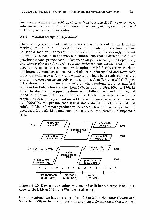
Too Little and Too Much: Water and Development in a Himalayan Watershed 23
fields were evaluated in 2001 at 46 sites (von Westarp 2002). Farmers were interviewed to obtain information on crop rotations, yields, and additions of fertilizer, compost and pesticides.
3.1.3 Production System Dynamics
The cropping systems adopted by farmers are influenced by the local soil fertility, rainfall and temperature regimes, available irrigation, labour, household food requirements and preferences, and increasingly, market opportunities. Based on the monsoon climate, the year is divided into three growing seasons: premonsoon (February to May), monsoon (June-September) and winter (October-January). Lowland irrigated cultivation (khet) centres around the monsoon rice crop, while upland rainfed cultivation (bari) is dominated by monsoon maize. As agriculture has intensified and more cash crops are being grown, fallow and winter wheat have been replaced by potato and tomato crops on intensively managed sites (Von Westarp 2004). Figure 3.1.5 shows the dominant shifts in production systems for khet and bari lands in the Bela sub-watershed from 1994 (n=200) to 1999/2000 (n=176). In 1994 the dominant cropping systems were fallow-rice-wheat on irrigated lands, and fallow-maize-wheat on rainfed lands. The importance of the staple monsoon crops (rice and maize) have not changed over time. However, by 1999/2000, the pre-monsoon fallow was reduced on both irrigated and rainfed fields and tomato production increased. In winter, wheat production decreased for both khet and bari, and potatoes had become an important crop.
fallow 70% wheat 48% KHET maize 28% il potato 8% 71994
monsoon rice y 100%
fallow 20% potato 44% 2000 tomato 12% wheat 21%
wheat4l% 1994 BARI fallow 97% 71 tomato 11%
maize maize 1 beans
100% V
fallow 71% potato 41% tomato 13% tomato 21%
2000
F M A M J J A S O N D J F M A
pre-monsoon monsoon winter (Feb - May) (Jun - Sep) (Oct - Jan)
Figure 3.1.5 Dominant cropping systems and shift in cash crops 1994-2000. (Brown 1997, Merz 2004, von Westarp et al. 2004)
Cropping intensities have increased from 2.2 to 2.7 in the 1990s (Brown and Shrestha 2000) to three crops per year on intensively managed khet and bari

24 Dynamic Changes Over Time: 1989-2004
fields (von Westarp et al. 2004). Seventy percent of households surveyed in 1995 (n=85) reported growing cash crops (Brown 1997) and all farmers intensively managing fields (3 crops per year) are growing at least 1 cash crop (von Westarp et al. 2004). The area under cash crop production has more than doubled since 1989 (Brown and Shrestha 2000), and with this shift toward market production, agro-chemical use has increased. Pesticide use and application rates (Figure 3.1.6) are highest for potato and tomato crops (Brown 1997), and fertilizer inputs (Figure 3.1.7) have increased parallel to intensification on irrigated khet and rainfed bari fields (von Westarp et al. 2004).
a) b)
100
80
60
40
20
0 w - o
. E 3 c.
o
E
+
100
75
50
25
0
-25
-50
-75
-100
Dithane
rice potato tomato
Figure 3.1.6 Pesticide applications to dominant crops a) % producers; b) dithane application relative to guidelines (Brown 1997).
a)
5000
4000
3000
2000
1000
0
1994 2000
khet
0
1994 2000
bar!
- maximum median
- minimum
Figure 3.1.7 Fertilizer inputs 1994-2000 for a) khet land and b) bari land. (von Westarp et al. 2004)
3.1.4 Farm Gross Margins
b)
5000
e 4000
G. ç c 3000
N 2000 t u 1000
The relative profitability of agricultural production between farms provides a mechanism to compare the economic status of farming households

Too Little and Too Much: Water and Development in a Himalayan Watershed 25
producing different crops. Computing gross margins defined as total returns less total variable costs (Rossiter 1995) for individual farms provides a measure of profitability. Total returns are equal to the value of all crops produced irrespective of whether the crop is sold. Variable costs include the purchase of seed, fertilizer and pesticides, hiring oxen and labour. Labour includes time planting, irrigation, fertilizing, spraying, weeding, harvesting, transporting and selling, and includes the opportunity cost of family labour. The farm gross margin is the return to fixed costs (land and livestock) and management (Brown and Kennedy 2005), and in agrarian economies where other sources of income are limited, gross margins are good approximations of economic well-being.
Gross margins were determined for individual crops and for the dominant cropping systems at the farm level for households in the Bela sub-watershed. Total returns are calculated by multiplying crop production (kg grain or vegetable components) by the selling price in the local market plus the value of the crop residue as it represents the opportunity cost of residues for animal fodder. Total returns and variable costs for individual crops are presented in Table 3.1.2.
Table 3.1.2 Total returns and variable costs (median values) for major irrigated and rainfed crops (Brown 1997).
Irrigated 1 Rainfed rice wheat tomato potato maize wheat otato tomato
n 69 47 10 16 84 40 15 9
Area (ha) 0.25 0.18 0.10 0.09 0.71 0.31 0.08 0.10 Production (kg) 964 280 620 477 1,610 385 431 239 Price ($/kg) 0.13 0.08 0.35 0.28 0.11 0.08 0.35 0.28 Total returns
481 134 2 152 1 531 328 80 1 858 1 042 ($/ha) , , , ,
Costs Seed ($) 3 4 3 14 5 4 3 13 Fertilizer ($) 20 10 5 18 41 3 5 10 Pesticide ($) 1 0 219 3 0 0 6 3 Oxen ($) 24 20 15 12 29 24 5 10 Labour ($) 49 16 45 21 65 16 24 20 Total variable costs ($/ha) 414 281 741 775 254 146 735 562
Total returns on a per hectare basis are greatest for tomatoes and potatoes on both irrigated and rainfed lands, but rice and maize grown during the monsoon are also important crops as the area under production is higher. Returns under irrigated conditions are greater than from rainfed land for the saure crops, indicative of the greater production potential of irrigated fields. The total variable costs are dominated by labour and oxen costs.
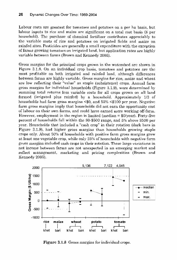
26 Dynamic Changes Over Time: 1989-2004
Labour costs are greatest for tomatoes and potatoes on a per ha basis, but labour inputs to rice and maize are significant on a total cost basis ($ per household). The purchase of chemical fertilizer contributes appreciably to the variable costs of rice and potatoes on irrigated fields and maize on rainfed sites. Pesticides are generally a small expenditure with the exception of farms growing tomatoes on irrigated land, but application rates are highly variable between farms (Brown and Kennedy 2005).
Gross margins for the principal crops grown in the watershed are shown in Figure 3.1.8. On an individual crop basis, tomatoes and potatoes are the most profitable on both irrigated and rainfed land, although différences between farms are highly variable. Gross margins for rice, maize and wheat are low reflecting their "value" as staple (subsistence) crops. Annual farm gross margins for individual households (Figure 3.1.9), were determined by summing total returns less variable costs for all crops grown on all land farmed (irrigated plus rainfed) by a household. Approximately 1/3 of households had farm gross margins <$0, and 55% <$100 per year. Negative farm gross margins imply that households did not earn the opportunity cost of labour on their own farms, and could have earned more working off-farm. However, employment in the region is limited (median = $0/year). Forty-five percent of households fall within the $0-$500 range, and 5% above $500 per year. Households that included a "cash crop" in their rotation (dark bars in Figure 3.1.9), had higher gross margins than households growing staple crops only. About 50% of households with positive farm gross margins grew at least one vegetable crop, while only 25% of households with negative farm gross margins included cash crops in their rotation. These large variations in net income between farms are not unexpected in an emerging market and reflect management, marketing and pricing complexities (Brown and Kennedy 2005).
2000 5,136 7,122 4,045
1500
u) 1000
-1000
-s - median
- min.
- max.
rice maize wheat potato tomato
1 1 II Il I
khet bari khet bari khet bari khet ban
Figure 3.1.8 Gross margins for individual crops.

Too Little and Too Much: Water and Development in a Himalayan Watershed
U)
2000
1500 +
V E 0
LL
-500 0
O staple crops only
with cash crop
10 20
-1'--. 1 -I T-
27
30 40 50
Sample number 60 70 80
Figure 3.1.9 Annual farm gross margins (each bar represents an individual household).
3.1.5 Farm Size and Food Security
Total returns and gross margins for farms are related to both land holdings and household food security. Households reporting that the land they farm was insufficient, marginal or sufficient to meet their basic need requirements are shown in Table 3.1.3. Forty-five percent of the households that reported insufficient production had farm gross margins < $0 per year, while 45% and 49% of marginal and sufficient households had gross margins > $100 per year. Of the households unable to meet their basic needs through agriculture, per capita land ownership was the lowest and none of these households had per capita gross margins > $33 per year.
Table 3.1.3 Self-sufficiency from land farmed versus land ownership and farm gross margins.
Sufficient n Land ownership (ha it
Farm gross margin (% households) per cap a) <$0 > $100
No 11 0.13 45 27 Marginal 29 0.15 17 45 Yes 45 0.20 31 49
Analyzing economic indicators by farm size (Figure 3.1.10) indicates that while small landholders have the ability to produce cash crops they often do

28 Dynamic Changes Over Time: 1989-2004
not sell the vegetable crops they produce. Small-scale farmers (<1 ha) make up 46% of producers in the watershed and the proportion growing vegetable crops is similar to medium and large-scale producers (16%, 14% and 12% respectively). Total returns increase with farm size, but small farms growing vegetables are more efficient on a per hectare basis. Variable costs diminish with the amount of land farmed, suggesting economies of scale exist, but gross margins are greatest for large landowners growing staple crops and medium landowners incorporating vegetable crops suggesting economic, labour and/or management constraints to large-scale vegetable production (Brown and Kennedy 2005).
100
75 +
small>1 ha
medium 1-2 ha
large >2 ha
50+------------------
---------------- 25 ---m n
staple
Crops sold (%)
staple vegetable
Returns ($) Gross margins ($)
Figure 3.1.10 Economic indicators by farm size.
3.1.6 Subsistence versus Commercial Production
1000
1- 750
1- 250
The level of involvement of farming households in the market is indicated by the amount and type of crops sold (Figure 3.1.11). Farmers sell a variety of crops including traditional staple (cereal crops) and non-traditional cash crops (vegetables). Only a small minority of farmers systematically produced for the market, but 45% of farmers derive some income from the sale of agricultural products. The majority sold < 50% of their crop, suggesting that sales were surplus production with the exception of vegetable crops. Tomatoes and potatoes comprised the largest amount sold on both a weight and revenue basis. Small producers (<1 ha) did not report selling >50% of crops; but focused on subsistence food production. Medium producers (1-2 ha) produced a mix of subsistence and commercial production, a combination likely to reduce risk, despite the higher returns to land and labour from cash
vegetable staple vegetable
% Farms

Too Little and Too Much: Water and Development in a Himalayan Watershed 29
crops. The high costs of inputs such as fertilizer, pesticides and seed restrict opportunities for farmers with limited access to capital. Retail prices fluctuate seasonally and inter-annually, vegetable yields are often variable, and labour requirements are increased substantially under vegetable production, limiting the participation of small-scale farmers. Mid-size producers are active in cash crop production, displayed higher gross margins and sold a greater proportion of their production (Brown and Kennedy 2005).
tomato
potato
maize
rice
wheat
0 20 40
% Producers selling > 50%
60
Figure 3.1.11 Involvement in market oriented agricultural production.
3.1.7 Conclusions
Population growth and poverty are two important socio-economic factors influencing farming system dynamics. Population growth rates up to 6% have reduced the available land per capita and contributed to agricultural intensification. Land distribution is highly skewed, and 55% of households are not able to meet their basic need requirements from the land they farm. Farmers with land holdings >1 ha were better suited to input intensive market production, resulting in greater local inequities. With vegetable production the aggregate gross margin is slightly higher, but the variability between farms growing cash crops ($137/year) and those growing only staple crops ($12/year) has resulted in greater economic disparity. Land ownership, cash availability to purchase inputs, and risk aversion appear to influence decision-making about the amount and type of cash crops produced and sold. Vegetable production is expected to continue in the watershed, but price fluctuations, variable yields, inflation and the current administrative instability in Nepal will likely constrain small scale farmers' entry into the cash crop market, and the costs and benefits of the developing market will continue to be unevenly distributed.

30 Dynamic Changes Over Time: 1989-2004
References
APROSC. 1995. Agriculture perspective plan, Nepal. Prepared for the National Planning Commision, His Majesty's Government Nepal and Asian Development Bank. Agriculture Project Services Center (APROSC) and John Mellor Associates.
Brown, S. 1997. Soil fertility, nutrient dynamics and socio-economic interactions in the Middle Mountains of Nepal. PhD Thesis. Faculty of Graduate Studies, University of British Columbia, Vancouver, Canada. 254 pp.
Brown, S., and G. Kennedy. 2005. A case study of cash cropping in Nepal: poverty alleviation or inequity. Agriculture and Human Values, 22:105-116.
Brown, S., and B. Shrestha. 2000. Market driven land-use dynamics in the middle mountains of Nepal. Journal of Environmental Management, 59: 217- 225.
Chitrakar, P.L. 1990. Planning, agriculture and farmers. Kedar Pradhan Printing, Kathmandu. 332 pp.
FAO. 2005. FAO Statistical Databases. (http://faostat.fao.org/default.aspx ).
Ives, J., and B. Messerli. 1989. The Himalayan dilemma: reconciling development and conservation. Routledge, London. 295 pp.
Kennedy, G., and C. Dunlop. 1989. A study of farming-household systems in Panchkhal Panchayat, Nepal. Department of Agricultural Economics, University of British Columbia. 126 pp.
Merz, J. 2004. Water Balances, Floods and Sediment Transport in the Hindu Kush-Himalayan region. Geographical Bernensia G72. Department of Geography, University of Bern and International Centre for Integrated Mountain Development, Kathmandu.
Rossiter, D. 1995. Economic land evaluation: why and how. Soil Use and Management, 11: 132-140.
von Westarp, S., H. Schreier, S. Brown, and P.B. Shah. 2004. Agricultural intensification and the impacts on soil fertility in the Middle Mountains of Nepal. Canadian Journal of Soil Science, 84(3) 323-332.
von Westarp, S. 2002. Linkages between agricultural intensification, soil- fertility dynamics, and low-cost drip irrigation in the Middle Mountains of Nepal. M.Sc. Thesis, Dept. of Soil Science, University of British Columbia. 198 pp.

Too Little and Too Much: Water and Development in a Himalayan Watershed 31
3.2 Land Use Dynamics 1947-2004
Bhuban Shrestha, Sandra Brown and Hans Schreier
Quantifying land use and tracking changes over time provides a good indication of the pressure exerted on land and water resources in the watershed. Land use can be determined from high resolution aerial photos or high resolution satellite photography, combined with field verification. However, information on land use intensification requires additional information usually obtained from farm interviews. In the first part of section 3.2 the land use changes are documented, and in the second part the changes in land use intensification are discussed.
3.2.1 Changes in Land Use Categories between 1947 and 2004
A quantitative assessment of land use change was accomplished using aerial imagery, photo-interpretation, and field verification techniques. Information on land use changes provide not only an indication of how economic activities are changing in the watershed, but also how the hydrological cycle is being affected by the différent land uses. Climatic events have a signif"icant influence on the hydrological cycle, but land use changes are of similar importance in altering the rainfall-run-infiltration processes. Land use changes in the watershed were documented over a 58 year period using a range of différent resources, as indicated in Table 3.2.1.
Table 3.2.1 Data sources for historie land use evaluation.
Year Data Sources Scale Land Use Categories
1947 Topographic & Land Use Map 1: 50,000 Agriculture, Shrub, Forest
1972 Aerial Photos 1: 20,000 Irrigated and Rainfed Agriculture, Grassland Shrub, Forest
1981 Land Use Map 1: 50,000 Agriculture, Shrub, Forest
1990 Aerial Photos 1; 20,000
1996 Aerial Photos 1: 20,000 Irrigated and Rainfed Agriculture, G l d Sh b F t
2004 IKONOS Satellite Image lm resolution
rass an , ru , ores
The original 1947 land use map produced by the Topographie Survey and the 1981 land use map produced by the Land Resources Mapping Project (LRMP 1983) were used as databases for the early historie analysis. These maps were digitized using ARCINFO© software, and land use change was determined using GIS overlay techniques. As is evident from Figure 3.2.1

32 Dynamic Changes Over Time: 1989-2004
and Table 3.2.2, over this 33 year time period forest degradation was widespread and 24% of the forest area was lost. Ten percent of the forest land was converted into agriculture and 14% degraded into shrub land.
1947 - 1981
Agriculture Forest
Shrub
Figure 3.2.1 Land use change between 1947 and 1981.
Table 3.2.2 Land use and change 1947-1981.
Land use types 1947 1981 Changes 1947-1981 Agriculture 49% 59% +10 % Forest 43% 19% -24% Shrub 7% 22 % +15%
Aerial photos at a 1:20'000 scale were used for the 1972-1996 land use comparison, and high resolution satellite imagery was used for the 2001 land use classification. This allowed for a more refined land use classification in which irrigated and rainfed agricultural land, forest, shrub and grazing land were differentiated. In all cases the aerial imagery was interpreted by the same interpreter using the saure classification scheme, and detailed fieid verification was conducted in 1990, 1996, and 2001. A digital topographic map was produced at a scale of 1:20'000 using the 1990 aerial photos, ground survey data and photogrammetric techniques. This formed the platform for ail subsequent GIS analysis.
The detailed land use dynamics, summarized in Table 3.2.3 demonstrate that major land use changes occurred between 1972 and 1990, while only minor changes occurred in the subsequent 11 years. Forestry was at an all time low as early as 1972; this confirmed the results of the LRMP data produced in 1981. Between 1972 and 1990 the forest improved significantly

Too Little and Too Much: Water and Development in a Himalayan Watershed 33
(10%) due to a major afforestation effort by the Nepal-Australia Forestry Project (Mahat et al. 1987, Griffin et al. 1988). Over this time period grass and shrub lands were reduced by half, and rainfed agriculture expanded by 5%. The area of irrigated agriculture did not change; likely related to the unavailability of additional water resources to expand irrigation. A more detailed description of the changes between 1947 and 1990 can be found in Schreier et al. (1994).
Table 3.2.3 Land use changes 1972-2001.
Land Use Type Percent of Watershed in
Différent Land Use Classes 1972 1990 1996 2001
Irrigated agriculture (khet) 15 16 16 15
Rainfed agriculture (bari) 34 39 38 40
Forest 20 30 30 29
Grass 10 4 6 5
Shrub 17 8 7 9
Other 4 3 3 2
In examining the entire 1947-2001 period there are a number of potential causes likely responsible for the observed land uses changes. The rapid decline in forest cover in the 1950-1970's is attributed to a policy change in 1957, the Forest Nationalization Act which essentially placed all non- cultivated land under national jurisdiction, and in which the Forestry Department took over the management of forests. Local people and community groups who previously used and/or owned the forests were no longer in charge of forest management. During the transition period from private to national control many forests were cleared and converted into agriculture so that individuals could maintain land ownership. As a result, over harvesting of forest products and soil degradation occurred. Forest conditions reached an all time low in the late 1960's to early 1970's; during that time a major afforestation program was initiated through international assistance (Nepal-Australia Forestry Program). The Australian team worked closely with the National Forestry Department and Community groups, and succeeded in replanting large areas, predominantly with chir-pine. The concept behind the NAFP initiative was that chir-pine is an excellent colonizing species, it is a native tree, well adjusted to the prevailing climatic conditions, and can survive very poor and degraded soil conditions. However, chir-pine has a very low non-timber value. The local people will generally avoid using chir-pine because it is not useful for animal feed and the sparking characteristics of its firewood make it less desirable for cooking in open fires within houses.

34 Dynamic Changes Over Time: 1989-2004
The idea was that once the trees are well established a natural, secondary regeneration would follow, and a mixed native forest could be re-established. However, the loss of grazing land, an increase in stall feeding of animais, and an expansion in milk production over the past 15 years lead to a significant increase in the demand for animal feed. This resulted in the collection and harvesting of most of the secondary growth of native trees that are more suitable for animal fodder. Consequently, a large proportion of forests in the watershed are chir-pine plantation with little or no understory and the animal feed production in these forests is now very limited (Plate 3.2.1).
Plate 3.2.1 Current chir-pine forests.
The resulting chir-pine forest provides some control against erosion but, with the exception of the potential for timber harvesting in the future, these forests are not particularly useful; they provide few non-timber products and the quality of the grass production under the forest canopy is very limited.
Interestingly, the expansion in forest cover in the 1980's occurred mainly at lower elevations and on less steep slopes than rainfed agricultural expansion. This data was obtained by superimposing the area of forest and agricultural expansion, and grazing land losses onto the elevation and slope maps using GIS overlay techniques (Figure 3.2.2). These results are contrary to what good conservation practices advocate. Steep, high elevation slopes are more prone to land instability and soil erosion when converted from grazing land to agriculture. Converting these degraded grasslands into forests is generally considered a more appropriate conservation strategy.

Too Little and Too Much: Water and Development in a Himalayan Watershed 35
The results suggest that the pressure on the land base to increase food production is very high in this part of Nepal. Farmers are well aware of the increased erosion risk and their response is to build extensive terracing systems to minimize erosion. However, this practice is very labour intensive and requires continuous maintenance.
a) b)
15
10
5
0
-5
-10
-15
0-4 5-19 20-35 36-49 50-155 750- 1000- 1200- 1400- 1600-
999 1199 1399 1599 2099
Slope Angle Category (%) Elevation Class
% Forest % Rainfed Agric. % Grazing Land
Figure 3.2.2 Land use gains and losses between 1972 and 1990 in relation to a) slope angle and b) elevation.
Another key event which resulted in significant land use policy changes was the establishment of democracy in Nepal in 1993. The management and control over forests was to be returned to local communities. This was greeted with much optimism in the hope that forest cover would improve. Through the 1990's it was suggested that communities would do a much better job of re-establishing and maintaining a multi-purpose forest than centralized forest management. The recent re-analysis of the data conducted in 2001 showed that there was no evidence that the forests expanded, but that the quality had improved. However, since the Maoist rebellion in 2003 forest degradation bas slightly increased once again due to the continued high demand for forest products and the lack of control over the forest resources during human conflicts.
Figure 3.2.3 shows that over a 58 year historic period, forests in the watershed have undergone a cycle of degradation, rehabilitation and once again degradation. Unfortunately, the rehabilitation period was insufficient to either re-establish the saure forest cover or the forest quality of the pre- 1950 period. As a result, the multi-purpose and non-timber use of forests have declined significantly, and under the current population pressure further deterioration is expected.

36 Dynamic Changes Over Time: 1989-2004
Figure 3.2.3 Overall changes in land use, 1947-2004.
Historic trends for agricultural land show a slow but consistent increase in the area under cultivation. Recent increases in rainfed agriculture (5%) are largely associated with the conversion of grasslands, while the expansion of irrigated land (1%) was limited by water availability. Most of the water resources were fully allocated during the 1990's, and severely constrained agricultural expansion. All easily convertible degraded lands were converted for food production, and by 1996 little additional land remained that could be put into production without major capital and/or human investment. Consequently, changes in land use categories have been minimal. However, the intensity of land use has changed.
3.2.2 Changes in Land Use Intensification
By 1990 most of the land area that could be converted into agriculture was used to produce food for local consumption, and from the socio-economic survey conducted at that time it was evident that food supplies were still insufficient to meet the basic annual demand. Over the history of the project, the cropping intensity has changed from an average of 1.3-1.6 crop rotations per year in the 1980's (Hagen 1980, Panth and Gautam, 1987) to 2.2-2.7 crop rotations per year in the mid 1990's (Brown 1997). With the introduction of market oriented production and shorter growing season varieties, intensification has continued to increase and has now reached 4 crop rotations per year in a few extreme cases.
The proportion of households producing crops for market has more than doubled, 77% of farmers reported irrigation water shortages by 1999, and fertilizer and pesticide use increased dramatically with cash crop cultivation (Table 3.2.4). Total livestock numbers have remained relatively constant, but the

Too Little and Too Much: Water and Development in a Himalayan Watershed 37
number of milking animais (largely female buffalo) has increased. With the reduction in the area of grazing lands, more animais are stall fed and pressures on forests for animal fodder continues to grow.
Table 3.2.4 Indicators of agricultural intensification.
Indicator Unit 1989/1990 1995/1996 2000/2001
Cropping intensity
# crops grown per year 1,2 2.2-2.7 3-4
Market % households producing cash crops' 48 70
production # potato producers (irrigated)2 8 44
Lack of irrigation
% farmers reporting water shortages 1,3 43 60 77
Fertilizer use kg/ha irrigated fields 2 590 1946
% growers using pesticides - tomato 1
90
Pesticide use
% growers using pesticides - potatol 80
Dithane application (kg/ha) - potato 1,4 10 20
Cultivated land
Ha cultivated per capita 1,5 0.18 0.13 0.10
ilk l
% farmers selling milk 1
27 45
sa es # milking animals per household 1,3 0.5 0.8 1.5
Fodder shortages
% farmers reporting fodder shortages 55 87
Stall feeding
% farmers stall feeding animals 1
63 85
1 Brown 1997 2 von Westarp 2002 3 Water use survey 1999 4 Integrated pest management survey 1999 5 Population census data 2001

38 Dynamic Changes Over Time: 1989-2004
In addition to the cropping intensity, there is also pressure to use marginal lands. Some farmers take the risk to reclaim land on a temporary basis in the floodplain of the Jhikhu Khola river, knowing that the field will not usually survive the monsoon flooding period. These framers are able to grow one crop during the dry season, and if the monsoon is weak the fields may survive for two to three seasons. However, these fields have to be reconstructed on a recurring basis, and the work involved to do this is hard. An example of this type of practice is provided in Plate 3.2.2.
References
Brown, S. 1997. Soil fertility, nutrient dynamics and socio-economic interactions in the Middle Mountains of Nepal. PhD Thesis. Faculty of Graduate Studies, University of British Columbia, Vancouver, Canada. 254 pp.
Grifffin, D., K. Shepherd, and T. Mahat. 1988. Human impact on some forests of the middle mountains of Nepal. Part 5. Comparisons, concepts and some policy implications. Mountain Research and Development, 8: 43-52.
Hagen, T. 1980. Nepal. Oxford and IBH Press, New Delhi. 145 pp.
Mahat, T., D. Griffin, and K. Sheperd. 1987. Human impacts on some forests of the Middle Hills of Nepal: 4. A detailed study in SE Sindhu Palchok and NE Kabhre Palanchok. Mountain Resource and Development, 7: 111-134.
Merz, J. 2004. Water Balances, Floods and Sediment Transport in the Hindu Kush-Himalayan region. Geographical Bernensia G72. Department of Geography, University of Bern and International Centre for Integrated Mountain Development, Kathmandu.
Panth, M.P., and J.C. Gautam 1987. Mountain Farming Systems in Nepal. In: K.W. Riley, N. Mateo, G.C. Hawtin, and R. Yadav (eds.) Mountain agriculture and crop genetic resources. Oxford and IBH Press, New Delhi. pp. 51-68.
Schreier, H., S. Brown, M. Schmidt, P.B. Shah, B. Shrestha, G. Nakarmi, and S. Wymann. 1994. Gaining forests but losing ground: A GIS evaluation in a Himalayan Watershed. Environ. Management, 18: 139-150.
von Westarp, S. 2002. Linkages between agricultural intensification, soil- fertility dynamics, and low-cost drip irrigation in the Middle Mountains of Nepal. M.Sc. Thesis, Dept. of Soil Science, University of British Columbia. 198 pp.

Too Little and Too Much: Water and Development in a Himalayan Watershed 39
Plate 3.2.2 Examples of high risk conversion of the floodplain for agriculture on a temporary basis for food production.

40 Dynamic Changes Over Time: 1989-2004
3.3 Soil Nutrient Dynamics
Hans Schreier, Stephanie von Westarp, P.B. Shah and Sandra Brown
Maintaining soil nutrients in agriculture and forestry under increasing demand for biomass production is a major challenge around the world. The problem is complex; some 16 elements are known to be essential to plant growth and they rarely occur in a balanced manner in any one location. Nutrients are only available to plants in specific ionic forms, and it is the combined interactions between climate, topography, parent material, biotic activity and external inputs that determine the nutrient status of the soil at any given time.
The success of the green revolution was primarily due to the high input of chemical fertilizers that contain nutrients in the ionic form, useful to plant growth. However, the nutrient holding capacity of soils is highly variable and finding the right balance between plant needs, nutrient retention in the soil, and nutrient availability at all times of the year is very challenging. This balance between nutrient inputs and plant uptake is particularly difficult to manage in intensive cropping systems where insufficient inputs can lead to long terra degradation through the removal of soil nutrients from the system. In contrast, excessive inputs can lead to widespread water pollution which affects both human health and aquatic biodiversity.
In section 3.2, land use dynamics and the rapid intensification of cropping systems that have occurred in the Jhikhu Khola watershed were discussed. This high level of intensification raises questions about how to maintain long terra soil fertility; a particularly critical issue in Nepal where cultivated slopes are prone to soil erosion and where continuous harvesting of crops removes large quantities of nutrients each year.
Soil nutrient conditions in the watershed were first evaluated in 1990, as part of a soil survey. This was followed by more detailed soil analyses in 1994 and 2000 in selective agricultural fields and forests in two sub- watersheds. Detailed farm interviews were conducted at the saure time as the soil samples were collected which allowed the team to: a) identify nutrient deficiencies, b) determine the factors that influence nutrient availability, c) document how the nutrient status has changed over time in relation to land use intensification, and d) calculate nutrient balances for individual fields to obtain a more realistic evaluation of nutrient dynamics.
3.3.1 Nutrient Status in the Watershed
The initial soil research conducted between 1989 and 1992 (Wymann 1991, Schmidt et al. 1995, Shah and Schreier 1991) showed that the nutrient status was highly variable and large différences were observed between topographie conditions, soil type and land use. Table 3.3.1 provides average

Too Little and Too Much: Water and Development in a Himalayan Watershed 41
values for the macro-nutrient status in the watershed. The data indicates that most of the soils were acidic, had relatively low cation exchange capacity, low base cations, low organic matter content and low phosphorus content. The soil parent material, which consists primarily of silica rich quartzite, sand and siltstone and highly weathered phyllite, is the primary reason the soils in the watershed are acidic and contain low base cations. Potassium was the only nutrient that was consistently in a desirable range, as mica minerais, which are a source of K, are dominant in several geological formations in the watershed.
Table 3.3.1 Soil nutrient status in the Jhikhu Khola watershed in the early 1990's.
Soil variables (mean values)
Jhikhu Khola
watershed Dhulikhel
subwatershed Andheri
subwatershed Desirable
levels
Number of Samples (n = 255) (n = 256) (n = 2000)
pH (CaC12)
4.6 4.4 4.8 5.0-6.5
Cation Exchange Capacity CEC (cmol/kg-1)
10.4 10.5 10.8 > 15
Exchangeable Ça (cmol/kg-1)
2.58 2.18 3.8 > 3
Exchangeable Mg (cmol/kg-1) 0.99 0.61 1.4 > 1.5
Exchangeable K (cmol/kg-1)
0.29 0.27 0.28 > 0.25
Base Saturation (%) 39.0 30.9 51.7 > 50
Available P (mg/kg')
2.1 11.6 16.6 > 15
Carbon (%) 1.01 0.68 0.99 1.5-2.0
The red soils, which are dominant in the lower elevations of the watershed (800-1700m elevation), are the oldest soils in Nepal. They developed under warm and wet climatic conditions, and as a result are highly weathered and depleted of soluble salts. Kaolinite is the dominant clay minerai in these soils, and as a result they have a low CEC and a low capacity to hold nutrients. Phyllite is the dominant bedrock material for the red soils while quartzites, sand and siltstone are the dominant bedrock in the non-red soils.

42 Dynamic Changes Over Time: 1989-2004
3.3.2 Factors that Influence Soit Nutrients
The key factors that influence nutrient conditions are the inherited properties induced by the bedrock, topographie conditions and climatic factors, and factors related to land use management. To account for these factors, the watershed was divided into a 2x2x2x4 GIS based factorial design as outlined in Table 3.3.2. A soils, aspect, elevation and land use classification was developed using the GIS layers and with overlay techniques each combination of factors was displayed. This allowed for the location of each factor combination to be identified, and samples were collected to determine the effect of each of the key factors influencing soil fertility.
Table 3.3.2 Stratification of watershed into four factors than influence soil nutrient.
Elevation Slope Aspect Soil Type Land Use
< 1200m North Non-red Irrigated Agric. > 1200m South Red Rainfed Agric.
Shrub/grass
Forest
No. Samples
10 samples for each existing combination; total 240 samples
Of the potential 32 possible combinations only 24 actually existed. Ten soil samples were collected for chemical analysis for each of these 24 combination categories. This then allowed for the différences in nutrient conditions in relation to the différent factors to be examined.
The average values for each factor class are displayed in Table 3.3.3 and the results of the Mann-Whitney U-Test are provided in Table 3.3.4. The majority of factors displayed a significant influence on nutrient content with the exception of %C. Soil carbon could only be differentiated by aspect; north facing slopes are cooler and more moist, which promotes a higher soil carbon content. Soil acidity was influenced primarily by land use and base cations, and phosphorus was influenced by land use, soil type, topography and climate factors.
When further stratified by land use and soil type, the data showed significant différences between red and non-red soils (Figure 3.3.1). Forests which occur mainly on red soils had the most degraded nutrient conditions with very low Ça and phosphorus values. Red soils, regardless of land use, had higher Mg values and were consistently deficient in phosphorus. The high Fe and Al content in these red soils is responsible for converting available P into occluded (insoluble) P. Irrigated agriculture (khet) generally

Too Little and Too Much: Water and Development in a Himalayan Watershed 43
Table 3.3.3 Average nutrient values stratified by climatic, topographie, soil type and land use factors.
Factors pH CEC cmol/kg
Ça cmol/kg
Mg cmol/kg
K cmol/kg
BS %
P mg/kg
C %
Land Use Irrigated Agriculture 5.2 11.2 5.29 1.52 0.23 63.9 21.6 0.9
Rainfed Agriculture
4,8 10.7 3.60 1.47 0.35 52.6 20.6 1.0
Shrub / Grass 4.7 10.6 2.81 1.22 0.24 42.0 8.3 1.1 Forest 4.3 14.0 1.80 0.60 0.30 21.0 3.5 0.9 Soil Type Red Soils 4.9 13.0 3.97 1.77 0.37 46.8 9.8 1.0 Non-Red Soils 4.8 8.9 3.56 1.09 0.21 55.8 22.1 1.0
Slope Aspect North Facing 4.8 11.0 4.09 1.19 0.33 53.2 20.9 0.9 South Facing 4.9 10.6 3.40 1.60 0.23 50.2 12.2 1.1 Elevation <1200m 4.9 11.2 4.18 1.56 0.28 55.1 14.5 1.0 > 1200 m 4.7 10.1 3.10 1.14 0.28 46.7 19.6 1.0
Table 3.3.4 Significant différences in nutrient content between factors.
Comparisons pH CEC Ça Mg K BS P Land use comparison Irrigated versus Rainfed Irrigated versus Shrub Irrigated versus Forest Rainfed versus Shrub Rainfed versus Forest Shrub versus Forest
Yes
Yes
Yes
Yes
Yes
Yes
No
No
Yes
No
Yes
Yes
Yes
Yes Yes
Yes
Yes
Yes
No
Yes
Yes
Yes
Yes
No
Yes
No
Yes
No
No
No
Yes
Yes
Yes
Yes
Yes
Yes
No
Yes
Yes
Yes
Yes
Yes
No
No
No
No
No
No
Soil Comparison Red versus Non-Red Soils No Yes No Yes Yes Yes Yes No
Aspect Comparison North versus South Facing No No Yes Yes Yes No Yes Yes
Elevation comparison < 1200m versus > 1200m No No Yes Yes No Yes No No
Yes = significant différence (p= 0.05), No = no différence (Based on Mann-Whitney-U test)

160 Assisting Community Efforts to Improve Livelihoods & Environment
manure addition, soif samples were collected from each plot, mixed and analyzed for basic nutrients (10 soif samples were collected and pooled for each of the species soif type combinations). The experiment was continued for 4 years and the nutrient conditions were monitored every 6 months. The aim of the experiment was to examine how red soifs, which are the most difficult soifs to rehabilitate, would respond to litter addition in comparison with non-red soifs. An example of the experiment is provided in Plate 4.4.1.
Table 4.4.3 Sampling design for green manure addition.
Plot Brown Soil Red Soil #1 Red Soil # 2
Size Soil Color : 10YR 5/6 Soil Colon 5YR 5/6 Soil Color: 2.5YR 3/6
Tithonia Litter Tithonia Litter Tithonia Litter 2 kg/m2 additions 2 kg/m2 additions 2 kg/m2 additions every 6 months every 6 months every 6 months
Sunhemp Litter Sunhemp Litter Sunhemp Litter
1m2 2 kg/m2 additions 2 kg/m2 additions 2 kg/m2 additions
each every 6 months every 6 months every 6 months
Pigeon Pea Litter Pigeon Pea Litter Pigeon Pea Litter 2 kg/m2 additions 2 kg/m2 additions 2 kg/m2 additions every 6 months every 6 months every 6 months
Duration of experiment : April 1996 to April 2000 (4 years)
Plate 4.4.1 Experiment with green manure additions.

44 Dynamic Changes Over Time: 1989-2004
exhibited higher pH and Ça values than all other land uses as these fields receive significant base cation inputs through the irrigation water. With a few exceptions, rainfed agricultural fields were more acidic and had lower Ça and P values than irrigated fields, but they were generally more enriched than the shrub and forest sites which received no inputs and in many cases lose nutrients due to the excessive collection of forest litter.
(6 L ( (` C7 u
1 II I
Red
Red Non-Red
m m (7 (i (9
I 11 1
Red Non-Red Non-Red
- N
m u)
(7 i° I 1 L
m o
Red Non-Red
Figure 3.3.1 Comparison of nutrient conditions stratified by land use and soil type.
The average nutrient values were assigned to each of the 24 combination factors in the GIS database, and the spatial extent of nutrient deficiency in the Andheri sub-watershed was then determined (Table 3.3.5). The results showed that more than half of the area has high acidity and around 40% had low P and Ca. Based on an examination of the combined nutrient status, only 14% of the watershed had nutrient conditions that were judged to be sufficient in all three key nutrients. In contrast, 35% of the sub-watershed had major nutrient deficiencies where all three indicators were in the deficient range.

Too Little and Too Much: Water and Development in a Himalayan Watershed 45
Table 3.3.5 Nutrient deficient and sufficient areas in the Andheri watershed.
Nutrient Indicators Deficient Moderate Sufficient pH (acidity) Area in watershed
< 4.8 55.0%
4.8-5.0
17.1% > 5
27.9% Available Phosphorus < Area in watershed
5 mg/kg 37.4%
5-15 mg/kg 26.5%
> 15 mg/kg 38.1%
Exchangeable Calcium < 3 cmol/kg 3-4 cmol/kg > 4 cmol/kg Area in watershed 43.3% 28.1% 28.6%
Deficient in Combined status pH, P, Ça
Sufficient in pH, P, Ça
Area in watershed 35% 14%
Since nutrient conditions are not static and are highly influenced by management, it is critical that the change in the status of nutrients is examined over time. This is particularly important because of the rapid land use intensification that has occurred since the initial soil surveys were conducted in the early 1990's.
3.3.3 Soit Nutrient Changes Over Time
Maintaining nutrients on sloping fields under rainfed agriculture has long been a concern. The risk of soil erosion is high, and returning sufficient organic matter and nutrients to these fields is very labour intensive. In addition, a new concern emerged in the late 1990's: Are there sufficient soil inputs to sustain long terra nutrient conditions in the intensively used irrigated fields which are under triple annual crop rotations? This question was addressed in two types of experiments: 1) comparing intensively used soils collected in 1994 and 2000, and 2) comparing soils in intensively used fields with adjacent undisturbed and uncultivated soils. These latter soils are considered control sites which have not received any nutrient inputs and should be reflective of the nutrient conditions that prevailed before agricultural intensification occurred. The number of samples that were available for this comparison of nutrient changes over time is provided in Table 3.3.6.
Table 3.3.6 Samples used to compare nutrient changes in intensively used agricultural fields.
Samples 1994 2000 control Intensively used irrigated fields (khet) (n=26) (n=26) (n=8) Intensively used rainfed fields (bari) (n=32) (n=20) (n=11)

46 Dynamic Changes Over Time: 1989-2004
As shown in Figure 3.3.2 exchangeable Ca, Mg, and K decreased significantly between 1994 and 2000 in intensively used irrigated fields. In contrast, available P values have increased dramatically in both irrigated and rainfed fields. Phosphorus values at the control sites were of the same order of magnitude as the 1994 values, and confirm the observed increase in phosphorus levels. The results suggest that insufficient inputs and leaching of base cations are responsible for the decline in cations over the 6 year period, while excess applications of chemical fertilizers (diammonium- phosphate, DAP) are likely responsible for the increase in the P status of the soils. P deficiencies in Nepalese soils were identified in the early phases of our project and foreign aid programs such as the Japanese program, addressed this issue by making diammonium-phosphate fertilizer readily available in the watershed in the mid 1990's. The resultant rapid increase in soil P, however, leads to concerns about eutrophication.
a) changes in exchangeable Mg b) changes in exchangeable Ça 1.5 6
coi
1994 2000
c) changes in available P 120
1994 2000
1994 2000
d) changes in exchangeable K 0.5
1994
Inigated -u-Rainfed Control
2000
Figure 3.3.2 Changes in nutrient status between 1994-2000 in intensively used fields and control sites.

Too Little and Too Much: Water and Development in a Himalayan Watershed 47
Phosphorus levels in the intensively used rainfed (bari) fields increased significantly between 1994 and 2000. However, in contrast to the irrigated fields, potash, calcium and magnesium levels increased or were maintained in the intensively used rainfed fields. This suggests that in rainfed agriculture base cations are maintained and managed in a sustainable manner, but additional inputs of cations are needed in the irrigated fields in order to sustain the long terra productivity of the soils. Phosphorus has now reached high levels in both intensively used irrigated and rainfed fields, and it is suggested that annual inputs should be reduced for environmental and economic efficiency reasons.
When the soil samples from the intensively used fields were collected in 1994 and in 2000, a household survey was conducted with each farmer to obtain information on crop yields, management practices and nutrient inputs. From this information it was possible to document how the fertilizer and compost inputs had changed. As shown in Figure 3.3.3, the overall nutrient inputs increased sharply between 1994 and 2000; and indicate that farmers were made aware of the increased nutrient demands of the new crops and higher yielding varieties. Not only has the amount of fertilizer and compost use increased but a significant change occurred in the type of fertilizers used. Urea (46-0-0) and complex fertilizer (20-20-20), which were the dominant fertilizers used in 1994, were replaced in favour of diammonium-phosphate (DAP), and this replacement is believed to be related to the rapid increase in soil P over this same time period. Changes in the type and rates of fertilizer and compost application were necessary due to the expansion of potato and tomato crop production in the early 1990's. The farmers rapidly learned that these crops are more nutrient demanding than the basic staple crops such as wheat, rice, and millets. Potash fertilizer was not used much in 1994 as it was not readily available and there was the perception that there were sufficient quantities of K in the soils, as corroborated by the early soil analysis. However, since potato and tomato crops have high demands for potassium it is evident that K additions will be required in irrigated fields if high production levels are to be maintained in the long run. Rainfed fields did not show a decline in potassium; likely due to lower leaching losses than in irrigated fields, and the fart that bari fields received more than twice the rate of compost application than the irrigated fields (Table 3.3.7). Compost in Nepal is high in cations as the ashes from the fuelwood used for cooking are incorporated.
These results clearly illustrate that managing nutrients in intensive farming systems is a complex process. Farmers are quick to adopt new crops, cropping cycle intensification and use of agro-chemicals. However, in order to maintain the long terra productivity it is essential to use a balanced approach that includes the combined use of carbon rich compost and chemical fertilizers. As shown above, focusing on N and P inputs in isolation of the other essential nutrients is short sighted, because ultimately, it is the balance of the remaining nutrients that control productivity. The next step is

48 Dynamic Changes Over Time: 1989-2004
to rectify the potash deficiency and that will need to be followed by additions of Ça and Mg in order to replenish the base cations and to control or improve acidity. Ultimately micro-nutrients will also be of concern but our preliminary analysis did not show major deficiencies in 2000.
a) Annual nutrient inputs 2000 b)
800
z z Q)
Cr
Fertilizer ci Compost
a d Y D ( i m m w f0 C N Ç m . O) .
Changes in annual fertilizer and compost applications 1994-2000
100000
o
â
10000
1000
100
10 - Compost -a Fertilizer
1994 2000
krigated 1994 2000
Rainfed
Figure 3.3.3 a) Fertilizer and compost application rates in 2000, and b) changes in total applications between 1994-2000, in intensively used agricultural fields.
Table 3.3.7 Compost application rates in intensively used agricultural fields.
Intensively used agricultural
fields
Irrigated (Khet)
Rainfed (Bari)
1994 - Median 2000 - Median 2000 - Maximum application application Application
(t/ha) (t/ha) (t/ha)
4.9
12.2
14.7
39.2
39
55
Monitoring the soil nutrient status every few years is a good first step in assuring adequate nutrient supplies, but this only provides a snapshot of the current problems. A more comprehensive evaluation should be carried out every 4-5 years in the form of a nutrient budget calculation for each farm or field. In this way, long terra sustainability problems can lie anticipated before yield declines are experienced. The topic of nutrient budgets is addressed in the following section.
D

Too Little and Too Much: Water and Development in a Himalayan Watershed 49
3.3.4 Calculating Nutrient Balances for Individual Fields
To gain a better insight about nutrient dynamics in intensively used sites it is essential to conduct nutrient balance sheets. This was first done using the 1994 data from the Andheri Khola watershed (Brown et al. 1999) and the results were then compared with the budget calculation obtained in 2000. In order to determine nutrient balances, detailed information is needed on crop yields, nutrient content in the harvested crop, nutrients lost via soil erosion, inputs of fertilizers, compost, atmospheric sources, nutrients made available via microbial activity, and nutrient inputs via irrigation water and sediments. A detailed description of the nutrient balance calculation is provided by Brown (1997), Brown et al. (1999), von Westarp (2002), and von Westarp et al. (2004). If annual inputs are less than losses via erosion, crop uptake and leaching, then soil nutrients are being mined over time. If the inputs exceed the demand then there is concern of polluting the water resources. The ultimate aim is to provide a more precise assessment of how well the nutrients are balanced in the soil on an annual basis.
Since the inherited soil conditions and management differ between fields, it is important to calculate nutrient balance sheets for individual fields. All inputs, uptakes and losses were calculated for each of the intensively surveyed 26 irrigated and rainfed fields. Figure 3.3.4 shows the overall median N, P, and K budget results for rainfed maize and irrigated rice fields for 1994 and 2000.
f K
1994 2000
Irrigated
1994 2000
Rainfed
Figure 3.3.4 Overall nutrient budget changes between 1994 and 2000 in intensively used fields (median values).
The results showed that in 1994 most of the rainfed and irrigated fields had a slight K deficit, but N and P budgets were balanced. By 2000 the median P-budget for rainfed and irrigated fields had a significant surplus and the median budget for rainfed N and K was also positive. In contrast the median

50 Dynamic Changes Over Time: 1989-2004
N and K budget in irrigated fields had significant deficits. This suggests that from an economic and environmental point of view a more precise management of nutrients is required.
The results of N, P, and K-budgets for individual fields are provided in Figures 3.3.5 and 3.3.6, and the results illustrate that most fields could benefit from more precise nutrient management practices. Fifty percent of all irrigated rice fields had an N deficit, 100% had a K deficit, and all fields had a P surplus. In contrast, 92% of rainfed maize fields had an N-surplus, 85% had a P-surplus, and 35% had a K -surplus. This suggests that a reduction in inputs is appropriate for rainfed fields and in the P input to irrigated fields; but N and K applications need to be increased in irrigated fields.
Given the assumptions made within the budget model, the practical aspects of improving nutrient management, and the variability of soils it is suggested that a small surplus is likely desirable. If it is assumed that a surplus of 50 kg/ha of N, 20 kg/ha of P and 50 kg/ha of K is tolerable from both the economic and environmental standpoints then it is possible to arrive at a more realistic nutrient management picture, as shown in Table 3.3.8. The results illustrate that 54% of the fields need to have improved nitrogen inputs and 100% need to improve K inputs. In contrast, phosphorus inputs need to be reduced in 100% of the irrigated fields and 85% of the rainfed fields. In addition, nitrogen inputs need to be reduced in 92% of the rainfed fields to reach a balanced nutrient budget.
Table 3.3.8 Percent of fields with surplus or deficit applications of nutrients 1994 and 2000.
Deficit Surplus 1994 2000 1994 2000
Irrigated fields N > 50 kg surplus/deficit 19% 54% 23% 27%
P > 20 kg surplus/deficit 4% 0% 8% 100%
K > 50 kg surplus/deficit 12% 100% 27% 0%
Rainfed fields
N > 50 kg surplus/deficit 35% 0% 23% 92%
P > 20 kg surplus/deficit 0% 0% 50% 85%
K > 50 kg surplus/deficit 54% 19% 12% 35%

Too Little and Too Much: Water and Development in a Himalayan Watershed
400
300
200 c 3 100 cy o 0
-100 zr -200 -300 -400
400
300 N y
200
100
400 300 200
G) 100 c 3 0
-100 -200 -300 . -400 -500 -600
Intensive khet fields: year 2000 (n=26)
Intensive khet fields: year 2000 (n=26)
8650119119Iliisa°
Intensive khet fields: year 2000 (n=26)
505®®©LI°-_.
51
m -200 -I
-300
-400
400
Non-intensive khet fields: year 1994 (n=26)
«nnngnnnmonnnuai Li-
-100
Non-intensive khet fields: year 1994 (n=26)
400 300 ------------------ 200 --------------- 100
0 ça o
-100 -200 - - -300 -400 -------------------- -500 -------------------- -600
Non-intensive khet fields: year 1994 (n=26)
Figure 3.3.5 Changes in N, P, and K nutrient budgets of individual khet (irrigated) fields between 1994 and 2000.

52 Dynamic Changes Over Time: 1989-2004
500
400
300
c 3 200 Co o Qw 100
z (u 0 M a, -100
-200 -
-300
300
Intensive bari fields: Non-intensive bari fields: year 2000 (n=20) year 1994 (n=32)
500
400
300
c 3 200 100
Z -100 -200 -300
300
w
a 0 . ,oooooaooo08 Ili
-100
Intensive bari fields: year 2000 (n=20)
200 --------------------
Li
-100
400
300
c 3 200
100 a w 0
-100
-200
-300
400
®®.-- ..®a JBUOOU®®DDDSOOODII F
Non-intensive bari fields: year 1994 (n=32)
v 300-(--------------------
200 c 3 i° 2 100 1 -------------
0 Y r -100
-200
-300 1
Non-intensive bari fields: year 1994 (n=32)
Intensive bari fields: year 2000 (n=20)
Figure 3.3.6 Changes in N, P, and K nutrient budgets of individual bari (rainfed) fields between 1994 and 2000.
Too Little and Too Much: Water and Development in a Himalayan Watershed 53
3.3.5 Conclusions
The impact of the green revolution on nutrient management was documented in the Jhikhu Khola watershed between 1990 and 2000. In an attempt to improve their livelihoods, Nepali farmers rapidly accepted the introduction of high yielding crop varieties, the introduction of cash crops and the use of chemical fertilizers. In the process a number of soil nutrient deficiencies were overcome, but at the same time new nutrient problems were created. Initially phosphorus was found to be the most limiting nutrient but with the improved availability of diammonium phosphate (DAP) by 2000, P application rates were in excess of crop needs in the majority of the intensively used agricultural fields. In contrast potassium, which in the initial phase of the project was in ample supply in the soil, became deficient in intensively used irrigated fields. One of the reasons for this K deficiency was the widespread expansion of potato production, which has a high K demand. In the past virtually none of the chemical fertilizers applied to these fields had a K component, and as a result, massive K deficits became apparent. In the rainfed fields only a few deficits occurred because compost applications, which are almost 3 times higher than in irrigated fields, supplied sufficient potassium.
The lesson learned from this research is that nutrient management is complex. Focusing on individual nutrients is insufficient; in order to maintain the production capacity of the soils a more balanced nutrient management approach is needed. A combination of compost and chemical fertilizer is likely the safest approach. Unfortunately, organic matter for composting is in short supply in the watershed and to maintain the very intensive triple annual crop rotations a more precise and balanced nutrient management program is required. This can be accomplished by ongoing monitoring of soil nutrients, calculating nutrient balances every 5-7 years, maintaining sufficient organic matter in the soils, controlling soil pH, and applying macro and micro nutrients in a balanced manner.
While only the three most important macro-nutrients were addressed in the nutrient budgeting, there is clear evidence that other nutrients such as Ça and Mg, and trace metals require equal attention. The reduction of base cations will lead to an additional decrease in soil pH, a topic that will be addressed in section 4.3 "restoring the production capacity of degraded red soils".
References
Brown, S. 1997. Soil fertility, nutrient dynamics and socio-economic interactions in the Middle Mountains of Nepal. PhD Thesis. Faculty of Graduate Studies, University of British Columbia, Vancouver, Canada. 254 PP

54 Dynamic Changes Over Time: 1989-2004
Brown, S., H. Schreier, P.B. Shah, and L.M. Lavkulich. 1999. Modelling of soil nutrient budgets: An assessment of agricultural sustainability in Nepal. Soil Use and Management, 15:101-108.
Schmidt, M., H. Schreier, and P.B. Shah. 1995. A GIS evaluation of land use and soil fertility in a watershed in Nepal. Intern. Journ. Geographic Information System, 9: 317-327.
Shah, P., and H. Schreier. 1991. Nutrient deficiencies and soil fertility .
Workshop Proceedings: Soil fertility and Erosion Issues in the Middle Mountains of Nepal, April 22-25. Jhikhu Khola Watershed, Nepal. Proc. ISS and IDRC. pp 260-266.
von Westarp, S. 2002. Linkages between agricultural intensification, soil- fertility dynamics, and low-cost drip irrigation in the Middle Mountains of Nepal. M.Sc. Thesis, Dept. of Soil Science, University of British Columbia. 198 pp.
von Westarp, S., H. Schreier, S. Brown, and P.B. Shah. 2004. Agricultural intensification and the impact on soil fertility in the Middle Mountains of Nepal. Canadian Journ Soil Science, 84(3): 323-332.
Wymann. S. 1991. Landnutzungsintensivierung und Bodendegration in Mepalishen Hugelgebiet. Eine Fallstudie in Dhulikhel Khola Enzugsgebiet. MSc Thesis, Dept. of Geography. University of Bern., Switzerland. 11157 pp.en.
3.4 Water Demands, Uses and Supplies
Jurg Merz, Gopal Nakarmi, Pradeep M. Dangol, Madhau P. Dhakal and Bhawani.S. Dongol
In rural catchments of the Middle Mountains water is mainly used for domestic and agricultural purposes. In the Jhikhu Khola catchment this includes livestock watering at a household scale. Small-scale industries exist only to a limited extent in this catchment. These include flourmills and other small agro-processing units, which withdraw but release the saure amount of water at the saure quality back into the stream after using it. In this context the discussion below will focus on domestic, livestock and agricultural water demand and supply.
3.4.1 Water Demand
For the assessment of the current situation in terras of water demand and supply of rural catchments in Nepal a survey was conducted in the Jhikhu Khola catchment in September 1999. It was based on household interviews

Too Little and Too Much: Water and Development in a Himalayan Watershed 55
involving the female and male household heads. Questions related to water and agriculture, water and domestic use, water and livestock, and perceptions of water were asked. In total 356 respondents (178 female/178 male) were interviewed. These respondents were evenly distributed throughout the catchment. The estimated water demand for domestic and agricultural purposes were based on results from the water need and supply survey.
The survey (Merz et al. 2002, Merz et al. 2003) revealed that, in general:
irrigation water supply was of major concern; drinking water supply was a problem in parts of the catchment, but mainly on the ridges along the divide and spurs; drinking water quality was increasingly becoming an issue throughout the watershed; agricultural intensity as well as productivity in the Jhikhu Khola was significantly higher than in other parts of the Middle Mountains; soil erosion was only a minor issue in the watershed.
Domestic use
Water demand for domestic use was very low. On average the respondents in the Jhikhu Khola watershed indicated a use of 23.2 L day-1 water per person (Table 3.4.1). These water demands are below the recommended value of the Department of Water Supply and Sewerage (DWSS) of 45 L person-lday-1 (RWSSSP 1994) by a factor of about 2. This recommended water use value includes 20% for losses and wastage. Based on these values, the overall water demand for domestic use per year can be assumed to be 412,629 m3 in the Jhikhu Khola watershed.
Table 3.4.1 Water demand for domestic use in the Jhikhu Khola watershed.
Population 1 Domestic water use 2 Annual domestic water use (year) [1 person-lday-1] [ m3] [mm]
48,728 (1996)
1 Allen et al. 2000 2 Merz et al. 2002
23.2 412,629 3.7
This water use is above average in comparison with the estimated water use for Nepal of 12 L person-lday-1 (Gleick 2000). This amount includes primarily the water requirements for drinking, cooking and food preparation. Other water related activities such as washing and personal hygiene happen mostly at the watercourses or taps themselves. RWSSSP (1994) estimated

56 Dynamic Changes Over Time: 1989-2004
the water demand at 45 L person-1day-1 for areas where piped water supply is possible. In areas with difficult access to water and collection times of more than 15 minutes they assumed 25 L person-lday-1 and in local markets (Nepali bazaars) and townships, 60 L person-lday-1.
Agricultural use
Agriculture is dependent on water resources due to the water demand for irrigation and water use for extensive agriculture on rainfed terraces. The crops most commonly grown on irrigated land in the Jhikhu Khola watershed were rice during the monsoon season, followed by potato or wheat (Figure 3.4.1). This crop was then followed by maize, potato or tomato. On rainfed terraces maize, the main monsoon staple crop was grown followed by wheat, tomato, potato or barley. Wheat was often intercropped with mustard.
IRRIGATED AGRICULTURAL LAND
TOMATO MAIZE
POTATO
W H EAT
RAINFED AGRICULTURAL LAND
BARLEY
TOMATO
RICE
MUSTARD
POTATO
MAIZE WHEA
J F M A M J J A S O N D
Figure 3.4.1 Cropping calendar in the Jhikhu Khola watershed.
The theoretical crop water demand of différent crops differs tremendously depending on the climatic conditions in the watershed. The water requirement values in Table 3.4.2 show average conditions based on the climatological data for the main meteorological station located in Panchkhal from 1993-2001. The water requirements were calculated by CROPWAT 4 for Windows 4.3 for all crops except rice. The crop specifics were compiled in Merz et al. (2004). Rice water requirement was calculated according to MacDonald and Partners (1990). It is important to note that these water requirement values are calculated in view of maximum yield under the given conditions. It is understood that the crops in the field may grow with lower water amounts; however, this may have a major impact on the yields.

Tab
le 3
.4.2
Wat
er r
equi
rem
ents
for
mai
n cr
ops
in t
he J
hikh
u K
hola
wat
ersh
ed.
Crop
Cro
p w
ater
req
uire
men
ts [
mm
/mon
th]
Jan
Feb
Mar
A
pr
May
Ju
n Ju
l A
ug
Sept
O
ct
Nov
D
ec
Tot
al
IRR
IGA
TE
D
Ric
e 23
0 40
4.4
332.
3 26
9.7
168.
1 14
04.4
Whe
at
80.3
94
.7
72.4
10
.7
43.8
30
1.8
Pota
to
78.5
28
.2
17.9
56
.8
181.
4
Tom
ato
17.2
83
.3
145.
7 98
.6
344.
8
Mai
ze
8.6
58.7
15
0 94
.2
311.
4
RAINFED
Mai
ze
21.4
84
.7
165.
8 17
1.8
91.7
53
5.4
Whe
at
80.3
94
.7
72.4
10
.7
43.8
30
1.8
Pota
to
54
82.9
80
.5
54.9
27
2.3
Tom
ato
46.5
10
7.5
121.
7 36
.6
312.
3
Bar
ley
80.3
94
.7
69.5
10
.7
43.8
29
8.9
Mus
tard
37
.8
74.5
73
.4
27.1
21
2.9

58 Dynamic Changes Over Time: 1989-2004
The impact of water stress on yields can be estimated by the use of the yield response factor, which calculates the actual expected yield on the basis of the yields estimated for optimum water supply conditions (Doorenboos et al. 1979). Here optimum water conditions are assumed for maximum growth and yield.
By far the most water demanding trop on irrigated land was rite at 1400 mm/trop. This value corresponds well with the values of 1200 to 1800 mm/trop given by ILACO (1981). However, the impact on annual water resources availability was limited as rite is grown during the monsoon season. The recently introduced cash trop tomato followed with an assumed 345 mm water demand. Potato required less water than the traditional wheat trop grown in winter, mainly due to its shorter growing season. It is however important to note that in the watershed most potatoes were irrigated, and therefore use more water than wheat. Due to the drought resistance of the wheat trop and the relative sensitivity to soil water deficits of the potato trop, farmers tend to keep the soil for a potato trop moist, whereas only one to two irrigations were supplied to the wheat trop (Doorenbos et al. 1979). On rainfed land the monsoon trop maize had the highest water demand, followed by wheat and tomato.
A number of different trop rotations exist in the Jhikhu Khola watershed. Pujara and Khanal (2002) identified 10 différent trop rotations on irrigated land always including rite, and 13 different rotations on rainfed agricultural land which included one maize trop. Water use is therefore only given for some major trop rotations as identified during the water demand and supply survey (Table 3.4.3).
Table 3.4.3 Water use for main trop rotations grown on irrigated fields.
Dominant rotation Annual water use Monthly water use rice-potato-maize rice-wheat-maize rice-potato-tomato rice-wheat
1897 mm/12 months 2018 mm/12 months 1931 mm/12 months 1706 mm/10 months
158 mm/month in 12 months 168 mm/month in 12 months 161 mm/month in 12 months 171 mm/month in 10 months
average 1898 mm/year 165 mm/month in 11.5 months
On rainfed agricultural land the following trop rotations (Table 3.4.4) were common in the Jhikhu Khola watershed according to the water demand and supply survey.
Recently différent vegetables have been introduced in the watershed such as bitter gourd, chilli, and eggplant. On the basis of Tables 3.4.3 and 3.4.4, and the area of the catchment, the annual water demand for the irrigated areas

Too Little and Too Much: Water and Development in a Himalayan Watershed 59
(1838 ha) was estimated to be about 313 mm/year. The water demand of the rainfed areas (4267 ha) was estimated at roughly about 349 mm/year.
Table 3.4.4 Water use for main trop rotations grown on rainfed fields.
Dominant rotation Annual water use Monthly water use maize-wheat maize-tomato maize-potato maize-mustard-wheat
837 mm/10 months 848 mm/7 months 808 mm/9 months 1050 mm/12 months
84 mm/month in 10 months 121 mm/month in 7 months 90 mm/month in 9 months 88 mm/month in 12 months
average 912 mm/vear 96 mm/month in 9.5 months
Livestock
Livestock are an important aspect of mountain agriculture in Nepal, and therefore, an important factor in the calculation of water demand. Cattle are often brought to the watering points. However, there has been an increase in stall feeding of goats, buffaloes and some cows which are less adapted to moving up and down the slopes, and these animais are watered on-site (Merz et al. 2002, RWSSSP 1994).
The water demand for the différent animais (Table 3.4.5) was estimated from a survey conducted in the Jhikhu Khola watershed and in the Kathmandu valley (n = 23), and verified with literature (ILACO 1981, RWSSSP 1994). In general the values for the Jhikhu Khola were slightly higher than the values in the literature, which seems to be appropriate given the hot conditions in the Jhikhu Khola watershed. Buffaloes required the greatest amount of water amongst the animals, followed by bullocks, cows and finally goats. With an average 1.2 buffaloes per household they account for the highest total water requirement per day, followed by the water requirements for goats. On average a household owned 3.5 goats. The total annual water requirement for livestock was 4.6 mm.
Table 3.4.5 Water demand for livestock watering.
Water demand T e of A i l Jhikhu Khola yp n ma (L/day) HH*no.1 m3/day
Buffalo 61 8,002* 1.2 585.7 Bullock 49 8,002* 0.8 313.7 Cow 23 8,002* 0.9 165.6 Goat 12 8,002* 3.5 336.0
Annual water use [m3] 511,365 Annual water use [mm] 4.6
Number of households (HH) from PARDYP times average number of animals per household (no.) from Merz et al. (2002)

60 Dynamic Changes Over Time: 1989-2004
Overall demand for human activities
The overall demand for water including domestic, agricultural and livestock water requirements amounted to approximately 670 mm per annum in the Jhikhu Khola watershed (Table 3.4.6).
Table 3.4.6 Overall water demand for human activities (all values in mm).
Agriculture Catchment Domestic Total Irrigated land Rainfed land Livestock
Jhikhu Khola 3.7
3.4.2 Water Supply
313 349 4.6 670.3
The people of the Jhikhu Khola watershed perceived water shortages both in terms of agricultural and domestic water supplies over the past 5 and 25 year periods (Table 3.4.7). Their concern was not only in terms of water quantity, but increasingly in terms of water quality. Water shortages were particularly felt during the pre-monsoon and early monsoon months (April to June). During this period, many water sources either dried up or had lower yields. The perception of the local residents is documented in detail in Merz et al. (2002) and Merz et al. (2003).
Table 3.4.7 Perceptions of water related problems in the Jhikhu Khola.
Jhikhu Khola watershed Total number of espondents = 356
No problems 12 %
I i ti quantity 41 %
rr ga on water quality 0%
D i ki quantity 37 %
r n ng water quality 9 %
Flooding 0%
Surface erosion 0%
Slumping 1%

Too Little and Too Much: Water and Development in a Himalayan Watershed 61
Domestic supply
Domestic water supply in the Jhikhu Khola catchment is met by the extensive network of taps (both proper tap stands and improvised, simple pipe ends) as well as traditional spring boxes, in Nepali called kuwas. According to Shrestha et al. (2000) more than 400 public water sources were identified in the Jhikhu Khola watershed during a mapping campaign in November and December of 1999. Out of these 400 sources, 319 were documented on the basis of relevance to local residents (Figure 3.4.1). Most of the observed sources were perennial, but according to the users flow decreased from March to May. Source yields varied significantly between sites from a minimum of 0.6 L/min to a maximum of 270 L/min. The combined yield of all sources was 3,492 L/min during the survey. The average flow was slightly higher in the case of taps (11.6 L/min) than in the spring boxes (8.2 L/min) and the natural springs (6.5 L/min). These values can be considered average as they were measured during the transition period from monsoon to dry season.
C) public water sources (monltored) + Public water sources (mapped)
Rivers
Figure 3.4.2 Documented public water sources in the Jhikhu Khola watershed (December 1999).

62 Dynamic Changes Over Time: 1989-2004
On average, 18 households depend on the same water source, with a maximum of 290 households dependent on one source. Average distances from the dependent households to the water sources varied from 3 to 600 m. The longer the distance to the water sources, the greater the pressure on the women's workloads. According to Merz et al. (2002), in 79% of households it was the women that fetched water. Children were often observed to support their mothers in this duty. The long distances to the sources were critical in terms of time, but also in terms of safety as steep and muddy paths become slippery and pose a major risk for water collection during the monsoon season.
In general, there was adequate water supply for domestic purposes in the watershed as determined on the basis of service levels using the approach of RWSSSP (1994) (Table 3.4.8). Service levels are given on the basis of population having access to the respective water sources. In this study, instead of the population, the public water sources themselves were documented and the service level of each source determined. This approach slightly overestimates the service level in terras of accessibility because an average distance was used for the assessment.
Table 3.4.8 Description of service level for water supplies (from RWSSSP 1994).
Categoryl Quality Quantity
(1 person-1 *day-1)
Reliability Accessibility (months/ (min) yr)
Continuity (h/day)
Service level 1 protected
> 45 <15 12 > 6 Good source
_ _
Service level 2 spring or
> 25 < 30 >_ 11 ? 5 Intermittent better _
Service level 3 any
> 15 <60 ?10 >4 Poor source _ _
Service level 4 Very poor
all water supplies All other water supplies
1 The service level of a source is determined by the lowest score in any of the five parameters.
The service levels determined for the Jhikhu Khola watershed are shown in Table 3.4.9. In general the overall service level was good to intermittent but 4.7% of sources ranked poor and 14.4% very poor. The main need for improvement was in accessibility and type of source.

Too Little and Too Much: Water and Development in a Himalayan Watershed 63
Table 3.4.9 Service levels for water sources.
Service level Description % water sources 1 good 57.4
2 intermittent 15.0
3 poor 4.7
4 very poor 14.4
Not assessed (missing parameters) 8.5
Agricultural supply
The most important water supply for agriculture is river discharge, which is supplied to the fields through a number of irrigation systems. In the Jhikhu Khola watershed, some of the fariner managed irrigation systems (FMIS) have been operational for over 100 years, and most systems are 50-65 years old. In the steep upland areas of Nepal, there is little possibility of extended, large-scale irrigation development. Therefore FMIS still play a crucial role in agricultural production. It is estimated that FMIS accounted for over 80% of the total irrigation development in the hills and mountains of Nepal in 1997 (Shah and Singh 2001).
In 1988, a total of 51 irrigation systems were operational in the Jhikhu Khola catchment with one of the best developed irrigation infrastructures in the Kavrepalanchok district (Multidisciplinary Consultants 1988). These systems supplied water to a total gross command area (GCA) of 1,491 ha. The main rivers acting as sources for these systems were the Danfey Khola, the Dhod Khola, the Dhital Khola, the Dhap Khola, the Subarno Khola, the Namde Khola, the Andheri Khola and the main Jhikhu Khola. The capacity of these systems ranged from 0.038 m3/s to 1.719 m3/s at the intake with GCAs from 10 to 186 ha. Sixty-five percent of these systems were perennial and the remaining 34% seasonal, only supplying water to crops during the monsoon. The cumulative capacity of all schemes was calculated as 9.6 m3/s for rice during the monsoon season, and as 4.95 m3/s for the winter crops.
Upadhyay (2001) conducted a detailed survey of the efficiency of water adequacy, equity in water allocation and technical aspects of two irrigation systems in the Jhikhu Khola watershed in 2000. The Devbhumitar irrigation system within the sub-catchment of the Andheri Khola had 43 users and a gross command area (GCA) of 33 ha. Only 16% of the farmers reported receiving adequate water for their winter crops, while all of them received ample supply for their monsoon crop. This has changed considerably over the last 30 years. Seventy-three percent of the users reported having an adequate supply for their winter crops 30 years ago and 66% reported an adequate supply 15 years ago. A similar situation was

64 Dynamic Changes Over Time: 1989-2004
shown in the Raj Kulo irrigation system in the upper Jhikhu Khola watershed. This was the largest irrigation system in the watershed with 1500 users and a 210 ha GCA. In this system the users at the head end usually received sufficient water throughout the year. The supply reduced dramatically towards the middle part and the tail end of the system, where only 35% reported receiving adequate water supply during the dry season. A similar temporal trend as seen in the Devbhumitar system was observed in terms of water supply over the last 30 years. In addition, unequal water allocation was strongly felt by the users of this system.
Conveyance losses are assumed to be high. Of the 76 km of irrigation canais, 75% were boulder lined and 24% were unlined (Teuling 2001). Only the remaining 1% of the total canal length was concrete lined. The conveyance losses of two irrigation systems in the Andheri Khola sub-catchment were documented by Nakarmi (1995). In one system a 35% water loss occurred over a distance of about 500 m. In the second system the initial water losses were small, but over a distance of 1 km, 90% of flow was lost through seepage. The greatest losses occurred when channels crossed fractured bedrock or sections of sandy and gravely soil material. MacDonald & Partners (1990) compiled the seepage losses on soils of different textures showing that the higher the clay content, the lower the expected seepage losses (Table 3.4.10), however the role of preferred pathways is unclear in this context.
Table 3.4.10 Seepage in irrigation canals.
Types of soil Seepage losses 1
Rock < 0.5
Impervious clay loam 0.8 to 1.2
Medium clay loam 1.2 to 1.7
Clay loam or silty soil 1.7 to 2.7 Gravelly clay loam, sandy clay or gravel cemented with clay 2.7 to 3.5
sandy loam 3.5 to 5.2
Sandy soil 5.2 to 6.4
Sandy soil with gravel 6.4 to 8.6
Pervious gravelly soil 8.6 to 10.4
Gravel with some earth 10.4 to 20.8
1 m3/s per mm2 of wetted perimeter or lis per km per m of wetted perimeter.
Source: Mac Donald & Partners (1990)

Too Little and Too Much: Water and Development in a Himalayan Watershed 65
In the Jhikhu Khola watershed, the soils in the valley bottom, the area with the most irrigation canais, are of loamy texture. Therefore, seepage Tosses are expected to be in the order of 1 to 5 m3/s per 1000 m2 of wetted perimeter. For a more detailed seepage assessment of the different systems a detailed soil map would be required. The intakes mapped by Teuling (2001) are temporary in nature, i.e. they often do not withstand monsoon floods. He mapped 30 intakes for the irrigation systems in the valley floor of the catchment. Nakarmi (1995) documented 72 diversion dams in the Andheri Khola sub-catchment feeding 58 ha of irrigated agricultural land.
Perceived changes in water supply
With the increasing intensity of agricultural production, the planting of high yielding varieties, and triple to quadruple crop rotations, the trend for irrigation water supply has, according to respondents, decreased in the Jhikhu Khola catchment in the last few years. Thirty-eight percent of the respondents indicated a decreasing trend in water availability, 29% reported no change, 24% did not answer and only 9 % reported an increase in water availability for irrigation over the last 5 years (Figure 3.4.3). Compared to 25 years ago, 40% of respondents indicated a decrease while only 8% perceived an increase in irrigation water availability. Domestic water supplies have also decreased over the last 5 and 25 years according to the interviewed households. Thirty-one percent and 35% perceived decreasing water availability for domestic purposes over the last 5 and 25 years, respectively. However, a large number of respondents also perceived an increase in domestic water availability; 25% and 26% over the last 5 and 25 years, respectively. This perceived increase in domestic water is largely related to the various programs on water supply funded by NGOs, INGOs and the government.
L increased decreased D no change D no answer
Domestic water 25 years
Irrigation water 25 years
Domestic water 5 years
Irrigation water 5 years
0% 10% 20% 30% 40% 50% 60% 70% 80% 90% 100%
Figure 3.4.3 Change in irrigation and domestic water supplies as perceived by the people interviewed.

66 Dynamic Changes Over Time: 1989-2004
3.4.3 Summary
Water demand in the Jhikhu Khola watershed is dominated by agricultural requirements. Irrigated agricultural land in particular requires large amounts of water per unit area. Rainfed agricultural land also requires a significant quantity of water, mainly due to the large areal coverage in the watershed and moderate to high requirements per unit area. Water demands for livestock and for domestic purposes are negligible in comparison. Based on a watershed-wide survey, the agricultural water supply was perceived to have decreased over the last 5 and 25 years.
References
Allen, R., H. Schreier, S. Brown, and P.B. Shah (eds.). 2000. The People and Resource Dynamics Project: the first three years (1996-1999). Workshop Proceedings, Boashan, Yunnan Province, China. March 2-5, 1999. International Centre for Integrated Mountain Development, Kathmandu. 333 pp.
Doorenbos, J., A.H. Kassam, C.L.M. Bentvelsen, V. Branscheid, J.M.G.A. Plusje, and M. Smith,G.O. Uittenbogaard, and H.K. Van der Wal. 1979. Yield response to water. FAO Irrigation and Drainage Paper No. 33. FAO, Rome.
Gleick, P.H. 2000. The world's water 2000-2001. Island Press, Washington.
ILACO. 1981. Agricultural Compendium for Rural Development in the Tropics and Subtropics. Elsevier Scientific Publishing Company, Amsterdam.
MacDonald & Partners. 1990. Design Manuals for Irrigation Projects in Nepal. Planning and Design Strengthening Project. His Majesties Government of Nepal, Ministry of Water Resources, Kathmandu.
Merz, J., G. Nakarmi, S. Shrestha, B. Shrestha, P.B. Shah, and R. Weingartner. 2002. Water and Erosion Studies of PARYP Nepal: Water Demand and Supply Survey. Brochure with CD-ROM. ICIMOD, Kathmandu.
Merz, J. G. Nakarmi, S.K. Shrestha, B.M. Dahal, P.M. Dangol, M.P. Dhakal, B.S. Dongol, S. Sharma, P.B. Shah, and R. Weingartner. 2003. Water: A scarce resource in rural watersheds of Nepal's Middle Mountains. Mountain Research and Development, 23 (1): 41-49.

Too Little and Too Much: Water and Development in a Himalayan Watershed 67
Merz, J., G. Nakarmi, S. Shrestha, B.M. Dahal, B.S. Dongol, M. Schaffner, S. Shakya and S. Sharma. 2004. Public water sources in rural watersheds of Nepal's Middle Mountains: Issues and constraints. Environmental Management, 34(1): 26-37.
Multidisciplinary Consultants. 1988. Water use inventory study of Kabhre Palanchok District. Volume 1: Main report. Water and Energy Commission Secretariat, Kathmandu.
Nakarmi, G. 1995. Indigenous water management systems in the Andheri Khola sub-watershed. In: Schreier, H, P.B. Shah, and S. Brown (eds). Challenges in mountain resources management in Nepal. Process, trends, and dynamics in middle mountains watershed. Kathmandu, 10-12 April 1995. ICIMOD, Kathmandu. pp 141-154.
Pujara, D.S., and N.R. Khanal. 2002. Use of pesticides in Jaishidihi sub- catchment, Jhikhu Khola catchment, Middle Mountains in Nepal. In: Herrmann, A., and S. Schumann (eds). International Workshop on Environmental Risk Assessment of Pesticides and Integrated Pesticide Management in Developing Countries. Heft 38. Braunschweig: Institute fuer Geooekologie, Technisiche Universitaet Braunschweig.
RWSSSP. 1994. Palpa District - Water supply and sanitation development plan. Rural Water Supply and Sanitation Project, Department of Water Supply and Sewerage, HMG/Ministry of Housing and Physical Planning, Kathmandu.
Shah, S.G., and G.N. Singh. 2001. Irrigation Development in Nepal: Investment, Efficiency and Institution. Research Report No. 47. Winrock International, Kathmandu.
Shrestha, S. G. Nakarmi, J. Merz, and R.C. Osti. 2000. Survey of public water sources in the Jhikhu Khola catchment. Capacity Building for Community Water Qualiy Assessment Project. Kathmandu. Unpublished report.
Teuling, A.J. 2001. A survey of fariner managed irrigation systems in the Jhikhu Khola watershed,Nepal. An application of GPS in the assessment of water availability. PARDYP, Kathmandu. Unpublished Report.
Upadhyay, K. 2001. Performance of local irrigation institutions in changing catchment conditions: a study of Jhikhu Khola catchment, Nepal. MSc Thesis, Asian Institute of Technology, Bangkok.

68 Dynamic Changes Over Time: 1989-2004
3.5 Hydrology and Sediment Transport
Jurg Merz, Pradeep M. Dangol, Madhau P. Dhakal, Bhawani S. Dongol, Gopal Nakarmi and Rolf Weingartner
From a regional perspective the main issues related to water are water availability, floods and sediment dynamics (Merz et al. 2005). Data availability for in-depth process studies has been the main limiting factor for improvement of the understanding of these environmental issues in Nepal. To better understand hydrological processes in the Himalayas, PARDYP set up a research monitoring network across the Hindu Kush Himalayas in five watersheds. The first network that was setup was located in the Jhikhu Khola watershed. While this is not a representative sample of the entire region, it provides insight into the relevant processes leading to flooding, water availability constraints, and sediment mobilization and transport at a high spatial and temporal resolution. The high resolution is achieved by means of automatic monitoring of temporal key parameters and detailed field surveys of spatial parameters.
3.5.1 Monitoring Network
A nested approach was used in the design of the monitoring stations. This approach to measurement network design has its origin in the understanding that hydrological processes vary with scale, as described in Ives and Messerli (1989), FAO (2002) and Schreier and Brown (2004). The network design was based on the investigation of processes and balances at different scales. For each scale all input variables were determined by means of measurements. For example, at the plot scale rainfall is measured with a rain gauge, and runoff and soil loss are measured using the erosion plot method. At the next largest scale, measurements are conducted by means of one or several representative rain gauges for the assessment of aerial rainfall, and by hydrological measurements at the hydrological stations located at the outlet of a well-defined sub-catchment. The integral systems response of the entire catchment is monitored at the outlet using hydrological and sediment measurements after establishing aerial rainfall from a number of representative and well-distributed rain gauges. The approach is schematically described in Figure 3.5.1.
Using the example in (Figure 3.5.1) the response of the surface to a rainfall event measured at the rain gauge R1 is investigated in the erosion plot Eladjacent to the rain gauge. The response to the saure event is then observed at the hydrological station of the sub-watershed B, and finally at the outlet of the main watershed A. Relating the processes from the rain gauge to the erosion plot and to the hydro stations at the sub-watershed and watershed levels allows one to draw conclusions on the processes involved. In the Jhikhu Khola watershed the size of the main watershed is 111 km2, corresponding to the hydrological meso-scale. The sub-catchments are
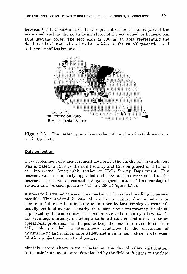
Too Little and Too Much: Water and Development in a Himalayan Watershed 69
between 0.7 to 5 km2 in size. They represent either a specific part of the watershed, such as the north-facing slopes of the watershed, or homogenous land use/land cover. The plot scale is 100 m2 in area representing the dominant land use believed to be decisive in the runoff generation and sediment mobilization process.
5
Erosion Plot A 6 Hydrological Station
r Meteorological Station i
Figure 3.5.1 The nested approach - a schematic explanation (abbreviations are in the text).
Data collection
The development of a measurement network in the Jhikhu Khola catchment was initiated in 1989 by the Soil Fertility and Erosion project of UBC and the Integrated Topographic section of HMG Survey Department. This network was continuously upgraded and new stations were added to the network. The network consisted of 5 hydrological stations, 11 meteorological stations and 7 erosion plots as of 15 July 2002 (Figure 3.5.2).
Automatic instruments were crosschecked with manual readings wherever possible. This assisted in case of instrument failure due to battery or electronic failure. All stations are maintained by local employees (readers), usually the land owner, a nearby shop keeper or a trustworthy individual supported by the community. The readers received a monthly salary, two 1- day trainings annually, including a technical session, and a discussion on operational problems. This helped to keep the readers up-to-date on their daily job, provided an atmosphere conducive to the discussion of measurement and maintenance issues, and maintained a close link between full-time project personnel and readers.
Monthly record sheets were collected on the day of salary distribution. Automatic instruments were downloaded by the field staff either in the field

70 Dynamic Changes Over Time: 1989-2004
office, if the readers could bring the loggers on the salary distribution day, or in-situ at the station using laptops and data shuttles or storage modules.
r r
Meteorologicai station
Erosion plot + Meteorological station
Hydrological station
Arniko Highway
Rivers
Catchments Jhikhu Khola Andheri Khola Kukhuri Khola UpoerAndheri Khola Kuh!nde Khola /\/ Watershed boundary
Figure 3.5.2 Research monitoring network of the Jhikhu Khola watershed (July 15, 2002)
3.5.2 Water Availability
Water availability is widely perceived to have decreased over recent years. Both farmers and scientists have noted the flows at the outlet of the watershed to have decreased over the last 10 to 15 years (Merz et al. 2002). However, this could not be shown on the basis of the streamflow data because the accuracy to determine low flow conditions was insufficient. The question therefore remains whether water resources were declining in the dry season due to potential climate change and more intensive use. The actual water availability and related issues were explored using a water balance approach. The main parameters (precipitation, evapotranspiration, runoff and storage) are discussed before this information is synthesized in a water accounting exercise.
Precipitation dynamics
The Jhikhu Khola watershed is a headwater system, and therefore, precipitation is the only input into its water cycle. Based on data from the
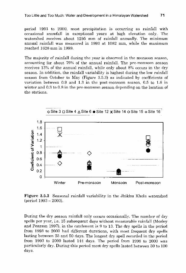
Too Little and Too Much: Water and Development in a Himalayan Watershed 71
period 1993 to 2000, most precipitation is occurring as rainfall with occasional snowfall in exceptional years at high elevation only. The watershed receives about 1295 mm of rainfall annually. The minimum annual rainfall was measured in 1993 at 1082 mm, while the maximum reached 1628 mm in 1999.
The majority of rainfall during the year is observed in the monsoon season, accounting for about 79% of the annual rainfall. The pre-monsoon season receives 13% of the annual rainfall, while only about 8% occurs in the dry season. In addition, the rainfall variability is highest during the low rainfall season from October to May (Figure 3.5.3) as indicated by coefficients of variation between 0.9 and 1.3 in the post-monsoon season, 0.5 to 1.6 in winter and 0.3 to 0.8 in the pre-monsoon season depending on the location of the stations.
0Site 3 Site 4 ASite 6 Site 12 )K Site 14 oSite 15 +Site 16
W inter Pre-monsoon Monsoon Post-monsoon
Figure 3.5.3 Seasonal rainfall variability in the Jhikhu Khola watershed (period 1993 - 2000).
During the dry season rainfall only occurs occasionally. The number of dry spells per year, i.e. 15 subsequent days without measurable rainfall (Mosley and Pearson 1997), in the catchment is 9 to 13. The dry spells in the period from 1993 to 2000 had différent durations, with most frequent dry spells lasting between 25 and 50 days. The longest dry spell recorded in the period from 1993 to 2000 lasted 144 days. The period from 1998 to 2000 was particularly dry. During this period most dry spells lasted between 50 to 100 days.

72 Dynamic Changes Over Time: 1989-2004
Spatially, the precipitation pattern is erratic during the dry season and no distinct pattern could be established. Elevation provided only a good relationship for annual and monsoon data and in months during the remainder of the year where exceptional high rainfall events occur. In general, the more rain, the better the relationship with elevation, and higher rainfalls occurred in the upper areas of the catchments.
In the context of water availability dynamics it is important to identify whether a trend could be observed in the measured data. Long-term data for Nepal do not show an increasing trend of precipitation (Shrestha et al. 2000), despite a number of climatic models predicting an increase in monsoon precipitation. These authors suggest that this may be due to the countering effects of increased atmospheric sulphate aerosols. Sharma (1997) came to a similar conclusion on the basis of his studies of the long terra precipitation data sets of Kathmandu and selected stations in the Kosi basin, where lie was not able to establish any homogenous and significant trends. Based on the long-term data available for the Jhikhu Khola watershed at Panchkhal and Dhulikhel, no significant trend could be established for annual precipitation amount at the confidence level of 5% (Table 3.5.1). The saure can be concluded for annual absolute maximum, where no trend was observed over the measurement period.
Table 3.5.1 Mann-Kendall test statistics for trend of mean annual rainfall in the Jhikhu Khola watershed (data: DHM, 2000; critical values see Salas 1992).
Station Period Critical value Test value Result Annual mean
Site 9 1948-1996
(n= 36) 1.96 (Sig.=0.05) 1.3605
HO is rejected
Site 12 1976-2000
(n= 23) 1.96 (Sig.=0.05) 0.1585
HO is rejected
Annual daily maximum
Site 9 1948-1996
(n= 36) 1.96 (Sig.=0.05) 0.1884
HO is rejected
Site 12 1976-2000
(n= 23) 1.96 (Sig.=0.05) 0.4465
HO is rejected
Test: HO is accepted if the test value is bigger than the critical value HO: there is a significant trend HA: there is no significant trend

Too Little and Too Much: Water and Development in a Himalayan Watershed 73
The short-term time series from the study period were distributed normally (Merz 2004) and therefore a parametric method to test for trends was applied. For this purpose the test for linear regression according to Sachs (1997) was selected. Unlike for the long-term data series, for the short-term data series of eight years all selected stations show a linear trend (Table 3.5.2).
Table 3.5.2 Linear trend test statistics for annual mean rainfall in the Jhikhu Khola watershed (critical value see Sachs, 1997)
Station Period Critical value Test value
1993-2000 0 707 Site 6 .
1.378 (N= 8) (Sig.=0.05)
1993-2000 0.707 Site 12 814 0 (N= 8) (Sig.=0.05) .
1993-2000 0 707 Site 15 .
1 123 (N= 8) (Sig.=0.05) .
1993-2000 0 707 Site 16 .
2 017 (N= 8) (Sig.=0.05) .
Result
HO is not rejected
HO is not rejected
HO is not rejected
HO is not rejected
Test: HO is accepted if the test value is bigger than or equals the critical value HO: there is a significant trend HA: there is no significant trend
In summary, there is ample rainfall in the catchment on an annual basis, but the temporal distribution is skewed towards the monsoon season. The little rainfall during the remainder of the year is highly variable, which poses a risk in farmers' decision making. The dry season precipitation is also spatially variable and no distinct relationship with elevation can be observed. On the basis of long-term data, no trend can be observed in the annual rainfall amounts. However, an increasing trend is observed for the study period from 1993 to 2000. Due to the short study period this trend however has to be considered with caution.
Evapotranspiration
In absence of physical evaporation measurements and other necessary data to estimate evapotranspiration data, the temperature based FAO Penman- Montheith evapotranspiration calculation approach (FAO 1998) was applied. The reference evapotranspiration values ETo in the Jhikhu Khola catchment range from 1.7 mm/day at différent sites both in January and December up to about 5 mm/day in the month of May (Figure 3.5.4).

74 Dynamic Changes Over Time: 1989-2004
J F M A M J J A S O N D
Figure 3.5.4 Mean daily reference evapotranspiration at the main meteorological station, Tamaghat, Jhikhu Khola watershed.
These results were compared with the results of other studies of Lambert and Chitrakar (1989), MacDonald & Partners (1990) and Tahal Consulting Engineers (2002) for validation. The calculated values correspond well throughout the range with the values reported by Lambert and Chitrakar (1989). In comparison with the values reported by MacDonald & Partners (1990) the calculated values in the Jhikhu Khola watershed were slightly lower. MacDonald & Partners (1990) used the method as proposed by FAO (1977), which according to FAO (1998) was reportedly found to frequently overestimate ETo. A considerable différence was observed between the values reported by Tahal Consulting Engineers (2002), mainly for sites above 1500 masl. It should be noted that the values of Tahal Consulting Engineers (2002) are all from Western and Central Western Nepal, and there is a considerable différence in sunshine duration between the western and the eastern parts of the country. The months of April, May and June, in particular, differ widely in terras of mean daily sunshine (Chalise et al. 1996). These are incidentally the months with the highest reference evapotranspiration rates and could therefore explain the différences between the two calculations. In general, the values calculated for the Jhikhu Khola are plausible.
On the basis of ETo, actual evapotranspiration AET was estimated with the crop coefficient approach presented in FAO (1998). These results are presented in Table 3.5.3. For the entire Jhikhu Khola catchment values of 850 to 886 mm per annum were estimated for the measurement period between 1993 to 2000.

Too Little and Too Much: Water and Development in a Himalayan Watershed 75
Table 3.5.3 Annual actual evapotranspiration data in the Jhikhu Khola watershed (mm/a).
1993 1994 1995 1996 1997 1998 1999 2000
Actual evapotranspiration 850 886 854 873 859 884 878 869
Flow regime
The mean discharge at the main station at the outlet of the Jhikhu Khola catchment was 1.45 m3/s in the period from 1993 to 2000. It ranged from 1.12 m3/s in 1994 to 1.79 m3/s in 1996. In this period, the daily maximum discharge was observed to be about 30 m3/s and the minimum was below 0.01 m3/s. However, these extreme values need to be considered with caution due to the inconsistencies related to the stage-discharge relationship.
The annual mean specific yields range from 10 to 16 1/s*km2. These values are very low and show a considerable human impact on the streamflow conditions in the catchment. For comparison the Rosi Khola (87km2) in an adjacent catchment south of the Jhikhu Khola catchment the specific yield was recorded to be 30 1/s*km2 (Alford 1992). The reason for the higher specific yield in this catchment is its location in a higher rainfall regime. The catchment extends up to 2,943 masl. at its highest point and receives significantly more rainfall than the Jhikhu Khola catchment which bas a maximum elevation of 2,200 masl.
From the average runoff regime, including the major percentiles and the extreme values, the seasonality is evident (Figure 3.5.5). The highest mean and median flows were observed during the month of August followed by July and June. The absolute minimum flows occur in the month of March closely followed by April, February and May indicating the driest time of the year in terms of discharge with the river system completely fed by groundwater. The monsoon season flows decline rapidly to reach dry season flows in November with September and October, usually showing intermittent flow amounts.
The monthly flows in the Jhikhu Khola catchment are generally variable (Figure 3.5.6).The lowest variability is observed in the monsoon season, the months of August and July in particular. February flows also have low variability as they are consistently low throughout the measurement period. Generally the pre-monsoon flows in March, April and May show the highest variability as these flows can be very low in case of erratic rainfall events or high in case of intense pre-monsoon events and extended showers. The highest flow at main station during the year is on average 16 times higher than the mean annual flow. With respect to the minimum daily flow, the

76 Dynamic Changes Over Time: 1989-2004
highest daily discharge is on average about 1500 times greater throughout the study period, and the mean flow is 83 times greater than the lowest annual flow.
-9-Q95 -Q75 -Mean -Q50 -Q25 -Q5 1 Min
2
Jan Feb Mar Apr May Jun Jul Aug Sep Oct Nov Dec
Figure 3.5.5 Comprehensive runoff regime at the main stations of the Jhikhu Khola watershed.
Jan Feb Mar Apr May Jun Jul Aug Sep Oct Nov Dec
Figure 3.5.6 Temporal variability on the basis of monthly data, site 1, Jhikhu Khola watershed.
The streamflow analyses can be summarized as follows:
distinct wet season/dry season regime with the lowest flows in the pre- monsoon season (March/April) and the highest flows in July/August; mean specific yields of about 12 L/s*km2 in the Jhikhu Khola catchment;

Too Little and Too Much: Water and Development in a Himalayan Watershed 77
annual runoff ranging from 300 to 500 mm during the period from 1993 to 2000 in the Jhikhu Khola catchment; and, the highest flow variability is observed in the pre-monsoon season flows.
Storage
While the flow during the monsoon season is governed by the rainfall distribution, the flow in the post-monsoon and winter season (and often to a large extent also in the pre-monsoon season), is dependant on the drainage of the storage pools in the watershed. These storages and their capacities are important for the potential water availability assessment. Some of the best storage systems are glaciers and snow, as well as lakes (natural and man- made), delaying flow by a year, or even years in the case of glaciers. None of the studied watersheds contains any of these storage mechanisms, and therefore rely solely on groundwater and soil water storage for the low and dry season flows. In general, these storage systems are believed to have capacities of up to 1 year. Kansakar (2001) mentions three primary types of geological settings where groundwater can be expected in the hills of Nepal:
thick unconsolidated fluvial, glacial and laccustrine sedimentary deposits in river and tectonic valleys; thick weathering mantles with coarse debris over bedrock; and, fractured bedrock.
In the Jhikhu Khola watershed the main valley is filled with alluvial deposits forming a potential aquifer of the first type. Adhikari et al. (2003) showed that spring yield closely correlated with rock type in the eastern part of the catchment, showing a potential aquifer of the third type. Seventy-five percent of the high yields were related to carbonate rocks such as limestone, dolomite and marble beds, observed to be highly fractured and containing interconnected holes and fissures. In contrast, metamorphic rocks like phyllite, schist, quartzite and gneiss showed moderate to low discharge. The highest yields were further observed in the base of the syncline fold in the Jhikhu calcareous beds.
To assess the storage capacities, the flow recession curves after the monsoon rains were determined at the hydrological station at the outlet of the watershed (Figure 3.5.7). The theoretical storage capacity was determined at 299 days in 1998/1999 and 305 days in 1999/2000, with an average of about 300 days.
Another indicator for the storage in the catchment is the water level changes of the dug wells. The local residents of the Jhikhu Khola catchment started to construct dug wells in several areas of the catchment in 1998/1999. In 2001 about 50 wells were established and mapped, and the number of wells increased to more than 100 wells scattered throughout the catchment by

78 Dynamic Changes Over Time: 1989-2004
2002 (Dongol et al. 2005). These wells allow a superficial assessment of shallow groundwater and its dynamics. The depth of the water table, measured from the soil surface at the wellhead, showed very différent patterns in différent wells (Figure 3.5.8). In most wells a clear seasonal pattern was visible with a recharge period of 1 to 4 months, usually around May to August, and a recession period lasting from August to April or May. This pattern is clearly visible in the wells W11 to W14 (Figure 3.5.8 c), where the largest différences between the maximum water level in the monsoon season and the minimum water level in the pre-monsoon season were observed. This is due to their location on top of an accordant ridge. The recharge of these wells was very fast, and usually within one to two months the maximum water level was reached. Recession of the water table followed an exponential decay function.
a) Recession 1998/99
10
8
6
4
2
0
0
10
8
0
0
- Discharge Q LN (Discharge Q)
y = -0.7553Ln(x) + 4.3073
RZ = 0.7722
50 100 150 200 250 300 350 400
Days
b) Recession 1999/2000
Discharge Q LN (Discharge Q)
50 100 150 200
Days
250 300 350 400
Figure 3.5.7 Flow recession curves in the Jhikhu Khola watershed: a) dry season 1998/1999, b) dry season 1999/2000.

Too Little and Too Much: Water and Development in a Himalayan Watershed 79
E
d
0 CD
2 3
o 4 5 r
CL 6 w 7
a) Wells 1 to 5
2001 2002 2003
b)Wells6to10 2001 2002 2003
--- W6 à W7 -o-W8 x W9 -o-W10
c) Wells 11 to 14
E
0
2
`w 4
3 6
o 8 m â10 w 0 12
2000 2001
> c: (D
>1
<coOzo-,u < - - <ci ozo
2002 2003
>1 0 0 Li< Oz O-
--r W11 -W12 x W13 -W14
Figure 3.5.8 Depth of the water table at selected wells.

80 Dynamic Changes Over Time: 1989-2004
E c, 0
2 3
34 o 5
6 â7 m
8
E 0
Q 1 ev
2 3
34 c 5
6 CL
7 G 8
C)
2000
0 a 0
O) o z
U 4) o
C ça
d) Wells 15 to 25
2001
LL
v>, Q. =10 Û <cûO O
o m o z 'f0
LL
C ça
LI >1
2002 2003
C C)
co Q o z
O 0 o
C co
W15 x W16 -x W17 -+--W19 e W20 -* W23 -o.---W25
2000
coOz° O 4)
o C f0
2002 2003
)
- I7X0 o z
o 4) o
C f0
e) Wells 30 to 38
2001 I
mL
'I
L T C LL Q - O >:
z0 C f6 4)
LL
co
2
- W30 --c-W31-W32 +W38
Figure 3.5.8 (cont.) Depth of the water table at selected wells.
Well W13 showed the largest recession, reaching a plateau at about 10m depth. Other wells, e.g. W3 did not reach this plateau prior to recharge in the early monsoon season. Wells, such as W38, W23 and W6 showed a slight seasonal pattern and very small différences between high and low water tables. These wells are all located adjacent to a stream, and therefore benefit from direct recharge of river flow. Consequently neither a distinct recharge nor recension period was visible in these wells.
3.5.3 Synthesis of WaterAccounting
The hydrological water balance of the Jhikhu Khola catchment with reference to the site at the outlet is presented in Figure 3.5.9. The area

Too Little and Too Much: Water and Development in a Himalayan Watershed 81
monitored at the outlet of the Jhikhu Khola catchment received about 1295 mm rainfall per annum on average during the study period. This amount was depleted by about 869 mm of evapotranspiration and 411 mm of runoff. This corresponds to approximately 67% lost through evapotranspiration, and 32% lost by runoff. The différence of 15 mm between the measured runoff and estimated evapotranspiration may be due to a number of reasons, including: inaccurate measurement of precipitation or runoff, inaccurate interpolation of rainfall or evapotranspiration, or inaccurate calculation of evapotranspiration. However, the difference is only 15 mm, or 1% of the entire rainfall.
Différence 15 mm
Evapotranspiration 869 mm
(67%)
Precipitation 1295 mm
Figure 3.5.9 Hydrological water balance in the Jhikhu Khola watershed.
In Table 3.5.4 human water consumption is incorporated. The water accounting analysis results of Merz (2004) revealed that:
Precipitation is the only inflow parameter accounting for the entire gross inflow;
No storage change was assumed in the period of one year; The resulting net inflow to the Jhikhu Khola catchment was about 1300 mm;
Crop evapotranspiration accounted for about 55% of the total process depletion of 886 mm in the catchment; About 40%, (or 355 mm), were accounted for by non-process and beneficial depletion by forest; Only 38 mm (or 4%) are non-process and non-beneficial depleted water in the catchment, which includes evaporation from free soil surface and water bodies;
All outflows from the catchment were utilizable.
Runoff 411 mm
(32%)

82 Dynamic Changes Over Time: 1989-2004
In the watershed only about 30% of the gross inflow is uncommitted. However, this is an annual value and includes the monsoon flows. During the dry season the uncommitted flow is reduced to a minimum and only accounts for 7 mm in the driest months of March and April.
Table 3.5.4 Water balance components.
Description Total Parts Gross inflow 1295
Surface diversion 0 Precipitation 1295 River inflow 0 Subsurface flow 0
Storage change 0
Surface storage 0 Subsurface storage 0
Net inflow 1295 Depletion 886 Process 493
Irrigation-crop evapotranspiration 484 Municipal and industrial 9
Non-process, non-beneficial 38 Irrigation-flows to sinks 38
Non-process, beneficial 355 Home gardens, forest 355
Beneficial 848 Low and Non-beneficial 38 Outflow 411
Committed outflow for downstream water rights 0 Committed outflow for environment 0 Uncommitted outflow 411
Utilisable 411
Non-utilisable 0 Available water at catchment level
1295 (net committed - non-utilisable)
Available water for agriculture 931
The results of this water accounting exercise demonstrate that water could be used more efficiently. During the dry season there is little scope for improvement in the Jhikhu Khola catchment, as there is already a high degree of beneficial depletion, with 85% of the available water in this catchment and hardly any uncommitted outflows from the catchment. However, there is scope of better utilisation of the monsoon waters.

Too Little and Too Much: Water and Development in a Himalayan Watershed 83
3.5.4 Flooding
Floods pose a problem in many parts of the Hindu Kush Himalayan (HKH) region, particularly in the plains and the adjacent foot hills. In the middle mountains, riverine floods are only a concern in extended valleys such as the Kathmandu valley or if they take on the form of flash floods. It is, however, in these middle mountains where rainfall triggered floods are initiated. For this reason, flood generation in the Jhikhu Khola catchment is a topic of importance for downstream areas.
Descriptive flood hydrology
Discharge was measured at five sites in the Jhikhu Khola catchment indirectly through a rating curve determined from irregular discharge measurements using velocity-area and dilution methods (Merz 2004). From 1993 to 2000 the daily maximum discharge at the main station was observed to range from 12 to more than 30 m3/s (Table 3.5.5). However, these extreme values should to be considered with caution due to inaccuracies related to the stage-discharge relationship under high flow conditions and missing measurements for the highest flows (Merz 2004). At site 2, the maximum flows ranged from about 1.8 to more than 3 m3/s, which is a magnitude smaller than the flows at the outlet of the entire catchment. The maxima at the other stations was generally below 1 m3/s.
Table 3.5.5 Annual maximum discharge for différent sites in the Jhikhu Khola catchment [m3/s].
1993 1994 1995 1996 1997 1998 1999 2000
Site 1 19.67 12.43 32.97 30.80 29.03 19.89 20.26 14.99
Site 2 2.39 1.92 1.89 3.81 3.29 2.17 2.33 1.22
Site 7 NA NA NA NA 0.28 0.12 0.25 0.24
Site 8 NA NA NA NA 0.39 1.04 0.63 0.47
Site 13 NA NA NA NA 0.82 0.75 0.55 0.41 (NA = not available)
From the average runoff regime, including the major percentiles and the extreme values, the seasonality is evident (Figure 3.5.5). In comparison with the monthly distribution of rainfall the discharge maximum is delayed by one month. With the increasing pre-monsoon showers in May the flow starts to pick up and rapidly increases to the maximum flows in the monsoon season. After reaching the maximum flows in this season the flows decline to reach dry season levels.

84 Dynamic Changes Over Time: 1989-2004
The daily discharge shows a distinct dry season / wet season pattern (Figure 3.5.10). The largest events usually occur during the wet season with few and small peaks during the dry season. These dry season events usually occur during the early dry season, the post-monsoon season (e.g. the event on October 19/20 1999), or during the late dry season. These events could tentatively be classified as wet season events, as they occur during the long and extended pre-monsoon showers lasting up to the onset of the monsoon rains. Occasionally, large events occur during the dry season, e.g. 15- 16/01/96.
35
30
y 25 E
0 20 o) c`a 15 o Dn 10
5H
0
rn rn rn rn rn rn rn rn rn rn rn rn
r r r rn rn rn rn rn rn rn rn ô ô rn rn rn rn rn rn rn rn o 0
Figure 3.5.10 Daily discharge at site 1 (main stem) of the Jhikhu Khola watershed.
For floods and water related land degradation the probability of the occurrence of high flows, Qx(exc), is of particular interest. As shown by Merz (2004) only the 20 to 30 largest events generate the majority of the annual runoff on the erosion plots. In terras of days this corresponds to 5 to 10% of the year. Assuming that the events on the erosion plots are also representative of the floods at the watershed scale, it can be postulated that only 5 to 10% of the annual events seriously affect the flood behaviour in the watershed. On this basis, the Q5(exc) and the Qlo(exc) the discharge exceedence at 5% and 10% probability levels, identified from the duration curves shown in Figure 3.5.11 were used for further analyses of the flood behaviour in the watershed.
At site 1, Q5(exc) was determined to be nearly 6 m3/s. This corresponds to 53 1/s*km2. At site 2, Q5(eae) was determined to be 0.41m3/s or 76 1/s*km2, which

Too Little and Too Much: Water and Development in a Himalayan Watershed 85
was the highest value in relation to the catchment area amongst the sub- catchments of the Jhikhu Khola catchment. In terras of low flows, the highest values were observed at site 8 with 0.02 m3/s or 11.2 1/s*km2 for Q25(def). The lowest values were observed at site 2 with 0.003 m3/s or 0.6 1/s*km2. This underlines the flashy nature of the stream at site 2 (Table 3.5.6).
35
30
725 n E
20
15
10
5
0 1
Q5 (exc
Q1o (exc) --
0 10 20 30 40 50 60 70 80 90 100
Probability [%]
Figure 3.5.11 Duration curve for site 1 in the Jhikhu Khola watershed.
Table 3.5.6 Critical values of exceedance, site 1 Jhikhu Khola watershed.
Site 1 Site 2 Site 7 Site 8 Parameter L/s* L/s* Lis L/s*
m3/s m3/s m3/s m3/s km2 km2 km2 km2
Q75(exc) 0.27 2.4 0.003 0.6 0.002 2.7 0.02 11.2
Q10(eXc) 3.27 29.4 0.19 35.3 0.03 40.1 0.08 44.9
Q5(exc) 5.92 53.1 0.41 76.1 0.04 54.1 0.12 67.4
For theoretical design flow estimation of daily discharge Shakya (2001) proposes the use of the Pearson Type III distribution. Chyurlia (1984) used the Log-Pearson Type III and the Gumbel extreme value (GEV) III for estimation of extreme events, and recommended the GEV distribution, as this distribution provided the best fit for the three highest-ranking events.
In this study, only 8 years of daily discharge data were available by the end of 2000. The three proposed distributions were calculated for the maximum

86 Dynamic Changes Over Time: 1989-2004
discharge at site 1 (Table 3.5.7) where the maximum theoretical event that can be estimated with reasonable confidence is the event with a 20-year return period. On the basis of this data the Log Pearson Type III distribution showed the best fit. This is confirmed both by analyzing the residuals for all cases as well as for the highest ranked cases.
Table 3.5.7 Comparison of theoretical design flows on the basis of différent distributions, site 1, Jhikhu Khola watershed (all flow values in m3/s).
Pearson Type III Log-Pearson Type III GEV Return 95% 5% 5% period Est. confidence Est. confidence Est. confidence [years] interval interval interval
value Lower Upper value Lower Upper value Lower Upper
2 21.66 16.56 26.78 21.02 16.37 26.98 21.27 16.46 26.07
5 28.49 21.29 35.69 28.08 21.01 37.54 27.94 19.85 36.02
10 32.56 23.32 41.79 33.00 23.03 47.29 32.35 21.43 43.28
25 37.29 25.25 49.33 39.49 24.10 64.71 37.93 23.20 52.66
Average residuals All values 0.078 0.068 0.071
Top 3 ranks 0.105 0.076 0.078
The différence between the estimated design flows calculated on the basis of the three different distributions is small. The estimated value for the 25- year flood applying the Log-Pearson Type III distribution was 39.49 m3/s. The flow for the saure return period estimated with the GEV was 37.93 m3/s, and with the Pearson Type III distribution the value was 37.29 m3/s. The 95% confidence interval was slightly larger in the case of the Log-Pearson Type III distribution, with a range from 24.10 to 64.71 m3/s. For the other two distributions the upper confidence limit was about 10 m3/s lower.
Trends in flow characteristics
Precipitation showed an increasing trend in the study period from 1993 to 2000, which may be part of a cycle or the start of an increase in annual precipitation. Flow data for the Jhikhu Khola showed a number of différent trends, while with the increase in precipitation an increase in flow would lie expected. This increase was observed in the case of mean annual discharge and mean specific discharge (Table 3.5.8), both of which showed an

Too Little and Too Much: Water and Development in a Himalayan Watershed 87
increasing trend on the basis of the Mann-Kendall test for trends. In the case of annual minimum flow, a decrease was observed over the study period. However, Q5(def) discharge deficit at a 5% probability level displayed no trend and Q25(deO displayed an increasing trend. In addition, the différences during low flows between 1993 and 2000 were only in the order of 1 to 2 litres. The maximum annual flows did not show any trend over the study period, and for monthly discharge, either increasing or no trends were observed.
Table 3.5.8 Mann-Kendall test statistics for trend of flow parameters at site 1 in the Jhikhu Khola catchment (period 1993 to 2000; critical values according to Sachs 1997).
Station n Critical Test Result value value Site 1 HO is not rejected
8 0.707 (a=0.05) 1.113 MQ (positive trend) Site 1
8 0.707 (a=0.05) 0.371 HO is rejected HQ Site 1
8 0.707 (a=0.05) 1 361 HO is not rejected
LQ . (negative trend) Site 1
8 0 707 (a=0 05) 2 103 HO is not rejected
Q25 . . .
(positive trend) Site 1
8 0.707 (a=0.05) 0.619 HO is rejected Q5 Test: HO is accepted if the test value is bigger than the critical value HO: there is a significant trend HA: there is no significant trend
Flood generation
Hydrological event analyses in relation to rainfall and erosion plot event parameters conducted by Merz (2004) showed that rainfall amount and rainfall intensity are the main hydro-meteorological parameters of interest for flood generation. Runoff at both the plot scale and at the sub-catchment scale was directly correlated with these two parameters. The rainfall events were grouped into four clusters, which showed very good relations with the runoff behaviour at both scales. The clusters are presented in Table 3.5.9. Cluster 1 was of 2 to 10 mm rainfall volume and 2 to 5 mm/30min (equivalent to 4 to 10 mm/h). Rainfall volumes of cluster 2 range from 10 to 30 mm with maximum 30 minute rainfall intensities of 3 to 10 mm/30minutes (6 to 20 mm/h). The most important clusters for flood generation were clusters 3 and 4. Cluster 3 occupied the middle segment of

88 Dynamic Changes Over Time: 1989-2004
rainfall volume and the top segment of rainfall intensity, while cluster 4 showed only low rainfall intensity, but high to very high event rainfall.
Table 3.5.9 Rainfall cluster of the Jhikhu Khola catchment.
Variable Cluster 1 Cluster 2 Cluster 3 Cluster 4 Min Max Min Max Min Max Mn Max
Ptot [mm] 2.1 9.6 9.4 32.5 12.8 45.4 52.1 164.4
tp [min] 22 250 98 728 46 421 795 1931
I3omax [mm/30min] 1.8 5.4 2.7 10.4 9.4 28.7 4.7 10.7
P50 [%] 40.0 82.6 29.7 80.6 43.3 91.3 36.6 62.2 Ptot = total precipitation Tp = raingall event duration I30max = maximum 30 minute rainfall intensity during the event P50 = rainfall amount after 50% of the event
Antecedent precipitation, an approximation of antecedent moisture conditions, had a limited influence on the runoff behaviour at the sub- watershed scale. It further demonstrated that land use at the plot scale was crucial in terms of runoff generation since the land use had an impact on the soil characteristics as well as on the vegetation cover. In order to extend the spatial dimension and to determine the impact of land use and other watershed characteristics, the hydrological parameters were related to selected characteristics. Based on literature on runoff processes, a number of watershed characteristics which may have an impact on the hydrological behaviour of the watershed during flood events were identified. To verify the assumption of impact, the selected characteristics were tested against the hydrological event parameters in meso-scale watersheds of the Middle Mountains in Nepal. The following hydrological event characteristics that were included in these analyses: the median runoff coefficient a [%], the median total event runoff Qtot [mm], the median direct event runoff QE [mm] and the median peak event runoff QEmax [mm]. Qmas, the maximum event discharge, though probably the most important parameter in terras of flooding, was excluded from this comparative analysis as it is directly correlated to watershed area. It was replaced by QEmax, which accounts for the different watershed areas, and can therefore be directly compared amongst catchments of different sizes. The characteristics were tested for both the median of all events as well as the median of the 10 largest events at each hydrological measurement site. As the variables are not normally distributed, linear regression could not be used to determine a linear relation between the parameters. For this purpose the Spearman correlation coefficient was used instead. Some plots with linear regression lines are presented purely to visualize the relationships.

Too Little and Too Much: Water and Development in a Himalayan Watershed 89
The areal morphometric characteristics that were tested included the watershed area, the width/elongation ratio and the drainage density (only for the Jhikhu Khola watershed and its sub-catchments). The topographic characteristics that were included were the mean Topoindex, the mean relative contributing area (only Jhikhu Khola watershed and sub- watershed), the mean slope, and the ratio between areas below 5 degree slope and the areas of more than 15 degree slope. Elevation was not included in this analysis as the influence of elevation is largely included in the rainfall characteristics (Merz 2004). Table 3.5.10 presents the Spearman correlation coefficients for these watershed characteristics in relation with the selected discharge event parameters.
Table 3.5.10 Spearman correlation coefficients r for morphometric and topographie watershed characteristics in relation to hydrological event characteristics.
Median of all events Median of 10 largest Parameters events
a Qtot QEmax QE Qtot QEmax QE
Catchment area r 0.14 -0.08 -0.52 0.08 0.42 -0.08 0.25
Sig. 0.79 0.83 0.15 0.83 0.27 0.83 0.52
idth/elongatio r -0.32 0.32 -0.62 -0.09 -0.09 -0.74*** -0.50
Sig. 0.68 0.53 0.19 0.87 0.89 0.10 0.31
ean slope r -0.12 -0.23 -0.03 -0.30 -0.25 -0.20 -0.25
Sig. 0.83 0.56 0.93 0.44 0.53 0.60 0.51
opoindex r 0.74 0.93* 0.44 0.73** 0.75** 0.23 0.58
Sig. 0.26 0.01 0.39 0.10 0.08 0.66 0.23
CA r -0.60 -0.80*** -0.30 -0.60 -0.50 -0.10 -0.50
Sig. 0.40 0.10 0.62 0.29 0.39 0.87 0.39
Slope ratio r -0.49 -0.17 -0.15 0.23 0.38 0.50 0.43
Sig. 0.33 0.67 0.70 0.55 0.31 0.17 0.24
Drainage densit r 1.00* -0.10 0.90* 0.00 0.40 1.00* 0.40
Sig. 0.00 0.87 0.04 1.00 0.51 0.00 0.51
* correlation is significant at the 0.05% level (Sig.<0.05%) ** correlation is significant at the 0.1% level (Sig.<0.1%) *** correlation is significant at the 0.15% level (Sig.<0.15%)

90 Dynamic Changes Over Time: 1989-2004
Generally the correlations are weak and/or insignificant. However, a number of correlations can be observed. For the median of all events, these include:
drainage density and a with an r of 1 and a correlation significant at 0.0% level;
drainage density and QEmax with an r of 0.90 and a correlation significant at 0.04% level;
Topoindex and Qtot with an r of 0.93 and a correlation significant at 0.01% level.
In addition to these significant and strong correlations, the Topoindex shows a rather strong relationship with QE and the relative contributing area with Qtot at a significance level of 0.15%. In Figure 3.5.12 the significant and strong relationships are shown for the sub-watersheds of the Jhikhu Khola.In addition to these significant and strong correlations, the Topoindex shows a rather strong relationship with QE and the relative contributing area with Qtot at a significance level of 0.15%. In Figure 3.5.12 the significant and strong relationships are shown for the sub-watersheds of the Jhikhu Khola.
For the median of the 10 largest discharge events drainage density again showed a high and significant correlation with QEmax and the Topoindex with Qtot at all sites. An additional significant and strong correlation was observed between the ratio of watershed width and watershed elongation in relation to QEmax. For the assessment of the watershed susceptibility to floods, the use of the Topoindex was therefore proposed. The width/elongation ratio can also be used. Drainage density would be an informative and good variable but due to difficulties in assessing this value across the region with mapping data of différent details, it was only possible to use this index for comparative analyses. This is also the reason why the concept of the relative contributing areas was not used for these analyses.
For the assessment of the impact of land use on hydrological event parameters, the percentage of each land use, the ratio of cultivated to uncultivated land, and the ratio of rainfed to irrigated land were used as parameters. A number of significant and strongly correlated relationships were observed for these characteristics in relation to all flood events (Table 3.5.11). The strongest and most significant correlations were observed between the ratio of rainfed and irrigated agricultural land and the hydrological parameters ci and Qtot.
In addition, QEmax and grassland showed a correlation at a significance of 0.22%. Shrub land showed a significant and strong correlation with QEmax as well as Qtot. The correlation with ci was significant at the 0.16% level. The other areas in the catchments, including settlements, landslides, and gullies, showed a strong a significant correlation with a and Qtot, as well as a strong

Too Little and Too Much: Water and Development in a Himalayan Watershed 91
10.0
rn 8.0
Drainage density and median runoff coefficient
0.00 0.02
G
0.04 0.06 0.08 0.10 0.12 0.14 Runoff coefficient [%]
Drainage density and median peak event runoff
QEmax (mm)
8
0.0
0
0.5
Mean topoindex
1.0 1.5
Qtot (mm)
2.0 2.5 3.0
Figure 3.5.12 Linear relationships between selected morphometric and topographic watershed characteristics and hydrological event parameters.

92 Dynamic Changes Over Time: 1989-2004
correlation with QEmax. The ratio between cultivated and uncultivated land exhibited a very strong and significant correlation with the runoff coefficient. At the saure time the correlations with Qtot and QEmax were not as strong, but still significant.
Table 3.5.11 Spearman correlation coefficients r for land use related watershed characteristics in relation to hydrological event characteristics.
Median of 10 largest Median of all events Parameters events Qtot QEmax QE Qtot QEmax QE
Cultivated/ ncultivated r -0.77** -0.57*** -0.50 -0.17 -0.12 0.12 0.03
Sig. 0.07 0.11 0.17 0.67 0.77 0.77 0.93
ainfed/ '
r -0.93* -0.88* 46 -0 -0 44 -0 11 0 32 0 04 rrigated . . . . .
Sig. 0.01 0.00 0.21 0.23 0.78 0.40 0.92
Irrigated area r -0.81* -0.28 -0.66** -0.12 0.08 -0.07 -0.01
Sig. 0.05 0.47 0.05 0.75 0.85 0.86 0.98
ainfed area r -0.66 -0.47 -0.28 -0.12 -0.08 0.15 0.10
Sig. 0.16 0.21 0.46 0.77 0.83 0.70 0.80
Forest area r 0.09 0.15 0.10 -0.18 -0.15 -0.17 -0.27
Sig. 0.87 0.70 0.80 0.64 0.70 0.67 0.49
Grass land area r 0.77** 0.48 0.23 0.52 0.72* 0.27 0.53
Sig. 0.07 0.19 0.55 0.15 0.03 0.49 0.14
Other areas r 0.77** 0.65** 0.45 0.13 -0.20 -0.28 -0.32
Sig. 0.07 0.06 0.22 0.73 0.61 0.46 0.41
Shrub area r 0.66 0.58*** 0.65** 0.42 0.05 -0.13 0.07
Sig. 0.16 0.10 0.06 0.27 0.90 0.73 0.87 * **
***
correlation is significant at the 0.05% level (Sig.<0.05%) correlation is significant at the 0.1% level (Sig.<0.1%) correlation is significant at the 0.15% level (Sig.<0.15%)
Four of these correlations are shown in Figure 3.5.13; the linear trend line is presented for the purpose of visualization of the relationship and not as prediction model. The two relations highlighting the impact of agricultural land in general and irrigated land in particular on the total event runoff and the peak event runoff, respectively, have a decreasing trend. (i.e. the more cultivated land the lower the Qtot, and the more irrigated land the lower the QEmax). Shrub land and other land cover showed the opposite trend, with increasing Qtot and QEmax with increasing percentage of shrub and other land use/cover types.

Rat
io c
ultiv
ated
/unc
ultiv
ated
land
v&
tot
al e
vent
run
off
5.0
5.0
Shr
ub la
nd v
s. p
eak
even
t ru
noff
1.0
0.0
0.5
1.0
1.5
2.0
2.5
3.0
3.5
4.0
4.5
0.0
2.0
4.0
6.0
8.0 10.0 12.0 14.0 16.0 18.0
Rat
io c
ultiv
ated
/unc
ultiv
ated
land
O
ther
are
as [%
]
4.0
4.0
3.0
s
3.0
2.0
CY
C
2.0
1.0
1.0
0.0
0.0
0.0
5.0
10.0
15
.0
20.0
25
.0
Shr
ub [
%]
0.8
0.6
0.4
0.2
0.0
Oth
er a
reas
vs.
tot
al e
vent
run
off
Irrig
ated
land
vs.
pea
k ev
ent
runo
ff
0.0
2.0
4.0
6.0
8.0
10.0
12.
0 14
.0
16.0
18
.0
Irrig
ated
lan
d [%
]
Figu
re
3.5.
13
Lin
ear
rela
tions
hips
bet
wee
n se
lect
ed
land
use
w
ater
shed
cha
ract
eris
tics
and
hydr
olog
ical
ev
ent
cc
para
met
ers.
w

94 Dynamic Changes Over Time: 1989-2004
The only strong and significant correlation observed in the case of the 10 largest events was established for the percentage of grassland and the total event runoff Qtot. An increase in grassland led to an increase in Qtot.
The determined relationships reflect observations from the erosion plots, where degraded land and grassland produced considerably more runoff on aggregated as well as on an event basis than rainfed agricultural land. The relationships were also supported on the basis of the fact that irrigated land, with its level terraces, is designed to keep water back and an enhanced water storage effect for rainfall is therefore not surprising.
The results also seem plausible when compared to published results in the literature. For the estimation of design floods on the basis of catchment characteristics in Switzerland, Duester (1994) based his calculations on elongation factor, mean slope, areal precipitation, area of grassland and others, relative contributing areas. Elongation, expressed here as width/elongation ratio, and the area of grassland and others were also established as potential factors influencing the hydrological event characteristics. Instead of mean slope, which only showed low correlations, the Topoindex, also a product of the slope conditions in the catchments, showed high correlations with the hydrological event parameters.
In general, the correlations between the median values of the hydrological event parameters and the catchment characteristics were the strongest and most significant. This observation supports the conclusions of Dangol et al. (2002) that the largest events are a function of climatological parameters and that human influence, through différent land uses would be negligibleduring these large events. They also found that during minor and intermediate events human impact could be observed. These observations are presumably true for the process of flood generation in the rural context as well as in natural channels. In-channel changes, e.g. bridge construction, embankments etc., may have considerable impact on the flood behaviour as shown by Hofer (1998).
3.5.5 Sediment Mobilisation and Transport
Sediment sources and mobilization
In 2001, a spatial assessment of the vulnerability of the Jhikhu Khola catchment (including the expected erosive processes) was done during the sediment source mapping campaign (MRE 2002). An empirical relationship between altitude, weathering, transport rate and deposition rate was observed (Figure 3.5.14).
Depth of weathering increased as altitude decreased, with particularly intense weathering on east or south facing gentle slopes. This suggests that climatic parameters important for weathering (radiation, rainfall and

Too Little and Too Much: Water and Development in a Himalayan Watershed 95
temperature) differ according to aspect. This was shown by Merz (2004) where the lower slopes from North facing aspect showed différent temperatures and rainfall than the South facing aspect slopes. In the upper slopes, however, no distinct différence between the two aspects was observed. Residual soils are well developed in the middle and lower reaches of the watershed. Additionally, residual soils can be observed on the ridges an spurs of the upper reaches. In general, in these areas bedrock is exposed on steep slopes with surrounding colluvial soils. Weathering in the valley floor is less pronounced due to frequent flooding and material deposition.
Upper Reaches
Middle Reaches I Reaches
ô Residual soif Soil slide Residual Soi' River Terrace > Gully erosionGully erosionAlluvial Fan
Debris flow Gully erosion Badlands
CD
Lower Valley Floor
Figure 3.5.14 Empirical relationship between altitude, weathering, transport rate and deposition rate observed in the Jhikhu Khola watershed (from MRE 2002).
The rate of material transport was directly related to the slope, precipitation and morphology. It was the lowest in the flat valley floor and peaked on the highest and steeper slopes. While in the upper reaches debris flows contributed to mobilized material, the steep soil slopes of the middle and lower reaches were the preferred areas for gully erosion and the formation of badlands. The rate of sediment deposition was based on the slope, morphology and the amount of transported material. Generally, sediment depositions increased from the upper reaches to the valley floor, where most of the sediment was deposited in the form of alluvial fans and river terraces. The rate of sediment deposition showed the opposite behaviour from the rate of material transport rate.

96 Dynamic Changes Over Time: 1989-2004
The observed processes include rock fall (`f in Figure 3.5.15, topple (t), debris flow (w), landslides (s), undercutting by streams (u) and surface erosion including gullying (e)). The study showed that the Jhikhu Khola is primarily vulnerable to surface and gully erosion and formation of badlands. About 92% of the watershed's area was identified to be prone to surface erosion and gullying. The most vulnerable areas for soil erosion were the middle and lower reaches of the watershed, while the upper areas were most vulnerable to mass movements. About 52% of the area was considered to be susceptible to landslides. Debris flows were considered to potentially affect 18%, rock falls 10%, undercutting of streams 9% and toppling 2% of the watershed area. MRE (2002) concluded that the Jhikhu Khola watershed in comparison with other catchments was one of the least vulnerable catchments in the middle mountains of Nepal. Therefore little soil loss and only small amounts of sediment are expected from this watershed.
Figure 3.5.15 Erosive processes in the Jhikhu Khola watershed. Legend: f = rock fall, t = topple, w = debris flow, s = landslides, u = undercutting by streams (u), s = surface erosion including gullying (Source: MRE 2002).

Too Little and Too Much: Water and Development in a Himalayan Watershed 97
The différent erosive processes are discussed in Carson (1985) in terms of adverse impacts on farmers' livelihoods. In this context, the uncatastrophic and annual loss of topsoil is rated highest for damage to the local farmers, followed by différent forms of mass wasting. Rockfall, mostly occurring in uncultivated and very steep, rocky areas, have the least effect on the farmers' livelihood (Table 3.5.12). For sediment output, Gerrard (2002) identified landsliding and debris flows as the most important sediment sources in the Likhu Khola catchment, a steep catchment to the north of Kathmandu. Debris flows are rated higher in terms of sediment outputs due to their high water content, high viscosity and their high likelihood of reaching the stream. For the saure reason, stream bank erosion was also ranked high as a sediment source, since by definition this erosive process has a high connectivity to the drainage system. On the basis of personal observations in the Jhikhu Khola and Yarsha Khola catchments, landslides are not as important as in the Lhikhu Khola mainly due to lower slopes in these catchments. Surface and streambank erosion seem to be the most important sediment sources, as was also proposed by Carver (1997). Rock falls were rated lowest since their debris does not usually leave the catchment, but produces debris scree slopes. The importance of surface erosion, including gully erosion, in large parts of the Jhikhu Khola catchment is also supported by a study by Saijo (1991).
Table 3.5.12 Priorities of the occurrence of erosive processes and their importance as sediment sources in the Jhikhu watershed (rating 1 to 5).
Impact on Occurrence Importance as Processes of Process sediment local
farmer's in JKW sources livelihoods Surface erosion lst lst lst
Land slides 2nd 4th 2nd
Debris flows 3rd 3rd 2nd
Streambank erosion 5th l st 4th
Rock fall 4th 5th 5th
Note that the occurrence of processes was identified in the field. The importance as well as the impact were assessed on the basis of literature and general process understanding. For future work this assessment should be verified with field data.
To assess the surface erosion rates prevalent in the catchment, data from the différent erosion plots was analyzed. Acknowledging the différences of

98 Dynamic Changes Over Time: 1989-2004
the plots including land use, slope, management and soils, the sediment yield was compared amongst the plots in order to understand the magnitude of soil erosion occurring in the catchment. Five plots of the Jhikhu Khola erosion plot network were selected for further analyses (Table 3.5.13). This included two plots on degraded land (plots 4a and 14a) and three plots on rainfed agricultural land (plots 6a, 16a and 17a). The plots on rainfed agricultural land extended over at least two terraces in order to incorporate at least one terrace riser. This excluded the 'terrace riser problem' (the assumption that terraced land is a priori beneficial to sediment conservation, though the terrace risers may contribute substantially to sediment losses (Critchley and Bruijnzeel 1995)) by integrating a whole system including the field and the corresponding terrace risers. The annual distribution of soil loss demonstrated that degraded plots yielded more sediment on average than rainfed agricultural land. Plot 14a (degraded land) yielded, on average, the highest sediment yield with 17 t/ha and showed a maximum annual soil loss of 34.3 t/ha in 1998.
Table 3.5.13 Annual soil loss (t/ha) (annual rainfall in mm at the plot in brackets).
Year Plot 4a
(degraded / Plot 6a
(rainfed / Plot 14a
(degraded / Plot 16a
(rainfed / Plot 17a
(rainfed / 11.5) 20.4) 14.0) 6.7) 9.2)
1993 37.21 (1045) 0.11 (949)
1994 7.0 (1136) 3.2 (1173)
1995 1.9 (1176) 0.6 (1157)
1996 18.7 (1291) 3.4 (1287)
1997 27.61 (1084) 8.4 (1294) 39.21 (1195) 1.1 (1313) 1.21 (1313)
1998 7.4 (1111) 20.1 (1288) 34.3 (1292) 1.4 (1217) 3.2 (1217)
1999 5.9 (1442) 2.8 (1546) 6.4 (1481) 0.1 (1464) 0.6 (1464)
2000 22.8 (1069 13.9 (1213) 10.2 (1188) 0.0 (1296) 0.4 (1296)
Average2 12.0 (1207) 10.4 (1278) 17.0 (1320) 1.4 (1272) 1.4 (1326)
Ave. 98-00 12.0 (1207) 11.8 (1349) 17.0 (1320) 0.7 (1326) 1.4 (1326) 1 This figure should not be used for calculations as it represents the data of the first
year of the plot where the soil in the plot was disturbed during setup of the plot. 2 This average is calculated excluding the first year's soil loss.
Comparing the plots on the saure land use, plot 14a yielded considerably more sediment on average than plot 4a with very similar rainfall conditions. The variability is very high on these degraded plots, which showed a range of 6 to 23 t/ha at site 4, and 6 to 35 t/ha at site 14. The plots on rainfed terraces varied in the order of one magnitude, where plot 6a showed ten times more soil loss than the other two plots on the same land use. The

Too Little and Too Much: Water and Development in a Himalayan Watershed 99
cause for this différence is presumably the difference in slope, with 20.4 degrees on plot 6a, and 6 to 10 degrees on plots 16a and 17a. Within the plots on rainfed agricultural land there was also large variability. Plot 6a varied from 2 to 20 t/ha, while at sites 16 and 17 the soil loss ranged from 0 to 4 t/ha with very similar rainfall. Plot 6a produced nearly as much sediment as plot 4a on degraded land, which again is presumably the direct impact of the high slope on this plot. Plots 4a and 14a have slopes of 11.5 and 14.0 degrees, respectively. This bas a practical relevance as rainfed agricultural land is dominantly located in the upper parts of the catchments on steeper slopes, while degraded areas are mainly located in the foot slopes of the catchment. For this reason, no major difference was expected between the sub-catchments of the foot slopes (e.g. Kubinde Khola sub-catchment) and the upland sub-catchment (e.g. Kukhuri Khola or Upper Andheri Khola) in terms of sediment loads.
Seasonally, soil loss occurs mainly in the two wet seasons of the pre-monsoon and the monsoon (Figure 3.5.16). On average, the highest soil Tosses occurred in the pre-monsoon season with the exception of plot 4a, where the monsoon season accounted for more soil loss. In terras of maximum soil losses (Figure 3.5.16b), the soil losses in the pre-monsoon and monsoon seasons were similar for the degraded plots. On the rainfed agricultural land, maximum pre-monsoon soil Tosses were higher by about 40% compared to the monsoon soil losses.
All the plots had their highest soil losses in late pre-monsoon - early monsoon in the period 1998 to 2000, i.e. the months May and June. The two plots on agricultural land produce >50% of their annual soil loss during the month of May. The plots on degraded land produced about 30% during that month, and the erosion activities extended up to July. This distinct difference between the plots on degraded land and the ones on rainfed agricultural terraces in terras of soil loss regime was also shown by the month with peak erosion. While the plots on agricultural land have a distinct erosion peak in May followed by June, the plots on degraded land peaked in May, June or July. Gardner et al. (2000) similarly identified the pre-monsoon to be the most susceptible season for soil loss due to bare and recently prepared land. In the case of the agricultural plots, the maximum soil erosion in May reached up to 95% of the annual total in plot 6a in 1998, and 100% in plot 16a in 2000. However, this 100% value was not representative as during 2000 only 0.04 t/ha soil loss was measured and all of it in May. These findings for agricultural fields are best explained by the annual dynamics of vegetation cover in relation to rainfall. The behaviour of degraded lands without any vegetation (e.g. plot 14a), are not yet well documented, but are assumed to be related to rainfall parameters.
Nakarmi et al. (2000) reported, on the basis of the 1998 data from the Jhikhu Khola watershed, that 10 events were responsible for 90% of the annual soil loss from agricultural plots. On degraded lands more events

100 Dynamic Changes Over Time: 1989-2004
were needed to reach same level. These authors indicate that 60 to 70 percent of the total soil loss occurred during 2 to 3 events. Gardner et al. (2000) noted that 75% of the soil loss was generated by 6 or fewer storms, usually early monsoon storms.
a) Mean Soil Loss
s Plot 4a degraded/11.5) Plot 14a degraded/14.0) -A Plot 6a rainfed/20.4) -t Plot 16a (rainfed/6.7)
Winter Pre- Monsoon Monsoon Post Monsoon
b) Maximum soit loss
---s- Plot 4a degraded/11.5) Plot 14a degraded/14.0) -A Plot 6a rainfed/20.4) t Plot 16a (rainfed/6.7)
120
100
80
60
40
20
Winter Pre- Nbnsoon Nbnsoon Fbst Nbnsoon
Figure 3.5.16 Seasonal soil loss Jhikhu Khola; a) average soil loss and b) maximum soil loss in the period 1998 to 2000.
These findings can be supported by the results of the data from 1998 to 2000. In 1998 (Figure 3.5.17a), 75% of the soil loss was generated by 2 to 3 events on plot 6a. For plot 16a, 4 to 5 events contributed about 75% of the

Too Little and Too Much: Water and Development in a Himalayan Watershed 101
annual soil loss. A similar number of events were responsible for 75% of the annual soil loss on plot 4a, while on plot 14a six events were required. In 1999, two events generated more than 75% of the annual soil loss on plot 6a, and 8 events were required to generate 75% annual soil loss on plot 16a (Figure 3.5.17b). Four events generated 74% of the annual soils loss on plot 14, while in the saure year, 10 events produced the saure soils loss on plot 4. In 2000 (Figure 3.5.17c), the degraded plots behaved very differently from plots on agricultural land with two events accounting for 75% of cumulative erosion) on agricultural land, and 5 and 9 events on the degraded plots. On agricultural land an average of about 3 events were responsible for more than 75% of the total annual soil loss (Figure 3.5.17d). The saure percentage was reached by 5 to 7 events on degraded land.
Comparing the number of events that generate about 75% of the annual runoff with the total number of events per year it can be stated that about 10% of the annual events caused about 75% of the annual total soil loss on all plots.
Figure 3.5.18a shows the median values and the range for all events during the study period from 1998 to 2000 at plots 6a andl6a (agricultural), and at plots 4a and 14a (degraded). The highest soil loss events were observed at site 14 with a median value of 0.15 t/ha and a 75% quartile of 0.54 t/ha. At site 4a, the other degraded plot, the observed median value was also 0.10 t/ha with a 75% quartile of 0.38 t/ha. On the rainfed agricultural plots the median event soil loss was 0.05 t/ha at site 6a and 0.01 t/ha at site 16a. The range on these plots was much lower, with a 75% quartile of 0.14 t/ha and 0.05 t/ha at plots 6a and site 16, respectively.
A comparison of the pre-monsoon and monsoon events at the différent erosion plots, presented in Figure 3.5.18b, shows that the highest range of event soil loss was observed at site 6a (agriculture) followed by site 14a (degraded) during the pre-monsoon season. The highest soil loss was observed at site 6a, with about 0.85 t/ha soil loss in one event. On the agricultural plots the monsoon events tend to show lower soif losses per event than during the pre-monsoon season, indication the importance of crop cover. On the degraded plots the events during the monsoon season showed higher soil losses.
Comparing the largest 10 events observed at each site during the period 1998 to 2000 (Figure 3.5.19) indicated that event soil loss at the rainfed agricultural site 6a is comparable to the soil loss at the degraded sites 4 and 14a. The 10 largest events at site 6a showed the largest range (from 1 to 5.5 t/ha) and a median of 2 t/ha for the period 1998 to 2000. At site 14a, event soil loss of the 10 largest events ranged from 2 to 3.5 t/ha with a median of 2.5 t/ha. The largest 10 events at site 4a showed between 1 and 2 t/ha soil loss, and at site 16a the soil loss was below 1 t/ha.

100
y
u,
o
80
a) Y
ear
1998
N
100
N
ç
80
0 i-
,1
' 0
1 3
5 7
9 11
13
15
17
19
21
23
No.
of e
vent
s
100
80
60
40
20
0
c) Y
ear
2000
1
3
5
7
9
11
13 15 17
19 21 23
No.
of e
vent
s
100
80
60
40
20
0
b) Y
ear
1999
1 3
5 7
9 11
13
15
17
19
21
23
N
o. o
f eve
nts
d) A
vera
ge 1
998-
2000
1 3
5 7
9 11
13
15
17
19
21
23
N
o. o
f ev
ents
Figu
re 3
.5.1
7 A
vera
ge c
umul
ativ
e so
il lo
ss o
f fou
r pl
ots
in th
e Jh
ikhu
Kho
la c
atch
men
t: a)
199
8, b
) 19
99,
c) 2
000
and
d) a
vera
ge f
or 1
998-
2000
.

Too Little and Too Much: Water and Development in a Himalayan Watershed 103
a) All events of the period 1998 to 2000
- 0.75 - 0.25 X 0.50
4 (rloOrorlarli
6 14 16 (o ovin ult,, roll (rl AOro rl Prll (o ori ritl fi i roll
Erosion Plot
b) Pre- and monsoon events of the period 1998 to 2000
- 75% - 25% X 50%
1.4
ô 1.2 1
U) 0.8 o 0.6
0.4
(0 0.2
0
PM M PM M PM M PM I
M
4 6 14 16 (rloorosloi-h (o ori ni ii tu,roll (rlnororlorl't (ocrrinuiifiiroi
Erosion Plot
Figure 3.5.18 Event soil loss for a) all events of the period 1998 to 2000, b) pre-monsoon and monsoon events of the period 1998 to 2000, Jhikhu Khola watershed.
From an analysis of rainfall parameters with erosion plot parameters it can be shown that soil losses were directly and significantly correlated with the rainfall intensity parameters and runoff (Table 3.5.14). The highest correlations were achieved by the intensity parameters. Ilomax (maximum 10 minute rainfall intensity during the event) showed a slightly higher correlation than I30max (maximum 30 minute rainfall intensity during the
X Y

104 Dynamic Changes Over Time: 1989-2004
event). This is opposite of the relationship found with runoff on the plots (RO), which had the highest correlations with I30max followed by I60max
(maximum 60 minute rainfall intensity during the event). Therefore, it is suggested that using I30max for all analyses would be sufficient; the additional benefit in terms of increased understanding of measuring at the 10-minute interval was not significant. The correlations between the soil losses from the agricultural plot at site 6 and the rainfall intensity parameters were low, suggesting that other processes are more important. Runoff was highly correlated to soil loss at all plots, except at site 14, but correlations were generally higher on the agricultural plots. None of the other parameters showed high correlations, though the shape of the hyetograph (rainfall intensity vs. time) suggests mostly significant correlations. The antecedent precipitation (AP) had only a very weak correlation in the case of site 4.
1
- 3rd quartile - 1 st quartile X Median
4 (rlParad d\
8
6
4
2
0
6 (aori,,ilfi,rall
14 16 (aarirnlfi,rall
Erosion Plot
Figure 3.5.19 Ten largest events for the period 1998 to 2000, Jhikhu Khola watershed.
The event soil loss data from the four erosion plots was classified into four precipitation clusters (Table 3.5.15). Events belonging to cluster 3 (i.e. high intensity rainfall events) were the main producers of mobilized sediment on all plots. However, the différence between the degraded plots and the agricultural land was also evident. Median event soil losses on degraded land were 0.5 to 1 t/ha with 75% quartiles reaching up to 2.5 t/ha on plot 14. Plot 4 produced up to 1 t/ha according to the 75% quartile. On agricultural land, these values were more than a magnitude less, with medians of 0.05 t/ha on plot 6 and 0.02 t/ha on plot 16. For clusters 1, 2 and 4 the sediment mobilization on plots 4, 6 and 14 were similar, with a median value of 0.02 t/ha and a range of 0 to 0.05 t/ha.

Too Little and Too Much: Water and Development in a Himalayan Watershed 105
Table 3.5.14 Correlation coefficients of significant correlations between event soil loss and selected parameters.
RO Ptot tp a lave I10max I30max I60max P25 P50
Site 4 0.57 0.41 0.54 0.49 0.66 0.65 0.59 0.17 0.24
Site 6 0.63 -0.15 0.51 0.31 0.36 0.33 0.28 0.15
Site 14 0.45 0.33 0.32 0.51 0.63 0.56 0.49 0.23
Site 16 0.69 0.29 -0.22 0.64 0.48 0.61 0.58 0.56 0.21 0.20
Site 4 Site 6
Site 14 Site 16
P75
0.42 0.21 0.31 0.30
API1 API7 API1o API14 API3o AP2 AP3 AP4
0.23 -0.18
-0.15 -0.21 -0.25 -0.37
0.22 0.16 0.16
0.19 RO = runoff Ptot = rainfall amount during the event (mm) tp = rainfall event duration (s) a = runoff coefficient, i.e. event runoff/event rainfall lave = average rainfall intensity during the event (mm/hr) I10max = maximum 10-minute rainfall intensity during the event (mm/hr) 130- = maximum 30-minute rainfall intensity during the event (mm/hr) 16om = maximum 60-minute rainfall intensity during the event (mm/hr) P25 = rainfall amount after 25% of the event duration in % of total rainfall (%) Pso = rainfall amount after 50% of the event duration in % of total rainfall (%) P75 = rainfall amount after 75% of the event duration in % of total rainfall (%) APx = rainfall x day before event (mm); e.g. AP1= rainfall 1 day before the event APix = sum of rainfall x days before the event divided by x (mm/d)
Table 3.5.15 Clusters for rainfall event classification in the Jhikhu Khola (Merz 2004).
Cluster Description
Cluster 1 Minor
Cluster 2 Medium
Cluster 3 High Intensity
Cluster 4 Large
Low amount, short duration, low maximum intensity
Low to medium amount, medium duration, medium intensity
Medium amount, medium duration, high intensity
High amount, long duration, medium intensity
* specific values for clusters described in Merz 2004. * specific details for rainfall clusters are provided in Table 3.5.9
106 Dynamic Changes Over Time: 1989-2004
The overview of the sediment sources and mobilization rates by surface erosion in the Jhikhu Khola catchment can be summarized as follows:
Surface erosion and streambank erosion appeared to be the main source of sediment in the catchment;
Degraded plots showed higher soil loss (6-35 t/ha) than agricultural land (0-20 t/ha);
With increasing slope agricultural plots showed a similar soil loss as the degraded land;
Soil loss on the agricultural slopes primarily occured in the pre-monsoon season and in the months of May and June, in particular;
Soil loss on the degraded plots was well distributed throughout the early wet season with peaks in May, June, and July;
About 3 events (approximately 10% of the events) caused more than 75% of the annual soil loss on agricultural land; and,
5 to 7 events (about 10%) caused more than 75% of the annual soil loss on the degraded land.
Sediment transport
Sediment concentrations in the Jhikhu Khola at the main hydrological station are seasonal (Figure 3.5.20a). The highest sediment concentrations were measured during the pre-monsoon season (74 samples) followed by concentrations during the monsoon season (1094 samples). The lowest concentrations were measured during winter from December to February, where only 6 samples were collected. Similar relationships can be shown at the other sites, except at site 2 where the number of pre-monsoon samples did not warrant the establishment of a sediment rating curve for that season (Figure 3.5.20b).
The seasonality of sediment concentration is provided in Table 3.5.16. The sediment rating curves of the différent sub-watersheds are compared below (Carver 1997):
Site 1 showed the lowest sediment concentrations of all sites, both in the pre-monsoon season as well as in the monsoon season;
The highest concentrations per unit area were observed at sites 7 and 8. During the pre-monsoon season the high flows (maximum flows at this site may reach up to 5 m3/s) are considerably higher at site 7, while they differ only marginally between the two sites during the monsoon season; and,
The larger the catchment, the lower the sediment concentration suggesting that there is an effect of scales, i.e. the scale has a major influence on the processes.

Too Little and Too Much: Water and Development in a Himalayan Watershed 107
a) Site 1
0.01 0.1 1 10
Discharge [m3/s]
100 1000
b) Site 2
1000
100
10
1
0.1
0.01
0.01 0.1
n
1 10
Discharge [m3/s]
100 1000
Pre-monsoon a Monsoon o Post-monsoon
x Winter -Pre-monsoon -Monsoon
Figure 3.5.20 Overview of seasonal sediment concentrations in the Jhikhu Khola watershed, at a) site 1, and b) site 2.
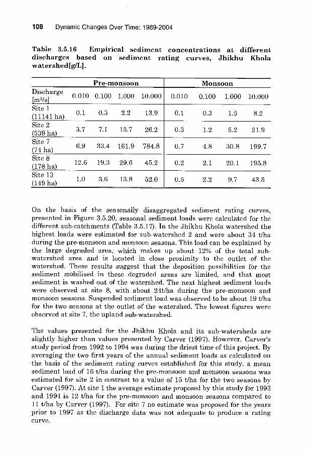
108 Dynamic Changes Over Time: 1989-2004
Table 3.5.16 Empirical sediment concentrations at different discharges based on sediment rating curves, Jhikhu Khola watershed[g/L].
Pre-monsoon Monsoon Discharge m3/s
0.010 0.100 1.000 10.000 0.010 0.100 1.000 10.000
Site 1
(11141 ha) 0.1 0.3 2.2 13.9 0.1 0.3 1.5 8.2
Site 2
539 ha) 3.7 7.1 13.7 26.2 0.3 1.2 5.2 21.9
Site 7
(74 ha) 6.9 33.4 161.9 784.8 0.7 4.8 30.8 199.7
Site 8 178 ha)
12.6 19.3 29.6 45.2 0.2 2.1 20.1 195.8
Site 13 (149 ha)
1.0 3.6 13.8 52.0 VO.5 2.2 9.7 43.5
On the basis of the seasonally disaggregated sediment rating curves, presented in Figure 3.5.20, seasonal sediment loads were calculated for the different sub-catchments (Table 3.5.17). In the Jhikhu Khola watershed the highest loads were estimated for sub-watershed 2 and were about 34 t/ha during the pre-monsoon and monsoon seasons. This load can be explained by the large degraded area, which makes up about 12% of the total sub- watershed area and is located in close proximity to the outlet of the watershed. These results suggest that the deposition possibilities for the sediment mobilised in these degraded areas are limited, and that most sediment is washed out of the watershed. The next highest sediment loads were observed at site 8, with about 24t/ha during the pre-monsoon and monsoon seasons. Suspended sediment load was observed to be about 19 t/ha for the two seasons at the outlet of the watershed. The lowest figures were observed at site 7, the upland sub-watershed.
The values presented for the Jhikhu Khola and its sub-watersheds are slightly higher than values presented by Carver (1997). However, Carver's study period from 1992 to 1994 was during the driest time of this project. By averaging the two first years of the annual sediment loads as calculated on the basis of the sediment rating curves established for this study, a mean sediment load of 16 t/ha during the pre-monsoon and monsoon seasons was estimated for site 2 in contrast to a value of 15 t/ha for the two seasons by Carver (1997). At site 1 the average estimate proposed by this study for 1993 and 1994 is 12 t/ha for the pre-monsoon and monsoon seasons compared to 11 t/ha by Carver (1997). For site 7 no estimate was proposed for the years prior to 1997 as the discharge data was not adequate to produce a rating curve.

Too Little and Too Much: Water and Development in a Himalayan Watershed 109
Table 3.5.17 Seasonal sediment loads of the Jhikhu Khola watershed (mean±standard deviation)
Site Catchment
area Pre-
monsoon Monsoon Sum Carver (1997)
(ha) (t/ha/y) (t/ha/y) (t/ha/y) (t/ha/y)
Site 11 11141 1±1 18±2 19±2 11±1
Site 21 539 2±3 32±17 34±20 15±5
Site 72 74 3±4 10±5 13±9 17±11
Site 82 178 9±1 15±11 24±12 -
1 on the basis of 1993 to 1999 data 2 on the basis of 1997 to 1999 data
The sediment loads shown in Table 3.5.17 compare with other studies from the region as follows:
Galay et al. (2001) and Galay (1995) compiled the sediment yields of a number of small catchment studies in Nepal. Two of the catchments are of similar size to the Jhikhu Khola catchment, the Kulekhani catchment (12,500 ha), which had a sediment delivery of 20.5 t/ha/y, and the Harpan Khola (12,000 ha) which had a sediment delivery of 8.9 t/ha/y. The Bagmati at Sundarijal (1,553 ha), comparable to the Lower Gopi Khola in the Yarsha Khola catchment, had a sediment delivery of 13 t/ha/y. The Godavari catchment showed only 3 t/ha/y with an area of 1,231ha.
Sharma (1988) reported 45 t/ha/y for the entire Sun Kosi system with a catchment area of 19,230km2.
These figures indicate that the data from the Jhikhu Khola catchment are plausible and within the range of the other studies in the country.
The calculated sediment loads were related to selected catchment characteristics using the Spearman correlation coefficient (Table 3.5.18). In general, the correlations are weak. For the pre-monsoon season sediment yields, only the Topoindex showed significant correlation at the 10% level. For the monsoon season, the annual sediment yields, grassland and the ratio of cultivated to uncultivated land showed significant correlations. Grassland showed a positive correlation, which suggests higher sediment yields for areas with more grassland. In contrast, the cultivated/uncultivated ratio showed a negative correlation, suggesting that an increase in cultivated land leads to lower sediment yields.

110 Dynamic Changes Over Time: 1989-2004
Table 3.5.18 Correlation coefficients according to Spearman of sediment yield per unit characteristics.
area with selected watershed
Pre-monsoon Monsoon Annual Catchment area r -0.29 0.35 0.32
Sig. 0.54 0.36 0.48 Irrigated land r -0.14 -0.18 -0.11
Sig. 0.76 0.65 0.82 Rainfed land r 0.21 -0.65* -0.57
Sig. 0.65 0.06 0.18 Forest land r -018 0.38 0.46
Sig. 0.70 0.31 0.29 Grass land r 0.11 0.77** 0.75**
Sig. 0.82 0.02 0.05 Shrub land r -0.04 0.28 0.00
Sig. 0.94 0.46 1.00 Otherland use r 0.14 0.25 0.14
Sig. 0.76 0.52 0.76 Ratio cultivated/uncultivated r 0.00 -0.77* -0.75**
Sig. 1.00 0.02 0.05
Ratio rainfed land/ 0.11 -0 44 -0 29 irrigated land
i,-Y. 0.82
.
0.23
.
0.54 Degraded land r -0.60 0.70 0.80
Sig. 0.40 0.19 0.20 Mean slope r 0.36 -0.18 -0.11
Sig. 0.43 0.64 0.82 Topoindex r -0.95* 0.56 0.21
Sig. 0.05 0.32 0.79 r = correlation coefficient according to Spearman, Sig. = significance levels * correlation is significant at the 0.05% level (Sig.<0.05%) ** correlation is significant at the 0.1% level (Sig.<0.1%) *** correlation is significant at the 0.15% level (Sig.<0.15%)
Synthesis
The key issues related to water in the Hindu Kush Himalayan (KHK) region were identified to be water availability, floods and soil erosion / sedimentation. In this context the findings of this study contribute towards an improved understanding of processes from the perspective of middle mountain catchments in the HKH region.

Too Little and Too Much: Water and Development in a Himalayan Watershed 111
The current water scarcity as perceived by the local residents is mainly a function of the seasonality of the water resources and the current management of the available resources, rather than the natural water endowment. From an overall water availability perspective, there should be no difficulty in meeting current use given the current annual rainfall of about 1300 mm in the Jhikhu Khola watershed. The reasons why people perceived that the water resource is scarce is predominantly due to the seasonality of flow. From an agricultural perspective, water availability is adequate for the current cultivation practices. The cropping calendar is adapted to the seasonality of the rainfall as well as the low flows in the irrigation canals during the dry season. Recent intensification and increased cash crop production bas, however, led to water shortages in the Jhikhu Khola watershed as perceived by the local farmers. Further intensification of the agricultural production under current practices, could lead to and increase in water shortages. The most critical time from the perspective of natural water availability and the current cropping calendar, was the time before the onset of monsoon for the planting of maize, the nursery of rice and the transplanting of rice (Figure 3.5.21). For good yields of the post-monsoon crops adequate soil moisture from the monsoon season and a few rains during the post-monsoon and winter seasons are critical. To improve the situation, cash crop production using alternative irrigation methods could be promoted further. This would decrease the vulnerability of the farmers on the rainfed agricultural land, as well as decrease the water demand on the irrigated land. The storage of monsoon rains in ponds and cisterns should receive further attention in order to meet the increased water demand during the dry season.
Sediment mobilization and transport can be looked at in several ways. From a farmer's perspective, the loss of fertile topsoil is important, while from the perspective of downstream users, the total sediment load in the river at the outlet is the main issue. Looking at these two perspectives separately it can be stated that the farmers generally do not perceive soil erosion as a significant issue. This view is supported by the soil losses from the agricultural plots, which are balanced by the annual natural soil development. On average, an agricultural plot would loose about 10 t/ha per annum, while the tolerable soil loss rates in Nepal's middle mountains are estimated at about 11 t/ha per annum. Most of this soil loss from the upper catchments is then transferred to the lower irrigated terraces through runoff and irrigation water (Carver 1997, Brown et al. 1999). Surface erosion only accounts for a part of the total soil loss from a watershed. Stream bank erosion and gullying tend to be of higher importance and of more concern to the downstream users. However, these processes only affect a small number of farmers, who own land along the rivers. From this perspective, the current surface soil erosion rates on the agricultural land do not warrant any major changes in land management. Carver (1997), however, warns that the current system could become more vulnerable in the near future with

112 Dynamic Changes Over Time: 1989-2004
increasing intensification. The question is: how far can this intensification proceed?
a) Irrigated land
Risk
Rainfall --- Water surplus
J F M A
Evapotranspiration Water deficit
M J J
x - Rainfall vanability !,
A S O N D
I medium high medium low
b) Rainfed land
Risk
J
1 medium
Rainfall a Evapotrans pi ration I Runoff Water surplus Water deficit - -x - - Rainfall variability
Barley
F
FOCUS
M A
Maize
M J J A
I medium high medium Iow
S
1
Mustard
0 N
medium
D
1
Figure 3.5.21 Comparison of temporal distribution of selected water resources components with crops on a) irrigated land and b) rainfed agricultural land.

Too Little and Too Much: Water and Development in a Himalayan Watershed 113
From a downstream perspective the total sediment output of the selected catchments was medium to high in relation to other catchments in the world. However, within the region, a number of rivers, particularly the ones originating in the Siwaliks, show much higher values. This suggests that in terms of upstream-downstream sediment linkages it is important to consider interventions to reduce the sediment loads from these middle mountain watersheds in case of downstream development. The major source of sediment was believed to be the drainage system itself (bank erosion and remobilisation of in-stream sediment), as well as the roads and path network in the watershed. The degraded lands in the watershed were shown to be of particular importance by Carver (1997). To reduce the sediment loads interventions should focus on the riparian zones as well as roads and paths. Proper slope stabilization of roads and punctual stabilization of stream banks should be envisaged. The rehabilitation of degraded lands and the stabilisation of stream banks should be coupled with the need for fodder for the large number of livestock in the catchments. Farmers are not likely to put significant effort into the rehabilitation of barren lands if there is no immediate benefit.
From the perspective of a farmer in the Jhikhu Khola catchment, improved soil conservation is not a first priority. The need is not obvious and the benefits of currently promoted soil conservation approaches are not directly visible. From the downstream perspective, the need for soil conservation will only become important with the development of water resources downstream. Consequently the main target areas should be the degraded lands, stream banks and the road network. If soil conservation simultaneously addresses an extreme case and a clearly perceived issue from the farmer's perspective, such as fodder availability, then rehabilitation efforts will have a greater chance of success.
Himalayan farmers are often held responsible for downstream flooding. Many authors have shown that due to the scales involved and the in-channel processes on flood plains, this hypothesis bas to be rejected. In fact, the area of cultivated land in différent sub-catchments showed a negative relationship with the flood peaks and flood volumes. Grassland as well as degraded land, on the other hand, showed a positive relationship, while the forest areas did not show a distinct relationship. The floods at the sub- catchment and the catchment outlet show a very high correlation with the processes on degraded and grassland plots. The runoff on these plots was largely generated by the infiltration excess overland flow generation mechanism. The corrélation, therefore, suggests that infiltration excess overland flow or similar processes are primarily responsible for flood generation at this scale. The correlation between floods and agricultural land is weak, suggesting that agricultural land only marginally contributes to floods. Consequently, the proper management of agricultural land is beneficial to flood protection for small to medium events. While the importance of catchment characteristics is proven for small to medium flood

114 Dynamic Changes Over Time: 1989-2004
events, at high events only rainfall characteristics were decisive in flood generation. In general, these large floods were generated during rainfall events with high rainfall volume or high rainfall intensities. During these events all land uses were contributing to the floods. This implies that watershed management in the traditional sense, with small-scale forest plantations, may not have the desired effect. Large scale land use changes have shown différences at the catchment scale (FAO 2002), but may not be practical in the context of rural catchments in the South Asia where land holdings are fragmented and small. Large scale land use change, such as the changes initiated by the upland conversion policy of the Chinese government, may potentially have an impact on the flashiness of streamflow due to its spatial extent, but 10 to 20 years will be needed before first conclusions can be drawn.
References
Adhikari, T.R., B.P. Upadhayay, M.P. Dhakal, P.M. Dangol, S. Shrestha, G. Nakarmi, B. Prajapati-Merz, and P.C Jha. 2003. Sustainable water management in the Jhikhu Khola catchment. In: Domroes, M. (ed.) Translating Development - The case of Nepal. Social Science Press, New Delhi. pp. 47-78.
Alford, D. 1992. Hydrological Aspects of the Himalayan region. Occasional Paper No. 18. ICIMOD, Kathmandu.
Brown, S.J., H. Schreier, P.B. Shah, and L.M. Lavkulich. 1999. Modelling of soil nutrient budgets: an assessment of agricultural sustainability in Nepal. Soil Use Management, 15: 101-108.
Carson, B. 1985. Erosion and sedimentation processes in the Nepalese Himalaya. Occasional Paper No. 1. ICIMOD, Kathmandu.
Carver, M. 1997. Diagnosis of headwater sediment dynamics in Nepal's Middle Mountains: Implications for Land Management. Ph.D. thesis. Interdisciplinary Studies in Resource Management Science, University of British Columbia. 374 pp.
Chalise, S.R., M.L. Shrestha, K.B. Thapa, B.R. Shrestha, and B. Bajracharya. 1996. Climatic and Hydrological Atlas of Nepal. ICIMOD, Kathmandu.
Chyurlia, J.P. 1984. Water Resources Report. Land Resources Mapping Project. Kenting Earth Science Ltd., Ottawa.
Critchley, W.R.S. and L.A. Bruijnzeel. 1995. Terrace risers: erosion control or sediment source? In: Singh, R.B., and M.J. Haigh (eds.). Sustainable

Too Little and Too Much: Water and Development in a Himalayan Watershed 115
Reconstruction of Highland and Headwater Regions. Oxford/IBP Press, New Delhi. pp. 529 - 541.
Dangol, P.M., J. Merz, and R. Weingartner. 2002. Flood generation in the middle mountains of Nepal. In: Spreafico, M. and R. Weingartner (eds.). Proceedings of the International Conférence on Flood Estimation, Bern, March 6-8, 2002. pp. 85 - 92.
Dongol, B.S., J. Merz, M. Schaffner, G. Nakarmi, P.B. Shah, S.K. Shrestha, P.M. Dangol, and M.P. Dhakal. 2005. Shallow groundwater in a middle mountain catchment of Nepal: Quantity and quality issues. Environmental Geology, 49(2):219-229.
Duester, H. 1994. Modellierung der raeumlichen Variabilitaet seltener Hochwasser in der Schweiz. Geographica Bernensia G44. Geographisches Institut, Universitaet Bern, Bern.
FAO. 1977. Crop water requirements. FAO Irrigation and Drainage Paper No. 24. FAO, Rome.
FAO. 1998. Crop evapotranspiration - Guidelines for computing crop water requirements. Irrigation and Drainage paper 56. FAO, Rome.
FAO. 2002. Land-Water linkages in rural catchments. FAO Land and Water Bulletin 9. FAO, Rome.
Galay, V.J., T. Okaji, and K. Nishino. 1995. Erosion from the Kulekhani catchment, Nepal during the July 1993 rainstorm. In: Schreier, H., P.B. Shah, and S. Brown (eds.). Challenges in mountain resources management in Nepal. Process, trends, and dynamics in middle mountains watershed. Kathmandu, 10-12 April 1995. ICIMOD, Kathmandu. pp 141-154.
Galay, V.J., H. Schreier, and R. Bestbier. 2001. Himalayan Sediments. Issues and Guidelines. CD-ROM. Canadian International Development Agency and Canadian International Waters and Energy Consultants, Vancouver.
Gardner, R. K. Mawdesley, B. Tripathi, S. Gaskin, and S. Adams. 2000. Soil erosion and nutrient loss in the Middle Hills of Nepal (1996 - 1998). NARC, Kathmandu, and Queen Mary and Westfield College, University of London, London.
Gerrard, J. 2002. Landsliding, runoff and soil loss in the Likhu Khola drainage basin, Middle Hills, Nepal. Case study for the Bishkek Global Mountain Summit. (http://www.mtnforum/bzms/paperel.htm )

116 Dynamic Changes Over Time: 1989-2004
Hofer, T. 1998. Floods in Bangladesh - A Highland-Lowland Interaction? Geographica Bernensia G48. Institute of Geography, University of Bern, Bern.
Ives, D.J., and B. Messerli. 1989. The Himalayan Dilemma - Reconciling Development and Conservation. Routledge, London.
Kansakar, D.R. 2001. Groundwater resources in the hills and mountain regions of Nepal. Paper presented at the Workshop on Groundwater Resource Management, Kathmandu December 20, 2001.
Lambert, L., and B.D. Chitrakar. 1989. Variation of Potential Evapotranspiration with Elevation in Nepal. Mountain Research and Development, 9 (2): 129-144.
MacDonald & Partners. 1990. Design Manuals for Irrigation Projects in Nepal. Planning and Design Strengthening Project. His Majesties Government of Nepal, Ministry of Water Resources, Kathmandu.
Merz, J. 2004. Water Balances, Floods and Sediment Transport in the Hindu Kush-Himalayan region. Geographical Bernensia G72. Department of Geography, University of Bern, Bern, and International Centre for Integrated Mountain Development, Kathmandu.
Merz, J., B. Shrestha, and R. Weingartner (eds.). 2005. Regional synthesis of water and erosion activities in PARDYP. CD-ROM (Draft). PARDYP, Kathmandu.
Merz, J., G. Nakarmi, S. Shrestha, B. Shrestha, P.B. Shah, and R. Weingartner. 2002. Water and Erosion Studies of PARYP Nepal: Water Demand and Supply Survey. Brochure with CD-ROM. ICIMOD, Kathmandu.
Mosley, M.P., and C. Pearson. 1997. Introduction: Hydrological Extremes and Climte in New Zealand. In: Mosley, M.P., and C. Pearson (eds.). Floods and Droughts: The New Zealand Experience. The New Zealand Hydological Society, Wellington. pp 1-4.
Mountain Risk Engineering Unit (MRE). 2002. Report on Mapping of sediment sources in the Jhikhu Khola catchment, Central Nepal. Unpublished Report.: PARDYP, Kathmandu.
Nakarmi, G., H. Schreier, J. Merz, and P. Mathema. 2000. Erosion Dynamics in the Jhikhu and Yarsha Khola Catchments in Nepal. In: Allen, R., H. Schreier, S. Brown, P.B. Shah (eds.). The People and Resource Dynamics Project; the first three years (1996-1999). Workshop Proceedings,

Too Little and Too Much: Water and Development in a Himalayan Watershed 117
Boashan, Yunnan Province, China. March 2-5, 1999. International Centre for Integrated Mountain Development, Kathmandu. pp. 209-217.
Sachs, L. 1997. Angewandte Statistik. 8th Edition. Springer Verlag, Berlin.
Saijo, K. 1991. Hillslope evolution in geological time scale and its significance on active erosion processes in the Jhikhu Khola catchment. In: Shah, P.B., H. Schreier, S.J. Brown, and K.W. Riley (eds.). Soil fertility and erosion issues in the middle mountains of Nepal. Proceedings of a workshop held in Dhulikhel, April 22 - 25, 1991. Integrated Survey Section, Topographical Survey Branch, Kathmandu, and University of British Columbia, Vancouver. pp. 188 - 194.
Salas, J.D. 1992. Analysis and Modelling of Hydrologic Times Series. In: Maidment, D.R. (ed.). Handbook of Hydrology. McGraw-Hill Inc., New York.
Schreier, H. and S. Brown. 2004. Multiscale approaches to water management: land-use impacts on nutrient and sediment dynamics. Scales in Hydrology and Water Management. Intern. Assoc. Hydrol. Sci. IAHS Publ., 287: 61-75.
Shakya, B. 2001. Estimation of main hydrological characteristics for mountain rivers of Nepal. Extended PhD Abstract. Central Asian Hydrometeorological Research Institute, Tashkent.
Sharma, C.K. 1988. Natural hazards and man made impacts in the Nepal Himalaya. Pushpa Sharma, Kathmandu.
Sharma, K.P. 1997. Impact of land use and climatic changes on hydrology of the Himalayan basin: A case study of the Kosi basin. Unpublished PhD thesis. Institute for the Study of Earth, Oceans and Space, New Hampshire.
Shrestha, A.B. C.P. Wake, J.E. Dib, and P.A. Mayewski. 2000. Precipitation fluctuations in the Nepal Himalaya and its vicinity and relationship with some large scale climatological parameters. International Journal of Climatology, 20: 317-327.
Tahal Consulting Engineers. 2002. Technical Report No.-4 Meteorological study. Nepal Irrigation Sector Project. Department of Hydrology and Meteorology, Ministry of Science and Technology, Kathmandu.

118 Dynamic Changes Over Time: 1989-2004
3.6 Water Quality
Jurg Merz, Bhawani S. Dongol, Gopal Nakarmi and S. Sharma
Water quality has become a major concern in recent years, both from the perception of the local farmers and from scientific data. Seventeen percent of the respondents in the water use survey indicated that they perceived water quality to be a problem in the Jhikhu Khola catchment (Merz et al. 2003, 2004). This included not only water quality issues related to public water supply, but also the issue of eutrophication. Intensive agriculture with high agrochemical inputs was the main reason for concern with respect to eutrophication, while the level of microbiological contamination needs to be addressed in order to ensure safe water supply.
3.6.1 River Water Quality
River quality in the Jhikhu Khola catchment was monitored over four seasons for a period of 1 year in 2000. Most of the surface waters in the lower stretches of the Jhikhu Khola watershed and selected tributaries displayed elevated levels for phosphate and nitrate.
Bedrock in the area is deficient in phosphate, and soils are inherently low in phosphate content. The farmers have been made aware of this and are adding high doses of fertilizers to their intensively used fields. They apply up to 400 kg/ha of urea (46 % nitrogen), 800 kg/ha of DAP (18 % nitrogen, 46% phosphorous) and 800 kg/ha of complex (20% nitrogen, 20% phosphorous) to their potato crops (Pandey and Joshy 2000). Other crops are supplied with up to 200 kg/ha of the différent fertilizer combinations. A large part of this applied fertilizer ends up in the river system of the watershed, as shown by the elevated phosphate levels observed at selected sites, during monsoon and pre-monsoon season (e.g. sites 2002, 2005, 2015 and 2016 - Figure 3.6.1). A large part of the applied fertilizer ends up in the river system of the watershed, as shown by elevated phosphate levels observed, during the monsoon and pre-monsoon season, at selected sites (e.g. sites 2002, 2005, 2015 and 2016) (Figure 3.6.1). These elevated P levels correspond to the time when DAP fertilizer was applied to the potato trop in these upper areas.
The nitrate levels (Figure 3.6.2), measured as N03-N, did not exceed recommended health values (10 mg/l as N; WHO (1997)), but they indicate high agricultural inputs during the pre-monsoon season in the upper areas. The sites on the tributaries showed low levels during the pre-monsoon season, mainly due to the greater distance from the sources of the pollution.
Other parameters showed no reason for concern; levels generally complied with guidelines, with only the occasional sample measured above guidelines values. Though microbiological contamination was generally high in the

Too Little and Too Much: Water and Development in a Himalayan Watershed 119
surface waters, this was only a concern where river water was diverted for domestic water supply.
3
2.5
2
1.5
1
0.5
0
- jîîm kâ. J'Ê
O) O N M V U) CO h oD O) O N M VO Oü)
OO N-O OO O N O O O O O O O O O O O O O O O O O O O O O O O N N N N N N N N N N N N N N N N N N N N
Site No.
4/16/2000 7/7/2000 9/3/2000 12/9/2000
Figure 3.6.1 Phosphate levels in river samples on four dates in 2000.
E 12
d 10 8
Z 6
Ii T O u Ô Ô Ô Ô Ô Ô Ô O _ N M V e O W m O O O O O O O O O O O O O O O O O O O O Ô N N N N N N N N N N N N N N N N N N N N
Site No.
4/16/2000 7/7/2000 09/3/2000 12/9/2000
Figure 3.6.2 Nitrate levels rivers samples on four dates in 2000.

120 Dynamic Changes Over Time: 1989-2004
3.6.2 Public and Private Water Sources Quality
Water quality investigations of the public water sources in the Jhikhu Khola watershed reflect similar issues as the river sites. The primary cause for concern was microbiological contaminants and phosphate. Dissolved oxygen, pH and turbidity were, in certain samples, higher than recommended. For human health, the main concern was the microbiological contamination of the majority public water sources exceeding health guidelines (KU/ICIMOD 2001). Thirty-one public water sources were monitored in two seasons (pre- monsoon and monsoon) over a one-year period. During this time only two sources were free of fecal coliforms during either of the seasons (Figure 3.6.3). Fecal concentrations were usually orders of magnitude above recommended values. Fecal coliform content in the samples was generally higher during the monsoon than during the premonsoon season. Lowest concentrations were measured in the post-monsoon and winter seasons (October to February). This is believed to be due to the increased interaction between surface water and shallow ground water, in addition to the influence of pollution around the water sources. Surface water is usually more contaminated as was shown in the case of river water quality monitoring. The microbiological contamination has a significant impact on the health of the people in the watershed, as a survey of the health posts in the catchment has illustrated. According to health officials, 25% of the patients visiting the 9 health units, health and sub-health posts, suffer from water related diseases. Most of the patients suffer from diarrhea followed by worm infestation and dysentery. It is interesting to note that malaria has returned to the area, after being eradicated in the late 1950's. According to the health officials in the area, malaria accounts for the majority of fever cases during monsoon in the valley bottom of the watershed.
1800
1600
1400
1200 -
1000 -
800 -
600
400 -
200
0- fli 111-il ----I -- IflI[
V V V Ln f O V O V O
N N W
O O
ch iA f- a0 O O M V f c`7 f a0 O O
Site No.
4/22/2000 7/2/2000
Figure 3.6.3 Fecal coliform in the pre-monsoon and monsoon seasons in 2000.

Too Little and Too Much: Water and Development in a Himalayan Watershed 121
Phosphate concentration in public water sources is another concern. Most of the water sources have phosphate levels that are above guidelines set by the EC (0.4 mg phosphate/1). This is predominantly due to the human activities in and around the public water sources. In many cases, washing and bathing are an integral part of the life around these sources. Leaching of agricultural fertilizers (such as DAP) into the ground water increases the phosphate levels in the water. While phosphate does not have a direct impact on human health, it can lead to eutrophication and oxygen depletion.
Schaffner (2003) studied different water sources including springs, taps, dug wells and water harvesting jars in selected areas of the Jhikhu Khola watershed. She concluded that microbiological contamination is the dominant parameter of concern in all drinking water systems, with the highest contamination risk during the pre-monsoon and monsoon seasons. Most affected are traditional public water sources, followed by dug wells, with the lowest risk at pipe-tap systems and water harvesting jars. Turbidity is commonly elevated in all drinking water systems during the pre-monsoon and monsoon seasons, and is mainly related to heavy rainfall. Agrochemical and human induced pollution, indicated by high nitrate and phosphate levels, is of concern mainly at dug wells. Basic water quality parameters show highly variable electrical conductivity and total hardness values, locally low pH and seasonal variations in yield. Analysis of trace elements (total iron, arsenic in dug wells; zinc, lead in water jars) revealed no levels of concern.
Recent studies by Apel et al. (2002) and Schumann et al. (2002) suggested that the high doses of different pesticides applied in the Jhikhu Khola watershed do not pose a risk for groundwater nor surface water contamination. The main risks to human health in connection with pesticide use are the residues on the crops, as well as unsafe handling and application.
A detailed study of the dug wells in the watershed by Dongol et al. (2005) showed that often the surrounding conditions of the wells are not hygienic, and that the microbiological contamination is, therefore, of concern in all the wells throughout the year. Some chemical parameters are also found to be elevated in certain wells, especially nitrate and phosphate. Nitrate in particular, is more prevalent in the water from shallow dug wells than in the other types of water sources, such as natural springs and taps. Nitrate pollution may be derived from the accumulation of domestic and agro- chemical pollutants in soif and groundwater, but potential causes should be more closely investigated in future.
Spatially, the comparison of différent well groups is interesting (Figure 3.6.4). For example, wells 6 to 10 located in the Shree Ram Pati displayed a similar pattern in the water quality parameters. During the pre-monsoon season, the nitrate levels were very low, while the phosphate loadings were

122 Dynamic Changes Over Time: 1989-2004
26
36 370,427 30
29
3
817
4 250
19 24 28t 20 22 15 1E _ y
38P 13 > île pi
2 t(m
Leâend Rivers Dug wells
Nitrate Total Phosphate coliform
Total Iran Class 1 = good Class 2 = fair Class 3 = low Class 4 = poor
Figure 3.6.4 Spatial variation of nitrate, phosphate, total iron and total coliform.

Too Little and Too Much: Water and Development in a Himalayan Watershed 123
high. During the monsoon season, phosphate was reduced, but total iron increased. In winter, only coliform remained a problem. Wells 11 to 14 showed similar nitrate contamination throughout the year, peaking in the monsoon season. During the monsoon season, phosphate begins to become a problem. Total iron was a problem at différent times in différent wells. Wells 1 to 5, all located in the main valley, showed similar patterns, with high phosphate levels and generally low nitrate levels throughout the year. Coliform contamination was also an issue through the year in these wells. In Tinpiple, it was more difficult to identify a pattern due to the large number of wells in a small area. In general, it can be noted that the wells located in close proximity displayed similar patterns.
3.6.3 Summary
Water quality bas increasingly become a concern, both for domestic water supply and for river ecology. Many water supplies have pathogen problems and the traditional systems for managing drinking water supplies appear to be the worst choice. Chemically, phosphate and nitrate levels pose the greatest pollution risk to water supplies and river water at many downstream locations in the Jhikhu Khola. Poor sanitary conditions and agricultural intensification are believed to be the primary causes for the poor water quality in the watershed. The problem is exacerbated by sediments.
References
Apel, H., M.S. Paudyal, and O. Richer. 2002. Environmental risk assessment of pesticide use based on the modelling of the environmental fate of pesticides in the soil. In: Herrmann, A. and S. Schumann (eds.). International Workshop on Environmental Risk Assessment of Pesticides and Integrated Pesticide Management in Developing Countries. Heft 38. Institut fuer Geooekologie, Technische Universitaet Braunschweig, Braunschweig. pp. 13-23.
Dongol, B.S., J. Merz, M. Schaffner, G. Nakarmi, P.B. Shah, S.K. Shrestha, P.M. Dangol, and M.P. Dhakal. 2005. Shallow groundwater in a middle mountain catchment of Nepal: Quantity and quality issues. Enuironmental Geology, 49(2):219-229.
KU/ICIMOD. 2001. Capacity building for community water quality assessment in the Jhikhu Khola catchment, Kavre District, Nepal. Kathmandu University and ICIMOD, Kathmandu.
Merz, J. G. Nakarmi, S.K. Shrestha, B.M. Dahal, B.M., B.S. Dongol, M. Schaffner, S. Shakya, S. Sharma, and R. Weingartner, 2004. Public water sources in rural catchments of Nepal's Middle Mountains - Issues and constraints. Enuironmental Management, 34(1): 26-37.

124 Dynamic Changes Over Time: 1989-2004
Merz , J., G. Nakarmi, S.K. Shrestha, B.M. Dahal, P.M. Dangaol, M.P. Dhakal, B.S. Dongol, S. Sharma, P.B. Shah and R. Weingartner. 2003. Water: A scarce resource in rural watersheds of Nepal's Middle Mountains. Mountain Research and Development, 23(1): 41-49.
Pandey, S.P. and D. Joshy. 2000. Fertilizer consumption and food grain production in Nepal. Nepal Agricultural Research Council, Kathmandu.
Schaffner, M. 2003. Drinking Water Quality Assessment and Improvement in the Jhikhu Khola Catchment, Nepal. Publikation Gewaesserkunde No. 281. Department of Geography, University of Bern, Bern.
Schumann, S., W. Stichler, and S.B. Prajapati. 2002. Underground water passages and runoff formation pattern in an irrigated khet catchment. In Herrmann, A. and S. Schumann (eds.). International Workshop on Environmental Risk Assessment of Pesticides and Integrated Pesticide Management in Developing Countries. Heft 38. Braunschweig: Institut fuer Geooekologie, Technische Universitaet Braunschweig. pp. 190-204.
WHO. 1997. Guidelines for drinking water quality. Volume 1: Recommendations, 2nd edition. World Health Organisation, Geneva.
3.7 Labour Allocation and Workloads: The Role of Women
Sandra Brown and Bhuban Shrestha
3.7.1 Introduction
Biological différences between women and men do not change, but social différences are learned, are changeable over time, and vary widely both within and between cultures. Gender divisions of rights, responsibilities, work and knowledge help us to explain the multiple roles of women and men as resource users and managers. Social factors influencing gender roles include religious practices, ethnic or cultural attitudes, class or caste, the formal legal system and institutional arrangements. Gender roles, in turn, influence activities, responsibilities and decision making authority (OECD 1999). As such, an integrated gender focus is fundamental to the collection of relevant information, and the development and adoption of effective resource management options.
In the Jhikhu Khola watershed, gender roles and responsibilities were examined through a gender sensitive household survey design. Eighty-five paired interviews with female and male farmers were conducted. The major role women play in farming in Nepal was explicitly acknowledged through their inclusion as participants; historically studies concerning farming in

Too Little and Too Much: Water and Development in a Himalayan Watershed 125
Nepal were based only on information provided by male farmers (Gurung 1987). Interviewing was conducted by Nepali researchers, and a local villager was included on each interview team. Interviews were simultaneous but separate, typically carried out at farmer's homes, with the women holding their discussion indoors and the men talking outside. This separation allowed us to account for the typical division of labour, to elicit open responses, and to compare responses between women and men. Key informant questionnaires from the Pive main villages were used as a cross check (Brown 1997).
3.7.2 Roles and Responsibilities
Engendered responsibilities in the watershed for agriculture, livestock husbandry, domestic activities and forest products are summarized in Table 3.7.1. Nearly all women in the study work in agriculture. They are largely responsible for the day-to-day tasks within the farming system. Planting, weeding and harvesting are almost exclusively female tasks and constitute 85-95% of the labour requirements for the main crops grown (rice, maize, potatoes). Women are solely responsible for "polluting" work, which in the Nepali context refers to direct contact with human or animal excrement; therefore men typically do not spread manure. Women should refrain from working with animals (ploughing) as it is considered to "cause pain to the animals". Men are responsible for heavier work such as land preparation, terrace repair and irrigation system maintenance.
In livestock husbandry, women collect fodder, stall feed animals, and milk female goats, cattle or buffalo. Their workloads depend on the availability of pasture and involvement in commercial milk production. Households involved in commercial milk production spend an average of 6.5 hours per day in the collection of fodder, livestock care and transporting milk; 70% of that workload being undertaken by female household members (see section 4.5). Children are often assigned the responsibility of animal grazing and watering, but stall feeding is becoming more prevalent.
Women are responsible for domestic activities: cooking, cleaning, child care and fetching water. The collection of water alone requires roughly 2.5 hours per day (see section 4.5). Decision making, particularly with regards to buying or selling agricultural products, supplies and animals is dominated by household males. Interestingly, decisions regarding household money are shared.
The collection of fuelwood, fodder and litter in the watershed is representative of the high labour demands placed on women (Plate 6.7.1). Collection by the 85 households sampled in the Bela-Bhimsenthan region is summarized Figure 3.7.1 and Table 3.7.2. Wives, daughters and daughters- in-law collect 86% of fuelwood, fodder and litter for a typical household. A median household makes one trip per week to collect fuelwood, seven trips

126 Dynamic Changes Over Time: 1989-2004
per week to collect fodder and three trips per week to collect litter. A return trip typically takes 2 to 3 hours. A median household spends 28 hours per week in the collection of forest products, but up to 100 hours per household per week may be spent (Brown 1997).
Table 3.7.1 Gender responsibilities for major farm and household tasks (n=27).
T k % Responsibility as Female Male
Irrigation 8 91 Terrace maintenance 12 88
Ploughing 12 88 Agriculture Planting 49 51
Harvesting 70 30 Applying compost 84 16 Applying fertilizer 27 73 Fodder collection 96 4 Animal watering 92 8
Livestock Animal grazing 75 25 Stall feeding 90 10 Milking 73 27
Domestic Fetching water 92 8 Collecting fuelwood 92 8 Household money 46 54
Decision Buy / sell animais 0 100
making What to plant 6 94
Buy seed / fertilizer 0 100
Farm labour 30 70
Fuelwood Fodder Lifter
Wives Daughters Daugter-in-law Sum
Figure 3.7.1 Fuelwood, fodder and litter collection by women (n=85).

Too Little and Too Much: Water and Development in a Himalayan Watershed 127
Plate 3.7.1 Forest litter collection for animal bedding and composting.

128 Dynamic Changes Over Time: 1989-2004
Table 3.7.2 Frequency of fuelwood, fodder and litter collection (median values).
Time spend Frequency Time per trip Product (hours per (trips / week) (hours) week)
Fuelwood 1 3 3.8 Fodder 7 2 14.0 Litter 3 2 7.0 Total 13.5 - 28.0
3.7.3 Labour Dynamics and Market Production
Women are central in resource management due to their traditional role within the farming system. Changes in the farming system, however, impact the responsibility and labour requirements imposed on women. Changes in labour allocation between 1989 and 1996 were documented by repeating surveys conducted by Kennedy and Dunlop (1989) in 1996 (n=27). The women and men farmers surveyed in 1989 were asked the saure questions in 1996. Topics discussed included labour allocation, cropping systems, livestock operations and forest access. Tasks where there bas been a significant change in labour allocation over time are shown in Figure 3.7.2 a- b, based on Fisher exact probability test.
a) Livestock care
1989 m D Û N o o -
1996
I I I
1989 E r (0
1996
I I I
1989 a, Ç Y E 1996
0% 25% 50% 75% 100%
Involvement
b) Fertilizing
1989
1996
1
ÿ 1989 0 CL
I
I I f
C
0 1996
ô 1989
E 1996 ° v
1989 Q N
I I : 1996
0% 25% 50% 75% 100%
Involvement
Figure 3.7.2 Dynamics of household allocation of labour 1989-1996.

Too Little and Too Much: Water and Development in a Himalayan Watershed 129
Land preparation, planting, household care and farm management have remained relatively stable with respect to labour allocation over time. Fertilizing related activities and tasks related to livestock care have been the most dynamic. Female responsibilities for gathering forest litter and manure, and applying compost have increased significantly from previously shared responsibilities. Adult males are more active in composting and the application of chemical fertilizers (Brown 1997). With the increase in vegetable production for market (Brown and Shrestha 2000), and the associated increase in the use of agrochemicals (von Westarp et al. 2004) there has been a shift in labour. More nutrients are required by vegetable crops such as tomatoes and potatoes compared to traditional staple crops, and consequently more effort is placed on nutrient management, both compost and chemical. Women have taken on the responsibility for additional organic nutrient collection and application (litter and manure), while men have undertaken a greater role in composting, and are in charge of chemical fertilizer purchases and application.
Tasks related to livestock have also been dynamic with significant increases in women's workloads related to fodder collection, animal grazing and milking. The daily feed requirement of improved breed buffalo is 84 kg or 2 head loads of fodder per day, and an extra 2-3 head loads (110 kg) of fuelwood per week are required for preparing dhana (cooked feed) (Brown 1997). Wives, daughters and daughter-in-laws typically collect 82% of fodder and 99% of fuelwood requirements, so as the number of milk animais have increased, so have female workloads. The percentage of households involved in commercial milk production has risen from 30% in 1991, to 45% in 1996, and >70% by 1998 (Brown and Shrestha 2000). With more households raising female buffalo, scarcity of fodder and fuelwood has meant that women and girls travel great distances, and spend more time for household and livestock needs.
3.7.4 Women and Workloads
Workloads in the agricultural watersheds of the Middle Mountains are high, particularly for women. Time use data indicate that females work longer hours than males in ail age groups. Adult women work on average from 11- 13.5 hours per day compared to 7.5-10 hours per day by men (Acharya 1982, Brown 2003). Women shoulder the responsibility for domestic and livestock care, forest product collection, and tasks such as planting, weeding and harvesting in agricultural production. Workloads and the gender division of responsibilities, however, may change in response to market opportunities. With cash crop and milk production increasing in the Jhikhu Khola watershed, workloads have increased, particularly for women, but men have begun to undertake non-traditional roles such as participating in composting and fertilizer application. Men however, still dominate in marketing and decision making roles.

130 Dynamic Changes Over Time: 1989-2004
References
Acharya, M. 1982. Time use data and the living standards measurement study. LSMS working paper No. 18. World Bank, Washington. 72 pp.
Brown, S. 2003. Spatial analysis of socioeconomic issues: gender and GIS in Nepal. Mountain Research and Development, 23(4): 338-344.
Brown, S. 1997. Soil fertility, nutrient dynamics and socio-economic interactions in the Middle Mountains of Nepal. PhD Thesis. Faculty of Graduate Studies, University of British Columbia, Vancouver, Canada. 254 PP.
Brown, S., and B. Shrestha. 2000. Market-driven land-use dynamics in the middle mountains of Nepal. Journal of Environmental Management, 59: 217- 225.
Gurung, D.K. 1987. Women's participation in forestry: a case study of Akrang Village. Forestry Research Paper Series, Number 10. Winrock International institute for Agricultural Development, Kathmandu.
Kennedy, G., and C. Dunlop. 1989. A study of farming-household systems in Panchkhal Panchayat, Nepal. Department of Agricultural Economics, University of British Columbia. 126 pp.
OECD. 1999. DAC guidelines for gender equality and women's empowerment in development co-operation. Development Co-Operation Guidelines Series, Organisation for Economic Co-Operation and Development. (http://www.oecd.org/dataoecd/56/46/28313843.pdf )
von Westarp, S., H. Schreier, S. Brown, and P.B. Shah. 2004. Agricultural intensification and the impacts on soil fertility in the Middle Mountains of Nepal. Canadian Journal of Soil Science, 84(3): 323-332.

Assisting Community Efforts to I m p rove Livelihoods & Environment
4.1 Rehabilitation of Degraded Sites
Hans Schreier and P.B. Shah
4.1.1 Introduction
4
Given the intense land use pressure in the Jhikhu Khola watershed it is inevitable that land degradation will continue to occur. Degradation is a long terra process and from our land use analysis it was shown that approximately 7% of the watershed area is in an advanced state of degradation. These degraded areas occur mostly on red soils, usually on common property land that has been overgrazed. These are the only sites in the watershed that do not contribute to biomass production. Most of the surfaces are heavily rilled and gullied, soil crusts are often formed at or near the surface, and weathered bedrock exposure is widespread (Plate 4.1.1. and 4.1.2.) Natural re-vegetation is difficult because of the poor physical and chemical soil conditions, and since the majority of these sites have been abandoned, any emerging vegetation that is suitable for animal feed is usually collected on a regular basis. Natural instabilities are common in these mountainous watersheds, and given the intense annual monsoon rainfall, soil erosion is a major problem in the watershed. As long as the soils are productive farmers use good soil conservation measures, but once accelerated erosion occurs then these sites are usually abandoned on a temporary or permanent basis. The cause of degradation is difficult to assess since many of the areas are subject to a combination of natural instability due to steep slopes, geological uplift, excessive rainfall events during the monsoon season, and human induced degradation resulting from overgrazing, deforestation, and insufficient inputs of organic matter and nutrients.
Most of the degraded sites are on common property land, and few people have an interest in rehabilitation. Efforts to reclaim and restore such sites are large and the potential benefits in terras of biomass production are small. There are few incentives to protect and restore these areas but without protection and rehabilitation the sediment contribution from these sites is potentially large. Carver (1997) estimated that 30-40% of the annual sediment load to the river system likely originated from degraded sites. These sediments clog irrigation channels, silt up water storage ponds and affect stream channel dynamics. The nutrient content in the eroded

132 Assisting Community Efforts to Improve Livelihoods & Environment
sediment is low and provide little benefit when deposited in downstream rite fields (Schreier et al. 1998).
As little prior experience existed in rehabilitation of these degraded sites, a number of research questions were explored. These ranged from: how much physical effort is needed to stabilize these sites?; what plants should be used to reestablish ground cover?; and how do we protect the sites once revegetation has taken place?
In 1993, a number of rehabilitation experiments were initiated on an extremely degraded 2.5 ha site on red soils in Luitelgaun. The site had a history of deforestation, excessive collection of fodder and litter, and was practically devoid of vegetation cover. Deep gullies and rills were widespread and much of the topsoil had been removed by erosion.
Plate 4.1.1 Degraded forested site.
Plate 4.1.2 Example of gully erosion in the Jhikhu Khola watershed.

Too Little and Too Much: Water and Development in a Himalayan Watershed 133
During the monsoon season headcutting was active and accelerated erosion had exposed quartzite and phyllitic bedrock in many places. There were no quick solutions to rehabilitating such a site, and simply contouring the site, redistributing the remaining soil, and building retention structures was not an option. The decision was made to use the site as a laboratory to conduct experiments that require minimum external inputs. The idea was put forward that if a reasonable amount of success could be achieved, then the methods could be replicated at other degraded sites.
After some initial physical work to fill in some of the deepest gullies, three experiments were conducted over a 7 year period:
Planting native, nitrogen fixing fodder trees and determining their survival and long terra growth rates. Testing the suitability of grasses to establish ground cover and produce biomass for animal feed.
Improving the soil fertility through organic matter additions.
4.1.2 Native, Nitrogen Fixing Fodder Trees
The fodder tree planting project had many challenges: species selection, degraded soil conditions, limited nutrient inputs, seed supply and the demand for biomass production. First a list of potential tree species was compiled. Given the degraded soil chemical and physical conditions of the site, and the consideration that only limited nutrient inputs were to be used, the planting of nitrogen fixing species was seen to be advantageous. In addition, there needed to be evidence that the tree leaves would be palatable for animal feed. Therefore only nitrogen fixing fodder tree species were considered.
More than 40 différent nitrogen fixing fodder trees were identified as being native to Nepal (Panday 1982). However, obtaining a good seed supply and seedling stocks proved to be a real challenge. The common practice of lopping branches at regular intervals for animal fodder meant that the trees rarely bloom or reach the seed production stage making it difficult to collect seeds. Seeds were collected from many différent sources over a six month period and a tree nursery was established on-site to produce sufficient seedlings for the experiments. In addition to the nitrogen fixing capacity of the trees, attention was also given to their phosphorous fixing capacity via mycorrhizal infestation. This was an important consideration due to the low the soil phosphorus content (as shown in section 3.3), particularly in the red forested soils. Since limited information was available on the mycorrhizal activity in the Nepalese soil, an inoculation experiment was carried out in a growth chamber at the University of British Columbia. Only three tree species and three différent Nepalese soils were used in this experiment. The results shown in Table 4.1.1 indicated that the mycorrhizal activity was

134 Assisting Community Efforts to Improve Livelihoods & Environment
generally low in the red forest soils. These soils are generally depleted of organic matter and nutrients, and receive no external nutrient input. The agricultural soils, which receive moderate nutrient input annually, showed moderate micorrhizal activity. Dalbergia sissoo was the only tree species of the three tested that consistently displayed micorrhizal activity, although the activity was less pronounced in the red soils than in the non-red agricultural soils.
Table 4.1.1 Micorrhizal experiments with three fodder trees and three soils.
Red soils (chir pine
forest)
Red soils (rainfed
agriculture - maize)
Non-red soil (rainfed
agriculture - maize)
Bauhinia purpurea
- No nodules - No mycorrhizae
No nodules Low-Mod. VM[M mycorrhizae
No nodules Low-Mod. VA/M
mycorrhizae
Dalbergia sissoo
Nodules - Low-High
VM/M mycorrhizae
Nodules High VM/M mycorrhizae
Nodules Mod. VW/M mycorrhizae
Alnus nepalensis
No nodules No mycorrhizae
No nodules Low VM/M mycorrhizae
Nodules Ecto-mycorrhizae
The tree nursery which was established at the experimental site became the planting stock for the rehabilitation efforts. The degraded site was divided into sixteen 30mx30m segments, and in each segment différent fodder tree seedlings were planted in hedgerows (Table 4.1.2). Trees were protected and no thinning or harvesting took place for the first two years. Survival rates and growth rates measured 2'/2 years after planting were highly variable, as shown in Figure 4.1.1.
The results showed much higher survival and growth for Siris and Dalbergia sissoo than for the other tree species, but the number on red soils were significantly lower. Trees grown on quartzitic parent material were much more productive than those planted on phyllite, while the red soils consistently had a poor growth response.
The study site remained protected from 1994 (when the rehabilitation started) until 2004, but once a year annual fodder collection was carried out. Over time this site became the main seed supply for all other rehabilitation experiments carried out by the PARDYP team.

Too Little and Too Much: Water and Development in a Himalayan Watershed 135
Table 4.1.2 Fodder trees used in the réhabilitation program.
Fodder tree, grass and soil nutrient experiments in différent bedrock dominated sections (Al to F5 in 30mx30 m plot sections, except Cl) A1.Quartzite
Siris d il R h ili i E i i il Cl. Grass an on xper ments So e ab tat n Red So s B1.Quartzite Sissoo
D1.Quartzite D2.Red Soils D3.Red Soils D4.Phyllite D5.Red Soils Tanke Siris Kutmiro Bakaino Sissoo
E1.Quartzite E2.Red (mixed) E3.Phyllite E4.Phyllite E5.Red Soils Siris Bakaino Tanke Kutmiro Siris
F2.Quartzite F3.Quartzite F4.Quartzite F5.Red Soils Sissoo Khayer Bakaino Sissoo
Sissoo = Dalbergia sissoo, Siris = Albizzia lebbek; Bakaino = Melia azedarech; Khayer = Acacia catechu; Kutmiro = Litea monopetala; Tanke = Bauhinia purpurea.
a)
0 10 20 30 40 # Trees/plot
phyllite phyllite red soif
Figure 4.1.1
b)
quartzite quartzite
Siris red soif red soif
quartzite
I
quartzite Dalbergia red soif
red soit
quartzite Tanke [ phyllite
Khutrniro [ phyllite
e phyllite
Khayer [ quartzite
0 2 4 6
Tree height (m)
Number of trees (a) and average tree height (b) after 2.5 years.
The rate of recovery and revegetation is illustrated in Plates 4.1.3 to 4.1.6, which provides a series of pictures of the recovery process over time.

Plat
e 4.
1.3
Reh
abili
tatio
n Si
te 1
994
Plat
e 4.
1.4
Reh
abili
tatio
n Si
te 1
995
Plat
e 4.
1.5
Reh
abili
tatio
n Si
te 1
998
Plat
e 4.
1.6
Reh
abili
tatio
n Si
te 2
000

Too Little and Too Much: Water and Development in a Himalayan Watershed 137
4.1.3 Grass Suitability for Soil Stabilization and Animal Feed
The farm survey (n=85) revealed that animal fodder was in short supply, particularly during the dry season (Brown 1997). Fodder shortages were related to the degradation of forests, the conversion of grassland into arable crops and an increased emphasis on milk production in the watershed (Shrestha 2000). Given that it takes considerable time before fodder trees can be harvested, experiments were also conducted with fodder grass species. Introducing grasses into degraded sites would not only provide additional fodder but would produce it more rapidly than trees. Since the tree planting on red soils was only marginally successful, grass experiments were conducted on the red soils. These degraded red soils were depleted in nutrients, had high Al content, high acidity and low cation content. Consequently the growth response experiment was carried out using a split plot design that included various rates of lime and manure application, and combinations of inputs before the grass seeds were planted. The split plot design and the annual above ground biomass are shown in Table 4.1.3.
Table 4.1.3 Grass experiment on red soils with various inputs.
Average annual grass yield (kg/m2)
T Ti 1998-2001 reatment me Lemon grass Setaria Stylo
Chinese Creeper
Thailand Creeper
1 Control (not planted)
Jan 1998
0 0 0 0 0
2 lkg/m2
Lime Jan 1998
3.51 0.72 1.05 0.79 0.71
3 2 x lkg/m2 Lime
Jan & June 98
5.17 0.27 1.12 0.42 0.74
4 1 kg/m2 Manure
Jan 1998 2.81 0.32 0.70 0.68 0.56
5 2 x lkg/m2 Manure
Jan & June 98
2.52 0.28 0.64 0.69 0.50
6 lkg/m2 Lime & Manure
Jan 1998
2.43 0.26 0.88 0.87 0.46
7 2 x lkg/m2 Lime & Manure
Jan & June 98
2.22 0.47 1.16 0.30 0.38
8 Control (Planted)
Jan 1998
1.43 0.32 0.00 0.49 0.20
Lemon grass was the most productive species and responded most effectively to lime applications with 78-188% higher yields than lemon grass grown without inputs (Figure 4.1.2). Stylo was difficult to germinate, but like lemon grass yields steadily improved over time. In contrast, Koduz and Seteria yields declined over time after single and double inputs of lime and

138 Assisting Community Efforts to Improve Livelihoods & Environment
manure. While Lemon grass was a successful colonizing grass it is not a desirable fodder material, however, oil can be extracted and the plant can also be used for tea and as a spice.
Lemon Grass
1998 1999 2000 2001
Stylo
2
0
1998 1999 2000 2001
Golden Botton
1998 1999 2000 2001
1.5
Seteria
1998 1999 2000 2001
Koduz
--- ---- -- ---------
1998 1999 2000 2001
Treatments Lime lx
o Lime 2x
Manure lx Manure 2x
Manure & Lime lx Manure & Lime 2x
Control, planted
Figure 4.1.2 Grass yields with différent treatment 1998-2001 (on red soils).

Too Little and Too Much: Water and Development in a Himalayan Watershed 139
A number of other grass species were planted with only limited inputs, and a permanent ground cover was established over the entire experimental site. This site then became the seed source for the outreach program that was aimed at helping community groups in the reclamation of degraded community forests. The amount of seeds collected from the test site between 1999 and 2003 is provided in Table 4.1.4.
Table 4.1.4 Annual seed production from the rehabilitation site that formed the basis for fodder enhancement elsewhere in the watershed.
Grass & Fodder Seed production (kg/year) Total 2000-2003 Species
2000 2001 2002 2003 (4 years) Tephrosia 52.5 41.35 30.70 18.5 143.1 Flemingia 9.2 9.5 3.89 5.25 27.84 Sunhemp 64.1 47.1 30.76 18.75 160.71 Tithonia 28.8 20.5 4.53 7.63 61.45 Kudju --- 3.88 3.88 Joint Vetch --- 4.73 4.73 Wyncassia --- 4.70 4.70 Stylo 11.2 3.2 3.28 5.5 23.18 Molasses 29.55 7.4 4.14 3.28 44.37 Dinnath --- 0.95 1.43 2.38 Ipillipil --- --- 0.8 0.8 Mott Napier --- 0.01 1.16 1.18 Signal Grass --- 0.01 0.86 0.87 Gini Grass --- 0.02 0.61 0.63 Vetiver --- 1.64 0.66 2.30 Guatemala --- --- 0.42 0.42 Napier 2.50 1.15 2.72 6.37 NB 21 --- 0.1 0.6 0.7
Broombrass --- 0.62 0.90 1.52 Hemata --- 0.59 0.59
Total Seed production 491.7 kg
The results indicated that, if degraded sites can be protected for a few years, it is possible to develop a range of vegetation cover that serves as erosion control but which also produces biomass that can be used for fodder and fuelwood. The initial experiments were restricted to nitrogen fixing species because of the poor state of soil nutrients. As these trees can be lopped at least twice per year, organic matter can be incorporated into the soil to improve the nutrient and moisture holding capacity of the soil which then provides an improved environnent for planting other species. Additional

140 Assisting Community Efforts to Improve Livelihoods & Environment
experiments were conducted with grasses and hedgerows to provide a range of fodder types for farmers to choose from. Table 4.1.4 shows the amount of the annual seed production that was generated from the demonstration site. These seeds were distributed to community forests and used for on-farm trials. Sunhemp, Tephrosia, Tithonia, Molasses and Napier grass were the most prolific seed producers. These where introduced to the site in the second phase once the soil conditions were improved. The ultimate aim was to produce a vegetation cover that had a high biodiversity, was self- sustaining and from which fodder and fuelwood products could be harvested at a sustainable rate without impacting erosion.
The outreach program between 1999 and 2005 included six community forests and a large number of farmers who were keen to participate in on- farm trials. A summary of the on-farm trials, average yields, and fodder preferences by the farmers is provided in Table 4.1.5.
Table 4.1.5 Results of the participatory on-farm trials for fodder production.
Species Average biomass
Farmers preference
Napier 4.1 kg/m2 (40t/ha) High
3.9 kg/m2 Molasses (39t/ha) High
Flemengia 2.5 kg/m2 (25t/ha) High
3.3 kg/m2 Tephrosia (33t/ha) Medium
Sunhemp 2.5 kg/m2 (25t/ha) Medium
Stylo 1.1 kg/m2 (l lt/ha) Medium
3 5 kg/m2 Tithonia . Low (35t/ha)
Farmers response / comments
Fast growing, good quality fodder during dry season Good quality, grows on degraded soils, germination is sometimes difficult Good quality, coppices well and provides good soif stability Good fodder. Grows on degraded soils but lower preference for cattle fodder
Good green manure, fast growing
High value seed but slow growth
Good pioneer species to improve soil fertility on degraded site, green manure, low fodder preference (goats only)
Overall, the experiments demonstrated that to have a successful fodder rehabilitation program on degraded sites a combination of species is necessary. Sunhemp, Tithonia, and Tephrosia are plants that survive and

Too Little and Too Much: Water and Development in a Himalayan Watershed 141
grow relatively well on degraded sites, and because they do not produce the most favorable fodder they are best used to provide ground cover and organic matter that helps in rehabilitating the soil nutrient status. Naper, Molasses and Flamengia are the most desirable fodder but will do best once the soil nutrient conditions have improved.
4.1.4 Restoration for Erosion Control and Biomass Generation
Since 7% of the watershed was in a highly degraded state, a 2.5 ha degraded site with red soils was selected for basic reclamation research. The main aim was to establish a permanent vegetation cover to control soil erosion, and ultimately, to produce biomass that could be sustained and contribute to improving the livelihood of the local people. Few resources were available to reclaim these degraded sites which are usually on community owned land, and labour shortages limit the physical effort which could be expended. Consequently, we opted for the establishment of a vegetation cover that required minimal inputs but would control erosion and provide supplementary fodder and fuelwood resources to the communities. The results showed that planting native nitrogen fixing trees in the initial phase helped in establishing ground cover, reducing erosion and improving soil fertility through the addition of organic matter. Once the soil nutrient and moisture holding capacity had improved, additional species were introduced to create biodiversity, to improve the resilience of the site and to provide a greater variety of fodder and fuelwood.
Establishing fodder trees and grasses on these sites proved to be quite a challenge. Over time it was shown that Siris and Dalbergia were the most successful fodder trees, while lemon grass, setaria, and stylo were the most successful grass colonizers. Sunhemp, Tephrosia, Tithonia, Molasses and Napier grasses were also successfully colonized. The experience gained by these experiments proved to be extremely valuable to the community forest reclamation program initiated in 2000. Not only could we apply the lessons learned, but the demonstration site served as the main seed source for the community forest reclamation program.
References
Brown, S. 1997. Soil fertility, nutrient dynamics and socio-economic interactions in the Middle Mountains of Nepal. PhD Thesis. Faculty of Graduate Studies, University of British Columbia, Vancouver, Canada. 254 pp
Carver, M. 1997. Diagnosis of headwater sediment dynamics in Nepal's Middle Mountains: Implications for Land Management. Ph.D. thesis. Interdisciplinary Studies in Resource Management Science, University of British Columbia. 374 pp.

142 Assisting Community Efforts to Improve Livelihoods & Environment
Panday, K.K. 1982. Fodder trees and tree fodder in Nepal. Swiss Development Corporation and Swiss Federal Institute of Forestry. 107 pp.
Schreier, H., S. Brown, M. Carver, and P.B. Shah. 1998. Linking land degradation to nutrient and sediment transport in a Middle Mountain watershed in Nepal. In: M. Haigh, J. Krecek, G.S. Rajwar, and M. Kilmartin (eds). IAHC Headwaters: water resources and soil conservation. A.A. Balkema / Rotterdam / Brookfield. pp. 315-327.
Shrestha, B. 2000. Milk Production Dynamics and the Animal feed situation in the Jhikhu Khola Watershed. In: R. Allen, H. Schreier, S. Brown, and P.B. Shah (eds.). The People and Resource Dynamics Project: the first three years (1996-1999). Workshop Proceedings, Boashan, Yunnan Province, China. March 2-5, 1999. International Centre for Integrated Mountain Development, Kathmandu. pp. 85-100.
4.2 Improving Community Forests
Bhuban Shrestha and Hans Schreier
4.2.1 Background
In the late 1950's forests in Nepal were placed under the control of the national government and this brought about a significant change in forest management. As discussed in section 3.2, the forest cover in the watershed has undergone a series of degradation periods followed by afforestation efforts, but due to the rapid population growth, pressure on the forests have steadily increased. Communities have long argued that they should control the management of forests, and the first community forest was established in Nepal in 1978. The community forestry program, implemented throughout Nepal, is facilitated by the Forest Act of 1993 and the Forest Rules of 1995, which empower local communities to manage forest resources for their benefit. Initially the fderal government was slow to return the control of forest management to local communities, but when democracy was introduced in 1993 forest self-government became a strong focus, and many communities forests were organized and legitimized as self-governing units (Kanel 2004). About 1.1 million hectares of forest lands (25% of the total) has so far been handed over to 13,000 Community Forest User Groups (CFUGs), which constitutes about 35% of the total population of Nepal (Kanel 2004).
The goal of community forestry in Nepal is to protect the forests, reduce ecological degradation and increase the supply of forest products with active community participation. The focus is primarily on non-timber products such as firewood, litter collection, fodder production, and the use of medical

Too Little and Too Much: Water and Development in a Himalayan Watershed 143
plants. According to government regulations the land managed under community forests (CF) belongs to the state but the land use rights are in the hands of the Forest User Groups (FUGs). A significant portion of the national forest has been handed over to FUGs in the belief that protection, sustainable management and the use of forests will be improved under the control of local communities. FUGs have been given the rights to sell and distribute forest products independently according to decisions made by the FUG committee without permission of Department of Forestry (DFO). Each FUG has its own rules and regulations regarding the protection and management of forests and the FUG committee usually decides on the openings and closures for the collection of forest products at different times of the year. Members of the FUG are allowed to collect litter, grass, timber, dry and green fuelwood on specific days according to decisions made by the FUG committee. The committee also decides on the penalties that are levied to those that collect forest products at times when the forests are closed for collection of forest products.
As discussed in section 3.2, the forest cover has changed significantly in the Jhikhu Khola watershed over the past 55 years. The GIS analysis showed that 44% of land was under forest in the 1950s but that this decreased to 19% in 1980s with the nationalization of forest land. Between 1972 and 1990 the forest cover increased to 30% of the watershed due to an active afforestation program. However, in the late 1990's the area under forest declined again. By 2004 the forest cover was at 29% (3358 ha) and at that time about 50% of forests were under community management control (Brown and Shrestha 2004, Shrestha and Brown 1995). The pressure on forest resources has continued to increase due to population growth, and as a result, it will be difficult to maintain the quantity and quality of forests without changes in forest policies (Schreier et al. 2000).
In 2002 the PARDYP team initiated a detailed community forestry inventory using 1:5,000 aerial photographs and rectified orthophoto images. In collaboration with District Forest Office in Dhulikhel, 36 community forests were identified in the watershed. The boundaries of each community forest were delineated in consultation with members of each FUG and marked onto the 1:5,000 aerial photographs. A detailed field survey was conducted to determine the dominant forest species composition, crown cover and maturity. The data was then incorporated into the GIS database. Based on the crown cover data seven good and seven degraded forests were selected (Figure 4.2.1), and a survey was carried out to determine what the perceptions of FUG members were about forest use, forest quality, accesses, penalties, security status and key issues facing the forest community.
The 14 contrasting community forests were selected to assure that they are representative of the topographie and climatic conditions in the watershed (different elevation, and north and south aspect). Fifty percent of the community forests are comprised of red soil, 29% are mixed and 21% have

144 Assisting Community Efforts to Improve Livelihoods & Environment
non-red soils. Sixty-six FUGs participated in the survey in the 14 community forests.
Ratmate
LaukeniJ
Kapileswo
Namdi Khola
Figure 4.2.1 Location of good and degraded community forests selected for detailed surveys.
The results revealed that the average operating time of the CFs was 11 years (ranging between 8 to 14 years). The forest user groups that participated in the survey were located in the following Village Development Committees (VDCs): Panchkhal, Anaikot, Patlekhet, Kabhre, Dhulikhel, Sathighar, Kharelthok, Baluwa, and Phoolbari VDCs.
4.2.2 Forest Status
Forest products play an integral role in farming systems in Nepal. Every household is directly or indirectly dependent on the forest. The distribution of forest under national government and community control is provided in Figure 4.2.2.

Too Little and Too Much: Water and Development in a Himalayan Watershed 145
Figure 4.2.2 Distribution of forests under national government and community control.
4.2.3 Forest Use
Most of the forest products (93%) are distributed on a per household basis and family size is not considered in the allocation. The FUG committee sets the days when users are allowed to collect products and each member household of the FUG and gets equal amount of the forest products. Members of the FUG will receive penalties if they collect forest products on days flot designated for collection.
The survey established that rules differ greatly between community groups. The periods when forest community members are allowed to collect grass, fuelwood, litter and timber is summarized in Table 4.2.1.
Table 4.2.1 Access to forest products in différent community forests.
Forest product
Grass
Litter
Fuelwood
Timber
Collection period from community forests (% CFUGs) 1 period / 2 periods / 3 periods /
Other year year year
21%
21%
57%
36%
43%
1%
21% 7% no collection
7% 29% open all year
21% 21% only dead twigs
Only allowed ater disasters to repair housing
146 Assisting Community Efforts to Improve Livelihoods & Environment
The typical length of opening for grass collection was between 7-90 days per period; 57% of the FUGs reported that only one load per day was allowed per household between 6 am and 10 am. The period of forest litter collection ranged between 36 and 60 days. Most FUGs collect litter as a precaution against forest fires and to improve organic matter management in agriculture. Fifty percent of FUG members reported that they were limited to one basket per household per day, while 43% reported that they had no restriction on the amount collected per day. The collection period was usually between March and May, the peak of the dry season.
Fuelwood collection periods ranged between 10 and 36 days. In most cases FUG members were permitted to collect the dead twigs, but were not allowed to eut any trees. Almost half of the FUGs reported that each household was allowed 280 to 480 kg fuelwood/year, while 36% were allowed to collect 1050 to 1320 kg of fuelwood/year.
In order to protect the existing timber resources, FUGs restricted timber harvesting in all CFs in accordance with Department of Forestry guidelines. Timber can only be cut for construction of houses that suffer from damage by Pire, landslides earthquakes or other natural disasters and for school repairs. The amount of timber was restricted to one or two trees per year per FUG.
Forest management, however, depends on how well members adhere to the stated rules and to the operational plan designated by the community user committee.. Only 36% CFUG said that they followed the rules and regulations of the operation plan 100% of the time. About 36% said that they mostly followed the regulations, while the rest mostly ignored the rules. The field based inventory conducted by the PARDYP team documented that the forests where regulations were enforced were in significantly better condition than those where rules were not enforced. Additional pressures have come from population expansion. The watershed population has increased dramatically over the past 11 years, the number of members joining CFUG having increased by 40%. About 64% of the CFUGs reported that the increase in the number of members is due to family separation and population migration from outside the watershed. About 36% of the population mentioned that they do not have access to forest resources.
4.2.4 Local Perception of Forest Resources
All the community forest user groups (CFUG) mentioned that the forest quality has increased over the last 10 years due to planting, protection, restrictions on grazing, and a greater awareness of the consequences of increased forest product harvesting. Over the past 3-4 years, 71% of CFUGs were unable to renew their community forest license from the District Forest Office. The general perception is that over the past several years the spatial area under forest and the forest quality has decreased due to the lack of CFUG ownership. CFUGs reported that DFO officers were unable to visit
Too Little and Too Much: Water and Development in a Himalayan Watershed 147
villages in the last 2 years, negotiate with CFUG members to renew ownership licenses or to listen to their concerns due to security issues associated with the Maoist conflict. In order to renew a CF license the officers have to go in the field and re-survey the community forest for species composition, crown cover, and maturity types. This has not happened at a sufficient scale and consequently the community forestry program is experiencing difficulties.
During the most recent survey it was found that the users of CFs are no longer listening to the CFUG committee authorities and that the government officiais are no longer visiting in the villages due to the security concerns. According to Bhattari (2006), 78% of FUGs in the Kabhrepalanchok district no longer have legal rights to their forests but are trying to get these rights renewed through the District Forest Office. The forests are uncontrolled, the collection of forest products is unrestricted as there is no authorized body to manage the resources, and villagers are encroaching on the forests. According to the CFUGs, particularly those in the Bela areas, large trees have been harvested and sold in several community forests by group members. As no security is in place, this process is unchecked. At the same time,, the extension of the army camps (UN peacekeepers) has put more pressure on the forest. The consensus of the CFUGs is that many forest resources have declined since 2002 due to the security situation.
4.2.5 Community-based Forest Management
About 29% of the watershed is under forest cover and 50% of the forest management has been turned over to communities over the past 11 years. Forest products play a significant role in the livelihood of the mountain communities. Giving management concessions to communities was thought to be a more effective way of improving forest condition than management by the national department (DFO). While many opportunities existed to achieve sustainable forest management in a community context there is clear evidence that the program has had mixed success. The political conflict and the rapid population growth are two main reasons why forest conservation has not been very successful. While good management regulations were put in place at the beginning of the community forestry program, the recent conflict has restricted the approval and license renewal process as DFO officers responsible for the approvals have not been able to visit the watershed due to safety concerns. Due to the lack of authority the CF program is going through a very difficult period and many users no longer adhere to the regulations set up by CFUG. As a result we have entered a new phase of forest degradation.
However, the successful PARDYP mapping and surveying program conducted in the watershed helped to set the stage for granting management
148 Assisting Community Efforts to Improve Livelihoods & Environment
licenses for community forests, and the inventory of the forest conditions will form the basis for determining the rate of change in forest cover and quality for the future, once the conflict is resolved.
References
Brown, S., and B. Shrestha. 2000. Market-driven land use dynamics in the middle mountains of Nepal. Journal of environmental management, 59: 217- 225.
Bhattari, B. 2006. Widening the gap between Terai and Hill farmers in Nepal; the implications of the new Forest Policy 2000. Federation of Community Forest User Groups (FECOFUN). In: S. Mahanty, J. Fox, M Nurse, P. Stephen, and L. McLees (eds). Hanging in the balance: equity in community-based natural resource management in Asia. East-West Center. pp. 43-161.
Kanel. R.K. 2004. Twenty five years of community forestry: contribution to millennium development goals. In: Kanel, R.K, and P. Mathema (eds). Twenty five years of community forestry. Kathmandu. pp. 4-18.
Shrestha, B, and S. Brown. 1995. Land use dynamics and intensification. In: Schreier, H, P.B. Shah, and S. Brown (eds). Challenges in mountain resources management in Nepal. Process, trends, and dynamics in middle mountains watershed. Kathmandu, 10-12 April 1995. ICIMOD, Kathmandu. pp 141-154.
Schreier H. B. Shrestha, and P.B. Shah. 2000. Forest dynamics in Nepal; Quantity, quality, and community forest issues in middle mountain watersheds. In: Allen, R.., H. Schreier, and S. Brown (eds). The People and Resource Dynamics Project: the first three years (1996-1999). Workshop Proceedings, Boashan, Yunnan Province, China. March 2-5, 1999. International Centre for Integrated Mountain Development, Kathmandu. ppl29-138.
4.3 Restoring the Production Capacity of Red Soifs
Hans Schreier and P.B. Shah
4.3.1 Introduction
The red soifs of Nepal represent the most genetically advanced and oldest soils in the country. These soils are usually associated with old weathered surfaces, are highly leached and only occur at lower elevations (up the 1700

Too Little and Too Much: Water and Development in a Himalayan Watershed 149
m elevation). The Jack of red sons at higher elevations is attributed to the absence of geomorphologically stable surfaces, inappropriate parent material, and unsuitable climatic conditions. In fact, these sons have developed under climatic conditions that were much warmer and more humid than today (Carson 1985). Red sons make up about 1% of the country and are the dominant sons at lower elevations in the Jhikhu Khola watershed. These sons play a significant role in Nepal's society. They are used as a surface sealant for walls and floors in farm houses, and are used for decorative purposes during religious ceremonies. Under good management practices they are known to be the "king of sons", particularly for maize production. However, they are also some of the most vulnerable soils in the watershed. The reason for this is manifold. Red soils have a high clay content and are slippery when wet. The cation capacity of these soils is low because the dominant clay mineralogy is kaolinite and sesquioxides (Fe- Al oxides). Consequently their nutrient holding capacity is low. The minerai structure is platy which reduces water infiltration and percolation rates, and leads to erosion and slope instability. Given their high iron and aluminum content, these sons have a high affinity to fix phosphorus, which in turn makes phosphorus unavailable to plants. Since these soils are heavily leached of basic cations they tend to have a pH range that is unfavorable for most of the dominant crops produced in the watershed. Finally, when exposed to high temperatures a surface crust is formed which makes root penetration more difficult.
As long as sufficient organic matter is added to these soils they can be highly productive. Organic matter and the resultant decomposition processes improve the soil structure, water percolation, soil workability, cation exchange capacity and nutrient release (N and P). Red sons are often used to seal paddy rice fields to enable flooding, and in turn they loose their red color as a result of the reducing conditions created by flooding.
Red soils cover 37% of the watershed and about 7% (780 ha) of these red soils are in a very advanced state of degradation. Slope instability and erosion in the watershed are primarily linked to red soils that were overgrazed, did not receive annual inputs of organic matter, or were disturbed by fire or construction activities. Based on evidence from historie aerial photos, gully and rill erosion on red soils was widespread at the time of the construction of the Araniko highway. Once advanced erosion was initiated, these soils were largely abandoned. As indicated in section 4.3, these eroded sites on red soils are the major source of sediment in streams. Degraded red soil sites are the only sites in the watershed that do not contribute to biomass production, but have large impacts on sediment transport, flooding and irrigation downstream. For these reasons the PARDYP team initiated a rehabilitation program on red soils (section 4.3). Establishing a vegetation cover on these soils was difficult, and the question of soil nutrient rehabilitation for long terra sustainability had to be addressed. As a result, a number of additional experiments were carried out

150 Assisting Community Efforts to Improve Livelihoods & Environment
to gain a better understanding of the processes that would best improve the chemical and physical processes, and the productive capacity of these sons. Given the scarcity of organic matter and the lack of purchasing power of the farmers, low cost solutions were thought to provide the best options. The main questions addressed in restoring red soils were: a) what are the difficulties in increasing organic matter in red sons?, b) do the red sons respond differently to soil organic matter additions than non-red sons?, c) what are the rates of pine litter decomposition, and do pine litter additions to red sons result in increased soil acidification? and d) what type of organic matter additions would best restore soil nutrients?
4.3.2 The Problem of Pine Litter Decomposition
The majority of plantation forests in the watershed are dominated by chir pine (pinus roxburghii), and consequently pine litter is relatively plentiful. Poor farmers collect the litter for animal bedding and composting. We expressed concern about this practice as pine litter decomposition is known to be slow (Shah et al. 1991), and in the process of decomposition it is thought that the organic acids released from the pine litter will acidify the sons, reduce decomposition rates and make the aluminum in the red sons more soluble, potentially resulting in Al-toxicity. Since soluble Al bas a high affinity for phosphorus, insoluble Al-phosphate could be formed, which means plants would no longer have access to sufficient available phosphate. As shown in Figure 4.3.1 aluminum is highly soluble at pH < 4 and ph > 7, hence additions of acid generating organic matter would reduce decomposition rates, reduce phosphorus availability, and make the soil less conducive for biomass production.
AI2O,
9
6 ?
5,
1
0 1 2 3 4 5 6 7 8 9 10 11
pH
Figure 4.3.1 Aluminum solubility and pH (Modified from Ollier 1984).

Too Little and Too Much: Water and Development in a Himalayan Watershed 151
4.3.3 Pine Litter Decomposition Rates in Red and Non-red Soils
The first experiment aimed to determine how quickly dry pine litter decomposes in red versus non-red soils. Two sets of 25 litter bags constructed from nylon mesh (20x20 cm in size) were filled with 10 g of dry pine litter. Air and water could freely penetrate the bags. The first set was buried into red soils at a depth of 15 cm, in strips of 10 m length, and the second set buried into non-red soils. Five bags were removed approximately every 4 months, and the remaining content was dried and weighed. The results, shown in Figure 4.3.2, were somewhat unexpected. They suggested that pine litter decomposition was rapid in red soils but not in non-red soils. However, most of the nylon bags in the red soils were destroyed, while those in the non-red soils remained largely undisturbed. It was determined that termites play a very active role in the decomposition process in red soils. They ate through the nylon, cut up the needles and removed most of the bag content within 8 months. In contrast, 50% of the litter buried in the non-red soils was still present over the saure time period. It took approximately 35 months for the litter to disappear from the bags in the non-red soils. A possible reason for the différence is that the clay content in the non-red soils was low, creating an unfavorable media for termites. Although termites appear to accelerate the decomposition process in red soils, this does not necessarily translate to improved soil properties as termites tend to concentrate organic matter in mounds. To demonstrate that termites accelerated the decomposition process in red soils a second experiment using metal mesh bags was carried out. The termites could not break the mesh and it was assumed that they were unable to access the litter. As shown in Figure 4.3.2, the decomposition rate of pine litter in red soils with the exclusion of termites appears to follow the decomposition rate in non-red soil: about 50% of the litter was still present after 12 months and it took more than 3 years for complete decomposition of pine litter.
120
6 Red Soils (Nylon)
s Non-Red Soils (Nylon)
Red Soils (Metal)
0 4 8 12 16 35
Months rince start
Figure 4.3.2 Pine litter decomposition rate.

152 Assisting Community Efforts to Improve Livelihoods & Environment
The results showed that pine litter decomposes very slowly even in a monsoonal type of climate. Termites appear to be responsible for speeding up the destruction and removal of the litter, but their impact on enhancing the soil conditions was not readily apparent.
4.3.4 Soi/ Acidity and Nutrient Changes after Continuous Addition of Pine Litter
The second experiment focused on the long terra effect of pine litter addition on soil pH and soil nutrients. To determine the long terra effects of pine litter additions a soil litter addition experiment was carried out. Eight 30x30 cm plots were prepared on degraded brown soils on quartzite parent material and on degraded red soils on phyllite parent material. Dry pine litter (10 kg/m2) was added to each plot at 20 cm depth and the litter was then covered with soil (Plate 4.3.1). After 6 months the soil below the pine litter layer was destructively sampled in the first plot and a second set of 10 kg/m2 of pine litter was added to the remaining 7 plots. This process was repeated every 6 months over a 42 months period. The sons were then analyzed for pH and soil nutrient conditions. The expérimental design is shown in Table 4.3.1.
Plate 4.3.1 Pine litter decomposition and soil pH experiment

Too Little and Too Much: Water and Development in a Himalayan Watershed 153
Table 4.3.1 Experimental design to determine soil response to continuous addition of pine litter.
Pine Litter Start
b f 1x10 2x10 3x10 4x10 5x10 6x10 7x10
Addition e ore addition kg/m2
Plot Size Phyllite control 1 2 3 4 5 6 7 30x30 cm Red Soils
Plot Size Quartzite control 8 9 10 11 12 13 14 Brown 30x30 cm ,
Non-Red Destructive
Sampling Months (Months 0 6 12 18 24 30 36 42 after
after addition addition)
With pine litter addition, available phosphorus levels increased to a significant extent in the non-red sons, while the red sons showed only a marginal increase. This can likely be attributed to the relatively high levels of available Al and Fe in red sons which convert the phosphorus that is becoming available from organic matter decomposition into insoluble Al and Fe phosphate.
There was a consistent increase in exchangeable Ca, Mg and K in both sons types and K was more substantial in the red sons (Figures 4.3.3 and 4.3.4) This is likely related to the higher clay content in the red sons which increases the cation exchange capacity.
The phosphorus deficiency in red sons is of particular interest as it appears that pine litter addition creates a lower pH, and despite organic-P released during the decomposition of organic matter P-availability was not significantly improved. Fe and Al concentrations are much higher in the red soils and are also in a form that enhances chemical reactions between Al, Fe and P. As P becomes available during decomposition Al and Fe phosphate is produced which makes P insoluble and unavailable to plants. As shown in Figure 4.3.5, the amount of reactive Fe and Al (CBD extraction - crystalline, amorphous and organic complexed and AAO extraction - amorphous form only) is much higher in red sons than in non-red sons. This is likely the reason that P availability did not improve with pine Litter addition.
The analytical data from this experiment (Figures 4.3.3 and 4.3.4) showed that the pH in both types of sons decreased by about half of a pH unit over a 31/2 year period and then reached a new equilibrium. The carbon content did not show a significant increase until two years into the experiment, which also reconfirms the slow rate of decomposition.

154 Assisting Community Efforts to Improve Livelihoods & Environment
a) pH
c) Bray-Phosphorus
-m Non-red soif Red soif
D
b) Soil Carbon
Non-red soif
d) Exchangeable Ça
Non-red soif
Red soif
Red soif
O -a O-0 O-0 O O
CD o c rn O)
4 CD
Figure 4.3.3 Changes in soil conditions after addition of 10 kg/m2 of pine litter every 6 months: a) pH, b) soil carbon, c) Bray-Phosphorus, d) exchangeable Ca.

Too Little and Too Much: Water and Development in a Himalayan Watershed 155
a) Exchangeable Mg b) Exchangeable K
1.0
Non-red soif Red soit
0.9
0.8 0.7
E 0.6
0.5
0.4
0.3 X
0.2
0.1
0.0
O D O A 'a A rF 1
Co CO Co
c) Cation Exchange Capacity d) % Base Saturation
18
16
--.14 aD Y12 E10
8 v
6 w ci A
2
0
-f- Non-red soif -- Red soif
D O D O D O D -0 A A A (O (O (O tO CO (O (O O) C v v Oo
O D O D O D O A A V A V A
Co (O (O
Non-red soif Red soif
80
70
60
50
40
30 - -
20
10
O D O D O D O D O A A A A a A CO (O (O (O (O (O (O (O (D (O C) O) l -1 OD 0o (O (O
Figure 4.3.4 Changes in soil conditions after addition of 10 kg/mz of pine litter every 6 months: a) Exch. Mg, b) Exch. K, c) CEC, d) % Base Saturation.

156 Assisting Community Efforts to Improve Livelihoods & Environment
Proportion of AI in amorphous form (CBD-AAO)
AAO-AI CBD-AI
Proportion of Fe in amorphous form (CBD-AAO)
AAO-Fe CBD-Fe 1
U)
O C O E
Non- Red
y L N Ç
E
Non- Red
L O C
O E
Red
U)
N C
E
Red
Figure 4.3.5 Amount of amorphous Al and Fe (AAO extraction) in comparison to (CBD extraction) in red versus non-red soifs at the beginning and after 42 months of pine litter addition.
4.3.5 Summary
Chir pine plantations were introduced in the watershed in the 1980's, and as a result pine litter is readily available during the dry season. Many framers collect pine litter for animal bedding and fire risk reduction, and utilize pine litter for compost which is then applied to agricultural fields. Concerns over this practice relative to agricultural soil fertility were noted early in the project, but needed to be confirmed through experimentation.
The results showed that pine litter decomposes very slowly, particularly in soils with low clay content. Termites were shown to be effective in removing the litter in red soifs, but their contribution to improving the soif nutrient status is believed to be low. Long terra additions of pine litter increased the soil acidity by about 0.5 pH units, and it took about 2 1/2 years before the effects of nutrient additions became apparent. Carbon levels, cation concentrations and cation exchange capacity improved significantly over time. Red soils, which have a higher Fe and Al content than non-red soils, were more efficient at increasing the carbon, Mg, and K content, while the P and Ça content improved more rapidly in non-red soils. Additions of pine

Too Little and Too Much: Water and Development in a Himalayan Watershed 157
litter did not improve the phosphoras availability in red soils to any extent and the inherent forms of extractable Fe and Al in the red soils were found to be responsible for converting the available phosphorus released for litter decomposition into insoluble Al and Fe phosphate.
The results confirmed that pine litter addition is not particularly effective when trying to improve the nutrient status of degraded red soils because it renders the soil more acidic, the decomposition rate is slow, and nutrient improvements only occurred after 2 1/2 years of additions.
References
Carson, B, 1985. Erosion and sedimentation processes in the Nepalese Himalaya. ICIMOD Occasional Paper # 1. 39 pp.
Ollier, C. 1984. Weathering. Longman, London, pp. 32-33.
Shah, P.B., H. Schreier, G. Kennedy, S.J. Brown, and S. Wymann. 1991. Discussion of major issues, research priorities and implementation of research results. In: Shah, P.B., H. Shreier, S.J. Brown, and K. Riley (eds.). Soil fertility and erosion issues in the Middle Mountains of Nepal. Workshop Proceedings. IDRC & UBC. pp.276-284.
4.4 Restoring Soil Production Capacity with Green Manure
Hans Schreier, P.B. Shah and Bhuban Shrestha
An alternative option to restoring soil nutrients in degraded sites is to use trees and shrub species that can grow on degraded, red and acidic soils, and apply the biomass as green manure to improve the soil nutrient conditions over time. Since chir pine litter is increasing soil acidity, the litter is decomposing very slowly, and phosphous deficiencies could not be improved in the red soils we decided to test alternative species that could have a more immediate impact. Three plants were selected for this experiment: Mexican Sunflower (Tithonia diversifolia), pigeonpea (Cajanus cajan) and sunhemp (Crotalaria juncea). The reasons for this choice are summarized in Table 4.4.1. All three plants grow well under the prevailing climatic and soil conditions, all can be harvested twice per year, the leaves have relatively high nutrient content and can be used as green manure to restore nutrients to degraded soils.

158 Assisting Community Efforts to Improve Livelihoods & Environment
Table 4.4.1 Advantages of using test plants as green manure to improve soil fertility.
Factors Tithonia Pigeonpea Sunhemp pH tolerant 4.5-7.0 5.0-7.0 5.0-8.0 Climatic conditions Well suited to prevailing climatic conditions
in the Jhikhu Khola watershed Soil nutrient demand Low Low Low
Nitrogen fixing capacity No
Yes - leguminous
Yes -
leguminous Phosphorus fixing capacity
Yes (arbuscular) Limited Limited
Nutrient content in biomass High N, P, K High N High N
Survival in degraded soil Good Good Good
Possible use Fodder (poor) Green manure
Food, fuelwood Green manure
Fodder (poor) Green manure
Rate of decomposition
Very fast (2 weeks)
Relatively fast fast
Disease resistance Moderate resistance
High resistance Moderate resistance
4.4.1 Background
Tithonia diuersifolia (Mexican sunflower) is a perennial invasive shrub that survives on acid soils, has a high biomass production, can accumulate nutrients in this biomass (N, P and K), decomposes rapidly, and can be lopped on a regular basis. Research has shown that using this species in an agroforestry system contributes significantly to enhancing soil nutrients. Green biomass of Tithonia has traditionally been used in rice paddies in the Philippines to maintain fertility, and significant research has also been done in Colombia (Rios-Katto 2002) and Africa (Jama et al. 2000, Seneviratne et al. 1998, Malama 2001, Gachengo et al. 1999).
There is evidence that Tithonia favors arbuscular mycorrhiza which may explain why this plant is capable of accumulating relatively high levels of phosphorus in its biomass. The green leaves also contain high levels of potassium, and surprisingly high concentrations of nitrogen, considering that it is not a leguminous plant. As demonstrated in Table 4.4.2, amongst the most popular agroforestry species Tithonia has exceptional potential to add nutrients when used as a green manure.

Too Little and Too Much: Water and Development in a Himalayan Watershed 159
Table 4.4.2 Percent nutrient content (median and range) of various green manure plants (green leaves/dry wt. basis).
Plant Species % Nitrogen % Phosphorus % Potassium Tithonia diversifolia 3.5 (3.0-4.0) 0.37 (0.24-0.56) 4.1 (2.7-5.5)
Cajanus cajan 3.6 (2.0-3.8) 0.23 (0.10-0.36) 2.1 (0.6-2.4)
Crotalaria juncea 2.7 (1.9-3.6) 0.33 (0.18-0.35) 1.5 (1.2-1.9)
Leucaena leucocephala 3.8 (2.8-6.1) 0.20 (0.12-1.33) 1.9 (1.3-2.2)
Sesbania sesban 3.7 (1.4-4.8 0.23 (0.11-0.43) 1.7 (1.1-2.1)
Tephrosia vogelli 3.0 (2.2-3.6) 0.19 (0.11-0.27) 1.0 (0.5-1.8)
Based on Gachengo et al. 1999, Poolpipatana and Hue 1994, Jama et al. 2000, Onim et al. 1990, Prasad et al. 2002, Bokhtiar and Sakurai 2005, Cherr et al. 2006, and Muthukumar and Udaiyan 2002.
Based on the literature, it is the green leaves and not the woody stems that are most effective in enhancing soil nutrients (Jama et al. 2000). Green leaves have relatively high moisture content and decompose more rapidly (within 10-12 days) as they generally have lower polyphenols than dry leaves which are known to inhibit decomposition. Thitonia yields range from 6.6 -
8.1 t/ha of dry matter per cutting and 2 cuttings per year are possible. The soft green leaves and soft stems average between 2.2 and 3.4 t/ha per cutting, with leaves making up about 10-17% of the total biomass on a dry weight basis (Jama et al. 2000). The absence of thorns makes Tihonia a more attractive species than other green manure species, but its use as fodder is somewhat limited due to the bitter taste.
Sunhemp is a leguminous plant and has low nutrient requirements. It can be used as a fodder species but is most effective as a green manure. It can tolerate acidic conditions and intense rainfall events, and produces up to 12 t/ha of green manure.
Pigeonpea is the most useful of the three plants as it is also nitrogen fixing (leguminous) and can be used as food, fuelwood, and green manure. It is drought tolerant and disease resistant and can form tree type plants that have relatively high biomass. Pigeonpea has nitrogen levels of 2 to 3.5 % and can yield between 2.5 and 5 t/ha of green manure.
4.4.2 Green Manure Experiment
All three plant species were cultivated on degraded land. The biomass was harvested on a regular basis and used as a green manure to restore soil nutrients in a long terra experiment. The experimental design is given in Table 4.3.4 and consisted of three soil types; brown, red 1, red 2 - all heavily degraded, acidic and nutrient poor. Every 6 months 2 kg of green biomass was added to 1 m2 plots in each of the three soil sites. Prior to each green

160 Assisting Community Efforts to Improve Livelihoods & Environment
manure addition, soil samples were collected from each plot, mixed and analyzed for basic nutrients (10 soil samples were collected and pooled for each of the species soil type combinations). The experiment was continued for 4 years and the nutrient conditions were monitored every 6 months. The aim of the experiment was to examine how red soils, which are the most difficult soils to rehabilitate, would respond to litter addition in comparison with non-red soils. An example of the experiment is provided in Plate 4.4.1.
Table 4.4.3 Sampling design for green manure addition.
Plot Brown Soil Red Soil #1 Red Soil # 2 Size Soil Color : 10YR 5/6 Soil Colon 5YR 5/6 Soil Color: 2.5YR 3/6
Tithonia Litter Tithonia Litter Tithonia Litter 2 kg/m2 additions 2 kg/m2 additions 2 kg/m`' additions every 6 months every 6 months every 6 months
Sunhemp Litter Sunhemp Litter Sunhemp Litter
1m2 2 kg/m2 additions 2 kg/m2 additions 2 kg/m2 additions
each every 6 months every 6 months every 6 months
Pigeon Pea Litter Pigeon Pea Litter Pigeon Pea Litter 2 kg/m2 additions 2 kg/m2 additions 2 kg/m2 additions every 6 months every 6 months every 6 months
Duration of experiment : April 1996 to April 2000 (4 years)
Plate 4.4.1 Experiment with green manure additions.

Too Little and Too Much: Water and Development in a Himalayan Watershed 161
The results, shown in Figure 4.4.1 and 4.4.2, indicated that the addition of green manure acidified all sons over the first 30 months of the experiment by about 0.6 pH units in the brown soil and by 0.4 pH units in the red sons. However, there was a clear recovery of the soil acidity between 30 and 48 months, suggesting that the continuing addition of cations contained in the green manure eventually resulted in controlling the pH. However, soil acidity in all three sons remained a concern as the pH values at the start and end of the experiment were still well below the suitable pH range for most staple crops. This suggested that lime applications in addition to green manure are an important remediation option.
The addition of green manure steadily increased the soil carbon concentrations in all sons, but the improvement was twice as rapid in the brown soil than in the red soils, with Tithonia being the most effective. Refurbishing organic matter in the red soils was much slower and much less effective, with virtually no response observed in the first 24 months.
Improvements in the soil phosphorus content followed the saure trend as carbon in that little change was observed over the first 24 months. Again the P improvement in brown sons was over double that observed in red soils, and Tithonia proved to be most effective in increasing soil available phosphorus. However, at the end of the 40 month experiment none of the soils had reach P-levels that are adequate for crop production.
The potassium levels also increased most rapidly in the brown soils, but the différence between the red and brown soils was not as dramatic as for C and P. There was also a relatively steady increase in K concentrations as soon as green manure was applied.
Tithonia appeared to be most effective in increasing the potassium and phosphorus content, and was also effective in improving the carbon content in brown soils. However there was little différence between the different species in improving conditions in red soils.
Knowing that Fe and Al at low pH have the potential to reduce phosphorus availability, it is important to determine the amorphous and acid soluble organic-complex Fe and Al (AAO extraction) and the crystalline Fe and Al content (CBD extraction - AAO). These extractions were performed on the samples at the beginning and at the end of the experiment, but the results showed that green manure addition did not influence the amount of amorphous Fe and Al. However, pH and not organic matter addition appeared to have a greater influence on P-availability in red soils. This is shown in Figure 4.4.3 which indicates that the carbon levels were about the saure for all three treatments, but the phosphorus concentrations increased slightly with an increase in pH. This suggests that liming of red soils in combination with addition to green manure would be a more effective way to restore red soil sites.

162 Assisting Community Efforts to Improve Livelihoods & Environment
4.4 I--
a) Changes in Soil pH
0 6 12 18 24 30 36 42 48
Time in Months
l -1- -- 1- 7 --r- -- - 1
0 6 12 18 24 30 36 42 48
Time in Months
0 6 12 18 24 30 36 42 48
Time in Months
1.8
1.6
1.4 - 1.2
0.8
0.6
0.4
0.2
0
1.8
1.6 -
1.4 -
1.2
0.8
0.6
0.4
0.2
0
1.8
1.6
1.4
1.2
0.8
0.6
0.4
0.2
0
b) Changes in Soil P
à
Brown
0 6 12 18 24 30 36 42 48
Time in Months
Red 2
À
0 6 12 18 24 30 36 42 48
Time in Months
s Pigeon Peas --- Sunhemp - - -à- - - Tithonia
a>
C)
E C
CL
w a>
E C CL
Red 1
0 6 12 18 24 30 36 42 48
Time in Months
Figure 4.4.1 Changes in soil conditions after continuing addition of green manure over a 48 months period: a) soil pH, and b) soil P

Too Little and Too Much: Water and Development in a Himalayan Watershed 163
1.6
1.2
r- 0
t0 0.8
0.4
a) Changes in Soil Carbon
0 6 12 18 24 30 36 42 48
Time in Months
Red 1
b) Changes in Soil K
0
0 6 12 18 24 30 36 42 48
Time in Months
0.0 - 0
0 6 12 18 24 30 36 42 48
Time in Months
1.6 Red 2
1.2
1.2 -
0 6 12 18 24 30 36 42 48
Time in Months
Red 1
0 6 12 18 24 30 36 42 48
Time in Months
Red 2
0 6 12 18 24 30 36 42 48
Time in Months
e Pigeon Peas - -Sunhemp ---à--- Tithonia
Figure 4.4.2 Changes in soil conditions alter continuing addition of green manure over a 48 months period: a) soil carbon, and b) soil K

164 Assisting Community Efforts to Improve Livelihoods & Environment
Phosphoras mglkg Carbon
pH
Figure 4.4.3 Relationships between soil phosphorus, carbon and pH on red soils after 48 months of continuous addition of three types of green manure.
4.4.3 Restoring the Soil Nutrient Pool
Periodic additions of three green manure crops over a four year period demonstrated that the nutrient pool in brown soils can effectively be improved. Carbon, potassium and phosphorus increased more than 3 fold, although there was a 24 months lag time before a phosphorus response could be demonstrated. In contrast, restoring nutrients in degraded red soils proved to be more difficult. Potassium levels improved steadily after each addition of green manure, but phosphorus, and to a lesser extent carbon levels, were only marginally improved. In all cases the soil pH initially declined but recovered to initial levels by the end of the experiment.
All three plant species performed similarly, with Tithonia being slightly better for improving P and K content but was only more effective in C accumulation in the brown soils. Pigeonpea was slightly less effective in refurbishing C and K content in all soils.
The results indicated that restoring nutrients in degraded red soils is challenging and that green manure input alone was not successful in restoring the P, K, C and pH to levels appropriate for most of the staple crops. Changing the pH with lime is likely the most effective way to re- establish phosphorus levels in red soils, and additions of chemical fertilizers might be needed after lime treatment.

Too Little and Too Much: Water and Development in a Himalayan Watershed 165
References
Bokhtiar, S.K., and K. Sakurai. 2005. Integrated use of organic manure and chemical fertilizer on growth, yield, and quality of sugar cane in high Ganges river floodplain soils of Bangladesh. Communications in Soil Science and Plant Analysis, 36:1823-1837.
Carson, B. 1981. Erosion and sedimentation Processes in the Himalaya. ICIMOD Occasional Paper # 1. 39 pp.
Cherr, C.M., J.M.S. Scholberg and R. McSorley. 2006. Green manure approaches to grop production. Agronomy Journal, 98:302-319.
Gachengo, C., C. Palm, B. Jama, and C.Othieno. 1999. Tithonia and Senna green manures and inorganic fertilizers as phosphorus sources for maize in western Kenya. Agroforestry Systems, 44:21-36.
Jama, B., C.A. Palm, R.J. Buresh, A. Niang, C. Gachengo, G. Nziguheba, and B. Amadalo. 2000. Tithonia diversifolia as green manure for soil fertility improvement in western Kenya: A review. Agroforestry Systems, 49(201):201-221.
Malama, C.N. 2001. Evaluating the agronomie potential of Tithonia diversifolia prunings in acid soils of northern Zambia. 7th Eastern and Southern African Pegional Maize Conférence, Proceedings. March 11-15, 2001. pp. 372-376.
Muthukumar, T., and K. Udaiyan. 2002. Growth and yield of cowpea as influenced by changes in arbuscular mycorrihza in response to organic manuring. Journ. Agronomy & Crop Science, 188:123-132.
Ollier, C. 1984. Weathering. Longmann, London. 32 pp.
Onim, J.F., M. Mathuva, M. Otieno, and K. Fitzhugh. 1990. Soil fertility changes and response of maize and beans to green manures of leucaena, sesbania and pigeopnpea. Agroforestry Systems, 12:197-215.
Poolpipatana, S. and B.V. Hue. 1994. Différent acidity tolerance of tropical legumes grown for green manure in acid sulfate soils. Plant & Soils, 163:131-139.
Prasad, P.V., V. Satyanarayana, V.R.K. Murthy, and K.J. Boote. 2002. Maximizing yields in rice-groundnut cropping sequence through integrated nutrient management. Field Crop Research, 75:9-21.
Rios-Katto, C.I. 2002. Usos, manejo y produccion de Boton de Oro, Tithonia fiversifolia (Hemsl.) Gray. In: Ospina, S and E. Murgueitio (eds.). Tres

166 Assisting Community Efforts to Improve Livelihoods & Environment
especies vegetales promisorias: Nacedero, Boton de Oro y Bore. CIPAV, Cali, Colombia, pp. 211-236.
Seneviratne, G, L. Hola, J. Van, and S.A. Kulasooriya. 1998. Quality of différent mulch materials and their decomposition and N release under low moisture regimes. Biol. Fertil. Soil, 26:136-140.
4.5 Reducing Women's Workloads
Sandra Brown, Bhuban Shrestha and Jurg. Merz
In the Jhikhu Khola watershed, women are responsible for water collection and use, sanitation and family hygiene, livestock watering, kitchen gardens, and components of irrigated agriculture. Their workloads are high and disproportionate compared to their male counterparts, necessitating a reduction in the workload of women as a condition for small-scale development projects. Example of workloads are provided in Plate 4.5.1.
A water use survey was employed to determine the status and dynamics of water resources within the watershed, to understand issues of concern from a community perspective, and to assess gender responsibilities and workloads. Female and male enumerators interviewed female and male household heads, respectively. Women were asked about household and animal water supply, men about agricultural water supply, and both their perception on water issues. In Jhikhu Khola, 356 respondents were interviewed (Merz et al. 2003).
4.5.1 Water and Workloads
Households in the Jhikhu Khola watershed draw water from a wide range of small sources, typically owned and managed by communities (Merz et al. 2004). Priorities for water use identified by female and male household heads are shown in Figure 4.5.1. Both women and men identified water for drinking and cooking as a high priority, and animal watering 2nd. Men ranked irrigation water more important compared to water for washing and cleaning by women, reflecting their respective roles in the farming system.
The collection of water of domestic purposes is exclusively the responsibility of women within 88% of households (Figure 4.5.2). Collection times (Figure 4.5.3) range from 15 minutes to 2 hours per trip and an average of 5 trips are made per family per day, accounting for 2.5 person hours daily. Water shortages are prevalent during the dry winter months (Merz et al. 2004), increasing trip times during this period, and may account for the low (25 litres/day) per capita water consumption.

Too Little and Too Much: Water and Development in a Himalayan Watershed 167
Plate 4.5.1 Examples of workload performed by women.

168 Assisting Community Efforts to Improve Livelihoods & Environment
1st
I I i
a) 2nd
E 3rd
4th
0 20 40 60 80 100
% of Respondents
drinking, cooking animal watering ® washing irrigation
Figure 4.5.1 Gender disaggregated priorities for water use.
man
woman
shared
0 20 40 60 80
% Responsibility 100
Figure 4.5.2 Gender disaggregated responsibility for water collection.
Livestock care and watering are activities largely undertaken by women and/or children. Animal watering, grazing and fodder collection obligations range from 67% to 98% female responsibility. An average household spends 45 minutes per day watering animals (Figure 4.5.4), and uses 70-105 litres per day for their animals, roughly 60% of that used for domestic consumption by a household of 5.5 persons. The workloads of women for livestock care have increased in the last decade with commercial milk production and the associated increase in the number of female buffalo being raised (section 3.7). In households producing milk for the market, women spend, on average, 4.5 hours per day collecting fodder, watering animals and milking animals.
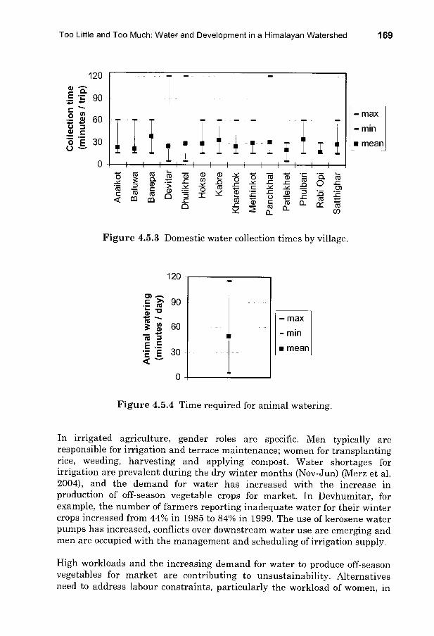
Too Little and Too Much: Water and Development in a Himalayan Watershed 169
120
90
60
30
0
(0
O-
4)
o
a)
L o
N U O 2
O
C L Q)
L L (a
L CL
ô (a C
Figure 4.5.3 Domestic water collection times by village.
- max
- min
mean
Figure 4.5.4 Time required for animal watering.
- max
- min
mean
In irrigated agriculture, gender roles are specific. Men typically are responsible for irrigation and terrace maintenance; women for transplanting rice, weeding, harvesting and applying compost. Water shortages for irrigation are prevalent during the dry winter months (Nov-Jun) (Merz et al. 2004), and the demand for water has increased with the increase in production of off-season vegetable crops for market. In Devhumitar, for example, the number of farmers reporting inadequate water for their winter crops increased from 44% in 1985 to 84% in 1999. The use of kerosene water pumps has increased, conflicts over downstream water use are emerging and men are occupied with the management and scheduling of irrigation supply.
High workloads and the increasing demand for water to produce off-season vegetables for market are contributing to unsustainability. Alternatives need to address labour constraints, particularly the workload of women, in

170 Assisting Community Efforts to Improve Livelihoods & Environment
order to be adopted and maintained. Sources of cash income are limited, and farmers' involvement in market driven production is likely to increase, necessitating more efficient water use. The long-term sustainability of small scale market production requires balanced nutrient inputs (section 3.3), efficient water use (section 3.4) and reduced, or at least no significant increases, in family labour. As workloads are already a production constraint, technologies which focus on reducing workloads will have a better chance of success.
4.5.2 Reducing Workloads; Improving Water Use Efficiency
Water and labour sustainability concerns point towards a combination of alternatives to store water for dry season use, use water more efficiently, reduce labour requirements and provide a livelihood option. Combinations of water harvesting and drip irrigation for cash crop production were evaluated to assess their possible impact on labour and water use.
Domestic water use in the Jhikhu Khola is less than one-half the WHO (2003) recommended 50 L/day water requirement, water collection typically occupies 2.5 hours per day of female labour, and bacterial contamination is common in drinking water sources (section 3.6). Rooftop water collection was seen as a potential option to reduce the labour requirements for household drinking water collection and to provide an alternative source of potable water. The "Thai- jar" rooftop rainfall collection method was evaluated from 1998-2001. Monsoon rainfall is re-directed from rooftops into a gutter system leading to a holding tank. Thirteen trial systems were constructed in the Jhikhu Khola, and cost, water use and labour were evaluated (Merz et al. 2003). Rooftop water collection was effective in terms of reducing workloads for water collection (Table 4.5.1), provided a potable water source, and increased water use slightly. Distances for the collection of water were reduced by more than 0.5 kilometre and collection times by more than 1
hour. This is potentially a significant reduction in female workload given the 4-5 trips per family per day requirement for the collection of water; however, the relatively small size of the jar (5 m3) limits its application to a supplemental domestic water supply.
Table 4.5.1 Reduction in women's workload with rooftop water collection jars.
Activity Before With jar Collection distance 564 m 0 m
Collection time 91 minutes 22 minutes Water use 15 L/day 17 L/day
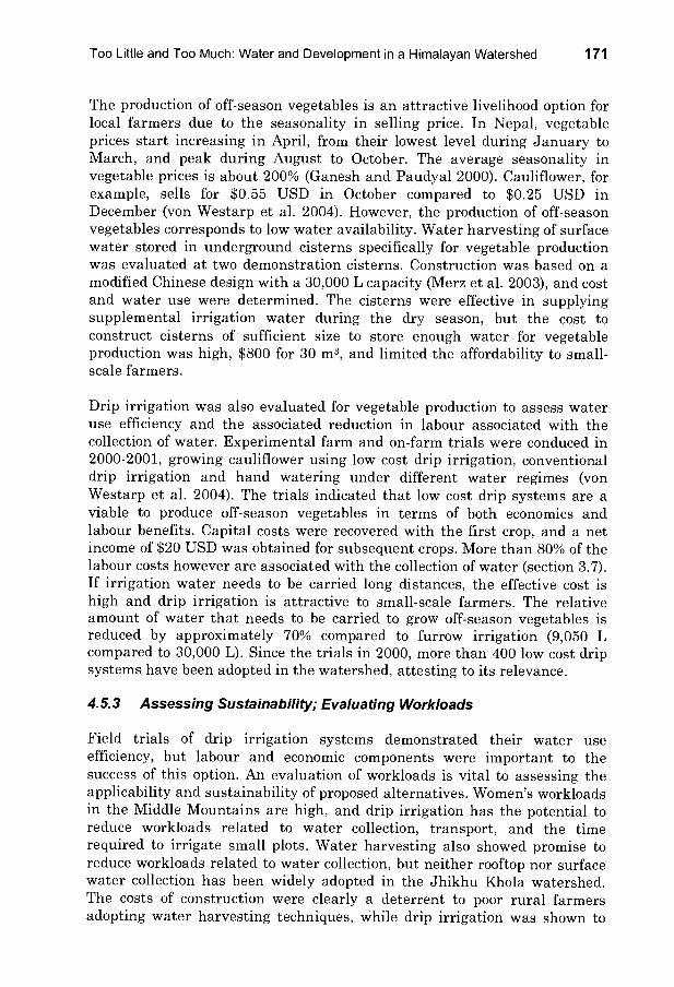
Too Little and Too Much: Water and Development in a Himalayan Watershed 171
The production of off-season vegetables is an attractive livelihood option for local farmers due to the seasonality in selling price. In Nepal, vegetable prices start increasing in April, from their lowest level during January to March, and peak during August to October. The average seasonality in vegetable prices is about 200% (Ganesh and Paudyal 2000). Cauliflower, for example, sells for $0.55 USD in October compared to $0.25 USD in December (von Westarp et al. 2004). However, the production of off-season vegetables corresponds to low water availability. Water harvesting of surface water stored in underground cisterns specifically for vegetable production was evaluated at two demonstration cisterns. Construction was based on a modified Chinese design with a 30,000 L capacity (Merz et al. 2003), and cost and water use were determined. The cisterns were effective in supplying supplemental irrigation water during the dry season, but the cost to construct cisterns of sufficient size to store enough water for vegetable production was high, $800 for 30 m3, and limited the affordability to small- scale farmers.
Drip irrigation was also evaluated for vegetable production to assess water use efficiency and the associated reduction in labour associated with the collection of water. Experimental farm and on-farm trials were conduced in 2000-2001, growing cauliflower using low cost drip irrigation, conventional drip irrigation and hand watering under différent water regimes (von Westarp et al. 2004). The trials indicated that low cost drip systems are a viable to produce off-season vegetables in terras of both economics and labour benefits. Capital costs were recovered with the first crop, and a net income of $20 USD was obtained for subsequent crops. More than 80% of the labour costs however are associated with the collection of water (section 3.7). If irrigation water needs to be carried long distances, the effective cost is high and drip irrigation is attractive to small-scale farmers. The relative amount of water that needs to be carried to grow off-season vegetables is reduced by approximately 70% compared to furrow irrigation (9,050 L compared to 30,000 L). Since the trials in 2000, more than 400 low cost drip systems have been adopted in the watershed, attesting to its relevance.
4.5.3 Assessing Sustainability; Evaluating Workloads
Field trials of drip irrigation systems demonstrated their water use efficiency, but labour and economic components were important to the success of this option. An evaluation of workloads is vital to assessing the applicability and sustainability of proposed alternatives. Women's workloads in the Middle Mountains are high, and drip irrigation has the potential to reduce workloads related to water collection, transport, and the time required to irrigate small plots. Water harvesting also showed promise to reduce workloads related to water collection, but neither rooftop nor surface water collection has been widely adopted in the Jhikhu Khola watershed. The costs of construction were clearly a deterrent to poor rural farmers adopting water harvesting techniques, while drip irrigation was shown to

172 Assisting Community Efforts to Improve Livelihoods & Environment
have short-term affordability and positive livelihood impacts, resulting in broader adoption. Combining water use efficiency, livelihoods and labour provided a mechanism to assess social and biophysical sustainability, and to improve the chance of long-terni success.
References
Ganesh, B.T., and D. Paudyal. 2000. Nepal. In: M. Ali (ed). Dynamics of vegetable production, distribution and consumption in Asia. The World Vegetable Center AVRDC. pp. 231-270 (www.avrdc.org/pub socio.html )
Merz, J., G. Nakarmi, S.K. Shrestha, B.M. Dahal, B.S. Dongol, M. Schaffner, S. Shakya, S. Sharma, and R. Weingartner. 2004. Public water sources in rural watersheds of Nepal's middle mountains: Issues and constraints. Environmental Management, 34(1): 26-37.
Merz, J., G. Nakarmi, S.K. Shrestha, B.M. Dahal, P.M. Dangol, M.P. Dhakal, B.S. Dongol, S. Sharma, P.B. Shah, and R. Weingartner. 2003. Water: A scarce resource in rural watersheds of Nepal's middle mountains. Mountain Research and Development, 23(1): 41-49.
von Westarp, S., H. Schreier, S. Brown, and P.B. Shah. 2004. Agricultural intensification and the impacts on soil fertility in the Middle Mountains of Nepal. Canadian Journal of Soil Science, 84(3):323-332.
WHO. 2003. Domestic water quantity, service level and health. World Health Organization, Geneva. 33pp.
4.6 Water Harvesting
Gopal Nakarmi
4.6.1 Introduction
Population growth and agricultural intensification bas resulted in rapidly increasing water demands. An inventory of available drinking water sources was completed by Merz et al. (2004) and, as indicated in section 3.4, more than one third of the population surveyed in 2002 reported critical shortages of drinking and irrigation water during the dry season (February - May). Some 65-75% of the annual rainfall occurs during the 4 month monsoon season (June-September), at which time there is massive runoff in the streams. Financial and spatial constraints and environmental concerns restrict the construction of large reservoirs. Consequently, small scale water

Too Little and Too Much: Water and Development in a Himalayan Watershed 173
harvesting methods were examined in order to provide supplemental quantities of drinking and irrigation water to individual homeowners for use during the dry season.
4.6.2 Above and Below Ground Water Storage
The problem of water storage depends on available space, cost, and suitable collection area. A project of harvesting roof-water for drinking water was initiated in 1999. Thirteen collection jars were constructed using locally available materials (Plates 4.6.1 and 4.6.2) and installed in collaboration with homeowners. These jars were particularly effective during the dry season when drinking water sources are scarce and women carry water over longer distances. While the jars were effective, the construction cost (> $80 USD) and maintenance proved to be somewhat of a deterrent. Only slate and galvanized roofs were found to be appropriate, and to maintain a clean roof and to disinfect the water in the jar proved to be a somewhat difficult task that required considerable education. Given the cost, many local farmers opted to dig shallow groundwater wells, but this proved to be of concern because of leaching and contamination of chemicals used in intense agricultural.
Storing water for efficient irrigation of small plots during the dry season was examined in two experiments: the construction of an underground cistern and plastic lined open pond.
An underground cistern was constructed in a trial test in Kubinde in 1999 (Nakami and Neupane 2000). A conical shaped cernent tank was constructed below a degraded area with a capacity of 10 m3. Stones were used as building blocks and cement was used to seal the inside of the cistern. The design and dimensions of the system are provided in Figure 4.6.1 and an overview of the collection system is provided in Plate 4.6.3. Polyethylene pipes were installed at the inlet and outlet of the cistern. Five sediment traps and one screen were installed in the runoff collection area to prevent excessive sediment accumulation in the cistern. The construction took 7 days and the total cost (inc. labour) was $356 USD.
Several open ponds were constructed and lined with plastic in farmers' fields in 2000, and this type of design was the most cost effective. However, each collection system had advantages and disadvantages as shown in Table 4.6.1. Available space and insects were the greatest concern about plastic lined ponds because malaria is known to occur in the lower portion of the watershed. Costs were the main constraints for the construction of underground systems.

174 Assisting Community Efforts to Improve Livelihoods & Environment
Plate 4.6.1 Construction of roofwater harvesting jars for drinking water.
Plate 4.6.2 Roofwater harvesting jar.
Plate 4.6.3 Underground cistern to collect monsoon runoff to be used for irrigation

Too Little and Too Much: Water and Development in a Himalayan Watershed 175
Figure 4.6.1 Design of underground cistern.
Table 4.6.1 Advantages and disadvantages of différent water storage systems.
Type of System
Jar (roofwater collection)
Underground Cistern
Pond (plastic lined)
Water Use Drinking Water Irrigation Irrigation
Cost inc. Labour $ 80.- $ 356.- $ 170.-
aintenance ow (roof maintenance, disinfection)
Moderate (leakages, sediment management)
Moderate (leakages, sediment, deterioration of plastic)
Losses Low Leakages Evaporation Health Constraints
Metal contamination, insects Few Insects
4.6.3 Summary
All water harvesting activities were carried out between 1998 and 2003, and plastic lined ponds seemed to be the most feasible option to local farmers. All three types of experiments were carried out as demonstration projects, but because of the social conflict between 2003 and 2006 it was not possible to determine the rate of adaptation of any of the three options. Building underground cisterns was the least feasible option because of cost, and farmers had a higher preference for plastic lined ponds. The incentive for

176 Assisting Community Efforts to Improve Livelihoods & Environment
storing monsoon water came with the introduction and availability of low cost drip irrigation systems, which allowed farmers to produce cash crops during the dry season (see section 4.7).
References
Merz, J., G. Nakarmi, S. Shrestha, B. Dahal, B. Dongol, M. Schaffner, S. Shakya, S. Sharma, and R. Weinghartner. 2004. Public water sources in rural watersheds of Nepals's Middle Mountains: Issues and constraints. Environmental Management, 34:26-37.
Nakarmi, G., and P. Neupane. 2000. Construction of a harvesting tank - experience from Kubinde, Jhikhu Khola Watershed. In: Allen, R.., H. Schreier, and S. Brown (eds). The People and Resource Dynamics Project: the first three years (1996-1999). Workshop Proceedings, Boashan, Yunnan Province, China. March 2-5, 1999. International Centre for Integrated Mountain Development, Kathmandu. pp. 231-242.
4.7 Low Cost Drip Irrigation
Stephanie von Westarp and Hans Schreier
4.7.1 Background
Water shortages are widespread in the Jhikhu Khola during the dry season as shown in section 3.4. Women are primarily responsible for drinking water collection, animal care, planting and household chores (section 3.7) and their workload increases as water resource degrade. Providing a source of cash income and at the same time reducing women's workloads was the primary motivation to introduce low cost drip irrigation systems (LCDI). Surface gravity irrigation is the common method of irrigation in the watershed, but its efficiency is only 40-50%. In contrast, drip irrigation can reach 70-90% efficiency (Postel 2000, Postel et al. 2001).
Until recently drip irrigation required significant economic and technical investment, but in 1996 International Development Enterprises (IDE) introduced a low cost drip irrigation system to small farmers on a trial basis in Nepal. Over the 1999-2001 period three low cost systems were tested; one at the experimental farm and two in on-farm trials. The aims were to determine: a) the amount of water that would need to be stored during the monsoon, in order to produce a vegetable crop with drip irrigation during the dry season, and b) how the LCDI system compared with conventional hand watering systems of irrigation in terras of water use, labour requirements and costs. Low cost drip irrigation bas the potential to not only increase food security, but also provide a source of cash income as dry season vegetable

Too Little and Too Much: Water and Development in a Himalayan Watershed 177
prices are high and the potential for generating a cash income source is favourable.
4.7.2 Low Cost Drip Irrigation Experiments
During the first year of the experiment three irrigation methods and regimes were compared, each applying a différent timing and amount of water delivered to cauliflower plants. The soil water content, biometric parameters, water use efficiency and profitability were all compared. A 12 x 12 m plot was used, and 18 différent rows of plants were irrigated using a low cost drip irrigation system (LCDI), a nozzle control system (CDI), and hand watering (HW). The experiment is described in detail by von Westarp (2002) and von Westarp et al. (2004), and the experimental design is provided in Figure 4.7.1. Three irrigation regimes were applied: 50% of daily water requirement, 100% water requirements (morning and evening application) and 100% daily requirement (evening application only). Soil moisture was monitored throughout the growing season.
The moisture content at field capacity was determined to be 24%, and the permanent wilting point 15%, hence the management allowed deficit was set at 19.5% (50% of available water holding capacity). Some plant stress was observed under the 50% daily water requirement irrigation scheme, while both 100% water requirement schemes were at field capacity ater each irrigation application.
t - endcap I- I ['
0.45 m 0.6 m
Figure 4.7.1 Experimental design for drip irrigation study.

178 Assisting Community Efforts to Improve Livelihoods & Environment
Cauliflower yields and above ground biomass were compared between the différent irrigation system and regimes. The cumulative yields are provided in Table 4.7.1. The results showed that hand watering (HW) produced between 13-27% more total above ground biomass than the LCDI and the CDI for all three watering regimes, but the cauliflower biomass was 14% higher under deficit irrigation. There was no différence between HW and LCDI for evening irrigation only, but the highest yields were obtained with HW using morning and evening irrigation. The CDI was the least productive system regardless of irrigation regime. In terms of water use efficiency (Table 4.7.1), it is evident that under deficit irrigation LCDI was the most efficient, and HW and LCDI were equally as efficient under evening only irrigation. While there were relatively small différences in yields between HW and LCDI, the issues of workload and economics also need to be considered. An overview of the drip system is provided in Plate 4.7.1.
Table 4.7.1 Yields of cauliflower mass and above ground biomass under différent irrigation and water use efficiency schemes (n =40).
Yield Water use efficiency (kg for 40 plants) (g cauliflower / ml water used)
Irrigation regime LCDI CDI HW LCDI CDI HW
Déficit 32.2 24.7 28.2 0.052 0.040 0.041 irrigation Cauliflower
Morning & 2
biomass evening
9.8 27.4 41.1 0.025 0.023 0.040 (kg/40
Evening plants) only 35.1 24.2 35.1 0.031 0.021 0.031
Deficit
irrigation 56.2 49.7 64.3 0.090 0.079 0.086 Above
Morning & ground
evening 63.6 57.7 87.3 0.054 0.049 0.085 biomass
Evening (kg/40
only 64.9 59.0 81.3 0.057 0.052 0.072 plants)
The introduction of drip irrigation was primarily aimed at women as these systems are best applied in a kitchen garden context and allow women to not only improve food security but also produce some cash crops. As the workload for women is already high (section 3.7), it is essential that additional work to produce the crop should be small, and the collection of water for irrigation adds significantly to that workload. Hence, in order to succeed with the drip irrigation system there bas to be both a financial and reduced workload incentive. Table 4.7.2 provides a comparison between the three types of irrigation systems in terms of labour, cost and economics.

Too Little and Too Much: Water and Development in a Himalayan Watershed 179
Table 4.7.2 Différences in labour cost and economics between the three différent irrigation systems.
LCDI CDI HW
Labour activity Total Labour Total Labour Total Labour time cost time cost time cost
(days) (USD) (days) (USD) (days) (USD)
Land preparation, 1 1 weeding set-up 1 1 1 1
Pesticide / fertilizer 0.5 0.5 application 0.5 0.5 0.5 0.5
Collecting water 13 13.3 13 13.3 13 13.3
Shifting irrigation 1.5 1.5 lines 1.5 0 0 0
Irrigation 0 0 0 6 6.1
Total 16 16.4 14.8 14.8 20.5 21
Capital costs LCDI (USD) CDI HW
Drip system 12.00 190.00 -
Water drum (100L) 5.90 5.90 -
Bucket and scoop - - 4.00
Variable costs LCDI CDI HW (USD)
Fertilizer and 3.50 pesticides 3.50 3.50
Seedlings 4.20 4.20 4.20
Labour 13.00 (water collection) 13.00 13.00
Labour 3.00 1 30 7 50 (other activities) . .
Total cost 41.70 219.00 32.30
Gross income (One crop @ $ 67.39 46.46 67.39 0.24/kg)
Net income (after 1 crop) + 25.69 -172.54 + 35.09 including labour Total cost
23.70 (2nd crop) 22.00 28.20
Net income (after 2 crops) +43.69 -128.08 + 39.19 including labour

180 Assisting Community Efforts to Improve Livelihoods & Environment
Plate 4.7.1 The low cost drip irrigation system (LCDI).

Too Little and Too Much: Water and Development in a Himalayan Watershed 181
These relatively straight forward calculations demonstrated that the LCDI system is the most efficient in terms of time commitment, and that the profitability increases after the second and third crop. The workload and profitability can further be improved if water harvesting is combined with the drip irrigation methods because in this way the collection time needed for water is further reduced.
Initially, two on-farm trials were conducted using a full LCDI system without modification and under deficit irrigation. In the first year, the on- farm trials were not effective because the water supply was erratic, the selected farmers were not fully committed to maintaining daily water additions to the LCDI system, and there was some reluctance to commit to the work because of the already full workload schedule. However, once it was demonstrated that using LCDI could be profitable and could provide additional income at a critical time of year when food shortages are the highest, three women farmers volunteered to participate in on farm experiments. A cost sharing approach was used to purchase the LCDI system and two of the three participants used water from dug-wells for the irrigation, while the third built a plastic lined collection system for lier water needs. Sediments that clog the drip system were a problem in several cases, but the addition of a sediment filter below the water tank helped remediate the problem. Bitter curd was the preferred vegetable crop and all three continued with the LCDI during the second dry season.
Some 40 farmers had taken up the LCDI system by 2004. In 2005 several hundred systems were reportedly operating in the watershed. Unfortunately, we were unable to conduct a follow-up survey to conf"irm the adaptation rate do to the security concerns in the watershed at that time.
4.7.3 Summary
Introducing new irrigation technology required time and education before it was widely accepted. From the research carried out, initially there was limited advantage to using LCDI over HW in terms of water savings and yields. However, when considering the lower workload, the capacity to gain cash from sales of vegetable during the dry season when food shortages exist and prices are high, and the possibility of paying off the LCDI system in the first year of operation, then a case can be made for using LCDI. Combining LCDI with water harvesting techniques can clearly reduce workloads even more. Under water stressed conditions the LCDI performed better that conventional irrigation approaches, both in terras of water use and yields. Since water scarcity is likely becoming more widespread due to climate change and on-going increases in production intensity and flood irrigation, water harvesting combined with LCDI have shown potential advantages. However, the long terra performance of these systems needs further evaluation.

182 Assisting Community Efforts to Improve Livelihoods & Environment
References
Postel, S., P. Polak, K. Gonzales, and J. Keller. 2001. Drip irrigation for small farmers. A new initiative to alleviate hunger and poverty. International Water Resources Association. Water International, 26(1):3-13.
Postel, S. 2000. Redesigning irrigated agriculture. In: Starke, L. (Ed). State of the World, W.W. Norton and Co., New York. pp. 39-58.
von Westarp, S., S. Chieng, and H. Schreier. 2004. A comparison between low-cost drip irrigation, conventional drip irrigation and had watering in Nepal. Agricultural Water Management, 64:143-160.
von Westarp, S. 2002. Agricultural intensification, soil fertility dynamics, and low-cost drip irrigation in the Middle Mountains of Nepal. M.Sc. Thesis, Faculty of Agricultural Sciences, University of British Columbia. 202 pp.
4.8 Improving Crop Yields by Lime Applications
Bandana Prajapati and P.B. Shah
4.8.1 Agricultural Intensification and Agrochemical Use
The project team has noticed a remarkable change in the farming systems in the Jhikhu Khola watershed over the past 16 year period. Between 1989 and 2005, significant intensification has occurred and there has been a major shift to incorporate cash crops. This move towards commercial farming was part of the green revolution that brought high yielding crop varieties, fertilizers and pesticide use into the watershed. Schreier and Shah (2000), and Brown (2000) documented that a major shift in crop type and crop rotation occurred between 1990 and 2005 from the traditional rainfed maize- wheat/mustard cropping rotation to a maize-potato-tomato dominated rotation. von Westarp (2002) reported that up to four crops per year were grown on the prime irrigated land in valley bottoms. This resulted in an enhancement of on-farm income and improved food supply for the growing population. However, intensification also lead to the depletion of soil fertility, created health issues related to the heavy use of agrochemicals, and increased the demand for irrigation water, particularly during the dry season.
As shown in section 3.3, continuous crop intensification and heavy use of urea and ammonium based fertilizers increased soil acidity and created an imbalance in soil nutrients. Results of the soil analyses showed that the carbon and potassium levels dropped well below the desirable levels. Farmers tried to compensate for reduced soil fertility by applying higher

Too Little and Too Much: Water and Development in a Himalayan Watershed 183
doses of minerai fertilizers. von Westarp (2002) and von Westarp et al. (2004) reported that farmers in the JKW applied up to 400 kg urea (46% nitrogen), 800 kg diammonium phosphate (18% nitrogen, 46% phosphorus), and 800 kg complex fertilizer (20% nitrogen, 20% phosphorus) per hectare for their main cash crop of potatoes. An additional 200 kg/ha per annum of other fertilizers were applied to other crops. Fertilizer input on the rainfed land also increased from 100 to 450 kg of N and from 50 to 150 kg of P per ha/yr. By 2000, 50 -70% of the soil samples in the intensively used fields showed pH values below 5.5. Red soils are of particular concern because at low pH (pH values below 4.3.) aluminium becomes soluble; this can result in aluminium toxicity and also create phosphorous availability problems. Thus the application of more minerai phosphorous fertilizer without addressing the soil pH may not improve soil fertility or yields. Farmers have recently noticed that the crop response to these heavy doses of fertilizer application has been relatively poor, and they complain that in order to maintain yields fertilizer doses must be increased. In economic terms, farmers do not see significant returns in cereal crop production as a result of the added fertilizer.
Liming the soils to increase the soil pH to an adequate level was seen as an option to improve the production capacity. One of the main challenges with these intensive agricultural systems is how to maintain sufficient soil nutrients, particularly when organic matter inputs are low. Compost and manure are scarce and the currently available fertilizers increase soil acidity. Adding lime will not only improve the pH but will also add calcium. An additional issue is the timing of lime applications as there is usually no fallow period between rotations, and there are only a few days between harvesting of a crop and planting of the second or third crop. Planting seeds immediately after lime application is a questionable management practice. To address this problem and to determine if lime application will improve soil pH and crop productivity, experiments were carried out on red soils under maize production.
4.8.2 Methodology
On-farm trials were carried out with interested farmers on the valley bottom where the most intensive farming is taking place. Discussions were held with the farmers as to their nutrient management practices and their perceptions about declining yields. The problem of inadequate soil pH and its consequences in the long term was not apparent to them; the focus has been on using nitrogen and phosphorus fertilizers. We proposed liming of the soil to enhance the soil pH, and three farmers with red soils in the pH range from 4.2 to 4.8 were selected for the trials. The terraces available measured from 34.5 m2 to 90 m2. The entire terrace was used for the trial at each site for the convenience of farmers. Approximately half of the field was treated with lime, while the other half was used as a control and received no lime.

184 Assisting Community Efforts to Improve Livelihoods & Environment
The data were then converted into a standard format to compare the results. The plot description is provided in Table 4.8.1.
Table 4.8.1 Description of plots used in the liming experiment.
Site No. Soil type' Plot size (m2) Soil pH Lime (kg) Remarks 1 CL 34.5 4.8 25 control
1 CL 40.5 4.8 30 lime 2 CL 70 4.2 50 control 2 CL 90 4.2 65 lime 3 CL 55 4.8 40 control 3 CL 44 4.8 32 lime
1 CL = Clay Loam
The dosages of lime application were calculated based on soi' pH and soil texture according to standard recommended figures provided by the HMGN Ministry of Agriculture (personal communication). Recommended doses of NPK (nitrogen, phosphorous and potash) and organic matter were applied (N: 35, P: 30, K: 30 kg/ha and 10 t/ha of organic matter). The timing and the method of lime and fertilizer application were determined by the participating farmers. The choice of maize variety was also selected by the farmers, but the saure variety was used in both the treated and limed plots. Farmers 1 and 3 used the Dolakha local variety of maize, while farmer 2 used the Jhikhu Khola local variety. The lime was applied 17 days before sowing the maize in plot 1, 33 days before in plot 2 and 28 days before in plot 3. The farmers in plot 2 applied lime and fertilizer only along the line where the maize was to be sown. At the two other sites, lime and fertilizer were applied over the entire area of the plots. The urea application was split into two doses. The first dose was applied on the day of planting, and the second dose was applied 40 to 45 days after planting as top dressing. The maize was sown in rows of 75 cm spacing with a 25 cm space between plants.
The average dates for flowering, cob formation and cob maturing were recorded for each site. Average biomass and grain weight were recorded separately based on random sampling from 1 m2 patches in five locations in each of the limed and the control sites. The average number of cobs per plant, cob length, and height the plants were determined at harvesting time. The soi' pH was determined before and after application of lime.
4.8.3 Results
There was no différence between limed versus control plots in terras of time to emergence of flowers (55 to 60 days of plantation). After 10-12 days of

Too Little and Too Much: Water and Development in a Himalayan Watershed 185
flowering, most of the plants started producing cobs. Almost all the cobs were matured within 40 to 45 days of formation. On average, there were 6 maize plants per m2 and 1 cob per plant. However the cobs in the treated plots were about 5 to 6 cm longer than in the controlled plots, and the maize plants were about 15 to 30 cm higher in the treated plots. This visual recording suggests a distinct increase in the yield of biomass and grain in the treated plots (Figures 4.8.1 and 4.8.2).
8
6
Control
o Lime
0
Site 1 Site 2 Site 3
Figure 4.8.1 Grain yield in t/ha for the différent fields and treatments.
Control
o Lime
Site 1 Site 2 Site 3
Figure 4.8.2 Total green biomass between différent fields and différent treatments.
The results (Figure 4.8.3) showed that liming of the soil had a positive effect on productivity, for both the tested varieties of maize and the différent pH's. The grain yield (12% average moisture content) was 22-40% higher in the lime treated plots than in the control plots, which represents a yield increase of 1.1-1.6 t/ha. Similarly, the total green biomass was 22-50% higher in the

186 Assisting Community Efforts to Improve Livelihoods & Environment
limed plots compared to the control plots, which represents a 4-5 t/ha increase.
Soil pH before and after trial
Before
o After
Figure 4.8.3 Différence in soil pH différence for control versus lime treated plots at harvesting time.
The monitoring of soil pH before and after the trial illustrated that with lime treatment it was possible to increase the pH by 0.2-0.5 pH units (Figure 4.8.3). With the exception of site 1, the final pH was still well below the 5.5- 6.5 pH range which is considered an appropriate pH for most cultivated staple crops. This suggests that a second lime treatment would be appropriate and would further enhance production. In addition, lime should be applied at the start of the monsoon rain, some 14 days before planting of the seeds. If this is not possible because of the length of the growing season required to produce 3-4 crops, then several applications of lower than recommended lime applications over several years would be needed to bring about the necessary changes to the soil pH.
Not only is the change in pH responsible for the increase in yield. With lime additions, the calcium content (an essential macro-nutrient) and phosphorus availability are also improved because the amount of soluble Al and Fe in the soil is decreased. In addition, the structural properties of the soil are improved which modifies the soil infiltration rate and makes the red soils easier to plough.
4.8.4 Summary
Preliminary results of the on-farm liming trials were encouraging. Although no effect in the phonological characters of the trial crop were documented, the cob size, plant height, and cob and total biomass yield were substantially

Too Little and Too Much: Water and Development in a Himalayan Watershed 187
higher in the lime treated soils than in the control plots on red soils. The participating farmers were pleased with the yield increases and showed an interest to continue the practice. A one year trial is obviously not sufficient to increase the pH in these soils, and it is recommended that several treatments will be needed over the next few years to bring the soils into an appropriate pH range. A one time large dose of lime application is not recommended because this would shock the system. Instead, an incremental stepwise approach is needed. In addition to the yield increases, the farmers also reported that the limed plots become easier to plough after lime treatment. This is likely a result of structural changes introduced by Ça additions. Once the pH is in the 5.5+ range then liming will not be required on an annual basis, but long terra monitoring will be needed to confirm the frequency and doses of lime application.
References
Brown, S. 2000. Socio-economic and biophysical indicators: Examples relating to soil fertility. In: Allen, R., H. Schreier, S. Brown, and P.B. Shah (eds). The People and Resource Dynamics Project: the first three years (1996-1999). Workshop Proceedings, Boashan, Yunnan Province, China. March 2-5, 1999. International Centre for Integrated Mountain Development, Kathmandu. pp. 301-308.
Schreier, H., and P.B. Shah. 2000. Soil fertility status and dynamics in the Jhikhu Khola and Yarsha Khola watersheds. In: Allen, R., H. Schreier, S. Brown, and P.B. Shah (eds.). The People and Resource Dynamics Project: the first three years (1996-1999). Workshop Proceedings, Boashan, Yunnan Province, China. March 2-5, 1999. International Centre for Integrated Mountain Development, Kathmandu. pp. 291-300.
von Westarp, S. 2002. Linkages between agricultural intensification, soil- fertility dynamics, and low-cost drip irrigation in the Middle Mountains of Nepal. M.Sc. Thesis, Dept. of Soil Science, University of British Columbia. 198 pp.
von Westarp, S., H. Schreier, S. Brown, and P.B. Shah. 2004. Agricultural intensification and the impact on soil fertility in the Middle Mountains of Nepal. Canadian Journ Soil Science, 84(3): 323-332.

188 Assisting Community Efforts to Improve Livelihoods & Environment
4.9 The Price of Milk: Balancing Income, Workloads and Environmental Impacts
Sandra Brown and Bhuban Shrestha
4.9.1 The Milk Chilling Centre
Milk cooperatives have been successful in poverty alleviation by allowing small-scale rural poor farmers to participate in the commercialization of the milk industry in many developing countries (Uotila and Dhanapala 1994). One of the factors that played a role in raising market demand was the restriction of imports of subsidized powdered milk from the European Union, which created new incentives and improved prices for Nepalese milk producers. The consequent establishment of a milk-collection system through the state-owned Dairy Development Corporation improved farmers' market access and linked them to urban milk consumers (IFAD 1993). Within the Jhikhu Khola watershed, milk production was largely for domestic consumption prior to 1990 when a chilling centre was established at Tamaghat (Plate 4.9.1.). Milk spoilage was significantly reduced with the chilling centre, and given the proximity and demand in Kathmandu, farmers entered the commercial milk market. Within 4 years of opening the chilling centre the number of households selling milk had increased by 43% (Brown 1997), and by 2000 the 12,000 litre capacity of the centre was fully utilized (Shrestha 2000). However, there are potentially positive and negative effects related to the number of animais, demand for animal feed, workload of women, pressure on agro-forestry resources for fodder, and household economics.
Plate 4.9.1 Milk chilling plant in Tamaghat.

Too Little and Too Much: Water and Development in a Himalayan Watershed 189
4.9.2 Cooperative Dairy
Most milk producing farmers are small landholders who are organized to form producers' associations, which channel milk to the Dairy Development Corporation that runs the chilling centre. The chilling center at Tamaghat does not accept milk from individual farmers, and cooperative collection centers were established to collect milk from households for delivery to the chilling center. A minimum of 25 households are required to register with the district co- operative board in order to from a cooperative, and in total 63 village cooperative centers were established. Of the cooperatives delivering milk to the Tamaghat chilling center, 40 were located within the Jhikhu Khola watershed, and 80% of the milk collected cornes from within the watershed boundaries (Shrestha 2000). The location of the chilling centre and village cooperatives are shown in Figure 4.9.1.
Cooperatives
O Sampled cooperatives
Chilling center
D o
Figure 4.9.1 Location of the Tamaghat chilling center and village milk cooperative centers.
4.9.3 Milk Survey
A milk survey was conducted at three levels (Table 4.9.1) to understand the trends, processes and dynamics of milk production in the watershed. Participatory Rural Appraisal, Rapid Rural Appraisal techniques, semi- structured interviews and focus group discussions were employed. At the Tamaghat chilling centre, 23 milk producers and 16 porters from 39 cooperatives were interviewed. Five of the 63 cooperatives were investigated in detail through interviews with 199 farmer producers. Focus group discussions were held in 11 villages, involving 71 farmers (female and male).

190 Assisting Community Efforts to Improve Livelihoods & Environment
All information was collected in a gender-disaggregated manner and geo- referenced to aerial photographs for spatial analysis.
Table 4.9.1 Milk survey sampling design.
Level Chilling Centre Village cooperatives Farmers
Sampling 39 producers and porters from 39 co-operatives 119 producers from 5 cooperatives 71 farmers from 11 villages
4.9.4 Milk production and dynamics
Milk collection at the chilling centre, farm level production and sales vary seasonally and annually. Changes in annual milk collection at the Tamaghat chilling center for 1994-1998 are shown in Figure 4.9.2. From 1994 to1996 there was a 26% increase in milk collected, followed by a decline of 18% between 1996 and 1998. Milk production at the farm level continued to increase but a new collection centre opened at Kunta (also within the Kabhrepalanchok District), private dairies established in Kathmandu after 1996 collected milk directly, and the National Dairy Corporation reduced the amount of milk they would accept at the Tamaghat Chilling Centre. "Milk holidays" or load shedding was introduced to lirait supply at the chilling centre to match the market capacity in Kathmandu. Six to seven milk holidays per month were introduced, and on these days no milk is accepted at the chilling centre.
4,500,000
4,000,000
3,500,000
3,000,000
2,500,000 1994 1995 1996 1997 1998
Figure 4.9.2 Annual milk collection at the Tamaghat chilling centre.

Too Little and Too Much: Water and Development in a Himalayan Watershed 191
More milk is collected at the Tamaghat chilling centre between October and March (winter) than in April to September (pre-monsoon / monsoon) (Figure 4.9.3) despite more milk being produced during the monsoon season (Figure 4.9.4). On average, monsoon milk production is 10% greater than winter production due to the availability of green fodder during the monsoon. Lower deliveries to the chilling centre during monsoon result from problems of transport and spoilage during this season. The 5 village cooperatives studied in detailed (n=71) produced a total of 908 litres/day in winter, but were only able to sell 680 litres/day (Figure 4.9.5) as milk sales were limited by the chilling centre. Consequently, household consumption is higher during the monsoon (Figure 4.9.6). Even though household consumption is greater during the monsoon season, total sales are also higher due to the greater production, with the exception of Deourali. In Deourali, household consumption during the monsoon is significantly higher due to greater spoilage with transport from areas located further from the chilling center, and as a result households produce butter fat.
600,000
500,000
C 400,000 o
300,000 .0 0
âi . 200,000 o o 100,000
0
J F M A M J J A S O N D
1998
1997
1996
--.---- 1995
-----1994
Figure 4.9.3 Seasonal variation in milk collection at the Tamaghat chilling center.
Deourali
Kaphaledihi
Upretithok
Shreerampati
Ranipani
Monsoon
O Winter
0 5 10 15
Household Milk production (Iitres/day)
Figure 4.9.4 Seasonal variability in milk production at the household level.

192 Assisting Community Efforts to Improve Livelihoods & Environment
Deourali
Kaphaledihi
Upretithok
Shreerampati
Ranipani
Production
Sales
0 50 100 150 200 250
Litres/ day
Figure 4.9.5 Winter milk production and sales by village cooperative.
Deourali
Kaphaledihi
Upretithok
Shreerampati
Ranipani
Monsoon
o Winter
0 1 2 3 4
Houshold Milk Consumption (Litreslday)
Figure 4.9.6 Household milk consumption by season.
Brahmin villages are the major producers of milk in the watershed, with 90% of families selling milk compared to only 29% and 6% in Danuwar and Tamang villages, respectively (Table 4.9.2). Overall, the proportion of households involved in milk sales is high (71%) but higher caste households keep more animals and appear to have a competitive advantage in the commercial market.
Travel distance is a factor influencing the volume of milk sales. Villages closest to the Tamaghat chilling centre tend to deliver the most milk, and those farthest away, the least (Figure 4.9.7). The average walking time from the 39 cooperatives sampled to the chilling centre is 2.3 hours, with a range from 12 minutes to 6 hours. The road has a significant impact on milk transportation. Jyamdi, the second largest milk producer, is about 3 hours and 15 minutes walk from the chilling centre, but most of the milk is

Too Little and Too Much: Water and Development in a Himalayan Watershed 193
transported by truck along the Araniko highway. The number of buffalo per household is also influenced by road access. In villages such as Deourali with direct road access, households average 2.0 buffalo, while the lowest numbers are found in villages such as Upretihok, 1.0 buffalo per household, some 5-6 hours walking distance from the road.
Table 4.9.2 Involvement in milk production by ethnicity.
Village Sa mple Total # % Households Dominant ethnie s ize households selling milk group
Shreerampati 15 140 89 Brahmin Kaphaledihi 3 33 94 Brahmin Baniyadihi 9 25 96 Brahmin Lamdihi 1 100 100 Brahmin Ranipani 4 75 67 Brahmin Bakultar 7 120 29 Danuwar Nayaguan 12 31 94 Brahmin Shikarkateri 8 30 100 Brahmin Deourali 3 10 100 Brahmin Kalinjor 5 105 6 Tamang Salleni 4 11 73 Brahmin
Partial road connection No road connection
Walking time (hours)
Figure 4.9.7 Average walking time to the chilling centre versus milk delivered.

194 Assisting Community Efforts to Improve Livelihoods & Environment
4.9.5 Livestock dynamics and feed implications
Livestock holdings over time (Figure 4.9.8) reflect the changes in milk production with the opening of the Tamaghat chilling centre in 1990. From 1989 to 1999 the number of milking animais increased from 0.5 to 1.2 per household (Kennedy and Dunlop 1989, Brown 1997, Shrestha 2000). Stocking densities are in the range of 3.8 to 4.0 TLU/ha of cultivated land, 5.1 TLU/ha of forest and rangelands, and 2.2 TLU/ha over the entire watershed area (Brown 1997, Merz 2004). Tropical livestock units per area of cultivated land are important from a nutrient / manure application perspective, and TLU/ha of forest area reflect the pressure on forest resources for bedding material and fodder.
Crop residues and grass are the two main sources of animal feed (Figure 4.9.9). Crop residues provide 69% of winter feed; grasses provide 76% of summer feed. Feed concentrate makes up 14% and 10% of winter and summer feed sources respectively (Shrestha 2000), and contributes to the milk yielding capacity of the animals (Sharma et al 2004, Uddin et al. 2002). Shortages in animal feed (Table 4.9.3) are reported for grasses from October until May, and for crop residues from April to July.
Figure 4.9.8 Milking animal dynamics 1989-1999.
Eighty-seven percent of farmers feed crop residues to their water buffalo in winter due to shortages of grasses. The remaining 13% carry fodder from forests, grasslands or other "waste" lands (Shrestha 2000). All milking animals are stall fed during the monsoon, compared to 85% in 1996 and only 63% in 1989 (Brown 1997). Stall feeding has increased as the area of rangelands has decreased (Brown and Shrestha 2000), and access to existing forest and grazing lands are restricted by forest user groups as part of their restoration efforts (Shrestha 2000).

Too Little and Too Much: Water and Development in a Himalayan Watershed 195
Grass
Crop residue
Concentrate feed
Forest product
Fodder
0 20 40 60 80
%Animal feed
Figure 4.9.9 Seasonal animal feed sources.
Table 4.9.3 Shortages in animal feed reported by local farmers.
Source Shortages Crop residues 4 months April - July Grasses 8 months October - May
4.9.6 Gender Based Workloads
Farmers in the Jhikhu Khola watershed report a substantial increase in workloads associated the new emphasis on milk (Shrestha 2000), but workloads in animal husbandry are unequal between men and women farmers. In households producing milk under the cooperative system in the watershed, women spend an average of 4.5 hours per day in activities related to milk production compared to 2 hours by men (Figure 4.9.10).
Women are largely responsible for livestock care and the collection of fodder, while men transport and sell milk (Figure 4.9.11). An average household spends 61 hours per week collecting fodder during the monsoon (Figure 4.9.12), the majority of the collection being done by women. Restrictions on community forest access and the small area of grasslands limit fodder sources to largely agricultural lands. During the monsoon a household typically makes 12 trips per week to collect grass from rainfed fields and 10 trips per week to collect grass from irrigated fields (Figure 4.9.13). In winter, little grass is available, and the average household makes only 1 trip per week to rainfed fields, the average return trip taking seven hours. Tree fodder is also collected from the farm, requiring an additional 5 hours per

196 Assisting Community Efforts to Improve Livelihoods & Environment
week. Ninety-five percent of the deliveries to the village cooperative centres are made by men (Shrestha 2000).
Within Nepal, milk production and processing is part of the national poverty alleviation strategy, and the 9th agricultural plan of the National Planning Commission (NPC 2004). While women are mentioned as a target group for calve raising programs, workloads are not specifically addressed.
Moming
Day
Evening
0
Men
Women
1 2 3
Hours / day
Figure 4.9.10 Average workload of women and men in milk production
Transport milk toi collection center
Livestock care
Private fodder trees
Grasslands
Forests
Rainfed agriculture
Irrigated agriculture
T Female
Male
Both
0 25 50 75 100
% Responsibility
Figure 4.9.11 Gender segregated division of tasks in milk production.

Too Little and Too Much: Water and Development in a Himalayan Watershed 197
,Private fodder trees
Grasslands
Forests
Rainfed agriculture
Irrigated agriculture
Monsoon
Winter
0 10 20 30
Hours / week
Figure 4.9.12 Time spent collecting animal fodder by season.
Private fodder trees
Grasslands
Forests
Rainfed agriculture
Irrigated agriculture
r-l
0 5 10
Hours / week
Figure 4.9.13 Frequency of animal fodder collection by season.
4.9.7 Economics of Milk Production
15
The price paid to producers at the Tamaghat chilling center is determined by the quantity and fat content (Figure 4.9.14). Median sales are 5.0 and 6.0 litres per household per day in the winter and monsoon, respectively. The median fat content is 6.5% in winter and 6.0% during the monsoon. The fat content of buffalo milk is higher than that in cows, accounting for the high proportion of milk buffalo and the home consumption of cow milk in the watershed. Prices ($/litre) paid to individual households varied from $0.15 to $0.43 / litre with a median of $0.26 in monsoon and $0.28 in winter.
Monsoon
Winter
The estimated expenses, benefits and net profits associated with milk production in the watershed are shown in Tables 4.9.4 to 4.9.6. The value of

198 Assisting Community Efforts to Improve Livelihoods & Environment
goods collected (e.g. green grass) is based on the trade value if it were to be sold. Household labour costs are also included at 100 Rs./day ($1.43/day), the normal rate for unskilled labour to account for the opportunity cost of household labour. Median total expenses per household in USD are $74.5 per month. Similarly, for the benefits associated with milk production, the value of goods (e.g. home consumption) is based on the trade value if it were to be sold. Benefits include home milk consumption and manure production. Median total benefits per household in USD are $76.0 per month (Shrestha 2000).
M
10
8
6
4
2
0
Monsoon
(13Winter
- el Production Fat content Sales Price ($/litre) (litreslday) (%) (litres/day)
1.0
0.8
0.6
0.4
0.2
0.0
Figure 4.9.14 Household milk production (litres/day), fat content (%), sales (litre/day) and price ($/litre) by season.
Table 4.9.4 Expenses associated with milk production at the farm level (median values).
Expense Quantity Value ($ USD/month)
Dhana (cooked feed) 50 kg $9.9 Dhuto (feed concentrate) 60 kg $5.6 Maize flour 50 kg $7.1 Rice straw 8 bundles / day $6.8 Green grass (1 doko/day) 30 dokos = 900 kg $0.3 Salt 15 mana = 8.55 L $0.3 Labour ($1.4/day)* 30 days $42.5 Total $74.5
* Includes the opportunity cost of household labour.

Too Little and Too Much: Water and Development in a Himalayan Watershed 199
Table 4.9.5 Benefits from milk production at the household level (median values).
Benefit Quantity Value ($ USD/month)
Mean monthly milk sales 180 litres/month $47.5 Mean home consumption 60 litres/month $15.8 Compost manure 60 dokos = 180 kg $12.8 Total $76.0
Table 4.9.6 Net profit associated with milk production at the household level (median values).
Monthly cost / value Value ($ USD/month)
Total expenses $74.5
Total value $76.0
Net $1.5
Estimates of monthly expenses (Table 4.9.4) includes the cost of family labour, and the value derived from milk production (Table 4.9.5) yields a net profit of $1.5 per household per month (Table 4.9.6). Estimates do not take into account the initial capital cost of a buffalo, risk of animal death, cost of disease treatment, gains from selling calves, the effect of "milk holidays" or time when no milk is produced.
If household labour costs (largely women) are excluded the net gain of $44.2 per month would be significant. Full cost accounting, which includes the cost of household labour, is often not considered by household decision makers (largely male). This approach however, is incorrect as women's time could be spent in other productive activities, including off-farm employment.
4.9.8 Issues and Impacts
Issues of concerns to milk producers in the watershed were identified at three différent levels: at the chilling center, at the milk cooperative level and at the individual farm scale (Figure 4.9.15). Load shedding was identified as the most important constraint at the chilling center and the second most important issue at the cooperative and farm levels. Fifty percent of farmers reported having more milk for home consumption than they could cope with, and limited options for processing excess milk due to water and fuelwood shortages. Fifty-seven percent of farmers felt that the surplus problem could

200 Assisting Community Efforts to Improve Livelihoods & Environment
be minimized with an improved management policy by the Dairy Corporation; 7% suggested improved marketing.
Load shading
Grass availability
Water shortages
Transport / roads
Disease
Fodder availability
Market access
Feed concentrate
Low price of milk
Low pay for porters
1
Chilling centre
Cooperative
Farm
0 10 20 30 40
% Sample
Figure 4.9.15 Issues and constraints identified by milk producers at the chilling centre, cooperative and farm scales.
Shortages of fresh fodder during winter were identified as the primary issue of concern at the cooperative and farm levels. The lack of green fodder was attributed to water shortages during winter (24%), lack of land (16%), restricted access to communal grazing lands (11%), and forest closures under community forestry rehabilitation efforts (11%). Within the forestry master plan, fodder collection is seen as part of the demand scenario, but the impacts of increased milk production are not specifically addressed (NPC 2004).
Transportation and the low price of milk were other concerns. In most cases, milk is carried for several hours to the chilling center, and during the monsoon when temperatures are high, spoilage is also high. Additionally, farmers complain that the price of milk (18-22 Rs/litre) is comparable to mineral water (19-20 Rs/litre).
Market opportunities and the establishment of a dairy collection center in the Jhikhu Khola watershed have lead to rapid changes in milk production with both positive and negative impacts. Negative impacts include the increased demand for animal feed and the increase in workload for women in

Too Little and Too Much: Water and Development in a Himalayan Watershed 201
livestock care. The principal positive impact has been cash income; and farmers are eager to produce more milk. Increased milk production is a concern for women's workloads which are already high and significantly increased with additional livestock. In addition to marketing constraints, the availability of green fodder during winter was a significant constraint and feed concentrates are too expensive for most farmers. Land use surveys between 1972 and 1990 showed a significant expansion of forest plantations at the expense of grazing areas (Brown and Shrestha 2000) and access to community forests has been restricted as part of rehabilitation efforts. Notwithstanding issues of overproduction, high workloads and modest cash returns, most farmers are interested in continued or expanded milk production. The benefits however, have been largely restricted to high caste households exasperating income différences within the watershed, and options to improve fodder availability require further investigation. The introduction of nitrogen fixing fodder trees and grasses is one avenue for future research, for both private and community forestry lands. Including common lands is important as the average land holdings are too small for the additional production of grass and may help to reduce constraints for low caste households wishing to enter into commercial milk production.
References
Brown, S. 1997. Soil fertility, nutrient dynamics and socio-economic interactions in the Middle Mountains of Nepal. PhD Thesis. Faculty of Graduate Studies, University of British Columbia, Vancouver, Canada. 254 pp
Brown, S., and B. Shrestha. 2000. Market-driven land-use dynamics in the middle mountains of Nepal. Journal of Environmental Management, 25: 217- 225.
IFAD. 1993. Nepal small fariner development project 1981-1992. International Fund for Agricultural Development. ( http://www.ifad.org/lrkm/region/pi/ni) 57.htm )
Kennedy, G., and C. Dunop. 1989. A study of farming-household systems in Panchkhal Panchayat, Nepal. Department of Agricultural Economics, University of British Columbia. 126 pp.
Merz, J. 2004. Water Balances, Floods and Sediment Transport in the Hindu Kush-Himalayan region. Geographical Bernensia G72. Department of Geography, University of Bern, Bern and International Centre for Integrated Mountain Development, Kathmandu.

202 Assisting Community Efforts to Improve Livelihoods & Environment
NPC. 2004. 9th Plan. National Planning Commission, His Majesty's Government of Nepal. (http://npc.gov.np:8080/plan/index.isp )
Sharma, K., N. Dutta and U. Naulia. 2004. An on-farm appraisal of feeding urea-treated straw to buffalos during late pregnancy and lactation in a mixed farming system. Livestock Research for Rural Development, 16(11): (htto://www.cipav.org.co/Irrd/Irrdl6/11/sharl6O9l.htm)
Shrestha, B. 2000. Milk production dynamics and the animal feed situation in the Jhikhu Khola watershed. In: Allen, R., H. Schreier, S. Brown, and P.B. Shah (eds.). The People and Resource Dynamics Project: the first three years (1996-1999). Workshop Proceedings, Boashan, Yunnan Province, China. March 2-5, 1999. International Centre for Integrated Mountain Development, Kathmandu. pp. 85-100.
Uddin, M.J., M. Shahjalal, F. Kabir, M.H. Khan, and S.A. Chowdhury. 2002. Beneficiary effect of feeding urea-molasses treated straw on buffalo cows in Bangladesh. Journal of Biological Sciences, 2(6): 384-385.
Uotila, M. and S.B. Dhanapala. 1994. Dairy development through cooperative structure. Experiences in dairy development. World Animal Review, 79(2): (http://www. fao. org/ag/againfo/resources/documents/WAR/war/T308OB/t3080 b0a.htm

Successes and Lesso n s Lea rn ed
Hans Schreier and Sandra Brown
5 Measuring the success of a research project in a developing country is difficult but can be accomplished in a retrospective manner. We are unable to conduct fieldwork at the time of writing this book due to of the civil unrest in Nepal; but felt it would be useful to share experiences and methods, and provide impressions on what worked. One of the most important lessons that was learned was that a long terra effort is needed in order to fully understand the dynamic processes that operate in Himalayan watersheds. Introducing innovations is best done after careful evaluation and preliminary research to determine the resource conditions, the dominant processes, and the social conditions. It is essential to offer a range of available options, because in all cases there are trade-offs and no single easy solution exists that will improve conditions. What we consider valuable accomplishments can be grouped into the following categories: Infrastructure development, capacity building and knowledge transfer, and the appropriate use of communication tools.
5.1 Infrastructure Development
5.1.1 The suspension bridge
One of the first essential components of a watershed project is to collect reliable hydrometric and climatic data. Over the time span of the project eight hydrometric stations were built and upgraded. The majority of these covered small creeks. However, the main channel of the Jhikhu Khola, at the lowest part of the watershed, is 14-16 m wide, and difficult to cross during the monsoon period between July and September. Over the first two years we attempted to measure peak stream flow using a cable way system. However, this proved to be very risky and difficult for the hydrologists involved, and a safety issue for the local children as they attempted to cross the river by hanging on to the cable way.
To reduce the safety concerns and assure that more precise streamflow measurement could be made, a suspension bridge was built in 1993 (Plate 5.1.1). This was a considerable undertaking as we had limited financial resources and little experience in building bridges. Building a bridge proved to be an important step in the project because it provided an excellent link

204 Successes and Lessons Learned
Plate 5.1.1 Views of suspension bridge constructed in 1993.

Too Little and Too Much: Water and Development in a Himalayan Watershed 205
between the communities in the lower watershed and the research team. It showed the local villagers that the researchers were there not only to collect data and write reports, but to help improve their livelihood. Many goods and materials were being transported from the valley bottom of the watershed to the nearest road, which is about 3 km upstream. During the monsoon season it is almost impossible to cross the river. Discussions were held with the local communities to determine if it would be in their interest to construct a river crossing for the 3-4 month period when access to the main road was most difficult. An agreement was made between the local communities and the research team to construct a multi-purpose bridge. The project would provide technical knowledge, the construction material, and supervision, and community members would participate in the construction by providing labour.
The design of the suspension bridge is provided in Plate 5.1.1. The components of the bridge included 4 steel cables of 18 m length and metal cross boards. Reinforced cernent pillars form the base of the bridge on each side. About 20 local villagers participated in the construction, which took 3 months to complete. The total cost was $6000 USD, which at the time was a large proportion of the annual research budget (Pathak et al. 1995). However, this proved to be one of the most cost effective bridges built in this part of the world. It bas survived 14 monsoon seasons to date, and the traffic was estimated to range from an average 175 people and animal crossings per day in the monsoon season to an average of 100 crossings per day during the dry season (Pathak et al. 1995).
From the perspectives of the villagers and the research team, this multi- purpose bridge was a great success. It provided safe crossing to the local people and gave the scientists a safe environment to more precisely measure high streamflows during the monsoon season. As a result of establishing the bridge the local community took a much greater interest in our research. The gesture of building a multi-purpose bridge and the trust gained through the collaboration with community members during the construction phase had enormous long terra benefits. The bridge facilitated social surveys in the community, scientific experiments on local farmers' fields, and the introduction of new ideas.
5.1.2 The Use of Solar Power
Despite having the greatest hydro-power potential in the world, 95% of Nepal's energy needs in 1990 were met by burning biomass. At the start of the project no electricity was available in the watershed. We introduced data loggers for our climate and hydrometric monitoring systems and required access to electricity to recharge batteries. Rather than carrying batteries in and out of the watershed it was decided in 1991 to introduce solar panels into the watershed. The first three systems were 12 volt solar panels (40 and

206 Successes and Lessons Learned
48 Watts) connected to car batteries. These provided light for the field laboratory, power for the computers and the recharging of batteries.
In the second year a double panel system (80 Watts) was introduced to determine whether solar would provide a good option for pumping irrigation water during the dry season; the alternative being the use of kerosene pumps that were available in Kathmandu at that time. The solar pump was thought to be an option to reduce the risk of kerosene spills that deteriorate drinking and irrigation water quality, and minimize the air pollution created by using low quality fuel. The solar powered irrigation pump (Siemens 40 W panel and pump by Minnesota Elect. Techn.) had a vertical water lift capacity of 20 m and was capable of pumping 270 L/hr. This system was used effectively for three years between 1994 and 1997 to pump streamwater to the tree nursery and to drip irrigation systems established at the rehabilitation site discussed in section 4.1.
By the late 1990s electricity was introduced to half of the watershed, which made recharging computers and batteries simple. The solar pump eventually failed after 3 years of extensive use and solar technologies were not pursued further. This type of infrastructure development however, should be revisited due to the advances made in solar panel technology. Hot water heaters in these rural areas are one example of how this technology could be used; they would reduce the demand for firewood and the time involved in collection since firewood is the main fuel for cooking and washing activities. With the increasing demand for irrigation water during the dry season, solar pumps could provide an effective alternative to conventional pumps, particularly if combined with drip irrigation which requires less water to be pumped.
As highlighted by Nakarmi et al. (1995), there were many economic and environmental benefits for using photovoltaic systems, even at this early stage in the use of the technology. The experience gained during this period of the project was extremely valuable and provided the inventive for several farmers to adapt the technology.
5.1.3 Water Harvesting, Drinking Water, and Low Cost Drip Irrigation
Water shortages are emerging as a key constraint to improving production capacity during the dry season (Merz et al. 2003a). As described in section 4.6, significant efforts were made to examine différent water harvesting systems and their use for drinking water and irrigation. Water shortages are anticipated to continue to increase over time as population continues to grow and as land use intensification proceeds. Building low cost storage systems to collect rainfall and surface runoff is constrained by space, costs and access to appropriate materials. These systems should not be considered as a replacement for conventional irrigation using check-dams in streams for water storage. However, as long as water harvesting systems are used for

Too Little and Too Much: Water and Development in a Himalayan Watershed 207
small scale applications and for bridging water shortages at critical periods, then their potential is significant. The idea of building underground cisterns came from experiences gained from working in another IDRC project in Egypt, where Bedouins and their animals rely almost entirely on water collected in cisterns from rainfall-runoff events in the Sahara desert (Abdel- Kader et al. 1996). Building underground collection systems proved to be difficult in Nepal due to the relatively high costs, the Jack of space, management problems associated with leakages, and the accumulation of sediments (section 4.6). In the Egyptian project, cisterns were built into limestone bedrock and sealing the inside walls was relatively easy compared to building systems in weathered and relatively unstable soils, in the tectonically active landscape of Nepal.
The roofwater harvesting jars were successful partially because training sessions were provided on how to build them with local materials (Merz et al. 2003b). Most of the 16 jars that were initially built are still in use today. However, no new systems have been constructed, likely due to cost, the continuous civil conflict, and the limited suitability of roofing materials.
Plastic lined ponds are not the most efficient way to store water due to evaporation losses, but they were found to be the most popular since they could be built near the farm. This significantly reduces the work involved in carrying water on a daily basis from a stream or spring source to the low cost drip irrigation systems (section 4.7), which are usually located in the kitchen garden near the bouse. By 2005 it was estimated that 400 farmers were using low cost drip irrigation, and many of these farmers used water from pond storage for their operation. The main reasons for adopting a low cost drip system were the reduced labour and the ability to produce a market crop during the dry season when prices are high.
The lesson learned from our water efficiency research was to use a range of technologies in the demonstrations and let farmers decide what is most appropriate. Transferring technologies from one location to another needs careful consideration of the social, economic and environmental conditions. It appears that the introduction of low cost drip systems bas been adopted and we are hopeful that this will continue to be a success.
5.1.4 Improving Drinking Water Supplies
A total of 322 drinking water sources were identified and mapped in the Jhikhu Khola watershed, and the water quality was analyzed and monitored in 29 source areas (section 3.6). From the survey it was evident that 1/3 of the population had inadequate access to drinking water. The average daily water use was determined to be 23 L/person/day, which is well below the 50 L/person/day value recommended by the World Health Organization. Having to carry water over significant distances from the source to the house was

208 Successes and Lessons Learned
one reason for the low water use, but shortages during the dry season were a contributing factor.
Only 17% pf the population complained of water quality problems. However, 25% of all patients visiting the local health units suffered from water born related illnesses including diarrhea, dysentery and malaria. From the water quality monitoring it became evident that phosphorus levels in many source water areas were at levels that promote eutrophication, and that microbial problems were widespread (Schaffner 2003, Merz et al. 2004).
1990 was the first time that a comprehensive survey of drinking water sources and water quality was conducted in the watershed. The mapped data can now be used to plan strategic action, to improve sanitary conditions around water sources, and improve the access and delivery of drinking water. Fifty-seven percent of the water sources were identified as providing adequate amounts of water and steps were taken in 2004 to address the problems of the remaining 43% of water sources, where the quality issues were of concern. Improving the sanitary conditions around each water source and access for carrying water were the top priorities as they impact the workload and health of women and children.
Having a comprehensive overview of where the water sources are located, and what the supply and water quality problems are, allowed us to identify where development was most needed (Merz et al. 2003a). The water quality information was particularly important because community members were largely unaware of the extent of the phosphorus and microbial problems since the impacts in the early stages of contamination are not readily visible. Sediment is an obvious contaminant that contributes to poor water quality, and steps were taken to control sediments in source water areas. As shown by Merz et al. (2003b) and Merz (2004), the water demand for human and animal needs represents less than 1 % of the annual rainfall, and as a result, it is not the overall quantity but the seasonal distribution of water that is a concern. Constructing water harvesting jars was a first step to providing supplementary water at critical times of the year. However, improving the overall water infrastructure is of equal importance. In recent years many shallow hand-dug wells were constructed in the most intensively used agricultural areas of the watershed. From a water quality point of view, this is not a wise action plan and the project was able to show, based on the water quality survey, that the communities would be better served by regulating land use activities around the current well and spring water sources than relying on shallow groundwater wells that have ongoing concerns with nutrients, sediments and pesticides.

Too Little and Too Much: Water and Development in a Himalayan Watershed 209
References
Abdel-Kader, F., H. Schreier, S. Brown, and J. Fitzsimons. 1996. Water and land management in the Bedouin area, Northwest Coast of Egypt. Final Report: International Development Research Centre (IDRC), Cairo & Ottawa. 77 pp.
Merz, J., G. Nakarmi, S.K. Shrestha, B.M. Dahal, P.M. Dongol, M.P. Dhakal, B.S. Dongol, S. Sharma, P..B. Shah, and R. Weingartner. 2003a. Water: a scarce resource in rural watersheds of Nepal's Middle Mountains. Mountain Research & Development, 23(1):41-49.
Merz, J., G. Nakarmi, and R. Weingartner. 2003b. Potential solutions to water scarcity in the rural watersheds of Nepal's Middle Mountains. Mountain Research & Development, 23(1):14-18.
Merz, J., G. Nakarmi, S.K. Shrestha, B.M. Dahal, P.M. Dongol, M.P. Dhakal, M. Shaffner, S. Shakya, S. Sharma, and R. Weingartner. 2004. Public water sources in rural watersheds of Nepal's Middle Mountains: Issues and Constraints. Environmental Management, 34(1):26-37.
Merz, J. 2004. Water balances, floods and sediment transport in the Hindu Kush-Himalayas. Geographica Bernensia G72. Institute of Geography, University of Bern, Switzerland. 332pp
Nakarmi, G., M. Carver, and J.N. Shrestha. 1995. Uses of Solar power in the Jhikhu Khola Watershed. In: Schreier, H., P.B. Shah and S. Brown (eds). Challenges in Mountain Resource Management in Nepal: Processes, trends and dynamics in Middle Mountain watersheds. Workshop Proceedings. IDRC and ICIMOD, pp. 229-235.
Pathak, A., G. Nakarmi, and P.B. Shah. 1995. The Jhikhu Khola suspension bridge. In Schreier, H., P.B. Shah and S. Brown (eds). Challenges in Mountain Resource Management in Nepal: Processes, trends and dynamics in Middle Mountain watersheds. Workshop Proceedings. IDRC and ICIMOD, pp. 226-228.
Schaffner, M. 2003. Drinking water quality assessment and improvement in the Jhikhu Khola watershed, Nepal. Publikation Gewesserkunde Nr. 281, University of Bern.

210 Successes and Lessons Learned
5.2 Capacity Building and Transferring Knowledge to Users
Training and capacity building was one of the key activities of the project. This included working with individual farmers, community groups, students, and government agencies.
5.2.1 Training of Staff and Students
Throughout the project we hosted many training courses and worked with over 100 co-workers on all aspects of watershed management. An entire hydrology team was trained to use state of the art instruments and loggers to measure and monitor streamflow, climatic information, and sediments. A large number of people were trained to use instruments and techniques such as pressure transducers, flow meters, sait tracing techniques, automated raingages. Since most of the monitoring was done using electronic data loggers, team members were trained in downloading, processing and analyzing digital data.
In the field of water quality, a number of people were trained to conduct chemical analysis (nitrate, ammonium, orthophosphate) in the field using a portable spectrophotometer. A portable microbial test kit was also used to determine total and fecal coliform counts in drinking water, and portable meters were used to measure conductivity and pH.
Capacity building included soil sampling, nutrient analysis, sediment analysis, using aerial imagery to determine land use, GPS to determine the field site locations, and GIS to quantify and map land use changes. Effort was made to train the staff in the development and management of georeferenced databases.
A number of workshops and training sessions were held on how to conduct socio-economic surveys and how to design and analyse survey data. Team members had opportunities to participate in numerous training courses in Nepal and abroad, which included: water harvesting technology (China), GIS and multi-media training (Canada, Nepal), hydrometric training (Switzerland, Nepal), water quality analysis (Nepal), composting and soil fertility management (Nepal),. The team also collaborated with Kathmandu University where we gave numerous lectures, and faculty and Nepali students conducted research in the watershed under the supervision of team members.
The effectiveness of the capacity building program was achieved by working in teams, where an international graduate student or researcher would work with one or two Nepali staff members on specific projects. In this manner, co-researchers were able to teach each other combinations of skills that were of mutual benefit. Table 5.2.1 provides a list of the international graduate students that have worked in the project.

Too Little and Too Much: Water and Development in a Himalayan Watershed 211
Table 5.2.1 International graduate student involved in the projects between 1989 and 2005.
Graduate Students
Year Degree Country & University Research Topic
Susan Wymann 1992 M.Sc.
Switzerland, Bern
Land use & soil fertility
Jean-Phillip Fontanelle 1990 MS(' France,
Montpellier Irrigation of rice
Olivia Aubriot 1990 M.Sc. France, Monpellier
Water balance in rice paddies
Martin Carver 1997 PhD Canada, UBC
Erosion & sediment dynamics
Margaret Smith 1992 PhD Canada,
UBC Forestry use & soil fertility
Franz Feigel 1993 M.Sc. Germany, Munich Forest productivity
Sandra Brown 1997 PhD Canada, UBC
Nutrients & socio- economics
Stephanie von Westarp 2002 M.Sc.
Canada, UBC
Drip irrigation & productivity
Y. Voegeli 2002 M.Sc. Switzerland, Bern
Ranifall, runoff & erosion
Monica Schaffner 2003 M.Sc.
Switzerland, Bern Water quality
Jurg Merz 2003 PhD Switzerland, Bern Hydrology
Building capacity within Nepal and providing international students with the opportunity to gain field experiences in a development setting was one of the most satisfying and rewarding components of the project. In addition, several Nepali students that worked on the project were able to complete their university degrees at universities in New Zealand, Australia and Nepal.
5.2.2 On-farm Experiences
On-farm research is not easy to accomplish; it requires trust between researcher and fariner, a good understanding of culture, economic constraints, and technical knowledge. Once the hydrometric, climatic and erosion monitoring equipment was set up, local farmers were responsible for the daily monitoring. The monitoring program not only provided farmers with a small supplementary income, but also engaged them in the research.

212 Successes and Lessons Learned
This proved to be a very useful approach. Farmers received a financial reward for their involvement, and over time became informed about specific research activities. At any one time approximately 10 farmers were involved in the daily monitoring of erosion, sediment sampling and flow measurements. Trust was established after several years of collaboration which then facilitated a wide range of on-farm experiments. Four examples of successful on-farm collaboration are provided below.
Obtaining seeds of nitrogen fixing fodder trees was difficult due to the traditional practice by the farmers of lopping trees for fodder. This practice does not enable the trees to go beyond the flowering stage, to the seed production stage. We needed to build up a seed bank to establish a fodder tree nursery for the rehabilitation program of degraded sites. The only option available was to rent trees and to compensate farmers for not cutting branches until sufficient seeds were produced. Having collaborated with farmers in other activities for several years made this program much easier to carry out.
In the early stages of the project five erosion plots were set up in différent farmers' fields. The farmers produced crops within the plot, but also participated in and were compensated for the monitoring. This was another excellent example of the direct engagement of farmers. From the erosion monitoring program we learned that soil erosion is most critical in the pre- monsoon season and not during the monsoon season when the largest amount of rainfall and runoff occurs. At the end of the dry season most fields were barren and farmers would wait for sufficient moisture from the first or second rainfall event before ploughing their fields. These early pre-monsoon storms proved to be the most erosive because of the absence of a vegetative cover. Consequently we worked with farmers to investigate the types of cover vegetation that was able to survive during the late dry season and be effective in reducing soil losses during this critical time of the year.
The introduction of the low cost drip irrigation was probably our most effective on-farm program. The initital trials were conducted at the local experimental farm where there was access to a reliable water source and control over the management of the system. During the first year of experimentation we organized several visits of fariner groups to the site, and explained the purpose of these experiments and what was involved in producing a cash crop during the dry season. At the saure time two on-farm trials were initiated, where farmers managed the system and the team provided guidance. During this first year the on-farm experiments did not work well. Farmers would not consistently irrigate on a daily basis due to other commitments and priorities. However, the production of cauliflower at the experimental farm, which Stephanie von Westarp (MSc student) managed, was a great success. She was able to demonstrate to the farmers that a profit could be made during the water short period by growing a

Too Little and Too Much: Water and Development in a Himalayan Watershed 213
vegetable crop. She consistently watered the crop and was not only able to pay off the investment for the irrigation system, but also demonstrated that the labour requirements were considerably less than the traditional hand watering method. In the second year, we selected three farmers in the on- farm outreach program. The farms were located on three différent soil types and the total water requirements were determined to range between 9800 and 16000 L for irrigation of a 150 m2 area with the drip system. All three were successful in producing bitter gourds, and the net income from drip irrigation ranged between $50 -$140 USD. The experiment also showed that the workload was about 1/6th compared to bucket irrigation. Drip irrigation not only improved the farmers' food security, but allowed them to move into the market economy. The farmers decided on which crops to grow, and the cost of the system was shared between the farmers and the project in order to minimize the risk to the individual families. The project staff provided training and management advice on a weekly basis, but the farmers undertook all of the production and marketing. These early successes built the base for the outreach and adaptation program, and over the next 2 years the technology was adopted by other farmers. The key to success was having lead farmers involved in the outreach program and clearly documenting the water needs, labour requirements and economics of introducing this technology.
The other on-farm experiments that were carried out involved soil fertility improvements, composting, bio-fertilizer use, crop production management, improving rice production to reduce water needs (SRI), corn production with lime applications on red soils, and mushroom cultivation. The on-farm trials were conducted with farmers that were knowledgeable about our research project and were eager to participate. We reduced their risk by guaranteeing that if the yields were below their average annual yield we would compensate them for the différence. The success and adoption of these initiatives were mixed. The lime experiments on red soils resulted in a significant yield increase for corn and the practice appears to be working well. In contrast, the introduction of mushroom production was not successful in spite of providing extensive training to the farmers.
Farmers in the Jhikhu Khola watersheds were generally progressive and willing to experiment, in part because they had previously been exposed to the green revolution which required using new crop varieties and external inputs. This helped make on-farm experiments in the watershed successful. Since production increases in the past were substantial, it was not difficult to find partners that were keen to collaborate.
Unfortunately, conflict in the watershed made it impossible to quantify or verify the extent to which these technologies and management techniques were adopted by other farmers in 2005 or 2006.

214 Successes and Lessons Learned
5.2.3 Working with Community Groups
Substantial effort was made to collaborate with community groups, including building a water tank system for the local school, community forestry, and rehabilitating degraded lands. The forests in the watershed are generally over-used and are in a fairly degraded state. Previous experience with afforestation by the Nepal-Australia program focused primarily on chir- pine plantations. Our approach was to focus on promoting nitrogen fixing fodder trees and grasses to: a) improve the community forests, b) restore the biomass production capacity, and c) stabilize erosion. All community forests in the watershed were surveyed and mapped, and two were selected for community-based rehabilitation efforts. Women and children are responsible for most of the collection of fodder, firewood and litter in the forests of Nepal; consequently we incorporated a specific gender focus. The rehabilitation site described in section 4.1 served as the seed source for many of the grasses and trees that were planted. Planting trees alone was not the most successful way to re-establish the production capacity as trees take time to grow before they produce non-timber products. It was quickly realized that planting grasses at the saure time as trees provided an immediate supply of fodder that could be harvested with 4-5 months; this was an important outcome due to the large fodder shortage in the watershed. Hence, community programs focused on planting grasses and predominantly nitrogen fixing fodder trees in two community forests between 2003 and 2005. Both of the community forests selected were under pressure for fuelwood, fodder and litter collection.
In both forests the team worked with the forest user groups to develop a planting and harvesting plan, and conducted training and planting sessions. In the case of the community forest on red soils, the soils were limed before planting began. The program was highly successful in both forests. The grass species that were found to be most desirable and productive were: Napier grass, Tephrosia, Sunhemp, Tithonia, Molasses and Stylo.
We are confident that sufficient local users and community groups had been trained during the final phase of the project that the rehabilitation and improvement of the community forestry program can be re-established once a peaceful solution for the conflict is established.
Another community effort was carried out to rehabilitate common land that was extremely degraded from over-use (Plates 5.2.1 and 5.2.2). Meetings were held with community leaders to develop an action plan and a community planting effort took place in 2004 and 2005. The experiences gained from the successful rehabilitation program, described in section 4.1, proved to be invaluable in this second rehabilitation effort.

Too Little and Too Much: Water and Development in a Himalayan Watershed 215
Plate 5.2.1 Rehabilitation efforts on the Dhotra site in 2005
Plate 5.2.2 Gully stabilization at Dhotra site

216 Successes and Lessons Learned
5.2.4 Influencing National Policy
The degree to which the project influenced national policy is difficult to evaluate. Considerable effort was made to collaborate and train staff in the HMG Department of Hydrology and Meteorology, the Ministry of Forests and Soil Conservation, the Department of Soil Conservation, and the Agricultural Departments in Khumultar. Given the turmoil over the past 4 years, relations have been sporadic. Probably our most successful collaboration was with the Department of Soil Conservation, and our efforts were in part responsible for the development of a national soil nutrient management program. The Department of Soil Conservation participated in the soil erosion monitoring program which created greater awareness about soil conservation strategies. Despite numerous attempts, collaboration with the Department of Hydrology and Meteorology was not successful. Our association with the Ministry of Forests worked well and resulted in the first 1:5000 scale maps of community forests in the watershed. This was a joint effort between the PARDYP team, the Department of Forestry, and the Forest User Groups. The maps produced formed the basis for administering permits given to user groups. It was the first GIS database available to the Ministry that provided digital information on forest conditions in each community forest, the users involved, prevailing conservation strategies, and regulations on how the forest is used. The approach developed can now be applied to other community forests that have been created in Nepal. Our impact at ICIMOD was somewhat mixed. In the initial phase there was an uneasy relationship between our comprehensive field based research program and an institution that is primarily focused on the dissemination of information. However, over time relations improved and being associated with an international institution was beneficial. ICIMOD allowed us to expedite the importation of field equipment, facilitated transport and travel, and provided access to facilities to conduct workshops and chemical analysis.
5.3 Communications Using Multi-media Tools
From the beginning of the project we attempted to introduce the up to date technological tools to help in data acquisition, data processing, and communication of results. These included photogrammetric methods, Geographic Information Systems (GIS), image processing, GPS, and modelling. Over the project period we also migrated from conventional paper based reporting to multi-media CD-ROM and WEB-based communication.
5.3.1 Using GIS and Multi-media CD-ROMs
Geographic Information System (GIS) tools were introduced in 1989 well before user friendly programs were available. In the early phases of the project the computers were run off car batteries because of unreliable

Too Little and Too Much: Water and Development in a Himalayan Watershed 217
electricity supply and high voltage fluctuations. Terrasoft° was the first PC- based GIS program that was used between 1989 and 1993. Later all base maps were converted into the Arclnfo© format. At the time the project initiated the only available topographie map was a 1:50,000 scale map produced in the 1950's. In order to produce an accurate GIS platform, a 1:20,000 scale base map had to be produced. This required surveying the watershed, developing new survey control points and then producing the new map using photogrammetric techniques.
To conduct the land use inventory and document land use changes over time various data sources were used including the first land use maps completed in 1954 and the first set of available airphotos from the 1970's LRMP program sponsored by CIDA. To update the land use information, additional aerial photos were flown in 1994 in collaboration with the Topographie Survey Branch. Both the high cost and the difficulty in obtaining high resolution images over a mountainous area with more the 2500 m of local relief made this process diff"icult. In the last phase of the project high resolution satellite imagery became available and improvements in image processing programs meant that a more detailed orthophoto of the watershed could be produced.
Using GIS tools from the very beginning of the project had both positive and negative components. It required significant training and capacity building. Software and computer capacity changes were rapid, digitizing maps was time consuming, and compatablizing digital data from différent software required conversion programs. However, the efforts were well placed as they allowed us to conduct quantitative spatial analysis, display results in innovative ways, and required that we invest in local skill development and capacity building.
In 1997, long before Powerpoint became popular, we used a multi-media software program Toolbook© as our primary communication tool for distributing results in a CD-ROM format. This proved to be an innovative way to incorporate images, graphies, GIS maps, text and databases into the documents, and the user friendly format made it an excellent and novel communication tool. Over the past 8 years we have produced numerous CD- ROMs that have been widely distributed, and Toolbook helped to improve the presentation capabilities of the team members at conférences and workshops. In 1997, access to the Internet was limited in Nepal but being able to present information in a WEB type format on a CD-ROM was clearly innovative and made the information available without the need for direct internet access. Much of the information was later used in the creation of several WEB-sites.
To build the GIS and the multi-media and computer capacity within the team required numerous training courses and workshops, but the skills developed as part of the training is likely having a long lasting impact.

218 Successes and Lessons Learned
5.3.2 Scaling Out to Other Watersheds in the Himalayas
After ten years of research, IDRC challenged the team by asking: What part of the findings and methodologies you used could be applied to other watersheds in developing countries? Our immediate reaction was that each watershed is unique and it would be difficult to coure up with a standardized approach to address all the complexities of water resources management in différent watersheds. However, there was sufficient interest and pressure to see if some of the approaches and tools used in the Jhikhu Khola watershed could be applied elsewhere. This lead to an expanded PARDYP project that included the Hilkot watershed in Pakistan, the Bheta Gad watershed in India, the Xi Zhuang watershed in China.
The activities and successes of the expanded watershed projects have been highlighted by Allen et al. 1999, and White et al. 2006, and will not be address in detail here. However, a similar hydrometric, climate and erosion monitoring program was set up in each of the watersheds, and socio- economic surveys and on-farm development research activities were carried out in a coordinated manner. In spite of the physical, social and economic différences between the watersheds, the integrated watershed framework developed in the Jhikhu Khola watershed (Figure 5.3.1) proved to be robust and flexible enough to accommodate the différences.
1. Introduction
2. Cultural setting
Systems Dynamlcs
3. Blophysical setting
4. Gender & ( 5. Landuse and 6.3011 Soclo.economics ) production systems) and water
7. Degradatlon
8. Prevention
10. Interactions and Implications
9. Réhabilitation
Figure 5.3.1 Framework used to develop an integrated watershed evaluation program.

Too Little and Too Much: Water and Development in a Himalayan Watershed 219
The joint effort was vert' useful in sharing ideas and information, comparing methods and building capacity to improve water resources management and development in the five watersheds.
5.3.3 Scaling Out to Other Watersheds in the Mountains of the World
Mountain watersheds are rapidly emerging as a barometer for how well water resources are being managed around the world. Mountains are the key to freshwater resources for the lowland populations. They provide a large portion of the energy that is used, and are sensitive systems that respond rapidly to climate and land use changes. Our knowledge base of mountain watersheds is poor. There are large data gaps, and because of the high spatial and temporal variability, and the complexity associated with elevation, aspect, geology and land use, most of the global climate models do not apply well in mountain regions.
In 2000, the Himalayan-Andean Watershed Project was initiated under separate funding from IDRC. The impetus of the project was the realization that in order to improve our knowledge base of water and natural resources management in mountains, and to bridge the communication gap between researchers in différent mountain regions, we needed to share experiences. The idea was to experiment with information technology tools in order to determine if we could collaborate over the Internet, to teach each participating team how to produce a multi-media CD-ROM, to share information and learn from each other in a global context.
The goal of the project was to examine the biophysical and human resources in eight mountain watersheds with a focus on land use, land-water interactions, rate of resource degradation, options for rehabilitation, and the conservation measures to prevent degradation of land and water resources. The specific aims were to:
1. Identify and compare key issues, problems, and priorities within and between watersheds;
2. Highlight successful techniques that focus on the linkages between water, people, land use, and resources;
3. Identify common and unique indicators to be used to characterize and compare watersheds;
4. Document what approaches were successful in improving the livelihood s of the people in each watershed;
5. Create a multi-media CD-ROM for each watershed that uses an integrative framework and facilitates information access and distribution;

220 Successes and Lessons Learned
6. Share successes in resource management that can be tested and applied to other watersheds; and
7. Produce a comparative CD-ROM that highlights the similarities and différences between the watersheds and regions, and that features the most successful lessons learned from the comparison.
Scaling out from watershed to region, and comparing watersheds between regions was facilitated by the advances in information technology. Techniques and tools such as Geographic Information Systems (GIS), remote sensing, remote data logging, Internet and multi-media tools can be used to quantify and visualize information in a more interesting and efficient manner than can been done using conventional communication tools. Content can be organized in a hyper-media manner so as to be of interest to multiple audiences.
5.3.4 Why the Himalayan and Andean watershed comparison?
The Himalayan and Andean mountain regions are home to more than 100 million people. The majority of residents rely on subsistence agriculture and are located in the headwaters of major streams that impact more than 50% of humanity. The indigenous people in these watersheds are among the poorest in the world, have some of the highest workloads, and earn a living under some of the harshest conditions on Earth. Although the mountain regions extend in différent directions (east-west versus north-south), the environmental conditions and resource constraints are similar. In contrast, the cultural, historie and political systems are quite différent. It is postulated that by learning what is common and unique in each watershed, and by exploring what experiences are transferable from watershed to watershed and between the regions, we can not only increase our understanding of the issues, but we can contribute to more effective development and management of the resources.
Methods and Approaches
The project relied heavily on the Internet and multi-media techniques to instruct the participating teams how to organize, evaluate, and integrate information. Eight research teams from six countries participated in the project (Table 5.3.1). The approach and experiences from the Jhikhu Khola watershed project served as the framework for the comparative research. In each watershed the natural resources, socio-economic conditions, and forestry and agricultural land uses were evaluated, and resource degradation rates were quantified. Methods to prevent degradation were highlighted and successful rehabilitation projects were identified. Each watershed had a rich database available for the evaluation. The key natural resource management issues were identified, and training was provided to each research team on how to produce a website and how to incorporate data

Too Little and Too Much: Water and Development in a Himalayan Watershed 221
into a multi-media CD-ROM format. An Internet bulletin board was used to assist each team in the development of the multi-media material and in sharing information. Two workshops were held, one in each region, to develop the framework and to identify quantitative watershed indicators that were then used for the comparison. The saure integrative framework used in the Jhikhu Khola watershed and the PARDYP project was used (Figure 5.3.1), and details on the approach used can be found at the following website: http://www.ires.ubc.ca/projects/himal/index.htm.
Table 5.3.1 General information on the eight watersheds used in the comparative study.
Country Watershed Key Collaborators Collaborating Institution
Nepal 1 Jhikhu Khola P.B. Shah, J. Merz, H. Schreier
ICIMOD, Kathmandu
Nepal 2 Yarsha Khola P.B. Shah, J. Merz, S. Brown
ICIMOD, Kathmandu
Bhutan Lingmutey Chhu
S. Duba, G. Chettry, Y. Yeshey
RNRRC, Min. Agric. Bajo
China Xizhuang Xu Jianchu, J Wang Kunming Inst. Botany, CAS
Ecuador El Angel S. Poats, W. Bowen, C. Chrissman
Manrecur II, CIP. Project Paramo, Quito
Peru 1 La Encanada R. Quiroz CIP, Lima
Peru 2 Ilave- Huenque R. Quiroz, R. Valdivia CIP, Lima,
CIRNMA, Puno
Bolivia Desaguadero R. Quiroz CIP & IGM, La Paz
Canada Coordination H. Schreier, S. Brown, R. Bestbier
IRE, UBC, Vancouver
Proiect Results
The CD-ROMs contain resource information for each watershed and serve as a comprehensive information system that is easily accessible in digital format. The value of the CD-ROMs is threefold: 1) they provide comprehensive information on the status of the watersheds and mechanisms to improve the livelihood of the people; 2) they provide educational material to create awareness on water issues and the factors that affect water

222 Successes and Lessons Learned
resources; and 3) they promote comparative learning and global information sharing.
The comparison of the watersheds is one of the most important components of the project; it identified common priorities, highlighted successful techniques or actions, and identified unique techniques that serve as examples that may be applied to other watersheds around the world.
1. Identifying common priorities that apply to ail watersheds
Teams were asked to rank resource management issues according to priorities in their watershed. As shown in Table 5.3.2, irrigation and drinking water issues were of high priority in most watersheds, followed by concerns over food security, maintaining soil fertility, market access, health concerns and the workload of women.
Table 5.3.2 Ranking of priority issues in the eight mountain watersheds.
Priority Issues C ÿ o ÿ sVr Û
wa w aa
Irrigation Water 1 3 1 1 3 5 1 1
Drinking Water 2 4 8 2 3 4 8 2
Adverse Climate 2 1 3
Food production 4 2 2 5 4 8 9 9
Animal Fodder 3 6 7 10 1 3
Health/ Pesticide 5 3 6 6 3
Land Tenure/Access 9 10 6 4
Market Access 8 1 4 6 7 7 4 7
Education/Extension 10 5 9 7 10 5 6
Soil Fertility/Erosion 7 8 3 8 5 2 2 5
Workload for Women 6 7 6 8 10
Forest Degrad.(fuel) 9 10 10 7 10
Rehab. Degrad. land 5
Migration 10 9 9 9 10 8
Community involvem. 4
Ranking of priorities: 1= most important, 10 = least important
As shown in Table 5.3.3, all eight watersheds are located in mountains and subsistence agriculture is the dominant land use. Poverty is widespread,

Too Little and Too Much: Water and Development in a Himalayan Watershed 223
food shortages are present in most areas, and high population growth and mobility were common challenges. Water related problems are of obvious concern because they determine the food production potential and the health of the people.
Table 5.3.3 Summary of watersheds used in the comparative study.
Watershed Elevation
Range (m)
Average Rainfall
(mm)
Subsistence production
(%)
Food shortages
weeks/year
Population age < 18 yrs (%)
Nepall 800-2200 1100 70 4 40
Nepal 2 930-3030 1700 90 12 40
Bhutan 1200-3000 713 90 12-16 40
China 1640-3000 1250 40 1-2 24
Ecuador 1500-3600 1046 31 0 51
Peru 1 2900-4400 750 70 16 48
Peru 2 3840-5550 650 99 16 38
Bolivia 3810-5000 600 91 16 41
The extent of the problems and the rate of resource degradation varied significantly between the watersheds, as did the techniques used to assess the problems and the action taken to improve the livelihoods of residents. The watershed comparison allowed us to determine how these problems were identified and quantified, and what actions were taken to overcome the issues in each watershed.
2. Successful techniques and actions with potential for application in other watersheds
While many of the resource conditions were similar, there were also some major biophysical and socio-economic differences between the two mountain regions. As shown in Table 5.3.4 volcanic rocks dominate the Andean watersheds while sedimentary and metamorphic rocks form the dominant geology in the Himalayas. Climatically there are also some significant differences in that the chosen Andean watersheds are drier and have more adverse climatic conditions, mainly because the watersheds were located in a slightly higher elevation zone than the Himalayan watersheds.
Population pressure in the Himalayan watersheds is much higher, resulting in more intensive land use activities (more annual crop rotations, more irrigation). Différences in grazing land, milk production and forest cover are a reflection of the elevation differences of the watersheds between the regions. Himalayan forest cover is significantly greater, and the use of

224 Successes and Lessons Learned
forests for a variety of purposes (fuelwood, fodder, litter collection, timber) is also much higher.
Table 5.3.4 Différences between the Andean and the Himalayan watersheds.
Himalayan Andean Indicators Watersheds Watersheds
Population Indicators Population density 1.2-4.4 people/ha 0.1-0.7 people/ha Infant mortality 10-20 per 1000 60-70 per 1000 Land UseIndicators Land Owned <1ha 1-26 ha Amount of irrigated land in
3-9 % 0-3 % watershed
Amount of forest land in watershed 32-89 % 28-55 %
Amount of grazing land in watershed 1-30 % 28-55 %
Average number of crop rotations 1.5-2.7 per year 1-1.7 per year
Average manure input in agriculture 2-12 t /ha 1-5 t/ha
Average fertilizer input in agriculture 20-200 kg N/ha 4-10 kg N/ha
Income from milk production $ 0-70.- /year $ 55-720.-/year Agro-biodiversity: 3
13-40 Potato varieties used Climate, Water and Geological Indicators Average annual Precipitation 713-1700 mm 400-807 mm Frost free days 270-365 days 105-350 days
Max. No. of days without rain 40-150 days 45-120 days Drinking Water Shortages 3-4 months / year 0.3-1 month / year Irrigation water shortages 1-4 months / year 0-3 months / year Farmers owning irrigated land 30-85 % 0-57%
Dominantly Dominantly Geology and rock formation sedimentar volcanic
The range of conditions between watersheds provides researchers the opportunity to evaluate watersheds with the greatest population pressure and land use intensity as an example of what can happen in other watersheds if similar population expansion or land use intensification occur. The Jhikhu Khola watershed in Nepal is the most densely populated and most intensively used watershed in the comparative study. The environmental stress and degradation processes experienced there can be

Too Little and Too Much: Water and Development in a Himalayan Watershed 225
used as an example of what to anticipate if, for example, similar pressures were to occur in the Bhutanese, Chinese, or the Ecuadorian watersheds. Innovative techniques used to improve food production or rehabilitate forests in one watershed can be applied in another watershed that is not yet facing the saure challenges. Anticipating problems and addressing issues in a proactive preventative manner is the principle advantage of comparing watersheds.
Information can be effectively transferred from one watershed to another by adopting an innovative technique or successful action from one watershed and testing it in new environments with a similar resource problem. Table 5.3.5 summarizes the approaches that were identified as the most promising to be tested and applied in other watersheds. These included assessment methods to quantify resource problems, action research to improve the resource, conservation approaches to minimize future problems, and rehabilitation efforts to reduce impacts.
Table 5.3.5 Successful approaches and actions highlighted in the comparison.
Source of successful Key topic addressed examples
Ecuadorian watershed
Nepalese watersheds
Health evaluation of pesticide use impacts on potato production Developing water budgets and balances for the watershed Determining nutrient budgets at the farm and
Nepalese watersheds watershed scale and address nutrient sustainability issues in agriculture & forestry
Nepalese watersheds How to determine gender workload and how to reduce it Peruvian & Bhutanese Improving pasture and forest by the introduction of watersheds nitrogen fixing fodder trees and grasses
Ecuadorian watershed
Bolivian & Peruvian watershed
Nepalese & Bhutanese watershed
Addressing water equity issues - Multi-stakeholder processes
Crop production in rustic greenhouses
Community based forest resources management
Nepalese watershed Constraints and opportunities in milk production Nepalese watersheds Water harvesting and drinking water protection
Nepalese Watershed Low cost drip irrigation for off season cash crop production
Bhutanese & Nepalese Rehabilitation of degraded land to improve biomass watersheds production and minimize soil erosion and sedimentation
Bhutanese & Peruvian Différent approaches to soil conservation and erosion watersheds control

226 Successes and Lessons Learned
Five examples are provided below to highlight specific accomplishments. They include: a) agro-biodiversity and pesticide use; b) soil nutrient dynamics and sustainability: c) water scarcity and quality concerns; d) gender and workload issues; and e) forest rehabilitation in community forests.
a) Agro-biodiverstiy and pesticide use
The knowledge of agro-biodiversity is much better developed in the Andes. Many crops have their origin in the region and the green revolution has not spread as rapidly nor as widely in the Andean mountains as in Asia.
Potatoes are grown in all watersheds (except China), but the cultivation of this crop has only become popular in the Himalayas over the past 15 to 20 years. Typical farmers in the Peruvian watersheds have access to more than 40 différent potato varieties, and they plant up to 20 différent varieties in a single field to ensure food security. In contrast, only 3 varieties are planted in Himalayan watersheds and, although their production is slightly higher than in the Andes due to higher inputs of chemicals and more favorable climatic conditions, there is a higher annual risk of crop failure caused by climatic variability and disease problems. Late blight is one of the greatest problems facing potato growers, and as a result pesticide use has increased rapidly. Excessive application of pesticides is a common problem in most of the watersheds. This impacts water quality and poses a significant long terra health hazard, related to both the high rate of application, and lack of protective measures when applying the products. Many of the pesticides available in the watersheds are banned or restricted in North America and Western Europe. Biodiversity, together with integrated pest management have the potential to reduce the use of these chemicals, and thus can reduce health risks.
The use of agro-biodiversity in potato production was best documented in the Peruvian watershed. The problem of excess pesticide use was identified and quantified in the Nepalese watershed, and the testing of the health effects was best illustrated in the Ecuadorian watershed. In each case innovative methods were developed to quantify a particular aspect of the problem. The most comprehensive evaluation of the pesticide problem was conducted in the Ecuadorian watershed where a UV tracer was used to track pesticide residues and medical tests were developed to diagnose the short and long- terni health impacts. The diagnostic process and the safety precautions were illustrated in this interesting case study displayed in the CD-ROM. The techniques used and the lessons learned can now readily be applied to other watersheds to document the extent of the problem, improve safety measures, and consider improved management options to reduce pesticide use.

Too Little and Too Much: Water and Development in a Himalayan Watershed 227
b) Soit fertility dynamics and nutrient sustainability
The inability to maintain a balanced soil nutrient pool was an issue identified in all watersheds. This problem is critical in mountains because productivity is generally lower due to adverse climatic conditions. A lack of sufficient nutrients has long-term consequences for crop yields, impacts the nutrient content of food, and can lead to serious soil degradation. Soil acidification, organic matter losses and phosphorus deficiencies are problems in most watersheds (except Ecuador and Bolivia). Simple soil testing proved to be insufficient to diagnosè the problem and nutrient budget calculations are essential in determining long-term deficiencies in nutrient inputs in agriculture and forestry. Determining deficiencies becomes particularly important when trying to increase food production by increasing the annual number of crop rotations.
In the Jhikhu Khola watershed in Nepal it was demonstrated that to meet the growing food demands average annual crop rotations had increased from 1.8-2.6 crops/year between 1985 and 2000. High nutrient demanding crops such as potatoes and tomatoes were introduced because of their potential to generate cash income. Nutrient budgets determined for individual farms have shown that in 1995 phosphorus and nitrogen inputs were insufficient to meet crop demands, leading to large N and P deficits. Concerns were expressed regarding potential long-term production declines and increased erosion rates. In the late 1990's more concentrated fertilizers became available and the inputs of nitrogen and phosphorus for potato and tomato production increased significantly. By 2000, the phosphorus budget calculation showed that P inputs were well in excess of the crop needs, and had resulted in widespread eutrophication and contamination of streams and drinking water. In same time period, potassium budgets had gone from a surplus to a significant deficit renewing concerns about nutrient imbalances.
The technique of conducting a linked soil and socio-economic survey, calculating nutrient budgets for farms and scaling up to the watershed level was well illustrated in the Jhikhu Khola watershed study. Many of the other watersheds are facing similar problems of increasing production through multiple cropping. The lessons learned and the analytical techniques used from the Nepalese study can be shared and tested to improve management of the soil nutrient pool, sustain the long-term productivity of the soils and minimize impacts on freshwater resources. This is critical to food security and human health as excess nutrients cause water pollution problems. In contrast, insufficient nutrient inputs will lead to yield declines and soil erosion, and result in increased sedimentation.
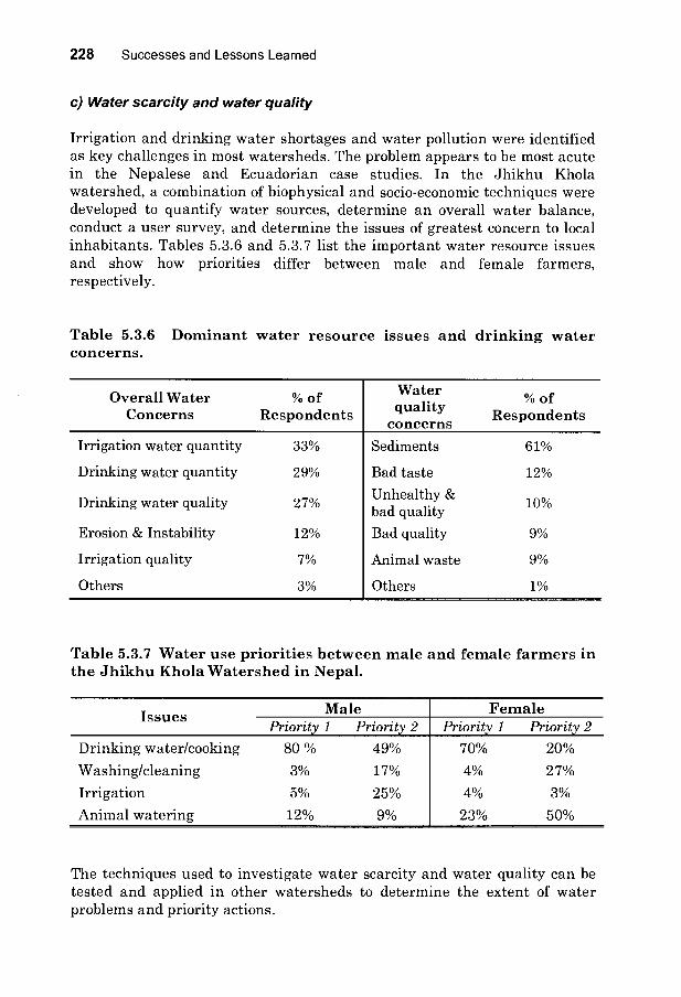
228 Successes and Lessons Learned
c) Water scarcity and water quality
Irrigation and drinking water shortages and water pollution were identified as key challenges in most watersheds. The problem appears to be most acute in the Nepalese and Ecuadorian case studies. In the Jhikhu Khola watershed, a combination of biophysical and socio-economic techniques were developed to quantify water sources, determine an overall water balance, conduct a user survey, and determine the issues of greatest concern to local inhabitants. Tables 5.3.6 and 5.3.7 list the important water resource issues and show how priorities differ between male and female farmers, respectively.
Table 5.3.6 Dominant water resource issues and drinking water concerns.
Overall Water % of Water % of
Concerns Respondents quality
Respondents concerns
Irrigation water quantity 33% Sediments 61%
Drinking water quantity 29% Bad taste 12%
Drinking water quality 27% Unhealthy &
10%
Erosion & Instability 12%
bad quality Bad quality 9%
Irrigation quality 7% Animal waste 9%
Others 3% Others 1%
Table 5.3.7 Water use priorities between male and female farmers in the Jhikhu Khola Watershed in Nepal.
I Male Female ssues Priority 1 Priority 2 Priority 1 Priority 2
Drinking water/cooking 80 % 49% 70% 20%
Washing/cleaning 3% 17% 4% 27%
Irrigation 5% 25% 4% 3%
Animal watering 12% 9% 23% 50%
The techniques used to investigate water scarcity and water quality can be tested and applied in other watersheds to determine the extent of water problems and priority actions.

Too Little and Too Much: Water and Development in a Himalayan Watershed 229
Water conflicts between upland and lowland users is a common problem in the watersheds, and resolving this issue is one of the most challenging problems facing watershed managers. The Ecuadorian team has addressed this by presenting a case study of a multi-stakeholder consortium that has the potential to manage conflicts through negotiation. They determined that good scientific data is needed, that the stakeholders need to be educated and exposed to other perspectives, and that negotiations need to be conducted in a patient and skillful manner.
Identifying the issues, documenting the extent of the water problems, and negotiating solutions to conflicts are only the first steps. How to reallocate water use, how to mitigate and prevent deterioration, and how to conserve the resource are equally challenging. Studies in the Jhikhu Khola watershed have shown that action research focused on water harvesting, source protection and efficiency in use are positive steps that can be taken to improve water quality and use. The research results for the Jhikhu Khola watershed illustrated how run-off water during the rainy season can successfully be collected and stored for use during the dry season. Experiments showed that low cost drip irrigation was technically and economic viability and can produce a cash crop with low water requirements during the critical dry season. The results demonstrated that under water stress conditions cauliflower yields were higher in a low-cost drip system than in a hand watering system. The low cost drip system which is designed to be used by poor farmers could be paid off over a one-year period using the added cash income obtained from producing off-season market crops. The results from these three studies can be replicated in other watersheds to determine their applicability to improve livelihoods and workloads.
d) Gender and workload problems
There are many reasons why the workload of women in mountain watersheds is increasing including différences in work allocation and decision-making. In the Nepalese watersheds, agricultural intensification, milk production, and temporary and permanent migration for off-farm employment, mostly by men, have contributed to the increase in the workload of women.
The case study in the Yarsha Khola watershed in Nepal provides an excellent example of how to document workloads, determine time allocations to différent tasks, and quantify and display the results in a georeferenced GIS format. Eighty households were interviewed using a participatory survey and the results, provided in Figure 5.3.2, illustrated that on average women in this watershed work 3.8 hours longer per day than their male counterparts. Women are primarily responsible for household care, water collection, animal care, and compost management. Due to the increase in agricultural intensification, water scarcity is increasing and as a result,

230 Successes and Lessons Learned
women spend more time collecting safe drinking water and watering animais. Workloads are further aggravated by the additional requirements for milk production, which has been deemed as the new mechanism to enter the market economy. Having more animais means more demand for water and fodder. Traditionally, women are responsible for looking after both of these resources, and as the resources degrade, the distance to alternative sources increases along with the associated workload.
18
16
0 10 20 30 40 50 60
each bar represents an individual 70 80 90
Figure 5.3.2 Différence in workload between males and females in the Nepalese watersheds.
Documenting how and where workloads have increased in the watershed was the first step in this study. This was followed by a second research initiative on how to improve water supplies and local fodder production so that the daily walking distances to collect water and fodder could be reduced. This action research focused on the use of grasses and fodder trees to improve feed sources, on introducing water-harvesting techniques and protecting local water supplies. Successful examples of how to improve fodder production were also documented in the Ilave-Huenque watershed in Peru, through the introduction of alfalfa and the enhancement of "bofedales". The techniques and approaches from both the Yarsha and Illave-Huenque watersheds can readily be tested and applied to other watersheds.
e) Forest rehabilitation in community forests
Forests play a key role in watershed management. The use of forests for timber, fuelwood, animal bedding, and fodder has been well documented in mountain watersheds. The forest resources in ail eight watersheds are under great pressure, many of these forests are common resource properties, and their management has been controversial. The establishment of community
Too Little and Too Much: Water and Development in a Himalayan Watershed 231
forests has been pioneered in India and Nepal in an effort to provide more local control over the resource. It was hoped that these initiatives would lead to a more sustainable way of managing forests. Examples were provided in the two Nepalese watersheds to demonstrate the variety of management practices that are being initiated by the différent community user groups. Using a GIS database presented the opportunity to display forest conditions spatially.
In many cases, soil erosion due to over-use of forest resources has resulted in higher erosion rates and degradation of forest land. These areas produce little biomass and contribute to the annual sediment load, which affects irrigation. To reduce sedimentation and increase fodder production, rehabilitation experiments were carried out in several degraded sites with a focus on planting nitrogen fixing fodder trees and grasses. These efforts have been very successful in both the Nepalese and the Bhutanese watersheds, particularly as they involved community groups. Soils were stabilized over a 3-5 year period, and the biomass produced is proving to be a highly valuable source of animal feed. At the same time, the workload of women has been reduced, biodiversity in the rehabilitated forest has increased, and the community has been given legal rights to own and manage these newly created forests in a community manner. Successful efforts in the Bhutanese watershed have resulted in the establishment of the first community managed forest in the country that is sanctioned by the national government. These efforts were well documented in the CD-ROMs and serve as useful training sets to be applied in other watersheds.
3. Unique challenges and techniques
The watershed comparison allowed us to identify how communities in the différent watersheds addressed issues, how widespread each problem was, and what successful techniques and approaches had been used to address these issues. There were a number of unique issues in individual watersheds, which were less applicable to the other watersheds (e.g. salinity problems in Bolivia, high elevation wetland protection in Ecuador, tea production in China). However, with the development of a global watershed network even these unique issues are useful for comparative purposes with other watersheds that experience similar challenges.
5.3.5 Conclusions and Lessons Learned
Each watershed team presented a series of success stories that focused on: 1) the use of techniques or evaluation methods that proved successful; 2) action research that improved the livelihoods of local people, or 3) approaches that improved resource conservation or rehabilitated degraded sites. These successes form the backbone for learning and sharing experiences. Gaps in the data and knowledge base existed in each of the watersheds. By conducting this collaborative project it was possible to show what essential

232 Successes and Lessons Learned
watershed resource information is needed to arrive at an integrated assessment. The results demonstrated that the social and biophysical components need to be balanced and integrated if we hope to improve watershed management and the livelihood of the people within it. In none of the watershed studies were all aspects of resource management assessed in a balanced manner. The majority of the efforts focused on documenting and quantifying the extent of the resource problems. Less effort was devoted to action research for improving the resources, and even less emphasis was placed on preventing resource degradation and rehabilitation. All watershed projects should strive towards an equal effort in all three areas.
The one research area that required considerable strengthening is the interaction between land use and water resources. The knowledge of hydrology and water quality was relatively poor in most watersheds, yet the increasing importance of water resources was well documented; it was identified as the most important issue by all teams. The increase in climatic variability in mountains is another key factor that needs to be addressed - the potential impacts of this variability are likely magnified in these fragile environments.
The Himalayan-Andean watershed project explored how information technology tools could be used more effectively to improve communication between watershed researchers. The production of the CD-ROMs and the use of the Internet for comparing and sharing information were relatively straight forward, and each team mastered the technology in an efficient manner. The main advantages of using a multi-media approach were: 1) the material is presented in an interesting manner by combining text, images, GIS maps, graphics and animations in an interactive style; 2) the CD-ROM based framework and hypertext format serve as an excellent platform to integrate all resource information; 3) the cost of producing and distributing the CD-ROMs is modest and thus allows for a wide distribution of the information; 4) the CD-ROM can be updated relatively easily and thus becomes a permanent and dynamic record of the watershed and its resources; 5) the CD-ROM and the Internet are an ideal platform for sharing information and cooperative learning; and 6) using common indicators for comparison and sharing success stories facilitates extrapolation globally.
References
Allen, R., H. Schreier, S. Brown, and P.B. Shah (Editors and Authors.) 2000. The People and Resource Dynamics Project: The First Three Years. International Centre for Integrated Mountain Development (ICIMOD), Kathmandu. 333 pp.

Too Little and Too Much: Water and Development in a Himalayan Watershed 233
Institute for Resources, Environment and Sustainability (IRES). 2002. Collaborative Himalayan Andean Watershed Project. http://www.ires.ubc.ca/projects/himal/index.htm
White, R. et all. (Forthcoming 2006). Final Report of the PARDYP Project. ICIMOD, SDC and IDRC, Kathmandu, Nepal.
5.4 Summary
Introducing innovation and determining how successful these innovations are in watershed management is challenging, particularly when dealing with the complexity of integrated watershed management in developing countries. However, being able to conduct research for development and building capacity to identify key issues, determine the status of the resources, and engage in applied research to improve the condition and livelihood of the residents is a very exciting and challenging proposition. Having the opportunity to work in the saure watershed for 16 years was invaluable as it provided a basis to fully understand the socio-economic fabric of the people and the dynamic natural processes that take place in the Himalayas. In addition to helping understand the physical and socio- economic processes in the watershed and physically improve the resource base, the project had a significant impact on capacity building. We hope that this will be a lasting contribution that bas enlightened individuals and will assure future progress.


A Vision for the Future
Hans Schreier and Sandra Brown
6 Having worked for 17 years in one of the most intensively used watersheds in the world, inevitably the question of the future of the watershed is raised. Is it possible to continue to increase productivity in a marginal environment when the average trop rotation is three crops per year; when almost every square meter of land is used for biomass production that is harvested and used? How do we deal with the extreme seasonal variation in water supplies, and how do we reconcile water for food, water for people and water for environmental services? These are some of the questions that need to be addressed, if we hope to arrive at a sustainable future.
6.1 Population, Food Security and Livelihoods
Over the last 20 years the population in the watershed has doubled and the population density now exceeds 630 people per km2. Development is particularly challenging as there are no major urban centres in the watershed and 95% of residents are engaged in agricultural activities. The reason for the population pressure is high birth rates, improvements in health tare, and immigration of labourers. The high trop intensities are maintained using elaborate terrace and irrigation systems. These systems cannot be maintained without large labour inputs since mechanization is limited by access, topography, and fragmented and highly dispersed land ownership. In spite of all the innovations and improvements in food production that have been achieved through large inputs of external fertilizers and pesticides, food security is still a major concern. Progress has been made to move from subsistence agriculture into the market economy. However, the associated benefits have been unequally distributed and the continuing increase in population raises the question as to how much more intensification is possible? If a sustainable production system is to be achieved then the population issue needs to be addressed. In the last 2-3 years, with the aggravation of the civil conflict, there appears to have been a considerable exodus of young male labourers to the Gulf States. Population pressure has been somewhat reduced, some of the income earned abroad will trickle back into the watershed, but the absence of young males is adding significantly to the workload of women left behind to look after the farms.

236 A Vision for the Future
Given this situation, it is diff"icult to see how production can be increased dramatically over current levels. If we hope to improve livelihoods other economic activities need to be considered. This is a challenging proposition. Access is difficult, the state of education is low and reliable energy sources are scarce. Tourism has expanded in a few areas in the upper portion of the watershed, but lack of reliable water resources, seasonal limitations, and access restricts these options. The continuing civil unrest has not helped this situation.
Through the successful export of milk, potatoes, tomatoes and vegetables the Jhikhu Khola watershed has become a model on how to move from a subsistence to a market economy. A positive impact has been the creation, for the first time, of a cash income source. However, there is potential to increase production as yields are relatively low in the marginal non-irrigated fields. Increasing yields becomes more challenging as farmers already use high yielding varieties of crops, and the input of macro-nutrients and pesticides is high. There appears to be few options available to control population and to increase food security unless migration and external income sources become more widely available.
Currently there are no industrial activities in the watershed, but with the development of hydro-power (in other parts of the country), the potential for food processing and small scale industrial development is a viable option. Farmers in the lower part of the watershed are producing large quantities of potatoes, tomatoes, and vegetables for markets in the nearest cities, and it may be possible to process food, provided access to a reliable electricity supply could be established. Food processing however, requires large quantities of water, and therefore, it might be best to encourage such developments in an adjacent watershed that have water sources originating in the High Mountains where water supplies are more abundant.
6.2 Water the Limiting Resources and Climate Change
The major constraint to water resource availability is its seasonal distribution. During the 3-4 month monsoon season excessive runoff leads to flooding and land instability, whereas during the dry season there are widespread water shortages. This Middle Mountain watershed has no glacial water sources that feed the stream, and snow accumulation is insignificant. As a result, the struggle is how to moderate the seasonal extremes. Farmers have a long tradition of building many small check dams to store and divert stream water into an intricate irrigation network. The network of check- dams is effective because the dams can easily be rebuilt with local materials after major storm events, and until recently, they could hold sufficient water for irrigation. However, few of the irrigation canals are lined, and consequently, losses in the conveyance system are high, as pointed out by Nakarmi (1995). Improving irrigation channels is therefore an obvious

Too Little and Too Much: Water and Development in a Himalayan Watershed 237
priority. While a considerable amount of water can be recovered in this manner, it does not eliminate water shortages during the dry season. Consequently, a major focus on water conservation and source water protection is required. In view of increased climatic variability, which will likely increase seasonal variability, water conservation and efficient use are ail the more urgent. Creating large dams and storage reservoirs is not a feasible option because of space constraints, terrain instability (due to frequent tectonics activities), a lack of suitable sites, financial constraints and cost effectiveness.
The promotion of innovative water harvesting and storage techniques, the construction of decentralized water supply systems, the use of water saving techniques, and the improvement of irrigation water use with low cost drip and sprinkler irrigation systems are some of the options available. Efforts have to be coordinated on a watershed wide basis, creating a social and administrative challenge.
Reducing crop production intensity during the dry season would reduce water demand and allow for a fallow period to restore nutrients into the soil and provide opportunities to combat soil acidity by liming. However, this is a difficult proposition to propose at a time when food security is a widespread problem. More attention should be given to the selection of the crops in view of their water use efficiency, particularly for dry season crops. As shown in section 3.5, the overall water use to satisfy both the irrigated and rainfed crop requirements is 664 mm/year; given the averaged rainfall of 1295 mm/year this represents 50% of the annual water available. Adding the water requirements for forest cover (29% of the area or 3219 ha), and the 8 mm/year demand for animais and domestic use, an additional 383 mm/year would be required; totalling 81% of the annual available rainfall. Given the uneven seasonal distribution, there are limited options to expand irrigation and that water conservation is critical.
Examples of the comparative water requirements for différent crops commonly grown in the watershed are provided in Table 6.2.1. From a water use efficiency point of view, chick peas, pigeon peas and chillies require the least amount of water per growing cycle, while cardmon is excessively water demanding. On a crop production basis, tomatoes, potatoes and chillies are more water efficient than the main staple crops.
Current food production is currently utilizing >50% of the annually available water, but this is likely >80% of the water available during the dry season. To maintain these year around intensive cropping systems, water storage during the monsoon season is becoming a necessity and progress in water conservation, water harvesting, and improved efficiency in irrigation are the key factors to consider.

238 A Vision for the Future
With a coordinated effort focused on improving the water use efficiency in agriculture it is possible to reduce the land use intensity. This will hopefully result in a more sustainable use of the food, forest and grassland resources.
As with the seasonal water distribution, development opportunitites in the watershed have been uneven; too little for some, too much for others. Improving the seasonal availability in water and inequities in development are key issues to be addressed for future progress in the watershed.
Table 6.2.1 Comparison of crop water requirements for typical crops grown in the watershed.
Crop-water R i t
Crop-water requirements
Virtual water Content (VWC)
Crops equ remen s
Nepal * Jhikhu Khola **
(mm/crop Nepal 1 Global
Average 2 (mm/ crop cycle)
cycle) (m3It) m3/t
Wheat 319 302 1888 1334
Rice 707 1404 2766 2291
Barley 282 300 2609 1388
Maize 267 311-535 1484 909
Millets 202 1875 4596
Potatoes 278 181-272 299 255
Chick-Peas 162 2083 3230
Pigeon Peas 217 2598 4103
Cardamon 788 19548 41041
Ginger 382 411 1792
Chillies 165 3866 323
Garlic 351 872 518
Tomatoes 312-344 184
Mustard 213 1724 1724
1 Based on Chapagain and Hoekstra 2004 z Based on Merz 2004 (Section 3.5)
References
Chapagain, A.K., and A.Y. Hoekstra. 2004. Water Footprints of Nations. UNESCO-IHE, Institute for water Education, Vol 1 and 2. UNESCO-IHE, Delft, Netherlands.
Nakarmi, G. 1995. Indigenous water management systems in the Andheri Khola sub-watershed. In: Schreier, H, P.B. Shah, and S. Brown (eds). Challenges in mountain resources management in Nepal. Process, trends,

Too Little and Too Much: Water and Development in a Himalayan Watershed 239
and dynamics in middle mountains watershed, Kathmandu, 10-12 April 1995. pp 211-225.
Merz, J. 2004. Water Balances, Floods and Sediment Transport in the Hindu Kush-Himalayan region. Geographical Bernensia G72. PhD Thesis, Department of Geography, University of Bern, Switzerland, 300 pp.
6.3 Future Training and Education
Many of the experiences gained by this project were incorporated into a WEB-based distance education program that has been offered through the University of British Columbia since 1998. The "Watershed Management Certificate Program" is open to graduate students and professionals from around the world. It consists of five graduate courses offered annually over the Internet. A multi-media CD-ROM text book was produced for each of the courses and is sent to each participant at the beginning of the course. Participants engage in discussions using a WEB bulletin board, sssignments and reference materials are posted on the WEB site on a weekly basis, and students submit their assignments via email.
One of the five courses entitled "Water in International Development" was developed with assistance and financial support from IDRC. Case study material which was incorporated in the CD-ROM includes part of the Jhikhu Khola watershed project and the Himalayan Andean watershed comparison project. Through distance education the results and lessons learned from the Jhikhu Khola and PARDYP projects continue to be disseminated, and the next generation of researchers and professionals are engaged in addressing water management issues in the developing world.
As of April 2006 some 700 students and professionals from 32 différent countries have participated in one or several of the courses. The experiences and accomplishment of the Jhikhu Khola watershed are thus shared globally.
The details of the program can be found on the following WEB-Site: http://www.rmes.ubc.ca/nav.php?page=web courses
6.4 Conflict resolution
Nepal has benefited from massive support from western countries and has been exposed to democracy, albiet for a relatively short period. In spite of these efforts, corruption and inequity have reached a high point in the history of the country and lead to the current civil unrest and turmoil. Little of the international development assistance has reached poor farmers in

240 A Vision for the Future
remote rural watersheds. Without a massive outreach program to help improve the livelihoods of \ mountain people, conflicts will continue. It is though research and development projects like those sponsored by IDRC and SDC that we hope to improve conditions, and build knowledge and capacity at the local level in all mountain regions of the world. Only when there is hope and the capacity to improve the livelihoods of rural people, can the current conflict lie resolved. It is ironic that within cive years the conditions in the watershed changed from one where a female graduate student was able to conduct extended field research without concerns related to safety or security to one where civil unrest and armed conflict are prominent. The sooner we can address poverty issues and make progress towards improving the lives of poor farmers in the Himalayas the more likely can we resolve the current conflict.

Epilogue
We were fortunate to have benefited from long terra support by IDRC and SDC to conduct research in the saure watershed over a 17 year period. This enabled the research team to gain a good understanding of the key socio- economic, physical and environmental processes that dominate watersheds in the Middle Mountains of Nepal. It allowed us to experiment with intervention projects that were aimed at improving production systems, human health, water management, and the environnent in the Jhikhu Khola watershed.
Beyond the Nepalese watershed we hope to have influenced, in a small way, watershed management processes in a large number of other mountain regions. Many of the methods and techniques developed in the Jhikhu Khola watershed have been used and adapted in the watersheds of the PARDYP program. Taking advantage of the digital revolution allowed us to expand communication globally, and to share information and experiences between different mountain regions of the world, which ultimately led to the Himalayan-Andean watershed comparison. By building the capacity to develop and use multi-media tools and WEB based technologies within the team we hope to have reduced the digital divide. An example of the multi- media tools available to disseminate results from the Jhikhu Khola watershed project is enclosed in the form of a CD-ROM.
All people involved in the project have benefited greatly from the experience. Most were able to improve their skills and knowledge in the cause for development and improvement of natural resources management in the mountains. Probably the most important accomplishment of the project was the capacity building effort. We were fortunate to work with a large number of young researchers and practitioners, to influence them to work more effectively and in a more integrated manner on all aspects of watershed management in Nepal and around the world. Much of the experiences gained from this project were incorporated into the delivery of a WEB-based graduate watershed management certificate, and this will enable us to continue the capacity building process for some time to come. We hope that the development of knowledge and the sharing of experiences are the keys to inspire the next generation of researchers to become leaders in addressing the complex and emerging watershed management problems globally.


Publications (Related to the Jhikhu Khola Watershed Project)
8.1 Refereed Journal Publications
8 Schreier, H., P.B. Shah, and G. Kennedy. 1990. Evaluating mountain watersheds in Nepal using Micro-GIS. Mountain Res. & Development, 10(2): 151-159.
Schreier, H., G. Kennedy, P.B. Shah, and S. Brown. 1991. The food, feed and fuelwood resources of Nepal: A GIS evaluation. Environmental Management, 15: 815-822.
Schmidt, M., and H. Schreier. 1993. Factors affecting the soil, foliar and litter nutrient status of forest sites in a mountain watershed in Nepal. Soil Science, 44:417-425.
Smith, K.T., G. Kennedy, P.B. Shah, and H. Schreier. 1993. A district evaluation of fuelwood resources in Nepal. Forest Chronicle, 69:594-599.
Schreier, H., S. Brown, M. Schmidt, P.B. Shah, B. Shrestha, G. Nakarmi, and S. Wymann. 1994. Gaining forests but losing ground; A GIS evaluation in a Himalayan Watershed. Environ. Management, 18: 139-150.
Schreier, H., P.B. Shah, L.M. Lavkulich, and S. Brown. 1994. Maintaining soil fertility under increasing land use pressure in the Middle Mountains of Nepal. Soil Use and Management, 10:137-142.
Schmidt, M., H. Schreier, P.B. Shah. 1995. A GIS evaluation of land use and soil fertility in a watershed in Nepal. Intern. Journ. Geographic Information System, 9: 317-327.
Schreier, H. and P.B. Shah. 1996. Water dynamics and population pressure in the Nepalese Himalayas. GeoJournal, 40(1-2):45-51.
Schreier, H., S. Brown, and H. Schreier. 1998. Conservation, degradation and rehabilitation; the great Himalayan Challenge. NATO Advanced Research Publication Series: Environmental reconstruction in headwaters Series 2: Enuironmental Security, 68:147-158.
Schreier, H., S. Brown, L.M. Lavkulich, and P.B. Shah. 1999. Phosphorus dynamics and soil P-fertility constraints in Nepal. Soil Science, 164(5): 341- 350.
Brown, S., H. Schreier, P.B. Shah, and L.M. Lavkulich. 1999. Soil nutrient budget modelling: An assessment of agricultural sustainability in Nepal. Soil Use and Management, 15:101-108.

244 Publications
Brown, S. and B. Shrestha. 2000. Market driven land use dynamics in the Middle Mountains of Nepal. Journal of Enuironmental Management, 59: 217-225.
Brown, S., H. Schreier, and P.B. Shah. 2000. Soil phosphorus fertility degradation: A GIS based assessment. Journ. Envionmental Quality, 29(4):1152-1160.
Schreier, H., S. Brown, P.B. Shah, B. Shrestha, G. Nakarmi, and R. Allen. 2001. Human interactions in soil and geomorphic processes in Nepal: The role of soil fertility in degradation and rehabilitation processes. Intern. Journ. of Applied Earth Observation and Geoinformation, 3(1):93-98.
Schreier, H., and S.. Brown. 2002. Scaling Issues in watershed assessments. Water Policy, 3 (2001):475-489.
Schreier, H., S.J. Brown, K. Hall, and R. Bestbier. 2002. Watershed Management: Distant Education at a Global Scale. AWRA, Water Resources Impact, 4 (5):24-27.
Merz, J. G. Nakarmi, S.K. Shrestha, B.M. Dahal, P.M. Dangol, M.P. Dhakal, B.S. Dongol, S. Sharma, P.B. Shah, and R. Weingartner. 2003. Water: A scarce resource in rural watersheds of Nepal's Middle Mountains. Mountain Research and Development, 23 (1): 41-49.
von Westarp, S., S. Chieng, and H. Schreier. 2003. Comparing low-cost drip irrigation, conventional drip irrigation, and hand watering in Nepal. Agricultural Water Management, 64(2):143-160.
Merz, J., G. Nakarmi, and R. Weingartner. 2003. Potential solutions to water scarcity in the rural watersheds of Nepal's Middle Mountains. Mountain Research & Development, 23(1):14-18.
Schreier, H. and S. Brown. 2004. Multiscale approaches to water management: land-use impacts on nutrient and sediment dynamics. Scales in Hydrology and Water Management. Intern. Assoc. Hydrological Sciences. IAHS Publ. 287: 61-75.
Von Westarp, S., H. Schreier, S. Brown, P.B. Shah. 2004. Agricultural intensification and the impact on soil fertility in the Middle Mountains of Nepal. Canadian Journ Soil Science, 84(3) 323-332.
Merz, J., G. Nakarmi, S.K. Shrestha, B.M. Dahal, P.M. Dongol, M.P. Dhakal, M. Shaffner, S. Shakya, S. Sharma, and R. Weingartner. 2004. Public water sources in rural watersheds of Nepal's Middle Mountains: Issues and Constraints. Enuironmental Management, 34(1):26-37.
Brown, S. 2004. Spatial analysis of socio-economic issues: Gender and Geographic Information Systems in Nepal. Mountain Research and Development, 23 (4): 28-34.

Too Little and Too Much: Water and Development in a Himalayan Watershed 245
Dhakal, M.P., B.S. Dongol, P.M. Dangol, and J. Merz. 2004. Water availability study in PARDYP - Nepal watersheds. In Journal of Hydrology and Meteorology of Nepal, 1(1):55-62.
Dongol, B.S., P.M. Dangol, P.M. Dhakal, P.B., Shah, S.K. Shrestha, D.R. Bajracharya, and J. Merz. 2004. First assessment of ground water quality status in Jhikhu Khola watershed, Nepal. Journal of Hydrology and Meteorology of Népal, 1(1): 6-12.
Brown, S., and G. Kennedy. 2005. A case study of cash cropping in Nepal: poverty alleviation or inequity. Agriculture and Human Values, 22:105-116.
Dongol, B.S., J. Merz, M. Schaffner, G. Nakarmi, P.B. Shah, A.K. Shrestha, P.M. Dangol, and M.P. Dhakal. 2005. Shallow groundwater in a middle mountain catchment of Nepal: Quantity and quality issues. Environmental Geology, 49: 219-229.
Merz, J, P.M. Dangol, M.P. Dhakal, B.S. Dongol, and R. Weingartner. 2006. Rainfall amount and intensity in a rural catchment of Nepal's middle mountains. Hydrological Sciences Journal, 51 (1):127-143.
Merz, J. G. Nakarmi, P.M. Dangol, M.P. Dhakal, B.S. Dongol, and R. Weingartner. Sediment mobilisation by surface erosion in middle mountain catchments of Nepal. International Journal of Sediment Research (in Press)
Merz, J. P.M. Dangol, M.P. Dhakal, B.S. Dongol, G. Nakarmi, and R. Weingartner. Rainfall-runoff events in a middle mountain catchment of Nepal. Journal of Hydrology (in Press).
8.2 Books and Chapters in Books
Shah , P.B., H. Schreier, S. Brown, and K. Riley. 1991. (Editors). Soil Fertility and Erosion Issues in the Middle Mountains of Nepal. Workshop Proceedings, Jhikhu Khola Watershed, April 22-25, IDRC, Ottawa, 286 pp.
Schreier, H., P.B. Shah, M. Schmidt, and G. Kennedy. 1991. Nepal 2000, A GIS evaluation of the major resources. GIS-World, Fort Collins, Colorado.,pp. 89-95.
Schreier, H., P.B. Shah, and S. Brown. (Editors) 1995. Challenges in Mountain Resource Management in Nepal. Processes, Trends and Dynamics in Middle Mountain Watershed. IDRC Ottawa, and International Centre for Integrated Mountain Development (ICIMOD), Kathmandu, Nepal, 286 pp.
Allen, R., H. Schreier, S. Brown, and P.B. Shah (Editors and Authors.) 2000. The People and Resource Dynamics Project: The First Three Years. International Centre for Integrated Mountain Development (ICIMOD), Kathmandu, 333 pp.

246 Publications
Schreier, H., S. Brown, M. Carver, and P.B. Shah. 1998. Linking land degradation to nutrient and sediment transport in a Middle Mountain Watershed, In: Haigh, M., J. Krecek, G.S. Rajwar and M. Kilmartin (eds.). Headwaters: Water resources and soil conservation. Proceedings of Headwater '98. 4th International Conference on Headwater Control, IAHC, WASWC, Merano, Italy. A.A. Balkema/ Rotterdam/ Brookfield, pp 315-327.
Schreier, H., P.B. Shah, and S. Brown. 1999. Challenges in Mountain Resource Management: Processes, trends and dynamics in Middle Mountain Watersheds. In: Beck, T., P. Bose, and B. Morrison (Eds.) The Cooperative Management of Water Resources in South Asia. Centre for India and South Asia Research. Institute for Asian Research, University of British Columbia, pp 275-282.
Schreier , H., S. Brown, P.B. Shah, G. Nakarmi, and B. Shrestha. 2000. Prevention, degradation and rehabilitation: A new dilemma in Himalayan watershed. In: Haigh, M. and J. Krecek (eds.). Environmental Reconstruction in Headwater Areas. Kluwer Academic Publishers, Dordrecht, NL. NATO Science Series, 2. Environmental Security, 68:147- 158
Schreier, H., S. Brown, and P.B. Shah, 2000. Soil-Sediment Nutrient Transport Dynamics in A Himalayan Watershed. International Symposium on the Role of Erosion and Sediment Transport in Nutrient and Contaminant Transfer. IAHS Proceedings, International Association of Hydrological Sciences (IAHS) IAHS Publ. No. 263-pp 1-7.
Schreier, H. S. Brown, and P.B. Shah. 2003. Methods used to address resource issues in integrated watershed management in Nepalese watersheds. Case study 18. In: Pound, B. S.S. Snap, C. McDougall, and A.R. Braun (eds.). Managing natural resources for sustainable livelihoods: Uniting Science and Participation. Earthscan Publications, London, GB. pp. 231-234.
8.3 Multi-Media - CD-ROM's
Brown, S., H. Schreier, M. Carver, P.B. Shah, N. Nakarmi, and B. Shrestha. 1995. Decisions for the future: Addressing resource issues in the Middle Mountains of Nepal. Multimedia computer display presentations in Hypertext, @ RMES, UBC. Version 1.1. Internet: IDRC's PAN Asia Network.
Brown, S., H. Schreier, C. Carver, W. Tamagi, P.B. Shah, B. Shrestha, G. Nakarmi, and R. Allen. 1997. Complex problems - complex options: preservation, degradation and rehabilitation in a Nepalese Watershed. PARDYP Project on people and resource dynamics in the Himalayas. CD- ROM. @Institute for Resources and Environment, University of B.C. and ICIMOD, Kathmandu, Nepal.

Too Little and Too Much: Water and Development in a Himalayan Watershed 247
Brown, S. 1998. Gender and Resources in the Middle Mountains of Nepal. CD-ROM. Documenting the situation of rural women and gender relationships in the Jiri region of Nepal. Issues examined include community forestry, labour allocation, socio-economic conditions and access. UBC/IDRC, Canada.
Galay, V., H. Schreier, and R. Bestbier. 2001. Himalayan Sediments: Issues, concerns and guidelines. A multi media CD-ROM for the Water and Energy Commission Secretariat, Nepal. With Northwest Hydraulics Consultants, North Vancouver, and Acres International, Canadian International Water and Energy Consultants (CIWEC). CD-ROM.
Schreier, H., S. Brown, and R. Bestbier. 2002. The Himalayan-Andean Watershed Comparison Project. Production of 9 CD-ROMs for 8 Watersheds in Nepal, Bhutan, China, Peru, Bolivia, and Ecuador. In collaboration with the International Potato Centre (CIP) in Lima, Peru, The Kunming Institute of Botany, in Kunming China, the Ministry of Agriculture in Thimphu, Bhutan, the International Centre for Integrated Mountain Development (ICIMOD), in Kathmandu, Nepal, and Manrecure II, in Quito Ecuador. Training was provided to each team to produce a multi-media CD-ROM of their watershed project. The final production of each CD-ROM and the Comparison of the 8 watersheds were done at UBC. Each CD-ROM consists of an integrated watershed assessment and common indicators were used to compare the 8 watersheds, @ IRES & IDRC.
Merz, J.; G. Nakarmi, S. Shrestha, B. Shrestha, P.B. Shah, and R. Weingartner. 2002. Water and Erosion Studies of PARYP Nepal: Water Demand and Supply Survey. CD-ROM. Kathmandu: ICIMOD.
Schreier, H., R. Bestbier, S. Brown, D. Brooks et al. 2003 Water in International Development. A multi-media textbook for a graduate level course in Development @ IRES, UBC, Vancouver.
8.4 Student Theses
1989 Aubriot, O. Culture du Riz et évaluation du bilan hydrique d'une rizière en terrasse au Nepal. M.Sc. Thesis, ENSA, Universite de Montpellier, France.
1989 Feigle, F. An assessment of forest and forest soil properties in the lower Jhikhu Khola Watershed, Nepal. M.Sc. Diploma, Ludwig-Maximillian University, Munchen, Germany, 90 pp.
1991 Wymann, S. Landnutungsintensivierung und Bodenfruchtbarkeit in Nepalischen Huegelgebiet. M.Sc. Diploma, Geography, University of Bern, Switzerland 92 pp.

248 Publications
1992 Schmidt, M. A GIS evaluation of forest land use dynamics and soil fertility in a mountain watershed in Nepal. PhD Thesis, Dept. of Soil Science, University of British Columbia, Canada.
1997 Carver, M. Diagnosis of headwater sediment dynamics in Nepal's Middle Mountains: Implications for land management. 374 pp. PhD Thesis, Resource Management Science, University of British Columbia, Canada.
1997 Brown, S. Soil fertility, nutrient dynamics and socio-economic interactions in the Middle Mountains of Nepal. 254 pp. PhD Thesis, Resource Management Science, University of British Columbia, Canada.
2002 von Westarp, Stephanie. Linkages between agricultural intensification, soil-fertility dynamics, and low-cost drip irrigation in the Middle Mountains of Nepal. M.Sc. Thesis, Dept. of Soil Science , University of British Columbia, Canada, 198 pp.
2003 Schaffner, M. Drinking Water Quality Assessment and Improvement in the Jhikhu Khola Catchment, Nepal. tion Gewaesserkunde No. 281. M.Sc. Diploma, Department of Geography, University of Bern, Switzerland.
2004 Merz, J. Water Balances, Floods and Sediment Transport in the Hindu Kush-Himalayan region. Geographical Bernensia G72. PhD Thesis, Department of Geography, University of Bern, Switzerland, 300 pp.
8.5 International Training Courses (Outreach to other researchers between 1998-2006)
Schreier, H., K. Hall, S. Brown 1998. Integrated Watershed Management at the University of Agriculture and Forestry, Ho Chi Minh City Vietnam. (March 3-7, 28 participants)
Schreier, H. and S. Brown. 1999. Four day training course on the use of Hypermedia tools in watershed studies, water quality monitoring, and nutrient modelling. At Kunming Institute of Ethno-Botany. IDRC-PARDYP project researchers. Kunming China (August 11-15, 20 participants).
Schreier, H., P. Zandbergen, and S. Brown. 1999. Four-day intensive training course on designing a multi-media CD-ROM and programming hypermedia products for the Himal-Andean Watershed project. CONDESAN, CIP, Ecuador, Peru, and Bolivia. University Agraria la Molina, Lima, Peru. (Oct. 20-24, 29 participants).
Schreier, H. 2000. One week international training course for Integrated Watershed Management. NGO's from Central American Countries associated with World Vision Projects in Nicaragua, Guatemala, Honduras, Columbia & the Caribbean, San Salvador (Feb.24-29, 30 Participants)

Too Little and Too Much: Water and Development in a Himalayan Watershed 249
Schreier, H. 2000. One week training course in Integrated Watershed Management for researchers associates with the Hillside projects in Central and South America (8 différent countries). IDRC, CIAT, and University of Costa Rica. At CIEDES, San Jose. (March 5-10, 28 participants).
Schreier, H. 2000. Three day training session in designing integrated watershed projects. Renewable Natural Resources Research Centre (RNRRC), Bajo, Wangdue, Kingdom of Bhutan, (Mar. 31-April 3, 11 participants).
Schreier, H. and S. Brown. 2000. One week training session in the production of an integrated watershed CD-ROM for the Andean CONDESAN Consortium. In collaboration with CIP (International Potato Research Centre), MANRECUR project, and Projecto Paramo. Quito, Ecuador. (May 1- 7, 15 participants 4 countries).
Schreier, H. 2000. Watershed management tools for community based natural resources management. Presentation to staff and students at Royal Department of Environment, Phnom Penh, Cambodia. (June 23, 15 participants)
Schreier, H. and S. Brown. 2000. Four day training course on Multi-media design and CD-ROM production of watershed study. Renewable Natural Resources Research Centre Bajo, Wangdue, Bhutan. (Oct. 21-25, 20 participants)
Schreier, H. 2000. Methods and approaches in watershed management. Two day training session. University of the Philippines, Bagio, Cordilleran Study Centre. (June 8-9, 70 participants).
Schreier, H. 2000. Hypermedia and GIS techniques in community based watershed management. Two day training workshop. Univ. of Agriculture & Forestry, Hue, Vietnam.(June 16-17,25 participants)
Schreier, H. and S. Brown. 2001. Six Day workshop on the use of indicators for watershed comparison: Himalayan Andean Watershed Comparison Project. Centro International de la Papa, CIP- La Paz, Bolivia (Feb.4-11, 15 participants).
Schreier, H., R. Bestbier, and S. Brown. 2001. Multi-media CD-ROM production for PARDYP Project. One week training Course. Kunming Institute of Botany, Chinese Academy of Sciences, Kunming. (May 5-10, 10 participants)
Schreier, H., R. Bestbier, and S. Brown. 2001. Training course in multi- media CD-ROM production at Angiang University, Angiang, Vietnam, (May 11-15, 45 participants from Laos, Cambodia, Vietnam, Philippines & Thailand).
Schreier, H. and S. Brown. 2001. Multi-media training program for Natural Resource Management in Watersheds. Renewable Natural Resource

250 Publications
Research Centre, Ministry of Agriculture, Bajo, Wangdue. Bhutan (March 29- April 4, 20 Participants)
Schreier, H. 2001. 4 Day training course in multi-media design for natural resources management. Mongolian Ministry of Nature and Environment, Ulaan Bataar, Mongolia. (Oct 24-27, 15 participants)
Schreier, H., S. Brown, and R. Bestbier. 2002. Multi-media computer training program on Water Resources management. Yorito, Honduras. Youth training. Collaborative program with CIAT (Intern. Tropical Agricultural Research Centre (CIDA) (April 11-14, 35 participants)
Schreier, H. 2002. Water quality monitoring and data evaluation. Part of a two week Training course for CIDA sponsored Egyptian Researchers, Vancouver. In collaboration with Environment Canada, National Water Resources Institute (October 29, 10 participants).
Schreier, H. 2003. Innovations in Urban and Agricultural Water Resources Management. 1/2 day workshop. Kathmandu University, Dhulikhel, Nepal, (August 7, 20 participants)
Brown, S. 2003. Integrated Watershed Management for INTA (Nigaraguan Institute for Agricultural Technology) Matagalpa. UNAM, National Agrarian University Matagalpa. Sponsored by Nicaraguan government. (March 17-22, 45 participants)
Schreier, H., S. Brown, M. Roa 2004. WEB design and low cost drip irrigation training course in Yorito, Honduras CIAT-CIDA. ( Feb 13-19, 20 participants)
Brown, S. 2004. Environmental and Socially Sensitive Area Assessment for the Nigaraguan Institute for Agricultural Technology (INTA) and the International Center for Tropical Agriculture (CIAT). (October 17-30, 40 Participants) from 5 INTA zones. Sponsored by Nicaraguan government.
Schreier, H., S. Brown 2004-2006 . Water in international Development, WEB based distance education Graduate course, Institute for Resources and Environment, University of British Columbia, Canada (Jan-April, 52 participants 3 times)
8.6 Conference Presentations and Proceedings
Schreier, H., P.B. Shah, M. Schmidt, and G. Kennedy. 1989. Himalayan Scale Problems and Micro-GIS Solutions. GIS-89 "A Wider Perspective", International Symposium on Geographic Information Systems. Forestry Canada. Pan Pacific Conv. Centre, Vancouver, B.C., Invited Plenary. Proc. 179-184.

Too Little and Too Much: Water and Development in a Himalayan Watershed 251
Schreier, H., P.B. Shah, and G. Kennedy. 1989. International Conférence on: "Transformation of Mountain Environments: Regional Development and Ecological Sustainability: Consequences on Global Change". USSR Academy of Sciences, Unesco, Man & Biosphere (MAB), United Nations University, Commission on Mountain Geoecology. Intern. Mount. Society. Moscow & Tsahkadzor, USSR. (Invited paper) 17 pp.
Schreier, H. 1990. The use of GIS techniques for land management in the Middle Mountains of Nepal. Annual Conférence of the Canadian Cartographie Association, Session on GIS in Third World projects, University of Victoria, Canada.
Brown, S., Schreier, H., G. Kennedy, and P.B. Shah. 1990. Nepal 2000: GIS Solutions to arrive at Sustainability of Food and Fuelwood Resources. African Mountains and Highland Conférence. Dynamics of resources use systems and its consequences for sustainable development, Rabat, Morocco, UNESCO-IGU, IUCN, United Nations University.
Schmidt, M. and H. Schreier. 1991. Quantitative GIS Analysis of Forest Resources in a Mountain Watershed in Nepal. Proc. GIS-91, Intern. Symp. on GIS, Vancouver, Forestry Canada, pp 227-232.
Schreier, H. P.B. Shah, G. Kennedy, and S. Brown. 1991. An Overview of the National Food, Feed, and Fuelwood resources of Nepal; A GIS based model. Workshop on : Soil fertility and Erosion Issues in the Middle Mountains of Nepal, Jhikhu Khola Watershed, Nepal, Proceedings.
Shah, P. and H. Schreier. 1991. 1. An Overview of the Jhikhu Khola Watershed Project (pp 176-179), 2. The hydrometric, sediment and erosion monitoring program (pp 208-212), 3. Nutrient deficiencies and soil fertility issues (pp 260-266). 4. Fodder tree research Initiatives (pp 267-275), 5. Summary of Major Issues, Research Priorities and Implementation of Research Results (pp 276-285). Workshop on : Soil fertility and Erosion Issues in the Middle Mountains, April 22-25. Jhikhu Khola Watershed, Nepal. Proc. ISS and IDRC.
Brown, S., H. Schreier, and P.B. Shah. 1991. Land Use Dynamics and soil fertility problems in an experimental watershed in Nepal; AS GIS analysis. Intern. Workshop on Mountain Geoecology of the Southern Andes, Resource Management & Sustainable Develop. (UNU/IMS) Santiago, Chile.
Schreier, H., S. Brown, and P.B. Shah. 1992. Gaining Forest but loosing ground; A GIS-based resource evaluation of the Jhikhu Khola watershed. The Canadian Conference of GIS, Ottawa, Ont.
Shah, P.B., H. Schreier, S. Brown, and G. Kennedy. 1992. Converting the Land Resource Mapping Data into GIS models to evaluate the food, feed, and fuelwood resources of Nepal. The Canadian Conférence on GIS, Ottawa, Ontario.

252 Publications
Schreier, H. 1992. GIS applications for Data Management in watershed based research in Nepal. Presentation to HMG Ministry of Agriculture/Winrock International, Policy Analysis in Agriculture and Related Resource Management Unit, Kathmandu, Nepal, May 25.
Shah, P.B. and H. Schreier. 1992. Resource conditions and processes of degradation in Nepal. Workshop Proceedings on Sustainable Mountain Agriculture, UP-Baguio, Cordilleran Section, and IDRC, Dec.mber 13-21, 1992, Baguio City, Philippines, 10 pp.
Schreier, H. and Sandra Brown. 1992. Headwater control issues in the Himalayas. International Conférence on Headwater Control II. Environmental Regeneration in Headwaters. World Association of Soil and Water Conservation, IUFRO, Forest Hydrology Group, and Czech Scientific Soc. on Water management. Sec, Jizera Mountain, Czechoslovakia, Nov. 1 -
7.
Schreier H. and P.B. Shah. 1994. Understanding degradation processes. International Workshop on rehabilitating degraded lands in mountain ecosystems in the Hindu Kush-Himalayan Region. Boashan, Yunnan, China, Proc. 8 pp.
Carver, M. and H. Schreier. 1995. Scale influence on water and sediment output in a first order mountain basin in Nepal. Intern. Association for Hydrological Sciences, Annual Conference. Boulder, Colorado, July IAHA Proceedings, 15 pp.
Carver, M., H. Schreier, G. Nakarmi, and A.R. Pathak. 1995. Land use effect on stream suspended sediments in the Middle Mountains of Nepal. Canadian Society of Hydrological Sciences, Annual Conference: Mountain Hydrology; Peaks and Valleys in Research. CSHS, Proceedings, pp 73-78.
Schreier, H. 1995. Water Dynamics and population growth in the Nepalese Himalayas. XVIII Pacifie Science Congress, Population, Resources and Environment, Prospects & initiatives, Beijing, China, June 5-12, 10 pp.
Schreier, H. and P.B. Shah. 1995. Degradation Processes in a mountain watersheds: Proceedings Workshop on Sustainable Mountain Agriculture, February 16-20. Sponsor by the International Development Research Centre (IDRC), IBTA, Bolivia & International Potato Centre (CIP). 7 pp.
Schreier, H., P.B. Shah, M. Carver. 1996. Soil Erosion and Nutrient Dynamics in a Middle Mountain Watershed. International Conférence on Ecohydrology of High Mountain Areas. UNESCO & ICIMOD, Kathmandu, March 16-18.
Schreier, H. 1996. A watershed/GIS approach to resource management in the Himalayas, and Soil fertility dynamics and degradation in the Nepalese Himalayas.. Presentation to the Ministry of Agriculture and Natural Resources, Royal Government of Bhutan. Thimpu, and Bajo, Bhuthan, March 28- April 3.

Too Little and Too Much: Water and Development in a Himalayan Watershed 253
Shah, P.B., G. Nakarmi, B. Shrestha, M. Carver, S. Brown, and H. Schreier. 1996. Soil Erosion and Fertility Maintenance under Sloping Dry Land in Agriculture: Case Study in the Jhikhu Khola Watershed.Proceedings of International Symposium on Soil Erosion and Sustainable Development of Steep Lands, Kunming, China, June 17-21. 11 pp.
Schreier, H. and S. Brown. 1997. Watershed sampling strategies in the Himalayas. People and Resources in Mountain Watersheds in Hindu-Kush Himalayas. PARDYP-Workshop. International Centre for Integrated Mountain Development (ICIMOD), Kathmandu, Nepal, March 22-27.
Schreier , H., S. Brown, and P.B. Shah. 1997. Some Concepts, Research methods and tools for small watershed management research projects (Overview Paper), and The Jhikhu Khola Watershed Project in the Nepalese Himalayas: Approaches used and Lessons Learned. Community based natural resource management in Asia Workshop proceedings pp. 76-84. University of Hue, Vietnam, May 12-16. IDRC,.
Schreier, H. S. Brown, P.B. Shah, G. Nakarmi and B. Shretha. 1997. Prevention, degradation and rehabilitation: A new dilemma in Himalayan watersheds and Perspectives on headwater control in North America. (2 Presentations). NATO Advanced Research Workshop on "Environmental Reconstruction on Headwater Areas", Liberec,, Czech Republic, Nov. 24-28.
Brown, S., H. Schreier, P.B. Shah. 1998. Common property nutrient dynamics in the Middle Mountains of Nepal; linking forestry with agriculture. Intern. Conf. on Common Property Resources. Vancouver. Jun. 10-14.
Schreier, H. 1998. Degradation, Prevention, and Rehabilitation Issues in the Himalayas. International Workshop on Community based watershed management at Intern. Centre for Integrated Mountain Development, & FAO, Kathmandu, Nepal, April 10.
Schreier, H., S. Brown, M. Carver and P.B. Shah. 1998. Linking land degradatio0n to nutrient and sediment transport in a Middle Mountain Watershed, In: Haigh, M., J. Krecek, G.S. Rajwar and M. Kilmartin (eds.). Headwaters: Water resources and soil conservation. Proceedings of Headwater '98. 4th International Conference on Headwater Control, IAHC, WASWC, Merano, Italy. A.A. Balkema/ Rotterdam/ Brookfield, pp 315-327.
Schreier, H., P.B. Shah. 1999. Soil Fertility degradation and rehabilitation in Nepalese watershed. Forest dynamics - Quality and quantity aspects in the Jhikhu Khola watershed; Constraints and options in watershed management in Nepal. Presentations at the PARDYP Conférence in Boashan, China. March 1-5, Chinese Academy of Science, Institute of Ethno-Botany, Kunming, Yunnan. Proc. IDRC and SDC.
Schreier, H. 1999. Issues, constraints and opportunities in integrated watershed management in the Himalayas. Presentation at the PARDYP

254 Publications
planning workshop, International Centre for Integrated Mountain Development (ICIMOD), Kathmandu, Nepal, May 24-30.
Schreier, H. 1999. Challenges in integrated watershed management in the Himalayas. 26th Annual Review & Research Workshop, CIP (Centro International de la Papa) Lima Peru. (Invited keynote).
Schreier, H. 1999. Effective use of Multi-media CD-ROM and Internet tools in Teaching Integrated Watershed Management. International Development Research Centre (IDRC) Ottawa, July 13, 99.
Schreier, H., S.J. Brown, P.B. Shah, B. Shrestha, G. Nakarmi, and R. Allen. 1999. Human Interactions in Soil and geomorphic processes in Nepal: The role of soil fertility in degradation and rehabilitation processes. RS and GIS for Monitoring soil and geomorphic processes to assist integrated development of mountain land. Proc. Intern. Symp. ISSS, IAG, ITC & ICIMOD, Kathmandu, Nepal. Aug. 22-29, 8 pp.
Schreier, H. 1999. Participatory, gender sensitive, community based natural resource management: Challenges, Options and Realities. Joint CG- PRGA/NRI International Workshop on Participatory Research in Natural Resource Management at the National Resources Institute, University of Greenwich, Chatham, UK. Organized by CIAT and NRI, August 31-Sept. 3. (Invited Keynote).
Schreier, H. 1999. The use of hypermedia tools to develop decision support systems for natural resource management. At International Development Research Centre (IDTRC) Ottawa, September 21.
Brown, S., H. Schreier, and P.B. Shah. 1999. Using nutrient budgets to measure cropping system stress in the Himalayas. 3rd Intern. Symposium on Systems Approaches for Agricultural Development. Methodologies for Interdisciplinary Multiple Scale Perspectives. ICASA, CIP, UNALM, Lima, Peru, Nov. 8-10. Proc. 10pp.
Schreier, H. 2000. Scaling Issues in Watershed Management, CAPRI Workshop on Watershed Management, Collective Action and Property Rights (CAPRI) CIAT and IFPRI, Managua, Nicaragua March 12-15, 2000 (Invited keynote)
Schreier, H. 2000. Hypermedia and GIS techniques in community based watershed management. Workshop at University of Agriculture and Forestry, Hue, Vietnam, June 16-17.
Schreier, H., S. Brown, and P.B. Shah. 2000. Soil-sediment nutrient transport dynamics in a Himalayan Watershed. The role of erosion and sediment transport in nutrient and contaminant transfer. International Symposium, University of Waterloo, July 10-14. IAHS . No. 263: 1-7
Merz, J., R. Weingartner, R. Allen, G. Nakarmi, and P.B. Shah, 2000. Impact of Land Use on Hydrological Processes, Middle Mountains, Nepal. In:

Too Little and Too Much: Water and Development in a Himalayan Watershed 255
Proceedings of the Xth World Water Congress March 12 - 17th 2000, Melbourne, Australia. Melbourne: International Water Resources Association (IWRA). [CD-ROM]
Merz, J.; T. Hofer, R. Weingartner, P.M. Dangol, G. Nakarmi. 2000. Water and Erosion Studies in an Integrated Watershed Management Project in the Hindu Kush-Himalayas. In: Mehrotra, R.; Soni, B.; Bhatia, K.K.S. (eds.) Integrated Water Resources Management for Sustainable Development. Roorkee: National Institute of Hydrology. pp. 889-899.
Schreier, H., B. Shrestha, P.B. Shah, S. Brown. 2000. People and Resource Dynamics Project in the Himalayas: An interdisciplinary watershed approach. 2nd International Workshop on Community based Natural Resource Management. Guiyang, China, Oct. 16-20. (IDRC, Chinese Academy of Sciences and Guiyang Academy of Agricultural Sciences). Proc., 17 pp. (Invited Keynote).
Schreier, H. and S. Brown. 2000. Comparative watershed dynamics: The Himalayan-Andean Experience. Annual Meeting of the American Society of Agronomy. Minneapolis Minnesota, Nov. 6-9.
Schreier, H., S. Brown, and R. Quiroz. 2001. Comparative Watershed Studies: The Himalayan-Andean Watershed Project. Conference on Challenges in Integrated Mountain Watershed Management. International Potato Research Centre (CIP), Lima, Peru, August 21-26
Schreier, H. and S. Brown. 2001. Scaling-up of nutrient budgets, and Building a global network in mountain watershed management. Workshop on Integrated Management for Sustainable Agriculture and Forestry. CGIAR System-wide conférence. Intern. Centre for Tropical Agriculture (CIAT) Cali, Columbia, August 28-31
Schreier, H., R. Quiroz, and S.Brown. 2001. Linking Himalayan and Andean Watersheds using Information Technology. Worlds Mountain Symposium, Interlaken, Switzerland Swiss Agency for Development and Cooperation Sept. 30-Oct. 4, CD-ROM Proceedings, 7pp.
Schreier, H. 2002. Building bridges between communities in watershed management. III MMSEA Conference: Indigenous Knowledge. Chinese Academy of Sciences, Centre for Biodiversity and Indigenous Knowledge. And Kunming Institute of Botany. Lijiang, Yunnan, China, August 25-28, 2000. In: J. Xu and S. Mikesell (eds.) 2003 Landscape Diversity: Indigenous Knowledge, sustainable livelihood and resource governance in Montane Mainland Southeast Asia, Proceedings III MMSEA Conférence, Chinese Academy of Sciences, CBIK. Yunnan Science & Technology Press, Yunnan, China, pp. 373-379
Schreier, H. 2002. Watershed management: Scaling-up and scaling-out. 23rd Workshop on Management of Mountain Watersheds. FAO, European Forestry Commission, and IUFRO, Davos, Switzerland, Sept. 16-19,

256 Publications
Proceedings: 15pp. Invited plenary. Swiss Agency for the Environment, Forest and Landscape, SAEFL. Environmental Documentation No. 165: pp 29-41
Schreier, H. 2003. Linking Himalayan-Andean Watersheds. World Water Forum 3, Kyoto Japan. Special Session organized by UNESCO on " Water Resources Management in Mountainous Areas". (One of 6 invited Keynote), UNESCO. March 16-17.
Dangol, P.M.; J. Merz, and R. Weingartner, 2002. Flood generation in the middle mountains of Nepal. In Spreafico, M.; Weingartner, R. (eds.) Proceedings, International Conférence on Flood Estimation, Bern, March 6- 8, pp. 85 - 92.
Schreier, H. 2003. Water for Food: Are we heading for a crisis? Environmental Research and Studies Centre, Lecture Services, University of Alberta, October 9th. Invited presentation.
Schreier, H. 2003. Innovations in Integrated Watershed Management. International Conférence on Integrated Watershed Management: Water Resources for the Future. Food and Agricultural Organization, UN (FAO) Porto Cervo, Sardinia, Italy. October 22-25. (Invited Plenary)
Schreier, H. 2003. Linking the Himalayas with the Andes. Integrated Global Change Programs. Global Change Research in Mountain Biosphere Reserves. The Mountain Research Initiative (MRI), UNESCO's Man and Biosphere Program (MAB), UNESCO's Intern. Hydrological Program (IHI). Entlebuch Biophere Reserve, Switzerland. Nov. 10-13. Invited Plenary, Proceedings 12 pp.
Schreier, H. 2003. Building bridges between communities in watershed management., In: J. Xu and S. Mikesell (eds.) Landscape Diversity: Indigenous Knowledge, sustainable livelihood and resource governance in Montane Mainland Southeast Asia, Proceedings III MMSEA Conference, Indigenous Knowledge and Sustainable Livelihood. Chinese Academy of Sciences, Centre for Biodiversity and Indigenous Knowledge. Yunnan Sci. & Technology Press, Kunming, Yunnan, SW China, pp. 373-379.
Merz, J.;P.M. Dangol, M.P. Dhakal, B.S. Dongol, F. Gao, M. Jehangir, B.K. Joshi, X. Ma, G. Nakarmi, B. Prajapati-Merz, A. Salam, G.S. Satyal, S. Shrestha, P.K. Verma, R. Weingartner, and S. Zokaib. 2003. Water related key issues in meso-scale catchments of the Hindu Kush-Himalayas. In Stocking. M.; Helleman, H.; White, R. (eds.) Renewable Natural Resources Management for Mountain Communities. Kathmandu: International Centre for Integrated Mountain Development. pp. 107-118.
Merz, J.; B. Shrestha, M.P. Dhakal, B. Dongol. 2003. Water and Rural Watershed: Middle Mountains of Nepal. In: Domroes, M. (ed.) Translating development - The case of Nepal. New Delhi: Social Science Press: pp. 34-46.

Too Little and Too Much: Water and Development in a Himalayan Watershed 257
Schreier, H. 2004 Integrated Mountain Watershed Management: Tools, Challenges and Innovations. International Conference on Interdisciplinary Research & Management of Mountain Areas (IRMMA). Banff Centre Mountain Community Series Sept 23-27. Banff Conference Centre (Invited Keynote).
Schreier, H. 2004. Multi-scale approaches to watershed management: land use impacts on nutrient and sediment dynamics. Kovacs Colloquium, UNESCO and International Association of Hydrological Sciences, Paris, France. June 16-17. Invited keynote, IAHS. 287:61-75
Schreier, H. 2004 Integrated Mountain Watershed Management: Tools, Challenges and Innovations. International Conférence on Interdisciplinary Research & Management of Mountain Areas (IRMMA). Banff Centre Mountain Community. Sept 23-27, 2004. Banff Conférence Centre. (Invited Keynote ).
Brown, S. 2004. What does the future hold? Intensive mountain agriculture in Nepal. International Conférence on Interdisciplinary Research and Management in Mountain Areas (IRMA), September 23-26, 2004. Banff.
Brown, S. 2005. Allocating mountain water: uncertainty and impacts. Glochamore 3rd thematic workshop: Sustainable land use and natural resource management in mountain regions. UNESCO-MAB, March 14-17. Sierra Nevada Spain.
Schreier, H. and S. Brown. 2005 Sediments and nutrients tracing in Mountain Watersheds: Scaling up and out. Intern. Conférence on Headwater Control VI. Hydrology, ecology and water resources in headwaters. Headwater 2005. Bergen Norway. June 20-23 Proceedings: Chapter Pollution, Water Quality & Limnology. Norwegian Water Resources & Energy Directorate, UNESCO, WASWC. 7pp.
Merz, J.; R. Weingartner, P.M. Dangol, M.P. Dhakal, N.S. Dongol, and G. Nakarmi. 2005. Challenges in water management in intensively used catchments in the Himalayan region. In White, R.; Bhuchar, S.K. (eds.) Resources constraints and management options in mountain watersheds of the Himalayas. Kathmandu: ICIMOD. pp. 121-144.
Dhakal, M.P.; B.S. Dongol, P.M. Dongol, J. Merz, and R. Weingartner. 2005. Issues and options in water management: A case study from two middle mountain watersheds in Nepal. In Herrmann, A. (ed.) Proceedings. Heft 48: International Conférence on Hydrology of Mountain Environments. Clausthal-Zellerfeld: Papierflieger. pp. 225-236.
Schreier, H. 2006. Global Water Resources in the 21st Century and their impact on competitive positions. Association of Agricultural Production Executives Annual Meeting. Amalia Island, Florida, USA. (Invited Keynote). Feb 2-3.

258 Publications i f 1111
UI
Schreier, H., and S. Brown. 2006. Himalayan-Andean Watershed Comparison. An example of global Networking Conférence on Linking Watershed, Canadian River Institute, Univ. of New Brunswick, Fredericton, Canadian Water Network NCE Feb. 28.
IRE, UBC Nepal Univ. Bern Canada Switzerland
IDRC * CRDL
Canada SDC Switzerland

IDRC CRDI International Development Centre de recherches pour le
Research Center development international