Water Resources Management 15: 41–54, 2001.© 2001 Kluwer Academic Publishers. Printed in the Netherlands.

41

Estimation of Soil Erosion for a HimalayanWatershed Using GIS Technique

SANJAY K. JAIN1∗, SUDHIR KUMAR1 and JOSE VARGHESE2

1 National Institute of Hydrology, University of Roorkee, Roorkee, India;2 Department of Earth Sciences, University of Roorkee, Roorkee, India(∗ author for correspondence, e-mail: sanjay@nih.ernet.in, fax: 0091-1332-72123)

(Received: 20 June 2000; accepted: 21 April 2001)

Abstract. The fragile ecosystem of the Himalayas has been an increasing cause of concern to en-vironmentalists and water resources planners. The steep slopes in the Himalayas along with depletedforest cover, as well as high seismicity have been major factors in soil erosion and sedimentationin river reaches. Prediction of soil erosion is a necessity if adequate provision is to be made inthe design of conservation structures to offset the ill effects of sedimentation during their lifetime.In the present study, two different soil erosion models, i.e. the Morgan model and Universal SoilLoss Equation (USLE) model, have been used to estimate soil erosion from a Himalayan watershed.Parameters required for both models were generated using remote sensing and ancillary data in GISmode. The soil erosion estimated by Morgan model is in the order of 2200 t km−2 yr−1 and is withinthe limits reported for this region. The soil erosion estimated by USLE gives a higher rate. Therefore,for the present study the Morgan model gives, for area located in hilly terrain, fairly good results.

Key words: erosion, GIS, Morgan, remote sensing, USLE

1. Introduction

Soil erosion is a complex dynamic process by which productive surface soils aredetached, transported and accumulated in a distant place resulting in exposure ofsubsurface soil and sedimentation in reservoirs. It is estimated that out of the totalgeographical area of 329 Mha of India, about 167 Mha is affected by serious waterand wind erosion. This includes 127 Mha affected by soil erosion and 40 Mhadegraded through gully and ravines, shifting cultivation, waterlogging, salinity andalkalinity, shifting of river courses and desertification (Das, 1985). Narayan andBabu (1983) have estimated that in India about 5334 Mt (16.4 t ha−1) of soil isdetached annually, about 29% is carried away by the rivers into the sea and 10% isdeposited in reservoirs resulting in the considerable loss of the storage capacity.

The entire Himalayan region is afflicted with a serious problem of soil erosionand rivers, flowing through this region, transport a heavy load of sediment. TheHimalayan and Tibetan regions cover only about 5% of the Earth’s land surface,but supply about 25% of the dissolved load to the world oceans (Raymo and Rud-diman, 1992). In the Himalayan mountains, as a consequence of loss of forest

42 S. K. JAIN ET AL.

cover coupled with the influence of the monsoon pattern of rainfall, the fragilecatchments have become prone to low water retention and high soil loss associatedwith runoff (Valdiya, 1985; Rawat and Rawat, 1994). A large-scale deforestationthat occurred in the lower range, known as Shivalik range of Himalayas, exposedthe soil on the land surfaces directly to the rains, during the 1960s. This unpro-tected soil was readily removed from the land surface in the fragile Shivaliksby the combined action of rain and resulting flow (Kothyari, 1996). Most partsof the Himalayas, particularly the Shivaliks, which represent the foothills of theHimalayas in the northern and eastern Indian states, are comprised of sandstone,shale and conglomerates with the characteristics of fluvial deposits and with deepsoils. These formations are geologically weak, unstable and hence highly prone toerosion. Accelerated erosion has occurred in this region due to intensive deforest-ation, large-scale road construction, mining and cultivation on steep slopes. Gardeand Kothyari (1987) reported that the soil erosion rate in the Northern Himalayanregion is high and in the order of 2000 to 2500 t km−2 yr−1.

Geographic Information System (GIS), a technology designed to store, manip-ulate, and display spatial and non spatial data, has become an important tool inthe spatial analysis of factors such as topography, soil, landuse/land cover etc. GISprovides a digital representation of the catchment, which can be used in hydrologicmodeling. The land surface slope, landuse and soil characteristics can be extractedusing this technique. Except for few cases, the GIS has usually been employed sep-arately in its own environment, uncoupled to the soil erosion model and requiringthe modeler to do the exchange of data between them manually. In this study, thecomponents of soil erosion models have been generated through GIS.

2. Theory

In the present study for estimating soil erosion, two different models were used inGIS environment.

2.1. MODEL I (MORGAN ET AL., 1984)

This model separates the soil erosion process into a water phase and a sedimentphase. In the sediment phase, soil erosion is considered due to detachment of soilparticles from the soil mass by raindrop impact (splash detachment) and transportof those particles by overland flow. Kinetic energy of rainfall (E) is dependent onthe amount of annual rainfall depth (R) and rainfall intensity (I ). Thus:

E = R×(11.9 + 8.7 log10 I ) (1)

where

ESTIMATION OF SOIL EROSION USING GIS TECHNIQUE 43

E = kinetic energy of rainfall (J m−2)

I = intensity of rainfall (mm hr−1)

R = amount of rainfall (mm yr−1)

Rate of splash detachment is a function of soil detachability index K defined asthe weight of the soil detached from the soil mass per unit of rainfall energy.

F = K×(Ee−0.05A)×10−3 (2)

where

F = the rate of splash detachment (kg m−2)

K = the soil detachment index (gm J−1)

A = the permanent rainfall interception in percent

Transport capacity of overland flow (G) (kg m−2) depends upon the volume ofoverland flow (Q), crop cover management factor (C) and the topographic slopefactor (S) in degrees.

G = CQ2 sin(S)×10−3 (3)

Overland flow Q is estimated based on the following equation

Q = R exp(−Rc/Ro) (4)

where

Q = volume of overland flow (in mm)

Rc = 1000×MS×BD×RD×(Et/Eo)0.5

Ro = R/Rn

MS = Moisture storage capacity

BD = Soil bulk density (gm cc−1)

RD = Rooting depth (m)

Et = Actual evaporation (mm day−1)

Eo = Potential evaporation (mm day−1)

Rn = Number of rainy days

The model compares the predicted rate of splash detachment with the transportcapacity of the overland flow and equates the rate of soil loss to the lower ofthe two values, thereby indicating, whether detachment or transport is the limitingfactor (Morgan et al., 1984). If the transport capacity is higher than the rate of soildetachment, the soil detachment value will be taken as the soil loss. Similarly, ifthe rate of soil detachment is higher than the transport capacity of overland flow,the value of the transport capacity is considered for the soil loss.

44 S. K. JAIN ET AL.

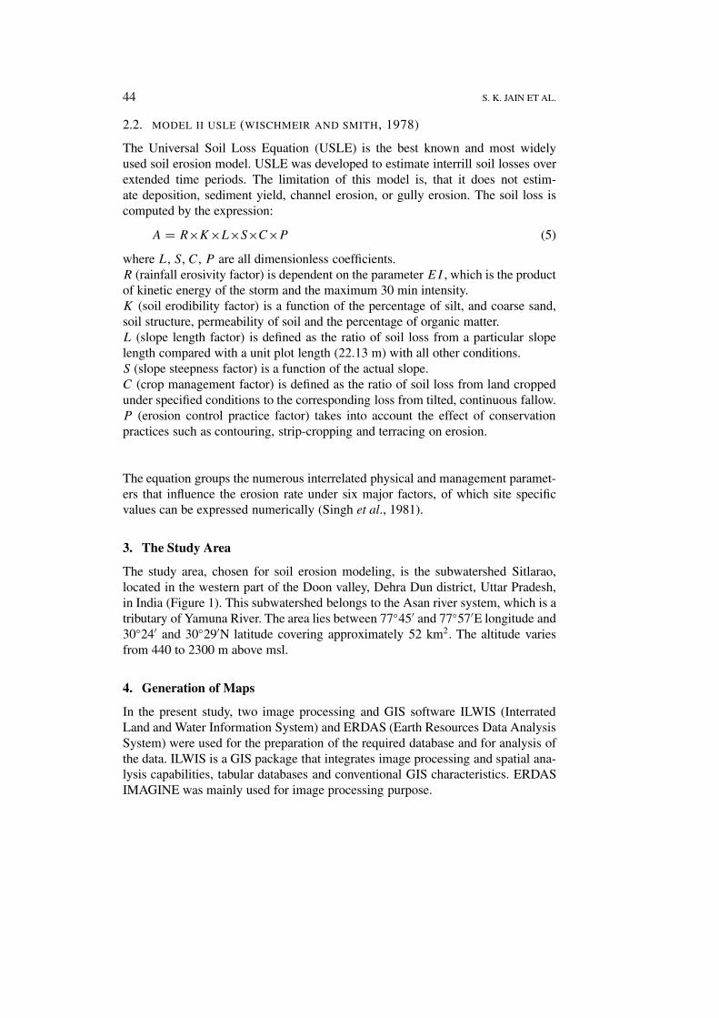
2.2. MODEL II USLE (WISCHMEIR AND SMITH, 1978)

The Universal Soil Loss Equation (USLE) is the best known and most widelyused soil erosion model. USLE was developed to estimate interrill soil losses overextended time periods. The limitation of this model is, that it does not estim-ate deposition, sediment yield, channel erosion, or gully erosion. The soil loss iscomputed by the expression:

A = R×K×L×S×C×P (5)

where L, S, C, P are all dimensionless coefficients.R (rainfall erosivity factor) is dependent on the parameter EI , which is the productof kinetic energy of the storm and the maximum 30 min intensity.K (soil erodibility factor) is a function of the percentage of silt, and coarse sand,soil structure, permeability of soil and the percentage of organic matter.L (slope length factor) is defined as the ratio of soil loss from a particular slopelength compared with a unit plot length (22.13 m) with all other conditions.S (slope steepness factor) is a function of the actual slope.C (crop management factor) is defined as the ratio of soil loss from land croppedunder specified conditions to the corresponding loss from tilted, continuous fallow.P (erosion control practice factor) takes into account the effect of conservationpractices such as contouring, strip-cropping and terracing on erosion.

The equation groups the numerous interrelated physical and management paramet-ers that influence the erosion rate under six major factors, of which site specificvalues can be expressed numerically (Singh et al., 1981).

3. The Study Area

The study area, chosen for soil erosion modeling, is the subwatershed Sitlarao,located in the western part of the Doon valley, Dehra Dun district, Uttar Pradesh,in India (Figure 1). This subwatershed belongs to the Asan river system, which is atributary of Yamuna River. The area lies between 77◦45′ and 77◦57′E longitude and30◦24′ and 30◦29′N latitude covering approximately 52 km2. The altitude variesfrom 440 to 2300 m above msl.

4. Generation of Maps

In the present study, two image processing and GIS software ILWIS (InterratedLand and Water Information System) and ERDAS (Earth Resources Data AnalysisSystem) were used for the preparation of the required database and for analysis ofthe data. ILWIS is a GIS package that integrates image processing and spatial ana-lysis capabilities, tabular databases and conventional GIS characteristics. ERDASIMAGINE was mainly used for image processing purpose.

ESTIMATION OF SOIL EROSION USING GIS TECHNIQUE 45

Figure 1. Location of the study area.

The main map of the study area was prepared from the Survey of India toposheetat a scale of 1:50 000. Drainage network, roads and important point locations likevillages, temples etc., were digitized as segment map and point map, respectively.For the creation of Digital Elevation Model (DEM), the contour map of the areawas prepared by digitizing the contours from the Survey of India toposheet.

For the present study, a contour interpolation algorithm in ILWIS was used tocreate DEM and slope map from the contour map. For this purpose height differ-ences need to be computed in X and Y directions, since overall slope gradient is afunction of height differences over horizontal distances in both X and Y directions.From DEM a slope map can be generated in degree or percentage.

In the present study the relationship between elevation and rainfall, developedby Shreshta (1997), has been used for the preparation of a rainfall map. Thisrelationship is as follows:

R = 1384.2 + 0.339Z (6)

where R is the rainfall in mm and Z is the elevation is meters.The resulted rainfall map showed different values of rainfall for each pixel. This

rainfall map has been classified and shown in Figure 2. Based on the climatic data,

46 S. K. JAIN ET AL.

Figure 2. Classified rainfall map of the study area.

the number of average rainy days in a year was found to be 75 days in the lowerelevations (up to 700 m), 85 days in the medium ranges (701 to 1200 m) and 95days for the higher elevations (Shrestha, 1997). Thus, a map, showing annual rainydays as a function of elevation, was created.

A physiographic soil map of the Doon valley was used to create the soil map ofthe area (Figure 3). The different soil units are named H11, H12, H13, H21 (soilsof residual hills), M1, M2, M3 (soils of mountainous areas), P11, P12, P21 (soilsof piedmont areas), V1, V2, and V3 (soils of river terrace) (Shrestha, 1997).

The landuse map was prepared by digital image processing of Indian remotesensing satellite, IRS-IC, LISS III data of February 1998. The different landuseclasses identified are dense forest, degraded forest, cultivation, mixed forest, fallowland, open scrub, river and snow covered area (Figure 4). Snow cover is a temporaryphenomenon occurring in the higher regions of the area.

5. Estimation of Parameters

5.1. MODEL I

To estimate the soil erosion due to splash detachment, the data of annual rainfalland 30 min intensity of the area is required. The annual rainfall map was generatedusing Equation (6) and rainfall intensity for the area was taken as 25 mm hr−1.

The overland flow map for the watershed was generated using Equation (2). Theparameter used in the equation depends on soil characteristics and landuse of thearea. The values of the parameters used in the present study are given in Tables Iand II.

ESTIMATION OF SOIL EROSION USING GIS TECHNIQUE 47

Table I. Different soil units and parameters

Soil Surface Bulk Moisture K factor Soil

map texture Density storage detachment

unit G/cc capacity index

H11 Gravely 1.3 0.18 0.45 0.22

Loam

H12 Loam 1.3 0.18 0.50 0.22

H13 Gravely 1.4 0.20 0.40 0.22

Loam

H21 Loam 1.3 0.20 0.48 0.22

M1 Gravely 1.2 0.26 0.45 0.35

Sandy Loam

M2 Gravely 1.2 0.25 0.43 0.35

Sandy Loam

M3 Gravely 1.2 0.25 0.4 0.35

Sandy Loam

P11 Gravely 1.4 0.18 0.35 0.22

Loam

P12 Loam 1.3 0.20 0.40 0.22

P21 Gravely 1.3 0.20 0.36 0.35

Sandy Loam

P22 Sandy Loam 1.2 0.28 0.38 0.30

V1 Loam 1.3 0.20 0.41 0.22

V2 Loamy Sand 1.4 0.10 0.30 0.36

V3 Sandy Loam 1.2 0.15 0.35 0.3

Table II. Landuse and different parameters

Landuse C factor P factor A (%) Et/Eo Rd

Open scrub 0.1 0.8 15 0.05 0.10

Degraded sal forest 0.03 0.8 20 0.80 0.10

Dense sal forest 0.004 0.8 20 0.90 0.10

Mixed forest 0.05 0.8 15 0.80 0.10

Cultivation 0.3 0.6 30 0.85 0.07

Fallow 0.5 0.7 10 0.58 0.05

Snow 0 0 – – –

River 0 0 – – –

48 S. K. JAIN ET AL.

Figure 3. Soil map of the study area.

Figure 4. Landuse map of the study area.

Soil loss is estimated from the transport capacity of the overland flow and theestimated rate of soil detachment. If the transport capacity is higher than the rate ofsoil detachment, the soil detachment value will be taken as the soil loss. Similarly,if the rate of soil detachment is higher than the transport capacity of overland flow,the value of the transport capacity will be considered for the soil loss. Soil loss wascomputed as follows:

Erosion = iff(G > F , F , G)

ESTIMATION OF SOIL EROSION USING GIS TECHNIQUE 49

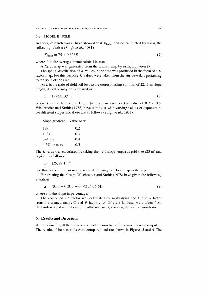
5.2. MODEL II (USLE)

In India, research works have showed that Rfactor can be calculated by using thefollowing relation (Singh et al., 1981)

Rfactor = 79 + 0.363R (7)

where R is the average annual rainfall in mm.A Rfactor map was generated from the rainfall map by using Equation (7).The spatial distribution of K values in the area was produced in the form of a K

factor map. For this purpose K values were taken from the attribute data pertainingto the soils of the area.

As L is the ratio of field soil loss to the corresponding soil loss of 22.13 m slopelength, its value may be expressed as

L = (λ/22.13)m , (8)

where λ is the field slope length (m), and m assumes the value of 0.2 to 0.5.Wischmeier and Smith (1978) have come out with varying values of exponent m

for different slopes and these are as follows (Singh et al., 1981).

Slope gradient Value of m

1% 0.2

1–3% 0.3

3–4.5% 0.4

4.5% or more 0.5

The L value was calculated by taking the field slope length as grid size (25 m) andis given as follows:

L = [25/22.13]mFor this purpose, the m map was created, using the slope map as the input.

For creating the S map, Wischmeier and Smith (1978) have given the followingequation

S = (0.43 + 0.30 s + 0.043 s2)/6.613 (9)

where s is the slope in percentage.The combined LS factor was calculated by multiplying the L and S factor

from the created maps. C and P factors, for different landuse, were taken fromthe landuse attribute data and the attribute maps, showing the spatial variations.

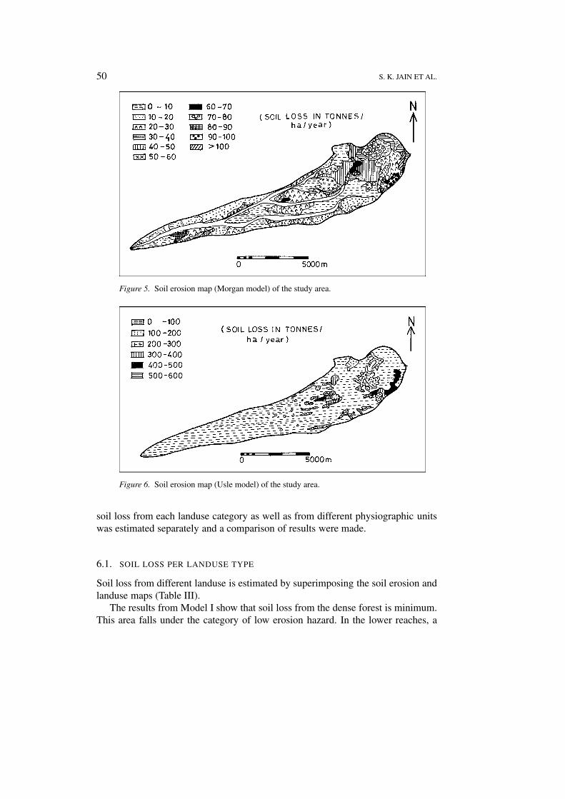
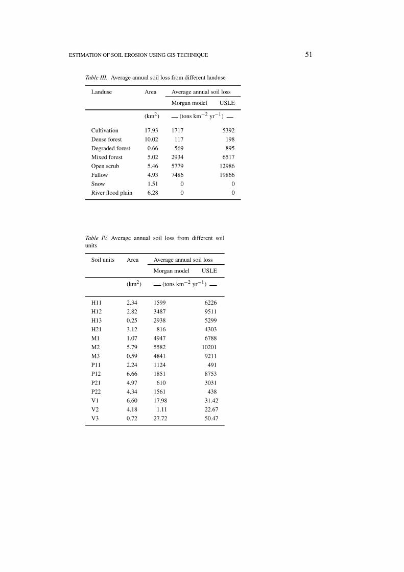
6. Results and Discussion

After estimating all the parameters, soil erosion by both the models was computed.The results of both models were compared and are shown in Figures 5 and 6. The

50 S. K. JAIN ET AL.

Figure 5. Soil erosion map (Morgan model) of the study area.

Figure 6. Soil erosion map (Usle model) of the study area.

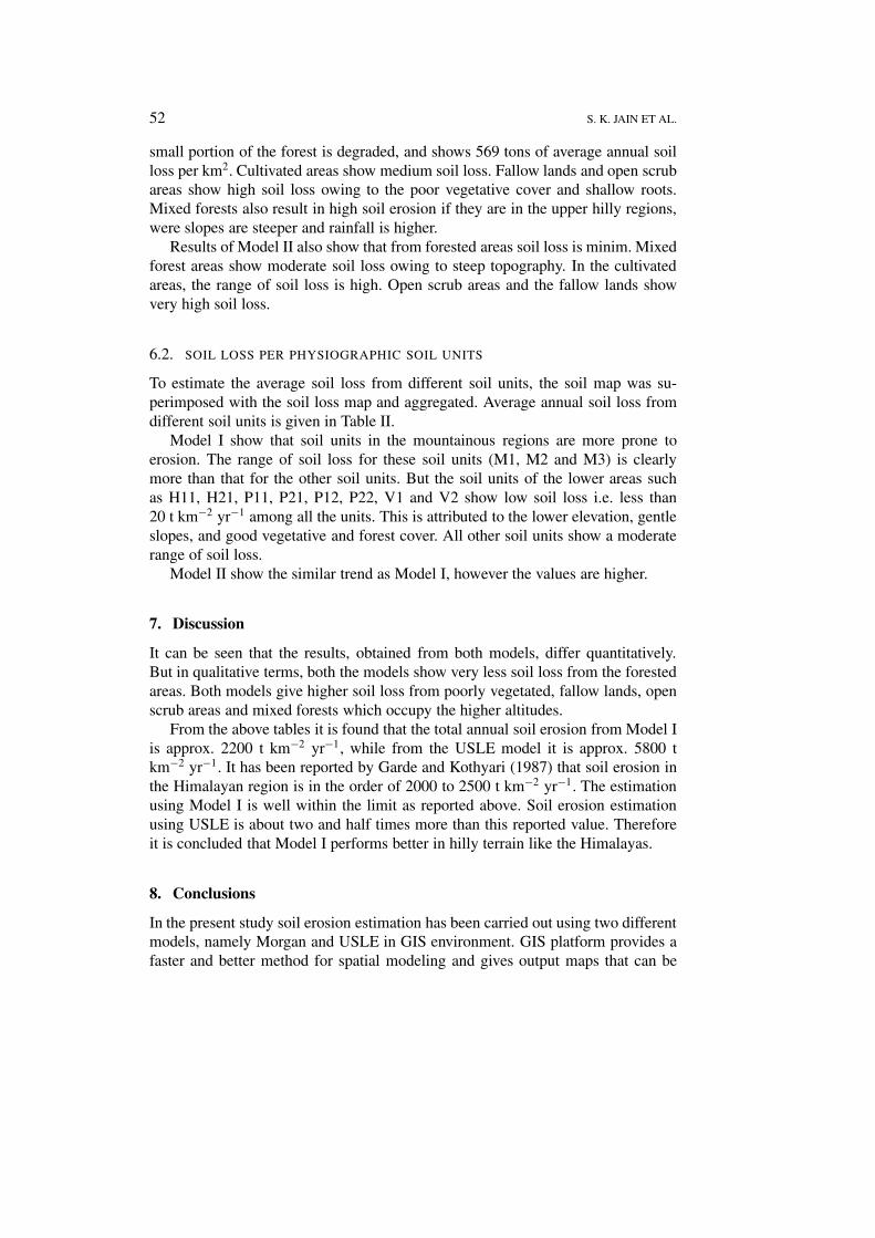
soil loss from each landuse category as well as from different physiographic unitswas estimated separately and a comparison of results were made.

6.1. SOIL LOSS PER LANDUSE TYPE

Soil loss from different landuse is estimated by superimposing the soil erosion andlanduse maps (Table III).

The results from Model I show that soil loss from the dense forest is minimum.This area falls under the category of low erosion hazard. In the lower reaches, a

ESTIMATION OF SOIL EROSION USING GIS TECHNIQUE 51

Table III. Average annual soil loss from different landuse

Landuse Area Average annual soil loss

Morgan model USLE

(km2) (tons km−2 yr−1)

Cultivation 17.93 1717 5392

Dense forest 10.02 117 198

Degraded forest 0.66 569 895

Mixed forest 5.02 2934 6517

Open scrub 5.46 5779 12986

Fallow 4.93 7486 19866

Snow 1.51 0 0

River flood plain 6.28 0 0

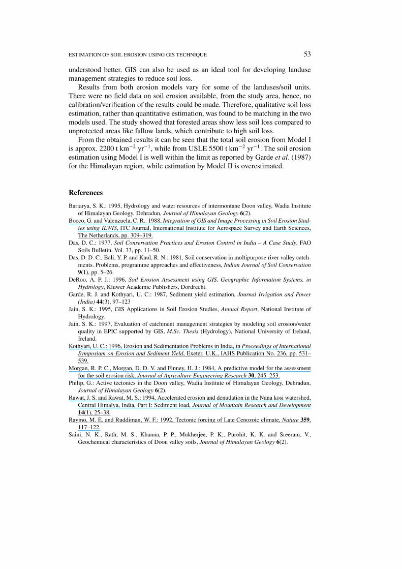
Table IV. Average annual soil loss from different soilunits

Soil units Area Average annual soil loss

Morgan model USLE

(km2) (tons km−2 yr−1)

H11 2.34 1599 6226

H12 2.82 3487 9511

H13 0.25 2938 5299

H21 3.12 816 4303

M1 1.07 4947 6788

M2 5.79 5582 10201

M3 0.59 4841 9211

P11 2.24 1124 491

P12 6.66 1851 8753

P21 4.97 610 3031

P22 4.34 1561 438

V1 6.60 17.98 31.42

V2 4.18 1.11 22.67

V3 0.72 27.72 50.47

52 S. K. JAIN ET AL.

small portion of the forest is degraded, and shows 569 tons of average annual soilloss per km2. Cultivated areas show medium soil loss. Fallow lands and open scrubareas show high soil loss owing to the poor vegetative cover and shallow roots.Mixed forests also result in high soil erosion if they are in the upper hilly regions,were slopes are steeper and rainfall is higher.

Results of Model II also show that from forested areas soil loss is minim. Mixedforest areas show moderate soil loss owing to steep topography. In the cultivatedareas, the range of soil loss is high. Open scrub areas and the fallow lands showvery high soil loss.

6.2. SOIL LOSS PER PHYSIOGRAPHIC SOIL UNITS

To estimate the average soil loss from different soil units, the soil map was su-perimposed with the soil loss map and aggregated. Average annual soil loss fromdifferent soil units is given in Table II.

Model I show that soil units in the mountainous regions are more prone toerosion. The range of soil loss for these soil units (M1, M2 and M3) is clearlymore than that for the other soil units. But the soil units of the lower areas suchas H11, H21, P11, P21, P12, P22, V1 and V2 show low soil loss i.e. less than20 t km−2 yr−1 among all the units. This is attributed to the lower elevation, gentleslopes, and good vegetative and forest cover. All other soil units show a moderaterange of soil loss.

Model II show the similar trend as Model I, however the values are higher.

7. Discussion

It can be seen that the results, obtained from both models, differ quantitatively.But in qualitative terms, both the models show very less soil loss from the forestedareas. Both models give higher soil loss from poorly vegetated, fallow lands, openscrub areas and mixed forests which occupy the higher altitudes.

From the above tables it is found that the total annual soil erosion from Model Iis approx. 2200 t km−2 yr−1, while from the USLE model it is approx. 5800 tkm−2 yr−1. It has been reported by Garde and Kothyari (1987) that soil erosion inthe Himalayan region is in the order of 2000 to 2500 t km−2 yr−1. The estimationusing Model I is well within the limit as reported above. Soil erosion estimationusing USLE is about two and half times more than this reported value. Thereforeit is concluded that Model I performs better in hilly terrain like the Himalayas.

8. Conclusions

In the present study soil erosion estimation has been carried out using two differentmodels, namely Morgan and USLE in GIS environment. GIS platform provides afaster and better method for spatial modeling and gives output maps that can be

ESTIMATION OF SOIL EROSION USING GIS TECHNIQUE 53

understood better. GIS can also be used as an ideal tool for developing landusemanagement strategies to reduce soil loss.

Results from both erosion models vary for some of the landuses/soil units.There were no field data on soil erosion available, from the study area, hence, nocalibration/verification of the results could be made. Therefore, qualitative soil lossestimation, rather than quantitative estimation, was found to be matching in the twomodels used. The study showed that forested areas show less soil loss compared tounprotected areas like fallow lands, which contribute to high soil loss.

From the obtained results it can be seen that the total soil erosion from Model Iis approx. 2200 t km−2 yr−1, while from USLE 5500 t km−2 yr−1. The soil erosionestimation using Model I is well within the limit as reported by Garde et al. (1987)for the Himalayan region, while estimation by Model II is overestimated.

References

Bartarya, S. K.: 1995, Hydrology and water resources of intermontane Doon valley, Wadia Instituteof Himalayan Geology, Dehradun, Journal of Himalayan Geology 6(2).

Bocco, G. and Valenzuela, C. R.: 1988, Integration of GIS and Image Processing in Soil Erosion Stud-ies using ILWIS, ITC Journal, International Institute for Aerospace Survey and Earth Sciences,The Netherlands, pp. 309–319.

Das, D. C.: 1977, Soil Conservation Practices and Erosion Control in India – A Case Study, FAOSoils Bulletin, Vol. 33, pp. 11–50.

Das, D. D. C., Bali, Y. P. and Kaul, R. N.: 1981, Soil conservation in multipurpose river valley catch-ments. Problems, programme approaches and effectiveness, Indian Journal of Soil Conservation9(1), pp. 5–26.

DeRoo, A. P. J.: 1996, Soil Erosion Assessment using GIS, Geographic Information Systems, inHydrology, Kluwer Academic Publishers, Dordrecht.

Garde, R. J. and Kothyari, U. C.: 1987, Sediment yield estimation, Journal Irrigation and Power(India) 44(3), 97–123

Jain, S. K.: 1995, GIS Applications in Soil Erosion Studies, Annual Report, National Institute ofHydrology.

Jain, S. K.: 1997, Evaluation of catchment management strategies by modeling soil erosion/waterquality in EPIC supported by GIS, M.Sc. Thesis (Hydrology), National University of Ireland,Ireland.

Kothyari, U. C.: 1996, Erosion and Sedimentation Problems in India, in Proceedings of InternationalSymposium on Erosion and Sediment Yield, Exeter, U.K., IAHS Publication No. 236, pp. 531–539.

Morgan, R. P. C., Morgan, D. D. V. and Finney, H. J.: 1984, A predictive model for the assessmentfor the soil erosion risk, Journal of Agriculture Engineering Research 30, 245–253.

Philip, G.: Active tectonics in the Doon valley, Wadia Institute of Himalayan Geology, Dehradun,Journal of Himalayan Geology 6(2).

Rawat, J. S. and Rawat, M. S.: 1994, Accelerated erosion and denudation in the Nana kosi watershed,Central Himalya, India, Part I: Sediment load, Journal of Mountain Research and Development14(1), 25–38.

Raymo, M. E. and Ruddiman, W. F.: 1992, Tectonic forcing of Late Cenozoic climate, Nature 359,117–122.

Saini, N. K., Rath, M. S., Khanna, P. P., Mukherjee, P. K., Purohit, K. K. and Sreeram, V.,Geochemical characteristics of Doon valley soils, Journal of Himalayan Geology 6(2).

54 S. K. JAIN ET AL.

Shrestha, D. P.: 1997, Soil Erosion Modeling, ILWIS 2.1 for Windows, Application Guide, Interna-tional Institute for Aerospace Survey and Earth Sciences, The Netherlands, pp. 323–341

Singh, G., Chandra, S, and Babu, R.: 1981, Soil loss and prediction research in India, Central Soiland Water Conservation Research Training Institute, Bulletin No. T-12/D9.

Thakur, V. C.: 1995, Geology of Doon valley, Garhwal Himalaya, Neotectonics and coeval depos-ition with fault propagation folds, Wadia Institute of Himalayan Geology, Journal of HimalayanGeology 6(2).

Valdiya, K. S.: 1985, Accelerated erosion and landslide-prone zones in the central Himalaya,Concepts and Strategies, Gyanodaya Prakashan, Nainital, pp. 122–38.

Wischmeier, W. H. and Smith, D. D.: 1978, Predicting rainfall erosion losses: A guide to conservationplanning, USDA Handbook No. 537.