Volume : 4 Issue : 2
342
ISSN: 2249-6645 International Journal of Modern Engineering Research (IJMER) Volume 4 2014 Issue 2 February
-
Upload
khangminh22 -
Category
Documents
-
view
4 -
download
0
Transcript of Volume : 4 Issue : 2

ISSN: 2249-6645
International Journal of Modern Engineering Research
(IJMER)
Volume 4 2014 Issue 2 February

International Journal of Modern Engineering Research (IJMER)
Editorial Board
Executive Managing Editor
Prof. Shiv Kumar Sharma India
Editorial Board Member
Dr. Jerry Van Department of Mechanical, USA
Dr. George Dyrud Research centre dy. Director of Civil Engineering, New Zealand
Dr. Masoud Esfal R& D of Chemical Engineering, Australia
Dr. Nouby Mahdy Ghazaly Minia University, Egypt
Dr. Stanley John Department of Textile Engineering, United Kingdom
Dr. Valfitaf Rasoul Professor and HOD of Electromechanical, Russian
Dr. Mohammed Ali Hussain HOD, Sri Sai Madhavi Institute of Science & Technology, India
Dr. Manko dora Associate professor of Computer Engineering, Poland
Dr. Ahmed Nabih Zaki Rashed Menoufia University, Egypt
Ms. Amani Tahat Ph.D physics Technical University of Catalonia-Spain
Associate Editor Member Dr. Mohd Nazri Ismail
University of Kuala Lumpur (UniKL), Malaysia
Dr. Kamaljit I. Lakhtaria Sir Padmapat Singhaniya University, Udaipur
Dr. Rajesh Shrivastava Prof. & Head Mathematics & computer Deptt. Govt. Science & commerce College Benazir. M.P
Dr. Asoke Nath Executive Director, St. Xavier’s College, West Bengal, India
Prof. T. Venkat Narayana Rao Head, CSE, HITAM Hyderabad
Dr. N. Balasubramanian Ph. D (Chemical Engg), IIT Madras
Jasvinder Singh Sadana
M. TECH, USIT/GGSIPU, India

Dr. Bharat Raj Singh Associate Director, SMS Institute of Technology, Lucknow
DR. RAVINDER RATHEE C. R. P, Rohtak, Haryana
Dr. S. Rajendran Research Supervisor, Corrosion Research Centre Department of Chemistry, GTN Arts College, Dindigul
Mohd Abdul Ahad Department of Computer Science, Faculty of Management and Information Technology, Jamia Hamdad, New Delhi
Kunjal Mankad Institute of Science & Technology for Advanced Studies & Research (ISTAR)
NILANJAN DEY JIS College of Engineering, Kalyani, West Bengal
Dr. Hawz Nwayu Victoria Global University, UK
Prof. Plewin Amin Crewe and Alsager College of Higher Education, UK
Dr. (Mrs.) Annifer Zalic London Guildhall University, London
Dr. (Mrs.) Malin Askiy Victoria University of Manchester
Dr. ABSALOM Sixth form College, England
Dr. Nimrod Nivek London Guildhall University, London

International
OPEN ACCESS Journal
Of Modern Engineering Research (IJMER)
| IJMER | ISSN: 2249–6645 | www.ijmer.com | Vol. 4 | Iss. 2 | Feb 2014 | 1 |
Finite Element Analysis of Convective Micro Polar Fluid Flow
through a Porous Medium in Cylindrical Annulus
1Dr. B. Tulasi Lakshmi Devi,
2Dr. B. Srinivasa Reddy,
3G. V. P. N. Srikanth,
4Dr. G. Srinivas
1,3 ,4Department of Mathematics,Guru Nanak Institute of Technology,Hyderabad,India
2Department of Applied Mathematics,Yogi Vemana University,kaddapah,A.P,India
I. INTRODUCTION
In recent years there have been considerable advancement in the study of free convection in a porous
annulus because of its natural occurrence and of its importance in many branches of science and engineering.
This is of fundamental importance to a number of technological applications, such as underground disposal of
radioactive waste materials, cooling of nuclear fuel in shipping flasks and water filled storage bays, regenerative
heat exchangers containing porous materials and petroleum reservoirs, burying of drums containing heat
generating chemicals in the earth, storage of agricultural products, ground water flow modeling, nuclear reactor
assembly, thermal energy storage tanks, insulation of gas cooled reactor vessels, high performance insulation for
building, and cold storage, free convective heat transfer inside a vertical annulus filled with isotropic porous
medium has been studied by many researchers, notable among them are Havstad et. al., [7], Reda [15], Prasad et.
al., [12,13], Prasad et. al., [14], Hickon et. al., [8], and Shiva kumara et. al., [16], they concluded that radius
ratio and Rayleigh number influence the heat and fluid flow significantly.
Eringen [5] presented the theory of micro polar fluid which explains adequately the internal
characteristics of the substructure particles subject to rotations and deformations, Ariman [1] Sylvester et. al.,
[17] and Ariman et. al., [2] confirmed that the micropolar fluid serves a better model for animal blood. The
liquid crystals, suspension solutions and certain polymeric fluids consisting of randomly oriented barlike
elements of dumbbell molecules, behave as micro polar fluid. Kazakai and Ariman [10] introduced the heat
conducting micropolar fluid and investigated the flow between two parallel plates. Eringen [6] extended the
theory further to include heat conduction and viscous dissipation. The application of this theory may be searched
in biomechanics.
Berman [4] has studied the flow of a viscous liquid under a constant pressure gradient between two
concentric cylinders at rest. Inger [9] solved the problem when the walls are permeable and the outer cylinder is
sliding with a constant axial velocity relative to the stationery inner one. Mishra and Acharya [11] examined the
elastico viscous effects in the flow considered by Inger [9]. Sastri and Maiti solved the problem of combined
convective flow of micro polar fluid in an annulus.
The problem of massive blowing into aerodynamic body flow fields is a complex 1 for a realistic flow
configuration. However the study the simplified flow models exhibits some of the essential physical features
involving the interaction of blowing with a shear flow. The classical coutte – poiseylle shear flow is an idealized
model for this purpose to investigate to micro polar structures at least theoretically on such a flow Agarwal and
Dhanpal [3] have analyzed the connective micro polar fluid flow and heat transfer between two concentric
porous circular cylinders when the outer cylinder moves parallel to itself with a constant velocity. A problem
solved by Inger [9] in viscous fluids.
In this paper we make an investigation of connective heat transfer flow micro polar fluid in a cylindrical
annulus between the porous concentric cylinders r = a and r = b. By employing Galerikin finite element analysis
with line elements with three nodes the transport equations of linear momentum, angular momentum and energy
are solved to obtain velocity, micro concentration and temperature distributions.
ABSTRACT: We analyze a finite element solution for the mixed convection micro polar flow through a
porous medium in a cylindrical annulus. The governing partial differential equations are solved
numerically by using finite element technique. The effect of Darcy parameter and Heat source parameter
and surface condition on velocity, micro rotation and temperature functions has been study.
Keywords: Porous medium, Micro polar Fluids, Convection, Cylindrical annulus.

Finite Element Analysis of Convective Micro Polar Fluid Flow through a Porous…
| IJMER | ISSN: 2249–6645 | www.ijmer.com | Vol. 4 | Iss. 1 | Feb. 2014 |2|
II. FORMULATION OF THE PROBLEM Consider the steady motion of an incompressible micro polar fluid through an annulus of two infinitely
long porous circular cylinders of radii a and b (a – b = h > 0) respectively. The fluid is injected through the inner
cylinder with arbitrary radial velocity ub and in view of continuity, also flows outward through the moving
cylinder with a radial velocity ua. The cylindrical polar co-ordinate system (, , z) with z co-ordinate along the
axis of the cylinders is chosen to specify the problem.
The velocity and micro rotation are taken in the form
vr = u(r), v = v = 0, vz = w(r)
vr = 0, v = v = (r), vz = 0 2.1
the basic equations are:
Continuity: 0
r
u
r
u 2.2
Momentum:
22
2 1)(
r
u
r
u
rr
uk
r
p
r
uu 2.3
)(1
)(2
2
Nrrr
k
r
w
rr
wk
z
p
r
wu
2.4
First stress Momentum:
Nkr
wk
r
N
r
N
rr
Nr
r
Nuj 2
122
2
2.5
Energy:
r
T
rr
Tk
z
TwC fp
12
2
2.6
Where T is the temperature, N is the micro rotation the density, p the pressure, j the micro inertia, Cp
the specific heat, kf the thermal conductivity, the fluid viscosity, k is the material constants.
At r = b, u = ub, w = 0, v = 0, T = T0 + A0 z
At r = a, u = ua, w = 0 v = 0, T = T1 + A0 z 2.7
Where the fluid is assumed to adhere to the solid boundaries.A0 is the constant of proportionality and
T0, T1 are the constant wall temperatures of inner and outer cylinders temperatures of inner and outer cylinders
respectively at z = 0.
The integration of (2.2) yields
ur = C, a constant 2.8
ru = aua = bub r
auu a
Also inview of the boundary condition on temperature, we may write
T = T0 + A0 (z) + (r) 2.9
Introducing the non-dimensional variables r, w, p, and N as
2
2,,
au
pp
a
ww
a
rr
22
0
0 )(,
a
wkuN
TT
TT
i
2.10
The governing equations in the non-dimensional form are
)(1
11 1
112
2
Nrrd
d
rGD
rd
wd
rrd
wd
2.11
rd
wd
rAN
Arrd
Nd
rA
rd
Nd 12111
22
2
2.12
rd
d
rrd
dwNP Tr
12
2
2.13

Finite Element Analysis of Convective Micro Polar Fluid Flow through a Porous…
| IJMER | ISSN: 2249–6645 | www.ijmer.com | Vol. 4 | Iss. 1 | Feb. 2014 |3|
where
k (Micropolar parameter)
J
rA
(Micropolar parameter
21a
A
aua (Suction parameter)
k
LD
21
(Darcy parameter) 2
3
LTgG
(Grashof number)
11
GG
11
f
p
rk
CP
(Prandtl number)
The boundary conditions are
w = 0, = 1, N = 0 on r = 1
w = 0, = 0, N = 0 on r = s
In order to predict the heat and mass transfer behavior in the porous medium equations (2.11) – (2.13)
are solved by using finite element method. A simple 3-noded triangular element is considered. , and vary
inside the element and can be expressed as
= N1 1 + N2 2 + N3 3
= N1 1 + N2 2 + N3 3
= N1 1 + N2 2 + N3 3
Gela kin’s method is used to convert the partial differential equation (2.11) – (2.13) into matrix form of
equations. Details of FEM formulations and good understanding of the subject is given in the books [3, 4]. The
matrix equations are, assembled to get global matrix equations for he whole domain, which is then solved
iteratively, to obtain, and in porous medium. In order to get accurate results, tolerance level of solution for
, and are set at 10-5
and 10-9
respectively. Element size in domain varies. Large number of elements are
located near the walls where large variations in , and are expected. The mesh is symmetrical about central
horizontal and vertical lines of the cavity. Sufficiently dense mesh is chosen to make the solution mesh invariant.
The mesh size of 3200 elements has good accuracy in predicting the heat transfer behavior of the porous
medium. The computations are carried out on high-end computer.
III. RESULTS AND DISCUSSION
On solving the equations, given by the finite element technique the velocity, micro rotation and
temperature distributions are obtained. The Prandtl number pr, material constants A & A are taken to be
constant, at 0.733, 1 and 1 respectively whereas the effect of other important parameters, namely micro polar
parameter , the section Reynolds number , Grashof number G and Darcy parameter D-1
has been studied for
these functions and the corresponding profiles are shown in figs. 1.
Fig. 1 depicts the variation of velocity function W with Grashof number G. The actual axial velocity W
is in the vertically downwards direction and w < 0 represents the actual flow. Therefore w > 0 represents the
reversal flow. We notice from fig. 1 that w>0 for G > 0 and w < 0 for G < 0 except in the vicinity of outer
cylinder r = 2. the reversal flow exists everywhere in the region (1.1 r 1.8) for G > 0 and in the neighborhood
of r = 2 for G < 0. The region of reversed flow enlarges with G 2x10³ and shrinks with higher G 3x10
3. Also
it grows in size with |G| (<0). |w| enhances with G 2x10³ and reduces with higher G 3x10
3. |w| experiences a
depreciation in the case of cooling of the boundaries with maximum at r = 1.5.The variation of w with Darcy
parameter D-1
. It is found that lesser the permeability of the porous medium larger |w| in the flow region (fig. 2).
The influence of micro rotation parameter on w is shown in fig. 3. As the micro polar parameter 3
increases, the velocity continuously increases and decreases with higher 5, with maximum attained in the
vicinity of r = 1. Fig. 4 represents w with suction parameter. IT is found that the axial velocity experiences an
enhancement with increase in 0.03 and depreciates with higher 0.05. Fig. 5 depicts w with the width of
the annular region. We notice that the axial velocity continuously decreases with increase in the width S of the
annular region. Thus the velocity enhances in the narrow gap region and depreciates in the wide gap case. The
effect of radiation parameter N1 on w is exhibited in Fig. 6. IT is observed that the velocity w enhances with
increase in N1 1.0 except in a narrow region adjacent to r = 2 and for higher N1 1.5, it experiences an
enhancement in the entire flow region.

Finite Element Analysis of Convective Micro Polar Fluid Flow through a Porous…
| IJMER | ISSN: 2249–6645 | www.ijmer.com | Vol. 4 | Iss. 1 | Feb. 2014 |4|
The micro rotation (N) in shown in figs 7-12 for different values of G, , , S and N1. It is found that
the values of micro rotation for G > 0 are negative and positive for G < 0. An increase in |G| 2x10³ editor an
enhancement in N and for higher |G| 3x10³, it reduces in the region adjacent to r = 1 and enhances in the
reform adjacent to r = 2 with maximum at r = 1.5 (fig. 7). From fig. 8 we find that lesser the permeability of the
porous medium larger the micro oration everywhere in the flow region.The effect of N on micro polar parameter
in shown in Fig. 9. We notice that an increase in 3 leads to an enhancement in |N| and for higher 5, it
enhances the first half (1.1 r 1.5) and reduces in the second half (1.6 r 1.9). Fig. 10 illustrates that the
micro oration enhances in the first half and reduces in the second half with increase in 0.02 and for higher
values of 0.03 we notice an increment in |N| everywhere in the flow region. Form fig. 11 we find that the
micro rotation depreciates in the narrow gap case and enhances in the wide gap case. Fig. 12 illustrates that the
micro rotation |N| enhances with increase in the radiation parameter N1 1.5 and for higher N1 2.5, the micro
rotation enhances in the let half and depreciates in the second half of the flow region.
The non-dimensional temperature () is shown in figs. 13 – 17 for different values of G, , , S and N1.
Fig. 13 illustrates that non-dimensional temperature is positive for all variations. The actual temperature
enhances with increase in G 2x10³ and depreciates with higher G 3x10
3. Also it enhances with G < 0. The
variation of with D-1
shows that lesser the permeability of the porous medium larger the actual temperature in
the flow region (Fig. 14), Fig. 15 illustrates that an increase in the micro rotation parameter increases the
actual temperature continuously with maximum attained at r=1.5. The variation of with suction parameter
shows that the temperature enhances with increase in 0.03. For further increase in 0.05, the temperature
depreciates in the first half and enhances in the second half. The influence of the suction of the boundary on is
shown in fig. 16. IT is found that increase in S 0.6 reduces in the left half and enhances it in the right half
and for S = 0. 7, reduces in the flow region except in a region adjacent to r =1. For further increase in S we
notice an enhancement in the central flow region and depreciation in in the regions abutting the cylinders r = 1
& 2. Fig. 17 represents the temperature with radiation parameter N1. It is found that an increase in N1 enhances
in the left half and depreciates in the right half and for higher values N1 1.5 we observe depreciation in the first
half and enhancement in the second half.
-6
-4
-2
0
2
4
6
8
10
1 1.1 1.2 1.3 1.4 1.5 1.6 1.7 1.8 1.9 2
r
u
I
II
III
IV
-10
-8
-6
-4
-2
0
2
4
6
8
1 1.1 1.2 1.3 1.4 1.5 1.6 1.7 1.8 1.9 2
r
M
I
II
III
IV
V
Fig. 1 : Variation of velocity (u) with G Fig. 2 : Variation of velocity (u) with G
I II III IV I II III IV V
G 103 3x10
3 5x10
3 -10
3 G -3x10
3 -5x10
3 10
3 2x10
3 3x10
3

Finite Element Analysis of Convective Micro Polar Fluid Flow through a Porous…
| IJMER | ISSN: 2249–6645 | www.ijmer.com | Vol. 4 | Iss. 1 | Feb. 2014 |5|
-4
-2
0
2
4
6
8
10
12
1 1.1 1.2 1.3 1.4 1.5 1.6 1.7 1.8 1.9 2
r
u
I
II
III
0
2
4
6
8
10
12
1 1.1 1.2 1.3 1.4 1.5 1.6 1.7 1.8 1.9 2
r
u
I
II
III
IV
Fig. 3 : Variation of velocity (u) with Fig. 4 : Variation of velocity (u) with
I II III I II III IV
1 3 5 0.01 0.02 0.03 0.05
-6
-4
-2
0
2
4
6
8
10
12
1 1.1 1.2 1.3 1.4 1.5 1.6 1.7 1.8 1.9 2
r
M
I
II
III
IV
V
VI
-8
-6
-4
-2
0
2
4
6
8
10
12
1 1.1 1.2 1.3 1.4 1.5 1.6 1.7 1.8 1.9 2
r
M
I
II
III
IV
Fig. 5 : Variation of velocity (u) with S Fig. 6 : Variation of velocity (u) with Nt
I II III IV V VI I II III IV
S 0.4 0.5 0.6 0.7 0.8 0.9 Nt 0.5 1.0 1.5 2.5
-15
-10
-5
0
5
10
15
1 1.1 1.2 1.3 1.4 1.5 1.6 1.7 1.8 1.9 2
r
N
I
II
III
IV
-15
-10
-5
0
5
10
15
1 1.1 1.2 1.3 1.4 1.5 1.6 1.7 1.8 1.9 2
r
N
I
II
III
IV
V
Fig. 7 : Variation of micro rotation (N) with G Fig. 8 : Variation of micro rotation (N) with G
I II III IV I II III IV V
G 103 3x10
3 5x10
3 - 10
3 G -3x10
3 -5x10
3 10 20 30

Finite Element Analysis of Convective Micro Polar Fluid Flow through a Porous…
| IJMER | ISSN: 2249–6645 | www.ijmer.com | Vol. 4 | Iss. 1 | Feb. 2014 |6|
-14
-12
-10
-8
-6
-4
-2
0
1 1.1 1.2 1.3 1.4 1.5 1.6 1.7 1.8 1.9 2
r
N
I
II
III
-10
-9
-8
-7
-6
-5
-4
-3
-2
-1
0
1 1.1 1.2 1.3 1.4 1.5 1.6 1.7 1.8 1.9 2
r
N
I
II
III
IV
Fig. 9 : Variation of micro rotation (N) with Fig. 10 : Variation of micro rotation (N) with
I II III I II III IV
1 3 5 0.01 0.02 0.03 0.05
-14
-12
-10
-8
-6
-4
-2
0
1 1.1 1.2 1.3 1.4 1.5 1.6 1.7 1.8 1.9 2
r
N
I
II
III
IV
V
-14
-12
-10
-8
-6
-4
-2
0
1 1.1 1.2 1.3 1.4 1.5 1.6 1.7 1.8 1.9 2
r
N
I
II
III
IV
Fig. 11 : Variation of micro rotation (N) with S Fig. 12 : Variation of micro rotation (N) with Nt
I II III IV V VI I II III IV
S 0.4 0.5 0.6 0.7 0.8 0.9 Nt 0.5 1.0 1.5 2.5
-1
0
1
2
3
4
5
6
7
8
1 1.1 1.2 1.3 1.4 1.5 1.6 1.7 1.8 1.9 2
r
I
II
III
IV
0
2
4
6
8
10
12
1 1.1 1.2 1.3 1.4 1.5 1.6 1.7 1.8 1.9 2
r
I
II
III
IV
Fig. 13 : Variation of temperature () with G Fig. 14 : Variation of temperature () with G
I II III IV I II III IV V
G 103 3x10
3 5x10
3 -10
3 G -3x10
3 -5x10
3 10 20 30

Finite Element Analysis of Convective Micro Polar Fluid Flow through a Porous…
| IJMER | ISSN: 2249–6645 | www.ijmer.com | Vol. 4 | Iss. 1 | Feb. 2014 |7|
0
2
4
6
8
10
12
1 1.1 1.2 1.3 1.4 1.5 1.6 1.7 1.8 1.9 2
r
I
II
III
0
1
2
3
4
5
6
7
8
9
10
1 1.1 1.2 1.3 1.4 1.5 1.6 1.7 1.8 1.9 2
r
I
II
III
IV
Fig. 15: Variation of temperature () with Fig. 16: Variation of temperature () with
I II III I II III IV
1 3 5 0.01 0.02 0.03 0.05
-1
0
1
2
3
4
5
6
7
8
9
10
1 1.1 1.2 1.3 1.4 1.5 1.6 1.7 1.8 1.9 2
r
I
II
III
IV
V
0
1
2
3
4
5
6
7
1 1.1 1.2 1.3 1.4 1.5 1.6 1.7 1.8 1.9 2
r
I
II
III
IV
Fig. 17: Variation of temperature () with S Fig. 18: Variation of temperature () with Nt
I II III IV V VI I II III IV
S 0.4 0.5 0.6 0.7 0.8 0.9 Nt 0.5 1.0 1.5 2.5
REFERENCES [1] T. ARIMAN, J. Biomech. 4. 185 (1971).
[2] T. ARIMAN, M.A.TURK and N.D.SYLVESTER, Int. J. Engng, sci. 11, 905 (1973).
[3] R.S. AGARWAL1 and C. DHANAPAL2 Numerical solution of micro polar fluid flow and heat transfer between two
co-axial porous circular cylinders Int. J. Engg. Sci, vol. 26. No.11, pp. 1133-1142, 1988.
[4] A.S. BERMAN, J. appal. Phys, 29, 71 (1958).
[5] A.C. ERINGEN, J. Math. Mech. 16. 1 (1966).
[6] A.C. ERINGEN, J. Math. Analysis Applic. 38 480 (1972).
[7] HAVSTAD, M.A, BURNS, P.J. convective heat transfer in vertical cylindrical Annuli filled with porous medium,
Int. J. Heat Mass Transfer. 25 (1982), 11, pp. 1755-1766.
[8] HICKON, C.E, GARTLING, D.K. A Numerical study of natural convection in a vertical Annulus porous layer, Int.
J. Heat Mass Transfer, 28 (1985) 3, pp. 720-723.
[9] G.R.INGER, phys. Fluids 12, 1741 (1969).
[10] Y. KAIZAKI and T. ARIMAN, Rheol. Acta 10 319 (1971).
[11] S.P.MISHRA and B.P. ACHARYA. Ind. J. phys. 46, 469 (1972).
[12] PRASAD, V., KULACKI, F.A. Natural convection in a vertical porous Annulus, Int. J. Heat Mass Transfer 27
(1984), 2 pp. 207-219.
[13] PRASAD, V. KULACKI, F.A. Natural convection in porous media bounded by short concentric cylinders, ASME J.
Heat Transfer, 107 (1985), 1. pp. 147-154
[14] PRASAD, V., KULACKI, F.A, KEYHANI, M. Natural convection in porous media, J. Fluid Mechanics, 150
(1985), 3, pp. 89-119.
[15] REDA, D.C. Natural convection experiments in a liquid saturated porous medium bounded by vertical coaxial
cylinders, ASME J. Heat Transfer, 105 (1983), 4, pp. 795-802.
[16] SHIVAKUMARA, I.S, PRASANNA, B.M.R, RUDRAISH, N. VENKATACHALAPPA, M. Numerical study of
natural convection in a vertical cylindrical Annulus using Non-Darcy equation. J. Porous Media, 5 (2003), 2, pp. 87-
102.
[17] N.D. SYLVESTER, M.A, TURK and T. ARIMAN Trans. Soc. Rheol. 17, 1 (1973).

International
OPEN ACCESS Journal
Of Modern Engineering Research (IJMER)
| IJMER | ISSN: 2249–6645 | www.ijmer.com | Vol. 4 | Iss. 1 | Feb. 2014 |8|
Biogas as a Alternate Source Of Energy And Creating Awareness
Among Rural People
Neeraj Kumar1, Sachin Gupta
2, Bharat atary
3
Assistant Professor, Department of ME1
Assistant Professor, Department of CSE2
Assistant Professor, Department of ME3
Maharishi Markandeshwar Group of Institutions (Ramba) Karnal, India
I. INTRODUCTION Biogas is a gas whose primary elements are methane (CH4) and carbon dioxide (CO2) and may have
small amount of hydrogen sulphide (H2S), Moisture and siloxanes. It is a mixture of methane (CH4), 50 to 70%
carbon dioxide (CO2), 30 to 40% hydrogen (H2), 5 to 10% nitrogren (N2) and 1 to 2% hydrogen sulphide
(H2S).Water vapour (0.3%). biogas is about 20% lighter than air and has an ignition temperature in the range of
650 to 750°C. It is a colourless and odourless gas that burns with 60% efficiency in a conventional biogas stove.
It is a product of the natural decomposition of any organic substance of animal or plant. It refers to a gas
produced by the biological breakdown of organic matter in the absence of oxygen organic waste such as dead
plant and animal material, animal dung and kitchen waste can be converted into a gaseous fuel called biogas.
The main source for production of biogas are cattle dung, night soil, poultry or piggery dropping, agricultural
residues animals manure, wood waste from forestry and industry, residues from food and paper industries,
municipal green wastes, sewage sludge dedicated energy crops such as short rotation (3 to 15 years) grasses,
sugar crops (sugarcane, beet), starch crops (corn, wheat) and oil crops (soy, sunflower, palm oil), kitchen waste,
household waste, green waste, human waste. The components of biogas – methane and carbon dioxide- act as
greenhouse gases that harm the environment if released unburned into the atmosphere. The production of biogas
in biogas plants prevents uncontrolled emission of methane into the atmosphere and, by generating renewable
energy in the form of biogas, reduces the use of fossil fuel.
II. BIOMASS CONVERSION PROCESS Biomass conversion process is divided into three categories, such as:
(i) Direct combustion (ii) Thermo chemical conversion (iii) Biochemical conversion
2.1 Direct combustion
Process of burning in presence of oxygen to produce heat and by products is called combustion
complete combustion to ashes is called is incineration. The process of combustion is applicable to solid, liquid
and gaseous fuel. Such as wood dung, vegetable waste can be dried and burnt to provide heat or converted into
low calorific value gas by “pyrolysis”. 2.1.1 Pyrolysis process
In this process organic material to gases solid and liquids by heating to 500 0C to 900
0C in the absence
of oxygen product of wood pyrolysis are methanol, charcoal and acidic acid all forms of organic materials
ABSTRACT: This paper deals with the use of biogas as a alternate source of energy and creating
awareness among rural people. Biogas refer to a gas made from anaerobic digestion of agricultural and
animal waste. The gas is useful as a fuel substitute for firewood, dung,agricultural residues,petrol and
electricity. Biogas, a clean and renewable form of energy could very well substitute (especially in the rural
sector) for conventional sources of energy (fossil fuels, oil, etc.) which are causing ecological–
environmental problems biogas digester involves anaerobic fermentation process in which different groups
of bacteria act upon complex organic materials in the absence of air to produce biogas.
Keywords: Alternate Source, Biogas, Methane, Waste, Biogas plant.

Biogas as a Alternate Source Of Energy And Creating Awareness Among Rural People
| IJMER | ISSN: 2249–6645 | www.ijmer.com | Vol. 4 | Iss. 1 | Feb. 2014 |9|
including such as rubber and plastic can be converted to a fuel gas which contains CO ,CH4, other hydrocarbons
(CnHm) CO2 and N2. 2.2 Thermo chemical conversion
Thermo chemical conversion process converts the biomass and its residues to fuel, chemical and power
using gasification and pyrolysis technologies. 2.3 Biochemical conversion
Biochemical conversion by micro-organisms converting biomass to biofuels are slow processes taking
place at low temp.The principal conversion process is fermentation. fermentation is a processs of decomposition
of organic matter by micro-organism. e.g- decomposition of suger to form ehanol and carbondioxide by yeast
and ethanol forming acetic acid in making vinegar. 2.3.1 Gassification
Heating biomass with about one-third of the oxygen necessary for complete combustion produces a
mixture of carbon dioxide and hydrogen known as syngas. Paralysis heating biomass in the absence of oxygen
produce a liquid pyrolysis oil both syngas and pyrolysis oil can be used as fuels both can also be chemically
converted to other valuable fuels and chemicals. ,” Gobar Gas” mainly because cow dung has been the material
for its production. It is not only the excreta of the cattle, but also the piggery waste as well as poultry droppings
are very effectively used for biogas generation. A few other material through which biogas can be generated are
algae, crop residues. Biogas is produced by digestion, pyrolysis or hydro gasification. Digestion is a biological
process that occurs in the absence of oxygen and in the presence of anaerobic organisms at ambient pressures
and temperatures of 35-70 C. The container in which this digestion takes place is known as the digester. 2.4 Anaerobic digestion
Biogas technology is concerned to micro organisms. These are living creatures which are microscopic
in size and are invisible to unaided eyes. There are different types of micro organisms. They are called bacteria,
fungi, virus etc. Bacteria again can be classified into two types’ beneficial bacteria and harmful bacteria.
Bacteria can be divided into two major groups based on their oxygen requirement. Those which grow in
presence of oxygen are called aerobic while the others grow in absence of gaseous oxygen are called anaerobic.
When organic matter undergoes fermentation (process of chemical change in organic matter brought about by
living organisms) through anaerobic digestion, gas is generated. This gas is known as bio-gas. Biogas is
generated through fermentation or bio-digestion of various wastes by a variety of anaerobic and facultative-
organisms. Facultative bacteria are capable of growing both in presence and absence of air or oxygen.
III. STEPS IN BIOGAS PRODUCTION Biogas microbes consist of a large group of complex and differently acting microbe species, notable
the methane-producing bacteria. The whole biogas-process can be divided into three steps: hydrolysis,
acidification, and methane formation. Three types of bacteria are involved

Biogas as a Alternate Source Of Energy And Creating Awareness Among Rural People
| IJMER | ISSN: 2249–6645 | www.ijmer.com | Vol. 4 | Iss. 1 | Feb. 2014 |10|
3.1 Hydrolysis In the first step (hydrolysis), the organic matter is enzymolyzed externally by extracellular enzymes
(cellulose, amylase, protease and lipase) of microorganisms. Bacteria decompose the long chains of the complex
carbohydrates, proteins and lipids into shorter parts. For example, polysaccharides are converted into
monosaccharide. Proteins are split into peptides and amino acids. 3.2 Acidification
Acid-producing bacteria, involved in the second step, convert the intermediates of fermenting bacteria
into acetic acid (𝐶𝐻3COOH), hydrogen (𝐻2 ) and carbon dioxide (𝐶𝑂2 ). These bacteria are facultatively
anaerobic and can grow under acid conditions. To produce acetic acid, they need oxygen and carbon. For this,
they use the oxygen solved in the solution or bounded-oxygen. Hereby, the acid-producing bacteria create an
anaerobic condition which is essential for the methane producing microorganisms. Moreover, they reduce the
compounds with a low molecular weight into alcohols, organic acids, amino acids, carbon dioxide, hydrogen
sulphide and traces of methane. From a chemical standpoint, this process is partially endergonic (i.e. only
possible with energy input), since bacteria alone are not capable of sustaining that type of reaction. Acid-
producing bacteria, involved in the second step, convert the intermediates of fermenting bacteria into acetic acid
(𝐶𝐻3COOH), hydrogen (𝐻2) and carbon dioxide (𝐶𝑂2).These bacteria are facultative anaerobic and can grow
under acid conditions. To produce acetic acid, they need oxygen and carbon. For this, they use the oxygen
solved in the solution or bound oxygen. Hereby, the acid producing bacteria create an anaerobic condition which
is essential for the methane producing microorganisms. Moreover, they reduce the compounds with a low
molecular weight into alcohols, organic acids, amino acids, carbon dioxide, hydrogen sulphide and traces of
methane. 3.3 Methane formation
Methane-producing bacteria, involved in the third step, decompose compounds with a low molecular
weight. For example, they utilize hydrogen, carbon dioxide and acetic acid to form methane and carbon dioxide.
Under natural conditions, methane producing microorganisms occur to the extent that anaerobic conditions are
provided, e.g. under water (for example in marine sediments), in ruminant stomach sand in marshes. They are
obligatory anaerobic and very sensitive to environmental changes. In contrast to the acidogenic and acetogenic
bacteria, the methanogenic bacteria belong to the archaebacter genus, i.e. to a group of bacteria with a very
heterogeneous morphology and a number of common biochemical and molecular-biological properties that
distinguish them from all other bacterial general. The main difference lies in the makeup of the bacteria’s cell
walls. 3.3.1 Symbiosis of bacteria
Methane and acid-producing bacteria act in a symbiotically manner. On the one hand, acid producing
bacteria create an atmosphere with ideal parameters for methane-producing bacteria (anaerobic conditions,
compounds with a low molecular weight). On the other hand, methane-producing microorganisms use the
intermediates of the acid producing bacteria.[2] Without consuming them, toxic conditions for the acid-
producing microorganisms would develop. In practical fermentation processes the metabolic actions of various
bacteria all act in concert. No single bacteria are able to produce fermentation products alone.
IV. PARAMETERS AND PROCESS OPTIMIZATION The metabolic activity involved in microbiological methanation is dependent on the following factors:
(i). Substrate temperature (ii). Available nutrients
(iii). Retention time (flow-through time) (iv). pH level (v). Nitrogen inhibition and C/N ratio
(vi). Substrat solid content and agitation Each of the various types of bacteria responsible for the three stages of the methanogenesisis affected
differently by the above parameters. Since interactive effects between the various determining factors exist, no
precise quantitative data on gas production as a function of the above factors are available. Thus, discussion of
the various factors is limited to their qualitative effects on the process of fermentation.

Biogas as a Alternate Source Of Energy And Creating Awareness Among Rural People
| IJMER | ISSN: 2249–6645 | www.ijmer.com | Vol. 4 | Iss. 1 | Feb. 2014 |11|
V. CASE STUDY: FLOATING-DRUM & FIXED-DOME TYPE PLANT 5.1 Floating-drum plants
Floating-drum plants consist of an underground digester and a moving gas-holder. The gas-holder
floats either directly on the fermentation slurry or in a water jacket of its own. The gas is collected in the gas
drum, which rises or moves down, according to the amount of gas stored. The gas drum is prevented from tilting
by a guiding frame. If the drum floats in a water jacket, it cannot get stuck, even in substrate with high solid
content.
Figure 1: Basic diagram of Floating Drum, Flexible balloon and Fixed dome
5.2 The Drum
In the past, floating-drum plants were mainly built in India. A floating-drum plant consists of a cylindrical or
dome-shaped digester and a moving, floating gas-holder, or drum. The gas-holder floats either directly in the
fermenting slurry or in a separate water jacket. The drum in which the biogas collects has an internal and/or
external guide frame that provides stability and keeps the drum upright. If biogas is produced, the drum moves
up, if gas is consumed, the gas-holder sinks back.
Figure 2: Basic Structure of the Drum
Floating-drum plants are used chiefly for digesting animal and human feces on a continuous-feed mode
of operation, i.e. with daily input. They are used most frequently by small- to middle-sized farms (digester size:
5-15m3) or in institutions and larger agro-industrial estates (digester size: 20-100m
3).
5.3 Fixed-dome Plants A fixed-dome plant consists of a digester with a fixed, non-movable gas holder, which sits on top of the
digester. When gas production starts, the slurry is displaced into the compensation tank. Gas pressure increases
with the volume of gas stored and the height difference between the slurry level in the digester and the slurry
level in the compensation tank. The costs of a fixed-dome biogas plant are relatively low. It is simple as no
moving parts exist. There are also no rusting steel parts and hence a long life of the plant (20 years or more) can
be expected. The plant is constructed underground, protecting it from physical damage and saving space. While
the underground digester is protected from low temperatures at night and during cold seasons, sunshine and
warm seasons take longer to heat up the digester. No day/night fluctuations of temperature in the digester

Biogas as a Alternate Source Of Energy And Creating Awareness Among Rural People
| IJMER | ISSN: 2249–6645 | www.ijmer.com | Vol. 4 | Iss. 1 | Feb. 2014 |12|
positively influence the bacteriological processes. The construction of fixed dome plants is labor-intensive, thus
creating local employment. Fixed-dome plants are not easy to build. They should only be built where
construction can be supervised by experienced biogas technicians. Otherwise plants may not be gas-tight
(porosity and cracks). The basic elements of a fixed dome plant (here the Nicarao Design) are shown in the
figure below.
VI. CONCLUSION Biogas as a alternate source of energy because it is a very cheap gas .it is a renewable source of energy.
Waste includes all items that people no longer have any use for, which they either intend to get rid of or have
already discarded. Additionally, wastes are such items which people are require to discard, for example by lay
because of their hazardous properties. Many items can be considered as waste e.g., household rubbish, sewage
sludge, wastes from manufacturing activities, packaging items, discarded cars, old televisions, garden waste, old
paint containers etc. Thus all our daily activities can give rise to a large variety of different wastes arising from
different sources.Biowaste refers to livestock manures, the biodegradable part of municipal wastes including
food and garden wastes, treated sewage sludge, organic industrial wastes such as paper and textiles and compost.
They are a major contributor to greenhouse gas emissions and pollution of waters courses if not managed
properly. Biowaste can be degraded anaerobically in a biogas digester to produce biogas and other gases. One
excellent source of energy is Biogas. This is produced when bacteria decompose organic material such as
garbage and sewage, especially in the absence of oxygen. Biogas is a mixture of about 60 percent methane and
40 percent Carbon dioxide. Methane is the main component of natural gas. It is relatively clean burning,
colorless, and odorless. This gas can be captured and burned for cooking and heating. This is already being done
on a large scale in some countries of the world. Farms that produce a lot of manure, such as hog and dairy farms,
can use biogas generators to produce methane.
REFERENCES [1] Eze J. I.1,2* and Ojike O.1,2 , Anaerobic production of biogas from maize wastes International Journal of the
Physical Sciences Vol. 7(6), pp. 982 - 987, 2 February, 2012. [2] Kumar et al. Ministry of Non- Conventional Energy Sources)(Source; 2009-10 MNRE Annual Report , Kumar et al,
IJES, 2010) [3] Ev Mamdouh A. El-Messery*, Gaber AZ. Ismail*,Anwaar K. Arafa**,J evaluation of Municipal Solid Waste
Management in Egyptian Rural Areas,Egypt Public Health Assoc Vol. 84 No. 1 & 2, 2009. [4] Usman M. A., Olanipekun O. O., Kareem O. M,Biogas Generation from Domestic Solid Wastes in Mesophilic
Anaerobic Digestion,International Journal of Research in Chemistry and Environment ,Vol. 2 Issue 1 January
2012(200-205) ,1SSN 2248-9649 [5] Eze J. I.1,2 and Ojike O.1,21, “Anaerobic production of biogas from maize wastes”, National Center for Energy
Research and Development, University of Nigeria, Nsukka, Enugu State, Nigeria.Department of Food Science and
Technology, University of Nigeria, Nsukka, Enugu State, Nigeria.Accepted 20 January, 2012 [6] Richard Arthura, Martina Francisca Baidooa , Edward Antwi, ”Biogas as a potential renewable energy source: A
Ghanaian case study”, Accepted 8 November 2010 [7] Cooper, E.L. 1997. Agriscience: Fundamentals & Applications. Delmar Publishers, Albany,New York),-
scienceResources [8] Teodorita Al Seadi, DominikRutz, Heinz Prassl, Michael Köttner, Tobias Finsterwalder,Silke Volk, Rainer Janssen,
ISBN 978-87-992962-0-0,Published by University of Southern Denmark Esbjerg, NielsBohrsVej 9-10,(project
Information and Advisory Service on Appropriate Technology (ISAT) [9] Amaratunga, M.: Structural Behaviour and Stress Conditions of Fixed Dome Type of Biogas Units. Elhalwagi, M.M.
(Ed.): Biogas Technology, Transfer and Diffusion, London & New York, pp. 295-301. 1986. 0001182; ISBN: 1-
85166-000-3 [10] Van Buren, A.; Crook, M.: A Chinese Biogas Manual - Popularising Technology in the Countryside. Intermediate
Technology Publications Ltd. London (UK), 1979, sixth impression 1985, 135 P. ISBN: 0903031655 [11] Fulford, D.: Fixed Concrete Dome Design. Biogas - Challenges and Experience from Nepal. Vol I. United Mission to
Nepal, 1985, pp. 3.1-3.10.

International
OPEN ACCESS Journal
Of Modern Engineering Research (IJMER)
| IJMER | ISSN: 2249–6645 | www.ijmer.com | Vol. 4 | Iss. 2 | Feb. 2014 |13|
On Contra – RW Continuous Functions in Topological Spaces
M. Karpagadevi1, A. Pushpalatha
2
1 Assistant Professor, S.V.S. College of Engineering, Coimbatore, India
2Assistant Professor, Government Arts College, Udumalpet, India
I. Introduction In 1996, Dontchev[1] presented a new notion of continuous function called contra-continuity. This
notion is a stronger form of LC-Continuity. In 2007, Benchalli.S.S. and Wali.R.S.[2] introduced RW-closed set
in topological spaces. In 2012, Karpagadevi.M. and Pushpalatha.A.[3] introduced RW-continuous maps and
RW-irresolute maps in topological spaces. The purpose this paper is to define a new class of continuous
functions called Contra-rw continuous functions and almost Contra rw-Continuous function and investigate their
relationships to other functions.
II. Preliminaries Throughout this paper X and Y denote the topological spaces (X,) and (Y,σ) respectively and on
which no separation axioms are assumed unless otherwise explicitly stated. For any subset A of a space (X,),
the closure of A, the interior of A and the complement of A are denoted by cl(A), int(A) and Ac respectively.
(X,) will be replaced by X if there is no chance of confusion. Let us recall the following definitions as pre
requesters.
Definition 2.1: A Subset A of (X,) is called
(i) generalized closed set (briefly g-closed) [5] if cl(A) U whenever A U and U is open in X.
(ii) regular generalized closed set (briefly rg-closed)[6] if cl(A) U whenever A U and U is regular open in
X.
The Complement of the above mentioned closed sets are their respective open sets.
Definition 2.2: A Subset A of a Space X is called rw-closed [2] if cl(A) U whenever A U and U is regular
semiopen in X.
Definiton 2.3: A Map f: (X,) → (Y,σ) is said to be
(i) rw-continuous[3] if f-1
(V) is rw-closed in (X,) for every closed set V in (Y,σ)
(ii) rw-irresolute[3] if f-1
(V) is rw-closed in (X,) for every rw-closed set V of (Y,σ)
(iii) rw-closed[2] if f(F) is rw-closed in (Y,σ) for every rw-closed set F of (X,)
(iv) rw-open[2] if f(F) is rw-open in (Y,σ) for every rw-open set F of (X,)
Definiton 2.4: A Map f: (X,) → (Y,σ) is said to be contra-continuous [1] if f-1
(V) is closed in (X,) for
every open set V in (Y,σ).
III. Contra RW-Continuous Function In this section we introduce the notions of contra rw-continuous, contra rw-irresolute and almost contra
rw-continuous functions in topological spaces and study some of their properties.
Definition 3.1: A function f: (X,) → (Y,σ) is called contra rw-continuous if f-1
(V) is rw-closed set in X for
each open set V in Y.
ABSTRACT: In this paper we introduce and investigate some classes of functions called
contra-rw continuous functions. We get several characterizations and some of their properties. Also we
investigate its relationship with other types of functions.
Mathematics Subject Classification: 54C08, 54C10
Keywords: Contra rw-continuous, Almost Contra rw-continuous, Contra rw-irresolute

On Contra – RW Continuous Functions in Topological Spaces
| IJMER | ISSN: 2249–6645 | www.ijmer.com | Vol. 4 | Iss. 2 | Feb. 2014 |14|
Example 3.2: Let X=Y=a,b,c with topologies = X,,a,b,a,b and σ = Y,,a,b. Let f: X → Y
be a map defined by f (a) = a, f (b) = b and f(c) = c. Clearly f is contra rw-continuous.
Theorem 3.3: Every contra-continuous function is contra rw-continuous.
Proof: The proof follows from the fact that every closed set is rw-closed set.
Remark 3.4: The converse of the above theorem need not be true as seen from the following example.
Example 3.5: Let X=Y=a,b,c with topologies = X,,a,b,a,b and σ = Y,,a,b. Let f: X → Y
be a map defined by f (a) = a, f (b) = b and f(c) = c. Clearly f is contra rw-continuous but not contra-continuous
since f -1
(a,b) = a,b which is not closed in X.
Theorem 3.6: If a function f: X → Y is contra rw-continuous, then f is contra-continuous.
Proof: Let V be an open set in Y. Since f is contra rw-continuous, f -1
(V) is closed in X. Hence f is contra-
continuous.
Remark 3.7: The concept of rw-continuity and contra rw-continuity is independent as shown in the following
examples.
Example 3.8 : Let X=Y=a,b,c with topologies = X,,a,b,a,b and σ = Y,,b,c. Let f: X → Y
be a map defined by f (a) = a, f (b) = b and f(c) = c. Clearly f is contra rw-continuous but not rw-continuous
since f -1
(a) = a is not rw-closed in X where a is closed in Y.
Example 3.9 : Let X=Y=a,b,c with topologies = X,,a,b,a,b and σ = Y,,b. Define f: X → Y
identity mapping. Then c learly f is rw-continuous but not contra rw-continuous since f -1
(b) = b is not
rw-closed in X where b is closed in Y.
Theorem 3.10: Every contra rw-continuous function is contra rg-continuous.
Proof: Since every rw-closed set is rg-closed, the proof is obvious.
Remark 3.11: The converse of the above theorem need not be true as seen from the following example.
Example 3.12: Let X=Y=a,b,c,d with topologies =X,,a,b,a,b,a,b,c and
σ = Y,,a,b,a,b,c. Let f: X → Y be a map defined by f (a) = c, f (b) = d, f(c) = a and f (d) =b. Clearly f
is contra rg-continuous but not contra rw-continuous since f -1
(a) = c is not rw-closed in X where a is
open in Y.
Remark 3.13: The composition of two contra rw-continuous functions need not be contra rw-continuous as
seen from the following example.
Example 3.14: Let X=Y=Z=a,b,c with topologies = X,,a,b,a,b and σ = Y,,a,b and
= Z, ,a. Let f: X → Y be a map defined by f (a) = c, f (b) = b and f(c) = a and g: Y→Z is defined by
g (a) =b, g (b) =c and g(c) =a.Then clearly f and g are contra rw-continuous. But g f: X → Z is not contra
rw-continuous since (g f)-1
a = f-1
(g-1
a) = f-1
(c) = a is not rw-closed in X.
Theorem 3.15: If f: (X,) → (Y,σ) is contra rw-continuous and g: Y→Z is a continuous function, then
g f : X→Z is contra rw-continuous.
Proof: Let V be open in Z. Since g is continuous, g -1
(V) is open in Y. Then f -1
(g -1
(V)) is rw-closed in X since f
is contra rw-continuous. Thus (g f) -1
(V) is rw-closed in X. Hence g f is contra rw-continuous.
Theorem 3.16: If f: X → Y is rw-irresolute and g: Y→Z is contra continuous function then g f: X→Z is
contra rw-continuous.
Proof: Since every contra continuous is contra rw-continuous, the proof is obvious.
Theorem 3.17: If f: X → Y is contra rw-continuous then for every x X, each F C(Y,f(x)), there exists
URWO(X,x) such that f(U) F (ie) For each x X, each closed subset F of Y with f(x) F, there exists a
rw-open set U of Y such that xU and f(U)F.

On Contra – RW Continuous Functions in Topological Spaces
| IJMER | ISSN: 2249–6645 | www.ijmer.com | Vol. 4 | Iss. 2 | Feb. 2014 |15|
Proof: Let f: X → Y be contra rw-continuous. Let F be any closed set of Y and f(x) F where xX. Then
f -1
(F) is rw-open in X. Also x f -1
(F). Take U = f -1
(F). Then U is a rw-open set containing x and f (U) F.
Theorem 3.18: Let (X,) be a rw-connected space (Y,σ) be any topological space. If X → Y is surjective and
contra rw-continuous then Y is not a discrete space.
Proof: Suppose Y is discrete space. Let A be any proper non-empty subset of Y. Then A is both open and
closed in Y. Since f is contra rw-continuous, f -1
(A) is both rw-open and rw-closed in X. Since X is
rw-connected, the only subset of Y which are both rw-open and rw-closed are X and. Hence f -1
(A) = X. Then
it contradicts to the fact that f: X → Y surjective. Hence Y is not a discrete space.
Definition 3.19: A function f: X → Y is called almost contra rw-continuous if f -1
(V) is rw-closed set in X for
every regular open set V in Y.
Example 3.20: Let X=Y=Z=a,b,c with topologies = X,,a,b,a,b and σ = Y,,a,c,a,c.
Define f: X → Y by f (a) =a, f (b) =b and f(c)=c. Here f is almost contra rw-continuous since f -1
(a) = a is
rw-closed in X for every regular open set a in Y.
Theorem 3.21: Every contra rw-continuous function is almost contra rw-continuous.
Proof: The proof follows from the definition and fact that every regular open set is open.
Definition 3.22: A function f: X → Y is called contra rw-irresolute if f -1
(V) is rw-closed in X for each rw-open
set V in Y.
Definition 3.23: A function f: X → Y is called perfectly contra rw-irresolute if f -1
(V) is rw-closed and rw-open
in X for each rw-open set V in Y.
Theorem 3.24: A function f: X → Y is perfectly contra rw-irresolute if and only if f is contra rw-irresolute and
rw-irresolute.
Proof: The proof directly follows from the definitions.
Remark 3.25: The following examples shows that the concepts of rw-irresolute and contra rw-irresolute are
independent of each other.
Example 3.26: Let X=Y=Z=a,b,c with topologies = X,,a,b,a,b and σ = Y,,a,c,a,c.
Define f: X → Y by f (a) = a, f (b) = b and f(c) = c. Here f is contra rw-irresolute but not rw-irresolute since
f -1
(a,b) = a,b is not rw-open in X.
Example 3.27: Let X=Y=Z=a,b,c with topologies = X,,a,b,a,b and σ = Y,,a,c,a,c.
Define f: X → Y by f (a) = a, f (b) = b and f(c) = c. Here f is rw-irresolute but not contra rw-irresolute since
f -1
(b) = b is not rw-closed in X.
Theorem 3.28: Let f: X → Y and g: Y → Z be a function then
(i) If g is rw-irresolute and f is contra rw-irresolute then g f is contra rw-irresolute
(ii) If g is contra rw-irresolute and f is rw-irresolute then g f is contra rw-irresolute
Proof: (i) Let U be a rw-open in Z. Since g is rw-irresolute, g -1
(U) is rw-open in Y. Thus f -1
(g -1
(U)) is
rw-closed in X. Since f is contra rw-irresolute (ie) (g f) -1
(U) is rw-closed in X. This implies that g f is contra
rw-irreolute.
(ii) Let U be a rw-open in Z. Since g is contra rw-irresolute, g -1
(U) is rw-closed in Y. Thus f -1
(g -1
(U)) is
rw-closed in X since f is rw-irresolute (ie) (g f) -1
(U) is rw-closed in X. This implies that g f is
contra rw-irresolute.
Theorem 3.29: Every perfectly contra rw-irresolute function is contra rw-irresolute and rw-irresolute.
Proof: The proof directly follows from the definitions.
Remark 3.30: The following two examples shows that a contra rw-irresolute function may not be perfectly
contra rw-irresolute and rw-irresolute function may not be perfectly contra rw-irresolute.

On Contra – RW Continuous Functions in Topological Spaces
| IJMER | ISSN: 2249–6645 | www.ijmer.com | Vol. 4 | Iss. 2 | Feb. 2014 |16|
Example 3.31: In example 3.29, f is rw-irresolute but not perfectly contra rw-irresolute and in example 3.28,
f is contra rw-irresolute but not perfectly contra rw-irresolute.
Theorem 3.32: A function is perfectly contra rw-irresolute iff f is contra rw-irresolute and rw-irresolute.
Proof: The proof directly follows from the definitions.
REFERENCES [1]. Dontchev.J.”Conra-continuous functions and strongly s closed spaces”, International J.Math&Math.Sci.19
(1996).303-310.
[2]. Benchalli.S.S. and Wali.R.S, “On RW-closed sets in topological spaces”, Bull. Malays. Math. Sci. Soc (2) 30(2)
(2007), 99-110.
[3]. Karpagadevi.M. and Pushpaltha. A., “RW-Continuous maps and RW-irresolute maps in topological spaces”,
International Journal of Mathematics Trends and Technology, Vol.4, Issue 2-2013, 21-25.
[4]. Karpagadevi.M. and Pushpaltha. A., “RW-Closed maps and RW- Open maps in topological spaces”, International
Journal of Computer Applications Technology and Research, Vol.2, Issue 2-2013, 91-93.
[5]. Levine.N. ”Generalized closed sets in topology”, Rend.Circ.Mat.Palermo 19.1970,89-96.
[6]. Palaniappan.N and Rao.K.C. “Regular generalized closed sets”, Kyungpook Math J 33, 1993, 211-219.
[7]. Syed Ali Fathima.S. and Mariasingam.M. “On contra #rg-Continuous functions”, International Journal of Modern
Engineering Research, Vol.3.Issue.2, March-April.2013 pp.939-943

International
OPEN ACCESS Journal
Of Modern Engineering Research (IJMER)
| IJMER | ISSN: 2249–6645 | www.ijmer.com | Vol. 4 | Iss. 2 | Feb. 2014 |17|
Heart Disease Prediction Using Associative Relational
Classification Technique (Acar) With Som Neural Network
Amit Sahu1, Mayank saxena
2
Department of Computer Science & Engineering PCST, Bhopal, India
I. INTRODUCTION The diversity of lifestyle invites much disease in our body. In all disease heart disease which is also
called cardiovascular disease is considered as one of the leading cause of death in the world with high
prevalence in the Asia subcontinent [1, 2]. There are several risk factors which account for the heart disease
such as age, sex, smoking etc. Patients with Hereditary risk factors (such as: high blood pressure, diabetes) have
more chances of heart disease. Some risk factors are controllable. While having so many risk factors, it is a
complicated task to analyze heart disease on the basis of patient’s report [4]. Particularly, doctors take decision
on their intuition and experience rather than on the knowledge-rich data hidden in the database. In healthcare
transactions, data is too complex and huge to be processed and analyzed by traditional methods. It requires high
skills and experiences for correct decisions. Classification based on association rules, also called associative
classification, is a technique that uses association rules to build classifier. Generally it contains two steps: first it
finds all the class association rules (CARs) whose right-hand side is a class label, and then selects strong rules
from the CARs to build a classifier [5]. In this way, associative classification can generate rules with higher
confidence and better understandability comparing with traditional approaches. Thus associative classification
has been studied widely in both academic world and industrial world, and several effective algorithms [6] have
been proposed successively. However, all the above algorithms only focus on processing data organized in a
single relational table. In practical application, data is often stored dispersedly in multiple tables in a relational
database. Simply converting multi-relational data into a single flat table may lead to the high time and space
cost, moreover, some essential semantic information carried by the multi-relational data may be lost. Thus the
existing associative classification algorithms cannot be applied in a relational database directly [7]. We propose
a novel algorithm, ACAR, for associative classification which can be applied in multi-relational data
environment. The main idea of ACAR is to mine relevant features of each class label in each table respectively,
and generate strong classification rules[8]. The ensemble of different rules in different level used SOM based
ensemble classifier. The SOM based ensemble classifier classified the data very accurately. The self-organizing
map (SOM) is one of the most popular algorithms in the classification of data with a good performance
regarding rate of classification[9]. The SOM is a widely used unsupervised neural network for clustering high
dimensional input data and mapping these data into a two-dimensional representation space. Self-organizing
map is one of the most fascinating topics in the neural network field. The SOM introduced by Kohonen (1982),
is a neural network that maps signals from a high-dimensional space to a one- or two-dimensional discrete
lattice of neuron units. Each neuron stores a weight. The SOM organizes unknown data into groups of similar
patterns, according to a similarity criterion. Such networks can learn to detect regularities and correlations in
ABSTRACT: Mining of medical diagnoses of data is very difficult task in current data mining
approach. The heart disease data is collective information of blood pressure, Cholesterol problem,
diabetes and another complex disease. The relational of one disease to another is rare so
classification task is very difficult. So prediction of heart disease is very critical. in the process of
data mining rule based classification technique used for prediction. The rule based classification
technique based on association rule mining. The better rule mining technique the better
classification and predication of heart disease. in this paper proposed a association based ensemble
classification method for heart disease prediction. the association ensemble classifier based on
association rule mining and self –organized map network model. For the association rule used
Apriori-like algorithm. This algorithm generates numbers of rules for all combination of factor of
heart disease and divided into different level such as high level , middle level and low level, the all
level ensemble through SOM network and generate optimized set of heart disease prediction.
Keywords: Heart Disease, Associative Classification, Ensemble and SOM Network

Heart Disease Prediction Using Associative Relational Classification Technique…
| IJMER | ISSN: 2249–6645 | www.ijmer.com | Vol. 4 | Iss. 2 | Feb. 2014 |18|
their input and adapt their future responses to that input accordingly. An important feature of this neural network
is its ability to process noisy data[13]. The map preserves topological relationships between inputs in a way that
neighboring inputs in the input space are mapped to neighboring neurons in the map space. The rest of paper is
organized as follows. In Section II discuss related work of associative classification. The Section III proposed
method for classification. The section IV discusses experimental result and finally followed section V
conclusion and future scope
II. RELATED WORK In this section discuss the related work in the field of medical data classification using associative
classification using neural network and other optimization technique. The neural network is important area of
research in the field of data mining classification. The neural network optimized the level of classification and
improved the ratio of classification.
[1] In this paper author proposed an ensemble method and classification for heart diseases and to
improve the decision of the classifiers for heart disease diagnosis. Homogeneous ensemble is applied for heart
disease classification and finally results are optimized by using Genetic algorithm. Data is evaluated by using
IO-fold cross validation and performance of the system is evaluated by classifiers accuracy, sensitivity and
specificity to check the feasibility of our system. Comparison of our methodology with existing ensemble
technique has shown considerable improvements in terms of classification accuracy. The focused on the
optimized heart disease classification problem. Genetic Algorithm has been found a very good technique for
optimization and searching for quality solution. The proposed framework of SVM classifier ensemble and
optimization of results using Genetic Algorithm technique improved the classification accuracy as compared to
existing work.
[2] In this paper author proposed a genetic algorithm based feature selection for the heart diseases and
the details are, we presented a genetic algorithm (GA) based feature-selection method to find informative
features that play a significant role in discrimination of samples. Selected subsets from multiple GA runs were
used to build a classifier. The proposed approach can be combined with various classifiers to improve
classification performance and selection of the most discriminative features. Starting with a set of pre-selected
features by using a filter (1000 features), we used a GA combined with Fisher’s linear discriminate analysis
(LDA) to explore the space of feature subsets. In fact, our proposed approach employs GA and uses the LDA
classifier to evaluate the fitness of a given candidate feature subset. An external test set was chosen by using
Kohonen self-organizing maps (SOMs) to evaluate the performance of feature selection at the final stage. The
proposed method can be used to diagnose CHD in patients without using any angiographic techniques, which
may have a high risk of death for the individuals.
[3] In this paper author discussed on data mining method for heart disease, the details are data
classification is based on supervised machine learning algorithms which result in accuracy, time taken to build
the algorithm. Tanagra tool is used to classify the data and the data is evaluated using 10-fold cross validation
and the results are compared. The selection of algorithms is based on their performance, but not around the test
dataset itself, and also comprising the predictions of the classification models on the test instance. Training data
are produced by recording the predictions of each algorithm, using the full training data both for training and for
testing. Performance is determined by running 10-fold cross-validations and averaging the evaluations for each
training dataset. Several approaches have been proposed for the characterization of learning domain. the
performance of each algorithm on the data attribute is recorded. The algorithms are ranked according to their
performance of the error rate. Author also deals with the results in the field of data classification obtained with
Naive Bayes algorithm, Decision list algorithm and k-nn algorithm, and on the whole performance made known
Naive Bayes Algorithm when tested on heart disease datasets. Naive Bayes algorithm is the best compact time
for processing dataset and shows better performance in accuracy prediction.
[4] In this paper author described a heart beat classification system using optimization techniques such
as particle swarm optimization, to proposes a novel system to classify three types of electrocardiogram beats,
namely normal beats and two manifestations of heart arrhythmia. This system includes three main modules: a
feature extraction module, a classifier module, and an optimization module. In the feature extraction module, a
proper set combining the shape features and timing features is proposed as the efficient characteristic of the
patterns. In the classifier module, a multi-class support vector machine (SVM)-based classifier is proposed. For
the optimization module, a particle swarm optimization algorithm is proposed to search for the best value of the
SVM parameters and upstream by looking for the best subset of features that feed the classifier. Simulation
results show that the proposed algorithm has very high recognition accuracy. This high efficiency is achieved
with only little features, which have been selected using particle swarm optimizer.
[5] In this paper author presented a Back propagation neural network and genetic algorithm for medical
diseases diagnosis classification, by using the Three-Term Back propagation (TBP) network based on the Elitist

Heart Disease Prediction Using Associative Relational Classification Technique…
| IJMER | ISSN: 2249–6645 | www.ijmer.com | Vol. 4 | Iss. 2 | Feb. 2014 |19|
Multiobjective Genetic Algorithm (MOGA). One of the recent MOGAs is a Non-dominated Sorting Genetic
Algorithm II (NSGA-II), which is used to reduce or optimize the error rate and network structure of TBP
simultaneously to achieve more accurate classification results. In addition accuracy, sensitivity, specificity and
10-fold cross validation are used as performance evaluation indicators to evaluate the outcome of the proposed
method.
[6] In This paper author analyses the performance of various classification function techniques in data
mining for prediction heart disease from the heart disease data set. The classification algorithms used and tested
in work are Logistics, Multi-layer Perception and Sequential Minimal Optimization algorithms. The
performance factor used for analyzing the efficiency of algorithm are clustering accuracy and error rate. The
result show logistics classification function efficiency is better than multi-layer perception and sequential
minimal optimization. Three classification algorithms techniques in data mining are intelligent for predicting
heart disease. They are function based Logistic, Multilayer perception and Sequential Minimal Optimization
algorithm. By analyzing the experimental results, it is observed that the logistic classification algorithms
technique turned out to be best classifier for heart disease prediction because it contains more accuracy and least
error rate. In future we tend to improve performance efficiency by applying other data mining techniques and
optimization techniques. It is also enhanced by reducing the attributes for the heart disease dataset.
[7] In This paper author describes about a prototype using data mining techniques, namely Naïve Bayes
and WAC (weighted associative classifier). It enables significant knowledge, e.g. patterns, relationships between
medical factors related to heart disease, to be established. It can serve a training tool to train nurses and medical
students to diagnose patients with heart disease. It is a web based user friendly system and can be used in
hospitals if they have a data ware house for their hospital. Presently we are analyzing the performances of the
two classification data mining techniques by using various performance measures.
[8] In this paper author discussed on a diseases Using Genetic Algorithm and Ensemble Support Vector
Machine, Support vector machine (SVM) is believed to be more efficient than neural network and traditional
statistical-based classifiers. an ensemble of SVM classifiers use multiple models to obtain better predictive
accuracy and are more stable than models consist of a single model. Genetic algorithm (GA), on the other hand,
is able to find optimal solution within an acceptable time, and is faster than dynamic programming with
exhaustive searching strategy. By taking the advantage of GA in quickly selecting the salient features and
adjusting SVM parameters, it was combined with ensemble SVM to design a clinical decision support system
(CDSS) for the diagnosis of patients with severe OSA, and then followed by PSG to further discriminate
normal, mild and moderate patients. The results show that ensemble SVM classifiers demonstrate better
diagnosing performance than models consisting of a single SVM model and logistic regression analysis.
[9] In this paper The aim of author for this work is to design a GUI based Interface to enter the patient
record and predict whether the patient is having Heart disease or not using Weighted Association rule based
Classifier. The prediction is performed from mining the patient’s historical data or data repository. In Weighted
Associative Classifier (WAC), different weights are assigned to different attributes according to their predicting
capability. It has already been proved that the Associative Classifiers are performing well than traditional
classifiers approaches such as decision tree and rule induction.
[10] In this paper author Enhanced the Prediction of Heart Disease with Feature Subset Selection based
on a Genetic Algorithm, Genetic algorithm is used to determine the attributes which contribute more towards the
diagnosis of heart ailments which indirectly reduces the number of tests which are needed to be taken by a
patient. Thirteen attributes are reduced to 6 attributes using genetic search. Subsequently, three classifiers like
Naive Bays, Classification by clustering and Decision Tree are used to predict the diagnosis of patients with the
same accuracy as obtained before the reduction of number of attributes. Also, the observations exhibit that the
Decision Tree data mining technique outperforms other two data mining techniques after incorporating feature
subset selection with relatively high model construction time.
III. PROPOSED METHODOLOGY In this section discuss the proposed methodology of ensemble associative classification based on SOM
network and also discuss the associative classification. the ensemble classification technique improved the
classification and prediction of heart disease.
III.A Associative classification (ACAR)
Let D is the dataset. Let I be the set of all items in D and C be the set of class labels. We say that a data
case di∈D contains X⊆ I, a subset of items, if X⊆di. A class association rule (CAR) is an implication of the
form X→c, where X⊆ I, and c∈C. Bing Liu et al. [22] first proposed the AC approach, named classification
based on association algorithm (CBA), for building a classifier based on the set of discovered class association
rules. The difference between rule discovery in AC and conventional frequent item set mining is that the former

Heart Disease Prediction Using Associative Relational Classification Technique…
| IJMER | ISSN: 2249–6645 | www.ijmer.com | Vol. 4 | Iss. 2 | Feb. 2014 |20|
task may carry out multiple frequent item set mining processed for mining rules of different classes
simultaneously. Data mining in associative classification (AC) framework usually consists of two steps [10]
Generating all the class association rules (CARs) which has the form of Iset=>c, where Iset is an item set and
c is a class.
Building a classifier based on the generated CARs. Generally, a subset of the association rules was
selected to form a classifier and AC approaches are based on the confidence measure to select rules [12].
Figure .1 Association Classifications
III.B PROPOSED METHOD
Proposed models are creating for data training for minority and majority class data sample for
processing of associative classification level of rules. The associative classification process a data input for
training phase for SMOTE and CMTNN sampling technique for classifier. While single-layer SOM networks
can potentially learn virtually any input output relationship, SOM networks with single layers might learn
complex relationships more quickly[12]. The function SOM creates wiener and successor matrix. For example,
a ensemble layer network has connections from layer 1 to layer 2, layer 2 to layer 3, and layer 1 to layer 3. The
ensemble -layer network also has connections from the input to all cascaded layers. The additional connections
might improve the speed at which the network learns the desired relationship. SOM artificial intelligence model
is similar to feed-forward back-propagation neural network in using the back-propagation algorithm for weights
updating, but the main symptom of this network is that each layer of neurons related to all previous layer of
neurons. Tan-sigmoid transfer function, log - sigmoid transfer function and pure linear threshold functions were
used to reach the optimized status.
1. Data are passes through ACR
2. ACR makes a multi-level rule set using rule mining algorithm
3. level of rules going to SOM ensemble process
4. The training phase data are passes through SMOTE AND CMTNN sampler
5. The sampling of data passes through SOM AND balanced the data for minority and majority ratio of
class
6. The sampled data assigned to k-type binary class
7. Binary class data are coded in bit form
8. if code bit value is single assigned the class value
9. Else data goes to training phase
10. . Balanced part of training is updated
11. Find accuracy and relative mean Error
12. Exit

Heart Disease Prediction Using Associative Relational Classification Technique…
| IJMER | ISSN: 2249–6645 | www.ijmer.com | Vol. 4 | Iss. 2 | Feb. 2014 |21|
Figure 2 proposed model for ensemble based associative classification with SOM network
IV. EXPERIMENTAL RESULT ANALYSIS It is simulating on mat lab 7.8.0 and for this work we use Intel 1.4 GHz Machine. MATLAB is a high-
level technical computing language and interactive environment for algorithm development, data visualization,
data analysis, and numeric computation Matlab is a software program that allows you to do data manipulation
and visualization, calculations, math and programming. It can be used to do very simple as well as very
sophisticated tasks. Three datasets (Cleveland, SPECT and Statlog) are obtained from UCI machine learning
repository and other is indian dataset [10]. IO-folds cross validation is applied in all experiments. Training and
testing sets are generated randomly form the dataset. In table I is the comparison of performance between
ACAR and the proposed scheme. The figure clearly shows that classifiers perform best on Cleveland dataset.
Considerable performance has also been achieved on other datasets by using ensemble based optimizing
technique.
Table I. Maximum accuracy of the ACAR and ensemble ACAR
Figure 3 shows that comparative result of Cleveland data set this data set is collection of heart disease. the
proposed algorithm shows that better prediction of ACAR algorithm.

Heart Disease Prediction Using Associative Relational Classification Technique…
| IJMER | ISSN: 2249–6645 | www.ijmer.com | Vol. 4 | Iss. 2 | Feb. 2014 |22|
Figure 4 shows that comparative result of SPECT data set this data set is collection of heart disease. The
proposed algorithm shows that better prediction of ACAR algorithm.
Figure 5 shows that comparative result of STANLOG data set this data set is collection of heart disease. The
proposed algorithm shows that better prediction of ACAR algorithm.
Figure 6 shows that comparative result of Indian data set this data set is collection of heart disease. The
proposed algorithm shows that better prediction of ACAR algorithm.
V. CONCLUSION AND FUTURE WORK Currently, ACAR uses a support-confidence framework to discover frequent item sets and generate
classification rules. It may discover more relevant features of each class label by using related measures
extending current framework. Also the current algorithm could be improved in terms of efficiency by using the
optimization technique. Multiple relational classification algorithm modified by SOM so improved rate of
classification in comparison of ACAR. In the process of SOM the calculation complexity are increases, the
complexity of time are also increases. Our proposed algorithm test heart disease data set. In this data set the rate
of classification is 92%.We also use another data set Indian heart disease and estimate some little bit difference
of rate of classification is 91%. The rate of classification increases in previous method on the consideration of

Heart Disease Prediction Using Associative Relational Classification Technique…
| IJMER | ISSN: 2249–6645 | www.ijmer.com | Vol. 4 | Iss. 2 | Feb. 2014 |23|
time complexity. In future we minimize the complexity of time and also increase the rate of classification using
Meta heuristic function such as ant colony optimization, power of swarm (pos) and dendrites cell algorithm
REFERENCES [1]. [1] Benish Fida, Muhammad Nazir, Nawazish Naveed, Sheeraz Akram “Heart Disease Classification Ensemble
Optimization Using Genetic Algorithm” Ieee 2011. Pp 19-25.
[2]. [2] Mahdi Vasighi, Ali Zahraei, Saeed Bagheri, Jamshid Vafaeimanesh “Diagnosis Of Coronary Heart Disease Based
On Hnmr Spectra Of Human Blood Plasma Using Genetic Algorithm-Based Feature Selection” Wiley Online
Library 2013. 318-322.
[3]. [3] Asha Rajkumar, G.Sophia Reena” Diagnosis Of Heart Disease Using Data Mining Algorithm” Global Journal
Of Computer Science And Technology ,Vol-10 2010. Pp 38-44.
[4]. [4] Ali Khazaee “ Heart Beat Classification Using Particle Swarm Optimization” Intelligent Systems And
Applications, 2013. Pp 25-33.
[5]. [5] Ashraf Osman Ibrahim, Siti Mariyam Shamsuddin, Nor Bahiah Ahmad, Sultan Noman Qasem “Three-Term
Backpropagation Network Based On Elitist Multiobjective Genetic Algorithm For Medical Diseases Diagnosis
Classification” Life Science Journal 2013. Pp 1815-1823.
[6]. [6] Pramod Kumar Yadav K.L.Jaiswal, Shamsher Bahadur Patel, D. P.Shukla “Intelligent Heart Disease Prediction
Model Using Classification Algorithms” International Journal Of Computer Science And Mobile Computing Vol-2,
2013. Pp 102-107.
[7]. [7] N. Aditya Sundar, P. Pushpa Latha, M. Rama Chandra “Performance Analysis Of Classification Data Mining
Techniques Over Heart Disease Data Base” International Journal Of Engineering Science & Advanced Technology
Vol-2, 2012. Pp 470-478.
[8]. [8] Liang-Wen Hang, Hsuan-Hung Lin, Yi-Wu Chiang Hsiang-Ling Wang, Yung-Fu Chen “ Diagnosis Of Severe
Obstructive Sleep Apnea With Model Designed Using Genetic Algorithm And Ensemble Support Vector Machine”
Applied Mathematics & Information Sciences, 2013. Pp 227-237.
[9]. [9] Jyoti Soni, Uzma Ansari, Dipesh Sharma, Sunita Soni “Intelligent And Effective Heart Disease Prediction System
Using Weighted Associative Classifiers” International Journal On Computer Science And Engineering Vol-3, 2011.
Pp 285-2397.
[10]. [10] M. Anbarasi, E. Anupriya, N.Ch.S.N.Iyengar “Enhanced Prediction Of Heart Disease With Feature Subset
Selection Using Genetic Algorithm” International Journal Of Engineering Science And Technology Vol-2. 2010, Pp
5370-5376.
[11]. [11] J. H. Eom, S. C. Kim and B.T. Zhang, "AptaCDSS-E: A classifier ensemble-based clinical decision support
system for cardiovascular disease level prediction", Expert Systems with Applications 34, 2008, Pp 2465-2479.
[12]. [12] R. Das, I. Turkoglu, A. Sengur "Effective diagnosis of heart disease through neural networks ensembles"Expert
Systems with Applications, 2009, Volume 36, Issue 4, Pp 7675-7680.
[13]. [13] A. Ebrahimzadeh, A. Khazaee”Detection of premature ventricular contractions using MLP neural networks: A
comparative study Measurement” 2010. Pp 103–112.
[14]. [14] S. Osowski, T. Markiewicz, L. T. Hoai “Recognition and classification system of arrhythmia using ensemble of
neural networks Measurement” vol. 41, 2008, Pp 610–617

International
OPEN ACCESS Journal
Of Modern Engineering Research (IJMER)
| IJMER | ISSN: 2249–6645 | www.ijmer.com | Vol. 4 | Iss. 2 | Feb. 2014 |24|
Design of Elliptical Patch Antenna with Single & Double U-Slot
for Wireless Applications: A Comparative Approach
P.Surya Anuja1, V.Uday Kiran
2, Ch.Kalavathi
3, G.N.Murthy
4, G.Santhi Kumari
5
1,2,3,4,5Dept. of Electronics, Lendi Institute of Engineering & Technology.
I. INTRODUCTION Now a day’s wireless communication devices needed more and more frequency bands because of
increasing wireless service requirements. Due to this specification the demand for multiband antenna design is
increasing continuously. Multiband antennas have derived rapidly increasing attention in modern wireless
communication systems in which the downward compatibility and the roaming capability among multi-
standards are demanded. For example, The global system for mobile communication (GSM), The wireless local
area networks (WLAN), The general packet radio services (GPRS), The universal mobile telecommunication
systems (UMTS) are generally a dual band or multiband wireless standards communication devices. Microstrip
patch antennas consist basically of three layers, a metallic layer with the antenna element pattern, a dielectric
substrate and another metallic layer as the ground plane. These antennas are relatively easy to manufacture
because of their simple planar configuration and the compact structure. They are light in weight and have the
capability to be integrated with other microwave circuits. It has a radiating patch on one side of a dielectric
substrate which has a ground plane on the other side. The patch is generally made of conducting material such
as copper or gold and can take any possible shape.
Microstrip patch antennas are increasing in popularity for use in wireless applications due to their low-
profile structure. They have a very high antenna quality factor (Q). To design the multiband antenna we have
different feeding techniques in which we are using coaxial cable or probe feed technique. The coaxial feed or
probe feed is a very common technique used for feeding microstrip patch antennas. The inner conductor of the
coaxial connector extends through the dielectric and is soldered to the radiating patch, while the outer conductor
is connected to the ground plane. The main advantage of this type of feeding scheme is that the feed can be
placed at any desired location inside the patch in order to match with its input impedance. It is easy to fabricate.
However, its main disadvantage is that it provides narrow bandwidth and is difficult to model since a hole has to
be drilled in the substrate and the connector protrudes outside the ground plane, thus not making it completely
planar for thick substrates.
Since the dimension of the patch is treated a circular loop, the actual radius of the patch is given by
(Balanis, 1982)
Where,
Above does not take into consideration the fringing effect. Since fringing makes the patch electrically
larger, the effective radius of patch is used and is given by (Balanis, 1982).
ABSTRACT: A novel approach in the field of wireless communication industry continues to drive the
requirements for small, compatible, and affordable multiband antennas. To overcome the challenges of
multi-frequency operation a new scheme of multiband is proposed. So, in this we are taking elliptical
probe-fed antenna with double U-shaped slot in order to increase the bandwidth to an extent. The presented
antennas are suitable for multiband wireless communication systems.
Keywords: Microstrip patch antenna, multiband, U-shaped slot, elliptical patch antenna.

Design Of Elliptical Patch Antenna With Single & Double U-Slot For Wireless…
| IJMER | ISSN: 2249–6645 | www.ijmer.com | Vol. 4 | Iss. 2 | Feb. 2014 |25|
Hence, the resonant frequency for the dominant TM110 should be modified by using above equation
and expressed as
.
where v0 is the free space speed of light.
II. ANTENNA DESIGN & ANALYSES
Here, antenna is designed using a HFSS (High Frequency Structural Simulator), it is one of several
commercial tools used for antenna design. The multi-band elliptical patch antenna is designed to operate at
particular frequency bands. The antenna consists of elliptical patch with U-shaped slot by coaxial or probe fed.
U-shaped slot is used to increase the Bandwidth. The antenna is printed on the FR4 epoxy substrate with
dielectric constant (ɛ r) =4.4, thickness of 0.8mm.
The designing of antenna is done by following steps.
Design Requirements:
Input Impedance =100 Ω
Resonant Frequency of the Antenna=10GHz
Relative permittivity of the substrate = 4.4
Dielectric loss tangent =0.02
Procedure:
1) Designing the Microstrip patch
a) Draw the substrate dimensions 3cm x 3cmx 62mm.
b) Draw the elliptical patch and trace on the top face of the substrate. The elliptical patch has Dimensions
Radius-0.525cm
Along x axis: 1.93cm
Along y axis: 1.93cm
Material used: FR-4 Epoxy
c) Draw an Air box on starting from the bottom of the substrate with the same length and width .The height of
the air box can be any value. Here the dimensions are taken to be 3cm x 3cmx 1.9cm.
d) Draw an Air box below the substrate of dimensions 3cm x 3cmx 1.9cm.
e) We need to define a wave port .To do so draw a circle on the XY plane of dimensions such that it covers the
trace. Make sure you select the XY Plane from the menu before drawing
2) Assigning Materials
a) Select the substrate to assign material
b) Assign a User defined material with a relative permittivity of 4.4 and dielectric loss tangent of 0.02 to the
substrate.
3) Assigning Boundaries and Excitations
a) Select the bottom face of the substrate and Assign the Perfect E boundary to it.
b) Assign the Radiation boundary to the top and bottom air boxes.
4) Making “U” slit around probe
a) 1st u slit of length 0.4cm and breadth 0.6cm
b) 2nd
u slit of length 0.25cm and breadth 0.25cm
Here as we are observing the comparison between the elliptical patch with single U-slot and double U-slot. So
we are comparing return loss, 3D gain plot, 2D gain plot and Radiation pattern. Designs of both single and
double U-slot are shown below.

Design Of Elliptical Patch Antenna With Single & Double U-Slot For Wireless…
| IJMER | ISSN: 2249–6645 | www.ijmer.com | Vol. 4 | Iss. 2 | Feb. 2014 |26|
Fig. 1. Design of elliptical patch antenna with single U-slot
Fig. 2. Shows the design of elliptical patch antenna with double U-slot
The model of the HFSS will be in this form with the x,y and z co-ordinates, the rectangular shape is the
substrate in which the antenna is designed, and the elliptical antenna is fed with coaxial cable on that double U-
slit is placed and the optimization is done. This is the closer view of the design process given in following figure
(2).
Fig. 3. Represents the closer view
III. RESULTS & DISCUSSION In the design process after the simulation, we will get Return loss, Input impedance (S11 parameters),
3D total gain, 2D gain total. So we are showing a comparison between the single U-slot and double U-shaped
slot.
Parameters Single U-Slot Double U-Slot
Operating
Frequency
10GHz 10GHz
Return loss 6.30GHz at -11 dB 4.6 to 6.25 GHz.
Substrate
material
FR4 Epoxy FR4 Epoxy
Feed material Teflon(tm) Teflon(tm)
Table 1. Comparison between single U-slot and double U-slot
Below figures are the results of elliptical patch antenna with single U-slot.

Design Of Elliptical Patch Antenna With Single & Double U-Slot For Wireless…
| IJMER | ISSN: 2249–6645 | www.ijmer.com | Vol. 4 | Iss. 2 | Feb. 2014 |27|
Fig.4. Represents Return loss
Fig. 5. Represents 3D gain total
Fig. 6. Represents 2D gain total
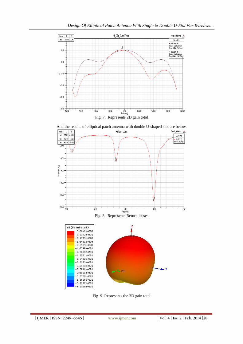
Design Of Elliptical Patch Antenna With Single & Double U-Slot For Wireless…
| IJMER | ISSN: 2249–6645 | www.ijmer.com | Vol. 4 | Iss. 2 | Feb. 2014 |28|
Fig. 7. Represents 2D gain total
And the results of elliptical patch antenna with double U-shaped slot are below.
Fig. 8. Represents Return losses
Fig. 9. Represents the 3D gain total

Design Of Elliptical Patch Antenna With Single & Double U-Slot For Wireless…
| IJMER | ISSN: 2249–6645 | www.ijmer.com | Vol. 4 | Iss. 2 | Feb. 2014 |29|
Fig. 10. Represents the Radiation pattern
Fig. 11. Represents the 2D gain total
The antenna gain is the key performance figure which combines the antenna’s directivity and electrical
efficiency. A plot of the gain as a function of direction is called the radiation pattern. The term antenna gain also
describes how much power is transmitted in the direction of peak radiation of that of an isotropic source. The
gain of a real antenna can be as high as 40-50 dB for very large dish antennas. Directivity can be as low as 1.76
dB for a real antenna.
ACKNOWLEDGEMENTS This is solely informing that “Design of elliptical patch antenna with single & double U-slot for
wireless applications: a comparative approach” paper was completed by the support of our college.
We would like to thank Management of Lendi Institute of Engineering & Technology, Dr.V.V.Rama
Reddy (Principal) Dr. M.Rajan Babu (Head of the Department), Mr.B.Sridhar, Professor, and Mr. D.Naresh
Kumar, Associate Professor, (Project coordinators).
IV. CONCLUSION In this paper, antenna is designed with a novel shape derived from the U-shaped slot with an elliptical
patch antenna structure. The antenna operated with a multiband frequency making it most suitable for the
wireless applications. The antenna achieves good impedance matching and gain in the entire band of operation.
The antenna does serve well in radiating in all frequencies of operation with good radiation efficiency.
REFERENCES [1] Antenna theory analysis and design by CONSTANTINE A. BALANIS
[2] Ratnesh kumari and Mithilesh kumar (member IEEE), Design of Multiband antennas for wireless communication,
2013 International conference on Communication Systems and Network Technologies.
[3] J.Chen, S.T.Fan, W.Hu, and C.H.Liang, Design of Tri-band printed monopole antenna for WLAN and WIMAX
applications, progress in Electromagnetics Research C, Vol. 23, 265-275, 2011.

Design Of Elliptical Patch Antenna With Single & Double U-Slot For Wireless…
| IJMER | ISSN: 2249–6645 | www.ijmer.com | Vol. 4 | Iss. 2 | Feb. 2014 |30|
[4] Joseph Costantine, Karim Y.Kabalan, Ali El-Hajj, and Mohammad Rammal, New Multi-Band Microstrip Antenna
Design for Wireless Communications, IEEE Antennas and Propagation Magazine, Vol. 49, No. 6, December 2007..
[5] A.Beno and D.S.Emmanuel, High gain inverted U-shaped miniaturized patch antenna for multiband wireless
applications, May 2012.
[6] Hussain Falih Mahdi, Simulation of Rectangular Microstrip Antenna by Integrating Matlab in Visual Basic, Diyala
Journal of Engineering Sciences, Vol.03, No. 01, pp. 16-24, June 2010.
[7] ANTENNA THEORY AND WAVE PROPAGATION by K.D.Prasad.
[8] A new dual-band microstrip antenna with U-shaped slot, J.Ghalibafan and A.R.Attari.

International
OPEN ACCESS Journal
Of Modern Engineering Research (IJMER)
| IJMER | ISSN: 2249–6645 | www.ijmer.com | Vol. 4 | Iss. 2 | Feb. 2014 |31|
Security in Wireless Sensor Networks Using Broadcasting
Sneh Lata1, Sandeep Gupta
2
1,2Hindu College of Engineering
I. INTRODUCTION A sensor is a device that translates parameters or events in the physical world into signals that can be
measured and analyzed. Sensor networks refer to a heterogeneous system combining tiny sensors and actuators
with general purpose computing elements.Wireless Sensor Networks are diverse due to the availability of micro-
sensors and low-power wireless communications. Unlike the traditional sensors, in the remote sensor network, a
vast numbers of sensors are densely deployed. These sensor nodes will perform significant signal processing,
computation and network self-configuration to achieve scalable, robust and long-lived networks.Broadcast is an
important communication primitive in wireless sensor networks. It is highly desirable to broadcast commands
and data to the sensor nodes due to the large number of sensor nodes and the broadcast nature of wireless
communication. Due to the limited signal range, it is usually necessary to have some receivers of a broadcast
packet forward it in order to propagate the packet throughout the network (e.g., through flooding, or
probabilistic broadcasting). Broadcast authentication is a basic and important security mechanism in a WSN
because broadcast is a natural communication method in a wireless environment. When base stations want to
send commands to thousands of sensor nodes, broadcasting is a much more efficient method than unicasting to
each node individually.A wireless sensor network (WSN) can cheaply monitor an environment for diverse
industries, such as healthcare, military, or home . A WSN typically consists of several base stations and
thousands of sensor nodes, which are resource limited devices with low processing, energy, and storage
capabilities.In WSN security,various types of attacks like Denial of service attack,sybil attack,wormhole attack,
blackhole attack create problem. Distributing data through wireless communication is also bandwidth limited. A
message authentication code (MAC) is an authentication tag derived by applying an authentication scheme and a
secret key to a message. MAC is an efficient symmetric cryptographic primitive for two-party authentication;
however, MAC is not suitable for broadcast communication without additional modification. Because the sender
and its receivers share the same secret key, any one of the receivers can impersonate the sender and forge
messages to other receivers. That is, both sender and receivers can sign messages. This problem stems from the
symmetric property of MAC. Therefore, to achieve authenticated broadcasts, it is necessary to establish an
asymmetric mechanism in which only the sender can sign messages, and the receivers can only verify messages.
II. WSN ARCHITECTURE
WSN architecture[1] is shown in following fig: –
Internet
ABSTRACT: Wireless sensor networks as one of the growing technology in the coming decades has
posed various unique challenges to researchers. A WSN typically consists of several base stations and
thousands of sensor nodes, which are resource limited devices with low processing, energy, and storage
capabilities.While the set of challenges in sensor networks are diverse, we focus on security of Wireless
Sensor Network in this paper. As today’s world is growing more towards the Wireless technology, our aim
must be towards providing the best security features to Wireless Sensor Network( WSN).We propose some
of the security requirements for Wireless Sensor Network. Further, security being vital to the acceptance
and use of sensor networks for many applications. We propose an efficient broadcast authentication
scheme for wireless sensor networks in this paper.
Keywords: Broadcast, security, sensors, Wireless sensor network(WSN).

Security in Wireless Sensor Networks Using Broadcasting
| IJMER | ISSN: 2249–6645 | www.ijmer.com | Vol. 4 | Iss. 2 | Feb. 2014 |32|
Fig 1 :- An example of WSN
Components:-
• Sensor motes (Field devices) – Field devices are mounted in the process, they characterize or control the
process or process equipment. A router is a special type of field device that does not have process sensor or
control equipment and as such does not interface with the process itself.
• Gateway or Access points – A Gateway enables communication between Host application and field devices.
• Network manager – A Network Manager is responsible for configuration of the network, scheduling
communication between devices, management of the routing tables and monitoring and reporting the health of
the network.
• Security manager – The Security Manager is responsible for the generation, storage, and management of
keys.
III. SECURITY REQUIREMENTS Sensor networks are used in a number of domains that handle sensitive information. Due to this, there
are many considerations that should be investigated and are related with protecting sensitive information
traveling between nodes[2].
A. Data Confidentiality
Data confidentiality is the most important issue in network security. Confidentiality requirement is needed to
ensure that sensitive information is well protected and not revealed to unauthorized third parties. A sensor
network should not leak sensor readings to its neighbors.
B. Authentication
In the case of sensor networks, it is essential for each sensor node and base station to have the ability to verify
that the data received was really send by a trusted sender and not by an adversary that tricked legitimate nodes
into accepting false data. If such a case happens and false data are supplied into the network, then the behavior
of the network could not be predicted and most of times will not outcome as expected.
C. Data Integrity
An adversary may be unable to steal information. However, this doesn‟t mean the data is safe. Lack of integrity
could result in many problems since the consequences of using inaccurate information could be disastrous.
Thus, data integrity ensures that any received data has not been altered in transit.
D. Availability
The wireless sensor network will introduce some extra costs to adjust the traditional encryption algorithms.
Availability ensures that services and information can be accessed at the time that they are required. Lack of
availability may affect the operation of many critical real time applications. Therefore, it is critical to ensure
resilience to attacks targeting the availability of the system and find ways to fill in the gap created by the
capturing or disablement of a specific node by assigning its duties to some other nodes in the network.
IV. PROTOCOLS
A Hop-by-Hop Broadcast Source Authentication Protocol[5] for WSN to mitigate DoS Attacks.Denial
of Service (DoS) is produced by the unintentional failure of nodes or malicious action. The simplest DoS attack
tries to exhaust the resources available to the victim node, by sending extra unnecessary packets and thus
prevents legitimate network users from accessing services or resources to which they are entitled. Broadcast
communication is a dominant communication pattern in WSN. As a major security concern, the broadcast
source authentication is needed to mitigate impersonation of a broadcast source, modifications of its broadcasted
data. Broadcast Source Authentication Protocols (BSAPs); one class of them is time asymmetry-based BSAPs
like TESLA protocol. These BSAPs operate delayed key-disclosure to secure broadcast communications, but
they suffer from a kind of DoS attack, called resource-draining attack, in which an attacker floods the network
with fake messages that all sensors of the network buffer and forward, then later verify, thus causing buffer
overflow and batteries depletion. We propose the H2BSAP protocol, to overcome this kind of DoS attacks, by

Security in Wireless Sensor Networks Using Broadcasting
| IJMER | ISSN: 2249–6645 | www.ijmer.com | Vol. 4 | Iss. 2 | Feb. 2014 |33|
achieving a hop-by-hop authentication of broadcasted messages, thus limiting the damage of an attacker to its
one-hop neighbors only, instead of the entire network.In addition, like TESLA[6], H2BSAP suffers from
scalability issue, because it does not efficiently support multiple broadcast sources in the network. An
asymmetric mechanism such as public key cryptography is generally required for broadcast authentication.
Otherwise, a malicious receiver can easily forge any packet from the sender. uTESLA introduces asymmetry by
delaying the disclosure of symmetric keys . A sender broadcasts a message with a Message Authentication Code
(MAC) generated with a secret key K, which is disclosed after a certain period of time. When a receiver gets this
message, if it can ensure that the packet was sent before the key was disclosed, the receiver buffers this packet
and authenticates the packet when it later receives the disclosed key. To continuously authenticate broadcast
packets, uTESLA divides the time period for broadcast into multiple intervals, assigning different keys to
different time intervals. All packets broadcast in a particular time interval are authenticated with the same key
assigned to that time interval. Multi-level uTESLA technique to extend the capabilities of uTESLA . The basic
idea is to construct a multi-level uTESLA structure, where any higher-level uTESLA instance is only used to
authenticate the commitments of its immediate lower-level ones and the lowest level uTESLA instances are
actually used to authenticate the data packets. This extension enables the original uTESLA to cover a long time
period and support a large number of receivers. Assume a sensor network application requires m uTESLA
instances, which may be used by different senders during different periods of time. For convenience, assume m
= 2k, where k is an integer. Before deployment, the central server pre-computes m uTESLA instances, each of
which is assigned a unique, integer-valued ID between1 and m. Merkle Hash Tree technique is used to
authenticate and distribute mTESLA parameters. This method removes the authentication delay as well as the
vulnerability to DOS attacks during the distribution of mTESLA parameters, and at the same time allows a large
number of senders.
V. COMPARISON BETWEEN MERKLE TREE AND MULTI MTESLA PROTOCOL
Compared with the multi-level mTESLA schemes[7][8] , the most significant gain of the proposed
approach is the removal of the authentication delay in distributing the mTESLA parameters. The multi-level
mTESLA schemes are subject to DOS attacks against the distribution of mTESLA parameters because of the
authentication delay. Specifically, receivers cannot authenticate parameter distribution messages immediately
after receiving them, and thus have to buffer such messages. An attacker may send a large amount of messages
to consume receivers buffers and thus prevent the receiver from saving the authentic messages.With the
proposed approach, senders may still duplicate parameter distribution messages to deal with communication
failures. However, unlike multi-level mTESLA schemes, a sender does not have to compete with malicious
attackers, since it can immediately authenticate the parameter distribution message instead of keeping it in the
buffer for future authentication. In other words, with the proposed approach, it is sufficient for a receiver to
receive one copy of each parameter distribution message.In general, our approach allows late binding of
mTESLA instances with senders. For example, the central server may reserve some mTESLA instances during
deployment time and distribute them to mobile sinks as needed during the operation of the sensor networks.
This allows us to add new senders dynamically by simply generating enough number of instances at the central
server for later joined senders.
VI. THE EFFICIENT SCHEME We propose using a cryptographic hash function Hash for example SHA-1[3][10] to construct H as follows
A. split the output of the hash function into k substrings of length log t each;[4]
B. interpret each (log t)-bit substring as integer written in binary;
C. combine these integers to form the subset of T of size at most k.
We believe that such H satisfies our definition it certainly does if the cryptographic hash function is modeled as
a random oracle.
Such construction of H results in the scheme we call HORS (for “Hash to Obtain Random subset”)
This scheme involves three phases and termed as HORS (Hash to Obtain Random Subset).The phases are[12]
1. Key Generation
2. Signing
3. Verifying
Key generation Input : p, d, l
Output: Key Pair
Private Key Kpri =(k, s1,s2 ,…..,sp)
Public Key Kpub =(k,v1 ,v2 ,…..,vln d)
1.Randomly generate p l-bit Random numbers as private key.

Security in Wireless Sensor Networks Using Broadcasting
| IJMER | ISSN: 2249–6645 | www.ijmer.com | Vol. 4 | Iss. 2 | Feb. 2014 |34|
2.Generate public key
Use p balls as pre-image of leaves to build c Merkle trees with height ln p.Take ln d tree root as public key
with each public key as sequence period.
3. Distribute Public key.
Signing(Base Station or Sender) Input: message m, Kpri, one-time session key(k1)
Output: Digital Envelope
1.Encrypt m with k1.
2.Compute Hash(H1) of m.
3.k1 encrypted with Kpri.
Verification(Sensor nodes or receiver) Input:Digital Envelope
Output:accept or reject
1.Decrypt k1 with its own Kpub
2.Extract original message m with k1
3.Compute Hash(H2) of decrypted message m.
4.Compare H1 wiith H2
If (H1)=(H2)
then output accept;
else output reject:
VII. CONCLUSION
The scheme which we have discussed is also efficient in many ways. As it provides security from
adversary that, in any case if it could extract public key that is in transit and get the confidential message out of
it. Then the adversary could not encrypt it in the same way as did by the sender. As a result the receiver come to
know that there is problem somewhere in transit. Our scheme exhibits many nice properties including individual
authentication, robustness to packet loss, and low overhead in computation, communication and storage. This
scheme improves upon Hash to Obtain Random Subset (HORS) in terms of reducing the large key storage
requirement. This scheme devised a simple and efficient Broadcast Authentication for Wireless Sensor Network.
REFERENCES [1]. Y. W. Law and P. Havinga. How to secure a wireless sensor network. pages 89–95,Dec. 2005.
[2]. Mayank Saraogi . Security in Wireless Sensor Networks. In ACM SenSys, 2004.
[3]. Huei-Ru Tseng, Rong-Hong Jan and Wuu Yang, "An Improved Dynamic User Authentication Scheme for Wireless
Sensor Networks", IEEE Global Communications Conference (GLOBECOM 2007, Washington, DC, USA), pages
986-990, Nov.2007.
[4]. Shang-Ming Chang, Shiuhpyng Shieh, Warren W. Lin, Chih-Ming Hsieh, “An Efficient Broadcast Authentication
Scheme in Wireless Sensor Networks”
[5]. D. Liu, P. Ning, S. Zhu, and S. Jajodia, “Practical broadcast authentication in sensor networks,” in Proc.2nd Annual
International Conf. Mobile Ubiquitous Syst.: Networking Services (MobiQuitous 2005), July 2005, pp. 118-132.
[6]. Chakib Bekara and Maryline Laurent-Maknavicius and Kheira Bekara InstitutTelecom, Telecom and Management
Sud-Paris CNRS Samovar UMR 5157, 9 rue Charles Fourier, 91000 Evry, France,„H2BSAP: A Hop-by-Hop
Broadcast Source Authentication Protocol for WSN to mitigate DoS attack‟.
[7]. Tsern-Huei Lee, “Simple Dynamic User Authentication Protocols for Wireless Sensor Networks”, Second
International Conference on Sensor Technologies and Applications (SENSORCOMM‟08), pages 657-660, France,
2008.
[8]. D. Liu and P. Ning, “Multi-level mTESLA: Broadcast authentication for distributed sensor networks,” ACM
Trans. Embedded Computing Systems (TECS), vol. 3, no. 4, pp. 800-836, 2004.
[9]. I.Akyildiz and I. Kasimoglu, “Wireless sensor and actor networks: research challenges,” Ad Hoc Networks 2(4),
pages 351- 367, 2004.
[10]. W. Du, R. Wang, and P. Ning “An efficient scheme for authenticating public keys in sensor networks,” in Proc.
6th ACM International Symposium Mobile Ad Hoc Networking Computing (MobiHoc), 2005, pp. 58-67.
[11]. S. Datema. A Case Study of Wireless Sensor Network Attacks. Master‟s thesis, Delft University of
Technology,September 2005.
[12]. J. Drissi and Q. Gu, “Localized broadcast authentication in large sensor networks,” in ICNS ‟06: Proceedings of the
International conference on Networking and Services, 2006, p. 25.

International
OPEN ACCESS Journal
Of Modern Engineering Research (IJMER)
| IJMER | ISSN: 2249–6645 | www.ijmer.com | Vol. 4 | Iss. 2 | Feb. 2014 |35|
“To Improve Thermal Efficiency of 27mw Coal Fired Power
Plant”
Amit Kumar Vishwakarma1, Gopal Kumar Choudhary
2, Rajendra Prasad Sahu
3
1,2,3Assistant Professor, Department of Mechanical Engineering, Technocrats Institute of Technology, Bhopal,
M.P 462021
I. INTRODUCTION Thermal power plants convert heat (via mechanical energy) into electrical energy. The most important
types are coal, gas and nuclear power stations. Thermal power plants are the backbone of our electricity system.
Their efficiency is typically between 30 and 50%. Based on this, it is often concluded that thermal power
stations are inadequate, waste energy, and need to be replaced by ’better’ facilities. To evaluate this conclusion,
one needs to look at the physical properties of heat energy, as well as at the fine-print in efficiency calculations,
defined by man.
Rapid growth of electrical energy demand, not only in developing countries, discussions on fossil fuel
reserves and the impact of thermal power generation on global warming, have increased the focus on alternative
primary energy sources and the efficiency improvement techniques for the conversion of the fossil fuels into
electricity. Development efforts are ongoing to reduce, capture and/or store CO2 emitted from burning fossil
fuels. The following is a quote from the McKinsey report of May 2007 ―Curbing the energy demand growth‖.
QUOTE Reducing current losses from electricity generation and distribution is another substantial
opportunity. Power generation used 155 QBTUs (Quad =1015) – representing a hefty 37% of global energy use
– to generate 57 QBTUs of deliverable electricity in 2003. In short, close to two-thirds of the energy put to the
process is lost before it reaches the final end user.
UNQUOTE In this essay, we will look at some of the auxiliary load in fossil-fueled power stations and
see what can be done to reduce this part of the losses. Thermal power stations use 3% to 10 % of their gross
generation capacity for auxiliary processes. A conventional coal-fired thermal power plant uses slightly more (5
– 10%) of the electricity it produces for the auxiliary load. For a combined-cycle power plant, the auxiliary
consumption can be less than 3.5 %. Auxiliary processes are required to keep the generator running; they are,
ABSTRACT: Booming demand for electricity, especially in the developing countries, has raised
power generation technologies in the headlines. At the same time the discussion about causes of global
warming has focused on emissions originating from power generation and on CO2 reduction
technologies such as:
(1) Alternative primary energy sources,
(2) Capture and storage of CO2,
(3) Increasing the efficiency of converting primary energy content into electricity.
In the dissertation, the thermal efficiency of the power plant is improved when Control of furnace draft
(nearer to balanced draft). Oxygen level decreases percentage of flue gases. Above this level heat
losses are increases & below this carbon mono-oxide is formed. Steam power plant is using fuel to
generate electrical power. The used of the fuel must be efficient so the boiler can generate for the
maximum electrical power. By the time the steam cycle in the boiler, it also had heat losses through
some parts and it effect on the efficiency of the boiler. This project will analyze about the parts of
losses and boiler efficiency. to find excess air which effect heat losses in boiler. By using the 27 MW
coal fired thermal power plant of Birla Corporation Limited, Satna (M.P.) the data is collect by using
types of Combustion & heat flow in boiler. Result of the analysis show that the efficiency of boiler
depends on mass of coal burnt & type of combustion .This study is fulfilling the objective of analysis to
find the boiler efficiency and heat losses in boiler for 27 MW thermal power plant of Birla Corporation
Limited, Satna (M.P.)
Keywords: Rankine Cycle, AFBC Boiler, Ash Handling System, Coal Fired Thermal Power Plant

“To Improve Thermal Efficiency of 27mw Coal Fired Power Plant”
| IJMER | ISSN: 2249–6645 | www.ijmer.com | Vol. 4 | Iss. 2 | Feb. 2014 |36|
for instance, conveying fuel coal to coal mills and maintaining the cooling water flowing through the condenser.
Most of the auxiliary power demand, up to 80%, is used by large electric motors that are typically connected to
the medium voltage switchboard, supplied through auxiliary transformers. The increasing demand for ―clean
coal‖ and CO2 emission capture and storage technologies will increase the auxiliary electricity consumption of
electric power generation. Power stations, especially base-load ones, are running at full load all the time. It is
easy to imagine that not much change or control is needed for the auxiliary processes in such cases. The fact is
however, that very few power stations run at their maximum capacity throughout the year; instead the capacity
is being adjusted all the time to match demand and various operation conditions and parameters. See Figure 1
illustrating a one year capacity utilization curve and Figure 2 for the corresponding operating hours of a 27 MW
steam generator
Fig 1: CAPACITY UTILIZATION CURVE OF A 27 MW STEAM GENERATOR.
Fig 2: OPERATING HOURS AT VARIOUS LOAD RANGES OF A 27 MW STEAM GENERATOR.
1.1 EFFICIENCY:
The efficiency of a power station is indicated with the Greek character n, and is defined
as follows:
η = 𝑜𝑢𝑡𝑝𝑢𝑡 𝑜𝑓 𝑠𝑡𝑎𝑡𝑖𝑜𝑛
𝑖𝑛𝑝𝑢𝑡 𝑜𝑓 𝑠𝑡𝑎𝑡𝑖𝑜𝑛 X100
This definition applies to any power plant. It seems to be straight forward, but in practice, a few
problems arise with it. First, power plants themselves use electricity for their operation (lighting, pumps, etc.).
Using the total amount of electricity generated yields the ’gross Efficiency’, while subtracting the power plants
own use gives ’net efficiency’. Comparisons are only meaningful based on net efficiency.
The energy efficiency of a conventional thermal power station, considered as salable energy as a
percent of the heating value of the fuel consumed, is typically 33% to 48%. This efficiency is limited as all heat
engines are governed by the laws of thermodynamics. The rest of the energy must leave the plant in the form of
heat. This waste heat can go through a condenser and be disposed of with cooling water or incooling towers. If
the waste heat is instead utilized for district heating, it is called co-generation. An important class of thermal
power station are associated with desalination facilities; these are typically found in desert countries with large
supplies of natural gas and in these plants, freshwater production and electricity are equally important co-

“To Improve Thermal Efficiency of 27mw Coal Fired Power Plant”
| IJMER | ISSN: 2249–6645 | www.ijmer.com | Vol. 4 | Iss. 2 | Feb. 2014 |37|
products. The outstanding efficiency of variable speed fans has been discussed in this paper. The fan input
power varies as the cube of the speed and while satisfying the system requirements at maximum continuous
rating or at lower loads, power savings are maximized as compared to any other method of flow control.
Sometimes it is difficult to match all three parameters (flow, pressure and speed) at the maximum efficiency
point. To select a fan at maximum efficiency, sometimes the fan needs to be selected at a speed other than
synchronous speed, which becomes possible with a variable speed drive. Also, a fan has higher efficiency when
inlet vanes or inlet dampers are totally eliminated. Through the energy efficiency of variable speed fan,
investment in electric variable speed drives can typically prove to be the most economical choice in all cases
with longer than few years operating period. This is especially the situation in cases where investment must be
split over several years and the alternative is to install and operate a heavily throttled fixed speed fan
dimensioned to future demand.
Fig 3 : A Rankine Cycle With A Two-Stage Steam Turbine And A Single Feed Water Heater.
Above the critical point for water of 374 °C and 22.06 MPa there is no phase transition from water to
steam, but only a gradual decrease in density. Boiling does not occur and it is not possible to remove impurities
via steam separation. In this case a super critical steam plant is required to utilize the increased thermodynamic
efficiency by operating at higher temperatures. These plants, also called once-through plants because boiler
water does not circulate multiple times, require additional water purification steps to ensure that any impurities
picked up during the cycle will be removed. This purification takes the form of high pressure ion exchange units
called condensate polishers between the steam condenser and the feed water heaters. Sub-critical fossil fuel
power plants can achieve 36–40% efficiency. Super critical designs have efficiencies in the low to mid 40%
range, with new "ultra critical" designs using pressures of 30.3 MPa and dual stage reheat reaching about 48%
efficiency.
Current nuclear power plants operate below the temperatures and pressures that coal-fired plants do.
This limits their thermodynamic efficiency to 30–32%. Some advanced reactor designs being studied, such as
the Very high temperature reactor, Advanced gas-cooled reactor and Super critical water reactor, would operate
at temperatures and pressures similar to current coal plants, producing comparable thermodynamic efficiency.
1.2 ELECTRICITY COST:
The direct cost of electric energy produced by a thermal power station is the result of
(1) Cost of fuel,
(2) Capital cost for the plant,
(3) Operator labour,
(4) Maintenance,
(5) Ash handling and disposal.
Indirect, social or environmental costs such as the economic value of environmental impacts, or
environmental and health effects of the complete fuel cycle and plant decommissioning, are not usually assigned

“To Improve Thermal Efficiency of 27mw Coal Fired Power Plant”
| IJMER | ISSN: 2249–6645 | www.ijmer.com | Vol. 4 | Iss. 2 | Feb. 2014 |38|
to generation costs for thermal stations in utility practice, but may form part of an environmental impact
assessment.
1.3 WHY POWER PLANT EFFICIENCY IS IMPORTANT:
Increased efficiency implies :
Same MW / Electricity from less quantity of coal
1%efficiency improvement implies:
~3%reduction in coal consumption and
~3% reduction CO2/GHG & particulate emission
Generation efficiency : percentage energy content of the fuel being converted into electrical energy. Focus
needed on technology options to improve generation efficiency of existing & new power stations.
Efficiency of modern coal power plant = 34-36%
Efficiency of old power plant = 20-30%
II. LITERATURE REVIEW 2.1 INTRODUCTION:
In this chapter, all the important information related of this project is stated. Besides that, the literature
review can give a brief explanation about the steam power plant and its operation also the effect of the excess air
& unburnt carbon loss. Some of the points in this chapter can give extra information which is useful while doing
this project.
2.2 THE USE OF THE STEAM:
Steam is a critical recourse in today's industrial world. It is essential for cooling and heating of large
buildings, driving equipment such as pump and compressors and for powering ships. However, its most
importance priority remains as source of power for the production of electricity. Steam is extremely valuable
because it can be produced anywhere in this world by using the heat that comes from the fuels that are available
in this area. Steam also has unique properties that are very important in producing energy. Steam is basically
recycled, from a steam to water and then back to steam again, all in manner that is nontoxic in nature. The steam
plant of today are a combination of complex engineered system that work to produce steam in the most efficient
manner that is economically feasible. Whether the end product of this steam is electricity, heat or a steam
process required to develop a needed product such as paper, the goal is to have that product produced at the
lowest cost possible. The heat required to produce the steam is a significant operating cost that affects the
ultimate cost of the end product. (Everett,
2005)
2.3 STEAM IS EFFICIENT AND ECONOMIC TO GENERATE:
Water is plentiful and inexpensive. It is non-hazardous to health and environmentally, sound. In its
gaseous form, it is a safe and efficient energy carrier. Steam can hold five or six times as much potential 'energy
as an equivalent mass of water. When water is heated in a boiler, it begins to absorb energy. Depending on the
pressure in the boiler, the water will evaporate at a certain temperature to form steam. The steam contains a
large quantity of stored energy which will eventually be transferred to the process or the space to be heated. It
can be generated at high pressures to give high steam temperatures. The higher the pressure, the higher the
temperature. More heat energy is contained within high temperature steam so its potential to do work is greater.
Modern shell boilers are compact and efficient in their design, using multiple passes and efficient burner
technology to transfer a very high proportion of the energy contained in the fuel to the water, with
minimum emissions.
The boiler fuel may be chosen from a variety of options, including combustible waste, which makes the
steam boiler an environmentally sound option amongst the choices available for providing heat. Centralized
boiler plant can take advantage of low interruptible gas tariffs, because any suitable standby fuel can be
stored for use when the gas supply is interrupted.
Highly effective heat recovery systems can virtually eliminate blow down costs, return valuable condensate
to the boiler house and add to the overall efficiency of the steam and condensate loop.
The increasing popularity of Combined Heat and Power (CHIP) systems demonstrates the high regard for
steam systems in today's environment and energy conscious industries. (Everett, 2005)
2.4 ENERGY IS EASILY TRANSFERRED TO THE PROCESS:
Steam provides excellent heat transfer. When the steam reaches the plant, the condensation process
efficiently transfers the heat to the product being heated. Steam can surround or be injected into the product
being heated. It can fill any space at a uniform temperature and will supply heat by condensing at a constant
temperature; this eliminates temperature gradients which may be found along any heat transfer surface - a
problem which is so often a feature of high temperature oils or hot water heating, and may result in quality

“To Improve Thermal Efficiency of 27mw Coal Fired Power Plant”
| IJMER | ISSN: 2249–6645 | www.ijmer.com | Vol. 4 | Iss. 2 | Feb. 2014 |39|
problems, such as distortion of materials being dried. Because the heat transfer properties of steam are so high,
the required heat transfer area is relatively small. This enables the use of more compact plant, which is easier to
install and takes up less space in the plant. A modern packaged unit for steam heated hot water rated to 1200 kW
and incorporating a steam plate heat exchanger and all the controls, requires only 0.7 rn2 floor spaces. In
comparison, a packaged unit incorporating a shell and tube heat exchanger would typically cover an area of two
to three times that size.
2.5 THE STEAM PLANT CYCLE:
The simplest steam cycle of practical value is called the Rankine cycle, which originated around the
performance of the steam engine. The steam cycle is important because it connects processes that allow heat to
be converted to work on a Continuous basis. This simple cycle was based on dry saturated steam being supplied
by a boiler to a power unit such as a turbine that drives an electric generator. Dry saturated steam is at the
temperature that corresponds to the boiler pressure, is not superheated, and does not contain moisture. The steam
from the turbine exhausts to a condenser, from which the condensed steam is pumped back into the boiler. It is
also called a condensing cycle, and a simple schematic of the system is shown in Fig. 4.
Fig 4 : Steam Plant Cycle
Fig 5: Rankine Thermal Cycle
This schematic also shows heat (Qin) being supplied to the boiler and a generator connected to the
turbine for the production of electricity. Heat (Qout) is removed by the condenser, and the pump supplies energy
(Wp) to the feed water in the form of a pressure increase to allow it to flow through the boiler. A higher plant
efficiency is obtained if the steam is initially superheated, and this means that less steam and less fuel are
required for a specific output. (Superheated steam has a temperature that is above that of dry saturated steam at
the same pressure and thus contains more heat content, called enthalpy, Btu/1b.) If the steam is reheated and
passed through a second turbine, cycle efficiency also improves, and moisture in the steam is reduced as it
passes through the turbine. This moisture reduction minimizes erosion on the turbine blades. When saturated
steam is used in a turbine, the work required rotating the turbine results in the steam losing energy, and a portion
of the steam condenses as the steam pressure drops. The amount of work that can be done by the turbine is
limited by the amount of moisture that it can accept without excessive turbine blade erosion. This steam
moisture content generally is between 10 and 15 percent. Therefore, the moisture content of the steam is a
limiting factor in turbine design. With the addition of superheat, the turbine transforms this additional energy
into work without forming moisture, and this energy is basically all recoverable in the turbine. A reheater often
is used in a large utility. (Kenneth, 2005).
2.6 FEEDWATER:
The feed water system requires accessories to supply the correct amount of water in the proper
condition to the boiler. A feed water accessory is equipment that is not directly attached to the boiler that
controls the quantity, pressure, and/or tore of water supplied to the boiler. Maintaining the correct level of water
in the boiler is critical for safety and efficiency. If the water level in the boiler is too high, water can be carried
over into steam lines, which can lead to water hammer and line rupture. If the water level in the boiler is too
low, heat from the furnace cannot be properly transferred to the water. This can cause overheating and damage

“To Improve Thermal Efficiency of 27mw Coal Fired Power Plant”
| IJMER | ISSN: 2249–6645 | www.ijmer.com | Vol. 4 | Iss. 2 | Feb. 2014 |40|
to boiler tubes and heating surfaces. Significant damage from over heating can lead to a boiler explosion.
Feedwater is treated and regulated automatically to meet the demand for steam. Valves are installed in feedwater
lines to permit access for maintenance and repair. The feedwater system must be capable of supplying water to
the boiler in all circumstances and includes feedwater accessories required for the specific boiler application, In
a steam heating system.) Heat necessary for providing comfort in the building starts at the boiler. Water in the
boiler is heated and turns to steam. Steam leaves the boiler through the main steam line (boiler outlet) where it
enters the main steam header-. From the main steam header, main branch lines direct the steam up a riser to the
heating unit (heat exchanger). Heat is released to the building space as steam travels through the heating unit,
Steam in the heating unit coals and turns into condense. The condensate is separated from the steam by a steam
trap that allows condensate, but not steam to pass. The condensate is directed through the condenser return line
to the condensate return tank. The feed water pump pumps the condensate and/or water back to the boiler
through check valves and stop valves on the feed water line. Feed water enters the boiler and is turned to steam
to repeat the process. (Kenneth, 2005)
2.7 BOILER EFFICIENCY:
Boiler Efficiency may be indicated by
1. Combustion Efficiency indicates the burners ability to burn fuel measured by unburned fuel and excess air
in the exhaust
2. Thermal Efficiency - indicates the heat exchangers effectiveness to transfer heat from the combustion
process to the water or steam in the boiler, exclusive radiation and convection losses
3. Fuel to Fluid Efficiency - indicates the overall efficiency of the boiler inclusive thermal efficiency of the
heat exchanger, radiation and convection losses - output divided by input. Boiler Efficiency is in general
indicated by either Thermal Efficiency or Fuel to Fluid Efficiency depending the context. (Chattopadhyay,
2005)
2.8 BOILER LOSSES:
1. Dry flue gas loss.
2. Moisture in combustion air loss
3. Unburnt carbon loss – carbon in ash loss.
4. Unburnt gas loss, due to incomplete combustion of carbon,
5. Wet flue gas loss loss due to moisture in fuel & due to moisture formed by combustion of H2 in fuel
6. Radiation & Unaccounted losses. (Dr. V.K. Sethi,2011)
III. MAJOR ENERGY SAVING POTENTIAL AREAS IN THERMAL POWER PLANT Thermal power plant is designated sector as per EC act 2001. Most thermal power plant uses 30-40%
of energy value of primary fuels. The remaining 60-70% is lost during generation, transmission and distribution
of which major loss is in the form of heat. Thermal power consist of various sub cycles / systems like air & flue
gas cycle, main steam, feed water & condensate cycle , fuel & ash cycle, Equipment cooling water (ECW),
auxiliary cooling water (ACW) system, Compressed air system, Electrical auxiliary power & lighting system,
HVAC system etc.. There is tremendous scope of energy saving potential in each system/cycle which is given
below.
3.1 AIR & FLUE GAS CYCLE:
(i) Optimizing excess air ratio: - It reduces FD fan & ID fan loading.
(ii) Replacement of oversize FD and PA fan: - Many thermal power plants have oversize fan causing huge
difference between design & operating point leads to lower efficiency. Hence fan efficiency can be
improved by replacing correct size of fan. If replacement is not possible, Use of HT VFD for PA & ID fan
can be the solution.
(iii) Attending the air & flue gas leakages: - Leakages in air & flue gas path increases fan loading. Use of
Thermo vision monitoring can be adopted to identify leakages in flue gas path.
(iv) Air preheater performance is one crucial factor in leakage contribution. If APH leakage exceeds design
value then it requires corrective action.
3.2 STEAM FEEDWATER &CONDENSATE CYCLE:
(i) BFP scoop operation in three element mode instead of DP mode: - In three element mode throttling losses
across FRS valve reduces leads to reduction in BFP power.
(ii) Optimization of level set point in LP & HP heater: - Heater drip level affects TTD & DCA of heater
which finally affect feed water O/L temp. Hence it requires setting of drip level set point correctly.
(iii) Charging of APRDS from CRH line instead of MS line: - APRDS charging from cold reheat (CRH) is
always more beneficial than from MS line charging.
(iv) Isolation of steam line which is not in use: - It is not advisable to keep steam line unnecessary charge if
steam is not utilized since there energy loss occurred due to radiation. For example deareator extraction

“To Improve Thermal Efficiency of 27mw Coal Fired Power Plant”
| IJMER | ISSN: 2249–6645 | www.ijmer.com | Vol. 4 | Iss. 2 | Feb. 2014 |41|
can be charged from turbine Extraction/CRH or from APRDS. In normal running APRDS Extraction is
not used so same can be kept isolated.
(v) Replacement of BFP cartridge: - BFP draws more current If Cartridge is wore out, causing short circuit of
feed water Flow inside the pump. It affects pump performance. Hence cartridge replacement is necessary.
(vi) Attending passing recirculation valve of BFP: - BFP Power consumption Increases due to passing of R/C
valve. It requires corrective action.
(vii) Installation of HT VFD for CEP: - CEP capacity is underutilized and also there is pressure loss occurs
across Deareator level control valve. There is large scope of energy saving which can be accomplished by
use of HT VFD for CEP or impeller trimming.
3.3 FUEL & ASH CYCLE:
(i) Optimized ball loading in Ball tube mill :- Excessive ball loading increases mill power. Hence ball
loading is to be Optimized depending upon coal fineness report.
(ii) Use of Wash Coal or Blending with A- grade coal : - F-grade coal has high ash content. Overall
performance can be improved by using Wash coal or blending of F-grade coal with A- grade coal instead
of only using F- grade coal.
(iii) Avoiding idle running of conveyors & crusher in CHP
(iv) Use of Dry ash Evacuation instead of WET deashing System: - Dry deashing system consumes less
power & also minimizes waste reduction.
(v) Optimize mill maintenance:- Mill corrective/preventive maintenance is to be optimized depending
parameter like- running hrs, mill fineness, bottom ash unburnt particle, degree of reject pipe chocking etc.
3.4 ELECTRICAL & LIGHTING SYSTEM:
(i) Optimizing Voltage level of distribution transformer: - It is found that Operating voltage level is on
higher side than required causing more losses. It is required to reduce the voltage level by tap changing.
(ii) Use of Auto star/delta/star converter for under loaded motor Lighting: - Use of electronic chock instead
of conventional use copper Chock, Use of CFL, Replacement of mercury vapor lamp by metal Halide
lamp. Use of timer for area lighting is the methods can be used. Lighting has tremendous potential of
saving.
3.5 ECW & ACW SYSTEM:
(i) Isolating ECW supply of standby auxiliaries: - Many times standby coolers are kept charged from
ECW side. Also Standby equipment’s auxiliaries like Lube oil system kept running for reliability. We can
isolate Standby cooler from ECW system & switching of standby auxiliaries, doing trade off between
return & reliability.
(ii) Improving condenser performance by condenser tube cleaning & use of highly efficient debris
filter: Tube cleaning by bullet shot method increases condenser performance, condenser tube cleaning is
necessary which is to be carried out in overhaul. Also highly advanced debris filter contribute condenser
performance.
(iii) Application of special coating on CW pump impeller: - It improves pump impeller profile condition,
increasing pump performance.
3.6 COMPRESSED AIR SYSTEM:-
(i) Optimizing discharge air pressure by tuning loading/unloading cycle: - It helpful to reduce sp. Power
consumption.
(ii) Use of heat of compression air dryer instead of electrically heated air dryer: - Heat of compression
air dryer use heat generated in compression cycle, thus reduces sp. Power consumption.
(iii) Use of screw compressor instead reciprocating compressor: - Sp. Power consumption of screw
compressor is less than reciprocating air compressor leads to reduce aux. power consumption.
3.7 HVAC SYSTEM:
(i) Cooling tower performance improvement
(ii) Installing absorption refrigeration system instead of vapor compression system Use of wind turbo
ventilators instead of conventional motor driven exhauster
IV. OBJECTIVES OF THE STUDY To increase the thermal efficiency of 27 MW coal fired power plant.
To identify and bring forth the operation and working of a typical thermal power plant with special
reference to Birla Corporation Limited, Satna (M.P.).
To explore the various avenues and areas, where the waste related to energy consumption can be
minimized.
To identify and study the key factors for improving the energy efficiency of a thermal power.

“To Improve Thermal Efficiency of 27mw Coal Fired Power Plant”
| IJMER | ISSN: 2249–6645 | www.ijmer.com | Vol. 4 | Iss. 2 | Feb. 2014 |42|
To study the various environmental issues in relation to the working efficiency of the thermal power
plants.
V. DESCRIPTION OF COAL FIRED POWER PLANT (1) Pulverized coal
(2) Fluidized Bed Combustion
(3) Atmospheric Fluidized Bed Combustion Boiler
(4) Ash Handling System
(5) Super heater
(6) Economizer
5.1 PULVERIZED COAL:
A pulverized coal-fired boiler is an industrial or utility boiler that generates thermal energy by burning
pulverized coal (also known as powdered coal or coal dust since it is as fine as face powder in cosmetic
makeup) that is blown into the firebox.
The basic idea of a firing system using pulverized fuel is to use the whole volume of the furnace for the
combustion of solid fuels. Coal is ground to the size of a fine grain, mixed with air and burned in the flue gas
flow. Biomass and other materials can also be added to the mixture. Coal contains mineral matter which is
converted to ash during combustion. The ash is removed as bottom ash and fly ash. The bottom ash is removed
at the furnace bottom. This type of boiler dominates the electric power industry, providing steam to drive large
turbines. Pulverized coal provides the thermal energy which produces about 50% of the world's electric supply.
Pulverized coal power plants account for about 97% of the world's coal-fired capacity. The conventional types
of this technology have an efficiency of around 35%. For a higher efficiency of the technology supercritical and
ultra-supercritical coal-fired technologies have been developed. These technologies can combust pulverized coal
and produce steam at higher temperatures and under a higher pressure, so that an efficiency level of 45% can be
reached (ultra-supercritical plants). Supercritical power plants have become the system of choice in most
industrialized countries, while ultra-supercritical plant technology is still in the process of demonstration.
Supercritical and ultra-supercritical plants are more expensive (because of the higher requirements to the steel
needed to stand the higher pressure and temperature) but the higher efficiency results in cost savings during the
technical lifetime of the plants.
In a pulverized coal-fired boiler of a large power plant, an oxygen analyzer is essential for combustion
ontrol. A pulverized coal-fired boiler is an industrial or utility boiler that generates thermal energy by burning
pulverized coal (also known as powdered coal or coal dust). This type of boiler dominates the electric power
industry, providing steam to drive large turbines. Pulverized coal provides the thermal energy which roduces
about 50% of the world's electric supply. Exhaust gases from the pulverized coal boiler contain a large quantity
of dust and flow very fast. Oxygen analyzers that employ a sampling method may be subject to wear or
clogging, resulting in increased maintenance workload and cost. A solution to this problem is the ZR22/ZR402
Direct In-Situ Zirconia Oxygen Analyzer that has no sampling system and utilizes a long-life sensor. A probe
protector is attached to protection it against wear.
5.1.1: PROCESS: Coal is inexpensive and readily available. coal produces a large quantity of ashes when it is
burned; necessitating pulverized coal-fired boilers to be equipped with an ash removal system such as a cyclone.
Exhaust gases from these boilers contain a large quantity of dust (10 to 30 g/Nm3) and flow very fast as the
result of the large volume of air being blown into the boiler. For oxygen measurement in large ducts, a probe
with a long insertion length is used.
Fig 7: Pulverized Coal Boiler

“To Improve Thermal Efficiency of 27mw Coal Fired Power Plant”
| IJMER | ISSN: 2249–6645 | www.ijmer.com | Vol. 4 | Iss. 2 | Feb. 2014 |43|
5.1.2: COMBUSTION EFFICIENCY
Operating your boiler with an optimum amount of excess air will minimize heat loss up the stack and
improve combustion efficiency. Combustion efficiency is a measure of how effectively the heat content of a fuel
is transferred into usable heat. The stack temperature and flue gas oxygen (or carbon dioxide) concentrations are
primary indicators of combustion efficiency.
Given complete mixing, a precise or stoichiometric amount of air is required to completely react with a
given quantity of fuel. In practice, combustion conditions are never ideal, and additional or ―excess‖ air must be
supplied to completely burn the fuel.
The correct amount of excess air is determined from analyzing flue gas oxygen or carbon dioxide
concentrations. Inadequate excess air results in unburned combustibles (fuel, soot, smoke, and carbon
monoxide), while too much results in heat lost due to the increased flue gas flow—thus lowering the overall
boiler fuel-to-steam efficiency. The table relates stack readings to boiler performance
5.1.3: FLUE GAS ANALYZER:
The percentage of oxygen in the flue gas can be measured by inexpensive gas-absorbing test kits. More
expensive (ranging in cost from $500 to $1,000) hand-held, computer-based analyzers display percent oxygen,
stack gas temperature, and boiler efficiency. They are a recommended investment for any boiler system with
annual fuel costs exceeding $50,000.
5.1.4: OXYGEN TRIM SYSTEM:
When fuel composition is highly variable (such as refinery gas, hog fuel, or multi-fuel boilers), or
where steam flows are highly variable, an online oxygen analyzer should be considered. The oxygen ―trim‖
system provides feedback to the burner controls to automatically minimize excess combustion air and optimize
the air-to-fuel ratio.
To ensure complete combustion of the fuel used, combustion chambers are supplied with excess air.
Excess air increase the amount of oxygen and the probability of combustion of all fuel.
when fuel and oxygen in the air are in perfectly balance - the combustion is said to be stoichiometric
The combustion efficiency will increase with increased excess air, until the heat loss in the excess air is larger
than the heat provided by more efficient combustion.
Fig 8 : COBUSTION EFFICIENCY
Typical excess air to achieve highest efficiency for different fuels are 15 - 60% for coal
Carbon dioxide - CO2 - is a product of the combustion and the content in the flue gas is an important indication
of the combustion efficiency.
Fig 9: EXCESS AIR VS O2&CO2 IN FLUE GAS (% BY VOLUME)

“To Improve Thermal Efficiency of 27mw Coal Fired Power Plant”
| IJMER | ISSN: 2249–6645 | www.ijmer.com | Vol. 4 | Iss. 2 | Feb. 2014 |44|
An optimal content of carbon dioxide - CO2 - after combustion is approximately 10% for natural gas
and approximately 13% for lighter oils.
5.2 FLUIDIZED BED COMBUSTION:
The major portion of the coal available in India is of low quality, high ash content and low calorific
value. The traditional grate fuel firing systems have got limitations and are techno-economically unviable to
meet the challenges of future. Fluidized bed combustion has emerged as a viable alternative and has significant
advantages over conventional firing system and offers multiple benefits – compact boiler design, fuel flexibility,
higher combustion efficiency and reduced emission of noxious pollutants such as SOx and NOx. The fuels burnt
in these boilers include coal, washery rejects, rice husk, bagasse & other agricultural wastes. The fluidized bed
boilers have a wide capacity range- 0.5 T/hr to over 100 T/hr.
FIG 10 : MECHANISM OF FLUIDISED BED COMBUSTION
When an evenly distributed air or gas is passed upward through a finely divided bed of solid particles
such as sand supported on a fine mesh, the particles are undisturbed at low velocity. As air velocity is gradually
increased, a stage is reached when the individual particles are suspended in the air stream – the bed is called
―fluidized‖. With further increase in air velocity, there is bubble formation, vigorous turbulence, rapid mixing
and formation of dense defined bed surface. The bed of solid particles exhibits the properties of a boiling liquid
and assumes the appearance of a fluid – ―bubbling fluidized bed‖.
At higher velocities, bubbles disappear, and particles are blown out of the bed. Therefore, some
amounts of particles have to be recirculated to maintain a stable system – ―circulating fluidized bed‖. This
principle of fluidization is illustrated in Figure1.
Fluidization depends largely on the particle size and the air velocity. The mean solids velocity increases
at a slower rate than does the gas velocity, as illustrated in Figure 6.2. The difference between the mean solid
velocity and mean gas velocity is called as slip velocity. Maximum slip velocity between the solids and the gas
is desirable for good heat transfer and intimate contact. If sand particles in a fluidized state is heated to the
ignition temperatures of coal, and coal is injected continuously into the bed, the coal will burn rapidly and bed
attains a uniform temperature. The fluidized bed combustion (FBC) takes place at about 840O
C to 950O
C. Since
this temperature is much below the ash fusion temperature, melting of ash and associated problems are avoided.
The lower combustion temperature is achieved because of high coefficient of heat transfer due to rapid mixing
in the fluidized bed and effective extraction of heat from the bed through in-bed heat transfer tubes and walls of
the bed. The gas velocity is maintained between minimum fluidization velocity and particle entrainment
velocity. This ensures stable operation of the bed and avoids particle entrainment in the gas stream.

“To Improve Thermal Efficiency of 27mw Coal Fired Power Plant”
| IJMER | ISSN: 2249–6645 | www.ijmer.com | Vol. 4 | Iss. 2 | Feb. 2014 |45|
Fig 11: Relation Between Gas Velocity And Solid Velocity
Combustion process requires the three ―T‖s that is Time, Temperature and Turbulence. In FBC,
turbulence is promoted by fluidisation. Improved mixing generates evenly distributed heat at lower temperature.
Residence time is many times greater than conventional grate firing. Thus an FBC system releases heat more
efficiently at lower temperatures.
Fig 12: Velocity Vs Increasing Expansion
Firing. Thus an FBC system releases heat more efficiently at lower temperatures.
Since limestone is used as particle bed, control of sulfur dioxide and nitrogen oxide emissions in the combustion
chamber is achieved without any additional control equipment. This is one of the major advantages over
conventional boilers.
5.3 ATMOSPHERIC FLUIDIZED BED COMBUSTION: In AFBC, coal is crushed to a size of 1 – 10 mm depending on the rank of coal, type of fuel feed and
fed into the combustion chamber. The atmospheric air, which acts as both the fluidization air and combustion
air, is delivered at a pressure and flows through the bed after being preheated by the exhaust flue gases. The
velocity of fluidising air is in the range of 1.2 to 3.7 m /sec. The rate at which air is blown through the bed
determines the amount of fuel that can be reacted. Almost all AFBC/ bubbling bed boilers use in-bed evaporator
tubes in the bed of limestone, sand and fuel for extracting the heat from the bed to maintain the bed temperature.
The bed depth is usually 0.9 m to 1.5 m deep and the pressure drop averages about 1 inch of water per inch of
bed depth. Very little material leaves the bubbling bed – only about 2 to 4 kg of solids are recycled per ton of
fuel burned. Typical fluidized bed combustors of this type are shown in Figures 9.1 and 9.2

“To Improve Thermal Efficiency of 27mw Coal Fired Power Plant”
| IJMER | ISSN: 2249–6645 | www.ijmer.com | Vol. 4 | Iss. 2 | Feb. 2014 |46|
Fig 13: Bubbling Bed Boiler
The combustion gases pass over the super heater sections of the boiler, flow past the economizer, the
dust collectors and the air preheaters before being exhausted to atmosphere.
The main special feature of atmospheric fluidized bed combustion is the constraint imposed by the relatively
narrow temperature range within which the bed must be operated. With coal, there is risk of clinker formation in
the bed if the temperature exceeds 950o
C and loss of combustion efficiency if the temperature falls below
800o
C. For efficient sulphur retention, the temperature should be in the range of 800o
C to 850o
C.
5.3.1 GENERAL ARRANGEMENTS OF AFBC BOILER
AFBC boilers comprise of following systems:
i) Fuel feeding system
ii) Air Distributor
iii) Bed & In-bed heat transfer surface
iv) Ash handling system
5.3.2 MANY OF THESE ARE COMMON TO ALL TYPES OF FBC BOILERS :
1. FUEL FEEDING SYSTEM For feeding fuel, sorbents like limestone or dolomite, usually two methods are followed: under bed pneumatic
feeding over-bed feeding.
5.2.4.1 UNDER BED PNEUMATIC FEEDING : If the fuel is coal, it is crushed to 1-6 mm size and pneumatically transported from feed hopper to the combustor
through a feed pipe piercing the distributor. Based on the capacity of the boiler, the number of feed points is
increased, as it is necessary to distribute the fuel into the bed uniformly.
5.4.4.2 OVER-BED FEEDING : The crushed coal, 6-10 mm size is conveyed from coal bunker to a spreader by a screw conveyor. The spreader
distributes the coal over the surface of the bed uniformly. This type of fuel feeding system accepts over size fuel
also and eliminates transport lines, when compared to under-bed feeding system.
5.4.3 AIR DISTRIBUTOR : The purpose of the distributor is to introduce the fluidizing air evenly through the bed cross section thereby
keeping the solid particles in constant motion, and preventing the formation of defluidization zones within the
bed. The distributor, which forms the furnace floor, is normally constructed from metal plate with a number of
perforations in a definite geometric pattern. The perforations may be located in simple nozzles or nozzles with
bubble caps, which serve to prevent solid particles from flowing back into the space below the distributor.
The distributor plate is protected from high temperature of the furnace by:
i) Refractory Lining
ii) A Static Layer of the Bed Material or
iii) Water Cooled Tubes.
5.3.3 BED & IN-BED HEAT TRANSFER SURFACE:
5.3.3.1 BED The bed material can be sand, ash, crushed refractory or limestone, with an average size of about 1 mm.
Depending on the bed height these are of two types: shallow bed and deep bed.
At the same fluidizing velocity, the two ends fluidise differently, thus affecting the heat transfer to an immersed
heat transfer surfaces. A shallow bed offers a lower bed resistance and hence a lower pressure drop and lower
fan power consumption. In the case of deep bed, the pressure drop is more and this increases the effective gas
velocity and also the fan power.

“To Improve Thermal Efficiency of 27mw Coal Fired Power Plant”
| IJMER | ISSN: 2249–6645 | www.ijmer.com | Vol. 4 | Iss. 2 | Feb. 2014 |47|
5.3.3.2 IN-BED HEAT TRANSFER SURFACE : In a fluidized in-bed heat transfer process, it is necessary to transfer heat between the bed material and an
immersed surface, which could be that of a tube bundle, or a coil. The heat exchanger orientation can be
horizontal, vertical or inclined. From a pressure drop point of view, a horizontal bundle in a shallow bed is more
attractive than a vertical bundle in a deep bed. Also, the heat transfer in the bed depends on number of
parameters like (i) bed pressure (ii) bed temperature (iii) superficial gas velocity (iv) particle size (v) Heat
exchanger design and (vi) gas distributor plate design.
5.3.4ADVANTAGES OF FLUIDIZED BED COMBUSTION BOILERS
1. HIGH EFFICIENCY FBC boilers can burn fuel with a combustion efficiency of over 95% irrespective of ash content. FBC boilers
can operate with overall efficiency of 84% (plus or minus 2%).
2. REDUCTION IN BOILER SIZE High heat transfer rate over a small heat transfer area immersed in the bed result in overall size reduction of the
boiler.
3. FUEL FLEXIBILITY FBC boilers can be operated efficiently with a variety of fuels. Even fuels like flotation slimes, washer rejects,
agro waste can be burnt efficiently. These can be fed either independently or in combination with coal into the
same furnace.
4. ABILITY TO BURN LOW GRADE FUEL FBC boilers would give the rated output even with inferior quality fuel. The boilers can fire coals with ash
content as high as 62% and having calorific value as low as 2,500 kcal/kg. Even carbon content of only 1% by
weight can sustain the fluidised bed combustion.
5. ABILITY TO BURN FINES Coal containing fines below 6 mm can be burnt efficiently in FBC boiler, which is very difficult to achieve in
conventional firing system.
6. POLLUTION CONTROL SO
2 formation can be greatly minimised by addition of limestone or dolomite for high sulphur coals. 3%
limestone is required for every 1% sulphur in the coal feed. Low combustion temperature eliminates NOx
formation.
7. LOW CORROSION AND EROSION The corrosion and erosion effects are less due to lower combustion temperature, softness of ash and low particle
velocity (of the order of 1 m/sec).
8. EASIER ASH REMOVAL – NO CLINKER FORMATION
Since the temperature of the furnace is in the range of 750 – 900o
C in FBC boilers, even coal of low ash fusion
temperature can be burnt without clinker formation. Ash removal is easier as the ash flows like liquid from the
combustion chamber. Hence less manpower is required for ash handling.
9. LESS EXCESS AIR – HIGHER CO2 IN FLUE GAS
The CO2 in the flue gases will be of the order of 14 – 15% at full load. Hence, the FBC boiler can operate at low
excess air - only 20 – 25%.
10. SIMPLE OPERATION, QUICK START-UP High turbulence of the bed facilitates quick start up and shut down. Full automation of start up and operation
using reliable equipment is possible.
11. FAST RESPONSE TO LOAD FLUCTUATIONS
Inherent high thermal storage characteristics can easily absorb fluctuation in fuel feed rates. Response to
changing load is comparable to that of oil fired boilers.
12. NO SLAGGING IN THE FURNACE-NO SOOT BLOWING In FBC boilers, volatilisation of alkali components in ash does not take place and the ash is non sticky. This
means that there is no slagging or soot blowing.
13 PROVISIONS OF AUTOMATIC COAL AND ASH HANDLING SYSTEM Automatic systems for coal and ash handling can be incorporated, making the plant easy to operate comparable
to oil or gas fired installation.
14 PROVISION OF AUTOMATIC IGNITION SYSTEM Control systems using micro-processors and automatic ignition equipment give excellent control with minimum
manual supervision.
15 HIGH RELIABILITY

“To Improve Thermal Efficiency of 27mw Coal Fired Power Plant”
| IJMER | ISSN: 2249–6645 | www.ijmer.com | Vol. 4 | Iss. 2 | Feb. 2014 |48|
The absence of moving parts in the combustion zone results in a high degree of reliability and low maintenance
costs.
16 REDUCED MAINTENANCE Routine overhauls are infrequent and high efficiency is maintained for long periods.
17 QUICK RESPONSES TO CHANGING DEMAND A fluidized bed combustor can respond to changing heat demands more easily than stoker fired systems. This
makes it very suitable for applications such as thermal fluid heaters, which require rapid responses.
18 HIGH EFFICIENCY OF POWER GENERATION By operating the fluidized bed at elevated pressure, it can be used to generate hot pressurized gases to power a
gas turbine. This can be combined with a conventional steam turbine to improve the efficiency of electricity
generation and give a potential fuel savings of at least 4%.
5.4. ASH HANDLING SYSTEM:
5.4.1: BOTTOM ASH REMOVAL:
In the FBC boilers, the bottom ash constitutes roughly 30 - 40 % of the total ash, the rest being the fly ash. The
bed ash is removed by continuous over flow to maintain bed height and also by intermittent flow from the
bottom to remove over size particles, avoid accumulation and consequent defluidization. While firing high ash
coal such as washery rejects, the bed ash overflow drain quantity is considerable so special care has to be taken.
5.4.2 FLY ASH REMOVAL: The amount of fly ash to be handled in FBC boiler is relatively very high, when compared to conventional
boilers. This is due to elutriation of particles at high velocities. Fly ash carried away by the flue gas is removed
in number of stages; firstly in convection section, then from the bottom of air preheater/economizer and finally a
major portion is removed in dust collectors. The types of dust collectors used are cyclone, bagfilters,
electrostatic precipitators (ESP’s) or some combination of all of these. To increase the combustion efficiency,
recycling of fly ash is practiced in some of the units.
Fig 15: Fly Ash Removal
5.5 SUPERHEATER:
Steam superheaters are widely used in steam generators and heat-recovery steam generators (HRSGs).
Their purpose is to raise steam temperature from saturation conditions to the desired final temperature, which
can be as high as 5500C in some cases. When used in steam turbines, superheated steam decreases steam heat
rate of the turbine and thus improves the turbine and overall plant power output and efficiency. Also, steam
conditions at the steam turbine exit will have little or no moisture, depending on the pressure ratio; moisture in
the last few stages of a steam turbine can damage the turbine blades. This article outlines some of the design
considerations and performance aspects of super heater. A superheater is a device used to convert saturated
steam or wet steam into dry steam used for power generation or processes. There are three types of superheaters
namely: radiant, convection, and separately fired. A superheater can vary in size from a few tens of feet to
several hundred feet.
A radiant superheater is placed directly in the combustion chamber.
A convection superheater is located in the path of the hot gases.
A separately fired superheater, as its name implies, is totally separated from the boiler.
A superheater is a device in a steam engine, when considering locomotives, that heats the steam
generated by the boiler again, increasing its thermal energy and decreasing the likelihood that it will condense
inside the engine. Superheaters increase the efficiency of the steam engine, and were widely adopted. Steam
which has been superheated is logically known as superheated steam; non-superheated steam is called saturated
steam or wet steam. Superheaters were applied to steam locomotives in quantity from the early 20th century, to

“To Improve Thermal Efficiency of 27mw Coal Fired Power Plant”
| IJMER | ISSN: 2249–6645 | www.ijmer.com | Vol. 4 | Iss. 2 | Feb. 2014 |49|
most steam vehicles, and to stationary steam engines. This equipment is still an integral part of power generating
stations throughout the world.
Fig 16: A Water Tube Boiler With A Superheater
5.5.1 ADVANTAGE & DISADVANTAGES: The main advantages of using a superheater are reduced fuel and water consumption but there is a price to pay
in increased maintenance costs. In most cases the benefits outweighed the costs and superheaters were widely
used. An exception was shunting locomotives (switchers). British shunting locomotives were rarely fitted with
superheaters. In locomotives used for mineral traffic the advantages seem to have been marginal. For example,
the North Eastern Railway fitted superheaters to some of its NER Class P mineral locomotives but later began to
remove them.
Without careful maintenance superheaters are prone to a particular type of hazardous failure in the tube bursting
at the U-shaped turns in the superheater tube. This is difficult to both manufacture, and test when installed, and a
rupture will cause the superheated high-pressure steam to escape immediately into the large flues, then back to
the fire and into the cab, to the extreme danger of the locomotive crew.
5.6 ECONOMIZER: In boilers, economizers are heat exchange devices that heat fluids, usually water, up to but not normally beyond
the boiling point of that fluid. Economizers are so named because they can make use of the enthalpy in fluid
streams that are hot, but not hot enough to be used in a boiler, thereby recovering more useful enthalpy and
improving the boiler's efficiency. They are a device fitted to a boiler which saves energy by using the exhaust
gases from the boiler to preheat the cold water used to fill it.
A feedwater economizer reduces steam boiler fuel requirements by transferring heat from the flue gas
to incoming feedwater. Boiler flue gases are often rejected to the stack at temperatures more than 100°F to
150°F higher than the temperature of the generated steam. Generally, boiler efficiency can be increased by 1%
for every 40°F reduction in flue gas temperature. By recovering waste heat, an economizer can often reduce
fuel requirements by 5% to 10% and pay for itself in less than 2 years. The table provides examples of the
potential for heat recovery.Economizers or economisers are mechanical devices intended to reduce energy
consumption, or to perform another useful function like preheating a fluid. The term economizer is used for
other purposes as well. Boiler, powerplant, and heating, ventilating, and air-conditioning (HVAC). In boilers,
economizers are heat exchange devices that heat fluids, usually water, up to but not normally beyond the boiling
point of that fluid. Economizers are so named because they can make use of the enthalpy in fluid streams that
are hot, but not hot enough to be used in a boiler, thereby recovering more useful enthalpy and improving the
boiler's efficiency. They are a device fitted to a boiler which saves energy by using the exhaust gases from the
boiler to preheat the cold water used to fill it (the feed water).
METHODOLOGY:
(1) I adopted for the conduct of my Project study was basically Survey and Observation.
(2) it was relatively easy for me to understand the working and operations of the plant, but still there were
many areas
(3) I was quite unacquainted with and hence had to take help and assistance from text books, journals ,
magazines and reference material provided by Birla Corporation Llimited, Birla vikas cement.27MW
thermal power plant.
(4) I studied the operations of the power plant 1x27, and was able to explore and identify the various
avenues and areas related to energy conservation and waste reduction.

“To Improve Thermal Efficiency of 27mw Coal Fired Power Plant”
| IJMER | ISSN: 2249–6645 | www.ijmer.com | Vol. 4 | Iss. 2 | Feb. 2014 |50|
(5) My focus of study was to enhance the Thermal efficiency of Boiler at different stages of working
cycle by unburnt carbon .
(6) I went on to studying the various aspects of the working of a Thermal Power Plant. Keeping in mind
the need of today that is the methods and measures adopted by Organizations and Government
initiatives.
(7) I thought why not study the factors responsible for achieving and improving thermal efficiency in
27MW coal fired power plants.
A NOTE ON THERMAL ENERGY CONSUMPTION
SATNA CEMENT WORKS :
Specific fuel consumption depend on various factors like Coal quality with respect to
(1) Calorific value,
(2) Ash content and
(3) Moisture content.
Specific Fuel consumption in terms of Kcal/kg Clinker was more during the year 2008-2009, while
percentage consumption of coal was lowest.This is due to more UHV and low coal ash content in coal during
this year, as compared to other two years. In 2009-2010, fuel consumption was more than 2008-2009, due to
low UHV of coal than previous and manufacturing Low Alkali sulphate resistant Cement for Export.To Produce
Low Alkali Clinker, Fuel consumption increases due to running of Alkali By-pass System to extract Alkali dust
from Kiln inlet at 1000 0C. A Comaprative table below confirms above statement.
Unit 2009-2010 2010-2011 2011-2012
Specific Heat
Consumption
Kcal/kg Clkr 754 760 746
Coal Consumption Kg/hr 20209 20152 20082
Specific Heat of Coal
(UHV)
Kcal/kg coal 4089 4223 4145
Ash Content % 31.97 30.97 31.22
Moisture Content % 2.89 2.92 3.24
Coal Consumption Tons/day 14459245 14459152 14459040
CASE STUDY:
ECONOMIZER:
Specification Box Econ. Rev.1, 04.04.2012
Boiler Economizer Specification – Rectangular Design
This specification defines the minimum requirements that must be met for the design and fabrication of vertical
gas flow, horizontal tube economizers. No deviation from this specification is permissible without documented
approval.
I. Description of Operation
The purpose of the equipment is to recover waste heat using the established principle of a gas to liquid heat
exchanger. The economizer should be a bare, welded, or extruded finned tube coil assembly installed either
inside or parallel to the boiler exhaust stack or duct. Feedwater under pressure will circulate in the tubes of the
coil and heat will be transferred from the flue gases to the water.
II. The Heat Exchanger
Furnish economizer, as described below, to recover waste heat from the boiler exhaust stack.
The economizer shall be a rectangular box type, completely packaged unit, utilizing bare tube or
extended surface.
The economizer shall be counterblow type arranged to allow the boiler exhaust gas to travel vertically
upward, while the feed water travels vertically downward (or vice versa).
Structural steel, inlet and outlet transitions, when required, shall be provided with the economizer. The
structural steel shall be designed to support the economizer, inlet and outlet transition, and stack.
III. Construction Features
All pressure parts shall conform to the applicable provisions of the current ASME Power Boiler Code.
The economizer shall be properly name plated and code stamped. The design pressure shall meet or
exceed the design pressure of the boiler.
Tubes shall of the welded type, 2‖ O.D. with a minimum wall thickness of .120‖.

“To Improve Thermal Efficiency of 27mw Coal Fired Power Plant”
| IJMER | ISSN: 2249–6645 | www.ijmer.com | Vol. 4 | Iss. 2 | Feb. 2014 |51|
Return bends shall be cold bent or manufactured by a forging process. Cold bends shall be assumed to
have a 30% thin out or less for code calculation purposes; hot forged bends shall have no thin out of
wall thickness. Headers shall be SA 106 B material, Sch. 80 minimum. Vent, drain, and safety relief
valve connections shall be a minimum of ¾‖ npt and shall include a plug.
The method of tube-to-header attachment shall be welded. Compression fittings, as they are not an
accepted Section I joint, shall not be used.
All coils shall be completely drainable by gravity.
Method of tube supports shall allow for free flow of hot gases
around the welds, return bends and manifolds. The outlet feedwater temperatures shall be at least 30°F
below the saturation temperature. The tubes shall be arranged for tube internal acid cleaning, and tube
external soot blowing (for fuels other than natural gas).
For fuels other than natural gas, the economizer shall be provided with a soot blower lane, soot blower
wall box (es), and distal bearings. Soot blowers shall be installed transverse to the tubes.
A gas tight inner seal welded 10 Ga. steel shall be insulated and covered with 30 Ga. thick corrugated,
galvanized, carbon steel metal lagging.
Finned tubes: 1. The tube pitch shall be square to ensure ease in cleaning for fuels other than natural gas or the equivalent in
which case triangular (staggered) tube pitch is allowable.
2. Fin pitch shall be: 6 fins/inch for natural gas, 4 fins/inch for #2 ,fuel oil, and 3 fins/inch for #6 fuel oil. For
solid fuels such as coal or wood, a maximum of 2 fins/inch shall be used.
3. The fin attachment shall be by high frequency weld process. Tension wrapped, embedded, or brazed finned
tubes are not acceptable.
4. The fin material shall be carbon steel.
All exterior surfaces not galvanized shall be painted with high temperature black paint.
Economizer shall be protected to prevent damage during shipping.
Maximum allowable pressure drops will be 15 PSIG for the feedwater and 1.5‖ W. C. for the flue gas.
Insulation shall be 8 lb density mineral wool and of sufficient thickness to yield a skin temperature no
greater than 140°F.
As a minimum, 10% of the tube to tube welds will be radiographed.
The economizer’s performance, while in a commercially clean condition, shall be guaranteed by the
manufacturer.
Three sets of operating and instruction manuals shall be furnished at time of shipment to include: ASME
Code Report; material test reports; nameplate facsimile; economizer assembly drawings; other as
required by customer or engineering specifications.
Economizer shall be designed to operate at 100 percent load without bypassing any flue gas or
feedwater.
TECHNICAL DATA
OBSERVATION
27MW Coal Fired Tharmal Power Plant
(1) Capacity of boiler = 65 TPH X 2 = 130 TPH
(2) Type of Boiler = Coal Fired, Semi door, Natural draught, Balanced
draft, Single drum, Water Tube
(3) Type of Combustion = Atmospheric Fluidized Bed Combustion
(4) Pressure of superheated steam = 86.4 Bar
(5) Temperature of superheated steam = 5050 C
(6) Temperature of feed water = 1880 C
(7) G.C.V. of Coal = 16568.64 KJ /Kg (3960Kcal/kg)
(8) N.C.V. of Coal = 15878.28 KJ/Kg
(9) Gas plenum Pressure At furnace = - 1.8 mm WC
(10) Oxygen level = 4.8%
(11) Ash content in coal = 45-52%
(12) Temperature of Flue Gases leaving in chimney = 138 0C
(13) Temperature of Boiler house = 320C
(14) Total steam generated (ms)=103416 Kg/Hr
(15) Total coal consumption (mf)= 20082 Kg/Hr
(16) Output of station = 24.33 MW

“To Improve Thermal Efficiency of 27mw Coal Fired Power Plant”
| IJMER | ISSN: 2249–6645 | www.ijmer.com | Vol. 4 | Iss. 2 | Feb. 2014 |52|
(17) FOR ECONOMIZER
a. Inlet temperature of feed water = 1880C
b. Outlet temperature of feed water = 2930C
c. Inlet temperature of Flue gases = 5500C
d. Outlet temperature of Flue gases = 2430C
e. Inlet draught = -4 mmWC
f. Outlet draft = - 34.8 mmWC
(18) FOR SUPERHEATER
a. Inlet temperature of flue gases = 5750C
b. outlet temperature of flue gases = 5500C
c. primary heat transfer = pendent convective type
d. secondary heat transfer = radiant type
(19) FOR REHEATER
a. inlet temperature of steam = 4230C
b. outlet temperature of superheated steam = 5020C
c. pressure of superheated steam = 84.4 kg/cm2
(20) FOR STEAM CONDENSER
a. inlet pressure of steam = -0.88 mmWC
b. outlet pressure of steam = -0.88 mmWC
c. inlet temperature of steam = 48.26 kg/cm2
d. outlet temperature of steam = 490C
(21) FOR STEAM TURBINE
a. inlet pressure of superheated steam = 82.88 kg/cm2
b. exit pressure of steam = 0.43 kg/cm2
c. inlet temperature of superheated steam = 5000C
d. inlet temperature of superheated steam = 480C
e. steam turbine heat rate = 2631 kcal/kwh
f. speed of steam turbine = 7059 rpm (rated)
(22) speed of generator = 1500 rpm (rated)
(23) FOR BOILER NO. 1
a) Mass of steam (ms )= 1343 T/day=55958 Kg/Hr
b) Mass of Coal consumption (mf)= 260.8 T/day= 10866 Kg/Hr
c) Mass of Gases formed = 76392 Kg/Hr
d) Mass of Unburnt Coal = 472 Kg/ Hr
e) Excess air for combustion = 61 T/hr to 56 T/Hr
(24) FOR BOILER NO 2
a) Mass of steam (ms )= 1139 T/day=47458 Kg/Hr
b) Mass of Coal consumption (mf)= 221.2 t/day= 9216Kg/Hr
c) Mass of Gases formed = 70534 Kg/Hr
d) Mass of Unburnt Coal = 390 Kg/ Hr
e) Excess air for combustion = 60 T/hr to 55 T/Hr
CALCULATION:
FOR BOILER NO 1
We know that
1. Pressure of superheated steam (P) = 86.4 kg/cm2
2. Temperature of superheated steam (T) = 5050C
3. Mass of steam (ms) =55958 Kg/Hr
4. Mass of coal (mf) = 10866 Kg/hr
5. C.V. of Coal = 16568.64 KJ/Kg
To calculate
1. Equivalent evaporation (E)= ?
2. Boiler Efficiency = ?
3. Heat Balance Sheet=?
We know that:
Equivalent evaporation (E)=𝑚𝑒 (ℎ𝑠𝑢𝑝 −ℎ𝑓1)
2257 kg /kg of coal

“To Improve Thermal Efficiency of 27mw Coal Fired Power Plant”
| IJMER | ISSN: 2249–6645 | www.ijmer.com | Vol. 4 | Iss. 2 | Feb. 2014 |53|
Boiler efficiency (ηboiler) = 𝑚𝑠 (ℎ𝑠𝑢𝑝 −ℎ𝑓1)
𝑚𝑓 𝑋 𝐶𝑉 𝑜𝑓 𝑐𝑜𝑎𝑙 X100
From steam table
For superheated steam at P= 86.4 bar , Temperature =5050C
Enthalpy of steam (hsup) = 3390.5 KJ/Kg
Enthalpy of feed water at 1880C
hf1= 1x 4.184 (188-0)
hf1 = 786.59 KJ/Kg
Equivalent mass (me)
me = 𝑚𝑎𝑠𝑠 𝑜𝑓 𝑠𝑡𝑒𝑎𝑚
𝑚𝑎𝑠𝑠 𝑜𝑓 𝑐𝑜𝑎𝑙 kg/kg of coal
me = 55958
10866
me = 5.149 kg/kg of coal
(1) EQUIVALENT EVAPORATION (E)
Equivalent evaporation (E)=𝑚𝑒 (ℎ𝑠𝑢𝑝 −ℎ𝑓1)
2257 kg /kg of coal
E =5.149 (3390.5−786.59)
2257
E= 5.149𝑋2603 .91
2257
E= 5.94 Kg/Kg of coal
BOILER (1)EFFICIENCY (ηboiler)
Boiler efficiency (ηboiler) = 𝑚𝑠 (ℎ𝑠𝑢𝑝 −ℎ𝑓1)
𝑚𝑓 𝑋 𝐶𝑉 𝑜𝑓 𝑐𝑜𝑎𝑙 X100
ηboiler = 55958 (3390.5−786.59)
10866 𝑋 16568 .64 X100
ηboiler = 55958 𝑋2603 .91
180034842 .24 X100
ηboiler = 145709595 .78
180034842 .24 X100
ηboiler= 80.93 %
(2) HEAT BALANCE SHEET :
HEAT
SUPPLIE
D
KJ HEAT UTILISATION KJ %
UTILISATIO
N
Heat
supplied
by coal
(Kg / hr)
QS = mf X CV of coal
Qs = 180034842.24
(1)heat utilized to generate
superheated steam
Q1= ms (hsup- hf1)
= 145709595.78
80.93%
(2)heat carried by dry flue
gases
Q2 = 8907074 4.94%
(3)heat lost due to unburnt
coal
Q3 = 7820398 4.34%
(4)heat lost due to
convection & radiation
Q4 = 17597774.14 9.77%
(1) Heat supplied :
Qs = mf X CV of coal
Qs = 10866 X 16568.64
Qs = 180034842.24 KJ
(2) Heat utilized to generate superheated steam
Q1 = ms (hsup – hf1)
Q1 = 55958 (3390.5 – 786.59)
Q1= 145709595.78 KJ
(3) Heat carried by dry flue gases
Q2 = mg X Cpg (Tg – Ta)
= 76390 X 1.1 (138-32)
Q2= 8907074 KJ
(4) Heat lost due to unburnt coal

“To Improve Thermal Efficiency of 27mw Coal Fired Power Plant”
| IJMER | ISSN: 2249–6645 | www.ijmer.com | Vol. 4 | Iss. 2 | Feb. 2014 |54|
Q3 = muf X CV of coal
= 472 X 16568.64
Q3= 7820398 KJ
(5) Heat lost due to convection & radiation
Q4 = Qs – (Q1 + Q2 + Q3 )
Q4 = 17597774.14 KJ
FOR BOILER NO 2
We know that:
1. Pressure of superheated steam (P) = 86.4 bar
2. Temperature of superheated steam (T) = 5050 C
3. Mass of superheated steam (ms) = 47458 Kg/hr
4. Mass of coal consumption (mf) = 9216 Kg/hr
5. Temperature of feed water (t 0 C ) = 188
0 C
6. C.V. of coal = 16568.64 KJ/Kg
CALCULATION:
(1) Equivalent evaporation (E)=?
(2) Boiler efficiency (ηboiler) =?
(3) Heat balance sheet = ?
From steam table for superheated steam
At P=86.4 bar , T=5050C
Enthalpy of superheated steam (hsup ) = 3390.5 kJ/Kg
At feed water temperature =1880 C
Enthalpy of feed water (hf1) = 1 x 4.184 (188-0)
hf1= 786.59 KJ/Kg
me = 𝑚𝑠
𝑚𝑓 =
𝑚𝑎𝑠𝑠 𝑜𝑓 𝑠𝑡𝑒𝑎𝑚
𝑚𝑎𝑠𝑠 𝑜𝑓 𝑐𝑜𝑎𝑙
me = 47458
9216
me = 5.149 Kg/kg of coal
hsup = 3390.5 kJ/Kg
hf1= 786.59 KJ/Kg
(1) EQUIVALENT EVAPORATION (E)
E = 𝒎𝒆 (𝒉𝒔𝒖𝒑−𝒉𝒇𝟏)
𝟐𝟐𝟓𝟕
E = 5.149(3390.5−786.59)
2257
E = 5.94 kg/kg of coal
(2) BOILER(2) EFFICIENCY (ηboiler)
ηboiler = 𝑚𝑠 (ℎ𝑠𝑢𝑝 −ℎ𝑓1)
𝑚𝑓 𝑥 𝐶𝑉 𝑜𝑓 𝑐𝑜𝑎𝑙 X 100
ηboiler = 47458 (3390.5−786.59)
9216 𝑥 16568 .64 X 100
ηboiler = 47458 𝑥 2603 .91
152696586 .24 X 100
ηboiler = 123576360 .78
152696586 .24 X 100
nboiler = 80.93%

“To Improve Thermal Efficiency of 27mw Coal Fired Power Plant”
| IJMER | ISSN: 2249–6645 | www.ijmer.com | Vol. 4 | Iss. 2 | Feb. 2014 |55|
(3) HEAT BALANCE SHEET :
Heat Supplied KJ Heat utilized KJ % Utilised
Heat supplied by
coal
(Kg per hour)
Qs = mf x CV of
coal
=152696586.24
1.Heat utilized to
generate
superheated steam
=123576360.78 80.93%
2.Heat carried by
dry flue gases
Q2 =
mg x Cpg(Tg- Ta)
=8224264.4
5.38%
3.Heat lost due to
unburnt coal
Q3 = muf x CV of
coal
=6461769.60
4.235%
4.Heat lost due to
convection &
radiation
Q4 = Qs-
(Q1+Q2+Q3)
=14434191.46
9.46%
Heat supplied by coal
Qs = mf x CV of coal
Qs = 9216 x 16568.64
Qs = 152696586.24 KJ
(1) Heat utilized to generate superheated steam
Q1 = ms (hsup=hf1)
Q1 = 47458 X (3390.5-786.59)
Q1 = 47458 X 2603.61
Q1=123576360.78KJ
(2) Heat carried by dry flue gases
Q2 = mg X Cpg(Tg- Ta)
Q2 = 70534 X 1.1 (138-32)
Q2 = 8224264.4KJ
(3) Heat lost due to unburnt coal
Q3 = mufx CV of coal
Q3= 390 X 16568.64
Q3= 6461769.60 KJ
(4) Heat lost due to convection & radiation
Q4 = Qs-(Q1+Q2+Q3)
Q4= 152696586.24 + 123576360.78+ 8224264.4 + 6461769.60
Q4=14434191.46 KJ
COAL SAMPLE GAVES BY WEIGHT PER KG OF COAL (PER KG OF COAL/HR) :
PERCENTAGE VOLUMETRIC ANALYSIS OF SAMPLE OF FLUE GASES OF 27 MW COAL
FIRED POWER PLANT OF BCL,SATNA
CO2 = 12%
CO = 0.7%
O2 = 7.8%
N2 = 79.5% (by difference)
& GRAVEMETRIC % ANALYSIS OF COAL PER HR
C= 55%
H2 = 3.5%
O2 = 4.7%
Incombustible = 36.8% (by difference)
CALCULATION :
(1) Weight of dry flue gases per kg of coal per hr
(2) Weight of excess air per kg of coal per hr
WEIGHT OF EXCESS AIR PER KG OF COAL PER HR

“To Improve Thermal Efficiency of 27mw Coal Fired Power Plant”
| IJMER | ISSN: 2249–6645 | www.ijmer.com | Vol. 4 | Iss. 2 | Feb. 2014 |56|
ELEMENT ,WT (kg) O2 used DRY PRODUCT
C= 0.55 0.55 x 8/3 = 1.47 0.55 x 11/3 = 2.017(CO2)
H2 = 0.035 0.035 x8 =0.28
O2 = 0.047 ----------------------
Total O2 = 1.75 kg
(i) Minimum weight of air needed for combustion =
= 1.75 x 100/23
Min. air = 7.61 Kg
Excess air supplied is about 10%
= 7.61 x 0.10
= 0.761 kg
Total air supplied for combustion = Min. air + Excess air
= 7.61 + 0.761
= 8.371 Kg
Weight of N2 in flue gases
= 8.371 x 77/100
= 6.44 kg
Minimum weight of air needed = (1.75-0.047) x 100/23
= 7.404 Kg
WEIGHT OF DRY FLUE GASES PER KG OF COAL PER HR:
Name of gas Volume per m3 of
DFG
(x)
Molecular wt
(y)
Relative volume
Z= xy
Wt. per kg of DFG
Z=Z/ ∑Z
CO2 0.12 44 5.28 0.1746
CO 0.007 28 0.196 0.00648
N2 0.795 28 22.26 0.7364
O2 0.078 32 2.496 0.08257
∑Z = 30.23
Amount of carbon present per kg of gases=
Amount of carbon in 0.1746 kg of CO2 + Amount of carbon in 0.00648 kg of CO
= 3/11 x 0.1746 + 3/7 x 0.00648
= 0.04762 + 0.00278
= 0.0504 kg
Also,
Carbon in coal = 0.55 kg
Weight of DFG per kg of coal/hr
= [wt of C in 1 kg of coal] / [wt of C in 1 kg of flue gas]
= 0.55 / 0.0504
= 10.91 kg
Weight of excess oxygen per kg of DFG
= 0.09524 - 4/7 x 0.00648
= 0.09524 – 0.0037
= 0.9154 kg [allowing for unburnt carbon monoxide]
Weight of excess oxygen = 10.91 x 0.09154
= 0.9987 ≈1 kg
Weight of excess air = 1 x 100/23
Weight of excess air= 4.35 kg
OVERALL PLANT EFFICIENCY :
At full load on turbine =24330 kW ,& total coal burnt = 20082 kg/hr
Total mass of coal = 47458 +9216 =20082 Kg/hr
ηoverall = 𝑜𝑢𝑡𝑝𝑢𝑡 𝑜𝑓 𝑠𝑡𝑎𝑡𝑖𝑜𝑛 𝑥 860
𝑐𝑜𝑎𝑙 𝑏𝑢𝑟𝑛𝑡 𝑋 𝑐𝑣 𝑜𝑓 𝑐𝑜𝑎𝑙 X100

“To Improve Thermal Efficiency of 27mw Coal Fired Power Plant”
| IJMER | ISSN: 2249–6645 | www.ijmer.com | Vol. 4 | Iss. 2 | Feb. 2014 |57|
ηoverall = 24330 𝑋860
20082 𝑋 3960 X100
𝜂overall = 26.31 %
Where 860 is the conversion factor which makes both numerator & denominator in same unit
But in the Birla Corporation Limited 27MW Thermal power Plant
Power generation is 24330 KW
Total coal burnt = 20082 – (472+390)
= 20082 - 862
mf = 19220 kg/hr
ηoverall = 𝑜𝑢𝑡𝑝𝑢𝑡 𝑜𝑓 𝑠𝑡𝑎𝑡𝑖𝑜𝑛 𝑥 860
𝑐𝑜𝑎𝑙 𝑏𝑢𝑟𝑛𝑡 𝑋 𝑐𝑣 𝑜𝑓 𝑐𝑜𝑎𝑙 X100
𝜂overall = 24330 𝑋 860
20082 𝑋3960 X100
𝜂overall l = 20923800
79409880 X100
𝜂overall =26.34%
MODIFICATION:
For Boiler No. 1 Total combustion of coal = 10866 - (unburnt coal X 0.01)
mf = 10866 – (472 x 0.01)
mf = 10866 – 47.2
mf =10861.287 kg/hr
Increases in boiler efficiency
ηboiler = 𝑚𝑠 (ℎ𝑠𝑢𝑝−ℎ𝑓1)
𝑚𝑓 𝑋 𝐶𝑉 𝑜𝑓 𝑐𝑜𝑎𝑙 X100
ηboiler = 55958 (3390.5−786.59)
10861 .287𝑋 16568 .64 X100
ηboiler = 145709595 .78
179956638 .3 X100
ηboiler = 80.96 %
Increase s in boiler (1) efficiency
Increase s in boiler efficiency= 80.96 - 80.93
Increases in boiler (1) efficiency=0.03% to 0.06%
Incresease in efficiency upto 0.03 % to 0.06%
In Boiler No. 2
Total combustion of coal = 9216 - (unburnt coal X 0.01)
mf = 9216 – (390 x 0.01)
mf = 9216 – 3.9
mf =9212.1 kg/hr
Increases in boiler efficiency
ηboiler = 𝑚𝑠 (ℎ𝑠𝑢𝑝−ℎ𝑓1)
𝑚𝑓 𝑋 𝐶𝑉 𝑜𝑓 𝑐𝑜𝑎𝑙 X 100
ηboiler = 47458 (3390.5−786.59)
9212.1 𝑋 16568 .64 X 100
ηboiler = 123576360 .8
152631968 .5 X 100
ηboiler = 80.96 %
Increase s in boiler (2) efficiency:
Increase s in boiler efficiency= 80.96 - 80.93
Increases in boiler (2) efficiency=0.03% to 0.06%
INCREASES IN OVERALL PLANT EFFICINCY

“To Improve Thermal Efficiency of 27mw Coal Fired Power Plant”
| IJMER | ISSN: 2249–6645 | www.ijmer.com | Vol. 4 | Iss. 2 | Feb. 2014 |58|
𝜂overall = 𝑜𝑢𝑡𝑝𝑢𝑡 𝑜𝑓 𝑠𝑡𝑎𝑡𝑖𝑜𝑛 𝐾𝑊 𝑥 860
𝑐𝑜𝑎𝑙 𝑏𝑢𝑟𝑛𝑡 𝑥 𝐶𝑉 𝑜𝑓 𝑐𝑜𝑎𝑙 X100
𝜂overall =24330 𝑥 860
20073 .38 𝑋 3960 X 100
𝜂overall = 20923800
79490584 .8 X 100
𝜼overall = 26.32%
Increase in Overall plant Efficiency in %
increase in overall efficiency= 26.32 – 26.31
increase in overall plant efficiency= 0.01% to 0.02%
RESULT & DISCUSSION
RESULT:
(1) Efficiency of boiler (1) = 80.93%
(2) Efficiency of boiler (2) = 80.93 %
(3) Overall plant efficiency = 26.31 %
After modification
(1) Efficiency of boiler (1) = 80.93% to 80.99%
(2) Efficiency of boiler (2) = 80.93 % to 80.99%
(3) Overall plant efficiency = 26.31 % to 26.32%
Increase in boiler efficiency is from 0.03 to 0.06%
Increases in overall plant efficiency is 0.01 % to 0.02%
DISCUSSION :
If the excesses air supplied is very large amount then the ignition temperature required for combustion of coal
is decrease which effect the combustion efficiency of coal is reduced and due to this losses in boiler is
maximized & formation of carbon monoxide is increase. So quantity of excess air is to maintained. And furnace
draft pressure is also effect the combustion of coal. The furnace draft pressure is maintained about the balanced
draft.
REFERENCES [1]. Thermal Power Technology By Dr. V.K. Sethi , First Edition, Chapter3 page no. 23,chapter no. 4,page no.53,
[2]. Energy Conversion System –I, By Bhupendra Gupta, Second Edition Chapter No. 1, page no. 5, page no. 17
[3]. Thermal Engg. By R.K. Rajput, chapter no. 10,page no.496,chapter no.11 page no.555, page no. 558,chapter no.
12,page no. 580, page no. 583
[4]. Power plant Technology by G.D. Rai, edition third(2003), chapter no. 7 page no.241,page no.246 ,chapter no. 3, page
no. 193,page no. 207
[5]. www.birlacorporationlimited.com/27mwtppsatna, paragraph 3
[6]. Data from 27MW thermal power plant of BCL, satna
[7]. Bullock, A., 2010, Ash Handling: Why Dry Bottoms are better than Wet Bottoms, Power-Gen Worldwide, May 1.
[8]. NETL, 2009c, Opportunities to Improve the Efficiency of Existing Coal‐Fired Power Plants, Workshop Report, July
15–16.
[9]. Congressional Research Service, Increasing Efficiency of Coal‐Fired Power Plants, Richard J. Campbell, December
20, 2013
Topper, J. (2011), Status of Coal Fired Power Plants ,World-Wide, Joint IEA-CEA Workshop on High Efficiency,
Low Emission (HELE) Roadmap, New Delhi, India, 29 November,
www.iea.org/media/workshops/2011/cea/Topper.pdf
[10]. Energy Analysis and Efficiency Improvement of a Coal Fired Thermal Power Plant By R. Mahamud, M.M.K. Khan,
M.G. Rasul and M.G. Leinster.

International
OPEN ACCESS Journal
Of Modern Engineering Research (IJMER)
| IJMER | ISSN: 2249–6645 | www.ijmer.com | Vol. 4 | Iss. 2 | Feb. 2014 |59|
FPGA Based Power Efficient Chanalizer For Software Defined
Radio
Ms. Anuradha S.Deshmukh1, Ms. Kalpana U. Pandey
2, Mr. Roshan P.
Ghodkhande3
1, 2,3Datta Meghe Institute Of Engineering & Tech.Sawangi (Meghe)
I. INTRODUCTION A software-defined radio (SDR) system is a radio communication system which can tune to any
frequency band and receive any modulation across a large frequency spectrum by means of a
programmable hardware which is controlled by software. A Software radio is an enabling technology for future
radio transceivers, allowing the realisation of multi-mode, multi-band, and reconfigurable base stations and
terminals. However, considerable research efforts and breakthroughs in technology are required before the ideal
software radio can be realised. The basic idea of SDR is to replace the conventional analog signal processing in
radio transceivers by digital signal processing by placing the analog to digital converter (ADC) in
receivers as close to the antenna as possible. Thus SDR should be able to support multiple communication
standards by dynamically reconfiguring the same hardware platform. Also, SDR should be able to use the same
architecture for any number of channels by simply reconfiguring the digital front-end as compared to a
conventional radio transceiver whose complexity grows linearly with the number of received channels.
In this paper, we review some of the existing digital filter banks and investigates the potential of these filter
banks for channelization in multi-standard SDR receivers. We also present two of our low complexity,
reconfigurable filter bank architectures for SDR channelizers.
II. OBJECTIVES OF THE PROPOSED TOPIC
The overall objective of this work has been to develop a low-power Channelizer design that can be
implemented on FPGA device. The design consists of schematic entry and RTL descriptions in Verilog. Specific
tasks include:
1. Improvements of Polyphase Channelizer.
2. Efficient M-Path Polyphase channelization architecture is designed for highly efficient and low-cost
(power and area) designs.
3. For providing a complete solution to the problem on hand, we need to address two aspects:
1)Programmability and 2) Low-Power and efficient design techniques. In a channelizer design, we need to
perform basic channelization and secondary signal processing operations.
2.1. FILTER BANKS FOR SDR CHANNELIZERS
In this section, we review existing digital filter banks and discuss their suitability for channelization in SDR
receivers.
ABSTRACT: Multiple communication channel support in RF transmission, such as that in a Software
Defined Radio (SDR) warrants the use of channelizers to extract required channels from the received RF
frequency band and to perform follow-on baseband processing. This paper describes the process of
channelization as it applies to low power and high-efficiency applications in wireless and Satellite
Communications (SATCOM) domains. Smaller bandwidths and changing requirements of bandwidth calls
for a programmable channel selection mechanism whereby channels and the resulting bandwidth can be
selected based on target application, which is the primary principle in the Software Defined Radio based
systems.
Keywords: Software defined radio, Channelization, Digital filter banks, Reconfigurability . Low
complexity

FPGA Based Power Efficient Chanalizer For Software Defined Radio
| IJMER | ISSN: 2249–6645 | www.ijmer.com | Vol. 4 | Iss. 2 | Feb. 2014 |60|
1. Per-Channel (PC) Approach
The PC approach is based on a parallel arrangement of many one-channel channelizers. Each one-
channel channelizer performs the channelization process.
The PC approach is a straight forward approach and hence relatively simple. But the main drawback is that,
the number of branches of filtering-DDC-SRC is directly proportional to the number of received channels.
Hence the PC approach is not efficient when the number of received channels is large. Furthermore, if the
channels are of uniform bandwidth, a filter bank approach would be a cost-effective solution than the PC
approach. Its hardware cost is very high, which has led to the development of DFT filter banks.
2. DFT Filter Banks
DFT filter bank is a uniformly modulated filter bank,which has been developed as an efficient
substitute for PC approach when the number of channels need to be extracted is more, and the channels are of
uniform bandwidth (for example many single-standard communication channels need to be extracted). The main
advantage of DFT filter bank is that, it can efficiently utilize the polyphase decomposition of filters.
However, DFTFBs have following limitations for multi-standard receiver applications:
2.1. DFTFBs cannot extract channels with different bandwidths. This is because DFTFBs are modulated filter
banks with equal bandwidth of all bandpass filters.
Therefore, for multi-standard receivers, distinct DFTFBs are required for each standard. Hence the complexity
of a DFTFB increases linearly with the number of received standards.
2.2. Due to fixed channel stacking, the channels must be properly located for selecting them with the
DFTFB.The channel stacking of a particular standard depends on the sample rate and the DFT size. To use the
same DFTFB for another standard, the sample rate at the input of the DFTFB must be adapted accordingly. This
requires additional sample rate converters (SRCs),which would increase the complexity and cost of DFTFBs.
2.3. If the channel bandwidth is very small compared to wideband input signal the prototype filter must be
highly selective resulting in very high-order filter. As the order of the filter increases, the complexity increases
linearly. Ideally, the reconfigurability of the filter bank must be accomplished by reconfiguring the same
prototype filter in the filter bank to process the signals of the new communication standard with the least
possible overhead, instead of employing separate filter banks for each standard. However reconfiguration of
DFTFB suffers from following overheads:
1. The prototype filter needs to be reconfigured. Generally DFTFB employs the polyphase decomposition.
Hence
reconfiguration can involve changing the number of polyphase branches which is a tedious and expensive task.
2. Downsampling factor needs to be changed. If down sampling is to be done after filtering, then we need
separate digital down converters. This will add more cost.
3. The DFT needs to be reformulated accordingly which is also expensive.

FPGA Based Power Efficient Chanalizer For Software Defined Radio
| IJMER | ISSN: 2249–6645 | www.ijmer.com | Vol. 4 | Iss. 2 | Feb. 2014 |61|
In the case of multiple channel extraction of single standard signal i. e., extraction of many channels of
identical bandwidth, the complexity of PC approach is given by N.L.fs, where N is the number of channels
extracted, L is the total length of filters employed in all
the branches for PC approach and fs is the sampling frequency. The complexity of DFTFB is only L.fs which is
N times lower than PC approach. But in the case of SDR, multiple channels of multiple standards need to be
extracted.
In that case, the complexity of PC approach and DFTFB are NCSs and NSs respectively, where NC and NS are
the number of channels and number of standards respectively.Thus the complexity of these channelizers can be
reduced further if (1) the length of filter, L, can be reduced and (2) the same filter bank can be reconfigured to
the new standard. Thus there is a need for developing new filter bank architectures for SDR receivers
3. ALTERNATIVE FILTER BANKS A Goertzel filter bank (GFB) based on modified Goertzel algorithm was proposed in as a substitute to
DFTFB. In GFB, the DFT is replaced by a modified Goertzel algorithm which performs the modulation of the
prototype low-pass frequency response to any centre frequency which is not possible using DFT. This will
eliminate the limitation of fixed channel stacking associated with DFTFBs.
This paper is an attempt towards design of FBs with reduced area complexity and improved
reconfigurability when compared with conventional resampling-based FBs The frequency response masking
(FRM) technique was originally proposed for designing low complexity sharp transition-band finite impulse
response (FIR) filters. A reconfigurable low complexity channel filter for SDR receivers based on the FRM
technique The objective of the work in was to realize a channel filter to extract a single channel (frequency
band) from the wideband input signal.
New low complexity reconfigurable architecture for the modal filter whichcan simultaneously extract
multiple channels is also presented in this paper. The proposed modal filter architecture can generate
simultaneous frequency responses employing different delay line adders.Coefficient multiplication, which is the
most power consuming operation, is done only once for obtaining different frequency responses simultaneously
in the proposed modal filter architecture. Consequently the proposed FB offers low multiplier complexity when
compared with other FBs in the literature. The proposed FB has been compared with the conventional PC
approach, DFTFB, GFB.
III. FREQUENCY RESPONSE MASKING BASED FILTER BANKS Ideally, the reconfigurability of the receiver must be accomplished in such a way that the filter bank
architecture serving the current communications standard must be reconfigured with least possible overhead to
support a new communication standard while maintaining the parallel operation (simultaneous
reception/transmission of multistandard channels). To realize a filter bank which can be reconfigured to
accommodate multiple standards with reduced hardware overhead, we have proposed a frequency response
masking (FRM) based reconfigurable filter bank (FRMFB) in The FRM technique was originally proposed for
designing application-specific low complexity sharp transition-band finite impulse response (FIR) filters.
Table 1 Comparison of channelization approaches,
IV. REVIEW OF FREQUENCY RESPONSE MASKING APPROACH In this section, a brief review of the FRM approach is presented. An SDR channelizer consists of a
bank of filters known as channel filters for extracting individual channels from the digitized wideband input
signal. FIR filters are employed as channel filters because of their linear phase property and guaranteed stability.
Sharp transition-band FIR filters are required in the channelizer to meet the stringent wireless communication
specifications. In conventional FIR filter designs, higher order filters are required to obtain sharp transition-
band.

FPGA Based Power Efficient Chanalizer For Software Defined Radio
| IJMER | ISSN: 2249–6645 | www.ijmer.com | Vol. 4 | Iss. 2 | Feb. 2014 |62|
The complexity of FIR filters increases with the filter order. Several approaches have been proposed
for reducing the complexity of FIR filters. In an FRM technique was employed for the synthesis of sharp
transition-band FIR filters with low complexity. The advantage of the FRM technique is that the bandwidths of
the filters are not altered and the resulting filter will have many sparse coefficients (because the subfilters have
wide transition-band) resulting in less complexity.
Fig. 1. FIR filter architecture based on FRM technique filters. The basic idea behind the FRM technique is to
compose the overall sharp transition-band filter using several wide transition-band subfilters.In this paper, the
sharp transition-band filter designed using FRM with necessary modifications has been employed as channel
filter in an SDR channelizer.
The FRM approach can be more clearly explained with the help of Fig. 2. Fig. 2(a) represents the
frequency response of an LPF Ha(z). The passband and stopband edges of the modal filter are fap and fas,
respectively. The complementary filter of the modal filter Hc(z) is shown in Fig. 2(b). Replacing each delay of
Ha(z) and Hc(z) by M delays, two filters Ha(zM) and Hc(zM) are obtained, and their frequency responses are
shown in Fig. 2(c). Two masking filters HMA(z) and HMC(z) as shown in Fig. 2(d), are used to mask Ha(zM)
and Hc(zM), respectively. If the outputs of HMA(z) and HMC(z), are added, as shown in Fig. 1, the frequency
response of the resulting filter H(z) is shown in Fig. 2(e). Thus a sharp transition-band FIR filter is obtained
using four subfilters. Since these subfilters are having wide transition-band specifications, the overall
complexity will be much less than direct or conventional design of sharp transition-band FIR filters.
In an SDR receiver, the specifications of the channelizer changes as the mode of communication
changes. In conventional multi-mode channelizers a separate channelizer is needed for each mode, and
reconfigurability is achieved by switching among distinct channelizers. This is not an efficient approach due to
its increased hardware complexity and poor resource utilization. In this section, a reconfigurable filter bank is
presented for SDR channelizers, which uses two blocks: a common hardware block at the front-end (modal
filter) for multiple communication standards and a reconfigurable masking filter at the back-end. The
complexity of the FB is dominated by the block at the front-end (as the order of the modal filter is substantially
higher than that of the masking filter). Since the front-end hardware in the proposed scheme is the same
(common) for all the communication standards, its complexity can be significantly reduced by using fixed-
coefficient optimization techniques as in [12], which will ensure low complexity of the overall FB. However, in
this paper, the idea discussed in has been extended by including the complete design details, generalized
expressions for the modal and masking filters, practical design example, and actual implementation results on
FPGA.The conventional FRM technique employs the direct form filter structure and therefore the critical path
delay is proportional to filter length. But if transposed direct is employed, the critical path delay can be made
independent of the filter length. Hence the transposed direct form is employed in the proposed FB. The proposed
channelizer offers reconfigurability at two levels, named
1) architectural level, and 2) filter level.
A.Architectural Reconfigurability
The architectural reconfigurability of the FRM-based FB can be illustrated using the expressions (3). Though
the proposed architecture is capable of handling multiple modes of communication, for ease of explanation, a
dual-mode channelizer is used to illustrate reconfigurability. Let fp1 and fp2 be the passband frequencies and fs

FPGA Based Power Efficient Chanalizer For Software Defined Radio
| IJMER | ISSN: 2249–6645 | www.ijmer.com | Vol. 4 | Iss. 2 | Feb. 2014 |63|
and fs2 be the stopband frequencies of the channels corresponding to two modes (communication standards) of
operation, m1 and m2 respectively. Reconfigurability can be achieved by using the same subfilters in Fig. 1 for
both the modes. The parameters fap and fas remain unchanged for both the modes and therefore, the same
modal filter is employed for both modes. The masking filters can be reconfigured by modifying the look up
table (LUT) values which are explained in detail later. Thus,
fp1M1 ¡bfp1M1c = fp2M2 ¡bfp2M2c (4)
fs1M1 ¡bfs1M1c = fs2M2 ¡bfs2M2c (5)
where M1 and M2 denote the upsampling factors for the two modes m1 and m2 respectively, which can be
obtained by solving (4) and (5). Thus by changing the number of delay elements, the same modal filter can be
employed to work for both the modes. It is assumed that the two channels are at baseband or need to be down
converted to baseband before filtering. However, the expressions (4) and (5) can be extended to bandpass
channels also. The dual-mode channelizer can be extended to incorporate additional communication modes by
choosing an appropriate nuIn addition to the architectural reconfigurability explained above, each of the
subfilters of the proposed FB has been implemented such that they can be reconfigured. This enables the same
FB architecture to operate for an entirely new communication standard.
The filter level reconfigurability is explained in the next section.
B. Filter Level Reconfigurability
Filter reconfigurability means changing the coefficients of each filter in Fig. 1 according to the specifications of
the new standard. It is well known that one of the efficient ways to reduce the complexity of multiplication
operation is to realize
it using shift and add operations. In contrast to conventional shift and add units used in previously proposed
reconfigurable filter architectures, a binary common subexpressions (BCSs) based shift and add
unit has been employed in the filter architectures.
Fig. 3. Proposed reconfigurable filter architecture.
In two new reconfigurable FIR filter architectures based on a binary subexpression elimination (BSE)
algorithm has been proposed. The architecture in consisted of a shift and add unit which will generate all the 3-
bit BCSs using 3 adders. In this paper, the architecture in is modified for reducing its complexity. In the filter
coefficients are stored in a LUT without any coding. As a result of this, if the first few bits are zeros, the adders
employed in the architecture are unnecessarily used. The proposed architecture of the filter for an 8-bit
coefficient is shown in Fig. 3. M1 and M2 are 8 : 1 multiplexers; M3 is a 4 : 1 multiplexer and M4 and M5 are 2
: 1 multiplexers. The input is given to the shift and add unit whose output is shared among the multiplexers.
V. COMPLEXITY COMPARISON In this section, we present a quantitative comparison of different filter banks reviewed in this paper.
Table 2 showsthe comparison of the multiplication rate of the PC approach, DFTFB, GFB [5], MPRB our
FRMFB and CDFB Multiplication complexity of a channelizer is defined as the total number of multiplications
for extracting NI number of channels (of same communication standard) simultaneously. The multiplications
involved in a channelizer can be grouped into three categories: Multiplications associated with (1) Channel
filtering; (2) Digital down conversion and (3) Modulation of filters (this is not applicable for PC approach,
FRMFB and CDFB).In Table 1, L represents the number of non-zero coefficients of the prototype filter for the
PC approach, DFTFB and GFB, l represents the additional number of non-zero coefficients of the modal filter
(because of over design) and masking filters in the proposed CDFB, lm represents the total number of non-zero
coefficients for the modal filter and masking filters in the FRMFB (We have considered only non-zero
coefficients as they will only result in multiplication complexity), and Fs represents the sampling frequency.
The multiplication complexities for PC approach, DFTFB and GFB are taken directly from. From
Table 2, it is clear that the complexity of PC approach is directly proportional to the number of channels, NI.

FPGA Based Power Efficient Chanalizer For Software Defined Radio
| IJMER | ISSN: 2249–6645 | www.ijmer.com | Vol. 4 | Iss. 2 | Feb. 2014 |64|
Thus higher the number of channels, the PC approach is not hardware efficient. It can be seen that, the
complexity of filtering (multiplication) operation is same for the proposed DFTFB and GFB and slightly higher
for CDFB (because of overdesigning and masking filters). The MPRB consists of an analysis DFTFB and a
synthesis DFTFB and hence the complexity is exactly twice that of DFTFB.As the FRMFB and CDFB do not
require any DFT, there are no modulation complexity associated with FRMFB and CDFB. However separate
(NI−1) digital down converters are required in the FRMFB and CDFB for converting all the channels except the
low-pass channel to baseband. We have not considered FFT for the implementation of IDFT in DFTFB and
MPRB, as FFT is appropriate only if the number of channels to be extracted is a power-of-two. From
Table 2, it can be seen that the over-all complexity of the proposed CDFB is lower than that of the PC
approach, MPRB and GFB. Also, the proposed CDFB is less complex compared to DFTFB, when the number
of channels, NI,increases. The FRMFB has the least filter length because ofthe wide transition-band subfilters
compared to other filterbanks and hence has the least over-all complexity
However, the design of FRMFB is a tedious task as it follows separate design procedure for each
bandpass channel. For the extraction of channels of different standards (non-uniform bandwidth channels), only
PC approach and FRMFB can be employed efficiently. Hence for non-uniform bandwidth channel extraction,
FRMFB is a very good substitute for PC approach because of former’s inherent low complexity and
easy reconfigurability. Similarly for the extraction of channels of uniform bandwidth, CDFB is an excellent
substitute for DFTFB, GFB and MPRB.
VI. CONCLUSIONS
In this paper,Low complexity and reconfigurability are the two key requirements of filter banks in SDR
receivers.
The proposed architecture is inherently less complex and offers two level of reconfigurability: 1) at architectural
level and 2) at filter level. The FRM technique is modified to improve the speed and reduce the complexity.
The filter bank based on frequency response masking can be used as an efficient substitute for the per-channel
approach and the filter bank .
In future, to increase the flexibility of the proposed reconfigurable FB multistage FRM techniques will be
investigated .
REFERENCES [1]. Hentschel, T. and Fettweis, G.“Software Radio Receivers,” CDMA Techniques for Third Generation Mobile
Systems. Norwell, MA: Kluwer Academic Publishers, 1999.
[2]. Mitola, J. Software Radio Architecture. Hoboken, NJ: Wiley, 2000.
[3]. Hentschel, T. Channelization for software defined base-stations. Annales des Telecommunications, 5—6 (May—
June2002).
[4]. Pucker, L.Channelization techniques for software defined radio. Spectrum Signal Processing Inc., Burnaby, B.C.,
Canada, Nov. 17—19, 2003.
[5]. Kim, C., Shin, Y., Im, S., and Lee,W.SDR-based digital channelizer/de-channelizer for multiple CDMA signals. In
Proceedings of IEEE Vehicular Technology Conference, vol. 6, Sept. 2000, 2862—2869.
[6]. Fung, C. Y. and Chan, S. C. A multistage filter bank-based channelizer and its multiplier less realization. In
Proceedings of IEEE International Symposium on Circuits and Systems, vol. 3, Phoenix, AZ, May2002,
[7]. Abu-Al-Saud, W. A. and Stuber, G. L.Efficient wideband channelizer for software radio systems using modulated
PR filter banks. IEEE Transactions on Signal Processing, 52, 10 (Oct. 2004), 2807—2820.
[8]. Lim, Y. C. Frequency-response masking approach for the synthesis of sharp linear phase digital filters.IEEE
Transactions on Circuits and Systems, 33 (Apr.2986), 357—364.
[9]. Hartley, R. I. Subexpression sharing in filters using canonic signed digit multipliers. IEEE Transactions on Circuits
and Systems-II, 43 (Oct. 1996), 677—688.
[10]. Peiro, M. M., Boemo, E. I., and Wanhammar, L. Design of high-speed multiplierless filters using a nonrecursive
signed common subexpression algorithm.IEEE Transactions on Computer Aided Design of
[11]. Integrated Circuits and Systems, 49, 3 (Mar. 2002), [11] Xu, F., Chang, C. H., and Jong, C. C. Contention resolution
algorithm for common sub
[12]. expression elimination in digital filter design. IEEE Transactions on Circuits and Systems-II, (Oct.2005)

Configurable Monitoring For Multi-Domain Networks
| IJMER | ISSN: 2249–6645 | www.ijmer.com | Vol. 4 | Iss. 2 | Feb. 2014 |1|
Configurable Monitoring For Multi-Domain Networks
Aymen Belghith1, Bernard Cousin
2, Samer Lahoud
2
1University of Sfax, Road of Aeroport Km 0.5, 3029 Sfax, Tunisia
2University of Rennes 1- IRISA, Campus de Beaulieu, 35042 Rennes Cedex, France
I. INTRODUCTION
Network monitoring is necessary to guarantee precise and efficient management of a network
communication system. It is required to control the Quality of Service (QoS) provided by the network. The
performance requirements of the services are typically specified through a contract called Service Level
Agreement (SLA). In order to guarantee the performance of the services, the network performance has to be
verified by performing measurements on well chosen metrics. Once the metrics to be measured are determined, it
is required to define the monitoring architecture to be used. A monitoring architecture can be based on standard
protocols, proposed for intra-domain networks, or proposed for multi-domain networks.
Many monitoring architectures were standardized such as Real-time Traffic Flow Measurement
(RTFM), IP Flow Information eXport (IPFIX), and Packet Sampling (PSAMP). The architecture of RTFM [1]
contains four components: a manager that configures the measurement points (meters), a meter that performs the
measurements, a meter reader that exports the results, and an analysis application that analyzes the results. The
architectures of IPFIX [2] and PSAMP [3] contain three processes: a metering process which performs the
measurements, an exporting process which exports the results, and a collecting process which analyzes the
results. The major difference between these architectures is that PSAMP exports information about individual
packets while IPFIX exports information about flows.
Some monitoring architectures were proposed for intra-domain networks. For example, the monitoring
architecture of AQUILA [4] contains three tools: a tool that produces traffic that emulates the traffic generated
by the Internet applications, a tool that injects probes into the network to evaluate the performance of a defined
path, and a tool that monitors the QoS parameters. The intra-domain monitoring architecture proposed in [5]
contains two services: a measurement service that measures a set of metrics and stores the results in a database
and an evaluation and violation detection service that retrieves the results from the database, analyzes them, and
sends notifications when detecting violations.
All the above architectures do not take into account the multi-domain heterogeneous structure of the
network. They suppose that the same set of monitoring services can be provided by any equipment of the
network homogeneously and independently of the domain owner of the equipment. This assumption is in general
erroneous. Particularly, every domain wants to apply its own policy and its own monitoring process. This
requirement is called the autonomously managed domain requirement. Moreover, each domain wants to keep
some monitoring processes or measurement results private. This requirement is called the confidential domain
requirement.
A domain can be either collaborative or non-collaborative. A domain is collaborative only and only if it
is ready to share measurement results as well as information about its measurement points with distant domains.
Obviously, when the domains do not collaborate, the networks monitoring becomes more complicated. However,
it is very interesting to monitor the services even if the domains are non-collaborative because the assumption
that all the domains are collaborative is in general erroneous. This requirement is called the non-collaborative
monitoring requirement.
ABSTRACT: In this paper, we review the state-of-the-art monitoring architectures proposed for multi-
domain networks. We establish the five requirements a multi-domain monitoring architecture must fulfilled.
We note that these architectures do not support measurement configuration that enables the providers to
perform flexible multi-domain measurements. Therefore, we propose a configurable multi-domain network
monitoring architecture in order to give more flexibility in monitoring and solve the heterogeneity and
interoperability problems. We also propose two collaboration schemes that can be applied in our
configurable monitoring architecture. These collaboration schemes are based on the proactive selection
and the reactive selection. We show through extensive simulations that the proactive collaboration scheme
provides a more flexible multi-domain monitoring and reduces the delay and the overload of the
monitoring establishment.
Keywords: About five key words in alphabetical order, separated by comma

Configurable Monitoring For Multi-Domain Networks
| IJMER | ISSN: 2249–6645 | www.ijmer.com | Vol. 4 | Iss. 2 | Feb. 2014 |2|
Monitoring is used to extract measurement results for performance analysis and, in multi-domain
networks, these measurement results may have to be exchanged between different domains or sent to a third
party for aggregation and multi-domain analysis. In order to have efficient and meaningful measurement results,
we want to assess in this paper that the export parameters such as the export methods and the export protocols
have to be configurable. This requirement is called the adaptive export process requirement. When the export
parameters of the different domains are configurable, we can request a domain to modify, for example, its export
method in order to have more frequent measurement results for better fault detection.
Due to the heterogeneity of the measurement parameters which can be used by different domains, we
want to assess in this paper that the measurement parameters such as the metrics to be measured and the
measurement protocols to be used have to be configurable. This requirement is called the adaptive measurement
process requirement. This requirement is mandatory especially when active measurements are performed
between two domains because these domains have to agree on the measurement process. Moreover, when the
measurement parameters of the different domains are configurable, we can modify, for example, the
measurement protocol used by two domains without applying any modification on other domains along the path
of the monitored service. This modification allows the providers, for example, to use a more efficient
measurement protocol without requiring implementing the same measurement protocol in all domains. This
configuration capability also offers more flexibility since multi-domain measurements can be provided even if a
non-collaborative domain exists in the path of the monitored service. Indeed, multi-domain measurements can be
performed measurements between two adjacent domains and these multi-domain measurements require the
configuration of these adjacent domains.
In this paper, we propose a configurable multi-domain network monitoring architecture that resolves the
heterogeneity problems by providing the adaptive measurement process and the adaptive export process
requirements. In this architecture, both the measurement parameters and the export parameters can be
configured. For a more efficient monitoring adaptation, we propose that the analysis functional block reacts to
anomaly detections and this also could require some adaptations of the monitoring process such as the
reconfiguration of the monitoring. Therefore, the measurement parameters and the export parameters have to be
reconfigured.
Our monitoring architecture also resolves the confidentiality problems and allows the different domains
to use own monitoring processes by providing the confidential domain and the autonomously managed domain
requirements, respectively. In order to provide the confidentiality of the domain topology, we propose to
perform multi-domain monitoring only between measurement points located at the border of the domains.
Furthermore, our monitoring architecture can perform measurements even if all domains are not collaborative by
providing the non-collaborative monitoring requirement.
Our work studies functionalities required for multi-domain network monitoring, thus this paper will
propose a functional architecture and the relevancy of a proposal has to be evaluated against the five
requirements listed previously. Moreover, we propose, in this paper, two collaboration schemes. These
collaboration schemes are used by our proposed configurable monitoring architecture in order to select the
measurement points participating in the multi-domain monitoring and to configure the different parameters of the
selected measurement points. These collaboration schemes are based on the proactive selection and the reactive
selection, respectively.
This paper is organized as follows. In section II, we discuss the main architectures already proposed for
multi-domain networks. We present our proposals for a configurable multi-domain network monitoring
architecture in section III. In section IV, we perform a functional evaluation of our configurable multi-domain
monitoring architecture. Section V presents the simulation model and performance evaluations and comparisons
of our proposed collaboration schemes. Conclusions are provided in section VI.
II. STATE-OF-THE-ART MONITORING ARCHITECTURES FOR MULTI-DOMAIN
NETWORKS We identify four functional blocks that are used by the current monitoring architectures: a configuration
block, a measurement block, an export block, and an analysis block. The configuration functional block
configures the monitoring. The measurement functional block performs measurements. The export functional
block exports measurement results for further analysis. The analysis functional block analyzes the measurement
results. In this section, we discuss the main monitoring architectures proposed for multi-domain networks. We
also verify whether these architectures allow the providers to perform multi-domain measurements and whether
the monitoring is configurable.
II.1. INTERMON architecture

Configurable Monitoring For Multi-Domain Networks
| IJMER | ISSN: 2249–6645 | www.ijmer.com | Vol. 4 | Iss. 2 | Feb. 2014 |3|
The objective of the INTERMON project is to improve the QoS in inter-domain networks and to
analyze the traffic in large scale [6]. The INTERMON architecture consists of four layers: a tool layer, a tool
adaptation layer, a central control and storage layer, and a user interface layer [7]. In each domain, a central
server called Global Controller (GC) coordinates the interaction between the different components of the
architecture. We can identify the following functional blocks:
The measurement functional block, which is located in the tool layer, consists of active and passive
measurement points.
The configuration functional block, which is located in the tool adaptation layer, is responsible for
configuration of the measurement points.
The export functional block, which is located in the central control and storage layer, is responsible for the
export of the results using IPFIX and the results are then stored in the global database.
The analysis functional block that is located in the central control and storage layer is responsible for the
data post processing.
The INTERMON architecture is applied in each domain and the communication between the different
domains is performed using Authorization, Authentication, and Accounting (AAA) local servers. Each provider
can request a distant provider to get intra-domain measurement results on one or some metrics. When receiving
this request, the distant provider checks if the sender has the right to obtain such information, using the AAA
server, and answers the request.
II.2. ENTHRONE architecture
The objective of the monitoring system of the ENTHRONE project is to verify whether the QoS
performance are respected using active and passive measurements. The management monitoring architecture of
ENTHRONE consists of three levels: Node level Monitoring (NodeMon), Network level Monitoring (NetMon),
and Service level Monitor (ServMon) [8].
The NodeMon performs intra-domain active and passive application-level measurements at the edge nodes.
These per-flow measurements are used to detect SLA violations such as QoS degradations, and then launch
failure localization procedures.
The NetMon processes and aggregates the measurements collected by the different NodeMons belonging to
its domain. Then, it exports only the relevant measurement results to the ServMon. Therefore, the ServMon
minimizes the quantity of the exported information since it exports only the relevant measurement results.
The exported measurement results depend on the analysis process.
The ServMon is responsible for reporting the QoS measurements between the different domains using
XML-based measurement statistic.
Two monitoring signaling protocols are added to the monitoring architecture: an inter-domain
monitoring signaling protocol (EQoS-RM) and an intra-domain active measurement signaling protocol (EMon).
A disadvantage of the ENTHRONE architecture is that the measurements are mostly done at an application-
level. The EQoS-RM and the EMON are used for monitoring exchanges between the ServMons of the different
domains and between the NodeMons of the same domain, respectively. The EMon also configures the
characteristics of the active measurements sessions (such as the one-way delay and the flow identification)
between the effective NodeMons.
II.3. EuQoS architecture
The Monitoring and Measurement System (MMS) of the EuQoS project provides traffic measurements
in real-time [9]. The EuQoS architecture consists of:
Measurement Points (MP) that perform QoS measurements.
Measurement Controller (MC) that launches and terminates the intra-domain measurements and collects the
results from the different MPs.
Monitoring, Measurement and Fault Management (MMFM) module that stores the measurement results
obtained from the MC in the Resource Management Database (RM DB). Each domain contains a single RM
DB and this database is accessible for the MMFM modules of all the domains.
For QoS performance evaluation, Net Meter [10] is selected as the intra-domain measurement tool. This
active tool provides measurements on QoS metrics such as the delay, the delay variation, and the packet loss
ratio. Moreover, the Monitoring and Measurement System (MMS) of EuQoS provides real-time measurements
using an on-line monitoring passive tool called Oreneta. The MMS is limited to monitor a single class of service
in a single domain. An active measurement tool, called Link Load Measurement Tool (LLMT), was developed

Configurable Monitoring For Multi-Domain Networks
| IJMER | ISSN: 2249–6645 | www.ijmer.com | Vol. 4 | Iss. 2 | Feb. 2014 |4|
by EuQoS to perform inter-domain measurements (on inter-domain links). The measurement results obtained by
LLMT are then stored in the RM DB.
II.3. Synthesis of the state-of-the-art monitoring architectures for multi-domain networks
We note that the measurement, export, analysis and configuration functional blocks exist in the
INTERMON and ENTHRONE monitoring architectures. Besides, the export block of the INTERMON
architecture uses a standardized export process (IPFIX). Moreover, the INTERMON architecture provides the
confidential domain requirement using the AAA servers. However, the INTERMON and ENTHRONE
architectures do not allow the providers to perform full multi-domain measurements and they are limited to the
exchange of the intra-domain measurement results between the providers. These architectures provide partial
multi-domain measurements because inter-domain measurements are not performed. Moreover, these
architectures require that all the domains are collaborative and each of them performs intra-domain
measurements and exchanges its measurement results with other domains. Therefore, the non-collaborative
monitoring requirement is not provided. Furthermore, the configuration block of the INTERMON and
ENTHRONE architectures are limited to the configuration of the measurement points and the configuration of
the active measurement sessions, respectively. However, these configurable parameters are not sufficient in a
heterogeneous environment (see subsection III.1). Then, the adaptive measurement process requirement is not
totally provided while the adaptive export process requirement is not provided.
The main advantage of the EuQoS monitoring architecture is that it performs full multi-domain
measurements by providing intra-domain and inter-domain measurements. However, this architecture uses its
own inter-domain measurement tool. Therefore, all the domains must use the same measurement tool and this
does not respect the autonomously managed domain requirement. Moreover, there is no configuration functional
block in the EuQoS architecture. Therefore, this monitoring architecture does not provide the adaptive
measurement process and the adaptive export process requirements.
Therefore, we propose in the following a configurable multi-domain networks monitoring architecture
that provides these five requirements: the autonomously managed domain, the confidential domain, the non-
collaborative monitoring, the adaptive measurement process, and the adaptive export process requirements.
Table I presents whether these five requirements are provided by the different monitoring architectures. In the
following section, we present our proposals for a configurable multi-domain monitoring in section III.
III. PROPOSALS FOR A CONFIGURABLE MULTI-DOMAIN MONITORING Our monitoring proposals should adapt to any compatible multi-domain network architecture like the
architecture model defined by the IPSphere forum [11]. This model allows providers to overcome scalability and
interoperability issues. The IPSphere forum has defined the role of each system entity: Administrative Owner
(AO), Element Owner (EO), and customer. AO is the entity that is responsible for providing and guaranteeing
end-to-end services over a multi-domain network. These services are requested by customers. EO is the entity
that manages the resources of a network domain. Each service provided by the AO uses the resources of one or
several EOs.
Table I. Multi-domain monitoring architectures vs monitoring requirements
Architectures Autonomously
managed domain
Confidential
domain
Non-
collaborative
monitoring
Adaptive
measurement
process
Adaptive
export
process
INTERMON Yes Yes No Partially No
ENTHRONE Yes No No Partially No
EuQoS No No No No No
Our configurable
monitoring
Yes Yes Yes Yes Yes
The principal elements of our monitoring architecture are represented in Fig. I. Each domain contains
measurement, export, analysis, and configuration blocks. We propose that the configuration block has the
capacity to configure the measurement and the export blocks to overcome the heterogeneity issues. The
configuration block can be initialized using a configuration file. To have more flexibility in monitoring, it is
required to have a dynamic configuration. For example, when the analysis block detects a network failure, it can
modify the measurement and/or the export parameters through the configuration block in order for instance to
locate the source of the failure. The details of our monitoring architecture and our proposals for a configurable
multi-domain network monitoring are giving in the following.

Configurable Monitoring For Multi-Domain Networks
| IJMER | ISSN: 2249–6645 | www.ijmer.com | Vol. 4 | Iss. 2 | Feb. 2014 |5|
Figure I. Principal elements of a configurable multi-domain monitoring
III.1. Configurable parameters of network monitoring
In this section, we present the main parameters of the measurement and the export functional blocks
that have to be configured. The parameters of the measurement functional block that should be adequately
chosen in order to have an effective network monitoring in a heterogeneous environment are the following:
Metrics: depend on the constraints defined in the contract that is already established between the user and
the provider and recursively between providers on the service path. In this paper, we consider the metrics
that have been standardized by the Internet Engineering Task Force (IETF) such as the network capacity
[12], One Way Delay (OWD) [13], IP Packet Delay Variation (IPDV) [14], One Way Packet Loss (OWPL)
[15], and connectivity [16]. We note that the International Telecommunication Union (ITU) defines
additional metrics in [17] such as IP Packet Transfer Delay (IPTD), and IP Packet Loss Ratio (IPLR).
However, these metrics can be easily mapped with the metrics defined by the IETF. For example, IPLR can
be mapped with OWPL.
Monitoring type: depends on the metrics to be measured as well as the capabilities of the measurement
point. The monitoring can be passive or active. A measurement point can support passive monitoring and/or
active monitoring. A well chosen monitoring type can ease the measurement process of the metrics. For
example, the number of transmitted packets is adequately computed using passive monitoring, while delay is
easily measured using active monitoring. Nevertheless, the same metric can be measured by both monitoring
types.
Measurement protocols: define the procedures used to perform the measurements of metrics into a network.
A measurement protocol can be passive and/or active. For example, Bidirectional Forwarding Detection
(BFD) [18], which is an active protocol, is used to determine the connectivity. In [19], it is recommended to
use standardized measurement protocols in order to ensure the interoperability between heterogeneous
measurement points. For example, it is recommended to use One Way Active Measurement Protocol
(OWAMP) [20] to provide one-way measurements such as OWD. Two-way measurements can be provided
using Two-Way Active Measurement Protocol (TWAMP) [21]. Once the measurement protocol is selected,
its parameters have to be chosen. For example, when the measurement protocol is active, the characteristics
of the additional traffic such as the packet size, the probe rate and the probe duration have to be chosen. The
choice of the additional traffic characteristics depends on the model used to infer the network traffic.
Sampling methods: determine when the packets are captured. These methods can reduce the network
resource utilization of the path between the physical channel and the measurement point. This path is called
the supervision path (see Fig. II). The sampling methods depend on the metrics to be measured. For
example, the periodic and the random sampling can provide acceptable performance when measuring the
delay and the packet loss [22]. When measuring the delay variation, the batch sampling provides the best
performance. In practice, the periodic sampling is almost always used because this sampling method is
easier to implement [23].

Configurable Monitoring For Multi-Domain Networks
| IJMER | ISSN: 2249–6645 | www.ijmer.com | Vol. 4 | Iss. 2 | Feb. 2014 |6|
Packet filtering methods: determine the packets that will not be taken into account in the measurements.
These methods can reduce the network resource utilization (computations at the measurement point level).
For example, a packet filtering method can specify to do not measure packets having a source IP address
equal to 205.10.0.0/24. A packet filtering method can be applied on packet field(s), flow field(s), and/or
service class field(s).
The parameters of the export functional block that should be configured are:
Statistic computation methods: determine how the measurement results are computed. For example, when
the OWD is measured, the export functional block can export the minimum OWD or the average OWD.
Generally, the statistic computation method depends on the analysis process.
item Export methods: determine when are the results exported. The export method has a direct influence on
the reaction time of the analysis process and the utilization of the path between the measurement point and
the database (where the measurement results are stored). We note that the results can be immediately
exported when they are obtained using the real-time method. This export method has the advantage of
speeding up the results analysis time and then reduce the violation detection delay. However, the quantity of
exchanged data can be quite large. To reduce the network resource utilization, the results can be exported
periodically. This method can also provide acceptable results analysis time when the export period is finely
tuned. The results can also be exported in a random method. This export method has the advantage of
following the random aspect of the failure generation instants. Another solution to reduce the network
resource utilization while rapidly reacting against failures is to export results using a trigger mechanism. For
example, the results are compared against thresholds. However, this method has the disadvantage that it
requires additional processing in the measurement functional block. The results can also be exported when
they are requested by the analysis block (on-demand, e.g. Simple Network Management Protocol (SNMP)
[24] request) or once at the end of the measurement campaign. In both methods, long delays can affect the
results analysis time.
Export protocols: define the procedures used to send the measurement results from the measurement point to
the analysis point. These measurement points can be stored in a database. For interoperability issues,
standardized export protocols are more interesting. For example, export protocol IPFIX is used by two
standardized monitoring architectures: IPFIX and PSAMP. The IPFIX protocol is described in [25].
Collecting methods: gather several measurement results in the same packet. The collecting method (applied
on the same metric, for example, the minimum delay) can be temporary or spatial. The temporary collecting
method consists of gathering several measurement results obtained in different sampling periods. The spatial
collecting method consists of gathering several measurement results obtained from different measurement
points. The collecting methods can reduce the network resource utilization of the path between the
measurement point and the database (export path, see Fig. II), and then minimize the amount of data stored
in the database.
Result filtering methods can minimize the amount of the measurement results to be exported while getting
enough measurement results for efficient analysis. For example, a result filtering method can specify to do
not export measurement results that have already been provided from packets having an source IP address
equal to 205.10.0.0/24. A result filtering method can be applied on packet field(s), flow field(s), and/or
service class field(s). The result filtering methods (like the collecting methods) can reduce the network
resource utilization of export path, and then minimize the amount of data stored in the database.
Figure II. Example of supervision paths and export paths
The main configurable parameters of the measurement and export functional blocks are presented in Table II.

Configurable Monitoring For Multi-Domain Networks
| IJMER | ISSN: 2249–6645 | www.ijmer.com | Vol. 4 | Iss. 2 | Feb. 2014 |7|
III.2. Proposals for the measurement functional block
In intra-domain, each provider configures its domain with its own method without taking into account
the monitoring characteristics of the other domains. However, in multi-domain, the providers have to share and
exchange configuration information to perform multi-domain measurements. For example, the operators have to
select the measurement protocol to be used. Indeed, each provider can have one or many measurement protocols.
We note that it is possible to perform the monitoring between two points (without performing intermediate
measurement, for example between measurement point a2 and measurement point b3 without performing
measurements between measurement point a2 and measurement point b1, see Fig. III) only if these measurement
points support the same measurement protocol to be used.
Table III. Configurable parameters of the measurement and export functional blocks
Configurable
parameters
Mandatory conditions Examples of possible
values
Metrics Always mandatory Delay, packet loss, etc.
Monitoring types Always mandatory Active, passive
Measurement
protocols
Mandatory if the monitoring type is active (in this case, the
additional traffic characteristics such as the probe size, and the
probe rate have to be defined)
BFD, OWAMP,
TWAMP, etc.
Sampling methods Mandatory if the sampling is used (in this case, the sampling
duration and the sampling frequency have to be defined)
Periodic, random, batch,
etc.
Packet filtering
methods
Mandatory if the filtering is used (in this case, the filtering
rules have to be defined)
Filtering according to
packet or flow field(s),
etc.
Statistic
computation
methods
Always mandatory (this parameter depends on the metric
measured)
Minimum delay, average
delay, etc.
Export protocols Always mandatory IPFIX, etc.
Export methods Always mandatory Periodic, random,
triggered, etc.
Collecting methods Mandatory if the measurement results collecting is used Temporary, spatial, etc.
Result filtering
methods
Mandatory if the filtering of the measurement results is used
(in this case, the filtering rules have to be defined)
Filtering according to
packet or flow field(s),
etc.
Fig. III. Multi-domain network monitoring scenario
In a close monitoring of a multi-domain flow or path, the providers have to perform multiple
measurements (segment by segment) and the measurement results have to be correlated. The multiple domain
measurements can be performed in two ways:

Configurable Monitoring For Multi-Domain Networks
| IJMER | ISSN: 2249–6645 | www.ijmer.com | Vol. 4 | Iss. 2 | Feb. 2014 |8|
All the providers use the same measurement protocol and measurement parameters and this makes easier the
correlation of the measurement results. However, this assumption of homogeneity cannot always fulfill. For
instance, let suppose a set of domains which share the same measurement protocol and have preselected a
fixed measurement parameter set. Let suppose now that a new type of service requires a new monitoring
method. When the homogeneity is a requirement, to monitor a new service, either all domains supported the
new monitoring method or none. In the latter case, the new service cannot be properly monitored. In the first
case, the new service will be monitored when and only when all domains support the new monitoring
method. This could be unnecessary because the path to be monitored could use only a subset of the domains.
The providers use different measurement protocols but two contiguous providers should mandatory run the
same measurement protocol. Therefore, there is more flexibility in the choice of the measurement protocol
to be used. However, the result correlation can become complex and each pair of providers have to select
the measurement protocol to be used. This requires an additional negotiation phase for each choice of
measurement protocol pair.
In both above ways, we make the assumption that the providers collaborate in the use of the
measurement protocols. However, a provider may be non-collaborative; for instance, he does not want to publish
measurement results on its traffic. A provider may do not support monitoring or the chosen measurement
parameters are not available or its measurement capacity is already allocated to other services. In these cases, we
can perform active measurements between his adjacent domains in order to monitor the traffic that traverses this
domain. However, it can be difficult to perform a passive monitoring between the adjacent domains because it
could be difficult to identify the traffic to be measured. Indeed, the outgoing border router of the non-
collaborative domain (and thus the incoming border router of the following domain) cannot be assessed with
sufficient precision. When monitoring a Label Switched Path (LSP) in Multi Protocol Label Switching (MPLS)
networks, it is possible to perform active and passive monitoring on the adjacent domains as the path of an LSP
is well-known.
In addition to the measurement protocol that is used in the remote measurement point, the local
provider has to know at least the localization of the remote measurement point. However, confidentiality
problems can take place since the router localization and then the network topology can be unveiled. One usual
policy is to propose that only the localization of the border measurement points is unveiled to distant domains.
III.3. Proposals for the export functional block
For scalability and interoperability purposes, we recommend that the intra-domain export block exports
the results to the AO for multi-domain analysis. The multi-domain analysis functional block verifies whether the
measured network performance complies with the performance specified in the contract. When this functional
block detects anomalies, some interventions of the multi-domain monitoring configuration are required (see Fig.
I).
For correlation purposes, it is required that statistic computation methods, the result filtering methods,
and the collecting methods used are the same for all the measurement points located on the monitored path.
Finally, we propose that the export and the collecting methods are compatible in order to have
meaningful results. For example, when the AO receives results from a domain that uses the periodic export
method and from another domain that exports results using a trigger mechanism, the AO can analyze the
measurement results if it can identify the trigger generation instants.
III.4. Proposals for the configuration functional block
We propose to locate the multi-domain configuration block at the AO since the global network
resources are managed by this entity. Likewise, we propose that the intra-domain configuration block is coupled
with the EO as this entity manages the resources of its network domain (see Fig. 1). The multi-domain
configuration block is responsible for the configuration of all the domains that participate in the multi-domain
monitoring by acting on their intra-domain configuration blocks.
We suppose that the client launches a multi-domain monitoring of a service by sending a multi-domain
network monitoring request. When receiving this request, the AO configures the domains concerned by the
multi-domain network monitoring of the service. These domains belong to the path of the monitored service. The
measurement points that participate in this monitoring are selected by the AO. However, an EO can participate
in the selection by preselecting a list of useful measurement points. The selection of the measurement points can
be with or after the service establishment. The selection can be proactive or reactive. For both selection methods,
the configuration blocks of the concerned domains have to transmit the information about the useful
measurement points (or the information about all the available measurement points in its domain). The
information about a measurement point consists in its localization (e.g. the Internet Protocol address of the

Configurable Monitoring For Multi-Domain Networks
| IJMER | ISSN: 2249–6645 | www.ijmer.com | Vol. 4 | Iss. 2 | Feb. 2014 |9|
measurement point), its configurable parameters (see subsection III.1), and its monitoring capacity (that
represents the maximum number of services that can be monitored simultaneously).
In proactive selection, each domain publishes the information about all its measurement points. When
all the information is available, the AO can efficiently select the measurement points to be used. However, the
transmitted information can be quite large. The proactive selection has two major drawbacks. First, the providers
cannot preselect the measurement points to be used. Second, the providers have to transmit update messages
when they need to update the list of the measurement points as well as their parameters or their monitoring
capacities.
In reactive selection, the AO requests each concerned domain to transmit the information about the
useful measurement points. Each provider preselects the measurement points and answers the request. The
reactive selection allows the providers to avoid measurement points update procedure and decreases the amount
of exchanged data for the publication (only preselected measurement points are sent). However, the selection has
to be performed with each incoming multi-domain monitoring request. Furthermore, the AO can select the
measurement points only when it receives all the responses from the domains concerned by the multi-domain
monitoring. Therefore, the measurement points selection can receive extra delay.
In both above selection methods, we propose that the AO requests the configuration blocks of the
domain on the monitored path to activate the selected measurement points.
In practice, the proactive selection mode is required when the monitoring establishment is performed
simultaneously with the service establishment. The major advantage of this selection mode is that the LSP
routing can take into account the characteristics of the measurement points. For example, the routing algorithm
selects compatible measurement points which can still monitor further services, i.e. having monitoring capacity
greater than zero. When the monitoring is established after the service establishment, the proactive selection
mode becomes useless as there is no need to send all the measurement points characteristics to the AO. In this
case, the reactive selection mode becomes more interesting
Finally, we propose that each intra-domain configuration block configures its measurement and export
parameters (see Table II). This configuration can be determined locally when performing intra-domain network
monitoring. However, this configuration has to be determined by the AO when performing multi-domain
network monitoring for two reasons: the heterogeneity and the confidentiality. For example, when we perform
active measurements between measurement point a1 belonging to domain A and measurement point d2
belonging to domain D (see Fig. 3), we have to configure these two measurement points in a coordinated way.
For example, in a heterogeneous environment, in order to measure the delay, we have to select the same metric
(for example OWD), the same statistic computation method (average OWD), the same measurement protocol
(for example OWAMP), and the same export method (periodic, each 5 s). These monitoring parameters are
selected among the set of the metrics, the statistic computation methods, the measurement protocols, and the
export methods available at these two measurement points.
Even in a homogeneous environment (all the measurement points use the same parameters), the multi-
domain monitoring configuration is still necessary for confidentiality reasons. Indeed, when we need, for
example, to perform active measurements between measurement point s and measurement point d2 (see Fig. 3)
without unveiling the localization of the measurement points located inside a local domain to any distant domain,
we can perform multiple segmented measurements. For example, we can perform active measurements between
measurement point s and a1 and between measurement point a1 and d2. Therefore, the localization of
measurement point s is known by measurement point a2 that belongs to the same domain. Moreover,
measurement point d2 uses only the localization of measurement point a2 that is located at the border of the
distant domain.
IV. FUNCTIONAL EVALUATION OF OUR PROPOSED MONITORING ARCHITECTURE
Now, we evaluate our configurable multi-domain monitoring architecture functionally. Recall that we
do not evaluate our propositions through prototype measurements or performance modeling since we study a
functional architecture. We consider the scenario presented in Fig. III. It is required to perform measurements
between measurement point s and measurement point d3 and these measurements are used to verify whether the
delay constraint is respected (the end-to-end delay of the service has to be lower than 150 ms). The domains
concerned by the monitoring are A, B, and D. The supported measurement protocols by the different
measurement points that can participate in these measurements are presented in Table III. We assume that the
service has been already established. The measurement protocols that can be used are p1, p2, and p3 and all
these protocols can provide measurements on OWD using active monitoring. The statistic computation method
of all the measurement points provides average delay. All the measurement points can export the measurement
results periodically or using a trigger mechanism. From the list of the configurable parameters (see Table II), we

Configurable Monitoring For Multi-Domain Networks
| IJMER | ISSN: 2249–6645 | www.ijmer.com | Vol. 4 | Iss. 2 | Feb. 2014 |10|
consider only the metric, the monitoring type, the measurement protocol, the statistic computation method, and
the export method but we do not loss any generality if any additional configurable parameter is selected.
Table III. Supported measurement protocols by measurement points
Measurement points Supported measurement protocols
s p1
a2 p1 and p2
b1 p1 and p3
b3 p3
d2 p2 and p3
d3 p2
IV.1. Autonomously managed domain requirement
We note that we cannot perform measurements directly between measurement point s and measurement
point d3 because they do not support the same measurement protocol (these measurement points support p1 and
p2, respectively). Moreover, we also note that the inter-domain measurements are performed using two different
measurement protocols: p1 (performed between domain A and domain B, in particular between measurement
point a2 and measurement point b1) and p3 (performed between domain B and domain D, in particular between
measurement point b3 and measurement point d2). So, even advanced inter-domain monitoring architecture (like
the EuQoS architecture) cannot provide inter-domain measurement results in our scenario since the same
measurement protocol has to be used in all multi-domain measurements.
Our proposed architecture allows the AO to configure and perform multi-domain monitoring between
measurement point s and measurement point d3 in spite of the heterogeneity of the measurement protocols of
these measurement points. In fact, the AO can select measurement protocol p1 between s and a2 and between a2
and b1, measurement protocol p3 between b1 and b3 and between b3 and d2, and measurement protocol p2
between d2 and d3. We note that the autonomously managed domain requirement is provided since the domains
do not have to use the same monitoring process (in our scenario they can use different measurement protocols).
IV.2. Confidential domain requirement
Using our monitoring architecture, the characteristics of the measurement points located inside the
domains and especially their localizations are not unveiled to the distant domains. For example, the measurement
point s characteristics are known only by domain A. Only the characteristics of the border measurement points
are unveiled to the distant domains (for example the characteristics of measurement point a2 are unveiled to
domain B). Therefore, the topology confidentiality of the different domains is assured using our configurable
monitoring architecture. We also notice that the border measurement points do not have a global view of the
possible values of the configuration parameters. For example, domain A does not know that measurement point
b1 supports measurement protocol p3 and this specificity can be useful for confidentiality purposes. We note that
the confidential domain requirement is provided.
IV.3. Non-collaborative monitoring requirement
Now, we assume that the AO thinks that domain B exports spurious measurement results. As
consequence, the AO can decide to perform measurements between the adjacent domains of domain B along the
path of the monitored service. Measurements can be performed between a2 and d2 and then these measurement
points have to be reconfigured. For example, the AO specifies to domain A that measurement point a2 will
communicate with measurement point d2 (instead of measurement point b1) using measurement protocol p2
(instead of measurement protocol p1). This reaction can also be performed when domain B is or becomes non-
collaborative. We note that the non-collaborative monitoring requirement is provided. We also note that the
existing monitoring architectures cannot react in this situation. Indeed, the INTERMON and ENTHRONE
architectures require that all domains used by the monitored service exchange their measurement results. The
EuQoS architecture has no configuration block and therefore the measurement protocol used by measurement
point a1, for example, cannot be replaced. In our case, measurement protocol p1 is replaced by measurement
protocol p2 that represents the only common measurement protocol with the distant measurement point (d2).
IV.4. Adaptive export process requirement

Configurable Monitoring For Multi-Domain Networks
| IJMER | ISSN: 2249–6645 | www.ijmer.com | Vol. 4 | Iss. 2 | Feb. 2014 |11|
We suppose that the AO selects the measurement result export method using a trigger mechanism in
order to minimize the volume of data exported to the database. We assume that the measurement results are
exported only if the delay exceeds 55 ms for measurements performed between measurements points belonging
to the same domain (for example between measurement point s and measurement point a2) or if the delay
exceeds 5 ms for measurements performed between measurements points belonging to two different domains
(for example between measurement point a2 and measurement point b1). These thresholds are determined by the
AO.
Now, we assume that the mean delay between measurement point b1 and measurement point b3 is equal
to 60 ms. Then, since this intra-domain measurement value exceeds the corresponding threshold (55 ms), domain
B exports measurement results to the AO. We propose that domain B, in a first stage, locally reacts to minimize
the delay before the client detects service degradation. In order to verify whether the multi-domain delay
constraint is respected (whether the end-to-end delay is lower than 150 ms), the AO can reconfigure the different
domains by requesting them to replace their current export methods by the periodic export method. We note that
the adaptive export process requirement is provided. After reconfiguring the export methods, the different
domains periodically export their measurement results. We assume that the total average delay is equal to 130
ms. As the multi-domain constraint is respected, it is no necessary to perform further reactions. However, if the
end-to-end delay exceeds 150 ms and domain B is the domain which does not respect its delay constraint, the
AO may, for example, give penalty to the faulty domain, renegotiate the contracts between the different domains,
and eliminate the faulty domain from the negotiation. The impact of configuration on monitoring reactions will
be studied in future work. Anyhow, we think that it will introduce a great enhancement.
In general, the monitoring reactions are performed once the multi-domain analysis functional block
detects anomalies, it has to react. We indicate that we do not consider anomaly diagnosis and fault detection.
Many works have already been done on these important fields such as [26], [27], and [28], and our solutions
should be compatible with any of them. The anomalies can be detected, for example, when the client announces
service degradation or using the measurement results exported by the different domains. Detection fault
mechanisms will be proposed and evaluated in future work.
IV.5. Adaptive measurement process requirement
We suppose that measurement protocol p3 is the least efficient. Now, we assume that measurement
point b3 supports measurement protocol p1 (in addition of measurement protocol p3). As measurement point b1
also supports measurement protocol p1, we can reconfigure measurement point b3 and measurement point b1
without reconfiguring the other measurement points. This reconfiguration allows domain B to use a more
efficient measurement protocol without disturbing domain A and domain D. This reconfiguration can also ease
the measurement results collecting in the AO because measurement points s, a2, b1, and b3 use the same
measurement protocol. We note that the adaptive measurement process requirement is provided.
V. PERFORMANCE EVALUATION OF THE PROPOSED COLLABORATION
SCHEMES V.1. Simulation model
In this section, we consider a topology formed by four domains and fourteen measurement points (see
Fig. III). We consider only measurement points that are located at the border of the domains for confidentiality
reasons. Domain A, Domain B, domain C, and domain D contains three measurement points (a1, a2, and a3),
four measurement points (b1, b2, b3, and b4), four measurement points (c1, c2, c3, and c4), and three
measurement points (d1, d2, and d3), respectively. The main simulation parameters are presented in Table IV.
The measurement point capacity represents the maximum number of services that this measurement point can
monitor simultaneously. The incompatibility ratio represents the ratio of the measurement points that are not
compatible with any other one. Two measurement points are compatible if and only if they can perform active
measurement between them. For example, if the incompatibility ratio is equal to 0.1 and if there are 10
measurement points, then we have, in average, one measurement point that is not compatible with all the other
ones.
Table IV. Simulation parameters
Simulation parameters Values
Number of domains 4
Number of measurement points 14
Simulation time 1500 s

Configurable Monitoring For Multi-Domain Networks
| IJMER | ISSN: 2249–6645 | www.ijmer.com | Vol. 4 | Iss. 2 | Feb. 2014 |12|
Monitoring requests arrival is chosen according exponential distribution on the interval [1, 200]
Measurement point capacity is chosen according uniform distribution on the interval [100, 120]
Incompatibility ratio 0 (all the MPS are compatibles), 0.1, 0.3, and 0.5 (the half of the
measurement points are incompatible)
V.2. Simulation results for compatible measurement points
First, we interest in the case when all the measurement points are compatible (incompatibility ratio is
equal to zero). We evaluate the blocking percentage due to the measurement points surcharge (the blocking
percentage due to the measurement points incompatibility is equal to zero), the monitoring throughput (that
represents the throughput of messages used to publish the measurement points characteristics and to configure
the measurement points), and finally the delay of the monitoring establishment.
V.2.1. Blocking percentage evaluation
Fig. IV represents the blocking percentage as a function of the total number of the generated services
during simulation. We note that, using the simulations parameters listed in Table IV, the blocking percentage is
equal to zero for both collaboration schemes when the total number of services is lower than 200. Indeed, the
measurement points do no reach their maximum monitoring capacity yet. From a total number of services
approximately equal to 200, the blocking percentage of the reactive mode starts increasing while the blocking
percentage of the proactive mode remains equal to zero until a total number of services equals to 300.
Fig. IV. Blocking percentage vs total number of the generated services during simulation
We notice that the proactive mode outperforms the reactive mode because when the first mode is
applied, the AO has a global view on the capacity of all the measurement points. Therefore, the AO can select
the measurement points that have the capacity to monitor further services. However, when the reactive mode is
applied, the LSP for a given service is already established and so it can cross a measurement point that has
already reached its maximum monitoring capacity.
When the number of services becomes very important, the curves of the proactive mode and of the
reactive mode become close as most of the measurement points cannot monitor further services.
V.2.2. Throughput evaluation
Fig. V represents the monitoring throughput, the publication throughput, and the publication throughput
as a function of the total number of services. The configuration throughput presented by the proactive mode is
more important than that presented by the reactive mode. This is explained by the fact that the proactive mode
allows our monitoring architecture to monitor more services than the reactive mode (the proactive more is
flexible and thus it generates lower monitoring requests blockage, see Fig. IV).

Configurable Monitoring For Multi-Domain Networks
| IJMER | ISSN: 2249–6645 | www.ijmer.com | Vol. 4 | Iss. 2 | Feb. 2014 |13|
Fig. V. Throughput vs total number of services
Now, we consider the publication throughput. We note that the reactive mode generates higher
publication throughput than the proactive mode. Indeed, we assumed that the refreshment period of the
measurement points characteristics update is longer than the simulation time and therefore, when the proactive
mode is used, each EO publishes the characteristics of its measurement points once during the simulation.
However, when the reactive mode is used, the EO sends the list of the preselected measurement points at each
monitoring request.
Recall that the monitoring throughput is equal to the configuration throughput added with the
publication throughput. As the publication throughput is more important than the configuration throughput and
therefore it has more effect on the monitoring throughput, we observe that the monitoring throughput of the
reactive mode is higher than that of the proactive mode. Evidently, the monitoring throughput depends on the
configuration and publication messages length as well as the number of accepted (non blocked) monitoring
requests. The number of accepted monitoring requests depends on the monitoring capacity of the different
measurement points as well as on the total number monitoring requests.
V.2.3. Delay evaluation
The mean delay of the monitoring establishment is presented in Table V. We note that the mean delay
of the monitoring establishment when the reactive mode is used is greater than that when the proactive mode is
used. This is because that, when the proactive mode is used, the AO has the characteristics of all the
measurement points. Therefore, in opposition to the reactive mode, the AO can locally select the useful
measurement points without needing to send messages (for requesting the list of the preselected measurement
points) to the EOs concerned by the multi-domain monitoring and so waiting their responses.
Table V. Mean delay of the monitoring establishment
Collaboration mode Proactive Reactive
Mean delay 0.1 s 0.18 s
V.3. Simulation results for measurement points having different incompatibility ratios
Now, we study the blocking percentage for measurement points having incompatibility ratio equal to 0,
0.1, 0.3, and 0.5. Fig. VI represents the blocking percentage due to the MPs incompatibility as a function of the
total number of services. Evidently, when all the MPS are compatible (incompatibility ratio is equal to zero), the
blocking percentage due to the MPS incompatibility is equal to zero for the proactive and reactive modes (the
curves of this incompatibility ratio are not presented is Fig. VI).

Configurable Monitoring For Multi-Domain Networks
| IJMER | ISSN: 2249–6645 | www.ijmer.com | Vol. 4 | Iss. 2 | Feb. 2014 |14|
Fig. VI. Blocking percentage due to the MPs incompatibility vs total number of services (for different
incompatibility ratios)
When the incompatibility ratio is equal to 0.1, the blocking percentage due to the MPs incompatibility
is the same independently of the collaboration mode. This is due to the small solicitation of the incompatible
measurement points for the multi-domain monitoring when the incompatibility ratio is too lower.
When the incompatibility ratio is equal to 0.3, the proactive mode outperforms the reactive mode. In
fact, when the proactive mode is used, the AO endeavors to select compatible measurement points while the LSP
paths are already established and then the measurement points that can participate in the multi-domain
monitoring are limited when the reactive mode is used.
For an incompatibility ratio equal to 0.5, both collaboration mode presents the same blocking
percentage due to the MPs incompatibility. Indeed, when the incompatibility ratio is important, even the
proactive mode cannot find a path (especially if the path has to cross many domains and then many measurement
points) that contains only compatible measurement points. However, we predict that the proactive mode
becomes more and more efficient than the reactive mode, even if the incompatibility ratio is important, when the
number of measurement points per domain increases (in our scenario, we have at most two measurement points
that can link two domains). We will study the influence of the increasing of the number of measurement points as
well as the increasing of the number of the domains in future work.
VI. CONCLUSION In this paper, we have studied the state-of-the-art monitoring architectures proposed for multi-domain
networks. We have concluded that these architectures assume that the set of monitoring methods is identical over
all the domains. This assumption achieves the potential interoperability of the methods. However, in the case of
autonomous domains (which is very common in practice), even with this homogeneous assumption, one
important point is missed: the need of a coordinated and wise selection of the monitoring parameters to achieve
an efficient monitoring of the multi-domain networks. Let us suppose that, for instance, one domain manages the
sampling method (which is a configurable parameter of the measurement functional block) of a certain flow on a
periodic basis which can be chosen between 100 ms and 200 ms, whereas another domain uses a period
sampling between 100 ms and 500 ms. It could be wise to offer the capability to select, on a flow basis, either
the lower period to have a precise monitoring or the larger period to have a lighter resource consumption. So, the
adaptive measurement process requirement (as well as the adaptive export process requirement) must be
provided.
We have supposed that in a multi-domain network, some domains can collaborate to monitor some
segments of the monitored services whereas some domains do not want or cannot collaborate. In this context, it
is required that the collaborative domains adjacent to the non-collaborative domains monitor a longer segment
which spans the non-collaborative domain. Thus even non-adjacent domains (for instance the above domains
which are adjacent to the non-collaborative domains) should have the mean to determine the most appropriated
monitoring methods and parameters to use. We have shown that the non-collaborative monitoring requirement
has to be provided.
Furthermore, we have shown that the autonomously managed-domain and the confidential domain
requirements have an impact on every monitoring process: the measurement process, the export process, and the

Configurable Monitoring For Multi-Domain Networks
| IJMER | ISSN: 2249–6645 | www.ijmer.com | Vol. 4 | Iss. 2 | Feb. 2014 |15|
reaction process. This requires and induces a flexible configuration of all (monitoring) processes, thus we have
made proposals for these monitoring processes.
In conclusion, configurable monitoring is required by in any current architecture (for instance
IPSphere) which manages multi-domain services. Our proposals fit with them and complement them with a
flexible monitoring function.
ACKNOWLEDGEMENTS This work has been performed within collaboration with Alcatel-Lucent Bell Labs France.
REFERENCES [1] Brownlee, N., Mills, C., Ruth, G.: Traffic Flow Measurement: Architecture. RFC 2722, October 1999.
[2] Sadasivan, G., Brownlee, N., Claise, B., Quittek, J.: Architecture for IP Flow Information Export. RFC 5470, May
2009.
[3] Claise, B., Johnson, Ed. A., Quittek, J.: Packet Sampling (PSAMP) Protocol Specifications. RFC 5476, March 2009.
[4] Strohmeier, F., Dörken, H., Hechenleitner, B.: AQUILA distributed QoS measurement. In: International Conference
on Advances in Communications and Control, Crete, Greece, 2001.
[5] Molina-Jimenez, C., Shrivastava, S., Crowcroft, J., Gevros, P.: On the monitoring of Contractual Service Level
Agreements. In: the first IEEE International Workshop on Electronic Contracting, WEC, San Diego , CA, USA,
2004.
[6] Schmoll, C, Boschi, E.: Final Architecture Specification. Delivrable 15, INTERMON, 2004.
[7] Boschi, E., D'Antonio, S., Malone, P., Schmoll, C.: INTERMON: An architecture for inter-domain monitoring,
modelling and simulation. In: NETWORKING 2005, Pages 1397 - 1400, Springer Berlin / Heidelberg, 2005.
[8] A. Mehaoua et al.: Service-driven inter-domain QoS monitoring system for large-scale IP and DVB networks. In:
Computer Communications, Volume 29, 2006.
[9] Dabrowski, M., Owezarski, P., Burakowski, W., Beben, A.: Overview of monitoring and measurement system in
EuQoS multi-domain network. In: International Conference on Telecommunications and Multimedia (TEMU'06),
Greece, 2006.
[10] Net Meter. http://www.hootech.com/NetMeter/ [6 October 2008].
[11] Uzé, J.-M.: IPSphere Forum: status on technical specifications. In: TERENA Networking Conference 2007,
Copenhagen, Denmark, 2007.
[12] Chimento, P., Ishac, J.: Defining Network Capacity. RFC 5136, February 2008.
[13] Almes, G., Kalidindi, S., Zekauskas M.: A One-way Delay Metric for IPPM. RFC 2679, September 1999.
[14] Demichelis, C., Chimento, P.: IP Packet Delay Variation Metric for IP Performance Metrics (IPPM). RFC 3393,
November 2002.
[15] Almes, G., Kalidindi, S., Zekauskas, M.: A One-way Packet Loss Metric for IPPM. RFC 2680, September 1999.
[16] Mahdavi, J., Paxson, V.: IPPM Metrics for Measuring Connectivity. RFC 2678, September 1999.
[17] Telecommunication Standardization Sector of ITU: Internet protocol data communication service - IP packet transfer
and availability performance parameters. Y.1540, March 2000.
[18] Katz, D., Ward, D.: Bidirectional Forwarding Detection. draft-ietf-bfd-base-11.txt, January 2010.
[19] Amante, S. et al.: Inter-provider Quality of Service. White paper draft 1.1, 2006.
[20] Shalunov, S., Teitelbaum, B., Karp, A., Boote, J., Zekauskas, M.: A One Way Active Measurement Protocol
(OWAMP). RFC 4656, September 2006.
[21] Hedayat, K., Krzanowski, R., Morton, A., Yum, K., Babiarz, J.: A Two-Way Active Measurement Protocol
(TWAMP). RFC 5357, October 2008.
[22] Hill, J.: Assessing the accuracy of active probes for determining network delay, jitter and loss". MSc Thesis in High
Performance Computing, 2002.
[23] Evans, J. W., Filsfils, C.: Deploying IP and MPLS QoS for Multiservice Networks: Theory & Practice. Morgan
Kaufmann, 2007.
[24] Case, J., Fedor, M., Schoffstall, M., Davin, J.: A Simple Network Management Protocol (SNMP). RFC 1157, May
1990.
[25] Claise, B.: Specification of the IP Flow Information Export (IPFIX) protocol for the exchange of IP traffic flow
information. RFC 5101, January 2008.
[26] Naidu, K.V.M., Panigrahi, D., Rastogi, R.: Detecting anomalies using end-to-end path measurements. In: the 27th
Conference on Computer Communications, INFOCOM 2008, Phoenix, AZ, USA, 2008.
[27] Barford, P., Duffield, N., Ron, A., Sommers, J.: Network performance anomaly detection and localization. In: the
28th Conference on Computer Communications, INFOCOM 2009, Rio de Janeiro, Brazil, 2009.
[28] Chu, L.W., Zou, S.H., Cheng, S.D., Wang, W.D., Tian, C.Q.: A distributed multi-domain oriented fault diagnosis
algorithm. In: the 2nd IEEE International Conference on Computer Science and Information Technology, Beijing,
China, 2009.

Radiation and Mass Transfer Effects on Mhd Natural Convection Flow Over An Inclined Plate
| IJMER | ISSN: 2249–6645 | www.ijmer.com | Vol. 4 | Iss. 2 | Feb. 2014 |90|
Radiation and Mass Transfer Effects on MHD Natural
Convection Flow over an Inclined Plate
R.L.V.Renuka Devi1, T.Poornima
2, N. Bhaskar Reddy
3, S.Venkataramana
4
1,2,3,4Department of Mathematics, Sri Venkateswara University, Tirupati, India
I. INTRODUCTION The buoyancy force induced by density differences in a fluid cause’s natural convection. Natural
convection flows are frequently encountered in physics and engineering problems such as chemical catalytic
reactors, nuclear waste material etc. Transient free convection is important in many practical applications such
as thermal regulation process, security of energy systems etc. In literature, extensive research work has been
performed to examine the effect of natural convection on flow past a plate. The first attempt in this direction
was made by Callahan and Marner [1] who solved the non-linear system of equations by explicit finite
difference scheme, which is not always convergent. Soundalgekar and Ganesan [2] studied the same problem by
implicit finite difference scheme which is always stable and convergent. Recently, finite difference solution of
natural convection flow over a heated plate with different inclination was studied by Begum et al. [3].
Two dimensional natural convection heat and mass transfer flow past a semi-infinite flat plate has been
receiving the attention of many researchers because of its wide applications in industry and technological fields.
Natural convection along an inclined plate has received less attention than the case of vertical and horizontal
plates. Finite-difference technique has been used in natural convective flow analysis by many researchers.
Callahan and Marner [4] have presented a paper on transient free convection with mass transfer effects and to
solve the problem by explicit finite difference technique. Soundalgekar and Ganesan [5] solved the same
problem using implicit finite difference technique and compared the result with those of Marner and Callahan
[6] and both the results agree well. Chamkha et al. [7] presented similarity solutions for hydromagnetic
simultaneous heat and mass transfer by natural convection from inclined plate with thermal heat generation or
absorption employing implicit finite difference technique. Ganesan and Palani [8] studied free convection
effects on the flow of water at 4ºC past a semi-infinite inclined flat plate and solved the problem using implicit
finite difference technique.
Magnetohydrodynamic flows have applications in meteorology, solar physics, cosmic fluid dynamics,
astrophysics, geophysics and in the motion of earth’s core. In addition from the technological point of view,
MHD free convection flows have significant applications in the field of stellar and planetary magnetospheres,
aeronautical plasma flows, chemical engineering and electronics. An excellent summary of applications is to be
found in Hughes and Young [9]. Raptis [10] studied mathematically the case of time varying two dimensional
natural convective flow of an incompressible, electrically conducting fluid along an infinite vertical porous
plate embedded in a porous medium. Helmy [11] studied MHD unsteady free convection flow past a vertical
porous plate embedded in a porous medium. Elbashbeshy [12] studied heat and mass transfer along a vertical
plate in the presence of magnetic field.
In the context of space technology and in the processes involving high temperatures, the effects of
radiation are of vital importance. Recent developments in hypersonic flights, missile re-entry, rocket
combustion chambers, power plants for inter planetary flight and gas cooled nuclear reactors, have focused
attention on thermal radiation as a mode of energy transfer, and emphasized the need for improved
understanding of radiative transfer in these processes. Cess [13] presented radiation effects on the boundary
layer flow of an absorbing fluid past a vertical plate, by using the Rosseland diffusion model. Several authors
have also studied thermal radiating MHD boundary layer flows with applications in astrophysical fluid
dynamics. Mosa [14] discussed one of the first models for combined radiative hydromagnetic heat transfer,
ABSTRACT: A numerical solution for the unsteady, natural convective flow of heat and mass
transfer along an inclined plate is presented. The dimensionless unsteady, coupled, and non-linear
partial differential conservation equations for the boundary layer regime are solved by an efficient,
accurate and unconditionally stable finite difference scheme of the Crank-Nicolson type. The
velocity, temperature, and concentration fields have been studied for the effect of Magnetic
parameter, buoyancy ratio parameter, Prandtl number, radiation parameter and Schmidt number.
The local skin-friction, Nusselt number and Sherwood number are also presented and analyzed
graphically.
Keywords: Unsteady flow, Inclined plate, Finite difference method, Radiation, Mass transfer.

Radiation and Mass Transfer Effects on Mhd Natural Convection Flow Over An Inclined Plate
| IJMER | ISSN: 2249–6645 | www.ijmer.com | Vol. 4 | Iss. 2 | Feb. 2014 |91|
considering the case of free convective channel flows with an axial temperature gradient. Nath et al. [15]
obtained a set of similarity solutions for radiative-MHD stellar point explosion dynamics using shooting
method. Takhar et al. [16] studied radiation effects on MHD free convection flow past a semi infinite vertical
plate where the viscosity and thermal conductivity were assumed constant. Azzam [17] studied radiation effects
on the MHD mixed convective flow past a semi infinite moving vertical plate for the case of high temperature
differences.
However, the interaction of natural convection flow of an electrically conducting fluid past an inclined
plate in the presence of radiation and mass transfer has received little attention. Hence, in the present chapter an
attempt is made to analyze the mass transfer effects on MHD natural convection flow along a heated inclined
semi-infinite plate in the presence of radiation. The equations of continuity, linear momentum, energy and
diffusion, which govern the flow field, are solved by an implicit finite difference method of Crank-Nicolson
type. The behavior of the velocity, temperature, concentration, skin-friction, Nusselt number and Sherwood
number has been discussed for variations in the physical parameters.
II. MATHEMATICAL ANALYSIS An unsteady two-dimensional natural convection flow of a viscous, incompressible, electrically
conducting, radiating fluid past a heated inclined semi infinite plate is considered. The fluid is assumed to be
gray, absorbing-emitting but non-scattering. The x-axis is taken along the plate and the y-axis normal to it.
Initially, it is assumed that the plate and the fluid are at the same temperature 'T and concentration level 'C
everywhere in the fluid. At time t >0, the temperature of the plate and the concentration level near the plate are
raised to 'wT and 'wC respectively and are maintained constantly thereafter. A uniform magnetic field is
applied in the direction perpendicular to the plate and that the induced magnetic field is neglected. The
transverse applied magnetic field and magnetic Reynolds number are assumed to be very small, so that the
induced magnetic field is negligible. It is assumed that the concentration C of the diffusing species in the binary
mixture is very less in comparison to the other chemical species, which are present, and hence the Soret and
Dufour effects are negligible. It is also assumed that there is no chemical reaction between the diffusing species
and the fluid. Then, under the above assumptions, in the absence of an input electric field, the governing
boundary layer equations with Boussinesq’s approximation are
0u v
x y
(1)
2 2
* 0
2( )sin ( )sin
'
u u u u Bu v g T T g C C u
t x y y
(2)
2' ' ' ' 1
'
r
p
T T T T qu v
t x y y c y
(3)
2
2
' ' ' '
'
C C C Cu v D
t x y y
(4)
The initial and boundary conditions are
' 0 : 0, 0, ' ' , 't u v T T C C ' 0 : 0, 0, ' ' , ' 0w wt u v T T C C at y
0, ' ' , 'u T T C C at x 0
0, ' ' , 'u T T C C as y (5)
Where u , v are the velocity components in x , y directions respectively, 't - the time, g - the
acceleration due to gravity, - the volumetric coefficient of thermal expansion, * - the volumetric coefficient
of expansion with concentration, T - the temperature of the fluid in the boundary layer, C - the species
concentration in the boundary layer, - the kinematic viscosity, 'wT - the wall temperature, 'T - the free
stream temperature far away from the plate, 'wC - the concentration at the plate, 'C - the free stream
concentration far away from the plate, - the electrical conductivity, 0B - the magnetic induction, - the
density of the fluid, - the thermal diffusivity, cp - the specific heat at constant pressure, rq - the radiation heat
flux and D - the species diffusion coefficient.

Radiation and Mass Transfer Effects on Mhd Natural Convection Flow Over An Inclined Plate
| IJMER | ISSN: 2249–6645 | www.ijmer.com | Vol. 4 | Iss. 2 | Feb. 2014 |92|
The second term on the right hand side of equation (2.3) represents the radiative heat flux; Thermal
radiation is assumed to be present in the form of a unidirectional flux in the y-direction i.e., rq (transverse to
the surface).
By using the Rosseland approximation ( Brewster [18] ), the radiative heat flux rq is given by
y
T
kq
e
s
r
4
3
4 (6)
Where s is the Stefan-Boltzmann constant and ek - the mean absorption coefficient. It should be
noted that by using the Rosseland approximation, the present analysis is limited to optically thick fluids. If the
temperature differences within the flow are sufficiently small, then Equation (2.6) can be linearized by
expanding 4'T into the Taylor series about 'T , which after neglecting higher order terms takes the form
3 44' 4 ' ' 3 'T T T T (7)
In view of equations (2.6) and (2.7), equation (2.3) reduces to 2 3 2
2 2
' ' ' ' 16 ' '
' 3
s
e p
T T T T T Tu v
t x y y k c y
(8)
From the technological point of view, for the type of problem under conditions, the coefficient of skin-
friction, heat and mass transfer are important.
Local and average skin-frictions are given respectively by
0
y
xy
u (9)
L
y
L dxy
u
L0 0
1 (10)
Local and average Nusselt numbers are given respectively by
0
'
' '
y
x
w
Tx
yNu
T T
(11)
0 0
'( )
L
L w
y
TNu T T dx
y
(12)
Local and average Sherwood numbers are given respectively by
0
'
y
x
w
Cx
ySh
C C
(13)
0 0
'( )
L
L w
y
CSh C C dx
y
(14)
In order to write the governing equations and the boundary conditions in dimensionless form, the
following non-dimensional quantities are introduced.
1 1 1 3 324 2 412
2 2
*2
0
2 3
*, , ' , , , ,
' ' ', , ,Pr , , ,
' ' 4
w w
w e
w w w s
g L T T g L C Cx yGr L uLGr vLGrX Y t Gr U V Gr Gc
L L v
C CT T C C B k kT C M Sc N F
T T C C L D T T T
where L is the characteristic length of the plate and k-the thermal conductivity.
In view of (2.15), the equations (1), (2), (8) and (4) are reduced to the following non-dimensional form
0
Y
V
X
U (16)
2
2( )sin
U U U UU V T NC MU
t X Y Y
(17)
(15)

Radiation and Mass Transfer Effects on Mhd Natural Convection Flow Over An Inclined Plate
| IJMER | ISSN: 2249–6645 | www.ijmer.com | Vol. 4 | Iss. 2 | Feb. 2014 |93|
2
2
1 41
Pr 3
T T T TU V
t X Y F Y
(18)
2
2
1C C C CU V
t X Y Sc Y
(19)
where, Gr, M, F, Pr, N and Sc are thermal Grashof number, radiation parameter, Prandtl number, buoyancy
ratio parameter and Schmidt number respectively.
The corresponding initial and boundary conditions are 0: 0 0 0 0t U ,V ,T ,C
0 : 0, 0, 1, 1 0t U V T C at Y
0, 0, 0, 0 0U V T C at X
0, 0, 0U T C as Y (20)
Local and average skin-frictions in non-dimensional form are
0
43
y
xy
uGr (21)
13
4
0 0y
uGr dX
y
(22)
Local and average Nusselt numbers in non-dimensional form are
14
0
x
y
TNu XGr
Y
(23)
11
4
0 0y
TNu Gr dX
Y
(24)
Local and average Sherwood numbers in non-dimensional form are
14
0
x
y
CSh XGr
Y
(25)
11
4
0 0y
CSh Gr dX
Y
(26)
III. METHOD OF SOLUTION In order to solve the unsteady, non-linear, coupled equations (16) - (19), under the boundary conditions
(20), an implicit finite difference scheme of Crank-Nicholson type has been employed. The region of
integration is considered as a rectangle with sides maxX (=1) and m axY (=14), where m axY corresponds to
Y , which lies very well outside the momentum, energy and concentration boundary layers. The
maximum value of Y was chosen as 14 after some preliminary investigations so that the last two of the
boundary conditions of equation (20) are satisfied with in the tolerance limit 10-5
. The grid system is shown in
the following figure A.
The finite difference equations corresponding to equations (16) - (19) are as follows

Radiation and Mass Transfer Effects on Mhd Natural Convection Flow Over An Inclined Plate
| IJMER | ISSN: 2249–6645 | www.ijmer.com | Vol. 4 | Iss. 2 | Feb. 2014 |94|
1 1 1 1 1 1
, 1, , 1, , 1 1, 1 , 1 1, 1 , , 1 , , 10
4 2
n n n n n n n n n n n n
i j i j i j i j i j i j i j i j i j i j i j i jU U U U U U U U V V V V
X Y
(27)
1 1 1 1 1
, , , 1, , 1, , 1 , 1 , 1 , 1
, ,2 4
n n n n n n n n n n
i j i j i j i j i j i j i j i j i j i jn n
i j i j
U U U U U U U U U UU V
t X Y
=
1 1 1 1 1 1
, , , , , 1 , , 1 , 1 , , 1 , ,
2
2 2sin
2 2 2( ) 2
n n n n n n n n n n n n
i j i j i j i j i j i j i j i j i j i j i j i jT T C C U U U U U U U UN M
Y
(28)
1 1 1 11, 1, , 1, , 1 , 1 , 1 , 1, ,
, ,
[ ]
2 4
n n n n n n n nn ni j i j i j i j i j i j i j i ji j i j n n
i j i j
T T T T T T T TT TU V
t X Y
1 1 1
, 1 , , 1 , 1 , , 1
2
2 21 41
Pr 3 2( )
n n n n n n
i j i j i j i j i j i jT T T T T T
F Y
(29)
1 1 1 1 1
, , , 1, , 1, , 1 , 1 , 1 , 1
, ,2 4
n n n n n n n n n n
i j i j i j i j i j i j i j i j i j i jn n
i j i j
C C C C C C C C C CU V
t X Y
1 1 1
, 1 , , 1 , 1 , , 1
2
2 21
2( )
n n n n n n
i j i j i j i j i j i jC C C C C C
Sc Y
(30)
Here, the subscript i-designates the grid point along the X-direction, j-along the Y-direction and the
superscript n along the t-direction. An appropriate mesh size considered for the calculation isX = 0.018, Y
= 0.25,and the time step t 0.01.During any one time step, the coefficients n
jiU . and
n
jiV .appearing in the
difference equations are treated as constants. The values of C, T, U and V at time level (n+1) using the known
values at previous time level (n) are calculated as follows.
The finite difference equation (30) at every internal nodal point on a particular i-level constitute a
tridiagonal system of equations. Such a system of equations is solved by using Thomas algorithm as discussed
in Carnahan et al. [33]. Thus, the values of C are known at every internal nodal point on a particular i at (n+1)th
time level. Similarly, the values of T are calculated from the equation (29). Using the values of C and T at
(n+1)th
time level in the equation (28), the values of U at (n+1)th
time level are found in similar manner. Thus
the values of C, T and U are known on a particular i-level. Then the values of V are calculated explicitly using
the equation (27) at every nodal point at particular i-level at (n+1)th time level. This process is repeated for
various i-levels. Thus the values of UTC ,, and V are known, at all grid points in the rectangular region at
(n+1)th
time level.
Computations are carried out until the steady state is reached. The steady-state solution is assumed to
have been reached, when the absolute difference between the values of U as well as temperature T and
concentration C at two consecutive time steps are less than 10-5
at all grid points.
The derivatives involved in the equations (21) - (26) are evaluated using five-point approximation formula and
then the integrals are evaluated using Newton-Cotes closed integration formula.
IV. STABILITY OF THE SCHEME In this section, the stability of the finite difference equations has been discussed using the well-known
Von-Neumann technique. This method introduces an initial error represented by a finite Fourier series and
examines how this error propagates during the solution. The general terms of the Fourier expansion for U, T and
C at a time arbitrarily called t = 0 are assumed to be of the form i x i ye e
(here i = 1 ). At a later time t,
these terms will become
U = F(t) i x i ye e
T = G(t) i x i ye e
(4.1)
C = H(t) i x i ye e
Substituting (4.1) in the equations (27) – (30) under the assumption that the coefficients U and V are
constants over any one time step and denoting the values after on time step by HandGF , , one may get
after simplification.

Radiation and Mass Transfer Effects on Mhd Natural Convection Flow Over An Inclined Plate
| IJMER | ISSN: 2249–6645 | www.ijmer.com | Vol. 4 | Iss. 2 | Feb. 2014 |95|
1 sin
2 2
i XF F eF F F F i YU V
t X Y
2
cos 1sin
2 2
G G H H F F YN
Y
(4.2)
1 sin
2 2
i XG G eG G G G i YU V
t X Y
2
cos 141
3 Pr
G G Y
F Y
(4.3)
1 sin
2 2
i XH H eH H H H i YU V
t X Y
2
cos 1H H Y
Sc Y
(4.4)
Equations (4.2) – (4.4) can be written as
(1 ) ' (1 )2
tA F A F G G N H H Sin
(4.5)
(1+B) G = (1-B)G (4.6)
(1+E) H = (1-E)H (4.7)
where
2
1 sin2 2
cos 1
i XU t V tA e i Y
X Y
tY
Y
2
1 sin2 2
4cos 1 1
3 Pr
i XU t V tB e i Y
X Y
tY
F Y
2
1 sin2 2
cos 1
i XU t V tE e i Y
X Y
tY
Sc Y
After eliminating G and H in the equation (4.5) using the equations (4.6) and (4.7), the resultant
equation and equations (4.6) and (4.7) can be written in matrix form as follows.
H
G
F
=
E
E
B
B
DDA
A
1
100
01
10
1
121
H
G
F
(4.8)
where 1D = 1 1
tsin
A B
and 2D =
1 1
tsin
A E
Now, for the stability of the finite difference scheme, the modulus of each eigen value of the
amplification matrix must not exceed unity. Since this matrix in the equation (4.8) is triangular, the eigen values
are diagonal elements. Hence, the eigen values of the amplification matrix are (1A)/(1+A), (1B)/(1+B) and
(1E)/(1+E). Assuming that U is everywhere non-negative and V is everywhere non-positive we get

Radiation and Mass Transfer Effects on Mhd Natural Convection Flow Over An Inclined Plate
| IJMER | ISSN: 2249–6645 | www.ijmer.com | Vol. 4 | Iss. 2 | Feb. 2014 |96|
2 22 sin 2 sin2 2
sin sin
X YA a c
i a X b Y
2 242 sin 2 1 sin
2 3 Pr 2
sin sin
X c YB a
F
i a X b Y
2 222 sin sin
2 2
sin sin
X YA a c
Sc
i a X b Y
where
a = X
tU
2, b =
Y
tV
2 and c =
2Y
t
Since the real part of A is greater than or equal to zero, 11/1 AA always. Similarly,
11/1 BB and 11/1 EE .
Hence, the scheme is unconditionally stable. The local truncation error is O( XYt 22) and it tends to
zero as t , Y and X tend to zero. Therefore the scheme is compatible. The stability and compatibility
ensures convergence.
V. RESULTS AND DISCUSSION The aim of present study is to investigate the effect of radiation and mass transfer on an unsteady free
convection flow of a viscous incompressible electrically conducting fluid over an inclined heated plate. A
representative set of numerical results is shown graphically in Figs.1-20, to illustrate the influence of physical
parameters viz., radiation parameter F, buoyancy ratio parameter N, Prandtl number Pr, Schmidt number Sc,
and magnetic parameter M on the velocity, temperature, concentration, skin-friction, Nusselt number and
Sherwood number. Here the value of Pr is chosen as 0.72, which corresponds to air. The values of Sc are
chosen such that they represent Helium (0.24), Ammonia (0.78). The other parameters are arbitrarily chosen.
In order to ascertain the accuracy of the numerical results, the present study is compared with the
previous study. The velocity profiles of the present problem for Sc = 0.0, Pr = 0.72, N = 0.0, M=0.0, F=0.0,
t=0.40, α=600, X = 1.0 are compared with the available solution of Begum et al [3] in Fig.1. It is observed that
the present results are in good agreement with that of Begum et al. [3] .
The effects of inclined angle α, on the transient velocity are displayed in Fig.2. It is noticed that the
velocity increases with increasing values of the inclined angle. The effects of the magnetic parameter M on the
transient velocity are illustrated in Fig.3. It is seen that, as expected, the velocity decreases with an increase in
the magnetic parameter. The magnetic parameter is found to retard the velocity at all points of the flow field. It
is because that the application of transverse magnetic field will result in a resistive type force (Lorentz force)
similar to drag force which tends to resist the fluid flow and thus reducing its velocity. Also, the boundary layer
thickness decreases with an increase in the magnetic parameter. The effect of N, on the transient velocity is
displayed in Fig.4. It is noticed that the velocity increases with increasing values of the buoyancy ratio
parameter. The effect of F, on the transient velocity is displayed in Fig.5. It can be seen that an increase in the
thermal radiation parameter produces significant decreases in the velocity boundary layer.
The steady state temperature for different values of M is displayed in Fig.6. It can be seen that an
increase in the magnetic parameter produces significant increases in the temperature boundary layer. Fig.7
shows the distribution of steady state temperature against Y for various N values. The profiles in Fig.7 attest
that with an increase in N the thermal boundary layer will be decreased in thickness and there will be a
corresponding uniformity of temperature distributions across the boundary layer. The effect of radiation
parameter on the transient temperature can be observed from Fig.8. It can be seen that an increase in the
radiation parameter leads to a decrease in the temperature.
Fig.9 shows the distribution of T against Y for various Pr values. The profiles in Fig.9 attest that with
an increase in Pr the thermal boundary layer will be decreased in thickness and there will be a corresponding
uniformity of temperature distributions across the boundary layer. It is observed that the maximum temperature

Radiation and Mass Transfer Effects on Mhd Natural Convection Flow Over An Inclined Plate
| IJMER | ISSN: 2249–6645 | www.ijmer.com | Vol. 4 | Iss. 2 | Feb. 2014 |97|
correspond to lower Pr values. The profiles also steepen and intersect the abscissa faster for higher Pr fluids i.e.
temperatures across the boundary layer (normal to wall) reach zero faster.
The steady state concentration for the different values M is displayed in Fig.10. It can be seen that an
increase in the magnetic parameter produces significant increase in the concentration boundary layer. The effect
of N, on the steady state concentration is displayed in Fig.11. It is noticed that the concentration decreases with
increasing values of the buoyancy ratio parameter. The effect of F, on the steady state concentration is
represented in Fig.12. It is noticed that the concentration decreases with increasing values of the radiation
parameter. Fig.13 shows the distribution of transient concentration against Y for various Sc values. The profiles
in Fig.13 attest that with an increase in Sc the concentration boundary layer will be decreased in thickness and
there will be a corresponding uniformity of concentration distributions across the boundary layer.
Fig.14 illustrates the effects of M, N and F on the local skin-friction. The local skin-friction is found to
decrease due to an increase in the magnetic field strength. An increase in N or F produces an increase in the
local skin-friction. The effects M, N and F on the average skin-friction are shown in Fig.15. It is observed that
the average skin-friction increases as N or F increases, and it decreases as M increases. Figs.16 and 17 show the
effect of Pr and F on the local and average Nusselt numbers respectively. It is observed that the local and
average Nusselt numbers increase as Pr increases, and decrease as F increases. Figs.18, 19 and 20 display the
effect of Sc and F on the local and average Sherwood numbers respectively. It can be observed that as Sc or F
increases the local and average Sherwood numbers increase.
VI. CONCLUTIONS
An Unsteady two dimensional natural convection boundary layer flow of heat and mass transfer over
heated plate with different inclinations in the presence of radiation has been studied. Implicit finite difference
scheme of Crank-Nicolson type was employed to obtain the solution of the governing equations. The present
solutions were validated by comparing with solutions existing in the literature. Our results show a good
agreement with the existing work in the literature. The results are summarized as follows:
1. Magnetic field elevates the temperature and concentration, and reduces the velocity.
2. The angle of inclination enhances the velocity
3. The radiation enhances the velocity and temperature, and reduces the concentration.
4. The radiation enhances the local and average skin-friction, and local and average Sherwood number, and
reduces the local and average Nusselt number.
Fig. 1 Comparison of velocity for t=0.40, Pr=0.72 and α=60
0

Radiation and Mass Transfer Effects on Mhd Natural Convection Flow Over An Inclined Plate
| IJMER | ISSN: 2249–6645 | www.ijmer.com | Vol. 4 | Iss. 2 | Feb. 2014 |98|
Fig 2 Transient velocity at X=1.0 for the different values of α.
Fig 3 Transient velocity at X=1.0 for the different values of M.
Fig 4 Transient velocity at X=1.0 for the different values of N.

Radiation and Mass Transfer Effects on Mhd Natural Convection Flow Over An Inclined Plate
| IJMER | ISSN: 2249–6645 | www.ijmer.com | Vol. 4 | Iss. 2 | Feb. 2014 |99|
Fig 5 Transient velocity for at X=1.0 the different values of F.
Fig 6 Steady state temperature for different values of M at X=1.0.
Fig 7 Steady state temperature for different values of N at X=1.0.

Radiation and Mass Transfer Effects on Mhd Natural Convection Flow Over An Inclined Plate
| IJMER | ISSN: 2249–6645 | www.ijmer.com | Vol. 4 | Iss. 2 | Feb. 2014 |100|
Fig 8 Transient temperature at X=1.0 for different values of F.
Fig 9 Transient temperature at X=1.0 for different values of Pr.
Fig 10 Steady state concentration for different values of M at X=1.0.

Radiation and Mass Transfer Effects on Mhd Natural Convection Flow Over An Inclined Plate
| IJMER | ISSN: 2249–6645 | www.ijmer.com | Vol. 4 | Iss. 2 | Feb. 2014 |101|
Fig 11 Steady state concentration for different values of N at X=1.0.
Fig 12 Steady state concentration for different values of F at X=1.0.
Fig 13 Transient concentration at X=1.0 for the different values of Sc.

Radiation and Mass Transfer Effects on Mhd Natural Convection Flow Over An Inclined Plate
| IJMER | ISSN: 2249–6645 | www.ijmer.com | Vol. 4 | Iss. 2 | Feb. 2014 |102|
Fig 14 The effects of M, N and F on local skin friction.
Fig 15 The effects of M, N and F on average skin friction.
Fig 16 The effects of Pr and F on local Nusselt number.

Radiation and Mass Transfer Effects on Mhd Natural Convection Flow Over An Inclined Plate
| IJMER | ISSN: 2249–6645 | www.ijmer.com | Vol. 4 | Iss. 2 | Feb. 2014 |103|
Fig 17 The effects of Pr and F on average Nusselt number.
Fig 18 The effects of Sc and F on local Sherwood number.
Fig 19 The effect of Schmidt number on average Sherwood number.

Radiation and Mass Transfer Effects on Mhd Natural Convection Flow Over An Inclined Plate
| IJMER | ISSN: 2249–6645 | www.ijmer.com | Vol. 4 | Iss. 2 | Feb. 2014 |104|
Fig 20 The effect of R on average Sherwood number.
REFERENCES [1]. Callahan, G. D. and Marner, W.J., (1976), Transient free convection with mass transfer on an isothermal vertical flat
plate, Int. J. Heat and Mass transfer, Vol.19, pp. 165-174.
[2]. Soundalgekar , V.M. and Ganesan, P., (1980), Transient free convection flow on a semi-infinite vertical plate with
mass transfer, Reg. J. Energy Heat Mass Transfer, Vol.2, pp. 83-91.
[3]. Asma Begum, Abdul Maleque, Md., Ferdows, M., and Masahiro Ota, (2012), Finite Difference Solution of Natural
Convection Flow over a Heated Plate with Different Inclination and Stability Analysis, Applied Mathematical
Sciences, Vol.6, No.68, pp.3367-3379.
[4]. Callahan, G. D. and Marner, W. J. (1976), Int. J. Heat and Mass Trans., pp 149-165.
[5]. Soundalgekar, V. M., and Ganesan, P., (1985) Finite difference analysis of transient free convection with mass
transfer on an isothermal vertical flat plate., Int. J. Engg Sci. 19, pp 757-770.
[6]. Marner, W. J. and Callahan, G. D., (1976), Int. J. Heat and Mass Trans., pp 19,165.
[7]. Chamkha, A. J., Rahim, A. and Khalid, A., (2001), Heat and Mass trans., Vol.37, pp.117.
[8]. Ganesan, P. and Palani, G., (2003), Free convection effects on the flow of water at 4ºC past a semi-infinite inclined
plate, Heat and mass Transfer, Vol.39, pp.785-789.
[9]. Huges, W.F. and Young, F.J., (1966), The Electro-Magneto Dynamics of fluids, John wiley and sons, New York.
[10]. Raptis, A., (1986), Flow through a porous medium in the presence of magnetic field, Int. J.Energy. Res., Vol.10, pp.
97-101.
[11]. Helmy, K.A., (1998), MHD unsteady free convection flow past a vertical porous plate, ZAMM, Vol.78, pp. 255-270.
[12]. Elabashbeshy, E.M.A., (1997), Heat and Mass transfer along a vertical plate with variable surface temperature and
concentration in the presence of the magnetic field, Int. J. Eng Sci., Vol.34, pp. 515- 522.
[13]. Cess, R.D., (1964), Radiation effects upon boundary layer flow of an absorbing gas, ASME. J. Heat Transfer,
Vol.86c, pp.469-475.
[14]. Mosa, M.F., (1979), Radiative heat transfer in horizontal MHD channel flow with buoyancy effects and an axial
temperature gradient, Ph.D. thesis, Mathematics Department, Bradford University, England, U.K,.
[15]. Nath, O., Ojha, S.N. and Takhar, H.S., (1991), A study of stellar point explosion in a radiative MHD medium,
Astrophysics and Space Science, Vol.183, pp.135-145.
[16]. Takhar H.S., Gorla R.S.R. and Soundalgekar, V.M., (1996), Radiation effects on MHD free convection flow of a gas
past a semi-infinite vertical plate, Int. J. Numer.Methods Heat Fluid Flow, Vol.6(2), pp77.
[17]. Gamal El-Din., Azzam, A., (2002), Radiation effects on the MHD mixed free-forced convection flow past a semi-
infinite moving vertical plate for high temperature difference, Phys. Scripta, Vol.66, pp71.
[18]. Brewster, M.Q., (1992), Thermal radiative transfer and properties, John Wiley & Sons, New York.

International
OPEN ACCESS Journal
Of Modern Engineering Research (IJMER)
| IJMER | ISSN: 2249–6645 | www.ijmer.com | Vol. 4 | Iss. 2 | Feb. 2014 |105|
Analysis of Genomic and Proteomic Sequence Using Fir Filter
P.Saranya1, V.Harigopalkrishna
2, D.Murali
3, M.Ravikumar
4, M.Sujatha
5
1,2,3,4,5ECE, LIET, INDIA
I. INTRODUCTION This paper represents a method for generating the response of genomic sequence using fir filter.
Genomics is a highly cross-disciplinary field that creates paradigm shifts in such diverse areas as medicine and
agriculture. It is believed that many significant scientific and technological endeavours in the 21st century will be
related to the processing and Interpretation of the vast information that is currently revealed from sequencing the
genomes of many living organisms, including humans. Genomic information is digital in a very real sense; it is
represented in the form of sequences ofwhich each element can be one out of a finite number of entities. Such
sequences, likeDNA and proteins, have been mathematically represented by character strings, in which each
character is a letter of an alphabet. In the case of DNA, the alphabet is size4 and consists of the letters A, T, C
and G; in the case of proteins, the size of the corresponding alphabet is 20.Biomolecular sequence analysis has
already been a major research topic among computer scientists, physicists, and mathematicians.
The main reason that the field of signal processing does not yet have significant impact in the field is
because it deals with numerical sequences rather than character strings. The possibility of finding a wide
application of DSP techniques to the analysis of genomic sequences arises when these are converted
appropriately into numerical sequences, for which several rules have been developed. Notice that genomic
signals do not have time or space as the independent variable, as occur with most physical signals. However, if
we properly map character string into one or more numerical sequences, then digital signal processing (DSP)
provides a set of novel and useful tools for solving highly relevant problems. Even the process of mapping DNA
into proteins and the interdependence of the two kinds of Sequences can be analyzed using simulations based
on digital filtering. The principles of DSP techniques are used to analyze both DNA and protein sequences.
DSP techniques such as FIR filter are applied to find the frequency response. This response is used to
identify protein coding region. When the DNA sequence is converted into protein sequence with the applications
of DSP techniques, the structure of DNA and PROTEIN sequence will be approximately same. The frequency
response of DNA and converted protein sequence can be obtained with the help of DSP algorithms. Among the
different DSP algorithms digital filters are one of technique used for the analysis of DNA and PROTEIN
sequences. With the use of FIR filter the response of these sequences can be obtained. Using the Kaiser window
the linear phase application will be stable. These DSP-based approaches result in alternative mathematical
formulations and may provide improved computational techniques for the solution of useful problems in
genomic information science and technology. As DNA sequences are character strings, for DSP techniques to be
applicable to these data, methods converting DNA sequences to numerical sequences are required. the generated
numerical sequences are then processed using DSP techniques.
ABSTRACT: Bioinformatics is a field of science that implies the use of techniques from mathematics,
informatics, statistics, computer science, artificial intelligence, chemistry, and biochemistry to solve
biological problems usually on the molecular level. Digital Signal Processing (DSP) applications in
genomic sequence analysis have received great attention in recent years.DSP principles are used to
analyse genomic and proteomic sequences. The DNA sequence is mapped into digital signals in the
form of binary indicator sequences. Signal processing techniques such as digital filtering is applied to
genomic sequences to identify protein coding region. Frequency response of genomic sequences is used
to solve many optimization problems in science, medicine and many other applications. The aim of this
paper is to describe a method of generating Finite Impulse Response (FIR) of the genomic sequence.
The same DNA sequence is used to convert into proteomic sequence using transcription and
translation, and also digital filtering technique such as FIR filter applied to know the frequency
response. The frequency response is same for both gene and proteomic sequence.
Keywords: DSP, FIR, Frequency response, Genomic sequence, Proteomic sequences

Analysis of Genomic and Proteomic Sequence Using Fir Filter
| IJMER | ISSN: 2249–6645 | www.ijmer.com | Vol. 4 | Iss. 2 | Feb. 2014 |106|
II. CONCEPTS OF MOLECULAR BIOLOGY 2.1 Central Dogma Of Molecular Biology
The Central dogma of molecular biology is that DNA codes for RNA and RNA codes for proteins. Thus
the production of a protein is a two-stage process, with RNA playing a key role in both stages.
Transcription is the process by which the information contained in a section of DNA is transferred to a
newly assembled piece of messenger RNA(mRNA). It is facilitated by RNA polymerase and transcription
factors. In eukaryotic cells the primary transcript pre-mRNA must be processed further in order to ensure
translation. This normally includes a 5' cap a poly-A tail and splicing. Alternative splicing can also occur, which
contributes to the diversity of proteins any single mRNA can produce.
Eventually, this mature mRNA finds its way to a ribosome, where it is translated. In prokaryotic cells,
which have no nuclear compartment, the process of transcription and translation may be linked together.
In eukaryotic cells, the site of transcription the cell nucleus is usually separated from in the site of translation
the cytoplasm), so the mRNA must be transported out of the nucleus into the cytoplasm, where it can be bound
by ribosome. The mRNA is read by the ribosome as triplet codon, usually beginning with an AUG (adenine-
Uracil−guanine), or initiator methionine codon downstream of the ribosome binding site. As the amino acids are
linked into the growing peptide chain, they begin folding into the correct conformation. Translation ends with a
UAA, UGA, or UAG stop codon. The nascent polypeptide chain is then released from the ribosome as a mature
protein.
2.2 Dna
A single strand of DNA is a bio molecule consisting of many linked, smaller components called
nucleotides. Each nucleotide is one of four possible types designated by the letters A, T, C, and G and has two
distinct ends, the 5′ end and the 3′end, so that the 5′ end of a nucleotide is linked to the 3′ end of another
nucleotide by a strong chemical bond (covalent bond), thus forming a long, one-dimensional chain (backbone) of
a specific directionality. Therefore, each DNA single strand is mathematically represented by a character string,
which, by convention specifies the 5′ to 3′ direction when read from left to right. Single DNA strands tend to
form double helices with other single DNA strands. Thus, a DNA double strand contains two single strands
called complementary to each other because each nucleotide of one strand is linked to a nucleotide of the other
strand by a chemical bond (hydrogen bond), so that A is linked to T and vice versa, and C is linked to G and vice
versa. Each such bond is weak (contrary to the bonds forming the backbone), but together all these bonds create
a stable, double helical structure. The two strands run in opposite directions, as shown in Figure, in which we see
the sugar-phosphate chemical structure of the DNA backbone created by strong (covalent) bonds, and that each
nucleotide is characterized by a base that is attached to it. The two strands are linked by a set of weak (hydrogen)
bonds. The bottom left diagram is a simplified, straightened out depiction of the two linked strands.
For example, the part of the DNA double strand shown in Figure is
5′ - C-A-T-T-G-C-C-A-G-T - 3′
3′ - G-T-A-A-C-G-G-T-C-A - 5′

Analysis of Genomic and Proteomic Sequence Using Fir Filter
| IJMER | ISSN: 2249–6645 | www.ijmer.com | Vol. 4 | Iss. 2 | Feb. 2014 |107|
Because each of the strands of a DNA double strand uniquely determines the other strand, a double-
stranded DNA molecule is represented by either of the two character strings read in its 5′ to 3′ direction. Thus, in
the example above, the character strings CATTGCCAGT and ACTGGCAATG can be alternatively used to
describe the same DNA double strand, but they specify two different single strands which are complementary to
each other. DNA strands that are complementary to themselves are called self-complementary, or palindromes.
For example AATCTAGATT is a palindrome. DNA molecules store the digital information that constitutes the
genetic blueprint of living organisms. This digital information has been created and reliably stored throughout
billions of years of evolution during which some vital regions of DNA sequences have been remarkably
preserved, despite striking differences in the body plans of various animals.
A DNA sequence can be separated into two types of regions: genes and intergenic spaces. Genes
contain the information for generation of proteins. Each gene is responsible for the production of a different
protein. Even though all the cells in an organism have identical genes, only a selected subset is active in any
particular family of cells.
2.3Rna
Ribonucleic acid (RNA) is a chemical similar to a single strand of DNA. Together with DNA, RNA
comprises the nucleic acids, which, along with proteins, constitute the three major macromolecules essential for
all known forms of life. Like DNA, RNA is assembled as a chain of nucleotides, but is usually single-stranded.
Cellular organisms use messenger RNA (mRNA) to convey genetic information often notated using the letters G,
A, U, and C for the nucleotides guanine, adenine, Uracil and cytosine that directs synthesis of specific proteins,
while many viruses encode their genetic information using an RNA genome.
Some RNA molecules play an active role within cells by catalyzing biological reactions,
controlling gene expression, or sensing and communicating responses to cellular signals. One of these active
processes is protein synthesis, a universal function whereby mRNA molecules direct the assembly of proteins
on ribosome. This process uses transfer RNA (tRNA) molecules to deliver amino acids to the ribosome,
where ribosomal RNA (rRNA) links amino acids together to form proteins
2.4 Protiens
Proteins are large biological molecules, or macromolecules, consisting of one or more chains of amino
acid residues. Proteins perform a vast array of functions within living organisms, including catalyzing metabolic
reactions, replicating DNA, responding to stimuli, and transporting molecules from one location to another.
Proteins differ from one another primarily in their sequence of amino acids, which is dictated by the nucleotide
sequence of their genes, and which usually results in folding of the protein into a specific three-dimensional
structure that determines its activity. Like other biological macromolecules such as polysaccharides and nucleic
acids, proteins are essential parts of organisms and participate in virtually every process within cells. Many
proteins are enzymes that catalyze biochemical reactions and are vital to metabolism. Proteins also have
structural or mechanical functions, such as actin and myosin in muscle and the proteins in the cytoskeleton,
which form a system of scaffolding that maintains cell shape. Other proteins are important in cell
signalling, immune responses, cell adhesion, and the cell cycle. Proteins are also necessary in animals' diets,
since animals cannot synthesize all the amino acids they need and must obtain essential amino acids from food.
Through the process of digestion, animals break down ingested protein into free amino acids that are then used in
metabolism.
2.5 GENETIC CODE
Protein synthesis is governed by the genetic code which maps each of the 64 possible triplets (codons)
of DNA characters into one of the 20 possible amino acids. Fig. shows the genetic code in which the 20 amino
acids are designated by both their one-letter and three-letter symbols. A particular triplet, ATG, serves as the
START codon and it also codes for the M amino acid (methionine); thus, methionine appears as the first amino
acid of proteins, but it may also appear in other locations. We also see that there are three STOP codons
indicating termination of amino acid chain synthesis, and the last amino acid is the one generated by the codon

Analysis of Genomic and Proteomic Sequence Using Fir Filter
| IJMER | ISSN: 2249–6645 | www.ijmer.com | Vol. 4 | Iss. 2 | Feb. 2014 |108|
preceding the STOP codon. Coding of nucleotide triplets into amino acids can happen in either the forward or the
reverse direction based on the complementary DNA strand. Therefore, there are six possible reading frames for
protein coding DNA regions.
The total number of nucleotides in the protein coding area of a gene will be a multiple of three, that the
area will be bounded by a START codon and a STOP codon, and that there will be no other STOP codon in the
coding reading frame in between. However, given a long nucleotide sequence, it is very difficult to accurately
designate where the genes are. Accurate gene prediction becomes further complicated by the fact that, in
advanced organisms, protein coding regions in DNA are typically separated into several isolated sub regions
called exons. The regions between two successive exons are called introns. When DNA is copied into mRNA
during transcription, the introns are eliminated by a process called splicing. The same gene can code for different
proteins. This happens by joining the exons of a gene in different ways. This is called alternative splicing.
Alternative splicing seems to be one of the main purposes for which the genes in eukaryotes are split into exons.
The mRNA obtained after splicing is uninterrupted and is used for making proteins.
III. SIGNAL PROCESSING FOR DNA SEQUENCES
3.1 Collection of Input Data
Most of the identified genomic data is publicly available over the Web at various places worldwide,
one of which is the entrez search and retrieval system of the National Center for Biotechnology Information
NCBI) at the National Institutes of Health (NIH). The NIH nucleotide sequence database is called GenBank and
contains all publicly available DNA sequences. For example, one can go to http://www.ncbi.nlm.nih.gov/entrez
and identify the DNA sequence with Accession Number AF324494 and AF320294; choose Nucleotide under
Search and then fill out the other entry by typing: [Accession Number] and pressing ―Go.‖ Clicking on the
resulting accession number will show the annotation for the genes as well as the whole nucleotide sequence in
the form of raw data. Similarly, Entrez provides access to databases of protein sequences as well as 3-D
macromolecular structures, among other options. As another example, a specialized repository for the processing

Analysis of Genomic and Proteomic Sequence Using Fir Filter
| IJMER | ISSN: 2249–6645 | www.ijmer.com | Vol. 4 | Iss. 2 | Feb. 2014 |109|
and distribution of 3-D, macromolecular structures can be found in Public databases. The collected nucleotide
sequences from such databases are such as AF324494 and AF320294.
3.2 Mapping of DNA Strand into Digital Signals
As explained Genomic information is in the form of alphabets A, T, C and G. Signal processing deals
with numerical sequences. Hence character strings have to be mapped into one or more numerical sequences.
Then signal processing techniques can be applied for analysis of DNA sequences.
In a DNA sequence we have to assign numbers to the characters A, T, C, G, respectively. A proper
choice of the numbers can provide potentially useful properties to the numerical sequence. The first approach to
convert genomic information in numerical sequences was given by Voss with the definition
Of the indicator sequences, defined as binary sequences for each base, where 1 at position k indicates the
presence of the base at that position, and 0 its absence.
\
For example, given the DNA sequence
ACTTAGCTACAGA…
The binary indicator sequences X for each base A, T, C and G are respectively:
XA [K] = 1000100010101…
XT [K] = 0011000100000…
XC [K] = 0100001001000…
XG [K] = 0000010000010…
The main advantages of the indicator sequences are theirsimplicity, and the fact that they can provide a four
dimensional representation of the frequency spectrum of a character string, by means of computing the DFT of
each one of the indicator sequences. The binary indicator sequences of both DNA and PROTEIN structure can
be obtained. This can be applied to the digital filters in order to obtain the frequency response of sequences
3.3 Digital Filters
Digital filters that incorporate digital-signal-processing (DSP) techniques have received a great deal of
attention in technical literature in recent years.
A digital filter is a discrete system capable of realizing some transformation to an input discrete
numerical sequence. There are different classes of digital filters namely linear, nonlinear, time-invariant or
adaptive digital filters. Digital filters are characterized by numerical algorithms that can be implemented in any
class of digital processors The system transfer function relates the input and output sequences x[n] and y[n],
through their respective Z transforms X[z] and Y[z]. A variety of digital filter design techniques allow to obtain
any desired magnitude response with frequency selectivity properties. Digital Filters can be very complicated
devices, but they must be able to map to the difference equations of the filter design. This means that since
difference equations only have a limited number of operations available (addition and multiplication), digital
filters only have limited operations that they need to handle as well. There are only a handful of basic
components to a digital filter, although these few components can be arranged in complex ways to make
complicated filters. A digital filter computes a quantized time-domain representation of the convolution of the
sampled input time function and a representation of the weighting function of the digital filter. They are realized
by an extended sequence of multiplications and additions carried out at a uniform spaced sample interval. . In
particular, LTI digital filters can pertain to one of two categories, according to the duration of their response to
the impulse, or Dirac delta function, when it is used as the input signal: infinite (IIR) or finite (FIR) impulse

Analysis of Genomic and Proteomic Sequence Using Fir Filter
| IJMER | ISSN: 2249–6645 | www.ijmer.com | Vol. 4 | Iss. 2 | Feb. 2014 |110|
response. A variety of digital filter design techniques allow to obtain any desired magnitude response with
frequency selectivity properties, whereas it is desired that the phase response be a linear function of , in order
to have low distortion .
3.3.1 Fir Filter
In signal processing, a finite impulse response (FIR) filter is a filter whose impulse response (or
response to any finite length input) is of finite duration, because it settles to zero in finite time. The impulse
response of an Nth-order discrete-time FIR filter lasts for N + 1 samples, and then settles to zero. An FIR filter is
based on a feed-forward difference equation
FIR digital filters are characterized by a discrete convolution operation of the form
𝑦 𝑛 = ℎ 𝑚 𝑥 𝑛 − 𝑚
𝑁−1
𝑚=0
In this equation, h[m] is the impulse response of the filter, which has a length of N samples. On the
other hand, a property of FIR digital filters is that they can exhibit a perfect linear phase response under certain
conditions of symmetry in their impulse response. This has been a motivation for the use of digital FIR filters in
many applications. According to the frequency interval (band) transmitted, the magnitude of the basic ideal
prototype filter frequency responses, can be low pass, high pass, band pass and band stop.
They can easily be designed to be linear phase by making the coefficient sequence symmetric. This
property is sometimes desired for phase-sensitive applications the response of DNA sequence and protein
sequence are generated using the FIR filter.FIR has different Types of implementations but this paper is
implemented using the Kaiser Windowing technique.
3.3.2 Kaiser Window
The Kaiser window is an approximation to the prolate-spheroidal window, for which the ratio of main
lobe energy to the side lobe energy is maximised. For a Kaiser window of particular length, the parameter β
controls the side lobe height. For a given β, the side lobe height is fixed with respect to window length. As β
increases the side lobe height decreases and the main lobe width increases. Kaiseord returns filter order n and
beta parameter to specify a Kaiser window for use with the fir1 function. Given a set of specifications in the
frequency domain, Kaiseord estimates the minimum FIR filter order that will exactly meet the specifications.
Kaiseord converts the given filter specifications into pass band and stop band ripples and converts cut-off
frequencies into the form needed for windowed FIR filter design.kaiser window method is constrained to
produce filters with minimum deviation in all of the bands. The Kaiser window is a kind of adjustable window
function which provides independent control of the main lobe width and ripple ratio. But the Kaiser window has
the disadvantage of higher computational complexity due to the use of Bessel functions.

Analysis of Genomic and Proteomic Sequence Using Fir Filter
| IJMER | ISSN: 2249–6645 | www.ijmer.com | Vol. 4 | Iss. 2 | Feb. 2014 |111|
Results
The frequency response for the genomic and proteomic sequences are generated using fir filter are shown below.
The peaks represent the exons which help in predicting the cancer cells. This can be useful for many genetic
applications using different dsp techniques.
IV. CONCLUSION The application of Digital Signal Processing in Genomic Sequence Analysis has received great attention
in the last few years, providing a new insight in the solution of various problems. The responses for the DNA and
genomic sequences when compared with the ideal characteristics of those sequences, provides the information
regarding sequences. This help in developing new diagnostic tools, therapeutic procedures and pharmacological
drugs for applications like cancer classification and prediction.
REFERENCES [1]. D. Anastassiou, ―Genomic signal processing,‖ IEEE Sign Proc Mag, vol. 18, no. 4, pp. 8-20, 2001.
[2]. D. Anastassiou, ―DSP in genomics processing and frequency-domain analysis of character strings,‖ in Proc. IEEE
International Conference on Acoustics, Speech, and Signal Processing, 2001, pp. 1053-1056.
[3]. J. V. Lorenzo-Ginori, A. Rodriguez-Fuentes, R. G. Abalo, and R. S. Rodriguez, ―Digital signal processing in the
analysis of genomic sequences,‖ Current Bioinformatics, vol. 4, pp. 28 – 40, 2009.
[4]. D. L. Brutlag, ―Understanding the human genome,‖ in Scientific American: Introduction to Molecular Medicine, P.
Leder, D. A. Clayton, and E. Rubenstein, Eds., New York NY: Scientific American Inc. 1994, pp. 153-168,.
[5]. A. Khare, A. Nigam, and M. Saxena, ―Identification of DNA sequences by signal processing tools in protein-coding
regions,‖ Search & Research, vol. 2, no. 2, pp. 44-49, 2011.
[6]. J. Tuqan and A. Rushdi, ―A DSP approach for finding the codon bias in DNA sequences,‖ IEEE J Select Topics
Sign Proc, vol. 2, pp. 343- 356, 2008.
[7]. R. K. Deergha and M. N. S. Swamy, ―Analysis of genomics and proteomics using DSP techniques,‖ IEEE
Transactions on Circuits and systems—I: Regular papers, vol. 55, no. 1, pp. 370-379, 2008.
[8]. E. N. Trifonov, ―3-, 10.5-, 200- and 400-base periodicities in genome sequences,‖ Physica A , vol. 249, pp. 511-
516, 1998.
[9]. D. Kotlar and Y. Lavner, ―Gene prediction by spectral rotation measure: a new method for identifying protein-
coding regions,‖ Genome Res , vol. 13, pp. 1930-1937, 2003.
[10]. T. W. Fox and A. Carreira, ―A digital signal processing method for gene prediction with improved noise
suppression,‖ EURASIP J Appl Sign Proc, vol. 1, pp. 108-111, 2004.
[11]. S. Datta and A. Asif, ―DFT based DNA splicing algorithms for prediction of protein coding regions,‖ in Proc. IEEE
Conference Record of 38th Asilomar Conference on Signals, Systems and Computer, 2004, vol. 1, pp. 45-49.
[12]. P. P. Vaidyanathan and B. J. Yoon, ―The role of signal-processing concepts in genomics and proteomics,‖ J
Franklin Inst , vol. 341, pp. 111-35, 2004.
[13]. J. Tuqan and A. Rushdi, ―A DSP perspective to the period-3 detection problem,‖ in Proc. IEEE International
Workshop on Genomic Signal Processing and Statistics, 2006, pp. 53-54.
[14]. A. Rushdi and J. Tuqan, ―Trigonometric transforms for finding repeats in DNA sequences,‖ in Proc. IEEE
International Workshop on Genomic Signal Processing and Statistics, 2008, pp. 1-4.
[15]. S. S. Sahu and G. Panda, ―A DSP approach for protein coding region identification in DNA sequence,‖
International Journal of Signal and Image Processing, vol. 1, no. 2, pp. 75-79, 2010.

International
OPEN ACCESS Journal
Of Modern Engineering Research (IJMER)
| IJMER | ISSN: 2249–6645 | www.ijmer.com | Vol. 4 | Iss. 2 | Feb. 2014 | 112 |
Speech Recognition for Agriculture based Interactive Voice
Response System
Santosh Gaikwad1, Bharti Gawali
2, Suresh Mehrotra
3
*(Department of Computer Science and Information Technology Dr. Babasaheb Ambedkar Marathwada University, Aurangabad Maharashtra, India
I. Introduction The prevalent mode of human computer interaction is via a keyboard or a pointing device for input and
visual display unit or a printer for output. In this age the machine oriented interfaces restrict the usage to
minuscule fraction of the population, who are both computer literate and conversant with written English. This
calls for human oriented interfaces with machines. Speech occupies a prominent role in human interaction.
Thus, it is natural that people are expecting speech interfaces with computers [1]. It is possible that a computer
speech interface permits spoken dialogue in one’s native language. The advantage of this is that the majority of
people can be benefit from this technology, when they are able to interact with computers in their native
language. This advantage emerged with the automatic interactive voice response system (IVRS). There is
various IVR systems for automated Attendants, ACD Systems, Call Distribution, Alerts & Reminders, Card
Activation, Hotlines and Helpdesk etc [2]. The purpose of IVRs is mostly to make the initial process of answering and routing a call more efficient.
Instead of talking to a live person, the caller is greeted by a pre-recorded voice coupled with technology that is
capable of Understanding words the caller speaks or selections he/she makes using the phone keypad. When
implemented correctly, an IVR can help people perform transactions or get answers over the phone faster than they
would by speaking to a live representative. Many people, , appreciate the ability to quickly check the balance on a
bank account, book a flight reservation with an airline, or refill a medical prescription. Most consumers are familiar
with the well-established IVR that uses keypad selections to direct callers through a series of pre-recorded menus.
Most advanced systems now include voice recognition, allowing callers to speak commands rather than punching in
numbers. This type of advanced solution is most appropriate labeled “interactive voice response,” since it involves not
only the voice of the pre-recorded message, but also what the caller says. Early speech-recognition features for IVR
systems weren’t very sophisticated, but they have been greatly improved in the past few years. These systems can
now understand not just words like “yes” and “no” but names and strings of numbers as well with a high degree of
accuracy. Yet another technology, text-to-speech (TTS), is now being coupled with speech recognition to make IVR
systems more flexible. Customized text — such as details of a bank account balance or specifics for an airline ticket
— can be created, and then read to the customer by a computerized voice. This removes the limits placed by having to
pre-record all information presented to the caller. Thus this paper focuses on the use of speech recognition
technology for interactive voice response system for agriculture assistance to farmers. The rest of the paper is organized as follows. The creation of Marathi speech database related to
agricultural application is presented in section 2. A concept of AGRO IVRS is presented in section 3. An
account of Experimental analysis is detailed in section 4. Section 5 presents results and conclusion. This paper
focuses on the use of an IVRS system for an agricultural assistance.
ABSTRACT: Speech is the most desirable medium of communication between humans. The goal of speech
processing is to provide natural interfaces to human –computer interaction through speech input and speech
output capabilities in Regional languages. Speech being a natural mode of communication among human
beings has the potential of being primary as well as convenient mode of interaction with computers. It is
desirable to have a human computer dialogue in audio mode to take place in local language. Marathi is one of
most widely used language in Maharashtra. The Interactive Voice response system is well known application
of speech processing. This paper explores a new approach of IVRS system for agricultural assistance to
farmers in Marathi.
Keywords: IVRS, Speech Recognition, CSL

Speech Recognition for Agriculture based Interactive Voice Response System
| IJMER | ISSN: 2249–6645 | www.ijmer.com | Vol. 4 | Iss. 2 | Feb. 2014 | 113 |
II. Marathi Speech Database For accuracy in the speech recognition, we need a collection of utterances, which are required for
training and testing[3,4]. The Collection of utterances in proper manner is termed as database. The generation of
a corpus for Marathi sentences as well as the collection of speech data for AGRO IVRS is given below. In this
application, we maintained three set of database. One database corresponds to the names of the crops, second for
queries regarding the infection symptoms of crops and third with the name of the disease and its solution. For
testing the age group of speakers selected for the collection of database ranges from 20 to 30. Mother tongue of
speakers was Marathi. The total number of speakers was 35 out of which 17 were Females and 18 were Males.
The vocabulary size of the database consists of: Database with the names of the crop = 5 * 35 =175 samples
Database with the infection symptoms = 5 crops * 2 symptoms * 35 = 350 samples
Names of the disease = 2 disease * 5 crops = 10 samples
Solution database as sentences = 5 crops * 2 solution = 10 samples a. Acquisition setup
To achieve a high audio quality the recording took place in the10 X 10 rooms without noisy sound and
effect of echo. The Sampling frequency for all recordings was 11025 Hz in the Room temperature and normal
humidity. The speaker were Seating in front of the direction of the microphone with the Distance of about 12-15
cm [5]. The speech data is collected with the help of Computerized speech laboratory (CSL) using the single
channel. The CSL is most advanced analysis system for speech and voice. It is a complete hardware and
software system with specifications and performance. It is an input/output recording device for a PC, which has
special features for reliable acoustic measurements [6].
III. Agro Interactive Voice Response System Agriculture has been the primary occupation of human being. Agriculture in India is the means of
livelihood of almost two thirds of the work force in the country. It has always been INDIA'S most important
economic sector. Generally farmers do not have the scientific information about diseases of crops and their
solutions. Farmers don’t wish to go to the Agro information Centre or visit the agro web site for their queries
related to the crops. Even they have the problem with understanding language and typing. To facilitate the
farmer having information regarding the solution with the crop diseases through their phones (land line or
mobile), we propose a model with voice response in Marathi language. This model will be advantageous in
following conditions: People with disabilities that prevent them from typing.
Illiteracy of farmer that keep him away from the automatics systems.
Lack of source to get the information.
To save the time to find the information.
For visually impaired users when it is not possible or convenient to use a Braille keyboard,
Today, many IVR systems are based on voice extensible markup language (VXML). This system has five main
components: [7] a) A phone network (PSTN or VoIP) through which calls are routed, a TCP/IP network for Internet/intranet
connectivity,
b) A VXML phone server which acts as an interpreter between the caller and the information they’re
accessing, a Web/application server to house the IVR software applications,
c) And a database from where information is accessed by the IVR applications.
The unique point of voice interfaces is the ability to access an information system remotely. The
ubiquitous telecommunication system enables one to access information on an “anytime anywhere” basis [8].
The proposed model of AGRO IVRS is shown in figure 1. A Computer Telephonic card will be used to setup
data collection environment. Once the farmer comes online, working of IVRS systems starts, which is as
follows: 1. The call will be connected to IVRS. 2. The System will prompt user to tell the name of the crop.
3. The System will prompt user to tell the symptoms regarding the crops.
4. The searching time will be communicated to the user (i.e. User will hold for some time)
5. Depending on the symptoms the database will be searched in IVRS database and the result will revert back
to the user.

Speech Recognition for Agriculture based Interactive Voice Response System
| IJMER | ISSN: 2249–6645 | www.ijmer.com | Vol. 4 | Iss. 2 | Feb. 2014 | 114 |
6. The Agro IVRS will prompt for the continuation, if user want to continue with other symptoms the system
will start by step 3 else it will thank the user and terminate.
The proposed IVRS model will be advantageous to farmers as it is will provide, in--hand solution for
the diseases of the crops on 24/7 basis.
FIGURE 1 MODEL OF AGRO IVRS
IV. Experimental Analysis
The Experiment of Agriculture based Interactive Voice Response System is based on Speech
Recognition. In this the query from farmer is given to the system for recognition .the time for training comes to
one minute forty second ,where for testing (recognition) one minutes for 260 continuous sentences .The process
is divided into two parts, first parts is identification of keywords from query and second part is recognizing the
sentences using the keywords. The performance of system in term of recognition is done using word error rate.
The recognition performance for accuracy is shown in table 1. Word error rate can then be computed as
Where S is the number of substitutions,
D is the number of the deletions,
I is the number of the insertions, N is the number of words in the reference
When reporting the performance of a speech recognition system, sometimes word recognition rate (WRR) is
used instead.
Where H is N-(S+D), the number of correctly recognized words
Table 1: Recognition performance for accuracy Sr. No Gender Sentences Sentences Accuracy
Passed Recognize
1 Male 50 46 92. %
2 Female 100 90 90%
V. Results and Conclusion
We presented an account of creation of Marathi language speech database with respect to agriculture.
When tested it is been observed that the overall recognition rate of system comes to be 91%. We tried to use the
created database for the prototype application of AGRO IVRS system. The corresponding application should be
valuable for training speaker independent, continuous speech recognition systems for Marathi language as well
as the IVRS model can further be extended to various sectors related to agriculture.

Speech Recognition for Agriculture based Interactive Voice Response System
| IJMER | ISSN: 2249–6645 | www.ijmer.com | Vol. 4 | Iss. 2 | Feb. 2014 | 115 |
REFERENCE [1]. K Samudravijaya “Speech input/output systems in Hindi “ Tata Institute of Fundamental Research , Homi Bhabha
road,Mumbai 400005
[2]. The Interactive Voice System [online]http://www.hjelectronics.com/ivr_intrective_voice_response_system.html
viewed on 1 Jan 2011.
[3]. Santosh Gaikwad ,Bharti Gawali ,Pravin Yannawar “ A review on speech recognition Technique” International
Journal of Computer Applicatin Bharti Gawali, Santosh Gaikwad, Pravin Yannawar, Suresh Mehrotra “ Marathi
isolated word Recognition system using MFCC & DTW features” ACEEE Dec 2010.
[4]. The website for The Disordered Voice Database Available
[online]http://www.kayelemetrics.com/Product%20Info/CSL%20Family/4500/4500.htm viewed on Jan 2011.
[5]. Burkhardt, A. Paeschke, M. Rolfes, W. Sendlmeier, B. Weiss, “A database of German Emotion Speech”,
INTERSPEECH 2005, September, 4-8, Lisbon, Portugal
[6]. IVRS Article [online] http://www.tmcnet.com/channels/ivr/articles/43969-introduction-ivr.htm viewed on 2 Jan
2011.
[7]. Samudravijay K “Marathi speech database by samudravijaya” Tata Institute of Fundamental Research , Homi
Bhabha Road, Mumbai.

International
OPEN ACCESS Journal
Of Modern Engineering Research (IJMER)
| IJMER | ISSN: 2249–6645 | www.ijmer.com | Vol. 4 | Iss. 2 | Feb. 2014 | 116 |
Identifying the Coding and Non Coding Regions of DNA Using
Spectral Analysis
R. Vijayashree1, D. Naresh Kumar
2, P. Madhuri
3, S. K. Asha Begum
4,
P. Sumanth5
1, 2, 3, 4, 5 Dept. of ECE, Lendi Institute of Engineering and Technology, Affiliated to JNTUK, Vizianagaram
I. Introduction The enormous amount of genomic and proteomic data that are available in public domain inspires
scientists to process this information for the benefit of the mankind. The genomic information is present in the
strands of DNA and represented by nucleotide symbols (A, T, C and G).The segments of DNA molecule called
gene is responsible for protein synthesis and contains code for protein in exon regions within it. When a
particular instruction becomes active in a cell ,the corresponding gene is turned on and the DNA is converted to
RNA and then to protein by slicing up to exons (protein coding regions of gene).Therefore finding coding
regions in a DNA strand involves searching of many nucleotides which constitute the DNA strand. As the DNA
molecule contains millions of nucleotide element, the problem of finding the exons in it is really a challenging
task. It is a fact that the base sequences in the protein coding regions of DNA molecules exhibit a period-3
pattern because of the non uniform distribution of the codons in recent past many traditional as well as modern
signal processing techniques have been applied to process and analyze these data have used DFT for the coding
region prediction.
The DFT based spectrum estimation methods produce the windowing or data truncation artifacts when
applied to a short data segment. The Parametric spectral estimation methods, such as the autoregressive model,
overcome this problem and can be used to obtain a high-resolution spectrum. But rapidly acquiring the genomic
data demands accurate and fast tools to analyze the genomic sequences. In this paper we propose an alternate
but efficient and cost effective technique for the identification of the protein coding regions exhibiting period-3
behaviour. These new methods employ the adaptive AR modelling which require substantially less computation
and yield comparable performance than the conventional approaches
DNA double helical structure
Abstract: This paper presents a new method for exon detection in DNA sequences based on multi-scale
parametric spectral analysis Identification and analysis of hidden features of coding and non-coding
regions of DNA sequence is a challenging problem in the area of genomics. The objective of this paper
is to estimate and compare spectral content of coding and non-coding segments of DNA sequence both
by Parametric and Non-parametric methods. In this context protein coding region (exon) identification
in the DNA sequence has been attaining a great interest in few decades. These coding regions can be
identified by exploiting the period-3 property present in it. The discrete Fourier transform has been
commonly used as a spectral estimation technique to extract the period-3 patterns present in DNA
sequence. Consequently an attempt has been made so that some hidden internal properties of the DNA
sequence can be brought into light in order to identify coding regions from non-coding ones. In this
approach the DNA sequence from various Homo Sapiens genes have been identified for sample test and
assigned numerical values based on weak-strong hydrogen bonding (WSHB) before application of
digital signal analysis techniques.

Identifying the Coding and Non Coding Regions of DNA Using Spectral Analysis
| IJMER | ISSN: 2249–6645 | www.ijmer.com | Vol. 4 | Iss. 2 | Feb. 2014 | 117 |
Only around 1.2 % of human DNA is known to be coding for proteins. Our knowledge of the role and
location of other elements is limited and new types of sequences unknown function are still discovered.
Recently, several sets of highly conserved non coding sequences have been identified in vertebrate genomes. A
combination of comparative genomic studies and laboratory experiments has shown that these conserved non-
coding elements (CNEs), most of which are more conserved than protein-coding exons.
Most of these sequences are located in and around developmental regulation genes and when some of
them were tested in the laboratory, they appeared to drive tissue-specific gene expression in early development.
Genome sequences contain the genetic information of living organisms. This information, which is
common to all life, is coded in the deoxyribonucleic acid (DNA) sequences. Understanding the codes will
enable us to understand the life processes of a particular organism. As such, even with the genome sequence in
hand, much work remains to be done to lay open the genetic secrets of a particular species.
II. DSP Techniques For Spectral Estimation Of DNA Sequences Decoding the meaning of the nucleotide characters A, T, C, and G is becoming even more pressing
with the final release of the sequencing of the human genome.
Double hydrogen bond Triple Hydrogen bond A=T signifies weak c=g signifies strong bond
bond
Gene identification is of great importance in the study of genomes, to determine which open reading
frames (ORFs) in a given sequence are coding sequences for prokaryotic, and to determine the exons and
introns, and the boundaries between them in a given gene for eukaryotic DNA sequences. There are a number of
identification methods being used, either with training datasets, or without any database information. Gene scan
use a semi-hidden Markov model, and FEX use a linear discriminant function to determine genes, are examples
of gene or exon finding algorithms based on database information.
Examples of algorithms without database information are statistical correlation analysis statistical
regularity to detect coding regions and Fourier analysis.
For example a DNA sequence of length N:
X [n] = [A T G C C T T A G G A T](1)
After mapping:
Xsw [n] = [2 2 3 3 3 2 2 2 3 3 2 2]
Among the various methods, the most prominent distinctive feature of coding and non-coding regions
is the 3 base pairs (bp) periodicity or 1/3 frequency,which has been shown to be present in coding sequences?
The periodicity is caused by the coding biases in the translation of codons into amino acids.
The Fourier transform analysis has been widely used for sequence processing However, Fourier
transform contains the problems of windowing or data truncation artifacts and spurious spectral peaks, and thus,
the spectral obtained using the Fourier transform will exhibit the same problems. This problem has been studied
extensively in digital signal and image processing, where autoregressive (AR) models are used to achieve a high
spectral resolution. The AR model or linear prediction (LP) process is a relatively new approach to spectral
analysis to overcome the limitation of Fourier methods.
III. Non-Parametric Analysis of DNA Sequence To perform the gene prediction based on period-3 property the total DNA sequence is first converted
into four indicator sequences, one for each base. The DNA sequence D(n) is mapped into binary signals uA(n),
uC(n), uG(n) and uT(n)
Which indicate the presence or absence of these nucleotides at location n.

Identifying the Coding and Non Coding Regions of DNA Using Spectral Analysis
| IJMER | ISSN: 2249–6645 | www.ijmer.com | Vol. 4 | Iss. 2 | Feb. 2014 | 118 |
For example the binary signal uA (n), attributed to nucleotide A takes a value of 1 at n = n0 if
D(n0) = A, else uA (n0) is 0. Suppose the DNA sequence is represented as
D(n) = [AT GAT CGCAT]
Then its numerical representation is given by
uA (n) = [1001000010]
uC (n) = [0000010100]
uG (n) = [0010001000]
uT (n) = [0100100001]
Thus uA (n) + uC (n) + uG (n) + uT (n) = 1
Non-parametric technique of spectrum estimation is based on the idea of first estimating the auto-
correlation of data sequence and then taking its Fourier Transform to obtain its Power Spectral Density
(PSD).This method also known as Periodogram method. Although periodogram is easy to compute it is limited
in its ability to produce an accurate estimate of the power spectrum, particularly for short data records. For
improvement of statistical property of periodogram method a variety of modifications have been proposed such
as Barlett’s method, Welch’s method and the Blackman-Tukey method. In periodogram method PSD is
estimated directly from signal itself.
IV. Parametric Analysis of DNA Sequence Parametric analysis can yield higher resolutions than nonparametric analysis in cases when the signal
length is short. These methods use a different approach to spectral estimation; instead of trying to estimate the
PSD directly from the data, they model the data as the output of a linear system driven by white noise, and then
attempt to estimate the parameters of that linear system.
The most commonly used linear system model is the all-pole model, a filter with all of its zeroes at the origin in
the z-plane. The output of such a filter for white noise input is an autoregressive (AR) process. For this reason,
these methods are sometimes referred to as AR methods of spectral estimation.
The AR methods tend to adequately describe spectra of data that is "peaky," that is, data whose PSD is
large at certain frequencies. The data in many practical applications (such as speech) tends to have "peaky
spectra" so that AR models are often useful. In addition, the AR models lead to a system of linear equations
which is relatively simple to solve. The Parametric method uses a different approach to Spectral estimation.
Instead of estimating PSD from data directly as is done in non-parametric method, it models the data as output
of a linear system driven by white noise and attempts to estimate parameters of this linear system.
|b(0)|2
PAR(ejw
) = ˗˗˗˗˗˗˗˗˗˗˗˗˗˗˗˗˗˗˗
|1+ap(k)e-jwk
|2
The output of such a filter for white noise input is an AR process, known as AR method of spectral
estimation. There are different types of AR methods such as Burg method, Covariance and Modified Covariance
method, Yule-Walker (auto-correlation) method etc.
Block diagram realization of an AR model PSD estimation system
The advantage of Yule-Walker Autoregressive method is that it always produces a stable model.
Parametric methods can yield higher resolution than non-parametric methods when the signal length is short For
achieving on line prediction of gene and exon the computational time needs to be reduced. Further the fixed AR
method requires all data to be available simultaneously which is not always feasible. With a motive to alleviate
these limitations an adaptive AR model based approach is suggested in this section for efficient prediction. The
AR process can be viewed as an adaptive prediction error filter. which uses two bases out of the four DNA
nucleotides by ignoring the base order, there are six combinations: AC, AC, AG, TC, TG, and CG. The power
spectrum as constructed using can be given by |P(f)|2 .

Identifying the Coding and Non Coding Regions of DNA Using Spectral Analysis
| IJMER | ISSN: 2249–6645 | www.ijmer.com | Vol. 4 | Iss. 2 | Feb. 2014 | 119 |
4.1 BURG METHOD:
Another type of parametric method is Burg method The Burg method for AR spectral estimation is
based on minimizing the forward and backward prediction errors while satisfying the Levinson-Durbin
recursion In contrast to other AR estimation methods, the Burg method avoids calculating the autocorrelation
function, and instead estimates the reflection coefficients directly.
The primary advantages of the Burg method are resolving closely spaced sinusoids in signals with low
noise levels, and estimating short data records, in which case the AR power spectral density estimates are very
close to the true values. It is always a stable model
In addition, the Burg method ensures a stable AR model and is computationally efficient.
The accuracy of the Burg method is lower for high-order models, long data records, and high signal-to-
noise ratios which can cause line splitting, or the generation of extraneous peaks in the spectrum estimate. The
spectral density estimate computed by the Burg method is also susceptible to frequency shifts (relative to the
true frequency) resulting from the initial phase of noisy sinusoidal signals. This effect is magnified when
analyzing short data sequences.
Main characteristics of burg method is Does not apply window to data, Minimizes the forward and
backward prediction errors in the least squares sense, with the AR coefficients constrained to satisfy the L-D
recursion.
4.2 Covariance and Modified Covarience Methods:
The covariance method for AR spectral estimation is based on minimizing the forward prediction error.
The modified covariance method is based on minimizing the forward and backward prediction errors. Does not
apply window to data. Major advantages of these methods are better resolution than Y-W for short data records
(more accurate estimates). Able to extract frequencies from data consisting of p or more pure sinusoids.
V. Genomic Sequence for Protein The protein sequences can be developed from DNA to codon and then protein codon sequences &
reverse codon sequences are shown in fig (a,b,c).
If we assign numerical values to the four letters in the DNA sequence, we can perform a number of
signal processing operations such as Fourier transformation, digital filtering, power spectrum estimations.

Identifying the Coding and Non Coding Regions of DNA Using Spectral Analysis
| IJMER | ISSN: 2249–6645 | www.ijmer.com | Vol. 4 | Iss. 2 | Feb. 2014 | 120 |
Some of the amino acids with nucleotide code can be represented by
For example:
Alanine (A) is GCT, GCC, GCA, GCG;
Arginine(R) is CGC, CGA, CGG, AGA, AGG;
Asparagines(N) is ATT,AAC
Part of a protein sequence could be
...PPVACATDEEDAF GGAYPO..
Similarly the gap sequence can be taken as DNA gap sequence...similarly indicator sequence
developed for protein sequences as same as indicator sequence of Genomic sequences...
The relation between DNA sequence, the indicator sequence, and the filtered gap sequence
A short analysis frame may detect short exons and introns, but causes more statistical fluctuations. A
larger window size may miss the short exons and introns, but cause fewer false negatives and false positives.
Thus, we make use of multiple window sizes, with the aim of reinforcing the advantages of both short and long
window sizes but overcome the disadvantages that are caused by them We select the window size within the
range of 60bp-360bp The Pratio combination of the windows.

Identifying the Coding and Non Coding Regions of DNA Using Spectral Analysis
| IJMER | ISSN: 2249–6645 | www.ijmer.com | Vol. 4 | Iss. 2 | Feb. 2014 | 121 |
VI. Results and Discussions
6.1 Graphical Representation of Parametric Methods:
(1) Welch –Yule walker AR
(2) Burg-Yule walker AR (3) Welch-Burg
(4) Covariance-modified covariance

Identifying the Coding and Non Coding Regions of DNA Using Spectral Analysis
| IJMER | ISSN: 2249–6645 | www.ijmer.com | Vol. 4 | Iss. 2 | Feb. 2014 | 122 |
VII. Conclusion We are well aware that stochastic or random signals have information bearing Power Spectral Density.
Parameterization of a stochastic signal for efficient representation of this information is already in use for
speech coding and various other biomedical signal processing applications. In this Paper we have applied
parametric as well as non-parametric power spectrum estimation techniques to coding and non-coding regions
of DNA sequence taken from Homo Sapiens genes. A comparative study has been organized in order to
distinguish coding from non-coding regions. The non-parametric Power Spectral estimation method is
methodologically straight forward and computationally simple among several parametric models available, AR
models presented here are popular because they provide accurate estimation of PSD by solving linear equations.
Data sets from various Homo Sapiens genes have been investigated.
It has been observed from the plots of average PSD for low order Auto Regressive Yule Walker method
that the spectral signatures of exons bear a significant pattern as compared to that of introns after finding the
exons used to convert DNA to protenic sequences. To find similar segments between gap sequences of DNA.
The normalized variance values show strong periodicities in case of exons for parametric and non-
parametric methods where as introns do not reveal any such property. Future course of investigation may be
steered towards other parametric methods such as Burg, Covariance, and Maximum Entropy etc.
Genes from other species may also be taken into consideration.
REFERENCES [1] Anastassiou D., “Frequency–domain analysis of biomolecular sequences”, Bioinformatics 16, 1073-1081.
[2] Anastassiou D., “DSP in genomics: Processing and frequency domain analysis of character strings,” IEEE, 0-7803-
7041-2001.
[3] Chakrabarty Niranjan, Spanias A., Lesmidis L.D. and Tsakalis K., “Autoregressive Modelling and Feature Analysis
of DNA Sequences”, EURASIP Journal on Applied Signal Processing 2004:I, 13-28.
[4] Ficket J.W. and Tung C.S., “Recognition of protein coding regions in DNA sequences”, Nucleic Acids Research,
Vol.10, No.17, pp.5303-5318, July 1982.
[5] Ficket J.W. and Tung C.S., “Assessment of protein coding regions in DNA sequences”, Nucleic Acid Res, 10, 5303-
5318, 2000.
[6] Hayes M.H., “Statistical digital signal processing and modelling”, John Wiley & Sons, Inc., New York, USA, 1996.

International
OPEN ACCESS Journal
Of Modern Engineering Research (IJMER)
| IJMER | ISSN: 2249–6645 | www.ijmer.com | Vol. 4 | Iss. 2 | Feb. 2014 | 123 |
Modeling, Simulation And Implementation Of Adaptive Optical
System For Laser Jitter Correction
Anjesh Kumar, Devinder Pal Ghai, A.K Maini
Laser Science and Technology Centre, DRDO, Metcalfe House, Delhi-110054, India
I. Introduction Adaptive Optical System (AOS) has emerged as an integral part of optical systems that find
applications in various fields such as astronomy, industry, laser communication, medical diagnostics and
defence. In astronomy, adaptive optics is an indispensible part of optical systems meant for imaging of variety
of stars and other science object of interest. In industry, AO system helps in generation of stable and diffraction
limited laser spot for precise cutting, marking or drilling of objects. In free space communication, adaptive
optics is used mainly for correction of beam wander to stabilize the laser spot in the receiver plane. Recently,
satellite to submarine communication has emerged as another potential application that needs adaptive optics for
establishment of effective communication link. Adaptive optics has also been used in ophthalmology for taking
clear images of retina for medical analysis related to the eye related problems. In defence, Directed Energy
Weapons (DEW) systems find direct use of adaptive optical system to concentrate brute laser power on the
target to cause structural or sensor damage. Stabilization of laser beam is also important for beam pointing and
tracking the target.
High power lasers system has inherent jitter and aberrations which severely degrade the performance of
these systems. The effect of jitter becomes more pronounced as the target range increases. The lethality of a
laser based system can be improved considerably by correction of beam jitter inherently present in HPL sources
and beam wander resulting from atmospheric turbulence. The source jitter occurs because of mechanical
vibrations of laser cavity and the platform supporting various optical components of beam delivery system. Low
frequency jitter (beam drift) results from in-homogeneities in the lasing medium. In solid state lasers, in-
homogeneities results from the thermal gradients in the lasing rods. In a chemical or a gas dynamic laser, the in-
homogeneities results from non uniform mixing of the reacting species. The source jitter can be treated at the
point of its origin, itself. Source jitter resulting from platform instabilities can be corrected to some extent by
passive means such as using a vibration free table. However, laser source jitter resulting from laser cavity
vibrations and in-homogeneities of lasing medium cannot be corrected by these methods. In such situations,
adaptive optical jitter correction system is the only solution to correct the laser beam jitter and stabilize the laser
beam, in real time.
II. Effect Of Beam Jitter Small beam jitters result in large beam displacements as the distance from laser source increases. These
beam displacements have very detrimental effect on the performance of a DEW system. On the source end the
beam displacements severely affect the tracking range and accuracy of gimble stabilized beam delivery system.
On the target end beam displacements adversely affect the lethality of the DEW system. The beam
displacements in the target plane results in decreasing its power density. Large beam displacements also raise
the probability of missing the target. The effect of jitter can be visualized with the help of Fig.1. A Laser beam
is focused to a spot of area A on the target at a distance R. Due to jitter in the beam, the position of the spot is
not stable at the target but keeps varying with time. If α is the maximum angular jitter then the maximum linear
movement of the spot on the target is Rα. If this displacement is larger than the the size of the target or the
ABSTRACT: Adaptive Optical System (AOS) for correction of beam jitter in a high power laser source
is described. The jitter in a high power laser may results from platform vibrations and dynamically
varying in-homogeneities in the lasing medium. The effect of beam jitter on the performance of high power
laser in directed energy weapon (DEW) system is discussed. Simulation studies have been carried out to
optimize parameters of jitter correction system. An experimental arrangement to stabilize a high power
laser beam is described and results are presented.
Keywords: Adaptive optics, Laser beam jitter, Tip-tilt mirror, Directed energy weapon.

Modeling, Simulation And Implementation Of Adaptive Optical System For Laser Jitter Correction
| IJMER | ISSN: 2249–6645 | www.ijmer.com | Vol. 4 | Iss. 2 | Feb. 2014 | 124 |
desired region of the target then there are chances of the laser beam mis-hitting the target or the desired location
of the target. Even if, the beam displacements are not so large as to cause mis-hit, it definitely reduces the power
density of the laser beam, thereby reducing the lethality of the DEW system.
Fig. 1 Effect of beam jitter
If Pr is the power received in the target plane, the power density at the target in the absence of beam
jitter would be Pr / A. In the presence of beam jitter at the source end, the displacement of the beam in the target
plane increases the effective area. If A’ is the effective area of the laser spot due to tilt errors, the effective
power density reduces to Pr / A’ . As a rule of thumb, the beam jitter correction should be such that there is at
least 50% overlap of the laser spots resulting from residual tilt errors. This will reduce the power density to half
of its value obtained in the absence of any tilt errors. This power density should be more than the threshold
power required to incorporate structural damage to the target or incapacitate its sensor unit. A higher degree of
jitter correction at the source end would increase the region of overlap of the laser spots on the target plane and
thus improve the lethal power of the DEW system. Alternately, it would require lesser laser power at the source
end to inflict the same damage to the target. In this entire discussion, the effect of beam wander resulting from
atmospheric turbulence has not been taken into account. Effect of beam wander is indeed small for shorter target
ranges or when atmospheric turbulence is low particularly for large laser wavelengths. However, for higher
degree of atmospheric turbulence and for longer ranges, a separate adaptive optical jitter correction system is
invariably required for correcting beam wander, in real time.
III. Simulation of Jitter Correction System A jitter correction system has been designed using Tip-tilt mirrors (TTMs) and pyro-electric quadrant
detectors for real time correction of a CO2 laser beam. Correction algorithm sums up the current error sample
with the previous one to obtain overall jitter error. Fig. 2 depicts block diagram of complete error correction
system. The control loop is simulated using LABVIEW control module as shown in Fig. 3.
Fig. 2 block diagram of error correction system
Fig. 3 Control loop simulation
TTM is modeled as a second order system with the transfer function as 4769856/
(S^2+1747S+4769856) and resonant frequency 1800 rad/sec (~287 Hz). Bode plot of the TTM is depicted in
Fig. 4. The plot shows an infinite Gain Margin (GM) at infinite phase crossover frequency and ~ 69 as Phase
Margin (PM) at 2547.1 rad/s Gain crossover frequency Bode Plot of overall closed loop system is depicted in
Fig.5. The closed loop system has a Gain Margin of 22 at 2184 rad/s phase crossover frequency and Phase
Margin of 87.1 at 135.5 rad/s gain crossover frequency. Simulation results clearly indicate that the close loop
system is stable.
α
d
Laser R

Modeling, Simulation And Implementation Of Adaptive Optical System For Laser Jitter Correction
| IJMER | ISSN: 2249–6645 | www.ijmer.com | Vol. 4 | Iss. 2 | Feb. 2014 | 125 |
Fig. 4 Bode plot of the TTM Fig. 5 Bode plot of closed loop system
IV. Experimental Arrangement Schematic of closed loop jitter correction system is shown in Fig. 6. The system uses a pair of tip-tilt
mirrors, pyro-electric quadrant detectors and the control electronics for online correction of laser beam jitter. A
tip tilt mirror TTM1 is used to incorporate tilt errors of desired amplitude and frequency. The other two TTMs,
TTM2 and TTM3 dynamically adjust themselves to ensure that the beam jitter is corrected without altering
initial optical axis of the laser beam. A He-Ne laser (632.8 nm)) is co-aligned with the CO2 laser beam (10.6
µm) for ease of optical alignment. A part of CO2 laser beam is sampled using a beam splitter and is made to
incident on pyro quad detectors. Output of pyro-quad detectors is processed in a quadrant detector electronics
unit to generate electrical signals corresponding to source beam jitter. The electrical signals are then digitized
and processed in the controller to generate desired correction signals. Equivalent analogue voltages are
generated through D/A converters interfaced with the controller. The analog voltages are then suitably amplified
using high voltage amplifiers and fed to TTMs to nullify the effect of source jitter. In close loop modeling, only
one TTM is used to correct the jitter but practically two TTMs are, in general, employed to correct the jitter all
along length of laser beam. Alignment of pyro-quad detectors is bit tricky as these detectors respond only to
temperature variations.
Fig. 6 Schematic of jitter correction system

Modeling, Simulation And Implementation Of Adaptive Optical System For Laser Jitter Correction
| IJMER | ISSN: 2249–6645 | www.ijmer.com | Vol. 4 | Iss. 2 | Feb. 2014 | 126 |
V. Results Results of closed loop jitter correction, using adaptive optical system described herein, are shown in Fig. 8.
Experimental system has maximum jitter correction of 94% and closed loop bandwidth 25Hz. Regeneration
effect at higher system gain as shown in simulation results was verified experimentally.
2Hz
2Hz 5Hz
10Hz Regeneration
Fig. 7 depicts the results of simulated jitter correction at different frequencies
2Hz 5Hz
10Hz 20Hz
Fig. 8 Experimental jitter correction at different frequencies
VI. Conclusions A closed loop jitter correction system has been developed using a pair of tip tilt mirrors and pyro-
electric quadrant detectors. The system has been successfully used to correct beam jitter in a 100 watt CO2
laser. The control loop was simulated using LABVIEW control module. Simulated jitter correction results at
various frequencies were found to be very close to actual experimental results.

Modeling, Simulation And Implementation Of Adaptive Optical System For Laser Jitter Correction
| IJMER | ISSN: 2249–6645 | www.ijmer.com | Vol. 4 | Iss. 2 | Feb. 2014 | 127 |
REFERENCES [1] Gregory C Loney. Design of a small-aperture steering mirror for high bandwidth acquisition and tracking. Opt Eng,
1990, 29(11), 1360-1365.
[2] Robert K. Tyson. Principles of Adaptive Optics, Taylor & Francis Group, CRC Press, 2011.
[3] Devinder Pal Ghai*, Anuya Venkatesh, Het Ram Swami, and Anjesh Kumar, Large Aperture, Tip Tilt Mirror for
Beam Jitter Correction in High Power Lasers, Defence Science Journal, Vol. 63, No. 6, November 2013, pp. 606-
610.
[4] Corley, C.M.S., Nagashima, M. & Agrawal, B.N, Beam control and a new laboratory testbed for adaptive optics in
a maritime environment”,IEEE Aerospace Conference. Big Sky, Montana, USA 2010.
[5] Tapos, F.M.; Edinger, D.J.; Hilby, T.R.; Ni, M.S.; Holmes, Buck C. & Stubbs, David M. High bandwidth fast
steeringmirror. Optomechanics, Proc. SPIE, 2005, 5877, pp. 60-73.
[6] Patel, B.. Flexure design for a fast steering scanning mirror. U.S. Patent 5550669. 27 August 1996.

International
OPEN ACCESS Journal
Of Modern Engineering Research (IJMER)
| IJMER | ISSN: 2249–6645 | www.ijmer.com | Vol. 4 | Iss. 2 | Feb. 2014 | 128 |
Range Query on Big Data Based on Map Reduce
Zhang Tingting1, Qu Haipeng
2
1(College of Information Science and Engineering, Ocean University of China, China)
2(Corresponding Author, College of Information Science and Engineering, Ocean University of China, China)
I. Introduction Today, the amount of data in various fields is increasing. Traditional data processing is transforming to
big data. Big data which is firstly put forward by Viktor Mayer-Schönberger 0 is a data set whose content can’t
be crawled, managed and processed through conventional software tools within a certain time. It has four
characteristics which are Volume, Variety, Velocity and Value 0. Google deals with data through large-scale
cluster and MapReduce software and the amount of data processed every month is over 400PB 0. Cloud
computing platform of Yahoo! has 34 clusters and more than 30000 computers. Its total storage capacity is over
100PB 0. The traditional query algorithm is unable to meet the needs of enterprises. How to quickly find
qualified data in such a flood of information becomes a major problem of enterprises.
Traditional range query is mainly based on establishing ordered indexes. Reference 0 presented a range
query algorithm in P2P system. Firstly it creates a B+ tree index for each numerical attributes of the file and the
index information of the file is only stored in the leaf nodes. When making range the original range is divided
into sub-ranges according to the data stored in the root node of the B + tree. Each sub-query is made along the
corresponding child node until the leaf node is reached. Then the queried results are returned. However, the
performance of this algorithm extended to big data environment is to be improved. Reference 0 proposed a
global index structure based on Map Reduce to optimize range query. Firstly sort the indexed attributes. Then
the original index table is divided into a number of sub-tables sequentially and these sub-tables are assigned to
different nodes of the cluster. Each sub-table of global index stores the location list of files. When making range
query the range condition is split to different nodes and each sub-condition is parallel executed. But
performance of this algorithm is limited to the speed of the global index.
The main difficulty of data queries on big data environment lies in how to extend the traditional query
algorithm to massive data environment while query efficiency is not affected. Establishing a global index will
lead to index being algorithm bottleneck of large data environment. Therefore, we need to get rid of the
limitations of traditional centralized structure algorithm.
Map Reduce precisely is a model for large-scale data sets. It includes two functions Map and Reduce.
Users only need to define these two functions without considering how to achieve the distribution of the
underlying system. So this model facilitates programmer to run program in distributed system under the
circumstance of not familiar with distributed programming. This model is frequently used to process large-scale
distributed systems 0.
This paper presents a range query algorithm processing big data based on Map Reduce and P-Ring
Error! Reference source not found.. Files on each node are organized by P-Ring and then nodes of
distributed system are organized by Map Reduce. Range query is divided into two steps: search files and query
data.
The rest of this paper is organized as follows, section II surveys related work. Section III introduces
dual-index. Section IV presents basic idea of the algorithm. Section V concludes this paper.
Abstract: Range query in P2P system is mainly made by establishing index, such as B+ tree or DST.
However when the number of nodes in the system and the amount of data in a single node increases
significantly, the above traditional index will become extremely large so it will affect the query
efficiency. In the present, enterprises require effective data analysis when making some important
decisions, such as user's consumption habits deriving from analyzing user data. This paper aims at
optimization of range query in big data. This algorithm introduces MapReduce in P2P system and
organizes files by P-Ring in different nodes. When making range query we use P-Ring to find the
corresponding files and then search data in the file by B+ tree.
Keywords: Range query, Big Data, Map Reduce, P-Ring, B+ tree

Range Query on Big Data Based on Map Reduce
| IJMER | ISSN: 2249–6645 | www.ijmer.com | Vol. 4 | Iss. 2 |Feb. 2014 | 129 |
II. Related Work Range query is achieved mainly based on building ordered indexes. But the index will become very
large in big data. So what we need to do is to try to simplify the index structure. At present, the main index
structure for range queries is B+ tree. It can sort files according to one attribute so that it is convenient for range
query.
In order to simplify the index structure, this paper combines P-Ring and B+ tree to build a dual-index
structure. This structure avoids the shortcoming of index being too large caused by establishing B+ tree directly
among documents. This paper establishes a P-Ring for files in different nodes of distributed system. The
algorithm complexity of exact search by P-Ring is O (logN) Error! Reference source not found.. N is the
number of nodes in P-Ring 0. Then create a B+ tree for a file based on attribute in the query condition and query
data inside a file. This method effectively reduces the height of the B + tree and takes full advantage of the
characteristics of P-Ring and B + tree.
At present P-Ring is mainly used in large-scale distributed P2P systems to search data. At present index
structures of range query about P2P have some defects in a certain extent. P-trees can only handle a single data
item per peer, and hence, are not well-suited for large data sets. The index proposed by Gupta et al. 0 only
provides approximate answers to range queries and can miss results. Mercury [4] and P-Grid 00 provide
probabilistic (as opposed to absolute) guarantees on search and load-balancing, even when the P2P system is
fully consistent. Reference 0 pointed out that the main advantage of P-Ring relative to existing index structures
of range query is high accuracy and it can be extended to environment where there are a large number of nodes
and data.
III. Dual-Index The index structure proposed in this paper firstly indexes to the file by improved P-Ring, and then to
specific data by B+ tree.
A. Defect of current P-Ring
Traditional P-Ring mainly index to data. Under the environment of big data, data is distributed different
nodes by the unit of file. So if we want to execute range query, the file including corresponding data must be
found. In this circumstance traditional P-Ring can’t meet our needs.
B. Improved P-Ring Index
P-Ring is an index based on sort. Data on P-Ring is strictly sequential. Each node stores a value and the
location between two nodes stores values ranging from previous node to next one. In P-Ring every node saves
hierarchically information about its successor node and the value of hierarchy is differentials of value between
successor node and current node. Improved P-Ring is improved to index by files through creating index for
ranges of attribute values in a file. Value segment between two nodes can store the index information for one or
more files.
The index structure proposed in this article organizes files between different nodes by improved P-
Ring. Every node stores one value according to ranges of attributes in file. Different nodes are arranged
sequentially and everyone stores a table of index information named infoTable. The infoTable stores range
segments, file name and file address of corresponding files of these segments.
The following are examples of file data:
Table 1 File information of node 1 File name Range of attribute value File address Node of P-Ring
F1 10-15 A1 P0
F2 5-10 A2 P1
F3 6-8 A3 P1
F4 10-18 A4 P0
F5 1-8 A5 P1,P2
Table 2 File information of node 2 File name Range of attribute value File address Node of P-Ring
F6 2-10 A6 P1,P2
F7 13-15 A7 P0
F8 4-6 A8 P1,P2
F9 2-10 A9 P1,P2
F10 16-20 A10 P3

Range Query on Big Data Based on Map Reduce
| IJMER | ISSN: 2249–6645 | www.ijmer.com | Vol. 4 | Iss. 2 |Feb. 2014 | 130 |
Process of establishing P-Ring index on the above documents is as follows.
1) Store F1. Firstly define two nodes P0 and P1 on the ring, respectively stores 10 and 15. Then save the
address and attribute ranges of F1 in infoTable of P0. Assuming the name of range is R, R0=(10,15);
2) Store F2. Because attribute range of F2 is 5 ~ 10, it is not included in the scope of R0, so create a new node
P storing value 5. Because 5 is smaller than 10 stored in P0, so the P0 and P1, respectively, plus 1 to P1 and
P2. The newly inserted node is P0. Save the address and attribute ranges R2=(5,10) of F2 in infoTable of P0;
3) Store F3. The attribute range of F3 is 6~8, so its name and address is stored in P0 and divide the range of P0
which is R2 into r21=(5,6), r22=(6,8) and r23=(8,10). Then corresponding files of every sub range are
stored its infoTable. In this example the corresponding file of r21, r22 and r23 is respectively F2, F2 and F3,
F2;
4) Store F4. The procedure is similar to 3). When storing file address we need to save the corresponding
machine number or address of file;
5) Follow this step to store the remaining files.
The P-Ring created in accordance with above steps using files in Table1 and Table2 is as shown below.
Figure 1 P-Ring index based on files
The first line of info Table in the above Fig.1 stores file name and file address. The second line stores
every sub ranges. Corresponding file name of every range is stored in third line. Node of this ring can be Map of
Map Reduce.
The central issue of P2P is routing. So after index structure is completed, we need to build the routing
table for nodes. Traditional P-Ring structure uses hierarchical routing algorithm and the value difference of
successor node and the current node in level n is 2n-1
. This article draws lessons from hierarchical algorithm and
improves it on the basis of current one. Specific algorithm is as follows:
Routing of every node includes its predecessor and successor node. The definition of level is same to
traditional P-Ring. As the number of levels in traditional P-Ring is and in this article predecessor nodes
are also indexed as similar with successor nodes so the number of levels is smaller than traditional P-Ring. It
is . N is the number of nodes.
Routing table of nodes in Fig.1 according to above algorithm is as Fig.2.
Because the query complexity of current P-Ring is . In the modified routing algorithm predecessor and
successor nodes respectively index half of all nodes in the ring. So as long as traversing nodes we can
find information we need. Therefore query complexity of this algorithm is .

Range Query on Big Data Based on Map Reduce
| IJMER | ISSN: 2249–6645 | www.ijmer.com | Vol. 4 | Iss. 2 |Feb. 2014 | 131 |
Figure 2 Routing table of nodes
When a range query is coming firstly we need to determine whether the scope of query contains sub
ranges. If a range is split into several sub-ranges we can firstly record corresponding file name of each sub-
range, and then merge them.
For example supposing that P4 receives a query whose attribute range is 1~8. Firstly find the minimum
value 1 in the infoTable of P4. It is located in P0. Because stored values of range in every node of P-Ring are no
smaller than the value of this node. As 8 is smaller than 10 which is the value of P2 so the maximum value 8 of
the query range is located in P1. Then the search goes on in P2 and P1. The locating based on nodes in this
example needs only once.
When completing locating nodes we need concretely search based on values in located nodes. In the
above example we firstly query P0. Since the range stored in P0 is 1~5 and our query range is 1~8 which
includes all values in P0. So all files stored in P0 need be queried in detail which are F5, F6, F8 and F9. Then
query P1 to find files meeting with 5~8. There are two sub ranges in P1 meeting conditions which are (5, 6) and
(6, 8). So record corresponding files of these two ranges and they are F2, F3, F5, F6, F8 and F9. Summarizing
files meeting with query condition of the above two ranges (The repeated files in two ranges don’t need to
search twice.). The final results are that F2, F3, F5, F6, F8 and F9 need to be searched in detail. According to
index information in infoTable find corresponding files to query concretely based on attribute values. That is B+
tree index.
C. B+ tree index
After finding corresponding files, we need to seek data meeting the condition in each file. Such search
based on data requires building a B+ tree. That is to say the logical organization structure among data is B +
tree. This paper takes F4 as an example. Assuming that data stored in F4 shows as the following table.
Table 3 Data in F4 Order Number Attribute Order Number Attribute
1 43 11 54
2 46 12 58
3 51 13 43
4 44 14 46
5 42 15 52
6 50 16 56
7 55 17 59
8 48 18 57
9 49 19 47
10 41 20 60
B+ trees established based on attribute of this file show as follow.

Range Query on Big Data Based on Map Reduce
| IJMER | ISSN: 2249–6645 | www.ijmer.com | Vol. 4 | Iss. 2 |Feb. 2014 | 132 |
Figure 3 B+ tree based on attribute of file 4
In B+ tree only leaf nodes store keywords (In this paper they refer to data in the table). Non-leaf nodes
store index only containing the biggest keyword of its sub-tree.
In the dual-index proposed in this paper, files found in Chord consist of information about B+ tree pointed
to these files. For example, when the query range is 47<a<51 F4 is the found file in Chord and then next step is
making specific search in B+ tree of F4. Query results are 48、49、50、51.
B + tree index is created before the first query and the following queries can use it directly unless data is
update.
D. Map Reduce
The Master node needs to know about information stored on each node so as to avoid sending query to
a node which will return null results. That will affect query efficiency. Therefore each node needs to send its
own ID, the range of fileID in this node and numeric attributes (Before receiving the query which attribute will
be searched is not determined.) in each file to Master node which stores these index information. When deciding
Map node we can choose nodes which don’t execute query.
When Master node receives query request it firstly checked index information stored in it. Then Master
node sends this request to a node containing this queried attribute. The chord will retrieve files containing the
query attribute and attributes whose values range meets the query condition.
IV. Range Query Processing When one query comes the Master node of Map Reduce decides which Map node the query will be
sent to. After Determining queried node the search based on file begins in each node to find qualified files. Then
search data inside the file. Finally data found is sent to the Reduce node to merge results.
The concrete steps show as following:
1. The query is sent firstly to the Master node. As the Master node stores attributes value range of files of the
other nodes. It maintains a P-Ring index including all files in other nodes. So the Master node can
determine which one or more nodes the query will be executed in. In this article we use P-Ring to organize
nodes of MapReduce. Every node under query is Map.
2. When Master receives query it firstly needs to determine which node the maximum and minimum value of
range is located in. Files in the node which storing values meeting with query range. There are following
circumstances. 1) The maximum and minimum value is exactly the value of node. If this happens, infoTable of all nodes (including
node which minimum value is located in) between these two nodes need to be searched concretely;
2) The minimum value is exactly equal to one node assuming it is P1 and the maximum value is between two nodes
assuming P0 and P3. We need to determine which sub range of infoTable of P0 the maximum value is located in.
So all files in P1 and files which are located in range from the first sub range of P0 to sub range includes the
maximum need to be query.
3) The maximum value is exactly equal to one node or two values of query range are between two nodes in ring.
Locate files according to step 2) and return file name and address needing to search concretely. If two values of
query range are between two nodes we can search files in two Map nodes at the same time using the parallelism
of MapReduce.

Range Query on Big Data Based on Map Reduce
| IJMER | ISSN: 2249–6645 | www.ijmer.com | Vol. 4 | Iss. 2 |Feb. 2014 | 133 |
1. Query B+ tree of each file in parallel in the list of found files according to file name and file address in
infoTable. The search begins with root node of B+ tree. If child nodes fit with query condition the search
will continue from this branch until the query arrives at leaf nodes. Finally results are returned to Reduce
nodes designated by Master.
2. On the end of each Map node query, it sends a message to the Master node. Master decides which Reduce
node to merge these results will send to.
V. Conclusion This paper proposed a range query algorithm mainly based on big data which applies dual- index
structure. In order to simplify B + tree we combined P-Ring with it. Files are stored in different nodes. The
range between two nodes is corresponding to files containing these values. MapReduce dispatches tasks among
nodes. The time complexity of this algorithm is finding files in P-Ring adding up to finding data in B+ tree. That
is +logP .N is the number of nodes in P-Ring and P is the maximum number of items in one file.
REFERENCES [1] Viktor Mayer-Schönberger, Big Data: A Revolution That Will Transform How We Live, Work, and Think.
[2] Wang Dan, Li Maozeng, A Range Query Model based on DHT in P2P System, 2009 International Conference on
Networks Security, Wireless Communications and Trusted Computing.
[3] Hui Zhao, Shuqiang Yang, Zhikun Chen, Songcang Jin, Hong Yin, Long Li, MapReduce model-based optimization
of range queries, 2012 9th International Conference on Fuzzy Systems and Knowledge Discovery (FSKD 2012).
[4] Adina Crainiceanu, Prakash Linga, Ashwin Machanavajjhala, P-Ring: An Efficient and Robust P2P Range Index
Structure, SIGMOD '07 Proceedings of the 2007 ACM SIGMOD international conference on Management of data
Pages 223-234 New York 2007 .
[5] A. R. Bharambe, M. Agrawal, and S. Seshan. Mercury: supporting scalable multi-attribute range queries. SIGCOMM
Comput. Commun. Rev., 34(4), 2004.
[6] Michael Cardosa, Chenyu Wang, Anshuman Nangia, Abhishek Chandra, Jon Weissman, Exploring MapReduce
efficiency with highly-distributed data, MapReduce '11 Proceedings of the second international workshop on Map
Reduce and its applications, Pages 27-34 , New York 2011.
[7] Samet Ayhan, Johnathan Pesce, Paul Comitz, Gary Gerberick, Steve Bliesner, Predictive analytics with surveillance
big data, BigSpatioal’12 Proceedings of the 1st ACM SIGSPATIAL International Workshop on Analytics for Big
Geospatial Data, Pages 81-90, New York 2012.
[8] Edward Z. Yang, Robert J. Simmons, Profile Jeff Dean: Big data at Google, XRDS: Crossroads, The ACM Magazine
for Students - Big Data, Volume 19 Issue 1, fall 2012, Pages 69-69
[9] Jens Dittrich, Jorge-Arnulfo Quiane-Rioz, Efficient big data processing in Hadoop MapReduce, Proceedings of the
VLDB Endowment, Volume 5 Issue 12, August 2012 , Pages 2014-2015.
[10] A. Gupta, D. Agrawal, and A. El Abbadi. Approximate range selection queries in peer-to-peer systems. In CIDR,
2003.
[11] A. Datta, M. Hauswirth, R. John, R. Schmidt, and K. Aberer. Range-queries in trie-structured overlays. In P2P Comp.
2005.
[12] P. Ganesan, M. Bawa, and H. Garcia-Molina. Online balancing of range-partitioned data with applications to peer-to-
peer systems. In VLDB, 2004.

International
OPEN ACCESS Journal
Of Modern Engineering Research (IJMER)
| IJMER | ISSN: 2249–6645 | www.ijmer.com | Vol. 4 | Iss. 2 | Feb. 2014 | 134 |
A Unique Application to Reserve Doctor Appointment by Using
Wireless Application Protocol (WAP)
Adnan Affandi¹, Othman Abdullah saleh Al-Rusaini
2, Mubashshir Husain
3
1Professor, Dept.,of Elect.& Comp. Eng., Faculty of Eng. King Abdul Aziz University Jeddah, KSA
2MS (Student), Dept.,of Elect.& Comp. Eng., Faculty of Eng. King Abdul Aziz University Jeddah, KSA
3Lecturer, Dept., of Elect. & Comp. Eng., Faculty of Eng. King Abdul Aziz University Jeddah, KSA
I. Introduction Wireless Application Protocol (WAP) is a result of continuous work to define an industry-wide
specification for developing applications that operate over wireless communication networks. The scope for the
WAP Forum is to define a set of specifications to be used by service applications. WAP was developed by the
WAP Forum as a standardized specification for technologies that operate over wireless networks. It is seen as an
attempt to define the standard for how content from the Internet is filtered for wireless communications, thus
bridging the gap between the mobile world and the Internet. The basic aim of WAP is to provide users with a
web-like experience but over a handheld device rather than a PC, whilst accessing the content is readily
available on the Internet. Most of the successful interactive services available on the Internet can be envisaged
in a WAP environment too.
WAP is more than just a protocol specification, it also incorporates its own language called WML or
Wireless Markup Language. WML is designed for low-power, resource-constrained devices. Developers
starting to use WAP and WML to extend their Internet services quickly discover that wireless handheld devices
differ significantly from the ordinary computer and must learn new ways of presenting information where the
target medium is mobile devices. WAP is the set of rules governing the transmission and reception of data by
computer applications on, or via, wireless devices like mobile phones. WAP is a standardized technology for
cross-platform, distributed computing, very similar to the Internet’s combination of Hypertext Markup
Language (HTML) and Hypertext Transfer Protocol (HTTP).[1]
A. The Architecture and Workings of WAP
When people think of networks, they always think of the World-Wide-Web and the Internet.
Generally people have a basic understanding of it, i.e. a two-tier architecture comprising clients (browsers) and
servers which host the pages that are viewed (or the applications that produce pages on-the-fly). Well, WAP is
essentially the same. The clients are now the wireless handheld devices and the servers are still hosting the
pages (and applications). The main difference between a WAP network and the Internet is the interconnecting of
the wireless network to the wired network, the basic view of the WAP network is shown in Figure 1.
Abstract: WAP is a standardized technology for cross-platform, distributed computing, very similar to
the Internet’s combination of Hypertext Markup Language (HTML) and Hypertext Transfer Protocol
(HTTP). WAP could be described as a set of protocols that has inherited its characteristics and
functionality from Internet standards and from standards developed for wireless services by some of the
world’s leading companies in the business of wireless telecommunications. This application will help
patients, the normal doctor and the medical director. The patient can reserve an appointment. The
normal doctor can view and print the lists of patient appointment under his responsibility. The medical
director can add new departments, add new doctors, and also can change the password to access the
database. He can also modify data and working schedules of doctors assigned. He can add new patients
and can have privilege access to transfer any patient appointment to another doctor. This Application
which has been developed by using WAP was the first of its kind here, where software has been
developed.
Keywords: WAP, WML etc.

A Unique Application to Reserve Doctor Appointment by Using Wireless Application Protocol (WAP)
| IJMER | ISSN: 2249–6645 | www.ijmer.com | Vol. 4 | Iss. 2 | Feb. 2014 | 135 |
Figure 1: Basic View of the WAP Network
B. WAP standard
As much as possible, WAP uses existing Internet standards for the basis of its own architecture and is
designed to allow standard Internet servers to provide services to wireless devices. However, Internet standards
such as HTML, HTTP, TLS, and TCP, which require large amounts of mainly text-based data to be sent, are
inefficient over wireless networks. So Internet standards such as HTML, HTTP, TCP, and TLS are not
appropriate for the restrictions associated with wireless networks.
WAP does, however, use many other Internet standards such as eXtensible Markup Language (XML),
User Datagram Protocol (UDP), and Internet Protocol (IP) to communicate with wireless devices. So WAP is
based on familiar standards such as HTTP and TLS, but has been optimized for the constraints of the wireless
environment. For example, a WAP gateway is required to communicate with other Internet nodes using HTTP,
and the WAP specification requires devices to use standard URL addressing to request services.
So WAP has been optimized with the restrictions of the wireless environment in mind. It is designed
for low bandwidth and long latency, and uses binary transmission for greater compression of data. WAP
sessions deal with intermittent coverage and operate using IP over a large variety of wireless transports
whenever possible.
It is important that WAP standards complement existing standards. For example, instead of the WAP
specification designating how data is transmitted over the air interface, it is designed to sit on top of existing
standards so that the bearer’s standard is used with the WAP protocol.
The WAP Forum works closely with the World Wide Web Consortium and other bodies such as the
European Telecommunications Standards Institute (ETSI), the Cellular Telecommunications Industry
Association (CTIA), and the Internet Engineering Task Force (IETF) to ensure that the future versions of
HTML, HTTP, and TCP take the special needs of wireless devices into account and can be supported in the
WAP framework. The WAP Forum also works closely with these bodies and others as they become members of
the Forum.
When the WAP Forum identifies a new area of technology with no existing standards specification, it
works to submit its specification to related standards groups, believing that active participation leads to the best
standards. With this approach, the WAP Forum hopes to produce open, not proprietary, standards through
industry consensus and with no one vendor receiving favorable treatment.[2][3]
C. WAP Architecture
WAP architecture was designed to provide a scalable and extensible environment for application and
content development. This is achieved through layered design of the entire protocol stack with many of the
protocols used analogous to those used in existing Internet technology, but optimised for the constraints
imposed by narrowband handheld devices and wireless networks, as shown in Figure 2. Each of these protocols
for WAP 1.X and WAP 2.0 (WAP versions presented in section 3.8) will be discussed in turn.
WAP Gateway
On-the-fly language
conversion
Web Server
(WML)
Web Server
(HTML)
WAP
Device
Internet Wireless Network
WML over
HTTP
HTML over
HTTP
WTP

A Unique Application to Reserve Doctor Appointment by Using Wireless Application Protocol (WAP)
| IJMER | ISSN: 2249–6645 | www.ijmer.com | Vol. 4 | Iss. 2 | Feb. 2014 | 136 |
Figure 2: The WAP Protocol Stack for WAP 1.X and WAP 2.0
II. Developing a WAP Application
A. Defining a template
<wml>
<template>
<do type="goBack" name="goBack" label="Back">
<prev/>
</do>
</template>
<card id="init" newcontext="true">
</card>
</wml>
The snippet of WML results in the Back option being displayed on each card in the deck. It uses the
<do> element to associate the label Back with the <prev> task.Whenever the user selects the Back option as
shown in Figure 3, the microbrowser will navigate to the previous card:
Figure 3: Back option
B. Defining a Card
<wml>
<card id="init" newcontext="true">
<p align="center">
<b>Portfolio Service</b><br/>
</p>
</card>
</wml>
This code snippet just shows a simple WML card. It includes some formatting elements to influence
how the text is laid out by the microbrowser. The card is shown in Figure 4:

A Unique Application to Reserve Doctor Appointment by Using Wireless Application Protocol (WAP)
| IJMER | ISSN: 2249–6645 | www.ijmer.com | Vol. 4 | Iss. 2 | Feb. 2014 | 137 |
Figure 4: Defining a card
C. Using anchors
<wml>
<card id="MainMenu" title="Main Menu">
<p>
<anchor>1. Market Indices
<go href="#MarketIndices"/>
</anchor><br/>
<anchor>2. Portfolio Valuation
<go href="#PortfolioValuation"/>
</anchor><br/>
<anchor>3. Current Fund Prices
<go href="#CurrentFundPrices"/>
</anchor><br/>
<anchor>4. Buy/Sell
<go href="#BuySell"/>
</anchor><br/>
</p>
</card>
</wml>
Anchors are used to link to other cards, as shown in the code snippet above and the screen shot here.
Each anchor element is bound to a <go> task that references another card in the deck as shown in Figure 5
Figure 5: Using anchors
D. Using input fields
<wml>
<card id="Login" title="Client Login">
<p>
Please enter:<br/>
Account No
<input type="text" name="txtAccountNo"/><br/>
Security Code
<input type=”password" name="txtSecurityCode"/><br/>
</p>
<do type="goMainMenu" label="Main Menu">
<go href="#MainMenu"/>
</do>
</card>
</wml>

A Unique Application to Reserve Doctor Appointment by Using Wireless Application Protocol (WAP)
| IJMER | ISSN: 2249–6645 | www.ijmer.com | Vol. 4 | Iss. 2 | Feb. 2014 | 138 |
Input fields are used to allow the user to enter data. The code snippet above creates two input fields,
one of which takes some text, the other of which takes a password. The password will be obscured by asterisks
as it is rendered on the screen as shown in Figure 4.5. The card is also bound to a <go> task, which links it to the
main menu, by a <do> element.
Figure 6: Using input fields
E. Using tables and graphics
<wml>
<card id="init" newcontext="true">
<p align="center">
<table columns="1">
<tr><td>
<img src="abcbank.gif" alt="ABC Bank"/><br/>
</td></tr>
</table>
<b>Portfolio Service</b><br/>
</p>
<do type="goLogin" label="Login">
<go href="#Login"/>
</do>
</card>
</wml>
A table containing one column is created using the <table> element. The <p> element is used to align
the table in the center of the screen.Within the table a <tr> element creates a single row that contains a single
cell, created by the <td> element. Inside the cell the <img> element creates a link to an image, with some
alternate text associated with it for use in the event that the image cannot be displayed. A <do> element binds
the card to a <go> task that links to the login card within the deck, that shown in Figure 7.
Figure 7: Using tables and graphics
This application is designed to help the patients, the normal doctor and the medical director .The
patient can reserve an appointment date with the doctor. The doctor can view and print the lists of patient
appointment under his responsibility. The medical director can add new departments, add new doctors, and also
can change the password to access the database. He can also add/modify data and working schedules of doctors
assigned. He can add new patients and can have privilege access to transfer any patient appointment to another
doctor.

A Unique Application to Reserve Doctor Appointment by Using Wireless Application Protocol (WAP)
| IJMER | ISSN: 2249–6645 | www.ijmer.com | Vol. 4 | Iss. 2 | Feb. 2014 | 139 |
III. Results & Discussion A. APPLICATION PAGES
The application home page can be seen in fig.8. The home page contains several links like new request,
Inquiries about request, doctors, etc. Doctor can enter into login page by clicking on link “Doctors”. On login
page they have to enter user name and password. After clicking on enter button , doctor can enter into another
page named “Doctors Menu”, where he can see his name , patients name report link and option for changing
password. He can anytime reach to home page by clicking on home page link. By clicking on “Patients Names
Report” , he can come to new page containing information about patients. That page containing patients names ,
date & time of appointment.
Figure 8 : The application home page
By clicking on “New Request” link, patient enters into another page . On this page patient can select
clinic , Doctor , date,etc. “New Request” page cab be seen in fig 9.
Figure 9: “New appointment request” page
After filling all the information in “ New Request “ page and pressing enter , the patient will move into new
page containing booking informations like patient name , clinic , appointment date , appointment time,
appointment day,etc. Patient can print this page and can be used as appointment slip.Confrmed appointment
page can be seen in fig.10
Figure 10: “Confirmed appointment” page
Through this application medical director has authority to access Doctors data, clinic data , doctors
unavailable dates , doctors’s patient transfer, patient data ,etc. By clicking on link “Doctors and clinic data” ,
medical director can modify clinics data and also modify doctors data like shifts working time,etc. By clicking
on link “ Doctor’s patients transfer” , director can transfer patient to another doctor of same speciality.Medical
director menu page can be seen in fig.11.

A Unique Application to Reserve Doctor Appointment by Using Wireless Application Protocol (WAP)
| IJMER | ISSN: 2249–6645 | www.ijmer.com | Vol. 4 | Iss. 2 | Feb. 2014 | 140 |
Figure 11: “Medical director menu” page
IV. Conclusion
In this paper, a Reserve Doctor Appointment Application using WAP has been developed. The WAP
successfully protocol is designed using the best of the existing protocol and then was optimized to suite the
wireless end-client. It was also found that WAP uses less than half the number of packets that the standard
HTTP/TCP/IP stack uses to deliver the same content. This improvement is essential for the end-user to
experience an acceptable transfer rate of data. To further enhance the browsing experience of HTML web pages
through a thin mobile client a network element was added – the WAP gateway. Through the gateway
infrastructure deployed in mobile operator's network it enables low capacity wireless devices to access web
servers of the Internet. Indeed, the use of the gateway and compression in the network interface reduces the
processing load at the handheld device so that an inexpensive CPU can be used and helps reducing power
consumption and extends battery life. Hence, the gateway has increased the functionality in the communication
subsystem, making the wireless clients much less flexible but making it possible to pleasantly view html content
of the web on the run.
Acknowledgment This article was funded by Deanship of Scientific Research (DSR), King Abdulaziz University, Jeddah. The
authors, therefore, acknowledge with thanks DSR technical and financial support.
REFERENCES [1] Adnan Affandi1, Abdullah Dobaie2, Mubashshir Husain3, “WAP- Mobile Personal Assistant Application” ,
International Journal of Modern Engineering Research (IJMER), ISSN: 2249-6645 Vol. 3, Issue. 4, Jul - Aug.
2013 pp-2048-2055
[2] Stuckmann, P. and Hoymann, C., “Performance Evaluation of WAP-based Applications over GPRS”, IEEE, pp.
3356, 2002.
[3] Leavitt, N., “Will WAP Deliver the Wireless Internet?”, IEEE Computer, pp. 16-20, May 2000.

International
OPEN ACCESS Journal
Of Modern Engineering Research (IJMER)
| IJMER | ISSN: 2249–6645 | www.ijmer.com | Vol. 4 | Iss. 2 | Feb. 2014 | 141 |
Improvement of Plant Layout by using 5S technique-An
industrial case study
Dinesh B. Shinde1, Prashant N. Shende
2
1(Department Of Mechanical Engineering, DMIETR Wardha, India)
2(Department Of Mechanical Engineering, YCCE Nagpur, India)
I. Introduction
5S – A simple, but effective, lean manufacturing methodology that helps organizations to simplify,
clean, and sustain a productive work environment.5S is a system to reduce waste and optimize productivity
through maintaining an orderly workplace and using visual cues to achieve more consistent operational results.
Implementation of this method "cleans up" and organizes the workplace basically in its existing configuration,
and it is typically the first lean method which organizations implement.The 5S pillars, Sort (Seiri), Set in Order
(Seiton), Shine (Seiso), Standardize (Seiketsu), and Sustain (Shitsuke), provide a methodology for organizing,
cleaning, developing, and sustaining a productive work environment. In the daily work of a company, routines
that maintain organization and orderliness are essential to a smooth and efficient flow of activities. This lean
method encourages workers to improve their working conditions and helps them to learn to reduce waste,
unplanned downtime, and in-process inventory.A typical 5S implementation would result in significant
reductions in the square footage of space needed for existing operations. It also would result in the organization
of tools and materials into labeled and color coded storage locations, as well as "kits" that contain just what is
needed to perform a task. 5S provides the foundation on which other lean methods, such as TPM, cellular
manufacturing, just-in-time production, and six sigma can be introduced.
II. Types of 5S 2.1 Sort
The first S, Sort, calls for the elimination of unnecessary items that have collected around work areas.
As debris and unused objects build up, productivity often takes a turn for the worse. In unproductive
workspaces, frustrations mount when workers find that they are unable to satisfactorily finish the task at hand.
Therefore, it is vital to implement a workplace sorting system. The effective visual method of identifying
unneeded items is called “Red Tagging”.
2.2 Set in order
Now that your workplace has been sorted, it is time to implement a more comprehensive system of
organization. While sorting is an effective method, used by it, it is only a preliminary measure. Set in Order
(Seiton) focuses on effective storage and organization methods, with the end goal of developing an environment
that resists clutter and aids long-term productivity.
2.3 Shine
Once you have eliminated the clutter in your work area, it is important to thoroughly clean that area and
the equipment in it. Leaks, squeals and vibrations involving clean equipment can often be easily detected, but a
Abstract: 5S is one of the most widely adopted techniques from the lean manufacturing toolbox. Along
with Standard Work and Total Productive Maintenance, 5S is considered a "foundational" lean concept, as
it establishes the operational stability required for making and sustaining continuous improvements. The
primary objective of 5S is to create a clean, orderly environment- an environment where there is a place for
everything and everything is in its place. Beyond this, many companies begin their lean transformation with
5S because it exposes some of the most visible examples of waste it also helps establish the framework and
discipline required to successfully pursue other continuous improvement initiatives.
Keywords: 5S, Continuous improvement, discipline, productivity.

Improvement of Plant Layout by using 5S technique-An industrial case study
| IJMER | ISSN: 2249–6645 | www.ijmer.com | Vol. 4 | Iss. 2 | Feb. 2014 | 142 |
dirty workplace tends to be distracting and equipment faults go unnoticed. Clean workplace conditions are also
important to employee health, morale, and safety.
2.4 Standardize
Cleaning and organization systems implemented without established standards tend to lose effectiveness
with time. Allow your employees to participate in the development of standards that improve workplace
conditions. Ask for feedback as you find the best way to balance employee morale with production concerns.
2.5 Sustain
This is by far the most difficult S to implement and achieve. People tend to resist change and even the
most well structured 5S plan will fail if not constantly reinforced. Fortunately, there are effective methods of
sustaining positive growth.
III. Company Information Name of Industry:- Metalfab Hightech Private Limited,Nagpur.(unit II)
Address: L-2, M.I.D.C., Hingna road, Nagpur (M.S.)
Establishment:-Company was established in year 1981 as M/S.METALFAB INDUSTRIES up to 1995,
subsequently later known as M/s. METALFAB HIGHTECH PVT. LTD on Day 17th
April 1996. ISO-9001-
2000 certified company. The owner of this company is Mr. Hukumchand C. Jain.
Company Client:-BHEL-Bharat heavy electrical limited
L & T – Larson and Turbo
Company Product:-General Fabrication work “I section beam”
Raw Material: - M.S.Plate, M.S.Angle, M.S.Channel etc.
Labor:-50 (2 shift).
3.1 Plant Layout
Fig 1.Plant Layout
3.2. Process
This is small industry. In which M.S.Plate is used as raw material and this raw material is converted into the
finish good. The process for the I section beam is given below.
1) When raw material comes into the company, it is store in the storage by using fork left (Manually)
2) After stage of storing material the quality inspector check the raw material visually. If any problem found in
the raw material then these raw materials send back or salvage it.
3) Then this raw material comes in CNC department where cutting operation perform as per requirement.
4) Built-up Machine fit the beam as per dimension.
5) After that Process next stage is welding for that submerged arc welding is used for welding purpose.
6) After that this product going to straitening department where straitening the beam operation are performed
7) After that this product is going to grinding machine where cleaning the beam is perform.
8) After that this product is going to sand blasting machine where super finishing is done.
9) After that Painting the beam and finally goes to the Final product store area.

Improvement of Plant Layout by using 5S technique-An industrial case study
| IJMER | ISSN: 2249–6645 | www.ijmer.com | Vol. 4 | Iss. 2 | Feb. 2014 | 143 |
3.3 Material flow of I section beam (Before improvement)
Fig 2. Material flow of I section beam
3.4. Department area
Table 1. Department area Table 2. Machine area
3.5 Operation Process chart (Before improvement)
Table 3. Operation process chart

Improvement of Plant Layout by using 5S technique-An industrial case study
| IJMER | ISSN: 2249–6645 | www.ijmer.com | Vol. 4 | Iss. 2 | Feb. 2014 | 144 |
IV. Area Of Study 1) Proper utilization of storage space more prominently.
2) Arrangement of departments in desired sequence.
4.1. Objective of study
Objectives of improve the plant layout are,
1) Minimize waiting time between straitening and grinding the beam .
2) Minimum material handling and related travelling cost.
3) Minimizing travelling distance in material flow.
4) Minimizing total time in process.
5) No backtracking moves.
6) Standard material flow pattern.
7) Better utilization of available space.
4.2 Problem Identification
1) More waiting time between straitening and grinding the beam .
2) More travelling distance and related time in material flow.
3) Material flow pattern is not standard.
4) Backtracking moves.
5) Scrap storage bins are located inside the industry which occupies extra space and material flow become
difficult.
V. Comparison Of Existing Layout And Improved Layout
Fig 3 a. Existing material flow Fig 3 b. Proposed material flow
1. Raw material 2. Built-up machine 3. SAW machine 4.Sand blasting machine 5.Staritening 6. Painting
7.Grinding 8. Drilling machine 9. CNC Machine 10. Product storage
5.1 performances Measure of Material Flow Sequence
Fig 4a. Before Implementation Fig 4 b. After Implementation

Improvement of Plant Layout by using 5S technique-An industrial case study
| IJMER | ISSN: 2249–6645 | www.ijmer.com | Vol. 4 | Iss. 2 | Feb. 2014 | 145 |
VI. Implementation of 5s Techniques 6.1 Sorting Out: Separate the necessary from the unnecessary and get rid of unnecessary
All unneeded tools, parts and supplies are removed from the area. The company layout is fixed
according to process but the company does not consist of a systematic arrangement for various material handling
and storage.
6.2 Set in Order: A place for everything and everything is in its place.
Fig 5. Set in order
66..33 SShhiinnee:: The area is cleaned as the work is performed.
Fig 6. Shine
6.4 Standardize: Cleaning and identification methods are consistently applied.
Fig 7. Standardize
6.5 Sustain: 5S is a habit and is continually improved the company culture.
VII. Benefits 1. The production rate will increase due to systematic arrangement.
2. The space utilization will increase.
3. The atmospheric conditions will improve.
4. Clean and hygienic condition is achieved.
5. It is convenient to handle and operate each and every material.
6. Moral support of the operators and workmen’s are improved.

Improvement of Plant Layout by using 5S technique-An industrial case study
| IJMER | ISSN: 2249–6645 | www.ijmer.com | Vol. 4 | Iss. 2 | Feb. 2014 | 146 |
7. Storage space is increased within the same area.
VIII. Conclusion By using “5s”technique improved visibility of problem conditions, improved safety, reduced waste,
improved morale, an increased sense of ownership of the workspace, improved productivity, improved quality,
improved maintenance, shorter lead times, and a better impression on customers. More fundamentally, a well-
implemented 5S program helps the culture develop a new sense of discipline and order that carries over into all
activities.
REFERENCES [1] Mohd Nizam Ab Rahman, Nor Kamaliana Khamis, Rosmaizura Mohd Zain,Baba Md Deros and Wan Hasrulnizzam
Wan Mahmood.“Implementation of 5S Practices in the Manufacturing Companies: A Case Study”. “American
Journal of Applied Sciences 7 (8): 1182-1189, 2010 ISSN 1546-9239”
[2] R.T. Salunkhe, G.S. Kamble, Prasad Malage. “Inventory Control and Spare Part Management through 5S, KANBAN
and Kaizen at ABC Industry “. “IOSR Journal of Mechanical and Civil Engineering (IOSR-JMCE) ISSN:2278-
1684,PP:43-47”
[3] Boca D. Gratiela. “Study case: yellow tag vs quality management” Procedia - Social and Behavioral Sciences 62 (
2012 ) 313 – 318.
[4] Alireza Anvari.ed “Evaluation of Approaches to Safety in Lean Manufacturing and Safety Management Systems and
Clarification of the Relationship Between Them” World Applied Sciences Journal 15 (1): 19-26, 2011 ISSN 1818-
4952.
[5] Marko Milosevic.ed. “implementation of the 5s system as a factor for improving the quality management” 7th
International Quality Conference May 24th 2013 Center for Quality, Faculty of Engineering, University of
Kragujevac.
[6] Raid A. Al-Aomar “Applying 5S Lean technology: An infrasture for continuous process improvement” World
academy of science ,Engineering and Technology 59 2011
[7] Alireza Anvari ed. “Evaluation of Approaches to safety in lean manufacturing and safety management system and
clarification of the Relationship between them” World Applied science journal 15(1); 19-26, 2011 ISSN 1818-4952.

International
OPEN ACCESS Journal
Of Modern Engineering Research (IJMER)
| IJMER | ISSN: 2249–6645 | www.ijmer.com | Vol. 4 | Iss. 2 | Feb. 2014 |147|
Denoising and Edge Detection Using Sobelmethod
P. Sravya1, T. Rupa devi
2, M. Janardhana Rao
3, K. Sai Jagadeesh
4,
K. Prasanna Kumar5
1,2,3,4 IV-ECE, Lendi institute of engineering and Technology
5Assistance professor, Lendi institute of engineering and Technology
I. Introduction Image processing is any form of signal processing, in which the input is an image such as a video,
photograph, the output of an image processing may be either an image or set of characteristic related to the
image. Edge detection is one of the foremost techniques in image processing. Edges carry important information
of the image ,it contains a wealth of internal information of the image. Therefore edge detection is one of the
key research works in the image processing. Edge detection is the name for a set of mathematical methods
which aim at identifying points in a digital image at which the image brightness changes sharply. The point at
which image brightness changes sharply are typically organized into a set of curved line segments termed edges.
In the ideal case, the result of applying an edge detector to an image may lead to a set of connected curves that
indicate the boundaries of objects, the boundaries of surface markings as well as curves that correspond to
discontinuities in surface orientation. Thus, applying an edge detection algorithm to an image may significantly
reduce the amount of data to be processed and may therefore filter out information that may be regarded as less
relevant, while preserving the important structural properties of an image.
II. Edge Detection Methods Edge widely exists between objects and backgrounds, objects and objects, primitives and primitives.
The edge of an object is reflected in the discontinuity of the gray. Therefore the general method of edge
detection is to study the changes of a single image pixel in a gray area, edge detection is mainly the
measurement, detection and location of the changes in image gray. Suppose in an image if there were two
pictures in an image which were attached or side by side, difference in these two will be identified by the edge,
therefore edge extraction is the important technique.
There are many ways to perform edge detection. However, the most may be grouped into two
categories, gradient and laplacian. The gradient method detects the edges by looking for the maximum and
minimum in the first derivative of the image. The laplacian method searches for zero crossings in the second
derivative of the image to find edges. This first figure shows the edges of an image detected using the gradient
method (Roberts, Prewitt, Sobel) and the Laplacian .
III. Principal of Edge Detection The basic idea of edge detection is as follows: First, use edge enhancement operator to highlight the
local edge of the image. Then, define the pixel "edge strength" and set the threshold to extract the edge point set.
However, because of the noise and the blurring image, the edge detected may not obtained edge point set into be
continuous. So, edge detection includes two contents. First is using edge operator to extract the edge point set.
Second is removing some of the edge points from the edge point set, filling it with some another and linking the
obtained edge point set into lines. in this paper we use sobel operator.
ABSTRACT: The main aim of our study is to detect edges in the image without any noise , In many of the
images edges carry important information of the image, this paper presents a method which consists of
sobel operator and discrete wavelet de-noising to do edge detection on images which include white
Gaussian noises. There were so many methods for the edge detection, sobel is the one of the method, by
using this sobel operator or median filtering, salt and pepper noise cannot be removed properly, so firstly
we use complex wavelet to remove noise and sobel operator is used to do edge detection on the image.
Through the pictures obtained by the experiment, we can observe that compared to other methods, the
method has more obvious effect on edge detection.
Keywords: sobeloperator, complexwaveletdenoising,white gaussian noise.

Denoising and Edge Detection Using Sobelmethod
| IJMER | ISSN: 2249–6645 | www.ijmer.com | Vol. 4 | Iss. 2 | Feb. 2014 |148|
IV. Sobel Operator Compared to other edge operator, Sobel has two main advantages:
Since the introduction of the average factor, it has some smoothing effect to the random noise of the
image. Because it is the differential of two rows or two columns, so the elements of the edge on both sides have
been enhanced, so that the edge seems thick and bright. A way to avoid having the gradient calculated about an
interpolated point between the pixels which is used 3 x 3neighborhoods for the gradient calculations
Since the Sobel kernels can be decomposed as the products of an averaging and a differentiation kernel,
they compute the gradient with smoothing. For example,
Can be written as
The x-coordinate is defined here as increasing in the "right"-direction, and the y-coordinate is defined
as increasing in the "down"-direction. At each point in the image, the resulting gradient approximations can be
combined to give the gradient magnitude, using:
Using this information, we can also calculate the gradient’ direction:
Where, for example, Θ is 0 for a vertical edge which is darker on the right side. Sobel operator is a kind
of orthogonal gradient operator. Gradient corresponds to first derivative, and gradient operator is a derivative
operator. For a continuous function f(x, y), in the position (x, y), its gradient can be expressed as vector (the two
components are two first derivatives which are along the X and Y direction respectively

Denoising and Edge Detection Using Sobelmethod
| IJMER | ISSN: 2249–6645 | www.ijmer.com | Vol. 4 | Iss. 2 | Feb. 2014 |149|
Every point in the image should use these two kernels to do convolution. One of the two kernels has a
maximum response to the vertical edge and the other has a maximum response to the level edge. The maximum
value of the two convolutions is used as the output bit of the point, and the result is an image of edge amplitude.
If gl (X, y) > g2 (X, y) , it means that there is an edge with a vertical direction passing through the
point (x ,y).otherwise, an edge with a level direction will pass through the point. If the pixel value of the point
(x,y) is f(x,y), and this point is judged as an edge point if f(x,y) Satisfy one of the following two conditions

Denoising and Edge Detection Using Sobelmethod
| IJMER | ISSN: 2249–6645 | www.ijmer.com | Vol. 4 | Iss. 2 | Feb. 2014 |150|
V. Image Denoising Information is important while processing an image that means it should not be lost. Due to noise we
couldn’t get the required information. . It is important to reduce noise before trying to extract features from a
noisy image. so before we give a short introduction to wavelets.. Many filters have been developed to improve
image quality .Recently there has been considerable interest in using wavelet transform as a powerful tool for
recovering data from noisy data. But wavelet transform we have some problems to achieve this problems we use
complex wavelets’.
VI. Complex wavelets The complex wavelets have difficulty in designing complex filters which satisfy perfect reconstruction.
To overcome this, Kingsbury proposed a dual tree implementation of the complex wavelet transform (DT CWT)
which uses 2 trees of real filters to generate the real and imaginary parts of the wavelet coefficients separately.
In our method we used dual tree complex wavelet transform
VII. Dual Tree Complex Wavelet Transform The dual-tree complex DWT of a signal x is implemented using two critically-sampled DWTs in
parallel on the same data, as shown in the figure. The transform is 2-times expansive because for an N-point
signal it gives 2N DWT coefficients [2][4]. If the filters in the upper and lower DWTs are the same, then no
advantage is gained. However, If the filters are designed is a specific way, then the sub band signals of the upper
DWT can be interpreted as the real part of a complex wavelet transform, and sub band signals of the lower
DWT can be interpreted as the imaginary part. One of the advantages of the dual-tree complex wavelet
transform is that it can be used to implement 2D wavelet transforms that are more selective with respect to
orientation than is the separable 2D DWT. 2-D dual-tree DWT of an image x is implemented using two
critically-sampled separable 2-D DWTs in parallel. Then for each pair of sub bands we take the sum and
difference. The wavelet coefficients w are stored as a cell array. For j = 1...J, k = 1..2, d = 1..3, wjkd are
the wavelet coefficients produced at scale j and orientation (k,d)The six wavelets associated with

Denoising and Edge Detection Using Sobelmethod
| IJMER | ISSN: 2249–6645 | www.ijmer.com | Vol. 4 | Iss. 2 | Feb. 2014 |151|
Complex wavelet
VIII. Denoising In an image like bacteria the information (micro cells)are very important ,if it is corrupted with noise it
will be difficult to segment the number of cells. Hence denoising may be useful for improving the SNR. By
improving the SNR the segmentation is related to SNR. Thus the probability of detecting the number of cells
may be improved. One technique for denoising is wavelet thresholding (or "shrinkage").[8] When we
decompose the data using the wavelet transform, some of the resulting wavelet coefficients correspond to details
in the data set (high frequency sub-bands). If the details are small, they might be omitted without substantially
affecting the main features of the data set. The idea of thresholding is to set all high frequency sub-band
coefficients that are less than a particular threshold to zero. These coefficients are used in an inverse wavelet
transformation to reconstruct the data set.
IX. Algorithm
The advantage of Sobel edge operand is its smoothing effect to the random noises in the image. And
because it is the differential separated by two rows or two columns, so the edge elements on both sides have
been enhanced and make the edge seems thick and bright. Sobel operator is a gradient operator. The first
derivative of a digital image is based on variety of two-dimensional gradient approximation, and generates a
peak on the first derivative of the image, or generates a zero-crossing point on the second derivative. Calculate
the magnitude and the argument value of the image horizontal and vertical first-order or second-order gradients,
at last calculate modulus maxima along the angular direction and obtain the edge of the image. But when the
image has lots of white Gaussian noises, it is very difficult to get the peak value of the first derivative; the
reason is because that the noise points and the useful signals mix up. Therefore this paper combine soft-
threshold wavelet de-noising and sobel operator. The core idea of the algorithm of de noising and sobel
operator:
1. The standard test images like bacteria, Lena are considered and are corrupted by additive White Gaussian
Noise. It is given as x = s + .g where s is original image, x is noisy image corrupted by additive white
Gaussian noise g of standard deviation. Both s and x are of same sizes
2. The dual tree complex wavelet transform uses 10 tap filters for analysis at different stages. The reconstruction
filters are obtained by simply reversing the alternate coefficients of analysis filters.
3. Perform the 2D Dual tree DWT to level J = 4. During each level the filter bank is applied to the rows and
columns of an image.
4. A different threshold value with soft Thresholding is applied for each sub band coefficients.
5.The inverse DT DWT is performed to get the Denoised image
6. The quantitative measures, Mean Square Error and Peak Signal to Noise Ratio are determined for different
thresholds.
7. Do wavelet decomposition to the image matrix and get the wavelet coefficients with noises.
8. Process the wavelet coefficients HL, LH and HH obtained by the decomposition, and keep the low frequency
coefficients unchanging.
9. Select an appropriate threshold to remove Gaussian white noise signals.
10. Do inverse wavelet transformation to the image matrix and get the image matrix after de-noising.
11. Custom template edge coefficient according to the Sobel operator template showed in Figure 1.
12. After given Sobel edge detection operator template, convolute on every pixel of the image using this
template, get the gradient of this point, and the gradient amplitude is the output of this point. At last we get the
edge detection image.

Denoising and Edge Detection Using Sobelmethod
| IJMER | ISSN: 2249–6645 | www.ijmer.com | Vol. 4 | Iss. 2 | Feb. 2014 |152|
X. Results The original image
complex wavelet denoising
Sobel operator image
XI. Conclusion As edges carry most important part of the information, here we used sobel operator and dual transform
wavelet on white Gaussian noise images. By using the denoising wavelet, image is noise free after that sobel
operator is applied to detect edges. By using this method we will obtain the edges thick and dark which we can
identify accurately.
References [1]. Chang S G, Bin Yu, Vetlerti M. Adaptive wavelet threshold for image denoising and compression [J ]. IEEE Trans
Image Processing, 2000,
[2]. Donoho D L. De-noising by soft-threshold [J ] . IEEE Trans Information Theory 1995,41: 613-627.
[3]. Xiaoguang Zhang Digital Media Department. Communication of University of china,ICICT 2010 Beijing, China
zxgprc [email protected] M. Young, The Technical Writer’s Handbook. Mill Valley, CA: University sciences,1989.
[4]. Ostu N.A. Threshold Selection Method from Gray – Level Histograms[J ].IEEE Trans on Systems. Man and
Cybernetics, SMC - 9,1979,9(1):62-66
[5]. International Journal of Engineering and Innovative Technology (IJEIT) Volume 2, Issue 7, January 2013
[6]. Kenneth R.Castleman. Digital Image Processing. Beijing : Tsinghua university press, 1998
[7]. Azzalini A, Farge M, Schneider K. Nonlinear wavelet threshold : Arecursive method to determine the optimal de-
noising threshold[J] .App\. Comput. Harmon. Anal , 2005,18: 177-185

International
OPEN ACCESS Journal
Of Modern Engineering Research (IJMER)
| IJMER | ISSN: 2249–6645 | www.ijmer.com | Vol. 4 | Iss. 2 | Feb. 2014 |153|
Stakeholders’ Perception of the Causes and Effect of
Construction Delays on Project Delivery
P. S. Gandhak1, Prof. Syed Sabihuddin
2
¹ P. G. Student, PRMCE, Amravati,
² HOD, Dept. of Civil Engg., PRMCE, Amravati,
I. Introduction The problem of delays in the construction industry is a global phenomenon, Delays and disruptions are
the challenges faced in the course of executing construction projects. The purpose of this paper is to assess
causes and effects and disruptions in construction projects. The growing rate of delays is adversely affecting the
timely delivery of construction projects. This paper therefore assesses stakeholders’ perception of the causes of
delays and its effects on project delivery in a bid to proper solution in minimizing the occurrences of delays.
Questionnaire survey was conducted to elicit responses from stakeholders, On the other hand, time overrun, cost
overrun, negative social impact, accumulation of interest rates, idling resources and disputes are the main effects
of delays and disruptions. The study concludes that there still exist a number of causes of delays and disruptions
and their effects put construction projects at great risk that have an effect on their performance.
Now a day’s construction industries are facing the problem of Delays and Disruptions while executing
the construction project
II. Delay In construction, the word “delay’’ refers to something happening at a later time than planned, beyond
the date that the parties agreed upon for the delivery of a project. Delay is defined as the slowing down of work
without stopping construction entirely and that can lead to time overrun beyond the date that the parties have
agreed upon for the delivery of the project. Delays are classified into non-excusable delays, excusable non-
compensable delays, excusable compensable delays and concurrent delays
Tables, figures, mathematics, acknowledgements, appendixes, notations are optional contents for
papers. When the figures and tables are added, all contents need to be numbered correctly.
Types of Delay
Delays can be grouped in the following four broad categories according to how they operate contractually:
I. Non-excusable delays
II. Excusable non-compensable delays
III. Excusable compensable delays
IV. Concurrent delays
Non-excusable Delays
Non-excusable delays are delays, when the contractor is responsible for the cause of the Delay; these
delays might be the results of underestimates of productivity, inadequate Scheduling or mismanagement,
ABSTRACT: Indian Construction industry is large, volatile, and requires tremendous capital outlays.
Typically, the work offers low rates of return in relation to the amount of risk involved. A unique element of
risk in the industry is the manner in which disputes and claims are woven through the fibre of the
construction process. Delay is generally acknowledged as the most common, costly, complex and risky
problem encountered in construction projects. Because of the overriding importance of time for both the
Owner and the Contractor, it is the source of frequent disputes and claims leading to lawsuits. The growing
rate of delays is adversely affecting the timely delivery of construction projects. Presently construction
industries are facing a lot of problems, considering that a paper assess construction stakeholder’s
perception to the causes of delays and its effects on project delivery. And also one case study is considered
in this paper to elicit responses from construction stakeholders. The primary aim of this paper is to identify
the perceptions of the different parties regarding causes of delays, the allocation of responsibilities and the
types of delays, and method of minimizing the construction delays.
Keywords: Delay, Project Delivery, Stake Holders, Cost overrun.

Stakeholders’ Perception of the Causes and Effect of Construction Delays on Project Delivery
| IJMER | ISSN: 2249–6645 | www.ijmer.com | Vol. 4 | Iss. 2 | Feb. 2014 |154|
construction mistakes, weather, equipment breakdowns, Staffing problems. The contractor cannot obtain a time
extension for non-excusable delays. The contractor is also liable for damages incurred by the owner as a result
of the non-excusable delay. These delays are within the control of the Contractor.
Non-compensable Excusable Delays:
When a delay is caused by factors that are beyond the Contractor’s control and not attributable to the
Contractor’s fault, it called as “Excusable delay”. This term has the implied meaning that neither party is at
fault under the Terms of the contract and has agreed to share the risk and consequences when excusable events
occur. The Contractor will not receive compensation for the cost of delay, but he will be entitled for an
additional time to complete his work and is relieved from any contractually imposed liquidated damages for the
period of delay.
Concurrent Delays
Concurrent delays occur when both Owner and the Contractor are responsible for the delay. Generally,
if neither the Contractor can be held responsible for the delay (forced to accelerate, or be liable for liquidated
damages) nor can he recover the delay damages from the Owner. Until the development of CPM schedule
analysis, there was no reliable method to differentiate the impact of Contractor caused delays from Owner-
caused delays. With the sophisticated computerized techniques now available, however, it has become possible
to segregate the impacts of apparently concurrent Owner and Contractor delays.
Causes of delays:
One of the most important problems in the Construction industry is delay. Delays occur in every
construction project and the magnitude of these delays varies considerably from project to project. Some
projects are only a few days behind the schedule; some are delayed over a year. So it is essential to define the
actual causes of delay in order to minimize and avoid the delays in any construction project. There is a wide
range of views for the causes of time delays for engineering and construction projects. The successful execution
of construction projects and keeping them within estimated cost and prescribed schedules depend on a
methodology that requires sound engineering judgment. Delays can be minimized only when their causes are
identified. Knowing the cause of any particular delay in a construction project would help avoiding the same.
There are two kinds of causes for delays in construction projects: external and internal causes. Internal
causes of delays include the causes, which come from four parties involved in that project. These parties include
the Owner, Designers, Contractors, and Consultants. Other delays, which do not come from these four parties,
are based on external causes for instance from the government, material suppliers, or weather.
In this step, all the causes for delays that may be encountered in a construction project were identified
and the causes of delays are classified into six broad categories depending on their nature and mode of
occurrence. Based on the findings, the delays checklist is as follows:
TABLE I
DELAYS CHECKLIST
Sr. No. Causes Sub Causes
a Acts of god
Flood
Hurricane
Fire
Wind Damage
b Design – related
design development
change order
decision during development stage
changes in drawings
c Construction-related
inspections
subsurface soil conditions
material procurement
poor subcontractor performance
equipment availability
d Financial/economica
l
financial process
financial difficulties
delayed payments
economic problems
e Management/admini
strative
labour dispute and strike
inadequate planning
inadequate scheduling

Stakeholders’ Perception of the Causes and Effect of Construction Delays on Project Delivery
| IJMER | ISSN: 2249–6645 | www.ijmer.com | Vol. 4 | Iss. 2 | Feb. 2014 |155|
staffing problems
f Code-related
building permits approval process
changes in laws and regulations
safety rules
Effects of delay:
Construction delays occur either as a liability on part of the client and his team, liability on part of the
contractor and his team, social political issues through the changes bye-laws, statues etc. The effects of these
delays is always debilitating on construction project performance. Studies conducted on the effect of delay on
project delivery have revealed that delays are associated with time and cost overruns as well as litigation and
project abandonment.
The followings are some of the possible effects of delays that the construction industry is facing now a days are:
Extension of time on the project
Cost overruns due to inflation and fluctuations
Accumulations of interest rate on the capital to finance the project
Wastage and under-utilization of man-power resources
Claims on the disturbance of regular progress of work by the main contractor
Under-utilization of equipment and plant purchased for the project
Loss of confidence on the contract, thereby jeopardizing the reputation of the contractor in the case of future
tendering chances
Late returns of income (Private developers)
Dispute between the parties involved.
Additional insurance charges
Extra taxes and dues due to delay
In solvency of the contractor.
Arbitration/ Litigation
Total Abandonment of project
Method to minimize delays and its effects:
A. Research Design
This survey was carried out base on the review of relevant literatures and questionnaire surveys. Data
used for the survey were primary and secondary. The primary data are the responses of the three main
classifications of construction stakeholders of clients, consultants and contractors. Information regarding causes
and effects of delays were extracted from above study and domesticated to the study population.
Data for this research were primarily gathered through a structured questionnaire. The questionnaire was
designed with three major parts; the first part seeks for the general information about the respondents. The
second part obtains the information on factors that contribute to the causes of delay in construction projects
while in the final part, respondents were asked to rank the individual causes of delay in construction project
based on frequency of occurrence according to their own judgment and working experience as clients’
contractors or consultants.
B. Population and Sample
The population of the research was drawn from the practitioners of the construction industry where
High concentration of construction works is prevalent in this areas, Judgmental sampling technique was adopted
in chosen respondents; construction clients, consultants and contractors were identified to provide their
perceptions and opinions on the causes and effects of delays on project delivery based on their experience.
C .Characteristics of Respondents
Following Table presents the characteristics of respondents with respect to their organization types.
From the table, 16% of the respondents are professionals that work in clients’ organization, while 39% and 45%
represent respondents working in contracting and consulting organizations respectively.
TABLE II
CHARACTERISTICS OF RESPONDENTS
Type of Organization No. Percent (%)
Client Organization
6 16

Stakeholders’ Perception of the Causes and Effect of Construction Delays on Project Delivery
| IJMER | ISSN: 2249–6645 | www.ijmer.com | Vol. 4 | Iss. 2 | Feb. 2014 |156|
Contracting Organization
15 39
Consulting Organization
17 45
Total
30
100
III. Case Study
The preliminary data for this Case study was collected through a literature review and the use of a
questionnaire survey targeted at Contractors in the State of Florida.
Detailed Literature Review
I
Questionnaire Survey
I
Florida’s construction
Contractors
I
Analysis
I
Conclusions &
Recommendations
In this step, all the causes for delays that may be encountered in a construction project were identified
through a detailed review of published technical papers, recent magazines, newspapers and via Internet. The
causes of delays are classified into six broad categories depending on their nature and mode of occurrence, as
early seen in the delays checklist.
Questionnaire:
The questionnaire survey was developed to identify:
The type of delay:
A=Non-Excusable
B=Excusable Non-Compensable
C=Excusable Compensable
D=Concurrent
Chance of occurrence:
1-Unlikely = 20 % probability to happen.
2-As likely as not = 40 %
3-Likely = 60 %
4-Almost certain = 80 %
5-Certain = 100 % probability to happen
Responsibility
Own=Owner
Cont=Contractor
Cons=Consultant
Gov=Government
Shared=Shared
Results of Case Study
This deals with the analysis of the information gathered
from the questionnaire survey and includes the identification of the critical causes of delays, responsibilities and
types of delays based on the delays checklist outlined in the methodology section of the report.
Questionnaire Response Rate:
A detailed questionnaire was prepared and sent to the different companies specially General Contractors in the
State of Florida by regular mail and also via Internet. The survey was carried out over the period from October
2001 to March 2002, and the response rate is as shown in the Table III:

Stakeholders’ Perception of the Causes and Effect of Construction Delays on Project Delivery
| IJMER | ISSN: 2249–6645 | www.ijmer.com | Vol. 4 | Iss. 2 | Feb. 2014 |157|
TABLE III
RESPONSE RATE
Questionnaire Sent Regular Mail Via Internet Total
No. of Participant 200 180 380
No. of Companies
Responding
23 12 35
Response Rate 11.5% 6.67% 9.21%
Identification of the Key Delays:
The key causes of delays are presented in tables IV – IX Each table categorizes the different causes of
delays (Acts of God, Design-Related Delays, Construction-Related Delays, Financial/Economical Delays,
Management/Administrative Delays and Code-Related Delays) based on the chance of occurrence. The chance
of occurrence was rated on a scale of 1 to 5 with 1 having the lowest frequency of occurrence and 5 is the
highest. The number in the filled cells indicates the number of respondents who chose that option. The last cell
in each category shows the average of the responses while the far most right column indicates the selection of
the key causes of delays, which were selected as those having a value of 2.5 or higher indication at least a 50%
chance of occurrence
TABLE IV
KEY DELAYS – ACTS OF GOD
Acts of God 1 2 3 4 5 Avrg. of
Responses
Key
Delay
Flood 20 4 3 0 0 1.37
Hurricane 5 10 9 1 0 2.24
Fire 11 11 3 0 0 1.68
Wind Damage 7 11 7 0 0 2.00
Total of Key
Delay 0
TABLE V
KEY DELAYS – DESIGN RELATED
Design-Related 1 2 3 4 5 Avrg.of
Responses
Key
Delay
Change Order 0 3 5 12 6 3.81
Decision in development
stage
0 5 11 6 4 3.35
Changes in Drawings 0 3 6 10 6 3.76
Changes in Specifications 2 4 8 8 5 3.37
Shop Drawings Approval 0 5 10 4 3 3.23
Incomplete Documents 0 4 8 5 7 3.63
Design Development 1 4 12 7 2 3.19
Total of Key Delay 7
TABLE VI
KEY DELAYS – FINANCIAL/ECONOMICAL
Financial/Economical 1 2 3 4 5 Avrg.of
Responses
Key
Delay
Financial Process 4 10 8 2 0 2.33
Financial Difficulties 5 10 8 1 0 2.21
Delayed Payments 2 8 8 5 0 2.70
Economic Problems 4 11 7 2 0 2.29
Total of Key Delay 1

Stakeholders’ Perception of the Causes and Effect of Construction Delays on Project Delivery
| IJMER | ISSN: 2249–6645 | www.ijmer.com | Vol. 4 | Iss. 2 | Feb. 2014 |158|
TABLE VII
KEY DELAYS – CONSTRUCTION RELATED
Construction Related 1 2 3 4 5 Avrg.of
Responses
Key
Delay
Lack of Inspections 0 4 12 4 5 3.40
Subsurface Soil Conditions 4 10 10 3 0 2.44
Material/Fabrication Delays 1 7 14 3 2 2.93
Material Procurement 1 13 6 5 1 2.69
Lack of Qualified Craftsmen 4 8 9 3 2 2.65
Poor Subcontractor
Performance
2 9 8 5 2 2.85
Construction Mistakes 5 9 6 2 3 2.56
Total of Key Delay 6
TABLE VIII
KEY DELAYS – MANAGEMENT AND ADMINISTRATIVE
Management and
Administrative
1 2 3 4 5 Avrg.of
Responses
Key
Delay
Labor Dispute and Strike 12 4 6 1 0 1.74
Inadequate Planning 5 9 7 3 0 2.33
Inadequate Scheduling 4 9 7 2 0 2.32
Contract Modifications 2 7 5 2 1 2.91
Staffing Problems 4 10 7 2 0 2.30
Lack of coordination On-
site
5 9 8 1 0 2.22
Transportation Delays 3 11 7 1 0 2.27
Total of Key Delay 1
TABLE IX
KEY DELAYS - CODE RELATED
Code Related 1 2 3 4 5 Avrg. of
Responses
Key
Delay
Building
Permits
Approval
Process
1 2 6 5 9 3.83
Changes in
Laws and
Regulations
1 7 8 4 3 3.04
Safety Rules 3 8 9 0 2 2.65
Florida
Building Code
1 7 9 3 3 3.00
Building
Regulations in
Coastal
Regions
0 10 9 1 3 2.87
Coastal
Construction
Control Line
Permit
3 4 9 3 3 2.95
Florida
Administrative
Code
4 6 6 4 2 2.73
National Flood
Insurance
program
5 7 5 3 2 2.55

Stakeholders’ Perception of the Causes and Effect of Construction Delays on Project Delivery
| IJMER | ISSN: 2249–6645 | www.ijmer.com | Vol. 4 | Iss. 2 | Feb. 2014 |159|
OSHA
Regulations
2 11 5 3 2 2.65
Total of Key
Delay
9
After analysing tables IV through IX, based on their chance of occurrence the main key delays ranked
from the highest to the lowest in each category affecting the Florida Construction Industry are shown in
highlighting.
Figures II through VII are briefly explained below:
Basic structure of the flow diagram as it relates to delays:
Figure I
Basic Structure Of Delay Showing Causes And Responsibilities
Acts of God:
There is no key delay in this category. The most likely to happen is a hurricane with a 44.8% (2.24
from table IV) chance of occurrence which is less than 50% to be considered as a key delay. In the event a delay
occurs due to Acts of God, the responsibility is borne by the Owner and the type of delay is an excusable
compensable
Figure II. Acts Of God
Design Related:
This is one of the most critical categories among the six because all of the causes were identified as key delays,
which means that a delay is most likely to happen due to a design related problem. In fact there is a 76.2%
chance (3.81 from table V) that a delay occurs due to a change order, which is very high in number. According
to the survey, Design-Related Delays are considered as excusable compensable delays.
Figure III. Design Related
Construction Related:
Basically in construction stage, the contractor will always have the responsibility and the construction company
will get no time or money if a delay occurs. However, if a delay occurs because of Subsurface Soil Conditions
or Different Site Conditions, the responsibility would be shared between the contractor and the owner and the
type of delay in this situation would be considered excusable compensable. Delays due to lack of inspections
with 68% (3.40 from table VII) are the most common in this stage
Figure IV. Construction Related
Financial/Economical:
A delayed payment (2.70) was selected as the only Key Delay. According to the results, it seems that
delays rarely occur because of Financial/Economical reasons. The owner of the project will always have the
responsibility, which means that the delay will be excusable compensable.

Stakeholders’ Perception of the Causes and Effect of Construction Delays on Project Delivery
| IJMER | ISSN: 2249–6645 | www.ijmer.com | Vol. 4 | Iss. 2 | Feb. 2014 |160|
Financial and Economical Owner Excusable Compensable
Figure V. Financial and Economical
Management/Administrative:
Similar to the above category (Financial/Economical), this also has just one key delay; Contract Modifications
(2.91). However there are two parties involved (Owner and Contractor) that have to carry the responsibility
depending on the cause of the delay and the type of delay is also depending on what caused the delay.
Figure VI, Management and Administrative
Code Related:
This is the category that influences the most in delays, especially on projects built on the coastal areas. Very
often (77.7%), the government is responsible for it and in this case they are excusable compensable delays.
However, there is a chance of 22.3% that the Contractor be responsible for it in which the delays are Non-
Compensable.
Figure VII. Code Related
IV. Conclusions For Case Study Based on the results of the questionnaire survey and information gathered, the following conclusions were
drawn.
Generally, whether a delay is determined to be excusable or non-excusable, a contractor is not entitled to an
extension of time or to an upward adjustment in costs without Understanding the full context of the contract.
Code-Related Delay is ranked as the most critical category followed by Design-Related Delays,
Construction-Related Delays, and so on, as shown below:
1. Code-Related Delays
2. Design-Related Delays
3. Construction-Related Delays
4. Financial/Economical Delays
5. Management/Administrative Delays
6. Acts of God
In general, the ten (10) most critical causes (across the six sub-headings given above) of delays are:
1. Building Permits Approval (3.83)
2. Change order (3.81)
3. Changes in Drawings (3.76)
4. Incomplete Documents (3.63)
5. Inspections (3.40)
6. Changes in Specifications (3.37)
7. Decision during Development Stage (3.35)
8. Shop Drawings Approval (3.23)
9. Design Development (3.19)
10. Changes Laws - Regulations (3.04)
Based on the overall results, we can conclude that the following is the ranking of Responsibilities of the
contractual from the most responsible (1) to the least (5):
1. Contractor = 44%
2. Owner = 24%

Stakeholders’ Perception of the Causes and Effect of Construction Delays on Project Delivery
| IJMER | ISSN: 2249–6645 | www.ijmer.com | Vol. 4 | Iss. 2 | Feb. 2014 |161|
3. Government = 14%
4. Shared = 12%
5. Consultant = 6%
It can be said that the most common type of delays are
Excusable Compensable at 48%,
Non-Excusable delays with 44%
Excusable Non - Compensable Delays with 8%.
In most of the cases, it is found that when the contractor has the responsibility, the type of delay respectively is
Non-Excusable; when the responsibility is the owner’s or the consultant’s it is an Excusable Compensable
Delay; and when the government is responsible, the delay is considered an Excusable Compensable. The
consultants play a very important role in Design-Related Delays because as they are in charge of the design
process in conjunction with the owner of the project. On the other hand, the government plays the most
important role in Code-Related Delays. The contractor has the major responsibility for delays in Construction-
Related Delays. Delays due to Financial/Economical Causes as well as Management/Administrative Causes
share an intermediate position of importance, just presenting one Key Delay –Delayed Payments. These
categories do not have the same negative impact on project
Completion times as other factors considered in this study such as code, design and construction related issues.
V. Conclusion Construction clients demand the timely completion of projects without delay or additional cost. The
findings from the views of construction stakeholders is that financial related delays such as financial / cash flow
difficulties faced by clients, contractors and public agencies, design changes, delays in payment to contractors,
information delays, funding problems, poor project management, compensation issues and disagreement are the
top significant causes of delay in construction project delivery. Cost and time overruns and interest
accumulation on capital are the most frequent effects of delay in the construction industry although the effects
are slightly more on time overruns than cost overruns. Arbitration/litigation and total abandonment of projects
were no longer seen to be the usual effects of delays.
However, it is therefore recommended that adequate construction budget, timely issuing of information,
finalization of design and project management skills should be the main focus of the parties in project
procurement process. Sufficient planning and the establishment of sufficient quality control mechanisms should
be put in place to avoid design changes. Appropriate time should be allocated to careful production of designs
and complete tender documents, so as to improve the quality of contract documents with minimum errors and
discrepancies and reduce delay during the construction stages.
REFERENCES [1] Olusegun Emmanuel Akinsiku,Akintunde Akinsulire “Stakeholders’ Perception of the Causes and Effects of
Construction Delays on Project Delivery”,KICEM journal of Construction Engineering and Project Management.
[2] Semple, F.T. Hartman, G. Jergeas, “Construction claims and disputes: Causes and cost/time overruns”, Journal of
Construction Engineering and Management, vol. 120, no. 4, pp. 785-795, 1994.
[3] Michael Ashworth, Planning Consultant, State of Florida, Department of community Affairs “Construction Delays
in Florida: An Empirical Study”
[4] A.H. Al-Momani, “Construction delay: a qualitative analysis”, International Journal of Project Management, vol. 18,
no. 1, pp. 51-59, 2000.
[5] Y. W. Soon, M. Sambasivan, “Causes and effects of delays in Malaysian construction industry”,International Journal
of Project Management, vol. 25, no. 5, pp.517-526, 2007.
[6] N.R. Mansfield, O. Ugwu, T. Doran, “Causes of delay and cost overruns in Nigerian construction projects”,
International Journal of Project Management, vol. 12, no. 4, pp. 254-260, 1994.

International
OPEN ACCESS Journal
Of Modern Engineering Research (IJMER)
| IJMER | ISSN: 2249–6645 | www.ijmer.com | Vol. 4 | Iss. 2 | Feb. 2014 | 162 |
Optimal Allocation of FACTS Device with Multiple
Objectives Using Genetic Algorithm
G. Sasank Das1, B. Mohan
2
1Department of EEE, PVP Siddhartha Institute of Technology, A.P, INDIA
2Department of EEE, PVP Siddhartha Institute of Technology, A.P, INDIA
I. Introduction Deregulated power systems suffer from congestion management problems. Also they cannot fully
utilize transmission lines due to excessive power loss that it could cause. FACTS devices such as Thyristor-
controlled series compensators (TCSC) can, by controlling the power flow in the network, help reducing the
flows in heavily loaded lines. Also they can minimize the power loss of the systems. However, because of the
considerable cost of FACTS devices, it is important to minimize their number and obtain their optimal locations
in the system [1].
The TCSC is one of the series FACTS devices. It uses an extremely simple main circuit. In this FACTS
device a capacitor is inserted directly in series with the transmission line to be compensated and a Thyristor-
controlled inductor is connected directly in parallel with the capacitor, thus no interfacing equipment, like high
voltage transformers, are required. This makes the TCSC much more economic than some other competing
FACTS technologies [2].
In [3], the TCSC may have one of the two possible characteristics: capacitive or inductive, respectively
to decrease or increase the overall reactance of the line XL. It is modeled with three ideal switched elements
connected in parallel: a capacitor, an inductor and a simple switch to short circuit both of them when they are not
needed in the circuit. The capacitor and the inductor are variable and their values are dependent on the reactance
and power transfer capability of the line in series with which the device is inserted. In order to avoid resonance,
only one of the three elements can be switched at a time. Moreover, in order to avoid overcompensation of the
line, the maximum value of the capacitance is fixed at -0.8 XL. For the inductance, the maximum is 0.2 XL. The
TCSC model is presented in [3] is shown in Fig. 1.
In [4], the TCSC is a capacitive reactance compensator which consists of a series capacitor bank
shunted by a thyristor-controlled reactor to provide a smooth control of the series capacitive reactance. Model of
the TCSC presented in [4] is shown in Fig. 2.
Another TCSC model has been used in [5]. According to this model a variable reactance is inserted in series
with the line to be compensated. This model is used in this paper and the reactance is assumed to vary in the
range from -0.3 XL to -0.7 XL.
ABSTRACT: In this paper Multi objective functions are simultaneously considered as the indexes of the
system performance minimize total generation fuel cost and maximize system load-ability within system
security margin. To find the optimal location and optimal value for Thyristor Controlled Series
Compensator (TCSC) using optimization technique Genetic Algorithm (GA) to maximize system load-
ability and minimize the system losses considering multi objectives optimization approach. A GA based
Optimal Power Flow (OPF) is proposed to determine the type of FACTS (Flexible AC Transmission
system) controllers, its optimal location and rating of the devices in power systems. The value of TCSC
and line losses is applied as measure of power system performance. The type of FACTS controllers are
used and modeled for steady-state studies: TCSC, minimize total generation fuel cost and maximize system
load-ability within system security margin. Simulations will be carrying on IEEE30 bus power system for
type of FACTS devices.
Keywords: FACTS Device, Genetic algorithm, Optimal Power Flow (OPF), Loss minimization.

Optimal Allocation of FACTS Device with Multiple Objectives Using Genetic Algorithm.....
| IJMER | ISSN: 2249–6645 | www.ijmer.com | Vol. 4 | Iss. 2 | Feb. 2014 | 163 |
Figure.1. Thyristor controlled-series capacitor
Figure.2. TCSC Model
Several research works are carried out to solve the optimal location problem of the TCSC. Optimization
techniques applied in most of these works cannot be accepted as general optimization techniques as they used a
fixed pre-specified number of FACTS devices. Some other works did not select the proper type or the proper
working range of FACTS devices used in the optimization problem. Power system can, in general, be measured
by system load-ability and/or system losses at a condition that nodal voltage magnitudes are kept within
acceptable limits and thermal constraints of system elements are not violated.
According to such optimization problem can be solved by using heuristic methods such as genetic
algorithms [6,7]. GA is integrated with conventional optimal power flow (OPF) [8]to select the best control
parameters to minimize the total generation fuel cost and keep the power flows within the security limits. In
proposed optimal choice and allocation of FACTS devices [9] in multi-machine power systems using genetic
algorithm. The objective is to achieve the power system economic generation allocation and dispatch in a
deregulated electricity market.
The objective is to achieve the power system economic generation allocation and dispatch in a
deregulated electricity market. In implementation of the proposed real genetic algorithm has performed well
when it is used to determine the location and compensation level of TCSC with the aim of maximizing the Total
Transfer Capability (TTC) [10] of the system. The location of FACTS devices and the setting of their control
parameters are optimized by a Bacterial Swarming Algorithm (BSA) [11] to improve the performance of the
power network. Two objective functions are simultaneously considered as the indices of the system
performance: maximization of system load-ability in system security margin and minimization of total generation
fuel cost.
In this paper, an approach to find the optimal location of TCSC in the power system to improve the
load-ability of the lines and minimize the total loss using GA is presented. The proposed approach aims to find
the optimal number of devices and their optimal ratings with taking into consideration the thermal and voltage
limits. Examination of the proposed approach is carried out on IEEE30-bus system.
II. The Proposed Optimization Technique The problem is to find the optimum numbers, locations and reactance of the TCSC devices to be used
in the power system. This problem is a nonlinear multi-objective one. The GA method will be used in this paper
where it only uses the values of the objective function and less likely to get trapped at a local optimum.

Optimal Allocation of FACTS Device with Multiple Objectives Using Genetic Algorithm.....
| IJMER | ISSN: 2249–6645 | www.ijmer.com | Vol. 4 | Iss. 2 | Feb. 2014 | 164 |
Minimize the total losses without taking into consideration on the number of devices. That is it is
required to minimize the objective function. Total system losses are equal to Sum of real losses of all system
lines. Total loss and real losses are founded using MATPOWER [12].
New reactance = Old reactance + . Power flows are calculated before and after placing
TCSC`s.
TCSC Modeling Thyristor controlled series compensation (TCSC) is shown in figure 3.
Figure.3 Thyristor controlled series compensation
Where is the reactance of the line , is the resistance of the line, and are the half-line
charging susceptance of the line at bus-i and bus-j. The difference between the line susceptance before and after
the addition of TCSC can be expressed as:
(1)
(2)
(3)
(4)
(5)
(6)
III. Problem Formulation
Problem Variables Optimal power system operation seeks to optimize the steady state performance of a power system in terms of an
objective function while satisfying several equality and inequality Constraints [7]-[9]. Generally, Optimal Power
Flow is formulated an optimization problem as follows:
Minimize J (x,u)
Subject to

Optimal Allocation of FACTS Device with Multiple Objectives Using Genetic Algorithm.....
| IJMER | ISSN: 2249–6645 | www.ijmer.com | Vol. 4 | Iss. 2 | Feb. 2014 | 165 |
(8)
u: Vector of problem control variable
x: Vector of system state variables
J (x, u): Objective function to be minimized
g(x, u) : Equality Constraints represents non-linear load flow equations.
h(x, u): Inequality Constraints i.e. system functional operating constraints.
Where u is a vector of control variables consisting of generator voltages VG, generator real power
outputs PG except at slack busPG1, transformer tap settings T and shunt VAR compensation Qc.
Hence u can be expressed as:
(9)
Objective Functions J is the objective function to be minimize, which is one of the following:
Fuel cost minimization It seeks to find the optimal active power outputs of the generation plants so as to minimize the total fuel cost.
This can be expressed as
(10)
Where is the fuel cost curve of the ith generator and it is assumed here to be represented by the following
quadratic function:
(11)
Where , , and are the cost coefficients of the generator.
Active power loss minimization The objective function J is considered as active power loss of the system.
(12)
Where n-line is the number of branches.
Problem Constraints
Equality constraints: The equality constraints that are the power flow equations corresponding to both real
and reactive power balance equations, which can be written as:
(13)
(14)
(15)
(16)
Inequality constraints: The inequality constraints are the system operating limits. The inequality constraints
that are real power outputs, reactive power outputs and generator outputs.
(17)
IV. Results And Discussions The proposed approach has been tested on the standard IEEE 30 bus test system. In order to show the
effectiveness of proposed method, a developed program in MATLAB environment is used.
Case Study: IEEE 30 bus system [12]:

Optimal Allocation of FACTS Device with Multiple Objectives Using Genetic Algorithm.....
| IJMER | ISSN: 2249–6645 | www.ijmer.com | Vol. 4 | Iss. 2 | Feb. 2014 | 166 |
IEEE 30 bus system is taken as a test system. That the system consists of 30 buses, 41 branches and 5 generators.
The range of TCSC is taken as -30% to -70% from line reactance as in [13] and the power flow is carried out
before and after allocating the TCSCs to determine their benefits. The cost coefficients of IEEE 30 bus system is
as shown in below table.1.
Table.1 a,b,c constants for generators
Generator No a b c
1 0 2 0.00375
2 0 1.75 0.0175
3 0 1 0.0625
4 0 3.25 0.002075
5 0 3 0.025
6 0 3 0.025
Table.2 Generator Voltages, Pg and Cost values
Unit
No
Bus no Voltage
Before
TCSC
Voltage
After
TCSC
Pgen
Before
TCSC
Pgen
After
TCSC
Cost
Before
TCSC
Cost
After
TCSC
1 1 1.050000 1.050000 176.35828 175.01343 469.34998 464.88824
2 2 1.038235 1.039999 50.342983 49.727625 132.45249 130.29798
3 5 1.045077 1.005882 20.435657 21.315960 46.536663 49.714096
4 8 1.027835 1.005882 23.680715 22.166740 81.639197 76.139884
5 11 1.008730 1.059999 10.854663 12.632362 35.509582 41.886502
6 13 1.055293 1.045294 12.047861 12.252980 39.772357 40.512329
Table.3 Fuel Cost
Before TCSC After TCSC
804.144360 $/hr 802.936280$/hr
problem converged in 47 iterations problem converged in 52 iterations
Voltage magnitudes of IEEE30-bus system without TCSC
Figure 4. Voltage magnitudes before and after placement of TCSC

Optimal Allocation of FACTS Device with Multiple Objectives Using Genetic Algorithm.....
| IJMER | ISSN: 2249–6645 | www.ijmer.com | Vol. 4 | Iss. 2 | Feb. 2014 | 167 |
Active power loss and Reactive power loss of IEEE30-bus system with and without TCSC
Figure 5. Active Power Loss before and after placement of TCSC
Figure 6. Reactive Power Loss before and after placement of TCSC
V. Conclusion Optimal location of TCSC is placed in line number 20 and rating of TCSC is -0.084375(Reactance
value) using GA is proposed in this paper. TCSC in a power system is improved the load-ability of its lines and
minimize its total loss. The proposed technique minimizes the real power loss and reactive power loss. And also
it improved the voltage profile. The fuel cost also reduced from 804.144360$/hr to 802.936280$/hr. The
power angles of nodal voltages are increased. A MATLAB program for optimal allocation and rating of TCSC
using GA results are presented.
REFERENCES [1] A. Y. Abdelaziz, M. A. El-Sharkawy, M. A. Attia “Optimal Allocation of TCSC Devices Using Genetic Algorithms”
Proceedings of the 14th International Middle East Power Systems Conference, Cairo University, Egypt, December
19-21, 2010.
[2] S. Meikandasivam, Rajesh Kumar Nema and Shailendra Kumar Jain, "Behavioral Study of TCSC Device - A
Matlab/Simulink Implementation," World Academy of Science, Engineering and Technology, Vol. 45, 2008, pp.
694-699.
[3] Stéphane Gerbex, Rachid Cherkaoui, and Alain J. Germond, "Optimal Location of Multi-Type FACTS Devices in a
Power System by Means of Genetic Algorithms," IEEE Transactions on Power Systems, Vol. 16, No. 3, August
2001, pp. 537-544.
[4] R. Narmatha Banu and D. Devaraj, "Genetic Algorithm Approach for Optimal Power Flow with FACTS Devices,"
4th International IEEE Conference Intelligent Systems, Varna, September 2008.

Optimal Allocation of FACTS Device with Multiple Objectives Using Genetic Algorithm.....
| IJMER | ISSN: 2249–6645 | www.ijmer.com | Vol. 4 | Iss. 2 | Feb. 2014 | 168 |
[5] M. Saravanan, S. M. R Slochanal, P. Venkatesh and J. P. S. Abraham, "Application of Particle Swarm Optimization
Technique for Optimal Location of FACTS Devices Considering Cost of Installation and System Loadability",
Electric Power Systems Research, Vol. 77, No. 3/4, 2007 , pp. 276-283.
[6] S. M. Sait and H. Youssef, "Iterative Computer Algorithms with Application in Engineering: Solving Combinatorial
Optimization Problems," IEEE Computer Society Press, 1999.
[7] D. E. Goldberg, "Genetic Algorithms in Search Optimization and Machine Learning", Addison-Wesley Publishing
Company, 1989.
[8] T. S. Chung and Y. Z. Li, "A Hybrid GA Approach for OPF with Consideration of FACTS Devices," IEEE Power
Engineering Review, August 2000, Vol. 20, Issue 8, pp. 54-57.
[9] L. J. Cai, I. Erlich and G. Stamtsis, "Optimal Choice and Allocation of FACTS Devices in Deregulated Electricity
Market Using Genetic Algorithms," in Proceeding of the IEEE Power Systems Conference and Exposition, October
2004, Vol. 1, pp. 201-207.
[10] W. Feng and G. B. Shrestha, "Allocation of TCSC Devices to Optimize Total Transmission Capacity in a
Competitive Power Market," Proceedings of the IEEE Power Engineering Society Winter Meeting, Columbus, OH,
Vol. 2, 2001, pp. 587-593.
[11] Z. Lu., M. S. Li, L. Jiang and Q. H. Wu, "Optimal Allocation of FACTS Devices with Multiple Objectives Achieved
by Bacterial Swarming Algorithm," IEEE Power and Energy Society 2008 General Meeting: Conversion and
Delivery of Electrical Energy in the 21st Century, Pittsburg, PA, July 2008, pp. 1-7.
[12] Ray D. Zimmerman and E. Carlos Murillo-Sanchez, "Matpower A Matlab™ Power System Simulation Package
Version 3.2", User's Manual, September 21, 2007. http://www.Pserc.Cornell.Edu/Matpower/
[13] G. Y. Yang, G. Hovland, R. Majumder and Z. Y. Dong, "TCSC Allocation based on Line Flow Based Equations Via
Mixed-Integer Programming," IEEE Transactions on Power Systems, Vol. 22, No. 4, November 2007, pp. 2262-
2269.
[14] W. Shao and V. Vittal, “LP-based OPF for corrective FACTS control to relieve overloads and voltage violations,”
IEEE Transactions on Power Systems, vol. 21, no. 4, pp. 1832–1839, Dec., 2006.
[15] S. Gerbex, R. Cherkaoui, and A. J. Germond, “Optimal location of multi type facts devices in a power system by
means of genetic algorithms,” IEEE Transactions on Power Systems, vol. 16, no. 3, pp. 537–544, Aug., 2001.
[16] N.G.Hingorani and L.Gyugyi, “Understanding FACTS”, the Institution of Electric and Electronics Engineers, 1998.
BIOGRAPHIES G. Sasank Das received the B. Tech degree in Electrical and Electronics Engineering from DMS
SVH College of Engineering Machilipatnam in the year 2010. At present Pursuing M. Tech
(Power Systems Control and Automation) in PVP Siddhartha Institute of Technology, A.P,
INDIA.
B. Mohan received the B. Tech degree in Electrical and Electronics Engineering from JNTU
Hyderabad in the year 2009 and M. Tech in Power Systems Engineering from NIT Warangal in
the year 2011. From July 2011-May 2012 he worked as an Assistant Professor at S.V.C.E.T,
Hyderabad, India and since May 2012 he is working as an Assistant Professor at P.V.P.S.I.T,
Vijayawada, India. His research interests include Power Systems, Power Systems Deregulation,
HVDC, FACTS and Power Electronics and Drives.

International
OPEN ACCESS Journal
Of Modern Engineering Research (IJMER)
| IJMER | ISSN: 2249–6645 | www.ijmer.com | Vol. 4 | Iss. 2 | Feb. 2014 | 169 |
Analysis of Coiled-Tube Heat Exchangers to Improve Heat
Transfer Rate With Spirally Corrugated Wall
Prof. Pravin R. Ingole1, Prof. Swapnil L. Kolhe
2
1(Department Of Mechanical Engg., D.M.I.E.T.R, Wardha, India)
2(Department Of Mechanical Engg., D.M.I.E.T.R, Wardha, India)
I. Introduction Helically coiled-tube heat exchangers are one of the most common equipment found in many industrial
applications ranging from solar energy applications, nuclear power production, chemical and food industries,
environmental engineering, and many other engineering applications. Heat transfer rate of helically coiled heat
exchangers is significantly larger because of the secondary flow pattern in planes normal to the main flow than
in straight pipes. Modification of flow is due to the centrifugal forces (Dean roll cells) caused by the curvature
of the tube. Several studies have been conducted to analyze the heat transfer rate of coiled heat exchangers in
laminar and turbulent flow regimes..Numerical study of laminar flow and forced convective heat transfer in a
helical square duct has been carried out by Jonas Bolinder and Sunden .Many authors investigated
experimentally the turbulent heat transfer in helical pipes .Further enhancement of heat transfer rate in coiled
pipes has great importance in several industrial applications mainly where the flow regime is in the laminar or
transitional zone like hot water solar energy applications. There are basically two different concepts to increase
the rate of heat transferred, the first one is the active and the other one is the passive method. Many different
active techniques exist to increase the heat transfer rate mostly for straight pipes. In case of passive techniques
heat transfer enhancement by chaotic mixing in helical pipes has great importance and investigated by Kumar
and Nigam and Acharya et al. Helical screw-tape inserts have been investigated in straight pipes experimental
by Sivashanmugam and Suresh. There is considerable amount of work reported in the literature on heat transfer
augmentation in straight pipes with different corrugation techniques; helical tape Experimental investigation of
thermosyphon solar water heater with twisted tape inserts has been carried out by Jaisankaretal. According to
the author’s knowledge a few examinations are considered in helically coiled tubes with different passive heat
transfer augmentation techniques like inside wall corrugation, helical tape inserts and this question is not studied
numerically at all in the available literature. Experimental investigations have been conducted in a helical pipe
tube possibly increases the heat transfer rate because of the developed swirling motion. Basic aim of this study
is to investigate the impact of different geometrical parameters of the corrugation for the inner side heat transfer
rate in case of helical tube.
ABSTRACT: Steady heat transfer enhancement has been studied in helically coiled-tube heat
exchangers. The outer side of the wall of the heat exchanger contains a helical corrugation which makes a
helical rib on the inner side of the tube wall to induce additional swirling motion of fluid particles.
Numerical calculations have been carried out to examine different geometrical parameters and the impact
of flow and thermal boundary conditions for the heat transfer rate in laminar and transitional flow
regimes. Calculated results have been compared to existing empirical formula and experimental tests to
investigate the validity of the numerical results in case of common helical tube heat exchanger and
additionally results of the numerical computation of corrugated straight tubes for laminar and transition
flow have been validated with experimental tests available in the literature. Comparison of the flow and
temperature fields in case of common helical tube and the coil with spirally corrugated wall configuration
are discussed. Heat exchanger coils with helically corrugated wall configuration show 80–100% increase
for the inner side heat transfer rate due to the additionally developed swirling motion while the relative
pressure drop is 10–600% larger compared to the common helically coiled heat exchangers. New
empirical Co-relation has been proposed for the fully developed inner side heat transfer prediction in case
of helically corrugated wall configuration.
Keywords: Heat exchanger, swirling motion, corrugated, regimes, boundary condition

Analysis of Coiled-Tube Heat Exchangers to Improve Heat Transfer Rate With Spirally.....
| IJMER | ISSN: 2249–6645 | www.ijmer.com | Vol. 4 | Iss. 2 | Feb. 2014 | 170 |
Fig1. Schematic figure of the corrugated coiled-tube heat exchangers with the following geometrical parameters
dp = 20 mm, pc = 40 mm, p = 44.5 mm and = 2 mm
II. Mathematical Formulation This section provides the basic equations that must be solved to describe the velocity field and the
temperature distribution inside the heat exchanger coils. It is well known that, the transition from laminar to
turbulent flow in curved pipes occur much higher critical Reynolds number(Re) than in straight pipes. The
critical Reynolds number for smooth helical pipes can be estimated by the following formula found in.
Recrit=2100(1+ 12 𝛿).
2.1. Conservation equations
The following set of partial differential equations for U1, U2, U3, P and T as functions of x, y, z
describes the flow and temperature field inside a helically coiled heat exchanger. The conservation equations are
formulated in the Cartesian coordinate system because the applied flow using the Cartesian system to formulate
the conservation equations for all quantities. Description of the entire geometry of the studied problem is
incorporated into the generated unstructured numerical grid.
2.1.1. Continuity equation
The continuity equation is formulated in the following manner in Cartesian coordinate system𝜕
𝜕𝑥 (𝜌𝑈𝑖) = 0.
2.1.2. Momentum equations
The following equation system is the representation of the momentum equations in Cartesian
coordinate system where I, j 1, 2, 3,
𝜕
𝜕𝑥𝜌𝑈𝑗𝑈𝑖 = −
𝜕𝑝
𝜕𝑥𝑖+
𝜕𝑝
𝜕𝑥𝑖 𝑛
𝜕𝑈𝑖𝜕𝑋𝑖
g is the dynamic viscosity and q is the density of the working fluid.
Fig 2. Computational domain with parameters dp = 25 mm, pc = 40 mm, p = 22.25 mm and h = 2.5 mm.

Analysis of Coiled-Tube Heat Exchangers to Improve Heat Transfer Rate With Spirally.....
| IJMER | ISSN: 2249–6645 | www.ijmer.com | Vol. 4 | Iss. 2 | Feb. 2014 | 171 |
Fig2 (a): horizontal pipes with different tapes
2.1.3. Heat transport equation
The following form of the energy equation is solved to calculate the temperature field
𝜕𝑝
𝜕𝑥𝑖 𝑝𝑐𝑝𝑈𝑖𝑇 =
𝜕
𝜕𝑥𝑖 𝜆
𝜕𝑇
𝜕𝑥𝑖
Where are the thermal conductivity function and the function of the working fluid at constant?
Fig. 3a shows the generated grid near the outlet region of the corrugated pipe. Fig. 3b presents an enlarged view
of the generated grid at the bottom zone of the outlet Diag.
Fig3. One of the applied grids for the calculations and an enlarged view at the bottom of the outlet side of the
corrugated coil.
2.5. Calculation of the dimensionless quantities
Representing calculated results the following dimensional andnondimensional quantities have been
used. In case of Re number calculations the value of the density and dynamic viscosity of the working fluids
have been calculated by averaging for the entire fluid volume. The thermal conductivity of the fluid K (avgas)
has been calculated at a specific cross section. It is important to note that the modification of the thermal
conductivity between the tube inlet and outlet is not more than 1–2%because of the variation of the fluid
temperature.

Analysis of Coiled-Tube Heat Exchangers to Improve Heat Transfer Rate With Spirally.....
| IJMER | ISSN: 2249–6645 | www.ijmer.com | Vol. 4 | Iss. 2 | Feb. 2014 | 172 |
III. Model Validation
Two completely different problems have been tested based on measurements available in the literature. All of
the necessary ingredients of the calculations are investigated to extend the validity of the numerical results to the
corrugated helical tubes.
Fig4a. An unstructured grid of a corrugated straight tube with pitch of corrugation p = 15.95 mm and
corrugation depth h = 1.03
Fig.4 (b): Secondary flow field inside a corrugated straight tube with corrugation parameters (p = 15.95 mm, h =
1.03 mm).

Analysis of Coiled-Tube Heat Exchangers to Improve Heat Transfer Rate With Spirally.....
| IJMER | ISSN: 2249–6645 | www.ijmer.com | Vol. 4 | Iss. 2 | Feb. 2014 | 173 |
IV. Result Several geometrical parameters of the studied heat exchanger configuration have been investigated numerically.
Length of the coil has been specified according to the assumption that the velocity and temperature field is fully
developed near the end of the first turn. For this reason 2 turns configuration of the corrugated helical coil has
been investigated because it should be enough to test the development of the peripherally averaged Nussle
number of dip = 20 mm the depths are h = 1, 1.5, 2 mm and in case of dip = 25 mm the corrugation depths are
h = 1.25, 1.875, 2.5 mm.
Fig (5): Comparison of the numerical results of a corrugated straight pipe (p = 15.95 mm, h = 1.03 mm) with
eased in the numerical calculations
Fig5 (b): Temperature isotherms at different location of a corrugated coiled heat exchanger configuration for De
= 1120.
In some cases higher and lower surface temperatures are examined but it was found that the different
surface temperatures does not significantly modify the heat transfer rate of the studied heat exchangers. The
presented results are valid in laminar and transitional flow regime in the Dean number range 30 < De < 1400
and Prandtl number range 3 < Pr < 30. Fig. presents temperature isotherms at different axial location of a
corrugated helically coiled heat exchanger .comparison of the isotherms presented in Fig. With the isotherms of
a smooth tube coiled heat exchanger indicates the substantial difference between the two temperature fields. It
can be concluded that the temperature field of the corrugated case is far more homogeneous than the smooth
tube case helical coil case. This process further increase the cross sectional mixing of the temperature field.

Analysis of Coiled-Tube Heat Exchangers to Improve Heat Transfer Rate With Spirally.....
| IJMER | ISSN: 2249–6645 | www.ijmer.com | Vol. 4 | Iss. 2 | Feb. 2014 | 174 |
The formula was obtained via curve-fitting of heat transfer results for the corrugated helical coils. The presented
formula is applicable in the following Dean and Prandtl number ranges 30 < De < 1400,
Fig6 (a): Development of the peripherally averaged Nusselt number along the axial direction in case of
geometrical parameters dp = 25 mm, p = 22.25 mm, h = 2.5 mm and Pr ≅ 5.
Fig6(b): Development of the peripherally averaged Nusselt number along the axial direction in case of
geometrical parameters dp = 20 mm, p = 22.25 mm, h = 2 mm and Pr ≅ 15.

Analysis of Coiled-Tube Heat Exchangers to Improve Heat Transfer Rate With Spirally.....
| IJMER | ISSN: 2249–6645 | www.ijmer.com | Vol. 4 | Iss. 2 | Feb. 2014 | 175 |
V. Conclusion Different geometrical parameters of helical corrugation on the outer surface of helically coiled-tube
heat exchangers are examined to improve the inside heat transfer rate. Several different in flow rates and
temperatures have been studied to test the impact of flow parameters for the efficiency of the heat exchanger. It
can be concluded that the heat transfer rate is almost independent from the inlet temperature and the outer
surface temperature. As it was expected the volumetric flow rate significantly influences the performance of
coiled-tube heat exchangers with and without outer helical corrugation. An empirical formula has been
suggested to indicate the dependency of the Nusselt number from the Dean and Prandtl numbers... The
presented results show that the ratio of the helical pitch and tube diameter (p/d) and the ratio of the corrugation
depth and the tube diameter (h/d) nearly increase or decrease in the same way the heat transfer rate of the
studied heat exchangers. The results also show that a spirally corrugated helical tube with corrugation
parameters (p/d = 1, h/d = 0.1) can increase the heat transfer rate nearly 100% larger than a smooth helical pipe
in the Dean number range 30 < De < 1400.
REFERENCES [1] W.R.Dean, Notes on the motion of fluid in a curved pipe, Philos. Mag. 4 (1927) 208–223.
[2] B. Zheng, C.X. Lin, M.A. Ebadian, Combined laminar forced convection and thermal radiation in helical pipe, Int. J.
Heat Mass Transfer 43 (2000) 1067– 1078.
[3] C.X. Lin, M.A. Ebadian, Developing turbulent convective heat transfer in helical pipes, Int. J. Heat Mass Transfer 40
(1997) 3861–3873.
[4] J.J.M. Sillekens, C.C.M. Rindt, A.A. Van Steenhoven, Developing mixed convection heat in coiled heat exchanger,
Int. J. Heat Mass Transfer 41 (1998) 61–72.
[5] C.E. Kalb, J.D. Seader, Heat and mass transfer phenomena for viscous flow in curved circular tubes, Int. J. Heat
Mass Transfer.

International
OPEN ACCESS Journal
Of Modern Engineering Research (IJMER)
| IJMER | ISSN: 2249–6645 | www.ijmer.com | Vol. 4 | Iss. 2 | Feb. 2014 | 176 |
An Energy Audit of Hindustan Machine Tools, Pinjore - A Case
Study
Jyoti Saraswat Asst. Professor, department of Electrical Engineering Baddi University
I. Introduction An energy audit identifies where energy is consumed and how much energy is consumed in an existing
facility, building or structure. Information gathered from the energy audit can be used to introduce energy
conservation measures (ECM). An energy audit, therefore, is a detailed examination of a facility’s energy uses
and costs that generates recommendations to reduce those uses and costs by implementing equipment and
operational changes [1]. The energy audit is an organized approach through which the energy wastage can be
easily identified also determine how this waste can be eliminated at a reasonable cost and within a suitable time
frame.
In developing countries like India, where electrical energy resources are scare and production of
electricity is very costly, energy conservation studies are given great importance.
The primary objective of energy audit is to determine ways to reduce energy consumption per unit of product
output or to lower operating costs. Energy audit gives a positive orientation to the energy cost reduction,
preventive maintenance and quality control programs which are vital for production and utility activities [2].
Under the energy audit program the first head is the Electrical Motor Energy Audit, which is performed during
the Facility Assessment process which involves a visit to the plant in order to identify eligible motors for the
Energy Conservation process.
Second head under which the energy audit program was performed is harmonics analysis. Harmonics
reflect the distortion of the wave form and detoriate the quality of the power this leads to increased transformer
heating and transmission losses. Harmonics can be defined as periodic, steady-state distortion of voltage or may
be current waveform in a power system. These distortions are produced by devices which exhibit non-linear
relationship between current and voltage.
II. Electrical Motor Energy Audit Normally, motors are operated more efficiently at 75% of rated capacity as compared to the motors
operated lower than 65% of rated capacity, because they were chosen in big capacity, performing inefficiently,
and due to reactive current increase, power factors are also decreased. These kinds of motors do not consume
the energy efficiently because they have been chosen in big power, not according to the need.
Three phase, 4 pole, 1470 rpm induction motors of Kirloskar make are being used for various
production processes in the plant. During the energy audit the focus area were the Light Machine shop and the
Foundry. Motors having rated capacity above 5 HP were analyzed and assessed. Table 1 represents the motors
which were under analysis during motor load based energy audit, table consists of the rated capacity of each
motor, the rated voltage, rated power factor (PF), rated capacity i.e true power (KW), rated speed in rpm and the
manufacturer of the respective motor.
Abstract: The scope for electrical energy conservation is gigantic and if properly harnessed can take the
organization to the path of opulence. Energy Audit becomes all the more important in the view of the energy
conservation Act 2001 enacted by govt. of India. This paper contains the findings and analysis of the results
obtained from energy audit program employed in an industrial unit “Hindustan Machine Tools”. Electrical
audit was carried out under two major heads, i) Motor load based energy audit, ii) Harmonic analysis at
PCC. Readings were taken under these heads, analyzed to find the scope of electrical energy conservation
opportunities in the selected test case industrial unit.
Keywords: Energy audit, point of common coupling, power harmonic analyzer, energy conservation.

An Energy Audit of Hindustan Machine Tools, Pinjore - A Case Study
| IJMER | ISSN: 2249–6645 | www.ijmer.com | Vol. 4 | Iss. 2 | Feb. 2014 | 177 |
Table 1: Motor load analysis
During the survey and measurement process it has been observed that some of the motors are under-loaded.
Two 60 HP (45 kW) motors has been running at 53% of the rated capacity.
Two 40HP (30 kW) motors has been running at 50% of the rated capacity.
One 18HP (12.5 kW) motor running at 65% of the rated capacity.
There are some problems with under loaded motors, under- loading increases motor losses and
reduces motor efficiency and the power factor. Under- loading is the most common cause of inefficiency of
motor performance due to following reasons:
a) Equipment manufacturers tend to use a large safety factor when selecting the motor.
b) Equipment is often under-utilized. For example, machine tool equipment
c) Manufactures provide for a motor rated for the full capacity, resulting in under- loaded operation most
of the time.
d)
1.1 Energy Efficient Motors
High efficiency electric motors have been designed especially to increase operating efficiency
compared to standard electric motors. Efficiencies are 5% to 9% higher compared with standard motors. Figure1
describes the improvement opportunities that are often used in the design of energy efficient motors.
Fig 1: comparison between high efficiency and standard motor [6].
Fig 2 the new energy efficiency classes [4]
Identity
of motor
Rated
Power
Rated
efficiency
Voltage Curren
t
PF Output
Power
(kW)
Motor
loading %
1 FAY 45 (60) 92 396 55 .64 24 53
2 Riveting 30 (40) 92 398 45 .82 27 90
3 STC-02 30 (40) 92 398 28 .76 15 50
4 RTV 22 (30) 91 397 31 .71 16 72
5 FN2 18.5 (25) 90.5 398 23 .81 13 70
6 M900 12.5 (18) 88.4 396 15 .78 8 64
7 S-Pilot 11 (15) 88.4 398 15 .86 9 81
8 L200 7.5 (10) 87 398 14 .84 5.63 75

An Energy Audit of Hindustan Machine Tools, Pinjore - A Case Study
| IJMER | ISSN: 2249–6645 | www.ijmer.com | Vol. 4 | Iss. 2 | Feb. 2014 | 178 |
1.2 Energy Efficient Motors performance Energy-efficient motors now available in India operate with efficiencies that are typically 5 to 7%
points higher than standard motors. In keeping with the demand of the BIS, energy-efficient motors are designed
to operate without loss in efficiency at loads between 75% and 100% of rated capacity. Energy-efficient motors
have lower operating temperatures and noise levels, greater ability to accelerate higher-inertia loads, and are less
affected by supply voltage fluctuation.
Fig 3 Losses comparison among standard & high efficiency motors [7]
1.3 Payback Period
Table 2: Payback period
III. Harmonic Analysis The usage of non-linear electric load and automation in industries is being increased as compared to the early
days, with this increase poor power quality due to harmonics has come up as a serious issue.
To tackle the problem of increasing harmonic distortion in power distribution network government has issued
guidelines for various large scale and medium scale industrial units of the state to get current and voltage
harmonic content evaluated at their premises at the point of common coupling (PCC), and if the current and
voltage harmonic content are not within the limits as stipulated by IEEE-519-1992Standard then it is under
guidelines to undertake remedial filtering solutions.
The goal of harmonic studies is to quantify the distortion in current and voltage waveforms in the power system
of industrial units. The results of the harmonic analysis are useful for evaluating corrective measures and
troubleshooting harmonic related problems.
2.1 Effects of harmonics on the network [5]
Overloading of neutral conductor
Reduced efficiency of motors.
Poor power factor of the total system due to introduction of distortion factor.
Overloading of power factor capacitors
Malfunctioning of control equipment
2.2 Harmonic Measurements at the industry under Energy Audit
The harmonic spectrum of LT currents in three phase distribution system of plant recorded with the help of
Power and Harmonic Analyzer is indicated in table 3.
Losses comparison among standard & high
efficiency motor(10 H.P,4 pole)
050
100150200250300350400450500
stator resist
rotor resist
Magnetic
Mechanical
Stray lo
ad
Losses
W
standard
EE

An Energy Audit of Hindustan Machine Tools, Pinjore - A Case Study
| IJMER | ISSN: 2249–6645 | www.ijmer.com | Vol. 4 | Iss. 2 | Feb. 2014 | 179 |
2.3 Verification of IEEE Limit Compliance.
From the data provided by the electrical division of the plant, per unit impedance of transformer is
0.103. The maximum demand current (IL) is 980 amperes. The short circuit current (ISC) calculated at Point of
Common Coupling (PCC) is 4273.64 amperes and Short-Circuit ratio is 4.4 amperes [Table 3].
The industrial consumer under study falls in the category of short-circuit ratio lying in range<20 for which the
maximum allowable THD value is 4% (up to 11th
harmonics).
It is seen that THD value at PCC of HMT,Ltd is within limit. Further calculations of TDD at PCC are
also within limit as per IEEE-519-1992 Std.
Table3: Values of LT currents as shown by Harmonic Analyzer
Table 4 Current Distortion Limit of IEEE-519-1992 Standard [8]
References [1] Guide Books for the National Certificate Examination for Energy Managers and Energy Auditors, Book I General
Aspect of Energy Management and Energy Auditing Book, Book II Energy Efficiency in Electrical Utilities,
http://www.energymanagertraining.com
[2] Detailed information and case studies on energy audits, Monitoring equipment & Energy Audit Report of MLA.
Hostel (Nagpur). http://www.energymanagertraining.com
[3] Guide for electrical energy conservation, “Proprietary Method for Energy Conservation in Electric Induction
Motors”.
[4] New standards and legal requirements, “Information about IE2, IE3 and NEMA motor changeover”.
[5] “IEEE recommended practice for electric power systems in commercial buildings”, Recognized as an American
National Standard (ANSI) IEEE Standard, pp.241, 1990
[6] Energy Efficiency Guide for Industry in Asia – www.energyefficiencyasia.org
[7] Cassio T. C. Andrade, Ricardo S. T, “THREE-PHASE INDUCTION MOTORS ENERGY EFFICIENCY
STANDARDS -A CASE STUDY”. Pontes Electrical Engineer Department Ceará Federal University.
[8] “IEEE STANDARD IEEE-519-1992”.
[9] RC Dugan, “Electrical Power Systems Quality”, 2nd edition, Tata McGraw-Hill, 2004.
[10] AtifZaman Khan.” Electrical Energy Conservation andits Application to a Sheet Glass Industry” Member IEEE
Department of Electrical Engineering King Fahd University of Petroleum & Minerals Dhahran, Saudi Arabia IEEE
Transactions on Energy Conversion, Vol. 11, No. 3, September 1996
[11] Putri Zalila Yaacoh and Dr. Abdullah Asuhainu Mohd. Zin “Electrical Energy Management in Small and Medium
Size Industries”, Faculty of Electrical Engineering University Tekmlogi, Malaysia Jalan Semarak 54100 Kuala
Lumpur, IEEE TENCON 1993/Beijing.
[12] R.Saidur, A review on electrical motors energy use and energy savings. “Renewable and sustainable energy
reviews”, university of Malaysia, 50603 Kuala Lumpur, Malaysia.www.elsevier.com
[13] H. K. Wong, C.K. Lee , “Applications of Energy Audit in Buildings and A CASE STUDY”, Electrical and
Mechanical Services Department, HONG KONGIEEE 2nd InternationalConference on Advances in Power System
Control, Operation and Management, December 1993, Hong Kong.
[14] D.P.Kothari, I.J Nagrath, “Modern Power System Analysis”, Tata McGraw-Hill, 2002.
Currents RMS Current
(A)
Total
Harmonic
Distortion
(THD)
Total
Demand
Distortion
(TDD)
I1 750 A 4% 3% I2 486 A 4.5% 2.2% I3 469 A 4.6% 2.29%

International
OPEN ACCESS Journal
Of Modern Engineering Research (IJMER)
| IJMER | ISSN: 2249–6645 | www.ijmer.com | Vol. 4 | Iss. 2 | Feb. 2014 | 180 |
Using of Dynamic Voltage Restorer (DVR) to Mitigate Sag
& Swell Voltage during Single Line to Ground & Three-
Phase Faults
1Rasool M. Imran,
2Jyoti Srivastava
1,2Department of Electrical & Electronics Engineering, Sam Higginbottom Institute of Agriculture, Technology
& Sciences, Allahabad-India
I. Introduction As well known, quality of the power is facing a various problems such as voltage sags/swells, surge,
flicker, voltage imbalance, interruptions and harmonic distortion, Voltage sags/swells can occur more frequently
than other Power quality problems, also these sags/swells are the most severe power quality disturbances in the
power distribution system. One of the most important custom power devices that have been created to improve
the performance of power quality is Dynamic Voltage Restorer (DVR). The DVR maintains the load voltage at
a nominal magnitude and phase by compensating the voltage sag/swell and voltage unbalance at the point of
common coupling (PCC). These systems are able to compensate voltage sags by increasing the appropriate
voltages in series with the supply voltage, and therefore prevent loss of power [5].
Voltage sags/swells caused by unsymmetrical line-to-line, single line-to-ground (SLG), double line-to-
ground and symmetrical three phase faults. the DVR injects the independent voltages to restore and maintained
sensitive to its nominal value The injection power of the DVR with zero or minimum power for compensation
purposes can be achieved by choosing an appropriate amplitude and phase angle [10].Voltage sags can occur at
any instant of time, with amplitudes ranging from 10-90% and a duration lasting for half a cycle to one minute.
Voltage swell, on the other hand, is defined as an increase in rms voltage for durations from 0.5 cycles to 1
minute. Typical magnitudes are between 1.1 and 1.8 up. IEEE 519 1992 and IEEE 1159-1995 describe the
voltage sags/swells as shown in Figure 1.
Figure (1) Voltage reduction standard of IEEE 1159-1995
ABSTRACT: The power quality (PQ) requirement is one of the most important issues for power
system. The main problems of the power quality like voltage sags/swells in low voltage distribution
systems and on the transmission side due to sensitive loads. There are different methods to
compensation of voltage sag and swell, one of the most popular methods of sag and swell compensation
is Dynamic Voltage Restorer (DVR), The Dynamic Voltage Restorer (DVR) is series-connected power
electronics based device. It provides advanced and economic solution to compensate voltage sag and
swell. This device can be implemented to protect a group of medium or low voltage consumers. The new
configuration of DVR has been proposed using improved d-q-0 controller. This study presents
compensation of sags and swells voltage during single line to ground (SLG) and three-phase faults.
Simulation results carried out by Matlab/Simulink verify the performance of the proposed method.
Keywords: Dynamic Voltage Restorer, Voltage Sags, Voltage Swells, Single Line to Ground & three
phase faults.

Using Of Dynamic Voltage Restorer (DVR) To Mitigate Sag & Swell Voltage during Single Line.....
| IJMER | ISSN: 2249–6645 | www.ijmer.com | Vol. 4 | Iss. 2 | Feb. 2014 | 181 |
Due to the fact that voltage swells are less common in distribution systems, they are not as important as voltage
sags. Voltage sag and swell can cause sensitive equipment (such as found in semiconductor or chemical plants)
to fail, or shutdown, as well as create a large current unbalance that could blow fuses or trip breakers. These
effects can be very expensive for customers, ranging from minor quality variations to produce downtime and
equipment damage [4].
II. Dynamic Voltage Restorer
In 1994, L. Gyugyi proposed a device and a method for dynamic voltage restoration of utility
distribution network. This method uses real power in order to inject the faulted supply voltages and is
commonly known as the Dynamic Voltage Restorer [15]. In this paper, a DVR design essentially contains a
voltage source inverter (VSI), an injection transformer connected between the AC voltage supply and the
sensitive load, a DC energy storage device, and a control system as shown in Figure 2.
Figure (2) Basic DVR topology
The main function of the DVR is the protection of sensitive loads from voltage sags/swells coming
from the network.
The DVR is connected in series between the source voltage or grid and sensitive loads through
injection transformer. There are several types of energy storage that has been used in the DVR such as battery,
capacitance and superconducting coil. These types of energy storages are very important in order to supply
active and reactive power to the DVR. The controller is an important part of the DVR for switching purposes.
The switching converter is responsible to do conversion process from DC to AC and to make sure that’s only the
swell or sag voltage is injected to the injection transformer.
The three-phase transformers connection used in the three-phase DVR can be configured either in delta/open or
star/open connection. In case of asymmetrical fault in the high voltage side, the zero sequence current flowing
almost zero, if the distribution transformer connection in Ä-Y with the grounded neutral. As such connection,
the DVR only mitigates the positive and negative sequence components [15].
III. Compensation Methods in DVR
The type of the compensation strategy mainly depends upon the limiting factors such as DVR power
ratings, various conditions of load, voltage sag type. Some loads are sensitive towards phase angel jump and
some are sensitive towards change in magnitude and others are tolerant to these [16]. Therefore, the control
strategies depend upon the type of load characteristics; there are three different methods of DVR voltage
injection which are:
(a) Pre-sag compensation method
(b) In-phase compensation method
(c) Voltage tolerance method with minimum energy injection
(a) Pre-Sag/Dip Compensation Method
The pre-sag method tracks the supply voltage continuously and if it detects any disturbances in supply voltage it
will inject the difference voltage between the sag or voltage at PCC and pre-fault condition, so that the load
voltage can be restored back to the pre-fault condition. Compensation of voltage sags in the both phase angle

Using Of Dynamic Voltage Restorer (DVR) To Mitigate Sag & Swell Voltage during Single Line.....
| IJMER | ISSN: 2249–6645 | www.ijmer.com | Vol. 4 | Iss. 2 | Feb. 2014 | 182 |
and amplitude. Sensitive loads would be achieved by pre-sag compensation method as shown in Figure 3. In this
method the injected active power cannot be controlled and it is determined by external conditions such as the
type of faults and load conditions. The voltage of DVR is given below:
VDVR = V pre fault – Vsag
Figure (3) phasor diagram of pre-sag/dip method
(b) In-Phase Compensation Method
In this method the injected voltage is in phase with the supply side voltage irrespective of the load current and
pre-fault voltage as shown in Figure 4. The phase angles of the pre-sag and load voltage are different but the
most important criteria for power quality that is the constant magnitude of load voltage are satisfied. The load
voltage is given below:
|VL| = |Vpre-fault|
One of the advantages of this method is that the amplitude of DVR injection voltage is minimum for
certain voltage sag in comparison with other strategies. Practical application of this method is in non-sensitive
loads to phase angle jump.
Figure (4) phasor diagram of in phase method
(c) Voltage Tolerance Method with Minimum Energy Injection
A small drop in voltage and small jump in phase angle can be tolerated by the load itself. If the voltage
magnitude lies between 90%-110% of nominal voltage and phase angle variations between 5% -10% of nominal
state that will not disturb the operation characteristics of loads. Both magnitude and phase are the control
parameter for this method which can be achieved by small energy injection. In this method, the phase angle and
magnitude of corrected load voltage within the area of load voltage tolerance are changed. The small voltage
drop and phase angle jump on load can be tolerated by load itself. The sensitivity of loads to phase angle jump
and voltage magnitude is different.
Figure (5) voltage tolerance method with minimum energy injection

Using Of Dynamic Voltage Restorer (DVR) To Mitigate Sag & Swell Voltage during Single Line.....
| IJMER | ISSN: 2249–6645 | www.ijmer.com | Vol. 4 | Iss. 2 | Feb. 2014 | 183 |
IV. Propose Control Technique
The control system of a DVR plays an important role, with the requirements of fast response when
voltage sag/swells are occur. When voltage sag/swells are detected, the DVR should react as fast as possible and
injects AC voltage to the grid. It can be implemented using a Space Vector PWM control technique based on the
voltage reference and instantaneous values of supply and load voltage. There are various basic rules of a
controller in a DVR: detection of the voltage sag/swell occurrences in the system; calculation of the
compensating voltage, generation of the trigger pulses of PWM inverter and stop triggering pulses when the
occurrence has passed. The dq0 method gives the information of the depth (d) and phase shift (q) of voltage sag
with start and end time. The load voltage is transformed to VD, VQ and V0 based on park transformation
according equations (1), (2) & (3).
Phase locked loop (PLL) is used to generate unit sinusoidal wave in phase with main voltage. The abc
components are given to generate three phase pulses using PWM technique. Proposed control technique block is
shown in Figure 6. The flow chart of the DVR operation is shown in Figure 7.
Figure (6) Block diagram control scheme of DVR

Using Of Dynamic Voltage Restorer (DVR) To Mitigate Sag & Swell Voltage during Single Line.....
| IJMER | ISSN: 2249–6645 | www.ijmer.com | Vol. 4 | Iss. 2 | Feb. 2014 | 184 |
Figure (7) Flow chart of DVR operation
V. Simulations and Results
Investigation on the DVR performance can be observed through testing under various disturbances
condition on the source voltage. The proposed control algorithm was tested for balanced and unbalanced
voltages sags/swells in low voltage distribution system.
The first simulation shows the single phase voltage sag. The simulation started with the supply voltage
50% sagging as shown in Figure 9 (a). The Figure 9 (a) also shows a 50% voltage sag initiated at 0.1 sec and it
is kept until 0.2 sec, with total voltage sag duration of 0.1 sec. Figure 9 (b) illustrates the voltage injected by the
aid of DVR and (c) shows the corresponding load voltage with compensation. As a result of the DVR, the load
voltage is kept at 1 PU, and the Figure 10 shows the occurrence of 50% three phase voltage sag on utility grid,
also the injected voltage and load voltage are shown.
The second simulation shows the DVR performance during a voltage swell condition. In case of
balance voltage swell, the source voltage has increased about 20- 25% of its nominal value. The simulation
results of the balance three phase voltage swell as shown in Figure 12(a). Figures 12(b) and (c) show the
injected and the load voltage respectively. The swells voltages occur at the time duration of 0.1 sec and after 0.2
sec the voltage will restore back to its normal value. As can be seen from the results, the load voltage is kept at
the nominal value with help of the DVR. Figures 11 (a), (b), and (c) show the single phase voltage swell,
injected voltage by the DVR and the load voltage respectively.
In addition, as a result of SLG fault. An unbalanced voltage sag is created immediately after the fault
as shown in Figure 13(a), the supply voltage with two of the phase voltages dropped down to 60-80%. The DVR
injected voltage and the load voltage are shown in Figure 13(b) and (c) respectively.
In case of unbalance voltage swells, this phenomenon caused due to single phase to ground fault. One
of the phase of voltage swells has increased around 20-25% with duration time of swells is 0.1 sec .The swells
voltage will stop after 0.2 sec as shown in Figure 14(a). At this stage the DVR will injects the missing voltage in
order to compensate it and the voltage at the load will be protected from voltage swells problem. The injected
voltage that is produced by the DVR in order to correct the load voltages and the load voltages maintain at the
constant level are shown in Figures 14(b) and (c), respectively.
The Figure 8 shows the Matlab/Simulink of power system grid under the fault condition connected to
the Dynamic Voltage Restorer. The table 1 summarizes the specification of the simulation of the DVR.
Supply voltage per phase 400V
Source voltage 22KV
Series transformer turn ratio 1:1

Using Of Dynamic Voltage Restorer (DVR) To Mitigate Sag & Swell Voltage during Single Line.....
| IJMER | ISSN: 2249–6645 | www.ijmer.com | Vol. 4 | Iss. 2 | Feb. 2014 | 185 |
DC bus voltage 150
Source resistance
0.8Ω
Line frequency 50
Line impedance L = 1mH, R = 0.01Ω
Filter inductance
7mH
Filter capacitance 10µF
Table (1) System parameters and constant values
Figure (8) Matlab model of the DVR connected system
Figure (9) Single phase voltage sag Figure (10) Three phase voltage sag
a) Source voltage b) Injected voltage c) Load voltage a) Source voltage b) Injected voltage c) Load voltage

Using Of Dynamic Voltage Restorer (DVR) To Mitigate Sag & Swell Voltage during Single Line.....
| IJMER | ISSN: 2249–6645 | www.ijmer.com | Vol. 4 | Iss. 2 | Feb. 2014 | 186 |
Figure (11) Single phase voltage swell Figure (12) Three phase voltage swell
a) Source voltage b) Injected voltage c) Load voltage a) Source voltage b) Injected voltage c) Load voltage
Figure (13) Unbalanced voltage sag Figure (14) Unbalanced voltage swell
a) Source voltage b) Injected voltage c) Load voltage a) Source voltage b) Injected voltage c) Load voltage

Using Of Dynamic Voltage Restorer (DVR) To Mitigate Sag & Swell Voltage during Single Line.....
| IJMER | ISSN: 2249–6645 | www.ijmer.com | Vol. 4 | Iss. 2 | Feb. 2014 | 187 |
V. Conclusions
A comprehensive study of a DVR as a powerful custom power device has been shown with aid of
matlab/Simulink. The main advantages of DVR are low cost, simpler implementation, require less
computational efforts and its control is simple as compared to other methods. The control system is based on
dq0 technique which is a scaled error between source side of the DVR and its reference for compensating sags
and swells. The simulation shows that the DVR performance is efficient in mitigation of voltage sags and
swells. The DVR handles both balanced and unbalanced situations without any difficulties. It injects an
appropriate voltage component to correct any anomaly rapidly in the supply voltage; in addition, it keeps the
load voltage balanced and constant at the nominal value.
REFERENCES
[1] A.A.D.R. Perera, D.M. Vilathgamuwa, S.S. Choi, “Voltage Sag Compensation with Energy Optimized Dynamic
Voltage Restorer”, IEEE Trans. on Power Del., Vol. 11, No. 3, pp. 928-936, July 2003.
[2] V. Salehi, S. Kahrobaee, S. Afsharnia, “Power Flow Control and Power Quality Improvement of Wind Turbine
Using Universal Custom Power Conditioner”, IEEE Conference on Industrial Electronics, Vol. 4, pp. 1688-1892,
July 2002.
[3] B.H. Li, S.S. Choi, D.M. Vilathgamuwa, “Design Considerations on the Line-Side Filter Used in the Dynamic
Voltage Restorer”, IEE Proc. Gener. Transmission Distrib., Issue 1, Vol. 148, pp. 1-7, Jan. 2001.
[4] H.P. Tiwari, Sunil Kumar Gupta, “DC Energy Storage Schemes for DVR Voltage Sag Mitigation System”
International Journal of Computer Theory and Engineering, Vol. 2, No. 3, June, 2010.
[5] P. Boonchiam , N. Mithulananthan, “Understanding of Dynamic Voltage Restorers through Matlab Simulation”
Thammasat Int. J. Sc. Tech., Vol. 11, No. 3, July-Sept. 2006.
[6] M.R. Banaei, S.H. Hosseini, S. Khanmohamadi, G.B. Gharehpetian, “Verification of a New Control Strategy for a
Dynamic Voltage Restorer by Simulation”, Elsevier Simulation Modeling Practice and Theory, Vol. 14, pp. 112-125,
March 2006.
[7] B.J. Quirl, B.K. Jhonson, H.L. Hess, “Mitigation of Voltage Sags with Phase Jamp Using a Dynamic Voltage
Restorer”, 38th Power Symposium, Carbondal, IL , North American, pp. 647-654, Sept. 2006.
[8] Yash Pal, A. Swarup, Senior Member, IEEE, and Bhim Singh, Senior Member, IEEE “A Review of Compensating
Type Custom Power Devices for Power Quality Improvement” IEEE Power India Conference, pp. 1-8, 2008.
[9] S.S. Mahesh, M.K. Mishra, B.K. Kumar, V. Jayashankar, “Rating and Design Issues of DVR Injection Transformer”,
Power Electronics Conference and Exposition, pp. 449-455, Feb. 2008.
[10] A. Ramasamy, V.K. Ramachandaramurthy, R.K. Iyer, Z.L. Liu, “Control of Dynamic Voltage Restorer Using
TMS320F2812”, Electrical Power Quality and Utilisation Conference, pp. 1-6, Oct. 2007.
[11] H. Toodeji, S.H. Fathi. “Cost Reduction and Control System Improvement in Electrical Arc Furnace Using DVR”,
IEEE Conference on Industrial Electronics and Applications, pp. 211-215, Tehran, Iran, May 2009.
[12] V.K. Ramachandaramurthy, A. Arulampalam, C. Fitzer, C. Zhan, M. Barnes, N. Jenkins, “Supervisory Control of
Dynamic Voltage Restorers”, IEEE Proc. Gener. Transm. Distrib, Issue 1, Vol. 151, pp. 509-516, July 2004.
[13] L. Gyugyi, C.D. Schauder, C.W. Edwards, M.Sarkozi, “Apparatus and Method for Dynamic Voltage Restoration of
Utility Distribution Networks”, U.S. Patent, Issue 1, Vol. 5, pp. 329-222, 1994.
[14] A.O. Ibrahim, T.H. Nguyen, D.C. Lee, “A Fault Ride-Through Technique of DFIG Wind Turbine Systems Using
Dynamic Voltage Restorers”, IEEE Transaction Energy Conversion, Vol. 26, No. 3, pp. 871- 882, Sept. 2011.
[15] C. Fitzer, M. Barnes, P. Green, “425Voltage Sag Detection Technique for a Dynamic Voltage Restorer”, IEEE
Transactions on Industry application, Issue 1, Vol. 40, pp. 203-212, Feb. 2004.
[16] John Godsk Nielsen, Frede Blaabjerg, “Control Strategies for Dynamic Voltage Restorer Compensating Voltage Sags
with Phase Jump”, Applied Power Electronics Conference and Exposition, IEEE, vol. 2, pp. 1267-1273, 2001.
[17] S. Deepa, S. Rajapandian, “Voltage Sag Mitigation Using Dynamic Voltage Restorer System by Modified Z-Source
Inverter”, 2nd International Conference on Electrical, Electronics and Civil Engineering (ICEECE’2012), pp. 1-4,
April 2012.
[18] M. Karimian, A. Jalilian, “Proportional Repetitive Control of a Dynamic Voltage Restorer (DVR) for Power Quality
Improvement”, International Journal on Technical and Physical Problems of Engineering (IJTPE), Issue 11, Vol. 4,
No. 2, pp. 18-23, June 2012.
[19] Mokhtarpour, H.A. Shayanfar, S.M.T. Bathaee, “Extention of Fourier Transform for Very Fast Reference Generation
of UPQC”, International Journal on Technical and Physical Problems of Engineering (IJTPE), Issue 9, Vol. 3, No. 4,
pp. 120-126, Dec. 2011.
[20] A.Teke, K.Bayindir, M.Tumay, Department of Electrical and Electronics Engineering, Cukurova University, Adana,
Turkey “Fast sag/swell detection method for fuzzy logic controlled dynamic voltage restorer” generation
transmission and distribution IET, vol. 4, pp. 1-12, 2010.

Using Of Dynamic Voltage Restorer (DVR) To Mitigate Sag & Swell Voltage during Single Line.....
| IJMER | ISSN: 2249–6645 | www.ijmer.com | Vol. 4 | Iss. 2 | Feb. 2014 | 188 |
BIOGRAPHIES
Rasool Mohammed Imran: Born in Iraq/Karbala in 1989. He received B.Sc. degree
(electrical engineering) from technical college of al-musaib in Iraq in 2011. He is currently
working toward the M. tech degree in electrical and electronics engineering (power system) in
SHIATS, Allahabad India.
Dr. Jyoti Srivastava: has done her graduation in electrical engineering and her post-
graduation in design of heavy electrical equipment at present she is serving as an Senior
Assistant Professor in Electrical Engineering Department at college of engineering and
technology SHIATS Allahabad India She has several international and national paper to her
credit Her field of interest and research are power system control and operation and condition
monitoring of heavy electrical equipment her research aims to increase Transmission
&Distribution systems capacity and enhancing system reliability.

International
OPEN ACCESS Journal
Of Modern Engineering Research (IJMER)
| IJMER | ISSN: 2249–6645 | www.ijmer.com | Vol. 4 | Iss. 2 | Feb. 2014 | 189 |
Integrated Geo-spatial ICT Solution for Scientific
Planning & Monitoring of MGNREGS works in Gujarat
Paru Thakkar1, Manoj Pandya
2, Leena Patel
3, Rajiv Kanzaria
4, Yogiraj Shete
5,
V. Kanagasabapathy6
1 (Project Manager,BISAG, Gandhinagar, Gujarat, India)
2 (Project Manager,BISAG, Gandhinagar, Gujarat, India)
3 (Project Manager,BISAG, Gandhinagar, Gujarat, India)
4 (Project Scientist,BISAG, Gandhinagar, Gujarat, India)
5(Subject Expert (GIS), MGNREGS, Commissionerate of Rural Development, Govt. of Gujarat)
6 (M&E Consultant State Resource Cente, (Managed by TRIOS development support (p) Ltd., MGNREGS)
I. Introduction MGNREGS marks a paradigm shift from all preceding wage employment programmes. Significant
aspects of this paradigm shift include a rights-based framework for wage employment. Employment is
dependent on the worker exercising the choice to apply for registration, obtain a Job Card, and seek employment
for the time and duration that the worker wants. The need to act within a time limit necessitates advance
planning. Timely generation of employment within 15 days with the assurance of the quality in design and
selection of works are the key concerns. Gram Panchayat prepares yearly development plan and maintain
various works under MGNREGS. After taking approval from Gram Sabha the proposed works are forwarded to
the Block Panchayat for scrutiny and for preliminary approval prior to their commencement in the year in which
the work is proposed. After obtaining approvals, at various levels of the Government hierarchy, a set of pre
approved works are kept ready, to be initiated as and when the demand is registered at the Gram Panchayat.
II. Methodology Satellite Images obtained from National Remote Sensing Center (NRSC) with 1:10,000 to 1:5,000
variable scales are used as a base maps for the geo-spatial database creation. Other departmental geo-data sets
(spatial & non-spatial data) generated over the years were also collected and superimposed on the Baseline map
to create composite village map. Revenue Department data & LISS IV Satellite images were used to digitize the
village local boundaries. Recently the village local boundary had been revised with 2011 village census codes.
Locations of ongoing works of rural natural resource development had also been captured to maintain digital
Geo-asset inventory on a real time basis. By overlaying these layers, composite map was generated for every
village in Gujarat state.
Technical Assistants facilitated the community participation in the Gram Sabha to plan the works that
could be undertaken in the financial year 2013-14. Thus the Composite Maps were used to prepare the 2014-14
- MGNREGS Labour Budget for the entire state.
ABSTRACT: Mahatma Gandhi National Rural Employment Guarantee Scheme (MGNREGS), aims at
enhancing livelihood security of households in rural areas by providing at least one hundred days of
guaranteed wage employment in a financial year to every household whose adult members volunteer to do
unskilled manual work. Its auxiliary objectives are strengthening natural resource management through
works that address causes of chronic poverty like drought, deforestation and soil erosion and to encourage
sustainable development. The objective of this paper is to illustrate the function and benefits of the mobile
based Geo-Information Communication Technology solution to monitor works performed in MGNREGS.
Use of Geo-ICT initiative enhances the effective management of the works undertaken in MGNREGS and
supports to better governance.
Keywords: MGNREGS, GIS, Geo ICT, Planning, cadastral map, Cell phone, GPS.

Integrated Geo-spatial ICT Solution for Scientific Planning & Monitoring of MGNREGS.....
| IJMER | ISSN: 2249–6645 | www.ijmer.com | Vol. 4 | Iss. 2 | Feb. 2014 | 190 |
I.I Use of natural resources
Table 1: Overview of natural resources and its features mapped for Geo-ICT initiative at village level
In addition, the requirement of the beneficiaries are also prepared and used along with the maps. The
composite village maps were provided to all MGNREGS Technical Assistants for use as a planning tool.
II.I Use of composite village maps
Composite Village Map used during Participatory Planning in Gram Sabha. Budgeted work plan of
MGNREGS had been digitised and a mobile application had been developed based on the budget. The Mobile
application is installed in the cost effective GPS enabled mobile devices. Each Technical Assistant uses the
mobile application for submission of current status of the proposed work in the labour budget. Apart from that,
the weekly work progress information is reported from the work site through SMS based reporting system. SMS
received with GPS coordinates provides the real time report for the supervisors and administrative functionaries
to act upon.
Other than the above described mobile application, additional two mobile applications were also
developed and used in the Geo-ICT initiative. With respect to the additional two applications, the first
application is used by the Technical Assistants for validating the MGNREGS assets created in the previous
financial years. The second one is used by Works manager for supervisory reporting. The information received
through the SMS reporting system is stored in the centralized server.

Integrated Geo-spatial ICT Solution for Scientific Planning & Monitoring of MGNREGS.....
| IJMER | ISSN: 2249–6645 | www.ijmer.com | Vol. 4 | Iss. 2 | Feb. 2014 | 191 |
Fig 1: Composite village map for District: sabarkantha, taluka: Dhansura and village: Ramanna
For each mobile application a corresponding modem and Gateway application had been developed for
running the application on internet. Refer the information flow diagram, the modem/ gateway applications 1, 2
& 3 are prepared to link the input mobile application information to the GIS website. The modem/ gateway
applications 4, 5 & 6 are developed to generate reports to the different supervisory officials. Access to the server
database and maps are provided to all the District and Block level officials through the web link accessible
through Gujarat State Wide Area Network (GSWAN) and in later phase it is available through live internet
access. Alerts on the MGNREGS performance variations are also displayed on the website. Customized alerts
are also sent to the State, District & Block level officials on a daily/weekly basis using the modem application 4,
5 & 6 respectively. These facilities are useful for taking real time decisions. The work progress information
captured in GIS website is linked with the NREGAsoft MIS. Following flow diagram depicts the technical
overview of information flow in Geo-ICT initiative.
II.II MGNREGS – Gujarat, information flow in Geo-ICT initiative
Fig 2: A framework for the integration of Web GIS and NREGA Soft and Gateway/ Modem Application

Integrated Geo-spatial ICT Solution for Scientific Planning & Monitoring of MGNREGS.....
| IJMER | ISSN: 2249–6645 | www.ijmer.com | Vol. 4 | Iss. 2 | Feb. 2014 | 192 |
II.III Technology used in Geo-ICT initiative of MGNREGS, Gujarat
Hardware Software
1 High End Server
1 GSM MODEM at Server side or SMS
Gateway service
Mobile Devices having GPS/ A-GPS
In house GIS Engine
Microsoft© Visual studio 2005
Microsoft© SQL Server 2005
Fig 3: Information flow diagram after integration of Web-GIS & NREGAsoft MIS
Integration of Web-GIS with NREGAsoft MIS through web interface: In order to comprehensively
track the MGNREGS progress, Geo-ICT tools have been integrated with NREGAsoft MIS at various levels.
Database-level integration has led to MIS and GIS sharing a common database; data changes in one reflects in
the other i.e., if there is a change in the MIS, the other system (GIS) automatically changes the visual
interpretation on the maps. Data sent over the mobile phones is transmitted to the central server which facilitates
map creation for monitoring before, during and post implementation phases of the project. SMS from the work
sites sent by the Technical Assistants are received in the Central server located at State Data Center through
Gateway service. The received data updates the GIS database which in turn updates the GIS maps & also the
NREGAsoft MIS.
III. Conclusion Mobile based SMS reporting system for tracking MGNREGS work progress are useful to the
supervisors & administrators to take decisions on near-real time basis. From the geo-asset directory the
composite village maps are generated and used for the scientific planning. This also helps to reduce the
duplication of works most efficiently. Gujarat’s Geo-ICT initiative is unique in its approach. It goes one step
ahead than all other initiatives in using the Geo-reference tracking system by measuring the GPS coordinates
(Latitude-Longitude) of all work sites. With the encouraging results from the piloting exercise, the full fledged
implementation of Geo-validation and near real time monitoring of the works have been achieved. The Geo-ICT
initiative enhances the effective management of the works undertaken in MGNREGS, Gujarat. It also increases
the transparency, accountability, and therefore credibility of the Program.
Acknowledgements Authors are thankful to the officials working in Commissionerate of Rural Development, District Rural
Development Agency, Block Panchayat, Ministry of Rural Development, Government of India, National
Informatics Center, New Delhi, National Institute of Rural Development, C-GARD and TRIOs Development
Support (P) Ltd. for various roles in implementation of Geo-ICT initiative in MGNREGS, Gujarat.

Integrated Geo-spatial ICT Solution for Scientific Planning & Monitoring of MGNREGS.....
| IJMER | ISSN: 2249–6645 | www.ijmer.com | Vol. 4 | Iss. 2 | Feb. 2014 | 193 |
We are sincerely thankful to Shri T. P. Singh, director, Bhaskaracharya Institute for space Applications and
Geo-Informatics (BISAG) for his encouragement and support in carrying out this task.
REFERENCES [1] The National Rural Employment Guarantee Act 2005 (NREGA), Operational Guidelines, 2008 – 3rd Edition
published by Ministry Of Rural Development, Department Of Rural Development, Government Of India, New Delhi
[2] NREGAsoft : Strengthening National Rural Employment Guarantee Scheme (NREGS) (http://nrega.nic.in)
implementation article written by Madhuri Sharma, Technical Director (NIC)
[3] Documentation of best practice SMS based monitoring system, October 2010, researched & documented by one
world.net, one world foundation India.
[4] Human Resource Management System (HRMS), Documentation of best practice, February 2011, researched &
documented by one world.net, one world foundation India.
[5] Documentation of best practice, Computerised Treasury Management Information System, December 2010,
researched & documented by one world.net, one world foundation India
[6] C. P. Lo & Albert K.W. Yeung (2004) “Concepts and Techniques of Geographic Information Systems”, PHI
[7] P. Paneervel (2005) “E-Governance, a change management tool”, Rawat Publications
[8] Subhash Bhatnagar, Robert Schware (2000) “Information and Communication technology in development - cases
from India”, Sage Publications

International
OPEN ACCESS Journal
Of Modern Engineering Research (IJMER)
| IJMER | ISSN: 2249–6645 | www.ijmer.com | Vol. 4 | Iss. 2 | Feb. 2014 | 194 |
Evaluation of Biodiesel as an Alternate Fuel to Compression
Ignition Engine and To Study Its Effect on Performance and
Emission Characteristics
Santosh Kumar S. (Department of Mechanical Engineering, Raja Reddy Institute of Technology, India)
I. Introduction Petroleum crude is expected to remain main source of transport fuels at least for the next 20 to 30 years.
The petroleum crude reserves however, are declining and consumption of transport fuels particularly in the
developing countries is increasing at high rates. Severe shortage of liquid fuels derived from petroleum may be
faced in the second half of this century. Energy security is an important consideration for development of future
transport fuels. Recently, more and more stringent environmental regulations being enacted in the USA and
EUROPE have led to research and development activities on clean alternate fuels. A number of liquid and
gaseous fuels are among the potential fuel alternatives. most important among them are alcohols, ethanol and
methanol, natural gas, liquefied petroleum gas (LPG), hydrogen, biodiesel and biogas etc. the large increase in
number of automobiles in recent years has resulted in great demand for petroleum products with crude oil
reserves estimated to last only for few decades; there has been an active search for alternate fuels. The depletion
of crude oil would cause a major impact on the transportation sector. of the various alternate fuels under
consideration, biodiesel, derived from vegetable oils, is the most promising alternative fuel to conventional
diesel fuel (derived from fossil fuels; hereafter just “diesel”) due to the following reasons [1]. A lot of research
work has been carried out using vegetable oil both in its neat form and modified form. Studies have shown that
the usage of vegetable oils in neat form is possible but not preferable [2]. The high viscosity of vegetable oils
and the low volatility affects the atomization and spray pattern of fuel, leading to incomplete combustion and
severe carbon deposits, injector choking and piston ring sticking. Methods such as blending with diesel,
emulsification, pyrolysis and transesterification are used to reduce the viscosity of vegetable oils. Among these,
the transesterification is the most commonly used commercial process to produce clean and environmentally
friendly fuel. a large number of studies on performance, combustion and emission using raw vegetable oils and
methyl/ethyl esters of sunflower oil [3], rice bran oil, palm oil [4], mahua oil, Jatropha oil, Karanja oil [5],
Soybean oil, rapeseed oil and rubber seed oil have been carried out on compression ignition(CI) engines. The
purpose of this paper is to review previous studies that look into the effect of bio-diesel on CI engine from the
viewpoint of performance, combustion and emissions.
1.1 Biodiesel
Biodiesel is methyl or ethyl ester of fatty acid made from virgin or used vegetable oils (both edible and
non edible) and animal fats. Neat (100%) biodiesel contains no petroleum, but it can be blended at any level with
ABSTRACT: To meet increasing energy requirements, there has been growing interest in alternate fuels
like biodiesel to provide a suitable diesel oil substitute for internal combustion engines. Biodiesel offer a
very promising alternate to diesel oil since they are renewable and have similar properties. Further it can
be used with/without any modifications to the engine. It is an oxygenated fuel and emissions of carbon
monoxide are less unlike fossil fuels, the use of biodiesel does not contribute to global warming as CO2
emitted is once again absorbed by the plants grown for vegetable oil/biodiesel production, thus CO2
balance is maintained. In the present work the Honge and Jatropha Curcas oil (Biodiesel) at various
blends is used with pure diesel to study its effect on performance and emission characteristics of the
engine. The performance of the engine under different operating conditions and blends are compared by
calculating the brake thermal efficiency and brake specific fuel consumption by using pure diesel and
adding various blends of Honge and Jatropha Curcas oil to diesel. The exhaust gas analyzers and smoke
meters are used to find the percentage of carbon monoxide (CO), carbon dioxide (CO2), Hydrocarbons
(HC) and oxides of nitrogen (NOx) emissions.
Keywords: Biodiesel, Brake thermal efficiency, Brake specific fuel consumption Honge, Jatropha.

Evaluation of Biodiesel as an alternate fuel to Compression Ignition Engine and to Study its.....
| IJMER | ISSN: 2249–6645 | www.ijmer.com | Vol. 4 | Iss. 2 | Feb. 2014 | 195 |
diesel to create biodiesel blends. Just like diesel, biodiesel operates in compression ignition (diesel) engine,
which essentially requires very little or no engine modifications as biodiesel as properties similar to that of diesel
fuels. It can be stored just like diesel fuel and hence does not require a separate infrastructure. The use of
biodiesel in conventional diesel engines results in substantial reduction of unburned hydrocarbons, carbon
monoxide and particulate matter emissions. Biodiesel is considered a clean fuel since it has no sulfur no aroma
has about 10% oxygen content, which helps it to burn fully. Its higher Cetane Number (CN) improves the
ignition quality even when blended with diesel [6].
II. Properties of Biodiesel 2.1 Density/Specific gravity
Biodiesel is slightly heavier than conventional diesel fuel (specific gravity 0.88 compared to 0.84 for
diesel fuel). This allows the use of splash blending by adding biodiesel on top of diesel fuel for making blends
[6].
2.2 Cetane Number
Cetane number is indicative of its ignition characteristics. The higher is the Cetane Number; the better
is its ignition properties. The Cetane Number affects a number of engine performance parameters like combustion,
stability, drivability, white smoke, noise and emissions of CO and HC. Biodiesel has a high Cetane Number than
conventional diesel fuel. This results in higher combustion efficiency and smoother combustion [6].
2.3 Viscosity
In addition to lubricating of fuel injection system components, fuel viscosity controls the characteristics
of the injection from the diesel injector (droplet size, spray characteristics etc). The viscosity of biodiesel can
reach very high levels and hence it is important to control it within an acceptable level to avoid negative impact
on the performance of the fuel injection system. Therefore, the viscosity specifications proposed are same as that
of the diesel [6].
2.4 Flash Point
The flash point of a fuel is defined as the temperature at which it will ignite when exposed to a flame or
a spark. The flash point of biodiesel is higher than the petroleum-based diesel fuel. Thus, in storage, biodiesel
and its blends are safer than conventional diesel. The flash point of biodiesel is around 1600C [6].
2.5 Cloud Point
Cloud point is the temperature at which a cloud or haze of crystals appears in the fuel under test
conditions and thus it is important for low temperature operations. Biodiesel generally has higher cloud point
than diesel [6].
2.6 Distillation Characteristics
The distillation characteristics of biodiesel are quite different from that of diesel fuel. Biodiesel does
not contain highly volatile components; the fuel evaporates only at high temperatures. This is the reason that
sometimes the dilution of sump lubrication oil is observed in many tests. Boiling point of biodiesel generally
ranges between 330-3570C [6].
Table I: Properties of Jatropha Curcas oil and Diesel
Sl
No Blend
Kinematic
Viscosity at 40°C
(mm2/s)
Flash
Point (°C)
Calorific
Value
(KJ/Kg)
1 J10 4.9 59 43647
2 J20 5.2 64 43093
3 J30 5.4 78 42207
4 Diesel 4 50 44755
Table II: Properties of Honge oil and Diesel
Sl
No Blend
Density at
40°C(Kg/m3)
Flash
Point (°C)
Calorific
Value
(KJ/Kg)

Evaluation of Biodiesel as an alternate fuel to Compression Ignition Engine and to Study its.....
| IJMER | ISSN: 2249–6645 | www.ijmer.com | Vol. 4 | Iss. 2 | Feb. 2014 | 196 |
1 H10 832 102 43647
2 H20 839 104 43093
3 H30 840 106 42207
4 Diesel 829 50 44755
III. Method of Bio-Diesel Production There are so many investigations on bio-diesel production of non-conventional feed stocks of oils have
done in last few years. Ramadhas et al. [1] described various methods by which vegetable oils technology
development of bio-diesel as an energy alternative 5 can be used in CI engines. Overview of transesterification
process to produce biodiesel was given for introductory purpose. It is reported that enzymes, alkalis, or acids can
catalyze process. Alkalis result in fast process. Barnwal and Sharma [7] give theoretical knowledge of catalyzed
and supercritical method of transesterification process to produce biodiesel. It is mentioned that catalyzed
process is easy but supercritical method gives better result. Usta et al. [8] produced a methyl ester bio-diesel
from a hazelnut soap stock (45-50% free fatty acids) and waste sunflower oil mixture using methanol, sulphuric
acid and sodium hydroxide in a two stage process and found satisfactory results. Adaptation of the vegetable oil
as a CI engine fuel can be done by four methods [1, 14]; Pyrolysis, Micro emulsification, Dilution, and
Transesterification.
3.1 Pyrolysis
The pyrolysis refers to a chemical change caused by the application of thermal energy in the absence of air or
nitrogen. The liquid fractions of the thermally decomposed vegetable oils are likely to approach diesel fuels. The
pyrolyzate had lower viscosity, flash point, and pour point then diesel fuel and equivalent calorific values. The
Cetane Number of the pyrolyzate was lower. The pyrolyzed vegetable oils contain acceptable amounts of sulfur,
water and sediments and give acceptable copper corrosion values but unacceptable ash, carbon residual and pour
point. Depending on the operating conditions, the pyrolysis process can be divided into three subclasses:
conventional pyrolysis, fast pyrolysis and flash pyrolysis. The mechanism of pyrolysis of triglycerides was given
by Schwab et al [9].
3.2 Micro-Emulsification
The formation of micro emulsion is one of the potential solutions for solving the problem of vegetable oil
viscosity. Micro emulsions are defined as transparent, thermodynamically stable colloidal dispersion. The
droplet diameters in micro emulsions ranges from 100 to 1000 Å. Micro emulsion can be made of vegetable oils
with an ester and dispersant (co solvent), or of vegetable oils, and alcohol and a surfactant and a Cetane
improver, with or without diesel fuels. All micro emulsions with Butnol, Hexanol and Octanol met the maximum
viscosity requirement for diesel fuel. The 2-octanol was found to be an effective amphiphile in the Micellar
Solubilization of methanol in Triolein and soybean oil [10].
3.3 Dilution
The dilution of vegetable oils can be accomplished with such material as diesel fuels, solvent or ethanol.
Dilution results in reduction of viscosity and density of vegetable oils. The addition of 4% ethanol to diesel fuel
increases the brake thermal efficiency, brake torque and brake power, while decreasing the brake specific fuel
consumption. Since the boiling point of ethanol is less than that of diesel fuel, it could assist the development of
the combustion process through an unburned blend spray [11].
3.4 Transesterification
The transesterification is the method of biodiesel production from oils and fats and can be carried out by two
ways [12].
3.4.1 Catalytic Transesterification.
3.4.2 Supercritical Methanol Transesterification.
3.4.1 Catalytic Transesterification
The “Catalytic Transesterification” process is the reaction of a triglyceride (fat/oil) with an alcohol in
the presence of some catalyst to form esters and glycerol. A triglyceride has a glycerin molecule as its base with
three long chain fatty acids attached. The characteristics of the oil/fat are determined by the nature of the fatty
acids attached to the glycerin. The nature of the fatty acids can in turn affect the characteristics of the bio-diesel.
A successful transesterification reaction is signified by the separation of the ester and glycerol layer after the

Evaluation of Biodiesel as an alternate fuel to Compression Ignition Engine and to Study its.....
| IJMER | ISSN: 2249–6645 | www.ijmer.com | Vol. 4 | Iss. 2 | Feb. 2014 | 197 |
reaction time. The heavier, co-product, glycerol settles out and may be sold as it is or it may be purified for use
in other industries, e.g. the pharmaceutical, cosmetics etc.
3.4.2 Super Critical Transesterification
The simple transesterification processes discussed above are confronted with two problems, i.e. the
processes are relatively time consuming and needs separation of the catalyst and saponified impurities from the
biodiesel. The first problem is due to the phase separation of the vegetable oil/ alcohol mixture, which may be
dealt with by vigorous stirring. These problems are not faced in the supercritical method of transesterification.
This is perhaps due to the fact that the tendency of two phase formation of vegetable oil/alcohol mixture is not
encountered and a single phase is found due to decrease in the dielectric constant of alcohol in the supercritical
state (at 340°C and 43 MPa). As a result, the reaction was found to be complete in a very short time within 2-4
min. Further, since no catalyst is used, the purification on biodiesel is much easier, trouble free and environment
friendly.
IV. Effect of Biodiesel on Engine Performance 4.1 Brake Thermal Efficiency
Thermal efficiency is the true indication of the efficiency with which the chemical energy input in the
form of fuel is converted into useful work. Much work has been done at many research institutes to examine the
potential of biodiesel engines for achieving high thermal efficiency. Researchers such as Tsolakis [13], Senatore
et al. [14], Shaheed and Swain [15], Graboski et al. [16], Canakci [17], reported no improvement in thermal
efficiency when using different types of biodiesel fuels. A small number of experiments, however, have reported
some improvement in thermal efficiency when using biodiesel fuels. Kaplan et al. [18] explained their observed
increase in efficiency by means of improved combustion, giving no further reasoning. Agarwal and Das [19]
tested linseed-oil biodiesel blended with high sulfur diesel fuel in a single cylinder 4 kW portable engine widely
used in the agricultural sector and showed increases in thermal efficiency, especially at low loads. A few studies
report small improvements in efficiency with biodiesel, or even synergic blending effects, which could be caused
by reductions in friction loss associated with higher lubricity.
4.2 Fuel Consumption
Brake-specific fuel consumption (BSFC) is the ratio between mass of fuel consumption and brake
effective power, and for a given fuel, it is inversely proportional to thermal efficiency. If the latter is unchanged
for a fixed engine operation mode, the specific fuel consumption when using a biodiesel fuel is expected to
increase by around 14% in relation to the consumption with diesel fuel, corresponding to the increase in heating
value in mass basis. In other words, the loss of heating value of biodiesel must be compensated for with higher
fuel consumption. Researchers such as Graboski et al. [16] and Canakci [17] have reported increases in BSFC
ranging from 2% to 10%. Most of the authors have explained these increases by the loss of heating value,
although some others attributed them to the different densities of biodiesel and diesel fuels.
V. Effect of Biodiesel on Emissions Biodiesel mainly emits unburned hydrocarbons, carbon monoxide, oxides of nitrogen, sulphur oxides
and particulates. A brief review has made of these pollutants emitted from biodiesel-fuelled engines.
5.1 Unburned Hydrocarbon
Most Researchers results show a sharp decrease in unburned hydrocarbon emissions when substituting
conventional diesel fuel with biodiesel fuels [20-22]. The US Environmental Protection Agency (EPA) review
[23] shows a 70% mean reduction with pure biodiesel with respect to conventional diesel as shown in Fig. 3.
Most of the authors have attributed this to better combustion in biodiesel fuelled engines. Since biodiesel is an
oxygenated fuel, it promotes combustion and results in the reduction of UBHC emissions. However, a few
studies show no significant differences [24-25] or increases [25] in UBHC emissions when fuelling diesel
engines with biodiesel instead of conventional diesel.
5.2 Carbon Monoxide (CO)
Some researchers [22-23], found a decrease in CO emissions when substituting diesel fuel with
biodiesel shown in Fig. 4. Most of the authors have explained this to better combustion in biodiesel fuelled
engine. Since biodiesel is an oxygenated fuel, it promotes combustion and results in reduction in CO emissions.
Nevertheless, other authors found no differences between diesel and biodiesel [25], and even noticeable
increases when using biodiesel [26].

Evaluation of Biodiesel as an alternate fuel to Compression Ignition Engine and to Study its.....
| IJMER | ISSN: 2249–6645 | www.ijmer.com | Vol. 4 | Iss. 2 | Feb. 2014 | 198 |
5.3 Nitrogen Oxides (NOx)
NOx is formed by chain reactions involving Nitrogen and Oxygen in the air. These reactions are highly
temperature dependent. Since diesel engines always operate with excess air, NOx emissions are mainly a function
of gas temperature and residence time. Most of the earlier investigations show that NOx emissions from biodiesel
engines are generally higher than that in conventional diesel fueled engines. Also earlier investigations revealed
that NOx emissions increase with an increase in the biodiesel content of diesel as shown in Fig. 5. They say this
is due to higher combustion temperatures and longer combustion duration [23]. The investigation of
Schumacher et al. [27] and Marshall et al. [28] report an increase in the biodiesel engine NOx emissions and
concluded that diffusion burning was the controlling factor for the production of NOx. An almost equal number
of investigations report a declining trend in the level of emissions of NOx e.g. Hamasaki et al. [26].
5.4 Smoke and Particulates (PM)
It might be expected that biodiesel engines would produce less smoke and particulates than standard
engines for reasons such as high gas temperatures and high temperatures of the combustion chamber wall.
Although some authors have occasionally reported some increases in PM emissions when substituting diesel fuel
with biodiesel [29-30], a noticeable decrease in PM emissions with the biodiesel content can be considered as an
almost unanimous trend [20-21].
VI. Experimental Setup The below figure (1) shows the schematic of four stroke diesel engine of variable compression ratio
type. The main components of the computerized diesel engine test rig are:
[1] PT Combustion Chamber Pressure Sensor. [2] F1 Liquid fuel flow rate. [3] PTF Fuel Injection Pressure
Sensor. [4] F2 Air Flow Rate. [5] FI Fuel Injector. [6] F3 Jacket water flow rate [7]. FP Fuel Pump.
[8] F4 Calorimeter water flow rate. [9] T1Jacket Water Inlet Temperature. [10] LC Load Cell. [11] T2 Jacket
Water Outlet Temperature. [12] CA Crank Angle Encoder. [13] T3 Inlet Water Temperature at Calorimeter.
[14] EGC Exhaust Gas Calorimeter. [15] T4 Outlet Water Temperature at Calorimeter. [16] T5 Exhaust Gas
Temperature before Calorimeter. [17] T6 Exhaust Gas Temperature after Calorimeter.
Figure 1: Schematic Diagram of the Experimental Set-up.
VII. Results and Discussion The performance evaluation is carried out on the diesel engine at various blends of Honge and Jatropha
Curcas oil. The present work shows no significant improvement in thermal efficiency (Refer Fig 2 & 3). At
blend (B30) both Honge and Jatropha Curcas oil exhibits little increase in brake thermal efficiency and decrease
in brake specific fuel consumption (Refer Fig 2, 3, 5 & 6). The results shows that the emission parameters such
as Carbon monoxide (CO), Carbon dioxide (CO2), Hydrocarbons (HC) and oxides of nitrogen (NOx) decreases
with increase in blends and load (Refer Fig 7 to 13). A significant decrease is observed in emission parameters in
particular oxides of nitrogen and carbon monoxide and Hydrocarbons; hence the biodiesel proves to be most
promising alternate fuel at higher blends.

Evaluation of Biodiesel as an alternate fuel to Compression Ignition Engine and to Study its.....
| IJMER | ISSN: 2249–6645 | www.ijmer.com | Vol. 4 | Iss. 2 | Feb. 2014 | 199 |
Figure 2: Brake Thermal Efficiency v/s Load Figure 3: Brake Thermal Efficiency v/s Load
Figure 4: Maximum Brake Thermal Efficiency v/s Blends Figure 5: Brake Specific Fuel Consumption v/s Brake Power
Figure 6: Brake Specific Fuel Consumption v/s Brake Power Figure 7: Emission Constituents v/s Load
Figure 8: Emission Constituents v/s Load Figure 9: Emission Constituents v/s Load
Figure 10: Emission Constituents v/s Load. Figure 11: Emission Constituents v/s Load.
Figure 12: Emission Constituents v/s Load. Figure 13: Emission Constituents v/s Load.

Evaluation of Biodiesel as an alternate fuel to Compression Ignition Engine and to Study its.....
| IJMER | ISSN: 2249–6645 | www.ijmer.com | Vol. 4 | Iss. 2 | Feb. 2014 | 200 |
REFERENCES [1] RAMADHAS A.S, JAYARAJ S, MURALEEDHARAN C, Use Of Vegetable Oils As I.C. Engine Fuel, A Review
Renewable Energy, 29 (2004), 727-742.
[2] BARI C.W.YU, LIM T.H, Performance Deterioration and Durability Issues While Running a Diesel Engine with
Crude Palm Oil, Proc. Instn. Mech. Engrs Part - J. Automobile Engineering 216 (2002), 785-792.
[3] KAUFMAN KR, ZIEJEWSKI M, Sunflower Methyl Esters for Direct Injected Diesel Engines, Trans. ASAE 27
(1984), 1626-1633.
[4] KALAM MA, MASJUKI H, Biodiesel from Palm Oil-An Analysis of Its Properties and Potential, Biomass and
Bioenergy 23 (2002), 471–479.
[5] RAHEMAN H PHADATARE A.G, Diesel Engine Emissions and Performance from Blends of Karanja Methyl Ester
and Diesel, Biomass and Bioenergy 27 (2004), 393–397.
[6] M.L. MATHUR AND R.P SHARMA, Internal Combustion Engines Dhanpat Rai Publications, New Delhi, 2010
[7] BARNWAL B.K AND SHARMA M.P, Aspects of Biodiesel Production from Vegetable Oils in India, Renewable
and Sustainable Energy Reviews, (2004), 1-16.
[8] USTA N, OZTURK E, CAN O, CONKUR E.S, NAS S, ÇON A.H, CAN A.C, AND TOPCU M, Combustion of
Biodiesel Fuel Produced From Hazelnut Soapstock/Waste Sunflower Oil Mixture in A Diesel Engine, Energy
Conversion and Management, (2005), 46, 741-755.
[9] SCHWAB A.W, DYKSTRA G.J., SELKE E, SORENSON S.C, PRYDE EH, Diesel Fuel from Thermal
Decomposition of Soybean oil, JAOCS 1988; 65:1781-6.
[10] SCHWAB A.W, BAGBY M.O, FREEDMAN B, Preparation and Properties of Diesel Fuels from Vegetable Oils,
Fuel (1987), (66), 1372-8.
[11] BILGIN A, DURGUN, SAHIN Z, The Effects of Diesel-Ethanol Blends On Diesel Engine Performance, Energy
Sources,(2002), (24), 431-40.
[12] P.MAHANTA AND A. SHRIVASTAVA, Technology Development of Biodiesel as an Energy Alternative,
Department of Mechanical Engineering, IIT Guwhati.
[13] TSOLAKIS A, Effects On Particle Size Distribution from the Diesel Engine Operating on RME-Biodiesel with EGR,
Energy Fuels 10 (2006) 1021/Ef050385c.
[14] SENATORE A, CARDONE M, ROCCO V, PRATI M.V, A Comparative Analysis of Combustion Process in D.I.
Diesel Engine Fueled With Biodiesel and Diesel Fuel, SAE Paper (2000) 2000-01-0691.
[15] SHAHEED A, SWAIN E, Combustion Analysis of Coconut Oil and Its Methyl Esters in a Diesel Engine, Proc I
MECH E Part A J Power Energy 213/5 (1999) 417–425.
[16] GRABOSKI MS, ROSS JD, MCCORMICK RL, Transient Emissions from No. 2 Diesel and Biodiesel Blends in a
DDC Series 60 Engine, SAE Paper (1996) 961166.
[17] CANAKCI M, Performance and Emissions Characteristics of Biodiesel from Soybean Oil, Proc I MECH E Part D J
Automob Eng D7 (2005) 915–922.
[18] KAPLAN C, ARSLAN R, SURMEN A, Performance Characteristics of Sunflower Methyl Esters as Biodiesel,
Energy Sources, Part A 28 (2006) 751–755.
[19] AGARWAL AK, DAS LM, Biodiesel Development and Characterization for Use as a Fuel in Compression Ignition
Engines, Trans ASME J Eng Gas Turbine Power 123 (2001) 440–447.
[20] MONYEM A, VAN GERPEN JH, The Effect of Biodiesel Oxidation on Engine Performance and Emissions,
Biomass and Bioenergy, 20 (2001) 317-325.
[21] PINTO AC, GUARIEIRO LLN, REZENDE MJC, RIBEIRO NM, TORRES EA, LOPES WA, DE P PEREIRA PA,
DE ANDRADE JB, Biodiesel: An Overview, J Braz Chem Soc 16/6B (2005) 1313–1330.
[22] Assessment and Standards Division (Office of Transportation and Air Quality of the US Environmental Protection
Agency), A Comprehensive Analysis of Biodiesel Impacts on Exhaust Emissions, (2002) EPA420- P-02001.
[23] LABECKAS G, SLAVINSKAS S, The Effect of Rapeseed Oil Methyl Ester on Direct Injection Diesel Engine
Performance and Exhaust Emissions, Energy Conversion Management 47 (2006) 1954–1967.
[24] SERDARI A, FRAGIOUDAKIS K, TEAS C, ZANNIKOS F, STOURNAS S, LOIS E, Effect of Biodiesel Addition
To Diesel Fuel on Engine Performance and Emissions, J Propul Power 15/2 (1999) 224–231.
[25] HAMASAKI K, KINOSHITA E, TAJIMA H, TAKASAKI K, MORITA D, Combustion Characteristics of Diesel
Engines with Waste Vegetable Oil Methyl Ester, In: The 5th International Symposium on Diagnostics and Modeling
of Combustion in Internal Combustion Engines (2001) (COMODIA 2001).
[26] SCHUMACHER LG, BORGELT SC, HIRES WG, FOSSEEN D, GOETZ W, Fueling Diesel Engines with Blends of
Methyl Ester Soybean Oil and Diesel, Fuel, (1994).
[27] MARSHALL W, SCHUMACHER LG, HOWELL S, Engine Exhaust Emissions Evaluation of a Cummins L10E
When Fuelled With A Biodiesel Blend, SAE Paper (1995) 952363.
[29] Munack A, SCHRODER O, KRAHL J, BUNGER J, Comparison of Relevant Gas Emissions from Biodiesel And
Fossil Diesel Fuel, Agricultural Engineering International: The CIGR Journal of Scientific Research and
Development 3 (2001) Manuscript EE 01 001.

Contents :
Journey from Six Sigma to Lean Six Sigma: A Literature Review 01-03Tapan Vora, Prof. P. M. Ravanan
Probabilistic Modeling and Performance Analysis of A 2(K)-Out-Of-3(N) System with 04-11Inspection Subject To Operational RestrictionG. S. Mokaddis, Y. M. Ayed, H. S. Al-Hajeri
Propabilistic Analysis of a Man-Machine System Operating Subject To Different 12-22Physical ConditionsG. S. Mokaddis, Y. M. Ayed, H. S. Al-Hajeri
Absorption of Nitrogen Dioxide into Sodium Carbonate Solution in Packed Column 23-35 Dr. Jafar Ghani Majeed
Some Operation Equation and Applications 36-45Ning Chen, Jiqian Chen
Implementation of Lean Manufacturing Principles in Foundries 46-50Praveen Tandon, Dr. Ajay Tiwari, Shashikant Tamrakar
Review of crosstalk free Network 51-54Ramesh Kumar, Vedant Rastogi
Data and Information Integration: Information Extraction 55-62Varnica Verma
Simulink Model for Cost-effective Analysis of Hybrid System 63-71Raja Sekhar Gorthi, K. Giri Babu, Dr. S. Shiv Prasad
Parking Management System 72-77S. B. Baglane, M. S. Kulkarni, S. S. Raut, T. S. Khatavkar
Volume : 4 Issue : 2 (Version-2) February - 2014ISSN : 2249-6645
International Journal of Modern Engineering Research
(IJMER)

International
OPEN ACCESS Journal
Of Modern Engineering Research (IJMER)
| IJMER | ISSN: 2249–6645 | www.ijmer.com | Vol. 4 | Iss. 2 | Feb. 2014 |1|
Journey from Six Sigma to Lean Six Sigma: A Literature Review
Tapan Vora1, Prof. P. M. Ravanan
2
1,2(Department of Production Engineering, VJTI/ Autonomous (affiliated to Mumbai University), India
I. Introduction What is Six Sigma? Imagine yourself as a head of management of an organization. Ask yourself, what
is it that your organization produces using different processes. Are the requirements tested? Are the customers
satisfied? Is everything working as per desired? There are so many questions that might pop up but crunching all
of them to one single answer is not easy. For a successful business, it is essential to keep track of all processes
involved and take adequate actions that satisfy the end user and helps maintain an everlasting relationship.
1.1 Six sigma
Motorola engineers expanded on the term in the 1980s when they decided that the traditional quality
levels (measuring defects in thousands of opportunities) were inadequate. Instead, they wanted to measure the
defects per million opportunities. By using statistical analysis to minimize variation, Six Sigma enables data-
based process improvements, but gained momentum after its adoption by General Electric in the mid-
1990s.Motorola developed Six Sigma to drive defects to zero, but did not explicitly address the elimination of
unnecessary tasks. Six Sigma is a data-driven process improvement methodology used to achieve stable and
predictable process results, reducing process variation and defects. Snee (1999) defined it as: „a business strategy
that seeks to identify and eliminate causes of errors or defects or failures in business processes by focusing on
outputs that are critical to customers‟. Six Sigma methodology is to accelerate the company‟s rate of
improvement in quality and productivity. Our conclusions are that Six Sigma is only a distant second to Lean in
terms of popularity.
In one research out of the 17 surveys examined, it was possible to estimate the percentage of
organizations implementing Six Sigma based on only eight studies. Based on the four large sample studies we
could conclude that the uptake of Six Sigma among organizations has been low, ranging from 5.0% to 15.5%.
Barriers to implement six sigma are that it is too complex to use, difficulty in collecting data, etc. In
recent years, companies have begun using Six Sigma Methodology to reduce errors, excessive cycle times,
inefficient processes, and cost overruns. The goal of the project was to streamline and standardize the
establishment and maintenance of costing and planning for all business activities.
1.2 Lean
The first applications of Lean were recorded in the Michigan plants of Ford in 1913, and were then
developed to perfection in Japan (within the Toyota Production System). Lean manufacturing inspects the
process by analyzing each task or activity to determine whether it is value-added, is not value-added but
necessary, or is not value-added. A value-added activity is something for which the customer is willing to pay.
An example of a value-added activity is the maintenance of a satellite operations center. If a contractor was
maintaining this center, then an example of a non-value added but necessary activity is an invoice payment.
Activities that neither add value nor are necessary should be eliminated.
ABSTRACT : This paper reviews the published literature related to six –sigma and lean six-sigma. The
paper shows that how the methodology changes with changing trend and competition. Nowadays, the
pressure of competition from multi-national companies had increased and among them is the automotive
industry. It is the impact when the level of competition is intensifying as the manufactured vehicles shifts
from being national to global. As a part of competition, the important of understanding the implementation
of LSS concept is really useful to be a good competitor. The review gives why the industries fail to
implement as well how they can overcome it.
Keywords: Six Sigma, Lean, LSS (Lean Six Sigma), DPMO (Defects Per Million Oppurtunities)

Journey from Six Sigma to Lean Six Sigma: A Literature Review
| IJMER | ISSN: 2249–6645 | www.ijmer.com | Vol. 4 | Iss. 2 | Feb. 2014 |2|
II. Methodolgy 2.1 DMAIC (Six Sigma)
Six Sigma as a whole can function primarily in three different mannerisms: As a metric, management
system, and methodology. As a metric, Six Sigma can be a scale of how good a company's quality is. To have
"Six Sigma" quality standard, a company must only have 3.4 DPMO. As a management system Six Sigma pulls
in the concepts of Six Sigma into a corporate business strategy. As a methodology, Six Sigma is represented by
the DMAIC model (Goodman, 2012). DMAIC method is applicable in both manufacturing and non-
manufacturing industries. DMAIC is defined as follows:
Define–To identifies the problems.
Measure – Gather the right data to accurately assess a problem.
Analyze – Use statistical tools to correctly identify the root causes of a problem.
Improve – Correct the problem (not the symptom).
Control – Put a plan in place to make sure problems stay fixed and sustain the gains.
2.2 Waste elimination process (Lean)
Lean similarly is an approach for improvement in an organization focusing on waste elimination. This
waste is of seven types: (1) Overproduction, (2) Waiting, time in queue, (3) Transportation, (4) Non-value-
adding processes, (5) Inventory, (6) Motion, and (7) Costs of quality: scrap, rework, and inspection (Pande and
Holpp, 2002). In short it is all about maximizing the added value to the customer.
III. Results Lean is clearly the most popular performance improvement programme with 36% to 40% of the
respondents implementing this programme. Six Sigma is the second most popular performance improvement
programme with just over 15% of the respondents implementing it. As already mentioned in the introduction, Six
Sigma techniques focus on reducing the variation in a process, making them the ideal tools for tackling an
incapable but stable process, whereas Lean tools focus more on the elimination of waste and would be the first
port of call for streamlining an unstable process. Priority should be given to unstable processes, using Lean tools
to eliminate the waste and simplify the process. Once it has stabilized, more advanced statistical tools from the
Six Sigma toolbox, can be used to reduce variation and make the process capable. Thus, Lean-Six Sigma came
to exist so that we can take the benefits of both of them.
3.1 Lean Six sigma
The management of the company will always be looking for opportunities that will enhance the
effectiveness of the company‟s processes. Lean Six Sigma is one of the significant methodologies of quality
management, this seeks to increase productivity and improve quality of process outputs. It emphasizes that
imperfection is an opportunity for improvement.
Lean Six Sigma is rooted in the manufacturing industry as well LSS starts with top management.
Lean Six Sigma (LSS) is a combination of historical methods for process improvement that focuses on the
bottom line and critical-to-customer requirements and that takes both suppliers and customers into account.
Lean Six Sigma is a business improvement methodology that aims to maximize shareholders‟ value by
improving quality, speed, customer satisfaction, and costs. It has been widely adopted widely in manufacturing
and service industries.
The benefits of Lean Six Sigma in the industrial world (both in manufacturing and services) have been
highlighted extensively in the literature and include the following:
1. Ensuring services/products conform to what the customer needs („voice of the customer‟).
2. Removing non-value adding steps (waste) in critical business processes.
3. Reducing the cost of poor quality.
4. Reducing the incidence of defective products/transactions.
5. Shortening the cycle time.
6. Delivering the correct product/service at the right time in the right place.
Every customer expects quality, speed and low cost so LSS provide these by DMAIC (Define, Measure,
Analyze, Improve, and Control) project management methodology and various lean tools are utilized to
streamline processes and enhance productivity. The companies that are the strongest proponents of LSS include
General Electric Co., Sony Corporation, Honeywell, TRW Inc., Bombardier, Johnson and Johnson, The Dow
Chemical Company, Exxon Mobil Corp., J.P. Morgan Chase & Co., Citibank, GMAC Mortgage Corporation,
and John Deere.

Journey from Six Sigma to Lean Six Sigma: A Literature Review
| IJMER | ISSN: 2249–6645 | www.ijmer.com | Vol. 4 | Iss. 2 | Feb. 2014 |3|
Lean Six Sigma combines the principles of both the reduction of the seven types of wastes as well as
the reduction of defects in manufacturing operations The DMAIC cycle (Design, Measure, Analyze, Implement
and Control) assists the researchers in reducing the various types of waste throughout the corporation being
assessed along with the organization performing the assessment.
Why has the government largely ignore it?
Air Force Base, was recently quoted as saying, “I will tell you that in virtually every one of our major
programs we are out of control on cost and schedule” [2]. LSS is designed for process improvement, but its
principles can help maintain both cost and schedule control.
A total of 135 organizations were contacted, of which only approximately 10% reported the application
of Lean Six Sigma. This is considered quite a negative phenomenon, because the success and prosperity of
organizations largely depends on appropriate methods applied for their improvement. Lean Six Sigma does not
require the application of new methods and techniques, but expects effective application of proven methods,
consistently and correctly. It can bring dramatic improvements and building and developing corporate culture.
The barriers in health care to implement LSS are 1. Measurement: It is often difficult to identify
processes, which is required to find out defects. 2.Psychology of workforce: It is particularly important to not use
jargonistic language, as this has a high chance of being rejected or accepted with cynicism by medical
professionals.
3.2 Critical success factors
Successful LSS application requires committed leadership, education, and institutionalization.
Regardless of future names and improvements LSS requires each of the following activities: (1) focusing on
what is critical to the customer, (2) emphasizing the bottom line, (3) validating any claims of success, and (4)
institutionalizing the process through extensive training programs and certification of expertise.
IV. Conclusion Lean Six Sigma is an approach that learns from past failures, one of them is insufficient support of management.
Focus on customer, processes, employee characterize the lean Six Sigma as a method of building and
developing a new corporate culture and providing organizations with a tool for a competitive advantage.
The integration of this two principles is logical and practical which can bring dramatic improvements. It
is not possible to achieve lean processes without statistical control of variables, since it is not possible to achieve
a 6 Sigma process level without optimal flows and elimination of waste. However, there are no. of barriers of
LSS in services, such as inmate characteristics of services, as well as manufacturing origins of LSS that have
conditioned service managers to consider them as physical products only.
Journal Papers [1] Kenneth D. Shere, Ph.D., Lean Six Sigma: How Does It Affect The Government?, The Journal of Defence Software
Engineering, March-2003, 8-11.
[2] A. Ansari, Seattle University, Diane Lockwood, Seattle University, Emil Thies, Zayed University, Batoul Modarress,
Zayed University and Jessie Nino, Seattle University, Application of Six-Sigma in finance: a case study, Journal of
Case Research in Business and Economics.
[3] Nabeel Mandahawia, Rami H. Fouad*,a, Suleiman Obeidata, An Application of Customized Lean Six Sigma to
Enhance Productivity at a Paper Manufacturing Company, Jordan Journal of Mechanical and Industrial Engineering,
6(1), Feb. 2012, 103-109.
[4] Boyer, K. K. (1996),, An assessment of managerial commitment to lean production, International Journal of
Operation Management, 16 (9), 48-59
[5] Alessandro Laureani, Lean Six Sigma in the service industry, Advanced topic in Applied Operations Mangement
[6] Elliot Boldt and Matthew Franchetti, Total Sustainability Assesments for Manufacturing Operations Using the Lean
Six Sigma Approach, Science Journal of Environmental Engineering Research, ISSN:2276-7495,201

International
OPEN ACCESS Journal
Of Modern Engineering Research (IJMER)
| IJMER | ISSN: 2249–6645 | www.ijmer.com | Vol. 4 | Iss. 2 | Feb. 2014 | - 4 - |
Probabilistic Modeling and Performance Analysis of A 2(K)-Out-
Of-3(N) System with Inspection Subject To Operational
Restriction
G. S. Mokaddis1, Y. M. Ayed
2, H. S. Al-Hajeri
3
1Ain shams University, Department of Mathematics, Faculty of Science, Cairo, Egypt.
2Suez University. Department of Mathematics, Faculty of Science, Suez, Egypt
3Kuwait University. Faculty of Science, Kuwait
I. Introduction Redundancy techniques are widely used to improve system performance in terms of reliability and
availability. Among various redundancy techniques standby is the simplest and commonly accepted one. In
general there are three types of standby; cold, worm and hot standby. Hot standby implies that the redundant
(spare) unit or component has same failure rate as when it is in operation mode where as in case of cold standby
the failure rate of the redundant unit or component is zero and it can’t fail in standby mode. Between hot and
cold there is an intermediate case known as worm standby. In this case the failure rate of redundant unit lies in
between that of hot and cold standby.
In order to reduce the down time redundancy is necessary. In literature, many researchers have been
discussed the reliability and availability of standby systems in detail by considering different cases and
strategies such as by considering weather conditions [2] , replacement policy with spares [3], dissimilar unit
system with perfect or imperfect switch [4].
In this paper a probabilistic model of a 2(k)-out-of -3 (n) worms standby systems are examined
stochastically. Such system found applications in various fields including the process industry, network design
and many more. For such a system when an operating unit fails the standby unit becomes operative after
repaired and the system works if at least 2k-out-of-3(n) units are in operative mode. In this model , server
attends the system promptly whenever needed and first inspects the failed unit to see the practicability of its
repair. If repair of the unit is not practicable, it is replaced by new one so that unnecessary expanses on repair
can be avoided. In real life, it is not always possible for the server to attend the system swiftly when required
may because of his pre-occupation. In such a situation server may be allowed to take some time to reach the
system. But it is urgently required that the server must arrive at the system promptly in case of urgent situation.
In this model, the standby server do not takes time to arrive at the system when 2(k)-out-of 3(n) units are
operative. While in case when the system has only one unit in operational mode the server has to attend the
system swiftly for inspection due to operational restriction imposed on it, so that the down time of the system
may be reduced. Failure time follows negative exponential distribution while repair and inspection times follow
arbitrary distributions. All the random variable are mutually independent and un-correlated. The expressions for
ABSTRACT: In repairable redundant the failed units can either be repaired or replaced by identical
standby to reduce the system down time. The failed units are inspected for repair/replacement. In this
paper, one stochastic model for 2(k)-out-of-3(n) redundant system of identical units with repair and
inspection are examined stochastically. The system is considered in up-state only if 2(k)-out-of-3(n) units
are operative in this model. Normally, the server either attends the system promptly or may take some
time, after failure. The system is studied under an operational restriction on the inspection i.e. in case
when system has only one unit in operational mode the server has to attend the system for inspection.
Semi- Markov processes and regenerative point technique is adopted to obtain the expressions for
measures of system effectiveness such as transition probabilities, mean sojourn times, to system failure ,
steady state availability, busy period, expected number of visits etc. Cost-analysis is also carried out for
the system model.
Keywords: Probabilistic modeling, performance analysis, regenerative point, semi-Markov process,
mean sojourn times, availability, busy period.

Probabilistic Modeling and Performance Analysis of A 2(K)-Out-Of-3(N) System…
| IJMER | ISSN: 2249–6645 | www.ijmer.com | Vol. 4 | Iss. 2 | Feb. 2014 |- 5 -|
various measures of system performances such as transition probabilities, sojourn times, MTSF (mean time of
system failure), availability, busy period of server and profit function are down for steady state.
II. Notations
0N Units in normal mode and operative.
0N Units in normal mode but not working.
iS ith
transition state.
a/b Probability that repair is useful/not useful.
c/d Probability that repair is useful/not useful of the standby unit.
Constant failure rate of an operative unit.
Constant failure rate of an warm standby unit.
( ) / ( )ij ijq t Q t pdf/cdf of first passage time from a regenerative state i to a regenerative state j or to a failed
state without visiting any other regenerative state in (0,t].
. .( ) / ( )ij kr ij krq t Q t pdf/cdf of first passage time from a regenerative state i to a regenerative state j or to a failed
state j visiting states k, r once in (0,t].
h(t)/H(t) pdf/cdf of inspection time.
g(t)/G(t) pdf/cdf of repair time of the server.
/ / /wi WI ui UIF F F F Unit is completely failed and waiting for inspection/ waiting for inspection
continuously from previous state/ under inspection/ under continuous inspection from previous state.
/ur URF F Unit is completely failed and under repair/ under repair continuously from previous state.
./ij ij krp p Probability of transition from regenerative state i to state j without visiting any other state in
(0,t]/ visiting state k,r once in (0,t].
*/ & Laplace/ laplace-stiltje’s transform.
III. Transition States
The following are the possible transition states of system. The state 0 ,S 1,S 2 ,S 3,S 4S
are
regenerative states while states 5,S 6 ,S 7 ,S 8,S 9 ,S 10S are failed and non-regenerative stat.
Figure. 1 : State Transition diagram
Up state Down state
Transition states:-
0 0 0( , , ) :sS N N W two units are operative and the other unit is kept as worm standby
1 0 0( , , ) :uiS N N F two units are operative and the other unit is under inspection

Probabilistic Modeling and Performance Analysis of A 2(K)-Out-Of-3(N) System…
| IJMER | ISSN: 2249–6645 | www.ijmer.com | Vol. 4 | Iss. 2 | Feb. 2014 |- 6 -|
2 0 0( , , ) :suiS N N F two unit are operative and the standby unit is under inspection
3 0 0( , , ) :urS N N F two units are operative and the other unit is under repair
4 0 0( , , ) :surS N N F two units are operative and the standby unit is under repair
5 0( , , ) :wi UIS N F F one unit is normal but not working , the second unit is wait for inspection and the
third unit is still under inspection
6 0( , , ) :wi SUIS N F F one unit is normal but not working , the second unit is wait for inspection and the
standby unit is still under inspection
7 0( , , ) :WI urS N F F one unit is normal but not working , the second unit is still wait for inspection and the
third unit is under repair
8 0( , , ) :wi URS N F F one unit is normal but not working , the second unit is wait for inspection and the
third unit is still under repair
9 0( , , ) :wi SURS N F F one unit is normal but not working , the second unit is wait for inspection and the
standby unit is still under repair
10 0( , , ) :WI surS N F F one unit is normal but not working , the second unit is still wait for inspection and the
standby unit is under repair
IV. Transition Probabilities
1. We shall consider the state transition from state 0S , there are two transitions one to state 1S and one to
2S . Therefore,
,2
22
0
2
01
dteeP tt 202
02
t tP e e dt
Thus, it can easily regarded that
10201 PP .
2. In state 1S , there are three transitions one to state 0S , one to state 3S , and one to state 5S . Therefore,
,0
2
10
dtethbP t ,
0
2
13
dtethaP t
,20
2
15
dttHeP t
Thus, it can easily regarded that
1151310 PPP
3. In state 2S , there are three transitions one to state 0S , one to state 4S , and one to state 6S . Therefore,
,0
2
20
dtethcP t ,
0
2
24
dtethdP t
,20
2
26
dttHeP t
Thus, it can easily regarded that
1262420 PPP .
4. In state 3S , there are two transitions one to state 0S , one to state 8S . Therefore,
,0
2
30
dtetgP t ,2
0
2
38
dttGeP t
Thus, it can easily regarded that
13830 PP .
5. In state 4S , there are two transitions one to state 0S , one to state 9S . Therefore,

Probabilistic Modeling and Performance Analysis of A 2(K)-Out-Of-3(N) System…
| IJMER | ISSN: 2249–6645 | www.ijmer.com | Vol. 4 | Iss. 2 | Feb. 2014 |- 7 -|
,0
2
40
dtetgP t
s
,2
0
2
49
dttGeP s
t
Thus, it can easily regarded that
14940 PP .
6. In state 5S , there are two transitions one to state 1S , one to state 7S . Therefore,
,0
51
dtthbP ,0
57
dtthaP
Thus, it can easily regarded that
15751 PP .
7. In state 6S , there are two transitions one to state 1S , one to state 10S . Therefore,
,0
61
dtthcP ,0
610
dtthdP
Thus, it can easily regarded that
161061 PP .
8. In state 7S , there is one transition to state 1S . Therefore,
0
71 dttgP
9. In state 8S , there is one transition to state 1S . Therefore,
0
81 dttgP
10. In state 9S , there is one transition to state 1S . Therefore,
0
91 dttgP s
11. In state 10S , there is one transition to state 1S . Therefore,
0
101 dttgP s
The mean sojourn times i , in state iS is given by: -
,0
20
dtee tt ,
0
21
dtetH t
,0
22
dtetH t
,0
23
dtetG t
.0
24
dtetG t
s
(4.1)

Probabilistic Modeling and Performance Analysis of A 2(K)-Out-Of-3(N) System…
| IJMER | ISSN: 2249–6645 | www.ijmer.com | Vol. 4 | Iss. 2 | Feb. 2014 |- 8 -|
V. MTSF Analysis
On the basis of arguments used for regenerative processes, we obtain the expressions for cdf ( ( )i t )of
first passage times from regenerative state i to a failed states
( ) ( ) ( )i ij ij ijt t t &
Their for
0 01 02( ) ( ) ( ) ( ) ( ),t Q t t Q t t 1 2& &
1 10 13 15( ) ( ) ( ) ( ) ( ) ,t Q t t Q t t Q 0 3& &
2 20 24 26( ) ( ) ( ) ( ) ( ) ,t Q t t Q t t Q 0 3& &
3 30 38( ) ( ) ( ) ( ),t Q t t Q t 0&
4 40 49( ) ( ) ( ) ( ).t Q t t Q t 0& (5.1)
Taking Laplace-Stieltjes transform for this equations and solving for 0~0 we get the Mean Time to
System Failure (MTSF) which is given by
0
00~
1
1100
D
NDs
ds
ds
,
(5.2)
where,
MTSF=0 01 1 02 2
01 10 02 20
.1
P P
P P P P
(5.3)
VI. Availability Analysis The following probabilistic arguments
2 20 1
2 22 3
24
( ) , ( ) ( ),
( ) ( ), ( ) ( ),
( ) ( ).
t t t
t t
ts
M t e e M t e H t
M t e H t M t e G t
M t e G t
(6.1)
Can be used in the theory of regenerative process in order to find the point wise availabilities
( )iA t as shown in following recessive relations:-
0 0 01 1 02 2( ) ( )© ( ) ( )© ( ),A t M t Q t A t Q t A t
51 1 10 0 13 3 11 1
5711 1
( ) ( )© ( ) ( )© ( ) ( )© ( )
( )© ( ),
A t M t Q t A t Q t A t Q t A t
Q t A t
62 2 20 0 24 4 21 1
61021 1
( ) ( )© ( ) ( )© ( ) ( )© ( )
( )© ( ),
A t M t Q t A t Q t A t Q t A t
Q t A t
83 3 30 0 31 1( ) ( )© ( ) ( )© ( ),A t M t Q t A t Q t A t
94 4 40 0 41 1( ) ( )© ( ) ( )© ( ).A t M t Q t A t Q t A t
(6.2)
Using Laplace transform for equations and solving for *0 ( )A s we can calculate the steady state availability such
that

Probabilistic Modeling and Performance Analysis of A 2(K)-Out-Of-3(N) System…
| IJMER | ISSN: 2249–6645 | www.ijmer.com | Vol. 4 | Iss. 2 | Feb. 2014 |- 9 -|
)0(
)0()(lim
2
2*
00
0D
NssAA
s
(6.3)
2 0 10 13 30 1 02 20 24 40 2 02 10 13 30
3 13 02 20 24 40 4 02 24 10 13 30
(0) 1
1 .
D p p p p p p p p p p p
p p p p p p p p p p
5 8 57 6 9 6102 0 11 13 31 11 1 01 02 21 24 41 21
5 8 57 6 9 6102 02 11 13 31 11 3 13 01 02 21 24 41 21
5 8 574 02 24 11 13 31 11
1
1
1 .
N p p p p p p p p p p
p p p p p p p p p p p p
p p p p p p
VII. Busy Period Analysis The following probabilistic arguments
2 21 2
2 23 4
( ) ( ), ( ) ( ),
( ) ( ), ( ) ( ).
t t
t ts
W t e H t W t e H t
W t e G t W t e G t
(7.1)
Can be used in the theory of regenerative process in order to find the busy period analysis for the expert
repairman ( )iB t (the probability that the operative unit is under repair at time t) as shown in following
recessive relations:-
0 01 1 02 2( ) ( ) ( ) ( ) ( ),B t Q t B t Q t B t & &
51 1 10 0 13 3 11 1
5711 1
( ) ( ) B ( ) ( ) B ( ) ( ) B ( )
( ) B ( ),
B t W t Q t t Q t t Q t t
Q t t
& & &
&
62 2 20 0 24 4 21 1
61021 1
( ) ( ) B ( ) ( ) B ( ) ( ) B ( )
( ) B ( ),
B t W t Q t t Q t t Q t t
Q t t
& & &
&
83 3 30 0 31 1( ) ( ) B ( ) ( ) B ( ),B t W t Q t t Q t t & &
94 4 40 0 41 1( ) ( ) B ( ) ( ) B ( ).B t W t Q t t Q t t & &
(7.2)
After using Laplace transform for equations and solving for *0 ( )B s we can calculate the busy period analysis
steady such that
)0(
)0()(
~lim
2
3
00D
NsBsB
os
(7.3)
where,
6 9 610 5 8 573 1 01 02 21 24 41 21 2 02 11 13 31 11
6 9 6103 13 01 02 21 24 41 21
5 8 574 02 24 11 13 31 11
1
1 .
N p p p p p p p p p p p
p p p p p p p
p p p p p p
(7.4)
VIII. The Expected Profit Gained In (0, T] Profit = total revenue in (0,t]- total expenditure incurred in (0,t] i.e.
At steady state the net expected profit per unit of time is:
0201/)(limProfit BCACttGt
, (8.1)

Probabilistic Modeling and Performance Analysis of A 2(K)-Out-Of-3(N) System…
| IJMER | ISSN: 2249–6645 | www.ijmer.com | Vol. 4 | Iss. 2 | Feb. 2014 |- 10 -|
where,
1C : is revenue per unit uptime by the system.
2C : is per unit repair cost.
IX. Special Cases The failure and repair times are exponential distributions
( ) 1 tG t e , ( ) 1 tsG t e , ( ) 1 .tH t e
(9.1)
3.10- GRAPHICAL REPRESENTATION
0.5 1.0 1.5 2.0
2
4
6
8
10
12
MTSF
Fig. 2 MTSF vs. failure rate
0.02 0.04 0.06 0.08 0.10
0.2
0.4
0.6
0.8
1.0
Avaliability
Fig. 3 Availability vs. failure rate
0.02 0.04 0.06 0.08 0.10
10
20
30
40
Profit
Fig. 4 Profit vs. failure rate

Probabilistic Modeling and Performance Analysis of A 2(K)-Out-Of-3(N) System…
| IJMER | ISSN: 2249–6645 | www.ijmer.com | Vol. 4 | Iss. 2 | Feb. 2014 |- 11 -|
X. Summary A 2(k)-out-of-3(n) worm standby system of identical units with arbitrary distribution of repair and
inspection under operational restrictions is studied. Expressions for various system performance characteristics
are drawn by using semi-Markov processes and re-generative point technique. By using these expressions, the
analytical as well numerical solutions of measures of performance can be obtained for the system in transient
and steady states.
In each figure we vary the parameter in question and fix the rest for consistency. It is evident from
figures 2 – 4 that the increase in deterioration or failure rates induces decrease in MTSF, availability and profit.
REFRENCES [1]. Barlow, R E. and Proschan, F. Mathematical Theory of Reliability, john Wiley, New York (1965).
[2]. Goel, L. R., Sharma, G. C., and Gupta, P., "Cost analysis of a two unit standby system under different weather
conditions", Microelectron. Reliab., Vol. 25, No. 4, pp. 655-659, (1985).
[3]. Nakagawa, T.”A replacement policy maximizing MTTF of a system with several spare units”, IEEE Transactions on
Reliability, 38(8), p. 1277-1287, (1989).
[4]. Mokaddis G.S., Labib S.W. and El Said M.K.H. two models for two dissimilar-unit standby redundant system with
three types of repair facilities and perfect or imperfect switch, Micro electron. Reliab., 34(7), pp. 1239–1247,(1994).
[5]. Singh, S.K. Profit evaluation of a tow- unit cold standby system with random appearance and disappearance time of
the service facility. Microelectron. Reliab., 29, p. 705-709, (1989).
[6]. Yadavalli V.S.S., Both M. and Bekker, A .Asymptotic confidence limits for the steady state availability of a tow –
unit parallel system with “preparartion time” for the repair facility, Asia Pac J Oper Res,19(2),p.249-256,(2002).

International
OPEN ACCESS Journal
Of Modern Engineering Research (IJMER)
| IJMER | ISSN: 2249–6645 | www.ijmer.com | Vol. 4 | Iss. 2 | Feb. 2014 |- 12 -|
Propabilistic Analysis of a Man-Machine System Operating
Subject To Different Physical Conditions
G. S. Mokaddis1, Y. M. Ayed
2, H. S. Al-Hajeri
3
1Ain shams University, Department of Mathematics, Faculty of Science, Cairo, Egypt.
2Suez University. Department of Mathematics, Faculty of Science, Suez, Egypt
3Kuwait University. Faculty of Science, Kuwait
I. Introduction and Description of The System Many authors have studied the single-unit system under different conditions and obtain various
reliability parameters by using the theory of regenerative process, Markov renewal process and semi-Markov
process [2, 3].
This paper investigates the model of a single-unit operating by a person who may be in good or poor
physical condition. The failure, physical conditions and repair times are stochastically independent random
variables each having an arbitrary distribution. The unit may fail in one of three ways, the first is due to
hardware failure, the second is due to human error when operator is in good physical condition and the third is
due to human error when operator is in poor physical condition. The operator reports to work in good physical
condition which may change to poor is generally distributed. He can revive to good physical condition with
another arbitrary distribution. It is assumed that when the system is down and the operator is in good physical
condition, it can’t determine as he is supposed to be at rest. Repair time distributions for the three types of
failure are taken arbitrary. Repair facility is always available with the system to repair the failed unit and after
repair of the unit becomes like new. Using the semi-Markov process technique, and the results of the
regenerative process, several reliability measures of interest to system designers are obtained as the distribution
time to the system failure. The mean time to system failure, pointwise availability and steady state availability,
busy period by the server, expected number of visits by the server and the cost per unit time in a steady state of
the system are also obtained. The results obtained by [5,6] are derived from the present paper as special cases. In
this system the following assumptions and notations are used to analysis the system.
(1) The system consists of a single unit which can operate by a person in good or poor physical condition.
(2) The unit fails in one of three ways; the first is due to hardware failure, the second is due to human error
when operator is in good physical condition and the third is due to human error when operator is in poor
physical condition.
(3) Failure, physical conditions and repair times are stochastically independent random variables each having
an arbitrary distribution.
(4) The operator reports to work in good physical condition which may change to poor and vice versa are
stochastically independent random variables each having an arbitrary distribution.
(5) When the system is down and the operator is in good physical condition, it cannot deteriorate as he is
supposed to be at rest.
(6) There is a single repair facility with the system to repair the failed unit.
(7) On repair of the failed unit, it acts like a new unit.
(8) All random variables are mutually independent.
ABSTRACT: This paper deals with the stochastic behavior of a single unit of man-machine system
operating under different physical conditions. Assuming that the failure, repair and physical conditions
(good - poor) times are stochastically independent random variables each having an arbitrary
distribution. The system is analyzed by the semi-Markov process technique. Some reliability measures of
interest to system designers as well as operations managers have been obtained. Explicit expressions for
the Laplace-Stieltjes transforms of the distribution function of the first passage time, mean time to
system failure, pointwise availability, and steady state availability of the system are obtained . Busy
period by the server, expected number of visits by the server and the cost per unit time in steady state of
the system are also obtained. Several important results have been derived as particular cases.
Keywords: Availability, Failure rate , Cost function, Busy period.

Propabilistic Analysis of a Man-Machine System Operating Subject To Different…
| IJMER | ISSN: 2249–6645 | www.ijmer.com | Vol. 4 | Iss. 2 | Feb. 2014 |- 13 -|
II. Notations and States of the System
0E state of the system at epoch t = 0,
E set of regenerative states; 0 1 2 3 4 5, , , , ,S S S S S S , as in fig. 1,
E set of non-regenerative state; 6 7,S S ,as in fig. 1
( ), ( )f t F t pdf and cdf of failure time of the unit due to hardware failure,
1 1( ), ( )f t F t pdf and cdf of failure time of the unit due to human error; where, the operator is in good
physical condition,
2 2( ), ( )f t F t pdf and cdf of failure time of the unit due to human error; where, the operator is in poor
physical condition,
( ), ( )l t L t pdf and cdf of change of physical condition from good mode to poor mode,
( ), ( )h t H t pdf and cdf of change of physical condition from poor mode to good mode,
( ), ( )g t G t pdf and cdf of time to repair the unit from hardware failure,
1 1( ), ( )g t G t pdf and cdf of time to repair the unit from human error; where the operator is in good physical
condition,
2 2( ), ( )g t G t pdf and cdf of time to repair the unit due to human error; where the operator is in poor
physical condition,
( ), ( )ij ijq t Q t pdf and cdf of first passage time from regenerative state i to a regenerative state i or to a
failed state j without visiting any other regenerative state in (0, t]; i, j E,
( ) ( )( ), ( )k Kij ijq t Q t pdf and cdf of first passage time from regenerative state i to a regenerative state j or to a
failed state j without visiting any other regenerative state in (0,t]; , ,i j E K E ,
ijp one step transition probability from state I to state j; , ,i j E
kijp probability that the system in state i goes to state j passing through state k; , ,i j E K E
( )i t cdf of first passage time from regenerative state i to a failed state,
( )iA t probability that the system is in upstate at instant t given that the system started from regenerative state
i at time t = 0,
( )iM t probability that the system having started from state i is up at time t without making any transition into
any other regenerative state,
( )iB t probability that the server is busy at time t given that the system entered regenerative state i at time t =
0,
( )iV t expected number of visits by the server given that the system started from regenerative state i at time
t = 0,
ij contribution mean sojourn time in state i when transition is to state j is )0(q)0(Q~ *
ijij ,
i Mean sojourn time in state i, i
j k
)k(ijij ][ ,
~ Symbol for Laplace-Stieltjes transform, e.g. )t(Fde)s(F
~ st ,
* Symbol for Laplace transform, e.g.
*( ) ( ) ,stf s e f t dt
Symbol for Stieltjes convolution, e.g. A(t) B(t) =
t
0
)u(dA)ut(B ,

Propabilistic Analysis of a Man-Machine System Operating Subject To Different…
| IJMER | ISSN: 2249–6645 | www.ijmer.com | Vol. 4 | Iss. 2 | Feb. 2014 |- 14 -|
© Symbol for ordinary convolution, e.g.
( )a t © ( )b t
t
0
du)ut(b)u(a
For simplicity, whenever integration limits are (0, ), they are not written.
Symbols used for the state
o Operative unit,
d The physical condition is good,
p The physical condition is poor,
r The failed unit is under repair when failed due to hardware failure,
1r The failed unit is under repair when failed due to human error; where the operator is in good physical
condition,
2r The failed unit is under repair when failed due to human error; where the operator is in poor physical
condition,
R The unit is in continued repair; where the failure is due to hardware failure,
2R The unit is in continued repair when failed due to human error; where the operator is in poor physical
condition.
Considering these symbols, the system may be in one of the following states at any instant where the first
letter denotes the mode of unit and the second corresponds to physical condition
S0 (o , d) , S1 (o , p) , S2 (r , d) , S3 (r1 , d) ,
S4 (r , p) , S5 (r2 , p) , S6 (R , d) , S7 (R2 , d) .
Stated and possible transitions between them are shown in Fig. 1.
Fig.1 state transition diagram
Up state Down state Regeneration point
III. Transition Probabilities And Mean Sojourn Times
It can be observed that the time points of entry into iS E ,i=0,1,2,3,4,5 are regenerative points so
these states are regenerative. Let T0 ( 0) , T1 , T2 , . . . denote the time points at which the system enters any
state Si E and Xn denotes the state visited at the time point Tn+1 , i.e. just after the transition at Tn+1 , then
Xn , Tn is a Markov-renewal process with state space E and
Qij = P [ Xn+1 = j , Tn+1 = Tn < t | Xn = i ]
is a semi-Markov kernel over E. The stochastic matrix of the embedded Markov chain is
P = (pij) = (Qij()) = Q() and the nonzero elements pij are
p01 = dt)t(F)t(F)t( 1 , p02 = dt)t(F)t(L)t(f 1 ,

Propabilistic Analysis of a Man-Machine System Operating Subject To Different…
| IJMER | ISSN: 2249–6645 | www.ijmer.com | Vol. 4 | Iss. 2 | Feb. 2014 |- 15 -|
p03 = dt)t(F)t(L)t(f1 , p10 = dt)t(F)t(F)t(h 2 ,
p14 = dt)t(H)t(F)t(f 2 , p15 = dt)t(H)t(F)t(f 2 ,
p20 = p30 = 1 , p41 = dt)t(H)t(g ,
p46 = dt)t(G)t(h , dudt)ut(L)t(g)u(hp)6(
40 ,
p51 = dt)t(H)t(g 2 , p57 = dt)t(G)t(h 2 ,
(7)250 ( ) ( ) ( ) .p h u g t L t u du dt (3.1)
The mean sojourn times i in state Si are
0 = dt)t(L)t(F)t(F 1 , 1 = dt)t(H)t(F)t(F 2 ,
2 = dt)t(L)t(G , 3 = dt)t(L)t(G1 ,
4 = dt)t(H)t(G
, 5 = dt)t(HG2 , (.3.2)
IV. Mean Time To System Failure Time to system failure can be regarded as the first passage to failed states S6 , S7 which are considered
as absorbing. By probabilistic arguments, the following recursive relations for i(t) are obtained
0(t) = Q02(t) + Q03(t) + Q01(t) 1(t) ,
1(t) = Q14(t) + Q15(t) + Q10(t) 0(t) (4.1)
Taking Laplace-Stieltjes transforms of equations (4.1) and solving for )s(~0 , dropping the argument “s” for
brevity, it follows
)s(~0 = N0(s) / D0(s) , (4.2)
where
N0(s) = )Q~
Q~
(Q~
Q~
Q~
1514010302
and
D0(s) = 1 1001Q~
Q~
. (4.3)
The mean time to system failure with starting state S0 is given by
MTSF = N0 / D0 , (4.4)
where
N0 = 0 + p01 1
and
D0 = 1 p01 p10 . (4.5)
V. Availability Analysis Elementary probability arguments yield the following relations for Ai(t)
A0(t) = M0(t) + q01(t) A1(t) + q02(t) A2(t) + q03(t) A3(t),
A1(t) = M1(t) + q10(t) A0(t) + q14(t) A4(t) + q15(t) A5(t),
A2(t) = q20(t) A0(t) ,
A3(t) = q30(t) A0(t) ,
A4(t) = q41(t) A1(t) + )t(q)6(
40 A0(t) ,

Propabilistic Analysis of a Man-Machine System Operating Subject To Different…
| IJMER | ISSN: 2249–6645 | www.ijmer.com | Vol. 4 | Iss. 2 | Feb. 2014 |- 16 -|
A5(t) = q51(t) A1(t) + )t(q)7(
50 A0(t). (5.1)
where
0( )M t )t(L)t(F)t(F 1 ,1( )M t )t(H)t(F)t(F 2 . (5.2)
Taking Laplace transforms of equations (5.1) and solving for )s(A*0 , it gives
)s(A*0 = A1(s) / D1(s) . (5.3)
where
N1(s) = *01
*1
*51
*15
*41
*14
*0 qM)qqqq1(M
and
1( )D s )qqqqq(q)qqqq1()qqqq1()*7(
50*15
)*6(40
*14
*10
*01
*51
*15
*41
*14
*30
*03
*20
*02 ,
(5.4)
The steady state availability of the system is
A0() = N1 / D1 , (5.5)
where
N1 = 0 (1 p14p41 p15p51) + 1p01
and
D1 = (1 p01) (14p41 + p1441 + p1551 + 15p51)
+ (1 p14p41 p15p51) (02 + p0220 + p0330 + 03)+ 01 (p10 + p14)6(
40p + p15)7(
50p ) + p01 (10 + 14)6(
40p + p14)6(
40
+ p15)7(
50 + 15)7(
50p ) . (5.6)
VI. Busy Period Analysis Elementary probability arguments yield the following relations for Bi(t)
B0(t) = q01(t) B1(t) + q02(t) B2(t) + q03(t) B3(t),
B1(t) = q10(t) B0(t) + q14(t) B4(t) + q15(t) B5(t),
B2(t) = V2(t) + q20(t) B0(t),
B3(t) = V3(t) + q30(t) B0(t) ,
B4(t) = V4(t) + q41(t) B1(t)+ (6)
40 ( )q t B0(t) ,
B5(t) = V5(t) + q51(t) B1(t) + )t(q)7(
50 B0(t) ,
(6.1)
where
V2(t) = )t(L)t(G , V3(t) = )t(L)t(G1 ,
V4(t) = )t(H)t(G , V5(t) = )t(H)t(G2 .
Taking Laplace transforms of equations (6.1) and solving for )s(B*0 , it gives
)s(B*0 = N2(s) / D1(s) , (6.2)
where
N2(s) = * * * * * * * * * * * * *02 2 03 3 14 41 15 51 01 14 4 15 5( )(1 ) ( ),q V q V q q q q q q V q V (6.3)
and
1( )D s is given by (5.4).
In long run the fraction of time for which the server is busy is given by
B0 () = N2 / D1 , (6.4)
where
N2 = (p022 + p033) (1 p14p41 p15p51) + p01 (p144 + p155) (6.5)
and
D1 is given by (5.6) .
The expected busy period of server facility in (0, t] is
b(t) = expected busy time of the repairman in (0, t] .
The repairman may be busy during (0, t] starting from initial state S0 .

Propabilistic Analysis of a Man-Machine System Operating Subject To Different…
| IJMER | ISSN: 2249–6645 | www.ijmer.com | Vol. 4 | Iss. 2 | Feb. 2014 |- 17 -|
Hence
b(t) = t
0
0 du)u(B ,
so that
s/)s(B)s( *
0*b .
Thus one can evaluate b(t) by taking inverse Laplace transform of )s(*b .
Expected idle time of the repairman in (0, t] is
1 (t) = 1 b (t) .
VII. Expected Number of Visits by The Repairman Elementary probability arguments yield the following relations for Bi (t)
V0(t) = Q01(t) [1 + V1(t)] + Q02(t) [1 + V2(t)] + Q03(t) [1 + V3(t)] ,
V1(t) = Q10(t) [1 + V0(t)] + Q14(t) [1 + V4(t)] + Q15(t) [1 + V5(t)] ,
V2(t) = Q20(t) V0(t) ,
V3(t) = Q30(t) V0(t) ,
V4(t) = Q41(t) V1(t) + )t(Q)6(
40 V0(t) ,
V5(t) = Q51(t) V1(t) + )t(Q)7(
50 V0(t) , (7.1)
Taking Laplace-Stieltjes transforms of equations (7.1) and solving for )s(V*0 , dropping the argument “s” for
brevity, it follows
)s(V*0 = N3 (s) / D2 (s) , (7.2)
where
N3(s) = )Q~
Q~
Q~
(Q~
)Q~
Q~
Q~
Q~
1()Q~
Q~
Q~
1( 1514100151154114030201
and
D2(s) = )Q~
Q~
Q~
Q~
1()Q~
Q~
Q~
Q~
1( 5115411430032002
)Q~
Q~
Q~
Q~
Q~
(Q~ )7(
5015)6(
40141001 (7.3)
In steady state, number of visits per unit is given by
V0 () = N3 / D2 , (7.4)
where
N3 = 1 + p01 p14p41 p15p51
and
D2 = p01 [1 p10 p14 (p41 + )6(
40p ) p15 (p51 + )7(
50p )] .
VIII. Cost Analysis The cost function of the system obtained by considering the mean-up time of the system, expected busy period
of the server and the expected number of visits by the server, therefore, the expected profit incurred in (0, t] is
C(t) = expected total revenue in (0, t]
expected total service cost in (0, t]
expected cost of visits by server in (0, t]
= K1 up (t) K2 b (t) K3 V0 (t). (8.1)
The expected profit per unit time in steady-state is
C = K1 A0 K2 B0 K3 V0 (8.2)
where K1 is the revenue per unit up time, K2 is the cost per unit time for which system is under repair and K3 is
the cost per visit by repair facility.
IX. Special Cases
9.1. The single unit with failure and repair exponentially distributed :
Let
failure rate of the unit due to hardware failure ,

Propabilistic Analysis of a Man-Machine System Operating Subject To Different…
| IJMER | ISSN: 2249–6645 | www.ijmer.com | Vol. 4 | Iss. 2 | Feb. 2014 |- 18 -|
failure rate of the unit due to human error; where the operator is in good physical condition ,
failure rate of the unit due to human error; where the operator is in poor physical condition ,
change of physical condition rate from good mode to poor mode ,
change of physical condition rate from poor mode to good mode ,
repair rate of the unit from hardware failure ,
repair rate of the unit from human error; where the operator is in good physical condition ,
repair rate of the unit from human error; where the operator is in poor physical condition .
Transition probabilities are
p01 = / ( + + ) , p02 = / ( + + ), p03 = / ( + + ), p10 = / ( + + ,
p14 = / ( + + ) , p15 = / ( + + ) , p41 = / ( + ), p46 = / ( + ),
p51 = / ( + ) , p57 = / ( + ) , )6(
40p = / ( + ) ( + ),
)7(50p = / ( + ) ( + ).
The mean sojourn times are
0 = 1 / ( + + ), 1 = 1 / ( + + ), 2 = 1 / ( + ), 3 = 1 / ( + ),
4 = 1 / ( + ), 5 = 1 / ( + ) .
MTSF= 2 1ˆ ˆ/N D where
0
1ˆ 1( ) ( )
N
0
ˆ, 1D
in this case, ˆ ( )iM t are
( )0
ˆ ( ) tM t e , ( )
1ˆ ( ) tM t e
.
The steady state availability of the system is
0 1 1ˆ ˆ ˆ( ) /A N D where,
1
1 1ˆ 1 ,( ) ( ) ( ) ( ) ( )
N
1
1ˆ , 1( ) ( )
D
1 1 1 1
( ) ( ) ( ) ( ) ( ) ( )
1 11
( ) ( ) ( ) ( )
2
( )
( ) ( ) ( )
2 2
2 2 2 21 2( )
( )( ) ( )( ) ( ) ( ) ( ) ( )
,
in this case ˆ ( )iV t are
( ) ( )2 3
( ) ( )4 5
ˆ ˆ( ) , ( )
ˆ ˆ( ) , ( )
t t
t t
V t e V t e
V t e V t e
.
In long run, the function of time for which the server is busy is given by
120 D/N)(B ,
where
)()()(
11
)(
1
)(
1
)(
1N2

Propabilistic Analysis of a Man-Machine System Operating Subject To Different…
| IJMER | ISSN: 2249–6645 | www.ijmer.com | Vol. 4 | Iss. 2 | Feb. 2014 |- 19 -|
+
)()()()(.
In steady state, number of visits per unit is given by
230 D/N)(V , where ,
)()()(
1
)(1N3 ,
)(1
)()()(1
)(D2
)(1
)()(
The expected profit per unit time in steady state is
030201 VKBKAKC .
9.2 Numerical Example :
Let K1 = 2000, K2 = 100, K3 = 50, = 0.3 , = 0.7 , = 0.5, = 0.6 , = 0.4, = 0.1
Table 1
Fig. 2
Relation between the failure rate of the unit due to hardware failure and the cost per unit time.
Let K1 = 2000 , K2 = 100, K3 = 50, = 0.5 , = 0.4 , = 0.5, = 0.6 , = 0.5 , = 0.1
C
= 0.3 = 0.5 = 0.8
0.1 1024.2690 1298.3750 1564.9260
0.2 826.5411 1075.1180 1322.3090
0.3 639.8087 890.6446 1123.4460
0.4 476.2774 734.9694 957.9896
0.5 330.6919 601.2720 818.3685
0.6 199.2988 484.7160 698.9977
0.7 100.3174 381.7681 595.7105
0.8 51.9091 189.7883 505.3575
0.9 23.8333 206.7642 425.5283

Propabilistic Analysis of a Man-Machine System Operating Subject To Different…
| IJMER | ISSN: 2249–6645 | www.ijmer.com | Vol. 4 | Iss. 2 | Feb. 2014 |- 20 -|
Table 2
Fig. 3
Relation between the failure rate of the unit due to human error ; where the operator is in good physical
condition and the cost per unit time
Let K1 = 5000 , K2 = 150, K3 = 20, = 0.3 , = 0.1 , = 0.7, = 0.1 , = 0.1 , = 0.1
Table 3
Fig. 4
C
= 0.4 = 0.6 = 0.8
0.1 998.1833 1226.7330 1401.331
0.2 785.9746 1014.0950 1183.079
0.3 612.1279 842.9411 1008.1970
0.4 464.8877 700.7023 863.8236
0.5 336.9454 579.4864 741.7718
0.6 223.4917 474.0720 636.5713
0.7 121.2211 380.8579 544.4236
0.8 27.7779 297.2745 462.6036
0.9 10.5644 221.4357 389.1040
C
= 0.2 = 0.4 = 0.6
0.1 1884.574 1657.749 1479.912
0.2 1808.792 1628.560 1474.749
0.3 1754.425 1603.204 1466.649
0.4 1717.041 1582.434 1458.143
0.5 1693.305 1566.145 1450.294
0.6 1680.808 1553.974 1443.551
0.7 1677.841 1545.511 1438.081
0.8 1673.205 1540.367 1433.920
0.9 1669.083 1538.083 1431.036

Propabilistic Analysis of a Man-Machine System Operating Subject To Different…
| IJMER | ISSN: 2249–6645 | www.ijmer.com | Vol. 4 | Iss. 2 | Feb. 2014 |- 21 -|
Relation between the failure rate of the unit due to human error ; where the
operator is in poor physical condition and the cost per unit time.
Let = 0.3 , = 0.7 , = 0.5 .
Table 4
MTSF
= 0.2 = 0.5 = 0.8
0.1 2.2059 1.9565 1.8103
0.2 1.8182 1.6522 1.5493
0.3 1.5455 1.4286 1.3529
0.4 1.3433 1.2575 1.2000
0.5 1.1875 1.1224 1.0776
0.6 1.0638 1.0132 0.9774
0.7 0.9633 0.9231 0.8940
0.8 0.8800 0.8475 0.8235
0.9 0.8099 0.7831 0.7632
Fig. 5.
Relation between the failure rate of the unit due to hardware failure and the mean time to system failure.
Let = 0.3 , = 0.9 , = 0.5 .
Table 5
MTSF
= 0.2 = 0.5 = 0.8
0.1 2.0652 1.7188 1.5244
0.2 1.7431 1.5172 1.3812
0.3 1.5079 1.3580 1.2626
0.4 1.3287 1.2291 1.1628
0.5 1.1875 1.1224 1.0776
0.6 1.0734 1.0329 1.0040
0.7 0.9794 0.9565 0.9398
0.8 0.9005 0.8907 0.8834
0.9 0.8333 0.8333 0.8333
Fig. 6.

Propabilistic Analysis of a Man-Machine System Operating Subject To Different…
| IJMER | ISSN: 2249–6645 | www.ijmer.com | Vol. 4 | Iss. 2 | Feb. 2014 |- 22 -|
Relation between the failure rate of the unit due to human error ; where the operator is in good physical
condition and the mean time to system failure. Let = 0.2 , = 0.9 , = 0.1 .
Table 6
MTSF
= 0.1 = 0.4 = 0.7
0.1 1.0638 1.000 0.9735
0.2 1.0169 0.9783 0.9600
0.3 0.9859 0.9615 0.9489
0.4 0.9639 0.9483 0.9396
0.5 0.9474 0.9375 0.9317
0.6 0.9346 0.9286 0.9249
0.7 0.9244 0.9215 0.9189
0.8 0.9160 0.9146 0.9137
0.9 0.9091 0.9091 0.9091
Fig. 7.Relation between the failure rate of the unit due to human error ; where the operator is in poor physical
condition and the mean time to system failure.
X. Summary Expressions for various system performance characteristics are drawn by using semi-Markov processes
and regenerative point technique. By using these expressions, the analytical as well numerical solutions of
measures of performance can be obtained for the system in transient and steady states.
In each figure we vary the parameter in question and fix the reset for consistency. It is evident from
figures 2-7 that the increase in failure rates (hardware failure and human error where the operating is in good
/bad physical condition) induces decrease in MTSF, and cost profit.
REFERENCES [1]. Barlow, R.E And Proschan, F., “Mathematical Theory Of Reliability”, New York, John Wiley, 1965.
[2]. Dhillon, B.S., “Stochastic Models For Producing Human Reliability”, Microelectron. Reliab., 22, 491, 1982.
[3]. Dhillon, B.S., “On Human Reliability Bibliography”, Microelectron. Reliab., 20, 371, 1980.
[4]. Feller, W., “An Introduction To Probability Theory And Its Applications”, Col. 2, New York, John Wiley, 1957.
[5]. Goel, L.R., Kumar, A., Rastogi, A.K., “Stochastic Behaviour Of Man-Machine Systems Operating Under Different
Weather Conditions”, Microelectron. Reliab., 25, No. 1, 87-91, 1985.
[6]. Mokaddis, G.S., Tawfek, M.L., El-Hssia, S.A.M., “Reliability Analysis Of Man-Machine System Operating Subject
To Physical Conditions”, Has Been Accepted For Publication In “Microelectronics And Reliability”, England, 1996.

International
OPEN ACCESS Journal Of Modern Engineering Research (IJMER)
| IJMER | ISSN: 2249–6645 | www.ijmer.com | Vol. 4 | Iss. 2 | Feb. 2014 |23|
Absorption of Nitrogen Dioxide into Sodium Carbonate Solution
in Packed Column
Dr. Jafar Ghani Majeed Department of Materials Engineering College of Engineering Al-Mustansiryia University, Baghdad, Iraq
I. Introduction The most important gas- purification is the chemical absorption in which one or more soluble
components of a gas mixture are dissolved in the solution. The sources of emissions of toxic gases to
atmospheric air are chemical factories as a result of certain chemical reactions or producing different chemical
products [1, 2]. Absorption of toxic gases from gas mixtures into chemical solutions is very important task for
environment protection. Nitrogen oxides belong to the most troublesome gaseous components polluting
atmospheric air. Among several nitrogen oxides (N2O3 NO3 N2O3, NO2, N2O4, N2O5), the most common in
atmospheric air are nitrogen mono oxide (NO) and nitrogen dioxide (NO2) [1, 3, 4]. In combustion techniques,
the total content of (NO + NO2 converted to NO2) is marked with a common symbol NOx [1, 3]. Those
pollutions are heavily toxic for human environment. In concentrated nitric acid producing plant, the colorless
nitrogen mono oxide (NO) is one of the emissions gases of nitrogen oxides (NOx) to atmospheric air. The NO
gas produces commercially by oxidizing of ammonia gas by air as shown in the chemical equation (1):
(1)
Oxidation of nitrogen mono oxide (NO) gas by pure oxygen in presence platinum as catalyst producing
brown color gas nitrogen dioxide (NO2) as seen in the equation (2):
(2)
The applied methods of absorption of nitrogen oxides from flue gases in recent years belong to
following groups [1, 5]:
* Catalytic reduction (non-selective catalytic reduction (NSCR), and selective catalytic reduction (SCR).
* Adsorption.
* Absorption (acid and alkaline).
Catalytic reduction is an efficient but very expensive method of gas treatment. It used mainly in highly
industrialized countries to neutralize nitrogen oxides from energetic exhaust fumes and from industrial flue
gases, which formed during production of nitric acid [1, 5]. Absorption methods exploiting traditional
adsorbents have not been commonly used in installation for absorption nitrogen oxides from industrial flue
ABSTRACT: Absorption of nitrogen dioxide (NO2) gas from (NO2/Air or NO2/N2) gas mixture into
sodium carbonate (Na2CO3) alkaline solution was performed using packed column in pilot scale. The
aim of the study was to improve the Absorption efficiency of this process, to find the optimal operation
conditions, and to contribute to the application of this process in the industry. Absorption efficiency (η)
was measured by using various operating parameters: gas mixture flow rate (QG) of 20-30 m3/h,
nitrogen dioxide inlet concentration (YNO2) of 500-2500 ppm, experimental temperature (T) of 30-50
, Na2CO3 solution concentration (CNa2CO3) of 10-30 wt %, and liquid holdup in the column (VL) of
0.02-0.03 m3according to experimental design. The measured η was in the range of η = 60.80-89.43 %,
and of η = 60.10-91.50 % respectively depending on the operating parameters investigated. Computer
program (Statgraphics/Experimental Design) was used to estimate the fitted linear models of η in terms
of (QG, YNO2, CNa2CO3, T, and VL), and the economic aspects of the process. The accuracy of η
models is ± 2.3 %. The linear models of η were adequate, the operating parameters were significant, and
the interactions were negligible. Results of η obtained reveal that a negligible influence of oxidation with
a maximum deviation of 2.2 %.
Keywords: Packed column, NO2 absorption, Na2CO3 solution, Absorption efficiency.

Absorption of Nitrogen Dioxide into Sodium Carbonate Solution in Packed Column
| IJMER | ISSN: 2249–6645 | www.ijmer.com | Vol. 4 | Iss. 2 | Feb. 2014 |24|
gases, mainly for economical reasons and because of difficulties connected with regeneration of adsorbent or its
utilization. Methods of absorption of nitrogen oxides in solutions belong to the earliest ones in technology of
industrial flue gases treatment. Those methods are based on fundamental properties of nitrogen oxides present in
gases: their solubility in water [1] or in solutions of nitric acid [6] and sulphuric acid [7] as well as their ability
to form appropriate salts, nitrates, and nitrites in reactions with substrate of alkaline character [8]. Application of
the alkaline absorption to protect environment is determined by physicochemical properties of nitrogen oxides.
Nitrogen dioxide has sufficiently high solubility and reactivity with water and with aqueous alkaline solutions,
and as such it can be absorbed in solutions [8-10]. Generally, the methods of absorption are characterized by a
simplified technological outlines and simple, typical apparatuses.
In present work alkaline solution of sodium carbonate (Na2CO3) is used to absorb nitrogen dioxide
(NO2) from NO2/Air and NO2/N2 gas mixtures separately Solution of Na2CO3 will react with NO2 gas to
produce (NaNO3 + NaNO2) solution with evolving of CO2 gas as in the following equation (3):
(3)
It was difficult in this work to separate NaNO3 and NaNO2 solutions from each other, dilute nitric acid
of (5-7 wt % HNO3) is added to produce NaNO3 solution and could be seen in the equation (4):
(4)
NaNO3 solution and NO gas send to HNO3 producing factory for further treatment operations.
NO2 gas is more toxic than NO gas according to OSHA standard. The allowable concentrations for
exposure time of 8 hours for NO and NO2 gases are 25 ppm. and 1 ppm. respectively, where ( 1 ppm. NO =
1.227 mg/m3, while 1 ppm. NO2 = 1.882 mg/m3). Many processes have been developed for NO2 removal from
flue gases [11-14] which are based on absorption in aqueous solutions of soluble alkali metal compound.
Sodium compounds are preferred over potassium or the other alkali metals strictly on the basis of cost.
II. Experimental Work 2.1 Experimental apparatus:
Figure 1: Schematic diagram of the experimental apparatus for NO2 gas absorption from gas mixture into
Na2CO3 solution in packed column.

Absorption of Nitrogen Dioxide into Sodium Carbonate Solution in Packed Column
| IJMER | ISSN: 2249–6645 | www.ijmer.com | Vol. 4 | Iss. 2 | Feb. 2014 |25|
The main equipment of the experimental apparatus as shown in Figure 1 is the packed column (1), and
its heat exchanger (2), the size to gather of 3.5 m height and 0.150 m in diameter. The main complementary
apparatus and pipe lines are as follows: Temperature gage (3), discharge point (4), digital pH- meter (5),
compressed nitrogen in (6), compressed air in (7), nitrogen dioxide gas in (8), nitrogen gas, air, and nitrogen
dioxide gas rotameters respectively (9), mixing chamber (10), gas mixture in (11), gas mixture out (12), Na2CO3
solution in (13), liquid recycle to top of the column (14), condenser (15), cold water in (16), cold water out (17),
NO2 gas analyzer (18), water to heat exchanger from thermostat (19), water from heat exchanger to thermostat
(20), solid Na2CO3 (21), process water (22), mixing tank to prepare Na2CO3 solution (23), feeding pump of
Na2CO3 solution to packed column (24), Na2CO3 solution tank (25), thermostat water bath (26), (Na2NO3, and
Na2NO2) solution tank (27), (Na2NO3, and Na2NO2) solution from bottom of column (28), CO2 gas out (29),
stirred tank for reaction of NaNO2 solution and (5-7 wt %) HNO3 acid (30), (5-7 wt %) HNO3 acid in (31), NO
gas to nitric acid plant (32), discharge pump of Na2NO3 solution (33), Na2NO3 solution to sub plant at nitric acid
plant for producing powder Na2NO3 (34), and drain line (35).
2.2 Operating parameters:
The preliminary experiments were carried out to absorb of NO2 gas from gas mixture into Na2CO3
solution in pilot scale packed column by using experimental apparatus as shown in Figure 1 to find the proper
operating parameters could be used in this work. Operating variable parameters were as follows:
* Gas mixture flow rate (QG): 20-30 m3/h.
* NO2 gas inlet concentration (YNO2): 500-2500 ppm.
* Na2CO3 solution concentration (CNa2CO3): 10-30 wt %.
* Experimental temperature (T): 30-50 .
* Liquid holdup in the column (VL): 0.02-0.03 m3.
2.3 Absorption of NO2 gas from NO2/Air gas mixture into Na2CO3 solution:
Sodium carbonate (Na2CO3) solution and NO2/Air gas mixture were prepared in the following
manners:
2.3.1. Preparation of Na2CO3 solution:
Solid Na2CO3 (21) and process water (22) are added to mixing tank (23) to prepare Na2CO3 solution in
the proper concentration range of (10-30) wt % which are required to perform present study.
2.3.2. Preparation of NO2/Air gas mixture:
The valves of compressed air line (7) and NO2 gas line (8) are opened in order to measured their
volumetric flow rates by using calibrated air and NO2 rotameters (9), valves in compressed nitrogen line (6) is
closed before and after nitrogen rotameter in this case. The NO2/Air gas mixture (11) is prepared to proper
required gas mixture flow rate in the range of (20-30) m3/h, NO2 gas inlet concentrations in the range of (500-
2500) ppm by using the valves before their rotameters, and by mixing them in mixing chamber (10). Volume
percent used to determine NO2 gas inlet concentration in the gas mixture (0.05 v/v % = 500 ppm.).
Experiments of absorption of NO2 gas from NO2/Air gas mixture into Na2CO3 solution have been
carried out using the mentioned various operating parameters by using experimental apparatus as shown in
Figure 1, according to experimental design plan seen in Table 1. The gas mixture (11) enters the packed column
(1) from lower part, while Na2CO3 solution from solution tank (25) by feeding pump (24) enters the upper part
of the column. The heat exchanger (2) is maintain the desired temperature constant in packed column (1) during
the all experiments runs by circulation water [(19), and (20)] from and to thermostat water bath (26) through the
heat exchanger (2). Gas mixture from the top of column enters the condenser (15) to condense any liquid drops
with it by cold water (16). The liquid (14) returns back to upper part of the column as recycle liquid or drain out
from drain line (35). The NO2 gas concentration in dry outlet gas mixture is measured by NO2-gas analyzer (18),
then the gas mixture (12) to atmosphere air with few traces of NO2 gas. In the column, the liquid temperature
measured by temperature gage (3), while the pH of the liquid is measured by digital pH-meter (5), the value was
in the range of (pH = 6.8- 7.3). The liquid (28) contains (NaNO3 + NaNO2) solution from downer part of column
sent to solution tank (27).The CO2 gas (29) evolves to atmosphere air. In stirred tank (30) there is (NaNO3and
NaNO2) solution, it is difficult to separate them from each other, for that reason (5-7 wt %) HNO3 acid (31) is
added to the stirred tank (30). In the tank, the dilute HNO3 acid reacts with NaNO2 solution to produce NaNO3
solution and NO gas. The NO gas (32) sends to HNO3 concentrated acid production plant to oxides it to NO2 gas
in presence of platinum as catalyst. The NO2 gas used to producing nitric acid, while the NaNO3 solution (34)
from tank (30) is transfer by using solution pump (33) to sub plant belongs to HNO3 acid plant for
concentration, crystallization, draying, and milling to produce powder NaNO3, which is demand product.

Absorption of Nitrogen Dioxide into Sodium Carbonate Solution in Packed Column
| IJMER | ISSN: 2249–6645 | www.ijmer.com | Vol. 4 | Iss. 2 | Feb. 2014 |26|
2.4. Absorption of NO2 gas from NO2/N2 gas mixture into Na2CO3 solution:
In order to check the effect of oxidation on the Absorption efficiency of NO2 gas absorption into
Na2CO3 solution in packed column, experiments were performed by using NO2/N2 gas mixture instead of
NO2/Air gas mixture according to experimental design plan seen in Table 1, and by using the same experimental
apparatus shown in Figure 1.
2.4.1. Preparation of Na2CO3 solution:
Na2CO3 solution in the concentration range of (10-30) wt % is prepared by the same manner mentioned
in section 2.3.1.
2.4.2. Preparation of NO2/N2 gas mixture:
From nitric acid plant, compressed nitrogen gas (N2) and nitrogen dioxide gas (NO2) are coming to
experimental apparatus via lines (6) and (8) respectively after their valves are opening and closing the valve of
compressed air line (7). Volumetric flow rates of N2 gas and NO2 gas are measured by using their calibrated
rotameters. The amount of volumetric flow rates of N2 gas and NO2 gas are regulated by valves fixed on their
lines before the rotameters. The NO2/N2 gas mixture flow rate in line (11) and the inlet NO2 gas concentration
are obtained by mixing the required amounts of flow rates of N2 gas and the NO2 gas in mixing chamber (10) by
volume relation. The gas mixture flow rate and NO2 gas inlet concentration in gas mixture were in the range of
(20-30) m3/h and (500-2500) ppm. respectively.
Table 1: Experimental design plan for absorption of NO2 gas from gas mixture into Na2CO3 solution.
Liquid
holdup in
the column
(VL)
Experiment
temperature
(T)
Na2CO3
solution
concentration
(CNa2CO3)
NO2 gas
inlet
concentration
(YNO2)
Gas
mixture
flow rate
(QG)
Run
No.
(m3)
((
(wt %) (ppm) (m3/h)
0.020 50 30 500 20 1
0.020 50 10 2500 20 2
0.030 50 10 2500 30 3
0.025 40 20 1500 25 4
0.020 30 10 500 30 5
0.020 30 30 500 30 6
0.030 50 30 500 20 7
0.025 40 20 1500 25 8
0.030 30 10 2500 20 9
0.020 50 10 500 20 10
0.030 30 30 2500 20 11
0.030 50 30 2500 30 12
0.030 30 10 500 20 13
0.020 30 10 500 20 14
0.020 50 30 2500 30 15
0.030 30 30 500 30 16
0.020 30 10 2500 30 17
0.025 40 20 1500 25 18
0.030 30 30 500 20 19
0.030 30 10 1500 30 20
0.020 50 30 500 30 21
0.030 50 30 2500 20 22
0.030 50 10 500 30 23
0.030 50 10 2500 20 24
0.020 50 30 2500 20 25
0.020 30 30 2500 30 26
0.030 50 30 500 30 27
0.020 50 10 500 30 28
0.020 50 10 2500 30 29

Absorption of Nitrogen Dioxide into Sodium Carbonate Solution in Packed Column
| IJMER | ISSN: 2249–6645 | www.ijmer.com | Vol. 4 | Iss. 2 | Feb. 2014 |27|
0.030 30 30 2500 30 30
0.020 30 30 2500 20 31
0.020 30 30 500 20 32
0.030 30 10 500 30 33
0.030 50 10 500 20 34
0.020 30 10 2500 20 35
III. Results and Discussion The absorption of NO2 gas from NO2/Air gas mixture (a) into sodium carbonate (Na2CO3) solution
were carried out according to experimental design plan in Table 1 with the variation of gas mixture flow rate
(QG), NO2 gas inlet concentration (YNO2), experimental temperature (T), Na2CO3 solution concentration
(CNa2CO3), and liquid holdup in the column (VL).
In order to check the influence of oxidation on the Absorption efficiency (η) of NO2 gas, experiments
were performed by using NO2/N2 gas mixture (b) instead of NO2/Air gas mixture (a) using the same experiment
design plan presented in Table 1
3.1 Definition of Absorption efficiency:
The NO2 Absorption efficiency (η) was defined as [2, 15]:
(5)
Where,
η = Absorption efficiency in (%).
𝒀𝑵𝑶𝟐,𝒊𝒏 = NO2 gas inlet concentration in gas mixture in (ppm).
𝒀𝑵𝑶𝟐,𝒐𝒖𝒕 = NO2 gas outlet concentration in gas mixture in (ppm).
Absorption efficiency (η) was calculated by using equation (5). The Absorption efficiency of NO2 gas
absorption from gas mixture (a) was in the range of η = 60.80- 89.43 %, and the Absorption efficiency of NO2
gas absorption from gas mixture (b) was in the range of η = 60.10-91.50 %. The results of Absorption
efficiency are summarized in Table 2 and Table 3. The η increased with the increase in YNO2,in, CNaCO3, and VL,
and decreased with an increase in QG, and T. The biggest effect of operating parameters on Absorption
efficiency was the gas mixture flow rate (QG,), and smallest one was the liquid holdup in the column (VL).
Table 2: Data base of experimental design and results of NO2 gas absorption from gas mixture (NO2 /Air) into
Na2CO3 solution.
Absorption
efficiency
(η)
Liquid
holdu
p in
the
colum
n
(VL)
Experiment
temperatur
e
(T)
Na2CO3
solution
concentration
(CNa2CO3)
NO2
Gas inlet
concentration
(YNO2)
Gas
mixture
flow rate
(QG)
Ru
n
No.
(%) (m3) ( ) (wt %) (ppm) (m
3/h)
75.39 0.020 50 30 500 20 1
79.72 0.020 50 10 2500 20 2
81.55 0.030 50 10 2500 30 3
76.83 0.025 40 20 1500 25 4
63.90 0.020 30 10 500 30 5
72.20 0.020 30 30 500 30 6
76.60 0.030 50 30 500 20 7
75.12 0.025 40 20 1500 25 8
85.78 0.030 30 10 2500 20 9
62.52 0.020 50 10 500 20 10

Absorption of Nitrogen Dioxide into Sodium Carbonate Solution in Packed Column
| IJMER | ISSN: 2249–6645 | www.ijmer.com | Vol. 4 | Iss. 2 | Feb. 2014 |28|
89.43 0.030 30 30 2500 20 11
81.30 0.030 50 30 2500 30 12
70.20 0.030 30 10 500 20 13
68.33 0.020 30 10 500 20 14
79.10 0.020 50 30 2500 30 15
72.44 0.030 30 30 500 30 16
79.32 0.020 30 10 2500 30 17
74.10 0.025 40 20 1500 25 18
77.77 0.030 30 30 500 20 19
81.55 0.030 30 10 1500 30 20
65.55 0.020 50 30 500 30 21
83.38 0.030 50 30 2500 20 22
62.90 0.030 50 10 500 30 23
81.67 0.030 50 10 2500 20 24
86.16 0.020 50 30 2500 20 25
80.13 0.020 30 30 2500 30 26
68.70 0.030 50 30 500 30 27
60.80 0.020 50 10 500 30 28
77.92 0.020 50 10 2500 30 29
82.50 0.030 30 30 2500 30 30
88.40 0.020 30 30 2500 20 31
74.92 0.020 30 30 500 20 32
65.80 0.030 30 10 500 30 33
64.86 0.030 50 10 500 20 34
83.62 0.020 30 10 2500 20 35
Table 3: Data base of experimental design and results of NO2 gas absorption from gas mixture (NO2 /N2) into
Na2CO3 solution.
Absorption
efficiency
(η)
Liquid
holdup
in the
column
(VL)
Experiment
temperature
(T)
Na2CO3
solution
concentration
(CNa2CO3)
NO2
gas inlet
concentration
(YNO2)
Gas
mixture
flow rate
(QG)
Run
No.
(%) (m3) ( ) (wt %) (ppm) (m
3/h)
75.20 0.020 50 30 500 20 1
80.01 0.020 50 10 2500 20 2
81.02 0.030 50 10 2500 30 3
77.20 0.025 40 20 1500 25 4
68.70 0.020 30 10 500 30 5
69.90 0.020 30 30 500 30 6
77.20 0.030 50 30 500 20 7
74.90 0.025 40 20 1500 25 8
91.50 0.030 30 10 2500 20 9
60.10 0.020 50 10 500 20 10

Absorption of Nitrogen Dioxide into Sodium Carbonate Solution in Packed Column
| IJMER | ISSN: 2249–6645 | www.ijmer.com | Vol. 4 | Iss. 2 | Feb. 2014 |29|
90.10 0.030 30 30 2500 20 11
80.90 0.030 50 30 2500 30 12
71.20 0.030 30 10 500 20 13
68.10 0.020 30 10 500 20 14
78.10 0.020 50 30 2500 30 15
75.80 0.030 30 30 500 30 16
79.90 0.020 30 10 2500 30 17
73.93 0.025 40 20 1500 25 18
78.11 0.030 30 30 500 20 19
81.20 0.030 30 10 1500 30 20
63.10 0.020 50 30 500 30 21
82.88 0.030 50 30 2500 20 22
63.20 0.030 50 10 500 30 23
81.21 0.030 50 10 2500 20 24
86.90 0.020 50 30 2500 20 25
80.30 0.020 30 30 2500 30 26
68.80 0.030 50 30 500 30 27
61.20 0.020 50 10 500 30 28
80.00 0.020 50 10 2500 30 29
81.98 0.030 30 30 2500 30 30
86.00 0.020 30 30 2500 20 31
75.10 0.020 30 30 500 20 32
65.23 0.030 30 10 500 30 33
64.55 0.030 50 10 500 20 34
83.42 0.020 30 10 2500 20 35
3.2 Correlation models of Absorption efficiency:
Computer program (Statgraphics/Experimental Design) were used to estimate the fitted linear models
of Absorption efficiency (η) of NO2 gas absorption from different gas mixtures into Na2CO3 solution in packed
column in terms of operating parameters: QG, YNO2, T, CNaCO3, and VL.
The model of η in case of NO2 gas absorption from NO2/Air gas mixture is:
η = 73.091 – 0.152 T – 0.454 QG + 180.937 VL + 0.263 CNa2CO3 + 0.007 YNO2 (6)
While, the model of η in case of NO2 gas absorption from NO2/N2 gas mixture as follows:
η = 74.229 – 0.194 T – 0.452 QG + 242.813 VL + 0.218 CNa2CO3 + 0.007 YNO2 (7)

Absorption of Nitrogen Dioxide into Sodium Carbonate Solution in Packed Column
| IJMER | ISSN: 2249–6645 | www.ijmer.com | Vol. 4 | Iss. 2 | Feb. 2014 |30|
The validity range for the models in equation (6) and equation (7) are:
30 ≤ T ≤ 50
20 ≤ QG ≤ 30 m3/h
0.02 ≤ VL ≤ 0.03 m3
10 ≤ CNa2CO3 ≤ 30 wt %
500 ≤ YNO2 ≤ 2500 ppm
The accuracy of the η models is ∓ 2.3 %.
The linear models in equation (6) and equation (7) were adequate, and the operating parameters were
significant and were in ordered of YNO2 > CNa2CO3 > QG > T > VL, and in ordered of YNO2 > QG > CNa2CO3 > T
> VL respectively. The interactions of operating parameters were negligible.
3.3. Comparison of Absorption efficiencies:
The Pareto Chart of Absorption efficiency (η) of NO2 gas absorption from NO2/Air gas mixture (a),
and from NO2/N2 gas mixture (b) could be seen in Figure 2 and Figure 3.
Figure 2: Effects of operating parameters on Absorption efficiency of NO2 gas
Figure 3: Effects of operating parameters on Absorption efficiency of NO2 gas
The main effects of operating parameters on Absorption efficiency of NO2 gas absorption from gas
mixers NO2/Air (a) and from NO2/N2 (b) are seen in following Figures (4, 5):

Absorption of Nitrogen Dioxide into Sodium Carbonate Solution in Packed Column
| IJMER | ISSN: 2249–6645 | www.ijmer.com | Vol. 4 | Iss. 2 | Feb. 2014 |31|
Figure 4: Main effects of operating parameters on Absorption efficiency of NO2
Figure 5: Main effects of operating parameters on Absorption efficiency of NO2
The observed and predicted Absorption efficiency of NO2 gas absorption from (NO2/Air and NO2/N2)
gas mixture are represent in following Figures (6, and 7) respectively:
Figure 6: Observed vs. predicted Absorption efficiency of NO2 gas.
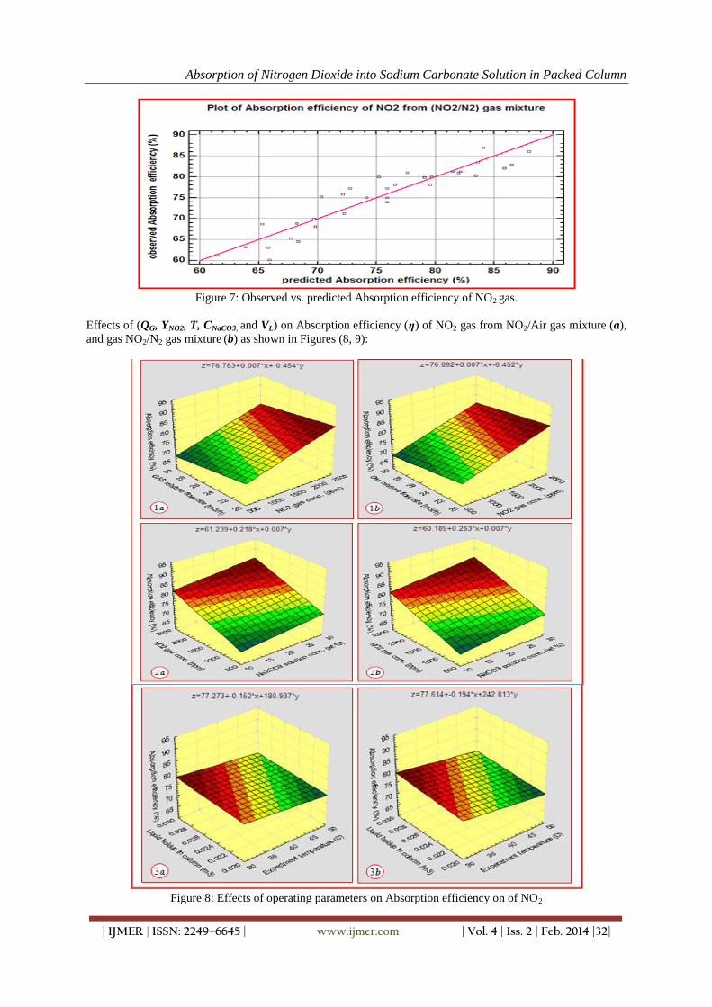
Absorption of Nitrogen Dioxide into Sodium Carbonate Solution in Packed Column
| IJMER | ISSN: 2249–6645 | www.ijmer.com | Vol. 4 | Iss. 2 | Feb. 2014 |32|
Figure 7: Observed vs. predicted Absorption efficiency of NO2 gas.
Effects of (QG, YNO2, T, CNaCO3, and VL) on Absorption efficiency (η) of NO2 gas from NO2/Air gas mixture (a),
and gas NO2/N2 gas mixture (b) as shown in Figures (8, 9):
Figure 8: Effects of operating parameters on Absorption efficiency on of NO2

Absorption of Nitrogen Dioxide into Sodium Carbonate Solution in Packed Column
| IJMER | ISSN: 2249–6645 | www.ijmer.com | Vol. 4 | Iss. 2 | Feb. 2014 |33|
Figure 9: Effects of operating parameters on Absorption efficiency on of NO2
Figures (8, and 9) are represent the influences of operating parameters (QG, YNO2, CNaCO3, T, and VL) on
Absorption efficiency (η) of NO2 gas absorption from gas mixtures (a and b). In general the η increases with
increasing in (YNO2, CNaCO3, and VL), and decreases with increasing of (QG, and T),
3.4. Optimal Response:
The optimum operating parameters for present work were obtained using the computer program to
analyze the experimental results. The goal of optimizing was to maximize the Absorption efficiency (η) of NO2
gas absorption from different gas mixtures. The results of optimizing were summarized in Table 4:

Absorption of Nitrogen Dioxide into Sodium Carbonate Solution in Packed Column
| IJMER | ISSN: 2249–6645 | www.ijmer.com | Vol. 4 | Iss. 2 | Feb. 2014 |34|
Table 4: Optimum operating parameters and optimum Absorption efficiency of NO2 gas.
Operating parameters Low value High value Optimum
value
Gas mixture flow rate (m3/h):
NO2 gas inlet conc. (ppm):
Na2CO3 solution conc. (wt %):
Experimental temperature ():
Liquid hold up in column (m3):
20
500
10
30
0.02
30
2500
30
50
0.03
20
2500
30
30
0.03
Absorption efficiency of NO2 gas from NO2/Air gas mixture (%): 89.88
Absorption efficiency of NO2 gas from NO2/N2 gas mixture (%): 90.38
IV. Conclusions * Absorption of NO2 gas from (NO2/Air or NO2/N2) gas mixture into Na2CO3 solution was carried out in pilot
scale packed column. The Absorption efficiency (η) of NO2 gas was measured at various operating conditions
(QG, YNO2, T, CNaCO3, and VL) according to experimental design. The measured Absorption efficiency was in the
range of η = 60.80-89.43 %, and of η = 60.10-91.50 % respectively. The η could be improved and increases by
increasing in the YNO2, CNaCO3, and VL and with decreasing of QG, and T.
* A negligible influence of oxidation on Absorption efficiency was observed in this work with a maximum
deviation of 2.2 %. For economical reasons we conclude to absorb NO2 gas from gas mixture by using Air as
carrier gas instead of N2 in the gas mixture.
* A computer program (Statgraphics/Experimental Design) was used to estimate the linear fitted models of
Absorption efficiency (η) in terms of operating conditions (QG, YNO2, T, CNaCO3, and VL. Both linear fitted
models of η were adequate, and operating parameters were significant, while the interactions were negligible.
The accuracy of Absorption efficiency models is ± 2.3 %.
* Using the same computer program the optimum operating conditions were obtained with values of QG = 20
m3/h, YNO2 = 2500 ppm, CNaCO3 = 30 wt %, T = 30 , and VL = 0.03 m
3. The optimum Absorption efficiency (η)
was in values of 89.88 % and 90.38 % respectively.
* On the base of results of measured Absorption efficiency, we conclude to scaling up the size of the pilot plant
used in this study by 3-4 times to commercial size plant and using the optimum operating parameters obtained in
future work.
REFERENCES [1]. Kurooka J., “Removal of nitrogen oxides from flue gases in a packed column”, Environment Protection
Engineering, Vol. 37 (1), 2011, pp. 13-22.2.
[2]. Majeed J.G., Korda B.,and Bekassy-Molnar E., “Comparison of the efficiencies of sulfur dioxide absorption using
calcium carbonate slurry and sodium hydroxide solution in an ALT reactor”, Gas Sep.Purif., Vol. 9 (2),1995, pp.
111-120.
[3]. Ishibe T.,Santo T.,Hyhashi T., Kato N., and Hata T., ”Absorption of nitrogen dioxide and nitric oxide by soda lime,
“Journal of Anaesthesia, Vol. 75, 1995, pp. 330-33.
[4]. Fowler D., Flechard C., Skiba U., Coyle M., and Cape J.N., “The atmospheric budget of oxidized nitrogen and its
role in ozone formation and deposition”, New Phytol., Vol. 139, 1998, pp. 11-23.
[5]. Jakubiak M. P., and Kordyleweski W. K.,”Pilot-scale studies on NOx removal from flue gas via NO ozonation and
absorption into NaOH solution”, Chem. Process Eng., Vol. 33 (3), 2012, pp. 345-358.
[6]. Weisweiler W., “Absorption of NO2/N2O4 in nitric acid”, Chem. Eng. Technol., Vol. 13 (1), 1990, pp. 97-101.
[7]. lefers J. B., and Berg P. G., “The oxidation and absorption of nitrogen oxides in nitric acid in relation to the tail
gas problem of nitric acid plants”, Chem. Eng. Sci., Vol. 35 (1-2),1980, pp. 145-159.
[8]. Glowiski J., Biskupski A., Slonka T., and Ttlus W., “Absorption of nitrogen oxides at the final stage of ammonium
nitrate production” Chem. Process Eng., Vol. 30 (2), 2009, pp. 217-229.
[9]. Lodder P., and Lefers, J. B., “The effect of natural gas, C2H6 and CO on the homogeneous gas phase reduction of
NOx by NH3”, Chem. Eng. Journal,Vol. 30 (3), 1985, pp. 161-167.
[10]. Chanq MB., Lee HM.,Wu F., and Lai CR., “Simultaneous removal of nitrogen oxide/nitrogen dioxide/Sulfur
dioxide from gas streams by combined plasma scrubbing technology”, J. Air waste Manaq Assoc., Vol. 54 (8),
2004, pp. 941-949.
[11]. Chu H., Chien T., and Twu B., “Simultaneous Absorption of SO2, and NO in a stirred Tank Reactor with
NaClO2/NaOH Solutions” Water, Air, and Soil Pollution, Vol. 143 (1-4), 2003, pp. 337-350.
[12]. Jakubiak M., and Kordylewski W., “Effectiveness of NOx removal from gas via preoxidation of NO with ozone and
absorption in alkaline solution”, Chem. Process Eng., Vol. 31 (4), 2010, pp. 699-709.13.
[13]. Barbooti M. M., Ibraheem N. K., and Ankosh A. H.., “Removal of Nitrogen Dioxide and Sulfur Dioxide from Air
Streams by Absorption in Urea Solutions” Journal of Environmental Protection, Vol. 2 (2), 2011, pp. 175-185.

Absorption of Nitrogen Dioxide into Sodium Carbonate Solution in Packed Column
| IJMER | ISSN: 2249–6645 | www.ijmer.com | Vol. 4 | Iss. 2 | Feb. 2014 |35|
[14]. Modlinski N. J., Kordylewski W. K. , and Jakubiak M. P., “Numerical Simulation of O3 and Reacting in Tubular
Flow Reactor”, Chem. Process Eng., Vol. 3 (3), 2013, pp. 361-375.
[15]. Bekassy-Molnar E., Marki E., and Majeed J.G.,”Sulphur dioxide absorption in air-lift-tube absorbers by sodium
citrate buffer solution”, Chem. Eng. Processing, Vol. 44, 2005, pp.1059-1046.

International
OPEN ACCESS Journal
Of Modern Engineering Research (IJMER)
| IJMER | ISSN: 2249–6645 | www.ijmer.com | Vol. 4 | Iss. 2 | Feb. 2014 |36|
Some Operation Equation and Applications
Ning Chen1, Jiqian Chen
2
1(College of Scienc , Southwest University of Science and Technology, Mianyang 621010, PR China) 2(College of Scienc , Southwest University of Science and Technology, Mianyang 621010, PR China
I. Introduction And Preliminaries The introduction of the paper should explain the nature of the problem, previous work, purpose, and the
contribution of the paper. The contents of each section may be provided to understand easily about the paper. In
recent years, the fixed point theory and application has rapidly development.
The topological degree theory and fixed point index theory play an important role in the study of fixed
points for various classes of nonlinear operators in Banach spaces (see [1-2],[3]and[4],[7],etc.). The new
conclusions of main theorems: Theorem 2.1 and theorem 2.4, theorem 2.6 and theorem 2.7, theorem 3.1 and
theorem 4.1. Next, the effective methods of variation iterative method to combine some integral-differential
equation and partial differential equations with He’s iterative method. First, we need following some definitions
and conclusion (see [3]).
Let E be a real Banach space, a bounded open subset of E and the zero element of E If :A E is a
complete continuous operator, we have some well known theorems for needing Lemma 1.1 as follows (see [3-4]).
Lemma 1.1 (see Corollary 2.1 [3]) Let E be a real Banach Space, is a bounded open subset of E and .
If :A E is a semi-closed 1-set -contractive operator such that satisfies the Leray-Schauder boundary condition
,Ax tx for all x and 1,t then deg( , , ) 1,I A and so A has a fixed point in .
II. Several fixed point theorems In recent years, some new types fixed point theory and application to study the differential-integral
equations in the physic and mechanics fields. Therefore, some application has rapidly development. First, we
extended some results as follows. For convenience, we give out following Theorem 2.1.
Theorem2.1 Let E be a real Banach Space, is a bounded open subset of E and . If :A E is a
semi-closed 1-set-contractive operator such that
)()(
2 )1(nnnn
xAxmxAxxmAx , for all .x (2.1)
(where 1, 0, 0 , nm, positive integer )
Then deg( , , ) 1I A , if A has no fixed points on and so A has a fixed point in .
Proof By lemma 1.1, we can prove theorem 2.1 .Suppose that A has no fixed point on .Then assume it is not
true, there exists 00
, 1x such that 0 0 0
Ax x .
It is easy to see that 0
1. Now, consider the function defined by
,1)())1(()( )()(2 nn mtmttf for any 1.t
Since ,0])())1()[(()(' 1)(1)(2 nn mtmtnntf 1t and 0)(' tf .
So, ( )f t is a strictly increasing function in ),,1[ and ( ) (1)f t f for 1t . Thus,
Consequently, noting that0 0,x 0 1 , we have
ABSTRACT: In this paper, we give several new fixed point theorems to extend results [3]-[4] ,and we apply
the effective modification of He’s variation iteration method to solve some nonlinear and linear equations are
proceed to examine some a class of integral-differential equations and some partial differential equation, to
illustrate the effectiveness and convenience of this method(see[7]). Finally we have also discussed Berge type
equation with exact solution.
Keywords: Semi-closed 1-set-contractive operator, Topology degree, Modified variation iteration method,
Integral-differential equation, Partial Differential Equation

Some Operation Equation And Applications
| IJMER | ISSN: 2249–6645 | www.ijmer.com | Vol. 4 | Iss. 2 | Feb. 2014 |37|
)(
0
)(
0
)(
0
2
0 ]1)[()1(nn
n
xmxmAx
)(
0000
nnnxAxmxAx ,
which contradicts (2.1), and so the condition ( )L S is satisfied. Therefore, it follows from lemma 1.1 that the
conclusion of theorem 2.1 holds.
Corollary 2.2. Let ,1m we get theorem 2.3 [3].
Corollary2.3. If nnn
AxmxAxxmAx
)(
2 )1( , then deg( , , ) 1I A by similar
proof method.
In fact,
)(nnnnn
xAxmxAxAxmxAx ,it satisfies condition of theorem 2.1.
In the same reason, we extend some theorem [3] as follows.
Theorem 2.4 Let E be a real Banach Space, is a bounded open subset of E and . If :A E is a
semi-closed 1-set-contractive operator such that satisfies condition:
)])1(3)[1(222333
xkxAxAxkxAxkkxAx , for all .x (2.4)
Then deg ( , , ) 1I A
Proof Similar as above stating, we shall prove that the L-S condition is satisfied. That is there exists 0 0, 1x
such that0 0 0
Ax x , and 0
1. Now, consider it by (2.4), we have that
))(1()1()( 0
33
0
3
0
3
0 kkkk .
This is a contradiction. By lemma 1.1, then deg ( , , ) 1I A that A has a fixed point in . We complete this
proof.
Theorem2.5.Let , ,E A be the same as theorem 2.7. Moreover, if substituting (2.4) into that inequality:
)6[2422444
xxAxAxxAxxAx , for all .x (2.5)
Then deg ( , , ) 1I A , then the A has at least one fixed point in .
Proof Similar as the proof of theorem2.4. If we suppose that A has no fixed point on . Then we shall prove
that the L-S condition is satisfied. We assume it is not true, there exists 0 0
, 1x such that0 0 0
Ax x , and 0
1.
Now, consider it by (2.5), we have that )16(2)1()1(2
0
4
0
4
0
4
0 .
By (2.5) we have that )16(2)1()1(2
0
4
0
4
0
4
0 . Thus, this is a contradiction,
then by lemma 1.1 that we get the conclusions of theorem 2.5.
Therefore, we shall consider some higher degree case as follow (Omit similar proof).
Theorem 2.6 Let E be a real Banach Space, is a bounded open subset of E and . If :A E is a
semi-closed 1-set-contractive operator such that satisfies
condition: 2222
2
21212[2 xAxCAxxAxxAx
n
n
nnn
]222222
2
42442
2
4424
2
nnn
n
nn
n
n
n xxAxCxAxCxAxC
, for every x (2.6)
Then deg ( , , ) 1I A , then if A has no fixed points on and so A has at least one fixed point in .
Theorem 2.7 Let E be a real Banach Space, is a bounded open subset of E and . If :A E is a
semi-closed 1-set-contractive operator such that satisfies condition: 2222
2
222[2 xAxCAxxAxxAx
n
n
nnn
]222222
2
42442
2
4424
2
nnn
n
nn
n
n
n xxAxCxAxCxAxC
for all .x (2.7)
Then deg ( , , ) 1I A , then if A has no fixed points on and so A has at least one fixed point in
(We omit the similar proof of above Theorems).
III. Some Notes For Altman Type Inequality It is well known we may extend that boundary condition inequality as bellow case:
222mxAxmxAx for all .0, mx (3.1)

Some Operation Equation And Applications
| IJMER | ISSN: 2249–6645 | www.ijmer.com | Vol. 4 | Iss. 2 | Feb. 2014 |38|
then the semi-closed 1-set-contractive operator A must have fixed point in .
In fact, there exists 0 0
, 1x such that0 0 0
Ax x , and 0
1. By (3.1), we have that
2 2 2 2
0 0 0( ) , 2 2 0.m m m m
Then 012
9 , this is a contradiction.
By Lemma 1.1, we obtain deg ( , , ) 1,I A then operator A must have fixed point in .
We can extend this Altman’s inequality into the determinant type form (also see [3]-[5], [6] etc):
222mxAxmxAx =
2)(,
,)(D
xAmx
mxxA
that we consider these general case: nD for n-order determinant. Similar Corollary (2) satisfy condition bellow:
),,2,1(2222
limxmxAxxBAxAx i . Then if these semi-closed operators lBBB ,,, 21 have not
common fixed point each other, then S have at least l numbers fixed points. Now, we write n-order determinant
type form
n
Ax x x x
x Ax x xD
x x Ax x
.
Then by simple calculation, .))()1(( 1 n
n xxAxxnxAxD
Moreover, in the similar discussion along this direction, we extend Corollary 2.6 in [3] with as following Theorem
3.1
Theorem 3.1 Let AE ,, be the same as in lemma 1.1.Moreover,if there exists n-positive integer such that ),2( n
,2
)1(2
nn
nDDAx for all ,x (3.2)
Then ,1),,deg( AI if A has no fixed points on , and so A has at least one fixed point in .
Proof Noting the determinant by nD , .))()1(( 1
2
n
n xxAxxnxAxD
By (3.2), we have
.))()1()()1(( 2)1(2 nnxxAxxnxAxxnxAxAx
In fact, there exists00 , 1x 0x 1, 00 x such that
00 0.Ax x It is easy to see that0
1.
Now, we have the inequality
.)]1())][1([(22
0
2
000
22
0
nnnnn
Hence, ,))()1()()1((22
0
2
000000000
nn AxxxAxxnxAxxnxAx
Which is a contradiction to (3.2), and so the boundary condition of Leray-Schauder condition is satisfied.
Therefore, it follows from lemma 1.1 that the conclusion of Theorem 3.1 holds.
Theorem 3.2 Let be the same as in lemma 1.1.Moreover, if there exists n positive integer such that ( 2)n ,
,2
2
1 nnn DDD for all ,x (3.3)
Then ,1),,deg( AI if A has no fixed points on , and so A has at least one fixed point in . (Omit
this similar proof).
Theorem 3.3 Let , ,E A be the same as in lemma 1.And, if there exists n positive integer such that ( 2)n .
,21
)1(3
nnn
nDDDxAx for all ,x (3.4)
Then ,1),,deg( AI if A has no fixed points on , and so A has at least one fixed point in .
Proof Notice the determinant nD , then ,))((1
n
n xxAxxnxAxD and
,))()1(( 1
2
n
n xxAxxnxAxD similar as in above way that we omit the similar proof of
Theorem 3.2. In fact, on the contrary, there exists 1, 00 x such that .000 xAx It is easy to see that

Some Operation Equation And Applications
| IJMER | ISSN: 2249–6645 | www.ijmer.com | Vol. 4 | Iss. 2 | Feb. 2014 |39|
01. It is well know by (3.4), we easy obtain that there is a contraction for this inequality. So A has at least one
fixed point in .
Theorem 3.4 Suppose that same as Theorem 3.3, satisfy follows form:
,321
)3(2
nnnn
nDDDDxAx for all ,x (3.5)
Then ,1),,deg( AI if A has no fixed points on and so A has at least one fixed point in . (Omit
this similar proof of Theorem 3.4).
Remark Notes that new case of non-symmetry form with nD for n-order determinant are given with more
conclusions.
IV. solution of integral equation by vim
To ensure a high-quality product, diagrams and lettering MUST be either computer-drafted or drawn
using India ink. Recently, the variation iteration method (VIM) has been favorably applied to some various kinds of
nonlinear problems, for example, fractional differential equations, nonlinear differential equations, nonlinear
thermo-elasticity, nonlinear wave equations.
They have wide applications in mechanics, physics, optimization and control, nonlinear programming,
economics, and engineer sciences.
In this section, we apply the variation iteration method (simple writing VIM) to Integral-differential equations
bellow (see [3] and [4-6] etc.). To illustrate the basic idea of the method, we consider:
),()]([)]([ tgtuNtuL
where L is a linear operator, N is a nonlinear operator and )(tg is a continuous function.
The basic character of the method is to construct functional for the system, which reads:
10
( ) ( ) ( ) ( )x
nn n nu x u x s Lu Lu Nu g s ds ,
where is the Lagrange multiplier which can be identified optimally via variation theory, nu is the nth
approximate solution, and nu denotes a restricted variation, .0nu There is an iterative formula:
b
ann dttutxkxfxu )(),()()(1
of this integral equation.
Theorem 4.1 ([4, theorem 4.1]).Consider the iteration scheme ),()(0 xfxu and the
b
ann dttutxkxfxu )(),()()(1 . (4.1a)
Now, for ,,2,1,0 n to construct a sequence of successive iterations that for the ( )nu t to the solution of
integral equation (4.1). In addition, we assume that b
a
b
aBdxdttxk 22 ),( , and assume that ,)( 2
],[ baLxf if
B/1 , then the above iteration converges in the norm of 2
],[ baL to the solution of integral equation (4.1).
Corollary4.2 If )()(),(1
tbxatxk ii
m
i
, and2 2( , ) ,
b b
a ak x t dxdt B then assume ,)( 2
],[ baLxf
if B/1 , the above iteration converges in the norm of 2
],[ baL to the solution of integral equation (4.1).
Corollary4.3 If 1 2( , ) ( , ) ( , ),k x t k x t k x t and2 2( , ) ,
b b
a ak x t dxdt B then assume ,)( 2
],[ baLxf
if B/1 , the above iteration converges in the norm of 2
],[ baL to the solution of integral equation (4.1).
Example4.1. Consider that integral equation
1
0
23 )()()( dttutxtxxxxu . (4.2)
Where )10(,)( 23
0 xxxxu , let 1 1 1
2 5 4
and that

Some Operation Equation And Applications
| IJMER | ISSN: 2249–6645 | www.ijmer.com | Vol. 4 | Iss. 2 | Feb. 2014 |40|
1
0
23
1 )()()( dttutxtxxxxu nn (4.2a)
Where b
a
b
aBdxdttxtdxdttxk 2111
1
0
1
0
22 9/7339)(),( , if ,7/3 then the
iterative (4.1a) is convergent to the solution of equation (4.2). Substituting )(0 xu in to (4.2a), it is that
(writing23)( xxxxP
)
1
00
23
1 )()()( dttutxtxxxxu ),1(23 xxxx
1 1
3 2
2 10 0
( ) ( ) ( ) ( ) ( 1) ( 1)( ) P x xt t u t dt P x x t t t t t dtu x
22 1( ) / 4xP x
2 321
3 20
( ) ( ) 2 ( 1) / 4 ( 1) ( ) ( ) 2 1 / 3 / 3u x P x x x t u t dt P x x
By inductively, 2
11 / 3 / 3 / 3( ) ( )
n
nxu x P x
Then the solution: )(lim)( xuxu nn
( ) 3 / (3 )P x x
.(See Fig 1and Fig 2)
Fig 1 Fig 2
Example 4.2 Consider that integral equation (positive integer )1k
1
0
2 )()()( dttutxxxxxu kkk (4.3)
Where 0)0( u , and )10()( 2
0 kk xxxxu
From that
1
01
2 )()()( dttutxxxxxu n
kkk
n
By theorem 4.1 and by simple computation, we obtain again that
b
a
b
a
k Bkdxdttxdxdttxk 21
0
1
0
22 )12(3/1)(),( ,
then if )12(3 k , then iterative
1
01
2 )()()( dttutxxxxxu n
kkk
n ,
which is convergent the solution of integral equation (4.3). We may omit the detail calculating (Let 1
2
1 1
4 2k k
).
22
11 2 2 2( ) / ( ) / ( ) / ( ) .
nk k k
nk k ku x x x x x
1
01
2 )()()( dttutxxxxxu n
kkk
n ,
which is convergent the solution of integral equation (4.3). We may omit the detail calculating
(Let 1 1 1
2 4 2k k
).

Some Operation Equation And Applications
| IJMER | ISSN: 2249–6645 | www.ijmer.com | Vol. 4 | Iss. 2 | Feb. 2014 |41|
22
11 2 2 2( ) / ( ) / ( ) / ( ) .
nk k k
nk k ku x x x x x
The solution 2
1( ) / ( )( ) 2 2 .
kk k
nxu x x x x k k
Theorem 4.2 (see theorem 3 in [5]) Let D be a bounded open convex subset in a real Banach
space X and ;D Suppose that EDA : is a semi-closed 1-set-contractive operator and satisfies the
following condition:
00 xxxAx for every Dx and Dx 0. (4.4)
Then the operator equation xAx has a solution in D (omit the proof)
To illustrate the application of the obtained results, we consider the examples.
Example 4.3 Similar as example 1 , we consider integral equation:
1 1
0(1 / 7) (1 / 11)sin cos 2.1 0,
x
t t dt x
],[ x (4.5)
It is easy to prove that this equation has a solution in ].,[
In fact, let 0
(1 / 7) (1 / 11)sin cos 2.1.x
Ax t t dt ],[ x , and that .:],,[ xDD We
write ,yy for every .Ry Thus, we have
0
1 1 1 1
0/ 77(1 / 7) (1 /11) (1 / 7) (1 /11)( ) 2.1 sin cos 18 2.1 2.1A t t dt dt
And
.1.21.277/18)cos)11/1(sin)7/1((1.2)( 11
0
dtttA
It follows that ,1.21.2 xAx for every Dx . Meanwhile, A is semi-closed 1-set-contractive operator
similar example 1 by theorem 4.2 that we obtain the xAx has a solution in ].,[ That is, Eq. (4.5) has a
solution in ].,[
V. Effective Modification of He’s variation iteration
In this section, we apply the effective modification method of He’s VIM to solve some
integral-differential equations [7]. In [7] by the variation iteration method (VIM) simulate the system of this form
).(xgNuRuLu
To illustrate its basic idea of the method .we consider the following general nonlinear system
),(xgNuRuLu (5.1)
Lu shows the highest derivative term and it is assumed easily invertible, R is a linear differential operator
of order less than L , Nu represents the nonlinear terms, and g is the source term. Applying the inverse operator
1
xL to both sides of equation (*), then we obtain ][][ 11 NuLRuLfu xx
.
The variation iteration method (VIM) proposed by Ji-Huan He (see [5], [7] has recently been intensively studied
by scientists and engineers. the references cited therein) is one of the methods which have received much concern
.It is based on the Lagrange multiplier and it merits of simplicity and easy execution. Unlike the traditional
numerical methods. Along the direction and technique in [9], we may get more examples bellow.
We notice that an effective iterative method and some examples
Example5.1 Consider the following integral-differential equation 1
'''
0(4 / 3)( ) ( )xu x e x xt u t dt ,
Where '' 2
(0) 1, '(0) 1 , (0)u u u with exact solution ( ) .xu x x e
In fact, we check 0 1( ) , ( ) 7 / 4,
xf x x e f x x
to divide f in tow parts for
0 1( ) ( ) ( ),f x f x f x and
writing 2 21/ 1/ 1/e
.
31 1 1
1 1 1
00 0 0
/ 3 ( /18) (( ) ( ) / 6)t
x x xx x xL xtu t dt L x t t e dt L x dx

Some Operation Equation And Applications
| IJMER | ISSN: 2249–6645 | www.ijmer.com | Vol. 4 | Iss. 2 | Feb. 2014 |42|
3
0(1 3 ) /18
x
x dx 41 3 / 72.x
By 1
4 1
10
(1/ 4) (1 3 ) /18( ) ( ) .x
n x nu x x e x L xtu t dt
Then, we have
1
4 1
1 00
(1 3 ) / 72( ) ( ) ,x x
xu x x e x L xtu t dt x e
1
4 1
2 10
(1 3 ) / 72( ) ( ) ,x t
xu x x e x L xtu t dt x e
, and we have that
( )x
nu x x e
Therefore, this is a closed form ( )
xu x x e
, shows that the method is a very convenient and
only one iterative leads to the exact solution.
Example5.2 Consider the following integral-differential equation
,)()3/4()(1
0
)6( dtttuxxexu x
(5.2)
where 5)5(4)4(3)3(2 )0(,)0(,)0(,)0('',1)0(',1)0( uuuuuu
In similar example1, we easy have it.(We may omit it)
where ,)()(0 00 00 0
1 dtdtdtdtdtdtLx xx xx x
x ,)()( 00
xexxfxu
3/7)())3/4(()()()( 01 xexxexfxfxf xx , ),()()( 10 xfxfxf
and writing 2 21/ 1/ 1/e
.
3 3
1 11 1 1
00 0
0 0 0 0
/ 3
( (
( ) ( )
/18) / 6) ,
t
x x x
x x x x
x x
x x
L xtu t dt L x t t e dt L
dx dxdxdx
4 7
0 0 01 3 ) / 18 1 3 ) / 18 .( / 4 ( / 7!
x x x
x dx x
71
1
1 00
1 3 ) / 3( ) ( / 7! ( ) , ,x x
xxu x x e L xtu t dt x e
and so on,
71
1
10
1 3 ) / 3( ) ( / 7! ( ) .x x
n x nxu x x e L xtu t dt x e
By simple operations, we have that
.1,)(,,)(,)( 10 nexxuexxuexxu x
n
xx
Therefore, the exact solution in a closed form xexxu )( , shows that the method
is a very convenient. The exact solution xexxu )( is only one iterative. (See Fig 3, 0.75 and 1.25 ).
Fig 3
VI. Some Notes of Burger’s Equation

Some Operation Equation And Applications
| IJMER | ISSN: 2249–6645 | www.ijmer.com | Vol. 4 | Iss. 2 | Feb. 2014 |43|
We shall consider the exact and numerical solutions for Burger’s equation ,which has attracted much
attention .Solving this equation has been an interesting tasks for mathematicians
VI.1 One-dimensional Burger’s equation
. Consider the following one-dimension Berger’s equation with initial and boundary conditions:
Example 6.1 Consider the following equation (similar as example 1 [15]): 2
2,
( ,0) 3 , 0.
u u uu
t x x
u x x t
(6.0)
According the direction of [2] and method for this example, then it can be written as by iterative formula (6) [2]:
.)),(),()((),(),(2
2
01
d
x
uvx
x
uux
utxutxu nn
n
nx
nn
(6.1)
Starting with .3),(0 xtxu
The following reads can be derived from iterative formula (6.1)
,241263),(
,63),(
32
2
1
xtxtxtxtxu
xtxtxu
.,3841929648241263),( 765432
3 xtxtxtxtxtxtxtxtxu
Thus, we have that
),(lim),( txutxu nn
nnn
n
tx
tttttttx
)3(2)1(
)1286432168421(3
0
765432
).21/(3 tx
This is an exact solution.
Remark Starting with ,)1(),(0 xatxu )21/()1(),(lim),( tatxutxu nn
.
As 0a ( as special case: 1a that is example 1 [15], ,2a this is example 1 in this paper ). Notice that
baxtxu ),(0 or xxtxu 2
0 ),( (similar polynomial case). More form.
),(lim),( txutxu nn
nnn
n
txx
ttttttxx
)(2)1(
)6432168421)((
2
0
654322
).21/()( 2 txx
This is an exact solution.
Or xxxtxu kk 1
0 ),( (similar polynomial case).more form.
).21/()(),(lim),( 1 txxxtxutxu kk
nn

Some Operation Equation And Applications
| IJMER | ISSN: 2249–6645 | www.ijmer.com | Vol. 4 | Iss. 2 | Feb. 2014 |44|
Fig 4
Fig 5
Example 6.2 Consider the following equation (similar as example 1 [15]): 2
2,
( , 0) 10 , 0.
u u uu
t x x
u x x t
(6.2)
For this example, by above Example 6.1, can be written as .9a Starting with .10),(0 xtxu Thus, we have that
an exact solution.
),(lim),( txutxu nn
).21/(10 tx
VI-2 Two-dimensional Burger’s equation
Similar as example 3 [15], we get following example 2 for two-dimension case.
Example 6.3 Consider the system of Burger’s equation in the following equation (similar as example 3 [15]):
),(1
2
2
2
2
y
u
x
u
Ry
uv
x
uu
t
u
).(
12
2
2
2
y
v
x
v
Ry
vv
x
vu
t
v
(6.3)
with initial conditions: .)0,,(,)0,,( 00 yxyxvyxyxu We have by iterative [15]:
y
uv
x
uu
utyxutyxu n
n
n
n
nt
nn
01 [),,(),,( ,](
12
2
2
2
dy
u
x
u
R
nn
y
vv
x
vu
vtyxvtyxv n
n
n
n
nt
nn
01 [),,(),,( .](
12
2
2
2
dy
v
x
v
R
nn
(6.4)
Consider the initial approximations .)0,,(,)0,,( 00 yxyxvyxyxu and applying VIM formula (6.4),
other term of the sequence are computed as follows:
.2),,(,2),,( 11 ytyxtyxvxtyxtyxu
,)3/4(222),,( 322
2 xtytxtxtyxtyxu
.)3/4(22.2.),,( 322
2 ytytxtytyxtyxv
),,(lim),,( tyxutyxu nn
)21(2)21()421( 2242 txttyttx
).21/()2( 2txtyx
),,(lim),,( tyxvtyxv nn
)21(2)21()421( 2242 tyttyttx
),21/()2( 2txtyx
which are exact solutions )2/1( t . We omit the detail stating for this results.
VII. Conclusion

Some Operation Equation And Applications
| IJMER | ISSN: 2249–6645 | www.ijmer.com | Vol. 4 | Iss. 2 | Feb. 2014 |45|
In this Letter, we apply the variation iteration method to integral-differential equation ,and extend some
results in [3]- [4]-[5]. The obtained solution shows the method is also a very convenient and effective for various
integral-differential equations, only one iteration leads to exact solutions.
Acknowledgements
This work is supported by the Natural Science Foundation (No.11ZB192) of Sichuan Education Bureau
and the key program of Science and Technology Foundation (No.11Zd1007) of Southwest University of Science
and Technology.
REFERENCES [1]. D. Guo, V. Lashmikantham, Nonlinear Problems in abstract Cones(Academic Press, Inc., Boston, New York, 1988).
[2]. S.Y. Xu, New fixed point theorems for 1-set-contractive operators in Banach spaces, Nonlinear
Anal.67,2007,938-944.
[3]. N. Chen, and J.Q. Chen, New fixed point theorems for 1-set-contractive operators and variation iteration method, Jp
Journal of fixed point theory and application,Vol.6(3),2011,147-162.
[4]. N. Chen, J.Q. Chen, Operation equation and application variation iteration method, Applied Mathematics,3
(8),2012,857-863.
[5]. N.Chen , J.Q.Chen, Some approximation in cone metric space and variation iterative method, Applied Mathematics,
3(12),2012,2007-2018.
[6]. C. X. Zhu, Generalization of Krasnoselskki’s theorem and Petrshyn’s theorem, Applied mathematics letters 19,2006,
628-632.
[7]. Asghar Ghorbani, Jafar Sabaeri–Nadjafi, An effective modification of He’s variational iteration method, Nonlinear
Analysis: Real World Application10,2009, 2828-2833.
[8]. Abdul–Majid Wazwaz, The variational iterative method :A reliable analytic tool for solving linear and nonlinear wave
equations, Computers & mathematics with applications ,54,2007,926-932.
[9]. S.Q.Wang,Ji-Huan He, Variational iterative method for solving integro-differential equations, Physics Letters A
367,2007,188-191.
[10]. J. Biazr, H. Ghazvini, He’s iterative method for forth-order parabolic equation,An international Journal of computers
and mathematics with applications,54,(2007,1047-1054.
[11]. N. Chen, Baodan Tian and Jiqian Chen, A class of new fixed point theorems and for 1-set -contractive operators and
some variation iterative method,[J]. Physics Procedia 33,2012,1932-1938.
[12]. Yousry S. Hanna, On Approximate solutions of second-order linear partial differential equations, Applied
Mathematics,3,2012,1001-1007.
[13]. Elcin YusufogIu, The variation iteration method for studying the Klein-Gordon equation., Applied Mathematics
Letters,21,2008,669-674.
[14]. Z.L.Yang, Nontrivial solutions of systems of nonlinear Hammerstein integral equations and applications, Acta
Mathematica Scientia, 26(A2),2006,233-240.
[15]. A. Saandatmandi, and M. Dehghan, He’s iterative method for solving a partial differential equation arising in modeling
of water waves, Zeitschrift fur naturfoschung ,64,2009,783-787.

International
OPEN ACCESS Journal
Of Modern Engineering Research (IJMER)
| IJMER | ISSN: 2249–6645 | www.ijmer.com | Vol. 4 | Iss. 2 | Feb. 2014 |46|
Implementation of Lean Manufacturing Principles in Foundries
Praveen Tandon1, Dr. Ajay Tiwari
2, Shashikant Tamrakar
3
1(Mechanical Engineering Department, RCET /CSVT University, INDIA) 2(Mechanical Engineering Department, REC /CSVT University, INDIA)
3(Mechanical Engineering Department, RCET /CSVT University, INDIA)
I. Introduction Lean manufacturing (LM) is seen as major breakthrough process and is widely used by major
industries all over the world. In a continuous process industry like casting the main approach of implementing
the lean manufacturing is to reduce the production cost by eliminating the non value added activities. A basic
concept of LM is pull production in which the flow on the factory floor is driven by demand from downstream
pulling production upstream as opposed to traditional batch-based production in which production is pushed
from upstream to downstream based on a production schedule. In a recent survey, approximately 36% of US-
based manufacturing companies have implemented lean or are in the process of implementing lean.
An LM facility is capable of producing product in only the sum of its value added work content time.
The significance of a LM model include: production of only one unit at a time; non-value added time
eliminated; production of the job within time pre decided ; relocation of required resources to the point of
usage; and all processes must be completed within same Takt time ,therefore it provide the smooth production
of the complete job . The rate at which work progresses through the shop floor is called Takt. The available
production time divided by customer demand. The objective of takt time is to measure the production with
respect to demand. It sets the rate for production so that production cycle times can be matched to customer
demand rate.
II. Principle Jerry Kilpatrick
[1] stated that “Lean” operating principles began in manufacturing environments and
are known by a variety of synonyms; Lean Manufacturing, Lean Production, Toyota Production System, etc. It
is commonly believed that Lean started in Japan (Toyota, specifically), but Henry Ford had been using parts of
Lean as early as the 1920’s, as evidenced by the following quote:
“One of the most noteworthy accomplishments in keeping the price of Ford products low is the gradual
shortening of the production cycle. The longer an article is in the process of manufacture and the more it is
moved about, the greater is its ultimate cost.” Henry Ford 1926
In order to set the groundwork for this paper, let’s begin with the definition of Lean, as developed by
the National Institute of Standards and Technology Manufacturing Extension Partnership’s Lean Network:
“A systematic approach to identifying and eliminating waste through continuous improvement, flowing
the product at the pull of the customer in pursuit of perfection.”
Keep in mind that Lean applies to the entire organization. Although individual components or building
blocks of Lean may be tactical and narrowly focused, we can only achieve maximum effectiveness by using
them together and applying them cross-functionally through the system.
ABSTRACT : It is the general perception that the foundry industries are inherently more efficient
and have a relatively less requirement for major improvement activities. Managers and engineers
have also been hesitant to implement lean manufacturing tools and techniques to the continuous
sector because of typical and identical characteristics that sector. These include costly and special
purpose inflexible machines, options of modifications in machines are limited ,long setup times,
and the general difficulty in producing in small batches.
Lean manufacturing technology when applied appropriately in a process industry , can
help in eliminating waste , enhance the quality of product , attain better and smooth control on
operations and thereby reducing the production cost and production time .
Keywords : casting shakeout, Lean manufacturing, Takt time, production line,

Implementation of Lean Manufacturing Principles in Foundries
| IJMER | ISSN: 2249–6645 | www.ijmer.com | Vol. 4 | Iss. 2 | Feb. 2014 |47|
III. Objective The lean manufacturing will help reducing the waste, waiting time and balancing the production line.
The major benefit is high productivity which is the need of the hour. Modification automation and effective
utilisation of production resources ultimately serve the purpose. Lean Manufacturing is one such area having
great potential to obtain higher productivity especially in foundry practice.
IV. Methodology Collection of data through literature survey, interviews, group discussions, questionnaires, databases,
seminars, conferences etc. Data analysis by using various tools like hypothesis testing, qualitative analysis,
using relevant statistical software Mat Lab ,ANSYS etc.
John S. W. Fargher [2]
suggested a method in his case study as follows:-
The first step is to group products into families of similar production processes.
The second step is to establish the Takt time. The Takt time is the demand rate and consequently the time
between completion of each product off of the production line. It is first necessary to find the available
capacity of the production line:
Available Capacity = Time Available x PFS x Utilization
Where:
Time Available = Hours / Time Period x Number of Employees
Personal, Fatigue, and Safety (PFS) = Standard Hours Produced / Hours Worked
Utilization = (Hours Available - Downtime) / Hours Available
The third step is to review the work sequence by:
i. Observing the sequence of tasks each worker performs,
ii. Break operations into observable elements,
iii. Identify value added versus non value added elements and minimize or eliminate non value added
operations, and Study machine capacity, cycle times and change over times
iv. In IE words, conduct methods and standards studies.
The fourth step is to balance the line using the calculated Takt times found in step two.
Step five is to design and construct the cell to:
Implement a “U” shaped line to assure one way flow and maximize visibility,
Provide a flexible layout to account for all members of the production family,
Decrease distance between operations and integrating process operations wherever possible for
simplicity, minimizing both transportation and production lot sizes, integrate in point of use storage next to each
assembly operation.
Minimize material handling by concentrating on value added motion
Establish replenishment procedures for point of use storage using the A-B-C rule
Assure the personnel understand their role and are cross trained to use their skills at a variety of tasks and work
stations.
Provide visibility to allow operator decisions on problem solving, moving to where work needs to be
performed, and focus management attention on production disruptions.
The objective of this practice is to achieve economies of scale by saving costs and making better use of
assets. In addition, with a smaller number of employees (30 to 1000, as Toyota has in each plant), it is also
easier for managers to motivate the workforce.

Implementation of Lean Manufacturing Principles in Foundries
| IJMER | ISSN: 2249–6645 | www.ijmer.com | Vol. 4 | Iss. 2 | Feb. 2014 |48|
Fig. No. – 1: Flow chart of Foundary Practice
To carry out the proposed research work through data collection, small and medium sized foundries to
be visited. Complexity of casting process and parameters need to be studied.
There are other lean practices to implement. If production flows perfectly, there is no inventory waiting
to be worked on. Metal casters have helped minimize work-in-process by installing conveyor lines to keep
castings moving right through to finished goods storage. This eliminated putting the castings in totes and the
added handling. One low to medium volume gray/ductile iron jobbing foundry (casting weights under 50
pounds) we know now ships 30% of its production the same day and believes they can achieve 70% same day
shipment. These standards aren’t just for the high volume or dedicated metal casting companies any more.
“Autonomation” or “smart automation” is a part of lean manufacturing as well. Autonomation refers to
automating the process so humans can focus o n what humans do best. The objective here is to design the
machine so it knows when it is working abnormally and alerts a human. The human no longer has to monitor
normal production but can focus on abnormal or fault conditions. Removing routine and repetitive activity
reduces the chance for error.
V. Case Study A Case study on Application of Lean Manufacturing to Higher Productivity in the Apparel Industry in
Bangladesh has been done and following outcomes have been observed :
5.1 Introduction Generally in an industry more focus is given on profit. Though there are different issues involved in
cost reduction internally spent by an industry through finding wastages, preventing and correcting defective
work would result in huge savings [3]. The apparel industry faced considerable changes as a result of the
removal of Multi Fiber Agreement in 2005 [4]. Delivering high quality garments at low cost in shorter lead
times are the major challenges faced by the apparel manufacturers. Most of the apparel manufacturers are trying
to achieve these challenges successfully. In 2008, global recession badly affected almost all the apparel
manufacturing industries in the world [4]. Due to that demand for the low cost garments are increased by the
customers. Suppliers are forced to deliver low cost garments. Because of many high cost factors in Bangladesh,
most of the companies faced difficulties in getting orders and some companies were closed down. The
companies are seeking ways to minimize their cost in order to meet the competition by other low cost countries
such as China, India, Sri Lanka, and Pakistan and to survive. Lean Manufacturing can be defined as "A
systematic approach to identify and eliminate waste through continuous improvement by flowing the product at
the demand of the customer” (Introduction to Lean, 2010) [6]. Lean manufacturing helps to identify productive
and non- productive activities. Group[5] located at, Gazipur, Bangladesh, to identify non productive activities so
as to eliminate them for saving time, cost and improve productivity. By eliminating waste in the processes,

Implementation of Lean Manufacturing Principles in Foundries
| IJMER | ISSN: 2249–6645 | www.ijmer.com | Vol. 4 | Iss. 2 | Feb. 2014 |49|
companies can achieve a shorter lead time, lower cost, highest quality and can understand a competitive
advantage over the others.
5.2 Basic Research Approach As shown in Fig. 1, a comprehensive literature review was carried out on Lean Manufacturing. After
that effective suggestion and recommendations were made. The steps considered in the process are given
below:-
Fig-1 Research approach- steps by steps process
5.3 Result of Case Study:
In Modern industries it is difficult to identify the key areas and practices, which can be used to
eliminate waste in their processes. Based on the practical experiment conducted, it can be seen that lean
manufacturing can be effectively applied to apparel industry as the key step of waste identification. Using this
tool, it is possible to map the current status and subsequently analyze to achieve waste elimination. The case
study presented in this paper, has shown that the wastes such as transport, inventory and defects, over
processing, excess motion, over production etc can be reduced to a great extent which in turn improves the
productivity of the organization. In order to accomplish this task, the managers of the case company have to
implement approaches like 5S, one piece flow etc. Thus, lean manufacturing helps the organization to visualize
the present level of wastes occurring in the organization and the future possibilities of reducing or eliminating
them. In order to continuously reduce or eliminate waste, management of companies need to apply different
Lean tools and techniques accordingly while giving adequate training to their employees. Therefore
organizations of similar type can use the research outcomes as a knowledge base to identify their wastes and
come up with suitable remedies. Findings of this research can be valuable to other organizations of Bangladesh,
which expect to implement Lean Manufacturing in the near future.
VI. Conclusion Expected outcome of the research to focus on the process of pouring metal inside the mould, cooling
casting, shake-out, and transport to the finishing area, cleaning and cut burr processes. At the foundry industry
where the research collected data, the scenarios simulated suggested to explore alternatives to reduce the time of
pouring times through an improvement in industrial lay out and workload balancing including worker’s multi
skilling training. These procedures can lead to reduce the waste of time and reduce the queuing inside the
processes, an agreement with lean manufacturing technology.
REFERENCES [1]. Jerry Kilpatrick, Lean Principles, Utah Manufacturing Extension Partnership,2003, 1-5.
[2]. John S. W. Fargher, “ lean manufacturing and manufacturing Implementation tools” case study, April 2004,
Missouri Enterprise, University of Missouri - Rolla
[3]. Feld,M.W.,(2000).Lean Manufacturing: Tools, Techniques, and how to use them. Boca Raton, London: The
St. Lucie Press
[4]. Kumar, S. A. (2008). Production and Operations Management. Daryaganj, Delhi, India: New Age
International, p. 217-220.

Implementation of Lean Manufacturing Principles in Foundries
| IJMER | ISSN: 2249–6645 | www.ijmer.com | Vol. 4 | Iss. 2 | Feb. 2014 |50|
[5]. http//www.viyellatexgroup.com
[6]. Shahidul, M. I. and Syed Shazali, S. T.Dynamics of manufacturing Productivity: Journal of Manufacturing
Technology Management Vol. 22 No. 5, 2011, p. 664-678
[7]. http//www.opexgroup.com
[8]. Productivity Development Team, ed. Cellular Manufacturing: (Portland, .Oregon: Productivity Press,
1999).
[9]. http//www.sepalgroup.com
[10]. Saroj Bala, Factors Influencing Costing of Woven Fabrics, The Indian Textile Journal, June 2003
[11]. Dr P Khanna: Work study, time and motion study, Dhanpat Rai and Sons, New Delhi, (pp 21).
[12]. Romm, Joseph J. Lean and Clean Management: How to Boost Profits and Productivity by Reducing.
Pollution (New York: Kodansha International, 1994)
[13]. Abdulmalek, F.A. and Rajgopal, J. (2007). Analyzing the benefits of Lean Manufacturing and Value Stream
Mapping via simulation: a process sector case study, International Journal of Production Economics, Vol.
107, pp. 223-36.
[14]. Introduction to Lean (n.d.). Available from: http://www.mamtc.com/lean/intro_intro.asp (Accessed 10
May 2010)
[15]. McBride, D. The 7 Manufacturing Wastes. Available from:
http://www.emsstrategies.com/dm090203article2.html (Accessed 05 May 2010)
[16]. Ohno, T. (1988). Toyota Production System, Productivity Press, New York, pp. ix
[17]. Seth, D., Seth, N. and Goel, D. (2008). Application of Value Stream Mapping for minimization of wastes in
the processing side of supply chain of cotton seed oil industry in Indian context, Journal of Manufacturing
Technology and Management, Vol. 16 No. 4, pp. 529-50.

International
OPEN ACCESS Journal
Of Modern Engineering Research (IJMER)
| IJMER | ISSN: 2249–6645 | www.ijmer.com | Vol. 4 | Iss. 2 | Feb. 2014 |51|
Review of crosstalk free Network
Ramesh Kumar, Vedant Rastogi 1(CSE, IET ALWAR/ Rajasthan technical UniversityKota, India)
2(Department Computer Science, RTU University Kota Rajasthan, India)
I. Introduction The multistage interconnection Network is an essential network for the Parallel computing
applications .It contains N inputs to N outputs and is known as an N×N MIN. The parameter N is called the size
of the network. In this paper we study the performance of optical multistage Interconnection network.
Omega network is a network configuration after used in parallel computing architecture .It is an indirect
topology that relies on the Perfect Shuffle interconnection algorithm. The omega network is a highly blocking
through one path can always be made from input to any output in free network. It connects N inputs to N outputs
and is known as an N*N MIN. Here N is the size of the network. In Omega network contains N/2 switches. An
omega network is a log2N stage shuffle –exchange Interconnection network .Here multistage Omega network
N=8 Multistage Interconnections network establishes a reliable communication between source and destination.
But now a days electro optic technologies have built optical communication a reliable and fast network that
fulfill the Increasing demands of users.
II. Analysis for the Network Most of the interconnection network analysis related to identical processor And a uniform reference
model. We shall analyze the performance of the n- stage Banyan network discussed.
1. Fixed size packets are generated by the modules at each source address
2. Arrival of packets at the network inputs are independent and identical.
3. A connection between two switches can carry the packet in each cycle.
4. If two packets arriving at two distinct network inputs require the use of common link between two stages, one
of the packets is discarded.
5. The switches and links have no internal buffers to temporarily store an incoming packet that cannot be
forwarded in the current.
6. There is no blocking at the output links of the network. This means that the output links have at least the same
speed as the internal links.
Moreover, if the network is uniform, then for each stage in the network, the patterns of packet arrivals
at the inputs of that stage have the same distribution. While Banyan networks are very attractive in their
simplicity, other considerations such as performance or reliability sometimes dictate the use of more complicated
ABSTRACT: Multistage interconnection networks (MIN) are among the most efficient switching
architectures for the number of switching Element (SE). Optical crosstalk in optical multistage
interconnection network on the omega network topology Switches are arranged in multiple stages.
These switches also referred to as switching element (SEs) have two input and two output ports,
interconnected to the neighboring stages in a shuffle exchange connected pattern message routing
in such a network is determined by the interstate connection pattern.
Optical Multistage interconnection networks (OMIN) are advanced version of MINs. The
main Problem with OMIN is crosstalk. The main purpose of this paper is to Present crosstalk free
modified omega network, which is based on time domain approach. This paper presents the source
and destination based Algorithm (SDBA) .SDBA does the scheduling for source and their respective
destination addresses for the message routing. SDBA is compared with the crosstalk modified omega
network (CFMON).CFMON also Minimizes the crosstalk. This paper is the modified form of the
omega network.
Keywords: Omega network, Multistage Interconnections network, Optical Multistage
interconnection network, Crosstalk, Time domain approach, Crosstalk Modified omega network.

Review of crosstalk free Network
| IJMER | ISSN: 2249–6645 | www.ijmer.com | Vol. 4 | Iss. 2 | Feb. 2014 |52|
networks. We consider packet-switching networks built of 2 × 2 unbuffered switches with the topology of an n-
stage square Banyan network. When several packets at the same switch require the same output, a randomly
chosen packet is forwarded and the remaining packets are deleted. An 8 × 8 Banyan network is shown in Figure
1
Figure 1. An 8 x 8 Banyan network topology
Since we are dealing with OMINs, at any instant of time we can only send one message through any
switch to avoid the effect of crosstalk. But here in this paper for an N × N network we are allowing limited
crosstalk’s up to C = (log2N – 1) (where ‘C’ is a parameter dependent on Technology). The number of stages for
such a network is given by n=log2N
Hence for the Banyan network shown in fig we can allow crosstalk In
switches at two stages out of three stages in the network .Hence in this paper we can have switches where 0, 1
or2 messages Can be allowed at the same time .In other words a switch can be active 2-active, 1-active or 0-
acive .Both 0-Acive and 1-active switches do not. Allow crosstalk where as the 2-active switch produces optical
conflicts. And hence could potentially contribute to crosstalk. We are most interested in analyzing the
performance of a banyan network allowing limited cross-Talk. For instance, one of the best ways for analyzing
the performance Is to calculate the bandwidth (BW) of the NxN Banyan network operating Under a load l .load
is defined as the probability, that an input is active. Thus, the expected number of active input s at load for an
NxN banyan network is Nl. We will derive some equations to find the BW of such a Banyan network built with
2 x 2 unbuffered switches. Let P (j) be the probability that a request exists at an input link Of a switch in stage j,
and let P(j + l) be the probability that an output link of this switch is used for routing a request. The analysis
involves the iterative computation of P (j + l) in terms of P (j), starting with P (1).For an n-stage network, the
probability of acceptance, PA is given by P(n) . The crucial step in the analysis of each network is the recurrence
relation to specify P (j + l) in terms of P (j). The recurrence relation depends on the network topology and the
routing algorithm. Since we are dealing with a Banyan network with 2-active, 1-active or 0-active switches, we
have the following equations.
For each stage (1≤j≤n), we define
P2 (j) = probability that a given switch is 2-active,
P1 (j) = probability that a given switch is 1-active,
P0 (j) = probability that a given switch is 0-active.
Various combination of load at stage 1
III. Optical Omega Network (Oon) The OON has a shuffle exchange connection pattern. In this pattern the address is shifted one bit to the
left circularly in each connection. This network connects the input to output nodes using n stages, where n=log2N
with each stage containing 2n-1
SEs. When any source sends the communication signal to a destination then it has
to pass through the OON. Each communication signal has a definite path from the given source to the given
destination. Crosstalk occurs when two or more signals follow the same path in the same time period. In Fig. 1
the dotted black arrows show the switch conflict and the solid black arrows show the link con-flict problem in
OON.
The remainder of this paper is organized as follows. In the second section, related work and the theoretical about
previously proposed algorithm is presented.
l
l
l
l
l
l
l-1
l-1
l-1

Review of crosstalk free Network
| IJMER | ISSN: 2249–6645 | www.ijmer.com | Vol. 4 | Iss. 2 | Feb. 2014 |53|
IV. Related Work Using any one of the following three techniques we can minimize the crosstalk: the Space Domain
Approach, the Wavelength Domain Approach, and the Time Domain Approach (TDA).The Time Domain
Approach reduces the crosstalk problem by allowing only one source and its corresponding destination address
to be active at a time within a SE in the network. The Window Method, the Improved Window Method, and
many other TDA based approaches have come into limelight in recent years.
The aim of ASA is to select a particular source address that does not create conflict in the network in
the first pass, and the remaining source address can be transmitted in the second pass. This algorithm is
applicable for the 8 x 8 Optical Multistage Interconnection Networks. Initially, in this algorithm, the SA and DA
are obtained sequentially. Next, the combination matrix of the source and corresponding destination address is
obtained. Furthermore, transformation and row selection operations are applied on the combination matrix. In
this way, two pairs of rows can be obtained. In the next step, addition and subtraction operations will be
performed between the corresponding bits in each pair. Finally, some SAs and their DAs are selected for a
current pass and again the ASA is applied to the rest of the addresses.
The routing process of RSA is little bit different from ASA. This algorithm emphasizes two operations
(i.e., column selection and the construction of a conflict matrix table that is based on these columns).The rest of
the operations of RSA is same as in ASA. Furthermore, providing crosstalk free routes in minimum passes is an
exigent problem. For this problem, CFMON and its routing algorithm were proposed in. After going through, we
found that the routing algorithm of CFMON does not provide the crosstalk-free routes in two passes in some
exceptional cases. Hence, we have compared our research work with CFMON.
V. Conclusion In this research work, we have analyzed the performance of an OMIN for crosstalk. The crosstalk is a
challenging promlem.Regarding this concern, we have proposed a new algorithm which is known as source
destination based algorithm(SDBA).SDBA makes the cost effective and efficient for message transmission. In
this result show minimum crosstalk and less time consume than the other CFMON. In the future research can be
per-formed to analyze the performance of an OMIN with limited crosstalk under the bursty traffic, uneven and
self- similar traffic conditions.
REFERENCES [1]. Nitin and Durg Singh Chauhan, “Stochastic Communication for Application Specific Networks-on-Chip,” Journal of
Supercomputing, 59 (2), DOI: 10.1007/s11227-010-0472-5, 2010, pp.779-810.
[2]. Nitin, S. Garhwali and N. Srivastava, “Designing a Fault-tolerant Fully-chained Combining Switches Multi-stage
Interconnection Network with Disjoint Paths,” Journal of Supercomputing, 55 (3), DOI 10.1007/s11227-009-0336-z,
2009, pp.400-431.
[3]. Nitin and Durg Singh Chauhan, “Comparative Analysis of Traffic Patterns on k-ary n-tree using Adaptive
Algorithms based on Burton Normal Form,” Journal of Supercomputing, 59 (2), DOI: 10.1007/s11227-010-0454-7,
2010, pp.569-588.
[4]. Ved Prakash Bhardwaj and Nitin, “A New Fault Tolerant Routing Algorithm for Advance Irregular Augmented
Shuffle Exchange Network, Proceedings of the 14th IEEE International conference on Computer Modeling and
Simulation,” Emmanuel College, Cambridge, UK, March 28-30, 2012, pp.505-509.
[5]. J.C. Berrnond, J.M. Fourneau, and A. Jean-Marie, “Equivalence of multistage interconnection networks,” Rapport
LRI-217, Univ. de Paris-Sud, France, May 1985.
[6]. L.N. Bhuyan, and D.P.Agrawal, “Design and performance Of generalized interconnection networks,” IEEE Trans.
Comput., Vol. C-32, no.12, pp.1081-I090, December 1983.
[7]. Laxmi N. Bhuyan, Qing Yang, Dharma P. Agrawal, “Performance of Multiprocessor Interconnection
Networks,”IEEE Computer 22(2): 25-37, February 1989.
[8]. M. Brenner, D. Tutsch, G. Hommel, “Measuring Transient Performance of a Multistage Interconnection Network
Using Ethernet Networking Equipment,” Proceedings of the International Conference on Communications in
Computing 2002 (CIC'02). Las Vegas, USA, 2002, pp. 211-216.
[9]. S. Cheemalavagu, M. Malek, “Analysis and Simulation of Banyan Interconnection Networks with 2x2, 4x4 and 8x8
Switching Elements,” IEEE Real-Time Systems Symposium 1982: 83-89.
[10]. A. Verma and C.S. Raghvendra, “Interconnection Networks for Multiprocessors and Mul-ticomputers:Theory and
Practice”, IEEE Computer Society Press, Los Alamitos, California, 1994.
[11]. A.K. Katanga, Y. Pan and M.D Fraser, “Message Routing and Scheduling in Optical Mul-tistageNetworks Using
Simulated Annealing”, International Proceedings of the Parallel and Distributed Processing Symposium (IPDPS),
2002

Review of crosstalk free Network
| IJMER | ISSN: 2249–6645 | www.ijmer.com | Vol. 4 | Iss. 2 | Feb. 2014 |54|
Ramesh Kumar was born on May 03, 1982, in Jehanabad (Bihar), India. He received the
B. Engg in Computer Sc & Engineering from Rajasthan Institute of Engineering &
Technology (RIET), Bhankrota jaipur in 2008 .In 2014, he received M. Tech in Computer
Science and Engineering form Institute of Engineering & Technology (IET) Alwar
Rajasthan India.
Vedant Rastogi working as an Associate Professor in department of Computer Science &
Engineering, I.E.T.,Alwar, Rajasthan. He received his M.Tech. from A.A.I. Deemed
University, Allahabad (U.P.). He is pursuing his Ph.D. in Computer Science from
K.L.University, Viajawada (A.P.). His research area are Speech recognition techniques,
Image processing and Mobile Adhoc network. He has guided 9 M.Tech. Students in
different research area.

International
OPEN ACCESS Journal
Of Modern Engineering Research (IJMER)
| IJMER | ISSN: 2249–6645 | www.ijmer.com | Vol. 4 | Iss. 2 | Feb 2014 | 55 |
Data and Information Integration: Information Extraction
Varnica Verma1
1(Department of Computer Science Engineering, Guru Nanak Dev University, Gurdaspur Campus, Punjab,
India)
I. Introduction Information Extraction (IE) is used to identify a predefined set of concepts in a specific domain,
ignoring other irrelevant information, where a domain consists of a corpus of texts together with a clearly
specified information need. In other words, IE is about deriving structured factual information from unstructured
text. For instance, consider as an example the extraction of information on violent events from online news,
where one is interested in identifying the main actors of the event, its location and number of people affected.
Information extraction identifies class of pre-specified entities and relationships and their relevant properties.
The main aim of information extraction is to represent the data in the database in structured view i.e., in a
machine understandable form [6].
II. Literature Survey According to Jakub Piskorski and Roman Yangarber [1], information extraction is an area of natural
language processing that deals with finding information from free text. Sunita Sarawagi [2] studies the different
techniques used for information extraction, the different input resources used and the type of output produced.
She says that information extraction can be studied in diverse communities. Devika K and Subu Surendran [3]
provide different tools for web data extraction. Jie Tang [5] details on the challenges in the field of information
extraction.
2.1 Early Years: Knowledge Extraction Systems
In the early years, information extraction systems were developed using the knowledge engineering
approaches where the creation of knowledge in the form of rules and patterns, for detecting and extracting the
required information from the database, was done by human experts. Most of the early IE systems had a
drawback that they showed a black-box character, which were not easily adaptable to the new scenarios. The aim
of knowledge based systems is put efforts for general purpose information extraction systems and frameworks
which are easier to adapt and learn by the new domains and languages [1]. Modularized approach was used for
the development of such systems. Two examples of modular approach used are IE2 and REES. The
ABSTRACT: Information extraction is generally concerned with the location of different items in any
document, may be textual or web document. This paper is concerned with the methodologies and
applications of information extraction. The field of information extraction plays a very important role in
the natural language processing community. The architecture of information extraction system which acts
as the base for all languages and fields is also discussed along with its different components. Information
is hidden in the large volume of web pages and thus it is necessary to extract useful information from the
web content, called Information Extraction. In information extraction, given a sequence of instances, we
identify and pull out a sub-sequence of the input that represents information we are interested in.
Manual data extraction from semi supervised web pages is a difficult task. This paper focuses on study of
various data extraction techniques and also some web data extraction techniques. In the past years, there
was a rapid expansion of activities in the information extraction area. Many methods have been proposed
for automating the process of extraction. We will survey various web data extraction tools. Several real-
world applications of information extraction will be introduced. What role information extraction plays in
different fields is discussed in these applications. Current challenges being faced by the available
information extraction techniques are briefly discussed along with the future work going on using the
current researches is discussed.
Keywords: DELA, HTML, IE, NLP, REES.

Data and Information Integration: Information Extraction
| IJMER | ISSN: 2249–6645 | www.ijmer.com | Vol. 4 | Iss. 2 | Feb 2014 | 56 |
first one achieved the highest scores for all IE tasks and the second had been the first attempt for large scale
events and relation extraction systems based on shallow text analysis methods.
2.2 Architecture: Components of Information Extraction System
Different IE systems are developed for performing different tasks but some components always remain
the same. These components typically include core linguistic components-which are useful to perform NLP
(natural language processing) tasks in general- and IE specific components which address the IE specific tasks.
Also, domain-independent and domain specific components are also included [1].
The following steps are followed in order to extract information:-
2.2.1 Domain Independent Components
Meta-Data Analysis: - Extracts the title, body, structure of the body and the date of the document i.e.,
the date when the document was created [1].
Tokenization: - Text is segmented into different parts called tokens which constitute words with capital
letters, punctuation marks, numbers used in the whole text etc. All the tokens are provided with
different headings and the relevant data from the text is added to the respective tokens [1].
Morphological Analysis: - In this step the information is extracted from the tokens [1].
Sentence or Utterance Boundary Detection: - This performs the formation of sequence of sentences
from the text, along with different items associated with it and their different features [1].
Common Named-Entity Extraction: - Extraction of domain-independent entities is performed. These
entities are represented with common names like number, currency, geographical references etc [1].
Phrase Recognition: - Recognition of verbs, nouns, abbreviations, prepositional phrases etc. is
performed in this step [1].
Syntactic Analysis:-Structure for sentences is designed based on the sequence of different items being
used in the sentence. The structure can be of two types: one is deep i.e. includes each and every detail
of the items being consumed and second is shallow i.e. includes only the specific items and not their
further properties or attributes. The structure can be like parse trees. The shallow structure fails to
represent ambiguities (if any) [1].
2.2.2 Domain Specific Components
The core IE tasks are domain specific and are therefore implemented by domain specific components.
Domain specific tasks can also be performed at lower level of database extraction. The following steps are
applied:-
Specific Named-Entity Recognition: - The text is extracted using some specifically highlighted terms
from the text. For example, in domains related to medicine some specialized terms related to medicine are
required whereas in case of a large enterprise there is no such requirement [1].
Pattern Matching: - The entities and their key attributes are extracted. These must be relevant to the target
relation or event. All the properties of each and every entity are detected from the text. The entities
constitute different patterns according to the properties inherited by them [1].
Co-Reference Resolution: - Implementation of inference rules is done in this step in order to create fully
fledged relations or events [1].
Information Fusion: - The entities with same attributes are combined to constitute one entity set. The
related information is generally grouped together in different sentences and documents. All this data is
collected and grouped together in the pattern of their properties so that a proper relation can be made [1].

Data and Information Integration: Information Extraction
| IJMER | ISSN: 2249–6645 | www.ijmer.com | Vol. 4 | Iss. 2 | Feb 2014 | 57 |
DATA-INDEPENDENT LINGUISTIC ANALYSIS
DOMAIN-SPECIFIC CORE IE COMPONENTS
Figure: 1. Architecture of information extraction system
2.3 Knowledge Extraction Techniques
2.3.1 Rule Based Technique
The detection and extraction of information and data is performed by using some knowledge based
rules. Human expertise plays an important role in this method [5].
Advantages:
Fast
Simple
Easy to understand
Easily implementable
Can be implemented on different data standards [4].
Disadvantages:
Ambiguity cannot be resolved
Cannot deal with facts
Mono-lingual technique
INPUT
TEXT
META-DATA ANALYSIS
TOKENIZATION
MORPHOLOGICAL ANALYSIS
SENTENCE BOUNDARY DETECTION
COMMON NAMED ENTITY DETECTION
PHRASE RECOGNITION
SYNTACTIC ANALYSIS
SPECIFIC NAMED-ENTITY RECOGNITION
PATTERN MATCHING
CO-REFERENCE RESOLUTION
INFORMATION FUSION
EXTRACTED FACTS
INFERENCE
RULES

Data and Information Integration: Information Extraction
| IJMER | ISSN: 2249–6645 | www.ijmer.com | Vol. 4 | Iss. 2 | Feb 2014 | 58 |
Not easily adaptable on different platforms [4].
2.3.2 Pattern Learning Technique
This technique involves writing and editing patterns which requires a lot of skill. It also consumes a
considerable amount of time. These patterns are not easily adaptable to new platforms used for different
databases [4].
2.3.3 Supervised Learning Technique
This is pipeline style information extraction technique. In this method the task is split into different
components and data annotation is prepared for these components. Several machine learning methods are used to
address these components separately. Name tagging and relation extraction are some of the progress made using
this field [4].
2.4 Web Data Extraction
Internet is a very powerful source of information. A lot many business applications depend on the
internet for collecting information which plays a very crucial role in the decision making process. Using web
data extraction we can analyze the current market trends, product details, price details etc. [7].
Web page generation is the process of combining data into a particular format. Web data extraction is the reverse
process of web page generation. If multiple pages are given as input then the extraction target will be the page
wide information and in case of a single page the extraction target will be record level information. Manual data
extraction is time consuming and error prone [3].
Figure: 2 web data extraction
2.4.1 WEB DATA EXTRACTION TOOLS
1) DELA (Data Extraction And Label Assignment For Web Databases)
DELA automatically extracts data from web site and assigns meaningful labels to data. This technique
concentrates on pages that querying back end database using complex search forms other than using keywords
[3].
DELA comprises of four basic components:-
a. A form crawler
b. Wrapper generator
c. Data aligner
d. Label assigner
FORM CRAWLER
It collects labels of the website form elements. Most form elements contain text that helps users to
understand the characteristics and semantics of the element. So, form elements are labeled by the descriptive
text. These labels are compared with the attributes of the data extracted from the query-result page [3].
WRAPPER GENERATOR
Pages gathered by the form crawler are given as input to the wrapper generator. Wrapper generator
produces regular expression wrapper based on HTML tag structures of the page. If a page contains more than
one instance of data objects then tags enclosing data objects may appear repeatedly. Wrapper generator
considers each page as a sequence of tokens composed of HTML tags. Special token “text” is used to represent
text string enclosed with in HTML tag pairs. Wrapper generator then extracts repeated HTML tag substring and
introduces a regular expression wrapper according to some hierarchical relationship between them [3].
THE WEB
EXTRACTINGDATA.COM
THE DATA YOU NEED

Data and Information Integration: Information Extraction
| IJMER | ISSN: 2249–6645 | www.ijmer.com | Vol. 4 | Iss. 2 | Feb 2014 | 59 |
DATA ALIGNER
Data aligner has two phases. They are data extraction and attribute separation [3].
DATA EXTRACTION
This phase extracts data from web pages according to the wrapper produced by wrapper generator.
Then it will load extracted data into a table. In data extraction phase we have regular expression pattern and
token sequence that representing web page. A nondeterministic finite automation is constructed to match the
occurrence of token sequences representing web pages. A data-tree will be constructed for each regular
expression.
ATTRIBUTE SEPARATION
Before attribute separation it is needed to remove all HTML tags. If several attributes are encoded in to
one text string then they should be separated by special symbol(s) as separator. For instances "@", "$", "." are
not valid separator. When several separators are found to be valid for one column, the attributes strings of this
column are separated from beginning to end in the order of occurrence portion of each separator.
Figure: 3 DELA (Data extraction and label assignment for web data extraction)
2) FIFA TECH
Fifa Tech is a page level web data extraction technique. It comprises of two data modules through
which data extraction is performed [3].
First module takes DOM trees of web pages as input and merges all DOM trees into a structure called
fixed/variant pattern tree.
In the second module template and schema are detected from fixed/variant pattern tree.
Peer node recognition: Peer nodes are identified and they are assigned same symbol.
Matrix alignment: This step aligns peer matrix to produce a list of aligned nodes. Matrix alignment
recognizes leaf nodes which represent data item.
Optional node merging: This step recognizes optional nodes, the nodes which are which disappears in
some column of the matrix.
Schema detection: This module detects structure of the website i.e., identifying the schema and defining
the template.

Data and Information Integration: Information Extraction
| IJMER | ISSN: 2249–6645 | www.ijmer.com | Vol. 4 | Iss. 2 | Feb 2014 | 60 |
Figure: 4 Fifa tech for web data extraction
3) IEPAD
It is an information extraction system which applying pattern discovery techniques. It has three
components, an extraction rule generator, pattern viewer and an extract module [3].
Extraction rule generator accepts input web page and generate extraction rules. It includes a token
translator, PAT tree constructor, pattern discoverer, a pattern validator and an extraction rule composer
as shown in Fig.
Pattern viewer is a graphical user interface which shows the repetitive pattern discovered.
Extractor module extracts desired information from pages. [3]Translator generates tokens from input
webpage. Each token is represented by a binary code of fixed length l.PAT tree constructor receives the
binary file to construct a PAT tree. PAT tree is a PATRICIA tree (Practical Algorithm to Retrieve
Information Coded in Alphanumeric). PAT tree is used for pattern discovery. Discoverer uses PAT tree
to discover repetitive patterns called maximal repeats. Validator filters out undesired patterns from
maximal repeats and generates candidate patterns.
HTML PAGE
EXTRACTION RULES
Figure: 5 IEPAD for web data extraction
III. Applications Of Information Extraction Information extraction is used in different areas like business enterprises, personal applications,
scientific applications etc. Information extraction plays a very important role in each and every field we work in.
Various applications are listed as:-
INPUT WEB PAGES
DOM TREES
TREE MERGING
SCHEMA DETECTION
SCHEMA AND
TEMPLATE DATA

Data and Information Integration: Information Extraction
| IJMER | ISSN: 2249–6645 | www.ijmer.com | Vol. 4 | Iss. 2 | Feb 2014 | 61 |
3.1 Enterprise Applications
News Tracking
Information extraction plays a very important role in extracting information from different sources.
There are two recent applications of information extraction on news articles: it integrates the data from
videos and pictures of different events and entities of news articles and gathers background information
on people, locations and companies [2].
Customer Care
A customer oriented enterprise requires to integrate itself with the customer requirements provided by
them through mails and other means. This can be done by integrating customer interaction with the
enterprise’s own structured databases and business’s ontologies [2].
Data Cleaning
Duplicacy of data needs to be removed from the databases. Data warehouse cleaning process is used to
clean the information by keeping the similar data in same format at one place so that no redundancy
arises. By dividing an entity into its properties it becomes easy to do the deduplication [2].
3.2 Personal Information Management
Personal information management systems aims to integrate the information provided in the form of e-mails,
documents, projects and people in a structured format which links them with each other. Such systems are
successful only if they are able to extract data from the predefined unstructured domains [2].
3.3 Scientific Applications
The rise in the field of bio-informatics has lead to the development of data extraction from terms like proteins
and genes. Earlier it was not possible to extract the data from such biological terms but with the success in the
field of information extraction and advancement in the techniques of data extraction it has become possible to
extract data from various scientific entities and not stay limited only to the classical terms like people and
companies [2].
3.4 Web Oriented Applications
Citation Databases
Many citation databases require different structure extraction steps for its creation. These are navigating
websites for locating pages containing publication records, extracting individual publication records as
per requirement of the database, extracting title, authors and references and segmenting all of them
resulting in a structured database [2].
Opinion Databases
There is a lot of data available on the web related to any topic but in rough format. By using different
structured techniques this data can be organized and all the reviews which lie behind the blogs, review
sites, newspaper reports etc. can be extracted [2].
Community Websites
These are the websites which are created using data about researchers, conferences, projects and events
which are related to a particular community. These structured databases require these steps for it’s
creation: locating the talks of the departments, finding the title of the conference, collecting the names
of the speakers and so on [2].
Comparison Shopping
Different websites are created listing the information of their products and their price details. Such
websites are used when looking for any product and its data is extracted from these collectively in order
to form a structured database [2].
IV. Challenges and Future Traditionally the task of information extraction was carried out in only one language i.e., English. But
with the growing textual data available in other languages there had become a need to extract data in all
these languages [1].
Designing information extraction techniques in different languages creates a difficulty in implementation.
Hence, in order to remove this difficulty such techniques are designed which work for all languages [1].
The different protocols to be used for information extraction are designed and formulated in such a way
that all the textual data from different languages can be extracted easily [1].
Thus, it is harder to implement information extraction using different languages and also the performance
of non-English information extraction techniques is also lower [1].

Data and Information Integration: Information Extraction
| IJMER | ISSN: 2249–6645 | www.ijmer.com | Vol. 4 | Iss. 2 | Feb 2014 | 62 |
Extracting different entities from database has become easy by the different methodologies being
developed but the identification of the relationship among these is still a very challenging task to
perform. Bunescu and Mooney (2005b) have introduced a Statistical Relational Learning model to deal
with this complex problem and are trying to investigate and find results on this side [5].
In current researches, emphasis is also laid on the characteristic of extracting information not only from
one single source but from multiple sources [5].
Extracting facts from multiple sources helps in defining them and understanding them more precisely and
accurately. Many efforts are being laid in this affect.
As another future work, more emphasis is required to be laid on the applications of information
extraction. Investigation on these applications will provide more sources of information extraction and
can bring new challenges to this field. This is because different applications have different
characteristics and different techniques are required to extract information from these fields.
V. Conclusion This paper includes the study of information extraction systems in the past. Then comes the architecture
of the knowledge extraction system and the different components included in it. It includes domain independent
and domain specific components. Different knowledge extraction techniques are discussed like rule based
technique, pattern learning technique and supervised learning technique. A method of data extraction, web data
extraction, is detailed with its different tools. Tools like DELA (data extraction and label assignment), fifa tech
and IEPAD have been discussed.
Extracting information from web plays a very important role in different business, personal and
scientific applications. The next part of the paper includes the various applications of information extraction.
The different techniques of information extraction helps in designing customer care applications, citation
databases, news tracking applications etc. and in used for the purpose of data cleaning.
A vast progress has been made in this field but a more lot is still to be done. Researches continue in this
field, emerging with new techniques with more efficiency and more performance. A model for information
extraction system which acts as the base model for all the language dependent databases has been developed and
removed the complex problem of developing a separate model for each database with different language as its
base. A great future development is expected in this field with the researches continuing to move in more depth
and bringing in new terms and techniques towards information extraction.
REFERENCES [1] Jakub Piskorski and Yoman Yangarber (2013), “Information extraction- past, present and future”, The 4th Biennial
International Workshop on Balto-Slavic Natural Language Processing, Multisource, Multilingual Information
Extraction and Summarization, Publisher: Springer, ISBN: 978-3-643-28568-4.
[2] Sunita Sarawagi (2008), “Information extraction”, Foundations and trends in databases, Volume.1, Issue No.
3(2007), 261-377, DOI: 10.1561/9781601981899, E-ISBN: 978-1-60198-189-9, ISBN: 978-1-60198-188-2.
[3] Devika K, Subu Surendran (April, 2013), “An overview of web data extraction techniques”, International journal of
scientific engineering and technology, Volume 2, Issue 4, pp: 278-287, ISSN: 2277-1581.
[4] Heng ji (june 12,2012), “Information extraction: techniques, advances and challenges”, North American Chapter of
the Association for Computational Linguistics (NAACL) Summer School.
[5] Jie Tang, Mingcai Hong, Duo Zhang, Bangyong Liang and Juanzi li (2007), “Information extraction: Methodologies
and applications”, Emerging Technologies of Text Mining: Techniques and Applications, pp: 1-33.
[6] Douglas E. Appelt (1999), “Introduction to information extraction”, Artificial Intelligence centre, SRI International,
Menlo Park, California, USA, ISSN: 0921-7126.
[7] Alexander Yates (2007), “Information Extraction from the Web: Techniques and Applications”, University of
Washington.

International
OPEN ACCESS Journal
Of Modern Engineering Research (IJMER)
| IJMER | ISSN: 2249–6645 | www.ijmer.com | Vol. 4 | Iss. 2 | Feb. 2014 | 63 |
Simulink Model for Cost-effective Analysis of Hybrid System
Raja Sekhar Gorthi1, K. Giri Babu
2, Dr. S. Shiv Prasad
3
1,2,3Department of Electrical & Electronics Engineering, JBIET, Hyderabad, A.P, India.
I. Introduction Hybrid power systems are intended for the generation of electrical power and are used in remote areas.
Hybrid systems consists of a number of power generation devices such as photovoltaic, micro-hydro and/or
fossil fuel (diesel) generators. Hybrid power systems range from 0.1kwh to 10 Mwh per day. Hybrid power
systems to provide reliable power to the many remote areas in the developing countries where transportation
costs of diesel fuel are very high. The use of non conventional power generation systems reduces the use of
fossil fuels, allows for the cleaner generation and also improves the standard of living .The use of non
conventional energy sources in remote areas could help reduce the operating cost through the reduction in fuel
consumption, increase system efficiency, and reduce emissions[1],[2]. There are issues associated with storage
of fuels. Therefore, photovoltaic and other renewable sources of energy are being integrated with DEGs to help
reduce the fuel consumed by the DEGs. The RTU provides the information for modeling of power system. Remote terminal unit processed by
the simulink model. In this way, the RTU and the model can be used to optimize the performance of the hybrid power system.
MATLAB Simulink is used to model the system and distribute the electrical load distribution
between the PV array and diesel-electric generator. Simulations are performed for three cases: 1) only diesel
system 2) diesel with battery and 3) PV with diesel-battery system using a one-year time period. The Simulation results used to perform a cost-effective analysis and predict the ecological impacts of hybrid power system. The
cost-effective part of the model calculates the fuel consumed, the energy obtained per gallon of fuel supplied,
and the total cost of fuel. These results are then utilized to calculate the EPBT (Energy payback time), the SPBT (simple payback time) for the PV module.
II. Hybrid Systems Model A hybrid system is a combination of one or more resources of renewable energy such as solar, micro
or mini-hydropower and biomass with other technologies such as batteries and diesel generator. Particularly, the solar hybrid system developed with a combination of solar with battery and diesel generator. The hybrid system offers clean and efficient power that will in many cases be more cost-effective than individual diesel systems. As a result, renewable energy options have increasingly become the preferred solution for off-grid power generation. The system has been installed at the middle and top stations. Hybrid system supplies power for base load from non conventional energy resources whilst the peak load could be met via battery and diesel generator.
When two or more different power sources are connected to a common grid and operate hand in hand to give the desired load, the system becomes a hybrid electric power system. Simple block diagram of a hybrid power system is shown in Fig 2.1. The hybrid system consists of a diesel generator, a battery bank, a PV array. The diesel generator is the main source of power for many of the distant villages and around the world. The Diesel generator gives ac voltage as output, which supplies the load through transformer.
Abstract: Utilization of non conventional sources of energy to meet the present day energy
requirement has become very much essential in the era of fossil fuel crises. The present paper discusses
the importance of PV-Diesel hybrid system to meet electrical requirement in remote areas. A model of a
photovoltaic array with diesel battery was designed by MATLAB simulink. In this paper, the cost-
effective analysis which includes the fuel consumed, the energy obtained per gallon of fuel supplied, and
the total cost of fuel. Simulations done for Diesel generator system, diesel-battery system and solar PV
with diesel-battery system using a one-year time period. Based on simulation results energy payback
period for PV array, the simple payback time for the PV module calculated. Simulation analysis
includes the comparison of system cost, efficiency, and kWh per gallon with those predicted by Hybrid
Optimization Model for Electric Renewables (HOMER). Keywords: Energy payback period, simple payback time, hybrid system, HOMER.

Simulink Model for Cost-effective Analysis of Hybrid System
| IJMER | ISSN: 2249–6645 | www.ijmer.com | Vol. 4 | Iss. 2 | Feb. 2014 | 64 |
Fig.2.1
The battery bank, the PV array is interlinked through a dc bus. The RTU controls the flow of power to and from the different units, depending on the load. RTU plays main role in a hybrid power system to improve the performance of the system. The purpose of the RTU is to monitor and control the hybrid system The RTU is interfaced with many sensors and control devices located at different locations within the hybrid system. The RTU processes the data from these sensors and transmits it to a control center.
In this paper, the hybrid power system consists of 21- and 35-kW diesel generators, 100 kWh of lead acid batteries, and a 12-kW PV array. The PV array consists of 8 kW and 4 kW solar panels. A 30-kVA bidirectional power controller is used to supply power to and from the batteries and from the PV array. The use of renewable energy in the form of a PV array combined with regulated battery storage helps in constraining the use of the diesel generator while optimizing the efficiency and economics of the system.
A hybrid power station typically includes (a) Inverter unit (b) Diesel engines, which are 1.5 times the inverter rating with diesel generator control system. A fully automatic diesel generator control system enables automatic operation and automatic selection of power sources (c) A battery storage system (d) A solar PV array and solar regulator (e) A microprocessor based controller unit to monitor and manage the system automatically.
The solar hybrid power system makes use of the solar PV to produce electricity that can be
supplemented by diesel generators. The configuration of solar hybrid system is analyzed for various
photovoltaic array sizes with respect to a diesel generator to operate in tandem with the battery system. The
power controller unit will determine the AC conversion of the DC power in relation to optimum diesel generator
operation following the load profile. The charge controller will charge the batteries with energy from solar
modules as well as from the diesel generator. The main objective of solar hybrid system is to reduce the cost of
operation and maintenance and cost of logistic by minimizing diesel runtime and fuel consumption. To achieve
this generator only runs as needed to recharge the battery and to supply excess load. It is started when the
battery reaches a preset discharge level and is run at full capacity until the battery is fully recharged and then
shut down. During day time, Solar PV panels used to generate the electricity while the generator is off mode.
The output of PV arrays i.e., DC power converts to AC power using inverter. The additional generated power is
stored in battery system. During Night Time, battery supplies the energy to load while the generator and PV
arrays are both off. The inverter again converts the battery output power to AC power for the load. The battery
will supply the load to its maximum discharge level. During shortfall, the battery reaches its maximum
discharge level and therefore, the generator is on. At this time, the generator serves the load as well as charges
the battery. The battery charge rate is adjusted to maintain the generator at full output. The operations, which
activate or deactivate generator set and charging or discharging battery are managed and done by a micro-
processor-based controller unit. The controller unit monitors and manages the load demand and energy supplied.
III. Simulation Model The simulation models for three cases are shown below viz., Fig 3.1,Fig 3.2 and Fig 3.3.The
Simulation model consists of nine blocks. The Input Parameters block consists of data files obtained from the
site. The model receives the information from the Remote terminal unit after installation. Sensors collects the
information from the location which includes the amount of sunlight insolation, incident upon the PV arrays,
charge and discharge level of the batteries, and operating parameters of the diesel generator and passed to signal
conditioning devices. These signals are then transmitted to A/D converter for processing. The data is then saved
within the memory of the RTU[3]. The data which includes solar insolation values, electrical load, and
temperature are useful to develop the model and also to find out efficiency and the amount of fuel used for the
Diesel generator. These parameters sufficient to analyze any hybrid power system.

Simulink Model for Cost-effective Analysis of Hybrid System
| IJMER | ISSN: 2249–6645 | www.ijmer.com | Vol. 4 | Iss. 2 | Feb. 2014 | 65 |
The PV Model block is the model of the 12-kW PV array to calculate the power available from the
PV array, based on the intensity of sunlight. The -function written in MATLAB performs the following tasks. 1) The total power available from the PV array (aligned due south and tilted at a 15 degrees) is calculated using the solar insolation values which are collected from NREL, the total area of the collector from the manufacturer data sheet , and the efficiency of the solar collector. In this project, a collector efficiency of 12% is assumed. 2) The model compares the calculated PV power to the required load.
The Battery Model block consists of the battery bank and controller. The -function in the Battery Model block performs the following tasks. The total battery voltage is calculated using the number of battery cells and the voltage per cell as follows:
Battery volt = n*volt_per_cell
Where volt per cell is obtained from the output of the Input Parameters block. The model then
compares the required load with the rated capacity of the two generators. If the required load more than the
capacity of the two generators, then the model displays the message that the load can’t be supplied. If the load is
less, then the Simulink model checks for the available energy and the mode (charging or discharging) of the
battery bank. If the battery bank energy is greater than 20% and the battery is in the discharging state, then the
battery energy will be supplied to the load. If the available energy of the battery bank is less than 20% of its
rated kilowatt-hours or if the battery bank is in the charging stage, then the energy from the diesel generator will
be used to supply the load and charge the battery bank simultaneously. The Generator Model block contains parameters like efficiency of the electric generator. The input
power to the generator can be calculated as
Pi P1
Where P1 is the load on the diesel generator. The Generator Model block is designed in such a way that the diesel generators are always operating at
95% of their kilowatt rating while operating in conjunction with the battery bank and the PV array. The Fuel Consumption Model block calculates the amount of fuel required by the diesel engine to
supply the load. The fuel consumed by the engine depends on the load and the electrical efficiency of the generator. The plot for the fuel consumption obtained from the manufacturer’s data sheet can be mathematically interpreted as follows:
F c 0.5* Pi 0.5
Fuel consumed Fc
7.1 Where Pi is the input power to the generator given in kilowatts; 7.1 is the factor that converts pounds (lbs) to gallons.
The Error block calculates the difference between the powers (supplied and required) .The error within the model is calculated by
Error Ps PG Pp v PL PD Where Ps is the power supplied by the battery bank, PG is the power supplied by the diesel generators, Pp v is
the power supplied by the PV array, PL is the power delivered to the load, and PD is the power delivered to the dump load. The rms value of error is given by
(Ins tan tan eous value) 2
Error (r m s) n
The Other Parameters block calculates the parameters such as the total energy per gallon supplied by the generator, fuel consumed, the total cost of fuel (in U.S. dollars). The kilowatt-hours per gallon and total fuel cost are calculated as
k wh
k whGen
gallon Fc
And Total cos t (USD ) Fc *
cos t
gallon

Simulink Model for Cost-effective Analysis of Hybrid System
| IJMER | ISSN: 2249–6645 | www.ijmer.com | Vol. 4 | Iss. 2 | Feb. 2014 | 66 |
The Display Parameters block is used to display all the calculated parameters
Fig 3.1 Remote diesel only System (Case-I)
Fig 3.2 Remote diesel-battery System (Case-II)

Simulink Model for Cost-effective Analysis of Hybrid System
| IJMER | ISSN: 2249–6645 | www.ijmer.com | Vol. 4 | Iss. 2 | Feb. 2014 | 67 |
Fig 3.3 Remote PV diesel-battery System (Case-III)
IV. Simulations and Results Simulations were performed for diesel system, diesel-battery system, and PV with diesel-battery
system. The costs of the different components were obtained from the various manufacturers listed[4] in Table I. Due to the distance of the site, the cost for transporting the various components is relatively high.
Table II shows the results for diesel,diesel battery and pv with diesel battery cases. In this model, converters efficiency was considered as 90%. The solar collector efficiency for the PV array is assumed as 12%.
As per HOMER, the density of fuel is assumed to be 840 Kg/m3 and the heating value of fuel is assumed to be
48.5 MJ/kg, and Simulation results were utilized to analyze cost-effective which includes the simple payback time and energy payback time. The cost-effective analysis part of the simulation model involves calculation of the simple payback time (SPBT) and energy payback time ( EPBT) for the PV module and array respectively. Usually, battery banks are used as back-up sources for power. Therefore, the PV with diesel-battery system is compared to the diesel-battery system in the analysis of SPBT. The Simple payback time is expressed as
SPBT Excess cos t of PV system
Rate of saving
From table 2, SPBT 18.11 years
In order to calculate the Energy payback time for the PV array, it is essential to know the energy required in the construction of the PV array is also called as embodied energy. In this method [5], the total energy required is the sum of energies required for raw materials and the energy required in the various processes involved to convert the raw materials into the PV array. The embodied energy of a PV system is given by Embodied energy 5600* Rated power of PV
And EPBT Embodied energy
E
EPBT 7.11 years The PV array is rated to produce 12 kW, and from Table II, the value for is 9445 Wh/yr.
Table III shows the comparison of the results using the Simulink model with those predicted by HOMER. It was observed that the efficiency of the diesel generator is higher using the Simulink model. This is because in the Simulink model, the battery bank has a longer charge/discharge cycle. So, the life time of the battery bank is less in the Simulink model as compared to that of HOMER.

Simulink Model for Cost-effective Analysis of Hybrid System
| IJMER | ISSN: 2249–6645 | www.ijmer.com | Vol. 4 | Iss. 2 | Feb. 2014 | 68 |
In HOMER, the energy generated by the diesel engine is higher because the battery bank is designed to cycle between 40% and 82% of its energy rating rather than between 20% and 95% in the Simulink model. The converters are operating with much less efficiency in HOMER as compared to the Simulink model (about 20% difference). In HOMER, the Diesel generator is loaded anywhere between 6.3–21 kW, with the average load of 13.4 kW, and, hence, operates with a lower electrical efficiency than in the Simulink model. In the Simulink model, the battery bank acts as a source of power. So whenever the Diesel generator is ―on,‖ it
operates at 95% of its rated power—therefore, with a higher electrical efficiency. If the load on the DEG is less than 95% of its rated power, the excess power is utilized to charge the battery bank. It can also be observed that the efficiencies for the DEG-battery and PV-DEG-battery are the same in the Simulink analysis. In the above analysis, HOMER has the advantage with a higher net present value (NPV) due to the longer life of the battery bank over the Simulink model. The battery bank is the most expensive component of the system.
After conducting the simulations for the three cases, it was observed that pv with diesel hybrid system
provided better results in terms of fuel consumption for the diesel generator .It was observed that the diesel
generator operates most efficiently for case 3, while the diesel-battery system has the highest kilowatt-hours per
gallon. In diesel only system the entire load was supplied without the PV array and the battery bank, leaving the
load to be supplied by the diesel generator. Since the diesel generator operates with the lowest load for the
diesel-only system, it is the least efficient system and has the lowest kilowatt-hours per gallon. In diesel battery
system, when the battery bank is discharged, the diesel generator is used to charge the battery bank, so finally,
the entire load is supplied with the help of the diesel generator. In case 3, part of the load was supplied using the
PV array. As a result, there is substantial saving in the fuel consumption by the diesel generator due to use of the
battery bank and the PV array with the diesel-only system.
Table I : Installation costs for 3 cases (Diesel, diesel-battery and PV with Diesel battery) Item Cost per No. of Diesel-only Diesel-Battery PV with Diesel-
unit units system system Battery system 35 KW diesel $28,000 1 $28,000 $28,000 $28,000
generator
21KW diesel $18,500 1 $18,500 $18,500 $18,500
generator
Switch gear to $16,000 1 $16,000 $16,000 $16,000
automatic control of
both diesels
Rectification/ $18,000 1 $0 $18,000 $18,000
Inversion
New absolyte IIP6- $2,143 16 $0 $34,288 $34,288
90A13 Battery bank
BP 275 Solar $329 105 $0 $0 $34,545
Siemens M55 Solar $266 75 $0 $0 $19,650
Engineering 1 $3,000 $3,500 $4,000
Commissioning, 1 $13,000 $14,000 $16,000
Installation, Freight,
Travel miscellaneous
Total $78,500 $1,32,288 $1,88,983
Table II: Comparison results for 3 cases ( Diesel,diesel-battery and PV with Diesel battery)
Parameter Diesel-only system Diesel-Battery PV with Diesel-
system Battery system
System cost $78,500 $1,32,288 $1,88,983
System efficiency (%) 26.22 29.94 29.96
KWh/gallons (KWh) 10.61 12.1 12.1
Fuel consumed(gallons) 8410 7367 6583
Total cost of fuel(USD) $33,640 $29,470 $26,340
System load(KWh) 89220 89220 89220
Energy supplied

Simulink Model for Cost-effective Analysis of Hybrid System
| IJMER | ISSN: 2249–6645 | www.ijmer.com | Vol. 4 | Iss. 2 | Feb. 2014 | 69 |
(a). DEG (KWh) 101900 100100 89500
(b). PV(KWh) 0 0 9455
Electrical efficiency of 87.56 89.13 90.17
DEG (%)
Table III : Comparison of results with HOMER
Parameter Simulink Model HOMER System efficiency 29.96 29
Fuel Consumed (gallons) 6,583 6,817
Kwh per gallon 12.1 11.84
Energy generated
1) Diesel engine 82497 87064
2) Solar Panels 9445 9444
Energy Supplied to load 89220 89224
(kwhr)
Operational life
1) Generator(years) 5.4 4.62 2) Battery bank(years) 5.4 6.07
System Cost(USD) 188,983 188,983 Net present value(NPV) 547,322 585,012
(USD)
Fig 4.1 Diesel System output ( Case-I)
Fig 4.2 Diesel system output (Case-II)

Simulink Model for Cost-effective Analysis of Hybrid System
| IJMER | ISSN: 2249–6645 | www.ijmer.com | Vol. 4 | Iss. 2 | Feb. 2014 | 70 |
Fig 4.3 Battery system output voltage (Case-II)
Fig 4.4 Diesel System Output (Case-III)
Fig 4.5 Battery Voltage (Case-III)
Fig 4.6 PV System Response (Case-III)

Simulink Model for Cost-effective Analysis of Hybrid System
| IJMER | ISSN: 2249–6645 | www.ijmer.com | Vol. 4 | Iss. 2 | Feb. 2014 | 71 |
V. Conclusion The preliminary results reported here demonstrate that the integration of a PV array into a diesel-
battery stand-alone hybrid power system reduces the operating costs. A Simulink model of the PV with diesel-
battery hybrid power system was developed in this project. The Simulink model can be used to study the
performance of any PV with diesel-battery hybrid power system if the operating characteristics of the power
system are known. With few modifications, the model can be extended to incorporate other renewable energy
sources. The incorporation of additional renewable sources of energy, such as wind turbines in this system,
could further reduce fuel consumption. The dynamic performance and the control system strategy of the power
system can also be incorporated into the model. The model was validated by comparing the results for supplying
an annual load profile with those predicted by HOMER. Although there is a significant capital investment to
purchase a PV system for this application, the PV system may have acceptable 20-yr LCCs for many remote
locations. Furthermore, over its life cycle, the PV hybrid power system will consume less fuel than the diesel-
only system. If the external costs associated with emissions are taken into account, the PV system discounted
payback period will further decrease. Hybrid energy systems, which result in more economical and efficient
generation of electrical energy, would not only improve the capability of automated and precision generation
systems, but would also help to extend the life of nonrenewable energy sources.
REFERENCES [1]. W. S. Fyfe, M. A. Powell, B. R. Hart, and B. Ratanasthien, ―A globalcrisis: Energy in the future,‖ Nonrenewable
Resources, pp. 187–195,1993. [2]. F. P. Dawson and S. B. Dewan, ―Remote diesel generator with photovoltaic cogeneration,‖ in Proc. Solar Conf.,
Denver, CO, Sep. 1989, pp.269–274. [3]. Wales, Alaska High Penetration ―Wind-Diesel Hybrid Power System:Theory of Operation‖ , National Renewable
Energy Laboratory, olden,CO, 2002. [4]. Lime Village Power System Alternative‖ , Alaska Energy Authority, Anchorage, AK, 2001. [5]. National Renewable Energy Laboratory, Golden, CO. [Online], Available: http://rredc.nrel.gov/solarPV payback,
2000.

International
OPEN ACCESS Journal
Of Modern Engineering Research (IJMER)
| IJMER | ISSN: 2249–6645 | www.ijmer.com | Vol. 4 | Iss. 2 | Feb. 2014 | 72 |
Parking Management System
S. B. Baglane1, M. S. Kulkarni
2, S. S. Raut
3, T. S. Khatavkar
4
PVG’s College of Engineering & Technology, Pune, India
I. Introduction
Now days in many public places such as malls, multiplex systems, hospitals, offices, market areas there
is a crucial problem of car parking. The car-parking area hasmany lanes/slots for car parking. So to park a car
one has to look for all the lanes. Moreover this involves a lot of manual labour and investment. So there is a
need to develop an automated parking system that indicates directly the availability of vacant parking slots in
any lane right at the entrance. The project involves a system including infrared transmitter- receiver pair in each
lane and an LED/ LCD display outside the car parking gate. So the person desirous to park his vehicle is well
informed about the status of availability of parking slot.Conventional parking systems do not haveany intelligent
monitoring system and the parking lots are monitored by security guards. A lot of time is wasted in searching
vacant slot for parking and many a times it creates jams. Conditions becomeworse when there are
multipleparking lanes and each lane with multiple parkingslots. Useofparking management system would reduce
the human efforts and time with additional comfort. In the proposed system, the display unit and the
LEDsindicate the status of the parking lanes viz. a GREEN LED indicates a vacant slotand a RED LED
indicates the unavailability. The system would not only save time but the software and hardware would also
manage the Check-in and check-outs of the cars under the control of RFID readers/ tags with additional features
of automatic billing, green communication, entry/exit data logging and obstacle indication during parking using
ultrasonic sensors.
II. Literature Survey The concept of the automated parking system is driven by two factors: need for parking space and
scarcity of available land.The earliest use of an Automated parking system(APS) was in Paris, France in 1905 at
the Garage Rue de Pontius[1].The APS consisted of a groundbreaking multi-story concrete structure with an
internal elevator to transport cars to upper levels where attendants parked the cars[2]. In the 1920s, a Ferris
wheel-like APS (for cars rather than people) called a paternoster system became popular as it could park eight
cars in the ground space normally used for parking two cars. Mechanically simple with a small footprint, the
paternoster was easy to use in many places, including inside buildings. In 1957, 74 Bowser, Pigeon Hole
systems were installed, and some of these systems remain in operation. However, interest in APS in the U.S.
waned due to frequent mechanical problems and long waiting times for patrons to retrieve their cars[3]. Interest
in APS in the U.S. was renewed in the 1990s, and there are 25 major current and planned APS projects
(representing nearly 6,000 parking spaces) in 2012 [4]. While interest in the APS in the U.S. languished until the
Abstract:The main objective of this project is to avoid the congestion in the car parking area by
implementing a parking management system. Normally at public places such as multiplex theaters,
market areas, hospitals, function-halls, offices and shopping malls, one experiences the discomfort in
looking out for a vacant parking slot, though it’s a paid facility with an attendant/ security guard. The
parking management system is proposed to demonstrate hazel free parking for 32 cars, with 16 slots on
each of the two floors. The proposed system uses 32 infrared transmitter-receiver pairs that remotely
communicate the status of parking occupancy to the microcontroller system and displays the vacant
slots on the display at the entrance of the parking so that the user gets to know the availability
/unavailability of parking space prior to his/her entry into the parking place. In this system the users
are guided to the vacant slot for parking using Bi-colored LEDs and the ultrasonic sensors enable the
drivers to park the vehicle safely. The parking charges are automatically deducted from the user’s
account using RFID technology. From security point of view a daily log-book of entry/exit along with
the vehicle details is also registered in the computer’s memory.Implementation of concept of green
communication and exception handling facility make the system concept unique and innovative.
Keywords: parking management system, RFID-tags, ultrasonic sensors, green communication.

Parking Management System
| IJMER | ISSN: 2249–6645 | www.ijmer.com | Vol. 4 | Iss. 2 | Feb. 2014 | 73 |
1990s, Europe, Asia andCentral America had been installing more technically advanced APS since the 1970s. In
the early 1990s, nearly 40,000 parking spaces were being built annually using the paternoster APS in Japan. In
2012, there are an estimated 1.6 million APS parking spaces in Japan. The ever-increasing scarcity of available
urban land and increase of the number of cars in use havecombined with sustainability and other quality-of-life
issues[1][5] to renew interest in APS as alternatives to multi-story parking garages, on-street parking and
parking lots.
III. Objectives of Proposed Design Proposed parking system would save time andprovide comfortable hazel free parking experience to the users.
Features of the parking management system are as listed below:
Monitoring of parking space and updated indication of vacant parking slots.
Assistance to the parking place via displays.
Safe parking assistance using ultrasonic sensors.
Automatic record of check-in and check-outs of the cars/vehicles under the control of RFID readers/ tags
[6].
Concept of Green Communication (for energy conservation) [7] i.e. need-based ON/OFF facility of parking
floor light.
Entry- exit log book.
Printed receipt using thermal printer.
Parking charges display.
Automatedpayment of parking chargesfrom the users account.
Fig.1 Proposed design layout of parking management system
IV. System Specifications
Number of parking slots: 32
Parking Floors : 2
Green Communication: 6 lights (3/floor).
Ultrasonic wall distance alarm for: <70 cm
Data logging capacity/Parking Record- Data:
Entry-Exit Log Book (Refresh rate: 1 month)
V. System Architecture
The system architecture, shown in figure 2 consists of 32 Infrared sensor(IR) array blocks at the input
and output followed by the latch blocks to hold the signals received from the sensor array in terms of logic1 and
logic0.If a vehicle is parked in a particular slot then RED indication is given and if the slot is vacant, GREEN
indication is given.The RFID reader/tags will control the check-in and check-outs of vehicle.Output of the latch
is given to receive and transmission lines using a microcontroller. At the exit section of the parking area, RFID
section and the microcontroller based system would calculate the parking-space usage time and automatically
deduct the parking charges from the owner‟s account and a receipt would be printed using thermal printersas
shown in Fig.2. In case of exceptions that there is no balance in the user‟s account, alarm indication and manual
payment provision is made.

Parking Management System
| IJMER | ISSN: 2249–6645 | www.ijmer.com | Vol. 4 | Iss. 2 | Feb. 2014 | 74 |
Fig.2 System Architecture
VI. Hardware Unit The hardware unit consists of array of sensors, latches, De multiplexer, RFID tags/readers, thermal
printer and ultrasonic sensors as shown in Fig.2.Each of the blocks are explained in this section.
Sensors:The proposed design consists of IR transmitters and IR receivers for each parking slot. The IR receivers
are interfaced to a microcontroller. IR rays are obstructed when a car is parked in any parking slot. Thus AVR
understands that the slot is occupied else it is free.The proposed system uses 40 IR sensors,32 for parking slots
and 8 for Green Communication.
Ultrasonic Sensors:These sensors are used for the obstacle detection. Sensors calculate the time interval
between sending the signal and receiving the echo to determine the distance to an object.
Microcontroller: The proposed design uses Atmega32L microcontroller. It is a low power controller that
provides support for high speed communications, with the ability to be programmed using AT commands.
Record of vehicles coming in a month would also be recorded. When the vehicle passes the RFID Reader, the
Reader reads the RFID Tag and sends the RFID tag information to the database system. The database notes the
vehicle information. The Bi-colored LEDmounted on the front panel at the parking entrance indicates the space
availability status.
Latches:Latches are the simplest memory units, storing individual bits.The basic function of the latch in our
project is that, when the output of the latch is high,implying the car is parked,then the red LED should glow else
when the output of the latch is low,implying the parking slot is vacant, then the green LEDshould glow. In all,
we are using 10 latches (5 at the transmitter and 5 at the receiver) in our design. For this we have selected 74LS
373.
RFID: The RFIDdetector is located at some distance from the car. As the driver will bring his preprogrammed
RFID tag near the detector, the RFID Reader will read the time in and time out, car details, bank account
number [6].
BI-COLOR LED: Bi means two, so this is an LED with two colors. This is typically two LED's in a single
package, one of each color. They are wired back to back, so one glows for current in one direction, and the other
glows for current in the other direction.
DEMULTIPLEXER:Single data input; n control inputs (“selects”); 2n outputs. Single input connects to one of
2n outputs. “Selects” or decides which output is connected to the input. When used as a decoder, the input is
called an “enable”. The proposed parking system uses 74LS154 IC.
MAX232: The MAX232 is an integrated circuitthat converts signals from an RS-232 serial port to signals
suitable for use in TTL compatible digital logic circuits.

Parking Management System
| IJMER | ISSN: 2249–6645 | www.ijmer.com | Vol. 4 | Iss. 2 | Feb. 2014 | 75 |
RS 232 PROTOCOL:It is used for serial communication between Micro-controller to PC. In the proposed
design the PC and the serial thermal printer is connected to Microcontroller via RS-232.
LCD:LCD is used in a project to display the output of the application. The design consists of 16x2 LCD which
indicates 16 columns and 2 rows and can write 16 characters in each line. So, total 32 characters we can display
on 16x2 LCD. The design consists ofLCD is used to display the deducted amount and a „THANK YOU‟
message.
THERMAL PRINTER:The function of thermal printers in proposed design is to print the receipt with car
details-time-in and time-out, the parking charges per hour and total charges deducted.
VII. Flowchart The parking management system functioning can be well understood from the flowchart shown in figure 3.
Figure 3: Flowchart 1

Parking Management System
| IJMER | ISSN: 2249–6645 | www.ijmer.com | Vol. 4 | Iss. 2 | Feb. 2014 | 76 |
Fig.3 Flowchart of proposed system
VIII. Results The hardware implementation and simulation results are discussed below.
[A] Simulation of IR sensor using Proteus software
Figure 4: IR sensor simulation
[B] Ultrasonic sensor results: The hardware implementation of the ultrasonic sensor based anti-collision circuit
was successfully done. While parking, when the distance between the car and the wall or any other obstacle
reduces to 75 cm, the alarm indication turns ON, thus alerting the driver.

Parking Management System
| IJMER | ISSN: 2249–6645 | www.ijmer.com | Vol. 4 | Iss. 2 | Feb. 2014 | 77 |
IX. Applications The system can be installed at the
Parking Lots of Offices
Malls
Toll plazas
Underground parking areas in Metros
Commercial buildings
X. Conclusion The proposed parking management system takes into account all possible attributes that is expected
from it. This system uses IR and ultrasonic sensors and RFID tags/readers to handle chaos-free and guided
parking for 32 vehicles. This system can be expanded to accommodate increased number of vehicles by
applying the concept to more number of floors and lanes and parking slots.The project can be customized to
authenticating military gate-pass entrants & it could also be improvised with a voice guided system.
Acknowledgement We would like to thank and acknowledge the support and guidance given by Prof. Mrs. Khatavkar T.S
in the formulation and implementation of this project.
REFERENCES [1] Sanders McDonald, Shannon. "Car Parkingand Sustainability”,The Transportation Research Forum.
[2] Hamelin, Ir. Leon J. (2011), “The Mechanical Parking Guide 2011”, ISBN 1-466-43786-3.
[3] Beebe, Richard S, “Automated Parking: Status in the United States”, 2011.
[4] Monahan, Don, "Man vs. Machine: Is Robotic Parking Right for Your Project?" International Parking Institute,
September 2012.
[5] Staff, GreenandSave, "Automated Parking and Garage Lights Take "Green" Garages to New Levels", 2012.
[6] International Journal of Research in Engineering & Applied Sciences. http:// www.euroasiapub.org
[7] V.Sumathi“ENERGY EFFICIENT AUTOMATED CAR PARKING SYSTEM”, TN 632014 India, and Volume 5
No 3 Jun-Jul 2013.

Contents :
Reliable Hydra SSD Architecture for General Purpose Controllers 01-07Renjith G., Prof. R. Bijukumar
A New approach for controlling the power flow in a transmission system using 08-14Unified Power Flow ControllerRamasamy A., Vibin R., Gowdham Kumar S.
Stability of Simply Supported Square Plate with Concentric Cutout 15-22Jayashankarbabu B. S., Dr. Karisiddappa
An Efficient Clustering Method for Aggregation on Data Fragments 23-28 Srivaishnavi D., M. Kalaiarasu
Improving Distribution Feeders for Photovoltaic Generation by Loop Power 29-38Control MethodHusam Saad Abdulla, Surya Prakashline
Multiple Optimization of Wire EDM Machining Parameters Using Grey Based Taguchi 39-45Method for Material HCHCR Anwarul Haque, A. B. Amale, P. D. Kamble
Minkowski Distance based Feature Selection Algorithm for Effective Intrusion Detection 46-50Rm. Somasundaram, K. Lakshmanan, V. K. Shunmuganaathan
Moving Object Detection for Video Surveillance 51-56Abhilash K.Sonara, Pinky J. Brahmbhatt
A production - Inventory model with JIT setup cost incorporating inflation and time 57-65value of money in an imperfect production processR. Chakrabarty, T. Roy, K. S. Chaudhuri
Wavelet Based Analysis of Online Monitoring of Electrical Power by Mobile Technology 66-70P. Ram Kishore Kumar Reddy
Volume : 4 Issue : 2 (Version-3) February - 2014ISSN : 2249-6645
International Journal of Modern Engineering Research
(IJMER)

International
OPEN ACCESS Journal
Of Modern Engineering Research (IJMER)
| IJMER | ISSN: 2249–6645 | www.ijmer.com | Vol. 4 | Iss. 2 | Feb. 2014 | 1 |
Reliable Hydra SSD Architecture for General Purpose
Controllers
Renjith G.1, Prof. R. Bijukumar
2
1PG Scholar, Dept. of Electronics and Communication Engg, TKM Institute of Technology, Kollam, Kerala,
India 2Head of the Dept., Dept. of Electronics and Communication Engg, TKM Institute of Technology, Kollam,
Kerala, India.
I. Introduction Flash memories are widely used as a storage medium in modern computing devices because of its low
power consumption, fast random access, and high shock resistance. Most of the conventional Hard Disk Drives
(HDDs) are replaced with the Solid State Disk Drives (SSDs). Solid State Disk Drives (SSDs) are much better
suited to embedded computers and the cost of flash memory still going decreases. The widely used Flash
memories are NAND flash based solid state disks (SSDs) [2] because of flash memories are nonvolatile, less
power consumable and shock resistant. A basic NAND flash memory chip consists of a set of blocks, each sub
divided with a set of pages. Each page has a provision for data that stores the user data and a separate provision
that stores metadata associated with the user data. HDDs can be overwritten data directly, but in flash memory it
is difficult to perform in place updating. The flash memory to get wide acceptance as a storage device, it has to
imitate the functionality of HDDs. The software layer that provides this imitation is called the flash translation
layer (FTL) [1]. It hides the anomalies of flash memory and gives the illusion of an HDD. The reliability of the
data is very much important while saving or reading, because the application may be scientific, real time or in
medical field. Here this project designs a new model of SSD architecture called Reliable Hydra SSD, which
exploits the parallelism of multiple NAND flash memory chips to enhance storage system performance and the
matrix code for increasing the reliability of the data.
Discrepancy between the slow flash memory bus and the fast host interface is overcome by
interleaving enough flash memory buses so that their effective bandwidth meets that that of the host interfaces.
In addition to this bus-level interleaving, chip-level interleaving hides the flash read latency. Multiple high level
flash memory controllers execute sequences of high level flash memory operations without any intervention by
the FTL. One of these controllers is named as the foreground unit and the other is called background units,
which have less priority. The foreground unit is used to accelerate the processing of host read requests for
which processes in the host system are waiting. Aggressive write buffering accelerates.
The bus level and chip level interleaving of flash memory provides the parallelism and increase the
transfer rate of the data. Most of the host controller transfers data in very high rate and a single chip memory
cannot follow the transfer rate of the interface. So this superchip increases the fastness of the data read and write
operations and it bring the speed up to the host controller. The flash translation layer (FTL) hides the anomalies
Abstract: The Solid State Disks (SSDs) had almost replaced the traditional Hard Disk Drives (HDDs)
in modern computing systems. SSDs possess advanced features such as low power consumption, faster
random access and greater shock resistance. In general, NAND Flash memories are used for bulk
storage applications. This project focus on an advanced SSD architecture, called Reliable Hydra to
enhance the SSD performance. Hydra SSDs overcomes the discrepancy between slow flash memory
bus and fast host interfaces like SATA, SCSI, USB etc. It uses multiple high level memory controllers to
execute flash memory operation without the intervention of FTL (Flash Translation Layer). It
accelerates the processing of host write requests by aggressive write buffering. Memories are
subjected to bit flipping errors, so this project also considers the incorporation of matrix code for
increasing the reliability and hence yield of the system. The highly sophisticated controllers for real
time systems in the industrial, robotics, medical and scientific applications require high performance
and reliable memories. The aim of this project is to design Reliable Hydra SSD architecture for
controller applications to enhance the performance. The design architecture is to be coded in VHDL
using Xilinx ISE tools.

Reliable Hydra SSD Architecture for General Purpose Controllers
| IJMER | ISSN: 2249–6645 | www.ijmer.com | Vol. 4 | Iss. 2 | Feb. 2014 | 2 |
of flash memory and imitates the functionality of an HDD. The most important role of the FTL is to maintain a
mapping between the logical sector address used by the host system and the physical flash memory address.
In this project, a high level method for detection and correction of multiple faults using Matrix [3] code is
presented. This code is a combination of Hamming codes and Parity codes in a matrix format which can correct
multiple faults in memory. A memory chip protected with the Matrix Code technique, it possess high reliability
than the Cyclic Redundancy Check (CRC), Hamming [3] or Reed-Muller codes. The overhead of Matrix Code
is less than the overhead imposed by the Reed-Muller code. Note that, although Cyclic Redundancy Check
(CRC), Hamming code has less overhead compared to the matrix Code method and Reed-Muller [3], it can
detect only two errors and correct one error.
II. Related Works Most of the modern computing devices have recently started replacing hard drives with NAND [2][8]
flash based solid state disks (SSDs). An SSD communicates with the host computer through a standard
interface, such as PATA (Parallel Advanced Technology Attachment), SATA (Serial Advanced Technology
Attachment), SCSI (Small Computer System Interface) or USB (Universal Serial Bus), and behaves much like a
standard hard drive. An SSD incorporates a controller and a flash memory array and the SSD controller
firmware performs disk emulation. The read/write/erase behavior of flash memory is differing than that of other
programmable memories, such as magnetic disks and volatile RAM (Random Access Memory).
In fact, flash memories come in two flavors, NOR and NAND, that are also entirely different from
each other. In both types, write operations can only clear bits (change their value from 1 to 0). The only way to
set bits (change their value from 0 to 1) is to erase an entire region of memory. These regions have fixed size in
a given device, typically ranging from several kilobytes to hundreds of kilobytes and are called erase units.
NOR flash memory, the older type for code storage, is a random access device that is directly addressable by
the processor. NOR flash memory suffers from high erase times. NAND flash memory [9], the newer type for
data storage, enjoys much faster erase times, but it is not directly addressable, access is by page (a fraction of an
erase unit, typically 512 bytes) not by bit or byte, and each page can be modified only a small number of times
in each erase cycle. That is, after a few writes to a page, subsequent writes cannot reliably clear additional bits
in the page; the entire erase unit must be erased before further modifications of the page are possible. Because
of these peculiarities, storage management techniques that were designed for other types of memory devices,
such as magnetic disks, are not always appropriate for flash memory.
Since most operating systems does not support flash memory directly but it is possible with a thin
software layer called FTL (Flash Translation Layer) is usually employed between OS and flash memory. The
main role of FTL is to imitate the functionality of HDD, hiding the latency of erase operation as much as
possible. FTL achieves this by redirecting each write request from OS to an empty location in flash memory
that has been erased in advance, and by maintaining an internal mapping table to record the mapping
information from the logical sector number to the physical location. The mapping schemes of FTL are classified
into a page level mapping scheme into a block level or into a hybrid mapping scheme. In page level mapping, a
logical page can be mapped to any physical page in flash memory. In block level mapping, only the mapping
information between the logical block number (LBN) and the physical block number (PBN) is maintained.
Hybrid mapping is a compromise between page level mapping and block-level mapping. Many FTL schemes
are proposed to reduce the number of block erase and the data page copying in block level mapping.
The use of block level mapping in Hydra considerably simplifies wear leveling since block level
mapping, unlike page level mapping, does not suffer from the complications that arise if wear leveling is
coupled to garbage. Instead, Hydra uses two simple techniques borrowed from wear leveling in page mapping
FTLs: one is implicit and the other explicit. In implicit wear-leveling [1] [10], when a merge operation is
performed, the free physical superblock with the smallest erase count is used as the destination of the copy back
superchip operation. In explicit wear leveling, when the SSD is idle, the physical superblock with the smallest
erase count (among those mapped to logical superblocks) is swapped with the free physical superblock with the
largest erase count, provided that the difference between the two counts is above a certain threshold.
Matrix Code is the combination of Hamming Code and the Parity Code. It can correct multiple faults
in the memory. Concurrent Error Detection (CED) [3] is one of the major approaches for transient errors
mitigation. In its simpler forms, CED allows only the detection of errors, requiring the use of additional
techniques for error correction. Nevertheless, the implementation of CED usually requires sometimes the
duplication of the area of circuit to be protected. One of the simpler examples of CED is called duplication with
comparison, which duplicates the circuit to be protected and compares the results generated by both copies to
check for errors. This technique imposes an area overhead higher than 100%, and when an error is detected the
outputs of the circuit must be recomputed.
Hamming codes and odd weight codes are largely used to protect memories against SEU because of
their efficient ability to correct single upsets with a reduced area and performance overhead. The Hamming

Reliable Hydra SSD Architecture for General Purpose Controllers
| IJMER | ISSN: 2249–6645 | www.ijmer.com | Vol. 4 | Iss. 2 | Feb. 2014 | 3 |
code implementation is composed by a combinational block responsible to code the data (encoder block),
inclusion of extra bits in the word that indicate the Parity (extra latches or flip flops) and another combinational
block responsible for decoding the data (decoder block). The encoder block calculates the parity bit, and it can
be implemented by a set of two input XOR gates. The decoder block is more complex than the encoder block,
because it needs not only to detect the fault, but it must also correct it.
The Reed–Muller [3] code is another protection code that is able to detect and correct more errors than
a Hamming code and is suitable for tolerating multiple upsets in SRAM memories. Although this type of
protection code is more efficient than Hamming code in terms of multiple error detection and correction, the
main drawback of this protection code is its high area and power penalties (since encoding and decoding
correcting circuitry in this code is more complex than for a Hamming code). Hence, a low overhead error
detection and correction code for tolerating multiple upset is required.
III. System Architecture The basic NAND flash based memories have single bus chip architecture and are constructed from an
array of flash packages. Each SSD must contain host interface logic to support some form of physical host
interface connection (USB [4], Fiber Channel, PCI Express, and SATA) and logical disk imitation, like a flash
translation layer mechanism to enable the SSD [2] to mimic a hard disk drive. The bandwidth of the host
interface is often a critical parameter on the performance of the device as a whole, and it must be matched to the
performance available to and from the flash array.
A. Basic NAND flash Architecture The basic NAND flash based memory architecture as the following figure 1. The architecture contains the
NAND based flash memory chip, NAND flash controller, Cache buffer controller and SRAM etc.
Figure: 1 Basic NAND flash Architecture.
One of the major disadvantages of the basic NAND flash based memory is the discrepancy between
the transfer rate of the host interface and the flash memory. Most of the host controllers (SATA, SCSI, and USB
[4] etc.) are operating at very high transfer rate because of the technology advantage. Operating systems use
storage devices to provide file systems and virtual memory, and it is usually assumed that these devices have an
HDD like interface. The software layer that provides this imitation is called the flash translation layer (FTL). It
hides the anomalies of flash memory and gives the illusion of an HDD. The FTL needs a device driver
installation for the particular storage volume. In the case of firmware it may not be feasible.
Another important parameter is the reliability of the data. In the basic NAND [10] flash based
memories only a simple error check and correction mechanism like CRC. It only detects and corrects single bit
errors. It cannot do the bulk data error check and correction. The disadvantages of basic NAND flash based
memories are at a glance is
1 The discrepancy between slow flash memory bus and the fast host interface.
2 The intervention of Flash Translation Layer (FTL).
3 There is no efficient mechanism for the reliability of the data.
B. Reliable Hydra SSD Architecture
The Reliable Hydra [1] Solid State Disk (SSD) architecture is a new proposed model which over comes all the
disadvantages of the conventional NAND flash based memories. The Hydra SSD architecture uses various
techniques to achieve this goal. The discrepancy between the slow flash memory bus and the fast host is
overcome by interleaving enough flash memory buses so that their effective bandwidth meets that of the host
interface. In addition to this bus level interleaving, chip level interleaving hides the flash read latency.
Host
Interface
Cache
Buffer
Controlle
r
Flash
Controller
NAND
Flash
Cache
Buffer
Processor SRAM

Reliable Hydra SSD Architecture for General Purpose Controllers
| IJMER | ISSN: 2249–6645 | www.ijmer.com | Vol. 4 | Iss. 2 | Feb. 2014 | 4 |
Multiple high level flash memory controllers execute the operations of high level flash memory without any
intervention by the FTL. One of these controllers is designated as the foreground unit and has priority over the
remaining controllers, called background units. Aggressive write buffering expedites the processing of host
write requests. More importantly, it also allows the parallelism in multiple flash memory chips to be exploited
by multiple background units that perform materialization to flash memory in parallel on different interleaved
units. By introducing Matrix Code [3] error detection and correction mechanism, which provides the reliability
of the data while reading or writing it to the flash memory without make high overheads. In Figure 2, block
MCE represents Matrix code encoder and block MCD represents Matrix code decoder.
Figure: 2 Reliable Hydra SSD Architecture.
C. Chip level and bus level interleaving
The Hydra SSD uses interleaving over multiple flash memory buses to overcome the bandwidth
limitation of the flash memory bus. In the bus level interleaving, each memory location within a superblock are
distributed in a round robin manner. In Hydra, the set of flash memory chips that are related to each other by the
bus level and chip level interleaving is called a superchip.
Figure: 3 Superchips.
D. Multiple high level memory controllers
The Hydra SSD architecture uses multiple high level flash memory controllers, consisting of one
foreground unit and several background units. Each controller is capable of executing a sequence of high level
flash memory operations, as the descriptors. In Hydra, a high level flash [9] memory operation is directed to a
superchip, and it is to be designed to perform the read, write, erase and program the chip. The operation of the
MHL memory controller is based on a counter FSM algorithm. Here two counters operate in parallel for the
operation of the MHL counter algorithm, read count FSM and write count FSM.
E. Matrix Code error check and correction mechanism
Matrix Code [3] is the combination of Hamming Code and the Parity Code. It can correct multiple
faults in the memory. By introducing Matrix Code error detection and correction mechanism, which provides
the reliability of the data while reading or writing it to the flash memory without make high overheads.
The Reed–Muller code is another protection code that is able to detect and correct more errors than a Hamming
code and is suitable for tolerating multiple upsets in SRAM memories. Although this type of protection code is
more efficient than Hamming code in terms of multiple error detection and correction, the main drawback of
this protection code is its high area and power penalties (since encoding circuitry ,decoding and correcting
circuitry in this code is more complex than for a Hamming code). Hence, a low-overhead error detection and
correction code for tolerating multiple upset is required.
In order to improve the efficiency of repairing embedded memories, a novel redundancy mechanism to
cope not only with defects but as well as with transients is required. The proposed technique, in comparison
with the previous techniques, improves the overall systems reliability.
IV. Simulation Results The design entry is modeled using VHDL in Xilinx ISE Design Suite 12.1 and the simulation of the
design is performed using ModelSim SE 6.2c from Mentor Graphics to validate the functionality of the design.
Chip structure for Super Chip flash memory module is designed as follows
Host
Interf
ace
Multiple High Level Memory
Controller
MCE
MCE
Enc
ode
r MCD
Dec
ode
r
Prioriti
zed
Forwar
der
DEM
UX
MUX
F/G Units
Units B/G Units
Units
Embedded
Processor
RAM
Super
Chip
0
Super
Chip
1
Super
Chip
2
Super
Chip
3
Flash
Memory
Bus

Reliable Hydra SSD Architecture for General Purpose Controllers
| IJMER | ISSN: 2249–6645 | www.ijmer.com | Vol. 4 | Iss. 2 | Feb. 2014 | 5 |
1 Word = 32 bit
1 Page = 4 Words (Word 0, Word 1, Word 2, Word 3)
1 Block = 2 Pages (Page 0, Page 1)
1 Chip = 4 Blocks (Bus 0, Bus 1, Bus 2, Bus 3)
1 Super Chip = 2 Chips (Chip 0, Chip 1)
Figure: 4 Synchronous reset.
The input signals to the memory are the global clk, rst, rd, wr, address and data_in. Applying the
global clk signal and run the simulation we can see that the flash memory is in high impedance state. After
applying the rst signal high, rd low, wr high it can be see that the entire memory is reset to zero. Data out is also
at high impedance state.
Figure: 5 Memory write operation.
For memory write operation the rst signal to low and make a particular data force to the data_in and
also force the address signal to a particular address. Make the rd signal is low and wr signal is high then run the
simulation it can see that the particular data is write to the particular memory.
Figure: 6 Memory read operation.
For memory read operation the rst signal to low and make a particular data force to the data_in and
also force the address signal to a particular address. Make the rd signal is high and wr signal is low then run the
simulation it can see that the particular data is read from the particular memory address to the data out.

Reliable Hydra SSD Architecture for General Purpose Controllers
| IJMER | ISSN: 2249–6645 | www.ijmer.com | Vol. 4 | Iss. 2 | Feb. 2014 | 6 |
Figure: 7 Check bit generation.
Check bit generator is the part of Matrix encoder and that module calculates according to the check bit
generation formula and generates the check bits for the particular input data to the encoder, here data is given to
the check bit generator and corresponding check bits are generated.
Figure: 8 Parity bit generation.
Parity bit generator is the part of Matrix encoder and that module calculates according to the parity bit
generation formula and generates the parity bits for the particular input data to the encoder. Parity bit is
calculated in the eight columns of the data separately and here two data is given to the parity bit generator and
corresponding parity bits are generated.
Figure: 9 Matrix code encoder.
Matrix encoder is the combined module of check bit generator and the parity bit generator modules and
this module encodes the data given to the memory as per the algorithm and the encoded data is to be writes to
the flash memory as the super chip sequence reading method. It is in a round robin manner.
Figure: 10 Matrix code encoder with flash memory.
The simulation result in the figure 10 shows the combination of the matrix code encoder and the super
chip flash memory. By applying the global clk and the rst signal the entire chip reset and ready for a read or
write operation. Data is given to the particular address as the input of the top module which first encode the data
by using the matrix code and write to the memory that the address of the memory is given.

Reliable Hydra SSD Architecture for General Purpose Controllers
| IJMER | ISSN: 2249–6645 | www.ijmer.com | Vol. 4 | Iss. 2 | Feb. 2014 | 7 |
Figure: 11 MHL memory controller counter FSM.
REFERENCES [1] Yoon Jae Seong, Eyee Hyun Nam, Jin Hyuk Yoon, Hongseok Kim, Jin-Yong Choi, Sookwan Lee, Young Hyun Bae,
Jaejin Lee, Member, IEEE, Yookun Cho, Member, IEEE, and Sang Lyul Min, Member, IEEE, “Hydra: A Block-
Mapped Parallel Flash Memory Solid-State Disk Architecture”, IEEE Transactions on Computers, Vol. 59, No. 7,
July 2010, pp 905-921.
[2] Li-Pin Chang, “A Hybrid Approach to NAND-Flash-Based Solid-State Disks”, IEEE Transactions on Computers,
Vol. 59, No. 10, October 2010, pp 1337-1349.
[3] Costas Argyrides, Member, IEEE, Dhiraj K. Pradhan, Fellow, IEEE, and Taskin Kocak, “Matrix Codes for Reliable
and Cost Efficient Memory Chips”, IEEE Transactions on Very Large Scale Integration (VLSI) Systems, Vol. 19,
No. 3, March 2011, pp 420-428.
[4] Chung-Ping Young, Michael J. Devaney, Member, IEEE, and Shyh-Chyang Wang, “Universal Serial Bus Enhances
Virtual Instrument-Based Distributed Power Monitoring”, IEEE Transaction on Instrumentation and Measurement,
Vol. 50, No. 6, December 2001, pp 1692-1696.
[5] Jin Hyuk Yoon1, Eyee Hyun Nam2, Yoon Jae Seong2, Hongseok Kim2, Bryan S. Kim2, Sang Lyul Min2, and
Yookun Cho3 School of Computer Science and Engineering, Seoul National University, Seoul, Korea, “Chameleon:
A High Performance Flash/FRAM Hybrid Solid State Disk Architecture”, IEEE Computer Architecture Letters, Vol.
7, No. 1, January-June 2008, pp 17-20.
[6] Tao Xie, Member, IEEE, and Yao Sun, “Dynamic Data Reallocation in Hybrid Disk Arrays”, IEEE Transactions on
Parallel and Distributed Systems, Vol. 21, No. 9, September 2010, pp 1330-1341.
[7] Dong Kim, Kwanhu Bang, Student Member, IEEE, Seung-Hwan Ha, Sungroh Yoon, Member, IEEE, and Eui-
Young Chung, Member, IEEE, “Architecture Exploration of High-Performance PCs with a Solid-State Disk”, IEEE
Transactions on Computers, Vol. 59, No. 7, July 2010, pp 878-890.
[8] Soojun Im and Dongkun Shin, Member, IEEE, “Flash-Aware RAID Techniques for Dependable and High-
Performance Flash Memory SSD”, IEEE Transactions on Computers, Vol. 60, No. 1, January 2011, pp 80-92.
[9] Seung-Ho Park, Jung-Wook Park, Shin-Dug Kim, and Charles C. Weems, “Brief Contributions A Pattern Adaptive
NAND Flash Memory Storage Structure”, IEEE Transactions on Computers, Vol. 61, No. 1, January 2012, pp 134-
138.
[10] Sarah Boyd, Arpad Horvath, and David Dornfeld, “Life-Cycle Assessment of NAND Flash Memory”, IEEE
Transactions on Semiconductor manufacturing, Vol. 24, No. 1, February 2011, pp 117-12.

International
OPEN ACCESS Journal
Of Modern Engineering Research (IJMER)
| IJMER | ISSN: 2249–6645 | www.ijmer.com | Vol. 4 | Iss. 2 | Feb. 2014 | 8 |
A New approach for controlling the power flow in a transmission
system using Unified Power Flow Controller
Ramasamy A.1, Vibin R.
2, Gowdham Kumar S.
3
1(Assistant Professor, Department of EEE, CMS College of Engineering and Technology/Anna University of
Technology, Chennai, India) 2(Assistant Professor, Department of EEE, CMS College of Engineering and Technology/Anna University of
Technology, Chennai, India) 3(Assistant Professor, Department of EEE, CMS College of Engineering and Technology/Anna University of
Technology, Chennai, India)
I. Introduction The technology of power system utilities around the world has rapidly evolved with considerable
changes in the technology along with improvements in power system structures and operation. The ongoing
expansions and growth in the technology, demand a more optimal and profitable operation of a power system
with respect to generation, transmission and distribution systems [1]. In the present scenario, most of the power
systems in the developing countries with large interconnected networks share the generation reserves to increase
the reliability of the power system. However, the increasing complexities of large interconnected networks had
fluctuations in reliability of power supply, which resulted in system instability, difficult to control the power
flow and security problems that resulted large number blackouts in different parts of the world. The reasons
behind the above fault sequences may be due to the systematical errors in planning and operation, weak
interconnection of the power system, lack of maintenance or due to overload of the network. The main objective
of the power system operation is to match supply/demand, provide compensation for transmission loss, voltage
and frequency regulation, reliability provision etc. The need for more efficient and fast responding electrical
systems has given rise to innovative technologies in transmission using solid-state devices. These are called
FACTS devices which enhance stability and increase line loadings closer to thermal limits [2]. FACTS have
gained a great interest during the last few years, due to recent advances in power electronics. FACTS devices
have been mainly used for solving various power system steady state control problems such as voltage
regulation, power flow control, and transfer capability enhancement. The development of power semiconductor
devices with turn-off capability (GTO, MCT) opens up new perspectives in the development of FACTS devices.
FACTS devices are the key to produce electrical energy economically and environmental friendly in future. The
latter approach has two inherent advantages over the more conventional switched capacitor- and reactor- based
compensators. Firstly, the power electronics-based voltage sources can internally generate and absorb reactive
power without the use of ac capacitors or reactors. Secondly, they can facilitate both reactive and real power
compensation and thereby can provide independent control for real and reactive power flow [3]. Since then
different kind of FACTS controllers have been recommended. FACTS controllers are based on voltage source
converters and includes devices such as Static Var Compensators (SVC), static Synchronous Compensators
(STATCOM), Thyristor Controlled Series Compensators (TCSC), Static Synchronous Series Compensators
(SSSC) and Unified Power Flow Controllers (UPFC) [4].Among them UPFC is the most versatile and efficient
ABSTRACT: Electrical power systems is a large interconnected network that requires a careful design
to maintain the system with continuous power flow operation without any limitation. Flexible Alternating
Current Transmission System (FACTS) is an application of a power electronics device to control the
power flow and to improve the system stability of a power system. Unified Power Flow Controller
(UPFC) is a new concept for the compensation and effective power flow control in a transmission
system.Through common DC link, any inverters within the UPFC is able to transfer real power to any
other and there by facilitate real power transfer among the line. In this paper a test system is simulated in
MATLAB/SIMULINK and the results of the network with and without UPFC are compared and when the
voltage sag is compensated, reactive power is controlled and transmission line efficiency is improved.
Keywords: FACTS, UPFC, Power flow, Real and reactive power, Matlab/simulink.

A New approach for controlling the power flow in a transmission system using Unified.....
| IJMER | ISSN: 2249–6645 | www.ijmer.com | Vol. 4 | Iss. 2 | Feb. 2014 | 9 |
device which was introduced in 1991. In UPFC, the transmitted power can be controlled by changing three
parameters namely transmission magnitude voltage, impedance and phase angle.
II. Control of Power Systems
2.1 Power System Constraints
The limitations of the transmission system can take many forms and may involve power transfer
between areas or within a single area or region and may include one or more of the following characteristics:
• Steady-State Power Transfer Limit
• Voltage Stability Limit
• Dynamic Voltage Limit
• Transient Stability Limit
• Power System Oscillation Damping Limit
• Inadvertent Loop Flow Limit
• Thermal Limit
• Short-Circuit Current Limit
• Others
Each transmission bottleneck or regional constraint may have one or more of these system-level problems. The
key to solving these problems in the most cost-effective and coordinated manner is by thorough systems
engineering analysis [5].
2.2 Controllability of Power Systems
To illustrate that the power system only has certain variables that can be impacted by control, we have
considered here the power-angle curve, shown in Figure 2. Although this is a steady-state curve and the
implementation of FACTS is primarily for dynamic issues, this illustration demonstrates the point that there are
primarily three main variables that can be directly controlled in the power system to impact its performance [5].
These are:
(1) Voltage
(2) Angle
(3) Impedance
Fig.1 Illustration of controllability of power systems
2.3 Conventional Devices for Enhancing Power System Control (1) Series Capacitor -Controls impedance
(2) Switched Shunt-Capacitor and Reactor -Controls voltage
(3) Transformer LTC -Controls voltage
(4) Phase Shifting Transformer -Controls angle
(5) Synchronous Condenser -Controls voltage
(6) Special Stability Controls-Focuses on voltage control but often include direct control of power.
2.4 FACTS Controllers for Enhancing Power System Control (1) Static Synchronous Compensator (STATCOM) -Controls voltage
(2) Static VAR Compensator (SVC) -Controls voltage
(3) Unified Power Flow Controller (UPFC)

A New approach for controlling the power flow in a transmission system using Unified.....
| IJMER | ISSN: 2249–6645 | www.ijmer.com | Vol. 4 | Iss. 2 | Feb. 2014 | 10 |
(4) Convertible Series Compensator (CSC)
(5) Inter-phase Power Flow Controller (IPFC)
(6) Static Synchronous Series Controller (SSSC)
2.5 Benefits of utilizing FACTS devices
The benefits of utilizing FACTS devices in electrical transmission systems can be summarized as follows [6]:
(1) Better utilization of existing transmission system assets
(2) Increased transmission system reliability and availability
(3) Increased dynamic and transient grid stability and reduction of loop flows
(4) Increased quality of supply for sensitive industries
(5) Environmental benefits Better utilization of existing transmission system assets
III. Incorporation of UPFC in Power System In real time applications the UPFC would have to manage the power flow control of a complex,
transmission system in which the length, voltage, and capacity of the individual lines could widely offer. One of
the attractive features of the UPFC is that it is inherently flexible to accommodate complex systems and several
operating requirements. The UPFC is particularly advantageous when controlled series compensation or other
shunt power flow control is already contemplated. Moreover, the single inverter of the UPFC can be operated as
independent series reactive compensator. The operating areas of the individual inverter of the UPFC can differ
significantly, depending on the voltage and power ratings of the individual ones and on the amount of
compensation desired. The UPFC is an ideal solution to balance both real and reactive power flow in a
transmission [7].
The basic operation of the unified power flow controller was described and the UPFC consists of two
switching converters operated from a common dc link, as shown in Fig.1.Converter 2 (series converter)
performs the main function of the UPFC by injecting an AC voltage with controllable magnitude and phase
angle is series with the transmission line. The basic function of converter 1 (shunt converter) is to supply or
absorb the active power demanded by converter 2 at the common dc link. This is represented by the current Iq.
Converter 1 can also generate or absorb controllable reactive power and provide independent shunt reactive
compensation for the line. This is represented by the current Iq. The open and closed loop modified system for
UPFC shunt injected current is as shown in the Fig.1
3.1 Operation of UPFC System
This arrangement of UPFC ideally works as a ideal ac to dc power converter in which real power can
freely flow in either direction between ac terminals of the two converters and each converter can independently
generate or absorb reactive power at its own AC output terminal. The main functionality of UPFC provided by
shunt converter by injecting an ac voltage considered as a synchronous ac voltage source with controllable
phase angle and magnitude in series with the line. The transmission line current flowing through this voltage
source results in real and reactive power exchange between it and the AC transmission system. The inverter
converts the real power exchanged at ac terminals into dc power which appears at the dc link as positive or
negative real power demand [8].
Series converter Operation: In the series converter, the voltage injected can be determined in different
modes of operation: direct voltage injection mode, phase angle shift emulation mode, Line impedance emulation
mode and automatic power flow control mode. Although there are different operating modes to obtain the
voltage, usually the series converter operates in automatic power flow control mode where the reference input
values of P and Q maintain on the transmission line despite the system changes [7]. Shunt converter operation:
The shunt converter operated in such a way to demand the dc terminal power (positive or negative) from the line
keeping the voltage across the storage capacitor Vdc constant. Shunt converter operates in two modes: VAR
Control mode and Automatic Voltage Control mode. Typically, Shunt converter in UPFC operates in Automatic
voltage control mode [7].

A New approach for controlling the power flow in a transmission system using Unified.....
| IJMER | ISSN: 2249–6645 | www.ijmer.com | Vol. 4 | Iss. 2 | Feb. 2014 | 11 |
Fig.2 Block diagram arrangement of the UPFC system
3.2 The Controlling Parameters of UPFC System
Without UPFC shunt compensation, the line current, which is consisted of active and reactive
components, made up of the following terms: (neglecting the dc and harmonic components).
i(t)=ip(t)+iq(t)
=Ip sin(wt)+Iq cos(wt) (1)
Where,
ip(t)- in phase line active current of the transmission line
iq(t)- reactive current of the transmission line
To regulate the voltage at bus connected to the shunt converter of the UPFC, the only component that this bus
should supply is the active current component. Using eqn(1), it can be noted that if the shunt converter of the
UPFC supplies the reactive component, then the sending bus needs only to supply the active component as
shown in figure.1. This can easily accomplished by subtracting the active current component from the measured
line current [9].
Iq(t)= i(t)-Ipsin(wt) (2)
In eqn. (2), Ip is the magnitude of the in-phase current to be estimated and sin (wt) is a sinusoidal in phase with
the line voltage. Consider the product of the line current of eqn. (2) and a sinusoid in phase with the line voltage.
IV. Simulation & Performance Analysis 4.1 Open Loop Model Based UPFC System The overall simulation model of open loop UPFC incorporated to the test system is shown below in Fig. 3.
Fig.3 Open loop based UPFC model to the test system
The test system represented in Fig.3 consists of single phase 230V/50Hz AC source, delivering active
and reactive power to non-linear load through a transmission system along with UPFC which is used to provide
necessary compensation. Voltage measurement block is used to measure the source and load voltage and current
measurement block is used to measure the instantaneous current flowing across the load. The active & reactive
power measurement block in Matlab/simulink is used to measure the real power and reactive power across the
non-linear load.

A New approach for controlling the power flow in a transmission system using Unified.....
| IJMER | ISSN: 2249–6645 | www.ijmer.com | Vol. 4 | Iss. 2 | Feb. 2014 | 12 |
Fig.4 Output waveforms across the non-linear load
Fig.5 FFT Analysis for open loop UPFC
In Fig.4, the load voltage & current and real & reactive power of the system measured by the scope is
shown. Here real and reactive power flow is obtained without any compensation. Here the active power (P) is
1kw and reactive power is 0.1kvar for uncompensated system model. So, it has to provide reactive power
compensation in order to keep the system stable. Now for compensated system model, the real power observed
is 20kw and reactive power is 0.4kvar.
Here for all three system models, generated waveforms are taken and calculations are done for the
common parameter C=1000μF, sampling time 50e-6 sec. The THD (Total Harmonic Distortion) block is used to
measure the THD level of the system and the THD is around 7.62%.
4.2 Closed Loop Model Based UPFC System
The overall simulation model of closed loop UPFC incorporated to the test system is shown below in Fig. 6.
Fig.6 Closed loop based UPFC model to the test system

A New approach for controlling the power flow in a transmission system using Unified.....
| IJMER | ISSN: 2249–6645 | www.ijmer.com | Vol. 4 | Iss. 2 | Feb. 2014 | 13 |
Fig.7 Output waveforms across the non-linear load
Fig.8 FFT Analysis for Closed loop UPFC
In Fig.7, the load voltage & current and real & reactive power of the system measured by the scope is
shown. Here real and reactive power flow is obtained without any compensation. Here the active power (P) is
2kw and reactive power is 0.4kvar for uncompensated system model. So, it has to provide reactive power
compensation in order to keep the system stable. Now for compensated system model, the real power observed
is 30kw and reactive power is 0.7kvar and the THD is around 0.31%.
Here for all three system models, generated waveforms are taken and calculations are done for the
common parameter C=1000μF, sampling time 50e-6 sec. The THD (Total Harmonic Distortion) block is used to
measure the THD level of the system.
Table.1 Performance analysis of UPFC
FACTS
DEVICE
Open loop system Closed loop system
Real power(kw) Reactive power(kvar) Real power(kw) Reactive power(kvar)
Without UPFC 1 0.1 2 0.4
With UPFC 20 0.4 30 0.7
Table.2 FFT analysis of UPFC
FACTS Device Open loop system
Closed loop system
With UPFC 7.62% 0.31%
V. Conclusion In this paper performance analysis of UPFC are presented in SMIB system and MATLAB
2009a/simulink environment is used for this comparative study to model and simulate UPFC connected to a
simple transmission line. Real power (P) and reactive power (Q) of the system is compared with and without the

A New approach for controlling the power flow in a transmission system using Unified.....
| IJMER | ISSN: 2249–6645 | www.ijmer.com | Vol. 4 | Iss. 2 | Feb. 2014 | 14 |
presence of UPFC in the system for both open loop and close loop configuration. It is shown from the table.1
that power profiles are improved with the addition of the compensating devices with respect to uncompensated
system model in each case.
In table.2 it is also shown with the help of FFT (Fast Fourier Transform) analysis that in open loop
system the total harmonic distortion level % for UPFC are very low and it is further improving in case of close
loop system.
REFERENCES [1] R. Billinton, L. Salvaderi, J. D. McCalley, H. Chao, Th. Seitz, R.N. Allan, J. Odom, C. Fallon, “ Reliability Issues In
Today’s Electric Power Utility Environment”, IEEE Transactions on Power Systems, Vol. 12, No. 4, November
1997.
[2] Ch. Kiran Kumar, M. Sudheer Kumar, V. SriramBabu, S. Nagulmeera, “A comparative analysis of UPFC as a Power
Flow controller with applications”, IOSR Journal of Electrical and Electronics Engineering, Vol. 4, No. 6, April
2013.
[3] N.G. Hingorani and L. Gyugyi “Understanding FACTS concepts and technology of flexible AC transmission
systems”, IEEE Press, New York, 2000.
[4] L. Gyugyi, “ Unified power-flow control concept for flexible ac transmission systems ”, IEE Proceedings-C, Vol.
139, NO.4, pp:323-33 I , July 1992.
[5] Alok Kumar Mohanty, Amar Kumar Barik, “Power System Stability Improvement Using FACTS Devices ”,
International Journal of Modern Engineering Research (IJMER), Vol.1, Issue.2, pp-666-672.
[6] Y. N. Yu, Electric Power System Dynamics. Academic Press, 1983.
[7] Rishabh shah, Sarafraz Gandhi, Bhavin Trivedi, “ Simulation and Performance Evaluation of UPFC and IPFC for
Power System Performance Enhancement ”, International Journal Of Engineering Development And Research ,
ISSN: 2321-9939.
[8] A.S. Kannan, R. Kayalvizhi, “Modeling and Implementation of d-q Control system for a unified power Flow
controller ”, International Journal of Engineering and Technology, Vol.2 (6), 2010.
[9] Rishabh Shah, Nehal Patel “Simulation Modeling & Comparison of Various FACTS Devices for Reactive Power
Control In Power System ”, emerging vistas of technology in 21st century 2013.
A.Ramasamy received his B.E degree in Electrical and Electronics Engineering from Sri
Subramanya College of Engineering and Technology, India in 2005 and M.E degree in
Power systems from Annamalai University, India in 2007. His areas of interest include
Control system, Electrical Machines and Power systems. He is a life member of ISTE and
IAENG. Now he is currently working as an Assistant Professor in the Department of
Electrical and Electronics Engineering, C.M.S College of Engineering and technology,
Coimbatore, India.
R.Vibin received his B.E degree in Electrical and Electronics Engineering from V.L.B
Janakiammal College of Engineering and Technology, in 2008 and honored M.E degree
with university rank & gold medal in Power systems from S.N.S College of Technology,
Coimbatore, India in 2012. His areas of interest include Electrical machines and Power
systems. He is a life member of IAENG and now he is currently working as an Assistant
Professor in the Department of Electrical and Electronics Engineering, C.M.S College of
Engineering and technology, Coimbatore, India. S.Gowdhamkumar received his B.E degree in Electrical and Electronics Engineering from
Bannari Amman Institute of Technology, in 2010 and M.E degree in Power electronics and
drives from Sri Ramakrishna Engineering College, Coimbatore, India. His areas of interest
include Electrical machines and Power electronics. He is a life member of IAENG and now
he is currently working as an Assistant Professor in the Department of Electrical and
Electronics Engineering, C.M.S College of Engineering and technology, Coimbatore, India.

International
OPEN ACCESS Journal
Of Modern Engineering Research (IJMER)
| IJMER | ISSN: 2249–6645 | www.ijmer.com | Vol. 4 | Iss. 2 | Feb. 2014 | 15 |
Stability of Simply Supported Square Plate with Concentric
Cutout
Jayashankarbabu B. S.1, Dr. Karisiddappa
2
1(Civil Engineering Department, PES College of Engineering, Mandya/ VTU, India)
2(Civil engineering Department, Government college of Engineering, Hassan/ VTU, India)
I. Introduction Steel plates are often used as the main components of steel structures such as webs of plate girders, box
girders, ship decks and hulls and platforms on oil rigs. Perforations are often included in the stressed skin cover
of air plane wings. In plates cutouts are provided to decrease the self-weight, to provide access, services and
even aesthetics. When these structures are loaded, the presence of cutouts will cause changes in the member
mechanical properties, consequently there will be change in the buckling characteristics of the plate as well as on
the ultimate load carrying capacity of the structure. The cutout shape and size, different plate thickness ratios and
the type of load applied, influence the performance of such plates. However, though the cutouts are provided to
achieve certain structural advantages, it is worth to mention here that they may inadvertently affect the stability
of the plate component in the form of buckling. This always can be accomplished by thicker plate but the design
solution will not be economical in terms of the weight of material used. It is possible to design an adequately
strong and rigid structural plate element by keeping its thickness as small as possible. Hence the study of plate
stability behavior is of paramount importance. Although much information is available regarding the buckling
strength of perforated plate under simply supported boundary conditions, very little published information is
available in the literature concerning the influence of different shape and size of cutout at centre and plate
thickness on the elastic buckling strength of plates, this is because of the difficulties involved in determining the
buckling strength of such plates by using classical methods of analysis. Owing to the complexity of the problem
caused by plate thicknesses and the cutout, it appears that a numerical method such as the finite element method
would be the most suitable for solving this problem.
The stability of plates under various compressive loading and boundary conditions has been the subject
and studied by Herrmann and Armenkas [1], Timoshenko and Gere [2] and many others. Thin plate theory is
based on several approximations, the most important of which is the neglect of transverse shear deformations.
The errors of such a theory naturally increase as the thickness of plate increases, Srinivas and Rao [3]. Chiang–
Nan Chang and Feung–Kung Chiang [4] observed the change of mechanical behaviors due to the interior holes
cut from plate structures and proved the importance to study the buckling behaviors to avoid the structure
instability. They used FEM and considering the incremental deformation concept to study the buckling behavior
of Mindlin thick plate with interior cutout for different plate boundaries and different opening ratios.
Christopher J. Brown, Alan L.Yettram and Mark Burnett [5] have used the conjugate load/displacement method
to predict the elastic buckling load of square plate with centrally located rectangular holes under different types
of loads. Shanmugam, Thevendran and Tan [6] have used FEM to develop a design formula to determine the
ultimate load carrying capacity of axially compressed square plates with centrally located perforations, circular
or square.
ABSTRACT: The finite element method is used to obtain the elastic buckling loads for simply supported
isotropic square plate containing circular, square and rectangular cutouts. ANSYS finite element software
had been used in the study. The applied inplane loads considered are uniaxial and biaxial compressions. In
all the cases the load is distributed uniformly along the plate outer edges. The effects of the size and shape
of concentric cutouts with different plate thickness ratios and having all-round simply supported boundary
condition on the plate buckling strength have been considered in the analysis. It is found that cutouts have
considerable influence on the buckling load factor k and the effect is larger when cutout ratios greater than
0.3 and for thickness ratio greater than 0.15.
Keywords: Elastic buckling load, Finite element method, inplane compression loads, Plate thickness ratio,
Plate with cutout

Stability of Simply Supported Square Plate with Concentric Cutout
| IJMER | ISSN: 2249–6645 | www.ijmer.com | Vol. 4 | Iss. 2 | Feb. 2014 | 16 |
They concluded that the ultimate load capacity of the square perforated plate is affected significantly by
the hole size and the plate slenderness ratios. Ultimate strength of square plate with rectangular opening under
axial compression using non-linear finite element analysis was studied by Suneel Kumar, Alagusundaramoorthy
and Sundaravadivelu [7]. El-Sawy and Nazmy [8] have used the FEM to investigate the effect of plate aspect
ratio and hole location on elastic buckling of uniaxially loaded rectangular plates with eccentric holes with
simply supported edges in the out-of-plane direction. The study concluded that the use of a rectangular hole,
with curved corners, with its short dimension positioned along the longitudinal direction of the plate is better
option than using a circular hole, from the plate stability point of view. A general purpose finite element software
ANSYS was used for carrying out the study. Jeom Kee Paik [9] studied the ultimate strength of perforated steel
plate under combined biaxial compression and edge shear loads for the circular cutout located at the centre of
the plate. A series of ANSYS elastic-plastic large deflection finite element analysis has been carried out on
perforated steel plates with varying plate dimension.
In the present paper it has been attempted to investigate the effect of the size and shape of concentric
circular, square and rectangular cutouts and the impact of plate thickness on the buckling load of all-round
simply supported isotropic square plate subjected to uniform inplane uniaxial and biaxial compression loadings.
To carry out the study, ANSYS software has been used with 8SHELL93 element [10]. The finite element mesh
used to model the plate has been decided upon carrying out a series of convergence tests and considered 10 x 10
mesh shows nearly the accurate results and hence considered in the analysis.
II. Problem Definition
The problem of elastic buckling of a square plate subjected to inplane compression loadings along its
ends, Fig.1, having different cutouts such as circular, square and rectangular shapes with all-round simply
supported boundary condition are considered. The plate has thickness h and dimensions A and B in x and y-
directions, respectively and circular cutouts with diameter d, square and rectangular cutout of size axb. Here
concentric cutout ratio is defined as the ratio of size of cutout to side of plate. The buckling load factor k is
assessed with respect to the concentric cutout, vary between 0.1 to 0.6 for circular and square where as for
rectangular cutout it is 0.1 to 0.5 and also with respect to the plate thickness ratios η, 0.01 to 0.3.
Fig.1: Plate coordinate system
III. Finite Element Analysis Procedure The finite element software program ANSYS was employed in this study. 8SHELL93 element is used
to model the perforated plate because it shows satisfactory performance in verification work previously
described by El-Sawy [8]. The elastic SHELL93 element has eight nodes possessing six degrees of freedom per
node. The material of the plate was assumed to be homogeneous, isotropic and elastic. The material properties
for Young‟s modulus E=210924N/mm2 and Poision‟s ratio μ=0.3, were used.
3.1 Buckling of Simply Supported Thick Plate under uniaxial compression
R.D. Mindlin in 1951, published the famous thick plate theory. This two dimensional theory of flexural
motions of isotropic elastic plates is deduced from the three dimensional equations of elasticity. The theory
includes the effects of rotary inertia and shear in the same manner as Timoshenko‟s one dimensional theory of
bars [2]. The following assumptions are also applied.
1. The straight line that is vertical to the neutral surface before deformation remains straight but not necessarily
vertical to the neutral surface after deformation.
2. Displacement is small so that small deformation theory can be applied.
3. Normal stress in the z-direction is neglected.
4. Body force is neglected.

Stability of Simply Supported Square Plate with Concentric Cutout
| IJMER | ISSN: 2249–6645 | www.ijmer.com | Vol. 4 | Iss. 2 | Feb. 2014 | 17 |
(a) Geometry (b) Inplane stress resultants
(c) Thick plate deformation
Fig.2: Plate with opening and inplane stress resultants.
A plate of size A and B subjected to a system of general external inplane loadings and the internal stress
resultants at the edges of an element due to the external inplane loads be NX, NY and Nxy as depicted in Fig 2.
The total potential energy of the plate due to flexure and the work done by the membrane stress resultants, taking
the shear deformation into account may be written as:
AAdA
y
w
x
w
x
v
z
v
z
u
y
uN
y
w
y
v
y
uN
x
w
x
v
x
uN
dAAA
h
DdA
AA
yx
w
y
w
x
w
y
w
x
wDU
cp
cpcp
xyyx
yx
0
222222
22
02
0
22
2
2
2
22
2
2
2
2
22
1
)1(6
2)1(2
2
(1)
Where χ is the Reissner‟s shear correction factor, Ap is the area of the plate including the cutout, Ac is
the area of the cutout, Φx, ΦY are average shear strains, NX, NY, NXY are inplane stress resultants and D is the
flexural rigidity of the plate. The stiffness matrix [K] is the combination of [Kb] and [Ks] such that [K] = [Kb] -
[Ks], in which the former is due to flexure [4] and the later is due to the work associated with the inplane stress
resultants. Thus static buckling equilibrium equation becomes,
[[Kb] - [Ks]] q = 0 (2)
The stress resultants NX, NY and NXY are functions of geometrical ordinates (X,Y) for the plate and
depend upon the magnitude of the external inplane loads,q is nodal displacement vector. Choosing a factor λ,
by which the inplane stress resultants can be gradually increased, equation (2) may be written as.
[[Kb] - λ [ K] ] q = 0, in which [KS] = λ [K] (3)
The Eigen values of the equation (3) give the critical loads λi of the plate under investigation. The
lowest Eigen value correspond to the fundamental critical load „λcr‟
Let Pcr be the critical bucking load and by replacing λ by Pcr the governing equation for the static stability
problem modified to
[ [Kb] – Pcr [K] ] q = 0 (4)
The general equation of stability given in equation (4) contain the structural properties in matrix
form, viz., [Kb] and [Ks]. The very basic assumption in the derivation of these equations is that the displacement
model of the entire structure which satisfies the equilibrium equations and compatibility conditions. Developing
such a true displacements model is a tedious exercise. In the present study an alternate method, using the finite
element technique through ANSYS software, has been used.

Stability of Simply Supported Square Plate with Concentric Cutout
| IJMER | ISSN: 2249–6645 | www.ijmer.com | Vol. 4 | Iss. 2 | Feb. 2014 | 18 |
IV. Results and Discussions Results on the effect of shape and size of circular, square and rectangular cutout and plate thickness
ratio on the buckling load factor k of the square plate having simply supported plate boundary conditions,
subjected to inplane uniaxial and biaxial compression loading cases are presented and discussed in this section.
Here, the concentric cutout ratio, defined as the ratio of side of the cutout to plate side, for circular β and square
δ lies between 0.1 – 0.6 and for rectangular cutout it is 0.1–0.5, along x-direction γ and along y-direction γ'. The
thickness ratio η, defined as the ratio of plate thickness to the plate side and varies from 0.01 - 0.3. The critical
buckling load factor is non-dimensionalised and represented as follows:
k = D
BNcr
2
2
(5)
Where, k = Buckling load factor.
Ncr = Critical buckling load.
D = Plate flexural rigidity = )1(12 2
3
Eh
μ = Poisson‟s ratio of isotropic plate.
h = Thickness of the plate.
4.1 Comparitive Study
In order to verify the present analysis, a comparison with existing results in the literature on buckling of
square plate with and without cutout has been performed. The results of present study with the available values
are tabulated in Table 1 and 2. It can be observed that the results from the present work are in good agreement
with the established work.
Table 1
Comparison of buckling load factor k for isotropic simply supported plate with concentric circular cutout
subjected to inplane uniaxial compression load.
Sl. no Cutout ratio, β Buckling load factor, k
Present study Reference value
1 0.1 3.8434 3.80[11]
2 0.2 3.5310 3.50[11]
3 0.3 3.2642 3.20[11]
4 0.4 3.1124 3.10[11]
5 0.5 3.0460 2.99[11]
6 0.6 2.8547 Present study
Table 2
Comparison of buckling load factor k for isotropic simply supported plate with concentric square cutout
subjected to inplane biaxial compression load.
Sl. no
Ratio of size of
hole to plate
side β=b/A
Buckling load factor, k
Present study Reference value
1 0 1.9980 2.0[2]
2 0.1 1.9051 Present study
3 0.2 1.7496 Present study
4 0.25 1.6986 1.65[12]
5 0.3 1.6684 Present study
6 0.4 1.7028 Present study
7 0.5 1.8891 1.55[12]
8 0.6 2.5182 Present study
4.2 Case of plate with simply supported boundary conditions
The results obtained are plotted as shown in Figs. 3 - 10 for plate with different cutout ratios and plate
thickness ratios having simply supported plate boundary condition subjected to inplane uniaxial and biaxial
compression loading cases. In all these Figs the variation of the buckling load factor k are plotted against

Stability of Simply Supported Square Plate with Concentric Cutout
| IJMER | ISSN: 2249–6645 | www.ijmer.com | Vol. 4 | Iss. 2 | Feb. 2014 | 19 |
thickness ratio η and cutout ratios. It can be noticed in these figures that, stability of the square plate with cutout
is greatly affected by increase in thickness ratios.
Fig.3: Variation of k with β and β for uniaxial compression.
Fig.4 : Variation of k with β and β for biaxial compression.
In Fig.3, buckling load factor k decreases gradually up to the thickness ratio η < 0.2 for all circular
cutout ratios β and when η > 0.2, k reduction is in higher magnitude i.e., in the range of 25% to 52% as η
increases from 0.01 to 0.3 for each cutout ratio. Fig.4 represents the variation of buckling load factor k for
square plate having concentric circular cutout subjected to biaxial loading. In case of biaxial loading, k value is
found to be almost 50% to that of uniaxial compression value. This may be due to stiffening of the plate in both
x and y-directions. It is noticed that k always decreases with increase in η and β and this decrease is more steeper
for β > 0.3 and η > 0.15, when β = 0.6 and η = 0.3, 60% of reduction in k is observed to that of β = 0.1.
Fig. 5: Variation of k with β and β for uniaxial compression.

Stability of Simply Supported Square Plate with Concentric Cutout
| IJMER | ISSN: 2249–6645 | www.ijmer.com | Vol. 4 | Iss. 2 | Feb. 2014 | 20 |
Fig. 6: Variation of k with β and β for biaxial compression.
Fig.5, represents the variation of buckling load factor k for square plate with concentric square cutout
ratios δ, subjected to uniaxial loading. Here, the value of k is 10% less than that of circular cutout and k value
decreases as δ and η increases, except at δ=0.6 for η=0.01, where an increase of 16.33% in k value can be
observed compared to δ=0.1. This doesnot necessarily mean that the actual increase in buckling strength of the
plate because the strength of the plate corresponds to less removal of plate material. When the cutout ratio
becomes large and η > 0.15, the reduction is more rapid and it is up to 50% for δ ≤ 0.3 for all values of η and it
is more than 50% for δ > 0.3. Fig.6, represents the variation of buckling load factor k for square plate having
concentric square cutout, subjected to biaxial loading. Here, k value is 50% compared to uniaxial loading case. It
is noticed that the variation of k is very less for δ up to 0.3 with respect to η values, but high variation is noticed
when δ > 0.3. Decrease in buckling load factor k is unpredictable at δ=0.6 and k reduction is noticed in the
magnitude of 54%, 67% and 74% when η=0.2, 0.25 and 0.3 respectively.
Fig.7: Variation of k with β and β for uniaxial compression.
Fig.8 : Variation of k with β and β for biaxial compression.

Stability of Simply Supported Square Plate with Concentric Cutout
| IJMER | ISSN: 2249–6645 | www.ijmer.com | Vol. 4 | Iss. 2 | Feb. 2014 | 21 |
Fig.7 represents the variation of buckling load factor k for square plate having concentric rectangular
cutout γ along x-direction, subjected to uniaxial loading. Here, the decrease in k is gradual when compared to
circular and square cutout and k always decreases as η and γ increases except for η lies between 0.2 to 0.25 and
γ=0.2, 0.3 and 0.5, where a sudden variation in k value can be observed. Fig.8 and Fig.10 represents the
variation of buckling load factor k for square plate having concentric rectangular cutout along x and y-directions
γ and γ' respectively under biaxial loading. Here, the value of k is half of that of uniaxial loading case and the
variation of k is very less as η and cutout ratios increases. In case of biaxial loading, rectangular cutout along x
and y-directions, k reduces in slower manner. Fig.9 represents the variation of buckling load factor k for square
plate having concentric rectangular cutout along y-direction subjected to uniaxial loading. Here, k increases with
increase in the value of γ' and for η up to 0.15, beyond k reduces with the increase of γ'. It is noticed that as η
increases k decreases and this decrease is significant when γ' > 0.3. The reduction of k is upto the range 43.5%,
51%, 60%, 69% and 76% with the increase of γ' from 0.1 to 0.5 with respect to η=0.01 - 0.3. It is also observed
that, for small cutout ratios, there is a little effect of thickness ratio η upto 0.15. But when cutout ratio becomes
larger, increasing the plate thickness ratio shows significant effect on the buckling strength of the plate.
Fig.9 :Variation of k with β and β' for uniaxial compression.
Fig.10 :Variation of k with β and β' for biaxial compression.
V. Conclusion A study of buckling behavior of uniformly compressed isotropic square plate with different cutouts such
as circular, square and rectangular are investigated using FEM. Simply supported square plate with wide ranges
of concentric cutout ratios and plate thickness ratios are considered. Following conclusions are drawn.
1. Buckling is the critical mode of failure for the major portion of the compressed plate with cutout especially
when its thickness is considerably small.
2. The cutouts have considerable influence on the buckling load factor k. The effect is larger in higher cutout
ratios ≥ 0.3 and for thickness ratio ≥ 0.15.
3. Square plates with circular cutouts and square cutouts have similar buckling loads, but, plate with circular

Stability of Simply Supported Square Plate with Concentric Cutout
| IJMER | ISSN: 2249–6645 | www.ijmer.com | Vol. 4 | Iss. 2 | Feb. 2014 | 22 |
cutout is more efficient compare to plate with square cutout.
4. In the plate with circular cutout and square cutout, buckling load factor k decreases with the increase of
thickness ratio and cutout ratios. The value of k is less by 10% in case of plate having square cutout compared
to circular cutout.
5. Plate with concentric rectangular cutout, along x-direction, decrease in the buckling load factor k of the plate
is 34-43%.
6. In case of biaxial loading, k value is found to be nearly 50% to that of uniaxial compression value.
In summary, buckling of simply supported plate with concentric cutout having different plate thickness ratio is
important for optimizing the engineering design. The present study offers useful information for the
researchers.
REFERENCES [1] G.Herrmann, and A.E.Armenakas, Vibration and stability of plates under initial stress, Journal of Engineering
Mechanics, ASCE, 86( no.EM3), June 1960, 65-94.
[2] S.P.Timoshenko, and James M. Gere., “Theory of Elastic Stability”, (second ed. McGraw- Hill company, Singapore,
1963) 348-389.
[3] S.Srinivas, and A.K. Rao, Buckling of thick rectangular plates, AIAA Journal, 7, 1969, 1645 – 1647.
[4] Chiang-Nan Chang, and Feung-Kung Chiang, Stability analysis of a thick plate with interior cutout, AIAA Journal,
.28(7), 1990, 1285-1291.
[5] Christopher J. Brown, Alan L. Yettram, and Mark Burnett, Stability of plates with rectangular cutouts, Journal of
Structural Engineering, vol.113, no 5, 1987, 1111-1116.
[6] N.E.Shanmugam, V. Thevendran, and Y.H. Tan, Design formula for axially compressed perforated plates, Thin-
Walled Structures, 34(1), 1999, 1-20.
[7] M.P.Suneel Kumar, Alagusundaramoorthy, R.Sundaravadivelu, Ultimate strength of square plate with rectangular
opening under axial compression, Journal of Naval Architecture and Marine Engineering, 2007, 15-26.
[8] El-Sawy K.M., Nazmy A.S., Effect of aspect ratio on the elastic buckling of uniaxially loaded plates with eccentric
holes, Thin Walled Structures, 39, 2001, 983-998.
[9] Jeom Kee Paik, Ultimate strength of perforated steel plate under combined biaxial compression and edge shear loads,
Thin-Walled Structures, 46, 2008, 207-213.
[10] ANSYS, User Manual, Version 10.0, Ansys Inc.
[11] A.B. Sabir, and F.Y. Chow, Elastic buckling containing eccentrically located circular holes, Thin-Walled Structures,
4, 1986, 135-149.
[12] A.L.Yettram, and C.J. Brown, The elastic stability of square perforated plates under biaxial loading, Computers and
Structures, 22(4), 1986, 589-594.

International
OPEN ACCESS Journal
Of Modern Engineering Research (IJMER)
| IJMER | ISSN: 2249–6645 | www.ijmer.com | Vol. 4 | Iss. 2 | Feb. 2014 | 23 |
An Efficient Clustering Method for Aggregation on Data
Fragments
Srivaishnavi D., M. Kalaiarasu PG Scholar (CSE), Sri Ramakrishna Engineering College, Coimbatore
Associate Professor, Dept. of IT(UG), Sri Ramakrishna Engineering College, Coimbatore
I. Introduction Clustering is a problem of partitioning data object into clusters that is object belongs to similar groups.
Clustering becomes a problem of grouping objects together so that the quality measure is optimized .The goal of
data clustering is to partition objects into disjoint clusters. Clustering is based on aggregation concepts.
The objective is to produce a single clustering that agrees m input clustering. Clustering aggregation is
a optimization problem where there is a set of m clustering, To find the clustering that minimizes the total
number of disagreement in the framework for problems related to clustering. It gives a natural clustering
algorithm data. It detects outliers; clustering algorithm is used in machine learning, pattern recognition, bio
informatics and information retrieval.
II. Related Works Point-based clustering aggregation is applying aggregation algorithms to data points and then
combining various clustering results. Apply clustering algorithms to data points increase the computational
complexity and decrease the accuracy. Many existing clustering aggregation algorithms have a time complexity,
decreases the efficiency, in the number of data points. Thus the Data fragments are considered. A Data fragment
is any subset of the data that is not split by any of the clustering results. Existing model gives error rate due to
lack of preprocessing of outliers. Non spherical clusters will not be split by using distance metric.
N.Nugen and R.Carunahave proposed each input clustering in effect votes whether two given data
points should be in same clustering. Consensus clustering algorithms often generate better clustering, find a
combined clustering unattainable by any single clustering algorithm; are less sensitive to noise, outliers or
sample variations, and are able to integrate solutions from multiple distributed sources of data or attributes..
X.Z.Fern and C.E.Brodly, it proposes random projection for high dimensional data clustering Data
reduction techniqueit does not use any ―interestingness ―criterion to optimize the projection. Random
projections have special promise for high dimensional data clustering. High dimension poses two challenges;
The drawback of random projection is that it is highly unstable and different random projection may lead to
radically different clustering results.
Inclustering based similarity partitioning algorithm if two objects are in the same cluster then they are
considered to be fully similar, and if not they are fully dissimilar. Define the similarity as a fraction of
clustering‘s in which two objects are in the same clusters.TheHyper graph partitioning algorithmis a direct
approach to cluster ensembles that re-partitions the data using the given clusters which indicates the strong
bonds .The hyper edge separator that partitions the hyper graph into k unconnected components of same size.
The main idea of Meta clustering algorithm is to group and collapse related hyper edges and assign object to the
ABSTRACT:Clustering is an important step in the process of data analysis with applications to
numerous fields. Clustering ensembles, has emerged as a powerful technique for combining different
clustering results to obtain a quality cluster. Existing clustering aggregation algorithms are applied
directly to large number of data points. The algorithms are inefficient if the number of data points is
large. This project defines an efficient approach for clustering aggregation based on data fragments. In
fragment-based approach, a data fragment is any subset of the data. To increase the efficiency of the
proposed approach, the clustering aggregation can be performed directly on data fragments under
comparison measure and normalized mutual information measures for clustering aggregation, enhanced
clustering aggregation algorithms are described. To show the minimal computational complexity.
(Agglomerative, Furthest, and Local Search); nevertheless, which increases the accuracy.
Key words: Clustering aggregation, Fragment based approach, point based approach.

An Efficient Clustering Method for Aggregation on Data Fragments
| IJMER | ISSN: 2249–6645 | www.ijmer.com | Vol. 4 | Iss. 2 | Feb. 2014 | 24 |
collapsed hyper edge in which it participates more strongly. The three methods require the constructions of edge
between each pair of points; all their complexities are atleast O (N2).
III. Proposed System
Fragment-based clustering aggregation is applying aggregation algorithms to data points and then
combining various clustering results. Applying clustering algorithms to data points increases the time
complexity and improves the quality of clustering. In this fragment –based approach, a data fragment is any
subset of the subset of the data that is not split by any of the clustering results. The main aim of the fragment
based clustering aggregation defines the problem of clustering aggregation and demonstrates the connection
between clustering aggregation and correlation clustering.
Fig.1. Architecture Diagram for Fragment Based Approach
Preprocess the datasets using the preprocessing technique then extract the data from the preprocessed
data sets. The extracted data are fragmented using clustering aggregation. After these steps transform the
fragment partition into point partitionwhich results the consensus clustering.
IV. Implementation Details In Fragment based extraction partitions the given data sets into a set of clusters. Each partition divides
the data set into three clusters. Large data sets are split into one sentences and then extracted into a one
word.The fragments can be represented as
F=F1,…..F2,….Fz
Z-Represent the number of fragments
Fig.2.Sample Extraction for Data Fragment
(a), (b), and (c) are three input partitions; (d) shows the union of all the three solutions. Each data
subset, enclosed by red lines and red borders in (d), is a data fragment. The number of fragments is six.
The clustering aggregation can be directly achieved on data fragments when either comparision
measure or the NMI measure is used. This provides a theoretical basis to guarantee that the fragment based
clustering aggregation is feasible.
Data Set Pre Processing

An Efficient Clustering Method for Aggregation on Data Fragments
| IJMER | ISSN: 2249–6645 | www.ijmer.com | Vol. 4 | Iss. 2 | Feb. 2014 | 25 |
Clustering Algorithm
4.1. F-Agglomerative
The Agglomerative algorithm is a standard bottom-up algorithm for the correlation clustering problem.
It starts by placing every node into a singleton cluster. It then proceeds by considering the pair of clusters with
the smallest average distance. The average distance between two clusters is defined as the average weight of the
edges between the two clusters. If the average distance of the closest pair of clusters is less than 0.5 then the two
clusters are merged into a single cluster. If there are no two clusters with average distance smaller than 0.5, then
no merging of current clusters can lead to a solution with improved cost of class.
The average distance between two clusters
avg_dis(πik, πjl) DMP(u, v) / (| πik || πjl)
uÎπik vÎπjl
…..1.1
Where,
u,v-Edges of data point
Avg-Average
D-Distance
Since the proposed system is performed on fragments, the average distance between two clusters can be
rewritten as then no merging of current clusters can lead to a solution with improved cost of class.
Algorithm 1 Input: X=x1,….,xi,….Xn,∏=π1,….πi,….πH
Output: Consensus clustering
Steps:
1) Extract data fragments based on input partitions
2) Calculate the distance matrix for fragments (DMF)
3) Place each fragment in a single cluster.
4) Calculate the average distance between each pair of clusters using formula, and choose the smallest
average distance is below 0.5.otherwise, go to the next step.
5) Transform the obtained fragment partition into a data point partition, and return the new data point
partition.
4.2. F-Furthest
Furthest algorithm is a top-down algorithm that‘s work on the correlation clustering problem. It is
inspired by the first traversal algorithm, it uses centers to partition the graph in a top-down fashion.
Its starts by placing all nodes into a single cluster .Its find the pair of nodes that are furthest apart and
places them into different clusters. Then the nodes become the center of clusters.
The DMP distance is largest, and then makes each point the center of a new cluster. The remaining
nodes are assigned to one or other of two clusters according to their distances to the two clusters centers. The
procedure is repeated iteratively: at each step, the furthest data point from the existing centers is choosen and
taken as a new center of singleton cluster; the nodes are assigned to the new cluster that leads to the least
moving cost defined by formula. If the total moving cost is not smaller than 0, the algorithm stops their work.it
moves the fragments instead of data points at each step .Equation and can be rewritten for fragment as
ik, - > il il ikcost(Fς,π π ) = cost(Fς,π ) -cost(Fς,π ) ..1.2
Where
Cost-To calculate the value for data points
Fζ-Total number of fragment
DMP-Distance matrix point
Then, the cost of moving Fζfrom cluster πiktoπil is
Algorithm 2 Steps of F-Furthest
Input: X=x1… xi…xN, ∏=π1,…,πi,….πh
Output: Consensus clustering
Steps:
1) Extract data fragments based on the input partitions.
2) Calculate the distance matrix for fragments.
3) Place the entire fragment in a single cluster, then find the pair of fragments whose distance (DMF
distance) is furthest, and make each of them the center of a singleton cluster.

An Efficient Clustering Method for Aggregation on Data Fragments
| IJMER | ISSN: 2249–6645 | www.ijmer.com | Vol. 4 | Iss. 2 | Feb. 2014 | 26 |
4) Assign the rest of the fragments to one of the two clusters in order to achieve the minimum moving
cost.
5) Choose the furthest fragment from the existing centers and make the fragment the center of a new
singleton cluster.
4.3. F-Local search
Local search algorithm is an application of a local search heuristic to the problem of correlation
clustering. The algorithm starts with some clustering of the nodes. The aim of the F-local search algorithm is to
find a partition of a data set such that the data points with low DMP distances the values is less than 0.5,the data
points are kept together.
Its start with initial clustering is given. The algorithm goes through the all the data point by
considering a local movement of a point from a cluster to one another or creating a new singleton cluster with
this node. For each local movement, calculate the moving cost by formula .If one data points yield a negative
moving cost, it improves the goodness of the current clustering. Repeatedly the node is placed in the cluster that
yields minimum moving cost .The algorithm iterates until all moving cots are not smaller than 0, Based on local
search ,the steps of F-Local search are detailed in Algorithm 3.
The process is iterated until there is no move that can improve the cost .
4.4.Comparision and Analysis
Three algorithms are used to evaluate the performance analysis .The input to the algorithm are datasets
which are evaluate using the following formula.
Entropy formula
πι
Εχ(πι) = (| πιφ | -μιφ) / Νφ=1
…..1.3
Where
E-Entropy
P-Partition of data sets
N-Number of data sets
Average entropy formula
pi | c |
AE(πi) = | πij | /N× ( -mij/ | πij | log2mij/ | πij |
j = 1 k = 1
….1.4
Where
AE-Average Entropy
N-Total number of data points
The above formula computes the entropy values which are compared to plot out the performance.
Based on the entropy values generated, the agglomerative algorithm has the best performance among the three
algorithms
V. Results and Discussion A graph is plotted to represent the sum of entropy values for three different algorithms. It is observed
that the value of the sum of entropy is least for agglomerative compared to other two algorithms.
Table 5.1. Comparision of algorithms with respect to datasets Data sets F-
Agglomerative
F-local
search
F-Furthest
search
Glass 30.84 37.38 32.3
Hayes 30.27 37.38 30.37
yeast 34.51 35.48 37.62

An Efficient Clustering Method for Aggregation on Data Fragments
| IJMER | ISSN: 2249–6645 | www.ijmer.com | Vol. 4 | Iss. 2 | Feb. 2014 | 27 |
Fig .3. Datasets results using entropy
Table.5.3.Table Comparison of algorithm with respect to data sets
Datasets F-agglomerative F-Local
search
F-
furthest
search
Glass 30.84 37.38 32.3
Hayes 30.27 37.38 30.37
yeast 34.51 37.62 71.6
Fig.4. Datasets results using entropy
Another graph is plotted to represents the sum of average entropy for three different algorithm using
the same algorithm. The results show that the agglomerative has the least value. Compared to other algorithms
using different datasets.
Results on the magic sets From the above table the lowest running time is F-agglomerative algorithm. Compared to other two
algorithms F-agglomerative is efficient one.
0
0.02
0.04
0.06
0.08
0.1
0.12
Glass Hayes yeast
F-AgglomerartiveF-Local search
Datasets
0
10
20
30
40
50
60
70
80
Glass Hayes yeast
av
era
ge
enrt
op
y
F-Agglomerartive F-Local search
Datasets

An Efficient Clustering Method for Aggregation on Data Fragments
| IJMER | ISSN: 2249–6645 | www.ijmer.com | Vol. 4 | Iss. 2 | Feb. 2014 | 28 |
VI. Conclusion Proposed system has defined data fragments and proposed a new fragment-based clustering
aggregation approach. This approach is based on the proposition that in an optimal partition each fragment is a
subset of a cluster. Existing point-based algorithms can be brought into our proposed approach. As the number
of data fragments is usually far smaller than the number of data points, clustering aggregation based on data
fragments is very likely to have a low error rate than directly on data points. To demonstrate the efficiency of
the proposed approach, three new clustering aggregation algorithms are presented, namely-Agglomerative, F-
Furthest, and F-Local Search (based on three existing point-based clustering aggregation algorithms ones).
Experiments were on three public data sets. The results show that the three new algorithms outperform the
original clustering aggregation algorithms in terms of running time without sacrificing effectiveness.
VII. Future Enhancement In our future work, we aim to solve the following problems:
The numbers of fragments increases when there are missing values or points with unknown clusters in
the original clustering results. This leads to a lower efficiency.
Clustering validity measurement technique such as Davies Bouldin Index technique is used. In this
Davies Bouldin Index technique, we determine the most similar cluster among the clusters has same similarity.
If the fragment has similar cluster more than one clusters means then this technique is calculated the most
similar cluster. The Davies – Bouldin index is based on similarity measure of clusters (Rij) whose bases are the
dispersion measure of a cluster (si) and the cluster dissimilarity measure (dij).
REFERENCES [1]. Ou Wu, Member, IEEE, Weiming Hu, Senior Member, IEEE,Stephen J. Maybank, Senior Member, IEEE, Mingliang
Zhu, and Bing Li,vol. 42, no 3, june* 2012
[2]. J. Wu, H. Xiong, and J. Chen, ―A data distribution view of clustering algorithms,‖ in Encyclopedia of Data
Warehousing and Mining, vol. 1,J. Wang, Ed., 2nd ed. Hershey, PA: IGI Global, pp. 374–381,2008.
[3]. Gionis.A, Mannila.H, and Tsaparas.P, ‗Clustering aggregation‘, ACM Trans. Knowl. Discov. Data, vol. 1, no. 1, pp.
1–30, Mar. 2007
[4]. Z. Zhou and W. Tang, ―Cluster ensemble,‖ Knowledge-Based Systems,vol. 19, no. 1, pp. 77–83, Mar. 2006.
[5]. Ailon.N, Charikar.M, and Newman. A, ‗Aggregating Inconsistent Information: Ranking and Clustering‘, in Proc.
STOC, New York, pp. 684–693,2005.
[6]. N. Nguyen and R. Caruana, ―Consensus clustering,‖ in Proc. IEEE ICDM,, pp. 607–612,2005.
[7]. M. Meil˘a, ―Comparing clustering‘s—An axiomatic view,‖ in Proc. ICML, pp. 577–584, 2005.
[8]. A. P. Topchy, M. H. C. Law, A. K. Jain, and A. L. Fred, ―Analysis of consensus partition in cluster ensemble,‖ in
Proc. IEEE ICDM, pp. 225–232,2004.
[9]. X. Z. Fern and C. E. Brodley, ―Random projection for high dimensional data clustering: A cluster ensemble
approach,‖ in Proc. ICML,pp. 186–93,2003.
[10]. Fred.A.L.N and Jain.A.K, ‗Robust data clustering‘, in Proc. IEEECVPR, vol. 2, pp. II-128–II-133,2002.
[11]. D. R. Cox and P. A.W. Lewis, The Statistical Analysis of Series of Events. London: Methuen, 1966.
[12]. [Online].Available: http://archive.ics.uci.edu/ml/

International
OPEN ACCESS Journal
Of Modern Engineering Research (IJMER)
| IJMER | ISSN: 2249–6645 | www.ijmer.com | Vol. 4 | Iss. 2 | Feb. 2014 | 29 |
Improving Distribution Feeders for Photovoltaic Generation by
Loop Power Control Method
Husam Saad Abdulla1, Surya Prakashline
2
1(Libyan Electricity Ministry/ University SHIATS, India)
2(Electrical Engineering Department, SHIATS, India
I. Introduction
Renewable energy resources such as wind turbines, hydrogen turbines and photovoltaic arrays are
environmental friendly. This type of generations rapidly increasing around the world because they can increasing
the demand of electric power and to decrease the green house gases. Penetration of wind power generation and
PV power generation into distribution systems is expected to increase dramatically, which raises concerns about
system impact by the intermittent power generation of DG [1]–[3]. Compared to large-scale wind power and
conventional bulk generation, the generation cost of a PV system is relatively higher However, many countries
offer significant financial subsidies to encourage customers to install PV systems. To achieve the goal of 1000
MW PV installed capacity by 2025, the Taiwan government has launched a promotion program to subsidize
50% of the PV installation cost and has increased the selling price of PV generation to 40¢/kWh [4].
Considerable efforts have been proposed in the previous works to solve the loading balance of distribution
systems. The distribution static compensator (DSTATCOM) was considered for compensation of loading
unbalance caused by stochastic load demand in distribution systems [6]. The control algorithm for static var
compensation (SVC) has been developed for loading balance at any given power factor [7]. Fuzzy multi
objective and Tabu search have been used to optimize the on/off patterns of tie switches and sectionalizing
switches to achieve feeder loading balance in distribution systems with distributed generators [8]. A heuristic-
expert system approach for network reconfiguration to enhance current balance among distribution feeders was
presented by Reddy and Sydulu [9]. A Petri-Net algorithm has also been proposed for loading balance of
distribution systems with open loop configuration by identifying open-tie switches [10]. For the distribution
system with large capacity of PV installation, the feeder loading will be varied dramatically because the power
injection by PV generation is varied with the intensity of solar radiation. The load transfer between feeders with
an open-tie switch must be adaptively adjusted according to PV power generation. Due to the intermittent power
generation by PV systems, it becomes very difficult to achieve loading balance with conventional network
reconfiguration methods by changing the status of line switches. With the advancement of power electronics, the
back-to-back (BTB) converters can be applied to replace the open-tie switch for better control of real power and
reactive power load transfer by changing the voltage ratio and phase shift between two feeders according to the
power unbalance at any time instant [11]. For the distribution system with high penetration of renewable energy
sources, voltage profiles and loading balance have to be enhanced by improving the power exchange capability
between feeders. This study pro- poses a loop power controller (LPC) [12], [13] to replace the conventional
open-tie switch so that loading balance of distribution feeders can be obtained by power flow control in a more
active manner. A transformer less converter with snubberless insulated gate bipolar transistor (IGBT) is applied
to the proposed LPC using an active-gate-control (AGC) scheme. The AGC scheme can balance the collector
ABSTRACT: Now a day’s solar power plants are more reliable, because no fuel and reduced CO2
emission. But the solar power generation system do not work in all weather conditions, it is power
generated only solar radiation time .To overcome this problem by using (pv)). In fuel cell power
generation there will be no problems, where as in fuel cell power distribution systems have some problems
like overloading the distribution feeders. In this project to overcome this overloading by using Loop
Power Controller (LPC).The loop power controller to control real power and reactive power flow by
adjusting voltage ratio and phase shift. Daily loading unbalance is determined by analyzing (pv) power
generation recording by using SCADA system and load profile based on Data Automation System
(DAS).The loop power controller can improve controllability, operational flexibility and reduce power
loss of the distribution system. The Loop Power Controller (LPC) is based on the MATLAB/ SIMULINK.
Keywords: Power, Distribution Grid, solar power, Loop Power Controller.

Improving Distribution Feeders for Photovoltaic Generation By Loop Power Control Method
| IJMER | ISSN: 2249–6645 | www.ijmer.com | Vol. 4 | Iss. 2 | Feb. 2014 | 30 |
voltage of IGBTs connected in series and allow the converter to connect directly to distribution feeders with a
high enough AC voltage output [14]. Additionally ,LPC canreduce the voltage fluctuation and system power loss
by enhancing reactive power compensation. In this paper, the three-phase balanced flow condition is assumed for
both distribution feeders to perform the load transfer by LPC. The design of the LPC control strategy must
consider intermittent power injection by PV generation and varying feeder loading so that the loading unbalance
and system power loss can be minimized in each study hour. This paper is organized as follows. First, Section II
introduces the distribution automation system with a loop power controller. Section III presents the feeder
loading balance simulation and LPC control algorithm. In Section IV, the impact of the PV system on feeder
loading balance and loss reduction of the distribution system is investigated. Finally, Section V gives
conclusions.
II. Loop Power Controller In Distribution Automation System The distribution automation system (DAS) as shown in fig .1 its take to reference from taipower
station. The DAS consists master station (MS) with software application, remote terminal unit (RTU) and feeder
terminal unit (FTU) in substation. The distribution feeders are connected as open loop configuration with one of
the automatic line switches selected the open tie switch. In open loop configuration feeder having circuit breaker,
when fault occurs in feeder the circuit breaker will be trips, the over current fault flags of all upstream FTUs are
set due to large fault currents, after the all fault flags are received in master station. The master station sends
command to open all line switches by using the open tie switches around the faulted location, after clearing the
faults the feeder has to be recloses.
In DAS fault restoration effectively in taipower, but balance of loading is difficult in distribution system
because the switching operation is required too frequently, to overcome the problem we are proposing the LPC,
it is applied to replace open tie switch by adaptive power flow control for load transfer. The advantages of LPC
in distribution feeder pair, 1) reduce the voltage fluctuations with fast compensate the reactive power. 2) The
real power an reactive power is controlled. 3) In the distribution system controllability operation flexibility is
improved. 4) Reduced power system losses with improved load balance of distribution system.
Fig .1: Distribution automation system with a loop power controller
III. Control Model of Loop Power Controller To derive the voltage ratio and phase shift of LPC for the control of load transfer, the equivalent circuit
model of LPC is proposed by considering the branch impedances of distribution feeders for the simulation of
feeder loading balance. Fig. 2 shows the overall process to derive the LPC control algorithm to enhance loading
balance of distribution feeders.

Improving Distribution Feeders for Photovoltaic Generation By Loop Power Control Method
| IJMER | ISSN: 2249–6645 | www.ijmer.com | Vol. 4 | Iss. 2 | Feb. 2014 | 31 |
Fig2: Flowchart of LPC control algorithm.
A. simulation of feeder loading balance
In this study, the LPC is considered as the combination of tap changer and phase shifter with a circuit
model as shown in Fig. 3. By adjusting the voltage ratio and phase shift between both sides of the LPC according
to the branch impedance and loading unbalance of distribution feeders, the real and reactive power flows through
the LPC can be controlled to achieve the loading balance. The equivalent circuit model can be represented as an
ideal transformer with turn ratio of 1:nejØ
and a series admittance y.
Fig3: Circuit model of loop power controller.
The mathematical model of LPC can be illustrated in (1) to represent the relationship between the node
injection currents and voltages:
…….(1)
where
To simplify the process to determine the voltage ratio and phase shift of LPC, this paper proposes a
modified equivalent circuit with dependent currents source and as shown in Fig. 4. Here, the dependent current
sources are revised according to the adjustments of turn ratio and phase shift during the iteration process. To
derive the injection currents due to the change of voltage ratio by LPC, the node currents are represented by
assuming zero phase shifts as follows:

Improving Distribution Feeders for Photovoltaic Generation By Loop Power Control Method
| IJMER | ISSN: 2249–6645 | www.ijmer.com | Vol. 4 | Iss. 2 | Feb. 2014 | 32 |
Fig4: Modified equivalent circuit model of LPC.
………(2)
……….(3)
The equivalent injection currents are solved as
…………..(4)
…………..(5)
To derive the injection current due to the change of phase shift by LPC, the node currents are represented by
assuming a fixed voltage ratio of 1.0 as follows:
………….(6)
…………(7)
The equivalent injection currents are solved as
………….(8)
…………..(9)
Therefore, the equivalent currents due to the change of both voltage ratio and phase shift by LPC in Fig. 4 are
determined as follows:
………….(10)
………….(11)
..........(12)
By this way, the network impedance matrix remains unchanged during the iteration process to solve the voltage
ration and phase shift of LPC.
B. loop power control Algorithm
To illustrate the proposed control algorithm for LPC to achieve feeder loading balance, consider the
two sample radial feeders connected with an LPC in Fig. 5. The desired real and reactive power flows through
the LPC for feeder loading balance are defined as
Fig. 5: Incremental circuit model of distribution feeders with LPC.

Improving Distribution Feeders for Photovoltaic Generation By Loop Power Control Method
| IJMER | ISSN: 2249–6645 | www.ijmer.com | Vol. 4 | Iss. 2 | Feb. 2014 | 33 |
………….(13)
If the branch impedances of Feeder 1 and Feeder 2 are (R1, X1) and (R2, X2) , respectively, the total impedance
of two feeders is defined as
………….(14)
Fig. 6: Taipower distribution feeders for computer simulation.
In order to perform the LPC control strategy to have the proper load transfer between both feeders for
loading balance, the terminal voltage VL1 at the primary side of LPC is assumed to have a fixed value of 1.0∟0°.
The terminal voltage at the secondary side of LPC is derived in (4.15):
………..(15)
The incremental terminal voltage V and phase shift Ø are therefore calculated as follows:
………..(16)
…………(17)
IV. Loading Balance and Loss Analysis Using LPC In and Distribution Feeder With the variation of customer loading profiles and the intermittent generation of PV systems, an
adaptive LPC control algorithm is derived to adjust the voltage ratio and phase shift between both feeders
according to the feeder loading and PV generation for each study hour. To illustrate the effectiveness of LPC for
system loading balance, an LPC is assumed to be installed to replace the open-tie switch between Feeders.
Fig.7:Balancing The Load Of Power Profile Of Feeder 1and 2 Without Photovoltaic System

Improving Distribution Feeders for Photovoltaic Generation By Loop Power Control Method
| IJMER | ISSN: 2249–6645 | www.ijmer.com | Vol. 4 | Iss. 2 | Feb. 2014 | 34 |
Fig 8: Balancing the Load of Both Feeders with the Control of LPC (W/O Photovoltaic System
Fig 9: Voltage Ratio for power transfer With the Control of LPC (W/O The PV System)
Fig 10: phase shift with the control of LPC (W/O The PV System).

Improving Distribution Feeders for Photovoltaic Generation By Loop Power Control Method
| IJMER | ISSN: 2249–6645 | www.ijmer.com | Vol. 4 | Iss. 2 | Feb. 2014 | 35 |
after execution the real power and reactive power load profile of two feeders without PV system power as show
in fig .8 , the distribution feeders to achieve the load balance using LPC only , the real power and reactive power
difference between feeder MF65 and MU67 to be reduced from 1864KW/1715KVAR to 170KW/71KV after
connecting LPC for power flow control. and the voltage ratio and phase shift also show in fig.9 and fig 10
respectively after connecting LPC.
V. Loading Balance When Using Both PV & LPC
Fig 11: power profiles of feeder MF65 and MU67 for both PV&LPC.
Fig 12: Loading balance of both feeders with the control of LPC & PV.
Fig13: Voltage ratio with the control of LPC & PV.

Improving Distribution Feeders for Photovoltaic Generation By Loop Power Control Method
| IJMER | ISSN: 2249–6645 | www.ijmer.com | Vol. 4 | Iss. 2 | Feb. 2014 | 36 |
Fig 14: phase shift with control of LPC&PV.
Power load profile of two feeder after using both LPC and PV system as show in fig.11 and fig 12 it shows the
real and reactive power after using the LPC and PV system, the differences of real and reactive power between
feeders MF65and MU67 have been reduced from 1689KW/1589KVAR after implementing LPC and PV system
and both of fig13 and fig14 as show voltage ratio and phase shift.
Distribution Feeder Loss Analysis
To investigate the effectiveness of LPC for the reduction of system power loss by loading balance, a
three-phase power flow analysis is performed for both feeders MF65 and MU67 by considering the daily feeder
power loading profiles before and after loading balance. Also, the loss incurred in LPC is assumed to be 1% of
the power transfer by the LPC which has been included in the system loss analysis for each study hour. For the
test distribution system with PV system, Fig. 15 shows the system power loss as percentages of feeder loading.
Without applying the LPC for loading balance, the feeder power loss varies from 1.2% of the feeder loading
during the light load period to 3.3% during the peak load period. The power loss over the daily period is reduced
from 3457 kWh (2.8%) to 2970 kWh (2.3%) after loading balance by LPC. The system power loss reduction has
therefore been obtained after implementing the LPC for loading balance.
Fig 15: Percentage of system power loss with PV system (w\o LPC).

Improving Distribution Feeders for Photovoltaic Generation By Loop Power Control Method
| IJMER | ISSN: 2249–6645 | www.ijmer.com | Vol. 4 | Iss. 2 | Feb. 2014 | 37 |
Fig 16: percentage of system power loss applying the LPC&PV.
VI. Conclusions This study evaluates a power electronics-based loop power controller to replace the open-tie switch for
the control of real power and reactive power transfer between distribution feeders to achieve loading balance of
distribution system. The voltage ratio and phase shift adjusted by LPC are derived according to mismatches of
real power and reactive power loadings between test feeders for each study hour. To demonstrate the
effectiveness of LPC for the enhancement of loading balance, a Taipower distribution system consisting of two
feeders with a large-scale PV system has been selected for computer simulation. The power loadings of the study
feeders and the PV power generation have been recorded. By applying the control algorithm of LPC to adjust the
voltage ratio and phase shift between both feeders, the proper amount of real power and reactive power can be
transferred from the heavily loading feeder to the lightly loading feeder for each study hour. According to the
computer simulation, it is concluded that the loading balance of distribution systems with intermittent PV power
generation can be obtained effectively by the implementation of LPC to achieve adaptive control of load transfer
between distribution feeders. The power loss reduction of test feeders after loading balance by LPC has also
been derived in this paper.
REFERENCES [1] J.Bebic,R.Walling, K.O’Brien, andB.Kroposki,“The sun alsorises,” IEEE Power Energy Mag., vol. 7, no. 3, pp. 45–
54, May./Jun. 2009.
[2] T. Key, “Finding a bright spot,” IEEE Power Energy Mag., vol. 7, no. 3, pp. 34–44, May./Jun. 2009.
[3] Y.ZhuandK.Tomsovic, “Adaptive power flow method for distribution systems with dispersed generation,” IEEE
Trans. Power Del., vol. 17, no. 3, pp. 822–827, Jul. 2002.
[4] 2008 Report of Long-Term Load Forecasting and Energy Development, Bureau of Energy, Ministry of Economic
Affairs, Taiwan, Dec. 2008.
[5] N. Okada, “A method to determine the distributed control setting of looping devices for active distribution systems,”
in Proc. 2009 IEEE Bucharest Power Tech (POWERTECH), Bucharest, Romania, Jun. 2009, pp. 1–6.
[6] B. Singh and J. Solanki, “A comparison of control algorithms for DSTATCOM,” IEEE Trans. Ind. Electron., vol. 56,
no. 7, pp. 2738–2745, Jul. 2009.
[7] S. A. Farouji, E. Bakhshizadeh, R. Kazemzadeh, and R. Ghazi, “The static var compensator equations development
for loading balance at desired power factor based on load admittance parameters and instantaneous voltage and
current values ,”in Proc.2009 Int. Conf. Elect.Power Energy Conversion Syst., Sharjah, United Arab Emirates, Nov.
10–12, 2009, pp. 1–6.
[8] N. Rugthaicharoencheep and S. Sirisumrannukul, “Feeder reconfiguration with dispatch able distributed generators
in distribution system by tabu search,” in Proc. 2009 44th Int. Universities Power Eng. Conf. (UPEC 1009),
Glasgow, U.K., Sep. 1–4, 2009, pp. 1–5.
[9] V. V. K. Reddy and M. Sydulu, “A heuristic-expert based approach for reconfiguration of distribution systems,” in
Proc. 2007 IEEE Power Eng. Soc. General Meeting, Tampa, FL, Jun. 24–28, 2007, pp. 1–4.
[10] C. H. Lin, “Distribution network reconfiguration for loading balance with a coloured petri net algorithm,” Proc. Inst.
Elect. Eng., Gen., Transm., Distrib., vol. 150, no. 3, pp. 317–324, May 2003.

Improving Distribution Feeders for Photovoltaic Generation By Loop Power Control Method
| IJMER | ISSN: 2249–6645 | www.ijmer.com | Vol. 4 | Iss. 2 | Feb. 2014 | 38 |
[11] N. Okada, M. Takasaki, H. Sakai, and S. Katoh, “Development of a 6.6 kv–1 MVA transformerless loop balance
controller,” in Proc. IEEE 38thAnnu. Power Electron.Specialists Conf.,Orlando, FL,Jun.17–21, 2007, pp. 1087–
1091.
[12] N. Okada, “Verification of control method for a loop distribution system using loop power flow controller,” in Proc.
2006 IEEE PES Power Syst. Conf. Expo., Atlanta, GA, Oct./Nov. 2006, pp. 2116–2123.
[13] N.Okada,H. Kobayashi, K.Takigawa, M.Ichikawa,and K.Kurokawa, “Loop power flow control and voltage
characteristics of distribution system for distributed generation including PV system,” in Proc. 3rd World Conf.
Photovoltaic Energy Conversion, Osaka, Japan, May 12–16, 2003, pp. 2284–2287.
[14] N. Okada, M. Takasaki, J. Narushima, R. Miyagawa, and S. Katoh, “Series connection of snubberless igbts for 6.6 kv
transformerless con- verters,” in Proc. 2007 Power Conversion Conf., Nagoya, Japan, Apr. 2007.
[15] G. L. Ockwell, “Implementation of network reconfiguration for Taiwan power company,” in Proc. 2003 IEEE Power
Eng. Soc. General Meeting, Toronto, ON, Canada, Jul. 2003.
Husam Saad Abdulla ,1981,Libya,Sebha, Master of Technology in Electrical Engineering
(Power System ) , SHIATS, Allahabad , UP,India
Dr. Surya Prakash Belongs to Allahabad, DOB is 01.05.1971, Received his Bachelor of
Engineering degree from The Institution of Engineers (India) in 2003, He obtained his
M.Tech. In Electrical Engg. (Power System) from KNIT, Sultanpur. UP-India in 2009.
Presently he is Pursuing Ph. D in Electrical Engg. (Power System). SSET, SHIATS
(Formerly Allahabad Agriculture Institute, Allahabad-India). His field of interest includes
power system operation & control, Artificial Intelligent control.

International
OPEN ACCESS Journal
Of Modern Engineering Research (IJMER)
| IJMER | ISSN: 2249–6645 | www.ijmer.com | Vol. 4 | Iss. 2 | Feb. 2014 | 39 |
Multiple Optimization of Wire EDM Machining Parameters
Using Grey Based Taguchi Method for Material HCHCR
Anwarul Haque1, A. B. Amale
2, P. D. Kamble
3
1PG Student, Dept of Mechanical Engineering, YCCE, Nagpur, (India)
2, 3Asstt. Prof., Dept of Mechanical Engineering YCCE, Nagpur, 441110 (India)
I. Introduction Wire electrical discharge machining (Wire-EDM) involves a series of complex heating and cooling
process. Electrical discharging happens when work piece (anode) and wire-electrode (cathode) are very close
(about 5--50 μm) with a gap voltage supplied. Good static and dynamic characteristic of machine are necessary
to obtain optimal machining performance. In addition, machining parameters, including pulse-on time, pulse-off
time, table-feed rate, flushing pressure, wire tension, wire velocity, etc., should be chosen properly. However,
selection of appropriate machining parameters for Wire-EDM is difficult, and relies heavily on operators’
experience.
The Grey theory can provide a solution of a system in which the model is unsure or the information is
incomplete [1]. Besides, it provides an efficient solution to the uncertainty, multi-input and discrete data
problem. The relation between machining parameters and performance can be found out with the Grey relational
analysis. Also, the Grey relational grade will utilize the discrete measurement method to measure the distance.
Some researches related to Wire-EDM machining-parameters setting were conducted. Kravet [2] proposed an
estimating calculation method for a multi-cut Wire-EDM process. Scott, Boyina and Rajurkar [3] used a factorial
design method to determine the optimal combination of control parameters in Wire-EDM. A number of 32
machining settings, which resulted in a better Metal removal rate and surface roughness, were determined from
729experiments.Tarng [4] applied neural network with simulated annealing (SA) algorithm to determine the
optimal machining-parameters in Wire-EDM process. However, it cannot provide the optimal machining
parameters for a desired surface roughness. Liao [5] presented an approach to determine optimal parameters
setting based on the Taguchi Quality design method, analysis of variance, regression analysis and feasible
direction method. Lin [6] presented the use of Grey relational grade to the machining parameters optimization of
the electrical discharge machining (EDM) process. Optimal machining-parameters setting for Wire-EDM still
has some difficulty: costly and time-consuming in conducting experiments, many machining parameters, and real
mathematical models hard to be derived. The purpose of this paper is to present inefficient method to find the
significant parameter affecting machining performance by integrating Grey relational analysis and statistical
method. Also the optimal machining-parameters setting for maximum machining speed and minimum surface
roughness can be obtained by applying Grey relational analysis. Furthermore, it is feasible to obtain optimal
machining parameters for a desired surface roughness and maximum metal removal rate by the Grey relational
analysis.
Abstract: Wire EDM is a non conventional machining process, which is used when the precision is prime
importance. Multiple optimization (Grey based Taguchi) technique is used to find out the optimum machining
setup for input parameter. This paper investigate the optimal set of process parameter such as Ton, Toff, Wp,
Wf in wire EDM machining process to find out the variation in two output parameter such as material
removal rate (MRR), and surface roughness (Ra) on material high chromium high carbon steel (HCHCr)
using wire Brass/super alloy (coated).Experimentation was conducted on orthogonal array L-9 based on
DOE. Analysis of experiment has been carried out using GRA. All the experimental data are fed into Minitab
software, through which various tables, graphs & optimum values are obtained. The experimental result
reveals that the optimum setting of input parameters significantly improves Wire EDM process.
Keywords: About five key words in alphabetical order, separated by comma.

Multiple Optimization of Wire EDM Machining Parameters Using Grey Based.....
| IJMER | ISSN: 2249–6645 | www.ijmer.com | Vol. 4 | Iss. 2 | Feb. 2014 | 40 |
II. Grey Relational Analyses (GRA)
2.1 Data Preprocessing
In a Grey relational analysis, experimental data, i.e., measured features of the quality characteristics, are
first normalized, ranging from zero to one. This process is known as Grey relational generation. Next, based on
normalized experimental data, the Grey relational coefficient is calculated to represent the correlation between
the desired and the actual experimental data. Then overall Grey relational grade is determined by averaging the
Grey relational coefficient corresponding to selected responses 9. The overall performance characteristic of the
multiple response process depends on the calculated Grey relational grade. This approach converts multiple-
response process-optimization problem into a single-response optimization situation with the objective function
of the overall Grey relational grade. The optimal parametric combination is then evaluated, which would result
in the highest Grey relational grade. The optimal factor setting for maximizing the overall Rey relational grade
can be performed using the Taguchi method.
In Grey relational generation, the normalized MRR and Ra corresponding to the smaller-the-better (SB)
criterion which can be expressed as:
(1)
MRR should follow the larger-the-better (LB) criterion, which can be expressed as:
(2)
Where and are the value after the Grey relational generation for the SB and LB criteria,
respectively. Min yi(k) is the smallest value of yi(k) and for the kth response, and max yi(k) is the largest value
of yi(k) for the kth response 9. An ideal sequence is x0(k) (k=1, 2… m) for the responses. The definition of the
Grey relational grade in the course of the Grey relational analysis is to reveal the degree of relation between the
9 sequences [x0(k) and xi(k), k = 1,2,…,m and i =1,2,…,9]. The Grey relational coefficient can be
calculated as:
(3)
where = || || is the difference of the absolute value x0(k) and xi(k); is the
distinguishing coefficient 0 1; (k) = ∈i || || is the smallest value of ;
and (k) = is the largest value of . After averaging the Grey
relational coefficients, the Grey relational grade can be computed as:
(4)
Where n is the number of process responses. The higher value of the Grey relational grade corresponds
to an intense relational degree between the reference sequencex0 (k) and the given sequence xi (k).The reference
sequence x0(k) represents the best process sequence; therefore, a higher Grey relational grade means that the
corresponding parameter combination is closer to the optimal. The mean response for the Grey relational grade

Multiple Optimization of Wire EDM Machining Parameters Using Grey Based.....
| IJMER | ISSN: 2249–6645 | www.ijmer.com | Vol. 4 | Iss. 2 | Feb. 2014 | 41 |
with its grand mean and the main effect plot of the Grey relational grade are very important because the optimal
process condition can be evaluated from this plot.
III. Experimental Procedures And Test Results 3.1 Experimental Details
The cutting experiments were carried out on an electronica 4-axes wire EDM using wire brass (super
alloy coated) on material high chromium high carbon steel (HCHCr). The mechanical properties and percent of
contains are shown in table 1
3.1.1Surface roughness (SR):-
A Phynix TR-100 model surface-roughness tester was used to measure the surface roughness of the
machined samples. No of reading was taken for getting average value of surface roughness. The multi-criteria
optimization technique was chosen to find the optimum value.
3.1.2 Material removal rate (MRR):-
MRR ( /min) was calculated using Eq. (5)
MRR = (5)
Where Wi=initial weight, Wf=final weight ρ=density of material (HCHCr) & t =time taken for machining.
3.2 Process Parameters and Test Results.
In full factorial design, the number of experimental runs exponentially increases as the number of
factors, as well as their level increases. This results in a huge experimentation cost and considerable time
periods. So, in order to compromise these two adverse factors and to search for the optimal process condition
through a limited number of experimental runs Taguchi’s L9 orthogonal array consisting of 9 sets of data was
selected to optimize the multiple performance characteristics of the Wire EDM process.
Table 1, shows the chemical composition of material high chromium high carbon steel (HCHCr).
Table 2 shows the selected design matrix based on the Taguchi L9 orthogonal array consisting of 9 sets of coded
conditions and the experimental results for the responses of, SR and MRR. All these data were utilized for the
analysis and evaluation of the optimal parameter combination required to achieve the desired quality within the
experimental domain.
Table 3 shows Ton Toff, Wf, Wp input parameter settings and its related output parameter values i.e. MRR &
SR.
Table 4 shows the material removal rate MRR & Surface roughness SR.
Table 5 represents the calculation of Δ0i (K), which is based upon the formula, Δ0i (K) =|x0 (K)-Xi (K)|
This helps to find out the value of Δ min & Δ max after calculation of Δ0i (K) we calculate the value of grey
relation coefficient with the help of equation no 4. Table no 6 shows the calculation of Grey Relational
Coefficient.
Table 7 shows the value grey relation grade calculation with the help of equation no 4.
Table no 1 show the chemical composition of HCHCr steels. Table no 2 Orthogonal Array L9
Element Content (%)
C 2.00-2.35
Mn 0.6
Si 0.6
Cr 11.00–13.50
Ni 0.3
W 1
V 1
P 0.03
S 0.03
Cu 0.25
EXPERIMENTS P1 P2 P3 P4
1 1 1 1 1
2 1 2 2 2
3 1 3 3
4 2 1 2 3
5 2 2 3 1
6 2 3 1 2
7 3 1 3 2
8 3 2 1 3
9 3 3 2 1

Multiple Optimization of Wire EDM Machining Parameters Using Grey Based.....
| IJMER | ISSN: 2249–6645 | www.ijmer.com | Vol. 4 | Iss. 2 | Feb. 2014 | 42 |
Table no 3 Experimental results
Table no 4 shows the Normalization value Table no 5: Calculation of Δ0i (K)
Δ0i (K) =|x0 (K)-Xi (K)|
Table 6. Grey Relational Coefficient: Table 7 Grey relational grades. Grades
(ψ = 0.33) COEFFICEINT FOR MRR & SR
A graphical representation of the S/N ratio for the overall grey relational grade is shown in figure. Figure 2 the center line is the value of total mean ratio.
Runs
Ton
(µ
sec)
To
ff
(µ
sec)
Wf
(mm/sec)
Wp
(mm3/min) MRR( )
SR (
µ-sec)
1 120 63 5 5 3.71 3.325
2 120 58 10 7 3.89 8.935
3 120 53 15 10 2.22 8.511
4 122 63 10 10 4.08 9.822
5 122 58 15 5 4.26 5.321
6 122 53 5 7 4.267 7.588
7 123 63 15 7 3.89 10.42
7
8 123 58 5 10 3.71 9.172
9 123 53 10 5 4.267 3.932
MAX 4.267 10.42
7
MIN 2.22 3.325
NORMALIZATION
NOR_MRR NORM Ra
0.728 1.000
0.816 0.210
0.000 0.270
0.909 0.085
0.997 0.719
1.000 0.400
0.816 0.000
0.728 0.177
1.000 0.915
MRR SR
1 1
0.272 0.000
0.184 0.790
1.000 0.730
0.091 0.915
0.003 0.281
0.000 0.600
0.184 1.000
0.272 0.823
0.000 0.085
0.774 0.191 0.03647
0.468 -0.115 0.013186
0.280 -0.303 0.092038
0.524 -0.059 0.003472
0.765 0.182 0.033064
0.677 0.094 0.008893
0.445 -0.138 0.019072
0.417 -0.166 0.027542
0.897 0.314 0.098644
MRR SR
1 1
0.548 1.000
0.642 0.295
0.248 0.311
0.783 0.265
0.990 0.540
1.000 0.355
0.642 0.248
0.548 0.286
1.000 0.794

Multiple Optimization of Wire EDM Machining Parameters Using Grey Based.....
| IJMER | ISSN: 2249–6645 | www.ijmer.com | Vol. 4 | Iss. 2 | Feb. 2014 | 43 |
123122120
-2
-4
-6
-8
635853
15105
-2
-4
-6
-8
1075
Ton
Me
an
of
SN
ra
tio
s
Toff
Wp Wf
Main Effects Plot for SN ratiosData Means
Signal-to-noise: Larger is better
0.20.10.0-0.1-0.2
99
90
50
10
1
Residual
Pe
rce
nt
0.80.60.40.2
0.1
0.0
-0.1
Fitted Value
Re
sid
ua
l
0.150.100.050.00-0.05-0.10-0.15
3
2
1
0
Residual
Fre
qu
en
cy
987654321
0.1
0.0
-0.1
Observation Order
Re
sid
ua
l
Normal Probability Plot Versus Fits
Histogram Versus Order
Residual Plots for GRA GRADE
Figure 2. Main effects plot for SN ratios Figure 3.Residual plots for GRA Grade
635853 1075
0.8
0.6
0.4
0.8
0.6
0.4
0.8
0.6
0.4
123122120
0.8
0.6
0.4
15105
Ton
Toff
Wp
Wf
120
122
123
Ton
53
58
63
Toff
5
10
15
Wp
5
7
10
Wf
Interaction Plot for GRA GRADEData Means
Toff
To
n
6260585654
123.0
122.5
122.0
121.5
121.0
120.5
120.0
>
–
–
–
–
–
< 0.3
0.3 0.4
0.4 0.5
0.5 0.6
0.6 0.7
0.7 0.8
0.8
GRADE
GRA
Contour Plot of GRA GRADE vs Ton, Toff
Figure 4.Interaction plot for GRA Grade Figure 5.Contour plot of GRA Grade Vs Ton, Toff
Wp
To
n
15.012.510.07.55.0
123.0
122.5
122.0
121.5
121.0
120.5
120.0
>
–
–
–
–
–
< 0.3
0.3 0.4
0.4 0.5
0.5 0.6
0.6 0.7
0.7 0.8
0.8
GRADE
GRA
Contour Plot of GRA GRADE vs Ton, Wp
Wf
To
n
1098765
123.0
122.5
122.0
121.5
121.0
120.5
120.0
>
–
–
–
–
–
< 0.3
0.3 0.4
0.4 0.5
0.5 0.6
0.6 0.7
0.7 0.8
0.8
GRADE
GRA
Contour Plot of GRA GRADE vs Ton, Wf
6. Contour plot of GRA Grade Vs Ton, Wp Figure 7.Contour plot of GRA Grade Vs Ton, Wf
Wp
To
ff
15.012.510.07.55.0
62
60
58
56
54
>
–
–
–
–
–
< 0.3
0.3 0.4
0.4 0.5
0.5 0.6
0.6 0.7
0.7 0.8
0.8
GRADE
GRA
Contour Plot of GRA GRADE vs Toff, Wp
Wf
To
ff
1098765
62
60
58
56
54
>
–
–
–
–
–
< 0.3
0.3 0.4
0.4 0.5
0.5 0.6
0.6 0.7
0.7 0.8
0.8
GRADE
GRA
Contour Plot of GRA GRADE vs Toff, Wf
Figure 8.Contour plot of GRA Grade Vs Toff, Wp Figure 9.Contour plot of GRA Grade Vs Ton, Wf

Multiple Optimization of Wire EDM Machining Parameters Using Grey Based.....
| IJMER | ISSN: 2249–6645 | www.ijmer.com | Vol. 4 | Iss. 2 | Feb. 2014 | 44 |
Wf
Wp
1098765
15.0
12.5
10.0
7.5
5.0
>
–
–
–
–
–
< 0.3
0.3 0.4
0.4 0.5
0.5 0.6
0.6 0.7
0.7 0.8
0.8
GRADE
GRA
Contour Plot of GRA GRADE vs Wp, Wf
123
1220.2
0.4
0.6
121
0.8
510 120
15
GRA GRADE
Ton
Wp
Surface Plot of GRA GRADE vs Ton, Wp
Figure 10.Contour plot of GRA Grade Vs Wp, Wf Figure11.Surface Plot of GRA Grade Vs Ton,Wp
IV. Result and discussion As indicated in Figure 2 the optimal condition for Wire EDM process for the parameter Ton 2,Toff
1,Wp 2, & Wf 1.As per the experiment performed on machine by taking the optimum values it is observed that
machine performed effectively. The percent contributions of the input parameters on the material-removal rate,
and the surface roughness are shown in Figure 2. The Main effects plot for SN ratios. Figure 3 shows the
Residual plots for GRA Grades, It contain normal probability chart, versus fits, histogram, versus order. Figure 4
shows the Residual plots for GRA Grades i.e. interaction graph for GRA grades for the input parameter
Ton.Toff,Wf, and Wp. Figure 5,6,7,8,9 Shows the Contour plot of GRA Grade simultaneously Vs (Ton, Toff),(
Ton, Wp),( Ton, Wf),( Toff, Wp) and (Ton, Wf).
V. Analysis of Variance (ANOVA) The purpose of the analysis of variance (ANOVA) is to investigate which turning parameters significantly affect
the performance characteristics 8–10. This is accomplished by separating the total variability of the grey
relational grades, which is measured by the sum of the squared deviations from the total mean of the grey
relational grade, into contributions from each of the turning parameters and the error 9. Thus;
(7)
(8)
SST – Total sum of the squared deviations about the mean j – Mean response for the jth experiment m –
Grand mean of the response
p – Number of experiments in the orthogonal array SSF – Sum of the squared deviations due to each factor SSe –
Sum of the squared deviations due to error In addition, the F test was used to determine which input parameters
have a significant effect on the per performance characteristic. Usually, the change of the input parameter has a
significant effect on the performance characteristics when the F value is large. According to this analysis, the
most effective parameters with respect to the material-removal rate and the surface roughness are the Ton, Toff,
Wf, Wp. The percentage contribution indicates the relative power of a factor to reduce the variation. For a factor
with a high percentage contribution, there is a great influence on the performance.
VI. Confirmation Test After evaluating the optimal parameter settings, the next step is to predict and verify the enhancement
of the quality characteristics using the optimal parametric combination 9. The estimated Grey relational grade ϒ
using the optimal level of the design parameters can be calculated as:
ϒ= (9)
Where ϒ m is the total mean Grey relational grade, ϒ i is the mean Grey relational grade at the optimal
level, and o is the number of the main design parameters that affect the quality characteristics 9. Table 11
indicates the comparison of the predicted values of input parameter. Good agreement between the actual and the
predicted results has been observed (the improvement in the overall Grey relational grade was found to be as
0.90). it shows the accuracy and effectiveness of the experiment

Multiple Optimization of Wire EDM Machining Parameters Using Grey Based.....
| IJMER | ISSN: 2249–6645 | www.ijmer.com | Vol. 4 | Iss. 2 | Feb. 2014 | 45 |
In the Taguchi method, the only performance feature is the overall Grey relational grade and the aim
should be to search for a parameter setting that can achieve the highest overall Grey relational grade 9. The Grey
relational grade is a representative of all the individual performance characteristics. In the present study, the
objective functions were selected in relation to the parameters of the material-removal rate, and surface
roughness. The importance weights of the material-removal rate, and the surface roughness were equally
adjusted to be 0.33. The results show that using the optimal parameter setting (Ton 2, Toff1, Wp2, Wf1) causes
lower surface roughness with a higher material removal rate and hence a better surface finish.
VII. Conclusions In this study, the Grey-based Taguchi method was applied for the multiple performance characteristics
of Wire EDM operations. A grey relational analysis of the material-removal rate, and the surface roughness
obtained from the Taguchi method reduced from the multiple performance characteristics to a single
performance characteristic which is called the grey relational grade. Therefore, the optimization of the
complicated multiple performance characteristics of the processes can be greatly simplified using the Grey-based
Taguchi method. As per the experimental result and graph it is clear that all the optimize values have significant
effect on output parameter i.e. SR and MRR.Optimize values for a particular material to be machined is
advantageous for the operator .As the repetition of the experiment causes delay in production and increases
machining time. This paper will help to take input paramer for the material HCHCr. It is also shown that the
performance characteristics of Wire WEDM operations, such as the material removal rate, and the surface
roughness are greatly enhanced by using this method.
REFERENCES [1] Yan ,Mu-Tian & Chiang,Tsung-Liang , Design and experimental study of a power supply for micro-wire EDM, Int J
Adv Manuf Technol (2009) 40.
[2] Norliana Mohd Abbas, Darius G. Solomon, Md. Fuad Bahari, A review on current research trends in electrical
discharge machining (EDM), International Journal of Machine Tools & Manufacture 47 (2007) .
[3] K.H. Ho, S.T. Newman, State of the art electrical discharge machining (EDM),International Journal of Machine
Tools & Manufacture 43 (2003).
[4] D.T Pham, S.S Dimov,Bigot.S, A.Irvanov, K.Popov, Micro-EDM-recent developments and research issues.,
International Journal of Machine Tools & Manufacture 149(2004).
[5] Y.S. Liao, Y.Y. Chu and M.T. Yan: Study of Wire Breaking Process and Monitoring Of WEDM, Int. J. Mach. Tools
Manufact. Vol. 37, No. 4, pp.555-567,1997
[6] R. E. Williams and K. P. Rajurkar, Study of wire electrical discharged machine surface characteristics, Journal of
Materials Processing Technology,28(1991) pp. 127-138
[7] S.S Mohapatra, Amar pattnaik,Optimization of WEDM process parameters using Taguchi method, International
Journal of Advanced manufacturing Technology (2006)
[8] P.J Ross. Taguchi Techniques for Quality Engineering. New York, McGraw- Hill, 1984 Page | 27
[9] Y.S Liao, J.T.Huang, A study on the machining parameter optimization of WEDM, Journal of Material Processing
Technology, 71(1997) pp. 487 493
[10] Mohd Amri Lajis , H.C.D. Mohd Radzi, The Implementation of Taguchi Method on EDM Process of Tungsten
Carbide, European Journal of Scientific Research ISSN 1450-216X Vol.26 No.4 (2009), pp.609-617
[11] C.L.Lin, J.L.lin & T.C.Ko ,Optimization of the EDM process based on the Orthogonal Array with Fuzzy Logic and
Grey Relational Analysis Method, International Journal of Advanced manufacturing Technology, 19(2002) pp. 271-
277
[12] Mu-Tian Yan, Hsing – Tsung Chien, Monitoring & Control of the micro wire–EDM process, International Journal of
Machine Tools & Manufacture 47(2007) pp.148-157.
[13] S.H.Lee, X.P Li ,Study of the effect of machining parameters on the machining characteristics in electrical discharge
machining of tungsten carbide, Journals of Material Processing Technology 115 (2001) pp.344-358.

International
OPEN ACCESS Journal
Of Modern Engineering Research (IJMER)
| IJMER | ISSN: 2249–6645 | www.ijmer.com | Vol. 4 | Iss. 2 | Feb. 2014 | 46 |
Minkowski Distance based Feature Selection Algorithm for
Effective Intrusion Detection
Rm. Somasundaram1, K. Lakshmanan
2, V. K. Shunmuganaathan
3
1(Dean, Computer Applications, SNS College of Engineering, Coimbatore, India)
2(Principal, Sri Durgadevi Polytechnic College, Chennai, India)
3(Principal, SNS College of Engineering, Coimbatore, India)
I. Introduction With the rapid advancements in computer networks, the number of attacks by criminals on such
computer networks also increases. Intrusion detection is an important technique which protects the computer
network and hence is an essential tool for the network security [2]. According to the type of used pattern,
intrusion detection techniques are classified into two categories namely misuse detection and anomaly detection
[3][2]. Misuse detection is a rule-based approach and uses stored signatures of known attacks to detect
intrusions. Therefore, this approach detects known intrusions reliably with low false positive rate. However, it
fails to detect novel attacks when they occur. Moreover, the signature database must be updated manually at
frequent intervals for future use when new attacks occur. On the other hand, anomaly detection uses normal
patterns to model intrusions. In this model, any deviation from the normal behaviors is considered as anomalies
[4]. However, it is very difficult to precisely model all normal behaviors. Therefore, it is easy to classify normal
behaviors as attacks by mistake which results in high false positive rate. Therefore, the key consent of anomaly
detection algorithm is to select an appropriate model to identify normal and abnormal behaviors.
Feature selection is the process of selecting relevant features by removing the irrelevant or redundant
features from the original dataset. This method plays an important role in many different areas including
statistical pattern recognition, machine learning, data mining and statistics [3]. Generally, feature selection and
structure design are performed independently, i.e., one task is performed without considering another task
[2][5]. However, since the subset of input features and the structure of neural network are interdependent, they
provide a joint contribution to the performance of the classifier. Recently, a variety of new approaches for
feature selection and classification have been proposed to solve the above problem [6][7], in which the input
feature subset and the network structure are optimized simultaneously. In such a scenario, the relationship
between input feature subset and neural network structure are considered resulting in the improvement of
performance of the classifier.
In this paper, we propose a new Minkowski Distance and feature ranking based feature selection
algorithm for detecting an effective intrusion detection system. This proposed method uses Minkowski distance
for feature ranking and performs exhaustive search to choose a better combination of features. From the
experiments conducted in this work, it is observed that the proposed feature selection provides optimal number
of features and enhanced the classification accuracy to reduce false alarm rate with minimum time for
classification.
The remainder of this paper is organized as follows: Section 2 describes the related works. Section 3
depicts the overall system architecture. Section 4 explains the proposed system. Section 5 provides the results
and discussion. Section 6 gives the conclusion and future works.
Abstract: Intrusion Detection System (IDS) plays a major role in the provision of effective security to
various types of networks. Moreover, Intrusion Detection System for networks need appropriate rule set
for classifying network bench mark data into normal or attack patterns. Generally, each dataset is
characterized by a large set of features. However, all these features will not be relevant or fully contribute
in identifying an attack. Since different attacks need various subsets to provide better detection accuracy.
In this paper an improved feature selection algorithm is proposed to identify the most appropriate subset
of features for detecting a certain attacks. This proposed method is based on Minkowski distance feature
ranking and an improved exhaustive search that selects a better combination of features. This system has
been evaluated using the KDD CUP 1999 dataset and also with EMSVM [1] classifier. The experimental
results show that the proposed system provides high classification accuracy and low false alarm rate when
applied on the reduced feature subsets.
Keywords: Feature Selection, Intrusion Detection, Minkowski Distance, Classification, EMSVM.

Minkowski Distance based Feature Selection Algorithm for Effective Intrusion Detection
| IJMER | ISSN: 2249–6645 | www.ijmer.com | Vol. 4 | Iss. 2 | Feb. 2014 | 47 |
II. Related Works There are many research works on clustering approach for data analysis. K-means [8] is one of the
simple portitioning algorithms available in the literature that solves the clustering problem. Moreover, the K-
means algorithm provides a very simple and easy way to classify a given data set through a certain number of k
clusters which are fixed in advance. A clustering algorithm that uses Self Organized Maps (SOM) and K-Means
[9] for intrusion detection was proposed in the past which doing the SOM finish its training process, the K-
means clustering refines the weights obtained by training, and when SOM finishes its cluster formation, K-
means again refines the final result of clustering. A parallel clustering ensemble algorithm was proposed by
Hongwei Gao et al [10] for IDS which achieves high speed, high detection rate and low false alarm rate. This
parallel clustering ensemble is based on the evidence accumulation algorithm and hence combines the results of
multiple clustering into a single data partition, and then detects intrusions with PEA algorithm.
Fengli Zhang and Dan Wang [3] proposed an effective wrapper feature selection approach based on
Bayesian Networks for network intrusion detection. The authors evaluated the performance of the selected
features using a detailed comparison between the wrapper approach and the other four feature selection methods
namely Information Gain, Gain Ratio, ReliefF and ChiSquare using the NSL-KDD dataset. Their experimental
results illustrate that the features extracted by their approach makes the classifier to achieve high classification
accuracy than the other methods. Sannasi Ganapathy et al [2] proposed two new feature selection algorithms
namely an Intelligent Rule based Attribute Selection algorithm and an Intelligent Rule-based Enhanced
Multiclass Support Vector Machine for effective classification of intrusion data. These intelligent algorithms
perform better feature selection and classification in the design of an effective intrusion detection system.
A hybrid learning approach was proposed by Muda et al [5] by using a combination of K-means and
naive Baye’s classification algorithm. This approach clusters the data to a corresponding group before applying
the classification algorithm. A hybrid anomaly detection system was proposed in [11] which combine k-means
clustering with two classifiers namely the k-nearest neighbor and naive Baye’s classifier. First, it performs the
feature selection from intrusion detection data set using an entropy based feature selection algorithm which
selects the important attributes by removing the redundant attributes. Next, it performs cluster formation using
the k-means clustering algorithm and then it classifies the results by using a hybrid classifier. Ganapathy et al
[1] proposed an intelligent multi level classification technique for effective intrusion detection in Mobile Ad-hoc
Networks. They use a combination of a tree classifier which uses a labeled training data and an Enhanced
Multiclass SVM (EMSVM) algorithm for enhancing the detection accuracy.
III. System Architecture This intrusion detection system proposed in this paper consists of five major components namely, KDD
Cup Dataset, User Interface Module, Feature Selection Module, Classification Module and Decision Making
module. The System Architecture is shown in figure 3.1.
Figure: 3.1 System Architecture
The user interface module collects the necessary data from the KDD’99 Cup dataset. Feature selection
module selects the important features using the proposed algorithm. The Classification module classifies the
data by using the proposed classification algorithm. Finally, the Decision making module decides whether the
particular data is normal or abnormal.
KDD
Cup Data
set
User Interface Module
Feature Selection
Module
EMSVM
Decision Making
Module

Minkowski Distance based Feature Selection Algorithm for Effective Intrusion Detection
| IJMER | ISSN: 2249–6645 | www.ijmer.com | Vol. 4 | Iss. 2 | Feb. 2014 | 48 |
IV. Proposed Work This section explains the proposed feature selection algorithm. The two important components of the
algorithm namely, the feature ranking algorithm and the improved exhaustive search algorithm are examined in
the following 2 subsections.
A. Minkowski Distance and Feature Ranking based Feature Selection Algorithm
Generally, feature ranking is performed in two stages, namely, ranking the individual features and
ranking by evaluating the subsets of features. Moreover, feature selection is grouped according to the attribute
evaluation measure is depending on the type (Filter or wrapper techniques). The filter model relies on common
characteristics of the data to evaluate and select feature subsets without involving any mining algorithm. The
wrapper model requires one fixed mining algorithm and uses its performance as the evaluation criterion. In this
paper, we propose a new feature ranking algorithm based on Minkowski Distance using a single-feature ranking
criteria with the filter model.
Phase 1: Feature Ranking Phase
Input : K = [k1,k2,….,kn] - the original feature set
Output: Ranking criterion function, c and ranked features [l1, l2,….ln]
1)Initialize: Ki, i=1…n
2)Divide the feature sets into m groups.
3) For each feature ki ∈ K
a) Compute the scalar Minkowski distance value (D1,k) between the mean of a particular group A and the whole
set of group, D2,k between the mean of a particular group B and the whole set of group.
b) Calculate and store merit scores fk using the criterion. fk = D1,k + D2,k
4) Rank features ki to provide ranked feature set L where L = [l1, l2….ln]
Phase 2: Exhaustive Search
Input: L = [l1, l2,….ln] the ranked feature set
Output: Evaluation criterion function. f(c,m) and optimal feature subsets R.
1) Initialize: R=[PCR=[ ]; MR=[ ] ].
2) Choose a reduced feature subsets which are greater than a threshold value: F = [k1, k2,…., km], m<=n.
3) Perform a discriminate analysis with F using Minkowski distance in stepwise statistics. To obtain the output
by the labeled data (group A and group B): C = classification rate and M = misclassification rate.
4) For each feature ki ∈ F and kj = max(Fi)
a) Select highest ranked feature and obtain: R= R ∪Fk ; F = F - Fk
b) Perform discriminate analysis with R using Minkowski distance in stepwise statistics. obtain the output
by the labeled data from groups A and B using ck = current classification rate and mk = current
misclassification rate·
c) Store ck and mk into PCR and MR separately.
5) End
6) Obtain the optimal feature subsets R based on evaluation criterion function min (f (c, m)): f(c,m) = sqrt
((1- c) ·100· m ·100)
In [12], a modified greedy search algorithm is used to select the feature subset, which can reduce the
iterations to some extent. However, the feature subset is not the optimal. In this work, the evaluation criterion
function, which is a quadratic function with the minimum value and hence we can get the optimal feature subset
based on the evaluation criterion function. The value range of the evaluation criterion function is between 0 and
100. The final output of this method provides important features for identifying every attack.
B. Enhanced Multiclass Support Vector Machine
In this work, we use the classification algorithm called Enhanced Multiclass Support Vector Machine
(EMSVM) [1] for effective classification. In this technique, we test the proposed feature selection algorithm
performance with classifier.
V. Results and Discussion To evaluate our proposed feature selection method, we carried out the implementation of this algorithm
by using WEKA software tool on KDD CUP 1999 dataset and calculated the classification rate and
misclassification rate. In the experiments, we used Enhanced Multiclass Support Vector Machine (EMSVM) [1]
for effective classification of the data set.
A. KDD Cup 1999 Data Set In the International Knowledge Discovery and Data Mining Tools Competition, only "10% KDD"
dataset is employed for the purpose of training [13]. We have selected "10% KDD" as the training data set and
"Corrected KDD" as the test data set. Finally, we use EMSVM [1] classifier to validate the algorithm.

Minkowski Distance based Feature Selection Algorithm for Effective Intrusion Detection
| IJMER | ISSN: 2249–6645 | www.ijmer.com | Vol. 4 | Iss. 2 | Feb. 2014 | 49 |
B. Experimental Result
The experiments have two phases namely selecting optimal feature subsets for every attack and then
classifying the testing data. In the first phase, important attributes from training data of "Corrected KDD" are
ranked by the feature ranking values and then an improved exhaustive search algorithm used to select the
optimal feature subset. In the second phase, the training data of "10% KDD" was used to train EMSVM
classifier and also for testing data of "Corrected KDD" using EMSVM classifier. This algorithm classified the
data with full features and also with selected optimal feature subset separately to find the classification rates and
false positive rates. Table I gives the optimal number of features selected in this work for all attack types after
applying the proposed feature selection algorithm.
Table I: List of Selected Features for Various types of attacks
Table II shows the performance analysis in terms of execution time taken for the proposed Feature Selection
Algorithm with classification.
Attacks Execution Time Taken (sec)
Malahanobis Distance + Feature Ranking Minkowski Distance + Feature Ranking
Probe 4.2 2.71
DoS 12 8
Others 4.5 2.16
Table II: Performance of the Proposed Feature Selection Algorithm
From this table, it is observed that the classification accuracy is increased for all types of attacks.
Moreover, the training and testing times are reduced for the all the types of attacks namely probe, DoS and
others.
Table III shows the comparison of SVM and EMSVM with respect to classification accuracy when the
classification is proposed with the selected features obtained from the proposed feature selection algorithms.
Exp.
No.
SVM with Malahanobis
Distance Feature Ranking EMSVM with Minkowski
Distance Feature Ranking
Probe DoS Others Probe DoS Others
1 90.53 89.80 59.62 90.58 90.69 60.52
2 90.78 89.45 61.20 91.21 91.27 62.30
3 90.67 89.70 59.92 91.58 90.49 60.12
4 90.29 89.68 59.70 91.10 91.24 60.13
5 89.83 89.94 60.43 90.30 90.22 61.10
Table III: Detection Accuracy Comparisons with Feature Selection
From this Table, it is observed that the classification accuracy is increased in the proposed algorithm
when it is compared with the existing algorithms for probe, DoS and others attacks. This is because proposed
algorithm performs distance computation with Minkowski distance measures to produce optimal features
leading to classification accuracy.
Figure 2 shows the false alarm rate comparison between the proposed feature selection with EMSVM and the
existing feature selection with SVM Classifier.
Attack Types Selected Features
DoS 1,5,6,10,12, 23, 24, 26, 27, 28, 29, 30,
31,32,33, 34,35, 36, 40,41
Probe 1,5,6,11,12,23,24,31,32,33,34,36,37
R2L 10, 14,17, 19, 26,27,28,29,30,32,35,37,38, 40,41
U2R 1, 5,6,12,13, 23, 24, 27, 28, 30, 31,32,33, 41

Minkowski Distance based Feature Selection Algorithm for Effective Intrusion Detection
| IJMER | ISSN: 2249–6645 | www.ijmer.com | Vol. 4 | Iss. 2 | Feb. 2014 | 50 |
Figure 2: False Positive Analysis
From this figure, it is observed that the false alarm rate is reduced in the proposed model when it is
compared with the existing model. This is due to the fact that in the proposed model, classification accuracy is
improved by using Minkowski distance.
VI. Conclusion and Future Work In this paper, we proposed a new intrusion detection system by combining the Enhanced Multiclass
Support Vector Machine Algorithm [1] and newly proposed feature selection algorithm called Minkowski
Distance and ranking based feature selection algorithm for effective decision making. The experimental results
of proposed system provide better detection accuracy and reduced the false alarm rate. In future, the
performance of the intrusion detection model can be improved further by adding temporal constraints.
REFERENCES [1] S.Ganapathy, P.Yogesh, A.Kannan, “An Intelligent Intrusion Detection System for Mobile Ad-Hoc Networks Using
Classification Techniques”, Computers and Communications and Information Systems, Vol. 148, pp. 117-121, 2011.
[2] Sannasi Ganapathy, Kanagasabai Kulothungan, Sannasy Muthurajkumar, Muthusamy Vijayalakshmi, Palanichamy
Yogesh, Arputharaj Kannan, “Intelligent Feature Selection and Classification Techniques for Intrusion Detection in
Networks: A Survey”, Journal on Wireless Communications and Networking, SprigerOpen, Vol. 271, pp. 1-16, 2013.
[3] Fengli Zhang, Dan Wang, “An Effective Feature Selection Approach for Network Intrusion Detection”, Eighth
International IEEE Conference on Networking, Architecture and Storage, pp. 307-311, 2013.
[4] Denning D E, “An Intrusion Detection Model”, IEEE Transactions on Software Engineering, Vol. 51, no. 8, pp. 12-
26, Aug. 2003.
[5] Z. Muda, W. Yassin, M.N. Sulaiman, N.I. Udzir, “Intrusion Detection based on K-Means Clustering and Naïve
Bayes Classification”, In Proceedings of 7th IEEE International Conference on IT in Asia, 2011.
[6] Guohua Geng, Na Li, Shangfu Gong, “Feature Selection Method for Network intrusion based on Fast Attribute
Reduction of Fuzzy Rough Set”, 2012 International Conference on Industrial Control and Electronics Engineering,
pp. 530-534, 2012.
[7] Janya Onpans, Suwanna Rasmequan,Benchaporn Jantarakongkul, Krisana Chinnasarn, Annupan Rodtook,
“Intrusion Feature Selection Using Modified Heuristic Greedy Algorithm of Itemset”, 13th International Symposium
on Communications and Information Technologies (ISCIT), pp. 627-632, 2013.
[8] Yang Zhong, Hirohumi Yamaki, Hiroki Takakura, “A Grid-Based Clustering for Low-Overhead Anomaly Intrusion
Detection”, IEEE Conference on Grid Computing and Security, pp.17-24, 2011.
[9] WANG Huai-bin, YANG Hong-liang, XU Zhi-jian, YUAN Zheng, “A clustering algorithm use SOM and K-Means
in Intrusion Detection” In Proceedings of IEEE International Conference on E-Business and EGovernment, pp.1281-
1284, 2010.
[10] Hongwei Gao, Dingju Zhu, Xiaomin Wang, “A Parallel Clustering Ensemble Algorithm for Intrusion Detection
System’’, In Proceedings of Ninth IEEE International Symposium on Distributed Computing and Applications to
Business, Engineering and Science, pp.450-453, 2010.
[11] Hari Om, Aritra Kundu, “A Hybrid System for Reducing the False Alarm Rate of Anomaly Intrusion Detection
System”, In Proceedings of First IEEE International Conference on Recent Advances in Information Technology,
2012.
[12] Janya Onpans, Suwanna Rasmequan,Benchaporn Jantarakongkul, Krisana Chinnasarn, Annupan Rodtook,
“Intrusion Feature Selection Using Modified Heuristic Greedy Algorithm of Itemset”, 13th International Symposium
on Communications and Information Technologies (ISCIT), pp. 627-632, 2013.
[13] KDD Cup 1999 Data, Information and Computer Science, University of California, Irvine.
0
5
10
15
20
25
30
35
40
1000 2000 3000 4000 5000
No
. o
f F
als
e P
osi
tives
No. of Records
False Positive Analysis
Malahanobis based
Feature Selection +
SVM
Minkowski
Distance based
Feature Selection + EMSVM

International
OPEN ACCESS Journal
Of Modern Engineering Research (IJMER)
| IJMER | ISSN: 2249–6645 | www.ijmer.com | Vol. 4 | Iss. 2 | Feb. 2014 | 51 |
Moving Object Detection for Video Surveillance
Abhilash K.Sonara1, Pinky J. Brahmbhatt
2
1Student (ME-CSE), Electronics and Communication, L. D. College of Engineering, Ahmedabad, India
2Associate Professor, Electronics and Communication, L. D. College of Engineering, Ahmedabad, India
I. Introduction Video surveillance systems have long been in use to monitor security sensitive areas. The history of
video surveillance consists of three generations of systems which are called 1GSS, 2GSS and 3GSS. The first
generation surveillance systems (1GSS, 1960-1980) were based on analog sub systems for image acquisition,
transmission and processing. They extended human eye in spatial sense by transmitting the outputs of several
cameras monitoring a set of sites to the displays in a central control room. They had the major drawbacks like
requiring high bandwidth, difficult archiving and retrieval of events due to large number of video tape
requirements and difficult online event detection which only depended on human operators with limited attention
span. The next generation surveillance systems (2GSS, 1980-2000) were hybrids in the sense that they used both
analog and digital sub systems to resolve some drawbacks of its predecessors. They made use of the early
advances in digital video processing methods that provide assistance to the human operators by filtering out
spurious events. Most of the work during 2GSS is focused on real-time event detection. Third generation
surveillance systems (3GSS, 2000- ) provide end-to-end digital systems. Image acquisition and processing at the
sensor level, communication through mobile and fixed heterogeneous broadband networks and image storage at
the central servers benefit from low cost digital infrastructure. Unlike previous generations, in 3GSS some part
of the image processing is distributed towards the sensor level by the use of intelligent cameras that are able to
digitize and compress acquired analog image signals and perform image analysis algorithms like motion and face
detection with the help of their attached digital computing components. The ultimate goal of 3GSS is to allow
video data to be used for online alarm generation to assist human operators and for offline inspection effectively.
In order to achieve this goal, 3GSS will provide smart systems that are able to generate real-time alarms defined
on complex events and handle distributed storage and content-based retrieval of video data. The making of video
surveillance systems “smart” requires fast, reliable and robust algorithms for moving object detection,
classification, tracking and activity analysis. Starting from the 2GSS, a considerable amount of research has been
devoted for the development of these intelligent algorithms. Moving object detection is the basic step for further
analysis of video. It handles segmentation of moving objects from stationary background objects. This not only
creates a focus of attention for higher level processing but also decreases computation time considerably.
Commonly used techniques for object detection are background subtraction, statistical models, temporal
differencing and optical flow. Due to dynamic environmental conditions such as illumination changes, shadows
and waving tree branches in the wind object segmentation is a difficult and significant problem that needs to be
handled well for a robust visual surveillance system [1].
ABSTRACT: Video surveillance has long been in use to monitor security sensitive areas such as banks,
department stores, highways, crowded public places and borders. The advance in computing power,
availability of large-capacity storage devices and high speed network infrastructure paved the way for
cheaper, multi sensor video surveillance systems. Traditionally, the video outputs are processed online by
human operators and are usually saved to tapes for later use only after a forensic event. The increase in
the number of cameras in ordinary surveillance systems overloaded both the human operators and the
storage devices with high volumes of data and made it infeasible to ensure proper monitoring of sensitive
areas for long times. In order to filter out redundant information generated by an array of cameras, and
increase the response time to forensic events, assisting the human operators with identification of
important events in video by the use of “smart” video surveillance systems has become a critical
requirement. The making of video surveillance systems “smart” requires fast, reliable and robust
algorithms for moving object detection, classification, tracking and activity analysis.
Keywords: Video-Based Smart Surveillance, Moving Object Detection, Background Subtraction, Object
Tracking.

Moving Object Detection for Video Surveillance
| IJMER | ISSN: 2249–6645 | www.ijmer.com | Vol. 4 | Iss. 2 | Feb. 2014 | 52 |
II. Moving Object Detection Each application that benefit from smart video processing has different needs, thus requires different
treatment. However, they have something in common: moving objects. Thus, detecting regions that correspond
to moving objects such as people and vehicles in video is the first basic step of almost every vision system since
it provides a focus of attention and simplifies the processing on subsequent analysis steps. Due to dynamic
changes in natural scenes such as sudden illumination and weather changes, repetitive motions that cause clutter
(tree leaves moving in blowing wind), motion detection is a difficult problem to process reliably. Frequently
used techniques for moving object detection are background subtraction, statistical methods, temporal
differencing and optical flow whose descriptions are given below [2].
Fig 1: A generic framework for smart video processing algorithms
A. Background Subtraction
Background subtraction is particularly a commonly used technique for motion segmentation in static
scenes. It attempts to detect moving regions by subtracting the current image pixel-by-pixel from a reference
background image that is created by averaging images over time in an initialization period. The pixels where
the difference is above a threshold are classified as foreground. After creating a foreground pixel map, some
morphological post processing operations such as erosion, dilation and closing are performed to reduce the
effects of noise and enhance the detected regions. The reference background is updated with new images over
time to adapt to dynamic scene changes. There are different approaches to this basic scheme of background
subtraction in terms of foreground region detection, background maintenance and post processing. In Heikkila
and Silven uses the simple version of this scheme where a pixel at location (x, y) in the current image It is
marked as foreground if
|It(x, y) − Bt(x, y)| > τ
Is satisfied where a predefined threshold is. The background image BT is updated by the use of an Infinite
Impulse Response (IIR) filter as follows:
Bt+1 = αIt + (1 − α) Bt
The foreground pixel map creation is followed by morphological closing and the elimination of small-sized
regions. Although background subtraction techniques perform well at extracting most of the relevant pixels of
moving regions even they stop, they are usually sensitive to dynamic changes when, for instance, stationary
objects uncover the background (e.g. a parked car moves out of the parking lot) or sudden illumination changes
occur [3].
B. Statistical Methods
More advanced methods that make use of the statistical characteristics of individual pixels have been
developed to overcome the shortcomings of basic background subtraction methods. These statistical methods are
mainly inspired by the background subtraction methods in terms of keeping and dynamically updating statistics
of the pixels that belong to the background image process. Foreground pixels are identified by comparing each
pixel’s statistics with that of the background model. This approach is becoming more popular due to its
reliability in scenes that contain noise, illumination changes and shadow. The W4 system uses a statistical
background model where each pixel is represented with its minimum (M) and maximum (N) intensity values and

Moving Object Detection for Video Surveillance
| IJMER | ISSN: 2249–6645 | www.ijmer.com | Vol. 4 | Iss. 2 | Feb. 2014 | 53 |
maximum intensity difference (D) between any consecutive frames observed during initial training period where
the scene contains no moving objects. A pixel in the current image It is classified as foreground if it satisfies:
|M (x, y) − It(x, y)| > D(x, y) or |N (x, y) − It(x, y)| > D(x, y)
After thresholding, a single iteration of morphological erosion is applied to the detected foreground
pixels to remove one-pixel thick noise. In order to grow the eroded regions to their original sizes, a sequence of
erosion and dilation is performed on the foreground pixel map. Also, small-sized regions are eliminated after
applying connected component labelling to find the regions. The statistics of the background pixels that belong
to the non-moving regions of current image are updated with new image data. As another example of statistical
methods, Stauffer and Grimson described an adaptive background mixture model for real-time tracking. In their
work, every pixel is separately modeled by a mixture of Gaussians which are updated online by incoming image
data. In order to detect whether a pixel belongs to a foreground or background process, the Gaussian
distributions of the mixture model for that pixel are evaluated [4].
III. Object Detection and Tracking The overview of our real time video object detection, classification and tracking system is shown in
Figure 3.1. The proposed system is able to distinguish transitory and stopped foreground objects from static
background objects in dynamic scenes; detect and distinguish left and removed objects; classify detected objects
into different groups such as human, human group and vehicle; track objects and generate trajectory information
even in multi-occlusion cases and detect fire in video imagery. In this and following chapters we describe the
computational models employed in our approach to reach the goals specified above. Our system is assumed to
work real time as a part of a video-based surveillance system. The computational complexity and even the
constant factors of the algorithms we use are important for real time performance. Hence, our decisions
on selecting the computer vision algorithms for various problems are affected by their computational run time
performance as well as quality. Furthermore, our system’s use is limited only to stationary cameras and video
inputs from Pan/Tilt/Zoom cameras where the view frustum may change arbitrarily are not supported. The
system is initialized by feeding video imagery from a static camera monitoring a site. Most of the methods are
able to work on both color and monochrome video imagery. The first step of our approach is distinguishing
foreground objects from stationary background. To achieve this, we use a combination of adaptive background
subtraction and low-level image post-processing methods to create a foreground pixel map at every frame. We
then group the connected regions in the foreground map to extract individual object features such as bounding
box, area, center of mass and colour histogram [5].
Fig 2: The system block diagram.

Moving Object Detection for Video Surveillance
| IJMER | ISSN: 2249–6645 | www.ijmer.com | Vol. 4 | Iss. 2 | Feb. 2014 | 54 |
Our novel object classification algorithm makes use of the foreground pixel map belonging to each
individual connected region to create a silhouette for the object. The silhouette and center of mass of an object
are used to generate a distance signal. This signal is scaled, normalized and compared with pre-labeled signals in
a template database to decide on the type of the object. The output of the tracking step is used to attain temporal
consistency in the classification step. The object tracking algorithm utilizes extracted object features together
with a correspondence matching scheme to track objects from frame to frame. The color histogram of an object
produced in previous step is used to match the correspondences of objects after an occlusion event. The output
of the tracking step is object trajectory information which is used to calculate direction and speed of the objects
in the scene. After gathering information on objects’ features such as type, trajectory, size and speed various
high level processing can be applied on these data. A possible use is real-time alarm generation by pre-defining
event predicates such as “A human moving in direction d at speed more than s causes alarm a1.” or “A vehicle
staying at location l more than t seconds causes alarm a2.”. Another opportunity we may make use of the
produced video object data is to create an index on stored video data for offline smart search. Both alarm
generation and video indexing are critical requirements of a visual surveillance system to increase response time
to forensic events. The remainder of this chapter presents the computational models and methods we adopted for
object detection and tracking [6].
A. Object Detection
Distinguishing foreground objects from the stationary background is both a significant and difficult
research problem. Almost the visual surveillance systems’ entire first step is detecting foreground objects. This
both creates a focus of attention for higher processing levels such as tracking, classification and behaviour
understanding and reduces computation time considerably since only pixels belonging to foreground objects
need to be dealt with. Short and long term dynamic scene changes such as repetitive motions (e. g. waiving tree
leaves), light reflectance, shadows, camera noise and sudden illumination variations make reliable and fast
object detection difficult. Hence, it is important to pay necessary attention to object detection step to have
reliable, robust and fast visual surveillance system. Our method depends on a six stage process to extract objects
Fig 3: The object detection system diagram.

Moving Object Detection for Video Surveillance
| IJMER | ISSN: 2249–6645 | www.ijmer.com | Vol. 4 | Iss. 2 | Feb. 2014 | 55 |
With these features in video imagery, first step is the background scene initialization. There are various
techniques used to model the background scene in the literature. In order to evaluate the quality of different
background scene models for object detection and to compare run-time performance, we implemented three of
these models which are adaptive background subtraction, temporal frame differencing and adaptive online
Gaussian mixture model. The background scene related parts of the system is isolated and its coupling with other
modules is kept minimum to let the whole detection system to work flexibly with any one of the background
models. Next step in the detection method is detecting the foreground pixels by using the background model and
the current image from video. This pixel-level detection process is dependent on the background model in use
and it is used to update the background model to adapt to dynamic scene changes. Also, due to camera noise or
environmental effects the detected foreground pixel map contains noise. Pixel-level post-processing operations
are performed to remove noise in the foreground pixels [7].
B. Foreground Detection
We use a combination of a background model and low-level image post-processing methods to create a
foreground pixel map and extract object features at every video frame. Background models generally have two
distinct stages in their process: initialization and update. Following sections describe the initialization and update
mechanisms together with foreground region detection methods used in the three background models we tested
in our system [8].
IV. Results And Analysis
Fig. 4(a)
Fig. 4(b)
Fig. 4(c)
Fig. 4(d)
Fig. 4 Position wise detection of moving object along with their corresponding reference frames

Moving Object Detection for Video Surveillance
| IJMER | ISSN: 2249–6645 | www.ijmer.com | Vol. 4 | Iss. 2 | Feb. 2014 | 56 |
V. Conclusions and Future Work
In this work we have described a unique moving object detection technique based on separation of
background and foreground. The approximate position of moving object is captured by comparing the reference
frame with consecutive frames.
In this work we have focussed mainly on the detection of a single object from a video sequence. As a
part of future work look forward to incorporate methods to enable our algorithm to detect multiple objects
present in the video sequence. Also we propose to work on video sequences having complex background.
REFERENCES [1] Komagal, E.; Vinodhini, A.; Srinivasan, A.; Ekava, B.” Real time Background Subtraction techniques for detection of moving
objects in video surveillancesystem” Computing, Communication and Applications (ICCCA), 2012.
[2] Soumya. T “A Moving Object Segmentation Method for Low Illumination Night Videos” Proceedings of the World Congress on
Engineering and Computer Science 2008.
[3] A. Amer. Voting-based simultaneous tracking of multiple video objects. In Proc. SPIE Int. Symposium on Electronic Imaging,
pages 500–511, Santa Clara, USA, January 2003.
[4] R. Bodor, B. Jackson, and N. Papanikolopoulos. Vision-based human tracking and activity recognition. In Proc. of the 11th
Mediterranean Conf. on Control and Automation, June 2003.
[5] H.T. Chen, H.H. Lin, and T.L. Liu. Multi-object tracking using dynamical graph matching. In Proc. of IEEE Computer Society
Conference on Computer Vision and Pattern Recognition, pages 210–217, 2001
[6] Lian Xiaofeng; Zhang Tao; Liu Zaiwen “A Novel Method on Moving-Objects Detection Based on Background Subtraction and
Three Frames Differencing Measuring Technology and Mechatronics Automation (ICMTMA), 2010 International Conference on,
Issue March 2010.
[7] Jin Wang; Lanfang Dong “Moving objects detection method based on a fast convergence Gaussian mixture model Computer
Research and Development (ICCRD), 2011 3rd International Conference on, Issue March 2011.
[8] C. B. Liu and N. Ahuja. Vision based fire detection. In IEEE International Conference on Pattern Recognition, Cambridge, UK,
August 2004.

International
OPEN ACCESS Journal
Of Modern Engineering Research (IJMER)
| IJMER | ISSN: 2249–6645 | www.ijmer.com | Vol. 4 | Iss. 2 | Feb. 2014 | 57 |
A production - Inventory model with JIT setup cost incorporating
inflation and time value of money in an imperfect production
process
R. Chakrabarty1 T. Roy2 and K. S. Chaudhuri3
1Department of Mathematics, Vidyasagar College for Women, 39, Sankar Ghosh Lane, Kolkata-700006, India
2Department of Mathematics, Vidyasagar College for Women, 39, Sankar Ghosh Lane, Kolkata-700006, India
3Department of Mathematics,Jadavpur University, Kolkata-700032, India
I. Introduction In the manufacturing system, a production process is not completely perfect. Producer may produce
defective items from the very beginning or it may happen that at the beginning of the production process, all the
produced items are non-defective. Consumers in the super market judge the goods on the basis of both quality
depending upon defective or non-defective goods and price. The choice of quality is often an important factor to
an industry. A lower quality product results in lower effectiveness with which a manufacturer meets consumers’
demands. Productivity of a manufacturer is also a measure of transformation of efficiency and is considered as
the inventory turnover ratio. The higher turnover causes much more productivity with which a manufacturer
uses its inventory. Considering all the above factors , our attention is to determine the quality factor and
maximum stock level so that the integrated total profit is maximized.
Volume flexibility is a major factor of flexible manufacturing systems (FMS) which helps to meet the
market-demand at the optimal level. Many researchers have published their article in this direction. Sethi and
Sethi (1990) presented five flexibilities at the system level and these are based on producers, routing, product
and volume flexibility. Yan and Chang (1998) analyzed a general production inventory model in which there
were production rate, deterioration rate and demand rate as a function of time. Skouri and Papachristos (2003)
extended the model of Yan and Chang (1998) considering the backlogging rate which is a time dependent
function and they introduced an algorithm for the solution of this problem. Rosenblatt and Lee (1986) and
Porteus (1986) proposed an EMQ (economic manufacturing quantity) model. In these models, they assumed that
the manufacturing process is in control state at the beginning of the production run and it may be shifted to an
out-of-control state after a certain time. These defective products are repaired/reworked at a cost. Khouja and
Mehrez (1994) extended a classical inventory model to the production model in which the production rate is a
variable under managerial control and production cost is a function of production rate. Sana et al. (2007 a,b)
discussed the EMQ model in an imperfect production system in which the defective items are sold at a reduced
price. In this model, the demand function of defective items is a non-linear function of reduction rate. Some of
the works in this direction are due to Khouja (1995), Mondal and Maiti (1997), Bhandari and Sharma (1971)
and Bhunia and Maiti (1997). Recently Sana (2010) discussed a production-inventory model in an imperfect
production process over a finite time horizon was considered. The production rate varies with time. The unit
production cost is a function of production rate and product reliability parameter.
In present competitive market situation, the selling of product and the marketing policies depend on
display of stock and advertisement. Advertisement through T.V, Newspaper, Radio, etc., and also through
salesman have motivational effect on the customer to buy more. It is seen in the market that lesser selling price
causes increase in demand whereas higher selling price decreases the demand. So, we can conclude that the
Abstract: A production inventory model with Just-In-Time (JIT) set-up cost has been developed in which
inflation and time value of money are considered under an imperfect production process. The demand
rate is considered to be a function of advertisement cost and selling price. Unit production cost is
considered incorporating several features like energy and labour cost, raw material cost and
development cost of the manufacturing system. Development cost is assumed to be a function of reliability
parameter.
Considering these phenomena, an analytic expression is obtained for the total profit of the model. The
model provides an analytical solution to maximize the total profit function.A numerical example is
presented to illustrate the model along with graphical analysis. Sensitivity analysis has been carried out
to identify the most sensitive parameters of the model.
Keywords: Inventory, variable setup cost, imperfect production, product reliability.

A production - Inventory model with JIT setup cost incorporating inflation and time value of
money.....
| IJMER | ISSN: 2249–6645 | www.ijmer.com | Vol. 4 | Iss. 2 | Feb. 2014 | 58 |
demand of an item is a function of selling price and advertisement cost. Kolter(1971) analyzed marketing
policies into inventory decisions and discussed the relationship between economic order quantity and decision.
Other notable papers are due to Ladany and Sternleib (1974), Urban(1992), Goyal and Gunasekaran (1997),
Leo(1998), etc., inventory models were discussed incorporating the effects of price variations and advertisement
cost in demand.
Most of the articles do not take into account the effect of inflation and time-value of money. In the
present economic situation, many countries have worsened due to large scale inflation and consequent sharp
decline in the purchasing power of money. Therefore, effects of inflation and time-value of money can no longer
be ignored in the present economy. The first article in this direction was presented by Buzacott (1975), taking
inflation into account. Misra (1975) also analyzed an article incorporating inflationary effects. Many other
researchers extended their ideas to other inventory situations by considering time-value of money, different
inflation rates for the internal and external costs, finite replenishment rate, shortage, etc.. Other articles in this
direction come from Bierman and Thomas (1977), Datta and Pal(1991), Bose et al.(1995), Ray and Chaudhuri
(1997), Roy and Chaudhuri (2006), Roy and Chaudhuri (2007), Sana (2010), Roy and Chaudhuri (2011). Taking
the above features into consideration, we develop a production-inventory model with variable set-up cost
incorporating inflation and time value of money in an imperfect production process. Demand rate is a linear
decreasing function of selling price and the advertisement cost. The unit production cost depends upon labour,
raw material charges, advertisement cost and product reliability parameter. In addition, effect of inflation and
time-value of money without lead time in finite time horizon are also considered. The total profit function is
maximized analytically in this model. The model has been illustrated with a numerical example along with
graphical analysis and sensitivity analysis of parameters of the total profit are presented.
II. Notations and Assumptions This paper is developed with the following Notations and Assumptions.
Notations :
s : the selling price per unit
A : advertisement cost per unit item
hc : the holding cost per unit per unit time
sc : the shortage cost per unit per unit time
0c : the set-up cost per production run
rc : the raw material cost per unit which is fixed
1t : the time upto which the production is made and after t = 1t the production is stopped
T : one cycle time
L : fixed cost like energy and labour
D : demand rate
P : production rate which is fixed , DP always.
: product reliability factor
)(f : developement cost of the production system
)(c : unit production cost
max : maximum value of
min : minimum value of
Q : maximum stock level
)(tq : stock level at time t
R : disposal or rework cost per unit defective item
a : cost of resource, technology and design complexity for the product when max =
b : represents the difficulties in increasing reliability which depends upon the technological design complexity
and resource limitation etc
P : represents die or tool cost which is proportional to the production rate
: ir ,where r is the interest rate per unit currency and i is the inflation rate per unit currency
hg, : constant values

A production - Inventory model with JIT setup cost incorporating inflation and time value of
money.....
| IJMER | ISSN: 2249–6645 | www.ijmer.com | Vol. 4 | Iss. 2 | Feb. 2014 | 59 |
Assumptions :
• The demand rate D depends on the sum of the advertisement cost and is a decreasing function of the
selling price, i.e hsgAsAD =),( , where g 0> and h 0>
• The unit production cost PP
fcLc r
)(=)(
• During the production period , the defective items are produced.The smaller value of provides better
quality product.The development cost of the production system is given by min
maxb
aef
)(
=)( ,
],[ maxmin
• Selling price s is determined by a mark-up over a unit production cost )(c i.e. )(= cs , is the
mark-up.
• Q
DccostupJITset 0= has been considered which depends upon the demand rate.
• Shortages are not allowed.
• Lead time is assumed to be zero.
III. Development of the model
During the interval ][0, 1t , the stock-level q(t) gradually increases due to production and demand until the
production is stopped and stock-level q(t) is at maximum level Q at 1= tt . In the interval ],[ 1 Tt only demand
occurs.So stock level q(t) gradually decreases due to demand in the interval ],[ 1 Tt until it is zero at Tt = .
The cycle repeats itself again. The pictorial representation of the model is given in the Fig.1. Insert Fig-1 here
The stock level )(tq at any time t can therefore be represented by the following differential equations :
10 ,=)(
ttDPdt
tdq (1)
and
TttDdt
tdq 1 ,=
)( (2)
with initial and boundary conditions are )(tq = 0 , when t = 0 and t =T and )(tq =Q , when t = 1t
The solution of the differential equations (1) and (2) are
10 ,)(=)( tttDPtq (3)
TttDtT 1 ,)(= (4)
From (3), we have
.=1DP
Qt
(5)
From (4), we have
.)(
=DPD
QPT
(6)
The present value of total revenue is
dtsDeC tT
REV
0=
).(1= TesD
(7)
The present value of production cost is
dtDecC tT
PRO
)(=0

A production - Inventory model with JIT setup cost incorporating inflation and time value of
money.....
| IJMER | ISSN: 2249–6645 | www.ijmer.com | Vol. 4 | Iss. 2 | Feb. 2014 | 60 |
).(1)(
= TeDc
(8)
The present value of holding cost is
dtQecC t
h
T
HOL
0=
).(1= Th eQc
(9)
The present value of set up cost is
dteQ
DcC t
T
SET
00=
).(1= 0 TeQ
Dc
(10)
The present value of reworked cost is
dtPeRC tT
REW
0=
).(1= TePR
(11)
The total profit incorporating inflation and time value of money is given by
][=),( REWSETHOLPROREV CCCCCQ
).(1)(1
= 0 T
h eQ
DcPRDcQcsD
(12)
Now, the problem is to determine the optimal values for Q and such that in (12) is maximized.
However, it is a two dimensional decision-making problem for a retailer.
IV. Optimal solution and theoretical results
The necessary conditions for ),( Q to be maximum are
))(1(1
=),(
2
Toh e
Q
Dcc
Q
Q
0.=)(1 0 T
h eQ
DcPRDcQcsD
(13)
and
)(1)(1
)(1)(
1)(1
=),(
ceDcQ T
DQ
cce
D
Q
c T )(1)(1
)(1 00
0.=)(1)( TT
h
T eRPT
ePRQcT
e
(14)
After rearranging the terms in (13) and (14), we get
).)(1(=))((2
0 T
h
Toh ec
Q
Dc
Q
Te
Q
DcPRDcQcsD
(15)
and
)(1)(1
)(1)(
1)(1 0
Q
cceD
c T

A production - Inventory model with JIT setup cost incorporating inflation and time value of
money.....
| IJMER | ISSN: 2249–6645 | www.ijmer.com | Vol. 4 | Iss. 2 | Feb. 2014 | 61 |
0.=)(1),(1
)(1 T
T
TT e
RPQ
T
e
ee
D
(16)
Applying (16), we have )(1 J =0 where
)(1)(1)()(1
)(=)( 02
1Q
chchD
ce T
min
J
).,(1
)(1
)( 22
QT
e
eeRP
T
T
min
T
min
(17)
Applying (15) and (17), we have the following propositions:
Proposition 1. If oDcQch >0
2 , then 2
2
Q
is negative .
Proof. We first obtain second-order derivative of ),( Q from (13) and using (15), we have
Q
Tec
Q
Dc
Q
Tec
Q
Dce
Q
Dc
Q
T
h
T
h
T
)()(1
)(12
=2
0
2
0
3
0
2
2
QcsDQ
Te
Q
DcPRDcQcsD h
T
h ()())(( 20
2
2
0 ))(Q
Te
Q
DcPRDc T
Q
Tec
Q
Dc
Q
Tec
Q
Dce
Q
Dc T
h
T
h
T
))(1()2()(12
=2
0
2
0
3
0
Q
TeDcQc
Qe
Q
Dc T
h
To
)(2
)(12
= 0
2
23
0<))(1(1
0
2
2 Q
TeDcQc
Q
T
h
Proposition 2. As min , )(1 J .
Proof. From (17), we have ,
)(1
=)(
)(
1 maxminmin
maxb
T
eP
abe
J
T
T
e
e
Q
chchD
1)(1)(1)( 0
)()(
)2(),(
)(
22 maxminmin
maxb
eP
abh
DPD
DPQPQ
)(1)( 2 T
min eRP
(18)
From (18), we have )(1 J as min . So we may formulate a lemma as follows.
Lemma. If 0<)(1 maxJ , then 0=)(1 J must have at least one solution in ],[ maxmin , otherwise
0=)(1 J may have or may not have a solution in ],[ maxmin . Also the solution gives a maximum value of

A production - Inventory model with JIT setup cost incorporating inflation and time value of
money.....
| IJMER | ISSN: 2249–6645 | www.ijmer.com | Vol. 4 | Iss. 2 | Feb. 2014 | 62 |
, since 2
2
is negative at that solution.
V. Numerical example To illustrate the proposed model , we consider the following parameter values of some product in appropriate
units: hc =$2, rc =$15, max =2.2, min =.01, =$.19, P =160 units, L =$2000, 0c =$50, a =$20, b =.25,
R =$15, A =$2000, g =55, h =.25, =5. We obtain the optimal solution of the model as * =402585,
*Q =314.639, * =2.00375.
Insert Fig-2 here
VI. Sensitivity analysis
Using the Numerical Example, the sensitivity of each of the decision variables *Q ,
* , and the maximum total
profit ),( *** Q to changes in each of the 8 parameters P , a , b , 0c , , g , max , and min is examined
in Table 1. The sensitivity analysis is performed by changing each of the parameters by -25%, -10%, +10% and
+25%, taking one parameter at a time and keeping the remaining parameters unchanged.
From Table 1, we can analyze the following cases.
• When P increases by 10 % , then *Q decreases and the total average profit decreases by 31.88 %. When
P decreases by 10 % and 25 % respectively , then *Q increases but
* decreases and the total average profit
increases by 31.48 % and 79.26 % respectively. The above discussion illustrates that the production rate
parameter is highly sensitive.
• The parameters a , b , 0c , min are insensitive.
• When is decreased by 10 % and 25 % respectively , then *Q increases but
* decreases and the total
average profit is increased by 46.45 % and 138.95 % respectively. So is highly sensitive.
• When g increases , then *Q also increases but
* decreases. The total average profit is increased by 92.52
% and 58.14 % due to change of g by 25 % and 10 % respectively. So it is clear that g is highly sensitive.
• When max is increased by 10 % , then *Q increases and the total average profit increases by 1.74 %.
Insert Table 1 here
VII. Conclusions The following features are observed in the present model.
1. Since demand for the product in an industry is dependent on several features like price, time and
advertisement cost , so in this model, demand has been considered as a sum of two functions, advertisement
cost and linear decreasing function of selling price.
2. In this model, product quality factor is an important variable which determines the unit production cost and
development cost of the production system. Also selling price is dependent on unit production cost.
3. Since effects of inflation and time-value of money can no longer be ignored in the present economy, so we
consider here effects of inflation and time value of money.
4. Deterioration of inventory which is a common feature in the inventory of consumer goods, has been
considered in this model.
We solve this problem analytically and numerically.The sensitivity of the solution to changes in different
parameters has been discussed.
The model can be extended in several ways:
a. We might extend the proposed profit function stochastically.
b. We could extend the model by considering the production rate which is either variable or linear increasing
function of demand.
c. The model can also be extended by taking into consideration shortages and lead time.

A production - Inventory model with JIT setup cost incorporating inflation and time value of
money.....
| IJMER | ISSN: 2249–6645 | www.ijmer.com | Vol. 4 | Iss. 2 | Feb. 2014 | 63 |
REFERENCES [1] Beirman, H, Thomas, J. Inventory decisions under inflationary condition. Decision Science 8, (1977) 151-155.
[2] Bhandari, R. M., Sharma, P. K. The economic production lot size model with variable cost function, Opsearch 36
(1999) 137-150.
[3] Bhunia, A. K., Maiti, M. An inventory model for decaying items with selling price, frequency of advertisement and
linearly time-dependent demand with shortages, IAPQR Transactions 22 (1997) 41-49.
[4] Bose, S., Goswami, A. and Chaudhuri, K.S. An EOQ model for deteriorating items with linear time-dependent
demand rate and shortages under inflation and time discounting, Journal of the Operations Research Society 46
(1995) 771-782.
[5] Buzacott, J. A.,. Economic order quantities with inflation. Operations Research Quarterly 26 (1975) 553-558.
[6] Datta, T. K., Pal, A. K.,. Effects of inflation and time-value of money on inventory model with linear time-dependent
demand rate and shortages. European Journal of Operational Research 52 (1991) 1-8.
[7] Goyal, S.K., Gunasekaran, A. An integrated production-inventory-marketing model for deteriorating items,
Computers and Industrial Engineering 28 (1997) 41-49.
[8] Khouja, M., Mehrez, A.,. An economic production lot size model with imperfect quality variable production rate.
Journal of the Operational Research Society 45(12) (1994) 1405-1417.
[9] Khouja, M. The economic production lot size model under volume flexibility, Computer and Operations Research
22 (1995) 515-525.
[10] Kotler, P. Marketing Decision Making: A Model Building Approach, Holt Rinehart and Winston,New York,1971.
[11] Ladany, S., Sternleib, A. The intersection of economic ordering quantities and marketing policies, AIIE Transactions
6(1974)35-40.
[12] Leo, W. An integrated inventory system for perishable goods with back ordering, Computers and Industrial
Engineering 34 (1998) 685-693.
[13] Mandal, M., Maiti, M. Inventory model for damageable items with stock- dependent demand and shortages,
Opsearch 34 (1997) 156-166.
[14] Misra, R. B.. A study of inflationary effects on inventory systems. Logistic Spectrum 9 (1975) 260-268.
[15] Porteus, E. L.. Optimal lot sizing,process quality improvement,and setup cost reduction. Operations Research 34
(1986) 137-144.
[16] Ray, J., Chaudhuri, K.S.. An EOQ model with stock- dependent demand, shortages, inflation and time discounting.
International Journal of Production Economics 53 (1997) 171-180.
[17] Rosenblatt, M. J., Lee,H. L.. Economic production cycles imperfect production processes. IIE Transactions 17
(1986) 48-54.
[18] Roy, T. and Chaudhuri, K. S.. Deterministic inventory model for deteriorating items with stock level-dependent
demand, shortages, inflation and time-discounting, Nonlinear Phenomena in Complex System 9(10), ((2006) 43-52.
[19] Roy, T. and Chaudhuri, K. S.. A finite time-horizon deterministic EOQ model with stock level-dependent
demand,effect of inflation and time value of money with shortage in all cycles, Yugoslov Journal of Operation
Research 17(2) (2007) 195-207.
[20] Roy, T. and Chaudhuri, K.S.. A finite time horizon EOQ model with ramp-type demand rate under inflation and
time-discounting, Int.J. Operational Research 11(1), (2011) .
[21] Sana, S.,Gogal, S. K.,Chaudhuri, K. S.,2007. An imperfect production process in a volume flexible inventory model.
International Journal of Production Economics 105 548-559.
[22] Sana, S., Gogal, S.K., Chaudhuri, K.S.. On a volume flexible inventory model for items with an imperfect production
system. International Journal of Operational Research 2(1) (2007b) 64-80.
[23] Sana, S. S. A production-inventory model in an imperfect production process, European Journal of Operational
Research 200 (2010) 451-464.
[24] Sethi, A. K., Sethi, S. P.. Flexibility in manufacturing:a survey. International Journal of Flexible Manufacturing
Systems 2 (1990) 289-328.
[25] Skouri, K., Papachristos, S.. Optimal stopping and restarting production times for an EOQ model with deteriorating
items and time-dependent partial backlogging. International Journal of Production Economics 81-82 (2003) 525-
531.
[26] Urban, T. L. Deterministic inventory models incorporating marketing decisions, Computers and Industrial
Engineering 22 (1992) 85-93.
[27] Yan, Y., Cheng, T.. Optimal production stopping restarting times for an EOQ model with deteriorating items .
Journal of the Operational Research Society 49 (1998) 1288-1295.

A production - Inventory model with JIT setup cost incorporating inflation and time value of
money.....
| IJMER | ISSN: 2249–6645 | www.ijmer.com | Vol. 4 | Iss. 2 | Feb. 2014 | 64 |
Table 1: Sensitivity analysis
Effects of P , a , b and 0c on profit (Example 1)
para- % change *Q * %
meter in the change
parameter in
+25 - - -
P +10 218.59 - -31.88
-10 404.57 1.8577 31.78
-25 522.564 1.75612 79.26
+25 313.743 - -.332
a +10 314.28 2.09023 -.134
-10 314.994 1.91292 .136
-25 315.551 1.76669 .343
+25 - - -
b +10 314.671 2.09024 -.0025
-10 314.606 1.91086 .0042
-25 314.571 1.75728 .014
+25 314.667 2.00376 -.0005
0c +10 314.65 2.00376 -.0002
-10 314.627 2.00375 .0002
-25 314.611 2.00376 .0004
Table 1: Continued
Effects of , g , max and min on profit (Example 1)
para- % change *Q * %
meter in the change
parameter in
+25 - - - +10 - - -
-10 446.426 1.77377 46.45
-25 691.7 1.55078 138.95
+25 574.883 1.51213 92.52 g +10 481.597 1.64376 58.14
-10 - - -
-25 - - -
+25 - - -
max +10 318.832 - 1.74
-10 314.697 1.88921 .038
-25 314.758 1.70794 .099
+25 318.832 - 1.74
min +10 314.639 2.00423 0
-10 314.639 2.00327 0
-25 314.638 2.00253 0

A production - Inventory model with JIT setup cost incorporating inflation and time value of
money.....
| IJMER | ISSN: 2249–6645 | www.ijmer.com | Vol. 4 | Iss. 2 | Feb. 2014 | 65 |
Fig 1: Graphical representation of Model
Fig. 2: Maximum total profit π (Q, ψ) versus Q and ψ of Example

International
OPEN ACCESS Journal
Of Modern Engineering Research (IJMER)
| IJMER | ISSN: 2249–6645 | www.ijmer.com | Vol. 4 | Iss. 2 | Feb. 2014 | 66 |
Wavelet Based Analysis of Online Monitoring of Electrical
Power by Mobile Technology
P. Ram Kishore Kumar Reddy Associate Professor, Department of EEE, MGIT, Hyderabad, India
I. Introduction On line Monitoring of the electrical energy in terms of voltage and current is very important for
taking appropriate steps basing on the observed data. Online monitoring of energy supports remote monitoring
of electrical energy if the system is interfaced with mobile technology such as GSM (Global System for Mobile
Communications or GPRS (General Packet Radio Service) systems. GSM is an interface connects the
automated meter to home appliances [1] .Similarly GPRS system interfaces the electrical energy to be
monitored to remote units where the monitored energy is observed continuously to take corrective measures if
any sort of anomalies are observed. In general voltage profile, current profile, KWH profile is monitored
continuously as the load is changing continuously. Basically the monitored electrical variables will be
measured by the meter which consists of microcontroller programmed to monitor the variables and the meter
consists of a modem which communicates the observed variables to remote units by GPRS technology. At the
sight of remote unit ,appropriate decision will be taken with the help of monitored data[2].As an illustration ,if
the measuring instrument consists of the said characteristics then it is called intelligence meter where logistics
can be implemented such as the meter disconnects the supply to home appliances or industrial customers if the
consumer consumes more than the intended power. That is the control center can monitor remotely about the
level of energy consumption by a particular consumer and can take the appropriate decision.
In order to achieve the online monitoring of electrical power, microcontroller based designs can be
preferred due to its versatile features while processing the data corresponding to the parameters. During the
past years a number of researches contribute with the help of microprocessors and controllers for continual
monitoring of system parameters. During theft of the power there will be corresponding changes in the Power
levels and these changes in the magnitude needs to be monitored via online process.
While doing so wavelet analysis can be implemented by interfacing the monitored data with PC by using RS
232 port. Wavelet analysis identifies even slight changes in the monitored data and thus facilitates indepth
analysis of the monitored power.
Thus Real-time monitoring of electrical power necessitates great abilities of data-handling and data-
processing. These requirements limit the possibility of monitoring, in spite of the fact that microprocessor-
based monitoring systems have observed vital development in their storage and computational power[3].
Development of compact algorithms will benefit power quality because they will allow monitoring of more
points simultaneously for large systems, and, they will help in building powerful embeddable monitoring
architectures within small power devices.
ABSTRACT: Electrical automation is an important option for obtaining optimal solution while
monitoring the electrical power consumption. While using the conventional methods the errors in
continuous monitoring of power consumption is more. But the system requires not only the monitoring of
the energy but also requires the analysis of the monitored energy. In this paper wavelet analysis is used
for the analysis of the monitored energy/power which is monitored by GPRS technology. By using the
GPRS mobile technology the energy consumption is monitored continuously and the observed data is
interfaced to the computer by RS 232 port. By using MATLAB the monitored data is processed to obtain
in depth analysis of the monitored power. The proposed method not only monitors the data but also
provides efficient means to analyze the observed data by Wavelet Transform
Keywords: Energy monitoring, GPRS system, Hardware system, Multi Resolution Analysis, Real time
monitoring, wavelet transforms.

Wavelet Based Analysis of Online Monitoring of Electrical Power by Mobile Technology
| IJMER | ISSN: 2249–6645 | www.ijmer.com | Vol. 4 | Iss. 2 | Feb. 2014 | 67 |
II. Online Monitoring System The introduction of wireless communication has allowed many technical applications around the
world to carry out technical activities in a novel way. General Packet Radio Service is a new, high-speed,
packet-switching technology, for GSM networks. It makes sending and receiving large volumes of data over a
mobile telephone network possible. A simple way to understand packet switching is to relate it to a puzzle.
GPRS offers a continuous connection to the Internet for mobile phone and computer user’s. In most of
the applications data communication require continuous data transfer especially in the cases of energy
monitoring applications. GPRS provides a significant advances to mobile data usage and usefulness..Its main
innovations are that it is packet based, that it will increase data transmission speeds, and that it will extend the
Internet connection all the way to the mobile PC – the user will no longer need to dial up to a separate ISP.
GTPRS will complement rather than replace the current data services available through today’s GSM
digital cellular networks, such as Circuit Switched Data and Short Message Service
Figure.1 Schematic diagram of GPRS
Figure.2 Architecture of GPRS system
To realize the online monitoring of the data, ATmega162 microcontroller which is shown in Figure.3
has been used to process the electrical data. Code is dumped on to the microcontroller (pin diagram shown in
fig 3) to control the electrical data to be monitored such as current, voltage and KWh [4]. At the sending end
and receiving end GPRS modem is established, and the monitored data is transmitted using GPRS at sending
end and the same data is received at remote location by using GPRS at receiving end [5]. The proposed
hardware model is shown in fig4. The module shown in fig4 is at sending and receiving end to transmit and
receive the monitored data by the microcontroller.

Wavelet Based Analysis of Online Monitoring of Electrical Power by Mobile Technology
| IJMER | ISSN: 2249–6645 | www.ijmer.com | Vol. 4 | Iss. 2 | Feb. 2014 | 68 |
Figure.3 Pin diagram of ATmega162 Microcontroller
In the laboratory the module is tested for variable inductive load such that the corresponding data is
received by the modem at receiving end which has been interfaced with PC for further analysis with Wavelet
Transform in MATLAB environment.
Figure.4 Hardware model for automated monitoring
As an illustration the observed data is given in the following table.
V=210 volt, Meter can measure up to 12A, KVA=2.0, R-L load
S.No Voltage Load current
in AMPS
1 209 1
2 209 2
3 209 3
4 209 4
5 209 5
6 209 6
7 208 7
8 208 8
9 208 9
S.No Time in
Minutes
KWh Measured from
Energy meter
1 5 0.142
2 10 0.200
3 15 0.424
4 20 0.546
5 25 0.723
6 30 0.788
7 35 0.967
8 40 1.116
9 45 1.266
10 50 1.417
11 55 1.554
12 60 1.698

Wavelet Based Analysis of Online Monitoring of Electrical Power by Mobile Technology
| IJMER | ISSN: 2249–6645 | www.ijmer.com | Vol. 4 | Iss. 2 | Feb. 2014 | 69 |
Figure.5 Load variation with corresponding kWh
III. Wavelet Multi Resolution Analysis The main idea of wavelet multi-resolution analysis is that any function f(t) can be approximated step
by step and the approximation of each step is just to smooth f(t) by a lower-pass function φ(t) which will also
expand or contract according to the step. f (t) is approximated in different precision in different steps. Mallet
algorithm is adopted to decompose the signal. The signal to be analyzed is to decompose at different dilations
and shifted till in-depth resolution of the signal is achieved. Firstly the high-pass filters h[n] and low pass filter
g[n] the load signal s can be decomposed into two sub serials c1 [n] and d1 [n].The transform is an orthogonal
decomposition of the signal [6]. The c1 [n], named the approximation of signal s contains the low frequency
component of the signal s and d1 [n] is the detail of the signal is associated with the high frequency component
of the signal s. The further step by expanding the scale function φ (t) the approximation c1 [n] is again
decomposed into c2[n] and d2[n] . By using the Wavelet analysis in the PC, the monitored data is analyzed to
observe the discontinuities in the observed data. While applying wavelet transform ,detailed and approximate
coefficients are obtained and these values provides information regarding any sort of anomalies in the observed
data shown in fig 6.
Figure.6 Selected coefficients
This concept can be extended even to monitor the condition monitoring of the power transformer with respect
to temparature,voltage,and overload condition.

Wavelet Based Analysis of Online Monitoring of Electrical Power by Mobile Technology
| IJMER | ISSN: 2249–6645 | www.ijmer.com | Vol. 4 | Iss. 2 | Feb. 2014 | 70 |
IV. Conclusion A real time energy monitoring system for simple load is proposed and developed and its automation
closer to real time is realized with microcontroller based GPRS system. The developed approach is low and
able to identify anomalies in monitored data with the help of approximate and detailed coefficients as the
receiving end GPRS system is interfaced with PC by RS232 port. The developed system is tested in laboratory
with variable resistive and inductive load.
REFERENCES [1] Fabio Borghese, "Evaluating The Leading-Edge Italian Telegestore Project", ENEL, Business Development
Executive, Infrastructure and Networks Division.
[2] Gerwen, R.J.F., Jaarsma, S. and Koenis, F., Cost Benefit Analysis for Automated Metering, Metering International,
issue 4, 2005
[3] Information on automated metering project on Continuon website: http://www.continuon.nl, visited June 8, 2006.
[4] Information on website Oxxio: http://www.oxxio.nl visited June 8, 2006 and brochure C 06-05-02.
[5] Sungmo Jung, Jae-gu Song, Seoksoo Kim, “Design on SCADA Test-bed and Security Device,” International
Journal of Multimedia and Ubiquitous Engineering, Vol. 3, No. 4, October, 2008
[6] S. Mallat, “A Theory for Multiresolution Signal Decomposition: The Wavelet Representation”, IEEE, Trans. on
Pattern Anal. and Mach. Intel., vol. 11, pp. 674-693, 1989