Volatile Organic Compound (VOC) Transport through Compacted Clay
Upload
khangminh22Category
view
0download
0
VOC Exposure in an Industry-Impacted Community
Timothy J. Buckley, Devon Payne-Sturges, Sung Roul Kim,Virginia Weaver
NUMBER 42005

ABOUT THE NUATRC
The Mickey Leland National Urban Air Toxics Research Center (NUATRC or the LelandCenter) was established in 1991 to develop and support research into potential humanhealth effects of exposure to air toxics in urban communities. Authorized under the CleanAir Act Amendments (CAAA) of 1990, the Center released its first Request for Applicationsin 1993. The aim of the Leland Center since its inception has been to build a researchprogram structured to investigate and assess the risks to public health that may beattributed to air toxics. Projects sponsored by the Leland Center are designed to providesound scientific data useful for researchers and for those charged with formulatingenvironmental regulations.
The Leland Center is a public-private partnership, in that it receives support fromgovernment sources and from the private sector. Thus, government funding is leveragedby funds contributed by organizations and businesses, enhancing the effectiveness of thefunding from both of these stakeholder groups. The U.S. Environmental Protection Agency(EPA) has provided the major portion of the Center’s government funding to date, and anumber of corporate sponsors, primarily in the chemical and petrochemical fields, havealso supported the program.
A nine-member Board of Directors oversees the management and activities of the LelandCenter. The Board also appoints the thirteen members of a Scientific Advisory Panel (SAP)who are drawn from the fields of government, academia and industry. These membersrepresent such scientific disciplines as epidemiology, biostatistics, toxicology and medicine.The SAP provides guidance in the formulation of the Center’s research program andconducts peer review of research results of the Center’s completed projects.
The Leland Center is named for the late United States Congressman George Thomas“Mickey” Leland from Texas who sponsored and supported legislation to reduce theproblems of pollution, hunger, and poor housing that unduly affect residents of low-incomeurban communities.
This project has been funded wholly or in part by the United States Environmental Protection Agency under assistance agreement R828678.The contents of this document do not necessarily reflect the views and policies of the Environmental Protection Agency, nor does mention oftrade names or commercial products constitute endorsement or recommendation for use.

VOC Exposurein an Industry-Impacted Community
Principal Investigator: Timothy J. Buckley
Co-Investigators: Devon Payne-Sturges,Sung Roul Kim, and Virginia Weaver
The Johns Hopkins Bloomberg School of Public HealthDepartment of Environmental Health Sciences (Room E7032)
615 N. Wolfe Street Baltimore, MD 21205

TABLE OF CONTENTS
NUATRC RESEARCH REPORT NO. 4
1
2
2
5
7
7
7
7
8
9
10
10
12
13
13
13
13
14
14
16
20
25
28
28
34
34
38
38
39
41
41
43
47
61
67
71
PREFACE
ABSTRACT
INTRODUCTION
MUCONIC ACID
STUDY SUMMARY DESCRIPTION AND OBJECTIVES
METHODS
EXPERIMENTAL DESIGN
SITE DESCRIPTION
EMISSIONS
SURVEY DESIGN
QUESTIONNAIRES
VOC SAMPLING AND ANALYSIS
QUALITY ASSURANCE/QUALITY CONTROL
DATA CODING
DATA ANALYSIS
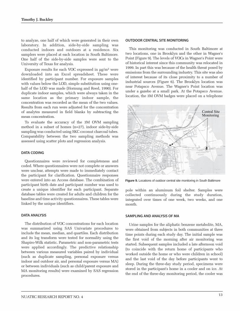
OUTDOOR CENTRAL SITE MONITORING
SAMPLING AND ANALYSIS OF MA
RESULTS
SURVEY
QUALITY ASSURANCE/QUALITY CONTROL
COTININE
CENTRAL SITE MONITORING
TRANS, TRANS -MUCONIC ACID (MA)
DISCUSSION AND CONCLUSIONS
ACKNOWLEDGEMENTS
REFERENCES
PUBLICATIONS RESULTING FROM THIS STUDY
ABBREVIATIONS
ABOUT THE AUTHORS
APPENDICES
A. JHSPH / TXSPH Inter-laboratory Comparison Study Protocol
B. Study Subject Demographics and Physical Characteristics
C. Personal, Indoor, and Outdoor Air Monitoring Results
D. South Baltimore Outdoor Fixed Site Air Monitoring Results
E. Laboratory Intercomparison Study Results
F. Survey Forms

PREFACE
The Clean Air Act Amendments of 1990 established acontrol program for sources of 188 “hazardous air pollutants,or air toxics,” which may pose a risk to public health. Also,with the passage of these Amendments, Congressestablished the Mickey Leland National Urban Air ToxicsResearch Center (NUATRC) to develop and direct anenvironmental health research program that would promotea better understanding of the risks posed to human health bythe presence of these toxic chemicals in urban air.
Established as a public/private research organization, theCenter’s research program is developed with guidance anddirection from scientific experts from academia, industry,and government and seeks to fill gaps in scientific data.These research results are intended to assist policy makers inreaching sound environmental health decisions. TheNUATRC accomplishes its research mission by sponsoringresearch on human health effects of air toxics by universitiesand research institutions and by publishing the researchfindings in its “NUATRC Research Reports,” therebycontributing meaningful and relevant data to the peer-reviewed scientific literature.
The study “VOC Exposure of An Industry-ImpactedCommunity” was developed in response to the MickeyLeland National Urban Air Toxics Research Center(NUATRC) Request For Application 98-03 (RFA 98-03),under the NUATRC Small Grants New InvestigatorsProgram. This NUATRC support was developed toencourage New Investigators to develop innovative air toxicsresearch areas. This specific RFA was developed to supportshort-term research projects on exposures and/or healtheffects of air toxics. The projects were envisioned to becommunity-based pilot projects that could serve as a basisfor more extended research. Preference was given to researchthat tested new techniques and/or were innovative or high-risk projects. Pilot projects by their nature are limited inscope and are designed to give preliminary results and newinsights so that larger studies, yielding results with broaderapplications, might follow.
Dr. Timothy J. Buckley of the Johns Hopkins Universitywas a recipient of a cost-reimbursable contract from theNUATRC to provide exposure information on an urbancommunity in close proximity to industrial sources. Dr.Buckley had conducted an initial exposure study in thiscommunity through pilot funding by the U.S. EPA Region III.Dr. Buckley and his research team addressed this issue bymeasuring levels of personal, indoor, and outdoor air toxicsand assessing indoor and outdoor source contribution. Inorder to provide the community a perspective on their level
of exposure, Dr. Buckley and his research team conductedsimilar measurements in a comparison community that wasnot impacted by industrial emissions. They also assessed theutility of measurement of a biomarker for benzene calledtrans, trans muconic acid for low level exposures to this airtoxic in both communities. This report presents a detaileddescription of the study objectives, design, methods, thenature and quality of the data, an initial descriptive analysisof the data, and interpretation of the results.
When a NUATRC-funded study is completed, theInvestigators submit a draft final research report. Every draftfinal report resulting from NUATRC-funded researchundergoes an extensive evaluation procedure, whichassesses the strengths and limitations of the study, andcomments on clarity of the presentation, data quality,appropiateness of study design, data analysis, andinterpretation of the study findings. The objective of thereview process is to ensure that the Investigator’s report iscomplete, accurate, and clear.
The evaluation first involves an external review of thereport by a team of three external reviewers including abiostatistician. The reviewers’ comments are thenconsidered by members of the NUATRC Scientific AdvisoryPanel (SAP), and the comments of the external reviewersand the SAP are provided to the Investigator. In itscommunication with the Investigator, the SAP may suggestalternate interpretations for the results and also discuss newinsights that the study may offer to the scientitfc literature.The Investigor has the opportunity to exchange commentswith the SAP and if necessary revise the draft report. Inaccordance with the NUATRC policy, the SAP recommendsand the Board of Directors approves the publication of therevised final report. The research presented in the NUATRCResearch Reports represents the work of its Investigators.
The NUATRC appreciates hearing comments from itsreaders from industry, academic institutions, governmentagencies, and the public about the usefulness of theinformation contained in these reports, and about otherways that the NUATRC may effectively serve the needs ofthese groups. The NUATRC wishes to express its sincereappreciation to Dr. Buckley and his research team, the SAP,and external peer reviewers whose expertise, diligence, andpatience have facilitated the successful completion of thisreport.
1NUATRC RESEARCH REPORT NO. 4
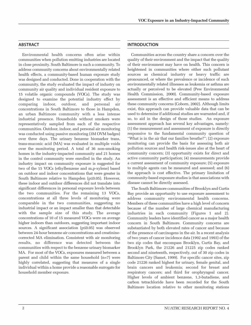
ABSTRACT
Environmental health concerns often arise withincommunities when pollution emitting industries are locatedin close proximity. South Baltimore is such a community. Toaddress community concerns about environmentally relatedhealth effects, a community-based human exposure studywas designed and conducted. Done in cooperation with thecommunity, the study evaluated the impact of industry oncommunity air quality and individual resident exposure to15 volatile organic compounds (VOCs). The study wasdesigned to examine the potential industry effect bycomparing indoor, outdoor, and personal airconcentrations in South Baltimore to those in Hampden,an urban Baltimore community with a less intenseindustrial presence. Households without smokers wererepresentatively sampled from each of the respectivecommunities. Outdoor, indoor, and personal air monitoringwas conducted using passive monitoring (3M OVM badges)over three days. The urinary benzene biomarker trans,trans-muconic acid (MA) was evaluated in multiple voidsover the monitoring period. A total of 36 non-smokinghomes in the industry-impacted community and 21 homesin the control community were enrolled in the study. Anindustry impact on community exposure is suggested fortwo of the 15 VOCs (ethylbenzene and m,p-xylene) basedon outdoor and indoor concentrations that were greater inSouth Baltimore relative to Hampden (p≤0.05). However,these indoor and outdoor differences did not translate intosignificant differences in personal exposure levels betweenthe two communities. For the remaining 13 VOCs,concentrations at all three levels of monitoring werecomparable in the two communities, suggesting noindustrial impact or an impact smaller than that detectablewith the sample size of this study. The averageconcentrations of 10 of 15 measured VOCs were on averagehigher indoors than outdoors, suggesting important indoorsources. A significant association (p≤0.05) was observedbetween 24-hour benzene air concentrations and creatinine-corrected MA elimination. Consistent with air monitoringresults, no difference was detected between thecommunities with respect to the benzene urinary biomarkerMA. For most of the VOCs, exposures measured between aparent and child within the same household (n=7) werehighly correlated, suggesting that measures of a singleindividual within a home provide a reasonable surrogate forhousehold member exposure.
INTRODUCTION
Communities across the country share a concern over thequality of their environment and the impact that the qualityof their environment may have on health. This concern isheightened in communities where either such pollutantsources as chemical industry or heavy traffic arepronounced, or where the prevalence or incidence of suchenvironmentally related illnesses as leukemia or asthma areactually or perceived to be elevated (Pew EnvironmentalHealth Commission, 2000). Community-based exposureassessment is an effective and efficient means to addressthese community concerns (Coborn, 2002). Although limitsexist, this approach can provide valuable data that can beused to determine if additional studies are warranted and, ifso, to aid in the design of those studies. An exposureassessment approach has several key advantages, namely:(1) the measurement and assessment of exposure is directlyresponsive to the fundamental community question of“What is in the air that our families breathe?”; (2) exposuremonitoring can provide the basis for assessing both airpollution sources and health risk-issues also at the heart ofcommunity concern; (3) opportunity exists for direct andactive community participation; (4) measurements providea current assessment of community exposure; (5) exposureto multiple agents can be measured and assessed; and (6)the approach is cost effective. The primary limitation ofcommunity-based exposure studies is that associations withdisease cannot be directly assessed.
The South Baltimore communities of Brooklyn and CurtisBay provide an opportunity to use exposure assessment toaddress community environmental health concerns.Members of these communities have a high level of concernbecause of the number of large chemical manufacturingindustries in each community (Figures 1 and 2).Community leaders have identified cancer as a major healthconcern in South Baltimore. Community concerns aresubstantiated by both elevated rates of cancer and becauseof the presence of carcinogens in the air. In a recent analysisof two years of cancer incidence data (1992 and 1993) of thetwo zip codes that encompass Brooklyn, Curtis Bay, andBrooklyn Park, the 21226 and 21225 zip codes rankedsecond and nineteenth, respectively, out of 30 zip codes inBaltimore City (Samet, 1999). For specific cancer sites, zipcode 21226 ranked highest for urinary, female genital, andbrain cancers and leukemia; second for breast andrespiratory cancers; and third for orophryngeal cancer.Higher levels of ambient benzene, 1,3-butadiene, andcarbon tetrachloride have been recorded for the SouthBaltimore location relative to other monitoring stations
2
VOC Exposure in an Industry-Impacted Community
NUATRC RESEARCH REPORT NO. 4

across the city and state (Figure 3). Using historical data, Littet al. (2002) found numerous hazardous operations inSoutheast Baltimore, including metal smelting, oil refining,warehousing, transportation, and paints, plastic, and metalsmanufacturing. Faced with elevated cancer rates and theintensity and proximity of industrial sources, thecommunity asks a fundamental public health question:“What is in the toxic soup that makes up the air that webreathe?” Although health and, especially, cancer are thecommunity's primary concerns, epidemiologic approachesare limited, both practically and technically, because ofissues of statistical power, sample size, cost, and diseaselatency. A study of community exposure potentially
addresses many community concerns and questions,provides a basis to assess the exposure distribution of thepopulation for purposes of risk assessment or forcomparison to health guidelines, and provides referencelocation information. In addition to providing thecommunity with valued information about environmentaltoxics that may contaminate their environment, suchstudies can provide necessary information to gauge theneed for and aid in the design of possible future healthstudies.
3
Timothy J. Buckley
NUATRC RESEARCH REPORT NO. 4
Figure 1. Aerial view showing the industrial region of South Baltimoreincluding adjacent communities of Curtis Bay and Brooklyn
Figure 2. Satellite image of South Baltimore showing the intense industrialactivity adjacent to Brooklyn and Curtis Bay
BrooklynCurtis BayBrooklyn Park
Carbon tetrachloride
0.00
0.05
0.10
0.15
0.20
0.25
1991 1992 1993 1994 1995 1996 1998
Year (1991-1996, 1998)ESSEX FMC FORTMcH GLENB NEPOLICE OLDTOWN
Benzene
0.00
0.20
0.40
0.60
0.80
1.00
1.20
1.40
1.60
1.80
2.00
1991 1992 1993 1994 1995 1996 1998
Year (1991-1996, 1998)ESSEX FMC FORTMcH GLENB NEPOLICE OLDTOWN
1,3-Butadiene
0.00
0.10
0.20
0.30
0.40
0.50
0.60
1991 1992 1993 1994 1995 1996 1998
Year (1991-1996, 1998)ESSEX FMC FORTMcH GLENB NEPOLICE OLDTOWN
Figure 3. Historical annual average levels of VOCs in South Baltimore(FMC site) relative to other Baltimore City monitoring sites (MarylandDepartment of the Environment)

On many levels, the community's interests are consistentwith industrial interests. Both seek good schools and ahealthy community and environment. However, industryand the community have vastly different perceptions of theeffects that industrial activity has on the community'senvironment and health. Local, state and federalgovernments become caught in the middle, and the absenceof relevant and objective information or data provides fertileground for speculation and for divisive rhetoric and rancor.Issues of exposure and risk often become volatile when thecommunity is economically or socially disadvantaged.Political and socio-economic factors can become moreimportant than the science. Stakeholders, including thecommunity, industry, and local government, often agreethat exposure assessment is an effective means to fill aninformation void that exacerbates the gap betweenperception and reality. When such research is available,effective risk communication is recognized as being a keyfactor in gaining stakeholder acceptance and in managingthe dynamic relationship between science and perception(Miller and Solomon, 2003; Payne-Sturges et al., 2004).
Community-based exposure research is most effectivelyachieved when it is planned and implemented through aprocess that engages and invests the community. Bysubstantively involving the community in the design,conduct, and interpretation of the study, communitymembers are not only informed, but are also involved in thecommunication and coordination of the project. Thecommunity's active participation increases its awareness,knowledge, and capacity to understand sources anddeterminants of exposure in the environment (Israel et al.,1998).
Exposure assessment can provide practical information tothe community and address a nationally recognized needfor information about human exposure to air toxins.Recognition is growing that the current shortage of actualhuman exposure data seriously hinders efforts to makereasoned and credible decisions about the assessment,management, and communication of environmental healthrisks (Burke et al., 1992; Burke and Sexton, 1995; Sexton etal., 1992, 1995; Pew Environmental Health Commission,2000; US GAO, 2000). Exposure data can help to identifysuch sub-populations as children, low-income groups, orethnic minorities that may be at increased health riskbecause they face disproportionately high levels ofexposure. Exposure data can strengthen epidemiologicstudies by: (1) examining links between human exposuresand health outcomes; (2) evaluating current status,historical trends, and possible future directions in humanexposure; and (3) evaluating environmental policies
designed to reduce exposures and to protect public health.Furthermore, these data can provide key informationneeded for risk-based decision making. Human exposuredata should play a vital role in shaping nationalenvironmental health policies.
Hazardous air pollutants (HAPs) or air toxics aregenerally defined as pollutants known or suspected to causecancer or other serious health effects or to harm theenvironment (NATA Glossary of Terms). The Clean Air ActAmendments of 1990 (CAAA) require EPA to regulateambient sources of 189 HAPS. The HAPs include industrialchemicals and intermediates, pesticides, chlorinated andhydrocarbon solvents, metals, combustion byproducts, autoexhaust, such chemical groups as polychlorinatedbiphenyls (PCBs), and such mixed chemicals as coke ovenemissions. More than 80% of the compounds on the federalHAPs list are VOCs, some of which, including benzene, areubiquitous ambient air contaminants.
According to the EPA, 42% of total HAP emissions intothe ambient environment are from mobile sources,including cars, trucks, buses, and non-road vehicles such asships and farm equipment. “Area sources” make up 34% ofthe HAP emissions and include such smaller stationarysources as dry cleaners, solvent cleaning industries,secondary lead smelters, gas stations, and smallmanufacturing companies. “Major sources,” which includelarge industrial complexes, chemical plants, oil refineriesand steel mills account for 24% of the HAP emissions(Figure 4). Consumer products such as as paints, householdcleaners and computer printer cartridges also containHAPs. However, emissions from these sources, whichmainly affect the indoor environment, are not regulated byEPA.
NUATRC RESEARCH REPORT NO. 44
VOC Exposure in an Industry-Impacted Community
Area Sources34%
Major Sources24%
Mobile Sources42%
Figure 4. 1993 U.S. total air toxic pollutant emissions (EPA, 1998)

NUATRC RESEARCH REPORT NO. 4
Considerable evidence links VOC exposure to suchadverse health effects as asthma and cancer. Ware andcoworkers (1993) identified a significant associationbetween VOCs of industrial origin and physician-diagnosedasthma (OR =1.27, 95% CI: 1.09-1.48) and chronic lowerrespiratory symptoms (OR=1.13; 95% CI: 1.02-1.26). Inchamber studies involving exposure of healthy adults to atypical indoor VOC air mixture (0, 25, 50 mg/m3), Pappasand coworkers (2000) observed a dose-dependent increasein respiratory symptoms. Wieslander and coworkers (1997)found higher rates of asthma and respiratory inflamationamong persons exposed to formaldehyde and VOCs off-gassing from newly painted surfaces. This VOC exposuremay also pose a cancer risk. Pearson and coworkers (2000)showed a significant association between residences nearhighly trafficked roadways and children's cancer of alltypes (odds ratio of 5.90; 95% C.I. from 1.69 to 20.56) andfor leukemia (8.28; 95% CI 2.09-32.80). Raaschou-Nielsenand coworkers (2001) reported no increased risk ofleukemia or central nervous system tumors associated withbenzene exposure but found a significant trend inlymphoma risk for exposure during pregnancy. Feychtingand coworkers (1998), who used ambient NO2 as a surrogatefor traffic-related air pollution, found significant relativerisks of leukemia and central nervous tumors for exposures≥80 µg/m3 (p≤0.05). Using a case-system control studydesign, Savitz and Feingold (1989) observed odds ratios of1.7 (95% CI 1.0-2.8) for total childhood cancers and 2.1(95% CI 1.1-4.0) for leukemia, with stronger associationsobserved for higher traffic volumes.
Exposure to environmental carcinogens is of particularconcern in Baltimore City where the cancer mortality rate(255 per 100,000) is significantly higher than for the State ofMaryland (191.4 per 100,000). It is noteworthy thatMaryland's cancer mortality rate is significantly higher thanthat of the rest of the United States, which is 172.8 per100,000 (Maryland Cancer Consortium, 1996). Humanexposure to cancer-causing agents in the environment isbelieved to be a contributing factor to the observed higherurban rates. For the period 1994 to 1998, according to Riesand coworkers (2001), Maryland was ninth in the nationand 7.8% greater than the national average (p≤0.0002).Maryland also has the unfortunate distinction of beingranked third among U.S. states for estimated cancer riskattributed to exposure to ambient concentrations of airtoxics. With an estimated 420 per million air toxics-relatedexcess cancer deaths, Maryland ranked behind the Districtof Columbia and New York, but above New Jersey.Moreover, Baltimore City ranked as number one for “addedcancer deaths attributable to air toxics,” with an estimatedrisk of 970 per million excess cancer deaths. These
estimates and rankings are available from the U.S. EPACumulative Exposure Project, which provides estimates ofoutdoor pollution levels for the 10,600 census tracts acrossthe U.S. based on dispersion modeling of point, area, andmobile sources (Woodruff et al., 1998; Caldwell et al., 1998;Rosenbaum et al., 1999). Estimates of cancer risk arederived from the application of standard cancer potencyfactors to the estimated outdoor concentrations. Since theseestimates are based on industrial, area, and mobile sourceemissions (U.S. EPA Toxic Release Inventory), these datasuggest that Baltimore has some of the highest emissions ofcancer-causing air pollution in the country.
The 1990 Clean Air Act Amendments require that EPAidentify effective control strategies to reduce public healthrisks from exposure to HAPs. However, for EPA to identifysuch strategies, basic information is needed about the levelof HAPs to which the general population is exposed acrossthe United States. This information must also be linkedwith potential adverse human health effects. While EPAand state environmental agencies maintain well establishedambient monitoring networks for such criteria pollutants asozone, particulate matter, and carbon monoxide, relativelylittle is known about the HAP concentrations in outdoor air,and even less is known about actual human exposures toHAPs.
MUCONIC ACID
Exposure assessment that includes measurement ofparent compounds and/or metabolites in biologicalspecimens adds substantially to the knowledge gained insuch research by providing information on individualvariation in absorption and metabolism. This information isessential for understanding the marked differences inhuman susceptibility for adverse health outcomes routinelyobserved in populations exposed to toxicants at similarlevels. Furthermore, a growing body of literature is availablefor meaningful interpretation of biological markers (Buckleyet al., 1995, 1997; Weaver et al., 2000). Such informationwill ultimately help to identify high-risk individuals andpopulations. This is particularly important when thetoxicant of interest is a carcinogen.
The optimal biological monitoring method for benzenevaries by level of exposure. In recent years, due to itsrecognition as a human carcinogen, benzene exposurelevels have declined. This is due, in large part, to USOccupational Safety and Health Administration (OSHA)and EPA legislation. This decline has had a substantialimpact on biological monitoring for benzene. Initially, thebenzene metabolite, phenol, was monitored in the urine of
5
Timothy J. Buckley

exposed workers. It is a relatively easy metabolite to assay,which is an important advantage in medical surveillanceand molecular epidemiological research. However, phenolis found in many foods and is a product of proteincatabolism. Hence, it lacks the specificity needed forexposures below 5 ppm (Ducos et al., 1992). At these lowerlevels, it is routinely found in most urine samples and is notcorrelated with exposure. Currently, phenol is useful as abenzene biomarker only after accidental high-levelexposures.
As a result, researchers have explored the biomarkerpotential of several other benzene metabolites as well as theparent compound itself. Trans, trans-muconic acid (MA), astraight chain metabolite, is both sensitive and specific inworkers exposed to a wide range of air benzeneconcentrations. Correlations between MA and air benzenehave been reported at levels of benzene as low as 0.5 ppm,and even lower in some studies (Ducos et al., 1992; Ducoset al., 1990; Lee et al., 1993; Lauwerys et al., 1994). Theassay for MA is also relatively fast and simple. Animal datasuggest that a greater proportion of benzene is metabolizedto MA at lower exposure levels, which is important, sincethis is thought to be a toxic pathway (Henderson et al.,1989). The effect of dose, dose rate, route of administration,and species on tissue and blood levels of benzenemetabolites (Environ Health Perspec. 1989;82:9-17). Aswith phenol, the use of MA as a biomarker for low-levelbenzene exposure is complicated by the fact that it is notcompletely specific for benzene either. Sorbate foodpreservatives, such as sorbic acid and potassium sorbate,are metabolized to MA (West, 1964). Approximately 0.05 to0.5 % of ingested sorbic acid tablets is metabolized to MA(Ruppert et al., 1997). Sorbate preservatives are used inseveral food categories including processed cheese slicesand spreads, refrigerated flavored drinks, sweet bakedgoods, frozen foods, mayonnaise, margarine, and saladdressing.
There is a growing body of literature evaluatingassociations between MA and low-level ambient benzeneexposure, where non-specificity is most likely to be aproblem. In general, significantly higher mean levels arefound in smokers compared to nonsmokers (Melikian et al.,1993). A linear correlation with cotinine in smokers hasalso been reported (Ong et al., 1996). Excretion of MA in a12-hour post-exposure period was correlated with short-term exposure to environmental tobacco smoke in a USpopulation; however, diet was carefully controlled in thisstudy (Yu, 1995). In contrast to phenol, MA is not routinelyfound in the urine of non-smokers. Bergamaschi andcoworkers (1998) studied MA levels in 24 non-smoking
volunteers who biked for two hours in urban and ruralsettings. A statistically significant correlation coefficient (r =0.59) was found between air benzene (ranging from 1.2 to26.1 ppb) and the increase in MA pre- to post-ride. Thecorrelation increased (r = 0.68) when the population waslimited to subjects who were homozygous for the wild typeepoxide hydrolase genotype. However, Ong and coworkers(1994) found no correlation between air benzene and post-shift MA in low-level occupationally exposed workers (<0.25 ppm). Urinary benzene and MA were not correlated ina study of 80 bus drivers, whose benzene exposure, basedon urine benzene, was calculated to range from 3 to 313 ppb(Gobba et al., 1997). In addition, other studies have notedexcessively high MA levels (consistent with exposures to1.0 ppm benzene) in controls who had no occupationalsource of benzene exposure to explain the elevated levels(Rauscher et al., 1994; Weaver et al., 1996; Gobba et al.,1997; Johnson and Lucier, 1992).
In order to determine the impact of sorbate preservativeson these inconsistent results, studies have assessed theurinary MA response following ingestion of sorbic acid orpotassium sorbate in pill form (Pezzagno et al., 1999;Ruppert et al., 1997) This work indicates that non-specificity of MA as a biomarker for low level benzeneexposure may be a problem in populations with substantialconsumption of sorbate preserved foods. However, theactual extent of this interference cannot be determined fromthis research, since the amount of these preservatives in thediet must be estimated. Non-specificity of MA from sorbatesis a particular concern in the US where significantconsumption of preserved food occurs. Furthermore, mostof the MA validation studies were not done in USpopulations, and so it cannot be assumed that adequatecorrelations at lower air benzene levels seen in otherpopulations will also apply in the US. Therefore, MA levelswere measured in sequential spot urine samples fromvolunteers who consumed foods containing sorbatepreservatives that are common in the US diet and usuallyingested in substantial amounts when consumed (Weaver etal., 2000). It has been found that, when refrigerated, flavoreddrinks and sweet snack foods resulted in the excretion oflarge amounts of MA in adults and children. Theseincreases were large enough to result in non-specificity ofMA as a biomarker for environmental exposure and formany occupational settings in industrialized countries.
If MA is to be used as a biomarker for low-level benzenein countries with significant ingestion of sorbate foodpreservatives, methods to avoid interference will need to beused. Potential solutions include simultaneously measuringurinary sorbic acid and/or dietary restriction. The latter
6
VOC Exposure in an Industry-Impacted Community
NUATRC RESEARCH REPORT NO. 4

approach is presently used in biomonitoring for inorganicarsenic. Prior to availability of arsenic speciation, and evencurrently to reduce costs, seafood ingestion is restrictedprior to urine collection in an effort to prevent elevations intotal arsenic from organic arsenic in seafood. This approachfor sorbic acid may be possible because, although severalfood types contain sorbate preservatives, the amount ofthese foods that is consumed in a sitting varies. Those thatare consumed only in small quantities likely have lesspotential to increase MA.
S-phenylmercapturic acid (S-PMA) is another benzenemetabolite. It is currently thought to be more specific forbenzene exposure than MA, making it attractive as abiomarker for environmental exposure. In addition, itprovides information on metabolic protective mechanisms.Thus far, however, its use has been more limited than MA,since a smaller proportion of benzene is metabolized to S-PMA and the assay is extremely time consuming.Nevertheless, results from analysis using a GC/MSassessment method to measure S-PMA from exposedworkers showed a linear relation with benzene air levelswell below 1.0 ppm (Boogard and van Sittert, 1995; vanSittert et al., 1993). Melikian and coworkers (2002)evaluated both MA and S-PMA in benzene exposedworkers and concluded that S-PMA was superior to MA asa biomarker for low levels of benzene exposure. Therefore,measurement of S-PMA may be useful despite the timeinvolved in the assay, when MA levels are high in settingsof low benzene exposure.
STUDY DESCRIPTION AND OBJECTIVES
The goal of this study was to provide exposureinformation to a community concerned about healthhazards posed by the intensity and proximity of industrialsources. This goal was achieved by measuring levels ofpersonal, indoor, and outdoor air toxics and assessingindoor and outdoor source contributions for the impactedcommunity and a comparison community that is notindustry impacted. This provided the industrially impactedcommunity with a perspective on their level of exposureand the relative importance of indoor and outdoor sources.To assess its utility as a biomarker for low-levelenvironmental exposures, MA was measured in bothpopulation groups. In a subset of homes, parent-child pairswere monitored to assess within-home correlations of VOCexposure and MA between parents and those childrenliving within the same home. This provided exposureinformation on children, a potentially susceptible
subpopulation; furthermore, the paired monitoring mayprovide information on possible age-related differences inbenzene metabolism.
These study objectives were achieved through fourspecific aims. These aims were:
1. To measure personal, indoor, and outdoorconcentrations of VOC air toxins and relatedtime/activity patterns over two seasons for arepresentative sample of individuals from thecommunities of Brooklyn and Curtis Bay
2. To compare exposures in the Brooklyn / Curtis Baycommunity to exposures of a sample of individualswho do not live or work in close proximity toindustrial/chemical sources
3. To delineate the contribution of indoor and outdoorsources to indoor residential air concentrations in asubset of study homes
4. To evaluate the predictive relationship betweenbenzene exposure and parent / child levels of thebiomarker MA
METHODS
EXPERIMENTAL DESIGN
To evaluate the effect of industry on community airquality, levels of air toxics in indoor, outdoor, and personalair were assessed in two Baltimore urban communitieshaving similar demographics but differing industrialprofile. In addition, the biomarker MA was measured inboth population groups to assess its utility for measuringlow-level environmental benzene exposures. In a subset ofhomes, parent-child pairs were monitored to assess within-home correlation in VOC exposure and excretion betweenparents and those children living within the same home.Monitoring of children was to provide exposureinformation on a potentially susceptible sub-population.
SITE DESCRIPTION
The control community of Hampden had a population in1990 of 15,424 and is located in central Baltimoreapproximately six miles due north of South Baltimore(Figure 5). According to the 1990 census, the experimentalSouth Baltimore communities (Brooklyn, Brooklyn Park,Brooklyn Manor, Arundel Village, Curtis Bay, and Fairfield)had a total population of 27,956, median household income
7
Timothy J. Buckley
NUATRC RESEARCH REPORT NO. 4

of $27,041, with 9.7% of the population comprised of non-whites (Table 1). The South Baltimore community in thisstudy included eight census blocks, specifically, 7502.02,7502.03, 7501.01, 7501.02, 2504.01, 2504.02, 2505, and2506 across two zip codes (21225 and 21226). TheHampden community consisted of approximately 2000households across five census blocks, including 1308.03,
1308.04, 1307, 1306, and 1305. All five census blocks werein the 21211 zip code. At the level of the census block, someaspects of the 2000 census data are available. This includesrace data. These data are given in Table 2. A comparison ofcensus data from 1990 and 2000 suggests a comparablechange in population demographics for the twocommunities, namely a decrease in population (13% and12%) and an approximate doubling of the nonwhiteminority population from 9.7% to 21% and 6.2% to 12%for South Baltimore and Hampden, respectively.
EMISSIONS
According to data from the EPA 1999 Toxic ReleaseInventory, 61 reporting facilities exist in South Baltimore's21225 and 21226 zip code regions. Fifteen of these report airtoxic releases (Figure 6). This compares to three reportingfacilities in Hampden, of which one reports air releases(Figure 7). Among these communities, seven industries inSouth Baltimore and one in Hampden report releases that
8
VOC Exposure in an Industry-Impacted Community
NUATRC RESEARCH REPORT NO. 4
Figure 5. Baltimore City map showing the industry-impacted and controlstudy locations
Parameter
PopulationRace White Black Asian/Pacific Islander Hispanic OtherMedian HH IncomeEducation<9th grade9th - 12th (no - diploma)
High School GraduateSome College (no degree)
Bachelors DegreeGraduate or Professional Degree
SouthBaltimore
27,956
90.3%8.2 %1.0 %0.9%0.2%
$27,041
17.3%27.9%36.0%14.3%3.5%1.1%
Hampden
15,424
93.8%4.1%1.5%NA
0.51%$27,223
16.8%26.1%27.6%13.0%8.6%8.0%
Table 1. Demographics for South Baltimore and Hampden from 1990census
Parameter
Population
Race
White
Black
Asian/Pacific Islander
Hispanic
Other
South Baltimore
24,280
79.0%
14.9%
1.6%
2.2%
2.3%
Hampden
13,601
87.8%
5.8%
2.8%
1.8%
1.8%
Table 2. Population and race for South Baltimore and Hampden accordingto the 2000 census*
*The 2000 Census does not include Hampden block number 1305
Baltimore City
Anne Arundel County
TRI Sites
SBC Participants
South Baltimore Area
I895
I895
I97
I195
I695
I895
I83 I95
I95
I95
US 40
US 40US 1
US 1
Figure 6. South Baltimore map showing study area, location of participanthomes, and TRI sites with VOC releases (from U.S. EPA 1999)

match the VOCs measured in the current study. A total of61,152 and 1,317 pounds of VOCs were released into therespective communities. This represents a 46-folddifference between the two communities (Table 3). None ofthe VOCs are common to both communities. With theexception of styrene, emissions of VOCs are higher in SouthBaltimore. The VOC with the highest release in SouthBaltimore is methyl tertiary-butyl ether (MTBE).
SURVEY DESIGN
Homes in the South Baltimore communities and in thecontrol community of Hampden were selected at randomand in proportion to the community population so thatinferences could be made to the entire sampling frame(Whitmore, 1988; Cox et al., 1988; Clickner et al., 1983). Thesampling frame was constructed from 1990 census files.The South Baltimore sampling frame consisted of 578census blocks. A three-stage sampling approach was used to
establish the final random selection (Figure 8). In the firststage, census blocks were weighted by population, and 50blocks were selected at random using Intercooled STATA6.0 for Windows 98. In the second stage, each block wasvisited and the homes were enumerated by address. The listof addresses was then randomized using Microsoft Excel™.Residents in each eligible home were approached in turnuntil residents from the next randomized eligible homeagreed to participate. Residents who satisfied preliminaryeligibility criteria were also required to meet the followingcriteria: (1) the selected home must have been their primaryresidence; (2) no current smokers could live in the home;and (3) subjects could not reside in such institutions asmilitary quarters or prisons. The primary residence criteriawere used to select individuals who represent thepopulation actually residing in the study region. Residenceswithout smokers were of interest because exposures fromindustry were of primary concern in this study and smokingwithin the home would overwhelm any outdoor source.The contribution of smoking to VOC exposure is wellestablished within the literature (Kim et al., 2001; Ashley etal., 1995; Hajimiragha et al., 1989; Gordon et al., 2002;Wallace 1996; Wallace et al., 1987; Wallace andPellizzari,1986). However, at the community’s request, twohomes with smokers were included. Smoking status wasconsidered in data analysis, interpretation, andpresentation.
Recruitment and enrollment in the community-basedexposure study and exposure monitoring were carried outconcurrently over a period of 18 months, from January 2000to July 2001. Personnel responsible for participantrecruitment and environmental monitoring included acommunity resident hired part-time and four students fromthe Johns Hopkins Bloomberg School of Public Health whowere available part-time. Homes were recruited by visiting
9
Timothy J. Buckley
NUATRC RESEARCH REPORT NO. 4
Total Air Emissions (pounds)ChemicalSouth Baltimore
21225/6Hampden
21211
Benzene 3,661Carbon Tetrachloride 90 Ethylbenzene 1,052Methyl Tert-Butyl Ether 44,679Toluene 7,815Xylene (Mixed Isomers) 3,855 Styrene 1,317
Total 61,152 1,317
Table 3. 1999 TRI reported target VOC emissions for South Baltimore andHampden
Figure 7. Map of the control location of Hampden showing the study area,location of participating homes, and TRI sites (U.S. EPA 1999)
Baltimore City
Anne Arundel County
TRI Sites
Hampden Participants
Hampden
I83
I895
I895
I83
US 40
US 1
I83
US 1
Brooklyn
Curtis Bay
Study Region
Census Blockn = 572
Selection Proportionalto Size n=40
Enumeration ofHouseholds
Random Selectionof Household
Recruit
Sample(Season 1)
(n = 23,138)
(n = 3,868)
Sample(Season 2)
Figure 8. Survey design schematic overview for South Baltimore
the home and knocking on the door. If there was no answer,a letter of invitation was left that included study personnelcontact information (see Appendix F-1). Five separate visitsat different times and days were made before the home wasclassified as a “no answer refusal” and the next home on therandomized list was approached. For addresses where suchfactors as boarded windows and doors, tips from neighbors,or other indicators made it clear that the home wasunoccupied, the address was logged as "vacant" and thenext random address selected. Where contact with aresident in a home was established, the household wasscreened for eligibility requirements. If the resident wasunwilling to participate, the address was logged as "refusal,"or if the resident was determined to be a smoker, the addresswas logged as "smoker" and the next home on the randomlist was approached. If a resident agreed to participate andmet the eligibility requirements, the address was recordedand an appointment was made for a home visit to furtherexplain the study, obtain consent, and set up themonitoring. Only one adult from each enrolled householdwas monitored. If children resided in the South Baltimorehomes, they were also invited to participate.
QUESTIONNAIRES
Four questionnaires were administered to each studyparticipant. The Baseline Questionnaire was used to collectsuch demographic information as age, race, occupation,household income, and potential sources of exposure toVOCs, including use of air fresheners, exposure to drycleaned clothes, and modes of transportation (Appendix F-5). The Technician Walk-Through Questionnaire was usedto gather such housing characteristic information as numberof floors, number of rooms, and distance of the home fromthe street (Appendix F-3). Both the Baseline Questionnaireand the Technician Walk-Through Questionnaire wereadministered by study personnel on the first day ofmonitoring. The Time Diary and Activity Questionnairewas used to determine the amount of time each participantspent indoors and outdoors and to help identify possibleVOC sources encountered during the three-day monitoringperiod (Appendix F-4). This questionnaire was completedby each participant at the end of each day of monitoring andcollected by study personnel at the end of the monitoringperiod. The questionnaires were developed from existingquestionnaires (such as NHEXAS and TEAM-VOC). Foreach day of monitoring, subjects were asked to complete afood diary to document the ingestion of foods containingsorbic acid or potassium sorbate as an interference for thebiomarker MA (Appendix F-6).
VOC SAMPLING AND ANALYSIS
At the home visit, signatures on consent forms wereobtained and the questionnaires were administered.Personal, residential indoor, and residential outdoorsamplers were set up for each study participant. The 3M(London, Ontario) Organic Vapor Monitor (OMV 3500)sampling badges were used for monitoring. Studyparticipants were asked to wear the sampling badges on ashirt lapel or collar near their breathing zone wheneverpossible, but not when bathing, sleeping or swimming.During these specific times, the participants were asked tokeep their badges within the same microenvironment theyoccupied. Indoor residential sampling badges were placedin the room where the participant spent most of his or hertime when not sleeping. The residential outdoor samplingbadges were placed in a protected but unobstructed locationjust outside the home, for example, on the front porch.
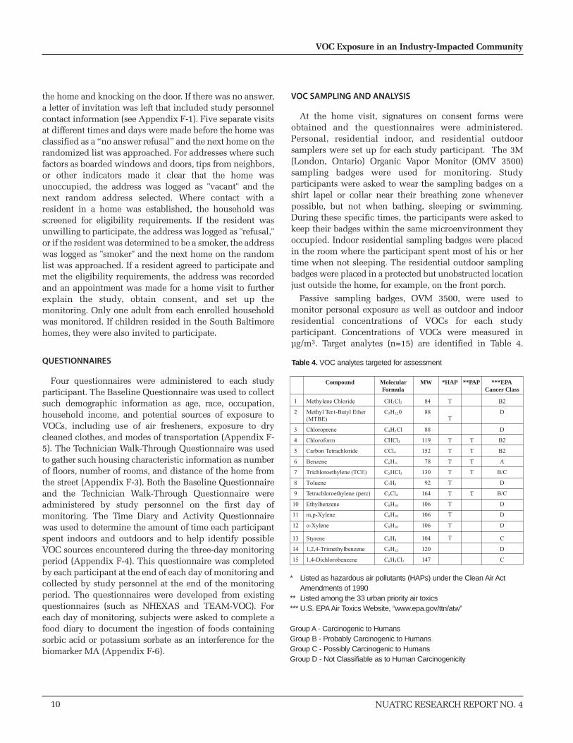
Passive sampling badges, OVM 3500, were used tomonitor personal exposure as well as outdoor and indoorresidential concentrations of VOCs for each studyparticipant. Concentrations of VOCs were measured inµg/m3. Target analytes (n=15) are identified in Table 4.
10
VOC Exposure in an Industry-Impacted Community
NUATRC RESEARCH REPORT NO. 4
Compound MolecularFormula
MW *HAP **PAP ***EPACancer Class
1 Methylene Chloride CH2Cl2 T
T
T
T
T
T
T
T
T
T
T
T
T
T
T
T
T
B2
2 Methyl Ter t-Butyl Ether (MTBE)
C5H120 D
3 Chloroprene C4H5Cl D
4 Chloroform CHCl3 B2
5 Carbon Tetrachloride CCl4 B2
6 Benzene C6H 6 A
7 Trichloroethylene (TCE) C2HCl3 B/C
8 Toluene C7H8 D
9 Tetrachloroethylene (perc) C2Cl4 B/C
10 Ethylbenzene C8H10 D
11 m,p-Xylene C8H10 D
12 o-Xylene C8H10 D
13 Styrene C8H8 C
14 1,2,4-Trimethylbenzene C9H12 D
15 1,4-Dichlorobenzene C6H4Cl2
84
88
88
119
152
78
130
92
164
106
106
106
104
120
147 C
Table 4. VOC analytes targeted for assessment
* Listed as hazardous air pollutants (HAPs) under the Clean Air Act Amendments of 1990
** Listed among the 33 urban priority air toxics*** U.S. EPAAir Toxics Website, “www.epa.gov/ttn/atw”
Group A - Carcinogenic to HumansGroup B - Probably Carcinogenic to HumansGroup C - Possibly Carcinogenic to HumansGroup D - Not Classifiable as to Human Carcinogenicity
These include 12 VOCs considered hazardous air pollutantsunder the CAAA. Six of targeted VOCs are also consideredpriority urban air pollutants by EPA under the IntegratedUrban Air Toxics Strategy. These six pollutants have beendetermined by EPA to present the greatest threat to publichealth in the largest number of urban areas and are,therefore, subject to health risk reduction goals under theCAAA. Selection of target analytes was based on these moregeneric public health concerns, as well specific communityconcerns regarding environmental carcinogens. In addition,these analytes satisfied logistical criteria since they could besampled using the 3M OVM badges.
All monitoring was conducted over a nominal 72-hourperiod. Badges absorb target VOCs by Fick's First Law ofDiffusion, which states that flux is proportional to theconcentration gradient (Shields, 1987; Brown, 1984). Thebadge samples each VOC at a unique characteristic rate asspecified by the manufacturer.
Sampling was initiated by a trained field technician. Thesampler was removed from its sealed canister, and the exacttime of removal was recorded on a sampling data form. Alsorecorded were the date, type of sample (indoor, outdoor, orpersonal), badge serial number, and home/subjectidentification. Sampling was discontinued three days laterby replacing the diffusion membrane with an air-tight cap,placing the sampler in its canister and sealing the canisterwith a resealable plastic cap. Additional precautions wereinstituted to minimize contamination. This includedsealing the canister with parafilm and placing the canisterinto a zip-lock plastic bag. The date and time of closeoutwere recorded onto the sample data sheet, and the datasheet was placed with the badge-containing canister in thezip-lock bag. Samples were transported to the laboratorywithin two hours of closeout and stored at -20° C in thelaboratory until analyzed.
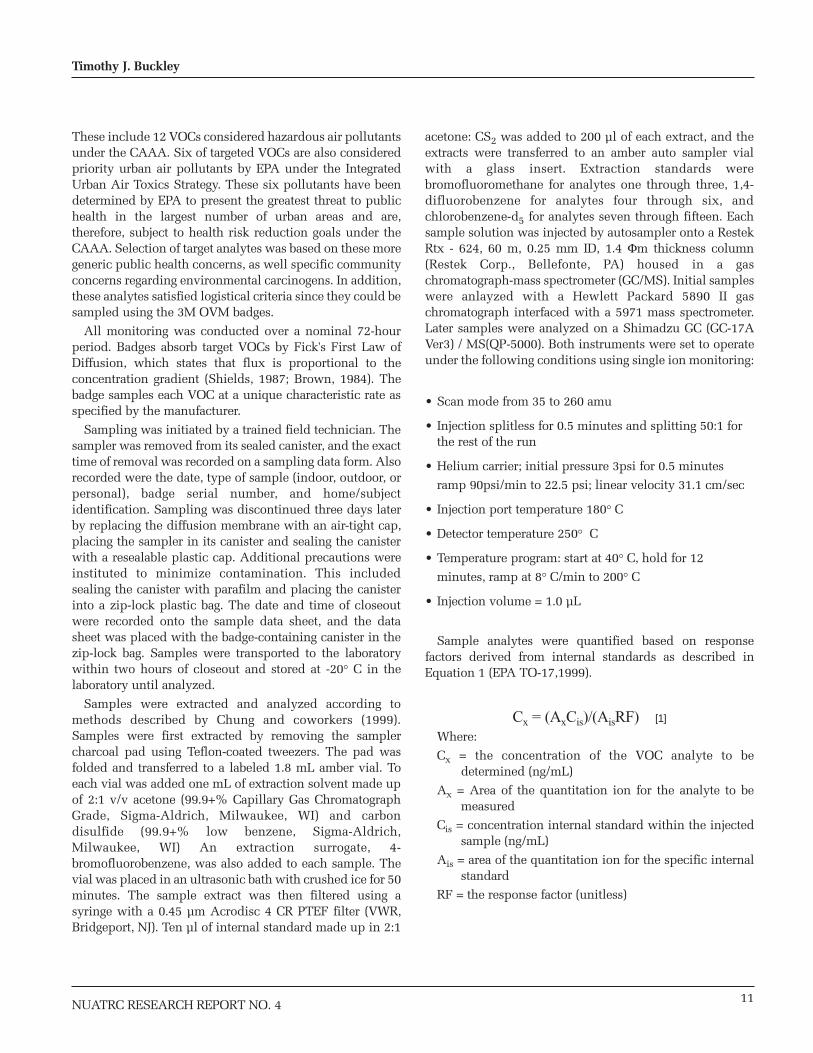
Samples were extracted and analyzed according tomethods described by Chung and coworkers (1999).Samples were first extracted by removing the samplercharcoal pad using Teflon-coated tweezers. The pad wasfolded and transferred to a labeled 1.8 mL amber vial. Toeach vial was added one mL of extraction solvent made upof 2:1 v/v acetone (99.9+% Capillary Gas ChromatographGrade, Sigma-Aldrich, Milwaukee, WI) and carbondisulfide (99.9+% low benzene, Sigma-Aldrich,Milwaukee, WI) An extraction surrogate, 4-bromofluorobenzene, was also added to each sample. Thevial was placed in an ultrasonic bath with crushed ice for 50minutes. The sample extract was then filtered using asyringe with a 0.45 µm Acrodisc 4 CR PTEF filter (VWR,Bridgeport, NJ). Ten µl of internal standard made up in 2:1
acetone: CS2 was added to 200 µl of each extract, and theextracts were transferred to an amber auto sampler vialwith a glass insert. Extraction standards werebromofluoromethane for analytes one through three, 1,4-difluorobenzene for analytes four through six, andchlorobenzene-d5 for analytes seven through fifteen. Eachsample solution was injected by autosampler onto a RestekRtx - 624, 60 m, 0.25 mm ID, 1.4 Φm thickness column(Restek Corp., Bellefonte, PA) housed in a gaschromatograph-mass spectrometer (GC/MS). Initial sampleswere anlayzed with a Hewlett Packard 5890 II gaschromatograph interfaced with a 5971 mass spectrometer.Later samples were analyzed on a Shimadzu GC (GC-17AVer3) / MS(QP-5000). Both instruments were set to operateunder the following conditions using single ion monitoring:
• Scan mode from 35 to 260 amu
• Injection splitless for 0.5 minutes and splitting 50:1 for the rest of the run
• Helium carrier; initial pressure 3psi for 0.5 minutes
ramp 90psi/min to 22.5 psi; linear velocity 31.1 cm/sec
• Injection port temperature 180° C
• Detector temperature 250° C
• Temperature program: start at 40° C, hold for 12
minutes, ramp at 8° C/min to 200° C
• Injection volume = 1.0 µL
Sample analytes were quantified based on responsefactors derived from internal standards as described inEquation 1 (EPA TO-17,1999).
Cx = (AxCis)/(AisRF) [1]
Where:
Cx = the concentration of the VOC analyte to bedetermined (ng/mL)
Ax = Area of the quantitation ion for the analyte to bemeasured
Cis = concentration internal standard within the injectedsample (ng/mL)
Ais = area of the quantitation ion for the specific internalstandard
RF = the response factor (unitless)
11
Timothy J. Buckley
NUATRC RESEARCH REPORT NO. 4

The value of Cx is readily calculated from a combinationof Ax and Ais, given by the sample chromatogram, andRF/Cis, given by the slope of the calibration curve. Externalstandards were obtained from AccuStandard Inc. (NewHeaven, CT). Once the concentration of the VOC within theextract solution was determined (Equation 1), the VOC airconcentration was determined from Equation 2.
C = (WU)/(TRRC) [2]
Where:
C = integrated air toxin concentration (µg/m3)
W = mass of analyte measured in 1.0 mL of extractsolution (µg)
T = sampling duration (min)
R = the sampling rate given by 3M (mL/min)
RC = the recovery coefficient (unitless)
U = a units conversion factor, 1 x 10⁶ mL/m3
The sampling rate was adjusted for temperatureaccording to Table 5.
QUALITY ASSURANCE/QUALITY CONTROL
Procedures for assessing the quality of measurementsmade with the 3M OVM badges were extensive andincluded the elements given in Table 6. The method limit ofdetection (LOD), defined as the lowest concentration of ananalyte that the analytical process can reliably detect(MacDougall et al., 1980), was evaluated in two ways,depending upon whether a discernable chromatographicpeak could be identified for the analyte. For analytes thatcould be discerned in the field blanks, the detection limitwas determined to be the upper 99% confidence intervalgiven by the t value corresponding to the number of blanks(p=0.01) multiplied by the standard deviation of the analytein the measured blanks. For analytes not found in the blank,the limit of detection was determined from the upper 99%confidence interval given by the repeated analysis of a lowlevel spike. Field blanks were treated in the same way ascollected samples, except, the blank was immediatelyclosed upon initiation of sampling. The field blank was keptin the home during the period of monitoring and wastransported in and out of the field with the collectedsample.
Blank and duplicate indoor samples were collected fromeach household. Field blanks were collected to account forcontamination of the badges during manufacturing,transport, sampling, storage, and/or analysis. All sampleswere adjusted for blanks by subtracting the mean quantity
of VOC measured on the blanks from samples. Temperatureand humidity were monitored, since they have been shownto influence diffusion sampling (Larson, 1996; Chung et al,1999). The precision of the 3-day 3M OVM air measurementwas estimated from 19 indoor and 38 outdoor duplicatesamples. Precision was evaluated by the coefficient ofvariation of duplicate samples; that is, the standarddeviation divided by the mean.
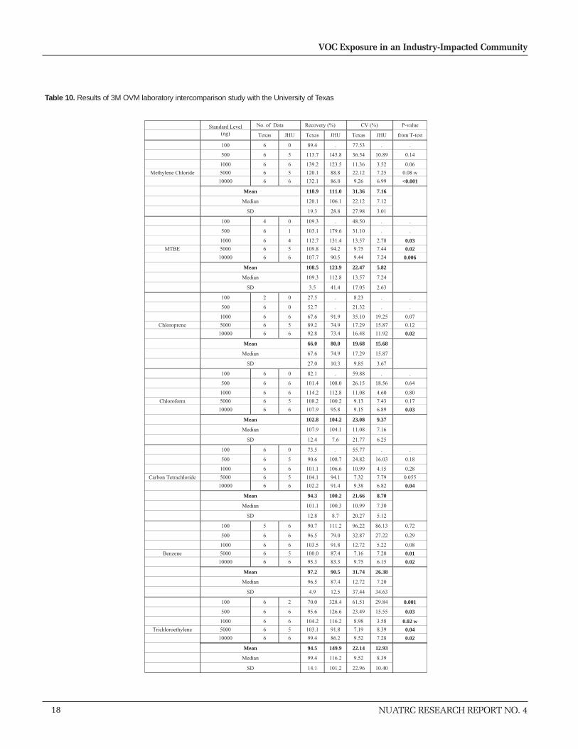
An intercomparison study was conducted with theUniversity of Texas to evaluate measurement precision. Theprotocol of this intercomparison study is given in AppendixA. Badges were spiked at six levels (0, 0.1, 0.5, 1.0, 5.0, and10 µg/badge) by each laboratory. Six badges were spiked ateach of six levels (0, 0.1, 0.5, 1.0, 5.0, and 10 µg/badge) byeach of two laboratories for a total of 72 badges (n= 6 x 6 x2). One half of the badges was retained by each laboratory,and the other half was shipped on ice by next day service tothe other laboratory. Each laboratory had a total of 36 badges
12
VOC Exposure in an Industry-Impacted Community
NUATRC RESEARCH REPORT NO. 4
(° C)
44
37
31
25
19
13
7
2
-3
-8
(° F)
111
99
88
77
66
55
45
36
27
18
(CFT)
0.97
0.98
0.99
1.00
1.01
1.02
1.03
1.04
1.05
1.06
From the above table, every 10-11° F above or below 77° Frequires one percent correction at the calculated time-weightedaverage concentration. CFT is the temperature-dependantcorrection factor.
Table 5. Adjustment for temperature dependent variability in sampling rate
Measurement Parameter Method of Evaluation
Precision Duplicate sampling
Recovery Inter-Laboratory Comparison
Analysis of badges spiked at six levels analyzed at Johns Hopkins and the University of Texas
Detection Limit Analysis of field blanks (for analytes present) or low-level spike samples
Method Comparison Side-by-side indoor sampling comparing the 3M OVM with SKC charcoal tube active sampling
Table 6. Elements of quality assurance / quality control of 3M OVM badges
to analyze, one half of which were generated in their ownlaboratory. In addition, side-by-side sampling wasconducted indoors and outdoors at a residence. Sixsamplers were placed at each location in South Baltimore.One half of the side-by-side samples were sent to theUniversity of Texas for analysis.
Exposure results for each VOC expressed in µg/m3 weredownloaded into an Excel spreadsheet. These wereidentified by participant number. For exposure sampleswith values below the LOD, simple substitution using one-half of the LOD was made (Hornung and Reed, 1990). Forduplicate indoor samples, which were always taken in thesame location as the primary indoor sample, theconcentration was recorded as the mean of the two values.Results from each run were adjusted for the concentrationof analytes measured in field blanks by subtracting themean concentration.
To evaluate the accuracy of the 3M OVM samplingmethod in a subset of homes (n=27), indoor side-by-sidesampling was conducted using SKC coconut charcoal tubes.Comparability between the two sampling methods wasassessed using scatter plots and regression analysis.
DATA CODING
Questionnaires were reviewed for completeness andcoded. Where questionnaires were not complete or answerswere unclear, attempts were made to immediately contactthe participant for clarification. Questionnaire responseswere entered into an Access database. The combination ofparticipant birth date and participant number was used tocreate a unique identifier for each participant. Separatedatabase tables were created for adults and children for thebaseline and time activity questionnaires. These tables werelinked by the unique identifiers.
DATA ANALYSIS
The distribution of VOC concentrations for each locationwas summarized using SAS Univariate procedures toinclude the mean, median, and quartiles. Each distributionand its log transform were tested for normality using theShapiro-Wilk statistic. Parametric and non-parametric testswere applied accordingly. The predictive relationshipbetween various measured variables paired by individual(such as duplicate sampling, personal exposure versusindoor and outdoor air, and personal exposure versus MA)or between individuals (such as child/parent exposure andMA monitoring results) were examined by SAS regressionprocedures.
OUTDOOR CENTRAL SITE MONITORING
This monitoring was conducted in South Baltimore attwo locations, one in Brooklyn and the other in Wagner'sPoint (Figure 9). The levels of VOCs in Wagner's Point wereof historical interest since this community was relocated in1999. In part this was because of the health threat posed byemissions from the surrounding industry. This site was alsoof interest because of its close proximity to a number ofindustrial sources (Figure 6). The Brooklyn location wasnear Potapsco Avenue. The Wagner's Point location wasunder a gazebo at a small park. At the Potapsco Avenue.location, the 3M OVM badges were placed on a telephone
pole within an aluminum foil shelter. Samples werecollected continuously during the study duration,integrated over times of one week, two weeks, and onemonth.
SAMPLING AND ANALYSIS OF MA
Urine samples for the aliphatic benzene metabolite, MA,were obtained from subjects in both communities at threetime points during each study day. The initial sample wasthe first void of the morning after air monitoring wasstarted. Subsequent samples included a late afternoon void(to coincide with the return home of participants whoworked outside the home or who were children in school)and the last void of the day before participants went tosleep. During the three-day study period, specimens werestored in the participant's home in a cooler and on ice. Atthe end of the three-day monitoring period, the cooler was
13
Timothy J. Buckley
NUATRC RESEARCH REPORT NO. 4
**
Central SiteMonitoring
Figure 9. Locations of outdoor central site monitoring in South Baltimore

transported to the lab and stored at -70° C until analyzed.
Dietary instructions were provided to each participant toreduce the ingestion of sorbate preservatives. Thispreservative is an important source of MA, and can interferewith the specificity of MA as a benzene biomarker (Weaveret al., 2000). Participants were asked to avoid the followingthree food types during the entire study:
1. Refrigerated fruit punch drinks such as Sunny Delight®
2. Store brand fruit drinks
3. Baked sweets/snacks such as Hostess Cupcakes®, Little Debbie®, or grocery store cakes
4. Packaged soft cookies such as Snack Wells® and Fig Newtons
5. Soft cheeses, including processed cheese slices, cottage cheese, cheese spreads, Velveeta™, cheese dips, low fat cream cheese, and low fat shredded cheese.
Participants were asked to keep a log with brand names ofall processed foods consumed during the study. Thoseparticipants who were monitored for benzene in 24-hourpersonal air samples were asked to avoid all products withsorbate food preservatives during the sampling period. Tohelp determine which foods to avoid, participants weregiven sample labels from foods containing sorbatepreservatives with the specific preservative highlighted onthe ingredients label. Particpants were asked to avoid allpackaged foods unless the ingredients label did not containthe words “sorbic acid” or “potassium sorbate.”
Three urine samples from each participant wereanalyzed. Two criteria were used to select which of the eightsamples from each participant were analyzed. First, forparticipants who collected 24-hour personal air benzenesamples, urine specimens provided during andimmediately following the air sampling period wereassayed. Based on the short half life of MA, these sampleswere considered most likely to represent benzene exposureduring the sampling period. Secondly, food logs werereviewed to determine which periods were least likely tohave confounding by sorbate food preservative ingestion.Specimens from these periods were then selected. Wherepossible, three sequential specimens were selected.
The HPLC -based assay for MA was a modification of theassay described by Ducos and coworkers (1990). For eachsample, one mL of urine was acidified to a pH of 4.50 to5.75 with 6.0 M HCl to ensure reproducible recovery of MA
(Bartczak et al., 1994). Using a Gilson minipulse peristalticpump (Middleton, WI), urine samples were applied to BondElut LRC strong anion exchange (SAX) 500-mg cartridges(Varian, Inc., Harbor City, CA) that were preconditionedwith 3.0 mL of 100% methanol and 3.0 mL of water. Theflow rate of application was 1.0 mL/min. After addition ofthe urine, the cartridges were washed with 3.0 mL of 1%acetic acid at a flow rate of 2.0 mL/min, and the MA waseluted with 4.0 mL of 10% acetic acid at a flow rate of 1.25mL/min.
The eluate (30 µL) was injected into an HPLC systemconsisting of a Rainin Dynamax SD-200 pump with a VarianProStar 330 photodiode-array detector (Varian, Inc., WalnutCreek, CA). An Altima C18 5 µm (25 cm x 4.6 mm)analytical column preceded by an Altima 5 µm (7.5 x 4.6mm) guard cartridge (Alltech Associates Inc., Deerfield, IL)was used. Chromatography was isocratic in a mobile phaseconsisting of 0.45% glacial acetic acid, 0.18% 1.0 M sodiumacetate, and 10% methanol. The flow rate was 1.0 mL/min.The column temperature was maintained at 40° C. MA wasdetected by UV at 8 = 262 nm. Peak area was quantified bythe area under the curve method of the Star workstationsoftware (Varian, Inc. Walnut Creek, CA). Concentration ofMA was calculated from a standard curve regression line.Diode array detection was used to assess spectra as anadditional confirmation other than retention time. Tenpercent duplicate samples were routinely analyzed.
RESULTS
SURVEY
A total of 59 and 22 subject-monitoring periods wereconducted in South Baltimore and Hampden, respectively.The 59 South Baltimore subject-monitoring days includedfour pilot studies, repeated measurements for 10individuals, and monitoring of 8 children. Therefore, toevaluate community differences, a total of 37 (59 less 4pilots less 10 repeats less 8 children) and 22 person-monitoring periods were available from each community.
Table 7 provides a summary description of theindividuals and homes selected for sampling in eachcommunity. The individual level data are provided inAppendix B. Subjects from the two communities weresimilar with respect to race, sex, and age (p<0.05). Theydiffered in body mass index. The body mass index of SouthBaltimore subjects, on average, exceeded that of Hampdenby 5 kg/m2 (p=0.005). The two groups of subjects differedmost significantly with respect to education. Subjects in the
14
VOC Exposure in an Industry-Impacted Community
NUATRC RESEARCH REPORT NO. 4

the Hampden sample were more highly educated(p<0.0001). The Hampden subjects were also more likely tobe employed outside of the home (p=0.045). Roomdeodorizers were more likely to be used in South Baltimorehomes (68% versus 36%, p=0.02) and respondents inHampden were more likely to dry clean their clothes. Manyof the differences between the two subject cohorts (such as
income, dry cleaning, use of room deodorizers, employmentoutside of the home) may partly reflect that men made up alarger proportion of the Hampden sample.
Sampling across seasons by community is shown inFigure 10. This analysis reveals that Hampden homes wereover-represented by fall sampling (41% relative to SouthBaltimore's 27%). This over-representation of Hampdensubjects during the fall sampling period was offset byevenly distributed increases in South Baltimore across theremaining three seasons.
A response rate of 37% was observed across both
15
Timothy J. Buckley
NUATRC RESEARCH REPORT NO. 4
0
5
10
15
20
25
30
35
40
45
Spring Summer Fall Winter
Season
% o
f H
om
es
Sa
mp
led
South Baltimore Hampden
Figure 10. Percent of homes sampled by season and community
Figure 11. Recruitment response across both communities
Refusal34%
No Answer13%Vacant
9%
Smoker26%
Enrolled18%
Standard
Field Sample
1: Methylene Chloride 2: MTBE 3: Chloroprene 4: Chloroform 5: Carbon Tetrachloride 6: Benzene7:Trichloroethylene 8: Toluene 9: Tetrachloroethylene 10: Ethylbenzene 11: m,p-Xylene12: o-Xylene 13: Styrene 14: 1,2,4-Trimethylbenzene 15: 1,4-DichlorobenzeneIS-1: Bromofluoromethane IS-2: 1,4-Difluorobenzene IS-2: Chlorobenzene-d5 SS: Surrogate Standard(BFB)
1,2 46
IS-28
10,11
IS-3
12,13 14 15
IS-1SS
1
3 4
5
6IS-2
7
8
9
10 11
IS-312,13
14 15
IS-1
SS
2
10 20
500000550000
400000450000
300000350000
200000250000
100000150000
050000
Intensity
10 20
500000550000
400000450000
300000350000
200000250000
100000150000
050000
Intensity
Figure 12. Representative chromatogram from the GC/MS analysis of 3MOVM air sample and associated standard
Demographic
n%MaleMean Age (years)Median BMI (kg/m2)Household Income Refused/Don’t Know <$20,000 $20,000-$49,999 $50,000-$74,999 $>75,000Race
WhiteAfrican AmericanHispanicAsian
EducationPrimary/Middle SchoolHigh School GraduateCollege Graduate
Employed outside of homeHome ACUse MothballsUse Room deodorizer Dry Clean Clothes
HampdenAdults
2245.5%
44.623.6
13.6%22.7%36.4%22.7%
4.6%
81.8%9.1%4.5%4.5%
9.5%23.8%66.7%
73%86%
5%36%64%
South BaltimoreAdults Children
3729.7%
50.928.6
14.7%17.6%44.1%14.7%
8.8%
83.8%10.8%
2.7%2.7%
29.7%59.5%10.8%
46%84%8%
68%32%
875.0%
94.4
NANANANANA
62.5%37.5%
0.0%0.0%
NANANANANANANANA
Difference1
p value
NA0.220.20
0.0050.87
0.96
<0.0001
0.0450.790.990.020.02
Table 7. Comparison of sample characteristics for South Baltimore (n=37)and Hampden (n=22) determined from the baseline questionnaire
1 Test for difference between adults in South Baltimore and Hampden determined byChi Square and t-test for categorical and continuous responses, respectively

communities. A total of 356 home contacts were made.Thirty-three homes were vacant (9.27%), and 91 (25.3%)were ineligible because a smoker resided in the home. Ofthe remaining eligible and available to be recruited, 63agreed, giving a response rate of 37% (Figure 11).
QUALITY ASSURANCE/QUALITY CONTROL
Representative chromatograms for a standard and fieldsample are provided in Figure 12. Measurement limits ofdetection for each of the analytes are given in Table 8 andare shown graphically in Figure 13. Table 8 also provides anestimate of measurement precision based on side-by-sidesampling. Detection limits varied from 0.11 µg/m3 forchloroform and chloroprene to 3.10 µg/m3 for toluene. Alarge percentage of measurements were above the limit ofdetection, with the exception of chloroprene (13%) andstyrene (44%). The average percent coefficient of variance(CV) ranged from 15 to 30% across the measured analytes,with the largest variability observed for 1,4-dichlorobenzene.
16
VOC Exposure in an Industry-Impacted Community
NUATRC RESEARCH REPORT NO. 4
Quantification ion 1 MDL 2 Recovery 3 Precision (%) 4
Analyte (ug/m 3) % of > MDL (%) N Mean SD Median
Methylene Chloride
1,3-Butadiene
MTBE
Chloroprene
Chloroform
Carbon Tetrachloride
Benzene
Trichloroethylene
Toluene
Tetrachloroethylene
Ethylbenzene
p-Xylene
o-Xylene
Styrene
1,2,4-Trimethylbenzene
1,4-Dichlorobenzene
0.41 59.3 94.9 68 27.4 41.5 9.0
Not Quantified
0.99 94.2 99.0 68 27.7 31.6 19.8
0.11 12.7 95.6 68 14.1 32.7 0.1
0.11 90.5 94.6 68 25.7 42.2 12.4
0.42 95.0 97.0 68 20.0 15.9 17.8
1.15 76.2 95.7 68 24.3 29.5 12.2
0.33 36.0 88.7 68 20.8 36.3 0.2
3.10 84.7 89.0 68 22.9 28.6 13.4
0.32 76.2 87.7 68 24.8 31.1 14.6
0.31 83.6 88.9 68 18.1 26.2 9.0
0.55 96.0 89.6 68 17.9 2 1.2 10.7
0.21 86.2 89.1 68 15.0 20.8 9.0
0.45 44.4 88.6 68 19.7 33.7 0.4
0.33 82.8 89.3 59 20.5 31.2 11.0
Primary
49
39
73
88
83
117
78
130
91
166
91
91
91
104
105
146
Secondary
84
54
41
90
85
119
50
132
92
164
106
106
106
78
120
148 0.56 59.8 88.0 68 30.4 53.4 6.6
1 Ref : Compendium of Methods for Toxic Organic Air Pollutants, TO-15, p422 MDLs were calculated by t(n-1, 0.01)*SD with f ield blanks and the assumption of 72 hours as sampling period
Ref : Compendium of Methods for Toxic Organic Air Pollutants, TO-17, p283 Recoveries were obtained by averaging the reference standard level of 5000 and 500 ng.4 The measurements of analytical precision were relative difference between two identical indoor samples from each subject’s house
Analytical precision = | Indoor sample - Indoor duplicate |Average value of two
Ref : Compendium of Methods for Toxic Organic Air Pollutants, TO-17, p29
Table 8. 3M OVM badge measurement detection limit (MDL), recovery, and precision for 72-h indoor measurements
Figure 13. Comparison of detection limits based on the intercomparisonstudy with the University of Texas and published article by Chung et al,1999
MD
L (µ
g/m
3)
7
6
5
4
3
2
1
0
Methylene C
hloride
MTBE
Chloropre
ne
Chloroform
Carbon Te
trach
loride
Benzene
Ethylbenze
ne
1,2,4-Trim
ethylbenze
ne
m,p-Xyle
ne
o-Xyle
ne
Styrene
Trichloro
ethylene
Tetra
chloro
ethylene
1,4-Dich
lorobenze
ne
Toluene
JHU [n=10, except 124-TMB (n=9)]UTH [n=9, Maria T. Morandi, et al, (ES&T 1993, 33 p3666-3671)]JHU-IC [n=3, except Benzene & Toluene (n=6)]UTH-IC [n=3, except Benzene & Toluene (n=2)]

17
Timothy J. Buckley
NUATRC RESEARCH REPORT NO. 4
No. Duplicates Mean CV (%)CV Standard
DeviationMedian CV(%)
Compound
Indoor AmbientIndoor AmbientIndoor AmbientIndoor Ambient
Differencep-value
68 19 19.4 15.7 29.3 30.8 6.4 0.0 0.01
68 19 19.6 11.6 22.4 14.0 14.0 6.5 0.11
68 19 10.0 10.3 23.2 20.8 0.1 0.1 0.78
68 19 18.2 16.3 29.8 14.5 8.8 12.6 0.28
68 19 14.2 7.6 11.2 7.1 12.6 3.2 0.03
68 19 17.2 8.4 20.9 9.5 8.6 5.5 0.16
68 19 14.7 14.5 25.7 19.9 0.1 9.4 0.28
68 19 16.2 11.3 20.2 16.3 9.5 5.5 0.16
68 19 17.5 7.4 22.0 5.9 10.3 6.8 0.31
68 19 12.8 9.8 18.5 10.8 6.4 7.1 0.86
68 19 12.7 10.8 15.0 14.6 7.6 5.8 0.30
68 19 10.6 8.0 14.7 8.6 6.3 4.8 0.80
68 19 13.9 9.1 23.8 25.1 0.3 0.0 0.005
59 19 14.5 8.6 22.1 8.0 7.8 4.3 0.56
68 19 21.5 2.5 37.8 4.8 4.7 0.0 0.008
P-values were obtained from Wilcoxon two sample test.(The P-value in bold-print represents statistically significant difference at the significance level of 0.05).
Methylene Chloride
MTBE
Chloroprene
Chloroform
Carbon Tetrachloride
Benzene
Trichloroethylene
Toluene
Tetrachloroethylene
Ethylbenzene
m,p-Xylene
o-Xylene
Styrene
1,2,4-Trimethylbenzene
Dichlorobenzene
Table 9. Comparison of %CV from indoor and ambient side-by-side duplicate sampling using 3M OVM badges
Met
hylen
e Chlo
ride
MTBE
Chloro
pren
e
Chloro
form
Carbo
n Te
trach
loride
Benze
ne
Trich
loroe
thyle
ne
Tolue
ne
Tetra
chlor
oeth
ylene
Ethylb
enze
ne
Styren
e
1,4-
Dichlor
oben
zene
% R
ecov
ery
VOC
180
160
140
120
100
80
60
40
20
0
UTHJHU
MedianMean
OuterUpper WhiskerUpper Quartle
Lower WhiskerLower QuartleOuter
Figure 14. Distribution of recovery results of 1000 ng spiked badges by VOC and lab from an intercomparison study with the University of Texas. In mostcases, recovery is determined based on the analysis of six spiked badges; i.e., three spiked badges generated from each laboratory.
18
VOC Exposure in an Industry-Impacted Community
NUATRC RESEARCH REPORT NO. 4
Standard Level No. of Data Recovery (%) CV (%) P-value
(ng) Texas JHU Texas JHU Texas JHU from T-test
100 6 0 89.4 . 77.53 . .
500 6 5 113.7 145.8 36.54 10.89 0.14
1000 6 6 139.2 123.5 11.36 3.52 0.06
Methylene Chloride 5000 6 5 120.1 88.8 22.12 7.25 0.08 w
10000 6 6 132.1 86.0 9.26 6.99 <0.001
Mean 118.9 111.0 31.36 7.16
Median 120.1 106.1 22.12 7.12
SD 19.3 28.8 27.98 3.01
100 4 0 109.3 . 48.50 . .
500 6 1 103.1 179.6 31.10 . .
1000 6 4 112.7 131.4 13.57 2.78 0.03
MTBE 5000 6 5 109.8 94.2 9.75 7.44 0.02
10000 6 6 107.7 90.5 9.44 7.24 0.006
Mean 108.5 123.9 22.47 5.82
Median 109.3 112.8 13.57 7.24
SD 3.5 41.4 17.05 2.63
100 2 0 27.5 . 8.23 . .
500 6 0 52.7 . 21.32 . .
1000 6 6 67.6 91.9 35.10 19.25 0.07
Chloroprene 5000 6 5 89.2 74.9 17.29 15.87 0.12
10000 6 6 92.8 73.4 16.48 11.92 0.02
Mean 66.0 80.0 19.68 15.68
Median 67.6 74.9 17.29 15.87
SD 27.0 10.3 9.85 3.67
100 6 0 82.1 . 59.88 . .
500 6 6 101.4 108.0 26.15 18.56 0.64
1000 6 6 114.2 112.8 11.08 4.60 0.80
Chloroform 5000 6 5 108.2 100.2 9.13 7.43 0.17
10000 6 6 107.9 95.8 9.15 6.89 0.03
Mean 102.8 104.2 23.08 9.37
Median 107.9 104.1 11.08 7.16
SD 12.4 7.6 21.77 6.25
100 6 0 73.5 . 55.77 . .
500 6 5 90.6 108.7 24.82 16.03 0.18
1000 6 6 101.1 106.6 10.99 4.15 0.28
Carbon Tetrachloride 5000 6 5 104.1 94.1 7.32 7.79 0.055
10000 6 6 102.2 91.4 9.38 6.82 0.04
Mean 94.3 100.2 21.66 8.70
Median 101.1 100.3 10.99 7.30
SD 12.8 8.7 20.27 5.12
100 5 6 90.7 111.2 96.22 86.13 0.72
500 6 6 96.5 79.0 32.87 27.22 0.29
1000 6 6 103.5 91.8 12.72 5.22 0.08
Benzene 5000 6 5 100.0 87.4 7.16 7.20 0.01
10000 6 6 95.3 83.3 9.75 6.15 0.02
Mean 97.2 90.5 31.74 26.38
Median 96.5 87.4 12.72 7.20
SD 4.9 12.5 37.44 34.63
100 6 2 70.0 328.4 61.51 29.84 0.001
500 6 6 95.6 126.6 23.49 15.55 0.03
1000 6 6 104.2 116.2 8.98 3.58 0.02 w
Trichloroethylene 5000 6 5 103.1 91.8 7.19 8.39 0.04
10000 6 6 99.4 86.2 9.52 7.28 0.02
Mean 94.5 149.9 22.14 12.93
Median 99.4 116.2 9.52 8.39
SD 14.1 101.2 22.96 10.40
Table 10. Results of 3M OVM laboratory intercomparison study with the University of Texas

19
Timothy J. Buckley
NUATRC RESEARCH REPORT NO. 4
Standard Level No. of Data Recovery (%) CV (%) P-value
(ng) Texas JHU Texas JHU Texas JHU from T-test
100 3 5 94.0 209.4 30.72 82.14 0.30
500 6 6 78.3 72.6 31.56 40.35 0.72
1000 6 6 98.1 101.5 11.26 10.11 0.60
Toluene 5000 6 5 94.7 86.0 7.21 7.76 0.06
10000 6 6 89.3 82.3 9.38 7.56 0.13
Mean 90.9 110.4 18.03 29.58
Median 94.0 86.0 11.26 10.11
SD 7.7 56.3 12.06 32.48
100 6 0 66.8 . 51.81 . .
500 6 6 82.9 113.5 22.02 16.34 0.07 w
1000 6 6 88.6 105.7 9.82 4.35 0.002
Tetrachloroethylene 5000 6 5 89.2 85.5 6.42 8.84 0.38
10000 6 6 86.3 79.7 9.46 8.05 0.15
Mean 82.8 96.1 19.90 9.40
Median 86.3 95.6 9.82 8.45
SD 9.3 16.1 18.81 5.02
100 6 5 71.3 142.7 59.77 47.63 0.06
500 6 6 94.6 92.8 21.88 24.66 0.89
1000 6 6 104.0 102.2 9.49 3.75 0.69
Ethylbenzene 5000 6 5 100.7 93.1 6.15 8.87 0.11
10000 6 6 94.2 87.7 9.62 7.11 0.18
Mean 93.0 103.7 21.38 18.40
Median 94.6 93.1 9.62 8.87
SD 12.8 22.4 22.28 18.21
100 6 5 119.8 153.5 87.81 50.82 0.56
500 6 6 143.5 94.6 53.24 26.44 0.19
1000 6 6 152.6 104.4 40.09 4.32 0.11
m,p - Xylene 5000 6 5 146.3 93.1 36.72 8.84 0.06
10000 6 6 135.6 87.7 36.39 7.17 0.06
Mean 139.5 106.7 50.85 19.52
Median 143.5 94.6 40.09 8.84
SD 12.6 26.9 21.77 19.53
100 4 3 29.9 238.5 28.28 35.64 0.004
500 5 6 42.2 99.5 78.40 24.49 0.009
1000 6 6 46.2 98.3 94.35 3.19 0.03
o - Xylene 5000 5 5 55.1 82.7 81.25 9.05 0.83 w
10000 6 6 45.5 77.0 88.94 7.18 0.12
Mean 43.8 119.2 74.24 15.91
Median 45.5 98.3 81.25 9.05
SD 9.1 67.4 26.45 13.67
100 6 1 57.8 215.6 69.72 . .
500 6 6 71.6 72.3 36.80 4.51 0.95
1000 6 6 76.3 70.9 25.02 18.87 0.59
Styrene 5000 6 5 78.7 60.6 13.70 17.34 0.021
10000 6 6 75.1 57.8 13.05 10.04 0.004
Mean 71.9 95.4 31.66 12.69
Median 75.1 70.9 25.02 13.69
SD 8.3 67.5 23.39 6.68
100 6 6 28.6 167.0 32.93 41.89 0.004
500 6 6 51.8 82.1 15.11 25.99 0.02
1000 6 6 61.3 84.6 23.93 3.21 0.01
Dichlorobenzene 5000 6 5 67.9 71.7 14.39 9.88 0.48
10000 6 6 66.7 67.3 13.21 8.46 0.89
Mean 55.3 94.6 19.92 17.88
Median 61.3 82.1 15.11 9.88
SD 16.2 41.1 8.43 15.89
The P-values in bold-print represent statistically significant difference at the significance level of 0.05
(w : obtained from wilcoxon two sample test)
Table 10. (continued)

The median CVs were considerably lower than mean values(which ranged from 1% to 20%) indicating the influence ofextreme values. In Table 9, the CV from indoor duplicates iscompared to the CV given from ambient duplicate side-by-side sampling. On an average, the CV values given by theoutdoor central site measurements were lower than valuesobserved for the indoor measurements, although thedifference was statistically significant in only four cases(methylene chloride, carbon tetrachloride, styrene, and 1,4-dichlorobenzene).
Two recovery studies were conducted. The first study wasconducted using the HP5971 GC/MS in the the inter-laboratory study conducted in collaboration with theUniversity of Texas. The second study was conducted usingthe Shimadzu GC/MS. In both cases, evaluation of recoverywas based on the analysis of multiple badges spiked atmultiple levels. Table 10 provides the results of the firststudy. Graphical results for the 1000-ng spike level are givenin Figure 14. For each analyte, the data were first analyzedfor normality using the Shapiro-Wilk test. Within each spikelevel, the null hypothesis that the data were normallydistributed could not be rejected (p≤0.05). The data werenext analyzed using Analysis of Variance (ANOVA) to testfor an effect of the spiking laboratory. For each analyte andspike level, the laboratory where the spike was conductedwas found to be nonsignificant (p≤0.05). Because no effectdue to spiking laboratory was detected, subsequent analysesinvestigating laboratory differences combined spikedbadges from both laboratories (n=6 for each level). For fiveof six spike levels, the Johns Hopkins University (JHU)standard deviation was less than the University of Texas atHouston (UTH). Based on both the side-by-side samplingand the analysis of the low level standard, it is clear that theJHU laboratory is less sensitive than UTH. It is likely thatthis difference is attributable to analytical instrumentation.The JHU laboratory used a HP5971 mass spectrometer,while the UTH laboratory used a more current instrument,the HP 5973. Hewlett Packard specifies that the HP5972 isthree to five times more sensitive than the HP5971, and theHP5973 is five times more sensitive than the HP5972.Therefore, the HP5973 should be 15 to 25 times moresensitive than the HP5971.
A similar second recovery study was conducted forsamples analyzed by the Shimadzu instrument. Thesestudy results were compared to HP recovery results (Figure15). All results have been adjusted for recovery based onrecovery efficiency for the instrument used. For the HPanalyzed samples, the mean recovery from the 1000-ng/badge study was used, whereas for the Shimadzu, themean recovery was applied by level for the 100, 500, and
20
VOC Exposure in an Industry-Impacted Community
NUATRC RESEARCH REPORT NO. 4
Table 11. Regression results of 3M OVM and SKC charcoal tube 72-h side-by-side sampling
VOC
Methylene Chloride MTBEChloroprene ChloroformCarbon TetrachlorideBenzeneTrichloroethyleneTolueneTetrachloroethyleneEthylbenzenem,p-Xyleneo-XyleneStyrene1,2,4-Trimethylbenzene1,4-Dichlorobenzene
n
272727272727272727272727272727
Slope
1.521.300.260.940.350.790.181.030.761.010.890.980.0880.870.87
Intercept
0.29-0.140.040.940.751.590.12-0.070.380.250.820.160.90-0.250.05
Paired t
0.0740.0390.2070.0000.1090.0050.0240.7600.1830.0480.6060.2300.0250.0010.263
R2
0.900.960.160.820.070.470.570.860.290.800750.840.060.901.00
Methylene C
hloride
MTBE
Chloroprene
Chloroform
Carbon Tetra
chlorid
e
Benzene
Ethylbenze
ne
1,2,4-Trim
ethylbenze
ne
m,p-Xyle
ne
o-Xyle
ne
Styrene
Trichloroethyle
ne
Tetra
chloroethyle
ne
1,4-Dich
lorobenzene
Toluene
Figure 15. Comparison of recoveries between the HP5971 Series II andShimadzu QP-5000 GC/MS
Differences with probability ≤0.05 are shown in bold

21
Timothy J. Buckley
NUATRC RESEARCH REPORT NO. 4
y = 1.30x - 0.14R2 = 0.96
0
20
40
60
80
100
0 20 40 60 80 100
MTBE (µg/m3)
2
SKC Sorbent Tube
3M O
VM
Bad
ge
y = 0.35x + 0.75R2 = 0.07
0
1
2
3
0 1 2 3
Carbon Tetrachloride (µg/m3)
SKC Sorbent Tube
3M O
VM
Bad
ge
0
3
6
9
12
15
0 3 6 9 12 15
1,2,4-Trimethylbenzene (µg/m3)
y = 0.87x - 0.25R2 = 0.90
SKC Sorbent Tube
3M O
VM
Bad
ge
0
20
40
60
80
0 20 40 60 80
3M O
VM
Bad
ge
Toluene (µg/m3)
y = 1.03x -0.07R2 = 0.86
SKC Sorbent Tube
y = 0.89x + 0.82
0
5
10
15
20
0 5 10 15 20
SKC Sorbent Tube
3M O
VM
Bad
ge
m,p-Xylene (µg/m3)
R2 = 0.75
y = 1.52x + 0.29R2 = 0.90
0
20
40
60
0 20 40 60
Methylene Chloride (µg/m3)
SKC Sorbent Tube
3M O
VM
Bad
ge
y = 0.94x + 0.94R2 = 0.82
0
2
4
6
8
10
0 2 4 6 8 10
Chloroform (µg/m3)
SKC Sorbent Tube
3M O
VM
Bad
ge
0
2
4
6
8
10
0 2 4 6 8 10
SKC Sorbent Tube
Styrene (µg/m3)
y = 0.88x + 0.90
R2 = 0.06
3M O
VM
Bad
ge
y = 0.18x + 0.12
0
1
2
3
0 1 2 3
3M O
VM
Bad
ge
Trichloroethylene (µg/m3)
R2 = 0.57
SKC Sorbent Tube
y = 1.01x + 0.25
0
1
2
3
4
5
6
7
0 1 2 3 4 5 6 7
3M O
VM
Bad
ge
Ethylbenzene (µg/m3)
R2 = 0.80
SKC Sorbent Tube
y = 0.26x + 0.04R2 = 0.16
0.0
0.1
0.2
0.3
0.4
0.0 0.1 0.2 0.3 0.4
Chloroprene (µg/m3)
SKC Sorbent Tube
3M O
VM
Bad
ge
y = 0.79x + 1.59R2 = 0.47
0
3
6
9
12
15
0 3 6 9 12 15
3M O
VM
Bad
ge
Benzene (µg/m3)
SKC Sorbent Tube
y = 0.87x + 0.05
0
100
200
300
400
0 100 200 300
1,4-Dichlorobenzene (µg/m3)
R2 = 1.00
400
SKC Sorbent Tube
3M O
VM
Bad
ge
y = 0.76x + 0.38
0
1
2
3
4
5
0 1 2 3 4 5
3M O
VM
Bad
ge
Tetrachloroethylene (µg/m3)
R2 = 0.29
SKC Sorbent Tube
0
2
4
6
8
0 2 4 6 8
3M O
VM
Bad
ge
o-Xylene (µg/m3)
y = 0.98x + 0.16R2 = 0.84
SKC Sorbent Tube
Figure 16a-s. Scatter plots with regression showing comparability between 72-h 3M OVM passive sampling and SKC charcoal tube active sampling

1000-ng/badge level spikes that were used.
Scatter-plot and regression results comparing the side-by-side sampling with the SKC coconut charcoal tubes areshown in Figures 16a-s and Table 11, respectively. Theseresults indicate considerable variability in methodcomparability across the 15 analytes. For the lighteranalytes, including methylene chloride and MTBE,regression results suggest a positive bias in the 3M OVMbadges as indicated by a slope greater than 1.0, although astrong R2 was observed in both cases (≥0.90). Goodagreement was observed between methods for chloroform,benzene, toluene, ethylbenzene, m,p-xylene, o-xylene, and1,2,4-trimethylbenzene, where slopes were within 0.21 of1.0 and at least 47% of the variability was explained. Apaired t-test indicated significant differences (p≤0.05) forMTBE, chloroform, benzene, trichloroethylene,ethylbenzene, styrene, and 1,2,4-trimethylbenzene.
COTININE
To assure that only nonsmokers were included in theanalysis of community differences, urinary cotinine wasmeasured. Cotinine was assayed from a composite sampleproduced by combining sample aliquots proportional to
22
VOC Exposure in an Industry-Impacted Community
NUATRC RESEARCH REPORT NO. 4
Subject ID
H-013H-019H-020H-021SB-001SB-002
SB-005CSB-006
SB-006CSB-006RSB-007SB-008SB-009SB-010
SB-010RSB-031SB-032SB-038SB-044
SB-044CSB-046
Cotinine(ng/mL)
206
38521296853126
348628
36241463867
109
819117
852
Smoker1
NoNoYesYesYesNoNoYesNoYesNoNoNoNoNoNoNoYesNoNoYes
Table 12. Urine cotinine (ng/mL) measured above detection amongHampden and South Baltimore samples. Smoker samples in bold.
1 Assuming a threshold of 100 ng/mL from Benowitz et al. 1994
Table 13. Outdoor VOC concentration distributions measured in South Baltimore compared to Hampden (µg/m3)
CompoundMethylene Chloride
MTBE
Chloroprene
Chloroform
Carbon Tetrachloride
Benzene
Trichloroethylene
Toluene
Tetrachloroethylene
Ethylbenzene
m,p-Xylene
o-Xylene
Styrene
1,2,4-Trimethylbenzene
1,4-Dichlorobenzene
SiteSBHDSBHDSBHDSBHDSBHDSBHDSBHDSBHDSBHDSBHDSBHDSBHDSBHDSBHDSBHD
N362136213621362136213621362136213621362136213621362132203621
Miss111111111111111111111111115211
Mean0.470.875.075.540.110.060.440.611.011.141.882.000.210.194.393.460.500.911.440.893.602.271.421.110.670.610.940.861.170.61
SD0.381.172.543.430.140.100.601.210.400.741.061.630.170.122.331.520.450.741.050.612.101.180.990.741.320.800.680.702.900.63
Min0.10.30.31.30.00.00.10.10.10.60.50.60.10.11.01.10.10.10.10.20.60.60.20.20.10.10.10.10.10.1
10th0.10.31.83.00.00.00.10.10.60.80.60.60.10.11.71.70.10.20.30.31.21.10.30.40.10.10.30.30.20.2
25th0.20.33.83.80.00.00.20.20.70.80.81.20.10.12.42.50.30.50.70.62.11.40.80.60.10.20.60.30.40.3
50th0.40.54.74.70.10.00.30.30.91.01.91.80.20.24.13.10.30.71.20.73.42.01.31.00.30.30.80.60.40.4
75th0.60.96.66.10.10.10.50.41.31.22.72.10.20.25.94.40.71.12.01.15.12.81.71.30.40.91.21.20.80.6
90th1.21.49.17.40.40.10.71.11.71.43.22.80.30.37.45.21.21.73.41.96.54.22.62.52.41.21.62.21.40.9
Max1.75.710.417.90.40.43.45.71.84.24.88.41.00.510.77.12.13.34.52.69.95.34.42.87.23.73.42.517.33.0
Wilcoxon0.084
0.875
0.165
0.980
0.721
0.791
0.771
0.211
0.006
0.026
0.011
0.199
0.278
0.439
0.535
T-test0.017
0.492
0.427
0.772
0.400
0.799
0.753
0.219
0.006
0.051
0.024
0.282
0.409
0.444
0.450

23
Timothy J. Buckley
NUATRC RESEARCH REPORT NO. 4
CompoundMethylene Chloride
MTBE
Chloroprene
Chloroform
Carbon Tetrachloride
Benzene
Trichloroethylene
Toluene
Tetrachloroethylene
Ethylbenzene
m,p-Xylene
o-Xylene
Styrene
1,2,4-Trimethylbenzene
1,4-Dichlorobenzene
SiteSBHDSBHDSBHDSBHDSBHDSBHDSBHDSBHDSBHDSBHDSBHDSBHDSBHDSBHDSBHD
N312031203120312031203120312031203120312031203120312028193120
Miss202020202020202020202020205120
Mean3.184.65
11.5811.640.120.084.353.381.021.053.993.470.430.16
21.6411.332.251.483.341.938.394.993.282.692.991.412.923.94
24.222.54
SD5.4911.8618.2822.410.140.115.833.400.460.382.702.850.750.0623.8313.485.591.433.612.3510.555.253.583.287.911.443.376.8975.275.26
Min0.10.30.31.90.00.00.10.60.10.60.70.60.10.14.82.50.10.40.50.61.61.50.60.70.10.10.30.30.20.2
10th0.10.32.92.10.00.00.70.70.60.71.11.10.10.16.43.10.20.41.10.83.01.81.00.70.20.20.30.30.40.3
25th0.40.53.73.90.00.01.61.00.80.81.41.70.10.17.95.20.30.61.30.83.82.21.20.90.30.31.00.80.40.4
50th1.20.95.24.60.10.02.41.70.91.03.12.20.20.2
13.67.90.61.02.21.25.33.42.31.40.40.92.11.21.00.8
75th3.04.09.26.20.20.16.05.21.21.26.34.40.40.2
21.611.01.21.94.31.87.94.63.52.32.52.43.13.23.72.4
90th7.87.0
23.034.60.40.38.08.11.41.67.48.50.60.2
53.822.63.52.95.74.3
15.412.95.88.17.53.67.1
11.519.64.6
Max28.254.181.790.00.40.431.013.12.72.210.210.44.00.3
110.162.124.46.419.410.760.221.817.012.843.34.914.828.8
384.424.1
Wilcoxon1.000
0.289
0.280
0.396
0.771
0.423
0.058
0.005
0.051
0.005
0.009
0.165
0.930
0.318
0.290
T-test0.752
0.739
0.483
0.671
0.499
0.465
0.014
0.008
0.118
0.014
0.019
0.260
0.968
0.585
0.132
CompoundMethylene Chloride
MTBE
Chloroprene
Chloroform
Carbon Tetrachloride
Benzene
Trichloroethylene
Toluene
Tetrachloroethylene
Ethylbenzene
m,p-Xylene
o-Xylene
Styrene
1,2,4-Trimethylbenzene
1,4-Dichlorobenzene
SiteSBHDSBHDSBHDSBHDSBHDSBHDSBHDSBHDSBHDSBHDSBHDSBHDSBHDSBHDSBHD
N312031203120312031203120312031203120312031203120312028193120
Miss202020202020202020202020205120
Mean2.543.62
16.1510.650.120.075.014.510.981.083.783.091.780.37
24.2518.242.332.203.652.839.507.873.673.053.832.013.433.74
21.173.10
SD4.348.5319.2715.500.140.096.415.350.450.302.402.007.630.4925.6120.244.971.803.643.3010.6010.253.502.839.171.813.435.0261.415.79
Min0.00.31.32.90.00.00.30.80.30.70.60.60.10.11.72.40.10.30.30.21.21.50.40.20.10.10.30.60.30.2
10th0.30.43.73.30.00.00.71.10.60.81.40.70.10.16.35.10.20.81.20.83.12.11.10.70.20.20.60.70.40.2
25th0.40.84.54.30.00.01.61.60.70.91.71.90.20.210.77.70.31.21.51.14.03.11.31.20.30.51.21.00.40.4
50th1.61.77.25.60.10.12.52.20.91.03.02.50.20.2
14.69.40.71.62.51.86.34.42.62.01.31.32.61.71.11.5
75th2.32.3
17.68.30.20.16.95.81.21.35.74.20.40.3
30.715.12.32.54.52.8
10.57.85.43.54.23.33.24.3
12.33.1
90th5.64.9
54.125.50.40.19.68.91.51.66.86.50.80.8
44.458.03.45.46.96.8
18.516.27.08.66.84.78.4
11.429.95.4
Max23.839.468.367.10.40.434.424.52.11.710.17.642.82.3
108.071.324.37.019.014.458.747.316.99.751.36.414.620.5
313.326.6
Wilcoxon0.609
0.165
0.265
0.714
0.210
0.475
0.652
0.107
0.020
0.101
0.135
0.401
0.977
0.481
0.343
T-test0.570
0.232
0.094
0.960
0.108
0.330
0.420
0.226
0.024
0.189
0.238
0.358
0.994
0.839
0.208
Table 15. Personal VOC concentration distributions measured in South Baltimore and Hampden (µg/m3)
Table 14. Indoor VOC concentration distributions measured in South Baltimore compared to Hampden (µg/m3)

24
VOC Exposure in an Industry-Impacted Community
NUATRC RESEARCH REPORT NO. 4
Methylene C
hloride
MTBE
Chloropre
ne
Chloroform
Carbon Te
trach
loride
Benzene
Ethylbenze
ne
1,2,4-Trim
ethylbenze
ne
m,p-Xyle
ne
o-Xyle
ne
Styrene
Trichloro
ethylene
Tetra
chloro
ethylene
1,4-Dich
lorobenze
ne
Toluene
Con
cent
ratio
n (µ
g/m
3 )
South Baltimore (n=33)Hampden (n=20)
Methylene C
hloride
MTBE
Chloropre
ne
Chloroform
Carbon Te
trach
loride
Benzene
Ethylbenze
ne
1,2,4-Trim
ethylbenze
ne
m,p-Xyle
ne
o-Xyle
ne
Styrene
Trichloro
ethylene
Tetra
chloro
ethylene
1,4-Dich
lorobenze
ne
Toluene
Con
cent
ratio
n (µ
g/m
3 )
South Baltimore (n=33)Hampden (n=20)
Figure 18. Indoor VOC concentrations in South Baltimore compared to the Hampden control community. The black arrows indicate the VOCs whereconcentrations in South Baltimore were significantly (p≤0.05) greater than Hampden based on the Wilcoxon sign rank test and/or t-test. The white arrowindicates the VOCs where concentrations in Hampden were significantly (p≤0.05) greater than South Baltimore.
Figure 17. Outdoor VOC concentrations in South Baltimore compared to the Hampden control community. The black arrows indicate the VOCs whereconcentrations in South Baltimore were significantly (p≤0.05) greater than Hampden based on the Wilcoxon sign rank test and/or t-test. The white arrowsindicate the VOCs where concentrations in Hampden were significantly (p≤0.05) greater than South Baltimore.

25
Timothy J. Buckley
NUATRC RESEARCH REPORT NO. 4
sample volume from the sample voids that were provided.Among the 81 person-samples assayed, all concentrationswere below detection, except for the 21 cases given in Table12. Based on information provided by Benowitz (1996),subjects with cotinine levels greater than 100 ng/mL wereclassified as active smokers and eliminated fromconsideration of indoor and personal communitydifferences. Therefore, data from two Hampden (H-020 andH-021) and four South Baltimore subjects (SB-001, SB-006,SB-006R, SB-038, and SB-046) were removed from theanalysis of personal and indoor community differences,giving a total subject number of 53 and 20 in each of therespective communities. However, smoking would not beexpected to affect the outdoor concentrations, and thesehomes were not omitted from the outdoor resultscomparison. Because children and repeat measurementswere not conducted in the control community of Hampden,comparisons with South Baltimore excluded thesemeasurements; that is, monitoring results from ten repeatedmeasures and eight children were excluded. Theseexclusions resulted in a final community comparison dataset of 36 and 21 outdoor home measurements and 31 and 20indoor and personal measurements for the twocommunities, respectively. Tables 13 through 15 andFigures 17 through 19 give the VOC concentrationdistributions for the two communities based on these
numbers, together with the results of parametric andnonparametric statistical tests.
The concentration of outdoor VOCs was higher onaverage in South Baltimore than in Hampden for eight ofthe fifteen measured VOCs. However, this difference onlyreached statistical significance (p≤0.05) for three of themeasured VOCs. Both ethylbenzene (median of 1.2 versus0.7 µg/m3) and m,p-xylene (median of 3.4 versus 2.0 µg/m3)were higher in South Baltimore than in Hampden.However, the reverse was the case for tetrachloroethylene,where Hampden average levels exceeded South Baltimore.
The average indoor levels of 11 of the 15 VOCs measuredwere greater in South Baltimore than in Hampden. Thedifference between concentrations reached statisticalsignificance in three cases. As with the outdoor VOCs, bothethylbenzene (median 2.2 versus 1.2 µg/m3) and m,p-xylene(median 5.3 versus 3.4 µg/m3) were significantly (p≤0.05)higher in South Baltimore homes than in Hampden homes.In contrast to the absence of an observed difference inoutdoor toluene, indoor toluene was nearly two timeshigher in South Baltimore than in Hampden (p≤0.05). Therelative concentrations of indoor tetrachloroethylene inSouth Baltimore and Hampden were the reverse of thoseobserved outdoors, with South Baltimore concentrationsexceeding those of Hampden (p≤0.05). Although average
Methylene C
hloride
MTBE
Chloropre
ne
Chloroform
Carbon Te
trach
loride
Benzene
Ethylbenze
ne
1,2,4-Trim
ethylbenze
ne
m,p-Xyle
ne
o-Xyle
ne
Styrene
Trichloro
ethylene
Tetra
chloro
ethylene
1,4-Dich
lorobenze
ne
Toluene
Con
cent
ratio
n (µ
g/m
3 )
South Baltimore (n=33)Hampden (n=20)
Figure 19. Personal VOC concentrations in South Baltimore compared to the Hampden control community. The white arrow indicates the VOCs whereconcentrations in Hampden were significantly (p≤0.05) greater than South Baltimore.
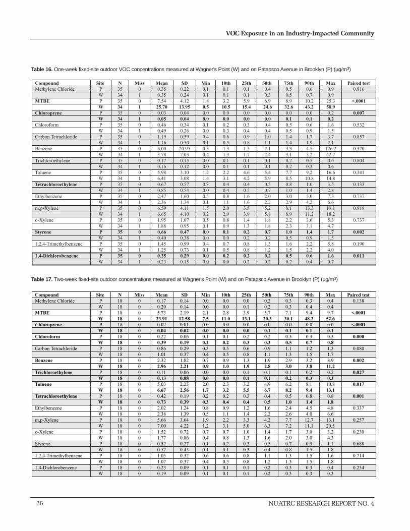
26
VOC Exposure in an Industry-Impacted Community
NUATRC RESEARCH REPORT NO. 4
CompoundMethylene Chloride
MTBE
Chloroprene
Chloroform
Carbon Tetrachloride
Benzene
Trichloroethylene
Toluene
Tetrachloroethylene
Ethylbenzene
m,p-Xylene
o-Xylene
Styrene
1,2,4-Trimethylbenzene
1,4-Dichlorobenzene
SitePWPWPWPWPWPWPWPWPWPWPWPWPWPWPW
N353435343534353435343534353435343534353435343534353435343534
Miss010101010101010101010101010101
Mean0.350.357.5425.700.030.050.460.491.191.166.003.780.170.165.986.410.670.852.472.366.596.651.951.880.660.401.451.250.350.23
SD0.220.244.1213.950.040.040.340.260.590.5020.957.030.150.123.103.080.570.541.601.344.114.101.070.950.470.380.990.730.290.15
Min0.10.11.80.50.00.00.10.00.40.10.30.40.00.01.21.40.30.00.50.11.50.20.50.10.00.00.40.10.00.0
10th0.10.13.210.50.00.00.20.30.60.51.31.30.10.12.23.10.40.40.81.12.02.90.80.90.10.00.70.50.20.0
25th0.10.15.915.40.00.00.30.40.90.81.51.70.10.14.64.20.40.51.61.63.53.91.41.30.20.20.80.80.20.2
50th0.40.36.9
24.60.00.00.40.41.01.12.12.40.10.15.45.90.50.72.02.25.25.81.81.80.70.21.31.20.20.2
75th0.50.58.932.60.00.10.50.51.41.43.33.10.20.27.78.50.81.03.02.98.18.92.22.31.00.51.61.50.50.2
90th0.60.7
10.243.20.00.10.60.91.71.94.55.20.50.39.2
10.81.01.45.04.2
13.311.23.63.11.40.92.22.20.60.4
Max0.90.9
25.358.90.20.21.61.53.72.1
126.242.70.60.6
16.614.83.52.87.36.6
19.118.25.34.71.71.55.84.01.60.7
Paired test0.816
<.0001
0.007
0.532
0.857
0.370
0.804
0.341
0.133
0.737
0.919
0.737
0.002
0.190
0.011
Table 16. One-week fixed-site outdoor VOC concentrations measured at Wagner's Point (W) and on Patapsco Avenue in Brooklyn (P) (µg/m3)
Table 17. Two-week fixed-site outdoor concentrations measured at Wagner's Point (W) and on Patapsco Avenue in Brooklyn (P) (µg/m3)
CompoundMethylene Chloride
MTBE
Chloroprene
Chloroform
Carbon Tetrachloride
Benzene
Trichloroethylene
Toluene
Tetrachloroethylene
Ethylbenzene
m,p-Xylene
o-Xylene
Styrene
1,2,4-Trimethylbenzene
1,4-Dichlorobenzene
SitePWPWPWPWPWPWPWPWPWPWPWPWPWPWPW
N181818181818181818181818181818181818181818181818181818181818
Miss000000000000000000000000000000
Mean0.170.205.7323.910.020.040.220.390.861.012.322.960.110.135.036.670.420.732.022.385.667.001.521.770.520.571.051.070.230.19
SD0.140.142.1912.580.010.020.060.190.290.371.822.210.060.082.232.560.190.391.241.393.644.220.720.860.270.450.320.370.090.09
Min0.00.02.17.50.00.00.10.20.30.40.70.90.00.02.01.70.20.30.80.51.91.20.70.40.10.10.60.40.10.1
10th0.00.02.811.00.00.00.10.20.50.50.91.00.00.02.33.20.20.40.91.12.23.10.70.80.20.10.60.50.10.1
25th0.00.13.913.10.00.00.20.30.60.81.31.90.10.13.25.50.30.41.21.43.35.01.01.30.30.30.80.80.10.1
50th0.20.25.7
20.30.00.10.20.30.91.11.92.80.10.14.96.70.40.51.62.24.26.31.41.60.50.41.11.20.20.2
75th0.30.37.130.10.00.10.30.51.11.32.93.00.10.26.28.20.51.02.42.67.77.21.72.00.70.81.31.30.30.3
90th0.30.49.4
48.20.00.10.30.71.21.53.23.80.20.38.19.40.81.44.54.0
12.711.13.03.00.91.51.51.50.30.3
Max0.40.49.7
52.60.00.10.30.81.31.78.9
11.20.20.3
10.813.10.81.84.86.6
13.120.53.24.31.11.81.61.80.40.3
Paired test0.138
<.0001
<.0001
0.000
0.080
0.002
0.027
0.017
0.001
0.337
0.257
0.230
0.688
0.714
0.234

27
Timothy J. Buckley
NUATRC RESEARCH REPORT NO. 4
Table 18. One-month fixed-site outdoor concentrations measured at Wagner's Point (W) and on Patapsco Avenue in Brooklyn (P) (µg/m3)
CompoundMethylene Chloride
MTBE
Chloroprene
Chloroform
Carbon Tetrachloride
Benzene
Trichloroethylene
Toluene
Tetrachloroethylene
Ethylbenzene
m,p-Xylene
o-Xylene
Styrene
1,2,4-Trimethylbenzene
1,4-Dichlorobenzene
SitePWPWPWPWPWPWPWPWPWPWPWPWPWPWPW
N101010101010101010101010101010101010101010101010101010101010
Miss111111111111111111111111111111
Mean0.060.044.8918.000.020.040.180.290.600.722.212.540.120.134.385.570.400.631.711.994.795.731.351.490.310.310.980.920.260.20
SD0.070.102.9111.120.020.030.110.140.310.341.441.530.080.092.232.300.210.321.081.003.032.870.740.680.160.210.530.440.170.16
Min0.00.00.44.80.00.00.00.20.10.40.20.70.00.00.41.60.10.20.20.80.62.10.20.60.10.10.10.40.10.1
10th0.00.01.57.60.00.00.10.20.20.40.50.90.00.01.42.50.20.30.50.91.32.40.40.70.10.10.30.50.10.1
25th0.00.02.810.40.00.00.10.20.40.40.91.20.10.12.44.80.30.40.81.32.14.00.71.10.20.20.60.60.20.1
50th0.10.05.4
14.90.00.00.20.20.60.62.22.40.10.15.25.50.40.61.61.84.54.81.51.40.30.30.80.80.20.2
75th0.10.06.223.90.00.10.30.40.91.12.92.70.20.25.86.00.60.82.82.77.87.51.92.00.50.41.51.00.30.2
90th0.20.28.8
35.90.10.10.30.51.01.24.35.10.20.36.89.00.71.13.23.68.9
10.32.32.50.50.61.71.60.60.5
Max0.20.3
11.042.90.10.10.40.61.11.24.85.70.30.37.8
10.10.71.23.53.79.4
11.12.52.60.50.91.82.00.60.6
Paired test0.343
0.001
0.005
0.000
0.055
0.055
0.229
0.027
0.003
0.257
0.177
0.307
0.950
0.429
0.015
Methylene Chloride
MTBE
Chloroprene
Chloroform
Carbon Tetrachlorid
e
Benzene
Ethylbenzene
1,2,4-Trimethylbenzene
m,p-Xylene
o-Xylene
Styrene
Trichloroethylene
Tetrachloroethylene
1,4-Dichlorobenzene
Toluene
0
2
4
Rat
io o
f ind
oor
to o
utdo
or
6
8
10
South BaltimoreHampden
Figure 20. Distribution of VOC indoor-to-outdoor ratios within non-smoking households by community

personal exposures to VOCs were greater in SouthBaltimore than in Hampden for 12 of the 15 VOCs, only fortetrachloroethylene was this difference great enough toachieve statistical significance (p≤0.05).
CENTRAL SITE MONITORING
Tables 16, 17, and 18 summarize results for the outdoorcentral site sampling at Wagner's Point and Brooklyn forsamples collected over periods of one, two and four weeks.The VOC levels in Wagner's Point and the adjacentcommunity of Brooklyn varied in the period of samplecollection, although VOC levels tended to be higher inWagner's Point. Across all three sampling periods, theconcentration of nine VOCs differed significantly inlocations (p≤0.05) based on a paired t-test. In all but two ofthose cases (1,4-dichlorobenzene and styrene), VOCconcentrations were greater at Wagner's Point. Theconcentration of MTBE, the one VOC measuredconsistently higher in all three sample categories, was three-to four-fold higher at Wagner's Point than in Brooklyn.
Figure 20 provides a comparison of indoor-to-outdoorratios in South Baltimore and Hampden. On average,indoor-to-outdoor ratios for most of the VOCs are greaterthan 1.0, indicating an indoor source contribution.
Exceptions to this generalization are MTBE,chlorprene, carbon tetrachloride, trichloroethylene, andtetrachloroethane. For these compounds, mean ratios arevery close to 1.0. The highest ratios were for chloroform,where indoor concentrations exceed outdoor levels by afactor that ranges from five to eight. Where mean indoor- to-outdoor ratios of VOCs were greater than 1.0, SouthBaltimore mean ratios exceeded the Hampden ratios. Thissuggests that, in general, South Baltimore had greater indoor
source contributions than Hampden.
In a subset of seven homes, a parent and child weremonitored over the 72-hour monitoring period. While thesample size was small, a strong association was observedbetween the two measures for most VOCs, suggestingsimilar time and location patterns of activity between theparent and child (Figure 21). For nine of the 15 VOCs(chlorprene, MTBE, chloroform, trichloroethylene,ethylbenzene, m,p- and o-xylene, trimethylbenzene anddichlorobenzene), at least 95% of the variability in thechild's exposure could be explained by the parent R2 values,which ranged from 0.63 to 0.82 for benzene,trichloroethylene, toluene, and styrene (Table 19). Noapparent association or trend for carbon tetrachloride ormethylene chloride was seen in the data.
TRANS, TRANS-MUCONIC ACID (MA)
Figure 22 presents a chromatogram and spectra from astandard spiked lab urine used for quality assurancepurposes. The concentration was chosen to reflectconcentrations commonly found in environmentalexposure. The spectra presented in Figure 23 showconsistency except for the final tail of the peak where somedistortion is present from the subsequent peak.
Summary statistics for the measurement of MA in asubset of adults and children are reported in Table 20 and,by community, in Table 21. Consistent with the air benzeneresults, a nonparametric test (Wilcoxon Sum Rank test) fordifferences between communities was not significant(p≤0.05). The relationship between benzene exposure (24-hour TWA) and MA levels is shown in Figure 24.Regression results are given in Table 22.
28
VOC Exposure in an Industry-Impacted Community
NUATRC RESEARCH REPORT NO. 4
VOC
BenzeneCarbon TetrachlorideChloropreneChloroformDichlorobenzeneEthyl BenzeneMethylene ChlorideMTBEStyreneTetrachloroethyleneTrichloroethyleneTrimethylbenzeneToluenem,p-Xyleneo-Xylene
N
777677777776777
Intercept
-0.331.060.010.13-1.18-0.150.60-1.76-0.51-0.270.08-0.15-0.16-1.09-0.16
SE0.880.410.010.630.940.410.841.690.790.1
0.170.768.191.120.66
p-value0.720.050.380.850.260.730.510.350.540.040.650.850.990.370.82
Slope
0.79-0.371.010.740.900.830.230.880.840.770.620.870.590.810.84
SE0.160.35
0.0270.080.020.050.310.060.210.010.210.070.140.050.08
p-value0.0053
0.34<0.00010.0008
<0.0001<0.00010.4959
<0.00010.0094
<0.00010.0320.00020.0093
<0.00010.0002
ModelR2
0.820.180.990.950.990.980.10.980.770.990.630.970.770.980.95
p-value0.00530.34
<0.00010.0008
<0.0001<0.00010.4959
<0.00010.0094
<0.00010.0320.00020.0093
<0.00010.0002
Table 19. Regression analysis results comparing personal air 72-h concentration measurements on parent and child within the same home(p-values ≤ 0.05 are bold)

29
Timothy J. Buckley
NUATRC RESEARCH REPORT NO. 4
0
0.2
0.4
0.6
0.8
1
1.2
0.0 0.1 0.1 0.2 0.2 0.3 0.3 0.4 0.4
Ch
ild E
xpo
sure
(µ
g/m
3 )
Chloroprene
y = 1.0067x + 0.0055R2 = 0.9964
Parent Exposure (µg/m3)
0.0
10.0
20.0
30.0
40.0
50.0
60.0
70.0
0.0 10.0 20.0 30.0 40.0 50.0 60.0 70.0 80.0
Ch
ild E
xpo
sure
(µ
g/m
3 )
MTBE
y = 0.8803x - 1.756R2 = 0.978
Parent Exposure (µg/m3)
0.0
0.2
0.4
0.6
0.8
1.0
1.2
0.0 0.5 1.0 1.5 2.0
Ch
ild E
xpo
sure
(µ
g/m
3 )
Carbon Tetrachloride
Parent Exposure (µg/m3)
0.0
1.0
2.0
3.0
4.0
5.0
6.0
7.0
8.0
9.0
0.0 2.0 4.0 6.0 8.0 10.0 12.0
Ch
ild E
xpo
sure
(µ
g/m
3)
Benzene
y = 0.785x - 0.3274
R2 = 0.8165
Parent Exposure (µg/m3)
0.0
0.2
0.4
0.6
0.8
1.0
1.2
1.4
0.0 0.5 1.0 1.5 2.0Ch
ild E
xpo
sure
(µ
g/m
3 )
Trichloroethylene
y = 0.6209x + 0.0799R2 = 0.6345
Parent Exposure (µg/m3)
y = 0.5901x - 0.1551
0.010.020.030.0
40.050.060.070.080.090.0
0.0 20.0 40.0 60.0 80.0 100.0 120.0Ch
ild E
xpo
sure
(µ
g/m
3)
Toluene
R2 = 0.7716
Parent Exposure (µg/m3)
0.0
0.51.01.52.02.5
3.03.54.04.55.0
0.0 1.0 2.0 3.0 4.0 5.0 6.0
Methylene Chloride
Parent Exposure (µg/m3)
Ch
ild E
xpo
sure
(µ
g/m
3 )
y = 0.2288x + 0.5957
R2 = 0.0973
0.0
5.0
10.0
15.0
20.0
25.0
30.0
0.0 5.0 10.0 15.0 20.0 25.0 30.0 35.0 40.0
Ch
ild E
xpo
sure
(µ
g/m
3 )
Chloroform
Parent Exposure (µg/m3)
y = 0.0741x + 0.1248
R2 = 0.9552
0.02.04.06.08.0
10.012.014.016.018.020.0
0.0 1.0 2.0 3.0 4.0 5.0 6.0 7.0 8.0
1,2,4-Trimethylbenzene
Parent Exposure (µg/m3)
Ch
ild E
xpo
sure
(µ
g/m
3 )
o-Xylene
y = 0.8443x - 0.1593
R2 = 0.9525
0.0
2.0
4.0
6.0
8.0
10.0
12.0
14.0
16.0
0.0 5.0 10.0 15.0 20.0
Parent Exposure (µg/m3)
Ch
ild E
xpo
sure
(µ
g/m
3)
Ethylbenzene
y = 0.8276x - 0.1513
R2 = 0.9802
0.0
2.0
4.0
6.0
8.0
10.0
12.0
14.0
16.0
18.0
0.0 5.0 10.0 15.0 20.0
Parent Exposure (µg/m3)
Ch
ild E
xpo
sure
(µ
g/m
3 )
Trichloroethane
y = 0.7728x - 0.2747
-5.0
0.0
5.0
10.0
15.0
20.0
0.0 5.0 10.0 15.0 20.0 25.0 30.0
R2 = 0.999
-5.0
Parent Exposure (µg/m3)
Ch
ild E
xpo
sure
(µ
g/m
3 )
m,p-Xylene
y = 0.815x - 1.0898R2 = 0.983
0.05.0
10.015.020.025.030.035.040.045.050.0
0.0 10.0 20.0 30.0 40.0 50.0 60.0 70.0
Parent Exposure (µg/m3)
Ch
ild E
xpo
sure
(µ
g/m
3 )
Styrene
y = 0.8449x - 0.5119
R2 = 0.7704
-1.0
0.0
1.0
2.0
3.0
4.0
5.0
6.0
7.0
8.0
0.0 1.0 2.0 3.0 4.0 5.0 6.0 7.0 8.0
Parent Exposure (µg/m3)
Ch
ild E
xpo
sure
(µ
g/m
3)
-20.0
0.0
20.0
40.0
60.0
80.0
100.0
120.0
140.0
160.0
0.0 20.0 40.0 60.0 80.0 100.0 120.0 140.0 160.0
Parent Exposure (µg/m3)
1,4-Dichlorobenzene
y = 0.9026x - 1.1849
R2 = 0.9983
Ch
ild E
xpo
sure
(µ
g/m
3 )
Figure 21. Scatter plots with linear regression analysis of VOCs concurrently measured (72-h) on parent and child

DISCUSSION AND CONCLUSIONS
This study was designed to investigate the impact of anintense industrial region on concentrations of VOCs inoutdoor, indoor, and personal environments. The effect ofindustry was evaluated by comparing VOCs in air levels inthe heavily industrialized community to those in acommunity that is comparable in every other respect except
30
VOC Exposure in an Industry-Impacted Community
NUATRC RESEARCH REPORT NO. 4
351.76229.88uAU
500
400
300
200
100
250 275 300 325 nm
0
0.078ugml 257.964 12.480 Within
0.078ugml 258.683 12.587 Within
0.078ugml 258.604 12.680 Within
0.078ugml 257.440 12.773 Down Slope
0.078ugml 252.945 12.827 Within
Reference 0.078ugml 6-16-03.run
Reference 0.078ugml 6-16-03.run
Reference 0.078ugml 6-16-03.run
Reference 0.078ugml 6-16-03.run
Reference 0.078ugml 6-16-03.run
Spectral Overlay Report
Name PuP (nm) tR Spectrum Correction FilenameType
Figure 23. Photo diode array (PDA) spectra of MA providing peakconfirmation
24 hour personal air benzene (µg/m3)
0 5 10 15 20 25
tra
ns,
tra
ns-
mu
con
ic a
cid
(n
g/m
g c
rea
tinin
e)
0
100
200
300
400
500
600
Figure 24. Comparison of urine MA concentrations to 24-h TWA personalair benzene concentration
Air Conc. Coefficientn
42
39
34
Intercept
94
99
65
SE
24
18
24
p-value
<0.00
<0.00
0.01
8.7
2.9
20
SE
3.8
3.9
7.6
p-value
0.03
0.47
0.01
Model
R2
0.11
0.01
0.18
p-value
0.03
0.47
0.01
Table 22. Regression results of MA on 24-h TWA personal air benzeneconcentration
Minutes
mA
U
tt-MA-0.41
-0.25
0.00
0.25
2.5 5.0 7.5 10.0 12.5 15.0
0.50
0.75
1.00
1.25
X: 12.6600 MinutesY: 0.362 mAU
Peak Name:Result: 0.668
Width: 0.000 secArea: 9.80 mAUx sec
a:\0.078ugml 6-16-03.runSPSPRP*
Wl:1
6
10
.75
1
12
.66
0
13
.23
3
15
.83
9
10
.13
5
12
.23
3
9.0
25
8.7
64
8.1
24
6.7
01
6.0
24
5.6
00
5.2
13
4.9
01
4.2
92
3.6
68
3.3
17
3.0
20
2.5
24
2.2
27
7.1
99
RP-
File: a:\0.078ugml 6-16-03.runChannel: 1 = 201.00-205.00 nm Results
Last recalc: 6/16/2003 12:18 PM
Figure 22. Chromatogram showing the separation and detection of 78ng/mL MA on baseline of 13.2 ng/mL in urine
Adults Childrenn 40 2Mean 24 hr Benzene (ug/m3) (SD) 4.1 (4.2) 9.5 (5.0) Median 2.3 9.5
Mean MA (ng/mg creatinine) (SD) 119.8 (94.4) 386.0 (172.2) Median MA 92.9 386.0 Range 21.7, 494.4 264.2, 507.7
Table 20. Concentration of MA relative to 24-h air concentration levelsmeasured in adults and children
Table 21. MAconcentration measured in South Baltimore residents relativeto Hampden
South Baltimore HampdenN 24 16Mean MA (ng/mg creatinine) (SD) 115.5 (107.4) 126.2 (73.6) Median MA 85.9 98.9

industrial presence. Therefore, a second Baltimore Cityurban community was selected that has similardemographics but lacks the intense industrial presence. Incontrast to South Baltimore where the community isadjacent to large chemical industrial complexes, thecommunity of Hampden is adjacent to the Johns Hopkinsundergraduate campus and is not close to large chemicalindustrial complexes. Although the communities ofHampden and South Baltimore had comparable
demographics based on the 1990 census, the 1999-2000sampling conducted under this study showedinconsistencies primarily associated with education level.Based on 2000 census data now available, the observeddifferences appear to be consistent with actual changes inHampden demographics. Although socioeconomic statushas been linked to differential exposure, the impact ofeducation by itself is unclear.
31
Timothy J. Buckley
NUATRC RESEARCH REPORT NO. 4
Table 23. Summary of key VOC exposure study results (all units in µg/m3)
1 24-hour TWA minimum and maximum values; 2 median values, no measures of variability given; 3 12-hour TWA median values and (minimum andmaximum values); 4 7-day TWA; 5 24-hour TWA
VOC
Benzene
Chloroform
Carbon Tetrachloride
Ethylbenzene
1,4-dichlorobenzene
Styrene
Tetrachloroethylene
Trichloroethylene
Toluene
Xyleneso,m&p
Lower Rio GrandeValley1
U.S. EPA9 homes
Indoor(Range)1.3 - 5.0
0.2 - 2.1
0.7- 0.7
0.4 -2.3
0.7 - 0.7
0.0 - 0.7
0.3 -3.5
1.7 - 8.1
1.5 - 11.7
Outdoor(Range)0.5 - 2.7
0.2 - 0.2
0.7 - 0.7
0.2 - 1.6
0.7 - 0.8
0.1 - 0.3
0.4 - 0.4
1.1 - 6.0
0.8 - 7.8
KanawhaValley2
Cohen et. al.35 homes
Indoor
2.1
3.3
2.7
1.9
1.3
1.3
2.6
9.9
Outdoor
2.5
2.3
1.1
0.9
0.9
0.8
1.3
3.3
CanadianStudy5
Otsonet. al.
GermanStudy4
Hoffmannet. al.
Personal
11
7
2
2
<1
69
21
BirminghamStudy5
Leunget. al
Personal
14.98(2.33 - 283.01)
31.8(3.6 - 536.3)
11.33(1.02 - 357.53)
Indoor Non-Smoking Homes
11.5 (2.24)
21.9 (6.03)
11.28 (4.34)
Indoor
5
2
8
<1
3
< 1
41
26
TEAM-Baltimore3
Wallace et. al.70 people
Personal(Range)
11.2(0.11 - 129)
3.10(0.15 - 51.0)
0.85(0.18 - 16.1)
3.90(0.16 - 409)
2.50(0.13 - 385)
1.75(0.26 - 173)
2.40(0.19 - 280)
1.11(0.14 - 401)
18.4(0.42 - 1845)
TEAM1
New JerseyWallace et. al.
350 people
Outdoor(Range)
5.35(0.07 - 255)
1.06(0.05 - 12.2)
0.91(0.14 - 7.06)
3.70(0.19 - 13.5)
0.95(0.08 - 12.2)
0.75(0.07 - 3.65)
3.30(0.10 - 30.3)
1.90(0.13 - 9.75)
14.47(1.13 - 43.0)
Personal(Range)
17.5(0.02 - 260)
3.75(0.08 - 152)
1.53(0.2 - 551)
7.15(0.46 - 752)
3.78(0.14 - 1140)
1.90(0.08 - 3250)
8.35(0.39 - 6010)
2.87(0.24 - 701)
25.2(3.19 -2000)
NHEXAS2
Claytonet. al.
250 people
Personal
5.37
1.96
1.98
0.63
Indoor
4.35
2.13
1.89
0.56
Outdoor
2.92
0.86
1.24
0.32
Figure 25. Average ASPEN 1996 estimates of ambient VOCconcentrations primarily of mobile source origin across Hampden (H) andSouth Baltimore (SB) census blocks
0.0
1.0
2.0
3.0
4.0
5.0
6.0
7.0
8.0
SB H SB H SB H SB H
Pollutant by Community
Co
nce
ntr
atio
n (
µg
/m3)
On-Road Bkg Area Non-Road Pt
Figure 26. Average ASPEN 1996 estimates of annual ambient VOCconcentration primarily of area source origin across Hampden (H) andSouth Baltimore (SB)
0.000
0.002
0.004
0.006
0.008
0.010
0.012
0.014
0.016
SB H SB H
Pollutant by Community
Co
nce
ntr
atio
n (
µg
/m3 )
On-Road Bkg Area Non-Road Pt
Carbon Tetrachloride Chloroform
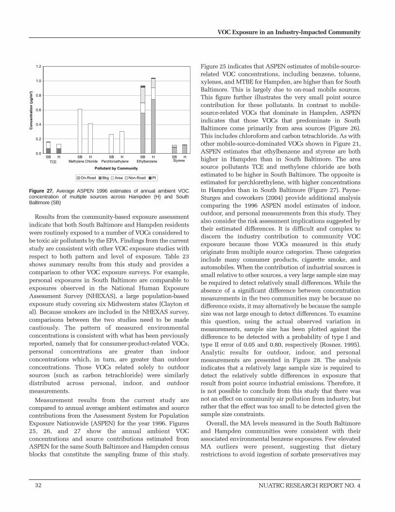
Results from the community-based exposure assessmentindicate that both South Baltimore and Hampden residentswere routinely exposed to a number of VOCs considered tobe toxic air pollutants by the EPA. Findings from the currentstudy are consistent with other VOC exposure studies withrespect to both pattern and level of exposure. Table 23shows summary results from this study and provides acomparison to other VOC exposure surveys. For example,personal exposures in South Baltimore are comparable toexposures observed in the National Human ExposureAssessment Survey (NHEXAS), a large population-basedexposure study covering six Midwestern states (Clayton etal). Because smokers are included in the NHEXAS survey,comparisons between the two studies need to be madecautiously. The pattern of measured environmentalconcentrations is consistent with what has been previouslyreported, namely that for consumer-product-related VOCs,personal concentrations are greater than indoorconcentrations which, in turn, are greater than outdoorconcentrations. Those VOCs related solely to outdoorsources (such as carbon tetrachloride) were similarlydistributed across personal, indoor, and outdoormeasurements.
Measurement results from the current study arecompared to annual average ambient estimates and sourcecontributions from the Assessment System for PopulationExposure Nationwide (ASPEN) for the year 1996. Figures25, 26, and 27 show the annual ambient VOCconcentrations and source contributions estimated fromASPEN for the same South Baltimore and Hampden censusblocks that constitute the sampling frame of this study.
Figure 25 indicates that ASPEN estimates of mobile-source-related VOC concentrations, including benzene, toluene,xylenes, and MTBE for Hampden, are higher than for SouthBaltimore. This is largely due to on-road mobile sources.This figure further illustrates the very small point sourcecontribution for these pollutants. In contrast to mobile-source-related VOCs that dominate in Hampden, ASPENindicates that those VOCs that predominate in SouthBaltimore come primarily from area sources (Figure 26).This includes chloroform and carbon tetrachloride. As withother mobile-source-dominated VOCs shown in Figure 21,ASPEN estimates that ethylbenzene and styrene are bothhigher in Hampden than in South Baltimore. The areasource pollutants TCE and methylene chloride are bothestimated to be higher in South Baltimore. The opposite isestimated for perchlorethylene, with higher concentrationsin Hampden than in South Baltimore (Figure 27). Payne-Sturges and coworkers (2004) provide additional analysiscomparing the 1996 ASPEN model estimates of indoor,outdoor, and personal measurements from this study. Theyalso consider the risk assessment implications suggested bytheir estimated differences. It is difficult and complex todiscern the industry contribution to community VOCexposure because those VOCs measured in this studyoriginate from multiple source categories. These categoriesinclude many consumer products, cigarette smoke, andautomobiles. When the contribution of industrial sources issmall relative to other sources, a very large sample size maybe required to detect relatively small differences. While theabsence of a significant difference between concentrationmeasurements in the two communities may be because nodifference exists, it may alternatively be because the samplesize was not large enough to detect differences. To examinethis question, using the actual observed variation inmeasurements, sample size has been plotted against thedifference to be detected with a probability of type I andtype II error of 0.05 and 0.80, respectively (Rosner, 1995).Analytic results for outdoor, indoor, and personalmeasurements are presented in Figure 28. The analysisindicates that a relatively large sample size is required todetect the relatively subtle differences in exposure thatresult from point source industrial emissions. Therefore, itis not possible to conclude from this study that there wasnot an effect on community air pollution from industry, butrather that the effect was too small to be detected given thesample size constraints.
Overall, the MA levels measured in the South Baltimoreand Hampden communities were consistent with theirassociated environmental benzene exposures. Few elevatedMA outliers were present, suggesting that dietaryrestrictions to avoid ingestion of sorbate preservatives may
32
VOC Exposure in an Industry-Impacted Community
NUATRC RESEARCH REPORT NO. 4
Figure 27. Average ASPEN 1996 estimates of annual ambient VOCconcentration of multiple sources across Hampden (H) and SouthBaltimore (SB)
0.0
0.2
0.4
0.6
0.8
1.0
1.2
SB H SB H SB H SB H SB H
Pollutant by Community
Co
nce
ntr
atio
n (
µg
/m3 )
On-Road Bkg Area Non-Road Pt
TCE Methylene Chloride Perchloroethylene StyreneEthylbenzene

have been successful. Furthermore, the association between24-hour personal air samples for benzene and MA alsosuggests that dietary restriction may increase the specificityof MA as a biomarker for environmental level benzene.However, the positive results reported here need to beinterpreted cautiously because of the small sample size andinfluential outliers. Further study will be needed to rule outresidual confounding from sorbate preservatives or chanceas explanatory factors for this association.
This study was conducted in cooperation with SouthBaltimore community residents to address concerns aboutthe impact of nearby industry on exposure to toxic airpollutants and possible health risks resulting fromexposure. Outdoor, indoor, and personal VOCconcentrations in an urban non-industry-impactedBaltimore location served as a comparison community.Residential outdoor measurements should provide the mostsensitive indications of an industry effect. Only two VOCs(ethylbenzene and m-p-xylene) were measured at
33
Timothy J. Buckley
NUATRC RESEARCH REPORT NO. 4
1
10
100
1000
1,000,000
10,000
100,000
0% 10% 20% 30% 40% 50% 60%
Percent Difference Detected
Indoor
Sam
ple
Siz
e
a
o
g
e
d
n
h
fk
l
c
b
j
m
i
1
10
100
1000
10000
0% 10% 20% 30% 40% 50% 60%
Percent Difference Detected
Outdoor
Sam
ple
Siz
e
a
o
g
m
e
n
l
d
f
kh,i,j
cb
1
10
100
1000
1,000,000
10,000
100,000
0% 10% 20% 30% 40% 50% 60%
Percent Difference Detected
Personal
Sam
ple
Siz
e
b
o
f
j
g
m
li
e
h
knd
ac
MTBE
1,4-Dichlorobenzene
Toluene
m,p-Xylene
Benzene
Styrene
Chloroform
Methylene Chloride
Ethylbenzene
o-Xylene
1,2,4-Trimethylbenzene
Tetrachloroethylene
Carbon Tetrachloride
Trichloroethylene
Chloroprene
a
b
c
d
e
f
g
h
i
j
k
l
m
n
o
Figure 28. Sample size needed in order to detect differences between exposed populations based on measured variance

statistically significant higher concentrations in SouthBaltimore than in the community of Hampden. The 1999toxic release inventory (U.S. EPA, Toxic Release Inventory)reports releases for both chemicals in South Baltimore andnone in Hampden. For both analytes, the elevated outdoorconcentrations translated into statistically significantdifferent indoor concentrations among sampled communityresidents. Corresponding elevations in indoor and personallevels would indicate that elevated outdoor concentrationsincrease indoor and personal exposures. Therefore, anindustry impact on community exposure could be inferredfor a VOC with elevated outdoor, indoor, and personalexposure concentrations. The indoor difference did nottranslate, however, into a statistically significant differencein personal exposure. Therefore, these data suggest anindustry impact on outdoor and indoor ethylbenzene andm,p-xylene exposures. Because of the large variability inpersonal exposure measurements, it may be that there wasinsufficient power to detect this difference. These resultsneed to be interpreted in light of limitations in the study,including a low response rate (37%) and potentiallyimportant differences in education between the SouthBaltimore and Hampden samples.
ACKNOWLEDGEMENTS
First and foremost, we acknowledge the late DorisMcGuigan, a South Baltimore community leader who wasthe impetus for this study and who fought generously andtirelessly to address environmental health concerns of theSouth Baltimore community. We acknowledge SouthBaltimore and Hampden community residents who gavetheir time and opened their homes so that this study couldbe successful. We are grateful to Alice O'Malley for herdedicated and skilled assistance in recruiting studysubjects. Members of our Community Advisory Committee,including the late Doris McGuigan, President of ConcernedCitizens for a Better Brooklyn, Mary Rosso, David Schuyler,Rebecca Kolber, and the late Ann Bonenberger providedvaluable insight and advice. Dr. Michael Trush, Co-Directorof Community Outreach for the NIEHS Johns HopkinsCenter for Urban Environmental Health providedinvaluable support and guidance for this study. D'AnnWilliams provided expert GIS mapping to support thisreport. Erin Knox, Laura Geer, and Joanna Gaitens providedinvaluable field support for the project. This work is basedon a community-based exposure study that was conductedthrough initial pilot funding by the U.S. EPA Region III(grant MM993948) followed by funding by the Mickey
Leland National Urban Air Toxics Research Center.Additional support has been provided through the JohnsHopkins Risk Science and Public Policy Institute, the JohnsHopkins Center in Urban Environmental Health (P30 ES03819), and the Maryland Cigarette Restitution Fund. Dr.Weaver's time and effort on this project was supported inpart through an NIEHS First Award (R29 ES07780).
REFERENCES
Ashley DL, Bonin MA, Cardinali FL, McGraw JM, Wooten J,1996. Measurement of volatile organic compounds inhuman blood. Environ Health Perspect 104, Suppl. 5:871-877.
Bartczak A, Kline SA, Yu R, Weisel CP, Goldstein BD, WitzG, Bechtold WE, 1994. Evaluation of assays for theidentification and quantitation of muconic acid, a benzenemetabolite in human urine. J Toxicol Environ Health,42:245-258.
Benowitz NL, 1996. Cotinine as a biomarker ofenvironmental tobacco smoke exposure. Epidemiol Rev,18(2):188-204.
Bergamaschi E, Brustolin A, DePalma G, Manini P, MozzoniP, Andreoli R, Cavazzini S, Mutti A, 1999. Biomarkers ofdose and susceptibility in cyclists exposed tomonoaromatic hydrocarbons. Toxicol Letters, 108:241-247.
Boogaard PJ, van Sittert NJ, 1995. Biological monitoring ofexposure to benzene: a comparison between S-phenylmercapturic acid, trans,trans-muconic acid, andphenol. Occup Environ Med 52:611-620.
Brown RH, Harvey RP, Purnell CJ, Sanders KJ, 1984. ADiffusive Sampler Evaluation Protocol. Am. Ind. Hyg.Assoc. J. 45:67-73.
Buckley TJ, Waldman JM, Dhara R, Greenberg A, Ouyang Z,Lioy PJ, 1995. An assessment of a urinary biomarker fortotal human environmental exposure to benzo[a]pyrene(BaP). Int Arch Occup Environ Health 67:257-266.
Buckley TJ, Liddle JD, Ashley D, Burse V, Paschal D, AklandG, 1997. Measurements of exposure and biomarkers in theLower Rio Grande Valley: multimedia results for pesticides,metals, PAH and VOCs. Environment International,23(5):705-732.
34
VOC Exposure in an Industry-Impacted Community
NUATRC RESEARCH REPORT NO. 4
Burke T, Anderson H, Beach N, Colome S, Drew RT,Firestone M, Hauchman FS, Miller TO, Wagner D, Zeise L,Tran N, 1992. Role of exposure databases in riskmanagement. 1992 Archives of Environmental Health,47(6):421-429.
Burke T, Sexton K, 1995. Integrating science and policy in anational human exposure assessment survey. J Expo AnalEnviron Epidemiol, 5(3):283-96.
Caldwell JC, Woodruff TJ, Morello-Frosch R, Axelrad DA,1998. Application of health information to hazardous airpollutants modeled in EPA's cumulative exposure project.Toxicology and Industrial Health, 14(3):429-454.
Chung C, Morandi MT, Stock TH, Afshar M, 1999.Evaluation of a passive sampler for volatile organiccompounds at ppb concentrations, varying temperatures,and humidities with 24-hour exposures. 2. Samplerperformance. Environ. Sci. and Technol, 33(20):3661-3665.
Clayton CA, Pellizzari ED, Whitmore RW, Perritt RL,Quackenboss JJ, 1999. National Human ExposureAssessment Survey (NHEXAS): distributions andassociations of lead, arsenic and volatile organiccompounds in EPA Region 5. J Expo Anal EnvironEpidemiol, 9(5):381-92.
Clickner R, Kalton G, Chu A, 1993. Statistical design issuesin human exposure assessment surveys: sampling designand options. Contract # 68-W1-019, US EPA.
Coburn J, 2002. Combinine community-based research andlocal knowledge to confront asthma and subsistence-fishinghazards in Greenpoint/Williamsburg, Brooklyn, New York.Environ Health Perspect, 110 Suppl 2:241-248.
Cohen M, Ryan B, Ozkaynak H, Epstein P, 1989.Indoor/outdoor measurements of volatile organiccompounds in the Kanawha Valley of West Virginia. J AirPollution Control Assn, 39:1086-1093.
Cox BG, Mage DT, Immerman FW, 1988. Sample designconsiderations for indoor air exposure surveys. APCA,38(10):1266-1270.
Ducos P, Gaudin R, Robert A, Francin JM, Maire C, 1990.Improvement in HPLC analysis of urinary trans,trans-Muconic acid, a promising substitute for phenol in theassessment of benzene exposure. Intl Arch Occup EnvironHealth, 62:529-534.
Ducos P, Gaudin R, Bel J, Maire C, Francin JM, Robert A,Wild P, 1992. Trans,trans-Muconic acid, a reliable biologicalindicator for the detection of individual benzene exposuredown to the ppm level. Int Arch Occup Environ Health,64:309-313.
Feychting M, Svensson D, Ahlbom A, 1998. Exposure tomotor vehicle exhaust and childhood cancer. Scand J WorkEnviron Health, Feb 24(1):8-11.
Gobba F, Rovesti S, Borella P, Vivoli R, Caselgrandi E, VivoliG, 1997. Inter-individual variability of benzene metabolismto trans,trans-muconic acid and its implications in thebiological monitoring of occupational exposures. Sci TotalEnviron, 199: 41-48.
Gordon SM, Wallace LA, Brinkman MC, Callahan PJ, KennyDV, 2002. Volatile organic compounds as breath biomarkersfor active and passive smoking. Environ Health Perspect,110(7):689-98.
Hajimiragha H, Ewers U, Brockhaus A, Boettger A, 1989.Levels of benzene and other volatile aromatic compoundsin the blood of non-smokers and smokers. Int Arch OccupEnviron Health, 61(8):513-8.
Hoffman K, Krause C, Seifert B, Ullrich D, 2000. TheGerman environmental survey 1990/92 (GerES II): Sourcesof personal exposure to volatile organic compounnnds. JExpo Anal Environ Epidemiol, 10(2):115-125.
Hornung R, Reed L, 1990. Estimation of an averageconcentration in the presence of nondetectable values. ApplOccup Environ Hyg, 5(1):46- 51.
Israel BA, Schulz AJ, Parker EA, Becker AB, 1998. Reviewof community-based research: Assessing partnershipapproaches to improve public health. Annu Rev PublicHealth, 19:173-202.
Johnson ES, Lucier G, 1992. Perspectives on risk assessmentimpact of recent reports on benzene. Am J Inds Med, 21:749-757.
Kim YM, Harrad S, Harrison RM, 2001. Concentrations andsources of VOCs in urban domestic and publicmicroenvironments. Environ Sci Technol Mar,15;35(6):997-1004.
Larsen DJ, Weber A, Johnson EW, 1996. Storagecharacteristics of exposed activated carbon diffusion
35
Timothy J. Buckley
NUATRC RESEARCH REPORT NO. 4

monitors. 3M Occupational Health and EnvironmentalSafety Division, presented at the American IndustrialHygiene Conference and Exposition, Washington, D.C.
Lauwerys RR, Buchet J-P, Andrien F, 1994. Muconic acid inurine: A reliable indicator of occupational exposure tobenzene. Am J Ind Med, 25:297-300.
Lee BL, New AL, Kok PW, Ong HY, Shi CY, Ong CN, 1993.Urinary trans,trans-muconic acid determined by liquidchromatography: Application in biological monitoring ofbenzene exposure. Clin Chem, 39:1788-1792.
Leung P, Harison R, 1998. Evaluation of personal exposureto monoaromatic hydrocarbons. Occup Environ Med,55(4):249-257.
Litt JS, Burke TA, 2002. Uncovering the historicenvironmental hazards of urban brownfields. J UrbanHealth, 79(4):464-481.
MacDougall D, Amore FJ, Cox GV, 1980. Guidelines for dataacquisition and data quality evaluation in environmentalchemistry. Anal Chem, 52:2242-2249.
Maryland Cancer Consortium, 1996. Maryland cancercontrol plan: Problems and priorities. Department of Healthand Mental Hygiene, Baltimore.
Melikian AA, Prahalad AK, Hoffman D, 1993. Urinary trans,trans-muconic acid as an indicator of exposure to benzenein cigarette smokers. Cancer Epidemiol Biomarkers andPrevention, 2:47-51.
Melikian AA, Qu Q, Shore R, Li G, Li H, Jin X, Cohen B,Chen L, Li Y, Yin S, Mu R, Zhang X, Wang Y, 2002. Personalexposure to different levels of benzene and its relationshipsto the urinary metabolites S-phenylmercapturic acid andtrans,trans-muconic acid. J Chromatogr B Analyt TechnolBiomed Life Sci, 5; 778(1-2):211-21.
Miller M, Solomon G, 2003. Environmental risk communi-cation for the clinician. Pediatrics, 112(1 Pt 2):211-7.
NATA Glossary of Terms(http://www.epa.gov/ttn/atw/nata/gloss1.html).
Ong C, Kok P, Ong H, Shi CY, Lee BL, Phoon WH, Tan KT,1996. Biomarkers of exposure to low concentrations ofbenzene: a field assessment. Occ Environ Med, 53:328-333.
Otson R, Fellin P, Tran Q, 1994. VOCs in representativeCanadian residences. Atmosph Environ, 28(22):3563-3569.Pappas GP, Herbert RJ, Henderson W, Koenig J, Stover B,Barnhart S, 2000. The respiratory effects of volatile organiccompounds. Int J Occup Environ Health, 6(1):1-8.
Payne-Sturges DC, Burke TA, Breysse PN, Diener-West M,Buckley TJ, 2004. Personal exposure meets risk assessment:a comparison of measured and modeled exposures and risksin an urban community. Environ Health Perspect,112(4):589-598.
Payne-Sturges DC, Schwab M, Buckley TJ, 2004. Closing theresearch loop: a risk-based tool for communicating results ofcommunity-based exposure studies. Environ HealthPerspect, 112(1):28-34.
Pearson RL, Wachtel H, Ebi KL, 2000. Distance-weightedtraffic density in proximity to a home is a risk factor forleukemia and other childhood cancers. J. Air and WasteManag. Assoc, 50:175-180.
Perlin SA, Wong D, Sexton K, 2001. Residential proximityto industrial sources of air pollution: interrelationshipsamong race, poverty, and age. J Air and Waste Manag Assoc,51(3):406-421.
Pezzagno G, Maestri L, 1997. The specificity of trans, trans-muconic acid as a biological indicator for low levels ofenvironmental benzene. Indoor Built Environ, 6:12-18.
Pew Environmental Health Commission, 2000. "America'senvironmental health gap: Why the country needs anationwide health tracking system." September 2000.
Raaschou-Nielsen O, Hertel O, Thomsen BL, Olsen JH,2001. Air pollution from traffic at the residence of childrenwith cancer. Am J Epidemiol, 1153(5):433-43.
Rauscher D, Lehnert G, Angerer J, 1994. Biomonitoring ofoccupational and environmental exposure to benzene bymeasuring trans, trans-muconic acid in urine. Clin Chem,40:1468-1470.
Ries LAG, Eisner MP, Kosary CL, Hankey BF, Miller BA,Clegg L, Edwards BK, eds., 2001, SEER Cancer StatisticsReview, 1973-1998. National Cancer Institute. Bethesda,MD.
36
VOC Exposure in an Industry-Impacted Community
NUATRC RESEARCH REPORT NO. 4

Rosenbaum AS, Axelrad DA, Woodruff TJ, Wei YH, LigockiMP, Cohen JP, 1999. National estimates of outdoor air toxicsconcentrations. Journal of the Air and Waste Mgmt Assn,49:1138-1152.
Rosner B, 1995. Fundamentals of Biostatistics, Fourthedition, Chapter 8, Hypothesis Testing: Two-SampleInference. Wadsworth Publishing Co., Belmont, CA. p. 283.
Ruppert T, Scherer G, Tricker AR, Adlkofer F, 1999. Trans,trans-muconic acid: a biological indicator to low levels ofenvironmental benzene. Some aspects of its specificity. AmJ Ind Med, 35:511-518.
Samet JM, 1999. “Cancer Incidence and Mortality Patternsin Baltimore City: An Economic and GeographicOverview.” Unpublished report prepared for the BaltimoreCity Health Department. Johns Hopkins UniversityBloomberg School of Public Health.
Savitz DA, Feingold L, 1989. Association of childhoodcancer with residential traffic density. Scand J WorkEnviron Health, 15:360-363.
Sexton K, Selevan SG, Wagener DK, Lybarger JA, 1992.Estimating human exposures to environmental pollutants:availability and utility of existing databases. Archives ofEnvironmental Health, 47(6):398-407.
Sexton K, Callahan M, Bryan E, Saint C, Wood, W, 1995.Informed decisions about protecting and promoting publichealth: rationale for a national expsoure assessment survey.J Expo Anal Environ Epidemiol, 5(3):233-256.
Shields HC, Weschler CJ, 1987. Analysis of ambientconcentrations of organic vapors with a passive sampler.Air Pollution Control Assoc, 37:1039-1045.
U.S. EPA. National Air Toxics Assessment Web Page(www.epa.gov/atw/nata)
U.S. EPA. Toxic Release Inventory(www.epa.gov/tri/index.htm)
U.S. EPA, 1999. Compendium of methods for thedetermination of toxic organic compounds in ambient air.2nd edition compendium method TO-17. Determination ofvolatile organic compounds in ambient air using activesampling onto sorbent tubes. Office of Research andDevelopment, EPA/625/R-96/010b, Cincinati, OH.
U.S. EPA, 1998. Draft Integrated Urban Air Toxics Strategyto Comply with Section 112(d), 112©(3) and Section 202(1)of the Clean Air Act; Notice. Federal Register, 63(177).
U.S. Government Accounting Office (GAO), 2000. Long-term Coordinated Strategy Needed to Measure Exposures inHumans. Washington, D.C. May 2000.
Van Sittert NJ, Boogaard PJ, Beulink GDJ, 1993. Applicationof the urinary S-phenylmercapturic acid test as a biomarkerfor low levels of exposure to benzene in industry. Brit J IndMed, 50:460-469.
Wallace LA, Pellizzari ED, 1986. Personal air exposures andbreath concentrations of benzene and other volatilehydrocarbons for smokers and nonsmokers. ToxicologyLetters, 35:113-116.
Wallace LA, 1987. The total exposure assessmentmethodology (TEAM) study: summary and analysis volume1 and 2. U.S. EPA. Office of Research and Development,Washington, D.C.
Wallace LA, 1996. Environmental exposure to benzene: anupdate. Environ Health Perspect, 104 Suppl 6:1129-1136.
Ware JH, Spengler JD, Neas LM, Samet JM, Wagner GR,Coultas D, Ozkaynak H, Schwab M, 1993. Respiratory andirritant health effects of ambient volatile organiccompounds. The Kanawha County health study. Am JEpidemiol, Jun 15;137(12):1287-1301.
Weaver VM, Davoli CT, Heller P, Fitzwilliam A, Peters H,Sunyer J, Murphy SE, Goldstein G, Groopman JD, 1996.Benzene exposure, assessed by urinary trans,trans-muconicacid, in urban children with elevated blood lead levels.Environ Health Perspec, 104:318-323.
Weaver VM, Buckley TJ, Groopman JD, 2000. Non-specificity of trans,trans-muconic acid as a benzeneexposure biomarker due to ingestion of sorbic acidpreserved foods. Cancer Epidemiology, Biomarkers &Prevention, 9:749-755.
West G, 1964. On the metabolism of sorbic acid in themouse. Acta Chemica Scand, 18:1373-1378.
Whitmore RW, 1988. Design of surveys for residential andpersonal monitoring of hazardous substances. Atmosph.Environ. 22(10):2077-2084.
37
Timothy J. Buckley
NUATRC RESEARCH REPORT NO. 4

Wieslander G, Norback D, Bjornsson E, Janson C, Boman G,1997. Asthma and the indoor environment: the significanceof emission of formaldehyde and volatile organiccompounds from newly painted indoor surfaces. Int ArchOccup Environ Health, 69(2):115-24.
Woodruff TJ, Axelrad DA, Caldwell J, Morello-Frosch R,Rosenbaum A, 1998. Public health implications of 1990 airtoxics concentrations across the United States. EnvironHealth Perspect, 106(5):245-251.
Woodruff TJ, Parker JD, Kyle AD, Schoendorf KC, 2003.Disparities in exposure to air pollution during pregnancy.Environ Health Perspect, 111(7):942-6.
Yu R, 1995. Measurement of partitioning of benzene inbreath and urinary benzene metabolites from benzeneexposure in humans. Ph.D. dissertation. Rutgers, The StateUniversity of New Jersey and Robert Wood Johnson MedicalSchool.
PUBLICATIONS RESULTING FROM THIS STUDY
Payne-Sturges DC, Schwab M, Buckley, TJ, 2004. Closingthe research roop: a risk-based approach for communicatingresults of air pollution exposure studies. Environ HealthPerspect, 112(1):23-34.
Payne-Sturges DC, Burke TA, Breysse PN, Diener-West M,Buckley, TJ, 2004. Personal exposure monitoring meets riskassessment: a comparison of measured and modeledexposures (and risks) in an urban community. EnvironHealth Perspect, 112(4):589-598.
ABBREVIATIONS
µg MicrogramµL Microliterµm MicrometerANOVA Analysis of varianceASPEN Assessment System for Population
Exposure NationwideCAAA Clean Air Act Amendments of 1990CI Confidence interval CV Coefficient of varianceEPA U. S. Environmental Protection AgencyETS Environmental tobacco smokeGC/MS Gas chromatography/mass spectrometryHAP Hazardous air pollutantHPLC High pressure liquid chromatographyID Inner diameterJHU Johns Hopkins UniversityLOD Limit of detectionm Meterm3 Cubic metermL MilliliterMA Trans,trans-muconic acidmin Minutesmm MillimeterMTBE Methyl tertiary butyl ether NHEXAS National Human Exposure Assessment
Survey OR Odds ratioOSHA U.S. Occupational Safety and Health
AdministrationOVM Organic vapor monitorPCB Polychlorinated biphenylppb Parts per billionpsi Pounds per square inchS-PMA S-phenyl mercapturic acidTEAM Total exposure assessment
methodologyTRI Toxic release inventoryTWA Time weighted averageUTH University of Texas at HoustonUV Ultraviolet lightVOC Volatile organic compound
38
VOC Exposure in an Industry-Impacted Community
NUATRC RESEARCH REPORT NO. 4
ABOUT THE AUTHORS
Dr. Timothy J. Buckley is an Associate Professor ofEnvironmental Health Sciences and Epidemiology at theJohns Hopkins Bloomberg School of Public Health. Dr.Buckley joined the Hopkins faculty in 1996 after five yearswith the U.S. EPA's National Exposure Research Lab. Hisresearch has focused on assessing total humanenvironmental exposure through measurements in multipleenvironmental media and biomarkers. Dr. Buckley has beenresponsible for the concept, design, implementation, andmanagement of several major studies involving humanexposure to PAHs, metals, VOCs, pesticides, and PCBsthrough multiple environmental media. These large-scaleprojects complement laboratory-based studies wherecontrolled exposures are used to more fully investigaterelationships between exposure, body burden, and effects.Dr. Buckley's current research includes community-basedexposure assessment, evaluation of chemical treatment toreduce lead bioavailability, the role of exposure to indoor airpollution, allergens in asthma among inner-city children,exposure and effects from mobile-source-related airpollution, improvement of methods to assess dermalexposure, and the development and evaluation ofbiomarkers of exposure. While with the U.S. EPA, Dr.Buckley received awards for his role and efforts in theNational Human Exposure Assessment Survey (NHEXAS)and the Lower Rio Grande Environmental Exposure Study.His published research was recognized in 1996 with a U.S.EPA Scientific and Technology Achievement Award andagain in 1999 by the Walter G. Berl Award given the JohnsHopkins Applied Physics Laboratory. Dr. Buckley is acertified industrial hygienist and has been elected toleadership positions among his professional associations,including chair of the American Industrial HygieneAssociation's Biological Monitoring Committee andAcademic Counselor of the International Society ofExposure Analysis. Dr. Buckley received his Ph.D. inEnvironmental Science from Rutgers University and aMasters of Health Science in Industrial Hygiene from theJohns Hopkins Bloomberg School of Public Health.
Dr. Virginia Weaver is assistant professor in the Departmentof Environmental Health Sciences at the Johns HopkinsBloomberg School of Public Health. Her research interestsinclude the use of molecular epidemiologic tools in theevaluation of populations exposed to occupational andenvironmental chemicals. The validation of exposure andearly biological effect markers to improve risk assessmentand medical surveillance is a primary focus of her research.
Specific research interests include benzene and renaltoxicants. Dr. Weaver seeks to include children in herstudies in order to provide data on this potentiallysusceptible group. Current projects utilize biomarkers forbenzene exposure in urban populations and renal effectbiomarkers in lead-exposed workers. Medical surveillanceof former Department of Energy Workers at Los AlamosNational Laboratory is an additional project.
Dr. Devon Payne-Sturges is currently working as anenvironmental scientist for the U.S. EPA's Office of Policy,Economics and Innovation. She was formerly theAssistant Commissioner for Environmental Health for theBaltimore City Health Department. Dr. Payne-Sturges’DrPH dissertation focused on comparing measured andmodeled estimates of exposure and risk.
Sung Roul Kim is a doctoral candidate within theDepartment of Environmental Health Sciences at the JohnsHopkins Bloomberg School of Public Health. Mr. Kim has aMasters of Science from Yeungnam University's Departmentof Environmental Engineering in Korea.
39
Timothy J. Buckley
NUATRC RESEARCH REPORT NO. 4

41
Timothy J. Buckley
NUATRC RESEARCH REPORT NO. 4
APPENDIX A
JHSPH / TXSPH Inter-laboratory Comparison Study Protocol

42
VOC Exposure in an Industry-Impacted Community
NUATRC RESEARCH REPORT NO. 4
No. SamplesSample Type
JHSPH UTSPH
JHSPH Spikes (6 levels in triplicate) 18 18
UofTX Spikes (6 levels in triplicate) 18 18
Field Blanks 4 4
Lab Blanks 2 2
Total 42 42
No. SamplesSample Type
JHSPH UTSPH
Side-by-Side Indoor 2 2
Side-by-Side Outdoor 2 2
Field Blank (indoor and Outd) 2 2
Lab Blank 1 1
Total 7 7
No. SamplesSample Type
JHSPH UTSPH
JHSPH Spikes (6 levels in triplicate) 18 18
UofTX Spikes (6 levels in triplicate) 18 18
Field Blanks 4 4
Lab Blanks 2 2
Total 42 42
No. SamplesSample Type
JHSPH UTSPH
Side-by-Side Indoor 2 2
Side-by-Side Outdoor 2 2
Field Blank (indoor and Outd) 2 2
Lab Blank 1 1
Total 7 7
Appendix A. JHSPH / TXSPH inter-laboratory comparison study protocol
JHSPH / TXSPH Inter-laboratory Comparison Study Protocol
1. Extraction Efficiency and Precision
The UTSPH and JHSPH laboratories will each spike two sets of six 3M OVM 3500 badges in triplicate (n total = 72). Eachlaboratory will generate their own set of spiked samples (n=36). One set of spikes (n=18) will be retained by the spikinglaboratory and the second set will be shipped to the other laboratory. The level of spikes will be identical (0, 0.1, 0.5, 1.0,5.0, and 10.0 µg) but the spiking procedure will vary slightly (UTSPH uses a 50 µl spike while JHSPH uses 5 µl spike).Therefore, each laboratory will be analyzing their own spikes (n=18) plus a set from the other laboratory (n=18) for a total of36 samples. Each set of 36 spiked samples will be accompanied by four field blanks (opened and closed at the time ofspiking) plus two laboratory blanks (unopened). These blank samples will be evenly split between the two laboratories sothat each lab will analyze one lab blank and two field blanks.
2. Inter-laboratory Comparison
Side-by-side sampling will be conducted at a indoor and outdoor location in a JHSPH study home in order to investigateinter-laboratory variability in the extraction and analysis of 3M OVM badge samples. Four badges will be placed at eachlocation for the standard sampling period of 3 days. Two badges will be analyzed by each laboratory for each location. Inaddition, two field blanks and one laboratory blank will be collected for each site so that each laboratory will have two fieldblanks and one laboratory blank.
Scheduling and shipping
Badge spiking, shipping, extraction, and analysis will be coordinated to occur at the same time in each laboratory. Sampleswill be shipped by FedEx Airborne overnight delivery in a hard plastic cooler with blue ice (kept at -20° C.).
Monday 18 September Badges SpikedTuesday 19 September Badges ShippedWednesday 20 September Badges Received, Extracted and AnalyzedThursday 21 September Analysis Complete

43
Timothy J. Buckley
NUATRC RESEARCH REPORT NO. 4
APPENDIX B
Study Subject Demographics and Physical Characteristics

44
VOC Exposure in an Industry-Impacted Community
NUATRC RESEARCH REPORT NO. 4
Community
Hampden
Hampden
Hampden
Hampden
Hampden
Hampden
Hampden
Hampden
Hampden
Hampden
Hampden
Hampden
Hampden
Hampden
Hampden
Hampden
Hampden
Hampden
Hampden
Hampden
Hampden
Hampden
SB
SB
SB
SB
SB
SB
SB
SB
SB
SB
SB
SB
SB
SB
SB
SB
SB
SB
Subject ID
H-001
H-002
H-003
H-004
H-005
H-006
H-007
H-008
H-009
H-010
H-011
H-012
H-013
H-014
H-015
H-016
H-017
H-018
H-019
H-020
H-021
H-022
SB-001
SB-002
SB-003
SB-004
SB-005
SB-006
SB-007
SB-008
SB-009
SB-010
SB-011
SB-012
SB-013
SB-014
SB-015
SB-016
SB-017
SB-018
A/C
Adult
Adult
Adult
Adult
Adult
Adult
Adult
Adult
Adult
Adult
Adult
Adult
Adult
Adult
Adult
Adult
Adult
Adult
Adult
Adult
Adult
Adult
Adult
Adult
Adult
Adult
Adult
Adult
Adult
Adult
Adult
Adult
Adult
Adult
Adult
Adult
Adult
Adult
Adult
Adult
Sex
Male
Female
Female
Female
Female
Female
Female
Female
Female
Female
Male
Male
Male
Male
Male
Male
Male
Female
Male
Male
Female
Female
Male
Male
Male
Female
Female
Female
Female
Female
Male
Male
Female
Female
Female
Female
Male
Female
Female
Male
Age (y)
37
38
52
43
32
28
59
60
33
NA
73
41
48
29
NA
69
87
25
27
35
28
47
48
18
39
75
29
44
57
24
73
42
34
53
75
62
67
27
64
75
BMI (kg/m^2)
26.9
27.8
21.3
28.7
21.7
20.9
21.5
28.1
23.4
33.1
24.7
22.4
NA
30.9
23.1
28.9
22.5
18.5
24.2
24.8
24.2
21.3
23.6
28.7
27.0
31.6
27.3
31.0
23.4
20.5
23.3
35.9
50.1
24.3
34.3
32.3
27.0
21.1
25.0
24.1
Race
AA
W/C
W/C
Hispanic
Asian
W/C
W/C
W/C
W/C
W/C
W/C
W/C
W/C
W/C
W/C
W/C
AA
W/C
W/C
W/C
W/C
W/C
W/C
Asian
W/C
W/C
W/C
W/C
W/C
W/C
W/C
W/C
AA
W/C
W/C
W/C
W/C
AA
W/C
AA
Education
HS
C+
C+
HS+
C
C+
P/MS
C+
C+
C+
C+
C+
HS
C
C+
P/MS
NA
C
HS+
C+
C+
HS
HS
HS
HS
P/MS+
HS+
HS
HS
P/MS
P/MS+
HS+
P/MS+
C+
HS
HS+
HS+
C
HS+
P/MS
HH Income
$10,000 to 19,000
$50,000 to 74,999
$75,000 to 99,999
$20,000 to $29,999
$40,000 to 49,999
$50,000 to 74,999
refused
$50,000 to 74,999
$50,000 to 74,999
$40,000 to 49,999
$50,000 to 74,999
refused
$50,000 to 74,999
$40,000 to 49,999
$30,000 to 39,999
refused
Less than $9,999
$10,000 to 19,999
$30,000 to 39,999
$30,000 to 39,999
$10,000 to 19,999
Less than $9,999
Less than $9,999
$50,000 to 74,999
$75,000 to 99,999
$10,000 to 19,000
$50,000 to 74,999
$30,000 to 39,000
$10,000 to 19,000
refused
$20,000 to $29,000
$30,000 to 39,000
$30,000 to 39,000
refused
$20,000 to $29,000
$10,000 to 19,000
$75,000 to 99,999
$40,000 to 49,000
$30,000 to 39,999
Less than $9,999
Table B. Study subject demographics and physical characteristics
SB
SB
SB
SB
SB
SB
SB
SB
SB
SB
SB
SB
SB
SB
SB
SB
SB
SB
SB
SB
SB
SB
SB-019
SB-021
SB-025
SB-026
SB-028
SB-029
SB-031
SB-032
SB-035
SB-036
SB-038
SB-039
SB-040
SB-042
SB-043
SB-044
SB-045
SB-046
SB-047
SB-004R
SB-005R
SB-006R
Adult
Adult
Adult
Adult
Adult
Adult
Adult
Adult
Adult
Adult
Adult
Adult
Adult
Adult
Adult
Adult
Adult
Adult
Adult
Adult-R
Adult-R
Female
Female
Female
Female
Male
Female
Female
Male
Female
Female
Female
Male
Female
Male
Female
Female
Female
Female
Female
Female
Female
78
71
38
19
59
31
59
67
54
53
43
42
53
60
54
69
39
28
58
76
30
33.5
31.6
28.2
23.4
25.8
22.6
28.3
31.6
26.5
32.3
26.2
26.6
37.9
29.0
33.7
41.1
25.4
16.8
26.1
31.7
26.9
W/C
W/C
W/C
W/C
W/C
W/C
W/C
W/C
W/C
W/C
W/C
W/C
W/C
W/C
W/C
AA
W/C
W/C
Hispanic
W/C
W/C
W/C
HS
P/MS
HS+
HS+
HS
C
HS
P/MS+
HS
HS
C+
HS
HS
P/MS
HS
P/MS+
HS+
P/MS+
P/MS
P/MS+
HS+
HS
refused
$20,000 to $29,999
$50,000 to 74,999
$100,000 or more
$20,000 to $29,999
$20,000 to $29,999
$30,000 to 39,999
$10,000 to 19,999
$30,000 to 39,999
refused
Don't know
$50,000 to 74,999
refused
$20,000 to $29,999
refused
Don't know
$50,000 to 74,999
$20,000 to $29,999
$20,000 to $29,999
$10,000 to 19,999
$50,000 to 74,999
$40,000 to 49,999

45
Timothy J. Buckley
NUATRC RESEARCH REPORT NO. 4
SB
SB
SB
SB
SB
SB
SB
SB
SB
SB
SB
SB
SB
SB
SB
SB
SB
SB
SB
SB
SB
SB
SB
SB
SB
SB
SB
SB
SB
SB
SB
SB
SB
SB
SB
SB
SB
SB-028
SB-029
SB-031
SB-032
SB-035
SB-036
SB-038
SB-039
SB-040
SB-042
SB-043
SB-044
SB-045
SB-046
SB-047
SB-004R
SB-005R
SB-006R
SB-007R
SB-009R
SB-010R
SB-012R
SB-014R
SB-017R
SB-025R
SB-005C
SB-006C
SB-008C
SB-011C
SB-016C
SB-029C
SB-044C
SB-045C
PILOT01
PILOT02
PILOT03
PILOT03C
Adult
Adult
Adult
Adult
Adult
Adult
Adult
Adult
Adult
Adult
Adult
Adult
Adult
Adult
Adult
Adult-R
Adult-R
Adult-R
Adult-R
Adult-R
Adult-R
Adult-R
Adult-R
Adult-R
Adult-R
Child
Child
Child
Child
Child
Child
Child
Child
Adult
Adult
Adult
Child
Male
Female
Female
Male
Female
Female
Female
Male
Female
Male
Female
Female
Female
Female
Female
Female
Female
Female
Female
Male
Male
Female
Female
Female
Female
Male
Male
Female
Male
Female
Male
Male
Male
Female
Male
Male
Male
59
31
59
67
54
53
43
42
53
60
54
69
39
28
58
76
30
45
58
73
43
52
62
65
39
8
6
8
9
8
10
12
12
74
51
50
7
25.8
22.6
28.3
31.6
26.5
32.3
26.2
26.6
37.9
29.0
33.7
41.1
25.4
16.8
26.1
31.7
26.9
33.4
23.3
22.6
34.2
24.2
32.3
24.8
24.7
4.9
6.4
3.4
3.8
3.9
4.3
4.5
4.7
31.6
19.6
33.0
6.1
W/C
W/C
W/C
W/C
W/C
W/C
W/C
W/C
W/C
W/C
W/C
AA
W/C
W/C
Hispanic
W/C
W/C
W/C
W/C
W/C
W/C
W/C
W/C
W/C
W/C
W/C
W/C
W/C
AA
AA
W/C
AA
W/C
W/C
W/C
W/C
W/C
HS
C
HS
P/MS+
HS
HS
C+
HS
HS
P/MS
HS
P/MS+
HS+
P/MS+
P/MS
P/MS+
HS+
HS
HS
P/MS+
HS
C
HS+
HS+
HS+
4
kindergarten
3
4
3
4
6
6
P/MS
C
HS+
1
$20,000 to $29,999
$20,000 to $29,999
$30,000 to 39,999
$10,000 to 19,999
$30,000 to 39,999
refused
Don't know
$50,000 to 74,999
refused
$20,000 to $29,999
refused
Don't know
$50,000 to 74,999
$20,000 to $29,999
$20,000 to $29,999
$10,000 to 19,999
$50,000 to 74,999
$40,000 to 49,999
Less than $9,999
$20,000 to $29,000
$30,000 to 39,999
refused
$10,000 to 19,999
$50,000 to 74,999
$50,000 to 74,999
NA
NA
NA
NA
NA
NA
NA
NA
$30,000 to 39,999
$10,000 to 19,999
$50,000 to 74,000
NA
Table B. (continued)
Community
Hampden
Hampden
Hampden
Hampden
Hampden
Hampden
Hampden
Hampden
Hampden
Hampden
Hampden
Hampden
Hampden
Hampden
Hampden
Hampden
Hampden
Hampden
Hampden
Hampden
Hampden
Hampden
SB
SB
SB
SB
SB
SB
SB
SB
SB
SB
SB
SB
SB
SB
SB
SB
SB
SB
Subject ID
H-001
H-002
H-003
H-004
H-005
H-006
H-007
H-008
H-009
H-010
H-011
H-012
H-013
H-014
H-015
H-016
H-017
H-018
H-019
H-020
H-021
H-022
SB-001
SB-002
SB-003
SB-004
SB-005
SB-006
SB-007
SB-008
SB-009
SB-010
SB-011
SB-012
SB-013
SB-014
SB-015
SB-016
SB-017
SB-018
A/C
Adult
Adult
Adult
Adult
Adult
Adult
Adult
Adult
Adult
Adult
Adult
Adult
Adult
Adult
Adult
Adult
Adult
Adult
Adult
Adult
Adult
Adult
Adult
Adult
Adult
Adult
Adult
Adult
Adult
Adult
Adult
Adult
Adult
Adult
Adult
Adult
Adult
Adult
Adult
Adult
Sex
Male
Female
Female
Female
Female
Female
Female
Female
Female
Female
Male
Male
Male
Male
Male
Male
Male
Female
Male
Male
Female
Female
Male
Male
Male
Female
Female
Female
Female
Female
Male
Male
Female
Female
Female
Female
Male
Female
Female
Male
Age (y)
37
38
52
43
32
28
59
60
33
NA
73
41
48
29
NA
69
87
25
27
35
28
47
48
18
39
75
29
44
57
24
73
42
34
53
75
62
67
27
64
75
BMI (kg/m^2)
26.9
27.8
21.3
28.7
21.7
20.9
21.5
28.1
23.4
33.1
24.7
22.4
NA
30.9
23.1
28.9
22.5
18.5
24.2
24.8
24.2
21.3
23.6
28.7
27.0
31.6
27.3
31.0
23.4
20.5
23.3
35.9
50.1
24.3
34.3
32.3
27.0
21.1
25.0
24.1
Race
AA
W/C
W/C
Hispanic
Asian
W/C
W/C
W/C
W/C
W/C
W/C
W/C
W/C
W/C
W/C
W/C
AA
W/C
W/C
W/C
W/C
W/C
W/C
Asian
W/C
W/C
W/C
W/C
W/C
W/C
W/C
W/C
AA
W/C
W/C
W/C
W/C
AA
W/C
AA
Education
HS
C+
C+
HS+
C
C+
P/MS
C+
C+
C+
C+
C+
HS
C
C+
P/MS
NA
C
HS+
C+
C+
HS
HS
HS
HS
P/MS+
HS+
HS
HS
P/MS
P/MS+
HS+
P/MS+
C+
HS
HS+
HS+
C
HS+
P/MS
HH Income
$10,000 to 19,000
$50,000 to 74,999
$75,000 to 99,999
$20,000 to $29,999
$40,000 to 49,999
$50,000 to 74,999
refused
$50,000 to 74,999
$50,000 to 74,999
$40,000 to 49,999
$50,000 to 74,999
refused
$50,000 to 74,999
$40,000 to 49,999
$30,000 to 39,999
refused
Less than $9,999
$10,000 to 19,999
$30,000 to 39,999
$30,000 to 39,999
$10,000 to 19,999
Less than $9,999
Less than $9,999
$50,000 to 74,999
$75,000 to 99,999
$10,000 to 19,000
$50,000 to 74,999
$30,000 to 39,000
$10,000 to 19,000
refused
$20,000 to $29,000
$30,000 to 39,000
$30,000 to 39,000
refused
$20,000 to $29,000
$10,000 to 19,000
$75,000 to 99,999
$40,000 to 49,000
$30,000 to 39,999
Less than $9,999

47
Timothy J. Buckley
NUATRC RESEARCH REPORT NO. 4
APPENDIX C
Personal, Indoor, and Outdoor Air Monitoring Results

48
VOC Exposure in an Industry-Impacted Community
NUATRC RESEARCH REPORT NO. 4
0.8 1.0 . 0.6 . 0.8 . .
6.3 5.5 . 0.3 . 3.5 . . .
0.3 0.3 . 0.3 . 0.3 . . .
0.3 0.3 . 0.3 . 0.3 . 0.3 .
1.6 1.4 . 0.4 . 1.7 . . .
0.3 0.3 . 0.9 . 0.8 1.0 . .
3.9 3.7 . 1.4 . 2.2 2.4 . .
0.5 0.6 0.5 0.3 . 1.1 1.7 . .
1.3 1.8 0.5 1.4 . 2.4 1.5 . .
1.0 NA 0.3 0.5 . 2.0 4.4 . .
6.0 5.6 1.5 5.7 . 1.6 NA . .
2.3 1.5 0.5 0.6 . 2.2 2.6 . .
7.7 6.2 3.6 0.3 . 6.2 11.2 . .
0.5 0.7 0.6 0.5 . 0.8 0.4 . .
4.1 4.4 4.6 1.2 . 2.9 3.7 . .
0.5 0.5 7.1 0.3 . 1.2 0.4 . .
54.1 46.6 33.7 1.4 . 39.4 73.6 . .
0.7 0.6 0.1 0.6 . 1.7 2.3 . .
0.4 0.9 0.4 0.4 . 0.9 1.2 . .
0.4 0.4 0.4 0.4 . 0.4 1.3 . .
0.4 NA . 0.4 . 0.4 1.6 . .
0.4 0.4 . NA 0.7 0.4 1.2 . .
0.1 0.1 . 0.1 . 0.1 . . .
0.1 0.1 . 0.1 . 0.1 . . .
1.8 2.0 . 0.1 . 0.0 . . .
0.7 0.6 . 0.2 . 0.8 . 0.9 .
7.1 7.0 . 0.1 . 5.7 . 0.1 .
. 0.1 . 0.1 . 0.1 . .
0.3 0.3 . 0.3 . 0.3 . . .
0.3 . . 0.3 0.3 0.3 . 0.3 .
0.1 0.1 . 0.1 . 2.0 . .
9.0 0.3 . 0.3 0.3 . . . .
0.9 0.7 . 0.6 . 1.8 . . .
3.0 . . 0.5 0.5 2.3 . . .
28.2 32.4 . 0.6 . 23.8 21.6 . .
5.2 4.9 2.5 1.2 . 5.6 2.5 . .
1.9 1.7 0.3 1.2 . 2.0 2.3 . .
11.5 12.0 3.6 1.7 . 7.1 9.8 . .
. 11.3 4.8 1.2 . . 21.8 . .
1.1 2.4 0.3 NA . 1.3 1.9 . .
1.1 0.9 0.6 0.5 . 0.5 1.1 . .
2.2 2.1 1.0 0.4 . 2.0 . 0.7 .
0.3 0.3 0.2 0.1 . 0.3 0.4 . .
2.5 2.6 1.4 0.8 . 1.7 3.1 . .
0.1 1.8 0.7 0.1 . 0.8 0.5 . .
H-001 H-002
H-003
H-004
H-005
H-006 H-007
H-008 H-009
H-010 H-011 H-012
H-013
H-014
H-015
H-016 H-017
H-018 H-019
H-020
H-021
H-022 SB-001 SB-002
SB-003
SB-008 SB-011 SB-013
SB-015
SB-016 SB-018 SB-019
SB-007R
SB-021
SB-009R
SB-014R
SB-004R
SB-025
SB-026
SB-017R
SB-028
SB-029
SB-006R
SB-031
SB-032
1
2
3
4
5
6
7
8
9
10
11
12
13
14
15
16
17
18
19
20
21
22
1
2
3
4
5
6
7
8
9
10
11
12
13
14
15
16
17
18
19
20
21
22
23
24
25
26
27
28
29
30
31
32
33
34
35
36
37
Concentration (µg/m3) : <LOD = 0.5MDL Methylene Chloride
No. Subject Indoor Ind_dup Ind_tube Outdoor Pers_72 Pers_24 Child_72 Child_24Outdoor_duplicate
1.0 1.1 NA 0.9 . 0.8 NA . .
1.2 1.2 1.0 0.7 . 1.6 2.5 . .
7.8 8.0 0.1 0.6 . 3.5 2.1 . .
0.1 0.5 0.1 0.1 . 0.7 1.5 . .
0.4 0.4 0.4 0.4 . 1.2 1.3 . .
0.4 0.4 0.4 0.4 . 4.1 5.3 . .
1.2 1.3 0.9 0.4 . 0.4 6.0 . .
0.4 0.4 4.1 0.4 . 0.4 1.2 . .
1.7 1.6 1.6 0.4 . 1.7 0.4 . .
1.4 1.4 . 0.4 . 0.9 1.2 . .
0.4 0.4 . 0.4 . 0.4 1.5 0.4 1.0 5.4 5.3 . 0.4 . 3.8 6.9 4.4 8.7
0.4 0.4 . 0.4 . 0.4 1.3 . .
0.4 0.4 . 0.4 . 2.3 4.4 . .
SB-010R
SB-0045R
SB-035 SB-036
SB-038
SB-039
SB-040
SB-012R
SB-042
SB-043
SB-044 SB-045
SB-046
SB-047
Table C. Personal, indoor, and outdoor air monitoring results

49
Timothy J. Buckley
NUATRC RESEARCH REPORT NO. 4
Table C. (continued)
1.9 4.6 . 3.4 . 5.8 . . 2.0 1.4 . 1.3 . 3.3 . . . 6.7 6.5 . 7.4 . 10.1 . . . 5.5 4.0 . 6.1 . 5.5 . 4.3 . 4.1 3.4 . 7.1 . 7.9 . . . 5.6 5.7 . 6.1 . 7.0 0.9 . . 61.0 54.5 . 7.4 . 40.2 32.2 . .
3.8 3.8 4.0 4.7 . 5.0 4.5 . . 7.5 8.9 4.9 9.6 . 8.7 8.1 . . 4.6 NA 2.1 3.0 . 5.7 6.4 . . 8.1 7.4 2.6 17.9 . 2.9 NA . . 4.3 2.4 1.1 2.3 . 7.2 7.1 . . 4.0 2.8 2.1 3.8 . 3.2 3.7 . .
2.5 3.3 3.3 4.2 . 3.5 1.5 . . 2.1 2.6 2.5 4.4 . 5.4 6.3 . . 4.3 4.0 3.2 4.2 . 5.0 1.7 . .
90.0 71.3 64.4 5.4 . 67.1 116.6 . . 4.5 3.7 4.6 5.5 . 5.1 4.8 . . 5.3 5.9 2.9 5.3 . 10.8 3.1 . . 4.6 4.0 5.3 3.8 . 7.7 6.1 . . 1.9 NA . 3.4 . 3.3 4.3 . . 4.9 3.8 . NA 4.6 3.6 6.0 . .
6.1 5.7 . 1.9 . 4.7 . . .
5.2 7.9 . 3.7 . 9.4 . . . 0.7 0.6 . 1.1 . 54.1 . . . 4.1 3.1 . 4.1 . 3.7 . 4.1 . 3.7 5.6 . 3.3 . 4.5 . 0.5 . . 1.1 . 2.3 . 1.6 . .
4.7 3.1 . 5.3 . 15.1 . . . 9.0 . . 6.4 5.5 26.0 . 25.6 . 4.9 3.7 . 5.1 . 5.5 . . 0.3 0.3 . 0.3 0.3 . . . . 6.2 5.8 . 8.6 . 7.2 . . .
81.7 . . 6.9 6.0 66.6 . . . 20.3 23.0 . 2.7 . 17.6 13.4 . . 4.6 3.6 3.4 4.3 . 4.4 2.5 . . 5.8 5.6 3.7 7.2 . 6.9 6.3 . . 23.3 25.5 25.4 10.4 . 23.1 16.3 . .
. 5.0 2.0 4.9 . . 5.1 . . 5.6 10.8 2.1 NA . 7.1 7.2 . .
4.7 3.7 3.8 5.2 . 8.8 2.6 . . 9.2 9.0 6.8 4.3 . 9.6 . 5.4 . 4.6 4.6 4.1 1.3 . 4.2 2.8 . . 2.5 2.4 2.0 4.0 . 3.9 4.3 . . 12.6 12.1 7.7 4.4 . 7.2 9.0 . .
5.9 7.0 NA 6.5 . 6.3 NA . . 23.0 22.9 23.6 7.4 . 23.2 18.2 . .
3.6 3.6 0.6 5.2 . 3.8 1.9 . . 3.4 5.1 3.8 3.8 . 60.4 178.8 . . 5.0 5.0 5.0 5.4 . 6.2 4.9 . . 6.0 5.4 5.6 6.6 . 13.2 8.2 . .
9.0 9.3 10.3 4.5 . 1.3 30.9 . . 4.8 5.6 4.8 5.8 . 5.2 30.5 . . 3.7 3.4 4.4 4.2 . 5.0 1.6 . . 2.9 2.9 . 1.8 . 3.1 1.5 . . 11.3 10.9 . 9.1 . 15.6 39.8 7.3 10.4 71.2 73.3 . 10.4 . 68.3 66.4 57.8 80.7
129.5 134.5 . 9.7 . 59.8 49.8 . . 5.1 4.2 . 4.4 . 12.9 22.4 . .
H-001
H-002 H-003
H-004
H-005
H-006
H-007
H-008
H-009
H-010
H-011 H-012
H-013 H-014 H-015 H-016 H-017
H-018 H-019 H-020 H-021
H-022 SB-001
SB-002 SB-003
SB-008
SB-011 SB-013 SB-015 SB-016 SB-018 SB-019 SB-007R
SB-021
SB-009R
SB-014R
SB-004R
SB-025
SB-026
SB-017R
SB-028
SB-029
SB-006R
SB-031 SB-032
SB-010R
SB-0045R
SB-035 SB-036 SB-038 SB-039 SB-040
SB-012R
SB-042
SB-043 SB-044 SB-045 SB-046 SB-047
1
2
3
4
5
6
7
8
9
10
11
12
13
14
15
16
17
18
19
20
21
22
1
2
3
4
5
6
7
8
9
10
11
12
13
14
15
16
17
18
19
20
21
22
23
24
25
26
27
28
29
30
31
32
33
34
35
36
37
Concentration (µg/m3) : <LOD = 0.5MDL MTBE
No. Subject Indoor Ind_dup Ind_tube Outdoor Pers_72 Pers_24 Child_72 Child_24Outdoor_duplicate

50
VOC Exposure in an Industry-Impacted Community
NUATRC RESEARCH REPORT NO. 4
Timothy J. Buckley
0.4 0.4 . 0.4 . 0.4 . .
0.0 0.0 . 0.0 . 0.0 . . . 0.0 0.0 . 0.0 . 0.0 . . . 0.0 0.0 . 0.0 . 0.0 . 0.0 . 0.0 0.0 . 0.0 . 0.0 . . . 0.0 0.1 . 0.0 . 0.1 0.0 . . 0.3 0.2 . 0.1 . 0.1 0.2 . .
0.1 0.1 0.2 0.1 . 0.1 0.2 . .
0.1 0.1 0.1 0.1 . 0.1 0.2 . .
0.1 NA 0.1 0.1 . 0.1 0.2 . .
0.1 0.1 0.2 0.2 . 0.1 NA . . 0.1 0.1 0.1 0.1 . 0.1 0.2 . .
0.1 0.1 0.1 0.1 . 0.1 0.2 . .
0.0 0.0 0.0 0.0 . 0.0 0.1 . .
0.0 0.0 0.0 0.0 . 0.0 0.1 . .
0.0 0.0 0.0 0.0 . 0.0 0.1 . .
0.2 0.1 0.1 0.0 . 0.1 0.1 . .
0.0 0.0 0.0 0.0 . 0.0 0.1 . .
0.0 0.0 0.0 0.0 . 0.0 0.1 . .
0.0 0.0 0.0 0.0 . 0.0 0.1 . .
0.0 NA . 0.0 . 0.0 0.1 . .
0.0 0.0 . NA 0.1 0.0 0.1 . .
0.4 0.4 . 0.4 . 0.4 . . . 0.4 0.4 . 0.4 . 0.4 . . . 0.4 0.4 . 0.4 . 0.3 . . .
0.4 0.4 . 0.4 . 0.4 . 0.4 . 0.4 0.4 . 0.4 . 0.4 . 0.4 . . 0.4 . 0.4 . 0.4 . .
0.0 0.0 . 0.0 . 0.0 . . . 0.0 . . 0.0 0.0 0.0 . 0.1 .
0.3 0.3 . 0.3 . 0.3 . .
0.0 0.0 . 0.0 0.0 . . . . 0.1 0.1 . 0.1 . 0.1 . . .
0.3 . . 0.1 0.1 0.3 . . .
0.1 0.1 . 0.1 . 0.1 0.2 . .
0.1 0.1 0.2 0.1 . 0.1 0.1 . .
0.1 0.1 0.1 0.1 . 0.1 0.2 . .
0.1 0.1 0.3 0.1 . 0.1 0.2 . .
. 0.1 0.1 0.1 . . 0.2 . .
0.1 0.1 0.1 NA . 0.1 0.2 . .
0.1 0.1 0.1 0.1 . 0.1 0.2 . .
0.1 0.1 0.1 0.1 . 0.1 . 0.1 .
0.1 0.1 0.2 0.1 . 0.1 0.2 . .
0.1 0.1 0.2 0.1 . 0.1 0.2 . .
0.1 0.1 0.1 0.1 . 0.1 0.2 . .
0.0 0.0 NA 0.0 . 0.0 NA . . 0.0 0.0 0.0 0.0 . 0.0 0.1 . .
0.0 0.0 0.0 0.0 . 0.0 0.1 . .
0.0 0.0 0.0 0.0 . 0.0 0.1 . .
0.0 0.0 0.0 0.0 . 0.0 0.1 . .
0.2 0.2 0.0 0.0 . 0.0 0.1 . .
0.0 0.0 0.0 0.0 . 0.0 0.1 . .
0.0 0.0 0.3 0.0 . 0.0 0.1 . .
0.0 0.0 0.0 0.0 . 0.0 0.0 . . 0.0 0.0 . 0.0 . 0.0 0.1 . .
0.0 0.0 . 0.0 . 0.0 0.1 0.0 0.1
0.3 0.4 . 0.1 . 0.2 0.1 0.2 0.1
0.4 0.6 . 0.0 . 0.2 0.1 . .
0.0 0.0 . 0.0 . 0.0 0.1 . .
H-001
H-002
H-003
H-004 H-005
H-006
H-007
H-008
H-009
H-010
H-011 H-012
H-013
H-014
H-015
H-016
H-017
H-018
H-019
H-020
H-021
H-022 SB-001
SB-002
SB-003
SB-008
SB-011 SB-013
SB-015
SB-016
SB-018
SB-019
SB-007R
SB-021
SB-009R
SB-014R
SB-004R
SB-025
SB-026
SB-017R
SB-028
SB-029
SB-006R
SB-031
SB-032 SB-010R
SB-0045R
SB-035
SB-036
SB-038
SB-039
SB-040 SB-012R
SB-042
SB-043
SB-044 SB-045
SB-046
SB-047
1
2
3
4
5
6
7
8
9
10
11
12
13
14
15
16
17
18
19
20
21
22
1
2
3
4
5
6
7
8
9
10
11
12
13
14
15
16
17
18
19
20
21
22
23
24
25
26
27
28
29
30
31
32
33
34
35
36
37
Concentration (µg/m3) : <LOD = 0.5MDL Chloroprene
No. Subject Indoor Ind_dup Ind_tube Outdoor Pers_72 Pers_24 Child_72 Child_24Outdoor_duplicate
Table C. (continued)
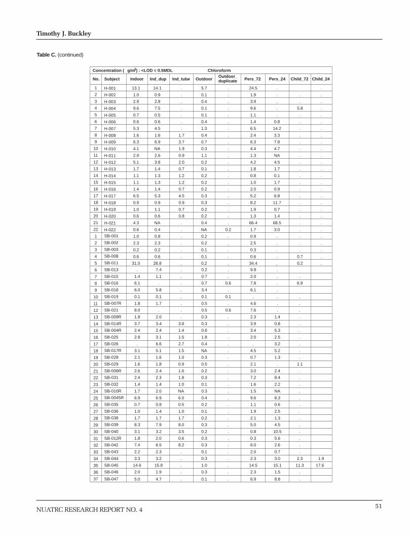
51
Timothy J. Buckley
NUATRC RESEARCH REPORT NO. 4
13.1 14.1 . 5.7 . 24.5 . . 1.0 0.9 . 0.1 . 1.9 . . .
2.9 2.8 . 0.4 . 3.9 . . .
9.6 7.5 . 0.1 . 9.6 . 5.8 .
0.7 0.5 . 0.1 . 1.1 . . . 0.6 0.6 . 0.4 . 1.4 0.8 . .
5.3 4.5 . 1.3 . 6.5 14.2 . . 1.6 1.6 1.7 0.4 . 2.4 3.3 . . 6.3 6.9 3.7 0.7 . 6.3 7.8 . .
4.1 NA 1.9 0.3 . 4.4 4.7 . . 2.9 2.6 0.9 1.1 . 1.3 NA . . 5.1 3.8 2.0 0.2 . 4.2 4.5 . . 1.7 1.4 0.7 0.1 . 1.8 1.7 . . 1.1 1.3 1.2 0.2 . 0.8 0.1 . . 1.1 1.3 1.2 0.2 . 1.0 1.7 . . 1.4 1.4 0.7 0.2 . 2.0 0.9 . .
6.5 5.3 4.5 0.3 . 5.2 6.8 . .
0.9 0.9 0.9 0.3 . 8.2 11.7 . . 1.0 1.1 0.7 0.2 . 1.9 0.7 . . 0.6 0.6 0.8 0.2 . 1.3 1.4 . . 4.3 NA . 0.4 . 66.4 68.5 . . 0.6 0.4 . NA 0.2 1.7 3.0 . .
1.0 0.8 . 0.2 . 0.9 . . .
2.3 2.3 . 0.2 . 2.5 . . . 0.2 0.2 . 0.1 . 0.3 . . . 0.6 0.6 . 0.1 . 0.6 . 0.7 .
31.0 28.8 . 0.2 . 34.4 . 0.2 . . 7.4 . 0.2 . 9.8 .
1.4 1.1 . 0.7 . 2.0 . .
6.1 . . 0.7 0.6 7.8 . 6.9
6.0 5.8 . 3.4 . 6.1 .
0.1 0.1 . 0.1 0.1 . . .
1.8 1.7 . 0.5 . 4.6 . .
8.0 . . 0.5 0.6 7.6 . .
1.8 2.0 . 0.3 . 2.3 1.4 .
3.7 3.4 3.8 0.3 . 3.9 0.8 .
2.4 2.4 1.4 0.6 . 3.4 5.3 .
2.8 3.1 1.5 1.8 . 2.0 2.5 .
. 6.6 2.7 0.4 . . 3.2 .
3.1 5.1 1.5 NA . 4.5 5.2 .
2.1 1.6 1.0 0.3 . 0.7 1.3 .
1.6 1.8 0.9 0.5 . 2.1 . 1.1
2.6 2.4 1.6 0.2 . 3.0 2.4 .
2.4 2.3 1.8 0.3 . 7.2 8.4 .
1.4 1.4 1.0 0.1 . 1.6 2.2 .
1.7 2.0 NA 0.3 . 1.5 NA .
6.9 6.9 6.0 0.4 . 9.6 8.3 .
0.7 0.8 0.5 0.2 . 1.1 0.6 .
1.0 1.4 1.0 0.1 . 1.9 2.5 .
1.7 1.7 1.7 0.2 . 2.1 1.3 .
8.3 7.9 8.0 0.3 . 5.0 4.5 .
3.1 3.2 3.5 0.2 . 0.8 10.5 .
1.8 2.0 0.6 0.3 . 0.3 5.6 .
7.4 6.5 8.2 0.3 . 6.0 2.6 .
2.2 2.3 . 0.1 . 2.0 0.7 .
3.3 3.2 . 0.3 . 2.3 3.0 2.3
14.6 15.8 . 1.0 . 14.5 15.1 11.3
2.0 1.9 . 0.3 . 2.3 1.5 .
5.0 4.7 . 0.1 . 6.9 8.8 .
1.9
17.6
H-001
H-002
H-003
H-004
H-005
H-006
H-007
H-008
H-009 H-010
H-011 H-012 H-013 H-014 H-015 H-016
H-017 H-018
H-019
H-020
H-021 H-022 SB-001
SB-002
SB-003
SB-008
SB-011 SB-013 SB-015 SB-016
SB-018
SB-019
SB-007R
SB-021 SB-009R
SB-014R
SB-004R
SB-025 SB-026
SB-017R
SB-028
SB-029
SB-006R
SB-031 SB-032 SB-010R
SB-0045R
SB-035 SB-036
SB-038
SB-039
SB-040
SB-012R
SB-042 SB-043 SB-044 SB-045 SB-046
SB-047
1
2
3
4
5
6
7
8
9
10
11
12
13
14
15
16
17
18
19
20
21
22
1
2
3
4
5
6
7
8
9
10
11
12
13
14
15
16
17
18
19
20
21
22
23
24
25
26
27
28
29
30
31
32
33
34
35
36
37
Concentration (µg/m3) : <LOD = 0.5MDL Chloroform
No. Subject Indoor Ind_dup Ind_tube Outdoor Pers_72 Pers_24 Child_72 Child_24Outdoor_duplicate
Table C. (continued)

52
VOC Exposure in an Industry-Impacted Community
NUATRC RESEARCH REPORT NO. 4
1.2 1.3 . 1.1 . 1.2 . .
0.6 0.6 . 0.6 . 0.8 . . . 0.8 0.6 . 0.9 . 1.0 . . . 0.7 0.6 . 0.8 . 1.0 . 0.8 . 1.0 0.8 . 1.0 . 1.0 . . . 0.8 0.9 . 1.1 . 1.1 0.9 . .
1.3 0.9 . 1.3 . 1.4 1.7 . .
1.1 1.1 1.5 1.5 . 1.5 1.8 . . 1.4 1.9 1.2 1.2 . 1.7 1.8 . . 1.1 NA 0.9 1.4 . 1.3 2.1 . . 2.2 1.7 0.9 4.2 . 0.7 NA . . 1.7 1.3 0.9 1.2 . 1.7 1.4 . .
1.0 0.8 0.8 0.8 . 0.9 0.2 . . 0.9 1.0 1.0 1.0 . 0.9 0.1 . . 0.6 0.8 0.8 1.0 . 0.7 0.7 . .
0.7 0.7 0.7 0.8 . 0.9 0.3 . . 1.1 0.9 0.9 1.0 . 1.0 0.8 . . 1.0 0.8 1.0 0.8 . 1.0 1.4 . .
0.9 1.1 0.6 0.8 . 1.0 0.9 . .
0.7 0.6 0.8 0.8 . 0.8 0.9 . .
0.6 NA . 0.6 . 0.7 0.4 . .
0.9 0.7 . NA 0.9 0.8 1.3 . . 0.7 0.5 . 0.7 . 0.6 . . . 0.6 0.5 . 0.6 . 0.7 . . .
0.5 0.5 . 0.6 . 0.6 . . . 0.6 0.7 . 0.6 . 0.8 . 0.7 .
1.4 1.3 . 1.3 . 1.8 . 0.1 . . 0.6 . 0.6 . 0.7 . .
0.9 0.6 . 0.9 . 0.7 . . .
1.1 . . 1.8 1.6 1.4 . 1.1 . 1.0 0.9 . 1.1 . 1.0 . . 0.1 0.1 . 0.1 0.1 . . . . 1.2 1.1 . 1.3 . 1.3 . . . 2.7 . . 1.4 1.4 2.1 . . . 1.7 1.9 . 1.7 . 1.5 1.4 . .
1.1 1.2 1.7 1.4 . 1.2 0.5 . .
1.2 1.1 0.9 1.4 . 1.1 1.2 . . 1.4 1.6 1.0 1.8 . 1.2 1.4 . .
. 2.5 1.6 1.7 . . 2.5 . .
1.8 2.7 1.0 NA . 2.0 2.8 . . 0.9 0.8 1.0 0.9 . 0.3 0.9 . .
1.1 0.9 0.9 1.0 . 1.2 . 0.4 .
0.7 0.9 0.9 1.1 . 0.9 1.4 . .
0.7 0.6 0.9 0.8 . 0.6 1.0 . . 0.8 0.8 0.9 0.8 . 0.6 0.2 . . 0.8 1.0 NA 1.1 . 0.9 NA . . 0.7 0.8 0.7 0.9 . 1.1 0.8 . . 0.9 0.7 0.2 0.9 . 1.0 0.9 . .
0.6 0.8 0.8 0.7 . 0.8 1.1 . . 0.7 0.7 0.9 0.7 . 0.6 0.4 . .
0.8 0.8 0.9 0.9 . 0.8 1.1 . . 1.1 1.1 1.3 0.6 . 0.3 3.7 . .
1.3 1.6 1.2 0.9 . 0.3 2.2 . . 0.9 0.9 0.9 1.0 . 0.9 0.3 . . 1.0 1.1 . 0.9 . 0.7 0.4 . .
0.9 0.9 . 0.8 . 0.7 1.4 0.6 0.6 1.0 1.1 . 1.6 . 1.0 0.9 0.8 1.0 0.7 0.8 . 1.1 . 0.8 0.4 . .
0.9 0.8 . 0.7 . 1.0 1.0 .
H-001 H-002 H-003 H-004
H-005
H-006 H-007
H-008 H-009
H-010 H-011 H-012 H-013 H-014
H-015
H-016 H-017
H-018 H-019
H-020 H-021 H-022 SB-001 SB-002 SB-003 SB-008 SB-011 SB-013 SB-015
SB-016 SB-018 SB-019
SB-007R
SB-021 SB-009R
SB-014R
SB-004R
SB-025
SB-026 SB-017R
SB-028 SB-029
SB-006R
SB-031 SB-032 SB-010R
SB-0045R
SB-035
SB-036 SB-038 SB-039
SB-040
SB-012R
SB-042
SB-043
SB-044 SB-045
SB-046
SB-047
1
2
3
4
5
6
7
8
9
10
11
12
13
14
15
16
17
18
19
20
21
22
1
2
3
4
5
6
7
8
9
10
11
12
13
14
15
16
17
18
19
20
21
22
23
24
25
26
27
28
29
30
31
32
33
34
35
36
37
Concentration (µg/m3) : <LOD = 0.5MDL Carbon tetrachloride
No. Subject Indoor Ind_dup Ind_tube Outdoor Pers_72 Pers_24 Child_72 Child_24Outdoor_duplicate
Table C. (continued)

53
Timothy J. Buckley
NUATRC RESEARCH REPORT NO. 4
4.6 4.9 . 2.5 . 4.9 . . 0.6 0.6 . 0.6 . 0.6 . . . 1.8 1.5 . 1.7 . 3.0 . . .
2.3 1.3 . 1.2 . 1.6 . 1.6 . 1.2 0.6 . 2.1 . 2.2 . . . 2.8 2.7 . 2.2 . 2.8 1.7 . .
8.9 7.6 . 3.3 . 6.7 8.6 . . 1.8 1.5 1.9 1.7 . 2.5 2.2 . . 2.4 3.1 1.3 2.8 . 2.9 2.3 . .
2.1 NA 1.0 0.8 . 1.6 2.4 . . 4.1 3.5 0.8 8.4 . 0.7 NA . .
3.8 2.2 0.7 1.6 . 3.6 5.3 . .
6.8 5.1 2.9 2.1 . 6.3 4.9 . . 8.0 10.1 8.2 1.8 . 4.8 0.8 . .
1.0 1.2 0.8 1.8 . 2.4 2.3 . .
1.7 1.7 0.9 1.0 . 2.4 0.9 . . 10.4 8.1 6.2 1.8 . 7.6 12.3 . .
2.0 1.7 1.8 1.8 . 2.2 2.7 . .
1.7 2.1 0.6 1.7 . 2.3 1.7 . .
0.6 0.6 0.6 0.6 . 1.8 1.8 . .
2.2 NA . 0.6 . 1.2 2.2 . . 1.3 0.6 . NA 0.9 0.6 1.7 . .
7.7 7.5 . 2.4 . 8.4 . . . 7.0 6.8 . 2.7 . 7.3 . . .
3.5 4.2 . 1.8 . 6.4 . . . 1.4 1.2 . 0.6 . 1.5 . 1.4 . 2.3 2.5 . 2.3 . 3.4 . 0.2 . . 1.0 . 0.9 . 1.3 . .
1.2 0.6 . 1.5 . 2.4 . . . 2.6 . . 2.5 2.0 4.8 . 4.1 .
5.0 5.1 . 2.8 . 6.7 . .
9.2 8.2 . 2.9 3.2 . . . . 2.9 2.7 . 3.0 . 3.4 . . . 8.8 . . 3.4 2.9 7.3 . . .
7.4 8.3 . 0.8 . 6.8 6.3 . .
3.1 2.8 3.7 0.7 . 3.0 0.7 . .
0.8 0.8 0.4 2.1 . 2.1 2.4 . . 4.5 5.0 3.1 4.8 . 4.3 2.7 . .
. 2.4 0.4 2.3 . . 2.4 . . 6.4 7.5 1.1 NA . 5.1 5.6 . . 2.8 2.1 0.9 3.2 . 0.7 2.0 . .
4.8 4.7 2.6 2.0 . 6.0 . 3.5 . 2.4 2.4 1.4 0.7 . 2.6 2.0 . .
0.7 0.7 0.4 1.6 . 2.0 2.3 . .
4.9 4.5 3.0 1.4 . 2.3 2.4 . . 2.6 3.1 NA 2.7 . 2.8 NA . . 4.0 3.9 3.3 1.9 . 5.7 2.9 . . 1.3 1.3 0.3 1.8 . 1.5 1.0 . .
0.9 1.4 0.6 0.8 . 2.9 6.7 . .
1.5 1.5 0.6 0.6 . 1.6 1.8 . .
2.9 2.6 2.8 1.6 . 2.1 1.7 . .
6.8 6.7 6.7 0.6 . 1.7 21.5 . . 1.1 1.4 5.7 1.2 . 0.6 4.2 . . 1.6 1.2 0.7 0.6 . 1.4 0.6 . . 1.2 1.2 . 0.6 . 1.4 1.7 . .
6.3 6.0 . 1.9 . 4.4 10.4 3.8 6.0
10.2 11.0 . 3.7 . 10.1 11.0 8.0 13.1
12.3 12.3 . 2.8 . 8.5 10.1 . .
5.4 4.9 . 0.5 . 5.7 7.9 . .
H-001
H-002
H-003
H-004
H-005
H-006
H-007
H-008
H-009
H-010
H-011 H-012
H-013 H-014
H-015
H-016
H-017 H-018 H-019
H-020
H-021
H-022 SB-001
SB-002
SB-003
SB-008
SB-011 SB-013 SB-015
SB-016
SB-018 SB-019
SB-007R
SB-021
SB-009R
SB-014R
SB-004R
SB-025 SB-026 SB-017R
SB-028
SB-029 SB-006R
SB-031 SB-032
SB-010R
SB-0045R
SB-035
SB-036
SB-038 SB-039
SB-040
SB-012R
SB-042 SB-043
SB-044 SB-045 SB-046 SB-047
1
2
3
4
5
6
7
8
9
10
11
12
13
14
15
16
17
18
19
20
21
22
1
2
3
4
5
6
7
8
9
10
11
12
13
14
15
16
17
18
19
20
21
22
23
24
25
26
27
28
29
30
31
32
33
34
35
36
37
Concentration (µg/m3) : <LOD = 0.5MDL Benzene
No. Subject Indoor Ind_dup Ind_tube Outdoor Pers_72 Pers_24 Child_72 Child_24Outdoor_duplicate
Table C. (continued)

54
VOC Exposure in an Industry-Impacted Community
NUATRC RESEARCH REPORT NO. 4
0.1 0.1 . 0.1 . 2.3 . .
0.2 0.2 . 0.2 . 0.3 . . .
0.2 0.2 . 0.2 . 0.2 . . .
0.2 0.2 . 0.2 . 0.9 . 0.2 . 0.2 0.2 . 0.5 . 0.2 . . .
0.2 0.2 . 0.2 . 0.6 0.5 . .
0.1 0.1 . 0.1 . 0.1 0.4 . .
0.1 0.1 0.4 0.3 . 0.3 0.4 . .
0.1 0.6 0.3 0.1 . 0.4 1.5 . .
0.1 NA 0.2 0.1 . 0.1 0.4 . .
0.2 0.2 0.2 0.5 . 0.2 NA . .
0.2 0.2 0.4 0.2 . 0.2 0.5 . .
0.2 0.2 0.6 0.2 . 0.2 0.5 . .
0.1 0.1 0.1 0.1 . 0.1 0.2 . .
0.1 0.1 0.1 0.1 . 0.2 0.3 . .
0.1 0.1 0.1 0.1 . 0.1 0.3 . .
0.1 0.1 0.1 0.1 . 0.2 0.3 . .
0.3 0.2 0.1 0.1 . 0.3 0.7 . .
0.2 0.2 0.2 0.2 . 0.2 0.7 . .
0.2 0.2 0.2 0.2 . 0.2 0.7 . .
0.2 NA . 0.2 . 0.2 0.9 . .
0.2 0.2 . NA 0.4 0.2 0.7 . .
0.1 0.1 . 0.1 . 0.1 . . .
0.1 0.1 . 0.1 . 0.1 . . .
0.1 0.5 . 0.1 . 0.1 . . .
0.1 0.1 . 0.1 . 0.1 . 0.1 . 0.2 0.1 . 0.1 . 0.2 . 0.1 . . 0.1 . 0.1 . 0.1 . .
0.2 0.2 . 0.2 . 0.4 . . .
0.5 . . 0.2 0.2 0.4 . 0.4 .
0.1 0.1 . 0.1 . 0.1 . .
0.2 0.2 . 0.2 0.2 . . . .
0.1 0.1 . 0.1 . 0.1 . . .
0.6 . . 0.1 0.1 0.4 . . .
4.0 4.2 . 0.6 . 2.9 1.5 . .
0.4 0.1 0.9 0.1 . 0.4 0.1 . .
0.4 0.1 0.6 0.4 . 0.4 1.7 . .
0.1 0.1 0.4 0.3 . 0.4 0.5 . .
. 0.2 0.4 0.2 . . 0.6 . .
0.2 0.2 0.4 NA . 0.2 0.5 . .
0.2 0.2 0.2 0.2 . 0.2 0.5 . .
0.2 0.2 0.2 0.2 . 0.2 . 0.2 . 0.2 0.2 0.3 0.2 . 0.2 0.5 . .
0.2 0.2 0.2 0.2 . 0.2 0.6 . .
0.2 0.2 0.7 0.2 . 0.2 0.6 . .
0.3 0.4 NA 0.2 . 0.2 NA . .
0.1 0.1 0.1 0.1 . 42.8 109.3 . .
0.1 0.1 0.1 0.1 . 0.1 0.3 . .
0.1 0.1 0.1 0.1 . 0.3 0.3 . .
0.2 0.2 0.2 0.2 . 0.2 0.7 . .
0.2 0.2 0.2 0.2 . 0.8 0.7 . .
0.2 0.2 0.2 0.2 . 0.2 0.9 . .
0.5 0.6 2.3 0.2 . 0.2 0.7 . .
0.2 0.2 0.3 0.2 . 0.2 0.2 . .
0.2 0.2 . 0.2 . 0.8 0.7 . .
1.4 1.3 . 0.2 . 0.5 0.8 0.8 0.6
1.6 2.3 . 1.0 . 1.7 1.5 1.3 2.2 3.3 3.1 . 0.2 . 2.5 2.2 . .
0.2 0.2 . 0.2 . 0.2 0.6 . .
H-001 H-002 H-003 H-004
H-005
H-006
H-007
H-008
H-009 H-010 H-011 H-012 H-013 H-014
H-015
H-016
H-017
H-018
H-019 H-020 H-021 H-022 SB-001 SB-002 SB-003 SB-008
SB-011 SB-013 SB-015
SB-016
SB-018
SB-019 SB-007R
SB-021 SB-009R
SB-014R
SB-004R
SB-025
SB-026
SB-017R
SB-028
SB-029 SB-006R
SB-031 SB-032 SB-010R
SB-0045R
SB-035
SB-036
SB-038
SB-039 SB-040
SB-012R
SB-042
SB-043
SB-044 SB-045
SB-046
SB-047
1
2
3
4
5
6
7
8
9
10
11
12
13
14
15
16
17
18
19
20
21
22
1
2
3
4
5
6
7
8
9
10
11
12
13
14
15
16
17
18
19
20
21
22
23
24
25
26
27
28
29
30
31
32
33
34
35
36
37
Concentration (µg/m3) : <LOD = 0.5MDL Trichloroethylene
No. Subject Indoor Ind_dup Ind_tube Outdoor Pers_72 Pers_24 Child_72 Child_24Outdoor_duplicate
Table C. (continued)
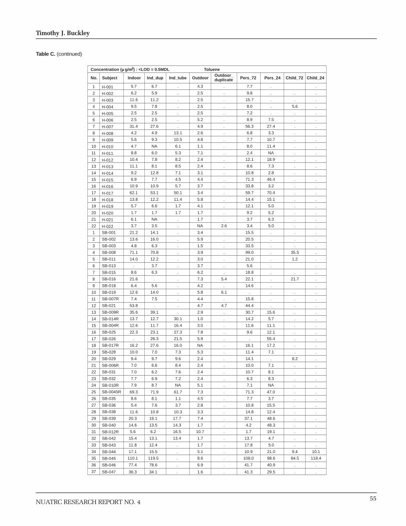
55
Timothy J. Buckley
NUATRC RESEARCH REPORT NO. 4
5.7 6.7 . 4.3 . 7.7 . .
6.2 5.9 . 2.5 . 9.8 . . . 11.6 11.2 . 2.5 . 15.7 . . . 9.5 7.8 . 2.5 . 8.0 . 5.6 . 2.5 2.5 . 2.5 . 7.2 . . . 2.5 2.5 . 5.2 . 8.9 7.5 . .
31.4 27.6 . 4.9 . 56.3 27.4 . . 4.2 4.9 13.1 2.6 . 6.8 3.3 . . 5.6 9.3 10.5 4.8 . 7.7 10.7 . . 4.7 NA 6.1 1.1 . 8.0 11.4 . . 8.8 6.0 5.3 7.1 . 2.4 NA . .
10.4 7.8 8.2 2.4 . 12.1 18.9 . . 11.1 8.1 8.5 2.4 . 8.6 7.3 . . 9.2 12.8 7.1 3.1 . 10.8 2.8 . . 6.9 7.7 4.5 4.4 . 71.3 46.4 . .
10.9 10.9 5.7 3.7 . 33.8 3.2 . . 62.1 53.1 50.1 3.4 . 59.7 70.4 . . 13.8 12.2 11.4 5.8 . 14.4 15.1 . .
5.7 6.6 1.7 4.1 . 12.1 5.0 . .
1.7 1.7 1.7 1.7 . 9.2 5.2 . . 6.1 NA . 1.7 . 3.7 6.3 . . 3.7 3.5 . NA 2.6 3.4 5.0 . .
21.2 14.1 . 3.4 . 15.5 . . . 13.6 16.0 . 5.9 . 20.5 . . . 4.8 6.3 . 1.5 . 33.5 . . .
71.1 70.8 . 3.9 . 99.0 . 35.5 . 14.0 12.2 . 3.0 . 21.0 . 1.2 .
. 3.7 . 3.7 . 5.6 . . 8.6 6.3 . 6.2 . 18.8 . . .
21.6 . . 7.3 5.4 22.1 . 21.7 . 6.4 5.6 . 4.2 . 14.6 . .
12.6 14.0 . 5.8 6.1 . . . .
7.4 7.5 . 4.4 . 15.8 . . . 53.8 . . 4.7 4.7 44.4 . . . 35.6 39.1 . 2.9 . 30.7 15.6 . . 13.7 12.7 30.1 1.0 . 14.2 5.7 . . 12.6 11.7 16.4 3.0 . 11.6 11.1 . .
22.3 23.1 27.3 7.8 . 9.6 12.1 . .
. 26.3 21.5 5.9 . . 55.4 . . 16.2 27.6 16.0 NA . 16.1 17.2 . . 10.0 7.0 7.3 5.3 . 11.4 7.1 . .
9.4 9.7 9.6 2.4 . 14.1 . 8.2 . 7.0 6.6 8.4 2.4 . 10.0 7.1 . .
7.0 6.2 7.6 2.4 . 10.7 8.1 . .
7.7 6.9 7.2 2.4 . 6.3 8.3 . . 7.9 8.7 NA 5.1 . 7.1 NA . .
69.3 71.9 61.7 7.3 . 71.3 47.0 . .
8.6 8.1 1.1 4.5 . 7.7 3.7 . . 5.4 7.6 3.7 2.8 . 10.8 15.5 . .
11.6 10.8 10.3 3.3 . 14.8 12.4 . . 20.3 19.1 17.7 7.4 . 37.1 48.6 . . 14.6 13.5 14.3 1.7 . 4.2 48.3 . . 5.6 6.2 16.5 10.7 . 1.7 19.1 . .
15.4 13.1 13.4 1.7 . 13.7 4.7 . . 11.8 12.4 . 1.7 . 17.8 5.0 . .
17.1 15.5 . 5.1 . 10.9 21.0 9.4 10.1
110.1 119.5 . 8.6 . 108.0 98.6 84.5 118.4 77.4 78.6 . 6.9 . 41.7 40.9 . . 36.3 34.1 . 1.6 . 41.3 29.5 . .
H-001
H-002
H-003
H-004
H-005
H-006
H-007
H-008
H-009
H-010
H-011 H-012
H-013
H-014
H-015
H-016
H-017
H-018
H-019
H-020
H-021
H-022 SB-001
SB-002
SB-003
SB-008
SB-011 SB-013
SB-015
SB-016
SB-018
SB-019
SB-007R
SB-021
SB-009R
SB-014R
SB-004R
SB-025 SB-026 SB-017R
SB-028 SB-029 SB-006R
SB-031
SB-032 SB-010R
SB-0045R
SB-035 SB-036 SB-038 SB-039 SB-040
SB-012R
SB-042 SB-043 SB-044 SB-045 SB-046 SB-047
1
2
3
4
5
6
7
8
9
10
11
12
13
14
15
16
17
18
19
20
21
22
1
2
3
4
5
6
7
8
9
10
11
12
13
14
15
16
17
18
19
20
21
22
23
24
25
26
27
28
29
30
31
32
33
34
35
36
37
Concentration (µg/m3) : <LOD = 0.5MDL Toluene
No. Subject Indoor Ind_dup Ind_tube Outdoor Pers_72 Pers_24 Child_72 Child_24Outdoor_duplicate
Table C. (continued)

56
VOC Exposure in an Industry-Impacted Community
NUATRC RESEARCH REPORT NO. 4
0.6 0.7 . 0.6 . 1.2 . .
0.5 0.6 . 0.5 . 0.7 . . . 2.8 2.7 . 0.8 . 7.0 . . . 1.0 0.8 . 1.1 . 1.6 . 0.7 . 1.0 0.9 . 1.2 . 2.0 . . . 6.4 6.8 . 1.0 . 6.0 2.5 . . 3.0 2.6 . 3.3 . 3.6 1.5 . . 1.0 1.1 1.5 1.0 . 1.7 2.0 . . 1.2 1.4 1.1 1.7 . 1.6 1.3 . .
0.4 NA 0.5 0.2 . 0.8 0.6 . . 1.0 0.8 0.7 1.7 . 1.0 NA . . 0.4 0.4 0.4 0.1 . 1.1 0.4 . .
2.1 1.6 1.5 0.5 . 1.4 1.9 . .
0.4 0.4 0.2 0.5 . 1.2 0.5 . . 0.5 0.5 0.2 0.5 . 2.4 0.6 . . 1.1 1.1 0.2 0.2 . 2.6 0.6 . . 1.7 1.2 1.2 0.7 . 1.6 1.6 . . 0.8 0.8 0.6 0.6 . 1.3 1.2 . . 2.8 3.3 1.0 1.9 . 4.8 3.7 . . 0.8 0.8 1.2 0.8 . 1.2 0.8 . .
2.7 NA . 0.3 . 0.9 1.0 . . 0.8 0.3 . NA 0.4 0.3 0.8 . .
0.4 0.3 . 0.4 . 0.1 . . . 0.3 0.5 . 0.3 . 0.6 . . . 1.0 1.3 . 0.3 . 0.2 . . . 0.1 0.1 . 0.1 . 0.1 . 0.1 . 0.1 0.1 . 0.1 . 0.3 . 0.1 . . 0.3 . 0.2 . 0.3 . .
0.8 0.6 . 0.8 . 3.4 . . .
1.2 . . 0.8 0.6 3.4 . 2.1 . 0.2 0.1 . 0.4 . 0.1 . . 0.1 0.1 . 0.1 0.1 . . . . 0.9 0.7 . 0.8 . 1.2 . . . 21.4 . . 1.5 1.3 15.9 . . .
3.6 4.0 . 0.3 . 3.0 2.4 . .
0.5 0.4 0.8 0.6 . 0.5 0.3 . .
3.5 3.3 1.8 0.8 . 2.4 1.9 . .
2.1 2.2 1.4 2.1 . 1.8 0.9 . .
. 10.6 6.8 0.4 . . 8.9 . .
0.4 0.7 0.4 NA . 1.1 0.4 . .
0.6 0.5 0.7 0.1 . 0.7 0.4 . .
0.3 0.3 0.3 0.3 . 0.4 . 0.1 . 0.1 0.3 0.3 0.1 . 0.3 0.4 . .
0.5 0.5 0.5 0.5 . 0.6 1.1 . . 0.8 0.8 0.7 0.1 . 0.6 1.1 . . 0.6 0.6 NA 0.4 . 0.4 NA . . 0.4 0.5 0.2 0.4 . 2.8 3.5 . . 0.2 0.2 0.2 0.2 . 0.2 0.6 . . 0.2 0.4 0.2 0.2 . 1.2 2.1 . . 0.3 0.7 0.3 0.3 . 0.3 0.8 . .
1.3 1.1 0.9 0.3 . 2.3 3.5 . . 1.2 0.9 0.8 0.3 . 0.3 2.8 . .
0.3 0.6 2.6 0.8 . 0.3 20.3 . .
0.3 0.3 0.3 0.3 . 0.3 0.3 . .
0.3 0.3 . 0.3 . 0.9 0.8 . .
0.7 0.6 . 0.3 . 0.7 1.0 0.3 0.7 24.4 26.2 . 1.2 . 24.3 27.1 18.6 30.1 0.3 0.3 . 0.3 . 0.3 0.8 . .
1.6 1.5 . 1.5 . 1.8 2.1 . .
H-001 H-002 H-003
H-004
H-005 H-006 H-007 H-008
H-009
H-010 H-011 H-012 H-013
H-014
H-015 H-016 H-017 H-018
H-019
H-020 H-021 H-022 SB-001 SB-002 SB-003
SB-008
SB-011 SB-013
SB-015 SB-016 SB-018
SB-019
SB-007R
SB-021 SB-009R
SB-014R
SB-004R
SB-025 SB-026 SB-017R
SB-028
SB-029
SB-006R
SB-031
SB-032
SB-010R
SB-0045R
SB-035
SB-036
SB-038
SB-039
SB-040
SB-012R
SB-042
SB-043
SB-044 SB-045
SB-046
SB-047
1
2
3
4
5
6
7
8
9
10
11
12
13
14
15
16
17
18
19
20
21
22
1
2
3
4
5
6
7
8
9
10
11
12
13
14
15
16
17
18
19
20
21
22
23
24
25
26
27
28
29
30
31
32
33
34
35
36
37
Concentration (µg/m3) : <LOD = 0.5MDL Tetrachloroethylene
No. Subject Indoor Ind_dup Ind_tube Outdoor Pers_72 Pers_24 Child_72 Child_24Outdoor_duplicate
Table C. (continued)

57
Timothy J. Buckley
NUATRC RESEARCH REPORT NO. 4
3.5 4.0 . 3.1 . 4.4 . .
1.5 1.4 . 0.6 . 2.2 . . . 2.4 2.4 . 1.9 . 4.6 . . . 3.2 2.6 . 1.4 . 3.1 . 2.5 . 4.6 3.9 . 2.8 . 4.2 . . . 4.8 4.8 . 2.1 . 5.3 3.0 . . 21.8 19.1 . 4.2 . 16.0 16.2 . . 1.6 1.7 4.0 1.8 . 3.0 2.9 . .
3.8 4.4 5.5 4.2 . 4.4 3.8 . .
2.3 NA 3.0 1.0 . 2.2 2.0 . . 4.6 3.9 4.7 5.3 . 2.0 NA . . 1.9 1.8 2.4 1.2 . 3.5 3.8 . .
4.3 3.4 4.1 2.2 . 3.7 2.9 . .
2.5 3.3 2.1 1.9 . 6.5 0.8 . .
2.1 2.2 1.7 2.2 . 47.3 38.5 . . 8.7 8.6 3.3 1.7 . 9.1 2.3 . . 17.0 14.7 15.2 2.0 . 16.3 22.9 . .
3.3 2.8 3.3 3.0 . 5.7 4.3 . . 3.8 4.4 0.4 2.7 . 12.3 7.0 . . 1.2 1.0 1.6 1.1 . 4.6 5.0 . . 11.7 NA . 1.3 . 6.1 7.8 . .
2.0 1.6 . NA 1.5 1.5 1.3 . . 9.2 8.0 . 2.4 . 6.9 . . .
5.3 5.1 . 5.1 . 7.3 . . . 1.6 2.6 . 1.2 . 24.2 . . . 8.9 7.3 . 0.6 . 9.5 . 5.3 . 4.1 3.7 . 2.1 . 5.2 . 0.4 . . 1.8 . 2.2 . 2.8 . .
3.1 2.3 . 3.6 . 10.0 . . . 7.8 . . 5.0 4.3 10.5 . 11.1 . 4.0 4.6 . 4.3 . 5.7 . .
3.8 4.0 . 2.2 2.1 . . . . 7.5 6.8 . 6.5 . 6.3 . . . 15.4 . . 4.4 4.0 13.1 . . . 21.7 23.9 . 1.9 . 19.5 14.1 . . 5.0 4.6 8.8 1.2 . 4.9 2.7 . .
7.7 7.4 8.9 7.1 . 6.8 5.7 . .
8.5 9.1 11.8 6.6 . 5.9 5.3 . . . 5.0 5.9 1.8 . . 5.8 . .
4.7 6.8 5.0 NA . 5.0 5.5 . . 2.8 2.0 3.1 2.3 . 4.0 3.3 . . 7.7 7.9 7.7 2.7 . 8.8 . 4.7 .
2.2 2.1 3.1 0.7 . 3.1 3.5 . . 4.5 4.2 5.4 2.8 . 4.1 6.2 . . 10.6 9.7 8.4 5.3 . 8.5 7.7 . .
4.0 4.3 NA 4.3 . 4.0 NA . . 15.5 16.3 13.3 3.5 . 18.5 8.3 . . 3.5 3.6 0.3 2.4 . 3.5 1.1 . . 3.4 4.3 2.7 3.6 . 5.0 5.4 . . 3.7 3.5 3.4 3.2 . 4.6 2.9 . .
7.5 7.0 6.5 5.5 . 14.8 25.0 . . 7.8 7.8 8.8 4.1 . 1.9 28.0 . . 4.6 5.0 4.2 9.9 . 1.2 11.9 . .
3.0 2.5 2.7 1.8 . 3.7 0.9 . .
2.4 2.6 . 0.8 . 3.1 1.3 . . 7.9 7.1 . 6.1 . 6.8 14.0 5.3 7.1 60.2 65.1 . 5.5 . 58.7 56.7 46.6 66.4 47.1 47.8 . 4.9 . 23.9 25.6 . . 5.7 5.5 . 2.1 . 11.1 18.6 . .
H-001 H-002 H-003 H-004 H-005 H-006 H-007
H-008
H-009
H-010 H-011 H-012 H-013 H-014 H-015 H-016 H-017
H-018
H-019
H-020 H-021 H-022 SB-001 SB-002 SB-003 SB-008
SB-011 SB-013 SB-015 SB-016 SB-018
SB-019
SB-007R
SB-021 SB-009R
SB-014R
SB-004R
SB-025 SB-026 SB-017R
SB-028
SB-029
SB-006R
SB-031 SB-032 SB-010R
SB-0045R
SB-035 SB-036 SB-038
SB-039
SB-040 SB-012R
SB-042 SB-043 SB-044 SB-045 SB-046 SB-047
1
2
3
4
5
6
7
8
9
10
11
12
13
14
15
16
17
18
19
20
21
22
1
2
3
4
5
6
7
8
9
10
11
12
13
14
15
16
17
18
19
20
21
22
23
24
25
26
27
28
29
30
31
32
33
34
35
36
37
Concentration (µg/m3) : <LOD = 0.5MDL p-Xylene
No. Subject Indoor Ind_dup Ind_tube Outdoor Pers_72 Pers_24 Child_72 Child_24Outdoor_duplicate
Table C. (continued)

58
VOC Exposure in an Industry-Impacted Community
NUATRC RESEARCH REPORT NO. 4
1.8 1.8 . 1.8 . 1.8 . .
0.8 0.8 . 0.2 . 1.1 . . .
1.3 1.4 . 1.1
. 2.5 . . .
10.4 8.3 . 1.0
. 8.1
. 7.2
.
2.1
1.8
. 1.6 . 2.3 . . .
3.4 3.5 . 1.3 . 0.2
2.2
. .
12.8 11.4 . 2.5 . 9.7 10.6 . .
0.8
1.0
1.6 1.1
. 1.7 1.9 . .
1.9 2.6 2.2
2.5 . 2.5 1.9 . .
1.4 NA
1.4 0.5 . 1.3 1.1
. .
2.4 2.0
1.7 2.8
. 0.9 NA
. .
1.0
0.9 1.0
0.6 . 2.0
2.5 . .
1.4 1.0
1.4 0.8
. 1.1
0.9 . .
0.7 1.0
1.0
0.7 . 1.9 0.3 . .
0.7 0.7 0.6 0.7 . 9.0
7.6 . .
2.1
2.0
1.0
0.5 . 2.5 0.8
. .
5.7 4.9 5.2
0.8
. 5.5 7.6 . .
1.1
0.8
1.1
1.0
. 1.8
2.1
. .
1.3 1.3 0.3 1.0
. 4.5 2.3 . .
0.4 0.3 0.6 0.4 . 1.4 1.6 . .
2.8
NA
. 0.4 . 1.3 1.
7
. .
0.7 0.6 . NA
0.5 0.5 0.4 . .
3.0
2.4 . 0.9 . 2.0
. . .
1.6 1.6 . 1.5 . 2.2
. . .
0.6 0.8
. 0.2
. 6.7 . . .
2.8
2.3 . 2.2
. 3.1
. 1.6 .
1.8
1.8
. 1.8
. 1.8
. 1.8
.
. 1.8
. 1.8
. 1.8
. .
1.2
0.9 . 1.3 . 3.7 . . .
4.4 . . 2.6 2.1
7.0
. 7.6 .
1.3 1.3 . 1.3 . 1.3 . .
3.5 4.0 . 0.2 0.2 . . . .
4.2 4.0 . 4.4 . 3.7 . . .
8.9 . .
2.4 2.1
7.8
. . .
12.6 13.7 . 1.1 .
11.5 8.4 . .
3.0
2.6 3.9 0.6 . 3.0
1.3 . .
3.4 3.4 2.6 3.1 .
3.3 2.5 . .
5.8
6.3 4.8
4.2 .
3.6 2.9 . .
. 2.6 2.2
1.1 .
. 2.9 . .
2.3 3.4 1.9 NA . 2.6 2.9 . .
1.0
0.7 1.2
0.8 .
1.4 1.3 . .
2.2
2.1
2.7 0.9 . 2.9 . 1.4 .
0.7 0.8
1.1
0.3 . 1.0
1.0
. .
1.2
1.2
1.8
0.9 . 1.3 2.0
. .
3.0
2.9 2.9 1.3 . 2.4 2.5 . .
1.2
1.3 NA
1.3 . 1.2
NA
. .
4.5 4.8
4.0
1.0 .
5.5 2.4 . .
1.1
1.0
0.1
0.7 . 1.1
0.5 . .
0.8
1.0
0.7 0.8 .
1.3 1.6 . .
1.0
1.0
1.0
0.9 . 1.3 1.0
. .
2.5 2.3 2.1
1.5 . 5.7 9.0
. .
2.4 2.2
2.9 1.2 .
0.7 8.5 . .
1.2
1.3 1.3 2.5 . 0.4 4.2
. .
0.9 0.7 0.8
0.6 . 1.2
0.3 . .
1.0
1.1
. 0.3 . 1.1
0.4 . .
2.5 2.1
. 1.5 . 2.2
4.2
1.4 1.8
17.0 18.3 . 1.6 . 16.9 18.0
13.4 20.2
15.5 16.0
. 1.5 . 8.3 8.4 . .
1.9 1.8
. 0.7 . 5.4 6.0
. .
H-001 H-002 H-003
H-004
H-005
H-006
H-007
H-008 H-009
H-010 H-011 H-012 H-013
H-014
H-015
H-016
H-017
H-018 H-019
H-020 H-021 H-022 SB-001 SB-002 SB-003
SB-008 SB-011 SB-013
SB-015
SB-016
SB-018 SB-019
SB-007R
SB-021 SB-009R
SB-014R
SB-004R
SB-025
SB-026
SB-017R
SB-028 SB-029
SB-006R
SB-031
SB-032
SB-010R
SB-0045R
SB-035 SB-036
SB-038
SB-039
SB-040
SB-012R
SB-042
SB-043 SB-044 SB-045 SB-046
SB-047
1
2
3
4
5
6
7
8
9
10
11
12
13
14
15
16
17
18
19
20
21
22
1
2
3
4
5
6
7
8
9
10
11
12
13
14
15
16
17
18
19
20
21
22
23
24
25
26
27
28
29
30
31
32
33
34
35
36
37
Concentration (µg/m3) : <LOD = 0.5MDL o-Xylene
No. Subject Indoor Ind_dup Ind_tube Outdoor Pers_72 Pers_24 Child_72 Child_24Outdoor_duplicate
Table C. (continued)

59
Timothy J. Buckley
NUATRC RESEARCH REPORT NO. 4
1.1 1.7 . 0.2 . 3.3 . .
0.3 0.3 . 0.3 . 0.3 . . . 2.5 1.7 . 0.3 . 3.8 . . .
3.2 3.0 . 0.3 . 4.7 . 3.3 . 1.5 1.6 . 1.3 . 1.4 . . .
0.3 0.3 . 0.9 . 1.2 1.0 . . 1.9 5.0 . 0.6 . 1.2 0.8 . .
0.3 0.9 0.6 1.1 . 2.9 4.6 . .
1.2 1.6 0.4 1.2 . 3.3 0.8 . .
4.0 NA 0.3 0.9 . 4.6 3.8 . .
4.9 3.6 0.3 3.7 . 0.4 NA . . 2.9 1.0 0.3 0.4 . 6.4 8.2 . . 2.2 1.4 1.0 0.4 . 1.4 1.2 . . 0.2 0.4 0.2 0.2 . 0.2 0.5 . .
0.2 0.2 0.2 0.2 . 2.2 1.6 . .
0.2 0.2 0.2 0.2 . 0.9 0.6 . .
0.7 0.6 0.9 0.2 . 1.0 0.6 . .
0.2 0.2 0.2 0.2 . 0.2 0.6 . .
0.3 0.4 0.1 0.1 . 0.6 0.2 . . 0.1 0.1 0.1 0.1 . 0.1 0.2 . . 0.1 NA . 0.1 . 0.1 0.2 . . 0.1 0.1 . NA 0.1 0.1 0.2 . . 1.8 1.7 . 0.3 . 1.4 . . .
0.3 0.6 . 0.3 . 1.5 . . .
0.3 0.3 . 0.3 . 1.3 . . . 0.3 0.3 . 0.3 . 0.3 . 0.3 . 2.5 1.6 . 0.2 . 4.2 . 0.5 .
. 0.2 . 0.2 . 0.2 . . 2.5 2.2 . 0.3 . 4.2 . . . 8.2 . . 2.4 2.1 7.4 . 7.2 . 0.1 0.1 . 0.1 . 6.8 . .
0.3 0.3 . 0.3 0.3 . . . . 1.9 1.5 . 7.2 . 2.5 . . .
10.2 . . 1.7 1.2 8.9 . . .
43.3 50.8 . 0.8 . 51.3 27.3 . . 4.5 3.6 1.4 0.2 . 6.5 1.7 . . 0.7 0.8 0.4 0.3 . 1.9 0.8 . .
7.5 9.3 1.0 2.7 . 4.5 10.7 . . . 10.3 0.8 2.6 . . 14.6 . .
2.6 8.0 0.3 NA . 6.2 17.1 . . 0.4 0.8 0.4 0.4 . 1.1 2.3 . . 0.4 0.4 0.7 0.4 . 1.9 . 0.9 .
0.4 0.4 0.5 0.4 . 0.7 1.1 . . 0.4 0.4 0.5 0.4 . 0.4 1.3 . . 0.4 0.4 0.7 0.4 . 0.4 1.3 . . 0.2 0.4 NA 0.2 . 0.7 NA . . 0.7 0.8 0.2 0.2 . 1.1 0.6 . .
0.2 0.2 0.2 0.2 . 0.2 0.7 . . 0.2 0.2 0.2 0.2 . 0.2 0.6 . .
0.1 0.1 0.3 0.1 . 0.2 0.2 . . 1.1 1.0 2.7 0.1 . 1.3 0.7 . . 0.3 0.3 0.5 0.1 . 0.1 1.9 . .
0.1 0.1 0.5 0.1 . 0.1 0.2 . . 0.1 0.1 0.1 0.1 . 0.2 0.1 . . 0.4 0.4 . 0.1 . 0.6 0.2 . . 0.2 0.1 . 0.1 . 0.2 0.2 0.1 0.1 1.6 1.9 . 0.1 . 1.7 1.1 1.2 1.3 1.5 1.6 . 0.1 . 1.4 1.2 . . 0.7 0.6 . 0.1 . 0.8 0.7 . .
H-001 H-002 H-003 H-004
H-005
H-006
H-007 H-008
H-009
H-010 H-011 H-012 H-013 H-014
H-015
H-016
H-017 H-018
H-019
H-020 H-021 H-022 SB-001 SB-002 SB-003 SB-008
SB-011 SB-013 SB-015
SB-016
SB-018
SB-019
SB-007R
SB-021 SB-009R
SB-014R
SB-004R
SB-025
SB-026
SB-017R
SB-028
SB-029
SB-006R
SB-031 SB-032 SB-010R
SB-0045R
SB-035
SB-036
SB-038
SB-039
SB-040
SB-012R
SB-042
SB-043
SB-044 SB-045
SB-046
SB-047
1
2
3
4
5
6
7
8
9
10
11
12
13
14
15
16
17
18
19
20
21
22
1
2
3
4
5
6
7
8
9
10
11
12
13
14
15
16
17
18
19
20
21
22
23
24
25
26
27
28
29
30
31
32
33
34
35
36
37
Concentration (µg/m3) : <LOD = 0.5MDL Styrene
No. Subject Indoor Ind_dup Ind_tube Outdoor Pers_72 Pers_24 Child_72 Child_24Outdoor_duplicate
Table C. (continued)

60
VOC Exposure in an Industry-Impacted Community
NUATRC RESEARCH REPORT NO. 4
24.1 25.7 3.0 . 26.6 . . .
0.3 0.3 0.3 . 1.5 . . . .
1.8 1.7 0.3
. 3.0
. . . .
2.7
1.9 0.3
. 2.8 . 1.9 . .
3.0
2.5 0.8 . 3.2
. . . .
0.3
0.3 0.3
. 0.3
1.0
. . .
0.4
0.4 0.6 . 1.4
0.4
. . .
0.5
0.8 1.6
0.5
. 1.6
1.3
. . 1.6
0.5
1.1 1.7
0.9 . 0.7
1.1
. . 1.7
2.0
NA 1.8 0.1
. 4.6
0.9 . . 1.8
1.0
0.2 0.5
0.5
. 0.2
NA
. . 0.5
0.2
0.2 0.5
0.2
. 0.2
0.5
. . 0.5
0.2
0.2 0.6
0.2
. 0.2
0.5
. . 0.6
2.0
2.9 1.6 0.4
0.4
. 2.4
1.0
. . 1.6 0.4
0.4 0.4
0.4
. 0.4
1.2
. . 0.4
0.4
0.4 0.4
. 0.4
1.1
. . 0.4 4.4
4.1 4.6
0.4
. 4.6
6.2
. . 4.6
4.8 4.1 4.8 0.9 . 6.1
7.2
. . 4.8
1.3 1.5 0.4 0.4 . 1.4 1.3 . . 0.4 0.4
0.4 0.4
0.4
. 1.1
1.4
. . 0.4
64.0 NA 1.5 . 19.9 20.3 . . .
0.4
0.4 NA
0.7 0.4
1.3
. . .
0.4 0.4 0.4 . 0.4 . . . .
0.4 0.4 0.4 . 0.4 . . . .
1.4 1.1 0.4 . 0.3 . . . .
158.7 145.0 1.3 . 150.0 . 134.3 . .
3.6 3.0 0.7 . 6.4 . 0.2 . .
. 0.2 1.0 . 1.1 . . .
0.3 0.3 0.3 . 0.7 . . . .
15.7 . 1.4 0.9 16.1 . 13.5 . .
119.3 119.3 17.3 . 66.4 . . .
3.6 4.2 3.3 3.4 . . . . .
0.9 0.7 0.7 . 0.7 . . . .
3.5 . 0.8 0.5 3.2 . . . .
0.5 0.3 0.7 . 0.5 0.4 . . .
0.7 0.7 1.1 0.1 . 1.4 0.4 . . 1.1
9.6 9.6 9.1 0.5 . 9.6 11.0 . . 9.1
1.0 1.4 1.3 1.0 . 0.5 1.1 . . 1.3 . 13.3
13.0
0.2
. . 14.8 . . 13.0
3.7
6.1
3.7
NA
. 3.8 4.0
. . 3.7
11.5 8.9 16.3
0.4
. 12.7
14.8 . . 16.3 0.4
0.4
1.1
0.2
. 1.5
. 0.4
. 1.1
0.2
0.2
0.5
0.2
. 2.2
7.9 . . 0.5
0.2
0.2
0.7
0.2
. 0.6
0.6
. . 0.7
0.2
0.2
0.6
0.2
. 0.4
0.6
. . 0.6
0.4
0.4
NA
0.4
. 0.8 NA
. . NA
0.4
0.4
0.4
0.4
. 0.4
1.2
. . 0.4
0.4 0.4
0.4
0.4
. 1.1
1.3
. . 0.4
0.4 0.4
0.4
0.4
. 0.4
1.1
. . 0.4
0.4
0.4
0.4
0.4
. 1.5
3.1
. . 0.4
19.6 18.7
17.0
0.9 . 18.3
31.2
. . 17.0
1.0 0.4
0.4
0.4
. 0.4
5.9 . . 0.4
0.4
0.4
4.3
0.4
. 0.4
1.3
. . 4.3
384.4
354.7
4.7
. 313.3 88.0
. . 442.1
3.2 3.5
0.4
. 29.9 1.3
. . .
3.2 2.5
0.5
. 2.4
1.6
2.9 2.9 . 2.9
0.4 0.4
0.4
. 0.4
1.4
0.4
1.4
. 1.4 1.0 1.1
0.4
. 0.4
1.3
. . .
1.6 1.3 0.4 . 12.3 8.1 . . .
H-001 H-002 H-003 H-004 H-005 H-006 H-007 H-008
H-009
H-010 H-011 H-012 H-013 H-014 H-015 H-016 H-017 H-018
H-019
H-020 H-021 H-022 SB-001 SB-002 SB-003 SB-008
SB-011 SB-013 SB-015 SB-016 SB-018
SB-019
SB-007R
SB-021 SB-009R
SB-014R
SB-004R
SB-025 SB-026 SB-017R
SB-028
SB-029
SB-006R
SB-031 SB-032 SB-010R
SB-0045R
SB-035 SB-036 SB-038
SB-039
SB-040 SB-012R
SB-042 SB-043 SB-044 SB-045 SB-046 SB-047
1
2
3
4
5
6
7
8
9
10
11
12
13
14
15
16
17
18
19
20
21
22
1
2
3
4
5
6
7
8
9
10
11
12
13
14
15
16
17
18
19
20
21
22
23
24
25
26
27
28
29
30
31
32
33
34
35
36
37
Concentration (µg/m3) : <LOD = 0.5MDL 1,4-Dichlorobenzene
No. Subject Indoor Ind_dup Ind_tube Outdoor Pers_72 Pers_24 Child_72 Child_24 T Child_24Outdoor_duplicate
Table C. (continued)
61
Timothy J. Buckley
NUATRC RESEARCH REPORT NO. 4
APPENDIX D
South Baltimore Outdoor Fixed Site Air Monitoring Results

62
VOC Exposure in an Industry-Impacted Community
NUATRC RESEARCH REPORT NO. 4
PSB-A-017SB-A-117SB-A-039SB-A-023
SB-A-031-2SB-A-151SB-A-237 SB-A-215 SB-A-062SB-A-205 SB-A-226 SB-A-173SB-A-083SB-A-152SB-A-128
SB-A-060-bSB-A-189SB-A-183SB-A-075SB-A-079SB-A-161
SB-A-056-bSB-A-090SB-A-199 SB-A-232 SB-A-242 SB-A-069SB-A-194 SB-A-145SB-A-054SB-A-210 SB-A-112SB-A-166SB-A-132SB-A-220 SB-A-124SB-A-243 SB-A-153SB-A-200 SB-A-113SB-A-178SB-A-233 SB-A-072SB-A-042SB-A-057SB-A-063
SB-A-035-bSB-A-094SB-A-001SB-A-211SB-A-190SB-A-123SB-A-167SB-A-221
SB-A-019-bSB-A-140SB-A-064SB-A-044
SB-A-026-bSB-A-103SB-A-227 SB-A-118SB-A-108SB-A-206
WSB-A-017-2SB-A-016SB-A-028
SB-A-032-bSB-A-036-bSB-A-037-bSB-A-045SB-A-047SB-A-049SB-A-051SB-A-055SB-A-061SB-A-065SB-A-066SB-A-067SB-A-068SB-A-070SB-A-071SB-A-076SB-A-077SB-A-078SB-A-082SB-A-088SB-A-093SB-A-095SB-A-096SB-A-099SB-A-100SB-A-105SB-A-106SB-A-109SB-A-115SB-A-116SB-A-120SB-A-121SB-A-126SB-A-130SB-A-134SB-A-136SB-A-137SB-A-142SB-A-148SB-A-155SB-A-156SB-A-158SB-A-164SB-A-170SB-A-174SB-A-175SB-A-177SB-A-180SB-A-181SB-A-186SB-A-187SB-A-202 SB-A-203 SB-A-213 SB-A-218 SB-A-229 SB-A-230 SB-A-235 SB-A-239 SB-A-240 SB-A-245
Weeks1111111111111111111111111111111111112222222222222222224444444444
P0.90.60.50.10.10.50.10.20.40.40.10.40.40.50.50.60.70.50.50.90.60.10.10.40.10.10.40.30.60.10.10.10.40.20.20.30.10.30.20.20.30
0.300
0.30
0.40
0.20.30.20.200
0.10.200
0.10
0.10.10
W0.20.70.20.10.10.50.30.50.10.70.10.40.30.40.60.40.40.40.10.90.50.10.80.20.10.10.60.3
.0.10.10.10.40.30.10.80.10.40.20.40.20.20.40.10
0.20
0.40.10.20.20.30.200
0.10.30000000
P4.36.97.23.11.87.76.86.4
10.25.56.46.1
16.99.14.6
25.3107
9.410.47.63.26.37.85.36.98.97.8105.96.67.14.32.86.65.95.15.46.97.19.76
3.33.93.58.22.16.22.87.59.44.55
6.62.80.4113.12.55.45.46.25.56.6
W69.914.522.413.52.5
12.735.832.643.241.431.819.151.517.915.431.858.926.60.529
19.410.527.237.622.338.526.355.3
.16.323.625.69.415
29.116.748.220.536.319.130.130.118.511
12.729.311.2207.5
23.352.616.413.130.510.44.8
42.912.510.414.428.815.416.523.9
P0.070.040.030.030.030.010.010.010.030.010.010.010.090.010.030.220.010.010.030.080.010.030.030.010.010.010.030.010.010.030.010.030.010.030.010.030.010.010.010.030.010.010.020.020.020.040.020.040.020.010.010.010.010.010.010.010.070.010.010.03
00.020.040.01
W0.180.040.090.030.030.010.010.040.150.090.010.010.140.010.030.110.050.010.030.080.010.030.120.010.010.010.090.08
.0.030.010.090.010.090.040.070.060.050.050.080.050.050.050.020.020.090.020.060.020.040.060.030.010.040.020.010.130.020.020.050.040.040.050.04
Sample Duration Methylene Chloride MTBE Chloroprene
Table D. South Baltimore outdoor fixed site air monitoring results (P=Potapsco Ave., W=Wagner’s Point)

63
Timothy J. Buckley
NUATRC RESEARCH REPORT NO. 4
PSB-A-017SB-A-117SB-A-039SB-A-023
SB-A-031-2SB-A-151SB-A-237 SB-A-215 SB-A-062SB-A-205 SB-A-226 SB-A-173SB-A-083SB-A-152SB-A-128
SB-A-060-bSB-A-189SB-A-183SB-A-075SB-A-079SB-A-161
SB-A-056-bSB-A-090SB-A-199 SB-A-232 SB-A-242 SB-A-069SB-A-194 SB-A-145SB-A-054SB-A-210 SB-A-112SB-A-166SB-A-132SB-A-220 SB-A-124SB-A-243 SB-A-153SB-A-200 SB-A-113SB-A-178SB-A-233 SB-A-072SB-A-042SB-A-057SB-A-063
SB-A-035-bSB-A-094SB-A-001SB-A-211SB-A-190SB-A-123SB-A-167SB-A-221
SB-A-019-bSB-A-140SB-A-064SB-A-044
SB-A-026-bSB-A-103SB-A-227 SB-A-118SB-A-108SB-A-206
WSB-A-017-2SB-A-016SB-A-028
SB-A-032-bSB-A-036-bSB-A-037-bSB-A-045SB-A-047SB-A-049SB-A-051SB-A-055SB-A-061SB-A-065SB-A-066SB-A-067SB-A-068SB-A-070SB-A-071SB-A-076SB-A-077SB-A-078SB-A-082SB-A-088SB-A-093SB-A-095SB-A-096SB-A-099SB-A-100SB-A-105SB-A-106SB-A-109SB-A-115SB-A-116SB-A-120SB-A-121SB-A-126SB-A-130SB-A-134SB-A-136SB-A-137SB-A-142SB-A-148SB-A-155SB-A-156SB-A-158SB-A-164SB-A-170SB-A-174SB-A-175SB-A-177SB-A-180SB-A-181SB-A-186SB-A-187SB-A-202 SB-A-203 SB-A-213 SB-A-218 SB-A-229 SB-A-230 SB-A-235 SB-A-239 SB-A-240 SB-A-245
Weeks1111111111111111111111111111111111112222222222222222224444444444
P0.820.580.510.250.110.370.470.360.520.310.360.291.620.380.341.550.420.320.61.3
0.520.160.490.330.320.420.430.340.410.340.260.360.180.170.330.330.190.220.220.320.280.2
0.180.180.150.340.1
0.280.130.220.270.230.160.2
0.090.030.420.080.110.220.170.250.250.18
W1
0.40.470.440.130.480.350.440.990.510.320.411.5
0.350.490.490.390.380.030.860.540.4
0.540.380.380.480.920.33
.0.340.320.670.4
0.520.320.740.370.490.320.480.360.290.680.170.2
0.650.280.780.190.2
0.320.640.290.330.150.150.570.190.180.4
0.220.4
0.390.2
P1.161.441.320.380.351.670.951.011.090.930.780.992.251.851.023.671.270.921.571.350.980.551.2
1.471.290.971.3
1.261.680.770.911.210.910.5
0.990.880.780.881.211.061.181.160.510.5
0.480.930.281.060.571.081.290.750.870.810.350.131.070.390.3
0.890.540.830.880.66
W2.530.951.090.4
0.351.540.971.031.321.940.970.842.021.512.041.2
1.281.440.051.320.760.462.131.050.790.841.281.24
.0.550.991.831.061.441.3
1.321.071.231.281.191.330.9
1.710.390.460.960.521.260.550.771.121.510.871.140.390.490.950.390.371.150.511.051.2
0.68
P0.753.432.120.960.344.111.442.133.431.942.012.385.564.472.5
126.242.782.133.283.232.731.322.661.531.5
1.532.891.984.991.982.013.271.691.091.5
2.771.272.2
1.723.212.881.291.471.068.942.670.74
30.931.782.852.281.951.590.910.2
3.734.810.842.691.432.882.821.76
W8.642.911.981.050.712.392.181.735.855.151.662.498.012.452.07
42.683.782.550.353.722.621.282.461.652.281.9
3.292.76
.1.441.583.891.673.1
2.522.382.912.843.013.132.912.692.650.93
11.213.791.582.950.971.473.362.431.942.541.120.724.485.671.152.512.392.422.7
2.19
Sample Duration Chloroform Carbon Tetrachloride Benzene
Table D. (continued)

64
VOC Exposure in an Industry-Impacted Community
NUATRC RESEARCH REPORT NO. 4
PSB-A-017SB-A-117SB-A-039SB-A-023
SB-A-031-2SB-A-151SB-A-237 SB-A-215 SB-A-062SB-A-205 SB-A-226 SB-A-173SB-A-083SB-A-152SB-A-128
SB-A-060-bSB-A-189SB-A-183SB-A-075SB-A-079SB-A-161
SB-A-056-bSB-A-090SB-A-199 SB-A-232 SB-A-242 SB-A-069SB-A-194 SB-A-145SB-A-054SB-A-210 SB-A-112SB-A-166SB-A-132SB-A-220 SB-A-124SB-A-243 SB-A-153SB-A-200 SB-A-113SB-A-178SB-A-233 SB-A-072SB-A-042SB-A-057SB-A-063
SB-A-035-bSB-A-094SB-A-001SB-A-211SB-A-190SB-A-123SB-A-167SB-A-221
SB-A-019-bSB-A-140SB-A-064SB-A-044
SB-A-026-bSB-A-103SB-A-227 SB-A-118SB-A-108SB-A-206
WSB-A-017-2SB-A-016SB-A-028
SB-A-032-bSB-A-036-bSB-A-037-bSB-A-045SB-A-047SB-A-049SB-A-051SB-A-055SB-A-061SB-A-065SB-A-066SB-A-067SB-A-068SB-A-070SB-A-071SB-A-076SB-A-077SB-A-078SB-A-082SB-A-088SB-A-093SB-A-095SB-A-096SB-A-099SB-A-100SB-A-105SB-A-106SB-A-109SB-A-115SB-A-116SB-A-120SB-A-121SB-A-126SB-A-130SB-A-134SB-A-136SB-A-137SB-A-142SB-A-148SB-A-155SB-A-156SB-A-158SB-A-164SB-A-170SB-A-174SB-A-175SB-A-177SB-A-180SB-A-181SB-A-186SB-A-187SB-A-202 SB-A-203 SB-A-213 SB-A-218 SB-A-229 SB-A-230 SB-A-235 SB-A-239 SB-A-240 SB-A-245
Weeks1111111111111111111111111111111111112222222222222222224444444444
P0.150.360.070.070.070.160.130.150.470.120.060.080.580.180.2
0.480.050.060.420.450.130.070.070.060.020.090.210.110.180.070.080.2
0.050.060.140.2
0.070.10.1
0.240.110.080.130.030.130.230.030.2
0.030.1
0.080.150.080.1
0.060.020.260.080.050.160.070.210.2
0.11
W0.560.210.230.070.070.1
0.250.140.390.240.090.1
0.580.110.070.230.080.120.070.380.1
0.070.180.050.020.140.160.16
.0.160.030.340.060.260.110.190.1
0.140.1
0.310.130.090.220.030.090.260.080.210.030.060.1
0.170.090.110.070.040.320.110.050.170.090.190.190.09
P3.056.874.661.431.375.925.3
5.986.144.065.924.2916.568.094.6
9.788.084.47.9
9.245.122.924.917.674.884.815.2613.737.954.875.476.742.191.215.395.6
3.914.226.836.238.125.543.243.512.715.642.295.392.046.8710.754.483.135.692.420.367.823.122.364.985.395.785.765.85
W25.064.7610.98
6.21.433.425.927.269.1710.487.653.8314.774.654.815.3
9.985.911.4
7.344.344.158.456.634.039.375.9711.21
.6.773.1310.82.573.686.964.6613.08
5.67.627.998.226.4
6.065.484.267.058.557.241.734.389.365.573.248.163.391.6110.12
5.45.865.047.834.836.045.58
P0.920.990.530.440.260.420.390.440.8
0.570.410.441.550.440.613.490.410.450.851.4
0.560.410.540.560.330.5
0.750.560.530.450.410.880.280.350.590.8
0.290.250.450.770.390.330.5
0.230.280.730.230.780.230.450.380.630.270.450.250.060.720.260.250.480.340.650.580.43
W2.761.050.680.530.430.570.550.931.440.890.690.412.070.5
0.940.910.591.270.031.410.540.5
1.280.4
0.471.570.980.75
.0.4
0.412.760.370.930.580.9
1.380.440.551.750.990.53
10.310.410.930.531.050.350.520.530.9
0.350.630.360.181.090.350.550.780.620.721.170.47
Sample Duration Trichloroethylene Toluene Tetrachloroethylene
Table D. (continued)

65
Timothy J. Buckley
NUATRC RESEARCH REPORT NO. 4
PSB-A-017SB-A-117SB-A-039SB-A-023
SB-A-031-2SB-A-151SB-A-237 SB-A-215 SB-A-062SB-A-205 SB-A-226 SB-A-173SB-A-083SB-A-152SB-A-128
SB-A-060-bSB-A-189SB-A-183SB-A-075SB-A-079SB-A-161
SB-A-056-bSB-A-090SB-A-199 SB-A-232 SB-A-242 SB-A-069SB-A-194 SB-A-145SB-A-054SB-A-210 SB-A-112SB-A-166SB-A-132SB-A-220 SB-A-124SB-A-243 SB-A-153SB-A-200 SB-A-113SB-A-178SB-A-233 SB-A-072SB-A-042SB-A-057SB-A-063
SB-A-035-bSB-A-094SB-A-001SB-A-211SB-A-190SB-A-123SB-A-167SB-A-221
SB-A-019-bSB-A-140SB-A-064SB-A-044
SB-A-026-bSB-A-103SB-A-227 SB-A-118SB-A-108SB-A-206
WSB-A-017-2SB-A-016SB-A-028
SB-A-032-bSB-A-036-bSB-A-037-bSB-A-045SB-A-047SB-A-049SB-A-051SB-A-055SB-A-061SB-A-065SB-A-066SB-A-067SB-A-068SB-A-070SB-A-071SB-A-076SB-A-077SB-A-078SB-A-082SB-A-088SB-A-093SB-A-095SB-A-096SB-A-099SB-A-100SB-A-105SB-A-106SB-A-109SB-A-115SB-A-116SB-A-120SB-A-121SB-A-126SB-A-130SB-A-134SB-A-136SB-A-137SB-A-142SB-A-148SB-A-155SB-A-156SB-A-158SB-A-164SB-A-170SB-A-174SB-A-175SB-A-177SB-A-180SB-A-181SB-A-186SB-A-187SB-A-202 SB-A-203 SB-A-213 SB-A-218 SB-A-229 SB-A-230 SB-A-235 SB-A-239 SB-A-240 SB-A-245
Weeks1111111111111111111111111111111111112222222222222222224444444444
P1.562.112.720.630.531.862.1
3.972.171.452.211.885.013.1
1.496.741.981.845.852.981.740.791.573.2
2.721.952.033.262.621.342.277.250.7
0.871.711.821.361.712.444.794.541.811.041.240.8
1.750.851.530.933.922.811.371.2
2.240.8
0.242.990.940.761.531.941.693.472.78
W7.651.832.881.340.562.262.372.2
2.963.142.8
1.064.192.192.521.943.242.2
0.082.211.2
1.154.471.881.595.672.862.45
.1.681.086.631.321.882.821.746.591.932.013.993.672.162.4
1.371.1
2.461.832.580.491.142.392.231.153.381.010.793.481.291.311.873.661.752.682.02
P2.855.156.871.561.495.134.9112.62
5.23.1
8.325.25
13.618.093.5313.345.495.2314.437.244.491.963.47
10.546.894.434.8610.55
7.33.3
7.9619.051.882.196.554.5
3.274.467.68
12.7213.086.192.583.311.924.532.23.92.4
11.657.673.593.287.482.110.587.782.542.044.186.2
4.729.438.28
W20.694.3710.073.291.475.778.618.017.5910.19.922.8611.165.676.1
4.298.96.2
0.165.623.183.8911.724.223.5818.166.915.74
.6.3
2.0118.243.564.459.854.2220.455.026.3111.1110.217.156.2
5.143.456.495.976.921.194.116.635.773.1410.692.752.099.444.583.995.0211.14.677.466.2
P0.922.12.1
0.590.511.531.652.242.011.212.311.394.432.151.535.271.521.383.582.661.250.781.542.061.921.561.772.182.141.262.1
4.490.590.752.011.8
1.151.191.733.163.011.361.041.050.771.560.731.5
0.742.361.971.380.911.70.7
0.172.240.840.671.421.481.612.451.87
W6.331.762.581.030.571.282.322.182.592.2
2.640.953.961.351.9
1.722.331.610.072.311.021.223.091.521.33.4
2.082.
1.770.854.710.821.551.941.464.271.331.473.042.341.611.821.281.081.971.611.890.431.191.791.680.832.290.830.562.641.141.051.452.431.382.021.43
Sample Duration Ethylbenzene m,p-Xylene o-Xylene
Table D. (continued)

66
VOC Exposure in an Industry-Impacted Community
NUATRC RESEARCH REPORT NO. 4
PSB-A-017SB-A-117SB-A-039SB-A-023
SB-A-031-2SB-A-151SB-A-237 SB-A-215 SB-A-062SB-A-205 SB-A-226 SB-A-173SB-A-083SB-A-152SB-A-128
SB-A-060-bSB-A-189SB-A-183SB-A-075SB-A-079SB-A-161
SB-A-056-bSB-A-090SB-A-199 SB-A-232 SB-A-242 SB-A-069SB-A-194 SB-A-145SB-A-054SB-A-210 SB-A-112SB-A-166SB-A-132SB-A-220 SB-A-124SB-A-243 SB-A-153SB-A-200 SB-A-113SB-A-178SB-A-233 SB-A-072SB-A-042SB-A-057SB-A-063
SB-A-035-bSB-A-094SB-A-001SB-A-211SB-A-190SB-A-123SB-A-167SB-A-221
SB-A-019-bSB-A-140SB-A-064SB-A-044
SB-A-026-bSB-A-103SB-A-227 SB-A-118SB-A-108SB-A-206
WSB-A-017-2SB-A-016SB-A-028
SB-A-032-bSB-A-036-bSB-A-037-bSB-A-045SB-A-047SB-A-049SB-A-051SB-A-055SB-A-061SB-A-065SB-A-066SB-A-067SB-A-068SB-A-070SB-A-071SB-A-076SB-A-077SB-A-078SB-A-082SB-A-088SB-A-093SB-A-095SB-A-096SB-A-099SB-A-100SB-A-105SB-A-106SB-A-109SB-A-115SB-A-116SB-A-120SB-A-121SB-A-126SB-A-130SB-A-134SB-A-136SB-A-137SB-A-142SB-A-148SB-A-155SB-A-156SB-A-158SB-A-164SB-A-170SB-A-174SB-A-175SB-A-177SB-A-180SB-A-181SB-A-186SB-A-187SB-A-202 SB-A-203 SB-A-213 SB-A-218 SB-A-229 SB-A-230 SB-A-235 SB-A-239 SB-A-240 SB-A-245
Weeks1111111111111111111111111111111111112222222222222222224444444444
P1.051.320.20.2
0.190.7
0.510.970.790.440.020.560.741.420.781.370.770.220.870.580.840.2
1.180.140.1
0.060.191.481.661.020.8
0.170.340.170.731.340.310.90.70.40.2
0.580.850.670.640.440.1
0.360.411.060.2
0.240.580.690.510.050.340.5
0.460.320.1
0.310.350.15
W3.890.230.20.20.2
0.010.020.590.870.770.280.360.470.520.730.2
0.010.010.20.2
0.530.2
1.480.010.010.5
0.190.54
.0.920.240.380.170.170.481.540.820.940.590.440.760.161.750.340.1
0.250.620.240.270.4
0.121.470.360.570.360.370.350.240.3
0.190.110.850.270.1
P0.912.011.4
0.680.411.2
1.221.151.921.111.170.7
3.661.321.415.780.930.692.242.520.730.811.591.230.681.251.511.531.571.3
0.931.960.4
0.621.511.751.020.721.241.641.160.920.970.850.811.420.611.530.611.141.131.3
0.571.3
0.610.111.840.760.581.3
0.721.471.480.92
W4.971.631.080.620.660.461.161.242.152.221.230.593.970.541.241.471.160.970.122.410.930.761.611.1
1.041.091.491.6
.0.920.692.370.321.181.171.2
1.490.941.341.791.081.221.290.480.791.490.9
1.230.430.781.091.230.5
1.250.650.381.950.620.621.030.921.041.240.75
P0.510.270.240.240.230.150.240.240.540.240.240.160.870.290.481.630.250.140.630.830.2
0.230.230.240.230.230.230.5
0.170.510.230.490.030.2
0.510.210.280.130.280.270.290.240.120.120.310.440.120.280.120.240.280.240.080.230.170.060.50.2
0.150.170.6
0.260.260.2
W1.350.270.240.240.240.040.240.240.240.240.240.040.7
0.040.230.230.040.040.230.480.090.230.6
0.230.230.230.230.23
.0.230.230.210.030.20.20.4
0.130.140.270.320.160.120.270.120.240.120.310.270.120.120.090.290.070.270.160.060.330.060.060.2
0.570.170.230.12
Sample Duration Styrene 1,2,4-Trimethylbenzene 1,4-Dichlorobenzene
Table D. (continued)

67
Timothy J. Buckley
NUATRC RESEARCH REPORT NO. 4
APPENDIX E
Laboratory Intercomparison Study Results

68
VOC Exposure in an Industry-Impacted Community
NUATRC RESEARCH REPORT NO. 4
Badge ID
4223 4224 4227 4190 4191 4192
ST 4187ST 4188ST 4189
H6.1H6.2H6.3
Badge ID
4223 4224 4227 4190 4191 4192
ST 4187ST 4188ST 4189
H6.1H6.2H6.3
SPK
TXTXTXTXTXTXTXTXTX
JHUJHUJHU
SPK
TXTXTXTXTXTXTXTXTX
JHUJHUJHU
Anal
JHUJHUJHUJHUJHUJHUTXTXTX
JHUJHUJHU
Anal
JHUJHUJHUJHUJHUJHUTXTXTX
JHUJHUJHU
Spike level
Field BlankField BlankLab blank
solventsolventsolventsolventsolventsolventsolventsolventsolvent
Spike level
Field BlankField BlankLab blank
solventsolventsolventsolventsolventsolventsolventsolventsolvent
Methylene Chlorideng/badge
0 0 0 0 0 0
32 25350 0 0
Toluene
ng/badge329 333 NA
251 280 277 143 100 196 502 478 553
MTBE
ng/badge0 0 0 0 0 0 0 0 0 0 0 0
Tetrachloro-ethyleneng/badge
0 0 0 0 0 0 0 0 NF0 0 0
Chloroprene
ng/badge0 0 0 0 0 0 0 0 0 0 0 0
Ethyl-benzeneng/badge
0 0 0 0 0
168 10 7
11150
0 140
Chloroform
ng/badge171
0 0 0 0
189 0 0 0
260 0 0
m,p-Xylene
ng/badge0 0 0 0 0
169 29 16 28
1550
195
CarbonTetrachloride
ng/badge0 0 0 0 0 0 0 0 0 0 0 0
o-Xylene
ng/badge0 0
154 0 0 0 0 0 NF
222 0 0
Benzene
ng/badge246 298 115245273 257 286 223 251 197 276 235
Styrene
ng/badge0 0 0 0 0 0
119
10 0 0 0
Trichloro-ethyleneng/badge
0 0 0 0 0 0
159
20 0 0 0
1,4-Dichloro-benzeneng/badge
0 181
0 181
0 0 0 0 0
200 0
187
Table E. Laboratory intercomparison study results
Badge ID
ST 4193ST 4194ST 4195
T5.1T5.2T5.34196 4197 4198 H5.1H5.2H5.3
Badge ID
ST 4193ST 4194ST 4195
T5.1T5.2T5.34196 4197 4198 H5.1H5.2H5.3
SPK
TXTXTXJHJHJHTXTXTX
JHUJHUJHU
SPK
TXTXTXJHJHJHTXTXTX
JHUJHUJHU
Anal
TXTXTXTXTXTX
JHUJHUJHUJHUJHUJHU
Anal
TXTXTXTXTXTX
JHUJHUJHUJHUJHUJHU
Spike level
0.1 ug0.1 ug0.1 ug0.1 ug0.1 ug0.1 ug0.1 ug0.1 ug0.1 ug0.1 ug0.1 ug0.1 ug
Spike level
0.1 ug0.1 ug0.1 ug0.1 ug0.1 ug0.1 ug0.1 ug0.1 ug0.1 ug0.1 ug0.1 ug0.1 ug
Methylene Chlorideng/badge
107 196 138 27 3036 NFNFNFNFNFNF
Toluene
ng/badge66 93
123 000
461 249 237 NF
20080
MTBE
ng/badge107 162 130
037 0NFNFNFNFNFNF
Tetrachloro-ethyleneng/badge
82 113 96 33 37 40NFNFNFNFNFNF
Chloroprene
ng/badge0000
29 26 NFNFNFNFNFNF
Ethyl-benzeneng/badge
87 133 103 3032 40
225 167 174 55 93 NF
Chloroform
ng/badge100153 119 37 38 45 NFNFNFNFNFNF
m,p-Xylene
ng/badge162 263 209 21 17 34
243 185 193 54 92 NF
CarbonTetrachloride
ng/badge90
131 106 36 38 41 NFNFNFNFNFNF
o-Xylene
ng/badgeNA18 NA32 3035
307 NF
266 NF
143 NF
Benzene
ng/badge56
227 128
06
23 272 135 151 24 64 22
Styrene
ng/badge74
113 92 16 19 22 NFNFNFNFNF
216
Trichloro-ethyleneng/badge
85 134 10031 29 41
398 NFNF
259 NFNF
1,4-Dichloro-benzeneng/badge
21 4029 23 16 38
264 205 214 91
112 116
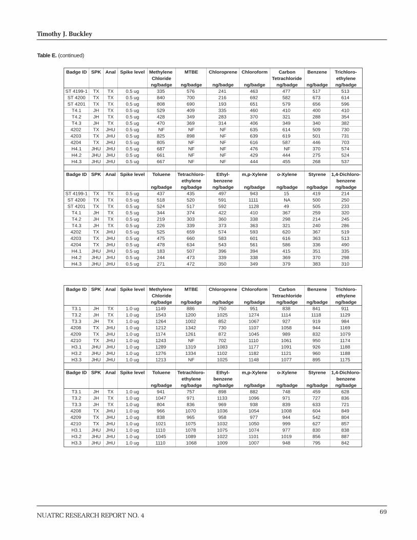
69
Timothy J. Buckley
NUATRC RESEARCH REPORT NO. 4
Badge ID
ST 4199-1ST 4200ST 4201
T4.1T4.2T4.34202 4203 4204 H4.1H4.2H4.3
Badge ID
ST 4199-1ST 4200ST 4201
T4.1T4.2T4.34202 4203 4204 H4.1H4.2H4.3
SPK
TXTXTXJHJHJHTXTXTX
JHUJHUJHU
SPK
TXTXTXJHJHJHTXTXTX
JHUJHUJHU
Anal
TXTXTXTXTXTX
JHUJHUJHUJHUJHUJHU
Anal
TXTXTXTXTXTX
JHUJHUJHUJHUJHUJHU
Spike level
0.5 ug0.5 ug0.5 ug0.5 ug0.5 ug0.5 ug0.5 ug0.5 ug0.5 ug0.5 ug0.5 ug0.5 ug
Spike level
0.5 ug0.5 ug0.5 ug0.5 ug0.5 ug0.5 ug0.5 ug0.5 ug0.5 ug0.5 ug0.5 ug0.5 ug
Methylene Chlorideng/badge
335840 808529 428470 NF
825805687661 667
Toluene
ng/badge437518524 344 219 226525475478183 244 271
MTBE
ng/badge576700 690 409 349 369 NF
898NFNFNFNF
Tetrachloro-ethyleneng/badge
435520 517374 303 339 659 660 634 507473 472
Chloroprene
ng/badge241 216193 335283 314 NFNFNFNFNFNF
Ethyl-benzeneng/badge
497591 592 422 360 373 574 583 543 396339 350
Chloroform
ng/badge463 692 651 460 370 406635639 616476429 444
m,p-Xylene
ng/badge943 11111128410 338363 593 601 561 394 338349
CarbonTetrachloride
ng/badge477582 579 410 321 349 614 619 587NF
444 455
o-Xylene
ng/badge15NA49
367298321 620 616586415369 379
Benzene
ng/badge517673 656400 288340 509 501 446370 275268
Styrene
ng/badge419 500 505259 214 240 367363 336351 370 383
Trichloro-ethyleneng/badge
513 614 596410 354 382 730 731 703 574 524 537
1,4-Dichloro-benzeneng/badge
214 250 233 320 245286519 513 490 335298310
Table E. (continued)
Badge ID
T3.1T3.2T3.34208 4209 4210 H3.1H3.2H3.3
Badge ID
T3.1T3.2T3.34208 4209 4210 H3.1H3.2H3.3
SPK
JHJHJHTXTXTX
JHUJHUJHU
SPK
JHJHJHTXTXTX
JHUJHUJHU
Anal
TXTXTX
JHUJHUJHUJHUJHUJHU
Anal
TXTXTX
JHUJHUJHUJHUJHUJHU
Spike level
1.0 ug1.0 ug1.0 ug1.0 ug1.0 ug1.0 ug1.0 ug1.0 ug1.0 ug
Spike level
1.0 ug1.0 ug1.0 ug1.0 ug1.0 ug1.0 ug1.0 ug1.0 ug1.0 ug
Methylene Chlorideng/badge
1149 1543 1264 1212 1174 1243 1289 12761213
Toluene
ng/badge941
1047804 966838
1021 1110 10451110
MTBE
ng/badge886
1200 1002 1342 1261
NF1319 1334
NF
Tetrachloro-ethyleneng/badge
757971 836
1070 965
10751078 1089 1068
Chloroprene
ng/badge750
1025852 730 872 702
1083 1102 1025
Ethyl-benzeneng/badge
898 1133 969
1036958
1032 10751022 1009
Chloroform
ng/badge951
1274 1067110710451110 11771182 1148
m,p-Xylene
ng/badge882
1096938
1054 977
1050 1074 1101 1007
CarbonTetrachloride
ng/badge838
1114 927
1058 989
1061 1091 1121 1077
o-Xylene
ng/badge748 971 839
1008 944 999 977
1019 948
Benzene
ng/badge841
1118 919 944 832 950 926960 895
Styrene
ng/badge459 727633 604 542 627830 856795
Trichloro-ethyleneng/badge
9111129 984
1169 1079 1174 1188 1188 1175
1,4-Dichloro-benzeneng/badge
628 836721 849 804 857838 887842

70
VOC Exposure in an Industry-Impacted Community
NUATRC RESEARCH REPORT NO. 4
Badge ID
ST 4211ST 4212ST 4213
T2.1T2.2T2.34214 4215 4216 H2.1H2.2H2.3
Badge ID
ST 4211ST 4212ST 4213
T2.1T2.2T2.34214 4215 4216 H2.1H2.2H2.3
SPK
TXTXTXJHJHJHTXTXTX
JHUJHUJHU
SPK
TXTXTXJHJHJHTXTXTX
JHUJHUJHU
Anal
TXTXTXTXTXTX
JHUJHUJHUJHUJHUJHU
Anal
TXTXTXTXTXTX
JHUJHUJHUJHUJHUJHU
Spike level
5.0 ug5.0 ug5.0 ug5.0 ug5.0 ug5.0 ug5.0 ug5.0 ug5.0 ug5.0 ug5.0 ug5.0 ug
Spike level
5.0 ug5.0 ug5.0 ug5.0 ug5.0 ug5.0 ug5.0 ug5.0 ug5.0 ug5.0 ug5.0 ug5.0 ug
Methylene Chlorideng/badge
60906632 7396 6263 61596645
NA4705 45373881 4506 4576
Toluene
ng/badge41785021 5035 45404602 4904
NA4421 425937674393 4670
MTBE
ng/badge5121 6115 62495066 5021 5439
NA5085 48574143 47884675
Tetrachloro-ethyleneng/badge
3954 4704 47194383 4392 4643
NA43574221 3715 4301 4772
Chloroprene
ng/badge3213 4356 4002 4982 4975 5267
NA3254 31083646 43074408
Ethyl-benzeneng/badge
4532 5353 53474894 4946 5187
NA4681 4575 4032 48115166
Chloroform
ng/badge50285775 6128538053395810
NA507948984473 51095500
m,p-Xylene
ng/badge8760
1023910219478748405093
NA46974591 402848085162
CarbonTetrachloride
ng/badge461755305683 50605021 5382
NA4805 4545 417048595143
o-Xylene
ng/badge110992 NA
426943204566
NA4195 40673535 4354 4514
Benzene
ng/badge4456 5265 5452 4815 4846 5146
NA4475 4283 3865 45594665
Styrene
ng/badge3915 46304543 3222 3602 3722
NA2751 2656 255035403660
Trichloro-ethyleneng/badge
456755005543 49904992 5373
NA46874524 4016 4646 5087
1,4-Dichloro-benzeneng/badge
263732793086 3664 3755 3941
NA3646 3583 3015 36983986
Table E. (continued)
Badge ID
4220 4221 4222 H1.1H1.2H1.3
ST 4217ST 4218ST 4219
T1.1T1.2T1.3
Badge ID
4220 4221 4222 H1.1H1.2H1.3
ST 4217ST 4218ST 4219
T1.1T1.2T1.3
SPK
TXTXTX
JHUJHUJHUTXTXTXJHJHJH
SPK
TXTXTX
JHUJHUJHUTXTXTXJHJHJH
Anal
JHUJHUJHUJHUJHUJHUTXTXTXTXTXTX
Anal
JHUJHUJHUJHUJHUJHUTXTXTXTXTXTX
Spike level
10 ug10 ug10 ug10 ug10 ug10 ug10 ug10 ug10 ug10 ug10 ug10 ug
Spike level
10 ug10 ug10 ug10 ug10 ug10 ug10 ug10 ug10 ug10 ug10 ug10 ug
Methylene Chlorideng/badge
9158 8613 8562 80767814 9376
123261526611884 1296513947 12877
Toluene
ng/badge8988 8214 8219 7661 7437 8869 8191
10273 8033 8671 94558876
MTBE
ng/badge9882 8959 9379 8413 8189 9490
10243 12631 9798
10397 11193 10361
Tetrachloro-ethyleneng/badge
87358021 79767279 7202 8607 7829 9859 77458443 9233 8680
Chloroprene
ng/badge7003 6300 66667669 7633 8747 7404 9452 7409 10208 1098510212
Ethyl-benzeneng/badge
94958764 8868 8007 80969381 860610897 8514 9139 100169328
Chloroform
ng/badge10233 9741 9520 89658702
10338 10082 12378 9648
10680 11467 10505
m,p-Xylene
ng/badge9508 8778 8882 8001 8090 9374
16382 20736163168978 9754 9171
CarbonTetrachloride
ng/badge977690859042 8489 8474 9950 9417
116569031
10164 10908 10165
o-Xylene
ng/badge8358 7640 7844 6979 7170 8221 477
1152 973
78958612 8184
Benzene
ng/badge8979 8184 8422 7859 7702 8823 8735
10958 8413 9393
101369498
Styrene
ng/badge5947 5098 5688 5293 59156744 7523 940673466609 7069 7078
Trichloro-ethyleneng/badge
9387 8683 8597 79157913 9238 9161 11422 8848 9798 106059804
1,4-Dichloro-benzeneng/badge
74656468 6978 5992 6289 7187 56657027 5473 69357531 7373

71
Timothy J. Buckley
NUATRC RESEARCH REPORT NO. 4
APPENDIX F
Survey Forms
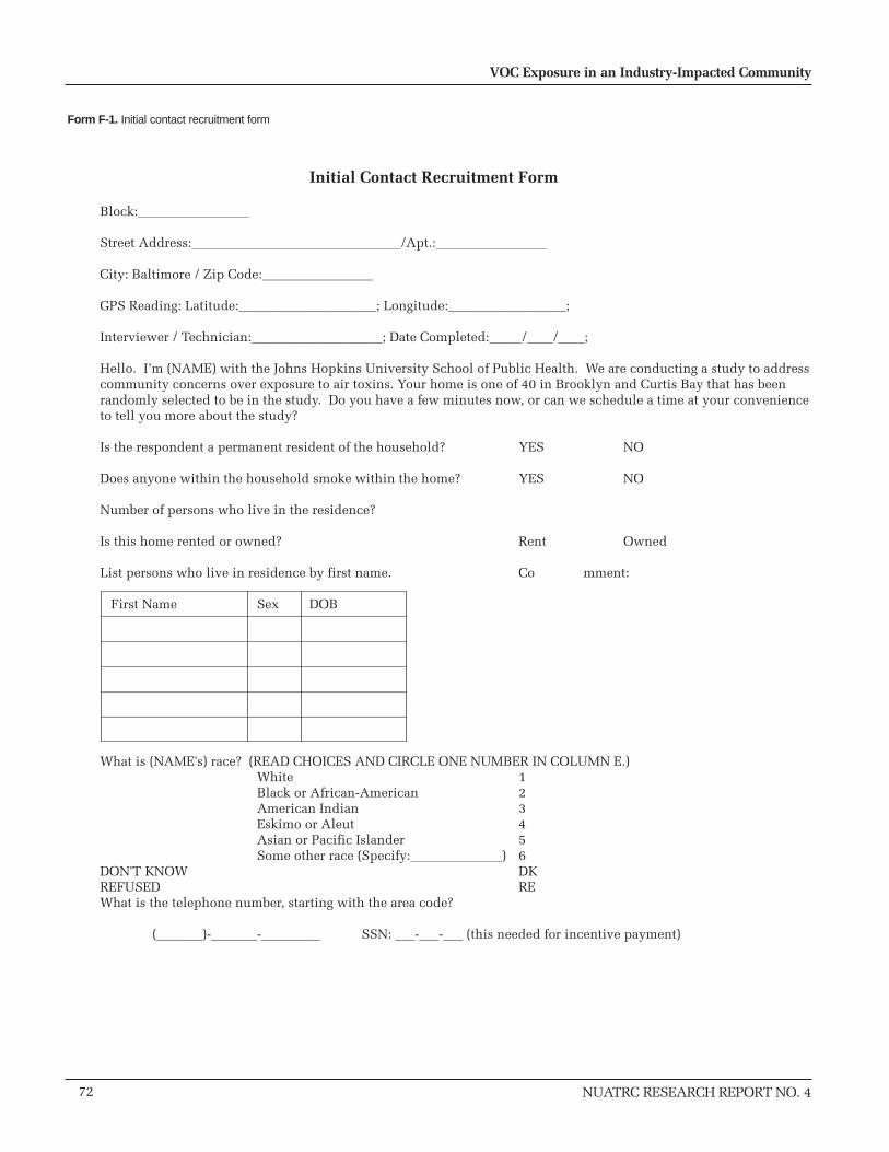
72
VOC Exposure in an Industry-Impacted Community
NUATRC RESEARCH REPORT NO. 4
Initial Contact Recruitment Form
Block:_________________
Street Address:________________________________/Apt.:_________________
City: Baltimore / Zip Code:_________________
GPS Reading: Latitude:_____________________; Longitude:__________________;
Interviewer / Technician:____________________; Date Completed:_____/____/____;
Hello. I’m (NAME) with the Johns Hopkins University School of Public Health. We are conducting a study to addresscommunity concerns over exposure to air toxins. Your home is one of 40 in Brooklyn and Curtis Bay that has beenrandomly selected to be in the study. Do you have a few minutes now, or can we schedule a time at your convenienceto tell you more about the study?
Is the respondent a permanent resident of the household? YES NO
Does anyone within the household smoke within the home? YES NO
Number of persons who live in the residence?
Is this home rented or owned? Rent Owned
List persons who live in residence by first name. Co mment:
First Name Sex DOB
What is (NAME's) race? (READ CHOICES AND CIRCLE ONE NUMBER IN COLUMN E.) White 1 Black or African-American 2 American Indian 3 Eskimo or Aleut 4 Asian or Pacific Islander 5 Some other race (Specify:______________) 6DON'T KNOW DKREFUSED REWhat is the telephone number, starting with the area code?
(_______)-_______-_________ SSN: ___-___-___ (this needed for incentive payment)
Form F-1. Initial contact recruitment form

73
Timothy J. Buckley
NUATRC RESEARCH REPORT NO. 4
Initial Contact Letter
Dear Brooklyn / Curtis Bay Resident:
The Johns Hopkins University School of Public Health is conducting a study to address community concerns overexposure to air toxins. Your home is one of forty in Brooklyn and Curtis Bay that has been randomly selected to bea part of this important study. Participation in the study is easy and we will give you $25 for helping us. If youagree, we will conduct air sampling for three days. During this time, you will be asked to wear a small air samplingbadge, complete a couple of short questionnaires, and provide a couple of urine samples each day.
I hope that you can work with us to help address your community’s concern over toxins in the air. If you have anyquestions or concerns, I can be reached at (410) 614-5750 or email [email protected].
Sincerely,
Timothy J. Buckley, Ph.D.Assistant Professor
Form F-1. (continued)

74
VOC Exposure in an Industry-Impacted Community
NUATRC RESEARCH REPORT NO. 4
Instructions for Participants
DietWe are trying to avoid one type of food preservative called sorbic acid or potassium sorbate. It is not dangerous, butit affects the urine test we do. Therefore, during the study we would like you to try to avoid the following 3 food types:1. fruit punch drinks that come refrigerated such as Sunny Delight™, and store brand fruit drinks;2. baked sweets/snacks such as Hostess Cupcakes™, Little Debbie™, grocery store cakes, and soft packaged cookies like Snack Wells™ and Fig Newtons;3. soft cheeses including processed cheese slices, cottage cheese, cheese spreads, Velveeta™, cheese dips, low fat cream cheese and low fat shredded cheese.
Some other foods, such as salad dressings and mayonnaise, also have this preservative in them. We would like you topick one day on the study, tomorrow or the next day, to be very careful about avoiding all packaged foods that mighthave this preservative in it. To make it easier, we are giving you a log that lists food to avoid and sample labels fromfoods with this preservative in them. On the day you pick to avoid all sorbic preservatives, please don’t eat anythingthat comes in a package unless you read the ingredients label and don’t see the words “sorbic acid” or “potassiumsorbate”. Labels usually note when substances are added as preservatives and so you can look for the words“preservative”, “to protect flavor”, and “to retain freshness”.
Urine CollectionSome of the chemicals in air pollution that you breathe in are changed by your body so that you can get rid of themin your urine. We collect samples of urine to test for the breakdown product from benzene, which is one of these airpollutants. Starting tomorrow morning, please collect three samples each day : 1) the first void of the morning;2) a late afternoon void when you come home from school or work or around 4-5 pm; and 3) the last void of the daybefore you go to bed at night. Please do not fill the container completely since the sample will expand when wefreeze it. Put a label on the container with the time, and date of the sample (press hard when you write out the labelto make the carbon copy). Place the sample in the cooler that we have provided.
Daily Time /Activity and Food QuestionnairesA questionnaire has been provided to keep track of the time that you spend indoors, outdoors, and around airpollution sources. A food log will be used to keep track of all packaged food you eat. These forms should be filledout over the course of each day or at the end of each day so that you can remember everything.
In Case of Trouble or QuestionsIf you have any questions or trouble do not hesitate to give us a call, day or night. We will especially want to knowif an air sampler should stop working so that we can repair or replace
Form F-2. Instruction for participants
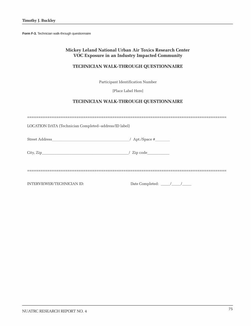
75
Timothy J. Buckley
NUATRC RESEARCH REPORT NO. 4
Mickey Leland National Urban Air Toxics Research CenterVOC Exposure in an Industry Impacted Community
TECHNICIAN WALK-THROUGH QUESTIONNAIRE
Participant Identification Number
[Place Label Here]
TECHNICIAN WALK-THROUGH QUESTIONNAIRE
=========================================================================================
LOCATION DATA (Technician Completed--address/ID label)
Street Address__________________________________________/ Apt./Space #________
City, Zip_______________________________________________/ Zip code____________
=========================================================================================
INTERVIEWER/TECHNICIAN ID: Date Completed: _____/_____/_____
Form F-3. Technician walk-through questionnaire

76
VOC Exposure in an Industry-Impacted Community
NUATRC RESEARCH REPORT NO. 4
TECHNICIAN WALK-THROUGH QUESTIONNAIRE
COMPLETE THIS QUESTIONNAIRE BY OBSERVATION. YOU MAY ASKPARTICIPANT ANY QUESTIONS THAT ARE NOT APPARENT.
T1. How many stories (floors) are in this building? (COUNT ONLY FLOORS WITH FINISHED ROOMS FOR LIVING PURPOSES OR FINISHED BASEMENTS.)
_____ Floors
IF MULTI-FAMILY BUILDING , CONTINUE. ELSE, GO TO QUESTION T3.
T2. Which floor(s) do respondents live on? ________ floor(s).
T3. Of these rooms, how many are carpeted or have rugs covering most (>50%) of their surface?
_____ Rooms
T4. Using the following statements, how would you rate the overall dust level within the residence? (CIRCLE ONE.)
Very Dusty -- 1 Some Dust -- obvious efforts to control dust 2 "No" Dust -- extreme dust control, very clean 3
T5. Indicate nearest major intersection:
EXTERIOR AND INTERIOR RESIDENTIAL CHARACTERISTICS
T6. Distance to street (MEASURE THE DISTANCE FROM THE CURB TO THE PRIMARY ENTRANCE TO THE RESIDENCE OR CHECK BOX IF DISTANCE IS ESTIMATED TO BE GREATER THAN 300 FEET.):
_____ Feet
_____ >300 feet
T7. Number of cars parked on the street outside of the front of the home (COUNT THE CARS ON BOTH SIDES OF THE STREET THAT ARE PARKED ON THE SAME BLOCK AS THE RESIDENCE)
_____ Cars
T8. Number of cars parked in the back of the home.
_____ Cars
Form F-3. (continued)
77
Timothy J. Buckley
NUATRC RESEARCH REPORT NO. 4
TIME DIARY AND ACTIVITY QUESTIONNAIRE
=========================================================================================
DESIGNATED PARTICIPANT
(If the participant is less than 10 years old, what is the name of the individual who is providing the answers for the designated respondent?)
Name of Participant_______________________________________
Completed by____________________________________________ (if other than participant)
Relation to participant____________________________________
Home Phone ____________________________________________ Date: _____/_____/_____
=========================================================================================
LOCATION DATA (Technician Completed--address/ID label)
Street Address__________________________________________/ Apt./Space #_________________
City, Zip_______________________________________________/ Zip code_____________________
Study Block # __________ Block Group #__________________ Census Tract #________________
=========================================================================================
INTERVIEWER/TECHNICIAN ID:_________________________________ Date Completed: _____/_____/_____
=========================================================================================
Form F-4. Time/activity questionnaire

78
VOC Exposure in an Industry-Impacted Community
NUATRC RESEARCH REPORT NO. 4
TIME DIARY AND ACTIVITY QUESTIONNAIRE
At the end of each day, take a few minutes to record the time (you/your child) spent in each of the seven listed locations. There is one box for each day of the study. The numbers in the box stand for hours of the day. For example, 5 in the morning is 5:00 a.m. to 5:59 a.m. For each hour of the day, place an X through the number for each location where (you/your child) spent any time during the hour. Make sure there is at least one X for each hour of the day.
The terms used in the time diary are defined as follows:
• Home: The house or apartment where (you live/your child lives); the location where we are collecting samples.
• School: A place away from home where (you attend/your child attends) school.
• Transit: Any travel from one location to another, including all travel between such places as home, school, and shopping centers, as well as all other travel on roads, paths, or trails.
• Other: All other places (you spend/your child spends) time besides home, work, school, and in transit between locations.
Form F-4. (continued)

79
Timothy J. Buckley
NUATRC RESEARCH REPORT NO. 4
47
Day 1Day ofWeek_______
Location Morning Afternoon EveningEarly Morning(Night time)
DATE__/__/__ In TransitRefuelingSmoker Nearby
5 6 7 8 9 10 115 6 7 8 9 10 115 6 7 8 9 10 11
12 1 2 3 4 512 1 2 3 4 512 1 2 3 4 5
6 7 8 9 10 116 7 8 9 10 116 7 8 9 10 11
12 1 2 3 412 1 2 3 412 1 2 3 4
Inside at HomeInside at Other
5 6 7 8 9 10 115 6 7 8 9 10 11
12 1 2 3 4 512 1 2 3 4 5
6 7 8 9 10 116 7 8 9 10 11
12 1 2 3 412 1 2 3 4
Outside at HomeOutside at Other
5 6 7 8 9 10 115 6 7 8 9 10 11
12 1 2 3 4 512 1 2 3 4 5
6 7 8 9 10 116 7 8 9 10 11
12 1 2 3 412 1 2 3 4
Day 2Day ofWeek_______
Location Morning Afternoon EveningEarly Morning(Night time)
DATE__/__/__ In TransitRefuelingSmoker Nearby
5 6 7 8 9 10 115 6 7 8 9 10 115 6 7 8 9 10 11
12 1 2 3 4 512 1 2 3 4 512 1 2 3 4 5
6 7 8 9 10 116 7 8 9 10 116 7 8 9 10 11
12 1 2 3 412 1 2 3 412 1 2 3 4
Inside at HomeInside at Other
5 6 7 8 9 10 115 6 7 8 9 10 11
12 1 2 3 4 512 1 2 3 4 5
6 7 8 9 10 116 7 8 9 10 11
12 1 2 3 412 1 2 3 4
Outside at HomeOutside at Other
5 6 7 8 9 10 115 6 7 8 9 10 11
12 1 2 3 4 512 1 2 3 4 5
6 7 8 9 10 116 7 8 9 10 11
12 1 2 3 412 1 2 3 4
Day 3Day ofWeek_______
Location Morning Afternoon EveningEarly Morning(Night time)
DATE__/__/__ In TransitRefuelingSmoker Nearby
5 6 7 8 9 10 115 6 7 8 9 10 115 6 7 8 9 10 11
12 1 2 3 4 512 1 2 3 4 512 1 2 3 4 5
6 7 8 9 10 116 7 8 9 10 116 7 8 9 10 11
12 1 2 3 412 1 2 3 412 1 2 3 4
Inside at HomeInside at Other
5 6 7 8 9 10 115 6 7 8 9 10 11
12 1 2 3 4 512 1 2 3 4 5
6 7 8 9 10 116 7 8 9 10 11
12 1 2 3 412 1 2 3 4
Outside at HomeOutside at Other
5 6 7 8 9 10 115 6 7 8 9 10 11
12 1 2 3 4 512 1 2 3 4 5
6 7 8 9 10 116 7 8 9 10 11
12 1 2 3 412 1 2 3 4
Day 4Day ofWeek_______
Location Morning Afternoon EveningEarly Morning(Night time)
DATE__/__/__ In TransitRefuelingSmoker Nearby
5 6 7 8 9 10 115 6 7 8 9 10 115 6 7 8 9 10 11
12 1 2 3 4 512 1 2 3 4 512 1 2 3 4 5
6 7 8 9 10 116 7 8 9 10 116 7 8 9 10 11
12 1 2 3 412 1 2 3 412 1 2 3 4
Inside at HomeInside at Other
5 6 7 8 9 10 115 6 7 8 9 10 11
12 1 2 3 4 512 1 2 3 4 5
6 7 8 9 10 116 7 8 9 10 11
12 1 2 3 412 1 2 3 4
Outside at HomeOutside at Other
5 6 7 8 9 10 115 6 7 8 9 10 11
12 1 2 3 4 512 1 2 3 4 5
6 7 8 9 10 116 7 8 9 10 11
12 1 2 3 412 1 2 3 4
Form F-4. (continued)

80
VOC Exposure in an Industry-Impacted Community
NUATRC RESEARCH REPORT NO. 4
DIALY ACTIVITY INFORMATION
1 2 3 4
Day Day Day Day
_____ _____ _____ _____
Date Date Date Date
/ / / / / / / /
Questions A1-A3: Please circle "Y" for Yes or "N" for No.
A1. Did (you/your child) start or tend a fire in a Y N Y N Y N Y Nfireplace or wood stove today?
A2. Did (you/your child) use an outdoor grill or Y N Y N Y N Y Nburn wood, leaves, or trash today?
A3. Were any tobacco products smoked in the Y N Y N Y N Y Nhome today?
A4. Did you burn candles or incense today? Y N Y N Y N Y N
A5. Did you visit hair or nail salon today? Y N Y N Y N Y N
A6. Did you pump gas today? Y N Y N Y N Y NWas you child with you? Y N Y N Y N Y N
A7. Did you visit a dry-cleaning store today Y N Y N Y N Y NWas you child with you? Y N Y N Y N Y N
A8. Did you bring dry cleaned clothes home today? Y N Y N Y N Y N
Questions A9-A13: Please enter time spent. If the time was less than 1 hour, enter 15 min, 30 min, 45 min, or 1 hr,whichever is closest to time actually spent. If time was greater than 1 hour, round to the nearest hour. Circle eithermin. or hr.
A9. (You/your child) traveled on roadways ____min or hr ____min or hr ____min or hr ____min or hror highways today?
A10. (You/your child) use any chemicals ____min or hr ____min or hr ____min or hr ____min or hrtoday in hobbies, home repair or carrepair (e.g. paints, paint stripper, glues,gasoline)
A11. (You/your child) spent in a vehicle with ____min or hr ____min or hr ____min or hr ____min or hrsomeone who was smoking?
A12. (You/your child) spent in an enclosed ____min or hr ____min or hr ____min or hr ____min or hrworkshop or garage used as a workshoptoday?
A13. Doors and windows at your house were ____min or hr ____min or hr ____min or hr ____min or hrleft open for ventilation today?
For Technician Use Only Comp. [ ] Comp. [ ] Comp. [ ] Comp. [ ]Asst. [ ] Asst. [ ] Asst. [ ] Asst. [ ]Do [ ] Do [ ] Do [ ] Do [ ]
Form F-4. (continued)
81
Timothy J. Buckley
NUATRC RESEARCH REPORT NO. 4
BASELINE QUESTIONNAIRE
=========================================================================================
DESIGNATED PARTICIPANT
(If the participant is less than 10 years old, what is the name of the individual who is providing the answers for the designated respondent?)
Name of Participant_______________________________________
Completed by____________________________________________ (if other than participant)
Relation to participant____________________________________
Home Phone ____________________________________________ Date: _____/_____/_____
=========================================================================================
LOCATION DATA (Technician Completed--address/ID label)
Street Address__________________________________________/ Apt./Space #_________________
City, Zip_______________________________________________/ Zip code_____________________
Study Block # __________ Block Group #__________________ Census Tract #________________
=========================================================================================
INTERVIEWER/TECHNICIAN ID:_________________________________ Date Completed: _____/_____/_____
=========================================================================================
NOTE: For children participants (less than 16 years of age), only answer Question numbers 59 - 65.
Form F-5. Baseline questionnaire

82
VOC Exposure in an Industry-Impacted Community
NUATRC RESEARCH REPORT NO. 4
DEMOGRAPHICS
1. What is the highest level of school (you have/this child has) completed? (READ CHOICES AND CIRCLE ONE.) IF CURRENTLY ENROLLED, MARK THE LEVEL OF PREVIOUS GRADE ATTENDED OR HIGHEST DEGREE RECEIVED.
No school completed or Kindergarten only 1 Primary or middle school (Grade 1-8) 2 Some high school (Grade 9-11) 3 High school graduate (Grade 12 or GED) 4 Some college or technical school 5 College graduate 6 Some post college 7
2. CIRCLE SEX OF PARTICIPANT.
MALE 1 FEMALE 2
3. What is (your/his/her) date of birth? _________/______/_______ Month Day Year
4. How tall (are you/is he/she) without shoes? _____ft _____inches
5. How much (do you/does he/she) weigh? _____ pounds
6. What is (your/his/her) racial/ethnic background? (READ CHOICED AND CIRCLE RESPONSE)
BLACK/AFRICAN AMERICAN 1 WHITE/CAUCASIAN AMERICAN 2 HISPANIC 3 ASIAN 4
Form F-5. (continued)

83
Timothy J. Buckley
NUATRC RESEARCH REPORT NO. 4
PERSONAL EXPOSURE ACTIVITIES
7. Do you currently work full time or part time at any location away from your home? (CIRCLE "Y" OR "N." INCLUDE WORKING FOR OTHERS, SELF-EMPLOYED, AND VOLUNTEER WORK. INCLUDE THOSE WHO WORK OUT OF A HOME OFFICE IF THEY WORK PART OF THE TIME AWAY FROM HOME.)
YES Y CONTINUE NO N GO TO 26
8. On average for the past month, how many hours per week did (you/he/she) work at (your/his/her) primary job? (INCLUDE WEEKS WHERE TIME WAS TAKEN OFF FOR VACATION, SICKNESS, ETC. IF LESS THAN 10 HOURS, ROUND TO THE NEAREST HOUR; IF GREATER THAN 10 HOURS, ROUND TO THE NEAREST 10 HOURS; e.g., 10, 20, 30, 40, 50 HOURS).
______ hours/week
i. On average, how many of these hours were spent working at home? ______ hours/week
9. What kind of business or industry is this? (For example, manufacturing, retail store, government, farm, school.)
______________________________________________________________________
10. Is the business or industry located in the South Baltimore community? (Curtis Bay, Brooklyn, Wagner's Point, Hawkins Point, or Fairfield)
YES NO
11. What is (your/his/her) job title? (For example, electrical engineer, stock clerk, typist)
__________________________________________________________________
12. What activities (do you/does he/she) perform most often as part of (your/his/her) duties at that job? (For example, typing, keeping account books, filing, selling cars, operating printing press, finishing concrete.)
____________________________________________________________________
13. (Do you/Does he/she) wear protective clothing while at (your/his/her) primary job? (CIRCLE "Y" OR "N.")
YES Y CONTINUE NO N GO TO 15
14. Which types of protective clothing (do you/does he/she) wear while at (your/his/her) primary job? (READ CHOICES AND CIRCLE ALL THAT APPLY.)
Gloves 1 Overalls 2 Overcoat (e.g. lab coat; smock) 3 Respirator 4 Other (Specify:_________________________) 5 DON'T KNOW DK
Form F-5. (continued)

84
VOC Exposure in an Industry-Impacted Community
NUATRC RESEARCH REPORT NO. 4
15. While at (your/his/her) primary job, (do you/does he/she) come into contact at least once a week with? (READ CHOICES AND CIRCLE ALL THAT APPLY.)
Welding fumes 1 Solder or flux fumes 2 Plastic fumes 3 Paint fumes (include varnish, shellac, etc.) 4 Gasoline or diesel fumes 5 Other known type of fumes, smoke, gas, or vapors
(Specify:___________________________) 6 Unknown type of fumes, smoke, gas, or vapors 7 No contact with fumes, smoke, gas, or vapors 8
16. Do you have a second job? (CIRCLE "Y" OR "N.")
YES Y CONTINUE NO N GO TO 26
17. On average for the past month, how many hours per week did (you he/she) work at (your/his/her) second job? (INCLUDE WEEKS WHERE TIME WAS TAKEN OFF FOR VACATION, SICKNESS, ETC. IF LESS THAN 10 HOURS, ROUND TO THE NEAREST HOUR; IF GREATER THAN 10 HOURS, ROUND TO THE NEAREST 10 HOURS; e.g., 10, 20, 30, 40, 50 HOURS).
_______ hours/week
i. On average, how many of these hours were spent working at home? ______ hours/week
18. What kind of business or industry is this? (For example, manufacturing, retail store, government, farm, school.)
______________________________________________________________
19. Is the business or industry located in the South Baltimore community? (Curtis Bay, Brooklyn, Wagner's Point, Hawkins Point, or Fairfield)
YES NO
20. What is (your/his/her) job title? (For example, electrical engineer, stock clerk, typist)
_______________________________________________________________
21. What activities (do you/does he/she) perform most often as part of (your/his/her) duties at that job? (For example, typing, keeping account books, filing, selling cars, operating printing press, finishing concrete.)
___________________________________________________________
22. (Do you/Does he/she) regularly wear protective clothing while at (your/his/her) second job? (CIRCLE "Y" OR "N.")
YES Y CONTINUE NO N GO TO 24
Form F-5. (continued)

85
Timothy J. Buckley
NUATRC RESEARCH REPORT NO. 4
23. Which types of protective clothing (do you/does he/she) wear while at (your/his/her) second job? (READ CHOICES AND CIRCLE ALL THAT APPLY.)
Gloves 1 Overalls 2 Overcoat (e.g., lab coat; smock) 3 Respirator 4 Other (Specify:_________________________) 5 Don't know DK
24. While at (your/his/her) second job, (do you/does he/she) come into contact at least once a week with? (READ CHOICES AND CIRCLE ALL THAT APPLY.)
Welding fumes 1 Solder or flux fumes 2 Plastic fumes 3 Paint fumes (include varnish, shellac, etc.) 4 Gasoline or diesel fumes 5 Other known type of fumes, smoke, gas, or vapors
(Specify:___________________________) 6 Unknown type of fumes, smoke, gas, or vapors 7 No contact with fumes, smoke, gas, or vapors 8
25. What methods of transportation did you use to go to work, school, shopping, etc in the past six months? (READ CHOICES AND CIRCLE ALL THAT APPLY.)
Car, truck, van, or taxi cab 1Bus, trolley bus, or trolley car 2
Train, subway or elevated train 3 Motorcycle 4Bicycle 5
Walk 6 Other method (Specify: __________________)
BASIC HOUSING CHARACTERISTICS
These next questions are about your (house/apartment). Please feel free to ask another member of your household for assistance if necessary.
26. About when was this building first built? (READ CHOICES AND CIRCLE ONE.)
1990 TO PRESENT 1 1985 TO 1989 2 1980 TO 1984 3 1970 TO 1979 4 1960 TO 1969 5 1950 TO 1959 6 1940 TO 1949 7 1939 OR EARLIER 8 DON'T KNOW DK
27. When did (you/he/she) move into this (house/apartment)? (READ CHOICES AND CIRCLE ONE.)
Month:________ Year ________
Form F-5. (continued)

86
VOC Exposure in an Industry-Impacted Community
NUATRC RESEARCH REPORT NO. 4
28. In the last week, have any of the following been performed in this home? (CIRCLE "Y" OR "N.")
YES NO Adding a room Y N Putting up or taking down a wall Y N Replacing windows Y N Refinishing floors Y N Exterior painting Y N Interior painting Y N
29. What is the source of the running water in your house/apartment? (READ CHOICES AND CIRCLE ALL THAT APPLY.)
Public or commercial water system 1 NAME_______________________
Private well 2 Cistern 3 Some other source __________________ 4 DON'T KNOW DK
30. Do you use any of the following to treat your water at home? (CIRCLE "Y" or "N" FOR EACH TREATMENT TYPE OR "DK" FOR DON'T KNOW.)
DON’T YES NO KNOW i. Water Softener Y N DK ii. Charcoal Filter Y N DK iii. Reverse Osmosis Y N DK iv. Distillation Y N DK v. Other (Specify:_______________________) Y N DK
31. Is there an enclosed garage attached to this (house/apartment)? (CIRCLE "Y" OR "N.")
YES Y CONTINUE NO N GO TO 35
32. Where is the attached garage? (READ CHOICES AND CIRCLE ONE.)
Underneath the main living quarters 1 Same level as the main living quarters 2 Somewhere else; Specify: _______________ 3
33. Is there a doorway leading directly from the garage into the living quarters? (CIRCLE "Y" OR "N.")
YES Y NO N
34. Are automobiles, vans, trucks or other motor vehicles parked in this attached garage? (CIRCLE "Y" OR "N".)
YES Y NO N
35. Are any gas powered devices stored in any room, basement, or attached garage in this (house/apartment)? (CIRCLE ONE. DO NOT INCLUDE CARS, VANS, OR TRUCKS. DO INCLUDE MOTORCYCLES, GAS- POWERED LAWN MOWERS, TRIMMERS OR BLOWERS, BOAT ENGINES, ETC.)
YES Y NO N
DON'T KNOW DK
Form F-5. (continued)

87
Timothy J. Buckley
NUATRC RESEARCH REPORT NO. 4
36. Is air conditioning (refrigeration) used to cool this (house/apartment)? (CIRCLE "Y" OR "N.")
YES Y CONTINUE NO N GO TO 38
37. Which types of air conditioning units do you use? (READ CHOICES AND CIRCLE ALL THAT APPLY.)
Central unit/units 1 Window or wall unit/units 2 Portable unit/units 3
38. Which fuels are used for heating this (house/apartment)? (READ CHOICES AND CIRCLE ALL THAT APPLY.)
Gas: from underground pipes serving the neighborhood 1
Gas: bottled, tank, or LP 2 Electricity 3 Fuel oil, kerosene, etc. 4 Coal or coke 5 Wood 6 Solar energy 7 Other fuel (Specify: ____________________) 8 No fuel used 9 Don't know DK
39. Does this (house/apartment) have a central heating system with ducts that blow air into most rooms? (CIRCLE "Y" OR "N.")
YES Y NO N
40. Do you use portable kerosene heaters in this (house/apartment)? (CIRCLE "Y" OR "N.")
YES Y CONTINUE NO N GO TO 42
41. How often do you use your kerosene heater during the heating season? (READ CHOICES AND CIRCLE ONE.)
Less than one day a month 1 One to three days per month 2 One or two days a week 3 3-5 days a week 4 More than 5 days a week 5
42. During the heating season, is a portable or nonvented gas heater used in this (house/apartment)? (CIRCLE "Y" OR "N.")
YES Y CONTINUE NO N GO TO 45
43. How many gas heaters? _________
Form F-5. (continued)
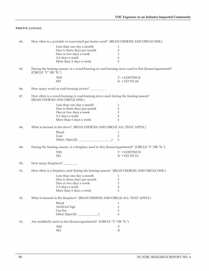
88
VOC Exposure in an Industry-Impacted Community
NUATRC RESEARCH REPORT NO. 4
NO N
44. How often is a portable or nonvented gas heater used? (READ CHOICES AND CIRCLE ONE.)
Less than one day a month 1 One to three days per month 2 One or two days a week 3 3-5 days a week 4 More than 5 days a week 5
45. During the heating season, is a wood-burning or coal-burning stove used in this (house/apartment)? (CIRCLE "Y" OR "N.")
YES Y CONTINUE NO N GO TO 49
46. How many wood or coal-burning stoves? ___________
47. How often is a wood-burning or coal-burning stove used during the heating season? (READ CHOICES AND CIRCLE ONE.)
Less than one day a month 1 One to three days per month 2 One or two days a week 3 3-5 days a week 4 More than 5 days a week 5
48. What is burned in the stove? (READ CHOICES AND CIRCLE ALL THAT APPLY.)
Wood 1 Coal 2 Other: (Specify: _____________________) 3
49. During the heating season, is a fireplace used in this (house/apartment)? (CIRCLE "Y" OR "N.")
YES Y CONTINUE NO N GO TO 53
50. How many fireplaces? _________
51. How often is a fireplace used during the heating season? (READ CHOICES AND CIRCLE ONE.)
Less than one day a month 1 One to three days per month 2 One or two days a week 3 3-5 days a week 4 More than 5 days a week 5
52. What is burned in the fireplace? (READ CHOICES AND CIRCLE ALL THAT APPLY.)
Wood 1 Artificial logs 2 Gas fire 3 Other (Specify: _____________) 4
53. Are mothballs used in this (house/apartment)? (CIRCLE "Y" OR "N.")
YES Y NO N
Form F-5. (continued)

89
Timothy J. Buckley
NUATRC RESEARCH REPORT NO. 4
54. Are room deodorizers being currently used in this (house/apartment)? (CIRCLE "Y" OR "N.")
YES Y NO N
55. Do you have your clothes dry cleaned?
YES Y NO N
56. Have you brought clothes home from the dry cleaner in the last week?
YES Y NO N
57. Have you cleaned your carpets in the last week?
YES Y NO N
FAMILY INCOME
58. Family income is often used in scientific studies to compare groups of people who are similar. We do some analysis of the data using these groups. Please remember that all the data you provide is held in strict confidence.
Approximately what is the gross annual income for all family members in this household? (HAND CARD,PENCIL, AND ENVELOPE TO RESPONDENT.) Please circle the number on this card and put the card in the
envelope. Seal the envelope and return it to me. (IF RESPONDENT PROVIDES ANSWER DIRECTLY, CIRCLE NUMBER BELOW. IF RESPONDENT SEALS RESPONSE IN ENVELOPE, CIRCLE "EN." IF RESPONDENT DOES BOTH, CIRCLE BOTH NUMBER AND "EN.")
Less than $9,999 1$ 10,000 - $ 19,999 2$ 20,000 - $ 29,999 3$ 30,000 - $ 39,999 4$ 40,000 - $ 49,999 5$ 50,000 - $ 74,999 6$ 75,000 - $ 99,999 7$100,000 or more 8
ANSWER IN ENVELOPE EN DON'T KNOW DK REFUSE RE
Form F-5. (continued)

90
VOC Exposure in an Industry-Impacted Community
NUATRC RESEARCH REPORT NO. 4
Children Participant QuestionsAges less than 16 years old
DEMOGRAPHICS
59. What is the highest level of school (you have/this child has) completed? (READ CHOICES AND CIRCLE ONE.) IF CURRENTLY ENROLLED, MARK THE LEVEL OF PREVIOUS GRADE ATTENDED OR HIGHEST DEGREE RECEIVED.
No school completed or Kindergarten only 1 Primary or middle school (Grade 1-8) 2 Some high school (Grade 9-11) 3 High school graduate (Grade 12 or GED) 4 Some college or technical school 5 College graduate 6 Some post college 7
60. CIRCLE SEX OF PARTICIPANT.
MALE 1 FEMALE 2
61. What is (your/his/her) date of birth? _________/______/_______ Month Day Year
62. How tall (are you/is he/she) without shoes? _____ft _____inches
63. How much (do you/does he/she) weigh? _____ pounds
64. What is (your/his/her) racial/ethnic background? (READ CHOICED AND CIRCLE RESPONSE)
BLACK/AFRICAN AMERICAN 1 WHITE/CAUCASIAN AMERICAN 2 HISPANIC 3 ASIAN 4
65. Do you/does he/she work? If so where? ______________________________
66. What methods of transportation did you/he/she use to go to work, school, or daycare in the past six months? (READ CHOICES AND CIRCLE ALL THAT APPLY.)
Car, truck, van, or taxi cab 1 Bus, trolley bus, or trolley car 2 Train, subway or elevated train 3
Motorcycle 4 Bicycle 5
Walk 6
Other method (Specify: __________________)
Form F-5. (continued)

91
Timothy J. Buckley
NUATRC RESEARCH REPORT NO. 4
Date: __ __-__ __-00 SBCS STUDY DAILY FOOD LOG - DAY ___ ID # __ __
M M D D
Please try not to eat the following foods during the entire study: 1. soft cheeses including processed cheese slices, cottage cheese, cheese spreads, Velveeta, cheese dips, low fat
cream cheese and low fat shredded cheese.2. fruit punch drinks that come refrigerated (Sunny Delight, store brands)3. baked sweets/snacks (Hostess cupcakes, Little Debbie, grocery store cakes). Packaged cookies OK except soft
ones like Snack Wells and Fig Newtons.
On the day you pick to avoid all sorbic preservatives, don’t eat anything that comes in a package unless you read the ingredients label and don’t see the words “sorbic acid” or “potassium sorbate”. Labels usually note when substancesare added as preservative and so you can look for the words “preservative”, “to protect flavor”, and “to retain fresh-ness”, then see what is listed by it. The sample labels you have been given for the study will also help with this.Please avoid fast or restaurant food on this day also. Foods that often have these preservatives are:
1. salad dressings2. mayonnaise3. prepared dips such as humus or for vegetables4. possibly wine5. margarine, frosting, syrup6. sometimes in ice cream (Jack & Jill)
In order to help us get the best test results, please list all packaged or processed foods or drinks that you eat at eachmeal or snack. Include amount and brand name from package.
Time Food/Drink Brand Name How Many/much
11 am Example: fruit punch Giant 16 oz
Form F-6. Daily food diary

Hans P. Blaschek Bernard D. GoldsteinUniversity of Illinois University of Pittsburgh
Josephine Cooper (Chair) Susan F. MooreToyota Motor North America, Inc. Georgia-Pacific Corporation
Wilma Delaney Monica SamuelsDow Chemical Company (Retired) Attorney
Mary Gade Arthur C. VailasSonnenschein Nath & Rosenthal University of Houston
NUATRC STAFF
SCIENTIFIC ADVISORY PANEL
BOARD OF DIRECTORS
Craig Beskid Carolyn WadePresident Financial Manager
Lata Shirnamé-Moré Jack ChangResearch Director Technical Assistant
Carolyn Nichol Brenda GehanStaff Scientist Consulting Staff Scientist
John C. Bailar III Brian P. LeadererUniversity of Chicago Yale University
Michael Brauer Dennis PaganoUniversity of British Columbia US EPA
James J. Collins (Chair) Dennis J. PaustenbachDow Chemical Company ChemRisk, Inc.
Michael L. Cunningham Bertram PriceNational Institute of Environmental Price Associates, Inc.Health Sciences
Joel SchwartzDavid H. Garabrant Harvard UniversityUniversity of Michigan
Linda SheldonPertti J. (Bert) Hakkinen US EPAEuropean Commission
Gary L. LarsenNational Jewish Medical and Research Center

P.O. Box 20286
Houston, Texas 77225-0286
Tel: 713.500.3450
Fax: 713.500.0345
http://www.sph.uth.tmc.edu/mleland/
Printed on 100% Recycled Paper
Authorized by the Clean Air Act Amendments of 1990 (Title III, Section 301/p)
Copyright © 2022 FDOKUMEN