Clemson University Clemson University

TigerPrints TigerPrints

All Theses Theses

12-2021

Visualizing Features From Deep Neural Networks Trained on Visualizing Features From Deep Neural Networks Trained on

Alzheimer’s Disease and Few-Shot Learning Models for Alzheimer’s Disease and Few-Shot Learning Models for

Alzheimer’s Disease Alzheimer’s Disease

John Reeder jreeder@clemson.edu

Follow this and additional works at: https://tigerprints.clemson.edu/all_theses

Part of the Artificial Intelligence and Robotics Commons, Data Science Commons, and the Other

Computer Sciences Commons

Recommended Citation Recommended Citation Reeder, John, "Visualizing Features From Deep Neural Networks Trained on Alzheimer’s Disease and Few-Shot Learning Models for Alzheimer’s Disease" (2021). All Theses. 3679. https://tigerprints.clemson.edu/all_theses/3679

This Thesis is brought to you for free and open access by the Theses at TigerPrints. It has been accepted for inclusion in All Theses by an authorized administrator of TigerPrints. For more information, please contact kokeefe@clemson.edu.

VISUALIZING FEATURES FROM DEEP NEURALNETWORKS TRAINED ON ALZHEIMER’S DISEASE AND

FEW-SHOT LEARNING MODELS FOR ALZHEIMER’SDISEASE

A Thesis

Presented to

the Graduate School of

Clemson University

In Partial Fulfillment

of the Requirements for the Degree

Master of Science

Computer Science

by

John G. Reeder

December 2021

Accepted by:

Dr. Kai Liu, Committee Chair

Dr. Brian Dean

Dr. Nianyi Li

Abstract

Alzheimer’s disease is an incurable neural disease, usually affecting the elderly. The

afflicted suffer from cognitive impairments that get dramatically worse at each stage. Pre-

vious research on Alzheimer’s disease analysis in terms of classification leveraged statistical

models such as support vector machines. However, statistical models such as support vector

machines train the from numerical data instead of medical images. Today, convolutional

neural networks (CNN) are widely considered as the one which can achieve the state-of-the-

art image classification performance. However, due to their black box nature, there can be

reluctance amongst medical professionals for their use. On the other hand, medical images

are not easy to get access to, in contrast to general image datasets, such as CIFAR-100, due

to several reasons, including privacy and professional cost, motivating us to train the model

with high accuracy based on few samples. This thesis focuses on two perspectives: the first

interpreting what the CNN model has learned in each layer and will the learned features

vary with different input; and second, how to train a reliable network with high accuracy on

few medical imaging samples. To address the questions raised above, two different models

are examined. First, we use a conventional residual CNN and experiment with two different

training methods. The first uses a standard training schedule where the model’s weights

are initialized randomly and the second uses transfer learning where we use the weights of

a model trained on a larger dataset of a different task as the initial weights for our model.

Our method can yield the accuracies of 98.5% and 99.53%, respectively. Our second model

studies metric learning instead of classification. In this method the model learns to group

images that are similar. The model is fed with a very small set of samples per class, so-

ii

called Few-Shot learning. The goal is to learn how similar an image is from another. The

model can learn deep embedded representations of an input such that similar inputs are

close together in the embedded space and dissimilar inputs are far apart.

iii

Acknowledgments

First and foremost, I am extremely grateful to Dr. Kai Liu for all his guidance and

support during my Masters program. I would also like to thank Dr. Brian Dean and Dr.

Nianyi Li for being part of my committee. Many thanks to all my friends and relatives that

encouraged me throughout my degree. Finally, I would like to thank my parents for all the

love and support they provided over the years to get me to this moment.

iv

Table of Contents

Title Page . . . . . . . . . . . . . . . . . . . . . . . . . . . . . . . . . . . . . . . i

Abstract . . . . . . . . . . . . . . . . . . . . . . . . . . . . . . . . . . . . . . . . ii

Acknowledgments . . . . . . . . . . . . . . . . . . . . . . . . . . . . . . . . . . iv

List of Tables . . . . . . . . . . . . . . . . . . . . . . . . . . . . . . . . . . . . . vii

List of Figures . . . . . . . . . . . . . . . . . . . . . . . . . . . . . . . . . . . . . viii

1 Introduction . . . . . . . . . . . . . . . . . . . . . . . . . . . . . . . . . . . . 11.1 Problem Statement . . . . . . . . . . . . . . . . . . . . . . . . . . . . . . . . 21.2 Thesis Organization . . . . . . . . . . . . . . . . . . . . . . . . . . . . . . . 3

2 Background . . . . . . . . . . . . . . . . . . . . . . . . . . . . . . . . . . . . 42.1 Convolutional Neural Networks . . . . . . . . . . . . . . . . . . . . . . . . . 42.2 Transfer Learning . . . . . . . . . . . . . . . . . . . . . . . . . . . . . . . . . 62.3 Few-Shot Learning . . . . . . . . . . . . . . . . . . . . . . . . . . . . . . . . 72.4 Feature Visualization and Attribution . . . . . . . . . . . . . . . . . . . . . 82.5 Summary . . . . . . . . . . . . . . . . . . . . . . . . . . . . . . . . . . . . . 8

3 Related Work . . . . . . . . . . . . . . . . . . . . . . . . . . . . . . . . . . . 113.1 Transfer Learning in Medical Imaging Domain . . . . . . . . . . . . . . . . 113.2 Alzheimer’s Disease and Machine Learning . . . . . . . . . . . . . . . . . . 123.3 Few-Shot Learning Methods . . . . . . . . . . . . . . . . . . . . . . . . . . . 153.4 Visualization Techniques . . . . . . . . . . . . . . . . . . . . . . . . . . . . . 163.5 Summary . . . . . . . . . . . . . . . . . . . . . . . . . . . . . . . . . . . . . 17

4 Deep Convolutional Neural Networks for Alzheimer’s Disease Classifi-cation . . . . . . . . . . . . . . . . . . . . . . . . . . . . . . . . . . . . . . . . 194.1 The Dataset . . . . . . . . . . . . . . . . . . . . . . . . . . . . . . . . . . . . 204.2 The ResNet Model . . . . . . . . . . . . . . . . . . . . . . . . . . . . . . . . 224.3 Experimental Setup . . . . . . . . . . . . . . . . . . . . . . . . . . . . . . . 224.4 Extracting the Features . . . . . . . . . . . . . . . . . . . . . . . . . . . . . 264.5 Results and Discussion . . . . . . . . . . . . . . . . . . . . . . . . . . . . . . 34

5 Alzheimer’s Disease and Few-Shot Learning . . . . . . . . . . . . . . . . . 37

v

5.1 The Dataset . . . . . . . . . . . . . . . . . . . . . . . . . . . . . . . . . . . . 385.2 Siamese Network . . . . . . . . . . . . . . . . . . . . . . . . . . . . . . . . . 385.3 Triplet Network . . . . . . . . . . . . . . . . . . . . . . . . . . . . . . . . . . 395.4 Embedding Network . . . . . . . . . . . . . . . . . . . . . . . . . . . . . . . 395.5 Experimental Setup . . . . . . . . . . . . . . . . . . . . . . . . . . . . . . . 405.6 Results and Discussion . . . . . . . . . . . . . . . . . . . . . . . . . . . . . . 50

6 Limitations and Future Work . . . . . . . . . . . . . . . . . . . . . . . . . . 516.1 Limitations . . . . . . . . . . . . . . . . . . . . . . . . . . . . . . . . . . . . 516.2 Future Work . . . . . . . . . . . . . . . . . . . . . . . . . . . . . . . . . . . 52

7 Conclusions . . . . . . . . . . . . . . . . . . . . . . . . . . . . . . . . . . . . 54

Bibliography . . . . . . . . . . . . . . . . . . . . . . . . . . . . . . . . . . . . . . 55

vi

List of Tables

4.1 Confusion Matrix, “From Scratch” model . . . . . . . . . . . . . . . . . . . 254.2 Confusion Matrix, Transfer Learned Model . . . . . . . . . . . . . . . . . . 25

vii

List of Figures

2.1 Individual Neuron . . . . . . . . . . . . . . . . . . . . . . . . . . . . . . . . 52.2 Vanilla Neural Network . . . . . . . . . . . . . . . . . . . . . . . . . . . . . 52.3 Convolutional Filter, an Example . . . . . . . . . . . . . . . . . . . . . . . . 62.4 Convolution Filters Visualization . . . . . . . . . . . . . . . . . . . . . . . . 82.5 Positive Feature Extraction, an Example . . . . . . . . . . . . . . . . . . . . 9

4.1 Dataset Examples . . . . . . . . . . . . . . . . . . . . . . . . . . . . . . . . 204.2 ResNet Model Architecture . . . . . . . . . . . . . . . . . . . . . . . . . . . 214.3 From Scratch Model Convergence . . . . . . . . . . . . . . . . . . . . . . . . 234.4 From Scratch Model Accuracy . . . . . . . . . . . . . . . . . . . . . . . . . 244.5 Transfer Learned Model Convergence . . . . . . . . . . . . . . . . . . . . . . 254.6 Transfer Learned Model Accuracy . . . . . . . . . . . . . . . . . . . . . . . 264.7 Effect of Different Regularization . . . . . . . . . . . . . . . . . . . . . . . . 274.8 Features Extracted, “From Scratch” model . . . . . . . . . . . . . . . . . . 294.9 Feature Extraction with Diversity, “From Scratch” model . . . . . . . . . . 304.10 Saliency Maps, “From Scratch” Model . . . . . . . . . . . . . . . . . . . . . 324.11 Saliency Maps, Transferred Model . . . . . . . . . . . . . . . . . . . . . . . 334.12 Differences Between “From Scratch” and Transfer Learned, Positive Extraction 354.13 Features Change, Negative Extraction . . . . . . . . . . . . . . . . . . . . . 36

5.1 Transformation Pipeline . . . . . . . . . . . . . . . . . . . . . . . . . . . . . 385.2 Embedding Network . . . . . . . . . . . . . . . . . . . . . . . . . . . . . . . 405.3 Siamese Network Embeds, “From Scratch” Model, 2-dimensions . . . . . . . 425.4 Siamese Network Embeds, Transfer Model, 2-dimensions . . . . . . . . . . . 435.5 Siamese Network Embeds, “From Scratch” Model, 3-dimensions . . . . . . . 445.6 Siamese Network Embeds, Transfer Model, 3-dimensions . . . . . . . . . . . 455.7 Triplet Network Embeds, “From Scratch” Model, 2-dimensions . . . . . . . 465.8 Triplet Network Embeds, Transfer Model, 2-dimensions . . . . . . . . . . . 475.9 Triplet Network Embeds, “From Scratch” Model, 3-dimensions . . . . . . . 485.10 Triplet Network Embeds, Transfer Model, 3-dimensions . . . . . . . . . . . 49

6.1 Different Brain Slices . . . . . . . . . . . . . . . . . . . . . . . . . . . . . . . 52

viii

Chapter 1

Introduction

Alzheimer’s disease is an incurable disease. It accounts for 60% to 80% of all de-

mentia cases [1]. Early symptoms include memory loss, apathy, and depression. These

get drastically worse as the disease progresses, causing impairment of communication, and

disorientation, as well physical impairments such as inability to walk [1]. As of 2021, 5.3%

of people between 65 and 74 are diagnosed with Alzheimer’s disease [1]. This rate increases

drastically the older the population; 13.8% for people 75 to 84 years old and 34.6% for 85

and older [1]. However, old age alone does not cause Alzheimer’s disease: other factors such

as genetics as well as family history play a part in developing Alzheimer’s disease. Even

though genetics and age are unchangeable risk factors, there are preventable risk factors

that play a part in developing Alzheimer’s disease later in life. Factors that can increase risk

include smoking, diet, and lifestyle. Recently, it was discovered that Alzheimer’s disease

can begin long before any symptoms, 20 years or more in some cases [1].

Applying machine learning techniques to medical imaging has become a large area

of interest. Being able to accurately identify different diseases automatically could cut

down on misdiagnosis as well as detecting the initial onset of certain diseases. Alzheimer’s

disease is one of these. Previous research for Alzheimer’s disease classification has shown

success using statistical means such as support vector machines. However, these methods

rely on training from numerical data rather than images. Today, deep learning models

1

such as convolutional neural networks (CNN) are the models used to achieve state-of-the-

art accuracy for image classification. They benefit from training directly on the dataset

images. There are, however, some downsides to using CNNs. First, currently CNNs are a

black-box approach. In some problem domains this is not a concern. However, in biomedical

imaging there is a need for the method to be reliable and explainable given the sensitive

nature of the data. Second, CNNs require large amounts of images in order to train a model

that will generalize well. In medical imaging, gathering large amounts of imaging data is

not easy due to several reasons, including privacy and professional cost. This thesis will

address both of these problems. For the first problem, we focus on how to extract features

from a conventional CNN trained on adequate amounts of data. We explore two different

methods to train the model. For the first method we train the network from randomly

initialized weights, and for the second, we train the model using weights transferred from

another task. For the second problem, we use a technique called few-shot learning. In this

method, we train the model with very few samples per class. We use two different metric

learning models to accomplish this: the Siamese network and the triplet network.

1.1 Problem Statement

Detection of Alzheimer’s disease is an important tool for radiologists and physicians.

Previously, most research focused on using statistical methods to analyze medical data to

construct classification models. More recently, research has focused on using deep learning

models to accomplish this task. It has been shown numerous times that these models

prove to be very accurate at correctly detecting different stages of Alzheimer’s disease

[8, 16, 21, 26, 27, 31]. However, there has been a scarce amount of research on feature

explainability for Alzheimer’s disease trained models. The research that has been done has

used three dimensional CNNs [21, 27]. In this thesis, we use a similar visualization method

as Oh et al. [21] and Rieke et al. [27], however, we use two dimensional CNNs similar to

[8, 26, 31]. We will also explore a different technique for visualizing features first introduced

2

by Mordvintsev et al. [18].

Medical imaging is often difficult to obtain due to numerous reasons. Traditional

CNNs require large amounts of data which might not be obtainable given the constraint.

In order to train a deep learning model with limited data we have to change how it learns.

We focus on two metric learning models that have some prior use in medical imaging

[4, 16, 17, 29]. This previous research has mainly used large datasets, however, we only

train on a very limited amount.

1.2 Thesis Organization

This thesis consists of seven chapters. First, an introduction describing Alzheimer’s

disease and the research problem. Second, highlights of some important background infor-

mation fundamental to the research problem. Third, expansion upon the previous chapter

and examination of relevant previous research. The fourth and fifth, details of the work done

and discussion. The sixth, discusses limitations and future work. The seventh, concludes

the thesis.

3

Chapter 2

Background

In this chapter, four important topics are introduced before the main matter. First,

is an overview of convolutional neural networks (CNN). Second, transfer learning is intro-

duced and its typical application. Third, few-shot learning is introduced and typical models

used. Finally, Feature Visualization is defined and described for its application in the thesis.

2.1 Convolutional Neural Networks

2.1.1 Vanilla Neural Network

In the most simplest example a vanilla neural network consists of three fully con-

nected layers: the input layer, a so-called hidden layer, and an output layer. Figure 2.2

shows this simple model. The goal of this model is to learn a function, F () : Rm → Ro,

where m is the number of input dimensions and o is the number of output dimensions. The

input layer takes in the input features, X = [x1, . . . , xn]. These input features are then

passed to the hidden layer where each node in the layer computes a linear weighted sum of

all the nodes from the previous layer and its weights, see Figure 2.1. The weighted sum is

then passed through a non-linear activation function and then finally to the output layer.

It is relatively simple to use this network to train on images. The 2d images are

flattened into 1-d images and that is used as the input into the network. For simple vision

4

Figure 2.1: Individual Neuron

Figure 2.2: Vanilla Neural Network

tasks vannila neural networks work very well. However, for more complex tasks they do

not. First, the amount of parameters required increases dramatically based on the size of

the input image and how many hidden layers are used. If the image size is 100x100 then

the first hidden layer requires 10,000 weights per neuron. Secondly, they do not account for

spatial information in the images.

2.1.2 Convolutional Neural Network

A convolutional neural network is a type of artificial neural network. It is used

mainly to solve computer vision problems. They were originally developed as a way to

mimic the human brain’s pattern recognition [7]. The network is made of multiple layers

5

Figure 2.3: Convolutional Filter, an Example

of convolutions. Figure 2.3 shows an example of a convolution operation. The outputs

from a convolution layer are called feature maps or activation maps. The output of each

convolutional layer is passed to the next convolution layer until the final layer. Typically, the

final layer flattens the feature map into a 1-d array and passes it through a fully connected

layer with n-outputs, where n is the number of classes. Initially, the weights of the filters

are started from random. Through the course of training, the filters are updated such that

they extract the best features needed to solve the task, typically classification.

For computer vision tasks these outperform vanilla neural networks in two ways.

First, the convolutions account for spatial information in the input. Second, a convolutional

layer requires far fewer trainable parameters compared to the vanilla neural network. For

these reasons they are typically used over vanilla neural networks for computer vision tasks.

2.2 Transfer Learning

Transfer learning can be defined as: using knowledge learned on one task, use it as

the basis for solving a new task. This is possible due to how CNNs typically learn. The first

layers typically have features that resemble Gabor filters or color blobs [32]. These features

then turn into simple patterns. At the very last layers, features are very specific to the task.

By taking advantage of the fact that most CNNs learn in this fashion, most or all layers

can be reused for the starting point for another task. This is beneficial if we have a dataset

6

with limited amount of samples. With a limited amount of samples it might be impossible

for the network to learn without overfitting. By transferring the weights of the network

trained on a very large dataset we can reuse them on the new task. Depending on the size

of the network, the transferred features are either fine-tuned or frozen. Yosinski et al. [32]

described that fine-tuning may cause overfitting if the size of the network is large and the

dataset very small, so it is best to “freeze” the layers. They also found that if the network

is small, then the transferred layers could be fine-tuned for better performance [32].

The most common dataset used as the source is the ImageNet dataset [5]. The

dataset contains 1000 classes of varying sources. Classes range from natural, such as an-

imals and plants, to man-made, such as cars and boats. Since the range of classes varies

drastically, for most applications it provides better results than if having trained from ran-

domly initialized weights.

2.3 Few-Shot Learning

Deep learning models require large amounts of data to learn without overfitting. In

contrast, the human brain is capable of remembering new objects having only seen them

a few times prior. This is the goal that few-shot learning is trying to achieve. There are

many different lines of research devoted to this task, but this thesis focuses on the metric

learning method. In metric learning the goal is to learn embedding function that causes the

embedding distance between similar classes to be small and dissimilar classes to be large.

There are numerous models that can be used for this type of learning but two popular

ones are: Siamese Network and Triplet Network. A Siamese network trains a pair of neural

networks that share weights. A Triplet network trains on a trio of neural networks that

share weights. These models will be further discussed in Chapter 5.

7

Figure 2.4: Convolution Filters Visualization

2.4 Feature Visualization and Attribution

As the name implies, feature visualization deals with visualizing the features a neural

network has learned. Similar to feature visualization, attribution deals with figuring out

what parts of the input triggered the highest response in the network. Both of these

techniques are important for helping to explain and interpret neural network models. Figure

2.5 shows an example extracted feature from ResNet-18 trained on the ImageNet dataset.

Figure 2.4 shows the filter weights for the first sixteen layers of the first convolutional layer

of ResNet-18 trained on ImageNet.

2.5 Summary

In summary, vanilla neural networks are unable to perform well on more complex

vision tasks. Their counterpart, a CNN, however, does and has become the typical neural

model used for imaging tasks. Secondly, transfer learning is an important technique used

8

Figure 2.5: Positive Feature Extraction, an Example

9

to jump start a model to learn a new task. This could be for a few reasons: the smaller

target dataset is closely related to the larger original dataset, or the target dataset could

have fewer samples. Third, few-shot learning is a technique used to mimic how the human

brain can recognize objects having only seen them a handful of times before. One method

used is metric learning, where a model transforms the models into an embedding space and

increases the distance between dissimilar objects and decreases the distance between similar

ones. Finally, feature visualization and attribution are techniques used to help explain or

interpret what deep learning models are learning and recognizing.

10

Chapter 3

Related Work

In the last chapter, we introduced some of the important topics relevant to the

research topic. In this chapter we examine more in depth specific applications and prior

research on these topics. In this examination, four different areas of prior research will be

discussed. First, we discuss transfer learning in the medical imaging domain. Second, we

look at prior research dealing with classification of Alzheimer’s disease. Third, we examine

two few-shot learning models. Finally, we look at research on visualization techniques.

3.1 Transfer Learning in Medical Imaging Domain

Transfer learning has become a common method used in deep learning on medical

imaging. Deep neural networks require large amounts of data in order to generalize well;

large amounts of data for certain diseases can be hard to obtain. This is for a variety of

reasons, such as: rare occurrence of certain diseases, or unable to obtain patient consent for

use. The most common method used is to use a model trained on the ImageNet dataset and

fine-tune it to the new dataset. Even though this method has been widely adopted, it is still

not clear how it effects training on medical datasets such as MRI scans. Raghu et al. [25]

studied the effects of transfer learning from the natural image domain to medical imaging.

In their experiments they found that for a model that was trained from scratch did not

11

have first layer convolution filters that resembled typical Gabor filters. When they trained

the same model but with transfer learning, they found that there was minimal change in

the first layer’s convolution filters. They further explored and found that only the first few

layers contribute to any meaningful feature reuse. Similar to them, we further explore how

transfer learning effects the model’s knowledge learned.

3.2 Alzheimer’s Disease and Machine Learning

3.2.1 Statistical Methods

One of the most common statistical modeling methods used in prior Alzheimer’s

disease (AD) classification research is the Support Vector Machine (SVM). The goal of

a SVM is two find a maximum margin hyperplane that separates two (or more) classes

of data. In 2010, Salas-Gonzalez et al [28] proposed a SVM approach for single photon

emission computed tomography (SPECT) scans for classifying if AD was present or not.

In their method they select features using Welch’s t-test, which is a t-test where equal

population variances are not assumed. They perform Welch’s t-test on each voxel for every

sample and keep those which are greater than a threshold. They use these as the feature

vector for input into a SVM with a linear kernel. Using their method they were able to

obtain an accuracy of 95% with 10-fold cross validation using 79 samples. In 2013, Lahmiri

and Boukadoum [14] proposed a different method for using SVMs on magnetic resonance

imaging (MRI) scans. They extracted features from the imagery using multiscale fractal

analysis to approximate Hurst’s exponents. Hurst’s exponents describe the long-memory

dependence or persistence in a time-series signal. Using a polynomial kernel of degree 2

they achieved a classification of 99.18% with 10-fold cross validation on 93 samples. A year

later, they extended their method to classify mild cognitive impairment (MCI) from AD,

AD from normal, and a multiclass SVM for the three [15]. Their method produces high

accuracies of 97% for MCI vs healthy, 97.5% for MCI vs AD, and 94% for multi-class on 33

samples with 10-fold cross validation.

12

More recently, Altaf et al. [2] proposed a different method for using SVM. The

model trains on features from not only the images but also clinical information. They use

three different questionnaires ranging from questions about daily chores, to emotional well-

being. They experimented with different texture based feature extraction methods such

as: gray-level co-occurrence matrix (GLCM), scale invariant feature transform, local binary

pattern, histogram of gradients, and bag of words. They found that GLCM features in

addition to clinical features provided the best performance with 98.4% accuracy on binary

classification, i.e. AD or Normal, and 79.8% accuracy on multi-class classification.

There are a few key observations to make from these past works. First, they test

their methods with very small datasets. In the case of Lahmiri and Boukadoum [15], the

total size of the dataset was 33 samples, and because they use 10-fold cross validation only

3 of these are used for testing. Secondly, none of the methods use raw image data to train

the model. All of them rely on other preprocessing and feature extraction methods using

other statistical methods.

3.2.2 Deep Learning Methods

In contrast to statistical methods like SVM, deep learning, in general, use models

that learn to extract the features themselves. This allows the model to learn novel features

that are not extracted via statistical methods. Recently, Alzheimer’s disease classification

research has shifted to using deep learning approaches. For example, Fulton et al. [8]

propose two different approaches for classification using deep learning. First, they use

ResNet-50 trained on MRI imagery from the OASIS-1 series dataset. They use random

transformations as a preprocessing step so the model can adapt to deviations that are

possible in the data. They used random rotations, random zooming, random shifting and

shearing, and random horizontal flipping. With this method they are able to achieve an

accuracy of 98.99% on the validation set. For their second model they used a gradient

boosted model that was trained on clinical information. They include statistics such as:

age, mini-mental state exam (MMSE), eTIV (intracranial volume), nWBV (brain volume),

13

and ASF (atlas scaling factor). They also include qualitative variables such as: gender,

education, and socioeconomic status. Without the use of any imagery data their model was

able to achieve 91.3% accuracy. They found that MMSE score and age were the two most

important features for predicting the presence of Alzheimer’s disease.

They are not the only ones to produce high accuracy results using a ResNet type

model. Sun et al. [31] also use ResNet-50, but they exchange the ReLU activation function

for the Mish activation function. The main problem with using ReLU is the dying ReLU.

The ReLU function is expressed as f(x) = max(x, 0). A dying ReLU is when a neuron

output is always zero. There are numerous different activations to handle this such as

Leaky ReLU, f(x) = max(α ∗ x, x), where a small slope is used for negative values. Mish

is a proposed alternative that restricts the negative range but has an unbounded positive

range. Having a lower bound prevents overfitting and has strong regularization effects.

Being unbounded above can prevent saturation which can slow down training. They also

use a non-local attention layer between the fourth and fifth residual blocks. To transform

the data they use a Spatial Transformer network that learns how to apply transformations.

The accuracy for their method reached 97.1% on three different classes.

Even the smallest ResNet model can achieve very accurate results on Alzheimer’s

disease classification. Ramzan et al. [26] use ResNet-18 on fMRI data from ADNI. ADNI

contains imaging from patients at six different stages of Alzheimer’s dementia. They test

three training methods for the model: from scratch, off the shelf transfer learning, and

fine-tuned transfer learning. For both transfer learning techniques, they use a network

pretrained on ImageNet. The “off the shelf” method refers to a type of transfer learning

where the transferred weights are frozen and only the last layer, the classifier, are retrained

for the new task. In the fine-tuning method the weights of more layers are fine-tuned to the

task. In their research, they fine-tuned all layers. With minimal preprocessing to remove

artifacts from the scans, they achieve accuracy of 97.37%, 97.92%, and 97.88% with the

from scratch, off the shelf, and fine-tuned models, respectively.

All of these past works are missing one vital component: explainability. Each of the

14

models is able to reach very high classification accuracies, but it is unclear what the models

learned to achieve this. There has been previous research on explainability for Alzheimer’s

disease [6, 21, 27], however, it has been mostly done on models using 3-dimensional CNNs.

In this thesis, we will use the same network architecture used in [8, 26, 31] and examine

how to visually explain what the model has learned.

3.3 Few-Shot Learning Methods

Siamese neural networks were first introduced in the 1990s for signature verification

[3]. They consist of two twin neural networks attached at the output layer. The goal is for

the network to extract features from two inputs and compute the similarity between the

two. Since then they have been adopted to the few-shot learning domain. Koch et al. [13]

used them for character recognition for different alphabets. In their implementation, they

use CNNs instead of only fully connected layers. Using CNNs gave them a few advantages

over prior implementations: they are much better at extracting features from images, and

they have fewer weights. Siamese networks use a contrastive loss [9], where the similarity

between two embedded inputs is calculated by using a distance formula, typically euclidean

or cosine similarity. The network then updates such that it pushes two samples further

away if they are not the same class, or pulls them closer together if they are.

Hoffer et al. [11] proposed a similar but different model called the triplet network.

In this network, there is a triplet of neural networks with shared weights. It takes as input

three data points: an anchor, a positive, and a negative. The anchor and positive belong

to the same class while the negative is from a different class. The model uses a triplet

loss which maximizes the distance between different classes while minimizing the distance

within a class. This has an added benefit over the contrastive loss of the Siamese network.

Since we have information about how close a same class pair is and a differing class pair is

we can update the model so the same class pair is pulled closer together while also pushing

the differing class pair further away.

15

Currently Siamese and triplet networks are relatively unexplored in the few-shot

medical imaging domain. Shorfuzzaman and Hossain [29] used a Siamese neural network

for diagnosis of COVID-19 patients. They chose VGG-16 as the embedding model and

which achieved an accuracy of 95.6% with only 10 samples per class. There has been some

prior work with Siamese networks in a non few-shot learning setting as well. Chung and

Weng [4] used Siamese CNNs to aid in the task of content based medical image retrieval

(CBMIR). Content based medical image retrieval is used by clinicians to retrieve cases

similar to theirs to aid in diagnosis [4]. Chung and Weng proposed that using a Siamese

CNN can reduce the amount of detailed expert labeled data that was needed in prior work.

Their results show that Siamese networks trained with minimal expert labeled data are just

as effective as normal CNNs trained with exact expert labeled data. Liu et al. [16] use

deep Siamese networks for detecting brain asymmetries associated with Alzheimer’s disease

and mild cognitive impairment. Their implementation differs from ours, in that they use

features extracted using MRICloud, an automated segmentation pipeline while we use a

CNN. They also use a large dataset to train, while we use just a few. In this thesis we

present novel work using Siamese and Triplet networks for few-shot Alzheimer’s disease

classification.

3.4 Visualization Techniques

There are many different visualization techniques for deep learning models. First,

there is the saliency map. A saliency map is an image that represents the spatial support

for a class in an image [30]. In other words, it is an image that shows what regions in the

input image contributed the most to the output of the model. This is one of the most widely

used visualization techniques. Philbrick et al. [24] used saliency maps to verify a model

trained to detect if a CT image was from the contrast enhancement phase. For research on

Alzheimer’s disease classification, these have been used to determine which region of the

brain contributed most to detecting Alzheimer’s disease [6, 21, 27]. However, it is important

16

to note that the models they used were for 3-dimensional CNNs trained on volumetric data.

Another really common strategy to determine a model has learned is to visualize the

weights of the convolutional layers, see Figure 2.3. These are helpful in seeing how transfer

learning has worked, i.e. how much the pretrained filters have been altered [25]. One less

common technique uses gradient descent to create an image that maximizes the activation

in a certain layer. This technique was first used [30] as a “class appearance” model. Using

gradient descent, they generate an image that maximizes a specific class score for a model.

The result image is therefore what the model thinks represents a given class. Nguyen et al.

[19] exploit this fact and show how networks can be fooled. Today, this method is known as

“DeepDream” [18]. In their work, rather than only use the output layer as the optimization

target, they apply it to any of the layers. In 2017, Olah et al. [22] expanded this work even

further. They detailed different steps and precautions that needed to be done in order to

produce compelling visualizations. In our work, we will focus on using saliency maps and

the gradient descent method as they are more interpretable.

3.5 Summary

In summary, transfer learning in medical imaging is a commonly used method,

however, it is unclear how it effects medical imaging tasks. Alzheimer’s disease classification

used to be done by statistical means. Most commonly, SVM were used and produced very

high accuracies, however, they only validate on a limited amount of data. They also require

hand selection of features to train on. A rapidly growing approach is to use deep learning

on medical imaging. Deep learning models benefit by being able to learn novel features on

their own, as well as train on large amounts of data. These have shown to produce high

accuracies comparable to statistical methods, however, they are validated on a bigger set

of data. The downside to deep learning methods is that they are a black-box model. In

order to gain insight into what the models are learning, we can use different visualization

techniques. Another problem with using deep learning is that it usually requires large

17

amounts of data. Prior research in other domains has shown success in training models on

small amounts of data, known as few-shot learning. Two metric models that are popular in

other domains have shown success in medical imaging. However, currently, they are trained

using large datasets.

18

Chapter 4

Deep Convolutional Neural

Networks for Alzheimer’s Disease

Classification

In the previous chapter we examined the difference between statistical and deep

learning methods. We saw that deep learning methods are able to learn to extract features

from images on their own without the need to be “hand-picked” using other methods.

However, this introduces a problem with being able to understand and interpret the model.

In order to alleviate this problem we also examined different visualization techniques used

for model explainability.

There are numerous different deep learning model architectures used for image clas-

sification. However, to focus on a model that has been used before for Alzheimer’s disease

classification, we focused on the ResNet architecture. Prior research has shown to be able

to achieve high accuracies, ≈ 97 + %, using this architecture for Alzheimer’s disease clas-

sification [8, 26, 31]. One area they do not cover in their research is exploring what the

model has learned. There has been research previously that explores what models trained

on Alzheimer’s disease have learned, but they have been focused on 3-dimensional data,

19

(a) Non-demented (b) Very Mild Demented (c) Mild Demented (d) Moderate Demented

Figure 4.1: Example images from dataset.

while ours is 2-dimensional.

In this chapter we examine how to create and train the model to achieve high

accuracy. We use two different standard training techniques, random initialization and

transfer learning. Then we detail how to extract the information learned by the model.

Finally, we discuss how our methods can be used to examine the validity of the model.

4.1 The Dataset

To train our model, we used an open source Alzheimer’s disease dataset obtained

from Kaggle1. The dataset consists of 4 different stages of Alzheimer’s disease: non-

demented, very mild demented, mild demented, and moderate demented. Mild and moder-

ate dementia stages are underrepresented in the dataset, with 896 and 64 samples for each,

respectively. Non-demented and very mild demented stages have far more with 3200 and

2240 samples each, respectively. Each sample is a 176x208 grayscale image of a patient’s

brain on the axial plane taken with MRI. The location of the slice varies, however, there

is no description of what ranges are used. There is also no indication of how many unique

brains there are.

1https://www.kaggle.com/tourist55/alzheimers-dataset-4-class-of-images/version/1

20

Figure 4.2: ResNet Model Architecture

4.1.1 Preprocessing

The dataset was split into an 80/20 train test split. Each class was shuffled and

80% of the samples were put in the training set, the rest were used as the test set. In order

to prevent overfitting, we added some preprocessing transformations. First, the image is

zero-padded to be 224x224 pixels in size which is required for the model. Next the images

are randomly flipped left to right with p = 0.5. Next they are randomly rotated, we found

θ = ±20◦ produces the best performance. These transformations help the model learn slight

deviations in the input and are similar to those in prior works [8]. Finally, the images are

normalized to have a mean of 0 and a standard deviation of 1, this serves to center the data

for better training performance. Only normalization was applied to the test set.

21

4.2 The ResNet Model

Traditional deep convolutional neural networks suffer from a degradation problem.

As the model becomes deeper, accuracy is saturated then rapidly degrades. He et al. [10]

proposed that this could be overcome by using residual mappings. The mapping can be

formally written as:

y = F(x, {Wi}) + x

. The x and y indicate the input and output vectors and F(x, {Wi}) is the residual mapping

to be learned. This mapping can be implemented as a “shortcut connection”, a direct

connection that connects two non-consecutive layers in the model, and a simple element-

wise addition. See Figure 4.2 for the full ResNet-18 model. The solid black connections

indicate an identity shortcut, i.e. the same input and output shape, the dotted connection

indicate an increase in size. The model takes as input the preprocessed grayscale image and

passes it through an initial convolution and max pooling layer. It is then passed through 4

blocks of convolutional layers. Each of these blocks consists of 4 convolutional layers. After

each convolution, batch normalization is applied followed by an ReLU activation function.

The first convolution of blocks 2, 3, and 4 use a stride of 2 to downsample the feature maps.

The output of the pooling layer is flattened into a 512 dimension tensor which is passed into

the final output layer with four output units. During training time, we use a cross entropy

loss to update the model’s weights through backpropagation. For inference, the outputs

are passed through a Softmax function which turns the outputs into probabilities between

0 and 1, and sum of 1.

4.3 Experimental Setup

4.3.1 The From Scratch Model

To implement our model we used a standard ResNet-18 model from the PyTorch

deep learning framework [23]. To account for the single input channel of our dataset we

22

Figure 4.3: From Scratch Model Convergence

replace the first layer with an equivalent convolution layer except the input dimension was

set as one, rather than three. Besides this change, no other modifications were necessary.

To train the model, we used stochastic gradient descent (SGD) optimization. We

used an initial learning rate of α = 0.01. This was decayed by γ = 0.1 after 30 epochs. A

momentum factor of 0.9 was used, as well as L2 regularization with λ = 0.00001. Finally,

we used a batch size of 128. All hyperparameters were chosen based on numerous trial

runs; these provided the best results on the test set. After 68 epochs, the test loss con-

verged. Figure 4.3 shows the training and testing losses. Figure 4.4 shows the test accuracy

during training. The final recorded training and testing accuracy was 100% and 98.44%,

respectively. Table 4.1 shows the confusion matrix for the trained model.

4.3.2 The Transfer Learned Model

The same ResNet-18 model from the PyTorch library was used for the transfer

learned model. The model’s weights were initialized from PyTorch’s supplied ImageNet

trained model. In the PyTorch implementation, their model has a top-1 accuracy of 69.758%

and top-5 accuracy of 89.078% on ImageNet. For this model, we had to make two modifi-

23

Figure 4.4: From Scratch Model Accuracy

cations. Similar to the “From Scratch” model, the first layer was replaced with an identical

layer, but with one input channel. For the second change, we had to replace the final output

layer. The original model was trained on one thousand different classes. The Alzheimer’s

dataset only has four, so the final output layer was replaced with one that has only four out-

puts. Besides these changes, no other modifications were necessary. All of the transferred

layers were fine-tuned, which produced the best performance, in terms of accuracy.

Similar to the “From Scratch” model, SGD was used. We found that an initial

learning rate of α = 0.01 proved to be best. The learning rate decayed by a factor of 10 after

30 epochs. A momentum of 0.9 was used, as well as L2 regularization with λ = 0.00001.

Finally, we used a batch size of 128. After 39 epochs, the test loss converged. Figure

4.5 shows the training and testing losses. Figure 4.6 shows the test accuracy. The final

reported training and testing accuracy was 100% and 99.53%, respectively. Table 4.2 shows

the confusion matrix for the trained model.

24

PredictedNon-Demented Very Mild Mild Moderate

Non-Demented 630 8 2 0

ActualVery Mild 5 443 0 0

Mild 2 2 175 0Moderate 0 0 0 13

Table 4.1: Confusion Matrix, “From Scratch” Model

PredictedNon-Demented Very Mild Mild Moderate

Non-Demented 638 2 0 0

ActualVery Mild 0 448 0 0

Mild 0 4 176 0Moderate 0 0 0 13

Table 4.2: Confusion Matrix, Transfer Learned Model

Figure 4.5: Transfer Learned Model Convergence

25

Figure 4.6: Transfer Learned Model Accuracy

4.4 Extracting the Features

To extract the features using optimization, we start with an image, feed it through

our network and perform backpropagation on the image. The target goal is to either

maximize or minimize the activation of a specific layer. Olah et al [22] found that different

regularization techniques are required in order to obtain decent visualizations. Without

regularization there tends to be too much noise and high-frequency patterns that are not

comprehensible. Their article [22] detailed two different types of regularization: frequency

penalization and transformations.

Frequency Penalization is used to reduce some of these high-frequency patterns. A

Gaussian blur filter is used to reduce these patterns. They were originally used for creating

fake images to fool a neural network into high-confidence predictions [19]. By definition, a

Gaussian blur is a low-pass filter that eliminates high-frequencies. As a preprocessing step,

a Gaussian blur is applied to the input prior to sending it through the model. A kernel size

of 7 was selected and a random standard deviation was chosen between 0.1 and 2.0.

26

(a) No Regularization (b) Frequency Penalization

(c) Transformations (d) Frequency Penalization

Figure 4.7: Effect of Different Regularization

27

Transformations are also used to further reduce the noise in the output. Applying

transformations randomly leads to extracting a feature that still responds highly even with

small transformations. Three transformations were applied. First, the image is zero-padded

on each side by 4 pixels, then it is randomly cropped then resized back to its original size.

Finally, a random rotation of θ = ±15◦ is applied. Random cropping was first introduced

for this task in 2015 by Mordvintsev et al. [18]. Using these simple transformations leads

to better results.

Algorithm 1: Feature Extraction Algorithm

Input : Trained neural network ΘTransformation function fTarget layer and channel θc

Output: Feature extracted X ∈ R224×224 s.t. Θ(X)→ minimize(θc)1 Randomly initialize X ∈ R224×224

2 for i←0 to T do3 Forward pass through network Θ(f(X))4 Calculate loss L = mean(θc)

5 Calculate gradients of loss L with respect to X. ∇ = δLδX

6 Update X via gradient descent. X = X− α ∗ ∇7 end

Figure 4.7 shows how each of these effects the feature we extract. The features were

extracted from the same layer and channel all using the same hyperparameters. Without

using any regularization it is clear to see the noise. By themselves, frequency penalization

and transformations remove some of the noise, but most of it is still there. By combining

them, we can obtain something that resembles something from our dataset. In this case,

we can see what looks to be bird beaks and eyes.

4.4.1 Vanilla Extraction

To extract the features, the optimization technique was used. Adam was used as the

optimizer for all feature extractions. Betas were left at default, β1 = 0.9 and β2 = 0.999.

Epsilon was also left at default value, ϵ = 1 × 10−8. AN L2 regularization of λ = 0.0001

was used. The starting image is initialized randomly from a normal distribution, µ = 0 and

28

From Scratch Transfer

Positive

Negative

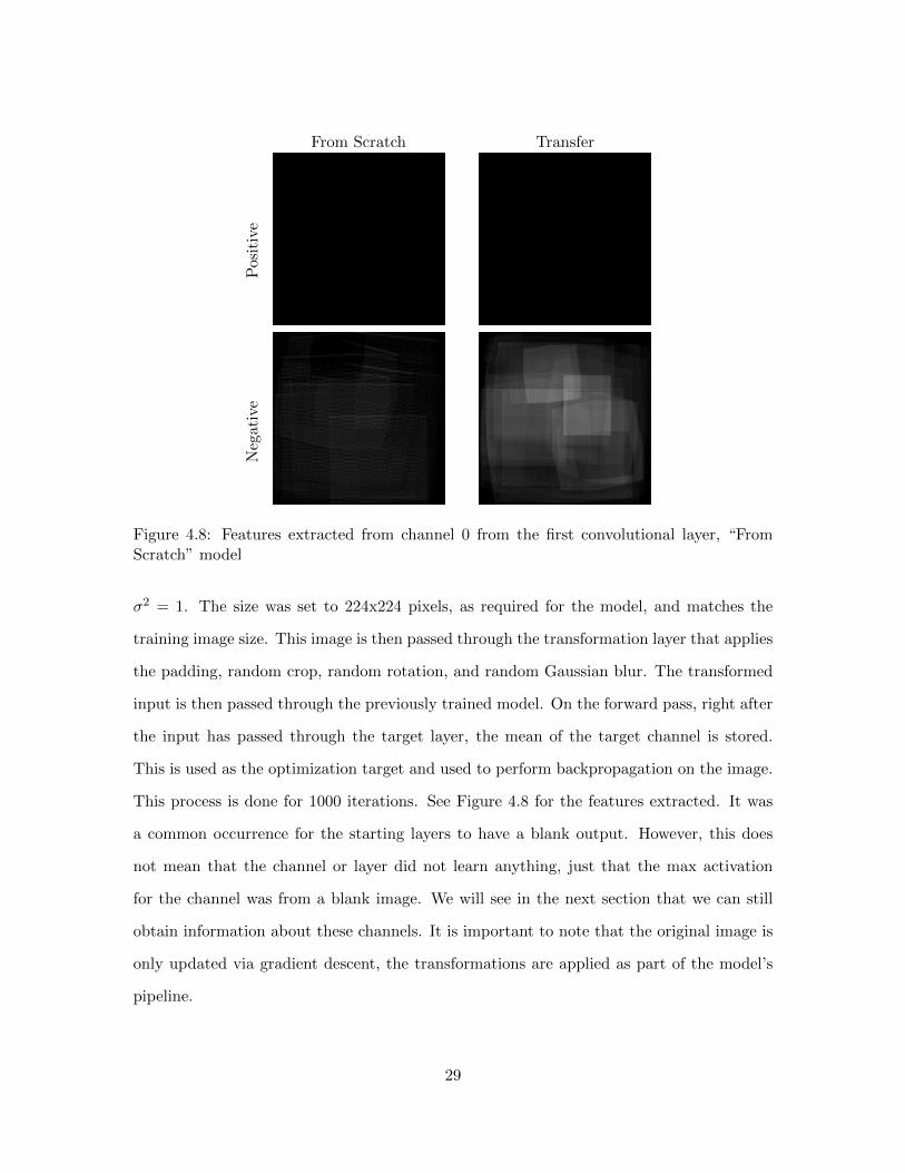
Figure 4.8: Features extracted from channel 0 from the first convolutional layer, “FromScratch” model

σ2 = 1. The size was set to 224x224 pixels, as required for the model, and matches the

training image size. This image is then passed through the transformation layer that applies

the padding, random crop, random rotation, and random Gaussian blur. The transformed

input is then passed through the previously trained model. On the forward pass, right after

the input has passed through the target layer, the mean of the target channel is stored.

This is used as the optimization target and used to perform backpropagation on the image.

This process is done for 1000 iterations. See Figure 4.8 for the features extracted. It was

a common occurrence for the starting layers to have a blank output. However, this does

not mean that the channel or layer did not learn anything, just that the max activation

for the channel was from a blank image. We will see in the next section that we can still

obtain information about these channels. It is important to note that the original image is

only updated via gradient descent, the transformations are applied as part of the model’s

pipeline.

29

(a) Non-demented (b) Very Mildly Demented

(c) Mildly Demented (d) Moderately Demented

Figure 4.9: Feature Extraction with Diversity, “From Scratch” model

30

4.4.2 Diversity Extraction

Due to the nature of optimization, the feature extracted may not be the only one

that a specific layer “knows”. We have also seen that it can also produce blank features. In

order to see more of the features that might be encapsulated in a single layer, the starting

input image is no longer initialized randomly. Instead, a dataset example can be used as

the initial input. This process was first described by Nguyen et al. in 2016 [20]. The rest

of the process remains the same; however, only 10 iterations are needed since we are only

refining the image to achieve our optimization target. See Figure 4.9 for the visualization

of these features that were extracted using diversity. In the figure, the features extracted

were positive extractions from the same layer and channel as Figure 4.8, but started from

a dataset image, each from a different class.

4.4.3 Saliency Maps

Another useful visualization tool is the saliency map. We can use saliency maps to

visualize what areas our model responds highly to when it makes a prediction. These have

been used in prior research to show that 3D CNN models are capable of recognizing areas

typically affected by Alzheimer’s disease [6, 21, 27]. These can be computed by passing an

image through the model then calculating the gradient of the outputs with respect to the

image. To see only the areas that affect the highest class prediction, we only calculate the

gradient of the top predicted class. Figure 4.10 shows saliency maps for samples of each

of the classes for the model trained from scratch. Figure 4.11 shows saliency maps for the

same samples, but for the model trained using transfer learning.

Algorithm 2: Saliency Map Algorithm

Input : Trained neural network ΘQuery Image I

Output: Saliency Map X ∈ R224×224

1 Forward pass through network y = Θ(I)

2 Calculate gradient of argmax(y) with respect to I. ∇ = δ argmax(y)δI

3 X = ∥∇∥

31

(a) Non-demented (b) Very Mildly Demented

(c) Mildly Demented (d) Moderately Demented

Figure 4.10: Saliency Maps, “From Scratch” model

32

(a) Non-demented (b) Very Mildly Demented

(c) Mildly Demented (d) Moderately Demented

Figure 4.11: Saliency Maps, Transferred model

33

4.5 Results and Discussion

Our “From Scratch” model performed very similar to the results in [8, 26, 31]. In

one case, we achieved better [26], which is the same ResNet-18 model, however they use

more classes. It is very close to the accuracy of [8] but our model uses fewer layers and thus

much lighter weight. Our transfer learned model performed slightly better than the “From

Scratch” model, ≈ 1%, with a test accuracy of 99.53%, which is higher than [8, 26, 31];

however, the purpose of this research is not to improve the classification accuracy.

Evaluating the features extracted from both of the models shows significant differ-

ences in learned features. Figure 4.12 shows the same channel and layer, but from different

training method. The features are drastically different; indicating that the transfer learned

model retains most of it’s prior information. This is supported by the work done by Raghu

et al. [25]. This effect is visible in all the other layers of the transfer learned model as well.

Consistent with prior research, the “From Scratch” model’s features become more complex

deeper into the network. However, contrary to prior work [22, 18], the model does not

learn complex features such as parts or objects. The deeper features in the model become

complex edge and texture features. This might be due to the nature task. In ordinary

datasets, classes can vary drastically, however, in this case most samples have very similar

structure. On the other hand, the transfer learned model does still have parts and objects

in the deeper layers. These are most likely remnants from being trained on ImageNet.

We can also see how the features change when given a different input. Figure 4.13

shows a feature extracted from the first channel and first convolution, but for different

inputs. The top image in the figure is the feature extracted using the vanilla method, while

the four images on the bottom use the diversity method. It appears that this layer segments

out the white matter of the brain.

While the extracted features show what the model has learned, the saliency map

shows what these learned features react to in a sample. Figure 4.10 and 4.11 show the

saliency maps for the same inputs but for different training methods. It appears that both

34

(a) “From Scratch” (b) Transfer Learned

Figure 4.12: Differences Between “From Scratch” and Transfer Learned, Positive Extraction

models react strongly to regions with gray matter. A study found that people suffering from

Alzheimer’s disease had reduced amounts of gray matter [12]. While the saliency maps do

show that gray matter is important part in classification it does not explain why. However,

gray matter is not the only reactive area; the ventricular regions have strong reactions in

some areas. These results are similar to those found by Eitel and Ritter [6], however, they

use 3-dimensional data and use binary classification. These findings should be validated

with clinical professionals; the purpose of this work is to produce the visualizations.

35

(a) Randomly Initialized

(b) Non-demented (c) Very Mild

(d) Mild (e) Moderate

Figure 4.13: Feature Change, Negative Extraction

36

Chapter 5

Alzheimer’s Disease and Few-Shot

Learning

In the previous chapter, we address the problem of model explainability in medical

imaging by training the model with adequate data. We showed that for two different

learning methods, random initialization and transfer learning, both learn to react heavily

to areas typically affected by Alzheimer’s disease. In this chapter we address the second

problem associated with deep learning: it requires large amounts of data. Previously, we

examined two different models that can be used to reduce the amount data required to train

accurate models. Namely, they are Siamese and Triplet networks. In previous works, these

models were used mainly on large datasets. However, based on previous research, they are

capable of learning with limited amounts of medical imaging data [29].

In this chapter, we examine how Siamese and Triplet networks can be used learn to

classify Alzheimer’s disease with limited data. We detail the ways we preprocess the data

in order to train the model. To train both networks, we use similar methods as in the last

chapter; we train the models both with random initialization and transfer learning. Finally,

we detail how to use the trained Siamese and Triplet networks to classify, since their goal

is not strictly classification.

37

Figure 5.1: Transformation Pipeline

5.1 The Dataset

We use the same base dataset obtained from Kaggle as described in Section 4.1. For

few-shot learning, we want to train the model only on a limited amount of data. We train

with 25 random samples from each class. The rest of the dataset is used as the test set.

To prevent extreme overfitting, we apply random augmentations in an online fashion

rather than offline. This helps to provide the network with constantly changing data. We

apply random horizontal flipping with probability of p = 0.5 as well as a random rotation

with θ = ±20◦. Finally, we inject noise into a random region with p = 0.25. We also

normalize the images to have a mean of 0 and standard deviation of 1. The test set is only

normalized. Figure 5.1 shows the entire transformation pipeline.

5.2 Siamese Network

A Siamese network is a pair of shared weight neural networks. It takes as input

two samples, either two same class samples or samples from different classes. We use a

contrastive loss function using euclidean distance:

L(x, x+) = y∥f(x)− f(x+)∥2 + (1− y)(max(α− ∥f(x)− f(x+)∥2, 0))

Here, y denotes whether the classes are the same or different and α is the margin.

With contrastive loss, the goal is to minimize the distance between a pair if the class is the

same or maximize the distance between a pair with different classes, but only if the pair is

38

within the margin.

5.3 Triplet Network

The Triplet network can be viewed as an extension of the Siamese net. Rather

than two neural networks with shared weights, the Triplet network uses three. During the

training phase we now pass three samples at a time, (x, x+, x−). Where x is a training

sample, x+ is a different sample from the same class, and x− is a sample from a different

class. The loss function is also changed to Triplet loss,

L(x, x+, x−) = max(∥f(x)− f(x+)∥2 − ∥f(x)− f(x−)∥2 + α, 0)

The goal is to minimize the L2 distance between embeddings from the same class

while maximizing the distance between different classes. Using both a positive and negative

sample has the benefit of being able to both move same classes closer while moving different

classes further away.

5.4 Embedding Network

To learn the feature embeddings we use a ResNet-18 CNN because we found it

performs well at classification of Alzheimer’s disease. Since we no longer classify, we remove

the final output layer from the model. After the average pooling layer, we flatten the result

and send it through a fully connected layer with n outputs, where n is our embedding

dimension size. For our experiments, we use n = 512 as it performed best. See Figure 5.2

for the full model architecture. We test both a model with randomly initialized weights as

well as a model transfer learned from ImageNet.

39

Figure 5.2: Embedding network used for Siamese and Triplet networks.

5.5 Experimental Setup

5.5.1 Siamese Network

To implement our models, we used the ResNet-18 model implemented in the PyTorch

framework. The transferred learned model was initialized from the PyTorch framework

ImageNet weights. We modified the network by removing the fully connected layer and

replacing it with a fully connected layer each with 512 inputs/outputs. Training the Siamese

networks was done using stochastic gradient descent (SGD). Both models used a starting

learning rate of 0.1 and was decreased by a factor of 10 every 30 epochs. A momentum of

0.9 was used as well as L2 regularization with λ = 0.00001. A batch size of 128 samples

was used and the contrastive loss was computed for each possible pair. We chose a margin

of α = 1.0 through experimentation.

After training the model, we could visualize the embeddings by reducing them to

two and three dimensions via PCA. Figures 5.3 and 5.4 show the embeddings reduced to

two principle components for the “from scratch” and transfer learned models, respectively.

Figures 5.5 and 5.6 show the embeddings reduced to three principles components for the

“from scratch” and transfer learned model, respectively. To perform classification, we chose

the closest embedding from the training set to each test sample embedding, i.e. k-nearest

neighbor with k = 1, a method similar to what has been done in prior work [11]. It is

40

important to note that k-nearest neighbor was performed in the full 512-dimensional space,

not the two or three dimensional space obtained via PCA. This produced class averaged

accuracies of 59.91% and 65.4% for “from scratch” and transfer learned Siamese models,

respectively.

5.5.2 Triplet Network

The same modified ResNet-18 model used for the Siamese network was used for

the Triplet network. Training the Triplet models was done using SGD. Both models used a

starting learning rate of 0.01 and decreased by a factor of 10 every 30 epochs. A momentum

of 0.9 was used as well as L2 regularization with λ = 0.00001. A random batch of 128 triplets

was chosen each iteration. We chose a margin of α = 3.0 through experimentation. For the

“from scratch” model, training time took 200 epochs before convergence. For the transfer

learned model, training time took 100 epochs before convergence.

We can use the same process as with the Siamese network to visualize and classify the

embeddings. Figures 5.7 and 5.8 show the embeddings reduced to two principle components

for the “from scratch” and transfer learned model, respectively. Figures 5.9 and 5.10 show

the embeddings reduced to three principle components for the “from scratch” and transfer

learned models, respectively. To perform classification, we chose the closest embedding

from the training set to each test sample embedding, i.e. k-nearest neighbor with k = 1.

This produced class averaged accuracies of 59.1% and 64.4% for “from scratch” and transfer

learned Triplet models, respectively.

41

(a)

(b)

Figure 5.3: Siamese Network Embeds, “From Scratch” Model, 2-dimensions

42

(a)

(b)

Figure 5.4: Siamese Network Embeds, Transfer Model, 2-dimensions

43

(a)

(b)

Figure 5.5: Siamese Network Embeds, “From Scratch” Model, 3-dimensions

44

(a)

(b)

Figure 5.6: Siamese Network Embeds, Transfer Model, 3-dimensions

45

(a)

(b)

Figure 5.7: Triplet Network Embeds, “From Scratch” Model, 2-dimensions

46

(a)

(b)

Figure 5.8: Triplet Network Embeds, Transfer Model, 2-dimensions

47

(a)

(b)

Figure 5.9: Triplet Network Embeds, “From Scratch” Model, 3-dimensions

48

(a)

(b)

Figure 5.10: Triplet Network Embeds, Transfer Model, 3-dimensions

49

5.6 Results and Discussion

All of the models were able to separate the training samples well. As reflected by

the accuracy and PCA visualizations, the test set isn’t as well separated, but still has some

structure. This is partly due to the training set not having samples from all slice depths.

The structure of the brain varies drastically based on depth of the slice taken. From our

experiments the models are not able to generalize well to slice depths it has not seen, we

will discuss this more in the next chapter when we discuss limitations.

For the Siamese models, they learned very different ways to separate the classes.

For the “From Scratch” model, it appears to have learned the relation of each class to the

others. In other words, non demented cases are closest to very mild, very mild is in between

non demented and mild, mild is between very mild and moderate, and moderate is only

closest to mild. In the case of the transfer learned model, it was not able to learn this

relation. This likely due to the combination of using a pretrained model, i.e. one that is in

a “good” state, and contrastive loss. For the Triplet networks, both training methods were

able to learn the relation between each stage of the disease, although slightly different. The

transfer learned model differed from that of the Siamese one due to the triplet loss. Rather

than only be able to ‘push’ two points away if they were different, or ‘pull’ them together

if they similar, the triplet loss could do both at the same time. This effect has been seen

before in other medical imaging domains [4, 16]. However, our results are obtained via PCA

rather than t-SNE, a different dimensionality reduction technique.

Based on our results, a transfer learned Siamese network might not be as useful

compared to the other three. The other three models benefit from the fact that when

querying the trained model if a sample embedding is in between two classes it could be

assumed that the input belongs to one of the classes. The transfer learned Siamese model

does not have this benefit, since the embeds do not appear to follow a progression like the

other three.

50

Chapter 6

Limitations and Future Work

6.1 Limitations

The most impactful limitation for both of our methods is the lack of knowledge of the

collection process of the dataset. There are numerous types of MRI scans that can be done

on the brain such as T1-weighted and T2-weighted; the images in the dataset we use appear

to be T1-weighted since the white matter is lighter in color than the gray matter. Another

issue is no indication of what range of slices that the MRI sequences came from, as well

as how many unique brains there are; typically, when a patient gets an MRI done multiple

slices of the brain are taken. Take for example, the images in Figure 6.1, both brains are

non-demented, but their structure is very different because they are from different depths.

This proved to be an issue at the start of our research. The supplied training set contained

few examples of the ventricular sections of the brain for all classes. While the supplied

testing set consisted mostly of the ventricular sections. This caused lower than expected

accuracy for our ResNet-18 model in initial test runs. To counter this, we merged the given

sets and performed our own randomized split, resulting in higher accuracy. This problem

is still evident with the results of the Siamese and Triplet networks.

51

Figure 6.1: Different Brain Slices

6.2 Future Work

While our method for visualizing features was applied to ResNet-18, future work

might explore using different models. Different model architectures learn differently, being

able to visually explain the network helps validate the model. Future work might also deal

with having results validated with a clinical professional.

Future work on Siamese and Triplet networks might explore:

• Treating a patient’s entire MRI scan sequence, i.e. all the slices, as ‘one’ sample,

rather than just a single slice.

• Use each sample is a slice at a different depth, instead of random selection.

• Pretrain the network from a different brain imagery task.

• Use volumetric 3D MRI scans

Having the data sampling be patient based rather than image based might be more

logical as MRI scans typically contain a sequence of slices rather than a single slice. This

52

has the added benefit of more raw data to train with, most likely improving performance.

For the second, having the model train on at least one sample per depth allows the model

to ‘see’ an example of the brain at every depth. For the third, Siamese and Triplet networks

are typically pretrained on a similar but disjoint task; pretraining the model from a different

brain imagery task might help to improve performance. Finally, using a 3D volumetric MRI

scan of the brain allows the model to learn from the entire brain rather than segments at a

time.

53

Chapter 7

Conclusions

Deep learning has become a standard approach for medical imaging tasks; however,

deep learning has its caveats. We had two goals for this thesis. First, aide in explaining

deep learning models. Second, train a network on limited amounts of data. For the first,

we trained a conventional network on an adequate amount of data and used two different

visualization techniques: saliency maps, which are commonly used, and a “deep dream”

style feature extraction, which has not been used, to our knowledge, in medical imaging.

For the second, we used two metric learning models that train on limited amounts of data.

By training on limited amounts of data we reduce the requirement of large amounts of data

that needs to be collected, which can be costly. Both of these methods are important steps

to help increase the adoption of deep learning in the medical sector.

54

Bibliography

[1] 2021 alzheimer’s disease facts and figures. Alzheimer’s & Dementia, 17(3):327–406,2021.

[2] Tooba Altaf, Syed Muhammad Anwar, Nadia Gul, Muhammad Nadeem Majeed, andMuhammad Majid. Multi-class alzheimer’s disease classification using image and clin-ical features. Biomedical Signal Processing and Control, 43:64–74, May 2018.

[3] Jane Bromley, Isabelle Guyon, Yann LeCun, Eduard Sackinger, and Roopak Shah.Signature verification using a “siamese” time delay neural network. In Advances inNeural Information Processing Systems, volume 6. Morgan-Kaufmann, 1994.

[4] Yu-An Chung and Wei-Hung Weng. Learning deep representations of medical imagesusing siamese cnns with application to content-based image retrieval. arXiv:1711.08490[cs], Dec 2017. arXiv: 1711.08490.

[5] Jia Deng, Wei Dong, Richard Socher, Li-Jia Li, Kai Li, and Li Fei-Fei. Imagenet: Alarge-scale hierarchical image database. In 2009 IEEE conference on computer visionand pattern recognition, pages 248–255. Ieee, 2009.

[6] Fabian Eitel and Kerstin Ritter. Testing the robustness of attribution methodsfor convolutional neural networks in mri-based alzheimer’s disease classification.arXiv:1909.08856 [cs, eess], Sep 2019. arXiv: 1909.08856.

[7] Kunihiko Fukushima. Neocognitron: A self-organizing neural network model for amechanism of pattern recognition unaffected by shift in position. Biological Cybernetics,36(4):193–202, Apr 1980.

[8] Lawrence V. Fulton, Diane Dolezel, Jordan Harrop, Yan Yan, and Christopher P.Fulton. Classification of alzheimer’s disease with and without imagery using gradientboosted machines and resnet-50. Brain Sciences, 9(9):212, Aug 2019.

[9] R. Hadsell, S. Chopra, and Y. LeCun. Dimensionality reduction by learning an invariantmapping. In 2006 IEEE Computer Society Conference on Computer Vision and PatternRecognition - Volume 2 (CVPR’06), volume 2, page 1735–1742. IEEE, 2006.

[10] Kaiming He, Xiangyu Zhang, Shaoqing Ren, and Jian Sun. Deep residual learningfor image recognition. In 2016 IEEE Conference on Computer Vision and PatternRecognition (CVPR), page 770–778, Jun 2016.

55

[11] Elad Hoffer and Nir Ailon. Deep metric learning using triplet network. In Aasa Feragen,Marcello Pelillo, and Marco Loog, editors, Similarity-Based Pattern Recognition, pages84–92, Cham, 2015. Springer International Publishing.

[12] G. B. Karas, P. Scheltens, S. A. R. B. Rombouts, P. J. Visser, R. A. van Schijndel, N. C.Fox, and F. Barkhof. Global and local gray matter loss in mild cognitive impairmentand alzheimer’s disease. NeuroImage, 23(2):708–716, Oct 2004.

[13] Gregory Koch, Richard Zemel, and Ruslan Salakhutdinov. Siamese neural networksfor one-shot image recognition. International Conference on Machine Learning, 2015.

[14] Salim Lahmiri and Mounir Boukadoum. Alzheimer’s disease detection in brain mag-netic resonance images using multiscale fractal analysis. ISRN Radiology, 2013, Oct2013.

[15] Salim Lahmiri and Mounir Boukadoum. New approach for automatic classification ofalzheimer’s disease, mild cognitive impairment and healthy brain magnetic resonanceimages. Healthcare Technology Letters, 1(1):32–36, Jun 2014.

[16] Chin-Fu Liu, Shreyas Padhy, Sandhya Ramachandran, Victor X. Wang, Andrew Efi-mov, Alonso Bernal, Linyuan Shi, Marc Vaillant, J. Tilak Ratnanather, Andreia V.Faria, and et al. Using deep siamese neural networks for detection of brain asym-metries associated with alzheimer’s disease and mild cognitive impairment. Magneticresonance imaging, 64:190–199, Dec 2019.

[17] Abhishaike Mahajan, James Dormer, Qinmei Li, Deji Chen, Zhenfeng Zhang, andBaowei Fei. Siamese neural networks for the classification of high-dimensional ra-diomic features. Proceedings of SPIE–the International Society for Optical Engineering,11314:113143Q, Feb 2020.

[18] Alexander Mordvintsev, Christopher Olah, and Mike Tyka. Inceptionism: Goingdeeper into neural networks, 2015.

[19] Anh Nguyen, Jason Yosinski, and Jeff Clune. Deep neural networks are easily fooled:High confidence predictions for unrecognizable images. arXiv:1412.1897 [cs], Apr 2015.arXiv: 1412.1897.

[20] Anh Nguyen, Jason Yosinski, and Jeff Clune. Multifaceted feature visualization: Un-covering the different types of features learned by each neuron in deep neural networks.Feb 2016.

[21] Kanghan Oh, Young-Chul Chung, Ko Woon Kim, Woo-Sung Kim, and Il-Seok Oh.Classification and visualization of alzheimer’s disease using volumetric convolutionalneural network and transfer learning. Scientific Reports, 9(1):18150, Dec 2019.

[22] Chris Olah, Alexander Mordvintsev, and Ludwig Schubert. Feature visualization. Dis-till, 2017. https://distill.pub/2017/feature-visualization.

56

[23] Adam Paszke, Sam Gross, Francisco Massa, Adam Lerer, James Bradbury, GregoryChanan, Trevor Killeen, Zeming Lin, Natalia Gimelshein, Luca Antiga, Alban Desmai-son, Andreas Kopf, Edward Yang, Zachary DeVito, Martin Raison, Alykhan Tejani,Sasank Chilamkurthy, Benoit Steiner, Lu Fang, Junjie Bai, and Soumith Chintala.Pytorch: An imperative style, high-performance deep learning library. In Advances inNeural Information Processing Systems 32, pages 8024–8035. Curran Associates, Inc.,2019.

[24] Kenneth A. Philbrick, Kotaro Yoshida, Dai Inoue, Zeynettin Akkus, Timothy L.Kline, Alexander D. Weston, Panagiotis Korfiatis, Naoki Takahashi, and Bradley J.Erickson. What does deep learning see? insights from a classifier trained to pre-dict contrast enhancement phase from ct images. American Journal of Roentgenology,211(6):1184–1193, Dec 2018.

[25] Maithra Raghu, Chiyuan Zhang, Jon Kleinberg, and Samy Bengio. Transfusion: Un-derstanding transfer learning for medical imaging. In Advances in Neural InformationProcessing Systems, volume 32. Curran Associates, Inc., 2019.

[26] Farheen Ramzan, Muhammad Usman Ghani Khan, Asim Rehmat, Sajid Iqbal, TanzilaSaba, Amjad Rehman, and Zahid Mehmood. A deep learning approach for automateddiagnosis and multi-class classification of alzheimer’s disease stages using resting-statefmri and residual neural networks. Journal of Medical Systems, 44(2):37, Dec 2019.

[27] Johannes Rieke, Fabian Eitel, Martin Weygandt, John-Dylan Haynes, and Kerstin Rit-ter. Visualizing convolutional networks for mri-based diagnosis of alzheimer’s disease.arXiv:1808.02874 [cs], 11038:24–31, 2018. arXiv: 1808.02874.

[28] D Salas-Gonzalez, J M Gorriz, J Ramırez, M Lopez, I Alvarez, F Segovia, R Chaves,and C G Puntonet. Computer-aided diagnosis of alzheimer's disease using supportvector machines and classification trees. Physics in Medicine & Biology, 55(10):2807–2817, apr 2010.

[29] Mohammad Shorfuzzaman and M. Shamim Hossain. Metacovid: A siamese neural net-work framework with contrastive loss for n-shot diagnosis of covid-19 patients. PatternRecognition, 113:107700, May 2021.

[30] Karen Simonyan, Andrea Vedaldi, and Andrew Zisserman. Deep inside convolutionalnetworks: Visualising image classification models and saliency maps. arXiv:1312.6034[cs], Apr 2014. arXiv: 1312.6034.

[31] Haijing Sun, Anna Wang, Wenhui Wang, and Chen Liu. An improved deep residualnetwork prediction model for the early diagnosis of alzheimer’s disease. Sensors (Basel,Switzerland), 21(12):4182, Jun 2021.

[32] Jason Yosinski, Jeff Clune, Yoshua Bengio, and Hod Lipson. How transferable arefeatures in deep neural networks? In Advances in Neural Information ProcessingSystems, volume 27. Curran Associates, Inc., 2014.

57