Virtual Telemetry for Dynamic Data-Driven

Application Simulations

Craig C. Douglas1,2, Yalchin Efendiev3, Richard Ewing3, Raytcho Lazarov3,Martin J. Cole4, Greg Jones4, and Chris R. Johnson4

1 University of Kentucky, Department of Computer Science, 325 McVey Hall,Lexington, KY 40506-0045, USA

{douglas}@ccs.uky.edu2 Yale University, Department of Computer Science, P.O. Box 208285

New Haven, CT 06520-8285, USAdouglas-craig@cs.yale.edu

3 Texas A&M University, College Station, TX, USA{efendiev,lazarov}@math.tamu.edu and richard-ewing@tamu.edu

4 Scientific Computing and Imaging Institute, University of Utah, Salt Lake City,UT, USA

mjc@sci.utah.edu and crj@cs.utah.edu

Abstract. We describe a virtual telemetry system that allows us to de-vise and augment dynamic data-driven application simulations (DDDAS).Virtual telemetry has the advantage that it is inexpensive to producefrom real time simulations and readily transmittable using open sourcestreaming software. Real telemetry is usually expensive to receive (if itis even available long term), tends to be messy, comes in no particularorder, and can be incomplete or erroneous due to transmission problemsor sensor malfunction. We will generate multiple streams continuouslyfor extended periods (e.g., months or years): clean data, somewhat errorprone data, and quite lossy or inaccurate data. By studying all of thestreams at once we will be able to devise DDDAS components useful inpredictive contaminant modeling.

1 Introduction

Consider an extreme example of a disaster scenario in which a major waste spilloccurs in a river flowing through the center of a major city. In short time, thewaste will be on kilometers of the city’s shoreline.

Sensors can now be dropped into an open water body to measure where thecontamination is, where the contaminant is going to go, and to monitor theenvironmental impact of the spill. Whether or not the procedure to drop thesensors exists today is not relevant for the moment; only that it could be done.Scrambling aircraft to drop sensors in a river is no longer such a far fetchedscenario.

A well designed DDDAS predictive contaminant tracking program will beable to determine where the flow will go, the neighborhoods that have to be

evacuated, and optimize a clean-up plan. A backward in time DDDAS programwill offer help in determining where and when a contaminant entered the en-vironment. For this to become reality data streaming tolerant algorithms withsensitivity analysis incorporated for data injection, feature extraction, and mul-tiple scaling must be developed for this to scenario to become a reality.

There are several approaches to designing DDDAS systems for disaster man-agement. One is to collect real data and replay it while developing new datadynamic algorithms. Another is to generate fictional data continuously over aseveral year period with disasters initiated at random times or by human inter-vention (possibly without informing the other researchers in advance).

In either case, data streaming is a useful delivery system. Like realistic teleme-try, data arrives that is usually incomplete, not in any order, and occasionallywrong. In short, it is an appalling mess.

In Sect. 2, we define an application that is our first test case. In Sect. 3, wedefine the DDDAS components that are of interest in this paper. In Sect. 4, wedefine model reduction for our application. In Sect. 5, we describe the telemetrymiddleware that we are in the process of developing and what our choices are. InSect. 6, we discuss the programming environment that we are using to generateuseful prototypes quickly so that a final package, useful to others as well, can bebuilt. In Sect. 8, we draw some conclusions.

2 An Example Application

As an example application we consider a single component contaminant trans-port in heterogeneous porous media taking into account convection and diffusioneffects. This simple model will be further extended by incorporating additionalphysical effects as well as uncertainties. The mathematical formulation of theproblem is given by coupled equations that describe pressure distribution andthe transport equations, ∇·k∇p = f , St+v·∇S = ∇·D∇S, v = −k∇p. We con-sider two different permeability field scenarios. For the first case we assume thata large horizontal permeability streak is located in the middle of the domain andthere are two vertical low permeability zones. The background permeability istaken to be 1, the permeability of high streak region is taken to be 2, and verticallow permeability regions have permeability 0.01. The second permeability fieldis chosen as an unconditional realization of a fractal field whose semivariogramis given by γ(h) = Ch0.5, where the semivariogram is defined as

γ(h) =1

2E[(ξ(x + h) − ξ(x))2].

A horizontal high permeability streak is added at the center of the domain. Togenerate a realization of this field we use fractional Brownian motion theory de-veloped in [1, 7, 15]. The realization of the field is generated from the generalizedWeierstrass-Mandelbrot function with fractal co-dimension β/2 (β = 0.5)

ξ(x) =

∞∑i=1

Aiλ−i

β

2 sin(λix · ei + φi),

where Ai are normally distributed random numbers with mean zero and variance1, ei are uniformly distributed on the unit sphere, φi are uniformly distributedover [0, 2π], and λ > 1. This isotropic random field has an approximately powersemivariogram, i.e., 0 < chβ < γ(h) < Chβ . In all the examples the rectangulardomain [0, 2] × [0, 1] × [0, 1] is consider and the following initial and boundaryconditions are imposed. We assume the pressure at the inlet x = 0 to be p = 1and p = 0 at the outlet x = 2. For the other faces we assume no flow boundaryconditions for the pressure equation. For the concentration field we assume thatthe concentration is S = 1 at the inlet x = 0 and ∂S/∂n = 0 is imposed on theother faces. Furthermore, D = 0.02 is taken to be constant. The computationsare implemented using 3-D finite element simulator developed at Texas A&Memploying the mesh generator NETGEN [16].

The concentration fields cannot easily be rendered in a grayscale. We havedecided to post the concentrations on the web at URL

http : //www.dddas.org/itr − 0219627/papers.html#iccs2003.

3 DDDAS Components

In contaminant movement predictions, it is common to run simulations for a fewhours or days as a batch process. Although the individual application simulationperiods are a few wall clock hours, they are built to update the early time stepswith real data as it becomes available.

Converting software from a data set oriented batch code to a data stream con-tinuously running code requires significant, nontrivial changes. We are dissectingcontaminant transport models and associated codes in order to understand howto convert these models into the DDDAS model. Underground situations (e.g.,nuclear waste contamination from a leaky containment vessel) are different froman above ground situation (contaminants in a lake and/or river). We are inves-tigating both of these situations as well as the combination of the two.

The addition of DDDAS features to a system requires that aspects relatedto the initial data must be identified. Additionally, the time-related updatingprocedures must investigated. As we approach these requirements we will focuson maintaining a solution that is generally useful to other application fields thatare initial boundary value problem (IBVP) based. Almost all IBVP formulationspreclude dynamic data or backward in time error checking, sometimes in quitesubtle ways.

The use of continuous data streams instead of initial guess only data setspresents an additional challenge for data driven simulations since the resultsvary based on the sampling rate and the discretization scheme used. Dynamicdata assimilation or interpolation might be necessary to provide a feedback toexperimental design/control. DDDAS algorithms also need to dynamically as-similate new data at mid-simulation as the data arrives, necessitating “warmrestart” capabilities.

Modifying application programs to incorporate new dynamically injecteddata is not a small change in the application program, particularly since the

incoming data tends to be quite messy. It requires a change in the applicationdesign, the underlying solution algorithms, and the way people think about theaccuracy of the predictions.

Uncertainties in DDDAS applications emanate from several sources, namelyuncertainty associated with the model, uncertainties in the input data (streamed),and the environment variables. Identifying the factors that have the greatest im-pact on the uncertainty output of the calculations is essential in order to controlthe overall processes within specific limits. Handling all output distributionsto provide error bounds is, for most realistic problems, a computationally pro-hibitive task. Hence, using prior observations to guide the output distributionestimations presents a possible approach to incorporating uncertainty in controldecisions.

Incorporating these statistical errors (estimations or experimental data un-certainties) into computations, particularly for coupled nonlinear systems, isdifficult. This is compounded by the fact that tolerances may also change adap-tively during a simulation. Error ranges for uncertainty in the data must be cre-ated and analyzed during simulations. Sensitivity analysis must be performedcontinuously during simulations with options in case of a statistical anomaly.

The common mathematical model in many DDDAS applications may be for-mulated as solving a time dependent, nonlinear problem of the form F(x+Dx(t))=0,by iteratively choosing a new approximate solution x based on the time depen-dent perturbation Dx(t).

At each iterative step, the following three issues may need to be addressed.Incomplete solves of a sequence of related models must be understood. In addi-tion the effects of perturbations, either in the data and/or the model, need to beresolved and kept within acceptable limits. Finally, nontraditional convergenceissues have to be understood and resolved. Consequently, there will be a highpremium on developing quick approximate direction choices, such as, lower rankupdates and continuation methods. It will also be critical to understand thebehavior of these chosen methods.

By generating telemetry in real time, we allow for the new, DDDAS codeto determine how well it has predicted the past, assuming the DDDAS coderuns much faster than real time. We run a simulation backwards in time toa point where we can verify that we have not introduced too great an errorinto a simulation at a future time. This is particularly important when decidingwhether or not to introduce all or just part of a data stream. For example, if adata stream update causes a loss or addition of mass when it is conserved, thedata stream update will lead to an abrupt loss of usefulness unless a filteringprocess is developed to maintain the conservation of mass. We are developingnew filters for our applications that resolve the errors introduced by convertingthe applications to data streams.

4 Model reduction and multiscale computations

Model reduction will largely be accomplished with the use of upscaling tech-niques. Due to complicated interactions and many scales, as well as uncer-tainties, upscaling is desirable. The upscaling is in general nontrivial becauseheterogeneities at all scales have a significant effect, and these effects must becaptured in the coarsened subsurface description. Most approaches for upscal-ing are designed to generate a coarse grid description of the process which isnearly equivalent (for purposes of flow simulation) to an underlying fine grid de-scription. We will employ both static and dynamic upscaling techniques. Staticupscaling techniques will generally be used in coarsening the media properties,while the dynamic upscaling will be employed to understand the effect of thesmall scale dynamics on the larger scales. One of the important aspects of ourupscaling approach is the use of carefully selected dynamic coarse scale variablesin a multiscale framework.

To demonstrate the main idea of our static upscaling procedures we considerour application model, the pressure equation ∇·k∇p = f . Within this approachthe heterogeneities of the media are incorporated into the finite element (or finitevolume element) base functions that are further coupled through the globalformulation of the problem We seek the solution of this equation in a coarsespace whose base elements φi(x) contain the local heterogeneity information,Vh = span(φi). The numerical solution uh is found from∫

D

k∇uh∇vhdx =

∫D

fvhdx, ∀vh ∈ Vh.

This approach allows us to solve the saturation equation on the on the finescale grid as well as on the coarse scale grid since the fine scale features ofthe velocity field can be recovered from the base functions. Consequently, wecan adjust the permeability at the fine scale directly. One of the advantages ofthese approaches is that the local changes of the permeability field will onlyaffect few base functions. Consequently, we will only need to re-compute fewbase functions and solve the coarse problem. This methodology will be useful inbackward integration for finding sources of inconsistencies within our DDDASapplication. We will also employ traditional approaches based on upscaling ofpermeability field [2] and use mainly the upscaling of permeability field withoversampling techniques [19]. The main idea of this approach is to use largerdomain (larger than the coarse block) in order to reduce the boundary effects.To reduce the grid effects grid based upscaling techniques will be employed.

For the time dependent transport problems we will employ coarsening tech-niques that are based on dynamic upscaling. For these approaches the dynamicquantities (e.g., quantities that depend on concentration) are coarsened and theirfunctionality is determined through analytical considerations. Determining theform of coarse scale equations is important for multiscale modeling. Our previousapproaches on this issue were mainly in two directions. First approach that isbased on perturbation techniques models subgrid effects as a nonlocal macrodis-persion term [5]. This approach takes into account the long range interaction in

the form of diffusion term that grows in time. Our second approach based onhomogenization techniques [6] computes the dynamic upscaled quantities usinglocal problems [4, 3].

5 Telemetry Middleware

Real telemetry is usually expensive to receive (if it is even available on a long termbasis), tends to be messy, comes in no particular order, and can be incompleteor erroneous due to transmission problems or sensor malfunction. For predictivecontaminant telemetry, there are added problems that due to pesky legal reasons(corporation X does not want it known that it is poisoning the well water ofa town), the actual data streams are not available to researchers, even onesproviding the simulation software that will do the tracking.

Virtual telemetry has the advantage that it is inexpensive to produce fromreal time simulations. The fake telemetry can easily be transmitted using opensource streaming software.

We will generate multiple streams continuously for extended periods (e.g.,months or years): clean data, somewhat error prone data, and quite lossy orinaccurate data. By studying all of the streams at once we will be able to deviseDDDAS components useful in predictive contaminant modeling.

Real telemetry used in predictive contaminant monitoring comes in smallpackets from sensors in wells or placed in an open body of water. There maybe a few sensors or many. With virtual telemetry, we can vary the amount oftelemetry that we broadcast and its frequency.

There are a number of issues that are being resolved in the course of ourproject.

1. Should the telemetry data be broadcast as an audio stream?2. Should the telemetry data be broadcast as a movie stream?3. Should a complete 3D visualization be broadcast (and in what form)?4. Should only sparse data from discrete points in a domain be broadcast?5. At what rate can the virtual telemetry be broadcast so that network admin-

istrators do not cut off the data stream?

We are building middleware to answer all of the questions above.There are a number of open source projects for doing reliable data streaming.

Palantir [8] is a former commercial product that has been re-released as opensource. It supports audio and video streaming as well as general data stream-ing. Gini [9] is an audio and video streamer that is still in beta, but is fairlyactive in development. GStreamer [10] is more of a streaming framework devel-oped by graduate students in Washington. It supports audio, video, and generaldata streaming. VideoLAN [18] is a video streamer developed by students at theEcole Centrale Paris. QuickTime Streaming Server is an audio and video stream-ing server that Apple offers. Of the five, GStreamer is the clear first choice toconcentrate on.

Broadcasting the telemetry as audio has the advantage that there are manyprograms to choose from to generate the data streams and to “listen” to themon the receiving end.

Broadcasting the telemetry as a movie stream or a full 3D visualization hasthe advantage that it can be trivially visualized on the receiving end. This isparticularly attractive when studying incomplete and/or erroneous data streams.However, there is a potential of transmitting too much data and overwhelmingthe network.

Broadcasting only sparse data from discrete points in any form has plusesand minuses. Almost any Internet protocol can be used. However, do we reallywant to tie ourselves to one Internet protocol?

Avoiding the attention of network administrators is a serious concern. Wemust balance adequate data streams with not having any serious impact on anetwork. This is highly dependent on where we are running the virtual telemetryfrom and to and cannot easily be determined a priori. However, it is easilydetermined a posteriori, which will be part of a well behaved, adaptive broadcastsystem.

6 Program Construction

Current interactive scientific visualization and computational steering implemen-tations require low latency and high bandwidth computation in the form of modelgeneration, solvers, and visualization. Latency is particularly a problem whenanalyzing large data sets, constructing and rendering three-dimensional modelsand meshes, and allowing a scientist to alter the parameters of the computa-tion interactively. However, large-scale computational models often exceed thesystem resources of a single machine, motivating closer investigation of meetingthese same needs with a distributed computational environment.

To achieve execution speeds needed for interactive three-dimensional prob-lem solving and visualization, we have developed the SCIRun problem solvingenvironment and computational steering system [12, 11]. SCIRun allows the in-teractive construction, debugging, and steering of large scale scientific compu-tations. SCIRun can be conceptualized as a computational workbench, in whicha scientist can design via a dataflow programming model and modify simula-tions interactively. SCIRun enables scientists to interactively modify geometricmodels, change numerical parameters and boundary conditions, and adaptivelymodify the meshes, while simultaneously visualizing intermediate and final sim-ulation results.

When the user changes a parameter in any of the module user interfaces,the module is re-executed, and all changes are automatically propagated to alldownstream modules. The user is freed from worrying about details of data de-pendencies and data file formats. The user can make changes without stoppingthe computation, thus steering the computational process. In a typical batchsimulation mode, the scientist manually sets input parameters, computes results,assesses the results with a combination of separate analytical and visualization

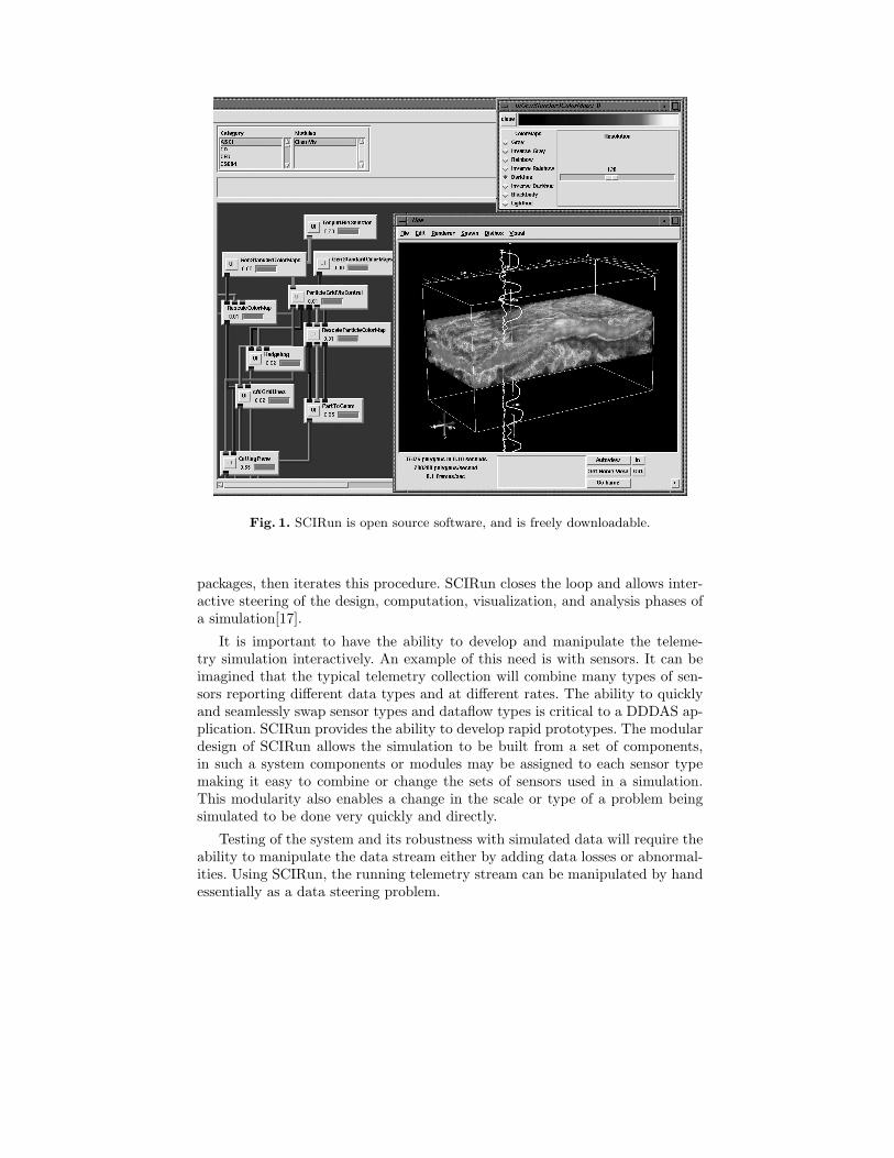
Fig. 1. SCIRun is open source software, and is freely downloadable.

packages, then iterates this procedure. SCIRun closes the loop and allows inter-active steering of the design, computation, visualization, and analysis phases ofa simulation[17].

It is important to have the ability to develop and manipulate the teleme-try simulation interactively. An example of this need is with sensors. It can beimagined that the typical telemetry collection will combine many types of sen-sors reporting different data types and at different rates. The ability to quicklyand seamlessly swap sensor types and dataflow types is critical to a DDDAS ap-plication. SCIRun provides the ability to develop rapid prototypes. The modulardesign of SCIRun allows the simulation to be built from a set of components,in such a system components or modules may be assigned to each sensor typemaking it easy to combine or change the sets of sensors used in a simulation.This modularity also enables a change in the scale or type of a problem beingsimulated to be done very quickly and directly.

Testing of the system and its robustness with simulated data will require theability to manipulate the data stream either by adding data losses or abnormal-ities. Using SCIRun, the running telemetry stream can be manipulated by handessentially as a data steering problem.

As the testbed is expanded it will almost certainly be a requirement thatthe application perform in a distributed environment. It will also be likely thatthe application be required to work, seamlessly, with other software packages orlibraries, not directly incorporated in the application. There are numerous exam-ples of the ease of bridging third party software with SCIRun, and of SCIRunoperating in a distributed environment [14, 13] . This will enable the utiliza-tion of existing free codes for streaming the dynamic data needed to drive thissimulation.

7 Aknowledgements

This work was supported in part by a National Science Foundation collaborativeresearch grant (EIA-0219627, EIA-0218721, and EIA-0218229).

8 Conclusions

We have described issues in constructing a virtual telemetry system. Our targetis enabling DDDAS components in a predictive contaminant model. We expectto have useful open source middleware readily available on the Internet soon.Once the middleware is completed, we can explore many interesting features ofDDDAS.

References

1. Chu, J., and Journel, A. In Geostatistics for the next Century, R. Dimitrakopou-los, Ed. Kluwer Academic Publishers, 1994, pp. 407–412.

2. Durlofsky, L. J. Numerical calculation of equivalent grid block permeabilitytensors for heterogeneous porous media. Water Resour. Res. 27 (1991), 699–708.

3. Efendiev, Y., and Durlofsky, L. Accurate subgrid models for two-phase flow inheterogeneous reservoirs. paper SPE 79680 presented at the 2003 SPE Symposiumon Reservoir Simulation, Houston, TX.

4. Efendiev, Y., and Durlofsky, L. A generalized convection diffusion model forsubgrid transport in porous media. submitted to SIAM on Multiscale Modelingand Simulation.

5. Efendiev, Y. R., Durlofsky, L. J., and Lee, S. H. Modeling of subgrid effectsin coarse scale simulations of transport in heterogeneous porous media. WaterResour. Res. 36 (2000), 2031–2041.

6. Efendiev, Y. R., and Popov, B. On homogenization of nonlinear hy-perbolic equations. submitted to SIAM J. Appl. Math. (available athttp://www.math.tamu.edu/∼yalchin.efendiev/submit.html).

7. Falconer, K. Fractal Geometry: Mathematical Foundations and Applications.John Wiley & Sons, 1990.

8. FastPath Research. Palantir. http://www.fastpath.it/products/palantir.9. Gini. Gini. http://gini.sourceforge.net.

10. GStreamer. Gstreamer. http://www.gstreamer.net.

11. Johnson, C., and Parker, S. The scirun parallel scientific computing problemsolving environment. In Ninth SIAM Conference on Parallel Processing forScien-tific Computing (1999).

12. Johnson, C., Parker, S., and Weinstein, D. Large-scale computational scienceapplications using the scirun problem solving environment. In Supercomputer 2000(2000).

13. Miller, M., Hansen, C., and Johnson, C. Simulation steering with scirun in adistributed environment. In Applied Parallel Computing, 4th InternationalWork-shop, PARA’98, E. E. B. Kagstrom, J. Dongarra and J. Wasniewski, Eds., vol. 1541of Lecture Notes in Computer Science. Springer-Verlag, Berlin, 1998, pp. 366–376.

14. Miller, M., Hansen, C., Parker, S., and Johnson, C. Simulation steeringwith scirun in a distributed memory environment. In Seventh IEEE InternationalSymposium on HighPerformance Distributed Computing (HPDC-7) (jul 1998).

15. Oh, W. Random field simulation and an application of kriging to image thresh-olding. PhD thesis, State Univeristy of New York at Stony Brook, 1998.

16. Schoeberl, J. NETGEN-An advancing front 2d/3d-mesh generator basedon abstract rules. Computing and Visualization in Science 1 (1997), 41–52.http://www.sfb013.uni-linz.ac.at/ joachim/netgen/.

17. SCIRun: A Scientific Computing Problem Solving Environment. Scientific Com-puting and Imaging Institute (SCI), http://software.sci.utah.edu/scirun.html,2002.

18. VideoLAN. Videolan. http://www.videolan.org.19. Wu, X. H., Efendiev, Y. R., and Hou, T. Y. Analysis of upscaling absolute

permeability. Discrete and Continuous Dynamical Systems, Series B 2 (2002),185–204.