VIBRATIONS OF AN AXIALLY MOVING BEAM WITH TIME-DEPENDENT VELOCITY
19
Journal of Sound and < ibration (1999) 227(2), 239 } 257 Article No. jsvi.1999.2247, available online at http://www.idealibrary.com on VIBRATIONS OF AN AXIALLY MOVING BEAM WITH TIME-DEPENDENT VELOCITY H. R. O G Z AND M. PAKDEMI 0 RLI 0 Department of Mechanical Engineering, Celal Bayar ;niversity, 45140 Muradiye, Mann R sa, ¹ urkey (Received 16 September 1998, and in ,nal form 15 March 1999) The dynamic response of an axially accelerating, elastic, tensioned beam is investigated. The time-dependent velocity is assumed to vary harmonically about a constant mean velocity. These systems experience a coriolis acceleration component which renders such systems gyroscopic. The equation of motion is solved by using perturbation analysis. Principal parametric resonances and combination resonances are investigated in detail. Stability boundaries are determined analytically. It is found that instabilities occur when the frequency of velocity #uctuations is close to two times the natural frequency of the constant velocity system or when the frequency is close to the sum of any two natural frequencies. When the velocity variation frequency is close to zero or to the di!erence of two natural frequencies, however, no instabilities are detected up to the "rst order of perturbation. Numerical results are presented for di!erent #exural sti!ness values and for the "rst two modes. ( 1999 Academic Press 1. INTRODUCTION Due to their technological importance, the vibrations of axially moving materials have been investigated by many researchers. Threadlines, high-speed magnetic and paper tapes, strings, power transmission chains and belts, band-saws, "bres, beams, aerial cable tramways and pipes conveying #uid are some of the examples. Ulsoy et al. [1] and Wickert and Mote [2] reviewed the literature on axially moving materials. Wickert and Mote [3] investigated the transverse vibrations of travelling strings and beams. They used travelling string eigenfunctions and introduced a convenient orthogonal basis suitable for discretization. The same authors [4] also presented a modal analysis using complex state eigenfunctions and their conjugates. Ulsoy [5] treated a model for the transverse vibration of an axially moving beam which includes elastic coupling between two adjacent spans. The system was then analyzed by using a classical approximate solution method. It was concluded that the presence of a beating phenomenon at low transport velocities was destroyed by higher velocities and/or tension di!erences in the two spans. Al-Jawi et al. [6}8] "rst investigated the vibration localization phenomenon in dual-span axially moving beams. Wu and Mote [9] studied simple torsion parametric resonances and combination torsion-bending parametric resonances in 0022-460X/99/420239#19 $30.00/0 ( 1999 Academic Press
Transcript of VIBRATIONS OF AN AXIALLY MOVING BEAM WITH TIME-DEPENDENT VELOCITY

Journal of Sound and <ibration (1999) 227(2), 239}257Article No. jsvi.1999.2247, available online at http://www.idealibrary.com on
VIBRATIONS OF AN AXIALLY MOVING BEAM WITHTIME-DEPENDENT VELOCITY
H. R. OG Z AND M. PAKDEMI0 RLI0
Department of Mechanical Engineering, Celal Bayar ;niversity, 45140 Muradiye,MannR sa, ¹urkey
(Received 16 September 1998, and in ,nal form 15 March 1999)
The dynamic response of an axially accelerating, elastic, tensioned beam isinvestigated. The time-dependent velocity is assumed to vary harmonically abouta constant mean velocity. These systems experience a coriolis accelerationcomponent which renders such systems gyroscopic. The equation of motion issolved by using perturbation analysis. Principal parametric resonances andcombination resonances are investigated in detail. Stability boundaries aredetermined analytically. It is found that instabilities occur when the frequency ofvelocity #uctuations is close to two times the natural frequency of the constantvelocity system or when the frequency is close to the sum of any two naturalfrequencies. When the velocity variation frequency is close to zero or to thedi!erence of two natural frequencies, however, no instabilities are detected up tothe "rst order of perturbation. Numerical results are presented for di!erent #exuralsti!ness values and for the "rst two modes.
( 1999 Academic Press
1. INTRODUCTION
Due to their technological importance, the vibrations of axially moving materialshave been investigated by many researchers. Threadlines, high-speed magnetic andpaper tapes, strings, power transmission chains and belts, band-saws, "bres, beams,aerial cable tramways and pipes conveying #uid are some of the examples. Ulsoyet al. [1] and Wickert and Mote [2] reviewed the literature on axially movingmaterials. Wickert and Mote [3] investigated the transverse vibrations of travellingstrings and beams. They used travelling string eigenfunctions and introduceda convenient orthogonal basis suitable for discretization. The same authors [4] alsopresented a modal analysis using complex state eigenfunctions and theirconjugates. Ulsoy [5] treated a model for the transverse vibration of an axiallymoving beam which includes elastic coupling between two adjacent spans. Thesystem was then analyzed by using a classical approximate solution method. It wasconcluded that the presence of a beating phenomenon at low transport velocitieswas destroyed by higher velocities and/or tension di!erences in the two spans.Al-Jawi et al. [6}8] "rst investigated the vibration localization phenomenon indual-span axially moving beams. Wu and Mote [9] studied simple torsionparametric resonances and combination torsion-bending parametric resonances in
0022-460X/99/420239#19 $30.00/0 ( 1999 Academic Press
240 H. R. OG Z AND M. PAKDEMI0 RLI0
an axially moving band by an in-plane periodic edge loading that was normal to thelongitudinal axis of the band. A theoretical basis for the analysis of band vibrationand stability was studied by Ulsoy and Mote [10]. The band natural frequencieswere found to decrease with increasing axial velocity at a rate dependent on thewheel support system constant, and to increase with increasing axial tension or&&strain''.
Pakdemirli and Ulsoy [11] investigated principal parametric resonances andcombination resonances for any two modes for an axially accelerating string. Theyfound that for velocity #uctuation frequencies near twice any natural frequency, aninstability region occurs whereas for the frequencies close to zero, no instabilitieswere detected. For combination resonances, instabilities occurred only for those ofadditive type. No instabilities were detected for di!erence-type combinationresonances in agreement with reference [12]. Oz et al. [13] investigated thetransition behaviour from strip to beam for axially moving continua. Anapproximate analytical expression for the natural frequency was given for theproblem. For variable velocity pro"les, stability borders were determinedanalytically. The beam e!ects were studied. Wickert [14] analyzed free non-linearvibrations of a moving beam over the sub- and superharmonic transport speedranges. Pellicano and Zirilli [15] presented a boundary layer solution for theaxially moving beam problem with small #exural sti!nesses. Asokanthan andAriaratnam [16] investigated #exural instabilities in moving bands underharmonic tension. They discussed the e!ects due to damping, mean band speed,and the band compliance on the band stability.
In most of the references given, the transport velocity was taken as constant. Inreality, the systems are exposed to accelerating and decelerating motions. Miranker[17] took a model for the transverse vibrations of a tape moving between a pair ofpulleys and by using a variational procedure derived the equations of motion fortime-dependent axial velocity. Mote [18] investigated the problem of an axiallyaccelerating string with harmonic excitation at one end and determined stability byLaplace transform techniques. Pakdemirli et al. [19] re-derived the equations ofmotion for an axially accelerating string using Hamilton's principle andnumerically investigated the stability of the response using Floquet theory.A sinusoidal variation of the transport velocity, about a mean velocity of zero,was considered in the analysis. Pakdemirli and Batan [20] considered a di!erenttype of velocity variation, namely the periodic, constant acceleration}decelerationtype.
In this study, an Euler}Bernoulli beam having di!erent #exural sti!ness valuesand moving with harmonically varying velocities is considered. The beam is simplysupported at both ends. The equation of motion is derived by following a methodsimilar to that given in reference [14]. A harmonically varying velocity function ischosen. The equation of motion is solved by directly applying the method ofmultiple scales to the partial di!erential system (direct-perturbation method). Forhigher order expansions, solutions obtained by using this direct-perturbationmethod better represent the real behaviour of the system than the common methodof discretization (discretization}perturbation method) [21}28]. In the present case,which contains only two terms in the expansion, the advantage of using the

AXIALLY MOVING BEAM 241
direct-perturbation method is that the equations need not be cast into a formconvenient for orthogonalizing the modes [11]. The natural frequency variationwith velocity for various #exural sti!ness values are determined for the "rst twomodes. Principal parametric resonances, sum and di!erence-type combinationresonances are investigated. For velocity #uctuation frequencies near twice anynatural frequency, an instability region occurs whereas for frequencies close to zero,no instabilities are detected. For combination resonances, instabilities occurredonly for those of additive type. No instabilities are detected for di!erence-typecombination resonances up to the "rst approximation order.
2. APPROXIMATE ANALYSIS
For the axially moving beam illustrated in Figure 1, by following a derivationsimilar to that given in reference [14], it can be shown that the linear,time-dependent, dimensionless equation of motion is
wK#2wR @v#w@v5 #l2fwil#(v2!1)wA"0, (1)
where w is the transverse displacement, v is the axial velocity and lf
is thedimensionless #exural sti!ness. The material particle of the travelling beamexperiences local wK , Coriolis 2wR @v, and centripetal v2wA acceleration components.The boundary conditions are
w(0, t)"w(1, t)"0, wA(0, t)"wA(1, t)"0. (2)
When l2f"0, equation (1) reduces to that of a travelling string. The dot denotes
di!erentiation with respect to time and the prime denotes di!erentiation withrespect to the spatial variable x.
Assuming that the velocity is harmonically varying about a constant meanvelocity v
0, one writes
v"v0#ev
1sinXt, (3)
where e is a small parameter and ev1, which is also small, represents the amplitude
of #uctuations, X is the #uctuation frequency. Unlike in reference [13], l2fis now an
order one term. Substituting equation (3) into equation (1) and keeping terms up tothe "rst order of approximation, one has
wK#2v0wR @#(v2
0!1)wA#l2
fwil#e(v
1X cosXtw@#2v
1sinXtwR @#2v
0v1sinXt wA)"0.
(4)
Figure 1. Axially moving beam with time-dependent velocity.

242 H. R. OG Z AND M. PAKDEMI0 RLI0
The direct perturbation method will be applied to equation (4) in search ofsolutions. This method does not require conversion of the equation into otherforms as done in the discretization}perturbation method [11]. Using the method ofmultiple scales [29, 30] and assuming a "rst order expansion, one writes
w(x, t; e)"w0(x,¹0 , ¹1)#ew1 (x,¹0, ¹1)#2 , (5)
where w0 and w1 are the displacement functions at orders 1 and e, ¹0"t and¹1"et are the usual fast and slow time scales. In terms of the new variables, thetime derivatives can be written as
d/dt"D0#eD1#2 , d2/dt2"D20#2eD0D1#2 , (6)
where Dn"L/L¹
n. Substituting equations (5) and (6) into equation (4), separating
terms at each order of e, one obtains
O(1): D20w0#2v0D0w@0#(v20!1)wA0#l2fwil0"0, (7)
O(e): D20w1#2v0D0w@1#(v20!1)wA1#l2fwil1"!2D0D1w0!2v0D1w@0
!2v1 sinX¹0D0 w@0!2v0v1 sin X¹0wA0!Xv1 cosX¹0w@0 (8)
The solution at order 1 can be written as follows:
w0(x,¹0,¹1 ; e)"An(¹1) eiun
¹0>
n(x)#AM
n(¹1) e~*un
¹0>1
n(x), (9)
The spatial functions >n(x) satisfy the equation
l2f>il
n#(v20!1)>A
n#2iv0un
>@n!u2
n>n"0, (10)
with the boundary conditions
>n(0)"0 >
n(1)"0; >A
n(0)"0, >A
n(1)"0. (11)
The solution is
>n(x)"c1n(eib1n
x#C2neib2n
x#C3neib3n
x#C4neib4n
x). (12)
The bin
satisfy the dispersive relation
l2fb4in#(1!v20)b2
in!2u
nv0bin
!u2n"0, i"1, 2, 3, 42 , n"1, 22 . (13)
Applying the boundary conditions to the solution, one obtains the matrix equation
1 1 1 1b21n
b22n
b23n
b24n
eib1n eib2n eib3n eib4n
b21n
eib1n b22n
eib2n b23n
eib3n b24n
eib4n
igjgk
1
C2n
C3n
C
egfgh
c1n"
igjgk
0
0
0
0
egfgh
. (14)
4n

AXIALLY MOVING BEAM 243
For non-trivial solutions, the determinant of the coe$cient matrix must be zero,which yields the support condition
[ei (b1n#b
2n)#ei (b3n
#b4n
)] (b21n!b2
2n) (b2
3n!b2
4n)
#[ei (b1n#b
3n)#ei (b2n
#b4n
)] (b22n!b2
4n) (b2
3n!b2
1n)
#[ei (b2n#b
3n)#ei (b1n
#b4n
)] (b21n!b2
4n) (b2
2n!b2
3n)"0. (15)
Numerical values of unas well as b
incan be calculated by using equations (13) and
(15). These results are presented in section 5. Using the set of equations in equation(14), one can "nd the coe$cients C
2n, C
3nand C
4nby elimination:
C2n"!
(b24n!b2
1n) (eib3n!eib1n)
(b24n!b2
2n) (eib3n!eib2n)
, C3n"!
(b24n!b2
1n) (eib2n!eib1n)
(b24n!b2
3n) (eib2n!eib3n)
, (16, 17)
C4n"!1!C
2n!C
3n. (18)
Hence, >n(x) now reads
>n(x)"c
1nGeib1nx!
(b24n!b2
1n) (eib3n!eib1n)
(b24n!b2
2n) (eib3n!eib2n)
eib2nx!
(b24n!b2
1n) (eib2n!eib1n)
(b24n!b2
3n)(eib2n!eib3n)
eib3nx
#A!1#(b2
4n!b2
1n) (eib3n!eib1n)
(b24n!b2
2n) (eib3n!eib2n)
#
(b24n!b2
1n) (eib2n!eib1n)
(b24n!b2
3n)(eib2n!eib3n)B eib4n
xH . (19)
At the second order of approximation, one substitutes equation (9) into equation(8). The result is
D20w
1#2v
0D
0w@1#(v2
0!1)wA
1#l2
fwil
1"
!2D1A
n(iu
n>n#v
0>@n)eiun
¹0#2D
1AM
n(iu
n>Mn!v
0>M @n) e~iu
n¹
0
!unv1[A
n> @n(ei(un
#X )¹0!ei(un
!X)¹0 )!AM
n>M @n(ei(X!u
n)¹
0!e~i(X#un)¹
0)]
#iv0v1[A
n>An
(ei(un#X )¹
0!ei(un!X)¹
0 )#AMn>M An
(ei(X!un)¹
0!e~i(X#un)¹
0)]
!
X2
v1[A
n> @n(ei(un
#X)¹0#ei(un
!X)¹0)#AM
n>M @n(ei(X!u
n)¹
0#e~i(X#un)¹
0)]. (20)
Di!erent cases arise depending on the numerical value of velocity variationfrequency. These cases will be treated in the following sections.

244 H. R. OG Z AND M. PAKDEMI0 RLI0
3. PRINCIPLE PARAMETRIC RESONANCES
In this section, one assumes that one dominant mode of vibration exists.Depending on the numerical value of frequency, three cases will be investigatedseparately.
3.1. X AWAY FROM 2un
AND 0
In this case, equation (20) becomes
D20w
1#2v
0D
0w@1#(v2
0!1)wA
1#l2
fwil
1
"!2D1A
n(iu
n>n#v
0> @n)eiu
n¹
0#cc#NS¹, (21)
where cc and NS¹ denote complex conjugates and non-secular terms respectively.One can take the solution of equation (21) as
w1(x, ¹
0,¹
1)"/
n(x,¹
1)eiu
n¹
0#= (x,¹0,¹
1)#cc, (22)
The "rst term is related to secular terms and the second term is related tonon-secular terms. If equation (22) is substituted into equation (21), the /
nare found
to satisfy the equation
l2f/iln#(v2
0!1)/A
n#2iv
0u
n/@
n!u2
n/
n"!2D
1A
n(iu
n>n#v
0> @n) (23)
and the boundary conditions are
/n(0)"0, /A
n(0)"0, /
n(1)"0, /A
n(1)"0. (24)
The solvability condition requires (see reference [29] for details of calculatingsolvability conditions)
D1A
n"0. (25)
This means a constant amplitude solution up to the "rst order of approximation:
An"A
0. (26)
Hence, solutions are bounded for this case up to O(e).
3.2. X CLOSE TO 0
For this case, the nearness of X to zero is expressed as
X"ep. (27)A similar calculation yields the solvability condition as
D1A
n#(k
1cosp¹
1#k
2sin p¹
1)A
n"0, (28)

AXIALLY MOVING BEAM 245
where
k1"
Xv1P
1
0
>@n>Mndx
2AiunP1
0
>n>Mndx#v
0P1
0
>@n>MndxB
, k2"
v1AiunP
1
0
>@n>Mndx#v
0P1
0
>An>MndxB
AiunP1
0
>n>Mndx#v
0P1
0
>@n>MndxB
.
(29)
After solving equation (28), one obtains
An"A
0e~(k
1sinp¹
1/p)#k
2cosp¹
1/p). (30)
Since Dsin p¹1D)1 and Dcosp¹
1D)1, the complex amplitudes are bounded in time.
Therefore, there are no instabilities up to this order of approximation.
3.3. X CLOSE TO 2un
In this case, to represent the nearness of velocity variation frequency to two timesone of the natural frequencies, one writes
X"2un#ep, (31)
where p is a detuning parameter. The solvability condition requires
D1A
n#k
0AM
neip¹
1"0, (32)
where k0
is
k0"
G12 (X!2un)P
1
0
>M @n>Mndx!iv
0P1
0
>M An>MndxH
2Giun P1
0
>Mn>ndx#v
0 P1
0
>Mn>@ndxH
v1,
(33)
To perform a stability analysis, one introduces the transformation
An"B
neip¹
1/2. (34)
Bn
can be written in real and imaginary parts in the form
Bn"(bR
n#ibI
n)ej¹
1. (35)
Substituting equation (34) into equation (32) and equation (35) into the resultingequation, and separating real and imaginary parts, one obtains the matrix equation
(j#k0R
) Ak0I!p2B
Ak0I#p2B (j!k
0R)GbRn
bInH"G
00H, (36)

246 H. R. OG Z AND M. PAKDEMI0 RLI0
where k0R
and k0I
are the real and imaginary parts of k0
de"ned in equation (33).For a non-trivial solution (bR
nO0, bI
nO0), the determinant of the coe$cient matrix
must be zero:
j2"!(p2/4)#k20R
#k20I
. (37)
Two roots are obtained from equation (37):
j1,2
"GJ!(p2/4)#k20R
#k20I
. (38)
For
!Jk20R
#k20I(p/2(Jk2
0R#k2
0I(39)
the response is unstable whereas it is stable outside this region. Hence the stabilityboundaries are determined by
p1,2
"G2Jk20R
#k20I
. (40)
Inserting p further into equation (31) gives the "nal result for the frequencies:
X"2unG2eJk2
0R#k2
0I. (41)
The two values of X denote the stability boundaries for small e. For a beam withconstant velocity, v
1"0 and hence k
0"0 from equation (33) and no instabilities
arise for this case. When the amplitude of #uctuations l1
increases, the stabilityregions widen.
4. COMBINATION RESONANCES
In this section, it is assumed that there are two dominant modes. Two cases aresigni"cant. The velocity variation frequency may either be nearly equal to the sumof any two modes or to the di!erence of any two modes.
4.1. COMBINATION RESONANCES OF SUM TYPE
Upon taking two dominant modes (i.e. the nth and mth modes)
X"um#u
n#ep, (42)
the solution can be written at O(1) as
w0(x,¹
0,¹
1)"A
n(¹
1)eiu
n¹
0>n(x)#A
m(¹
1) eiu
m¹
0>m(x)#cc, (43)
AXIALLY MOVING BEAM 247
where>nis de"ned in equation (19). Substituting equation (43) into equation (8) and
using relation (42), one obtains
D20w
1#2v
0D
0w@1#(v2
0!1)wA
1#l2
fwil
1
"M!2D1A
n(iu
n>n#v
0> @n)
#((um!1
2X)>M @
m#(iv
0>M Am)AM
mv1eip¹
1Neiun¹
0
#M!2D1A
m(iu
m>m#v
0>@m)
#((un!1
2X)>M @
n#iv
0>M An
)AMnv1eip¹
1Neium¹
0#cc#NS¹. (44)
Taking the solution for O(e) as
w1(x,¹
0,¹
1)"/
n(x,¹
1)eiu
n¹
0#/m(x,¹
1)eiu
m¹
0#= (x,¹0,¹
1)#cc, (45)
where the "rst two terms are related to secular terms and the third term is fornon-secular terms. Substituting equation (45) into equation (44) and separating thesolutions for nth and mth modes, one obtains
l2f/il
n#(v2
0!1)/A
n#2iv
0u
n/@
n!u2
n/n
"!2D1A
n(iu
n>n#v
0>@
n)#M(u
m!1
2X )>M @
m#iv
0>M AmNAM
mv1eip¹
1 , (46)
l2f/il
m#(v2
0!1)/A
m#2iv
0u
m/@m!u2
m/
m
"!2D1A
m(iu
m>m#v
0>@
m)#M(u
n!1
2X )>M @
n#iv
0>M AnNAM
nv1eip¹
1 . (47)
These two equations can be solved in a way similar to that for the principalparametric resonance case and the complex amplitude modulation equations areobtained as
D1A
n#k
3AM
meip¹
1"0, D1A
m#k
4AM
neip¹
1"0, (48, 49)
where
k3"!
G(um!1
2X)P
1
0
>M @m>Mndx#iv
0P1
0
>M Am>MndxH v
1
2AiunP1
0
>n>Mndx#v
0 P1
0
>@n>MndxB
, (50)
k4"!
G(un!1
2X)P
1
0
>M @n>Mmdx#iv
0P1
0
>M An>Mm
dxH v1
2AiumP1
0
>m>Mm
dx#v0 P
1
0
>@m>Mm
dxB. (51)
248 H. R. OG Z AND M. PAKDEMI0 RLI0
For equations (48) and (49), one introduces the transformations
An"B
neip¹
1/2, A
m"B
meip¹
1/2 (52)
and obtains
D1B
n#i
p2Bn#k
3B1
m"0, D
1B
m#i
p2Bm#k
4BMn"0. (53, 54)
The stability may be directly determined from the above equations. One assumesthat equations (53) and (54) possess solutions of the form
Bn"b
nej¹
1, Bm"b
mej1 ¹
1 , (55)
where bn
and bm
are real. Substituting (55) into the equations (53) and (54),taking the complex conjugate of the second equation, one obtains for non-trivialsolutions
j"GJ!(p2/4)#k3k14. (56)
Using de"nitions (50) and (51), one may show that k3k14
is always real. If k3k14(0,
then the system is stable everywhere and if k3k14*0 then the stability boundaries
are determined by the lines
p"G2Jk3k14, (57)
or
X"um#u
nG2eJk
3k14. (58)
Numerical treatment of the above equation is given in the next section.
4.2. COMBINATION RESONANCES OF DIFFERENCE TYPE
Upon assuming m'n without loss of generality, the nearness of frequency to thedi!erence of mth and nth modes is expressed as
X"um!u
n#ep. (59)
A calculation similar to that for the sum-type resonances yields the complexamplitude equations
D1A
n#k
5A
me~ip¹
1"0, D1A
m#k
6A
neip¹
1"0, (60, 61)

AXIALLY MOVING BEAM 249
where
k5"!
G(um!1
2X)P
1
0
> @m>Mndx!iv
0 P1
0
>Am>MndxHv
1
2A iun P
1
0
>n>Mndx#v
0 P1
0
>@n>MndxB
, (62)
k6"!
G!(un#1
2X)P
1
0
> @n>Mm
dx#iv0 P
1
0
>An>Mm
dxHv1
2Aium P
1
0
>m>Mm
dx#v0 P
1
0
>@m>Mm
dxB, (63)
A suitable transformation for this case is
An"B
ne~ip¹
1/2, A
m"B
meip¹
1/2 . (64)
Substituting into the equations yields
D1Bn!i
p2
Bn#k
5B
m"0, D
1B
m#i
p2
Bm#k
6B
n"0. (65, 66)
One assumes solutions of the form
Bn"b
nej¹
1, Bm"b
mej¹
1 , (67)
For non-trivial solutions,
j"GJ!(p2/4)#k5k6. (68)
From the de"nitions given in equations (62) and (63) it can be shown that k5k6
isalways a negative real number,
k5k6(0. (69)
In equation (68), the region inside of the root is always negative. j is then a pureimaginary number denoting that the solutions are always bounded. In conclusion,for di!erence-type combination resonances, no instabilities arise up to O(e).
5. NUMERICAL EXAMPLES
In this section, numerical plots for the natural frequencies and stability borderswill be presented.
Natural frequencies are found by solving equations (13) and (15) simultaneouslyand plotted in Figures 2 and 3 for the "rst and second modes respectively for sixdi!erent #exural sti!ness values. As seen, with increasing mean velocity, naturalfrequencies decrease. Increasing #exural sti!ness (introducing beam e!ects) on theother hand causes an increase in natural frequencies.

Figure 2. Comparisons of "rst natural frequency values for di!erent #exural sti!nesses.
Figure 3. Comparisons of second natural frequency values for di!erent #exural sti!nesses.
250 H. R. OG Z AND M. PAKDEMI0 RLI0

Figure 4. Stable and unstable regions for principle parametric resonances for the "rst mode (n"1,lf"0)2).
Figure 5. Stable and unstable regions for principle parametric resonances for the "rst mode (n"1,lf"0)6).
AXIALLY MOVING BEAM 251

Figure 6. Stable and unstable regions for principle parametric resonances for the "rst mode (n"1,lf"1)0).
Figure 7. Stable and unstable regions for principle parametric resonances for the second mode(n"2, l
f"0)2).
252 H. R. OG Z AND M. PAKDEMI0 RLI0
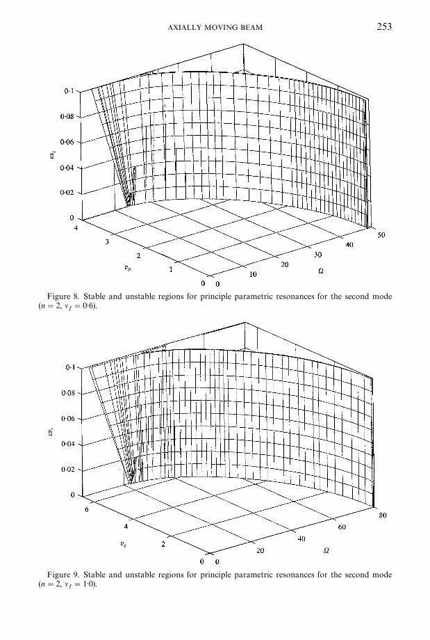
Figure 8. Stable and unstable regions for principle parametric resonances for the second mode(n"2, l
f"0)6).
Figure 9. Stable and unstable regions for principle parametric resonances for the second mode(n"2, l
f"1)0).
AXIALLY MOVING BEAM 253

Figure 10. Stable and unstable regions for combination resonances of sum type for the "rst twomodes (n"1, m"2, l
f"0)2).
Figure 11. Stable and unstable regions for combination resonances of sum type for the "rst twomodes (n"1, m"2, l
f"0)6).
254 H. R. OG Z AND M. PAKDEMI0 RLI0

Figure 12. Stable and unstable regions for combination resonances of sum type for the "rst twomodes (n"1, m"2, l
f"1)0).
AXIALLY MOVING BEAM 255
In Figures 4}6, stable and unstable regions are plotted for principle parametricresonances case for the "rst mode for three di!erent #exural sti!ness values(l
f"0)2, 0)6 and 1). In all "gures (Figures 4}12), the regions in between the planar
surfaces are unstable whereas the remaining regions are stable. With increasing#exural sti!ness value, the stability regions shift to higher X values. Increasing thevelocity variation amplitude enlarges the stability regions. In Figures 7}9, stableand unstable regions are given for the second mode. Similar conclusions can bedrawn, as written for Figures 4}6.
In Figures 10}12, stable and unstable regions are plotted for combinationresonances of sum-type case for the "rst two modes for three #exural sti!nessvalues. As the #exural sti!ness value increases, the stability regions shift to higherX values. Increasing the velocity variation amplitude causes the stability regions tobe wider.
6. CONCLUDING REMARKS
In this study, the vibrations of an axially moving Euler}Bernoulli beam has beeninvestigated. The velocity is assumed to be harmonically changing about a meanvalue. The method of multiple scales is applied to the equation of motion.Velocity-dependent natural frequencies are found by using a standard root-"ndingalgorithm for di!erent #exural sti!nesses for the "rst two modes.

256 H. R. OG Z AND M. PAKDEMI0 RLI0
The in#uence of small #uctuations of velocity on the stability of the system isinvestigated. The boundaries separating stable and unstable regions are calculated.Principal parametric resonances and combination resonances of sum and di!erencetype for any two modes are considered in the analysis. It is found that for velocity#uctuation frequencies near twice any natural frequency, an instability regionoccurs whereas for the frequencies close to zero, no instabilities are detected up tothe "rst order of approximation. For sum-type combination resonances,instabilities do occur. On the contrary, no instabilities are detected fordi!erence-type resonances up to the "rst order of approximation. Boundariesseparating stable and unstable regions are plotted for principle parametric andcombination resonances of sum type. It is shown that beam e!ects cause thestability boundaries to shift to higher frequency values and increasing the velocityvariation amplitude causes the stability regions to be wider.
ACKNOWLEDGMENT
This work is supported by the Scienti"c and Technical Research Council ofTurkey (TUBITAK) under project number MISAG-119.
REFERENCES
1. A. G. ULSOY, C. D. MOTE JR and R. SYZMANI 1978 Holz als Roh-und =erksto+ 36,273}280. Principal developments in band saw vibration and stability research.
2. J. A. WICKERT and C. D. MOTE JR 1988 Shock and <ibration Digest 20, 3}13. Currentresearch on the vibration and stability of axially moving materials.
3. J. A. WICKERT and C. D. MOTE JR 1990 ¹ransactions of the American Society ofMechanical Engineers, Journal of Applied Mechanics 57, 738}744. Classical vibrationanalysis of axially moving continua.
4. J. A. WICKERT and C. D. MOTE JR 1991 Applied Mechanics Reviews 44, 279}284.Response and discretization methods for axially moving materials.
5. A. G. ULSOY 1986 ¹ransactions of the American Society of Mechanical Engineers,Journal of <ibration, Acoustics, Stress and Reliability in Design 108, 207}212. Couplingbetween spans in the vibration of axially moving materials.
6. A. A. N. AL-JAWI, C. PIERRE and A. G. ULSOY 1995 Journal of Sound and <ibration 179,243}266. Vibration localization in dual-span, axially moving beams, part 1: formulationand results.
7. A. A. N. AL-JAWI, C. PIERRE and A. G. ULSOY 1995 Journal of Sound and <ibration 179,267}287. Vibration localization in dual-span, axially moving beams, part 2:perturbation analysis.
8. A. A. N. AL-JAWI, C. PIERRE and A. G. ULSOY 1995 Journal of Sound and <ibration 179,289}312. Vibration localization in band-wheel systems: theory and experiment.
9. W. Z. WU and C. D. MOTE, JR. 1986 Journal of Sound and <ibration 110, 27}39.Parametric excitation of an axially moving band by periodic edge loading.
10. A. G. ULSOY and C. D. MOTE, JR. 1980=ood Science 13, 1}10. Analysis of band-sawvibration.
11. M. PAKDEMI0 RLI0 and A. G. ULSOY 1997 Journal of Sound and <ibration 203, 815}832.Stability analysis of an axially accelerating string.
12. E. M. MOCKENSTRUM, N. C. PERKINS and A. G. ULSOY 1994 ¹ransactions of theAmerican Society of Mechanical Engineers, Journal of <ibration and Acoustics 118,346}350. Stability and limit cycles of parametrically excited, axially moving strings.

AXIALLY MOVING BEAM 257
13. H. R. OG Z, M. PAKDEMI0 RLI0 and E. OG ZKAYA 1998 Journal of Sound and <ibra-tion. Transition behavior from string to beam for an axially accelerating material 215,571}576.
14. J. A. WICKERT 1992 International Journal of Non-¸inear Mechanics 27, 503}517.Non-linear vibration of a travelling tensioned beam.
15. F. PELLICANO and F. ZIRILLI 1998 International Journal of Non-¸inear Mechanics 33,691}711. Boundary layers and non-linear vibrations in an axially moving beam.
16. S. F. ASOKANTHAN and S. T. ARIARATNAM 1994 Journal of <ibration and Acoustics 116,275}279. Flexural instabilities in axially moving bands.
17. W. L. MIRANKER 1960 IBM Journal of Research and Development 4, 36}42. The waveequation in a medium in motion.
18. C. D. MOTE JR. 1975 ¹ransactions of the American Society of Mechanical Engineers,Journal of Dynamic Systems, Measurements and Control 97, 96}98. Stability of systemstransporting accelerating axially moving materials.
19. M. PAKDEMI0 RLI0 , A. G. ULSOY and A. CERANOG[ LU 1994 Journal of Sound and <ibration169, 179}196. Transverse vibration of an axially accelerating string.
20. M. PAKDEMI0 RLI0 and H. BATAN 1993 Journal of Sound and <ibration 168, 371}378.Dynamic stability of a constantly accelerating strip.
21. A. H. NAYFEH, J. F. NAYFEH and D. T. MOOK 1992 Nonlinear Dynamics 3, 145}162. Onmethods for continuous systems with quadratic and cubic nonlinearities.
22. M. PAKDEMI0 RLI0 , S. A. NAYFEH and A. H. NAYFEH 1995 Nonlinear Dynamics 8, 65}83.Analysis of one-to-one autoparametric resonances in cables-discretization vs directtreatment.
23. M. PAKDEMI0 RLI0 , 1994 Mechanics Research Communications 21, 203}208. A comparisonof two perturbation methods for vibrations of systems with quadratic and cubicnonlinearities.
24. M. PAKDEMI0 RLI0 , and H. BOYACI 1995 Journal of Sound and <ibration 186, 837}845.Comparison of direct-perturbation methods with discretization-perturbation methodsfor nonlinear vibrations.
25. A. H. NAYFEH, S. A. NAYFEH and M. PAKDEMI0 RLI0 , 1995 Nonlinear Dynamics andStochastic Mechanics (N. S. Namachchivaya and W. Kliemann, editors), 175}200. BocaRaton, Florida: CRC Press. On the discretization of weakly nonlinear spatiallycontinuous systems.
26. M. PAKDEMI0 RLI0 , and H. BOYACI 1997 Journal of Sound and <ibration 199, 825}832. Thedirect-perturbation method versus the discretization-perturbation method Linearsystems.
27. A. H. NAYFEH and S. A. NAYFEH 1995 ¹ransactions of the American Society ofMechanical Engineers, Journal of <ibration and Acoustics 117, 199}205. Nonlinearnormal modes of a continuous system with quadratic nonlinearities.
28. A. H. NAYFEH and W. LACARBONARA 1997 Nonlinear Dynamics 13, 203}220. On thediscretization of distributed-parameter systems with quadratic and cubic nonlinearities.
29. A. H. NAYFEH 1981 Introduction to Perturbation ¹echniques. New York: Wiley.30. A. H. NAYFEH and D. T. MOOK 1979 Nonlinear Oscillations. New York: Wiley.