Vegetation height products between 60° S and 60° N from ICESat GLAS data

Geosci. Model Dev., 5, 413–432, 2012www.geosci-model-dev.net/5/413/2012/doi:10.5194/gmd-5-413-2012© Author(s) 2012. CC Attribution 3.0 License.

GeoscientificModel Development

Vegetation height and cover fraction between 60◦ S and 60◦ N fromICESat GLAS data

S. O. Los1, J. A. B. Rosette1, 2, N. Kljun 1, P. R. J. North1, L. Chasmer3, J. C. Suarez2, 4, C. Hopkinson3, R. A. Hill 5,E. van Gorsel6, C. Mahoney1, and J. A. J. Berni6

1Department of Geography, Swansea University, Singleton Park, Swansea SA2 8PP, UK2Biospheric Sciences Branch, code 614.4, NASA/Goddard Space Flight Center, Greenbelt and University of MarylandCollege Park, Maryland 20771, USA3Cold Regions Research Centre, Wilfrid Laurier University, Waterloo ON N2L 3C5, Canada4Forest Research, Northern Research Station, Roslin, Midlothian, EH25 9SY, UK5School of Applied Science, Bournemouth University, Poole, Dorset, BH12 5BB, UK6CSIRO Marine and Atmospheric Research, Pye Laboratory, Canberra ACT 2601, Australia

Correspondence to:S. O. Los ([email protected])

Received: 23 August 2011 – Published in Geosci. Model Dev. Discuss.: 19 September 2011Revised: 25 January 2012 – Accepted: 19 March 2012 – Published: 27 March 2012

Abstract. We present new coarse resolution (0.5◦× 0.5◦)

vegetation height and vegetation-cover fraction data sets be-tween 60◦ S and 60◦ N for use in climate models and ecolog-ical models. The data sets are derived from 2003–2009 mea-surements collected by the Geoscience Laser Altimeter Sys-tem (GLAS) on the Ice, Cloud and land Elevation Satellite(ICESat), the only LiDAR instrument that provides close toglobal coverage. Initial vegetation height is calculated fromGLAS data using a development of the model ofRosetteet al. (2008) with further calibration on desert sites. Filtersare developed to identify and eliminate spurious observationsin the GLAS data, e.g. data that are affected by clouds, atmo-sphere and terrain and as such result in erroneous estimatesof vegetation height or vegetation cover. Filtered GLAS veg-etation height estimates are aggregated in histograms from 0to 70 m in 0.5 m intervals for each 0.5◦

×0.5◦. The GLASvegetation height product is evaluated in four ways. Firstly,the Vegetation height data and data filters are evaluated us-ing aircraft LiDAR measurements of the same for ten sitesin the Americas, Europe, and Australia. Application of fil-ters to the GLAS vegetation height estimates increases thecorrelation with aircraft data fromr = 0.33 to r = 0.78, de-creases the root-mean-square error by a factor 3 to about 6 m(RMSE) or 4.5 m (68 % error distribution) and decreases thebias from 5.7 m to−1.3 m. Secondly, the global aggregatedGLAS vegetation height product is tested for sensitivity to-wards the choice of data quality filters; areas with frequentcloud cover and areas with steep terrain are the most sensi-tive to the choice of thresholds for the filters. The changesin height estimates by applying different filters are, for the

main part, smaller than the overall uncertainty of 4.5–6 m es-tablished from the site measurements. Thirdly, the GLASglobal vegetation height product is compared with a globalvegetation height product typically used in a climate model,a recent global tree height product, and a vegetation green-ness product and is shown to produce realistic estimates ofvegetation height. Finally, the GLAS bare soil cover frac-tion is compared globally with the MODIS bare soil frac-tion (r = 0.65) and with bare soil cover fraction estimatesderived from AVHRR NDVI data (r = 0.67); the GLAS tree-cover fraction is compared with the MODIS tree-cover frac-tion (r = 0.79). The evaluation indicates that filters appliedto the GLAS data are conservative and eliminate a large pro-portion of spurious data, while only in a minority of cases atthe cost of removing reliable data as well.

The new GLAS vegetation height product appears morerealistic than previous data sets used in climate models andecological models and hence should significantly improvesimulations that involve the land surface.

1 Introduction

Global biophysical parameters such as the fraction of photo-synthetically active radiation (fAPAR) and leaf area index(LAI) are essential parameters in calculating fluxes in theglobal carbon cycle, water cycle and energy budget. They areclosely linked to the amount of solar radiation absorbed andscattered by the vegetation canopy and can be estimated fromdata collected by passive optical radiometers that measure

Published by Copernicus Publications on behalf of the European Geosciences Union.

414 S. O. Los et al.: Vegetation height between 60◦ S and 60◦ N from GLAS

in visible and near-infrared wave bands. Examples of thesesensors collecting global data are the advanced very highresolution radiometer (AVHRR; August 1981–present), theSea-viewing Wide Field-of-view Sensor (SeaWiFS; Septem-ber 1997–December 2010), the Systeme Pour l’Observationde la Terre – Vegetation instrument (SPOT-VGT; April 1998–present), the Along Track Scanning Radiometer (ATSR-2and AATSR; June 1995–present) and the moderate resolu-tion image spectrometer (MODIS; February 2000–present);see e.g.Sellers et al.(1996); Myneni et al. (2003); Gob-ron et al.(2005). However, these sensors are not particu-larly suitable to obtain estimates of biophysical parameterslinked to canopy structure – e.g. vegetation height, above-ground biomass, canopy inflection point and stem diameter –although there are approaches that exploit indirect relation-ships between measurements such as the Normalized Differ-ence Vegetation Index (NDVI) and biomass with some de-gree of success for particular biomes (Tucker et al., 1986;Prince, 1991; van der Werf et al., 2006). Knowledge ofstructural vegetation parameters is, for example, essentialto assess the amount of carbon stored in vegetation, to im-prove modelling of light absorption and scattering throughthe canopy and of photosynthesis (Alton et al., 2005) andto model the wind profile at the surface which affects the ex-change of water and carbon between the land and atmosphere(Sellers et al., 1996).

A problem using passive optical sensors to infer canopystructure is that different canopy structures can lead to thesame spectral and bidirectional response; the inversion ofbiophysical parameters in these cases is a non-unique prob-lem with more than one solution and this inhibits unambigu-ous estimation of canopy parameters. An active optical sen-sor, such as the Geoscience Laser Altimeter System (GLAS)on the Ice, Cloud and land Elevation Satellite (ICESat) emitsa light pulse of known intensity and duration (Zwally et al.,2002; Brenner et al., 2003). The pulse is transmitted, ab-sorbed and scattered at various depths throughout the vege-tation canopy by leaves and branches and the returned wave-form therefore provides information on canopy structure andheight (Drake et al., 2003; Lefsky et al., 2005; Rosette et al.,2008). Compared to active microwave (RADAR) instru-ments, spaceborne LiDAR has the ability to obtain vegetationparameters at much higher biomass levels (Drake et al., 2003;Waring et al., 1995) but is also more sensitive to atmosphericinterference by clouds, water vapour and aerosols (Spinhirneet al., 2005). Furthermore, interpretation of GLAS wave-forms is not straightforward since the waveform is not onlyaffected by the vegetation canopy, but also by other fac-tors such as the occurrence of thin clouds and topography(Rosette et al., 2008; North et al., 2010; Rosette et al., 2010;Lee et al., 2011).

The objective of the present paper is to obtain a vegeta-tion height and vegetation cover data set from the GLASinstrument for most of the land surface between 60◦ S and60◦ N that can be used in global climate models and global

ecological models. To estimate vegetation height from theGLAS data we use the vegetation height model developed byRosette et al.(2008). The model was derived for a mixedforest in the United Kingdom over an area of moderate topo-graphic complexity. Tree height was estimated with an accu-racy (root mean square error) of about 4.5 m. The advantageof the vegetation height model for global applications is thatvegetation height can be estimated directly from GLAS datawithout the requirement of a highly accurate high resolutiondigital elevation model (DEM).

To obtain a vegetation height data set for the land-surfacewe set out to achieve the following four aims:

1. Test the vegetation height model byRosette et al.(2008)derived for the Forest of Dean in the UK to see if it hasmore general applicability. GLAS vegetation height ob-tained with the model is therefore compared with air-craft LiDAR measurements for ten sites with differenttree-cover types (Sect.4.1).

2. Develop and test data quality filters to screen GLASdata and thus reduce the effects of cloud contamina-tion, aerosols and topography in estimates of vegeta-tion height. Filters are obtained from the literature andfrom inspection of desert data (Sect.3). The filters aretested on the same site data used to evaluate the vege-tation height model (Sect.4.1). The tests are applied todata collected for all GLAS laser campaigns.

3. Develop and test the derived near global (60◦ S–60◦ N)vegetation height product. Tests consist of a sensitivityanalysis of global vegetation height fields to varying thethresholds of the data filters (Sect.4.2) and of a com-parison with other global vegetation data such as vege-tation height (Sellers et al., 1996), tree height (Lefsky,2010) and vegetation greenness (Los et al., 2000, 2005)(Sect.4.3).

4. Derive bare soil fraction and tree cover fraction fromthe GLAS tree height product and compare this prod-uct with the MODIS vegetation-cover fraction estimates(Hansen et al., 2003, 2006) and the Fourier Adjusted,Sensor and Solar zenith angle corrected, Interpolatedand Reconstructed (FASIR) vegetation-cover fractionestimates (Los et al., 2000, 2005) (Sect.4.4).

A version of the data in netcdf format is distributed as aSupplement to the present paper.

2 Data

We used the ICESat GLAS land data (GLA14) product, re-lease 31 (Zwally et al., 2008; Brenner et al., 2003). GLASemits a pulse waveform in the 532 or 1064 nm bands whichis 1 m wide (corresponding to a duration of 5–6 ns) betweenthe points where the signal is half the size of the maximum

Geosci. Model Dev., 5, 413–432, 2012 www.geosci-model-dev.net/5/413/2012/

S. O. Los et al.: Vegetation height between 60◦ S and 60◦ N from GLAS 415

0.0 0.2 0.4 0.6 0.8 1.0

1000

900

800

700

600

Returned pulse (V)

Rel

ativ

e tim

e (n

s)

Signal Begin

Signal End

a) Waveform 885917506_14

Raw waveformModel alternate fit

0.0 0.2 0.4 0.6 0.8

1000

900

800

700

600

Alternate fit returned pulse (V)

Rel

ativ

e tim

e (n

s)

Gaussian

654321

b) Decomposition

Fig. 1. (a) Example of GLAS waveform collected for a vegetatedfootprint and approximate indication of start and end of the wave-form signal. The first return is reflected from the top of the canopy(Signal Begin), incremental parts of the waveform are reflected bylower parts of the canopy; the end of the signal usually provides anunder estimate of the elevation of the ground surface.(b) Decom-position of the waveform by six Gaussians. Gaussians 1 and 2 areused to estimate the location of the ground.

amplitude. The returned waveform is measured for a du-ration equivalent to a length of about 82 m at 15 cm inter-vals for the Laser 1A and 2A periods, and for an equiva-lent length for 150 m for the other periods (NSIDC, 2011).The footprint size is an ellipse with dimension of 95 by52 m for the Laser 1A to 2C periods and 61 by 47 m forthe other periods. The returned waveform contains variouspeaks which are fitted by up to 6 Gaussians (Fig.1). TheGLAS instrument collected data intermittently during 2003–2009, usually for 2 or 3 periods of about 1 month per year(Zwally et al., 2002; Harding and Carabajal, 2005). For thederivation of the filters we used data from the Laser 1A pe-riod; for testing the filters and the vegetation height model(Sect.4) and for assembling the global vegetation height datawe used data from all laser periods.

Table1 provides a list of the GLA14 parameters. For eas-ier processing, this subset of the GLA14 data is organised in5◦

× 5◦ tiles which conform to the tiles of the SRTM ver-sion 4.1 data (Rodriguez et al., 2005; Jarvis et al., 2008).Data without geo-location, i.e. missing latitude and longi-tude values, are removed, as are data without a saturationelevation adjustment (GLAS quality flag isatElevCorr> 2;seeNSIDC, 2011, Sect.3.2), since without this parameter itis not possible to calculate elevation. Data below 60◦ S andabove 60◦ N are not analysed because two of the filters re-quire SRTM data (Sect.3.2).

The interpolated SRTM DEM version 4.1 distributed bythe Consultative Group for International Agriculture Re-search – Consortium for Spatial Information (CGIAR-CSI)(Jarvis et al., 2008; Rodriguez et al., 2005) was used to com-pare with the GLAS waveform reference elevation (ielev)and to obtain an indication of the slope. The CGIAR-CSIdata were used rather than the SRTM DEM data included

in the GLA14 product because the agreement with GLASwaveform reference elevation (ielev) was closer.

The MODIS continuous fractional cover data (Hansenet al., 2003, 2006), FASIR Normalized Difference Vegeta-tion Index (NDVI) and FASIR vegetation-cover fraction (Loset al., 2000, 2005) and global tree height data (Lefsky, 2010)were used to evaluate the vegetation height and vegetationcover fraction products derived in the present paper.

Aircraft LiDAR measurements of vegetation height fromCanada, Peru, the United Kingdom, the Netherlands, Ger-many and Australia were used to test the GLAS vegeta-tion height estimates and application of data quality filters.These globally distributed validation test sites incorporateboreal, temperate and tropical vegetation; managed and nat-ural woodland and varied canopy cover (e.g. sparse cover inthe case of the Australian sites and near complete closure forthe Peru site). The product is thus evaluated using a rangeof conditions including those known to be problematic forGLAS.

The Canadian sites, the former southern BOREAS studysites in Saskatchewan, consist of fairly homogeneousforested areas and flat topography with an aspen stand (Popu-lus tremuloides Michx.), a black spruce stand (Picea marianaMill. ) an old jack pine site (Pinus banksiana Lamb.) and are-grown jack pine site (Barr et al., 2006; Kljun et al., 2007).The Peru site is located in the Tambopata National Reserveand consists of dense mature forest, regenerating forest, partflood plain and wetland, in an area of flat topography (Hillet al., 2011). The UK sites are the Glen Affric and Aberfoylesites both measured by the UK Forest Research. Glen Af-fric (Suarez et al., 2008) is an area of ancient woodland, itcontains one of the largest ancient Caledonian pinewoods inScotland. Common species are Scots pine (Pinus Sylvestris,Juniper (Juniperus communis), birch (Betula pubescens), andaspen (Populus tremula). The Aberfoyle site (Suarez, 2010)is a silviculture area where trees are planted and clearfelled inrotations of 40–60 yr. The dominant species is Sitka spruce(Picea sitchensis (Bong.) Carr.). At the Netherlands Loo-bos site Scots pine (Pinus Sylvestris) is the dominant species(89 %) and is planted on flat, sandy terrain with some openareas (Dolman et al., 2002). The German Tharandt site isa mixed forest stand with trees of different ages consistingof mainly spruce (Picea abies) with scattered pine (PinusSylvestris) and European Larch (Larix decidua) on undulat-ing terrain (Grunwald and Bonhofer, 2007). The Australiandata were collected 7 km East of Tumbarumba research sta-tion to coincide with the GLAS measurements. The area islocated in Bago State Forest, New South Wales and con-sisted of mainly eucalyptus trees (Eucalyptus delegatensisR. T. BakerandEucalyptus dalrympleana Maiden) in rela-tively complex terrain (Leuning et al., 2005).

www.geosci-model-dev.net/5/413/2012/ Geosci. Model Dev., 5, 413–432, 2012


Table 1. List of GLAS parameters retained and of parameters added (last three rows).

GLA14 code Description

i lat Latitudei lon Longitudei elev Waveform reference elevation (often located at the waveform centroid)i SolAng Solar incidence anglei gdHt Geoid height (EGM2008 geoid)i DEM elv DEM elevationi SigBegOff Signal begin range incrementi ldRngOff Land range offseti SigEndOff Signal end range offseti gpCntRngOff Centroid range increment for up to six peaksi maxSmAmp Peak amplitude of smoothed received echoi numPk Number of peaks found in the returni Gamp Amplitude of up to six Gaussiansi Garea Area under up to six Gaussiansi satElevCorr Saturation Elevation Correctioni satCorrFlg Saturation Correction Flagi FRir cldtop Full Resolution 1064 Cloud TopField Vegetation height (m)slope Maximum of slope with 8 surrounding cells (%)jday03 Days since 1 January 2003 (= 1)

3 Method

Estimation of vegetation height is based on the GLAS wave-form (GLA14) data, version 31. Figure1a illustrates thewaveform data for a vegetated footprint. The returned wave-form is the result of interaction of a light pulse emitted bythe GLAS laser with a vegetation canopy and the groundsurface. The GLAS GLA14 product contains parameters ob-tained from the raw waveform data such as the start and endof signal and the decomposition of the waveform by up to sixGaussians (Fig.1b).

3.1 Estimating vegetation height

The accuracy of the estimation of vegetation height fromGLAS waveforms is highly dependent on the ability to detectthe uppermost canopy surface (the signal begin parameter)and a ground elevation which is representative of the terrainwithin the broad lidar footprint (Rosette et al., 2010). Re-garding the latter, here we select the centroid of whichever ofthe first two Gaussians has the greater amplitude to representthe ground surface. The method is modified by calibrationon desert sites (Sect.3.2, Eq.3)

The limits of the waveform signal are determined usinga threshold above the mean noise level (+4.5σ in the caseof GLAS) (Brenner et al., 2003). The Signal Begin param-eter within a waveform (isigBegOff) is assumed to repre-sent the highest intercepted surface of the forest canopy. Thecertainty with which the Signal Begin can be placed is de-pendent on the gradient of the leading edge of the waveform(Lefsky et al., 2007; Hancock et al., 2011). The strength of

the beginning of the waveform signal is a function of the in-tercepted surface area at this elevation plus its reflectivity andwill vary with vegetation crown shape and surface roughness,canopy density, fractional cover and slope (e.g. if vegetationis uniformly distributed upon a sloped surface). Additionally,since the illumination of the pulse on the ground is Gaussianin form, the amplitude of the beginning of the waveform sig-nal is also influenced by the distribution of vegetation withinthe footprint (Hyde et al., 2005), tall vegetation towards thefootprint limits thereby contributing relatively less to the re-ceived waveform. The broad GLAS footprint poses chal-lenges for the identification of the ground surface beneath avegetation canopy. This is particularly the case upon slopedsurfaces where vegetation and ground can occur at similarelevations meaning that their signals are combined withinthe waveform. The accuracy of vegetation estimates fromGLAS waveforms are therefore influenced by the conditionsin mountainous environments (Hyde et al., 2005) and areasof low stature vegetation (Nelson, 2010). The necessity ofallocating a single, representative ground elevation within awaveform is more challenging for sites with complex topog-raphy and vegetation distribution.

Various approaches exist to obtain vegetation height esti-mates from GLAS waveform data. Here, we estimate vege-tation height according toRosette et al.(2008):

hV = 1.06(r1−rA1,2) (1)

with hV = vegetation height;r1 = signal start (iSigbegOff);rA1,2 = the centroid range increment, igpCntRngOff; formax amplitude between Gaussians 1 and 2.



The equation was derived for the Forest of Dean in theUK, an area with complex topography and mixed broadleafand needleleaf trees. The choice of the maximum of the firsttwo Gaussians to represent the elevation of the ground sur-face reduces the effect of slope for areas of low to moderatetopography (Rosette et al., 2008).

3.2 Data filters

The tests below are intended to detect and eliminate spuri-ous values, e.g. high vegetation height values over deserts,from the GLAS data. Where possible, thresholds for the datafilters rely on error estimates from the peer reviewed litera-ture. In cases where no estimates are available, the thresholdsrely on visual interpretation of the data. A test of the filteredGLAS product is carried out in Sect.4.1 and a sensitivityanalysis of the filters in Sects.4.2and4.4.

To design the filters for identification of spurious data,GLAS data from a desert site are explored. Vegetation heightestimates for deserts should as a general rule be low; highvalues therefore indicate problems in the GLAS data. Occur-rences of spurious, high vegetation height values are com-pared with other measures such as slope, the difference be-tween the GLAS waveform reference elevation (ielev) andthe elevation indicated by a DEM and the strength of theGLAS signal.

GLAS data from a 5◦ ×5◦ tile between 20◦ N–25◦ N and0◦–5◦ E are analysed; this tile covers a desert area with thenorthern part located in Algeria. Data collected over 41 daysin February 2003 and March 2003 during the Laser 1A pe-riod are investigated (51 270 GLAS shots). The location ofthe data is shown in Fig.2a. The waveform reference eleva-tion (i elev) measured by the GLAS instrument and the ele-vation in the SRTM DEM version 4.1 data (Rodriguez et al.,2005; Jarvis et al., 2008) are compared in Fig.2b as a func-tion of latitude. The waveform reference elevation (ielev) isadjusted to the match the SRTM ellipsoid using:

h = he+1he−1hg+1hl (2)

with

h = topographic elevation

he = GLAS elevation; ielev

1he = Saturation elevation correction; isatElevCorr

1hg = Height of the EGM2008 geoid above the

TOPEX/Poseidon ellipsoid; igdHt

1hl = Difference WGS84 and TOPEX/Poseidon

ellipsoid

= 1ra(cosφ)2+1rb(sinφ)2

with

1ra = Difference radius of WGS84 and

TOPEX/Poseidon ellipsoids at equator (0.7 m)

1rb = Difference radius for meridian (0.713682 m).

φ = Latitude

Parameter names ielev (the reference position of the wave-form), i satElevCorr, igdHt indicate records of the GLASdata (Table 1); a further description of these records and ofelevation calculations can be found inZwally et al. (2002)and the GLAS on-line documentation provided by the Na-tional Snow and Ice Data Center (http://nsidc.org/).

Vegetation height as a function of latitude is shown inFig. 2c. High vegetation height estimates are found in ar-eas where the topography changes rapidly; note that, e.g. thespikes in vegetation height in Fig.2c occur in the same loca-tion as the spikes in topography in Fig.2b. Thus a first in-spection of the data indicates that a large proportion of highvegetation height values are spurious.

3.2.1 Slope test (Fig.2d)

Slopes affect the GLAS waveform; the waveform from aslope without vegetation can look similar to that of a veg-etation canopy over a flat surface (North et al., 2010; Rosetteet al., 2010). Using the SRTM DEM 4.1 data, an approxi-mation of the slope was calculated as the maximum of the8 slopes between the grid cell for which the GLAS measure-ment was collected and its 8 surrounding neighbours. Thegrid cell size of the SRTM DEM 4.1 data is 90 m; thus in ar-eas with variations in terrain at shorter lengths the SRTMslope will underestimate the topographic variations withinthe 50 to 60 m footprint most commonly produced by GLAS.

Grid cells with a slope exceeding 10◦ (17 %) were re-moved from further analysis. Based on theoretical groundsand analysis of the desert data, a threshold of a 10◦ slopeappears a reasonable compromise between retaining a suffi-cient proportion of the signal and avoiding erroneous values(Nelson et al., 2009; North et al., 2010; Rosette et al., 2010).Figure2d indicates that for a slope<17 % both realistic lowvalues and spurious high values are collected; whereas for aslope>17 % a very low number of realistic values and a verylarge number of spurious high values for vegetation heightare found.

3.2.2 Elevation test (Fig.2e)

The GLAS waveform reference elevation (Eq.2) is com-pared with the SRTM DEM version 4.1. It is assumed thatlarge differences between the SRTM DEM version 4.1 dataand the GLAS waveform reference elevation (ielev) indi-cate problems in either data set. For the area shown inFig. 2a, the root mean square error (RMSE) between GLASand the SRTM 4.1 DEM data was about 3.7 m for February2003 only and was 4.2 m for data of February and March2003 combined. The 95 % confidence interval of the SRTMdata globally is estimated at approximately 8 m; it variesfor different continents between 7 m to 8.8 m with the ex-ception of New Zealand where the RMSE was about 12 m


http://nsidc.org/


Fig. 2. (a) Location of the GLAS data collected between 20◦–25◦ N and 0◦–5◦ E prior to April 2003 (Grey lines represent boundaries).(b) Elevation as a function of latitude for the measurements shown under a; black circles are GLAS elevation measurements; they areoverlain by grey dots (SRTM 4.1 values).(c) Vegetation height estimated from the GLAS data afterRosette et al.(2008); no filter wasapplied. (d) Estimated vegetation height as a function of slope. The slope was calculated as the maximum of the slope in 8 directionscalculated from the 90 m SRTM version 4.1 data. Grey values show data for slope≥ 17 %; black values are for slopes<17 %. (e)Vegetationheight as a function of the difference between the GLAS reference elevation and the SRTM version 4.1 elevation. Grey circles show valuesthat passed the 17 % slope filter in(d); black circles show the data with a difference in DEM<8 m. 1.f) Vegetation height as a function ofthe Area of the first Gaussian; black circles pass the test, line indicates the best fit through the 5 % values per equal area interval of 10 V ns.(g) Amplitude test; threshold at 5 V, top 0.1 % of highest values per Amplitude interval are removed,(h) values with a very high signal width(sigma) are removed (grey values),(i) remaining values after Neighbour test is applied (compare withc).

(Rodriguez et al., 2005; Jarvis et al., 2008). The differencebetween SRTM and GLAS elevation appears small and unbi-ased, although the root-mean-square error increases with to-pographic roughness and vegetation density (Carabajal andHarding, 2006). The errors in SRTM elevation include anerror for geo-location (i.e. no adjustment for geo-locationwas made). Based onRodriguez et al.(2005) and our anal-ysis of the Sahara desert we set a threshold at 8 m, ap-proximately the 95 % confidence interval; data are deemed

spurious and are eliminated when the difference betweenthe GLAS elevation and SRTM DEM version 4.1 data islarger than 8 m (Fig.2e). In cases where dense canopy ex-ists, the SRTM data and GLAS waveform reference eleva-tion (i elev) are affected by the dense canopy and may rep-resent an elevation value about half way in the canopy; forthese cases the 95 % of the error distribution in both is likelylarger than 8 m (Carabajal and Harding, 2006) and the ele-vation test may therefore be too conservative. Whether or



not this is a problem is further investigated in the analysisof the site data from Peru4.1and the comparison of vegeta-tion height in tropical forests found in this study with valuesfound in other studies4.3.

3.2.3 Area under first Gaussian test (Fig.2f)

Refinement of the height model

Estimates of vegetation height in the present paper use thedifference between the start of signal and the centroid rangeincrement of the first or second Gaussian (Rosette et al.,2008). The returned waveform will always have a measur-able width even in cases where no vegetation is present be-cause of the duration of the emitted signal, the atmosphericattenuation of the signal and the reflection of the signal froma surface that is rarely completely flat. The implication isthat for bare soil a small difference between the signal startand the centre of the first Gaussian is found and this translatesinto an equivalent estimate of vegetation height. In Fig.2f theestimated vegetation height is plotted as a function of the areaunder the first Gaussian (in units of V× ns; i.e. Volt× nanosecond) to obtain an indication of the magnitude of the effect.Figure2f shows that, as the area under the first Gaussian in-creases, the estimate for the minimum vegetation height in-creases. It is assumed that the 5 % values of the height distri-butions (per interval of 0.1 V ns (Volt× nano s) on the x-axis)provide an indication of the magnitude of the effect. A lineis fitted and the estimated vegetation height (Eq.1) is subse-quently adjusted according to:

h0.05 = a+bA (3)

with A the area under the first Gaussian (V ns) and fitted co-efficientsa = 1.91 andb = 0.11 estimated from about 14005 % values. The value forh0.05 is subtracted from all GLASvegetation height estimates.

Filter based on area under the first Gaussian

Figure2f reveals a second potential problem; for low valuesof the area under the first Gaussian, the spread in estimatedvegetation height is large. The higher values in this intervalare likely to be unrealistic. A likely cause is that low val-ues for the area under the first Gaussian indicate weak signalstrengths, possibly caused by attenuation of the signal in theatmosphere or by low energy emitted. The latter problemoccurred frequently during the last two years of the ICESatmission (Lefsky, 2010). A threshold is applied to eliminatevalues with low first Gaussian areas. Because a low area un-der the first Gaussian can also occur for vegetation with adense canopy or multiple scattering delaying the signal re-sponse, the threshold cannot be too large so as not to elimi-nate values from tall, dense vegetation. As a compromise avalue of 1 V ns was selected.

3.2.4 Amplitude of First Gaussian test (Fig.2g)

A low amplitude of the first Gaussian indicates a data qual-ity problem similar to the low area under the first Gaussian.The ability to separate the true returned waveform start andend from the background noise is reduced. A test was imple-mented to eliminate data with low amplitude (Fig.2g) hereset at 0.05 V. Figure2g indicates a number of outliers overthe entire range of amplitudes. A second test was applied toeliminate the highest 0.1 % of values per amplitude intervalof 0.1 V; these values appear as outliers in Fig.2g.

3.2.5 Sigma test (Fig.2h)

Gaussians with a large spread (range between the 5 % and95 % values over 80 m or so) are unlikely to be from vegeta-tion which only in exceptional cases reaches these heights. Atest was applied to all Gaussians to remove waveforms withhigh sigma values. The threshold for the sigma test was cal-culated as the>99.9 % value; this test eliminates the datawith the highest 0.1 % sigma values. The thresholds for thistest were calculated from frequency distributions of the un-filtered data.

3.2.6 Neighbour test (Fig.2i)

Finally, data were removed where the along-track neighbouron either side failed any of the above tests.

3.2.7 Choice of filters

The sequence in which the filters are applied startswith thresholds obtained from the peer reviewed literature(Sect. 3.2.1–3.2.2) and ends with the neighbour test. Thechoice of thresholds for the data filters obtained from thedesert analysis is obtained from visual inspection rather thanoptimisation. The sensitivity of estimated vegetation heighttowards the choice of these filters is therefore further evalu-ated in Sect.4.2.

The scatter plots (Fig.2) indicate that a large proportion ofspurious data is removed but some spurious values are likelystill to be present (Fig.2i). The discussion in the next sec-tion and Table2 provide further indications as to how muchdata are removed by the filters. If the filter thresholds are ad-justed, a larger proportion of spurious values is removed, butthis may be at the cost of removing too many reliable data.Prior to a potential adjustment of the thresholds, the filteredvegetation height values are evaluated in Sect.4.

3.3 Application of filters to a temperate and a tropicalarea

The filters are applied to data from western Europe and theAmazon to obtain an indication of the amount of data re-moved by each of the processing steps. Table2 summarizesthe results for data collected over 2003 for three 5◦

×5◦ tiles,



Table 2. Cumulative percentage of data removed by subsequent filters (Sect.3.2) for 3 test tiles (Reported for data collected for 2003 only).

20◦–25◦ N, 0◦–5◦ E 50◦–55◦ N, 0◦–5◦ E 5◦ S–0◦, 65◦–60◦ W(Algeria) (W. Europe) South America

Dominant land cover Bare soil Agriculture Broad leaf evergreen

Missing data 0.00 % 0.00 % 0.00 %Slope> 10◦ 1.33 % 56.25 % 0.99 %Differenceh > 8 m 2.93 % 59.2 % 11.54 %Area Gaussian 1> 1 V ns 5.49 % 62.4 % 46.41 %Amplitude Gaussian 1> 0.05 V 6.00 % 63.0 % 57.4 %Outlier test (>99.9 %) 6.10 % 63.1 % 57.5 %Sigma test (Gaussian 1–6;>99.9 %) 6.11 % 63.1 % 57.5 %Neighbour test 9.16 % 66.8 % 76.1 %

the desert tile shown in Fig.2, the tile in western Europe andthe tile over the Amazon. Note that the statistics in Table2refer to the entire year of 2003; whereas Fig.2 refers to datacollected prior to April 2003. For the desert tile, the filterswith the most impact are the elevation test (1.6 %), the areaunder the first Gaussian test (2.5 %) and the neighbour test(3 %).

For the tile that covers part of western Europe most ofthe spurious data are removed by the slope test; a majorityof data removed by this test is because of missing SRTMDEM values over the sea. The elevation test, area underthe first Gaussian test and neighbour test each remove ap-proximately 3 % of the data. For tropical forests the largestamount of data, about 35 %, is removed by the area underthe first Gaussian test. About 10 % is removed by the differ-ence in elevation test, amplitude test and the neighbours test.The elevation test is principally intended to eliminate cloudcontaminated data. When more aircraft LiDAR data becomeavailable for these regions it may be justified to relax the 8m uncertainty range over dense forests to acknowledge thegreater uncertainty in the SRTM and GLAS elevation data.The large effect of the area under the first Gaussian test mayindicate problems with the ground return of the waveform fordense vegetation canopies. Therefore, in Sect.4.2it is inves-tigated how much the canopy height changes in response tochanging the thresholds for the filters.

4 Testing the vegetation height model and the GLASdata filters

For convenience of processing the data, raw, unfilteredGLAS data were organised in 5◦

× 5◦ tiles similar to theSRTM DEM v 4.1 tiles. A selection of statistics from theGLA14 record were retained and a number of measureswere added as well (Table1). The filters and adjustmentsdiscussed in Sect.3 were applied to the tiled GLAS data;data that did not pass the filters were removed. An esti-mate of vegetation height (Eq.1) adjusted for the area under

the first Gaussian (Eq.3) was added. Measurements fromindividual laser shots were compared with aircraft data inSect.4.1 and were then aggregated to global histograms for0.5◦

×0.5◦ cells.

4.1 Comparison with airborne LiDAR

Filtered GLAS vegetation height estimates obtained for allLaser periods (2003–2009) were compared with airborneLiDAR measurements of vegetation height for 10 sites(Sect.2): the former southern old aspen, old black spruceand two jack pine BOREAS sites in Canada; a tropical forestsite in Tambopata near Puerto Maldonado; Peru; the Loo-bos needle-leaf forest site in the Netherlands (Dolman et al.,2002); the Tharandt mixed forest site in Germany; the GlenAffric (ancient woodland) and Aberfoyle (silviculture) sitesin the UK; and a transect 7 km East of the Tumbarumba fluxtower site in Australia. Airborne LiDAR data were collectedat a point density of 0.25 m, 0.5 m or 1 m. LiDAR point datawere sampled to a 50 m resolution by one of three meth-ods: (1) by selecting the maximum vegetation height value(BOREAS, Loobos, Tharandt, Tumbarumba, Peru) by firstsampling to 1 m resolution by taking the 99.9 % value andthen selecting the maximum vegetation height (BOREAS) orby taking the 99.9 % value (the Glen Affric and Aberfoyle).Notice the BOREAS data are sampled in two ways to evalu-ate the sensitvity of the validation of GLAS data on airbornedata. The Tharandt data were post processed to remove er-roneous data from sparse clouds during the airborne survey.The Peru data were matched with the centres of the GLASfootprint; reported GLAS footprint dimensions and azimuthfor each laser campaign (NSIDC, 2011) were used to extractcoincident subsets of the airborne LiDAR data. Vegetationheight estimated from the GLAS waveforms and the airborneLiDAR point clouds could then be directly compared. Forthe other data sets, aircraft data were mapped to a univer-sal transverse Mercator (UTM) projection. Latitude and lon-gitude were calculated for the centres of all grid cells, anddata were compared if the distance (in the horizontal plane)



0 10 30 50 70

010

3050

70

Vegetation height (m) from aircraft

GLA

S v

eget

atio

n he

ight

(m

)a) Boreas sites

0 10 20 30 40 50 60

010

2030

4050

60


GLA

S v

eget

atio

n he

ight

(m

)

b) Loobos

0 10 20 30 40

010

2030

40


GLA

S v

eget

atio

n he

ight

(m

)

c) Tharandt

0 50 100 150

050

100

150


GLA

S v

eget

atio

n he

ight

(m

)

d) Peru

0 20 40 60 80 100

020

4060

8010

0


GLA

S v

eget

atio

n he

ight

(m

)

e) Tumbarumba

0 20 60 100 140

020

6010

014

0

Vegetation height (m) from aircraftG

LAS

veg

etat

ion

heig

ht (

m)

Filter=1Raw

f) Glen Affric and Aberfoyle

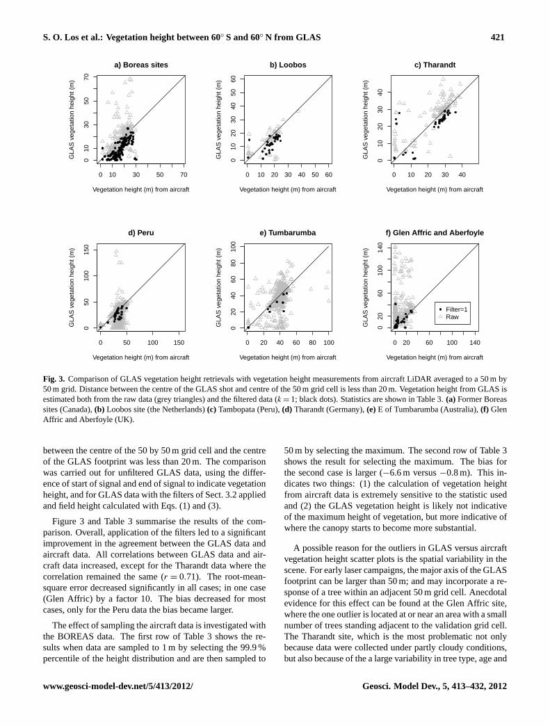
Fig. 3. Comparison of GLAS vegetation height retrievals with vegetation height measurements from aircraft LiDAR averaged to a 50 m by50 m grid. Distance between the centre of the GLAS shot and centre of the 50 m grid cell is less than 20 m. Vegetation height from GLAS isestimated both from the raw data (grey triangles) and the filtered data (k = 1; black dots). Statistics are shown in Table3. (a) Former Boreassites (Canada),(b) Loobos site (the Netherlands)(c) Tambopata (Peru),(d) Tharandt (Germany),(e) E of Tumbarumba (Australia),(f) GlenAffric and Aberfoyle (UK).

between the centre of the 50 by 50 m grid cell and the centreof the GLAS footprint was less than 20 m. The comparisonwas carried out for unfiltered GLAS data, using the differ-ence of start of signal and end of signal to indicate vegetationheight, and for GLAS data with the filters of Sect.3.2appliedand field height calculated with Eqs. (1) and (3).

Figure 3 and Table3 summarise the results of the com-parison. Overall, application of the filters led to a significantimprovement in the agreement between the GLAS data andaircraft data. All correlations between GLAS data and air-craft data increased, except for the Tharandt data where thecorrelation remained the same (r = 0.71). The root-mean-square error decreased significantly in all cases; in one case(Glen Affric) by a factor 10. The bias decreased for mostcases, only for the Peru data the bias became larger.

The effect of sampling the aircraft data is investigated withthe BOREAS data. The first row of Table3 shows the re-sults when data are sampled to 1 m by selecting the 99.9 %percentile of the height distribution and are then sampled to

50 m by selecting the maximum. The second row of Table3shows the result for selecting the maximum. The bias forthe second case is larger (−6.6 m versus−0.8 m). This in-dicates two things: (1) the calculation of vegetation heightfrom aircraft data is extremely sensitive to the statistic usedand (2) the GLAS vegetation height is likely not indicativeof the maximum height of vegetation, but more indicative ofwhere the canopy starts to become more substantial.

A possible reason for the outliers in GLAS versus aircraftvegetation height scatter plots is the spatial variability in thescene. For early laser campaigns, the major axis of the GLASfootprint can be larger than 50 m; and may incorporate a re-sponse of a tree within an adjacent 50 m grid cell. Anecdotalevidence for this effect can be found at the Glen Affric site,where the one outlier is located at or near an area with a smallnumber of trees standing adjacent to the validation grid cell.The Tharandt site, which is the most problematic not onlybecause data were collected under partly cloudy conditions,but also because of the a large variability in tree type, age and



[t]

0 50 100 150

050

100

150

Aircraft vegetation height (m)

GLA

S v

eget

atio

n he

ight

(m

)

a) Combined data

Raw dataFilter k = 1

0 50 100 150

050

100

150

Aircraft vegetation height (m)G

LAS

veg

etat

ion

heig

ht (

m)

b) Laser 1

0 50 100 150

050

100

150


GLA

S v

eget

atio

n he

ight

(m

)

c) Laser 2

0 50 100 150

050

100

150


GLA

S v

eget

atio

n he

ight

(m

)

d) Laser 3

0 5 10 15 20

010

2030

40

Distance centers (m)

Diff

eren

ce H

eigh

t (m

)

e) Effect of distance

0 5 10 15 200

1020

3040

St. dev. 3x3 window

Diff

eren

ce H

eigh

t (m

)

f) Effect of spatial variability

Fig. 4. (a) Combined aircraft data and GLAS data (-Peru) of Fig.3. See Table 3 for statistics.(b–d) Combined aircraft data and GLASdata (-Peru) shown per GLAS laser campaign. Panels(b)–(d) indicate validity of the vegetation height model (Eq.1) and of the applicationof filters (Sect.3) across all laser campaigns.(e) Difference in GLAS (Filterk = 1) and aircraft vegetation height estimates as a function ofdistance between the centre of the GLAS pulse and the centre of the aircraft 50 m by 50 m grid cell. The slope of the regression line is notstatistically significant. The maximum error does increase with distance, however.(f) Variation in difference between the GLAS and aircraftvegetation height (absolute values) as a function of the spatial variability in the vegetation height aircraft measurements (standard deviationof a 3 by 3 window around the centre of the 50 m grid cell). The slope of the regression is statistically significant; (p � 0.01), the coefficientof correlation isr = 0.3.

height, shows an improvement in values close to the 1:1 line,but contains various outliers that remain in the data. Thereis reason to assume that these outliers are related to smalldifferences in footprint size in combination with a large vari-ability in tree height (below). The overall improvement isdemonstrated when all data (without Peru; not included be-cause information from surrounding grid cells was missing)are combined (Fig.4a); the correlation increases from 0.33to r = 0.78 and the RMSE decreases from 22.2 to 6.2 m (Ta-ble 3).

The vegetation height model, as well as the applicationof the filters, improve the correspondence between airbornedata and GLAS data for all laser campaigns (Fig.4b–d)The bias for GLAS laser campaign 3 is larger than forGLAS campaign 1 (Table3); the GLAS laser 1 campaign

is represented by BOREAS data only, hence the smaller biascan be explained by the smaller bias in the BOREAS data(row 1, Table3).

Differences in vegetation height estimated from the GLASinstrument and aircraft LiDAR can be caused by errors ineither instrument, registration errors, differences in the sizeof the footprint and land-cover changes between times ofmeasurement. The geo-location error of the GLAS footprinthas a bias smaller than 1 m and a RMSE around 4 m for allbut three GLAS laser campaigns (laser 2D–2F; seeNSIDC,2011). Figure4e shows the absolute difference between theheight measurements as a function of distance of the centresof the GLAS waveforms and the 50 m lidar grid cells derivedfrom aircraft. There is no significant decrease in average ac-curacy with increasing distance, but there is an increase in the



Table 3. Summary statistics comparing estimates of vegetation height from GLAS data with aircraft LiDAR measurements. Columns under“Raw” show statistics with no filter applied to the GLAS data and the vegetation height estimated from the difference between the beginningand end of signal. Columns under “Filtered” show the statistics with a filterk = 1 applied to the GLAS data (Sect.3.2); “n” indicates thenumber of observations where the centres of the aircraft laser shots and the GLAS laser shots were located within 20 m; “r” is the coefficientof correlation, “RMSE” is the root mean square error and “bias” is the average difference between GLAS and aircraft measurements. Therow with Boreas (MAX) selects the maximum height in a 50 by 50 m pixel; the agreement is better when the top 0.1 % of the data is removed.see also Fig.3.

Raw Filtered

n r RMSE bias n r RMSE bias

Boreas (CDN) 225 0.43 11.2 0.6 141 0.80 4.2−0.8Boreas (MAX) 225 0.43 11.2 0.6 141 0.73 8.1−6.6Loobos (NL) 57 0.66 6.9 −0.8 31 0.63 6.5 −4.6Tharandt (D) 112 0.72 8.8 3.7 34 0.71 8.3−1.7Tambopata (PE) 648 0.32 15.1−3.9 27 0.72 9.9 −6.5Tumbarumba (AUS) 420 0.39 15.5 −1.6 10 0.91 9.5 −5.8Glen Affric (GB) 61 0.13 42.3 24.4 8 0.89 4.1 0.4Aberfoyle (GB) 190 0.16 39.0 24.8 17 0.40 12.1 3.5Combined (-Peru) 1065 0.33 22.4 5.7 241 0.78 6.2−1.3Combined L1A+B 101 0.39 11.1 2.6 60 0.76 3.9−0.4Combined L2A–F 331 0.56 15.8 −3.2 79 0.74 7.4 −1.1Combined L3A–K 633 0.28 26.4 10.8 102 0.81 6.5−2.0

maximum error with distance. The average error increasessignificantly as a function of spatial variability, expressed asthe standard deviation in vegetation height for a 3× 3 gridcell window (Fig.4f). The mismatch of some of the GLASdata with aircraft data can therefore be explained by errors inregistration in combination with high spatial variability.

Overall the comparison with the aircraft data indicates adramatic improvement in the estimates of vegetation heightwhen the filters are applied to the GLAS data. A largeamount of error, expressed as the RMSE in Table 3 is causedby high spatial variability in combination with a differencein what the GLAS waveform measures and what is repre-sented by the 50 m aircraft grid cell. The RMSE valuesin Table 3 are therefore likely too high, an error estimatemore resistant to outliers is the 68 % value of the distances inFig. 4b and this number is (≈4.5 m). This value of 4.5 m ismarginally larger than the RMSE of the elevation measuredby GLAS (4 m) and is similar to the RMSE of 4.5 m reportedby Rosette et al.(2008).

4.2 Sensitivity of vegetation height estimates toapplication of filters

The screened GLAS data are aggregated into frequency dis-tributions from 0 to 70 m in 0.5 m intervals for each 0.5◦

×

0.5◦ land-surface cell between 60◦ S and 60◦ N. The 90thvegetation height percentile was determined from the his-tograms. The sensitivity of the 90th vegetation height per-centile to the choice of data filters is explored. Thresholds forthree filters are varied simultaneously by a factork = 1,2,3,producing increased severity of the filters:

(θ < 10◦/k)

&(A1 > k×1 V ns)

&(S1 > k×0.05 V) (4)

whereθ is the slope,A1 the area of the first Gaussian (V ns)andS1 amplitude of the first Gaussian (V). Figure5comparesthe cumulative distributions of vegetation height per Sim-ple Biosphere model (SiB) vegetation cover type (Lovelandet al., 2001) for a filter factork = 1 versusk = 2 in twelvequantile-quantile plots and Fig.6 shows the same compari-son but for a filter factork = 2 versusk = 3. The quantile-quantile plots of vegetation height for a filter factork = 1versusk = 2 vary only slightly for most biomes, indicatingthat the choice of filters does not affect the height distribu-tions much at the biome level. The exceptions are mostly inthe shorter vegetation classes: for the shrubs and bare soil,and to a lesser extent for ground cover and shrubs and tun-dra. For these classes the larger height estimates for the filterfactor k = 2 are somewhat lower. Changing the filter factorfrom k = 2 tok = 3 affects the broad-leaf deciduous class; formost other classes the height distributions are similar. Thusat the biome level, application of filters does not change theheight distribution much.

The effect of application of the filters for a specific localeis investigated by looking at the sensitivity global distribu-tion of 90th percentile of the height frequency distributionsper 0.5◦

×0.5◦ cell. The 90th percentile of the height distri-butions globally for a filter factork = 3 are shown in Fig.7a.The values range from over 40 m in tropical forests to 0 min deserts. The effect of the filter factorsk = 1 andk = 3



0 20 40 60

020

4060

Filt

er: k

= 2

Filter: k = 1

a. Broadleaf Evergreen

0 20 40 60

020

4060

Filt

er: k

= 2

Filter: k = 1

b. Broadleaf Deciduous

0 20 40 60

020

4060

Filt

er: k

= 2

Filter: k = 1

c. Broadleaf and Needleleaf

0 20 40 60

020

4060

Filt

er: k

= 2

Filter: k = 1

d. Needleleaf Evergreen

0 20 40 60

020

4060

Filt

er: k

= 2

Filter: k = 1

e. Needleleaf Deciduous

0 20 40 60

020

4060

Filt

er: k

= 2

Filter: k = 1

f. Gr. Cover, Shrubs, Trees

0 20 40 60

020

4060

Filt

er: k

= 2

Filter: k = 1

g. Ground Cover

0 20 40 60

020

4060

Filt

er: k

= 2

Filter: k = 1

h. Gr. Cover and Shrubs

0 20 40 60

020

4060

Filt

er: k

= 2

Filter: k = 1

i. Shrubs and bare soil

0 20 40 60

020

4060

Filt

er: k

= 2

Filter: k = 1

j. Tundra

0 20 40 60

020

4060

Filt

er: k

= 2

Filter: k = 1

k. Bare soil

0 20 40 60

020

4060

Filt

er: k

= 2

Filter: k = 1

l. Agriculture

Fig. 5. Quantile-quantile plots for probability distributions of vegetation height using filtered data withk = 1 (x-axis) ork = 2 (y-axis) for12 SiB classes.

is shown spatially as a change in difference in the 90th per-centile for filter factork = 1 andk = 3 in Fig.7b. Most areasdo not show a significant change. In some areas, mostly inthe tropical forests, vegetation increases in height by up to4 m if k = 3 is used. In some other, mostly mountainous ar-eas, the vegetation decreases in height by at most 4 m. Forthe majority of cases the change in height is smaller than theRMSE of 4.5–6 m.

4.3 Global vegetation height evaluation

Histograms of the 90th percentile of the globally retrievedvegetation height distributions (filterk = 3 to conform withFig. 8) are shown per SiB biome type (Sellers et al., 1996)in Fig. 8. Where in previous work one vegetation height perbiome was used, e.g. to obtain an estimate of surface rough-ness (Sellers et al., 1996), we find a wider, more realistic,



0 20 40 60

020

4060

Filt

er: k

= 3

Filter: k = 2

a. Broadleaf Evergreen

0 20 40 60

020

4060

Filt

er: k

= 3

Filter: k = 2

b. Broadleaf Deciduous

0 20 40 60

020

4060

Filt

er: k

= 3

Filter: k = 2

c. Broadleaf and Needleleaf

0 20 40 60

020

4060

Filt

er: k

= 3

Filter: k = 2

d. Needleleaf Evergreen

0 20 40 60

020

4060

Filt

er: k

= 3

Filter: k = 2

e. Needleleaf Deciduous

0 20 40 60

020

4060

Filt

er: k

= 3

Filter: k = 2

f. Gr. Cover, Shrubs, Trees

0 20 40 60

020

4060

Filt

er: k

= 3

Filter: k = 2

g. Ground Cover

0 20 40 60

020

4060

Filt

er: k

= 3

Filter: k = 2

h. Gr. Cover and Shrubs

0 20 40 60

020

4060

Filt

er: k

= 3

Filter: k = 2

i. Shrubs and bare soil

0 20 40 60

020

4060

Filt

er: k

= 3

Filter: k = 2

j. Tundra

0 20 40 60

020

4060

Filt

er: k

= 3

Filter: k = 2

k. Bare soil

0 20 40 60

020

4060

Filt

er: k

= 3

Filter: k = 2

l. Agriculture

Fig. 6. Same as Fig.5 but for filtered data withk = 2 (x-axis) andk = 3 (y-axis).

distribution of vegetation heights per biome. There is goodagreement between vegetation cover types 1–6 (dominatedby trees) and the occurrence of tall vegetation in the GLASdata; a similar agreement is found for land cover types 7–12(shrubs, grasses, tundra, agriculture, bare soil) and the occur-rence of mostly short vegetation. The exception is agricultureand to a lesser extent tundra. It is likely, however, that theseclasses do contain a minority proportion of tall vegetation.

Lefsky (2010) derives vegetation height for forests andwoodlands at approximately 0.5 km resolution by mergingthe MODIS land-cover product (Friedl et al., 2010) with ICE-Sat GLAS measurements. The MOD12Q1 product he usesis different from the SiB classification scheme used in thepresent paper. Nevertheless, for the more or less compara-ble tropical forest classLefsky (2010) derives height inter-vals different from the present results; his tropical and sub-tropical moist broadleaf height estimates range between 10



−150 −100 −50 0 50 100 150

−60

−40

−20

020

4060

0

10

20

30

40

a) 90 % of vegetation height distribution (k = 3)

−150 −100 −50 0 50 100 150

−60

−40

−20

020

4060

−4

−2

0

2

4

b) 90 % height distribution difference (k = 3 − k = 1)

Fig. 7. (a) Spatial distribution of the 90th vegetation height per-centiles (in m) for filtered data withk = 3; (b) difference in 90thheight percentiles (in m) for filtered data withk = 3 andk = 1 (fil-ter k = 3 – filter k = 1); vegetation height in the tropics increaseswhen a more conservative filter is used, whereas vegetation heightin mountainous regions decreases at the same time.

and 30 m with a peak at 25 m, whereas our estimates forbroad-leaf evergreen forest show a range between 30 and60 m with a peak at 40 m (Fig.8a). Feldpausch et al.(2011)analysed field data obtained from tropical forests in Amer-ica, Africa and Asia based on an inventory of field studiesand for trees with a stem diameter over 40 cm average treeheight values between 30 and 40 m. Height estimates for tallvegetation classes outside the tropics have a similar range tothe estimates byLefsky (2010), differences can to some ex-tent be attributed to differences in class definitions.

Figure 9 shows the spatial distribution in height differ-ences between the 90th percentile of tree heights ofLef-sky (2010) and the 90th percentile of the present vegeta-tion height product. The 90th percentile of Lefsky’s datawas calculated for each 0.5◦

×0.5◦ cell as the median of the90th percentiles at 0.5 km resolution. For areas outside thetropics both higher values (North America and south eastAsia) and lower values (Eurasian boreal forest) are foundin the Lefsky data. The comparison for these areas is not

straightforward, however, since Lefsky’s product pertains totree height, whereas the product in the present study pertainsto vegetation height. When the comparison is limited to ar-eas with more than 40 % tree cover in the MODIS continuousfields product (Hansen et al., 2003, 2006), the differences be-tween the two data sets are smaller and are for the main partlimited to the tropics.

Figure10 compares Lefsky’s tree height product and thepresent vegetation height product with the mean NDVI fieldsfor 1982–1999. The comparison is for areas with more than40 % tree cover (Hansen et al., 2003, 2006). The NDVI isnear linearly related to the fraction of photosynthetically ac-tive radiation absorbed by the vegetation canopy for photo-synthesis and is linked to the amount of CO2 absorbed byvegetation (Sellers et al., 1996). The carbon absorbed by veg-etation is allocated to leaves and woody biomass above andbelow ground. From these principles, it is expected that apositive relationship exists between mean annual NDVI andvegetation or tree height. Fig.10a shows a density scatterplot of Lefsky’s tree height product as a function of mean an-nual NDVI. Tree height shows a modest increase with meanannual NDVI (r = 0.24). The relationship with the presentvegetation height product is different; at high NDVI valuesthe vegetation height shows an exponential increase; the co-efficient of correlation isr = 0.51.

4.4 Comparison of GLAS cover fraction with MODISdata

The University of Maryland (UMD) MODIS continuousfield land-cover product provides the percentage cover forthree classes: bare soil, trees and other vegetation (Hansenet al., 2003, 2006). The Fourier Adjusted, Solar and sen-sor zenith angle corrected, interpolated and reconstructed(FASIR) vegetation-cover fraction (Los et al., 2000) can beused to calculate the bare soil fraction as well:fb = 1−fV ,with fV the vegetation-cover (all vegetation) fraction. Fromthe GLAS height estimates, a bare-cover fraction and a tree-cover fraction can be estimated and these can be comparedwith the MODIS continuous fields and the FASIR bare soilfraction. Bare soil fraction can be calculated as the fractionof GLAS measurements within each 0.5◦

×0.5◦ cell heightsbelow a set threshold. This threshold is likely to be higherthan some value above zero, otherwise small unevenness ofthe soil topography may appear as low estimates of vegeta-tion height. The bare soil fraction was calculated from the0.5◦

×0.5◦ degree GLAS height frequency distributions asthe proportion of footprints below a height threshold, start-ing at 0 m and moving up at increments of 0.5 m:

fb,z =

∑nh≤z

N(5)

with∑

nh≤z being the number of observations for a heightinterval smaller thanz m with z varying from 0 to 70 m in0.5 m intervals andN the total number of observations per



0 200 600

020

4060

Frequency

90 %

Hei

ght Q

uant

ile (

m)

a) Broadleaf Evergreen

0 100 200 300

020

4060

Frequency

90 %

Hei

ght Q

uant

ile (

m)

b) Broadleaf Deciduous

0 200 400 600

020

4060

Frequency

90 %

Hei

ght Q

uant

ile (

m)

c) Broadleaf and Needleleaf

0 200 600

020

4060

Frequency

90 %

Hei

ght Q

uant

ile (

m)

d) Needleleaf Evergreen

0 200 400 600

020

4060

Frequency

90 %

Hei

ght Q

uant

ile (

m)

e) Needleleaf Deciduous

0 500 1500

020

4060

Frequency

90 %

Hei

ght Q

uant

ile (

m)

f) Gr. Cover, Shrubs, Trees

0 500 1000 1500

020

4060

Frequency

90 %

Hei

ght Q

uant

ile (

m)

g) Ground Cover

0 200 400 600

020

4060

Frequency

90 %

Hei

ght Q

uant

ile (

m)

h) Gr. Cover and Shrubs

0 500 1500 2500

020

4060

Frequency

90 %

Hei

ght Q

uant

ile (

m)

i) Shrubs and bare soil

0 100 300 500

020

4060

Frequency

90 %

Hei

ght Q

uant

ile (

m)

j) Tundra

0 1000 3000

020

4060

Frequency

90 %

Hei

ght Q

uant

ile (

m)

k) Bare soil

0 500 1500 2500

020

4060

Frequency

90 %

Hei

ght Q

uant

ile (

m)

l) Agriculture

Fig. 8. Globally retrieved height frequency distributions by SiB vegetation class (Loveland et al., 2001) for Filter k = 3; height values forSiB biomes (Sellers et al., 1996) are given for comparison: broadleaf evergreen(a) = 35 m; broadleaf deciduous(b) and mixed broadleafand needleleaf(c)= 20 m; evergreen needleleaf(d) and deciduous needleleaf(e)= 17 m; classes with a majority of ground cover (f, g, h, i),bare soil(k) and agriculture(l) = 1 m; shrubs and bare soil= 0.5 m and tundra = 0.6 m



−150 −100 −50 0 50 100 150

−60

−20

2060

−30

−20

−10

0

10

20

30

a) 90 % Tree height (Lefsky) − 90 % Vegetation height (this study)

−150 −100 −50 0 50 100 150

−60

−20

2060

−30

−20

−10

0

10

20

30

b) Same as (a) but for % tree cover > 40 %

Fig. 9. (a) Differences between the 90th percentile oftree heightdistributions per 0.5◦

×0.5◦ cell obtained from (Lefsky, 2010) andthe 90th percentile ofvegetation height(trees, shrubs, grasses andbare soil) distributions of the present study. Notice that the two datasets are only similar for areas where tree cover is high.b) Same as(a) but for areas where tree cover is larger than 40 %, the compari-son in(b) is more valid. Results indicate consistently lower valuesfor tropical forests byLefsky (2010); values outside the tropics aremore similar (grey areas indicate differences smaller than 5 m).

grid cell. Similarly, tree-cover fraction for each grid cell wascalculated using the fraction of observations above a heightthreshold:

ft,z =

∑nh≥z

N(6)

with∑

nh≥z being the number of observations for a heightinterval larger than or equal toz m.

The GLAS bare soil fraction and tree-cover fraction arecompared with the MODIS bare soil and tree-cover fractionsampled to 0.5◦

×0.5◦ resolution. Bare soil fraction and tree-cover fraction were estimated from the raw GLAS data andthe filtered GLAS data (k = 1,2,3). For the 4 versions ofGLAS bare soil fraction and tree-cover fraction, a coefficientof correlation with the MODIS data for land data between60◦ S and 60◦ N was calculated for every height intervalz.The correlation as a function of the threshold height is shownin Fig. 11a for bare soil and in Fig.11b for tree-cover. Thehighest agreement was obtained fork = 3; the GLAS baresoil fraction using a threshold heightz = 1 m resulted in thehighest correlation (r = 0.66) for k = 2 the correlation was

0.0 0.2 0.4 0.6 0.8

010

2030

4050

6070

Mean annual NDVI

90 %

tree

hei

ght (

m)

50000

100000

150000

200000

250000

a) Lefsky

0.0 0.2 0.4 0.6 0.8

010

2030

4050

6070

Mean annual NDVI

90 %

veg

etat

ion

heig

ht (

m)

50000

100000

150000

b) This study

Fig. 10. (a)Colour density plot showing the relationship betweenthe average annual NDVI (Los et al) and the 90th percentile valuesfor the height distribution per 0.5◦

×0.5◦ cell obtained fromLefsky(2010) for areas with more than 40 % tree cover. The coefficient ofcorrelationr = 0.24. (b) Same as(a) but showing the 90th vegeta-tion height percentiles of the present study for cells with tree coverover 40 %. The coefficient of correlationr = 0.51.

similar, r = 0.65 at 1.5 m. For the tree-cover fraction themaximum correlation fork = 1 was at 9 m (r = 0.794); thedifference withk = 2 at 8 m was small (r = 0.789). In allcases, estimates of tree height fraction and bare soil fractionusing filters were in much closer agreement with the MODISdata compared to estimates from the raw data (Fig.11). Fil-ter k = 2 appears an acceptable compromise between retain-ing sufficient high quality data to obtain reasonable heightestimates and removing the bulk of spurious data.

The maximum correlations between the GLAS bare soilfraction and the FASIR bare soil fraction are only slightlyhigher than the correlations with the MODIS bare soil frac-tion (Fig.11a).



0 10 20 30 40

−0.

20.

00.

20.

40.

60.

8

Height threshold <= (m)

r w

ith b

are

soil

cove

r

a) Bare soil correlations

rawk = 1; MODISk = 3; MODISk = 2; FASIR; 1−fv

0 10 20 30 40

−0.

20.

00.

20.

40.

60.

8Height threshold >= (m)

r w

ith U

MD

tree

cov

er

rawFilter k = 1Filter k = 3

b) Tree cover correlations

Fig. 11. (a)Coefficient of correlation between University of Maryland (UMD) MODIS bare soil fraction and GLAS bare soil fraction as afunction of the height threshold used to identify bare soil. For bare soil estimated from raw data, the maximumr = 0.42 is at 6 m; for filterk = 1 the maximumr = 0.64 is at 1.5 m; for filterk = 2 the maximumr = 0.65 is at 1.5 m (line not shown); for filterk = 3 the maximumr = 0.66 is at 1 m. Maximum correlation with FASIR 1−fV r = 0.67 is at 2.0 to 2.5 m.(b) Coefficient of correlation between UMD MODIStree-cover fraction and GLAS tree-cover fraction as a function of the height threshold used to identify trees. For raw data the maximumr = 0.584 is at 12.5 m; for filterk = 1 the maximumr = 0.794 is at 9 m; for filterk = 2 the maximumr = 0.789 is at 8 m (line not shown);for filter k = 3 the maximumr = 0.777 is at 6–7 m.

5 Discussion and conclusion

The present study describes the estimation of a global vege-tation height data set from the ICESat GLAS instrument. Thespatial extent of the data is limited to the spatial coverage ofthe SRTM DEM data between 60◦ S and 60◦ N. The presentanalysis consists of the following four parts: Evaluation ofthe vegetation height model ofRosette et al.(2008), devel-opment and evaluation of data quality filters, compilation ofa global vegetation height data set, and comparing the globalvegetation height data with various other global vegetationproducts: vegetation height, tree height, tree cover fraction,bare soil cover fraction and vegetation greenness.

The vegetation height model, developed byRosette et al.(2008) for a mixed forest in the UK, was tested on aircraftLiDAR data for ten sites. The test sites covered a range ofland-cover types including boreal forests, mixed temperateforests, tropical forests and dense woodlands. Analysis ofthe test sites showed that the GLAS vegetation height esti-mates were in good agreement with the measurements fromaircraft when the GLAS data were filtered prior to analysis.The RMSE for the ten sites was larger to that obtained in

the initial study byRosette et al.(2008), 6.2 versus 4.5, andthe coefficient of correlation was slightly lower, 0.86 versus0.79; most differences are explained by a few outliers whichare, at least in part, the result of a mismatch between thelocation of the GLAS data and aircraft data. The robust esti-mate of the RMSE, the 68 % of the error distribution, 4.5 m,is similar to the results obtained byRosette et al.(2008). Thevegetation height model is likely representative of the loca-tion where the canopy becomes more substantial, rather thanof the maximum extent of the canopy. This measure of veg-etation height is more useful for the calculation of aerody-namic roughness. The vegetation height model and appliedfilters results in consistent improvements for campaigns fromall three GLAS lasers.

Some of the filters developed to screen the GLAS data(based on slope and elevation) were based on the literature,whereas other filters (the area under the first Gaussian, peakof the first Gaussian, neighbour test) were based on a visualanalysis of desert data. The filters are not optimised usingan objective minimization criterion such as least squares, be-cause of the large volumes of data that need to be handled.The most important filters are linked to slope (derived from



the SRTM data, hence independent of a particular GLASlaser campaign) and difference in elevation (likely less af-fected by the laser campaign as well) and the energy of thepulse (area for the first Gaussian) which should have a depen-dency on the age of the GLAS laser. A sensitivity analysis ofthe filters indicated that estimates of vegetation height werenot overly sensitive to the choice of filters. As more data setsfrom air campaigns become available, optimisation of the fil-ter thresholds and tuning filters for individual campaigns maylead to further improvements. However the product has beenthoroughly tested for a range of vegetation types and condi-tions found globally, including those known to be challeng-ing for the GLAS instrument, and further improvements aretherefore likely to be minor.

For global aggregates of GLAS vegetation height distri-butions various comparisons with other data products weremade. Vegetation height histograms per 0.5◦

×0.5◦ cell showmore realistic values than existing products. For example,vegetation height derived by biome uses only one averagevalue, the GLAS data indicate that a large variation in veg-etation height exists within land-cover classes. The latter ismore realistic. Compared to the tree height product ofLef-sky (2010), 10–30 m with a peak at 25 m for tropical forest,our estimate of the corresponding 90th height percentiles isalmost twice as large: a range up to 60 m with 40 m heightsbeing the most frequently occurring. We believe our esti-mates to be more realistic since the compare better with theaverage estimate of 35 m ofSellers et al.(1996) that is basedon a review of the literature, and they compare better with therange of values published byFeldpausch et al.(2011) who,based on an inventory of field studies, found 0.05 quantilesbetween 15 to 60 m for trees with a diameter over 40 cm andaverage tree height values between 30 and 40 m.

Measuring tree height from waveform LiDAR in tropicalforests is notoriously difficult to determine due to the diffi-culty in identifying the ground return. Further improvementscan be expected if ground elevation can be estimated withhigher certainty. This is challenging for a large footprint Li-DAR such as GLAS. A future satellite waveform sensor, pro-ducing a smaller footprint, would improve the capability ofdetecting the ground for sloped and vegetated surfaces.

The GLAS vegetation height data show remaining prob-lems over bare soil (r = 0.64 for a height threshold of 1 m).The “apparent” vegetation height over bare soil is most likelycaused by unevenness of the ground and the presence ofobjects such as boulders. However this offers a significantimprovement on observations of other authors of estimatedvegetation heights of several metres for bare soil. More-over, for some applications such as the calculation of rough-ness length, an indication of variations in height of solid ob-jects at sub footprint level may be beneficial. Combining anNDVI-based bare soil estimate or land-cover classification-based bare soil estimate with the GLAS estimates should im-prove the overall product further. Compared to calculatingthe bare soil fraction, measuring the tree cover fraction is

more straightforward and correlation with the MODIS prod-uct is higher than for bare soil (r = 0.79 for a 8 m heightthreshold).

Only a small percentage of each 0.5◦× 0.5◦ grid cell is

sampled by the GLAS instrument. This can lead to uncer-tainties as to how representative the sample average is forthe grid cell average.MacDonald and Hall(1980) found thatcrop yield for large areas could be estimated well with only asmall percentage of land sampled. The limited sensitivity ofthe GLAS 0.5◦

×0.5◦ vegetation height estimates to varyingthe data quality filters is further indication that reasonableestimates are obtained.

The GLAS vegetation height distributions derived in thepresent paper are a first attempt to obtain near-global esti-mates of vegetation height for all biomes without the use ofadditional vegetation data sets. Despite some limitations, thepresent product is a substantial improvement over existingproducts used in climate models and ecological models.

Supplementary material related to thisarticle is available online at:http://www.geosci-model-dev.net/5/413/2012/gmd-5-413-2012-supplement.zip.

Acknowledgements.The MODIS global vegetation continuousfields, MOD44B, were obtained from the Global Land CoverFacility, http://www.landcover.org/, the ICESat GLAS data wereobtained from the National Snow and Ice Data Center (NSIDC),http://nsidc.org/, and the interpolated SRTM-DEM version 4.1data were obtained from the Consultative Group for InternationalAgriculture Research – Consortium for Spatial Information(CGIAR-CSI),http://www.cgiar-csi.org/. Airborne LiDAR data forthe UK were provided by the UK government Forestry Commissionresearch agency, Forest Research. The LiDAR data of Peru wereacquired by Dr Bryan Mark of Ohio State University. We are alsograteful to Doreen Boyd of the University of Nottingham who ispart of the team working on this data set. Airborne LiDAR datafrom the Canadian sites were obtained with support from NERC(grant NE/G000360/1, PI NK), from the Netherlands and Germansites with support from NERC/ARSF/FSF grant EU10-01 andNERC/GEF grant 909 (PI NK); and from Australia with supportfrom NCEO EO mission support 2009 (PI NK). Special thanks tothe Applied Geomatics Research Group (AGRG) in Nova Scotia,the NERC Airborne Research and Survey Facility (ARSF) andAirborne Research Australia (ARA) for carrying out the airbornecampaigns. We thank Mike Lefsky for making his tree heightproduct available.

Edited by: D. Lawrence


http://www.geosci-model-dev.net/5/413/2012/gmd-5-413-2012-supplement.zip

http://www.geosci-model-dev.net/5/413/2012/gmd-5-413-2012-supplement.zip

http://www.landcover.org/

http://nsidc.org/

http://www.cgiar-csi.org/


References

Alton, P. B., North, P., Kaduk, J., and Los, S. O.: Radiative transfermodelling of direct and diffuse sunlight in a Siberian pine for-est, J. Geophys. Res., 110, D23209,doi:10.1029/2005JD006060,2005.

Barr, A. G., Morgenstern, K., Black, T. A., McCaughey, J. H., andNesic, Z.: Surface energy balance closure by eddy covariancemethod above three boreal forest stands and implications for themeasurement of CO2 fluxes, Agr. Forest Meteorol., 140, 322–337, 2006.

Brenner, A. C., Zwally, H. J., Bentley, C. R., Csatuo, B. M., Hard-ing, D. J., Hofton, M. A., Minster, J. B., Roberts, L. A., Saba,J. L., Thomas, R. H., and Yi, D.: Geoscience laser altime-ter system algorithm theoretical basis document: Derivation ofrange and range distributions from laser pulse waveform anal-ysis, ATBD v 4.1, available at:http://www.csr.utexas.edu/glas/(last access: 23 March 2012), 2003.

Carabajal, C. C. and Harding, D. J.: SRTM C-band and ICESATlaser altimetry elevation comparisons as a function of tree coverand relief, Photogram. Eng. Remote Sens., 72, 287–298, 2006.

Dolman, A. J., Moors, E. J., and Elbers, J. A.: The carbon uptakeof a mid-latitude pine forest growing on sandy soil, Agr. ForestMeteorol., 111, 157–170, 2002.

Drake, J. B., Knox, R. G., Dubayah, R. O., Clark, D. B., Condit,R., Blair, J. B., and Hofton, M.: Above-ground biomass esti-mation in closed canopy neotropical forests using lidar remotesensing: factors affecting the generality of relationships, GlobalEcol. Biogeogr., 12, 147–159, 2003.

Feldpausch, T. R., Banin, L., Phillips, O. L., Baker, T. R., Lewis,S. L., Quesada, C. A., Affum-Baffoe, K., Arets, E. J. M. M.,Berry, N. J., Bird, M., Brondizio, E. S., de Camargo, P., Chave,J., Djagbletey, G., Domingues, T. F., Drescher, M., Fearnside, P.M., Franca, M. B., Fyllas, N. M., Lopez-Gonzalez, G., Hladik,A., Higuchi, N., Hunter, M. O., Iida, Y., Salim, K. A., Kassim,A. R., Keller, M., Kemp, J., King, D. A., Lovett, J. C., Mari-mon, B. S., Marimon-Junior, B. H., Lenza, E., Marshall, A. R.,Metcalfe, D. J., Mitchard, E. T. A., Moran, E. F., Nelson, B. W.,Nilus, R., Nogueira, E. M., Palace, M., Patino, S., Peh, K. S.-H., Raventos, M. T., Reitsma, J. M., Saiz, G., Schrodt, F., Sonk,B., Taedoumg, H. E., Tan, S., White, L., Woll, H., and Lloyd,J.: Height-diameter allometry of tropical forest trees, Biogeo-sciences, 8, 1081–1106,doi:10.5194/bg-8-1081-2011, 2011.

Friedl, M. A., Sulla-Menashe, D., Tan, B., Schneider, A., Ra-mankutty, N., Sibley, A., and Huang, X. M.: MODIS collection5 global land cover: Algorithm refinements and characterizationof new datasets, Remote Sens. Environ., 114, 168–182, 2010.

Gobron, N., Pinty, B., Taberner, M., Melin, F., Verstraete, M. M.,and Widlowski, J.: Monitoring the photosynthetic activity veg-etation from remote sensing data, Adv. Space Res., 38, 2196–2202,doi:10.1016/j.asr.2003.07.079, 2005.

Grunwald, T. and Bonhofer, C.: A decade of carbon, water andenergy flux measurements of an old spruce forest at the ArcherStation Tharandt, Tellus, 59B, 387–396, 2007.

Hancock, S., Disney, M., Muller, J. P., Lewis, P., and Foster, M.:A threshold insensitive method for locating the forest canopy topwith waveform lidar, Remote Sens. Environ., 115, 3286–3297,doi:10.1016/j.rse.2011.07.012, 2011.

Hansen, M. C., DeFries, R. S., Townshend, J. R. G., Carroll, M.,Dimiceli, C., and Sohlberg, R. A.: Global percent tree cover at

a spatial resolution of 500 meters: First results of the MODISvegetation continuous fields algorithm, Earth Interact., 7, 1–15,2003.

Hansen, M. C., DeFries, R. S., Townshend, J. R. G., Carroll, M.,Dimiceli, C., and Sohlberg, R. A.: Vegetation continuous fieldsMOD44b, 2001 percent tree cover, collection 4, Tech. Rep., Uni-versity of Maryland, College Park, Maryland, 2006.

Harding, D. J. and Carabajal, C. C.: ICESat waveformmeasurements of within-footprint topographic relief andvegetation structure, Geophys. Res. Lett, 32, L21S10,doi:10.1029/2005GL023471, 2005.

Hill, R. A., Boyd, D. S., and Hopkinson, C.: Relationship be-tween canopy height and Landsat ETM+ response in low-land Amazonian rainforest, Remote Sens. Lett., 2, 203–212,doi:10.1080/01431161.2010.510810, 2011.

Hyde, P., Dubayah, R., Peterson, B., Blair, J. B., Hofton, M., Hun-saker, C., Knox, R., and Walker, W.: Mapping forest structurefor wildlife habitat analysis using waveform lidar: Validationof montane ecosystems, Remote Sens. Environ., 96, 427–437,2005.

Jarvis, A., Reuter, H. I., Nelson, A., and Guevara, A.: Hole-filledSRTM for the globe version 4, available from the CGIAR-CSISRTM 90 m database, available at:http://srtm.csi.cgiar.org(lastaccess: 23 June 2009), 2008.

Kljun, N., Black, T. A., Griffs, T. J., Barr, A. G., Gaumont-Guay,D., Morgenstern, K., McCaughey, J. H., and Nesic, Z.: Re-sponse of net ecosystem productivity of three boreal forest standsto drought, Ecosyst., 10, 1039–1055,doi:10.1007/s10021-007-9088-x, 2007.

Lefsky, M., Harding, D., Keller, M., Cohen, W., Carabajal,C., Del Bom Espirito-Santo, F., Hunter, M., and De OliveiraJr., R.: Estimates of forest canopy height and abovegroundbiomass using ICESat, Geophys. Res. Lett., 32, L22S02,doi:10.1029/2005GL023971, 2005.

Lefsky, M. A., Keller, M., Pang, Y., de Camargo, P., and Hunter, M.O.: Revised method for forest canopy height estimation from theGeoscience Laser Altimeter System waveforms. J. Appl. RemoteSens., 1, 1–18, 2007.

Lefsky, M. A.: A global forest canopy height map from the Moder-ate Resolution Imaging Spectroradiometer and the GeoscienceLaser Altimeter System, Geophys. Res. Lett., 37, L15401,doi:10.1029/2010GL043622, 2010.

Lee, S., Ni-Meister, W., Yang, W., and Chen, Q.: Physically basedvertical vegetation structure retrieval from ICESat data: Val-idation using LVIS in White Mountain National Forest, NewHampshire, USA, Remote Sens. Environ., 115, 2776–2785,doi:10.1016/j.rse.2010.08.026, 2011.

Leuning, R., Cleugh, H. A., Zegelin, S. J., and Hughes, D.: Carbonand water fluxes over a temperate Eucalyptus forest and a tropi-cal wet/dry savanna in Australia: measurements and comparisonwith MODIS remote sensing estimates, Agr. Forest Meteorol.,129, 151–173,doi:10.1016/j.agrformet.2004.12.004, 2005.

Los, S. O., Collatz, G. J., Sellers, P. J., Malmstrom, C. M., Pol-lack, N. H., DeFries, R. S., Bounoua, L., Parris, M. T., Tucker,C. J., and Dazlich, D. A.: A global 9-yr biophysical land surfacedataset from NOAA AVHRR data, J. Hydrometeorol., 1, 183–199, 2000.

Los, S. O., North, P. R. J., Grey, W. M. F., and Barnsley,M. J.: A method to convert AVHRR Normalized Difference


http://dx.doi.org/10.1029/2005JD006060

http://www.csr.utexas.edu/glas/

http://dx.doi.org/10.5194/bg-8-1081-2011

http://dx.doi.org/10.1016/j.asr.2003.07.079

http://dx.doi.org/10.1029/2005GL023471

http://dx.doi.org/10.1080/01431161.2010.510810

http://srtm.csi.cgiar.org

http://dx.doi.org/10.1007/s10021-007-9088-x

http://dx.doi.org/10.1007/s10021-007-9088-x

http://dx.doi.org/10.1029/2005GL023971

http://dx.doi.org/10.1029/2010GL043622

http://dx.doi.org/10.1016/j.rse.2010.08.026

http://dx.doi.org/10.1016/j.agrformet.2004.12.004


Vegetation Index time series to a standard viewing and il-lumination geometry, Remote. Sens. Environ., 99, 400–411,doi:10.1016/j.rse.2005.08.017, 2005.

Loveland, T. R., Reed, B. C., Brown, J. F., Ohlen, D. O., Zhu, J.,Yang, L., and Merchant, J. W.: Development of a global landcover characteristics database and IGBP DISCover from 1-kmAVHRR data, Int. J. Remote Sens., 21, 1303–1330, 2001.

MacDonald, R. B. and Hall, F. G.: Global crop forecasting, Science,208, 670–679, 1980.

Myneni, R., Knyazikhin, Y., Glassy, J., Votava, P., and Shabanov,N.: User’s guide FPAR LAI (ESDT: MOD15A2) 8-day com-posite NASA MODIS land algorithm, Tech. rep., Terra MODISLand Team, available at:http://cybele.bu.edu/(last access: 23March 2012), 2003.

National Snow and Ice Data Center: Attributes for ICESAT laseroperational periods, available at:http://nsidc.org/data/icesat/laserop periods.html, updated December 2011, last access: 10January 2011.

Nelson, R., Ranson, K. J., Sun, G., Kimes, D. S., Kharuk, V.,and Montesano, P.: Estimating Siberian timber volume usingMODIS and ICESat/GLAS, Remote. Sens. Environ., 113, 691–701, 2009.

Nelson, R.: Model Effects on GLAS-based Regional Estimates ofForest Biomass and Carbon, Int. J. Remote Sens., 31, 1359–1372, 2010.

North, P. R. J., Rosette, J. A. B., Suarez, J. C., and Los, S. O.: AMonte Carlo radiative transfer model of satellite waveform Li-DAR. Int. J. Remote Sens., 31, 1343–1358, 2010.

Prince, S. D.: Satellite remote sensing of primary production: com-parison of results for Sahelian grasslands 1981–1988, Int. J. Re-mote Sens., 12, 1301–1311, 1991.

Rodriguez, E., Morris, C. S., Belz, J. E., Chapin, E. C., Mar-tin, J. M., Daffer, W., and Hensley, S.: An assessment of theSRTM topographic products, Tech. Rep. JPL D-31639, NASAJet Propulsion Laboratory, Pasadena, California, 2005.

Rosette, J. A. B., North, P. R. J., and Suarez, J. C.: Vegetation heightestimates for a mixed temperate forest using satellite laser altime-try, Int. J. Remote Sens., 29, 1475–1493, 2008.

Rosette, J. A. B., North, P. R. J., Suarez, J. C., and Los, S. O.:Uncertainty within satellite LiDAR estimations of vegetation andtopography, Int. J. Remote Sens., 31, 1325–1342, 2010.

Sellers, P. J., Los, S. O., Tucker, C. J., Justice, C. O., Dazlich, D. A.,Collatz, G. J., and Randall, D. A.: A revised land-surface param-eterization (SiB2) for atmospheric GCMs, part 2: The generationof global fields of terrestrial biophysical parameters from satel-lite data, J. Climate, 9, 706–737, 1996.

Spinhirne, J. D., Palm, S. P., Hart, W. D., Hlavka, D. L., andWelton, E. J.: Cloud and aerosol measurements from GLAS:Overview and initial results, Geophys. Res. Lett., 32, L22S03,doi:10.1029/2005GL023507, 2005.

Suarez, J. C.: An analysis of the consequences of stand variabilityin Sitka spruce plantations in Britain using a combinations ofairborne LiDAR analysis and models, PhD Thesis, University ofSheffield, Sheffield, UK, 2010.

Suarez, J., Rosette, J., Nicoll, B., and Gardiner, B.: A practicalapplication of airborne LiDAR for forestry managemen in Scot-land, in: Proc. Silvilaser 2008, edited by: Hill, R. A., Rosette,J., and Suarez, J., 8th Int. Conf. on LiDAR applications in forestassessment and inventory, Edinburgh, UK, ISBN 978-0-85538-774-7, 2008.

Tucker, C. J., Justice, C. O., and Prince, S. D.: Monitoring the grass-lands of the Sahel 1984–1985, Int. J. Remote Sens., 7, 1571–1582, 1986.

van der Werf, G. R., Randerson, J. T., Giglio, L., Collatz, G. J.,Kasibhatla, P. S., and Arellano Jr., A. F.: Interannual variabil-ity in global biomass burning emissions from 1997 to 2004, At-mos. Chem. Phys., 6, 3423–3441,doi:10.5194/acp-6-3423-2006,2006.

Waring, R. H., Way, J., Hunt Jr., E. R., Morrissey, L., Ranson,K. J., Weishampel, J. F., Oren, R., and Franklin, S. E.: ImagingRADAR for ecosystem studies, BioScience, 45, 715–723, 1995.

Zwally, H. J., Schutz, R., Abdalati, W., Abshire, J., Bentley, C.,Brenner, A., Bufton, J., Dezio, J., Hancock, D., Harding, D.,Herring, T., Minster, B., Quinn, K., Palm, S., Spinhirne, J., andThomas, R.: ICESat’s laser measurements of polar ice, atmo-sphere, ocean, and land, J. Geodyn., 34, 405–445, 2002.

Zwally, H. J., Schutz, R., Bentley, C., Bufton, J., Herring, T., Min-ster, J., Spinhirne, J., and Thomas, R.: GLAS/ICESat L2 GlobalLand Surface Altimetry Data (GLA14), release V31, availableat: http://nsidc.org/data/gla14.html(last access: 12 July 2010),2008.


http://cybele.bu.edu/

http://nsidc.org/data/icesat/laser_op_periods.html

http://nsidc.org/data/icesat/laser_op_periods.html

http://dx.doi.org/10.1029/2005GL023507

http://dx.doi.org/10.5194/acp-6-3423-2006

http://nsidc.org/data/gla14.html

Vegetation height products between 60° S and 60° N from ICESat GLAS data

Documents

Transcript of Vegetation height products between 60° S and 60° N from ICESat GLAS data