Vector Sensors and User Based Link Layer QoS - KEEP

Vector Sensors and User Based Link Layer QoS

for 5G Wireless Communication Applications

by

Frank Lee James III

A Dissertation Presented in Partial Fulfillment Of the Requirements for the Degree

Doctor of Philosophy

Approved April 2019 by the Graduate Supervisory Committee:

Martin Reisslein, Chair

Michael McGarry Patrick Seeling Yanchao Zhang

ARIZONA STATE UNIVERSITY

May 2019

i

ABSTRACT

The commercial semiconductor industry is gearing up for 5G communications in the

28GHz and higher band. In order to maintain the same relative receiver sensitivity, a

larger number of antenna elements are required; the larger number of antenna elements is,

in turn, driving semiconductor development. The purpose of this paper is to introduce a

new method of dividing wireless communication protocols (such as the 802.11a/b/g/n and

cellular UMTS MAC protocols) across multiple unreliable communication links using a

new link layer communication model in concert with a smart antenna aperture design

referred to as Vector Antenna. A vector antenna is a ‘smart’ antenna system and as any

smart antenna aperture, the design inherently requires unique microwave component

performance as well as Digital Signal Processing (DSP) capabilities. This performance

and these capabilities are further enhanced with a patented wireless protocol stack

capability.

ii

ACKNOWLEDGMENTS

I would like to acknowledge Dr. Martin Reisslein for the opportunity to present this

dissertation.

To all of those who have helped me over the many years that I have spent pursing higher

education. I cannot give back the lost time spent studying over long sleepless nights and

the lack of studious attention to the most important elements of life. Thank you.

iii

TABLE OF CONTENTS Page

LIST OF TABLES ................................................................................................................... vi

LIST OF FIGURES .............................................................................................................. viii

CHAPTER

1 INTRODUCTION ............. ........................................................................................... 1

Wireless Transceiver Design Trends ..................................................................... 2

Sampling and Decimation ...................................................................................... 6

Receiver Design Architectural Characteristics ...................................................... 8

Receiver Noise Algorithms .................................................................................... 9

Maximum Distance of Modern Communication Channel .................................. 11

2 PROPOSED DESIGN ESTABLISHING MODERN COMMUNICATION

CHANNELS ............. ........................................................................................ 16

Use of Parallel Correlators……. .......................................................................... 21

Improved Equalization Performance……. .......................................................... 24

Proposed Vector Aperture Design……. .............................................................. 26

Spatially Diverse Arrays ……. ............................................................................ 41

Block Least Mean Square (BLMS) ……. ........................................................... 45

Overlap and Save ……......................................................................................... 51

Microwave Design Approach ……. .................................................................... 58

3 NEW MULTI-NODAL WIRELESS COMMUNICATION SYSTEM

METHOD....... .................................................................................................... 67

Cellular Technology ............................................................................................. 68

iv

CHAPTER Page

Cellular and Wi-Fi System Comparison .............................................................. 69

4 PROPOSED WIRELESS SYSTEM DESIGN .............. .......................................... 76

Link Layer Communication Model ..................................................................... 80

Cellular Link Layer MAC .................................................................................... 85

Link Layer Hardware ........................................................................................... 91

Link Layer Software ............................................................................................. 98

5 MOBILE AND BASE STATIONS .............. .......................................................... 101

Roaming .............................................................................................................. 105

Power Spectral Density Estimation .................................................................... 110

Factor and Factor Ranges ................................................................................... 113

Factors, Factor Levels, and Response Variables ............................................... 118

JMP Results ........................................................................................................ 138

JMP Results/Conclusions ................................................................................... 144

6 SYSTEM DESIGN .............. ................................................................................... 146

Hardware Design And Verification ................................................................... 150

Hardware Simulation And Verification ............................................................. 153

Hardware Performance Simulation .................................................................... 157

7 5G SYSTEM PERFORMANCE ENHANCEMENTS............. ............................. 159

5G Introductions ................................................................................................. 159

5G Downlink ...................................................................................................... 165

5G UPlink ........................................................................................................... 169

Performance Improvements ............................................................................... 172

v

CHAPTER Page

4G/5G Handover................................................................................................. 202

User-Based Technology ..................................................................................... 207

8 CONCLUSION.............. .......................................................................................... 217

Summary of Results ........................................................................................... 217

Future Research Directions ................................................................................ 222

REFERENCES....... .............................................................................................................. 225

APPENDIX

A MATLAB PROGRAM AMPLITUDE/PHASE/FREQUENCY ESTIMATOR 239

B .MATLAB PROGRAM BURG PSD ESTIMATOR…. …………………….. . 244

C….MATLAB PROGRAM BLACKMAN-TUKEY PSD ESTIMATOR ………248

D….MATLAB PROGRAM COVARIANCE PSD ESTIMATOR…. ……… …252

E….MATLAB PROGRAM MODIFIED COVARIANCE PSD ESTIMATOR …256

F….MATLAB PROGRAM MUSIC PSD ESTIMATOR …………………... ……260

G….MATLAB PROGRAM MUSIC ALGORITHM…...…………… ……... ……264

H….MATLAB PROGRAM WELCH PSD ESTIMATOR……...………… ... ……268

I…..MATLAB PROGRAM YULE-WALKER PSD ESTIMATOR………... …… 272

J…..MATLAB PROGRAM RECURSIVE LEAST SQUARE (RLS) VS LMS.… .. 276

K…MATLAB PROGRAM VECTOR SENSOR CRLB... …… ............................... 280

L….MATLAB PROGRAM CALCULATE PSEUDO SPECTRUM... …… ............ 285

M…MATLAB PROGRAM COMPARISON ROOT-MUSIC VERSUS MUSIC 288

N ..MATLAB PROGRAM VECTOR SENSOR ESTIMATE EXAMPLE …… ... 291

O MATLAB PROGRAM LEVINSON-DURBIN ESTIMATE EXAMPLE… .... 295

vi

LIST OF TABLES

Table Page

Table 1 Link Budget Calculation ...................................................................................... 15

Table 2 Pattern Bandwidth Figures of Merit .................................................................... 35

Table 3 Model Properties and Associated Considersations (eee 627, fall 2016) .............. 60

Table 4 802.11 Real Time Messages ................................................................................ 83

Table 5 802.11 Non-Real Time Messages ........................................................................ 84

Table 6 Example Cellular UMTS Messages (wikipedia, 2014) ....................................... 85

Table 7 Sample Link Layer Feature List .......................................................................... 91

Table 8 Input Signals for PSD Measurement Tests ........................................................ 117

Table 9 Response Variables (Measured Results)............................................................ 117

Table 10 Output Response results (ANOVA) ................................................................ 139

Table 11 New Terminology (ref 3gpp specification release 15) .................................... 163

Table 12 Performance Estimates of Spatial Diversity Aperture (RLS) .......................... 184

Table 13 Performance Estimates of Spatial Diversity Aperture (LMS) ......................... 185

Table 14 DOA Performance Estimates of Vector Aperture ........................................... 189

Table 15 DOA Performance Estimates of Uniform Planar Array (3x3) Array .............. 189

Table 16 Exemplar Order p=10 Leninson Durbin Voice Communication Performance

Improvement ................................................................................................................... 197

Table 17 Example Voice Communication Improvement (32,000 ues/16 Sample Order

p=10) ............................................................................................................................... 198

Table 18 Performance Estimates .................................................................................... 206

vii

Table Page

Table 19 LTE Reources Blocks (ref 3 gpp specifications) ............................................. 214

Table 20 5g NR Resources Blocks (ref 3 gpp specifications) ........................................ 214

Table 21 5g NR Single Carrier UE and GNB Bandwidth Requirement (ref 3 gpp

specifications) ................................................................................................................. 214

Table 22 5g NR Channel Spacing Requirement (ref 3 gpp specifications) .................... 215

Table 23 5g NR OFDM Symbol Durations (ref 3 gpp specifications) ........................... 215

Table 24 5g NR Projected Performance Calculations .................................................... 216

Table 25 Superior Performance of the Vector Aperture (Beamforming Energy Detection)

......................................................................................................................................... 218

Table 26 Example Voice Communication Improvement (32,000 ues/16 sample) Model

Order ............................................................................................................................... 219

Table 27 Performance Estimates .................................................................................... 219

Table 28 Performance Enhancements ............................................................................. 221

viii

LIST OF FIGURES

Figure Page

Receiver Sensitivity Drives Larger # Of Antenna Elements .............................................. 2

Atmospheric Absorption Versus Frequency ....................................................................... 3

Mimo Channel Equalization ............................................................................................... 4

Adaptive Filter Is A Learning System ................................................................................ 5

ADC/DAC Architecture Defines Achievable Performance (Garrity, 2016) ...................... 7

Pb(E) Qpsk, Convolutional Encoded, Soft Decision ......................................................... 12

Receiver Synchronization Detection Design .................................................................... 17

Receiver Synchronization Using Pseudo-Random (Pn) Sequence ................................... 21

RLS/LMS Error Minimization Convergence.................................................................... 23

Recursive Least Square (RLS) Matab Equation Exemplar ............................................... 23

RLS Versus LMS Convergence Performance (LMS Unstable In This Example) ........ 24

Mimd Dsp Array Concept (Efficient Floating Point Performance) .................................. 25

Vector Antenna Polarization Plot (Nehorai, 1994) ........................................................... 27

Vector Antenna Music Performance ................................................................................. 31

Mutual Coupling Diagram (Two Elements) ..................................................................... 36

Vector Antenna Poynting Vector (Nehorai, 1994) ........................................................... 36

Vector Antenna Doa Estimate Using Music ..................................................................... 39

M-Element Doa And (Soi) Receiver Diagram .................................................................. 41

Uniform Linear Array (Ula) Example .............................................................................. 42

Adaptive Beam Forming Algorithm (Dc=Down Conversion) ......................................... 44

No Overlap (S=N) ............................................................................................................. 46

ix

Figure Page

LMS Performance (S=N) .................................................................................................. 46

Implementation Of Block LMS Algorithm....................................................................... 47

No Overlap (S=N) ............................................................................................................. 48

Mse No Overlap (S=N) ..................................................................................................... 48

No Overlap (S=N) ............................................................................................................. 49

No Overlap (S=N), Nee Plot ............................................................................................. 49

Nee Algorithm Block Diagram ......................................................................................... 49

No Overlap (S=N) ............................................................................................................. 50

(S=N), Noisy Mse Plot ...................................................................................................... 50

No Overlap (S=N) ............................................................................................................. 51

Noisy Nee Plot, No Overlap (S=N) .................................................................................. 51

Overlap And Save Using Linear Convolution .................................................................. 52

Overlap And Save With Order L = 64 .............................................................................. 54

Normalized Impulse Response Performance (Order L=64) ............................................. 55

Exemplar Impulse Response To Fit (RLS Example) ........................................................ 56

RLS Mean Square Error (Mse) Performance.................................................................... 56

Eight Element (Non-Uniform: Dolph-Tschebyshev) Linear Array (Low Sidelobes) ...... 57

Eight Element Uniform Linear Array (Higher Sidelobes) ................................................ 58

Proposed Chiplet Stack Up (2.5 Interposing Technology) ............................................... 59

Receiver Front-End Diagram (Typical) ............................................................................ 62

Vmmk-1225 Technology Capabilities From 2ghz To 17ghz ........................................... 63

Smith Chart Lna Design @ 5.8ghz ................................................................................... 64

x

Figure Page

Keysight Advanced Design System (Ads) Simplified Circuit .......................................... 64

Broadband P-Hemt Lna Performance Curve .................................................................... 65

Microstrip Insertion Loss Using Differential Length Method (Rogers Corporation

R04000©) ................................................................................................................. 65

Overview Of 802.11 Subsystems ...................................................................................... 68

Overview Of Cellular Subsystems .................................................................................... 69

802.11 Mac Layer Communication Note: No Rtc/Cts Handshake Depicted In Diagram

Above. (Airstream, 2014) ......................................................................................... 71

Proposed System Architecture .......................................................................................... 78

Simplified System Topology ............................................................................................ 80

802.11 Link Layer Subsystem Partition............................................................................ 82

Probe Response Exemplar ................................................................................................ 83

Example Inter-Rat Handover Setup (4g Source To 3g Target Network) (Barton, 2012) . 86

Example Of Inter-Rat Handoff Execution (4g Source To 3g Target Network) (Barton,

2012) ......................................................................................................................... 88

New Cellular Link Layer Topology With Combined 802.11 Subsystems ....................... 89

Hw State Machines In Soc Architecture ........................................................................... 92

Use Of Random Numbers In Hw Data Path (Co-Inventor, Freescale Patent : Patent Nbr:

9,158,499) ................................................................................................................. 97

Network Frame Headers That Most Be Pre-Populated On A Per Flow Basis .................. 99

Frame Format Examples ................................................................................................. 100

Cellular Cell Reselection Rule Evaluation Process ........................................................ 102

xi

Figure Page

Lte Handset (Basic State Machine Terminology)(Sharetechnote, 2013) ....................... 104

Example Of 802.11 Roaming Utilizing Cell Controller Concept ................................... 106

Example Of Cellular Roaming Utilizing Cell Controller Concept ................................. 108

802.11 Mobile Device State Machine ............................................................................. 109

Example Spread Spectrum Tx (5 Mhz) .......................................................................... 111

Example Spread Spectrum Rx (5 Mhz) Mixed With Awgn ........................................... 112

Blackman-Tukey (Signal +No Noise, Left Plot: Signal+Noise, Right Plot), ......................................... 118

Blackman-Tukey (Signal+No Noise, Left Plot: Signal+Noise, Right Plot), Hamming

Window, Lag = 20 .................................................................................................. 119

Blackman-Tukey (Signal+No Noise, Left Plot: Signal+Noise, Right Plot), .................. 120

Welch Periodogram (Signal +No Noise, Left Plot, Signal+Noise, Right Plot), Hamming

Window, Shift = 20 ................................................................................................. 121

Welch Periodogram (Signal +No Noise, Left Plot, Signal+Noise, Right Plot), Hamming

Window, Shift = 10 ................................................................................................. 122

Yule-Walker, (Signal+No Noise, Left Plot, Signal+Noise, Right Plot) Biased Acf, Model

Order = 30 ............................................................................................................... 123


Order = 15 ............................................................................................................... 124


Order = 5 ................................................................................................................. 125

Burg Psd, (Signal+No Noise, Left Plot, Signal+Noise, Right Plot), Model Order = 30 126

Burg Psd, (Signal+No Noise, Left Plot, Signal+Noise, Right Plot), Model Order = 15 127

xii

Figure Page

Burg Psd, (Signal+No Noise, Left Plot, Signal+Noise, Right Plot), Model Order = 5 .. 127

Covariance, (Signal+No Noise, Left Plot, Signal+Noise, Right Plot) Model Order = 30

................................................................................................................................. 129

Covariance, (Signal+No Noise, Left Plot, Signal+Noise, Right Plot) Model Order = 15

................................................................................................................................. 130

Covariance, (Signal+No Noise, Left Plot, Signal+Noise, Right Plot) Model Order = 5 131

Modified Covariance, (Signal+No Noise, Left Plot, Signal+Noise, Right Plot), Model

Order = 30 ............................................................................................................... 132


Order = 15 ............................................................................................................... 133


Order = 5 ................................................................................................................. 134

Music Psd, (Signal+No Noise, Left Plot, Signal+Noise, Right Plot) Model Order = 30 135

Music Psd, (Signal+No Noise, Left Plot, Signal+Noise, Right Plot), Model Order = 15

................................................................................................................................. 136

Music Psd, (Signal+No Noise, Left Plot, Signal+Noise, Right Plot), Model Order = 5 137

Output Results (Response) Table.................................................................................... 139

Anova Analysis Of Output Results (Plot 1: (L) Algorithm Vs Mean & Plot 2: (R)

Resolution Vs Mean) .............................................................................................. 140

Anova Analysis Of Output Results ((L) Algorithm Vs Mean & (R) Resolution Vs Mean)

................................................................................................................................. 141

xiii

Figure Page

Anova Analysis Of Output Results ((L) Algorithm Vs Mean & (R) Resolution Vs Mean)

- Continued.............................................................................................................. 142

(2-Way Anova) Full Factorial ......................................................................................... 143

Tukey Hsd Means Test (Test For Interaction) ................................................................ 144

Packet Walkthrough On Example Soc,(Freescale, 2014) With Newly Proposed/Designed

Wireless Link Layer Capability .............................................................................. 148

Example Of A Hw Design/Ip Verification And Unit Test Environment........................ 155

Unit Co-Simulation Test Environment Ported To Real Silicon...................................... 156

Hw Co-Simulation Environment That Can Be Used To Test Hw Performance ............ 157

4g / 5g Integration (Release 15) ...................................................................................... 161

5g Cloud Service Integration (High Level) Options (Modified 3gpp) ........................... 162

Lte To 5g Nr Comparison (Ref: 3gpp) ........................................................................... 163

Release 15, Supported 4g And 5g Integration Use Cases ............................................... 164

New 5g Nr Proposed Core (Ref: 3gpp)........................................................................... 165

5g Uplink/Downlink Stack ............................................................................................. 165

Exemplar: 4g Model – Next Changes To Model (5g Specification Is Not Final) .......... 166

Mac Downlink Mapping (Unchanged In 5g) .................................................................. 167

4g Pbch, Fdd Normal Cp, 20mhz (Ref:3gpp) ................................................................. 170

5g Pbch, Changes, Normal Cp, Fdd 20mhz (Ref: 3gpp) ................................................ 171

Proposed Change To Reduce Latency To 1msec (Ref: 3gpp) ........................................ 173

High Frequency Beamforming Necessary To Increase Directivity Towards Mobile

Devices .................................................................................................................... 174

xiv

Figure Page

5g Frequency Coverage Plan (Ref: 3gpp) ....................................................................... 174

Beam Sweeping Provides Basic Information To Ue’s ................................................... 175

Process Of Receiving Energy From Ue And Redirecting A Response To That Device 176

Uniform Pattern 10x10 Panel = 30, = 45 .............................................................. 178

Adaptive Beam Forming Increases The Number Of Devices Serviced Simultaneously 179

Beam Forming Processing Chain.................................................................................... 180

Adaptive Antenna Sensor Weights Updated Dynamically ............................................. 181

Beam Forming Weight Convergence Performance Improved By RLS Algorithm ........ 183

Uniform Pattern = 30, = 45 ................................................................................... 184

Vector Antenna Performance Using Cross Product Df .................................................. 188

Matrix Math Performance As A Function Of Aperture Array Size................................ 190

Forward Linear Prediction For The Levinson-Durbin Voice Algorithm ........................ 192

Filter Excited By White Noise ........................................................................................ 194

Example Speech Frame 1................................................................................................ 195



Wcdma To Gsm Handover (Ref: Technote 2009) .......................................................... 200

Gsm To Wcdma Handover Sequence ............................................................................. 201

4g Handover Sequence ................................................................................................... 202

Exemplar Freescale/Cavium Hardware Protocol Termination (Up To 6ghz) With A

Uniform Planar Array Of 10x10, Circularly Polarized ........................................... 204

Example User Based Packet Queue (Hw Synthesis Provides 40gbps Stream) .............. 208

xv

Figure Page

Example Dijkstra's Algorithm Deriving Link-State (Ls) Routing (Computer Networking,

Kurose Ross, 5th Edition) ....................................................................................... 210

Hardware Instruction Set Verification ............................................................................ 212

1

CHAPTER 1

INTRODUCTION

Wireless Technologies such as Wi-Fi and Cellular are converging in the market place.

This convergence promotes a need for a different link layer protocol stack technology

that better facilitates the convergence of these technologies both from the radio frequency

(RF) modulation adaptation perspective as well as from the link layer protocol

perspective. This convergence has also driven a desire to increase bandwidth, reduce

symmetrically Gaussian noise, reduce insertion loss and increase carrier signal frequency.

These performance improvements are addressed utilizing microwave component design,

digital signal processing (DSP) and aperture [material and structural] design; both

aperture and digital signal processing are required for ‘smart’ antenna system design.

This paper will introduce the use of a new vector antenna technology to improve the

performance of modern communication signal sets in concert with massive MIMO, such

as those proposed in 5G communication proposals, in concert with a patented link layer

routing protocol stack concept.

2

Wireless Transceiver Design Trends

To maintain the required relative receiver sensitivity, a larger number of antenna

elements are required; the larger number of antenna elements is, in turn, driving

semiconductor development requirements. 5G communication requirements are

increasing the target frequencies up in the millimeter wave frequency range of 24GHz to

86GHz. When operating at frequencies above 10GHz, atmospheric absorption must be

considered when selecting a frequency of operation.

Figure 1. Receiver Sensitivity Drives Larger # of Antenna Elements

3

Figure 2 Atmospheric Absorption versus Frequency

Additional antenna elements are enabling Massive Multiple Input Multiple Output

(MIMO) system applications that are increasing system performance as well as

improving spectral efficiency. Achievable rates are given by a variation of the Shannon-

Hartley limit as follows:

1

(1)

M = # of antennas BW = Bandwidth K = # of users SINR = Signal to Interference plus Noise Ratio

All received signals in a discrete-time MIMO signal model:

4

= !"#$%" & ' (, )!*+* = - ./⋮123 , != 4 !./⋮!125 , 6&7

(2)

6 = 89:*+;**9*<= > = 89:*+;?9@*=

= A6B%.#$C & ' (

(3)

Figure 3 MIMO Channel Equalization

MIMO channel equalization solves)D, = 0…. The following equation is solved:

&D∗ ' G*? = )D∗H#$C '

(4)

5

Assuming the knowledge of the channel transform H[0],…,H[L], find )D, = 0…. Solve the weights for the following equation:

GD∗ = )D∗H#$C A ' , )!*+* = 0,… , I

(5)

where )DJK=6&1, GDJK=L&1, AK=6&L(*M<+=

GD∗ = )D∗H#$C A ' , )!*+* = 0,… , I

(6)

Machine learning will be used to perform adaptive beamforming based upon cognitive

spectral learning. An adaptive FIR filter is a learning system.

Figure 4 Adaptive Filter is a Learning System

By making the filter B(z) behave like H(z), we adaptively identify the system. This then

becomes a learning element for a neural network. By using the adaptive filter technique

in the RLS or LMS sense, we match the output to the desired output by changing the

weights using a gradient .

6

The following figures of merit relative to antenna gain:

N+**@?M*I== = 4O PK=<. N+*R. M

(7)

S<*?T?K ≅ 10 .C #S<*?W*9*<=

(8)

*?<K(*N+**@?M*I== = 20 .C YN+*R.N+*RZ W&?9@*: N. = 28TA], N = 5TA], S<*?T?K ≅ 30**9*<=

(9)

As shown in the example above, in order to maintain the same relative receiver

sensitivity, extending a 5GHz receiver with one antenna to 28GHz requires ~30 elements.

Sampling and Decimation

The following are ADC/DAC architectural performance characteristics. Generally, there

are two types of ADC/DAC designs: Nyquist and oversampling noise shaping data

converters. Oversampling in Nyquist type converters improves SNR by reducing the

average quantization noise power. The advantage of sigma-delta converters is the use

oversampling in conjunction with noise shaping. Higher instantaneous bandwidth is now

available which dramatically improves Effective Number of Bits (ENOB) permitting

500MHz of instantaneous bandwidth complex sample rate.

7

Figure 5. ADC/DAC Architecture Defines Achievable Performance (Garrity, 2016)

The above graph depicts the different data converter design approaches and the

limitations associated to the data converter architecture, each architecture type defines the

realizable/achievable ENOB. Each architecture continues to invade the territory of the

other. Process improvements are pushing up the sampling rates (Fs). Pipeline and

Sigma-Delta architecture bandwidths is inherently programmable at the sacrifice of signal

to noise ratio (SNR).

^_` ∶= 6.02 1.76 10 .C d (10)

We gain SNR through by utilizing digital filtering in concert with oversampling. By

sampling faster, the quantization noise is spread over a wider band and therefore a gain in

SNR is achieved by digitally filter a subset of the instantaneous bandwidth.

d ∶= N72 ∗

(11)

When utilizing Nyquist Sampling, SNRmax increases by ~3dB per octave (factor of 2) per

OSR. As shown in the equation below, as the sampling rate increases sampling

8

[aperture] jitter limits resolution regardless of signal power (i.e. >6e. Jitter limits are

described by the following equation:

f1g> DLLhi ∶= √d2ON/10k>61C l

(12)

Jitter requirements are very important to ADC and DAC performance. As the sample

rate increases, jitter requirements become more critical. Reductions in power come

mainly from ADC/DAC architectural breakthroughs and secondarily from IC process

advances. Adding on bit of resolution requires at least 4x increase in power:

m)*+N?M<+ ∶= m)*+2N7 N*9<n8*=

(13)

In broad band sampling fabric (i.e. 64Gsps), decimation is accomplished by multiple

digital down conversion (DDC) stages enabling multiple portions of the entire sampled

band to be output per antenna element. Following DDC stages, half band filter stages are

provided for further reduction of output bandwidth from ADC sampling fabric.

Interpolation logic on DAC fabrics are provided. Wireless communication demands

return to zero (RTZ) sampling and interpolation is used to ensure output waveforms are

not distorted.

Receiver Design Architectural Characteristics

Aperture jitter causes inaccuracies and/or increases in Digital Signal Processing (DSP) in

regard to processing multiple versions of [interfering] signals allowed within narrow

band channels channelized by downstream processing firmware/software; such aperture

jitter also reduces adjacent channel rejection of Power Spectral Density (PSD) ‘spilling’

9

into narrow band channels (this ‘spilling’ is referred to as reciprocal mixing). Aperture

jitter is generally caused by frequency translation (i.e. mixing). Such translations occur

as a function of the number of down converters required in the receiver path. The

number of down converters is driven by the frequency of the received signal and the

bandwidth of the received signal.

The reciprocal mixing and phase noise problem is described adequately as the maximum

allowable phase noise L (in dBc/Hz) that allows the design to achieve the adjacent

channel rejection (selectivity) of S (in dB) is given by the following equation:

I ∶= o ' ' ' 10 .C

(14) I ≝ ?&K989?)?:*@!?=*K=*KG o ≝ o?++K*+m)*+KG ≝ SGn?M*<M!?*+*n*M<KKG K. *. **M<K(K< ≝ <*+;*+*M*m)*+KG

The interfering signal (I) that is permitted from an adjacent subchannel due to jitter in the

mixing signal. All frequency components in the passband (i.e. smaller subchannel sizes)

must adhere to this formula.

Receiver Noise Algorithms

Reducing the level of the noise floor to improve the receive sensitivity and improving the

Dynamic Range (DR) of the receiver is important. The following equations measure the

noise contributions of the Analog Front End (AFE). The cascaded noise figure is

expressed through the following equation (Pozar, 2005):

10

Nq_7 ∶= N. N ' 1T. Nr ' 1T.T ⋯

(15)

Receiver noise temperature adds noise to the receiver and reduces dynamic range. The

cascaded noise temperature is expressed through the following equation:

fq_7 ∶= fh. fhT. fhrT.T ⋯

(16)

Shot noise is associated with the transfer charge across a PN junction, since it is a

Gaussian white process like thermal noise, it can be modeled as an appropriate increase

in effective temperatures of the device. Any active Integrated Circuit (IC) exhibits

Flicker noise, also called .t noise, is attributed to random fluctuations of the carrier

density in the device. Any non-linearities present will cause .t noise sidebands around the

carrier frequency. Since the background temperatures is uniform, the brightness

temperatures is independent of the antenna pattern and equal to the background

temperature:

fu ∶= fvI I ' 1I fw

(17)

Example: If the total loss of the antenna apertures is 9dB or L=9dB=7.9433

dimensionless. Tb is the brightness temperatures (example: Ground Noise Temperature ≅4). This sets the noise level to the input to the receiver.

f> ∶= fu fx6y

(18)

Most RF communication is established through the electromagnetic far-field, Fraunhofer

region. The SNR at the input of a receiver is proportional to the antenna’s G/T ratio

which is defined as the following equation (Balanis, 2009):

11

m?+K]?<KI==N?M<+ mIN = || ∗ |_|, 0 mIN 1

(19)

S@*+<8+*W;;KMK*M S*:0 S* 1 PK+*M<K?S<*?=, S* >> 1 N+K+*S<*?=

(20)

mimL = Y 4OZ TL L , LTi i , i|| ∗ |_|

(21)

T f ∶= 10 .C YTif7Z

(22)

The above equation is expressed in dB per degree Kelvin and used to express the gain

versus symmetrically Gaussian noise generated by the antenna and low-noise block of the

receiver. The following equation is used to express the temperature of the antenna and

the input to the low-noise block of the receiver:

f = fu N ' 1fC (23)

Maximum Distance of Modern Communication Channel

In order for communication to occur, the receiver must synchronize with the transmitter.

During initial control channel negotiation, physical layer modulation often utilize PSK

using a convolutional encoder with a Viterbi/Trellis decoder. Therefore, it is now

possible to then calculate the maximum distance based upon a minimum SNR at the

receiver. The following equation is derived from Friis equations and is based upon a

12

minimum SNR of 0 or 1dB of received power which is the minimum required for these

modulated signals with a Pb = 0.5. The following curbs below:

Figure 6. Pb(E) QPSK, Convolutional Encoded, Soft Decision

The maximum bit rate achievable across the link is expressed by the following equation

derivation:

v ≅ C kWv C l

(24)

The maximum achievable distance for a communication link:

^_` = Y M2O;Z mLTLTiihC

(25)

13

C = fu = )?<<=

(26)

Note: Assuming a noiseless receiver (modify for real world)


(27)

; = N+*R8*M;M?++K*+ BW = Bandwidth of signal

TLTi = T?K;+*M*K(*+/<+?=9K<<*+?@*+<8+*= GK9*=K*==R8?<.

(28)

C = ihC = m /

(29)

m / = Y M4O;^_`Z TLTimL

(30)

Now solve for the maximum distance:


(31)

The derivation above calculating the maximum distance expectation for received signals

using the modulation and forward error correction (FEC) defined above. Other

modulation and FEC types can be approached in the same fashion. Another important

figure of merit is the SNR at the input of the receive antenna is G/T. The equation for

G/T is the following (Pozar, 2005):

14

Tf = 10 .C YTfuZ

(32)

The gain (G) of the receiver over the antenna noise temperature (TA). Increasing gain

minimizes the noise from sources at low elevation angles. These equations are used to

calculate the link budget by estimating the relative power to the receiver when using the

gain of the receiver:

mi = TLTi 4O mL ?<<=

(33)

Receive power Pr is the maximum receive power which ignores partial field cancellation

caused by multipath, impedance mismatch, polarization mismatch, propagation

attenuation effects.

Sh = P4O , )!*+*PK=<!*GK+*M<K(K<;<!*?<*?@?<<*+

(34)

For electrically large antennas (such as dishes, horns, etc…) Ae is close to the physical

aperture area; however, modern communication devices utilize electrically small

apertures (such as dipoles, loops, PIFAs, etc…) are used that have much larger Ae than

their physical size. The D in the equation above can be replaced by the effective gain G

of the antenna which can take into account the effective loss within the antenna aperture.

IC = 20 .C Y4O Z

(35)

L0 is the path loss between the receiver and transmitter. Using the equation above in

concert with the Friis equation, a link budget can be derived.

15

I i|L^w = '10 .C 1 ' ||

(36)

The equation above includes a reflection coefficient which is calculated in the following manner: = x ' >x >

(37)

The following table demonstrates the calculation of the link budget using losses and gains using the equations earlier described. Table 1 Link Budget Calculation

Transmit Power Pt

Transmit antenna line loss (-)Lt

Transmit antenna gain Gt

Path loss (free-space) (-)L0

Atmospheric attenuation (-)LA

Receive antenna gain Gr

Receiver impedance mismatch (-)Lr-imp

Transmitter impedance mismatch (-)Lt-imp

Receive antenna line loss (-)Lr

Total Receive power Pr

Other losses such as absorption loss depends on the absorption medium and the path

length within the medium. As an example, a rain cloud of 10km would produce a 2dB

loss. In desert conditions, atmospheric scintillation will add loss. These and other such

losses are in addition to those outlined above and are addressed on a case by case basis.

16

Chapter 2

PROPOSED DESIGN ESTABLISHING MODERN COMMUNICATION

CHANNELS

Establishing communications between two mobile devices in the presence of channel

distortion is challenging when uncertainty in both the frequency and time domains is

combined with further challenges introduced by the frequency drift in the transmitter of the

peer and sparse communication time opportunities. In wireless communication, time

synchronization is guaranteed by frequent and regular transmission of time information;

however, in cases where time information is not readily available a different approach must

be used. An exploration of a different approach will be investigated to determine if a

common method for transmitter and receiver synchronization can be used. A set of adaptive

algorithms that implement techniques to establish a reliable communication channel is

accomplished by reducing the frequency and time uncertainty windows and parallelizing

adaptive signal detection algorithms, a highly reliable signal acquisition technique is

established that enables communication under challenging channel distortion conditions.

The performance of this technique will be demonstrated in two areas: signal acquisition

and, once signal is detected, signal tracking.

To successfully model establishing a time efficient communication synchronization

technique, implemented in the presence of a distorted fading channel model, a fading

distribution model must be utilized. Such fading distributions can be modeled using

Rayleigh, Ricean, Nakagami or Chi2 algorithms. Frequency selectivity depends upon the

transmission rate; therefore, in a multi-rate system, different # of adaptive filter taps can

be used. To address the frequency selectivity of the channel, channel estimation followed

17

by a reverse filter equalization will be performed. To derive the filter tap coefficients, a

training sequence will be used as part of the communication process. The synchronization

technique often used to cross correlate the signal to the a-priori known orthogonal code

sequence taking into account uncertainty in frequency, time and channel distortion within

a very small time requirement. The following block diagram describes an exemplar

design which is used in conjunction with the overall receiver design. In such a design

signal acquisition is achieved by the following parallelized approach: a convolution

operation will be performed on the input signal which is used in detector that utilizes an

order Recursive Least Square (RLS) algorithm to adapt the variable control oscillator

(VCO). This operation is parallelized to reduce the amount of time required to converge

on a cross correlation. The VCO handles the uncertainty in frequency while the detector

handles the uncertainty in time. An exemplar detector called a Tong1 detector is

described below. This detector was then improved by use of the order RLS algorithm to

accommodate system identification.

Figure 7. Receiver Synchronization Detection Design

18

The system diagram above depicts the detection path for the correlation receiver

described. This correlation receiver is used to acquire the transmitted signal within a

small window of uncertainty in time and frequency. A correlation receiver must

implement the equations associated to correlation in a Doppler Environment. The

transmitted signal is convolved with the impulse response of the channel; the following

description follows in regard to transmit and receive signal in a Doppler environment.

An example of the transmitted signal is:

*8 <*DtL (38)

In this scenario the receive signal is:

+ < = ∑ o/8 < ' f/*D tt L%6/$.

(39)

Where f/ represents the multipath delay length that can be derived statistically from

several distribution models described earlier. The frequency shift caused by Doppler is as

follows:

;/ = ; _` M= / = q M= / (40)

Where is the relative speed between the two peer devices and q is the wavelength of ;q 8 < is the complex baseband signal Cn are channel coefficients (iid: independent,

identically distributed). ; _` is the maximum Doppler frequency shift describing the

relative velocity of the time varying impulse response of the channel between the

communication peers as represented by 8 < and + <. The symbol / represents the

angle of the nth wave impinging upon the receive antenna with receiver velocity. If we

assume / is uniformly distributed (due to high number of reflections) over the angular

range0, 2O, the following substitutions can be applied:

19

/ = 2O ;q ;//

(41) m = .Uniformly distributed over: 0, 2O.

o , < = o/8 < ' f/*Dt*%D ' /6/$.

(42)

The following correlation equation is utilized to describe the Doppler spectrum as well as

the multipath intensity profile:

Sq , ∆< = m C *%Dt∆L q7

(43)

Therefore, this leads us to the following Bessel function (order 0):

C 2O∆< = . *%Dt∆LC

(44)

The following Doppler spectrum (scattering function) follows. For a fixed , the Doppler

spectrum is the Fourier Transform of the Bessel function C . . ℑSq , <¡ = ¢ .

.%kt t l£

(45)

To estimate the channel coefficients ℎ[], a training sequence is used at the beginning of

the transmission to provide a mechanism to provide a mechanism for the receiver to

verify the received sequence to the known, a-priori sequence. In this scenario, the channel

acts as a Finite Impulse Response (FIR) filter. To account for the frequency selectivity of

the channel, we implement equalization, the following equation relates to the discrete

time domain representation of the channel:

+ = ∑ != ' JH¤$. )

(46)

20

) = o 0, +

(47)

In the equation above, K represents the channel order and is based upon the transmission

rate (1f=) and the “Coherence Time”. As the rate of transmission increase, causing the

symbol period f= to decrease, the channel order K increases (i.e. number of channel

coefficients). In this model, the FFT point size was limited to one Pseudo-Random

Number (PN) period and this point size is equal to the number of coefficient taps

calculated during the training sequence period. This correlation receiver mixes the input

signal to a reference variable controlled oscillator (VCO) that is used to perform

frequency translation on the receive signal. As depicted in the system diagram below,

multiple correlation threads are executing in parallel. The Low Pass Filter (LPF) is used

to remove the associated frequency spurs that occur as a result of frequency translation.

Each correlation thread has a frequency offset that is equivalent to the inverse of a

fraction of the chip or symbol time Tc. This symbol period Tc is spread over N parallel

receiver paths. The following estimate is performed in the discrete time domain:

!¥9 = ∑ +J=J ' 96¤$C

(48)

Where [J] represents the receive signal and [J−9] represents the training sequence. The

following vector equation follows from this equation:

+ = !§ ∗ = ) (49)

The received signal is convolved with the impulse response of the channel where + represents the receive signal, ℎ represents the channel, = represents the symbol and )

represents additive noise.

21

!¥9 = ∑ !JH¤$C ∑ = ' J= ' 96#$C

(50)

Where [−9] represents the training sequence and [−J] represents the received symbol.

In these equations, we able to recover [] because = comes from a finite alphabet/code

book. In this case, the Verterbi algorithm was implemented using a Trellis to model the

FIR channel. The goal of this approach is to reduce the Euclidean distance with respect to

[].

Figure 8. Receiver Synchronization using pseudo-random (PN) Sequence

Use of Parallel Correlators

The transmit path does not require the parallelization required on the receive path; though

the transmit path is not depicted in this paper, a reverse filter operation (])−1 is

performed on the transmitted signal data to pre-distort the transmitted signal based upon

channel coefficients calculated on the receive path. The goal of this procedure is to

counter act the channel distortion detected during the receive operation. The transmission

22

improvement is limited if there are long time periods between transmissions or if the

relative speed between communication devices is too high and is related to what is

referred to as the “Coherence Time” of the channel.

The Coherence Time of a channel is the period of time in which the condition of the

channel remains static and is proportional to the Doppler environment.

o!*+*M*fK9* ∝ 1Ng_`

(51)

Since the Order Recursive Least Square (RLS) algorithm family is closer to the Newton

type performance, the following equations were chosen to perform a Recursive Least

Square (RLS) to converge to an optimum Wiener solution.

K9→"W: K¡ = :C

(52)

There are numerous advantages with using the order recursive (RLS) algorithm. The

RLS is based upon the partitioned structure of the autocorrelation matrix which makes it

easier to integrate with time averaged sampling. The RLS algorithm used the partitioned

form of the Matrix Inversion Lemma, making partial matrix updates possible reducing

overall computational overhead, reducing complexity to O(L2). The algorithm utilizes

the diagonal portion of the Toeplitz matrix and therefore, further reduces algorithm

complexity. The RLS algorithm provides better performance by converging much faster

than with the LMS approach.

Given an input signal x(n) and a desired signal d(n), the concept is to minimize the error

e(n) as expressed by the following system diagram:

23

Figure 9. RLS/LMS Error Minimization Convergence

By enabling a hardware architecture that enables faster floating point calculations, we can

the utilize the RLS algorithm that is faster when an input is characterized by an

autocorrelation with eigenvalue disparity. Each parallel thread is performing a RLS

estimation. In this example, each correlator is executing the following thread of

calculations:

% % Matlab Code Excerpt % RLS Algorithm % L = Est. Order, mu=Step Size % FGetFctr=0.999; % Forgetting Factor β P=eye(L)/mu; ... xx=X(n:-1:n-L+1); ... k=FGetFctr^(-1)*P*xx/(1+FGetFctr^(-1)*xx'*P*xx); yHat=bHat'*xx; e(iter)=d(n)-yHat; bHat=bHat+k*conj(e(iter));

P=FGetFctr^(-1)*P-FGetFctr^(-1)*k*xx'*P;

Figure 10 Recursive Least Square (RLS) MATAB Equation Exemplar

The following diagram depicts the convergence performance improvement over the use

of Least Mean Square (LMS) approach.

24

Figure 11. RLS versus LMS Convergence Performance (LMS unstable in this example)

Improved Equalization Performance

By mitigating the computational complexity through the use of the Matrix Inversion

Lemma (MIL) as well as mitigating numeric instability by using a floating point (with

bound definitions), versus a fixed point, implementation in each parallelized thread of

execution enables a dramatic improvement in convergence performance. In legacy

communication devices, transmitter instability is common and must be dealt with after

signal acquisition to ensure message communication is not lost. The following diagram

depicts this instability.

Additional issues arise from longer time periods between communication message

periods coupled with non-deterministic frequency uncertainty. When this occurs, the

signal must be re-acquired using the methods previously described. Once the signal is

25

acquired, the phase tracker algorithm below implements a time varying Block Modified

Covariance Algorithm (BMCA-2) to maintain signal lock.

The following BMCA algorithm is used to perform the time varying simulation:

N« ] = 1 ] ' ¬ *D / (53)

Each frequency is time varying note: (). In order to maintain phase tracking, sample

blocks are limited to only four samples. These small sample blocks maintain the

frequency response necessary to quickly adjust to transmitter drift as it occurs.

This exemplar system is composed of two adaptive system components: Signal

Acquisition and Phase Tracking. As described earlier, the Signal Acquisition adaptive

system component performs tasks in parallel to reduce the time required for signal

acquisition. To ensure the computational needs of the architecture are achieved the

following, parallelized, processing fabric is assumed. An array processing capability

enables processors to work in parallel autonomously.

Figure 12. MIMD DSP Array Concept (Efficient Floating Point Performance)

26

An example of such architecture enables a Multiple Instruction Multiple Data (MIMD)

implementation (as defined by Flynn’s taxonomy) that enables complete parallelization

architecture which is not possible with a Single Instruction Multiple Data (SIMD)

architecture provided by a Graphic Processor Unit (GPU). One advantage of this

structure is its ability to pipeline the RLS algorithm using Scaled Tangent Rotation

(STAR).

By the use of several adaptive techniques on the receiver architecture, the RLS algorithm

(in sequential form) is used to orchestrate the detection of the signal during signal

acquisition. During detection, equalization also occurs and is demonstrated on the

receiver design. Once signal acquisition is achieved, phase tracking is also important and

described. Though the use of the RLS algorithm requires the inversion of the

autocorrelation matrix, the MIL can aid in reducing this complexity. Additionally, to

avoid numeric instability, a floating point implementation is utilized with bounds defined.

Proposed Vector Aperture Design

To increase the performance of 5G wireless communication without requiring extensive

changes to the wireless protocol stack, vector antennas will be used to exploit the

polarization diversity inherent in these apertures to double the effective bandwidth

available between mobile devices and base stations. This exploration will transmit two

linearly polarized signals that are spatially and temporally orthogonal with an OFDM

27

modulated signal that is more resilient to multipath effects that utilize a circularly

polarized signals with opposite spins. In the receive direction, the polarization state can

be estimated without an antenna that is polarization sensitive. The improved capability of

deriving the Direction of Arrival (DoA) using all six field components comprised of

W , ∅, + and A , ∅, + will enhance how the system adapts to device density

distribution at each transceiver spatially distributed (discussed in the link layer design

portion of this document). In addition, the DOA information can then be used to increase

the directionality of the transmitted signal. The transmitted signal is directed towards the

arrived signal by calculating an instantaneous direction without suffering from spatial

ambiguity caused by uniform and non-uniform planar arrays such as 2-dimensional

planar arrays.

Figure 13. Vector Antenna Polarization Plot (Nehorai, 1994)

By using a vector sensor in addition to the super resolution direction finding algorithm

such as MVDR, MUSIC or ESPRIT. The vector sensor must search two polarization

state parameters ®, ¯ in addition to the two angle parameters , ∅. This polarization

28

state search and the adapted angular response techniques is solved by a generalized

eigenvalue problem of the form:

°( = ±( (54)

The use of in this equation corresponds to the eigenvalues of the decomposition and v

the associated eigenvectors. In MATLAB, the [V,] = eig(Y,X) and can be easily solved

mathematically. The pseudo spectrums for minimum variance distortionless response

(MVDR as proposed by Capon in 1967) and multiple signal classification (MUSIC) are

as follows:

mg²1 , = (³7 , (³7 , (³7 , `%.(³7 , (55)

mgµ>¶· , = (³7 , (³7 , (³7 , W6W6(³7 , (56)

(³7 , is the steering vector for a single vector sensor. For the receiver with an

unknown polarization state, a maximization of the eigenvalue ^_` is performed over the

mg²1 or mgµ>¶· pseudo spectrums to determine the correct polarization. Once this is

derived, the individual polarization parameters ®, ¯ can be solved:

® = <?%. ¸m _` 1m _` 2¸ ?G¯ = ∠ºm _` 1m _` 2» = ∠m _` 1 ' ∠m _` 2 (57)

A vector version of the mg²1 or mgµ>¶· pseudo spectrum can be used to create a two

dimensional surface: 10 .C , , elevation angle and azimuth angle . The

maximum peak of the two dimensional surface of the pseudo-spectrum for a single signal

29

arriving at , ; using this peak, the associated eigenvector is used to estimate the

polarization parameters ®, ¯.

Vector sensors exploit their spatial and polarization diversity of incident signals by

weighing the complex electromagnetic field components as opposed to the traditional

spatial derivation utilized by uniform planar arrays. By using the steering vector

(³7 ¼ , ¼ , ®¼, ¯¼ where ¼ , ¼ is the arrival angle and ®¼, ¯¼ is the polarization.

Using the dummy variable ½¼ = ¼ , ¼ , ®¼, ¯¼,the beam pattern ½¼, ½ is then the

response of the vector sensor (³7 ½¼ when steered toward ½¼ (Gross, 2015).

½¼, ½ = |(³7 ½¼´(³7 ½|4 (58)

The maximum directivity is achieved when ½¼ = ½ and is normalized to unity when the

equation above reaches it maximum. The quality measurement of the estimate is

described using the Cramer Rao Lower Bound (CRLB). To derive the CRLB for the

arriving angles , and the unwanted parameters polarization state ®, ¯, the equation

is as follows (Gross, 2015):

= ¾ ,∅ ,∅ ,∅ ¿,À ¿,À ,∅ ¿,À ¿,ÀÁ (59)

o , ∅ = ¾o o ∅o ∅ o ∅∅Á = Â ,∅ ,∅ ' ,∅ ¿,À%. ¿,À ¿,À ¿,À ,∅Ã (60)

To derive the CRLB , ∅, the signal power Ä7 = 1 is unity and the associated noise

power is derived using the following equation (Nehorai, 1994) (Gross, 2015):

30

Ä6 = Ä710>61.C (61)

By steering beams towards mobile devices using the DOA information from received

signals, one can utilize the MUSIC algorithm, known as the root-MUSIC algorithm

which utilizes the roots of a polynomial in the denominator to derive the MUSIC pseudo-

spectrum.

m1gµ>¶· = 1|= ´Å§= | , Å§# = S#*%D¤¼# 7/ g%.#$g. , +<= Å§#

(62)

SS′= = '=K%. º+<= Å§#O » Y180O Z (63)

The root-MUSIC approach is used to improve the performance of DOA estimates while

reducing the computational requirements of the algorithm.

31

Figure 14. Vector Antenna MUSIC Performance

As the SNR increases, the signal averaging and correlation provided by MUSIC

converges to the CRLB standard deviation estimation accuracy; however, under high

signal correlation the MUSIC algorithm performance degrades significantly. Subject to a

uniform linear array or vector array, SNR, signal correlation and time averaging the use

of root-MUSIC improves the performance of the traditional MUSIC algorithm. The

vector sensor provides six vector measurements in a single antenna aperture with full

polarization sensitivity and diversity. It provides two dimensional angle of arrival (AoA)

and polarization state estimation with a single vector sensor and a single time snapshot.

Vector sensors are more accurate than spatially displayed arrays of the same footprint

with no spatial under sampling ambiguities caused by grating lobes. No synchronization

32

required between separate sensors due to all elements are collocated with superior co-

channel/co-direction interference mitigation performance. Since the array elements of

the vector antenna has three elements (x, y, z) in both the E and H fields given the

antenna system a wide field of view and outstanding low frequency performance (~6GHz

or less). The performance is defined by the achievable SNR as defined the Friis radio

link equation.

The goal of the vector antenna design is to create an adaptive smart antenna system that

can automatically adapt signal transmission and reception based upon the achievable

power spectral density (PSD) by individual mobile devices which is often associated to

their spatial distribution. Additionally, the design goal is direct the main beam toward the

signal of interest (SOI) and direct nulls towards signal interferers. Though references to

mathematical equations that describe transceiver design have been provided earlier in this

document, the focus of this analysis will be on results that can be qualitatively measured

and to what extent do elements [within a vector antenna] interfere or couple with each

other in a vector antenna as well as an array of such antennas. The largest challenge is to

overcome in the design of the vector antenna are the effects of mutual coupling between

the antenna elements. (In other words, some of the signal on one of the six elements will

be re-radiation from the other five elements.) The objective of this analysis is to enhance

knowledge in regard to the effects of mutual coupling, what they are and how can they be

mitigated practically. The focus of this analysis will be on results that can be

quantitatively measured, specifically when a signal is directed towards an antenna

element. To achieve maximum energy transfer from the electromagnetic field to the

33

antenna element, the element impedance should match such that the response is equal in

magnitude and phase to the reflected wave in an antenna array to minimize reflected

energy (Allen & Diamond, 1966). The impedance is measured in the presence of coupled

waves which depend upon the excitation as well as the distance between antenna

elements; therefore, the impedance selected is optimum only for a particular frequency

and spatial separation. The radiation efficiency of an array of antenna elements vary with

the frequency range of operation; a plane wave incident on a receiving array causes

current to flow on the element(s), the element(s) retransmit energy into space and into

adjacent antennas (Balanis, 2009). This retransmitted complex energy adds to the wave

directly incident from space. The total input energy to each antenna from an incident

wave is the sum of the wave and those coupled from other antennas. Again, the energy

from these coupled elements is dependent upon their relative position. The total amount

of energy absorbed and reradiated from one element depends upon the impedance match

at all other elements. Additionally, to achieve maximum extraction of energy, a

terminating, closely matched impedance of the elements is selected to minimize the

retransmission of energy to space. Reciprocity dictates that the impedance based upon

the placement and excitation of the other elements is the same as the impedance on the

transmit path of the array element. Because of mutual coupling, it is clear that array

efficiency will vary depending upon the frequency of transceiver signals.

The following basic parameters of measurement of this, or any, antenna starts with the

directivity and gain which is calculated as follows (Balanis, 2009):

?G. <*=K<:Ç , = Ç , ÇÈ , , Ç ∝ |W|, ÇÈ ∝ ÉWÈÉ (64)

34

m?+<. PK+*M<K(K<K*=P , = P , PÈ , , P = 4OÇmi_¼ , PÈ = 4OÇÈmi_¼ (65)

mi_¼ = Ç^_`Êu, )!*+*Êu = 4OPC (66)

PK+*M<K(K< P = Ç , ÇC = 4OÇ , mi_¼ , )!*+*P^_` = 4OÇ^_`mi_¼ (67)

T?K T = 4OÇ , m/ , )!*+*m/ = mi_¼*q¼ = mi_¼*q*¼ ∶ T , = *q¼P , (68)

Absolute gain accounts for the reflection efficiency coefficient when an antenna element

is connected to a transmission line. The reflection efficiency coefficient and absolute

gain are calculated as follows:

= / ' Ë / Ë , *i = 1 ' ||, * = *q¼ 1 ' || (69) / = S@*+<8+*K@8<K9@*G?M* Ë = o!?+?M<*+K=<KMK9@*G?M*;<!*<+?=9K==KK*

S:=8<*T?K T_v7 = *i*q*¼ 4OÇ , mi_¼ , )!*+*T_v7 , = *CP , (70) *q = oG8M<K*;;KMK*M *¼ = PK**M<+KM*;;KMK*M

U is a far field parameter that is defined as the power radiated from an aperture per unit

solid angle.

Ç = +i_¼, )!*+*Ç = ?GK?<KK<*=K< (71) i_¼ = ?GK?<KG*=K< + = PK=<?M*

35

i_¼ +, , = Ç , + , )!*+*i_¼ ∝ 1+ (72) i_¼ = ?GK?<KG*=K< + = PK=<?M*

Another figure of merit is called beam efficiency and is used a measure of quality of

receive and transmit apertures. The beam efficiency (BE) is defined as the following:

W = Ç , =K GGCC Ç , =K GGCC , )!*+*q = M*?* (73)

q = ?*;1=<8/9KK989

A very important figure of merit is the pattern and impedance bandwidths. The pattern of

the vector antenna can vary greatly based upon aperture design. The proposed design is

based upon the use of a either a set of Vivaldi antenna elements or a set of

monopole/dipole elements that are orthogonally arranged around the x, y and z axis. As

the term bandwidth suggests, both the pattern and the impedance are frequency

dependent. The impedance bandwidth is comprised of the input impedance and the

antenna radiation efficiency. The pattern bandwidth is comprised of the following

components (Balanis, 2009):

Table 2 Pattern Bandwidth Figures of Merit

Pattern Metric

Beam direction Directivity/Gain Beamwidth Polarization

As beamwidth goes up, directivity decreases. The previously discussed parameters

influence the performance of the antenna array design by varying its reflection

36

coefficients, element impedance and overall antenna pattern. The following is a diagram

of the mutual coupling between antennas co-located:

Figure 15 Mutual Coupling Diagram (Two Elements)

Array impedance changes as a function of scan angle and frequency. The vector antenna

below describes the x, y and z axis for either the E or H field. The other field (not

depicted) is orthogonal to this field.

Figure 16. Vector Antenna Poynting Vector (Nehorai, 1994) (Polarization depicted in Figure 13)

37

8§ = -M= =K =K =K M= 3 (74)

8§ × W§ < = '¯A < (75)

° < = W§ < < (76)

By substitution of Maxwell’s equation, we get the following:

° < = 8§ × W§ < < (77)

Estimation of 8§ is derived from reducing measurement noise through averaging:

= 1 * < × §´ <6L$. , )!*+*8§ = ‖‖

(78)

W < = Å® <, )!*+*® < = <+?=9K<<*G=K? (79)

= -M= =K =K =K M= 3, vector pointing toward target source (Figure 16) (80)

= *%D ÎÏÐÑÒÓÔeÕÖ, m!?=*GK;;. :*<)****9*<=, +*?<K(*×Sw7 = &, , ] (81)

×Sw7 is a matrix which contains the relative (to each other) vector antenna locations on

each axis x, y, and z.

Å =ØÙÙÙÙÚM= M= =K =K M= M= ' =K 0'=K M= M= M= =K M= 0 =K ÛÜ

ÜÜÜÝ

(82)

38

×7 = ⨂, f*=+@+G8M<<**+K(*M<+ (83)

Polarization phase difference P0 between ®, ¯ of the incoming signal using the

following equation:

mC = =K ®*DÀ .ßC M= ® (84)

Compute covariance matrix Rxx for the vector antenna antenna (sized by six elements,

one for each dimension):

& = ÅmC C, )!*+*`` = &&o89= & (85)

`` = &&o89= &, ;K?`` = ``<+?M* `` (86)

Calculate the eigenvalues and eigenvectors using Jacobi rotations by determining the

roots of the following equation:

`` ⋅ × = ×,)!*+*× = *K*(*M<+=, ?G = *K*(?8*= (87) G*<|`` ' | = 0, )!*+*× = *K*(*M<+=, ?G = *K*(?8*= (88)

Since the of the covariance matrix order is six, one element for each dimension (i.e.

W , , +?GA , , +, the Jacobi method is sufficiently efficient and simpler to

implement than other approaches such as the inverse iteration method. Once the

eigenvectors V is obtained, we have obtained the noise subspace En:

W/ = × : ,1: (89)

39

T. =×7W/W/×7, ?GT =×7×7 (90)

Calculate eigenvalues and eigenvectors for matrices G1 and G2 (i.e. G1V = G2V*). Extract elements of diagonal matrix and take the maximum eigenvalue and

eigenvector V.

Figure 17 Vector Antenna DOA Estimate Using MUSIC

The overall receive and transmit capabilities can be derived by calculating the link

margin. The following Friis radio link equation describes how much power is received

by the receive antenna:

40

mi = TLTi 4O mL (91)

This equation describes the maximum amount receive power and is frequency dependent

as described by the use of the wavelength . The parameters related to TLTi are

dimensionless and are dependent upon the directivity aperture pattern given the angle of

reception. Since a vector antenna does not have high gain, receive design is a key factor

in the performance of the vector antenna. The better the receiver sensitivity (i.e. low

cascaded noise figure, high transceiver gain, etc...), the better the performance of the

vector antenna design. Polarization mismatch, atmospheric attenuation and multipath

effects reduce the performance of the vector antenna. An obvious outcome of the

equation above, is that the receive power is inversely proportional to distance:

mi ∝= 1 (92)

The link margin can be calculated using the following equation and is equation form of

the table reference (Table 1).

mi = mL ' IL TL ' IC ' Iu Ti ' Ii (93)

Other losses (L), such as impedance mismatch can also be added to the equation above.

The noise power N0 is the following:

C = Jf, W&?9@* @300/80.33N = 4.1 10%. A] = '203.9G (94)

Therefore, the receive power to noise ratio ãÏ6ä:

41

miC = miG ' CG = YGA]Z (95)

Spatially Diverse Arrays

As a comparison, the typical direction of arrival (DOA) algorithms as well as proper

combining of received signals for [digital] signal processing rely upon what can be

referred to as an array correlation matrix, steering matrix or covariance matrix. The

following diagram depicts this concept:

Figure 18 M-Element DOA and (SOI) Receiver Diagram

± J = S J J J (96)

Where steering vector A(k) is a M x D matrix for each direction of arrival.

Therefore, the spatial covariance matrix Rxx is calculated as follows:

`` = SW´S´ W´ (97)

42

`` = S>>S´ 66

Spatially diverse arrays are depicted below. As is the case with the steering vector A(k),

their weights are frequency dependent. In practical applications, this matrix is indexed

and calibrated over the intended frequency range so that each angle of arrival can be

calculated.

Figure 19 Uniform Linear Array (ULA) Example

The following equations relate frequency to angles of arrival, these equations have the

following Vandermonde matrix structure:

å &CJ&.J⋮&6%.Jæ = å1 1*%Dçä *%Dçè*%Dçä*%D 6%.çä ⋮⋯

⋯ 1⋯ *%DçÏéè⋱⋯ ⋮*%D 6%.çÏéèæ åCJ.J⋮i%.Jæ å

×CJ×.J⋮×6%.Jæ (98)

ë = 2OG =K , )!*+*S/ = *%D/çä , ?G×K=<!*K=*=?9@*

43

In this example, spectral estimation algorithms (such as MUSIC, ESPIRIT, etc…) are

used to estimate ë and DOAs are then estimated by solving for .

The previous paragraphs demonstrate an understanding of DOA estimation using uniform

linear arrays as well as Vector apertures. This study focuses on the performance of

Vector apertures utilizing root-MUSIC and ESPIRIT spectral estimation. The following

diagram depicts the use of adaptive digital signal processing to perform adaptive beam

forming that permits the null of interfering signals or accentuating beans in the direction

of particular signals of interest (SOI).

From a beamforming perspective, MUSIC is utilized to identify signal direction and

polarization within a subspace orthogonal to beam forming array noise subspace.

Eigenmodes of array sample vectors are found by factoring the estimated observed signal

covariance matrix ì««: ì«« = WìíWìí = 4. ⋯ 0⋮ ⋱ ⋮0 ⋯ `«5 , )!*+*Wì = *. … *`«

(99)

í is a diagonal matrix of positive real eigenvalues, each of which is the energy in an

observed signal mode. Wì is a column matrix of eigenvectors that are orthonormal and

span the observed signal space. During the formulation of MUSIC when formulating the

signal subspace, signal amplitude is lost because the power signal information does not

enter the minimization of the magnitude of the error vector. This minimization is

accomplished by maximizing the vector’s inverse length squared over all signal

44

propagation directions and polarizations. However, once the directions and polarization

within the signal subspace are established, the signal amplitudes can be estimated by

forming the beam weights for these directions. The precision of this signal maximization

process depends on the MUSIC functional’s parametric M dimensional landscape (i.e. the

functional .ï è∆B ï£ viewed as a function of NM variables), where M is the number of

incoherent received signals, a total of M unique local maxima are identifiable and N is

the number of aperture elements. The degree of precision available in identifying the

parameters for each maximum depends on the functional peakedness, which in turn

depends on the second derivative of the MUSIC function with respect to each of the N

peakedness parameters (i.e. polarization, direction, etc…). The signal power does not

affect the MUSIC functional maximization, rather the SNR for the M presumed signals

affects the subspace eigenvector determination via the eigenvector decomposition, and

thus nonlinearity affects the determination of the signal directions and polarizations. A

high SNR (10dB or higher) for each signal is needed to reliably separate the signal and

noise subspaces.

Figure 20 Adaptive Beam Forming Algorithm (DC=Down Conversion)

45

The following algorithm is the Least Mean Square (LMS) approach to adapting the beam

pattern to desired pattern. Desired beam forming patterns are very similar to a Finite

Impulse Response (FIR) filter patterns using windows to reduce the side lobe levels.

¤. = ¤ 2&¤ G¤ ' &¤)¤ (100)

A ; = 1 )/*%Dç/6%./$C , )!*+*ë = 2O;

(101)

= 1 )/*%DçÕ/6%./$C , )!*+*ë7 = 2OG=K (102)

The difference in the two equations is the spatial frequency ë7. ë7 varies as =K while

ë varies directly as frequency f. The coefficients of a FIR filter is analogous to design

the complex weights of a beam former in a uniform linear array. Also, windowing

techniques used in FIR filter design can also be used in the design of beam patterns.

Sidelobe levels of beam formers can be lowered by multiplying beam pattern with

window types such as Hamming or Chebyschev (see Dolph-Chebyshev).

Block Least Mean Square (BLMS)

The implementation of the Block Least Mean Square (BLMS) algorithm in both the time

and frequency domains is now described. The following demonstrates a comparison

between the LMS approach and the BLMS algorithms in the time and frequency

domains. All converge to the Weiner Solution (Spanias, 2009):

K9→"W: K¡ = :C (103)

46

The following plots utilize colored noise as defined below to demonstrate that the same

answers are obtain with or without the presence of colored noise.

Periodogram:

``*Dð = W Â .g. É∑ & *%D/ðg/$%g ÉÃ x(n)=1,2,-1 n=0,1,2

(104)

``*Dð = É1 2*%ð ' *%ðÉ

(105)

The following examples are a plot of the LMS algorithm performance to be used as

reference for comparison to the additional plots in regard to the BLMS algorithms. The

following plot demonstrates a perfect system identification. The estimation is a perfect

overlay.

Figure 21 No Overlap (S=N) Figure 22 LMS Performance (S=N)

The Mean Square Error Plot versus iteration plot demonstrates the convergence of the

algorithm. The [time domain] BLMS algorithm is described by the following state

diagram, equations and the plots follow.

47

Figure 23 Implementation of Block LMS Algorithm

The algorithm above is composed of the following elements:

The following Input Matrix N x (L + 1):

&y K = - & K ⋯ & K ' I⋮ ⋱ ⋮& K ' 1 ⋯ & K ' I 13

(106)

The following is the Error Matrix (N x 1):

- * K⋮* K ' 13= - G K⋮G K ' 13'- & K ⋯ & K ' I⋮ ⋱ ⋮& K ' 1 ⋯ & K ' I 13 -

:C K⋮:x K3

(107)

The following is the block update equation:

48

4:Cñ K⋮:xñ K5 = 4:Cñ K⋮:xñ K5 ' 2 -

& K ⋯ & K ' I⋮ ⋱ ⋮& K ' 1 ⋯ & K ' I 13y - * K⋮* K ' 13

(108)

The following is an example simulation of a Finite Impulse Response (FIR) the

simulation of the time domain BLMS algorithm:

Figure 24 No Overlap (S=N) Figure 25 MSE No Overlap (S=N)

The convergence plot above (Figure 25Figure 24) will smooth out if the block size is

larger. As was the case in the LMS reference plot above, the [time domain] BLMS

estimation above is a perfect overlay. The following is the Mean Square Error Plot versus

iteration plot which demonstrates the convergence of the BLMS algorithm:

This Mean Square Error (MSE) plot (of the BLMS algorithm) is identical to the LMS

plot. Closely related, the Normalized Energy Estimation (NEE) double precision plot of

49

the BLMS [time domain] algorithm is described below. The following is the state

diagram for the BLMS algorithm:

Figure 26 No Overlap (S=N) Figure 27 No Overlap (S=N), NEE Plot

The plot of the BLMS estimation as well as the NEE plot are displayed above for the

BLMS algorithm using double precision with a filter order of L=16. As was the case

when plotting the adaptive filter order L=64, the plot of the adaptive filter for order L=16

is displayed below. The plot of the convergence using the NEE algorithm is plotted

above using double precision variables to calculate the NEE (in dB).

Figure 28 NEE Algorithm Block Diagram

Frequency Domain BLMS

As is the case of with the BLMS time domain algorithm, the frequency domain BLMS is

a block type algorithm. All signals are transformed to the frequency domain. All

50

multiplies are convolutions in the time domain and therefore reduces the complexity.

The FFT computations used in the BLMS frequency domain algorithm is while

the convolution approach in the time domain represents computation complexity of

.

Figure 29 No Overlap (S=N) Figure 30 (S=N), Noisy MSE Plot

The plot below describes a convergence of a BLMS algorithm that utilizes the circular

convolution, a suboptimal algorithm, therefore the convergence is limited to

approximately ~20dB. The plot below shows the suboptimal performance (i.e. spikes in

the mean square error (MSE) plot). The following is the NEE plot with an adaptive filter

of order L=64:

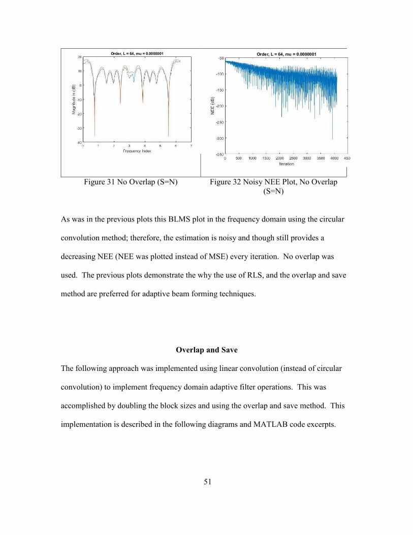
51

Figure 31 No Overlap (S=N) Figure 32 Noisy NEE Plot, No Overlap (S=N)

As was in the previous plots this BLMS plot in the frequency domain using the circular

convolution method; therefore, the estimation is noisy and though still provides a

decreasing NEE (NEE was plotted instead of MSE) every iteration. No overlap was

used. The previous plots demonstrate the why the use of RLS, and the overlap and save

method are preferred for adaptive beam forming techniques.

Overlap and Save

The following approach was implemented using linear convolution (instead of circular

convolution) to implement frequency domain adaptive filter operations. This was

accomplished by doubling the block sizes and using the overlap and save method. This

implementation is described in the following diagrams and MATLAB code excerpts.

52

Figure 33 Overlap and Save Using Linear Convolution

(109)

(110)

(111)

The following overlap and save function is then performed in the following manner:

(112)

The following equation is the multiplication of the input diagonal matrix with the

coefficients to form the output Y of the adaptive filter in the frequency domain:

(113)

53

To remove the circular convolution effects, we then take the inverse Fourier transform of

the output Y and save only the last N points of this transform output and the calculate the

error vector:

J§§§§ = NNf%.° J¡ (114) ]§§§ = J k 1: *J§§§§l

* = P KG*&1: , 1 ' ]§§§, )!*+*KG*& = 9Lò:MJ

*J§§§ = ]*+= 1, *.ó

W§ô = NNfõ*J§§§ö

The gradient is calculated using the pre-padded Ez error vector and the diagonal input

matrix Xd. We then only utilize the first N points of the inverse Fourier transform

output. We then perform a 2N Fourier transform of the first N point output of the inverse

Fourier transform by zero padding the input to the Fourier transform thereby obtaining

Gz’. Gz’ was constrained by zero padding.

T÷ = '2±¼ó JW] (115) T = NNf%.T÷¡

]§§§ = T 1: , 1.ó ]*+= 1, . ′

T¥÷ = NNf]§§§¡ , where T¥÷ = Gradient

Finally, the error vector is calculated in the frequency domain based upon the output of

the update equation.

W§÷ = Pô ' ±§¼§ô (116) *ô = NNf%.W§ô¡

54

The convergence and estimation is then plotted with the following results. I have

included MATLAB code that allows for a change the input signal sample to further adjust

the overlap of the input vector. Though this overlap has nothing to do with the overlap &

save operation, it does aid in the in the overlap of samples of the input matrix.

Figure 34 Overlap and Save with Order L = 64

The following is a normalized convergence factor that demonstrates the reduction in

convergence noise by implementing a µk that is averaged across the frequency bins per

block. The normalization equation is given below:

¤ K = ¬1 2 ∑ |±¤ K|¤$¤%¶ , )!*+*¬ = 0.5, = 10 (117)

The following are the resultant performance curves. Note that increasing order improves

the performance of each algorithm, but increases the number of iterations required to

converge. This algorithm entirely consistent and can be erratic.

55

Figure 35 Normalized Impulse Response Performance (Order L=64)

The concept of Block Least Mean Square in both the frequency domain and the time

domains have been described. In both cases, these algorithms converge to the mean (i.e.

wiener solution). In the time domain, the structure of the input matrix aids in the

convolution operation. In the frequency domain, multiplications are the same as

convolution in the time domain. By performing adaptive filter operations in the

frequency domain, computational complexity is reduced. In order to obtain a proper

BLMS output in the frequency domain, one must utilize linear convolution. Linear

convolution is achieved by using either overlap and add or overlap and save. In this

report, I implemented the overlap and save method; this required the implementation of

linear convolution enabled by doubling the size of the input blocks and the FFT’s and

appropriately pre-padding or padding matrices to eventually calculate the gradient.

Though all plots were noisy, even the Normalized Error Estimates. To improve

performance a Recursive Least Square (RLS) implementation should be performed.

Ideally, for better performance (i.e. less estimate noise) a line RLS should be performed

utilizing the following step size (see Figure 11):

56

Note: = ø|ùú /|£

Figure 36 Exemplar impulse Response to Fit (RLS Example)

Figure 37 RLS Mean Square Error (MSE) Performance

Further, in the presence of non-stationary data, convergence is affected by block size and

the degree of overlap. To calculate the Recursive Least Square (RLS) beam pattern, on a

uniform or non-uniform (Dolph-Chebyshev) linear array the following equations must be

implemented:

57

/. = û%.`%. &/.1 û%.&/. `%. &/. (118)

*/. = G/. ' : &/. (119)

:/. = :/ /.*/.

(120)

`%. 1 = û%.`%. ' û%./.&/. `%.

(121)

The following are antenna patterns for two linear arrays of eight element combinations.

The steering weights are adjusted adaptively to match the following patterns (Balanis,

2009):

Figure 38 Eight Element (Non-Uniform: Dolph-Tschebyshev) Linear Array (Low Sidelobes)

58

Figure 39 Eight Element Uniform Linear Array (Higher Sidelobes)

By implementing an adaptive recursive least square (RLS) algorithm, the patterns

described in the two figures above are achieved with the least number of calculations

utilizing floating point calculations. Floating point calculations prevents algorithm

singularities, ensuring stable algorithm execution and fast convergence that is closer to

the Newton multi-dimensional case. This will be used to perform beam forming using a

Vector aperture.

Microwave Design Approach

The goal is to introduce a set of modular design, development and fabrication concepts

utilizing heterogeneous technologies that reduce non-recurring engineering (NRE) cost.

The use of materials such as Silicon© and/or Polystrata© materials provide the basis for

the development of modular analog and digital circuits which can be referred to as

chiplets. Monolithic designs can be made modular utilizing interposer technologies to

create reusable chiplets.

59

Interposer technologies enable the integration of heterogeneous materials such as HEMT,

PHEMT, InP, GaN and Si CMOS. Si interposers enable the integration of multiple chips

within the same Si package. Si interposer technology enables I/O interfaces between

chips to be utilized without the use of ESD protection circuits and therefore reduces the

power draw and impedance thereby improving overall chip performance. Si interposers

enables the finer pitch for increased densities. Silicon© and Polystrata© interposer

technology supports isolation, lower loss and larger footprints where the coefficient of

thermal expansion (CTE) is well matched to Rodgers© printed circuit board (PCB)

material.

Figure 40 Proposed Chiplet Stack up (2.5 Interposing Technology)

This enables applications such as millimeter wave, microwave, beamforming, software

define radio (SDR), satellite communications and radar applications. Numerous chiplets

can be developed and reused across numerous PCB designs thereby reducing NRE costs.

Chiplets represent multiple semiconductor chips that are combined together to create

reusable analog or digital tiles that can be placed on numerous PCB designs.

Chiplets can combine microwave component combinations that are designed with well-

matched impedances. Additionally, chiplets containing digital component combinations

60

can also be created such as ADC, DAC, and processing architecture. Chiplets, due to the

small distance between chips, drive smaller signal levels leveraging a combination of

complementary metal-oxide semiconductor (CMOS) and current mode logic to use

voltage level thresholds that do not require impedance match requirements chip to chip.

The interposing technology used by chiplets also enable 3D integration using FinFET

technology nodes such as 5nm, 7nm, 14nm, and 16nm technology. Through the use of

digital design tools, issues such as corner effects and proximity effects dominate error

that do occur during the synthesis process. One example is the derivation of the corner

models for the analog portion of a digital circuit. The electrical performance of a device

is expressed in the following table:

Table 3 Model Properties and Associated Considerations (EEE 627, Fall 2016) Simulation

Model Model

Classification Properties Considerations

BSIM3 BSIM4

VTH Based Widely used, but outdated

Singularity at VDS=0 causes issues w/ mixers, charge switching (in circuit design)

Unphysically moderate inversion, asymmetric capacitances

Region boundaries inaccurate

Analog conductance/capacitance problems around simulation regions

Problems with inversion low power designs

Analog CMOS for VDS charge changes discontinuously as charge changes between source and drain

EKV2.8 EKV3.0 BSIM6

Inversion Charge Based

Improved simulation of high frequency circuits

Considers EM effects of signal lines and passives

Improves upon model inaccuracies experienced in VTH based modeling

PSP Surface Potential Based

Symmetric Linearization

Future Vision

Best for analog model 2/3-D process and device simulation

61

The implication in the analog domain, ýhÔýwú varies with ep and geometry, bias and analog

circuit topology as well as the fact that ep is important for every analog circuit. In the

digital domain, worst and bast case corner models are adequate and therefore less

sensitive to these variances. Most of the problems occur in in analog modeling when

developing in 3D FinFET technology.

hÔ = þ*wþ@ w

(122)

ep = Electrical Performance (device or circuit)

pi =Physical process parameter

The following will describe the technical design details of a radio transceiver design and

how Chiplet and transposer technology is applied to modularize the design of a radio.

The use of ultra-low noise GaAs based, 0.2 and 0.25 pseudomorphic High Electron

Mobility Transistor (pHEMT) technology provided by Avago technologies enables the

design of microwave components such as low noise amplifiers (LNA), mixers, oscillators

and filters. The noise figure for 0.2 micron gates enable a noise figure of < 1dB with a

frequency range that spans .5 and 12GHz and is a key technology in the development of

smart vector antenna systems.

The noise figure of the receiver chain is set by the 1st components (see equation 9) in the

receiver chain such as a band pass filter (BPF) and/or a Low Noise Amplifier (LNA).

The noise figure of a two port, low noise, amplifier is the following:

62

N = N / 6T> |°> ' °Ëã| (123)

Fmin = Minimum noise figure of transistor °> = T7 n7 =8+M*?G9K<<?M* °Ëã = @<K989=+M?G9K<<?M*N = N / 6 = WR8K(?*<K=*+*=K=<?M*;<+?=K=<+

Figure 41 Receiver Front-End Diagram (Typical)

In the figure above, the band pass filter (BPF) and the LNA set the noise figure for the

entire receiver chain. Using pHEMT technology, a noise figure < 1dB is possible by

using the device S- and noise parameters in the design assuming a bias condition of Vds

= 3.0 V and Id = 20 mA. By utilizing component size of 0402 using the Avago Tech

VMMK-1225 Low Noise E-PHEMT and Rogers RO4003™ substrate (20 mil thickness

with 1/2 ounce electrodeposited copper cladding on both sides). To investigate the

feasibility of such a design, the following are the parameters for the 3V, 20mA E-

pHEMT, VMMK-1225 technology from 2GHz to 17GHz. This along with high

performance passive components from Murata.

63

Figure 42 VMMK-1225 technology Capabilities from 2GHz to 17GHz

The design approach to the LNA depicted in Figure 41, the optimum design technique is

to derive intersection between noise circle and gain circle to determine the appropriate

‘L’ matching network for the broadband frequency range of operation. In the following

example, for high speed multi-media wireless communication link at 5.8GHz, the

optimum design parameter occurs at the intersection between the gain & noise circles on

the smith chart occur. The following Smith Chart performance demonstrates an optimum

design point.

64

Figure 43 Smith Chart LNA Design @ 5.8GHz

The following plot describes the output of the low noise amplifier (LNA). The following

design schematic utilized the VMMK-1225 Low Noise E-PHEMT transistor technology.

Figure 44 Keysight Advanced Design System (ADS) Simplified Circuit

65

Figure 45 Broadband P-HEMT LNA Performance Curve

Based upon the Rogers 4003 material used for the design of this Low Noise Amplifier

(LNA), the following plots describe the expected performance as a function of frequency.

Based upon Vds = 1V, Ids = 20mA, and Vgs = 0.6V. VDD = 5V, the bias resistance is the

following:

v_7 = 5 ' 120W ' 3 = 250Ê (124)

Figure 46 Microstrip insertion loss using differential length method (Rogers Corporation R04000©)

66

This model will required adjustment of substrate lengths to meet the gain requirements

(i.e. Design the LNA at the ADS schematic level to achieve over the frequency range of 1

to 10GHz, a noise figure that is less than 1.2 dB, and ≥ 13.0 dB of transducer gain with

no more than ± 0.25 dB gain ripple in a 50 ohm system). All components in this design

will utilize passives with size 0402.

67

Chapter 3

NEW MULTI-NODAL WIRELESS COMMUNICATION SYSTEM METHOD

(Multi-nodal wireless communication systems and methods,

US Patent 9,717,088, Granted July 25, 2017.)

The RF characteristics of Wi-Fi devices commonly utilize an omni-like directional

antennas. Multiple antennas on these devices are controlled separately to transmit

separate spatially diverse streams. WiFi device modulation techniques such as the use of

Complementary Code Key (CCK) in concert with Quadrature Phase Shift Keying

(QPSK) for 802.11b, CCK and Orthogonal Frequency Division Multiplexing (OFDM) in

concert with Quadrature Amplitude Modulation (QAM) (e.g. 16 or 64 QAM) or Phase

Shift Keying (PSK) (.e.g. BPSK or QPSK) are both used for 802.11g, OFDM with QAM

or PSK used on each subcarrier is only used for 802.11a, 802.11n (max. 64 QAM, rate

5/6) utilizes OFDM in concert with QAM and PSK modulation techniques, and lastly

802.11ac which can utilize 256 QAM (rates 3/4 and 5/6) with use of MIMO to perform

spatial diversity between multiple OFDM user streams using much smaller cell sizes.

Further research in the use of Alamouti space-time block coding (STBC) is planned to

identify the achievable gain in 5G millimeter frequency ranges.

Management support interfaces for Wi-Fi devices are defined by the Telecommunications

Management Network (TMN) model which encourage protocol support for different

layers of a network infrastructure. Simple Network Management Protocol (SNMP) is the

predominant protocol in national provider networks today.

68

Figure 47. Overview of 802.11 Subsystems

Cellular Technology

Background: Cellular base stations, as is the case with Wi-Fi base stations, are located

across the country in proximity to cellular towers. Often these towers are visible in close

proximity to interstates, highways, and neighborhoods; these towers are found

(sometimes camouflaged) in areas where RF coverage is needed. These towers are

commonly referred as “cell towers” and often are equipped with dipole antennas so as to

reduce impedance mismatch between the receiver and the antenna (impedance mismatch

causes Voltage Standing Wave Ratio (VSWR) which is a measure of reflected voltage)

that causes transmitter and receiver signal distortion. As with the case with WiFi,

transceivers are located behind antenna elements. The following depicts the high level

structure of the cellular subsystems involved with 2G, 3G and 4G network devices.

69

Figure 48. Overview of Cellular Subsystems

Wireless Technology Not Considered

Other wireless protocols include Bluetooth, 802.11z, 802.11p (MS-Aloha) and Wi-Fi-

Direct; however, these protocols are not used to support a large number of users

simultaneously. This paper is only focused on systems that can support a large user

population.

Cellular and Wi-Fi System Comparison

Wi-Fi RF cell coverage sizes are limited by their higher frequency (2.4GHz and 5GHz

versus 900MHz), limited allowed power transmission interference from other devices in

this unlicensed band (though somewhat mitigated by its modulation technique), and more

importantly by their link layer communication specification. Unlike cellular

communication, Wi-Fi communication devices specify a link layer communication model

70

based upon a CSMA/CA format. The CSMA/CA format is not as effective multiple

access protocol as is the case with TDMA or CDMA technologies. Though Wi-Fi can

close links at longer distances, greater amplification and antenna directivity is required as

well as cooperative changes to the Wi-Fi link layer timing specifications. Example: DIFS

is the amount of time a station must sense a clear radio before beginning a new

transmission sequence. Note that a node can format and buffer a data frame to be

transmitted during this time interval. SIFS is the amount of time a station must wait

before sending or beginning to receive a RTS, CTS or ACK frame, note that the SIFS

time includes the amount of time to format the ACK frame to be transmitted; this is

possible since only the first portion of the data frame (e.g. BSSID) is used in the ACK

message. PIFS is the DIFS for the access point in a special access method known as

Point Coordination Function. The times are defined such that the RTS, CTS, and ACK

frames are given a higher priority (ie once a packet transmission sequence has begun, the

station holds onto the channel until it is finished). Without 802.11 RTS/CTS

handshaking the following time periods are observed.

71

Figure 49. 802.11 MAC Layer Communication Note: No RTC/CTS handshake depicted in diagram above. (Airstream, 2014)

IEEE mandates the following timing for 802.11a:

• Time Slot = 9 µs • SIFS = 16 µs

PNßC..._ = N 2&fK9*< = 34μ= (125)

IEEE mandates the following timing for 802.11b:

• Time Slot = 20 µs

• SIFS = 10 µs • PIFS = SIFS + Time Slot = 30 µs

PNßC...v = N 2&fK9*< = 50μ= (126)

IEEE mandates the following timing for 802.11g:

• Time Slot = 9 µs • SIFS = 10 µs

PNßC... = N 2&fK9*< = 28μ= (127)

72

Sender procedure: Wait DIFS, Send Data, Wait SIFS, Listen for and receive ACK (until

maximum ACK timeout), Repeat

Receiver Procedure: Listen for and receive Data,Wait SIFS, Send ACK, Wait DIFS

Given this link layer communication protocol, the destination must start constructing the

ACK message once the first part of the data message has been received. Once it has been

determined that the data message was received without error, an ACK message may be

transmitted. The following is the timing calculation for sending the ACK message:

_<<? = _So _N (128)

LL_# = f<?fK9* u·H = f+?=9K==K;So9*==?* >¶> = !+<<*+;+?9*@?MK

With the speed of light 3&10ß9 =*M⁄ , a 802.11 ACK transmission can travel a distance

of 300 9 8=*M⁄ . Assuming a normal transmission of an ACK message, the receiver

could be no greater than 3 km (given the speed of light, a nice number) away or 10 usec.

If ACK timeout was increased (to say 19 usec), the maximum slot time for a point to

multi-point communication environment is equal to the slot time. For 802.11b the slot

time of 20 usec equates to a maximum distance of 6 km. Other wireless standards have

similar limitations but the distances are shorter.

73

Cellular requirements to address cellular reselection within greater cell sizes (> 1Km),

though is possible with some cellular protocols, requires special configuration of the

cellular chipsets to accomplish. 802.11, due to the CSMA/CA protocol requirements is

much harder to accomplish unless it is a point to point connection. Figure 49 describes

the general cellular reselection process as defined by the 2G specification (3G

specification includes neighbor list evaluation -not depicted here).

By observing the parameters in our cellular transmission cellular devices will choose a

base station over other base stations in the area (even though there is a mismatch Power

Spectral Density (PSD) may be less than others). See Chapter 3 for additional

information. This is important because it implies that the number of cellular devices

connected to a specific cellular base station can be control with the use of parameters

transmitted in the Broadcast Channel (BCCH).

Unlike 802.11 devices, assuming sufficient transmit power and sufficient receive

sensitivity; a base station can attract distant devices in the same manner. Though many

3G/4G chipsets (i.e. Mindspeed) have a time limitation (~1Km distance) in regard to how

long they will wait for a response from a peer device, however chipsets can be

programmed to deal with devices at greater distances > ~1Km by configuring the chipset

to only respond to devices within a circular area with a diameter of ~1Km ‘distance of

interest’ for distances > 1Km, ignoring devices that are not within that area of interest.

74

Wi-Fi and cellular devices used in hot spots (locations that represent extensions to the

Internet) use link layer protocols to control access to the Wireless Local Area Network

(WLAN) and ultimately to the Wide Area Network (WAN). Both wireless technologies

form a LAN environment where IP addresses with a subnet designation are delivered to

individual devices for data access. Cellular devices utilize IP addresses primarily for data

access, but with Long Term Evolution will use these services for using voice services as

well. These addresses are then allowed access to the WAN through a network process

referred to as Network Address Translation (NAT). During normal operation each device

initiates a data connection and delivers network frames that are transmitted to the

backbone network of a service provider through a network gateway. The network

gateway provides the NAT service that is used to proxy IP network requests to the WAN.

Wi-Fi and cellular devices used in an enterprise environment may not utilize NAT, but

rather be assigned IP addresses distributed by a router or server that supplies Dynamic

Host Configuration Protocol (DHCP) for the enterprise network.

Link layer network technology can be used to facilitate adaptation to legacy network

infrastructure, adaptation to new network backhauls, QoS of wired integration points

within a legacy or new Wide Area Network (WAN) entry point. QoS of wireless

technology that utilizes techniques such as MIMO and virtual roaming (discussed later).

As the performance at the edge of the network continues to increase, more demands will

be made on the network infrastructure to perform QoS functions nearer to the edge of the

network.

75

This paper will focus on the use of a centralized communication controller that will

control link layer communication between radios and the communication controller for

the purpose of load balancing between radio nodes, automated discovery of new radio

nodes, QoS in regard to RF communication channels, authentication, cryptography, and

virtual roaming. This paper is structured into the following sections: Wired integration

with existing networks, 802.11a/b/g/n, Cellular 3G/4G technology and Ethernet / Fiber

optic communication with a focus on link layer communication. These areas will be

evaluated as it relates to the Open Systems Interconnection (OSI) model starting at the

physical layer and moving to the Link Layer.

76

CHAPTER 4

PROPOSED WIRELESS SYSTEM DESIGN

The new aspects of the following design depicted in Figure 50 entail the following

attributes:

1. High performance roaming and autonomous distribution of wireless devices.

2. The measurement of Power Spectral Density across multiple RF cells to

determine the best integration of 802.11 and cellular backhaul systems while performing

intelligent frequency distribution across adjacent cells.

3. Integration of WiFi and cellular backhaul networks to utilize the same network

topology.

4. Cognitive adaptation of Digital Signal Processing (DSP) parameters based upon

empirical measurement of RF environmental parameters.

5. The ability to prioritize frames based upon link layer behavior.

6. The use of security encryption utilizing random numbers that are generated from a

system with a sufficient amount of entropy (to be quantified later).

The wireless system design follows the paradigm that the radios are simply radio

interfaces that simply communicate as commanded by a regional communication

controller. The radio interfaces are comprised of a radio (with a transmitter and receiver),

a very small processor, memory resources and an Ethernet interface. These radios can

communicate Cellular Frequencies utilizing W-CDMA using a 5MHz channel bandwidth

or the radios can communicate Wi-Fi with 22 and 25 MHz channel bandwidth. 802.11n

can utilize 20Mhz or 40Mhz channel bandwidths. LTE (using OFDMA/SC-FDMA)

77

comprised of channel bandwidths of 1.4, 3, 5, 10, 15 and 20 Mhz. LTE clients are

communicated a mask that indicates the OFDMA subcarrier(s) to be used in the uplink

transmission.

The radios are preconfigured with real time link layer messages that are required to

support real-time communication messages while all non real-time messages are sent to

the regional communication controller where the message can be characterized and where

an appropriate response can be constructed. The link layer messages will be

characterized per technology so that subsystem functions can be clearly identified and

aspects of the design can be described adequately.

Elements of this new innovation relating to both structure and operation can best be

understood by referring to the following diagrams and their descriptions.

This is a system of radios and their use in a large network. This new link layer

communication design is implemented using the Ethernet technology (MAC header, the

VLAN header, and a proprietary layer 2 protocol header) to implement communication

features that implement features 1 thru 6 above as well as specialized hardware that

processes wireless link layer functions and communication, classification of network

frames (wired and wireless), queuing and routing of frames, encryption/decryption of

frames, and network buffer management. Though most wireless systems provide adaptive

features, these features are not implemented with cognitive feedback from a RF and

network environment that is not visible to the device. The design depicted in Figure 50

78

describes the overall hardware functions implemented on the cell controller that support

these new features.

Figure 50. Proposed System Architecture

By communicating the TMSI, IMSI, and TLLI between different cellular base stations

within the same cell controller, the system is able to improve the speed at which a device

changes from one Location Area Code (LAC) to another. This is because the normal

sequence of messages required to move from one cell to another is no longer required.

This dramatically improves the performance of the Location Area Update process in

cellular networks. As all of the existing cellular technologies implement this portion of

the specification as it is required when moving from one cellular coverage area to

another. Additionally, if the TMSI & TLLI are ensured to be unique across all cell

79

controllers, then this information can be moved in between interconnected cell controllers

thus improving performance further.

This new wireless system design is based upon the concept of splitting the wireless

Media Access Control (MAC) across interconnected cell controllers using specialized

hardware that process non-real time portions of the wireless MAC protocol as well as

handle high speed frame processing for wireless devices under its control. These cell

controllers make “intelligent” decisions based upon feedback from multiple radios within

a physical area. The wireless system design is comprised of hardware systems that are

connected utilizing unreliable communication media (Ethernet) but could utilize other

forms of unreliable communication such as satellite and wireless bridges as long as the

required communication delay does not violate time constraints imposed by the MAC

layer communication required between a central communication controller and radio that

communicates the wireless MAC protocol. Such a system needs to be capable of

providing ubiquitous RF coverage across many desperate physical locations as well as be

capable of integrating into existing, legacy network topologies that may be strictly based

upon wired communication technologies. The wireless system design utilizes RF

transmitters and receivers that perform real time data communication to devices. These

devices are typically mobile; however, they can also include stationary devices such as

desktop computers. The major components of the hardware system are comprised of the

following components:

The overall system topology looks deceptively simple (see Figure 51). This system

topology describes the overall top-level architecture. The hardware link layer

80

communication methods used in the overall system will now be described. The system

topology must be adaptable to ensure that the link layer design can be implemented

without violating existing cellular and WiFi standards. This introduces a challenge that is

addressed in the following manner.

Figure 51. Simplified System Topology

Link Layer Communication Model

The link layer communication model splits both the cellular and the 802.11 MAC

protocols across unreliable communication links in a unique way. As depicted in Figure

51, Virtual Local Area Network (VLAN) technology as specified by the IEEE 802.1pq is

utilized between the cell controller and the base stations. In doing so, I can prioritize the

communication links dynamically. This design approach employs a fourfold advantage.

1. The new link layer communication model can be implemented across an existing

wired infrastructure with very low impact to the existing network infrastructure. As an

example, a network architect can overlay a completely different IP subnet over an

existing wired network infrastructure without changing the existing wired network.

2. Based upon link layer communication behavior, prioritization of wireless frames

can be changed dynamically. As an example, if Quality of Service (QoS) parameters

81

dictate a particular percentage of the system bandwidth, this system design can quickly

change the VLAN priority tag to prioritize frames to one RF base station over another RF

base station.

3. Unlike autonomous wireless routers and access points, the cell controller has

visibility to the RF spectrum where radios exist. This design enables the cell controller to

perform cognitive adaptation to the RF environment. Based upon the RF noise

temperature, the cell controller can equally distribute mobile devices across the available

RF spectrum in a fashion that provides for the greatest network performance. As an

example, BER as well as neighboring cell information transmitted by the RF base station

can be communicated back to the cell controller. Neighbor cell information can be

communicated in the form of Power Spectral Density (PSD) calculations (this is covered

in a later section). The cell controller can make a dynamic decision to send data frames

across a different RF base station, in essence the device is now communicating with a

different RF base station without awareness by the mobile device. This is a form of a

cognitive adaptation based upon BER.

4. The integration of cellular and WiFi stacks provides the ability for cellular and

WiFi devices to utilize the same backhaul network infrastructure. This provides relief of

the cellular systems in regard to bandwidth utilization and improves the use of

unoccupied bandwidth on the backhaul network infrastructure.

The link layer design includes adapters for both WiFi and cellular technologies. 802.11

technology will be discussed first followed by cellular technology. As depicted in Figure

51, the wireless 802.11 MAC is split across unreliable communication links. RT

82

messages are addressed at the RF base station, while higher level management messages

are handled at the cell controller.

Figure 52. 802.11 Link Layer Subsystem Partition

The following 802.1l link layer subsystem functions are addressed in the RF base station.

The RF base station handles all RT messages. Since Probe Response messages are very

similar to Beacon Messages, Beacon Messages are also handled in the RF base station.

83

Table 4 802.11 Real-Time Messages 1 Beacon/DTIM

2 Probe Response

3 Acknowledgements

4 RTS/CTS (If Enabled)

Templates for these messages are sent by the cell controller to the RF base station for

purposes of transmission to their RF coverage area. When cells overlap, these messages

can also be forwarded by other RF base stations in the coverage area. A measure of the

received power (Eb/No) can be made and a decision in regard to which RF base station

should ultimately respond to later Association requests can be calculated. The following

diagram depicts an 802.11 example:

Figure 53. Probe Response Exemplar

On Ethernet there are two distinct delays: propagation delay and transmission delay. The

following equation describes the nodal delay, the delay per node in an Ethernet network.

84

G/¼_# =Gwiq Ghh GLi_/7 Gwiw (129)

The velocity of an electromagnetic wave through a copper media is approximately

×·wwhi = 2.1 ∗ 10ß. Though base transmission rate has no bearing on propagation

delay, base rate directly affects transmission rateGLi_/7. Assuming full duplex Ethernet

operation GLi_/7 = .5128=*M for a 64 byte frame. A probe request, including a

proprietary header, can be no less than this size; therefore, round trip (RT) delay of

2*GLi_/7 = 1.0248=*M. Assuming a maximum length of 100 meters, Gwiw =.47628=*M with a round trip delay of 2*Gwiw = .95248=*M. Ignoring

Ghh?GGwiq for a moment, one RT segment is 1.9768=*M. Adding the segments

depicted in Figure 53 we have aGLL_# = 3.95288=*M. Figure 53 is representative of the

minimum network delay between a cell controller and a RF base station; therefore, the

802.11 messages depicted in Table 4 represent messages that must be handled in RT by

the RF base station.

Table 5 802.11 Non-Real Time Messages

1 Association/Reassociation/Disassociation

2 Authentication/Deauthentication

3 802.1x, EAPOL, etc…

4 802.11 Data Messages

WiFi messages listed in Table 5 are handled by the cell controller which manages

messages from all devices in a large regional area. These messages provide for a

centralized management of all 802.11 devices in the area as well as provide for the

accurate application of Quality of Service (QoS) between individual wireless networks

85

since all data frame are sent through the cell controller. For example, if a network

identifier (e.g. SSID) is suppose to have available 60% of the available bandwidth while

another network identifier is suppose to have available 40% of the available band, the

bandwidth between the two networks can be arbitrated in RT instantaneously since the

cell controller has full access to all traffic being delivered to the whole network prior to

be distributed to individual RF base stations in the regional areas.

Cellular Link Layer MAC

There are many system design differences between the different cellular technologies

(e.g. 2G/GSM, 3G/UMTS, 3G/CDMA2000, 4G/LTE). Cellular vendors have changed

their subsystem designs to improve access speeds, coverage, and reduce cost to

deployment. I will focus on cellular subsystems that intersect GSM, 3G/UMTS, and

4G/LTE cellular link layer subsystem functions. Unlike WiFi devices, cellular provider

networks have routinely (out of necessity) split their link layer communication across

unreliable communication links (e.g. Ethernet/Fiber).

Table 6 Example Cellular UMTS Messages (Wikipedia, 2014)

MOBILITY MANAGEMENT (MM)

MESSAGES

RADIO RESOURCE (RR)

MESSAGES

imsi detach/attach indication additional assignment location updating reject immediate assignment

location updating request immediate assignment extended

location updating response immediate assignment reject authentication reject ciphering mode command authentication request ciphering mode complete authentication response assignment command

identity request assignment complete

identity response assignment failure tmsi reallocation command handover command

86

tmsi reallocation complete handover complete cm service accept handover failure cm service reject physical information cm service abort paging request type 1-3 cm service request system information type 1-

8,2(bis/ter), 5(bis/ter) cm establishment request channel mode modify ack Abort classmark change/enquiry mm status measurement report/

frequency redefinition

The cellular link layer communication model is much more distributed; however, there

are improvements that can be made. I will outline the link layer communication model

changes that integrate WiFi and cellular technologies together as well as improve

roaming between the technologies. In addition, I will describe why this approach is

superior to other approaches.

Figure 54. Example Inter-RAT Handover Setup (4G Source to 3G Target Network) (Barton, 2012)

87

The example above describes the handover setup procedure example between a 4G

source to a 3G target network. The end goal is to ensure that when the handover is

complete data frames will be sent to the new serving gateway service in this the GGSN

3G service. The Source MME subsystem initiates the Handover resource allocation

procedure by sending a Forward Relocation Request (IMSI, Target Identification, CSG

ID, CSG Membership Indication, MM Context, PDN Connections, MME Tunnel

Endpoint Identifier for Control Plane, MME Address for Control plane, Source to Target

Transparent Container, RAN Cause, MS Info Change Reporting Action (if available),

CSG Information Reporting Action (if available), UE Time Zone, ISR Supported)

message to the target SGSN subsystem of the 3G cellular network. Note that this entire

setup process occurs before the User Equipment (UE) has actually “roamed” to the 3G

network. Once the setup has completed, the source MME subsystem initiates the

handover process by coordinating with the UE by sending a handover command

(depicted in Figure 55). The UE responds to the network with a handover complete

message to the target RNC subsystem who initiates a message to its SGSN subsystem

which then conveys a completion message to the source MME subsystem. The source

MME acknowledges the completion message and the SGSN notifies its GGSN service

(using a “Modify Bearer” request). Once the GGSN service then notifies the source

PGW of the change, data frames are now presented through the new serving 3G gateway

(e.g. SGSN and GGSN).

88

Figure 55. Example of Inter-RAT Handoff Execution (4G Source to 3G Target Network) (Barton, 2012)

Using a cell controller, these subsystems are combined into a single platform that can

more quickly execute the roaming examples such as this. Latency is reduced greatly

because fewer messages across unreliable communication links are required. A cell

89

controller would be used to handle large geographic areas. With the use of Fiber channel

communication links (assuming the use of repeaters and proper configuration), very low

latency and high bandwidth can be achieved.

Figure 56. New Cellular Link Layer Topology With Combined 802.11 Subsystems

With the architecture above, the cellular MAC is split between the cell controller and

BTS, NodeB, and eNodeB transceivers. Today these cellular subsystems are found in

desperate locations across the country. Since these subsystems interact with each other

across vast physical locations, very little information is communicated in regard to the RF

environment as it relates to BER and RF performance. With this new link layer

architecture, cellular coverage can be provided for large geographic areas by the same

system controller. In this case a full hardware data path can be applied to handle frame

90

classification and distribution to the wireless subsystems required to handle this

processing as well as gather BER information in regard to RF performance in local areas.

This integrated with Wi-Fi capability provides the ability to off load traffic from the

cellular network, freeing up cellular bandwidth for other users. By the use of a 802.11

split MAC, we can now provide Authentication and Association credentials directly into

the cellular network using Extensible Authentication Protocol of Local Area Network

EAPOL. Using the same authentication triplets used between the service provider and

the UE, WiFi can be enabled and provide service to cellular UE. Just as is the case with

the Packet Gateway (PGW) or the Gateway GPRS Support Node (GGSN), Network

Address Translation (NAT) services are provided for IP addresses that are provided for

the local area. This service is used to go to the Internet from a UE that is using WiFi

instead of the straight cellular services. Because the WiFi base stations can be elevated,

and have amplification added for both transmit and receive, it is possible to use WiFi to

offload some cellular data traffic.

The link layer communication model has been described for both the 802.11 where the

RF MAC is split between a RF base station and the addition of the 802.11 subsystem to

cellular subsystems. The point areas where the 802.11 subsystems are integrated will

function correctly for all versions (e.g. GSM, UMTS, LTE) of cellular subsystems. In

addition, a method of authentication has been described as well as how access to the

Wide Area Network (WAN) is provided as is the case with all data services on UE.

91

Link Layer Hardware

In order to provide the best class of service for the link layer model described in the

previous section, the hardware must be designed to support the following features:

Table 7

Sample Link Layer Feature List 1 Link Layer Encryption/Decryption (Cellular & WiFi). Encryption over the

wired network. 2 Frame Manager (Classification Engine), Queue Manager, and Data Path

Acceleration Architecture (DPAA -Freescale Standard) 3 Fixed format headers sent to wireless base stations

4 Table of all UE required

5 NAT and Proxy ARP provided for all bridged UE (different modes of operation), MAC learning feature to support MAC address transition across Layer 2 switch interfaces.

6 High performance frame processing with little or no intervention with GPP HW

7 Large number of Fiber and Ethernet interfaces available in one unit

8 Security Fuses, secure boot, security monitor (can be connected to tamper detection).

9 Numerous other hardware attributes not relevant for a research paper such as dual power supplies, solid state disks, etc...

The hardware design to support the link layer hardware would start with the design of the

SoC. This design would facilitate the use of dedicated hardware state machines that act

independently from each other. These hardware state machines are provided instructions

in memory that are then loaded into their internal register cache for execution. These

instructions facilitate the functions required to support the predefined headers found for

both the link layer Ethernet communication as well as the cellular and 802.11 MAC

fields. Since most of these fields are based upon configuration parameters that are

configured by software, it would the responsibility of the link layer software to

92

implement the structures that are accessed by the hardware to support this link layer

communication.

Figure 57. HW State Machines in SoC Architecture

The hardware state machines (as configured by software and depicted in Figure 57) used

for frame processing would contain internal register memory that is used to communicate

frames to a wireless base station. This internal register memory would be used to

construct the proper frame header for a particular device that has been configured. In

addition some hardware state machines would also include a hardware internal Direct

Memory Address (DMA) engine. When a base station device has properly authenticated

itself to the network, the base station MAC address, BSSID, radio MAC address(es),

VLAN header information, security key information, and capabilities will be

communicated and stored into system memory (not in hardware registers). When a

network frame buffer is received from a wireless base station, the hardware frame

classification engine would evaluate the source MAC address, VLAN tag information.

93

Based upon this information it will do further classification to identify the source MAC

address of the actual wireless client. The source MAC address would then translate to

unique hardware queue ID. A message with the address of the frame and that queue ID

would be sent to the hardware queue. This hardware queue is configured to send frames

with this queue ID to the security engine for link layer decryption. The security engine

returns a specific queue ID after decrypting this frame (based upon its hardware memory

cache structure). The hardware queue is configured to send frames with this queue ID to

the wireless link layer engine for further processing. As an example, based upon the

fields in the 802.11 MAC header, the wireless hardware engine will perform standard

operations on the frame starting at the address of the frame. The wireless link layer

hardware state machine is specifically designed to understand the 802.11 and UMTS

MAC protocols. Using 802.11 as an example, the hardware state machine behavior can

be based on the source (radio MAC) address of the sender in the forward direction. If the

destination MAC address is that of another wireless device that is managed by this cell

controller the frame will be forwarded onto the same queue that other frames from the

network in the reverse direction are placed for eventual transmission to the wireless

device.

Link layer encryption is based upon cryptographic algorithms verified and validated by

the The National Institute of Standards and Technology (NIST). NIST issued the Federal

Information Processing Standard (FIPS) Publication 140-2 (FIPS PUB 140-2) is a United

States government computer security standard that is used to accredit cryptographic

94

modules. This publication is titled “Security Requirements for Cryptographic Modules”

and was published on May 25, 2001 and was updated on December 3, 2002.

The National Institute of Standards and Technology (NIST) issued the FIPS 140

Publication Series to define requirements and standards for cryptography modules for

both hardware and software components developed by technology companies. Federal

agencies and departments can validate whether a module, termed a Hardware Security

Module, is covered by an existing FIPS 140-1 or FIPS 140-2 certificate which specifies

module name, hardware, software, firmware, and/or applet version numbers. Many

cryptographic modules are produced by the private sector (and even by the open source)

communities for use by the U.S. government and other regulated industries, including

financial and health-care institutions, that collect, store, transfer, share, and disseminate

sensitive but unclassified (SBU) information.

NIST regulated security programs enforce government and industry cooperation to

establish secure systems and networks by developing, managing and promoting security

assessment tools, techniques, and services, and supporting programs for testing,

evaluation and validation. NIST security programs extend to development and

maintenance of security metrics; security evaluation criteria and evaluation

methodologies; tests and test methods; security-specific criteria for laboratory

accreditation; guidance on the use of evaluated and tested products; research to address

assurance methods and system-wide security and assessment methodologies; security

95

protocol validation activities; and appropriate coordination with assessment-related

activities of voluntary industry standards bodies and other assessment regimes.

Annex C of FIPS 140-2 specifies Approved Random Number Generators. Random

Number Generators (RNG) are used to generate random content for cryptographic

algorithms that require the need of random content such as content required for the

generation of IV information for IPSEC or DTLS protocols as two examples.

United States Federal Government standard Federal Information Processing Standard

(FIPS) Publication 140-2 (FIPS PUB 140-2) requires verification that each sample

produced by a Random Number Generator (RNG) be compared against the immediately

preceding sample to verify that the random number generator does not generate the same

numeric value twice sequentially; statistically, this would indicate a hardware or software

fault rather than a coincidence. FIPS 140-2 specifies that any time a Random Number

Generator (RNG) generates a new random number, the generated number is to be

compared against a previously generated random number. If the two are the same, the

event indicates a hardware (or software) failure rather than by some extraordinary,

statistical chance. If the two are the same, an error indication is generated.

In order for any system to be compliant with requirements such as FIPS 140-2, but not

perform the check in software, the hardware must enable the security engine utilizing a

“bump in the wire” architecture in a mostly-hardware autonomous data path to perform

this function. Thus, security can be implemented in separate devices interposed between

96

devices intended to communicate securely, for example cellular link layer encryption

datagram, 802.11 link layer datagram and insecure Internet Protocol (IP) datagrams can

be repackaged securely for transport over the public Internet or other unprotected

network infrastructure.

The design of a RNG requires the use of hardware design techniques known as

“Asynchronous Design”. When using asynchronous design techniques to design a RNG

subsystem, one must use the instability inherent in relying upon propagation delays in a

logic design that vary with temperature, voltage level fluctuation, substrate differences,

and register settling time that occur through combinatorial logic designs. These

techniques are used to ensure that the RNG subsystem does provide random numbers

with sufficient entropy. The following illustrative technique can facilitate random

number generator verification, which may be performed without using any

microprocessor execution time or specialized hardware.

97

Figure 58. Use of Random Numbers in HW Data Path (Co-Inventor, Freescale Patent : Patent Nbr: 9,158,499)

An input frame that requires encryption is received by the hardware data path and is

parsed, stored in system memory (1 in Figure 58) by the hardware receive DMA engine.

A message is sent by the frame parser to the HW queue across a hardware bus. This

message contains the address of the HW cache associated to the queue ID in system

memory (2b in Figure 58). The Queue Interface reads the message in the HW Queue (2a

in Figure 58) and alerts the DMA to read the HW memory using the address found in the

HW Queue message) and distribute a processing request to a CryptoEngine (3 in Figure

58). The Queue Interface also instructs the DMA to read the Frame Buffer memory using

the address found in the HW Queue message (4 in Figure 58). The CryptoEngine

requests a random number because it must generate an IV. This IV contains a mask (e.g.

98

seed) that is XOR’d with the random number (5 in Figure 58). Finally, the CryptoEngine

executes its loaded instructions (in its internal memory cache) and checks the newly

generated IV to the previous IV. If these IV’s are identical, it is indicative of a problem

and an error is returned, otherwise the new IV is stored at the address of the previous IV

by use of its DMA engine and processing continues normally (6 in Figure 58).

This process illustrates a FIPS compliant hardware design to meet the cryptographic

needs of the cell controller.

Link Layer Software

The link layer software is comprised of the following subsystems that interact with the

hardware state machines described in the hardware section above. The software must

pre-populate the hardware memory of the state machines to accommodate the

transmission of frames to wireless device from other wireless devices as well as devices

from the WAN side of the network device. Network headers that are used to

communicate to the wireless base stations must be pre-populated on a per-flow basis.

The following depicts the headers that must be pre-populated. Note that the wireless link

layer engine will modify some portions of the header as data moves through the

autonomous hardware data path.

99

Figure 59. Network Frame Headers that most be pre-populated on a per Flow basis

As described in Figure 57, the wireless link layer engine requires HW memory cache that

contains the proper Ethernet, VLAN, Cellular or 802.11 MAC header pre-populated on a

per flow basis. This means two per wireless device (1 for the forward direction and 1 for

the reverse direction) flow to and from a wireless device. The network header formats

described in Figure 59 must be pre-populated in the wireless link layer hardware state

machine. This finite state machine (FSM) must also maintain flow control structures

between the cell controller and the RF base stations. There are mechanisms in place in

regard to the cellular protocol specification; however, on the 802.11 side there are not

integrated specifications. The following frame formats are specified to support link layer

communication between the RF base stations and the cell controller:

100

Figure 60. Frame Format Examples

101

CHAPTER 5

MOBILE AND BASE STATIONS

Wireless State Machines

Cellular and 802.11 devices are constantly measuring the RF environment. As such they

are constantly performing neighbor cell power measurements, if sufficient BER rate is

sensed by the receiver (where rate adaptation did not improve), a 802.11 client device

will initiate its form of cell reselection (issues a 802.11 Reassociation request). On

cellular devices this is performed by monitoring all BCCH carriers contained and making

one measurement per BCCH carrier. The size of the neighbor cell list (e.g. number of

neighboring transmitters), either increases or decreases the amount of time UE spend

performing these measurements. Cellular devices initiate the process of cell reselection

by a process referred to as Location Area Update (LAU). This process is analogous to

the example when in a moving vehicle. The cellular device in your hand will receive a

signal from a new tower which will have a different Location Area Code (LAC). This

process is repeated as the car continues to move from one tower to the next. This process

is sufficient for voice services, while processes referred to as Routing Area Update and

MM Attach is required for data services. A cellular device can also request

supplementary services such as [no] call waiting, [no] call forwarding, and activate Short

Message Service (SMS).

102

Finite State Machine Behavior

The cell reselection state machine is depicted in Figure 61; he P*(_±9K<_oooA^_` and

the o*_*=**M<_d;; field values are transmitted on the Broadcast Channel (BCCH) of

a cellular base station. In order to distribute the load of cellular devices across cellular

base stations, the cell controller can dynamically modify the parameters being transmitted

on this channel thereby influencing the state machine of the UE to connect to a different

RF base station. For UMTS and LTE UE, the network can also request a cell reselection.

Figure 61. Cellular Cell Reselection Rule Evaluation Process

o1 = mP_³ ' P*(_&_RG^/ ' 9?& P*(_±9K<_oooA^_`'P*(_m)+_o?== (130)

mP_³ = Average receive signal level

103

P*(_&_RG^/= Minimum mP_³ the MS must receive to access this cell

P*(_±9K<_oooA^_` = Maximum power the MS is allowed to transmit on the RACH

P*(_m)+_o?== = MS power class

o2 = o1 o*_*=**M<_d;; ' 9?& f*9@Ëtt;+m*?<_fK9* (131)

o*_*=**M<_d;; = dB weighting applied to a cell which may be positive or negative

f*9@Ëtt = Positive dB weighting applied to a cell for the time m*?<_fK9* m*?<_fK9* = Timer set in the MS by the neighbor cell; on it expiry, the f*9@Ëtt is

removed. f*9@Ëtt is only applied to neighbor cells.

In addition, cellular and 802.11 wireless devices also perform rate adaptation based upon

sensed BER information. An 802.11 wireless client device normally initiates a

Reassociation request, while a cellular device utilizes the LAU procedure as well as

manage the cell reselection.

104

Figure 62 LTE Handset (Basic State Machine Terminology)(ShareTechnote, 2013)

An example LTE cell reselection, initiated by the network side: A UE is in connection

with a cell ‘A’. The network sends a command to the UE to perform a signal quality

measurement on cell ‘B’ (e.g. UMTS command = “Measurement Control”, while LTE

command = “RRC Connection Reconfiguration”). The UE performs the measurement

and sends the result to Cell ‘A’. (e.g. UMTS and LTE = “Measurement Report”). If the

controller deems the measurement favorably, the UE is sent a change cell command. (e.g.

UMTS command = “Physical Channel Reconfiguration or ActiveSetUpdate”, while LTE

= “RRC Connection Reconfiguration”). Once the UE changes to cell ‘B’ successfully,

the UE will send a cell change completion message to cell ‘B’ (e.g. UMTS = “Physical

Channel Reconfiguration Complete or ActiveSetUpdateComplete”, while LTE = “RRC

Connection Reconfiguration Complete”). (ShareTechnote, 2013)

105

LTE phones presently have two antennas that can be used in a 2x2 MIMO mode. The

LTE phone can use one antenna to talk to one tower while using the second antenna to

communicate to the second cell tower.

Roaming

In 802.11 roaming to another access point involves sending a ‘Reassociation” request to

the new access point. This “new” access point was discovered by an outcome of signal

strength measurements by the client device. In the 802.11 state machine below, the

Reassociation message speeds up the Authentication and Association state change so it

more quickly moves to the successfully Authenticated and Associated state. When a

wireless device roams, it is important that data transfer is not lost during the process. The

MS state machine has an impact on this behavior. When a 802.11 device sends it

“ReAssociation” message, it must still properly receive frames from the base station it is

presently Associated to. In addition, if the base station it is roaming to does not have

direct communication and coordination with the base station it is roaming from the

device will be forced to perform a complete Association to the device it is roaming to.

With the cell controller link layer approach, the roaming between access points can be

seamless. The following state machine diagram depicts the change in the typical state

machine behavior of the mobile device.

106

Figure 63. Example of 802.11 Roaming Utilizing Cell Controller Concept

The remote sensing software that manages the hardware link layer (e.g. 802.11/Cellular

Measure) RF measurement subsystem either measures that the RF energy from a

particular device is actually stronger on a different RF base station that it is presently

receiving data or that a Reassociation message is received from that device. In either

case, a seamless roaming event is initiated by the software (refer to 1 in Figure 63). This

software modifies the per device table managed in memory using the Queue Interface

specified above. The Queue Interface is the only hardware entity that can assure the

change to this shared memory location is updated atomically without interrupt to other

processing flows and to the hardware that is processing the hardware data path. The

fields updated are the pre-populated Eth/VLAN header template, the 802.11 MAC to

reflect a change to any 802.11 parameters required such as BSSID & RF MAC address

107

change, and device state (refer to 2 in Figure 63). Note that the Frame Queue Address

List (records addresses of all frames to be transmitted to a device), Key and IV

information is not modified; therefore, frames queued toward the wireless device will be

sent to the new RF base station immediately when the change occurs through 802.1pq

link layer communication toward the correct RF base station.

Cellular Roaming

The cell controller commands mobile devices thru their mobile station (MS) to perform a

measurement of a neighboring cell. The cellular measurement subsystem is used to

continually command a measurement of neighboring RF base stations. Software

executing on one or more cores makes a decision based upon signal strength as well as

traffic load across the base stations. The cell controller makes it possible to better

understand the RF environment in regional areas and to be more responsive to changes in

these areas.

108

Figure 64. Example of Cellular Roaming Utilizing Cell Controller Concept

Based upon RF measurements roaming is initiated by the software (refer to 1 in Figure

64). This software modifies the per device table managed in memory using the Queue

Interface specified above. The Queue Interface is the only hardware entity that can

assure the change to this shared memory location is updated atomically without interrupt

to other processing flows and to the hardware that is processing the hardware data path.

The fields updated are the pre-populated Eth/VLAN header template, the Cellular MAC

to reflect the new cellular parameters (Note: TMSI, TLLI, should all remain the same.

These identifiers can be globally unique by utilizing the MAC address of the unit for their

derivation) and device state (refer to 2 in Figure 64). Note that the Frame Queue

Address List (records addresses of all frames to be transmitted to a device), Key

(authentication triplet) and IV information is not modified; therefore, frames queued

109

toward the wireless device will be sent to the new cellular RF base station immediately

when the change occurs through 802.1pq link layer communication toward the correct

cellular RF base station.

Figure 65. 802.11 Mobile Device State Machine

With the use of MIMO and 802.11ac technology, a ‘Reassociation’ message is not

required when a cell controller can be used to authenticate the user over an existing

encrypted channel. The cell controller can make it possible, using link layer command

and control, for the neighboring 802.11 RF base station to start communicating with the

wireless client (using its second antenna) in a 2x2 MIMO configuration while the

wireless client device is still communicating with the other RF base station through the

use of the other antenna. The RF base stations would need to be told to not answer on its

second antenna for this client device. This is acceptable since the RF base station must

transmit ACKs with the BSSID of the network it is associated to. The client device

110

would not know that the second spatially diverse antenna it was using is on another RF

base station. The cell controller would make the decision as to when to complete the full

process of 802.11 roaming. This process is identical to the method used by LTE mobile

devices. LTE devices can utilize their second antenna in a 2x2 MIMO configuration to

interact with multiple base stations simultaneously. This requires only software support

for the proper analysis of eigenvectors to be performed on the 802.11 client based upon

the concept of having two (very separated) spatially diverse streams possibly on two

separate channel frequencies.

Power Spectral Density Estimation

In order for mobile devices to make roaming decisions, these devices must calculate

power spectral density. In addition, channel information from a RF base station can be

provided to the cell controller to determine and estimate the active signals in the area. An

evaluation of PSD and estimation techniques will now be described. To calculate the

power of a W-CDMA signal, we must integrate over the entire bandwidth of the signal.

For instance, a WCDMA signal based upon the 3GPP WCDMA Frequency Division

Duplex (FDD) release 99 Downlink Dedicated Physical Channel (DPCH) with a

bandwidth of 5MHz will generate the following Power Spectral Density plot.

111

Figure 66. Example Spread Spectrum Tx (5 MHz)

112

Figure 67. Example Spread Spectrum Rx (5 MHz) Mixed with AWGN

Other signals of interest can be derived from base stations in the area. These base

stations can perform signal analysis of the RF environment and report the results of this

analysis to the cell controller. Such information can be used to determine why high

incidents of BER are reported in specific cell coverage areas. I studied signal estimation

and detection methods with the goal to determine the best Power Spectral Density (PSD)

estimation method for the derivation of the PSD of sinusoid signals in the presence of

white noise utilizing different estimation methods. In order to achieve this goal, I will

utilize two general classification methods: non-parametric and parametric methods. Non-

parametric methods derive their PSD estimate directly from the input data. Parametric

113

methods model the data as an output of a linear system driven by White Gaussian Noise

(e.g. W.G.N) with a specified variance so system parameters can be estimated. I will

utilize two different input levels: Level 1: Three input sinusoids, Level 2: Three input

sinusoids and regenerated random noise (for each factor).

I will utilize the following estimation methods as my factors in this experiment:

Blackman-Tukey correlogram, Welch Periodogram, Yule-Walker, Burg, Covariance,

Modified Covariance, and Multiple Signal Classification (MUSIC). I then utilize the

analysis of variance (ANOVA) method to analyze the variance within each estimation

method as well as the variances between different estimation methods.

Factors and Factor Ranges

For each estimation method, I will vary the ranges of the factor to best illustrate

frequency resolution and derivation of power spectral density. Though I will utilize a

Hamming Window for both the correlogram and periodogram estimation methods, the

ranges of the factors will be different for both the correlogram and periodogram

estimation methods. I will use the following lag ranges for the correlogram estimation

method as 10, 20, and 70. In the equation below L indicates the lag index and is

computed using the Discrete Time Fourier Transform (DTFT) of the autocorrelation

sequence.

m ` ; = f + `x^$%x 9*%t^

(132)

114

For the periodogram estimation method, I will use different shift adjustments for the

analysis window. By utilizing an analysis window, I can cause different overlapping

sequences and therefore improve the PSD estimate. In the equation below, n represents

the index of the input sample sequence.

m ; = f |&6%./$C *%t/|

(133)

Again, the input sequence can be overlapped (accomplished by utilizing different shift

adjustments) to improve the power spectral density estimate. I will use the following

shift adjustments for the periodogram estimation method as 10, 20, and 30.

For the Yule-Walker, Burg, Covariance (& modified covariance), and MUSIC PSD

estimation methods, I will utilize model order 5, 15, and 30. The following is the

equation used to calculate the Yule-Walker PSD:

mu1 ; ∶= f ∗ (?+ )|1 ∑ ?w J*%D¤tw¤$. | (134)

Since the Burg method is an AR process, the following is the equation used to calculate

the Burg PSD:

mu1 ; ∶= f ∗ (?+ )|1 ∑ ?w J*%D¤tw¤$. |

(135)

The value ?w J is derived by utilizing a harmonic mean between the forward and

backward partial correlation coefficients to calculate the reflection coefficient, w. Once

115

these AR parameters are calculated, the PSD estimate is calculated as described in the

equation above.

w ∶= '2∑ *w%.t *w%.v∗ 6/$w.∑ |*w%.t |6/$w. ∑ |*w%.v |6/$w.

(136)

At each order, P, the variance of the forward and backward linear error prediction is

minimized. This calculated utilizing an arithmetic mean:

(?+ ;: ∶=1 2 41 |*wt|6/$w. 1 |*wv|6

/$w. 5

(137)

Since the Covariance method is also an AR process, the following is the equation used to

calculate the Covariance PSD:

mu1 ; ∶= f ∗ (?+ )|1 ∑ ?w J*%D¤tw¤$. |

(138)

The following is how to compute the covariance matrix of a signal x of time series length

N, with maximum lag M:

oD ∶= .6%g∑ & J K& J n6%g¤$. (139)

and individual elements of Rp:

+wK, n ∶= ∑ &∗ J ' K& J ' n & ' @ K&∗ ' @ n.6¤$w.

(140)

This PSD algorithm minimizes the forward error prediction utilizing least squares to

determine AR parameters, ?w J.

116

Since the Modified Covariance method is also an AR process, the following is the

equation used to calculate the Modified Covariance PSD:

mu1 ; ∶= f ∗ (?+ )|1 ∑ ?w J*%D¤tw¤$. |

(141)



oD ∶= .6%g∑ & J K& J n6%g¤$.

(142)


+wK, n ∶= ∑ &∗ J ' K& J ' n & ' @ K&∗ ' @ n.6¤$w.

(143)

This PSD algorithm minimizes the both the forward error prediction and the backward

error prediction utilizing least squares to determine AR parameters, ?w J. The ‘pseudo’ (not true PSD) MUSIC spectrum estimate is derived from the following

equation:

mgµ>¶· ; ∶= 1*´ ; ∑ (¤(¤ã.¤$g. * ;

(144)

The power spectral density information is lost when utilizing the MUSIC algorithm;

however, it is quite useful in the derivation of the frequency components of signals

embedded in white noise. MUSIC makes the assumption that the noise in each channel is

uncorrelated making the noise correlation matrix diagonal. This estimation technique

117

requires advance knowledge of the number of incoming signals or a search for the

eigenvalues to determine the number of incoming signals.

Levels

I will input the following signal combinations (Levels):

Table 8 Input Signals for PSD Measurement Tests 1 Signal (3 sinusoids) 2 Signal (3 sinusoids) + AWGN

I will create the noise signal using a randomly generated noise signal in MATLAB, using

the” rand()” function.

Measurement

I will measure the magnitude (y-axis) of the three output sinusoids as function of

frequency (x-axis) for each factor, range, and input level for a large (10) replicated set of

test executions. Random noise is regenerated per replicated test.

Response Variables

The following will be used to as response variables for the tests to be performed.

Table 9 Response Variables (Measured Results) 1 Number of output signal frequencies.

2 Magnitude of each output signal frequency. This is a maximum of three magnitudes per replicated test.

118

Factors, Factor Levels, and Response Variables

The following sections will describe the Factors, Factor Levels, and Response Variables

for each of the following algorithms: Blackman-Tukey correlogram, Welch Periodogram,

Yule-Walker, Burg, Covariance, Modified Covariance, and Multiple Signal Classification

(MUSIC). I have also included test runs for these algorithms. I will execute and record

the results for 5 runs [replicates] for each algorithm.

Blackman-Tukey Test Factors, Factor Levels, and Response Variables

Three input sinusoids at the following frequencies: 10Hz, 11Hz, and 25Hz, with Factor

having 3 levels: 10, 20, and 70. Factor: Lag equals variable ‘L’ as used in the following

equation:

m ` ; = f + `x^$%x 9*%t^

(145)

Figure 68. Blackman-Tukey (Signal +no noise, left plot: Signal+noise, right plot), Hamming Window, Lag = 70

119

Figure 69. Blackman-Tukey (Signal+no noise, left plot: Signal+noise, right plot), Hamming Window, Lag = 20

120

Figure 70. Blackman-Tukey (Signal+no noise, left plot: Signal+noise, right plot), Hamming Window, Lag = 10

Welch Test Factors, Factor Levels, and Response Variables


having 2 levels: Shift Index 10 and 20. Factor: Shift index used in the following

equation. The shift index is used to overlap the input sequence & in the equation

below.

m ; = f |&6%./$C *%t/|

(146)

121

Figure 71. Welch Periodogram (Signal +No Noise, left plot, Signal+Noise, right plot), Hamming Window, Shift = 20

122

Figure 72. Welch Periodogram (Signal +No Noise, left plot, Signal+Noise, right plot), Hamming Window, Shift = 10

Yule-Walker Test Factors, Factor Levels, and Response Variables


having 3 levels: Model Order 5, 15, and 30. Factor: Model order is used in the following

equation. The model order represents the ‘p’ summation range in the equation below.

The following is the equation used to calculate the Yule-Walker PSD:

mu1 ; ∶= f ∗ (?+ )|1 ∑ ?w J*%D¤tw¤$. |

(147)

123

Figure 73. Yule-Walker, (Signal+No Noise, left plot, Signal+Noise, right plot) Biased ACF, Model Order = 30

124


125


Burg Test Factors, Factor Levels, and Response Variables




mu1 ; ∶= f ∗ (?+ )|1 ∑ ?w J*%D¤tw¤$. |

(148)

Unlike the Yule-Walker AR process, the value ?w J for the Burg PSD estimator, is

derived by utilizing a harmonic mean between the forward and backward partial

correlation coefficients to calculate the reflection coefficient, w. Once these AR

126

parameters are calculated, the PSD estimate is calculated as described in the equation

above.

w ∶= '2∑ *w%.t *w%.v∗ 6/$w.∑ |*w%.t |6/$w. ∑ |*w%.v |6/$w.

(149)

At each order, P, the variance of the forward and backward linear error prediction is

minimized. This calculated utilizing an arithmetic mean:

(?+ ;: ∶=1 2 1 ∑ |*wt|6/$w. 1 ∑ |*wv|6/$w. (?+ ;: ∶=1 2 41 |*wt|6

/$w. 1 |*wv|6/$w. 5

(150)

Figure 76. Burg PSD, (Signal+No Noise, left plot, Signal+Noise, right plot), Model Order = 30

127



128

Covariance Test Factors, Factor Levels, and Response Variables




mu1 ; ∶= f ∗ (?+ )|1 ∑ ?w J*%D¤tw¤$. |

(151)

Unique to the covariance PSD estimator, the following is used to compute the covariance

matrix of a signal x of time series length N, with maximum lag M:

oD ∶= .6%g∑ & J K& J n6%g¤$.

(152)


+wK, n ∶= &∗ J ' K& J ' n & ' @ K&∗ ' @ n6¤$w.

(153)

This PSD algorithm minimizes the forward error prediction utilizing least squares to

determine AR parameters, ?w J in the equation above.

129

Figure 79. Covariance, (Signal+No Noise, left plot, Signal+Noise, right plot) Model Order = 30

130


131


Modified Covariance Test Factors, Factor Levels, and Response Variables




mu1 ; ∶= f ∗ (?+ )|1 ∑ ?w J*%D¤tw¤$. |

(154)



132

oD ∶= .6%g∑ & J K& J n6%g¤$.

(155)


+wK, n ∶= ∑ &∗ J ' K& J ' n & ' @ K&∗ ' @ n.6¤$w.

(156)

This PSD algorithm minimizes the both the forward error prediction and the backward

error prediction utilizing least squares to determine AR parameters, ?w J in the above

equation.

Figure 82. Modified Covariance, (Signal+No Noise, left plot, Signal+Noise, right plot), Model Order = 30

133


134


Music Test Factors, Factor Levels, and Response Variables




The ‘pseudo’ (not true PSD) MUSIC spectrum estimate is derived from the following

equation:

mgµ>¶· ; ∶= 1*´ ; ∑ (¤(¤ã.¤$g. * ;

(157)

135

Figure 85. MUSIC PSD, (Signal+No Noise, left plot, Signal+Noise, right plot) Model Order = 30

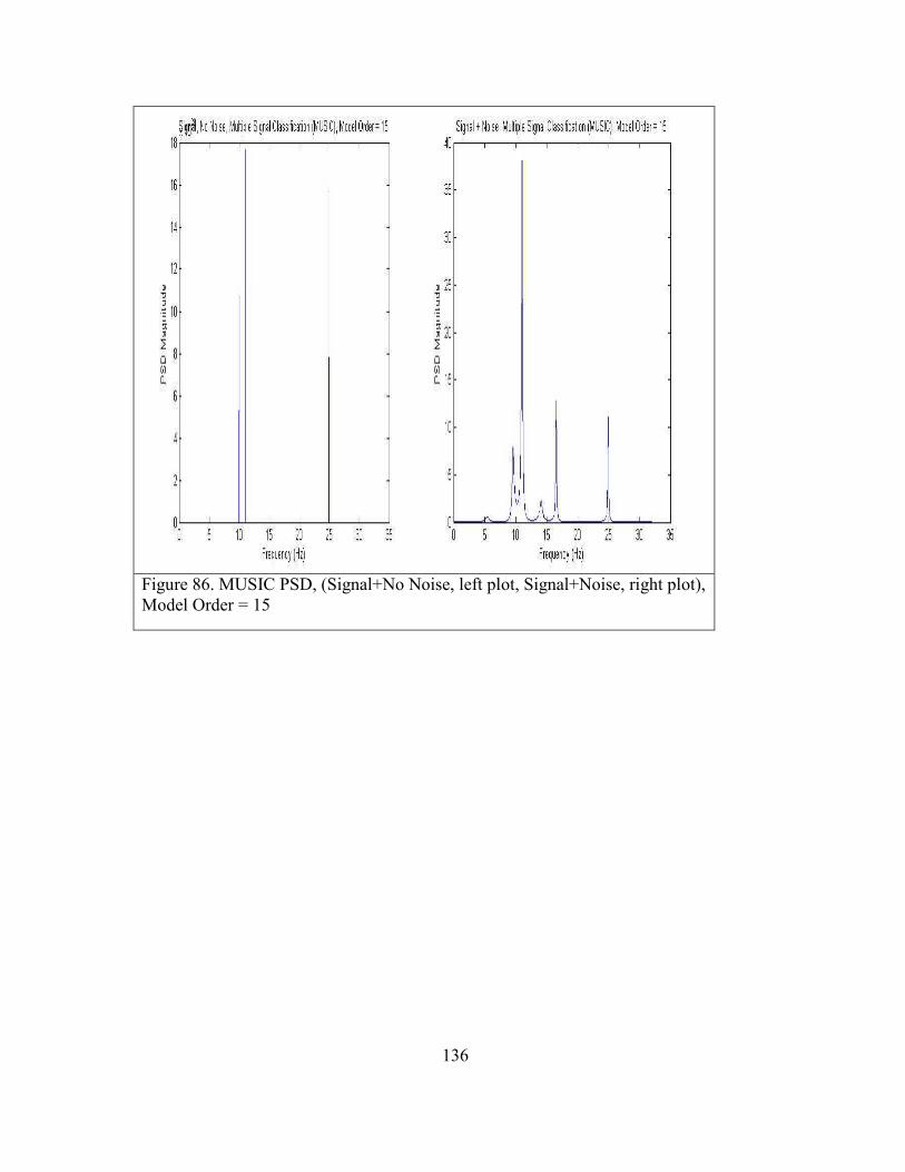
136

Figure 86. MUSIC PSD, (Signal+No Noise, left plot, Signal+Noise, right plot), Model Order = 15

137

Figure 87. MUSIC PSD, (Signal+No Noise, left plot, Signal+Noise, right plot), Model Order = 5

138

JMP Results

I model three input signals described above using MATLAB. Each signal was mixed

with White Gaussian Noise (WGN) with zero mean. I utilized the following estimation

methods as my algorithms in this experiment: Blackman-Tukey correlogram, Welch

Periodogram, Yule-Walker, Burg, Covariance, Modified Covariance, and Multiple Signal

Classification (MUSIC). I then measured the accuracy of the estimation method using a

low, medium, and high resolution factor (pertinent to each algorithm). The goal of this

test is determine which estimation algorithm is most accurate given similar resolution

factors. The way this is measured is to determine if, when I input three signals mixed

with random noise (two signals very close in frequency), that I can accurately estimate

the frequency of all three signals on the output. I ran 10 runs with each algorithm using a

random estimation model with a low, medium, and resolution factor for each algorithm.

JMP Output Data

The following output data was produced by JMP. I performed several tests to determine

if there was any interaction between the main effects: Algorithm and Resolution, as well

as, test the variances of each algorithm. I executed a one-way ANOVA, a two-way

ANOVA, several means tests, and finally the conclusion drawn from the two-way

ANOVA test output.

139

Figure 88. Output Results (Response) Table

The output response data table above is coded in the following way:

Table 10 Output Response Results (ANOVA)

1 All three signals correctly estimated

100

2 Only two signals correctly estimated

66.67

3 Only one signal correctly estimated

33.33

Runs

AlgorithmResolution 1 2 3 4 5 6 7 8 9 10

Mean

(u)

Blackman

Tukey High 100 66.67 100 100 66.67 100 100 100 66.7 66.7 86.668

Welch High 66.67 66.67 33.33 66.67 33.33 66.7 66.7 66.67 66.7 100 63.335

Yule Walker High 66.67 100 100 100 33.33 100 100 66.67 66.7 66.7 80.001

Burg High 66.67 66.67 66.67 66.67 66.67 66.7 66.7 33.33 66.7 66.7 63.336

Covariance High 66.67 100 66.67 33.33 66.67 33.3 100 33.33 66.7 66.7 63.334

Modified

Covariance High 66.67 33.33 33.33 100 100 66.7 33.3 100 100 100 73.333

MUSIC High 100 33.33 100 100 66.67 66.7 66.7 100 100 66.7 80.001

Blackman

Tukey Medium 66.67 66.67 66.67 66.67 66.67 33.3 66.7 66.67 66.7 66.7 63.336

Welch Medium 66.67 66.67 33.33 33.33 33.33 66.7 66.7 66.67 66.7 66.7 56.668

Yule Walker Medium 66.67 66.67 66.67 66.67 66.67 66.7 66.7 33.33 66.7 66.7 63.336

Burg Medium 66.67 66.67 66.67 66.67 33.33 66.7 66.7 66.67 66.7 66.7 63.336

Covariance Medium 66.67 66.67 66.67 33.33 66.67 33.3 66.7 66.67 66.7 66.7 60.002

Modified

Covariance Medium 33.33 33.33 66.67 66.67 66.67 66.7 66.7 66.67 66.7 66.7 60.002

MUSIC Medium 100 33.33 66.67 66.67 33.33 100 66.7 66.67 66.7 100 70.001

Blackman

Tukey Low 66.67 66.67 66.67 66.67 66.67 66.7 33.3 66.67 66.7 66.7 63.336

Welch Low 66.67 66.67 33.33 33.33 33.33 66.7 66.7 66.67 66.7 66.7 56.668

Yule Walker Low 66.67 66.67 66.67 66.67 66.67 66.7 66.7 66.67 66.7 66.7 66.67

Burg Low 66.67 66.67 66.67 66.67 33.33 66.7 66.7 66.67 66.7 66.7 63.336

Covariance Low 66.67 66.67 66.67 33.33 66.67 66.7 33.3 66.67 66.7 66.7 60.002

Modified

Covariance Low 33.33 0 66.67 66.67 66.67 66.7 66.7 66.67 66.7 33.3 53.335

MUSIC Low 33.33 66.67 33.33 66.67 33.33 66.7 66.7 66.67 33.3 33.3 50

140

Each algorithm is listed with its resolution factor level of Low, Medium, or High. We

expect to see the best results for each algorithm using the high resolution factor level.

JMP ANOVA (One-Way)

Figure 89. ANOVA analysis of output results (Plot 1: (L) Algorithm vs Mean & Plot 2: (R) Resolution vs Mean)

141

Response variable = mean output. I compared the mean output to both the algorithm and

the resolution of the algorithm model. I should see parallel quantile plots data versus

normal distribution. The tilt of each plot line indicates different standard deviations.

Also, the distance between the plot lines indicates differences in variances. I do note the

variances are different for each algorithm. Additionally, it is clear that the Burg

algorithm has the smallest variance. The different quantile box sizes strongly indicate

different variances.

Figure 90. ANOVA analysis of output results ((L) Algorithm vs Mean & (R) Resolution vs Mean)

142

Differences in variances are confirmed by the difference of variance test whose output is

displayed above.

Figure 91. ANOVA analysis of output results ((L) Algorithm vs Mean & (R) Resolution vs Mean) - Continued

The various differences in means are displayed above in the table. Note that the variance

for High resolution is quite different from both the low and medium resolution models.

143

JMP ANOVA (Two-Way)

Figure 92. (2-Way ANOVA) Full Factorial

The purpose of this test is to determine any interactions of the main effects. The Main

effects: Algorithm and Resolution with their interaction (Algorithm and Resolution). The

Least Squares Means plots [in the lower portion of the figure above] indicate that

resolution factor (P-Value) is a significant factor. At first glance it would seem there is a

significant interaction effect present -plot in lower portion of the 2-Way ANOVA

display; however, after review of the Effect Tests, it is clear that the P-Value is only

significant for the Resolution factor. There doesn’t appear to be a strong interaction

effect between factors Algorithm and Resolution.

144

JMP Results/Conclusion

Figure 93. Tukey HSD Means Test (Test for Interaction)

This indicates no strong interaction between Resolution and Algorithm. However, it does

suggest the major differences between the Algorithm and Resolution combinations. It

indicates that the Blackman Tukey algorithm model and the MUSIC algorithm model

when operated utilizing high resolution parameters provide the highest overall mean and

therefore the most accurate result of the algorithms tested.

In fact, the estimation accuracy of the algorithms is accurately described above. We can

therefore conclude that the best methods to estimate and calculate the PSD for wireless

signals are the top two algorithms: the Blackman Tukey using its high resolution factor

145

and the Yule Walker algorithm using its high resolution factor. Music using its high

resolution factor cannot be considered for wireless PSD estimation since the algorithm

loses the spectral power components of the signal; it is strictly to be used for estimating

frequency components, but not spectral power components. Note that some of the

algorithms perform better using their lower resolution factors than other algorithms that

are using their highest resolution factors.

146

CHAPTER 6

SYSTEM DESIGN

The hardware component types of the system design are the 802.11X and cellular base

stations and the cell controller. The base stations are comprised of a System on Chip

(SoC) that is comprised of symmetric multiprocessing General Purpose Processors

(GPP), a number of Digital Signal Processors (DSP), and a number of RF receive and

transmit chains. Both the transmitter and receiver will have an antenna. The receiver

may have a (e.g. Low Noise Amplifier) a matched filter on the front end as well as an

Analog to Digital Converter (ADC), the transmitter will have a Digital to Analog

Converter (DAC) and may have a LNA along with an impedance matching circuit to

ensure VSWR is not produced. The focus on the design of the base station is to ensure

the design allows for a continual evolution in regard to the physical modulation

techniques. The design needs to be capable of adapting to changes in the modulation

techniques. The design also must ensure that the receive sensitivity is sufficient to

receive the minimum desired signal. The receive sensitivity can be defined as the

minimum desired signal power above the noise floor of the receiver as defined by the

following equation:

m)+ / =K=*N+iq³i ¼h7ih¼

(158)

System-On-Chip (SoC) designs now include GPP and a number of DSPs are typical.

Often these designs do include an FPGA, however, some implementations are now

focusing on DSP arrays such as those provided by Picochip (now Mindspeed) and

Coherent Logix (HyperX). In these cases, small FPGAs are used for I/O multiplexing

147

only while all DSP functions are performed in software on DSP arrays (27nm

technology) fully integrated with DSP tools such as MATLAB and SIMULINK.

The cell controller is comprised of specialized hardware that is designed to perform high

performance network frame processing and will be designed to handle > 40Gbs encrypted

link layer network traffic. In order for the cell controller to handle encrypted network

traffic at this rate, it must have a hardware based data path. The hardware data path

requires the following functions:

Classification of network frames. This is required so that frames with encrypted traffic

can be characterized based upon the source MAC address of the mobile device that

transmitted the frame as well as any relevant network headers such as VLAN tags. Once

classification is performed, the address of the received frame must be distributed to a

cryptography engine for decryption as well as pre and post processing engines. The

following packet walkthrough is an example of an architecture where majority of frame

processing is off-loaded from GPP and GPU cores within a SoC.

148

Figure 94. Packet Walkthrough on Example SoC,(Freescale, 2014) With Newly Proposed/Designed Wireless Link Layer Capability

The HW state machine described above require their own Direct Memory Address

(DMA) engines to read and write data to and from memory as required during frame

processing through a memory gasket and memory controller. Such a configuration would

require a GPP to provide configuration and management of the HW during its

configuration and boot cycles [this is sometimes referred to as the control plane]. In

addition, it would require a slow speed peripheral memory bus so that configuration

registers on the HW could be modified during configuration. A GPP would also be

required to handle exceptional conditions that occur during frame processing such as

error frames and could be helpful in handling conditions that were not perceived during

HW design.

149

Since both configurations require frame processing, additional aspects of the design need

to be considered. What is the queue latency of frame processing? For instance, must

frame be processed strictly in the order they are received or can some frames be

processed in parallel. For performance reasons, if multiple channels are required, frames

should be allowed to be multiplexed to different dedicated HW blocks at the same time.

However, this implies that the adaptive properties of each channel must be maintained by

all dedicated HW IP blocks. These properties would have to be stored in memory and

then retrieved from memory as different blocks receive frames that require different

adaptive properties. Therefore, a cache is required to ensure unnecessary memory fetches

were not required by the DMA engine prior to processing a frame. In order to determine

which adaptive properties are required to be loaded by the HW block requires

classification of network and wireless frames as they are received. Additional dedicated

HW is required to handle frame classification and queuing logic. These HW state

machines would communicate to each other via private, HW dedicated buses between the

frame processor, the queue processor, and the link layer encryption HW IP blocks. The

GPP core(s) would provide the ability to configure the HW registers in each of these

blocks via a peripheral memory bus. The peripheral memory bus would also be used for

monitoring, dynamic reconfiguration, error conditions, and management (thru a network

interface). In this approach, memory transactions are limited to the frame processor and

link layer encryption blocks. HW blocks utilize a private bus for communication and the

GPP only accesses memory a very small percentage of time mostly for monitoring and

management functions. Additional provisions can be provided that force received frames

to be stored on memory aligned pages thereby reducing non-aligned memory transactions

150

to a very small percentage of overall memory transactions. HW would generate memory

transactions to access adaptive properties stored on a per channel basis.

A key component of the HW data path is the wireless MAC engine. This programmable

engine bridges wireless frames to the wired interface, decrypts/encrypts wireless link

layer data & management frames, performs RF measurements of mobile devices,

implements wireless roaming between base stations, provides network proxy ARP (if

required) for mobile devices, provides per device instruction execution, and monitors the

state of the mobile device at all times. As depicted in Figure 57, the wireless MAC engine

uses information such as instructions, VLAN tag info, 802.11 or cellular MAC template

(used to modify frames to and from the mobile device), and reserved memory that is used

by the engine in real-time to modify and/or bridge wireless frames.

Hardware Design And Verification

The most important step in hardware design is to ensure the requirements are well

defined and understood. In particular functions that implement features such as the

wireless link layer MAC subsystem I described earlier in this paper must be implemented

with a thorough knowledge of the protocols so the proper functional decomposition can

be accomplished between software and hardware. In particular, standards in the wireless

area are changing all the time; the portions of the system that have a high degree of

volatility should be implemented in software. However, after many years the data path

for these technologies continues to converge toward IP based protocol services. The LTE

EPC now is moving all traffic (even voice) to IP based data frames. This commonality

151

aids in the development of hardware to support the data path. This ensures that even the

latest technology can benefit from the development of this type of hardware technology.

However, even functions that are implemented in software still require hardware support.

Often this aspect is overlooked during the system design phase. For instance, how does

software interact with the hardware to redirect its data path to a new base station? As

discussed earlier, this requires a hardware synchronized ability to perform an atomic

operation while the data path is still active. Interruption of the data path would cause

delay in frame transmissions to a device and reduce its perceived performance. In this

case hardware must enable the ability to be updated on a per user basis without mobile

devices losing their connectivity and network access. In order to implement this new

hardware feature, a systematic review of all 802.11 and cellular specifications would be

required to determine what features requirements would be required to achieve the end

goal of having all data and voice packets from wireless technology to be handled fully in

hardware (e.g. data path acceleration architecture).

Once the requirements have been completed and fully understood, the hardware interface

requirements with other subsystems within the SoC must be evaluated to determine if

they will impede the wireless subsystem from achieving its functional or performance

requirements. All electrical interfaces have to be evaluated to ensure that they meet the

performance bench marks and that there is sufficient electrical interface support for

system level interfaces required from other subsystems.

152

During Verilog development there should be well defined interfaces between the

functional hardware blocks. This is important at the very beginning because too often

functions are duplicated or require too many additional wires of communication between

the blocks which increases the die size, increases complexity, and increase the likelihood

of failure particularly when implementing large designs. Implementation of

combinatorial logic blocks should be consistent throughout the design to reduce

complexity as an example when many personnel work on the same project. Once

sufficient subsystems have been implemented, software should be written to interact with

the test hardware simulation interfaces as early and often as possible so that problems can

be spotted as early as possible. Figure 95 depicts such an environment where Linux

executes on a simulation of the processor instruction set and the software drivers are

written within this environment to interact directly with the Verilog co-simulation

environment through the use of SystemC adapters. The SystemC co-simulation adapters

are provided by companies such as Virtutech (processor/system simulator and SystemC

adapter) and Cadence tools (Verilog/SystemC adapters and simulator). Software

engineers can implement software and test against the actual hardware during the

hardware development cycle prior to hardware synthesis. In addition, randomized

hardware simulations should run continuously (with hardware simulation probes) to catch

timing problems and error signals that are caught during execution. When a random

simulation fails, it is important to reproduce the failure; the hardware test co-simulation

software should record parametric configuration information captured before each test.

In only this way will test be reproduced and problems resolved efficiently.

153

Once all electrical interfaces have been defined, then these interfaces and their

descriptions and definitions go into a requirements verification test matrix (RVTM), unit

level test benches are created that imitate the electrical interfaces from other subsystems

as well as connect all electrical interfaces to hardware signal sources. This enables the

unit level tests to randomize patterns and clock edges across these electrical interfaces so

that problems can be identified early and often. These tests then would feed into a larger

collection of tests that are executed by system level test execution.

Hardware Simulation And Verification

In order to design the hardware and verify the function of a hardware subsystem, a

hardware co-simulation environment is required. This foundation for this environment is

comprised of Verilog simulation using tools such as those developed by Cadence.

Layered above this foundation are the Verilog hardware finite state machines that must

be tested. In addition, software libraries built with the SystemC library are also used to

drive bus functional models to test the hardware. The Cadence co-simulation library

provides SystemC adapters for their simulation environment that allow a SystemC model

to connect digital logic to hardware connector names. Typically this is done through

what is referred to as a “bus functional model”. Such a model supports the ability to test

individual hardware subsystems. Hardware subsystems interact with each other through

the use of logic signals and buses. Assuming no transitional change of clock domains, all

hardware subsystems are clocked with the same clock source; however, there are clock

delays through different components used in a Verilog model such as combinatorial and

sequential logic. Testing of individual subsystems entail the use of randomization of

154

clock signals and data bits across all data buses and should include the variance of the

clock signals within the specified operational range. As with all logic signals, these

signals will vary temporarily (within a range) as a function of temperature and variances

in the silicon and randomization of the skew of the clock signal is crucial to identify

problems before synthesis. Building upon these subsystem tests, the subsystems are then

connected together. New Bus Functional Models (BFM) are built that represent the new

or combination of the new digital interfaces. As the tests include more and more logic

blocks that must be simulated, the hardware test (SystemC) library needs to ensure that it

is built as optimally as possible. The model must reduce unnecessary events (such as per

pin events on a clock edge as an example), but be based upon a concept referred to as

Transaction Level Modeling (TLM). This approach focuses on functional block events

instead of events produced on each individual clock edge. When developing BFMs to

connect to subsystems under test, it is important to base the event structure on TLM

concepts. This approach still provides a very accurate digital signal timing display while

the model runs at a very high rate of speed. As shown Figure 95, hardware models of IP

within a SoC can be in a near cycle accurate way, with very acceptable performance,

using the TLM based transaction model approach. In this example (Figure 95), a Linux

operating system is executing on a simulation of the Power Architecture instruction set

while executing a Linux kernel module that actually runs against the real hardware

simulation using a shared (shared between the processor simulation) and the SystemC

adapter that drives the logic pins on the Verilog model. The Verilog model actually

executed and reacted as if it were already synthesized as part of the SoC. This testing

would ensure that the Wireless Link Layer Subsystem hardware IP will execute as

155

expected in real platform environments and ensure early testing of software can occur

prior to tape-out of hardware.

Hardware tests are executed at the intended simulated clock speed of the hardware and

are executed using a simulated clock signal at the programmed clock speed. An example

of tests that are executed include the ability to skew the input and output digital signals in

a random way to ensure the finite state machines are robust enough to handle differences

found in silicon after SoC synthesis has occurred. Other tests include functionality tests

to ensure that functions within the hardware Intellectual Property (IP) works as intended.

Other tests include the random ordering of memory transactions to and from the hardware

IP as well as negative testing. This simulation test software executes quickly because a

very lightweight threading model is used to drive the hardware state machines. All

hardware state machines are executed in simulation as they would in hardware. Each

independently clocked state machine is another thread that executes in a round robin

fashion to ensure that all clock dependencies are enforced.

Figure 95. Example of a HW Design/IP Verification and Unit Test Environment

156

This same model can then be applied to a real synthesized SoC. Instead of the peripheral

and memory buses being simulated virtual memory of a test processor running our

memory simulation model, we use real system memory and write to real peripheral bus

memory interfaces. Thus no changes to the actual tests need occur, just simply modify

the memory adapters in the model so they map directly to SoC memory, not simulation

memory. An example of this is depicted in Figure 96.

Figure 96. Unit Co-Simulation Test Environment Ported to Real Silicon

Note how the Linux kernel modules (e.g. drivers) are used to provide the mapping

between application simulation memory and real system memory. The hardware only

understand hardware addresses, so all memory translations must occur between the co-

simulation application and the real hardware memory map. Thus, the memory writes all

occur (not across a simulated bus to simulated memory) to real system memory.

157

Randomization of clock gitter has been especially helpful in finding bugs that may have

escaped our testing prior to developeing this functional verification, validation, and

performance testing software tools and libraries.

Hardware Performance Simulation

Figure 97. HW Co-Simulation Environment that can be used to test HW Performance

Using the Cadence co-simulation environment with a simulated memory gasket and a

robust SystemC test class library, unit level tests can be executed at the simulated clock

rate that the target hardware will execute. By measuring simulation time, number of

hardware clocks, and unit of time (e.g. seconds), hardware IP designers can ascertain if

the design meets the required performance specifications. In addition to running the

design as a cycle-accurate simulation, this environment can support executing the design

at higher than planned clock rates to determine how performance can be improved in the

future. This environment also includes randomization of the address ranges utilized so

that an accurate model can be measured as it relates to real-world memory latency due to

system memory collisions (e.g. heavy utilization). HW performance is not based upon

158

raw bus rates, it based upon the ability of the hardware to reach a rate of speed that meets

the minimum performance specifications. For example, a memory gasket can perform at

6.4GB/sec; however, it can never reach that because it can only support 3 memory

transactions at one time. This is because the memory bus interface being used will only

be used for a large number of relatively short memory transactions, not one large

transaction. Therefore, though the raw performance of the bus is impressive, it does not

meet the requirements because with only 3 transactions allowed in parallel, we are

limited to only a very small fraction of the maximum bandwidth.

This does not replace the testing of subsystems that interact with the hardware IP under

test. Connected subsystems must meet their performance specification and must be

tested to ensure their committed performance target is met when used as intended by the

end product user. Hardware can be designed to meet a performance specification, but the

preconditions and post conditions are important. If the only way the hardware is going to

meet its performance target is to use it in a way that would never occur in its actual use, it

should be considered compliant with the requirements.

159

CHAPTER 7

5G SYSTEM PERFORMANCE ENHANCEMENTS

The final research focused on proposed improvements to accommodate 5G

communication systems. I focused on three areas: Beamforming, voice communication

and wireless roaming performance. These areas were chosen because of their

consequential impact to 5G wireless performance. This research starts out with a short,

abbreviated introduction of the recent 3GPP specification changes as it relates to 5G.

Following this short introduction, I described proposed improvements in adaptive

beamforming, directing energy towards end users. Next, I describe a proposed

improvement in voice communication related to the well-known Levinson-Durbin

algorithm. Lastly, an improvement in wireless roaming is proposed that reduces the

number of interactions required by the mobile device as well as fewer 3GPP state

machine operations on the 5G UE.

5G Introduction

The 3GPP new radio (NR) in release 15 provides both a non-standalone operation (used

in concert with existing LTE network technology) and a full release for the standalone

version which was scheduled for September 2018. The 5G capabilities include some of

the following attributes:

1. Network can support both LTE and 5G NR, including dual connectivity where

devices connected to both LTE and 5G NR which is referred to as dual connectivity

(DC).

2. Carrier aggregation up to 32 carrier components (CC) with 16 CCs in 5G NR.

160

3. Massive MIMO and beamforming

4. FDD and TDD support for 5G NR frequency bands.

5. Forward error correction utilizes computationally more efficient Low Density

Parity Codes (LDPC) are used in place of Turbo Codes at higher data rates.

6. Polar codes are used on the enhanced Mobile Broad Band (eMBB) control

channels for the 5G NR interface.

7. Cloud RAN support replaces LTE PDCP and radio link layer (RLC) protocol

layers.

8. Lower latency time intervals

9. QoS support using a new model (see user based QoS)

10. Co-existence with LTE in the same radio channels

Policy and charging rules function (PCRF) are not depicted (see Figure 56). The

following diagram is the cutout for the 4G portion of the design depicted in Figure 56).

Note that both 3G and 4G utilize a P-GW subsystem for network address translation

(NAT) toward the rest of the network (RoN).

161

Figure 98 4G / 5G Integration (Release 15)

The 3GPP specification committee is specifying the first phase of 5G in Release 15. To

enable wireless operators to deploy 5G quicker, the committee divided release 15 into

two parts. The first set of requirements define how a 5G Radio Access Network (RAN)

can integrate with an LTE network, this is called a non-standalone option. Such 5G

deployments rely upon an existing LTE network in both the RAN and the EPC.

162

Figure 99 5G Cloud Service Integration (High Level) Options (Modified 3GPP)

The 5G release has been split into two releases: Release 15, which corresponds to NR

phase 1, and release 16, which corresponds to NR phase 2. The table below describes

3GPP release 15 NR phase 1 which has put forth some requirements for 5G that focus on

fulfilling three key performance indicates (KPIs):

• Greater than 10Gbs peak data rates for the enhanced mobile broadband (eMBB)

• Greater than 1M/km2 connections for massive machine-type communications

• Less than 1msec latency for low-latency communications (URLLC)

Previously, 3GPP and IEEE committees have defined RAT types such as LTE (E-UTRA)

and the WLAN 802.11 family of standards that are in wide use for cellular and wireless

access. The new 5G RAT in 3GPP releases 14,15 and 16 which also includes Internet of

Things (IoT) machine to machine communication access methods.

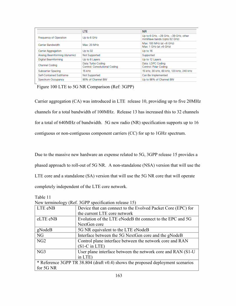
163

Figure 100 LTE to 5G NR Comparison (Ref: 3GPP)

Carrier aggregation (CA) was introduced in LTE release 10, providing up to five 20MHz

channels for a total bandwidth of 100MHz. Release 13 has increased this to 32 channels

for a total of 640MHz of bandwidth. 5G new radio (NR) specification supports up to 16

contiguous or non-contiguous component carriers (CC) for up to 1GHz spectrum.

Due to the massive new hardware an expense related to 5G, 3GPP release 15 provides a

phased approach to roll-out of 5G NR. A non-standalone (NSA) version that will use the

LTE core and a standalone (SA) version that will use the 5G NR core that will operate

completely independent of the LTE core network.

Table 11 New terminology (Ref. 3GPP specification release 15) LTE eNB Device that can connect to the Evolved Packet Core (EPC) for

the current LTE core network eLTE eNB Evolution of the LTE eNodeB tht connect to the EPC and 5G

NextGen core gNodeB 5G NR equivalent to the LTE eNodeB NG Interface between the 5G NextGen core and the gNodeB NG2 Control plane interface between the network core and RAN

(S1-C in LTE) NG3 User plane interface between the network core and RAN (S1-U

in LTE) * Reference 3GPP TR 38.804 (draft v0.4) shows the proposed deployment scenarios for 5G NR

164

Figure 101 Release 15, Supported 4G and 5G Integration Use Cases

For non-stand alone operation, a frequency plan is proposed between LTE and the 5G NR

for dual connectivity. The following table from 3GPP release 15 specifies the how LTE

bands correspond to proposed 5G NR frequency ranges.

165

Figure 102 New 5G NR Proposed Core (Ref: 3GPP)

5G Downlink

To define this quantitatively, we will briefly describe the 5G communication channels in

more detail. A description of the stacks will be described followed by a representation of

the improvements to increase performance in the following areas: Beam Forming, Voice

Communication and data transport. To provide proper context, a brief introductory

description of the downlink stack followed by the uplink stack will follow.

Figure 103 5G Uplink/Downlink Stack

166

The lowest level of the protocol stack is the physical layer (PHY) that includes the

physical modulation orthogonal frequency division modulation (OFDM) with M-ARY

subcarrier modulation. The transport block, delivered from the PHY to the media access

(MAC) layer, it contains data from the previous radio subframe. It may contain multiple

or partial packets, depending on scheduling and modulation. The MAC level functions is

responsible for transport block (see Figure 104) retransmission, referred to as hybrid

automatic repeat-request (HARQ) implemented as layer 2 transmission retry.

Figure 104 Exemplar: 4G Model – Next changes to model (5G Specification is Not Final)

The mapping of the MAC logical to physical channels follows in the diagram below. The

control channel in the lower portion of the picture is used for scheduling, signaling and

other low-level functions. The downlink shared channel contains both a transport

167

channel for paging and for the downlink of data. The physical broadcast channel flows

all the way through for broadcast.

Figure 105 MAC Downlink Mapping (Unchanged in 5G)

The transport channels above user different modulations and coding. Paging and

broadcast channels must be received everywhere in the cell, so they must use robust

modulation. The DL-SCH can be optimized by the UE.

• Dedicated Control Channel (DCCH): A point-to-point bi-directional channel that

transmits dedicated information between a UE and the network.

• Paging Control Channel (PCCH): A downlink channel that transfers paging

information. This channel is used when the network does not know the location cell of

the UE.

168

• Common Control Channel (CCCH): Uplink channel for transmitting control

information between UE and network. This channel is used by the UE having no RRC

connection with the network.

• Dedicated Traffic Channel (DTCH): A point-to-point channel, dedicated to one

UE for the transfer of user information. A DTCH can exist in both uplink and downlink.

• Broadcast Control Channel (BCCH): A downlink channel for broadcasting system

control information.

• Multicast Control Channel (MCCH): A downlink channel for multicast system

control information

• Multicast Traffic Channel (MTCH): A downlink channel for multicast traffic

The UE interprets the transport format field in the downlink MAC which provides the

Modulation Coding Scheme (MCS) for the next transport block; the MCS changes

dynamically. The MAC also coordinates measures from the local PHY to the RRC

regarding local status and conditions, and RRC reports back to the eNodeB using control

messages. From the eNodeB to the RRC, the RRC controls modulation and configuration

settings. MAC measurements support downlink scheduling based upon Bit Error Rates

(BER) and radio conditions at the UE. Buffer status reports are conveyed via the RRC to

ensure flow control is maintained between UE and eNodeB.

The Radio Link Control (RLC) performs segmentation and reassembly. The RLC

operates in three modes: transparent, unacknowledged, and acknowledged. The RLC

provides in-sequence and duplicate detection. The segmentation process involves

unpacking an RLC PDU into RLC SDU (or portions of SDUs). The RLC PDU size is

169

not a fixed because it depends upon the conditions of the channel, it is based on the

transport block (TB) size. The condition of the channel varies due to bandwidth

requirements, distance, power levels and modulation scheme.

The Packet Data Convergence Protocol (PDCP) layer in the user plane is used for packet

data bearers, circuit switched bearers, performs decryption, ROHC header

decompression, sequence numbering and duplicate removal. In the control plane, it is

used for decryption, integrity protection, sequence numbering and duplicate removal.

The ROHC is defined in IETF RFC3095, RFC4815 and RFC3843.

5G Uplink

In 4G LTE and 5G the processes on the uplink side are similar to processes on the

downlink side. In 4G the peak data rate is half that of downlink; access is granted by the

eNodeB; there are changes in logical channels and transport channels; and random access

is used for initial transmissions. The 4G PHY uses SC-FDMA for the uplink because it

has a lower peak-average ratio, which allows a more power-efficient transmitter in the

UE. In 5G NR the uplink modulation is DFT-S-OFDM and CP-OFDM; however, the

uplink performance is approximately the same between 4G and 5G.

Synchronization signals (SS) and system information transmit basic information to all

user equipment. Timing information is shared with all devices the transmitter and

receiver can synchronize, the receiver can perform synchronous detection and

demodulation of the transmitted information from the UE. This is accomplished using

170

the synchronization signal block (SSB) through the physical broadcast channel (PBCH).

LTE 4G has only one pattern of SSB transmission in time domain (see diagram below).

Figure 106 4G PBCH, FDD Normal CP, 20MHz (Ref:3GPP)

Time Domain transmission pattern of SS Block in 5G NR is more complicated than LTE

SS Block (see Figure 106) In 4G LTE, the subframe number and the OFDM symbol

number are within the subframe is always the same. In 5G NR, there are many different

cases of Time Domain pattern of SSB Transmission as illustrated below (see Figure 107).

171

Figure 107 5G PBCH, Changes, Normal CP, FDD 20MHz (Ref: 3GPP)

In order for data to be transmitted the FFT processor of the IFFT is combined into a time

domain composite signal which is used to reduce the number of FFT streams required to

support the communication of information across 1024 subcarriers, utilizing a linear

modulation, such as QPSK as an example, the complex symbol amplitude and phase is

modulated according to the associated I/Q constellation and is then multiplied with the

individual subcarriers to convey the information on the downlink. This means 1200

resource elements carrying 1200 different complex symbols over 1200 subcarriers. Each

subcarrier is assigned to different users. Utilizing the IFFT function, these subcarriers are

combined into samples of a composite time domain signal. These time domain samples

are then transmitted as the downlink where users pull out the information allocated for

them. As a function of the reception of by the handheld devices, a waveform windowing

function is used to reduce the inter-user interference due to non-zero out-of-band

emission.

172

Performance Improvements

The following performance improvements in the areas of adaptive beamforming, voice

modeling, and roaming performance. Each improvement will be quantified and described

in detail. An additional improvement, is in microwave component design. 5G NR

requirements inform us of our receiver design and specifically our microwave component

design that enables the performance of the receive and transmit chains. The channel

spacing below is defined as 15KHz and defines the required phase noise and receiver

sensitivity required. Since 5G has higher path loss, signal to noise ratio (SNR) is

important, therefore, receiver sensitivity is even more important than was previously the

case. The following equation, derived from equation 14, defines our phase noise

requirements:

Assuming that carrier power (C) and interference power (I) are the same, to achieve 50dB

of adjacent channel rejection, we must achieve a phase noise (L) of the following:

I ∶= '50G ' 10 .C 18A] = '92GM/A]

(159)

The channel structure defined below requires -92dBc/Hz of phase noise offset from the

tuned frequency of the receiver. In order to reduce the peak to average ration and increase

the efficiency of the power amplifier and save battery life, the uplink is different for both

4G and 5G LTE. As depicted in the diagram (see Figure 104), the uplink signal has a

very short symbol duration and sends the same data over multiple subcarriers, while the

CP-OFDM downlink utilizes long symbol durations of 66.7usec duration. In a 20MHz

bandwidth, the highest frequency is 9MHz and therefore requires 18Msps Nyquist based

sampling or 1200 samples per symbol. For backwards compatibility with UMTS

sampling rate of 3.84Msps, LTE 4G and 5G utilize 30.72Msps, a multiple of the

173

3.84Msps, for a 20MHz bandwidth providing 2048 samples per symbol. To improve

latency, a change to the original OFDM modulation scheme has been proposed to add a

scalable modulation framework by adding different time slots of 1, 2, 4, 8, 16 or 32. This

thereby reduces the minimum transport block size to .hrr = 31.258=*M.

1 Radio Frame= 10 subframes

10ms1ms

1 Subframe

Time

1ms

1 Subframe 32 Slots = 31.25usec

1 Slot = 14 Symbols

Figure 108 Proposed Change to Reduce Latency to 1msec (Ref: 3GPP)

5G downlink utilized CP-OFDM which is also used by 4G LTE. 5G has changed the

uplink frequency to a factor of 2:

480A] = 2 15*3A], )!*+*8 = 0 ' 5

(160)

Adaptive Beam Forming

LTE has been a continuous evolution of spatially diverse, multi-antenna transmission

encompassed in spatial multiplexing (SU-MIMO) and SDMA (MU-MIMO). Multiple

Input, multiple output (MIMO) becomes an even more important component of the

5GNR RAT. The 5G NodeB has two TxRus per polarization, which are connected to

cross polarized Tx antenna panels. The 5G NodeB selects one analog beam on each

174

antenna panel polarization for the downlink MIMO transmission. The UE must be able

to measure multiple Tx beams swept on different time units on each panel polarization

and select which Tx beam is the best beam. For higher frequencies, beamforming is a

necessity due to increased path loss.

Figure 109 High Frequency Beamforming Necessary to increase Directivity towards Mobile Devices

The following frequency ranges related to mm-Wave are only proposed at this time and

are not intended to be final specifications:

Figure 110 5G Frequency Coverage Plan (Ref: 3GPP)

175

The initial access procedure for all user equipment is provided by a beam sweep to all

user equipment (UE) is accomplished through a user beam transmit sweep. Timing

synchronization information is provided to all devices. For high frequency applications,

the beam is highly directional and therefore requires multiple transmissions in the

following manner:

Figure 111 Beam Sweeping provides basic information to UE’s

Beamforming and MIMO Wireless Technologies such as Wi-Fi and Cellular are converging in the market place.

This convergence promotes a need for a different link layer protocol stack technology

that better facilitates the convergence of these technologies both from the radio frequency

(RF) modulation adaptation perspective as well as from the link layer protocol

perspective. This convergence has also driven a desire to increase bandwidth, reduce

symmetrically Gaussian noise, reduce insertion loss and increase carrier signal frequency.

These performance improvements are addressed utilizing microwave component design,

digital signal processing (DSP) and aperture [material and structural] design; both

176

aperture and digital signal processing are required for ‘smart’ antenna system design.

This paper will introduce the use of a new vector antenna technology to improve the

performance of modern communication signal sets in concert with massive MIMO, such

as those proposed in 5G communication proposals, in concert with a patented link layer

routing protocol stack concept.

Figure 112 Process of Receiving Energy from UE and Redirecting a Response to that Device

We will define the use spatial and vector arrays in a cellular system. Algorithms will be

utilized to receive and beam form energy towards individual devices with in the cell

being serviced by the wireless base station. According to the specifications, 1M/km2

connections must be supported for device-to-device communication support and is based

upon the following mathematical model:

= =K%. º 1JG Y 2.782 ' Z» ,A?;m)*+*?9KG<! Am= | ' %| (161)

177

= 'JG =K C, )!*+*C = <**+KS*

(162)

Spatial Arrays

A spatial array utilizes spatial diversity with spacing relative to so that angles of arrival

can be estimated. Spacing of < removes grating lobes and improves aperture cross-

section efficiency. Spatial arrays are used in an adaptive way to service numerous

sensors at once in a network scenario. In such a configuration, a device responds to the

PRACH channel of the wireless base station. Timing synchronization messages are

broadcast by the wireless base station. The PBCH channel sends the physical cell ID

(PCI) which contains the cell group id and the cell id. The user equipment (UE) response

impinges on the following array elements:

Two spatial array approaches were analyzed to determine the algorithm execution

required to determine the direction of propagation such that an adequate response is

possible in the correct direction to the received signal. Since a-priori knowledge of the

received signal is determined through the broadcast channel (PBCH), and assuming a

digital beam former (DBF), the weights of the received signal are determined and the

direction of arrival (DOA) is computed in the following manner:

We will assume digital beam forming with an analog band pass filter along with a low

noise amplifier (LNA), that sets the noise figure of the receiver, which provides the

analog bandwidth that is digitally sampled. Signals are received through a spatial array

which has an array manifold; the array manifold vector is also referred to as the array

steering vector:

178

? = 1 *D ¤¼ 7/ ∆ ⋯ * 6%. ¤¼ 7/ ∆

(163)

J = 2O , G = W*9*<=@?MK, = #;**9*<= = W*M<+KM?m!?=*PK;;*+*M*:*<)**<)?Gn?M*<**9*<=

ØÙÙÚ±CJ±.J±J±rJÛÜ

ÜÝ = ØÙÙÚ ?C C ⋯ ?C i%.?. C ⋯ ?. i%.? C ⋯ ? i%.?6%. C ⋯ ?6%. i%.ÛÜ

ÜÝ ØÙÙÚ CJ.JJi%.JÛÜ

ÜÝ ØÙÙÚ CJ.JJ6%.JÛÜ

ÜÝ (164)

The matrix ?/ is a vandermonde matrix structure referred to as matrix A. But what

do we do when N is very large? It is no longer practical to execute a matrix operation that

could handle large > 100 element matrices.

Figure 113 Uniform Pattern 10x10 Panel = 30, = 45

As depicted the diagram above, the uniform array is symmetric. The major lobes exist

above and below the horizontal because of the array symmetry. The array has a major

lobe and 30 degrees as well as at 120 degrees symmetric around 90 degrees at broadside.

179

The algorithm will be defined to cover a large number of elements and how the algorithm

will scale according to these large number of elements. We will describe how MIMO is

used in concert with beamforming to improve communications with individual user

devices.

Figure 114 Adaptive Beam Forming Increases the number of devices serviced simultaneously

Beam selection is comprised of a large number of antennas which can be comprised of a

uniform, Dolph-Tschebyscheff or binomial planar array. Planar arrays can be

rectangular, circular or an irregular shape. Irregular shapes are used to address spatial

ambiguity for a variety of apertures when wider frequency band coverage is required for

DOA analysis and beamforming where avoiding grating lobes is important; as the

frequencies change, the relationship changes. While the uniform array yields the best

(smallest) half-power beamwidth, superior side lobe performance is provided by the

binomial array. Due to the large number of elements required for 5G communication,

180

binomial arrays are not practical because of the wide variations of amplitudes required

across the array. Uniform arrays have the best directivity and their manufacturability

makes them the best choice for 5G communication.

A beamforming array is steered towards an azimuth and elevation through a set of

weights that are expressed through the array manifold or steering vector. Signals are

received through a spatial array which has an array manifold; the array manifold vector is

also referred to as the array steering vector:

? = 1 *D ¤¼ 7/ ∆ ⋯ * 6%. ¤¼ 7/ ∆

(165)

J = 2O , G = W*9*<=@?MK, = #;**9*<=

= W*M<+KM?m!?=*PK;;*+*M*:*<)**<)?Gn?M*<**9*<=

The steering is performed by changing the electrical phase on each element. Normally,

these values are pre-constructed towards a pre-defined set of angles that have been

calibrated per frequency and beam angle.

Figure 115 Beam Forming Processing Chain

181

A beamformer is a weighted sum of sampled baseband signals. By adapting complex

weights, we can define the beam pattern. A beamformer in a uniform linear array is

analogous to finite impulse response (FIR) filter design by windows. Window functions

such as Hanning reduce the side lobe level of beam steering angles. The diagram below

describes the beam forming process. The weights in the diagram below are complex

weights (real and imaginary).

Figure 116 Adaptive Antenna Sensor Weights Updated Dynamically

Two algorithms were evaluated to determine the best in adapting the beam pattern based

upon a wireless device accessing the base station. The beam is adapting as signals of

interest are received so the beam will steer towards the device of interest during

communication.

182

The 1st algorithm evaluated was the Least Mean Square (LMS) algorithm. The following

equation describes this algorithm process:

¤. = ¤ 2±¤ G¤ ' ±¤¤

(166)

The 2nd algorithm evaluated was the Recursive Least Square (RLS) algorithm. The

following equation describes this algorithm process:

/. = û%.`%. &/.1 û%.&/. `%. &/. (167)

*/. = G/. ' : &/. (168)

:/. = :/ /.*/.

(169)

`%. 1 = û%.`%. ' û%./.&/. `%.

(170)

The following performance was observed. As the graphs depict, the RLS algorithm does

converge more quickly than the LMS algorithm providing an improvement of

approximately 10dB in mean square error (MSE). Since beam steering events are

frequent and numerous, the convergence time improves performance of the wireless

communication link during communication events with a large number of wireless

devices.

183

Figure 117 Beam Forming Weight Convergence Performance Improved by RLS Algorithm

Based upon a savings of 15 iterations per wireless beam forming steer event, for a worst

case of approximately 1M/km2 devices.

184

Figure 118 Uniform Pattern = 30, = 45

Table 12 Performance Estimates of Spatial Diversity Aperture (RLS)

Array Size Performance (10x10)

(MATLAB)

RLS (MATLAB) Measured Performance (usec)

Samples

Ê 10 = 2.15 10% 12928 Ê 1000

Ê 10 = 2.15 10% 12826 Ê 2000

Ê 10 = 2.15 10% 12864 Ê 4000

185

Table 13 Performance Estimates of Spatial Diversity Aperture (LMS)

Array Size Performance (10x10) (MATLAB)

LMS (MATLAB) Measured Performance (usec)

Samples

Ê 10 = 2.15 10% 4672 Ê 1000

Ê 10 = 2.15 10% 1589.5 Ê 2000

Ê 10 = 2.15 10% 742.5 Ê 4000

Two approaches were investigated along with algorithms to compare the overall

performance of each approach: spatial arrays, vector arrays. This work focused on using

antenna arrays or smart antennas to increase capacity of the network. The signal

processing algorithms that are important in these applications are direction of arrival

estimators and adaptive beamformers. The following will describe the attributes

associated with arrival estimators and adaptive beamforming algorithms.

A broad category of arrival estimators can be addressed by evaluating two categories of

estimators. Those estimators using spatial diversity and those using a vector aperture.

The first category will be spatial arrays followed by vector aperture arrays. This will be

covered in the context of establish a 5G communication channel at a high frequency.

To address the use of increased matrix sizes (see Figure 120 for performance factor)

based upon additional MIMO and aperture interfaces, we utilize the Matrix inversion

lemma to reduce the complexity of matrix inverse operations.

186

The fully configured 5G bandwidth is sampled digitally, the following spatial covariance

matrix is created:

`` = 1 ±/±/H%./$C

= 89:*+;?9@*=

(171)

The signal observed at element m at time k is expressed through the following equation,

where r is the number of signals:

±^ = J*%D^çú ^Ji%.$C

(172)

This equation can be viewed as the equation for a time domain signal consisting of

complex sinusoids in noise if m is interpreted as a discrete time index. Therefore,

spectral analysis could be used to computing direction of arrivals (DOA’s). In frequency

estimation, ) are the parameters of interest In DOA estimation, the ) is estimated and

the is computed using the following equation:

) = 2OG =K

(173)

The matrixabove is a vandermonde matrix structure. Spectral estimation algorithms

such as iterative FFT’s can be used to perform DOA. Instead, since we are using a

uniform planar array or vector aperture, we will use the super resolution spectral

algorithm ESPRIT and MUSIC to calculate the DOA.

The columns of the vandermonde matrix A are the steering vectors corresponding to the

(r) signals C J… i%. J. ±¤ is the data vector snapshot at time k.

187

77 = WHH , )!*+*`` = S77S´ Ä

(174)

The matrix properties in regard to orthogonality of eigenvectors can now be used to

separate the signal from the noise. This is used by multiple signal classification

(MUSIC) to obtain high resolution spectral estimates and hence angles of arrival.

Vector Arrays

A vector array is a six-axis aperture, each element represents the W , , + and

A , , +. The calculation in regard to deriving Direction of Arrival (DOA) is now

discussed. Super resolution DOA algorithms are used both for spatial and vector

apertures. This means algorithms such as MUSIC, MVDR and ESPRIT can be used.

The difference with a vector antenna are the following:

1. A vector antenna requires little to no directionality. Therefore, signal gain is not

possible as is the case with spatial arrays. The vector aperture cannot achieve gain and is

more susceptible to path loss than spatial arrays.

2. A vector antenna is wideband; however, when in the presence of high frequencies,

the size of the vector antenna must be reduced due to resonance on each element due to

the size of the wavelength impinging on the array elements.

The W , , + portion of the vector antenna elements can be thought of as three dipoles.

Due to the cyclical nature of the signals that impinge on these elements, the current

standing wave pattern of an element longer that undergoes 1800 phase shifts between

adjoining half cycles. Therefore the current in all parts of the element do not have the

same phase. As a result, the fields radiated by some parts of the element will not

188

reinforce those of the others causing significant interference and cancelling effects.

Therefore the size of the vector elements must be reduced as a function of very small

wavelengths .

The vector aperture DOA performance was compared to the uniform planar array. The

performance was the following:

Figure 119 Vector Antenna Performance Using Cross Product DF

This result was achieved by only calculated the cross-product of the received vectors on a

vector aperture. This results in a very short equation and fewer instructions are required

than using a super-resolution direction finding technique such as MUSIC or MVDR:

= 4J`J«J÷5 =* × !§‖*‖ ⋅ !§ = -=K M= =K M= M= 3

(175)

189

= M=%. J÷ = =K%. YJ J«Z (176)

= <?%. ºJ«J`» (177)

Therefore, the direction of propagation for beamforming can be easily calculated based

upon the following estimates:

Table 14 DOA Performance Estimates of Vector Aperture Array Size Performance (6)

(MATLAB) MATLAB Measured Performance (usec) Samples

Ê 6 = 0.5 10% 422.5 Ê 1000

Ê 6 = 0.5 10% 649 Ê 2000

Ê 6 = 0.5 10% 1359.5 Ê 4000

As compared to the vector aperture, the uniform planar array must compensate for spatial

ambiguity, create a signal covariance and utilize a minimal ESPRIT calculation to derive

the DOA with twice the number of elements to maintain polarization discrimination

between multiple, co-located devices. I used the same array size as that used by the

vector array; however, in reality the spatial array must have twice more elements (i.e. 18

elements) and require additional processing.

Table 15 DOA Performance Estimates of Uniform Planar Array (3x3) array

Array Size Performance (9) (MATLAB)

MATLAB Measured Performance (usec) Samples

Ê 9 = 0.5 10% 59052 Ê 1000

190

Ê 9 = 0.5 10% 215947 Ê 2000

Ê 9 = 0.5 10% 822244 Ê 4000

The following is the Array Size impact on the use of matrices across the systems when

performing beamforming calculations:

Figure 120 Matrix Math Performance as a Function of Aperture Array Size (Elements vs )

The RLS versus LMS performance results were a bit surprising to me. Though the RLS

algorithm did, generally, converge more quickly and provide an initial ~20dB better

convergence performance, the approach appeared to be outweighed by the additional

matrix math required to implement the algorithm; further research is required to

determine performance comparisons using a floating point engine such as provided by a

DSP or GPU. The performance results demonstrate that the Vector aperture is far

191

superior than any other aperture type when determining beamforming patterns and

directing energy towards those beams. These algorithms were used to set beam weights

that demonstrate apply nulls in the direction of the interfering signals; however, I only

used one interfering signal because that analysis was beyond the scope of this project.

Linear Prediction Voice Algorithm

Voice communications performance is achieved by improving upon using a linear

prediction whose coefficients are solved using the Levinson-Durbin algorithm. Linear

prediction performance can also be improved using the RLS algorithm. The Linear

prediction algorithm reduces the symbol rates required over a wireless communication

link to support voice communication; only the model coefficients are transmitted. The

following is an example of the Levinson-Durbin algorithm performance. The following

overview is followed by a derivation for the Levinson-Durbin algorithm for forward

linear prediction follows:

In general, we may express this predicted value as a function of the given P past samples:

& &n|n − 1, n − 2, ..., n − P) = Ψ(x(n − 1), x(n − 2), ..., x(n − p)) (178)

Now, if this function Ψ is a linear function of the variables: x(n − 1), x(n −2), ..., x(n − P)

, we say that the prediction is linear. In a M dimensional space spanned by x(n-1), x(n-

2), ..., x(n-P). Hence, we can write:

& | ' 1, ' 2,… , ' m = ∑ ?¤ ' Jã¤$. (179)

Based upon the following diagram:

192

Figure 121 Forward Linear Prediction for the Levinson-Durbin Voice Algorithm

;ã = & ' & | ' 1, ' 2,… , ' m = ∑ ?¤ ' Jã¤$. : P represents the number

of past samples used to predict the next sample. We will now derive the Levinson-

Durbin algorithm:

+ . = 1 2⋯ + 9 + 9 1 = Â ++ 9 1Ã (180)

^. = ¾ ^ +y +y+ 0Á = ¾+ 0+ +^Á (181)

= Â?^%.0 Ã ' ^%.m %. ¾ 0?^%.y Á ^%.= +?^%.y = ?^%. +y= + 9 ?^%.+ 9 ' J^%.

¤$.

(182)

8<K@K<!*+K!<=KG*:^. = ¾ ^ +y +y+ 0Á = ¾+ 0+ +^Á

193

^. = ^. Â?^%.0 Ã ' ãéè ¾ 0?^%.y Á = ¾ ^ +y +y+ 0Á Â?^%.0 Ã ' éèãéè ¾+ 0+ +^Á ¾ 0?^%.y Á

(183)

= ¾ ^?^%. +y?^%.Á ' ^%.m %. +?^%.y^?^%.y = ¾^?^%.^%. Á ' éèãéè ¾ ^%.^?^%.y Á=- m %.d^%.^%.3 ' éèãéè -^%.d^%.m %. 3

å m %. ' éè£ãéèd^%.^%.'^%.æ=-m %. ' éè£ãéèd^ 3

…Augmented Wiener-Hopf Equation: ^.?^ = Âmg0 Ã (184)

^. = -m %. ' éè£ãéèd^ 3… 1 = ?^%.,C = 1 , (185)

Since Rm is nonsingular, the unique solution above provides the optimal detector am=;

the following recursion and optimal error power is the following:

m = m %. ' ^%.m %. = m %. º1 ' ^%.m %.» = m %. 1 ' +…+ = '^%.m %. (186)

Finally, the following Levinson-Durbin Recursive Equations now follow:

?^ = Â?^%.0 Ã + ¾ 0?^%.y Á = Vector Form of Levinson Durbin (187)

194

?^,¤ = ?^%.,¤ + ?^%..^%¤J = 0,1, … ,9 = Scalar form of Levinson Durbin

(188)

^%.= ?^%. +y = + 9 ?^%.,¤+ 9 ' J^%.¤$.

(189)

+ = ' éèãéè m %. 1 ' + (190)

In such a model, we assume the signal can be represented as a time series where the

digital filter is excited by white noise. The digital filter parameters are estimated during

recording the voice information. We utilize Auto Regressive (AR) method for parametric

estimation:

= = :C) ' ?¤= ' Jã¤$.

(191)

Figure 122 Filter Excited by White Noise

The following frequency domain representation describes the AR process that is based

upon the IIR (all-pole) model where coefficients are calculated using linear prediction:

= = Ä 1S *Dð (192)

195

The AR parameters are used to represent the signal through autocorrelation equations

which are called AR Yule-Walker equations:

+77 J = Ä J ?+77 J ' Kã$.

(193)

Represented in matrix form as the following:

4+77 1+77 2…+77 m5 = 4+77 0+77 1…+77 m ' 1

+77 '1+77 0…+77 m ' 2 ⋱+77 1 ' m+77 2 ' m…+77 0 5 4

?.?…?ã5 (194)

In order to solve for matrix coefficients ?§.%ã, the autocorrelation matrix must be

inverted. This is performed utilizing the Levinson-Durbin algorithm. The following is an

example speech wave form that was modeled using the Linear Prediction and the

Levinson Durbin algorithms:

Figure 123 Example speech frame 1

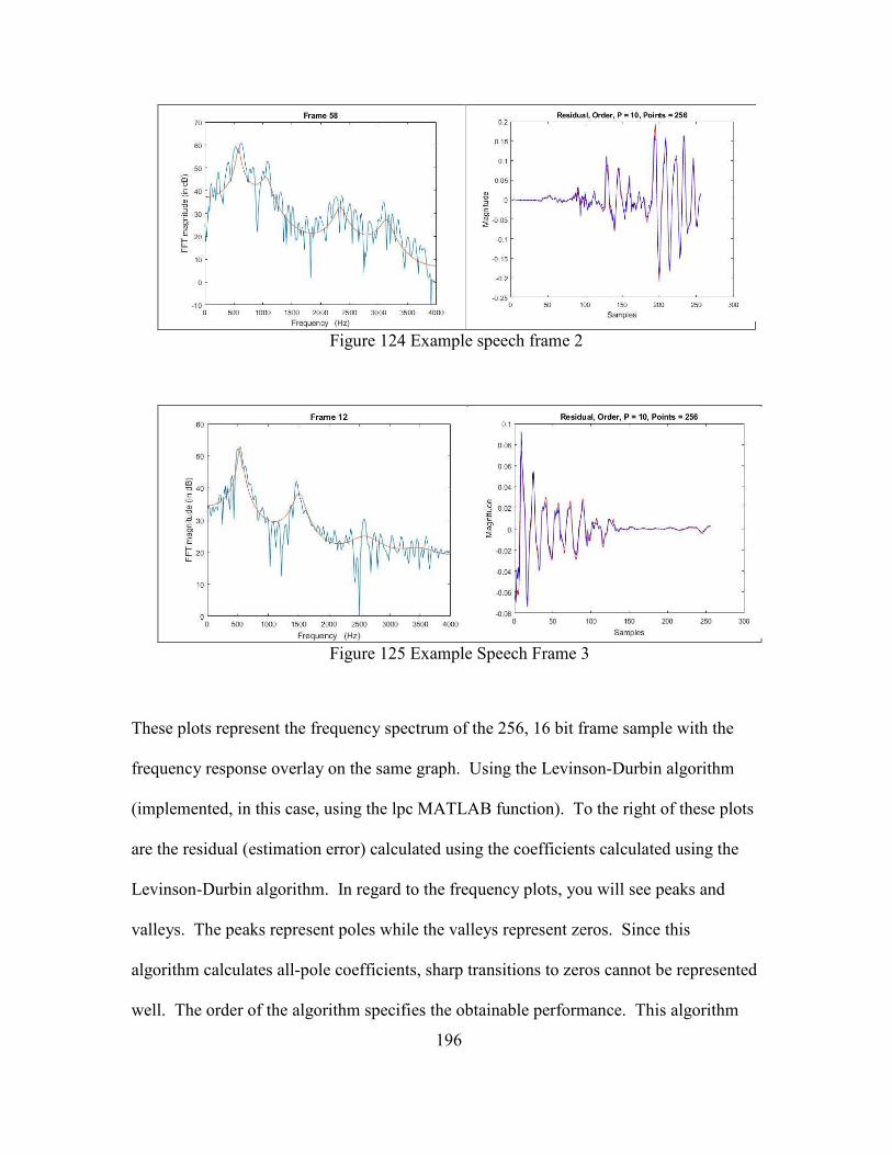
196

Figure 124 Example speech frame 2

Figure 125 Example Speech Frame 3

These plots represent the frequency spectrum of the 256, 16 bit frame sample with the

frequency response overlay on the same graph. Using the Levinson-Durbin algorithm

(implemented, in this case, using the lpc MATLAB function). To the right of these plots

are the residual (estimation error) calculated using the coefficients calculated using the

Levinson-Durbin algorithm. In regard to the frequency plots, you will see peaks and

valleys. The peaks represent poles while the valleys represent zeros. Since this

algorithm calculates all-pole coefficients, sharp transitions to zeros cannot be represented

well. The order of the algorithm specifies the obtainable performance. This algorithm

197

demonstrates that signals can be reconstructed using the all-pole 1 S ] coefficient

estimates derived using the Levinson-Durbin algorithm. As an example, by transmitting

only these all-pole coefficients across a wireless communication channel, a white noise

source [on a cell phone] can be used in conjunction with these coefficients to reconstruct

the transmitted voice signal. In so doing, this reduces the symbol rates required over a

wireless communication link to support voice communication; only the model

coefficients are transmitted providing the following performance improvements over the

wireless channel:

Table 16 Exemplar: Order P = 10, Levinson-Durbin Voice Communication Performance Improvement (Higher order will have higher accuracy, but less reduction performance) Voice Sample Bits Model Bits Reduction Performance Improvement

4096 160 96.1%

If the input sound on the audio device does not detect a magnitude of 9dB or higher

above the noise floor, further reduction in bits can be achieved. In such a model, when

people converse, there are times of no sound; during these times, no analog input above

10dB is detected and therefore no data should be transmitted during this time. Assuming

an average conservative model of ~6% idle pause in speaking (~200ms Ref: Stephen

Levinson, Max Planck Institute for Psycholinguistics), the following further improvement

is achieved:

198

Table 17 Example Voice Communication Improvement (32,000 UEs/16 sample, Order P =10), Higher Order will have greater improvement Voice Sample Bits (~8KHz Rate)

Model Bits

Reduction Performance Improvement

Reduction After Proposed Improvement

Additional Performance Improvement

Final Rate After Improvement

~4,096,000

Kbs

~160,000

Kbs

~96.1% 96.33% ~9,600 Kbs ~150,400

Kbs

Additional improvements in the performance of the linear predictor utilizing the RLS

algorithm are possible. The RLS/LMS comparison was discussed in other sections of this

document: Beamforming and MIMO (spatial and vector apertures), Channel Equalization

and Use of Parallel Correlators.

Roaming Performance

The proposed approach is for software programmed, hardware accelerated state machines

to receive the measurement reports from mobile users. Upon receipt of these reports, the

hardware accelerated state machines roam devices (from the network side) based upon

RF performance and/or load distribution. This section will describe three roaming

conditions followed by quantitative numbers in regard to expected performance based

upon a hardware accelerated data path that supports load sharing and roaming. Two types

of inter-RAT handover algorithms and a 4G handover were evaluated. The first case was

the Inter-RAT (WCDMA RAN to GSM) based upon the Inter-RAT handover algorithm.

The following are the measurement report attributes:

199

• The UE monitors the Downlink CPICH Ec/No and CPICH RSCP. The UE

informs (in uplink) the connection quality (i.e. DL:Ec/No, DL:Rscp ) the RNC monitors

this report along with UL power quality (RSCP: received signal code power)

• The Uplink UE Tx power is monitor by the RNC

• When at least one of these measurements drops below a threshold, a IRAT GSM

handover (HO) is requested, if improvement is detected once request is made, HO is

aborted

Note: WCDMA RAN allows different thresholds to be set.

• If conditions remain unchanged, the HO to WCDMA completes.

A handover (HO) from WCDMA RAN to GSM can also occur when load sharing is

required by sending Radio Access Bearer (RAB) assignment reject messages with

‘directed retry’ as the cause for speech only calls. The call network (CN) will redirect the

call to the GSM cellular network.

200

One that performs the Inter-RAT (GSM to WCDMA) based upon the Traffic Channel

(TCH) is below the percentage of idle TCH is below the is hand over level (ISHOLEV)

and the Ec/No in the Common Pilot Channel (CPICH) is greater than the Mobile Relay

Station Level (MRSL)

Note: 2G/GSM to 3G/WCDMA can occur because UTRAN is the preferred network.

• Under these conditions, when a UE is connected to a packet-switch (ps) network,

a Cell change & reselection function is activated

Note: Inter-RAT handover enables resources on the target cell while Inter-RAT Cell

Change requires no resources reserved in the target cell before hand

Figure 126 WCDMA to GSM Handover (Ref: TechNote 2009)

201

GSM Core BSC/BTS UE

Perform

Measurement

Measurement Report

Core Network GSM UE

Evaluation

UE

Evaluation

Cell Change

Or

Handover CMD

Access and Synchronization to target

UTRAN

Cell Change Information

Or

IRAT Handover Information

WCDMA

Service Request

Service Accept

Activate PDP Request

Accept PDP Context

Measurement Control

Cell Change Request

Or

IRAT Handover Request

Cell Change Ack

Or

IRAT Handover Ack

Release

Release

Figure 127 GSM to WCDMA Handover Sequence

• The following parameters are evaluated during the GSM to WCDMA handover.

The following must be true:

• TCH <= ISHOLEV

• CPICH Ec/No > MRSL and CPICH Ec/No > FDDQMIN

• CPICH RSCP > RLA (serving + neighboring GSM cells) + FDDQOFF

• Note: FDDQOFF is the key parameter: it defines an offset between signal quality

of WCDMA and GSM cells. Lower values of FDDQOFF ould be used to off-load the

GSM system. Higher values of FDDQOFF could used to keep multi-RATE MS in the

202

GSM system, example: if a WCDMA to GSM off-load priority setting is applied in the

WCDMA system.

4G/5G Handover

The case that requires a new serving gateway (SGW) is required was the only case

evaluated since the proposed change to the design would have to work even when the

new node is part of a different cell which requires a different IP address domain such that

a new SGW would be required.

Figure 128 4G Handover Sequence

203

Improved Roaming Performance

The architecture depicted below describes the physical dimensions (i.e. 25.4mm per 4

analog isolated channels) to support a RF configuration that provides greater than 60dB

per channel receive and transmit isolation for frequencies up to 6GHz. At higher

millimeter wave (mm-wave) frequencies, due to their smaller size, the analog signals

are more dense and harder to isolate; in the architecture above, the analog portion of the

design is separated from the digital side to provide a method of isolating and scaling the

analog portion to these higher frequencies. Further research is planned in the use of

special fabrication & integration techniques such as the use of Polystrata material where

the interposer could be 3D air substrates separating the individual components thereby

providing improved isolation at mm-wave frequencies for large aperture arrays.

204

Figure 129 Exemplar Freescale/Cavium Hardware Protocol Termination (up to 6GHz) with a Uniform Planar Array of 10x10, Circularly Polarized

The architecture is a version of an access independent architecture that describes ~12, 64

bit von Neumann processor utilizing 14nm FinFET 3-dimensional System on Chip (SoC)

CMOS technology; while on the physical layer processing, a Multiple/Single Instruction

Multiple Data (MIMD/SIMD) architecture implemented using either a Harvard or Vector

processor design, so classified by Flynn’s taxonomy, is depicted. For RF processing, it is

estimated that, given a density of 1M/Km2. For network frame processing, it provides

hardware accelerated protocol termination where user traffic flows directly through the

14nm FinFET hardware state machines without intervention by the SoC GPP cores. On

Cloud Services

HW Interfaces

full duplex @20Gbps per interface

3 SoCs =240Gbps

Scaled to Needs

Sampling

/Decimation

UE

Perform/Report

Measurement

Wireless Standby

Services

Cloud Wireless

Services

Primary

Secondary

1...N

HW Frame Processing

120Gbps

120Gbps

12

12

Includes Nodes

Discovered

During idle

Frame

Accelerator

(Parse, Classify,

Distribute)

Queue

Accelerator

Security

Accelerator

Pattern

Match

Accelerator

I/O

Accelerator

64 Bit

Cores

Buffer

Accelerator

64 Bit

Cores64 Bit

Cores64 Bit

Cores64 Bit

Cores64 Bit

Cores

64 Bit

Cores64 Bit

Cores64 Bit

Cores64 Bit

Cores64 Bit

Cores64 Bit

Cores

HW Protocol Termination

Frame Processing

5G

4G/LTE

3G/UMTS

2G/GSM

Exemplar: 3 SoCs

Exemplar: 3 SoCs

RF

(PHY Layer)

Proessing

(MIMD/

SIMD)

~25.4mm

Analog Isolation

~60dB/Channel

25.4 mm

Limit ~4 RF channels

100

channels

2540mm

Horizonta

l

Or

Vertical

Network

Processor

SoC

+

PHY

Processor

25

4 Channel

Combinations

Per

Polarization

gNB (DU)

gNB (CU)

Measurement Reports

From mobile devices

(IoT measurements not forwarded to

higher portions of the stack)Sampling

/Decimation~25.4mm

Sampling

/Decimation~25.4mm

Sampling

/Decimation~25.4mm

Vector

Sensor

Based

Beam

Forming

205

the 10Gbps links, hardware managed buffering is provided by the buffer accelerator;

based upon RFC 3439, average buffering is calculated as follows for N flows:

Iy = ff 10√£ , )!*+*ff = 2508=*M, o = IKJ=@**G, = #;;)= (195)

Due to the density of devices 1M/Km2 , the IPv6 addresses must be used so that all

devices can be accommodated with assigned IP addresses. At a minimum, the following

IPv6 address range is required with a 108 bit prefix:

[fe80:0000:0000:0000:9999:999x:xxxx] to [fe80:0000:0000:0000:9999:999f:ffff] to

permit greater than 1M addresses. Since IPv6 mobility is integrated into the IPv6

protocol, no special accommodations are required to support roaming between nodes in

the network. The concept of the design depicted above is to reduce the network

transactions required when roaming is necessary due to loss of RF visibility.

The roaming diagrams above depict the sequence of transactions required for a device to

hand off to another base station. This transaction sequence can occur with less UE

interaction. The cloud service in the diagram above can detect the loss of link based

upon the measurement report which can include the device location. The combination of

the device location and the measurement report provides the cell controller with the

information required to command the device. In this scenario the SGSN GW and

possibly the target SGSN GW is in the cellular cloud service layer. Therefore, the IPv6

address is managed internally through memory interfaces. Additionally, since an IP

tunnel can exist between geographically dispersed cloud services, target GW’s are

managed in a similar manner. This more centralized cloud service approach reduces the

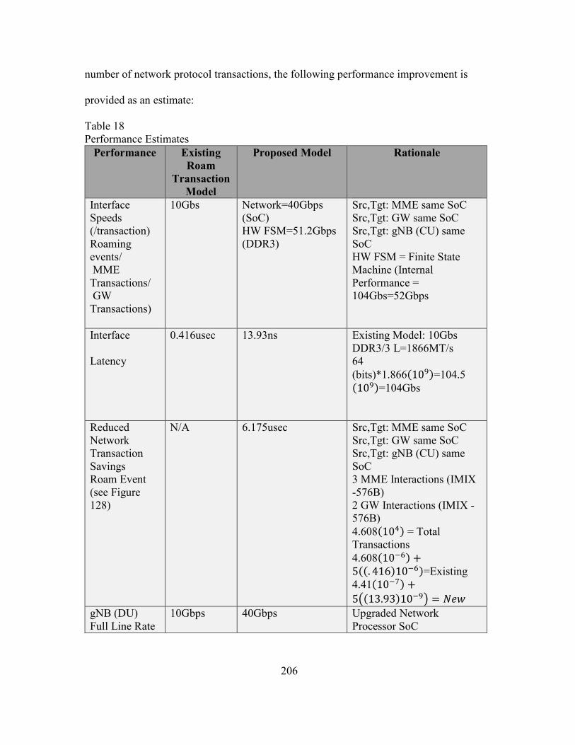
206

number of network protocol transactions, the following performance improvement is

provided as an estimate:

Table 18 Performance Estimates

Performance Existing

Roam

Transaction

Model

Proposed Model Rationale

Interface Speeds (/transaction) Roaming events/ MME Transactions/ GW Transactions)

10Gbs Network=40Gbps (SoC) HW FSM=51.2Gbps (DDR3)

Src,Tgt: MME same SoC Src,Tgt: GW same SoC Src,Tgt: gNB (CU) same SoC HW FSM = Finite State Machine (Internal Performance = 104Gbs=52Gbps

Interface

Latency

0.416usec 13.93ns Existing Model: 10Gbs DDR3/3 L=1866MT/s 64 (bits)*1.866 10=104.5 10=104Gbs

Reduced Network Transaction Savings Roam Event (see Figure 128)

N/A 6.175usec Src,Tgt: MME same SoC Src,Tgt: GW same SoC Src,Tgt: gNB (CU) same SoC 3 MME Interactions (IMIX -576B) 2 GW Interactions (IMIX -576B) 4.608 10 = Total Transactions 4.608 10% 5 . 41610%=Existing 4.41 10% 5 13.9310% = *)

gNB (DU) Full Line Rate

10Gbps 40Gbps Upgraded Network Processor SoC

207

Transactions speeds were calculated based upon the assumption that the 5G model is

based upon interface rates related to 10Gb Ethernet technology for most transaction

interfaces. The proposed model processes transactions with SW programmed HW state

machines that utilize memory interfaces. Using the Freescale T4240 as an example, the

transaction speeds are equivalent 104Gbs.

Moore’s Law has slowed, and semiconductor vendors are forced to provide value in new

ways to enhance their capabilities to generate new sales. This is forcing greater

integration of specialized capabilities to be integrated into their products. The exemplars

above represent network processing chips where specialized network frame processing

capabilities continue to be integrated.

User-Based Technology

5G NR technology utilizes user-based performance which implements user-based quality

of service (QoS). During negotiation of the cellular session established by the user

equipment (UE) through the Radio Access Technology (RAT) protocol, which permits

communication with individual UE, UE identifiers are extracted from protocol field

elements. 5G RAT is comprised of the enhanced LTE RAT technology + new RAT

technology. Enhanced LTE RAT technology provide enhancements to the orthogonal

frequency division multiple access (OFDMA) carriers which permit different uses of

subcarrier implementations which were previously focused on single carrier (SC)

OFDMA communication in the reverse direction from the UE to the network. In some

208

cases, more (or less) carriers can be assigned to an individual UE based upon QoS

classification related to the device type.

At the protocol level, 5G NR enables user-based technology that provides QoS and

routing that changes the previous network QoS paradigm of routing classification via IP

address, IP protocol, IP port numbers, and type of service (ToS) or differentiated services

code point (DSCP). Instead, 5G enables user groups with differing levels of service.

Device information is extracted during the initial device entry into the network. During

the initial attach procedure, Device queues are configured so that QoS can be

implemented for traffic to/from the rest of the network (RoN). The following is an

example of queues set up for device groups:

Figure 130 Example User Based Packet Queue (HW Synthesis Provides 40Gbps Stream)

These user groups provide characterization that supports the network slicing architecture

defined by the new 5G NR specification. The 5G NR slicing architecture provides the

209

ability to provide different performance characteristics where each slice operates as an

independent, virtualized version of the network. For the application, the network slice is

the only network it sees; other, unsubscribed, slices are not visible to the application. The

concept is that each slice targets a different user group, one slice could target low-

throughput IoT sensors, another autonomous vehicles, while another provides enhanced

broadband. The proposed concept supplements this capability by enabling QoS

differentiated services within the same network topology using hardware state machines

to implement the LLQ or WFQ schemes. These QoS hardware services can then be

integrated with existing network infrastructure directly to cloud services which utilize

both 802.1pq, layer 3 switching and IP based differentiated services as part of the

software defined network (SDN) created as part of the cloud network service layer.

QoS management of user-based queues is based upon several algorithms such as:

• Weighted Random Early Detect (WRED)

A hardware accelerator would implement a weighted average by maintaining the length

of the output queue; if the output queue length is less than a minimum threshold minth

when a packet arrives, the packet is admitted to the queue. If the queue is full or the

average queue length is greater than a max threshold maxth, the packet is dropped. If the

average queue length is in the interval [minth, maxth] when the packet arrives, it is

dropped. Used as a congestion avoidance algorithm that drops packets that are marked

with a certain probability which depends on weight and queue length for data frame

exchanges for each user group.

• Low Latency Qeueing (LLQ)

210

The hardware accelerator would provide strict priority frame queueing similar to the

concept described above except the queue is managed on strict priority basis such that

jitter and latency are constant for voice and video data exchange for each user group.

These algorithms are then used to provide input into Dijkstra’s algorithm; the example

below can be compute optimized by using an enhanced queueing methodology where a

priority queue (see Brodal queue or Fibonacci heap (Fredman & Tarjan 1984)) is

implemented using an abstract data type and data structure:

function Dijkstra():

N’ = U//N’ is subset of nodes, v is in N’ if the least-cost path

//from the source to v is definitely known

for all nodes v

if v is adjacent to u

then D(v) = c(u,v) // where c(u,v) is the cost from u to v

else

D(v) = INFINITY

end

end

for all nodes in N’

find w not in N’ such at D(w) is a minimum

add w to N’

update D(v) for all adjacent to w and not in N’:

D(v)=min(D(v),D(w)+c(w,v))

// new cost to v is either old cost to v or known shortest path

// cost to w plus cost from w to v */

end

end // function Dijkstra ()

Figure 131 Example Dijkstra's Algorithm deriving Link-State (LS) Routing (Computer Networking, Kurose Ross, 5th Edition)

User based prioritization prioritizes data toward the rest of network (RoN) by translating

priority to network protocol fields in the following virtualized cloud service protocol

211

examples: IP DSCP (ToS), 802.1pq, Routing Protocols: MPLS, RIP, OSPF and EIGRP;

at the core of these protocols are the complementary Dijkstra’s (LS) and Distance-Vector

(DV) algorithms. In the opposite direction, user-based prioritization prioritizes wireless

data from RoN to wireless user equipment (UE) at the RAT level, through user based

QoS queues and with protocol prioritization. In 5G the notion of QoS network slicing

was presented where virtual access is provided only to specific users within a group who

have differentiated service access.

As wireless and backhaul communication rates increase (such as over FioS as one

example), frame processing will continue to transition to HW acceleration without SW

intervention due to the inability of software frame processing to keep up with the required

frame processing rates. As defined by the Flynn taxonomy, wireless technology appears

to be implementing a mix of Von Neumann and hyperscale processing technology using

Xilinx FPGAs that enable processing of complex data sets. Presently, the Von Neumann

bottleneck has only gotten worse over time, as the disparity between processor speed and

memory access throughput speed has widened. Other hyperscale processing solutions for

complex data sets are under evaluation to include GPU’s provided by Nvidia and AMD.

Future silicon implementing massively parallel MIMD processing architectures include

PicoChip (now part of Intel) and Coherent Logix. Bandwidths are increasing, forcing 5G

base stations to transition to more capable processors that provide hardware accelerated

data frame processing and enhanced security protections. Examples of such architectures

are the network processors provided by Intel (IXP2800), Freescale QorIQ (T4240),

Broadcomm (BCM5871X), Nokia (FP3/FP4) and Qualcomm (X50) to name a few. Such

212

architectures terminate and route L2 andL3 based data path protocols used over wireless

links to eNodeB without SW intervention. Specialized SoC’s such as these provide

software defined network (SDN) control over frame processing while hardware state

machines accelerate frame processing beyond the speeds possible using SW.

Figure 132 Hardware Instruction Set Verification

In addition to network processing capabilities, semiconductor vendors are integrating

improved security features into their SoCs. The security chain of trust starts at the

beginning by the use of anti-tamper and anti-clone technology; these are implemented

using Physical Uncloneable Function (PUF) technology in concert with such protections

as zeroizable fuses that deactivate the chip upon power up or upon security violation

detection. SRAM PUF leverages inherent manufacturing variations to create identifiers

that are more unique that the human fingerprint. Further, HW trust architectures maintain

chain of trust by providing hardware protection engines: I/O isolation, secure boot,

hypervisors, pattern match, entropy sources and block/stream based cryptographic

algorithms (such as elliptical and RSA) that protect against cyber threats. Security

hardware engines verify SW instructions from the beginning using secure boot, HW I/O

isolation using hypervisors and peripheral management units (PAMU). Instruction

memory is continually protected against cyber threat manipulation by continually

213

verifying portions of the processor memories used for instruction sets; if any instructions

are modified, a security violation is detected and the security policy is implemented.

Network data is routed (by hardware state machines -without SW intervention) to real-

time HW engines to detect patterns (in some cases millions of pattern combinations are

evaluated to detect cyber threats). In such architectures, SW is not trusted to access raw

key material; no unencrypted key material is present on any external bus including the

memory bus, any and all keys provided to SW are encrypted using cryptographic

algorithms such as AES-256 CCM using random entropy. The processors include

cryptographic engines with 32- and 64-bit entropy sources (e.g. Random Number

Generators (RNG)) that can be configured to add random content on a per cryptographic

frame basis at rates exceeding 40Gbsec (>40Gbsec/chip). The architecture assumes a

“bump in the wire” cryptography in HW managed frame processing.

Most cellular devices have HW implemented entropy sources (such as RNG) to provide

random input to the Levinson-Durbin algorithm used to reconstruct voice information

over challenged links. Such entropy sources can also be used to provide random entropy

for secure communications.

Control, management and exception frames are routed to the central processing unit to be

handled by SW, though hardware must be used to verify security key material since SW

is not a trusted source for key material on such an architecture.

214

The following are the published 3GPP specifications for the 5G protocol stack, though

there is misleading information due to differences between published literature and the

actual 3GPP specification under document control and further leaks of coming 3GPP

specification releases.

Table 19 LTE Resource Blocks (Ref. 3GPP specification)

Channel BW (MHz)

1.4 3 5 10 15 20

Resource Blocks

6 15 25 50 75 100

Table 20 5G NR Resource Blocks (Ref. 3GPP specification) Min.

Downlink Resource Blocks

Max. Downlink Resource Blocks

Min. Upllink

Resource Blocks

Max. Uplink

Resource Blocks

0 24 275 24 275 1 24 275 24 275 2 24 275 24 275 3 24 275 24 275 4 24 138 24 138

Table 21 5G NR Single Carrier UE and gNB Bandwidth Requirement (Ref. 3GPP specification) Min.

Resource Blocks

Max. Resource Blocks

Sub. Carrier Spacing (KHz)

Freq. BW

Minimum (MHz)

Freq. BW

Maximum (MHz)

0 24 275 15 4.32 49.5 1 24 275 30 8.64 99 2 24 275 60 17.28 198 3 24 275 120 34.56 396 4 24 138 240 69.12 397.44

215

Table 22 5G NR Channel Spacing Requirement (Ref. 3GPP specification) Subcarr

ier Spacing

Cyclic Prefix

Supported for Data (PDSCH,PUSCH)

Supported for Sync.

(PSS,SSS,PBCH)

PRACH

N/A 1.25 No No Long Preamble

N/A 5 No No Long Preamble

0 15 Normal Yes Yes Short Preamble


2 60 Normal, Extended

Yes No Short Preamble


4 240 Normal No Yes Short Preamble

Table 23 5G NR OFDM Symbol Durations (Ref. 3GPP specification) Numerology 0 1 2 3 4

Carrier Spacing (KHz) 15 30 60 120 240 Symbol Duration (us) 66.67 33.33 16.67 8.33 4.17 Prefix Duration (us) 4.69 2.34 1.17 0.57 0.29

Symbol including CP (us) 71.35 35.68 17.84 8.92 4.46

Pi_Lh = 10% !_/L q k_i« q l; q Ç^_`"ã1yy# q qf7$ % 1 ' dA q&·q$.

Ç^_` = o!?*Å8?K<GKM?<+, 64: ÅS = 8731024 , 256: ÅS = 9481024 (196)

o = #;S+*?<*Go9@*<o?++K*+= dA q = d(*+!*?G ' ?==89*G*R8??M!?*= = 25% = 89*+ 0 ' 5, release 15 = (0-4) ; q = N+*R. =M?K;?M<+ 0.75 f7$ = 10%r14 2 , ?(. dNP=9:G8+?<KK?=8:;+?9*;+89*+

ã1yy# ( = isthemax. resourceblock RBfornumerologyμ. BW c = Max.BWsupportedbytheUE MDEF ( = ModulationOrder

216

N( = #ofsubcarriers = 12 NDIJ = #ofAntennas (Ref: 3GPP performance estimation algorithm -Easily reproduced/derived utilizing digital communication algorithms) Table 24 5G NR Projected Performance Calculations (reduced to release 14) μ Channel

Spacing KHz

Max Nbr of Resource Blocks

Max. Downlink

Performance

**Max. Uplink

Performance 0 15 270 1.16Gbps 620Mbps 1 30 273 2.34Gbps 1.25Gbps 2 60 135 2.31Gbps 1.235Gbps

**Note: Reduced to only 2 Antennas on uplink

Though 5G has identified 8x4 MIMO (8 spatial layers down, 4 spatial layers up), I have

assumed the numbers above represent the predominate number of mobile users who will

only have 2 spatially diverse antennas available for the reverse direction.

217

Chapter 8

CONCLUSION

Summary of Results

Based upon the performance results described in the sections above, I focused on three

areas: Beamforming, voice communication and wireless roaming performance. These

areas were chosen because of their consequential impact to 5G wireless performance.

The following research describes proposed improvements in adaptive beamforming

(utilizing machine learning) to direct energy towards end users. Next, a proposed

improvement in voice communication building up the well-known Levinson-Durbin

algorithm. Lastly, an improvement in wireless roaming is proposed that reduces the

number of interactions required between the base station and the 5G user equipment (UE)

as well as the state machine transitions on the UE. An important aspect of the design is

to ensure microwave components meet the requirements of the waveform. One aspect of

the design relates to the channel spacing requirement for 4G & early 5G systems which

utilize 15KHz channel spacing. Based upon this narrow band requirement, receivers

must meet the following phase noise requirements to enable adequate demodulation of

these new, large M-ary linear modulation constellations. Assuming carrier and

interference power is approximately the same, in order to achieve ~50dB of adjacent

channel rejection (i.e. selectivity), the following the following phase noise requirement is

described:

L ∶= '50dB ' 10 log.C 15KHz = '92dBcHz @~15KHzOffset

(197) (

218

The first investigation focused on the practical aspects of beamforming and the use of a

superior co-channel and co-direction interference mitigation performance of a new type

of vector sensor that can be used in conjunction with spatially diverse arrays used to

identify beam directionality. This design showed great promise due to its exceptional

Direction of Arrival (DOA) performance achieved through a lower computational

overhead. This performance translates into greater transaction rates and responses:

Table 25 Superior Performance of the Vector Aperture (Beamforming Energy Detection)

For beamforming performance, being able to detect energy so that beams can be formed

at the appropriate angle was discussed earlier. For this purpose, based upon the half

power beam width in horizontal & vertical directions at 6GHz, the Poynting Vector cross

product provided the most economic processing solution for a sufficient resolution to be

used for dynamically beam forming.

The next research investigation built upon the Levinson-Durbin algorithm as a basis for

evaluating voice communication performance. As demonstrated by the results of the

Levinson-Durbin test results, the algorithm performance demonstrates impressive voice

modeling performance. As part of my research I proposed an algorithm modification to

Technique Samples Latency + Ω

Accuracy

(deg.) Best Performance

Poynting 1000 422.5 <2 90% over spatial array

Poynting 2000 649 0.5 41% over spatial array

ESPRIT 1000 4672 1 Susceptible to correlated noise

ESPRIT 2000 1589.5 0.2 Susceptible to correlated noise

219

further reduce voice traffic bandwidth and thereby increase bandwidth as shown in the

following table:

Table 26 Example Voice Communication Improvement (32,000 UEs/16 sample), Model Order P=10, Higher Model Order will Yield Additional Performance Improvement Voice Sample Bits (~8KHz Rate)

Model Bits

Reduction Performance Improvement

Reduction After Proposed Improvement

Additional Performance Improvement

Final Rate After Improvement

~4,096,000

Kbs

~160,000

Kbs

~96.1% ~96.33% ~9,600 Kbs ~150,400

Kbs

This improvement takes advantage of the periodic nature of voice conversations. Lastly,

I described a new link layer communication system design that manages and routes

wireless communication frame traffic to and from wireless devices that decreases latency

and increases performance as defined in the following table:

Table 27 Performance Estimates

Performance Existing

Roam

Transac

tion

Model

Proposed Model Rationale

Interface Speeds (/transaction) Roaming events/ MME Transactions/ GW Transactions)

10Gbs Network=40Gbps (SoC) HW FSM=59.7Gbps (DDR3)

Src,Tgt: MME same SoC Src,Tgt: GW same SoC Src,Tgt: gNB (CU) same SoC HW FSM = Finite State Machine (Internal Performance = 119Gbs~=60Gbps

Interface Latency 0.416us 13.93ns Existing Model: 10Gbs DDR3/3 L=1866MT/s 64 (bits)*1.866 10~=119.4Gbs

220

Reduced Network Transaction Savings Roam Event (see Figure 128)

N/A 6.175usec Src,Tgt: MME same SoC Src,Tgt: GW same SoC Src,Tgt: gNB (CU) same SoC 3 MME Interactions (IMIX -576B) 2 GW Interactions (IMIX -576B) 4.608 10 = Total Transactions 4.608 10% 5 . 41610%=Existing 4.43 10% 5 13.9310% = New

gNB (DU) Full Line Rate

10Gbps 40Gbps Upgraded Network Processor SoC (IMIX) Existing: 9 cores ~=250,000pps (limited by 8K instructions/packet @ 2GHz) Existing: 40Gbs ~=36 cores New: 40Gbs ~=8,389,261pps

Ref: Freescale T4240

This research focused on the requirements and algorithms required to improve

beamforming performance with a larger number of antenna elements, an improvement in

the use of the Levinson-Durbin voice communication algorithm and the use of hardware

acceleration on the network base station side to improve wireless network performance.

From the tables above, I have derived the following performance numbers assuming a

realistic population of only 250K (Ref: Deployment of 5G Olympics, 2020) concurrent

active mobile users within the total 5G population of 1M/Km2.

221

Table 28 Performance Enhancements

Performance Before

Algorithm

Improveme

nt

After

Algorithm

Improvement

Total Savings

Increase in Mobile Communication Bandwidth (Voice)

1.25Gbs 1.175Gbs

75Mbs, Higher Efficiency Assumed (IoT)

Beamforming Coefficient Calculations Using Vector Aperture

4672usec 422.5usec As much as 91% reduction in latency Reduction=0.91(new beam caused by user access)

Frame Processing 500Kpps 2Mpps *Based upon HW acceleration performance measurements per 10G interface, 4K instructions per frame @2GHz

Beam steering, improved RF efficiency and higher performance network processing will

become much more important in 5G architecture and this paper focused on additional

design considerations and approaches to provide superior co-channel and co-direction

interference mitigation performance by using a new type of vector sensor that can be used

in conjunction with a new link layer communication design that manages and routes

wireless communication frame traffic to and from wireless devices. The vector sensor

provided superior beam forming performance and sufficient DOA accuracy which is

estimated by the half power beam width, at 6GHz requires ~2 degrees, at 24GHz ~1

degree is sufficient beam forming accuracy. Further research is planned in the area of

MIMO concepts such as the use of Alamouti STBC to increase the achievable gain in the

millimeter frequency ranges using a uniform planar array (ULA); however, Maximmal

Ratio Combining (MRC) has proven to be more effective. I evaluated the performance

222

between LMS and RLS algorithms in the use of beam forming and discovered that,

though the RLS algorithm converges more quickly, it required a greater number of

instructions to execute. Further research is necessary to fully evaluate the convergence

performance with a larger set of interfering signals. This research concluded with the

beginning of an overall hardware architecture that depicts an approach to distribute RF

bandwidth and network processing required to exceed the goals of 5G. This architecture

depicts the advantage of centralized processing subsystems that have now evolved into

cloud services and where the gNB (DU) has turned into RF ports as I depicted in my

earlier work patented work in wireless communication. It appears my approach

described in our earlier, patented, work and the 5G strategy are converging.

Future Research Directions

The research presented in this dissertation offers a multitude of interesting future

directions to further advance user-based link QoS in 5G wireless communications

applications. One direction is to closely examine the QoS at the link level by adapting

admission control and traffic policing mechanisms (Kozat, et al., 2004; Lai et al, 2009;

Reisslein, et al., 1998, 1999) to the approaches presented in this dissertation. With

admission control and traffic policing, 5G networks can support general low latency

communications (Jiang, et al., 2019; Nasrallah, et al., 2019), which is needed for a wide

range of 5G communications services, as well as support popular bandwidth-demanding

applications, e.g., video streaming (Reisslein & Ross, 1998; Wang, Chen et al., 2013;

Wang, Kwon, et al., 2013). Another future research direction is to expand this research to

223

future communications paradigms, e.g., cognitive communications and networking

(Amjad, et al., 2017; Kakalou, 2017; Tseng, 2015).

The user-based link QoS mechanisms developed in this dissertation research exploit SDN

mechanisms (Amin et al., 2018; Jagadeesan & Krishnamachari, 2014; Kellerer et al.,

2019; Yang et al., 2015) for the adaptive control of the user QoS. Future research can

examine specifically the time scales and performance characteristics of transient

adaptations in the proposed 5G communication system. Also, it may be interesting to

examine the role of SDN gateway nodes (Thyagaturu et al., 2016; Vilalta et al., 2016)

and specifically controlled SDN-based routing (Davoli et al., 2015; Guck et al., 2018) for

providing QoS on large 5G networks that incorporate large aggregated network domains.

A closely related future research topic is to examine network virtualization (Blenk, et al.,

2016; Roozbeh, et al., 2018; Yang, et al., 2018) in the context of the examined link QoS

mechanisms.

The emerging multi-access edge computing (MEC) paradigm, which is also referred to as

mobile edge computing or fog computing (Bi, et al., 2018; Blanco et al., 2017;

Shantharama et al., 2018; Xiang, et al., 2019) presents interesting novel trade-offs in

conducting service computing for 5G communications functions in local hardware or

software nodes, or in MEC hardware or software nodes (Hsieh, et al., 2018; Van

Kempen, et al., 2017; Zanni, et al., 2017). Future research could examine the trade-offs in

performance and cost between executing portions of the computing for the proposed link-

level QoS mechanisms in local or MEC nodes.

224

Finally, network coding (Farooqi, et al., 2014; Gabriel et al., 2018; Lucani, et al., 2018;

Naeem, et al., 2017; Taghouti, et al., 2019; Wang, et al., 2016) has recently emerged as

an attractive coding paradigm for large-scale networks that suffer from unreliable

wireless links. An important future research direction is to examine the infusion of

network coding into the link-layer QoS scheme developed in this dissertation. Network

coding may be able to enhance the overall network throughput, both for unicast and

multicast transmissions, and can play an important role in further enhancing 5G

communication systems (Patil, et al., 2019; Tsimbalo, et al., 2018; Vukobratovic, et al.,

2018).

225

REFERENCES

Barton, B. (2012, March 30). eUTRAN to UTRAN (4G to 3G). Retrieved March 20,

2014, from LTE and BEYOND: http://www.lteandbeyond.com/2012/03/few-last-articles-

were-about-handover.html

Wikipedia. (2014, February 24). Cellular data communication protocol. Retrieved March

15, 2014, From Wikipedia, the free encyclopedia:

https://en.wikipedia.org/wiki/Cellular_data_communication_protocol

Freescale. (2014, March 15). T4240/P4080: QorIQ T4240/P4080/P4040/P4081

Communications Processors with Data Path. Retrieved March 15, 2014, From Freescale

Semiconductor: http://www.freescale.com/

Airstream. (2014, April 3). ACK Timeouts and the effects on distance. Retrieved March

1, 2014, From Airstream: http://www.air-stream.org/technical/ack-timeouts-and-effects-

distance-links

ShareTechnote. (2013, September 4). Handover LTE. Retrieved February 28, 2014,

From ShareTechnote: http://www.sharetechnote.com/html/Handover_LTE.html

Peter McGuiggan. (2004). GPRS in Practice. West Sussex, England: John Wiley & Sons.

James F. Kurose, Keith W. Ross. (2010). Computer Networking, Fifth Edition. Boston:

Pearson.

Steven M. Kay. (2010). Fundamentals of Statistical Signal Processing (Estimation

Theory). Hamilton in Castleton: Prentice-Hall.

Steven M. Kay. (2008). Fundamentals of Statistical Signal Processing (Detection

Theory). Troy: Prentice-Hall.

Douglas C. Montgomery. (2013). Design and Analysis of Experiments, Eighth Edition.

Hoboken: John Wiley & Sons.

Reisslein, M., & James, F. (2017). U.S. Patent No. 9,717,088. Washington, DC: U.S. Patent and Trademark Office, Multi-Nodal Wireless Communication Systems and Methods

226

Torla, M. J., James, F. L., Tkacik, T. E., & Millman, S. D. (2012). U.S. Patent No.

9158499. Washington, DC: U.S. Patent and Trademark Office. Cryptographic processing

with random number generator checking

Cover, T. (1972). Admissibility properties of Gilbert’s encoding for unknown source

probabilities. IEEE Transactions on Information Theory, 18:216–217.

Krichevsky, R. (1998). Laplace’s law of succession and universal encoding. IEEE

Transactions on Information Theory, 44:296–303.

McDiarmid, C. (1989). On the method of bounded differences. In Surveys in

Combinatorics, pages 148–188. Cambridge University Press.

Miller, G. (1955). Note on the bias of information estimates. In Information theory in

psychology II-B, pages 95–100.

Nemenman, I., Shafee, F., and Bialek, W. (2002). Entropy and inference, revisited. NIPS,

14.

Paninski, L. (2003). Estimation of entropy and mutual information. Neural Computation,

15:1191–1253.

Paninski, L. (2004). Estimating entropy on m bins given fewer than m samples. IEEE


Paninski, L. (2005). Variational minimax estimation of discrete distributions under KL

loss. Advances in Neural Information Processing Systems, 17.

Paninski, L. (2008). A coincidence-based test for uniformity given very sparsely-sampled

discrete data. IEEE Transactions on Information Theory, 54:4750–4755.

Paninski, L. and Yajima, M. (2008). Undersmoothed kernel entropy estimators. IEEE


NIST. (2001, May 1) FIPS PUB 140-2. Security Requirements for Cryptographic

Modules. Federal Information Processing Standards Publication. Category: Security.

Subcategory: Cryptography.

NIST. (2012, February 16) Annex C: Approved Random Number Generators for FIPS

PUB 140-2, Security Requirements for Cryptographic Modules.

227

Rodgers Corporation. “Rodgers Corporation: RO3000 Series High Frequency Circuit Materials”, Data Sheet 1.3000, Publication #92-130, 3/2005. Rod Waterhouse, “Printed Antennas for Wireless Communications”, 1st Edition, John Wiley & Sons, Inc., New York, 01/02/2008, ISBN-13: 9780470510698.

D. M. Pozar, “Microwave Engineering,” 3rd Edition, John Wiley & Sons, Inc., New York, 2005.

Guo Yichao, Guo Jianmin, Lv Pin, Huan Hao, Tao Ran, “A Code Doppler Compensation Algorithm in Acquisition for High Dynamic Spread Spectrum Signals,”, IEEE Signal Processing, Communications and Computing (ICSPCC), 2016 Digital Object Identifier (DOI): 10.1109/ICSPCC.2016.7753594.

Dr. Andreas Spanias, “Adaptive Filtering, Chapter 9” in Digital Signal Processing An Interactive Approach, 2nd ed. Tempe, Az.

B. Widrow et al, Adaptive noise cancelling: Principles and applications, Proc. IEEE, Vol. 63(12), Jan. 1976.

B. Widrow, S. Stearns, Adaptive Signal Processing, Prentice Hall, 1985.

Gross, Frank B. Smart Antennas with MATLAB, , 2nd Edition, McGraw Hill, 2015.

Douglas, S.C. “Introduction to Adaptive Filters” Digital Signal Processing Handbook Ed. Vijay K. Madisetti and Douglas B. Williams Boca Raton: CRC Press LLC, 1999

Block implementation of adaptive digital filters,Clark, G.; Mitra, S.; Parker, S.;Circuits and Systems, IEEE Transactions on Volume: 28 , Issue: 6, Digital Object Identifier:10.1109/TCS.1981.1085018, Publication Year: 1981 , Page(s): 584 – 592

Fast implementations of LMS adaptive filters Ferrara,E.; Acoustics, Speech and Signal Processing, IEEE Transactions onVolume:28,Issue:4Digital Object Identifier (DOI): 10.1109/TASSP.1980.1163432 Publication Year: 1980 , Page(s): 474 – 475

228

Comparison of several frequency-domain LMS algorithms Mikhael,W.;Spanias,A.; Circuits and Systems, IEEE Transactions on Volume:34,Issue:5, Digital Object Identifier (DOI): 10.1109/TCS.1987.1086164, Publication Year: 1987 , Page(s): 586 - 588

Johan Duplouy, Christophe Morlaas, Hervé Aubert, Philippe Pouliguen, Patrick Potier, et

al.. Reconfigurable Grounded Vector Antenna for 3D Electromagnetic Direction Finding

Applications. IEEE Antennas and Wireless Propagation Letters, Institute of Electrical and

Electronics Engineers, December, 2017.

Van Trees, Harry L., Optimum Array Processing. Part IV of Detection, Estimation, and

Modulation Theory, John Wiley & Sons, Inc., New York, Copyright 2002

Hart, Ted, Birke, Paul V., The Poynting Vector Antenna, 1st Edition, 2016.

Nehorai, A, and Paldi, E, Vector-sensor array processing for electromagnetic source

localization, IEEE Trans, on Signal Processing, SP-42, 376-398, Feb, 1994

Nehorai, A, and Paldi, E., Vector sensor processing for electromagnetic source location,

Proc, 25th Asilomar Conf. Signals, Syst, Comput., Pacific Grove, Ca, Nov 1991, 566-572

SchWartz, M, Bennett, W. R, and Stein, S, Communication Systems and Techniques

McGraw-Hill, New York, 1966.

Keiser, B.E., Broadband Coding, Modulation, and Transmission Engineering, Prentice-

Hall, Englewood Cliffs, New Jersey, 1989.

Stoica, P. and Nehorai, A., Performance study of conditional and unconditional direction-

of-arrival estiamte, IEEE Trans. Acoust, Speech, Signal Processing, ASSP-38, 1783-

1795, Oct. 1990.

Ottersten, B., Viberg, M. and Kailath, T., Analysis of subspace fitting and ML techniques

for paraeter estsimate for sensor array data, IEEE Trans. Signal Processing, SP-40, 90-

600, March 1992.

229

Schmidt, R.O., A signal subspace approach to multiple emitter location and spectral

estimation Ph.D, Dissertation, Stanford University, Standford, Ca. Nov 1981.

Ferrara, Jr., E.R. and Parks, T.M., Direction finding with an array of antennas having

diverse polarization, IEEE Trans, Antennas Propagat., AP-31, 231-236, March 1983

Ziskind, I. and Wax, M., Maximum Likelihood location of diversely polarized sources

byt simualted annealing, IEEE Trans. Antennas Progagat. AP-38, 1111-1114, July 1990.

Li, J. and Compution, R.T., JR., Angle and polarization estimation using ESPRIT with a

polarization sensitive array, IEEE Trans., Antennas Progat., AP-39, 1376-1383, Sept.

1991

Weiss, A.J. and Friedlander, B., Performance analysis of diversely polarized antenna

arrays, IEEE Trans, Signal Processing, SP-39, 1589-1603, July 1991.

Means, J.D., Use of three-dimensional covariance matrix in analyzing the polarization

properties of plane waves, J. Geophys, Res., 77, 5551-5559, Oct. 1972

Hatke, G.F., Performance analysis of the SuperCART antenna array, Project Report No.

AST-22, Lincoln Laboratory, Massachusetts Institute of Technology, Lexington, Ma,

March 1992.

Ferrara, E., Fast LMS implementation of adaptive filters, (Volume:28, Issue:4), IEEE

Transactions Digital Identifier (DOI): 10.1109/TASSP.1980.1163432 Publication Year:

1980 , Page(s): 474 – 475

Comparison of several frequency-domain LMS algorithms Mikhael,W.;Spanias,A.;

Circuits and Systems, IEEE[20] Spanias, Dr. Andreas Digital Signal Processing An

Interactive Approach, 2nd ed. Tempe, Az.: Copyright 2007

230

Kanda, M., An electrogmatnic near-field sensor for simultaneous electric and magnetic-

field measurements, IEEE Trans. on Electromagnetic Compatibility, 26(1), 102-110,

Aug. 1984

Clark, G.; Mitra, S.; Parker, S, Block implementation of adaptive digital filters,.;Circuits

and Systems, IEEE Transactions on Volume: 28 , Issue: 6, Digital Object Identifier:

10.1109/TCS.1981.1085018, Publication Year: 1981 , Page(s): 584 – 592

Cox, Christopher (2014, John Wiley and Sons), An Introduction to LTE: LTE, LTE-

Advanced, SAE, VoLTE and 4G Mobile Communications, 2nd Edition

Rodriquez, Jonathan (2015, John Wiley and Sons), Fundamentals of 5G Mobile

Networks

Liyanage, Madhusanka (2015, John Wiley and Sons), Software Defined Mobile

Networks

Holler, Jan; Tsiatsis, Vlasios (2014, Elsevier Ltd.) From Machine-to-Machine to the

Internet of Things

Barton, B. (2012, March 30). eUTRAN to UTRAN (4G to 3G). Retrieved March 20,

2014, from LTE and BEYOND: http://www.lteandbeyond.com/2012/03/few-last-articles-

were-about-handover.html

Wikipedia. (2014, February 24). Cellular data communication protocol. Retrieved March

15, 2014, From Wikipedia, the free encyclopedia:

https://en.wikipedia.org/wiki/Cellular_data_communication_protocol

Airstream. (2014, April 3). ACK Timeouts and the effects on distance. Retrieved March

1, 2014, From Airstream: http://www.air-stream.org/technical/ack-timeouts-and-effects-

distance-links

231

ShareTechnote. (2013, September 4). Handover LTE. Retrieved February 28, 2014,

From ShareTechnote: http://www.sharetechnote.com/html/Handover_LTE.html

McGuiggan, Pete. (2004). GPRS in Practice. West Sussex, England: John Wiley & Sons.

Kay, Steven M. (2010). Fundamentals of Statistical Signal Processing (Estimation

Theory). Hamilton in Castleton: Prentice-Hall.

Kay, Steven M. (2008). Fundamentals of Statistical Signal Processing (Detection

Theory). Troy: Prentice-Hall.

Montgomery, Douglas C. (2013). Design and Analysis of Experiments, Eighth Edition.

Hoboken: John Wiley & Sons.

Cover, T. (1972). Admissibility properties of Gilbert’s encoding for unknown source

probabilities. IEEE Transactions on Information Theory, 18:216–217.

Krichevsky, R. (1998). Laplace’s law of succession and universal encoding. IEEE


McDiarmid, C. (1989). On the method of bounded differences. In Surveys in

Combinatorics, pages 148–188. Cambridge University Press.

Spanias, Andreas (2014). Digital Signal Processing; An Interactive Approach, Second

Edition. Tempe, Az.

Balanis, Constantine (2005). Antenna Theory, Third Edition. Hoboken: John Wiley &

Sons.

James, Tsui (2004). Digital Techniques for Wideband Receivers. Raleigh: SciTech

Publishing.

232

Kay, Stephen (2006). Intuitive Probability and Random Processes using MATLAB.

Springeronline.com.

Miller, G. (1955). Note on the bias of information estimates. In Information theory in

psychology II-B, pages 95–100.

Nemenman, I., Shafee, F., and Bialek, W. (2002). Entropy and inference, revisited. NIPS,

14.

Paninski, L. (2003). Estimation of entropy and mutual information. Neural Computation,

15:1191–1253.

Paninski, L. (2004). Estimating entropy on m bins given fewer than m samples. IEEE


Paninski, L. (2005). Variational minimax estimation of discrete distributions under KL

loss. Advances in Neural Information Processing Systems, 17.

Paninski, L. (2008). A coincidence-based test for uniformity given very sparsely-sampled

discrete data. IEEE Transactions on Information Theory, 54:4750–4755.

Paninski, L. and Yajima, M. (2008). Under smoothed kernel entropy estimators. IEEE


NIST. (2001, May 1) FIPS PUB 140-2. Security Requirements for Cryptographic

Modules. Federal Information Processing Standards Publication. Category: Security.

Subcategory: Cryptography.

NIST. (2012, February 16) Annex C: Approved Random Number Generators for FIPS

PUB 140-2, Security Requirements for Cryptographic Modules.

233

Freescale. (2014, March 15). P4080: QorIQ P4080/P4040/P4081 Communications

Processors with Data Path. Retrieved March 15, 2014, From Freescale Semiconductor:

http://www.freescale.com/webapp/sps/site/prod_summary.jsp?code=P4080

James F. Kurose, Keith W. Ross. (2010). Computer Networking, Fifth Edition. Boston:

Pearson.

Allen, J. L., Diamond, B. L. (1966), “Mutual Coupling in Array Antennas”, Lincoln

Laboratory, Massachusetts Institute of Technology (MIT), Lexington, Massachusetts

Garrity, Doug, EEE 627, Lecture Notes Fall 2016, “Oversampling Sigma-Delta Data

Converters”

Miller, Matt, IEEE CICC Ed Session 2004: Introduction to Sigma-Delta Data Converters,

Freescale Semiconductor

Guo Yichao, Guo Jianmin, Lv Pin, Huan Hao, Tao Ran, “A Code Doppler Compensation

Algorithm in Acquisition for High Dynamic Spread Spectrum Signals,”, IEEE Signal

Processing, Communications and Computing (ICSPCC), 2016 Digital Object Identifier

(DOI): 10.1109/ICSPCC.2016.7753594.

Dr. Andreas Spanias, “Adaptive Filtering, Chapter 9” in Digital Signal Processing An

Interactive Approach, 2nd ed. Tempe, Az., 2009.

B. Widrow et al, Adaptive noise cancelling: Principles and applications, Proc. IEEE, Vol.

63(12), Jan. 1976.

B. Widrow, S. Stearns, Adaptive Signal Processing, Prentice Hall, 1985.

Douglas, S.C. “Introduction to Adaptive Filters” Digital Signal Processing Handbook Ed.

Vijay K. Madisetti and Douglas B. Williams Boca Raton: CRC Press LLC, 1999

234

Clark, G.; Mitra, S.; Parker, S. “Block implementation of adaptive digital filters”;

Circuits and Systems, IEEE Transactions on Volume: 28, Issue: 6, Digital Object

Identifier: 10.1109/TCS.1981.1085018, Publication Year: 1981 , Page(s): 584 – 592

Ferrara,E.;”Fast implementations of LMS adaptive filters. Acoustics, Speech and Signal

Processing”, IEEE Transactions onVolume:28,Issue:4, Digital Object Identifier (DOI):

10.1109/TASSP.1980.1163432 Publication Year: 1980 , Page(s): 474 – 475

Mikhael,W.;Spanias,A.; “Comparison of several frequency-domain LMS algorithms”

Circuits and Systems, IEEE Transactions on Volume:34,Issue:5, Digital Object Identifier

(DOI): 10.1109/TCS.1987.1086164, Publication Year: 1987 , Page(s): 586 - 588

Nehorai, A, and Paldi, E, Vector-sensor array processing for electromagnetic source

localization, IEEE Trans, on Signal Processing, SP-42, 376-398, Feb, 1994

Nehorai, A, and Paldi, E., Vector sensor processing for electromagnetic source location,

Proc, 25th Asilomar Conf. Signals, Syst, Comput., Pacific Grove, Ca, Nov 1991, 566-

572.

Kozat, U. C., Koutsopoulos, I., and Tassiulas, L., A framework for cross-layer design of

energy-efficient communication with QoS provisioning in multi-hop wireless networks,

In Proc. IEEE INFOCOM 2004, vol. 2, pp. 1446-1456. 2004.

Lai, C.-C., R.-G. Lee, C.-C. Hsiao, H.-S. Liu, and C.-C. Chen, A H-QoS-demand

personalized home physiological monitoring system over a wireless multi-hop relay

network for mobile home healthcare applications, Journal of Network and Computer

Applications, 32(6):1229-1241, 2009.

Reisslein, M., Ross, K.W. and Rajagopal, S., Guaranteeing statistical QoS to regulated

traffic: The single node case. In Proc. IEEE INFOCOM, vol. 3, pp. 1061-1072, 1999

Reisslein, M., Ross, K.W. and Rajagopal, S., Guaranteeing statistical QoS to regulated

traffic: The multiple node case. In Proc. IEEE Conference on Decision and Control, vol.

1, pp. 531-538, 1998.

235

Jiang, X., Shokri-Ghadikolaei, H., Fodor, G., Modiano, E., Pang, Z., Zorzi, M. and

Fischione, C., Low-latency networking: Where latency lurks and how to tame it.

Proceedings of the IEEE, 107(2):280-306, 2019.

Nasrallah, A., Thyagaturu, A., Alharbi, Z., Wang, C., Shao, X., Reisslein, M. and El

Bakoury, H., Ultra-low latency (ULL) networks: The IEEE TSN and IETF DetNet

standards and related 5G ULL research, IEEE Communications Surveys & Tutorials,

21(1):88–145, 2019.

Reisslein, M., and Ross, K.W., High-performance prefetching protocols for VBR

prerecorded video, IEEE Network, 12(6):46-55, 1998.

Wang, X., Kwon, T., Choi, Y., Wang, H. and Liu, J., Cloud-assisted adaptive video

streaming and social-aware video prefetching for mobile users, IEEE Wireless

Communications, 20(3):72-79, 2013.

Wang, X., M. Chen, T. T. Kwon, L. T Yang, and V. CM. Leung. AMES-cloud: A

framework of adaptive mobile video streaming and efficient social video sharing in the

clouds, IEEE Transactions on Multimedia, 15(4):811-820, 2013.

Amjad, M., F. Akhtar, M. H. Rehmani, M. Reisslein, and T. Umer, Full-duplex

communication in cognitive radio networks: A survey, IEEE Communications Surveys &

Tutorials, 19(4):2158-2191, 2017.

Kakalou, I., Psannis, K.E., Krawiec, P. and Badea, R., Cognitive radio network and

network service chaining toward 5G: Challenges and requirements. IEEE

Communications Magazine, 55(11):145-151, 2017.

Tseng, F.H., Chao, H.C. and Wang, J., Ultra-dense small cell planning using cognitive

radio network toward 5G. IEEE Wireless Communications, 22(6):76-83, 2015.

Amin, R., Reisslein, M. and Shah, N., Hybrid SDN networks: A survey of existing

approaches. IEEE Communications Surveys & Tutorials, 20(4):3259-3306, 2018.

236

Jagadeesan, N.A. and Krishnamachari, B., Software-Defined Networking Paradigms in

Wireless Networks: A Survey, ACM Comput. Surv., 47(2):27-1—27-12, 2014.

Kellerer, W., Kalmbach, P., Blenk, A., Basta, A., Reisslein, M. and Schmid, S.,

Adaptable and Data-Driven Softwarized Networks: Review, Opportunities, and

Challenges, Proceedings of the IEEE, in print, 2019.

Yang, M., Li, Y., Jin, D., Zeng, L., Wu, X. and Vasilakos, A.V., Software-defined and

virtualized future mobile and wireless networks: A survey. Mobile Networks and

Applications, 20(1):4-18, 2015.

Thyagaturu, A.S., Dashti, Y. and Reisslein, M., SDN-based smart gateways (Sm-GWs)

for multi-operator small cell network management. IEEE Transactions on Network and

Service Management, 13(4):740-753, 2016.

Vilalta, R., Mayoral, A., Pubill, D., Casellas, R., Martínez, R., Serra, J., Verikoukis, C.

and Muñoz, R., End-to-End SDN orchestration of IoT services using an SDN/NFV-

enabled edge node. In Proc. IEEE/OSA Optical Fiber Communications Conference and

Exhibition (OFC) (pp. 1-3), 2016.

Davoli, L., Veltri, L., Ventre, P.L., Siracusano, G. and Salsano, S., Traffic engineering

with segment routing: SDN-based architectural design and open source implementation.

In Proc. IEEE European Workshop on Software Defined Networks (pp. 111-112), 2015.

Guck, J.W., Van Bemten, A., Reisslein, M. and Kellerer, W., Unicast QoS routing

algorithms for SDN: A comprehensive survey and performance evaluation. IEEE

Communications Surveys & Tutorials, 20(1):388-415, 2018.

Blenk, A., Basta, A., Zerwas, J., Reisslein, M. and Kellerer, W., Control plane latency

with SDN network hypervisors: The cost of virtualization. IEEE Transactions on

Network and Service Management, 13(3):366-380, 2016.

Roozbeh, A., Soares, J., Maguire, G.Q., Wuhib, F., Padala, C., Mahloo, M., Turull, D.,

Yadhav, V. and Kostić, D., Software-Defined “Hardware” Infrastructures: A Survey on

237

Enabling Technologies and Open Research Directions. IEEE Communications Surveys &

Tutorials, 20(3):2454-2485, 2018.

Yang, G., Yu, B.Y., Kim, S.M. and Yoo, C., LiteVisor: A Network Hypervisor to

Support Flow Aggregation and Seamless Network Reconfiguration for VM Migration in

Virtualized Software-Defined Networks. IEEE Access, 6:65945-65959, 2018.

Bi, Y., Han, G., Lin, C., Deng, Q., Guo, L. and Li, F., Mobility support for fog

computing: An SDN approach. IEEE Communications Magazine, 56(5):53-59, 2018.

Blanco, B., Fajardo, J.O., Giannoulakis, I., Kafetzakis, E., Peng, S., Pérez-Romero, J.,

Trajkovska, I., Khodashenas, P.S., Goratti, L., Paolino, M. and Sfakianakis, E.,

Technology pillars in the architecture of future 5G mobile networks: NFV, MEC and

SDN. Computer Standards & Interfaces, 54:216-228, 2017.

Shantharama, P., Thyagaturu, A.S., Karakoc, N., Ferrari, L., Reisslein, M. and Scaglione,

A., LayBack: SDN Management of Multi-Access Edge Computing (MEC) for Network

Access Services and Radio Resource Sharing. IEEE Access, 6:57545-57561, 2018.

Xiang, Z., Gabriel, F., Perez, E.U., Nguyen, G.T., Reisslein, M., and Fitzek, F.H.P.,

Reducing Latency in Virtual Machines Enabling Tactile Internet for Human Machine Co-

working, IEEE Journal on Selected Areas in Communications, in print, 2019.

Hsieh, H.C., Lee, C.S. and Chen, J.L., Mobile edge computing platform with container-

based virtualization technology for IoT applications. Wireless Personal Communications,

102(1):527-542, 2018.

Van Kempen, A., Crivat, T., Trubert, B., Roy, D. and Pierre, G., MEC-ConPaaS: An

experimental single-board based mobile edge cloud. In Proc. IEEE Int. Conf. on Mobile

Cloud Computing, Services, and Eng. (MobileCloud) (pp. 17-24), 2017.

Zanni, A., Yu, S.Y., Bellavista, P., Langar, R. and Secci, S., Automated selection of

offloadable tasks for mobile computation offloading in edge computing. In Proc. IEEE

Int. Conf. on Network and Service Management (CNSM) (pp. 1-5), 2017.

238

Farooqi, M.Z., Tabassum, S.M., Rehmani, M.H. and Saleem, Y., A survey on network

coding: From traditional wireless networks to emerging cognitive radio networks, Journal

of Network and Computer Applications, 46:166-181, 2014.

Gabriel, F., Wunderlich, S., Pandi, S., Fitzek, F.H. and Reisslein, M., Caterpillar RLNC

with feedback (CRLNC-FB): Reducing delay in selective repeat ARQ through coding.

IEEE Access, 6:44787-44802, 2018.

Lucani, D.E., Pedersen, M.V., Ruano, D., Sørensen, C.W., Fitzek, F.H., Heide, J., Geil,

O., Nguyen, V. and Reisslein, M., Fulcrum: Flexible Network Coding for Heterogeneous

Devices. IEEE Access, 6:77890-77910, 2018.

Naeem, A., Rehmani, M.H., Saleem, Y., Rashid, I. and Crespi, N., Network coding in

cognitive radio networks: A comprehensive survey, IEEE Communications Surveys &

Tutorials, 19(3):1945-1973, 2017.

Taghouti, M., Lucani, D.E., Cabrera, J.A., Reisslein, M., Pedersen, M.V. and Fitzek,

F.H., Reduction of Padding Overhead for RLNC Media Distribution With Variable Size

Packets, IEEE Transactions on Broadcasting, in print, 2019.

Wang, X., Mei, Q. and Yao, X., The Techniques of Network Coding Applied in the

Physical-Layer of the Wireless Communication Systems: A Survey. In Proc. Conference

of Spacecraft TT&C Technology in China (pp. 531-541). Springer, Singapore, 2016.

Patil, V., Gupta, S. and Keshavamurthy, C., S-RLNC Multi-generation Mixing Assisted

MAC Optimization for Multimedia Multicast over LTE-A. In Cognitive Informatics and

Soft Computing (pp. 505-524). Springer, Singapore, 2019.

Tsimbalo, E., Tassi, A. and Piechocki, R.J., Reliability of multicast under random linear

network coding. IEEE Transactions on Communications, 66(6):2547-2559, 2018.

Vukobratovic, D., Tassi, A., Delic, S. and Khirallah, C., 2018. Random linear network

coding for 5G mobile video delivery. Information, 9(4-72):1-20, 2018.

239

APPENDIX A

MATLAB PROGRAM AMPLITUDE/PHASE/FREQUENCY ESTIMATOR

240

% % Amplitude & Phase & Frequency unknown. % -Must estimate frequency using periodogram. % -Must estimate amplitude. % -Must estimate phase. samples = 1000; N = 5; u0 = 0; phi = .25 *(2*pi); f0 = 0.25; A = 2; var0 =1; %all_known_pd=zeros(samples,1); %all_known_pfa=zeros(samples,1); %energy_noise=zeros(samples,1); %A_unknown_pd=zeros(samples,1); %A_unknown_pfa=zeros(samples,1); %A_phi_unknown_pd=zeros(samples,1); %A_phi_unknown_pfa=zeros(samples,1); all_unknown_pd=zeros(samples,1); all_unknown_pfa=zeros(samples,1); wgn = zeros(samples,1); x0=zeros(samples,1); x1=zeros(samples,1); x=zeros(samples,1); freq_est=zeros(samples,1); phase_est=zeros(samples,1); a_est=zeros(samples,1); for iter=1:samples; wgn = u0 + (sqrt(var0)*randn(samples,1)); x0 = wgn; for sig_iter=1:samples; x1(sig_iter) = wgn(sig_iter) + cos((2*pi*f0*sig_iter)+phi); end;

241

index = 1; sfreq=.005; efreq=.495; incfreq=.005; i_freq = zeros(((efreq-sfreq)/incfreq)+2,1); for freq=sfreq:incfreq:efreq; x_cos = 0; x_sin = 0; for icnt=1:N; x_cos = x_cos + x1(icnt)*cos(2*pi*freq*icnt); x_sin = x_sin + x1(icnt)*sin(2*pi*freq*icnt); end; i_freq(index) = (2/N * (x_cos^2 + x_sin^2)); index = index + 1; end; [value,indice] = max(i_freq); freq_est(iter) = (sfreq + ((indice-1)*incfreq)); x_cos = 0; x_sin = 0; for icnt=1:N; x_cos = x_cos + x1(icnt)*cos(2*pi*freq_est(iter)*icnt); x_sin = x_sin + x1(icnt)*sin(2*pi*freq_est(iter)*icnt); end; a_est(iter) = (2/N)*sqrt(x_cos^2 + x_sin^2); dphase = 0; nphase = 0; for icnt=1:N; nphase = nphase + x1(icnt)*sin(2*pi*freq_est(iter)*icnt); dphase = dphase + x1(icnt)*cos(2*pi*freq_est(iter)*icnt); end; phase_est(iter) = abs(atan(-nphase/dphase)); tx1_var0 = 0; tx1_var1 = 0; for tx1=1:N

242

tx1_var0 = tx1_var0 + abs( x1(tx1)*a_est(iter)*(cos(2*pi*freq_est(iter)*tx1)+phase_est(iter)) ); tx1_var1 = tx1_var1 + abs( x1(tx1)*a_est(iter)*(sin(2*pi*freq_est(iter)*tx1)+phase_est(iter)) ); end; all_unknown_pd(iter) = 1/(4*var0)*( ((2/N)*tx1_var0)^2 + ((2/N)*tx1_var1)^2 ); end; tx_pd = sort(all_unknown_pd); % Derived from sort() total_cnt=samples; range = 20; incr = range/100; size = range/incr; %Monte Carlo Solution pd_y=zeros(range/incr,7); engy_x=zeros(range/incr,7); var_pd = var(all_unknown_pd); pfa = 10^-1; for nplots=1:7; index = 1; for iter=0: incr : range-.2; pd_cnt=0; nA = sqrt( ((2*var0)/N)*(10^(iter/10)) ); gamma = nA*(1/2)*chi2cdf((1-pfa),2); for n=1:samples; if (all_unknown_pd(n) > gamma) pd_cnt = pd_cnt + 1; end; end; pd_y(index,nplots) = pd_cnt/total_cnt; engy_x(index,nplots) = (range-.2) - iter;

243

index = index + 1; end; pfa = pfa*10^-1; end; plot(engy_x,pd_y);

244

APPENDIX B

MATLAB PROGRAM BURG PSD ESTIMATOR

245

% % % Burg PSD Estimator % % % With & Without Noise % % Fs=64;% Samples/sec F01 = 10; %Hz F02 = 11; %Hz F03 = 25; %Hz T1 = 1/F01; T2 = 1/F02; T3 = 1/F03; UnitAmplitude = 1; duration = 2; %length of simulation (sec) samples = duration*Fs; t=(1/Fs:1/Fs:duration)'; N = duration * Fs; T = 1/Fs; %Sampling Interval DBM = 0; s1 = UnitAmplitude*sin(2*pi*F01*t);%Pure Signal s2 = UnitAmplitude*sin(2*pi*F02*t);%Pure Signal s3 = UnitAmplitude*sin(2*pi*F03*t);%Pure Signal noise = rand(1,samples)';%noise added to signal S = s1 + s2 + s3; %Combined Signals Without Noise x1 = awgn(s1,0);%add WGN 0db SNR x2 = awgn(s2,0);%add WGN 0db SNR x3 = awgn(s3,0);%add WGN 0db SNR X = x1 + x2 + x3; %Combined Signals With Noise %plot (t,s3,t,x3); %Test Only %plot(t,s3); %Test Only for nextPlot = 1: 6

246

if (nextPlot < 4) x=S; %Data Set 1 if (nextPlot == 1) modelOrder = 5; elseif (nextPlot == 2) modelOrder = 15; else modelOrder = 30; end; else x=X; %Data Set 2 if (nextPlot == 4) modelOrder = 5; elseif (nextPlot == 5) modelOrder = 15; else modelOrder = 30; end; end; freqPlot = (0:.0078125:31.9921875)'; f = freqPlot; P = modelOrder; Pxx = pburg(x,P,f,Fs); F; if (DBM == 0) plot(freqPlot,Pxx); %plot(freqPlot,psdEst); else plot(freqPlot,10*log10(Pxx)); %dB/Hz %plot(freqPlot,psdEst); end; if (nextPlot < 4) title(['Signal, No Noise, Burg, Model Order = ' int2str(modelOrder)]); else title(['Signal + Noise, Burg, Model Order = ' int2str(modelOrder)]); end; xlim([0 32]);

247

xlabel('Frequency (Hz)'); if (DBM == 0) ylabel('PSD Magnitude'); else ylabel('PSD Magnitude (dB)'); end; testPoint = 0; %For debug purposes end; % % % %

248

APPENDIX C

MATLAB PROGRAM BLACKMAN-TUKEY PSD ESTIMATOR

249

% % Blackman-Tukey PSD Estimator % % % With & Without Noise % % Fs=64;% Samples/sec F01 = 10; %Hz F02 = 11; %Hz F03 = 25; %Hz T1 = 1/F01; T2 = 1/F02; T3 = 1/F03; UnitAmplitude = 1; duration = 2; %length of simulation (sec) samples = duration*Fs; t=(1/Fs:1/Fs:duration)'; N = duration * Fs; T = 1/Fs; %Sampling Interval s1 = UnitAmplitude*sin(2*pi*F01*t);%Pure Signal s2 = UnitAmplitude*sin(2*pi*F02*t);%Pure Signal s3 = UnitAmplitude*sin(2*pi*F03*t);%Pure Signal noise = rand(1,samples)';%noise added to signal S = s1 + s2 + s3; %Combined Signals Without Noise x1 = awgn(s1,0);%add WGN 0db SNR x2 = awgn(s2,0);%add WGN 0db SNR x3 = awgn(s3,0);%add WGN 0db SNR X = x1 + x2 + x3; %Combined Signals With Noise %plot (t,s3,t,x3); %Test Only %plot(t,s3); %Test Only for nextPlot = 1: 6

250

if (nextPlot < 4) x = S; %Without Noise if (nextPlot == 1) Lag = 10; %Without Noise -All Freq. Components visible elseif (nextPlot == 2) Lag = 20; else Lag = 70; end; M = Lag; else x = X; %With Noise if (nextPlot == 4) Lag = 10; %Without Noise -All Freq. Components visible elseif (nextPlot == 5) Lag = 20; else Lag = 70; end; M = Lag; end; Rxx2 = xcorr(x,x,M,'unbiased'); hammingW = hamming(2*M,'periodic'); %hammingW = hamming(2*M); freq=0; psdEst=zeros(1,300); for k=1: 300 % 30Hz band in a .1 Hz interval realM = -M; for m=1: 2*M psdEst(k) = psdEst(k) + (hammingW(m)*Rxx2(m)*exp(-1i*2*pi*T*realM*freq)); realM = realM + 1; end; psdEst(k) = T * psdEst(k); freq = freq + .1; end; freqPlot = (0:.1:29.9)'; figure; plot(freqPlot,real(psdEst)); %plot(freqPlot,10*log10(real(psdEst))); %dB/Hz

251

if (nextPlot < 4) title(['Signal, no noise, Blackman-Tukey Plot Lag = ' int2str(Lag)]); else title(['Signal + noise, Blackman-Tukey Plot Lag = ' int2str(Lag)]); end; xlabel('Frequency (Hz)'); ylabel('PSD Magnitude'); end; testPoint = 0; %For debug purposes

252

APPENDIX D

MATLAB PROGRAM COVARIANCE PSD ESTIMATOR

253

% % % % Covariance PSD Estimator % % % With & Without Noise % % Fs=64;% Samples/sec F01 = 10; %Hz F02 = 11; %Hz F03 = 25; %Hz T1 = 1/F01; T2 = 1/F02; T3 = 1/F03; UnitAmplitude = 1; duration = 2; %length of simulation (sec) samples = duration*Fs; t=(1/Fs:1/Fs:duration)'; N = duration * Fs; T = 1/Fs; %Sampling Interval s1 = UnitAmplitude*sin(2*pi*F01*t);%Pure Signal s2 = UnitAmplitude*sin(2*pi*F02*t);%Pure Signal s3 = UnitAmplitude*sin(2*pi*F03*t);%Pure Signal noise = rand(1,samples)';%noise added to signal S = s1 + s2 + s3; %Combined Signals Without Noise x1 = awgn(s1,0);%add WGN 0db SNR x2 = awgn(s2,0);%add WGN 0db SNR x3 = awgn(s3,0);%add WGN 0db SNR X = x1 + x2 + x3; %Combined Signals With Noise %plot (t,s3,t,x3); %Test Only %plot(t,s3); %Test Only DBM = 0;

254

for nextPlot = 1: 6 if (nextPlot < 4) x=S; %Data Set 1 if (nextPlot == 1) modelOrder = 5; elseif (nextPlot == 2) modelOrder = 16; else modelOrder = 30; end; else x=X; %Data Set 2 if (nextPlot == 4) modelOrder = 5; elseif (nextPlot == 5) modelOrder = 15; else modelOrder = 30; end; end; freqPlot = (0:.0078125:31.9921875)'; f = freqPlot; P = modelOrder; %Covariance PSD Pxx = pcov(x,P,f,Fs); figure; if (DBM == 0) plot(freqPlot,Pxx); %plot(freqPlot,psdEst); else plot(freqPlot,10*log10(Pxx)); %dB/Hz %plot(freqPlot,psdEst); end; xlim([0 32]);

255

if (nextPlot < 4) title(['Signal, No Noise, Covariance, Model Order = ' int2str(modelOrder)]); else title(['Signal + Noise, Covariance, Model Order = ' int2str(modelOrder)]); end; xlabel('Frequency (Hz)'); if (DBM == 0) ylabel('PSD Magnitude'); else ylabel('PSD Magnitude (dB)'); end; testPoint = 0; %For debug purposes end;

256

APPENDIX E

MATLAB PROGRAM MODIFIED COVARIANCE PSD ESTIMATOR

257

% % % Modified Covariance PSD Estimator % % % With & Without Noise % % Fs=64;% Samples/sec F01 = 10; %Hz F02 = 11; %Hz F03 = 25; %Hz T1 = 1/F01; T2 = 1/F02; T3 = 1/F03; UnitAmplitude = 1; duration = 2; %length of simulation (sec) samples = duration*Fs; t=(1/Fs:1/Fs:duration)'; N = duration * Fs; T = 1/Fs; %Sampling Interval s1 = UnitAmplitude*sin(2*pi*F01*t);%Pure Signal s2 = UnitAmplitude*sin(2*pi*F02*t);%Pure Signal s3 = UnitAmplitude*sin(2*pi*F03*t);%Pure Signal noise = rand(1,samples)';%noise added to signal S = s1 + s2 + s3; %Combined Signals Without Noise x1 = awgn(s1,0);%add WGN 0db SNR x2 = awgn(s2,0);%add WGN 0db SNR x3 = awgn(s3,0);%add WGN 0db SNR X = x1 + x2 + x3; %Combined Signals With Noise %plot (t,s3,t,x3); %Test Only %plot(t,s3); %Test Only DBM = 0;

258

for nextPlot = 1: 6 if (nextPlot < 4) x=S; %Data Set 1 if (nextPlot == 1) modelOrder = 5; elseif (nextPlot == 2) modelOrder = 15; else modelOrder = 30; end; else x=X; %Data Set 2 if (nextPlot == 4) modelOrder = 5; elseif (nextPlot == 5) modelOrder = 15; else modelOrder = 30; end; end; freqPlot = (0:.0078125:31.9921875)'; f = freqPlot; P = modelOrder; %Modified Covariance PSD Pxx = pmcov(x,P,f,Fs); figure; if (DBM == 0) plot(freqPlot,Pxx); %plot(freqPlot,psdEst); else plot(freqPlot,10*log10(Pxx)); %dB/Hz %plot(freqPlot,psdEst); end; if (nextPlot < 4) title(['Signal, No Noise, Modified Covariance, Model Order = ' int2str(modelOrder)]); else title(['Signal + Noise, Modified Covariance, Model Order = ' int2str(modelOrder)]);

259

end; xlabel('Frequency (Hz)'); xlim([0 32]); if (DBM == 0) ylabel('PSD Magnitude'); else ylabel('PSD Magnitude (dB)'); end; testPoint = 0; %For debug purposes end;

260

APPENDIX F

MATLAB PROGRAM MUSIC ESTIMATOR

261

% % % % % MUSIC PSD Estimator % % % With & Without Noise % % Fs=64;% Samples/sec F01 = 10; %Hz F02 = 11; %Hz F03 = 25; %Hz T1 = 1/F01; T2 = 1/F02; T3 = 1/F03; UnitAmplitude = 1; duration = 2; %length of simulation (sec) samples = duration*Fs; t=(1/Fs:1/Fs:duration)'; N = duration * Fs; T = 1/Fs; %Sampling Interval s1 = UnitAmplitude*sin(2*pi*F01*t);%Pure Signal s2 = UnitAmplitude*sin(2*pi*F02*t);%Pure Signal s3 = UnitAmplitude*sin(2*pi*F03*t);%Pure Signal noise = rand(1,samples)';%noise added to signal S = s1 + s2 + s3; %Combined Signals Without Noise x1 = awgn(s1,0);%add WGN 0db SNR x2 = awgn(s2,0);%add WGN 0db SNR x3 = awgn(s3,0);%add WGN 0db SNR X = x1 + x2 + x3; %Combined Signals With Noise %plot (t,s3,t,x3); %Test Only %plot(t,s3); %Test Only

262

DBM = 0; for nextPlot = 1: 6 if (nextPlot < 4) x=S; %Data Set 1 if (nextPlot == 1) modelOrder = 5; elseif (nextPlot == 2) modelOrder = 15; else modelOrder = 30; end; else x=X; %Data Set 2 if (nextPlot == 4) modelOrder = 5; elseif (nextPlot == 5) modelOrder = 15; else modelOrder = 30; end; end; freqPlot = (0:.0078125:31.9921875)'; f = freqPlot; P = modelOrder; % Multiple Signal Classification (MUSIC) % Returns the pseudospectrum in the vector x computed at the % frequencies specified in vector f Pxx = pmusic(x,P,f,Fs); figure; if (DBM == 0) plot(freqPlot,Pxx); %plot(freqPlot,psdEst); else plot(freqPlot,10*log10(Pxx)); %dB/Hz %plot(freqPlot,psdEst);

263

end; if (nextPlot < 4) title(['Signal, No Noise, Multiple Signal Classification (MUSIC), Model Order = ' int2str(modelOrder)]); else title(['Signal + Noise, Multiple Signal Classification (MUSIC), Model Order = ' int2str(modelOrder)]); end; xlabel('Frequency (Hz)'); if (DBM == 0) ylabel('PSD Magnitude'); else ylabel('PSD Magnitude (dB)'); end; testPoint = 0; %For debug purposes end;

264

APPENDIX G

MATLAB PROGRAM MUSIC ALGORITHM

265

% % Calculates the MUSIC pseudo-spectrum % Also provides an example of the Root version % of the MUSIC AOA algorithm for a M element % array with noise variance = 1 % 1st calculate regular MUSIC algorithm, % 2nd calculate polynomial coefficients for root-MUSIC % Plots the two methods. % M=4; % Number of Antenna Elements % D = 2; % number of signals D = 1; sig1=1; %sig2=.3 th1=-4*pi/180; %th2=8*pi/180; ii=1:M; s1=exp(1j*(ii-1)*pi*sin(th1)); % s2=exp(1j*(ii-1)*pi*sin(th2)); % A=[s1.' s2.']; A=[s1.']; N=600 s=sqrt(sig1)*sign(randn(D,N)); % calculate the N time samples of the signals for the % 'D' signal directions Rss=s*s'/N; n=sqrt(sig2)*randn(M,N); % calculate the N noise samples for the M array % elements % Calculate the correlation matrices % Noise Rnn=(n*n')/N; % calculate the noise correlation matrix (which is no longer diagonal) % Noise & Signal correlations Rns=(n*s')/N;

266

Rsn=(s*n')/N; % Array correlation matrix Rrr=A*Rss*A'+A*Rsn+Rns*A'+Rnn; % Determine the eigenvalues [V,Diag1]=eig(Rrr); % Sort eigenvalues from smallest to largest [Z,idx]=sort(diag(Diag1)); % Determine noise subspace En=V(:,idx(1:M-D)); % Determine signal eigenvectors Es=V(:,idx(M-D+1:M)); for k=1:360; %theta(k)=-pi/12+pi*k/(6*360); % 2nd signal theta(k)=-pi/6+pi*k/(3*360); clear s; s=exp(1j*(ii-1)*pi*sin(theta(k))); s=s.'; Pmu(k)=1/abs(s'*En*En'*s); end % Calculate the noise matrix A A=En*En'; % Now determine the polynomial coefficients % for the root-MUSIC polynomial % Based on M elements for kk=-M+1:M-1 a(kk+M) = sum(diag(A,kk)); end % Now determine the polynomial % roots (should be 2* (M-1) rts=roots(a); % Calculate the angle(s) w/ these roots angs=-asin(angle(rts)/pi)*180/pi; figure; % plot z plane (imaginery & real parts) zplane(rts) figure; plot(th*180/pi,Pmu/max(Pmu),'k',angs,abs(rts),'kX','markersize',10) grid on xlabel('Angle')

267

ylabel('|P(\theta)|') axis([-10 20 0 2])

268

APPENDIX H

MATLAB PROGRAM WELCH PSD ESTIMATOR

269

% % % % Welch PSD Estimator % % % With & Without Noise % % Fs=64;% Samples/sec F01 = 10; %Hz F02 = 11; %Hz F03 = 25; %Hz T1 = 1/F01; T2 = 1/F02; T3 = 1/F03; UnitAmplitude = 1; duration = 2; %length of simulation (sec) samples = duration*Fs; t=(1/Fs:1/Fs:duration)'; N = duration * Fs; T = 1/Fs; %Sampling Interval s1 = UnitAmplitude*sin(2*pi*F01*t);%Pure Signal s2 = UnitAmplitude*sin(2*pi*F02*t);%Pure Signal s3 = UnitAmplitude*sin(2*pi*F03*t);%Pure Signal noise = rand(1,samples)';%noise added to signal S = s1 + s2 + s3; %Combined Signals Without Noise x1 = awgn(s1,0);%add WGN 0db SNR x2 = awgn(s2,0);%add WGN 0db SNR x3 = awgn(s3,0);%add WGN 0db SNR X = x1 + x2 + x3; %Combined Signals With Noise %plot (t,s3,t,x3); %Test Only %plot(t,s3); %Test Only

270

d = 32; for nextPlot = 1: 6 if (nextPlot < 4) x=S; %Data Set 1 if (nextPlot == 1) s = 10; elseif (nextPlot == 2) s=20; else s=30; end; else x=X; %Data Set 2 if (nextPlot == 4) s = 10; elseif(nextPlot == 5) s=20; else s=30; end; end; p = nearest((length(t)-d)/(s+1)); hammingW = hamming(d); xp=zeros(p,d); shift=0; for j=1: p for jj=1: d; xp(j,jj)=xp(j,jj)+ hammingW(jj)*x(jj+(shift*s)); end; shift = shift + 1; end; freq=0; U=0; for j=1: d; U = U + (hammingW(j))^2; end; U = T*U;

271

psdEst=zeros(1,p); WelchpsdEst=zeros(1,300); for kk=1 : 300; % 30Hz band in a .1 Hz interval accumPSD=0; for k=1: p for m=1: d psdEst(k) = psdEst(k) + (xp(k,m)*exp(-1i*2*pi*T*m*freq)); end; psdEst(k) = (1/(U*d*T))*(abs((T * psdEst(k))))^2; accumPSD = accumPSD + psdEst(k); end; WelchpsdEst(kk) = accumPSD/p; freq = freq + .1; end; %pwelch(x,d,d-s,length(x),Fs,'onesided'); %Hamming window freqPlot = (0:.1:29.9)'; figure; plot(freqPlot,WelchpsdEst); %plot(freqPlot,10*log10(WelchpsdEst)); %dB/Hz if (nextPlot < 4) title(['Signal, no noise, Welch Periodogram, sample shift = ' int2str(s)]); else title(['Signal + noise, Welch Periodogram, sample shift = ' int2str(s)]); end; xlabel('Frequency (Hz)'); ylabel('PSD Magnitude'); testPoint = 0; %For debug purposes end;

272

APPENDIX I

MATLAB PROGRAM YULE-WALKER PSD ESTIMATOR

273

% % % % Yule-Walker PSD Estimator % % % With & Without Noise % % Fs=64;% Samples/sec F01 = 10; %Hz F02 = 11; %Hz F03 = 25; %Hz T1 = 1/F01; T2 = 1/F02; T3 = 1/F03; UnitAmplitude = 1; duration = 2; %length of simulation (sec) samples = duration*Fs; t=(1/Fs:1/Fs:duration)'; N = duration * Fs; T = 1/Fs; %Sampling Interval s1 = UnitAmplitude*sin(2*pi*F01*t);%Pure Signal s2 = UnitAmplitude*sin(2*pi*F02*t);%Pure Signal s3 = UnitAmplitude*sin(2*pi*F03*t);%Pure Signal noise = rand(1,samples)';%noise added to signal S = s1 + s2 + s3; %Combined Signals Without Noise x1 = awgn(s1,0);%add WGN 0db SNR x2 = awgn(s2,0);%add WGN 0db SNR x3 = awgn(s3,0);%add WGN 0db SNR X = x1 + x2 + x3; %Combined Signals With Noise %plot (t,s3,t,x3); %Test Only %plot(t,s3); %Test Only

274

%s=3; %s=10; s=20; d=32; %x=S; %Data Set 1 x=X; %Data Set 2 freqPlot = (0:.1:29.9)'; f = freqPlot; %modelOrder = 5; %modelOrder = 15; %modelOrder = 60; modelOrder = 30; T = 1 / Fs; P = modelOrder; Rxx = xcorr(x,x,P,'biased'); %Rxx = xcorr(x,x,P,'unbiased'); [ar_coeffs, var] = aryule(x,modelOrder); rxx = zeros(1,2*P); for m=2*P: -1 : 1 for k=1: P % rxx(m) = rxx(m) + (ar_coeffs(k)*Rxx(m)) + var; rxx(m) = rxx(m) + (ar_coeffs(k)*Rxx(m)); end; rxx(m) = -rxx(m); end; freq=0; psdEst=zeros(1,300); for k=1: 300 % 30Hz band in a .1 Hz interval realM = -P; for m=1:2*P % psdEst(k) = psdEst(k) + (rxx (m)*exp(-1i*2*pi*T*realM*freq)); psdEst(k) = psdEst(k) + (Rxx (m)*exp(-1i*2*pi*T*realM*freq)); realM = realM + 1; end; freq = freq + .1; psdEst(k) = T * psdEst(k); end;

275

Pxx = pyulear(x,modelOrder,f,Fs); %-This uses the biased correlation % estimate only. %-The unbiased correlation estimate can % cause unstable solutions (e.g.outside % the unit circle %plot(freqPlot,real(psdEst)); plot(freqPlot,Pxx); %plot(freqPlot,10*log10(Pxx)); %dB/Hz title(['Yule-Walker, Biased, Model Order = ' int2str(modelOrder)]); xlabel('Frequency (Hz)'); ylabel('PSD Magnitude'); testPoint = 0; %For debug purposes end; %

276

APPENDIX J

MATLAB PROGRAM RECURSIVE LEAST SQUARE VS LEAST MEAN SQUARE

277

%%%%%%%%%%%%%%%%%%%%%%%%%%%%%%%%%%%%%%%%%%%%%%%%%%%%%%%%%%%%%%%%%%% % % Time Domain Order Recursive RLS & LMS Together (Used for Comparison) % % Frank James % %%%%%%%%%%%%%%%%%%%%%%%%%%%%%%%%%%%%%%%%%%%%%%%%%%%%%%%%%%%%%%%%%%% clear; N=2000; %White Noise x=randn(N,1); %Colored Noise X=zeros(N,1); for ii=1:N; for jj=1:N X(ii)=X(ii)+(x(jj)*exp((-1i*2*pi*jj*ii)/N)); end end % Precompute discrete frequencies Nf=N; theta=((2*pi/Nf).*(0:Nf-1)); %L=2; %Order of adaptive filter %L=4; %Order of adaptive filter %L=16; %Order of adaptive filter L=36; %Order of adaptive filter %mu=0.000001; % Best %mu=0.00009; % Ok mu=0.000001; % Fixed 'unknown' filter H(z)= MA b=[1 -1.3435 0.9025]; a=[1 -0.45 0.55]; %b=[ -0.1241 -1.2075 0.7172 1.6302 0.4889 1.0347 0.7269 ... % 1.4897 1.4090 1.4172 0.6715 -0.3034 0.2939 -0.7873 0.8884 -1.1471]; %a=[1];

278

%Compute filter output (excited by white noise) d=filter(b,a,X); % Calculate the output & error of the adaptive filter H=freqz(b,a,theta); bHat=zeros(L,1); bHatLMS=zeros(1,L); FGetFctr=0.9999; P=eye(L)/mu; X=X(:); d=d(:); ll=1; iter=1; for n=L:N xx=X(n:-1:n-L+1); % Order Recursive RLS vs LMS % %RLS k=FGetFctr^(-1)*P*xx/(1+FGetFctr^(-1)*xx'*P*xx); yHat=bHat'*xx; e(iter)=d(n)-yHat; bHat=bHat+k*conj(e(iter)); P=FGetFctr^(-1)*P-FGetFctr^(-1)*k*xx'*P; %LMS % yHlms=bHatLMS*xx; el(iter)=d(n)-yHlms; bHatLMS=bHatLMS+2*mu*el(iter)*xx'; ll=ll+1; if ll==10; Hh=freqz(bHat,1,theta); Hhl=freqz(bHatLMS,1,theta); ll=1; end iter=iter+1;

279

end figure(1); %plot(theta,20*log10(abs(Hh)),theta,20*log10(abs(H))); plot(theta,20*log10(abs(Hh)),theta,20*log10(abs(Hhl)),theta,20*log10(abs(H))); %plot(theta,20*log10(abs(Hh))); t = sprintf('RLS-vs-LMS Order, L = %d, mu = %3.7f', L, mu); title(t); xlabel('Frequency Index'); ylabel('Magnitude in (dB)'); figure(2); %plot(10*log10(abs(e(1,L:N)).*abs(e(1,L:N))+1e-8)); plot([1:iter-1],10*log10(abs(e).*abs(e)+1e-8),[1:iter-1], 10*log10(abs(el).*abs(el)+1e-8)); title(t); ylabel('MSE (dB)'); xlabel('Iteration');

280

APPENDIX K

MATLAB PROGRAM VECTOR SENSOR CRLB

281

%%%%%%%%%%%%%%%%%%%%%%%%%%%%%%%%%%%%%%%%%%%%%%%%%%%%%%%%%%%%%%%%% % % Compute the Cramer-Rao lower bound for a vector sensor % for a given angle and polarization state % % % (Gross, 2005) % % Revised: Frank James %%%%%%%%%%%%%%%%%%%%%%%%%%%%%%%%%%%%%%%%%%%%%%%%%%%%%%%%%%%%%%%%% N = 20; % Number of trials Fc = 10e3; % Center freq. Fs = 25e3; % Sampling freq. t = 0:1/Fs:N-1/Fs; % time axis (s) theta = 45; % elevation (deg) +/-90 phi = -150; % azimuth (deg) +/-180 gamma = 75; % aux. pol. angle (deg) eta = 45; % pol. phase diff. (deg) SNR_dB = -10:2:20; SNR = 10.^(SNR_dB/10); sigPwr = ones(1,length(SNR)); noisePwr = sigPwr./SNR; noise_std = sigPwr./sqrt(SNR); nbrAxes = 6; xyz = [0 0 0]; % relative E & H sensor (x,y,z) positions NrTrials = 20; % # of Monte-Carlo trials %------------------------------------------------------- %---------- Estimate Arrival Angles Using MUSIC -------- %------------------------------------------------------- DOAMUSIC_th = zeros(NrTrials,length(SNR)); DOAMUSIC_phi = zeros(NrTrials,length(SNR)); for kk = 1:NrTrials for jj = 1:length(SNR)

282

x = zeros(nbrAxes,length(t)); % Derived from Vector Elements ThetaPrime = [cosd(theta).*cosd(phi) -sind(phi);... cosd(theta).*sind(phi) cosd(phi);... -sind(theta) 0 ;... -sind(phi) -cosd(theta).*cosd(phi);... cosd(phi) -cosd(theta).*sind(phi);... 0 sind(theta) ]; P = [sind(gamma).*exp(1j*eta*pi/180);cosd(gamma)]; n = noise_std(jj)*randn(size(x)).*exp(1j*(2*pi*rand(size(x)))); x = x + kron(ThetaPrime*P,exp(1j*2*pi*Fc*t))+n; Rxx = x*x'/size(x,2); % Compute MUSIC Pseudo-spectrum over % meshgrid of arrival angle [Phi,Theta] = meshgrid(sort([linspace(-180,180,361) phi]),... sort([linspace(0,90,91) theta])); phi1 = Phi(:); theta1 = Theta(:); Sxx = zeros(size(theta1,1),1); for k = 1:size(theta1,1) angle = [phi1(k) theta1(k)]; Sxx(k,1)= pseudoSpec(angle,xyz,2*pi*Fc,Rxx,'MUSIC'); end % Estimate arrival angle as the peak % of the MUSIC pseudo-spectrum [~,idx] = max(Sxx); DOAMUSIC_theta(kk,jj) = theta1(idx); DOAMUSIC_phi(kk,jj) = phi1(idx); end end %------------------------------------------------------- %------- Compute RMS errors for each arrival angle ----- %------------------------------------------------------- RMS_MUSIC_phi = std(phi-DOAMUSIC_phi,[],1); RMS_MUSIC_theta = std(theta-DOAMUSIC_theta,[],1);

283

%-------------------------------------------------------- %--- Compute Cramer-Rao Lower Bound for the elevation --- %--- and azimuth arrival angles --- %-------------------------------------------------------- CRLB_theta = zeros(length(SNR),1); CRLB_phi = zeros(length(SNR),1); for i = 1:length(SNR) CRLB_theta_phi = VSCRLB_calc_func(theta,phi,gamma,eta, ... sigPwr(i),noisePwr(i),100); CRLB_theta(i) = sqrt(real(CRLB_theta_phi(1,1))); CRLB_phi(i) = sqrt(real(CRLB_theta_phi(2,2))); end % Plot Results figure('Position',[402 104 712 562]) subplot(221), semilogy(SNR_dB,RMS_MUSIC_th,'g','LineWidth',2),hold on semilogy(SNR_dB,CRLB_theta*180/pi,'k','LineWidth',2) %phi = -150; % azimuth (deg) +/-180 %theta = 45; % elevation (deg) +/-90 ylabel('\fontsize8Angle Estimate Standard Deviation (deg)') xlabel('\fontsize8SNR (dB)') title('\fontsize8Vector Antenna Elevation_(\theta) Angle (deg)') grid on, box on set(gca,'gridlinestyle','-','fontsize',8,'Yminorgrid','on','minorgridlinestyle','-') axis tight xlim([-10 20]) ylim([10^-1 10^2]) legend('MUSIC','CRLB_(\theta,\theta)^1/2') subplot(222) semilogy(SNR_dB,RMS_MUSIC_ph,'g','LineWidth',2),hold on semilogy(SNR_dB,CRLB_phi*180/pi,'k','LineWidth',2) % % Combined Plot % ylabel('\fontsize8Angle Estimate Standard Deviation (deg)') xlabel('\fontsize8SNR (dB)') title('\fontsize8Vector Antenna Azimuth_(\phi) Angle (deg)') grid on,box on set(gca,'gridlinestyle','-','fontsize',8,'Yminorgrid','on','minorgridlinestyle','-') axis tight

284

xlim([-10 20]) ylim([10^-1 10^2]) legend('MUSIC','CRLB_(\phi,\phi)^1/2') subplot(223) semilogy(SNR_dB,(RMS_MUSIC_ph+RMS_MUSIC_th)/2,'g','LineWidth',2),hold on semilogy(SNR_dB,((CRLB_phi+CRLB_theta)/2)*180/pi,'k','LineWidth',2) ylabel('\fontsize8Angle Estimate Standard Deviation (deg)') xlabel('\fontsize8SNR (dB)') title('\fontsize8Vector Antenna Angular(\theta,\phi) Estimation (deg)') grid on,box on set(gca,'gridlinestyle','-','fontsize',8,'Yminorgrid','on','minorgridlinestyle','-') axis tight xlim([-10 20]) ylim([10^-1 10^2]) legend('MUSIC','CRLB_(\theta,\phi)^1/2')

285

APPENDIX L

MATLAB PROGRAM CALCULATE VECTOR SENSOR PSEUDO SPECTRUM

286

function [Sxx,V] = pseudoSpec(x,xyz,freq,Rxx,type) %%%%%%%%%%%%%%%%%%%%%%%%%%%%%%%%%%%%%%%%%%%%%%%%%%%%%%%%%%%%%%%%%%%%%% % Evaluates both MUSIC and MVDR pseudo-spectrums % for a given set of arrival angles for a Vector Sensor % % Inputs: % x - (K,2) Angle of Arrival, where K=# of signals % Column 1: Azimuth, Column 2: Elevation % xyz - Vector Sensor relative positions of vector sensor antennas [x,y,z] % freq - Frequency (in radians) to determine phase between vector sensors if they are not co-located along the same x,y,z axis % Rxx - received signal covariance matrix with noise % Alg - 'MVDR' or 'MUSIC' % % Outputs: % Sxx - Eigenvectors associated with the pseudo spectrum % V - Eigenvalues associated with the pseudo spectrum % % (Gross, 2005) % % Created/Revised: Frank James %%%%%%%%%%%%%%%%%%%%%%%%%%%%%%%%%%%%%%%%%%%%%%%%%%%%%%%%%%%%%%%%% c = 3e8; % speed of light (m/s) Sxx = zeros(size(x,1),1); % Matrix storage for MVDR pseudo-spectrum for k = 1:size(x,1) theta = x(k,2); % kth elevation phi = x(k,1); % kth azimuth % Transformation Coord = [ cosd(theta).*cosd(phi) -sind(phi);... cosd(theta).*sind(phi) cosd(phi);... -sind(theta) 0 ;... -sind(phi) -cosd(theta).*cosd(phi);... cosd(phi) -cosd(theta).*sind(phi);... 0 sind(theta) ]; u = [cosd(phi)*sind(theta);sind(phi)*sind(theta);cosd(theta)]; % direction unit vector

287

q = exp(1j*freq/c*xyz*u); % phase delays between vector sensor elements vs_steer = kron(q,Coord); % steering vector (VS) % % Setup generalized eigenvalue problem for % evaluating MVDR and MUSIC pseudo-spectrums % switch type case 'MVDR' G1 = vs_steer'*inv(Rxx)*vs_steer; case 'MUSIC' [V,D] = eig(Rxx); % perform eigenvalue decomposition of covariance matrix EN = V(:,1:4); % Extract noise subspace G1 = vs_steer'*(EN*EN')*vs_steer; % Identify noise peaks end G2 = vs_steer'*vs_steer; [V,D] = eig(G2,G1); % generalized eigenvalue problem d = diag(D); % associated eigenvalues [Sxx(k,1),idx] = max(real(d));% maximum eigenvalue is hypothesis v(k,:) = V(:,idx).';% associated eigenvector of max eigenvalue end

288

APPENDIX M

MATLAB PROGRAM COMPARISON ROOT-MUSIC VERSUS MUSIC

289

% %%%%%%%%%%%%%%%%%%%%%%%%%%%%%%%%%%%%%%%%%%%%%%%%%%%%%%%%%%%%%%%%%%%%%%%%%%%%%% % % Root-MUSIC AOA estimation for a M element array with % noise variance = sig2 use time averages instead of expected % values by assuming ergodicity of the mean and ergodicity of the correlation. % % Calculate regular MUSIC problem, calculate polynomial % coefficients for Root-MUSIC, and plot the two methods: % MUSIC, Root-MUSIC % % Where M >> D, the number of elements are much larger than the number % of signals being estimated. % %% (Gross, 2005) % % Created/Revised: Frank James %%%%%%%%%%%%%%%%%%%%%%%%%%%%%%%%%%%%%%%%%%%%%%%%%%%%%%%%%%%%%%%%%%%%%%%%%%%%%%%%%%%%%%%%%%%%%%%%%%%%%%%%%%%%%%%%%%%%%%%%%%%%%%%%%%%%%%%%%%%%%% M=4; D = 2; % number of signals sig1=1; %sig2=.1; sig2=.3 th1=-4*pi/180; th2=8*pi/180; th1=-5*pi/180; th2=5*pi/180; ii=1:M; a1=exp(1j*(ii-1)*pi*sin(th1)); a2=exp(1j*(ii-1)*pi*sin(th2)); A=[a1.' a2.']; K=300; % K = length of time samples K=600 s=sqrt(sig1)*sign(randn(D,K)); % calculate the K time samples of the signals for the % two arriving directions Rss=s*s'/K; % source correlation matrix with uncorrelated signals

290

n=sqrt(sig2)*randn(M,K); % calculate the K time samples of the noise for the 6 array % elements Rnn=(n*n')/K; % calculate the noise correlation matrix (which is no longer diagonal) Rns=(n*s')/K; % calculate the noise/signal correlation matrix Rsn=(s*n')/K; % calculate the signal/noise correlation matrix Rrr=A*Rss*A'+A*Rsn+Rns*A'+Rnn % combine all to get the array correlation matrix [V,Dia]=eig(Rrr); [Y,Index]=sort(diag(Dia)); % sorts the eigenvalues from least to greatest EN=V(:,Index(1:M-D)); % calculate the noise subspace matrix of eigenvectors % using the sorting done in the previous line ES=V(:,Index(M-D+1:M)); % subspace of signal eigenvectors for k=1:360; %th(k)=-pi/12+pi*k/(6*360); th(k)=-pi/6+pi*k/(3*360); clear a a=exp(1j*(ii-1)*pi*sin(th(k))); a=a.'; P(k)=1/abs(a'*EN*EN'*a); end C=EN*EN'; % calculate the matrix C % Find the coefficients for the root-MUSIC polynomial for kk=-M+1:M-1 cc(kk+M) = sum(diag(C,kk)); end rts=roots(cc); % find the roots of the 2*(M-1) polynomial angs=-asin(angle(rts)/pi)*180/pi % find the angles associated with these root figure;zplane(rts) figure; plot(th*180/pi,P/max(P),'k',angs,abs(rts),'kX','markersize',10) grid on xlabel('Angle') ylabel('|P(\theta)|') axis([-10 10 0 1.6]) axis([-30 30 0 1.6])

291

APPENDIX N

MATLAB PROGRAM VECTOR SENSOR ESTIMATE EXAMPLE

292

%%%%%%%%%%%%%%%%%%%%%%%%%%%%%%%%%%%%%%%%%%%%%%%%%%%%%%%%%%%%%%%%%%%%%%%%%%%%%%%%%%% % Vector Antenna Estimation % Computed for 100MHz @ 250Msps % % Fc = 100MHz % Fs = 250Msps %%%%%%%%%%%%%%%%%%%%%%%%%%%%%%%%%%%%%%%%%%%%%%%%%%%%%%%%%%%%%%%%%%%%%%%%%%%%%%%%%%% clear close all, Fc = 100e6; % Center freq. rad = 2*pi*Fc; % Radian freq. Fs = 250e6; % Sampling freq. t = (0:100000)/Fs; % Time axis (seconds) Amp = 2; % Amplitude of damped sinusoid (V) % % Damping coefficient % a = 315; % Coeff. 1 b = 1200; % Coeff. 2 s = Amp*sin(rad*t).*(exp(-a*t)-exp(-b*t)); % damped sinusoidal signal s(t) %------ Steering Vector -------- theta = 28; % Elevation (deg) phi = -20; % Azimuth (deg) eta = 28; % Polarization phase difference (deg) gamma = 65; % Auxilliary polarization angle (deg) vs_xyz = [0 0 0]; % [x,y,z] position of vector sensor antenna AzElVecAngle = [ cosd(theta).*cosd(phi) -sind(phi) ;... cosd(theta).*sind(phi) cosd(phi) ;... -sind(theta) 0 ;... -sind(phi) -cosd(theta).*cosd(phi) ;... cosd(phi) -cosd(theta).*sind(phi) ;... 0 sind(theta) ]; P = [sind(gamma).*exp(1j*eta*pi/180);cosd(gamma)];

293

v_vs = AzElVecAngle*P; rng(1) % set seed on random number generator for repeatability %noise_std = 0.01; noise_std = 0.1; n = noise_std.*randn(6,length(s)).*exp(1j*rand(6,length(s))); x = AzElVecAngle*P*s+n; %------------ Covariance ------------- Rxx = x*x'/size(x,2); Rxx = Rxx/trace(Rxx); %-- Each Azimuth and Elevation -- [Ph,Th] = meshgrid(sort([linspace(-180,180,361) phi]),sort([linspace(0,90,91) theta])); ph1 = Ph(:); th1 = Th(:); Sxx = zeros(size(th1,1),1); v = zeros(size(th1,1),2); for i = 1:size(th1,1) % AoA Estimate angle = [ph1(i) th1(i)]; [Sxx(i,1),v(i,:)] = pseudoSpec(angle,vs_xyz,2*pi*Fc,Rxx,'MUSIC'); Sxx(i,1) = 10*log10(Sxx(i,1)); end %---------- Surface:MUSIC ------------------ Sxx = reshape(Sxx,size(Th,1),size(Th,2)); Sxx_Norm = Sxx-max(Sxx(:)); figure, surf(Ph,Th,Sxx_Norm,'EdgeColor','none'),hold on axis square,axis tight colormap(parula),colorbar view(-30,60) set(gca,'fontsize',8,'gridlinestyle','-') zlim([min(Sxx_Norm(:)) 0]) xlabel('\fontsize8Azimuth Angle \phi (deg)') ylabel('\fontsize8Elevation Angle \theta (deg)') zlabel('\fontsize810log_1_0 \lambda (\theta,\phi)')

294

str=sprintf('Dampened Input Signal + Noise(%s) = %4.2f Signal Elev(%s)=%d Az(%s)=%d Pol(%s,%s)=(%d,%d)','\sigma',noise_std,'\theta',theta,'\phi',phi,'\gamma','\eta',gamma,eta) title(str)

295

APPENDIX O

MATLAB PROGRAM LEVINSON-DURBIN ESTIMATE EXAMPLE

296

%%%%%%%%%%%%%%%%%%%%%%%%%%%%%%%%%%%%%%%%%%%%%%%%%%%%%%%%%%%%%%%%%%% % % Levinson-Durbin, System ID % % Frank James % %%%%%%%%%%%%%%%%%%%%%%%%%%%%%%%%%%%%%%%%%%%%%%%%%%%%%%%%%%%%%%%%%%% % clear; P=15; % order of the predictor nPts=100; %nPts=10; %x=input(’Enter the signal(row vector): ’); x=randn(nPts,1); %for M=1:200 rss=zeros(P+1,1); % Column matrix of the autocorrelation %Calculating the autocorrelation functions upto order M % Fixed 'unknown' filter H(z)= MA()/AR() bb=[1 -1.3435 0.9025]; %bb=[1]; aa=[1 -0.45 0.55]; %Compute filter output (excited by white noise) si=filter(bb,aa,x); theta=((2*pi/nPts).*(0:nPts-1)); H=freqz(bb,aa,theta); Nf=nPts; %S=P/2; theta1=((pi/Nf).*(0:Nf-1)); Fz=freqz(bb,aa,theta1); plot([1:nPts],20*log10(abs(Fz))); for m=0:P for l=1:length(si) if((l-m)>=1) rss(m+1)=rss(m+1)+(si(l)*si(l-m));

297

end end rss(m+1)=rss(m+1)/(length(si)-m); end r0=rss(1); rss=rss(2:P+1,1); % remove r(0) from the matrix % Now compute the coeff. (here we are using direct matlab inv. function) %a=inv(R)*rss % the coefficients % Levinson-Durbin Recursion to get the coefficients a(1)=1; % a0 (start) Pwr=r0; % Power in error D=rss(1); thresh=0.04; index=1:P*nPts; %while( m <=P && abs(a(m)) > thresh) m = 0; while( m < P ) %index = m*S+1:min((m*S)+2*P,nPts); % indices for the mth frame %if (length(index) < (2*P)) % index= nPts-(2*P)+1:nPts; %end %index = m*S+1:((m*S)+S); % indices for the mth frame index = m*nPts+1:((m*nPts)+nPts); % indices for the mth frame %index = 1:((m*nPts)+nPts); % indices for the mth frame m = m + 1; Reflect=-D/Pwr; % The reflection coeff. for mth order filter %a=[a;0] + Reflect.* conj(flipud([a;0])); % The coeff. for the pth order a=[a;0] + Reflect.*(flipud([a;0])); % The coeff. for the pth order % filter Pwr=Pwr*(1-(abs(Reflect))^2); % Power of the error for mth filter if(m+1<=P) D=(flipud(rss(1:m+1))')*a; % calculate Delta(D)(m) end Bze=freqz(1,a,theta1); nee(index(1):index(Nf))= ((abs(Fz')-abs(Bze')).^2)./((abs(Fz')).^2); neeAvg(m)= (1/Nf)*sum(((abs(Fz')-abs(Bze')).^2)./((abs(Fz')).^2)); %m = m + 1;

298

end %aa1=-a(2:m-1); % remove the first element of the Prediction-error filter aa1=-a(2:P+1); % remove the first element of the Prediction-error filter % coeff. vector (since it is equal to 1 and we do not % use it here) also we need to put a negative sign % as the prediction-error-filter has a -ve sign for % prediction-filter coeff. P % Now we need to estimate the signal % Calculate the residual s=zeros(size(si)); % estimate of x s(1)=si(1); for k=2:length(s) % for l=1:m-2 for l=1:P if(k-l>=1) s(k)=s(k)+aa1(l)*si(k-l); end end end %end %Bze=freqz(1,a,theta1); %nee(1:nPts)= ((abs(Fz')-abs(Bze')).^2)./((abs(Fz')).^2); %nee(1:S)= ((abs(Fz')-abs(Bze')).^2)./((abs(Fz')).^2); Hh=freqz(1,a,theta); figure(1); plot(theta,20*log10(abs(Hh)),theta,20*log10(abs(H))); t = sprintf('Order, P = %d, Points = %d', P, nPts); title(t); xlabel('Frequency Index'); ylabel('Magnitude in (dB)'); figure(2); plot(1:length(si),si,'r-',1:length(s),s,'b-'); t = sprintf('Residual, Order, P = %d, Points = %d', P, nPts); title(t); xlabel('Samples’); ylabel('Magnitude'); figure(3); %plot(1:length(s),abs(fft(s-si)))

299

plot(10*log2(nee)); t = sprintf('Order, P = %d, Points = %d', P, nPts); title(t); ylabel('All points NEE (dB)'); xlabel('Iteration'); figure(4); %plot(1:length(s),abs(fft(s-si))) plot(10*log2(neeAvg)); t = sprintf('Order, P = %d, Points = %d', P, nPts); title(t); ylabel('Averaged NEE (dB)'); xlabel('Iteration');

Vector Sensors and User Based Link Layer QoS - KEEP

Documents

Transcript of Vector Sensors and User Based Link Layer QoS - KEEP