Variational Formulations and Extended Thermodynamics for Resting Irrevers ible Fluids with Heat Flow

Variational Formulations and Extended Thermodynamics for Resting Irreversible Fluids with Heat Flow

STANISLAW SIENIUTYCZ and PIOTR KURAN

Faculty of Chemical and Process Engineering Warsaw University of Technology

PL 00-645, 1 Waryńskiego Street, Warsaw POLAND

[email protected] [email protected] http://www. ichip.pw.edu.pl Abstract: - Nonequilibrium statistical mechanics helps to estimate corrections to the entropy and energy of the fluid with heat flux in terms of the nonequilibrium distribution function, f. This leads to the coefficients of wave model of heat: relaxation time, propagation speed and thermal inertia. With these data a quadratic Lagrangian and a variational principle of Hamilton’s type follows for the fluid in the field representation of fluid’s motion. We analyze canonical conservation laws and show the satisfaction of the second law under the constraint of these conservation laws. Key-Words: - Grad solution, variational calculus, wave equations, conservation laws, entropy.

1 Introduction Extended thermodynamics of fluids can be applied to set variational principles for the irreversible energy transfer. Significant help can be obtained from nonequilibrium statistical theories when evaluating kinetic or flux-dependent terms in energies and macroscopic Lagrangians. Especially, we can treat statistical aspects of nonequilibrium fluids with heat flow by applying an analysis that uses Grad’s results [1] to determine nonequilibrium corrections ∆s or ∆e to the energy e or entropy s in terms of the nonequilibrium density distribution function f. To find the required corrections to the energy e and kinetic potential L we exploit corrections ∆s and a relationship that links energy and entropy representations of thermodynamics. We may also evaluate coefficients of wave model of heat, such as: relaxation time, propagation speed and thermal inertia factors, g and θ. With these data we can formulate a variational principle of Hamilton’s or least action type for fluids with heat flux in the field or Eulerian representation of fluid motion.

To find a variational formulation we apply here an approach that adjoints a given set of constraints to a kinetic potential L and transfers the original variational formulation to the space of the Lagrange multipliers (also called state adjoints). Considering limiting reversible process we evaluate canonical components of energy-momentum tensor and associated conservation laws. The approach works efficiently; it leads to exact imbedding of constraints in the potential space of Lagrange multipliers, implying that the appropriateness of the constraining set should be verified by physical

rather than mathematical criteria. An analysis shows that the approach is particularly useful in the field (Eulerian) description of transport phenomena, where equations of thermal field follow from variational principles based on the state adjoints rather than on the original physical variables. Exemplifying process is hyperbolic heat transfer, but the approach can also be applied to coupled parabolic transfer of heat, mass and electric charge. With various gradient or non-gradient representations of physical fields in terms of state adjoints useful action-type criteria emerge. Symmetry principles are effective, and components of the formal energy-momentum tensor can be found. Focusing on heat flow, our work represents, in fact, an approach that shows the advantage of approaches borrowed from the optimal control theory in the variational setting of irreversible transport. The limiting reversible process provides a suitable reference frame for more involved irreversible evolutions.

2 Optimization Type Approach Statistical theories are useful [1] to evaluate nonequilibrium corrections to the energy and other thermodynamic potentials in situations when a continuum is inhomogeneous because of the presence of irreversible fluxes. To illustrate benefits resulting from nonequilibrium statistical thermodynamics, heat transfer in locally non-equilibrium fluids is analyzed [2]. Quite essential therein is the connection between various representations of thermodynamics and a relationship (resembling the Gouy-Stodola law) that links energy and entropy pictures. With this relationship nonequilibrium corrections to the energy can be found from those known

WSEAS TRANSACTIONS on APPLIED and THEORETICAL MECHANICS Stanislaw Sieniutycz, Piotr Kuran

ISSN: 1991-8747 759 Issue 8, Volume 3, August 2008

for the entropy. These energy corrections can next be used to find a suitable kinetic potentials L.

The present approach is optimization-type; it differs from the conventional variational ones in that the action functional is systematically constructed rather than assumed from the beginning. Equations of constraints (reversible or not) follow in the form of their counterparts in the space of Lagrange multipliers; they are extremum conditions for the action based on a composite (constraint involving) Lagrangian Λ or its gauge counterpart. As long as the representations of physical variables are explicit in terms of Lagrange multipliers, the whole variational formalism can be transferred to the adjoint space of multipliers, i.e. a variational principle can be formulated in the adjoint space. The Lagrangian can also be used to obtain the matter tensor and associated conservation laws.

Finally we show that the use of the canonical conservation laws constructed for the reversible process and variational extremum conditions assures the satisfaction of the second law of thermodynamics, the property that renders the variational theory considered a candidate to be the physical one.

3 Energy and Entropy Representations Now our task is to recall some basic knowledge on the thermodynamics of heat flow without local equilibrium. This will help us to construct Lagrangians, variational principles and conservation laws. We work in the framework of extended thermodynamics of fluids [3] and restrict to incompressible, one-component fluid with heat flow.

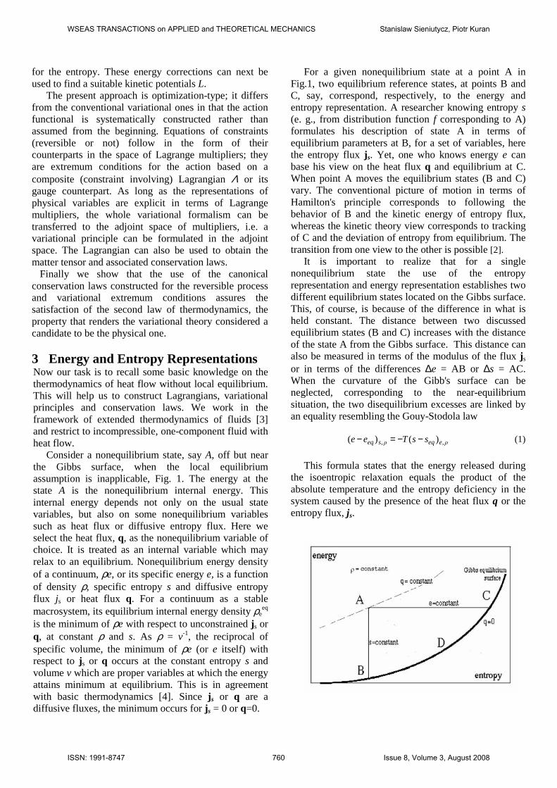
Consider a nonequilibrium state, say A, off but near the Gibbs surface, when the local equilibrium assumption is inapplicable, Fig. 1. The energy at the state A is the nonequilibrium internal energy. This internal energy depends not only on the usual state variables, but also on some nonequilibrium variables such as heat flux or diffusive entropy flux. Here we select the heat flux, q, as the nonequilibrium variable of choice. It is treated as an internal variable which may relax to an equilibrium. Nonequilibrium energy density of a continuum, ρe, or its specific energy e, is a function of density ρ, specific entropy s and diffusive entropy flux js or heat flux q. For a continuum as a stable macrosystem, its equilibrium internal energy density ρe

eq is the minimum of ρe with respect to unconstrained js or q, at constant ρ and s. As ρ = v-1, the reciprocal of specific volume, the minimum of ρe (or e itself) with respect to js or q occurs at the constant entropy s and volume v which are proper variables at which the energy attains minimum at equilibrium. This is in agreement with basic thermodynamics [4]. Since js or q are a diffusive fluxes, the minimum occurs for js = 0 or q=0.

For a given nonequilibrium state at a point A in Fig.1, two equilibrium reference states, at points B and C, say, correspond, respectively, to the energy and entropy representation. A researcher knowing entropy s (e. g., from distribution function f corresponding to A) formulates his description of state A in terms of equilibrium parameters at B, for a set of variables, here the entropy flux js. Yet, one who knows energy e can base his view on the heat flux q and equilibrium at C. When point A moves the equilibrium states (B and C) vary. The conventional picture of motion in terms of Hamilton's principle corresponds to following the behavior of B and the kinetic energy of entropy flux, whereas the kinetic theory view corresponds to tracking of C and the deviation of entropy from equilibrium. The transition from one view to the other is possible [2].

It is important to realize that for a single nonequilibrium state the use of the entropy representation and energy representation establishes two different equilibrium states located on the Gibbs surface. This, of course, is because of the difference in what is held constant. The distance between two discussed equilibrium states (B and C) increases with the distance of the state A from the Gibbs surface. This distance can also be measured in terms of the modulus of the flux js or in terms of the differences ∆e = AB or ∆s = AC. When the curvature of the Gibb's surface can be neglected, corresponding to the near-equilibrium situation, the two disequilibrium excesses are linked by an equality resembling the Gouy-Stodola law

ρeeqρseq ssTee ,, )()( −−=− (1)

This formula states that the energy released during

the isoentropic relaxation equals the product of the absolute temperature and the entropy deficiency in the system caused by the presence of the heat flux q or the entropy flux, js.



Fig. 1. Diverse reference equilibrium states (B, D, C, etc.) for a given nonequilibrium state A.

4 Nonequilibrium Corrections to Energy and Entropy

It is essential that the entropy representation is assumed in the Grad’s formalism of the kinetic theory [1]. Hence the specific energy of an ideal gas or fluid with heat at the point A is equal to the specific energy at equilibrium C in Fig. 1. The reference temperatures and pressures that appear in the expressions of kinetic theory are T(C) and P(C). From the formalism one finds disequilibrium corrections ∆s or ∆e in terms of the non-equilibrium density distribution function f. Here we recapitulate the results of several different works [3]-[6] all using Grad’s [1] solution of the Boltzmann equation in macroscopic predictions for dilute gas of rigid spheres.

The molecular velocity distribution function, f, out of equilibrium but close to it is given as

)1)(()( 1ϕ+= CC eqff (2)

where feq is the local equilibrium (Maxwell-Boltzmann) distribution pertaining to the entropy representation equilibrium (point C, Fig. 1). f and feq are scalars, but functions of the peculiar velocity C = c - u, and ϕ1 is a function of the deviation from equilibrium. This deviation is expressed in terms of the gradT in the Chapman-Enskog method and in terms of the heat flux q in the Grad's method. Using Eq. (2) in the entropy definition, one integrates the expression flnf over all of the space of the molecular velocity c,

∫−= cfdfkρ Bs ln (3)

Proceeding with development of ρs up to second order in φ1, one obtains ....)2()1(

sseqss ρρρρ ++= with the local

equilibrium entropy

∫−= cdffkρeqeq

Beqs ln (4)

and the nonequilibrium correction

0ln1)1( =−= ∫ cdffkρ

eqeqBs ϕ (5)

Again, this proves that one deals with the entropy representation where the entropy is maximum at equilibrium. A counterpart of the above equation in the energy representation

,021

)1( =−= ∫ cc dmfρeq

e ϕ (6)

would correspond to the minimum energy. The second order correction to the entropy density (in entropy representation) is

∫−=∆= cdfksρρeq

Bs21

)2(

2

1 ϕ (7)

Hence, in view of the relation between ∆e and ∆s implied by Fig. 1 or Eq. (1)

∫−−=∆ cdfTρke eq

B21

1

2

1 ϕ (8)

Since the state A is close to the equilibrium surface, the multiplicative coefficients involving usual thermostatic variables can always be evaluated at arbitrary equilibrium points (B or C in Fig. 1). However, in Eqs. (1), (9) and (10), they are evaluated (in the kinetic theory) for the case of the isoenergetic equilibrium (point C, Fig. 1). The function ϕ1, obtained in Grad's method when the system's disequilibrium is maintained by a heat flux q is

qCC .)2

5

2

1)(/(

5

2 2221 TkmTPkm BB −=φ (9)

where m is the mass of a molecule ([1], [3]). From Eqs. (7), (8) and (9) one obtains for the entropy deviation

22)/(5

1qTρPkms B−=∆ (10)

and for the energy deviation, Eq. (1), with entropy flux js = qT-1

22222

2

1)/(

5

1ssB gρρkme jj −==∆ (11)

Equations (10) and (11) hold to the accuracy of the thirteenth moment of the velocity [1]. When passing from Eq. (10) to (11) state equation P = ρkBTm-1 is used and a constant g is defined as

.5

2

5

22

2

BB k

m

Pk

mTg =≡ ρ

(12)

Here we abandoned the entropy representation. Pressure in Eqs. (9) and (12) is that of an ideal gas, given by the definition used in the kinetic theory (Grad 1958 [1]). Eq. (11) with constant g defined by Eq. (12) is the characteristic feature of the ideal monoatomic gas (dilute Boltzmann gas composed of hard spheres). For arbitrary fluids (polyatomic gases, dense monoatomic gases and liquids) one can retain the form of the last expression in Eq. (11) by using a general formula for by noting that

eqseq esρg )/(),( 222 j∂∂≡ ρ (13)

In the ideal gas case the derivative ∂2e/ 2sj∂ =

(2/5)(m2/kB2ρ2) from Eq. (11) and the definition (12) is

recovered form definition (13). quation (13) is consistent with a hypothesis about the equality of the kinetic and static nonequilibrium energy corrections in a thermal shock-wave front [5]. The hypothesis can be used to compute (∂2e/∂js

2)eq for arbitrary fluids as T/(ρcpG) and



hence g as Tρ/(cpG), where G is the shear modulus. Equilibrium values of thermodynamic parameters can be applied in such expressions. For an ideal gas the shear modulus is just the pressure P (the result of Maxwell) and cp = 5kB/(2m). These results allow one to recover definition (12) from the expression g = Tρ/(cpG); they support the hypothesis mentioned above. Yet, for the purpose of general considerations the use of the implicit dependence of g on the basic variables (ρ, s) is often enough, i. e., function g(ρ, s) will be used when passing to arbitrary fluids. Some entropy flux adjoints, as and is, are useful. They are defined, respectively, by equations

sssρsss gρseρs jjjja 2, /),,(),,( −=∂∆∂= ρ (14)

and

)(),,( 1 uuvjji −=== −sssss gsgsgρρs (15)

The entropy diffusion velocity vs = us - u = js/ρs appears in Eq. (15). One may also introduce the product kBgs which has the dimension of mass. For the ideal gas this product yields ms = 2/5(m2skB

-1), a measure of heat inertia.

In the model of a constant g, nonequilibrium temperature T(B) is equal to the equilibrium temperature T(ρ, s) which is both the measure of mean kinetic energy of an equilibrium and the derivative of energy with respect to the entropy. This equality emerges because, above, we have chosen the entropy flux js, not the heat flux q, as the nonequilibrium variable in energy e. If one differentiates the nonequilibrium entropy s with respect to the energy holding q constant, then a quantity T(C) of Jou et al ([3]) follows, which differs from the reciprocal of the related temperature Teq by a term quadratic in q. In general, "nonequilibrium temperatures" (understood as the fifth moment of the nonequilibrium density functions) are not the measures of mean kinetic energy.

The knowledge of inertial coefficients, such as g, from statistical considerations helps to calculate two basic quantities in the model of heat transfer with finite wave speed. They are: thermal relaxation time τ and and the propagation speed, c0. Of several formulae available that link τ and g, probably the following expression

1)( −= Tgτ ρk (16) is most useful ([6], p. 199). It links thermal relaxation time τ with thermal conductivity k, inertia g and state parameters of the system. As, by definition, the propagation speed of the thermal wave c0=(a/τ)1/2, where a= k /(ρcp) is thermal diffusivity, the quantity c0 may be determined from the useful formula

.g

)(

2/1

2/10

==

pc

Tac

τ (17)

Substituting to this formula the ideal gas data, i.e. g of Eq. (12) and cp = 5kB/(2m), yields propagation speed in the ideal gas

2/12/1

0 g

=

=

m

Tk

c

Tc B

p

(18)

(thermal speed). Thus the results of nonequilibrium statistical mechanics help to estimate coefficients of the heat transfer model. Data ofτ� and c0 are used below in a variational principle for heat transfer. One more coefficient that is quite useful in the wave theory of heat is that describing a thermal mass per unit of entropy

θ=T 20−c , (19)

[6]. For an ideal gas, Eq. (18) yields θ as

1−= Bmkθ (20)

We can now set a variational model of the heat problem.

5 Approaches Ajoining Constraints to a Kinetic Potential

For a heat conduction described in an Eulerian frame by the Cattaneo equation and conservation law for the internal energy, the constraints are

020

20

=∇++∂

∂e

ctcρ

τqq

(21)

and

0. =∇+∂

∂q

teρ

, (22)

where the density of the thermal energy ρe satisfies dρe = ρcvdT, c0 is propagation speed for the thermal wave, τ is thermal relaxation time, and D=c0

2τ is the thermal diffusivity. Equation (22) assumes the conservation of thermal energy (rigid medium and neglect of the viscous dissipation). For simplicity we assume constant values of involved fields at the boundary. We ignore the vorticity properties of the heat flux.

The energy-representation of the Cattaneo equation,

022

=∇++∂

∂T

ctc s

s

s

s

τjj

(23)

uses diffusive entropy flux js instead of heat flux q. The coefficient cs is defined as

2/11)( −≡ θρ vs cc (24)



where θ=T 20−c , and thermal diffusivity τρ 2

0ccv≡k . Equation (23) is Kaliski’s equation [6]. For an incompressible medium one may apply this equation in the form

020

20

=∇++∂

∂s

ss

ctcρ

τjj

(25)

which uses the entropy density ρs as a field variable. Yet, we focus here on the action and extremum conditions in the entropy representation (Eqs. (21) and (22) in variables q and ρe). For Eqs. (23) - (25) another approach will be developed in a complementary paper. Action approaches should be distinguished from entropy-production approaches [6], [7]. Here an action is assumed that absorbs constraints (21) and (22) by Lagrange multipliers, the vector ψψψψ and the scalar φ

.)}. ().(

2

1

2

1

2

1{

20

20

22

20

2

,

12

1

dVdtt

φctc

cA

ee

e

t

Vt

qqq

ψ

q

∇+∂

∂+∇++

∂∂+

−−= ∫−

ρρτ

ερε. (26)

As kinetic potentials can be diverse, the conservation laws for energy and momentum substantiate the form (26). In Eq. (26), ε is the energy density at an equilibrium reference state, the constant which ensures action dimension for A, but otherwise is unimportant. Yet we assume that the actual energy density�ρe is close to ε, so that the variable ρe can be identified with the constant ε in suitable approximations.

We call the multiplier-free term of the integrand of Eq. (26)

}{2

1 2220

21 ερε −−≡ −

ec

Lq (27)

the kinetic potential of Hamilton type for heat transfer. It is based on the quadratic form of an indefinite sign, and it has usual units of the energy density. Not far from equilibrium, where ρe is close to ε, two static terms of L yield altogether the density of thermal energy, ρe. Indeed, in view of admissibility of the approximation ρe =ε in Eqs. (27), the kinetic potential (27) represents - in the framework of the linear heat theory - the Hamiltonian structure of a difference between “kinetic energy of heat”, and the nonequilibrium internal energy, ρe. To secure proper conservation laws, no better form of L was found in the entropy representation. The theory obtained in the present case is a linear one.

Vanishing variations of action A with respect to multipliers ψψψψ and φ recover constraints, whereas those with respect to state variables q and ρe yield representations of state variables in terms of ψψψψ and φ . For the accepted Hamilton-like structure of L,

φcτt

∇+−∂∂= 2

0ψψ

q (28)

and

.te ∂

∂−−∇= φρ ψ (29)

These equations enable one to transfer variational formulation to the space of Lagrange multipliers.

For the accepted structure of L, the action A, Eq. (26), in terms of the adjointsψψψψ and φ is

) ..2

1.

2

1

2

1 22

2202

0

12

,1

dVdtt

ctc

At

t V

−

∂∂+∇−∇+

−∂∂= ∫

− εφφτ

ε ψψψ

(30) Its Euler equations with respect to ψψψψ and φ are

0.11 2

020

202

0

=

∂∂+∇∇−

∇+−∂∂+

∇+−∂∂

∂∂

tc

tcc

tct

φφττ

φτ

ψψψψψ (31)

and

.0.. 20 =

∇+−∂∂∇+

∂∂+∇

∂∂− φ

τφ

cttt

ψψψ (32)

It is easy to see that (31) and (32) are the original

equations of the thermal field, eqs. (21) and (22), in terms of potentials ψψψψ and φ. Their equivalent form below shows the damped wave nature of the transfer process. In fact, Lagrange multipliers ψψψψ and φ of this problem satisfy certain inhomogeneous wave equations. In terms of the modified quantities ΨΨΨΨ and Φ satisfying

ΨΨΨΨ = ψψψψ 20τc and Φ = − φτ 2

0c these equations are

.2

022

0

22 q

ΨΨΨ =

∂∂+

∂∂−∇

tctc τ (33)

and

.20

220

22

etc

Φ

tc

ΦΦ ρ

τ=

∂∂+

∂∂−∇ (34)

As both state variables (q, ρe) and adjoints (ψψψψ, φ) appear herein, they represent mixed formulations of the theory.

6 Canonical Conservation Laws The energy-momentum tensor is defined as

( ) Λ−

∂∂∂Λ∂

∂∂≡∑ jk

lk

ljljk

v

vG δ

χχ (35)

where δjk is the Kronecker delta and χ = (x, t) comprises the spatial coordinates and time. Our approach here follows those in [8] and [9], where components of Gjk



are calculated for a reversible Λ whose gauged form is obtained from the reversible limit of Eq. (26) at ψψψψ=0 by use of the divergence theorem and the differentiation by parts. In our problem

}2

1)(

2

1)(

2

1{ 22

021 εε −∇−

∂∂=Λ −

φct

φ (36)

Below the results for tensor G = Gjk are discussed in

physical variables. The momentum density of heat is αααα

ερ

qcqcG e 20

20

4 −− ≅=−=Γ (37)

Clearly, ΓΓΓΓ vanishes in the Fourier’s case (c0 ∞→ ). The stress tensor Tab has the form

Λ−−= −− αββααβ δqqcεT 2

01 (38)

whence (after substituting the stationary Lagrangian)

}2

1

2

1

2

1{ 22

02212

01 ερεδαββααβ −−−−= −−−− cqqcεT e q (39)

The energy density follows as the Legendre transform of the Lagrangian Λ with respect to rate change of φ

eec

q

c

qGE ρ

εερε +≅++== −

20

222

20

2144

2

1}

2

1

2

1

2

1{ (40)

Finally, density of energy flux follows as

ββββ ρε qqQG e ≅== −14 . (41)

The associated conservation laws for the energy and momentum show the role of thermal inertia effects

( )qq ee tc ρερε 1220

1 ./)2

1( −−− −∇=∂+∂ (42)

( ){ })( 2212

212

02

212

01

120 .

)(ερδε

ρε αββαα

+−+−∇=∂

∂ −−−−−

ee cqqc

t

qcq . (43)

These are canonical conservation laws which are

obtained on the reversible paths. Now the important question is if these laws can be recovered for irreversible processes in which the entropy is produced and the Second Law holds.

7 Satisfaction of Second Law Calculating the four-divergence of the entropy flow ( t∂∂∇ /, ) and using the global conservation law for the total energy E we obtain the entropy balance

∂∂−∇−=

∂∂−∇=∇+

∂∂ −

tTk

kTtTcT

Tt

Sv qqqq

q τε

.1

.).(22

0

1 . (44)

Applying Cattaneo equation we arrive at the second law

22

2

20

2

).( sv a

kTTcTt

Sj

qqq=≡=∇+

∂∂

ετ, (45)

where a = k-1 is the thermal resistance. It should be kept in mind that the density Sv appearing in the above equations is not identical with the density of classical equilibrium entropy ρs. As shown by Eq. (61) in Sec.8, Sv is rather the density of the nonequilibrium entropy which contains the heat flux as an extra variable and appears in extended irreversible thermodynamics (EIT; [3]).

222

qT

S sv λτρ −=

8 Sources of internal energy and conservation laws

However, while simple and useful, the method of construction of a suitable action A in the space of potentials by the direct substitution of the representation equations to the kinetic potential L is limited to cases with linear constraints that do not contain sources. This may be exemplified when the internal energy balance contains a source term a’q2, where a’ is a positive constant. The augmented action integral, generalizing Eq. (26), should now contain the negative term - a’q2 in its φ term.

2'. qq ate −

∂∂

=∇−ρ

(46)

The energy representation (29) is unchanged, but the heat flux representation follows in a generalized form

)()( φcτt

ca ∇+−∂∂φ′2−1= 2

01−2

0ψψ

q (47)

Substituting Eqs. (29) and (47) into action A of Eq. (26) (L of Eq. (27)) shows that in terms of the potentials the action acquires the form

) dVdtct

cac

At

t V

φ∇+

τ−

∂∂φ′2−1

21ε=

220

2−202

0

1−∫2

1

ψψ)(

,

dVdtt

t

t V

ε21+

∂φ∂+∇

21ε− 2

21−

∫2

1

ψ.,

. (48)

However the Euler-Lagrange equations for this action are not the process constraints in terms of potentials, i.e. the method fails to provide a correct variational formulation for constraints with sources. The way to improve the situation is to substitute the obtained representations to a transformed augmented action in



which the only terms rejected are total time or space derivatives. The latter can be selected via partial differentiation within the integrand of the original action A. (As we know from the theory of the functional extrema the addition of subtraction of terms with total derivatives and divergences do not change extremum properties of a functional.) When this procedure is applied to the considered problem and total derivatives are rejected, a correct action follows in the form

) dVdtct

cac

At

t V

φ∇+

τ−

∂∂φ′2−1

21ε=

220

1−202

0

1−∫2

1

ψψ)(

,

dVdtt

t

t V

ε21+

∂φ∂+∇

21ε− 2

21−

∫2

1

ψ.,

(49)

This form differs from that of Eq. (34) only by the

power of the coefficient containing the constant a’, related to the source. With the related representation equations (29) and (47), action (49) yields the proper Cattaneo constraint (21) and the generalized balance of internal energy which extends equation (22) by the source term a’q2.

Equation (49) proves that four-dimensional potential space (ψψψψ, φ) is sufficient to accommodate an exact variational formulation for the problem with a source. Yet, due to the presence of this source, the formulation does not exist in the original four-dimensional original space (q, ρe), and, if somebody insists to exploit this space plus possibly a necessary part of the potential space, the following action is obtained from Eqs. (29), (47) and (49)

dVdtc

caA e

t

Vt

})'{(,

2202

0

220

1− ε21+ρ

21−

2φ2−1ε= ∫

2

1

q (50)

This form of A shows that, when original state space

is involved, the state space required to accommodate the variational principle must be enlarged by inclusion of the Lagrange multiplier φ as an extra variable. In fact, Eq. (50) proves that original state space (“physical space”) is lacking sufficient symmetry (Vainberg’s theorem [6]). Yet, as Eq. (50) shows, the adjoint space of potentials (ψψψψ, φ), while also four-dimensional as space (q, ρe0), can accommodate the variational formulation. Why is this so? Because the representation equations do adjust themselves to the extremum requirement of A at given constraints, whereas the given constraints without controls cannot exhibit any flexibility.

Somewhat surprisingly, it follows that a source term in the internal energy balance, as in Eq. (46), should be the necessary property of the Cattaneo model, else the energy conservation will be violated. Indeed, aimed at the evaluation of energy conservation we multiply the non-truncated Cattaneo formula

020

20

=∇++∂

∂e

ctcρ

τqq

(21)

by heat flux q. The result is an equation

τερε

ερ

ε 20

21

20

2

).(.2 ctc

ee q

qqq

−=∇+∇−∂

∂ − (51)

which describes an energy balance We observe that the combination of this balance with the sourceless balance of internal energy

0. =∇+∂

∂q

teρ

, (22)

leads to a differential result

τερερ

ερ

ε 20

21

20

2

).(2 cttc e

ee qq

q −=∇+∂

∂+∂

∂ − (52)

which – under the linear approximations of the present theory – yields not a conservation law for the total energy, but a balance formula with an energy source

τερε

ε 20

21

e20

2

).(ρ2 cct e

qq

q−=∇+

+

∂∂ − . (53)

This shows violation of the total energy conservation for the source-less internal energy of the model, and leads to the conclusion that the model composed of the Cattaneo equation and source-less balance of internal energy is physically admissible only in the reversible case of an infinite τ. Certainly, this is not a demanded property of the energy transfer model, thus a further analysis is required. The solution of the dilemma seems to admit a properly large, yet a non-vanishing, source in the internal energy balance.

Admitting a source of the internal energy, as in equation (46), and using Eq. (46) in Eq. (51) we find

τερε

ερρ

ερ

ε 20

212

20

2

).('2 c

attc e

eee qqq

q −=∇+−∂

∂+

∂∂ − . (54)

From this formula we observe that for a’ satisfying



TTDcca

hve k1=

ρ1=

τρ1= 2

00

' . (55)

and - under the approximation of the linear theory - conservation of total energy is satisfied by the source-less equation

0).(ρ2

1e2

0

2

=∇+

+

∂∂ −

ect

ρεε

qq (56)

The positive value of a’ in Eq. (55) implies generation of the internal energy in the heat transfer process, as described by Eq. (46). Still, the internal energy equation with the positive source caused by the quadratic heat flux is a dubious structure. Nonetheless, it is a step forward in comparison with sourceless internal energy balance as we may observe that this generation awkwardly mimics the entropy production with the coefficient a=Ta’=1/k. This finally leads us to the conclusion that it is the entropy balance with the source j2/k than that should replace Eq. (46) in the entropy representation.

Replacing Eq. (46) with a’ of Eq. (55) by its conserved counterpart i.e. total energy balance expressed in entropy terms

q.−∇=∂

∂t

T sρ (57)

(where ρs is equilibrium entropy density) we expect to obtain a pronounced result. After rearranging

1.).( −∇+−∇=∂

∂T

Tts q

qρ (58)

and using in this result the Cattaneo equation (21) in the equivalent form

0=λ

−∇+∂∂

λτ− 2

1−2 T

TtT

qq (59)

we obtain

+∂∂+−∇=

∂∂

22.).(

TtTTts

λλτρ qq

qq

(60)

and hence the second law balance for the entropy of extended thermodynamics

2

212

2).(

2 TT

Tt s λλτρ q

qq =∇+

−∂∂ − (61)

The total energy is conserved in the linearized form (56) or in an exact form

0).(ρ2 e

2

=∇+

+

∂∂

ss T

k

T

tj

jτ (62)

A similar scheme of reasoning can be applied in the energy representation where the entropy balance is the process constraint.

9 Entropy balance as process constraint Assume that a variational functional can be constructed in the entropy representation for the Kaliski’s equation (25) [10]. This assumption means that after transforming the variational stationarity condition of an action with respect to ψψψψ

020

20

=∇++∂

∂s

ss

ctcρ

τjj

(25)

into the form

TTcctc

vss ∇ρ−=τ

+∂

∂ 1−20

20

jj (63)

and using the relation between coefficients cs and c0

)( 1−20

2 ρ= Tccc vs (64)

we obtain Kaliski’s equation of entropy transfer with explicit temperature gradient

0=∇+τ

+∂

∂22 T

ctc s

s

s

s jj (23)

Af ter multiplying Kaliski’s equation (23) by js we

find

τ−=∇−∇+

∂2∂

2

2

2

2

s

sss

s

s

cTT

tc

jjj

j.).( . (65)

Under the assumption of the entropy conservation Eq.(65) would yield an equation

τρ

2

2

2

2

).(2 s

sss

s

s

ctTT

tc

jj

j−=

∂∂

+∇+∂

∂ (66)

thus leading to the following energy balance



τ−=∇+ρ+

2∂∂

2

2

02

2

s

sse

s

s

cT

ct

jj

j).()( . (67)

This result implies a non-vanishing source of the energy and means that the assumption of the conserved entropy would result in the violation of the energy conservation law.

Yet, for the ‘physical’ entropy satisfying the non-conserved balance

2−∂ρ∂

=∇− ss

s at

jj. (68)

with the coefficient a equal to the reciprocal of thermal conductivity

kTca

s

1=τ

1= 2 . (69)

total energy balance follows from Eqs. (65), (68) and (69) in the form

τρ

2

22

2

2

).()2

(s

ssse

s

s

cTaT

ct

jjj

j−=−∇++

∂∂

(70)

which is conservative because the two source terms mutually cancel. This is show in Eq. (71) below. Thus the energy conservation is preserved whenever the coefficient a satisfies Eq. (69).

Importantly, even when the conservation laws are satisfied in irreversible processes in their canonical form the related extremum action and potential representations of physical variables do explicitly contain potentials not only their derivatives.

We may thus claim that whenever a irreversible process occurs with the coefficient a satisfying Eq. (69), conservation laws in their canonical form (the same as for reversible processes) can be obtained from the Noether’s theorem. In particular the energy conservation law has the form

0).(2 2

2

=∇+

+

∂∂

ses

s Tct

jj ρ . (71)

As the coefficient cs

2=k(Tτ)-1, the above equation is equivalent with Eq. (62). In conclusion, the mathematical scheme obtained preserves the conservation of energy and simultaneous production of the entropy, in accordance with laws of

thermodynamics.

10 Conclusions The most important physical properties resulting from the obtained generalization are: a finite momentum of heat and the non-classical terms in the stress tensor caused by the heat flux. And with all this one still has both the first and the second law satisfied. Here the product of temperature T and positive entropy source of Eq. (68) (quadratic in js) emerges as the kinetic energy of heat in the energy balance (70) or (71). While this result is simple, its role is nontrivial for the existence of the variational formulation. Let us recall that in the variational dynamics of real fluids it is always extremely difficult to simultaneously satisfy both laws of thermodynamics (classical Hamilton's principle holds only for reversible processes i.e. those without entropy production). The optimizing approach overcomes familiar difficulties resulting from the presence of both odd and even derivatives with respect to time in the differential equations of heat, and, consequently, sets a variational formulation for the irreversible heat conduction.

Extremum conditions, Eqs. (33) and (34), show that for given q and ρe heat transfer can be broken down to potentials. This is similar to the case of electromagnetic field theory or gravitation theory, where the knowledge of sources defines the field potentials. An important case is a “ ballistic” transfer with τ ∞→ , when undamped thermal waves propagate with speed c0 and satisfy d'Alembert's equation. As shown by Eq. (45) the results are consistent with the second law in an identically satisfied form; this holds in both classical irreversible theory (CIT) and extended irreversible thermodynamics (EIT; [3]).

Associated approaches with Lagrange multipliers and Dirac brackets are available [11,12,13]. It is interesting that not only variational calculus but also other optimization methods may also be fruitful in the context of problems considered here, such as, e.g., simulated annealing [14] and dynamic programming [15, 16].

Acknowledgements This work was supported by TU Warsaw statute grant Simulation and optimization of thermal and mechanical separation processes in 2008.

References: [1] H. Grad, “Principles of the theory of gases”, in

Handbook der Physik 12, S. Flugge, Ed., Berlin: Springer, 1958.

[2] S. Sieniutycz and R. S. Berry, “Conservation laws from Hamilton's principle for nonlocal



thermodynamic equilibrium fluids with heat flow”, Phys. Rev. A. 40 (1989) 348-361.

[3] D. Jou, J. Casas-Vazquez and G. Lebon, Extended Irreversible Thermodynamics, Heidelberg: Springer, 1993.

[4] H. Callen, Thermodynamics and an Introduction to Thermostatistics, New York: Wiley, 1998.

[5] S. Sieniutycz, “Thermodynamics of coupled heat, mass and momentum transport with finite wave speed. I.,II.Intern. J. Heat Mass Transfer 24 (1981) 1723-1732 and 24 (1981) 1759-1769.

[6] S. Sieniutycz, Conservation Laws in Variational Thermo-Hydrodynamics, Dordrecht:, Kluwer, 1994.

[7] S. Sieniutycz, “Variational thermomechanical processes and chemical reactions in distributed Systems”, Intern. J. Heat and Mass Transfer, 40 (1997) 3467-3485.

[8] J.J. Stephens, “Alternate forms of the Herrivel-Lin variational principle”, Phys. Fluids 10 (1967) 76-77.

[9] R. L. Seliger and G. B. Whitham, “Variational principles in continuum mechanics”, Proc. Roy. Soc. 302A (1968) 1-25.

[10]. S. Sieniutycz and H. Farkas, eds. Variational and Extremum Principles in Macroscopic Systems, Oxford, Elsevier, 2005. (See especially Chap.7 of part II.)

[11]G.L.Liu, The first exact variational formulation of 3D Navier-Stokes, Comp. Mech. VI, (2004) 438-443.

[12]G.L.Liu, A unified variational formulation of aeroelasticity in 3D unsteady transonic flow, IUTAM Symp.Transsonicum IV (in Gottingen), H. Sobieczky (ed.), Kluwer Acad. Publ. (2003) 85-90.

[13] S. Nguyen and Ł. A. Turski, Examples of the Dirac approach to dynamics of systems with constraints, Physica A 290 (3-4) (2001), 431-444.

[15] H.G Arango and G.L. Tores, Spatial electric load distribution forecasting using simulated annealing, WSEAS Transactions on Systems, 3(1) 2004, 14-19.

[16] M.T. Suzuki, A dynamic programming approach to search similar portions of 3D models, WSEAS Transactions on Systems, 3(1) 2004, 14-19.

[17] S. Sieniutycz, Optimization of multistage electrochemical systems of fuel cell type by dynamic programming, WSEAS Transactions on Mathematics, 2(3) 2003, 228-232.



Variational Formulations and Extended Thermodynamics for Resting Irrevers ible Fluids with Heat Flow

Documents

Transcript of Variational Formulations and Extended Thermodynamics for Resting Irrevers ible Fluids with Heat Flow