Valuing Health-Risk Reductions: Sick-years, LostLife-Years, and Latency

Trudy Ann Cameron and J.R. DeShazo1,2

December, 2004

Abstract

We develop a utility-theoretic model in which individuals choose among alternative pro-grams to reduce their risk of experiencing future years of illness and/or lost life-years. Unlikeprevious approaches to deriving the Value of a Statistical Life (V SL), our model is able toproduce separate estimates of the marginal utilities of both avoided sick-years and avoidedlost life-years. With these marginal utilities, we may infer willingness to pay to avoid widerange of adverse health profiles over an individual’s future life. Such estimates are particu-larly important for ex ante benefit-cost analyses of environmental, health or safety interven-tions where costs must be incurred now to reduce health risks that will not fully materializeuntil much later. The model generalizes the single-period, single-risk models (typically usedto produce single-valued V SL estimates) in that we allow individuals to substitute acrosshealth risks with different time profiles. We evaluate our model using data from an extensivenationally representative survey that contains a set of randomized choice experiments.

JEL Classifications: I1, H43, Q51

Keywords: Value of a Statistical Life (V SL), mortality risk, morbidity risk, health, optionprice

1Senior authorship is not assigned. Nominal lead authorship will rotate though this paper series.2Department of Economics, University of Oregon, and School of Public Affairs, UCLA, respectively. We

thank Kip Viscusi, Vic Adamowicz, Richard Carson, Maureen Cropper, Baruch Fischhoff, Jim Hammitt,Alan Krupnick, and V. Kerry Smith for helpful comments. Rick Li implemented our survey very capably.Ryan Bosworth, Dan Burghart, and Graham Crawford have provided able assistance. This research hasbeen supported by the US Environmental Protection Agency (R829485, Program Director Will Wheeler).It was was also encouraged by Paul De Civita and has been supported in part by Health Canada (ContractH5431-010041/001/SS). This work has not yet been formally reviewed by either agency. Any remainingerrors are our own.

1

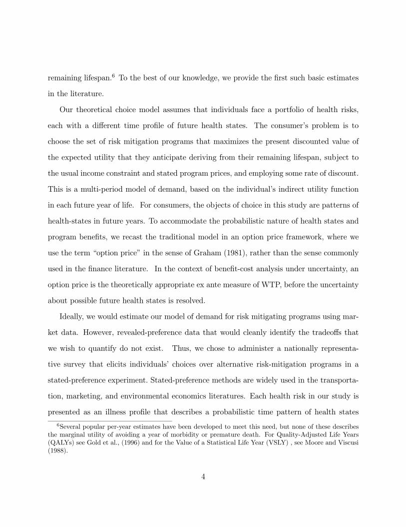
1 Introduction

Over their lifetimes, individuals face a portfolio of distinct health risks such as heart disease,

accidents, cancers, strokes, respiratory disease and many others. Individuals and policymak-

ers may mitigate these risks through expenditures on privately available preventative care

and medical therapies and publicly provided environmental, safety and health programs.

The consumer’s problem is to optimally allocate expenditures to each risk-mitigating pro-

gram for each future year of their life. An important dimension of this problem is that the

severity of each health risk will vary over an individual’s lifespan. Furthermore, the majority

of these risk-mitigating programs involve multiple periods of costs and yield uncertain future

benefits. How to accommodate long latencies in health risks has been a particular challenge

in the benefit-cost analysis of many public programs.

In empirical analyses, researchers tend to simplify the consumer’s problem to render it

more tractable. It is common to estimate wage-risk (or wealth-risk) trade-offs by assuming

the individual considers a single health risk in the current period (Dreze, 1962; Jones-Lee,

1974). These models do not incorporate multiple risks or inter-temporal decision-making

under uncertainty. Traditional single-risk, single-period models have motivated hundreds of

empirical demand analyses, including many of those currently used to evaluate the social

benefits of life-saving public policies.

Much of this literature focuses on deriving a single one-size-fits-all measure of the Value

of a Statistical Life (V SL), a construct that measures the marginal rate of substitution

between mortality risk reductions and income, scaled up to a 1.00 change in risk. A V SL is

intended to measure aggregate willingness to pay (WTP) for very small changes in mortality

risks experienced by large numbers of people. The US Environmental Protection Agency,

for example, currently relies upon a V SL of about $6 million for its ex ante benefit-cost

2

analyses for environmental regulations.3 In contrast, the Department of Transportation uses

a V SL on the order of $1 million for road safety measures.

Our model generalizes the traditional single-risk, single-period V SL model in several

ways. Parameter estimates for the marginal utilities of avoided degraded health-state years

depend explicitly upon the latency of the program benefits, the stream of program costs,

and the individual’s discount rate and future income. We allow individuals to substitute

mitgation expenditures across health risks with different time profiles, since omitting relevant

substitutes from the individual’s choice set may bias estimates of marginal utility (Rosen,

1988; Dow et al., 1999).4 Furthermore, to assume that the individual’s allocation of risk-

mitigation expenditures is a one-period problem, when in fact it is a multi-period problem,

has the potential to yield distorted estimates, so our model explicitly addresses the multi-

period nature of the problem and the relevance of disease latencies and discounting.5

Most importantly, our model permits us to estimate both the marginal utility of avoid-

ing a future year of morbidity and the marginal utility of avoiding a lost life-year. Most

actual programs do not “save” lives; rather they extend life by deferring the future onset

of morbidity or the event of death. We introduce the concept of the value of statistical

illness profile (V SIP ) which represents the individual’s marginal rate of substitution be-

tween income, morbidity risks, and mortality risks. Both policymakers and scholars have

long sought a tractable and theoretically consistent empirical model that describes how the

marginal value of avoiding a year of morbidity or a lost life-year varies across an individual’s

3This number is a central tendency among a set of 26 defensible studies. Five of these studies employstated preference data (as does the present study) and the rest are based on revealed preference data (Viscusi,1993).

4Recently, scholars have sought to allow for substitution between pairs of risks (Liu and Hammitt, 2003).5One might argue that hedonic wage studies are exempt from this critique, since wage contracts may

be interpreted as one-period contracts. However, when choosing across occupations, individuals may, ineffect, choose across time-paths of risk-wage premia that implicitly embody inter-temporal substitution ofrisk mitigation (Aldy and Viscusi, 2003).

3

remaining lifespan.6 To the best of our knowledge, we provide the first such basic estimates

in the literature.

Our theoretical choice model assumes that individuals face a portfolio of health risks,

each with a different time profile of future health states. The consumer’s problem is to

choose the set of risk mitigation programs that maximizes the present discounted value of

the expected utility that they anticipate deriving from their remaining lifespan, subject to

the usual income constraint and stated program prices, and employing some rate of discount.

This is a multi-period model of demand, based on the individual’s indirect utility function

in each future year of life. For consumers, the objects of choice in this study are patterns of

health-states in future years. To accommodate the probabilistic nature of health states and

program benefits, we recast the traditional model in an option price framework, where we

use the term “option price” in the sense of Graham (1981), rather than the sense commonly

used in the finance literature. In the context of benefit-cost analysis under uncertainty, an

option price is the theoretically appropriate ex ante measure of WTP, before the uncertainty

about possible future health states is resolved.

Ideally, we would estimate our model of demand for risk mitigating programs using mar-

ket data. However, revealed-preference data that would cleanly identify the tradeoffs that

we wish to quantify do not exist. Thus, we chose to administer a nationally representa-

tive survey that elicits individuals’ choices over alternative risk-mitigation programs in a

stated-preference experiment. Stated-preference methods are widely used in the transporta-

tion, marketing, and environmental economics literatures. Each health risk in our study is

presented as an illness profile that describes a probabilistic time pattern of health states

6Several popular per-year estimates have been developed to meet this need, but none of these describesthe marginal utility of avoiding a year of morbidity or premature death. For Quality-Adjusted Life Years(QALYs) see Gold et al., (1996) and for the Value of a Statistical Life Year (VSLY) , see Moore and Viscusi(1988).

4

that the individual could experience. Based upon each individual’s gender and current age,

each health profile consists of randomly assigned values for the individual’s future age at the

time of onset, the severity and duration of treatments and morbidity, the age at recovery (if

recovery occurs), and the number of lost life-years (if any).

We present respondents with an illness-specific health-risk reduction program that in-

volves diagnostic screening, remedial medications and life-style changes that would reduce

their probability of experiencing that illness profile. Individuals must pay an annual fee to

participate in each risk-reducing program. They are asked to choose between one of two risk

reducing programs (each associated with a different illness profile) or to reject both programs.

An advantage of this choice setting is that the individual faces a portfolio of health risks

that resemble those they actually face. Through their choices, individuals reveal trade-offs

across specific illnesses and a full continuum of health states of different durations. We also

observe them strategically allocating expenditures for risk mitigating programs across the

current year and future years of their remaining lifespan.

To analyze individuals’ program choices, we estimate a modified translog indirect utility

function using over 7,500 choices made by respondents to a representative national survey

of over 2,400 U.S. citizens. Our estimated model permits estimates of the marginal utility of

avoiding a year spent in each of three health states: morbidity, post-morbidity and mortality.

Two important innovations in our specification are that it (a) accomodates interactions

between the marginal utility of years of morbidity and years premature mortality, and (b)

controls for the correlation between an individuals’ age and the set of health outcomes they

face over their remaining lifespan.

To illustrate the implications of our model, we estimate individuals’ willingness to pay to

avoid five archetypical illness profiles. This exercise demonstrates how our model generalizes

5

the concept of a V SL. Rather than capturing only the special case of mortality in the current

year, we show how our model can value the discounted benefits of avoiding a wide variety

of statistical illness profiles across an individual’s remaining lifespan. Finally, by way of

sensitivity analysis, we illustrate how different conditions—with respect to (1) discount rates,

(2) income levels and (3) program latency for individuals of different ages—affect the marginal

value of risk mitigation and, in turn, the value of avoiding different types of statistical illness

profiles. The structural model in Section 2 shows that the conventional concept of a V SL

is a special case of our more-general Value of Statistical Illness Profile (V SIP ). We outline

our survey methods in Section 3, and our model’s parameter estimates in Section 4, along

with some sensitivity analyses. Section 5 concludes.

2 A Utility-Theoretic Choice Model

Our model interprets individuals’ choices as revealing their option prices, in the sense of

Graham (1981), for programs that mitigate the risks of adverse future health states.7 The

underlying model allows a great deal of flexibility in characterizing how individuals assume

that future health states will impact their future income and program costs. While program

choices have inter-temporal consequences, our model is one of static decision-making, with

future costs and benefits converted into the appropriate present values.

We focus on four distinct health states: 1) a pre-illness healthy state, 2) an illness state,

3) a post-illness state (if the illness is non-fatal) and 4) death. Let i index individuals and

let t index time periods.8 Let 1 (preit), 1 (illit), 1 (rcvit), and 1 (lylit) be a set of mutually

7Cameron (2005) employs a less-elaborate model in a similar vein to the problem of climate changemitigation programs, where costs must be incurred starting now to reduce the chance of adverse consequencesmany years into the future.

8Time is measured in years or months, as needed.

6

exclusive and exhaustive 0,1-variables that indicate individual i’s health state in time period

t. Let the undiscounted utility from the pre-illness status quo health state (1 (preit) = 1) be

α0, and let the (dis)utility from each future period of illness (1 (illit) = 1) be defined as α1,

from each period of the post-illness state (i.e. “recovered,” 1 (rcvit) = 1) be α2, and from

each period of premature death (i.e. “life-year lost,” 1 (lylit) = 1) be α3. We interpret the

disutility of each of these states as being the same as the utility associated with avoiding

them. In its simplest form, the individual’s indirect utility function in period t might be

specified as:

Vit = βf(Yit) + α0 1 (preit) + α1 1 (illit) + α2 1 (rcvit) + α3 1 (lylit) + ηit (1)

This form allows the undiscounted marginal utility of some function of current income,

f(Yit), to be some parameter β. Algebraically, the indicators for each health state will play

a role that is equivalent to adjusting the limits of the summations used in calculating the

present value of future continued good health, future intervals of illness, post-illness time,

and life-years lost.

In our data, individuals will face choices that involve three alternatives: Program A,

Program B, or neither program (labeled A, B, and N). In developing our estimating specifi-

cation, however, we will describe our model in terms of just two choices: Program A versus

no program (just A and N). The three-alternative case is completely analogous.

Let undiscounted indirect utility be V jkit for the ith individual in period t, where j = A

if Program A is chosen and j = N if the program is not chosen. The superscript k will be

S (denoting “sick”) if the individual suffers the illness and H (denoting “healthy”) if the

individual does not suffer the illness. From the perspective of a program choice made today,

individuals will discount the streams of utility derived from each future health state. When

7

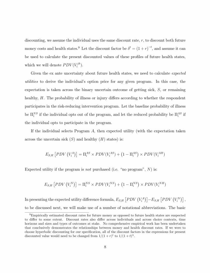
discounting, we assume the individual uses the same discount rate, r, to discount both future

money costs and health states.9 Let the discount factor be δt = (1 + r)−t, and assume it can

be used to calculate the present discounted values of these profiles of future health states,

which we will denote PDV (V jki ).

Given the ex ante uncertainty about future health states, we need to calculate expected

utilities to derive the individual’s option price for any given program. In this case, the

expectation is taken across the binary uncertain outcome of getting sick, S, or remaining

healthy, H. The probability of illness or injury differs according to whether the respondent

participates in the risk-reducing intervention program. Let the baseline probability of illness

be ΠNSi if the individual opts out of the program, and let the reduced probability be ΠAS

i if

the individual opts to participate in the program.

If the individual selects Program A, then expected utility (with the expectation taken

across the uncertain sick (S) and healthy (H) states) is:

ES,H

£PDV

¡V Ai

¢¤= ΠAS

i × PDV (V ASi ) +

¡1−ΠAS

i

¢× PDV (V AH

i )

Expected utility if the program is not purchased (i.e. “no program”, N) is:

ES,H

£PDV

¡V Ni

¢¤= ΠNS

i × PDV (V NSi ) +

¡1−ΠNS

i

¢× PDV (V NH

i )

In presenting the expected utility difference formula, ES,H

£PDV

¡V Ai

¢¤−ES,H

£PDV

¡V Ni

¢¤,

to be discussed next, we will make use of a number of notational abbreviations. The basic

9Empirically estimated discount rates for future money as opposed to future health states are suspectedto differ to some extent. Discount rates also differ across individuals and across choice contexts, timehorizons and sizes and types of outcomes at stake. No comprehensive empirical work has been undertakenthat conclusively demonstrates the relationships between money and health discount rates. If we were tochoose hyperbolic discounting for our specification, all of the discount factors in the expressions for presentdiscounted value would need to be changed from 1/(1 + r)t to 1/(1 + t)λ.

8

discounting term to be applied to any constant stream of payments between now and the

individual’s nominal life expectancy, Ti, is pdvcAi =

XTi

t=1δt. Other discounted terms, also

summed from t = 1 to t = Ti include:

pdveAi =X

δt1¡preAit

¢pdviAi =

Xδt1¡illAit

¢pdvrAi =

Xδt1¡rcvAit

¢pdvlAi =

Xδt1¡lylAit

¢Recall that the indicator variables for each health state are mutually exclusive and exhaus-

tive, so that the comprehensive discounting term is pdvci = pdvei + pdvii + pdvri + pdvli.

Finally, to accommodate the time profiles for program costs over the individual’s remaining

lifespan, it is convenient to define an additional term, pdvpAi = pdveAi + pdvrAi .

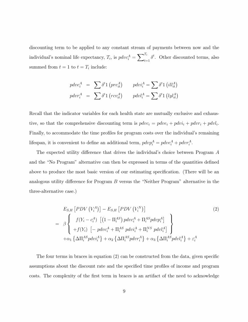
The expected utility difference that drives the individual’s choice between Program A

and the “No Program” alternative can then be expressed in terms of the quantities defined

above to produce the most basic version of our estimating specification. (There will be an

analogous utility difference for Program B versus the “Neither Program” alternative in the

three-alternative case.)

ES,H

£PDV

¡V Ai

¢¤−ES,H

£PDV

¡V Ni

¢¤(2)

= β

⎧⎪⎨⎪⎩ f(Yi − cAi )£¡1−ΠAS

i

¢pdvcAi +ΠAS

i pdvpAi¤

+f(Yi)£− pdvcAi +ΠAS

i pdviAi +ΠNSi pdvlAi

¤⎫⎪⎬⎪⎭

+α1©∆ΠAS

i pdviAiª+ α2

©∆ΠAS

i pdvrAiª+ α3

©∆ΠAS

i pdvlAiª+ εAi

The four terms in braces in equation (2) can be constructed from the data, given specific

assumptions about the discount rate and the specified time profiles of income and program

costs. The complexity of the first term in braces is an artifact of the need to acknowledge

9

different time profiles of income and program costs in the sick and healthy states. We assume

that individuals anticipate sustaining their current real income while they are sick, but not

if they are dead. We also assume that they expect not to have to pay the costs of the

program if they are either sick or dead. The four basic utility parameters β, α1, α2, and

α3, which are the same marginal utilities appearing in equation (1), are the focus of our

empirical illustration.

To simplify the way we display the complicated term involving net income that is modified

by the coefficient β, we will use two abbreviations:

ctermAi =

£¡1−ΠAS

i

¢pdvcAi +ΠAS

i pdvpAi¤

ytermAi =

£−pdvcAi +ΠAS

i pdvsAi +ΠNSi pdvlAi

¤We will also abbreviate the set of terms in equation (2) that involve the discounted health

states in the illness profile:

ptermAi = ∆ΠAS

i

£α1pdvi

Ai + α2pdvr

Ai + α3pdvl

Ai

¤Then the expression in equation (2) for the difference in the expected present discounted

indirect utilities can be written more compactly as:

ES,H

£PDV

¡V Ai

¢¤− ES,H

£PDV

¡V Ni

¢¤(3)

= β©f(Yi − cAi ) cterm

Ai + f(Yi)yterm

Ai

ª+ ptermA

i + εAi

The Graham-type option price for the program is the maximum common certain payment

that makes the individual just indifferent between paying for the program and enjoying the

10

risk reduction, or not paying for the program and not enjoying the risk reduction. Once the

parameters β, α1, α2, and α3 have been estimated from a conditional logit model based on

equation (2), the annual option price that will make ES,H

£PDV (V A

i )¤− ES,H

£PDV (V N

i )¤

exactly zero, bcAi , can be calculated.bcAi = Yi − f−1

µβf(Yi)yterm

Ai + ptermA

i + εAi−βctermA

i

¶(4)

While the payment bcAi is the maximum annual payment the individual is willing to make,these payments are necessary for the rest of the individual’s life, so the present value of these

payments must be calculated. In this context, however, there is some uncertainty over just

what will constitute “the rest of the individual’s life,” since this may differ according to

whether the individual suffers the illness or not. If they do not suffer the illness, they will

pay for the rest of their lives. If they do suffer the illness, they will pay only during the

pre-illness period and during any post-illness period, but not if they are sick or dead. We will

use the expected present value of this time profile of costs (with the expectation taken over

whether or not the individual suffers the illness when they are participating in the program).

EhPV ( bcAi )i = ( bcAi ) £¡1−ΠAS

i

¢pdvcAi +ΠAS

i pdvpAi¤= ( bcAi )ctermA

i (5)

= ctermAi

∙Yi − f−1

µβf(Yi)yterm

Ai + ptermA

i + εAi−βctermA

i

¶¸

The option price that we estimate represents a willingness to pay to reduce an illness-

specific risk that jointly determines a profile of different health state outcomes, not just

the mortality outcomes upon which a conventional V SL is based. To convert our expected

present-value option price to the “value of a statistical illness profile” (V SIP ), we normalize

arbitrarily on a 1.00 risk change by dividing this WTP by the absolute size of the risk

11

reduction:

V SIP =EhPV ( bcAi )i|∆ΠAS

i |=

ctermAi

|∆ΠASi |

∙Yi − f−1

µβf(Yi)yterm

Ai + ptermA

i + εAi−βctermA

i

¶¸(6)

As a concrete example, suppose that indirect utility is merely linear in net income, so

that that f(Yi) = Yi. Then

bcAi = Yi −µβYiyterm

Ai + ptermA

i + εAi−βctermA

i

¶(7)

To calculate a measure analogous to traditional V SL estimates, we take the expected present

value of this annual option price (with the expectation taken relative to the uncertainty in

future health profiles), multiply by ctermAi and divide by the absolute value of the risk

difference:

V SIP =

µctermA

i

∆ΠAi

¶ ∙Yi −

µβYiyterm

Ai + ptermA

i + εAi−βctermA

i

¶¸(8)

In this linear case, the formula for V SIP simplifies to

V SIP = YipdvlAi −

α1βpdviAi −

α2βpdvrAi −

α3βpdvlAi −

εiβ |∆ΠAS

i |(9)

where we take advantage of the fact that pdvyAi +pdvlAi = pdvcAi so that¡pdvyAi − pdvcAi

¢=

−pdvlAi . This form emphasizes the dependence of the more-general concept of a V SIP on

the entire illness profile.

How does the magnitude of the estimated V SIP vary with changes in it components?

In this simple model with a constant marginal utility of income, increases in income Yi will

increase the predicted point estimate of the V SIP . The effect of income on V SIPAi is given

by ∂V SIPAi /∂Yi = pdvlAi , which is non-negative. The effect of an increase in income on the

12

predicted V SIP will be larger (i.) as more life-years are lost and (ii.) as the individual is

older, so that life-years lost come sooner in time. The income-elasticity of the conventional

V SL has been an important issue for policy-making in the face of growing real incomes.

The linear version of our model would yield an income elasticity for the V SIP equal to

pdvlAi¡Yi/V SIP

Ai

¢10

The V SIP will clearly depend on the different marginal utilities of avoided periods of

illness, post-illness status, and premature death, and on the time profiles for each of these

states as embedded in the terms pdviAi , pdvrAi , and pdvlAi , and (implicit in the pdv terms)

upon the individual’s own discount rate.11 Heterogeneity in preferences can be accommo-

dated by making the indirect utility parameters α1, α2, and α3, and even β, depend upon

other individual characteristics, notably age.12,13

To calculate a measure closest to the conventional V SL, one would assume death in the

10Nothing in this specification precludes negative point estimates of the V SIP . The key undiscountedmarginal utility parameters are not presently constrained to be strictly positive (for income) and strictlynegative (for episodes of undesirable health profiles). This is especially a concern when these marginal utilitiesare permitted to vary systematically with of the attributes of the illness profile and/or the characteristics ofthe individual in question. The marginal utility of income, the scalar parameter β in our simplest models,bears a point estimate that is robustly positive, but positive values for the important systematically varyingparameters capturing the marginal utility of an illness-year (α1) or a lost life-year (α3) can push an individualfitted value of the VSI for a particular morbidity/mortality profile, for respondents with extreme ages in oursample, into the negative range.11Subsequent work will preserve individual discount rates as systematically varying parameters that depend

upon respondent characteristics. In a separate subsample for our survey, we elicited choices that allow usto infer individual specific discount rates. Here, however, discount rates are presumed to be exogenous andconstant across individuals although our empirical analyses explores the senstivity of our results to differentdiscount rates.12For example, illness characteristics can be expected to shift the value of α1, the marginal (dis)utility of

a sick-year, and possibly the marginal utility of each period in the post-illness state, α2, since the type ofillness may connote the degree of ”health” that nominal recovery from that illness actually implies. Also,the marginal utility of a lost life-year may depend upon the health state prior to death. Many of thesedimensions of heterogeneity will be explored in detail in subsequent papers.13The error term ε is assumed to be identically distributed across observations in a manner appropriate

for conditional logit estimation. Given the transformation needed to solve for the V SIP , however, the errorterm in the V SIP formula will be heteroscedastic, with smaller error variances corresponding to cases withlarger absolute risk reductions,

¯̄∆ΠASi

¯̄.

13

current year, with no period of illness or post-illness status. The terms in pdviAi and pdvrAi

will be zero. The remainder of the individual’s nominal life expectancy would be experienced

as lost life-years. If we assume that E[εi] = 0, our analog to the conventional V SL formula

in the linear case will be:

V SIP =

µYi −

α3β

¶pdvlAi (10)

where pdvlAi =X

δtlylAit .

The summation in the formula for pdvlAi is from the present until the end of the individ-

ual’s nominal life expectancy. This interval depends upon the individual’s current age, so

even in a model with homogeneous preferences, the V SIP will vary with age. The term α3/β

is the monetized disutility of a lost life-year. We assume that avoiding a lost life-year means

avoiding disutility equivalent to this amount of money (which accounts for the negative sign)

and preserving future income.

The linear-in-net-income form is simple and convenient, but in this paper we use a model

that is more general in terms of the permitted relationships between indirect utility and

net income. An indirect utility function that is quadratic in net income is not necessarily

monotonic, but can be very flexible in terms of capturing arbitrary degrees of risk aversion

with respect to income without necessitating generalized nonlinear optimization.14 In this

case, we generalize the coefficient β to depend linearly on the value of net income, either

βf(Yi) = (β0 + β1Yi)(Yi) or βf(Yi − cAi ) = (β0 + β1(Yi − cAi ))(Yi − cAi ). This specification

includes the linear model described above as a special case when β1 = 0. For this quadratic-

14A Box-Cox-type transformation is monotonic and would be ideal in that it subsumes linear and log-arithmic transformations and all power-type transformations within and beyond those two special cases.However, since the Box-Cox transformation parameter enters non-linearly, this generality comes at the costof shifting to general non-linear optimization software. This generalization is part of our future researchplan.

14

in-income model, the annual option price bcAi can then be solved from the quadratic form:

0 = (β0 + β1(Yi − bcAi ))(Yi − bcAi )ctermAi + (β0 + β1Yi)yterm

Ai + ptermA

i + εAi (11)

=³ bcAi ´2 ¡β1ctermA

i

¢−³ bcAi ´ (β0 + 2β1Yi) ctermA

i

+(β0 + β1Yi)¡Yicterm

Ai + ytermA

i

¢+ ptermA

i + εAi

The value of the corresponding statistical illness profile can then be constructed from

estimates of bcAi in the usual manner, by taking the present value of these expected annualpayments and scaling to a 1.00 risk change:

V SIP =

µctermA

i

∆ΠAi

¶h bcAi i (12)

In this paper, we report empirical results for models that are quadratic in net incomes.

While this specification allows for fitted marginal utilities of income that become negative

at high enough levels of income, the empirical estimates of these marginal utilities remain

positive within the range of our sample, and the flexibility of this form is an appealing

property.15

It is important to recognize that the fitted V SIP s that we will estimate are based on

the sets of illness attributes designed for the choice experiment, rather than those actually

associated with specific illnesses. To be clear on what is needed to construct predicted

V SIP s using our present results, we offer the following checklist of needs and tasks:

1. For the illness in question: An approximate joint distribution for the ill-

15The formula for ccAi in the quadratic-in-net-income case is a non-linear function of the error term. Wepreserve the variance-covariance matrix for the model’s parameters when simulating distributions for the

fitted value of ccAi , but we assume εAi = 0 in these calculations.15

ness profile (possible ages of onset, possible reductions in lifespans, and possible

outcomes (recovery, sudden death, limited morbidity, chronic morbidity). In

practice, this joint distribution will be constructed using expert judgment and

its validity will in part determine the validity of the eventual V SIP estimates

our model will produce.

2. For the population affected by this health threat: An approximate joint distri-

bution of age, gender, and income level. The distribution of these characteristics

may be based on expert judgment combined with exposure and epidemiological

data. Again, the validity of the assumptions underlying this approximate joint

distribution will in part determine the validity of the resulting V SIP estimates.

3. Make a large number of random draws from the joint distribution of illness

profiles and affected population characteristics and combine these illness profiles

and individual characteristics with our formulas for the values of statistical illness

profiles.

4. Build up a sampling distribution for the implied V SIP s. The mean of this

distribution can be interpreted as our model’s prediction about the average of

V SIP s for this type of health threat affecting this particular population.

The overall V SIP , estimated in this fashion and calculated for a given policy by simu-

lation methods, allows the researcher to more fully capture the policy choice context for the

risk in question.

16

3 Survey Methods and Data

Market data that adequately illustrate how individuals allocate risk mitigation expenditures

across competing risks and across their remaining years of life are not available.16 Therefore,

we have conducted a survey of over 2,400 randomly chosen adults in the United States.

The centerpiece of the survey is a conjoint choice experiment that presents individuals with

specific illness profiles and programs to mitigate these illness risks.

The development of this survey instrument involved 36 cognitive interviews, three pretests

(n=100 each) and an unusually large pilot study (n=1,400).17 Knowledge Networks admin-

istered the final version of the demand survey and the health-profile survey to a sample of

2,439 of their panelists.18,19 Our response rate for those panelists contacted was 79 percent.

(See our discussion of sample selection correction techniques below.)

We designed this survey to ameliorate several limitations of existing risk valuation meth-

ods. First, many studies have focused on non-representative sub-populations (e.g., working

age men) while our sample is of the general population of men and women, including a wide

range of ethnicities, age groups, and income groups. Second, many studies focus upon only

mortality risks from one source, often ignoring indivduals’ marginal rates of substitution

16Most market data characterize at best only one source of risk (e.g. hedonic wage data) and are oftenmissing essential variables such as the baseline risk, risk reduction, the latency of the programs or thecosts of programs. For example, using the Health and Retirement Survey, Picone, Sloan and Taylor (2004)explored how time preferences, expected longevity and other demand shifters affect women’s propensitiesto get mammograms or pap-smears and to conduct regular breast self-exams. However missing data onprogram costs, baseline risks, and latency of program benefits prevented a fuller demand analysis.17We thank Vic Adamowicz, Richard Carson, Maureen Cropper, Baruch Fischhoff, Jim Hammitt, Alan

Krupnick, and V. Kerry Smith for their careful reviews of the second of four versions of this instrument.18Panelists are recruited in the Knowledge Network sample using standard RDD techniques. Recruits

without home computers are equipped with WebTV technology that enables them also to receive and an-swer our web-based surveys. More information about Knowledge Networks is available from their website:www.knowlegdenetworks.com.19Respondents were paid 10 dollars for completing our survey, in addition to the usual benefits of Knowl-

edge Networks panel membership.

17

between morbdity and mortality states. Furthermore, many of these stated preferences

studies focus on only one, or at most two, risk reduction(s). To enhance representativeness

of the V SIP , we assess the most common health risks over a wide range of risk reductions.

Third, the results of many revealed and stated preference studies may be subject to a biases

because they omit relevant substitute risks and mitigating programs from the individual’s

choice set. In contrast, we strive to establish in the individual’s mind a more complete

health risk decision environment before valuing the reduction of any one given risk.

Here, we review the structure of the survey only briefly.20 The first module evaluates

the individual’s subjective risk assessments for the major illnesses they face, their familiarity

with each illness, and any current mitigating and averting behavior they may undertake.

The second module consists of a tutorial that introduces individuals to the idea of an illness

profile and programs that may manage these illness-specific risks. As shown in Table 1,

these illnesses include prostate cancer, breast cancer, colon cancer, skin cancer, lung cancer,

heart disease (i.e., heart attack, angina), stroke (e.g., blood clot, aneurysm), respiratory

diseases (i.e., asthma, bronchitis, emphysema) as well as diabetes and Alzheimer’s.21

Each illness profile is a description of a time sequence of health states associated with a

major illness that the individual is described as facing with some probability over the course

of his or her lifetime.22 The attributes of the illness profiles are randomly varied, subject to

a few plausibility constraints for each illness type.23 We summarize the key attribute levels

20An annotated version of the survey is available athttp://darkwing.uoregon.edu/˜cameron/vsl/Annotated survey DeShazo Cameron.pdf21There is also an adaptation for traffic accidents.22In addition, each illness was randomly assigned a particular name (with just a few exclusions for implau-

sibility). In this paper, we rely on the essential randomness of this assignment to minimize any potentialomitted variables bias in the specifications we employ here. Controlling for illness names should reduce theerror variances in the model, but are not expected to make much difference to the point estimates. Weexplore the systematic effects of illness names in a separate paper.23We took great care to try to ensure individuals did not reject the scenario because it was completely

implausible (e.g., one does not recover from Alzheimer’s or die suddenly from diabetes).

18

employed in our choice set in Table 1. The first row in this table presents the frequency with

which each of the twelve randomly assigned illness names appeared in the choice sets. Up

to eleven attributes characterize each illness profile and program, although we concentrate

on just the main attributes in this paper.24 In terms of the number and type of attributes,

our design is comparable to existing state of the art health valuation studies (Viscusi et

al., 1991; O’Connor and Blomquist, 1997; Sloan et al., 1998; Johnson, et al., 2000). We

seek to estimate demand conditional on the individual’s ex ante information set about each

health risk.25 Appendix A provides one example of a choice set from the primary survey

instrument.

After presenting an illness profile, we next explain to individuals that they could pur-

chase a new program that would be coming on the market that would reduce their risk of

experiencing specific illnesses over current and future periods of their life. These programs

are described as involving annual diagnostic testing and, if needed, associated drug therapies

and recommended life-style changes. We choose this class of interventions because pretest-

ing showed that individuals view this combination of programs (diagnostic tests, followed by

drug therapies) as feasible, potentially effective and familiar for a wide range of illnesses.26

The effectiveness of these programs is described in four ways: 1) graphically, with a risk grid,

2) in terms of risk probabilities, 3) in terms of measures of relative risk reduction across the

two illness profiles and 4) as a qualitative textual description of the risk reductions (Corso

24These illness profiles included the illness name, the age of onset, medical treatments, duration and levelof pain and disability, and a description of the outcome of the illness. Our selection of these attributes wasguided by a focus on those attributes that 1) most affected the utility of individuals and 2) spanned all theillnesses that individuals evaluated (Moxey et al. 2003).25Prior to the choice experiments, we ask individuals questions about their subjective assessment of: 1)

various background environmental risks, 2) their risk of each illness, 3) their personal experience with illness,and 4) the experience of friends and family with each illness.26Depending upon their gender and age, individuals were familiar with comparable diagnostic tests such

as mammograms, pap smears and prostate exams, or the new C-reactive protein tests for heart disease.

19

et al., 1999; Krupnick et al., 2000). The payment vehicle for each program is presented as

a co-payment that would have to be paid by the respondent for as long as the diagnostic

testing and medication are needed.27 For the sake of concreteness we ask respondents to

assume that these payments would be needed for the remainder of their lifespan unless they

actually experienced that illness.

The third module contains the five main choice sets, each offering the individual two pro-

grams that reduced the risk of two distinct illness profiles. We carefully explain to individuals

that they can choose neither program. We also point out several possible explanations why

reasonable people might choose neither program in some cases.28 If individuals choose “nei-

ther program,” we assume that they prefer their status quo illness profile to either of the

two costly illness-reducing programs in each choice set.

The fourth module contains various debriefing questions that are used to document the

individual’s status quo health profile and to cross-check the validity of the responses (Baron

and Ubel, 2002). Module five was administered separately from the choice experiment. It

collects a detailed medical history of the individual, as well as household socioeconomic

information.

3.1 Robustness, Validation Checks and Bias Mitigation

We subjected individuals’ responses to an extensive set of robustness and validity checks.

Due to space limitations, we summarize our results.

Risk Comprehension Verification. After administering an extensive risk tutorial

27Costs were expressed in both monthly and annual terms. The interventions (diagnosis and treatmentregimens) were selected to be as minimally invasive (or onerous) as possible, while still remaining credible.28These reasons include that they 1) cannot afford either program, 2) did not believe they faced these

illness risks, 3) would rather spend the money on other things, 4) believed they would be affected by anotherillness first. If the individual chooses neither program, we ask them why they did so in a follow-up question.

20

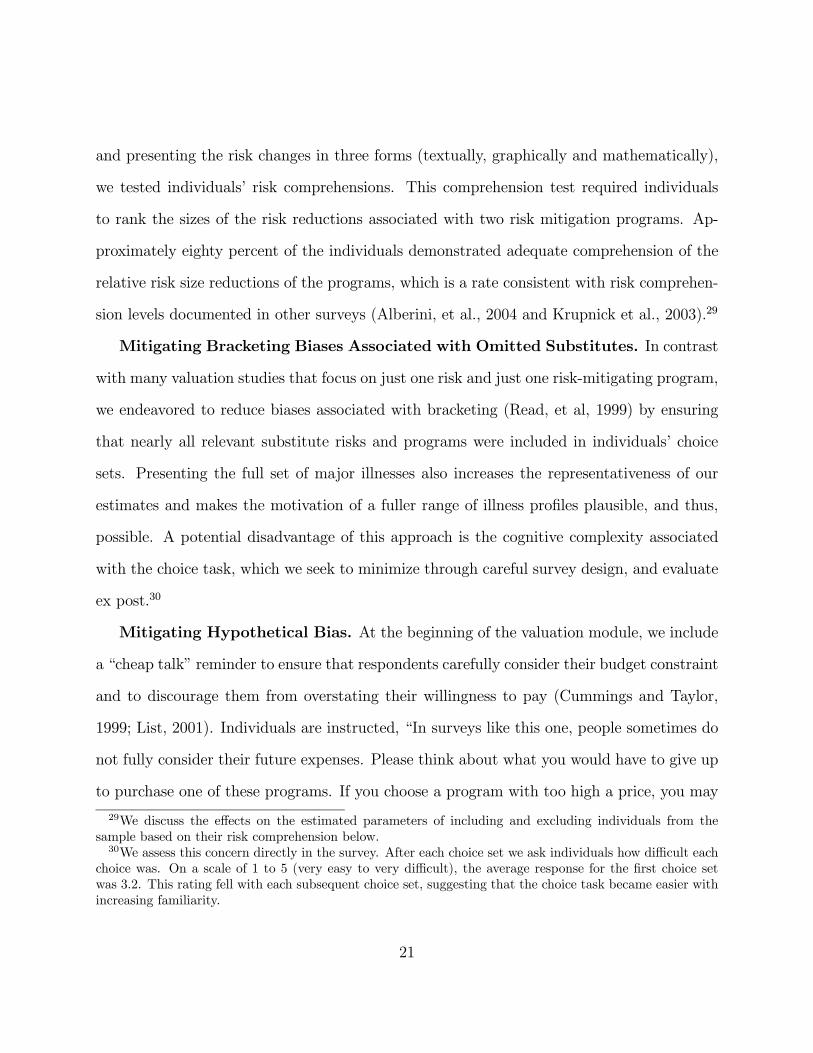
and presenting the risk changes in three forms (textually, graphically and mathematically),

we tested individuals’ risk comprehensions. This comprehension test required individuals

to rank the sizes of the risk reductions associated with two risk mitigation programs. Ap-

proximately eighty percent of the individuals demonstrated adequate comprehension of the

relative risk size reductions of the programs, which is a rate consistent with risk comprehen-

sion levels documented in other surveys (Alberini, et al., 2004 and Krupnick et al., 2003).29

Mitigating Bracketing Biases Associated with Omitted Substitutes. In contrast

with many valuation studies that focus on just one risk and just one risk-mitigating program,

we endeavored to reduce biases associated with bracketing (Read, et al, 1999) by ensuring

that nearly all relevant substitute risks and programs were included in individuals’ choice

sets. Presenting the full set of major illnesses also increases the representativeness of our

estimates and makes the motivation of a fuller range of illness profiles plausible, and thus,

possible. A potential disadvantage of this approach is the cognitive complexity associated

with the choice task, which we seek to minimize through careful survey design, and evaluate

ex post.30

Mitigating Hypothetical Bias. At the beginning of the valuation module, we include

a “cheap talk” reminder to ensure that respondents carefully consider their budget constraint

and to discourage them from overstating their willingness to pay (Cummings and Taylor,

1999; List, 2001). Individuals are instructed, “In surveys like this one, people sometimes do

not fully consider their future expenses. Please think about what you would have to give up

to purchase one of these programs. If you choose a program with too high a price, you may

29We discuss the effects on the estimated parameters of including and excluding individuals from thesample based on their risk comprehension below.30We assess this concern directly in the survey. After each choice set we ask individuals how difficult each

choice was. On a scale of 1 to 5 (very easy to very difficult), the average response for the first choice setwas 3.2. This rating fell with each subsequent choice set, suggesting that the choice task became easier withincreasing familiarity.

21

not be able to afford the program when it is offered. . . .” (See the online Annotated Survey

for a complete description.)

Mitigating Bias from Provision Rules and Order effects. In order to clarify

provision rules for each choice set (Taylor, et al, 2004) and to avoid potential choice set

order effects (Ubel et al., 2002; de Bruin and Keren, 2003), we instructed individuals to

assume that every choice is binding and to evaluate each choice set independently of the

other choice sets. Our empirical analyses showed that the first four choice sets appeared

largely free of order effects. Individuals did exhibit a slightly higher propensity to select

a program from the last choice set, an effect that has also been demonstrated in similar

settings (Bateman, et al, 2004).

Testing for the Effects of Scope on Willingness to Pay. We explore whether

individual choices are sensitive to the scope of the illness profile and the scope of the risk

mitigating program (Hammitt and Graham, 1999; Yeung et al., 2003). We show, using

simple ad hoc conjoint choice analyses, that individuals were highly sensitive to changes in

the scope or level of our central attributes. (See models 1 and 2 in Table 2.) These models

evaluate the two most crucial attributes of the program, its cost and the size of the risk

reduction, as well as the two most important dimensions of the illness profiles, the number

of years spent in a morbid condition and the number of lost life-years.

Other Validity Checks on Willingness to Pay. We also show that individuals’

willingness to pay for these programs varies with several factors as economic theory would

predict it should. It rises with income, as shown in the analysis in this paper. For any

given age, it rises with the expected incidence of health risks in future years (DeShazo and

Cameron, 2004a). It also varies systematically as predicted by economic theory with same

illness and other-illness morbidity (DeShazo and Cameron, 2004b)

22

Validating the Representativeness of Our Estimating Sample. Our estimating

sample is representative of the U.S. population in terms of standard demographic charac-

teristics. Appendix B illustrates this by comparing the individuals in our estimating sample

with corresponding population characteristics (e.g., age, income, and gender) from the 2000

Decennial Census. Our sample consists of 7,520 choices involving 22,560 alternatives. We

arrived at this sample after cleaning the data based on two primary quality control crite-

ria. We exclude individuals if they failed to answer correctly the simple risk comprehension

question at the end of the survey’s risk tutorial. We also exclude individuals if they rejected

the program scenario.31 Sensitivity analyses with respect to these minimal necessary data

exclusion criteria are presented in Appendix C (available from the authors).

4 Empirical Analysis

We begin this analysis by estimating marginal utilities of years spent in each of three health

states: morbidity, a post-illness state, and a lost life-year. We also explore interactions

between years of morbidity and lost life years in order to assess the assumption of additive

separability that characterizes our most basic model. Using the implied marginal rates of

substitution between illness profiles and money, we then construct individual measures of

willingness to pay to avoid five archetypical illness profiles to be introduced in the next

section. Our underlying structural model requires (for now) that we make assumptions

about individuals’ time preferences and future expected income levels. Thus, in Section 4,

we explore how our implied V SIP s vary systematically with these two factors.

Our basic quadratic-in-net-income structural model, which assumes homogeneous prefer-

31We excluded 2,236 choices because the respondent selected “Neither Program” and indicated as the onlyexplanation, “I did not believe the programs would work.” If any other (economic) reason was given, weretained the choice.

23

ences, produces the five parameter estimates shown as Model 3 in Table 2. These homogenous-

preferences specifications are estimated without sign restrictions and show robust significance

and the expected signs on all five primary parameters.32 The marginal utility of income is

positive, but declines with the level of income (yet does not go negative within the range

of incomes in our sample). The marginal utilities of sick-years, post-illness-years, and lost

life-years are all negative and very strongly significantly different from zero.33 While simple

intuition might suggest that death should be “worse” than illness and recovery, it is impor-

tant to keep in mind that the units involved are years in each health state. The relatively

large (dis)utility associated with recovered state probably reflects the general seriousness of

the illnesses our survey describes. Respondents seem not to interpret being recovered from

any of this list of major illnesses as being fully equivalent to the pre-illness state.

We now relax the maintained hypothesis in Model 3 that the marginal utilities from each

state are independent of the duration of that state and the durations of other health states

that characterize the profile in question. Our original model was developed in terms of the

individual’s undiscounted per-period indirect utility, where current-period health status is

captured only by a set of mutually exclusive and exhaustive dummy variables. At the moment

of the individual’s program choice, however, each alternative is likely to be perceived in terms

of the present value of the sequence of future health states it represents. These present values

reflect the mix of future health states in each illness profile. If they capture the relevant

attributes of each alternative in the individual’s choice set, we can consider richer models

that allow for diminishing, rather than constant, marginal utilities from present discounted

32Not surprisingly, the additional structure in Model 3, as opposed to Models 1 and 2, produces a lowermaximized value of the log-likelihood function. This is a common tradeoff. The structure is required for arigorous utility-theoretic interpretation of the results, but the ad hoc model provides a better fit to the data.33A positive marginal utility associated with a lost life-year might be expected only when the illness is

question constitutes a ”fate worse than death.”

24

health-state years, and for interactions between the numbers of present discounted years in

different health states. In contrast, Model 3 constrains the marginal utility of each health

state to be constant and imposes a constant marginal rate of substitution between different

health-state-years.

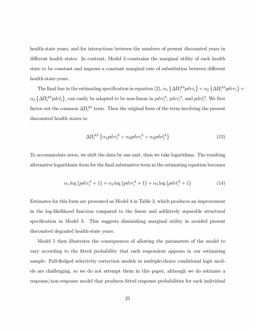
The final line in the estimating specification in equation (2), α1©∆ΠAS

i pdviiª+ α2

©∆ΠAS

i pdvriª+

α3©∆ΠAS

i pdvliª, can easily be adapted to be non-linear in pdviAi , pdvr

Ai , and pdvl

Ai .We first

factor out the common ∆ΠASi term. Then the original form of the term involving the present

discounted health states is:

∆ΠASi

©α1pdvi

Ai + α2pdvr

Ai + α3pdvl

Ai

ª(13)

To accommodate zeros, we shift the data by one unit, then we take logarithms. The resulting

alternative logarithmic form for the final substantive term in the estimating equation becomes

α1 log¡pdviAi + 1

¢+ α2 log

¡pdvrAi + 1

¢+ α3 log

¡pdvlAi + 1

¢(14)

Estimates for this form are presented as Model 4 in Table 3, which produces an improvement

in the log-likelihood function compared to the linear and additively separable structural

specification in Model 3. This suggests diminishing marginal utility in avoided present

discounted degraded health-state years.

Model 5 then illustrates the consequences of allowing the parameters of the model to

vary according to the fitted probability that each respondent appears in our estimating

sample. Full-fledged selectivity correction models in multiple-choice conditional logit mod-

els are challenging, so we do not attempt them in this paper, although we do estimate a

response/non-response model that produces fitted response probabilities for each individual

25

in our sample.34 We allow each basic parameter of our model to vary systematically with the

deviation of that individual’s fitted response propensity from the median response propen-

sity among all 500,000-plus members of the random-digit-dialed initial Knowledge-Networks

recruiting sample. Only the coefficient on the lost life-years term differs significantly with the

fitted probability that the respondent shows up in our estimating sample. The greater the

probability of being in our sample, relative to the median probability, the lesser the disutility

the individual appears to experience from a percentage increase in discounted lost life-years.

While the shift is statistically significant, comparison of Model 5 and Model 4 reveals that the

difference in the magnitude of this key coefficient across these two specifications is minimal.35

Whenever a linear-in-logs form is a better predictor of consumer choices than a linear

form, the researcher is typically inclined to explore even more general logarithmic forms.

In particular, the translog form represents a second-order local approximation to any arbi-

trary functional relationship. This form is fully quadratic in all of the log terms and their

pairwise interactions. We have explored the inclusion of all three squared terms and all

three interaction terms. Only the squared term in pdvlAi and the interaction term between

pdviAi and pdvlAi are robustly significant. This more general specification is presented as

Model 6. Again, it produces a substantial improvement in the log-likelihood. The estimates

suggest that the disutility of an additional discounted lost life-year shrinks as the number

34Our selection model takes the over 525,000 original random-digit dialed recruiting contacts for theKnowledge Networks panel and fits a probit model to explain the presence or absence of each household inour final estimating sample. As explanatory variables, we use a set of 15 orthogonal factors derived froma factor analysis of over 100 census tract characteristics, county voting records, county mortality from eachmajor disease over the previous decade as a fraction of 2000 census population, and the number of hospitalsin the same census tract(s) as the address (or telephone exchange) of the contacted household. Discussionof this response/nonresponse model constitutes a separate manuscript, currently under preparation.35We employ differences from the median response probability so that the estimated utility parameters

correspond to the simulated case where all response probabilities are exactly equal to the median in thepopulation. We employ the median because the distribution is skewed, with a number of large positiveoutliers.

26

of discounted lost life-years increases. They also suggest that the disutility of an additional

discounted lost life-year is reduced by increases in the number of discounted illness-years

that precede it (e.g., as the number of years of morbidity preceding death increases, dying

earlier becomes less bad).

In this application, however, there is a further complication. The illness profiles that were

eligible to be considered by each respondent were constrained by the respondent’s current

age. No respondent considered illnesses that could strike at an age younger than their

current age, so current age defines the maximum duration of any illness profile. The result is

a degree of multicollinearity between the respondent’s remaining nominal life expectancy and

the range of sick-years, post-illness years, and lost life-years they were eligible to consider. In

particular, when including interactions between the pdviAi terms and the pdvlAi terms, large

values of these interaction terms were closely associated with the youth of the respondent.

It is not possible to include current age as a factor that might have an additively separable

effect on the individual’s level of utility, since terms such as these drop out of the utility-

difference calculation across alternatives. To control for the effect of current age on the

apparent marginal utility of each health state, we need to allow current age, agei0, to shift

the marginal utility parameters. An intermediate model (not shown in Table 3) assessed the

consequences of allowing agei0 to shift only the coefficients on each of the linear terms in

the logs of discounted years in each adverse health state. Each of the additional coefficients,

α11, α21, and α31, was statistically significant. Older respondents appear to anticipate lesser

disutility from discounted sick-years and discounted lost life-years, but greater disutility from

discounted post-illness years.

We allow all of the translog coefficients to vary systematically with agei0 and age2i0 since

27

earlier empirical research has suggested the presence of quadratic age effects in V SLs.36

The age shifters on the sick-years and post-illness years terms (pdviAi and pdvrAi ) become

statistically insignificant. However, the presence of significant quadratic-in-age shifters on the

linear and quadratic lost life-years terms (pdvlAi ) and on the interaction between the pdviAi

term and the pdvlAi term, prevents counter-intuitive negative fitted V SIP estimates for

some illness profiles for young respondents. Therefore, we prefer the specification presented

as Model 7 in Table 3, even though two coefficients (on the lower-order level and linear

age effects on the interaction between the pdviAi and pdvlAi terms) are not individually

statistically significant.

For Model 7, if we simulate identical response probabilities for all participants, the final

substantive term in equation (2) is specified as follows:

+∆ΠASi

⎧⎪⎪⎪⎪⎪⎪⎪⎪⎪⎪⎪⎪⎪⎪⎨⎪⎪⎪⎪⎪⎪⎪⎪⎪⎪⎪⎪⎪⎪⎩

(α10) log¡pdviAi + 1

¢+(α20) log

¡pdvrAi + 1

¢+(α30 + α31agei0 + α32age

2i0) log

¡pdvlAi + 1

¢+(α40 + α41agei0 + α42age

2i0)£log¡pdvlAi + 1

¢¤2+(α50 + α51agei0 + α52age

2i0)£log¡pdviAi + 1

¢¤ £log¡pdvlAi + 1

¢¤

⎫⎪⎪⎪⎪⎪⎪⎪⎪⎪⎪⎪⎪⎪⎪⎬⎪⎪⎪⎪⎪⎪⎪⎪⎪⎪⎪⎪⎪⎪⎭

(15)

To our knowledge, these are the first attempts to estimate, within a common model, the age-

varying marginal utilities of avoiding a present discounted year of morbidity and a present

discounted lost life-year. We assess the validity of our estimates by exploring whether they

36See for example Jones-Lee et al. (993) or Krupnick et al. (2002). The specification with just linear ageeffects on the linear-in-logarithms terms in discounted health-state years produces a substantial improvementin the log-likelihood function, but leads to some outliers in the simulation results when we use the parameterestimates to predict VSIs for specific illness profiles. The quadratic forms in age for the systematicallyvarying parameters appear necessary to accommodate nonlinearities in these relationships.

28

vary systematically in a manner that economic theory or simple intuition would predict.37

It is relevant to examine how our estimates vary with assumptions about average time

preferences, as well as with the data concerning each individual’s income, and with current

age and disease latency. We employ the estimated parameters reported for Model 7 in Table

3 to characterize the V SIP associated with selected combinations of years of morbidity,

years in post-illness status, and years of premature mortality. A vast range of different

illness profiles could be selected, but for illustrative purposes, we examine five representative

illness profiles: 1) a period of shorter-term morbidity followed by recovery, 2) a period

of longer-term morbidity followed by recovery, 3) a combination of shorter-term morbidity

followed by premature mortality, 4) a combination of longer-term morbidity followed by

premature mortality, and 5) sudden death. Recall that a V SIP reflects willingness to pay

for typically a very small risk reduction, scaled up (proportionately) to the amount that

would correspond to a risk reduction of 1.00. While the individual’s budget will constrain

the underlying willingness-to-pay, the V SIP is not so limited, and the benchmarks against

which we compare our V SIP figures are the roughly $6 million V SL used by the U.S. EPA

and the roughly $1 million used by the U.S. Department of Transportation.

Our models currently require that the researcher specify each individual’s time prefer-

ences. In Table 4, we consider an individual who is now 45 years old with an income of

$42,000 and calculate the fitted V SIP (in millions of dollars) for each of our five illness

profiles to illustrate the sensitivity of our models to our choice of discount rate. In Table 3,

the results for Model 7 were derived under the assumption that r = 0.05. The middle column

of Table 4 shows the medians and 90% ranges of simulated point estimates of the V SIP for

37The only other ordinal utility measure expressed per year is the concept of the value of a statistical lifeyear. However, this is not a measure of marginal utility, rather it is constructed by dividing a VSL estimateby the remaining number of expected life-years.

29

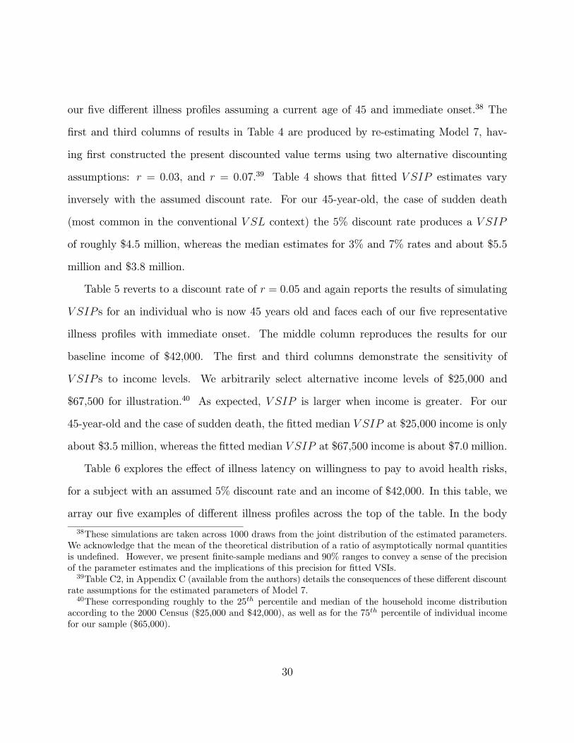
our five different illness profiles assuming a current age of 45 and immediate onset.38 The

first and third columns of results in Table 4 are produced by re-estimating Model 7, hav-

ing first constructed the present discounted value terms using two alternative discounting

assumptions: r = 0.03, and r = 0.07.39 Table 4 shows that fitted V SIP estimates vary

inversely with the assumed discount rate. For our 45-year-old, the case of sudden death

(most common in the conventional V SL context) the 5% discount rate produces a V SIP

of roughly $4.5 million, whereas the median estimates for 3% and 7% rates and about $5.5

million and $3.8 million.

Table 5 reverts to a discount rate of r = 0.05 and again reports the results of simulating

V SIP s for an individual who is now 45 years old and faces each of our five representative

illness profiles with immediate onset. The middle column reproduces the results for our

baseline income of $42,000. The first and third columns demonstrate the sensitivity of

V SIP s to income levels. We arbitrarily select alternative income levels of $25,000 and

$67,500 for illustration.40 As expected, V SIP is larger when income is greater. For our

45-year-old and the case of sudden death, the fitted median V SIP at $25,000 income is only

about $3.5 million, whereas the fitted median V SIP at $67,500 income is about $7.0 million.

Table 6 explores the effect of illness latency on willingness to pay to avoid health risks,

for a subject with an assumed 5% discount rate and an income of $42,000. In this table, we

array our five examples of different illness profiles across the top of the table. In the body

38These simulations are taken across 1000 draws from the joint distribution of the estimated parameters.We acknowledge that the mean of the theoretical distribution of a ratio of asymptotically normal quantitiesis undefined. However, we present finite-sample medians and 90% ranges to convey a sense of the precisionof the parameter estimates and the implications of this precision for fitted VSIs.39Table C2, in Appendix C (available from the authors) details the consequences of these different discount

rate assumptions for the estimated parameters of Model 7.40These corresponding roughly to the 25th percentile and median of the household income distribution

according to the 2000 Census ($25,000 and $42,000), as well as for the 75th percentile of individual incomefor our sample ($65,000).

30

of the table, we display fitted median V SIP estimates and 90% ranges for one respondent

aged 35 now and another aged 65 now. The age at onset of each illness is varied to include

immediate onset, as well as onset at decade intervals starting five years from now. Consider-

able variability is present. Focusing again on the sudden death scenario, our model suggests

that the 65-year-old respondents are willing to pay less to avoid sudden death than the 35-

year-old respondent. Looking forward, however, both individuals are willing to pay less to

avoid the same illness profile when it commences at a later age. Our model allows V SIP s

to reflect the duration of each type of health state. The numbers of prospective sick-years

and life-years lost can be expected to have a substantial effect on willingness-to-pay to avoid

each illness profile.

As a visual summary of the effect of the respondent’s age now on the V SIP for sudden

death, we offer Figure 1, which shows the simulated median and 90% confidence interval

for this fitted V SIP as a function of age now. As the term in (15) indicates, age has an

nonlinear effect on several of the parameters of the model. The combined influence of these

three different types of quadratic age effects on the fitted V SIP for this particular illness

profile is captured by Figure 1. Figure 2 illustrates one other possible illness profile. In this

case, it is an illness that lasts five years, ending in death, but with ten years of latency prior

to onset. Willingness to pay to avoid this illness profile also differs systematically with age.41

When evaluating the social benefits of a policy change that alters the incidence of a

particular illness, there are great advantages to being able to estimate the continuum of

statistical illness profiles associated with that particular illness. Our approach offers the

41For some age levels, the simulated 90% confidence interval for the predicted Value of a StatisticalIllness includes zero. There is no opportunity for respondents to express a negative willingness to pay,so it may be appropriate to adopt a Tobit-type interpretation of the implied fitted distribution and tomove any probability in the negative domain to zero. Alternatively, by resorting to a fundamentally non-linear estimating model, one could estimate the logarithm of willingness-to-pay, instead of its level, therebyconstraining fitted willingness-to-pay to be strictly positive.

31

flexibility to evaluate changes in the type, future timing, and duration of heterogeneous

illness profiles. Additionally, it does so within a consistent theoretical and empirical model,

rather than requiring researchers to cobble together estimates for current period morbidity

and mortality from separate valuation methods and studies.

5 Discussion and Conclusions

Unlike many previous empirical efforts to measure willingness to pay to reduce mortality

risks, our model does not produce just a single best estimate for the Value of a Statistical Life

(V SL) for use in all policy contexts. Instead, our model is best understood as a generalization

of the standard single-period, single-risk valuation model. It explicitly allows the individual

to allocate risk-reduction expenditures across health risks that come to bear across different

future time periods. Our model allows for substitution across health risks with different

time profiles that more-completely characterize the duration of morbidity and the eventual

health outcomes that result from those risks. Rather than focusing on only a single risk of

death in the current period, the model considers entire future illness profiles as its objects of

choice. The most significant advantages of this simple generalization are that it allows us

to accommodate (a) varying latencies in health risks, (b) morbidity in addition to mortality,

and (c) non-fatal as well as fatal risks. Along these three dimensions, our model represents

a major departure from previous empirical specifications.

Although the model is a generalization, it nonetheless produces a new and important

type of economic information: distinct estimates of the marginal utilities of avoiding a year

of morbidity and a lost life year within a single model. It also appears that these marginal

utilities are not simple constants. From these heterogeneous marginal values, which seem to

depend upon the current age of the respondent (and therefore possibly upon other factors

32

which are correlated with age) and the mix of health states in an illness profile, we have

illustrated how to construct average values for a wide range of illness profiles, for individuals

of different ages. Estimates such as these may diminish the need for policy analysts to piece

together disparate estimates of morbidity and mortality from different valuation methods.

To further enhance program and policy evaluation, we organize our analysis around the

task of estimating the value of a statistical illness profile (V SIP ), although we allow for the

identification of a simpler concept that is similar to the more-traditional value of statistical

life (V SL). The V SIP evaluates the set of heterogeneous health outcomes associated with

a given illness risk. Policy changes that affect the prevalence and severity of that illness

will shift the joint distribution of the duration of morbidity and premature mortality, for

specified populations, and our model is capable of assessing the benefits of such broad shifts.

Our analyses illustrate some initial results concerning how marginal utility of risk mit-

igation varies systematically across individuals. Specifically, we evaluate how the demand

for mortality risk reduction varies with the individual’s current age and the disease latencies

that dictate the future ages at which degraded health states would be experienced. Our

results suggest that, however convenient it may be, the presumption that there should be a

single-valued V SL is probably misguided. While the use of a single number may continue

to be dictated by political concerns, the V SL should be viewed as a function, rather than a

scalar. A V SL is ultimately a type of inverse demand function, so the prospect of systematic

variation in willingness to pay, according to the qualities of the good and with indicators of

individual preferences, should not be surprising.

33

6 References

Aldy, J.E. and W.K. Viscusi. 2003. “Age variation in worker’s value of statistical life.”

Mimeograph

Baron J., and Ubel P.A. 2002. “Types of inconsistency in health-state utility judgments.”

Organizational Behavior and Human Decision Processes 89 (2): 1100-1118.

Cameron, T.A. 2005. “Individual option prices for climate change mitigation.” Journal

of Public Economics, forthcoming.

Corso, P.S., Hammitt, J.K., and Graham, J.D. 2001. “Valuing mortality-risk reduction:

Using visual aids to improve the validity of contingent valuation.” Journal of Risk and

Uncertainty 23 (2): 165-184.

Cummings, R.G., and Taylor, L.O. 1999. “Unbiased value estimates for environmen-

tal goods: A cheap talk design for the contingent valuation method.” American Economic

Review. 89 (3): 649-665.

de Bruin, W.B., and Keren, G. 2003. “Order effects in sequentially judged options due

to the direction of comparison.” Organizational Behavior and Human Decision Process. 92

(1-2): 91-101.

Dow, W.H., Philipson, T.J., and Sala-I-Martin X. 1999. “Longevity complementarities

under competing risks.” American Economic Review 89 (5): 1358-1371

Dreze, J. 1962. “L’Utilite Sociale d’une Vie Humaine.” Revue Francaise de Recherche

Operationalle 6: 93 - 118.

Gold, Marthe R., Russel, Lousie B., Siegel, Joanna E., Weinstein, Milton C. (eds). .1996.

Effectiveness in Health and Medicine. New York: Oxford University Press.

Graham, D.A. 1981. “Cost-benefit analysis under uncertainty.” American Economic

Review 71 (4): 715-725 1981

34

Hammitt, J.K., and Graham, J.D. 1999 “Willingness to pay for health protection: Inad-

equate sensitivity to probability?” Journal of Risk and Uncertainty 18 (1): 33-62.

Johnson, F.R., Banzhaf, M.R., and Desvousges, W.H. 2000. “Willingness to pay for

improved respiratory and cardiovascular health: A multiple-format, stated-preference ap-

proach.” Health Economics 9 (4): 295-317.

Jones-Lee, M.W. 1974. “The value of changes in the probability of death or injury.”

Journal of Political Economy 82(4): 835 - 849.

Jones-Lee, M.W., G. Loomes, D. O’Reilly, and P.R. Phillips .1993. “The value of prevent-

ing non-fatal road injuries: findings of a willingness-to-pay national sample survey.” TRY

Working Paper, WP SRC2.

Krupnick A., Alberini A., Cropper M., Simon N., O’Brien B., Goeree R., and Heintzelman

M. 2002. “Age, health and the willingness to pay for mortality risk reductions: A contingent

valuation survey of Ontario residents” Journal of Risk and Uncertainty. 24 (2): 161-186.

List J.A. 2001. “Do explicit warnings eliminate the hypothetical bias in elicitation pro-

cedures? Evidence from field auctions for sportscards” American Economic Review. 91 (5):

1498-1507.

Liu, J.-T. and Hammitt,J.K. 2003. “Effects of disease type and latency on the value of

mortality risk,” NBER Working Paper no. w10012.

Moore, M., and Viscusi, W.K. 1988. “The quantity-adjusted value of life.” Economic

Inquiry 26 (3): 369-388.

Moxey, A., O’Connell, D., McGettigan, P., and Henry, D. 2003. “Describing treatment

effects to patients - How they are expressed makes a difference.” Journal of General Internal

Medicine 18 (11): 948-U8.

O’Connor, R.M. and Blomquist, G.C. 1997. “Measurement of consumer-patient prefer-

35

ences using a hybrid contingent valuation method.” Journal of Health Economics 16 (6):

667-683.

Picone, G., Sloan, F., and Taylor, D. 2004. “Effects of risk and time preference and

expected longevity on demand for medical tests.” Journal of Risk and Uncertainty 28 (1):

39-53.

Rosen, S. 1988. “The value of changes in life expectancy.” Journal of Risk and Uncer-

tainty 1: 187-203.

Sloan F.A., Viscusi, W.K., Chesson, H.W., Conover, C.J., and Whetten-Goldstein K.

1998. “Alternative approaches to valuing intangible health losses: the evidence for multiple

sclerosis” Journal of Health Economics 17 (4): 475-497.

Ubel P.A., Richardson J., and Baron J. 2002. “Exploring the role of order effects in

person trade-off elicitations.” Health Policy (2): 189-199.

Viscusi, W.K. 1993 “The value of risks to life and health.” Journal of Economic Literature

31: 1912 - 1946.

Viscusi, W.K., Magat, W.A., and Huber, J. 1991. “Pricing environmental health risks:

survey assessments of risk-risk and risk-dollar trade-offs for chronic bronchitis.” Journal of

Environmental Economics and Management 21 (1): 32-51.

Yeung, R.Y.T., Smith, R.D., and McGhee, S.M. 2003. “Willingness to pay and size of

health benefit: an integrated model to test for ’sensitivity to scale.” Health Economics 12

(9): 791-796.

36

40

Table 1 – Main Illness Profile Attributes, by Label Assigned to Health Threat, Means and Standard Deviations (Estimating Sample = 1619 individuals, 7520 choice sets, 15040 illness profiles, 22560 alternatives)

Health Threat: Breast Prostate Colon Lung Skin Heart Heart Stroke Resp. Traffic Diabetes Alzheim. Cancer Cancer Cancer Cancer Cancer Attack Disease Disease Accident disease

# profiles 697 676 1357 1368 1353 1406 1423 1424 1337 1295 1357 1347 Monthly cost (dollars)

30.78 (30.09)

28.12 (26.09)

29.35 (28.37)

30.4 (28.7)

30.19 (28.81)

29.85 (29.62)

29.87 (28.63)

30.85 (29.43)

29.77 (29.41)

29.72 (27.92)

29.17 (28.07)

29.84 (28.54)

Risk difference

-0.0033 (0.0016)

-0.0034 (0.0017)

-0.0034 (0.0017)

-0.0034 (0.0017)

-0.0035 (0.0017)

-0.0035 (0.0017)

-0.0034 (0.0017)

-0.0034 (0.0017)

-0.0034 (0.0017)

-0.0034 (0.0017)

-0.0033 (0.0016

-0.0033 (0.0016)

Latency (years)

17.0 (11.0)

18.5 (11.2)

18.4 (11.6)

19.4 (11.5)

17.6 (11.7)

20.5 (12.5)

19.4 (11.9)

21.8 (12.7)

21.4 (12.2)

18.2 (12.3)

18.2 (10.8)

22.6 (12.5)

Illness years

4.9 (3.5)

4.9 (3.9)

8.5 (8.3)

8.3 (7.7)

7.5 (7.3)

3.4 (6.6)

10.2 (8.8)

3.6 (6.4)

7.4 (6.5)

4.0 (7.6)

6.8 (5.8)

6.8 (4.7)

Lost life-years

11.5 (11.4)

12.0 (11.5)

8.9 (9.7)

10.3 (9.8)

10.3 (10.8)

13.5 (11.3)

7.4 (8.4)

12.0 (10.1)

8.0 (7.8)

14.5 (12.5)

13.4 (10.7)

8.8 (6.4)

Sudden death

0

0

0

0

0

0.52

0

0.51

0

0.51

0

0

Recover

0.60

0.64

0.39

0.23

0.40

0.19

0.26

0.19

0.38

0.19

0

0

Die within 6 years

0.40

0.36

0.22

0.36

0.30

0.08

0.11

0.07

0.21

0.07

0.85

0.84

Chronic effects

0

0

0.37

0.41

0.30

0.21

0.63

0.24

0.41

0.23

0.15

0.16

41

Table 2 – Ad Hoc Models; Linear Additively Separable Structural Model (No selection correction, Fixed effects conditional logit)a

Model 1 Ad hoc

Model 2 Ad hoc

Model 3 Structural

Monthly Cost of Program -0.007581 -0.007491 - (-9.63)*** (-9.48)***

Risk Reduction 89.27 57.64 - (9.95)*** (5.77)***

Sick-Years - 0.0879 -

(3.85)***

Lost Life-Years - 0.01138 -

(7.13)***

( )[ ]500 10 first income termβ × - - 4.88

(8.60)*** ( )[ ]9

10 10 second income termβ × - - -0.220 (-4.71)*** ( )10

AS Ai ipdviα ∆Π - - -8.390

(-5.00)*** ( )20

AS Ai ipdvrα ∆Π - - -8.02

(-2.48)*** ( )30

AS Ai ipdvlα ∆Π - - -8.08

(-6.04)***

Alternatives 22560 22560 22560 Log-likelihood -11735.13 -11706.11 -11733.47 a Asymptotic t-test statistics in parentheses (***=statistically significant at better than 1% level)

42

Table 3 – Evolution of Estimating Specification (Alternatives = 22560)

Model 4 Model 5 Model 6 Model 7

(Parameter) Variable Simple Logs w/ P(select) Translog Quad in Age

5.35 5.34 5.89 5.19 ( )[ ]500 10 first income termβ ×

(9.20)*** (9.18)*** (9.79)*** (8.31)*** -0.2155 -0.2159 -0.2094 -0.1991 ( )[ ]9

10 10 second income termβ × (4.61)*** (4.61)*** (4.46)*** (4.22)***

-24.7 -26.8 -51.3 -47.8 ( ) ( )10 log 1AS Ai ipdviα ∆Π +

(4.22)*** (4.52)*** (5.75)*** (5.32)*** 3.181 3.153 3.280

( ) ( )13 ( ) log 1AS Ai i iP sel P pdviα ⎡ ⎤⎡ ⎤− ∆Π +⎣ ⎦ ⎣ ⎦

(2.13)**

(2.12)**

(2.19)**

-21.52 -21.54 -19.59 -16.45 ( ) ( )20 log 1AS A

i ipdvrα ∆Π + (2.29)** (2.30)** (2.09)** (1.74)* -30.59 -30.48 -68.62 -582.4 ( ) ( )30 log 1AS A

i ipdvlα ∆Π + (6.00)*** (5.98)*** (3.66)*** (3.26)***

- - - 20.58 ( ) ( )31 0 log 1AS Ai i iage pdvlα ⋅∆Π +

(2.84)*** - - - -0.1888 ( ) ( )2

32 0 log 1AS Ai i iage pdvlα ⋅∆Π +

(2.72)*** - - 9.263 200.6

( ) ( ) 2

40 log 1AS Ai ipdvlα ⎡ ⎤∆Π +⎣ ⎦

(-1.13)

(2.43)**

- - - -7.848

( ) ( ) 2

41 0 log 1AS Ai i iage pdvlα ⎡ ⎤⋅∆Π +⎣ ⎦

(2.33)**

- - - 0.0746

( ) ( ) 2242 0 log 1AS A

i i iage pdvlα ⎡ ⎤⋅∆Π +⎣ ⎦

(2.29)**

- - 34.71 102.1 ( ) ( )( )

50 log 1

log 1

AS Ai i

Ai

pdvi

pdvl

α ⎡ ⎤∆Π +⎣ ⎦⎡ ⎤⋅ +⎣ ⎦

(4.25)***

(-1.40)

- - - -4.47

( ) ( )

( )51 0 log 1

log 1

AS Ai i i

Ai

age pdvi

pdvl

α ⎡ ⎤⋅∆Π +⎣ ⎦⎡ ⎤⋅ +⎣ ⎦

(-1.57)

- - - 0.056

( ) ( )

( )

252 0 log 1

log 1

AS Ai i i

Ai

age pdvi

pdvl

α ⎡ ⎤⋅∆Π +⎣ ⎦⎡ ⎤⋅ +⎣ ⎦

(2.10)**

Alternatives 22560 22560 22560 22560 Log L -11729.021 -11726.662 -11716.989 -11694.991

Sample mean fitted VSIP ($ million) a 7.15 7.47 0.9 2.59 a The survey provides no opportunity for respondents to express a negative willingness to pay. At worst, they can merely prefer the status quo alternative. In this table, we interpret individual negative fitted VSIP estimates as zero values.

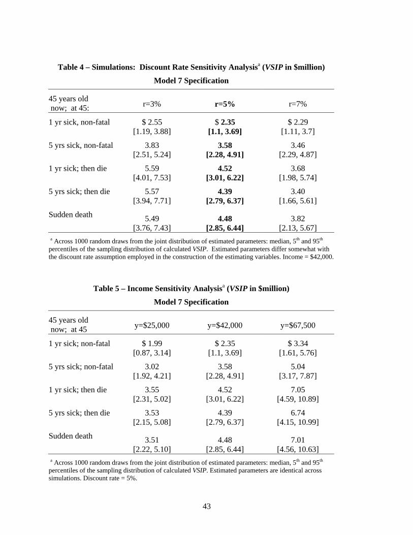
43

Table 4 – Simulations: Discount Rate Sensitivity Analysisa (VSIP in $million)

Model 7 Specification

45 years old now; at 45: r=3% r=5% r=7%

1 yr sick, non-fatal

$ 2.55 [1.19, 3.88]

$ 2.35 [1.1, 3.69]

$ 2.29 [1.11, 3.7]

5 yrs sick, non-fatal

3.83 [2.51, 5.24]

3.58 [2.28, 4.91]

3.46 [2.29, 4.87]

1 yr sick; then die

5.59 [4.01, 7.53]

4.52 [3.01, 6.22]

3.68 [1.98, 5.74]

5 yrs sick; then die

5.57 [3.94, 7.71]

4.39 [2.79, 6.37]

3.40 [1.66, 5.61]

Sudden death 5.49

[3.76, 7.43] 4.48

[2.85, 6.44] 3.82

[2.13, 5.67] a Across 1000 random draws from the joint distribution of estimated parameters: median, 5th and 95th percentiles of the sampling distribution of calculated VSIP. Estimated parameters differ somewhat with the discount rate assumption employed in the construction of the estimating variables. Income = $42,000.

Table 5 – Income Sensitivity Analysisa (VSIP in $million)

Model 7 Specification

45 years old now; at 45 y=$25,000 y=$42,000 y=$67,500

1 yr sick; non-fatal

$ 1.99 [0.87, 3.14]

$ 2.35 [1.1, 3.69]

$ 3.34 [1.61, 5.76]

5 yrs sick; non-fatal

3.02 [1.92, 4.21]

3.58 [2.28, 4.91]

5.04 [3.17, 7.87]

1 yr sick; then die

3.55 [2.31, 5.02]

4.52 [3.01, 6.22]

7.05 [4.59, 10.89]

5 yrs sick; then die

3.53 [2.15, 5.08]

4.39 [2.79, 6.37]

6.74 [4.15, 10.99]

Sudden death 3.51

[2.22, 5.10] 4.48

[2.85, 6.44] 7.01

[4.56, 10.63] a Across 1000 random draws from the joint distribution of estimated parameters: median, 5th and 95th percentiles of the sampling distribution of calculated VSIP. Estimated parameters are identical across simulations. Discount rate = 5%.

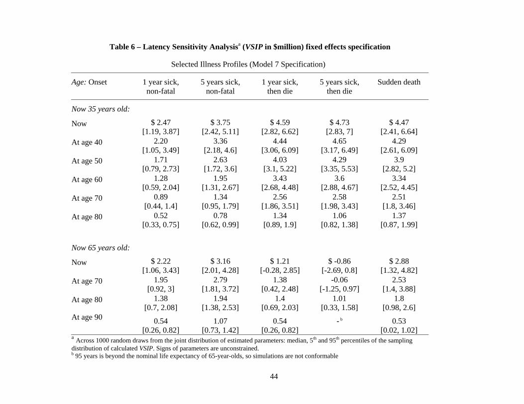
44

Table 6 – Latency Sensitivity Analysisa (VSIP in $million) fixed effects specification

Selected Illness Profiles (Model 7 Specification)

Age: Onset

1 year sick, non-fatal

5 years sick, non-fatal

1 year sick, then die

5 years sick, then die

Sudden death

Now 35 years old: Now $ 2.47

[1.19, 3.87] $ 3.75

[2.42, 5.11] $ 4.59

[2.82, 6.62] $ 4.73

[2.83, 7] $ 4.47

[2.41, 6.64] At age 40 2.20

[1.05, 3.49] 3.36

[2.18, 4.6] 4.44

[3.06, 6.09] 4.65

[3.17, 6.49] 4.29

[2.61, 6.09] At age 50 1.71

[0.79, 2.73] 2.63

[1.72, 3.6] 4.03

[3.1, 5.22] 4.29

[3.35, 5.53] 3.9

[2.82, 5.2] At age 60 1.28

[0.59, 2.04] 1.95

[1.31, 2.67] 3.43

[2.68, 4.48] 3.6

[2.88, 4.67] 3.34

[2.52, 4.45] At age 70 0.89

[0.44, 1.4] 1.34

[0.95, 1.79] 2.56

[1.86, 3.51] 2.58

[1.98, 3.43] 2.51

[1.8, 3.46] At age 80 0.52

[0.33, 0.75] 0.78

[0.62, 0.99] 1.34

[0.89, 1.9] 1.06

[0.82, 1.38] 1.37

[0.87, 1.99]

Now 65 years old: Now $ 2.22

[1.06, 3.43] $ 3.16

[2.01, 4.28] $ 1.21

[-0.28, 2.85] $ -0.86

[-2.69, 0.8] $ 2.88

[1.32, 4.82] At age 70 1.95

[0.92, 3] 2.79

[1.81, 3.72] 1.38

[0.42, 2.48] -0.06

[-1.25, 0.97] 2.53

[1.4, 3.88] At age 80 1.38

[0.7, 2.08] 1.94

[1.38, 2.53] 1.4

[0.69, 2.03] 1.01

[0.33, 1.58] 1.8

[0.98, 2.6] At age 90 0.54

[0.26, 0.82] 1.07

[0.73, 1.42] 0.54

[0.26, 0.82] - b

0.53 [0.02, 1.02]

a Across 1000 random draws from the joint distribution of estimated parameters: median, 5th and 95th percentiles of the sampling distribution of calculated VSIP. Signs of parameters are unconstrained. b 95 years is beyond the nominal life expectancy of 65-year-olds, so simulations are not conformable

45

Figure 1 – Implicit VSIP associated with sudden death now, as a function of respondent age ($ million) Estimated without sign constraints. Figure 2 – Implicit VSIP for ten years of latency, five years of illness, death in fifteen years, as a function of respondent age now ($ million) Estimated without sign constraints.

46

Appendix A

Example: Conjoint Choice Set

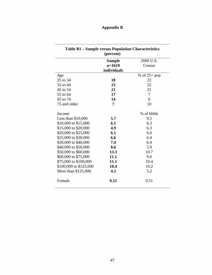
47

Appendix B

Table B1 – Sample versus Population Characteristics (percent)

Sample n=1619

individuals

2000 U.S. Census

Age % of 25+ pop 25 to 34 18 22 35 to 44 23 25 45 to 54 21 21 55 to 64 17 7 65 to 74 14 6 75 and older 7 10 Income % of hhlds Less than $10,000 5.7 9.5 $10,000 to $15,000 6.1 6.3 $15,000 to $20,000 4.9 6.3 $20,000 to $25,000 6.1 6.6 $25,000 to $30,000 6.6 6.4 $30,000 to $40,000 7.4 6.4 $40,000 to $50,000 8.6 5.9 $50,000 to $60,000 13.3 10.7 $60,000 to $75,000 11.1 9.0 $75,000 to $100,000 11.1 10.4 $100,000 to $125,000 10.4 10.2 More than $125,000 4.2 5.2 Female 0.51 0.51

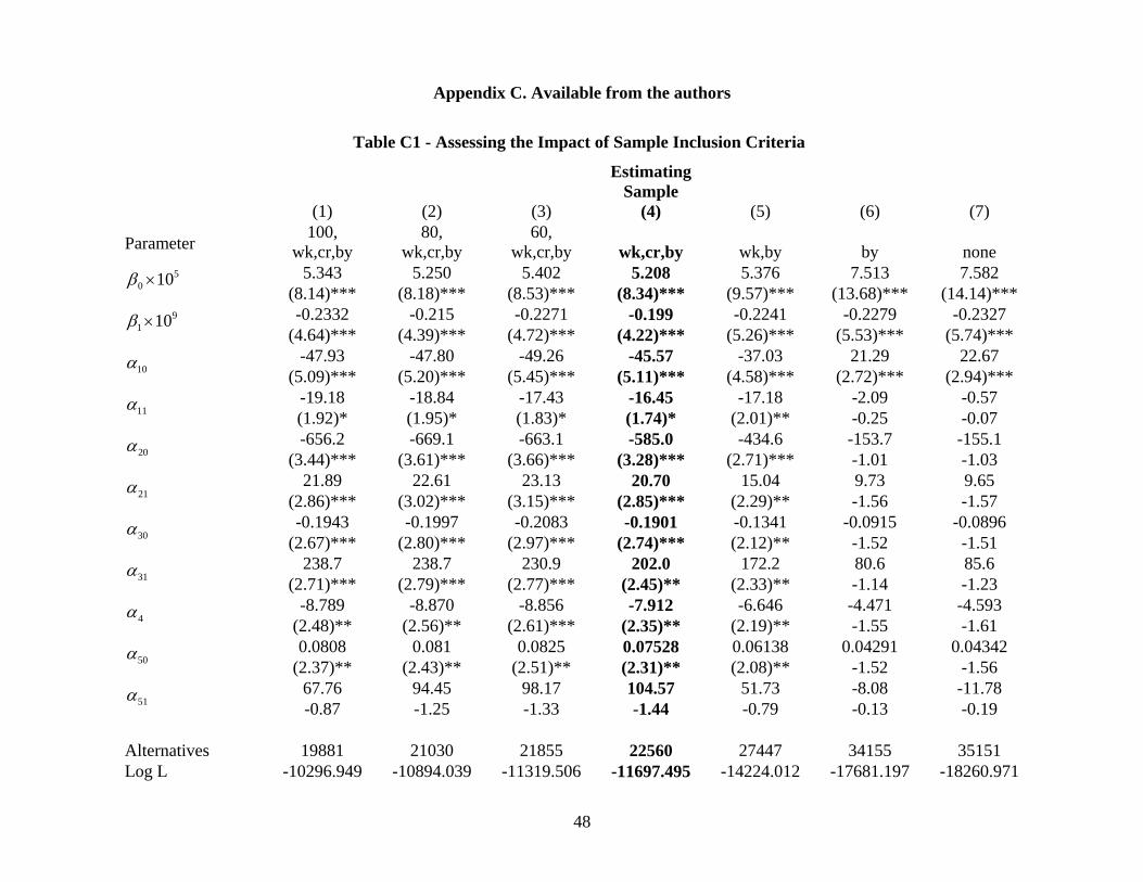
48

Appendix C. Available from the authors

Table C1 - Assessing the Impact of Sample Inclusion Criteria

(1) (2) (3)

Estimating Sample

(4) (5) (6) (7)

Parameter 100, wk,cr,by

80, wk,cr,by

60, wk,cr,by wk,cr,by wk,by by none

5.343 5.250 5.402 5.208 5.376 7.513 7.582 50 10β ×

(8.14)*** (8.18)*** (8.53)*** (8.34)*** (9.57)*** (13.68)*** (14.14)*** -0.2332 -0.215 -0.2271 -0.199 -0.2241 -0.2279 -0.2327 9

1 10β × (4.64)*** (4.39)*** (4.72)*** (4.22)*** (5.26)*** (5.53)*** (5.74)***

-47.93 -47.80 -49.26 -45.57 -37.03 21.29 22.67 10α

(5.09)*** (5.20)*** (5.45)*** (5.11)*** (4.58)*** (2.72)*** (2.94)*** -19.18 -18.84 -17.43 -16.45 -17.18 -2.09 -0.57

11α (1.92)* (1.95)* (1.83)* (1.74)* (2.01)** -0.25 -0.07 -656.2 -669.1 -663.1 -585.0 -434.6 -153.7 -155.1

20α (3.44)*** (3.61)*** (3.66)*** (3.28)*** (2.71)*** -1.01 -1.03

21.89 22.61 23.13 20.70 15.04 9.73 9.65 21α

(2.86)*** (3.02)*** (3.15)*** (2.85)*** (2.29)** -1.56 -1.57 -0.1943 -0.1997 -0.2083 -0.1901 -0.1341 -0.0915 -0.0896

30α (2.67)*** (2.80)*** (2.97)*** (2.74)*** (2.12)** -1.52 -1.51

238.7 238.7 230.9 202.0 172.2 80.6 85.6 31α

(2.71)*** (2.79)*** (2.77)*** (2.45)** (2.33)** -1.14 -1.23 -8.789 -8.870 -8.856 -7.912 -6.646 -4.471 -4.593

4α (2.48)** (2.56)** (2.61)*** (2.35)** (2.19)** -1.55 -1.61 0.0808 0.081 0.0825 0.07528 0.06138 0.04291 0.04342

50α (2.37)** (2.43)** (2.51)** (2.31)** (2.08)** -1.52 -1.56

67.76 94.45 98.17 104.57 51.73 -8.08 -11.78 51α

-0.87 -1.25 -1.33 -1.44 -0.79 -0.13 -0.19 Alternatives 19881 21030 21855 22560 27447 34155 35151 Log L -10296.949 -10894.039 -11319.506 -11697.495 -14224.012 -17681.197 -18260.971

49

continued… (1) (2) (3) (4) (5) (6) (7)

Parameter 100, wk,cr,by

80, wk,cr,by

60, wk,cr,by wk,cr,by wk,by by none

Sample mean VSIP 6.61 3.31 3.52 2.5 2.52 0.05 0.05 Sample 5th % 0a 0 0 0 0 0 0 Sample 25th % 1.28 1.16 1.11 1.07 0.76 0 0 Sample 50th % 2.33 2.19 2.08 1.94 1.54 0 0 Sample 75th % 4.15 3.82 3.63 3.23 2.71 0 0 Sample 95th % 12.94 9.69 9.95 6.95 7.24 0.03 0 Key to inclusion criteria: “100” = aggregate time on all five program choice tasks at least 100 seconds (e.g. average time 20 seconds per choice set); analogously for “80” and “60”; “wk” = choice of Neither Program not explained solely by “I did not believe the programs would work” (i.e. scenario rejection); “cr” = passed simple risk comprehension question at end of risk tutorial; “by” = choice did not involve an (erroneously designed) life extension from the illness experience. The most substantial impact is associated with the “wk” (scenario rejection) criterion. a The distribution of point estimates for fitted VSIPs is calculated across the estimating sample. The variation in fitted VSIPs stems from differences in the illness profiles and differences and differences in ages. Fitted VSIPs are not constrained to be non-negative, but there is likewise no opportunity for any respondent to convey a negative willingness to pay. At most, they may prefer the status quo, at zero net cost, to any offered program. In these descriptive statistics, we set any individual negative VSIP estimates to zero. The specification used in this illustration is a simplified version of that reported in the body of the paper, but the effects of different exclusion assumptions are similar across specifications.

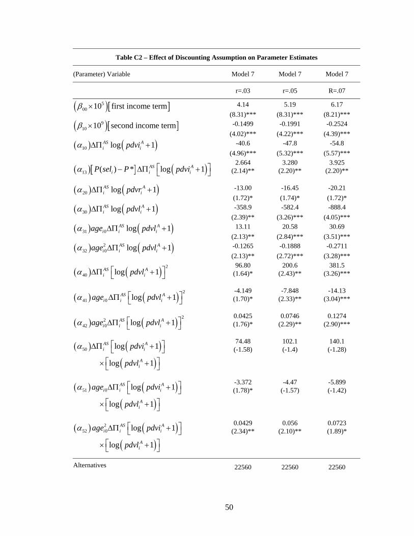
50

Table C2 – Effect of Discounting Assumption on Parameter Estimates

(Parameter) Variable Model 7 Model 7 Model 7

r=.03 r=.05 R=.07

4.14 5.19 6.17 ( )[ ]500 10 first income termβ ×

(8.31)*** (8.31)*** (8.21)*** -0.1499 -0.1991 -0.2524 ( )[ ]9

10 10 second income termβ × (4.02)*** (4.22)*** (4.39)***

-40.6 -47.8 -54.8 ( ) ( )10 log 1AS Ai ipdviα ∆Π +

(4.96)*** (5.32)*** (5.57)*** 2.664 3.280 3.925

( )[ ] ( )13 ( ) * log 1AS Ai i iP sel P pdviα ⎡ ⎤− ∆Π +⎣ ⎦ (2.14)** (2.20)**

(2.20)**

-13.00 -16.45 -20.21 ( ) ( )20 log 1AS Ai ipdvrα ∆Π +

(1.72)* (1.74)* (1.72)* -358.9 -582.4 -888.4 ( ) ( )30 log 1AS A

i ipdvlα ∆Π + (2.39)** (3.26)*** (4.05)***

13.11 20.58 30.69 ( ) ( )31 0 log 1AS Ai i iage pdvlα ∆Π +

(2.13)** (2.84)*** (3.51)*** -0.1265 -0.1888 -0.2711 ( ) ( )2

32 0 log 1AS Ai i iage pdvlα ∆Π +

(2.13)** (2.72)*** (3.28)*** 96.80 200.6 381.5

( ) ( ) 2

40 log 1AS Ai ipdvlα ⎡ ⎤∆Π +⎣ ⎦ (1.64)* (2.43)**

(3.26)***

-4.149 -7.848 -14.13 ( ) ( ) 2

41 0 log 1AS Ai i iage pdvlα ⎡ ⎤∆Π +⎣ ⎦ (1.70)* (2.33)**

(3.04)***

0.0425 0.0746 0.1274 ( ) ( ) 22

42 0 log 1AS Ai i iage pdvlα ⎡ ⎤∆Π +⎣ ⎦ (1.76)* (2.29)**

(2.90)***

74.48 102.1 140.1 ( ) ( )( )

50 log 1

log 1

AS Ai i

Ai

pdvi

pdvl

α ⎡ ⎤∆Π +⎣ ⎦⎡ ⎤× +⎣ ⎦

(-1.58)

(-1.4)

(-1.28)

-3.372 -4.47 -5.899 ( ) ( )( )

51 0 log 1

log 1

AS Ai i i

Ai

age pdvi

pdvl

α ⎡ ⎤∆Π +⎣ ⎦⎡ ⎤× +⎣ ⎦

(1.78)*

(-1.57)

(-1.42)

0.0429 0.056 0.0723 ( ) ( )( )

252 0 log 1

log 1

AS Ai i i

Ai

age pdvi

pdvl

α ⎡ ⎤∆Π +⎣ ⎦⎡ ⎤× +⎣ ⎦

(2.34)**

(2.10)**

(1.89)*

Alternatives 22560 22560 22560

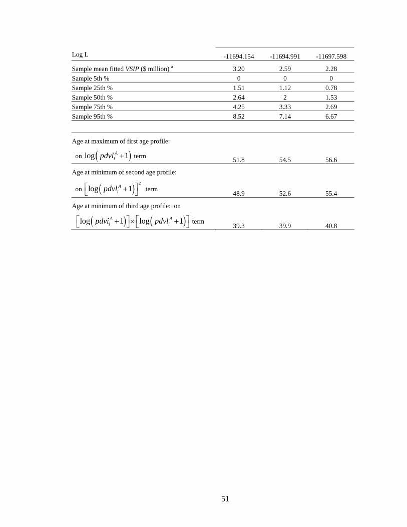
51

Log L -11694.154 -11694.991 -11697.598

Sample mean fitted VSIP ($ million) a 3.20 2.59 2.28 Sample 5th % 0 0 0 Sample 25th % 1.51 1.12 0.78 Sample 50th % 2.64 2 1.53 Sample 75th % 4.25 3.33 2.69 Sample 95th % 8.52 7.14 6.67

Age at maximum of first age profile:

on ( )log 1Aipdvl + term 51.8 54.5 56.6

Age at minimum of second age profile:

on ( ) 2log 1A

ipdvl⎡ ⎤+⎣ ⎦ term 48.9 52.6 55.4

Age at minimum of third age profile: on

( ) ( )log 1 log 1A Ai ipdvi pdvl⎡ ⎤ ⎡ ⎤+ × +⎣ ⎦ ⎣ ⎦ term

39.3 39.9 40.8