1

Valuing Flexibilities in the Design of Urban 1

Water Management Systems 2

Yinghan Deng1, Michel-Alexandre Cardin1*, Vladan Babovic2, 3, Deepak 3

Santhanakrishnan1, Petra Schmitter2, Ali Meshgi2 4

1Department of Industrial and Systems Engineering, National University of 5

Singapore 6

Block E1A #06-25, 1 Engineering Drive 2, 117576, Singapore 7

2Singapore-Delft Water Alliance 8

Block E1 #08-25, 1 Engineering Drive 2, 117576, Singapore 9

3Department of Civil & Environmental Engineering, National University of 10

Singapore 11

Block E1A, #07-03, 1 Engineering Drive 2, 117576, Singapore 12

Abstract 13

Climate change and rapid urbanization requires decision-makers to develop 14

a long-term forward assessment on sustainable urban water management 15

projects. This is further complicated by the difficulties of assessing 16

sustainable designs and various design scenarios from an economic 17

standpoint. A conventional valuation approach for urban water management 18

projects, like Discounted Cash Flow (DCF) analysis, fails to incorporate 19

uncertainties, such as amount of rainfall, unit cost of water, and other 20

uncertainties associated with future changes in technological domains. Such 21

approach also fails to include the value of flexibility, which enables 22

managers to adapt and reconfigure systems over time as uncertainty unfolds. 23

* Corresponding author. Tel: +65 6516 5387 Email: macardin@nus.edu.sg

*ManuscriptClick here to download Manuscript: manuscript_revised2_clean_v2.doc Click here to view linked References

2

This work describes an integrated framework to value investments in urban 24

water management systems under uncertainty. It also extends the 25

conventional DCF analysis through explicit considerations of flexibility in 26

systems design and management. The approach incorporates flexibility as 27

intelligent decision-making mechanisms that enable systems to avoid future 28

downside risks and increase opportunities for upside gains over a range of 29

possible futures. 30

A water catchment area in Singapore was chosen to assess the value of a 31

flexible extension of standard drainage canals and a flexible deployment of 32

a novel water catchment technology based on green roofs and porous 33

pavements. Results show that integrating uncertainty and flexibility 34

explicitly into the decision-making process can reduce initial capital 35

expenditure, improve value for investment, and enable decision-makers to 36

learn more about system requirements during the lifetime of the project. 37

Keywords: Urban water management systems; Real options analysis; 38

Engineering system design and evaluation 39

1 Introduction 40

Traditional water resources planning and analysis methods are based on 41

requirements that are unrealistically deterministic (Medellín-Azuara et al., 42

2007). Under such considerations, the most common practice consists of 43

three phases. First, after relevant data is collected and analyzed, the most 44

likely scenarios are identified, which include projections of major 45

exogenous drivers of the system, such as markets, government policy, and 46

climate change. Then, according to those predictions, system designers 47

generate design concepts and select design parameters that enable the 48

system to perform optimally under the predictions. Economic evaluation of 49

the design is then conducted, of which standard methodology, like 50

3

discounted cash flow (DCF) analysis, optimization, and scenario planning, 51

is applied to achieve the best optimal design (de Neufville & Scholtes, 52

2011). 53

Such kind of design practice based on deterministic forecasts and the 54

assumption of fixed design parameters, however, may not provide a design 55

that performs best in the real world. First, the typical approach does not 56

capture the socio-technical and economic uncertainties that affect the water 57

resources systems, which ultimately shapes the efficacy of water supply 58

systems (S. X. Zhang & Babovic, 2011)– e.g. markets, regulations, and 59

technology. Such system as designed to be optimal in a specific realization 60

of the future achieves the expected performance only when the predicted 61

scenario is realized. Besides, standard design and evaluation analysis, which 62

uses expected values as inputs, may also mislead decision makers, and lead 63

to incorrect design decisions (de Neufville & Scholtes, 2011). This is 64

because the output response (e.g. economic value, rainfall drainage or 65

storage) of most complex systems today is not linear, and the performance 66

observed in downside scenarios cannot be balanced by the upside scenarios. 67

Such situation is described   as   “flaw   of   averages” (Savage, 2000). 68

Furthermore, the conventional approach of DCF is not able to capture 69

managerial flexibility (Trigeorgis, 1996). The sequence of decisions is 70

embedded over time in the cash flow profile as irreversible investment at t = 71

0. The system is assumed to remain   “passive”   and even though in reality 72

managers would try and adapt to the environment so as to capture better 73

economic performance. Standard DCF does not account for such flexibility 74

which may consequently leads to an underestimation of the performance of 75

systems and veils the ability of systems in managing uncertainties. Due to 76

the reasoning above, a paradigm shift in systems design and evaluation is in 77

need. 78

4

Flexibility in engineering design is one avenue to deal with uncertainty pro-79

actively. In this case, flexibility-also referred as real options-is defined as 80

the   “right,   but   not   the obligation, to change a project in the face of 81

uncertainty”(Trigeorgis, 1996). This different perspective on systems design 82

and evaluation is characterized by considering a wide range of possible 83

future scenarios and taking pro-active actions to mitigate critical uncertainty 84

sources. There are several applications of this methodology on large-scale 85

infrastructure systems (Babajide et al., 2009; Buurman et al., 2009; Cardin 86

et al., 2008; Michailidis et al., 2009), which have demonstrated that 87

incorporating flexibility considerably improves the life cycle performance 88

of systems. One typical example of flexible engineering designs in the real 89

estate sector is the Health Care Service Corporation (HCSC) building in 90

Chicago. In 1997, the building was initially designed to prepare for 91

expansion if demand for working space reached a certain level in the future. 92

The second phase of the vertical expansion option was exercised in 2010 93

(Guma et al., 2009). 94

The rest of this paper is organized as follows. The next section discusses the 95

motivations to apply the aforementioned approach, which considers 96

explicitly uncertainty and flexibility, to designing and evaluating urban 97

water management systems. The relevant literature is reviewed, and the 98

research gap for further contribution is identified. Following this section, the 99

details of the proposed methodology in this paper are introduced. Then a 100

case study on a novel water infrastructure system is presented, as to 101

demonstrate the implementation of the proposed methodology as well as its 102

effectiveness in terms of improving performance of the target system. 103

Finally discussions and conclusions are made in the last section. 104

5

2 Motivation 105

The world is experiencing a high rate of urbanization. For those countries 106

with highly urbanized population, like Singapore (100% of total population 107

in 2010), the size of urban population is still growing; while for countries 108

which are not highly urbanized at the current stage, like China (47% of total 109

population in 2010), the rate of urbanization change is high ("Urbanization," 110

2012). Increasing urbanization worldwide could intensify local competition 111

for all types of resources, water being amongst the most vital (Zoppou, 112

2001). In addition, many other factors, like land scarcity, climate change, 113

and depleting energy resources, require urban system designers to think 114

forward and provide efficient solutions that make better use of resources and 115

maintain sustainability. 116

Development of sustainable water systems has been subjected to heated 117

discussions recently. These systems  are  defined  as  “water  systems  that  are  118

managed to satisfy changing demands placed on them (both human and 119

environmental) now and into the future, whilst maintaining ecological and 120

environmental   integrity   of   water” (UNESCO, 1998). However, for such 121

emerging sustainable urban water management systems, we lack knowledge 122

of how sustainable development should be attained and how sustainability 123

of various technical systems should be assessed (Hellstrom et al., 2000). 124

Traditional water resources planning and analysis methods based on fixed 125

requirements and design parameters do not address how to properly evaluate 126

systems under uncertainties as well as how to effectively manage 127

uncertainties that are pervasive in urban systems of today. Some studies 128

have been proposed to support the decision process to manage urban water 129

(Makropoulos et al., 2008; Pearson et al., 2009; Thomas & Durham, 2003). 130

Results from these studies provide suggestions and tools on selection of 131

design alternatives and making policies. For example, Integrated Water 132

Resource Management (IWRM) is proposed to support the management of 133

6

alternative water resources from multiple perspectives (Thomas & Durham, 134

2003). Those studies, however, have not explicitly accounted for the various 135

sources of uncertainties, like instability of technical efficiency or fluctuation 136

in rainfall that may impact the results of decision-making. Some of the 137

recent studies have taken one step further to recognize the exogenous and 138

endogenous uncertainties faced by water systems, and even explicitly take 139

those uncertainties into account when doing evaluation analysis. For 140

example, Morimoto and Hope (2001, 2002) applied probabilistic techniques 141

to the cost-benefit analysis of hydroelectric projects in Sri Lanka, Malaysia, 142

Nepal, and Turkey, where they generated Net Present Value (NPV) 143

distribution for design alternatives. Their analysis, however, has not 144

incorporate pro-active actions to handle situations that may go beyond 145

designers’   predictions. Even though sensitivity analysis is conducted, it 146

merely acts as one part of the evaluation process and not as a way of 147

inspiring novel solutions to optimize the design itself. In some studies (Pahl-148

Wostl et al., 2007), Adaptive Management is introduced into urban water 149

management. These works, however, mainly deal with the operational part 150

of the systems and have not revealed how to make changes to design 151

configurations of the system as well as how to measure the additional 152

benefits brought by those changes. 153

In light of the situation explained above, this study considers applying 154

flexibility in engineering design thinking to planning and assessment of 155

urban water management systems. It has been indicated that incorporating 156

flexibility into systems can bring about performance improvements ranging 157

between 10% and 30%, compared to standard design and evaluation 158

approaches (de Neufville & Scholtes, 2011). These improvements are 159

achieved because flexible designs enable systems to hedge against downside 160

scenarios (e.g. by reducing the scale of initial capital expenditure) and 161

prepare for the unexpected favorable conditions (e.g. by allowing for future 162

expansion of the system). For example, in the case of Iridium and Globalstar, 163

7

the company would be able to reduce the life cycle cost by more than 20% if 164

a phasing deployment strategy could have been adopted (de Weck et al., 165

2004). 166

A set of procedures has been proposed in terms of designing and evaluating 167

flexibility in complex engineering systems (Cardin et al., 2008; Cardin et 168

al., 2007; S. X. Zhang & Babovic, 2011). One such procedure (Cardin et al., 169

2007) starts with conventional design and evaluation approaches, and then 170

further investigates into uncertainty and flexibility of the target system. 171

Although the detailed modeling of each system and its specific flexibility 172

varies from system to system, it is expected that those procedures and 173

frameworks can be modified and applied in the context of urban water 174

management systems. 175

Indeed, there were some recent studies already moving towards this 176

direction by using the real options approach to analyzing water systems. For 177

example, Zhang and Babovic (2012) have conducted real options analysis to 178

identify optimal water supply strategies, and Wang (2005) applied the 179

approach to optimize the development of a hypothetical river basin 180

involving decisions to build dams and hydropower stations. These studies 181

have indicated that by applying flexibility analysis to water systems, 182

designers are able to offer more cost-effective and sustainable solutions. 183

The main contribution of this paper is a systematic methodology to analyze 184

urban water management systems in an engineering context, considering 185

uncertainty and flexibility explicitly as part of the engineering design and 186

management process. The methodology is similar to the approaches used by 187

Zhang and Babovic (2012). However their work is mainly focused on 188

strategic policy making, while the methodology introduced in this paper is 189

rooted in an engineering design perspective. As for Wang’s   study (Wang, 190

2005), the logic of doing the analysis is similar, but the target system of 191

Wang’s   study   is   hydroelectric   dams, which differ with urban water 192

8

management systems in terms of scale and complexity. Besides, the 193

uncertainties faced by these two kinds of water systems are also distinct. 194

Different modeling techniques need to be proposed so as to simulate the 195

behavior of the system and its uncertainty drivers in an urban context. 196

Furthermore, Wang applied mixed integer programming to modeling the 197

decision-making process and relied on dynamic programming in the aspect 198

of evaluation. This approach, however, imposes limitation on the decision 199

rules being evaluated, and may be trapped by curse of dimensionality when 200

confronted with a multitude of decision periods and states. The approach 201

here incorporates decision rules as another variable in the analytical model, 202

which enables modeling of diverse decision rules with relatively less 203

computational burden. Besides, it is a direct extension of existing design and 204

evaluation approaches, and is designed via a systematic step-wise process 205

for more practical impact in engineering practice. Another contribution from 206

a modeling standpoint involves the use of so-called Intensity Duration 207

Frequency (IDF) curves to simulate the rainfall behavior in order to 208

understand how rainfall intensities and durations as uncertainty factors may 209

influence the economic performance of the system. The last contribution is 210

to report on the first application of this methodology in the design and 211

deployment of porous pavement and green roof technologies, as a way to 212

recuperate and store grey water from natural rain events. Since not many 213

studies have been done, the study provides another example of how these 214

ideas can be considered in urban water management systems and how this 215

new catchment technology can be better deployed. It is hoped that the 216

results reported here will offer a different perspective on how to design, 217

evaluate and implement urban water management systems, which can be of 218

value to both research scholars and practitioners. 219

9

3 Methodology 220

This study proposes a four-step procedure to design and evaluate flexible 221

urban water management systems. The procedure is based on and modified 222

from a design process proposed by a past study (Cardin et al., 2007). Similar 223

to the original one, this proposed methodology is also a step-wise process on 224

flexibility in design and evaluation, starting with the baseline model and 225

further stepping into the uncertainty analysis and the flexibility analysis. 226

One additional step of sensitivity analysis is added as to provide more 227

reliable analytical results. 228

3.1 Step 1: Baseline Model 229

The starting point of the methodology is to build a baseline model. The 230

objective here is to understand the main components of the system that 231

influence its full life cycle performance. Costs and benefits involved in the 232

system are calibrated by defining necessary design parameters and design 233

variables. Additionally, assumptions on the system are defined. Following 234

that, a preliminary deterministic cost-benefit analysis (Boardman et al., 235

2006) can be carried out. Generally, in this step, the conventional DCF 236

model is built to assess the performance of the system under the 237

deterministic conditions. This step captures the standard practice in terms of 238

design and project evaluation. 239

3.2 Step 2: Uncertainty Analysis 240

In this step, designers need to model major uncertainty drivers, and 241

investigate design alternatives under a range of possible future scenarios. 242

Historical data on the uncertainty drivers is collected and calibrated into 243

stochastic or probability models, like Geometric Brownian Motion (GBM) 244

and normal distribution. Then simulation is applied to generate scenarios 245

that are used to assess the life cycle performance of design alternatives. The 246

performance of these designs is compared under the criteria of Expected Net 247

Present Value (ENPV), VAG (Value At Gain, which quantifies the 248

10

performance in the upside scenarios), VAR (Value At Risk, which 249

quantifies the performance in the downside scenarios), and variance. 250

Through this analysis, designers capture a more comprehensive picture 251

about the pros and cons of the design alternatives, compared with the 252

deterministic analysis in Step 1. 253

3.3 Step 3: Flexibility Analysis 254

In this step, designers first need to generate flexible design concepts. A 255

complete flexible concept is defined by four elements: uncertainty source, 256

flexible strategy, flexible enabler, and decision rule (Cardin et al., 2012). 257

Flexible strategies are the actions designers can take when a particular path 258

of uncertainties is realized (e.g. expand the capacity of the system if demand 259

turns out to be higher than prediction), while flexible enablers are the design 260

configurations that make the strategies feasible from a design and 261

management standpoint. A decision rule is a triggering mechanism or an 262

“if”   statement that specifies clearly when the flexible strategies will be 263

exercised, based on some uncertainty realizations. For example, in the case 264

of the HCSC building (Guma et al., 2009),   the   flexible  concept  can  be  “in 265

order to deal with the uncertainty from working space demand, extra 266

strength is added into the load bearing walls so that the building can be 267

expanded if the working space is not enough”. In this case, adding extra 268

strength is the flexible enabler and capacity expansion is the flexible 269

strategy,   while   the   “if”   statement   about   the   working   space   is   the   decision  270

rule. 271

After flexible concepts are generated, they are evaluated under the same 272

scenarios and metrics stated in Step 2. The Value of Flexibility (VoF) is 273

calculated by equation (1). 274

275

(1) 276

11

The computation of VoF can be resolved from several perspectives. The 277

classical works in pricing financial options (Black & Scholes, 1973; Cox et 278

al., 1979) are the origins of the valuation of real options. Later, the binomial 279

approach proposed by Cox et al. (1979) was suggested to value options on 280

real investments, hence real options (Trigeorgis, 1996). This approach has 281

also been applied to obtaining the value of real options in engineering 282

systems (de Weck et al., 2004). Decision tree is another method to assess 283

the VoF, when the number of decisions is limited and the uncertainty can be 284

modeled by discrete random variables. This method has been adopted to 285

evaluate the VoF in oil deployment projects (Babajide et al., 2009). An 286

important aspect of these two methodologies is that the evaluation process 287

relies on dynamic programming where the decision rule essentially is 288

decided by optimizing at each decision point based on expected value. This 289

kind of approach may not capture well the full realm of possible decision 290

rules. Besides, as the number of decision-making periods and states 291

increases, the computation may become intractable. Although the 292

assumption of path-independency in the binomial approach allows a 293

recombination structure to reduce computational burden, this assumption of 294

path-independency may not hold for engineering systems. This is because 295

different realizations of uncertainty may lead to different changes on system 296

configurations which in return result in different realizations in the next time 297

period (e.g. upgrading the efficiency of urban water systems may lead to 298

lower price of water next period). Another approach to obtain the VoF is 299

simulation. This approach can be more generally applied, since it has fewer 300

restrictions on the number of time periods being considered and the 301

distribution of uncertainties. Besides, this approach considers decision rules 302

as explicit variables in the modeling framework, so that the model itself can 303

be more easily modified to capture more diverse design configurations. 304

12

3.4 Step 4: Sensitivity Analysis 305

Finally, sensitivity analysis is carried out in order to assess how the results 306

obtained following the above steps respond to changes in underlying 307

assumptions. This step can be seen as a way to test the robustness of the 308

design alternatives in response to the variation that may happen to the 309

assumptions. There are several standard mathematical methods that can be 310

applied in terms of doing sensitivity analysis. For example, one-factor-at-a-311

time method (OFAT) (Czitrom, 1999) is one of simplest and most common 312

approaches. 313

4 Application 314

In order to demonstrate an application of the methodology introduced 315

above, this study applies the approach to the feasibility analysis of a new 316

water technology. Besides, the results from this section also work as a 317

demonstration to show that the methodology is effective in terms of 318

improving the performance of urban water management systems. 319

4.1 Problem Definition 320

As part of an effort to investigate possible solutions for next-generation 321

water infrastructure systems, which aim to reduce damage caused by floods 322

in rainy seasons and re-use of the run-offs, a new technology based on 323

porous pavements and green roofs is being proposed. The technology allows 324

rainwater to infiltrate into the sub-surface layer where it is temporarily 325

stored. For porous pavements, the sub-surface layer is filled with porous 326

materials, while for the green roofs, the vegetation cover and space 327

underneath function as the storage facility. The stored rainwater is then 328

either detained in the ground, or be harvested by the pipe installed under 329

pavements or the underneath space of green roofs. Later this harvested 330

water   can   be   recycled   as   “grey”   water or be channeled to reservoirs. By 331

13

implementing this technology, revenues (as cost savings of re-using 332

rainwater) are generated. Besides, the porous pavements and green roofs 333

reduce frequency and peak flow rate of rainwater that enters the drainage 334

system. Consequently, less space is required for drainage, and the likelihood 335

of flooding damage is also reduced. (S. Zhang & Buurman, 2010) 336

A test site has been chosen for a preliminary analysis on the possibilities and 337

limitations of this innovative solution. The site is located within the Kent 338

Ridge campus of the National University of Singapore (NUS). The size of 339

the catchment has an area of about 8.2 ha. The land use distribution of the 340

catchment comprises the following: 41% of bushes, 35.5% of other green 341

areas, mostly grass patches on mild and steep slopes, 16.8% of rooftop and 342

4.77% of road areas. 343

There are two considered design alternatives: a traditional expansion of the 344

current drainage canal system (referred as design A) and alternative based 345

on catchment measures of porous pavements and green roofs (referred as 346

design B). Although design B has several aforementioned advantages 347

compared with design A, since design B incurs a higher construction cost 348

and maintenance cost, analysis is needed to better understand the costs and 349

benefits. Also, one aims to assess whether there is potential to further 350

improve the economic performance of those two design alternatives under 351

uncertainties by applying the flexibility analysis. 352

4.2 Step 1: Baseline DCF Model 353

The following is the list of notations used in the analysis. 354

Total area of the test site under study (m2) 355 Area that can be deployed to porous pavements (m2) 356 Area that can be deployed to green roofs (m2) 357

Drainage capacity of canals in design A (m3) 358 Drainage capacity of canals in design B (m3) 359

Depth of canals (m) 360 Area of existing canals (m2) 361 Area of expanded canals in design A (m2) 362

Storage capacity of porous pavements (m3) 363

14

Storage capacity of green roofs (m3) 364 Depth of porous materials in porous pavements (m) 365 Depth of vegetation covers in green roofs (m) 366 Depth of underneath space in green roofs (m) 367

Porosity of porous materials in porous pavements 368 Porosity of vegetation covers in green roofs 369

Recycle efficiency of porous pavements 370 Recycle efficiency of green roofs 371

Initial investment of design A ($) 372 Initial investment of design B ($) 373

Unit flood damage cost ($/m3) 374 Unit maintenance cost of design A ($/m2) 375 Unit maintenance cost of porous pavements ($/m2) 376 Unit maintenance cost of green roofs ($/m2) 377

Unit cost of water treatment ($/m3) 378 Discounted rate 379

Annual cost in kth year ($) 380 Annual revenue in kth year ($) 381 Unit water price in kth year ($/m3) 382

Rainfall quantity of the ith rain of the kth year (m) 383 Number of rain events of the kth year 384

The assumptions for the design parameters and input data needed in the case 385

study are shown in Table 1. The cost information is based on personal 386

communications with the design team members (as shown in Table 1). 387

Although it may not be perfectly accurate, it is based on experienced 388

designers’ inputs and reflects the essence of the system to some degree. The 389

annual rainfall information is summarized from the online published data of 390

National Environmental Agency ("Weather Statistics," 2013). 391

Table 1 Assumptions on Parameters and Input Data 392

For design A, the following equations are developed. As there are no 393

mechanisms of generating revenues, the analysis only needs to quantify the 394

costs involved. There are two categories of costs under consideration. Flood 395

damage cost is calculated based on the occurrence of the rain events where 396

the rainfall quantity exceeds the drainage capacity. Maintenance cost is a 397

variable cost that links with the drainage area. The maintenance cost is 398

related to activities of physical cleansing, maintenance and minor structural 399

repairs of drains and canals. 400

401 (2) 402

15

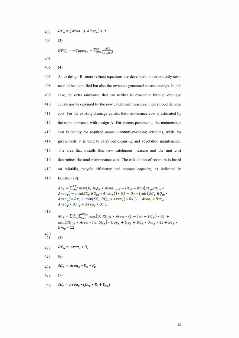
403

(3) 404

405

(4) 406

As to design B, more refined equations are developed, since not only costs 407

need to be quantified but also the revenues generated as cost savings. In this 408

case, the extra rainwater, that can neither be evacuated through drainage 409

canals nor be captured by the new catchment measures, incurs flood damage 410

cost. For the existing drainage canals, the maintenance cost is estimated by 411

the same approach with design A. For porous pavements, the maintenance 412

cost is mainly for required annual vacuum-sweeping activities, while for 413

green roofs, it is used to carry out cleansing and vegetation maintenance. 414

The area that installs this new catchment measure and the unit cost 415

determines the total maintenance cost. The calculation of revenues is based 416

on rainfalls, recycle efficiency and storage capacity, as indicated in 417

Equation (9). 418

419

420 (5) 421

422

(6) 423

424

(7) 425

426

16

(8) 427

428

429

430 (9) 431

432

(10) 433

Based on the aforementioned assumptions and models, the deterministic 434

analysis is carried out, where the two design alternatives are evaluated under 435

deterministic values of unit water price, the number of rain events and the 436

rainfall in a single rain event ( =1.7$/m3, =178, =13.16mm, 437

). Table 2 summarizes the computation results. The deterministic DCF 438

analysis shows that overall introducing porous pavements and green roofs 439

may be more cost beneficial than the canal expansion alternative, as the 440

former shows a less negative NPV compared with design A. 441

Table 2 Results of Deterministic Analysis 442

4.3 Step 2: Uncertainty Analysis 443

Uncertainty analysis addresses two research objectives: generate a wide 444

range of scenarios of major uncertainty sources, and evaluate the 445

performance of the design alternatives under the scenarios. To simplify the 446

analysis, only two major uncertainty sources are identified at the current 447

stage: price of water and rainfall. More uncertainty drivers can be 448

introduced if needed. 449

17

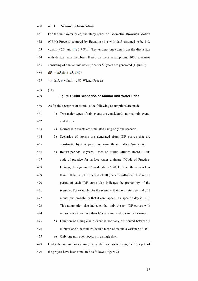
4.3.1 Scenarios Generation 450

For the unit water price, the study relies on Geometric Brownian Motion 451

(GBM) Process, captured by Equation (11) with drift assumed to be 1%, 452

volatility 2% and 1.7 $/m3. The assumptions come from the discussion 453

with design team members. Based on these assumptions, 2000 scenarios 454

consisting of annual unit water price for 50 years are generated (Figure 1). 455

* 456

* -drift, -volatility, -Wiener Process 457

(11) 458

Figure 1 2000 Scenarios of Annual Unit Water Price 459

As for the scenarios of rainfalls, the following assumptions are made. 460

1) Two major types of rain events are considered: normal rain events 461

and storms. 462

2) Normal rain events are simulated using only one scenario. 463

3) Scenarios of storms are generated from IDF curves that are 464

constructed by a company monitoring the rainfalls in Singapore. 465

4) Return period: 10 years. Based on Public Utilities Board (PUB) 466

code of practice for surface water drainage ("Code of Practice-467

Drainage Design and Considerations," 2011), since the area is less 468

than 100 ha, a return period of 10 years is sufficient. The return 469

period of each IDF curve also indicates the probability of the 470

scenario. For example, for the scenario that has a return period of 1 471

month, the probability that it can happen in a specific day is 1/30. 472

This assumption also indicates that only the ten IDF curves with 473

return periods no more than 10 years are used to simulate storms. 474

5) Duration of a single rain event is normally distributed between 5 475

minutes and 420 minutes, with a mean of 60 and a variance of 100. 476

6) Only one rain event occurs in a single day. 477

Under the assumptions above, the rainfall scenarios during the life cycle of 478

the project have been simulated as follows (Figure 2). 479

18

1) Reverse engineering of the IDF curves by using nonlinear 480

regression to calibrate the relationship between rain durations and 481

intensities. 482

2) Calculate the rainfall of the normal rain event using the equations 483

in Figure 2. 484

3) Apply the procedures described in the dashed box of Figure 2 to 485

generate the rainfall scenario of a single day. 486

4) Repeating step 3) by 365 x 50 x 2000 times, 2000 scenarios of 487

daily rainfalls in 50 years are obtained. A histogram is built to 488

show the distribution of daily rainfalls (Figure 3) (Days without 489

rain events are not counted). 490

Figure 2 Procedures of Generating Rainfall Scenarios 491

Figure 3 Histogram of 2000 scenarios of daily rainfalls in 50 492

years 493

4.3.2 Evaluation Results 494

Subsequently to the scenario generation, the costs and benefits of the two 495

design alternatives are evaluated under each simulated scenario. Equation 496

(12) is used to calculate ENPV in this study. Here, is the net present 497

value under the nth path of the uncertain factors, and is the probability of 498

nth path. In this analysis, for simplicity of computation, every path is 499

assumed to have the same probability, which here is 1/2000 since 2000 500

paths are generated. 501

502

(12) 503

Combined with results from the deterministic analysis in the previous 504

section and the uncertainty analysis, a probabilistic distribution (Figure 4) 505

and a multi-criteria comparison table (Table 3) are constructed. 506

19

Figure 4 Distribution of NPV of Design A and Design B 507

Table 3 Multi-metrics Table of Design A and Design B 508

As indicated from the above results, if only the deterministic analysis is 509

referred as the basis of decision-making, although the ranking of design 510

alternatives remains the same, the economic value of two design alternatives 511

is either overestimated or underestimated. For design A, as shown in the 512

cumulative probability curve, the likelihood that the realized NPV is smaller 513

than the deterministic NPV is 1, which means the probability that such NPV 514

can be obtained in the reality is negligible. This finding is supported by the 515

Jensen’s  inequality (Jensen, 1906) shown in Equation (13). As we take the 516

average of uncertainty drivers (unit price, rainfall quantity and number of 517

rainfall events), the NPV in the upside scenarios cannot be averaged out by 518

the downside scenarios. In fact, since here the flood cost is incurred when 519

the rainfall is higher than the drainage capacity, as long as the assumed 520

deterministic value of single rainfall is lower than the drainage capacity, 521

there is no flood damage cost resulted in the whole life cycle of the system. 522

In reality, however, the rainfall is subjected to high fluctuations, which leads 523

to the presence of storms that lead to flood damage cost. The Flaw of 524

Averages (Savage, 2000) is also observed in the result of design B but just 525

turns out in an opposite direction. As shown in Figure 4, the deterministic 526

value of NPV is even away from the lower tail of the CDF curve, which 527

means the chance of obtaining such a low NPV in real world is very slim. 528

As for the standard deviation, since design A is only subjected to the 529

fluctuation of rainfall, while design B is influenced by rainfall and price of 530

water, the variance of design A is relatively lower. 531

) 532

(13) 533

20

4.3.3 Further Discussions 534

To further investigate how the two design alternatives perform under 535

different scenarios, especially on the aspect of preventing flood damage, the 536

flood damage costs under different rainfalls ranging from 0mm to 300mm 537

are calculated. Figure 5 shows the computation results. 538

Figure 5 Flood Functions of Design A and Design B 539

Based on Figure 5, when the rainfall is higher than 20mm, flood damage 540

occurs to design B, while this threshold is almost doubled for design A. This 541

indicates that there is a higher chance of flood damage in design B. Besides, 542

since the rainfall in a single rain event is rarely higher than 160mm (shown 543

in Figure 3), mostly higher flood damage costs happen to design B rather 544

than design A. 545

This seemly counter-intuitive result may come from the fact that only a 546

small proportion of the test area (40.02%) can be deployed to either green 547

roofs or porous pavements. Therefore the rain dropping to other area that is 548

not covered by the new technology can only be evacuated through existing 549

drainage canals. Meanwhile, compared with design A that expands the 550

capacity of canals, the drainage capacity in design B is much smaller. 551

Because of the reasoning above, design B is more vulnerable to rainfall 552

fluctuations in terms of flood damage. 553

4.4 Step 3: Flexibility Analysis 554

To further improve the life cycle performance of the two design alternatives, 555

this study proceeds with flexibility analysis. An expansion option is 556

incorporated into both design A and design B, which is enabled by 557

deploying a smaller capacity initially but reserving the necessary resources 558

(e.g. land and capital) for possible future expansion. The process of 559

generating flexible designs is a topic of active research (Cardin et al., 2012). 560

Here, only one strategy is considered for demonstration purposes, although 561

21

more real options opportunities exist (e.g. early abandonment, switching 562

between different technologies, etc.) 563

4.4.1 Flexible Designs 564

For design A, the flexible design is as follows. The existing canals are not 565

expanded at the beginning. If the number of floods happening within one 566

year exceeds ten times, the drainage capacity will be expanded until it 567

reaches the upper bound (5000m3). This expansion option is further 568

explained using the following expressions. 569

570

571

572

* is the indicator function of 573 574

As for design B, the same area is deployed for the new technology but only 575

half of the depth is deployed for the pavements and the underneath space of 576

roofs. If the number of floods happening within one year exceeds ten times 577

the storage capacity will be expanded by enlarging the depth until it reaches 578

the upper bound. Details of this expansion option are shown below. 579

For green roofs, 580

581

582

* is the indicator function of 583 584

For porous pavements, 585

586

587

* is the indicator function of 588

589

22

590

4.4.2 Evaluation Results 591

The two flexible designs are evaluated under the same 2000 scenarios 592

generated in the uncertainty analysis. By summarizing results from the 593

flexibility analysis and the uncertainty analysis, Figure 6 and Table 4 are 594

obtained. Figure 6 shows the distribution of the NPV of all alternatives, 595

while Table 4 summarizes the information on the predefined metrics. 596

Figure 6 Distribution of NPV of All Design Alternatives 597

Table 4 Multi-metrics Comparison Table of All Design 598

Alternatives 599

For design B, based on equation (14), the value of flexibility is $105,799. 600

The results show that incorporating flexibility makes design B profitable as 601

ENPV turns out to be positive. One interesting observation is that the value 602

of flexibility closely corresponds to the difference in CAPEX between 603

flexible design B and baseline design B ($121,875). This indicates that 604

baseline design B may be designed with unnecessary storage capacity 605

whereas flexible design B gains the advantage by reducing the redundant 606

initial investment. This is further confirmed by the fact that among the 2000 607

times of simulation, porous pavements are expanded only in a small 608

proportion of scenarios (197 out of 2000), and it has never reached the 609

maximum capacity, while the expansion option is never exercised for green 610

roofs. 611

612

(14) 613

For design A, the economic performance is also improved by considering 614

the flexibility of a staged capacity deployment approach. According to 615

Table 4, the extra value brought by this expansion option is $44,840. The 616

expansion decisions made through the simulation indicate that the 617

23

improvement on design A is also achieved through reducing excessive 618

capacity of the inflexible design. It is found that in less than 10% of the 619

simulation does the drainage capacity of canals expands above 4000m3, and 620

mostly (over 70%) a capacity of 3520m3 is considered sufficient based on 621

the decision rule. The trade-off between the economy of scale and the time 622

value of money may be another factor that leads to the better performance of 623

flexible design A. The influence from the economy of scale suggests that a 624

larger capacity deployed all at once is a more economic decision, while the 625

time value of money favors that more investment should be placed later. In 626

the case of design A, the latter factor seems to impose more impact on the 627

final result. 628

4.5 Step 4: Sensitivity Analysis 629

After the flexibility analysis has been carried out, the best design alternative, 630

flexible design B in this case study, is selected and subjected to the 631

sensitivity analysis. Namely, the performance of flexible design B is 632

reevaluated under the change of major assumptions made in Table 1. 633

Recycle efficiency, maintenance cost, treatment cost, discounted rate 634

expansion cost, and flood damage cost are assumed to be major influences 635

on the performance of flexible design B. OFAT is applied in the sensitivity 636

analysis. The values of the aforementioned factors are varied by ± 20% and 637

5% at a time, and then the ENPV of flexible design B is reevaluated under 638

the new inputs. 639

According to Figure 7, the variation of expansion costs imposes almost no 640

influence on the ENPV. This evidence supports the conclusion made on the 641

flexibility analysis, that the expansion is rarely exercised. On the other hand, 642

the recycle efficiency of green roofs is shown to affect the performance of 643

flexible design B most, which is even stronger than that of the discounted 644

rate. The observation here contrasts to the recycle efficiency of porous 645

pavements that does not influence the result so much. This difference 646

24

between porous pavements and green roofs is also observed on the 647

maintenance cost where green roofs lead to a stronger degree of changes on 648

the ENPV. The observation may be resulted from the fact, that a larger area 649

is deployed for roofs so that the ENPV depends more on the change of 650

roofs. Water treatment cost also influences the result to a certain degree that 651

is close to that of the maintenance cost of pavements, but higher than that of 652

the unit flood cost. The relatively weak effect of unit flood cost may be 653

explained by the low frequency of flood. This result also indicates the 654

robustness of choosing design B, as in the worst case, the ENPV of flexible 655

design B is still far better than flexible design A. Even a higher unit flood 656

cost cannot diminish the advantage of flexible design B. 657

Figure 7 Sensitivity Analysis of ENPVfb 658

By varying the same factors, this study also applies the OFAT to the VoFB. 659

Results are shown in Figure 8. Due to the negligible influence of expansion 660

cost and maintenance cost on the result, Figure 8 does not include these 661

factors. According to Figure 8, discounted rate is the most critical factor on 662

the VoF. The result on discounted rate also corresponds to the conclusion 663

made in the flexibility analysis that a higher discounted rate contributes to a 664

higher VoF. It is also interesting to note that increasing recycle efficiency 665

of pavements leads to lower value of flexibility. One reason for this 666

observation is that higher recycle efficiency may prefer developing a larger 667

capacity at the beginning so as to generate more revenues by re-using more 668

rainwater. On the contrary, the influence from the recycle efficiency of roofs 669

is almost negligible. This is explained by the fact that the capacity of roofs 670

is never expanded in the simulation. Treatment cost and flood damage cost 671

only have a slight effect on the result. 672

Figure 8 Sensitivity Analysis of VoFB 673

25

5 Discussion and Conclusions 674

The analysis presented in this paper demonstrated how to explicitly 675

incorporate uncertainty and flexibility into the design and evaluation of 676

urban water management systems. Through relevant literature, it has been 677

shown that the typical system design approach and evaluation might lead to 678

suboptimal system performance and flaws in the evaluation results (de 679

Neufville & Scholtes, 2011). This finding was also confirmed by 680

uncertainty analysis of the water catchment site in this study, which showed 681

that the deterministic analysis resulted in considerably inaccurate evaluation 682

of design alternatives. 683

One advantage of applying the described methodology into systems design 684

is the effectiveness in improving the life cycle performance. For example, 685

for flexible design B in the application analysis, the extra benefits were 686

brought by reducing the initial excessive capacity, and by enabling an 687

expansion option, so that the system was able to avoid unnecessary initial 688

investment if downside scenarios happened (e.g. low cost  savings  by  “grey  689

water” that could not balance the cost of the system). Meanwhile, the 690

system was prepared to handle upside scenarios (e.g. high unit price of 691

water which made the system more profitable). This action was similar to 692

buying insurance for the system by which the distribution of the system 693

performance was shifted to the right side. This improvement on economic 694

performance resulted from incorporating flexibility was also observed on 695

design A. 696

However, flexible designs may not always result in improvement on system 697

performance. As shown in the sensitivity analysis, there were many factors 698

one would need to consider, such as the time value of money and 699

opportunity cost. Although in the case study flexible design B was shown to 700

be the best even under variations of assumptions, when faced with different 701

26

systems, designers need to be careful about the trade-offs between those 702

factors so that the system performance can be maximized. 703

The framework and procedures introduced in this study can be generalized 704

into the applications of other urban water management systems. The four-705

step analysis (baseline model building, uncertainty analysis, flexibility 706

analysis and sensitivity analysis) is one example that can be applied to a 707

wide range of water systems. Whereas since different systems are subjected 708

to distinct costs and benefits, and faced with their respective source of 709

uncertainties, details of modeling and computation may need to be adjusted 710

to suit the particular system at hand. Another contribution of this analysis is 711

combining historical data and IDF curves to simulate daily rainfall 712

scenarios. The model can be easily modified to another region with different 713

IDF curves or requirements of return periods. 714

There are some limitations in this study. First, in the case study, the analysis 715

has not accounted for all possible benefits. For example, for design B, the 716

benefit of reduced mosquito breeding resulting from reduced standing water 717

is not included. This case study should be considered as a first analysis of 718

the major costs and benefits involved in this new water catchment 719

technology. Follow-up contribution can be made to identify proper models 720

to capture a more comprehensive picture of such systems. Second, only two 721

flexible designs are considered in the application. It is highly possible that 722

the economic performance of the system can be further enhanced by a better 723

flexible design. Therefore, another opportunity of extending the study is to 724

explore better methods to assist the conceptual design of flexible urban 725

water management systems. The concept generation technique proposed by 726

Cardin et al. (2012) is one option to assist such process. Finally, future 727

research can also focus on introducing stochastic optimization analysis on 728

the design of flexible urban water management systems, so that better 729

design configurations will be identified. Optimization techniques, like the 730

27

screening model proposed by Wang (2005) may be applied to accelerate the 731

efficiency of doing optimization analysis. 732

Acknowledgements 733

The authors are thankful for the financial support provided by the National 734

University of Singapore (NUS) Faculty Research Committee via MOE 735

AcRF Tier 1 grant WBS R-266-000-061-133. The financial support 736

provided by NUS Research Scholarship is also acknowledged. The authors 737

would like to thank to the ISE department of NUS and Singapore-Delft 738

Water Alliance for supporting this research work. Also, the authors would 739

like to give thanks other   colleagues   in   Dr.   Cardin’s   research   group,   who  740

gave critical feedback on the completion of this work. 741

References 742

743 Babajide, A., De Neufville, R., & Cardin, M.-A. (2009). 744

Integrated Method for Designing Valuable Flexibility 745 in Oil Development Projects. SPE Projects, Facilities, 746 and Construction, 4, 3-12. 747

Black, F., & Scholes, M. (1973). The Pricing of Options and 748 Corporate Liabilities. Journal of Political Economy, 749 81(3), 637-654. 750

Boardman, A. E., Greenberg, D. H., Vining, A. R., & Weimer, D. 751 L. (2006). Cost Benefit Analysis: Concepts and 752 Practice (3rd ed.). New Jersey: Prentice Hall. 753

Buurman, J., Zhang, S., & Babovic, V. (2009). Reducing risk 754 through real options in systems design: the case of 755 architecting a maritime domain protection system. 756 [Research Support, Non-U.S. Gov't]. Risk Anal, 29(3), 757 366-379. doi: 10.1111/j.1539-6924.2008.01160.x 758

Cardin, M.-A., de Neufville, R., & Kazakidis, V. (2008). A 759 Process to Improve Expected Value of Mining 760 Operations. Mining Technology: IMM Transactions, 761 117, 65-70. 762

Cardin, M.-A., Kolfschoten, G. L., Frey, D. D., de Neufville, R., 763 Weck, O. L., & Geltner, D. M. (2013). Empirical 764 evaluation of procedures to generate flexibility in 765

28

engineering systems and improve lifecycle 766 performance. Research in Engineering Design, 24(3), 767 277-295. doi: 10.1007/s00163-012-0145-x 768

Cardin, M.-A., Nuttall, W. J., de Neufville, R., & Dahlgren, J. 769 (2007). Extracting Value from Uncertainty: A 770 Methodology for Engineering Systems Design. Paper 771 presented at the 17th Annual International 772 Symposium of the International Council on Systems 773 Engineering (INCOSE), San Diego, California. 774

. Code of Practice-Drainage Design and Considerations. 775 (2011), from 776 http://www.pub.gov.sg/general/code/Pages/SurfaceDrainagePart2-777 7.aspx 778

Cox, J. C., Ross, S. A., & Rubinstein, M. (1979). Option Pricing: 779 A Simplified Approach. Journal of Financial 780 Economics(7), 229-263. 781

Czitrom, V. (1999). One-Factor-at-a-Time versus Designed 782 Experiments. The American Statistician, 53(2), 126-783 131. 784

de Neufville, R., & Scholtes, S. (2011). Flexibility In 785 Engineering Design. Engineering Systems. Cambridge, 786 MA, United States: MIT Press. 787

de Weck, O., de Neufville, R., & Chaize, M. (2004). Staged 788 Deployment of Communications Satellite 789 Constellations in Low Earth Orbit. JOURNAL OF 790 AEROSPACE COMPUTING, INFORMATION, AND 791 COMMUNICATION, 1, 119-136. 792

Guma, A., Pearson, J., Wittels, K., Neufville, R. d., & Geltner, D. 793 (2009). Vertical Phasing as a Corporate Real Estate 794 Strategy and Development Option. Journal of 795 Corporate Real Estate, 11(3), 144-157. 796

Hellstrom, D., Jeppssonb, U., & Karrman, E. (2000). A 797 framework for systems analysis of sustainable urban 798 water management. Environmental Impact 799 Assessment Review, 20(2000), 311-321. 800

Jensen, J. L. W. V. (1906). Sur les fonctions convexes et les 801 inégalités entre les valeurs moyennes. Acta 802 Mathematica, 30(1), 175-193. doi: 803 10.1007/bf02418571 804

Makropoulos, C. K., Natsis, K., Liu, S., Mittas, K., & Butler, D. 805 (2008). Decision support for sustainable option 806 selection in integrated urban water management. 807 Environmental Modelling & Software, 23(12), 1448-808 1460. doi: 10.1016/j.envsoft.2008.04.010 809

Medellín-Azuara, J., Mendoza-Espinosa, L. G., Lund, J. R., & 810 Ramírez-Acosta, R. J. (2007). The application of 811 economic-engineering optimisation for water 812 management in Ensenada, Baja California, Mexico. 813 Water Science & Technology 55(1-2), 339-347. 814

29

Michailidis, A., Mattas, K., Tzouramani, I., & Karamouzis, D. 815 (2009). A Socioeconomic Valuation of an Irrigation 816 System Project Based on Real Option Analysis 817 Approach. Water Resources Management, 23(10), 818 1989-2001. 819

Morimoto, R., & Hope, C. (2001). An Extended CBA Model of 820 Hydro Projects in Sri Lanka,. Research Papers in 821 Management Studies. Judge Institute of 822 Management,. University of Cambridge. UK. 823 Retrieved from 824 http://www.jbs.cam.ac.uk/research/working_papers/2001/wp0115.825 pdf 826

Morimoto, R., & Hope, C. (2002). An Empirical Application of 827 Probabilistic CBA: Three Case Studies on Dams in 828 Malaysia, Nepal, and Turkey. Research Papers in 829 Management Studies. Judge Institute of Management. 830 University of Cambridge. UK. Retrieved from 831 http://www.jbs.cam.ac.uk/research/working_papers/2002/wp0219.832 pdf 833

Pahl-Wostl, C., Craps, M., Dewulf, A., Mostert, E., Tabara, D., 834 & Taillieu, T. (2007). Social Learning and Water 835 Resources Management. Ecology and Society, 12(2). 836

Pearson, L. J., Coggan, A., Proctor, W., & Smith, T. F. (2009). 837 A Sustainable Decision Support Framework for 838 Urban Water Management. Water Resources 839 Management, 24(2), 363-376. doi: 10.1007/s11269-840 009-9450-1 841

Savage, S. (2000). The Flaw of Averages, SAN JOSE 842 MERCURY NEWS. 843

Thomas, J.-S., & Durham, B. (2003). Integrated Water 844 Resource Management: looking at the whole picture 845 Desalination, 156(1-3), 21-28. 846

Trigeorgis, L. (1996). Real Options. Cambridge, MA, United 847 States: MIT Press. 848

UNESCO, A. (1998). sustainability criteria for water resource 849 systems. ASCE, Reston, VA. 850

. Urbanization. (2012), from 851 http://www.cia.gov/library/publications/the-world-852 factbook/fields/2212.html 853

Wang, T. (2005). Real options "in" projects and systems 854 design-identification of options and solution for path 855 dependency. (Doctor of Philosophy), Massachusetts 856 Institute of Technology, Cambridge, MA, USA. 857

. Weather Statistics. (2013), from http://app2.nea.gov.sg/weather-858 climate/climate-information/weather-statistics 859

Zhang, S., & Buurman, J. (2010). Under Carriageway Water 860 Storage (UCWS) Desktop Feasibility Study In V. 861 Babovic (Ed.): Singapore-Delft Water Alliance. 862

Zhang, S. X., & Babovic, V. (2011). An evolutionary real 863 options framework for the design and management 864

30

of projects and systems with complex real options 865 and exercising conditions. Decision Support Systems, 866 51(1), 119-129. doi: 10.1016/j.dss.2010.12.001 867

Zhang, S. X., & Babovic, V. (2012). A real options approach 868 to the design and architecture of water supply 869 systems using innovative water technologies under 870 uncertainty. Journal of Hydroinformatics, 14(1), 13. 871 doi: 10.2166/hydro.2011.078 872

Zoppou, C. (2001). Review of urban storm water models. 873 Environmental Modelling & Software, 16(3), 195-231. 874

875 876

Assumptions and Input Data Catchment area (m2) 82000 Pave area (m2) 7500 Roofs area (m2) 13000

Recycle efficiency (roofs) 0.45 Recycle efficiency (pavements) 0.65 Depth of canals (m) 0.5

Existing area of canals (m2) 2600 Expanded area of canals (m2) 5400 Porosity (pavements) 0.3

Depth (pavements) (m) 0.3 Porosity (roofs) 0.6 Depth (vegetation of roofs) (m) 0.15

Depth (space underneath of roofs) (m) 0.3 CAPEX (design A) ($) 150,000 CAPEX (design B) ($) 421,875

Maintenance cost (pavements) ($/m2) 1.0 Maintenance cost (roofs) ($/m2) 1.2 Maintenance cost (canals) ($/m2) 0.85

Water price ($/m3) 1.7 Water treatment cost ($/m3) 0.3 Flood damage cost ($/m3) 0.5

Average NO. of rain events (year) 178 Average rainfall in one rain (mm) 13.16 CAPEX (Flexible B) ($) 300,000

Expansion cost (pavements) ($/112.5m3) 70,000 Expansion cost (roofs) ($/650m3) 50,000 Expansion cost (canals) ($/740m3) 48,000

Table 1 Assumptions on Parameters and Input DataClick here to download Table: TAB1.docx

Design A Design B Best Design NPV ($) -266,846 -252,274 Design B

Table 2 Results of Deterministic AnalysisClick here to download Table: TAB2.docx

Deterministic NPV ENPV P5(VAR) P95(VAG) Standard deviation

Design A -$266,846 -$310,207 -$321,648 -$299,584 $6,673 Design B -$252,274 -$90,956 -$103,443 -$78,419 $7,557 Better Design Design B Design B Design B Design B Design A

Table 3 Multi-metrics Table of Design A and Design BClick here to download Table: TAB3.docx

ENPV P5(VAR) P95(VAG) Standard deviation

Design A -$310,207 -$321,648 -$299,584 $6,673 Design B -$90,956 -$103,443 -$78,419 $7,557 Flexible A -$265,367 -$297,644 -$234,641 $19,331 Flexible B $14,843 -$3,121 $30,151 $11,486 Better Design Flexible B Flexible B Flexible B Design A

Table 4 Multi-metrics Comparison Table of All Design AlternativeClick here to download Table: TAB4.docx

Figure 1 2000 Scenarios of Annual Unit Water PriceClick here to download high resolution image

Figure 2 Procedures of Generating Rainfall ScenariosClick here to download high resolution image

Figure 3 Histogram of 2000 scenarios of daily rainfalls in 50 yeClick here to download high resolution image

Figure 4 Distribution of NPV of Design A and Design BClick here to download high resolution image

Figure 5 Flood Functions of Design A and Design BClick here to download high resolution image

Figure 6 Distribution of NPV of All Design AlternativesClick here to download high resolution image

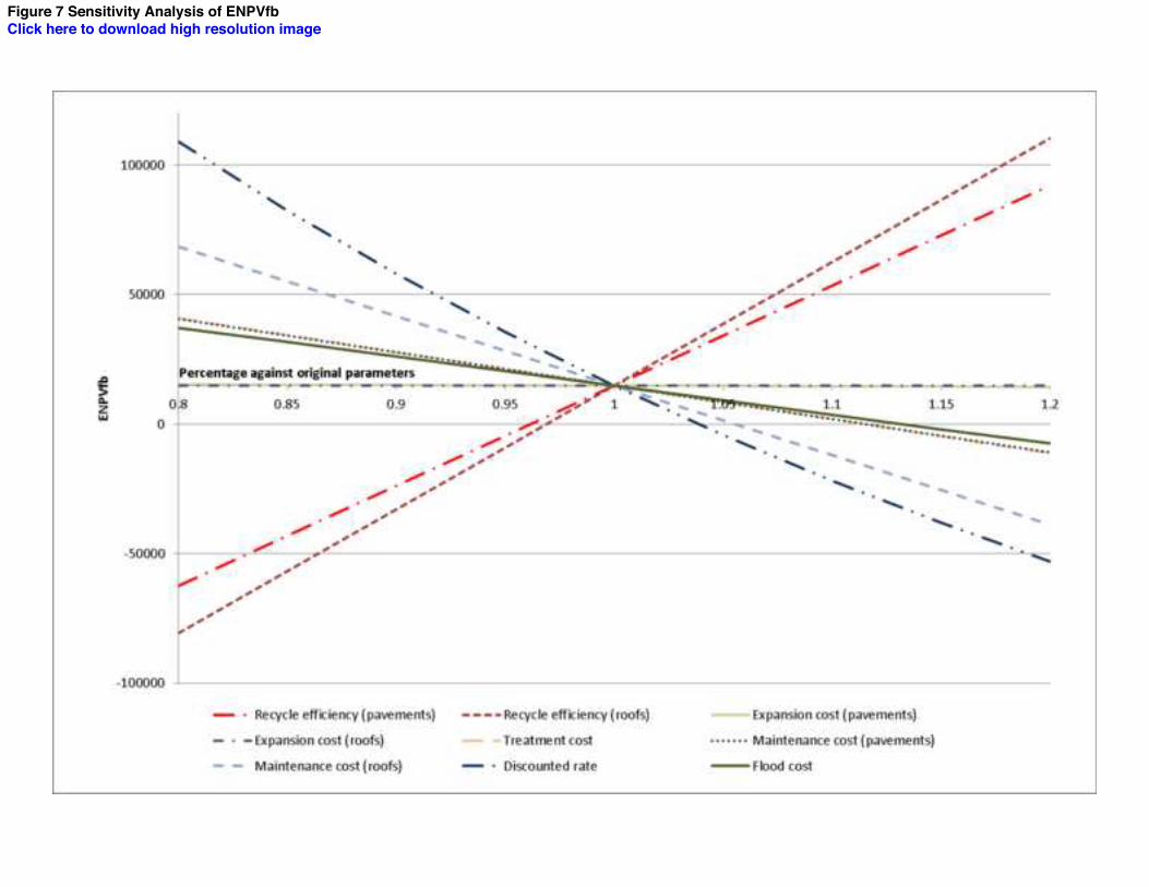
Figure 7 Sensitivity Analysis of ENPVfbClick here to download high resolution image

Figure 8 Sensitivity Analysis of VoFBClick here to download high resolution image