Non-residential Urban Water Demand Modelling - VU ...
283
Non-residential Urban Water Demand Modelling – a Disaggregation Approach By Suchana Barua B.Sc. (Civil Engg.) Thesis submitted in fulfilment of the requirements for the degree of Doctor of Philosophy College of Engineering and Science Victoria University, Australia May 2018
-
Upload
khangminh22 -
Category
Documents
-
view
2 -
download
0
Transcript of Non-residential Urban Water Demand Modelling - VU ...

Non-residential Urban Water Demand Modelling –
a Disaggregation Approach
By
Suchana Barua
B.Sc. (Civil Engg.)
Thesis submitted in fulfilment of the requirements for the degree
of Doctor of Philosophy
College of Engineering and Science
Victoria University, Australia
May 2018

Dedicated To
My Husband and two beautiful kids Senoy and Siwan

i
ABSTRACT
Rapid population growth over the 20th
century and changing climate has put many
urban water supply systems under pressure around the world. Such pressure also
exerted on most of the Australian water supply systems, which has led to the
introduction of water use restrictions to ensure environmentally sustainable water
supply. To operate cost effective and reliable urban water supply systems, analysing
urban water use and forecasting future water demand is an essential task.
Generally, the urban water use classified as residential and non-residential water use
based on different activities. In Melbourne (Australia), water authorities have used
end-use models to forecast water demand, in which the residential component is
extensively modelled. In these end-use models, the total household water use is broken
down to the end-use level (e.g. toilets, showers, washing machines, etc.) for forecasting
water demand in the residential sector. However, a simple historical trend-based annual
water demand is considered for the non-residential sector, as a whole. No temporal (i.e.
quarterly or monthly) and spatial disaggregation were considered in the non-residential
water demand forecasts in these end-use models. It was also found that the existing
work around the world on water demand modelling mainly focused on residential
water use modelling. However, a significant portion of urban water usage is non-
residential. For example, around 25% of the total water use in Melbourne is used by
the non-residential sector. Therefore, the modelling of non-residential urban water use
has significant importance for effective water supply system in any urban area.
Considering this knowledge gap for effective urban water supply, this project aims to
forecast short term (i.e. month to year) non-residential water demand which is useful
for system operation as well as budgeting and financial management.
To achieve this aim, the water use billing data for each non-residential customer
located in the Yarra Valley Water service area (in Melbourne, Australia) were used for
developing non-residential water demand models in this research. All customers were
disaggregated into several groups based on the homogenous water activity such as
Schools, Sports Grounds, Councils, Restaurants, Hospitals, Hotels, and Laundries. The
high water users (>50 ML/year) were also considered as a separate group in this study
named as High Water Users. All customers in the homogenous groups were further
divided into smaller groups based on the annual water use (>20 ML, >15-20 ML, >10-

ii
15 ML, 5-10 ML, and <5 ML). Data analysis was then carried out for each of these
user groups to identify the water use pattern. Data analysis showed that there were
some seasonal effects on Schools, Sports Grounds and Councils. Therefore, water use
among these groups was modelled using the Multiple Linear Regression (MLR)
technique with the available climatic variable and water restrictions data. In the
remaining groups no seasonal variations were identified during data analysis.
Moreover, most of their water uses are for indoor purposes and therefore, water use
modelling was carried out for these remaining groups with the past water use data only
due to unavailability of data for other influential factors. All forecasting models
developed in this research were validated with the observed data and the model
performance was measured with the Nash-Sutcliffe efficiency criteria. Results showed
that most of these developed models performed well except for few cases. Some issues
and challenges were also identified during models development among the
homogenous groups in non-residential sectors. All these issues and challenges are
listed in this thesis for future research.
The major innovation of this study was the development of the disaggregation
approach for sector based non-residential water demand modelling. This approach is
successfully demonstrated in this research by disaggregating customers based on their
activity and their annual water use. The development of non-residential water demand
models at individual customer level is also the knowledge advancement, as limited
work was found in this area.


Acknowledgment
iv
ACKNOWLEDGMENTS
First and foremost I would like to thanks God for sending me through this
journey with huge strength and unfailing supports.
During my intellectually and emotionally stimulating time over this study
periods, I received lots of support, guidance and affections from numerous individuals.
I would like to express my gratitude to those for everything they did for me.
I received enormous scholastic guidance and support from my principal
supervisor Anne Ng through my study period at Victoria University (VU). Her
continuous encouragement and valuable suggestions make this study more interesting
to me. She has given me great freedom to pursue independent work during this study. I
would also like to thanks her for all the financial supports that I received for attending
the conferences.
I also equally thankful to my associate supervisor Shobha Muthukumaran for
being extremely supportive and source of inspiration during this study time at VU. She
carefully listened to my problems and provided valuable directions during project
development as well as during thesis writing. She demonstrated her faith in my ability
and encouraged me to rise to the occasion.
Emeritus Professor Chris Perera has been a strong and supportive associate
supervisor throughout my study at VU. His great intellectual support during my whole
study period helps me to survive and pursue to the end. I appreciate his quick response
to all my writings in every stage of my study period, which helps me to progress better.
What kept me moving constantly, were his amazingly insightful comments with
detailed attention to my arguments, showing the ways of dramatically improving them.
I am really fortunate for having him through this journey.
I would like to give special thanks to Peters Roberts, Demand forecasting
Manager from the YVW for his quick response to all queries and managing time for

Acknowledgment
v
having meeting from time to time. I also like to express thanks for his valuable
comments and suggestion during the writing of conference and journal papers.
I am also thankful to following individuals and institutions for their contribution over
the study period:
College of Engineering and Science in VU for providing financial support for
this research project;
College of Engineering and Science and Secomb Scholarship Fund for their
financial support for attending two conferences in Sydney and Adelaide,
Australia;
Office of Post-graduate Research (OPR) of VU for research training provided;
Yarra Valley Water (YVW) and Bureau of Meteorology (BOM) in Australia
for providing required data for this study;
Michael Quilliam in City West Water for providing valuable information and
guidance to gain knowledge on current forecasting models;
Ashoka Athuraliya in YVW for making time to provide valuable ideas,
information and guidance for managing the huge data files;
Associate Prof Neil Diamond and Dr. Fuchun Huang for their help in
understanding some statistical techniques;
Lesley Birch, Senior Coordinator in Research Development, and Elizabeth
Smith, Senior Officer in Graduate Research and many other staffs from the
College of Engineering and Science at VU for helping me in numerous ways;
and
Friends like Mitu, Tonni, Prasad, Leni and many others who gave me social
and intellectual supports; and Royal Children Hospital in Melbourne for their
continuous support for balancing my family life.
Finally, I owe my greatest gratitude to my parents and my elder brother for their
dedications and supports during my different stages of studies. I am very grateful for
having a beautiful family with my husband (Shishutosh Barua) and two beautiful kids
(Senoy and Siwan) who provided nice life balance to pursue the PhD work.
Thank you!!

List of publications and Award
vi
LIST OF PUBLICATIONS AND AWARDS
Journal Articles:
1. Barua, S., Ng, A.W.M., Muthukumaran, S., Roberts, P. and Perera, B.J.C., 2015.
Modeling Water Use in Schools: A Disaggregation Approach, Urban Water
Journal, 13(8), 875-881.
Conference Articles:
1. Barua, S., Ng, A.W.M., Muthukumaran, S., Huang, F., Roberts, P. and Perera,
B.J.C., 2013. Modeling water use in schools: a comparative study of quarterly and
monthly models. Proceedings of 20th
International Congress on Modelling and
Simulation. Adelaide, Australia, December 1-6, 2013, pp. 3141-3147.
2. Barua, S., Ng, A.W.M., Muthukumaran, S., Roberts, P., Athuraliya, A., Diamond,
N.T. and Perera, B.J.C., 2012. Modelling non-residential urban water use: case
study on two high water use schools in Melbourne. Proceedings of 34th
Hydrology
and Water Resources Symposium, Sydney, Australia, November 19–November 22,
2012, pp. 700 – 707.
Awards:
Winner of Three Minutes PhD Thesis Presentation Heat 2014 held in Victoria
University, Melbourne, Australia. The presentation title was “Non-residential
Water Demand Modelling - A Disaggregation Approach.

Table of Contents
vii
TABLE OF CONTENTS
Abstract……. ................................................................................................................... i
Declaration.. . .................................................................................................................. iii
Acknowledgements ........................................................................................................ iv
List of Publications and Awards .................................................................................... vi
Table of Contents .......................................................................................................... vii
List of Figures ................................................................................................................ xi
List of Tables ............................................................................................................... xiv
List of Abbreviations ................................................................................................... xix
List of Symbols ............................................................................................................. xx
1. INTRODUCTION ............................................................................. 1-1
1.1. Background ................................................................................................... 1-1
1.2. Problem Statement and Motivation for this Study ........................................ 1-3
1.3. Aims of the Research .................................................................................... 1-4
1.4. Scope of the Study ........................................................................................ 1-5
1.5. Research Methodology in Brief .................................................................... 1-6
1.5.1. Review of Urban Water Demand Modelling Approaches ....................... 1-6
1.5.2. Selection of Study Area, Data Sources and Processing .......................... 1-6
1.5.3. Water Use Modelling at Disaggregated Customer Groups Levels ........ 1-7
1.6. Research Significance, Outcomes and Innovations ...................................... 1-8
1.6.1. Significance ............................................................................................. 1-8
1.6.2. Outcomes ................................................................................................. 1-9
1.6.3. Innovations .............................................................................................. 1-9
1.7. Thesis Layout .............................................................................................. 1-10
2. REVIEW OF URBAN WATER DEMAND MODELLING
APPROACHES .................................................................................. 2-1
2.1. Overview ....................................................................................................... 2-1
2.2. Urban Water Demand Modelling Approaches ............................................. 2-2
2.2.1. Historical Average or Pattern Based Approach ..................................... 2-3
2.2.2. Climate Correction ............................................................................... 2-10
2.2.3. Trend Analysis ...................................................................................... 2-12
2.2.4. Analysis of Base and Seasonal Use ...................................................... 2-12
2.2.5. Regression Modelling ........................................................................... 2-15

Table of Contents
viii
2.2.6. End-Use Modelling ............................................................................... 2-17
2.2.7. Agent Based Modelling ......................................................................... 2-19
2.2.8. Artificial Intelligence Methods ............................................................. 2-20
2.3. Selection of Suitable Modelling Approaches for this Project ..................... 2-21
2.4. Challenges in Urban Water Demand Modelling ......................................... 2-23
2.5. Summary ..................................................................................................... 2-26
3. STUDY AREA, DATA SOURCES AND PROCESSING ............. 3-1
3.1. Overview ....................................................................................................... 3-1
3.2. Background of Melbourne Water Supply System ........................................ 3-2
3.2.1. Yarra Valley Water (YVW) ...................................................................... 3-3
3.2.2. City West Water (CWW) ......................................................................... 3-3
3.2.3. South East Water (SEW) ......................................................................... 3-3
3.3. Selection of Study Area ................................................................................ 3-5
3.4. Data Sources ................................................................................................. 3-5
3.5. Data Processing ............................................................................................. 3-8
3.5.1. Water Use Data ....................................................................................... 3-8
3.5.2. Water Restrictions Data ........................................................................ 3-11
3.5.3. Climate Data ......................................................................................... 3-12
3.6. Disaggregation of Customer Groups .......................................................... 3-12
3.7. Summary ..................................................................................................... 3-20
4. WATER USE MODELLING FOR SCHOOLS, SPORTS
GROUNDS AND COUNCILS ......................................................... 4-1
4.1. Overview ....................................................................................................... 4-1
4.2. Variables Used for Model Development ...................................................... 4-2
4.2.1. Past Water Use ....................................................................................... 4-2
4.2.2. Levels of Water Restrictions ................................................................... 4-2
4.2.3. Climate Variables ................................................................................... 4-3
4.2.4. Fixed Quarterly Effects ........................................................................... 4-3
4.3. Procedure for Model Development ............................................................... 4-4
4.3.1. Data Transformation .............................................................................. 4-4
4.3.2. Correlation Test ...................................................................................... 4-5
4.3.3. Mathematical Structure .......................................................................... 4-5
4.3.4. Measurement of Model Performance ...................................................... 4-6
4.3.5. Significance Test for Model Parameters ................................................. 4-7
4.3.6. Steps for Model Development ................................................................. 4-7
4.4. Water Use Models for Schools ..................................................................... 4-9

Table of Contents
ix
4.4.1. Data Analysis and Disaggregation ......................................................... 4-9
4.4.2. Model Calibration and Validation ........................................................ 4-11
4.4.3. Results and Discussions ........................................................................ 4-11
4.5. Water Use Models for Sports Grounds ....................................................... 4-25
4.5.1. Data Analysis and Disaggregation ....................................................... 4-25
4.5.2. Results and Discussions ........................................................................ 4-27
4.6. Water Use Models for Councils .................................................................. 4-38
4.6.1. Data Analysis and Disaggregation ....................................................... 4-38
4.6.2. Results and Discussions ........................................................................ 4-40
4.7. Models Applications, Limitations and Challenges ..................................... 4-53
4.8. Summary ..................................................................................................... 4-54
5. WATER USE MODELLING FOR RESTAURNTS, HOSPITALS,
HOTELS AND LAUNDRIES ........................................................... 5-1
5.1. Overview ....................................................................................................... 5-1
5.2. Data Exploration ........................................................................................... 5-3
5.2.1. Historical Water Use .............................................................................. 5-3
5.2.2. Disaggregation of Water User Groups ................................................... 5-4
5.3. Model Development ...................................................................................... 5-6
5.3.1. Data Analysis and Model Development for Restaurants ........................ 5-6
5.3.1.1. Data Analysis .................................................................................... 5-6
5.3.1.2. Forecasting Water Use Model Development ....................................... 5-17
5.3.2. Data Analysis and Model Development for Hospitals .......................... 5-24
5.3.2.1. Data Analysis .................................................................................. 5-24
5.3.2.2. Forecasting Water Use Model Development ....................................... 5-32
5.3.3. Data Analysis and Model Development for Hotels ............................... 5-38
5.3.3.1. Data Analysis .................................................................................. 5-38
5.3.3.2. Forecasting Water Use Model Development ....................................... 5-46
5.3.4. Data Analysis and Model Development for Laundries ......................... 5-50
5.3.4.1. Data Analysis .................................................................................. 5-50
5.3.4.2. Forecasting Water Use Model Development ....................................... 5-57
5.4. Issues and Challenges Faced and Limitations of the Study ........................ 5-61
5.4.1. Restaurants ........................................................................................... 5-62
5.4.2. Hospitals ............................................................................................... 5-63
5.4.3. Hotels .................................................................................................... 5-63
5.4.4. Laundries .............................................................................................. 5-64
5.5. Summary ..................................................................................................... 5-65
6. WATER USE MODELLING FOR HIGH WATER USERS ....... 6-1

Table of Contents
x
6.1. Overview ....................................................................................................... 6-1
6.2. Historical Water Use and Subgroups of HWU ............................................. 6-3
6.3. Data Analysis and Model Development for Forecast Water Use ................. 6-6
6.3.1. Manufacturing Companies ...................................................................... 6-7
6.3.2. Packaging Companies .......................................................................... 6-14
6.3.3. Shopping Centres .................................................................................. 6-17
6.3.4. Hospitals ............................................................................................... 6-21
6.3.5. Laundries .............................................................................................. 6-24
6.3.6. Confectionary Factories ....................................................................... 6-26
6.3.7. Universities ........................................................................................... 6-30
6.3.8. Motor Companies .................................................................................. 6-33
6.3.9. Poultry Factories .................................................................................. 6-34
6.3.10. Institutions ............................................................................................. 6-36
6.4. Limitations of the Study and Applications ................................................. 6-38
6.5. Summary ..................................................................................................... 6-39
7. SUMMARY, CONCLUSIONS, AND RECOMMENDATIONS . 7-1
7.1. Summary and Conclusions ........................................................................... 7-1
7.1.1. Review of Urban Water Demand Modelling Approaches ...................... 7-1
7.1.2. Selection of Study Area, Data Sources and Processing ......................... 7-2
7.1.3. Water Use Modelling for Schools, Sports Grounds and Councils .......... 7-4
7.1.4. Water Use Modelling for Restaurants, Hospitals, Hotels and Laundries 7-5
7.1.5. Water Use Modelling for High Water Users .......................................... 7-6
7.2. Conclusions ................................................................................................... 7-7
7.3. Limitation of the Study and Recommendations for Future Research ........... 7-8
REFERENCES ....................................................................................... R-1
APPENDIX : Correlation Coefficient between the Independent
Variables…….…………………………………………………..…A-1
A. Correlation coefficient between the independent variables for
Schools group ……….…………….…………………………..……..……A-1
B. Correlation coefficient between the independent variables for
Sports Grounds group ………………………………………………..……A-7
C. Correlation coefficient between the independent variables for
Councils group ………………………...…………………….......………A-13

List of Figures
xi
LIST OF FIGURES
Figure 1.1 Thesis Layout ........................................................................................ 1-10
Figure 3.1 Melbourne metropolitan three water retailers geographic regions ......... 3-4
Figure 3.2 Yarra Valley Water (YVW) service area by municipality ...................... 3-6
Figure 3.3 Locations of water use customers and climate data measurement
station measurement station .................................................................... 3-7
Figure 3.4 Flow chart of water use billing data processing procedure ................... 3-10
Figure 3.5 Water uses by different homogeneous user groups in 2011 ................. 3-14
Figure 3.6 Customer ranking based on average yearly water use .......................... 3-15
Figure 3.7 Non-residential water uses per customer in different groups ............... 3-16
Figure 3.8 Average percentages of quarterly water uses in Schools, Sports
Grounds and Councils ........................................................................... 3-18
Figure 3.9 Average percentages of quarterly water uses in Hospital, Hotels,
Laundries and Restaurants .................................................................... 3-19
Figure 4.1 MLR model development procedure ...................................................... 4-8
Figure 4.2 Time series of quarterly percentage to annual water use among the
different user groups in Schools ........................................................... 4-10
Figure 4.3 Observed vs modelled water use for >20 ML Schools group ............... 4-16
Figure 4.4 Observed vs modelled water use for School 1 in >15-20 ML Schools
group ..................................................................................................... 4-17
Figure 4.5 Observed vs modelled water use for School 2 in >15-20 ML Schools
group ..................................................................................................... 4-18
Figure 4.6 Scatter plots of observed vs modelled water use for the three schools
in >10-15 ML Schools group ................................................................ 4-20
Figure 4.7 Scatter plots of observed vs modelled water use for the five school
subgroups in 5-10 ML Schools group .................................................. 4-22
Figure 4.8 Scatter plots of observed vs modelled water use for the five school
subgroups in <5 ML Schools group ...................................................... 4-24
Figure 4.9 Time series of quarterly percentage to annual water use among the
different user groups in Sports Grounds ............................................... 4-26
Figure 4.10 Time series of water use data for >20 ML Sports Grounds group ........ 4-29

List of Figures
xii
Figure 4.11 Observed vs modelled water use in >15-20 ML Sports Grounds
group ..................................................................................................... 4-31
Figure 4.12 Scatter plots of observed vs modelled water use for the five sports
grounds in >10-15 ML Sports Grounds group ...................................... 4-33
Figure 4.13 Scatter plots of observed vs modelled water use for the five
subgroups in 5-10 ML Sports Grounds group ...................................... 4-35
Figure 4.14 Scatter plots of observed vs modelled water use for the five
subgroups in <5 ML Sports Grounds group ......................................... 4-37
Figure 4.15 Time series of quarterly percentage to annual water use among the
different user groups in Councils .......................................................... 4-39
Figure 4.16 Observed vs modelled water use for Council 1 in >20 ML Councils
group ..................................................................................................... 4-43
Figure 4.17 Observed vs modelled water use for Council 2 in >20 ML Councils
group ..................................................................................................... 4-44
Figure 4.18 Observed vs modelled water use for Council 3 in >20 ML Councils
group ..................................................................................................... 4-45
Figure 4.19 Observed vs modelled water use for Council 4 in >20 ML Councils
group ..................................................................................................... 4-46
Figure 4.20 Scatter plots of observed vs modelled water use for the four councils
in >15-20 ML Councils group .............................................................. 4-47
Figure 4.21 Scatter plots of observed vs modelled water use for the five councils
in >10-15 ML Councils group .............................................................. 4-49
Figure 4.22 Scatter plots of observed vs modelled water use for the five subgroups
in 5-10 ML Councils group ................................................................... 4-51
Figure 4.23 Scatter plots of observed vs modelled water use for the five subgroups
in <5 ML Councils group ...................................................................... 4-53
Figure 5.1 Annual water uses of Restaurants, Hospitals, Hotels, and Laundries
over the study period ............................................................................... 5-3
Figure 5.2 Water use pattern of >20 ML Restaurants group .................................... 5-7
Figure 5.3 Water use pattern of >15-20 ML Restaurants group .............................. 5-8
Figure 5.4 Water use pattern of >10-15 ML Restaurants group .............................. 5-9
Figure 5.5 Water use pattern of 5-10 ML Restaurants group ................................. 5-11
Figure 5.6 Water use pattern of <5 ML Restaurants group .................................... 5-13
Figure 5.7 Water use pattern of >20 ML Hospitals group ..................................... 5-24

List of Figures
xiii
Figure 5.8 Water use pattern of >10-15 ML Hospitals group ................................ 5-25
Figure 5.9 Water use pattern of 5-10 ML Hospitals group .................................... 5-26
Figure 5.10 Annual water use time series of <5 ML Hospitals group ..................... 5-27
Figure 5.11 Quarterly percentages of individual hospital in <5 ML Hospitals
group ..................................................................................................... 5-27
Figure 5.12 Water use pattern of Pathologies in Hospitals group ............................ 5-28
Figure 5.13 Water use pattern of >10-15 ML Hotels group ..................................... 5-39
Figure 5.14 Water use pattern of 5-10 ML Hotels group ......................................... 5-40
Figure 5.15 Water use pattern of <5 ML Hotels group ............................................ 5-42
Figure 5.16 Water use pattern of >15-20 ML Laundries group ............................... 5-51
Figure 5.17 Water use pattern of 5-10 ML Laundries group ................................... 5-52
Figure 5.18 Water use pattern of <5 ML Laundries group ...................................... 5-54
Figure 5.19 Annual water use in >15-20 ML Laundries group ................................ 5-57
Figure 6.1 Annual water use of HWU group over the study period ........................ 6-4
Figure 6.2 Water use percentages by different homogenous HWU subgroups
in 2011 .................................................................................................... 6-5
Figure 6.3 Water use time-series by different homogenous HWU subgroups ......... 6-6
Figure 6.4 Water use pattern of Manufacturing Companies subgroup .................... 6-8
Figure 6.5 Annual water use trend in Manufacturing Companies 1, 2, 4, 5, 7
and 9 ...................................................................................................... 6-12
Figure 6.6 Water use pattern of Packaging Companies subgroup ......................... 6-14
Figure 6.7 Water use pattern of Shopping Centres subgroup ................................. 6-18
Figure 6.8 Water use pattern of Hospitals subgroup .............................................. 6-21
Figure 6.9 Water use pattern of Laundries subgroup ............................................. 6-24
Figure 6.10 Water use pattern of Confectionary Factories subgroup ....................... 6-27
Figure 6.11 Annual water use trend in Confectionary Factory 2 ............................. 6-29
Figure 6.12 Water use pattern of Universities subgroup .......................................... 6-30
Figure 6.13 Water use pattern of motor Companies subgroup ................................. 6-33
Figure 6.14 Water use pattern of Poultry Factories subgroup .................................. 6-35
Figure 6.15 Water use pattern of Institutions subgroup ........................................... 6-36

List of Tables
xiv
LIST OF TABLES
Table 2.1 Summary of urban water demand modelling approaches ....................... 2-4
Table 3.1 Historical water restrictions record ....................................................... 3-11
Table 3.2 Water use by different sub-groups based average on annual
water use in 2005-2009 ......................................................................... 3-16
Table 4.1 Dummy variables used for water restrictions ......................................... 4-3
Table 4.2 Dummy variables used for four quarters ................................................ 4-4
Table 4.3 Disaggregated annual water use of Schools in the YVW service area ... 4-9
Table 4.4 Subgroups in 5-10 ML Schools group .................................................... 4-9
Table 4.5 Subgroups in <5 ML Schools group ..................................................... 4-10
Table 4.6 Correlation coefficient between the dependent and independent
variables used in all subgroups in the Schools group ........................... 4-12
Table 4.7 E values for the best models in Schools group ..................................... 4-14
Table 4.8 Estimated regression coefficients for different Schools group models
(calibration period: 2006-2010, validation period: 2011) ..................... 4-15
Table 4.9 Disaggregated annual water use of Sports Grounds in the YVW
service area ............................................................................................ 4-25
Table 4.10 Subgroups in 5-10 ML Sports Grounds group ...................................... 4-26
Table 4.11 Subgroups in <5 ML Sports Grounds group ......................................... 4-26
Table 4.12 Correlation coefficient between the dependent and independent
variables used in all subgroups in the Sports Grounds group ............... 4-28
Table 4.13 E values for the best models and estimated regression coefficients
for different Sports Grounds group models .......................................... 4-30
Table 4.14 Disaggregated annual water use of Councils in the YVW
service area ............................................................................................ 4-38
Table 4.15 Subgroups in 5-10 ML Councils group ................................................ 4-39
Table 4.16 Subgroups in <5 ML Councils group .................................................... 4-39
Table 4.17 Correlation coefficient between the dependent and independent
variables used in all subgroups in the Councils group .......................... 4-41
Table 4.18 E values for the best models and estimated regression coefficients
for different Councils group models ..................................................... 4-42

List of Tables
xv
Table 5.1 Disaggregation of water users of Restaurants, Hospitals, Hotels and
Laundries in the YVW service area ........................................................ 5-5
Table 5.2 Water use percentage among Restaurants subgroups in 5-10 ML
group ..................................................................................................... 5-10
Table 5.3 Water use percentage among Restaurants subgroups in <5 ML
group ..................................................................................................... 5-12
Table 5.4 Summary of water use data analysis and selection of modelling
approach for Restaurants group ............................................................ 5-15
Table 5.5 Disaggregating factors for >20 ML Restaurants group ........................ 5-17
Table 5.6 Comparison of observed and forecast water use of >20 ML
Restaurants group in 2011 .................................................................... 5-18
Table 5.7 Quarterly disaggregating factors in >15-20 ML Restaurants group ..... 5-19
Table 5.8 Comparison of observed and forecast water use of >15-20 ML
Restaurants group in 2011 .................................................................... 5-19
Table 5.9 Quarterly disaggregating factors in >10-15 ML Restaurants group ..... 5-20
Table 5.10 Comparison of observed and forecast water use of >10-15 ML
Restaurants group in 2011 .................................................................... 5-20
Table 5.11 Quarterly disaggregating factors in 5-10 ML Restaurants group ......... 5-21
Table 5.12 Comparison of observed and forecast water use of 5-10 ML
Restaurants group in 2011 .................................................................... 5-22
Table 5.13 Quarterly disaggregating factors in <5 ML Restaurants group ............ 5-23
Table 5.14 Comparison of observed and forecast water use of <5 ML
Restaurants group in 2011 .................................................................... 5-23
Table 5.15 Summary of water use data analysis and selection of modelling
approach for Hospitals group ................................................................ 5-30
Table 5.16 Quarterly disaggregating factors in >20 ML Hospitals group .............. 5-32
Table 5.17 Comparison of observed and forecast water use of >20 ML
Hospitals group in 2011 ........................................................................ 5-33
Table 5.18 Quarterly disaggregating factors in >10-15 ML Hospitals group ......... 5-33
Table 5.19 Comparison of observed and forecast water use of >10-15 ML
Hospitals group in 2011 ........................................................................ 5-34
Table 5.20 Quarterly disaggregating factors in 5-10 ML Hospitals group ............. 5-35
Table 5.21 Comparison of observed and forecast water use of 5-10 ML
Hospitals group in 2011 ........................................................................ 5-35

List of Tables
xvi
Table 5.22 Quarterly disaggregating factors in <5 ML Hospitals group ................ 5-36
Table 5.23 Comparison of observed and forecast water use of <5 ML
Hospitals group in 2011 ........................................................................ 5-36
Table 5.24 Quarterly disaggregating factors in Pathologies in Hospitals group .... 5-37
Table 5.25 Comparison of observed and forecast water use of Pathologies
in Hospitals group in 2011 .................................................................... 5-38
Table 5.26 Water use percentages among Hotels subgroups in <5 ML group ....... 5-41
Table 5.27 Summary of water use data analysis and selection of modelling
approach for Hotels group .................................................................... 5-44
Table 5.28 Quarterly disaggregating factors in >10-15 ML Hotels group ............. 5-47
Table 5.29 Comparison of observed and forecast water use of >10-15 ML
Hotels group in 2011 ............................................................................. 5-47
Table 5.30 Quarterly disaggregating factors in 5-10 ML Hotels group .................. 5-48
Table 5.31 Comparison of observed and forecast water use of 5-10 ML Hotels
group in 2011 ........................................................................................ 5-48
Table 5.32 Quarterly disaggregating factors and E values in <5 ML
Hotels group .......................................................................................... 5-49
Table 5.33 Comparison of observed and forecast water use of <5 ML
Hotels group in 2011 ............................................................................. 5-50
Table 5.34 Water use percentage among Laundries subgroups in group <5 ML ... 5-53
Table 5.35 Summary of water use data analysis and selection of modelling
approaches for Laundries group ............................................................ 5-56
Table 5.36 Quarterly disaggregating factors in >15-20 ML Laundries group ........ 5-58
Table 5.37 Comparison of observed and forecast water use of >15-20 ML
Laundries group in 2011 ....................................................................... 5-58
Table 5.38 Quarterly disaggregating factors in 5-10 ML Laundries group ............ 5-59
Table 5.39 Comparison of observed and forecast water use of 5-10 ML
Laundries in 2011 ................................................................................. 5-59
Table 5.40 Quarterly disaggregating factors of subgroups in <5 ML Laundries .... 5-60
Table 5.41 Comparison of observed and forecast water use of <5 ML
Laundries group in 2011 ....................................................................... 5-61
Table 6.1 HWU Subgroups ..................................................................................... 6-5
Table 6.2 Summary of water use data analysis and selection of modelling
approach for Manufacturing Companies subgroup ............................... 6-10

List of Tables
xvii
Table 6.3 Disaggregating factors for individual Manufacturing company ........... 6-11
Table 6.4 Comparison of observed and modelled water use of Manufacturing
Companies subgroup in 2011 ................................................................ 6-13
Table 6.5 Summary of water use data analysis and selection of modelling
approach for Packaging Companies subgroup ...................................... 6-15
Table 6.6 Disaggregating factors for individual Packaging Company subgroup . 6-16
Table 6.7 Comparison of observed and forecast water use of Packaging
Companies subgroup in 2011 ................................................................ 6-16
Table 6.8 Summary of water use data analysis and selection of modelling
approach for Shopping Centres subgroup ............................................. 6-19
Table 6.9 Disaggregating factors for individual Shopping Centre ....................... 6-19
Table 6.10 Comparison of observed and forecast water use of Shopping
Centres subgroup in 2011 ..................................................................... 6-20
Table 6.11 Summary of water use data analysis and selection of modelling
approach for Hospitals subgroup .......................................................... 6-22
Table 6.12 Disaggregating factors for individual Hospital ..................................... 6-23
Table 6.13 Comparison of observed and forecast water use of Hospitals
subgroup in 2011 ................................................................................... 6-23
Table 6.14 Summary of water use data analysis and selection of modelling
approach for Laundries subgroup ......................................................... 6-25
Table 6.15 Disaggregating factors for individual Laundry ..................................... 6-25
Table 6.16 Comparison of observed and modelled water use of Laundries
subgroup in 2011 ................................................................................... 6-26
Table 6.17 Summary of water use data analysis and selection of modelling
approach for Confectionary Factories subgroup ................................... 6-28
Table 6.18 Disaggregating factors for individual Confectionary Factory .............. 6-28
Table 6.19 Comparison of observed and forecast water use of Confectionary
Factories subgroup in 2011 ................................................................... 6-29
Table 6.20 Summary of water use data analysis and selection of modelling
approach for Universities subgroup ...................................................... 6-31
Table 6.21 Disaggregating factors for Universities Subgroup ................................ 6-32
Table 6.22 Comparison of observed and Forecast water use of Universities
subgroup in 2011 ................................................................................... 6-32
Table 6.23 Summary of water use data analysis and selection of modelling

List of Tables
xviii
approach for Motor Companies subgroup ............................................ 6-33
Table 6.24 Disaggregating factors for individual Motor Company ........................ 6-34
Table 6.25 Comparison of observed and forecast water use of Motor Companies
subgroup in 2011 ................................................................................... 6-34
Table 6.26 Summary of water use data analysis and selection of modelling
approach for Poultry Factories subgroup .............................................. 6-35
Table 6.27 Disaggregating factors for individual Poultry Factory ......................... 6-35
Table 6.28 Comparison of observed and forecast water use of Poultry Factories
subgroup in 2011 ................................................................................... 6-36
Table 6.29 Summary of water use data analysis and selection of modelling
approach for Institutions subgroup ....................................................... 6-37
Table 6.30 Disaggregating factors for individual Institutions ................................ 6-37
Table 6.31 Comparison of observed and modelled water use of Institutions
subgroup in 2011 ................................................................................... 6-38
Table 6.32 Types of Annual Water Use Pattern and Approach Used to Forecast
Water Use in 2011 ................................................................................ 6-40

List of Abbreviations
xix
LIST OF ABBREVIATIONS
The following list of abbreviations is used throughout this thesis. The other
abbreviations, which are used only in particular sections or chapters are defined in the
relevant sections or chapters.
ABM Agent Based Modelling
ANN Artificial Neural Network
ANSIC Australian and New Zealand Standard Industrial Classification
BoM Bureau of Meteorology
BWPD Bulk Water Production Data
CWW City West Water
CMDD Customer Meter Demand Data
FIS Fuzzy Inference System
HWU High Water Users
MF Membership Functions
MLR Multiple Linear Regression
MW Melbourne Water
PCPD Per Capita Per Day
PWSR Permanent Water Saving Rules
SEW South East Water
SIMDEUM SIMulation of water Demand, an End-Use Model
YVW Yarra Valley Water

List of Symbols
xx
LIST OF SYMBOLS
The following list of symbols is used throughout this thesis. The other symbols,
which are used only in particular sections or chapters are defined in the relevant
sections or chapters.
E Nush-Sutcliffe model efficiency
p p-value or probability value
ML Megalitre
KL Kilolitre
Chapter 1: Introduction
Page 1-1
Chapter 1. Introduction
1.1. Background
The world’s urban population grew very rapidly (from 220 million to 2.8
billion) over the 20th
century, and the 21st century marks the first time in history that
half of the global human population resides in urban areas (United Nations Population
Fund, 2007). The increasing growth in population and changing climate has put many
urban water supply systems under immense pressure, often being required to supply a
demand which is close to or exceeding its sustainable demand limit to meet the water
demands of their residents (House-Peters and Chang, 2011). Such pressures have been
exerted on most Australian water supply systems, resulting in record restriction periods
and in some cases the introduction of permanent water saving measures (Melbourne
Water, 2009). Therefore, although analysing and forecasting urban water demand is a
complex task, yet it is essential to operate cost effective and reliable urban water
supply systems.
Urban water supply systems provide water for a range of uses from human
consumption to fire control, and from garden irrigation to industrial processes. Each
urban area has its own economic base, creating its own pattern of water use. The types
of activities creating this pattern are categorized into different sectors: residential (e.g.
single house, multi-unit apartment, etc.), non-residential (e.g. industrial, commercial,
institutional, etc.) and unmetered (non-revenue) (Institute for Sustainable Futures,
2002).
Despite these enormous dissimilar uses of water, a common area of interest for
policymakers and hence researchers is the urban water demand forecasting
(Worthington, 2010). This is an essential work as it allows water providers often in
highly regulated sectors, to better understand and manage the needs of their customers.

Chapter 1: Introduction
Page 1-2
More specifically, urban water demand forecasting is useful to the water authorities for
effective planning for present and future needs including water rates setting, revenue
forecasting and budgeting, water conservation program tracking and evaluation, and
system operations management and optimization (Department of Sustainability and
Environment, 2011). There are two types of urban water demand forecasting; 1) short
term water demand forecasts (i.e. month to year), which are used for system operation
as well as budgeting and financial management, and 2) long term water demand
forecasts (i.e. years to decades), which are required for planning and infrastructure
design (Billings and Jones, 2008).
Urban water demand consists of both residential and non-residential demand. A
large amount of work was found in the literature on modelling total urban water
demand, mainly focused on water demand modelling in the residential sector, but the
existing works were not focused on modelling non-residential water demand both in
Australia and overseas. For example, an end-use model is used by water authorities in
Melbourne, Australia as the primary tool for its water demand forecasts in which the
residential component is extensively modelled (Institute for Sustainable Futures 2005).
Total household water use in single-family and multi-residential homes is broken down
to the end-use level (e.g. toilets, showers, washing machines, etc.) for forecasting the
water demand in the residential sector. However, a simple historical trend-based annual
water demand is considered for the non-residential sector, as a whole. No temporal (i.e.
quarterly or monthly) and spatial disaggregation are considered in these non-residential
water demand forecasts, although they are important for short term sector wise
planning and management of urban water system. In addition, the non-residential water
demand component is relatively high in many urban areas. For example, in Melbourne,
Australia, around 25% of the total water use was used by the non-residential sector in
2014-2015 (Melbourne Water, 2016). Consequently, the non-residential water demand
forecasting has great importance for effective urban water demand management.
Therefore, to promote research in non-residential water demand sector, this project
aims to forecast water demand in non-residential sector. Moreover, this research
mainly focused on short term water demand forecasting, more specifically at quarterly
time step as this is the usual time interval for billing non-residential water use.

Chapter 1: Introduction
Page 1-3
1.2. Problem Statement and Motivation of this Study
Australia is a highly urbanized country (around 89 percent of the population
lives in towns and cities), and urban populations are expected to grow rapidly over the
next 40 years (Collett and Henry, 2011). Many urban areas have been relied on limited
water supplies. To better manage the urban water supply systems with the limited
water resources, a large number of studies have been conducted on modelling urban
water use in Australia as well as around the world (e.g., Miaou, 1990a; Zhou et al.,
2000; Gato et al., 2007b, Perera et al., 2009, Blokker et al., 2010). These studies
focused either on the total urban water use or in most cases on modelling the
residential water use component. However, as was mentioned in Section 1.1, a
significant portion of urban water usage is non-residential (around 25% of total water
use in Melbourne). Therefore, modelling non-residential urban water use has
significant importance for effective water resources management in any urban area.
However, there was not much attention given to model non-residential urban water
use. This is an important omission, but has enormous importance to address the
emerging water-related challenges including the need for a reliable water supply, rising
water prices and seasonal water scarcity (Worthington, 2010). Therefore, reducing the
knowledge gap in urban water demand modelling for non-residential sector was the
primary motivation of this research.
The possible reason for the abovementioned omission is that the appropriate
data required for estimating non-residential water use is difficult to collect and also the
heterogeneous nature of this sector. These challenges have been addressed in various
ways recently and they are:
1) Billing data at individual customer level is now available in electronic
formats (Polebitski and Palmer, 2010). These data can be used to model
non-residential water use.
2) The heterogeneous nature of non-residential urban water demands can be
handled through considering several homogenous demand groups based on
their activities such as schools and colleges, restaurants, hotels and motels,

Chapter 1: Introduction
Page 1-4
laundries and hospitals (Turner et al., 2008). Billings and Jones (2008) also
suggested that the water users can also be classified based on their volume
of water use. Therefore, it is feasible to disaggregate the non-residential
water users into different user groups and conduct specific analysis to
forecast non-residential water demand for those user groups.
3) The Institute for Sustainable Futures (2002) found that the water use in the
non-residential sector exhibit seasonal patterns as in the residential sector.
This pattern can be considered for water demand modelling in the non-
residential sector.
All above details also motivated this research work on modelling the non-
residential water use.
1.3. Aims of the Research
The main aim of this research is to develop a generic methodology for non-
residential urban water demand modelling to forecast quarterly water use in a year for
short-term planning as outlined in Section 1.1. This aim was achieved through
conducting research via the following tasks:
1. Disaggregation of non-residential water use customers based on the
homogenous water use activities such as Schools, Hospitals and
Restaurants (i.e. water use customer groups), and then further
disaggregation of each customer group based on the average annual water
use.
2. Identification of quarterly water use patterns of the different customer
groups.
3. Development of water demand models for forecasting short term non-
residential water demand using the identified water use patterns at
disaggregated customer group levels.

Chapter 1: Introduction
Page 1-5
The developed methodology is demonstrated via a case study using the non-
residential water use within the Yarra Valley Water (YVW) service area which is
managed by the YVW retailer in Melbourne, Australia. This approach can be adapted
to any other urban water supply system in Australia as well as in other countries
around the world to develop own non-residential water demand models using their
water use data.
The results of this research project will be useful for short term planning of
urban water resources system. This research is also expected to assist water resources
managers in decision making related to water conservation program evaluation and
water pricing policy assessment for sustainable water resource management.
1.4. Scope of the Study
The scope of the research was to develop non-residential urban water demand models
to forecast quarterly water demand at disaggregated levels of homogenous non-
residential customers.
Limitations of the study include the followings:
There were many non-residential customers with different homogenous
activities could not be identified and were not included in the study.
All the data for influential variables were not available for most of the
identified homogenous customers groups. Therefore, modelling among these
groups is limited in explaining unexpected water use variation.
All the models performance were measured with the assumption that historical
data as the observed data in forecasting period.

Chapter 1: Introduction
Page 1-6
1.5. Research Methodology in Brief
The following tasks were conducted in this research project to achieve the
above aims:
1. Review of urban water demand modelling approaches
2. Selection of study area, and data collection and processing
3. Water use modelling at disaggregated customer group level
Brief descriptions of each of the above tasks are given below.
1.5.1. Review of Urban Water Demand Modelling Approaches
There are few studies were found on water demand modelling in the non-
residential sector. Most of the studies were on modelling the total urban water demand
predominantly focused on residential sector. Therefore, a review of existing modelling
approaches which were used in both residential and non-residential water demand
modelling as well as on the total urban water demand modelling were conducted in this
research. This was done to understand the existing modelling approaches and to select
a suitable modelling approach for this research. It should be noted that consideration
was also given on data requirements during selection of a suitable modelling approach
as generally limited data are available in the non-residential sector, as was the case for
this study.
1.5.2. Selection of Study Area, Data Sources and Processing
The Yarra Valley Water (YVW) service area which is managed by the YVW
retailer was selected as the case study area in this research for modelling non-
residential urban water use. The YVW is the largest water retailer in Melbourne which
has valuable contribution to water service delivery for a large population. As the YVW
provides water service to more people than the two other water retailers in
Metropolitan Melbourne (i.e. City West Water (CWW) and South East Water (SEW)),
it was considered to have more variation in different types of non-residential customers
(e.g. industrial, commercial and institutional) than the two other water retailers in
Melbourne. Water use and water restrictions data, and climate data used in this

Chapter 1: Introduction
Page 1-7
research were collected from the YVW and the Bureau of Meteorology (BoM)
respectively. Data processing and analysis were then carried out to obtain the water use
patterns which were used for water use modelling at disaggregated customer group
levels.
1.5.3. Water Use Modelling at Disaggregated Customer Groups
Levels
As was outlined in Section 1.3, based on the different activities, all water use
customers were disaggregated into several groups based on homogenous use of water
such as Schools, Sports Grounds, Councils, Restaurants, Hospitals, Hotels, and
Laundries. The high water users in the study area were also considered as a separate
group in this study named as High Water Users. Data analysis for each of these groups
was then carried out individually to explore the water use pattern at the disaggregated
levels as well as to identify the variables that affect the water use in these customer
groups.
In general, there are outdoor uses in Schools, Sports Grounds and Councils
groups, and therefore, water use modelling was performed using the Multiple Linear
Regression (MLR) technique considering climate data and water restrictions data. On
the other hand, as most of the water use in Restaurants, Hospitals, Hotels, and
Laundries groups are for indoor purposes, water use modelling was carried out with the
past water use data only due to limitation of data availability of other influential
factors.
It should be noted that some customers were not identified with any particular
activity and named as Others group. However, due to availability of limited
information, water use modelling was not performed for this customer group in this
research.

Chapter 1: Introduction
Page 1-8
1.6. Research Significance, Outcomes and Innovations
1.6.1. Significance
This research project has made several significant contributions in the field of
urban water resources management, specifically in short term water demand modelling
within the non-residential sector. They are listed below:
As was mentioned in Section 1.2, very limited work was found in the
literature for modelling urban water demand in the non-residential sector,
which uses a considerable amount of water. Therefore, the proposed non-
residential water demand modelling using disaggregation approach will be
a valuable contribution to the water resources managers and researches for
producing an accurate estimation of non-residential water demand.
Data analysis and modelling non-residential water demand carried out in
this research at various disaggregation levels (e.g. activities and water use
volumes) helped in better understanding of water use behaviour in various
disaggregated demand sectors. The developed individual water demand
forecasting models in this study will allow the visualization and evaluation
of water demand information at different spatial scale (i.e., water
distribution zone, census tract) in combination with the customer’s
geographic locations. This information is useful to the water authorities to
make informed decisions when they consider options for conservation
efforts to cope with the limited water resources.
A list of issues and challenges in modelling water use in different non-
residential customers were identified in this research, which will be
valuable resources to the researchers in urban water area for considering
future research in non-residential urban water demand modelling.

Chapter 1: Introduction
Page 1-9
1.6.2. Outcomes
The outcomes of this research are listed below:
Water use pattern analysis at disaggregated level was useful for identifying
the customer groups who are affected by weather. It was found that water
use in Schools, Sports Grounds and Councils are affected by weather, and
there were not much effects of weather on water use in Restaurants,
Hospitals, Hotels and Laundries groups.
Water use data analysis at disaggregated level showed that water use
pattern not only varies from one customer group to another, but also varies
from high water user to low water user customers within the same
customer types (such as the School group).
Introduction of disaggregation approach was successful in explaining water
use variations for modelling non-residential water demand in this research.
Unlike the modelling urban water demand in the residential sector, it was
found that there are significant issues and challenges in the non-residential
sector. These are not limited to the availability of historical water use data
in different non-residential sectors and the data on variables that affect non-
residential demand, but also they are related to the variability in water uses
at the temporal scale. These issues and challenges are listed in various
chapters in this thesis.
1.6.3. Innovation
There were few studies discussed about the heterogenous nature of the non-
residential water use sector (Section 1.2). However, no study was found in developing
sector based non-residential water demand model. Therefore, the major innovation of
this study is the development of a disaggregation approach for sector based non-
residential water demand modelling. This approach was successfully illustrated in this
research through disaggregating the non-residential customers based on homogenous

Chapter 1: Introduction
Page 1-10
water use activities and also based on the annual water use volume within each
customer group, and subsequently, water demand modelling was carried out for each
customer group. The development of non-residential water demand model at individual
level in this research is also the knowledge advancement in the non-residential water
demand forecasting as limited work was found in this area.
1.7. Thesis Layout
The thesis layout is presented in Figure 1.1. This figure shows that the thesis
consists of seven chapters. The background of the research project along with the
motivation for the study, the aims, a brief methodology, the significance, outcomes and
innovations of this project are presented in the first chapter. The second chapter
presents a review of existing literature related to the research project. Details of the
study area, data used in this research, and their sources and processing are described in
the third chapter. The fourth chapter provides details on water use modelling for
Schools, Sports Grounds and Councils groups. Water use modelling performed for
Restaurants, Hospitals, Hotels and Laundries groups are presented in the fifth chapter.
The sixth chapter provides the details on water use modelling for High Water Users
group. Finally, a summary of the thesis and the main conclusions, and the
recommendations for future work are presented in the seventh chapter.

Chapter 1: Introduction
Page 1-11
Figure 1.1 Thesis layout
Chapter 1: Introduction
- Background, motivation, aims of the research
- Research significance, outcomes and innovations
- Research methodology and thesis layout
Chapter 2: Review of Urban Water Demand Modelling Approaches
- Urban water demand modelling approaches
- Selection of suitable modelling approach
- Challenges in urban water demand modelling
Chapter 3: Study Area, Data Sources and Processing
- Selection of study area, data sources and processing
- Disaggregation of customer groups
Illustration on Yarra Valley Water Service Area
Chapter 4: Water Use Modelling for Schools, Sports Grounds and
Councils
- Variable used and procedure for model development
- Water use models for Schools, Sports Grounds and Councils
Illustration on Yarra Valley Water Service Area
Chapter 5: Water Use Modelling for Restaurants, Hospitals, Hotels,
and Laundries
- Data exploration including data analysis at disaggregated level
- Model development for Restaurants, Hospitals, Hotels and
Laundries
Illustration on Yarra Valley Water Service Area
Chapter 6: Water Use Modelling for High Water Users
- Data exploration including data analysis at disaggregated level
- Model development for each High Water User
Illustration on Yarra Valley Water Service Area
Chapter 7: Summary, Conclusions and Recommendations
- Summary and conclusions drawn from the research
- Recommendations made for future research

Chapter 2: Review of Urban Water Demand Modelling Approaches
Page 2-1
Chapter 2. Review of Urban Water Demand
Modelling Approaches
2.1. Overview
Urban water demand modelling is an essential tool for design, operation, and
management of urban water supply systems. It supports a number of activities such as:
planning new developments or system expansion; estimating the size and operation of
reservoirs, pumping stations and pipe capacities; pricing policies setting; and water use
restrictions (Bougadis et al, 2005; Herrera et al, 2010). There are two types of urban
water demand modelling: short term and long term demand modelling. Short term
water demand modelling helps water managers making better informed water
management decisions when balancing the needs of water supply and demand for
residential and non-residential sectors (Bougadis et al, 2005). It also helps water
utilities to plan and manage water demands for near-term events (Jain and Ormsbee,
2002). Long term water demand modelling is required for planning and infrastructure
design (Herrera et al, 2010; House-Peters and Chang, 2011). Therefore, reliable urban
water demand modelling plays a key role in assisting water managers and utilities for
optimizing their operational and investment decisions (Cutore et al, 2008; Donkor et
al, 2014).
Urban water demands are highly variable and depends on various factors such
as size of city, characteristics of the population, the nature and size of commercial and
industrial establishments, climatic conditions, and cost of supply (Zhou et al, 2002).
Therefore, modelling urban water demand has always been a challenging task.
Traditionally, urban water demand modelling has been carried out using a range of
modelling approaches varying from simple to complex mathematical formulations.
Some are suitable for short term water demand modelling, and they include trend
analysis, analysis of base and seasonal use, and end-use modelling approaches (Zhou et

Chapter 2: Review of Urban Water Demand Modelling Approaches
Page 2-2
al, 2000; Billings and Jones, 2008; Blokker et al, 2010; 2011). Others that are suitable
for long-term water demand modelling include regression and artificial intelligence
techniques (Miaou, 1990b; Ghiassi et al, 2008; Yurdusev and Firat, 2009). A vast
amount of literatures are available on these modelling approaches which have been
used in the past. Nevertheless, knowledge base of urban water demand modelling has
changed progressively to adapt with the changes in coupled human and natural system
(House-Peters and Chang, 2011). Therefore, understanding of the current and historical
modelling approaches used in urban water demand modelling is crucial for making any
future contributions to the field.
The aim of the current chapter is to review the existing urban water demand
modelling approaches which have been used for total urban water demand modelling
as well as for modelling the residential and the non-residential water demands
individually. The outcome of this chapter was used to identify the suitable non-
residential water demand modelling techniques in this research. It was outlined in
Section 1.1 (Chapter 1) that most of the modelling works in the literature were focused
on total urban water demand with special attention to the residential sectors. Therefore,
it should be noted that although the focus of this research is the non-residential urban
water demand modelling, literature review was extended to the works done in the
residential and the total urban water demand modelling, as only few studies were found
on water demand modelling in the non-residential sector.
The chapter first reviews the existing modelling approaches applied in urban
water demand modelling, followed by selection of suitable modelling approach for this
research. The understanding of challenges in urban water demand modelling was then
presented. A summary of the review is presented at the end of the chapter.
2.2. Urban Water Demand Modelling Approaches
As stated earlier, there are several urban water demand modelling approaches
that have been used around the world to develop urban water demand models for
estimating urban water use. Among them, the most commonly used approaches are:
historical average or pattern based approach (Snelling et al, 2005; Alvisi et al, 2007);

Chapter 2: Review of Urban Water Demand Modelling Approaches
Page 2-3
climate correction (Maheepala and Roberts, 2006; Perera et al, 2009); trend analysis
(DEUS, 2002; Billings and Jones, 2008); analysis of base and seasonal use (Maidment
et al, 1985; Zhou et al, 2000; Gato et al, 2007b); regression modelling (Froukh, 2001;
Berke et al, 2002; Babel et al, 2007); end-use modelling (Roberts, 2005; Gato et al,
2007a; Blokker et al, 2010; 2011); agent based modelling (Athanasiadis et al, 2005;
Galán et al, 2009); and artificial intelligence methods (Ghiassi et al, 2008; Yurdusev
and Firat, 2009). Few other approaches were also found which have limited application
for specific purpose or applied in a particular region; list of these approaches can be
found in House-Peters and Chang (2011) and Donkor et al (2014).
A summary of the abovementioned approaches used in urban water demand
modelling is presented in Table 2.1 with some of the important features listed,
including explanatory variables considered in these approaches, modelling time steps,
sector coverage of model application and location of study conducted. Further details
on these modelling approaches are briefly discussed below in several sub-sections. It
should be noted that in-depth mathematical details of these modelling approaches are
not provided in this section, as all of them were not used in this research. Mathematical
details will be provided only for the modelling techniques that were used in this study
in the various sections of Chapters 4, 5 and 6. The reader is referred to the original
references listed in Table 2.1 for further details of the other approaches.
2.2.1. Historical Average or Pattern Based Approach
The historical average or pattern based approach is used by the water utilities as
the primary method for estimating water demand (Institute for Sustainable Futures,
2011). In this approach, the historical average or water use patterns are determined
based on different ways, these are:
1) Per capita based: average per capita per day (PCPD) water use is first
calculated based on historical bulk water use data. The PCPD water use
value is then multiply with the projected population. This approach is
applied by Snelling et al (2005) in the three water utilities (i.e. City West
Water, South East Water and Yarra Valley Water) in Melbourne, Australia
to estimate the PCPD residential water demand;

Chapter 2: Review of Urban Water Demand Modelling Approaches
Page 2-4
Table 2.1 Summary of urban water demand modelling approaches
Modelling
Approach
Reference Explanatory Variable/
Data Used
Time Scale Sector Location of Study Purpose of Study
Historical
Average or
Pattern Based
(Section 2.2.1)
Snelling et al (2005)
Snelling et al (2005)
Alvisi et al (2007)
Past water use, Population
Past water use, Population
Past water use
Daily
Annual
Daily, weekly
Residential
Non-residential
Total urban area
Melbourne, Australia
Melbourne, Australia
Castelfranco Emilia,
Italy
To estimate the per capita per day
residential water demand.
To estimate per property non-
residential water demand.
To estimate total urban water
demand.
Climate
Correction
(Section 2.2.2)
Maheepala and
Roberts (2006)
Perera et al (2009)
Past water use, Climate
variables, Population
Past water use, Climate
variables, Population
Daily
Daily
Total urban area
Total urban area
Yarra Valley Water,
Melbourne
Barwon Water,
Geelong
To estimate total urban water
demand.
To estimate total urban water
demand
Trend Analysis
(Section 2.2.3)
DEUS (2002)
Billings and Jones
(2008)
Past water use
Past water use
Daily
Daily
Total urban area
Total urban area
NSW, Australia
All states, USA
To understand the climate effects
in total urban water demands.
To detect the trend in total urban
water demand.
Analysis of Base
and Seasonal Use
(Section 2.2.4)
Maidment et al
(1985)
Maidment and Miaou
(1986)
Past water use, Temperature
Past water use, Temperature
Daily
Daily
Total urban area
Total urban area
Austin at Texas, USA
Florida, Pennsylvania
and Texas, USA
To model the daily base and
seasonal water use.
To model the daily base and
seasonal water use.

Chapter 2: Review of Urban Water Demand Modelling Approaches
Page 2-5
Zhou et al (2000)
Gato et al (2005)
Gato et al (2007b and
2007c)
Miaou (1990a)
Past water use, Temperature,
Evaporation
Rainfall, Temperature
Rainfall, Temperature,
Evaporation, Socioeconomic
factors (e.g., Population,
Household income and Water
price)
Rainfall, Temperature,
Evaporation, Socioeconomic
factors (e.g., Population,
Household income and Water
price)
Daily
Daily
Daily
Daily, Monthly
Total urban area
Total urban area
Residential
Total urban area
Melbourne, Australia
East Doncaster,
Australia
East Doncaster,
Australia
Austin at Texas, USA
To model the daily base and
seasonal water use.
To model the daily base and
seasonal water use.
To model the daily base and
seasonal water use.
To model the daily base and
seasonal water use.
Regression
Modelling
(Section 2.2.5)
Froukh (2001)
Babel et al (2007)
Past water use, Household
income, Household occupancy
rate, Household composition
(i.e., number of adults in
relation to children), Water
price, Climatic conditions (i.e.,
Rainfall and Temperature)
Population, Ratio of the total
population to the university
student, household size, Number
of households, Income, Water
price, Educational level,
Temperature, Rainfall
Daily
Daily
Residential
Residential
Swindon, UK
Kathmandu Valley,
Nepal
To estimate daily household
consumptions.
To estimate daily household
consumptions.

Chapter 2: Review of Urban Water Demand Modelling Approaches
Page 2-6
Polebitski and Palmer
(2010)
Williams and Suh
(1986), Schneider
and Whitlach (1991)
Malla and
Gopalakrishnan
(1999)
Miaou (1990b)
Berke et al (2002)
Population, household size, Lot
size, Number of households,
Income, Water price,
Temperature, Rainfall, Policy
Customer size, Different price
measures (e.g., Marginal price,
Average revenue, etc.), Average
temperature during summer
months
Water Price, Number of
Employee
Water price, Household income
and population, Total annual
precipitation, Total annual
precipitation in the summer
months, Average yearly
temperature, Average yearly
temperature in the summer
months
Water Price, Temperature,
Rainfall
Bi-monthly
Annual
Monthly
Annual
Monthly
Residential
Non-residential
Non-residential
Residential
Residential
Seattle, Washington,
USA
USA
Honolulu
Oklahoma City,
Tulsa and Tucson
area, USA
Washington, USA
To model single family residential
water demands within individual
census tracts.
To model annual water demand
for commercial and industrial
sectors.
To model monthly water demand
for commercial and industrial
sectors.
To modelling annual residential
water demand.
To model monthly single-family
residential water demand.
End-Use
Modelling
(Section 2.2.6)
Mayer et al (1999)
Census data such as the number
of people per household and
their ages, The frequency of use,
Duration and flow per water-use
event, Occurrence over the day
for different end-uses such as
flushing the toilet, doing the
laundry, washing hands, etc.
Daily
Residential
Several states in USA
To analyse water use patterns at
end-use level and to estimate
daily household water use.

Chapter 2: Review of Urban Water Demand Modelling Approaches
Page 2-7
Loh and Coghlan
(2003)
Roberts (2005)
Heinrich (2007)
Willis et al (2009)
Jacobs and Haarhoff
(2004a; 2004b)
Blokker et al (2010)
Gato et al (2007a)
Blokker et al (2011)
Household size, Frequency and
duration of occurrence, flow per
event.
Household size, Frequency and
duration of occurrence, flow per
event
Household size, Frequency and
duration of occurrence, flow per
event
Household size, Frequency and
duration of occurrence, flow per
event
Household size, Frequency and
duration of occurrence, flow per
event
Household size, Frequency and
duration of occurrence, flow per
event
Household size, Frequency and
duration of occurrence, flow per
event
Household size, Frequency and
duration of occurrence, flow per
event
Daily
Daily
Daily
Daily
Monthly
Second time
interval
5 Second time
interval
Second time
interval
Residential
Residential
Residential
Residential
Residential
Residential
Residential
Non-residential
Perth, Australia
Melbourne, Australia
Kapiti coast, New
Zealand
Gold Coast, Australia
South Africa
Netherlands
Greater Melbourne,
Australia
Netherlands
To analyse water use patterns at
end-use level and to estimate
daily household water use.
To analyse water use patterns at
end-use level and to estimate
daily household water use.
To analyse water use patterns at
end-use level and to estimate
daily household water use.
To analyse water use patterns at
end-use level and to estimate
daily household water use.
To estimate monthly average
water demand for a number of
indoor (e.g., bath, dishwasher,
shower, etc.) and outdoor (e.g.,
pool evaporation, garden
vegetation, etc.) activities.
To predict water demand pattern
at one second time scale.
To model GIS-based end water
use.
To predict water demand pattern
in office buildings, hotels and
nursing homes.

Chapter 2: Review of Urban Water Demand Modelling Approaches
Page 2-8
Pieterse-Quirijns et
al, (2010)
Household size, Frequency and
duration of occurrence, flow per
event
Second time
interval
Non-residential
Netherlands
To drive design rule through end-
use demand modelling.
Agent Based
Modelling
(Section 2.2.7)
Athanasiadis et al
(2005)
Rixon et al (2007)
Perugini et al (2008)
Galán et al (2009)
Simulator agent, Meteorological
agent, Water supplier agents,
Consumer agents
Artificial data
Household type, Price
Past water use, socioeconomic
and geo-referenced data, Urban
development plan, Census data
Monthly
Quarterly
Yearly
Quarterly
Residential
Total urban area
Residential
Residential
Thessaloniki, Greece
Australia
Australia
Valladolide, Spain
To simulate the residential water
demand and supply chain.
To explore the effects of tariff
structure depletion on urban water
demand.
To analyse the impact of urban
water trading on households.
To evaluate the impacts of
interactions between water
consumption, urban dynamics,
technological and opinion
diffusion.
Artificial
Intelligence
Methods
(Section 2.2.8)
Jain et al (2001)
Bougadis et al (2005)
Zhang et al (2006)
Adamowski (2008)
Past water use, Temperature,
Rainfall
Past water use, Temperature,
Rainfall
Past water use, Temperature,
Rainfall
Past water use, Temperature,
Weekly
Weekly
Weekly
Daily
Total urban area
Total urban area
Total urban area
Total urban area
Kanpur, India
Ottawa, Canada
Louisville, USA
Ottawa, Canada
To predict weekly urban water
demand.
To predict weekly urban water
demand.
To predict weekly urban water
demand.
To forecast peak daily urban

Chapter 2: Review of Urban Water Demand Modelling Approaches
Page 2-9
Firat et al (2009;
2010)
Herrera et al (2010)
Ghiassi et al (2008)
Yurdusev and Firat
(2009)
Rainfall, Population
Past water use, Temperature,
Rainfall, Past water use
Past water use, Temperature,
Rainfall, Past water use
Past water use, Temperature,
Rainfall, Past water use
Average monthly water bill,
Population, Number of
households, Gross national
product, Monthly average
temperature, Monthly total
rainfall, Monthly average
humidity, Inflation rate
Monthly
Hourly
Monthly,
Weekly, Daily,
Hourly
Monthly
Total urban area
Total urban area
Total urban area
Total urban area
City of Izmir, Turkey
South-eastern Spain
San Jose, California,
USA
Izmir, Turkey
water demand.
To forecast monthly urban water
demand.
To forecast hourly urban water
demand.
To forecast monthly, weekly,
daily and hourly urban water
demand.
To forecast monthly urban water
use.

Chapter 2: Review of Urban Water Demand Modelling Approaches
Page 2-10
2) sector based: average water use per sector such as residential (single and
multi-residential properties), non-residential (commercial, industrial,
institutional, etc. sectors) and non-revenue (real and apparent losses) is first
calculated. This is then projected based on population growth or sector-
specific base units (e.g. number of properties or utility accounts,
employment, floor space, etc.). Snelling et al (2005) also used this
approach to estimate non-residential water demand per property in the
three water retailers (i.e. City West Water, South East Water and Yarra
Valley Water) in Melbourne, Australia;
3) pattern-based: average water use is calculated at different time steps such
as daily or weekly for the Julian day or specific week of the year to get the
water use pattern at different time scale. This approach is used by Alvisi et
al (2007) in the municipality of Castelfranco Emilia, Italy to estimate the
total urban water demand.
The historical average or pattern based approach is a simple water use
estimation method and easy to use by water utilities. However, this approach relies on
a historical average to estimate future water use and has limited capability to
adequately account for changes in demand caused by external factors such as climate,
structural (e.g. growth in use of more water efficient appliance such as dual flush
toilets and low flow shower heads) and other changes to the urban water system (e.g.,
increased dependency on water source, such as rainwater and major reuse) (Institute
for Sustainable Futures, 2011). Hence, it is necessary to complement this primary
forecasting method with other analytical techniques that adequately account for the
impacts of the above factors.
2.2.2. Climate Correction
The process that uses for identifying and quantifying the influence of weather
on urban water use is called climate-correction (Maheepala and Roberts, 2006).
Specifically, climate correction is a process in which observed water use values are
adjusted by either increasing or decreasing it to a level that it would have been under

Chapter 2: Review of Urban Water Demand Modelling Approaches
Page 2-11
normal climatic conditions in the absence of water restrictions. The normal climatic
condition represents the typical climate of the area of interest and it is usually defined
as the 30-year average of climatic parameters (Maheepala and Roberts, 2006; Perera et
al, 2009). In more recent years, the climate correction process is occasionally applied
to the estimated water demand obtained by using the abovementioned historical
average or pattern based approach to get the climate corrected PCPD water demand
(Institute for Sustainable Futures, 2011). Application of climate correction process
allows accounting the influence of climate and weather in calculation of PCPD water
demand.
Primarily, the climate correction method first establish an appropriate starting
point for demand projections, ensuring that the starting point for a forecast is based
upon a figure for demand that is representative of typical seasonal demand and not
influenced by a typical weather (Beatty et al, 2007). Water demand is then extrapolated
from this starting point based on population (or other base unit) growth using historical
average or pattern based approach. In recent years, the climate correction approach is
applied by Maheepala and Roberts (2006) in the Yarra Valley Water (YVW) service
area in Melbourne, Australia and by Perera et al (2009) in the Barwon Water service
area in Geelong, Australia for estimating daily total urban water use. There are some
other applications of this approach were also found in the literature, a list of these
works can be found in Institute for Sustainable Futures (2011).
The formulation of a climate correction model typically involves performing a
multiple regression on water demand/use in a selected „baseline‟ period. Outside of this
baseline period, there is no certainty that the derived relationships will hold (Institute
for Sustainable Futures, 2011). Therefore, the climate correction models are not used to
generate demand forecasts directly; rather it has been used as a part of the other water
demand modelling approaches such as trend analysis, and base and seasonal uses
analysis.

Chapter 2: Review of Urban Water Demand Modelling Approaches
Page 2-12
2.2.3. Trend Analysis
Analysis of trends in urban water demand is a simple and essential part that has
been most commonly used to provide an indication of long-term changes in water
demand on an aggregated or PCPD or per sector (e.g. household, building, production
unit) basis (Institute for Sustainable Futures, 2011). The most straightforward means of
identifying longer term trends in demand is to apply a moving (or running) average to
time series of customer meter demand data (CMDD) or bulk water production data
(BWPD), thereby smoothing the „noise‟ in the data to reveal the more general direction
of demand over the period of interest (Billings and Jones, 2008). The identified trend is
then adjusted for weather effects using the climate correction approach discussed
earlier. This is to avoid the influence of any extreme climate events or climate
variability.
The trend analysis approach was used by DEUS (2002) in developing Water
Demand Trend Tracking and Climate Correction software (Version 10, May 2002) to
be used by New South Wales (NSW) water utilities in Australia to get a better
understanding of climate effects in determining total urban water demands. This
approach was also used by Billings and Jones (2008) across all states in USA for
detecting trend in total urban water use. The application of the trend analysis approach
is useful at a broad strategic level of planning. Moreover, the trend analysis at sector
based is also useful in developing projections of demand for PCPD or sector-based
forecasts. While the trend analysis approach can provide some insight into the presence
of trends in water demand, the approach is unable to explain causes of the trends that
are occurred. Nevertheless, identifying the trends in water use with the trend analysis
approach helps to further investigate different analytical techniques such as fitting a
regression model.
2.2.4. Analysis of Base and Seasonal Use
Analysis of base and seasonal use approach has been widely used in total urban
water demand modelling (Maidment et al, 1985; Zhou et al, 2000; Gato et al, 2007b).
Total urban water use is considered as the sum of base and seasonal use. In general,

Chapter 2: Review of Urban Water Demand Modelling Approaches
Page 2-13
base use is defined as the average low period (i.e. winter) use, and seasonal use is
defined as the water use obtained by subtracting base use from the total use (Danielson,
1979; Billings and Jones, 2008). Further, the seasonal use has been analyzed in three
separate components: seasonal cycle, potential or climate dependent, short memory or
persistent water use. Methods used for modelling the base and seasonal use are
discussed below.
Base Use:
Typically, the base use is considered as the monthly (or daily) average water
use identified from the lowest monthly (or daily) water use and assume that it is
weather insensitive. This technique was used by Maidment et al (1985) in Austin at
Texas, USA to model the daily base water use. The same technique was also applied in
nine cities from Florida, Pennsylvania and Texas, USA by Maidment and Miaou
(1986) and in Melbourne, Australia by Zhou et al (2000). However, studies conducted
by Gibbs (1978), Miaou (1987) and Gato et al (2003) found that the base water use can
also be quite weather sensitive in some areas. Therefore, in recent times, researchers
modelled the base water use (mainly indoor water use) as function of climatic variables
such as rainfall and temperature, and socioeconomic factors such as population,
household income and water price. Some examples of the application of this technique
are: Gato et al (2005) modelled daily base water use at East Doncaster water supply
distribution zone level in Australia as a function of daily air temperature and total
rainfall; later, Gato et al (2007b and 2007c) also included the socioeconomic factors
with these two climatic variables where they have modelled the daily base water use
for the same study area. This approach was also applied by Miaou (1990a) in Austin at
Texas, USA to model the monthly base water use.
Seasonal Use:
Seasonal water use is the remaining water use (mainly outdoor water use)
component after the expected base water use is subtracted from the total water use.
This component of the total water use is weather sensitive and generally varies with
climate conditions such as temperature, evaporation and rainfall (Gato et al, 2005).
Miaou (1990a) modelled the monthly seasonal water use separately in two different

Chapter 2: Review of Urban Water Demand Modelling Approaches
Page 2-14
components: potential and short memory water use. Potential water use was modelled
as a function of monthly maximum air temperature. The short memory water use was
obtained by subtracting the potential water use from the total seasonal water use, and
modelled as a function of monthly total rainfall. A different approach was used by
Maidment et al (1985), Maidment and Miaou (1986), and Gato et al (2005) to model
these two components at daily time scale. They modelled the potential water use as a
function of normal or average air temperature which was calculated from the long term
records. The short memory water use was modelled as a function of residual air
temperature which was obtained after deducting the normal air temperature from the
daily maximum record. In different studies, Zhou et al (2000) and Gato et al (2007b
and 2007c) modelled the seasonal water use at daily time scale separately in three
different components: seasonal cycle, climate dependent and persistent water use. The
seasonal cycle component represents the periodic pattern of water use in a calendar
year and modelled as the daily means in yearly records. The climate dependent
seasonal water use represents the dependence of water use on weather and modelled as
function of daily maximum air temperature, and total rainfall and evaporation. The
persistent water use represents the dependence of water use on its own past value
which is the remaining portion of seasonal water use after subtracting the seasonal
cycle and climate dependent water use. An autoregressive procedure was fitted to this
residual time series.
The analysis of base and seasonal use approach is relatively easy and simple to
use. However, its application is often specific to a region and depends on reliable data
available at small time scale such as daily or monthly time scale. Moreover, the base
water use identified using the above techniques does not necessarily correspond to
indoor water use as garden watering may be occurred even during the periods of
minimum demand (Institute for Sustainable Futures, 2011). Nonetheless, despite peak
seasonal use generally being associated with discretionary uses, such as watering and
evaporative cooling, the assumption that base use directly reflects non-discretionary
use is also confounded by winter watering. Thus, close attention is required to the
distinction between base and non-discretionary, and between seasonal and
discretionary water demand when interpreting the seasonality of water use in a specific
region.

Chapter 2: Review of Urban Water Demand Modelling Approaches
Page 2-15
2.2.5. Regression Modelling
Application of several types of regression modelling approaches was found in
residential and non-residential water demands modelling. The commonly used
regression models are: simple linear regression (Froukh, 2001), multiple linear
regression (MLR) (Froukh, 2001; Babel et al, 2007; Williams and Suh, 1986; Malla
and Gopalakrishnan, 1999) and stepwise MLR (Miaou, 1990b; Berke et al, 2002)
models. Unlike the base and seasonal water use approach, the regression modelling
approach models the total water use without splitting into several components. The
total water use was modelled as a function of a set of explanatory variables such as
household income, household occupancy rate, water price and climatic variables (e.g.
rainfall and temperature).
The simple linear regression modelling approach was used by Froukh (2001)
for the Swindon area located in the Wiltshire municipality of Thames basin, UK to
project the future daily household consumptions based on the available historical
records. Froukh (2001) also used the MLR modelling approach to estimate daily
household consumptions for the same area with a set of independent variables such as
household income, household occupancy rate, household composition (i.e. number of
adults in relation to children), water price and climatic conditions (i.e. rainfall and
temperature), and incorporated this approach in their decision support system as an
alternative approach to be used depending on data availability. The MLR modelling
approach was also used by Babel et al (2007) to model daily total residential water use
in Kathmandu Valley, Nepal where nine independent variables (i.e. population, ratio of
the total population to the university student, household size, number of households,
income, water price, educational level, temperature and rainfall) were used. Polebitski
and Palmer (2010) also used a similar approach for modelling single family residential
water demands within individual census tracts in Seattle, Washington, USA at
bimonthly time-step.
Few studies were also found on application of the regression modelling
approach for estimating non-residential water demand, mostly the MLR modelling
approach. It was used by Williams and Suh (1986), and Schneider and Whitlach (1991)

Chapter 2: Review of Urban Water Demand Modelling Approaches
Page 2-16
for developing annual water demand models for commercial and industrial sectors in
USA. Several explanatory variables including customer size, different price measures
(e.g., marginal price, average revenue, etc.) and average temperature during summer
months were used in their studies. A similar approach was also used by Malla and
Gopalakrishnan (1999) where the monthly non-residential demand models were
developed for the abovementioned sectors in USA.
It can be seen from the above discussion that the MLR modelling approach was
the regression approach that was used mostly for both residential and non-residential
water demand modelling. However, Miaou (1990b) noted that the MLR modelling
approach has four associated issues: 1) it require long records of time series data; 2)
need to consider a large set of candidate explanatory variables; 3) input variables can
be highly correlated with each other (i.e. multi-collinearity issue); and 4) model error
series are often highly auto-correlated or even non-stationary. To overcome these
issues, a stepwise MLR modelling approach was proposed in that study where they
tested the proposed approach for Oklahoma City, Tulsa and Tucson area in USA by
developing annual residential water demand model. Dependent variables were used in
that study: water price, household income, household population, total annual
precipitation, total annual precipitation in the summer months, average yearly
temperature and average yearly temperature in the summer months. The proposed
procedure adopted the sequential input variable selection concept of stepwise
regression. The stepwise selection procedure begins with a univariate time series
demand model with no input variables. Subsequently, input variables are selected and
inserted into the equation one at a time until the last entered variable is found to be
statistically insignificant. The order of insertion is determined by a statistical measure
called between-variable partial correlation. This correlation measure is free from the
contamination of serial autocorrelation. The stepwise MLR modelling approach was
also found to be quite successful by Berke et al (2002), where this approach was used
to develop monthly single-family residential water demand model for Lakehaven Utility
District in Washington, USA.

Chapter 2: Review of Urban Water Demand Modelling Approaches
Page 2-17
2.2.6. End-Use Modelling
The “end-use” of water is a breakdown of the total water usage at the user end
levels such as toilet, shower, taps, lawn watering, etc (Gato, 2006). The end-use water
demand modelling approach has been used to estimate urban water demand and
simulate the water demand patterns by considering humans behavioral parameters (e.g.
frequency of use, duration and flow per use-event, etc.) (Roberts, 2005; Gato et al,
2007a; Blokker et al, 2010; 2011). This approach was developed based on large
amount of statistical information of users and end-uses. They are: census data such as
the number of people per household and their ages; the frequency of various end uses;
duration and flow per water-use event; and occurrence over the day for different end-
uses such as flushing the toilet, doing the laundry, washing hands, etc (Blokker et al,
2010). Therefore, to apply this approach an extensive field survey is required to collect
these micro scale water use data. Once these data are available, water use patterns are
analysed and subsequently water demand models are developed using simple water
demand modelling approaches mentioned earlier such as pattern based, trend analysis
and regression modelling approaches.
There are number of end-use studies that were found on residential water use
around the world. Mayer et al (1999) conducted an extensive end-use study on
residential water use across several states in USA where they conducted mail surveys
over 5,000 households and details end-use data collected from around 1,200
households. Loh and Coghlan (2003) conducted an end-use study in Perth, Australia
where water end-use data were collected from around 1,000 households. A similar
study was also performed by Roberts (2005) in Melbourne, Australia where the end-
use data were collected for 100 selected households from 840 appliance stock and
usages pattern survey participants. Heinrich (2007) conducted an end-use study in
Kapiti coast, New Zealand on 12 households. Willis et al (2009) conducted detailed
end-use analysis in Gold Coast, Australia on two highly variable water end-uses
namely shower and irrigation. Water use patterns were analysed at end-use level in
most of these studies using pattern based and trend analysis approaches. In some of
these studies, simple water demand models were also developed to estimate daily
household water use in a multiplicative form where co-efficient for each of the
components were determined using the regression modelling approach.

Chapter 2: Review of Urban Water Demand Modelling Approaches
Page 2-18
Residential end-use water demand modelling was also found at different
temporal scale using the household end-use data. Jacobs and Haarhoff (2004a; 2004b)
developed an end-use model in South Africa to estimate monthly average water
demand for a number of indoor (e.g. bath, dishwasher, shower, etc.) and outdoor (e.g.
pool evaporation, garden vegetation, etc.) activities. Blokker et al (2010) developed an
end-use simulation models in Netherlands to predict water demand pattern at one
second time scale. Gato et al (2007a) developed a GIS-based end-use demand model in
Greater Melbourne, Australia using end-use data at 5 seconds interval. Rathnayaka et
al (2017) developed end-use based models for predicting residential water use at
different time-scale in Melbourne, Australia.
Limited studies were found on end-use modelling in non-residential sector.
This is due to lack of end-use data which is not readily available for the non-residential
sector and they are also difficult to collect. Blokker et al (2011) developed end-use
based non-residential water demand simulation model in Netherlands to predict water
demand pattern in office buildings, hotels and nursing homes at one second time scale.
They used a modular approach where assumption was made that each type of building
is composed of functional rooms such as lodging, restaurant and conference rooms. A
functional room is characterised by its typical users and water using appliances. With
this work, they have extended the end-use modelling capability to non-residential
water demand in SIMDEUM (SIMulation of water Demand, an End-Use Model)
model. Pieterse-Quirijns et al, (2010) used the simulated data from SIMDEUM model
to drive design rule through end-use demand modelling in Netherlands for the peak
demand values of both cold and hot water for various types of non-residential buildings
such as offices, hotels and nursing homes.
Although human behavioural parameters were considered in the end-use
modelling approach, but it is limited to simulate the consumer behaviour and responses
to urban water planning policy and initiatives (Institute for Sustainable Futures, 2011).
Moreover, this approach require a significant amount of disaggregated data that are
usually not available and difficult to collect, thus the end-use modelling approach is
expensive and often impractical (Galan et al, 2009).

Chapter 2: Review of Urban Water Demand Modelling Approaches
Page 2-19
2.2.7. Agent Based Modelling
The agent based modelling (ABM) approach has been used for residential water
management because of its ability to address the complexity in the system (House-
Peters and Chang, 2011). This approach can simulate complex social interactions
between consumers and demand management policy instruments such as water pricing,
public awareness campaigns and urban water trading. The ABM approach typically
includes agents to represent water utilities, water regulators and other stakeholders in
the water industry (Institute for Sustainable Futures, 2011). The means of defining
agents vary with the purpose of the study and with data availability. However, the only
agreed feature for an agent is that it can act autonomously, thus it can take decisions
and adapt (Rathnayaka, 2015). Agent behaviours such as learning are defined using
sets of rules, which can be adaptive or fixed, stochastic or deterministic, and complex
or simple (Billari et al, 2006).
There are only few applications of ABM that were found in the literature on
total urban water demand and residential water demand modelling as this is a fairly
new water demand modelling approach. No ABM application was found on non-
residential water demand modelling. Athanasiadis et al (2005) used the ABM approach
in Thessaloniki, Greece to simulate the residential water demand and supply chain
using the simulator agent, meteorological agent, water supplier agents and consumer
agents. In similar applications in Australia, Rixon et al (2007) explored the effects of
tariff structure depletion on urban water demand using artificial data, and Perugini et al
(2008) analysed the impact of urban water trading on households. In a separate
application of the ABM approach in Valladolide metropolitan area in Spain, Galán et
al (2009) evaluated the impacts of interactions between water consumption, urban
dynamics, technological and opinion diffusion. Chu et al (2009) used the ABM
approach in Beijing City, China to evaluate the heterogeneous consumer responses on
residential water use.
The ABM modelling approach often requires the input of other models such as
end-use models and may form part of a broader modelling framework or a decision
support system. The main advantage of the ABM approach is that it has capacity to

Chapter 2: Review of Urban Water Demand Modelling Approaches
Page 2-20
incorporate behavioural information in water demand modelling, which was the
limitation in the end-use modelling approach. However, its success depends on the
collection of accurate behavioural data which are not readily available, requiring
potentially expensive market research studies (Institute for Sustainable Futures, 2011).
In the absence of these data, a range of assumptions require to be made leading to
potentially large uncertainties in the model outputs. As a result, the ABM modelling
approach has been mainly used to explore the implication of various water
conservation scenarios (Institute for Sustainable Futures, 2011), rather than for
generating accurate estimation of water demand.
2.2.8. Artificial Intelligence Methods
Artificial intelligence methods such as artificial neural network (ANN) and
fuzzy inference system (FIS) have become popular in recent years for forecasting total
urban water demand (Bougadis et al, 2005; Adamowski, 2008; Ghiassi et al, 2008;
Yurdusev and Firat, 2009; Firat et al, 2009). An ANN is an information processing
system that resembles the structure and operation of the brain (ASCE Task Committee
on Application of Artificial Neural Networks in Hydrology, 2000; Maier and Dandy,
2000). Given sufficient data and complexity, ANN can be designed to model any
relationship between a series of independent and dependent variables. FIS is a rule
based system consisting of three components, these are: 1) a rule-base, containing
fuzzy if-then rules, 2) a data-base, defining the membership functions (MF), and 3) an
inference system that combines the fuzzy rules and produces the system results
(Yurdusev and Firat, 2009). In contrast to binary logic, fuzzy logic defines the degree
to which a given element belongs to a set and has demonstrated improved forecasting
performance over the traditional regression methods by minimizing the deviations of
the estimates (Bárdossy et al, 2009; House-Peters and Chang, 2011). The ANN and
FIS approaches have been used in urban water demand modelling as effective
alternatives to traditional linear modelling approaches because of their ability to
explicitly analyse nonlinear time series events.
A number of ANN and FIS applications were found around the world on total
urban water demand modelling. Jain et al (2001), Bougadis et al (2005) and Zhang et

Chapter 2: Review of Urban Water Demand Modelling Approaches
Page 2-21
al (2006) used the ANN to predict weekly urban water demand in Kanpur (India),
Ottawa (Canada) and Louisville (USA) respectively. They used the climate variables
such as temperature and rainfall along with past water use as the independent variables
in their models. In addition to these variables, population data was also used by
Adamowski (2008) to forecast peak daily urban water demand in Ottawa, Canada. A
similar approach was also used by Firat et al (2009; 2010) to forecast monthly urban
water demand for the City of Izmir, Turkey, and Herrera et al (2010) to forecast hourly
urban water demand in an urban area of a city in south-eastern Spain. In a separate
study, Ghiassi et al (2008) used an ANN modelling approach to forecast monthly,
weekly, daily and hourly urban water demand for the city of San Jose, California
(USA). Very few applications of the FIS approach were found in the literature;
Yurdusev and Firat (2009) used this approach to forecast monthly urban water use in
Izmir, Turkey. They have used several socio-economic and climatic variables
including average monthly water bill, population, number of households, gross national
product, monthly average temperature observed, monthly total rainfall, monthly
average humidity observed and inflation rate.
All above studies in the literature which had used the artificial intelligence
modelling approach had shown that it had performed better than the traditional
modelling approaches in urban water demand modelling. However, this approach is
significantly more time intensive to apply compared to more basic techniques such as
the regression approach, requiring trial and error optimization of important network
parameters and topology. Moreover, the artificial intelligence modelling approach
requires extensive and reliable data dependency which is very hard to get at discrete
level. It could be the reason, no work was found to use the ANN modelling approach
for modelling residential and non-residential water use separately.
2.3. Selection of Suitable Modelling Approaches for this
Project
As can be seen in Section 2.2, only few studies were found on water demand
modelling in the non-residential sector mainly due to limited data availability and also
large number of challenges involved in this sector compared to the residential sector.

Chapter 2: Review of Urban Water Demand Modelling Approaches
Page 2-22
Therefore, the literature review was conducted on modelling of both residential and
non-residential demands as well as on total urban water demand (Section 2.2). Suitable
modelling approaches were selected based on this review work and also data
availability for this study (which will be presented in Chapter 3).
In the review, it was found that the ABM modelling approach is suitable for
scenario analysis and it was mainly used to explore the implications of various urban
water conservation scenarios (Section 2.2.7). Therefore, the application of this
approach was out of scope in this research where the main focus of the study was to
estimate water use in non-residential sector (Chapter 1). The analysis of base use and
seasonal use, end-use modelling approaches and artificial intelligence methods have
shown good capability in water demand modelling (Section 2.2.4, 2.2.6 and 2.2.8
respectively). However, the application of the base use and seasonal use approach, and
the artificial intelligence methods require discrete level or shorter time scale (e.g.
hourly and daily) data which is not often available in the non-residential sector. On the
other hand, the end-use modelling approach requires data at end-use level which is also
difficult to collect in the non-residential sector. In case of this study, data were
available mostly in quarterly time scale, and only for few customers data were
available in monthly time scale (Chapter 3). Also, no data were available at end-use
level. Therefore, the adoption of any of these three approaches was not possible in this
research. Moreover, as was outlined in Section 2.2.2, the climate correction approach is
generally used as part of other modelling approaches such as trend analysis, rather than
directly forecasting water demand. Therefore, after considering all the above water
demand modelling approaches, regression and historical pattern based modelling
approaches were adapted in this research.
As outlined in Section 1.4.3, all non-residential customers were disaggregated
into several groups such as Schools, Sports Grounds, Councils, Restaurants, Hospitals,
Hotels and Laundries based on their homogenous nature of water use. The above
selected modelling approaches were used to model water demand individually for each
of these groups based on the data availability of their influential factors. In Schools,
Sports Grounds and Councils groups, there are some outdoor water uses and therefore,
climate data and water restrictions data were considered for modelling water use

Chapter 2: Review of Urban Water Demand Modelling Approaches
Page 2-23
among these groups. As discussed in Section 2.2, several regression modelling
approaches were found in water demand modelling, and in most cases the MLR
modelling approach were used. Therefore, water use modelling was performed using
the MLR technique considering climate data and water restrictions data among these
customer groups as data related to the other influential factors were not available.
However, multiple studies were showed that the MLR approach has some limitation
(Miaou, 1990b, Berke et al, 2002) and to overcome these limitations a stepwise MLR
modelling approach used in this study and presented in Chapter 4. Water use in
Restaurants, Hospitals, Hotels and Laundries are mostly for indoor purposes and water
use modelling was carried out with the past water use data only due to limitation of
data availability of other influential factors. Therefore, historical pattern based
approach was used for modelling water use among these groups and presented in
Chapter 5. This approach was also used for modelling water use in High Water Users
group as limited data was available for this group, and presented in Chapter 6.
2.4. Challenges in Urban Water Demand Modelling
Urban water demands are highly variable and modelling urban water demand is
always been a challenging task as outlined in Section 2.1. There are more challenges in
modelling water use in non-residential sectors due to large diversity in the customer
classes as well as variability in water use. A literature review was also performed to
understand the challenges that have been identified in the past studies. A list of
challenges noted in the literature is listed below which include both residential and
non-residential urban water demand modelling:
The complex relationship between human and natural systems in urban areas
makes urban water demand modelling a complicated process. This relationship
results from multiple interactions between micro-scale (i.e. individual,
household or parcel level) and macro-scale (i.e. municipal or regional level)
processes and patterns (House-Peters and Chang, 2011). This embedded nature
of social and ecological systems in natural resource management poses a
significant challenge to water managers in urban water demand modelling.

Chapter 2: Review of Urban Water Demand Modelling Approaches
Page 2-24
Urban dynamics put a significant challenge in urban water demand modelling.
For instance, people moving from more compact housing (with predominately
indoor water use) in the city centre to more disbursed houses in the suburbs
(with significant outdoor water use) can significantly increase city-wide water
use (Galan et al, 2009).
Incorporating impact of climate change in urban water demand modelling is a
challenging task. For this reason, water managers generally produce water
demand estimates using long term trends and assume that the natural systems
fluctuate within an unchanging envelope of variability (Milly et al, 2008).
Therefore, uncertainties associated with the impact of climate change limits the
accuracy of reliable urban water demand forecasts.
The outdoor water use is generally poorly characterized as it is dominated by
user behaviour rather than the technical efficiency of equipment (White et al,
2004). Changes in lawn and garden watering are often driven by land use
changes, such as the tendency for new developments to have larger houses on
smaller lots, and a trend towards urban consolidation which increases the
proportion of multi-family dwellings.
There is a large number of urban water demand models found in the literature.
However, models that contain many variables and those utilize derivatives such
as “days since 2 mm of rainfall” pose the greatest challenge to practice in terms
of collecting and keeping track of the data (Donkor et al, 2014).
Operationalising such models will be practically difficult.
Non-residential sectors (e.g. commercial, industrial, etc.) have large
heterogeneity than the residential sector, which poses more difficulty in
characterizing the customer class. The commercial sector in particular, is
dependent on employment and economic activity, and the industrial sector to
long terms structural changes in the economy of a city.
Water use patterns in non-residential sector are quite specific to the particular
customer classes (e.g. schools, hotels, nursing homes, etc.) and therefore, it is
difficult to get any generic water use patterns across the customer classes

Chapter 2: Review of Urban Water Demand Modelling Approaches
Page 2-25
(Blokker et al, 2011). Therefore, success of non-residential water demand
model depends on extensive field survey to collect a diverse range of field data.
Water use in non-residential sectors is a “drive demand” that depends on
production of goods and services (Kiefer, 2015). In many cases, sale of
products depend on the demand in foreign country leading to greater challenges
in accounting for the accurate market information in water demand modelling,
and subsequently model outputs accrue large uncertainties.
Industrial water demands are sensitive to economic factors such as input prices
and the level of output, and the accurate relationship between these two factors
varies across the different industries and their production capacity. Thus, the
knowledge of industrial water demand is quite limited (Reynaud, 2003).
Data on explanatory variables are generally not available for non-residential
sector and also difficult to collect (Reynaud, 2003). Because of that very few
works on non-residential water demand modelling exist in the literature.
Significant variability in water use between and within the customer classes
exists in the non-residential sectors. Some customers have the flexibility to vary
techniques in usage (e.g. recycle used water) and some customers do not
(Reynaud, 2003). Therefore, it is difficult to define a representative water
demand function to estimate industrial water demand.
Water demand in non-residential sectors is plan dependent such as hospital
expansion, increase in industry size, etc. Therefore, any model developed based
on the past water use data will give an under estimate of future water use when
expansions happen.
Small customers in non-residential sectors often will not exist over time or
change to a different type of water use class (e.g. restaurant may change to a
small business). Therefore, there is a greater challenge in modelling water use
in small customers in the non-residential sectors.
In general, there are large number of challenges exists in urban water demand
modelling as listed above. There are even more challenges in the case of water demand

Chapter 2: Review of Urban Water Demand Modelling Approaches
Page 2-26
modelling for the non-residential sector compared to the residential sector. These
challenges in the non-residential sector led to very limited studies on water demand
modelling of non-residential sector. In this research, attempts were made to overcome
some of these challenges which will be further elaborated in Chapters 4, 5 and 6.
2.5. Summary
Urban water demand modelling is an important component in the successful
operation of any water supply system. However, accurate estimation of urban water
use through developing a good water demand model always been a challenging task.
To deal with this immense challenge, researchers and professionals have used a range
of modelling approaches for urban water demand modelling. Some approaches are
suitable for short term modelling, while others are suitable for long term modelling.
Moreover, some approaches require extensive data at micro scale as well as in shorter
time scale. To understand these existing modelling approaches, a literature review was
conducted in this research which lad to selection of suitable modelling approaches for
this study.
Various urban water demand modelling approaches were found in the
literatures which were used to estimate urban water use. Some are widely used around
the globe and some are used in a particular region for a specific purpose. In general, it
was found that there are eight general modelling approaches which were widely used
for urban water demand modelling. They are; historical average or pattern based
approach; climate correction; trend analysis; analysis of base and seasonal use;
regression modelling; end-use modelling; agent based modelling; and artificial
intelligence methods. Among them, the agent based modelling approach was used for
scenario analysis rather than for actual estimation of water use, and the analysis of base
use and seasonal use, artificial intelligence methods and end-use modelling approaches
require an extensive micro scale data in shorter time scale. The application of climate
correction and trend analysis approaches were found to be limited to certain extends.
Moreover, these approaches are often used as part of other modelling approaches such
as regression modelling approach where some of their limitations are overcome. Based
on the data available in this research (presented in Chapter 3), it was found that the

Chapter 2: Review of Urban Water Demand Modelling Approaches
Page 2-27
regression modelling approach; particularly the stepwise multiple linear regressions
(MLR) and the historical pattern based modelling approaches were suitable for this
research. Therefore, these modelling approaches were used for developing water
demand models for several customer groups in the non-residential sector in this
research.
A literature review was also conducted on various challenges in urban water
demand modelling listed in the past studies to understand the difficulty in non-
residential urban water demand modelling and presented in this chapter. This helped to
focus on some of the challenges in this research and will be presented in Chapters 4, 5
and 6.

Chapter 3: Study Area, Data Sources and Processing
Page 3-1
Chapter 3. Study Area, Data Sources
and Processing
3.1. Overview
As stated in Chapter 1, the Yarra Valley Water (YVW) service area located in
the Melbourne metropolitan water service region in Victoria (one of the States in
Australia) was used as the study area in this research. The YVW retailer is one of the
important water retailers in Melbourne which has valuable contribution to water
service delivery for a large population. It is one of the most efficient water retailers in
Australia (National Water Commission and Water Services Association of Australia,
2008).
Water use billing data for non-residential customers located in the YVW
service area were used in this research for developing the water use model for non-
residential customers. Historical water restrictions and climate data such as rainfall and
temperature were also used in the research work as independent variables during model
development.
To have consistent time interval, data across the variables used in this study
were processed which were important before the model development. Then all non-
residential customers were disaggregated into groups to capture the best hidden nature
of water use behaviour. Homogeneous nature of water use customers and their water
use patterns were used to disaggregate the non-residential customers into different
groups. Based on these groups, non-residential water use models were developed in
this research which is presented in Chapters 4 to 6.
This chapter first provides the background of Melbourne water supply system
including a brief overview of the sources of water, description of Melbourne
metropolitan water retailers and their distribution system. Then, the selection of study
area and its importance are described, followed by sources of water use billing data,

Chapter 3: Study Area, Data Sources and Processing
Page 3-2
and water restrictions and climate data which were used in this research. Data
processing is then presented, followed by disaggregation of customer groups which
were used to develop the water use models separately for different customer groups.
Finally, a summary is presented.
3.2. Background of Melbourne Water Supply System
Melbourne Water (MW) manage water supply catchments, treat and supply
drinking and recycled water, remove and treat most of Melbourne’s sewage, and
manage waterways and major drainage systems in Melbourne (Melbourne Water,
2014). Most of Melbourne’s drinking water comes from the protected catchments with
limited public access. Rainfalls are captured in the catchment area and directed into 10
major storage reservoirs. These reservoirs are interconnected, making the Melbourne
water supply system very flexible. While the water supply catchments are the
Melbourne’s primary source of drinking water, in times of critical need they also have
other supply options like the desalination plant and north-south pipeline where water
gets from outside the catchments (Melbourne Water, 2014).
Stored water is then passed through water treatment plants, so it meets the
water quality requirements and is safe to drink. Most of Melbourne’s water needs very
little treatment since it comes from the protected catchments, but water from open
catchments is fully treated to make sure it also meets water quality guidelines. After
treatment, water flows through large pipes to 38 service reservoirs located around
suburban Melbourne, which range in capacity from 2 to 250 million litters (Melbourne
Water, 2014). These service reservoirs are often in elevated areas so water can be
transferred via gravity, which is less costly and power-intensive than pumping water.
From the service reservoirs, water flows through smaller pipes to the water
retailers who operate the water distribution and sewerage systems. There are three
water retailers in Melbourne metropolitan area (Victorian Water, 2014). They are
Yarra Valley Water (YVW), City West Water (CWW) and South East Water (SEW).
They own thousands of kilometres of pipes that carry the water through an intensive
pipe network to individual water users. Each retail company provides water supply and
sewerage services within their specified geographic region of the metropolitan
zone/service areas as shown in Figure 3.1. It should be noted that within the individual

Chapter 3: Study Area, Data Sources and Processing
Page 3-3
service area, retailers have their own distribution zones where they supply water
accordingly. Further details of these three water retailers are given below briefly.
3.2.1. Yarra Valley Water (YVW)
YVW provides essential water and sanitation services to more than 1.76 million
people in the northern and eastern suburbs in Melbourne – from as far north as Wallan
to as far east as Warburton in the Yarra Valley area (Yarra Valley Water, 2014). It
manages more than $3.5 billion of infrastructure across a service area of approximately
4,000 square kilometres. The YVW deliver its services through over 9,908 kilometres
of water supply mains and 9,345 kilometres of sewer mains with the support of 79
water pumps and 95 sewage pump stations. The key stakeholders include residential
and non-residential customers.
3.2.2. City West Water (CWW)
CWW provides water, sewerage, trade waste and recycled water services to
over 0.9 million people in the Melbourne's Central Business District, and inner and
western suburbs in Melbourne – from Melbourne (north of Yarra River) to Wyndham,
and parts of Melton and Hume (City West Water, 2012). The CWW manages a
significant asset base including 4,561 km of water mains, which supply more than 80
GL of water each year, 4,043 km of sewer pipes and an increasing dual supply
network. Around 380,000 residential and non-residential customers are the key
stakeholders of CWW.
3.2.3. South East Water (SEW)
SEW provides water, sewerage and recycled water services to more than 1.65
million people in Melbourne’s south east region (South East Water, 2014). Its service
region spreads across 3,640 square kilometres from Port Melbourne to Portsea to
Pakenham. The SEW is responsible for $3.5 billion of assets and manages over 23,500
kilometres of pipeline to deliver its services with the support of 80 water pump stations
and 255 sewage pump stations. The key stakeholders include residential, industrial and
commercial customers. In addition, SEW provides reticulated Class A and C recycled
water to customers in Melbourne’s southeast and on the Mornington Peninsula areas.

Chapter 3: Study Area, Data Sources and Processing
Page 3-4
Figure 3.1 Melbourne metropolitan three water retailers geographic regions

Chapter 3: Study Area, Data Sources and Processing
Page 3-5
3.3. Selection of Study Area
Among the three water retailers, YVW is the largest water utility, delivering
sustainable, innovative and forward-thinking urban water solutions to more than 1.7
million people in the northern and eastern suburbs in Melbourne covering 16
municipalities as shown in Figure 3.2 (Yarra Valley Water, 2011). It is owned by the
Victorian Government and governed by an independent Board of Directors.
The YVW has been the lead global water industry in serving both the customer
and the environment, by maintaining a high-performing culture and by continuously
improving service efficiency. Their service efficiency was assessed independently and
found as one of the most efficient water utilities in Australia (National Water
Commission and Water Services Association of Australia, 2008).
As the YVW provides water service to more people than the two other water
retailers (i.e. CWW and SEW), it was considered to have more variation in different
types of non-residential customers (e.g. industrial, commercial and institutional) than
other water retailers in Melbourne. Therefore, considering the valuable contributions to
Melbourne’s community in water service delivery and large number of non-residential
customers, YVW’s service area was selected as the study area in this research.
3.4. Data Sources
The available data required for this research project to develop the non-
residential water demand models were water use billing data, water restrictions levels
history and climate (i.e. rainfall and temperature) variables data. Water use billing and
water restrictions level data were collected from the YVW retailer. Rainfall and
temperature data were collected from the Bureau of Meteorology (BoM). Moreover,
water use customer’s locations and distribution zone level map were also obtained
from the YVW. Locations of water use customers and climate data measurement
station are shown in Figure 3.3. Water use data were available for around 36,000
customers. However, customers with missing data were not used in this study. Climate
data (i.e. rainfall and temperature) record at Melbourne Regional Office (Station
#86071; Bureau of Meteorology, 2013) station was used in this study as most of the
water use customers are located nearby this station.

Chapter 3: Study Area, Data Sources and Processing
Page 3-6
Figure 3.2 Yarra Valley Water (YVW) service area by municipality (adapted from Yarra Valley Water 2008)

Chapter 3: Study Area, Data Sources and Processing
Page 3-7
Figure 3.3 Locations of water use customers and climate data measurement station

Chapter 3: Study Area, Data Sources and Processing
Page 3-8
Data ranged from 2000 to 2011 (12 years) were available for this study for all
variables (i.e. water use billing data, water restrictions level, rainfall and temperature).
However, water usage patterns significantly different in pre and post 2005 due in part
to permanent water saving rules which were introduced in 2005. Other reasons for the
reduced water use patterns after 2005 could be due to alternate sources of water use
and use of water efficient appliances etc. (Yarra Valley Water, 2008). As there were no
information available for the changed water use pattern, it was considered that the
current reduced water use pattern will continue into the future and consequently data
from 2005 to 2011 (7 years) were used in this study for model development and
validation. It should be noted that disaggregation of customer groups were performed
at the beginning of the study and models development were done for the disaggregated
customer groups progressively. Therefore, to keep the consistency in models
development among the different customers groups, same data period (2005-2011)
were used for all disaggregated customers groups.
It is worth to mention here that the data were available for the abovementioned
variables were in different time scales (i.e. water use data mainly in quarterly,
restrictions level data in monthly, and climate data in daily). However, water use data
in monthly time scale were available for very few customers (only around 100 out of
36,000 customers). Therefore, the model development was performed in this study
mainly using the quarterly time step and data processing was carried out at this scale.
The procedures that were used in data processing are described in the following
section.
3.5. Data Processing
3.5.1. Water Use Data
Water use billing data for about 36,000 customers within the YVW service area
were provided by YVW along with the billing start and end dates for this research
project, as was mentioned in Section 3.4. Data were provided in two different stages
for this project. First, data were obtained for the period from 2000 to 2009. Later on,

Chapter 3: Study Area, Data Sources and Processing
Page 3-9
data from 2010 to 2011 were also obtained. Other information such as postal address of
each customer, geographic location of the customers, and Australian and New Zealand
Standard Industrial Classification (ANSIC) code were also provided by YVW. ANSIC
code provides the information about the industry type. This information was useful in
this study to identify the customer types.
As mentioned in Section 3.4, although water use billing data were available
from 2000 to 2011, but data from 2005 to 2011 were used in this study. After careful
observation at billing start and end dates, it was found that there was inconsistency in
billing record (i.e. billing start and end date were not the same for all customers).
Therefore, data processing was done to make the data consistent and obtain the
quarterly water use time series. The approach followed in this data processing is shown
in Figure 3.4 using two successive quarterly billing data, as an example. First, quarterly
metered consumption for two successive quarters were taken with the billing start and
end dates. Thereafter, average daily consumption was obtained by dividing the
quarterly metered consumption data with the number of days between the billing start
and end dates (i.e. number of billings days). Therefore, the daily average water use for
a month lying fully within the quarter is the same as the daily average water use for
that quarter. However, for the month spanning end of one quarter and beginning of the
next quarter, daily average water use is the weighted average of these two quarters
based on the how many days of the month lies in each quarter. Thereafter, monthly
data was produced by multiplying the daily average with the number of days in that
month. Finally, monthly data was transformed into quarterly data by summing three
months water use and named as Quarter 1 (January – March), Quarter 2 (April – June),
Quarter 3 (July – September), and Quarter 4 (October – December). An MS Excel
macro was written and used in this project to perform this data processing for all the
36,000 customers in this research project.

Chapter 3: Study Area, Data Sources and Processing
Page 3-10
Figure 3.4 Flow chart of water use billing data processing procedure
Quarterly
consumption for
customer i
Quarterly metered consumption for
the period j, = Qj
(e.g. from mid January to mid April)
Quarterly metered consumption for
the period j+1, = Qj+1
(e.g. from mid April to mid July)
Calculate average
daily consumption
for each quarter
Average daily consumption, qj
= Qj / number of days from mid
January to mid April
Average daily consumption, qj+1
= Qj+1 / number of days from mid
April to mid July
Calculate number
of contributing
days from each
month for a
specific quarter
Calculate portion
of monthly
consumption
within a quarter
mJan j
=
qj*dJan
mFeb j
=
qj*dFeb
mMar j
=
qj*dMar
mApr j
=
qj*dApr
mApr j +1
=
qj+1*dApr
mMay j+1
=
qj+1*dMay
mJun j+1
=
qj+1*dJun
mJul j+1
=
qj+1*dJul
dApr
=
16
days
dMay
=
31
days
djun
=
30
days
djul
=
15
days
dJan
=
15
days
dFeb
=
28
days
dMar
=
31
days
dApr
=
14
days
Calculate monthly
consumption
∑Jan =
mJan j-1
+ mJan j
∑Feb =
mFeb j
∑Mar
= mMar j
∑Apr =
mApr j +
mApr j+1
∑May =
mMay j+1
∑Jun =
mJun j+1
∑Jul =
mJul j+1 +
mJul j+2
Calculate the
revised quarterly
consumption
Quarter 1 (Jan – Mar) =
∑Jan + ∑Feb + ∑Mar
mJan j-1 mJul j+2
Quarter 2 (Apr – Jun) =
∑Apr + ∑May + ∑June

Chapter 3: Study Area, Data Sources and Processing
Page 3-11
3.5.2. Water Restrictions Data
Historical water restrictions records were obtained from YVW are shown in
Table 3.1. It should be noted that the start date of each restrictions level was the first
day of the indicated month in this table, and when one level of restrictions starts, the
previous level becomes ineffective. The details of each water restrictions level shown
in Table 3.1 can be found in Yarra Valley Water (2010).
Table 3.1 Historical water restrictions record
Water Restrictions Stage Start Date
Stage 1 November 2002
Stage 2 August 2003
PWSR March 2005
Stage 1 September 2006
Stage 2 November 2006
Stage 3 January 2007
Stage 3a April 2007
Stage 3a + T 155 December 2008
Stage 3 + T 155 April 2010
Stage 2 September 2010
Stage 1 December 2011
PWSR December 2012

Chapter 3: Study Area, Data Sources and Processing
Page 3-12
From the above Table, it can be seen that various levels of water restrictions –
Stage 1 (mild) to Stage 3a (severe) have been in place over the last decade. Following
Stage 1 and Stage 2 restrictions from November 2002 to February 2003, Permanent
Water Saving Rules (PWSR) were introduced in March 2005. PWSR is a set of
common sense water use rule that apply at all times, whether or not any stage of water
restrictions are in force. In 2006, restrictions were imposed again transitioning rapidly
into Stage 3a restriction level over the following seven months. From December 2008
to March 2010, an additional voluntary water conservation program Target 155 (155
L/person/day) was in place.
It can be seen from Table 3.1 that Stage 1 and Stage 2 restrictions levels were
for very short period of time after 2005 compared to Stage 3 and Stage 3a restrictions
levels. It was also found that restrictions Stage 3 and Stage3a has very little difference
in severity and therefore, was considered as same restrictions level as far the YVW
suggestion. It was outlined in Section 3.4, that water use data from 2005 to 2011 were
used in this research for developing quarterly time step model and Stage 1 and Stage 2
restrictions levels were for very short period of time. Therefore, to make the
restrictions variable simple, all the restrictions levels were considered as same level of
restrictions and PWSR as for no water restrictions in place.
3.5.3. Climate Data
Total rainfall amount and maximum temperature are the two climate variables
that were considered in this study. Daily records of these two variables data were
obtained at the Melbourne Regional Office (Station #86071) station from January 2005
to December 2011 as was mentioned in Section 3.4. Daily data were converted to the
quarterly time scale (i.e. total rainfall in mm and mean daily maximum temperature in
°C) to be similar with the water use data.
3.6. Disaggregation of Customer Groups
As outlined in Section 3.1, water demand modelling was performed with
different levels of customer groups based on their homogenous character. First,

Chapter 3: Study Area, Data Sources and Processing
Page 3-13
different types of non-residential customers were identified by matching the ANZIC
code with the name and address obtained with the water use billing data.
It was found that only 8,000 customers out of 36,000 were identified as
homogeneous user types falling into seven different groups such as Schools, Sports
Grounds, Councils, Restaurants, Hospitals, Hotels, and Laundries. Additionally
customers with very high water use (>50 ML/year) were considered as separate group
and named as High Water Users in this study. The remaining customers were named as
Others in this study as they were not able to be identified into homogeneous categories.
Percent water uses by the abovementioned homogeneous user groups based on
2011 water use is shown in Figure 3.5. From the figure, it can be seen that the highest
percentage of (52%) non-residential water is used by the “Others” group which has a
large number of customers (around 28,000). The next highest percentage of non-
residential water is used by the High Water Users group, which was expected, as
customers in this group are the highest water users among the non-residential
customers. Figure 3.5, also shows that total percentage of water used by the
abovementioned eight identified groups is 48% of the total non-residential water uses
in 2011, although only 22% of the total non-residential customers are falls within these
groups.
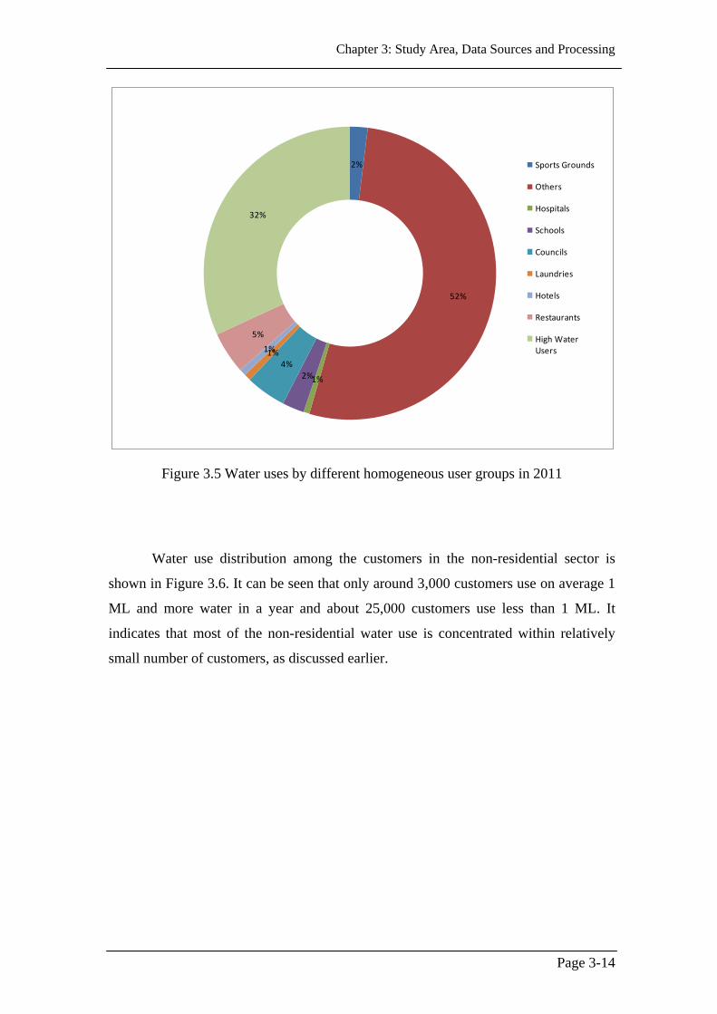
Chapter 3: Study Area, Data Sources and Processing
Page 3-14
Figure 3.5 Water uses by different homogeneous user groups in 2011
Water use distribution among the customers in the non-residential sector is
shown in Figure 3.6. It can be seen that only around 3,000 customers use on average 1
ML and more water in a year and about 25,000 customers use less than 1 ML. It
indicates that most of the non-residential water use is concentrated within relatively
small number of customers, as discussed earlier.
2%
52%
1%2%4%
1%1%
5%
32%
Sports Grounds
Others
Hospitals
Schools
Councils
Laundries
Hotels
Restaurants
High Water Users

Chapter 3: Study Area, Data Sources and Processing
Page 3-15
Figure 3.6 Customer ranking based on average yearly water use
As a part of data analysis, all non-residential customers were further
disaggregated into different groups based on the average yearly water uses (based on
2005-2009 data) such as >20 ML, >15-20 ML, >10-15 ML, 5-10 ML and <5 ML. the
average water use percentage among these groups is presented in Table 3.2. It can be
seen from Table 3.2 that the customers in >20 ML group uses over 40% of the total
non-residential water, although only 0.3% of total non-residential customers are falls in
this group. Also, Table 3.2 shows that almost 60% of the total non-residential water
used by only 2.11% of the total non-residential customers (>5 ML).
0.001
0.1
10
1000
1
30
01
60
01
90
01
12
00
1
15
00
1
18
00
1
21
00
1
24
00
1
27
00
1
Wa
ter
use
(M
L)
Customer Number

Chapter 3: Study Area, Data Sources and Processing
Page 3-16
Table 3.2 Water use by different sub-groups based average on annual water use in
2005-2009
Group
Total
number of
customers
% of total
customers
Average Water use
per customer
(ML/year)
% Contribution to
the total water use
> 20 ML 84 0.30 109.92 40.2
>15-20 ML 43 0.15 16.85 3.2
>10-15 ML 90 0.32 11.90 4.7
5-10 ML 377 1.34 6.86 11.3
<5 ML 27482 97.89 0.34 40.6
Total 28076 100 - 100
Note: customers with missing data are not used in this table.
Water use pattern per customer by the above mentioned groups over the years
from 2005 to 2011 is shown in Figure 3.7. From this figure, it can be seen that water
use per customer in <5 ML group is almost same over the years from 2007. On the
other hand, there is a decreasing trend among the remaining groups.
Note: Water use in >20 ML group is presented in secondary axis.
Figure 3.7 Non-residential water uses per customer in different groups
0
20
40
60
80
100
120
140
0
5
10
15
20
25
2005 2006 2007 2008 2009 2010 2011 To
tal W
ate
r U
se P
er C
ust
om
er (
ML
)
Tota
l Wate
r U
se P
er C
ust
om
er (
ML
)
Years
>15-20 ML >10-15 ML 5-10 ML <5 ML >20 ML

Chapter 3: Study Area, Data Sources and Processing
Page 3-17
Based on the aforementioned homogeneity and different amounts of water use,
the non-residential water use modelling was performed individually for each group (i.e.
>20 ML, >15-20 ML, >10-15 ML, 5-10 ML and <5 ML) within the different
homogeneous customer groups (i.e. Schools, Sports Grounds, Councils, Restaurants,
Hospitals, Hotels and Laundries) to capture the best hidden nature of water use
behaviour.
Before performing the water use modelling, data analysis was done to check the
water use pattern over the different quarters in a year for each homogenous customer
group. Average percentages of quarterly water use was calculated using all seven years
of available water use data where quarterly water use volume was divided by the total
yearly water use volume, and then average them separately for each quarter. This
analysis was done individually for all seven homogeneous customer groups (i.e.
Schools, Sports Grounds, Councils, Restaurants, Hospitals, Hotels and Laundries).
Average percentages of quarterly water use for Schools, Sports Grounds and
Councils are shown in Figure 3.8, whereas they shown in Figure 3.9 for Hospitals,
Hotels, Laundries and Restaurants. From Figure 3.8, it can be seen that Schools, Sports
Grounds and Councils uses less water in quarter 2 and quarter 3, which are usually
cooler months than the months in quarter 1 and quarter 4. Moreover, there is more
rainfall during the cooler months in Melbourne than the warmer months. Therefore, it
might be less outdoor water use in gardens, sports fields and pools among these groups
in quarter 2 and 3 than in quarter 1 and 4. It shows that there are some seasonal effects
on water use in these groups. Therefore, climate data and water restrictions data were
used in case of modelling water use in Schools, Sports Grounds and Councils and
presented in Chapter 4.
On the other hand, Figure 3.9 shows that the average percentage of quarterly
water use is almost the same in all four quarters in Hospitals, Hotels, Laundries and
Restaurants groups. There is less variation in water use over the year indicating no
seasonal effect. Moreover, due to most of the water uses are indoor purposes among
these groups, models was developed considering only water use for Restaurants,
Hospitals, Hotels and Laundries groups, which are presented in Chapter 5.

Chapter 3: Study Area, Data Sources and Processing
Page 3-18
Total water use by the High Water Users group is 32% of total non-residential
water use in YVW’s service area in 2011 as were shown in Fig 3.5. There are different
types of industry, manufacturer, and company falls in this group and their water uses
are quite different over the study years. The water use data analysis and model
development for these customers are discussed in Chapter 6.
Figure 3.8 Average percentages of quarterly water uses in Schools, Sports Grounds and
Councils
0.00
0.10
0.20
0.30
0.40
0.50
1 2 3 4
Per
cen
tage
(%)
Quarters
Schools
>20 ML
>15-20 ML
>10-15 ML
>5-10 ML
<5 ML
0.00
0.10
0.20
0.30
0.40
0.50
1 2 3 4
Per
cen
tage
(%)
Quarters
Sports Grounds
>15-20 ML
>10-15 ML
>5-10 ML
<5 ML
0.00
0.10
0.20
0.30
0.40
0.50
1 2 3 4
Per
cen
tage
(%)
Quaretrs
Councils
>20 ML
>15-20 ML
>10-15 ML
>5-10 ML
<5 ML

Chapter 3: Study Area, Data Sources and Processing
Page 3-19
Figure 3.9 Average percentages of quarterly water uses in Restaurants, Hospital,
Hotels and Laundries
0.00
0.10
0.20
0.30
0.40
0.50
1 2 3 4
Per
cen
tage
(%)
Quarters
Restaurants
>20 ML
>15-20 ML
>10-15 ML
>5-10 ML
<5 ML
0.00
0.10
0.20
0.30
0.40
0.50
1 2 3 4
Per
cen
tage
(%)
Quaretrs
Hospital
>20 ML
>10-15 ML
>5-10 ML
<5 ML
0.00
0.10
0.20
0.30
0.40
0.50
1 2 3 4
Per
cen
tag
e (%
)
Quarters
Hotels
>10-15 ML
>5-10 ML
<5 ML
0.00
0.10
0.20
0.30
0.40
0.50
1 2 3 4
Per
cen
tages
(%
)
Quarters
Laundries
>5-10 ML
<5 ML
>15-20 ML

Chapter 3: Study Area, Data Sources and Processing
Page 3-20
3.7. Summary
There are three water retailers in Melbourne metropolitan area (Victorian
Water, 2014). They are Yarra Valley Water (YVW), City West Water (CWW) and
South East Water (SEW). Among them YVW is the largest retailer provides essential
water and sanitation services to more than 1.76 million people in the northern and
eastern suburbs in Melbourne. The YVW has been the lead global water industry in
serving both the customer and the environment, and found as one of the most efficient
water utilities in Australia. Therefore, considering the valuable water services to
Melbourne’s community YVW’s service area was selected as the study area in this
study.
Water use billing data and historical water restrictions data were collected for
the YVW service area from YVW. Moreover, climate data such as rainfall and
temperature were obtained from Bureau of Meteorology. These data were used in this
study to develop non-residential water use models. However, as there was
inconsistency in water use billing period (i.e. number of billing days were not same)
among various non-residential water customers, data processing were required to make
a consistent time series data across all customers.
Data for different variables were obtained for different time scales. However,
most water use data were in quarterly time scale and only few customers’ water use
data were in monthly time scale. Therefore, data for all variables were transformed into
the quarterly time scale, and the quarterly time scale was used in non-residential water
use models development (Chapters 4). Water use billing data were obtained from 2000
to 2011. However, it was found that water use pattern significantly different before and
after 2005, when Permanent Water Savings Rule (PWSR) was introduced. It was
considered that this water use pattern will continue in future and therefore, data record
from 2005 to 2011 was used for model development and validation.
Disaggregation of non-residential customer was performed to capture the best
hidden nature of water use behaviour during model development in this study. This
was done based on the homogeneous nature of water use customers and their annual

Chapter 3: Study Area, Data Sources and Processing
Page 3-21
average water use patterns. It was found that there were seven homogeneous customer
groups: Schools, Sports Grounds, Councils, Restaurants, Hospitals, Hotels and
Laundries. Each of these homogenous groups was further disaggregated into five
groups: >20 ML, >15-20 ML, >10-15 ML, 5-10 ML and <5 ML. The data analysis and
models development for the above listed homogenous groups and High Water Users
customers are presented in Chapters 4, 5 and 6 progressively.

Chapter 4: Water use Modelling for Schools, Sports Grounds and Councils
Page 4-1
Chapter 4. Water use Modelling for Schools,
Sports Grounds and Councils
4.1. Overview
As discussed in Chapter 3, there are some seasonal effects on water use in
Schools, Sports Grounds and Councils groups. Similar quarterly water use pattern was
observed in these three groups. Therefore, water use modelling was done for these
three groups in a similar way considering the seasonal effects and presented in this
Chapter.
Multiple Linear Regression (MLR) technique was used in this research to
develop the water use models for the abovementioned three groups as mentioned in
Chapter 2 (Section 2.3). Several independent variables such as past water use, different
levels of water restrictions, climate variables (i.e. rainfall and temperature) and fixed
quarterly effects were tested during model development and the best combination of
these variables was used in the final model. Five years of quarterly water use data
(2006-2010) were used for model calibration, whereas data for one year (2011) was
used for model validation. Model performance was measured using the Nash-Sutcliffe
efficiency. Based on the water use analysis, it was found that different customers use
different amounts of water volume ranging from >20 ML to <1 ML per year. It was
also found that only few customers use large volumes of water per year (e.g. >20 ML
and >15-20 ML), whereas more customers use smaller volume of water per year (e.g.
<5 ML). Therefore, higher water use customers were modelled at an individual level,
whereas smaller water use customers were modelled at a group level in this study.
This chapter first describes the variable used for model development followed
by the stepwise procedure used for model development in this research. Water use
models developed for Schools, Sports Grounds and Councils groups are then presented

Chapter 4: Water use Modelling for Schools, Sports Grounds and Councils
Page 4-2
separately. Finally, a summary of water use model development for these three groups
is presented.
4.2. Variables Used for Model Development
As discussed in Chapter 3 (Section 3.5.1) quarterly water use billing data were
available for this study. Therefore, quarterly water use modelling was carried out for
forecasting quarterly water use over next year in this study for Schools, Sports
Grounds and Councils. The variables used for modelling water use among these groups
were also transformed into quarterly time step. It should be noted that the quarters are
named as Quarter 1 (January – March), Quarter 2 (April – June), Quarter 3 (July –
September) and Quarter 4 (October – December) in this study. More details about
those variables are stated below.
4.2.1. Past Water Use
As discussed in Chapter 2, previous work revealed that there was strong
influence of past water use on the current water use (House-Peters and Chang, 2011).
Moreover, there are seasonal cycle of water use in Schools, Sports Grounds and
Councils over a year due to school holidays, festival and cultural things. Therefore, the
past water use in terms of (t-1) and (t-4) time-lagged (i.e. the previous quarter and the
same quarter in the preceding year) was considered as important independent variables
to model quarterly water use for Schools, Sports Grounds and Councils in this
research. These variables also useful in explaining the nature of adaptive seasonal
variations in water use behaviour.
4.2.2. Levels of Water Restrictions
The water use in Sports Grounds is mostly for outdoor use, and in case of
Schools and Councils there might be some significant outdoor water uses. Therefore,
the levels of water restrictions were considered as an independent variable for
modelling water use in these groups. As discusses in Chapter 3, there were five levels
of water restrictions: Permanent Water Saving Rules (PWSRs), stage 1, stage 2, stage 3

Chapter 4: Water use Modelling for Schools, Sports Grounds and Councils
Page 4-3
and stage 3a in Melbourne over the period of 2005-2011. The PWSRs is a set of water
use rules that apply at all times, whereas other different levels of water restrictions
were in force to reduce some water use. However, due to insufficient length of some
restriction levels during this period, PWSRs were considered as ‘no restrictions’, and
all other four levels of water restrictions were considered as a single restriction level in
this study. Dummy variables were used to handle the water restrictions for water use
modelling, as shown in Table 4.1.
Table 4.1 Dummy variables used for water restrictions
Water restriction information R
No restrictions 0
Imposed water restrictions 1
4.2.3. Climate Variables
Water use in Sports Grounds mainly depends on climatic factors such as
rainfall and temperature as most water use in this group is for outdoor purposes.
Schools usually have gardens, play grounds and sometimes pools where water use also
depends on climatic factors. In Councils, there are different types of organizations (i.e.
library, council office, aquatic centre, police station, youth club, community centre,
community garden) where water use might also be affected by climatic factors both for
indoor and outdoor purposes. Therefore, total rainfall and mean maximum daily
temperature were considered as likely independent variables for modelling water use in
these three customer groups.
4.2.4. Fixed Quarterly Effects
There are some fixed time periods over the year when some activities among
the schools and councils are run. Some sports also take place in certain time of the
year. Therefore, to account these fixed effects in the quarterly water use model
(Section 4.2) development, four quarters were considered as one of the important

Chapter 4: Water use Modelling for Schools, Sports Grounds and Councils
Page 4-4
variables through dummy variables as shown in Table 4.2 where, D2, D3 and D4 are the
dummy variables.
Table 4.2 Dummy variables used for four quarters
Quarter D2 D3 D4
Quarter 1 (January – March) 0 0 0
Quarter 2 (April – June) 1 0 0
Quarter 3 (July – September) 0 1 0
Quarter 4 (October –December) 0 0 1
4.3. Procedure for Model Development
Quarterly water use data from 2005-2011 (Chapter 3, Section 3.4) were used in
this study for developing MLR model along with the other variables discussed in
Section 4.2. As discussed in section 4.1 model developments were performed in
different disaggregated levels based on average annual water use in 2005-2009. It
should be noted that data arrangement also performed in case of water use modelling at
group level. Data set for one customer were arranged after the data set of another
customer to make a longer data set and than a general model was developed for the
group. Therefore, developed model for all group in this study are able to forecast at
individual customer level. As part of modelling process, data for both dependent and
independent variables were transformed and tested for correlation between them. More
details of these procedures are stated below.
4.3.1. Data Transformation
It was discussed in Section 4.1 that, water use in previous quarters in terms of
(t-1) and (t-4) time-lagged, mean maximum daily temperature, total rainfall, and
dummy variables to represent water restrictions and four quarters are used as the
independent variables to model the current water use (which is the dependent variable)
in this study. In order to make the data normally distributed for both independent and
dependent variables (which is a requirement for multiple linear regressions method

Chapter 4: Water use Modelling for Schools, Sports Grounds and Councils
Page 4-5
(Lewis-Beck 1980)), data transformation was performed before model development.
Data were transformed using a log function because of its more interpretability as
changes in a log value are relative (percent) changes on the original scale (Makridakis et
al., 1998).
4.3.2. Correlation Test
A correlation analysis was carried out separately for each water user groups
before the model development to investigate the degree of correlation among the
dependent and independent variables, and also between independent variables. This
has given an early indication of independent variables that may play a significant role
for development of the best model, and also to check the multicollinearity between the
independent variables. The Pearson correlation coefficient r was used in this study,
which indicates the strength of the linear relationship between two variables X and Y:
𝑟 = 𝑋𝑖 − X 𝑌𝑖 − Y 𝑛𝑖=1 𝑛 − 1 𝑆𝑋𝑆𝑌 (4.1)
where, n is the number of data points, 𝑋 and 𝑌 are the mean values of data of
variables X and Y, SX and SY are the standard deviations of data of variables X and Y .
Generally, high and low relationships are considered to have values of the
correlation coefficient between (0.68-1) and (0-0.35) respectively. The values between
0.35 and 0.68 are considered to have moderate relationships (Taylor, 1990).
4.3.3. Mathematical Structure
Mathematical details of the multiple linear regression (MLR) model used in this
study using the above mentioned independent variables are as follows:
Log10 (WUt) = b0 + b1log10 (WUt-1) + b2log10 (WUt-4) + b3log10 (T)
+ b4log10 (Rn) + b5R + b6D2 + b7D3 + b8D4 (4.2)
WUt = 10(log
10 (WU
t))
(4.3)

Chapter 4: Water use Modelling for Schools, Sports Grounds and Councils
Page 4-6
where,
It should be noted that the quarterly water use, mean maximum daily
temperature and total rainfall are continuous variables, while dummy variables used for
water restrictions and quarters are nominal variables. The nominal variables are
handled in MLR through matrices as shown in Tables 4.1 and 4.2.
4.3.4. Measurement of Model Performance
The model performance was measured using the Nash-Sutcliffe model
efficiency (E) which is commonly used for such performance evaluation. This measure
is as follows:
E = 1 − Oi − Pi 2n
i=1 Oi − O 2ni=1 (4.4)
where, n is the number of data points; Oi and Pi are the observed and predicted
water use values respectively for the time step i; and Ō is the average observed water
use.
E is a normalized statistic that determines the relative magnitude of the residual
variance compared to the observed data variance (Nash and Sutcliffe 1970). It indicates
WUt, WUt-1 and WUt-4 = Quarterly water use at time t, (t-1) and (t-4)
respectively (KL)
T = Quarterly mean maximum daily temperature (oC)
Rn = Total quarterly rainfall (mm)
R = Dummy variable to represent water restrictions as
shown in Table 4.1
D2, D3 and D4 = Dummy variables to represent four quarters as
shown in Table 4.2
b0, b1… b8 = Regression constant and coefficients

Chapter 4: Water use Modelling for Schools, Sports Grounds and Councils
Page 4-7
how well the plot of observed vs. modelled data fits the 1:1 line. E varies from -∞ to 1
(perfect fit). An efficiency of lower than zero indicates that the mean value of the
observed time series would have been a better predictor than that predicted by the
model. Large E values (e.g. close to 1) were considered in selecting the best model in
this study.
4.3.5. Significance Test for Model Parameters
All parameters considered in this study are tested for statistical level of
significance by its p value. The p value is the smallest level of significance at which
the parameter is significant (called the significance level of the test). Conventionally
(and arbitrarily), p value of 0.05 (5%) is generally regarded as sufficiently small (Gato
et al, 2007b).
4.3.6. Steps for Model Development
The overall steps followed during the model development are shown in Figure
4.1. The brief descriptions of each of these steps are given below:
Step 1: Consider the influential variables to perform MLR.
Step 2: Perform MLR with all variables considered and obtain the regression
coefficients.
Step 3: Check the regression coefficient sign of each influential variable considered in
MLR. Remove the variable with contrary sign to the expected sign of the
coefficient (i.e. +ve coefficient for rainfall) and the highest insignificant level,
and follow Step 2. This step is repeated for all such variables until all the
coefficients are as were expected sign to be.
Step 4: Once there are no regression coefficients with signs contrary to the expected
signs, check whether coefficients are significant at 5% level. If all coefficients
are significant at 5% level, then proceed to Step 5. Otherwise, remove the
variables with highest insignificant level and perform MLR again (Step 2).
This step is repeated until all remaining variables become significant.

Chapter 4: Water use Modelling for Schools, Sports Grounds and Councils
Page 4-8
Step 5: Calculate E value for the validation period with the final model in step 4.
Step 6: If E value is satisfactory (e.g. above 0.5) then select the model in Step 4 as the
best model. Otherwise, include the last removed variables with expected sign
one at a time and re-construct the MLR model and subsequently re-perform
Steps 5 and 6. This step is repeated until the E value for the validation period
is above the threshold value (e.g. above 0.5).
Figure 4.1 MLR model development procedure
Considered variables (i.e. log10(WUt-1),
log10(WUt-4), log10(Rn), log10(T), R and D2-D4)
Perform MLR and obtain the regression co-
efficients
Are all coefficients
are significant at
5% level
Remove the variable
with contrary sign and
highest insignificance
level
Calculate the E value for the validation period
Found the best
MLR model
Is regression coefficient signs are contrary to
expectation ?
Yes No
Threshold, E > 0.5
Yes No
Include the last removed
variables with expected
sign one at a time
Perform MLR
Yes No Remove the
insignificant variable
one at a time with
lowest significance level
Ste
p 1
Ste
p 2
Ste
ps 3
an
d 4
Ste
p 5
Ste
p 6
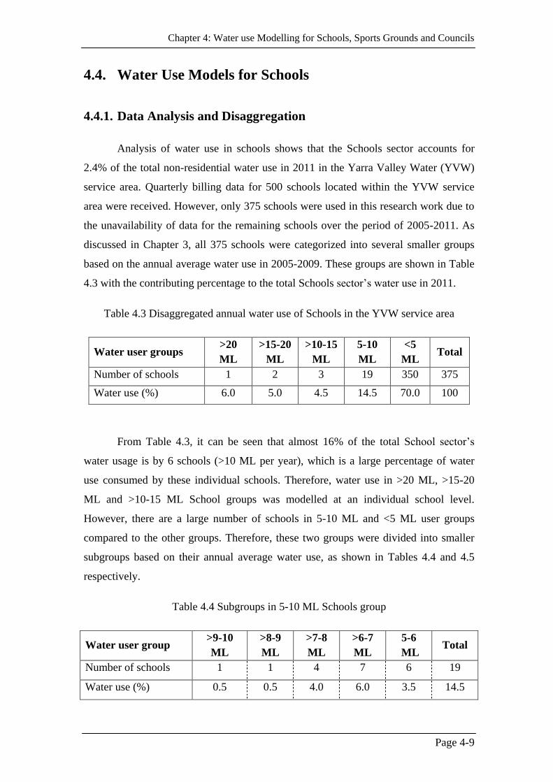
Chapter 4: Water use Modelling for Schools, Sports Grounds and Councils
Page 4-9
4.4. Water Use Models for Schools
4.4.1. Data Analysis and Disaggregation
Analysis of water use in schools shows that the Schools sector accounts for
2.4% of the total non-residential water use in 2011 in the Yarra Valley Water (YVW)
service area. Quarterly billing data for 500 schools located within the YVW service
area were received. However, only 375 schools were used in this research work due to
the unavailability of data for the remaining schools over the period of 2005-2011. As
discussed in Chapter 3, all 375 schools were categorized into several smaller groups
based on the annual average water use in 2005-2009. These groups are shown in Table
4.3 with the contributing percentage to the total Schools sector’s water use in 2011.
Table 4.3 Disaggregated annual water use of Schools in the YVW service area
Water user groups >20
ML
>15-20
ML
>10-15
ML
5-10
ML
<5
ML Total
Number of schools 1 2 3 19 350 375
Water use (%) 6.0 5.0 4.5 14.5 70.0 100
From Table 4.3, it can be seen that almost 16% of the total School sector’s
water usage is by 6 schools (>10 ML per year), which is a large percentage of water
use consumed by these individual schools. Therefore, water use in >20 ML, >15-20
ML and >10-15 ML School groups was modelled at an individual school level.
However, there are a large number of schools in 5-10 ML and <5 ML user groups
compared to the other groups. Therefore, these two groups were divided into smaller
subgroups based on their annual average water use, as shown in Tables 4.4 and 4.5
respectively.
Table 4.4 Subgroups in 5-10 ML Schools group
Water user group >9-10
ML
>8-9
ML
>7-8
ML
>6-7
ML
5-6
ML Total
Number of schools 1 1 4 7 6 19
Water use (%) 0.5 0.5 4.0 6.0 3.5 14.5

Chapter 4: Water use Modelling for Schools, Sports Grounds and Councils
Page 4-10
Table 4.5 Subgroups in <5 ML Schools group
Water user group >4-<5
ML
>3-4
ML
>2-3
ML
1-2
ML
<1
ML Total
Number of schools 11 28 70 145 96 350
Water use (%) 6.5 13.0 20.0 26.0 4.5
70
Quarterly percentages of total annual water use (Section 3.6 ) were calculated
for all five groups mentioned in Table 4.3 are shown in Figure 4.2. From the figure, it
can be seen that the water use pattern over the year is different from one schools group
to the other. It can also be seen from Figure 4.2 that there are high percentages of water
use during quarters 1 and 4 and low percentages of water use during quarters 2 and 3
among the high water user groups as well as low water users group. This difference in
quarterly water use percentages over the year reflects more outdoor activity during
summer period. Moreover, from figure it also can be seen that the difference in
quarterly water use percentages in warmer and cooler quarters are very high in the high
water user Schools groups than in the low water user Schools groups. Therefore, it is
apparent that high water user schools have more play grounds and gardens than those
with low water user schools.
Figure 4.2 Time series of quarterly percentage to annual water use among the different
user groups in Schools
0.00
0.10
0.20
0.30
0.40
0.50
0.60
20
05
_1
20
05
_2
20
05
_3
20
05
_4
20
06
_1
20
06
_2
20
06
_3
20
06
_4
20
07
_1
20
07
_2
20
07
_3
20
07
_4
20
08
_1
20
08
_2
20
08
_3
20
08
_4
20
09
_1
20
09
_2
20
09
_3
20
09
_4
20
10
_1
20
10
_2
20
10
_3
20
10
_4
20
11_
1
20
11_
2
20
11_
3
20
11_
4
Per
cen
tag
e (%
)
Quarters
Schools
>20 ML >15-20 ML >10-15 ML 5-10 ML <5 ML

Chapter 4: Water use Modelling for Schools, Sports Grounds and Councils
Page 4-11
4.4.2. Model Calibration and Validation
Model calibration and validation were performed using two independent data
sets by splitting the total data period into two sets. Initially, the calibration period was
considered as 2006-2009 (66.67% of total data) and the validation period as 2010-2011
(33.33% of total data). However, to see whether increasing calibration period produce
better results, the model was then calibrated using 2006-2010 data (83.33% of total
data) and validated with 2011 data (16.67% of total data).
4.4.3. Results and Discussions
Results of the correlation test performed among the dependent and the
independent variables for all subgroups in the Schools group are shown in Table 4.6.
Correlation between the independent variables for all School subgroups is presented in
Appendix A.

Chapter 4: Water Use Modelling for Schools, Sports Grounds and Councils
Page 4-12
Table 4.6 Correlation coefficient between the dependent and independent variables used in all subgroups in the Schools group
Group Modelled by Log10(WUt) Log10(WUt-1) Log10(WUt-4) Log10(T) Log10(Rn) R D2 D3 D4
>20 ML Individual 1 0.06 0.77a 0.89
a -0.17 -0.06 -0.21 -0.71
a 0.24
>15-20 ML Individual (School 1) 1 0.19 0.82
a 0.87
a -0.14 -0.11 -0.20 -0.67
b 0.07
Individual (School 2) 1 0.48 b 0.76
a 0.46
b -0.20 -0.48
b -0.24 -0.22 -0.09
>10-15 ML
Individual (School 1) 1 -0.02 0.40 b 0.59
b -0.15 -0.26 -0.30 -0.38
b 0.05
Individual (School 2) 1 0.92 a 0.70
a 0.04 -0.44
b -0.71
a 0.04 -0.08 -0.07
Individual (School 3) 1 0.42 b 0.31 0.29 -0.43
b -0.47
b -0.08 -0.21 -0.02
>9-10 ML Individual 1 0.78 a 0.44
b 0.26 0.01 -0.72
a 0.06 -0.34 -0.08
>8-9 ML Individual 1 0.80 a 0.62
b -0.08 -0.17 -0.64
b 0.13 -0.02 -0.16
>7-8 ML Group 1 0.58 b 0.43
b -0.16 0.21 -0.25 0.03 -0.25 0.03
>6-7 ML Group 1 0.82 a 0.46
b 0.05 -0.14 -0.30 0.01 -0.05 -0.05
5-6 ML Group 1 0.75 a 0.49
b 0.13 -0.28 -0.40
b -0.03 -0.11 -0.03
>4-<5 ML Group 1 0.85 a 0.62
b 0.06 -0.14 -0.36
b 0.02 -0.06 -0.09
>3-4 ML Group 1 0.73 a 0.38
b 0.07 -0.16 -0.32 0.00 -0.07 -0.04
>2-3 ML Group 1 0.75 a 0.37
b 0.03 -0.11 -0.34 0.04 -0.06 -0.06
1-2 ML Group 1 0.78 a 0.44
b -0.01 -0.09 -0.21 0.03 -0.01 -0.04
<1 ML Group 1 0.88 a 0.76
a -0.01 -0.04 -0.16 0.02 -0.01 -0.02
Note: a – variables are highly correlated, b – variables are moderately correlated.

Chapter 4: Water Use Modelling for Schools, Sports Grounds and Councils
Page 4-13
It can be seen from Table 4.6 that there are moderate to high correlations
between the current water use and the water use of previous quarters (in terms of WUt-1
and WUt-4) for most of the subgroups, particularly previous quarter’s water use (WUt-1).
Similar correlations can also be seen with the mean maximum daily temperature for
high water use subgroups. There are moderate correlations with restrictions for some
subgroups (Table 4.6). Remaining variables were found to have low correlation with
the current water use.
From correlation analysis between the independent variables (Appendix A), it
was found that the correlation coefficient ranged from -0.70 to 0.70 for most of the
groups except for >20 ML, School 1 in >15-20 ML, School 2 in >10-15 ML and sub-
group 9 ML. Babel et al., 2007 noted that the correlation coefficients within this range
should not be considered as a significant correlation to cause the multicollinearity
effect in the MLR model development. Therefore, it can be considered that there are no
significant correlations between all independent variables for most of the groups. Only
few variables were found to be inter-correlated for above subgroups. However, it was
found that one of those inter-correlated variables was not included in the best model
considered in this study (refer to Appendix A and Table 4.7).
The E values of the best models for the two different calibration (i.e. 2006-2009
and 2006-2010) and validation (i.e. 2010-2011 and 2011) periods are presented in
Table 4.7. The variables used in these models are given within the parenthesis. It can
be seen in Table 4.7 that the independent variables used in the best models of each
subgroup are found to be the same for both calibration periods (i.e. 2006-2009 and
2006-2010). Also, the E values obtained are quite similar in the calibration results for
both calibration periods, as expected. However, the E values of the 2011 validation
period are either greater or same to the values of the 2010-2011 validation period in 11
models out of 16 models. Therefore, it was concluded that the models with a longer
calibration period yielded better results in validation, and the best models developed
with the 2006-2010 calibration period are discussed in Section 4.4.3.1 to 4.4.3.5. It
should be noted that for the same reason, model calibration was only performed using
the 2006-2010 data period for the Sports Grounds and Councils groups, which are
discussed later in this Chapter. The regression coefficients obtained for the best models
(developed with the 2006-2010 calibration period) of different School subgroups are
presented in Table 4.8. Further discussions on individual model performance are
presented in the following sub-sections.

Chapter 4: Water Use Modelling for Schools, Sports Grounds and Councils
Page 4-14
Table 4.7 E values for the best models in Schools group
School
Group
School
subgroups
Number of
Schools
Modelled by
Calibration period: 2006-2009
Validation Period: 2010-2011
Calibration Period: 2006-2010
Validation Period: 2011
Calibration Validation Calibration Validation
>20 ML 1 Individual 0.86 (T,Rn,R) 0.71 0.89 (T,Rn,R) 0.18
>15-20 ML
2
Individual (School 1) 0.86 (WUt-1,T,Rn,R) 0.92 0.88 (WUt-1,T,Rn,R) 0.92
Individual (School 2) 0.68 (WUt-4,T,R) 0.67 0.65 (WUt-4,T,R) 0.67
>10-15 ML
3
Individual (School 1) 0.48 (T,R) 0.38 0.47 (T,R) 0.56
Individual (School 2) 0.80 (T,Rn,R) 0.79 0.78 (T,Rn,R) 0.68
Individual (School 3) 0.62 (T,Rn,R) 0.60 0.59 (T,Rn,R) 0.76
5-10 ML
>9 -10 ML 1 Individual 0.77 (WUt-1,T) 0.81 0.77 (WUt-1,T) 0.86
>8-9 ML 1 Individual 0.73 (WUt-1,Rn,R) 0.80 0.70 (WUt-1,Rn,R) 0.86
>7-8 ML 4 Group 0.32 (WUt-1, WUt-4,T) 0.69 0.44 (WUt-1, WUt-4,T) 0.76
>6-7 ML 7 Group 0.68 (WUt-1, WUt-4,T,Rn,R) 0.75 0.69 (WUt-1, WUt-4,T,Rn,R) 0.75
5-6 ML 6 Group 0.52 (WUt-1, WUt-4,T,Rn,R) 0.78 0.62 (WUt-1, WUt-4,T,Rn,R) 0.57
<5 ML
>4-<5 ML 11 Group 0.71 (WUt-1,T) 0.78 0.73 (WUt-1,T) 0.75
>3-4 ML 28 Group 0.46 (WUt-1, WUt-4,T,R) 0.70 0.55 (WUt-1, WUt-4,T,R) 0.80
>2-3 ML 70 Group 0.35 (WUt-1, WUt-4,R) 0.41 0.58 (WUt-1, WUt-4,R) 0.62
1-2 ML 145 Group 0.61 (WUt-1, WUt-4,R) 0.60 0.62 (WUt-1, WUt-4,R) 0.57
<1 ML 96 Group 0.81 (WUt-1, WUt-4) 0.73 0.79 (WUt-1, WUt-4) 0.75
Note: E values with bold number in the 2011 validation period are either greater or same to the values of the 2010-2011 validation period

Chapter 4: Water Use Modelling for Schools, Sports Grounds and Councils
Page 4-15
Table 4.8 Estimated regression coefficients for different Schools group models (calibration period: 2006-2010, validation period: 2011)
School Group
School
subgroups
Modelled by
Constant log10(WUt-1) log10(WUt-4) log10(T) log10(Rn) R D2 D3 D4
(b0) (b1) (b2) (b3) (b4) (b5) (b6) (b7) (b8)
>20 ML Individual 1.54 - - 2.33 (0.00) -0.28 (0.01) -0.12 (0.03) - - -
>15-20 ML
Individual (School 1) 0.44 0.19 (0.07) - 2.17 (0.00) -0.15 (0.18) -0.08 (0.18) - - -
Individual (School 2) 1.20 - 0.48 (0.01) 0.53 (0.19) - -0.16 (0.09) - - -
>10-15 ML
Individual (School 1) 1.86 - - 1.29 (0.00) - -0.17 (0.07)
Individual (School 2) 4.12 - - 0.29 (0.18) -0.42 (0.00) -0.33 (0.00) - - -
Individual (School 3) 3.59 - - 1.79 (0.02) -1.08 (0.01) -0.64 (0.00) - - -
5-10 ML
>9 -10 ML Individual -1.30 0.74 (0.00) - 1.55 (0.00) - - - - -
>8-9 ML Individual 1.71 0.60 (0.00) - - -0.18 (0.09) -0.12 (0.20) - - -
>7-8 ML Group 0.13 0.53 (0.00) 0.21 (0.05) 0.49 (0.05) - - - - -
>6-7 ML Group 0.52 0.81 (0.00) -0.02 (0.79) 0.26 (0.15) -0.09 (0.32) -0.08 (0. 11) - - -
5-6 ML Group 0.68 0.60 (0.00) 0.13 (0.08) 0.34 (0.05) -0.14 (0.09) -0.10 (0.03) - - -
<5 ML
>4-<5 ML Group 0.10 0.85 (0.00) - 0.23 (0.00) - - - - -
>3-4 ML Group 0.37 0.69 (0.00) 0.11 (0.01) 0.21 (0.04) - -0.06 (0.02) - - -
>2-3 ML Group 0.68 0.69 (0.00) 0.06 (0.00) - - -0.6 (0.00) - - -
1-2ML Group 0.44 0.73 (0.00) 0.09 (0.00) - - -0.04 (0.00) - - -
< 1ML Group 0.09 0.73 (0.00) 0.19 (0.00) - - - - - -
Note: p-value is presented in the parenthesis; bold coefficients are statistically significant at 5% level

Chapter 4: Water Use Modelling for Schools, Sports Grounds and Councils
Page 4-16
4.4.3.1. Group: >20 ML
There is only one school in this group, and therefore, it was modelled as an
individual school. Table 4.8 shows that the mean maximum daily temperature, total
rainfall and water restrictions have statistically significant contributions on the current
water use in this school. This might be due to the more outdoor water use (i.e. large
playground and swimming pools), where water use is affected by the climate and also
by the water restrictions.
Comparison of observed against modelled water use for this school is shown in Figure
4.3, with scatter plots for both calibration and validation periods. Figure 4.3 shows that
the modelled water uses time series is well matched with the observed data in both
calibration and validation periods. Also, it can be seen from the scatter plots in Figure
4.3 that the data points lie close to the 1:1 line. The E value for calibration is high, but
for validation it is low (Table 4.7). Low E value in validation might be because of the
sudden change in water use of the school in 2011. From the time series plot, it can be
seen that there was a big drop in water use in 2011.
Figure 4.3 Observed vs modelled water use for >20 ML Schools group
Time series plot
Note: values are in log(WUt)
Scatter plot
0
5000
10000
15000
20000
25000
01
/20
06
02/2
00
6
03/2
00
6
04/2
00
6
01/2
00
7
02
/20
07
03/2
00
7
04/2
00
7
01/2
00
8
02/2
00
8
03
/20
08
04/2
00
8
01/2
00
9
02/2
00
9
03/2
00
9
04
/20
09
01
/20
10
02/2
01
0
03/2
01
0
04/2
01
0
01
/20
11
02
/20
11
03/2
011
04/2
011
Wate
r u
se (
KL
)
Quarter
Observed Modeled
0
1
2
3
4
5
0 1 2 3 4 5
Mod
elle
d
Observed
Calibration
E = 0.89
0
1
2
3
4
5
0 1 2 3 4 5
Mo
del
led
Observed
Validation
E = 0.18
Calibration Validation

Chapter 4: Water Use Modelling for Schools, Sports Grounds and Councils
Page 4-17
4.4.3.2. Group: >15-20 ML
There are two schools in this group and modelling water use was performed
individually for each of these schools. From Table 4.8, it can be seen that the mean
maximum temperature is the only statistically significant independent variable for
School 1 in this group. However, it should be noted that the previous quarter’s water
use WUt-1, rainfall and restrictions variables were also included in this model although
they were not statistically significant as including these variables improved the model
performance (see Figure 4.1 for model development procedure). Comparison of
observed against modelled water use time series and scatter plots are shown in Figure
4.4 for both calibration and validation periods. It shows that the modelled water use
time series is well matched with the observed data in both calibration and validation
periods. From Figure 4.4, it can also be seen that the data points in the scatter plots lie
close to the 1:1 line.
Time series plot
Note: values are in log(WUt)
Scatter plot
Figure 4.4 Observed vs modelled water use for School 1 in >15-20 ML Schools group
0
2000
4000
6000
8000
10000
12000
01
/20
06
02/2
00
6
03/2
00
6
04/2
00
6
01/2
00
7
02
/20
07
03/2
00
7
04/2
00
7
01/2
00
8
02/2
00
8
03
/20
08
04/2
00
8
01/2
00
9
02/2
00
9
03/2
00
9
04
/20
09
01
/20
10
02/2
01
0
03/2
01
0
04/2
01
0
01
/20
11
02
/20
11
03/2
011
04/2
011
Wa
ter
use
(K
L)
Quarter
Observed Modeled
0
1
2
3
4
5
0 1 2 3 4 5
Mo
del
led
Observed
Calibration
E = 0.88
0
1
2
3
4
5
0 1 2 3 4 5
Mo
del
led
Observed
Validation
E = 0.92
Validation Calibration

Chapter 4: Water Use Modelling for Schools, Sports Grounds and Councils
Page 4-18
For School 2, it was found that the previous quarter’s water use in terms of
WUt-4 was the only the statistically significant independent variable. However, the
mean maximum daily temperature and water restrictions were also included in this
model. Although, they were not statistically significant, including these variables
improved the model performance (see Figure 4.1 for model development procedure).
Comparison of observed against modelled water use time series for School 2 is shown
in Figure 4.5 with scatter plots for both calibration and validation periods. Figure 4.5
shows that the modelled water use time series is well matched with the observed data
in both calibration and validation periods. Moreover, E values presented in Table 4.7
for both calibration and validation periods indicate that the model performed well,
which can also be seen from the scatter plots (Figure 4.5).
Time series plot
Note: values are in log(WUt)
Scatter plot
Figure 4.5 Observed vs modelled water use for School 2 in >15-20 ML Schools group
0100020003000400050006000700080009000
01
/20
06
02/2
00
6
03/2
00
6
04/2
00
6
01/2
00
7
02
/20
07
03/2
00
7
04/2
00
7
01/2
00
8
02/2
00
8
03
/20
08
04/2
00
8
01/2
00
9
02/2
00
9
03/2
00
9
04
/20
09
01
/20
10
02/2
01
0
03/2
01
0
04/2
01
0
01
/20
11
02
/20
11
03/2
011
04/2
011
Wa
ter
use
(K
L)
Quarter
Observed Modeled
0
1
2
3
4
5
0 1 2 3 4 5
Mo
del
led
Observed
Calibration
E = 0.65
0
1
2
3
4
5
0 1 2 3 4 5
Mo
del
led
Observed
Validation
E = 0.67
Validation Calibration

Chapter 4: Water Use Modelling for Schools, Sports Grounds and Councils
Page 4-19
From the above discussion, it can be seen that climatic variables and
restrictions are the common independent variables in modelling the current water use
in both of the schools in this group. Therefore, it is apparent that there are significant
outdoor water uses in the two schools of this group.
4.4.3.3. Group: >10-15 ML
There are three schools in this group and they were individually modelled
because of high average annual water use as discussed in Section 4.4.1. It can be seen
from Table 4.8 that the mean maximum daily temperature and water restrictions were
found as important independent variables in all three schools. Although these variables
were not statistically significant in all cases, including these variables improves the
model performance (see Figure 4.1 for model development procedure). The total
rainfall variable was also found to have significant contribution on current water use in
Schools 2 and 3 in this group. Therefore, it implies that there are some outdoor water
uses in this Schools group. Comparison of observed against modelled water use is
shown in scatter plots in Figure 4.6 for both calibration and validation periods for all
three schools. It can be seen from the figure that the modelled water use in all three
schools is well matched with the observed water use, which is also reflected with the E
values (Table 4.7).
a) School 1
0
1
2
3
4
5
0 1 2 3 4 5
Mo
del
led
Observed
Calibration
E = 0.47
0
1
2
3
4
5
0 1 2 3 4 5
Mo
del
led
Observed
Validation
E = 0.56

Chapter 4: Water Use Modelling for Schools, Sports Grounds and Councils
Page 4-20
b) School 2
Note: values are in log(WUt)
c) School 3
Figure 4.6 Scatter plots of observed vs modelled water use for the three schools in >10-
15 ML Schools group
4.4.3.4. Group: 5-10 ML
There are five subgroups in this group as shown in Table 4.4 (Section 4.4.1).
Among these subgroups, >8-9 ML and >9-10 ML subgroups have only one school, but
there are multiple schools in the remaining subgroups (i.e. >7-8 ML, >6-7 ML and 5-6
ML). Therefore, as outlined in Section 4.4.1, >8-9 ML and >9-10 ML subgroups were
modelled as individual schools and the other subgroups were modelled as individual
groups with multiple schools.
From Table 4.8, it can be seen that previous quarter’s water use WUt-1 has
statistically significant contribution on the current water use of the school in all
0
1
2
3
4
5
0 1 2 3 4 5
Mo
del
led
Observed
Calibration
E = 0.78
0
1
2
3
4
5
0 1 2 3 4 5
Mo
del
led
Observed
Validation
E = 0.68
0
1
2
3
4
5
0 1 2 3 4 5
Mo
del
led
Observed
Calibration
E = 0.59
0
1
2
3
4
5
0 1 2 3 4 5
Mo
del
led
Observed
Validation
E = 0.76

Chapter 4: Water Use Modelling for Schools, Sports Grounds and Councils
Page 4-21
subgroups of this group. Although the other variables such as total rainfall and mean
maximum daily temperature (Table 4.8) were included as important variables in this
group (see Figure 4.1 for model development procedure), it can be seen from Table 4.8
that the coefficient of these variables were small. Therefore, these results indicate that
there are less outdoor activities among the schools in this group.
Comparison of observed against modelled water use is shown in scatter plots in
Figure 4.7 for both calibration and validation periods for all five subgroups. It can be
seen from this figure that the modelled water use in these subgroups are well matched
with the observed water use, which is also reflected with the E values (Table 4.7).
a) Subgroup >9-10 ML
b) Subgroup >8-9 ML
0
1
2
3
4
5
0 1 2 3 4 5
Mo
del
led
Observed
Calibration
E = 0.77
0
1
2
3
4
5
0 1 2 3 4 5
Mod
elle
d
Observed
Validation
E = 0.86
0
1
2
3
4
5
0 1 2 3 4 5
Mo
del
led
Observed
Calibration
E = 0.70
0
1
2
3
4
5
0 1 2 3 4 5
Mod
elle
d
Observed
Validation
E = 0.86

Chapter 4: Water Use Modelling for Schools, Sports Grounds and Councils
Page 4-22
c) Subgroup >7-8 ML
d) Subgroup >6-7 ML
Note: values are in log(WUt)
e) Subgroup 5-6 ML
Figure 4.7 Scatter plots of observed vs modelled water use for the five school
subgroups in 5-10 ML Schools group
4.4.3.5. Group: <5 ML
Models for >4-<5 ML, >3-4 ML, >2-3 ML, 1-2 ML and <1 ML subgroups
were developed as for 5-6 ML, >6-7 ML and >7-8 ML subgroups as there are more
0
1
2
3
4
5
0 1 2 3 4 5
Mo
del
led
Observed
Calibration
E = 0.44
0
1
2
3
4
5
0 1 2 3 4 5
Mod
elle
d
Observed
Validation
E = 0.76
0
1
2
3
4
5
0 1 2 3 4 5
Mo
del
led
Observed
Calibration
E = 0.69
0
1
2
3
4
5
0 1 2 3 4 5
Mo
del
led
Observed
Validation
E = 0.75
0
1
2
3
4
5
0 1 2 3 4 5
Moed
lled
Observed
Calibration
E = 0.62
0
1
2
3
4
5
0 1 2 3 4 5
Mod
elle
d
Observed
Validation
E = 0.57

Chapter 4: Water Use Modelling for Schools, Sports Grounds and Councils
Page 4-23
than one school within these subgroups. From Table 4.8, it can be seen that the WUt-1
and WUt-4 water use are the statistically significant independent variables in all of these
school subgroups except the >4-5 ML subgroup. However, restrictions was also
included as an important variable in >3-4 ML, >2-3 ML and 1-2 ML subgroups as
including this variable improved the model performance (see Figure 4.1 for model
development procedure). It can also be seen that climate variables do not contribute to
the water use in these subgroups in the <5 ML group. This could be due to less outdoor
activities among the schools in these low annual water use subgroups.
Similar to the 5-10 ML group, comparison of observed against modelled water
use is shown in scatter plots in Figure 4.8 for both calibration and validation periods
for all five subgroups. The modelled water uses in these subgroups are well matched
with the observed water use as can be seen from Figure 4.8, which is also reflected
with the E values (Table 4.7).
a) Subgroup >4-5 ML
b) Subgroup >3-4 ML
0
1
2
3
4
5
0 1 2 3 4 5
Mod
elle
d
Observed
Calibration
E = 0.73
0
1
2
3
4
5
0 1 2 3 4 5
Mod
elle
d
Observed
Validation
E = 0.75
0
1
2
3
4
5
0 1 2 3 4 5
Mo
del
led
Observed
Calibration
E = 0.55
0
1
2
3
4
5
0 1 2 3 4 5
Mo
del
led
Observed
Validation
E = 0.80

Chapter 4: Water Use Modelling for Schools, Sports Grounds and Councils
Page 4-24
c) Subgroup >2-3 ML
d) Subgroup 1-2 ML
Note: values are in log(WUt)
e) Subgroup <1 ML
Figure 4.8 Scatter plots of observed vs modelled water use for the five school
subgroups in <5 ML Schools group
0
1
2
3
4
5
0 1 2 3 4 5
Mo
del
led
Observed
Calibration
E = 0.58
0
1
2
3
4
5
0 1 2 3 4 5
Mo
del
led
Observed
Validation
E = 0.62
0
1
2
3
4
5
0 1 2 3 4 5
Mod
elle
d
Observed
Calibration
E = 0.62
0
1
2
3
4
5
0 1 2 3 4 5
Mo
del
led
Observed
Validation
E = 0.57
0
1
2
3
4
5
0 1 2 3 4 5
Mo
del
led
Observed
Calibration
E = 0.79
0
1
2
3
4
5
0 1 2 3 4 5
Mo
del
led
Observed
Validation
E = 0.75

Chapter 4: Water Use Modelling for Schools, Sports Grounds and Councils
Page 4-25
4.5. Water Use Models for Sports Grounds
4.5.1. Data Analysis and Disaggregation
Analysis of water use in sports Grounds shows that the Sports Grounds sector
accounts for 2.0% of the total non-residential water use in 2011 in the YVW service
area. Although, quarterly billing data for 277 sports grounds located within the YVW
service area were received, only 154 sports grounds were used in this research work
due to the missing data record for the remaining sports grounds over the period of
2005-2011. As discussed in Chapter 3 (Section 3.6), all 154 sports grounds were
categorized into several smaller groups based on the average annual water use in 2005-
2009. These groups are shown in Table 4.9 with the contributing percentages to the
total Sports Grounds group’s water use in 2011.
Table 4.9 Disaggregated annual water use of Sports Grounds in the YVW service area
Water user groups >20
ML
>15-20
ML
>10-15
ML
5-10
ML
<5
ML Total
Number of sports grounds 1 1 5 36 111 154
Water use (%) 1.0 2.5 6.5 33.5 56.5 100
From Table 4.9, it can be seen that 10% of the total sports ground’s water usage
is by 7 sports grounds with more than 10 ML water use, which is a large percentage of
water use consumed by these individual sports grounds. Therefore, they were modelled
at an individual level. However, the water use by the sports ground in >20 ML was not
modelled in this research due to its changing water use behaviour and discussed in
Section 4.5.2.1. There are large number of sports grounds in 5-10 ML and <5 ML user
groups compared to the other groups. These two groups were divided into smaller
subgroups based on their annual average water use, as shown in Tables 4.10 and 4.11
respectively. They were modelled at individual subgroup level with multiple sports
grounds.

Chapter 4: Water Use Modelling for Schools, Sports Grounds and Councils
Page 4-26
Table 4.10 Subgroups in 5-10 ML Sports Grounds group
Water user group >9-10
ML
>8-9
ML
>7-8
ML
>6-7
ML
5-6
ML Total
Number of sports grounds 5 2 6 4 19 36
Water use (%) 4.0 6.0 5.0 5.5 13.0 33.5
Table 4.11 Subgroups in <5 ML Sports Grounds group
Water user group >4 -<5
ML
>3-4
ML
>2-3
ML
1-2
ML <1 ML Total
Number of sports grounds 18 20 29 32 12 111
Water use (%) 13.0 15.0 14.0 13.5 1 56.5
Quarterly percentages of total annual water use (Section 3.6) were calculated
for all groups in Table 4.9 and are shown in Figure 4.9 except for >20 ML group. It
can be seen from the figure that the water use pattern over the year is quite similar in
all Sports grounds subgroups. However, with careful observation it is clear that high
user group use more percentage of annual water use in quarter 1 and 4 and less
percentage in quarter 2 and 3 than the low user groups.
Figure 4.9 Time series of quarterly percentage to annual water use among the different
user groups in Sports Grounds
0.00
0.10
0.20
0.30
0.40
0.50
0.60
0.70
20
05
_1
20
05
_2
20
05
_3
20
05
_4
20
06
_1
20
06
_2
20
06
_3
20
06
_4
20
07
_1
20
07
_2
20
07
_3
20
07
_4
20
08
_1
20
08
_2
20
08
_3
20
08
_4
20
09
_1
20
09
_2
20
09
_3
20
09
_4
20
10
_1
20
10
_2
20
10
_3
20
10
_4
20
11_
1
20
11_
2
20
11_
3
20
11_
4
Per
cen
tage
(%)
Quarters
Sports Grounds
>15-20 ML >10-15 ML 5-10 ML <5 ML

Chapter 4: Water Use Modelling for Schools, Sports Grounds and Councils
Page 4-27
4.5.2. Results and Discussions
Results of the correlation analysis performed among the dependent and the
independent variables for all subgroups in the Sports Grounds group are shown in
Table 4.12. Correlation between the independent variables for all Sports Grounds
subgroups is presented in Appendix B.
It can be seen from Table 4.12 that there are moderate to high correlations
between the current water use and the temperature for all subgroups except for lowest
four water use subgroups. Similar correlations can also be seen with the previous
quarter’s water use (in terms of WUt-4) for most of the high water use subgroups. There
are moderate correlations with the previous quarter’s water use (in terms of WUt-1) for
the subgroups 8 ML or less (Table 4.12). Remaining variables were found to have low
correlation with the current water use in most cases.
From correlation analysis between the independent variables (Appendix B), it
was found that the correlation coefficients ranged from -0.70 to 0.70 for most of the
groups except for Sports Grounds 1, 2, 3 and 5 in >10-15 ML, and <1 ML subgroups.
However, one of the inter-correlated variables in these subgroups was not found to be
significant variable in the best model as was in the Schools group.
As mentioned in Section 4.4.3, model calibration and validation were
performed for the Sports Grounds group using 2006-2010 and 2011 period data
respectively. The E values found for the best models in this research are presented in
Table 4.13. The regression coefficients obtained for the best models of different Sports
Grounds subgroups are also presented in Table 4.13.

Chapter 4: Water Use Modelling for Schools, Sports Grounds and Councils
Page 4-28
Table 4.12 Correlation coefficient between the dependent and independent variables used in all subgroups in the Sports Grounds group
Group Modelled by Log10(WUt) Log10(WUt-1) Log10(WUt-4) Log10(T) Log10(Rn) R D2 D3 D4
>20 ML Individual - - - - - - - - -
>15-20 ML Individual 1 0.34 0.90 a 0.82
a 0.02 -0.36
b -0.27 -0.63
b 0.33
>10-15 ML
Individual (Sports G.1) 1 0.37 b 0.47
b 0.56
b -0.01 -0.31 -0.38
b -0.33 0.34
Individual (Sports G.2) 1 0.36 b 0.70
a 0.69
b -0.29 -0.27 -0.12 -0.57
b 0.12
Individual (Sports G.3) 1 0.19 0.70 a 0.80
a -0.13 -0.06 -0.32 -0.58
b 0.30
Individual (Sports G.4) 1 0.36 b 0.79
a 0.80
a -0.25 -0.18 -0.29 -0.56
b 0.20
Individual (Sports G.5) 1 0.32 0.75 a 0.78
a -0.27 -0.12 -0.19 -0.63
b 0.20
>9-10 ML Individual 1 0.32 0.65 b 0.54
b -0.09 -0.26 -0.08 -0.48
b 0.16
>8-9 ML Individual 1 0.23 0.24 0.60 b 0.07 -0.20 -0.15 -0.52
b 0.23
>7-8 ML Group 1 0.44 b 0.65
b 0.54
b -0.21 -0.32 -0.06 -0.51
b 0.11
>6-7 ML Group 1 0.67 b 0.63
b 0.45
b -0.19 -0.30 -0.11 -0.36
b 0.09
5-6 ML Group 1 0.55 b 0.46
b 0.39
b -0.06 -0.26 -0.13 -0.30 0.11
>4-<5 ML Group 1 0.53 b 0.46
b 0.43v 0.03 -0.26 -0.14 -0.35 0.17
>3-4 ML Group 1 0.57 b 0.34 0.33 -0.01 -0.28 -0.08 -0.29 0.11
>2-3 ML Group 1 0.65 b 0.43
b 0.25 -0.09 -0.39 -0.06 -0.22 0.04
1-2 ML Group 1 0.65 b 0.40
b 0.20 0.04 -0.39
b -0.09 -0.17 0.08
<1ML Group 1 0.78 a 0.67
b 0.05 -0.14 -0.30 0.01 -0.06 -0.03
Note: a – variables are highly correlated, b – variables are moderately correlated.

Chapter 4: Water Use Modelling for Schools, Sports Grounds and Councils
Page 4-29
4.5.2.1. Group: >20 ML
There is one sports ground in this group. The time series of water use data of
this sports ground is shown in Figure 4.10. It can be seen from the figure that water
uses was started to decrease from 4th
quarter in 2006 and has become very low from 2nd
quarter of 2009 onward. After discussion with the YVW, it was found that this
customer had invested in stormwater collection and reuse from 4th
quarter of 2006 and
also has licence to extract water from a nearby Creek. All of these alternate sources of
water make this customer less dependent on using water from YVW. Therefore, water
use for this sports ground was not modelled in this research.
Figure 4.10 Time series of water use data for >20 ML Sports Grounds group
0
10000
20000
30000
40000
01
/20
06
02
/20
06
03
/20
06
04
/20
06
01
/20
07
02
/20
07
03
/20
07
04
/20
07
01
/20
08
02
/20
08
03
/20
08
04
/20
08
01
/20
09
02
/20
09
03
/20
09
04
/20
09
01
/20
10
02
/20
10
03
/20
10
04
/20
10
01
/20
11
02
/20
11
03
/20
11
04
/20
11
Wate
r u
se (
KL
)
Quarter

Chapter 4: Water Use Modelling for Schools, Sports Grounds and Councils
Page 4-30
Table 4.13 E values for the best models and estimated regression coefficients for different Sports Grounds group models
Sports
Grounds
Group
Sports
Grounds
subgroups
Number of
Sports
Grounds
Modelled by E values
Constant log10(WUt-1) log10(WUt-4) log10(T) log10(Rn) R D2 D3 D4
Calibration Validation (b0) (b1) (b2) (b3) (b4) (b5) (b6) (b7) (b8)
>20 ML - 1 Not modelled - - - - - - - - - - -
>15-20 ML - 1 Individual 0.89 0.76 -1.59 - - 4.02 (0.00) - -.53 (0.00) - - -
>10-15 ML - 5
Individual (S.G. 1) 0.46 0.64 0.35 - - 2.47 (0.00) - -0.39 (0.05)
Individual (S.G. 2) 0.60 0.40 -4.66 - - 6.31 (0.00) - -0.78 (0.03) - - -
Individual (S.G.3) 0.67 0.38 -1.45 - - 3.65(0.00) - -0.18 (.26) - - -
Individual (S.G.4) 0.83 0.90 -0.03 - - 3.68 (0.00) -0.65 (0.01) -0.33 (0.01) - - -
Individual (S.G.5) 0.77 0.42 1.31 - - 2.30 (0.00) -0.43 (0.01) -0.17 (0.05) - - -
5-10 ML
>9 -10 ML 5 Group 0.54 0.62 -0.73 0.19 (0.01) 0.42 (0.00) 1.54 (0.00) - -0.15 (0.10) - - -
>8-9 ML 2 Group 0.50 0.68 -1.09 0.17 (0.19) -0.26 (0.10) 3.61 (0.00) - -0.31 (0.06) - - -
>7-8 ML 6 Group 0.58 0.43 -2.50 0.40 (0.00) - 3.42 (0.00) - -0.31 (0.00) - - -
>6-7 ML 4 Group 0.63 0.33 -2.63 0.62 (0.00) - 2.90 (0.00) - -0.18 (0.11) - - -
5-6 ML 19 Group 0.47 0.42 -2.46 0.50 (0.00) - 3.06 (0.00) - -0.25 (0.00) - - -
<5 ML
>4-<5 ML 18 Group 0.56 0.52 1.51 0.59 (0.00) - - - -0.29 (0.00) -0.57 (0.00) -0.50 (0.00) 0.29 (0.00)
>3-4 ML 20 Group 0.51 0.53 1.42 0.60 (0.00) - - - -0.27 (0.00) -0.47 (0.00) -0.48 (0.00) 0.21(0.00)
>2-3 ML 29 Group 0.54 0.33 1.28 0.62 (0.00) - - - -0.34 (0.00) -0.49 (0.00) -0.45 (0.00) 0.12 (0.08)
1-2 ML 32 Group 0.51 0.36 1.13 0.60 (0.00) - - - -0.29 (0.00) -0.32 (0.00) -0.22 (0.00) 0.18 (0.00)
<1 ML 12 Group 0.61 0.51 0.35 0.77 (0.00) - - - - - - -
Note: p-value is presented in the parenthesis; S.G. is Sports Grounds; bold coefficients are statistically significant at 5% level

Chapter 4: Water Use Modelling for Schools, Sports Grounds and Councils
Page 4-31
4.5.2.2. Group: >15-20 ML
Water use modelling for this group was performed as an individual sports
ground as there is only one sport ground in this group. It was found that the mean
maximum daily temperature and water restrictions have statistically significant
contributions on current water use in this sports ground (Table 4.13). Comparison of
observed and modelled water use time series for this sports ground is shown in Figure
4.11 with scatter plots for both calibration and validation periods. It shows that the
modelled and observed water use is well matched. Higher E values for both calibration
and validation shown in Table 4.13 also indicate that the model performed well.
Time series plot
Note: values are in log(WUt)
Scatter plot
Figure 4.11 Observed vs modelled water use in >15-20 ML Sports Grounds group
0
2000
4000
6000
8000
10000
12000
14000
16000
01
/20
06
02
/20
06
03
/20
06
04
/20
06
01
/20
07
02
/20
07
03
/20
07
04
/20
07
01
/20
08
02
/20
08
03
/20
08
04
/20
08
01
/20
09
02
/20
09
03
/20
09
04
/20
09
01
/20
10
02
/20
10
03
/20
10
04
/20
10
01
/20
11
02
/20
11
03
/20
11
04
/20
11
Wate
r u
se (
KL
)
Quarter
Observed Modeled
0
1
2
3
4
5
0 1 2 3 4 5
Mo
del
led
Observed
Calibration
E = 0.89
0
1
2
3
4
5
0 1 2 3 4 5
Mo
del
led
Observed
Validation
E = 0.76
Validation Calibration

Chapter 4: Water Use Modelling for Schools, Sports Grounds and Councils
Page 4-32
4.5.2.3. Group: >10-15 ML
There are five sports grounds in this group and are modelled separately
(Section 4.5.1). From Table 4.13, it can be seen that the mean maximum daily
temperature has statistically significant contribution on current water use for all sports
grounds. Similar contribution was also found for the water restrictions in all cases
except for Sports Grounds 3, having insignificant contribution. It can be also seen from
Table 4.13 that total rainfall has statistically significant contribution on current water
use in Sports Grounds 4 and 5. However, for these two sports grounds, it is clear that
the mean maximum daily temperature has more contribution than the total rainfall and
water restrictions as coefficient obtained for this variable is higher than the coefficients
of rainfall and water restrictions variables (Table 4.13).
Comparison of observed and modelled water use scatter plots for both
calibration and validation periods are shown in Figure 4.12. It shows that the modelled
and observed water use is well matched for all sports grounds in this group as most of
the data points are closed to 1:1 line. E values for both calibration and validation
(Table 4.13) also indicate that the models performed well in all cases in this group.
a) Sports Ground 1
b) Sports Ground 2
0
1
2
3
4
5
0 1 2 3 4 5
Mo
del
led
Observed
Calibration
E = 0.46
0
1
2
3
4
5
0 1 2 3 4 5
Mod
elle
d
Observed
Validation
E = 0.64
0
1
2
3
4
5
0 1 2 3 4 5
Mo
del
led
Observed
Calibration
E = 0.60
0
1
2
3
4
5
0 1 2 3 4 5
Mod
elle
d
Observed
Validation
E = 0.40
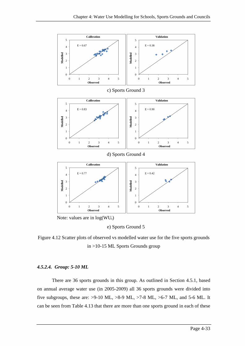
Chapter 4: Water Use Modelling for Schools, Sports Grounds and Councils
Page 4-33
c) Sports Ground 3
d) Sports Ground 4
Note: values are in log(WUt)
e) Sports Ground 5
Figure 4.12 Scatter plots of observed vs modelled water use for the five sports grounds
in >10-15 ML Sports Grounds group
4.5.2.4. Group: 5-10 ML
There are 36 sports grounds in this group. As outlined in Section 4.5.1, based
on annual average water use (in 2005-2009) all 36 sports grounds were divided into
five subgroups, these are: >9-10 ML, >8-9 ML, >7-8 ML, >6-7 ML, and 5-6 ML. It
can be seen from Table 4.13 that there are more than one sports ground in each of these
0
1
2
3
4
5
0 1 2 3 4 5
Mod
elle
d
Observed
Calibration
E = 0.67
0
1
2
3
4
5
0 1 2 3 4 5
Mo
del
led
Observed
Validation
E = 0.38
0
1
2
3
4
5
0 1 2 3 4 5
Mod
elle
d
Observed
Calibration
E = 0.83
0
1
2
3
4
5
0 1 2 3 4 5
Mo
del
led
Observed
Validation
E = 0.90
0
1
2
3
4
5
0 1 2 3 4 5
Mod
elle
d
Observed
Calibration
E = 0.77
0
1
2
3
4
5
0 1 2 3 4 5
Mo
del
led
Observed
Validation
E = 0.42

Chapter 4: Water Use Modelling for Schools, Sports Grounds and Councils
Page 4-34
subgroups and therefore, water use for these subgroups were modelled at individual
group level with multiple sports grounds, as discussed in Section 4.5.1.
From Table 4.13, it can be seen that previous quarter’s water use in terms of
WUt-1, mean maximum daily temperature and water restrictions have statistically
significant effect on current water use in case of all subgroups in this group. Moreover,
previous quarter’s water use in terms of WUt-4 was also found to have effect on current
water use in subgroups >9-10 ML and >8-9 ML. From Table 4.13, it can also be seen
that the coefficient for the mean maximum daily temperature is higher than the
coefficients of other variables used in the models. Therefore, it is clear that the current
water use in this group is adjusted based on the previous quarter’s water use along with
the temperature and the water restrictions levels.
Scatter plots for both calibration and validation periods are presented for all
subgroups in Figure 4.13. E values for both calibration and validation in Table 4.13
also indicates that the models performed well in most of the subgroups.
a) Subgroup >9-10 ML
b) Subgroup >8-9 ML
0
1
2
3
4
5
0 1 2 3 4 5
Mod
elle
d
Observed
Calibration
E = 0.54
0
1
2
3
4
5
0 1 2 3 4 5
Mod
elle
d
Observed
Validation
E = 0.62
0
1
2
3
4
5
0 1 2 3 4 5
Mod
elle
d
Observed
Calibration
E = 0.50
0
1
2
3
4
5
0 1 2 3 4 5
Mod
elle
d
Observed
Validation
E = 0.68

Chapter 4: Water Use Modelling for Schools, Sports Grounds and Councils
Page 4-35
c) Subgroup >7-8 ML
d) Subgroup >6-7 ML
Note: values are in log(WUt)
e) Subgroup 5-6 ML
Figure 4.13 Scatter plots of observed vs modelled water use for the five subgroups in
5-10 ML Sports Grounds group
4.5.2.5. Group: < 5 ML
There are 111 sports grounds customers in this group and all these customers
were classified into five subgroups based on the average annual water use (in 2005-
2009), and model development was performed at individual group level.
0
1
2
3
4
5
0 1 2 3 4 5
Mod
elle
d
Observed
Calibration
E = 0.58
0
1
2
3
4
5
0 1 2 3 4 5
Mod
elle
d
Observed
Validation
E = 0.43
0
1
2
3
4
5
0 1 2 3 4 5
Mod
elle
d
Observed
Calibration
E = 0.63
0
1
2
3
4
5
0 1 2 3 4 5
Mod
elle
d
Observed
Validation
E = 0.33
0
1
2
3
4
5
0 1 2 3 4 5
Mo
del
led
Observed
Calibration
E = 0.47
0
1
2
3
4
5
0 1 2 3 4 5
Mo
del
led
Observed
Validation
E = 0.42

Chapter 4: Water Use Modelling for Schools, Sports Grounds and Councils
Page 4-36
From Table 4.13, it can be observed that previous quarter’s water uses in terms
of WUt-1 have statistically significant contribution on the current water use in all
subgroups. Similar contribution was also found for water restrictions and fixed
quarterly effects for all subgroups except the <1 ML subgroup. It is also apparent that
the coefficient for WUt-1 is higher than the coefficient for the water restrictions and the
dummy variables representing the fixed quarterly effects. Therefore, it is clear that
water use in these less user sports grounds are almost same for each quarter from year
to year, and current water use are also depends on previous quarter’s water uses in
terms of WUt-1 and imposed water restrictions levels.
Scatter plots for both calibration and validation periods are presented for all
subgroups in Figure 4.14. They show that most of the data points are close to 1:1 line.
E values for both calibration and validation in Table 4.13 also indicate that the models
performed well in all subgroups.
a) Subgroup >4-<5 ML
b) Subgroup >3-4 ML
0
1
2
3
4
5
0 1 2 3 4 5
Mod
elle
d
Observed
Calibration
E = 0.56
0
1
2
3
4
5
0 1 2 3 4 5
Mod
elle
d
Observed
Validation
E = 0.52
0
1
2
3
4
5
0 1 2 3 4 5
Mod
elle
d
Observed
Calibration
E = 0.51
0
1
2
3
4
5
0 1 2 3 4 5
Mod
elle
d
Observed
Validation
E = 0.53

Chapter 4: Water Use Modelling for Schools, Sports Grounds and Councils
Page 4-37
c) Subgroup >2-3 ML
d) Subgroup 1-2 ML
Note: values are in log(WUt)
e) Subgroup <1 ML
Figure 4.14 Scatter plots of observed vs modelled water use for the five subgroups in
<5 ML Sports Grounds group
0
1
2
3
4
5
0 1 2 3 4 5
Mod
elle
d
Observed
Calibration
E = 0.54
0
1
2
3
4
5
0 1 2 3 4 5
Mod
elle
d
Observed
Validation
E = 0.33
0
1
2
3
4
5
0 1 2 3 4 5
Mod
elle
d
Observed
Calibration
E = 0.51
0
1
2
3
4
5
0 1 2 3 4 5
Mod
elle
d
Observed
Validation
E = 0.36
0
1
2
3
4
5
0 1 2 3 4 5
Mod
elle
d
Observed
Calibration
E = 0.61
0
1
2
3
4
5
0 1 2 3 4 5
Mod
elle
d
Observed
Validation
E = 0.51

Chapter 4: Water Use Modelling for Schools, Sports Grounds and Councils
Page 4-38
4.6. Water Use Models for Councils
4.6.1. Data Analysis and Disaggregation
There are 1429 customers listed as Councils in the data provided by YVW,
having all quarter’s data for the period of 2005-2011. Different types of organisations
lie in the Councils list such as Library, Community Garden, Club and Office in various
types, Police station, and Aquatic facility. However, the identification of the specific
type of customers was not carried out in this research. From data analysis, it was found
that, the total water use by these 1429 councils is about 4.5% of the total non-
residential water use in YVW in 2011. As outlined in Chapter 3, all these councils
were categorized into several smaller groups based on the average annual water use in
2005-2009. These groups are shown in Table 4.14 along with their contributing
percentages to the total Council’s water use in 2011.
Table 4.14 Disaggregated annual water use of Councils in the YVW service area
Water user groups >20
ML
>15-20
ML
>10-15
ML
5-10
ML
<5
ML Total
Number of councils 4 4 5 27 1269 1429
Water use (%) 10 6 7 16 61 100
From Table 4.14, it is clear that there are 13 councils using more than 10 ML
and contributing 23% to the total Council’s water use in 2011. Therefore, water use in
these 13 councils was modelled at an individual council level.
Similar to the School and Sports Grounds groups, as there are large number of
councils in the 5-10 ML and <5 ML user groups, these two groups were divided into
smaller subgroups based on their average annual water use and shown in Table 4.15
and Table 4.16 respectively. All subgroups in these two groups were modelled at
individual subgroup level with multiple councils.
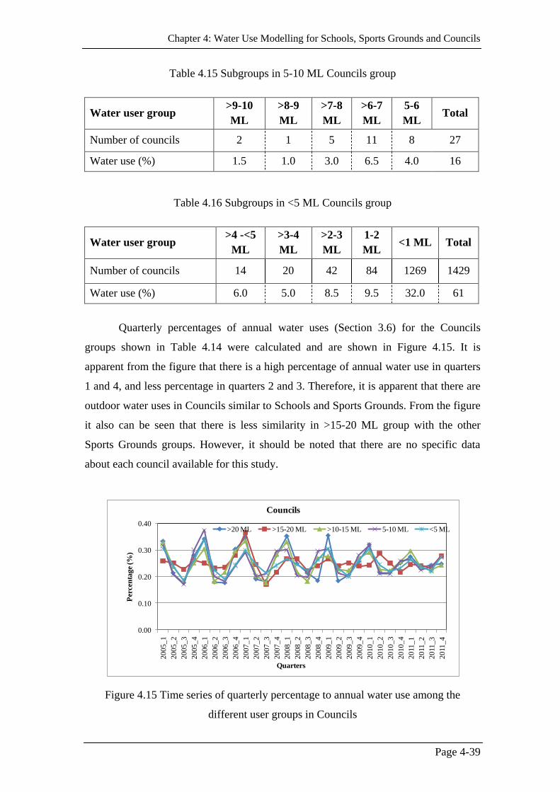
Chapter 4: Water Use Modelling for Schools, Sports Grounds and Councils
Page 4-39
Table 4.15 Subgroups in 5-10 ML Councils group
Water user group >9-10
ML
>8-9
ML
>7-8
ML
>6-7
ML
5-6
ML Total
Number of councils 2 1 5 11 8 27
Water use (%) 1.5 1.0 3.0 6.5 4.0 16
Table 4.16 Subgroups in <5 ML Councils group
Water user group >4 -<5
ML
>3-4
ML
>2-3
ML
1-2
ML <1 ML Total
Number of councils 14 20 42 84 1269 1429
Water use (%) 6.0 5.0 8.5 9.5 32.0 61
Quarterly percentages of annual water uses (Section 3.6) for the Councils
groups shown in Table 4.14 were calculated and are shown in Figure 4.15. It is
apparent from the figure that there is a high percentage of annual water use in quarters
1 and 4, and less percentage in quarters 2 and 3. Therefore, it is apparent that there are
outdoor water uses in Councils similar to Schools and Sports Grounds. From the figure
it also can be seen that there is less similarity in >15-20 ML group with the other
Sports Grounds groups. However, it should be noted that there are no specific data
about each council available for this study.
Figure 4.15 Time series of quarterly percentage to annual water use among the
different user groups in Councils
0.00
0.10
0.20
0.30
0.40
2005_1
2005_2
2005_3
2005_4
2006_1
2006_2
2006_3
2006_4
2007_1
2007_2
2007_3
2007_4
2008_1
2008_2
2008_3
2008_4
2009_1
2009_2
2009_3
2009_4
2010_1
2010_2
2010_3
2010_4
20
11_
1
20
11_
2
20
11_
3
20
11_
4
Per
cen
tag
e (%
)
Quarters
Councils
>20 ML >15-20 ML >10-15 ML 5-10 ML <5 ML

Chapter 4: Water Use Modelling for Schools, Sports Grounds and Councils
Page 4-40
4.6.2. Results and Discussions
Table 4.17 presents the correlation coefficients among the dependent and the
independent variables for all subgroups in the Councils group. Correlation results
between the independent variables for all groups are presented in Appendix C.
From Table 4.17, it is noticeable that there are moderate to high correlations
between the current water use and the previous quarter’s water use in terms of WUt-1
for all subgroups except for Council 4 in >15-20 ML and Council 5 in >10-15 ML
subgroups. Similar correlation was also found with the previous quarter’s water use in
terms of WUt-4 for most of the subgroups. Although, the mean maximum daily
temperature has moderate correlation with the current water use in some subgroups, in
most subgroups this variable has low correlation with the current water use. Remaining
variables used in this study have very low correlations with the current water use in
almost all cases.
From the correlation analysis between the independent variables (Appendix C),
it was found that the correlation coefficients ranged from -0.70 to 0.70 for most of the
groups except for Councils 1 and 3 in >20 ML, Council 4 in 15-20 ML, Council 3 in
>10-15 ML, >8-9 ML and <1 ML subgroups. However, one of the inter-correlated
variables in these councils and subgroups was not found to be significant variable in
the best model as was in the Schools and Sports Grounds groups.
As mentioned in Section 4.4.3, model calibration and validation were
performed for the Councils group using 2006-2010 and 2011 data respectively. The E
values found for the best models in this research are presented in Table 4.18. The
regression coefficients obtained for the best models of different councils subgroups are
also presented in Table 4.18.

Chapter 4: Water Use Modelling for Schools, Sports Grounds and Councils
Page 4-41
Table 4.17 Correlation coefficient between the dependent and independent variables used in all subgroups in the Councils group
Group Modelled by Log10(WUt) Log10(WUt-1) Log10(WUt-4) Log10(T) Log10(Rn) R D2 D3 D4
>20 ML
Individual (Council 1) 1 0.78 a
0.51 b
0.31 0.12 -0.81 a
-0.08 -0.28 0.06
Individual (Council 2) 1 0.63 b
0.15 0.38 b
0.02 -0.23 -0.21 -0.24 0.13
Individual (Council 3) 1 0.40 b
0.49 b
0.63 b
-0.42 b
-0.22 -0.20 -0.44 b
0.03
Individual (Council 4) 1 0.59 b
0.14 0.34 0.17 0.08 -0.18 -0.22 0.19
>15-20 ML
Individual (Council 1) 1 0.62 b
0.28 0.43 b
-0.01 -0.34 -0.17 -0.30 0.11
Individual (Council 2) 1 0.68 a
-0.27 -0.20 -0.46 b
-0.38 b
0.24 0.10 -0.29
Individual (Council 3) 1 0.60 b
-0.35 -0.22 0.19 0.04 0.02 0.14 0.05
Individual (Council 4) 1 0.13 0.73 a
0.70 a
-0.29 0.42 b
-0.01 -0.65 b
0.07
>10-15 ML
Individual (Council 1) 1 0.59 b
0.66 b
0.03 -0.08 -0.69 a
-0.29 0.20 -0.09
Individual (Council 2) 1 0.85 a
0.46 b
0.08 0.36 b
0.47 b
0.04 -0.12 0.06
Individual (Council 3) 1 0.50 b
0.60v 0.53 b
-0.52 b
-0.19 0.08 -0.51 b
-0.04
Individual (Council 4) 1 0.54 b
0.24 -0.01 -0.26 -0.20 -0.01 0.01 0.09
Individual (Council 5) 1 0.13 0.53 b
0.78 a
0.13 0.20 -0.60 b
-0.38 b
0.48 b
>9-10 ML Group 1 0.43 b
0.72 a
0.47 b
-0.14 -0.34 -0.15 -0.40 b
0.17
>8-9 ML Individual 1 0.51 b
0.14 0.05 0.30 -0.63 b
-0.31 0.08 0.15
>7-8 ML Group 1 0.89 a
0.53 b
0.14 -0.09 -0.25 -0.04 -0.09 0.02
>6-7 ML Group 1 0.52 b
0.39 b
0.27 -0.01 -0.12 -0.13 -0.19 0.12
5-6 ML Group 1 0.64 b
0.35 0.32 -0.06 -0.12 -0.11 -0.24 0.11
>4-<5 ML Group 1 0.64 b
0.45 b
0.25 -0.02 -0.20 -0.05 -0.23 0.07
>3-4 ML Group 1 0.73 a
0.47 b
0.20 -0.16 -0.21 -0.05 -0.16 0.02
>2-3 ML Group 1 0.63 b
0.37 b
0.22 -0.08 -0.19 -0.04 -0.20 0.02
1-2 ML Group 1 0.72 a
0.55 b
0.21 -0.11 -0.20 -0.06 -0.16 0.05
<1ML Group 1 0.88 a
0.78 a
0.00 -0.03 -0.09 0.02 -0.01 -0.02

Chapter 4: Water Use Modelling for Schools, Sports Grounds and Councils
Page 4-42
Table 4.18 E values for the best models and estimated regression coefficients for different Councils group models
Councils
Group
Councils
Group
subgroups
Number of
Councils
Modelled by E values
Constant log10(WUt-1) log10(WUt-4) log10(T) log10(Rn) R D2 D3 D4
Calibration Validation (b0) (b1) (b2) (b3) (b4) (b5) (b6) (b7) (b8)
>20 ML - 4
Individual (Council 1) 0.61 0.36 1.01 0.65 (0.00) 0.08 (0.59) - - - - - -
Individual (Council 2) 0.40 0.22 1.55 0.60 (0.01) - - - -0.04 (0.58) - - -
Individual (Council 3) 0.73
(T,Rn,R)
0.75 0.04 - - 6.08 (0.00) -2.00 (0.00) -0.74 (0.02) - - -
Individual (Council 4) 0.43 0.68 1.46 0.56 (0.01) - 0.16 (0.15) - - - - -
>15-20 ML - 4
Individual (Council 1) 0.39 0.22 1.24 0.57 (0.01) 0.09 (0.62) - - - - - -
Individual (Council 2) 0.64 0.99 2.35 0.60 (0.00) - - -0.39 (0.04) -0.18 (0.06) - - -
Individual (Council 3) 0.36 0.25 1.44 0.61 (0.01) - - - - - - -
Individual (Council 4) 0.59 0.18 0.57 0.33 (0.04) - 1.39 (0.00) - - - - -
>10-15 ML - 5
Individual (Council 1) 0.43 0.27 1.18 - 0.66 (0.00) - - - - - -
Individual (Council 2) 0.80 0.97 0.37 0.81 (0.00) - - - 0.38 (0.03) - - -
Individual (Council 3) 0.68
(T,Rn,R)
0.56 2.01 - - 3.98 (0.00) -1.79 (0.30) -0.51 (0.04) - - -
Individual (Council 4) 0.29 0.81 1.57 0.54 (0.01) - - - - - - -
Individual (Council 5) 0.62 0.34 0.39 - - 2.23 (0.00) - - - - -
5-10 ML
>9 -10 ML 2 Group 0.58 0.74 0.89 - 0.76 (0.00) - - -0.19 (0.03) - - -
>8-9 ML 1 Individual 0.34 0.81 1.13 0.50 (0.02) - - 0.24 (0.17) - - - -
>7-8 ML 5 Group 0.80 0.49 -0.32 0.93 (0.00) - 0.43 (0.02) - -0.06 (0.22) - - -
>6-7 ML 11 Group 0.37 0.52 0.08 0.45 (0.00) 0.24 (0.00) 0.67 (0.00) - - - - -
5-6 ML 8 Group 0.49 0.54 -0.88 0.64 (0.00) - 1.47 (0.00) - - - - -
<5 ML
>4-<5 ML 14 Group 0.53 0.67 -0.65 0.58 (0.000 0.21 (0.00) 0.93 (0.00) - - - - -
>3-4 ML 20 Group 0.60 0.71 -1.11 0.68 (0.00) 0.19 (0.00) 1.06 (0.00) - - - - -
>2-3 ML 42 Group 0.47 0.52 -1.09 0.61 (0.00) 0.12 (0.00) 1.35 (0.00) - - - - -
1-2 ML 84 Group 0.60 0.62 -0.68 0.62 (0.00) 0.24 (0.00) 0.74 (0.00)
<1 ML 1269 Group 0.78 0.77 0.16 0.88 (0.00) - - - - - - -
Note: p-value is presented in the parenthesis; bold coefficients are statistically significant at 5% level

Chapter 4: Water Use Modelling for Schools, Sports Grounds and Councils
Page 4-43
4.6.2.1. Group: >20 ML
There are four councils in this group. These councils use 11% of total water use
of the Councils group. Water use was modelled individually for these four councils
(Section 4.6.1).
From Table 4.18, it can be seen that in case of Council 1, E value for
calibration was 0.61, although for validation it was 0.36. The low E value could be due
to changed water use in the validation period. Moreover, it should be noted that as
there are many other factors affects the council’s water use are not available in this
study. Table 4.18 indicates that previous quarter’s water use in terms of WUt-1 and
WUt-4 have important contributions to the current water use of these councils.
Although, WUt-4 was not statistically significant, including this variable improved the
model performance. The scatter plots and the time series plot in Figure 4.16 show that
the modelled water use agrees with the observed water use.
Time series plot
Note: values are in log(WUt)
Scatter plot
Figure 4.16 Observed vs modelled water use for Council 1 in >20 ML Councils group
0
2000
4000
6000
8000
10000
12000
01
/20
06
02
/20
06
03
/20
06
04
/20
06
01
/20
07
02
/20
07
03
/20
07
04
/20
07
01
/20
08
02
/20
08
03
/20
08
04
/20
08
01
/20
09
02
/20
09
03
/20
09
04
/20
09
01
/20
10
02
/20
10
03
/20
10
04
/20
10
01
/20
11
02
/20
11
03
/20
11
04
/20
11
Wate
r u
se (
KL
)
Quarter
Observed Modeled
0
1
2
3
4
5
0 1 2 3 4 5
Mo
del
led
Observed
Calibration
E = 0.61
0
1
2
3
4
5
0 1 2 3 4 5
Mod
elle
d
Observed
Validation
E = 0.36
Validation Calibration

Chapter 4: Water Use Modelling for Schools, Sports Grounds and Councils
Page 4-44
For Council 2, it can be seen from Table 4.18 that the previous quarter’s water
use in terms of WUt-1 and water restrictions have important contributions in modelling
the current water use although water restrictions are not statistically significant. Scatter
plots and the time series plot for Council 2 are shown in Figure 4.17. From the time
series plot, it can be seen that modelled and observed water use are matched well.
Time series plot
Note: values are in log(WUt)
Scatter plot
Figure 4.17 Observed vs modelled water use for Council 2 in >20 ML Councils group
In case of Council 3, it can be seen from Table 4.18 that the mean maximum
daily temperature, the total rainfall and the water restrictions have significant effects on
current water use. The E values in Table 4.18 indicate that the modelled and observed
water use are well matched, which can also be seen from the time series plot and the
scatter plots of calibration and validation, shown in Figure 4.18.
0
2000
4000
6000
8000
10000
12000
14000
01
/20
06
02
/20
06
03
/20
06
04
/20
06
01
/20
07
02
/20
07
03
/20
07
04
/20
07
01
/20
08
02
/20
08
03
/20
08
04
/20
08
01
/20
09
02
/20
09
03
/20
09
04
/20
09
01
/20
10
02
/20
10
03
/20
10
04
/20
10
01
/20
11
02
/20
11
03
/20
11
04
/20
11
Wate
r u
se (
KL
)
Quarter
Observed Modeled
0
1
2
3
4
5
0 1 2 3 4 5
Mo
del
led
Observed
Calibration
E = 0.40
0
1
2
3
4
5
0 1 2 3 4 5
Mod
elle
d
Observed
Validation
E = 0.22
Validation Calibration

Chapter 4: Water Use Modelling for Schools, Sports Grounds and Councils
Page 4-45
Time series plot
Note: values are in log(WUt)
Scatter plot
Figure 4.18 Observed vs modelled water use for Council 3 in >20 ML Councils group
For Council 4, it is clear that the previous quarter’s water use in terms of WUt-4
and the mean maximum daily temperature are the important variables affecting the
current water use. Although, the E value for calibration was little less (0.43) than 0.5,
for validation it was 0.68. The time series plot of observed and modelled water use is
shown in Figure 4.19 along with the scatter plots for both calibration and validation. It
can be seen from the figure that observed and modelled water uses agree well with
each other.
0
5000
10000
15000
20000
25000
30000
35000
40000
01
/20
06
02
/20
06
03
/20
06
04
/20
06
01
/20
07
02
/20
07
03
/20
07
04
/20
07
01
/20
08
02
/20
08
03
/20
08
04
/20
08
01
/20
09
02
/20
09
03
/20
09
04
/20
09
01
/20
10
02
/20
10
03
/20
10
04
/20
10
01
/20
11
02
/20
11
03
/20
11
04
/20
11
Wate
r u
se (
KL
)
Quarter
Observed Modeled
0
1
2
3
4
5
0 1 2 3 4 5
Mo
del
led
Observed
Calibration
E = 0.73
0
1
2
3
4
5
0 1 2 3 4 5
Mod
elle
d
Observed
Validation
E = 0.75
Validation Calibration

Chapter 4: Water Use Modelling for Schools, Sports Grounds and Councils
Page 4-46
Time series plot
Note: values are in log(WUt)
Scatter plot
Figure 4.19 Observed vs modelled water use for Council 4 in >20 ML Councils group
4.6.2.2. Group: >15-20 ML
There are four councils in this group contributing 6% of the total Council’s
water use and these councils were modelled separately. From Table 4.18, it is
observable that the previous quarter’s water use (WUt-1) is the common statistically
significant variable in case of all four councils. However, the other variables such as
the mean maximum daily temperature in Council 4, the total rainfall and the water
restrictions in Council 2 and the previous quarter’s water use (WUt-1) in Council 1
were also included (see Figure 4.1 for model development procedure). The E value for
calibration in Councils 1 and 3 were below 0.5, which could be attributable to the
omission of other influential variables that was not considered in this study due to
unavailability of data. Therefore, a field survey to collect these data and consider them
as additional variables is recommended as a future study to improve the model
performance. Scatter plots for both calibration and validation are shown in Figure 4.20;
shows that observed and modelled water use are well matched as most of the data
points are close to 1:1 line.
0100020003000400050006000700080009000
01
/20
06
02
/20
06
03
/20
06
04
/20
06
01
/20
07
02
/20
07
03
/20
07
04
/20
07
01
/20
08
02
/20
08
03
/20
08
04
/20
08
01
/20
09
02
/20
09
03
/20
09
04
/20
09
01
/20
10
02
/20
10
03
/20
10
04
/20
10
01
/20
11
02
/20
11
03
/20
11
04
/20
11
Wate
r u
se (
KL
)
Quarter
Observed Modeled
0
1
2
3
4
5
0 1 2 3 4 5
Mod
elle
d
Observed
Calibration
E = 0.43
0
1
2
3
4
5
0 1 2 3 4 5
Mod
elle
d
Observed
Validation
E = 0.68
Validation Calibration

Chapter 4: Water Use Modelling for Schools, Sports Grounds and Councils
Page 4-47
a) Council 1
b) Council 2
c) Council 3
Note: values are in log(WUt)
d) Council 4
Figure 4.20 Scatter plots of observed vs modelled water use for the four councils in
>15-20 ML Councils group
0
1
2
3
4
5
0 1 2 3 4 5
Mod
elle
d
Observed
Calibration
E = 0.39
0
1
2
3
4
5
0 1 2 3 4 5
Mo
del
led
Observed
Validation
E = 0.22
0
1
2
3
4
5
0 1 2 3 4 5
Mod
elle
d
Observed
Calibration
E = 0.64
0
1
2
3
4
5
0 1 2 3 4 5
Mo
del
led
Observed
Validation
E = 0.99
0
1
2
3
4
5
0 1 2 3 4 5
Mod
elle
d
Observed
Calibration
E = 0.36
0
1
2
3
4
5
0 1 2 3 4 5
Mo
del
led
Observed
Validation
E = 0.25
0
1
2
3
4
5
0 1 2 3 4 5
Mod
elle
d
Observed
Calibration
E = 0.59
0
1
2
3
4
5
0 1 2 3 4 5
Mo
del
led
Observed
Validation
E = 0.18

Chapter 4: Water Use Modelling for Schools, Sports Grounds and Councils
Page 4-48
4.6.2.3. Group: >10-15 ML
There are five councils in this group and they were modelled individually.
From Table 4.18, it is apparent that the previous quarter’s water uses (WUt-1 and WUt-
4) have statistically significant effect on current water use in Councils 1, 2 and 4. In
case of Council 2, the water restrictions found to be statistically significant.
In case of Council 3, it was found that the mean maximum daily temperature,
the total rainfall and the water restrictions have significant contributions on the current
water use. In case of Council 5, the mean maximum daily temperature was found to
have statistically significant contribution on the current water use. Based on these
results, it can be concluded that these two councils might have outdoor water use.
Scatter plots of calibration and validation for all five councils are shown in
Figure 4.21. It can be seen that data points are close to the 1:1 line, which show that
that the modelled water use is matched well with the observed water use.
a) Council 1
b) Council 2
0
1
2
3
4
5
0 1 2 3 4 5
Mod
elle
d
Observed
Calibration
E = 0.43
0
1
2
3
4
5
0 1 2 3 4 5
Mo
del
led
Observed
Validation
E = 0.27
0
1
2
3
4
5
0 1 2 3 4 5
Mod
elle
d
Observed
Calibration
E = 0.80
0
1
2
3
4
5
0 1 2 3 4 5
Mo
del
led
Observed
Validation
E = 0.97

Chapter 4: Water Use Modelling for Schools, Sports Grounds and Councils
Page 4-49
c) Council 3
d) Council 4
Note: values are in log(WUt)
e) Council 5
Figure 4.21 Scatter plots of observed vs modelled water use for the five councils in
>10-15 ML Councils group
4.6.2.4. Group: 5-10ML
There are five subgroups in this Councils group. From Table 4.18, it can be
seen that within each subgroup there are multiple councils except in case of >8-9 ML
subgroup. From the table, it can also be seen that previous quarter’s water use in terms
of WUt-1 and, WUt-4 have statistically significant impact on the current water use in all
subgroups. The mean maximum daily temperature also found to have statistically
0
1
2
3
4
5
0 1 2 3 4 5
Mod
elle
d
Observed
Calibration
E = 0.68
0
1
2
3
4
5
0 1 2 3 4 5
Mo
del
led
Observed
Validation
E = 0.56
0
1
2
3
4
5
0 1 2 3 4 5
Mod
elle
d
Observed
Calibration
E = 0.29
0
1
2
3
4
5
0 1 2 3 4 5
Mo
del
led
Observed
Validation
E = 0.81
0
1
2
3
4
5
0 1 2 3 4 5
Mod
elle
d
Observed
Calibration
E = 0.62
0
1
2
3
4
5
0 1 2 3 4 5
Mo
del
led
Observed
Validation
E = 0.34

Chapter 4: Water Use Modelling for Schools, Sports Grounds and Councils
Page 4-50
significant contribution on the current water use in case of >7-8 ML, >6-7 ML and 5-6
ML subgroups. Although, the total rainfall in >8-9 ML subgroup and water restrictions
in >9-10 ML and >7-8 ML subgroups are found to have some effect, the coefficients of
these variable are very small.
Scatter plots of calibration and validation for all five subgroups are shown in
Figure 4.22. This figure shows that the modelled water use is well matched with the
observed water use as data points lie close to the 1:1 line and E values was also found
to have more than 0.5 in most cases (Table 4.18).
a) Subgroup >9-10 ML
b) Subgroup >8-9 ML
c) Subgroup >7-8 ML
0
1
2
3
4
5
0 1 2 3 4 5
Mo
del
led
Observed
Calibration
E = 0.58
0
1
2
3
4
5
0 1 2 3 4 5
Mo
del
led
Observed
Validation
E = 0.74
0
1
2
3
4
5
0 1 2 3 4 5
Mo
del
led
Observed
Calibration
E = 0.34
0
1
2
3
4
5
0 1 2 3 4 5
Mo
del
led
Observed
Validation
E = 0.81
0
1
2
3
4
5
0 1 2 3 4 5
Mod
elle
d
Observed
Calibration
E = 0.80
0
1
2
3
4
5
0 1 2 3 4 5
Mo
del
led
Observed
Validation
E = 0.49

Chapter 4: Water Use Modelling for Schools, Sports Grounds and Councils
Page 4-51
d) Subgroup >6-7 ML
Note: values are in log(WUt)
e) Subgroup 5-6 ML
Figure 4.22 Scatter plots of observed vs modelled water use for the five subgroups in
5-10 ML Councils group
4.6.2.5. Group: <5 ML
There are 1269 customers in this Councils group and all customers were
classified into five subgroups based on the average annual water use (in 2005-2009),
and models were developed at individual group level.
From Table 4.18, it can be observed that the previous quarter’s water uses in
terms of both WUt-1 and WUt-4 and the mean maximum daily temperature have
statistically significant contributions on the current water use in all subgroups except in
<1 ML subgroup. In case of <1 ML subgroup, the previous quarter’s water uses in
terms of WUt-1 was found to have significant effect on the current water use.
Therefore, it can be said that in this less water user subgroups, current water use are
adjusted based on previous quarter’s water use and temperature.
0
1
2
3
4
5
0 1 2 3 4 5
Mo
del
led
Observed
Calibration
E = 0.37
0
1
2
3
4
5
0 1 2 3 4 5
Mod
elle
d
Observed
Validation
E = 0.52
0
1
2
3
4
5
0 1 2 3 4 5
Mod
elle
d
Observed
Calibration
E = 0.49
0
1
2
3
4
5
0 1 2 3 4 5
Mo
del
led
Observed
Validation
E = 0.54

Chapter 4: Water Use Modelling for Schools, Sports Grounds and Councils
Page 4-52
Scatter plots for both calibration and validation periods presented for all
subgroups in Figure 4.23 show that most of the data points are close to 1:1 line.
Moreover, E values for both calibration and validation in Table 4.18 also indicate that
models performed well in all subgroups.
a) Subgroup >4-<5 ML
b) Subgroup >3-4 ML
c) Subgroup >2-3 ML
0
1
2
3
4
5
0 1 2 3 4 5
Mod
elle
d
Observed
Calibration
E = 0.53
0
1
2
3
4
5
0 1 2 3 4 5
Mod
elle
d
Observed
Validation
E = 0.67
0
1
2
3
4
5
0 1 2 3 4 5
Mod
elle
d
Observed
Calibration
E = 0.60
0
1
2
3
4
5
0 1 2 3 4 5
Mod
elle
d
Observed
Validation
E = 0.71
0
1
2
3
4
5
0 1 2 3 4 5
Mod
elle
d
Observed
Calibration
E = 0.47
0
1
2
3
4
5
0 1 2 3 4 5
Mod
elle
d
Observed
Validation
E = 0.52

Chapter 4: Water Use Modelling for Schools, Sports Grounds and Councils
Page 4-53
d) Subgroup 1-2 ML
Note: values are in log(WUt)
e) Subgroup <1 ML
Figure 4.23 Scatter plots of observed vs modelled water use for the five subgroups in
<5 ML Councils group
4.7. Models Applications, Limitations and Challenges
Modelling performed for Schools, Sports Grounds and Councils groups using a
single approach are able to provide individual water demand forecasting for the
customers are presented in this chapter. This individual forecasting will be useful for
considering different conservation efforts for different customer group and for different
geographic area. The modelling approach used are also useful in case of water demand
estimation at distribution zone level as models are able to forecast individual
customer’s water use.
All the models in this chapter were developed with the available data (i.e.
rainfall, mean maximum temperature and water restrictions level. However, there are
many other factors affect the water use among the customers, such as:
0
1
2
3
4
5
0 1 2 3 4 5
Mod
elle
d
Observed
Calibration
E = 0.60
0
1
2
3
4
5
0 1 2 3 4 5
Mod
elle
d
Observed
Validation
E = 0.62
0
1
2
3
4
5
0 1 2 3 4 5
Mod
elle
d
Observed
Calibration
E = 0.78
0
1
2
3
4
5
0 1 2 3 4 5
Mod
elle
d
Observed
Validation
E = 0.77

Chapter 4: Water Use Modelling for Schools, Sports Grounds and Councils
Page 4-54
Factors affecting water use at Schools
1) number of students, teachers and staff, 2) size and layout of school grounds
swimming pool, 3) availability of alternate water source, 4) garden watering
time/irrigation practices, 5) gardening practices (e.g. mulching, soil preparation, soil-
wetting agents), 6) water wise garden design (using native plants), 7) presence of
evaporative air conditioners, 8) water-efficient appliances (e.g. dual-flush toilets, flow
regulators in taps and showers), 9) behavioural practices (e.g. reporting and fixing
leaking taps), 10) type of specialised classes (e.g. gymnasium, home economics,
hairdressing, bricklaying), 11) cleaning practices, and 12) use of school facilities after
hours (community group meetings/weekend sports).
Factors affecting water use at Sports Grounds
1) size of the sports ground, 2) availability of alternate water source, 3)
watering time/irrigation practices, 4) type of grass, and 5) Activity taking places in the
sports ground (e.g. golf, football, cricket)
Factors affecting water use at Councils
1) number of employee, customers or participants, 2) Presence of garden and
swimming pool, 3) availability of alternate water source, 4) efficiency of water use
appliances 5) garden watering time/irrigation practices, 6) gardening practices (e.g.
mulching, soil preparation), and 7) occurrence of community and other festival.
Difficulty in accessing these information, limits the water use modelling in this
research to explain the water use variation precisely. Moreover, some of these factors,
such as the level of awareness of users are difficult to quantify. Therefore, water
demand forecasting among these groups can be improved by conducting field survey.
4.8. Summary
Modelling water use was performed for Schools, Sports Grounds and Councils
groups using a single approach as similar water use pattern was observed in these three
groups.

Chapter 4: Water Use Modelling for Schools, Sports Grounds and Councils
Page 4-55
Past modelling work on total urban water use has shown that a number of
independent variables such as previous water use, different levels of water restrictions,
and climate variables such as rainfall and temperature have some effects on the water
use pattern. In addition, data analysis in the current study revealed that water uses in
these groups are affected by seasonal cycle over the year. Therefore, the past water use
in terms of (t-1) and (t-4) time-lagged, level of water restrictions, climate variables
such as total rainfall and mean maximum daily temperature, and fixed quarterly effects
were used as the independent variables during model development in this research.
The Multiple Linear Regressions (MLR) technique was used in this research for
model development of water use in Schools, Sports Grounds and Councils groups. At
first all customers in these groups are disaggregated into subgroups based on the
average annual water use. Then, before the model development, data transformation
was done in order to make the data normally distributed for both independent and
dependent variables using a log function. A correlation analysis was also carried out
separately for each water users groups to investigate the degree of correlation among
the dependent and independent variables, which has given an early indication of which
variables may play significant role in model development. Moreover, the correlation
analysis between the independent variables was performed to check whether there is
any multi co-linearity effect between the independent variables. It was found that the
independent variables are not correlated each other for most of the cases. In those
exceptional cases where variables found to be inter-correlated, one of the variables was
not used in best model.
Model calibration for Schools was performed using two different periods:
2005-2009 and 2005-2010 to see whether increasing calibration periods produce better
results. At the same time models were also validated with the data of 2010-2011 and
2011 respectively. The Model performance was measured by the Nash-Sutcliffe
efficiency (E) and the significance test for model parameters was done using the p
value. It was found that increasing data period during calibration results better E values
in most of the Schools subgroups. Therefore, models developed with the calibration
period of 2005-2010 were discussed and followed for models development in case of
other two groups (Sports Grounds and Councils) in this Chapter.

Chapter 4: Water Use Modelling for Schools, Sports Grounds and Councils
Page 4-56
Based on the water use analysis, it was found that different customers use
different amount of water ranging from >20 ML to <1 ML. It was also found that only
few customers use large amount of water (e.g. >20 ML and >15-20 ML), whereas a
large number of customers use smaller volume of water (e.g. 5-10 ML and <5 ML).
Therefore, higher water use customers are modelled as an individual customer,
whereas the smaller water use customers are modelled at group level in this study.
Among the independent variables considered in this study, it was found that
mean maximum daily temperature, total rainfall and water use restrictions have
significant effect on current water use of high water users Schools (e.g. >10 ML),
where as in low water users Schools, past water use in terms of (t-1) and (t-4) has
significant effect on current water use. Therefore, it implies that high water user
Schools have more outdoor activities than the low water user Schools, could be due to
more play grounds and gardens.
In case of Sports Grounds, water use restrictions was found to have significant
effect on current water use of both high water users (e.g. >10 ML) and low water users
(e.g. <10 ML) as was expected due to outdoor water use. Moreover, it was found that
mean maximum daily temperature has significant effects on current water use of high
water users Sports Grounds and past water use in terms of (t-1) has significant effects
on current water use of low water users Sports Grounds.
The past water use in terms of (t-1) in Councils has significant effects on
current water use. Moreover, unlike Schools and Sports Grounds, different variables
were found to have significant effect on current water use of Councils regardless of
high and low users, which were also expected as there are different types of
organization exist in the Councils group.
In general, comparison of observed against modelled water use shown in time
series and scatter plots are well matched, and also high E values were found in most
models, implies that the developed model are performed well. It was found that few
cases E values were poor for validation with compare to the calibration although
observed and modelled data lies close to 1:1 line in the scatter plot. This poor model

Chapter 4: Water Use Modelling for Schools, Sports Grounds and Councils
Page 4-57
performance might be due to omission of some important independent variables due to
lack of data availability.

Chapter 5: Water Use Modelling for Restaurants, Hospitals, Hotels and Laundries
Page 5-1
Chapter 5. Water Use Modelling for Restaurants,
Hospitals, Hotels and Laundries
5.1. Overview
Generally, water use in restaurants, hospitals, hotels and laundries has no
seasonal variation as most of the water uses among these groups are for indoor
purposes (Chapter 3, Section 3.6). There are many factors affect the water use in these
groups (i.e. opening hours for restaurants, number of beds in hospitals, number of
rooms in hotels, and number of customers and frequency of use in laundries), data for
these factors are not readily available as was the case in this study. Therefore, as
mentioned in Chapter 3, water use modelling was done for these four groups
differently from the Schools, Sports Grounds and Councils groups and only historical
water use data were used for analysis and forecasting. The details of this work is
presented in this Chapter.
As mentioned in Chapter 1, short term water demand forecasting (1 year) was
carried out using quarterly time steps in this research. Disaggregation of water users
for each customer group was done first based on the average historical water use
volume. Thereafter, data analysis was performed at disaggregated level for all four
customer groups.
Historical quarterly water use data from 2005 to 2010 were used for analysing
purpose and then quarterly water use in 2011 were forecasted in this study. From data
analysis, there were three different patterns were identified in historical annual water
use and those are:
1) The annual water uses were variable over the period (2005-2010).

Chapter 5: Water Use Modelling for Restaurants, Hospitals, Hotels and Laundries
Page 5-2
2) The annual water uses were constant over the very recent period (2008-
2010) or over the period (2005-2010). and
3) The annual water use followed an increasing or decreasing trend.
Based on the historical annual water use pattern, forecast annual water uses in
2011 were forecast differently. In type 1, annual water use in 2010; in type 2, average
annual water use in 2008-2010; and in type 3, a linear regression model were
considered to forecast annual water use in 2011.
Thereafter, forecast annual water uses were disaggregated into quarterly water
uses in 2011 based on the quarterly water use disaggregating factors obtained from
data analysis. From the data analysis, it was found that most of the customers among
Restaurants, Hospitals, Hotels and Laundries groups follow consistent quarterly
percentages of annual water use over years (2005-2010). However, there were very
few years when quarterly water use percentages were different from the other years.
Therefore, the average quarterly water use percentages were considered as the
quarterly disaggregating factors excluding those exceptional years in this study. As
outlined in Chapter 3 (Section 3.5.1) the quarters are named as Quarter 1 (January –
March), Quarter 2 (April – June), Quarter 3 (July – September) and Quarter 4 (October
– December).
This chapter first describes the data exploration includes analysis of historical
water use and disaggregation of water user. The water use models developed at
disaggregated level for Restaurants, Hospitals, Hotels and Laundries groups is then
presented followed by issues and limitations of the modelling work performed for
these water user groups. Finally, a summary of the chapter is presented.

Chapter 5: Water Use Modelling for Restaurants, Hospitals, Hotels and Laundries
Page 5-3
5.2. Data Exploration
5.2.1. Historical Water Use
Annual water use variation in Restaurants, Hospitals, Hotels and Laundries
customer groups over the study period (2005-2011) is shown in Figure 5.1. From
Figure 5.1, it can be seen that the annual water use in 2005 and 2006 was almost the
same in each of all four customer groups. In general, since 2006, water use in
Restaurants and Hospitals has decreased, and water use in Hotels and Laundries was
less variable.
There are many factors that could be attributable to the abovementioned
changes in water use among all four customer groups. For example, the presence,
diversity and efficiency of various types of appliances in hotels, restaurants, hospitals
and laundries that affect the quantity of water used (Dziegielewski, et al, 2000).
Furthermore, the activity in one customer group could affect the water use in another
customer group. For example, the number of guests in hotels and restaurants, and the
number of patients in hospitals could affect the water use in laundries, and the number
of guests in hotels can affect the water use in restaurants. However, it should be noted
that these are general comments and have not been validated for the current study due
to limited data.
Figure 5.1 Annual water uses of Restaurants, Hospitals, Hotels, and Laundries over the
study period
0
300
600
900
1200
0
40
80
120
160
20
05
20
06
20
07
20
08
20
09
20
10
20
11 Res
tau
ran
ts W
ate
r U
se (
ML
)
Hosp
itals
, H
ote
ls a
nd
Lau
nd
ries
Wate
r U
se (
ML
)
Year
Hospitals Hotels Laundries Restauants

Chapter 5: Water Use Modelling for Restaurants, Hospitals, Hotels and Laundries
Page 5-4
5.2.2. Disaggregation of Water User Groups
Water uses in Restaurants, Hospitals, Hotels and Laundries accounts for 4.6%,
0.5%, 0.7%, and 0.8% of total non-residential water use in 2011 respectively in the
Yarra Valley Water (YVW) service area (Chapter 3, Section 3.6). As discussed in
Section 3.6, all customers within Restaurants, Hospitals, Hotels and Laundries were
classified into five groups based on the average annual water use in 2005-2009 as
shown in Table 5.1. Water use models were then developed at these disaggregated
levels in this research. It should be noted that some pathologies were also classified as
hospitals in the YVW customer list. All the pathologies were considered as a separate
group within the Hospitals in this study as their water use pattern could be different
from hospitals although they are in the same list.
From Table 5.1, it is apparent that there is no hotel and laundry using average
annual water use more than 20 ML. It can also be seen that most of the customers
among all these water customer groups are low water users (<5 ML group), and they
use higher percentages of the total water except in Hospitals. However, the >20 ML
Hospitals group’s water use was high which was around 32% of total Hospital water
use.

Chapter 5: Model Development for Restaurants, Hospitals, Hotels and Laundries
Page 5-5
Table 5.1 Disaggregation of water users of Restaurants, Hospitals, Hotels and Laundries in the YVW service area
Water user
groups
Restaurants Hospitals Hotels Laundries
Number of
restaurants
Water use
(%)
Number of
hospitals
Water use
(%)
Number of
hotels
Water use
(%)
Number of
laundries Water use (%)
>20 ML 1 3.0 1 26.5 - - - -
>15-20 ML 1 1.9 - - - - 1 22.8
>10-15 ML 4 4.0 2 21.4 2 15.6 - -
5-10 ML 26 17.4 2 12.1 4 21.6 2 9.2
<5 ML 1031 73.7 4 5.3 38 62.8 124 68
Healthscope - - 5 34.7 - - - -
Total 1063 100 14 100 44 100 127 100

Chapter 5: Model Development for Restaurants, Hospitals, Hotels and Laundries
Page 5-6
5.3. Model Development
There are many factors that affect the water use in Restaurants, Hospitals,
Hotels and Laundries groups such as the number of meals served by restaurants, the
number of rooms in a hotel, the number of bed in hospitals and the number of
customers for a laundry. However, these details data are not available for this research
as mentioned in Section 5.1. Moreover, water uses among these groups are mostly for
indoor purposes. Therefore, weather and water restrictions data that were used for
water use model development for Schools, Sport Grounds and Councils groups were
not considered in modelling water use for the Restaurants, Hospitals, Hotels and
Laundries groups. Model development for these groups in this chapter was performed
with only historical water use data.
Data period used is 2005 -2011 for model development in this part of the study.
As outlined in Chapter 4 (in Section 4.4.3), the water use data in 2005-2010 were used
to determine the quarterly water use pattern and also for model development to forecast
quarterly water use in 2011. The water use data in 2011 were used for the comparison
of the forecast and observed water use. All the model performance was measured using
the Nash-Sutcliffe model efficiency (E). The details of this efficiency criterion can be
found in Chapter 4 (Section 4.3.4). Further details on the water use data analysis and
model development for each customer group are discussed in the following sections.
5.3.1. Data Analysis and Model Development for Restaurants
5.3.1.1. Data Analysis
Total water use of the Restaurants group is about 4.6% of the total non-
residential water use in 2011 in the study area. There are 1,063 restaurants within the
study area. All these restaurants are grouped into different groups based on the annual
water use, as discussed in Section 5.2.2 and data analysis were then performed
separately for these groups.

Chapter 5: Model Development for Restaurants, Hospitals, Hotels and Laundries
Page 5-7
a. Group: >20 ML
There is one restaurant in this group with 3% of water use of the total
Restaurants water use in 2011. The time series of annual water use data of this
restaurant is shown in Figure 5.2 along with the quarterly percentages of water use in
each year. It can be seen from this figure that the annual water use in this restaurant is
highly variable. From Figure 5.2, it can also be seen that the percentage of quarterly
water use pattern was quite similar in most of the years except in 2005 and 2007.
Figure 5.2 Water use pattern of >20 ML Restaurants group
b. Group: >15-20 ML
There is one restaurant in this group with 1.9% of water use of the total
Restaurants water use in 2011. The time series of annual water use data and quarterly
percentages of water use in each year for this restaurant is shown in Figure 5.3. It can
be seen from the figure that although there is decreasing trend in water use from 2005
to 2009, water use in 2008-2010 were fairly constant and close to 15 ML. From Figure
5.3, it can also be seen that the quarterly water use pattern was different in 2009 but it
was fairly consistent in the remaining years.
0
5
10
15
20
25
30
35
1 2 3 4
Qu
art
erly
Per
cen
tage
Quarters
2005
2006
2007
2008
2009
2010
2011
0
10000
20000
30000
40000
20
05
20
06
20
07
20
08
20
09
20
10
20
11
Wate
r U
se (
KL
)
Years

Chapter 5: Model Development for Restaurants, Hospitals, Hotels and Laundries
Page 5-8
Figure 5.3 Water use pattern of >15-20 ML Restaurants group
c. Group: >10-15 ML
There are four restaurants in this group with 4% of water use of the total
Restaurants water use in 2011. As this is a high percentage of water use within this
group, all four restaurants were analysed separately. The time series of the annual
water use data and the percentage of quarterly water use in each year for all these four
restaurants are shown in Figure 5.4. From the figure, it can be seen that there was a
huge reduction in Restaurant 1 water use since 2006. In case of Restaurant 2, the
annual water use decreased from 2006-2009 and it was constant in 2009-2010. In case
of Restaurant 3, the annual water use was fairly constant over the years. The annual
water use in Restaurant 4 was moderately varied and in 2006-2009, it was fairly
constant before an increase in 2010. From Figure 5.4, it can also be seen that the
quarterly water use patterns for Restaurants 2, 3 and 4 are reasonably consistent over
the years except the percentages for Restaurant 4 in 2007. It was also found that the
quarterly water use pattern of the Restaurant 1 was not consistent over the years.
0
5
10
15
20
25
30
35
1 2 3 4
Qu
art
erly
Per
cen
tag
e
Quarters
2005
2006
2007
2008
2009
2010
2011
0
10000
20000
30000
20
05
20
06
20
07
20
08
20
09
20
10
2011
Wate
r U
se (
KL
)
Years

Chapter 5: Model Development for Restaurants, Hospitals, Hotels and Laundries
Page 5-9
Figure 5.4 Water use pattern of >10-15 ML Restaurants group
0
10
20
30
40
50
60
1 2 3 4
Qu
art
erly
Per
cen
tag
e
Quarters
Restaurant-1
2005
2006
2007
2008
2009
2010
2011
0
10000
20000
30000
40000
50000
20
05
20
06
20
07
20
08
20
09
20
10
20
11
Wa
ter
Use
(K
L)
Years
Restaurant-1
0
5
10
15
20
25
30
35
1 2 3 4
Qu
art
erly
Per
cen
tag
e
Quarters
Restaurant-2
2005
2006
2007
2008
2009
2010
2011
0
10000
20000
20
05
20
06
20
07
20
08
20
09
20
10
20
11
Wa
ter
Use
(K
L)
Years
Restaurant-2
0
5
10
15
20
25
30
35
1 2 3 4
Qu
art
erly
Per
cen
tage
Quarters
Restaurant-3
2005
2006
2007
2008
2009
2010
2011
0
10000
20000
20
05
20
06
20
07
20
08
20
09
20
10
20
11
Wate
r U
se (
KL
)
Years
Restaurant-3
05
10152025303540
1 2 3 4
Qu
art
erly
Per
cen
tag
e
Quarters
Restaurant-4
2005
2006
2007
2008
2009
2010
2011
0
10000
20000
20
05
20
06
20
07
20
08
20
09
20
10
20
11
Wa
ter
Use
(K
L)
Years
Restaurant-4

Chapter 5: Model Development for Restaurants, Hospitals, Hotels and Laundries
Page 5-10
d. Group: 5-10 ML
There are 26 restaurants in this group using 17.4% of the total Restaurants
water use in 2011. All these 26 restaurants were divided into five smaller subgroups
based on the average annual water use from 2005 to 2009. These subgroups with their
water use percentages within the Restaurant group and the numbers of restaurants in
each subgroup are shown in Table 5.2. The annual water use by each restaurant
subgroup is presented in the left hand charts in Figure 5.5. It should be noted that the
average annual water use by the subgroup was calculated and shown with the bold
black line in the same chart. The average quarterly percentages of water use by each
subgroup were calculated for each year and are also shown in Figure 5.5. From Figure
5.5, it can be seen that in the subgroups 5-6 ML and >6-7 ML, the water use of one
restaurant is quite different from the other restaurants. Therefore, the specific
restaurants were not included in calculating the average water use in these two
subgroups.
From Figure 5.5, it is apparent that although there was water use reduction over
the years in all subgroups, the average annual water uses in 2008-2010 were fairly
constant. From the figure it is also can be seen that quarterly percentages of the annual
water use in subgroups >8-9 ML, >6-7 ML and 5-6 ML were consistent over the years.
However, in subgroup >7-8 ML, the quarterly percentages of 2006 and 2010 were
different from the percentages of other years and in subgroup >9-10 ML the quarterly
percentages of 2010 were different from the percentages in other years.
Table 5.2 Water use percentage among Restaurants subgroups in 5-10 ML group
Subgroup Number of Restaurants Water use (%) in
Restaurants group
>9-10 ML 6 5.2
>8-9 ML 3 2.5
>7-8 ML 3 2.2
>6-7 ML 5 2.7
5-6 ML 9 4.8
Total 26 17.4

Chapter 5: Model Development for Restaurants, Hospitals, Hotels and Laundries
Page 5-11
Figure 5.5 Water use pattern of 5-10 ML Restaurants group
0
5
10
15
20
25
30
35
1 2 3 4
Qu
art
erly
Per
cen
tag
e
Quarters
Subgroup: >9-10 ML
2005
2006
2007
2008
2009
2010
2011
0
5000
10000
15000
20
05
20
06
20
07
20
08
20
09
20
10
20
11
Wa
ter
Use
(K
L)
Year
Subgroup: >9-10 ML
0
5
10
15
20
25
30
1 2 3 4
Qu
art
erly
Per
cen
tag
e
Quarters
Subgroup: >8-9 ML
2005
2006
2007
2008
2009
2010
2011
0
5000
10000
15000
20
05
20
06
20
07
20
08
20
09
20
10
20
11
Wa
ter
Use
(K
L)
Year
Subgroup: >8-9 ML
0
5
10
15
20
25
30
35
1 2 3 4
Qu
art
erly
Per
cen
tag
e
Quarters
Subgroup: >7-8 ML
2005
2006
2007
2008
2009
2010
2011
0
5000
10000
15000
20
05
20
06
20
07
20
08
20
09
20
10
20
11
Wa
ter
Use
(K
L)
Year
Subgroup: >7-8 ML
0
5
10
15
20
25
30
1 2 3 4
Qu
art
erly
Per
cen
tag
e
Quarters
Subgroup: >6-7 ML
2005
2006
2007
2008
2009
2010
2011
0
5000
10000
15000
20
05
20
06
20
07
20
08
20
09
20
10
20
11
Wa
ter
Use
(K
L)
Year
Subgroup: >6-7 ML
0
5
10
15
20
25
30
1 2 3 4
Qu
arte
rly
Percen
tag
e
Quarters
Subgroup: 5-6 ML
2005
2006
2007
2008
2009
2010
2011
0
5000
10000
15000
20
05
20
06
20
07
20
08
20
09
20
10
2011
Wate
r U
se (
KL
)
Year
Subgroup: 5-6 ML

Chapter 5: Model Development for Restaurants, Hospitals, Hotels and Laundries
Page 5-12
e. Group: <5 ML
There are 1,031 restaurants in this group using 73.7% of the total Restaurants
water use in 2011. All these 1031 restaurants were divided into five smaller subgroups
based on the average annual water use from 2005 to 2009. These subgroups with their
water use percentages and the numbers of restaurants in each subgroup are shown in
Table 5.3. Similar to Figure 5.5, the annual water use by each restaurant is presented in
Figure 5.6. It should be noted that the average yearly water use by the subgroup was
calculated and shown with the bold black line in the same chart. The average quarterly
percentages of water use by each subgroup were calculated for each year and also
shown in Figure 5.6 as well. It should be noted that there is a restaurant having very
high water use in 2010 and 2011 in the subgroup >4-<5 ML and this particular
restaurant was not included in calculating the average annual water use. From Figure
5.6, it can also be seen that the average annual water use by each subgroups are
constant over the years and the quarterly percentages of the average annual water use
by each subgroup are consistent over the years.
Table 5.3 Water use percentage among Restaurants subgroups in <5 ML group
Subgroup Number of
Restaurants
Water use (%) in
Restaurants group
>4-<5 ML 13 6.8
>3-4 ML 21 7.5
>2-3 ML 47 11.0
1-2 ML 132 19.4
<1 ML 818 29.0
Total 1,031 73.7
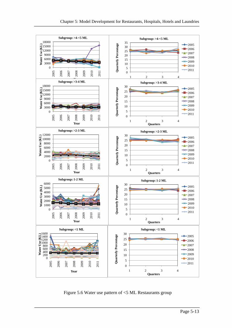
Chapter 5: Model Development for Restaurants, Hospitals, Hotels and Laundries
Page 5-13
Figure 5.6 Water use pattern of <5 ML Restaurants group
0
5
10
15
20
25
30
35
1 2 3 4
Qu
art
erly
Per
cen
tag
e
Quarters
Subgroup: >4-<5 ML
2005
2006
2007
2008
2009
2010
20110
3000
6000
9000
12000
15000
18000
20
05
20
06
20
07
20
08
20
09
20
10
20
11
Wa
ter
Use
(K
L)
Year
Subgroup: >4-<5 ML
0
5
10
15
20
25
30
1 2 3 4
Qu
art
erly
Per
cen
tag
e
Quarters
Subgroup: >3-4 ML
2005
2006
2007
2008
2009
2010
20110
3000
6000
9000
12000
15000
18000
20
05
20
06
20
07
20
08
20
09
20
10
20
11
Wa
ter
Use
(K
L)
Year
Subgroup: >3-4 ML
0
5
10
15
20
25
30
1 2 3 4
Qu
art
erly
Per
cen
tag
e
Quarters
Subgroup: >2-3 ML
2005
2006
2007
2008
2009
2010
20110
2000
4000
6000
8000
10000
12000
20
05
20
06
20
07
20
08
20
09
20
10
20
11
Wate
r U
se (
KL
)
Year
Subgroup: >2-3 ML
0
5
10
15
20
25
30
1 2 3 4
Qu
art
erly
Per
cen
tag
e
Quarters
Subgroup: 1-2 ML
2005
2006
2007
2008
2009
2010
20110
1000
2000
3000
4000
5000
6000
20
05
20
06
20
07
20
08
20
09
20
10
20
11
Wa
ter
Use
(K
L)
Year
Subgroup: 1-2 ML
0
5
10
15
20
25
30
1 2 3 4
Qu
art
erly
Per
cen
tag
e
Quarters
Subgroup: <1 ML
2005
2006
2007
2008
2009
2010
2011
0200400600800
1000120014001600
2005
2006
2007
2008
2009
2010
2011
Wate
r U
se (
KL
)
Year
Subgroup: <1 ML

Chapter 5: Model Development for Restaurants, Hospitals, Hotels and Laundries
Page 5-14
f. Summary of Data Analysis
A summary of the findings of the above water use data analysis is presented in
Table 5.4. Based on this analysis, the approach used for modelling (or forecasting) the
annual water use in 2011 and the disaggregating factors to disaggregate the annual
water use into quarterly water use, were also identified and presented in the Table 5.4.
From the table, it can be seen that the most of the Restaurants groups follow the similar
annual water use pattern over the different years, and therefore, the average annual
water use over the 2008-2010 periods was considered to forecast annual water use in
the following year (i.e. 2011) for these groups. There are few water user groups where
the annual water use is highly variable, and for these water user groups, the annual
water use in the latest year (i.e. 2010) was considered as the next year’s (i.e. 2011)
forecast annual water use. However, it was found that the quarterly water use
percentages that in most of the subgroups were consistent over the years. Therefore,
the disaggregating factors were considered as the average over the period of 2005-2010
excluding the exception years.

Chapter 5: Model Development for Restaurants, Hospitals, Hotels and Laundries
Page 5-15
Table 5.4 Summary of water use data analysis and selection of modelling approach for Restaurants group
Group Subgroups Number of
restaurants Modelled by
Variation of
annual water
use
Variation of
quarterly water
use percentages
Approach used for
annual water use
forecast in 2011
Approach used for
disaggregating factors
(quarterly
percentages)
>20
ML - 1 Individual Highly variable
Similar over the
years except in
2005 and 2007
Annual water use in
2010
Average of 2006 and
2008-2010
>15-20
ML - 1 Individual
Moderately
varied and fairly
constant in
2008-2010
Similar over the
years except in
2009
Average annual water
use in 2008-2010
Average of 2005-2008
and 2010
>10-15
ML - 4
Individual
(Restaurant 1)
Significant
reduction since
2006
Highly variable
over the years Not modelled Not modelled
Individual
(Restaurant 2)
Moderately
varied
Similar over the
years
Annual water use in
2010 Average of 2005-2010
Individual
(Restaurant 3) Fairly constant
Similar over the
years
Average annual water
use in 2008-2010 Average of 2005-2010
Individual
(Restaurant 4)
Moderately
varied with an
increase in 2010
Similar over the
years except in
2007
Annual water use in
2010
Average of 2005-2010
excluding 2007
5-10
ML >9 -10 ML 5 Group Fairly constant
Similar over the
years except in
2010
Average annual water
use in 2008-2010
Average of 2005-2010
excluding 2010

Chapter 5: Model Development for Restaurants, Hospitals, Hotels and Laundries
Page 5-16
>8-9 ML 2 Group Fairly constant Similar over the
years
Average annual water
use in 2008-2010 Average of 2005-2010
>7-8 ML 6 Group Fairly constant
Similar over the
years except in
2006 and 2010
Average annual water
use in 2008-2010
Average of 2005-2010
excluding 2006 and
2010
>6-7 ML 4 Group Fairly constant Similar over the
years
Average annual water
use in 2008-2010 Average of 2005-2010
5-6 ML 19 Group Fairly constant Similar over the
years
Average annual water
use in 2008-2010 Average of 2005-2010
<5 ML
>4-<5 ML 18 Group Fairly constant Similar over the
years
Average annual water
use in 2008-2010 Average of 2005-2010
>3-4 ML 20 Group Fairly constant Similar over the
years
Average annual water
use in 2008-2010 Average of 2005-2010
>2-3 ML 29 Group Fairly constant Similar over the
years
Average annual water
use in 2008-2010 Average of 2005-2010
1-2 ML 32 Group Fairly constant Similar over the
years
Average annual water
use in 2008-2010 Average of 2005-2010
<1 ML 12 Group Fairly constant Similar over the
years
Average annual water
use in 2008-2010 Average of 2005-2010

Chapter 5: Model Development for Restaurants, Hospitals, Hotels and Laundries
Page 5-17
5.3.1.2. Forecasting Water Use Model Development
Based on the data analysis two different modelling approaches (i.e. average of
2008-2010 water use and 2010 water use) were considered to forecast the annual water
use in 2011 for different Restaurants groups and was outlined in Table 5.4. This
forecast annual water use was then disaggregated into quarterly water use using the
quarterly disaggregating factors. For most of the water user groups, the quarterly
disaggregating factors were obtained from the average percentages over 2005-2010
periods as similar quarterly percentages of total annual water use were observed during
this period. Further details on water use modelling for individual groups are discussed
below.
a. Group: >20 ML
As outlined in Table 5.4, it was found that the annual water use in this
restaurant was highly variable. Therefore, the total water use (as it is the recent year’s
water use) in 2010 was considered as the forecast total water use in 2011. The
disaggregating factors also obtained using the outlined procedure in Table 5.4 and
presented in Table 5.5.
Table 5.5 Disaggregating factors for >20 ML Restaurants group
The forecast annual water use in 2011 was then disaggregated into quarterly
water use with the factor outlined in Table 5.5. The comparison of the observed and the
modelled water use in 2011 are presented in Table 5.6 in both quarterly and annual
time steps. The resulted E value from the comparison of the quarterly observed and
forecast water use is also presented in the table. The negative E value indicates that the
average values would be better predictions than the forecast quarterly water uses.
Restaurant
Group
Disaggregating factors for quarters
Quarter 1 Quarter 2 Quarter 3 Quarter 4
>20 ML 24.5 24 24.5 27

Chapter 5: Model Development for Restaurants, Hospitals, Hotels and Laundries
Page 5-18
Table 5.6 Comparison of observed and forecast water use of >20 ML Restaurants
group in 2011
It can be also seen from Figure 5.2, the forecast water use in 2011 was very
different from the past annual water use for this restaurant. As this is very high water
using restaurant and there is no particular trend can be identified without more
information, a future field survey should be considered for predicting the quarterly
water use of this restaurant.
b. Group: >15-20 ML
From the data analysis, it can be seen that the total water use in 2008, 2009 and
2010 for this restaurant is close to 15 ML. As the annual water use is almost same in
these three consecutive years, the average annual water use of 2008-2010 was consider
as the forecast annual water use in 2011 as outlined in Table 5.4. In Table 5.4, it is also
outlined that the quarterly percentages of 2005-2010 are similar except those in the
year 2009. Therefore, the average quarterly percentages in 2005-2008 and 2010 were
considered as the quarterly water use disaggregating factors for this restaurant which is
shown in Table 5.7. Finally, the quarterly water use by this restaurant in 2011 was then
forecasted using these disaggregating factors and the forecast annual water use in 2011.
The observed and forecast water use in 2011 for this restaurant in both quarterly and
annual time steps are presented in Table 5.8. The E value from the comparison of the
forecast quarterly water uses with the observed quarterly water use in 2011 also
presented in the table.
Restaurant
Group
Annual
water use
in 2011
(KL)
Water use in each quarter in 2011
(KL)
E
value
1 2 3 4
>20 ML Observed 25,617 6,871 6,296 6,117 6,333
-0.23
Forecasted 28,375 6,952 6,810 6,952 7,661

Chapter 5: Model Development for Restaurants, Hospitals, Hotels and Laundries
Page 5-19
Table 5.7 Quarterly disaggregating factors in >15-20 ML Restaurants group
Table 5.8 Comparison of observed and forecast water use of >15-20 ML Restaurants
group in 2011
c. Group: >10-15 ML
There are four restaurants in this group. Water use in Restaurant 1 has
significantly changed in 2007. Therefore, water use modelling for this restaurant was
not performed in this research. Future field survey is recommended to model the water
use of this restaurant. As mentioned in Table 5.4, the total water use in 2010 was
considered as the forecast annual water use in 2011 for Restaurants 2 and 4. In case of
Restaurant 3, from data analysis it was found that the water use was fairly constant
over the years. Therefore, the average annual water use in 2008-2010 was considered
as the forecast annual water use in 2011 for Restaurant 3.
From data analysis, all these three restaurants were found to have similar
quarterly water use percentages for different years except in 2007 in Restaurant 4.
Therefore, the average quarterly percentages in 2005-2010 (excluding 2007 in
Restaurant 4) were considered as the quarterly water use disaggregating factors
individually for all three restaurants as shown in Table 5.9. Thereafter, using the
Restaurant
Group
Disaggregating factors for quarters
Quarter 1 Quarter 2 Quarter 3 Quarter 4
>15-20 ML 28 24 22 26
Restaurants
Group
Annual
water use
in 2011
(KL)
Water use in each quarter in
2011 (KL)
E
value
1 2 3 4
>15-20 ML Observed 16,159 4,296 3,500 3,859 4,505
0.22 Forecasted 14,738 4,127 3,537 3,242 3,832

Chapter 5: Model Development for Restaurants, Hospitals, Hotels and Laundries
Page 5-20
forecast annual water use and these disaggregating factors, quarterly water use in 2011
were forecasted for Restaurants 2, 3 and 4. The E values were also obtained from the
comparison of observed and forecast quarterly water use in 2011 for all three
restaurants. The E values along with the observed and forecast water use in 2011 for
annual and quarterly time steps are presented in Table 5.10. From the table it can be
seen that models performed well for Restaurants 2 and 4. However, in case of
Restaurants 3, negative E value indicates that the average of previous quarterly water
use would be better prediction than the forecast water use in this research.
Table 5.9 Quarterly disaggregating factors in >10-15 ML Restaurants group
Table 5.10 Comparison of observed and forecast water use of >10-15 ML Restaurants
group in 2011
>10-15 ML
Restaurants
Group
Quarter 1 Quarter 2 Quarter 3 Quarter 4
Restaurant 2 26 25 24 25
Restaurant 3 24 25 26 25
Restaurant 4 26.5 24.5 24 25
>10-15 ML
Restaurants
Group
Annual
water use
in 2011
(KL)
Water use in each quarter in
2011 (KL)
E
value
1 2 3 4
Restaurant 2 Observed 9,337 2,583 2,289 2,157 2,309
0.97 Forecasted 9,643 2,507 2,411 2,314 2,411
Restaurant 3 Observed 10,299 2,773 2,739 2,462 2,325
-0.58 Forecast 10,472 2,513 2,618 2,723 2,618
Restaurant 4
Observed 13,592 3,602 3,488 3,428 3,074
0.52 Forecast 14,874 3,942 3,644 3,570 3,718

Chapter 5: Model Development for Restaurants, Hospitals, Hotels and Laundries
Page 5-21
d. Group: 5-10 ML
There is more than one restaurant in each subgroup in this group (Section
5.3.1.1) and the annual water uses among the restaurants are similar over the years.
Therefore, average water use for each subgroup was considered for modelling and
forecasting. From data analysis, it was also found that the average water use by the
subgroups are similar from 2008-2010. Therefore, average annual water use by each
subgroups from 2008 – 2010 are considered as the forecast average annual water use in
2011 for all subgroups.
The quarterly water use disaggregating factors were obtained for each subgroup
from the average quarterly percentages excluding for the years mentioned in Table 5.4.
These factors are shown in Table 5.11. Finally, the forecast average annual water uses
were disaggregated into quarterly water use in each subgroup. The observed and the
forecast average quarterly water uses in 2011 for each subgroup are presented in Table
5.12. The E values obtained from the comparison of the forecast quarterly average
water uses with the observed quarterly average water uses in 2011 among the
subgroups are also presented in Table 5.12. It can be seen from this table that high E
values were obtained among all the subgroups.
Table 5.11 Quarterly disaggregating factors in 5-10 ML Restaurants group
5-10 ML
Restaurants
Group
Disaggregating factors for quarters
Quarter 1 Quarter 2 Quarter 3 Quarter 4
Subgroup: >9-10 ML 26 25 24 25
Subgroup: >8-9 ML 26 25 24 25
Subgroup: >7-8 ML 26 24 23 27
Subgroup: >6-7 ML 26 24.6 24 25.4
Subgroup: 5-6 ML 26 25 25 24

Chapter 5: Model Development for Restaurants, Hospitals, Hotels and Laundries
Page 5-22
Table 5.12 Comparison of observed and forecast water use of 5-10 ML Restaurants
group in 2011
e. Group: <5 ML
As listed in Table 5.4, the average annual water use by the each subgroup from
2008-2010 were considered as the average annual forecast water use in 2011. The
quarterly water use disaggregating factors were obtained for each subgroup from the
average quarterly percentages excluding for the years mentioned in Table 5.4. These
factors are shown in Table 5.13. Thereafter, quarterly average water uses in 2011 were
forecasted using the average annual forecast water use in 2011 and the disaggregating
factors.
The forecast average quarterly water uses were than compared with the
observed average quarterly water use in 2011. The E values obtained from this
comparison are shown in Table 5.14 along with the observed and the forecast average
5-10 ML
Restaurants
Subgroups
Annual
water
use in
2011
(KL)
Water use in each quarter in 2011
(KL)
E
value
1 2 3 4
>9-10 ML Observed 7,472 1,934 1,780 1,780 1,978
0.84 Forecasted 8,224 2,138 2,056 1,974 2,056
>8-9 ML Observed 7,186 1,808 1,780 1,753 1,846
0.94 Forecasted 7,300 1,898 1,789 1,789 1,825
>7-8 ML Observed 6,342 1,520 1,527 1,498 1,798
0.91 Forecasted 6,642 1,760 1,594 1,528 1,760
>6-7 ML Observed 4,720 1,185 1,100 1,227 1,208
0.72 Forecasted 4,731 1,230 1,159 1,135 1,206
5-6 ML
Observed 4,446 1,205 1,139 1,073 1,029
0.82 Forecasted 4,866 1,265 1,216 1,216 1,168

Chapter 5: Model Development for Restaurants, Hospitals, Hotels and Laundries
Page 5-23
quarterly and annual water use in 2011. From this table, it can be seen that models for
all subgroups are performed well with good E values.
Table 5.13 Quarterly disaggregating factors in <5 ML Restaurants group
Table 5.14 Comparison of observed and forecast water use of <5 ML Restaurants
group in 2011
Group: <5 ML Disaggregating factors for quarters
Quarter 1 Quarter 2 Quarter 3 Quarter 4
Subgroup: >4-<5 ML 26 24.4 24.6 25
Subgroup: >3-4 ML 26 24 24 26
Subgroup: >2-3 ML 26 25 24 25
Subgroup: 1-2 ML 25 25 25 25
Subgroup: <1 ML 25 25 25 25
<5 ML
Restaurants
Subgroups
Annual
water use
in 2011
(KL)
Water use in each quarter in
2011 (KL)
E
value
1 2 3 4
>4-<5 ML Observed 3,586 890 853 807 1,036
0.65 Forecasted 4,010 1,043 978 986 1,003
>3-4 ML Observed 3,057 799 781 737 739
0.66 Forecasted 3,095 805 743 743 805
>2-3 ML Observed 2,074 543 551 496 484
0.50 Forecasted 2,331 606 583 559 583
1-2 ML Observed 1,263 315 314 308 326
0.93 Forecasted 1,251 313 313 313 313
<1 ML Observed 305 76 76 80 73
0.62 Forecasted 308 77 77 77 77

Chapter 5: Model Development for Restaurants, Hospitals, Hotels and Laundries
Page 5-24
5.3.2. Data Analysis and Model Development for Hospitals
5.3.2.1. Data Analysis
The total water use of the Hospitals group is about 0.5% of the total non-
residential water use in 2011 in the study area. There are nine hospitals within the
study area. Water use in all these hospitals was analysed separately. As outlined in
Section 5.2, pathologies in the YVW service area were also analysed in the Hospitals
customer group. All hospitals except pathologies were grouped into different water
user groups based on the average yearly water use from 2005 to 2009. All the
pathologies were considered as a separate group.
a. Group: >20 ML
There is one hospital in this group with 26.5% water use of the total Hospitals
water use in 2011. The annual water use time series of this hospital is shown in Figure
5.7 with its quarterly percentages for each year. From Figure 5.7, it can be seen that the
total water use has decreased since 2008 to 2009 and then it was similar in 2011. From
the same figure, it can also be seen that the quarterly percentages of water use of each
year have similar patterns except in 2011, which is quite different.
Figure 5.7 Water use pattern of >20 ML Hospitals group
0
5
10
15
20
25
30
35
40
1 2 3 4
Qu
art
erly
Per
cen
tag
e
Quarters
2005
2006
2007
2008
2009
2010
2011
0
10000
20000
30000
40000
50000
60000
20
05
20
06
20
07
20
08
20
09
20
10
20
11
Wate
r U
se (
KL
)
Year

Chapter 5: Model Development for Restaurants, Hospitals, Hotels and Laundries
Page 5-25
b. Group: >10-15 ML
There are two hospitals in this group with 21.4% of the total Hospitals water
use in 2011. The water use of these two hospitals was analysed separately. The annual
water use of these two hospitals is presented in Figure 5.8 along with their quarterly
percentages for each year. In Hospital 1, it can be seen that the annual water use is
fairly variable although it has stabilized after 2009. The quarterly percentages for this
hospital are similar in all years. In case of Hospital 2, the annual water uses is highly
variable over the years, although the quarterly water use percentages were similar in all
years.
Figure 5.8 Water use pattern of >10-15 ML Hospitals group
c. Group: 5-10 ML
There are two hospitals in this group using 12.1% of the total Hospitals water
use in 2011. The annual water use of these two hospitals is presented in Figure 5.9
along with their quarterly percentages for each year. In Hospital 1, it can be seen that
water use decreased from 2005 to 2008, and after 2008 it was fairly constant. The
0
5
10
15
20
25
30
1 2 3 4
Qu
art
erly
Per
cen
tag
e
Quarters
Hospital 1
2005
2006
2007
2008
2009
2010
2011
9000
10000
11000
12000
13000
20
05
20
06
20
07
20
08
20
09
20
10
20
11
Wate
r U
se (
KL
)
Year
Hospital 1
0
5
10
15
20
25
30
1 2 3 4
Qu
art
erly
Per
cen
tag
e
Quarters
Hospital 2
2005
2006
2007
2008
2009
2010
2011
9000
10000
11000
12000
13000
20
05
20
06
20
07
20
08
20
09
20
10
20
11
Wa
ter
Use
(K
L)
Year
Hospital 2

Chapter 5: Model Development for Restaurants, Hospitals, Hotels and Laundries
Page 5-26
Hospital 2 has a similar pattern to Hospital 1 but more variable. Quarterly percentages
for both of the hospital were similar in all years (Figure 5.9).
Figure 5.9 Water use pattern of 5-10 ML Hospitals group
d. Group: <5 ML
There are four hospitals in this group and these were analysed separately. The
annual water use time series for these hospitals is shown in Figure 5.10. From Figure
5.10, it is apparent that the annual water use in each hospital was similar over the years
for except the water use of Hospital 2 in 2008. Quarterly water use percentages for all
four hospitals are shown in Figure 5.11. It can be seen that in Figure 5.11, the quarterly
water use percentages were consistent across the years in Hospitals 3 and 4. In case of
Hospital 2, the quarterly percentages of 2008 and 2009 were similar but different those
from the other years. From Figure 5.11, it is also apparent that there was not much
consistency in the quarterly water use percentages in Hospital 1.
0
5
10
15
20
25
30
35
1 2 3 4
Qu
art
erly
Per
cen
tag
e
Quarters
Hospital 1
2005
2006
2007
2008
2009
2010
2011
4000
5000
6000
7000
8000
9000
20
05
20
06
20
07
20
08
20
09
20
10
20
11
Wate
r U
se (
KL
)
Year
Hospital 1
0
5
10
15
20
25
30
35
1 2 3 4
Qu
art
erly
Per
cen
tag
e
Quarters
Hospital 2
2005
2006
2007
2008
2009
2010
2011
4000
5000
6000
7000
8000
9000
20
05
20
06
20
07
20
08
20
09
20
10
20
11
Wate
r U
se (
KL
)
Year
Hospital 2
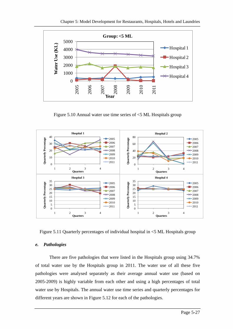
Chapter 5: Model Development for Restaurants, Hospitals, Hotels and Laundries
Page 5-27
Figure 5.10 Annual water use time series of <5 ML Hospitals group
Figure 5.11 Quarterly percentages of individual hospital in <5 ML Hospitals group
e. Pathologies
There are five pathologies that were listed in the Hospitals group using 34.7%
of total water use by the Hospitals group in 2011. The water use of all these five
pathologies were analysed separately as their average annual water use (based on
2005-2009) is highly variable from each other and using a high percentages of total
water use by Hospitals. The annual water use time series and quarterly percentages for
different years are shown in Figure 5.12 for each of the pathologies.
0
1000
2000
3000
4000
5000
20
05
20
06
20
07
20
08
20
09
20
10
20
11
Wa
ter
Use
(K
L)
Year
Group: <5 ML
Hospital 1
Hospital 2
Hospital 3
Hospital 4
0
10
20
30
40
1 2 3 4
Qu
art
erly
Per
cen
tag
e
Quarters
Hospital 1
2005
2006
2007
2008
2009
2010
20110
20
40
60
80
1 2 3 4
Qu
art
erly
Per
cen
tag
e
Quarters
Hospital 2
2005
2006
2007
2008
2009
2010
2011
0
5
10
15
20
25
30
35
1 2 3 4
Qu
art
erly
Per
cen
tag
e
Quarters
Hospital 3
2005
2006
2007
2008
2009
2010
20110
5
10
15
20
25
30
35
1 2 3 4
Qu
art
erly
Per
cen
tag
e
Quarters
Hospital 4
2005
2006
2007
2008
2009
2010
2011

Chapter 5: Model Development for Restaurants, Hospitals, Hotels and Laundries
Page 5-28
Figure 5.12 Water use pattern of Pathologies in Hospitals group
0
5
10
15
20
25
30
35
1 2 3 4
Qu
art
erly
Per
cen
tag
e
Quarters
Pathology 1
2005
2006
2007
2008
2009
2010
20110
10000
20000
30000
40000
20
05
20
06
20
07
20
08
20
09
20
10
20
11
Wate
r U
se (
KL
)
Year
Pathology 1
0
5
10
15
20
25
30
35
40
1 2 3 4
Qu
art
erly
Per
cen
tag
e
Quarters
Pathology 2
2005
2006
2007
2008
2009
2010
20110
5000
10000
15000
20
05
20
06
20
07
20
08
20
09
20
10
20
11
Wate
r U
se (
KL
)
Year
Pathology 2
0
10
20
30
40
50
60
1 2 3 4
Qu
art
erly
Per
cen
tage
Quarters
Pathology 3
2005
2006
2007
2008
2009
2010
20110
2000
4000
6000
8000
10000
20
05
20
06
20
07
20
08
20
09
20
10
20
11
Wa
ter
Use
(K
L)
Year
Pathology 3
0
5
10
15
20
25
30
35
1 2 3 4
Qu
art
erly
Per
cen
tage
Quarters
Pathology 4
2005
2006
2007
2008
2009
2010
20110
20
40
60
80
100
20
05
20
06
20
07
20
08
20
09
20
10
20
11
Wa
ter
Use
(K
L)
Year
Pathology 4
0
20
40
60
80
100
1 2 3 4
Qu
art
erly
Per
cen
tag
e
Quarters
Pathology 5
2005
2006
2007
2008
2009
2010
20110
20
40
60
80
20
05
20
06
20
07
20
08
20
09
20
10
20
11
Wate
r U
se (
KL
)
Year
Pathology 5

Chapter 5: Model Development for Restaurants, Hospitals, Hotels and Laundries
Page 5-29
From the Figure 5.12, it can be seen that the annual water use were almost
constant in 2008-2010 for Pathologies 1, 2, and 3. In case of Pathology 4, the annual
water use was variable over years, but the variability was very high in Pathology 5.
From the Figure 5.12, it is apparent that the quarterly percentages of the Pathologies 1,
2, and 3 were fairly consistent over the years and those for Pathologies 4 and 5 were
highly variable over years. It should be noted that in Pathology 5, quarterly water use
percentages in 2010 were highly variable than those of other years as it shows that
most of the water used in 4th
quarter (82%).
f. Summary of Data Analysis
A summary of above water use data analysis is presented in Table 5.10; based
on this analysis, different modelling approaches were considered for forecasting annual
water use for the different groups which are also presented in this table. From the table,
it can be seen that the most of the Hospitals groups follow the similar annual water use
pattern over the different years. Therefore, average annual water use over the 2008-
2010 periods were considered for the forecast annual water use in 2011 for these
groups. There were few groups with variable annual water use over the years and for
them the annual water use in 2010 was considered as the forecast annual water use in
2011. However, it was found that the quarterly water use percentages in most of the
subgroups were consistent over the years. Therefore, the disaggregating factors were
considered as the average over the period of 2005-2010 excluding the exception years.

Chapter 5: Model Development for Restaurants, Hospitals, Hotels and Laundries
Page 5-30
Table 5.15 Summary of water use data analysis and selection of modelling approach for Hospitals group
Group
Number
of
hospitals
Modelled by Variation of annual
water use
Variation of
quarterly water
use percentages
Approach used for
annual water use
forecast in 2011
Approach used for
disaggregating factors
(quarterly
percentages)
>20 ML 1 Individual Highly variable Similar over the
years
Annual water use in
2010
Average of
2005-2010
>15-20 ML - - - -
>10-15 ML 2
Individual
(Hospital 1) Fairly variable
Similar over the
years
Annual water use in
2010
Average of
2005-2010
Individual
(Hospital 2) Highly variable
Similar over the
years
Annual water use in
2010
Average of
2005-2010
5-10 ML 2
Individual
(Hospital 1)
Decreased until 2008
and then almost
constant
Similar over the
years
Average annual
water use in 2008-
2010
Average of
2005-2010
Individual
(Hospital 2)
Decreased until 2008
and then fairly
constant
Similar over the
years
Average annual
water use in 2008-
2010
Average of
2005-2010
<5 ML 4 Individual
(Hospital 1)
Similar over the
years
Not consistent over
the years
Average annual
water use in 2008-
2010
Same as in 2010

Chapter 5: Model Development for Restaurants, Hospitals, Hotels and Laundries
Page 5-31
Individual
(Hospital 2)
Similar over the
years except 2008
Similar over the
years except in
2008 and 2009
Average annual
water use in 2009-
2010
Average of
2005-2010 excluding
2008 and 2009
Individual
(Hospital 3)
Similar over the
years
Similar over the
years
Average annual
water use in 2008-
2010
Average of
2005-2010
Individual
(Hospital 4)
Similar over the
years
Similar over the
years
Average annual
water use in 2008-
2010
Average of
2005-2010
Pathologies 5
Individual
(Pathology 1)
Fairly constant in
2008-2010
Similar over the
years except in
2006 and 2010
Average annual
water use in 2008-
2010
Average of
2005-2010 excluding
2006 and 2010
Individual
(Pathology 2)
Fairly constant in
2008-2010
Similar over the
years except in
2006
Average annual
water use in 2008-
2010
Average of
2005-2010 excluding
2006
Individual
(Pathology 3)
Fairly constant in
2008-2010
Similar over the
years except in
2006
Average annual
water use in 2008-
2010
Average of
2005-2010 excluding
2006
Individual
(Pathology 4) Highly variable
Not consistent over
the years
Annual water use in
2010 Same as in 2010
Individual
(Pathology 5) Highly variable
Not consistent over
the years
Annual water use in
2010 Same as in 2010

Chapter 5: Model Development for Restaurants, Hospitals, Hotels and Laundries
Page 5-32
5.3.2.2. Forecasting Water Use Model Development
Since the findings from the data analysis for the Hospitals group (Section
5.3.2.1) was similar to those of the Restaurants group (Section 5.3.1.1), model
development procedure for Hospitals group is also the same as that of the Restaurants
group (Section 5.3.1.2).
a. Group: >20 ML
The annual water use in this hospital was highly variable over the years as was
outlined in Table 5.15. Therefore, the total water use in 2010 is considered as the
forecast annual water use for 2011. From data analysis it was also found that the
quarterly water use percentages over the different years were consistent and therefore,
the quarterly disaggregating factors (shown in Table 5.16) were obtained from the
average of quarterly water use percentages over years (2005-2010). The forecast
annual water use in 2011 was then disaggregated into quarterly water use with the
disaggregating factors. The observed and forecast water uses in 2011 are presented in
Table 5.17 for both annual and quarterly time step. The E value obtained from the
comparison of quarterly observed and forecast water use in 2011 is -0.49, which
indicates poor model performance. From Table 5.17, it is clear that the forecast annual
water use were very different from the observed water use, especially in 3rd
quarter of
2011. However, there was no detail information available except water use data to
further investigate for possible reasons. Therefore, it is recommended that a field
survey should be considered for collecting more information on factors affecting the
water use for better forecast.
Table 5.16 Quarterly disaggregating factors in >20 ML Hospitals group
Group Disaggregating factors for quarters
Quarter 1 Quarter 2 Quarter 3 Quarter 4
>20 ML 28 24 23.5 24.5

Chapter 5: Model Development for Restaurants, Hospitals, Hotels and Laundries
Page 5-33
Table 5.17 Comparison of observed and forecast water use of >20 ML Hospitals group
in 2011
b. Group: >10-15 ML
From Table 5.15, it was seen that the annual water use in both of these hospitals
in this group were not consistent over the years. However, the quarterly percentages of
annual water uses were consistent over the different years. Therefore, the quarterly
disaggregating factors obtained from the average quarterly percentages over the last
years (2005-2010) which are also shown in Table 5.18. The annual water use in 2010
was considered as the forecast annual water use in 2011 for these two hospitals. The
forecast annual water use was then disaggregated into the quarterly water use using the
disaggregating factors shown in Table 5.18. These observed and forecast water use in
2011 for both quarterly and annual time step are shown in Table 5.19. The E values
obtained from the comparison of forecast and observed quarterly water use in 2011 are
also presented in Table 5.19. A negative E value shows the poor model performance,
indicating the average quarterly water use of previous years would be better prediction
for 2011 than the forecast quarterly water use in this research.
Table 5.18 Quarterly disaggregating factors in >10-15 ML Hospitals group
Hospitals
Group
Annual
water use
in 2011
(KL)
Water use in each quarter in 2011
(KL)
E
value
1 2 3 4
>20 ML Observed 26,873 2,619 4,624 10,198 9,432 -0.49
Forecasted 12,591 3,526 3,022 2,959 3,085
Group
Disaggregating factors for quarters
Quarter
1
Quarter 2 Quarter 3 Quarter 4
Hospital 1 25 25.6 25 24.4
Hospital 2 24.5 24 25.5 26

Chapter 5: Model Development for Restaurants, Hospitals, Hotels and Laundries
Page 5-34
Table 5.19 Comparison of observed and forecast water use of >10-15 ML Hospitals
group in 2011
c. Group: 5-10 ML
As outlined in Table 5.15, the annual water uses in the two hospitals in this
group were similar from 2008 to 2010. Therefore, the average annual water use by
each hospital in 2008-2010 was considered as the forecast annual water use in 2011.
From data analysis, it was also found that the quarterly water use percentages over
different years (2005-2010) were similar. Therefore, the disaggregating factors were
obtained from the average of the quarterly water use percentages over years (2005-
2010). These disaggregating factors for each of the hospitals are shown in the Table
5.20.
Thereafter, the forecast annual water uses in 2011 were disaggregated into the
quarterly water uses using the disaggregating factors. The forecast and observed water
use for both quarterly and annual water use in 2011 are presented in Table 5.21. The E
value obtained from the comparison of forecast and observed quarterly water use in
2011 are also presented in Table 5.21 show that models were performed well for this
Hospitals group.
>10-15
ML
Hospitals
Group
Annual
water
use in
2011
(KL)
Water use in each quarter in 2011
(KL)
E
value
1 2 3 4
Hospital 1 Observed 10,637 2,686 2,618 2,595 2,739
-0.30 Forecasted 11,027 2,757 2,823 2,757 2,691
Hospital 2 Observed 11,181 2,678 2,733 2,887 2,883
-2.60 Forecasted 10,379 2,595 2,491 2,647 2,647

Chapter 5: Model Development for Restaurants, Hospitals, Hotels and Laundries
Page 5-35
Table 5.20 Quarterly disaggregating factors in 5-10 ML Hospitals group
Table 5.21 Comparison of observed and forecast water use of 5-10 ML Hospitals
group in 2011
d. Group: <5 ML
As mentioned in Table 5.15, the annual water uses by each hospital are similar
over the years (2005-2010). Therefore, the average annual water use of the last three
years (2008-2010) was considered as the forecast annual water use in these hospitals
for 2011. As outlined in Table 5.15, the average quarterly percentages over years
(2005-2010) were considered as the disaggregating factors for Hospitals 3 and 4, while
for Hospitals 1 and 2, the 2010 quarterly percentages were considered. These
disaggregating factors are presented in Table 5.22. Finally, the forecast annual water
uses were disaggregated into quarterly water use in 2011 by using the quarterly
disaggregating factors. The forecast and observed water uses for annual and quarterly
time steps in 2011 are presented in Table 5.23. The E value obtained from the
Group
Disaggregating factors for quarters
Quarter 1 Quarter 2 Quarter 3 Quarter 4
Hospital 1 26 24.5 24 25.5
Hospital 2 28.5 27 23 21.5
5-10 ML
Hospitals
Group
Annual
water use
in 2011
(KL)
Water use in each quarter in 2011
(KL)
E
value
1 2 3 4
Hospital 1 Observed 5,134 1,479 1,237 1,254 1,165
0.98 Forecasted 5,542 1,441 1,358 1,330 1,413
Hospital 2 Observed 7,218 2,000 1,779 1,682 1,758
0.01 Forecasted 6,298 1,795 1,700 1,449 1,354

Chapter 5: Model Development for Restaurants, Hospitals, Hotels and Laundries
Page 5-36
comparison of forecast and observed water uses are also presented in Table 5.23. The
E values in Table 5.23 show that models performed well to forecast quarterly water use
in 2011 for this Hospitals group.
Table 5.22 Quarterly disaggregating factors in <5 ML Hospitals group
Table 5.23 Comparison of observed and forecast water use of <5 ML Hospitals group
in 2011
e. Group: Pathologies
Based on the analysis of water use data (Table 5.15), it was found that
Pathologies 1, 2 and 3 individually had similar annual water use in 2008-2010, but the
Group <5 ML
Disaggregating factors for quarters
Quarter 1 Quarter 2 Quarter 3 Quarter 4
Hospital 1 23 27 24 26
Hospital 2 38.5 32.5 9.6 19.4
Hospital 3 25.5 26.5 24.5 23.5
Hospital 4 25 25.5 25 24.5
<5 ML
Hospitals
Subgroups
Annual
water use
in 2011
(KL)
Water use in each quarter in
2011 (KL)
E
value
1 2 3 4
Hospital 1 Observed 503 144 141 111 107
0.10 Forecasted 343 79 93 82 89
Hospital 2 Observed 23 6 5 6 6
0.55 Forecasted 98 38 32 9 19
Hospital 3 Observed 1,678 421 420 430 408
0.53 Forecasted 1,754 447 465 430 412
Hospital 4 Observed 3,150 763 774 795 818
0.60 Forecasted 3,341 835 852 835 819

Chapter 5: Model Development for Restaurants, Hospitals, Hotels and Laundries
Page 5-37
annual water uses in Pathologies 4 and 5 were highly variable over this period.
Therefore, it was considered that the average annual water use in 2008-2010 as the
forecast annual water use in 2011 for Pathologies 1, 2 and 3, and the water use in 2010
as the forecast annual water use in 2011 for Pathologies 4 and 5.
The average quarterly percentages were considered as the quarterly
disaggregating factors for Pathology 1, 2 and 3 excluding those of the outlined years in
Table 5.15. In Pathologies 4 and 5, there were no consistency in quarterly water use
percentages and therefore, the percentages of quarterly water use in 2010 and 2009
were considered for the Pathologies 4 and 5 respectively. Finally, the forecast annual
water uses were disaggregated into quarterly water uses by using the quarterly
disaggregating factors presented in Table 5.24.
The forecast and observed water uses in 2011 are presented in Table 5.25 for
both annual and quarterly time steps. The E values obtained from the comparison of
forecast and observed quarterly water uses for this group are also presented in Table
5.25. It can be seen that for most of the Pathologies, model performed well to forecast
water use in 2011.
Table 5.24 Quarterly disaggregating factors in Pathologies in Hospitals group
Group Disaggregating factors for quarters
Quarter 1 Quarter 2 Quarter 3 Quarter 4
Pathology 1 29 24.5 21 25.5
Pathology 2 25 26 25 24
Pathology 3 24.5 26 25 24.5
Pathology 4 23 25 27 25
Pathology 5 18 36 8 38
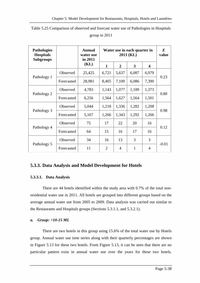
Chapter 5: Model Development for Restaurants, Hospitals, Hotels and Laundries
Page 5-38
Table 5.25 Comparison of observed and forecast water use of Pathologies in Hospitals
group in 2011
5.3.3. Data Analysis and Model Development for Hotels
5.3.3.1. Data Analysis
There are 44 hotels identified within the study area with 0.7% of the total non-
residential water use in 2011. All hotels are grouped into different groups based on the
average annual water use from 2005 to 2009. Data analysis was carried out similar to
the Restaurants and Hospitals groups (Sections 5.3.1.1, and 5.3.2.1).
a. Group: >10-15 ML
There are two hotels in this group using 15.6% of the total water use by Hotels
group. Annual water use time series along with their quarterly percentages are shown
in Figure 5.13 for these two hotels. From Figure 5.13, it can be seen that there are no
particular pattern exist in annual water use over the years for these two hotels.
Pathologies
Hospitals
Subgroups
Annual
water use
in 2011
(KL)
Water use in each quarter in
2011 (KL)
E
value
1 2 3 4
Pathology 1 Observed 25,425 6,721 5,637 6,087 6,979
0.23 Forecasted 28,981 8,405 7,100 6,086 7,390
Pathology 2 Observed 4,783 1,143 1,077 1,189 1,373
0.80 Forecasted 6,256 1,564 1,627 1,564 1,501
Pathology 3 Observed 5,044 1,218 1,336 1,282 1,208
0.98 Forecasted 5,167 1,266 1,343 1,292 1,266
Pathology 4 Observed 75 17 22 20 16
0.12 Forecasted 64 15 16 17 16
Pathology 5 Observed 34 16 13 3 3
-0.01 Forecasted 11 2 4 1 4

Chapter 5: Model Development for Restaurants, Hospitals, Hotels and Laundries
Page 5-39
However, the quarterly water use pattern was similar over the years except in 2009 for
both hotels and in 2008 for Hotel 2.
Figure 5.13 Water use pattern of >10-15 ML Hotels group
b. Group: 5-10 ML
There are four hotels in this group with 21.6% of the total water use by Hotels
group in 2011. All these four hotels were analysed separately. The time series of
annual water use and the percentages of quarterly water use in each year for all four
hotels are shown in Figure 5.14. From Figure 5.14, it can be seen that the annual water
use in Hotels 1, 2 and 3 were fairly similar over the years. In Hotel 4, the annual water
use was fairly similar until 2009 and then in 2010 it has increased. From the same
figure, it is also apparent that the quarterly percentages were consistent across the
different years among the hotels.
0
10
20
30
40
50
1 2 3 4
Qu
art
erly
Per
cen
tag
e
Quarters
Hotel 1
2005
2006
2007
2008
2009
2010
2011
0
6000
12000
18000
20
05
20
06
20
07
20
08
20
09
20
10
20
11
Wate
r U
se (
KL
)
Year
Hotel 1
0
10
20
30
40
50
1 2 3 4
Qu
art
erly
Per
cen
tag
e
Quarters
Hotel 2
2005
2006
2007
2008
2009
2010
2011
0
6000
12000
18000
20
05
20
06
20
07
20
08
20
09
20
10
20
11
Wa
ter
Use
(K
L)
Year
Hotel 2

Chapter 5: Model Development for Restaurants, Hospitals, Hotels and Laundries
Page 5-40
Figure 5.14 Water use pattern of 5-10 ML Hotels group
0
10
20
30
40
1 2 3 4
Qu
art
erly
Per
cen
tag
e
Quarters
Hotel 1
2005
2006
2007
2008
2009
2010
2011
0
6000
120002
00
5
20
06
20
07
20
08
20
09
20
10
20
11
Wa
ter
Use
(K
L)
Year
Hotel 1
0
5
10
15
20
25
30
35
1 2 3 4
Qu
art
erly
Per
cen
tag
e
Quarters
Hotel 2
2005
2006
2007
2008
2009
2010
2011
0
6000
12000
20
05
20
06
20
07
20
08
20
09
20
10
20
11
Wa
ter
Use
(K
L)
Year
Hotel 2
0
5
10
15
20
25
30
35
1 2 3 4
Qu
art
erly
Per
cen
tag
e
Quarters
Hotel 3
2005
2006
2007
2008
2009
2010
2011
0
6000
12000
20
05
20
06
20
07
20
08
20
09
20
10
20
11
Wa
ter
Use
(K
L)
Year
Hotel 3
0
5
10
15
20
25
30
35
1 2 3 4
Qu
art
erly
Per
cen
tag
e
Quarters
Hotel 4
2005
2006
2007
2008
2009
2010
2011
0
6000
12000
20
05
20
06
20
07
20
08
20
09
20
10
20
11
Wa
ter
Use
(K
L)
Year
Hotel 4

Chapter 5: Model Development for Restaurants, Hospitals, Hotels and Laundries
Page 5-41
c. Group: <5 ML
There are 38 hotels in this group with 62.8% of total water use by Hotels group
in 2011. All these hotels were divided into five subgroups based on the average annual
water use volume in 2005-2009 and then each subgroup analysed separately. These
subgroups with their water use percentages within the Hotels group and the numbers of
hotels in each subgroup are shown in Table 5.26.
Table 5.26 Water use percentages among Hotels subgroups in <5 ML group
Subgroup Number of Hotels Water use (%) in
Hotels
>4-<5 ML 7 22.0
>3-4 ML 7 17.1
>2-3 ML 8 14.1
1-2 ML 9 9.4
<1 ML 7 1.4
Total 38 64
The time series of annual water use and the average percentages of quarterly
water use in each year for each subgroup are shown in Figure 5.15. It should be noted
that the black bold line in the annual water use time series shows the average water use
of the subgroup.
From the annual water use plots in Figure 5.15, it is found that the water uses
among the hotels within this group were similar over the years except one hotel in the
subgroup >2-3 ML. This hotel was not included in calculating the average water use
for this subgroup. A constant average quarterly percentages over different years can
also be seen from this figure except the average quarterly percentage in 2009 in the <1
ML subgroup.

Chapter 5: Model Development for Restaurants, Hospitals, Hotels and Laundries
Page 5-42
Figure 5.15 Water use pattern of <5 ML Hotels group
0
5
10
15
20
25
30
1 2 3 4
Qu
art
erly
Per
cen
tag
e
Quarters
Subgroup: >4-<5 ML
2005
2006
2007
2008
2009
2010
2011
0
6000
12000
20
05
20
06
20
07
20
08
20
09
20
10
20
11
Wa
ter
Use
(K
L)
Year
Subgroup: >4-<5 ML
0
5
10
15
20
25
30
1 2 3 4
Qu
art
erly
Per
cen
tag
e
Quarters
Subgroup: >3-4 ML
2005
2006
2007
2008
2009
2010
2011
0
6000
12000
20
05
20
06
20
07
20
08
20
09
20
10
20
11
Wate
r U
se (
KL
)
Year
Subgroup: >3-4 ML
0
5
10
15
20
25
30
1 2 3 4
Qu
art
erly
Per
cen
tag
e
Quarters
Subgroup: >2-3 ML
2005
2006
2007
2008
2009
2010
2011
0
6000
12000
20
05
20
06
20
07
20
08
20
09
20
10
20
11
Wate
r U
se (
KL
)
Year
Subgroup: >2-3 ML
0
5
10
15
20
25
30
35
1 2 3 4
Qu
art
erly
Per
cen
tag
e
Quarters
Subgroup: 1-2 ML
2005
2006
2007
2008
2009
2010
2011
0
3000
6000
20
05
20
06
20
07
20
08
20
09
20
10
20
11
Wa
ter
Use
(K
L)
Year
Subgroup: 1-2 ML
0
10
20
30
40
50
1 2 3 4
Qu
art
erly
Per
cen
tag
e
Quarters
Subgroup: <1 ML
2005
2006
2007
2008
2009
2010
2011
0
3000
6000
20
05
20
06
20
07
20
08
20
09
20
10
20
11
Wa
ter
Use
(K
L)
Year
Subgroup: <1ML

Chapter 5: Model Development for Restaurants, Hospitals, Hotels and Laundries
Page 5-43
d. Summary of Data Analysis
A summary of the above water use data analysis is presented in Table 5.27;
Based on this analysis, the approaches that was used to forecast annual water use for
the different groups and in some cases for the individual hotels within the group, is
also presented in this table. Furthermore, this table also shows how the quarterly water
use disaggregating factors were obtained to disaggregate the forecast annual water use
into forecast quarterly water use. From the table, it can be seen that the most of the
Hotels groups follow the similar annual water use pattern over the different years
except for >10-15 ML group and Hotel 4 in 5-10 ML group. Therefore, average annual
water use over the 2008-2010 periods were considered to forecast the annual water use
in 2011 for these groups. In the case of highly variable water use groups, the annual
water use in 2010 was considered as the forecast water use for 2011.

Chapter 5: Model Development for Restaurants, Hospitals, Hotels and Laundries
Page 5-44
Table 5.27 Summary of water use data analysis and selection of modelling approach for Hotels group
Group Subgroups Number of
hotels Modelled by
Variation of
annual water use
Variation of
quarterly water
use percentages
Approach used for
annual water use
forecast in 2011
Approach used
for
disaggregating
factors
>20 ML - - - - - -
>15-20 ML - - - - - -
>10-15 ML - 2
Individual
(Hotel 1) Highly variable
Similar over the
years except in
2009
Annual water use in
2010
Average of 2005-
2010 excluding
2009
Individual
(Hotel 2) Highly variable
Similar over the
years except in
2008 and 2009
Annual water use in
2010
Average of 2005-
2010 excluding
2009
5-10 ML 4
Individual
(Hotel 1)
fairly constant over
the years
Similar over the
years
Average annual
water use in 2008-
2010
Average of 2005-
2010
Individual
(Hotel 2)
fairly constant over
the years
Similar over the
years
Average annual
water use in 2008-
2010
Average of 2005-
2010
Individual
(Hotel 3)
fairly constant over
the years
Similar over the
years
Average annual
water use in 2008-
2010
Average of 2005-
2010
Individual
(Hotel 4)
fairly constant until
2009 and then
increased in 2010
Similar over the
years
Annual water use in
2010
Average of 2005-
2010

Chapter 5: Model Development for Restaurants, Hospitals, Hotels and Laundries
Page 5-45
<5 ML
>4-<5 ML 7 Group Similar over the
years
Similar over the
years
Average annual
water use in 2008-
2010
Average of 2005-
2010
>3-4 ML 7 Group Similar over the
years
Similar over the
years
Average annual
water use in 2008-
2010
Average of 2005-
2010
>2-3 ML 8 Group Similar over the
years
Similar over the
years
Average annual
water use in 2008-
2010
Average of 2005-
2010
1-2 ML 9 Group Similar over the
years
Similar over the
years
Average annual
water use in 2008-
2010
Average of 2005-
2010
<1 ML 7 Group Similar over the
years
Similar over
years except in
2009
Average annual
water use in 2008-
2010
Average of 2005-
2010 excluding
2009

Chapter 5: Model Development for Restaurants, Hospitals, Hotels and Laundries
Page 5-46
5.3.3.2. Forecasting Water Use Model Development
Since the findings from the data analysis for the Hotels group (Section 5.3.3.1)
were similar to those of the Restaurants and Hospitals group (Sections 5.3.1.1 and
5.3.2.1), model development procedure for Hotels group is also the same as those of
the Restaurants and Hospitals group (Sections 5.3.1.2 and 5.3.2.2).
a. Group: >10-15 ML
As outlined in Table 5.27, it was found from the data analysis that the water use
in these two hotels is highly variable and therefore, the annual water use in 2010 is
considered as the forecast annual water use in 2011 for these hotels. However, from
Table 5.27, it is apparent that there were consistent quarterly water use pattern exists
among these two hotels except in 2009 for Hotel 1, and 2008 and 2009 for Hotel 2.
Therefore, the data for these years were excluded when calculating the quarterly water
use disaggregating factors. The disaggregating factors are presented in Table 5.28. The
forecast annual water use in 2011 was then disaggregated into quarterly water use
using the disaggregating factors. The forecast and observed water use in 2011 for these
Hotels are presented in Table 5.29 for both of the annual and quarterly time steps.
The E value obtained from the comparison of quarterly forecast and observed
water uses in 2011 are also presented in Table 5.29. Low E values in the table show
that models are not performing well for these two hotels. This could be due to the
different annual water use in 2011 than the annual water use in 2010, which also can be
seen from Figure 5.13. As there was not enough information available in this study, it
is recommended that a survey should be considered in future for predicting annual
water use of this group.

Chapter 5: Model Development for Restaurants, Hospitals, Hotels and Laundries
Page 5-47
Table 5.28 Quarterly disaggregating factors in >10-15 ML Hotels group
Table 5.29 Comparison of observed and forecast water use of >10-15 ML Hotels group
in 2011
b. Group: 5-10 ML
It was found from the data analysis that the annual water uses and the quarterly
percentages were fairly consistent over the years for Hotels 1, 2 and 3. Therefore, as
outlined in Table 5.17, it was considered that the average annual water use in 2008-
2010 as the forecast water use in 2011 for Hotels 1, 2 and 3; and for Hotel 4, the annual
water use in 2010 was considered. The disaggregating factors obtained from the
average quarterly percentages over years (2005-2010) as similar quarterly pattern were
found over that period for all the Hotels in this group. These disaggregating factors for
each hotel are presented in Table 5.30.
Thereafter, forecast annual water use in 2011 was disaggregated into quarterly
water use by using the disaggregating factors presented in Table 5.30. The observed
and the forecast water use in 2011 for all hotels in this group are presented in Table
Group Disaggregating factors for quarters
Quarter 1 Quarter 2 Quarter 3 Quarter 4
Hotel 1 24 24.5 26.5 25
Hotel 2 28 23 24 25
>10-15 ML Hotels
Group
Annual
water use
in 2011
(KL)
Water use in each quarter in 2011
(KL)
E
value
1 2 3 4
Hotel 1 Observed 10,028 2,085 2,292 2,592 3,059
0.10 Forecasted 8,352 2,005 2,046 2,213 2,088
Hotel 2 Observed 11,757 3,961 2,695 2,547 2,555
-2.1 Forecasted 16,607 4,650 3,820 3,986 4,152

Chapter 5: Model Development for Restaurants, Hospitals, Hotels and Laundries
Page 5-48
5.31 in both the annual and the quarterly time step. The E values obtained from the
comparison of observed quarterly water use with the forecast quarterly water use in
2011 is also presented in Table 5.31. The E values in Table 5.31 indicate that the
model performed well for Hotels 1, 2 and 4, and in case of Hotels 3 model
performance were low.
Table 5.30 Quarterly disaggregating factors in 5-10 ML Hotels group
Table 5.31 Comparison of observed and forecast water use of 5-10 ML Hotels group in
2011
Group Disaggregating factors for quarters
Quarter 1 Quarter 2 Quarter 3 Quarter 4
Hotel 1 28 24 23 25
Hotel 2 27 25 23 25
Hotel 3 26 24.5 24 25.5
Hotel 4 23.5 24 26.5 26
5-10 ML Hotels
Subgroups
Annual
water use
in 2011
(KL)
Water use in each quarter in 2011
(KL)
E
value
1 2 3 4
Hotel 1 Observed 9,177 2,570 2,228 2,018 2,360
0.38 Forecasted 8,245 2309 1,979 1,896 2,061
Hotel 2 Observed 5,119 1,332 1,228 1,194 1,365
0.64 Forecasted 5,975 1,613 1,494 1,374 1,494
Hotel 3 Observed 7,264 1,701 1,565 1,754 2,244
0.04 Forecasted 6,063 1,576 1,486 1,455 1,546
Hotel 4 Observed 8,498 1,912 2,119 2,479 1,988
0.87 Forecasted 7,642 1,796 1,834 2,025 1,987

Chapter 5: Model Development for Restaurants, Hospitals, Hotels and Laundries
Page 5-49
c. Group: <5 ML
From the data analysis it was seen that there were many hotels in each
subgroup and their annual water uses were similar. Therefore, the average water use by
the subgroup was considered for modelling purpose in this study. From data analysis it
was found that the average annual water use by each subgroup was similar over years
(2005-2010) and average quarterly percentages were same over that period for most of
the subgroups. Therefore, as listed in Table 5.27, the average annual water use by the
each subgroup from 2008-2010 were considered as the average annual forecast water
use in 2011 and the disaggregating factors were obtained from the average quarterly
percentages excluding for the years mentioned in the table. These factors are presented
in Table 5.32. Thereafter, using the average annual forecast water use in 2011 and the
disaggregating factors, quarterly average water uses in 2011 were forecasted.
The forecast and the observed average quarterly and annual water use in 2011
are presented in Table 5.33 for each subgroup. The E values obtained from the
comparison of average quarterly observed and forecast water use are also presented in
Table 5.33. From the E value in the table, it can be seen that models for most of the
subgroups were performed well.
Table 5.32 Quarterly disaggregating factors and E values in <5 ML Hotels group
Group Disaggregating factors for quarters
Quarter 1 Quarter 2 Quarter 3 Quarter 4
Subgroup: >4-<5 ML 25.5 24.5 24.5 25.5
Subgroup: >3-4 ML 25 25 25 25
Subgroup: >2-3 ML 25 25 25 25
Subgroup: 1-2 ML 25 24 25 26
Subgroup: <1 ML 26.5 24 25 24.5

Chapter 5: Model Development for Restaurants, Hospitals, Hotels and Laundries
Page 5-50
Table 5.33 Comparison of observed and forecast water use of <5 ML Hotels group in
2011
5.3.4. Data Analysis and Model Development for Laundries
5.3.4.1. Data Analysis
There are 127 laundries within the study area using 0.8% of the total non-
residential water use in 2011. As discussed in Section 5.2.2, all laundries were grouped
into different groups based on the average yearly water use from 2005 to 2009 and then
analysed individually for each group. Data analysis in Laundries was carried out
similar to the Restaurants, Hospitals and Hotels groups (Sections 5.3.1.1, 5.3.2.1 and
5.3.3.1)
<5 ML
Hotels
Subgroups
Annual
water use
in 2011
(KL)
Water use in each quarter in
2011 (KL)
E value
1 2 3 4
>4-<5 ML Observed 4,073 1,078 1,014 996 985
0.44 Forecasted 4,341 1,107 1,063 1,063 1,107
>3-4 ML Observed 3,147 769 772 824 782
0.47 Forecasted 3,447 862 862 862 862
>2-3 ML Observed 2,392 571 615 649 557
-0.38 Forecasted 2,277 569 569 569 569
1-2 ML Observed 1,329 376 318 313 321
0.13 Forecasted 1,472 368 353 368 383
<1 ML Observed 364 79 90 96 99
-0.75 Forecasted 263 70 63 66 64

Chapter 5: Model Development for Restaurants, Hospitals, Hotels and Laundries
Page 5-51
a. Group: >15-20 ML
There is only one laundry in this group using 22.8% of the total water use by
Laundries in 2011. The time series of annual water use of this laundry is shown in
Figure 5.16 along with the quarterly percentages in each year. This figure shows that
there is an increasing trend in water use for this laundry. From the figure, it is also
apparent that the quarterly percentage of the annual water use is similar over the years.
Figure 5.16 Water use pattern of >15-20 ML Laundries group
b. Group: 5-10 ML
There are two laundries within this group using 9.2% of the total water use by
Laundries in 2011 in the YVW service area. Time series of the annual water use of
these two laundries and the quarterly percentages of annual water uses are shown in
Figure 5.17. It can be seen from this figure that the annual water use in Laundry 1 since
2007 is almost similar. In case of Laundry 2, it was found that the water use varies over
the years. From Figure 5.17, it is also apparent that the quarterly percentages of water
use in both laundries were consistent over the years except for 2011 in Laundry 2.
0
5
10
15
20
25
30
1 2 3 4
Qu
art
erly
Per
cen
tag
e
Quarters
Group: >15-20 ML
2005
2006
2007
2008
2009
2010
2011
0
10000
20000
30000
40000
20
05
20
06
20
07
20
08
20
09
20
10
2011
Wate
r U
se (
KL
)
Year
Group: >15-20 ML

Chapter 5: Model Development for Restaurants, Hospitals, Hotels and Laundries
Page 5-52
Figure 5.17 Water use pattern of 5-10 ML Laundries group
c. Group: <5 ML
Most of the laundries (about 124 out of 127) within study area fall into this
group covering 68% of the total water use by the Laundries. Therefore, all these
laundries were disaggregated into smaller subgroups based on the annual water use in
2005-2009. These subgroups with their water use percentages and the number of
laundries in each subgroup are presented in Table 5.34. The time series of the annual
water use and the average percentage of quarterly water use in each year for each
subgroup are shown in Figure 5.18. It should be noted that the black bold line in the
annual water use time series shows the average water use by the subgroup.
0
5
10
15
20
25
30
1 2 3 4
Qu
art
erly
Per
cen
tag
e
Quarters
Laundry 1
2005
2006
2007
2008
2009
2010
20110
2000
4000
6000
8000
10000
20
05
20
06
20
07
20
08
20
09
20
10
2011
Wate
r U
se (
KL
)
Year
Laundry 1
0
10
20
30
40
50
1 2 3 4
Qu
art
erly
Per
cen
tag
e
Quarters
Laundry 2
2005
2006
2007
2008
2009
2010
2011
0
2000
4000
6000
8000
20
05
20
06
20
07
20
08
20
09
20
10
20
11
Wate
r U
se (
KL
)
Year
Laundry 2

Chapter 5: Model Development for Restaurants, Hospitals, Hotels and Laundries
Page 5-53
Table 5.34 Water use percentage among Laundries subgroups in group <5 ML
Subgroup Number of
Laundries
Water use (%) in
Laundries group
>4-<5 ML 2 5.0
>3-4 ML 3 8.8
>2-3 ML 6 7.9
1-2 ML 24 21.2
<1 ML 89 25.1
Total 124 68
From the annual water use plot in Figure 5.18, it was found that water use
among the laundries within this group are similar over the years except for few
laundries in >2-3 ML subgroup. It should be noted that those laundries were not
included in average water use data analysis and forecasting. From Figure 5.18, it can
be seen that the average annual water use was moderately variable in >4-<5 ML
subgroup and in >3-4 ML subgroup, there was an increasing trend until 2009 before
decreased in 2010. However, the average annual water use was constant over the years
(2005-2010) for rest of the subgroups in this group. The average quarterly percentages
over the different years was similar among the subgroups (Figure 5.18) except in 2006
for >4-<5 ML subgroup.

Chapter 5: Model Development for Restaurants, Hospitals, Hotels and Laundries
Page 5-54
Figure 5.18 Water use pattern of <5 ML Laundries group
0
5
10
15
20
25
30
35
1 2 3 4
Qu
art
erly
Per
cen
tag
e
Quarters
Subgroup: >4-<5 ML
2005
2006
2007
2008
2009
2010
2011
0
1000
2000
3000
4000
5000
6000
20
05
20
06
20
07
20
08
20
09
20
10
2011
Wate
r U
se (
KL
)
Year
Subgroup: >4-<5 ML
0
5
10
15
20
25
30
35
1 2 3 4
Qu
art
erly
Per
cen
tag
e
Quarters
Subgroup: >3-4 ML
2005
2006
2007
2008
2009
2010
2011
0
1000
2000
3000
4000
5000
6000
20
05
20
06
20
07
20
08
20
09
20
10
20
11
Wa
ter
Use
(K
L)
Year
Subgroup: >3-4 ML
0
5
10
15
20
25
30
1 2 3 4
Qu
art
erly
Per
cen
tag
e
Quarters
Subgroup: >2-3 ML
2005
2006
2007
2008
2009
2010
2011
0
2000
4000
6000
8000
10000
20
05
20
06
20
07
20
08
20
09
20
10
2011
Wate
r U
se (
KL
)
Year
Subgroup: >2-3 ML
0
5
10
15
20
25
30
1 2 3 4
Qu
art
erly
Per
cen
tag
e
Quarters
Subgroup: 1-2 ML
2005
2006
2007
2008
2009
2010
2011
0
500
1000
1500
2000
2500
20
05
20
06
20
07
20
08
20
09
20
10
2011
Wate
r U
se (
KL
)
Year
Subgroup: 1-2 ML
0
5
10
15
20
25
30
1 2 3 4
Qu
art
erly
Per
cen
tage
Quarters
Subgroup: <1 ML
2005
2006
2007
2008
2009
2010
2011
0200400600800
100012001400
20
05
20
06
20
07
20
08
20
09
20
10
20
11
Wate
r U
se (
KL
)
Year
Subgroup: <1 ML

Chapter 5: Model Development for Restaurants, Hospitals, Hotels and Laundries
Page 5-55
d. Summary of Data Analysis
A summary of above water use data analysis is presented in Table 5.35; based
on this analysis, different modelling approaches were considered for forecasting annual
water use for the different groups which are also presented in this table. From the table,
it can be seen that the most of the Laundries groups follow the similar annual water use
pattern over the different years. Therefore, average annual water use over the 2008-
2010 periods were considered to get the forecast annual water use in 2011 in these
groups. However, it was found that the quarterly water use percentages in most of the
subgroups were consistent over the years. Therefore, the disaggregating factors were
considered as the average over the period of 2005-2010 excluding the exception years.

Chapter 5: Model Development for Restaurants, Hospitals, Hotels and Laundries
Page 5-56
Table 5.35 Summary of water use data analysis and selection of modelling approaches for Laundries group
Group Subgroups
Number
of
laundries
Modelled by Variation of
annual water use
Variation of
quarterly water
use percentages
Approach used for
annual water use
forecast in 2011
Approached used for
disaggregating
factors (quarterly
percentages
>20 ML - - - - - -
>15-20 ML - 1 Individual Increased each
year
Similar over the
years
A linear regression
model developed
years
Average of 2005-2010
>10-15 ML - - - - - -
5-10 ML - 2
Individual
(Laundry 1)
Constant after
2007
Similar over the
years
Average annual water
use in 2008-2010
Average of 2005-2010
Individual
(Laundry 2)
Moderately
variable
Similar over the
years
Annual water use in
2010
Average of 2005-2010
<5 ML
>4-<5 ML 2 Group Moderately
variable
Similar over the
years except in
2006
Average annual water
use in 2010
Average of 2005-2010
excluding 2006
>3-4 ML 3 Group Moderately
variable
Similar over the
years
Average annual water
use in 2010
Average of 2005-2010
>2-3 ML 6 Group Constant over
years
Similar over the
years
Average annual water
use in 2008-2010
Average of 2005-2010
1-2 ML 24 Group Constant over
years
Similar over the
years
Average annual water
use in 2008-2010
Average of 2005-2010
<1 ML 89 Group Constant over
years
Similar over the
years
Average annual water
use in 2008-2010
Average of 2005-2010

Chapter 5: Model Development for Restaurants, Hospitals, Hotels and Laundries
Page 5-57
5.3.4.2. Forecasting Water Use Model Development
Since the findings from the data analysis for the Laundries group (Section
5.3.4.1) were similar to those of the Restaurants, Hospitals and Hotels group (Sections
5.3.1.1, 5.3.2.1 and 5.3.3.1), model development procedure for Laundries group is also
the same as those of the Restaurants, Hotels and Hospitals group (Sections 5.3.1.2,
5.3.2.2 and 5.3.3.2).
a. Group: >15-20 ML
An analysis of the annual water use over 2005-2010 shows that there is an
increasing trend in the annual water use time series, as can be seen from Figure 5.19.
Therefore, as listed in Table 5.35, a linear regression model was developed to forecast
the annual water use in 2011 considering the past trend. The regression equation is:
Annual water use = 3793x + 4624.5 (5.1)
Where, x = 1, 2, 3, …. (2005=1; 2006= 2; ….. and 2011= 7)
Figure 5.19 Annual water use in >15-20 ML Laundries group
y = 3793x + 4624.5, x≥1R² = 0.98
0
5000
10000
15000
20000
25000
30000
2005 2006 2007 2008 2009 2010
Wate
r U
se (
KL
)
Year

Chapter 5: Model Development for Restaurants, Hospitals, Hotels and Laundries
Page 5-58
The quarterly water use disaggregating factors were obtained from the average
of quarterly percentages over the past years which are presented in Table 5.36. The
forecast annual water use obtained for 2011 was then disaggregated into quarterly
water use using the disaggregating factors. The annual and quarterly observed and
forecast water uses in 2011 are presented in Table 5.37. The E value obtained from the
comparison of forecast and observed quarterly water use in 2011 is also presented in
Table 5.37 shows that model performed well for this Laundry.
Table 5.36 Quarterly disaggregating factors in >15-20 ML Laundries group
Table 5.37 Comparison of observed and forecast water use of >15-20 ML Laundries
group in 2011
b. Group: 5-10 ML
As listed in Table 5.35, the forecast annual water use in 2011 for Laundry 1
was considered as the average annual water use in 2008-2010 and for Laundry 2 it was
considered as the annual water use in 2010. The disaggregating factors for both these
laundries were obtained from the average of quarterly percentages over the years
(2005-2010).These disaggregating factors are presented in Table 5.38. Finally, the
forecast annual water uses were disaggregated into quarterly water use for these
laundries, using the forecast annual water use in 2011 and the disaggregating factors.
Group
Disaggregating factors for quarters
Quarter 1 Quarter 2 Quarter 3 Quarter 4
Laundry 23 24 26 27
Laundries Group Annual
water use
in 2011
(KL)
Water use in each quarter in 2011
(KL)
E
value
1 2 3 4
>20 ML Observed 32,813 8,352 8,809 7,404 8,247
0.94 Forecasted 31,176 7,170 7,482 8,106 8,417

Chapter 5: Model Development for Restaurants, Hospitals, Hotels and Laundries
Page 5-59
These forecast annual and quarterly water use in 2011 are presented in Table 5.39 with
the observed value in 2011 for the laundries in this group. The E values obtained from
the comparison of observed and forecast quarterly water use in 2011 in both laundries
are also presented in Table 5.39. It can be seen from the table that model performed
well in case of Laundry 1 and poor performance was found in Laundry 2. The negative
E value could be due to change in quarterly water use in quarter 1 and 2. However, as
there are limited information available in this research, future field survey could be
useful for better forecast.
Table 5.38 Quarterly disaggregating factors in 5-10 ML Laundries group
Table 5.39 Comparison of observed and forecast water use of 5-10 ML Laundries in
2011
Group
Disaggregating factors for quarters
Quarter 1 Quarter 2 Quarter 3 Quarter 4
Laundry 1 24.5 24.5 25.5 26
Laundry 2 23.5 27 27 22.5
5-10 ML Laundries
Group
Annual
water use
in 2011
(KL)
Water use in each quarter in
2011 (KL)
E
value
1 2 3 4
Laundry 1 Observed 7,241 1,819 1,764 1,715 1,943
0.54 Forecasted 7,171 1,748 1,748 1,819 1,855
Laundry 2 Observed 5,930 661 716 2,124 2,428
-0.1 Forecasted 5,207 1,224 1,406 1,406 1,172

Chapter 5: Model Development for Restaurants, Hospitals, Hotels and Laundries
Page 5-60
c. Group: <5 ML
As listed in Table 5.35, the average annual water use by the subgroup from
2008-2010 were considered as the average annual forecast water use in 2011 for >2-3
ML, 1-2 ML and <1ML subgroups. In case of >4-5 ML and >3-4 ML subgroups,
average annual water use in 2010 were considered as the forecast average annual water
use in 2011. The quarterly water use disaggregating factors were obtained for each
subgroup from the average quarterly percentages excluding for the years mentioned in
Table 5.35. These factors are presented in Table 5.40. Thereafter, quarterly average
water uses in 2011 were forecasted using the average annual forecast water use in 2011
and the disaggregating factors. These observed and forecast average quarterly and
annual water use in 2011 for all the subgroups are presented in Table 5.41. The E value
obtained from the comparison of observed and forecast quarterly water use in 2011 is
also presented in the Table 5.41. From this table, it can be seen that models for all
subgroups are performed well with good E values.
Table 5.40 Quarterly disaggregating factors of subgroups in <5 ML Laundries
Group
Disaggregating factors for quarters
Quarter 1 Quarter 2 Quarter 3 Quarter 4
Subgroup: >4-<5 ML 26 24 24.5 25.5
Subgroup: >3-4 ML 23.5 25 26.5 25
Subgroup: >2-3 ML 23.5 26 26 24.5
Subgroup: 1-2 ML 23.5 26 26 24.5
Subgroup: <1 ML 24.5 25 25 25.5

Chapter 5: Model Development for Restaurants, Hospitals, Hotels and Laundries
Page 5-61
Table 5.41 Comparison of observed and forecast water use of <5 ML Laundries group
in 2011
5.4. Issues and Challenges faced and Limitations of the
Study
Water use in restaurants, hospitals, hotels and laundries can vary due to many
different factors such as size of the establishment, number of employees, number of
beds in hospitals, outdoor gardening, etc. Unfortunately, all this information was not
available for this research. If this information was available, they could have been used
in modelling water use. Therefore, a different approach was considered in this study by
disaggregating the water customer groups (i.e. Restaurants, Hospitals, Hotels and
Laundries) into various groups based on the magnitude of the historical annual water
use and analysing the water use pattern of these groups, which was used to get the
water use forecast for one year ahead. Moreover, as most of the water uses in these
groups are for indoor purposes, it was considered that all these factors were same and
<5 ML Hotels
Subgroups
Annual
water use
in 2011
(KL)
Water use in each quarter in 2011
(KL)
E
value
1 2 3 4
>4-<5 ML Observed 3,563 903 882 833 946
0.34 Forecasted 4,362 1,134 1,047 1,069 1,112
>3-4 ML Observed 4,218 934 1,229 1,007 1,048
0.58 Forecasted 3,880 912 970 1,028 970
>2-3 ML Observed 2,578 649 694 712 523
0.18 Forecasted 2,693 633 700 700 660
1-2 ML Observed 1,149 300 309 292 248
0.16 Forecasted 1,226 288 319 319 300
<1 ML Observed 383 95 96 96 96
0.94 Forecasted 380 93 95 95 97
Chapter 5: Model Development for Restaurants, Hospitals, Hotels and Laundries
Page 5-62
will be same in near future. However, there are some abrupt changes in water use
volume have found in some cases where reasons for these changes were unknown
mainly because of lack of data, and lack of access to discuss these issues with the water
customers due to confidentiality issues. In addition, there were other issues and
limitations specific to the individual group which are discussed below.
5.4.1. Restaurants
Water use in restaurants can vary due to
1) Different types of restaurants have different water use patterns. For example,
the Asian style restaurants are unique in their water use patterns. Due to traditional
food preparation and cooking practices, the Asian restaurants typically use 2 to 4 times
higher volume of water compared to the other types of restaurants (Yarra Valley
Water, 2016);
2) The largest use of water in restaurants is associated with equipment and
processes that take place in the kitchen. Change in appliances lead to different water
use patterns. For example a Boston University cafeteria successfully reduced its water
use by 63 percent after upgrading the kitchen with high-efficiency pre-rinse spray
valves (US EPA, 2012);
3) Intensity of the activities in the restaurants leads to different water use
patterns. For example, different restaurants have different number of days (e.g. seven
days, five days, etc.) and hours (e.g. only open for lunch or dinner time or both) open
for business. More open hours and days will lead to higher volume of water use.
Data for none of the above factors were available for this research. Therefore, it
is recommended that a field survey to get all the above details information will be
useful for better water use forecast.

Chapter 5: Model Development for Restaurants, Hospitals, Hotels and Laundries
Page 5-63
5.4.2. Hospitals
Hospitals have a number of unique water-use activities, which include vacuum
systems, medical air and compressor equipment, sterilizers and central sterile
operations, water-cooled laboratory and therapeutic equipment, laboratory hood
scrubbers, X-ray equipment and film developers, water-treatment systems for kidney
dialysis and laboratory water, therapeutic baths and treatments (East Bay Municipal
Utility District, 2008). Different types of system available in the hospital can lead to
variation in water use pattern.
Water use pattern in a hospital could also be affected by various other factors: 1)
Hospitals type: women, public, children, cardiologic, dental, eyes and ears and so on,
2) number of beds and number of employees, 3) efficiency of water use and outdoor
water use for gardening, 4) Different activities (classes on medical study can take place
in the hospital), and 5) facility of onsite laundry and size of the cafe, onsite pathology,
accommodation and so on. Total water use by hospitals can also vary from one year to
the subsequent years due to different extension or renovation of the hospitals. Data for
none of these factors were available for this research. Therefore, the forecast water use
model development for hospitals can be improved by conducting field surveys for
collecting above the listed information and to identify their future plan for change in
systems in the hospitals that can influence the water use.
5.4.3. Hotels
The water use in hotels can vary greatly not only between regions, but also
within a region. Factors influencing the hotel water use can be classified into physical
and operational parameters (Bohdanowicz and Martinac, 2007). The physical
parameters include size, structure and design of the hotel building (high rise, resort
style), geographical and climatic location (urban-rural), age of the facility, type of
water systems installed (recycle water to flush toilet and urinals, efficient and low flow
shower head), operation and maintenance schemes, types and amounts of water
resources available locally, as well as water-use regulations and cost.

Chapter 5: Model Development for Restaurants, Hospitals, Hotels and Laundries
Page 5-64
The operational features that influence water use in hotels include the service
affected by different sub-facilities including catering outlets, laundries, swimming
pools and spas, recreational and business centres, fluctuations in occupancy levels, and
variations in customer preferences relevant to indoor comfort (e.g. campside, 1-5-star
hotel), as well as culture and awareness of water resource consumption (Gossling et al,
2011). Laundry volumes per guest per day in sports and health centres in hotels, as
well as affected by textile quality and/or weight of laundry items, including very large
towels for spa facilities or beach use results in high water use hotels.
All these information was not available for this research. Moreover, some of
these factors, such as the level of environmental awareness of users are difficult to
quantify or evaluate as they are mostly qualitative in character. Therefore, significant
variations in facility type within the hotel sector make it difficult to provide a general
model explaining the water use of these individual facilities. However, as most of the
water uses in hotels are for indoor purposes, only historical water use were used for
modelling water use in hotels in this research assuming that facility were same and will
be same in near future. It was found that high water using hotel’s water uses are very
different from year to year. Therefore, to improve water use forecast, a field survey is
essential to the high using hotel for collecting the above stated information and their
future plan which can affect water use.
5.4.4. Laundries
Water use by the Laundries sector can vary depending on: the types of
laundries (e.g. commercial laundries, coin laundries), number of customer using the
laundry, types of customers (e.g. hospital, hotel, and restaurants), different types of
technologies (continuous-batch washing machines, extractor washing machines) used
in laundries etc. Difficulty in accessing these information, limits the water use
modelling for laundries in this research to explain the water use variation precisely.
Chapter 5: Model Development for Restaurants, Hospitals, Hotels and Laundries
Page 5-65
5.5. Summary
Water use modelling was performed to forecast water use one year ahead on a
quarterly basis for Restaurants, Hospitals, Hotels and Laundries groups using only the
historical water use data, as data for influencing factors in these water use customer
groups were not available for the study. Example of such influencing factors include
are opening hours for restaurants, number of beds in hospitals, number of rooms in
hotels, and number of customers and frequency of use in laundries. Moreover, in
general there is no sufficient seasonal variation in water use among these groups as
most of the water uses among these groups are for indoor purposes.
All customers in the above four water use customer groups were disaggregated
into different subgroups based on the magnitude of the average annual water use. Data
analysis was then performed for annual and quarterly water use at disaggregated group
levels to identify the water use pattern which were later used for forecast water use
model development.
Three different patterns were identified in the annual water use analysis among
the disaggregated groups in these four customer groups. They are:
1) The annual water uses were variable over the period (2005-2010).
2) The annual water uses were constant over the period (2005-2010) or over
very recent period (2008-2010). and
3) The annual water use followed an increasing or decreasing trend over the
period (2005-2010).
Therefore, annual water uses in 2011 were forecasted differently for these three types
of customer. In case of type 1, annual water use in 2010; in type 2, average annual
water use in 2008-2010 and in type 3, annual water use from the linear regression
were considered as the forecast annual water use in 2011. The quarterly forecast water

Chapter 5: Model Development for Restaurants, Hospitals, Hotels and Laundries
Page 5-66
uses were then obtained from the forecast annual water use in 2011 and the
disaggregating factors. These disaggregating factors were obtained from the quarterly
percentage water use over years (2005-2010). In most of the cases, the quarterly
percentage water uses were consistent over the years. Therefore, average quarterly
percentage water uses over years (2005-2010) were considered as disaggregating
factors to disaggregate the annual forecast to quarterly forecast excluding the
exceptional years. Model performances were then measured with the Nash-Sutcliffe
model efficiency (E). Most of the developed models in this study performed well with
good E value. There are few cases, models performed poorly and therefore, identified
issues, Challenges and limitation of the modelling in this research were presented at
the end of the Chapter.

Chapter 6: Water Use Modelling for High Water Users
Page 6-1
Chapter 6. Water Use Modelling for
High Water Users
6.1. Overview
There were thirty-five customers (among the 28,000) use a large portion of the
total non-residential water in the Yarra Valley Water (YVW) service area; these non-
residential customers were named as High Water Users (HWU) and were considered as
a separate group in this research. The customers in this group use around 7,740
ML/year, which is about 33.8% of the average non-residential water use (based on
2005-2009) in a year in the YVW service area. Individually, the annual water use by
these HWU customers is >50 ML as per data received for this research and
communication with the YVW officers. As the customers in the HWU group use a large
volume of water, water use among the customers are analysed and modelled separately
in this study. All customers in this group were divided into subgroups based on their
different activities such as Manufacturing Companies, Packaging Companies, Shopping
Centres, Hospitals, Laundries, Confectionary Factories, Universities, Motor Companies,
Poultry Factories and Institutions. This approach of customer grouping and modelling
their water demand is useful to the water authority for better water management such as
water supply system development, expansion and maintenance, and establishment of
water rate. It should be noted that the hospitals and laundries considered in this chapter
were not included in Chapter 5, as they use more than 50 ML/year individually.
There are many factors affecting the water use among the above subgroups such
as number of users of Shopping Centres, student numbers in Universities, number of
beds in Hospitals, and demand for the products in Manufacturing Companies and
Confectionary Factories (Dziegielewski, et al, 2000). Moreover, after having
discussions with the YVW officers, it was found that the driving factors for some of
these customers such as Manufacturing Companies and Confectionary Factories are the

Chapter 6: Water Use Modelling for High Water Users
Page 6-2
demand for their goods in foreign countries. However, data for all these influencing
factors were not available for this research. It was also noted that most of the water uses
of these customers are for indoor purposes, which are not generally affected by climatic
factors and water restrictions. Therefore, only the water use data were used for analysis
and modelling in this research, and presented in this chapter.
As mentioned in Chapter 1, short term water demand modelling (1 year) was
carried out using quarterly time steps in this research. To forecast the future water use,
the past water use was analysed first using the quarterly water use data from 2005 to
2010. In this analysis, it was found that the annual water use pattern varies differently
over the period among the customers. All the annual water use pattern were categorised
into following four types in this study:
Type 1. the annual water use is highly variable over the period,
Type 2. the annual water use is moderately varied (i.e. less varied compared to
type 1) over the period,
Type 3. moderately varied over the period and it was fairly constant in 2008-
2010, and
Type 4. water use followed an increasing or decreasing trend.
Thereafter, the annual water use in 2011 for the customers in these four
categories was forecasted differently. In the case of type 1 and type 2, annual water use
in 2011 was considered as the total water use in 2010 assuming that the most recent
condition will continue in near future as the driving factors for the past annual water use
variation were unknown in this study. For the same reason, annual water use before
2008 were not considered in type 3. In this case, annual water use in 2011 was
considered as the average annual water use in 2008-2010. In the case of type 4, water
use in 2011 was forecasted using the regression analysis of past annual water use over
the period (2005-2010).
From data analysis, it was found that the quarterly percentages of annual water
use were consistent for most of the customers over the period of 2005-2010. Therefore,
the quarterly disaggregating factors of annual water use were obtained from the average

Chapter 6: Water Use Modelling for High Water Users
Page 6-3
quarterly water use percentages over the past years (2005-2010). It should be noted that
the quarters are named as Quarter 1 (January – March), Quarter 2 (April – June),
Quarter 3 (July – September) and Quarter 4 (October – December) in this chapter as
was done in Chapter 4 and 5. The forecasted annual water use for 2011 was then
disaggregated to quarterly water use using the disaggregating factors. Finally, the
forecast quarterly water uses were compared with the observed quarterly water use in
2011 and the model performance was measured using the Nash-Sutcliffe efficiency (E).
This chapter first describes the historical water use data and the classification of
the HWU into different subgroups based on their activities. Water use data analysis and
models developed for individual customers in each subgroup are then presented.
Thereafter, the limitations of the present work are discussed along with the application
of this study. Finally, a summary of the chapter is presented.
6.2. Historical Water Use and Subgroups of HWU
The annual water use variation in HWU group over the study period (2005-
2011) is shown in Figure 6.1. From Figure 6.1, it can be seen that the water use has been
reduced from around 8,000 ML/year in 2006 to 6,000 ML/year in 2011. This is a huge
reduction in water use by only 35 water customers. As was discussed in Chapter 3
(Section 3.4), the possible reason for this reduction could be due to several factors such
as the use of alternate water sources, adapting dry process, reuse water in the system
and the use of water efficient appliances as part of the water savings measures (Yarra
Valley Water, 2008).

Chapter 6: Water Use Modelling for High Water Users
Page 6-4
Figure 6.1 Annual water use of HWU group over the study period
All customers in the HWU group were classified into different subgroups based
on their activities to analyse the water use pattern and to develop the water use models
individually for each customer in these subgroups. These subgroups are shown in Table
6.1 with the number of customers. The percentage of the average annual water use
based on 2011 annual water uses by different subgroups are shown Figure 6.2. From
this figure, it can be seen that around 44% of the total water use of HWU group were
from the manufacturing companies subgroup, followed by the packaging companies.
The annual water uses time series of HWU subgroups are shown in Figure 6.3.
From this figure, it is clear that the water use in manufacturing companies, packaging
companies and shopping centres gradually reduced over the years since 2007.
Moreover, it can also be seen that the water uses among the remaining high user
subgroups are fairly constant since 2007.
0
2000
4000
6000
8000
10000
20
05
20
06
20
07
20
08
20
09
20
10
2011
Wate
r u
se (
ML
)
Year

Chapter 6: Water Use Modelling for High Water Users
Page 6-5
Table 6.1 HWU Subgroups
Subgroups Number of Customers
Manufacturing Companies 9
Packaging Companies 4
Shopping Centres 5
Hospitals 4
Laundries 3
Confectionary Factories
3
Universities 4
Motor Companies 1
Poultry Factories 1
Institutions 1
Total 35
Figure 6.2 Water use percentages by different homogenous HWU subgroups in 2011
4%
44%
7%
3%
15%
12%
5%
1%4%
5%Hospitals
Manufacturing CompaniesShopping Centres
Laundries
Packaging CompaniesUniversites
Confectionary FactoriesInstitutions
Motor Companies
Poultry Factories

Chapter 6: Water Use Modelling for High Water Users
Page 6-6
Figure 6.3 Water use time-series by different homogenous HWU subgroups
6.3. Data Analysis and Model Development for Forecast
Water use
Many factors affect the water use among the HWU subgroups as discussed in
Section 6.1. However, data for those factors were not available for this research due to
customers privacy and most of the water uses among the customers are for indoor
purposes. Therefore, only water use data for the HWU group customers, which are
available, were analysed to develop models for forecasting water use. As outlined in
Chapter 4 (in Section 4.4.3), water use data in 2005-2010 were used to determine the
forecast annual water use in 2011 and the quarterly disaggregating factors were then
used to disaggregate the forecast annual water use (to forecast quarterly water use). The
model performance was measured with the Nash-Sutcliffe Efficiency (E). The details of
this efficiency criterion can be found in Chapter 4 (Section 4.3.4). Further details on the
water use data analysis and model development for each of the HWU subgroups are
discussed in the following sub-sections.
0
500
1000
1500
2000
2500
3000
3500
4000
4500
0
200
400
600
800
1000
1200
1400
20
05
20
06
20
07
20
08
20
09
20
10
20
11
Wate
r u
se i
n M
an
ufa
ctu
rer
(ML
)
Wa
ter
use
(M
L)
Year
Hospitals
Shopping CentresLaundries
Packaging CompaniesUniversites
Confectionary FactoriesManufacturing CompaniesInstitutions
Motor CompaniesPoultry Factories

Chapter 6: Water Use Modelling for High Water Users
Page 6-7
6.3.1. Manufacturing Companies
There are nine manufacturing companies in this subgroup. The total water use
by these companies is about 44% of total water use of HWU group. The annual water
use time series for each manufacturing company are presented in Figure 6.4 along with
their quarterly percentage of annual water use over the period of 2005-2010.
0
500000
1000000
1500000
2000000
2500000
20
05
20
06
20
07
20
08
20
09
20
10
20
11
Wa
ter
Use
(K
L)
Year
Manufacturing Company 1
0
5
10
15
20
25
30
1 2 3 4Q
ua
rter
ly P
erce
nta
ge
Quarters
Manufacturing Company 1
2005
2006
2007
2008
2009
2010
2011
0
400000
800000
1200000
1600000
20
05
20
06
20
07
20
08
20
09
20
10
20
11
Wa
ter
Use
(K
L)
Year
Manufacturing Company 2
0
5
10
15
20
25
30
35
1 2 3 4
Qu
art
erly
Per
cen
tag
e
Quarters
Manufacturing Company 2
2005
2006
2007
2008
2009
2010
2011
140000
150000
160000
170000
180000
190000
20
05
20
06
20
07
20
08
20
09
20
10
20
11
Wate
r U
se (
KL
)
Year
Manufacturing Company 3
0
5
10
15
20
25
30
35
1 2 3 4
Qu
art
erly
Per
cen
tag
e
Quarters
Manufacturing Company 3
2005
2006
2007
2008
2009
2010
2011
01
00
00
02
00
00
0
20
05
20
06
20
07
20
08
20
09
20
10
20
11
Wate
r U
se (
KL
)
Year
Manufacturing Company 4
0
5
10
15
20
25
30
1 2 3 4
Qu
art
erly
Per
cen
tag
e
Quarters
Manufacturing Company 4
2005
2006
2007
2008
2009
2010
2011

Chapter 6: Water Use Modelling for High Water Users
Page 6-8
Figure 6.4 Water use pattern of Manufacturing Companies subgroup
0
20000
40000
60000
80000
100000
120000
20
05
20
06
20
07
20
08
20
09
20
10
20
11
Wate
r U
se (
KL
)
Year
Manufacturing Company 5
0
5
10
15
20
25
30
35
1 2 3 4
Qu
art
erly
Per
cen
tag
e
Quarters
Manufacturing Company 5
2005
2006
2007
2008
2009
2010
2011
0
40000
80000
120000
160000
20
05
20
06
20
07
20
08
20
09
20
10
20
11
Wate
r U
se (
KL
)
Year
Manufacturing Company 6
0
10
20
30
40
50
60
1 2 3 4Q
ua
rter
ly P
erce
nta
ge
Quarters
Manufacturing Company 6
2005
2006
2007
2008
2009
2010
2011
0
20000
40000
60000
80000
100000
120000
20
05
20
06
20
07
20
08
20
09
20
10
20
11
Wate
r U
se (
KL
)
Year
Manufacturing Company 7
0
10
20
30
40
50
1 2 3 4
Qu
art
erly
Per
cen
tag
e
Quarters
Manufacturing Company 7
2005
2006
2007
2008
2009
2010
2011
0
20000
40000
60000
80000
100000
20
05
20
06
20
07
20
08
20
09
20
10
20
11
Wate
r U
se (
KL
)
Year
Manufacturing Company 8
0
5
10
15
20
25
30
1 2 3 4
Qu
art
erly
Per
cen
tag
e
Quarters
Manufacturing Company 8
2005
2006
2007
2008
2009
2010
2011
0
20000
40000
60000
80000
100000
20
05
20
06
20
07
20
08
20
09
20
10
20
11
Wate
r U
se (
KL
)
Year
Manufacturing Company 9
0
10
20
30
40
50
1 2 3 4
Qu
art
erly
Per
cen
tag
e
Quarters
Manufacturing Company 9
2005
2006
2007
2008
2009
2010
2011

Chapter 6: Water Use Modelling for High Water Users
Page 6-9
From Figure 6.4, it is seen that the annual water uses among the manufacturing
companies are not consistent over the years (2005-2010). The annual water use
moderately varied in Manufacturing Companies 1, 2, 4, 5 and 8. However, it is also can
be seen that there were a decreasing pattern in Manufacturing Companies 1 and 2, and
an increasing pattern in Manufacturing Companies 4 and 5. The annual water use of
2008-2010 in Manufacturing Company 8 were fairly constant. In case of Manufacturing
Company 3 and 6, annual water use highly varied over the period (2005-2010). It can
also be seen from the Figure 6.4 that there is a significant decreasing trend in annual
water use of Manufacturing Company 7 and 9 where annual water use reduced to less
than 5,000 KL/year from about 100,000 KL/year. However, there was not enough
information available in this study to investigate this significant reduction in annual
water use.
Therefore, based on this data analysis, regression models were considered to
forecast annual water use in 2011 for Manufacturing Companies 1, 2, 4, 5, 7 and 9 as
decreasing/increasing trend were identified in their annual water use time series (Figure
6.4). For Manufacturing Companies 3 and 6, the total water uses in 2010 were
considered as the forecast annual water uses in 2011. In case of Manufacturing
Companies 8, average annual water use of 2008-2010 was considered as forecast annual
water use in 2011.
The quarterly water use percentages in Figure 6.4 shows that they were not
consistent over the period of 2005-2010 for the Manufacturing Companies 7 and 9.
However, they were quite similar for different years in other Manufacturing companies
except in Manufacturing Company 6 in 2010. Based on these quarterly water use
patterns, the disaggregating factors were obtained for all manufacturing companies
(except 7 and 9) from the average quarterly percentages over the different years (2005-
2010) excluding the percentages of 2010 for Manufacturing Company 6. For
Manufacturing Companies 7 and 9, the quarterly percentages of 2010 were considered
as the disaggregating factors. These disaggregating factors were used to disaggregate
the forecast annual water use into the quarterly water use in 2011.

Chapter 6: Water Use Modelling for High Water Users
Page 6-10
A summary of above water use data analysis and modelling approach considered
for the different manufacturing companies are presented in Table 6.2. The
disaggregating factors obtained using the abovementioned procedures are presented in
Table 6.3 for each of the manufacturing companies.
Table 6.2 Summary of water use data analysis and selection of modelling approach for
Manufacturing Companies subgroup
Manufacturing
Companies
Variation of
annual water
use
Variation of
quarterly
water use
percentages
Approach
used for
annual water
use forecast
in 2011
Approach used
for
disaggregating
factors
(quarterly
percentages)
Manufacturing
Company 1
Moderately
varied
(decreasing trend)
Similar over
the years
Regression
analysis
Average over
2005-2010
Manufacturing
Company 2
Moderately
varied
(decreasing trend)
Similar over
the years
Regression
analysis
Average over
2005-2010
Manufacturing
Company 3
Highly variable Similar over
the years
Annual water
use in 2010
Average over
2005-2010
Manufacturing
Company 4
Moderately
varied (increasing
trend)
Similar over
the years
Regression
analysis
Average over
2005-2010
Manufacturing
Company 5
Moderately
varied (increasing
trend)
Similar over
the years
Regression
analysis
Average over
2005-2010
Manufacturing
Company 6
Highly variable Similar over
the years
except in
2010
Annual water
use in 2010
Average over
2005-2009
Manufacturing
Company 7
Decreased in
each year
Highly
variable over
the years
Regression
analysis
Percentages of
2010
Manufacturing
Company 8
Moderately
varied
Similar over
the years
Average
annual water
use in 2008-
2010
Average over
2005-2010
Manufacturing
Company 9
Decreased in
each year
Highly
variable over
the years
Regression
analysis
Percentages of
2010

Chapter 6: Water Use Modelling for High Water Users
Page 6-11
Table 6.3 Disaggregating factors for individual Manufacturing company
The annual water use in 2011 was forecasted first with the approaches outlined
in Table 6.2 for all the manufacturing companies. In case of linear regression approach,
trend lines were obtained from the annual water use time series for those manufacturing
companies (shown in Figure 6.5). The resulted linear regression models to forecast the
annual water use in 2011 for Manufacturing Companies 1, 2, 4, 5, 7 and 9 are given
below:
Annual water use of Manufacturing Company 1 = -122396x + 2000000 (6.1)
Annual water use of Manufacturing Company 2 = -128293x + 2000000 (6.2)
Annual water use of Manufacturing Company 4 = 10714x + 105603 (6.3)
Annual water use of Manufacturing Company 5 = 4390.9x + 75986 (6.4)
Annual water use of Manufacturing Company 7 = -18607x + 140131 (6.5)
Annual water use of Manufacturing Company 9 = -17574x + 112432 (6.6)
Where, x = 1, 2, 3,…. (2005=1; 2006= 2; ….. and 2010= 6)
It should be noted that the forecast obtained from the regression analysis of past
annual water use for Manufacturing Company 9 resulted in a negative annual water use
for 2011. Therefore, the total water use in 2010 was considered as the forecast annual
water use in 2011 for the Manufacturing Company 9.
Manufacturing Companies Disaggregating factors for quarters
1 2 3 4
Manufacturing Company 1 25.5 25.5 25.0 24.0
Manufacturing Company 2 27.0 24.5 24.0 24.5
Manufacturing Company 3 27.5 25.5 24.5 22.5
Manufacturing Company 4 26.0 24.0 23.5 26.5
Manufacturing Company 5 27.0 24.0 23.5 25.5
Manufacturing Company 6 26.0 28.0 21.0 25.0
Manufacturing Company 7 37.0 19.5 12.0 31.5
Manufacturing Company 8 25.0 25.0 24.5 25.5
Manufacturing Company 9 34.0 15.0 26.5 24.5

Chapter 6: Water Use Modelling for High Water Users
Page 6-12
Figure 6.5 Annual water use trend in Manufacturing Companies 1, 2, 4, 5, 7 and 9
The forecast annual water use in 2011 of each manufacturing company was then
disaggregated into quarterly water use with the disaggregating factors outlined in Table
6.3. The comparison of observed and forecast water use in 2011 for both annual and
quarterly time steps is presented in Table 6.4. The resulted E values from the
comparison of observed and forecast quarterly water use are also presented in this table.
It can be seen from the Table 6.4 that the E values were good for Manufacturing
Companies 1, 2, 7, 8 and 9. However, in case of other manufacturing companies the E
values were negative which indicates that the average values would be better predictions
than the forecast quarterly water uses. It can be seen from Figure 6.4, the past annual
water use pattern changed in 2011 for these manufacturing companies. Therefore, it is
y = -122396x + 2*106, x ≥1R² = 0.93
0
500000
1000000
1500000
2000000
2500000
20
05
20
06
20
07
20
08
20
09
20
10
Wa
ter
Use
(K
L)
Year
Manufacturing Company 1
y = -128293x + 2*106, x≥ 1R² = 0.92
-
400,000
800,000
1,200,000
1,600,000
2,000,000
20
05
20
06
20
07
20
08
20
09
20
10
Wate
r U
se (
KL
)
Year
Manufacturing Company 2
y = 10714x + 105603, x ≥ 1R² = 0.94
01
00
00
02
00
00
0
20
05
20
06
20
07
20
08
20
09
20
10
Wa
ter
Use
(K
L)
Year
Manufacturing Company 4
y = 4390.9x + 75986, x ≥ 1R² = 0.86
0
20000
40000
60000
80000
100000
120000
20
05
20
06
20
07
20
08
20
09
20
10
Wate
r U
se (
KL
)
Year
Manufacturing Company 5
y = -18607x + 140131, x ≥ 1R² = 0.90
0
20000
40000
60000
80000
100000
120000
140000
20
05
20
06
20
07
20
08
20
09
20
10
Wate
r U
se (
KL
)
Year
Manufacturing Company 7
y = -17574x + 112432, x ≥ 1R² = 0.95
0
20000
40000
60000
80000
100000
20
05
20
06
20
07
20
08
20
09
20
10
Wate
r U
se (
KL
)
Year
Manufacturing Company 9

Chapter 6: Water Use Modelling for High Water Users
Page 6-13
recommended that a discussion with the manufacturing companies to know their water
use map and plan change ahead will result better water demand forecasting.
Table 6.4 Comparison of observed and modelled water use of Manufacturing
Companies subgroup in 2011
Manufacturing Companies Annual
water use
in 2011
(KL)
Water use in each quarter in 2011 (KL)
E
value
1 2 3 4
Manufacturing
Company 1
Observed 1,185,161 307,696 241,995 307,547 327,923
0.93
Forecasted 1,143,228 291,523 291,523 285,807 274,375
Manufacturing
Company 2
Observed 956,259 251,835 249,662 234,209 220,553
0.64
Forecasted 1,101,949 297,526 269,978 264,468 269,978
Manufacturing
Company 3
Observed 169,312 43,306 44,715 35,888 45,403
-1.00
Forecasted 159,089 43,749 40,568 38,977 35,795
Manufacturing
Company 4
Observed 109,425 30,082 24,818 25,691 28,834
-3.20 Forecasted 180,601 46,956 43,344 42,441 47,859
Manufacturing
Company 5
Observed 63,184 18,942 15,183 14,269 14,790
-1.25
Forecasted 106,722 28,815 25,613 25,080 27,214
Manufacturing
Company 6
Observed 98,405 25,987 25,332 24,096 22,990
-111.4
Forecasted 145,494 37,829 40,738 30,554 36,374
Manufacturing
Company 7
Observed 5,628 2,088 919 883 1,738 0.99
Forecasted 9,882 3,656 1,927 1,186 3,113
Manufacturing
Company 8
Observed 61,220 16,515 15,382 15,762 13,561
0.41
Forecasted 71,030 17,757 17,757 17,402 18,113
Manufacturing
Company 9
Observed 3,842 674 759 955 1,454
0.99
Forecasted 2,450 833 367 649 600

Chapter 6: Water Use Modelling for High Water Users
Page 6-14
6.3.2. Packaging Companies
There are four packaging companies in this subgroup. The total water use by this
subgroup is around 15% of total water use by the HWU group in 2011 in the YVW. The
annual water use time-series for each of these companies are presented in Figure 6.6
along with their quarterly percentage of water use over the different years.
Figure 6.6 Water use pattern of Packaging Companies subgroup
From Figure 6.6, it can be seen that the annual water uses in Packaging
Company 1 was highly variable over past years (2005-2010). It can also be seen from
0
200000
400000
600000
800000
20
05
20
06
20
07
20
08
20
09
20
10
2011
Wate
r U
se (
KL
)
Year
Packaging Company 1
0
10
20
30
40
50
1 2 3 4Q
uart
erly
Per
cen
tag
eQuarters
Packaging Company 1
2005
2006
2007
2008
2009
2010
2011
0
100000
200000
300000
400000
20
05
20
06
20
07
20
08
20
09
20
10
2011
Wate
r U
se (
KL
)
Year
Packaging Company 2
21
22
23
24
25
26
27
28
1 2 3 4
Qu
art
erly
Per
cen
tag
e
Quarters
Packaging Company 2
2005
2006
2007
2008
2009
2010
2011
0
20000
40000
60000
80000
20
05
20
06
20
07
20
08
20
09
20
10
2011
Wate
r U
se (
KL
)
Year
Packaging Company 3
0
10
20
30
40
1 2 3 4
Qu
art
erly
Per
cen
tag
e
Quarters
Packaging Company 3
2005
2006
2007
2008
2009
2010
2011
0
50000
100000
150000
200000
250000
300000
20
05
20
06
20
07
20
08
20
09
20
10
2011
Wate
r U
se (
KL
)
Year
Packaging Company 4
0
10
20
30
40
1 2 3 4
Qu
art
erly
Per
cen
tag
e
Quarters
Packaging Company 4
2005
2006
2007
2008
2009
2010
2011

Chapter 6: Water Use Modelling for High Water Users
Page 6-15
the figure that the annual water use of Packaging Company 2 was fairly constant and the
annual water use of Packaging Companies 3 and 4 were moderately varied over the
same periods. Therefore, it was considered that the total water use in 2010 for
Packaging Companies 1, 3 and 4 as the forecast annual water use in 2011 and for
Packaging Company 2, the forecast annual water use in 2011 was considered as the
average of annual water use in 2008-2010.
From Figure 6.6, it also apparent that quarterly percentages for Packaging
Companies 3 and 4 were similar over the years but were not for Packaging Company 1
and 2. Therefore, the disaggregation factors for the Packaging Companies 3 and 4 were
obtained from the average value of the quarterly percentages over the years (2005-
2010). In case of Packaging Companies 1 and 2, the disaggregation factors were
considered as the quarterly percentages in 2010.
A summary of above water use data analysis and the modelling approach
considered for the different packaging companies is presented in Table 6.5. The
disaggregating factors obtained using the abovementioned procedures are presented in
Table 6.6 for each of the packaging companies.
Table 6.5 Summary of water use data analysis and selection of modelling approach for
Packaging Companies subgroup
Packaging
Companies
Variation
of annual
water use
Variation of
quarterly water
use percentages
Approach used
for annual
water use
forecast in 2011
Approach used
for disaggregating
factors (quarterly
percentages)
Packaging
Company 1
Highly
variable
Not consistent
over the years
Annual water
use in 2010
Same as 2010
Packaging
Company 2
Fairly
constant
Not consistent
over the years
Average annual
water use in
2008-2010
Same as 2010
Packaging
Company 3
Moderately
varied
Similar over the
years
Annual water
use in 2010
Average over
2005-2010
Packaging
Company 4
Moderately
varied
Similar over the
years
Annual water
use in 2010
Average over
2005-2010

Chapter 6: Water Use Modelling for High Water Users
Page 6-16
Table 6.6 Disaggregating factors for individual Packaging Company subgroup
The annual water use in 2011 was forecasted first with the approaches outlined
in Table 6.5 for all packaging companies. The forecasted annual water use in 2011 was
then disaggregated to quarterly water use with the disaggregating factors as outlined in
Table 6.6. The observed and modelled water use in 2011 for both annual and quarterly
time steps are presented in Table 6.7 with the E values from the comparison of observed
and forecast quarterly water use. It can be seen from Table 6.7 that the E values were
good for Packaging Companies 2, 3, and 4. However, in case of Packaging Company 1,
the E value was negative which indicates that the average values would be better
predictions than the forecast quarterly water use. As seen from Figure 6.6, the forecast
annual water use in 2011 was very different from the past annual water use.
Table 6.7 Comparison of observed and forecast water use of Packaging Companies
subgroup in 2011
Packaging Companies Disaggregating factors for quarters
1 2 3 4
Packaging Company 1 40.0 21.5 19.5 19.0
Packaging Company 2 25.0 25.0 25.5 24.5
Packaging Company 3 31.0 22.0 19.5 27.5
Packaging Company 4 26.5 26.0 25.5 22.0
Packaging companies Annual
water use in
2011 (KL)
Water use in each quarter in 2011
(KL)
E
value
1 2 3 4
Packaging
company 1
Observed 427,436 125,129 110,344 102,286 89,677 -1.50
Forecasted 499,461 199,784 107,384 97,395 94,898
Packaging
company 2
Observed 311,616 83,561 74,363 78,119 75,573 0.27
Forecasted 317,504 79,376 79,376 80,963 77,788
Packaging
company 3
Observed 39,889 13,672 8,199 7,581 10,437 0.91
Forecasted 43,571 13,507 9,586 8,496 11,982
Packaging
company 4
Observed 121,059 30,462 40,918 33,456 16,223 0.83
Forecasted 122,566 32,480 31,867 31,254 26,965

Chapter 6: Water Use Modelling for High Water Users
Page 6-17
6.3.3. Shopping Centres
There are five shopping centres in this subgroup and the total water use by these
shopping centres is about 7% of the total water use by HWU group in the YVW in
2011. The annual water use time-series for all these five shopping centres along with
their quarterly water use percentages over the different years are presented in Figure
6.7.
From Figure 6.7, it can be seen that the annual water use of the Shopping
Centres 1, 2 and 4 were moderately varied over the years of 2005-2010 and it was
constant in 2008-2010 in case of Shopping Centres 2 and 4. However, in case of
Shopping Centres 3 and 5, the annual water use was highly variable over the years of
2005-2010. Therefore, the total water uses in 2010 in Shopping Centres 1, 3 and 5 were
considered the forecasted annual water use in 2011 and in case of Shopping Centres 2
and 4 the average of annual water use in 2008-2010 were considered as the forecast
annual water use in 2011.
0
40000
80000
120000
160000
200000
20
05
20
06
20
07
20
08
20
09
20
10
20
11
Wa
ter
Use
(K
L)
Year
Shopping Centre 1
0
5
10
15
20
25
30
35
1 2 3 4
Qu
art
erly
Per
cen
tag
e
Quarters
Shopping Centre 1
2005
2006
2007
2008
2009
2010
2011
0
20000
40000
60000
80000
100000
20
05
20
06
20
07
20
08
20
09
20
10
20
11
Wa
ter
Use
(K
L)
Year
Shopping Centre 2
0
5
10
15
20
25
30
35
1 2 3 4
Qu
art
erly
Per
cen
tag
e
Quarters
Shopping Centre 2
2005
2006
2007
2008
2009
2010
2011
0
40000
80000
120000
160000
20
05
20
06
20
07
20
08
20
09
20
10
20
11
Wa
ter
Use
(K
L)
Year
Shopping Centre 3
0
10
20
30
40
50
1 2 3 4
Qu
art
erly
Per
cen
tag
e
Quarters
Shopping Centre 3
2005
2006
2007
2008
2009
2010
2011

Chapter 6: Water Use Modelling for High Water Users
Page 6-18
Figure 6.7 Water use pattern of Shopping Centres subgroup
From Figure 6.7, it can be seen that the quarterly water use percentages in
Shopping Centres 1 and 2 were consistent over the years and in Shopping Centre 3, the
percentages were very different (over the years). In case of Shopping Centres 4 and 5,
the quarterly water use percentages were similar over years except those in 2005 and
2007 for Shopping Centre 4, and in 2007 for Shopping Centre 5.
Based on the above data analysis, the quarterly disaggregating factors were
obtained differently for each shopping centre is stated below:
for Shopping Centres 1 and 2, the disaggregating factors were considered as the
average of quarterly percentages over the years (2005-2010),
for Shopping Centre 3, the disaggregating factors were considered same as the
quarterly percentages of 2010,
For Shopping Centres 4 and 5, the disaggregating factors were considered the
average of quarterly percentages over the years (2005-2010) excluding the
percentages of 2005 and 2007 for Shopping Centre 4 and the percentages of
2007 in Shopping Centre 5.
0
40000
80000
120000
160000
20
05
20
06
20
07
20
08
20
09
20
10
20
11
Wa
ter
Use
(K
L)
Year
Shopping Centre 4
0
10
20
30
40
1 2 3 4
Qu
art
erly
Per
cen
tag
e
Quarters
Shopping Centre 4
2005
2006
2007
2008
2009
2010
2011
0
50000
100000
150000
200000
250000
20
05
20
06
20
07
20
08
20
09
20
10
20
11
Wa
ter
Use
(K
L)
Year
Shopping Centre 5
0
10
20
30
40
50
60
1 2 3 4Q
ua
rter
ly P
erce
nta
ge
Quarters
Shopping Centre 5
2005
2006
2007
2008
2009
2010
2011

Chapter 6: Water Use Modelling for High Water Users
Page 6-19
A summary of the above water use data analysis, and modelling approach
considered for the different shopping centres are presented in Table 6.8. The
disaggregating factors obtained using the abovementioned procedure are presented in
Table 6.9 for each of the shopping centres.
Table 6.8 Summary of water use data analysis and selection of modelling approach for
Shopping Centres subgroup
Table 6.9 Disaggregating factors for individual Shopping Centre
Shopping
Centres
Variation
of annual
water use
Variation of
quarterly water
use percentages
Approach used
for annual water
use forecast in
2011
Approach used
for disaggregating
factors (quarterly
percentages)
Shopping
Centre 1
Moderately
varied
Similar over the
years
Annual water use
in 2010
Average over
2005-2010
Shopping
Centre 2
Moderately
varied
Similar over the
years
Average annual
water use in
2008-2010
Average over
2005-2010
Shopping
Centre 3
Highly
variable
Different over
the years
Annual water use
in 2010
Same as 2010
Shopping
Centre 4
Moderately
varied
Similar over the
years except in
2005 and 2007
Average annual
water use in
2008-2010
Average over
2006-2010
excluding 2007
Shopping
Centre 5
Highly
variable
Similar over the
years except in
2007
Annual water use
in 2010
Average over
2005-2010
excluding 2007
Shopping Centres Disaggregating factors for quarters
1 2 3 4
Shopping Centre 1 28.5 24.0 21.0 26.5
Shopping Centre 2 26.5 24.5 23.5 25.5
Shopping Centre 3 19.0 12.0 29.0 40.0
Shopping Centre 4 27.0 23.5 23.5 26.0
Shopping Centre 5 22.5 22.0 23.5 32.0

Chapter 6: Water Use Modelling for High Water Users
Page 6-20
The annual water use in 2011 was forecasted first with the approaches outlined
in Table 6.8 for all shopping centres. The forecast annual water use in 2011 was then
disaggregated to quarterly water use with the disaggregating factors outlined in Table
6.9. The observed and forecast water use in 2011 for both annual and quarterly time
steps are presented in Table 6.10 with the E values from the comparison of observed
and forecast quarterly water use.
It can be seen from Table 6.10 that the E values were good in most of the
shopping centres except Shopping Centre 3. The E value was negative in case of
Shopping Centre 3, which indicates that the averages of past quarterly water uses would
be better predictions than the forecast quarterly water use. As can be seen from Figure
6.7, the observed annual water use in 2011 was very different from the forecast annual
water use.
Table 6.10 Comparison of observed and forecast water use of Shopping Centres
subgroup in 2011
Shopping Centres Annual
water use
in 2011
(KL)
Water use in each quarter in 2011
(KL)
E
value
1 2 3 4
Shopping
Centre 1
Observed 99,431 25,721 25,256 23,962 24491
0.82 Forecasted
112,903 32,177 27,097 23,710 29,919
Shopping
Centre 2
Observed 63,089 16,637 14,063 14,773 17,616
0.52 Forecasted
66,328 17,577 16,250 15,587 16,914
Shopping
Centre 3
Observed 110,967 30,519 28,701 23,245 28,503
-3.30 Forecasted
68,743 13,061 8,249 19,936 27,497
Shopping
Centre 4
Observed 81,371 21,733 19,174 18,989 21,475
0.89 Forecasted
84,738 22,879 19,914 19,914 22,032
Shopping
Centre 5
Observed 60,036 17,333 17,217 13,372 12,114
0.69 Forecasted
35,375 7,959 7,782 8,313 11,320

Chapter 6: Water Use Modelling for High Water Users
Page 6-21
6.3.4. Hospitals
There are four hospitals in this subgroup. The total water use by this subgroup is
about 4% of the total water use by HWU group in the YVW in 2011. The annual water
use time-series and quarterly water use percentages of these hospitals for different years
are presented in Figure 6.8.
Figure 6.8 Water use pattern of Hospitals subgroup
0
20000
40000
60000
80000
100000
120000
20
05
20
06
20
07
20
08
20
09
20
10
2011
Wa
ter
Use
(K
L)
Year
Hospital 1
0
5
10
15
20
25
30
35
1 2 3 4
Qu
art
erly
Per
cen
tag
e
Quarters
Hospital 1
2005
2006
2007
2008
2009
2010
2011
0
20000
40000
60000
80000
100000
120000
20
05
20
06
20
07
20
08
20
09
20
10
2011
Wate
r U
se (
KL
)
Year
Hospital 2
0
5
10
15
20
25
30
35
1 2 3 4
Qu
art
erly
Per
cen
tag
e
Quarters
Hospital 2
2005
2006
2007
2008
2009
2010
2011
05
00
00
10
00
00
20
05
20
06
20
07
20
08
20
09
20
10
2011
Wa
ter
Use
(K
L)
Year
Hospital 3
0
20
40
60
80
1 2 3 4
Qu
art
erly
Per
cen
tag
e
Quarters
Hospital 3
2005
2006
2007
2008
2009
2010
2011
0
20000
40000
60000
80000
20
05
20
06
20
07
20
08
20
09
20
10
20
11
Wate
r U
se (
KL
)
Year
Hospital 4
0
10
20
30
40
1 2 3 4
Qu
art
erly
Per
cen
tag
e
Quarters
Hospital 4
2005
2006
2007
2008
2009
2010
2011

Chapter 6: Water Use Modelling for High Water Users
Page 6-22
From Figure 6.8, it can be seen that the annual water uses in Hospitals 1, 2 and 3
are moderately varied but fairly constant in 2008-2010. In case of Hospital 4, the annual
water use was highly variable over the period. Therefore, based on this analysis, it was
considered that the forecast annual water use in 2011 as the average annual water use in
2008-2010 for Hospitals 1, 2 and 3, and for Hospital 4, the forecast annual water use as
the total water use in 2010.
The quarterly percentages in Figure 6.8 show that over the years (2005-2010),
they were similar for all hospitals except for Hospital 4 (which were different in 2007
and 2009 compared to the other years). Therefore, the disaggregation factors for
Hospitals 1, 2, 3 and 4 were obtained from the average values of the quarterly
percentages over the years (2005-2010) excluding the percentages of 2007 and 2009 for
case of Hospital 4.
A summary of the above water use data analysis and the modelling approach
considered for different hospitals are presented in Table 6.11. The disaggregating
factors obtained using the abovementioned procedures are presented in Table 6.12 for
each of the hospitals.
Table 6.11 Summary of water use data analysis and selection of modelling approach for
Hospitals subgroup
Hospitals Variation
of annual
water use
Variation of
quarterly
water use
percentages
Approach used
for annual water
use forecast in
2011
Approach used for
disaggregating
factors (quarterly
percentages)
Hospital 1 Moderately
varied
Similar over
the years
Average annual
water use in
2008-2010
Average over 2005-
2010
Hospital 2 Moderately
varied
Similar over
the years
Average annual
water use in
2008-2010
Average over 2005-
2010
Hospital 3 Moderately
varied
Similar over
the years
Average annual
water use in
2008-2010
Average over 2005-
2010
Hospital 4 Highly
variable
Similar over
the years
except in
2007 and
2009
Annual water use
in 2010
Average over 2005-
2010 excluding 2007
and 2009

Chapter 6: Water Use Modelling for High Water Users
Page 6-23
Table 6.12 Disaggregating factors for individual Hospital
The forecast annual water use was then disaggregated to quarterly water use
with the disaggregating factors, which are outlined in Table 6.12. The forecast and
observed water use for both annual and quarterly water use in 2011 are presented in
Table 6.13. The E values obtained from the comparison of the quarterly forecast and
observed water use are also presented in Table 6.13. The E values show good model
performance for Hospitals 1, 2 and 4. For Hospital 3, it was negative E value indicating
that the average quarterly water uses would be better predictions than the modelled
water use. However, from Figure 6.8, it can be seen that the quarterly water use in 2011
are very different from the usual quarterly water use in the past years. The reasons for
this sudden change in quarterly water use was not possible to explore due to availability
of limited information in this study as outlined in Section 6.1.
Table 6.13 Comparison of observed and forecast water use of Hospitals subgroup in
2011
Hospitals Disaggregating factors for quarters
1 2 3 4
Hospital 1 27.0 24.0 22.5 26.5
Hospital 2 29.5 23.5 22.5 24.5
Hospital 3 27.5 24.0 24.0 24.5
Hospital 4 28.5 23.5 23.5 24.5
Hospitals Annual
water use
in 2011
Water use in each quarter in 2011
(KL)
E
value
1 2 3 4
Hospital 1 Observed 85,354 23,058 19,917 20,348 22,031
0.58 Forecasted 92,207 24,896 22,130 20,747 24,435
Hospital 2 Observed 63,164 16,756 14,952 16,184 15,272
0.84 Forecasted 62,141 18,332 14,603 13,982 15,225
Hospital 3 Observed 54,348 17,90 30 39,828 12,700
-0.02 Forecasted 61,210 16,833 14,690 14,690 14,996
Hospital 4 Observed 39,797 10,763 11,035 8,718 92,81
0.64 Forecasted 32,883 9,372 7,728 7,728 8,056

Chapter 6: Water Use Modelling for High Water Users
Page 6-24
6.3.5. Laundries
There are three laundries in this subgroup and the total water use by these
laundries is about 3% of water used by HWU group in the YVW in 2011. The annual
water use time-series and the quarterly water use percentages for different years are
presented in Figure 6.9 for each laundry in the subgroup.
Figure 6.9 Water use pattern of Laundries subgroup
From Figure 6.9, it is apparent that annual water uses were moderately varied
over the different years in all three laundries. However, in case of Laundries 2 and 3 the
annual water uses of 2008-2010 were fairly constant. Therefore, it was considered that
the average annual water use in 2008-2010 as the forecasted annual water use in 2011
for Laundries 2 and 3, and for Laundry 1, the forecasted annual water use in 2011 was
considered similar to the total water use was in 2010.
0
20000
40000
60000
80000
20
05
20
06
20
07
20
08
20
09
20
10
2011
Wa
ter
Use
(K
L)
Year
Laundry 1
0
5
10
15
20
25
30
35
1 2 3 4
Qu
art
erly
Per
cen
tag
e
Quarters
Laundry 1
2005
2006
2007
2008
2009
2010
2011
0
20000
40000
60000
80000
100000
20
05
20
06
20
07
20
08
20
09
20
10
2011
Wate
r U
se (
KL
)
Year
Laundry 2
0
5
10
15
20
25
30
35
1 2 3 4
Qu
art
erly
Per
cen
tag
e
Quarters
Laundry 2
2005
2006
2007
2008
2009
2010
2011
0
20000
40000
60000
80000
100000
20
05
20
06
20
07
20
08
20
09
20
10
2011
Wa
ter
Use
(K
L)
Year
Laundry 3
0
5
10
15
20
25
30
35
1 2 3 4
Qu
art
erly
Per
cen
tag
e
Quarters
Laundry 3
2005
2006
2007
2008
2009
2010
2011

Chapter 6: Water Use Modelling for High Water Users
Page 6-25
The quarterly water use percentages in Figure 6.9 for different years also show
that they were fairly similar in all laundries except for Laundry 1 in 2008. Based on this
analysis, the disaggregation factors for all laundries were obtained from the average
value of the quarterly percentages over the years (2005-2010) excluding the percentages
of 2008 for Laundry 1.
A summary of the above water use data analysis and the modelling approach
considered for different laundries are presented in Table 6.14. The disaggregating
factors obtained using the abovementioned procedures are presented in Table 6.15 for
each laundry in this subgroup.
Table 6.14 Summary of water use data analysis and selection of modelling approach for
Laundries subgroup
Table 6.15 Disaggregating factors for individual Laundry
Laundries Variation
of annual
water use
Variation of
quarterly
water use
percentages
Approach used
for annual water
use forecast in
2011
Approach used
for disaggregating
factors (quarterly
percentages)
Laundry 1 Moderately
varied
Similar over
the years
except in 2008
Annual water use
in 2010
Average over
2005-2010
excluding 2008
Laundry 2 Moderately
varied
Similar over
the years
Average annual
water use in
2008-2010
Average over
2005-2010
Laundry 3 Moderately
varied
Similar over
the years
Average annual
water use in
2008-2010
Average over
2005-2010
Laundries Disaggregating factors for quarters
1 2 3 4
Laundry 1 27.0 25.5 23.0 24.5
Laundry 2 23.5 27.0 26.0 23.5
Laundry 3 22.0 26.5 26.5 25.0

Chapter 6: Water Use Modelling for High Water Users
Page 6-26
The forecast annual water uses in 2011 were than disaggregated into quarterly
water uses with the disaggregating factors outlined in Table 6.15. The forecast and
observed water uses in 2011 are presented in Table 6.16 for both annual and quarterly
time steps. The E values were obtained from the comparison of forecast and observed
quarterly water uses for all three laundries are also presented in Table 6.16. From the
table, it is apparent that the models performed well for Laundries 1 and 3. However, in
case of Laundry 2, the E value was negative indicating that the average quarterly water
use would be a better forecast.
Table 6.16 Comparison of observed and modelled water use of Laundries subgroup in
2011
6.3.6. Confectionary Factories
There are three confectionary factories in this subgroup. The total water use by
these confectionary factories is about 5% of the total water use by the HWU group in
the YVW in 2011. The annual water use time-series and quarterly water use percentages
for each year are shown in Figure 6.10 for these confectionary factories.
Laundries Annual
water
use in
2011
Water use in each quarter in 2011
(KL)
E
value
1 2 3 4
Laundry 1
Observed 31,646 9,685 6,672 7,607 7,682
0.79
Forecasted 41,199 11,124 10,506 9,476 10,094
Laundry 2
Observed 55,867 12,788 13,727 15,512 13,840
-4.29
Forecasted 46,496 10,927 12,554 12,089 10,927
Laundry 3
Observed 85,547 20,116 20,754 20,600 24,077
0.52
Forecasted 74,048 16,290 19,623 19,623 18,512

Chapter 6: Water Use Modelling for High Water Users
Page 6-27
Figure 6.10 Water use pattern of Confectionary Factories subgroup
From Figure 6.10, it can be seen that in Confectionary Factories 1 and 3, the
annual water use in 2008-2010 were fairly constant although annual water uses were
moderately varied over different years. In Confectionary Factory 2, the annual water use
gradually decreased from 2006 to 2010. Therefore, based on this analysis the average
annual water uses in 2008-2010 were considered as the forecast annual water use in
2011 for Confectionary Factories 1 and 3. For Confectionary Factory 2, a regression
model was considered to forecast annual water use in 2011.
It also can be seen from Figure 6.10 that the quarterly water use percentages of
annual use were fairly similar over the years (2005-2010) for all confectionary factories.
Therefore, the disaggregation factors to disaggregate the forecast annual water use to
quarterly water use in 2011 were obtained from the average quarterly percentages over
the period.
0
20000
40000
60000
80000
100000
20
05
20
06
20
07
20
08
20
09
20
10
20
11
Wa
ter
Use
(K
L)
Year
Confectionary Factory 1
0
5
10
15
20
25
30
35
1 2 3 4
Qu
art
erly
Per
cen
tag
e
Quarters
Confectionary Factory 1
2005
2006
2007
2008
2009
2010
2011
0
40000
80000
120000
160000
20
05
20
06
20
07
20
08
20
09
20
10
20
11
Wa
ter
Use
(K
L)
Year
Confectionary Factory 2
0
5
10
15
20
25
30
35
1 2 3 4Q
ua
rter
ly P
erce
nta
ge
Quarters
Confectionary Factory 2
2005
2006
2007
2008
2009
2010
2011
0
50000
100000
150000
200000
250000
300000
20
05
20
06
20
07
20
08
20
09
20
10
2011
Wa
ter
Use
(K
L)
Year
Confectionary Factory 3
0
5
10
15
20
25
30
35
1 2 3 4
Qu
art
erly
Per
cen
tag
e
Quarters
Confectionary Factory 3
2005
2006
2007
2008
2009
2010
2011

Chapter 6: Water Use Modelling for High Water Users
Page 6-28
A summary of the above data analysis, and the modelling approach used for the
different confectionary factories are presented in Table 6.17. The disaggregating factors
obtained using the abovementioned procedures are presented in Table 6.18 for each
confectionary factory.
Table 6.17 Summary of water use data analysis and selection of modelling approach for
Confectionary Factories subgroup
Table 6.18 Disaggregating factors for individual Confectionary Factory
The annual water use in 2011 were forecasted for all confectionary factories
with the approaches outlined in Table 6.17. The equation used for developing the linear
regression model to forecast annual water use in 2011 for Confectionary Factory 2 is
given below:
Annual water use of Confectionary Factory 2 = -11829x + 136514 (6.3)
Where, x =1, 2, 3,….( 2005 = 1; 2006 = 2; ….. and 2011 = 6)
The resulted trend lines of the annual water use Confectionary Factory 2 with
the regression equation is shown in Figure 6.11.
Confectionary
Factories
Variation
of annual
water use
Variation of
quarterly
water use
percentages
Approach used
for annual
water use
forecast in 2011
Approach used
for disaggregating
factors (quarterly
percentages)
Confectionary
Factory 1
Moderately
varied
Similar over
the years
Average annual
water use in
2008-2010
Average over
2005-2010
Confectionary
Factory 2
Decreased
in each year
Similar over
the years
Regression
model
developed
Average over
2005-2010
Confectionary
Factory 3
Moderately
varied
Similar over
the years
Average annual
water use in
2008-2010
Average over
2005-2010
Confectionary
Factories
Disaggregating factors for quarters
1 2 3 4
Confectionary Factory 1 25.5 24.0 25.0 25.5
Confectionary Factory 2 29.5 21.0 23.0 26.5
Confectionary Factory 3 28.5 21.0 22.0 28.5

Chapter 6: Water Use Modelling for High Water Users
Page 6-29
Figure 6.11 Annual water use trend in Confectionary Factory 2
The forecast annual water uses were then disaggregated into quarterly water use
with the disaggregating factors outlined in Table 6.18. The forecast and observed water
uses for both annual and quarterly time steps are presented in Table 6.19. The E values
for all confectionary factories were obtained from the comparison of forecast and
observed quarterly water use in 2011, are also presented in Table 6.19. From the Table
6.19, it is apparent that the E values in case of Confectionary Factories 1 and 2 were
negative indicating that average quarterly water uses would be better predictions for
these two customers. It is seen from Figure 6.10 that the annual water use in 2011 is
quite different to the past annual water use considered for modelling.
Table 6.19 Comparison of observed and forecast water use of Confectionary Factories
subgroup in 2011
y = -11829x + 136514, x ≥ 1R² = 0.84
0
40000
80000
120000
160000
20
05
20
06
20
07
20
08
2009
20
10
Wa
ter
Use
(K
L)
Year
Confectionary Factory 2
Confectionaries Annual
water use
in 2011
(KL)
Water use in each quarter in 2011
(KL)
E
value
1 2 3 4
Confectionary
Factory 1 Observed 76,923 24,055 22,771 14,980 15,117
-0.22 Forecasted 62,605 15,964 15,025 15,651 15,964
Confectionary
Factory 2 Observed 82,226 25,079 19,765 20,868 16,514
-1.90 Forecasted 53,711 15,845 11,279 12,354 14,233
Confectionary
Factory 3 Observed 158,647 37,447 31,961 42,520 46,719
0.64 Forecasted 153,600 43,776 32,256 33,792 43,776

Chapter 6: Water Use Modelling for High Water Users
Page 6-30
6.3.7. Universities
There are four universities in this subgroup and the total water use by these
universities is 12% of the total water use by the HWU group in the YVW in 2011. The
annual water use time-series for these universities are shown in Figure 6.12 along with
their quarterly percentages of annual water use in different years (2005-2010).
Figure 6.12 Water use pattern of Universities subgroup
From Figure 6.12, it is clear that annual water uses of Universities 1, 2, and 4
were moderately varied over 2005-2010. However, in case of Universities 2 and 4
0
100000
200000
300000
400000
500000
20
05
20
06
20
07
20
08
20
09
20
10
20
11
Wate
r U
se (
KL
)
Year
University 1
0
5
10
15
20
25
30
35
1 2 3 4Q
uart
erly
Per
cen
tag
eQuarters
University 1
2005
2006
2007
2008
2009
2010
2011
0
20000
40000
60000
80000
20
05
20
06
20
07
20
08
20
09
20
10
2011
Wate
r U
se (
KL
)
Year
University 2
0
10
20
30
40
1 2 3 4
Qu
art
erly
Per
cen
tag
e
Quarters
University 2
2005
2006
2007
2008
2009
2010
2011
0
100000
200000
300000
20
05
20
06
20
07
20
08
20
09
20
10
2011
Wa
ter
Use
(K
L)
Year
University 3
0
5
10
15
20
25
30
35
1 2 3 4
Qu
art
erly
Per
cen
tag
e
Quarters
University 3
2005
2006
2007
2008
2009
2010
2011
0
50000
100000
150000
200000
250000
20
05
20
06
20
07
20
08
20
09
20
10
20
11
Wate
r U
se (
KL
)
Year
University 4
0
10
20
30
40
50
1 2 3 4
Qu
art
erly
Per
cen
tag
e
Quarters
University 4
2005
2006
2007
2008
2009
2010
2011

Chapter 6: Water Use Modelling for High Water Users
Page 6-31
annual water uses were fairly constant in 2008-2010. The annual water uses in
University 3, was highly variable over the period of 2005-2010. Based on this analysis,
the forecasted annual water use in 2011 for Universities 2 and 4 was considered as the
average annual water use in 2008-2010, and for Universities 1 and 3 it was considered
to be the same as the annual water use in 2010.
From Figure 6.12, it can be seen that quarterly water use percentages over
different years in 2005-2010 were similar in all four universities except in University 2
for 2006. Therefore, the quarterly percentages of 2006 were not included for the
disaggregating factors obtained from the average quarterly percentages over the years
(2005-2010) in University 2.
A summary of the above data analysis, and the modelling approach used for the
different universities are presented in Table 6.20. The disaggregating factors obtained
using the abovementioned procedures are presented in Table 6.21 for each of the
universities.
Table 6.20 Summary of water use data analysis and selection of modelling approach for
Universities subgroup
Universities Variation
of annual
water use
Variation of
quarterly
water use
percentages
Approach used
for annual
water use
forecast in 2011
Approach used
for disaggregating
factors (quarterly
percentages)
University 1 Moderately
varied
Similar over
the years
Annual water
use in 2010
Average over
2005-2010
University 2 Moderately
varied
Similar over
the years
except in
2006
Average annual
water use in
2008-2010
Average over
2005-2010
excluding 2006.
University 3 Highly
Variable
Similar over
the years
Annual water
use in 2010
Average over
2005-2010
University 4 Moderately
varied
Similar over
the years
Average annual
water use in
2008-2010
Average over
2005-2010

Chapter 6: Water Use Modelling for High Water Users
Page 6-32
Table 6.21 Disaggregating factors for Universities Subgroup
The annual water uses in 2011 were forecasted for all universities with the
approaches outlined in Table 6.20. The forecast annual water use in 2011 was then
disaggregated into quarterly water use with the disaggregating factors in Table 6.21.
The observed and forecast water use are presented in Table 6.4 for both time steps. The
E values obtained from the comparison observed and forecast quarterly water uses in
2011 for all universities are also presented in Table 6.22. It can be seen from Table 6.22
that the E values were negative in case of Universities 2 and 3, indicating that average
quarterly water uses would be better predictions for these two Universities. It is seen
from Figure 6.12 that the annual water use in 2011 are different to the past annual water
use considered for modelling in these two universities.
Table 6.22 Comparison of observed and Forecast water use of Universities subgroup in
2011
Universities Disaggregating factors for quarters
1 2 3 4
University 1 26.5 26.0 23.0 24.5
University 2 25.5 30.5 22.0 22.0
University 3 25.5 26.0 23.5 25.0
University 4 30.5 23.0 22.0 25.0
Universities Annual
water use
in 2011
(KL)
Water use in each quarter in 2011
(KL)
E
value
1 2 3 4
University 1 Observed 284,304 68,508 67,883 73,584 74,329
0.84 Forecasted 277,422 73,517 72,130 63,807 67,968
University 2 Observed 42,387 10,517 10,002 9,705 12,163
-0.38 Forecasted 60,488 15,425 18,449 13,307 13,307
University 3 Observed 238,477 52,706 59,443 75,314 51,014
-0.42 Forecasted 200,819 51,209 52,213 47,192 50,205
University 4 Observed 144,801 42,419 34,161 33,460 34,761
0.82 Forecasted 150,529 45,683 34,449 32,952 37,445

Chapter 6: Water Use Modelling for High Water Users
Page 6-33
6.3.8. Motor Companies
There is only one motor company in this subgroup, and it uses 3.5% of total
water use by HWU group in 2011. The annual water use time-series along with their
quarterly water use percentages of annual water use over different years (2005-2011)
are shown in Figure 6.13.
From Figure 6.13, it can be seen that the annual water use are moderately varied
over past years (2005-2010). Therefore, the forecasted annual water use in 2011 was
considered as the annual water use in 2010. It also can be seen from the figure that
quarterly water use percentages were similar over the years (2005-2010) excluding the
quarterly percentages of 2010. Therefore, the disaggregating factors were obtained from
the average quarterly percentages of 2005-2009.
Figure 6.13 Water use pattern of motor Companies subgroup
A summary of above water use data analysis, and the modelling approach used
for the Motor Companies subgroup is presented in Table 6.23. The disaggregating
factors obtained using the abovementioned procedure are presented in Table 6.24.
Table 6.23 Summary of water use data analysis and selection of modelling approach for
Motor Companies subgroup
0
100000
200000
300000
400000
500000
20
05
20
06
20
07
20
08
20
09
20
10
2011
Wa
ter
Use
(K
L)
Year
Motor Company
0
5
10
15
20
25
30
35
1 2 3 4
Qu
art
erly
Per
cen
tag
e
Quarters
Motor Company
2005
2006
2007
2008
2009
2010
2011
Motor
Companies
Variation
of annual
water use
Variation of
quarterly
water use
percentages
Approach used
for annual
water use
forecast in 2011
Approach used for
disaggregating
factors (quarterly
percentages)
Motor
Company
Moderately
varied
Similar over
the years
Annual water
use in 2010
Average over 2005-
2009

Chapter 6: Water Use Modelling for High Water Users
Page 6-34
Table 6.24 Disaggregating factors for individual Motor Company
The forecast annual water use in 2011 was then disaggregated into quarterly
water use using the disaggregating factors in Table 6.24. The observed and forecast
water uses in 2011 for both annual and quarterly time steps are presented in Table 6.25.
The E values obtained from the comparison of observed and forecast quarterly water
use are also presented in this table. It can be seen from the Table 6.25 that the E values
was negative, indicating that the average quarterly water use would be a better forecast.
As can be seen from Figure 6.13, the observed annual water use in 2011 was very
different from the forecast annual water use.
Table 6.25 Comparison of observed and forecast water use of Motor Companies
subgroup in 2011
6.3.9. Poultry Factories
There is only one poultry factory in this subgroup. The annual water use by this
factory is about 5% of the total water use of HWUs group in 2011. The annual water use
time-series along with their quarterly water use percentages of annual water use over
different years (2005-2010) are shown in Figure 6.14.
Motor
Companies
Disaggregating factors for quarters
1 2 3 4
Motor
Company 26.0 26.0 25.0 23.0
Motor company Annual
water use
in 2011
(KL)
Water use in each quarter in 2011
(KL)
E
value
1 2 3 4
Motor
company Observed 197,972 51,604 51,411 50,096 44,861
-0.20
Forecasted 332,236 86,381 86,381 83,059 76,414

Chapter 6: Water Use Modelling for High Water Users
Page 6-35
Figure 6.14 Water use pattern of Poultry Factories subgroup
From Figure 6.14, it can be seen that the water use in the poultry factory
increased from 2005 to 2008 and then water use decreased until 2010. As the annual
water use are highly variable in the 2005-2010, the forecasted annual water use in 2011
was considered as the annual water use in 2010. From Figure 6.14, it is also clear that
the quarterly water use percentages in different years were fairly similar. Therefore, the
average quarterly percentages over different years (2005-2010) were considered as the
disaggregating factors to disaggregate the forecast annual water use in 2011 to quarterly
water use.
A summary of the above water use data analysis, and the modelling approach
used for the Poultry Factory is presented in Table 6.26. The disaggregating factors
obtained using the abovementioned procedure is presented in Table 6.27.
Table 6.26 Summary of water use data analysis and selection of modelling approach for
Poultry Factories subgroup
Table 6.27 Disaggregating factors for individual Poultry Factory
0
50000
100000
150000
200000
250000
300000
350000
20
05
20
06
20
07
20
08
20
09
20
10
20
11
Wa
ter
Use
(K
L)
Year
Poultry Factory
0
10
20
30
40
1 2 3 4
Qu
art
erly
Per
cen
tag
e
Quarters
Poultry Factory
2005
2006
2007
2008
2009
2010
2011
Poultry
Factories
Variation
of annual
water use
Variation of
quarterly
water use
percentages
Approach used
for annual
water use
forecast in 2011
Approach used for
disaggregating
factors (quarterly
percentages)
Poultry
Factory
Highly
variable
Similar over
the years
Annual water
use in 2010
Average over 2005-
2010
Poultry Factories Disaggregating factors for quarters
1 2 3 4
Poultry Factory 21.0 24.5 25.5 29.0

Chapter 6: Water Use Modelling for High Water Users
Page 6-36
The forecast annual water use in 2011 were then disaggregated into quarterly
water use using the disaggregating factors in Table 6.27. The comparisons of observed
and forecast water use in 2011 for both annual and quarterly time steps are presented in
Table 6.29. The E values obtained from the comparison of observed and forecast
quarterly water use are also presented in this table. It can be seen from the Table 6.29
that the E value was good for the Poultry Factory.
Table 6.28 Comparison of observed and forecast water use of Poultry Factories
subgroup in 2011
6.3.10. Institutions
Only one institute is in this subgroup and it uses around 1% of the total water
use of HWU group in 2011. The average annual water use of this institute is around 57
ML. The annual water use time-series along with the quarterly water use percentages of
annual water uses over different years (2005-2010) are shown in Figure 6.15.
Figure 6.15 Water use pattern of Institutions subgroup
From Figure 6.15 it can be seen that the annual water use were moderately
varied over the past years. Therefore, the forecasted annual water use in 2011 was
01000020000300004000050000600007000080000
20
05
20
06
20
07
20
08
20
09
20
10
20
11
Wa
ter
Use
(K
L)
Year
Institution
0
5
10
15
20
25
30
35
1 2 3 4
Qu
art
erly
Per
cen
tag
e
Quarters
Institution
2005
2006
2007
2008
2009
2010
2011
Poultry Factories Annual
water use
in 2011
(KL)
Water use in each quarter in 2011
(KL)
E
value
1 2 3 4
Poultry
Factory
Observed 297,551 68,604 67,326 77,157 84,464 0.64
Forecasted 244,362 51,316 59,869 62,312 70,865

Chapter 6: Water Use Modelling for High Water Users
Page 6-37
considered as the annual water use in 2010. It is also clear from Figure 6.15 that the
quarterly water use percentages were similar over different years (2005-2010).
Therefore, the average quarterly percentages over different years (2005-2010) were
considered as the disaggregating factors to disaggregate the forecast annual water use in
2011 to quarterly water use.
A summary of above water use data analysis and the modelling approach used
for the Institutions subgroup are presented in Table 6.29. The disaggregating factors
obtained using the abovementioned procedure are presented in Table 6.30.
Table 6.29 Summary of water use data analysis and selection of modelling approach for
Institutions subgroup
Table 6.30 Disaggregating factors for individual Institutions
The forecast annual water use in 2011 was then disaggregated into quarterly
water use using the disaggregating factors in Table 6.30. The comparison of observed
and forecast water use in 2011 for both annual and quarterly time steps are presented in
Table 6.31. The E values obtained from the comparison of observed and forecast
quarterly water use are also presented in the same table. It can be seen from Table 6.31
that the E value was negative, indicating that the average quarterly water use would be a
better forecast. As can be seen from Figure 6.15, the observed annual water use in 2011
was different from the forecast annual water use.
Institutions Variation
of annual
water use
Variation of
quarterly
water use
percentages
Approach used
for annual
water use
forecast in 2011
Approach used for
disaggregating
factors (quarterly
percentages)
Institution Moderately
varied
Similar over
the years
Annual water
use in 2010
Average over 2005-
2010
Institutions Disaggregating factors for quarters
1 2 3 4
Institution 28.5 24.0 24.5 23.0

Chapter 6: Water Use Modelling for High Water Users
Page 6-38
Table 6.31 Comparison of observed and modelled water use of Institutions subgroup in
2011
6.4. Limitations of the Study and Applications
The grouping of HWU customers into different subgroups in this study provides
more homogeneous groups of non-residential water demand. Water use in these HWU
can vary due to different factors (as mentioned in Section 6.1) such as size of
establishment, number of employee, number of customers benefited from their services,
outdoor gardening, types and difference in technology used. There were no such details
available on these HWU at the time of the study and it was not possible to contact these
customers to obtain the required information due to confidentiality reasons. Therefore,
only past water use data were analysed and used for forecasting quarterly water use for
the following year in different subgroups (as outlined in Section 6.2).
As mentioned in Chapter 3, water use data before 2005 were not used in this
research as it was found that water use pattern were very different before and after 2005.
Therefore, it is recommended to incorporate recent water use data to account current
water use pattern to ensure better model performance with the modelling approach used
in this study.
Water use modelling were performed individually for each customer in the
HWU subgroups in this research. The modelling approach at disaggregated level will
also provide customer base knowledge to the authority. This highly disaggregated
forecast in combination with the customer’s geographic locations will allow the
visualization and evaluation of water demand information at different spatial scale (i.e.
water distribution zone, census tract), at the same time total quarterly water demand for
each subgroups. These information will be useful for upgrading and maintenance of
Institutions Annual
water use
in 2011
(KL)
Water use in each quarter in 2011
(KL)
E
value
1 2 3 4
Institution Observed 58,040 14,330 15,820 14,540 13,350
-4.50 Forecasted 63,600 18,126 15,264 15,582 14,628

Chapter 6: Water Use Modelling for High Water Users
Page 6-39
existing urban water supply system, enhancing conservation programs, implementing
land use policy and initiating water resources project (Polebitski and Palmer 2010).
Moreover, water authority interested in spatial pricing schemes, which will also be
benefited with this modelling approach.
6.5. Summary
Water use modelling was performed for the HWU group in the YVW (Yarra
Valley Water) service area. There are many influencing factors affects the water usage
of these customers were not available for the study. Examples of such factors include
the size of establishment, number of employees, number of customers benefited from
their services, outdoor gardening, types of different technology used, etc. However, it
should be noted that water use of most of the customers in this group are mainly for
indoor purposes, which are not affected by weather and water restrictions level.
Therefore, only the historical water use data were used in this study.
All customers in this HWU group were classified into different subgroups based
on the activity such as manufacturing companies, packaging companies, shopping
centres, hospitals, laundries, confectionary factories, universities, motor companies,
poultry factories and institutions. Data analysis was then performed for annual and
quarterly water use for each HWU in the subgroups separately to identify the annual
water use patterns and the quarterly disaggregating factors, which were used in
forecasting quarterly water use.
Based on the annual water use variation in 2005-2010, the total water use in
2011 was forecasted first for each HWU customers. It was found that there were four
different types of patterns based on the analysis of annual water use time series. These
annual water use patterns are presented in Table 6.32. The annual water uses in 2011 of
these four types of customers were forecast differently and presented in the same table.

Chapter 6: Water Use Modelling for High Water Users
Page 6-40
Table 6.32 Types of Annual Water Use Pattern and Approach Used to Forecast Water
Use in 2011
Annual Water Use Pattern Approach Used to Forecast Annual
Water use in 2011
1) Highly variable over the period Total water use in 2010
2) Moderately varied (i.e. less varied
compared type 1) over the period
Total water use in 2010
3) Moderately varied over the period and it
was fairly constant in 2008-2010
Average annual water use of 2008-2010
4) Followed an increasing or decreasing trend Modelled with regression analysis
From Table 6.32, it can be seen that the annual water uses in 2011 of these four
types of customers were forecast differently. For the customers in type 1 and type 2
categories, the forecast annual water use in 2011 was considered as the total water use
in 2010 and for type 3 category the forecast annual water use in 2011 was considered as
the average annual water use of 2008-2010. In case of customers of type 4 category, the
forecast annual water use in 2011 was modelled with regression analysis.
The forecast annual water use was then disaggregated into quarterly water use
using the disaggregating factors. Finally, the Nash-Sutcliffe model efficiency (E) was
obtained from the comparison of observed and forecast quarterly water use in 2011. The
E values show that in most of the cases models performed well. However, in some cases
the E values were negative indicating that the average quarterly water use was a better
prediction for forecast. It should be noted that from the analysis, it was found that the
annual water use in 2011 were very different for those HWU although the quarterly
percentages were similar.
As the customers in HWU group are the highest water users in the YVW service
area, a field survey to get their future plan for production of their goods along with the
details of the onsite water use management technology would be important for better
forecasting results.

Chapter 7: Summary, Conclusions, and Recommendations
Page 7-1
Chapter 7. Summary, Conclusions, and
Recommendations
7.1. Summary
The primary aim of this research was to develop water demand models for
forecasting short term non-residential water demand at disaggregated customer group
levels. Therefore, a detail data analysis was performed in this study to disaggregate the
non-residential water use customers and to identify the water use patterns among the
different customer groups at disaggregated levels. These were done using the Yarra
Valley Water (YVW) service area in Melbourne, Victoria (Australia) as the case study
area. The aim of the study was achieved by undertaking the following tasks:
1. Review of urban water demand modelling approaches
2. Selection of study area, and data sources and processing
3. Water use modelling for Schools, Sports and Councils
4. Water use modelling for Restaurants, Hospitals, Hotels and Laundries
5. Water use modelling for High Water Users
A brief summary drawn from each of these tasks are presented in the following
sections.
7.1.1. Review of Urban Water Demand Modelling Approaches
Several urban water demand modelling approaches have been used in the past
for estimating urban water use. A review on the existing urban water demand
modelling approaches (applied in both residential and non-residential sectors) was
conducted to understand and select the appropriate non-residential water demand

Chapter 7: Summary, Conclusions, and Recommendations
Page 7-2
modelling approach to use in this research. It should be noted that although the focus
of this research was on non-residential water demand modelling, literature review was
also extended to the work done in the residential sector as only few studies were found
on water demand modelling in the non-residential sector.
In general, it was found that there are eight general modelling approaches,
which were widely used for urban water demand modelling. They are: historical
average or pattern based approach; climate correction; trend analysis; analysis of base
and seasonal use; regression modelling; end-use modelling; agent based modelling;
and artificial intelligence methods. Some of these modelling approaches are suitable
for scenario analysis rather than for actual estimation of water use and some
approaches require an extensive micro scale data in shorter time scale which are not
readily available in the non-residential sector. Moreover, some of these modelling
approaches were found to be simple and their applications are limited to certain
extends; often used as part of other modelling approaches such as regression modelling
approach where some of their limitations were overcome.
Based on the data available in this research, the regression modelling approach;
particularly the stepwise multiple linear regressions (MLR) technique was found to be
suitable for developing non-residential water demand models for Schools, Sports
grounds and Councils. It should be noted that due to limitation in data availability, the
MLR approach was not used for water demand models development in Hotels,
Hospitals, Restaurants, Laundries and High users groups. A historical average or
pattern based approaches were used for modelling water demand in these groups.
7.1.2. Selection of Study Area, and Data Sources and Processing
The Yarra Valley Water (YVW) service area located in Melbourne, Australia
was selected as the case study area in this research. It is managed by the YVW retailer.
The YVW is the largest water retailer in Melbourne provides essential water and
sanitation services for a large population (more than 1.76 million people) in the
northern and eastern suburbs. As the YVW provides water service to more people than
the two other water retailers (i.e. City West Water and South East Water), it was

Chapter 7: Summary, Conclusions, and Recommendations
Page 7-3
considered to have more variation in different types of non-residential customers (e.g.
industrial, commercial and institutional) than the two other water retailers in
Melbourne. Therefore, considering the valuable contributions to Melbourne’s
community in water service delivery and large number of non-residential customers,
modelling non-residential water demand considered to be useful for the YVW service
area.
Water use billing data and historical water restrictions data were obtained for
around 36,000 customers from the YVW retailer. However, customers with missing
data were not used in this study. Climate data such as rainfall and temperature record
was collected from the Bureau of Meteorology at Melbourne Regional Office (Station
#86071) station as most of the water use customers are located nearby this station.
These data were used in this study to develop non-residential water use models for
some customers groups at various disaggregated levels.
Data for different variables were obtained in several time scales. Water use
billing data for most of the customers were in quarterly time scale and only few
customers’ water use billing data were in monthly time scale. Moreover, it was found
that there were inconsistency in water use billing period (i.e. number of billing days
were not same) among various non-residential water use customers. Therefore, data
processing was required to make a consistent time series data across all customers’
water use data and all types of variables’ data.
All data were transformed into the quarterly time scale, and the quarterly time
scale was used in non-residential water use models development in this research as it is
the usual water use billing period in the YVW. Water use billing data were obtained
from 2000 to 2011. However, it was found that water use pattern significantly different
before and after 2005, when Permanent Water Savings Rule (PWSR) was introduced.
It was considered that this water use pattern will continue in future and therefore, data
record from 2005 to 2011 was used for model development and validation in this
study.

Chapter 7: Summary, Conclusions, and Recommendations
Page 7-4
Disaggregation of non-residential customer was performed to capture the best
hidden nature of water use behaviour during model development in this study. This
was done based on the homogeneous nature of water use customers and their annual
average water use. There were seven homogeneous customer groups: Schools, Sports
Grounds, Councils, Restaurants, Hospitals, Hotels, and Laundries. Each of these
homogenous groups was further disaggregated into five groups: >20 ML, >15-20 ML,
>10-15 ML, 5-10 ML and <5 ML. As mentioned above, non-residential water use
models were developed individually for each of these subgroups in this research.
Customers using >50 ML/year were also considered as a separate group in this study
for modelling due to their high percentage of water use, and named as High Water
Users.
7.1.3. Water Use Modelling for Schools, Sports Grounds and Councils
A single modelling approach was used for modelling quarterly water use in
Schools, Sports Grounds and Councils groups as similar quarterly water use pattern
was identified during data analysis (in Chapter 3). As mentioned in Section 7.1.2, all
the customers in these homogenous groups were further disaggregated into different
groups based on the average annual water use volume (i.e. >20 ML, >15-20 ML, >10-
15 ML, 5-10 ML, and <5 ML) to develop models at these disaggregated levels. It
should be noted that customers in high user group (i.e. >20 ML, >15-20 ML and >10-
15 ML) are modelled individually as these few customers uses large amount of water
with compare to the low user groups (i.e. 5-10 ML and <5 ML) having many
customers. Water use of low user customers was modelled at the group level.
However, the developed models at the group level can be used to forecast water use of
any individual customer.
The MLR technique was used for water use models development for the
abovementioned groups. Based on the past literature and data availability; total rainfall,
mean maximum daily temperature, water use restrictions, past water use in terms of (t-
1) and (t-4) time-lagged and fixed quarterly effects were used as the independent
variables during the models development. Before developing the MLR models, all the
dependent and independent variables data were transformed using log function to make

Chapter 7: Summary, Conclusions, and Recommendations
Page 7-5
the data normally distributed. A correlation analysis was also carried out between the
dependent and independent variables and also among the independent variables to
identify the degree of correlation. Most of the independent variables were found not
inter-correlated. Only few cases independent variables were found inter-correlated, and
in those cases one of the independent variable was not included during MLR model
development. Data from 2005-2010 was used for model calibration and data in 2011
was used for model validation. The model performance was measured with the Nash-
Sutcliffe efficiency (E) and the significance test for model parameters were done using
p value.
In general, the observed and modelled water uses were well matched, and high
E values were obtained in most cases. Among the independent variables used in this
study, different variables were found to have significant effects on the current water
use in different groups (i.e. Schools, Sports Grounds and Councils). Moreover, the
significant variables were found to vary from high to low water users within the same
group.
7.1.4. Water Use Modelling for Restaurants, Hospitals, Hotels and
Laundries
Water use in Restaurants, Hospitals, Hotels and Laundries were modelled using
only the historical water use data. During data analysis, no seasonal effect was
identified among these groups (Chapter 3) and water uses among the groups are mainly
for indoor purposes. Moreover, data on influencing factors for water uses in these
groups (e.g. opening hours for Restaurants, number of beds in Hospitals, number of
rooms in Hotels, and number of customers and frequency of use in Laundries) were not
available in this study. Therefore, only historical water use data were analysed and
used for forecasting. Quarterly water use data from 2005 to 2010 were used for data
analysis and to forecast quarterly water demand in 2011.
All the customers in Restaurants, Hospitals, Hotels and Laundries were
disaggregated into different groups based on the annual water use volume (i.e. >20
ML, >15-20 ML, >10-15 ML, 5-10 ML, and <5 ML) as outlined in Section 7.1.2.

Chapter 7: Summary, Conclusions, and Recommendations
Page 7-6
Thereafter, data analysis was performed at these disaggregated levels to identify the
historical annual and quarterly water use pattern. There were three different patterns
were identified and they are: 1) the annual water uses were variable over the period
(2005-2010), 2) the annual water use were constant over the very recent period (2008-
2010) or over the period of 2005-2010, and 3) the annual water use followed an
increasing and decreasing trend. Based on these water use patterns annual water use in
2011 were forecasted. During data analysis, it was found that most of the customers
among these four groups (i.e. Restaurants, Hospitals, Hotels and Laundries) follow
consistent quarterly percentages of annual water use over the period (2005-2010)
except for few years for some cases. Therefore, average quarterly percentages were
considered as the quarterly disaggregating factors (excluding the exceptional years) in
this study. These factors were used to forecast quarterly water use in 2011 from the
forecast annual water use. Comparisons of the forecast quarterly water use were carried
out with the observed water use in 2011 and models performance was measured with
the Nash-Sutcliffe efficiency (E) in this study. Results show that most of the developed
models in this study performed well with good E value. In few cases models performed
poorly and therefore, challenges and limitation of the modelling in this research were
also identified and presented.
7.1.5. Water Use Modelling for High Water Users
There are thirty five customers who use a large percentage (33.8%) of total
non-residential water use in 2011 in the YVW service area named as High Water User
(HWU) group in this research. The annual water use by these HWU customers is >50
ML as per data received and based on the communications with the YVW officers. As
these customers use large amount of water, water use in these customers were analysed
and forecast separately in this study.
All the customers in this group were divided into subgroups based on the
different activities such as Manufacturing Companies, Packaging Companies,
Shopping Centres, Hospitals, Laundries, Confectionary Factories, Universities, Motor
Companies, Poultry Factories and Institutions. There are many factors affecting the
water use among the above subgroups (e.g. number of users of Shopping Centres,

Chapter 7: Summary, Conclusions, and Recommendations
Page 7-7
student numbers in Universities, number of beds in Hospitals, and demand for the
products in Manufacturing Companies and Confectionary Factories) were not available
in this study. Moreover, it was found that, the driving factors for some of these
customers such as Manufacturing Companies and Confectionary Factories are the
demand for their goods in foreign countries (from discussions with the YVW officers).
Therefore, as most of the water uses are for indoor purposes, only the water use data of
2005-2010 were analysed and modelled to forecast quarterly water use in 2011 using
the similar approach outlined in Section 7.1.4.
The Nash-Sutcliffe efficiency (E) was used for measuring model performance
in this study. The E values show that most of the developed models in this study
performed well. However, in some cases negative E value indicating that the average
quarterly water use would be better predictions. It was also found that in those cases
annual water use in 2011 were very different although the quarterly percentages were
similar. Therefore, it is recommended to conduct a field survey to get their onsite water
use management technology details and future plan (e.g. productions of goods, changes
in services, and future renovation or constructions) for better forecast as they are the
highest water users in the YVW service area.
7.2. Conclusions
The following conclusions are drawn in this study against the aims stated in
Chapter 1 (Section 1.3):
1. Disaggregation of non-residential water use was performed based on the
homogenous water use activities and it was found that there were seven
homogeneous customer groups: Schools, Sports Grounds, Councils,
Restaurants, Hospitals, Hotels, and Laundries. Furthermore, each of these
homogenous groups was disaggregated into five different groups based on
average annual water use such as >20 ML, >15-20 ML, >10-15 ML, 5-10
ML and <5 ML.

Chapter 7: Summary, Conclusions, and Recommendations
Page 7-8
2. Quarterly water use pattern were identified for the different homogenous
customer groups in this study. It was found that the Schools, Sports
Grounds and Councils have similar water use pattern and has seasonal
climatic effect due to their outdoor water use. In case of Restaurants,
Hospitals, Hotels and Laundries, most of the water use were for indoor
purposes and there were no variation identified in their quarterly water use
pattern over the year. Moreover, data analysis at disaggregated level
showed that quarterly water use pattern also varied from high water users
to low water users.
3. It was possible to develop water demand model for Schools, Sports
Grounds and Councils using multiple linear regression technique in this
study. For other groups, water demand was modelled based on historical
water use patterns. There were significant issues and challenges identified
in modelling non-residential urban water use which are not limited to the
availability of historical water use data, also related to the variability of
water uses at temporal scale.
7.3. Limitation of the Study and Recommendations for
Future Research
Based on the data analysis and modelling of non-residential water use in this
research, some limitations of the present study were identified. A number of
recommendations for future studies to lessen these limitations are discussed below.
There were around 36,000 non-residential customers’ data available in this
study. Around 8,000 customers were identified with their major homogeneous
activities, use around half of the total non-residential water use. Water use modelling
were performed for these customers in this research. Rest of the 28,000 customers were
falls into many smaller homogeneous activities and not modelled in this study.
Therefore, the present work could be extended to more homogeneous customer groups
in future.

Chapter 7: Summary, Conclusions, and Recommendations
Page 7-9
There were many influential independent variable data were not available for
different homogeneous customer groups in this study. Also, for some groups sudden
change in water use pattern was observed where reason for this sudden changes were
unknown. Therefore, modelling among these customer groups is limited in unexpected
water use variation. It is recommended to conduct field survey to obtain data on the
different factors outlined in this study (in different chapters) for future research on
modelling water use in non-residential sectors.
The proposed approach in this study can be adopted in other water service
areas. However, it is recommend to carefully consider the independent variables as in
different cities may have different climatic conditions, population densities and cultural
background varying the water use pattern. Moreover, there were significant effort had
been put in this research on data processing and modelling non-residential water use at
disaggregated level. Therefore, it is also recommend to develop a computer
programming package for efficiently applying the proposed modelling approach and
for future update.

References
Page R-1
REFERENCES:
Adamowski, J.S. (2008), Peak daily water demand forecast modelling using artificial
neural networks, Journal of Water Resources Planning and Management,
134(2), 119–128.
Alvisi, S., Franchini, M. and Marinelli, A. (2007), A short-term, pattern-based model
for waterdemand forecasting, Journal of Hydroinformatics, 9(1), 39-50.
Aly, A.H. and Wanakule, N. (2004), Short-term forecasting for urban water
consumption, Journal of Water Resources Planning and Management, 130(5),
405-410.
ASCE Task Committee on Application of Artificial Neural Networks in Hydrology,
(2000), Artificial neural networks in hydrology. I: Preliminary concepts,
Journal of Hydrologic Engineering, 5(2), 115-123.
Athanasiadis, I., Mentes, A., Mitkas, P. and Mylopoulos, Y. (2005), A hybrid agent-
based model for estimating residential water demand, Simulation, 81(3), 175–
187.
Babel, M.S., Gupta, A.D. and Pradhan, P. (2007), A multivariate econometric
approach for domestic water demand modelling: An application to Kathmandu,
Nepal, Water Resources Management, 21, 573–589.
Bárdossy, G., Halasz, G. and Winter, J. (2009), Prognosis of urban water consumption
using hybrid fuzzy algorithms, Journal of Water Supply Research and
Technology, 58(3), 203–211.
Beatty, R., Stinchcombe, K., Aitken, K., Dawson, M. and O‘Brien, S. (2007), Securing
the water future for south east Queensland—best practice integrated water
resources planning at a regional scale, Efficient 2007: Proceedings of 4th IWA
Specialist Conference on Efficient Use and Management of urban Water
Supply, Jeju, Korea.

References
Page R-2
Billari, F.C., Fent, T., Prskawetz, A. and Scheffran, J. (2006), Agent-based
computational modelling: An introduction, Agent-Based Computational
Modelling, 1-16.
Billings, R.B. and Jones, C.V. (2008), Forecasting urban water demand, Second
edition, American Water Works Association, USA.
Blokker, E.J.M., Vreeburg, J.H.G. and van Dijk, J.C. (2010), Simulating Residential
Water Demand with a Stochastic End-Use Model, Journal of Water Resources
Planning and Management, 136(1), 19-26.
Blokker, E.J.M., Pieterse-Quirijns, E.J., Vreeburg, J.H.G. and van Dijk, J.C. (2011),
Simulating nonresidential water demand with a stochastic end-use model,
Journal of Water Resources Planning and Management, 137(6), 511–520.
Bohdanowicz, P. and Martinac, I. (2007). Determinants and benchmarking of resource
consumption in hotels a case study of Hilton International and Scandic in
Europe. Energy and Buildings, 39, 82-95.
Bougadis, J., Adamowski, K. and Diduch, R. (2005), Short-term municipal water
demand forecasting, Hydrological Processes, 19, 137–148.
Berke, L., Milton, D., Larsen, M.A. and Lynn T. (2002), Suburban water demand
modelling using stepwise regression, Journal American Water Works
Association, 94, 65-75.
Bureau of Meteorology, (2013), http://www.bom.gov.au/climate/data/stations/ (access
in November, 2013).
Chu, J., Wang, C., Chen, J. and Wang, H. (2009), Agent-based residential water use
behavior simulation and policy implications: A case study in Beijing
City, Water Resources Management, 23, 3267–3295.
City West Water, (2012), Water Plan 3: Price Review 2013-2018, Melbourne,
Australia.
Collett, B. and Henry, N. (2011), Urban Water Supply and Use, The Australian
Collaboration, Australia.

References
Page R-3
Cutore, P., Campisano, A., Kapelan, Z., Modica, C. and Savic, D. (2008), Probabilistic
prediction of urban water consumption using the SCEM-UA algorithm, Urban
Water Journal, 5(2), 125-132.
Danielson, L.E. (1979), An analysis of residential demand for water using micro time-
series data, Water Resources Research, 15(4), 763-767.
Department of Sustainability and Environment, (2011), Development of a Water
Supply Demand Strategy, Melbourne, Australia.
DEUS (Department of Energy, Utilities and Sustainability), (2002), Water demand
trend tracking and climate correction, DEUS, Sydney, Australia.
Donkor, E.A., Mazzuchi, T.A., Soyer, R. and Alan Roberson, J. (2014), Urban water
demand forecasting: Review of methods and models, Journal of Water
Resources Planning and Management, 140(2), 146-159.
Dziegielewski, B., DeOreo, W., Kiefer, J., Lantz, G., Mayer, P., Nelson, J., Opitz, E.
and Porter, G. (2000), Commercial and Institutional End Uses of Water,
Denver, Colo.: Awwa Research Foundation and the American Water Works
Association.
East Bay Municipal Utility District (EBMUD), (2008), A Water-Use Efficiency Plan-
Review Guide for New Businesses, Watersmart Guidebook, Oakland,
California, USA.
Firat, M., Yurdusev, M.A. and Turan, M.E. (2009), Evaluation of artificial neural
network techniques for municipal water consumption modelling, Water
Resources Management, 23, 617–632.
Firat, M., Turan, M.E. and Yurdusev, M.A. (2010), Comparative analysis of neural
network techniques for predicting water consumption time series, Water
Resources Management, 23, 617–632.
Froukh, M.L. (2001), Decision-support system for domestic water demand forecasting
and management, Water Resources Management, 15, 363–382.

References
Page R-4
Galán, J.M., López-Paredes, A. and del Olmo, R. (2009), An agent-based model for
domestic water management in Valladolid metropolitan area, Water Resource.
Research, 45, W05401.
Gato, S., Jayasuriya, N. and Hadgraft, R. (2003), A simple time series approach to
modelling urban water demand, Presented at 28th International Hydrology and
Water Resources Symposium, Institution of Engineers, Australia.
Gato, S., Jayasuriya, N., Hadgraft, R. and Roberts, P. (2005), A simple time series
approach to modelling urban water demand, Australian Journal of Water
Resources, 8(2), 153-164.
Gato, S. (2006), Forecasting urban residential water demand, PhD thesis, RMIT
University, Melbourne, Australia.
Gato, S., Gerardo, T. and Jayasuriya, N. (2007a), A GIS based water end use demand
modelling, Presented at 7th Philippine Computing Science Congress (PSCS),
Boracay, Philippines.
Gato, S., Jayasuriya, N. and Roberts, P. (2007b), Forecasting residential water
demand: case study, Journal of Water Resources Planning and Management
133(4), 309-319.
Gato, S., Jayasuriya, N. and Roberts, P. (2007c), Temperature and rainfall thresholds
for base use urban water demand modelling, Journal of Hydrology, 337(3-4),
364-376.
Ghiassi, G., Zimbra, D.K. and Saidane, H. (2008), Urban water demand forecasting
with a dynamic artificial neural network model, Journal of Water Resources
Planning and Management, 134(2), 138-146.
Gibbs, K.C. (1978), Price variable in residential water demand models, Water
Resources Research, 14(1), 15–18.
Gossling, S., Peeters, P., Hall, C. M., Ceron, J.-P., Dubois, G., Lehman, L. V. and
Scott, D. (2011). Tourism and water use: Supply, demand and security, and
international review. Tourism Management, 33(1), 16–28.

References
Page R-5
Heinrich, M. (2007), Water End Use and Efficiency Project (WEEP) – Final Report,
BRANZ Study Report 159. BRANZ Ltd, Judgeford, New Zealand.
Herrera, M., Torgo, L., Izquierdo, J. and Perez-Garcia, R. (2010), Predictive models
for forecasting hourly urban water demand, Journal of Hydrology, 387, 141–
150.
House-Peters, L.A. and Chang, H. (2011), Urban water demand modelling: Review of
concepts, methods, and organizing principles, Water Resources Research,
47(5).
Institute for Sustainable Futures, (2002), Melbourne end use and water consumption
influences study, Report to Water Resources Strategy Committee, University of
Technology, Sydney, Australia.
Institute for Sustainable Futures, (2005), Melbourne Options Model (MOM). Manual,
University of Technology, Sydney, Australia.
Institute for Sustainable Futures, (2011), Integrated resource planning for urban water,
Institute for Sustainable Futures, Waterlines Report Series No. 41, National
Water Commission, Canberra, Australia.
Jacobs, H. and Haarhoff, J. (2004a), Application of a residential end-use model for
estimating cold and hot water demand, wastewater flow and salinity, Water
SA, 30, 305–316.
Jacobs, H. and Haarhoff, J. (2004b), Structure and data requirements of an end-use
model for residential water demand and return flow, Water SA, 30, 293–304.
Jain, A., Varshney, A.K. and Joshi, U.C. (2001), Short-term water demand forecast
modelling at IIT Kanpur using artificial neural networks, Water Resources
Management, 15(5), 299–321.
Jain, A. and Ormsbee, L.E. (2002), Short-term water demand forecasting modelling
techniques-conventional versus AI. Journal American Water Works
Association, 94, 64–72.

References
Page R-6
Kiefer, J.C. (2015), Research considerations for evaluating water use among CII
sectors, Presentation in a Urban Water Demand Roundtable, USA.
Lewis-Beck and Michael, S. (1980), Applied Regression: An introduction, Sage
Publications, Beverly Hills, Califonia, USA.
Loh, M. and Coghlan, P. (2003), Domestic Water Use Study. Report, Water
Corporation, Perth, Australia.
Maheepala, S. and Roberts, P. (2006), Towards development of an improved method
for estimation of climate corrected urban water use, Paper presented at 30th
Hydrology and Water Resources Symposium, Launceston, Tasmania, Australia,
December 4-7.
Maidment, D.R., Miaou, S.P. and Crawford, M.M. (1985), Transfer function models of
daily urban water use, Water Resources Research, 21(4), 425-432.
Maidment, D.R. and Miaou, S. (1986), Daily water use in nine cities, Water Resources
Research, 22(6), 845-851.
Maier, H.R. and Dandy, G.C. (2000), Neural networks for the prediction and
forecasting of water resources variables: a review of modelling issues and
applications, Environmental Modelling and Software, 15(1), 101-124.
Makridakis, S., Wheelwright, S.C. and Hyndman, R.J. (1998), Forecasting: Methods
and Applications (3rd edition), Wiley Publication, USA.
Malla, P.B. and Gopalakrishnan, C. (1999), The economics of urban water demand:
the case of industrial and commercial water use in Hawaii, International
Journal of Water Resources Development, 15(3), 367-374.
Mayer, P.W., DeOreo, W.B., Opitz, E.M., Kiefer, J.C., Davis, W.Y., Dziegielewski, B.
and Nelson, J.O. (1999), Residential End Uses of Water, AWWA Research
Foundation and American Water Works Association, USA.
Melbourne Water, (2009), Melbourne water 2009 Water Plan, Melbourne, Australia.
Melbourne Water, (2014), www.melbournewater.com.au (access in October, 2014).

References
Page R-7
Melbourne Water, (2016), http://www.melbournewater.com.au/waterdata/wateruse
(accessed in September, 2016).
Miaou, S.P. (1987), Metropolitan’s daily water use—Analysis and forecasting,
Technical Report, Metropolitan Water District of Southern California, Los
Angeles, USA.
Miaou, S.P. (1990a), A class of time series urban water demand models with nonlinear
climatic effects, Water Resources Research, 26(2), 169-178.
Miaou, S.P., (1990b), A stepwise time series regression procedure for water demand
model identification, Water Resources Research, 26(9), 1887-1897.
Milly, P.C.D., Betancourt, J., Falkenmark, M., Hirsch, R.M., Kundzewicz, Z.W.,
Lettenmaier, D.P. and Stouffer, R. J. (2008), Stationarity is dead: Whither
water management?, Science, 319(5863), 573–574.
Nash, J.E. and Sutcliffe, J.V. (1970), River Flow Forecasting through Conceptual
Models: Part 1. A Discussion of Principles. Journal of Hydrology, 10 (3), 282-
290.
National Water Commission and Water Services Association of Australia, (2008),
National Performance Report 2006-07: urban water utilities, Melbourne,
Australia.
Perera, B.J.C., Muttil, N. and Hasofer, M. (2009), Climate corrected urban water use
and estimation of water savings, Presented at 18th MODSIM Congress, Cairns,
Australia, pp. 3633-3639.
Perugini, D., Perugini, M. and Young, M. (2008), Water saving incentives: and agent-
based simlation approach to water trading, unpublished, Intelligent Software
Development.
Pieterse-Quirijns, E.J., Blokker, E.J.M., Van der Blom, E. and Vreeburg, J.H.G.
(2010), Modelling characteristic values for non-residential water use, Water
Distribution System Analysis, WDSA 2010, Tuscon, AZ, USA.

References
Page R-8
Polebitski, A.S. and Palmer, R.N. (2010), Seasonal Residential Water Demand
Forecasting for Census Tracts, Journal of Water Resources Planning and
Management, 136(1), 27-36.
Rathnayaka, K. (2015), Prediction of Urban Residential End-use Water Demand, PhD
Thesis, The University of Melbourne, Melbourne, Australia.
Rathnayaka, K. Malano, M. Arora, M. George, B. Maheepala, S. and Nawarathna B.
(2017), Prediction of urban residential end-use water demands by integrating
known and unknown water demand drivers at multiple scales II: Model
application and validation. Resources, Conservation and Recycling, 118, 1-12.
Reynaud, A. (2003), An econometric estimation of industrial water demand in
France, Environmental and Resources Economics, 25, 213–232.
Rixon, A., Moglia, M. and Burn, S. (2007), Exploring water conservation behaviour
through participatory agent based modelling, In: Castellini, A., Sessa, R.S.,
(eds), Topics on Systems Analysis for Integrated Water Resource Management,
Elsevier.
Roberts, P. (2005), Yarra Valley Water 2004 Residential End Use Measurement Study,
Report, Yarra Valley Water, Melbourne, Australia.
Schneider, M.L. and Whitlach, E.E. (1991), User-specific water demand
elasticities, Journal of Water Resources Planning and Management, 171, 52–
75.
Snelling, C., Mitchell, C. and Campbell, S. (2005), End use sub-model: Melbourne
End Use and Option Model (MOM) Volume 4, Institute for Sustainable Futures,
University of Technology Sydney, Sydney, Australia.
Spyros, M., Steven,Lewis-Beck and Michael, S. (1980), Applied Regression: An
introduction, Sage Publications, Beverly Hills, California, USA.
South East Water, (2014), Annual Report 2013-2014, Melbourne, Australia.
Taylor, R. (1990), Interpretation of the correlation coefficient: a basic review. Journal
of Diagnostic Medical Sonography, 1, 35–39.

References
Page R-9
Turner, A., Willetts, J., Fane, S., Giurco, D., Kazaglis, A. and White, S. (2008), Guide
to demand management, Water Services Association of Australia.
United Nations Population Fund, (2007), State of the world population 2007:
Unleashing the potential of urban growth, report, New York, USA.
United States Environmental Protection Agency (US EPA), (2012), Saving Water in
Restaurants, Washington, D.C., USA.
Victorian Water, (2014), http://vicwater.org.au/victorian-water-industry/the-
metropolitan-water-businesses (access in October, 2014).
White, S., Milne, G. and Riedy, C. (2004), End Use Analysis: Issues and Lessons,
Water Science and Technology: Water Supply, 4(3), 57-65.
Williams, M. and Suh, B. (1986), The Demand for Urban Water by Customer Class,
Applied Economics, 18, 1275-1289.
Willis, R., Stewart, R., Panuwatwanich, K., Capati, B. and Giurco, D. (2009), Gold
Coast Domestic Water End Use Study, Journal of Australian Water
Association, 36(6), 79-85.
Worthington, C.A. (2010), Commercial And Industrial Water Demand Estimation:
Theoretical and Methodological Guidelines for Applied Economics Research,
Estudios de economía aplicada, 28 (2), 237-258.
Yarra Valley Water, (2008), Water Plan 2009/10 - 2012/13, Melbourne, Australia.
Yarra Valley Water, (2010), Drought Response Plan for Yarra Valley Water,
Melbourne, Australia.
Yarra Valley Water, (2011), Sustainable Report 2010/11, Melbourne, Australia.
Yarra Valley Water, (2014), Yarra Valley Water Annual Report 2013/14, Melbourne,
Australia.
Yarra Valley Water, (2016), Water Efficiency in Asian Restaurants, Melbourne,
Australia.

References
Page R-10
Yurdusev, M.A. and Firat, M. (2009), Adaptive neuro fuzzy inference system approach
for municipal water consumption modelling: An application to Izmir,
Turkey, Journal of Hydrology, 365, 225–234.
Zhang, J.J., Song, R., Bhaskar, N.R. and French, M.N. (2006), Short-term water
demand forecasting: a case study, Presented at 8th Annual Water Distribution
Systems Analysis Symposium, Ohio, USA.
Zhou, S.L., McMahon, T.A., Walton, A. and Lewis, J. (2000), Forecasting daily urban
water demand: a case study of Melbourne, Journal of Hydrology, 236(3-4),
153-164.
Zhou, S.L., McMahon, T.A., Walton, A. and Lewis, J. (2002), Forecasting operational
demand for an urban water supply zone, Journal of Hydrology, 259(1-4), 189-
202.

Appendix: Correlation Coefficient between the Independent Variables
Page A-1
Appendix: Correlation Coefficient between the
Independent Variables
Appendix A: Correlation coefficient between the independent variables for Schools
group
Table A1 School group >20 ML
Pearson
Correlation Log10(WUt-1) Log10(WUt-4) Log10(T) Log10(Rn) R D2 D3 D4
Log10(WUt-1) 1.00 .02 -.11 -.51 -.12 .66 -.24 -.74
Log10(WUt-4) .02 1.00 .90 .09 .06 -.22 -.75 .29
Log10(T) -.11 .90 1.00 .06 .12 -.41 -.68 .35
Log10(Rn) -.51 .09 .06 1.00 -.09 -.27 .06 .33
R -.12 .06 .12 -.09 1.00 -.08 -.08 .24
D2 .66 -.22 -.41 -.27 -.08 1.00 -.33 -.33
D3 -.24 -.75 -.68 .06 -.08 -.33 1.00 -.33
D4 -.74 .29 .35 .33 .24 -.33 -.33 1.00
Table A2 School 1 in group >15-20 ML
Pearson
Correlation Log10(WUt-1) Log10(WUt-4) Log10(T) Log10(Rn) R D2 D3 D4
Log10(WUt-1) 1.00 0.17 -0.13 -0.32 -0.44 0.67 -0.25 -0.68
Log10(WUt-4) 0.17 1.00 0.84 -0.20 -0.04 -0.20 -0.69 0.20
Log10(T) -0.13 0.84 1.00 0.06 0.12 -0.41 -0.68 0.35
Log10(Rn) -0.32 -0.20 0.06 1.00 -0.09 -0.27 0.06 0.33
R -0.44 -0.04 0.12 -0.09 1.00 -0.08 -0.08 0.24
D2 0.67 -0.20 -0.41 -0.27 -0.08 1.00 -0.33 -0.33
D3 -0.25 -0.69 -0.68 0.06 -0.08 -0.33 1.00 -0.33
D4 -0.68 0.20 0.35 0.33 0.24 -0.33 -0.33 1.00

Appendix: Correlation Coefficient between the Independent Variables
Page A-2
Table A3 School 2 in group >15-20 ML
Pearson
Correlation Log10(WUt-1) Log10(WUt-4) Log10(T) Log10(Rn) R D2 D3 D4
Log10(WUt-1) 1.00 0.56 0.02 -0.16 -0.57 0.44 -0.31 -0.29
Log10(WUt-4) 0.56 1.00 0.47 -0.27 -0.38 -0.18 -0.31 0.01
Log10(T) 0.02 0.47 1.00 0.06 0.12 -0.41 -0.68 0.35
Log10(Rn) -0.16 -0.27 0.06 1.00 -0.09 -0.27 0.06 0.33
R -0.57 -0.38 0.12 -0.09 1.00 -0.08 -0.08 0.24
D2 0.44 -0.18 -0.41 -0.27 -0.08 1.00 -0.33 -0.33
D3 -0.31 -0.31 -0.68 0.06 -0.08 -0.33 1.00 -0.33
D4 -0.29 0.01 0.35 0.33 0.24 -0.33 -0.33 1.00
Table A4 School 1 in group >10-15 ML
Pearson
Correlation Log10(WUt-1) Log10(WUt-4) Log10(T) Log10(Rn) R D2 D3 D4
Log10(WUt-1) 1.00 0.08 -0.15 -0.41 -0.25 0.64 -0.29 -0.38
Log10(WUt-4) 0.08 1.00 0.65 -0.11 -0.25 -0.20 -0.42 -0.01
Log10(T) -0.15 0.65 1.00 0.06 0.14 -0.41 -0.68 0.35
Log10(Rn) -0.41 -0.11 0.06 1.00 -0.08 -0.27 0.06 0.33
R -0.25 -0.25 0.14 -0.08 1.00 -0.08 -0.08 0.24
D2 0.64 -0.20 -0.41 -0.27 -0.08 1.00 -0.33 -0.33
D3 -0.29 -0.42 -0.68 0.06 -0.08 -0.33 1.00 -0.33
D4 -0.38 -0.01 0.35 0.33 0.24 -0.33 -0.33 1.00
Table A5 School 2 in group >10-15 ML
Pearson
Correlation Log10(WUt-1) Log10(WUt-4) Log10(T) Log10(Rn) R D2 D3 D4
Log10(WUt-1) 1.00 0.79 0.05 -0.43 -0.66 0.03 -0.04 -0.15
Log10(WUt-4) 0.79 1.00 0.12 -0.26 -0.50 0.07 -0.11 -0.09
Log10(T) 0.05 0.12 1.00 0.06 0.12 -0.41 -0.68 0.35
Log10(Rn) -0.43 -0.26 0.06 1.00 -0.09 -0.27 0.06 0.33
R -0.66 -0.50 0.12 -0.09 1.00 -0.08 -0.08 0.24
D2 0.03 0.07 -0.41 -0.27 -0.08 1.00 -0.33 -0.33
D3 -0.04 -0.11 -0.68 0.06 -0.08 -0.33 1.00 -0.33
D4 -0.15 -0.09 0.35 0.33 0.24 -0.33 -0.33 1.00

Appendix: Correlation Coefficient between the Independent Variables
Page A-3
Table A6 School 3 in group >10-15 ML
Pearson
Correlation Log10(WUt-1) Log10(WUt-4) Log10(T) Log10(Rn) R D2 D3 D4
Log10(WUt-1) 1.00 0.17 -0.01 -0.39 -0.46 0.26 -0.15 -0.28
Log10(WUt-4) 0.17 1.00 0.53 -0.09 -0.04 -0.24 -0.29 0.07
Log10(T) -0.01 0.53 1.00 0.06 0.12 -0.41 -0.68 0.35
Log10(Rn) -0.39 -0.09 0.06 1.00 -0.09 -0.27 0.06 0.33
R -0.46 -0.04 0.12 -0.09 1.00 -0.08 -0.08 0.24
D2 0.26 -0.24 -0.41 -0.27 -0.08 1.00 -0.33 -0.33
D3 -0.15 -0.29 -0.68 0.06 -0.08 -0.33 1.00 -0.33
D4 -0.28 0.07 0.35 0.33 0.24 -0.33 -0.33 1.00
Table A7 School subgroup >9-10 ML
Pearson
Correlation Log10(WUt-1) Log10(WUt-4) Log10(T) Log10(Rn) R D2 D3 D4
Log10(WUt-1) 1.00 0.48 -0.17 -0.05 -0.83 0.24 -0.01 -0.36
Log10(WUt-4) 0.48 1.00 0.34 -0.23 -0.34 0.08 -0.42 0.03
Log10(T) -0.17 0.34 1.00 0.06 0.14 -0.41 -0.68 0.35
Log10(Rn) -0.05 -0.23 0.06 1.00 -0.08 -0.27 0.06 0.33
R -0.83 -0.34 0.14 -0.08 1.00 -0.08 -0.08 0.24
D2 0.24 0.08 -0.41 -0.27 -0.08 1.00 -0.33 -0.33
D3 -0.01 -0.42 -0.68 0.06 -0.08 -0.33 1.00 -0.33
D4 -0.36 0.03 0.35 0.33 0.24 -0.33 -0.33 1.00
Table A8 School subgroup >8-9 ML
Pearson
Correlation Log10(WUt-1) Log10(WUt-4) Log10(T) Log10(Rn) R D2 D3 D4
Log10(WUt-1) 1.00 0.68 -0.01 0.00 -0.65 -0.02 0.05 -0.09
Log10(WUt-4) 0.68 1.00 0.14 -0.24 -0.41 0.07 -0.17 -0.09
Log10(T) -0.01 0.14 1.00 0.06 0.12 -0.41 -0.68 0.35
Log10(Rn) 0.00 -0.24 0.06 1.00 -0.09 -0.27 0.06 0.33
R -0.65 -0.41 0.12 -0.09 1.00 -0.08 -0.08 0.24
D2 -0.02 0.07 -0.41 -0.27 -0.08 1.00 -0.33 -0.33
D3 0.05 -0.17 -0.68 0.06 -0.08 -0.33 1.00 -0.33
D4 -0.09 -0.09 0.35 0.33 0.24 -0.33 -0.33 1.00

Appendix: Correlation Coefficient between the Independent Variables
Page A-4
Table A9 School subgroup >7-8 ML
Pearson
Correlation Log10(WUt-1) Log10(WUt-4) Log10(T) Log10(Rn) R D2 D3 D4
Log10(WUt-1) 1.00 0.34 -0.07 -0.24 -0.32 0.17 0.00 -0.29
Log10(WUt-4) 0.34 1.00 0.33 -0.15 -0.20 0.03 -0.33 0.03
Log10(T) -0.07 0.33 1.00 0.06 0.14 -0.41 -0.68 0.35
Log10(Rn) -0.24 -0.15 0.06 1.00 -0.08 -0.27 0.06 0.33
R -0.32 -0.20 0.14 -0.08 1.00 -0.08 -0.08 0.24
D2 0.17 0.03 -0.41 -0.27 -0.08 1.00 -0.33 -0.33
D3 0.00 -0.33 -0.68 0.06 -0.08 -0.33 1.00 -0.33
D4 -0.29 0.03 0.35 0.33 0.24 -0.33 -0.33 1.00
Table A10 School subgroup >6-7 ML
Pearson
Correlation Log10(WUt-1) Log10(WUt-4) Log10(T) Log10(Rn) R D2 D3 D4
Log10(WUt-1) 1.00 0.56 -0.01 -0.13 -0.29 0.05 -0.02 -0.09
Log10(WUt-4) 0.56 1.00 0.09 -0.24 -0.16 0.02 -0.09 -0.03
Log10(T) -0.01 0.09 1.00 0.06 0.14 -0.41 -0.68 0.35
Log10(Rn) -0.13 -0.24 0.06 1.00 -0.08 -0.27 0.06 0.33
R -0.29 -0.16 0.14 -0.08 1.00 -0.08 -0.08 0.24
D2 0.05 0.02 -0.41 -0.27 -0.08 1.00 -0.33 -0.33
D3 -0.02 -0.09 -0.68 0.06 -0.08 -0.33 1.00 -0.33
D4 -0.09 -0.03 0.35 0.33 0.24 -0.33 -0.33 1.00
Table A11 School subgroup >5-6 ML
Pearson
Correlation Log10(WUt-1) Log10(WUt-4) Log10(T) Log10(Rn) R D2 D3 D4
Log10(WUt-1) 1.00 0.48 0.02 -0.29 -0.42 0.11 -0.08 -0.17
Log10(WUt-4) 0.48 1.00 0.20 -0.17 -0.25 -0.04 -0.15 -0.01
Log10(T) 0.02 0.20 1.00 0.06 0.14 -0.41 -0.68 0.35
Log10(Rn) -0.29 -0.17 0.06 1.00 -0.08 -0.27 0.06 0.33
R -0.42 -0.25 0.14 -0.08 1.00 -0.08 -0.08 0.24
D2 0.11 -0.04 -0.41 -0.27 -0.08 1.00 -0.33 -0.33
D3 -0.08 -0.15 -0.68 0.06 -0.08 -0.33 1.00 -0.33
D4 -0.17 -0.01 0.35 0.33 0.24 -0.33 -0.33 1.00

Appendix: Correlation Coefficient between the Independent Variables
Page A-5
Table A12 School subgroup >4-5 ML
Pearson
Correlation Log10(WUt-1) Log10(WUt-4) Log10(T) Log10(Rn) R D2 D3 D4
Log10(WUt-1) 1.00 0.66 -0.03 -0.11 -0.41 0.08 -0.02 -0.11
Log10(WUt-4) 0.66 1.00 0.10 -0.18 -0.28 0.03 -0.11 -0.07
Log10(T) -0.03 0.10 1.00 0.06 0.14 -0.41 -0.68 0.35
Log10(Rn) -0.11 -0.18 0.06 1.00 -0.08 -0.27 0.06 0.33
R -0.41 -0.28 0.14 -0.08 1.00 -0.08 -0.08 0.24
D2 0.08 0.03 -0.41 -0.27 -0.08 1.00 -0.33 -0.33
D3 -0.02 -0.11 -0.68 0.06 -0.08 -0.33 1.00 -0.33
D4 -0.11 -0.07 0.35 0.33 0.24 -0.33 -0.33 1.00
Table A13 School subgroup >3-4 ML
Pearson
Correlation Log10(WUt-1) Log10(WUt-4) Log10(T) Log10(Rn) R D2 D3 D4
Log10(WUt-1) 1.00 0.40 0.02 -0.17 -0.36 0.07 -0.05 -0.12
Log10(WUt-4) 0.40 1.00 0.13 -0.18 -0.19 -0.01 -0.11 0.00
Log10(T) 0.02 0.13 1.00 0.06 0.14 -0.41 -0.68 0.35
Log10(Rn) -0.17 -0.18 0.06 1.00 -0.08 -0.27 0.06 0.33
R -0.36 -0.19 0.14 -0.08 1.00 -0.08 -0.08 0.24
D2 0.07 -0.01 -0.41 -0.27 -0.08 1.00 -0.33 -0.33
D3 -0.05 -0.11 -0.68 0.06 -0.08 -0.33 1.00 -0.33
D4 -0.12 0.00 0.35 0.33 0.24 -0.33 -0.33 1.00
Table A14 School subgroup >2-3 ML
Pearson
Correlation Log10(WUt-1) Log10(WUt-4) Log10(T) Log10(Rn) R D2 D3 D4
Log10(WUt-1) 1.00 0.43 -0.05 -0.15 -0.34 0.05 0.01 -0.09
Log10(WUt-4) 0.43 1.00 0.09 -0.23 -0.22 0.04 -0.09 -0.07
Log10(T) -0.05 0.09 1.00 0.06 0.14 -0.41 -0.68 0.35
Log10(Rn) -0.15 -0.23 0.06 1.00 -0.08 -0.27 0.06 0.33
R -0.34 -0.22 0.14 -0.08 1.00 -0.08 -0.08 0.24
D2 0.05 0.04 -0.41 -0.27 -0.08 1.00 -0.33 -0.33
D3 0.01 -0.09 -0.68 0.06 -0.08 -0.33 1.00 -0.33
D4 -0.09 -0.07 0.35 0.33 0.24 -0.33 -0.33 1.00

Appendix: Correlation Coefficient between the Independent Variables
Page A-6
Table A15 School subgroup 1-2 ML
Pearson
Correlation Log10(WUt-1) Log10(WUt-4) Log10(T) Log10(Rn) R D2 D3 D4
Log10(WUt-1) 1.00 0.48 -0.02 -0.07 -0.20 0.00 0.01 -0.04
Log10(WUt-4) 0.48 1.00 0.03 -0.13 -0.13 0.03 -0.04 -0.04
Log10(T) -0.02 0.03 1.00 0.06 0.14 -0.41 -0.68 0.35
Log10(Rn) -0.07 -0.13 0.06 1.00 -0.08 -0.27 0.06 0.33
R -0.20 -0.13 0.14 -0.08 1.00 -0.08 -0.08 0.24
D2 0.00 0.03 -0.41 -0.27 -0.08 1.00 -0.33 -0.33
D3 0.01 -0.04 -0.68 0.06 -0.08 -0.33 1.00 -0.33
D4 -0.04 -0.04 0.35 0.33 0.24 -0.33 -0.33 1.00
Table A16 School subgroup <1 ML
Pearson
Correlation Log10(WUt-1) Log10(WUt-4) Log10(T) Log10(Rn) R D2 D3 D4
Log10(WUt-1) 1.00 0.77 0.00 -0.04 -0.18 -0.01 0.00 -0.03
Log10(WUt-4) 0.77 1.00 0.00 -0.09 -0.12 0.01 -0.01 -0.01
Log10(T) 0.00 0.00 1.00 0.06 0.14 -0.41 -0.68 0.35
Log10(Rn) -0.04 -0.09 0.06 1.00 -0.08 -0.27 0.06 0.33
R -0.18 -0.12 0.14 -0.08 1.00 -0.08 -0.08 0.24
D2 -0.01 0.01 -0.41 -0.27 -0.08 1.00 -0.33 -0.33
D3 0.00 -0.01 -0.68 0.06 -0.08 -0.33 1.00 -0.33
D4 -0.03 -0.01 0.35 0.33 0.24 -0.33 -0.33 1.00

Appendix: Correlation Coefficient between the Independent Variables
Page A-7
Appendix B: Correlation coefficient between the independent variables for sports
grounds group
Table B1 Sports grounds group >15-20 ML
Pearson
Correlation Log10(WUt-1) Log10(WUt-4) Log10(T) Log10(Rn) R D2 D3 D4
Log10(WUt-1) 1.00 0.36 0.08 -0.46 -0.51 0.48 -0.29 -0.63
Log10(WUt-4) 0.36 1.00 0.73 -0.13 -0.27 -0.24 -0.59 0.32
Log10(T) 0.08 .73 1.00 0.06 0.12 -0.41 -0.68 0.35
Log10(Rn) -0.46 -0.13 0.06 1.00 -0.09 -0.27 0.06 0.33
R -0.51 -0.27 0.12 -0.09 1.00 -0.08 -0.08 0.24
D2 0.48 -0.24 -0.41 -0.27 -0.08 1.00 -0.33 -0.33
D3 -0.29 -0.59 -0.68 0.06 -0.08 -0.33 1.00 -0.33
D4 -0.63 0.32 0.35 0.33 0.24 -0.33 -0.33 1.00
Table B2 Sports grounds 1 in group >10-15 ML
Pearson
Correlation Log10(WUt-1) Log10(WUt-4) Log10(T) Log10(Rn) R D2 D3 D4
Log10(WUt-1) 1.00 0.15 0.23 -0.45 -0.36 0.37 -0.38 -0.33
Log10(WUt-4) 0.15 1.00 0.70 0.24 -0.09 -0.16 -0.60 0.20
Log10(T) 0.23 0.70 1.00 0.06 0.12 -0.41 -0.68 0.35
Log10(Rn) -0.45 0.24 0.06 1.00 -0.09 -0.27 0.06 0.33
R -0.36 -0.09 0.12 -0.09 1.00 -0.08 -0.08 0.24
D2 0.37 -0.16 -0.41 -0.27 -0.08 1.00 -0.33 -0.33
D3 -0.38 -0.60 -0.68 0.06 -0.08 -0.33 1.00 -0.33
D4 -0.33 0.20 0.35 0.33 0.24 -0.33 -0.33 1.00
Table B3 Sports grounds 2 in group >10-15 ML
Pearson
Correlation Log10(WUt-1) Log10(WUt-4) Log10(T) Log10(Rn) R D2 D3 D4
Log10(WUt-1) 1.00 -0.01 -0.02 -0.54 -0.40 0.53 -0.21 -0.69
Log10(WUt-4) -0.01 1.00 0.83 0.01 0.06 -0.24 -0.68 0.36
Log10(T) -0.02 0.83 1.00 0.06 0.12 -0.41 -0.68 0.35
Log10(Rn) -0.54 0.01 0.06 1.00 -0.09 -0.27 0.06 0.33
R -0.40 0.06 0.12 -0.09 1.00 -0.08 -0.08 0.24
D2 0.53 -0.24 -0.41 -0.27 -0.08 1.00 -0.33 -0.33
D3 -0.21 -0.68 -0.68 0.06 -0.08 -0.33 1.00 -0.33
D4 -0.69 0.36 0.35 0.33 0.24 -0.33 -0.33 1.00

Appendix: Correlation Coefficient between the Independent Variables
Page A-8
Table B4 Sports grounds 3 in group >10-15 ML
Pearson
Correlation Log10(WUt-1) Log10(WUt-4) Log10(T) Log10(Rn) R D2 D3 D4
Log10(WUt-1) 1.00 0.16 0.06 -0.32 -0.32 0.54 -0.35 -0.60
Log10(WUt-4) 0.16 1.00 0.79 -0.04 0.02 -0.21 -0.68 0.36
Log10(T) 0.06 0.79 1.00 0.06 0.12 -0.41 -0.68 0.35
Log10(Rn) -0.32 -0.04 0.06 1.00 -0.09 -0.27 0.06 0.33
R -0.32 0.02 0.12 -0.09 1.00 -0.08 -0.08 0.24
D2 0.54 -0.21 -0.41 -0.27 -0.08 1.00 -0.33 -0.33
D3 -0.35 -0.68 -0.68 0.06 -0.08 -0.33 1.00 -0.33
D4 -0.60 0.36 0.35 0.33 0.24 -0.33 -0.33 1.00
Table B5 Sports grounds 4 in group >10-15 ML
Pearson
Correlation Log10(WUt-1) Log10(WUt-4) Log10(T) Log10(Rn) R D2 D3 D4
Log10(WUt-1) 1.00 0.33 0.05 -0.46 -0.36 0.57 -0.34 -0.60
Log10(WUt-4) 0.33 1.00 0.68 -0.22 -0.13 -0.20 -0.58 0.30
Log10(T) 0.05 0.68 1.00 0.06 0.12 -0.41 -0.68 0.35
Log10(Rn) -0.46 -0.22 0.06 1.00 -0.09 -0.27 0.06 0.33
R -0.36 -0.13 0.12 -0.09 1.00 -0.08 -0.08 0.24
D2 0.57 -0.20 -0.41 -0.27 -0.08 1.00 -0.33 -0.33
D3 -0.34 -0.58 -0.68 0.06 -0.08 -0.33 1.00 -0.33
D4 -0.60 0.30 0.35 0.33 0.24 -0.33 -0.33 1.00
Table B6 Sports grounds 5 in group >10-15 ML
Pearson
Correlation Log10(WUt-1) Log10(WUt-4) Log10(T) Log10(Rn) R D2 D3 D4
Log10(WUt-1) 1.00 0.10 -0.03 -0.64 -0.27 0.56 -0.24 -0.68
Log10(WUt-4) 0.10 1.00 0.88 -0.02 0.10 -0.22 -0.72 0.32
Log10(T) -0.03 1.00 0.06 0.12 -0.41 -0.68 0.35
Log10(Rn) -0.64 -0.02 0.06 1.00 -0.09 -0.27 0.06 0.33
R -0.27 0.10 0.12 -0.09 1.00 -0.08 -0.08 0.24
D2 0.56 -0.22 -0.41 -0.27 -0.08 1.00 -0.33 -0.33
D3 -0.24 -0.72 -0.68 0.06 -0.08 -0.33 1.00 -0.33
D4 -0.68 0.32 0.35 0.33 0.24 -0.33 -0.33 1.00

Appendix: Correlation Coefficient between the Independent Variables
Page A-9
Table B7 Sports grounds subgroup >9-10 ML
Pearson
Correlation Log10(WUt-1) Log10(WUt-4) Log10(T) Log10(Rn) R D2 D3 D4
Log10(WUt-1) 1.00 0.20 -0.04 -0.36 -0.43 0.34 -0.12 -0.51
Log10(WUt-4) 0.20 1.00 0.54 -0.11 -0.21 -0.12 -0.46 0.21
Log10(T) -0.04 0.54 1.00 0.06 0.12 -0.41 -0.68 0.35
Log10(Rn) -0.36 -0.11 0.06 1.00 -0.09 -0.27 0.06 0.33
R -0.43 -0.21 0.12 -0.09 1.00 -0.08 -0.08 0.24
D2 0.34 -0.12 -0.41 -0.27 -0.08 1.00 -0.33 -0.33
D3 -0.12 -0.46 -0.68 0.06 -0.08 -0.33 1.00 -0.33
D4 -0.51 0.21 0.35 0.33 0.24 -0.33 -0.33 1.00
Table B8 Sports grounds subgroup >8-9 ML
Pearson
Correlation Log10(WUt-1) Log10(WUt-4) Log10(T) Log10(Rn) R D2 D3 D4
Log10(WUt-1) 1.00 0.09 -0.05 -0.26 -0.42 0.42 -0.16 -0.53
Log10(WUt-4) 0.09 1.00 0.55 -0.04 -0.20 -0.13 -0.47 0.18
Log10(T) -0.05 0.55 1.00 0.06 0.12 -0.41 -0.68 0.35
Log10(Rn) -0.26 -0.04 0.06 1.00 -0.09 -0.27 0.06 0.33
R -0.42 -0.20 0.12 -0.09 1.00 -0.08 -0.08 0.24
D2 0.42 -0.13 -0.41 -0.27 -0.08 1.00 -0.33 -0.33
D3 -0.16 -0.47 -0.68 0.06 -0.08 -0.33 1.00 -0.33
D4 -0.53 0.18 0.35 0.33 0.24 -0.33 -0.33 1.00
Table B9 Sports grounds subgroup >7-8 ML
Pearson
Correlation Log10(WUt-1) Log10(WUt-4) Log10(T) Log10(Rn) R D2 D3 D4
Log10(WUt-1) 1.00 0.34 -0.10 -0.47 -0.42 0.40 -0.10 -0.54
Log10(WUt-4) 0.34 1.00 0.57 -0.25 -0.24 -0.05 -0.51 0.13
Log10(T) -0.10 0.57 1.00 0.06 0.12 -0.41 -0.68 0.35
Log10(Rn) -0.47 -0.25 0.06 1.00 -0.09 -0.27 0.06 0.33
R -0.42 -0.24 0.12 -0.09 1.00 -0.08 -0.08 0.24
D2 0.40 -0.05 -0.41 -0.27 -0.08 1.00 -0.33 -0.33
D3 -0.10 -0.51 -0.68 0.06 -0.08 -0.33 1.00 -0.33
D4 -0.54 0.13 0.35 0.33 0.24 -0.33 -0.33 1.00

Appendix: Correlation Coefficient between the Independent Variables
Page A-10
Table B10 Sports grounds subgroup >6-7 ML
Pearson
Correlation Log10(WUt-1) Log10(WUt-4) Log10(T) Log10(Rn) R D2 D3 D4
Log10(WUt-1) 1.00 0.48 0.00 -0.34 -0.39 0.33 -0.16 -0.41
Log10(WUt-4) 0.48 1.00 0.49 -0.06 -0.15 -0.10 -0.42 0.15
Log10(T) 0.00 0.49 1.00 0.06 0.12 -0.41 -0.68 0.35
Log10(Rn) -0.34 -0.06 0.06 1.00 -0.09 -0.27 0.06 0.33
R -0.39 -0.15 0.12 -0.09 1.00 -0.08 -0.08 0.24
D2 0.33 -0.10 -0.41 -0.27 -0.08 1.00 -0.33 -0.33
D3 -0.16 -0.42 -0.68 0.06 -0.08 -0.33 1.00 -0.33
D4 -0.41 0.15 0.35 0.33 0.24 -0.33 -0.33 1.00
Table B11 Sports grounds subgroup 5-6 ML
Pearson
Correlation Log10(WUt-1) Log10(WUt-4) Log10(T) Log10(Rn) R D2 D3 D4
Log10(WUt-1) 1.00 0.35 0.00 -0.25 -0.34 0.29 -0.16 -0.33
Log10(WUt-4) 0.35 1.00 0.40 -0.06 -0.18 -0.12 -0.31 0.14
Log10(T) 0.00 0.40 1.00 0.06 0.13 -0.41 -0.68 0.35
Log10(Rn) -0.25 -0.06 0.06 1.00 -0.09 -0.27 0.06 0.33
R -0.34 -0.18 0.13 -0.09 1.00 -0.08 -0.08 0.24
D2 0.29 -0.12 -0.41 -0.27 -0.08 1.00 -0.33 -0.33
D3 -0.16 -0.31 -0.68 0.06 -0.08 -0.33 1.00 -0.33
D4 -0.33 0.14 0.35 0.33 0.24 -0.33 -0.33 1.00
Table B12 Sports grounds subgroup >4-<5 ML
Pearson
Correlation Log10(WUt-1) Log10(WUt-4) Log10(T) Log10(Rn) R D2 D3 D4
Log10(WUt-1) 1.00 0.30 0.01 -0.22 -0.35 0.29 -0.16 -0.36
Log10(WUt-4) 0.30 1.00 0.43 -0.04 -0.17 -0.12 -0.35 0.17
Log10(T) 0.01 0.43 1.00 0.06 0.13 -0.41 -0.68 0.35
Log10(Rn) -0.22 -0.04 0.06 1.00 -0.09 -0.27 0.06 0.33
R -0.35 -0.17 0.13 -0.09 1.00 -0.08 -0.08 0.24
D2 0.29 -0.12 -0.41 -0.27 -0.08 1.00 -0.33 -0.33
D3 -0.16 -0.35 -0.68 0.06 -0.08 -0.33 1.00 -0.33
D4 -0.36 0.17 0.35 0.33 0.24 -0.33 -0.33 1.00

Appendix: Correlation Coefficient between the Independent Variables
Page A-11
Table B13 Sports grounds subgroup >3-4 ML
Pearson
Correlation Log10(WUt-1) Log10(WUt-4) Log10(T) Log10(Rn) R D2 D3 D4
Log10(WUt-1) 1.00 0.29 -0.03 -0.19 -0.36 0.24 -0.10 -0.31
Log10(WUt-4) 0.29 1.00 0.37 0.00 -0.21 -0.06 -0.31 0.11
Log10(T) -0.03 0.37 1.00 0.06 0.13 -0.41 -0.68 0.35
Log10(Rn) -0.19 0.00 0.06 1.00 -0.09 -0.27 0.06 0.33
R -0.36 -0.21 0.13 -0.09 1.00 -0.08 -0.08 0.24
D2 0.24 -0.06 -0.41 -0.27 -0.08 1.00 -0.33 -0.33
D3 -0.10 -0.31 -0.68 0.06 -0.08 -0.33 1.00 -0.33
D4 -0.31 0.11 0.35 0.33 0.24 -0.33 -0.33 1.00
Table B14 Sports grounds subgroup >2-3 ML
Pearson
Correlation Log10(WUt-1) Log10(WUt-4) Log10(T) Log10(Rn) R D2 D3 D4
Log10(WUt-1) 1.00 0.43 -0.03 -0.19 -0.46 0.21 -0.09 -0.25
Log10(WUt-4) 0.43 1.00 0.31 -0.13 -0.30 -0.05 -0.26 0.03
Log10(T) -0.03 0.31 1.00 0.06 0.13 -0.41 -0.68 0.35
Log10(Rn) -0.19 -0.13 0.06 1.00 -0.09 -0.27 0.06 0.33
R -0.46 -0.30 0.13 -0.09 1.00 -0.08 -0.08 0.24
D2 0.21 -0.05 -0.41 -0.27 -0.08 1.00 -0.33 -0.33
D3 -0.09 -0.26 -0.68 0.06 -0.08 -0.33 1.00 -0.33
D4 -0.25 0.03 0.35 0.33 0.24 -0.33 -0.33 1.00
Table B15 Sports grounds subgroup 1-2 ML
Pearson
Correlation Log10(WUt-1) Log10(WUt-4) Log10(T) Log10(Rn) R D2 D3 D4
Log10(WUt-1) 1.00 0.46 0.01 -0.07 -0.48 0.15 -0.11 -0.18
Log10(WUt-4) 0.46 1.00 0.26 -0.08 -0.31 -0.07 -0.20 0.06
Log10(T) 0.01 0.26 1.00 0.06 0.13 -0.41 -0.68 0.35
Log10(Rn) -0.07 -0.08 0.06 1.00 -0.09 -0.27 0.06 0.33
R -0.48 -0.31 0.13 -0.09 1.00 -0.08 -0.08 0.24
D2 0.15 -0.07 -0.41 -0.27 -0.08 1.00 -0.33 -0.33
D3 -0.11 -0.20 -0.68 0.06 -0.08 -0.33 1.00 -0.33
D4 -0.18 0.06 0.35 0.33 0.24 -0.33 -0.33 1.00

Appendix: Correlation Coefficient between the Independent Variables
Page A-12
Table B16 Sports grounds subgroup <1 ML
Pearson
Correlation Log10(WUt-1) Log10(WUt-4) Log10(T) Log10(Rn) R D2 D3 D4
Log10(WUt-1) 1.00 0.68 0.01 -0.12 -0.32 0.04 -0.02 -0.10
Log10(WUt-4) 0.68 1.00 0.10 -0.13 -0.28 0.02 -0.10 -0.03
Log10(T) 0.01 0.10 1.00 0.06 0.12 -0.41 -0.68 0.35
Log10(Rn) -0.12 -0.13 0.06 1.00 -0.09 -0.27 0.06 0.33
R -0.32 -0.28 0.12 -0.09 1.00 -0.08 -0.08 0.24
D2 0.04 0.02 -0.41 -0.27 -0.08 1.00 -0.33 -0.33
D3 -0.02 -0.10 -0.68 0.06 -0.08 -0.33 1.00 -0.33
D4 -0.10 -0.03 0.35 0.33 0.24 -0.33 -0.33 1.00

Appendix: Correlation Coefficient between the Independent Variables
Page A-13
Appendix C: Correlation coefficient between the independent variables for Councils
group
Table C1 Council 1 in group >20 ML
Pearson
Correlation Log10(WUt-1) Log10(WUt-4) Log10(T) Log10(Rn) R D2 D3 D4
Log10(WUt-1) 1.00 0.57 0.02 -0.18 -0.85 0.22 -0.14 -0.32
Log10(WUt-4) 0.57 1.00 0.30 -0.19 -0.44 -0.08 -0.23 0.06
Log10(T) 0.02 0.30 1.00 0.06 0.12 -0.41 -0.68 0.35
Log10(Rn) -0.18 -0.19 0.06 1.00 -0.09 -0.27 0.06 0.33
R -0.85 -0.44 0.12 -0.09 1.00 -0.08 -0.08 0.24
D2 0.22 -0.08 -0.41 -0.27 -0.08 1.00 -0.33 -0.33
D3 -0.14 -0.23 -0.68 0.06 -0.08 -0.33 1.00 -0.33
D4 -0.32 0.06 0.35 0.33 0.24 -0.33 -0.33 1.00
Table C2 Council 2 in group >20 ML
Pearson
Correlation Log10(WUt-1) Log10(WUt-4) Log10(T) Log10(Rn) R D2 D3 D4
Log10(WUt-1) 1.00 0.08 0.00 -0.39 -0.20 0.32 -0.21 -0.24
Log10(WUt-4) 0.08 1.00 0.34 -0.44 -0.26 -0.15 -0.20 0.00
Log10(T) 0.00 0.34 1.00 0.06 0.12 -0.41 -0.68 0.35
Log10(Rn) -0.39 -0.44 0.06 1.00 -0.09 -0.27 0.06 0.33
R -0.20 -0.26 0.12 -0.09 1.00 -0.08 -0.08 0.24
D2 0.32 -0.15 -0.41 -0.27 -0.08 1.00 -0.33 -0.33
D3 -0.21 -0.20 -0.68 0.06 -0.08 -0.33 1.00 -0.33
D4 -0.24 0.00 0.35 0.33 0.24 -0.33 -0.33 1.00
Table C3 Council 3 in group >20 ML
Pearson
Correlation Log10(WUt-1) Log10(WUt-4) Log10(T) Log10(Rn) R D2 D3 D4
Log10(WUt-1) 1.00 0.11 -0.03 -0.53 -0.31 0.55 -0.29 -0.54
Log10(WUt-4) 0.11 1.00 0.74 -0.12 -0.08 -0.24 -0.54 0.22
Log10(T) -0.03 0.74 1.00 0.06 0.12 -0.41 -0.68 0.35
Log10(Rn) -0.53 -0.12 0.06 1.00 -0.09 -0.27 0.06 0.33
R -0.31 -0.08 0.12 -0.09 1.00 -0.08 -0.08 0.24
D2 0.55 -0.24 -0.41 -0.27 -0.08 1.00 -0.33 -0.33
D3 -0.29 -0.54 -0.68 0.06 -0.08 -0.33 1.00 -0.33
D4 -0.54 0.22 0.35 0.33 0.24 -0.33 -0.33 1.00

Appendix: Correlation Coefficient between the Independent Variables
Page A-14
Table C4 Council 4 in group >20 ML
Pearson
Correlation Log10(WUt-1) Log10(WUt-4) Log10(T) Log10(Rn) R D2 D3 D4
Log10(WUt-1) 1.00 0.59 0.14 0.34 0.17 0.08 -0.18 -0.22
Log10(WUt-4) 0.59 1.00 0.10 0.10 0.29 -0.11 0.21 -0.18
Log10(T) 0.14 0.10 1.00 0.34 0.39 -0.47 -0.15 -0.27
Log10(Rn) 0.34 0.10 0.34 1.00 0.06 0.12 -0.41 -0.68
R 0.17 0.29 0.39 0.06 1.00 -0.09 -0.27 0.06
D2 0.08 -0.11 -0.47 0.12 -0.09 1.00 -0.08 -0.08
D3 -0.18 0.21 -0.15 -0.41 -0.27 -0.08 1.00 -0.33
D4 -0.22 -0.18 -0.27 -0.68 0.06 -0.08 -0.33 1.00
Table C5 Council 1 in group >15-20 ML
Pearson
Correlation Log10(WUt-1) Log10(WUt-4) Log10(T) Log10(Rn) R D2 D3 D4
Log10(WUt-1) 1.00 0.31 0.00 -0.21 -0.33 0.33 -0.19 -0.31
Log10(WUt-4) 0.31 1.00 0.40 0.03 -0.45 -0.15 -0.28 0.07
Log10(T) 0.00 0.40 1.00 0.06 0.12 -0.41 -0.68 0.35
Log10(Rn) -0.21 0.03 0.06 1.00 -0.09 -0.27 0.06 0.33
R -0.33 -0.45 0.12 -0.09 1.00 -0.08 -0.08 0.24
D2 0.33 -0.15 -0.41 -0.27 -0.08 1.00 -0.33 -0.33
D3 -0.19 -0.28 -0.68 0.06 -0.08 -0.33 1.00 -0.33
D4 -0.31 0.07 0.35 0.33 0.24 -0.33 -0.33 1.00
Table C6 Council 2 in group >15-20 ML
Pearson
Correlation Log10(WUt-1) Log10(WUt-4) Log10(T) Log10(Rn) R D2 D3 D4
Log10(WUt-1) 1.00 -0.43 -0.09 -0.25 -0.20 -0.11 0.21 0.05
Log10(WUt-4) -0.43 1.00 -0.50 -0.13 0.20 0.42 0.27 -0.43
Log10(T) -0.09 -0.50 1.00 0.06 0.12 -0.41 -0.68 0.35
Log10(Rn) -0.25 -0.13 0.06 1.00 -0.09 -0.27 0.06 0.33
R -0.20 0.20 0.12 -0.09 1.00 -0.08 -0.08 0.24
D2 -0.11 0.42 -0.41 -0.27 -0.08 1.00 -0.33 -0.33
D3 0.21 0.27 -0.68 0.06 -0.08 -0.33 1.00 -0.33
D4 0.05 -0.43 0.35 0.33 0.24 -0.33 -0.33 1.00

Appendix: Correlation Coefficient between the Independent Variables
Page A-15
Table C7 Council 3 in group >15-20 ML
Pearson
Correlation Log10(WUt-1) Log10(WUt-4) Log10(T) Log10(Rn) R D2 D3 D4
Log10(WUt-1) 1.00 -0.02 -0.02 0.20 0.07 -0.18 0.04 0.17
Log10(WUt-4) -0.02 1.00 0.02 -0.34 0.48 -0.06 0.01 0.21
Log10(T) -0.02 0.02 1.00 0.06 0.12 -0.41 -0.68 0.35
Log10(Rn) 0.20 -0.34 0.06 1.00 -0.09 -0.27 0.06 0.33
R 0.07 0.48 0.12 -0.09 1.00 -0.08 -0.08 0.24
D2 -0.18 -0.06 -0.41 -0.27 -0.08 1.00 -0.33 -0.33
D3 0.04 0.01 -0.68 0.06 -0.08 -0.33 1.00 -0.33
D4 0.17 0.21 0.35 0.33 0.24 -0.33 -0.33 1.00
Table C8 Council 4 in group >15-20 ML
Pearson
Correlation Log10(WUt-1) Log10(WUt-4) Log10(T) Log10(Rn) R D2 D3 D4
Log10(WUt-1) 1.00 -0.06 -0.24 -0.10 0.09 0.58 -0.04 -0.70
Log10(WUt-4) -0.06 1.00 0.77 0.07 0.42 -0.17 -0.66 0.28
Log10(T) -0.24 0.77 1.00 0.06 0.12 -0.41 -0.68 0.35
Log10(Rn) -0.10 0.07 0.06 1.00 -0.09 -0.27 0.06 0.33
R 0.09 0.42 0.12 -0.09 1.00 -0.08 -0.08 0.24
D2 0.58 -0.17 -0.41 -0.27 -0.08 1.00 -0.33 -0.33
D3 -0.04 -0.66 -0.68 0.06 -0.08 -0.33 1.00 -0.33
D4 -0.70 0.28 0.35 0.33 0.24 -0.33 -0.33 1.00
Table C9 Council 1 in group >10-15 ML
Pearson
Correlation Log10(WUt-1) Log10(WUt-4) Log10(T) Log10(Rn) R D2 D3 D4
Log10(WUt-1) 1.00 0.58 0.16 -0.09 -0.58 0.14 -0.32 0.16
Log10(WUt-4) 0.58 1.00 0.11 -0.18 -0.28 -0.24 0.13 -0.11
Log10(T) 0.16 0.11 1.00 0.06 0.12 -0.41 -0.68 0.35
Log10(Rn) -0.09 -0.18 0.06 1.00 -0.09 -0.27 0.06 0.33
R -0.58 -0.28 0.12 -0.09 1.00 -0.08 -0.08 0.24
D2 0.14 -0.24 -0.41 -0.27 -0.08 1.00 -0.33 -0.33
D3 -0.32 0.13 -0.68 0.06 -0.08 -0.33 1.00 -0.33
D4 0.16 -0.11 0.35 0.33 0.24 -0.33 -0.33 1.00

Appendix: Correlation Coefficient between the Independent Variables
Page A-16
Table C10 Council 2 in group >10-15 ML
Pearson
Correlation Log10(WUt-1) Log10(WUt-4) Log10(T) Log10(Rn) R D2 D3 D4
Log10(WUt-1) 1.00 0.52 -0.15 0.48 0.25 0.07 0.09 -0.08
Log10(WUt-4) 0.52 1.00 0.01 0.29 0.04 0.07 -0.14 0.06
Log10(T) -0.15 0.01 1.00 0.06 0.12 -0.41 -0.68 0.35
Log10(Rn) 0.48 0.29 0.06 1.00 -0.09 -0.27 0.06 0.33
R 0.25 0.04 0.12 -0.09 1.00 -0.08 -0.08 0.24
D2 0.07 0.07 -0.41 -0.27 -0.08 1.00 -0.33 -0.33
D3 0.09 -0.14 -0.68 0.06 -0.08 -0.33 1.00 -0.33
D4 -0.08 0.06 0.35 0.33 0.24 -0.33 -0.33 1.00
Table C11 Council 3 in group >10-15 ML
Pearson
Correlation Log10(WUt-1) Log10(WUt-4) Log10(T) Log10(Rn) R D2 D3 D4
Log10(WUt-1) 1.00 0.17 -0.14 -0.65 -0.28 0.44 -0.03 -0.70
Log10(WUt-4) 0.17 1.00 0.74 -0.18 -0.11 -0.03 -0.71 0.19
Log10(T) -0.14 0.74 1.00 0.06 0.12 -0.41 -0.68 0.35
Log10(Rn) -0.65 -0.18 0.06 1.00 -0.09 -0.27 0.06 0.33
R -0.28 -0.11 0.12 -0.09 1.00 -0.08 -0.08 0.24
D2 0.44 -0.03 -0.41 -0.27 -0.08 1.00 -0.33 -0.33
D3 -0.03 -0.71 -0.68 0.06 -0.08 -0.33 1.00 -0.33
D4 -0.70 0.19 0.35 0.33 0.24 -0.33 -0.33 1.00
Table C12 Council 4 in group >10-15 ML
Pearson
Correlation Log10(WUt-1) Log10(WUt-4) Log10(T) Log10(Rn) R D2 D3 D4
Log10(WUt-1) 1.00 0.08 0.19 -0.46 0.08 -0.11 -0.03 -0.01
Log10(WUt-4) 0.08 1.00 -0.06 -0.23 -0.27 -0.03 0.08 0.01
Log10(T) 0.19 -0.06 1.00 0.06 0.12 -0.41 -0.68 0.35
Log10(Rn) -0.46 -0.23 0.06 1.00 -0.09 -0.27 0.06 0.33
R 0.08 -0.27 0.12 -0.09 1.00 -0.08 -0.08 0.24
D2 -0.11 -0.03 -0.41 -0.27 -0.08 1.00 -0.33 -0.33
D3 -0.03 0.08 -0.68 0.06 -0.08 -0.33 1.00 -0.33
D4 -0.01 0.01 0.35 0.33 0.24 -0.33 -0.33 1.00

Appendix: Correlation Coefficient between the Independent Variables
Page A-17
Table C13 Council 5 in group >10-15 ML
Pearson
Correlation Log10(WUt-1) Log10(WUt-4) Log10(T) Log10(Rn) R D2 D3 D4
Log10(WUt-1) 1.00 -0.07 0.30 -0.35 0.09 0.49 -0.60 -0.38
Log10(WUt-4) -0.07 1.00 0.68 0.29 -0.27 -0.52 -0.36 0.40
Log10(T) 0.30 0.68 1.00 0.06 0.12 -0.41 -0.68 0.35
Log10(Rn) -0.35 0.29 0.06 1.00 -0.09 -0.27 0.06 0.33
R 0.09 -0.27 0.12 -0.09 1.00 -0.08 -0.08 0.24
D2 0.49 -0.52 -0.41 -0.27 -0.08 1.00 -0.33 -0.33
D3 -0.60 -0.36 -0.68 0.06 -0.08 -0.33 1.00 -0.33
D4 -0.38 0.40 0.35 0.33 0.24 -0.33 -0.33 1.00
Table C14 Council subgroup >9-10 ML
Pearson
Correlation Log10(WUt-1) Log10(WUt-4) Log10(T) Log10(Rn) R D2 D3 D4
Log10(WUt-1) 1.00 0.42 0.02 -0.44 -0.42 0.34 -0.18 -0.42
Log10(WUt-4) 0.42 1.00 0.51 -0.22 -0.13 -0.11 -0.40 0.15
Log10(T) 0.02 0.51 1.00 0.06 0.12 -0.41 -0.68 0.35
Log10(Rn) -0.44 -0.22 0.06 1.00 -0.09 -0.27 0.06 0.33
R -0.42 -0.13 0.12 -0.09 1.00 -0.08 -0.08 0.24
D2 0.34 -0.11 -0.41 -0.27 -0.08 1.00 -0.33 -0.33
D3 -0.18 -0.40 -0.68 0.06 -0.08 -0.33 1.00 -0.33
D4 -0.42 0.15 0.35 0.33 0.24 -0.33 -0.33 1.00
Table C15Council subgroup >8-9 ML
Pearson
Correlation Log10(WUt-1) Log10(WUt-4) Log10(T) Log10(Rn) R D2 D3 D4
Log10(WUt-1) 1.00 0.27 0.23 0.03 -0.71 0.07 -0.31 0.07
Log10(WUt-4) 0.27 1.00 0.21 -0.13 -0.20 -0.10 -0.11 0.06
Log10(T) 0.23 0.21 1.00 0.06 0.12 -0.41 -0.68 0.35
Log10(Rn) 0.03 -0.13 0.06 1.00 -0.09 -0.27 0.06 0.33
R -0.71 -0.20 0.12 -0.09 1.00 -0.08 -0.08 0.24
D2 0.07 -0.10 -0.41 -0.27 -0.08 1.00 -0.33 -0.33
D3 -0.31 -0.11 -0.68 0.06 -0.08 -0.33 1.00 -0.33
D4 0.07 0.06 0.35 0.33 0.24 -0.33 -0.33 1.00

Appendix: Correlation Coefficient between the Independent Variables
Page A-18
Table C16 Council subgroup >7-8 ML
Pearson
Correlation Log10(WUt-1) Log10(WUt-4) Log10(T) Log10(Rn) R D2 D3 D4
Log10(WUt-1) 1.00 0.54 0.04 -0.17 -0.23 0.09 -0.07 -0.13
Log10(WUt-4) 0.54 1.00 0.14 -0.15 -0.12 -0.06 -0.10 0.06
Log10(T) 0.04 0.14 1.00 0.06 0.12 -0.41 -0.68 0.35
Log10(Rn) -0.17 -0.15 0.06 1.00 -0.09 -0.27 0.06 0.33
R -0.23 -0.12 0.12 -0.09 1.00 -0.08 -0.08 0.24
D2 0.09 -0.06 -0.41 -0.27 -0.08 1.00 -0.33 -0.33
D3 -0.07 -0.10 -0.68 0.06 -0.08 1.00 -0.33
D4 -0.13 0.06 0.35 0.33 0.24 -0.33 -0.33 1.00
Table C17 Council subgroup >6-7 ML
Pearson
Correlation Log10(WUt-1) Log10(WUt-4) Log10(T) Log10(Rn) R D2 D3 D4
Log10(WUt-1) 1.00 0.23 0.06 -0.09 -0.24 0.18 -0.16 -0.22
Log10(WUt-4) 0.23 1.00 0.31 0.01 0.00 -0.15 -0.21 0.17
Log10(T) 0.06 0.31 1.00 0.06 0.12 -0.41 -0.68 0.35
Log10(Rn) -0.09 0.01 0.06 1.00 -0.09 -0.27 0.06 0.33
R -0.24 0.00 0.12 -0.09 1.00 -0.08 -0.08 0.24
D2 0.18 -0.15 -0.41 -0.27 -0.08 1.00 -0.33 -0.33
D3 -0.16 -0.21 -0.68 0.06 -0.08 -0.33 1.00 -0.33
D4 -0.22 0.17 0.35 0.33 0.24 -0.33 -0.33 1.00
Table C18 Council subgroup 5-6 ML
Pearson
Correlation Log10(WUt-1) Log10(WUt-4) Log10(T) Log10(Rn) R D2 D3 D4
Log10(WUt-1) 1.00 0.31 0.04 -0.17 -0.18 0.22 -0.14 -0.27
Log10(WUt-4) 0.31 1.00 0.33 0.18 -0.04 -0.11 -0.27 0.17
Log10(T) 0.04 0.33 1.00 0.06 0.12 -0.41 -0.68 0.35
Log10(Rn) -0.17 0.18 0.06 1.00 -0.09 -0.27 0.06 0.33
R -0.18 -0.04 0.12 -0.09 1.00 -0.08 -0.08 0.24
D2 0.22 -0.11 -0.41 -0.27 -0.08 1.00 -0.33 -0.33
D3 -0.14 -0.27 -0.68 0.06 -0.08 -0.33 1.00 -0.33
D4 -0.27 0.17 0.35 0.33 0.24 -0.33 -0.33 1.00

Appendix: Correlation Coefficient between the Independent Variables
Page A-19
Table C19 Council subgroup >4-<5 ML
Pearson
Correlation Log10(WUt-1) Log10(WUt-4) Log10(T) Log10(Rn) R D2 D3 D4
Log10(WUt-1) 1.00 0.28 -0.02 -0.16 -0.29 0.19 -0.07 -0.25
Log10(WUt-4) 0.28 1.00 0.27 0.02 -0.05 -0.02 -0.25 0.09
Log10(T) -0.02 0.27 1.00 0.06 0.13 -0.41 -0.68 0.35
Log10(Rn) -0.16 0.02 0.06 1.00 -0.09 -0.27 0.06 0.33
R -0.29 -0.05 0.13 -0.09 1.00 -0.08 -0.08 0.24
D2 0.19 -0.02 -0.41 -0.27 -0.08 1.00 -0.33 -0.33
D3 -0.07 -0.25 -0.68 0.06 -0.08 -0.33 1.00 -0.33
D4 -0.25 0.09 0.35 0.33 0.24 -0.33 -0.33 1.00
Table C20 Council subgroup >3-4 ML
Pearson
Correlation Log10(WUt-1) Log10(WUt-4) Log10(T) Log10(Rn) R D2 D3 D4
Log10(WUt-1) 1.00 0.39 0.01 -0.22 -0.25 0.16 -0.09 -0.20
Log10(WUt-4) 0.39 1.00 0.25 -0.05 -0.13 -0.07 -0.17 0.06
Log10(T) 0.01 0.25 1.00 0.06 0.13 -0.41 -0.68 0.35
Log10(Rn) -0.22 -0.05 0.06 1.00 -0.09 -0.27 0.06 0.33
R -0.25 -0.13 0.13 -0.09 1.00 -0.08 -0.08 0.24
D2 0.16 -0.07 -0.41 -0.27 -0.08 1.00 -0.33 -0.33
D3 -0.09 -0.17 -0.68 0.06 -0.08 -0.33 1.00 -0.33
D4 -0.20 0.06 0.35 0.33 0.24 -0.33 -0.33 1.00
Table C21 Council subgroup >2-3 ML
Pearson
Correlation Log10(WUt-1) Log10(WUt-4) Log10(T) Log10(Rn) R D2 D3 D4
Log10(WUt-1) 1.00 0.34 -0.04 -0.14 -0.24 0.18 -0.06 -0.22
Log10(WUt-4) 0.34 1.00 0.25 -0.03 -0.13 -0.02 -0.23 0.04
Log10(T) -0.04 0.25 1.00 0.06 0.13 -0.41 -0.68 0.35
Log10(Rn) -0.14 -0.03 0.06 1.00 -0.09 -0.27 0.06 0.33
R -0.24 -0.13 0.13 -0.09 1.00 -0.08 -0.08 0.24
D2 0.18 -0.02 -0.41 -0.27 -0.08 1.00 -0.33 -0.33
D3 -0.06 -0.23 -0.68 0.06 -0.08 -0.33 1.00 -0.33
D4 -0.22 0.04 0.35 0.33 0.24 -0.33 -0.33 1.00

Appendix: Correlation Coefficient between the Independent Variables
Page A-20
Table C22 Council subgroup 1-2 ML
Pearson
Correlation Log10(WUt-1) Log10(WUt-4) Log10(T) Log10(Rn) R D2 D3 D4
Log10(WUt-1) 1.00 0.48 0.02 -0.18 -0.24 0.15 -0.09 -0.19
Log10(WUt-4) 0.48 1.00 0.24 -0.08 -0.11 -0.06 -0.18 0.06
Log10(T) 0.02 0.24 1.00 0.06 0.13 -0.41 -0.68 0.35
Log10(Rn) -0.18 -0.08 0.06 1.00 -0.09 -0.27 0.06 0.33
R -0.24 -0.11 0.13 -0.09 1.00 -0.08 -0.08 0.24
D2 0.15 -0.06 -0.41 -0.27 -0.08 1.00 -0.33 -0.33
D3 -0.09 -0.18 -0.68 0.06 -0.08 -0.33 1.00 -0.33
D4 -0.19 0.06 0.35 0.33 0.24 -0.33 -0.33 1.00
Table C23 Council subgroup <1 ML
Pearson
Correlation Log10(WUt-1) Log10(WUt-4) Log10(T) Log10(Rn) R D2 D3 D4
Log10(WUt-1) 1.00 0.78 -0.01 -0.03 -0.09 0.01 0.01 -0.02
Log10(WUt-4) 0.78 1.00 0.02 -0.05 -0.06 0.01 -0.02 -0.02
Log10(T) -0.01 0.02 1.00 0.06 0.13 -0.41 -0.68 0.35
Log10(Rn) -0.03 -0.05 0.06 1.00 -0.09 -0.27 0.06 0.33
R -0.09 -0.06 0.13 -0.09 1.00 -0.08 -0.08 0.24
D2 0.01 0.01 -0.41 -0.27 -0.08 1.00 -0.33 -0.33
D3 0.01 -0.02 -0.68 0.06 -0.08 -0.33 1.00 -0.33
D4 -0.02 -0.02 0.35 0.33 0.24 -0.33 -0.33 1.00