This article appeared in a journal published by Elsevier. The attachedcopy is furnished to the author for internal non-commercial researchand education use, including for instruction at the authors institution

and sharing with colleagues.

Other uses, including reproduction and distribution, or selling orlicensing copies, or posting to personal, institutional or third party

websites are prohibited.

In most cases authors are permitted to post their version of thearticle (e.g. in Word or Tex form) to their personal website orinstitutional repository. Authors requiring further information

regarding Elsevier’s archiving and manuscript policies areencouraged to visit:

http://www.elsevier.com/copyright

Author's personal copy

Validation of a large scale hydrological model with data fields retrieved fromreflective and thermal optical remote sensing data – A case study for theUpper Rhine Valley

Markus C. Casper a,*, Michael Vohland b

a Department of Physical Geography, University of Trier, Campus II, D-54286 Trier, Germanyb Remote Sensing and Geoinformatics, University of Trier, Campus II, D-54286 Trier, Germany

a r t i c l e i n f o

Article history:Received 8 October 2007Received in revised form 26 May 2008Accepted 4 June 2008Available online 11 June 2008

Keywords:Model validationEvaporationEvapotranspirationThermal IRRemote sensingLandsat-TM

a b s t r a c t

For the entire Upper Rhine Valley between Karlsruhe and Basel, a long term simulation (1985–2002) withthe GWN_BW model (partly physically based 1-D water balance model) resulted in the retrieval of thefollowing hydrological process variables: daily potential and actual evaporation, surface runoff fromsealed surfaces and groundwater recharge. Meteorological data has been interpolated from all availablestations in France, Germany and Switzerland including the mountainous regions of the Vosges Mountainsand the Black Forest. The primary grid size of the model was 500 m; for landuse, the sub-grid variabilityhas been taken into account additionally.

In an alternative approach, Landsat-5 TM scenes from two different acquisition dates were integratedto model the daily rates of actual evaporation (Ea). To this end, data fields retrieved from both the thermaland reflective Landsat channels were combined with ancillary meteorological and digital elevation data.Assuming a single layer canopy-soil system, the daily Ea rates were estimated from the modelled net radi-ation and the differences between maximum surface and maximum air temperatures; the final partition-ing of sensible and latent heat fluxes was strongly determined by the pixel-wise derived vegetationabundances. The results of the remote sensing approach were compared quantitatively to the Ea ratesprovided by the hydrological model by means of both correlation and geostatistical pattern analysis.

Extreme differences between both approaches were detected. The low spatial variability of the simu-lated Ea was explained by the parameterisation scheme for surface resistances. In total, the hydrologicalmodel often underestimated Ea due to a non realistic representation of soil water availability underdeciduous forests and a missing representation of irrigation. In addition, a static and very simple repre-sentation of capillary rise of groundwater was found to cause large overestimates of the modelled Ea dur-ing periods with low groundwater table.

� 2008 Elsevier Ltd. All rights reserved.

1. Introduction

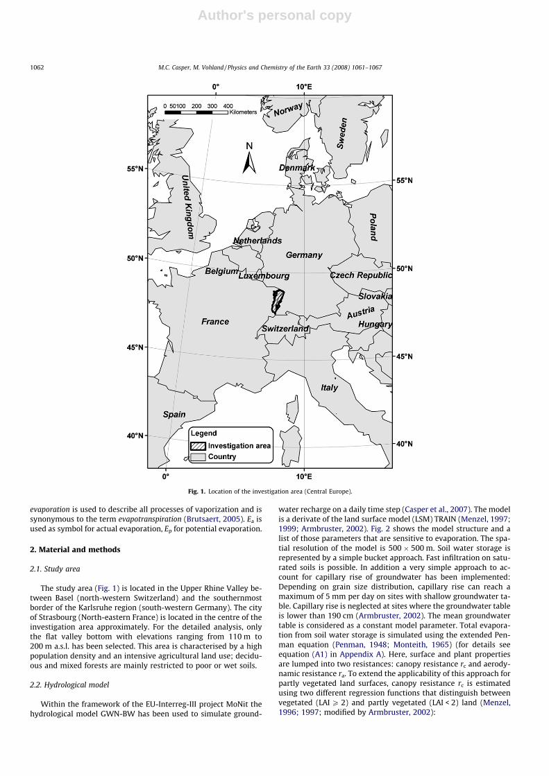
Within the framework of the MoNit project (LUBW, 2006; Cas-per et al., 2007), the land surface model (LSM) GWN_BW has beenused to simulate the long term water balance for the southern partof the Upper Rhine Valley (Fig. 1), mainly focussing on the precisedetermination of groundwater recharge. Usually, validation ofhydrological models is based on discharge measurements at theoutlet of catchments, but this kind of validation is very flat as itonly refers to a lumped variable. Furthermore, it does not provideany information about an appropriate reproduction of the spatialdifferentiation of the hydrologic cycle. Otherwise, alternative vali-dation strategies are often hindered by a lack of available ground

data. This calls attention to the potentials of remote sensing dataand its spatially distributed mapping capacities. From thermal sa-tellite imagery, spatial variations of surface temperature can be as-sessed directly which provides a valuable key for evaluating heatflux partitioning and consequently also actual evaporation on pixelscale. Nevertheless, additional data determines the link betweenland surface temperatures and evaporation rates (e.g. vegetationcoverage, net radiation, albedo or available soil moisture), andthese data sets are only partly available from remote sensing dataor climatic stations. Thus, the remote sensing approach provides aplausibility check rather than an absolute validation of the model-ling results. This study compares the spatial patterns reproducedby remote sensing data and the hydrological modelling tool. Onthis basis, inconsistencies of the modelling approach may be re-vealed, and urgent needs of alternative modelling concepts orparameterisation strategies may be clarified. In our paper the term

1474-7065/$ - see front matter � 2008 Elsevier Ltd. All rights reserved.doi:10.1016/j.pce.2008.06.001

* Corresponding author. Tel.: +49 6512014518.E-mail address: casper@uni-trier.de (M.C. Casper).

Physics and Chemistry of the Earth 33 (2008) 1061–1067

Contents lists available at ScienceDirect

Physics and Chemistry of the Earth

journal homepage: www.elsevier .com/locate /pce

Author's personal copy

evaporation is used to describe all processes of vaporization and issynonymous to the term evapotranspiration (Brutsaert, 2005). Ea isused as symbol for actual evaporation, Ep for potential evaporation.

2. Material and methods

2.1. Study area

The study area (Fig. 1) is located in the Upper Rhine Valley be-tween Basel (north-western Switzerland) and the southernmostborder of the Karlsruhe region (south-western Germany). The cityof Strasbourg (North-eastern France) is located in the centre of theinvestigation area approximately. For the detailed analysis, onlythe flat valley bottom with elevations ranging from 110 m to200 m a.s.l. has been selected. This area is characterised by a highpopulation density and an intensive agricultural land use; decidu-ous and mixed forests are mainly restricted to poor or wet soils.

2.2. Hydrological model

Within the framework of the EU-Interreg-III project MoNit thehydrological model GWN-BW has been used to simulate ground-

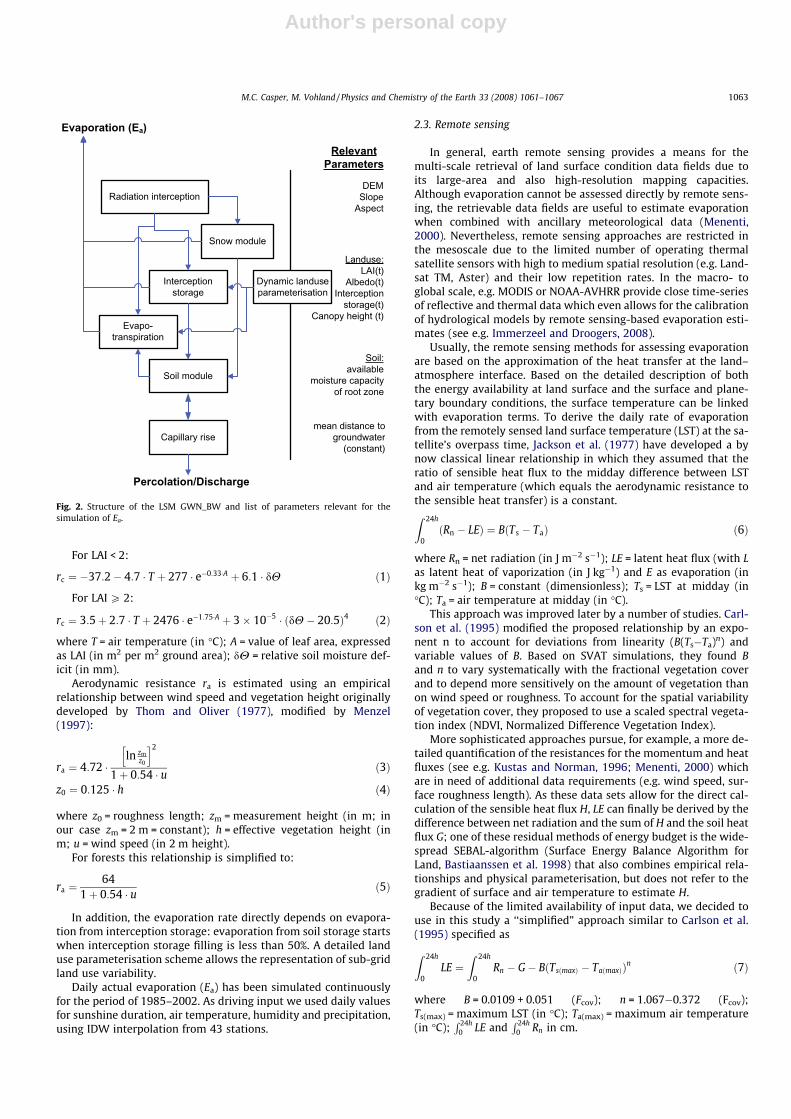
water recharge on a daily time step (Casper et al., 2007). The modelis a derivate of the land surface model (LSM) TRAIN (Menzel, 1997;1999; Armbruster, 2002). Fig. 2 shows the model structure and alist of those parameters that are sensitive to evaporation. The spa-tial resolution of the model is 500 � 500 m. Soil water storage isrepresented by a simple bucket approach. Fast infiltration on satu-rated soils is possible. In addition a very simple approach to ac-count for capillary rise of groundwater has been implemented:Depending on grain size distribution, capillary rise can reach amaximum of 5 mm per day on sites with shallow groundwater ta-ble. Capillary rise is neglected at sites where the groundwater tableis lower than 190 cm (Armbruster, 2002). The mean groundwatertable is considered as a constant model parameter. Total evapora-tion from soil water storage is simulated using the extended Pen-man equation (Penman, 1948; Monteith, 1965) (for details seeequation (A1) in Appendix A). Here, surface and plant propertiesare lumped into two resistances: canopy resistance rc and aerody-namic resistance ra. To extend the applicability of this approach forpartly vegetated land surfaces, canopy resistance rc is estimatedusing two different regression functions that distinguish betweenvegetated (LAI P 2) and partly vegetated (LAI < 2) land (Menzel,1996; 1997; modified by Armbruster, 2002):

Fig. 1. Location of the investigation area (Central Europe).

1062 M.C. Casper, M. Vohland / Physics and Chemistry of the Earth 33 (2008) 1061–1067

Author's personal copy

For LAI < 2:

rc ¼ �37:2� 4:7 � T þ 277 � e�0:33�A þ 6:1 � dH ð1Þ

For LAI P 2:

rc ¼ 3:5þ 2:7 � T þ 2476 � e�1:75�A þ 3� 10�5 � ðdH� 20:5Þ4 ð2Þ

where T = air temperature (in �C); A = value of leaf area, expressedas LAI (in m2 per m2 ground area); dH = relative soil moisture def-icit (in mm).

Aerodynamic resistance ra is estimated using an empiricalrelationship between wind speed and vegetation height originallydeveloped by Thom and Oliver (1977), modified by Menzel(1997):

ra ¼ 4:72 �ln zm

z0

h i2

1þ 0:54 � u ð3Þ

z0 ¼ 0:125 � h ð4Þ

where z0 = roughness length; zm = measurement height (in m; inour case zm = 2 m = constant); h = effective vegetation height (inm; u = wind speed (in 2 m height).

For forests this relationship is simplified to:

ra ¼64

1þ 0:54 � u ð5Þ

In addition, the evaporation rate directly depends on evapora-tion from interception storage: evaporation from soil storage startswhen interception storage filling is less than 50%. A detailed landuse parameterisation scheme allows the representation of sub-gridland use variability.

Daily actual evaporation (Ea) has been simulated continuouslyfor the period of 1985–2002. As driving input we used daily valuesfor sunshine duration, air temperature, humidity and precipitation,using IDW interpolation from 43 stations.

2.3. Remote sensing

In general, earth remote sensing provides a means for themulti-scale retrieval of land surface condition data fields due toits large-area and also high-resolution mapping capacities.Although evaporation cannot be assessed directly by remote sens-ing, the retrievable data fields are useful to estimate evaporationwhen combined with ancillary meteorological data (Menenti,2000). Nevertheless, remote sensing approaches are restricted inthe mesoscale due to the limited number of operating thermalsatellite sensors with high to medium spatial resolution (e.g. Land-sat TM, Aster) and their low repetition rates. In the macro- toglobal scale, e.g. MODIS or NOAA-AVHRR provide close time-seriesof reflective and thermal data which even allows for the calibrationof hydrological models by remote sensing-based evaporation esti-mates (see e.g. Immerzeel and Droogers, 2008).

Usually, the remote sensing methods for assessing evaporationare based on the approximation of the heat transfer at the land–atmosphere interface. Based on the detailed description of boththe energy availability at land surface and the surface and plane-tary boundary conditions, the surface temperature can be linkedwith evaporation terms. To derive the daily rate of evaporationfrom the remotely sensed land surface temperature (LST) at the sa-tellite’s overpass time, Jackson et al. (1977) have developed a bynow classical linear relationship in which they assumed that theratio of sensible heat flux to the midday difference between LSTand air temperature (which equals the aerodynamic resistance tothe sensible heat transfer) is a constant.Z 24h

0ðRn � LEÞ ¼ BðTs � TaÞ ð6Þ

where Rn = net radiation (in J m�2 s�1); LE = latent heat flux (with Las latent heat of vaporization (in J kg�1) and E as evaporation (inkg m�2 s�1); B = constant (dimensionless); Ts = LST at midday (in�C); Ta = air temperature at midday (in �C).

This approach was improved later by a number of studies. Carl-son et al. (1995) modified the proposed relationship by an expo-nent n to account for deviations from linearity (B(Ts�Ta)n) andvariable values of B. Based on SVAT simulations, they found Band n to vary systematically with the fractional vegetation coverand to depend more sensitively on the amount of vegetation thanon wind speed or roughness. To account for the spatial variabilityof vegetation cover, they proposed to use a scaled spectral vegeta-tion index (NDVI, Normalized Difference Vegetation Index).

More sophisticated approaches pursue, for example, a more de-tailed quantification of the resistances for the momentum and heatfluxes (see e.g. Kustas and Norman, 1996; Menenti, 2000) whichare in need of additional data requirements (e.g. wind speed, sur-face roughness length). As these data sets allow for the direct cal-culation of the sensible heat flux H, LE can finally be derived by thedifference between net radiation and the sum of H and the soil heatflux G; one of these residual methods of energy budget is the wide-spread SEBAL-algorithm (Surface Energy Balance Algorithm forLand, Bastiaanssen et al. 1998) that also combines empirical rela-tionships and physical parameterisation, but does not refer to thegradient of surface and air temperature to estimate H.

Because of the limited availability of input data, we decided touse in this study a ‘‘simplified” approach similar to Carlson et al.(1995) specified as

Z 24h

0LE ¼

Z 24h

0Rn � G� BðTsðmaxÞ � TaðmaxÞÞn ð7Þ

where B = 0.0109 + 0.051 (Fcov); n = 1.067�0.372 (Fcov);Ts(max) = maximum LST (in �C); Ta(max) = maximum air temperature(in �C);

R 24h0 LE and

R 24h0 Rn in cm.

Radiation interception

Snow module

Dynamic landuseparameterisation

Interceptionstorage

Evapo-transpiration

Soil module

Capillary rise

Evaporation (Ea)

Percolation/Discharge

DEMSlope

Aspect

Landuse:LAI(t)

Albedo(t)Interception

storage(t)Canopy height (t)

Soil:available

moisture capacityof root zone

mean distance togroundwater

(constant)

RelevantParameters

Fig. 2. Structure of the LSM GWN_BW and list of parameters relevant for thesimulation of Ea.

M.C. Casper, M. Vohland / Physics and Chemistry of the Earth 33 (2008) 1061–1067 1063

Author's personal copy

B and n are both calculated as a function of the fractional vege-tation coverage (Fcov) that is derived from a scaled vegetation in-dex. To retrieve vegetation index values (Iveg), we used – in linewith Carlson et al. – the NDVI formula that is a traditional andwidespread approach incorporating reflectance values R measuredin the near infrared (nIR) and the visible red (vis) (Rouse et al.,1974).

Fcov ¼ðIveg � Ivegð0ÞÞðIvegðsÞ � Ivegð0ÞÞ

� �2

ð8Þ

where Iveg = vegetation index value retrieved from the NDVI for-mula ðRnIR�RvisÞ

ðRnIRþRvisÞ

� �; Iveg(s) = index value at 100% vegetation cover; Ive-

g(0) = index value for bare soil.In total, the satellite data interpretation was accomplished for

two different Landsat-5 TM scenes (08.06.2000, 11.08.2000) thatcovered the complete study area without any clouds. Based onavailable radiation measurements (yet limited to the number ofonly five stations in or close to the study region), clear-sky condi-tions can be assumed for the entire day for these two dates. As theraw satellite data is not suitable for the retrieval of quantitativedata fields (e.g. Fcov, LST), a radiometric preprocessing was per-formed based on the atmospheric correction code MODTRAN-4to convert the raw digital numbers to pixel-wise absolute reflec-tances and kinetic surface temperatures. For the LST retrieval fromthe thermal channel of Landsat TM, the atmospheric correctionwas based on the MLS (mid-latitude summer) standard atmo-sphere (2.92 g cm�2 total water vapour content); furthermore, sur-face emissivity was integrated employing the approach of Brunselland Gillies (2002).

To obtain Ts(max) from the LST at the satellite’s overpass time(about 10:00 GMT), the diurnal evolution of the surface tempera-ture was modelled according to the ‘‘sine function” – model ofLagouarde and Brunet (1993). The maximum air temperatures thatwere measured at the climatic stations and afterwards spatiallyinterpolated were used to define (Ts(max)�Ta(max)).

In addition to (Ts(max)�Ta(max)), B and n, the net radiation andalso the soil heat flux have to be determined in the ‘‘simplified ap-proach” to assess LE. Estimates of the daily net radiation are feasi-ble with reasonable accuracy for clear-sky conditions, and the

calculation of the different terms of the net radiation budget (glo-bal radiation, surface albedo, incoming and emitted longwave radi-ation) was accomplished as fully described in Table 1; G wasafterwards calculated as fraction of Rn, whereas (G/Rn) was relatedto the fractional vegetation cover (Fcov) according to Boegh et al.(2002).

3. Results

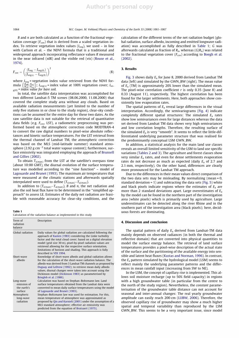
Fig. 3 shows daily Ea for June 8, 2000 derived from Landsat TMdata (left) and simulated by the GWN_BW (right). The mean valueof Ea (TM) is approximately 20% lower than the simulated mean.The pixel-wise correlation coefficient r is only 0.35 (June 8) and0.33 (August 11), respectively. The highest correlation has beenfound for the larger settlements. Here, both approaches show con-sistently low evaporation rates.

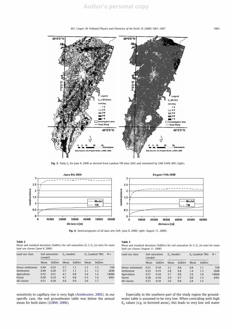
The spatial patterns of Ea reveal large differences in the visualinterpretation. Accordingly, the semivariograms (Fig. 4) indicatecompletely different spatial structures: The simulated Ea ratesshow low semivariances even for large distances whereas the dataset derived from Landsat TM data shows very high semivariancesand low correlation lengths. Therefore, the resulting surface ofthe simulated Ea is very ‘‘smooth”. It seems to reflect the little-dif-ferentiated underlying parameter structure that was realised forthe predominantly conceptual LSM GWN_BW.

In addition, a statistical analysis for the main land use classesreveals an overall limited sensitivity of the LSM to land use specificvariations (Tables 2 and 3). The agriculture and forest classes showvery similar Ea rates, and even for dense settlements evaporationrates do not decrease as much as expected (daily Ea of 2.7 and2.1 mm, respectively). On the other hand, differences are clearlymore pronounced for the Landsat TM approach.

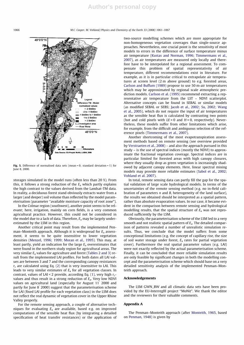
Due to the differences in their mean values direct comparison ofthe two data sets may be misleading. By normalizing (mean = 0,standard deviation = 1) and subtracting the data sets (Fig. 5) whiteand black pixels indicate regions where the estimates of Ea aremore than 2 standard deviations apart. Large overestimates of Ea

by the model can be found in the northern part of the investigationarea (white pixels) which is primarily used by agriculture. Largeunderestimates can be detected along the river Rhine and in thesouthern part of the investigation area (black pixels); here, decid-uous forests are dominating.

4. Discussion and conclusion

The spatial pattern of daily Ea derived from Landsat-TM datamainly depends on observed radiances (in both the thermal andreflective domain) that are converted into physical quantities tomodel the surface energy balance. The retrieval of land surfacetemperatures provides a pixel-wise description of the actual stateof the surface and the partitioning of the available energy into sen-sible and latent heat fluxes (Kustas and Norman, 1996). In contrast,the Ea pattern simulated by the hydrological model (LSM) seems toreflect mainly the underlying parameter patterns and the differ-ences in mean rainfall input (increasing from SW to NE).

In the LSM, the concept of capillary rise is implemented. This al-lows soil moisture recharge (up to 50% field capacity) in regionswith a high groundwater table (in particular from the centre tothe north of the study region). Nevertheless, the constant parame-terisation of the groundwater table distance can not account forseasonal and inter-annual changes: The real yearly groundwateramplitude can easily reach 200 cm (LUBW, 2006). Therefore, theobserved capillary rise of groundwater may show a much higherspatial and temporal variability than reproduced by the LSMGWN_BW. This seems to be a very important issue, since model

Table 1Calculation of the radiation balance as implemented in this study

Term ofradiationbalance

Description

Global radiation Daily values for global radiation are calculated following theapproach of Kasten (1983) considering the Linke turbidityfactor and the total cloud cover; based on a digital elevationmodel (grid size 30 m), pixel-by-pixel radiation values areretrieved allowing for the respective surface orientation,limitations of horizon and shading. This approach is fullydescribed in VDI 1994.

Short-wavealbedo

Knowledge of short-wave albedo and global radiation allowsfor the calculation of the short-wave radiation balance. Thealbedo was derived from 3 Landsat TM channels as proposed byDuguay and LeDrew (1992); to retrieve mean daily albedovalues, diurnal changes were taken into account using theDickinson model (Dickinson 1983) as parameterised byBriegleb et al. (1986).

Long-waveemission ofthe earth’ssurface

Calculation was based on Stephan–Boltzmann law. Landsurface temperatures obtained from the Landsat data wereconverted to mean daily surface temperatures using the modelof Lagouarde and Brunet (1993).

Atmosphericlong-waveradiation

Stephan–Boltzmann law was used for estimation. For this,mean temperature of atmosphere was approximated asproposed by Qin and Karnieli (2001) under the assumption of aMLS standard atmosphere; effective air emissivity waspredicted from the equation of Brutsaert (1975).

1064 M.C. Casper, M. Vohland / Physics and Chemistry of the Earth 33 (2008) 1061–1067

Author's personal copy

sensitivity to capillary rise is very high (Armbruster, 2002). In ourspecific case, the real groundwater table was below the annualmean for both dates (LUBW, 2006).

Especially in the southern part of the study region the ground-water table is assumed to be very low. When coinciding with highEp values (e.g. in forested areas), this leads to very low soil water

Fig. 3. Daily Ea for June 8, 2000 as derived from Landsat-TM data (left) and simulated by LSM GWN_BW (right).

Fig. 4. Semivariograms of all data sets (left: June 8, 2000; right: August 11, 2000).

Table 2Mean and standard deviation (StdDev) for soil saturation (0..1) Ea (in mm) for mainland use classes (June 8, 2000)

Land use class Soil saturation(model)

Ea (model) Ea (Landsat TM) N =

Mean StdDev Mean StdDev Mean StdDev

Dense settlement 0.49 0.22 2.7 1.1 1.3 1.3 528Settlement 0.49 0.20 3.7 1.1 2.1 1.3 2646Agriculture 0.52 0.21 4.7 0.8 3.4 1.2 14666Forest 0.50 0.19 4.7 0.8 5.5 1.4 4361All classes 0.51 0.20 4.6 0.9 3.6 1.7

Table 3Mean and standard deviation (StdDev) for soil saturation (0..1) Ea (in mm) for mainland use classes (August 11, 2000)

Land use class Soil saturation(model)

Ea (model) Ea (Landsat TM) N =

Mean StdDev Mean StdDev Mean StdDev

Dense settlement 0.31 0.18 2.1 0.8 0.8 1.1 528Settlement 0.33 0.19 2.8 0.8 1.4 1.3 2646Agriculture 0.37 0.18 3.7 0.8 2.8 1.0 14666Forest 0.38 0.18 3.9 0.7 4.0 1.3 4361All classes 0.37 0.18 3.6 0.8 2.8 1.5

M.C. Casper, M. Vohland / Physics and Chemistry of the Earth 33 (2008) 1061–1067 1065

Author's personal copy

storages simulated in the model runs (often less than 20 %). Fromthis, it follows a strong reduction of the Ea which partly explainsthe high contrast to the values derived from the Landsat-TM data.In reality, a deciduous forest stand obviously extracts water from alarger (and deeper) soil volume than reflected by the model param-eterisation (parameter ‘‘available moisture capacity of root zone”).

In the Colmar region (southwest), another point seems to be rel-evant; here, irrigation, mainly on corn fields, is a very commonagricultural practice. However, this could not be considered inthe model due to a lack of data. Therefore, Ea may be largely under-estimated by the LSM in this region.

Another critical point may result from the implemented Pen-man–Monteith approach. Although it is widespread for Ea assess-ment, it seems to be quite insensitive to lower vegetationdensities (Menzel, 1996; 1999; Moran et al., 1995). This may, atleast partly, yield an indication for the large Ea overestimates thatwere found in the northern study region for agricultural areas. Thevery similar Ea values for agriculture and forest (Tables 2 and 3) re-sult from the implemented LAI profiles. For both dates all LAI val-ues are between 3 and 7 and the corresponding canopy resistancesrc are calculated using Eq. (2) that is very insensitive to LAI. Thisleads to very similar estimates of Ea for all vegetation classes. Incontrast, values of LAI < 2 provide, according Eq. (1), very high rc-values and thus result in a strong reduction of Ea. Very low NDVIvalues on agricultural land (especially for August 11’ 2000 andpartly for June 8’ 2000) suggest that the parameterisation schemefor LAI (fixed LAI profile for each vegetation class) in the LSM doesnot reflect the real dynamic of vegetation cover in the Upper RhineValley properly.

For the remote sensing approach, a couple of alternative tech-niques for evaluating Ea are available, based e.g. on improvedcomputations of the sensible heat flux (by integrating a detailedspecification of heat transfer resistances) or the application of

two-source modelling schemes which are more appropriate fornon-homogeneous vegetation coverages than single-source ap-proaches. Nevertheless, one crucial point is the sensitivity of mostmodels to errors in the difference of surface temperature minusair temperature (Kustas and Norman, 1996; Timmermans et al.,2007), as air temperatures are measured only locally and there-fore have to be interpolated for a regional assessment. To com-pensate this problem of spatial representativity of airtemperature, different recommendations exist in literature. Forexample, as it is in particular critical to extrapolate air tempera-tures at screen level (2 m above ground) to e.g. forested areas,Carlson and Buffum (1989) propose to use 50 m-air temperatureswhich may be approximated by regional scale atmospheric pre-diction models. Carlson et al. (1995) recommend extracting a rep-resentative air temperature from the LST – NDVI scatterplot.Alternative concepts can be found in SEBAL or similar models(as modified SEBAL or SEBS; Jacob et al., 2002; Su, 2002; Wanget al., 2005), which do not require the input of air temperaturesas the sensible heat flux is calculated by contrasting two points(hot and cold pixels with LE = 0 and H = 0, respectively). Never-theless, these models suffer from other limitations which arise,for example, from the difficult and ambiguous selection of the ref-erence pixels (Timmermans et al., 2007).

Another shortcoming of the most evapotranspiration assess-ment methods based on remote sensing (see overview providedby Verstraeten et al., 2008) – and also the approach pursued in thisstudy – is the use of spectral indices (mostly the NDVI) to approx-imate the fractional vegetation coverage. Spectral indices are inparticular limited for forested areas with high canopy closures,where they usually drop as green vegetation is increasingly shad-owed by adjacent canopy elements. Here, linear spectral mixingmodels may provide more reliable estimates (Sabol et al., 2002;Vohland et al. 2007).

In total, remote sensing data can partly fill the gap for the spa-tial validation of large scale hydrological models. In terms of theuncertainties of the remote sensing method (e.g. no in-field cali-bration of parameters n and B, heterogeneity of the land surface),the results we obtained should be interpreted as a spatial pattern,rather than absolute evaporation values. In our case, it became evi-dent in the comparison between remote sensing and hydrologicalmodelling results, that the spatial structure of Ea was not repro-duced sufficiently by the LSM.

Obviously, the parameterisation scheme of the LSM led to a verysmooth and not realistic spatial pattern of Ea. The detailed compar-ison of patterns revealed a number of unrealistic simulation re-sults. Thus, we conclude that the model suffers from someconceptional limitations (e.g. the concept of capillary rise, the sizeof soil water storage under forest, Ea rates for partial vegetationcover). Furthermore the real spatial parameter values (e.g. LAI)were not exactly reflected by the actual parameterisation scheme.Finally, it can be concluded that more reliable simulation resultsare only feasible by significant changes in both the modelling con-cept and the parameterisation scheme which should base on a verydetailed sensitivity analysis of the implemented Penman–Mon-teith approach.

Acknowledgements

The LSM GWN_BW and all climatic data sets have been pro-vided by the EU-InterregIII project ‘‘MoNit”. We thank the editorand the reviewers for their valuable comments.

Appendix A

The Penman–Monteith approach (after Monteith, 1965, basedon Penman, 1948) is given by

Fig. 5. Difference of normalised data sets (mean = 0; standard deviation = 1) forJune 8, 2000.

1066 M.C. Casper, M. Vohland / Physics and Chemistry of the Earth 33 (2008) 1061–1067

Author's personal copy

Ea ¼D � Rn þ Cp

ðesatðTaÞ�eaÞfa

k Dfc

h iþ c

fcþfa�

24

35 � 1

f cðA1Þ

where Ea is actual evaporation rate, Rn is net external energy, Cp isheat capacity of air at constant pressure, esat(Ta) is saturation vapourpressure at air temperature Ta, ea is actual vapour pressure, k is la-tent heat of vaporization, D is slope of saturation vapour pressurecurve at air temperature, c is psychrometric constant, fc canopyresistance and fa aerodynamic resistance.

References

Armbruster, V., 2002. Grundwasserneubildung (groundwater recharge) in Baden-Württemberg, Ph.D. Thesis University of Freiburg, Freiburger Schriften zurHydrologie 17.

Bastiaanssen, W.G.M., Menenti, M., Feddes, R.A., Holtslag, A.A.M., 1998. A remotesensing surface energy balance algorithm for land (SEBAL). J. Hydrol. 212–213,198–212.

Boegh, E., Soegaard, H., Thomsen, A., 2002. Evaluating evaporation rates and surfaceconditions using Landsat TM to estimate atmospheric resistance and surfaceresistance. Rem. Sens. Environ. 79, 329–343.

Briegleb, B.P., Minnis, P., Ramanathan, V., Harrison, E., 1986. Comparison of regionalclear-sky albedos inferred from satellite observations and model computations.J. Climate Appl. Meteor. 25, 214–226.

Brunsell, N.A., Gillies, R.R., 2002. Incorporation of surface emissivity into a thermalatmospheric correction. Photogrammetric Engineering and Remote Sensing 68,1263–1269.

Brutsaert, W., 1975. On a derivable formula for long-wave radiation from clearskies. Water Resources Research 11, 742–744.

Brutsaert, W., 2005. Hydrology. Cambridge University Press.Carlson, T.N., Buffum, M.J., 1989. On estimating total daily evapotranspiration

from remote surface temperature measurements. Rem. Sens. Environ. 29,197–207.

Carlson, T.N., Capehart, W.J., Gillies, R.R., 1995. A new look at the simplified methodfor remote sensing of daily evaporation. Rem. Sens. Environ. 54, 161–167.

Casper, M., Grimm-Strele, J., Gudera, T., Korte, S., Lambrecht, H., Schneider, B., vanDijk, P., Graveline, N., Finck, M., 2007. EU-Project MoNit a DSS to assess theimpact of actions and changing frameworks on the nitrate load in the UpperRhine Valley aquifer, vol. 317. IAHS Publication. pp. 96–101.

Dickinson, R.E., 1983. Land surface processes and climate-surface albedos andenergy balance. Adv. Geophys. 25, 305–353.

Duguay, C.R., LeDrew, E.F., 1992. Estimating surface reflectance and albedo fromLandsat-5 Thematic Mapper over rugged terrain. Photogram. Eng. Rem. Sens.58, 551–558.

Immerzeel, W.W., Droogers, P., 2008. Calibration of a distributed hydrologicalmodel based on satellite evapotranspiration. J. Hydrol. 349, 411–424.

Jackson, R.D., Reginato, R.J., Idso, S.B., 1977. Wheat canopy temperature: A practicaltool for evaluating water requirements. Water Res. Res. 13, 651–656.

Jacob, F., Olioso, A., Gu, X.F., Su, Z., Seguin, B., 2002. Mapping surface fluxes usingairborne visible, near infrared, thermal infrared remote sensing data and aspatialized surface energy balance model. Agronomie 22, 669–680.

Kasten, F., 1983. Parametrisierung der Globalstrahlung durch Bedeckungsgrad undTrübungsfaktor. Annalen der Meteorologie 20, 49–50.

Kustas, W.P., Norman, J.M., 1996. Use of remote sensing for evaporation monitoringover land surfaces. Hydrol. Sci. J. 41, 495–516.

Lagouarde, J.P., Brunet, Y., 1993. A simple model for estimating the daily upwardlongwave surface radiation flux from NOAA-AVHRR data. Int. J. Rem. Sens. 14,907–925.

LUBW 2006. Landesanstalt für Umwelt, Messungen und Naturschutz Baden-Württemberg (LUBW) (Ed.): Grundwasserströmung und Nitrattransport/Modélisation hydrodynamique et transport des nitrates, final report of theInterreg-III project MoNit, Karlsruhe.

Menenti, M., 2000. Evaporation. In: Schultz, G.A., Engman, E.T. (Eds.), RemoteSensing in Hydrology and Water Management. Springer, Berlin-Heidelberg, pp.157–188.

Menzel, L., 1996. Modelling Canopy Resistances and Transpiration of Grassland.Phys. Chem. Earth 21, 123–129.

Menzel, L., 1997. Modellierung der Evaporation im System Boden-Pflanze-Atmosphäre. Zürcher Geographische Schriften, Nr. 67. Geographisches InstitutETH, Zürich.

Menzel, L., 1999. Flächenhafte Modellierung der Evaporation mit TRAIN. PIK ReportNo. 54. Potsdam.

Monteith, J.L., 1965. Evaporation and the environment. Symp. Soc. Expl. Biol. 19,205–234.

Morgan, M.S., Rahman, A.F., Washburne, J.C., Goodrich, D.C., Weltz, M.A., Kustas,W.P., 1996. Combining the Penman–Montheith equation with measurements ofsurface temperature and reflectance to estimate evaporation rates of semiaridgrassland. Agr. Forest Meteorol. 80, 87–109.

Penman, H.L., 1948. Natural evaporation from open water, bare soil and grass. In:Proc. Roy. Soc. 193, 120–145.

Qin, Z., Karnieli, A., 2001. A mono-window algorithm for retrieving land surfacetemperature from Landsat TM data and its application to the Israel-Egyptborder region. Int. J. Rem. Sens. 22, 3719–3746.

Rouse, J.W., Haas, R.H., Schell, J.A., Deering, D.W., Harlan, J.C., 1974. Monitoring thevernal advancement of retrogradation of natural vegetation. NASA/GSFC, TypeIII, Final Report, Greenbelt, MD.

Sabol Jr., D.E., Gillespie, A.R., Adams, J.B., Smith, M.O., Tucker, C.J., 2002. Structuralstage in Pacific Northwest forests estimated using simple mixing models ofmultispectral images. Rem. Sens. Environ. 80, 1–16.

Su, Z., 2002. The surface energy balance system (SEBS) for estimation of turbulentheat fluxes. Hydrol. Earth Syst. Sci. 6, 85–99.

Thom, A.S., Oliver, H.R., 1977. On Penman’s equation for estimating regionalevaporation. Quart. J. Roy. Meteorol. Soc. 103, 345–357.

Timmermans, W.J., Kustas, W.P., Anderson, M.C., French, A.N., 2007. Anintercomparison of the Surface Energy Balance Algorithm (SEBAL) and theTwo-Source Energy Balance (TSEB) modelling schemes. Rem. Sens. Environ. 108,369–384.

VDI, 1994. Umweltmeteorologie. Wechselwirkungen zwischen Atmosphäre undOberflächen. Berechnung der kurz- und langwelligen Strahlung. VereinDeutscher Ingenieure (VDI), Düsseldorf, VDI Richtlinie 3789 Blatt 2.

Verstraeten, W.W., Veroustraete, F., Feyen, J., 2008. Assessment ofevapotranspiration and soil moisture content across different scales ofobservation. Sensors 8, 70–117.

Vohland, M., Stoffels, J., Hau, C., Schüler, G., 2007. Remote sensing techniques forforest parameter assessment: Multispectral classification and linear spectralmixture analysis. Silva Fennica 41, 441–456.

Wang, J., Sammis, T.W., Meier, C.A., Simmons, L.J., Miller, D.R., Samani, Z. (2005). AModified SEBAL Model for Spatially Estimating Pecan Consumptive Water Usefor Las Cruces, New Mexico. in: Proc. American Meteorological Society 15thConference on Applied Climatology, Savannah, GA, June 20–24.

M.C. Casper, M. Vohland / Physics and Chemistry of the Earth 33 (2008) 1061–1067 1067