Vachier Lagrave S A

Arnulfo Félix Campos A01280077

César García Segovia A01087439

Marco Antonio Villalobos Regalado A00812515

PhD Rafael Bourguet Díaz

System Dynamics

Final Project: Market Growth

4th July 2014

Anything that can go wrong will go wrong. – J. A Murphy

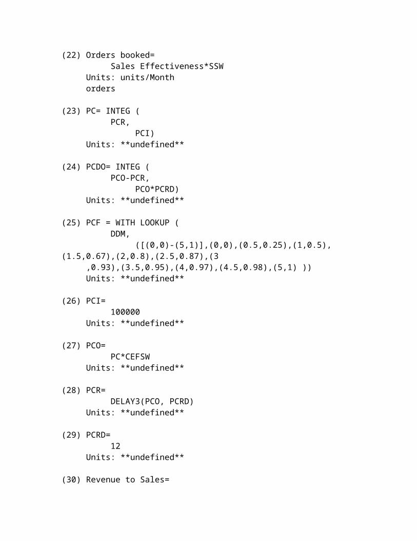
Introduction to system dynamics

System dynamics is the use of both informal maps and

formal models with computer simulation to test, uncover and

understand endogenous sources of a system behavior. We use

systems thinking to hypothesize, test and refine endogenous

explanations of a system change, and to use those

explanations we come up with to guide our policies and

decision making along the efforts of increasing both revenue

and profits. Effective learning using system dynamics will

often require training for participants in scientific

method. Along with techniques developed in system dynamics,

many tools and protocols for group model building are now

available, including causal loop diagrams, policy structure

diagrams, interactive computer mapping, and various problem

structuring and soft systems methods.

Forrester, the author of this model presented a four –

tiered hierarchy, which he considers of high importance when

studying a model such as the one described on this paper.

The following parts composed that hierarchy: the closed

boundary around the system, feedback loops as the basic

structural elements within the boundary, stock variables

representing accumulations within the feedback loops and a

rate variable representing activity within the feedback

loops. This particular tiered hierarchy can actually apply

in a generalization to any system as a whole.

An exogenous and an endogenous point of view could be

express in the next statement by Benjamin Disraeli “Man is

not the creature of circumstances. Circumstances are the

creatures of men.” Feedback loops enable the endogenous

point of view and give it structure. The endogenous point of

view is fundamental to systems thinking in the system

dynamics tradition.

Case Summary

This paper by Professor Jay Wright Forrester of

Massachusetts Institute of Technology presents the “Market

Growth Model” as an example of modeling a complex system.

The first several sections of the paper are rather an

introduction in form of a description to the structure of

systems in terms of feedback loops, levels (stocks) and

rates.

Further, the paper then proceeds to build and explain the

market growth model using both Fortran (programming

language) and Dynamo. Professor Forrester describes the

dynamics of changing the delivery delay goal of the company.

Such behavior is often referred to as “eroding goals” type

of archetype, which we saw during our summer course.

By taking a decision unwillingly or willingly the manager

changes the rules of the game by altering the policies that

guide further or future decision-making. Such systems have a

feedback loop structure that determines the growth and

stability of the enterprise. The complexity of these systems

usually needs a tremendous amount of intuition (experience)

to determine with accuracy how a policy change will affect

the total system. A simulation model of the feedback

structure and policies allows one to try policy changes to

see how the system reacts.

Growth and sluggishness of a brand new product is given as

an example to demonstrate how the ideas of a feedback

structure can explain a common event in market behavior.

Very often early sales grow rapidly, only to level off even

while the market demand continues to rise and new

competitors start to enter the growing market and capture an

increasing share of that specific market. One cause is found

in the capital investment policy of the firm, as shown in a

model involving salesmen, market reaction to delivery delay,

and capital equipment expansion.

On Market Growth and decline

For decades and decades, managers have been learning to play

by a set of rules. Companies must be flexible to respond

rapidly and mercilessly to rivalry and market changes. They

must outsource aggressively to gain efficiencies. And they

must nurture a few core competencies in race to stay ahead

of rivals. Positioning, during the past decade tended to be

insanely important, just like in the game of chess, to gain

special advantage or to tumble the concurrence. It was once

thought and taught that position and strategy had nothing to

do with one another. In the game of chess we can see how

both of them collide to become one; in our modern times it

is necessary, for business to stay on top of things and step

they game up to combine these features, that will inevitable

merge into a new concept called strategic positioning; in

other words preserving what is distinctive/different about a

company.

To fairly give the approach that this economical or

strategic theme that our work handles we will need to bare

out certain facts such as the ones portrayed in the

following books:

On Blue Ocean Strategy by W. Chan Kim and Renée Mauborgne which

is based on a study of 150 strategic moves spanning more

than a hundred years and thirty industries, Kim & Mauborgne

argue that companies can succeed not by battling

competitors, but rather by creating blue oceans of uncontested

market space. They assert that these strategic moves create

a leap in value for the company, its buyers, and its

employees, while unlocking new demand and making the

competition irrelevant. This strikes right at the center of

our story by the fact that we are encouraging to create a

brand new submarket that will clearly distinguished our

company from the competition and give ourselves a first hand

advantage by not only opening this market rather than

putting prices according to a study that will follow.

In the other hand, right at the center, on top of it all,

there is an statement that came into awareness in the highly

laureate book Strategic Marketing Planning by Derek F. Abell and

John S. Hammond which talks about portfolio strategy

therefore on how, when on what cash should be invested in

the seek of added values to the company.

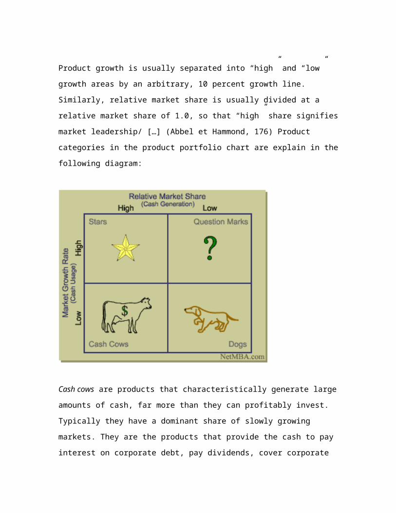
Product growth is usually separated into “high” and “low”

growth areas by an arbitrary, 10 percent growth line.

Similarly, relative market share is usually divided at a

relative market share of 1.0, so that “high” share signifies

market leadership/ […] (Abbel et Hammond, 176) Product

categories in the product portfolio chart are explain in the

following diagram:

Cash cows are products that characteristically generate large

amounts of cash, far more than they can profitably invest.

Typically they have a dominant share of slowly growing

markets. They are the products that provide the cash to pay

interest on corporate debt, pay dividends, cover corporate

overhead, finance R&D, and help other products to grow.

(Abbel et Hammond, 177)

Dogs are products with low share of slowly growing markets.

They neither generate nor require significant amounts of

cash. Maintaining share usually requires reinvestment of

their modest cash flow from operations, as wells as modest

amounts of additional capital. Because of low share their

profitability is poor and they are unlikely to ever be

significant sources of cash; therefore they are often called

“cash traps”. (Abbel et Hammond, 177)

Problem children or Questions marks are products with lo share of

fast-growing markets. Their low share often means low

profits and weak cash flow from operations; at the same time

because they are in rapidly growing markets, they require

large amounts of cash to maintain market share, and still

larger amounts to gain share. Hence their name, market

growth is attractive, yet large amounts of cash will be

required if they will ever gain sufficient share to be

strong members of the product portfolio. (Abbel et Hammond,

178)

Stars are high-growth, high-share products, which may or may

not be self-sufficient in cash flow. This depends on whether

their strong cash flow form operations is sufficient to

finance rapid growth. Their present, modest cash need or

throw off will change to a large cash throw off in the

future, when the growth rate if their market slows. (Abbel

et Hammond, 178)

Model’s objective

The objective of this work is to put into practice our

abilities on what refers to the usage of Vensim as software

for modeling systems. In the other hand, and speaking solely

about the software, we can acceptably conclude that we are

trying to model, predict outcomes and make changes in

policies into a fictitious environment that in reality all

enterprises in modern times have to fight against. Knowing,

beforehand that several variables intervene on outcomes like

the ones of this class we were required to enhance on

background information.

Model’s audience

We dare to conclude that our audience can range from any

other of ages between 15 and 90 whether knowing much or less

about marketing, strategic planning, entrepreneurship,

system dynamics or whatsoever. Nevertheless, we can also

argue that specialist on this area will find this work

resourcefully, innovative and unique in the near future.

Model’s restrictions

The model has several restrictions. Firstly, the economic

activity is not modeled in an ideal manner and it clearly

reinforces the markets. This is because it is modeled with a

positive and linear growth without any disturbance over

time. This is wrong and idealistic since in economy suffers

devaluations, inflation and crises among other things.

Additionally, it is difficult to model economic growth over

time because it is a difficult task to "predict" the

economic performance of a country. This is caused by the

dependency between the different economies in this

everlasting ever-interconnecting world.

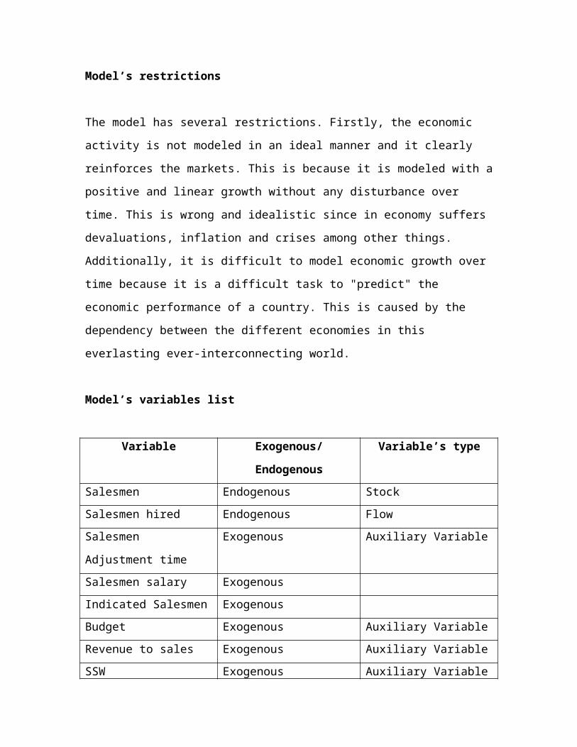
Model’s variables list

Variable Exogenous/

Endogenous

Variable’s type

Salesmen Endogenous StockSalesmen hired Endogenous FlowSalesmen

Adjustment time

Exogenous Auxiliary Variable

Salesmen salary ExogenousIndicated Salesmen ExogenousBudget Exogenous Auxiliary VariableRevenue to sales Exogenous Auxiliary VariableSSW Exogenous Auxiliary Variable

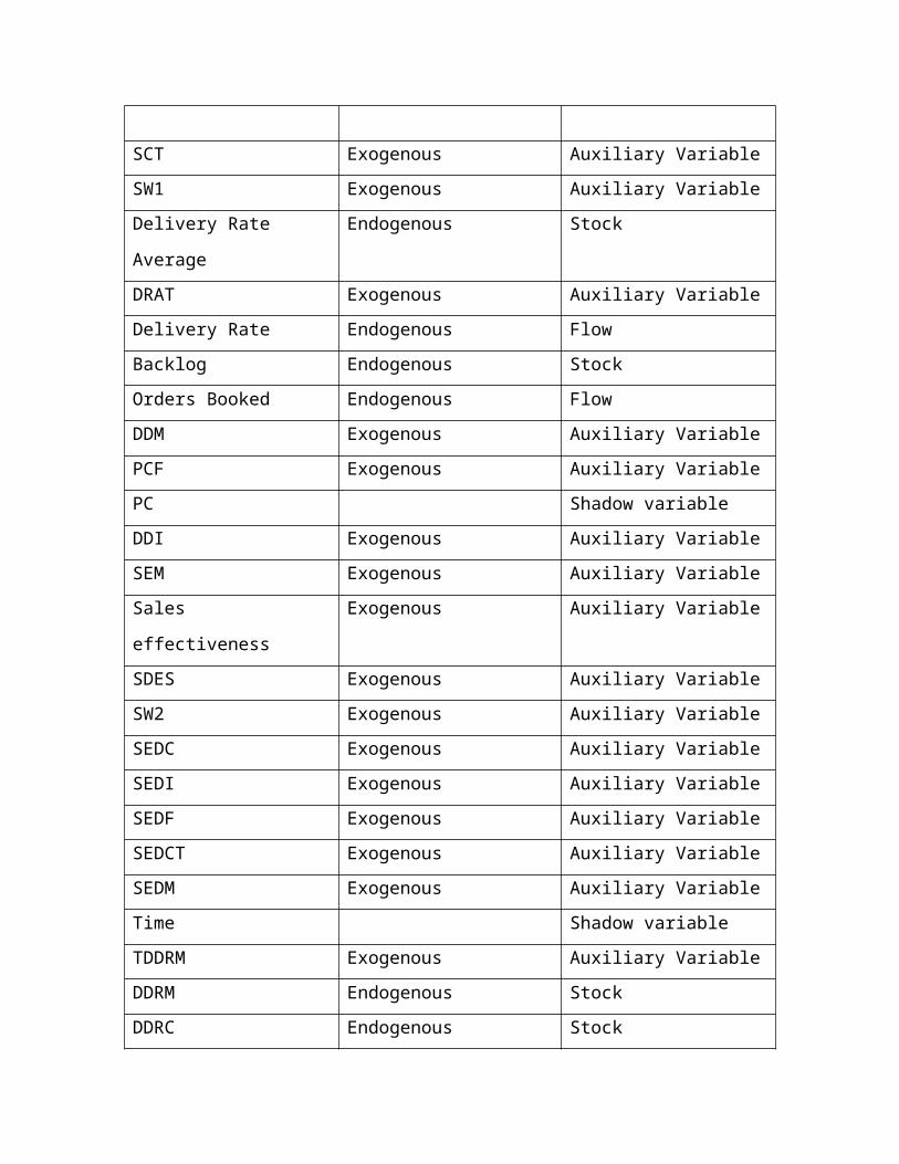
SCT Exogenous Auxiliary VariableSW1 Exogenous Auxiliary VariableDelivery Rate

Average

Endogenous Stock

DRAT Exogenous Auxiliary VariableDelivery Rate Endogenous FlowBacklog Endogenous StockOrders Booked Endogenous FlowDDM Exogenous Auxiliary VariablePCF Exogenous Auxiliary VariablePC Shadow variableDDI Exogenous Auxiliary VariableSEM Exogenous Auxiliary VariableSales

effectiveness

Exogenous Auxiliary Variable

SDES Exogenous Auxiliary VariableSW2 Exogenous Auxiliary VariableSEDC Exogenous Auxiliary VariableSEDI Exogenous Auxiliary VariableSEDF Exogenous Auxiliary VariableSEDCT Exogenous Auxiliary VariableSEDM Exogenous Auxiliary VariableTime Shadow variableTDDRM Exogenous Auxiliary VariableDDRM Endogenous StockDDRC Endogenous Stock

DDT Endogenous StockTDDRC Exogenous Auxiliary VariableDDC Exogenous Auxiliary VariableDDB Exogenous Auxiliary Variable

CEFSW Exogenous Auxiliary VariableCEF Exogenous Auxiliary VariableSW3 Exogenous Auxiliary VariableDDMG Exogenous Auxiliary VariableTDDT Exogenous Auxiliary VariableDDW Exogenous Auxiliary VariableDDWC Exogenous Auxiliary VariableDDOG Exogenous Auxiliary VariablePCI Exogenous Auxiliary VariablePCRD Exogenous Auxiliary VariablePCO Endogenous FlowPC Endogenous StockPCDO Endogenous StockPCR Endogenous Flow

Story

The concept that

gets into

perspective in

this model is the

idea of sale

effectiveness so

that it is circumscribed in the bowels of our system. This

concept more or less, relates the ideas of delivery rate and

pending orders, which could be seen as exclusive events.

Salesmen and backlog stocks determine the effects in our

effectiveness to sale, produce and therefore our everlasting

goal as a company: revenues.

On June 23, 2014, Maxime Vachier Lagrave Jr., in charge

of the marketing division at Vachier Lagrave S.A stood at a

crossroad. He had to make a decision regarding whether

necessary to hire or to fire salesmen and finding a solution

to that bottleneck in production and delivery for the

company’s personalized wristwatches.

The company’s name Vachier Lagrave (client) is an eponymous for

its founder Maxim Vachier Lagrave Sr. and handles the

manufacture of top notch, high class, luxury and

personalized wristwatches. The company’s reputation is quite

respectable being qualified by specialized magazines such as

Hodinkee and Time Lords as one of the best out in the market

with a range of prices that would exclude most of us from

buying or even personalizing a watch. Nevertheless, the

company is having serious issues in what refers to the

delivery rate and the pending orders and this will be

explained further. The company sees an area of opportunity

by enhancing the understanding of how the indicator sells

efficiency works. The company wants sees plausible to fire

some salesmen without even studying the causes and effects

simply by arguing “they are taking revenue and we still

cannot find a solution to our tardiness in what refers to

deliveries”.

First of all an order is placed by any client and all those

orders are registered in the system, establishing the time

of delivery, the perception flow (how long it takes to

perceive all the data for the personalized watch). The

delivery limit connects both the known delivery rate and the

booked orders that have not been delivered yet. By using a

shadow variable (time) the company can calculate the

velocity of delivery considering facts such as the limits of

capacity of pending deliveries and compare it to the

forecast or previous experiences that apply to the same

case. There is a rate by the stock variable (backlog), which

is the remainder of out going orders and in going orders.

All this effectiveness can be compared to a standard (normal

time of delivery), which affects the effectiveness of the

sale. The sellers are the entity that interacts with the

customer and the list of brand new and therefore pending

orders.

Vachier Lagrave has a limited production capacity of 150,000

wristwatches per month and it has none of them in the

inventory due to the fact that they are personalized

including the inner parts and the fact of being string,

automatic or battery watches must be highly considered.

Right after booked the order is send and the production (art

masterpiece and meticulous care) gets started. All materials

are beforehand available and there will not be lack of them

(any kind of precious metals or pieces). Once ready the

seller will call the client and they will properly arrange

an appointment for tests and in the best of scenarios the

clients will pay and take the wristwatch with him/her. The

company has a yearly demand of 8,000,000 watches. The

estimated costs for each watch waggle around 204,000 USD and

the paid price around 222,000 USD.

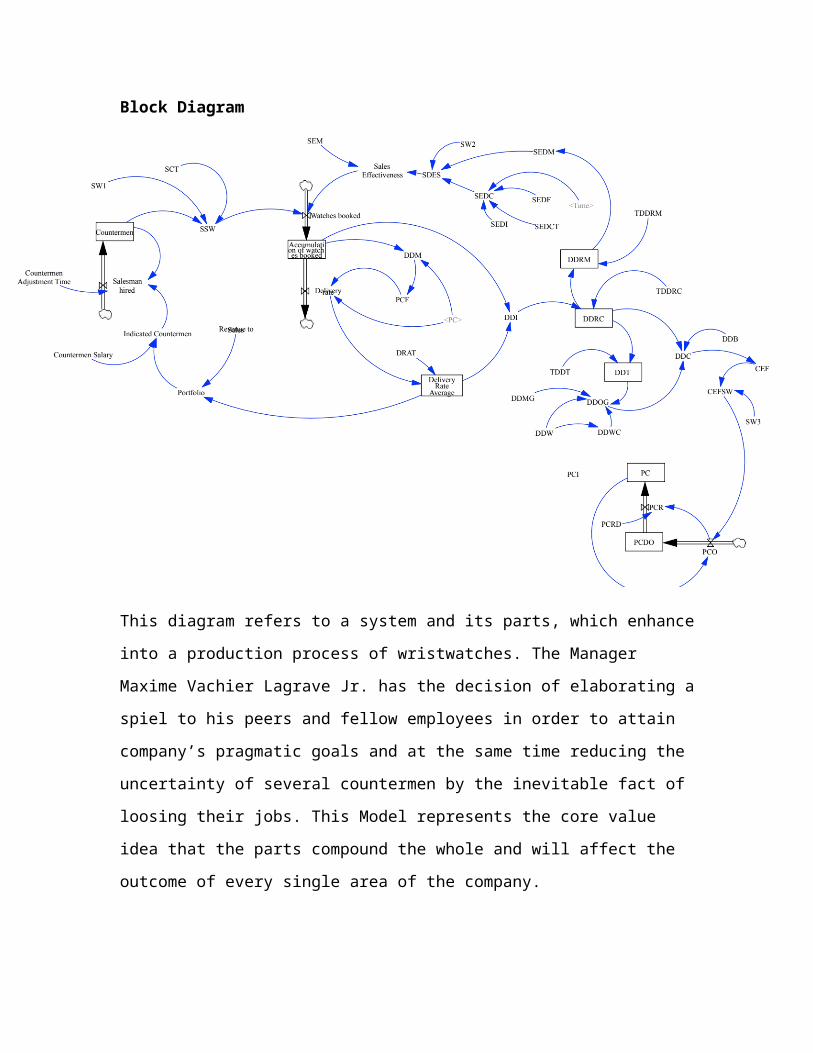
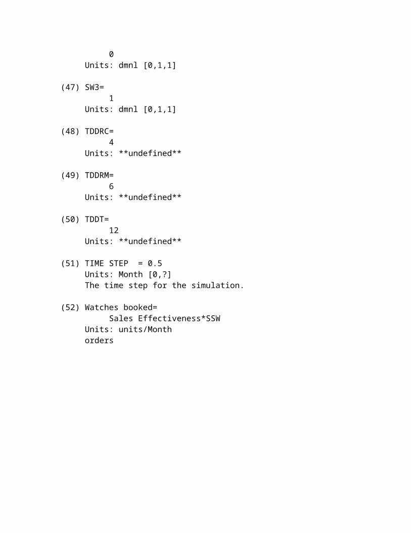
Block Diagram

This diagram refers to a system and its parts, which enhance

into a production process of wristwatches. The Manager

Maxime Vachier Lagrave Jr. has the decision of elaborating a

spiel to his peers and fellow employees in order to attain

company’s pragmatic goals and at the same time reducing the

uncertainty of several countermen by the inevitable fact of

loosing their jobs. This Model represents the core value

idea that the parts compound the whole and will affect the

outcome of every single area of the company.

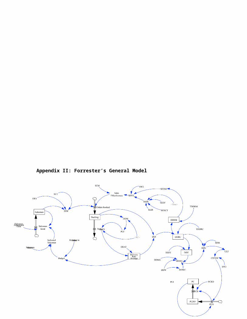
Graphs

It is quite acceptable to conclude that the graphs

representing the process of the client aka Vachier Lagrave

S.A lead to an inevitable affair: counterman aka salesmen

are properly and formerly doing their tasks to attain

mission and vision of the company and will stay on board. In

the other hand, contacting and hiring new elements,

capacitation, new fabrics, and new materials in order to

attend the evergreen, ever growing, demand will reduce the

portfolio but in the long and medium term will refer to us

as net profits and inevitable impulse the client into future

pursues.

Conclusions

The clear solution to this problem will be to enhance two

things in particular: communication within the departments

of the company and, of course, the upgrading of a far

better, production capacity by hiring more people in the

manufacture department rather than in the selling department

which seems to us is making a real great deal out of things.

They need to study by methods of work design factors of

recoil such as bottlenecks. This particular analysis

requires time while the production will still be working,

waiting furiously for that upgrade. In the other hand, lack

of communications between departments states for most of the

problems in every enterprise not to say it is the main

cause, in our believe, of the existence of human problems of

all kind. Seeing in retrospective this is one of the

advantages of preventive care so undervalued in our modern

times.

In an ever-evolving world with tremendous changes from time

to time, from generation to generation and an increasing

complexity accurateness and stability are quite scarce. By

pursuing the study of such a field as system dynamics

introduced by the American pioneer Jay W. Forrester our

lives as, entrepreneurs, clients, suppliers or even buyers

can find certain relief. Modeling systems can predict the

future by using a simulator. Our capacity to overcome the

problems has increased as well as the problem complexity

itself; so we as free thinkers have no excuse whatsoever not

to keep up with the work and make our society (system) a

better place.

The field of system dynamics is rather young and vast. Over

the past decades, many top companies, consulting firms, and

governmental organizations have used system dynamics to

address critical issues. More innovative universities and

business schools are teaching system dynamics and finding

enthusiastic and growing enrollments. Sooner or later after

this course our paths thru professional life will once again

meet up with this area of study knowing that we are not

alone on that one.

References

Sterman, John. Business dynamics: systems thinking and

modeling for a complex world. Boston: Irwin/McGraw-Hill,

2000. Print.

Kim, W. Chan, and Renée Mauborgne. Blue ocean strategy: how

to create uncontested market space and make the competition

irrelevant. Boston, Mass.: Harvard Business School Press,

2005. Print.

Abell, Derek F., and John S. Hammond. Strategic market

planning: problems and analytical approaches. Englewood

Cliffs, N.J.: Prentice-Hall, 1979. Print.

Forrester, Jay Wright. Market growth as influenced by

capital investment. Ithaca, N.Y.: Industrial Management

Review, 1968. Print.

Buettner, Blake. "A Week On The Wrist: The Chopard L.U.C

Lunar Twin." Hodinkee. Hodinkee, 5 Feb. 2014. Web. 2 July

2014. <http://www.hodinkee.com/blog/a-week-on-the-wrist-

chopard-luc-lunar-twin>.

Appendix I

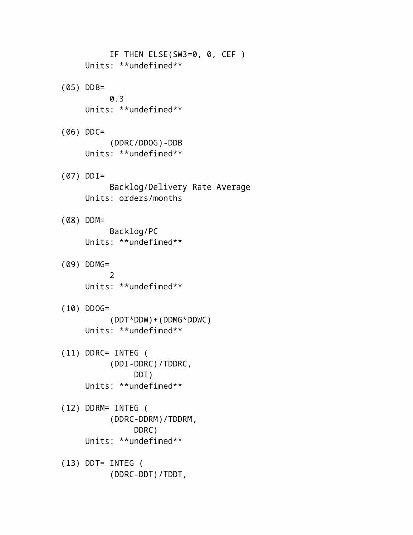
(01) Accumulation of watches booked= INTEG (INTEGER( Watches booked-Delivery rate),

8000)Units: ordersorders

(02) CEF = WITH LOOKUP (DDC,

([(0,-0.07)-(2.5,0.15)],(0,-0.07),(0.5,-0.02),(1,0),(1.5,0.02),(2,0.07),

(2.5,0.15) ))Units: **undefined**

(03) CEFSW=IF THEN ELSE(SW3=0, 0, CEF )

Units: **undefined**

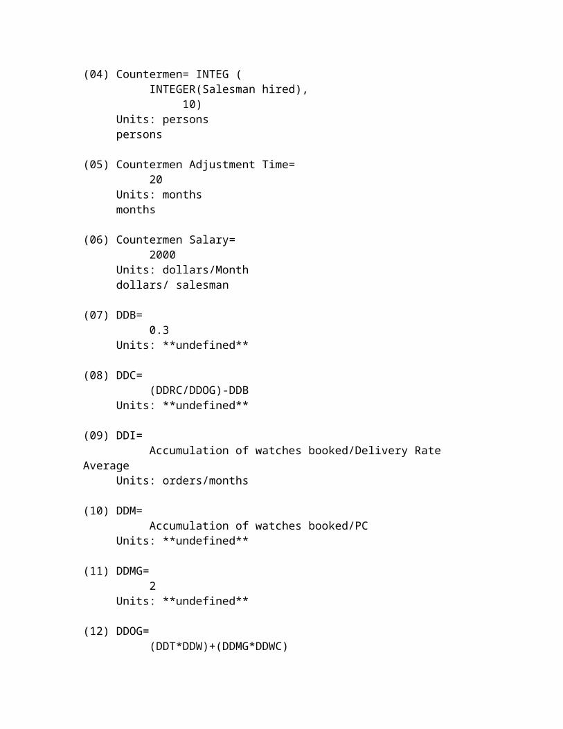
(04) Countermen= INTEG (INTEGER(Salesman hired),

10)Units: personspersons

(05) Countermen Adjustment Time=20

Units: monthsmonths

(06) Countermen Salary=2000

Units: dollars/Monthdollars/ salesman

(07) DDB=0.3


(08) DDC=(DDRC/DDOG)-DDB


(09) DDI=Accumulation of watches booked/Delivery Rate

AverageUnits: orders/months

(10) DDM=Accumulation of watches booked/PC


(11) DDMG=2


(12) DDOG=(DDT*DDW)+(DDMG*DDWC)


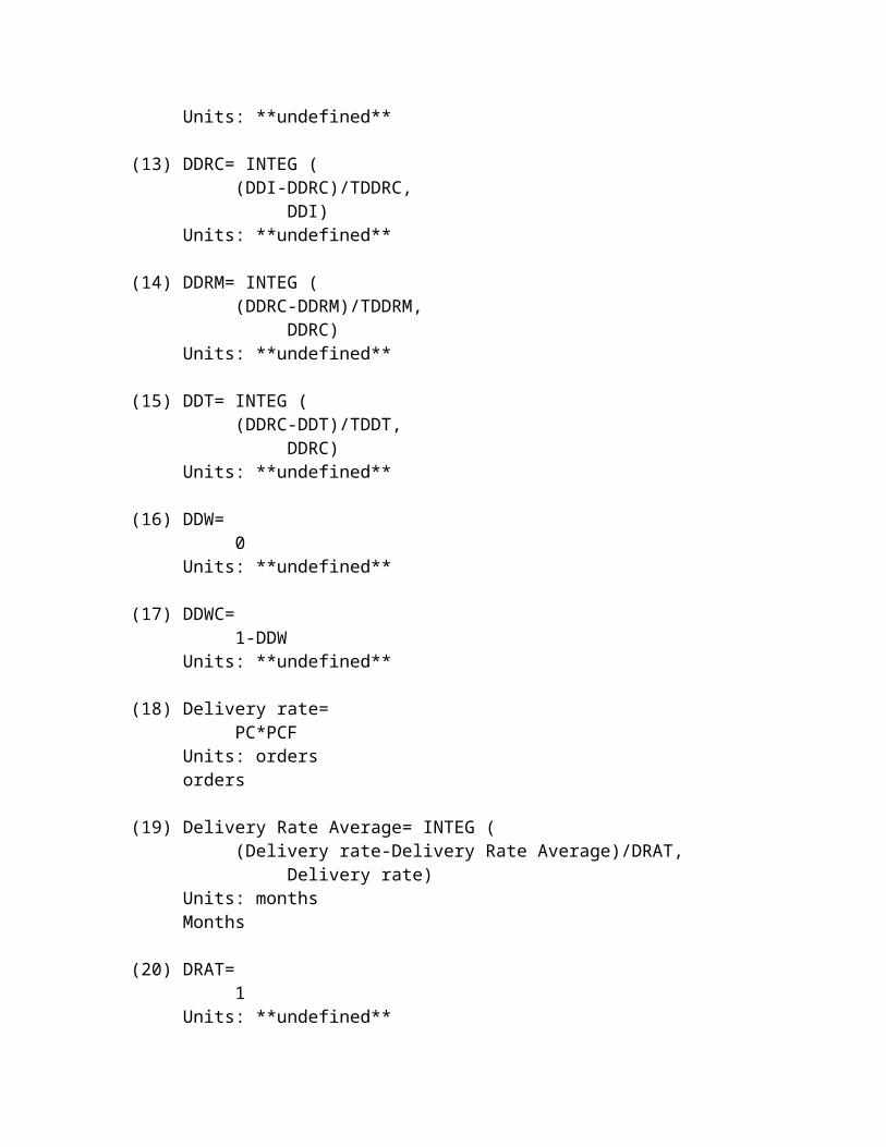
(13) DDRC= INTEG ((DDI-DDRC)/TDDRC,

DDI)Units: **undefined**

(14) DDRM= INTEG ((DDRC-DDRM)/TDDRM,

DDRC)Units: **undefined**

(15) DDT= INTEG ((DDRC-DDT)/TDDT,


(16) DDW=0


(17) DDWC=1-DDW


(18) Delivery rate=PC*PCF

Units: ordersorders

(19) Delivery Rate Average= INTEG ((Delivery rate-Delivery Rate Average)/DRAT,

Delivery rate)Units: monthsMonths

(20) DRAT=1


(21) FINAL TIME = 100Units: MonthThe final time for the simulation.

(22) Indicated Countermen =Portfolio/Countermen Salary

Units: peopleSalesman

(23) INITIAL TIME = 0Units: MonthThe initial time for the simulation.

(24) PC= INTEG (PCR,

PCI)Units: **undefined**

(25) PCDO= INTEG (PCO-PCR,

PCO*PCRD)Units: **undefined**

(26) PCF = WITH LOOKUP (DDM,

([(0,0)-(5,1)],(0,0),(0.5,0.25),(1,0.5),(1.5,0.67),(2,0.8),(2.5,0.87),(3

,0.93),(3.5,0.95),(4,0.97),(4.5,0.98),(5,1) ))Units: **undefined**

(27) PCI=150000


(28) PCO=PC*CEFSW


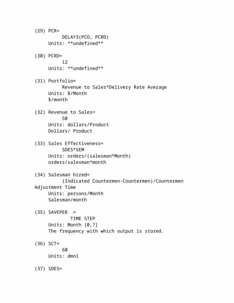
(29) PCR=DELAY3(PCO, PCRD)


(30) PCRD=12


(31) Portfolio=Revenue to Sales*Delivery Rate Average

Units: $/Month$/month

(32) Revenue to Sales=50

Units: dollars/ProductDollars/ Product

(33) Sales Effectiveness=SDES*SEM

Units: orders/(salesman*Month)orders/salesman*month

(34) Salesman hired=(Indicated Countermen-Countermen)/Countermen

Adjustment TimeUnits: persons/MonthSalesman/month

(35) SAVEPER = TIME STEPUnits: Month [0,?]The frequency with which output is stored.

(36) SCT=60

Units: dmnl

(37) SDES=

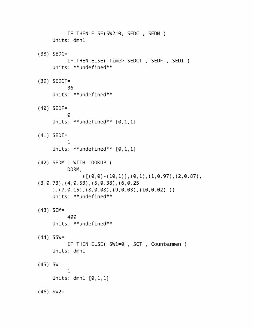
IF THEN ELSE(SW2=0, SEDC , SEDM )Units: dmnl

(38) SEDC=IF THEN ELSE( Time>=SEDCT , SEDF , SEDI )


(39) SEDCT=36


(40) SEDF=0

Units: **undefined** [0,1,1]

(41) SEDI=1


(42) SEDM = WITH LOOKUP (DDRM,

([(0,0)-(10,1)],(0,1),(1,0.97),(2,0.87),(3,0.73),(4,0.53),(5,0.38),(6,0.25

),(7,0.15),(8,0.08),(9,0.03),(10,0.02) ))Units: **undefined**

(43) SEM=400


(44) SSW=IF THEN ELSE( SW1=0 , SCT , Countermen )

Units: dmnl

(45) SW1=1

Units: dmnl [0,1,1]

(46) SW2=

0Units: dmnl [0,1,1]

(47) SW3=1

Units: dmnl [0,1,1]

(48) TDDRC=4


(49) TDDRM=6


(50) TDDT=12


(51) TIME STEP = 0.5Units: Month [0,?]The time step for the simulation.

(52) Watches booked=Sales Effectiveness*SSW

Units: units/Monthorders

Appendix II: Forrester’s General Model

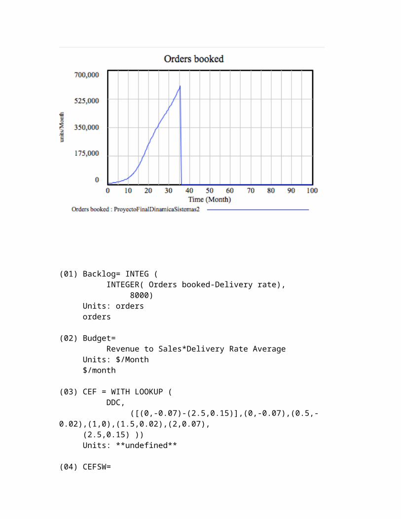
(01) Backlog= INTEG (INTEGER( Orders booked-Delivery rate),

8000)Units: ordersorders

(02) Budget=Revenue to Sales*Delivery Rate Average

Units: $/Month$/month

(03) CEF = WITH LOOKUP (DDC,

([(0,-0.07)-(2.5,0.15)],(0,-0.07),(0.5,-0.02),(1,0),(1.5,0.02),(2,0.07),

(2.5,0.15) ))Units: **undefined**

(04) CEFSW=

IF THEN ELSE(SW3=0, 0, CEF )Units: **undefined**

(05) DDB=0.3


(06) DDC=(DDRC/DDOG)-DDB


(07) DDI=Backlog/Delivery Rate Average

Units: orders/months

(08) DDM=Backlog/PC


(09) DDMG=2


(10) DDOG=(DDT*DDW)+(DDMG*DDWC)


(11) DDRC= INTEG ((DDI-DDRC)/TDDRC,

DDI)Units: **undefined**

(12) DDRM= INTEG ((DDRC-DDRM)/TDDRM,


(13) DDT= INTEG ((DDRC-DDT)/TDDT,


(14) DDW=0


(15) DDWC=1-DDW


(16) Delivery rate=PC*PCF

Units: ordersorders

(17) Delivery Rate Average= INTEG ((Delivery rate-Delivery Rate Average)/DRAT,

Delivery rate)Units: monthsMonths

(18) DRAT=1


(19) FINAL TIME = 100Units: MonthThe final time for the simulation.

(20) Indicated Salesman =Budget/Salesman Salary

Units: peopleSalesman

(21) INITIAL TIME = 0Units: MonthThe initial time for the simulation.

(22) Orders booked=Sales Effectiveness*SSW

Units: units/Monthorders

(23) PC= INTEG (PCR,

PCI)Units: **undefined**

(24) PCDO= INTEG (PCO-PCR,

PCO*PCRD)Units: **undefined**

(25) PCF = WITH LOOKUP (DDM,

([(0,0)-(5,1)],(0,0),(0.5,0.25),(1,0.5),(1.5,0.67),(2,0.8),(2.5,0.87),(3

,0.93),(3.5,0.95),(4,0.97),(4.5,0.98),(5,1) ))Units: **undefined**

(26) PCI=100000


(27) PCO=PC*CEFSW


(28) PCR=DELAY3(PCO, PCRD)


(29) PCRD=12


(30) Revenue to Sales=

50Units: dollars/ProductDollars/ Product

(31) Sales Effectiveness=SDES*SEM

Units: orders/(salesman*Month)orders/salesman*month

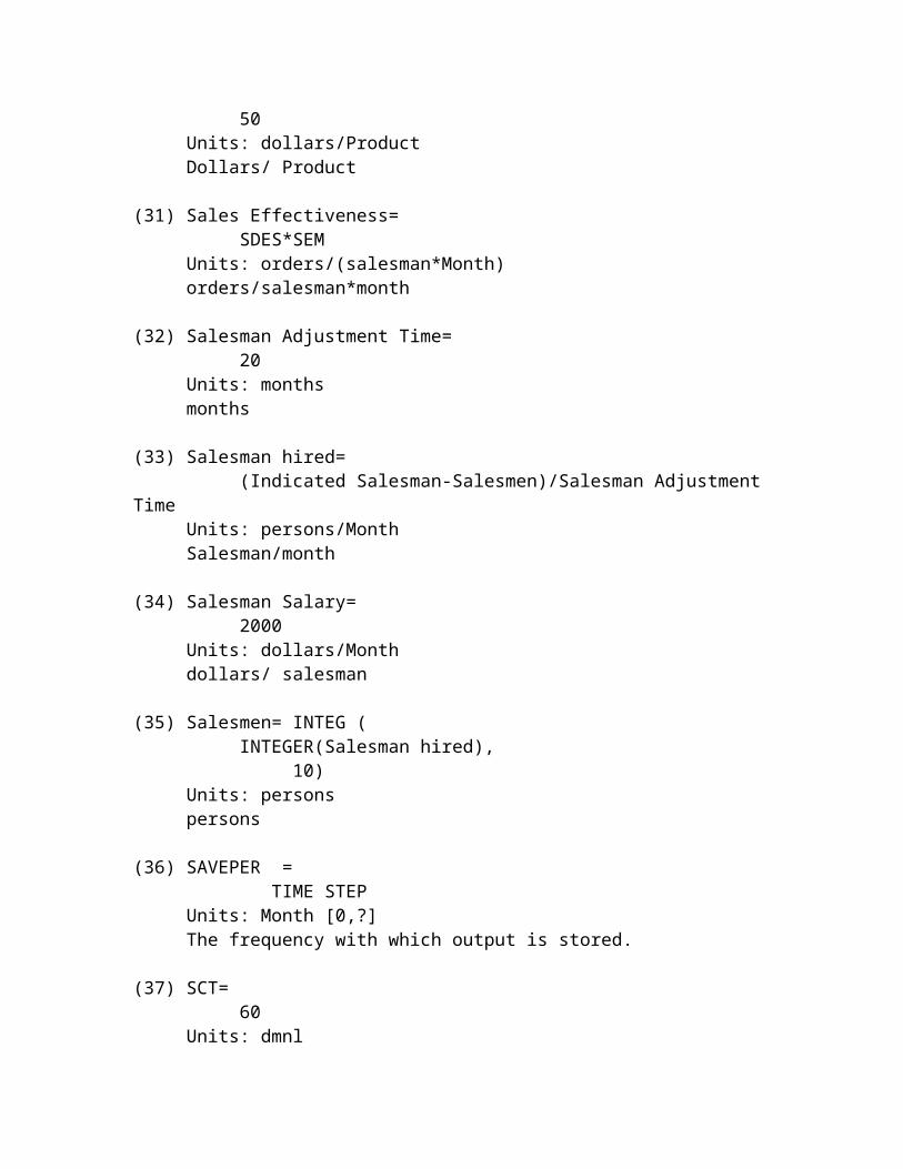
(32) Salesman Adjustment Time=20

Units: monthsmonths

(33) Salesman hired=(Indicated Salesman-Salesmen)/Salesman Adjustment

TimeUnits: persons/MonthSalesman/month

(34) Salesman Salary=2000

Units: dollars/Monthdollars/ salesman

(35) Salesmen= INTEG (INTEGER(Salesman hired),

10)Units: personspersons

(36) SAVEPER = TIME STEPUnits: Month [0,?]The frequency with which output is stored.

(37) SCT=60

Units: dmnl

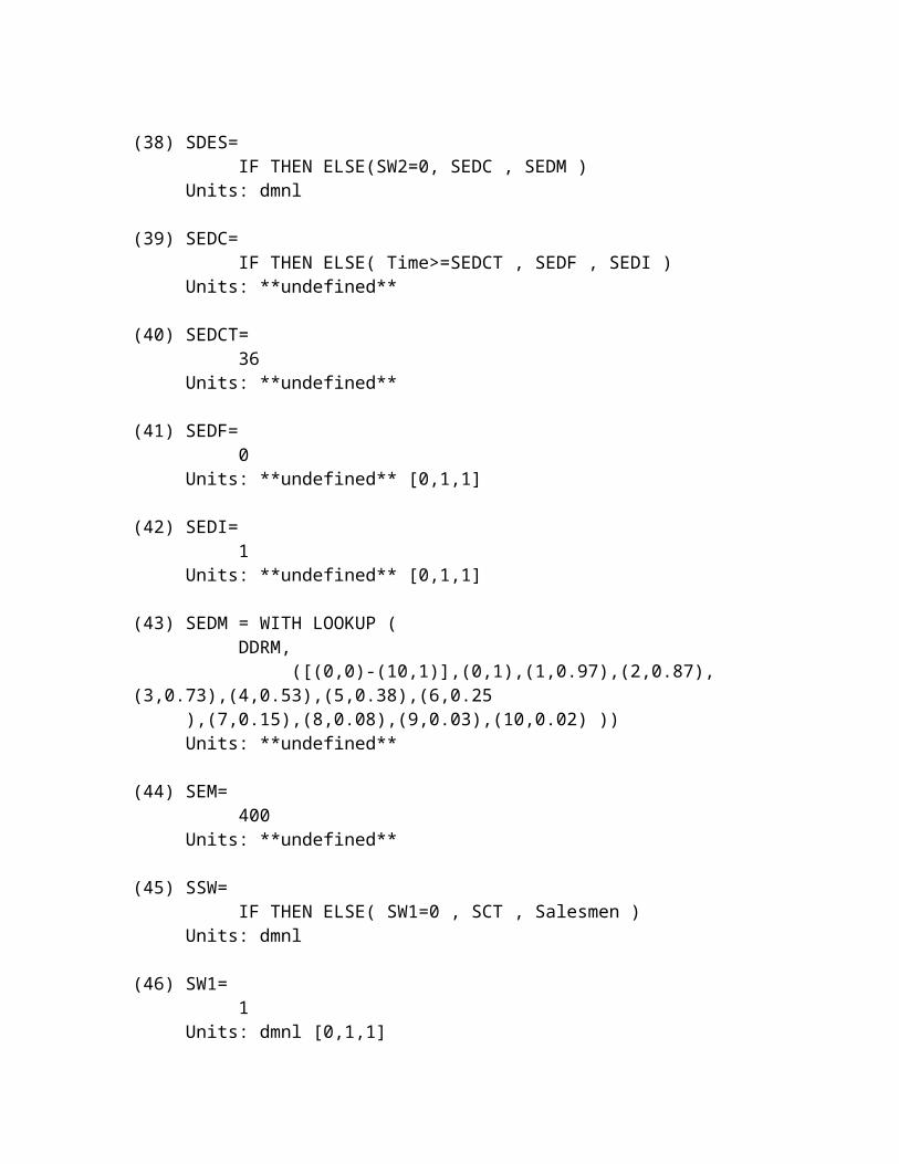
(38) SDES=IF THEN ELSE(SW2=0, SEDC , SEDM )

Units: dmnl

(39) SEDC=IF THEN ELSE( Time>=SEDCT , SEDF , SEDI )


(40) SEDCT=36


(41) SEDF=0


(42) SEDI=1


(43) SEDM = WITH LOOKUP (DDRM,

([(0,0)-(10,1)],(0,1),(1,0.97),(2,0.87),(3,0.73),(4,0.53),(5,0.38),(6,0.25

),(7,0.15),(8,0.08),(9,0.03),(10,0.02) ))Units: **undefined**

(44) SEM=400


(45) SSW=IF THEN ELSE( SW1=0 , SCT , Salesmen )

Units: dmnl

(46) SW1=1

Units: dmnl [0,1,1]

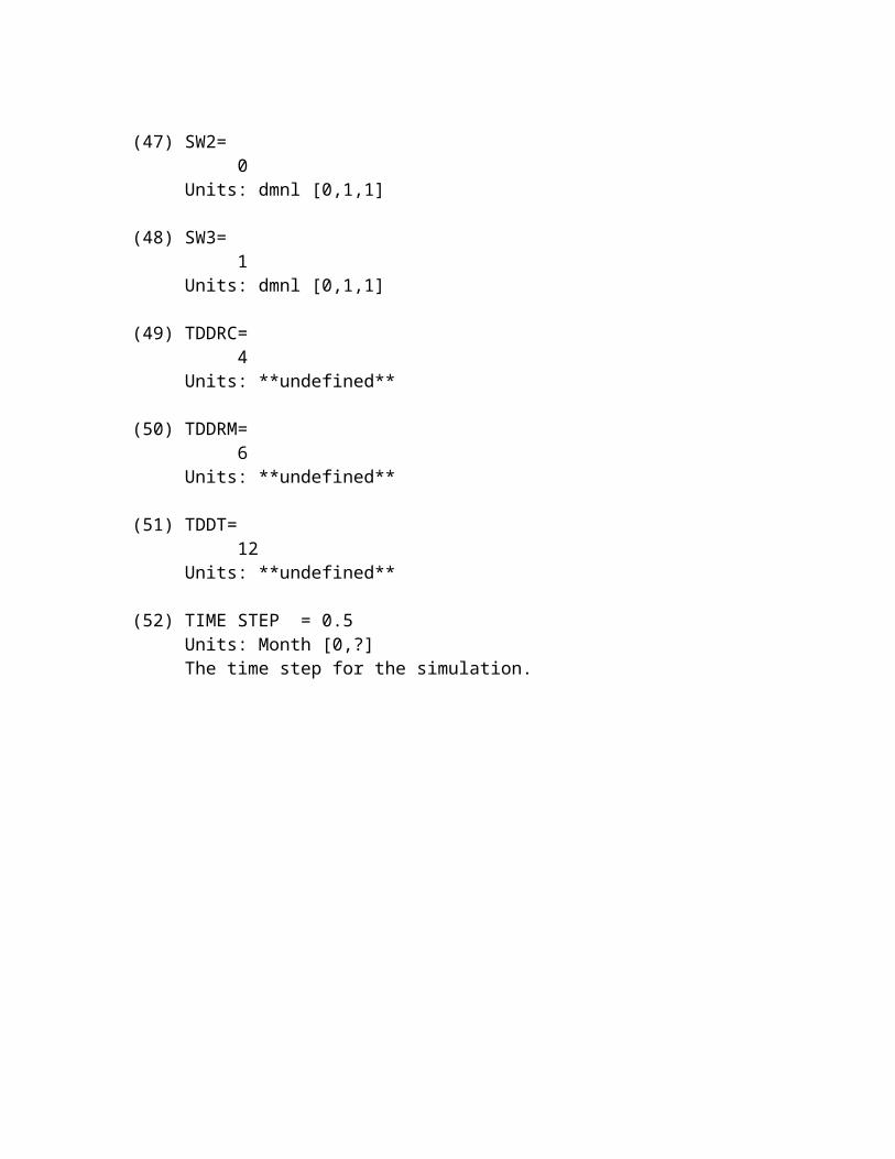
(47) SW2=0

Units: dmnl [0,1,1]

(48) SW3=1

Units: dmnl [0,1,1]

(49) TDDRC=4


(50) TDDRM=6


(51) TDDT=12


(52) TIME STEP = 0.5Units: Month [0,?]The time step for the simulation.

Vachier Lagrave S A

Documents

Transcript of Vachier Lagrave S A