Utility of Red Mud as an Embankment Material
202
December 2012 Volume 05 No 06 ISSN 0974-5904 INTERNATIONAL JOURNAL OF EARTH SCIENCES AND ENGINEERING Indexed in: Scopus Compendex and Geobase (products hosted on Engineering Village) Elsevier, Amsterdam, Netherlands, Chemical Abstract Services-USA, Geo-Ref Information Services-USA EARTH SCIENCE FOR EVERYONE Published by CAFET-INNOVA Technical Society Hyderabad, INDIA www.cafetinnova.org
-
Upload
independent -
Category
Documents
-
view
0 -
download
0
Transcript of Utility of Red Mud as an Embankment Material

December 2012 Volume 05 No 06 ISSN 0974-5904
INTERNATIONAL JOURNAL OF EARTH SCIENCES AND ENGINEERING
Indexed in: Scopus Compendex and Geobase (products hosted on Engineering Village)
Elsevier, Amsterdam, Netherlands, Chemical Abstract Services-USA, Geo-Ref Information
Services-USA
EARTH SCIENCE FOR EVERYONE
Published by
CAFET-INNOVA Technical Society Hyderabad, INDIA
www.cafetinnova.org

CAFET-INNOVA Technical Society
1-2-18/103, Mohini Mansion, Gagan Mahal Road, Domalguda
Hyderabad – 500 029, Andhra Pradesh, INDIA
Website: http://www.cafetinnova.org
Mobile: +91-9866587053, +91-7411311091
Registered by Government of Andhra Pradesh
Under the AP Societies Act. 2001 Regd. No.: 1575
The papers published in this journal have been peer reviewed by experts. The authors are solely
responsible for the content of the papers published in the journal.
Each volume, published in six bi-monthly issues, begins with February and ends with December
issue. Annual subscription is on the calendar year basis and begins with the February issue every
year.
Note: Limited copies of back issues are available.
Copyright © 2012 CAFET-INNOVA Technical Society
All rights reserved with CAFET-INNOVA Technical Society. No part of this journal should be
translated or reproduced in any form, Electronic, Mechanical, Photocopy, Recording or any
information storage and retrieval system without prior permission in writing, from CAFET-
INNOVA Technical Society.

INTERNATIONAL JOURNAL OF EARTH SCIENCES AND ENGINEERING
The International Journal of Earth Sciences and Engineering (IJEE) focus on Earth
sciences and Engineering with emphasis on earth sciences and engineering.
Applications of interdisciplinary topics such as engineering geology, geo-
instrumentation, geotechnical and geo-environmental engineering, mining engineering,
rock engineering, blasting engineering, petroleum engineering, off shore and marine
geo-technology, geothermal energy, resource engineering, water resources and
engineering, groundwater, geochemical engineering, environmental engineering,
atmospheric Sciences, Climate Change, and oceanography. Specific topics covered
include earth sciences and engineering applications, RS, GIS, GPS applications in earth
sciences and engineering, geo-hazards such as earthquakes, landslides, tsunami, debris
flows and subsidence, rock/soil improvements and development of models validations
using field, laboratory measurements.
Professors / Academicians / Engineers / Researchers / Students can send their papers
directly to: [email protected]
CONTACT:
For all editorial queries:
D. Venkat Reddy (Editor-in-Chief)
Professor, Department of Civil Engg.
NIT-Karnataka, Surathkal, INDIA
� +91-9739536078
All other enquiries:
Hafeez Basha. R (Managing Editor)
� +91-9866587053
Raju. Aedla (Editor)
� +91-7411311091

EDITORIAL COMMITTEE
D. Venkat Reddy
NIT-Karnataka, Surathkal
EDITOR-IN-CHIEF
Trilok N. Singh
IIT-Bombay, Powai, Mumbai
EXECUTIVE EDITOR
R. Pavanaguru
Osmania University, Hyderabad
EXECUTIVE EDITOR
P. Ramachandra Reddy
Scientist G (Retd.), NGRI, Hyderabad
EXECUTIVE EDITOR
Hafeez Basha R
K L University, Vijayawada
MANAGING EDITOR
Raju Aedla
NIT-Karnataka, Surathkal
EDITOR
INTERNATIONAL EDITORIAL ADVISORY BOARD
Paul M. Santi Colorado School of Mines
USA
Choonam Sunwoo
Korea Inst. of Geo-Sci & Mineral
SOUTH KOREA
Hsin-Yu Shan National Chio Tung University
TAIWAN
Hyun Sik Yang
Chonnam National Univ Gwangu
SOUTH KOREA
Krishna R. Reddy University of Illinois, Chicago
USA
L G Gwalani NiPlats Australia Limited
AUSTRALIA
Abdullah MS Al-Amri King Saud University, Riyadh
SAUDI ARABIA
Suzana Gueiros Dra Engenharia de Produção
BRAZIL
Zhuping Sheng Texas A&M University System
USA
Luigia Binda DIS, Politecnico di Milano, Milan
ITALY
Gonzalo M. Aiassa Cordoba Universidad Nacional
ARGENTINA
Shuichi TORII Kumamoto University, Kumamoto
JAPAN
Ganesh R. Joshi University of the Rykyus, Okinawa
JAPAN
Kyriakos G. Stathopoulos DOMI S.A. Consulting Engineers
Athens, GREECE
Nguyen Tan Phong Ho Chi Minh City University of
Technology, VIETNAM
Robert Jankowski
Gdansk University of Technology
POLAND
Joanna Maria Dulinska Cracow University of Technology
POLAND
U Johnson Alengaram
University of Malaya, Kuala
Lumpur, MALAYSIA
Anil Cherian United Arab Emirates
DUBAI
Vahid Nourani Tabriz University
IRAN
Paloma Pineda University of de Sevilla, Seville
SPAIN
Nicola Tarque
Department of Engineering
Catholic University of Peru
Jaya naithani
Université catholique de Louvain
Louvain-la-Neuve, BELGIUM
P Hollis Watts
WASM School of Mines
Curtin University, AUSTRALIA
Abdullah Saand
Quaid-e-Awam University of Eng.
Sc. & Tech., Sindh, PAKISTAN
S Neelamani
Kuwait Institute for Scientific
Research, SAFAT, KUWAIT
Mani Ram Saharan
National Geotechnical Facility
DST, Dehradun, INDIA
S Viswanathan
IIT- Bombay, Powai, Mumbai
Maharashtra, INDIA
Ramana G V
IIT– Delhi, Hauz Khas
New Delhi, INDIA
Subhasish Das
IIT- Kharagpur, Kharagpur
West Bengal, INDIA
K U Maheshwar Rao
IIT- Kharagpur, Kharagpur
West Bengal, INDIA
Kalachand Sain
National Geophysical Research
Institute, Hyderabad, INDIA
Katta Venkataramana NITK- Surathkal
Karnataka, INDIA
M K Nagaraj
NITK- Surathkal
Karnataka, INDIA
R Sundaravadivelu
IIT- Madras
Tamil Nadu, INDIA
G S Dwarakish NITK- Surathkal
Karnataka, INDIA

M R Madhav JNTU- Kukatpally, Hyderabad
Andhra Pradesh, INDIA
Chachadi A G Goa University, Taleigao Plateau
Goa, INDIA
S M Ramasamy
Gandhigram Rural University
Tamil Nadu, INDIA
Gholamreza Ghodrati Amiri
Iran University of Sci. & Tech.
Narmak, Tehran, IRAN
C Natarajan NIT- Tiruchirapalli,
Tamil Nadu, INDIA
R Bhima Rao
IMMT, Bhubaneswar
Odissa, INDIA
Shamsher B. Singh BITS- Pilani, Rajasthan
Rajasthan, INDIA
Pradeep Kumar R IIIT- Gachibowli, Hyderabad
Andhra Pradesh, INDIA
N Ganesan
NIT- Calicut, Kerala
Kerala, INDIA
D P Tripathy
National Institute of Technology
Rourkela, INDIA
E Saibaba Reddy JNTU- Kukatpally, Hyderabad
Andhra Pradesh, INDIA
Chowdhury Quamruzzaman
Dhaka University
Dhaka, Bangladesh
Parekh Anant kumar B Indian Institute of Tropical
Meteorology, Pune, INDIA
Datta Shivane
Central Ground Water Board
Hyderabad, INDIA
Gopal Krishan
National Institute of Hydrology
Roorkee, INDIA
P Sreenivas Sarma
Chaitanya Bharathi Institute of
Technology, Hyderabad, INDIA
Prasoon Kumar Singh
Indian School of Mines, Dhanbad
Jharkhand, INDIA
A G S Reddy
Central Ground Water Board,
Pune, Maharashtra, INDIA
Rajendra Kumar Dubey
Indian School of Mines, Dhanbad
Jharkhand, INDIA
Subhasis Sen
Retired Scientist
CSIR-Nagpur, INDIA
M V Ramanamurthy
Geological Survey of India
Bangalore, INDIA
C Sivapragasam
Kalasalingam University,
Tamil Nadu, INDIA
Bijay Singh Ranchi University, Ranchi
Jharkhand, INDIA
B R Raghavan
Mangalore University, Mangalore
Karnataka, INDIA
CH Hanumantha Rao K. L. University, Guntur
Andhra Pradesh, INDIA
Anand V. Shivapur SDM College of Engg. and Tech.
Karnataka, INDIA
S Suresh Babu Adhiyamaan college of Engineering
Tamil Nadu, INDIA
Kripamoy Sarkar
Assam University
Silchar, INDIA
Xiang Lian Zhou
ShangHai JiaoTong University
ShangHai, CHINA
Naveed Ahmad
University of Engg. & Technology,
Peshawar, PAKISTAN
Nandipati Subba Rao
Andhra University, Visakhapatnam
Andhra Pradesh, INDIA
M Suresh Gandhi
University of Madras,
Tamil Nadu, INDIA
Debadatta Swain
National Remote Sensing Centre
Hyderabad, INDIA
H K Sahoo
Utkal University, Bhubaneswar
Odissa, INDIA
R N Tiwari Govt. P G Science College, Rewa
Madhya Pradesh, INDIA
B M Ravindra
Dept. of Mines & Geology, Govt. of
Karnataka, Mangalore, INDIA
M V Ramana
CSIR NIO
Goa, INDIA
N Rajeshwara Rao
University of Madras
Tamil Nadu, INDIA
R Baskaran
Tamil University, Thanjavur
Tamil Nadu, INDIA
Salih Muhammad Awadh
College of Science
University of Baghdad, IRAQ
Sonali Pati
Eastern Academy of Science and
Technology, Bhubaneswar, INDIA
K. Bheemalingeswara
Mekelle University
Mekelle, Ethiopia
Samir Kumar Bera
Birbal sahni institute of
palaeobotany, Lucknow, INDIA
Raj Reddy. Kallu
University of Nevada
1665 N Virginia St, RENO
Manish Kumar
Tezpur University
Sonitpur, Assam, INDIA
C N V Satyanarayana Reddy
Andhra University
Visakhapatnam, INDIA
S M Hussain
University of Madras
Tamil Nadu, INDIA
Safdar Ali Shirazi
University of the Punjab,
Quaid-i-Azam Campus, PAKISTAN
T J Renuka Prasad
Bangalore University
Karnataka, INDIA
S S S V Gopala Raju
GITAM University
Hyderabad, INDIA
Glenn T. Thong
Nagaland University
Meriema, Kohima, INDIA
Mohammed Sharif
Jamia University
New Delhi, INDIA
A M Vasumathi
K.L.N. College of Inf. Tech.
Pottapalayam, Tamil Nadu, INDIA
Ashutosh Das
PRIST, Tamilnadu
Tamil Nadu, INDIA


INDEX Earth Science for everyone
Volume 05 December 2012 No.06
EDITORIAL NOTE
Is the Prediction of Human Generation End by the Year 2012? A Geologic Perspective on
Mass Extension.
By BUSNUR RACHOTAPPA MANJUNATHA and D. VENKAT REDDY
RESEARCH PAPERS
Luminescence Techniques as a Low-Cost Geophysical Tool in Mineral Exploration: Some
Examples
By R. DHANA RAJU
1472-1480
Ensemble Empirical Mode Decomposition of the Lightning Return Stroke
By XUQUAN CHEN and WENGUANG ZHAO
1481-1491
Peak Ground Acceleration on Bedrock and Uniform Seismic Hazard Spectra for different
Regions of Behbahan, Iran
By SEYED ALI RAZAVIAN AMREI, GHOLAMREZA GHODRATI AMIRI, ARMAN SAED
and ALI SABZEVARI
1492-1499
Coal Mine Seal Design – Numerical Approach
By RAJ R. KALLU
1500-1509
A Note on Three Way Quality Control of Argo Temperature and Salinity Profiles - A Semi-
Automated Approach at INCOIS
By T. V. S. UDAYA BHASKAR, E. PATTABHI RAMA RAO, R. VENKAT SHESU
and R. DEVENDER
1510-1514
Peak Ground Acceleration on Bedrock and Uniform Seismic Hazard Spectra for Different
Regions of Zanjan, Iran
By GHOLAMREZA GHODRATI AMIRI, SEYED ALI RAZAVIAN AMREI, ALI SABZEVARI,
ARMAN SAED and YASER SHOKRANI
1515-1521
Heavy Minerals and Provenance of the Lower Gondwana Sandstones, Ong-River
Gondwana Basin, Odisha
By ARYA GOUTAMI NATH and RABINDRA NATH HOTA
1522-1529
Rating of Tunnel by Visual Field Inventory – A Case Study of Punasa Tunnel, District
Khandawa, M. P. India
By GUPTA. M. C, SINGH. B. K and SINGH. K. N
1530-1534
Geology and Characteristics of Metalimestone-Hosted Iron Deposit near Negash, Tigray
and Northern Ethiopia
By SOLOMON GEBRESILASSIE, BHEEMALINGESWARA KONKA and FISEHA ADHANOM
1535-1544
Ore Fluids Associated With the Metasediment Hosted Central Auriferous Zone of Gadag
Gold Field, Karnataka
By M. A. MALAPUR, S. MANJUNATHA, B. CHANDAN KUMAR and A. G. UGARKAR
1545-1551
A Case Study of Particle Size Distribution of Paleosols around Sargur Supracrustal
Terrain, Dharwar Craton, South India
By NARGES GOHARI RAD, PRAKASH NARASIMHA. K. N and MADESH. P
1552-1559
Effect of Ground Moisture on Spread of Contaminants in Sand Deposit -An Experimental
Study
By E. SAIBABA REDDY, SINA BORZOOEI and G. V. NARASIMHA REDDY
1560-1566
Identification of Rain/No-Rain Events using QuikSCAT Scatterometer Data
By PRITI SHARMA, RAJESH SIKHAKOLLI, B. S. GOHIL and ABHIJIT SARKAR
1567-1571

Genesis of Thermal Springs of Odisha, India
By S. C. MAHALA, P. SINGH, M. DAS and S. ACHARYA
1572-1577
Remote Sensing Studies in Delineating Hydrogeological Parameters in the Drought-Prone
Kuchinda-Bamra Area in Sambalpur District, Odisha
By NANDITA MAHANTA and H. K. SAHOO
1578-1583
Impact Analyses of Industrial and Mining Activities on Groundwater Regime -Case Studies
in Goa
By A. G. CHACHADI
1584-1589
Identification of Artificial Recharge Sites in a Hard Rock Terrain using Remote Sensing
and GIS
By S. SARAVANAN
1590-1598
Drinking and Irrigation Water Quality in Jalandhar and Kapurthala Districts, Punjab,
India: Using Hydrochemsitry
By P. PURUSHOTHAMAN, M. SOMESHWAR RAO, B. KUMAR, Y. S. RAWAT,
GOPAL KRISHAN, S. GUPTA, S. MARWAH, A. K. BHATIA, Y. B. KAUSHIK,
M. P. ANGURALA and G. P. SINGH
1599-1608
Groundwater Quality Assessment around Talabasta Area, Banki Sub-Division, Odisha,
India
By ROSALIN DAS, MADHUMITA DAS and SHREERUP GOSWAMI
1609-1618
Terrain Analysis and Hydrogeochemical Environment of Aquifers of the southern West
Coast of Karnataka, India
By S. S. HONNANAGOUDAR, D. VENKAT REDDY and MAHESHA. A
1619-1629
Water Quality Modeling and Management of Karanja River in India
By BASAPPA. B. KORI, SHASHIKANTH MISE and SHASHIDHAR
1630-1638
Prediction of Penetration Rate and Sound Level Produced during Percussive Drilling using
Regression and Artificial Neural Network
By S. B. KIVADE, Ch. S. N. MURTHY and HARSHA VARDHAN
1639-1644
Utility of Red Mud as an Embankment Material
By SUBRAT KUMAR ROUT, TAPASWINI SAHOO and SARAT KUMAR DAS
1645-1651
Rapid Chloride Penetration Test on Geopolymer Concrete
By SHANKAR H. SANNI and R. B. KHADIRANAIKAR
1652-1658
News and Notes
NIT Professor spoke at an International Conference in SanFransisco, USA. i
Dr. Subhash C. Yaragal, is conferred with Prof. Satish Dhawan Young Engineer State
Award -2011 ii

www.cafetinnova.org
Indexed in
Scopus Compendex and Geobase Elsevier, Chemical Abstract
Services-USA, Geo-Ref Information Services-USA
ISSN 0974-5904, Volume 05, No. 06
Dec 2012, Editorial Note
Volume 5, No. 6, December 2012
Is the Prediction of Human Generation End by the Year 2012?
A Geologic Perspective on Mass Extension.
BUSNUR RACHOTAPPA MANJUNATHA1 and D. VENKAT REDDY
2
1Department of Marine Geology, Mangalore University, Mangalagangothri-574 199, India 2Department of Civil Engineering-National Institute of Technology –Karnataka, India
Email: [email protected], [email protected]
There are many documentaries, movies and armature articles regarding the extinction of human generation by end of
the year 2012. The first prediction has been the Mayan astrological calendar that built out of stones indicates an
abrupt end of the world on 21st December 2012. Like-wise, some of religious books, including the Bible implicate
the end of human domain by 2012. This has caused curiosity and anxiety among people across the world. The main
purpose of this note is to address the public form geologist perspectives about the mass extension of life.
The age of the earth has been measured by radioisotopic method to about 4550 million years (Ma) before present.
Form the violent beginning of the earth, it took nearly 800 Ma to cool down (Hadean Eon) by allowing to from
mainly igneous and metamorphic rocks from 3800 Ma to 2500 Ma (Achaean Eon), principally sedimentary rocks
from 2500 Ma to 570 Ma (Proterozoic Eon) and mixed types of rocks on land as well as in the oceans from 570 Ma
to the present (Phanerozoic Eon). The origin of life and its commencement during the Achaean Eon is still infancy
because of the lack of preservation of fossils in igneous and metamorphic rocks as these rocks form at high
temperatures. The atmospheric conditions during Hadean and to some extent Archaean Eons were not conducive for
the advancement/evolution of life as the atmosphere was dominated by large quantities of water vapour, carbon
dioxide, sulphur and nitrogen gases and perhaps hydro chloric acid. However, there are some evidences of life
existed, for e.g., biogenic stromatolites dated older than 3500 Ma (belong to the Archaean Eon). The existence of
life during the Proterozoic Eon has been very well documented from the sedimentary rocks. During this Eon, the
free diatomic oxygen that necessary for evolution of life gradually built up in the atmosphere due increase in the rate
of photosynthesis by the cyanobacteria (blue green algae).
The life prevailed during the Proterozoic was principally of unicellular organisms, while at the beginning of
Phanerozoic Eon, a sudden advancement of life noticed. Over a little more than 500 Ma, most of species including
human beings originated as the last species. Based on the biotic evolution, the Phanerozoic Eon can be classified
into Palaeozoic Era (early life; 570-245 Ma), Mesozoic Era (middle life; 245-65 Ma) and Cenozoic Era (recent life;
65 Ma -today).
In contrast to the Proterozoic Eon, the Paleozoic Era began with the origin of multi-cellular organisms, for e.g.,
trilobites, jelly fish and worms (during the Cambrian period; 545-505 Ma), suggesting that an abrupt change in the
life on earth. This was followed by snail, sponges during the Ordovician (505-438 Ma), corals and star fish during
the Silurian (438- 408 Ma), fish, lungfish and fern during the Devonian (408 - 360 Ma), amphibianin, insect and
trees during Carboniferous (360-286 Ma), fin back reptiles and reptiles during the Permian periods (286-245 Ma).
The life existed during Mesozoic Era was quite different than that during the Paleozoic Era in terms of the
advancement of reptiles, primitive mammals and gymnosperms. The Mesozoic Era can be demarcated into three
periods Triassic (245-208 Ma) Jurassic 208-144 Ma) and Cretaceous (144-65 Ma). The life existed in the former
period comprises of (i) the first appearance of dinosaurs and ammonoite, followed by (ii) dominance of giant
dinosaurs both in the oceans and on land, first appearance mammals and conifers, and (iii) dominance of flying
dinosaurs, carnivorous dinosaurs and horned dinosaurs, flowering plants, and insects during the latter period
respectively. The Cenozoic Era dominated by the mammals began with dominance of flowering plants, ancestral
horse, insects, birds whale clawed mammals camel dating back to 65 to 1.6 million years. The first appearance of
humans noticed during the Quaternary period (1.6 Ma) along with mammoth saber toothed tiger.
However, the life existed earlier either became greatly reduced or extinct in the latter time span of the earth. Such
process can be termed as mass extinction of life. A mass extinction usually noticed during the end of particular
geologic period. Mass extinction refers to the species diminishing or almost end of biological world probably due to

BUSNUR RACHOTAPPA MANJUNATHA and D. VENKAT REDDY
Editorial Note
large-scale calamities or catastrophic processes such as earth quakes, tsunamis, volcanic eruptions and meteoritic
impact. However, there could have been climatic factors such as famine, drought, and biological factors for instance,
genetic factors causing infertility, and human factors leading to deforestation and large-scale hunting of animals.
There are as many as six major mass extinctions and a number of smaller ones occurred in the Phanerozoic Eon
(history of the earth):
(1) 52 % reduction in the families of trilobite, sponge and gasteropod occurred during the late Cambrian,
(2) 24 % reduction in the families of trilobite, brachiopod, crinoid and echinoid families during late Ordovician,
(3) 30 % reduction in the families of coral, stromatoporoid, trilobite, ammonoide bryozoan, brachiopod and fish
during late Devonian,
(4) 50 % reduction in the families of bryozoans and reptiles during late Permian,
(5) 35 % reduction in the families of brachiopod, ammonoite fish and reptile during late Triassic and
(6) 26% reduction in the families of beleminites, corals, echinoids, sponges and planktonic foraminifera during the
ate Cretaceous period.
Among the above, the major extinction of rugose corals, trilobites, blastoids, inadunate, flexibiliate, camerate,
crinoids, productid, brachiopods and fusulinid foraminifera occurred during the late Permian, conodonts during the
late Triassic and ammonoites, rudistid mollusks, dinosaurs and large marine reptiles at the end of Cretaceous period.
However, certain species, for e.g., sponges, brachiopods, bivalves and ostrocods continue to exist through out the
Phanerozoic Eon with variations in their populations. The dominance of sponges, bryozoans, brachiopods and
ostracods particularly during the transition particularly during the Palaeozoic Eon to Mesozoic Eon. This suggests
that the dominant species become extinct by the end of particular geological period by making a place for the
advanced life.
In most of major mass extinctions, the main causative factor was the trigger of large-scale volcanic eruption. The
Antrim volcano erupted in Ireland about 511 Ma that must have caused mass extinction noticed in between
Cambrian and Ordovician periods.
The boundary between Permian and Triassic has been the most conspicuous by a massive and large-scale Siberian
volcanic eruption that occurred at about 251-250 Ma ago. The volume of eruption estimated at 1.0 - 4 million cubic
kilometers covering an area of 2 million sq km. The dinosaurs extinction noticed at the end of Cretaceous period can
be linked to Deccan volcanic eruption (India) where the volume of lava erupted has been estimated to 1.5 million
cubic kilometers and cover an area more than 500,000 sq km. Nevertheless, meteorites bombardment on earth as
well as cold periods appeared to have been significant foe the mass extinction. Therefore, it appears that the rate of
extinction is controlled by the quantum of volcanic eruption, as it has been mentioned above that Siberian volcanic
eruption led to the extinction of about 50 families of biota while the Deccan volcanism accounts to about half of
that from Siberian volcanism.
It is clear from the recent studies that volcanic eruption can reduce the global temperature by 1- 2 oC because of the
absorption incoming solar radiation by volcanic materials. This gradually reduces photosynthesis leading to a
considerable reduction in the species as well as their population as a consequence of shortage of food. Another thing
that volcano emits lot of oxides of carbon, sulphur and nitrogen leading to the acidification of the ecosphere.
Volcanoes may often trigger ice age, for instance, the boundary between Permian and Triassic, and Cretaceous and
Tertiary periods marked by cold (glacial) conditions. Other processes responsible for the mass extinction of life on
earth are climate, physical, chemical and biological warfare. Climate change has serious consequence on sustenance
of life on earth. For instance, the severe drought that occurred over 4000 years ago collapsed the old world’s
civilization, for e.g., Akkadian, Mayan, Indus Valley and Chinese civilizations. Similarly long-term climate change
such as solar activity due to human impacts and prevalence of glacial (cold) conditions can disrupts life on the planet.
Now the puzzle is that when do the human’s generation going to extinct? Our answer to this question is not very
soon and certainly not during the end of 2012, because the catastrophic processes may not occur simultaneously on
the earth. More than that the highly civilized human beings today can bear the risk of extinction. However, gradual
processes, such as evolution can cause a considerable amount of species reduction and population explosion because
of scarcity natural resources. Still longer processes are the consequence of solar flares and Sun’s evolution can lead
to substantial extinction of life on earth.
In a nutshell, we conclude that although mass extinction processes are violent and catastrophic, however, it is
evident that they mark origin of new species. For example, the extinction of the dinosaurs led the rise of the
mammals. As William Shakespeare said life of a human being can be comparable to a “drama stage”, similarly the
whole earth is a stage for origin of new species, while extinction for living ones. In this context, extinction of
humans is inevitable, but a long way to go.

www.cafetinnova.org
Indexed in
Scopus Compendex and Geobase Elsevier, Chemical
Abstract Services-USA, Geo-Ref Information Services-USA
ISSN 0974-5904, Volume 05, No. 06
December2012, P.P.1472-1480
#02050601 Copyright ©2012 CAFET-INNOVA TECHNICAL SOCIETY. All rights reserved.
Luminescence Techniques as a Low-Cost Geophysical Tool in
Mineral Exploration: Some Examples
R. DHANA RAJU A.M.D., Dept. of Atomic Energy
Dept. of Applied Geochemistry, Osmania University
ASR Mining Company, Kondapur, Hyderabad – 500 084
Email: [email protected]
Abstract: Luminescence is the phenomenon of emission of light or photons, mainly in the visible domain, from a substance when it is stimulated by any means other than heating to incandescence. It is believed to result from motion of electrons. Based on the nature of motion, it is of numerous types and constitutes a low-cost geophysical tool. Of these types, three, viz., fluorescence (-phosphorescence), cathodoluminescence (CL) and thermoluminescence (TL) have many applications in mineral exploration, which are documented in this paper through the following examples: (i) fluorescence (-phosphorescence) of some uranyl- and non-radioactive-minerals; (ii) CL in discriminating Uraniferous sandstone/conglomerate from barren ones, and in probing hydrothermal
alterations, fluid migration pathways and fractures, all of which have critical bearing on mineralization; and (iii) Natural TL on whole-rock samples for: (a) broad classification of the schistose rocks
and (b) discrimination of the Uranium and Rare Element mineralized horizons fromethe adjacent barren zones, as demonstrated in the Jublatola, Domiasiat and Bast r-Malkangiri areas.
The above applications point to the utility of these low-cost, direct and sensitive geophysical techniques as a powerful exploration tool. These techniques can be profitably used during the reconnoitory stage of exploration, prior to costly drilling, in the virgin areas or in deciphering the concealed mineralized zones as well as for predicting the blind-extensions of the already established mineralized horizons.
Keywords: Fluorescence (-Phosphorescence), Cathodoluminescence, Thermoluminescence, Mineral Exploration.
Introduction:
Luminescence is the phenomenon of emission of light or photons, mainly in the visible domain, from a substance when it is stimulated by any means other than heating to incandescence. It is believed to result from motion of electrons and is classified as per the nature of motion. It is of several following types: radioluminescence is by excited X-ray photons and γ-rays, and bombardment of α- and β-nuclear particles; chemiluminescence produced by chemical reactions, e.g., oxidation of P; electroluminescence by electrical discharges; triboluminescence due to mechanical deformation by rubbing or crushing crystals like diamond and sphalerite; ionoluminescence generated under an energetic beam as in an ion microprobe; bioluminescence by living organisms like some bacteria, glowworms, fireflies and many deep-sea fish; fluorescence; phosphorescence; crystalloluminescence during crystallization from a solution like arsenic oxide, As2O3; cathodoluminescence produced by energetic electrons; thermoluminescence due to an activator in a mineral when it is heated; and photoluminescence
involving selective energy of photons to excite electronic levels of luminescent centers. Of these, fluorescence (-phosphorescence), cathodoluminescence (CL) and thermoluminescence (TL) are used as tools in (a) identification of minerals, including ore minerals, which emit these phenomena; (b) examination of certain features like zoning, overgrowth and ultra-fine inclusions present in such minerals as they are much easy (due to better clarity and contrast) to identify than by optical microscopy alone; and (c) mineral exploration. Fluorescence (-phosphore-scence), CL and TL, which constitute the low-cost, direct and sensitive geophysical tools, have notable applications in mineral exploration, especially during its reconnoitory and semi-detailed stages. These applications, together with some Indian examples, are presented in this paper to demonstrate their relevance in mineral exploration, particularly before undertaking costly drilling.
Fluorescence (-Phosphorescence):
The emission of light from a substance like mineral when it is exposed to direct radiation such as ultraviolet

1473 R. DHANA RAJU
International Journal of Earth Sciences and Engineering ISSN 0974-5904, Vol. 05, No. 06, December 2012, pp. 1472-1480
(UV) light, or in certain instances to an electrical discharge in a vacuum tube is called fluorescence that ceases when radiation stops. This phenomenon is best exhibited by the mineral, fluorite and, hence, the name. Fluorescence is the process of emission of electromagnetic radiation produced by energy transitions, not just in the visible range. A number of others minerals, like scheelite, malayaite and uranyl (U6+ or secondary U) minerals such as autunite, uranophane, gummite, torbernite and schroekingerite fluoresce due to the presence of activators or spikes (Mn, U, Rare Earths) as impurities in them. If a beam of white light were passed through a cube of colourless fluorite, a delicate violet colour can be seen in its path due to change of refrangibility in the transmitted light. The continued emission of light by a substance (phosphor) for a finite time even after exposure to light, or an electrical discharge and especially after heating is called phosphorescence. Fluorescence and phosphorescence differ only in the amount of time it takes for electrons to return to their ground states. With fluorescence, vacant lower energy positions are filled within small fractions of a second. Phosphorescent materials, however, continue emitting light significantly after the exciting radiation has been turned off, sometimes for hours. Since the process of displacing electrons into higher energy configurations absorbs electromagnetic radiation, the electrons as they return to the ground state emit radiation. The emitted radiation is always of lower energy than the radiation used to displace the electron, and of a definite wavelength, corresponding to the difference between the excited state and the ground state. This process is most transparent for X-rays. Many transitions contribute to fluorescence in the visible range, and the spectra are not as sharp as those in the range of X-rays. Furthermore, similar to colour, visible fluorescence depends critically on trance elements and defects, but is nevertheless a diagnostic property used in mineral identification and mineral prospecting. Fluorite is highly phosphorescent and gives off different colours of emerald green, purple, blue and reddish tints, after heating to above 1500C. Scheelite (CaWO4), an important ore of tungsten, is another mineral with strong fluorescence. To discriminate scheelite from carbonates is rather difficult in hand specimens, but it is immediately recognized by its bright white fluorescence, when irradiated with ultraviolet light. The phenomenon of fluorescence and phosphorescence under UV radiation is used as a guide in identification of some minerals as well as to get information on their zoning, inclusions and crystal growth. UV light is of two wavelengths, viz., short wave of 185-300 nm and long wave of 300-400 nm, with the former cannot and the latter can penetrate cover glass of a thin section. Since the short-wave UV light excites most fluorescence in minerals, it is better to
observe under it in darkness the fluorescence and phosphorescence on uncovered polished slabs, polished thin-sections and surface of hand-specimens. A useful model for laboratory work is MINERALIGHT model MPR2 (or later advanced ones of M/s. Ultraviolet Products Inc., San Gabriel, California 91778, USA). This has two externally clamped tubular bulbs that can be adjusted in position above the polished surface on either side of microscope-objectives and, with a short UV filter on one or both bulbs, the fluorescence colours can be studied through the microscope. Furthermore, the fluorescent minerals on the surface of a hand-specimen can be scrapped for their correct identification later by XRD. When once the identity of fluorescent mineral in a terrain or an area is established, then the UV fluorescent technique can be used as a rapid mineral exploration technique like in the Sn-W mineralized region of Southeast Asia. For a comprehensive list of minerals, rocks and gemstones, which exhibit UV reactions, the reader is referred to Gleason (1960).
Warning: Since UV light, especially of the short wavelength, can cause temporary or permanent blindness, it should not be looked either directly from the lamp or its reflection from surface. Hence, it is necessary to observe UV fluorescence through spectacles or microscope system.
Fluorescence of Uranium Minerals and Non-
Radioactive Minerals:
It may be noted that fluorescence (and phosphorescence) exhibited by certain non-radioactive minerals is of impurity-activated type, such as zinc orthosilicate activated by manganese as impurity, whereas that by uranium (and thorium) minerals is an intrinsic fluorescence due to uranyl [(UO2)
2+] ion. About the fluorescence of uranium minerals, the following generalizations can be made (Frondel, 1958, p. 357):
a) All the fluorescent uranium minerals contain uranyl ion and are secondary in origin, whereas the uranium minerals containing quadrivalent uranium, (U4+), such as uraninite, coffinite and uranoan varieties of niobate-tantalates, which are generally black in colour and primary in origin, do not show fluorescence.
b) The characteristic emission colour of the strongly and moderately fluorescent uranium minerals is greenish yellow to yellowish green (except andersonite and liebigite, which are green). These minerals comprise chiefly the hydrated uranyl phosphates and arsenates containing alkaline earths, alkalies or hydrogen (members of these groups containing copper or iron fluoresce weakly, if at all), together with certain uranyl sulphates and carbonates.

1474 Luminescence Techniques as a Low-Cost Geophysical
Tool in Mineral Exploration: Some Examples
International Journal of Earth Sciences and Engineering ISSN 0974-5904, Vol. 05, No. 06, December 2012, pp. 1472-1480
c) The uranyl silicates/vanadates and hydrated oxides fluoresce weakly or not at all.
d) The uranyl minerals containing lead fluoresce either weakly in yellow-brown or brown rather than yellow-green colours, or do not fluoresce at all.
e) Dehydration, in general, reduces the intensity of fluorescence.
Fluorescence in Exploration for U:
As many uranium salts fluoresce under UV light of suitable wavelengths (2537 Å and 3660 Å), the technique of fluorescence is an appropriate tool for detection of some uranium minerals that might otherwise escape detection by routinely used GM counter or scintillometer because of their youth and fine subdivision. In fact this is one of the methods of radiation survey (the others are radiometric survey using gamma-ray detectors of GM counter and scintillometer, radio-activation analysis, autoradiography, radiation track analysis and radioactive tracers) (Boyle, 1982, pp. 166-174). Since certain substances (e.g., bitumen, petroleum) and non-radioactive minerals interfere with, inhibit or mimic uranium fluorescence, corroborating analyses should always be carried out to definitely establish the presence or absence of uranium. After establishing the presence of U in the fluorescent minerals, recorded either in the field or in laboratory examination of samples, their exact identification by XRD is a must. It helps in understanding the geochemical system of U operating in the sampled area, like establishing the exact nature of transport of U (after its release from a source rock like fertile granite) as a uranyl carbonate or phosphate complex, and their respective Eh-pH conditions. Such a probing of the geochemical system helps in better planning of exploration for U, like in selecting the potential target areas and their specific zones having necessary reducing environment for precipitation and concentration of U. For more details on the use of fluorescence as a tool in exploration for U, the reader is referred to Walenta (1959) and Gleason (1972).
Fluorescence in Exploration for Non-Radioactive
Minerals:
As many non-radioactive minerals like fluorite, scheelite, sphalerite, calcite, aragonite and willemite exhibit the phenomenon of fluorescence (with some even phosphorescence), the fluorescence technique may be used as a tool in exploration for these minerals. For example, in exploration for tin and tungsten, which are usually associated together in the S-type granitic rocks and their related pegmatites, reconnaissance survey using UV light can be carried out to locate zones of fluorescence in which the main tungsten mineral, namely scheelite occurs. Tin mineralisation, mainly in the form of cassiterite, occurs usually in the altered and
greisenised zones of S-type granitic rocks and their related/associated pegmatites, and more concentrated in the eluvial-colluvial-alluvial placers derived from these rocks. In all these, fluorite and occasionally scheelite may also occur. Hence, fluorescence survey may be employed during reconnoitory stage of exploration. This may help in delineating potential zones of Sn (and W)-mineralization. Like in exploration for U, this should be, of course, followed by semi-detailed and detailed exploration to establish the Sn-W mineralization by other more reliable tools. It is, thus, feasible to use fluorescence survey with UV light as a tool during reconnoitory stage of exploration in the areas like Bastar Sn-bearing pegmatite belt in Chhattisgarh, India as well as in other provinces such as Sn-W province in Malaysia and Myanmar. Furthermore, fluorescence survey may also help in differentiating S-type granitic rocks that are potential for Sn-W mineralisation from the other types, viz., I-, A- and M-types, which are usually devoid of such mineralisation. In such a scenario, the fluorescence survey becomes a potential tool even in selection of target areas in reconnoitory exploration for Sn and W.
Cathodoluminescence:
When minerals, with impurities of activators like U, Th, Rare Earths and Mn, are bombarded in vacuum by an electron-beam, they emit ectron excited luminescence that is termed as ‘Cathodoluminescence’ (CL). Since last few decades, CL is becoming a very useful technique having many applications in geosciences. Thus, CL can supplement petrographic observations and geological considerations, made by polarizing microscopy and other conventional analytical methods. CL, in combination with XRD, SEM and EPMA, contributes to the phase-characterization of technical products and waste materials. CL microscopy alone provides at least a clear differentiation of several phases even in samples with a high content of non-crystalline components or extremely heterogeneous material. In combination with spectral measurements of the CL emission, conclusions concerning structural states of solids and trace element incorporation are possible. This enables detection of differences in the crystal structure and monitoring of diffusion process or can reveal processes of alteration and formation of new phases. A combination of CL microscopy and image analysis allows quantification of different mineral phases. Only when the phases in rocks or technical products with a complex mineralogy have no luminescence, the use of CL to determine phase proportions is limited. All these advantages of CL offer promising perspectives in the specific investigations of minerals and technical products in research and industrial applications (Gotze, 2000). Furthermore with CL technique, new subjects like allochthonous vs.

1475 R. DHANA RAJU
International Journal of Earth Sciences and Engineering ISSN 0974-5904, Vol. 05, No. 06, December 2012, pp. 1472-1480
autochthonous soil, alterations during transportation, palaeopermeability and palaeoporosity reconstruction, and paleoenvironmental studies could be investigated (Pagel et al. 2000).
Advantages of CL:
Compared to the UV light and XRF methods, CL has the advantages of: (a) high sensitivity, e.g., 6 x 10⁻³ ppm Dy; (b) no serious health hazard unlike XRF; (c) no excitation radiation to filter unlike in UV light excitation; and (d) excitation not variable with REE; however, it requires vacuum. Compared to the electron microprobe, CL has advantages like (a) features readily comparable with those seen in normal petrographic study; (b) use of uncoated and unpolished thin-sections; and (c) illumination of much larger areas, up to 10 x 15 mm.
Preparation of Samples for CL Study:
In preparation of samples for CL study, thinning by emery powder creates a dead or de-structured layer that is removed by polishing to observe the maximum luminescence. A well-polished slab or thin section is required to obtain a good CL image. The CL emission is linked to the temperature for both the position and the width of the peaks. Close to 0oK, the transitions are phonon-free, pure and noiseless and, therefore, the peaks appear as narrow lines, with a much higher intensity. The electronic beam increases strongly the temperature of the sample. This emphasizes the problem for the beam conditions in the scanning mode: focused or not focused spot, slow scan or TV scan. The observed colours are not stable over time with an optical microscope. In the first few seconds, there is a fugacious emission and, therefore, the sample is difficult to photograph. Afterwards, there is a new colour set-up that is often stable. Instead of optical observation of the colours, it is possible to record these changes in the spectra. With CCD detectors, the entire spectrum can be recorded in a very short time and repeatedly. The intensity could increase with time, when new centers are created under the electron beam. In the case of self-activated peaks corresponding to bound defects or oxygen vacancy, the number of defects increases under the beam with time. One of the new and very interesting approaches is valence changing during electron bombardment. For example, Eu3+ ions can capture electrons and be reduced to Eu2+ ions (Pagel et al. 2000).
Analytical Systems of CL:
The CL-analytical system is of two types: (1) CL generated by an electron gun, coupled to an optical microscope (cold cathode optical microscope CL system) and (2) CL as attachment to EMP, SEM and TEM. Other combinations include as the attachment of
a hot cathode to an optical microscope (Ramseyer et al. 1989, cited in Pagel et al. 2000). In cold cathode optical microscope CL-system, the electrons are generated by an electric discharge between two electrodes under a low gas pressure. The commercially available CL-stage consists of an electron gun, a vacuum chamber with windows and an X-Y stage movement. The conditions are usually 17 keV (16 ± 2 keV) and 450 mA. The advantages of this system are: low price of the stage that is adaptable to an optical microscope; easy to use due to simple low vacuum system; large field of observation, up to 2 cm; no coating, since the positive ions generated in the gas phase are sufficient to neutralize the charge effects; and easy check of chemical composition of minerals, when coupled to an EDS (Energy Dispersive Spectrometer). However, it has a few inconveniences like low spatial resolution, instability due to variation of gas-pressure, damage of surface due to electron bombardment and recording system that gives mainly qualitative results. A new cold CL equipment was introduced by the OPEA (Laboratoire de Optique Electronique Appliquee), which allows better observations and spectral analysis, as the stability is very good due to the use of argon as residual gas In the hot cathode CL-system, the electrons are generated by heating a filament (2000-3000oC) and are focused on the sample by magnetic optics. Compared to the cold CL-system, the advantages of hot cathode CL-system are: good spatial resolution due to low size of the electron beam; high magnification; possibility of imaging at a given wavelength; coupling with BSE X-ray mapping; and local high current density. Some disadvantages of this system are: necessity of coating (C, Al, Ni, Pa or Au) and high vacuum, and phosphorescence phenomenon in SEM-CL inducing difficulties in obtaining images in some materials like calcite (Pagel et al. 2000).
Geological Applications of CL:
The CL is an effective method with wide ranging applications in geology. Of these, the petromineralogical applications include: (a) identification of ultra-fine, submicroscopic radioactive minerals present in other minerals as inclusions that are not identifiable by normal transmission optical microscopy, e.g., zircon crystals revealed by reddish luminescence, surrounded by bluish luminescence of host mineral, quartz; (b) delineation of different parts like core and rim of a mineral, which were formed under different environments, e.g., quartz core formed at elevated temperature in an igneous environment shows bright bluish luminescence, whereas its overgrowth formed in a sedimentary environment gives dull red colour; (c) probing minerals formed in diverse rock types, e.g., apatite from (i) basalt yellow luminescence, alkaline plutonic rocks lavender-coloured

1476 Luminescence Techniques as a Low-Cost Geophysical
Tool in Mineral Exploration: Some Examples
International Journal of Earth Sciences and Engineering ISSN 0974-5904, Vol. 05, No. 06, December 2012, pp. 1472-1480
luminescence, and (ii) pegmatite many colours, including green; (d) easy identification of individual phases of different mineral groups like carbonates and feldspars, e.g., calcite – orange red and dolomite – darker colour luminescence, and in perthites, K-phase giving dark blue and Na-rich phase pink and red luminescence; (e) distinction between carbonate rocks of magmatic origin (carbonatites, containing high contents of lanthanide-activators, particularly Eu2+, e.g., apatite giving blue luminescence) from those of sedimentary origin (limestone, dolostone, e.g., yellow luminescence due to Mn in apatite); and (f) distinguishing cements precipitated from marine and fresh water, e.g., calcite cement - orange red and Fe-rich dolomite - dark bands. In exploration for radioactive minerals like of U, brilliant luminescence of coronas due to radiation damage, e.g., brilliant orange-red rim of a quartz grain, against brick red or bluish colour of non-damaged interior part of quartz, can be made use of to locate U-bearing sandstone/conglomerate. Other applications of CL in mineral exploration are identification of hydrothermal alteration of crystalline rocks like post-intrusion alteration sequence down to late stage hydrous alterations, fluid migration pathways and fractures recording complex history of mineral growth, and replacement and radiation damage of surrounding minerals like quartz and feldspars (Ramseyer and Mullis, 2000).
Thermoluminescence:
Thermoluminescence (TL) is the phenomenon of emission of light from a crystal previously irradiated, either by exposure to naturally occurring radioactive minerals in the field (Natural TL, NTL) or by exposure to artificial radioactive sources in the laboratory, like 60Co gamma rays (Artificial TL, ATL). When an ionizing radiation like gamma ray enters a crystal, it dislodges electrons from their atomic positions resulting in formation of free electrons and electronic holes or sites that have lost an electron. Although most electrons and holes recombine immediately, a small percentage will, however, be trapped on substitutional and structural defects. Thus in quartz, the most widely used mineral in TL investigations, these holes may be trapped on Al3+ sites and electrons on vacant oxygen sites. These charges, once trapped, can be released by heating the crystal. Once released, the holes and electrons will recombine, which may produce a pulse of light when recombination occurs at a colour centre. Such emission of light is measured with a photomultiplier (PM) tube and recorded as a glow peak. As release of trapped charges occur over a range of temperatures, a number of glow peaks results and these constitute a glow curve. The intensity and shape of the TL glow curve depend upon a few factors like the
number and type of defect centres capable of acting as traps and their occupancy rate, which is largely a function of ionizing radiation. As charge occupancy rate affects the strength of the TL signal, TL has been used as a dosimeter to gain meaningful information.
Important Parameters of TL of Geological
Materials:
TL of geological materials like minerals, rocks and soils involves four important parameters, viz., TL-Sensitivity, -Saturation, -Emission spectral peaks and Life-time of the TL trap. The physical significance and measurement of each of these are as follows (Sankaran et al. 1983): TL sensitivity: This depends upon the centres of available trapping and luminescence. In specific cases of rocks and soils, this can be correlated with a particular mineral and its relative presence in a suite of samples. It is measured by the slope of the linear region of TL-intensity (in coloumbs or photons, or amperes per rad) growth curve with increasing gamma dose over and above the natural dose present in the sample.
TL saturation: This depends on either the saturation of the trapping centres or luminescence centres. In many cases, the relative TL saturation level of a family of samples will indicate relative levels of available trapping centres, when the levels have been weighted for their respective TL sensitivity. TL saturation is measured by the light intensity level at which TL reaches saturation for large irradiations.
TL emission spectral peaks: The spectral peaks in a majority of cases are indicative of impurity-ions (transition elements and REE) that are responsible for emission. They are measured by scanning the emitted TL light, using a grating, prism or band pass filters.
Life-time of the trap: This directly gives the upper limit for the TL dating method for a particular sample. When the TL sensitivity and the self-dose rate of the sample are known, the dynamic equilibrium reached, if any, could be calculated. In samples with large trap life-times but of younger ages, any thermal exposure of the sample in antiquity can be worked out. The life-time of the trap is measured by the evaluation of the activation energy of trap and frequency factor. The value obtained should be checked independently by recording isothermal decay curves at two or more temperatures less than the plateau temperature.
Instrumental Set-up of TL:
The instrument set-up for TL study includes an arrangement for heating the sample-powder (–100 to +140 mesh, ASTM) in a strip of 15 x 10 x 1 mm central depression of a sample-heater, made up of a non-corrosive material, a thermocouple spot-welded to the heater strip to determine the temperature profile, a

1477 R. DHANA RAJU
International Journal of Earth Sciences and Engineering ISSN 0974-5904, Vol. 05, No. 06, December 2012, pp. 1472-1480
temperature programmer for linear heating the sample-strip, a PM-tube and a recorder, with four selective chart speeds and five sensitivity ranges for monitoring the PM-output and the temperature (Dhana Raju et al. 1984). A representative portion of 30 mg of sample is to be hated on the heating strip from room temperature to 400OC, at a uniform rate of 5O s-1, and TL intensity is to be recorded in arbitrary units. Necessary precautions are to be taken to avoid the effects of light, UV radiation and other sources, during sample preparation and thermal read-out. First, background (BG) curves are to be taken, and usually the level of BG is negligible compared to the TL signal. Each sample is to be repeated for three to four times and the average temperature and intensity of glow peak are to be measured.
Geological Applications of TL:
TL of geological materials has found wide applications (Sankaran et al. 1983) during the last five decades in different branches of geology like stratigraphy (Saunders, 1953; Nambi and Mitra, 1978), mineralogy (Zeller, 1954; Kaul et al. 1972; Ramesh Babu and Dhana Raju, 1998), geothermometry (Johnson, 1968), geochronology (Ganguli and Kaul, 1968; Nambi et al. 1978), and ore prospecting (Zeschke, 1963; McDougal, 1966; Nambi et al. 1978). Most TL studies are carried out on TL-sensitive minerals like quartz, calcite, dolomite, fluorite, zircon and diamond, whereas TL study on whole-rock has received less attention (Sankaran et al. 1980; Dhana Raju et al. 1984).
TL of rocks, compared to that of minerals, is more complex and depends upon the combined effect of quantity and sensitivity of TL-sensitive minerals present in a rock. Like TL of minerals, TL data on whole-rock samples, containing TL-sensitive minerals, are useful in mineral exploration as well as occasionally in classification of ore-bearing rocks, as shown in a later section.
TL of Ore Bodies:
In the zones adjacent to ore bodes, the TL signatures are either enhanced or depressed due to the following causes (McDougal, 1966, 1968): Increased TL is due to (a) introduction of some amounts of either radioactive or other activating elements into pre-existing minerals; (b) recrystallization of pre-existing minerals at elevated temperatures; (c) formation of new TL minerals by either metamorphism or metasomatism; and (d) state of physical stress in wall-rocks, related to emplacement of ores.
Decreased TL is due to (a) introduction of suppressing elements into pre-existing minerals; (b) formation of non-TL minerals by metamorphism or metasomatism; and (c) natural discharge of trapped electrons from
normal TL minerals by elevated temperature (low TL due to natural heating of carbonate rocks by igneous intrusive or ore mineralization would be eliminated in about 104-106 years through refilling of traps by natural radioactivity).
Many factors govern the development or alteration of TL patterns in rocks hosting ore bodies, and these are as follows: (a) size of the ore body; (b) difference in the temperature between ore-bearing fluids and wall-rocks; (c) thermal conductivity and permeability of wall-rocks; (d) efficiency of diffusion of trace elements into wall-rocks during ore deposition; (e) composition of ore-fluids; (f) possibility of changes in the background radioactivity; (g) geological age of ore deposition; and (h) reactivity of wall-rocks.
Generally, the amplitude of glow curves shows an increase away from the non-radioactive ore deposits like Pb, Zn and Ag, with a perceptible difference in altered and unaltered rocks. The TL profile in the environs of ‘natural fossil reactor’ at Oklo, Gabon Republic in western Africa is of the following pattern (Durrani et al. 1975): near the core, samples showed absolute radiation damage and no TL, either natural or artificial, whereas the TL sensitivity gradually increased away from the zone; however, with depletion of TL sensitive minerals in host rocks, the TL also correspondingly changed.
TL as a Tool in Exploration for U and Rare Element
Pegmatites:
Some examples of how NTL has been used as a tool in exploration for two types of U-mineralization, viz., Hydrothermal type U-mineralization at Jublatola in the Singhbhum shear zone (SSZ), Jharkhand (Dhana Raju et al. 1984) and Sandstone-type U-deposit at Domiasiat and U-prospects at Gomaghat and Pdengshakap of Meghalya (Dhana Raju et al. 1989), as well as for Rare Element Pegmatites in the Bastar-Malkangiri pegmatite belt in central India (Ramesh Bahu and Dhana Raju, 1998) are described in the following.
Hydrothermal Type U-Mineralisation at Jublatola,
Singhbhum Shear Zone, Jharkhand:
Taking first the example of hydrothermal type U-mineralization at Jublatola (nearby to the Jaduguda U-deposit) in SSZ, many drill core samples from both the U-mineralized horizons and their adjacent barren zones were selected from complete core of a single bore hole of this area. Some of these samples were petromineragraphically studied, prior to TL study, for both assigning proper rock nomenclature and understanding the nature of U-mineralization. Then, powders (-60 to +140#) of these and a few other samples without any prior petromineragraphic study (subsequent petrographic study confirmed that both the

1478 Luminescence Techniques as a Low-Cost Geophysical
Tool in Mineral Exploration: Some Examples
International Journal of Earth Sciences and Engineering ISSN 0974-5904, Vol. 05, No. 06, December 2012, pp. 1472-1480
methods point to the same rock nomenclature) were subjected to NTL study by heating them from room temperature to 400oC, at a uniform rate of 5oC/second, and TL intensity (in arbitrary units) was recorded; each sample was repeated four times to get the average temperature and intensity of glow peak (Dhana Raju et al. 1984). The data are examined from the point of relating NTL to (i) rock type and (ii) radioactivity.
(i) Relating NTL (Temperature of Glow peak) to Rock Type: Different rock types yield glow peaks at different temperatures (Table 1). Quartzite and schistose rocks, containing TL-sensitive minerals, like quartz and biotite, have given significant glow peaks, whereas tremolite-actinolite rock has not recorded any significant glow peak, as it consists mostly of these two minerals, the TL sensitivity of which is very low. It is, thus, demonstrated that the NTL study on whole-rock samples can be used for broad rock-classification (metamorphic rocks in the present case) and even within the same group like schistose rocks, different specific types can be identified; this technique appears to be particularly suitable when diverse rock types are to be studied in the field itself, as within a bore hole. Table1.
(ii) Relation between NTL (intensity of glow-peak) with Radioactivity: Theoretically, in the same rock type, the intensity of TL glow peak from the sample near to a radioactive ore body should be higher than the one that is far away. In case of the schistose rocks, samples remote from the radioactive horizon show less TL intensity as compared to those close to it, by an order of 2 to 5. This is again well brought out by the abrupt increase in TL intensity of the sample in the radioactive horizon and the subsequent fall in the intensity for samples further down the bore hole. For evaluating the relative contribution of U, Th, and K to the observed NTL intensities, schistose rock samples with glow peaks around 174oC were compared with their radiometric data (Table 2). Samples, 1 to 4, 12 and 13, with more or less equal amounts of K and Th but different uranium contents, show markedly different TL intensities, indicating that such variation in TL intensities are mostly due to uranium. This study, thus, demonstrates that the TL study on whole-rock samples can be used as an aid in U-exploration, and this appears particularly promising for indicating hidden ore bodies that are not otherwise encountered in the bore hole. Table 2.
Sandstone-type U-mineralisation in the Domiasiat –
Gomaghat – Pdengshakap Area, Meghalaya:
NTL study of whole-rock and its corresponding quartz-predominant bromoform-light mineral fraction of the Upper Cretaceous, Lower Mahadek sandstone from the sandstone-type U-deposit at Domiasiat and U-prospects
at Gomaghat and Pdengshakap in Meghalaya in northeastern India has shown that NTL patterns on whole-rock sandstone and its quartz-rich mineral fraction are very much similar, except for a shift in TL glow peak temperature by about 30oC toward higher side in case of the former, as compared to that of the latter. Furthermore, NTL glow curve of uraniferous (with > 0.01% U3O8) samples is characterized by two glow peaks – one of low temperature (LT) at 210o ± 10oC for whole-rock and at 180o ± 14oC for quartz-rich bromoform-light mineral fraction, and another of high temperature (HT) at 260o ± 10oC and 230o ± 10oC, respectively --, whereas that of U-poor (ppm level) samples is marked by HT peak only (Dhana Raju et al., 1989). These observations, together with rapid and easy way of taking NTL pattern on whole-rock, point to the NTL technique on whole-rock as a potential tool in large scale exploration for sandstone-type U-deposits/-mineralization.
Advantages of NTL Study on Whole-Rock Samples:
The above account documents the advantages of NTL study on whole-rock samples, which is simple, direct, rapid and does not require any laborious and time-consuming separation of TL-sensitive minerals in a rock. It is profitable especially for (i) deciphering the concealed mineralized zones of even low-level radioactivity, as TL being the net effect of long time radiation exposure, and (ii) predicting the extensions of the already known uraniferous zones (Dhana Raju et al. 1989), before costly drilling. Thus, this study may be attempted to predict the blind-extensions on either side of the 6 km-long Tummalapalle – Giddankipalle U-deposit (~ 65,000 t, with average grade of 0.045% U3O8) in the Kadapa district of Andhra Pradesh, which is presently under exploitation by the Uranium Corporation of India Ltd.
Rare Metal Pegmatites in the Bastar-Malkangiri
Pegmatite Belt, Central India:
NTL on pegmatitic feldspars (perthitic microcline and albite) and quartz from the Bastar-Malkangiri Pegmatite belt (BMPB) of central India shows that NTL of feldspars is marked by low glow peak temperature (187o - 242oC; rarely 279oC) as compared to that of quartz (220o – 313oC). With increasing internal evolution of pegmatitic melt that resulted in the progressive formation barren (type I) to rare element mineralized pegmatites (types II to V with columbite-tantalite, beryl, lepidolite, amblygonite, and cassiterite mineralization; Ramesh Babu, 1993), there is an increase in the intensity of NTL glow peak of feldspars and to a lesser extent of quartz. Thus, perthite with glow peak of 3.9 to 9.0 mV intensity at 187o –229oC, albite with 0.3 to 1.9 mV at 210o-279oC, and quartz with up to 27 mV at 220o-313oC indicate mineralized nature (Nb-Ta, Sn, Be

1479 R. DHANA RAJU
International Journal of Earth Sciences and Engineering ISSN 0974-5904, Vol. 05, No. 06, December 2012, pp. 1472-1480
and Li) of pegmatites emplaced in amphibolites. NTL of pegmatitc feldspars and quartz can, thus, be used as an aid to discriminate the mineralized from the barren pegmatites in other areas with similar geological set up (Ramesh Babu and Dhana Raju, 1998).
Conclusions:
1. Luminescence techniques like fluoresceince - phosphorescence, cathodo-luminescence (CL) and thermoluminescence (TL) constitute low-cost, sensitive and direct geophysical tools, having wide applications in geological sciences, in general, and mineral exploration, in particular. 2. Fluorescence – phosphorescence under ultraviolet light of both short and long wavelength are used for identification of fluorescent minerals, viz., radioactive (mainly uranyl-phosphates and –arsenates) and non-radioactive (fluorite, scheelite, etc.,) as well as their exploration. 3. CL, in combination with optical microscopy, XRD, SEM, EMP and Image Analysis, has many applications like phase-characterization and –differentiation, their quantification and in studies of palaeo-permeability, -porosity and –environment, and in U-exploration like identifying sandstone-type and quartz-pebble conglomerate type U-mineralization. 4. TL has diverse applications in stratigraphy, geothermometry, geochronology and ore prospecting. Natural TL (NTL) study of TL-sensitive minerals like quartz and whole-rock samples containing such minerals is useful in mineral exploration, as demonstrated by three case-studies of hydrothermal-type U-mineralization in the Jublatola area in Jharkhand, sandston-type U-mineralization in the Domiasiat-Gomaghat-Pedengshakap area in Meghalaya and rare element pegmatites in the Bastar-Malkangiri pegmatite belt in central India. NTL on whole-rock samples is a potential tool in exploration for radioactive and rare element minerals, especially for (a) deciphering concealed mineralization and (b) predicting blind-extensions of known mineralization, before undertaking costly drilling.
Acknowledgements:
Sincere thanks are due to my former colleagues in the Atomic Minerals Directorate for Exploration and Research (AMD), Dept. of Atomic Energy for many discussions and support during the course of the work.
References:
[1] Boyle, R.W. (1982). Geochemical prospecting for Thorium and Uranium. Elsevier Sci. Publ. Co., Amsterdam, 498 p.
[2] Dhana Raju, R., Bhargava, R.C., Selvam, A.P. and Virnave, S.N. (1989). Natural thermoluminescence of whole-rock as a potential tool in exploration
for sandstone-type uranium deposits: Application to Lower Mahadek sandstones of Meghalaya, India. Proc. Uranium Tech., v. 1, pp. 74-89, BARC, Mumbai (issued in Oct., 1991).
[3] Dhana Rraju, R., Venkataraman, B. and Ananthara-man, K.B.(1984). Natural thermo-luminescence of whole-rock samples as an aid in uranium exploration: A case study from Singhbhum shear zone, Bihar, India. Uranium, v. 1, pp. 279-287.
[4] Duranni, S.A., Kazal, K.A.R., Malik, S.R., Fremlin, T.H. and Hendry, G.L. (1975). Thermoluminescence and fission track studies of the Oklo fossil reactor materials. Proc. Symp. on ‘Oklo Phenomenon’, Libreville, June 23-27, 1975, IAEA, Vienna, pp. 207-222.
[5] Frondel, C. (1958). Systematic mineralogy of uranium and thorium. U.S. Geol. Survey Bulle. 1064, 400 p.
[6] Ganguli, D.K. and Kaul, I.K. (1968).The age of radioactive mineralisation of placer deposits of Kerala, India. Econ. Geol., p. 63, pp. 838-839.
[7] Gleason, S. (1960). Ultraviolet Guide to Minerals. Van Nostrand, Princeton, New Jersey, 244 p.
[8] Gotze, J. (2000). Cathodoluminescence in applied geosciences. Chapter 18, In: Pagel et al. (Eds.), Cathodoluminescence in Geosciences. Springer Verlag, Berlin, pp. 457-475.
[9] Johnson, N.M. (1968). Determination of magma temperatures from natural thermolumi-nescence. In: D.J. McDougal (Ed.), Thermoluminescence of geological materials. Academic Press, London, pp. 545-546.
[10] Kaul, I.K., Ganguli, D.H. and Hess, B.F.H. (1972). Influencing parameters in thermo -luminescence. In: D.J. McDougal (Ed.), Thermoluminescence of quartz. Mod. Geol., v. 3, pp. 201-207.
[11] Mcdougal, D.J. (1966). A study of the distribution of thermoluminescence around ore deposits. Econ. Geol., v. 61, pp. 1090-1103.
[12] Mcdougal, D.J. (1968). Natural thermoluminescence of igneous rocks and associated ore deposits. In: D.J. McDougal (Ed.), Thermoluminescence of geological materials. Academic Press, London, pp. 527-544.
[13] Nambi, K.S.V., Bapat, V.N. and David, M. (1978). Geochronology and prospecting of radioactive ores by their thermoluminescence. Indian Jour. Earth Sci., v. 5, pp. 154-160.
[14] Nambi, K.S.V. and Mitra, S. (1978). Thermoluminescence investigations of old carbonate sedimentary rocks. Neub. Jahrb. Miner. Abh., v. 133, pp. 210-226.
[15] Pagel, M., Barbin, V., Blanc, P. and Ohnenstetter, D. (2000). Introduction, Chapter 1, In: Pagel et al.

1480 Luminescence Techniques as a Low-Cost Geophysical
Tool in Mineral Exploration: Some Examples
International Journal of Earth Sciences and Engineering ISSN 0974-5904, Vol. 05, No. 06, December 2012, pp. 1472-1480
(Eds.), Cathodoluminescence in Geosciences. Springer Verlag, Berlin, pp. 1- 21.
[16] Ramesh Babu, P.V. (1993). Tin and rare metal pegmatites of the Bastar – Koraput pegmatite belt, Madhya Pradesh and Orissa, India: Characterisation and Classification. Jour. Geol. Soc. India, v. 42 (2), pp. 180-190.
[17] Ramesh Babu, P.V. and Dhana Raju, R. (1998). Natural thermoluminescence of pegmatitic feldspars and quartz as an aid in exploration for rare element pegmatites: A case study of Bastar-Koraput Pegmatite belt, central India. Indian Jour. Geochem., v. 13, pp. 51-60.
[18] Ramseyer, K. and Mullis, J. (2000). Geologic appli-cation of cathodoluminescence of silicates. Chapter 7, In: Pagel et al. (Eds.), Cathodoluminescence in Geosciences. Springer Verlag, Berlin, pp. 177-191
[19] Sankaran, A.V., Nambi, K.S.V. and Sunta, C.M. (1983). Progress of thermoluminescence research
on geological materials. Proc. Indian Nat. Sci. Acad., v. 49 A, pp. 18-112.
[20] Sankaran, A.V., Sunta, C.M., Nambi, K.S.V. and Bapat, V.M. (1980).Thermoluminescence studies in Geology. BARC-1060, Bhabha Atomic Research Centre (BARC), Bombay, 96 p.
[21] Saunders, D.F. (1953). Thermoluminescence and su-rface correlation of limestone. Bulle. Amer. Assoc. Pet. Geol., v. 37, pp. 114-124.
[22] Walenta, K. (1959). Uranprospektion mit der UV-Lampe. Zeit, Erzbergbau u. Metallhuttenw, v. 12, pp. 51-55.
[23] Zeller, E.J. (1954). Thermoluminescence of carbon-ate sediments. In: H. Faul (Ed.), Nuclear Geology. Wiley, New York, pp. 180-188.
[24] Zeschke, G. (1963). Thermal glow tests as a guide to ore deposit. Econ. Geol.., v. 58, pp. 800-803.
Table 1: NTL Glow Peak Temperatures of different Rock Types from a Borehole in the Jublatola Area, Singhbhum
Shear Zone, Jharkhand.
Rock type Glow peak (oC)
1. Quartzite 232 ± 2 2. Tremolite-actinolite rock No peak 3. Schistose rocks 87 and 170-212
a. Chlorite-hornblende schist 176 ± 2 b. Hornblende schist 190 ± 2 c. Biotite-quartz schist 87 ± 1 and 175 ± 1 d. Hornblende-biotite-quartz schist 202 ± 7 e. Tourmaline-biotite-chlorite schist 170 f. Tourmaline-biotite-quartz schist 212
Table 2: Comparison of Gamma-Ray Spectrometric Data with NTL Glow-Peak Intensity of the Schistose Rocks from
Jublatola, Singhbhum Shear Zone, Jharkhand
Sample no. eU3O8
(ppm) Ra.eq. (ppm)
ThO2
(ppm) K
(%) Glow peak (oC ± 2oC)
Peak intensity (arbitrary units)
1. 5.6 1.6 1.0 2.0 176 31 2. 3.5 1.0 1.0 1.1 175 30 3. 1.7 <1.0 <1.0 0.5 177 26 4. 7.0 1.7 1.3 2.6 178 18
12. 128 125 5.0 2.1 170 91 13. 10 4.7 4.3 2.5 174 140
www.cafetinnova.org
Indexed in Scopus Compendex and Geobase Elsevier, Chemical
Abstract Services-USA, Geo-Ref Information Services-USA
ISSN 0974-5904, Volume 05, No. 06
December2012, P.P.1481-1491
#02050602 Copyright ©2012 CAFET-INNOVA TECHNICAL SOCIETY. All rights reserved.
Ensemble Empirical Mode Decomposition of the Lightning Return
Stroke
XUQUAN CHEN and WENGUANG ZHAO
School of civil engineering & mechanics, Huazhong University of Science and Technology, Wuhan, P. R. China
Email: [email protected]
Abstract: In this investigation, the electric field waveforms of 16 negative lightning return strokes were analyzed.
Ensemble Empirical Mode Decomposition (EEMD) and Empirical Mode Decomposition (EMD) of the return
strokes were conducted. Contrary to the wavelet analysis, both the EEMD and EMD provide a better representation
of the multi scale characteristics of lightning discharge process for the advantage of better representation of the non-
stationary data. For the close return stroke, the ramp due to the electrostatic components can be represented by the
residual item, which was often treated as the data trend. We inferred that the mode mixing phenomenon may easily
occur on the EMD-based Hilbert Huang spectrum. After processing with EEMD, the EEMD-based Hilbert Huang
spectrum can significantly improve on the mode mixing for 11 return strokes, which demonstrated that the
intermittence of these return strokes was significant. However, the improvement for the other 5 return strokes was
not evident, which indicated that the intermittence of the 5 return strokes was not significant. The multi scale
characteristics of the lightning electric field waveforms can be clearly represented in the EEMD-based Hilbert
Huang Spectrum showing less mode mixing problem. The corresponding marginal spectrum of these electric field
waveforms showed that the energy of the close return strokes were mainly concentrated in the low-frequency ranges.
Taken together, this study demonstrates the utility of EEMD in analyzing the pattern of lightning return strokes and
provides new insights into the understanding of the lightning physical discharge structure.
Keywords: Eemd, Electric Field Waveform, Hilbert Huang Spectrum, Lightning Return Stroke, Wavelet Analysis
1 Introduction:
Cloud-to-ground lightning strikes often produce strong
electromagnetic pulse which has the potential to damage
the power systems, information and telecommunication
facilities. The destructive power of these strikes may
also cause lethal harm as well as cause significant
property damage. Therefore, it is necessary to develop
methods to locate and track lightning and design strong
protection systems against lightning [1]. In addition to
locating lightning strikes, studying the frequency
spectrum of the electric fields is also important not only
for the physical investigation of lightning phenomenon
but also for the engineering assessments of designing
lightning protection schemes [2].
The high-frequency content of the electric field
waveforms amplitude is attenuated because of
propagation effects, and the parameter characterizing
the lightning return stroke waveform such as the peak
value, rise time, and zero crossing time, will also vary
with the propagation distance [3] [4] [5]. The frequency
spectrum of lightning electric field changes produced by
the return strokes have been extensively studied in the
past [6] [7] [8] [9].Generally, two techniques have been
used to study the lightning electric fields spectrum; one,
is the narrowband recording device, which is often used
to measure the average spectrum in particular
frequency; and the other is wideband recording device,
which is able to record the shape of the waveform
corresponding to a wide frequency range [10]. In
comparison to the narrowband recording device, the
wideband recording device has the advantage of making
it possible to probe electric and magnetic field
waveforms in the time domain with minimal distortion,
which often facilitates the understanding of a particular
lightning process when the spectrum is obtained using
the Fast Fourier Transform. The spectrum of the
different lightning events such as the first and
subsequent return strokes, stepped and darted stepped
leaders, were analyzed by Willett et al who reported that
both of the spectra were in the range between 0.2 and 20
MHz [11].
Although the Fourier Transform has been successfully
applied to many different scientific fields, it still has
some limitations when applied to non-stationary data
analysis. A time-frequency analysis method named
wavelet analysis has become increasingly popular in
recent years, and is suitable for processing non-
stationary signals [12]. For the advantage of observing
the data in both time and frequency domain, it has been
1482 XUQUAN CHEN and WENGUANG ZHAO
International Journal of Earth Sciences and Engineering
ISSN 0974-5904, Vol. 05, No. 06, December 2012, pp. 1481-1491
widely applied to numerous scientific studies, such as
speech enhancement, image processing, fault diagnosis,
structure health monitoring and so on. Recently, the
wavelet analysis was applied to analyze the electric field
waveforms data of lightning return stroke, and the
results showed that the characteristics of the frequency
distributions can be clearly revealed in the wavelet
power spectrum [13]. The different lightning events
were also analyzed using the wavelet transform, and
they often correspond to different frequency distribution
ranges [14]. The wavelet multiresolution based
multifractal analysis of the return stroke was performed,
which often facilitates the understanding of lightning
scaling property [15]. Moreover, because of the capacity
of noise reduction, the wavelet transform can help
locate the lightning path accurately when used in
conjunction with a broadband interferometer [16].
Despite its advantages, wavelet analysis retains some
shortcomings that the Fourier analysis always possesses.
Similar to the Fourier analysis, the wavelet analysis is
essentially an adjustable window Fourier Transform.
Before analyzing the data, the wavelet basis is to be
selected, thus the selection of different basis may give
rise to different decomposition results for one set data,
leading to difficulties in data interpretation. Moreover,
the pre-fixed wavelet basis often does not make the
decompositions physical sense. For the lightning multi-
scale irregular discharge phenomenon, the
decompositions produced by wavelet analysis does not
represent the physical multi-scale discharge
characteristics. In other words, the pre-fixed wavelet
basis may lead to decompositions which are
meaningless physically and thus the analysis cannot
process the data in an adaptive manner.
Another time-frequency analysis approach named
Hilbert-Huang Transform (HHT) based on Empirical
Mode Decomposition (EMD) was invented by Huang
and his colleagues [17]. The core of the method is
EMD, which works through decomposing the data into
a set of complete and almost orthogonal components
named intrinsic mode functions (IMFs) that often can
make sense for the IMFs. Subsequently applying the
Hilbert Transform to the IMFs, one can obtain the
Hilbert Huang spectrum. The variable amplitude and the
instantaneous frequency often enable the IMFs to give a
better representation of the non-stationary data.
Contrary to the previous time-frequency analysis tools,
this method has an adaptive basis and offers excellent
resolution both in time domain and frequency domains.
Due to the advantages in data analysis, this technique
has been quickly applied to many different scientific
fields, such as biomedical signals processing,
geophysics, image processing, fault diagnosis, structure
testing and so on. Even so, there were still some
shortcomings unresolved for the EMD, for example, the
mode mixing phenomenon has always been an obstacle
when applying this technique for the data processing. In
resolution of this pitfall, Huang and his colleagues
invented an improved approach named Ensemble
Empirical Mode Decomposition (EEMD) [18], which
can essentially eliminate the mode mixing phenomenon.
Thus, the IMFs without mode mixing problem often can
provide a better representation of the physical meaning
of processed data.
In this study, the EEMD based Hilbert-Huang spectrum
and the EMD based Hilbert-Huang spectrum of the 16
negative return strokes were obtained, respectively. The
natural multi-scale characteristics of the electric field
waveforms were revealed in the corresponding Hilbert-
Huang spectrum, which provides new insights into the
understanding of the lightning physical discharge
structure. This paper begins with a brief introduction of
EEMD method (Section 2). This is followed by an
explanation of the data acquisition system (Section 3)
along with the results and discussion (Section 4).
Section 5 is the conclusions and prospects.
2 EEMD Method:
Before introducing the EEMD technique, a brief
introduction of EMD and HHT approaches is provided.
2.1 EMD and HHT:
As it is known that the Hilbert Transform of signal x(t)
has the definition of the convolution of x(t) with 1/t, as
follows:
+
-
( )( )
p xy t d
t
ττ
π τ
∞
∞=
−∫ (1)
Where p indicates the Cauchy principle value. Then
x(t)’s analytical signal denoted as z(t) is as follows: ( )( ) ( ) ( ) ( )
i tz t x t iy t a t e
θ= + = (2)
Where, 2 2 1/2( ) [ ( ) ( )]a t x t y t= +
(3)
( )( ) arctan ( ) / ( )t y t x tθ =. (4)
a(t) is the instantaneous amplitude of x(t), andθ(t) is the
instantaneous phase of x(t). Thus, one can see the
Hilbert Transform has the function of emphasizing the
local properties of x(t). Then the instantaneous
frequency having the physical meaning can be obtained
by the time derivative of instantaneous phaseθ(t), as
follows: ( )
( )( )
d t
d tt
θω = (5)
However, the Hilbert Transform requires that the
instantaneous frequency of the x(t) have physical
meaning when the signal x(t) is monocomponent.
Consequently, in almost all of the practical applications,
the signal is hardly treated as monocomponent which

1483 Ensemble Empirical Mode Decomposition of the Lightning Return Stroke
International Journal of Earth Sciences and Engineerin
ISSN 0974-5904, Vol. 05, No. 06, December 2012, pp. 1481-1491
makes the concept of instantaneous frequency not
applied extensively. To address this issue, Huang and
his colleagues invented a method named EMD which
decomposes a signal into a set of almost complete and
orthogonal monocomponents named as IMFs to which
the instantaneous frequency can be applied. This form
of Hilbert Transform based on EMD is named as the
Hilbert-Huang Transform.
An IMF is a function that satisfies the following two
conditions: (1) in the whole data set, the number of
extreme value point and the number of zero crossing
must either equal or differ at most by one; and (2) at
every point, the mean value of the envelope defined by
the local maxima and the envelope defined by the
minima is zero. An IMF represents the oscillation mode
embedded in the data. With this definition, the IMF in
each cycle, defined by the zero crossings, involves only
one mode of oscillation and no complex riding waves
superimposed on one cycle. For this reason, IMF is not
restricted to a narrow band signal, and it can be both
amplitude and frequency modulated. In fact, it can be
non stationary, which is very significant in analyzing
the non stationary data, such as the lightning return
stroke data. The IMF does not always guarantee a
perfect instantaneous frequency under all conditions,
however, even under the worst conditions, the
instantaneous frequency defined as Eq.(5) is still
consistent with the physics of the system. Actually,
most of the data are not IMFs but instead may involve
more than one oscillatory mode. The EMD method can
then decompose a signal into a set of IMFs (cj, j=1,...,n)
through a sifting process, which is as follows: (1) For
the data rj-1, Extract all the extreme value point of the
data and connect the local maxima and the local minima
by a cubic spline as the upper envelope and lower
envelop, respectively; (2) Obtain the first component h
by taking the difference between the data and mean of
the upper and lower envelopes;(3) let h the data and
repeat step1 and step 2 as many times as is required
until h satisfies the IMF definition. Thus, the final h is
denoted as cj. When the sifting process stops, all the
IMFs (cj, j=1, ... , n) and the residue rn can be obtained.
Then a set of IMFs and a residue rn can be obtained
from above procedure. When summing up all the IMFs
and residue, we can have
1
( )n
i n
i
x t c r=
= +∑ (6)
Applying the Hilbert Transform to each of the IMFs,
and computing the instantaneous frequency and
instantaneous amplitude based on the Eqs. (3) and (4),
we can obtain
1
( ) exp( ( ) ( ))n
j j
j
x t a i t d tω=
=∑ ∫ (7)
Equation. (7) enables us to represent the amplitude and
instantaneous frequency as functions of time in a three-
dimensional plot, in which we can observe the data in
the frequency-time space. The frequency-time
distribution of the amplitude is designated as the
Hilbert-Huang spectrum, H(ω,t). With the Hilbert-
Huang spectrum defined, one can define the marginal
spectrum, h(ω), as
0( ) ( , )
T
h H t dtω ω= ∫ (8)
The marginal spectrum can offer a measure of total
amplitude (or energy) contribution from each frequency
value, and represents the cumulated amplitude over the
entire data span in a probabilistic sense. Contrary to the
Fourier spectrum, the marginal spectrum has meaning
physically when the data are non-stationary. More
details about the EMD and HHT can be found in Huang
et al [17].
2.2 EEMD:
Although the EMD method has been used widely in
many different fields, the mode mixing problem always
troubles the researchers. Mode mixing is defined as a
single IMF including oscillations of dramatically
disparate scales, often caused by intermittency of the
driving mechanisms. Inspired by the noise-added
analysis initiated by Flandrin and Gledhill [19], a new
method named EEMD was proposed by Huang and his
colleagues to alleviate the mode mixing problem. This
method defines the true IMFs as the mean of an
ensemble of trials, and each trial consists of the
decomposition results of the signal added with a
normally distributed white noise with a constant
standard deviation (STD). The principle of the EEMD is
simple: white noise added to the system would populate
the whole time-frequency space uniformly with the
constituting components of different scales. When a
signal is added to the uniformly distributed white noise
background, the components in different scales of the
signal are automatically projected onto proper scales of
reference established by the white noise in the
background. Since each trial produces the noisy results,
each of the noise-added decompositions consists of the
signal and the added noise. As a result, the noise can be
canceled out in the ensemble mean of enough trials, and
the ensemble mean is treated as the true answer. Then
the only persistent part is the signal as more and more
trials are added in the ensemble.
The EEMD method is developed as follows:
(a) Add a white noise series with a constant standard
deviation to the targeted data;
(b) Decompose the data with the added white noise into
IMFs;

1484 XUQUAN CHEN and WENGUANG ZHAO
International Journal of Earth Sciences and Engineering
ISSN 0974-5904, Vol. 05, No. 06, December 2012, pp. 1481-1491
(c) Repeat step 1 and step 2 again and again, but with
different white noise series each time; and
(d) Treat the ensemble means of corresponding IMFs of
the decompositions as the final results.
The relationship among the number of ensemble
number, the amplitude of the added noise and the final
standard deviation of error is as follows:
nN
εε =
(9)
Or
ln ln 02
n Nε
ε + = (10)
Where N is the ensemble number, ε is the amplitude of
the added noise, and εn is the final standard deviation of
error, which is defined as the difference between the
input signal and the corresponding IMFs. Generally, an
ensemble number of a few hundred will make a good
result, and the remaining noise would cause less than
one percent of error if the added noise has an amplitude
that is a fraction of the standard deviation of the input
signal. Huang and his colleagues recommended that in
most cases, that the amplitude of the added noise be
about 0.2 standard deviation of that of the input data,
whereas the data is dominated by high-frequency
signals, the noise amplitude needs to be smaller, and if
the data is dominated by low-frequency signals, the
noise needs to be increased. More details about EEMD
can be found in [18].
3. Data:
In the summer of 2008, the observations on natural
lightning discharges were conducted at Guangzhou
Field Experiment Site, China (113.6E°, 23.6N°). In the
experiment, a slow antenna, fast antenna and the
radiation antenna, respectively, were employed to
record the different lightning discharge characteristics
simultaneously.
The radiation antenna consists of one broadband holder
(Schwarzbeck HFBA9122) and a pair of biconical
elements (Schwarzbeck BBVU9135). The output of the
radiation antenna was filtered with a low-pass filter
(40MHz) and digitized by a National Instruments
PCI5122 (14 bit 512 MB) data acquisition card with a
sampling rate of 100 MHz. The zero-to-peak risetimes
for both the slow and fast antenna was less than 30 ns.
The decay time constant of the slow antenna and the fast
antenna were 6 s and 2 ms with a frequency bandwidth
of 10 Hz~3.5MHz and 1 kHz~2MHz, respectively.
Then the outputs of the antennas were digitalized by a
14-bit A/D converter and recorded by a computer at a
sampling rate of 15 MHz. The recording length was
800ms, and the pre-triggered time length was 160ms,
which can almost cover a lightning event.
The distances of the cloud-to-ground return strokes
from the station were obtained by measuring the time
difference between the arrivals of the lightning visual
observation and the hearing of thunder. Notice that the
measured distances were the approximate values. Two
thunderstorms occurred respectively on July 30 and
August 4 of 2008 within the observation station of about
5~20km, and the corresponding lightning data were
acquired. In this paper, 16 electric field waveforms of
negative cloud-to-ground return stroke recorded by the
fast antennas are chosen for analysis. More details about
the data acquisition system can be found in Lan et al
[20].
4. Results and Discussions:
Before applying the EEMD method to the return
strokes, the wavelet analysis and the EMD of the return
stroke would be first performed to make a comparison
among these methods. This next section is arranged as
follows: Section 4.1 gives a brief introduction of the
wavelet analysis of lightning return strokes. The EMD
and HHT of the return strokes were performed in Sect.
4.2. Section 4.3 is the EEMD-based HHT of the return
strokes, and the marginal spectrum of the return strokes
was also performed in this section. Here, the analyzed
data length is 7500 points corresponding to about 500µs.
4.1 The Wavelet Analysis of Lightning Return
Stroke Field:
Wavelet transform has become a well accepted time-
frequency analysis tool and has been extensively
employed in many scientific studies. Since it is very
well known, the introduction about it will be omitted.
Figure 4.1 depicts a negative return stoke waveform
with a range of about 15km. Different from what were
discussed by Miranda [13], for the close negative stroke,
the return stroke waveform can be divided as two
portions: one is called return stroke stage denoted as RS
stage, and the other is called ramp, which is due to the
electrostatic component domination when the return
stroke was close to the observer [3]. The continuous
wavelet spectrum of this negative return stroke is shown
in Fig.4.2, which was represented by color, whose
amplitudes are represented by the color bar at the right
side of the plot. The DOG wavelet function was chosen
for analysis because it is more appropriate to analyze
the transient signals, such as the return stroke [13].
From the wavelet spectrum, it could be observed that
the characteristics of the frequency distribution varying
with time can be clearly revealed. Moreover, the
lightning discharge process in different scales from the
wavelet spectrum of the corresponding electric field
waveforms could be observed, especially in the RS
stage. Contrary to the Fourier spectral analysis, the
wavelet spectral analysis has the potential to observe the
lightning electric field waveforms both in time and

1485 Ensemble Empirical Mode Decomposition of the Lightning Return Stroke
International Journal of Earth Sciences and Engineerin
ISSN 0974-5904, Vol. 05, No. 06, December 2012, pp. 1481-1491
frequency domain. Thus, from the time-frequency
spectrum, the characteristics of lightning multi-scale
discharge can be represented.
4.2 The EMD and HHT of Return Stroke:
Since the EMD has the adaptive basis when compared
to the wavelet analysis, the decompositions by the EMD
often have physical meaning. Figure 4.3 depicts the
IMFs produced by the EMD for that return stroke
depicted in Fig.4.1. Obviously, the first item c1 in
Fig.4.3 is the high-frequency item, which can be treated
as the system noise. The last item is the low-frequency
residual, which is often treated as the trend of the data.
As discussed above, for the close return stroke, the ramp
is due to the electrostatic, which is predominant in the
electric fields and mainly composed of the low-
frequency components. In comparison with the IMFs,
the residual has larger amplitude with an increasing
trend. Based on this, we can infer that the residual is
mainly the result of the electrostatic interactions. The
other IMFs can be treated as the multi-scale discharge
signals which often have physical meaning.
Applying the Hilbert Transform to each of the IMFs,
one can obtain the lightning return stoke EMD-based
Hilbert-Huang spectrum depicted in Fig.4.4, which was
represented by color, whose amplitudes are represented
by the color bar at the right side of the plot. Apparently,
the natural multi-scale characteristics of the return
stroke have already been revealed. From the spectrum
one can observe the time-frequency distribution
characteristics of the return stroke. The multi-scale
characteristic in RS stage is significant, which is due to
the multi-scale dramatic discharge process. However, in
the ramp stage, the multi-scale characteristic in the
Hilbert-Huang spectrum is not evident, which is due to
slow-change and low-frequency electrostatic
components. By the comparison of the return stroke
between the wavelet spectrum and the Hilbert-Huang
spectrum corresponding to Fig.4.2 and Fig.4.4,
respectively, one can see the spectral distribution in the
Hilbert-Huang spectrum is different from that of the
wavelet spectrum. The spectral distribution in the
wavelet spectrum is continuous while it is distributed in
discrete scales in the Hilbert-Huang spectrum, which
exactly represent the natural multi-scale characteristics
of the return stroke. From the Hilbert-Huang spectrum
in Fig.4.4, one can see the spectrum spread distribution
is mainly in the range less than about 400 kHz with the
adaptive scale levels, which shows more detailed
frequency distribution characteristics than that of the
wavelet spectrum.
As analyzed above, the differences of the frequency
spread distribution between wavelet spectrum and
EMD-based Hilbert-Huang spectrum are determined by
the different decomposition basis. For the wavelet
analysis, the pre-fixed basis cannot change adaptively in
the analyzing process, which often leads to decomposed
components which are physically meaningless. In the
contrary, using the adaptive basis of the EMD, one can
obtain the IMFs often having physical meaning. Aside
from that, the number of the decomposed scale in the
wavelet analysis is man-made while it is determined by
the data in the EMD. In comparison with the Hilbert-
Huang spectrum, because of the effect of the
Heisenberg uncertainty principle, the time and
frequency resolution of wavelet analysis cannot be
achieved at a best value simultaneously, and they were
of mutual influence. In the contrary, the EMD-based
Hilbert-Huang spectrum has better resolution in both
time and frequency domain, and they were independent
of each other.
From the above, so we can infer that the EMD-based
Hilbert-Huang spectrum can give a better description of
the natural multi-scale characteristics of the return
stroke in contrary with the wavelet spectrum. The
EMD-based HHT is more appropriate to analyze the
lightning return stroke’s multi-scale characteristics
rather the wavelet transform.
4.3 The EEMD of the Return Stroke:
Here give a detail description of the return stroke
waveforms in Fig.4.1. Notice that there were several
larger subsidiary peaks following the first peak, which
is due to the effects of branches [21]. For the return
stroke with a distance of about 15 km, in the RS stage,
the radiation is dominant, then the electrostatic and
induction will become larger at longer times,
corresponding to the ramp stage. Thus, the measured
electric field waveforms were the superposition of the
electric fields emitted from the tortuous and branching
channel [22]. Therefore, electric fields’ multi-scale
characteristics are determined by the tortuous and
branching channels’ multi-scale characteristics. The
large scale corresponds to the low-frequency signal such
as the subsidiary peaks’ signal due to the branches.
Then the small scale corresponds to the high-frequency
signal, for example, the radiation signal due to channel’s
tortuosity [23].
As discussed in section 2.2, one of the drawbacks of
EMD is the mode mixing problem, which often yields a
nonsensical solution to IMFs. As illustrated by Wu and
Huang [18], the mode mixing will occur when the data
was a mixture of intermittent high-frequency
oscillations riding on a continuous low-frequency
signal. For the electric field waveforms of the lightning
return stroke, the multi-scale discharge characteristics
determine that they were intermittent signal. The
reasons are as follows: As discussed above, electric
fields’ multi-scale characteristics were due to the
tortuous and branching channels’ multi-scale

1486 XUQUAN CHEN and WENGUANG ZHAO
International Journal of Earth Sciences and Engineering
ISSN 0974-5904, Vol. 05, No. 06, December 2012, pp. 1481-1491
characteristics. Once the intermittent high-frequency
signals corresponding to small scale ride on the low-
frequency signals corresponding to large scale, it may
cause the intermittence of the data. Thus, one can see
that the intermittence may easily occur on the lightning
return stroke signals, which is based on the multi-scale
characteristics of the discharge process. Thus, the IMFs
produced by EMD can cease to have physical meaning
due to mode mixing. In this section, the EEMD of the
return stroke will be performed, and then the EEMD-
based Hilbert-Huang spectrum and the corresponding
marginal spectrum based on EEMD will also be
obtained.
Figure 4.5 depicts the IMFs decomposed with the
EEMD of the return stroke depicted in Fig 4.1. Here, we
adjusted the noise standard deviation to 0.01 and the
ensemble number to 200.One can see c1 is still the noise
item, and the trend is mainly due to the electrostatic
components. Applying the Hilbert Transform to each of
the IMFs, one can generate an EEMD-based Hilbert-
Huang spectrum as shown in Fig.4.6. From that one can
see the multi-scale characteristics are very significant
especially in the RS stage as the same as the EMD-
based Hilbert Huang spectrum in Fig.4.4.
When observing the EMD-based Hilbert-Huang
spectrum depicted in Fig.4.4, one can see the alias at the
transition points from one scale to another is clearly
visible at about 50µs and 150µs, which is the result of
mode mixing. Then observing the EEMD-based Hilbert-
Huang spectrum as depicted in Fig.4.6 at about 50µs
and 150µs, one can see the transition is not evident at
about 50µs and 150µs. Moreover, notice that the scale
distribution in Fig.4.6 becomes smoother than that in
Fig.4.4. Obviously, the EEMD-based Hilbert-Huang
spectrum allows an improvement on the mode mixing
problem for the lightning return stroke. Therefore, the
multi-scale discharge characteristics of the lightning
return stroke can be precisely represented in the EEMD-
based Hilbert-Huang spectrum.
Attention should be paid to how the selection of the
STD may influence the results. The authors have tried
the STD level with a step size of 0.01 from 0.01 to 0.1
and 0.05 from 0.1 to 0.4. For this return stroke, setting
STD=0.01 gives a better result. However, the results
may be even worse if the selection of STD is not
appropriate. Figure 4.7 depicts the corresponding
EEMD-based Hilbert-Huang spectrum of this return
stroke with STD=0.05 and N=200. From that one can
see the mode mixing phenomenon becomes severe in
general. We can infer the reason may be due to the
result of the lightning return stroke’s serious
intermittency characteristics, which is determined by its
multi-scale property. In other words, the selection of
some determined STD can only eliminate the mode
mixing corresponding to that level, which can not be
eliminated by selecting the other STD.
Despite this issue, the mode mixing problem still can be
ameliorated by choosing the appropriate STD.
Observation of the EEMD-based Hilbert-Huang
spectrum and the EMD-based Hilbert-Huang spectrum
of 16 return stokes was done, respectively. Still, try the
STD level with a step size 0.01 from 0.01 to 0.1 and
0.05 from 0.1 to 0.4, and set N=200. In order to make a
best improvement for mode mixing, select the
appropriate STD for each of the return stoke for EEMD.
The results showed that 11 out of 16 return strokes have
a significant improvement on the mode mixing
phenomenon, and the 11 STD values correspond to
different levels, respectively. However, the
improvement was not significant for the other 5 return
strokes no matter what STD was selected. Then one can
infer the 11 return strokes have significant intermittent
characteristics, and the intermittent characteristics were
not evident for the other 5 return strokes. Therefore, the
multi-scale characteristics determine that the return
stroke signals are intermittent, which proves our
inference at the beginning of this section. Together, it is
concluded that the EEMD is more suitable for the
lightning return stroke spectra analysis than both the
wavelet analysis and EMD in investigating the natural
multi-scale characteristics of lightning discharge
process.
Then the marginal spectrum based on EEMD of this
return stroke can be obtained from Eq.(8) and is
illustrated in Fig.4.8, from which one can see the
frequency distributions were mainly concentrated in the
low-frequency range. As it is known that the marginal
spectrum has meaning physically when the data are non-
stationary, therefore, it has the better representation of
the characteristics in frequency domain. Then the
EEMD based marginal spectrum of 11 negative return
strokes and the EMD based marginal spectrum of 5
negative return strokes were also obtained, respectively.
The results show that the distributions of the peak value
of marginal spectrum were in the range from about 0.4
kHz to 9 kHz, which demonstrates that the energy of
close return stroke was mainly concentrated in the low
frequency range.
From the above, we can conclude that the EEMD-based
Hilbert-Huang Transform is more suitable for
processing the lightning return stroke signals than both
the EMD-based Hilbert-Huang Transform and wavelet
analysis. The multi-scale characteristics showing less
mode mixing problem of the return stroke in the
EEMD-based Hilbert-Huang spectrum can be clearly
revealed, which contributes to understanding the
physical discharge structure of the tortuous and
branching channels.

1487 Ensemble Empirical Mode Decomposition of the Lightning Return Stroke
International Journal of Earth Sciences and Engineerin
ISSN 0974-5904, Vol. 05, No. 06, December 2012, pp. 1481-1491
5. Conclusions:
This study focused on the utilization of EEMD and
EMD technique to 16 close negative return strokes, and
the natural multi-scale characteristics of lightning
electric field waveforms have been investigated. The
decompositions denoted as IMFs having physical
meaning were often amplitude and frequency
modulated, and they were more meaningful to represent
the non stationary discharge process. We found that the
trend or residual was mainly the result of ramp. Then
the corresponding Hilbert-Huang spectrum based on
EEMD and EMD was obtained, respectively. Results
show that the multi-scale characteristics were very
significant in the RS stage. However, they were not
evident in the ramp stage due to the slow-change and
low-frequency electrostatic components for the close
return stroke.
In contrary with the wavelet spectrum, both of the
Hilbert-Huang spectrum based EMD and EEMD
method can give a better representation of the return
stroke natural multi-scale characteristics. We also found
that the return stroke signals were intermittent, which
was determined by the tortuous and branching channels’
multi-scale characteristics. Thus, the mode mixing
phenomenon may easily occur on the EMD-based
Hilbert-Huang spectrum. After being performed with
the EEMD method, the corresponding Hilbert-Huang
spectrum can give a significant improvement on mode
mixing problem for 11 return strokes, demonstrating
that these return strokes have significant intermittence
characteristics. However, there was not evident
improvement on the mode mixing for the other 5 return
strokes, indicating that the intermittence characteristics
of these return strokes were not significant. Therefore, it
is more accurate to observe the lightning multi-scale
characteristics in the EEMD-based Hilbert-Huang
spectrum. Moreover, the corresponding marginal
spectrum of the return strokes was also obtained. The
peak value distributions show that the energy of return
strokes was concentrated in the low-frequency range.
Some attention should be paid to the selection of the
different STDs which may influence on the
decomposition. Different return strokes may correspond
to different STDs to give an improvement on mode
mixing phenomenon. The reason we inferred may be the
serious intermittency characteristics. Even so, the mode
mixing can still be ameliorated by selecting the
appropriate STD for different return strokes.
Taken together, this study demonstrates the utility of
EEMD and EMD in analyzing the pattern of lightning
return strokes and provides new insights into the
understanding of the lightning physical discharge
structure. Apart from that, the EMD method may help
obtain a more accurate time of arrival (TOA) of the
return stroke’s peak value, which often can improve the
lightning location precision. Further study will focus on
the utilization of EEMD or EMD to that and to
investigate other lightning events to further assess the
utility of the EEMD method in investigating lightning
discharge process.
Acknowledgments:
This work was supported by the national key technology
program under grant NO.2008BAC36B00. The authors
would like to express their appreciation to Professor
Meng Qing and Lan Yu for their help in providing the
lightning measuring data.
References:
[1] Cummins, K. L. and Murphy, M. J.2009. An
overview of lightning locating systems: history,
techniques, and data uses, with an in-depth look at
the U.S. NLDN, IEEE Transansactions on
Electromagnetic Compatibility. 51, 499–518.
[2] Levine, D. M.1987. Review of measurements of the
RF spectrum of radiation from lightning,
Meteorology and Atmospheric Physics. 37, 195-
204.
[3] Lin, Y.T., Uman, M.A., Tiller, J.A., Brantley, R.D.,
Beasley, H.W., Krider, E.P. and Weidman,
C.D.1979. Characterization of lightning return
stroke electric and magnetic fields from
simultaneous two station measurements. Journal of
Geophysical Research. 84, 6307–6314.
[4] Weidman, C.D., Krider, E.P. and Uman,
M.A.1981.Lightning amplitude spectra in the
interval from 100 kHz to 20 MHz, Geophysical
Research Letters. 8, 931–934.
[5] Cooray, V. and Lundquist, S.1983. Effects of
propagation on the rise times and the initial peaks
of radiation fields from return strokes, Radio
Science. 18, 409–415.
[6] Krider, E. P. and Radda, G. J.1975. Radiation field
wave forms produced by lightning stepped leaders,
Journal of Geophysical Research.80, 2653-2657.
[7] Uman, M.A., Swanberg, C.E., Tiller, J.A., Lin,
Y.T. and Krider, E.P.1976. Effects of 200 km
propagation on Florida lightning return stroke
electric fields, Radio Science .11, 985–990.
[8] Serhan, G.I., Uman, M.A., Childers, D.G. and Lin,
Y.T.1980. The RF spectra of first and subsequent
lightning return strokes in the 1-to 200-km range,
Radio Science. 15, 1089-1094.
[9] Weidman, C.D. and Krider, E.P.1986. The
amplitude spectra of lightning radiation fields in the
interval from 1 to 20MHz, Radio Science. 21, 964–
970.
[10] Willet, J.C., Bailey, J.C. and Krider, E.P.1989. A
class of unusual lightning electric field waveforms

1488 XUQUAN CHEN and WENGUANG ZHAO
International Journal of Earth Sciences and Engineering
ISSN 0974-5904, Vol. 05, No. 06, December 2012, pp. 1481-1491
with very strong high-frequency radiation, Journal
of Geophysical Research. 94., 16,255–16,267.
[11] Willet, J.C., Bailey, J.C., Leteinturier, C. and
Krider, E.P.1990. Lightning electromagnetic
radiation field spectra in the interval from 0.2 to 20
MHz, Journal of Geophysical Research. 95,
20,367–20,387.
[12] Mallat, S.2003.A wavelet tour of signal processing,
China Machine Press, Beijing.
[13] Miranda, F.J.2008. Wavelet analysis of lightning
return stroke, Journal of Atmospheric and Solar-
Terrestrial Physics. 70, 1401-1407.
[14] Sharma, S.R., Cooray, V., Fernando, M. and
Miranda, F.J.2011. Temporal features of different
lightning events revealed from wavelet transform,
Journal of Atmospheric and Solar-Terrestrial
Physics. 73. 507-515.
[15] Gou, X.Q., Chen, M.L, Zhang, Y.J., Dong, W.S.
and Qie, X.S.2009. Wavelet multi-resolution based
multifractal analysis of electric fields by lightning
return strokes, Atmospheric Research. 91, 410–415.
[16] Qiu, S., Zhou, B. H., Shi, L. H., Dong, W. S.,
Zhang, Y. J. and Gao, T. C.2009. An improved
method for broadband interferometric lightning
location using wavelet transforms, Journal of
Geophysical Research. 114, D18211.
[17] Huang, N. E., Shen, Z., Long, S. R., Wu, M. C.,
Shih, H. H., Zheng, Q. N., Yen, N. C., Tung, C. C.
and Liu, H. H.1998. The empirical mode
decomposition and the Hilbert spectrum for
nonlinear and non-stationary time series analysis,
Proceedings of the Royal Society of London Series
a-Mathematical Physical and Engineering Sciences.
454, 903–995.
[18] Wu, Z .H. and Huang, N. E.2009. Ensemble
empirical mode decomposition: a noise assisted
data analysis method, Advances in Adaptive Data
Analysis. 1, 1–41.
[19] Wu, Z .H. and Huang, N. E.2004. A study of the
characteristics of white noise using the empirical
mode decomposition method, Proceedings of the
Royal Society of London Series a-Mathematical
Physical and Engineering Sciences. 460, 1597–
1611.
[20] Lan, Y., Zhang, Y. J., Dong, W.S., Lu, W. T., Liu,
H.Y. and Zheng, D.2011. Broadband analysis of
chaotic pulse trains generated by negative cloud-to-
ground lightning discharge, Journal of Geophysical
Research. 116, D17109.
[21] Lee, B.H., Eom, J.H., Kang, S.M., Peak, S.K. and
Kawamura, T.2004. Characteristics of radiation
field waveforms by the lightning return strokes,
Japanese Journal of Applied Physics. 43, 4379-
4385.
[22] Levine, D.M. and Willett, J. C.1995. The influence
of channel geometry on the fine scale structure of
radiation from lightning return strokes, Journal of
Geophysical Research. 100, 18629-18638.
[23] Meredith, S.L, Earles, S. K. and Kostanic,
I.N.2010. How lightning tortuosity affects the
electromagnetic fields by augmenting their
effective distance, Progress in Electromagnetics
Reaserch B, 25, 155-169.
Figure 4.1: An Example of Electric Field Waveforms of
a Negative Return Stroke with a Range of About 15 Km.
The Close Return Stroke is Divided as Two Portions:
One is Called Return Stroke Stage Denoted as Rs Stage,
and the other is called Ramp
Figure 4.2: The Wavelet Amplitude Spectrum of the
Negative Return Stroke Depicted in fig.4.1. Here, the
Dog Wavelet Function was Chosen for Analysis

1489 Ensemble Empirical Mode Decomposition of the Lightning Return Stroke
International Journal of Earth Sciences and Engineerin
ISSN 0974-5904, Vol. 05, No. 06, December 2012, pp. 1481-1491
Figure 4.3: The IMFs Produced with Emd Method of the Return Stroke Depicted in Fig. 4.1.
Figure 4.4: The EMD-Based Hilbert Huang Spectrum of the Return Stroke Depicted in Fig.4.1

1490 XUQUAN CHEN and WENGUANG ZHAO
International Journal of Earth Sciences and Engineering
ISSN 0974-5904, Vol. 05, No. 06, December 2012, pp. 1481-1491
Figure 4.5: The IMFs Produced with Eemd Method of the Return Stroke Depicted in Fig.4.1
with STD=0.01 and N=200.
Figure 4.6: The EEMD-Based Hilbert Huang Spectrum of the Return Stroke Depicted in Fig.4.1
with STD=0.01and N=200

1491 Ensemble Empirical Mode Decomposition of the Lightning Return Stroke
International Journal of Earth Sciences and Engineerin
ISSN 0974-5904, Vol. 05, No. 06, December 2012, pp. 1481-1491
Figure 4.7: The EEMD-Based Hilbert Huang Spectrum of the Return Stroke Depicted in Fig.4.1
with STD=0.05 and N=200
Figure 4.8: The EEMD Based Marginal Spectrum of the Return Stroke Depicted in Fig.4.1
with STD=0.01and N=200

www.cafetinnova.org
Indexed in
Scopus Compendex and Geobase Elsevier, Chemical
Abstract Services-USA, Geo-Ref Information Services-USA
ISSN 0974-5904, Volume 05, No. 06
December2012, P.P.1492-1499
#02050603 Copyright ©2012 CAFET-INNOVA TECHNICAL SOCIETY. All rights reserved.
Peak Ground Acceleration on Bedrock and Uniform Seismic Hazard
Spectra for different Regions of Behbahan, Iran
SEYED ALI RAZAVIAN AMREI1, GHOLAMREZA GHODRATI AMIRI
2, ARMAN SAED
3
and ALI SABZEVARI4
1Department of Civil Engineering, Payame Noor University, Tehran, Iran
2Center of Excellence for Fundamental Studies in Structural Engineering, School of Civil Engineering Iran,
University of Science & Technology, Tehran, Iran 3Department of Civil, Behbahan Branch, Islamic Azad University, Behbahan, Iran 4Department of Civil Engineering, Islamic Azad University, Shahrekord Branch
Email: [email protected], [email protected], [email protected], [email protected]
Abstract: The present paper was done under the title of peak ground acceleration (PGA) on bedrock and uniform
seismic hazard spectra (UHS) for different regions of Behbahan city. A set of seismic sources, historical, and
instrumental seismic were used by means of data regarding the time since 8th century until now with a radius of 150
km. Kijko program (2000) was applied for calculation of seismic parameters considering lack of suitable seismic
data and uncertainty of magnitude in different periods. The calculations were performed by using the logic tree
method. Three weighted attenuation relations were used; including, Ramazi (1999), 0.35, Campbell (1997), 0.25 &
Ghodrati Amiri et al (2007), 0.4. In order to determine the seismic spectra based on weighted attenuation spectral
relations, and also for the reason of being spectral and more suitable with the conditions of the zone, Ambraseys et
al (1996), 0.35, Ghodrati Amiri et al (2010), 0.4 & Campbell (1997), 0.25 were used. The SEISRISK III software
was used to calculate the earthquake hazard. The results of this analysis were submitted including the spectra and
maps for 2% and 10% PE in 50 years.
Keywords: Seismic hazard analysis, Peak Ground Acceleration, Uniform seismic hazard spectra, Behbahan, Iran
1. Introduction:
Behbahan with the area 3743 sq. km where dates back
to the second millennium BC is located in the extreme
southern part of the Khuzestan province. It is one of the
most important cities of the province and country.
There are numerous important historical, religious and
industrial places in Behbahan, including two gas and
two large dams; Kosar and Maroon. Given the past
recorded history of earthquakes and faults in the range
of the city, the possibility of another earthquake event is
inevitable. Due to the lack of detailed engineering
design of structures, especially in older structures, if a
large earthquake in this city happens, a terrible tragedy
will be experienced. Probabilistic analysis is one of
modern methods in analyzing seismic risk. In this
analysis, the uncertainty within different parameters is
taken in consideration and results are presented
logically. In this study, it was sought to accurately
identify both local area faults and numerous attenuation
relations suitable for the region to ensure more reliable
results [1].
2. Seismotectonics:
Due to active faults in the surrounding areas, Behbahan
is among active seismic places. Throughout the present
study, in order to evaluate the seismic hazard in the
region, all sources of possible earthquakes and their
ability to generate strong ground movement have been
collected. A list of critical faults in the range of 150 km
is given in Table 1 and in Figure 1 some of the faults in
the studied areas are shown.
Table 1: Main Faults within 150 km Radius of
Behbahan
Length of the faults Km Faults No.
150 Aghajari 1
80 Rag Sefid 2
150 Lahbari 3
76 Mishan 4
100 Dena 5
In Figure 1 some of the faults which were studied in the
area were shown.

1493 SEYED ALI RAZAVIAN AMREI, GHOLAMREZA GHODRATI AMIRI,
ARMAN SAED and ALI SABZEVARI
International Journal of Earth Sciences and Engineering
ISSN 0974-5904, Vol. 05, No. 06, December 2012, pp. 1492-1499
3. The Peak Earthquake Magnitude and Fault
Rupture Length Appendix:
To estimate the relationship between the peak expected
magnitude and fault length, seismotectonic and
geotectonic behaviors of the concerned area were taken
into consideration and the following relation was used
[2].
LogLMs 244.1259.1 += (1)
Where, In Eq. (1), Ms is the surface magnitude and L is
the rupture length in meter.
Figure 1: Main Faults within 150 km Radius of the
Behbahan City [3]
4. Seismicity:
The history of past earthquakes in each width is an
indication of the Seismicity of that area. Thus, in order
to conceive the Seismicity features, we should have a
comprehensive list of occurred earthquakes in the area.
In the present work, a number of earthquakes in a radius
of 150 km of Behbahan city were collected and
considered.
4.1 Historical Earthquakes:
The historical documents indicate that the historical
earthquakes occurred before 1900. As far as the
collected information from old and historical books was
concerned, their validity may be under question because
they may have exaggerated the extent of the damage
and destruction in excess negligence. However, the
existence of such places could be important in the
process of gathering information. Among the most
important historical earthquakes, the following ones are
to be mentioned [4].
The first Earthquake occurred in the year 452 (AD)
Arjan - successive earthquakes in the fifth century AD -
as it is stated by Ebne-Kasir in his book, two severe
earthquakes occurred in 445 AD and 478 AD in Arjan
(the old name of the present Behbahan) written by one
of two severe earthquakes in 445 years.
4.2 Instrumental Earthquakes:
In spite of the uncertainties in estimating the epicenter,
focal depth, and magnitude of earthquakes in seismic
data in twentieth century, these earthquakes are crucial
with regard to the instrumental registration. From 1963,
with the installation of seismography network, the
uncertainties in their estimations were prominently
decreased. A list of instrumental earthquakes in
Behbahan from 1900 to the present has been collected,
the most important of which is the website of
international seismological center [3].
4.3 Earthquake Magnitude:
In the present study, the surface-wave magnitude, Ms,
was used in order to analyze the seismic hazard
magnitude. As far as, the collected magnitudes were not
of Ms type, they were converted to Ms. Thus, in order to
convert the wave magnitude and Local magnitude to
Ms, Table 2 [1] was employed. Moreover, in order to
convert mb to Ms, equation 2 was used [5].
MS = 1.21*Mb - 1.29 (2)
Where, Ms and Mb stand for the surface-wave
magnitude and the body-wave magnitude respectively.
Table 2: Magnitude Convert [1]
Ms Mw ML
3.6 4.5 4.8
4.6 5.2 5.3
5.6 5.8 5.8
6.6 6.6 6.3
7.3 7.3 6.8
5. Seismicity Parameters of Behbahan:
Seismicity parameters or the peak expected magnitude,
Mmax, λ, and β are among the basics of the seismicity
of a place. They are used to indicate the seismicity of a
place. Collecting earthquake data for Behbahan
according to the fundamental assumption in estimating
Seismicity parameters, Filtered data was evaluated in
Poisson distribution. The method that was used for
elimination of foreshocks and aftershocks is the variable
windowing method in time and space domains Gardner
and Knopoff [6].
5.1 Determination of Seismicity Parameters:
In this paper, in order to estimate the seismic parameters
due to the shortage of appropriate seismic data and the
uncertainty of earthquake magnitude, the Kijko method
[7] was used based on the probabilistic method of peak
likelihood estimation. In this method, according to the
faults of Seismic data and the low accuracy at different
times, their occurrence in determination of seismicity
parameters Mmax, λ, and β are used. The results of

1494 Peak Ground Acceleration on Bedrock and Uniform Seismic
Hazard Spectra for different Regions of Behbahan, Iran
International Journal of Earth Sciences and Engineering
ISSN 0974-5904, Vol. 05, No. 06, December 2012, pp. 1492-1499
applying this method includes determination of the
seismic parameters (Table 3), the return period,
probability of event and the magnitude of seismic events
at different times. In Figure (2) estimation of the return
period of earthquakes in Behbahan (Kijko method) is
presented.
Table 3: values of Seismic Parameters in the range of
150 km Behbahan (Kijko method) [6].
Results
Beta 1.61 + - 0.11 (b=1.05+-0.03)
Lambda 3.5 For Mmin=4
Figure 2: Estimation of the Return Period of
Earthquakes in Behbahan (Kijko method)
6. Seismic Hazard Analysis:
The present paper aims at providing Peak Ground
Acceleration (PGA) on bedrock and uniform seismic
hazard spectra (UHS) for different regions of Behbahan
using Probabilistic Seismic Hazard Analysis.
In this method, the procedure starts with identifying and
modeling the distribution of seismic sources, evaluation
of recurrence relationship, evaluation of local site
effects such as soil types, estimation of activity rate for
probable earthquakes, evaluation of attenuation
relationships for peak ground acceleration, geotechnical
characteristics of sediments, topographic effects
resources and the probabilistic analysis of the risk of
earthquakes the likely location of earthquakes causing
them the determination of the acceleration spectra on
bedrock has been used.
6.1 Attenuation Relationship:
The selection of an appropriate attenuation relationship
is of high importance in the reliability of the results
taken from seismic hazard assessment. Throughout this
process, the following points are to be taken into
consideration. The needed points are as follow, source
specifications, direction of the wave propagation,
geology and topography effects of the site, magnitude,
refraction and energy absorption due to the properties of
the material through which the waves pass, fault
mechanism, reflection, and distance from seismic
source. Knowing about just above mentioned points,
here are three different attenuation relationship,
Ghodrati Amiri et al [8], Campbell [9], Ramazi [10]
using the logic-tree method with the weighs of 0.4, 0.25,
0.35 respectively, used in the process of providing Peak
Ground Acceleration (PGA) on bedrock and uniform
seismic hazard spectra (UHS). Moreover, in order to
provide spectra aceleration map and uniform seismic
hazard spectra, Ghodrati Amiri et al [11], Ambraseys et
al [12] and Campbell [9] using logic-tree method with
the weighs of 0.4, 0.25, and 0.35 respectively.
The reason for using the Logic-tree method is that using
a single attenuation relationship is not an appropriate
choice because the uncertainty of given data is not as
reliable as desired. Moreover, the local and global
relationships which enjoy a higher accuracy in
comparison with those of Iran, the other countries’ data
are used in the provision of their model. Therefore, as a
logical conclusion, the best method is the use of both
different attenuation relationships together with the
Logic-tree. Performing in this way, each one
compensate for the other one’s shortage. There are two
parameters in assigning the weigh to the branches of
each Logic-tree, including conditions in the given site
and considering higher effect of local relationship. In
Figures 3 and 4 the used Logic-trees with the weight of
each branch are indicated.
Figure 3: the Used Logic-Tree Together With Weight of
Each Category for Determination of PGA
Figure 4: The Used Logic-Tree Together With Weight
of Each Category for Determination of UHS

1495 SEYED ALI RAZAVIAN AMREI, GHOLAMREZA GHODRATI AMIRI,
ARMAN SAED and ALI SABZEVARI
International Journal of Earth Sciences and Engineering
ISSN 0974-5904, Vol. 05, No. 06, December 2012, pp. 1492-1499
Figure 5: Zoning Maps of PGA with 10% and 2% PE in 50 years (Left to Right), and the Border of Behbahan
(Thick Line)
Figure 6: Zoning Maps of 0.2 s Spectral Acceleration with 10% and 2% PE in 50 Years (Left to Right) in Soil Type
2, and the Border of Behbahan (Thick Line)
Figure 7: Zoning Maps of 0.2 s Spectral Acceleration with 10% and 2% PE in 50 Years (Left to Right) in Soil Type
3, and the Border of Behbahan (Thick Line)

1496 Peak Ground Acceleration on Bedrock and Uniform Seismic
Hazard Spectra for different Regions of Behbahan, Iran
International Journal of Earth Sciences and Engineering
ISSN 0974-5904, Vol. 05, No. 06, December 2012, pp. 1492-1499
Figure 8: Zoning Maps of 0.5 s Spectral Acceleration with 10% and 2% PE in 50 years (Left to Right) in Soil Type
2, and the Border of Behbahan (Thick Line)
Figure 9: Zoning Maps Of 0.5 S Spectral Acceleration with 10% and 2% PE in 50 years (Left to Right) in Soil Type
3, and the Border of Behbahan (Thick Line)
Figure 10: Zoning Maps of 1.0 S Spectral Acceleration with 10% and 2% PE in 50 years (Left to Right) in soil type
2, and the border of Behbahan (Thick Line)

1497 SEYED ALI RAZAVIAN AMREI, GHOLAMREZA GHODRATI AMIRI,
ARMAN SAED and ALI SABZEVARI
International Journal of Earth Sciences and Engineering
ISSN 0974-5904, Vol. 05, No. 06, December 2012, pp. 1492-1499
Figure 11: Zoning Maps of 1.0 S Spectral Acceleration With 10% and 2% Pe in 50 Years (Left To Right) in Soil
Type 3, and The Border of Behbahan (Thick Line)
Figure 12: Zoning Maps of 2.0 s Spectral Acceleration with 10% and 2% PE in 50 years (Left to Right) in Soil Type
2, and the Border of Behbahan (Thick Line)
Figure 13: Zoning Maps of 2.0 s Spectral Acceleration with 10% and 2% PE in 50 years (Left to Right) in Soil Type
3, and the Border of Behbahan (Thick Line)

1498 Peak Ground Acceleration on Bedrock and Uniform Seismic
Hazard Spectra for different Regions of Behbahan, Iran
International Journal of Earth Sciences and Engineering
ISSN 0974-5904, Vol. 05, No. 06, December 2012, pp. 1492-1499
6.2 Probabilistic Seismic Hazard Analysis:
In this part, based on the modeled seismic sources,
seismic parameters, and SEISRISK III software [13],
the peak horizontal acceleration on bedrock (PGA) and
horizontal spectral acceleration, each with 10% and 2%
PE in 50 years (equivalent to a return period of 475 and
2475 years) in accordance with the levels of 1 and 2 of
Seismic Rehabilitation of Existing Building [14], for a
4x6 network where surround Behbahan appropriately,
were estimated. As far as the type of soil is unknown, in
each place of the network, exact calculations for soil
type 2 and 3 (the most probable soil type in the area)
based on Iranian Code of Practice for Seismic Resistant
Design of Buildings [15] were done. The maps for peak
ground acceleration on bedrock (PGA) and horizontal
spectral acceleration based upon the two soil types of
Behbahan city for the 0.2, 0.5, 1, 2 periods are presented
in Figures 5 to 13.
7. Uniform Hazard Spectra (UHS):
The uniform hazard spectra (UHS) are formed in the
form of a response in which any time, there is the same
probability range for its occurrence. Throughout these
spectra, within all periods in the life of the structure, the
probability of occurrence is considered as the same. In
other words, in designing a structure, the return period
of spectral acceleration for different periods is
considered the same. For this purpose, in any part of the
network with given seismic hazard, this range is
obtained for different periods.
In Figures 14 and 15, the uniform hazard spectra for the
two soil types and risk levels 1 and 2 based on Seismic
Rehabilitation of Existing Building for Behbahan city
are presented. The spectra in these figures are presented
as the peak, minimum and average values of spectral
acceleration at different points in the range of the
network. Also to compare the risk levels 1 based on
Iranian Code of Practice for Seismic Resistant Design of
Buildings [15] and 70% and the standard range for the
risk level 2, the standard spectra range of Iranian Code
of Practice for Seismic Resistant Design of Buildings
[15] and 150% of it is presented.
Figure 14: UHS for Soil Type 2, with 10% and 2% PE in 50 years (Up to Down)
Figure 15: UHS for Soil Type 3, with 10% and 2% PE in 50 Years (Up to Down)
8. Conclusion:
1- PGA with the probability event, 10% PE in 50 years
(the period to 475 years or risk level 1) in the range of
Behbahan varies from 0.17 to g 0.24, also, this amount
in the Iranian Code of Practice for Seismic Resistant
Design of Buildings [15] is presented as 0. 3 g.

1499 SEYED ALI RAZAVIAN AMREI, GHOLAMREZA GHODRATI AMIRI,
ARMAN SAED and ALI SABZEVARI
International Journal of Earth Sciences and Engineering
ISSN 0974-5904, Vol. 05, No. 06, December 2012, pp. 1492-1499
2- PGA with the probability event, 2% PE in 50 years
(the period to 2475 years or risk level 2) in the range of
Behbahan varies from 0.17 to g 0.24, also, this amount
in the Iranian Code of Practice for Seismic Resistant
Design of Buildings [15] is presented as 0. 3 g.
3- Acceleration and spectral acceleration values in the
northeast region have the highest value in comparison to
other regions.
4- The peak spectral acceleration at the surface of the
soil type 2 is obtained 0.87 g in the risk level 1.
5- The peak spectral acceleration at the surface of soil
type 3 is obtained 1.04 g in the risk level 1.
References
[1] A. Saed, “Peak Ground Acceleration (PGA) on
bedrock and uniform seismic hazard spectra for
different regions of Behbahan city”, M.Sc. thesis,
Azad University of Shahrekord, Supervised by
Prof. Ghodrati Amiri, and Dr. Razavian Amrei,
2011.
[2] Nowroozi, “Empirical relations between magnitude
and fault parameters for earthquakes in Iran”,
Bulletin of the Seismological Society of America
,Vol. 75, No. 5, pp. 1327-1338, 1985.
[3] International Institute of Earthquake Engineering
and Seismology website: http://www.iiees.ac.ir
[4] N.N. Ambraseys, and C.P. Melville, A History of
Persian Earthquakes, Cambridge University Press,
Cambridge, Britain, 1982.
[5] “IRCOLD, Iranian Committee of Large Dams
“Relationship between Ms and mb,” Internal
Report, 1994. (in Persian)
[6] J.K. Gardaner, L. Knopoff, “Is the sequence of
earthquake in southern California, with aftershocks
removed, poissonian?”, Bulletin of the
Seismological Society of America ,Vol. 64, No. 5,
pp. 1363-1367, 1974.
[7] A. Kijko, “Statical estimation of peak regional
earthquake magnitude Mmax”, Workshop of
Seismicity Modeling in Seismic Hazard Mapping,
poljce, Slovenia, May, 22-24, 2000.
[8] G. Ghodrati Amiri, A. Mahdavian, F. Manouchehri
Dana, “Attenuation Relationship for Iran”, Journal
of Earthquake Engineering, Vol. 11, Issue 4, pp.
469-492, 2007.
[9] K.W. Campbell, “Empirical near-source attenuation
relationships for horizontal and vertical components
of peak ground acceleration, peak ground velocity,
and pseudo-absolute acceleration response spectra”,
Seismological Research Letters, Vol. 68, No. 1, pp.
154–179, 1997.
[10] H.R. Ramazi, “Attenuation laws of Iranian
earthquakes”, proceedings of th 3rd International
Conference on Seismology and Earthquake
Engineering, Tehran, Iran, 1999.
[11] G. Ghodrati Amiri, M. Khorasani, R. Mirza Hesabi,
and S.A .Razavian Amrei, “Ground-Motion
Prediction Equations of Spectral ordinates and
Arias Intensity for Iran”, Journal of Earthquake
Engineering, Vol. 14, Issue 1, pp. 1-29, 2010.
[12] N.N. Ambraseys, K.A. Simpson and J.J. Bommer.
“Prediction of horizontal response spectra in
Europe”. Earthquake Eng. Struct. Dynam. Vol. 25,
pp. 371-400, 1996.
[13] A. Bender, D.M. Perkins, “SEISRISK-ІІІ: A
computer program for seismic hazard estimation”,
US Geological Survey, Bulletin 1772, 1987.
[14] IIEES. Seismic Rehabilitation Code for Existing
Buildings in Iran, International Institute of
Earthquake Engineering and Seismology, Tehran,
Iran, 2002.
[15] BHRC. Iranian Code of Practice for Seismic
Resistant Design of Building, Standard No. 2800,
Third Revision, Building and Housing Research
Center, Tehran, Iran, 2005.

www.cafetinnova.org
Indexed in
Scopus Compendex and Geobase Elsevier, Chemical
Abstract Services-USA, Geo-Ref Information Services-USA
ISSN 0974-5904, Volume 05, No. 06
December2012, P.P.1500-1509
#02050604 Copyright ©2012 CAFET-INNOVA TECHNICAL SOCIETY. All rights reserved.
Coal Mine Seal Design – Numerical Approach
RAJ R. KALLU Macky School of Earth Sciences- Mining and Metallurgical Engineering , University of Nevada, Reno, NV, 89557,
United States of America
Email: [email protected]
Abstract: This paper addresses the design of reinforced concrete (RC) seals for coal mines for the 120 psi design
standard, in the USA, using numerical simulation techniques. The 3D explicit finite element code, ABAQUS, is
used in the simulation to understand the basic seal mechanical response to the design explosion loading. Structural
testing data available from full-scale explosion tests on concrete structures conducted in National Institute of
Occupational Safety and Health (NIOSH)’s Lake Lynn Experimental Mine (LLEM) is used for verifying the validity
of the modeling results. Based on the results obtained from the simulation of verification cases and the modeling
experience, design guidelines are proposed for reinforced concrete seals that meet the 120 psi design standard.
Finally, based on the comprehensive modeling work, RC seal design charts are proposed for typical coal mine entry
dimensions in the USA.Various other issues related to RC seal designs, such as, the influence of the roof-to-floor
convergence on the ability of the seal, the maximum allowable roof-to-floor convergence on the seal for a particular
entry dimension, etc., are discussed in detail. The effect of duration of explosion loading on the RC seal response is
also discussed in this paper.
Keywords: Coal Mine Seal, Roof-To-Floor Convergence, Explosion Loading, Numerical Modeling
1. Introduction:
The new 120 psi (827 kPa)mine seal design and
evaluation practices in the USA are mostly based on
simple analytical solutions.Considering the simplistic
assumptions and limitations involved in simple
analytical solutions and practical difficulties involved in
conducting conventional full-scale explosion tests for
evaluating 120 psi (827 kPa) seal designs, there is a
need for developing new scientific methods and
engineering practices for design, analysis and evaluation
of mine seals.
Among all other available alternatives, this paper
focuses on the use of numerical simulation techniques
for design of reinforced concrete (RC) seals. Three
dimensional finite-element based numerical simulation
program, ABAQUS, is used as a tool for design of RC
seals for 120 psi (827 kPa)design standard. This paper
provides insight into how the reinforced concrete
structures respond to the dynamic explosion pressure
loading, and also discusses the failure mechanism of the
seal structures under these loading conditions.
Appropriate design guidelines are proposed for design
of RC seals that meet the 120 psi (827 kPa)design
standard. Also, based on the comprehensive modeling
work RC seal design chart isdeveloped for use in typical
coal mine entries. Various other issues related to RC
seal designs, such as, influence of roof-to-floor
convergence, nature of explosion loading (different p-t
curves), multiple explosions, and duration of explosion
loading are discussed in detail.
2. Factors Considered in RC Seal Design:
A number of factors that affect the performance of the
reinforced concrete seals are considered in this paper.
Numerical models are used for evaluating these factors
and help identifying the key influential parameters in
the mine seal design. Factors considered in the current
study include:
• Nature of explosion loading – The pressure-time (p-
t) curves proposed in the 30 CFR is used for design
of reinforced concrete seals to comply with the
regulatory requirements.
• Concrete constitutive behavior – Complete stress-
strain curve in compression as well as in tension.
• Surrounding rock constitutive behavior - including
roof, floor and coal ribs
• Interaction of the roof, floor and coal ribs with the
seal structure
• Roof-to-floor convergence
3. ABAQUS Model: General:
Figure 1 shows the general layout of the ABAQUS
model. Two sets of vertical and horizontal rebars (grade
60 steel) are laid about 2.5 in (0.063 m). (cover
distance) from both faces of the seal, in accordance with
the guidelines suggested by the ACI (American

1501 RAJ R. KALLU
International Journal of Earth Sciences and Engineering
ISSN 0974-5904, Vol. 05, No. 06, December 2012, pp. 1500-1509
Concrete Institute) [1] for design of reinforced concrete
structures.
After applying the appropriate initial and boundary
conditions, interface properties, and constitutive
behavior of materials the model is solved dynamically
in two steps. In the first step, a very small amount of
velocity is applied on the top face of the model to allow
initialization of self- weight of the structure. In the
second step, explosion pressure is applied on the inby
face of the seal using the MSHA specified 120 psi (827
kPa) pressure-time curve and the model is solved for the
prescribed amount of time. A number of predefined
monitoring points are selected in the model to record the
history of seal’s lateral displacements, seal response
pressures and axial forces in the rebars.
Figure 1: Shows the General Layout of the ABAQUS.
4. Material Models:
The immediate roof and floor rocks and coal are
modeled using the extended Drucker-Prager model.
Deformation prior to yielding is assumed to be linear
elastic governed by the elastic parameters E and υ. The
modified Drucker-Prager plasticity model in ABAQUS
is intended for geological materials that exhibit
pressure-dependent yield. The model uses non-
associated flow in the shear failure region.
Geo-mechanical properties of the coal, immediate roof
and floor rock, and reinforced steel rebars used in the
models are given in Table 1.
The reinforced steel rebar is assumed to behave as a bi-
linear elastic-perfectly plastic material. A classical Von-
Mises yield criterion with associated plastic flow is used
in the modeling. The reinforced rebars are modeled as
beam elements embedded in the host concrete/rock
elements. These rebars are embedded into the roof and
floor to a distance of 2 ft (0.61 m) in the simulation
models. The concrete and the internal steel rebars
interaction is approximately considered in the modeling
by tension stiffening of the concrete material model.
The interface between the reinforced concrete seal and
the surrounding rock is modeled using the bi-linear
Coulomb friction model with zero cohesion. According
to this model, sliding will occur if the magnitude of the
shear stress along the interface reaches a critical value,
τmax, regardless of the magnitude of the contact pressure.
Table 1: Geo-Mechanical Properties of Rock, Coal and Steel
Property Rock Coal Steel
Young’s Modulus (E), psi (GPa) 3.00E+06 3.00E+05
2.9e+07 (199.948) -20.684 -2.068
Poisson’s ratio (υ) 0.19 0.35 0.28
Density, lbs/ft3 (kg/m
3)
162.3 86.5 486 (7785)
-2600 -1386
Friction angle 35 29 -
Cohesion, psi (MPa) 370 psi 163 psi
- (2.55 MPa) (1.12 MPa)
Yield strength, psi (MPa) - - 60,000 psi (413.68 MPa)
5. Ceb & Barth et al., Concrete Model:
Non-linear behavior of concrete is simulated with a
uniaxial stress-strain curve with strain softening and
tension stiffening (Figure 2). The compressive part of
concrete material model was initially developed by
Comite European Du Beton (CEB) and has been
verified by Barth and Wu [2] by comparing the
complete load-deflection relationships and ultimate
capacities resulting from the finite element analysis of
two simply supported composite girders and a 4-span
continuous composite steel bridge with experimental
data. Simply supported composite girder experimental
tests were conducted by Mans [3] at the University of
Nebraska and the 4-span continuous composite steel
bridge experimental test was reported by Burdette et al.
[4]. Barth et al.[3] used the finite element based
software ABAQUS in their analysis.
The CEB compressive concrete model relates the stress-
strain by the following equation which is a function of
only one parameter (f’c), yet it can accurately reflect the

1502 Coal Mine Seal Design – Numerical Approach
International Journal of Earth Sciences and Engineering
ISSN 0974-5904, Vol. 05, No. 06, December 2012, pp. 1500-1509
variation in response to different strengths that are
observed in practice, Hognestad et al. [5]. However, it is
noted that the compressive concrete constitutive law
appears to have only minor effects on the overall results,
ASCE [6] and Cope and Rao [7].
Figure 2: Stress-Strain Behavior of Concrete in
Compression and Tension
c
cccc
b
aff
ε
εε
+
−=
1
)000,206(85.0 '
Where, a = 6193.6(0.85 fc + 1.015)-0.953
b = 8074.1(0.85 fc + 1.450)-1.085
- 850
fc= 28-day concrete compressive strength, ksi
εc = compressive strain in concrete
Based on available data in the literature,Wittry [8], a
value of 0.0038 is assumed for the maximum
compressive strain (εcmax). This value is typical
American Concrete Institute (ACI) maximum
compressive strain value and is thought to be
conservative since higher values of crushing strain have
been reported in physical tests by Wittry [8].
Barth and Wu [3] used a non-linear concrete tension
model in the analysis, according to which the tensile
stress increases linearly up to concrete cracking stress
(ft) and then unloads gradually. A parabolic curve
passing through the concrete cracking point (ft,εt) and
concrete maximum strain point (εtu) is suggested for the
gradual unloading portion by Barth and Wu (2006).
Beyond the cracking stress concrete exhibits a
significant tension stiffening behavior and the tensile
load carrying capacity of the concrete decreases
exponentially. The concrete and the internal steel rebars
interaction is approximately considered by the tension
stiffening behavior of the concrete.
Concrete Damaged Plasticity:
The Concrete Damage Plasticity option in ABAQUS is
used to define the yield function and flow potential. An
isotropic damaged elasticity in combination with
isotropic tensile and compressive plasticity is used in
the Concrete Damage Plasticity model to better
represent the inelastic behavior of concrete.
Figure 3 shows the relationship between concrete
damage and plastic strain for compression and tension,
Barth and Wu [3]. A damage variable close to 1.0
indicates complete failure of the material and, close to
0.0 indicates no-damage in the material.
6. Verification Case:
Although NIOSH engineers conducted extensive full-
scale explosion tests in LLEM on mine seals
constructed from various types of construction
materials, there were only two tests that were conducted
on seals constructed from concrete like materials with
internal steel reinforcement that meet the reinforced
concrete seal criteria, Zipf et al. [9]. These seals were
tested for the old 20 psi (137 kPa) design standard.
Explosion overpressure was created by igniting a
methane-air mixture in a confined area and monitored
using pressure transducers. Lateral displacements on the
outbycenter of the seal were monitored using LVDT’s.
The results from these full-scale explosion tests are used
for validation of the predictions from the ABAQUS
models. Kallu et al. [10] reported complete description
of the verification cases and the modeling results in
their work.
Figure 3: Relationship between Concrete Damage and
Plastic Strain
7. RC seal mechanical response:
A number of finite element seal models were
constructed,for 6 ft(1.83 m) entry height and 20 ft (6.1
m) entry width with #9 vertical rebars spaced at 10 in.
(0.25 m) apart and #6 horizontal rebars spaced at 18 in.
(0.46 m) apart, to understand RC seal mechanical
response to the dynamic explosion loading and the seal
failure mechanism under these loading conditions.The
seal thickness varied from 12 to 30 in. (0.30 m to 0.76
m) and is subjected to 120 psi (827kPa) instantaneous
explosion loading pressure lasting for 4 sec and

1503 RAJ R. KALLU
International Journal of Earth Sciences and Engineering
ISSN 0974-5904, Vol. 05, No. 06, December 2012, pp. 1500-1509
removed instantaneously. Figure 4 shows typical seal
response curves. Although the seal is subjected to 120
psi (827 kPa) instantaneous pressure, the lateral
pressures in the seal reached a maximum of about 160
psi (1100kPa) at various locations in the seal.
Figure 4: Typical Seal Response Curves: Lateral
Pressure Monitored at different Locations on the Seal
At 12 in. (0.30 m)thickness, seal exhibits extensive
damage of concrete in tension and offers no
bending/shear resistance to absorb the explosion
pressure. The seal is under continuous deformation for
the entire duration of loading. A very high level of
tensile forces is observed in the rebars on the outby as
well as on the inby side of the seal. With the increase in
seal thickness to 24 in. (0.61 m) and beyond the extent
of the damage (tensile cracks)in the seal reduces
significantly. The structural integrity of the seal
improvesquite significantly at the same time, and offers
high internal bending and shear resistance to absorb and
transfer the explosion pressure effectively to the
surrounding rock through the internal steel rebars. At
higher seal thickness, high axial forces concentrated in
the sections of the rebars near the roof and floor line.
Figure 5 shows the plot of the maximum lateral
dipslacements for different seal thickness measured at
various locations in the seal. The displacements in the
seal near the roof and floor are very much the same. The
difference in the displacements at Outby_M and
Outby_T/B decreases sharply with increasing in seal
thickness but once the seal reaches sufficient thickness
the difference approaches near zero and remains
constant with further increase in seal
thickness,indicating that at higher thickness seal
behaves like a rigid body (plug) and tries to shear along
the seal-rock/coal interfacesunder the applied explosion
loading. The seal eventually transfers the applied
explosion loading to the surrounding rock through the
steel rebars and seal-rock interfaces.
Figure5: Maximum Lateral Displacements Vs. Seal Thickness
Under the applied explosion loadingseal, when it is
sufficiently thin, bends over its heightand causes the
horizontal tensile cracks develop on the surface of the
seal and when the seal is sufficiently thick, 24 in. (0.61
m) and beyond in this particular case, it bends over its
length and develops vertical tensile cracks on the outby
surface of the seal. Figure 6 shows the tensile damage
contour (red) and bending of the 24 in. (0.61 m) thick
seal.
In either case, bending of the seal under the explosion
loading causes the inby section of the seal to be subject
to compressive stresses and the outby section of the seal
to be subject to tensile stresses. Concrete being weaker
in tension develops tensile cracks on the outby surface
of the seal, whereas the inby surface of the seal shows
no signs of damage. These tensile cracks extend only
half way deep into the seal (Figure 7). Also notice in
Figure 7 the development of shear failure surfaces
originating from the top outby corner of the seal and
extending deep into the seal. The extent of the shear
failure is reduced significantly with increase in seal
thickness to 21 in. (0.53) and nonexistent in seals with
thickness more than 24 in. (0.61 m)
It is important to recognize the fact that development of
the tensile cracks in normal concrete material cannot be
completely avoided unless the seal is highly

1504 Coal Mine Seal Design – Numerical Approach
International Journal of Earth Sciences and Engineering
ISSN 0974-5904, Vol. 05, No. 06, December 2012, pp. 1500-1509
overdesigned or constructed using the fiber reinforced
concrete material. Simple cracking in the concrete does
not necessarily indicate the complete failure of the seal.
The primary purpose of installing the reinforced rebars
close to the seal surface is to take care of the high
tensile stresses that may develop near the surface of the
seal in the event of an explosion.
Figure 6: Tensile Cracks (red) in 24 in. (0.61 m) Thick
Seal
Figure 7: Different Failure Modes in 18 in. Thick Seal
(Mid-Vertical Section)
Figure 8 shows the plot of weighted average damage
factor (WADF) for different seal thicknesses. The
WADF decreases sharply with increase in seal thickness
to 21 in. (0.53 m) and reaches a value of about 0.057.
Further increase in seal thickness beyond 21 in. (0.53
m) showed very little change in WADF. The trend of
WADF plot can be effectively used as a tool in
determining the optimal thickness of a reinforced
concrete seal for a particular entry situation.
7.1 RC Seal Design Guidelines:
Based on the results obtained from modeling of the
verification cases, in-depth analysis of the seal response
to the explosion loading, and the extensive modeling
work the
Figure 8: Weighted Average Damage Factor for
different Seal Thickness
Following guidelines are proposed for the design of the
reinforced concrete seals.
• Tensile cracking: The seal design can be limited to a
single or no tensile crack in the seal
• WADF: The weighted average damage factor
decreases exponentially with the increase in seal
thickness and reaches a ‘near-steady’ value once the
seal reaches sufficient thickness. The ‘Near-steady’
value can be used to identify the optimal seal design
• Lateral displacements: Exhibits very much similar
behavior compared to that of WADF
• No shear failure in the seal is allowed in the seal
• No yielding in the steel rebars is allowed
8. RC Seal Design Chart:
A large number of numerical models have been built to
design the RC seals for typical coal mine entry sizes
based on the guidelines discussed in the previous
section. Entries with width-to-height (W/H) ratio
greater than or equal to 2.0 are modeled based on one-
way slab loading concept i.e., only the vertical rebars
are assumed to transfer the explosion loading and
therefore keyed to the roof and floor. Entries with
width-to-height ratio less than 2.0 are modeled based on
two-way slab loading concept i.e., both vertical and
horizontal rebars are keyed to the surrounding rock.
Figure 9 shows the RC seal design chart for typical coal
mine entry dimensions. Entry height showed greater
influence on the seal design than the entry width. At
lower entry heights, width of the entry showed a very
little or no influence on the seal design. On the other

1505 RAJ R. KALLU
International Journal of Earth Sciences and Engineering
ISSN 0974-5904, Vol. 05, No. 06, December 2012, pp. 1500-1509
hand, at higher entry heights, width of the entry has
some influence on the seal design.
Figure 9: Reinforced Concrete Seal Design Chart for
Typical Entry Dimensions
9. Roof-to-Floor Convergence:
After the initial development of coal mine entries they
are subjected to different levels of roof-to-floor
convergence. The rate of convergence depends on many
factors including but not limited to: the stress around the
entry, the geological conditions, the age of mine entry,
the mining method, the proximity of the entry to the
mined out areas, etc. In general, it is observed in
practice that the convergence rate is high during the
initial phases of life of the mine entry and in due course
of time the rate of convergence decreases exponentially
and very much stabilizes after a certain period of time.
Figure 10 shows the measured rate of convergence at
acoal mine in Western Kentucky byKallu et al. [11].
Figure 10: Measured Rate of Convergence for different
Entry Ages by Kallu et al. [11].
While designing a particular type of seal it is important
to understand how the seal responds to the roof-to-floor
convergence. This is particularly true with the
reinforced concrete seals because they are stiffer than
any other type of seals and cannot take a large amount
of roof-to-floor convergence.
This particular section tries to address how the
reinforced concrete seal respond to convergence loading
and its ability to sustain higher explosion loading
pressures when subjected to limited amount of roof-to-
floor convergence. Previous research by Kallu et al. [11]
on ‘pre-stressed’ seals showed that the capacity of the
seal to sustain explosion pressure loading increased,
within in certain limits, with increase in roof-to-floor
convergence.
Table 2 shows the summary of the stability condition of
the seals at different levels of roof-to-floor convergence
and explosion pressure. The convergence values shown
in the table are calculated by averaging the relative
displacements of the nodes at the top and bottom of the
seal at mid vertical section. Actual convergence values
measured in coal mine entries may be a lot higher than
these values since the convergence stations are usually
installed at least a few feet away from the mine seals. In
order to use the convergence values shown in the table
below in a meaningful way, there is a need to develop
appropriate relationship between the actual convergence
measured in the mine entries and the convergence on
the seals for a particular mining situation.
The letter ‘S’ shown in the table indicates that the seal is
stable and the letter ‘F’ indicates that the seal is ‘not
suitable’ under the given loading conditions. From the
table it can be observed that the explosion resistant
capacity of the seal increases with increase in
convergence on the seal. At zero convergence, the seal
is only able to withstand 120 psi (827 kPa) explosion
pressure but the same seal can withstand about 280 psi
(1930kPa) explosion pressure at 0.073 in. (1.854 mm)
of convergence. This positive influence of roof-to-floor
convergence is only valid as long as the stresses induced
in the seal due to the convergence loading are well
within the strength limits of the concrete material. Once
these induced stresses exceed the strength of the
concrete the seal fails under the convergence loading
alone. At about 0.085 in. (2.16 mm) of convergence the
seal fails completely under the convergence loading
alone.
Figure 11 shows the contours of plastic strain in the seal
and rebars at 0.1 in. (2.54mm) of convergence on the
seal. Observing the plastic strain and damage contours
in the seal at this stage indicate the onset of shear failure
in the seal due to the excessive convergence loading on
the seal.

1506 Coal Mine Seal Design – Numerical Approach
International Journal of Earth Sciences and Engineering
ISSN 0974-5904, Vol. 05, No. 06, December 2012, pp. 1500-1509
Table 2: Convergence Table (6’x20’x24’’ seal)
Convergence
on seal, in.
Explosion pressure, psi
12
0
14
0
16
0
18
0
20
0
22
0
24
0
26
0
28
0
30
0
0 S F F F
0.0023 S S F F
0.0047 S S S F
0.0093 S S S S F F
0.014 S S S S S F
0.0235 S S S S S F F F
0.0345 S S S S S S F F
0.044 S S S S S S F F
0.0528 S S S S S S S F
0.0629 S S S S S S S S F
0.0728 S S S S S S S S S F
0.0827 S S S F F F F F F F
0.0929 F F F F F F F F F F
0.104 F F F F F F F F F F
0.1825 F F F F F F F F F F
S – Stable, F – Not suitable
Figure 11: Contours of Plastic Strain in The Seal (half
section) and in Rebars at 0.1 in. (2.54 mm)
Convergence
9.1 Maximum Allowable Convergence:
This section tries to determine the maximum amount of
roof-to-floor convergence that a particular RC seal,
designed for various entry dimensions, can sustain
without losing its ability to withstand the explosion
pressure loading.
Based on the comprehensive modeling work, the
maximum allowable convergence for different seal
heights are plotted in figure 12. The slope of the line
shown in figure 12 represents the maximum amount of
strain (0.0012) that can be allowed on the RC seal.
Figure 12: Maximum Allowable Convergence on the
RC Seal for Various Seal Heights
10. Explosion Loading Nature:
Four different pressure-time (p-t) curves with a
maximum of 120 psi (827 kPa) explosion pressure as
shown in figure 13 are considered for investigating the
seal response. In the first two p-t curves, the explosion
pressure is applied for 4 seconds and then released
instantaneously. On the other hand, in the later two p-t
curves the explosion pressure is gradually reduced from
120 psi (827 kPa) to zero over a period of 0.1 sec.

1507 RAJ R. KALLU
International Journal of Earth Sciences and Engineering
ISSN 0974-5904, Vol. 05, No. 06, December 2012, pp. 1500-1509
Figure 13: 120 psi (827 kPa) Pressure-Time Curves
with different Rise and Down Times
Figure 14: WADF for Seals Subjected to different P-T
Curves Shown in Figure 13
It is observed from the results that the seal subjected to
instantaneous pressure loading lasting for 4 seconds
sustained higher damage compared to all other cases.
The seal subjected to explosion pressure with 0.1 sec
rise time and lasting for 4 sec showed similar but lower
damage compared to the previous case. On the other
hand, seals subjected to explosion pressures with
different rise times and 0.1 sec down time (Figures 13
(c) & (d)) showed no damage (tensile cracks) on the
surface of the seal. Figure 14 shows the weighted
average damage factor for seals subjected to different p-
t curves.
Explosion pressures maintained for longer durations at
peak values significantly influence the seal stability
compared to any other parameter. Explosion pressures
applied using p-t curve having instantaneous rise time
produces comparatively more damage in the seal
compared to the p-t curve with 0.1 sec rise time; this
influence is more significant when the peak explosion
pressure is maintained for longer durations.
10.1 Explosion Loading Duration:
It is evident from the discussion in the previous section
that explosion pressures maintained for longer durations
at peak values significantly influences the seal stability.
At the same time,p-t curves with longer duration of
loading require significant amount of computational
time for solving the numerical models. There is a need
to determine appropriate loading duration that can
sufficiently represent the longer duration explosion
loadings.
Figure 15 shows the plot of WADF of the seal over the
complete duration of the explosion loading (MSHA p-t
curve). The WADF curve showed a sharp initial rise and
reached a near steady value in about 1.5 sec and
remained almost unchanged thereafter. A similar
behavior is also observed with the lateral displacements
in the seal. Based on these results, the author believed
that the explosion pressure maintained for about 1.5 to 2
seconds can sufficiently represent the longer duration
explosion loadings.
Figure 15: Change of WADF over the Duration of
Explosion Loading (p-t Curve Also Shown)

1508 Coal Mine Seal Design – Numerical Approach
International Journal of Earth Sciences and Engineering
ISSN 0974-5904, Vol. 05, No. 06, December 2012, pp. 1500-1509
11. Multiple Explosions:
In some instances in underground coal mines there is a
possibility that mine seals may be subjected to multiple
explosions. In order to understand the effect of multiple
explosion loadings on the seal behavior different
pressure-time (p-t) curves shown in figure 13 are used
with two and three explosion pulses.
Figure 16: Multiple Explosions: Maximum Axial Forces
Developed in Steel Rebars
Figure 17: Multiple Explosions: Max. Lateral
Displacements Developed in Steel Rebars
The extent of the tensile damage in the concrete
material increased with increase in number of
explosions (to three) in all cases, but is very much
limited to a couple of tensile cracks on the outby surface
of the seal. Similarly,maximum axial forces in the steel
rebars and lateral displacements on the outby surface of
the seal also increased with each explosion loading
pulse. It is interesting to note that the maximum axial
forces developed in the steel rebars are well within yield
strength of the steel, and the lateral displacements
remained steady over time after each explosion pulse.
Refer to figures 16 to 18 for comparison of results.
Despite of the above mentioned factors, the seal designs
suggested in Table 2 can withstand multiple explosions
without any catastrophic failure.
Figure 18: Multiple Explosions: Weighted Average
Damage Factor.
12. Discussion and Conclusions:
There are different methodologies available, though
some are simple and some are complex, for design of
mine seals but no single method could provide accurate
solutions to various issues associated with the mine seal
design for the new MSHA 120 psi design standard
because of their unique strengths and weakness.
Although numerical simulation methods demand
significant amount of quality input data and user
expertise in their application to design problems, the
author believe that those are currently the best available
tools for a design engineer for addressing the seal
design issues with certain degree of acceptability.
In the absence of any specific guidelines for the design
of reinforced concrete seals, the recommendations
provided in this paper can serve as a reference for
design of a RC seal. Based on the design guidelines
proposed in this paper and comprehensive modeling
work, RC seal designs are summarized into a simple
design chart that can help readily identify appropriate
design for a particular entry dimension.
Various topics discussed in this paper, such as, seal
response to dynamic explosion loading and failure
mechanism, effect of roof-to-floor convergence, nature
of explosion loading and multiple explosions, and
duration of explosion loading on the seal behavior,
could help answer many unanswered questions about
the reinforced concrete seal design.
Acknowledgements:
The authors would like to thankSr. Syd S. Peng of
WVU, Morgantown, USA, Dr. Zipf and Dr. Morsy of

1509 RAJ R. KALLU
International Journal of Earth Sciences and Engineering
ISSN 0974-5904, Vol. 05, No. 06, December 2012, pp. 1500-1509
the National Institute for Occupational Safety and
Health (NIOSH), Pittsburgh, USA, and Dr. Yassien for
their help and adviceduring this work. Also, would like
to recognize CDC (NIOSH) for sponsoring this work.
Disclaimer:
The opinions expressed in this paper are belong to the
authors and do not necessarily reflect those of the
institutions they belong to.
References:
[1] ACI 318-95, Building code requirements for
structural concrete and commentary, American
Concrete Institute.
[2] Barth, K. E., and H. Wu, (2006). Efficient nonlinear
finite element modeling of slab on steel stinger
bridges, Finite elements in analysis and design,
Volume 42, No. 14, pp. 1304-1313.
[3] Mans, P.H., (2001). Full scale testing of composite
plate girder constructed using 70-ksi high
performance steel, M.S. Thesis, 2001, University of
Nebraska-Lincholn, USA.
[4] Burdette, E.G., and Goodpasture, D. W., (1971).
Final report in full scale bridge testing an
evaluation of bridge design criteria, Department of
Civil Engineering, the University of Tennessee,
USA.
[5] Hognestad, E., Hanson, N. W., and McHenry, D.
(1955). “Concrete stress distribution in ultimate
strength design.” J. American Concrete Institute,
27(4), pp. 454-479.
[6] ASCE (1993). State-of-the-Art Report on Finite
Element Analysis of Reinforced Concrete, ASCE,
New York, NY.
[7] Cope, R. J., and Rao, P. V. (1981). “Non-Linear
finite element strategies for bridge slabs.” IABSE
Colloquium, Delft University, Netherlands, pp.
273-288.
[8] Wittry, D. M. (1993). “An analytical study of the
ductility of steel-concrete composite sections.”M.S
Thesis, the University of Texas at Austin, USA.
[9] Zipf, R. K., E. S. Weiss, S. P. Harties, and M. J.
Sapko, (2009). Compendium of Structural Testing
Data of 20 psi Coal Mine Seals. Pittsburgh, PA:
U.S. Department of Health and Human Services,
National Institute for Occupational Safety and
Health, IC in press.
[10] Kallu, R. R., Yassien, A., Morsy, K. M., and Peng,
S. S., (2009), 3D Dynamic Simulation of
Reinforced Concrete Seals for 120 psi Design
Standard, 28th
International Conference on Ground
Control in Mining, July, pp 162-168.
[11] Kallu, R. R., Peng, S. S., Turner, D., Morsy, K. M.,
Zingano, A., (2007), Effect of Roof Convergence
on Stability of Mine Seal Subjected to Explosion
Loading – Numerical Approach, 26th
International
Conference on Ground Control in Mining, Aug, pp
370-378.

www.cafetinnova.org
Indexed in
Scopus Compendex and Geobase Elsevier, Chemical
Abstract Services-USA, Geo-Ref Information Services-USA
ISSN 0974-5904, Volume 05, No. 06
December2012, P.P.1510-1514
#02050605 Copyright ©2012 CAFET-INNOVA TECHNICAL SOCIETY. All rights reserved.
A Note on Three Way Quality Control of Argo Temperature and
Salinity Profiles - A Semi-Automated Approach at INCOIS
T. V. S. UDAYA BHASKAR1, E. PATTABHI RAMA RAO
1, R. VENKAT SHESU
1 and R. DEVENDER
1
1Indian National Centre for Ocean Information Services (INCOIS), Pragathi nagar (BO), Nizampet (SO),
Hyderabad – 500090
Email: [email protected], [email protected], [email protected], [email protected]
Abstract: A three way semi-automated quality control system established at Indian National Centre for Ocean
Information Services (INCOIS) for quality control of near real time temperature and salinity profiles obtained from
Argo deployed by India as well as other countries in the Indian Ocean is presented. At the outset, all the temperature
and salinity profiles are passed through 18 automated quality checks as suggested by the International Argo Data
Management Team (ADMT). Further, all the profiles are utilized in generating objectively analyzed product. Bad
profiles appearing as bulls eye are automatically rejected based on preset statistics. These bad profiles are then
visually checked (which requires manual intervention) using a visual quality control tool developed in house, for
their correctness. At the end of the quality control procedures, 10days and monthly objectively analyzed gridded
product of 1˚ X 1˚ resolution for the period 2002 - 2012 is generated and is made freely available on INCOIS Live
Access Server (las.incois.gov.in) in NetCDF format.
Keywords: Argo, Objective Analysis, Visual Quality Control, Real Time Quality Control
1. Introduction:
Argo is an internationally coordinated program directed
at deploying the global ocean with 3000 profiling floats
that measure temperature and salinity (T/S). The
profiling float sinks after launch to a prescribed pressure
level, typically 1000 dbars and after a preset time
(typically 10 days) the float dives to 2000 dbars and
returns to the surface, collecting T/S measurements
(Argo Science Team, 2001; Ravichandran et al., 2004).
On the surface the float transmits the data to ARGOS
satellite which are received at the ground station and are
analyzed.
Since the year 2000, the number of Argo floats in the
world oceans has been increasing year by year and the
projects goal of 3000 operating floats in the world ocean
was reached in November 2007, At the time of writing
this manuscript 3573 floats are in operation in the world
oceans. The number of profiles obtained annually by
Argo in the world oceans was more than 30,000 in 2003
and this number tripled to about 90,000 in 2006. Thus,
the annual total of Argo profiles obtained every year is
now equivalent to three quarters of the total number of
historical Conductivity-Temperature-Depth (CTD)
profiles deeper than 2000 m archived in the world ocean
data base 2001 (Ohno et al., 2009).
Quality control (QC) is an important part of ocean data
assimilation system. If erroneous values are assimilated
they can cause immediate spurious overturning and also
error propagation due to the sparse distribution of
oceanographic data (Bruce et al., 2007). In preparing his
ocean atlas Levitus (1982) noted that “By far the biggest
problem faced in this project concerned quality control
of the data”. Various data centers have developed
different QC procedures and also documented the same.
The semi-automated system described here processes
T/S profiles obtained from Argo profiling floats
deployed by India and other countries in the Indian
Ocean. With minor variations this system is suitable for
QC of near real-time as well as old archived T/S data
pertaining to global and/or regional domain. The output
of this QC process is specifically targeted for generation
of objectively analyzed gridded product which can be
used for studying the variability of the ocean over a
period for which the gridded product is available.
Further, this gridded product can also be used for
assimilation into ocean models.
Taking in to view the vast number of T/S profiles
produced by Argo floats, manual quality control of all
these profiles is time consuming and not affordable. In
this work, we present a semi-automated three way
quality control system developed at Indian National
Centre for Ocean Information Services (INCOIS) for
near-real time quality control of the Argo T/S profiles.
The system use a combination of automated QC
procedures (real time checks and Objective Analysis)
and visual QC system (which require manual
intervention). These QC procedures increase the quality

1511 T. V. S. UDAYA BHASKAR, E. PATTABHI RAMA RAO,
R. VENKAT SHESU and R. DEVENDER
International Journal of Earth Sciences and Engineering
ISSN 0974-5904, Vol. 05, No. 06, December 2012, pp. 1510-1514
and reliability of the data there by increasing the value
of these important data sets for climate and ocean
studies and reanalysis efforts.
The rest of the paper is organized as follows. Section 2
briefly reviews the data and methods and describes the
QC processing and checks which are relevant to these
observations. Section 3 provides a discussion and
summary.
2. Data and Methods:
INCOIS being the Argo Data Assembly Centre (DAC)
for India and Argo Regional Centre (ARC) for the
Indian Ocean, archives Argo T/S data from Indian
Ocean (20° – 140° E and 70° S – 30° N). Profiles
obtained from various floats deployed by countries
participating in International Argo program are archived
at INCOIS on a day to day basis. Each DAC at various
countries are responsible for the real time quality
control (RTQC) of floats deployed by them, as
prescribed by the Argo Data Management Team (Wong
et al.,2012). In the light of this, INCOIS DAC is
performing automatic RTQC of profiles obtained from
274 floats deployed by India over the years, starting
from October 2002. Similarly profiles from floats
deployed by other countries will undergo RTQC at their
respective centres and are made available at Global Data
Assembley Centres (GDAC). All T/S profiles obtained
from Indian as well as non-Indian floats, are archived at
INCOIS for additional QC processes. These additional
QC procedures along with the automatic RTQC
procedures forms the three way QC system which is
described in detail below.
Figure 1 shows the flow of the three way quality control
system in place at INCOIS for near real time quality
control of Argo T/S profiles. The T/S profiles obtained
from Argo floats are subjected to three levels of QC as
described below:
• Argo Real-Time QC: The first level is the real-
time system that performs a set of agreed checks (as
prescribed by Argo Data Management Team (Wong et
al., 2012)) on all profiles obtained from Argo floats.
Real-time data with quality flags assigned are available
to users within the 24 hrs timeframe at GDACs and
Global Telecommunication Systems (GTS).
• Objective Analysis: The second level of QC
involves usage of objective analysis method for
identification of outlier which appear as bulls eyes.
• Visual Quality Check: The third level of quality
control involves adjustment of suspicious quality flags
set by the Argo RTQC procedures, by visual inspection.
2.1 Argo Real-Time Quality Control (RTQC) Tests:
Because of the requirement for delivering data to users
within 24 hours of the float reaching the surface, the QC
procedures on the real-time data are limited and
automatic. The tests followed in RTQC are listed in
Table 1. There are total 18 RTQC tests conducted on the
Argo profile data. More detail on the tests can also be
found in IOC Manuals and Guides #22 or at
http://www.meds-sdmm.dfo-mpo.gc.ca/ ALPHAPRO/
gtspp/ qcmans/ MG22/ guide22_e.htm.
Even though majority of the profiles pass the RTQC
tests, there can be cases where in the profiles are
incorrectly assigned flags. Also as most of the automatic
QC tests for T/S profiles rely on individual records, a
bad value in one record might cause others records to be
assigned a bad flag.
2.2 Quality Control using Objective Analysis:
To over come some of the problems with the automatic
QC procedures, data is further subjected to additional
quality checks. Objective analysis is used for identifying
profiles with bad T/S values. All the available T/S
profiles are objectively gridded. Kessler and McCreary
(1993) method is used for objective analysis of the Argo
T/S profiles on to regular grids (1˚X1˚). Details of this
method is given in (Udaya Bhaskar et al., 2007). Bad
T/S profiles appear as bull’s eye like structure in the
objectively analysed output. Figure 2 shows a typical
objective analysis output where the bad temperature
profile is clearly shown as a bull’s eye (within the circle
pointed by arrow). Once the bad profiles are pinpointed
by the objective analysis, they can be visually checked
for assigning correct quality flags using visual quality
control (VQC) tool.
2.3 Visual Quality Control:
All the profiles which appear as bull eyes in the
objective analysis product (described above) are isolated
and subjected to further visual treatment. In this method,
all the Argo T/S profiles that are identified to be
appearing as bull's eye are segregated and visually
checked for their quality using a VQC tool.
Geographical position and month of the observation
under scanner (appearing as bulls eye) is used to obtain
climatological mean T/S profile and associated standard
deviations from world ocean atlas 2001 (WOA01)
climatology (Conkright et al., 2002). The profile under
examination is then overlaid on this climatological
profile and the quality flags are corrected.
This VQC system was developed in house and is being
used for quality control of CTD data. Udaya Bhaskar et
al., (2012) describes the details of the VQC system.
Argo profiles which are deviating beyond 2 standard
deviations from the mean profile obtained from the
WOA01 are assigned a bad flag by the visual operator.
Figure 3 shows a typical case of T/S profiles which are
checked visually for the correctness of the quality flags
assigned. For instance one can observe from figure 3

1512 A Note on Three Way Quality Control of Argo Temperature and Salinity Profiles
- A Semi-Automated Approach at INCOIS
International Journal of Earth Sciences and Engineering
ISSN 0974-5904, Vol. 05, No. 06, December 2012, pp. 1510-1514
that, T/S records with in the ellipses are incorrectly
assigned bad flags. Using the VQC system one can
thoroughly check the profiles for their quality, visually
and flags can be corrected. At the end of this exhaustive
quality process, the good quality T/S profiles are
utilized in generation of objectively analysed gridded
products with a spatial resolution of 1° x 1° and
temporal resolution of 10 days and month. Various
value added products viz., Heat Content, Mixed Layer
Depth, D20, Geostrophic Currents etc. are derived using
this gridded product and are also made available on
INCOS web site. Details about gridding procedure and
derived value added products can be obtained in Udaya
Bhaskar et al., (2007). The objectively analysed gridded
product for the period 2002 to 2012 is made available
on INCOIS Live Access Server (www.las.incois.gov.in)
in Network Common Data Format (NetCDF) format.
3. Discussion and Summary:
Quality control is a important part of ocean data
assimilation system. As the automated QC of Argo T/S
profiles are sometimes susceptible to errors, a system
consisting of additional quality control procedures was
developed and is put to use at INCOIS. In this system
all the profiles obtained from Argo profiling floats are
passed through three mode of QC procedures viz.,
RTQC, objective analysis and VQC. Compared to the
purely automated system, this systems requires a
manual intervention (particularly for visual inspection)
preferably by experts in the field of oceanography hence
the system is deemed as semi-automatic. Overall, it
appears to be performing well although there is scope
for improvement in any QC system. At the end of the
exhaustive QC process objectively analysed gridded
product on 10 day and monthly scale is generated and
made available on INCOIS Live Access Server in
NetCDF format.
Acknowledgments:
Autors are grateful to Dr. SSC Shenoi, Director,
INCOIS for his encouragement and providing the
facilities to carry out the work. Authors are also grateful
to Dr Christine Coatanoan and Thierry Carval of
Coriolis/IFREMER for their useful discussion on the
VQC system. Argo data is made freely available by the
Argo community. Authors thank the anonymous
reviewers for their constructive comments which helped
in improving the quality of the manuscript. This is
INCOIS contribution number 132.
References:
[1] Argo Science Team, 2001. The Global Array of
Profiling Floats, in observing Oceans in 21st
century. C.Z. Koblinsky and N.R. Smith, eds.,
Godae Proj. Off., Bur. Meteorol., Melbourne,
Australia, (2001) 248 – 258.
[2] Ravichandran M., P. N. Vinaychandran, S. Joseph
and K. Radhakrishnan, 2004. Result from the first
Argo float deployed by India, Current. Science, Vol
86, 651 – 659.
[3] Conkright, M.E., R. A. Locarnini, H.E. Garcia,
T.D. O’Brien, T.P. Boyer, C. Stephens, J.I.
Antonov, 2002. World Ocean Atlas 2001:
Objective Analyses, Data Statistics, and Figures,
CD-ROM Documentation. National Oceanographic
Data Center, Silver Spring, MD, 17 pp.
[4] Ohno, Y., N. Iwasaka, F. Kobashi, Y. Sato, 2009.
Mixed Layer depth climatology of the North Pacific
based on the Argo observations, Journal of
Oceanogaphy, Vol 65, 1 - 16.
[5] Bruce, I., M. Hudleston, 2007. Quality control of
ocean temperature and salinity profiles - Historical
and real-time data, Journal of Marine systems, Vol
65, 158 - 175.
[6] Levitus, S., 1982. Climatological Atlas of the
World Ocean. NOAA Professional Paper, Vol. 13.
U.S. Government Printing Office, Washington,
D.C.
[7] Wong, A., R. Keeley, T. Carval and the Argo Data
Management Team, 2012. Argo quality control
manual, Ver. 2.7, Report, 47 pp.
[8] Kessler, W.S., J.P. McCreary, 1993. The Annual
Wind-driven Rossby Wave in the Subthermocline
Equatorial Pacific, Journal of Physical
Oceanography, Vol 23, 1192 -1207.
[9] Udaya Bhaskar, T.V.S., M Ravichandran, R.
Devender, 2007. An operational objective analysis
system at INCOIS for generation of Argo value
added products, Tech. Rept, INCOIS-MOG-
ARGO-TR-04-2007.
[10] Udaya Bhaskar, T.V.S., E. Pattabhi Rama Rao, R.
Venkat Shesu, R. Devender, 2012. GUI based
interactive system for quality control of Argo data,
Tech. Rept, INCOIS-DMG-TR-2012-02.

1511 T. V. S. UDAYA BHASKAR, E. PATTABHI RAMA RAO,
R. VENKAT SHESU and R. DEVENDER
International Journal of Earth Sciences and Engineering
ISSN 0974-5904, Vol. 05, No. 06, December 2012, pp. 1510-1514
Table 1: Real Time Quality Control (RTQC) Tests as Prescribed by the Argo Data Management Teal
(Wong et al., 2012)
1. Platform identification 2. Impossible date test
3. Impossible location test 4. Position on land test
5. Impossible speed test 6. Global range test
7. Regional range test 8. Pressure increasing test
9. Spike test 10. Top and bottom spike test
11. Gradient test 12. Digit rollover test
13. Stuck value test 14. Density inversion
15. Grey list 16. Gross salinity or temperature sensor drift
17. Frozen profile test 18. Deepest pressure test
Figure 1: Flow Diagram Showing the Modules of Three Way Quality Control System Implemented
at INCOIS for Quality Control of Temperature and Salinity Data Obtained from Argo Floats

1512 A Note on Three Way Quality Control of Argo Temperature and Salinity Profiles
- A Semi-Automated Approach at INCOIS
International Journal of Earth Sciences and Engineering
ISSN 0974-5904, Vol. 05, No. 06, December 2012, pp. 1510-1514
Figure 2: Error Profiles Appearing as Bulls Eye in the Objectively Analysed Product.
The Error Profiles are Shown with in the Circle Pointed by Arrow
Figure 3: Typical Example of Temperature and Salinity Profiles with Flags Assigned by Real Time Quality Control.
Blue Dots are Argo Observations and Green Thick Lines are Climatological means obtained from Woa01. Red Dots
are Records under Observation for their Quality.

www.cafetinnova.org
Indexed in
Scopus Compendex and Geobase Elsevier, Chemical
Abstract Services-USA, Geo-Ref Information Services-USA
ISSN 0974-5904, Volume 05, No. 06
December2012, P.P.1515-1521
#02050606 Copyright ©2012 CAFET-INNOVA TECHNICAL SOCIETY. All rights reserved.
Peak Ground Acceleration on Bedrock and Uniform Seismic Hazard
Spectra for Different Regions of Zanjan, Iran
GHOLAMREZA GHODRATI AMIRI1, SEYED ALI RAZAVIAN AMREI
2, ALI SABZEVARI
3,
ARMAN SAED4 and YASER SHOKRANI
5
1Center of Excellence for Fundamental Studies in Structural Engineering, School of Civil Engineering Iran, University of Science
& Technology, Tehran, Iran 2Department of Civil Engineering, Payame Noor University, Tehran, Iran
3Department of Civil Engineering, Islamic Azad University, Shahrekord Branch, Islamic Azad University 4Department of Civil, Behbahan Branch, Islamic Azad University, Behbahan, Iran
5School of Civil Engineering Iran, University of Science & Technology, Tehran, Iran
Email: [email protected], [email protected], [email protected], [email protected],
Abstract: The present paper was done under the title of peak ground acceleration (PGA) on bedrock and uniform
seismic hazard spectra (UHS) for different regions of Zanjan. A set of seismic sources, historical, and instrumental
seismic were used by means of data regarding the time since 1678 until 2011 with a radius of 150 km. Kijko
program (2000) was applied for calculation of seismic parameters considering lack of suitable seismic data and
uncertainty of magnitude in different periods. The calculations were performed by using the logic tree method. Four
weighted attenuation relationship were used; including, Ramazi (1999), 0.15, Campbell (1997), 0.30, Ambraseys et
al (1996) ,0.15& Ghodrati Amiri et al (2007), 0.40. Furthermore, Ambraseys et al (1996), 0.25, Ghodrati Amiri et al
(2010), 0.45 & Campbell (1997), 0.30 were used in order to determine the acceleration spectra based on weighted
attenuation spectral relations, and also to be spectral and more suitable with conditions of the zone in question. The
SEISRISK III software (1987) was used to calculate the earthquake hazard. The results of this analysis were
submitted including the spectra and maps for 2% and 10% probability in 50 years.
Keywords: Seismic Hazard Analysis, PGA, Uniform Seismic Hazard Spectra, Zanjan, Iran.
1. Introduction:
The city of Zanjan is one of densely populated cities
located in the north west of Iran. With a population of
more than 349,800, Zanjan is a main connecting road
between many important cities. In addition, it contains
many important industrial centers. Given the past
history of earthquakes and faults in the range of likely
event, another earthquake is inevitable. Due to the lack
of detailed engineering design of structures especially in
older structures if a large earthquake happens in this
city, a terrible tragedy will be seen. Probabilistic
analysis is one of modern methods in analyzing seismic
hazard in which the uncertainty in different parameters
is considered and the results are presented logically. In
this study, it was sought to accurately identify both local
area faults and numerous attenuation relations suitable
for the region to ensure more reliable results [1].
2. Seismotectonics:
Due to active faults in the surrounding areas, Zanjan is
among active seismic places. Throughout the present
study, in order to evaluate the seismic hazard in the
region, all sources of possible earthquakes and their
ability to generate strong ground movement have been
collected. A list of critical faults in the range of 150 km
is given in Table 1 [1].
Table 1: Main Faults within 150 km Radius of Zanjan
No. Faults
1 Zanjan
2 Soltaneyeh
3 Lahbari
4 Roudbar
5 Gazvin North
6 Manjil
7 Takhte Solayman
8 Fouman
9 Tarom
In Figure 1 some of the faults which were studied in the
area were shown.
3. The Peak Earthquake Magnitude and Fault
Rupture Length Appendix:
To estimate the relationship between the peak expected
magnitude and fault length, seismotectonic and
geotectonic behaviors of the concerned area were taken

1516 GHOLAMREZA GHODRATI AMIRI, SEYED ALI RAZAVIAN AMREI,
ALI SABZEVARI, ARMAN SAED and YASER SHOKRANI
International Journal of Earth Sciences and Engineering
ISSN 0974-5904, Vol. 05, No. 06, December 2012, pp. 1515-1521
into consideration and the following relation was used
[2].
LogLMs 244.1259.1 += (1)
Where, In Eq. (1), Ms is the surface magnitude and L is
the rupture length in meter.
Figure 1: Main Faults within 150 km Radius of the Zanjan City [3]
4. Seismicity The history of past earthquakes in each width is an
indication of the seismicity of that area. Thus, in order
to conceive the seismicity features, we should have a
comprehensive list of occurred earthquakes in the area.
In the present work, a number of earthquakes in a radius
of 150 km of Zanjan were collected and considered.
4.1 Historical earthquakes
The historical documents indicate that the historical
earthquakes occurred before 1900. As far as the
collected information from historical books was
concerned, their validity may be under question because
they may have exaggerated the extent of the damage
and destruction is in excess negligence. However, the
existence of such places could be important in the
process of gathering information.
4.2 Instrumental Earthquakes
In spite of the uncertainties in estimating the epicenter,
focal depth, and magnitude of earthquakes in seismic
data in twentieth century, these earthquakes are crucial
with regard to the instrumental registration. From 1963,
with the installation of seismography network, the
uncertainties in their estimations were prominently
decreased. A list of instrumental earthquakes in Zanjan
from 1900 to the present has been collected, the most
important of which is the website of international
seismological center [3].
4.3 Earthquake magnitude
In the present study, the surface-wave magnitude, Ms,
was used in order to analyze the seismic hazard
magnitude. As far as, the collected magnitudes were not
of Ms type, they were converted to Ms. Thus, in order to
convert the wave magnitude and Local magnitude to
Ms, Table 2 [1] was employed. Moreover, in order to
convert Mb to Ms, equation 2 was used [15].
MS = 1.21*Mb - 1.29 )2(
Where, Ms and Mb stand for the surface-wave
magnitude and the body-wave magnitude respectively.
Table 2: Magnitude Convert [1]
Ms Mw ML
3.6 4.5 4.8
4.6 5.2 5.3
5.6 5.8 5.8
6.6 6.6 6.3
7.3 7.3 6.8
5. Seismicity Parameters of Zanjan:
Seismicity parameters or the peak expected magnitude,
Mmax, λ, and β are among the basics of the seismicity
of a place. They are used to indicate the seismicity of a
place. Collecting earthquake data for Zanjan according
to the fundamental assumption in estimating Seismicity
parameters, Filtered data was evaluated in Poisson
distribution. The method recommended used for the
elimination of foreshocks and aftershocks are the
variable windowing method in time and space domains
Gardner and Knopoff [5].
5.1 Determination of Seismicity Parameters:
In this paper, in order to estimate the seismic parameters
due to the shortage of appropriate seismic data and the
uncertainty of earthquake magnitude, Kijko method [6]
was used based on the probabilistic method of peak
likelihood estimation. In this method, according to the
faults of Seismic data and the low accuracy at different
times, their occurrence in determination of seismicity
parameters Mmax, λ, and β are used. The results of
applying this method includes determination of the
seismic parameters (Table 3), the return period,
probability of event and the magnitude of seismic events
at different times. In Figure 2 estimation of the return
period of earthquakes in Zanjan (Kijko method) is
presented.
Table 3: values of Seismic Parameters in the range of
150 km Zanjan (Kijko method) [6].
Results
Beta 1.61 + - 0.11 (b=0.70 -+0.05)
Lambda 3.5 For Mmin=3
1517 Peak Ground Acceleration on Bedrock and Uniform Seismic Hazard
Spectra for Different Regions of Zanjan, Iran
International Journal of Earth Sciences and Engineering
ISSN 0974-5904, Vol. 05, No. 06, December 2012, pp. 1515-1521
Figure 2: Estimation of the Return Period of
Earthquakes in Zanjan (Kijko method)
6. Seismic Hazard Analysis:
The present paper aims at providing Peak Ground
Acceleration (PGA) on bedrock and uniform seismic
hazard spectra (UHS) for different regions of Zanjan
using Probabilistic Seismic Hazard Analysis.
In this method, the procedure starts with identifying and
modeling the distribution of seismic sources, evaluation
of recurrence relationship, evaluation of local site
effects such as soil types, estimation of activity rate for
probable earthquakes, evaluation of attenuation
relationships for peak ground acceleration, geotechnical
characteristics of sediments, topographic effects
resources and the probabilistic analysis of the risk of
earthquakes the likely location of earthquakes causing
them the determination of the acceleration spectra on
bedrock has been used.
6.1 Attenuation Relationship:
Of an appropriate attenuation relationship is of high
importance in the reliability of the results taken from
seismic hazard assessment. Throughout this process, the
following points are to be taken into consideration. The
needed points are as follow, source specifications,
direction of the wave propagation, geology and
topography effects of the site, magnitude, refraction and
energy absorption due to the properties of the material
through which the waves pass, fault mechanism,
reflection, and distance from seismic source. Knowing
about just above mentioned points, here are three
different attenuation relationships, Ghodrati Amiri et al.
[7], Ambraseys et al. [8], Campbell [9] and Ramazi
[10], using the logic-tree method with the weighs of 0.4,
0.15, 0.30 & 0.15 respectively, used in the process of
providing Peak Ground Acceleration (PGA) on bedrock
and Uniform Seismic Hazard Spectra (UHS). Moreover,
in order to provide spectra Acceleration map and
uniform seismic hazard spectra, Ghodrati Amiri et al.
[11], Ambraseys et al. [8] and Campbell [9] using logic-
tree method with the weighs of 0.45, 0.25, and 0.30
respectively.
The reason for using the Logic-tree method is that using
a single attenuation relationship is not an appropriate
choice because the uncertainty of given data is not as
reliable as desired. Moreover, the local and global
relationships which enjoy a higher accuracy in
comparison with those of Iran, the other countries’ data
are used in the provision of their model. Therefore, as a
logical conclusion, the best method is the use of both
different attenuation relationships together with the
Logic-tree. Performing in this way, each one
compensate for the other one’s shortage. There are two
parameters in assigning the weigh to the branches of
each Logic-tree, including soil conditions in the given
site and considering higher effect of local relationship.
In Figures 3 and 4 the used Logic-trees with the weight
of each branch are indicated.
Figure 3: The Used Logic-Tree Together With Weight
of Each Category for Determination of PGA
Figure 4: The Used Logic-Tree Together With Weight
of Each Category for Determination of UHS
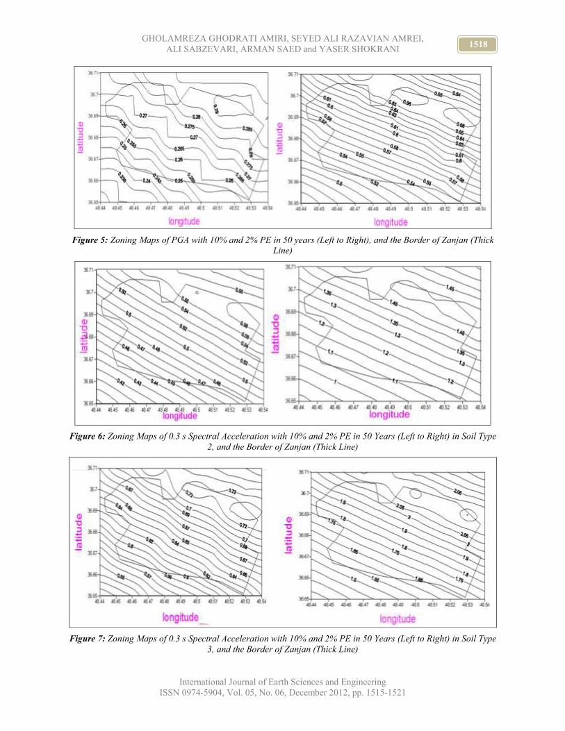
1518 GHOLAMREZA GHODRATI AMIRI, SEYED ALI RAZAVIAN AMREI,
ALI SABZEVARI, ARMAN SAED and YASER SHOKRANI
International Journal of Earth Sciences and Engineering
ISSN 0974-5904, Vol. 05, No. 06, December 2012, pp. 1515-1521
Figure 5: Zoning Maps of PGA with 10% and 2% PE in 50 years (Left to Right), and the Border of Zanjan (Thick
Line)
Figure 6: Zoning Maps of 0.3 s Spectral Acceleration with 10% and 2% PE in 50 Years (Left to Right) in Soil Type
2, and the Border of Zanjan (Thick Line)
Figure 7: Zoning Maps of 0.3 s Spectral Acceleration with 10% and 2% PE in 50 Years (Left to Right) in Soil Type
3, and the Border of Zanjan (Thick Line)
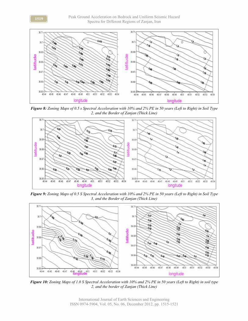
1519 Peak Ground Acceleration on Bedrock and Uniform Seismic Hazard
Spectra for Different Regions of Zanjan, Iran
International Journal of Earth Sciences and Engineering
ISSN 0974-5904, Vol. 05, No. 06, December 2012, pp. 1515-1521
Figure 8: Zoning Maps of 0.5 s Spectral Acceleration with 10% and 2% PE in 50 years (Left to Right) in Soil Type
2, and the Border of Zanjan (Thick Line)
Figure 9: Zoning Maps of 0.5 S Spectral Acceleration with 10% and 2% PE in 50 years (Left to Right) in Soil Type
3, and the Border of Zanjan (Thick Line)
Figure 10: Zoning Maps of 1.0 S Spectral Acceleration with 10% and 2% PE in 50 years (Left to Right) in soil type
2, and the border of Zanjan (Thick Line)
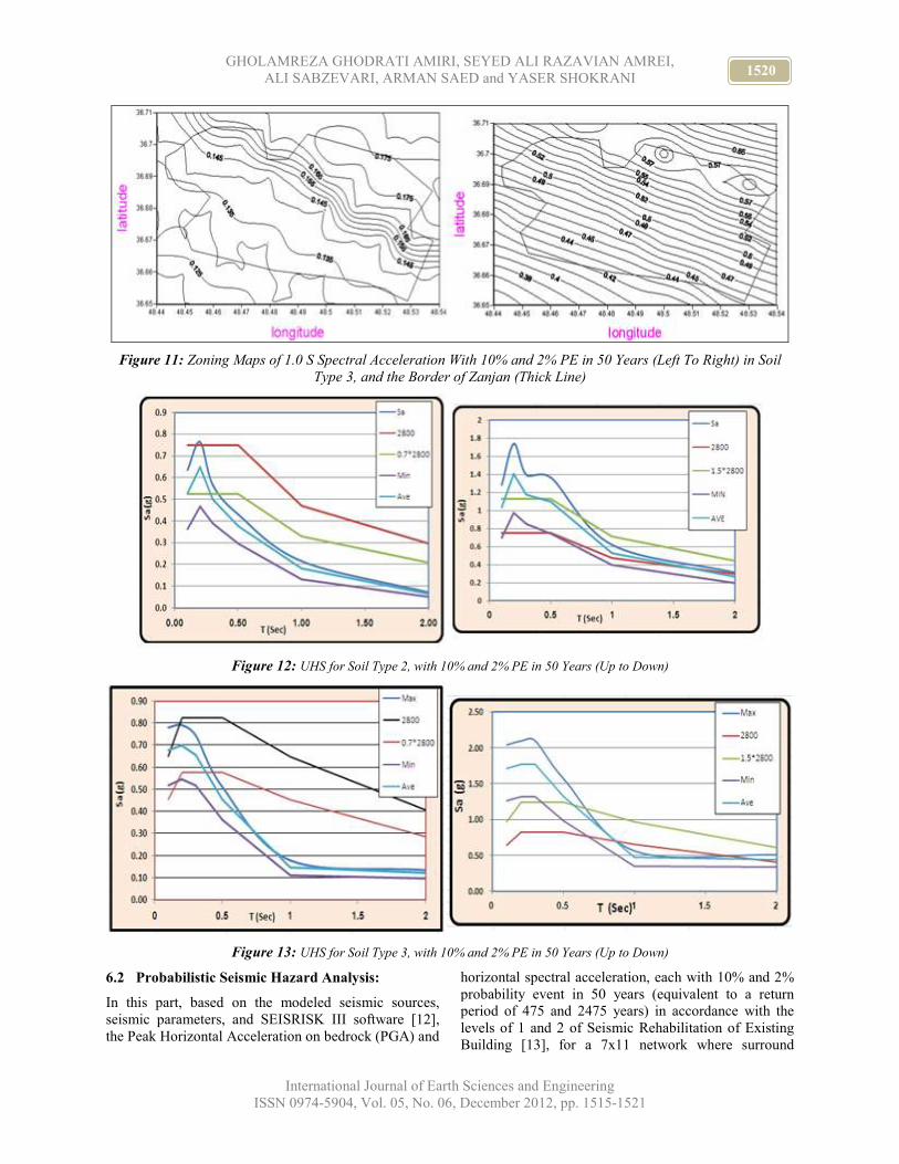
1520 GHOLAMREZA GHODRATI AMIRI, SEYED ALI RAZAVIAN AMREI,
ALI SABZEVARI, ARMAN SAED and YASER SHOKRANI
International Journal of Earth Sciences and Engineering
ISSN 0974-5904, Vol. 05, No. 06, December 2012, pp. 1515-1521
Figure 11: Zoning Maps of 1.0 S Spectral Acceleration With 10% and 2% PE in 50 Years (Left To Right) in Soil
Type 3, and the Border of Zanjan (Thick Line)
Figure 12: UHS for Soil Type 2, with 10% and 2% PE in 50 Years (Up to Down)
Figure 13: UHS for Soil Type 3, with 10% and 2% PE in 50 Years (Up to Down)
6.2 Probabilistic Seismic Hazard Analysis:
In this part, based on the modeled seismic sources,
seismic parameters, and SEISRISK III software [12],
the Peak Horizontal Acceleration on bedrock (PGA) and
horizontal spectral acceleration, each with 10% and 2%
probability event in 50 years (equivalent to a return
period of 475 and 2475 years) in accordance with the
levels of 1 and 2 of Seismic Rehabilitation of Existing
Building [13], for a 7x11 network where surround

1521 Peak Ground Acceleration on Bedrock and Uniform Seismic Hazard
Spectra for Different Regions of Zanjan, Iran
International Journal of Earth Sciences and Engineering
ISSN 0974-5904, Vol. 05, No. 06, December 2012, pp. 1515-1521
Zanjan appropriately, were estimated. As far as the type
of soil is unknown, in each place of the network, exact
calculations for soil type 2 and 3 (the most probable soil
type in the area) based on Iranian Code of Practice for
Seismic Resistant Design of Buildings [14] were done.
The maps for peak ground acceleration on bedrock
(PGA) in Figure 5 and horizontal spectral acceleration
based upon the two soil types of Zanjan city for the 0.3,
0.5, 1 periods are presented in Figures 5 to 11.
7. Uniform Hazard Spectra (UHS):
The uniform hazard spectra (UHS) are formed in the
form of a response in which any time, there is the same
probability range for its occurrence. Throughout these
spectra, within all periods in the life of the structure, the
probability of occurrence is considered as the same. In
other words, in designing a structure, the return period
of spectral acceleration for different periods is
considered the same. For this purpose, in any part of the
network with given seismic hazard, this range is
obtained for different periods.
In Figures 12 and 13, the uniform hazard spectra for the
two soil types and risk levels 1 and 2 based on Seismic
Rehabilitation of Existing Building for Zanjan are
presented. The spectra in these figures are presented as
the peak, minimum and average values of spectral
acceleration at different points in the range of the
network
8. Conclusion:
1- PGA with the probability event, 10% in 50 years (the
period to 475 years or risk level 1) in the range of
Zanjan varies from 0.23g to g 0.295g, also, this amount
in Iranian Code of Practice for Seismic Resistant Design
of Buildings is presented as 0.3g.
2- PGA with the probability event, 2% in 50 years (the
period to 2475 years or risk level 2) in the range of
Zanjan varies from 0.47g to 0.68g.
3- Acceleration and spectral acceleration values in the
northeast region have the highest value in comparison to
other regions.
4- The peak spectral acceleration at the surface of the
soil type 2 in the range of Zanjan varies from 0.75g to
1.8g in the risk level 1.
5- The peak spectral acceleration at the surface of the
soil type 3 in the range of Zanjan varies from 0.78g to
2.2 g in the risk level 1
9. References:
[1] A. Sabzevari, “Peak Ground Acceleration (PGA)
on bedrock and uniform seismic hazard spectra for
different regions of Zanjan city”, MA thesis, Azad
University of Shahrekord, Supervised by Professor
Gh. Ghodrati Amiri, and Dr. S.A. Razavian Amrei,
2011.
[2] A. Nowroozi, “Empirical relations between
magnitude and fault parameters for earthquakes in
Iran”, Bulletin of the Seismological Society of
America ,Vol. 75, No. 5, pp. 1327-1338, 1985.
[3] International Institute of Earthquake Engineering
and Seismology website: http://www.iiees.ac.ir
[4] N.N. Ambraseys, and C.P. Melville, A History of
Persian Earthquakes, Cambridge University Press,
Cambridge, Britain, 1982.
[5] J.K. Gardaner, L. Knopoff, “Is the sequence of
earthquake in southern California, with aftershocks
removed, poissonian?”, Bulletin of the
Seismological Society of America ,Vol. 64, No. 5,
pp. 1363-1367, 1974.
[6] A. Kijko, “Statical estimation of maximum
regional earthquake magnitude Mmax”, Workshop
of Seismicity Modeling in Seismic Hazard
Mapping, poljce, Slovenia, May, 22-24, 2000
[7] G. Ghodrati Amiri, A. Mahdavian, F. Manouchehri
Dana, “Attenuation Relationship for Iran”, Journal
of Earthquake Engineering, Vol. 11, Issue 4, pp.
469-492, 2007.
[8] N.N. Ambraseys, K.A. Simpson, J.J. Bommer,
“Prediction of Horizontal Response Spectra in
Europe”, Earthquake Engineering and Structural
Daynamics, Vol. 25, pp. 371-400, 1996.
[9] K.W. Campbell, “Empirical near-source
attenuation relationships for horizontal and vertical
components of peak ground acceleration, peak
ground velocity, and pseudo-absolute acceleration
response spectra”, Seismological Research Letters,
Vol. 68, No. 1, pp. 154–179, 1997.
[10] H.R. Ramazi, “Attenuation laws of Iranian
earthquakes”, proceedings of the 3rd International
Conference on Seismology and Earthquake
Engineering, Tehran, Iran, 1999.
[11] G. Ghodrati Amiri, M. Khorasani, R. Mirza Hesabi,
and S.A .Razavian Amrei, “Ground-Motion
Prediction Equations of Spectral ordinates and
Arias Intensity for Iran”, Journal of Earthquake
Engineering, Vol. 14, Issue 1, pp. 1-29, 2010.
[12] B. Bender, D.M. Perkins, “SEISRISK-ІІІ: A
computer program for seismic hazard estimation”,
US Geological Survey, Bulletin 1772, 1987.
[13] IIEES. Seismic Rehabilitation Code for Existing
Buildings in Iran, International Institute of
Earthquake Engineering and Seismology, Tehran,
Iran, 2002.
[14] BHRC. Iranian Code of Practice for Seismic
Resistant Design of Building, Standard No. 2800,
Third Revision, Building and Housing Research
Center, Tehran, Iran, 2005.
[15] “Relationship between fault length and maximum
expected magnitude”, Iranian Committee of Large
Dams (IRCOLD), Internal Report, 1994 (In
Persian).

www.cafetinnova.org
Indexed in
Scopus Compendex and Geobase Elsevier, Chemical
Abstract Services-USA, Geo-Ref Information Services-USA
ISSN 0974-5904, Volume 05, No. 06
December2012, P.P.1522-1529
#02050607 Copyright ©2012 CAFET-INNOVA TECHNICAL SOCIETY. All rights reserved.
Heavy Minerals and Provenance of the Lower Gondwana
Sandstones, Ong-River Gondwana Basin, Odisha
ARYA GOUTAMI NATH and RABINDRA NATH HOTA
Department of Geology, Utkal University, Vani Vihar, Bhubaneswar-751004, Odisha
Email: [email protected], [email protected]
Abstract: Heavy mineral analysis of the Talchir and Karharbari sandstones of the Ong-river Gondwana basin,
Odisha, has been carried out in the present study. The characteristic transparent heavy minerals of the Talchir
Formation are garnet, biotite, brown tourmaline, sillimanite, apatite, zircon, enstatite, hypersthene, epidote, rutile,
chlorite, staurolite and sphene. The Karharbari sandstones, in addition to the above mentioned heavy minerals,
contain brookite, hornblende, andalusite, monazite, spinel and pink tourmaline. These heavy minerals are
comparable with the heavy accessories of the Eastern Ghats Supergroup rocks and suggest their derivation from
these rocks. Variation of heavy mineral frequencies can be ascribed to prolonged and deep weathering in the source
area, climate change and/or prevalence of geochemical conditions that prohibited dissolution.
Keywords: Heavy mineral, Talchir Formation, Karharbari Formation, Ong-river Gondwana basin.
Introduction:
Determination of provenance and its different aspects
like its position with respect to the depositional basin,
lithology, prevailing climate and tectonic setting are
some of the significant parameters of basin analysis.
Location of the source area can be inferred from the
scalar and vector attributes of the sediments while the
source rock lithology, climate and tectonic setting can
be determined from the composition of the sediments.
Common minerals like quartz and feldspars, which
constitute bulk of the sediment, are contributed by an
array of rocks whereas the uncommon heavy
accessories provide valuable clue to ascertain the source
rock lithology precisely. The study of heavy minerals
has been used to decipher the provenance lithology both
in unconsolidated and consolidated sediments of
different ages and countries (Tewari and Trivedi, 2001;
Mishra and Tiwari, 2005 etc).
Out of the eight Gondwana basins of Odisha (Fig. 1),
the Talchir and Ib-river basins have been studied in
detail for their economic potential of coal. Little
attention has been paid to the remaining basins. In the
past few years, Hota et al. (2008a, b and 2010) have
studied the texture, palaeocurrent, palaeohydrology and
cyclic aspect of the Talchir and Karharbari formations
of the Ong-river basin. The present study deals with the
heavy mineral analysis of the Talchir and Karharbari
sandstones of the Ong-river Gondwana basin with a
view to deduce the source rock lithology and prevailing
climatic condition.
Geological Setting:
The Lower Gondwana rocks of the Ong-river basin
occur in the Bargarh, Balangir and Sonapur districts of
Orissa extending over an area of about 2 – 6 km wide
and 50 km long (Fig. 1). The rocks of the Eastern Ghats
Supergroup composed of khondalite, charnockite,
garnetiferous granite gneiss, biotite schist, quartzite etc.
intruded by pegmatite, quartz vein and anorthosite
forms the basement (Pandya, 2006). The foliations of
metamorphic rocks strike N80ºE – S80ºW to E – W and
dip towards south at high angle ranging from 40º to 70º.
The strike of the Gondwana sedimentary rocks, on the
other hand, vary from E – W to NE – SW and they show
variable dip ranging from 5º to 25º due north to
northwest. The stratigraphic sequence based on surface
and subsurface studies is given in Table 1.
The Talchir Formation is dominated by coarse clastics.
It is composed of diamictite, matrix-supported
conglomerate, graded conglomerate, massive sandstone,
very coarse- to medium-grained flat- and cross-bedded
sandstones and interbedded sandstone-shale formed in
glacial, glacio-fluvial and fluvial environments (Hota et
al. 2010). Sandstones are the dominant constituents of
the Karharbari Formation. Various lithic units are thin
conglomerate, trough cross-bedded very coarse- to fine-
grained sandstones, interbedded sandstone-shale, gray
shale and interbedded carbonaceous shale-shaly coal-
coal. These lithofacies are characteristics of channel,
point bar, flood plain and swamp deposits of the fluvial
environment.

1523 ARYA GOUTAMI NATH and RABINDRA NATH HOTA
International Journal of Earth Sciences and Engineering
ISSN 0974-5904, Vol. 05, No. 06, December 2012, pp. 1522-1529
Methodology:
Forty three sandstone samples, 13 from the Talchir
Formation and 30 from the Karharbari Formation were
collected from exposures. These were disaggregated by
a porcelain mortar and pestle and sieved. The heavy
minerals were separated from 0.125 – 0.088 mm (fine-
to very fine-grained) sand fraction by standard
technique using bromoform as the heavy liquid.
Separated heavy minerals were washed with acetone
and stannus chloride and mounted on glass slide with
Canada balsam. The minerals were identified under
microscope by their diagnostic optical characters and
their number frequencies were determined by field
count method following the procedure outlined by Hota
(2011). Parameters like ZTR, shape and density indices
were calculated following Hubert (1962) and Flores and
Schideler (1978). The ZTR index is the percentage of
zircon, tourmaline and rutile among the transparent
nonmicaceous detrital heavy minerals. It is a measure of
the mineralogical maturity of the sediment. The shape
index is the ratio of bladed and elongated minerals like
pyroxene, hornblende, tourmaline, rutile, zircon,
sillimanite vs. equant minerals like garnet and epidote.
Density index is the ratio of opaque and transparent
heavies.
Heavy Minerals:
Both opaque and transparent heavy minerals constitute
the heavy mineral crop of the Gondwana sandstones.
The opaque minerals, which could not be identified
precisely in the present study, are mostly oxides and
hydroxides of iron like magnetite, hematite, limonite,
goethite, ilmenite etc. In the present study, they have
been categorized as rounded (Fig. 2a) and elongated
(Fig. 2b). The elongated minerals are more likely to be
ilmenite. Many of the ilmenite grains have been altered
to leucoxene, which are identified by their dead white
colour. In some instances they are associated with
unaltered ilmenite (Fig. 2c). Since it is an altered
product of ilmenite, it has been treated at par with
opaque minerals in the present study. The opaque
minerals (51%) are nearly equal to the transparent heavy
minerals (49%) in case of the Talchir Formation while
in case of the Karharbari Formation the opaque minerals
(63%) dominate over transparent heavies (37%).
The transparent heavy minerals of the Talchir
Formation are garnet, biotite, brown tourmaline,
sillimanite, apatite, zircon, pyroxene, epidote, rutile,
chlorite, staurolite and sphene. The Karharbari
Formation, in addition to these minerals, contains
brookite, hornblende, andalusite, monazite, spinel and
pink tourmaline. The characteristic optical properties of
these heavy minerals are as follows:
Garnet: Garnet is the dominant heavy mineral of the
sandstones. On the basis of colour, two types of garnets
have been recognised. These are colourless (Fig. 2d)
and pink (Fig. 2e). The grains are angular to subrounded
and show conchoidal fractures, inclusions are frequently
present and in a few instances the surfaces are pitted.
These are isotropic.
Biotite: Detrital biotite grains occur as brown flakes
(Fig. 2f) and are strongly pleochroic. The basal sections
are isotropic and alteration is a common feature.
Zircon: Zircon occurs as elongate, oval to rounded
grains, identified by high relief, dark border and parallel
extinction. Colourless (Fig. 2g) and pink (Fig. 2h)
varieties have been reported. Inclusions of other
minerals, liquid and gas are frequently present.
Sillimanite: Sillimanite occurs as non-pleochroic,
colourless, needle to long prism shaped grain marked by
striations parallel to length, high order interference
colour, straight extinction and negative sign of
elongation (Fig. 2i).
Apatite: Grains are oval and elongate prismatic,
colourless, low relief, negative sign of elongation,
parallel extinction and show first order interference
colour (Fig. 2j). Some grains contain abundant
inclusions arranged in rows.
Tourmaline: On the basis of colour, two types of
tourmalines have been identified. These are brown and
pink. The brown tourmaline (Fig.2k) is pleochroic from
yellowish brown to dark brown and pink variety (Fig.
2l) is pleochroic from pink to brownish pink. They
occur as short prismatic grains and a few of them
contain inclusions. The grains show straight extinction
and negative sign of elongation. The brown tourmaline
is more abundant in the Talchir Formation whereas the
pink variety has been reported from the Karharbari
Formation only.
Pyroxene: Two varieties of pyroxenes, viz. enstatite
and hypersthene have been recorded. The enstatite is
identified by its colourless, nonpleochroic nature, first
order interference colour, positive sign of elongation
and straight extinction. Some grains appear slightly
brown due to iron incrustation (Fig. 2m). Hypersthene
occurs as elongate to irregular grains, greenish in
colour, pleochroic from green to pink, presence of
cleavage, straight extinction and positive sign of
elongation (Fig. 2n).
Epidote: The grains are subrounded, weakly pleochroic
from pale green to lemon yellow (Fig. 2o) and show
straight extinction.
Rutile: Rutile is characterised by deep red colour, broad
and thick boarder around the grain. A few are sub-
rounded but most of them are elongated prismatic (Fig.

1524 Heavy Minerals and Provenance of the Lower Gondwana Sandstones,
Ong-River Gondwana Basin, Odisha
International Journal of Earth Sciences and Engineering
ISSN 0974-5904, Vol. 05, No. 06, December 2012, pp. 1522-1529
2p) and show the same colour under crossed nicols as in
ordinary light.
Chlorite: Chlorite is marked by pale green colour and
flat irregular grain of micaceous habit (Fig. 2q). Grains
show blotchy ultrablue abnormal interference colour.
Staurolite: Occurs as prismatic grain of golden yellow
colour (Fig.2r), marked by hackly to subconchoidal
fracture, pleochroic from straw yellow to russet brown,
bright yellow interference colour and straight extinction.
Many grains contain profuse inclusions.
Sphene: It occurs as subrounded grain of high refractive
index, colourless to light yellow, show same colour
under crossed nicols as in polarised light, incomplete
extinction and turn bluish near the extinction position
(Fig. 2s).
Brookite: The grains are squarish with truncated
corners, striated, orange to brown in colour and show
incomplete extinction (Fig. 2t). It occurs only in the
Karharbari sandstones.
Hornblende: It occurs as subrounded grain, bluish in
colour, pleochroic from greenish blue to bluish green
(Fig. 2u) having two sets of cleavage and extinction
angle of 15° - 25°.
Andalusite: The grains are nonpleochroic or pleochroic
from colourless to pink, show first order interference
colour, negative sign of elongation and straight
extinction (Fig.2v).
Monazite: The grains are rounded or oval in habit,
yellow to greenish yellow in colour, show the same
interference colour as under plane polarized light and
low angle of extinction varying from 2°-10° (Fig.2w).
Spinel: Grains are grass green in colour, irregular to
subrounded, marked by conchoidal fracture and
isotropic (Fig. 2x). It occurs in the Karharbari
sandstones only.
Provenance:
The frequency percentages of the transparent heavy
minerals of the Talchir and Karharbari formations along
with probable source rocks is presented in Table 2 and
graphically shown in Fig. 3. Garnet and biotite are the
most abundant heavy minerals of both the formations.
The transparent heavy crop of the Talchir Formation
consists of garnet (50.19%), biotite (20.85%), brown
tourmaline (12.02%), sillimanite (6.59%), apatite
(3.81%), zircon (2.04%), pyroxene (1.67%), epidote
(1.30%), rutile (0.80%), chlorite (0.60%), staurolite
(0.09%) and sphene (0.04%). The transparent heavy
mineral assemblage of the Karharbari Formation
comprises garnet (50.45%), biotite (15.55%), brown
tourmaline (1.05%), sillimanite (7.67%), apatite
(1.88%), zircon (11.40%), pyroxene (1.15%), epidote
(1.17%), rutile (2.09%), chlorite (2.60%), staurolite
(1.04%), sphene (1.95%), brookite (1.07%), hornblende
(0.37%), andalusite (0.35%), monazite (0.10%), spinel
(0.08%) and pink tourmaline (0.03%). The ZTR and
shape indices of heavy minerals of both the formations
are nearly same. In case of the Talchir Formation, the
ZTR index is mostly due to presence of brown
tourmaline, while in case of the Karharbari Formation, it
is due to higher proportions of zircon and rutile. Higher
density index of the Karharbari sandstones is due to the
presence of higher percentage of opaque minerals.
These heavy minerals can be linked with four types of
lithounits viz. acid and basic igneous and low- and high-
rank metamorphic rocks. Apatite, zircon, sphene,
monazite and pink tourmaline suggest the acid igneous
source. Basic igneous parentage is indicated by
pyroxene, rutile, brookite and spinel. Minerals like
biotite, chlorite and brown tourmaline are derived from
low-rank metamorphic rocks, whereas high-rank
metamorphic source is suggested by garnet, hornblende,
sillimanite, staurolite, epidote and andalusite. Though
these minerals represent diverse source rocks and of
variable mineral stability, their close association may be
due to high stability and preservation potential of certain
species and equal degree of mineral stability in case of
others (Pettijohn, 1984). Presence of unstable species
like pyroxene and sillimanite in appreciable quantity,
which would otherwise have been eliminated, may be
due to their abundance in the source rocks like
khondalite, basic granulite and charnockite, which
constitute bulk of the Eastern Ghats Supergroup and/or
existence of favourable geochemical conditions, which
inhibited complete dissolution. These observations
suggest deep weathering in the source area with
exposure of different types of rocks and favourable
hydrodynamic and geochemical conditions for
attainment of mineralogical maturity of the heavy
minerals as revealed by relatively higher ZTR index.
The palaeocurrent pattern of the Ong-river Gondwana
sediments indicates a predominantly northerly
palaeoflow and existence of the source area towards the
southern boundary of the basin (Hota et al. 2008b). The
southern margin of the Gondwana basin is bounded by
the Eastern Ghats Supergroup of rocks of Precambrian
age. These are composed of metamorphic rocks like
khondalite, basic granulite, charnockite, mica schist,
leptynite, quartzite, acid-gneiss and pyroxene granulite
intruded by granitic plutons and basic igneous rocks.
The observed heavy mineral suites are comparable with
heavy accessories of the Eastern Ghats Supergroup of
rocks and suggest their derivation form these rocks.
Euhedral and less amount of rounding of many heavy
mineral grains suggest short distance of transportation
and presence of the source rock in the vicinity of the
depositional basin. Large number of heavy minerals in

1525 ARYA GOUTAMI NATH and RABINDRA NATH HOTA
International Journal of Earth Sciences and Engineering
ISSN 0974-5904, Vol. 05, No. 06, December 2012, pp. 1522-1529
Karharbari sandstones in comparison to Talchir
sediments can be ascribed to exposure of diverse rock
types in the source area caused by deep chemical
weathering in humid climatic condition. The gradual
changeover of climate from cold glacial during Talchir
sedimentation to warmer humid climatic condition
during Karharbari sedimentation is attested by increase
of the percentage of opaque minerals from 51% to 63%.
Conclusions:
Following conclusions have been drawn in the present
study.
1. Garnet, biotite, zircon, sillimanite, apatite,
tourmaline, pyroxenes, epidote, rutile, chlorite,
staurolite, sphene, brookite, hornblende, andalusite,
monazite and spinel including opaques and leucoxene
constitute the heavy mineral suites of the Gondwana
sandstones of the Ong-river basin.
2. Garnet, sillimanite and biotite are the dominant
heavy minerals of both the formations. In addition to
these, the Talchir Formation contains appreciable
quantity of brown tourmaline, while the Karharbari
sandstones contain higher percentage of zircon.
3. Source area denudation, tectonism and action of
intrastratal solution played important roles to account
for the variation of the heavy mineral suites.
4. The observed heavy minerals are comparable with
the accessory constituents of khondalite, basic granulite,
charnockite, mica schist, leptynite, quartzite, acid-
gneiss, pyroxene granulite, granite, and basic igneous
rocks of the Eastern Ghats Supergroup. Proximity of the
source area is indicated by euhedral to subrounded
grains of most of the heavy minerals.
5. Progressive denudation, release of some heavy
minerals in the source region, climate change and/or
existence of favourable geochemical condition to escape
dissolution account for the variation of heavy mineral
frequencies of two formations of the Gondwana
Supergroup.
Acknowledgements:
The authors are thankful to the reviewers Prof. S. Das of
IIT, Kharagpur, India and Prof. W. Maejima of Osaka
City University, Japan for their critical and constructive
suggestions that enhanced the quality of the paper.
References:
[1] Flores, R. M. & Schideler, G. L. (1978). Factor
controlling heavy mineral variations on the South
Texas outer continental shelf gulf of Mexico.
Journal of Sedimentary Petrology, 48, 269-280.
[2] Goswami, S., Das, M. & Guru, B. C. (2006).
Permian biodiversity of Mahanadi master basin,
Orissa, India and their environmental countenance.
Acta Palaeobotanica, 46,101 – 118.
[3] Hota, R. N. (2011). Practical approach to petrology.
CBS publishers and Distributors, New Delhi, 150p.
[4] Hota, R. N., Dalabehera, L. & Nath, A. G. (2008a).
Textural characteristics and discriminant Analysis
of Talchir and Karharbari sandstones of the Ong-
River Gondwana Basin of Orissa. Journal of Indian
Association of Sedimentologists, 27 (No.1), 77 –
86.
[5] Hota, R. N., Maejima, W. & Nath, A. G. (2008b).
River transmutation during Lower Gondwana
sedimentation in Ong-river basin, Orissa. Journal of
Indian Association of Sedimentologists, 27 (No.2),
29 – 37.
[6] Hota, R. N., Nath, A. G. & Maejima, W. (2010).
Cyclic sedimentation of the Karharbari Formation,
Ong-River Gondwana basin, Orissa – Statistical
assessment from subsurface data. Journal of Indian
Association of Sedimentologists, 29, pp.1 – 12.
[7] Hubert, J. F. (1962) A zircon-tourmaline-rutile
maturity index and the interdependence of the
composition of heavy mineral assemblages with the
gross composition and texture of sandstones.
Journal of Sedimentary Petrology, 32, 440-450.
[8] Mishra, D. & Tiwari, R. N. (2005). Provenance
study of siliciclastic sediments, Jhura dome,
Kachchh, Gujrat. Journal of the Geological Society
of India, 65, 703-714.
[9] Pandya, K. L. (2006) Gondwanas. In: Mahalik, N.
K., Sahoo, H. K., Hota, R. N., Mishra, B. P.,
Nanda, J. K. & Panigrahi, A. B. (Eds) Geology and
Mineral Resources of Orissa. Society of
Geoscientists and Allied Technologists,
Bhubaneswar, pp. 91 – 103.
[10] Pettijohn, F. J. (1984). Sedimentary rocks, CBS,
New Delhi, 628p.
[11] Tewari, R.C. & Trivedi, G. S. (2001). Heavy
mineral assemblages viz-a-viz composition of
provenance of Gondwana rocks of peninsular India.
Indian Journal of Petroleum Geology, 10, 33-42.

1526 Heavy Minerals and Provenance of the Lower Gondwana Sandstones,
Ong-River Gondwana Basin, Odisha
International Journal of Earth Sciences and Engineering
ISSN 0974-5904, Vol. 05, No. 06, December 2012, pp. 1522-1529
Table 1: Stratigraphic Sequence of the Ong-River Basin, Orissa (Modified After Goswami et al. 2006
and Pandya, 2006)
Age Group Formation Dominant lithology
Recent to -
Sub-recent Soil, laterite, alluvium and gravel
Lower
Permian Lower
Gondwana
Group
Karharbari
Formation
Medium to very coarse grained sandstone with occasional
conglomerate, gray shale and coal stringer
Talchir
Formation Greenish sandstone and shale with diamictite at base
~ ~ ~ ~ ~ ~ ~ ~ ~ ~ ~ ~ ~ ~ ~ ~ ~ ~ ~ Unconformity ~ ~ ~ ~ ~ ~ ~ ~ ~ ~ ~ ~ ~ ~ ~ ~ ~ ~ ~ ~ ~ ~ ~ ~ ~ ~ ~ ~ ~ ~
Precambrian
Eastern
Ghats
Supergroup
Intrusives
Pegmatites, quartz vein and anorthosite
Metamorphics Khondalite, charnockite, garnetiferousgranite gneiss, biotite
schist and quartzite
Table 2: Average Transparent Heavy Mineral Content (In Number Percent) of the Gondwana Sandstones of the
Ong-River Basin and Possible Source Rock Types
Heavy Mineral Talchir
Formation
Karharbari
Formation Source rock type
Garnet 50.19 50.45 High rank metamorphic
Biotite 20.85 15.55 Low rank metamorphic, acid igneous
Tourmaline (brown) 12.02 1.05 Low rank metamorphic
Sillimanite 6.59 7.67 High rank metamorphic
Apatite 3.81 1.88 Acid igneous
Zircon 2.04 11.40 Acid igneous
Pyroxene 1.67 1.15 Basic igneous
Epidote 1.30 1.17 High rank metamorphic
Rutile 0.80 2.09 Basic igneous
Chlorite 0.60 2.60 Low rank metamorphic
Staurolite 0.09 1.04 High rank metamorphic
Sphene 0.04 1.95 Acid igneous
Brookite 0.00 1.07 Basic igneous
Hornblende 0.00 0.37 High rank metamorphic
Andalusite 0.00 0.35 High rank metamorphic
Monazite 0.00 0.10 Acid igneous
Spinel 0.00 0.08 Basic igneous
Tourmaline (pink) 0.00 0.03 Acid igneous
ZTR Index 23.33 21.66
Shape Index 0.32 0.31
Density Index 1.04 1.70
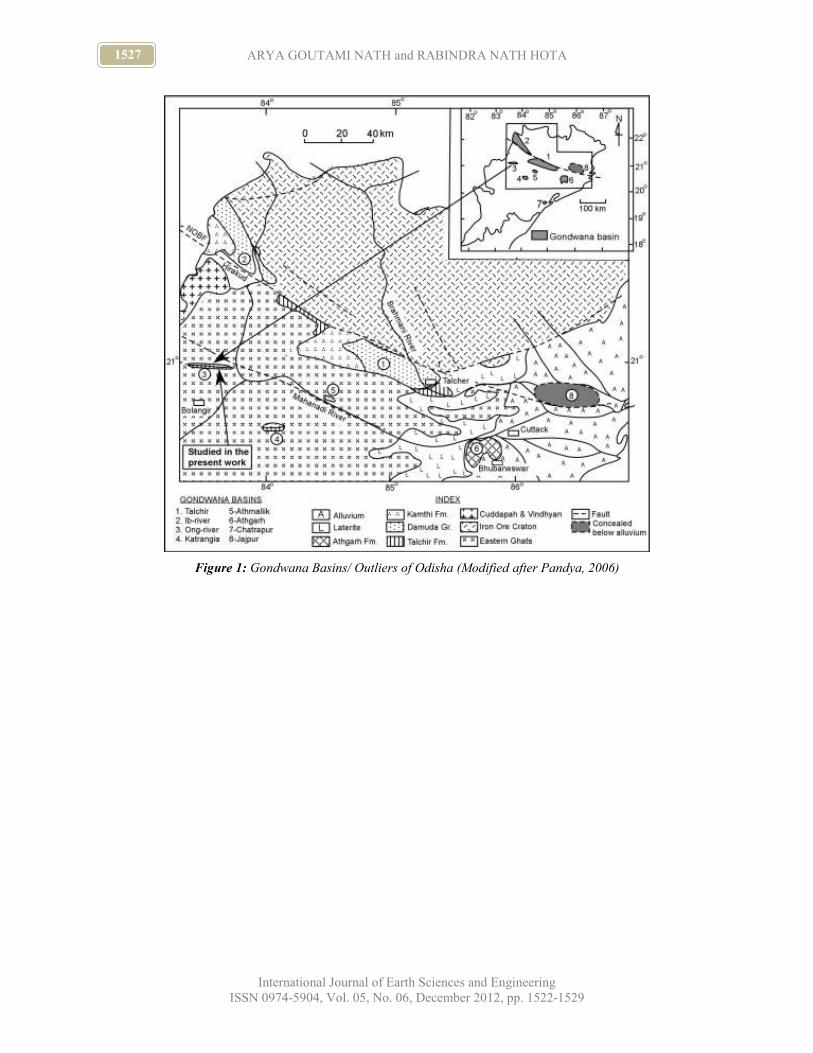
1527 ARYA GOUTAMI NATH and RABINDRA NATH HOTA
International Journal of Earth Sciences and Engineering
ISSN 0974-5904, Vol. 05, No. 06, December 2012, pp. 1522-1529
Figure 1: Gondwana Basins/ Outliers of Odisha (Modified after Pandya, 2006)

1528 Heavy Minerals and Provenance of the Lower Gondwana Sandstones,
Ong-River Gondwana Basin, Odisha
International Journal of Earth Sciences and Engineering
ISSN 0974-5904, Vol. 05, No. 06, December 2012, pp. 1522-1529
Figure 2: Photomicrographs of the Heavy Minerals. (a) Rounded Opaque, (b) Elongated opaque, (c) Leucoxene
with Partially Altered Ilmenite, (d) Colourless Garnet, (e) Pink Garnet, (f) Biotite, (g) Colourless Zircon, (h) Pink
Zircon, (i) Sillimanite, (j) Apatite, (k) Brown Tourmaline, (l) Pink Tourmaline, (m) Enstatite, (n) Hypersthene,
(o) Epidote, (p) Rutile, (q) Chlorite, (r) Staurolite, (s) Sphene, (t) Brookite, (u) Hornblende, (v) Andalusite,
(w) Monazite and (x) Spinel

1529 ARYA GOUTAMI NATH and RABINDRA NATH HOTA
International Journal of Earth Sciences and Engineering
ISSN 0974-5904, Vol. 05, No. 06, December 2012, pp. 1522-1529
Figure 3: Histogram Showing Transparent Heavy Mineral Frequency Percentages of the Lower Gondwana
Sandstones of the Ong-River Basin, Odisha

www.cafetinnova.org
Indexed in
Scopus Compendex and Geobase Elsevier, Chemical
Abstract Services-USA, Geo-Ref Information Services-USA
ISSN 0974-5904, Volume 05, No. 06
December2012, P.P.1530-1534
#02050608 Copyright ©2012 CAFET-INNOVA TECHNICAL SOCIETY. All rights reserved.
Rating of Tunnel by Visual Field Inventory – A Case Study of
Punasa Tunnel, District Khandawa, M. P. India
GUPTA. M. C1, SINGH. B. K
2 and SINGH. K. N
3
1Water Resources Deptt. , Narmada-Tapti Area, (MP), India.
2Applied Geology, Deptt.of Civil Engg. Govt. Engg. College, Ujjain (MP) India 3School of Studies in Earth Science, Vikram University, Ujjain, (MP) India
Email: [email protected]
Abstract: This paper proposes a new rating system for tunnel by visual field inventory method for Punasa tunnel a
part of Narmada Sagar Project. The new CRTVFI (Classification for Rating of Tunnel by Visual Field Inventory)
technique has been developed after modification in the methods proposed by Romana et al. (1983) considering other
geotechnical parameters given by Bieniawski, (1974, 1989) and Barton et al. (1974). The modified classification
has been used in the investigated area and paper focuses on design recommended on the basis of the classification
systems such as maximum span opening, lining and support recommendations. A very handsome amount of about
32.45% has been saved using CRTVFI classification against the proposed total cost of the tunnel. This classification
technique implied in the area, has not only saved money, but also saved precious time of construction.
Keywords: Tunnel rating, Tunnel stability, CRTVFI classification.
Introduction:
The rating of tunnel has been proposed by different
engineers and scientists from time to time for their
stability estimation stand up time and protection /
treatment measures. The various criteria for
classification of Rock Mass Rating (RMR) given by
Bieniawski (1974), "Q" classification by Barton et al.
(1974) and Romana et al. (1983) have been analyzed
and applied for concrete lining to check the stability in
Punasa tunnel (Gupta et al. 2011). The “Classification
based on Rating of Tunnel by Visual Field Inventory"
(CRTVFI) has been implemented at the time of
tunneling in basaltic lava flow for their longevity,
stability and finalization for stand up time with
treatment/ protection measures. Supporting system in
different condition i.e. dry and wet for their longer
stability has been applied for different rock mass
category i.e. in massive/dense basalt, vesicular
amygdular basalt and red bole. This classification has
helped in many ways especially in terms of saving the
time and money of the studied tunnel project.
Location of the Study Area:
The study area is part of Nimar Plateau, situated in
South Western part of Punasa Block, District Khandwa,
Madhya Pradesh belonging to Survey of India
Topographic Sheet Nos. 55 B/7 and 55 B/12 between
the longitude 76o20′ and 76
o32′ E and latitude 22
o and
22o13′ N.
Geology of the Tunnel Site:
The area of investigation is mainly covered with Deccan
Traps basaltic lava flows erupted during the Cretaceous
to Eocene period (Blandford, 1967). On the basis of
thirty two bore hole drill logs and resistivity survey
seven flows and aquifer zones have been recognized in
the area. The Punasa tunnel is covered with Middle
Trap, which forms a part of the Nimar Plateau. The
numerous dykes are present in the area and are running
parallel to the river Narmada. The top basaltic flows are
highly vesicular and amygdular; where as middle flows
are compact in nature. The river and nala are filled with
black colored alluvial soil.
Geotechnical Appraisal of Tunnel:
The tunnel appraisal has been carried out for the
estimation and support system for the project using
Rock Mass Rating System (RMR) and NGI index or Q
rating and Classification based on Rating of Tunnel by
Visual field Inventory (CRTVFI).
Joint Pattern in the Study Area:
The joint patterns/sets have been analyzed (Ahmed et al.
1999) for the estimation of tunnel quality with the help
of five sets of joints J1, J2, J3, J4 and J5 present in the
area under investigation. Joint J1 & J5 are horizontal to
sub horizontal in nature with 5 to 100cm spacing causes
crown fall in the tunnel. Joints J2, J3 and J4 are vertical
to sub vertical or columnar in nature with 20 to 50 cm.
spacing. 0.20 to 0.50 meters thick seams or weathered

1531 GUPTA. M. C, SINGH. B. K and SINGH. K. N
International Journal of Earth Sciences and Engineering
ISSN 0974-5904, Vol. 05, No. 06, December 2012, pp. 1530-1534
layer present in between surface of joints. More often
the surfaces of joints are smooth, plane or uneven filled
with silica and clay materials with a few noticeable
slickensides.
Table1: Geomechanical classification and required support in tunnel of Upper Punasa (After Bieniawski 1974;
modified after Gupta et al. 2011)
Rock mass Rock
Class RMR
Full-face or Heading and
benching method Rock bolt Shotcrete
Good rock
(massive/
dense basalt)
II 69 to
74
1 to 1.5m complete support
max. 20 meter at exit & inlet
portal ISMB/steel support
200mm with lagging
3m long +
spaced 3 m.
c/c 25 mm ,
shell type
50mm + 50mm in
crown & wall portion,
some patches are
covered with reinforced
shotcrete (in damp area)
Fair rock
(Vesicular
amygdular
Basalt)
III 52 to
55
Top heading and bench, 6.20
and 2.15 m. required support
system, 10 m. at exit & inlet
portal ISMB/steel support 200
mm with lagging
Systematic
rock bolt
4meters long,
spaced 1.5 -2
m. in crown
50-100mm in crown,
30mm in side walls.
Poor rock (Red
bole/
tuffaceous/
fractured zone/
shear zone)
IV 29
Top heading and bench, 6.20
and 2.15 m. required support
system, 10 m. at exit & inlet
portal ISMB/steel support
200mm with lagging
Systematic
rock bolt 4 to
5 meters long,
spaced 1-1.5
m. in crown
100-150mm in crown,
100mm in side walls.
Rock Mass Rating (RMR) System:
Rock mass rating system was developed by Bieniawski
(1973) and have been visualized for Punasa Tunnel Site
(Gupta et al. 2011). On the basis of the rock mass class,
Bieniawski (1989) has recommended a primary support
for tunnels of shallow depth having the diameter
between 5 - 12 meters with vertical stresses below 25
mpa (Table-1).
Q-System:
The Q - system of rock mass classification was
proposed by Barton, Lien and Lunde (1974) for the
determination of the tunnel quality of a rock mass. The
numerical value of this index Q is defined by quality
using different parameters, viz. Rock Quality
Designation (RQD), joint pattern or discontinuity of
joints, Joint number (Jn), joint roughness number (Jr),
joint alteration number (Ja), joint water reduction factor
(Jw) and stress reduction factors (SRF). After evaluating
various parameters the support system have been found
for the Punasa tunnel has been given in table-2.
( ) ( ) ( )RQD Jr JwQ x x
Jn Ja SRF=
Required De (Equivalent dimension) and ESR
(Excavation support ratio)
)(sup
)(,
ESRratioportExcavation
meterdiameterspanExcavationDe =
218.56.1
35.8==eD
(Value of ESR = 1.6) Above parameters have been used
in geological appraisal for different rock mass
categories. The value of excavation support ratio (ESR)
has been taken from Barton et al. (1974). The support
system for treatment/protection measures of tunnel has
been suggested as per Q-system & Rock mass
categories.
For massive/dense basalt or Grade I, II, II/I or hard
rock, the Q value is 13.33 where tunneling quality (Q) is
fair to good. For vesicular amygdular basalt or III, III/II,
II/III or soft rock, the Q value is 24.8 and Tunneling
quality (Q) is good. For red bole/ tuffaceous basalt or
III/IV, IV or soil, the Q value is 0.0825 where as
Tunneling quality (Q) is Very poor
Comparison of Support System:
The Upper Punasa tunnel has been excavated through
the basaltic lava flow which are competent than other
rock. The support system has been developed based on
the Rock Mass Rating (RMR) classification of
Bieniawski (1974) and Q system of Barton et al. (1974).
The Excavation Support Ratio (ESR) has been
considered to the support system in tunneling. The
comparison of various support systems modified after
Rutledge (1978), Wickham et al. (1972 & 74)
Bieniawski (1974) and, Barton et al. (1974). has been
shown in Table-3.

1532 Rating of Tunnel by Visual Field Inventory – A Case Study
of Punasa Tunnel, District Khandawa, M. P. India
International Journal of Earth Sciences and Engineering
ISSN 0974-5904, Vol. 05, No. 06, December 2012, pp. 1530-1534
Table 2: Support System Required for Underground Excavation (After Barton et al. 1974)
Rock mass
category/ Support
category
Q
Conditional
factor
RQD/Jn
P(kg/cm²)
(Approx.)
Span/
ER
(m)
Type of support
Massive/dense
basalt
/ 17 - 20
10 – 4 < 5 - > 30 1 3.5 – 9
Sb (utg), B (utg)1.5 to 2 m + S 2-3
cm.to B (tg) 1.5 - 2 m.+ clm or
S(Mr),10-15cm
Vesicular
amygdular basalt /
13 - 16
40– 10 < 10 - >15 0.5 5 – 23 Sb (utg) B (utg) 1.5 - 2 m. B (utg)1..5
– 2 m. + S 2 - 3 m. + S (mr) 5 - 10 cm.
Red bole /
tuffaceous / 29 - 32 0.4 - 1 1.4 - > 5 3 2.2 – 14.5
B (tg) 1 m. + S (mr) 5 - 12 cm. S (mr)
7.5 -25 cm. CCA – 20 - 40 m + B (tg)
1 m. CCA (sr) 30 -50 cm. + (tg) 1 m.
Index: Sb- Spot Bolting, B - Systematic Rock Bolting, S -Shotcrete, utg- Tensioned (Expanding Shell type for
competent Rock Mass, Grouted Post Tensioned in Very Poor Quality Rock Mass)
Table 3: Comparison of Support System for Different Rock Mass Category as Per Various I.S. codes of 1971,72, &
78 (Modified after Barton et al. 1974)
Index: B-Systematic Rock Bolting; Sb- Spot Bolting; (utg)- Untensioned, Grouted; (tg)- Tensioned, Grouted;
(mr)Mesh Reinforced; Clm - Chain Link Mesh; CCA- Cast Concrete Arch; (Sr) - Steel Reinforced;
R.S.- Reinforcedshotcrete; C/C - Center to Center; R.T.- Rock Type; R.M.R.- Rock Mass Rating; S.C.- Support
Category; R.M.Q.- Rock Mass Quality; S.S.- Support System. The Value of Q has been determined by Excavation
Support Ratio for Water Tunnel as 1.6.
Table 4: Classifications for Rating of Tunnel by Visual Field Inventory (CRTVFI) (Modified after Romana et al.,
1983)
Rock mass Gr. I, II
(1)
Gr. III, III/II
(2)
Gr. III/IV
(3)
Characterization
/rating Good Poor Very Poor
In dry condition/
Stability
Stable more than One
Year
Stable more than Six
Month Stable Three to Seven Days
Treatment Spot bolting(tg) Rock bolt(tg) + shotcrete
(50mm)
Systematic rock bolting(tg) +
Reinforced shotcrete(100mm)
In Wet condition/
Stability
Stable Six
Month(Maximum) Stable 15 to 30 Days Immediate or Twenty four hours
Treatment
Reinforced
shotcrete(100mm) +
Systematic rock bolt(tg)
Reinforced shotcrete
(100mm) + Systematic
rock bolt (tg)
Shotcrete (25mm)+Systematic
rock bolt (tg) + Steel support
(ISMB200mm) +Probe +back fill
concrete
Index: Gr.I and II: Massive dense basalt,Gr.II/III and III:Vesicular amygdular basalt, Gr. III/IV: Red bole,
tg: Tensioned grouted

1533 GUPTA. M. C, SINGH. B. K and SINGH. K. N
International Journal of Earth Sciences and Engineering
ISSN 0974-5904, Vol. 05, No. 06, December 2012, pp. 1530-1534
Classification for Rating of Tunnel by Visual Field
Inventory (CRTVFI):
Several classifications have been proposed by
geotechnical engineers and are followed for estimating
the nature of rock and treatment or supports in the
tunnel. The CRTVFI classification has been developed
for the field inventory of tunnel at the time of
monitoring by visual observation for tunnel stability.
The classification applied at the time of excavation of
tunnel is very simple and terminology used has been
widely accepted by geologist and engineers. The
classification of Romana et al. (1983) has been modified
on the basis of rating of tunnel by visual field inventory
and other parameters like joints, pattern, seepage points
and percolation quality. The property of rock reflects
the strength and stability of rock mass characterization.
The classification for rating of tunnel by visual field
inventory used in the study area in dry and wet
conditions with treatment and support system is given in
the table-4.
Conclusion:
The different rock type mainly Massive / Dense Basalt
or grade I, II and II/I, Vesicular Amygdular Basalt or
III, III/II and II/III and Red bole/Tuffaceous or III/IV,
IV/V has been applied to different types of support
system in dry and wet conditions. The classification of
rock mass rating and Q given by Bieniawski (1974;
modified in 1989) and Barton et al. (1974) utilized only
at an early stage of the projects for estimation and
support system. The author and his team executed
support system in the tunnel as per site conditions and
applied at the time of excavation and developed a new
Classification for Rating of Tunnel by Visual Field
Inventory (CRTVFI) including other geotechnical
parameters at the time of monitoring by visual
observation. The calculated numerical value as per
Bieniawski classification, the rock mass rating value for
massive/dense basalt is higher than vesicular amygdular
basalt but as per Q classification the value for vesicular
amygdular basalt is higher (24.8) and stable without any
treatment under the dry condition and stable with
nominal treatment in wet condition.
Acknowledgement:
The authors are highly thankful to the Narmada Valley
Development Authority & Water Resource Department,
Madhya Pradesh, Bhopal for providing the information
related to the work. Thanks are due to the team
members of the Narmada Valley Development
Authority for their help rendered during the field work.
References:
[1] Ahmed, M.J. & Soni, C.K., 1999: Geotechnical
Evaluation of deep rock cut tail channel, Narmada
(Indira) Sagar Project (M.P.) Indian Society of
Engineering Geology Bhopal. Geol. Vol. XXVII
pp.200-206
[2] Ahmed, M. J. and Pathak, S.K., 1999: Geotechnical
appraisal of river diversion arrangement of
Narmada Sagar Project, district Khandwa, (M.P.).
Indian Society of Engineering Geology Vol. VII
No.4, pp.126-130
[3] Barton, N., Lien, R. and Lunde, J., 1974:
Engineering classification of rock masses for the
design of tunnel support. Rock mechanics v16 (4),
pp.189-236
[4] Bieniawski, Z.T., 1973: Engineering classification
of jointed rock masses. Trans. S. African Inst. Civil
Engg. V 5, pp 335-343.
[5] Bieniawski, Z.T., 1974: The geomechanics
classification of rock masses and its application in
tunnelling proceeding, 3rd International Conf. on
rock mechanics, Denver, Vol. II A, pp. 27 - 32.
[6] Bieniawski, Z.T., 1984: Rock mechanics design in
mining and tunneling. A.A. Balkema, Rotterdam,
272p.
[7] Bieniawski, Z.T., 1989: Engineering rock mass
classification. John Willey & Sons., New York,
251p.
[8] Blandford, W.T., 1967 b. On the Traps and
intertrappean beds of Western and Central India
Mem. Geol. Surv. Ind. 6 pp. 137-162.
[9] Gupta,M. C.2008: Geotechnical and Env. Appraisal
of Upper Punasa canal, Khandwa District, M. P.
Unpublished Ph.D. Thesis, Vikram University,
Ujjain, M. P.
[10] Gupta, M.C., Singh, B.K. and Singh K.N.2011:
Engg. Geo. rock mass classification of Punasa
Tunnel site, Khandwa District, M.P.Geol. Soc.
India, Bangalore, vol. 77(3), pp 269-272.
[11] I.S. code 5878 (part II/Sec1) 1971: Indian
Standards code of practice for tunnel excavation in
rock, section 1- Drilling and blasting (Reaffirmed
2000).
[12] I.S. code 5878 (part II/Sec2) 1971: I S code of
practice for tunnel excavation in rock, section 2-
Ventilation, lighting, mucking and dewatering
(Reaffirmed 2000).
[13] I.S. code 5878 (part II/Sec3) 1971: IS code of
practice for Underground excavation in rock,
section 3- Tunneling method for steeply inclined
tunnels, shaft and underground powerhouse
(Reaffirmed 2000).
[14] I.S. code 5878 (part III) 1972: Indian Standards
code of practice for construction of tunnel.
Underground excavation in soft strata (Reaffirmed
2000).
[15] I.S. code 5878 (Part VII) 1972: Indian Standards
code of practice for Grouting (Reaffirmed 2000).

1534 Rating of Tunnel by Visual Field Inventory – A Case Study
of Punasa Tunnel, District Khandawa, M. P. India
International Journal of Earth Sciences and Engineering
ISSN 0974-5904, Vol. 05, No. 06, December 2012, pp. 1530-1534
[16] I.S. code 4756 -1978: Indian Standards code of
practice for safety code for tunneling 1978
(Reaffirmed 2007).
[17] Romana, M and Samuel Estefania, 1983: Field
inventory of tunnel for classification purpose. Vol.1
Tome/ Band2 (1983) International Society for Rock
Mechanics (ISRM), pp.207-210.
[18] Rutledge,T.C. and Preston,R.L.,1978: New Zealand
experiences with Engineering classification of rock
for the predicting of tunnel support . Proc.
International tunnel support, Tokyo, pp.23-29.
[19] Wickham, G.E, Tiedmann, H.R, and Skinner, E.H.,
1972: Support determinations based on geological
predictions. Proc. 1st North America Rapid
Excavation and Tunneling Conference, Chicago,
vol.1, pp 43-64.
[20] Wickham, G.E, Tiedmann, H.R, and Skinner, E.H.,
1974: Ground control prediction model RSR
concept. Proc. Rapid Excavation and Tunneling
Conference, AIME, New York, pp 691-707

www.cafetinnova.org
Indexed in
Scopus Compendex and Geobase Elsevier, Chemical
Abstract Services-USA, Geo-Ref Information Services-USA
ISSN 0974-5904, Volume 05, No. 06
December2012, P.P.1535-1544
#02050609 Copyright ©2012 CAFET-INNOVA TECHNICAL SOCIETY. All rights reserved.
Geology and Characteristics of Metalimestone-Hosted Iron Deposit
near Negash, Tigray and Northern Ethiopia
SOLOMON GEBRESILASSIE, BHEEMALINGESWARA KONKA and FISEHA ADHANOM Department of Earth Science, CNCS, P.O. Box 231, Mekelle University, Mekelle, Ethiopia
Email: [email protected], [email protected]
Abstract: Recent exploration efforts in Ethiopia have helped in locating Mukuat iron deposit of about 300,000 tons.
The area forms part of Arabian Nubian Shield and consists of Neoproterozoic low grade N-S to NE-SW trending
basement rocks of Tsaliet Group (~860-750Ma) with metavolcanics, metavolcaniclastics and metasediments, and
younger Tambien Group (~740 Ma) with metasediments, slate, phyllite, metalimestone and pebbly slate (diamictite).
Apart from foliation, Tambien Group rocks show development of synclinal structures (Negash syncline). These are
intruded by post-tectonic granitoids (~600 Ma) and overlain unconformably by fluvial Paleozoic iron-rich Enticho
Sandstone and Edaga Arbi Tillite and by marine Mesozoic iron-rich Adigrat Sandstone, Antalo Limestone, Agula
Shale and Amba Aradom Sandstone. Dolerite dikes have intruded during uplift and faulting during Cenozoic time.
Iron deposit hosted by metalimestone of Tambien Group is confined to western limb of the Negash syncline. It
occurs in pockets (about 20-40m deep, 50-75m thick, 33-50 wt% Fe), and extends a kilometer along strike and
show red, brown and yellow colors. Hematite, goethite and limonite dominate the mineralogy and show columnar,
replacement and flow textures indicating ore remobilization. Presence of quartz and clay with iron ores, iron deposit
in discontinuous cavities, and at places dolerite dikes forming the wall of cavities suggest that the deposit is
younger, structurally controlled, and remobilized filling the solution cavities in limestone. Mineralogy and higher
Fe2O3 values (38-55%) compared to SiO2 (21-33%) and Al2O3 (1-4%) indicate development of iron-rich laterite as
part of weathering process and residual enrichment of Enticho Sandstone prior to remobilization possibly after
Eocene.
Keywords: Lateritic Iron Deposit, Cavity Filling, Metalimestone, Mukuat, Negash, Tigray, Ethiopia.
Introduction:
Ethiopia is one of the NE African countries with not
many known iron deposits except the few occurrences
such as the mafic intrusions hosted Bikilal P-Ti-Fe
deposit in western Ethiopia; iron-rich laterites e.g.
Melka Sedi, central eastern Ethiopia, Yubdo in Wollega
region, western Ethiopia and sulfide-related iron-rich
gossan deposits e.g. Rahwa (Tadesse et al., 2003;
Bheemalingeswara and Atakilty, 2012; Ottemann and
Augustithis, 1967). Recently increased exploration
activities have successfully delineated many metallic
(base metals sulfides) and non-metallic deposits (salt)
for further studies. Tigray region, northern part of
Ethiopia, which belongs to the southern part of the
Arabian-Nubian Shield (ANS) also, seen the surge in
the exploration activities as ANS is known to host many
gold, base metal and iron deposits elsewhere. As a result
of these concerted efforts presence of lateritic iron
deposits have been reported from different parts of
Tigray, northern Ethiopia e.g. at Shire, Sheraro and
Mukuat near Negash. The deposits at Shire and Sheraro
have developed on ferruginous sandstones (about 100mt
each) of Paleozoic/Mesozoic(?) age (Ebrahim, 2011,
Bheemalingeswara, 2012) while at Mukuat it is hosted
by metalimestones of Neoproterozoic age (Fig.
1)(Fiseha, 2012) with a calculated reserve of 300,000 t
(Ezana, 2011). Mukuat iron deposit is currently being
exploited and used as one of the ingredients to produce
cement in the region. Although it is being mined, many
questions such as ore mineralogy and paragenesis, mode
of occurrence and mechanisms of ore formation
remained obscure and unanswered. So, in this paper we
tried to provide answers to some of the questions on the
nature and characteristics of the iron deposit, its host
rocks, and other related geology by employing field,
petrographical and geochemical data.
2. Regional Geological Setting:
The Precambrian geological setting of northern Ethiopia
is mainly defined by the presence of low-grade
metavolcano-sedimentary domains in the southern part
of the ANS. The ANS is a collage of different terranes,
which were accreted from ~ 780 to 550 Ma (Johnson
and Woldehaimanot 2003). These basement rocks host
majority of the metallic and non-metallic deposits in the
region and in northern Ethiopia they are broadly divided
into two (Beyth, 1972): the Lower Tsaliet Group and
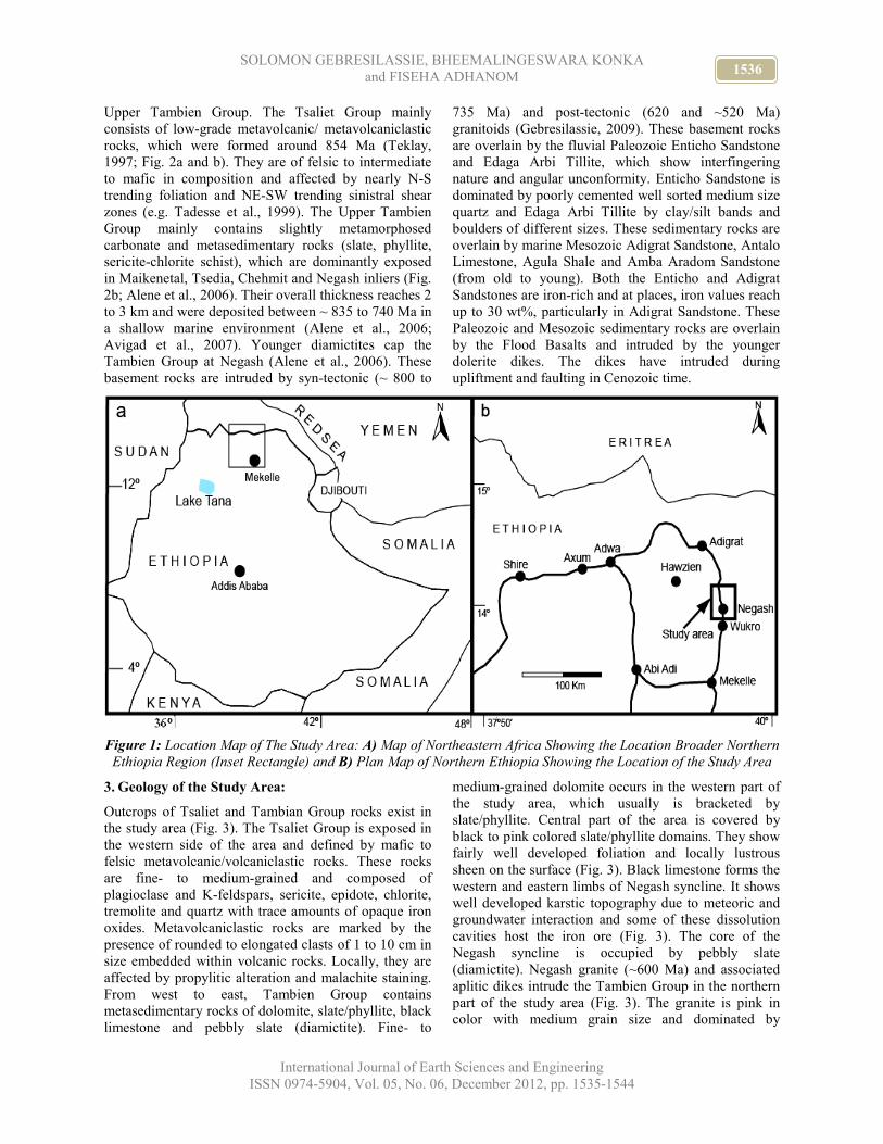
1536 SOLOMON GEBRESILASSIE, BHEEMALINGESWARA KONKA
and FISEHA ADHANOM
International Journal of Earth Sciences and Engineering
ISSN 0974-5904, Vol. 05, No. 06, December 2012, pp. 1535-1544
Upper Tambien Group. The Tsaliet Group mainly
consists of low-grade metavolcanic/ metavolcaniclastic
rocks, which were formed around 854 Ma (Teklay,
1997; Fig. 2a and b). They are of felsic to intermediate
to mafic in composition and affected by nearly N-S
trending foliation and NE-SW trending sinistral shear
zones (e.g. Tadesse et al., 1999). The Upper Tambien
Group mainly contains slightly metamorphosed
carbonate and metasedimentary rocks (slate, phyllite,
sericite-chlorite schist), which are dominantly exposed
in Maikenetal, Tsedia, Chehmit and Negash inliers (Fig.
2b; Alene et al., 2006). Their overall thickness reaches 2
to 3 km and were deposited between ~ 835 to 740 Ma in
a shallow marine environment (Alene et al., 2006;
Avigad et al., 2007). Younger diamictites cap the
Tambien Group at Negash (Alene et al., 2006). These
basement rocks are intruded by syn-tectonic (~ 800 to
735 Ma) and post-tectonic (620 and ~520 Ma)
granitoids (Gebresilassie, 2009). These basement rocks
are overlain by the fluvial Paleozoic Enticho Sandstone
and Edaga Arbi Tillite, which show interfingering
nature and angular unconformity. Enticho Sandstone is
dominated by poorly cemented well sorted medium size
quartz and Edaga Arbi Tillite by clay/silt bands and
boulders of different sizes. These sedimentary rocks are
overlain by marine Mesozoic Adigrat Sandstone, Antalo
Limestone, Agula Shale and Amba Aradom Sandstone
(from old to young). Both the Enticho and Adigrat
Sandstones are iron-rich and at places, iron values reach
up to 30 wt%, particularly in Adigrat Sandstone. These
Paleozoic and Mesozoic sedimentary rocks are overlain
by the Flood Basalts and intruded by the younger
dolerite dikes. The dikes have intruded during
upliftment and faulting in Cenozoic time.
Figure 1: Location Map of The Study Area: A) Map of Northeastern Africa Showing the Location Broader Northern
Ethiopia Region (Inset Rectangle) and B) Plan Map of Northern Ethiopia Showing the Location of the Study Area
3. Geology of the Study Area:
Outcrops of Tsaliet and Tambian Group rocks exist in
the study area (Fig. 3). The Tsaliet Group is exposed in
the western side of the area and defined by mafic to
felsic metavolcanic/volcaniclastic rocks. These rocks
are fine- to medium-grained and composed of
plagioclase and K-feldspars, sericite, epidote, chlorite,
tremolite and quartz with trace amounts of opaque iron
oxides. Metavolcaniclastic rocks are marked by the
presence of rounded to elongated clasts of 1 to 10 cm in
size embedded within volcanic rocks. Locally, they are
affected by propylitic alteration and malachite staining.
From west to east, Tambien Group contains
metasedimentary rocks of dolomite, slate/phyllite, black
limestone and pebbly slate (diamictite). Fine- to
medium-grained dolomite occurs in the western part of
the study area, which usually is bracketed by
slate/phyllite. Central part of the area is covered by
black to pink colored slate/phyllite domains. They show
fairly well developed foliation and locally lustrous
sheen on the surface (Fig. 3). Black limestone forms the
western and eastern limbs of Negash syncline. It shows
well developed karstic topography due to meteoric and
groundwater interaction and some of these dissolution
cavities host the iron ore (Fig. 3). The core of the
Negash syncline is occupied by pebbly slate
(diamictite). Negash granite (~600 Ma) and associated
aplitic dikes intrude the Tambien Group in the northern
part of the study area (Fig. 3). The granite is pink in
color with medium grain size and dominated by

1537 Geology and Characteristics of Metalimestone-Hosted Iron Deposit near
Negash, Tigray and Northern Ethiopia
International Journal of Earth Sciences and Engineering
ISSN 0974-5904, Vol. 05, No. 06, December 2012, pp. 1535-1544
orthoclase feldspar, quartz, plagioclase feldspar, biotite
and sericite, in the decreasing order. Remnants of
Paleozoic Enticho sandstone and Adaga Arbi Tillte
locally overlie these basement rocks. The younger
dolorite dykes of Cenozoic age that intruded these rocks
are particularly seen in the metalimestone rock (Fiseha,
2012).
Figure 2: A) Regional Geological Map of Northern Ethiopia Showing the Exposure of Tsaliet and Tambien Group
Rocks and B) Enlarged Regional Geological Map of The Area Around Negash where the Mukuat Iron Deposit is
Located. Circles with Number Shows Distribution of the Granitoid in the Region which Intruded the Basement
Rocks (After Gebresilassie, 2009 and References Therein)
4. Geological Structures:
The whole sequence is affected by different phases of
deformations. The first phase of deformation (D1) has
resulted in the development of foliation (particularly in
phyllites), which is pervasive and trending N-S to
N40°E. The second phase of deformation (D2) is
resulted in the development of a prominent synclinal
structure, known as Negash syncline with a fold axis
trending nearly N-S and forming 1 km wide core .
Grade of metamorphism being low it is well reflected
only in the metasedimentary rocks in the form of
foliation and slaty cleavage compared to mildly affected
black limestone and dolomite. Normal and dextral strike
slip faults and younger geological structures related to
E-W trending Wukro fault (not in the map) (related to
D3) are also present, displacing the metavolcanic and
metasedimentary rocks as well as the Paleozoic and
Mesozoic sedimentary sequences (Fig. 3) (Fiseha,
2012).
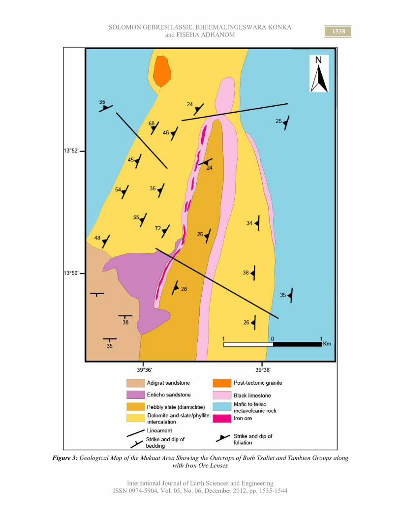
1538 SOLOMON GEBRESILASSIE, BHEEMALINGESWARA KONKA
and FISEHA ADHANOM
International Journal of Earth Sciences and Engineering
ISSN 0974-5904, Vol. 05, No. 06, December 2012, pp. 1535-1544
Figure 3: Geological Map of the Mukuat Area Showing the Outcrops of Both Tsaliet and Tambien Groups along
with Iron Ore Lenses
1539 Geology and Characteristics of Metalimestone-Hosted Iron Deposit near
Negash, Tigray and Northern Ethiopia
International Journal of Earth Sciences and Engineering
ISSN 0974-5904, Vol. 05, No. 06, December 2012, pp. 1535-1544
5. Methodology:
Out of 8 samples selected for analysis, seven were
collected from mineralized zone and one from
weathered dolerite dike. All the rock samples were
analyzed powdered using jaw crusher and pulverizer at
Ezana Laboratory, Mekelle. The fine rock powders
about 100gm each were given for geochemical analysis
(major oxides) using XRF (PANAlytical, 2424). The
analysis was carried out at the laboratory of Mossobo
Building Materials Production Plc, Mekelle, using the
standard references. The precision of the results was
within the acceptable limits. The results are shown in
table 1. In addition to geochemical analysis, the
mineralized samples were cut and polished. The
polished sections were studied for ore petrography using
reflected light microscope at Petrography laboratory,
Department of Earth Science, Mekelle University,
Mekelle.
6. Iron Mineralization and Paragenesis:
Iron mineralization at Mukuat (Negash) is present
within the black limestone filling fractures and the
cavities developed by karstification and confined to the
western limb of Negash syncline (Fig. 4a-d). It displays
dark brown, reddish brown and yellowish brown colors.
The iron ore occurs as pockets especially at the contact
within the metalimestone wall rock and at places
parallel to and/or perpendicular to the bedding of the
weakly metamorphosed black limestone (Fig. 4a). A
pocket of an iron mineralized zone is about 20-40 m
deep and 50-75 m thick and extends a kilometer along
strike (Fig. 4d). At the contact between the black
limestone and slate/phyllite, the fractures developed in
the former are filled by iron-rich lateritic material and
clay (Fig. 4b) possibly mobilized from the overlying
Enticho Sandstone (Fig 3). This indicates that the iron
ore is remobilized from previously laterized overlying
Enticho Sandstone. The karst features, fractures,
bedding planes and dikes seem to have served as
channels, sites or conduits for the mobilization and
accumulation of iron ore. Ore microscopic study of the
polished sections from the iron deposit indicates
presence of hematite, goethite and limonite in different
proportions. They, together with trace amounts of pyrite
(Fig. 5a-f) within the matrix of quartz and clay form the
gangue. Hematite, the dominant ore mineral, that
varies from colloidal to fine and medium grain size is
present as aggregates, nodules, sub-rounded, irregular
grains etc. Hematite is not the primary mineral. It has
developed by replacing goethite. It has developed in the
interstices within the groundmass of goethite (Fig. 5a
and b), as collofom bands with goethite (Fig. 5c) and as
replacement to and/or discontinuous veinlets cutting
goethite (Fig.5e). Goethite is another abundant mineral,
which occurs in the form of lensoidal bodies (Fig. 5a)
and veinlets cutting the earlier formed hematite and
goethite grains (Fig. 5d). Traces of pyrite also occur
within the groundmass of iron minerals (Fig. 5f).
Limonite, though common could not be well
differentiated in the ore microscopic studies. It is
inferred to occur as dark grey grains where some of
them are showing replacement to goethite (Fig. 5a).
Pyrite is euhedral to subhedral in shape and does not
show alteration (Fig. 5f). The paragentic sequence of
Mukuat iron deposit is shown in figure 6. The
replacement of goethite by hematite and continuous
growth of the latter along grain boundaries of the former
suggest that goethite is the source for hematite.
Limonite is expected to have formed first from iron
oxide and hydroxide cement. It is the source for
goethite. So, it is a gradual process that has produced
these three minerals in suitable conditions. It has
resulted in the development of the iron minerals in
different phases. Occurrence of hematite as
discontinuous veinlets cutting across hematite and
goethite and forming alternate banding with goethite
suggests different phases/ generation of hematite and
goethite. The fact that goethite veinlets cut the earlier
generation hematite, limonite and goethite indicates that
goethite II formed after hematite I. The euhedral to
subhedral shape and absence of deformation in pyrite
shows that it is the youngest sulfide formed within the
groundmass of iron oxides and hydroxides.
7. Geochemistry:
Major oxide values for Fe2O3 vary from 38 to 55 wt%,
Al2O3 from 1 to 4%, SiO2 from 21 to 33% and CaO
from 13 to 27%. Others are present in trace amounts.
Highest values of Fe2O3 are reported from the center of
the mineralized zone, where the iron ore is filling the
cavities and fractures within the black limestone. Iron
mineralization does not indicate any alteration, similar
to one of the dolerite samples (N-07). It is not affected
by any alteration as indicated by its major oxide values
(Fiseha, 2012) and are similar to those of unaltered
basalts (Wilson, 1989) (Table 1).

1540 SOLOMON GEBRESILASSIE, BHEEMALINGESWARA KONKA
and FISEHA ADHANOM
International Journal of Earth Sciences and Engineering
ISSN 0974-5904, Vol. 05, No. 06, December 2012, pp. 1535-1544
Figure 4: Plates Showing the Mode of Occurrence of Mukuat Iron Deposit at an Outcrop Level; a) Iron Ore
Occurring Parallel to the Bedding of Black Limestone, b) Iron Ore Interfingered with Enticho Sandstone, C) Some
of The Karsts Filled By Clay and Iron Ore and d) an Overview of Lensoidal Pocket of Iron Ore, Which is Structure
Controlled.
Table 1: Major Oxide Values (Wt%) of Iron Ore taken from Filled Cavities and Fractures within the Black
Limestone and Enticho Sandstone and Dolerite

1541 Geology and Characteristics of Metalimestone-Hosted Iron Deposit near
Negash, Tigray and Northern Ethiopia
International Journal of Earth Sciences and Engineering
ISSN 0974-5904, Vol. 05, No. 06, December 2012, pp. 1535-1544
Figure 5: Ore Microphotographs showing a) Hematite Grains Forming from Goethite Ground Mass, b) Continuous
Growth of Hematite along Goethite Grain Boundary and Interstices, c) Alternate Colloform Bands of Hematite and
Goethite, d) Younger Goethite Veinlets Cutting earlier developed Hematite and Goethite Grains, e) Hematite
Overgrowths Over Goethite and f) Pyrite Grain in Hematite and Goethite Groundmass [Note: ht = Hematite,
gt = Goethite, and py = Pyrite].
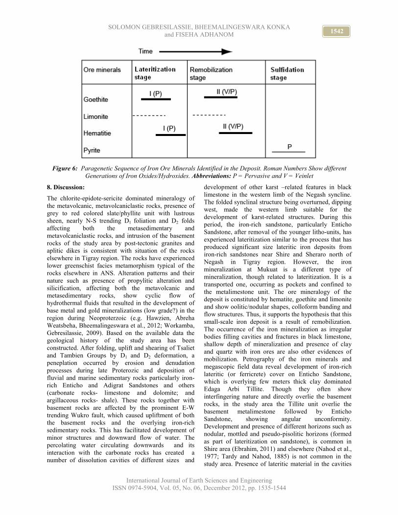
1542 SOLOMON GEBRESILASSIE, BHEEMALINGESWARA KONKA
and FISEHA ADHANOM
International Journal of Earth Sciences and Engineering
ISSN 0974-5904, Vol. 05, No. 06, December 2012, pp. 1535-1544
Figure 6: Paragenetic Sequence of Iron Ore Minerals Identified in the Deposit. Roman Numbers Show different
Generations of Iron Oxides/Hydroxides. Abbreviations: P = Pervasive and V = Veinlet
8. Discussion:
The chlorite-epidote-sericite dominated mineralogy of
the metavolcanic, metavolcaniclastic rocks, presence of
grey to red colored slate/phyllite unit with lustrous
sheen, nearly N-S trending D1 foliation and D2 folds
affecting both the metasedimentary and
metavolcaniclastic rocks, and intrusion of the basement
rocks of the study area by post-tectonic granites and
aplitic dikes is consistent with situation of the rocks
elsewhere in Tigray region. The rocks have experienced
lower greenschist facies metamorphism typical of the
rocks elsewhere in ANS. Alteration patterns and their
nature such as presence of propylitic alteration and
silicification, affecting both the metavolcanic and
metasedimentary rocks, show cyclic flow of
hydrothermal fluids that resulted in the development of
base metal and gold mineralizations (low grade?) in the
region during Neoproterzoic (e.g. Hawzien, Abreha
Weatsbeha, Bheemalingeswara et al., 2012; Workamba,
Gebresilassie, 2009). Based on the available data the
geological history of the study area has been
constructed. After folding, uplift and shearing of Tsaliet
and Tambien Groups by D1 and D2 deformation, a
peneplation occurred by erosion and denudation
processes during late Proterozic and deposition of
fluvial and marine sedimentary rocks particularly iron-
rich Enticho and Adigrat Sandstones and others
(carbonate rocks- limestone and dolomite; and
argillaceous rocks- shale). These rocks together with
basement rocks are affected by the prominent E-W
trending Wukro fault, which caused upliftment of both
the basement rocks and the overlying iron-rich
sedimentary rocks. This has facilitated development of
minor structures and downward flow of water. The
percolating water circulating downwards and its
interaction with the carbonate rocks has created a
number of dissolution cavities of different sizes and
development of other karst –related features in black
limestone in the western limb of the Negash syncline.
The folded synclinal structure being overturned, dipping
west, made the western limb suitable for the
development of karst-related structures. During this
period, the iron-rich sandstone, particularly Enticho
Sandstone, after removal of the younger litho-units, has
experienced lateritization similar to the process that has
produced significant size lateritic iron deposits from
iron-rich sandstones near Shire and Sheraro north of
Negash in Tigray region. However, the iron
mineralization at Mukuat is a different type of
mineralization, though related to lateritization. It is a
transported one, occurring as pockets and confined to
the metalimestone unit. The ore mineralogy of the
deposit is constituted by hematite, goethite and limonite
and show oolitic/nodular shapes, colloform banding and
flow structures. Thus, it supports the hypothesis that this
small-scale iron deposit is a result of remobilization.
The occurrence of the iron mineralization as irregular
bodies filling cavities and fractures in black limestone,
shallow depth of mineralization and presence of clay
and quartz with iron ores are also other evidences of
mobilization. Petrography of the iron minerals and
megascopic field data reveal development of iron-rich
lateritic (or ferricrete) cover on Enticho Sandstone,
which is overlying few meters thick clay dominated
Edaga Arbi Tillite. Though they often show
interfingering nature and directly overlie the basement
rocks, in the study area the Tillite unit overlie the
basement metalimestone followed by Enticho
Sandstone, showing angular unconformity.
Development and presence of different horizons such as
nodular, mottled and pseudo-pisolitic horizons (formed
as part of lateritization on sandstone), is common in
Shire area (Ebrahim, 2011) and elsewhere (Nahod et al.,
1977; Tardy and Nahod, 1885) is not common in the
study area. Presence of lateritic material in the cavities

1543 Geology and Characteristics of Metalimestone-Hosted Iron Deposit near
Negash, Tigray and Northern Ethiopia
International Journal of Earth Sciences and Engineering
ISSN 0974-5904, Vol. 05, No. 06, December 2012, pp. 1535-1544
in metalimestone and absence of lateritic cover on the
surface of sandstone amply indicate its removal and
mobilization. Apart from the nature of rock, the factors
like pH and Eh which are themselves controlled by the
climate, vegetation and the morphology of the landscape
play an important role in defining the mobility of iron,
aluminum, silica etc. At the same time, the area has
experienced climatic condition (18.3-30oC and up to
300cm rainfall) suitable for the development of laterite
(Ebrahim, 2011). Presence of hematite, goethite,
limonite and ochre in the deposit suggests their presence
in the source lateritic cover. Hematite is fresh and does
not show any signs of alteration. It is formed by
replacing goethite. Petrographic study amply suggests
conversion of goethite to hematite but hematite does not
show any alteration to goethite as expected in an
oxidizing weathering condition. Such conditions are
common in arid conditions and the reason for such
development seems to be due to: a) transformation of
iron cement (iron hydroxide) to ferrihydrites (Combes et
al., 1990; Ramanaidu et al., 1996) similar to limonite
(crysptocrystalline) structure; b) limonite to metastable
goethite; c) the metastable goethite in the presence of
water into hematite during long burial digenesis of
sediments of Tertiary to Paleozoic in age (Tardy and
Nahod, 1985); this is noticed by not well developed
goethite in the polished sections; d) goethite does not
replace hematite because the temperature is relatively
high and does not favor hydration of hematite to
goethite in the lateritic profile particularly that occurs at
the top of the profile; e) the relative stability of goethite
and hematite depends on many factors such as grain size
effect. If the crystal of hematite is greater or equal to the
grain size of the crystal of goethite, hematite is stable
than goethite in water but in the reverse situation
goethite is stable. But in the case of concretion and
development of nodules in iron crust (ferricrete), both
minerals do not form into large crystals and appear as
very tiny particles (Tardy and Nahod, 1985). So, the
governing conditions for stability of these minerals are
mainly dehydration and water activity compared to the
less effective particle size; f) kinetics of precipitation, if
the iron is released from silicates and from other
primary source in water then it will form into goethite;
if the solubility product of goethite is excess than that of
ferrihydrite. So, the factor that favors ferrihydrite
formation will also favor the formation of hematite by
high temperature resultant dehydration. The factors
controlling the formation of ferrihydrite in solution
include rapid release of Fe, and low concentration of
organic compound (allowing concentration of inorganic
Fe3+). So, in ferruginous sandstone the iron release is
very high, as the large pore size of the quartz (in which
the iron serve as matrix) favors high activity of water
and release of iron. This may be one of the reasons for
the stability of hematite over goethite during
lateritization; and g) equilibrium condition involving
water activity, pore size and nodule formation. The
relative abundance of the major oxides especially SiO2,
Fe2O3, Al2O3 indicates increase of Fe2O3 (55 wt%)
compared to SiO2 (21 wt%) and Al2O3 (1.44 wt%) in
lateritic iron deposit. This clearly indicates
desilicification and removal of Al, though SiO2 removal
is relatively more. The suitable Eh and pH conditions
thus favoured residual concentration of Fe2O3.
Weathering and erosion of a laterite developed on top of
Enticho Sandstone is a continuous phenomenon.
Weathering and erosion resultant remobilization has
resulted in hematite filling the cavities in black
limestone. The concentration of iron ore in the fractures,
bedding and flanks of dolerite dikes suggest that these
structures served as conduits for the laterite migration
during remobilization. Generally, common in all
laterites, repetition of wet and dry seasons lead to
lateritization of the Enticho Sandstone. Leached iron
and other cations during the wet season are brought to
the surface by capillary action during the dry season.
The process of intrusion has no direct relation with the
iron deposit. It only has facilitated development of
fractures in the black limestone by upliftment and
helped in the formation of cavities by percolating rain
water. These cavities, inturn, have become sites for
accumulation of lateritic material. Based on the
stratigraphic and textural relationships, age of the
Mukuat (Negash) iron deposit is inferred to be much
younger compared to Enticho Sandstone, which formed
during Lower Ordovician (Garland, 1980).
Lateritization process was initiated during the exposure
of Enticho Sandstone after its uplift due to Wukro Fault.
Development of laterite and its mobilization to the site
of accumulation continued for considerable period
subsequent to dolerite dyke intrusion during Eocene and
later (Fiseha, 2012).
9. Conclusion:
Genetic mechanism associated with Mukuat iron ore
deposits is unique for arid tracts. Even though the
deposit is small in size and quantity, has brought into
light a series of processes responsible for metalimestone
cavities acting as hosting locales for lateritic iron
accumulation. Weathering and erosion of laterite and
resultant mobilization has led to iron ore minerals filling
the discontinuous cavities in metalimestone. Repetition
of wet and dry seasons facilitated mobilization of
leached iron through capillary action on to the surface
and its enrichment. One can use this input to explore
vast stretches of arid and semi arid tracts to locate such
isolated ore deposits elsewhere in similar terrains.
10. Acknowledgement:
We acknowledge Ezana Mining Plc and Messobo
construction materials Plc for providing necessary help

1544 SOLOMON GEBRESILASSIE, BHEEMALINGESWARA KONKA
and FISEHA ADHANOM
International Journal of Earth Sciences and Engineering
ISSN 0974-5904, Vol. 05, No. 06, December 2012, pp. 1535-1544
during field work and sharing drill and chemical data.
Thanks are due to the reviewers Dr. Parvata Reddy
Ramachandra Reddy, Scientist, NGRI, Hyderabad,
India and Prof. Solomon Tadesse, Addis Ababa
University, Addis Ababa, Ethiopia for providing critical
comments and improving the quality of the paper.
9. References:
[1] Alene, M., Jenkin, G. R.T., Leng, M. J and
Darbyshire, F.D.P. 2006. The Tambien Group,
Ethiopia: An early Cryogenian (ca. 800-735 Ma)
Neoproterozoic sequence in the Arabian-Nubian
Schield. Precambrian Research, 147: 79-99.
[2] Avigad, D., Stern, R.J., Beyth, M., Miller, N and
Mc Williams, M.O. 2007. Detrital zircon U-Pb
geochronology of Cryogenian diamictites and
Lower Paleozoic sandstone in Ethiopia (Tigrai):
Age constraints on Neoproterozoic glaciation and
crustal evolution of the southern Arabian-Nubian
Shield. Precambrian Research, V.154, 88-106.
[3] Bheemalingeswara Konka., Solomon Gebresilassie
and Kassa Amare. 2012. Shear zone controlled base
metal mineralization around Abraha Weatsebaha -
Adidesta and Hawzein, Tigray region, northern
Ethiopia, Momena Journal of Ethiopian Sciences,
V.4(1), 3-28.
[4] Beyth, M. 1972. The Geology of Central-Western
Tigre. Ph.D. Thesis, Rheinische Friedrich-Wilhems
Universität, Bonn, Germany, 159p.
[5] Combes, J.M., Manceau, A and Calas, G. 1990.
Formation of ferric oxides from aqueous solutions:
a polyhedral approach by x-ray spectroscopy; II.
Hematite formation from ferric gels. Geochem
Cosmoch Acta, V.54, 1083-1091.
[6] Ebrahim, N.H. 2011. Geology and geochemistry of
lateritic iron deposit in Mydmu area near Shire
Indessilassie, western Tigray, Ethiopia. M.Sc
thesis, Mekelle Univ., Mekelle, Ethiopia, 136p.
[7] Ezana Mining Development plc. 2011. Mukuat Iron
mining near Negash (per. comm).
[8] Fiseha Adhanom. 2012. Geology and iron
mineralization in Mukuat, Wukro area, eastern
Tigray, northern Ethiopia, M.Sc Thesis, Mekelle
Univ., Mekelle, Ethiopia. 100p.
[9] Garland, C.R. 1980. Geology of the Adigrat area,
Memor No. 1. Ministry of Mines and Energy,
Addis Ababa, 51p.
[10] Gebresilassie, S. 2009. Nature and Characteristics
of Metasedimentary rock Hosted Gold and Base
metal Mineralization in the Workamba area,
Central Tigray, Northern Ethiopia, Ludwig-
Maximilans Univ., Munich, Germany, Ph.D.
Thesis, 134p.
[11] Johnson, P.R and Woldehaimanot, B. 2003.
Development of the Arabian-Nubian Shield:
perspectives on accretion and deformation in the
northern East African Orogen and the assembly of
Gondwana. In: M. Yoshida, B.F. Windley and S.
Dasgupta (eds.), Proterozoic East Gondwana:
Supercontinent Assembly and breakup. Geological
Society of London, Special Publication, V.206,
289-325.
[12] Nahod, D., Janot, C., Karpoff, A.M., Paquet, H and
Tardy, Y. 1977. Mineralogy, petrography and
structures of iron crusts developed on sandstones in
the western part of Senegal. Geoderma, V.19, 263-
277.
[13] Ramanaidu, E., Nahon, D., Decarreau, A and Melfi,
A.J. 1996. Hematite and goethite from durycrusts
developed by lateritic chemical weathering of
Precambrian Banded Iron Formations, Minas
Gerais, Brazil,Claysandclayminerals,V. 44(1),22-31
[14] Tadesse, T., Hoshino, M and Sawada, Y. 1999.
Geochemistry of low grade metavolcanic rocks
from the Pan African of the Axum area, northern
Ethiopia, Precambrian Research, V.99, 101-124.
[15] Tadesse, S., Milesi, J.P and Deschamps, Y. 2003.
Geology and mineral potential of Ethiopia: a note
on Geology and mineral map of Ethiopia. J. African
Earth Sciences, V.36, 273-313.
[16] Tardy, Y and Nahod, D. 1885. Geochemistry of
laterites, stability, Al-goethite, Al-hematite and Fe3+
kaolinite in bauxites and ferricretes, American
Journal of Science, V.285, 865-903.
[17] Teklay, M. 1997. Petrology, Geochemistry, and
Geochronology of Neoproterzoic Magmatic Arc
Rocks from Eritrea: Implications for Crustal
Evolution in the southern Nubian Shield. Eritrea
Department of Mines, Memoir 1, 125p.
[18] Wilson, M. 1989. Igneous petrogenesis: a global
tectonic approach. Unwin Hyman, London, 466p.
[19] Bheemalingeswara, K. 2012. Geological and
geochemical study of lateritic iron deposit near
Mentebteb, Shiraro, Northern Tigray, Ethiopia.
Project Report, CNCS, Mekelle University,
Ethiopia, 30p(unpubl.).
[20] Bheemalingeswara, K and Atakilt Araya, 2012.
Rahwa auriferous gossan, northern Ethiopia: A
strong indicatorfor subsurface massive sulfide
mineralization. International Journal of Earth
Sciences and Engineering, 5(3): 402-408.
[21] Ottemann, J and Augustithis, S.S. 1967.
Geochemistry and origin of “platinum-nuggets” in
lateritic covers from ultrabasic rocks and birbirites
of W. Ethiopia. Mineralium Deposita, 1(4): 269-
277.

www.cafetinnova.org
Indexed in
Scopus Compendex and Geobase Elsevier, Chemical
Abstract Services-USA, Geo-Ref Information Services-USA
ISSN 0974-5904, Volume 05, No. 06
December2012, P.P.1545-1551
#02050610 Copyright ©2012 CAFET-INNOVA TECHNICAL SOCIETY. All rights reserved.
Ore Fluids Associated With the Metasediment Hosted Central
Auriferous Zone of Gadag Gold Field, Karnataka
M. A. MALAPUR1, S. MANJUNATHA
2, B. CHANDAN KUMAR
1 and A. G. UGARKAR
1
1Department of Studies in Geology, Karnatak University, Dharwad 580 003 2Department of Geology, Karnatak Science College, Dharwad 580 001
Email: [email protected]
Abstract: In Gadag gold field, three almost parallel and tabular auriferous zones, namely western, central and
eastern auriferous zones, each with a distinct lithological assemblage, occur within a sequence of metavolcanics and
a thick pile of metasediments. The western auriferous zone is hosted by mafic to felsic metavolcanics, the central
zone is hosted mainly by greywackes, just above the boundary with the metabasalt and the eastern zone is hosted by
arenite-argillites and chlorite phyllites. In this paper, the nature and composition of hydrothermal ore fluids
associated with the sediment hosted central auriferous zone are presented based on the fluid inclusion micro-
thermometry. In this zone, gold mineralization is structurally controlled epigenetic vein type, and is invariably
associated with wall rock alterations. In addition to gold, ore minerals that occur are arsenopyrite, pyrite, pyrrhotite,
chalcopyrite, sphalerite, galena and scheelite. The gangue minerals are quartz, chlorite, plagioclase, sericite,
carbonates and carbonaceous matter. Three types of fluid inclusions, namely CO2-rich inclusions, H2O inclusions
and CO2-H2O inclusions are recorded in the auriferous quartz veins of central auriferous zone. Due to tiny size
constraints, micro-thermometric determinations are made only on CO2-H2O inclusions. The hydrothermal fluids that
caused gold deposition in these zones were of low salinity (2.0 to 6.6 wt% NaCl equivalent), dominated by CO2-
H2O (about 30 mole % CO2 ) with moderate densities (0.7 to 1.04 g/cc) at a maximum depth 1.3 km, and gold
deposition occurred over a wide temperature range of 175 to 325oC. Similar to Archaean greenstone hosted vein
type lode gold deposits elsewhere, large volumes of low-salinity CO2-H2O and CO2-rich fluids were probably
produced by metamorphic devolatilization during prograde regional metamorphism at greenschist-amphibolite
facies boundary in Gadag Gold field. During retrograde greenschist facies metamorphism, interaction of gold
bearing H2O-CO2-NaCl fluids with the wall rocks at decreasing PT conditions (in the shear zone vicinity) might
have lead to fluid immiscibility and separated H2O–rich and CO2-rich phases, there by significantly changing the
gold solubility and causing its precipitation. The ore fluids of sediment hosted auriferous zone are comparable with
the volcanic hosted western auriferous zone.
Keywords: Gold, Ore fluids, Fluid inclusions, Gadag Gold Field, Karnataka
I. Introduction:
Significant contribution for world gold production has
been from mesohydrothermal vein type lode gold
deposits of Archaean granite greenstone terrains. Thus
such type of gold mineralization represents an important
genetic class. An understanding of their nature and
genesis is not only fundamentally important from an
academic viewpoint, but can help to formulate
exploration strategies and better define potential areas
of mineralization. Obviously, studies of fluid inclusions
in veins deposited during the mineralizing event have
proved to be inevitable to understand the nature and
source of the ore fluid, components and genetic aspects.
Although, there are several gold deposits/occurrences
distributed in the well-known granite-greenstone terrain
of Dharwar Craton, the fluid inclusion data comes from
very few gold deposits like, Kolar (Santosh, 1986;
Mishra and Panigrahi, 1999; Solankar et al., 2006),
Hutti (Pal and Mishra, 2002), Gadag (Ugarkar et al.,
2000) and Kuchiganahalu of Chitradurga (Mukherjhee
et al., 2001). Further, as far as the data on the fluid
inclusions of gold bearing vein quartz in Gadag Gold
Field is concerned, it is restricted to the auriferous zones
hosted within the metavolcanics (Ugarkar et al., 2000).
In this paper, the nature and composition of
hydrothermal ore fluids associated with the
metasediment hosted central auriferous zone is
presented based on the fluid inclusion
microthermometry.
II. Geological Setting:
Gadag greenstone belt, a northern continuation of the
well known Chitradurga belt (Dharwar Type) of middle
to late Archaean age (2600-2400 Ma, Swaminath and
Ramakrishnan, 1981) of Karnataka, is well known for

1546 M. A. MALAPUR, S. MANJUNATHA, B. CHANDAN KUMAR and A. G. UGARKAR
International Journal of Earth Sciences and Engineering
ISSN 0974-5904, Vol. 05, No. 06, December 2012, pp. 1545-1551
gold mineralization. The detailed geology and map of
Gadag gold field (Fig.1) are given by Narayanaswamy
and Ahmed (1963) and Ugarkar and Deshpande (1999).
The gold mineralization in Gadag gold field is
distributed in three main auriferous zones where group
of gold bearing lode-quartz veins are found in clusters.
These auriferous zones are namely Western, Central and
Eastern auriferous zones that run in a linear pattern
almost sub-parallel to regional foliation (i.e. NNW-
SSE). The various litho units of Gadag gold field
include metavolcanics (metabasalt to felsic volcanics)
and metasediments (conglomerate, greywacke, argillite,
arenite, arkoses, phyllite, banded iron formation and
limestone/dolomite). The entire sequence starting from
metavolcanics in the west and metasediments towards
east is well exposed on the western limb of the main
synclinal structure.
Although the central auriferous zone occurs in the
contact between metavolcanics and metasediments,
majority of the lodes of this auriferous zone are hosted
by greywacke-argillite suite of rocks, extending from
Beladhadi to NE of Kadkol passing through Nabhapur,
Kabuliyatkatti, Attikatti, Mysore mine and Sangli mine.
Figure 1: Geological Map of the Gadag Gold Field Showing the Western, Central and Eastern Auriferous Zones
(after Ugarkar et al., 2000)
Eastern auriferous zone, which lies to the southwest of
Singatrayankeri Tanda and east of Dindur Tanda, is
entirely hosted within metasedimentary rocks. This zone
occurs within greywacke-argillite assemblage.
The primary layering (bedding) in the sulphidic chert,
greywacke-argillite suite, chlorite phyllite and the
intercalated BIF bands dips towards east at angles
varying from 200 to 55
0. The schistosity dips at higher
angles ~700, most commonly towards northeast. The
trend of bedding varies from N200W to N40
0W and that
of schistosity N-S to N150W. The entire sequence is
younging towards northeast as indicated by way up
criteria like vesicular and convex surface in pillowed
metabasalt, graded bedding in greywacke. Therefore,
the volcanic unit found in the western side is considered
to be older. A thin band of thinly layered chert bed
occurs interbedded with chlorite-sericite phyllite
overlying the eroded surface of the volcanic substratum.
This chert bed acts as a marker horizon while mapping.
In the greywacke-argillite suite numerous interbedded
sequences of greywacke and argillite occur alternately.
The competent beds of greywacke and the incompetent
argillite have moved past each other due to the shearing
contemporaneous with the thrusting along the NNW-
SSE directions. These planes being low tension gashes
(areas) might have acted as channels for the upcoming
mineralizing hydrothermal solutions.

1547 Ore Fluids Associated With the Metasediment Hosted Central
Auriferous Zone of Gadag Gold Field, Karnataka
International Journal of Earth Sciences and Engineering
ISSN 0974-5904, Vol. 05, No. 06, December 2012, pp. 1545-1551
III. Central Auriferous Zone:
The central auriferous zone of Gadag gold field is
hosted by shear zones within greywacke-argillite and
carbonaceous phyllites and located closer to the contact
between metavolcanics and metasediments. The
auriferous zone in the area of investigation is
characterized by hydrothermal wall-rock alterations
represented by chloritisation, sericitization,
carbonatisation, carbonate spottings, quartz mylonites
and iron sulphide porphyroblasts as disseminations and
stringers. Another important character is ubiquitous
presence of carbonaceous matter with mineralized zone
especially in central auriferous zone. In general, the
rock type of central auriferous zone of Gadag gold field
can be classified based on the mineral assemblages,
texture and physical properties in hand specimen, the
crudely schistose and banded mesocratic rock. These
rocks are strongly deformed, altered, chloritised,
carbonated and silicified. At places, the carbonaceous
matter contains euhedral pyrite grains as well as veins
of pyrite. Carbonaceous matter also occurs as thin layers
along schistosity planes. Shear zones/fractures, contacts
between different litho units with competency contrast,
schistosity planes are better places for hosting the gold
bearing milky white quartz veins and lenses. About 15
cm to 1.50 m thick quartz veins with encrustations of
rusty brown ankerite patches and inclusions of
chloritised host rock are often observed to occur along
the shear zones especially between competent
greywacke and incompetent phyllite beds. This quartz
contain fine to medium grained sulphides as
disseminations which often may be invisible to naked
eyes. Quartz is medium to fine grained and deformed
which in thin sections exhibits development of quartz-
mylonites with elongation and orientation of grains with
undulose extinction and highly sutured grain
boundaries. Sometimes, it exhibits cherty nature. Quartz
occurs as clots of crystals as well as grains with sutured
margins and exhibits wavy extinction. It also occurs as
irregular shaped branching veins. At places, quartz
veins are seen cutting across carbonate veins. Often,
quartz and carbonates occur as filling spaces between
fractured sulphides. Occasionally, minute discrete
grains of gold are seen within the vein quartz. These
features indicate that the shear zones hosting auriferous
zone are ductile type. The different ore minerals and
gangue minerals are gold, arsenopyrite, pyrite,
pyrrhotite, chalcopyrite, sphalerite, galena, scheelite,
quartz, chlorite, plagioclase, sericite, carbonates and
carbonaceous matter.
IV. Fluid Inclusions:
Twenty doubly polished sections of 0.3 to 0.5mm
thickness were prepared from quartz samples spatially
associated with gold mineralization from the gold-
quartz sulphide reefs hosted within the metagreywacke-
argillite suite of rocks in central auriferous zone. In
some of the sections, the inclusions were too small to be
studied for microthermometry. In fact, tiny sizes of
inclusions are a characteristic feature of inclusions in
mesothermal gold bearing quartz veins (see Wilkinson,
2001). Only eight sections with good number of
inclusions and suitable for study were finally chosen for
microthermometry. Microthermometric determinations
were carried out by using Linkam THMSG 600
heating/cooling stage in the Department of Geology,
Karnatak University, Dharwad.
In the microthermometry, the density of CO2 inclusions
was calculated from the P-T plots for CO2 in the low
temperature range as suggested by Angus et al. (1976).
In case of aqueous inclusions, the degree of fill is
determined by visual estimation with the help of
standard figures (Shepherd et al., 1985) and salinity
values were calculated from the T-X plots for the low
temperature part of the system NaCl–H2O given by
Potter et al. (1978). The density of aqueous inclusions
was calculated from standard figure compiled by
Ahmed and Rose (1980). The trapping depths were
calculated with the help of Haas (1971) NaCl boiling
curve diagram.
Three types of inclusion namely Type I, CO2-rich
inclusions, Type II, H2O inclusions and Type III, CO2-
H2O inclusions are observed. Microthermometric
determinations are made only on Type III, CO2-H2O
inclusions.
Type I, CO2-rich inclusions are less in population when
compared to CO2-H2O inclusions. They occurs either as
isolated inclusions, scattered within quartz or as arrayed
inclusions indicating their primary to secondary nature.
Type II, H2O inclusions are scattered in quartz grains.
Mostly they are of primary type. Type III, CO2-H2O
inclusions occur as isolated as well as arrayed within
quartz grains and vary in size from 10 - 20 µm. The
volume proportion of CO2 in these is about 30 percent.
Microthermometric determinations were carried out for
these CO2-H2O inclusions.
The results of microthermometric determinations of
H2O-CO2 fluid inclusions from auriferous quartz veins
hosted within metasediments in Central auriferous zone
of Gadag gold field are given in Table 1.

1548 M. A. MALAPUR, S. MANJUNATHA, B. CHANDAN KUMAR and A. G. UGARKAR
International Journal of Earth Sciences and Engineering
ISSN 0974-5904, Vol. 05, No. 06, December 2012, pp. 1545-1551
Figure 2: Frequency Histogram of Th-Co2 from Microthermometric Data of H2o-Co2 Inclusions in the
Ore Quartz Veins from Central Auriferous Zone of Gadag Gold Field
Figure 3: Frequency Histogram of Tmco2 from Microthermometric Data of H2o-Co2 Inclusions in the
Ore Quartz Veins from Central Auriferous Zone of Gadag Gold Field
Table 1: Microthermometric Data of H2o-Co2 Inclusions in Auriferous Quartz Veins from Central Auriferous Zone,
Gadag Gold Field
Sample
No.
Tm CO2 0C
Tm ice 0C
Th CO2 0C
Tht CO2+H2O 0 0C
Salinity
Wt. % NaCl
Density
gm/cc
G1 -56.60 -2 to -16 -42.60 293.00 2.0 to 4.2 0.88 to 0.91
G2 -56.80 -3 to -17 -42.70 325.00 2.0 to 6.6 1.02 to 1.04
G3 -56.70 -2 to -26 -51.60 185.00 2.1 to 3.8 0.72 to 0.74
G4 -56.70 -1 to -17 -55.20 to -57.10 175 to 185 3.1 to 5.2 0.70 to 0.74

1549 Ore Fluids Associated With the Metasediment Hosted Central
Auriferous Zone of Gadag Gold Field, Karnataka
International Journal of Earth Sciences and Engineering
ISSN 0974-5904, Vol. 05, No. 06, December 2012, pp. 1545-1551
Figure 4: Frequency Histogram of Calculated Thtco2 from Microthermometric Data of H2o-Co2 Inclusions in the
Ore Quartz Veins from Central Auriferous Zone of Gadag Gold Field
Figure 5: Plots of Salinity V/S Temperature of
Homogenization for H2o-Co2 Inclusions in the Ore
Quartz Veins from Central Auriferous Zone of Gadag
Gold Field
The temperature of homogenization (Th) of CO2 varies
from -42.6 to -57.10C. In Th histogram for CO2,
maximum Th values are recorded at -51.60, -42.60, -
42.70 and -57.100C (Fig. 2). The temperature of melting
(Tm) of CO2 varies from -56.60 to -56.80 0C with
maximum Tm values at -56.70 and -56.800C (Fig.3).
The temperature of melting of ice (Tm of ice) varies
from -2 to -260C.
The total temperature or final temperatures of
homogenization of CO2-H2O inclusions [(Tht)
CO2+H2O] range from 1750C to 325
0C. However,
maximum numbers of investigated inclusions are found
at 1850C. It is noteworthy to point out the pronounced
skewness of the frequency histogram is closer to the
homogenization temperatures at 1750C, 293
0C and
3250C (Fig. 4).
The salinity v/s homogenization temperature plot (Fig.
5) indicates an isothermal mixing trend for inclusions
homogenizing from 1750C to 185
0C. However, elevated
homogenization temperatures of some inclusions
between 2930C and 325
0C probably represent post-
entrapment changes (Mernagh and Wygralak, 2007).
Figure 6: NaCl Curve Diagram after Haas (1971), For
the H2o-Co2 Inclusions in the Ore Quartz Veins from
Central Auriferous Zone of Gadag Gold Field
The presence of halite crystals as inclusions in the ore
vein quartz indicates that the ore forming fluids were
saline. The calculated salinity of these inclusions is low
1550 M. A. MALAPUR, S. MANJUNATHA, B. CHANDAN KUMAR and A. G. UGARKAR
International Journal of Earth Sciences and Engineering
ISSN 0974-5904, Vol. 05, No. 06, December 2012, pp. 1545-1551
with 2.0 to 6.6 wt % of NaCl equivalent, while the
density varies from 0.7 to 1.04 g/cc. These inclusions
are mostly trapped at a maximum depth of 1.3 km
(Fig.6).
V. Discussion and Conclusion:
A review of data available on temperature, pressure and
composition of hydrothermal solution suggest that
deposition of gold and sulphide in the Archaean
mesothermal hydrothermal gold deposits in the granite-
greenstone terrain principally occur between 250 and
4000C, salinity being 2 to 6 wt % NaCl equivalent
(Brown and Lamb, 1986; Groves, 1993 and references
there in).
Phase separation in a H2O-CO2-CH4-NaCl fluid system
is a mechanism which cause gold deposition in a variety
of environments and fluid inclusion studies have
demonstrated the existence of low-saline, immiscible
H2O and CO2 rich fluids related to ore in a number of
gold deposits (Robert and Kelly, 1987; Guha et al.,
1991; Wilkinson and Johnston, 1996; Mishra and
Panigrahi, 1999; Barrie and Touret, 1999).
The microthermometric measurements of fluid
inclusions in gold-quartz veins of central auriferous
zone of Gadag field indicate that the auriferous
hydrothermal fluids were of low salinity (2.0 to 6.6 wt%
NaCl), dominated by CO2-H2O (about 30 mole % CO2)
with moderate densities (0.7 to 1.04 g/cc) at a maximum
depth of 1.3 kms. Gold deposition occurred over a wide
temperature range of 175 to 3250C.
Metamorphism of volcano-sedimentary host rocks at
greenschist–amphibolite facies boundary with chlorite-
calcite-quartz assemblage produces large volumes of
low-salinity CO2-H2O fluids, similar in composition to
those recorded in the Archaean greenstone hosted vein
type lode gold deposits in general (Groves, 1993;
Kerrich and Cassidy, 1994 and references there in).
Carbonatization is one of the prominent wall rock
alterations in the auriferous zone hosted in
metasediments in Gadag field. Gold-quartz vein type
mineralization here is consistent with a structurally
controlled (shear zone), hydrothermal epigenetic type
(Ugarkar and Deshpande, 1999). Further, it has been
suggested that there is a close relationship between gold
mineralization and retrograde greenschist facies
metamorphism (Ugarkar, 1998). Retrograde
metamorphism and corresponding mineral assemblages
can be maintained during metamorphism in presence of
CO2 dominance (Clark et al., 1986). Thus, CO2 seems to
be an almost universal constituent of the ore fluids
depositing gold and it forms a major constituent of most
of fluid inclusions in gold ores from the metamorphic
environment (Roedder, 1984). It has been suggested by
Hutchinson (1993) that in such environment gold might
have been carried as carbonyl or carbonate complex and
that the extraction of CO2 from the ore fluids by
reaction with divalent cations in the wall rock to form
carbonates, would result in the precipitation of gold
(Roedder, 1984) within suitable structural sites (shear
zones), through a combination of decreasing
temperature and fluid-wall rock interaction. Progressive
carbonization of wall-rocks with decreasing temperature
and pressure might lead to fluid immiscibility and
separate H2O-rich and CO2-rich phases. These physical
separations of two immiscible fluids significantly
change the solubility of gold and thus cause
precipitation (Sibson and Scot, 1998; Groves and
Foster, 1993) in the form of quartz veins.
Gold appears to have been precipitated in veins as a
result of fluid immiscibility at low to intermediate
temperature range of 175-3250C in the sediment hosted
central auriferous zone of Gadag field. The
hydrothermal fluids responsible for the gold
mineralization in the metavolcanic hosted western
auriferous zone of Gadag field were also of low salinity
(2 to 6 wt% NaCl), dominated by H2O-CO2 (20 to 40
mole % CO2) with moderate densities (0.8 to 1.0 g/cc)
at temperature range of 240-2500C (Ugarkar et al,
2000), which are comparable with the sediments hosted
central auriferous zone of present study, however, with
a wide temperature range of 175-3250C.
References:
[1] Ahmed, S.N. and Rose, A.W. (1980) Fluid
inclusions in porphyry and skarn ore at Santa Rita,
New Mixico: Econ. Geol., V.75, pp.229-250.
[2] Angus, S., Armstrong, B., DeReuck, K.M., Altunin,
V.V., Gadtskii, O.G., Chapela, G.A. and
Rowlinson, J.S. (1976) International
Thermodynamic Tables of the Fluid State, Vol.3,
Carbon Dioxide: Pergamon Press, Oxford,
England, p.385.
[3] Barrie, I. and Touret, J.L.R. (1999) Fluid inclusion
studies of gold bearing quartz veins from the
Yirisen deposit, Sula Mountains greenstone belt,
Masumbiri, Sierra Leone. Ore Geol. Rev. V.14,
pp.203-225.
[4] Brown, P.E. and Lamb, W.M. (1986) Mixing of
H2O and CO2 in fluid inclusions; geobarometry and
Archaean gold deposits. Geochem, Cosmochim.
Acta.50, pp.847-852.
[5] Clark, M. E., Archibald, N.J. and Hodgson, C.J.
(1986) The structural setting of the Victory Gold
Mine, Kambalda, Western Australia. In:
Macdonald, A.J. (Ed) Proceedings of Gold’86,
Toronto, pp.243-254.
[6] Groves, D.I. (1993) - The crustal continuum model
for late-Archaean lode-gold deposits of the Yilgarn
1551 Ore Fluids Associated With the Metasediment Hosted Central
Auriferous Zone of Gadag Gold Field, Karnataka
International Journal of Earth Sciences and Engineering
ISSN 0974-5904, Vol. 05, No. 06, December 2012, pp. 1545-1551
Block, Western Australia. Mineral. Deposita, V.28,
pp.366-374.
[7] Groves, D.I. and Foster, R.P. (1993) Archaean lode
gold deposits. In: Foster, R.P. (Ed.) Gold
Metallogeny and Exploration. Chapman and Hall,
London, pp.63-103.
[8] Guha, J., Lu, H.Z., Dube, B., Robert, F. and
Gagnon, M. (1991) Fluid characteristics of vein and
altered wall rock in Archaean mesothemal deposits.
Econ. Geol. V.86, pp.667-684.
[9] Haas, J.L. (1971) The effect of salinity on the
maximum thermal gradient of a hydrothermal
system at hydrostatic pressure. Econ. Geol. V.66,
pp.940-946.
[10] Hutchinson, R.W. (1993) A multistage
multiprocess genetic hypothesis for greenstone
hosted gold deposits. Ore Geol. Rev., v.8.pp.349-
382.
[11] Kerrich, R. and Cassidy, K.F. (1994) Temporal
relationship of lode gold mineralisation to
accretion, magmatism, metamorphism and
deformation-Archaean to present: A review. Ore
Geol. Rev., V.9, pp.263-310.
[12] Mernagh, T.P. and Wygralak, A.S. (2007) Gold
ore-forming fluids of the Tanami region, Northern
Australia. Mineralium Deposita, V.42, pp.145-173.
[13] Mishra, D.C. and Panigrahi, M.K. (1999) Fluid
evolution in the Kolar Gold Field-Evidence from
fluid inclusion studies: Mineralium Deposita. V.34,
pp.173-181.
[14] Mukherjhee, A., Roy, G. and Tripathi, A. (2001)
Fluid inclusions associated with gold mineralization
in Kunchiganahalu banded iron formation,
Chitradurga Schist Belt, Karnataka: A preliminary
Appraisal. Jour. Geol. Soc. India. V.58, pp.533-
537.
[15] Narayanaswamy, S. and Ahmed, M. (1963)
Geology of Gadag gold field, Dharwar district,
Mysore State. Geol. Soc. India. Mem. 1, pp.107-
116.
[16] Pal, N. and Mishra, A. (2002) Alteration
geochemistry and fluid inclusion characteristics of
the greenstone-hosted gold deposit of Hutti, Eastern
Dharwar Craton, India. Mineralium Deposita. V.37,
pp.720-736.
[17] Potter, R.W., Clynne, M.A. and Brown, D.L.
(1978) Freezing point depression of aqueous
sodium chloride solutions. Econ. Geol, V.73,
pp.284-285.
[18] Roedder E. (1984) Fluid inclusions. Mineralogical
Society of America, Revs. In Mineralogy, V.12,
644 p.
[19] Robert, F. and Kelly, W.C. (1987) Ore forming
fluids in Archaean gold bearing quartz veins at the
Sigma Mine, Abitibi greenstone belt, Quebec,
Canada, Econ. Geol.V.82, pp.1464-1482.
[20] Santosh, M. (1986) Ore fluids in auriferous
Champion reef of Kolar, South India. Econ. Geol.,
V.81, pp.1546-1552.
[21] Shepherd, T.J, Rankin, A.H. and Alderton, D.H.M.
(1985) A practical guide to fluid inclusion studies.
Blackie, Glasgow.
[22] Sibson, R.H. and Scott, J. (1998) Stress/fault
controls on the containment and release of over
pressured fluids: Examples from the gold-quartz
vein systems in Juneau, Alaska; Victoria, Australia
and Otago, New Zealand. Ore Geol. Rev. Special
Issue, 13, pp.293-306.
[23] Solankar, S.N., Ugarkar, A.G. and Vasudev, V.N.
(2006) Characteristics of fluids associated with
polymict conglomerate hosted gold mineralization
near Surapalli of eastern part of Kolar greenstone
belt, Dharwar craton. Indian Mineralogist, V.40,
No.2, pp.156-169.
[24] Swaminath, J. and Ramakrishnan, M. (1981)
Present classification and correlation. In
Swaminath, J. and Ramakrishnan, M. (Ed.), Early
Precambrian Supracrustals of Southern Karnataka.
Geol. Surv. India, Mem., 112, pp.23-38.
[25] Ugarkar, A.G. (1998) Implications of retrograde
metamorphism for gold mineralization in the
greenstone belts of northern Dharwar craton,
Karnataka, India. Gondwana Res. V.l, pp.215-219.
[26] Ugarkar, A.G. and Deshpande, M.P. (1999)
Lithology and gold mineralization of Gadag gold
field, Dharwar craton - Evidences for epigenesis of
gold in diversified host rocks. Indian Mineralogist,
V.33, pp.37-52.
[27] Ugarkar, A.G., Suresh, K.J. and Srikantappa, C.
(2000) Fluid inclusions in the western auriferous
zone of Gadag Gold field, Karnataka. Indian
Mineralogist, V.34, pp.91-99.
[28] Wilkinson, J.J. and Johnston, J.D. (1996) Fluid
pressure fluctuations, phase separation and gold
precipitation during seismic fracture propagation,
Geology, V.24, pp.395-398.
[29] Wilkinson, J. J. (2001) Fluid inclusions in
hydrothermal ore deposits. Lithos, V.55, pp.229-
272.

www.cafetinnova.org
Indexed in
Scopus Compendex and Geobase Elsevier, Chemical
Abstract Services-USA, Geo-Ref Information Services-USA
ISSN 0974-5904, Volume 05, No. 06
December2012, P.P.1552-1559
#02050611 Copyright ©2012 CAFET-INNOVA TECHNICAL SOCIETY. All rights reserved.
A Case Study of Particle Size Distribution of Paleosols around
Sargur Supracrustal Terrain, Dharwar Craton, South India
NARGES GOHARI RAD, PRAKASH NARASIMHA. K. N and MADESH. P Department of Studies in Earth Science, University of Mysore, Manasagangotri, Mysore -570006, Karnataka– India
Email: [email protected], [email protected]
Abstract: An investigation was carried out to know the quantitative mineralogical composition of various grain size
fractions in soil samples collected fromBettadabidu, Sargur and Doddakanya(magnesite mines) around Mysore
district. The methods used for determination of particle size distribution are sieve analysis and hydrometer test.
There are different types of soils present in these areas and classified according to Folk’s classification system. The
majority of rock types of the research area have been identified namely calc silicate, gneiss and meta-pelite (garnet
biotite schist), amphibolite, banded iron formation and ultramafic rock. Grain size greater than 2mm was considered
as gravel, between 2 to 0.05 mm was sand and in between 0.05 to 0.002 mm was silt. The grain size lesser than
0.002 mm was considered as clay (USDA Classification System). Geological map of the study area has been
prepared with help of GIS tools.
Keywords: Paleosols, Grain Size, Soil Classification, GIS
1. Introduction:
Soil is the top most layer of the earth's crust and it is an
organized mixture of organic and mineral matter. Soil is
created by geologic processes and responsive to
organisms, climate, and contain four main components
and many process acts on these components, four major
components of soil are inorganic material (clay, silt,
pebbles, and sand), soil water, soil air, microorganisms
and decaying organic matter [1, 2].
Soil plays a vital role in land ecosystems; its formation
begins with the weathering of bedrock or the transport
of sediments from another area. These small grains of
rock accumulate on the surface of the earth. This
formation process is very slow (hundreds to thousands
of years), and thus soil loss or degradation can be very
detrimental to a community.
Ancient soil formation is a kind of early diagenesis,
which can be obscured by additional changes after
burial of the soil (late diagenesis), these fossil soil types
could be identified within modern soil classification.
Fossil soils are the evidence of past soil forming factors,
such as climate, organisms, topographic relief and
parent material and time of formation [3].
Most of paleosols have been buried in the sedimentary
record, covered by flood debris, landslides, volcanic
ash, or lava. Some paleosols, however, are still at the
land surface but are no longer forming in the same way
that they did under different climates and vegetation in
the past [4].
Soils are formed in direct contact with the atmosphere,
and their chemistry is strongly affected by interaction
with atmospheric oxygen and carbon dioxide.
Therefore, paleosols should be a good record of former
atmospheric composition [5].
Undisturbed soil has its own distinctive profile
characteristics which are utilized in soil classification
and survey and are of great practical importance. The
grain size distribution is commonly used for soil
classification; however, there is also potential to use the
grain size distribution as a basis for estimating soil
behaviour and process of weathering in past. Particle-
size distribution is a basic physical property of mineral
soils that affects many important soils attributes [6].
The different types of soil are found developed on
metasedimentary, meta Igneous rocks and Peninsular
gneiss exposed around Bettadabidu, Doddakanya
(magnesite mines) and Sargur areas belonging to
ancient supracrustals suite, Sargur schist belt. Since
different types of soil are found developed on different
types of rocks, the present study is an attempt to classify
the soils associated with the rock types of the study
area.
1.1 Geology of the Study Area:
The study areas are located between latitude 11˚59' 00"
to 12˚12' 02" N and longitude 76˚26' 20" to 76˚38'00" E
falling in Survey of India toposheets numbers 57 D/11
and 58A/9 on 1:50000 scale (Fig.1). The entire areas
have a semi arid climate. Mean temperature is 16ºC and

1553 NARGES GOHARI RAD, PRAKASH NARASIMHA. K. N and MADESH. P
International Journal of Earth Sciences and Engineering
ISSN 0974-5904, Vol. 05, No. 06, December 2012, pp. 1552-1559
mean maximum temperature is 34.6ºC and average
rainfall is 783.1 mm.
Rock types of the study area have been subjected to
various types of deformation and regional high-grade
metamorphism [7, 8, 9, 10, 11]. The rock types belong
to the older Sargur Group of rocks of Precambrian age
[12]. Numerous shear and fault zones have been
recognized in the area which are the weak planes along
which development of thick soil cover is noticed.
Geomorphologically the area is an undulating terrain
with no significant break in geomorphologic feature.
Generally exhibits a peneplane feature [13]. This
undulating terrain show slopes ranging from 2 to 10
degrees.
Figure 1: Geological Map of the Area around Sargur, Mysore District
Materials and Methods:
Extensive field work has been carried out to identify
different types of soils developed on calc silicate and
meta-pelite (garnet biotiteschiest) around Bettadabedu
village, Amphibolites and banded iron formation around
Sargurarea and ultramafic rock near
Doddakanya,magnesitemine in Mysore district. The
district resource map published by Geological survey of
India has been used for the preparation of geological
map of the study area (Arc GIS 9.3). Soil and rock
samples were collected from the profile representing the
massive hard rock at the base followed by weathered
rock and topsoil layer.USDA standard charts and Folk’s
classification system are used to classify soil types in
the study area and compared with the grain size
distribution of soil on different bed rocks. Sieving
technique has been used for fractionation of soil
samples [14].
All soil samples fractionated by sieving technique
following 10 grain size fractions [15].
The grain-size distribution of fine grained soils is
usually determined by performing routine tests such as
hydrometer test followed by Stokes’ law [16],
Weatherly [17] and Brittain[18].
Results and Discussion:
Soil size analysis was carried out based on USDA
Classification with sieving methods (ten different sizes
(Table 1). The soils have been classified and identified
in Folks triangles based on the percentage of gravel,
sand and silt, those particles having less than 75 micron
have been subjected to hydrometer analysis

1554 A Case Study of Particle Size Distribution of Paleosols around
Sargur Supracrustal Terrain, Dharwar Craton, South India
International Journal of Earth Sciences and Engineering
ISSN 0974-5904, Vol. 05, No. 06, December 2012, pp. 1552-1559
(Stoke’sLaw) and percentage of sand, silt and clay are
determined based on gravity. The studied soils have
been classified and identified in Folks triangles based on
the percentage of sand, silt and clay [19].
Three soil profiles of Bettadabidu village have been
studied and top soils developed on calc-silicate rocks
analysed (Fig. 2). Sieve and hydrometric investigation
of horizon “A” of soil profiles of Bettadabidu village
showed that the soil profile of a and c areclassified as
muddy gravel(mg) and loam soil respectively, whereas
profile b is classified as gravely mud(gm) and loam
(Table. 2,3 and Fig. 3,4). Results of particle size and
density of all soil profiles, reported as percentages of the
total sample weight (Table. 4 and Fig. 5). Based on
grain size distribution by sieve, the histogram graph has
been made and showed multimodal distribution on
profile a andc and bimodal distribution in b (Fig. 6).
Extensive field studies have been conducted in Sargur
area and four soil profiles which developed on three
types of parent rocks namely amphibolites, meta-pelite
and BIF are examined. Sieve and hydrometric study of
horizon “A” determined in profile d and e which
developed on amphibolite are muddy sandy gravel
(msg) and loam respectively. In profile f, the soil has
developed on meta-pelite rock, identified as sandy mud
(sm) and loam respectively. The soils developed on BIF
in profile g have been classified as gravely muddy sand
(gms) and sandy loam. Histogram distribution of profile
d, f and gare determined as multimodal distribution and
in e, asbiomodal distribution.
In Doddakanya area one profile has been studied and
soil developed on ultramafic rock is identified as muddy
sandy gravel (msg) and loam based on Folk’s
classification. Soil size distribution of profile h
determined as multimodal.
In the studied area soils developed on the meta
ultramafic and mafic rock are similar and they range
from muddy sandy gravel (msg) to loam, whereas
metamorphosed sedimentary rocks like pelites and BIF
have yielded soil which vary from sandy mud(sm) to
loam in meta pelites to gravely muddy sand (gms) and
sandy loam in BIF. However calc–silicates rock in
different profiles show muddy gravel (mg), gravelly
mud (gm) and loam soil. The studied profile of soil
developed on different parent rock indicates that the
derivation of soil is controlled largelyby the parent rock.
Acknowledgment:
The authors are grateful to the Department of Civil
Engineering, Sri Jayachamarajendra College of
Engineering, Manasagangotri, Mysore for providing
IOE facilities for the present investigation. Chairman,
Department of Earth Science, university of Mysore is
gratefully acknowledged for constant encouragement
and help.
References:
[1] D. D. Richter and D. Markewitz, How Deep Is
Soil? (1995). Vol.45No.9, pp. 600-609.
[2] J. F.Petersen, D. Sack and R. E. Gabler, Physical
geography, (2011),p. 646.
[3] G. J. Retallack, A paleopedological approach to the
interpretation of terrestrial sedimentary rocks: the
mid–tertiary fossil soils of Badlands National Park,
South Dakota, geological society of America
bulletin, (1983), Vol. 94, pp. 823-840.
[4] G.J. Retallack, Pedogenic carbonate proxies for
amount and seasonality of precipitationin paleosols:
Geology, (2005), Vol.33, pp. 333– 336.
[5] J. B. Maynard, Chemistry of Modern Soils as a
Guide to Interpreting Precambrian Paleosols,
Journal of Geology, (1993), Vol. 100,No. 3, pp.
279-289.
[6] L.M.Arya,F.J. Leij, M.T.van Genuchten and P.J.
Shouse. (1999). Scaling parameter to predict the
soil water characteristic from particle-size
distribution data, Soil Sci. Soc. Am. J. 63:510–519.
[7] JanardhanaRao, L. H. Srinivasarao, Sargur Group
of rocks from South India. J. Geol. Soci. Of India,
(1978), Vol.43, pp.67-89.
[8] C.Srikantappa, M. Raith, and K. Hormann,
Petrology and geochemistry of layered Ultramafic
to Mafic rocks from the Archaen, South Indias,
Archean Geochemistry,(1984), pp. 139-160.
[9] K.N.PrakashNarasimuha, S. Kobayashi, T. Shoji
and M. Sasaki, XRD, EPMA and FTIR studies on
garnet from Bettadabidu, Sargur
area, Karnataka, India. Journal of Applied
Geochemistry,(2009), Vol.11, No.1, pp. 1-11.
[10] K.N. PrakashNarasimha,Ramalingaiah. H,
KarelMelka, Krishnaveni, P.S.R Prasad, C.
Krishnaiah, K.S Jayappa and A.V. Ganesha,
Vermiculite mineralization associated with
ultramafics in Agasthyapura area, Mysore District,
Karnataka state, India-A mineralogical study.
ActaGeodynamicaetGeomaterialia,(2006), Vol.3,
No.4, pp. 19-31.
[11] K.N. PrakashNarasimha,Krishnaveni, P.S.R.
Prasad,Ramalingaiah.H and J. S.
Venugopal,Vermiculite in the Gopalpura area
Karnataka –A mineralogical study. Journal
ofGeological Society of India, (2006), Vol.67,No.2,
pp.159-163.
[12] Ramahrishnan, M. and Vydydhyanadhan, S,
Geology of India JGSI publication,(2008), p. 160.
[13] KS. Valdiya.,Geology, Environment and Society,
Universities Press, Hyderabad, (2004), p.72.
[14] S. O. Wanogho, The Forensic Analysis of Soils
with Particular Reference to Particle Size

1555 NARGES GOHARI RAD, PRAKASH NARASIMHA. K. N and MADESH. P
International Journal of Earth Sciences and Engineering
ISSN 0974-5904, Vol. 05, No. 06, December 2012, pp. 1552-1559
Distribution Analysis, Ph.D. thesis, University of
Strathclyde, (1985).
[15] W. D. Kemper and R. C. Rosenau, Methods on soil
analysis. Part 1. Physical and mineralogical
methods- agronomy monograph. No. 9 (2nd Edn.)
ASSA., USA,(1986).
[16] G. Stokes, Mathematical and physical paper III,
Cambhhge University Press, Cambridge, MA.S,
(1891),p. 597.
[17] W. C. Weatherly, The Hydrometer Method for
Determining the Grain Size Distribution Curve of
Soils, Master of Science thesis, Department of Civil
Engineering, Massachusetts Institute of
Technology, Cambridge, (1929).
[18] H. G. Brittain, Particle-Size Distribution, Part II,
Determination by Analytical Sieving,
Pharmaceutical Physics, (2002), Vol.26, No.7, pp.
67–73.
[19] R.L. Folk, Petrology of Sedimentary Rocks.
HemphillPublishing Co., Austin, TX, (1974), pp.
182.
Table 1: Sieve Size and Grain Size Classification
(for coarse-grained soils with D > 75 mm)
Sieve
No.
Sieve Size/
mm Category
4 4.75 Gravel
10 2.00
Sand
16 1.18
30 0.600
40 0.425
50 0.300
60 0.250
100 0.150
200 0.075
pan 0.000 Fines (Silts&Clays)
Figure 2: Different Soil Profiles of Study Area; a, b, c) Bettadabedu, d, e, f, g) Sargur and
h) Doddakanya,magnesite mines (Nanjangud), Whereas A- Top Soil (Horizon A), B- Highly Weathered Rock
(Horizon B), C- Semi Weathered Rock (Horizon C), D- Less Weathered Rock (Horizon D), E- Bed Rock (Horizon E)

1556 A Case Study of Particle Size Distribution of Paleosols around
Sargur Supracrustal Terrain, Dharwar Craton, South India
International Journal of Earth Sciences and Engineering
ISSN 0974-5904, Vol. 05, No. 06, December 2012, pp. 1552-1559
Figure 3: Folk’s Classification System Based on Gravel (G), Sand (S) and Mud (M)
Table 2: Profile ID and Top Soil Classification (Sieve Analysis): a, b, c) Bettadabidu, d, e, f, g) Sargur and
h) Doddakanya, Magnesite Mine (Nanjangud)
SOIL DATA
Profile
ID Horizon
Percentage from material passing Classification
Gravel Sand Silt
Be.a A 37.50% 30% 32.50% Muddy gravel
Be.b A 27.50% 25.50% 47% Gravelly mud
Be.c A 34% 27% 39% Muddy gravel
Sa.d A 25.50% 50.50% 24% Muddy sandy
gravel
Sa.e A 59% 24% 17% Muddy sandy
gravel
Sa.f A 5% 43% 52% Sandy mud
Sa.g A 27.50% 54% 18.50%
Gravelly muddy
sand
Nan.h A 37.50% 40% 22.50% Muddy sandy
gravel

1557 NARGES GOHARI RAD, PRAKASH NARASIMHA. K. N and MADESH. P
International Journal of Earth Sciences and Engineering
ISSN 0974-5904, Vol. 05, No. 06, December 2012, pp. 1552-1559
Figure 4: Folk’s Classification System Based on Sand, Silt and Clay
Table 3: Profile ID and Top Soil Classification (Hydrometer Analysis): a, b. c) Bettadabidu, d, e, f, g) Sargur and
and h) Doddakanya, magnesite mine(Nanjangud)
SOIL DATA
Profile
ID Horizon
material passing
Percentage Classification
Sand Silt Clay
Be.a A 40% 39% 21% Loam
Be.b A 42% 41% 17% Loam
Be.c A 41% 43% 16% Loam
Sa.d A 44% 40% 16% Loam
Sa.e A 48% 40% 12% Loam
Sa.f A 47% 39% 14% Loam
Sa.g A 62% 28% 10% Sandy loam
Nan.h A 47% 40% 13% Loam
Table 4: Grain Size Distribution of Horizon A (Hydrometer Analysis): PF% value of (Percentage of Fine Grain),
a, b, c) Bettadabidu, d, e, f, g)Sargur, h)Doddakanya, Magnesite Mine (Nanjangud).
Grain Size
(mm)
PF%
(Be.a. A)
PF%
(Be.b.A)
PF%
(Be.c.A)
PF%
(Sa.d.A)
PF%
(Sa.e.A)
PF%
(Sa.f.A)
PF%
(Sa.g.A)
PF%
(Nan.h.A)
0.057 99% 96% 97% 91.50% 85% 92% 63% 97%
0.0045 35% 28% 27% 26% 19% 30% 17% 27%

1558 A Case Study of Particle Size Distribution of Paleosols around
Sargur Supracrustal Terrain, Dharwar Craton, South India
International Journal of Earth Sciences and Engineering
ISSN 0974-5904, Vol. 05, No. 06, December 2012, pp. 1552-1559
Figure 5: Hydrometer Graph of Grain Size Distribution): a, b, c) Bettadabidu, d, e, f, g) Sargur and
h) Doddakanya, Magnesite Mine (Nanjangud). PF %) Precentage of Fine Grain
Table 5: Grain size distribution of horizon A (Sieve Analysis): a, b, c) Bettadabidu, d, e, f, g) Sargur and
h) Doddakanya, magnesite mine (Nanjangud)
Size of
Sieve
(mm)
Weight
percent
Be.aA
Weight
percent
Be.b.A
Weight
percent
Be.c. A
Weight
percent
Sa.d.A
Weight
percent
Sa.e.A
Weight
percent
Sa.f.A
Weight
percent
Sa.g.A
Weight
percent
Nan.h.A
0.053 24.4% 38.3% 25.2% 18.2% 15.3% 41.8% 12.8% 16.4%
0.075 8% 8.8% 12.9% 5.3% 2.1% 10.4% 5.7% 6.1%
0.1 3.8% 5.2% 8.1% 4.3% 2.1% 7.1% 4.6% 5%
0.2 3.2% 2.6% 2.7% 5.4% 2.1% 5.1% 5.7% 5%
0.3 4.8% 2.6% 5.4% 9.7% 2.7% 8.7% 10.3% 6.1%
0.4 2.7% 2.6% 2.7% 9.1% 2.7% 5.1% 9.8% 3.9%
0.6 4.8% 3.6% 3.8% 13.4% 3.7% 7.6% 14.4% 6.7%
1 10.7% 8.8% 4.8% 8.6% 10.6% 9.7% 9.2% 13.4%
2 18.8% 11.9% 10.2% 9.7% 16% 2.5% 10.3% 22.3%
4 18.8% 15.6% 24.2% 16.1% 42.7% 2% 17.2% 15.1%

1559 NARGES GOHARI RAD, PRAKASH NARASIMHA. K. N and MADESH. P
International Journal of Earth Sciences and Engineering
ISSN 0974-5904, Vol. 05, No. 06, December 2012, pp. 1552-1559
Figure 6: Histogram Chart of Grain Size Distribution): a, b, c) Bettadabidu, d, e, f, g) Sargur and and)
Doddakanya, Magnesite Mine (Nanjangud)

www.cafetinnova.org
Indexed in
Scopus Compendex and Geobase Elsevier, Chemical
Abstract Services-USA, Geo-Ref Information Services-USA
ISSN 0974-5904, Volume 05, No. 06
December2012, P.P.1560-1566
#02050612 Copyright ©2012 CAFET-INNOVA TECHNICAL SOCIETY. All rights reserved.
Effect of Ground Moisture on Spread of Contaminants in Sand
Deposit -An Experimental Study
E. SAIBABA REDDY1, SINA BORZOOEI
2 and G. V. NARASIMHA REDDY
1
1Department of Civil Engineering, J.N.T.U.H. College of Engineering, Kukatpally,Hyderabad (A.P) 500085, INDIA
2Department of Civil Engineering, Indian Institute of Technology Bombay, Powai, Mumbai-400076, India
Email: [email protected], [email protected], [email protected]
Abstract: Contaminant transport modeling needs the understanding of the factors affecting the movement of
contaminant through dry, partially saturated and saturated zone. When the contaminant reaches the ground water, it
primarily follows the pattern of ground water flow in sand deposits. While the contaminant passing through dry or
partially saturated soil, its movement depends on a number of parameters such as porosity, soil moisture and
contaminant properties. This paper presents the details of a laboratory investigation carried out to study the spread of
Glycerol and engine oil, in dry and wet sandy soil. Experiments were conducted, using ‘Pollutant Transport Test
apparatus’ which was designed and developed for the project. The test results indicated that : the spread of an
aqueous phase liquid is greater in wet sand than in dry sand and the vertical spread of nonaqueous phase liquid was
less in wet sand than in dry sand, but the lateral spread of that was more.
Keywords: Contaminant spread in sand, Laboratory tests on contaminant transport, LNAPL, Glycerol, Engine oil,
Pollutant transport test apparatus.
I. Introduction:
Soil and ground water contamination takes place due to
various sources such as underground oil/chemical
storage tanks, spillovers, leakage of industrial waste
from deep injection wells, septic tanks, use of fertilizers
and pesticides in agricultural field. These contaminants
get transported, through soil and ground water, to the
surrounding places. Studies related to the movement of
contaminant through ground and ground water is termed
as contaminant transport studies [Bear (1972), Anderson
(1984), Qusim and Chiang (1994), Rowe and Booker
(1985) and Reddi and Inyang (2000)].Contaminants are
classified as aqueous phase liquids (which dissolve in
water) and nonaqueous phase liquids (NAPL) which do
not dissolve in water. NAPLs are further classified,
depending on their densities, as light nonaqueous phase
liquids (LNAPL) and dense nonaqueous phase liquids
(DNAPL). The immiscible (NAPL) fluids exhibit
different behavior and properties in the subsurface than
dissolved contaminant plumes. Dissolved plumes are
transported by advection, diffusion, dispersion,
adsorption, biodegradation and chemical reaction
mechanism, however, the migration of NAPL is
governed by gravity, buoyancy, viscosity and capillary
forces. The study of contaminant transport can be
divided into two phases: 1) Movement of contaminant
before reaching ground water and 2) Movement of
contaminant after reaching the ground water. When the
contaminant reaches ground water the contaminant
transport is governed mainly by the characteristics of
ground water flow as shown in Fig.1 [Fetter (1993),
CONCAWE (1981), Bedientet.al. (1994) and Fried
(1975)]. As can be seen in Fig.1, the contaminant moves
through dry and partially saturated soil
Figure 1: Contaminant Spread in Ground Water Flow
The contaminant transport or spread in dry and partially
saturated soil depends on the properties of the soil and
contaminant [Brooks and Corey (1964), Van Genuchten
(1980), Nielson et. al. (1986), Davidson et. al.(1966),

1561 E. SAIBABA REDDY, SINA BORZOOEI and G. V. NARASIMHA REDDY
International Journal of Earth Sciences and Engineering
ISSN 0974-5904, Vol. 05, No. 06, December 2012, pp. 1560-1566
Stephens (1994), Cooke and Mitchell (1991), Lenhard
and Parker (1990)]. Among them the major properties
which affect the contaminant transport are:
a) Viscosity of contaminant
b) Soil sorption
c) Permeability of soil
d) Moisture content of soil
e) Mode of introduction of contaminant
(Instantaneous or continuous)
An experimental investigation was carried out to study
the effect of ground moisture on the spread
characteristics of water and Glycerol and engine oil
contaminants. These tests were conducted using
pollutant transport test apparatus. The design details of
the apparatus are presented elsewhere. [Ravi (1999),
Reddy (2003), Reddy and Peter (2003)]. This paper
presents a brief description of “Pollutant Transport Test
Apparatus”, the testing procedure and test program
adopted in the investigation. This is followed by the
analysis and discussion of the test results. Finally a set
of conclusions is drawn on the soil moisture affecting
the contaminant spread in sand.
II. Apparatus and Properties of the Material:
In this investigation, a series of the laboratory tests was
conducted to study the effect of soil moisture on
contaminant (plume) spread in sandy soil. In order to
conduct these experiments, an experimental apparatus
was developed. In the following sections the design
details of the apparatus and the properties of the
materials used in the investigation were presented.
II. a. Apparatus Design:
The objective of the experimental investigation was to
observe and study the spread of the plume when a fluid
is introduced vertically in to the soil. Fig. 2 shows
different components of the test apparatus, which
consist of:
1) Test tank
2) Inlet tubes
3) Tracing paper
Test Tank:
The test tank was made up of a perplex glass sheets with
inside dimensions of 600mm x 300mm x 305 mm deep
(Fig. 2). All the five faces of the test tank were provided
with 2mm diameter perforations to facilitate the free
movement of air and fluid through the soil in tank.
Inlet Tubes:
The test fluid (pollutant) was introduced vertically
downward through a thin circular ring (called inlet tube)
with an internal diameter of 51 mm.
Tracing Paper:
After introduction of fluid and waiting for the adequate
time, the spread of the plume was traced at different
level, using transparencies, by gently removing the
layers of soil and tracing the plan of plume at each
elevation. To trace the plume a transparent tracing paper
having dimensions close to the plan size of the test tank
(595mm x 295mm) was placed on the sand surface, the
transparency was placed on it and trace the plan of the
plume.
Figure 2: Overall View of Test Apparatus
ІІ.b Properties of Materials:
In the investigation silica sand was used in dry and wet
conditions. The wet sand was prepared by adding 1.5 %
(by weight of dry sand) of water. Different fluids were
used as pollutants.

1562 Effect of Ground Moisture on Spread of Contaminants in Sand Deposit
-An Experimental Study
International Journal of Earth Sciences and Engineering
ISSN 0974-5904, Vol. 05, No. 06, December 2012, pp. 1560-1566
Properties of Sand:
The sand was tested as per the British standard BS:1377
for its physical and engineering properties. The test
results are presented in Table 1.
Properties of Fluid:
Water, glycerol and engine oil were used as the
contaminant fluids. The properties of the fluids used are
presented in Table 2.
Table1: Properties of Sand
Property value
Grain size distribution
property, D10 0.35mm
Specific gravity of soil
solids, G 2.644
Minimum density(γmin) 13.89 KN/m3
Maximum density(γmax) 16.48 KN/m3
Density 16.41 KN/m3
Void ratio 0.578
Density index (ID) 97.95%
Permeability 1.10 x 10⁻⁵
m/s
Angle of internal friction (φ) 41o
Table2: Properties of Contaminants
Fluid
Property
Density
(KN/m3)
Viscosity
(N.s/m2)
Water 9.8 0.001
Glycerol (85%) 11.95 0.147
Engine oil 8.65 0.242
III. Experimental Procedure:
The test procedure involves compaction of the sand,
introduction of the fluid, waiting for a period to give
time for the fluid to spread into the soil, and tracing of
the plan of the plume at the different levels.
ІІІ.a Compaction of Sand:
Initially 20 kg sand was poured into the tank and
leveled. This sand layer was then compacted with a
rammer (4 kg weight with a square base of 10 cm x 10
cm) such that the complete plan area was compacted
with overlapping blows. The procedure was repeated for
three more layers totaling to80kg. At this stage another
10 kg of sand was poured and compacted with the same
energy as that of earlier layers. With this process the
tank got filled. A final layer of 2 kg of sand was then
placed to get the surface perfectly level with the top of
the tank. The 92 kg (4x20kg+10kg+2kg) of sand was
therefore used to fill the tank gave an average density of
1.675g/cc. To prepare the wet sand bed, 10 kg of dry
sand was weighed and poured into a wide tray and 1.5%
by weight (150cc) of water was added to it and mixed
thoroughly. This wet sand was then transferred into the
tank. After transferring two such weights of sand, it was
compacted in similar fashion that as of the dry sand.
The procedure was completed in five layers
(4x20kg+10kg) by using 90kg of dry sand and 1.35kg of
water.
ІІІ.b Preparation of Fluid:
As the tests were conducted with various fluids and
designated volume (100cc) of fluid as contaminant. The
glycerol samples were prepared with 85% concentration
a day before the testing so that a homogeneous solution
can be used in the test.
ІІІ.C Introduction of Fluid:
A 51mm diameter circular ring was used to introduce
the fluid into the sand. To introduce the fluid, the center
of the sand surface was initially located. The inlet ring
was placed over the center of the sand surface and then
the fluid was introduced.
ІІІ. D spread Period:
After completing the introduction of the fluid, a
spreading time was given for each liquid depending
upon the viscosity of the fluid. For example for water 5-
10 min was sufficient, but for engine oil an hour or
more was given. After completing the spread period, the
plan of the plume was traced.
III.E Tracing of Spread:
After introducing the fluid, the plume spread was traced
at different depths below the sand surface. For this, the
tracing plate (as shown in Fig. 2) was placed centrally
over the sand surface. The tracing sheet (transparency)
was placed centrally over the tracing plate and the sand
surface. The plan of the plume, which could be seen on
top of the sand surface, was then traced using a marker
onto the tracing sheet. After tracing the plume at the top
surface, the tracer plate was removed and a thin layer of
the sand was gently removed from the tank such that the
plume portion was not disturbed. The tracing plate was
then re-placed into the tank and a new transparency
sheet used to trace the plume at the new depth. The
depth at which it was being traced was marked on the
transparency. This procedure was repeated until the end
of the plume or to the bottom of the tank, whichever
was reached first.
IV. Test Program:
The test program was conducted on dry and wet sand.
The fluids used for the contamination included water,
glycerol (85%) and engine oil. For the sake of
convenience each test was identified with an

1563 E. SAIBABA REDDY, SINA BORZOOEI and G. V. NARASIMHA REDDY
International Journal of Earth Sciences and Engineering
ISSN 0974-5904, Vol. 05, No. 06, December 2012, pp. 1560-1566
identification name such as T1, T2, T3, T4, and T5. The
details of the tests are also presented in Table 3.
Table3: Test Details (Volume of fluid=100cc)
Test ID Soil condition Fluid
T1 Compacted Dry sand Water
T2 Compacted Dry sand Glycerol (85%)
T3 Compacted wet sand Glycerol (85%)
T4 Compacted Dry sand Engine oil
T5 Compacted wet sand Engine oil
V. Analysis and Discussion of Test Results:
Initially test, T1 was conducted on dry sand using water
(100 cc) as fluid. This fluid was introduced using 14mm
diameter inlet tube. The top view of the plume at
different depths below the sand surface was traced and
shown in Fig.3.Fig. 3(a) indicates the tracing that was
obtained at zero depth (i.e. at the top surface of sand).
Similarly, Fig. 3(b) is the top view of the plume traced
at 4 cm depth (d = 4 cm) below sand surface. Fig.3(c),
(d), (e), (f) represent the top view of the plume at 8 cm,
11 cm, 13.5 cm, and 15.5 cm depth below the sand
surface respectively and Fig. 4 shows the combined top
view of the plume at different depths. The area of each
top view was calculated using AutoCAD software and is
tabulated in Table 4. The curves in Fig. 3 are further
processed to obtain the vertical section of the plume. To
obtain the vertical section the maximum spread of each
of the plots in Fig. 3 were measured in XX and YY
directions as shown in Table 4. After obtaining the
spread at each elevation (Table 4) the spread with depth
can be plotted as shown in Fig. 5. It can be observed
from Fig. 5 that the plume reaches a maximum depth of
15.5cm below the sand surface. The data used for Fig.
5(a) and (b) was combined to obtain a volume spread of
plume with AutoCAD 3D tools (Fig. 6) and the volumes
of plume were computed. Similar computations were
made for tests T2 to T5 and the volumes of spread were
calculated, then spread of contamination in sand deposit
is computed and comp the volume of introduced
contaminant and expressed as a volumetric ratio (Rv),
which is defined as ratio of volume of contaminated
sand deposit to the volume of introduced contamination
fluid.
The volumetric ratio of various contaminant fluids were
calculated to know the volume of spread and the results
are tabulated in Table 5.
Effect of Soil Moisture:
A set of experiments were conducted to study the effect
of moisture content of the sand on the pollutant spread.
To analyze the effect of soil moisture the tests T2, T3, T4
and T5 are analyzed. T2 and T3 are the tests conducted
on dry and wet sand respectively using glycerol (85%)
as the contaminant fluid. These test results are
combined in Fig.7 (a). Similarly, tests T4 and T5 were
conducted in dry and wet sand respectively using engine
oil as the contaminant fluid. The combined results of T4
and T5 are presented in Fig.7 (b).
Table 4: Spread Area of different Depth (Test T1)
Depth
(cm)
Spread in XX
direction (cm)
Spread in YY
direction (cm)
Area of
tracing
results
(cm²)
0 (-)0.7 to (+) 0.8 (+)0.4 to (-) 0.8 1.458
4 (-)2.8 to (+) 2.8 (+)2.0 to (-) 3.6 26.83
8 (-)3.3 to (+) 3.5 (+)2.8 to (-) 4.5 40.24
11 (-)3.3 to (+) 3.2 (+)2.8 to (-) 3.9 35.41
13.5 (-)2.0 to (+) 1.3 (+)0.8 to (-) 3.0 11.62
15.5 (+)0.2 (-)0.5 0.06
Table 5: Volume of Plume
Test ID Volume of contaminated
area(cm³)
Volumetric
ratio (Rv)
T1 380.24 3.8
T2 468.53 4.7
T3 1064.55 10.6
T4 637.12 6.4
T5 694.39 6.9
From Fig.7 (a) it can be observed that the spread of
Glycerol plume (both vertically and laterally) is more in
wet sand compared to dry sand. Further from Table 5 it
can be observed that , Volumetric ratio in dry sand is
4.7 and it increased to 10.6 in wet sand, resulting in
125% increase in volume of glycerol spread in wet sand
compared to dry sand. This is because, when glycerol is
introduced, it mixes with moisture content (water)
present in sand and results in decrease of viscosity of
fluid. This reduction in viscosity will result in increase
in permeability and hence free movement of fluid and
more spread.
The spread of the engine oil (which is light nonaqueous
phase liquid) is greater in the vertical direction for the
dry sand than the wet sand. This is because, in wet
condition NAPL acts as a nonwetting fluid that must
overcome capillary forces in order to squeeze through
the pores filled with wetting fluid (i.e. water), because
the capillary forces, repel the movement of NAPL and

1564 Effect of Ground Moisture on Spread of Contaminants in Sand Deposit
-An Experimental Study
International Journal of Earth Sciences and Engineering
ISSN 0974-5904, Vol. 05, No. 06, December 2012, pp. 1560-1566
results in decreasing downward migration. Whereas in
dry condition NAPL migrate downwards relatively
easily into the soil media, whose pores are largely filled
with air because capillary forces do not exist to repel the
movement of NAPL (Fig.7 (b)). Volumetric ratio in dry
sand is 6.4 and it increased slightly to 6.9 in wet sand,
resulting in just 8% increase in volume of engine oil
spread in wet sand compared to dry sand.
Figure 3: Tracing Results for Test T1

1565 E. SAIBABA REDDY, SINA BORZOOEI and G. V. NARASIMHA REDDY
International Journal of Earth Sciences and Engineering
ISSN 0974-5904, Vol. 05, No. 06, December 2012, pp. 1560-1566
D = Depth below the Sand Surface
Figure 4: Tracing Results for Test T1 in Different
Depths from Sand Surface
Figure 5 (a): Vertical Spread (Xx Direction)
Figure 5 (b): Vertical Spread (Yy-Direction)
VI. Conclusion:
Based on the experimental investigation conducted and
the analysis of results following major conclusions are
drawn on the effect of moisture content on aqueous and
nonaqueous contaminant spread.
1. The vertical and horizontal spread of an aqueous
phase liquid is more in wet sand than in dry sand.
Volumetric spreading of aqueous phase liquid increases
with increase in the moisture contents of the soil.
2. The volumetric spread of Glycerol-85% (aqueous
phase liquid) in wet sand is 125 % more than that of in
dry sand.
3. The vertical spread of nonaqueous phase liquid is
less in wet sand than in dry sand, but the lateral spread
of that will be more.
4. Volumetric spread of Engine oil (nonaqueous phase
liquid) in wet sand is marginally (8%) more than
volumetric spread in dry sand.
Figure 6: Shape of Contaminated Plume (3D)
Figure 7 (a): Effect of Soil Moisture (Glycerol, T2 and
T3)
Figure 7 (b): Effect of Soil Moisture (Engine oil,
T4 and T5)
VII. Future Scope of Research:
The present paper presents the pollutant transport/spread
in soil in dry and wet conditions. The number of factors
influencing the pollutant spread includei) type of soil

1566 Effect of Ground Moisture on Spread of Contaminants in Sand Deposit
-An Experimental Study
International Journal of Earth Sciences and Engineering
ISSN 0974-5904, Vol. 05, No. 06, December 2012, pp. 1560-1566
cohesive and non-cohesive soil, ii) viscosity and density
of fluid, iii) density of soil. The spread in layered soil
also help in predicting the behavior in real life
conditions. Investigation of these parameters will
provide more understanding on the pollutant transport.
Further all these studies reported and suggested above
are for the point source of contamination. There is a
very large scope for study for the estimation of pollutant
spread with continuous source of pollutions. Hence this
paper is a binging of methodical study initiated to obtain
comprehensive knowledge on pollutant transport studies
and modeling.
Acknowledgements:
The authors express their gratitude to the learned
Reviewers speciallyDr.PR.Reddy,Scientist (Retd),
NGRI, for their valuable comments and suggestions
which improved the present work to a great extent.
Reference:
[1] Anderson, M. P. 1984. Movement of contaminants
in ground water: ground water transport-Advection
and dispersion in ground water contamination.
National Academy press, Washington, D. C. 37-45.
[2] Bear, J. 1988. Dynamics of fluids in porous media.
Dover publ., Inc., New York.
[3] Bedient. B. Philip, Rafi S. Hanadi and Newell
J.Charles 1994. Groundwater contamination-
transport and remediation. PTR prentice-Hall In.,
New Jersey, USA.
[4] Brooks, R. H., and Corey, A. T. 1964. Hydraulic
properties of porous media. Hydrology Papers,
Colorado State University, 27.
[5] CONCAWE 1981. Revised inland oil spill clean-up
manual. Report no: 7/81, Den Haag.
[6] Cooke, A. B., Mitchell, R.J. 1991. Evaluation of
contaminant transport in partially saturated soils.
Centrifuge '91, Boulder, Colorado, 503-508.
[7] Davidson, J. M., Nielson, D. R., and Biggar, J.
1966. The dependency of soil water uptake and
release upon the applied press. Increment. Soil
science society Amer. journal, 30 (3), 298-304.
[8] Fetter, C. W. 1993. Contaminant hydrology.
Macmillan Publishing Company, New York.
[9] Fried J. Jean 1975. Ground water pollution.
Elsevier scientific publishing company,
Amsterdam. Lenhard, R. J. and Parker, J. C. 1990.
Estimation of free hydraulic volume from fluid
levels in monitoring wells. Groundwater, 28, 57-67
[10] Nielsen, D. R., Van Genuchten, M. Th. and Biggar,
J. W. 1986. Water flow and solute transport
processes in the unsaturated zone. Water Resource.
Res., 22(9), 895-1085.
[11] Qasim, Syed R. and Chiang, Walter 1994. Sanitary
Landfill Leachate Generation, Control and
Treatment. Technomic Publishing A.G, Basel,
Switzerland.
[12] Ravi, K. 1999. Design and development of
laboratory test apparatus to study the behavior of
contaminant transport. M. Tech. thesis, submitted
to Jawaharlal Nehru Technological University,
Hyderabad, India.
[13] Reddy Saibaba , E. 2003. An experimental
investigation of contaminant spread in sand. Post
doctoral research report, submitted to the
department of civil Engineering, The University of
Birmingham, U. K.
[14] Saibaba Reddy, E. and Nirmala Peter, E.C. 2003.
Effect of soil moisture on pollutant spread in sandy
soil. Indian Geotechnical Conference, 18-20
December 2003, Indian Institute of Technology
Roorkee , 221-224
[15] Reddi Lakshmi N. and Inyang Hilary. I. 2000.
Geoenvironmental Engineering principles and
applications. Marcel Dekker Inc., New York.
[16] Rowe, R. K. and Booker, J. R. 1985. 1-D
contaminant migration in soils of finite depth.
Journal of Geotechnical Engineering, ASCE,
111(4), 479-499.
[17] Stephens. D. B. 1994. Hydraulic conductivity
assessment of unsaturated soils. Hydraulic
conductivity and waste contaminate transport in
soil, ASTM, STP 1142, David E. Daniel and
Stephen J. Trautweinn, Eds., ASTM, Philadelphia.
[18] Van Genuchten, M. Th. 1980. A closed form
equation for predicting the hydraulic conductivity
of unsaturated soils. Soil scientific society Amer.J.,
44, 892-898

www.cafetinnova.org
Indexed in
Scopus Compendex and Geobase Elsevier, Chemical
Abstract Services-USA, Geo-Ref Information Services-USA
ISSN 0974-5904, Volume 05, No. 06
December2012, P.P.1567-1571
#02050613 Copyright ©2012 CAFET-INNOVA TECHNICAL SOCIETY. All rights reserved.
Identification of Rain/No-Rain Events using QuikSCAT
Scatterometer Data
PRITI SHARMA1, RAJESH SIKHAKOLLI
2, B. S. GOHIL
2 and ABHIJIT SARKAR
2
1National Centre for Medium Range weather Forecasting, New Delhi
2Space Applications Centre, Ahmadabad
Email: [email protected], [email protected], [email protected],
Abstract: The Ocean surface vector winds derived from Ku-band scatterometer measurements are known to be
affected by rain. For rain-free situations, the empirical relationship used for wind retrievals have the power-law and
the bi-harmonic dependencies of the radar backscatter on wind speed and wind direction, respectively, is modified
under rainy situations. This leads not only to the changes in the derived winds but also to the modifications of the
retrieval cost function in the presence of rains. Utilizing the change in the characteristics of the backscatter
measurements as well as derived winds from those under the rain-free situations, a new attempt has been made for
the identification of rain/no-rain events using QuikSCAT measurements. Based on the proposed rain-flagging
approach, rain identification for QuikSCAT Level 2A backscatter data over global oceans for the month of
November, 2009 has been compared with TRMM-PR Level 2A25 near surface rain data within 0.250×0.25
0 and
within 10 minutes. Similar comparison of QuikSCAT Finished Product (FP) rain-flags has Been Performed using
TRMM-PR Level 2A25 rain for the same period. For rain free situations, the false reporting of rain events has been
reduced to 0.4% from 0.8 % found for QuikSCAT FP rain-flags for inner swath. Performance for identification of
missing rain events under rainy situations has also been reported.
Keywords: QuikSCAT, TRMM-PR, Scatterometer, Rain Flagging, Performance
Introduction:
A microwave scatterometer measures the normalized
radar backscattering cross-section of the ocean surface
for deriving ocean surface wind vectors by making use
of suitable relationship between radar backscatter and
wind vector which is known as Geophysical Model
Function (GMF). In the presence of rain, retrieval of
ocean surface wind vector from scatterometer is
affected due to modifications in the measured radar
backscatter in many ways. Rain drops falling on the
ocean surface create crater, crown, stalk and ring waves.
Out of these different forms, ring waves are the main
contributor for the changes in the radar backscatter
through the mechanism of Bragg resonance [1]. Due to
the isotropic nature of the ring waves, backscatter
signals are depolarized causing diminishing difference
of radar backscatter in vertical and horizontal
polarizations. Apart from this, rain attenuates the radar
signal as well as contributes through the volume
backscattering. Exploiting this impact of rain on the
characteristics of measured radar backscatter and the
retrieval of wind vector, a preliminary attempt for
identification of rain/no rain situations has been made
by using QuikSCAT data over global oceans during
November, 2009 and the corresponding winds from
European Center for Medium-Range Weather Forecast
(ECMWF) model. The QuikSCAT Finished Product
(FP) rain flag is based on Multidimensional Histogram
(MUDH) algorithm [2], which utilizes various
parameters like rain probability, normalized beam
difference, and rank-1 wind vectors in a complex way
[3]. We have used TRMM-PR rain data to compare the
skills of rain flagging of present approach using
QuikSCAT data along with those of QuikSCAT FP.
Theoretical Basis:
As mentioned above, we have attempted rain-flagging
of scatterometer data primarily utilizing the changes
caused by rain in derived wind vector and the cost
function relative to rain-free situations. Before its
implementation, we have studied the impact of rain on
wind retrieval. For which, rain-affected radar
backscatter data has been simulated at QuikSCAT
observational geometry using simulated wind vectors,
QuikSCAT-1 GMF and the rain impact model [4].
Using simulated wind vectors and rain affected radar
backscatter (as mentioned above) wind vector solutions
have been derived by employing the Normalized
Standard Deviation (NSD) based wind retrieval
algorithm [5]. The set of wind vector solutions comprise

1568 PRITI SHARMA, RAJESH SIKHAKOLLI, B. S. GOHIL and ABHIJIT SARKAR
International Journal of Earth Sciences and Engineering
ISSN 0974-5904, Vol. 05, No. 06, December 2012, pp. 1567-1571
of wind speed, wind direction and the NSD cost
function and are prioritized according to increasing
NSD values. The rank-1 wind vector solution has
minimum NSD value. The impact of rain on wind-
retrieval has been studied which indicates that the Rank-
1 wind speeds below 10 m/s are over estimated due to
increase in backscatter caused by volumetric scattering
due to rain and the enhanced ocean surface roughness.
For higher intensity winds above 10 m/s, the derived
winds are under estimated due to decrease in backscatter
caused by attenuation due to rain with no additional
change in ocean surface roughness. Apart from this, it is
seen that retrieved wind directions get aligned toward
the direction normal to the sub-satellite track possibly
due to the directional symmetry of ring waves, the
surface roughness becoming increasingly isotropic. It is
found for the rain free situations that the trend of
variation of the Rank-1 SD cost function (product of
Rank-1 NSD value and rank-1 wind speed) initially
decreases slightly and then increases with increasing
rank-1 wind speed. For rainy situations, the Rank-1 SD
has been found to be much higher as compared to those
of rain free cases for the same Rank-1 wind speed.
However, at high wind speed there is not much
difference in SD values for rainy and rain-free cases
causing false or missing rain events, as discussed later.
Based on the aforementioned simulation study related to
the impact of rain on the radar backscatter and
associated wind retrieval, a set of five conditions for
rain-flagging has been proposed that are described in the
next section and are found to have potential of
identifying the rain/no rain situations in scatterometer
data. Moreover, based on the experiment comprising of
simulation of radiometric brightness temperature at Ku
band using a radiative transfer model using different
wind speed and rain rate, it has been found that in rain
free situations brightness temperature marginally
increases with increasing wind speed, but in the
presence of rain, brightness temperatures are found to
be much higher than those for rain free cases. More so,
H-pol brightness temperature shows higher variations as
compared to that of V-pol brightness temperature. Thus,
H-pol radiometric brightness temperature has been used
in our analysis.
Methodology:
To implement the rain-flagging scheme the rain-free
radar backscatter data has been simulated by using
simulated wind speed by varying it from 1 to 25 m/s
with an interval of 1 m/s, wind direction within a range
of 0 to 3500 within an interval of 10° at a varying
observational geometry of QuikSCAT for all the wind
vectors cells over the inner beam swath through
QuikSCAT-1 Geophysical Model Function (GMF) and
10 percent noise has been added (as real data is
erroneous). For rain-free conditions, using simulated
noisy radar backscatter data and the QuikSCAT -1 GMF
(as mentioned above), the wind vector solutions have
been derived by using NSD algorithm. Keeping in view
the impact of rain on retrieved wind vector solutions as
discussed before, for each Rank-1 wind speed bin
(typically 1 m/s), the average and the standard deviation
of SD parameter (modified cost function) have been
estimated for the Rank-1 wind vectors as depicted in
Figure 1. Binned mean and standard deviation of Rank-
1 SD denoted by SDavg and SDsd are modeled as
polynomial functions of Rank-1 ws respectively and are
expressed as
SDavg = ∑=
3
0K
Ak (ws)k ………..(1)
SDsd = ∑=
3
0K
Bk (ws)k
………..(2)
where, Ak and Bk are the respective polynomial
coefficients for SDavg and SDsd, k is the degree of the
polynomial. On the basis of simulation study discussed
earlier for rainy conditions the Rank-1 wind speed are
found to be higher than 7 m/s, the Rank-1 wind
direction is found to be about 15° around the sub-
satellite track and the Rank-1 SD is found to be higher
for rainy conditions for the same wind speed as
compared to those for rain-free conditions. Hence,
these criteria have been chosen to identify the data
indicating rain. The difference of the derived Rank-1
SD value (from test data) from the calculated rain-free
SDavg, using eq. (1) should be greater than a certain
threshold value calculated using SDsd (from eq. (2)), as
given below
|SD-SDavg | > 0.7. α.SDSD………..(3)
The SD threshold multiplier α is used for controlling the
false rain reporting and missing rain events under rain-
free and rainy conditions, respectively. After testing the
above three conditions on simulated data, comprising of
rainy and rain-free conditions, it has been observed for
the rain-free cases that the false reporting of rain cases
is about 2 percent of the total rain-free cases while for
the rainy cases, the missing rain events are about 30 %
of the rainy cases. The Occurrence of false and missing
rain events possibly for high wind speed is attributed
due to overlapping Rank-1 SD values for rainy and rain-
free cases. In order to further improve the rain-flagging
performance under rainy and rain-free conditions, we
have additionally used the parameters indicating the rain
impact on the characteristics of radar backscatter and
the brightness temperature.
Using QuikSCAT Level 2A radar backscatter data for
the period of November, 2009, under rain-free and rainy
conditions, categorized based on the wind vector quality
flag available in QuikSCAT Level 2B product it has
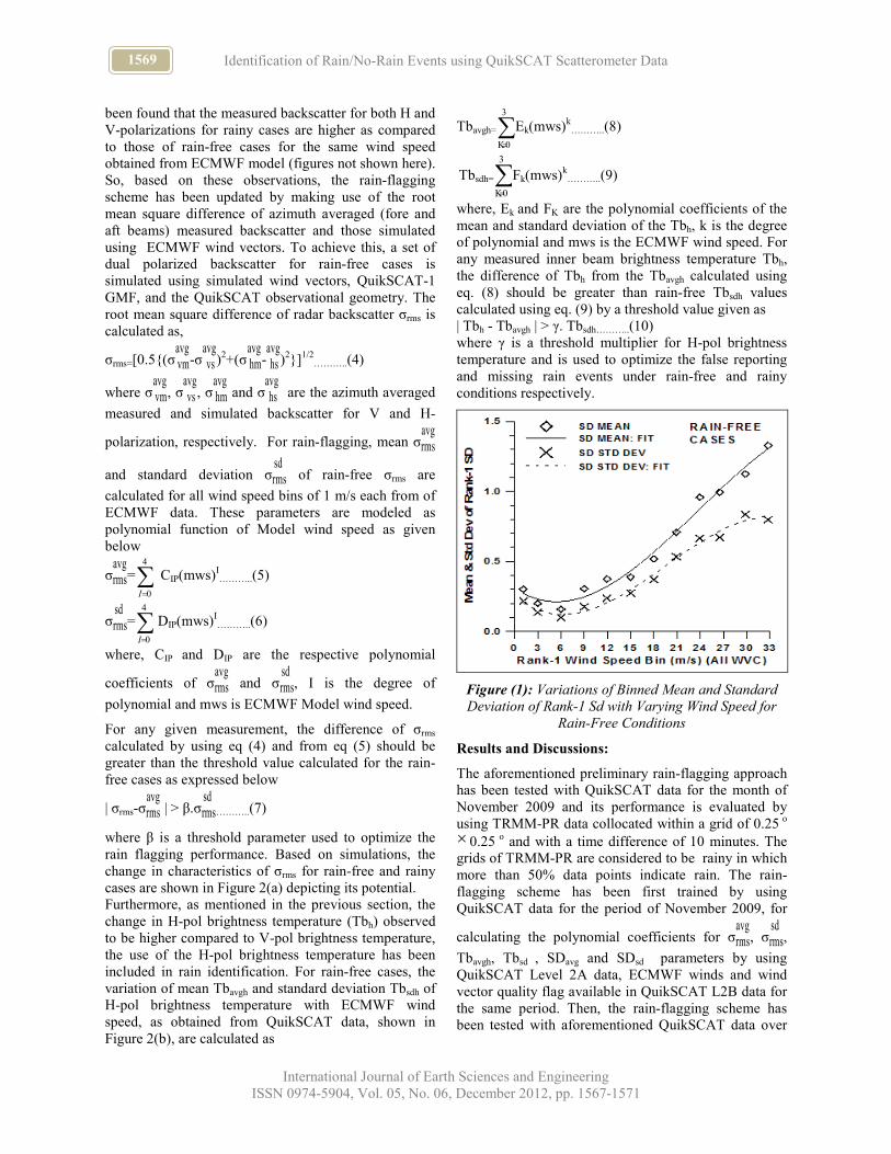
1569 Identification of Rain/No-Rain Events using QuikSCAT Scatterometer Data
International Journal of Earth Sciences and Engineering
ISSN 0974-5904, Vol. 05, No. 06, December 2012, pp. 1567-1571
been found that the measured backscatter for both H and
V-polarizations for rainy cases are higher as compared
to those of rain-free cases for the same wind speed
obtained from ECMWF model (figures not shown here).
So, based on these observations, the rain-flagging
scheme has been updated by making use of the root
mean square difference of azimuth averaged (fore and
aft beams) measured backscatter and those simulated
using ECMWF wind vectors. To achieve this, a set of
dual polarized backscatter for rain-free cases is
simulated using simulated wind vectors, QuikSCAT-1
GMF, and the QuikSCAT observational geometry. The
root mean square difference of radar backscatter σrms is
calculated as,
σrms=[0.5{(σavg vm-σ
avg vs )
2+(σ
avg hm-
avg hs )
2}]
1/2………..(4)
where σavg vm, σ
avg vs , σ
avg hm and σ
avg hs are the azimuth averaged
measured and simulated backscatter for V and H-
polarization, respectively. For rain-flagging, mean σavgrms
and standard deviation σsd rms of rain-free σrms are
calculated for all wind speed bins of 1 m/s each from of
ECMWF data. These parameters are modeled as
polynomial function of Model wind speed as given
below
σavgrms=∑
=
4
0I
CIP(mws)I………..(5)
σsd rms=∑
=
4
0I
DIP(mws)I………..(6)
where, CIP and DIP are the respective polynomial
coefficients of σavgrms and σ
sd rms, I is the degree of
polynomial and mws is ECMWF Model wind speed.
For any given measurement, the difference of σrms
calculated by using eq (4) and from eq (5) should be
greater than the threshold value calculated for the rain-
free cases as expressed below
| σrms-σavgrms | > β.σ
sd rms………..(7)
where β is a threshold parameter used to optimize the
rain flagging performance. Based on simulations, the
change in characteristics of σrms for rain-free and rainy
cases are shown in Figure 2(a) depicting its potential.
Furthermore, as mentioned in the previous section, the
change in H-pol brightness temperature (Tbh) observed
to be higher compared to V-pol brightness temperature,
the use of the H-pol brightness temperature has been
included in rain identification. For rain-free cases, the
variation of mean Tbavgh and standard deviation Tbsdh of
H-pol brightness temperature with ECMWF wind
speed, as obtained from QuikSCAT data, shown in
Figure 2(b), are calculated as
Tbavgh=∑=
3
0K
Ek(mws)k
………..(8)
Tbsdh=∑
=
3
0K
Fk(mws)k
………..(9)
where, Ek and FK are the polynomial coefficients of the
mean and standard deviation of the Tbh, k is the degree
of polynomial and mws is the ECMWF wind speed. For
any measured inner beam brightness temperature Tbh,
the difference of Tbh from the Tbavgh calculated using
eq. (8) should be greater than rain-free Tbsdh values
calculated using eq. (9) by a threshold value given as
| Tbh - Tbavgh | > γ. Tbsdh………..(10)
where γ is a threshold multiplier for H-pol brightness
temperature and is used to optimize the false reporting
and missing rain events under rain-free and rainy
conditions respectively.
Figure (1): Variations of Binned Mean and Standard
Deviation of Rank-1 Sd with Varying Wind Speed for
Rain-Free Conditions
Results and Discussions:
The aforementioned preliminary rain-flagging approach
has been tested with QuikSCAT data for the month of
November 2009 and its performance is evaluated by
using TRMM-PR data collocated within a grid of 0.25 o
×0.25
o and with a time difference of 10 minutes. The
grids of TRMM-PR are considered to be rainy in which
more than 50% data points indicate rain. The rain-
flagging scheme has been first trained by using
QuikSCAT data for the period of November 2009, for
calculating the polynomial coefficients for σavgrms, σ
sd rms,
Tbavgh, Tbsd , SDavg and SDsd parameters by using
QuikSCAT Level 2A data, ECMWF winds and wind
vector quality flag available in QuikSCAT L2B data for
the same period. Then, the rain-flagging scheme has
been tested with aforementioned QuikSCAT data over

1570 PRITI SHARMA, RAJESH SIKHAKOLLI, B. S. GOHIL and ABHIJIT SARKAR
International Journal of Earth Sciences and Engineering
ISSN 0974-5904, Vol. 05, No. 06, December 2012, pp. 1567-1571
inner beam swath and its performance for rain-free and
rainy cases has been evaluated in terms of false
reporting and missing rain events based on TRMM-PR
data with typical values of threshold multiplier α, β and
γ. As we increase the threshold multiplier α for σrms
from 0.5 to 2.5 keeping the values of β and γ constant
(within the range of 0.5 to 2.5), respectively, the false
reporting for rain-free condition increases with a
decrease in the missing rain events for rainy situation.
Since more than 90% of the global backscatter data
corresponds to rain-free situations hence our concerned
should be more towards reducing the false rain
reporting. The results related to false reporting and the
missing rain events are depicted in Table (1). Similarly,
rain-flags for QuikSCAT FP have also been compared
with TRMM-PR rain data. The comparison of the
performance of the proposed rain-flagging approach and
the QuikSCAT FP rain flags with TRMM-PR rain is
summarized in Table (1) indicating reduction in false
rain reporting over inner beam swath at the cost of
increasing missing rain rate as compared to that of
QuikSCAT FP and vice-versa. Therefore, the overall
success (considering both rain and rain-free cases) of
the presented rain flagging approach is more or less
similar to that of QuikSCAT FP. Thus, present approach
indicates its potential towards rain flagging of
scatterometer data and it is inferred that the proposed
rain-flagging approach tested with the QuikSCAT data
has yielded satisfactory results.
Conclusions:
The proposed approach comprising a set of conditions
provides improved identification of rain-free conditions
and thus facilitates larger statistics of wind retrieval
case. Scatterometer however is found to miss some
rainy events.
Acknowledgement:
The authors would like to thank Dr. R. R. Navalgund,
Former Director, Space Applications Centre, for the
constant encouragement. We thankfully acknowledge
NASA-JPL for QuikSCAT and TRMM-PR data used in
our analysis.
References:
[1] Contreras and Robert F., (2003), “Effects of rain on
Ku- band backscatter from the ocean”, J. Geophy,
Res., Vol. 108, C5, 3165, doi:
10.1029/2001JC001255, pp 34-1 to 34-15
[2] Huddleston, J. N. and B.W.Stiles, (2000),
“Multidimensional histogram rain-flagging
technique for Sea Winds on QuikSCAT”, Proc.
IGARSS2000, vol.3, pp.1232-1234
[3] QuikSCAT Science Data Product User’s Manual,
(2006), version 3.0, JPL Document D-18053-Rev
A, Jet Propulsion Laboratory, Pasadena, CA.
[4] Draper, D.W. and D.G. Long, (2004b), “Evaluating
the effect of rain on SeaWinds scatterometer
measurements”, J. Geophy. Res., Vol. 109,
C02005, doi: 10.1029/20021C001741, pp 1-12
[5] Gohil, B.S., Abhijit Sarkar and V.K. Agarwal,
(2008), “A new algorithm for wind vector retrieval
from scatterometer”, IEEE Geosci and Remote
Sensing Letters, vol. 5, No. 3, July, pp 387-391
Table 1: Rain Flagging Performance of the Qscat Data for the Period of November 2009 Collocated with TRMM
PR Data. Grids of 0.25 o ×0.25 o are Considered Rainy, If More than 50% Data Points Indicate Rain
False Rain Reporting
(%)
Missing Rain Events
(%)
Overall Success
(%)
FP Proposed FP Proposed FP Proposed
0.87 0.48 47.72 65.78 97.42 97.13
Total TRMM PR and QuikSCAT Collocated Data = 25948
Rain-free Cases = 25001, Rainy Cases = 947

1571 Identification of Rain/No-Rain Events using QuikSCAT Scatterometer Data
International Journal of Earth Sciences and Engineering
ISSN 0974-5904, Vol. 05, No. 06, December 2012, pp. 1567-1571
Figure (2): Trend of Mean and Standard Deviation of (a) RMS difference of Backscatter with ECMWF Wind Speed
(b) H-polarized Brightness Temperature with ECMWF Model Wind Speed

www.cafetinnova.org
Indexed in
Scopus Compendex and Geobase Elsevier, Chemical
Abstract Services-USA, Geo-Ref Information Services-USA
ISSN 0974-5904, Volume 05, No. 06
December2012, P.P.1572-1577
#02050614 Copyright ©2012 CAFET-INNOVA TECHNICAL SOCIETY. All rights reserved.
Genesis of Thermal Springs of Odisha, India
S. C. MAHALA1, P. SINGH
2, M. DAS
2 and S. ACHARYA
3
1Hydrogeological Unit, RWS&S PMDI Circle, Lane-II, Unit-III, Bhubaneswar-751001, Odisha, India
2P. G. Dept. of Geology, Utkal University, Bhubaneswar-751004, Odisha, India 3Plot No- 155, VIP Colony, Nayapalli, Bhubaneswar-751015, Odisha, India
Email: [email protected], [email protected]
Abstract: Thermal springs are considered as energy centric natural resource emitting earth’s outlet mechanism .
The geothermal energy is outlined as a combination of heat, water, gas source, and mineral component. Thermal
springs of Odisha are more or less aligned in specific tectonic lineament of the region and may be related to
structural disturbance. They are mostly confined along the periphery of the Gondwana Graben of Odisha. The
chemical constituents of the water are usually related to interaction between water and rock. The source of water is
accepted as meteoric. The heating process is due to geothermal gradient, decay of radioactive materials and
exothermic reactions. The associated gaseous phase is related to the decay of radioactive elements and organic
matter. The paper discusses the genesis of the thermal springs of Odisha considering these various parameters.
Keywords: Thermal Spring, Genesis, Odisha
Introduction:
Thermal springs are the springs that discharge water at
temperatures noticeably higher than the atmospheric
temperature of the surrounding and ascend from great
depth. They are natural phenomena linked to earth’s
internal energy; geothermal energy. They are named as:
hot springs, mineral springs, magic water, geysers,
fumaroles etc depending on the nature, character and
mode of manifestation on the earth surface. In a
geothermal field, the water percolates into sub surface
fractures and then gets heated by the internal heat. The
natural geothermal gradient, decay of radioactive
materials and exothermic reactions influence the heating
process. Later on the hot water and steam escape to the
surface of the earth along the fractures. Origin of
thermal springs deals with source of heat, water, gas and
mineral constituents. Allen and Day (1935), Day (1939),
Barth (1950) and Ellis & Mahon (1977) have made
valuable contributions on the origin of thermal springs.
An attempt is made to discuss the origin of thermal
springs of Odisha, on the basis of data documented
during the present study. A conceptual model has been
proposed.
Geological Setting and Tectonic Framework:
Manifestations of thermal springs are traced at eight
places in Odisha till date. The springs are located within
the Eastern ghat mobile belt, North Odisha craton and
western Odishan Proterozoic sedimentary basins (Fig
1). The thermal spring water is discharged either from a
single spot at Attri, Taptapani, Magarmuhan, Bankhol
and Boden areas or from several spots, clustered
together at Tarabalo, Deuljhori and Badaberena areas.
The highest number of spots have been recorded at
Tarabalo thermal spring area.
The thermal springs are mainly confined to crystalline
schists or gneissic terrain of Eastern ghat Supergroup
and Iron Ore Supergroup.However, Boden is located
within Vindhyan Supergroup. The litho-types
encountered at Attri, Tarabalo, Taptapani and Deuljhori
are khondalite, charnockite, augen-gneiss (granitic)
from Eastern ghat Super group. These rocks have
suffered highest grade of regional metamorphism and
are intricately folded. Quartzites of Iron Ore Super
group are exposed around Magarmuhan and Bankhol
region. The Precambrian rocks are considered to be the
repository of radioactive minerals (Ghosh, 1954). They
do not have any volcanic association as there is no
recent/sub-recent igneous activity in and around these
springs in Odisha.
The thermal springs of Odisha are pigeon- holed into
two categories of geothermal environment-
1. Mahanadi valley geothermal province (Boundary
faults along Gondwana graben).
2. Archaean/Pre-Cambrian geothermal province-
(lineaments along Pre-Cambrian terrain).
The hot springs follow certain tectonic systems and tend
to occur in areas associated with tectonic movement
(Gupta, 1974). Regional geological investigation
established the relationship between the hot springs and
the mega lineaments, especially in Odisha. Thermal

1573 S. C. MAHALA, P. SINGH, M. DAS and S. ACHARYA
International Journal of Earth Sciences and Engineering
ISSN 0974-5904, Vol. 05, No. 06, December 2012, pp. 1572-1577
springs of Odisha are confined along the following
lineaments.
i. Mahanadi lineament (Attri, Tarabalo, Deuljhori),
southern fault of Gondwana basin.
ii. Lineament in Easternghat granulite terrain
(Taptapani), secondary lineament parallel to east coast
lineament.
iii. Lineament in Iron Ore Supergroup terrain
(Magarmuhan and Bankhol), secondary lineament
parallel to the northern fault of Gondwana basin.
iv. Lineament along boundary of Chhatisgarh basin
(Boden) and v.Lineament along Gondwana-
Precambrian boundary (Badaberena), northern fault of
Gondwana basin.
Hydrological and Chemical Characters:
The temperature of surface water of the thermal springs
ranges from 32oC (Boden) to 67
o C (Tarabalo). The pH
value of the thermal waters indicates a neutral to mildly
alkaline character. All the thermal springs discharge
colourless and clear hot water. Sulphur odour is
discernable throughout the year at Attri, Tarabalo,
Deuljhori, Taptapani and Badaberena. Though the
volume of water released remains more or less constant,
difference in the rate of discharge is observed.
Chemical nature of water of thermal spring often
provides clues to their origin. Chemistry of water in
some thermal springs of Odisha has been carried out but
to a limited extent (Swain and Padhi1986; Bhargav et. al
2001). The water and gas samples collected from these
hot springs (Fig.2) have been analysed in the laboratory
,by adopting standard techniques. The water quality of
the eight thermal springs is not identical. The total
dissolved solids indicate low mineral content.
On the basis of concentration of various chemical
constituents, the water of thermal springs have been
categorised mainly into three categories (i) Sodium
chloride (NaCl) rich, (ii) Sodium Bicarbonate
(NaHCO3) rich and (iii) Calcium Bicarbonate
(CaHCO3) rich. The thermal spring water of Attri,
Tarabalo, Deuljhori and Taptapani are sodium chloride
rich while that of Magarmuhan, Bankhol, Badaberena
are sodium bicarbonate rich. Boden water is calcium
bicarbonate rich. This indicates that thermal springs
lying south of Gondwana graben are predominantly
NaCl rich and those lying north of it are Na-HCO3 rich.
Analysis of gas samples reveals that nitrogen is the
main component of geothermal gases (88%-90.5%)
followed by oxygen (1.2-6.6%). Together they
constitute more than 95% in volume. Other gases
detected are helium, argon, traces of methane and
carbon dioxide.
Genesis of Thermal Springs:
Several views regarding the origin of the thermal
springs have been proposed [ Allen and Day (1935),
Day (1939), Barth (1950) and Ellis & Mahon (1977)].
Two schools of thought exist about the origin of hot
springs. One school has correlated the thermal springs
with the volcanic activity or molten magma at depth,
where large amount of circulating ground water are
mixed up and interacted with the components from
magmatic sources. The final products of such
combination are the sources of mineral constituents and
heated water of the hot springs. The other school
advocated for non-volcanogenic origin. However, it is
accepted that the heating of circulating ground water at
depth can be caused by the geothermal gradient,
disintegration of radioactive substances and exothermic
reactions.
Source of Water:
The water of the thermal spring is invariably accepted
as of meteoric . In a simple meteoric origin, the
meteoric water percolating downwards along deep
fractures can be heated up by the rise of temperature due
to normal geothermal gradient. Lindgren (1935) has
reported a rise of 1o C temperature for every 30 m of
vertical depth.
Source of Heat:
Heat is accepted as an essential physical property of the
thermal springs. As a matter of fact the water generating
from a thermal spring is heated by geothermal gradient,
i.e. heat from the earth’s interior. The water (meteoric)
percolating deep down into the crust through structural
breaks are heated up, while coming in contact with the
hot rocks . The water from thermal springs, in non-
volcanic areas, is supposed to be heated in this manner.
But normal regional heat flow is considered as the
source of heat for the hot springs in Indian shield
(Ravishanker et al., 1991). Five heat flow zones in
Indian sub-continent have been reported, where heat
flow values range between 30 to 468 mW/m2. Odisha
falls in zone-II (100-180mW/m2) and zone-III (70-
100mW/m2) on the basis of heat flow values. Northwest
of Eastern ghats in Odisha sector, Talcher coal field and
thermal spring belt of Attri and Tarabalo fall within
zone-II. The average temperature gradient is 61+/- 20oC
in this zone. Roy and Rao (1996) mentioned that
variation in heat flow is primarily due to the heat
generated by radioactive elements present in the crust.
Source of Minerals:
The dissolved mineral constituents are likely to have
been derived from water- rock interactions. It is the
mineral composition instead of rocks that has
contributed the elements to the thermal spring water.

1574 Genesis of Thermal Springs of Odisha, India
International Journal of Earth Sciences and Engineering
ISSN 0974-5904, Vol. 05, No. 06, December 2012, pp. 1572-1577
Dissolved CO2 in the water plays a key role in such
reaction through liberation of H+ ions that react with
various silicates of the wall rock to release the alkalies,
alkaline earths and chloride. As a result, the water gets
depleted in H+ resulting an increase in its alkalinity.
Prevalence of Na over K is due to the greater solubility
of sodium salts and their tendency to be derived from
reactions involving minerals like plagioclases,
pyroxenes and amphiboles in a high pH condition.
Differences in chemical composition of waters are
mainly due to differences in host rock composition
(Ellis and Mahon, 1977).
Source of Gas:
Thermal springs are normally associated with various
gas phases. The gases come out through the fissures in
rocks in the form of bubbles that create micro-rings of
waves on the water surface. Gases such as nitrogen,
oxygen, argon, methane and carbon dioxide are present
in decreasing order (Mahala et. al., 1997). The gaseous
composition of the thermal springs is different from the
present atmospheric level (PAL). Presence of
appreciable level of nitrogen in the geothermal gases,
suggests its derivation from the atmosphere along with
meteoric water. Besides, methane and ammonia of the
primitive atmospheric air under high pressure and
temperature might have got dissociated into nitrogen
and hydrogen that also explains high percentage of
nitrogen in the thermal spring gases (Datta Munshi et.al,
1984). The thermal spring gases of Odisha having traces
of carbon dioxide indicate a non-magmatic origin of
these springs. Less amount of oxygen (6.6%) in the
thermal spring gases reveals that the atmospheric air
containing about 16% oxygen might have been utilized
in the oxidation process. The rare gas helium is very
likely formed due to radioactive disintegration and
presence of methane may be attributed to the
decomposition of organic matter inside earth’s crust
(Ellis and Mahon, 1977). Sulphurous smell of the
thermal springs is seemingly due to formation of
hydrogen sulphide, due to inter action between sulphide
mineral-bearing rocks and/or organic matter.
Discussion:
Genesis of thermal spring is an important aspect of
present investigation. The paradigm on the genetic
aspect of components (water, heat and gas) of thermal
springs has been drawn on the basis of database
generated during present study. Thermal springs of
Odisha are mainly confined to the crystalline schists and
gneissic terrains of Precambrian age. Most of them are
located in or close to the boundary (contact zone) of the
Precambrian crystalline and Gondwana sedimentary
rocks. These springs usually emerge along the deep
faults or fissures. Field studies supplemented by satellite
data indicate that the thermal springs lie along
lineaments. This infers close relationship between
tectonism and thermal activity.
It is accepted that the meteoric water is the main source
of the water of these thermal springs (Singh et.al, 1996,
Swain & Padhi, 1986). Since the water of the thermal
springs in Odisha has low TDS, the heat is inferred to be
derived from a non-magmatic source as the thermal
systems associated with volcanism usually have very
high TDS (White, 1957, Saxena & Gupta, 1982).
The higher temperature of the spring water is because of
rise of temperature by geothermal gradient, exothermic
reactions, and disintegration of radio-active elements (
Baranwal et.al ,2006). As there is no igneous activity,
rise of temperature is not related to magmatism. In fact
the geothermal gradient has been responsible in adding
heat vis-a –vis rise of temperature of the spring water.
The metamorphic reactions (exothermic) are responsible
for rise of temperature of the water. The Precambrian
terrain is enriched in radioactive elements (Ghosh,
1954). The quartz-pebble-conglomerate (QPC) of Iron
Ore Supergroup also reported to have radioactive
elements (Ray et.al, 1990). Since these springs
discharged water through the Precambrian metamorphic
terrain, the storehouse of radioactive minerals, might
have released temperature through disintegration of
radons. Thus, high temperatures of these thermal
springs are results of multiple processes involved
therein.
The chemical elements present in the minerals/ rocks
get dissolved in the hot water while coming in contact
during circulation. It has already been reported that
rocks of Eastern Ghat Granulites contain sulphide
bearing minerals like pyrite, pyrrhotite etc. These
minerals, while coming in contact with hot water,
impart sulphur smell.
As cited by Acharya (1966), Gautier’s suggestion of
foundering of sialic blocks and consequent squeezing
out of water from the mass resulted in the formation of
water vapour. This is because of the down faulting of
Gondwana basin against the fault contact between two
tectono-stratigraphic terrain; Iron Ore Super Group
(IOSG) in the north and Eastern Ghat Super Group
(EGSG) in the south. A conceptual model on the genesis
of thermal springs of Odisha along Gondwana graben is
given in Fig.3. The middle part of Odisha is down
faulted (rifted) and the rift valley is filled with
sediments. The northern fault is termed as Sukinda
thrust and the southern one is designated as north-
Khurda fault. The two faults form the boundary of the
Gondwana graben and got filled up later by sediments.
These two mega lineaments are responsible for the
occurrence of the thermal springs.
1575 S. C. MAHALA, P. SINGH, M. DAS and S. ACHARYA
International Journal of Earth Sciences and Engineering
ISSN 0974-5904, Vol. 05, No. 06, December 2012, pp. 1572-1577
Conclusions:
Thermal spring is a natural phenomenon and
manifestation of earth’s internal source of energy that is
received on the surface of the earth, in the form of
water, heat, mineral and gas. The thermal springs of
Odisha are situated in different litho-stratigraphic areas.
They are associated with mega lineaments, especially
along the contacts of Gondwana Graben and Pre-
cambrian crystalline rocks. The source of water is of
meteoric origin, which gets heated up by deep
circulation through fissures and faults. Hydro chemical
characters of the hot spring water have been influenced
significantly by water - rock interaction. The mineral
composition and radioactive character is influenced by
the rock assemblages through which the water
circulated. Presence of helium, the noble gas, is
indicative of radioactive disintegration. The atmospheric
air, litho-types and water-rock inter action together
contribute to the thermal spring gas composition.
Even though the conceptual model basically projects the
role of the two crustal scale faults, it is essential to note
that hot water circulation along the faults do suggest the
entire area in between the two faults also has hidden hot
spring chambers and they may emerge, in future,on the
surface through secondary faults associated with the two
main faults, as and when a structural disturbance
occurs.And as such, it is advisable to delineate the
subsurface conductivity pattern using an integrated
magneto telluric and deep resistivity surveys.
Acknowledgements:
We are thankful to Dr.P.R.Reddy, Retd. Scientist,
NGRI, Hyderabad for valuable suggestions and
objective reviewing/ editing.
References
[1] Acharya, S (1966) the thermal springs of Odisha.
The Explorer. pp.29-35.
[2] Allen, E.T. and Day, A.L., (1935) Hot springs of
Yellowstone National Park. Carnegie Inst.
Washington. Publ. No.466, pp.1.
[3] Baranwal, V.C., Sharma, S.P., Sengupta, D.,
Sandilya, M. K.., Bhaumik, B. K., Guin, R.K., and
Saha, S.K. (2006) A new high back ground
radiation area in the geothermalregion of
Easternghats mobile Belt(EGMB) of Orissa, India.
Radiation Measurements, 41,pp;602-610.
[4] Barth, T. F. W., (1950) volcanic geology, hot
springs and geysers of Iceland.Carnegie Institute,
Washington, publ. 587, pp. 1748.
[5] Bhargav, J. S., Srivastav, S. K. and Naik, P. K.,
(2001) A study on the geochemistry of Attri hot
spring area, Odisha.Bhu-Jal, (CGWB) vol.16, No-
324.
[6] Day, A. L., (1939) Presidential address to Geol.
Soc. America on hot spring problem. Bull. Geol.
Soc. Amer. Vol. 50.
[7] Datta Munshi, J.S., Billgrami, S. K., Verma, P. K.,
Datta Munshi, J. and Yadav, R. N., (1984) Gases
from thermal springs of Bihar,
India.National.Academy Science letters” India,
vol.7, No-9, pp. 291-293.
[8] Ellis, A.J. and Mahon, W.A.J. (1977) Chemistry
and geothermal systems. Academic press.
Newyork.
[9] [9] Ghosh, P. K., (1954) Mineral springs of India.
Rec. Geol. Surv. Of India. Vol. 80. pp. 541-558.
[10] Gupta, M. L., (1974) Geothermal resources of some
imalayan hot spring areas. Himalayan Geology,
Vol. 4, pp. 492-515.
[11] Lindgren, W (1935) Mineral deposits. 3rd edition.
McGraw Hill , New York
[12] Mahala, S., Singh,P., Das, M., Ray, P., and
Acharya, S. (1997) Trait on Geothermal Gases from
thermal Springs of Odisha. Vistas in Geol
Res.No.2, pp. 221-225.
[13] Ray, P., Singh, P., and Acharya, S., (1990) A note
on quartz pebble conglomerate around Sikheswar-
Burhaparbat in Dhenkanal-Keonjhar district,
Odisha. Proc.77th Ind. Sci. cong. Assoc. Cochin,
p.33. (Abst).
[14] Roy, S. and Rao, R. U. M., (1996)- Regional heat
flow and the perspective for the origin of hot
springs in the Indian shield. GSI. Spl. Publ. No-45,
pp. 39-40
[15] Saxena, V.K. and gupta, M.L (1982) Geochemistry
of thermal and cold waters of Godavari valley.
Jour. Geol.scc.Ind. Vol.23, No-II, pp;551-560.
[16] Shanker, Ravi., Guha, S.K., Seth, S.K., Ghosh, A.,
Ghosh, S., Nandy, D.R., Jangi, B.L. and
Muthuraman, K., (1991) Geothermal Atlas of India.
GSI Spl. Publ. No-19.
[17] Singh, P., Mahala, S., Ray, P., Das, M. and
Acharya, S.(1996) a study on hydrology and
geochemistry of thermal springs in Orissa, India.
Jour. Ind. Acad. Geosci. Vol.39(1), pp:31-35.
[18] Swain, P. K. and Padhi, R. N. (1986) Geothermal
fields of Ganjam and Puri districts, Odisha. GSI,
Records Vol. 114, Pt. 3, pp. 41-46
[19] White, D. E., (1957) Magmatic, connte and
metamorphic water.Geol. Soc. of America, vol.68,
pp.1659-1682.

1576 Genesis of Thermal Springs of Odisha, India
International Journal of Earth Sciences and Engineering
ISSN 0974-5904, Vol. 05, No. 06, December 2012, pp. 1572-1577
Figure 1: Outline Map of Odisha showing location of Thermal Springs. 1. Deuljhori, 2. Tarabalo, 3. Attri,
4. Bankhol, 5. Magarmuhan, 6. Badaberena, 7. Taptapani, 8. Boden

1577 S. C. MAHALA, P. SINGH, M. DAS and S. ACHARYA
International Journal of Earth Sciences and Engineering
ISSN 0974-5904, Vol. 05, No. 06, December 2012, pp. 1572-1577
Figure 2: Photographs Showing Thermal Springs at A. Tarabalo B. Taptapani C. Deuljhori D.Attri
Figure 3: Conceptual Model Showing Location of Thermal Springs along Gondwana Graben

www.cafetinnova.org
Indexed in
Scopus Compendex and Geobase Elsevier, Chemical
Abstract Services-USA, Geo-Ref Information Services-USA
ISSN 0974-5904, Volume 05, No. 06
December2012,P.P.1578-1583
#02050615 Copyright ©2012 CAFET-INNOVA TECHNICAL SOCIETY. All rights reserved.
Remote Sensing Studies in Delineating Hydrogeological Parameters
in the Drought-Prone Kuchinda-Bamra Area in Sambalpur District,
Odisha
NANDITA MAHANTA1 and H. K. SAHOO
2
1Department of Geology, Bonaigarh College, Bonaigarh, Sundargarh -770038
2P. G. Department of Geology, Utkal University, Bhubaneswar -751004
Email: [email protected], [email protected]
Abstract: The hydrogeomorphological map of Kuchinda-Bamra area was prepared from IRS IA (LISS – II)
satellite imagery in the scale of 1:250,000 by visual interpretation method for delineation of fresh groundwater
potential zones using remote sensing techniques. The various hydrogeomorphic units such as structural hills,
residual hills, intermontanne valleys, pediments, buried pediplains and denudational hills are identified. The
groundwater potential zones have been classified into low, moderate and good which is also corroborated from
geophysical studies and field checks.
Keywords: Hydrogeomorphic units, Darjing Group, Kuchinda-Bamra area
Introduction:
The Kuchinda-Bamra area in Sambalpur district of
Odisha is a drought prone area and forms a part of the
hard rock terrain. Because of erratic nature of rainfall
and unscientific management of water resources, the
area frequently experiences drought. The demand of
groundwater has increased due to growth of population,
rapid industrialization and development in agricultural
activities. The development of groundwater resources
can play an important role in the economic development
of the area. Keeping the above facts in view an attempt
has been made in the present work to analyze the remote
sensing data systematically and to draw meaningful
inferences with additional inputs from geophysical data
in the Kuchinda- Bamra blocks of Kuchinda subdivision
lying in the northern part of Sambalpur district of
Odisha. The present study shall help in understanding
the geomorphological, lithological and hydrogeological
factors, which govern the occurrence and distribution of
groundwater in the study area.
Study Area:
The study area consists of two blocks namely Kuchinda
and Bamra of Kuchinda subdivision in northern part of
Sambalpur district and forms north-west upland of
Odisha. It is situated 85 km away from the district
headquarter, Sambalpur and lies between latitude 210
37’ N to 220 13’N and longitude 84
0 15’E to 84
0 42’ E
in the Survey of India Toposheet Numbers 73 B/8, 73
C/2, 73 C/5, 73 C/6, 73 C/9, 73 C/10, 73 B/12. The
total population of the study area is 155,585 as per 2001
census. The area experiences a subtropical climate with
maximum temperature of 43°C during summer and
minimum temperature of 10°C during winter. The area
receives most of the rain from south west monsoon. The
location map of the study area is given in Fig. 1.
Physiography and Drainage:
Physiographycally, the area is highly undulated with
very large elevated hills with maximum height of 736 m
above MSL (Bamlo Pahar) and flat areas of altitude 221
m above MSL. Some parts of the area are characterized
by gently undulating plains with isolated residual hills
and mounds. The major drainage system is controlled
by Bheden River with streamlets and nallas like Purtala
nala, Kharla nala, Lamdora, Tabko Jharan, Lohranga
nala and Sian Jhor etc. The drainage pattern is dendritic
and influent in nature. Because of the predominance of
granitic and metasedimentary rocks, the area
experiences medium drainage density. The drainage
map of the area is shown in Fig. 2.
Geological Setting:
The study area comprises a variety of rock types
varying in age from Precambrian to Recent.
Garnetiferous biotite-quartz schist of the Older
Metamorphic Group is the oldest rock type in the study
area which is overlain by metavolcanics and quartzites
belonging to Deogarh Group. These are succeeded by
granitoids (Bamra granite). The rocks of Darjing Group
comprising of Birtola Formation(mostly quartzite and
conglomerate) and Jalda Formation (mostly staurolite
schist, calc-gneiss, garnetiferous mica- schist) overlie
the granitoids with an unconformity at the base which

1579 NANDITA MAHANTA and H. K. SAHOO
International Journal of Earth Sciences and Engineering
ISSN 0974-5904, Vol. 05, No. 06, December 2012, pp. 1578-1583
has been assigned an age of 2700 Ma (Mahalik, 1987;
Mahalik and Nanda, 2006). The rocks of Darjing Group
are intruded by mafic and ultramafic sills and dykes.
During the Meso-Proterozoic period, another basin
(Kunjar basin) has been developed over the 2700 Ma
granitic basement (Chaki et al. 2005) now represented
by quartzite. Laterite and alluvium of Recent age of
considerable thickness form the surficial cover. The
rocks of the Precambrian age are affected by atleast
three generations of deformation with development of
folds, faults, foliations, joints etc creating secondary
porosities in the hard rocks that help in the storage and
movement of groundwater.
Hydrogeological Setting:
Presence of a variety of rock types in the study area
with different degrees of deformation is responsible for
different hydrogeological condition in various parts with
wide variation in groundwater potential. About 85% of
the total area is covered by hard (consolidated) rocks
where groundwater is stored and moves in secondary
porosities developed due to weathering and fracturing.
Groundwater in Kuchinda-Bamra area is found to exist
in semi-confined to confined conditions in the fractured
and jointed rocks at deeper depths but under unconfined
condition in shallow weathered zones. The
unconsolidated formations are constituted by laterite
and alluvium. The yield of groundwater in the
weathered granitoids varies from very low (1 lps) to
moderate (7 lps) in Bamra block and from 1 lps to 9.2
lps in Kuchinda block. The depth to water table during
post-monsoon period varied from 0.91 to 6.7 mbgl in
2008 and from 2.44 to 8.23 mbgl during pre-monsoon
period in 2009. The net annual utilizable groundwater
resource of Kuchinda and Bamra blocks are 5470 Ham
and 6642 Ham respectively. Groundwater development
is relatively less in Bamra block (8.93%) in comparison
with Kuchinda block (11.83%). However, both the
blocks of the study area fall under safe/ (white)
category.
Remote Sensing Studies:
Remote sensing technique provides an effective modern
tool in delineating groundwater potential zones. It is one
of the most useful tools for watershed characterization,
planning and management of groundwater resources in
recent times. The integrated approach of remote sensing
plays an important role in the systematic analysis of
various lithological, geomorphological, soil,
hydrological, and land use characterization of an area.
The surface information of a particular area is necessary
for interpretation of the subsurface geological and
hydrogeological features. Information on various
aspects of surface and subsurface can be known from
remote sensing studies, geophysical surveys and various
logging techniques. Remote sensing method is the
quickest method for the interpretation of various
hydrogeomorphological units and groundwater
conditions. In recent years, remote sensed data have
been increasingly used in groundwater studies viz: Hari
Narayan et al. (2000), Mahapatra and Maharana (2000),
Per Sander et al. (1997), Sankar (2001), Sankar and
Venkataraman (2002), Rokade et al (2007), Chakrabarty
and Paul (2004), Gopinath et al. (2003), Sakram et
al.(2011) etc. The combination of landform – cum –
lineament mapping is very much useful in areas where
the overburden and / or weathered rock as well as partly
weathered / fractured rock contain adequate quantities
of groundwater (Beeson & Jones, 1988).
Data used and Methodology:
The present study was carried out by visual
interpretation of the satellite imageries of IRS- IA (LISS
– II) in the scale of 1:250,000. The Survey of India
toposheets were referred for the preparation of the base
maps. With the help of satellite data, based on image
characteristics, the study area has been divided in to
number of geomorphological units. Various geological
formations, landuse, landcover classifications and
lineaments were delineated and verified during the field
visits. The hydrogeomorphological map prepared from
setellite imagery(Fig.3) provide integrated information
on several factors which directly or indirectly control
the movement and occurrence of groundwater.
Result and Discussion:
The analysis of IRS- IA LISS-II data based on various
image interpretations led to the identification of six
hydrogeomorphological units differing in groundwater
occurrences. These are named as structural hills,
denudational hills, residual hills, intermontanne valleys,
pediments and buried pediplains. Different
hydrogeomorphic units with their lithostratigraphic
classification, structural features and groundwater
occurrence is presented in Table 1. The structural hills
are represented by both Darjing Group and Deogarh
Group of rocks which are well foliated, folded and
faulted but sometimes also are massive and their
groundwater occurrence is poor. Denudational hills
comprise of rocks of Deogarh Group mostly where
groundwater occurrence is poor but can be available
only in intermontane valleys. Residual hills comprising
of Darjing Group of rocks and granitoids are found as
isolated hills in the flat terrain but their groundwater
content is very limited. The most important groundwater
host in the area of study is the buried pediplains which
are flat terrains with thickness varying from 5 to 20m
comprising of alluvium and weathered residues of
granitoids. In this unit, the groundwater occurrence is
moderately good to very good. The pediments which are
gently undulating areas with fractures and joints
comprise of granitoids and metavolcanics where

1580 Remote Sensing Studies in Delineating Hydrogeological Parameters in the
Drought-Prone Kuchinda-Bamra Area in Sambalpur District, Odisha
International Journal of Earth Sciences and Engineering
ISSN 0974-5904, Vol. 05, No. 06, December 2012, pp. 1578-1583
groundwater occurrence is poor to moderate. Among all
these geomorphic units, the buried pediplains can be
exploited for getting good groundwater supplies.
Lineaments are linear features commonly associated
with dislocations and deformations. They provide the
pathway for groundwater movement and are
hydrogeologically very important. Excellent
groundwater prospects are expected at intersections of
lineaments (Sankar, 2001). In the study area, two large
lineaments trending NE-SW intersect at a point which
represent a good source of groundwater. A fault
trending ENE-WSW near Kusumi has the potential of
storage and movement of huge amount of groundwater
resources. Resistivity survey by Vertical Electrical
Sounding was conducted at 26 locations in the area of
study with a maximum current electrode separation of
250m. This indicates presence of 3 to 5 layer situations
where a soil or lateritic horizon represents the first layer.
The thickness of this layer varies from 0.4 to 6.3m and
resistivity varies from 8.0 to 1130 ohm-m. This layer
contains water in very limited quantities with some parts
indicating a dry soil zone. The second layer represents
highly weathered granitoids in most places but in a few
locations it contains clay, sandy loam and sandy clay.
The thickness of this layer varies from 0.9 to 16.7m and
the resistivity varies from 3.0 to 169.6 ohm-m.
Groundwater occurrence in this layer is very good. The
third layer in some cases represents highly weathered
and highly fractured granitoids and granulites but in
other cases it represents hard and consolidated rocks.
The thickness of this layer varies from 1.9m to infinity
and the resistivity varies from 29 ohm-m to more than
2000 ohm-m. The fourth layer represents partly
fractured and partly weathered granite in some cases
and hard and unconsolidated rocks in other cases. The
thickness of this layer varies from 6.2m to infinity. The
resistivity varies from 12.5 ohm-m to more than 6500
ohm-m. The groundwater occurs only in fractured and
weathered zones in limited quantities. The isoresistivity
map of the groundwater rich second layer (Fig.4)
indicates resistivity value varying from 90 to 120 ohm-
m at Mantrimunda, Niktimal, Gorpos etc corresponding
to buried pediplain which are very good locales of
groundwater. The interpretation of lineaments in the
southern part of the area also corresponds to areas
representing values of around 60 ohm-m representing
good sources of groundwater. This is further
corroborated from field observation.
Conclusion:
The present study has helped to identify the
groundwater prospect zones by using the remote sensing
techniques. In various hydrogeomorphological units
such as structural hills, denudational hills and residual
hills, the groundwater is of limited occurrence and
intermontanne valleys in these units can be searched for
to get groundwater. In pediments the groundwater
potential is found to be poor to moderate but sometimes
good. The buried pediplains are of moderate thickness
varying from 5 to 20 m which are flat terrain and
contain significant quantity of groundwater. The
groundwater from this can be exploited by dug wells
and shallow tube wells. Presences of lineaments in the
buried pediplains are suitable sites for groundwater
exploitation.
References:
[1] Beeson,S. and Jones,C.R.C.(1988) The combined
EMT/VES geophysical method for siting bore
holes, Groundwater, Vol.26, pp.54 – 63
[2] Chaki A, Bhattacharya D, Rao J.S. , Chaturvedi
A.K. and Bagchi A.K. (2005), Geochronology of
the Granitoids of the Kunjar area, Sundargarh
District, Orissa : Implication to the Regional
Stratigaphy. Journal Geological Society of India,
Vol. 65, PP, 428 – 440.
[3] Chakraborty,S. and Paul,P.K.(2004). Identification
of potential ground water zonesin the Baghamundi
block of Purulia district of West Bengal using
remote sensing and GIS, Jour. Geol. Soc.Ind,
Vol.64, No.1, pp.69 – 75.
[4] Gopinath,G.,Seralathan,P.,Ramasamy,S.and
Unnikrishnan,K.(2003) Delineation of groundwater
potential zones in the hard rock terrains of
Madurai-Dindigal district, Tamilnadu using remote
sensing technique, Jour. Of Applied Hydrology,
Vol.XVI, No.1, pp.49 – 55.
[5] Harinarayanan, P., Gopalkrishna, G.S. and
Balasubramanian, A. (2000) Remote sensing data
for groundwater development and management in
Keralapura watersheds of Cauvery basin, Karnatak.
In: National Seminar on Earth Resources,
Mangalore University, pp. 7-8 (abs).
[6] Jaiswal, R.K., Mukharjee, S., Krishnamurthy, J. &
Saxena, R. (2003) Role of remote sensing and GIS
techniques for generation of groundwater prospect
zones towards rural development- an approach.
Intern. Jour. Remote Sensing, Vo. 24, No. 5, pp.
993-1008.
[7] Mahalik, N.K. & Nanda, J.K. (2006) Geology &
mineral resources of Orissa, Precambrian, SGAT
Publication, pp. 45-90.
[8] Mahalik N.K., (1987), Geology of rocks lying
between Gangpur Group and Iron Ore Group of the
Horse shoe syncline in North Orissa, Indian Journal
of Earth Sciences, Vol. 14, No 1 PP. 73 – 83.
[9] Mahapatra,K.C. and Maharana,R.C. (2000).
Integrated survey on groundwater potential in
Turva town of Balangir district, In Proc. Of
Seminar on “Prospect of groundwater development

1581 NANDITA MAHANTA and H. K. SAHOO
International Journal of Earth Sciences and Engineering
ISSN 0974-5904, Vol. 05, No. 06, December 2012, pp. 1578-1583
and management in Orissa”, Organised by CGWB,
Bhubaneswar, pp.38 – 50.
[10] Per Sander, Minor, T.B. & Chesley, M.M. (1997)
Groundwater exploration based on lineament
analysis and reproducibility tests. Groundwater,
Vol. 35, pp. 888-894.
[11] Rokade,V.M., Kundal,P. and Joshi,A.K.(2007)
Groundwater potential modeling through remote
sensing and GIS: A case study from Rajura Taluka,
Chandrapur district, Maharastra, Jour. Geol. Soc.
India, Vol.69, No.5, pp.943 – 948.
[12] Sakram,G., Rajita Sanda, Sudhakar, A.and Sexena
Praveen Raj(2011) Groundwater resources and its
management in the lateritic terrain around
Zaheerabad, Medak district, Andhra Pradesh,India
– A remote sensing and GIS approach, International
Jour. of Earth Sciences and Engineering, Vo.04,
N0.6, pp.995 – 999.
[13] Sankar, K. (2001) Remote sensing study of
groundwater occurrence in Kanyakumari District,
Tamilnadu, India, Jour. Appl. Hydrology. Vol.
XIV, No. 4, pp. 16-26.
[14] Sankar,K. and Venkataraman,S.(2002) Geological
and geomorphological mapping in and around
Bharatidasan University: a remote sensing
approach, Jour of Applied Hydrology, Vol. XV,
No.1, pp. 15 – 22.
Table 1: Various Geomorphic Units of the Study Area with their Groundwater Potential
Sl.
No.
Geomorphic
units
Lithostrati-
graphic units
Major
structure
Description Groundwater condition
1 Structural Hills
(SH) a)Darjing Group
–Quartzite, schist
and phyllite
b)Deogarh
Group - Quartzite
Massive,
Well
foliated &
folded
Folded and
faulted
A group of linear to
curvilinear hill ranges
at times with
intermontanne valleys
Groundwater occurrence
is poor but good in
intermontanne valleys but
of limited occurrence
2 Denudational
Hills (DH) a)Deogarh
Group –
Quartzite
b)Bamra Granite
Folded and
faulted
Intrusive
into Country
rocks,
Fractured
A group of linear to
curvilinear hill ranges
at times with
intermontanne valleys
Group of hill ranges
with domal shape
Poor Groundwater
occurrence but good in
intermontanne valleys but
of limited occurrence
Groundwater occurs in
weathered and fractured
zones, Ground water
occurrence is moderate
3 Residual Hills
(RH)
a)Granite and
gneisses
b)Darjing Group
–Quartzite, schist
and phyllite
c)Bamra Granite
Forms
basement,
sometimes
foliated
Massive,
Well folia
ted & folded
Massive,
also foliated
Isolated massive hills
of less areal extension
surrounded by plains
Isolated hills
surrounded by plains
Isolated mounds
surrounded by plains
Limited ground water
occurrence
Limited ground water
occurrence
Limited ground water
occurrence
4 Intermontanne
valley (IV)
In between
various rock
groups forming
hills
May be
structurally
controlled
A broad or linear
valley between
mountains filled with
alluvium
Moderate with limited
quantity
5 Pediment(P) Bamra granite
and
metavolcanics
Gently
undulating
with
fractures/
joints
Gently undulating
with weathered zone
and fractured zone
Poor to moderate,
sometimes good
6 Buried Pediplain
(BPP)
Alluvium of
recent age
underlain by
granite, gneiss,
meta volcanic and
quartzites
Fractures at
deeper
levels
Flat terrain with 5 to
20 m thickness of
overburden with
extensive occurrence
of alluvium
Moderate to good,
sometimes very good

1582 Remote Sensing Studies in Delineating Hydrogeological Parameters in the
Drought-Prone Kuchinda-Bamra Area in Sambalpur District, Odisha
International Journal of Earth Sciences and Engineering
ISSN 0974-5904, Vol. 05, No. 06, December 2012, pp. 1578-1583
Figure 1: Location Map of the Study Area
Figure 2: Drainage Map of the Study Area
Figure 3: Hydrogeomorphological Map, RH– Residual Hill, DH-Denudational Hill, SH – Structural Hill,
IV-Intermontanne Valley, P-Pediment, BPP-Buried Pediplain

1583 NANDITA MAHANTA and H. K. SAHOO
International Journal of Earth Sciences and Engineering
ISSN 0974-5904, Vol. 05, No. 06, December 2012, pp. 1578-1583
Figure 4: Isoresistivity Map of the Second Layer

www.cafetinnova.org
Indexed in
Scopus Compendex and Geobase Elsevier, Chemical
Abstract Services-USA, Geo-Ref Information Services-USA
ISSN 0974-5904, Volume 05, No. 06
December2012,P.P.1584-1589
#02050616 Copyright ©2012 CAFET-INNOVA TECHNICAL SOCIETY. All rights reserved.
Impact Analyses of Industrial and Mining Activities on
Groundwater Regime -Case Studies in Goa
A. G. CHACHADI Department of Earth Science, Goa University,
Email: [email protected]
Abstract: In the present study analysis of impacts of industrial and mining activities on groundwater regime has
been carried out. It is found that mining activities in specific locations have been impacting both shallow
groundwater as well as moderately deep groundwater systems. The industrial activity at one site studied has not
indicated significant change in groundwater levels during the study period. The geological data indicate that the
shallow aquifers located in the peripheral areas of the Plateau region are in continuity with plateau laterites and
behave as a single geological unit.
Keywords: Hydrograph, Mining, Piezometer, Verna
Introduction:
The measurement and analysis of ground water level
fluctuations in piezometers and observation wells is an
important facet of groundwater studies. Water-level
fluctuations can result from a wide variety of
hydrologic, meteorological, and hydrogeological
phenomena. Some are natural phenomena like
groundwater recharge, evapotranspiration,
phreatophytic consumption, bank storage effects near
streams, tidal effects near oceans, change in
atmospheric pressure, earthquakes etc. and some
induced by man such as external loading of confined
aquifers, artificial recharge, groundwater pumping,
deep-well injection, return flows from irrigation,
geotechnical drainage and open pit mine pumping, land
use changes etc. In many cases, there may be more than
one mechanism operating simultaneously.
Well hydrographs even under natural undisturbed
conditions show seasonal and diurnal fluctuations. Only
the long term fluctuation (secular) is absent. Reduced
rainfall or changed climatic conditions will lead to
changes in groundwater levels even in the absence of
anthropogenic causes. On the other hand under human
induced conditions this balance can still be retained by
well-managed recharge and discharge conditions in an
area. This means in an area where tremendous
anthropogenic activities are witnessed involving the
groundwater regime and still the well hydrograph do
maintain their undisturbed original trend could only
mean that the groundwater regime is balanced. In other
words the system has reached a steady state condition.
Aquifer response to recharge to and discharge from it is
indicated in the water level changes measured at
different time periods. Unconfined aquifers, which are
in continuity with the ground surface and the
atmospheric pressure, are quicker in responding than
confined and semi confined aquifers. The magnitude of
change in water level below ground at a given point
depends not only on magnitude of groundwater
withdrawals and recharges but also on the intrinsic
characteristics of geological matrix both of saturated
and unsaturated zones besides initial water table depths
and antecedent soil moisture conditions. For example
long and steady spell of rain on a loamy saturated soil
with deep water table condition in a highly permeable
geologic section could raise the water table to greater
height than an intense rainfall event of shorter duration
on dry clayey soil with shallow water table condition in
a low permeable geologic section. Qualitative
information on the saturated – unsaturated media, nature
of aquifer recharges and discharges can be ascertained
from the study of well hydrographs. For example
identical features in rising and falling limbs of the
hydrographs from different locations in the watershed
should indicate similar aquifer hydraulic conditions. In
order to achieve such objectives the observation wells
and piezometers should have to be located carefully so
that each of them represents a sizable hydrogeological
regime in space and depth and should be well
distributed over the entire watershed area.
Objective of the Present Study:
Groundwater regime in the State of Goa has been
subjected to variety of anthropogenic stresses such as
mining, industrialization and urbanization. Mining and
industrialization have been on rise in the recent past and
have impacted groundwater regime in several ways. It is
therefore intended in the present study to evaluate
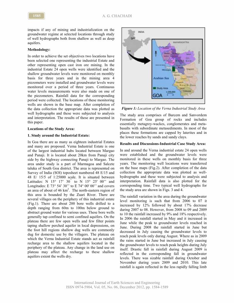
1585 A. G. CHACHADI
International Journal of Earth Sciences and Engineering
ISSN 0974-5904, Vol. 05, No. 06, December 2012, pp. 1584-1589
impacts if any of mining and industrialization on the
groundwater regime at selected locations through study
of well hydrographs both from shallow as well as deep
aquifers.
Methodology:
In order to achieve the set objectives two locations have
been selected one representing the industrial Estate and
other representing open cast iron ore mining. In the
industrial Estate 24 open wells were identified and the
shallow groundwater levels were monitored on monthly
basis for three years and in the mining area 4
piezometers were installed and groundwater levels were
monitored over a period of three years. Continuous
water levels measurements were also made on one of
the piezometers. Rainfall data for the corresponding
period were collected. The locations of these monitoring
wells are shown in the base map. After completion of
the data collection the appropriate data was plotted as
well hydrographs and these were subjected to analysis
and interpretation. The results of these are presented in
this paper.
Locations of the Study Area:
1. Study around the Industrial Estate:
In Goa there are as many as eighteen industrial Estates
and many are proposed. Verna Industrial Estate is one
of the largest industrial hubs located between Margao
and Panaji. It is located about 20km from Panaji city
side by the highway connecting Panaji to Margao. The
area under study is a part of Marmagoa and Salcete
taluka of South Goa district. The area is represented on
Survey of India (SOI) toposheet numbered 48 E/15 and
48 E/ 15/5 of 1:25000 scale. It is situated between
Latitudes: N 15° 17’ 30’’ to N 15° 25' 00’’ and
Longitudes: E 73° 54’ 30’’ to E 74° 00' 00’’ and covers
an area of about of 46 km2. The north-eastern region of
this area is bounded by the Zuari River. There are
several villages on the periphery of this industrial estate
(Fig.1). There are about 200 bore wells drilled to a
depth ranging from 60m to 100m below ground to
abstract ground water for various uses. These bore wells
generally tap confined to semi confined aquifers. On the
plateau there are few open wells and few filter points
taping shallow perched aquifer in local depressions, on
the foot hill regions shallow dug wells are commonly
dug for domestic use by the villagers. The plateau on
which the Verna Industrial Estate stands act as rainfall
recharge area to the shallow aquifers located in the
periphery of the plateau. Any change in the land use on
plateau may affect the recharge to these shallow
aquifers extent the wells dry.
Figure 1: Location of the Verna Industrial Study Area
The study area comprises of Barcem and Sanvordem
Formation of Goa group of rocks and includes
essentially metagrey-wackes, conglomerates and meta-
basalts with subordinate metasediments. In most of the
places these formations are capped by laterites and in
the lower reaches by sands and sandy clays.
Results and Discussions-Industrial Case Study Area:
In and around the Verna industrial estate 24 open wells
were established and the groundwater levels were
monitored in these wells on monthly basis for three
years. The monitoring well locations were transferred
on the base maps (Fig.2). After completion of the data
collection the appropriate data was plotted as well-
hydrographs and these were subjected to analysis and
interpretation. Rainfall data is also plotted for the
corresponding time. Two typical well hydrographs for
the study area are shown in Figs. 3 and 4.
The rainfall variation in the area during the groundwater
level monitoring is such that from 2006 to 07 it
increased by 12% followed by about 17% decrease
during 2007 to 08. However, from 2008 to 09 and 2009
to 10 the rainfall increased by 9% and 18% respectively.
In 2006 the rainfall started in May and it increased in
June while the peak to groundwater levels reached in
June. During 2008 the rainfall started in June but
decreased in July causing the groundwater levels to
reach peak levels only during August. Where as in 2009
the rains started in June but increased in July causing
the groundwater levels to reach peak heights during July
itself. Drastic fall in rainfall during August 2009 is
reflected in the corresponding fall in groundwater
levels. There was sizable rainfall during October and
November during years 2009 and 2010. This late
rainfall is again reflected in the less rapidly falling limb

1586 Impact Analyses of Industrial and Mining Activities on
Groundwater Regime -Case Studies in Goa
International Journal of Earth Sciences and Engineering
ISSN 0974-5904, Vol. 05, No. 06, December 2012, pp. 1584-1589
of the hydrograph during 2009-10 compared to 2008-09
especially in well number 23.
W1
W2
W3
W4 W5
W6
W7
W8
W9
W10
W11W12
W13
W14
W15
W16
W17
W18
W19
W20
W21
W22
W23
W24
Spring
Spring
Kesarwal
Mhalsa
Siphrem
Nuvem
Mogarupoy
Umorem
Mardhwal
Verna
Verna
Arosim
Kansavlim
Konsua
Mosil
Karvona
Mudli
Nakordem
Lotli
Ambora
Kelosim
Navtawada
Sindoli
Kortali
Sankval
Verna Industrial Estate
0 1000 2000
SCALE
m m
Zuari River
W8Well number
Drainage network
Spring
Area of ground level
Sub-watersheds
Index
25m & more amsl
Figure 2: Location of the Groundwater Level
Monitoring Wells in and around the Study Area
Figure 3: Groundwater Level Hydrograph for Well no.
23 in the Study Area
Figure 4: Groundwater Level Hydrograph for Well no.
18 in the Study Area
As seen from the above figures the rainfall during the
period of record has increased to some extent steadily
except during the year 2008. The groundwater levels
show a seasonal fluctuation in their temporal behavior
during those three years of recording. The distribution
of rainfall intensity and duration influences the behavior
of the groundwater level fluctuations.
It is observed from the hydrographs that there is no
significant change in the groundwater levels over the
period of recording and the fluctuations are only
seasonal due to rainfall recharge and various
abstractions during non monsoon season. The following
conclusions can be drawn:
1. The groundwater levels show fluctuations mainly
due to rainfall recharge and various abstractions. With
existing short term water level data and in the absence
of pre industrial groundwater level records it shall be
unwise to conclude on the long term behavior of the
phreatic groundwater levels in the area. However, it is
learnt from the field inquiries from the well owners that
the groundwater levels in the area in lateritic aquifers
have not changed significantly in the past.
2. The geological data indicate that the shallow
aquifers located in the peripheral areas of the Verna
Plateau are in continuity with plateau laterites and
behave as a single geological unit.
3. The peripheral shallow aquifers around the Verna
Plateau are also fed by rainfall recharge that could be
taking place on the Plateau area.
2. Study around Mining Lease Area:
Mining in Goa is considered as backbone of Goa’s
economic activity. Opencast iron ore mining has been
on rise with mechanized means. The recent trends of
iron ore markets have attracted many to enter into
mining activity. This has led to widespread unscientific
mining activity causing multiple impacts on other
resources including groundwater. In the present study it
has been attempted to evaluate the possible influences
of open cast mining on groundwater regimes in the
neighborhood of the mining activity. Two locations
have been chosen for this study one is located in the
close proximity to the Arabian sea and the other in the
interior area.
Study Area Location:
This study area falls in the Survey of India Toposheet
No. 48 E/4. The mine is situated at latitiude N 150 28
’
20’’ and longitude E 73
0 35
’ 44
’’ in Bardez taluka, North
Goa. The lease area is located on the northeastern flank
of the plateau extending northwest southeast (Fig.5).
The plateau is elevated to about 128m above sea level
and the drainage network is almost negligible. The
surface run-off moves on north and south along the
slopes. A village is located along the southeastern
boundary of the mine lease. The present study area is an
iron ore mine where in the mine pits are located at the
hill bottom. The slope of the hill is fairly steep and
made up of detrital laterites and siliceous clays lying
above the sequence of clays. The laterites are blocky in
nature and have gaps between the blocks which provide
avenue for rain water percolation and saturation. Four
piezometers were installed to a depth varying from 77m
to 105m below ground as shown in figure 5. The fourth

1587 A. G. CHACHADI
International Journal of Earth Sciences and Engineering
ISSN 0974-5904, Vol. 05, No. 06, December 2012, pp. 1584-1589
piezometer could not remain intact due to collapse
inside and groundwater levels recording could not be
continued.
The details of the lithological logs recorded during the
drilling of the four piezometers in the study area are
given in Table 1. As seen from the lithological sections
the laterite is found upto 19m depth in the area. It is
generally hard and compact on the surface and becomes
gradually soft and gravelly with depth. Except at
piezometer no. 2 remaining sections do not have
phyllitic clay layer under laterite. Siliceous and chlorite
schists are very often encountered in this area.
Figure 5: Location of the Piezometers around the
Mining Lease
Seasonal Behavior of Groundwater Levels:
Of the 83 days of southwest monsoon recorded up to
12.8.2009 there was no rain for 26 days, and rainfall
was less than 10mm for 16 days. Only two days on
6/6/09 and 1/7/09 it rained about 300mm on each day.
Remaining days witness moderate rains. The uneven
distributions of rainfall events have increased in the last
one decade and the number of rainy days has come
down drastically. Although the total monsoon rainfall in
Goa does not change substantially but its time
distribution has become uneven. Most of the time it
rains heavily within a short time spans leaving rest of
the monsoon days dry. The total southwest monsoon
rainfall up to 30/6/2009 just before the second highest
rainfall event was 760.20mm (Fig.6).
The groundwater level hydrographs at piezometer 1 and
2 (Fig. 6) have not shown significant rising levels
during this period. This indicates that during this period
the effective rainfall infiltration was used to saturate the
soil moisture and the zone of aeration in the area besides
interflows.
The second rainfall peak occurred on 1/7/09 and all the
hydrographs soon showed a rising trend which is quick
in time and has a steep rising limbs. This indicates that
the aquifers tapped by the piezometers are mainly
unconfined in nature. The steep falling limb of
hydrographs of piezometer 1 and 2 further indicate that
the aquifer is fairly permeable thereby diffusing the
raised groundwater levels quickly. In piezometer 3 the
falling of groundwater level is fairly slow and it decays
over a period of time. No assessment could be made for
piezometer 4 as the data was not complete. Except in
piezometer 1 the groundwater levels in piezometer 2
and 3 continue to fall despite occurrence of rainfall
events post 1/7/09 rainfall event indicating rapid aquifer
drainability.
Table 1: Lithological Details of Piezometers in the
Study Area
Bore hole no: PZ-1
Date 19/5/09
Depth :105.40m
Water Table:84m
Depth Range(m) Lithology
From To
0.00 12.00 laterite
12.00 45.00 siliceous chlorite
45.00 61.00 Chlorite Schist
61.00 90.00 Clay & Chlorite Schist
90.00 105.40 Chlorite Schist
Bore hole no: PZ-2
Date : 29/5/09
Depth : 77 m
Water Table:84m
Depth Range(m) Lithology
From To
0.00 18.00 laterite
18.00 27.00 phyllitic clay
27.00 48.00 Chlorite Schist & Clay
48.00 77.00 Chlorite Schist
Bore hole no: PZ-3
Date: 20/05/09
Depth :95.70m
Water Table:62m
Depth Range(m) Lithology
From To
0.00 19.00 laterite
19.00 95.70 Chlorite Schist
Bore hole no: PZ-4
Date :22/05/09
Depth: 80m
Wate Table:60m
Depth Range(m) Lithology
From To
0.00 18.00 laterite
18.00 47.00 Siliceous chlorite
47.00 57.00 Siliceous phyllite
57.00 65.00 Friable silica
65.00 80.00 powdery iron ore

1588 Impact Analyses of Industrial and Mining Activities on
Groundwater Regime -Case Studies in Goa
International Journal of Earth Sciences and Engineering
ISSN 0974-5904, Vol. 05, No. 06, December 2012, pp. 1584-1589
Figure 6: Short Term Variation of Groundwater Levels
and Rainfall
Long Term Behavior:
The long term three years groundwater level
hydrographs are shown in Figs. 7, 8 and 9 respectively
for piezometers 1, 2 and 3. In piezometers 2 and 3
several sharp spikes, both positive and negative are seen
in the non-rainy season of 2009-10 as well as 2010-11.
These spikes are also seen in piezometer 1 but less
pronounced. The mine pit is dewatered during non-rainy
season which would cause cone of depression in the
ground water levels. As the piezometers 2 and 3 are
close to the mine pit than piezometer 1 the water level
fluctuations are more conspicuous in the piezometers 2
and 3. These non-rainy season water level fluctuations
indicate that the mine pit has hydraulic connection with
the surrounding aquifers. The water levels respond very
moderately to normal rainfall events. On the other hand
if the rainfall is exceptionally high the spiked behavior
in the water levels is conspicuously seen as shown in
2009 monsoon season. The water level in piezmeter 1
kept on rising between the two spiked rainfall events on
6/6/2009 and 1/7/2009; however, the water levels in the
other two piezometers fell during the corresponding
time. This might be due to hydraulic disposition and
variable hydraulic parameters of the aquifer tapped by
piezometers. Groundwater levels have remained within
the limits of seasonal fluctuations during the period of
observation.
Figure 7: Ground Water Level Hydrograph At
Piezometer-1 along with Rainfall
Figure 8: Ground Water Level Hydrograph At
Piezometer-2 along with Rainfall
Figure 9: Ground Water Level Hydrograph at
Piezometer-3 along with Rainfall
The impact of rainfall runoff on the mine pit water
levels is shown in Fig.10 The mine pit water levels have
been rising gradually till the second rainfall event that
took place on 1/7/09. There is spike in the pit water
level due to surface runoff contribution from the rainfall
event on 1/7/09. The fact that the general pit water level
is around a steady 40m amsl during the entire period
except for spikes indicate normal draining of pit water
by way of outflow. The gradual rise in pit water levels
from June to July can be attributed to base flow and
interflow contributions to the mine pit.
Figure 10: Variation of Pit Water Level due to Rainfall
Conclusions:
The Vernal plateau at Verna industrial estate act as
groundwater recharge area to the peripheral shallow
aquifers. The groundwater levels have not shown
significant change in their trend during the period of
record. Although long term water level data is necessary
for drawing conclusions on the trends of groundwater
levels however, inquiries from the owners of the wells

1589 A. G. CHACHADI
International Journal of Earth Sciences and Engineering
ISSN 0974-5904, Vol. 05, No. 06, December 2012, pp. 1584-1589
show that there is no much change in the groundwater
levels in the area. The fact that the mine pit water level
remains constant at around 40m amsl indicates that the
surrounding aquifer continuously contributes to the
mine pit water and hence mining activity certainly leads
to groundwater runoff in the area. Also the groundwater
levels are much higher than the mine pit water levels
therefore ground water flow occurs to the pit due to
favourable hydraulic gradient towards the pit.
References:
[1] Chachadi, A.G. (2004). Well hydrographs as tools
for impact assessment of open cast mining on
groundwater regime in Goa- Journal of Applied
Hydrology, No.2 &3, pp.20-26.
[2] Chachadi, A.G., B.S. Choudri, Ligia Naronha,
Lobo Ferreira, J.P. (2004). Estimation of surface
run-off and groundwater recharge in Goa mining
area using daily sequential water balance model-
BALSEQ. Journal of Hydrology (IAH), 27 (1-2),
pp.1-15.
Acknowledgements:
The financial assistant from UGC under SAP is greatly
acknowledged.

www.cafetinnova.org
Indexed in
Scopus Compendex and Geobase Elsevier, Chemical
Abstract Services-USA, Geo-Ref Information Services-USA
ISSN 0974-5904, Volume 05, No. 06
December2012,P.P.1590-1598
#02050617 Copyright ©2012 CAFET-INNOVA TECHNICAL SOCIETY. All rights reserved.
Identification of Artificial Recharge Sites in a Hard Rock Terrain
using Remote Sensing and GIS
S. SARAVANAN Department of Civil Engineering, National Institute of Technology Tiruchirappalli Tiruchirappalli 620 015,
Tamilnadu, India
Email: [email protected]
Abstract: In order to demonstrate, a case study was conducted in lower Palar basin of Tamilnadu, India using
remote sensing and GIS. The study focuses on the identification of the potential groundwater zones and suitable
sites for artificial recharge zone in hard rock areas. Utilizing the remote sensing data and GIS techniques, thematic
maps, such as geomorphology, geology, land use, slope, drainage density, lineament density and soil type were
prepared on 1:50,000 scale. Each unit in the thematic maps are assigned to a suitable rank and weightages depending
on the groundwater occurrence. These maps were overlaid two at a time and integrated coverage was classified into
four categories based on the groundwater potential and artificial recharge; viz very good, good, moderate and poor.
Later on, the final results were compared with the groundwater level data from the bore wells collected by
Groundwater Board, Tamilnadu, India. It was found that the integrated remote sensing and GIS techniques are the
most suitable methods for delineating groundwater potential zone and artificial recharge zone in hard rock terrain.
Keywords: Artificial Recharge, GIS, Groundwater Potential, Remote Sensing.
Introduction:
Precipitation in India is confined to only about three or
four months in a year and varies from 100 mm in the
western parts of Rajasthan to over 1000 cm in north-
eastern part. Due to the topographic and climatic effect
the availability of water is highly uneven in both space
and time. The assessment of potential zone for ground
water is essential for effective management of water
supplies, irrigation and industries. Remote sensing and
Geographical Information System (GIS) are playing an
important role in the field of hydrology and water
resources development. The technique of integration of
remote sensing and GIS has proved to be extremely
useful for groundwater studies (Ravindran et al., 1993;
Krishnamurthy et al., 1996; Saraf and Chaudhury,
1998). Groundwater exploration is essentially a
hydrologic inference operation and is dependent on the
correct interpretation of the hydrological indicators and
evidence. The occurrence of groundwater in hard rock
regions is erratic and its analysis needs information of
geomorphology and other associated parameters (Rao,
1991; Pradeep, 1998; Kumar et al., 1999). Assessment
of groundwater availability in hard rock regions
primarily a function of fracture-controlled permeability
and zone of weathering (Dhokariker, 1991). The depth
of fracture zone and weathering determine the
availability of groundwater. Present study attempts to
identify the potential zones for groundwater exploration
and artificial recharge using an integrated approach of
GIS and remote sensing for a hard rock terrain in Lower
Palar Basin, Tamilnadu, India.
The Study Area:
The study area is bounded by longitudes E 79o57’10”
and E 80o12’10” and latitudes N 12
o28’30” and N
12o41’05”, Kanchipuram district in Tamilnadu, India.
The total geographical area of watershed is 360.5 km2
and shown in Figure 1.1. This basin is getting rainfall by
northeast monsoon, which starts in last week of
September and extends until the end of December. The
average annual rainfall is 957.7 mm and temperature
ranges from 20.9oC to 34.5
oC. The climate of the region
varies between arid and semi-arid region. The
topography of the area is characterized by uniform and
very gentle slope and the eastern part shows undulating
rolling. The general elevation of the area ranges from 60
m to 240 m above mean sea level with a gentle gradient
from west to east. The area is mainly drained by Palar
River flowing towards the eastern parts and finally
confluences in to the Bay of Bengal. There are few
small drainages in the central part of the block
contributing to the numerous tanks. Buckingham canal
flows from northeast to south east part. All the tanks in
this block are mainly fed by rainfall only.
Methodology and Data used:
The input map was generated from the satellite image,
based on colour, tone, texture, pattern and association of
features. The geomorphology and lineaments maps have
1591 S. SARAVANAN
International Journal of Earth Sciences and Engineering
ISSN 0974-5904, Vol. 05, No. 06, December 2012, pp. 1590-1598
been prepared by visual interpretation on 1:50,000 scale
using IRS 1C LISS-III data. The Survey of India
toposheet no. 57P/14, 66D/2, and 66D/3 have been used
for preparation of drainage and base map. The
geological map of the study area has been delineated
from the geological map prepared by Geological Survey
of India (1978). All primary input maps such as
geomorphology, lineament, geology, soil, land use, and
drainage, were digitized in Arc/Info, GIS software from
ESRI. Features in each of the thematic layers were
labelled and categorised separately. Suitable weightages
were assigned depending on the geospatial
characteristics to delineate groundwater prospective
zones (Krishnamurthy et al., 1996, 1997). The
groundwater potential zone was delineated into four
classes such as (i) very good (ii) good (iii) moderate and
(iv) poor, by grouping the corresponding weightages.
Classification was made by assuming normal
distribution. The artificial recharge zone was delineated
with the help of Boolean logic and conditional methods.
This method is to identify the criteria and to formulate
the set of logical conditions to extract the suitable zones.
Finally the output has classified into (i) suitable and (ii)
unsuitable. The overall methodology adopted for the
present study has been depicted in Figure 1.2.
Results and Discussion:
Geological Setup:
Geologically, the area consists of charnockites of
Achaean age and Alluvium deposit of recent age, found
along the western part and southern part (Figure 1.3) of
the study area. Small pockets of Pegmatite, Laterite and
lime stones also identified. Marine formations of
Quaternary age are found along the south-eastern part.
Charnockites shows medium grey tone and medium to
coarse texture. Alluvium occurs along the river course
the thickness of alluvial aquifer ranges from 10-15 m. It
consists unconsolidated materials composed of various
proportions of sand, silt and clay, which forms fertile
soil strata that support agriculture. This deposit forms
very good water bearing horizon.
Geomorphology:
Geomorphology is the highly influencing parameter of
groundwater occurrence. The study area predominantly
consists of buried pediment deep, followed by alluvial
plains, pediments, buried pediments shallow and
residual hills. The buried pediment is formed due to
weathering of the hornblende, biotite gneisses under
semi-arid climatic conditions (Sankar, 2002). In this
zone infiltration is moderately good. The thickness of
weathered zone varies from 10-15 m and favours a good
amount of water to circulate within this zone before
reaching the deeper fractured zone. Groundwater
potential of this zone is very good. Alluvial plains are
along the river course of the Palar River; it is the
youngest geological unit and including various
landforms formed by fluvial action. The flood plains
have deposition of loose unconsolidated materials such
as sand and silt, which is having more pore spaces and
highly permeable zone. It is very good in ground water
prospect. Pediments are isolated residual hillocks that
consists very low weathered zone with thickness of
varying up to 4 m. These areas have high runoff
potential, but poor ground water recharge. Residual hills
are the end products of the process of pediplanation,
which reduces the original mountain masses into series
of scattered knolls standing on the pediplains
(Thornbury, 1990). Groundwater prospect is very poor
in this area. The mud flat, beach and coastal plains are
found in the eastern part of the study area. Figure 1.4
depicts the geomorphologic features of the study area.
Lineament:
Lineament is defined as topography of the underlying
linear structural features. Lineaments provide the
pathways for ground water movements and are hydro
geologically very important. The lineaments
intersections are considered as good ground water
potential zones. Numerous lineaments have been
mapped and shown in Figure 1.5. The lineaments are
trending in the direction of northwest to southeast; also
a few of them are oriented in northeast to southwest
direction. The lineaments are more in north, south
central part and the length of the lineaments varying
from few km to several km. The lineament present in
the hard rock region is very significant for ground water
occurrence. In the present study area, it is a function of
a fracture - induced secondary permeability and
hydraulic conductivity.
Drainage Density:
Drainage density provides a direct measure of surface
runoff and permeability. Increasing drainage density
reduces the recharge capabilities of ground water
regime. It was seen that the least drainage density
occurs in the alluvial plains of the study area, which
have the maximum ground water prospect.
Slope:
Infiltration and runoff capacities are controlled by slope
of the terrain, soil and landuse practices. Slope with
lesser gradient tend to spread the overland flows thus
favouring the infiltration and ground water prospects.
The areas with 0-1% and 1-2% of slope are excellent
from the point of occurrence of ground water, while the
areas with slope greater than 30% have poor ground
water prospect.

1592 Identification of Artificial Recharge Sites in a Hard Rock
Terrain using Remote Sensing and GIS
International Journal of Earth Sciences and Engineering
ISSN 0974-5904, Vol. 05, No. 06, December 2012, pp. 1590-1598
Landuse and Soil Type:
Figure 1.6 shows the landuse map of the study area. The
study area predominantly has agricultural land, other
than, settlement, degraded forest, fallow harvested land,
salt affected land, upland with or without scrub, water
logged area, and few tanks. To note that agricultural
land and forest allows more water to infiltrate than
barren land.
The study area predominantly contains hydrological soil
group B, followed by A and C. The porous soil (such as
A and B) allows more water to infiltrate than clay soil
(such as D). In order to produce the final map for
ground water potential and artificial recharge zone, GIS
model has been used, to integrate the above thematic
maps such as geomorphology, geology, land use, slope,
drainage density and soil type. Each thematic layer
consists of a number of polygons, which correspond to
different features. The polygons in each of the thematic
layers have been categorized, depending on the
suitability/relevance to the ground water potential, and
suitable weights were assigned based on Krishnamurthy
et al. (1996; 1997). Subsequently, Table 1 shows the
weightages assigned for the features. Finally, all the
thematic layers were integrated and the ground water
potential zone map was arrived, based on the statistical
analysis of final weights. Figure 1.7 presents the final
map of ground water potential zone of the Lower Palar
basin with four classes viz., very good, good,
moderately good, and poor.
Selection of Artificial Recharge Zones:
For Selection of artificial recharge zones the first task
was to identify the factors facilitating recharge to take
place (Saraf and Choudhury, 1998). The existing
artificial recharge system in the area has been studied
with respect to its hydrogeology, topography and
response in the water level of the wells. The prime task
in this method is to identify the criteria and to
Formulate the set of logical conditions to extract the
suitable zones. In this case, the output will have only
two classes i.e. suitable or unsuitable. The areas in
which the defined conditions of the information layers
are fulfilled together, a value of 1 is given whereas, the
remaining part will have a zero value. This analysis is
suitable for objective criterion but is not suitable to
show gradational values (Kundu, 2000). Suitability
analysis has been done using Boolean logic model. The
criteria for site selection are:
1. The sites should be over a slope of 2°-5°.
2. The sites should be on channel fills of alluvial plains.
3. Geologically, the area should be covered with sand,
silt or weathered zone.
4. The drainage networks in the sites should be on the
2nd or 3
rd order stream.
Although an attempt has been made for selection of
sites for artificial recharge by an integrated analysis
through a combination of weighted indexing and
Boolean logic method in the GIS platform, but detailed
litholog information and geophysical data of the
proposed sites and the surrounding areas are likely to
improve the results of this analysis. Based on the
weighted indexing and Boolean logic analysis figure 1.8
presents the final map of suitable zone for artificial
recharge of the Lower Palar basin with two classes viz.,
suitable, and unsuitable.
The summary of the results shows that almost all
alluvial plains and valley fills associated with high
density of lineaments and lineament intersections have
been classified as relatively high groundwater
prospective zone. The low groundwater potential zone
matches with steeply mountainous areas underlain by
granite with low lineament density. Furthermore, it
shows that in hard rock areas, the groundwater potential
is high with high lineament density and low drainage
density. Similarly for the artificial recharge zone, the
alluvial flood plain region having mild slope shows
suitable. Finally to verify the ground water potential
zone map, it is compared with the ground water level
fluctuation map (Figure 1.9) generated from the water
level measured from the bore well of the study area.
Visual comparison of both maps proves that the analysis
yield reliable ground water potential zone map for the
study area.
Conclusion:
This study has successfully utilized the remote sensing
data on the GIS environment to obtain a detailed
understanding of the potential zones for groundwater
and artificial recharge zone in a watershed of a hard
rock terrain. Most of the thematic maps necessary for
groundwater prospecting zones in the study area were
directly generated from the processing of digital remote
sensing data using ERDAS Imagine software. Various
algorithms necessary for hydrological application
incorporated in Arc/Info GIS were useful in creating
stream network, watershed, sub-basin, lineament and
river gradients maps. Further, the present study
concludes the following:
The present result show that integrated remote sensing
and GIS techniques is the most suitable method for
groundwater potential prediction zoning.
(1) The analysis of the surface water bodies,
lineaments, and intersection of lineaments are directly
influencing the ground water potential. The deep buried
pediments and alluvial flood plains are the most
prospect zone for ground water.
(2) The methods and results of this study were
effective only for groundwater zone prediction in hard

1593 S. SARAVANAN
International Journal of Earth Sciences and Engineering
ISSN 0974-5904, Vol. 05, No. 06, December 2012, pp. 1590-1598
rock terrain, but were less effective in the alluvium
environment.
(3) The suitable zone for artificial recharge has
been made through a combination of weighted indexing
and Boolean logic method in the GIS platform, but
detailed litholog information and geophysical data of
the proposed sites and the surrounding areas are likely
to improve the results of this analysis.
Furthermore, the comparative analysis with the ground
water level fluctuation map generated from water level
data of bore well in the study area, shows that the
analysis gives satisfactory results for delineation of
potential ground water zone.
References:
[1] Dhokarikar, B.G. (1991). Groundwater resource
development in basaltic rock terrain of Mahastra.
Water Industry Publication, Pune, 275p.Geological
Survey of India. (1978). Know your district
(published), Tamilnadu and Pondicherry,
Geological Survey of India.
[2] Krishnamurthy, J., Arul Mani, M., Jayaraman, V.,
and Manivel, M. (1997). Selection of Sites for
Artificial Recharge Towards Groundwater
Development of Water Resource in India.
Proceeding of the 18th Asian Conference on
Remote Sensing, Kuala Lumpur. 20 - 24 October.
[3] Krishnamurthy, J., Kumar, V.N., Jayaraman, V.,
and Manivel, M. (1996). An approach to demarcate
ground water potential zones through remote
sensing and GIS. International Journal of Remote
Sensing, 17(10), 1867-1884.
[4] Kumar, A., Tomar, S., and Prasad, L.B. (1999).
Analysis of fractures inferred from DBTM and
remotely sensed data for ground water development
in Godavari sub-watershed, Giridith, Bihar. Journal
of Indian Society Remote Sensing, 26(2), 105-114.
[5] Kundu, P 2000,Integrated remote sensing and GIS
based Hydrologic modeling for groundwater
recharge investigation. M. Tech dissertation report,
University of Roorkee (Unpublished).
[6] Pradeep, K.J. (1998). Remote sensing techniques to
locate ground water potential zones in Upper Urmil
river basin, District Chatarpur, Central India.
Journal of Indian Society Remote Sensing, 26(3),
135-147
[7] Rao, U.R. (1991). Remote sensing for national
development. Curr. Sci., 61(3&4), 121-128.
[8] Ravinderan, K.V., and Jayaram, A. (1997). Ground
water prospects of Shahbad Teshil, Baran District,
Eastern Rajasthan: A remote sensing approach.
Journal of Indian Society of Remote Sensing, 25(4),
239-246.
[9] Sankar, K. (2002). Evaluation of Ground water
potential zones using Remote sensing data in upper
Vaigai river basin,Tamil nadu, India. Journal of
Indian Society of Remote Sensing, 30(3), 119-129.
[10] Saraf, A.K., and Chaudhury, P.R. (1998).
Integrated Remote Sensing and GIS for
Groundwater Exploration and Identification of
artificial recharge sites. International Journal of
Remote Sensing, 19(10), 1825-1841.
[11] Thronbury, W.D. (1990). Principle of
Geomorphology. Wiley Eastern Limited, New
Delhi, 594p.
Figure 1.1: Study Area Map of Lower Palar River Basin, Tamilnadu, India

1594 Identification of Artificial Recharge Sites in a Hard Rock
Terrain using Remote Sensing and GIS
International Journal of Earth Sciences and Engineering
ISSN 0974-5904, Vol. 05, No. 06, December 2012, pp. 1590-1598
Figure 1.2: Overall Methodology of the Present Study
Figure 1.3: Geology of Lower Palar River Basin, Tamilnadu

1595 S. SARAVANAN
International Journal of Earth Sciences and Engineering
ISSN 0974-5904, Vol. 05, No. 06, December 2012, pp. 1590-1598
Figure 1.4: Geomorphology of Lower Palar River basin, Tamilnadu
Figure 1.5: Lineament of Lower Palar River basin, Tamilnadu

1596 Identification of Artificial Recharge Sites in a Hard Rock
Terrain using Remote Sensing and GIS
International Journal of Earth Sciences and Engineering
ISSN 0974-5904, Vol. 05, No. 06, December 2012, pp. 1590-1598
Figure 1.6: Landuse of Lower Palar River Basin, Tamilnadu
Figure 1.7: Groundwater Potential Zone of Lower Palar River Basin, Tamilnadu

1597 S. SARAVANAN
International Journal of Earth Sciences and Engineering
ISSN 0974-5904, Vol. 05, No. 06, December 2012, pp. 1590-1598
Table 1 Ranking and Weightages of Various Themes.
Theme Class
Weights for
Groundwater
potential zone
Weights for
Artificial
recharge zone
Geomorphology
BuriedPediment (Deep), FloodPlain,
Bazada, Valleyfill Buried Channel,
Palaeo Channel,
4 4
Medium Dissected Plateau, Buried
Pediment (Shallow), 3 3
Inselberg, Highly Dissected Plateau,
Pediment, 2 2
Denudational Hills Deflection Slope,
Ridges Structural Hills 1 1
Hydrological Soil
Group
A 4 4
B 3 3
C 2 2
D 1 1
Slope
0-3% 4 3
3-5% 3 3
5-10% 2 2
>10% 1 1
Lineament
Density
High 4 4
Moderate 3 3
Less Moderate 2 2
Low 1 1
Geology
Alluvium, Schist with low clay
content, Weathered Gneiss 4 4
Charnockite, Kankar, Limestone 3 3
Pegmatite, Laterite 2 1
Landuse
Wet crop, Plantation 4 3
Dry crop, Fallow, Harvested land 3 3
Scrub, Barren 2 2
Rock outcrops, Forest & Others 1 1
Drainage Density
Less 4 4
Less Moderate 3 3
Moderate 2 3
High 1 1

1598 Identification of Artificial Recharge Sites in a Hard Rock
Terrain using Remote Sensing and GIS
International Journal of Earth Sciences and Engineering
ISSN 0974-5904, Vol. 05, No. 06, December 2012, pp. 1590-1598
Figure 1.8: Artificial Recharge Zone of Lower Palar River Basin, Tamilnadu
Figure 1.9: Groundwater Level Fluctuation Map of Lower Palar River Basin, Tamilnadu

www.cafetinnova.org
Indexed in
Scopus Compendex and Geobase Elsevier, Chemical
Abstract Services-USA, Geo-Ref Information Services-USA
ISSN 0974-5904, Volume 05, No. 06
December2012,P.P.1599-1608
#02050618 Copyright ©2012 CAFET-INNOVA TECHNICAL SOCIETY. All rights reserved.
Drinking and Irrigation Water Quality in Jalandhar and
Kapurthala Districts, Punjab, India: Using Hydrochemsitry
P. PURUSHOTHAMAN1, M. SOMESHWAR RAO
1, B. KUMAR
1, Y. S. RAWAT
1, GOPAL KRISHAN
1,
S. GUPTA2, S. MARWAH
2, A. K. BHATIA
2, Y. B. KAUSHIK
2, M. P. ANGURALA
2 and G. P. SINGH
2
1National Institute of Hydrology, Roorkee- 247 667, India
2Central Groundwater Board (North Western Region), Chandigarh, India
Email: [email protected]
Abstract: The physical and chemical parameters of groundwater play a significant role in classifying and assessing water quality. Hydrochemical study reveals quality of water that is suitable for irrigation, agriculture, drinking and industrial purposes. In this study groundwater samples from different aquifers, shallow, medium and deep, were collected and analysed for major ions. The analysed samples were used for classifying water type, source and quality for irrigation purpose. The major ionic abundance in the area shows that trend Ca++>Mg+>Na+>K+ (Shallow and Medium aquifer) Na+>Ca++>Mg+>K+ (Deep aquifer) and HCO3
->Cl->SO4--. The dominant hydrochemical facies in
shallow and medium aquifer is CaMgHCO3 type and in deep aquifer is NaHCO3 type. The drinking water quality is very good with the water quality for irrigation purpose is good in the study area. The study reveals that there is a chance of precipitation of carbonate minerals which may poses risk for soils in the study area.
Keywords: Drinking water Quality, Groundwater Chemistry, Irrigation water Quality, Jalandhar and Kapurthala
Districts, Punjab
Introduction:
Groundwater is one of the most important resources for human life. It is estimated that approximately one third of the world’s population use groundwater for drinking [1]. Generally, groundwater quality depends on the quality of recharged water, atmospheric precipitation, inland surface water and subsurface geochemical processes [2]. The domestic and industrial contaminants discharged in to the environment deteriorate the quality of groundwater and resulting in the pollution of irrigation and drinking water [3]. As the groundwater contains a wide variety of dissolved inorganic species in various concentrations, as a result of chemical and biochemical interactions between groundwater and geological materials through which it flows; and to a lesser extent because of contributions from the atmosphere, surface water bodies and anthropogenic activities [4]. Each groundwater system in an area is known to have a unique chemistry, which is acquired as a result of chemical alteration of the meteoric water recharging the system [5,6]. The chemical alteration of meteoric water depends on several factors such as soil-water interaction, dissolution of mineral species, duration of rock-water interaction and anthropogenic sources. Thus, the groundwater chemistry could reveal important information on the geological characteristics of the aquifers and the suitability of groundwater for domestic, industrial and agricultural purposes [7].
Importance of hydrochemistry of groundwater has led to a number of detailed studies on geochemical evolution of groundwaters [4, 7-29]. In which the chemistry of the groundwater have been used to understand the hydrogeochemical characteristics of the region. The Jalandhar and Kapurthala districts in the state of Punjab, India depends mainly on groundwater for agricultural and domestic purpose despite the presence of two perennial rivers, R. Satluj and R. Beas, and well connected canal network. The groundwater level show declining trends particularly around the areas of Phagwara in Kapurthala district and Shahkot and Nakodar of Jalandhar district [30,31]. Groundwater is used more than 80% for day to day activities in the urban regions of Jalandhar and Kapurthala districts [32]. The irrigation activity in these districts is done through canal systems and groundwater. The usage of canal system is very minimal for irrigation purpose with about 11.37% in Jalandhar and none in Kapurthala districts resulting in more usage of groundwater. But there has been decrease of over 35% in the use of canal system in the state for irrigation purpose with increase in usage of groundwater [32]. The main crop production in these districts is paddy and wheat (fig. 1a,b) and there is an increase in the consumption of water for agricultural activities from 1981- 2007 (Fig. 1c) [33]. Due to these intense usage of groundwater the groundwater in all the blocks of Jalandhar and Kapurthala districts has been experiencing high groundwater draft and have resulted

1600 P. PURUSHOTHAMAN, M. SOMESHWAR RAO, B. KUMAR, Y. S. RAWAT, GOPAL KRISHAN, S. GUPTA, S. MARWAH, A. K. BHATIA, Y. B. KAUSHIK, M. P. ANGURALA and G. P. SINGH
International Journal of Earth Sciences and Engineering ISSN 0974-5904, Vol. 05, No. 06, December 2012, pp. 1599-1608
in overexploitation with high groundwater stage of 254% and 204% in Jalandhar and Kapurthala districts respectively [30,31]. But, there is a lack of knowledge about the groundwater chemistry and suitability of groundwater for various purposes of this area. Hence,
the present study is focussed to understand the hydrochemical characteristics and groundwater quality for both drinking and irrigation purpose in these districts.
Figure 1: Water Utilized for Two Major Crops A: Rice, b: Wheat and c: Irrigation Purpose in the Jalandhar and
Kapurthala Districts (Source: Dept of Agriculture Punjab, 2007 [33])
Study Area:
The study area, Jalandhar and Kapurthala districts lies between latitude 30°59′ to 31°39′N and longitude 74°55′ to 75°57′ with a total geographical area of about 4000 sq.km [30,31] (Fig. 2). The study area is part of Bist Doab Tract, which is inter- alluvial plain between Beas and Satluj River. The district Kapurthala comprises of two non-contiguous parts with Tehsil Phagwara as separated portion. Jalandhar District is bounded in the south by R. Satluj and Kapurthala, Hoshiarpur and Nawanshahar districts in W-NW, N-NE and Eastern part respectively [31]. Kapurthala District is bounded partly in the North and wholly in the West by the Beas River. The Phagwara block is surrounded on three sides, the NW, W and SW by Jalandhar District, on the NE and east by Hoshiarpur District and by Nawan Shahar in the South. Climate in the study region is classified as tropical and dry sub humid. The study area receives average annual precipitation 701mm and 779 mm in Jalandhar and Kapurthala districts respectively with almost 70% of rainfall occurring during the southwest monsoon [30,31]. The Jalandhar district and Phagwara
and Kapurthala areas of Kapurthala districts are well connected with the R. Satluj canal system and its tributaries for irrigation purpose. Physiographically, the study area comprises of recent alluvium belonging to Indo- Gangetic alluvial plain of Quaternary age [30,31]. The Jalandhar district is mainly drained by the R. Satluj and its tributaries East (White) and West (Black) Bein and the Kapurthala district by the R. Beas. The groundwater flow in the Jalandhar district is towards South-West direction while the Kapurthala district is from north to southeast direction [30,31].
Sampling and Analysis:
The sampling of groundwater at different depths from peizometer (shallow (<30m), medium (30-60m) and deep aquifer (>60m)) was carried out during 2007- 2009 from various locations in the Jalandhar and Kapurthala Districts (Fig. 2) by Central Groundwater Board, Northwest Region (CGWB(NWR)), Chandigarh. The collected groundwater samples were analysed for major cations and anions at the chemistry lab in the CGWB (NWR), Chandigarh.

1601 Drinking and Irrigation Water Quality in Jalandhar and Kapurthala Districts, Punjab, India: Using Hydrochemsitry
International Journal of Earth Sciences and Engineering ISSN 0974-5904, Vol. 05, No. 06, December 2012, pp. 1599-1608
PUNJAB
INDIA
K
Figure 2: Sampling Location Map of the Study Area (Jalandhar and Kapurthala Districts)
Result and Discussion:
A. Major Ion Chemistry:
The pH of the groundwater in the study regions shows alkaline nature irrespective of the aquifer sampled. The shallow and medium aquifer show less alkalinity with pH values ranges from 7 to 8 whereas, the deeper aquifer show higher alkalinity with values ranging between 7.6 and 8·2. The pH of groundwater in the study area is within the limits of Indian Standard (IS) [34] and WHO standard [35] for drinking water quality. The electrical conductivity (EC) of the groundwater samples in the shallow aquifer shows values higher than desirable limit (782 µS/cm) and lesser than the permissible limit (2340 µS/cm) of WHO Standard. The other two aquifers (medium and deep) show lower EC with the values less than the desirable limit of Indian and WHO standards.
The total dissolved cations and anions are well balanced within ±5% of normalized inorganic charge balance (NICB). The calcium ions dominate the overall cation concentration in the groundwater followed by magnesium, sodium and potassium ions (Table 1) in shallow and medium aquifers. In deep aquifer the sodium ion dominates followed by the calcium ions the overall cation concentration in the groundwater. The concentration of sodium (Na+) increases than other ions in the medium and deep aquifer when compared with shallow aquifer. The sodium (Na+) and potassium (K+) does not have any prescribed limit for drinking water quality, but high concentration of sodium ion results in salty nature of water. The calcium (Ca++) concentration in the shallow groundwater shows that all the samples except that of Kartarpur and Bholath are within the Desirable limit of both WHO and IS standards of drinking water (<75Mg/l). The locations kartarpur and Bholath show calcium (Ca++) concentration within the permissible limit of WHO and IS standards (<200Mg/l).
The other two aquifers, medium and deep, show calcium (Ca++) concentration within the desirable limit of WHO and IS standards. The magnesium (Mg++) concentration in the groundwater of the study area is well within the permissible limit of the WHO and IS standards (<100Mg/l). Among the anions, bicarbonate ion dominates the total anion concentration in all the aquifers followed by chloride. The chloride concentration in the groundwater in all the aquifers are well within the desirable limit of the WHO and IS standards (<250Mg/l) except the shallow groundwater at Kartarpur (445Mg/l) which is below the desirable limit. The concentration of chloride in the shallow aquifer at Kartarpur is very high (445 mg/l) indicating high evaporation activity in this part of the study area. The sulphate concentration increases at some locations making it as the second most dominant species in the shallow (Shahkot) and deeper aquifer (Shahkot and Sarih). The sulphate and nitrate concentration in the groundwater is well within the desirable limit of the WHO and IS standards. This shows that the groundwater in the study area is less affected with anthropogenic activities and is suitable for drinking purposes.
B. Classification of Groundwater:
To understand the similarities between the groundwater in the study area they have been classified hydrochemically using the major cations and anions with the conventional Piper trilinear diagram [36] and Chadha’s diagram [37]. To evaluate the hydrochemistry of the groundwater the major cations (Ca++, Mg++, Na+, K+) and anions (HCO3
-, Cl-, SO4--) in the groundwater
samples were plotted on the Piper trilinear diagram. The plot shows that the groundwater in the study area is rich in alakaline earths with the location Kartarpur showing alkalis rich water in the shallow aquifer. The diamond domain explains the variations in major cations and

1602 P. PURUSHOTHAMAN, M. SOMESHWAR RAO, B. KUMAR, Y. S. RAWAT, GOPAL KRISHAN, S. GUPTA, S. MARWAH, A. K. BHATIA, Y. B. KAUSHIK, M. P. ANGURALA and G. P. SINGH
International Journal of Earth Sciences and Engineering ISSN 0974-5904, Vol. 05, No. 06, December 2012, pp. 1599-1608
anions. The groundwater in shallow aquifer samples fall mostly on the CaMgHCO3 field with the samples at locations Goraya, Bholath fall on the field and at Kartarpur falls on the CaMgCl field (Fig. 3). The groundwater in the medium aquifer shows mixed trend with the samples fall in the CaMgHCO3 and NaHCO3 fields (Fig. 3). The plot shows that deep groundwater is of NaHCO3 field (Fig. 3). The two triangle plot shows that the water samples are of bicarbonate type except that of Kartarpur which is of chlorine type. Among cations the water samples fall mostly on the sodium field and with few samples falling on the mixed water field. The Chadha’s diagram (Fig. 4) clearly shows that most of the water samples at shallow groundwater fall on CaMgHCO3 field with samples at location Goraya and Bholath falling at NaHCO3 field and with Kartarpur falling at NaClSO4 field. The medium groundwater shows mixed characteristics with the samples falling both at CaMgHCO3 and NaHCO3 field. The groundwater at deeper aquifer shows the water is mainly of NaHCO3 type with the samples at locations Adampur and Phillaur showing CaMgHCO3 type.
The water type in the study area can be stated as follows: Shallow aquifer: CaMgHCO3 + NaHCO3 (Goraya +
Bholath) + CaCl (Kartarpur) Medium Aquifer: CaMgHCO3 + NaHCO3 Deep Aquifer: NaHCO3 + CaMgHCO3 (Adampur,
Shahkot)
C. Water Quality Classification for Irrigation:
As the study area mainly utilizes the groundwater for irrigation purposes it is necessary to know the quality of the groundwater for irrigation purposes. Sodium concentration is an important criterion in irrigation-water classification because sodium reacts with the soil to create sodium hazards by replacing other cations. The extent of this replacement is estimated by Residual Sodium carbonate (RSC) and sodium percentage (Na %). The diagram used for understanding the suitability of ground water for irrigation purposes is based on the sodium adsorption ratio (SAR) and electrical conductivity of water. Hence, to understand the water quality for irrigation purposes all the above said parameters have been analysed (Table 2).
1. Sodium Adsorption Ratio:
This is also expressed as salinity hazard. This index quantifies the proportion of sodium (Na+) to calcium (Ca2+) and magnesium (Mg2+) ions in a sample. Sodium hazard of irrigation water can be well understood by knowing SAR. The SAR values for each water sample were calculated by using the equation [38] SAR= Na+/ √ (Ca+++Mg++)/2)
Where, the concentrations are in meq/l. SAR is an important parameter for the determination of the suitability of irrigation water because it is responsible for the sodium hazard [39].The SAR value of groundwater in all the aquifers of the study region is less than 10 showing excellent nature of soil for irrigation purpose. The SAR shows excellent (Table 2) nature of water quality for irrigation purpose.
2) Salinity and Sodium Hazard:
The water quality for irrigation can be classified using the salinity and sodium hazard diagram [41]. The diagram is divided in to C1 to C4 with increase in salinity hazard and S1 to S4 with increase in SAR (Fig. 5). In the present study the groundwater in different aquifers of the study area falls mostly on the C2S1 field indicating good quality. Three samples in the deeper aquifer fall on C2S2 field (Sarih, Sultanput Lodhi and Shahkot) shows moderate quality and almost all the samples in shallow aquifer and one sample in medium aquifer falls on C3S1 filed also indicates moderate quality. Overall, the groundwater in the study area is suitable for irrigation purpose.
3) Sodium Percentage:
The high concentration of sodium in the soil releases calcium and magnesium in the soil particles due to absorption of sodium in clay particles. Sodium concentration is important in classifying irrigation water because sodium reacts with soil to reduce its permeability. The role of sodium in the classification of groundwater for irrigation was emphasised because of the fact that sodium reacts with soil and as a result clogging of particles takes place, thereby reducing the permeability [39, 40]. Wilcox [41] proposed a classification of irrigation waters based sodium percentage which is calculated using the formula given below. Na%= (Na++K+)*100/ (Ca+++Mg+++Na++K+) The EC vs Na% (Fig. 7) plot shows that groundwater samples in the shallow aquifer show good to permissible nature. The medium and most of the deep aquifer samples show excellent to Good nature with few deep aquifer samples showing good to permissible nature (Fig. 6).
4) Residual Sodium Carbonate:
The relative abundance of sodium with respect to alkaline earths and boron, and the quantity of bicarbonate and carbonate in excess of alkaline earths also influence the suitability of water for irrigation. This excess is denoted by ‘Residual sodium carbonate’ (RSC) and is determined as suggested by Richards [38]. The water with high RSC has high pH and land irrigated by such waters becomes infertile owing to deposition of
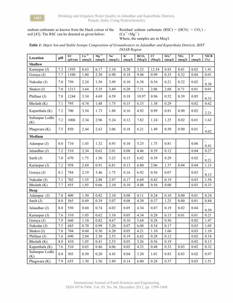
1603 Drinking and Irrigation Water Quality in Jalandhar and Kapurthala Districts, Punjab, India: Using Hydrochemsitry
International Journal of Earth Sciences and Engineering ISSN 0974-5904, Vol. 05, No. 06, December 2012, pp. 1599-1608
sodium carbonate as known from the black colour of the soil [43]. The RSC can be denoted as given below:
Residual sodium carbonate (RSC) = (HCO3- + CO3
-) - (Ca+++Mg++) Where, the samples are in Meq/l.
Table 1: Major Ion and Stable Isotope Composition of Groundwaters in Jalandhar and Kapurthala Districts, BIST
DOAB Region
Location pH EC
(µS/cm)
Ca 2+
(meq/l)
Mg 2+
(meq/l)
Na+
(meq/L)
K+
(meq/l)
HCO3-
(Meq/l)
Cl-
(Meq/l)
SO42-
(meq/l)
NO3-
(meq/l)
F-
(meq/l)
NICB
(%)
Shallow Kartarpur (J) 7.2 1595 8.63 6.17 2.10 0.20 3.23 12.54 0.83 0.01 0.02 1.41 Goraya (J) 7.7 1100 1.80 2.30 6.90 0.18 9.48 0.99 0.35 0.32 0.04 0.01
Nakodar (J) 7.0 750 2.24 1.56 3.49 0.10 6.38 0.54 0.21 0.32 0.02 -0.38
Shakot (J) 7.0 1213 3.64 5.35 3.49 0.20 7.31 2.06 2.60 0.71 0.01 0.01
Phillaur (J) 7.8 1244 3.34 4.69 4.59 0.18 10.97 0.96 0.52 0.39 0.05 -0.33
Bholath (K) 7.1 795 4.74 1.48 1.75 0.15 6.33 1.38 0.29
0.02 0.62
Kapurthala (K) 7.2 700 3.54 1.73 1.88 0.16 4.92 0.99 0.81 0.90 0.02 -2.21
Sultanpur Lodhi (K)
7.2 1006 2.34 2.96 5.24 0.12 7.82 1.24 1.25 0.02 0.01 1.62
Phagwara (K) 7.5 850 2.44 2.63 3.06 0.18 6.21 1.49 0.50 0.90 0.01 -4.62
Medium
Adampur (J) 8.0 710 1.45 1.32 4.93 0.10 5.25 1.75 0.81
0.06 -0.41
Jalandhar (J) 7.2 510 2.34 0.62 2.01 0.08 4.46 0.39 0.12
0.04 0.27
Sarih (J) 7.0 670 1.75 1.56 3.23 0.15 6.02 0.39 0.29
0.02 -0.21
Kartarpur (J) 7.2 958 2.69 0.91 6.81 0.13 6.80 2.06 1.37 0.04 0.04 1.13
Goraya (J) 8.1 784 2.19 3.46 1.75 0.16 6.92 0.56 0.07
0.03 -0.13
Nakodar (J) 7.1 702 1.55 2.88 2.97 0.17 6.69 0.42 0.19
0.03 1.58 Bholath (K) 7.7 455 1.85 0.66 2.10 0.10 4.08 0.56 0.00
0.03 0.33
Deep Adampur (J) 7.8 400 1.50 0.82 2.10 0.08 4.11 0.24 0.10 0.00 0.01 0.24 Sarih (J) 8.0 565 0.49 0.39 5.07 0.08 4.30 0.37 1.25 0.00 0.01 0.84
Jalandhar (J) 8.0 550 0.60 0.74 4.02 0.05 4.34 0.87 0.19 0.02 0.04 -0.59
Kartarpur (J) 7.6 510 1.05 0.62 3.10 0.05 4.34 0.28 0.15 0.01 0.01 0.21 Goraya (J) 7.9 660 1.10 0.82 4.67 0.10 5.64 0.28 0.56
0.02 1.47
Nakodar (J) 7.5 685 0.70 0.99 5.20 0.07 6.08 0.54 0.17
0.03 1.05 Shakot (J) 7.6 704 0.60 0.30 6.20 0.05 4.21 1.10 1.66
0.03 1.10
Phillaur (J) 7.6 690 2.04 2.30 2.53 0.19 6.62 0.28 0.12
0.02 0.18 Bholath (K) 8.0 410 1.05 0.41 2.53 0.05 3.26 0.56 0.19
0.02 0.13
Kapurthala (K) 7.6 510 0.65 0.46 4.06 0.05 4.33 0.48 0.33 0.03 0.02 0.32 Sultanpur Lodhi (K)
8.0 503 0.50 0.20 4.45 0.04 3.20 1.01 0.83 0.03 0.02 0.97
Phagwara (K) 7.9 655 1.30 1.56 3.89 0.14 6.00 0.28 0.37
0.03 1.51

1604 P. PURUSHOTHAMAN, M. SOMESHWAR RAO, B. KUMAR, Y. S. RAWAT, GOPAL KRISHAN, S. GUPTA, S. MARWAH, A. K. BHATIA, Y. B. KAUSHIK, M. P. ANGURALA and G. P. SINGH
International Journal of Earth Sciences and Engineering ISSN 0974-5904, Vol. 05, No. 06, December 2012, pp. 1599-1608
Figure 3: Piper Plot of the Groundwater at different Aquifers in Jalandhar and Kapurthala Districts
of Bist- Doab Region
-80 -40 0 40 80
(Ca+Mg)-(Na+K)
-80
-40
0
40
80
(HCO3)-(C
l+SO4)
-80 -40 0 40 80
-80
-40
0
40
80
Shallow
Medium
Deep
Figure 4: Chadha’s Classification of Groundwater at different Depth in the Jalandhar and Kapurthala Districts
of Bist- Doab Region
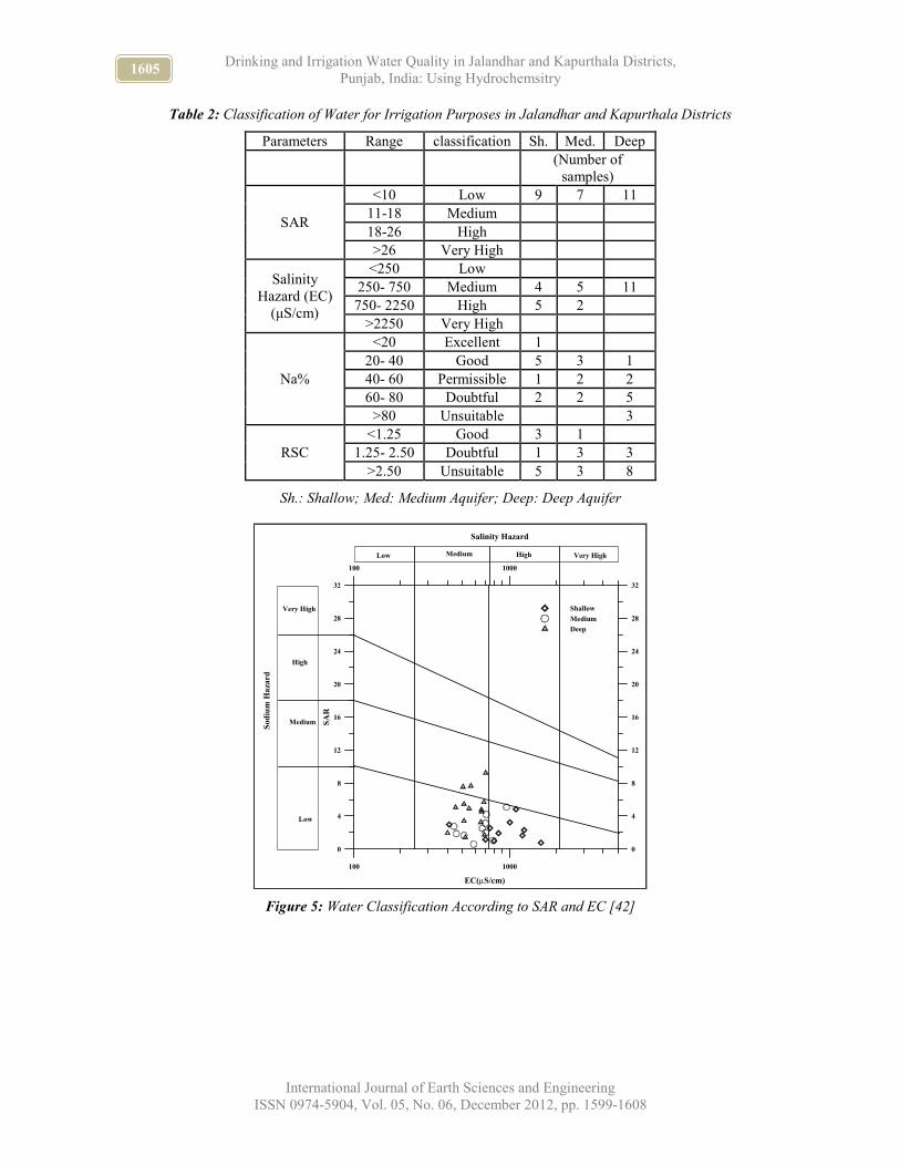
1605 Drinking and Irrigation Water Quality in Jalandhar and Kapurthala Districts, Punjab, India: Using Hydrochemsitry
International Journal of Earth Sciences and Engineering ISSN 0974-5904, Vol. 05, No. 06, December 2012, pp. 1599-1608
Table 2: Classification of Water for Irrigation Purposes in Jalandhar and Kapurthala Districts
Parameters Range classification Sh. Med. Deep
(Number of
samples)
SAR
<10 Low 9 7 11 11-18 Medium 18-26 High >26 Very High
Salinity Hazard (EC)
(µS/cm)
<250 Low 250- 750 Medium 4 5 11 750- 2250 High 5 2
>2250 Very High
Na%
<20 Excellent 1 20- 40 Good 5 3 1 40- 60 Permissible 1 2 2 60- 80 Doubtful 2 2 5
>80 Unsuitable 3
RSC <1.25 Good 3 1
1.25- 2.50 Doubtful 1 3 3 >2.50 Unsuitable 5 3 8
Sh.: Shallow; Med: Medium Aquifer; Deep: Deep Aquifer
Sodium H
azard
Low
Very High
High
Medium
Salinity Hazard
Low Medium High Very High
100 1000
EC(µS/cm)
0
4
8
12
16
20
24
28
32
SAR
100 1000
0
4
8
12
16
20
24
28
32
Shallow
Medium
Deep
Figure 5: Water Classification According to SAR and EC [42]

1606 P. PURUSHOTHAMAN, M. SOMESHWAR RAO, B. KUMAR, Y. S. RAWAT, GOPAL KRISHAN, S. GUPTA, S. MARWAH, A. K. BHATIA, Y. B. KAUSHIK, M. P. ANGURALA and G. P. SINGH
International Journal of Earth Sciences and Engineering ISSN 0974-5904, Vol. 05, No. 06, December 2012, pp. 1599-1608
UnsuitableExcellent to Good
Good to Permissible Permissible to
Unsuitable
1000 2000 3000 4000 5000
EC(µS/cm)
0
10
20
30
40
50
60
70
80
90
100
Sodium Percent
1000 2000 3000 4000 5000
0
10
20
30
40
50
60
70
80
90
100
Shallow
Medium
Deep
Figure 6: Classification of Irrigation Waters (Wilcox, 1955)
Almost all groundwater samples in the study region show high percentage of sodium and high RSC values (Table 2) indicating high concentration of sodium precipitation of carbonates. When the concentration of sodium ion is high in irrigation water, Na+ tends to be absorbed by clay particles, displacing magnesium and calcium ions. This exchange process of sodium in water for Ca2+ and Mg2+ in soil results in precipitation of calcium and magnesium bicarbonate with high concentration of bicarbonate resulting the reduction of permeability and eventually results in soil with poor internal drainage [27]. This shows that the soil in the study region suffers high risk in precipitation of carbonate that will result in the decrease in permeability.
Conclusion:
The study shows that groundwater quality in the area varies with different aquifers. The groundwater quality in the study area is suitable for drinking purpose with the concentration of most of the ions falling below desirable limit and all values lying within the permissible range of WHO and IS standards. The Piper plot and Chadha’s Diagram shows that groundwater in the shallow and medium aquifer are similar i.e. Ca+Mg+Na bicarbonate type whereas the deep aquifer shows NaHCO3 type of water. The study also shows that water quality for irrigation purpose differs widely. The sodium adsorbtion ratio (SAR) shows that water quality in all the aquifers is excellent. The SAR vs EC and Wilcox classification of water shows that the
groundwater in the study area is suitable for irrigation purpose. The sodium percentage and residual sodium carbonate (RSC) values in the groundwater shows possible precipitation of clay particles or Ca, Mg carbonates in the soil resulting in the deterioration/ degradation of soil. In summary, it is evident from the study that the water quality for drinking and irrigation purpose is suitable in the study area.
Acknowledgement:
The authors are thankful to Chandigarh regional Directorate of Central Ground Water Board for providing groundwater chemistry data for Jalandhar and Kapurthala Districts, Punjab, India. The present work is part of the research project funded by the World Bank under Purpose Driven Study of HP II, Ministry of Water Resources, Government of India, (GoI), initiated by the Hydrological Investigations Division of NIH, Roorkee, India. Hence, the financial support from the World Bank is acknowledged.
References:
[1] Nickson, R.T., Mc Arthur, J.M., Shrestha, B., Kyaw- Nyint, T.O. and Lowry, D. 2005. Arsenic and other drinking water quality issues, Muzaffargarh District, Pakistan. App. Geochem. 20, 55-68.
[2] Twarakavi, N. K. C. and Kaluarachchi, J. J. 2006. Sustainability of groundwater quality considering land use changes and public health risks. J. Environ. Manag. 81, 405-419.

1607 Drinking and Irrigation Water Quality in Jalandhar and Kapurthala Districts, Punjab, India: Using Hydrochemsitry
International Journal of Earth Sciences and Engineering ISSN 0974-5904, Vol. 05, No. 06, December 2012, pp. 1599-1608
[3] Forstner, U. K. and Wittman, G. T. W. 1981. Metal Pollution in the Aquatic Environment. Springer Verlag, Berli, Heidelberg, pp- 255.
[4] Obiefuna, G. I. and Orazulike, D. M. 2011. The Hydrochemical Characteristics and Evolution of Groundwater in Semiarid Yola Area, Northeast, Nigeria. Res. J. Environ. Earth Sci. B, 400-416.
[5] Back, W. 1966. Hydrochemical facies and groundwater flow pattern in northern part of Atlantic Coastal Plain. US Geological Survey Professional Paper 498A.
[6] Drever, J. J. 1982. The geochemistry of natural waters. Prentice-Hall, Englewood Cliffs, p. 388.
[7] Aghazadeh, N. and Mogaddam, A. A. 2010. Assessment of Groundwater Quality and its Suitability for Drinking and Agricultural Uses in the Oshnavieh Area, Northwest of Iran. J. Environ. Protect. 1, 30-40.
[8] Garrels, R. M. 1967. Genesis of some groundwaters from igneous rocks. In: Abelson, P. H. (ed) Researches in geochemistry. Wiley, New York, 405-420.
[9] Garrels, R. M. and MacKenzie, F. T. 1967. Origin of the chemical compositions of some springs and lakes. In: Equilibrium Concepts in Natural Waters. American Cancer Society, Washington, DC.
[10] Paces, T. 1973. Steady state kinetics and equilibrium between groundwater and granite rock. Geochim. Cosmochim. Acta. 37, 2641- 2663.
[11] Frape, S. K., Fritz, P. and McNutt, R. H. 1984. Water-rock interaction and chemistry of groundwaters from the Canadian Shield. Geochim. Cosmochim. Acta. 48, 1617-1627.
[12] Stuyfzand, P. J. 1986. A new Hydrochemical classification of water Types: Principles and application to the coastal dunes aquifer system of the Netherlands. Proceedings of the 9th Salt water Intrusion Meeting, Delft, pp- 641-655.
[13] Hem, J. D. 1989. Study and interpretation of the chemical characteristics of natural water. US Geol. Surv. Water-Supply Paper 2254.
[14] Sarin, M. M., Krishnaswami, S., Killi, K., Somayajulu, B. L. K. and Moore, W. S. 1989. Major ion chemistry of the Ganga-Brahmaputra River basin system: weathering processes and fluxes to the Bay of Bengal. Geochim. Cosmochim. Acta. 53, 997-1009.
[15] Walraevens, K. 1990. Hydrogeology and Hydrogeochemistry of the Ledo-Paniselian semi confined aquifer in East and West Flanders. Acad. Analecta 52, 11-66
[16] Stuyfzand, P. J. 1993. Hydrogeochemistry and hydrology of the coastal dune area of the western Netherlands. Ph.D. Thesis, Free University Amsterdam, Netherlands.
[17] Garcia, M. C., Hidalgo-Medel, V., Apella, M. C. and Blessa, M. A. 1998. Chemical quality of deep groundwater in Yerba Buena and San-Miguel de Tucuman Cities (Abstract). Vol. 2, School of Environment Sciences and Technology, Buenos- Aires, pp: 498.
[18] Garcia, M. C., Hidalgo-Medel, V., Apella, M. C. and Blessa, M. A. 1998. Chemical characteristics of deep groundwater in the cities of San Miguel de Tucuman and Yerba Buena Province of Tucuman. Proc. 10th Lat.-Am.Geol. Cong. and 6th Natural Cong. of Eco. Geol., Buenos- Aires, Vol. 3, 342-347.
[19] Mclean, W., Jankowski, J. and Lavitt, N. 2000. Groundwater Quality and Sustainability in an Alluvial Aquifer, Australia. In: Silio, O. and Balkema, A. A. (Eds.), Groundwater, Past Achievements and Future Challenges. Rotterdam, 567-573.
[20] Pannatier, E. G., Broers, H. P., Venema, P. and Van Beusekom, G. 2000. A new Process- Based Hydrogeochemical classification of Groundwater: Application to the Netherlands National Monitoring System. INO report, NITG 00-143-B, 38, NITG, Utrecht.
[21] Galindo, M. C., Vece, M. B., Perondi, M. E., Moserrate Araoz, M., Garcia, M.G., Hidalgo-Medel, V., Apella, M. C. and Blesa, M. A. 2001. Chemical behaviour of the Sali-River Province of Tucuman, Argentina. Environ. Geol. 40, 847-852.
[22] Walraevens, K., Mahauden, M. and Coetsiers, M. 2003. Natural background Concentration of trace element in aquifers of the Flemish region, as a reference for the government sanitation policy. FZK/TNO Conference on contaminated soil (Consoil), Ghent, 215-224.
[23] Hartman, J., Berna, Z., Stuben, D. and Henze, N. 2005. A statistical procedure for the analysis of seismotechtonically induced hydrochemical signals: a case study from the Eastern Carpathians, Romania. Tectonophy. 405, 77-98.
[24] Nagaraju, A., Suresh, S., Killham, K. and Hudson-Edwards, K. 2006. Hydrogeochemistry of Waters of Mangampeta Barite Mining Area, Cuddapah Basin, Andhra Pradesh, India. Turk. J. Eng. Environ. Sci. 30, 203-219.
[25] Jezersky, Z. 2007. Hydrogeochemistry of a deep gas storage cavern, Czech Republic. Hydrogeol. J. 15, 599-614.
[26] Zhu, G. F., Su, Y. H. and Feng, Q. 2008. The hydrochemical characteristics and evolution of groundwater and surface water in the Heihe River Basin, northwest China. Hydrogeol. J. 16, 167-182.
[27] Belkhiri, L., Boudoukha, A. and Mouni, L. 2010. Groundwater quality and its suitability for drinking

1608 P. PURUSHOTHAMAN, M. SOMESHWAR RAO, B. KUMAR, Y. S. RAWAT, GOPAL KRISHAN, S. GUPTA, S. MARWAH, A. K. BHATIA, Y. B. KAUSHIK, M. P. ANGURALA and G. P. SINGH
International Journal of Earth Sciences and Engineering ISSN 0974-5904, Vol. 05, No. 06, December 2012, pp. 1599-1608
and agricultural use in Ain Azel plain, Algeria. J. Geogr. Reg. Plann. 3, 151-157.
[28] Karmegam, U., Chidamabram, S., Sasidhar, P., Manivannan, R., Manikandan, S. and Anandhan, P. 2010. Geochemical Characterization of Groundwater’s of Shallow Coastal Aquifer in and around Kalpakkam, South India. Res. J. Environ. Earth Sci. 2, 170-177.
[29] Tiri, A., Belkhiri, L., Boudoukha, A. and Lahbari, N. 2011. Characterization and evaluation of the factors affecting the geochemistry of surface water of Koudiat Medouar Basin, Algeria. African J. Environ. Sci. Tech. 5, 355-362.
[30] CGWB. 2007. Ground Water Scenario of Jalandhar District, Punjab. Central Ground Water Board North Western Region, Chandigarh, pp- 15.
[31] CGWB. 2007. Groundwater Information Booklet Kapurthala District Punjab. Central Ground Water Board North Western Region, Chandigarh, pp- 20.
[32] Tiwana, N. S., Jeerat, N., Ladhar, S. S., Singh, G., Paul, R., Dua, D. K. and Parwana, H. K. 2007. State of Environment: Punjab- 2007. Punjab state council for science and technology, pp. 243.
[33] BIS. 1991. Specification for drinking water IS: 10500: 1991. Bureau of Indian Standards. New delhi.
[34] WHO (World Health Organization). 2004. Guidelines for drinking water quality. 2nd edn, Vol. 1, Geneva, WHO, pp- 130.
[35] Piper, A. M. 1944. A graphic procedure in the geochemical interpretation of water analyses. Trans. Am. Geophys. Union 25, 914-928.
[36] Chadha, D. K. 1999. A proposed new diagram for geochemical classification of natural waters and interpretation of chemical data. Hydrogeol. J. 7, 431-439.
[37] Richards, L. A. 1954. Diagnosis and Improvement of Saline and Alkali Soils Agriculture Handbook. 60, Department of Agricultural, Washington DC, US, pp- 160.
[38] Todd, D. K. 1980. Groundwater Hydrology. 2nd ed., John Wiley and Sons, New York, p. 535.
[39] Domenico, P. A. and Schwartz F. W. 1990. Physical and Chemical Hydrogeology. John Wiley and Sons, New York.
[40] Wilcox, L. V. 1955. Classification and use of irrigation water. US Geological Department Agri. Circ. 969: 19.
[41] U.S. Salinity Laboratory. 1954. Diagnosis and Improvement of Saline and Alkaline soils. U.S. Dept. of Agriculture. Hand Book, No. 60, 160.
[42] Eaton, E. M. 1950. Significance of Carbonate in irrigation water. Soil Sci. 69, 123-133.

www.cafetinnova.org
Indexed in
Scopus Compendex and Geobase Elsevier, Chemical
Abstract Services-USA, Geo-Ref Information Services-USA
ISSN 0974-5904, Volume 05, No. 06
December2012,P.P.1609-1618
#02050619 Copyright ©2012 CAFET-INNOVA TECHNICAL SOCIETY. All rights reserved.
Groundwater Quality Assessment around Talabasta Area, Banki
Sub-Division, Odisha, India
ROSALIN DAS1, MADHUMITA DAS
2 and SHREERUP GOSWAMI
3
1Department of Geology, Banki Autonomous College, Banki-754008
2Department of Geology, Utkal University, Vani Vihar, Bhubaneswar-751004, Odisha
3Department of Geology, Ravenshaw University, Cuttack-753003, Odisha
Email: [email protected], [email protected], [email protected]
Abstract: The study area forms part of the Athgarh basin of upper Gondwana formation consisting of a thick pile of
fresh water fluviatile and lacustrine sediments. The deeper aquifers are the main source of drinking water supply for
the local community. Twenty groundwater samples have been collected during the pre-monsoon and post-monsoon
periods of 2010 and analyzed for the water quality parameters such as pH, electrical conductivity, total dissolved
solids, calcium, magnesium, sodium, potassium, bicarbonate, sulphate, chloride etc. Suitability of the ground water
for different purposes such as drinking and irrigation is evaluated following various classification schemes and water
quality standards. Piper’s Trilinear diagram reveals that water of the study area belongs to the Ca-Mg- HCO3 facies.
Keywords: Talabasta, Athgarh Formation, Groundwater quality, Odisha
Introduction:
The study area is located in Banki sub-division of
Cuttack district, Odisha (Fig. 1) bounded by 200 15’ N
to 200 29’N latitudes and 85
0 20’ to 85
0 45’ E longitudes
and covers a total area of 58.5 hectors. The study area
belongs to the Athgarh basin of upper Gondwana
formation. It consists of a thick pile of fresh water
fluviatile and lacustrine sediments. The area enjoys
humid tropical climate. The nearest perennial source of
water is Rana river. The rock types of this area are
laterite, conglomerate, sandstone (feldspathic and
ferruginous), sandy clay, ironstone shale and fireclay.
Fireclay occurs interstratified with sandstone having
limited down dip extension. Ironstone shale appears to
be a marker horizon above fireclay bed. The occurrence
of fireclay is formed by weathering of feldspathic
constituents in the zone of oxidation.
Materials and Method:
20 water samples have been collected during pre and
post-monsoon periods of 2010. Out of 20 samples 10
samples have been collected from tube wells and 10
samples from dug wells. Electrical conductivity (EC)
and pH have been measured using digital meters
immediately after sampling. Water samples have been
analysed for chemical constituents, such as sodium,
potassium, calcium, magnesium, chloride, bicarbonate,
carbonate, sulphate, nitrate, fluoride and Total
Dissolved Solids (TDS) in the laboratory using the
standard methods as suggested by the American Public
Health Association (APHA, 1995); Trivedi and Goel
(1984) and Vogel (1964). The groundwater quality is
assessed with respect to WHO (2004) and BIS (1991)
standards.
Results and Discussion:
Groundwater Chemistry:
Understanding the quality of groundwater with its
temporal and seasonal variation is important because it
is the factor that determines suitability for drinking,
domestic and agricultural purposes. The pH of water is
an indicator of its quality and geochemical equilibrium
(Hem, 1985). pH of the pre-monsoon samples are acidic
and ranged from 5.25 to 6.89 with an average value of
6.07, while in the post-monsoon an increase is observed
and ranged from 6.05 to 8.21 with an average 7.13
(Tables 1, 2). The EC values ranged from 235µs/cm to
998µs/cm during pre-monsoon and 268µs/cm to
1090µs/cm during post-monsoon period. Higher values
are generally noticed in the southeastern part of the
study area. The TDS values ranged from 177mg/l to
739mg/l and 211mg/l to 827mg/ during pre and post-
monsoon periods respectively. Total Hardness values
ranged from 97mg/l to 466mg/l during pre-monsoon
and 87mg/l to 300mg/l during post-monsoon (Tables 1,
2). Water samples of 14 locations are hard whereas in 2
locations the waters are very hard and water samples of
4 locations are moderately hard in nature.
The chemical parameters of different groundwater
samples are given in the Tables 1 and 2. The
concentrations of chloride ranged from 20.7mg/l to
127.8mg/l during pre-monsoon and 2.53mg/l to

1610 ROSALIN DAS, MADHUMITA DAS and SHREERUP GOSWAMI
International Journal of Earth Sciences and Engineering
ISSN 0974-5904, Vol. 05, No. 06, December 2012, pp. 1609-1618
142.81mg/l during post-monsoon period. The
concentrations of fluoride ranged from 0.101mg/l to
1.76mg/l during pre-monsoon and 0.04mg/l to 1.73mg/l
during post-monsoon period. Sulphate concentrations
ranged from 0.27mg/l to 63.7mg/l during pre-monsoon
and 0.062mg/l to 56.3mg/l during post-monsoon period.
Nitrate values ranged from 0mg/l to 23.5mg/l and
0.01mg/l to 39.8mg/l during pre and post-monsoon
periods respectively. The calcium concentration ranged
from 26mg/l to 127mg/l and 11.7mg/l to 112mg/l during
pre- and post-monsoon periods respectively. The
magnesium content of the water samples ranged from
7.63mg/l to 36.23mg/l during pre-monsoon and 6.48mg/l
to 34.26mg/l during post-monsoon period. Sodium
concentrations ranged from 1.7mg/l to 88.3mg/l during
pre-monsoon and 9.76mg/l to 97.0mg/l during post-
monsoon period. Potassium concentrations of the study
area ranged from 0.68mg/l to 59mg/l and 1.0mg/l to
65mg/l during pre and post-monsoon periods respectively
(Tables 1, 2).
Drinking Water Suitability:
To assess the suitability of groundwater for drinking
purpose, the concentrations were compared with the
WHO standards (2004) for drinking water, which shows
that most of the surface and subsurface water of the
study area are suitable for the drinking and domestic use
with few exceptions, as most of the parameters are
within the permissible limits (Table 3). Based on TDS
classification, 20% of water samples are excellent in
both the seasons (Table 4). 10% samples of pre-
monsoon and 5% samples of post-monsoon are
classified under poor class on the basis of total hardness
(Table 5).
Piper Trilinear Diagram:
The groundwater samples are plotted in the Piper (1944)
Trilinear Diagram (Fig. 2). The plot shows that most of
the groundwater samples fall in the field of mixed Ca–
Mg-HCO3 type of water. The groundwater samples of
pre-monsoon and post-monsoon fall in the fields 4 and
5, (Fig. 2), which suggest that alkaline earth exceeds
strong acids. Calcium and Sodium are the major cations
in the study area forming 75-90% of the cations.
Bicarbonate is the major anion in the study area.
Irrigation Purpose:
The quality of water suitable for irrigation purpose is
judged on the basis of Sodium Adsorption Ratio (SAR),
Percent Sodium (Na %), Residual Sodium Carbonate
(RSC), Potential Soil Salinity (PS), Permeability Index
(PI) etc.
Sodium Adsorption Ratio (SAR):
Excessive sodium content relative to the calcium and
magnesium reduces the soil permeability (Kelley, 1995;
Tijani, 1994) and thus, inhibits the supply of water
needed for the crops. The excess sodium or limited
calcium and magnesium are evaluated by SAR which is
expressed as,
( ) 2/MgCa
NaSAR
++++
+
+=
Where concentrations are expressed in equivalent per
million (epm). The sodium or alkali hazard in the use of
water for irrigation is determined by the absolute and
relative concentrations of cations and is expressed in
terms of sodium absorption ratio (SAR), proposed by
the U.S.Salinity Laboratory (USSL, 1954). The
calculated values of SAR in the study area ranged from
0.339 to 14.79 in pre-monsoon and 2.717 to 16.69 in
post-monsoon. From SAR value (Table 6) quality of
water is detected. A more detailed analysis for the
suitability of water for irrigation is made by plotting the
data on U.S. Salinity Laboratory diagram (Richards,
1954) (Fig. 3).
In the U.S. Salinity diagram (Richards, 1954) EC is
plotted against SAR (Fig. 3). The analytical data plotted
on the USSL diagram (Richards, 1954) illustrates that
10% of the groundwater samples from pre-monsoon and
20% from post-monsoon fall in the field C3S1,
indicating high salinity and low sodium water, which
can be used for irrigation for almost all types of soil
with little danger of exchangeable sodium (Fig. 3).
Groundwater samples that fall in the low salinity hazard
class (C1) can be used for irrigation of most crops in
majority of soils. However, some leaching is required,
but this occurs under normal irrigation practices except
in soils of extremely low permeability. In pre and post-
monsoon periods 45% and 35% of groundwater samples
respectively fall in medium salinity hazard class (C2).
They can be used if a moderate amount of leaching
occurs. High salinity water (C3) cannot be used in soils
with restricted drainage. Even with adequate drainage,
special management for salinity control is required and
crops with good salt tolerance should be selected. Such
areas need special attention as far as irrigation is
concerned.
Percent Sodium (Na %):
In all natural waters percent of sodium content is a
parameter to assess suitability for agriculture (Wilcox,
1948). A maximum of 60% sodium in ground water is
allotted for agricultural purposes (Ramakrishna, 1998).
Wilcox (1948) defined Sodium percentage in terms of
epm of the common Cations.
++++++
++
+++
+=
KNaMgCa
100)KNa(%Na
In pre-monsoon the sodium percentage (%Na) in the
study area ranges from 10.29% to 58.16%. The highest

1611 Groundwater Quality Assessment around Talabasta Area, Banki Sub-Division, Odisha, India
International Journal of Earth Sciences and Engineering
ISSN 0974-5904, Vol. 05, No. 06, December 2012, pp. 1609-1618
percentage of sodium is found in the dug well water
sample of Pakhalakhala. And the minimum value is
located in the tube well water sample of Talabasta. In
post-monsoon the value of sodium percentage (% Na)
varies within 11.06 % to 70.53%. Wilcox (1955) used
%Na and specific conductance in evaluating irrigation
waters using the Wilcox diagram as given in (Fig. 4).
Most of the water samples fall in excellent to good and
good to permissible categories indicating their
suitability for irrigation. 25% of samples in post-
monsoon are doubtful, but no water sample is strictly
unsuitable for irrigation (Table 7). The water of
excellent to good and good to permissible can be used
for irrigation purpose.
Residual Sodium Carbonate (RSC):
In addition to the SAR and %Na, the excess sum of
carbonate and bicarbonate in groundwater over the sum
of calcium and magnesium also influences the
suitability of groundwater for irrigation. An excess
quantity of sodium bicarbonate and carbonate is
considered to be detrimental to the physical properties
of soils as it causes dissolution of organic matter in the
soil, which in turn leaves a black stain on the soil
surface on drying. This excess is denoted by Residual
Sodium Carbonate (RSC) and is calculated as follows
(Raghunath, 1987)
RSC= (CO3--
+ HCO3-) – (Ca
+++ Mg
++)
Where all concentrations are expressed in epm.
The classification of irrigation water (WHO, 2004)
according to the RSC values is presented in (Table 8).
The residual sodium carbonate varies from -4.91 to 2.52
in pre-monsoon, while it varies from -3.88 to 1.94 epm
in post-monsoon water samples.
Potential Soil Salinity (PS):
Doneen (1962) proposed a criterion based on the
salinity of the irrigation water, which is an improvement
over the U.S. soil salinity. The potential soil salinity
(PS) is given by the concentration of chloride added to
half of sulphate expressed in epm.
PS=Cl +1/2 SO4
Potential soil salinity varies from 0.66epm to 4.21epm
in pre-monsoon where as in post-monsoon it varies from
0.65epm to 4.11epm. From the PS classification, the
groundwaters of the study area come under excellent to
good category (Table 9).
Permeability Index (PI):
The soil permeability is affected by long-term irrigation
influenced by Na+, Ca
++, Mg
++ and HCO
-3 contents of
the soil. The permeability index (PI) values also indicate
the suitability of groundwater for irrigation. It is defined
as (Doneen, 1962)
The concentration of cations and anions are in epm. The
groundwater samples of the study area fall in class I and
II (Doneen, 1962) on the basis of Permeability Index
(PI) values (Fig.5). According to these values, 30% of
the groundwater comes under class-I category and 70%
comes under class-II category in pre-monsoon. In post-
monsoon period 25% samples fall in class-I and 75%
samples fall in class-II category (Fig. 5). According to
Doneen chart (Domenico and Schwartz 1990) the
ground water of the study area is of good quality for
irrigation purpose based on the permeability index. The
increased percentage of groundwater samples under
class–I1 is due to dilution and subsequent lower values
of permeability index.
Magnesium Ratio (MR):
Generally calcium and magnesium maintain a state of
equilibrium in most waters. More Mg2+
present in
waters will adversely affect the soil quality, converting
it to alkaline and decreases crop yields. Rocks in the
watershed contain more magnesium and most waters
contain Mg2+
more than Ca2+
.
The magnesium ratio can be expressed as,
Where all the ions are expressed in epm. The
Magnesium ratio in all most all the pre-monsoon and
post-monsoon samples is below 50, except in four
locations,where the ratio is more than 50.
Gibb’s Diagram:
Based on aquifer lithology, the mechanism, controlling
chemical relationship of ground water has been studied
by Gibb (1970). In the Gibb’s diagram, three kinds of
fields are recognized namely precipitation dominance,
evaporation dominance and rock water dominance. In
case of anion, all the samples pointed towards rock
dominance in the chemistry of ground water (Fig. 6).
This reflects the influence of aquifer lithology vis-à-vis
ground water chemistry. Similarly, in case of cations, all
the samples show rock dominance (Fig. 6). Hence, the
groundwater of the study area is mainly dominated by
the lithology of aquifer of the region.
Conclusion:
From the chemical analysis, it is revealed that the
groundwater of Talabasta area is acidic or / and weakly
acidic in nature. Calcium and Magnesium are the major
cations and bicarbonate is the major anion in the study
area. The higher concentrations of the bicarbonate
indicate chemical weathering of the rocks. The
groundwater belongs to Ca-Mg-HCO3 facies. The Ca,

1612 ROSALIN DAS, MADHUMITA DAS and SHREERUP GOSWAMI
International Journal of Earth Sciences and Engineering
ISSN 0974-5904, Vol. 05, No. 06, December 2012, pp. 1609-1618
Mg, HCO3 indicate the temporary hardness, alkalinity
and dominance of alkaline earth and weak acids. All the
chemical parameters indicate that the groundwater of
the study area is safe for drinking. Graphical
representation of the chemical data on the irrigation
suitability diagram (USSL, 1954) shows that medium
salinity-low sodium (C2S1) and high salinity-low
sodium (C3S1) waters are present, which need adequate
drainage to overcome the salinity problem. Chemical
composition of ground water is a reflection of rock
weathering, decomposition and anthropogenic
interventions, causing changes in time and space. The
chemical quality of the study area is well within the
permissible limit meant for drinking and irrigation
purpose. As water quality is interlinked with water
quantity, regular monitoring should be undertaken to
maintain the quality of ground water, as ground water
consumption is bound to increase due to erratic
monsoon pattern and higher demand due to population
growth.
Acknowledgements:
The authors thank to Groundwater Survey and
Investigation (GWSI), Bhubaneswar for chemical
analysis. The authors are also thankful to revered
reviewers for critically going through our manuscript
and suggesting many alterations to improve the standard
of the paper.
References:
[1] APHA 1995Standard methods for the examination
of water and wastewater, 19th edn. American
Public Health Association, Washington, D.C., pp
1467
[2] BIS 1991. Indian Standard for Drinking Water as
per BIS specifications (IS 10500-1991)
[3] Domenico, P.A. and Schwartz, F.W. 1990. Physical
and chemical Hydrogeology. John Wiley and Sons,
New York, pp 410-420
[4] Doneen, L.D. 1962. The influence of crop and soil
on percolating water. Proc. 11961 Biennial
conference on Groundwater Recharge, pp 156-163.
[5] Gibbs, R.J. 1970. Mechanism controlling world
water chemistry. Science 170, 1088-1090
[6] Hem, J.D. 1985. Study and interpretation of the
chemical characteristics of natural water. USGS,
Water Supply Paper 2254, 264
[7] Kelley, W.P. 1995. Alkali soils-Their formation
properties and reclamation, Reinold Publ.Corp.,
New York
[8] Piper, A.M. 1944. A graphical procedure in the
geochemical interpretation of water analysis. Am
Geophys Union Trans 25, 914–928
[9] Ragunath, H.M. 1987. Groundwater. Wiley
Eastern, New Delhi, pp 563
[10] Ramakrishna 1998. Ground water, Hand book,
India, pp 556
[11] Richards, L.A. 1954. Diagnosis and improvement
of saline and alkaline soils U.S. Deptt. Agri. Hand
Book 60, pp160
[12] Tijani, J. 1994. Hydrochemical assessmrnt of
groundwater in Moro area, Kwara State, Nigeria,
Environment Geology 24, 194-202
[13] Trivedi, R.K. and Goel, P.K. 1984. Chemical and
biological methods for water pollution studies. Env.
Publ. Karad, India. pp 215
[14] Vogel, A.L. 1964. A text book of qualitative
inorganic analysis, 3rd
edition, pp 438
[15] WHO 2004. Guideline of Drinking water quality in
Health criteria and other supporting information.
World Health Organization 2:336
[16] Wilcox, L.V. 1948. The Quality of water for
irrigation, Use U.S. Dept. of Agriculture, Tech,
Bull, 1962, Washington, DC, pp 19
[17] Wilcox, L.V. 1955. Classification and use of
irrigation water, USDA, Circular, 969, Washington
D.C., U.S.A., pp 19

1613 Groundwater Quality Assessment around Talabasta Area, Banki Sub-Division, Odisha, India
International Journal of Earth Sciences and Engineering
ISSN 0974-5904, Vol. 05, No. 06, December 2012, pp. 1609-1618
Figure 1: Location Map of the Study Area

1614 ROSALIN DAS, MADHUMITA DAS and SHREERUP GOSWAMI
International Journal of Earth Sciences and Engineering
ISSN 0974-5904, Vol. 05, No. 06, December 2012, pp. 1609-1618
Figure 2: Piper’s Trilinear Diagram
Figure 3: U.S. Salinity Laboratory Diagram Showing Classification of Water Samples for Irrigation Purpose

1615 Groundwater Quality Assessment around Talabasta Area, Banki Sub-Division, Odisha, India
International Journal of Earth Sciences and Engineering
ISSN 0974-5904, Vol. 05, No. 06, December 2012, pp. 1609-1618
Figure 4: Wilcox diagram for Classification of Groundwater Based on EC and Na%
Figure 5: PI Diagram

1616 ROSALIN DAS, MADHUMITA DAS and SHREERUP GOSWAMI
International Journal of Earth Sciences and Engineering
ISSN 0974-5904, Vol. 05, No. 06, December 2012, pp. 1609-1618
Figure 6: Gibb’s Diagram
Table 1: Chemical Parameters of Groundwater (Pre-monsoon)
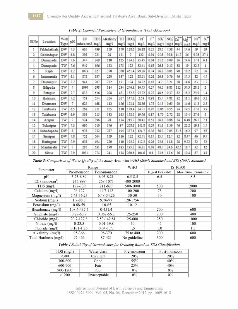
1617 Groundwater Quality Assessment around Talabasta Area, Banki Sub-Division, Odisha, India
International Journal of Earth Sciences and Engineering
ISSN 0974-5904, Vol. 05, No. 06, December 2012, pp. 1609-1618
Table 2: Chemical Parameters of Groundwater (Post -Monsoon)
Table 3: Comparison of Water Quality of the Study Area with WHO (2004) Standard and BIS (1991) Standard
Parameter Range WHO
IS 10500
Pre-monsoon Post-monsoon Higest Desirable Maximum Permissible
pH 5.25-6.89 6.05-8.21 6.5-8.5 6.5 8.5
EC (mhos/cm2) 235-998 268-1073 400-2000
TDS (mg/l) 177-739 211-827 500-1000 500 2000
Calcium (mg/l) 26-127 11.7-112 100-200 75 200
Magnesium (mg/l) 7.63-36.23 6.48-34.26 30-50 30 100
Sodium (mg/l) 1.7-88.3 9.76-97 20-1756
Potassium (mg/l) 0.68-59 1.0-65 10-12
Bicarbonate (mg/l) 108.6-437.5 0-451.4 200 600
Sulphate (mg/l) 0.27-63.7 0.062-56.3 25-250 200 400
Chloride (mg/l) 20.7-127.8 2.53-142.81 25-600 250 1000
Nitrate (mg/l) 0-23.5 0.01-39.8 50 45 100
Fluoride (mg/l) 0.101-1.76 0.04-1.73 1.5 1.0 1.5
Alkalinity (mg/l) 95-366 98-370 75 to 400 200 600
Total Hardness (mg/l) 97-466 87-421 No guideline 300 600
Table 4 Suitability of Groundwater for Drinking Based on TDS Classification
TDS (mg/l) Water class Pre-monsoon Post-monsoon
<300 Excellent 20% 20%
300-600 Good 55% 40%
600-900 Fair 25% 40%
900-1200 Poor 0% 0%
>1200 Unacceptable 0% 0%

1618 ROSALIN DAS, MADHUMITA DAS and SHREERUP GOSWAMI
International Journal of Earth Sciences and Engineering
ISSN 0974-5904, Vol. 05, No. 06, December 2012, pp. 1609-1618
Table 5: Suitability of Groundwater for Drinking Based on Total Hardness (TH) as CaCO3 (mg/L)
TH(mg/l) Water class Pre-monsoon Post-monsoon
<75 Excellent 0% 0%
75-150 Good 25% 50%
150-300 Fair 65% 45%
>300 Poor 10% 5%
Table 6: Quality of Water Based on SAR Values
Water classes for Irrigation SAR value No. of sample (out of 20)
Pre-monsoon Post-monsoon
Excellent Up to 10 15 13
Good 18-Oct 5 7
Medium 18-26 Nil Nil
Bad >26 Nil Nil
Table 7: Water Class for Irrigation Based on Na%
Water class for irrigation % of Na No of sample Pre-monsoon
(out of 20)
Post-monsoon
(out of 20)
Excellent to Up to 20 3 1
Good 20-40 11 6
Permissible to 40-60 6 8
Doubtful 60-80 Nil 5
Unsuitable >80 Nil Nil
Table 8: Rating of Waters Based on Residual Sodium Carbonate
RSC(epm) Water category Pre-monsoon Post-monsoon
No. of wells % of sample No. of wells % of sample
<1.25 Safe 17 85% 16 80%
1.25-2.5 Marginally 02 10% 04 20%
>2.5 Unsuitable 01 5% Nil Nil
Table 9: Classification of Ground Water Based on P.S. (Potential Soil Salinity)
P.S Class No. of Sample (out of 20)
Pre-monsoon Post-monsoon
<5 Excellent to Good 20 20
5-10 Good to Injurious Nil Nil
>10 Injuries to Satisfactory Nil Nil

www.cafetinnova.org
Indexed in
Scopus Compendex and Geobase Elsevier, Chemical
Abstract Services-USA, Geo-Ref Information Services-USA
ISSN 0974-5904, Volume 05, No. 06
December2012,P.P.1619-1629
#02050620 Copyright ©2012 CAFET-INNOVA TECHNICAL SOCIETY. All rights reserved.
Terrain Analysis and Hydrogeochemical Environment of Aquifers
of the southern West Coast of Karnataka, India
S. S. HONNANAGOUDAR1, D. VENKAT REDDY
1 and MAHESHA. A
2
1Dept of Civil Engineering, National Institute of Technology Karnataka, Surathkal, Mangalore - 575025, Karnataka
2Department of Applied Mechanics and Hydraulics, National Institute of Technology Karnataka, Surathkal,
Mangalore - 575025, Karnataka
Email: [email protected], [email protected], [email protected]
Abstract: Dakshina kannada district is situated in peninsular region. The peninsula is composed of geologically
ancient rocks of diverse original and most of them have undergone metamorphism. The early Precambrian tonalitic
gneisses invaded by granites, granulites and dolerite dykes. Granulites are mostly restricted to areas south of
Mangalore. High grade alumina rich (corundum bearing) metamorphic schists have been encountered and younger
alkaline intrusive rocks like Aegerine syenites have been reported. There are five rivers and estuaries. Number of
lineaments cut across each other and some lineaments are parallel to each other. The Arabian sea class is the largest
among other land cover features in the study area. The river/tidal creek land cover appear as long irregular and
sinous in outline. Mulki river, Netravati river, Gurupur river at southern terrain. The qualities of groundwater at
sandy aquifer are good, lateritic/weathered gneissic rocks it is sweet.
Keywords: Groundwater, Rock Types, Lineaments, Water Quality
Introduction:
The Dakshina Kannada district which is a coastal
district of Karnataka spreads along the west coast of
India covering coastal track of about 40 km. It has been
found that two-third of the population lives within a
narrow belt, directly landward from the ocean edges.
Also, the rivers of district are being seasonal and tidal in
nature; seawater intrusion into adjoining aquifers during
the non-monsoon period is greatly felt up to several
kilometres inland along and on either side of the river
courses. Hence, the present work is aimed at
groundwater related investigation involving aquifer
characterization and seawater intrusion of coastal
Dakshina Kannada district, Karnataka between
Talapady to Mulki towns. The focus of the present work
is to create awareness on water quality degradation and
its management in rural coastal areas between the rivers
Talpady, Gurupur, Pavanje, Mulki, and Netravati. The
fresh water partly met by surface water resources.
Geology:
Dakshina kannada district is situated in peninsular
region. The process of erosion, transportation and
deposition, the shape of the coastline changes, often
slowly but sometimes rapidly. The intersection between
rock, water, wind and vegetation are responsible for the
dramatic landforms along the coast. The peninsula is
composed of geologically ancient rocks of diverse
original and most of them have undergone
metamorphism. It represents a stable land of the earth’s
crust. The geological formations of the district are
similar those of Karnataka state but for the coastal
sedimentary deposits and laterites. The geological
section across Netravati river of dakshina kannada
district is shown in figure (Figure1)
The early Precambrian tonalitic gneisses invaded by
granites, granulites and dolerite dykes. Granulites are
mostly restricted to areas south of Mangalore; however
tongues of granulites can be seen in gneissic granite
quarries north of mangalore. High grade alumina rich
(corundum bearing) metamorphic schists have been
encountered and younger alkaline intrusive rocks like
Aegerine syenites have been reported (Ravindra and
Janardhan 1981). Marine expeditions conducted by
Geological Survey of India (GSI) identified the
existence of sandy paleobeach ridges some 25 km
offshore of Mangalore coast. Earlier Murty (1977)
reported occurrences of lignite in clays from the
foundation wells of Netravati bridge, south of
Mangalore. Black clays occur in some of the paleo
fluvial courses such as Baikampadi, Kuloor and Kottar
usually admixed with plant remains (peat or lignite).
The geology of the terrain comprises peninsular gneissic
basements, laterites, coastal alluvium, granite-migmatite
complexes and intrusions of acid, basic and ultramafic
into the basement rocks. Sparsely developed quaternary
formations are also seen along the coastal tract. The
deposition of number of rocky and Sandy Island of the
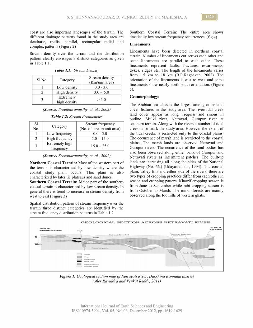
1620 S. S. HONNANAGOUDAR, D. VENKAT REDDY and MAHESHA. A
International Journal of Earth Sciences and Engineering
ISSN 0974-5904, Vol. 05, No. 06, December 2012, pp. 1619-1629
coast are also important landscapes of the terrain. The
different drainage patterns found in the study area are
dendratic, trellis, parallel, rectangular radial and
complex patterns (Figure 2)
Stream density over the terrain and the distribution
pattern clearly envisages 3 distinct categories as given
in Table 1.1.
Table 1.1: Stream Density
Sl No. Category Stream density
(Km/unit area)
1 Low density 0.0 - 3.0
2 High density 3.0 - 5.0
3 Extremely
high density > 5.0
(Source: Sreedharamurthy, et. al., 2002)
Table 1.2: Stream Frequencies
Sl
No. Category
Stream frequency
(No. of stream unit area)
1 Low frequency 0.0 - 5.0
2 High frequency 5.0 - 15.0
3 Extremely high
frequency 15.0 – 25.0
(Source: Sreedharamurthy, et. al., 2002)
Northern Coastal Terrain: Most of the western part of
the terrain is characterized by low density where the
coastal study plain occurs. This plain is also
characterized by lateritic plateaus and sand dunes.
Southern Coastal Terrain: Major part of the southern
coastal terrain is characterized by low stream density. In
general there is trend to increase in stream density from
west to east (Figure 3)
Spatial distribution pattern of stream frequency over the
terrain three distinct categories are identified by the
stream frequency distribution patterns in Table 1.2.
Southern Coastal Terrain: The entire area shows
drastically low stream frequency occurrences. (fig 4)
Lineaments:
Lineaments have been detected in northern coastal
terrain. Number of lineaments cut across each other and
some lineaments are parallel to each other. These
lineaments represent faults, fractures, escarpments,
dykes, ridges etc. The length of the lineaments varies
from 1.5 km to 18 km (B.R.Raghavan, 2002). The
orientation of the lineaments is east to west and some
lineaments show nearly north south orientation. (Figure
5).
Geomorphology:
The Arabian sea class is the largest among other land
cover features in the study area. The river/tidal creek
land cover appear as long irregular and sinous in
outline. Mulki river, Netravati, Gurupur river at
southern terrain. Along with the rivers a number of tidal
creeks also mark the study area. However the extent of
the tidal creeks is restricted only to the coastal plains.
The occurrence of marsh land is restricted to the coastal
plains. The marsh lands are observed Netravati and
Gurupur rivers. The occurrence of the sand bodies has
also been observed along either bank of Gurupur and
Netravati rivers as intermittent patches. The built-up
lands are increasing all along the sides of the National
Highway (No. 66.) (Udayashankar, 1994). The coastal
plain, valley fills and either side of the rivers; there are
two types of cropping practices differ from each other in
season and cropping pattern. Kharrif cropping season is
from June to September while rabi cropping season is
from October to March. The minor forests are mainly
observed along the foothills of western ghats.
Figure 1: Geological section map of Netravati River, Dakshina Kannada district
(after Ravindra and Venkat Reddy, 2011)

1621 Terrain Analysis and Aquifer Characteristics of West Coast
of Dakshina Kannada District, Karnataka, India
International Journal of Earth Sciences and Engineering
ISSN 0974-5904, Vol. 05, No. 06, December 2012, pp. 1619-1629
Figure 2: Drainage Pattern: Southern Coastal Karnataka
Figure 3: Distribution of Stream Density
Figure 4: Distribution of Stream Frequency

1622 S. S. HONNANAGOUDAR, D. VENKAT REDDY and MAHESHA. A
International Journal of Earth Sciences and Engineering
ISSN 0974-5904, Vol. 05, No. 06, December 2012, pp. 1619-1629
Figure 5: Lineaments of Southern Coastal Karnataka
Land use:
Land use refers to human activities for various use
carried out on land and cover refers to natural
vegetation, water bodies, rock, soil, artificial cover and
others resulting due to land transformations. Change in
land use pattern influences the hydrological regime of
the basin (James et, al., 1987). Various hydrological
processes such as infiltration, evapotranspiration, soil
moisture status etc., are influenced by land use
characteristics of water shed. The deforestation may
cause peak flows in the river due to reduced infiltration
leading to floods, due to increased soil erosion, removal
of too fertile soil layer may result in drop in soil
fertility.
The spatial information on land use and their pattern of
changes are essential for planning, management and
utilization of land for agriculture, forestry, urban
industries, environmental studies etc.
Infiltration:
Infiltration rates are very widely depending on the
condition of the land surface. Infiltration has an
important place in the hydrological cycle. Detailed
study of hydrological process helps planners,
hydrologists, farmers and decision makers in number of
ways. The infiltration rate of the area which helps in
estimating peak rate and volume of runoff, estimation of
surface runoff and overland flow, estimation of
groundwater recharge, estimation of soil moisture
deficits. Typical infiltration rates are at the end of one
hour after the commencement of the storm are presented
in Table 1.3.
Table 1.3: Infiltration Rate
Sl.
No. Soil Type
Infiltration
rate cm/hr
1 High (Sandy soil) 1.25 – 2.54
2 Intermediate (loam,
silt, clay) 0.25 -1.25
3 Low (clay, clay-loam) 0.025 – 0.25
From east to west the majority of the sedimentary units
consists of a wedge of permeable sand sediments
deposited in shallow marine water, littoral sands formed
in the fore shore and the adjacent beach and sand-dune
systems (Antonelline et al. 2008). In the westernmost
are fine continental alluvial deposits (silt and clay)
overlay the littoral sands (Amorosi et al. 2002;
Bondesan et al. 1995).

1623 Terrain Analysis and Aquifer Characteristics of West Coast
of Dakshina Kannada District, Karnataka, India
International Journal of Earth Sciences and Engineering
ISSN 0974-5904, Vol. 05, No. 06, December 2012, pp. 1619-1629
Groundwater Quality:
The qualities of groundwater at sandy aquifer are good,
lateritic/weathered gneissic rocks it is sweet. The dug
wells in the alluvial area are saline water during summer
months and in the monsoon period fresh water they are
getting. There are 30 open well samples are collected
and test the well water samples to detect the presence of
drinking water. The drinking water quality parameters
for analysis are TDS, pH, Turbidity, Total hardness, Fe,
Nitrate, Sulphate and Coliform. The well location is
mentioned in Table no. 1.4. The results are calculated in
Table 1.5 to Table 1.13 in the three seasons April,
August and October 2012.
Table 1.4: Well Inventories
Well
No.
Location Well
No.
Location
1 Hotel Nisarga, Talapady 16 NMPT, Panambur
2 Uchilla 17 Hotel Vishwasagar, Panambur
3 Kotekar 18 Jyothi service station, Hosabettu
4 Thokkuttu 19 KEB Quarters, Surathkal
5 S.S. Bricks, Thokkuttu 20 Veerabhadra Temple, Marigudi
6 Adam kadru school 21 NITK, Surathkal
7 Kalapu 22 Gerald Kuvelo Nivas, Mukka
8 Shaikh cottage 23 K.A. Abdulkadar, Mukka
9 Mogaru (Near Netravathi Bridge) 24 “Kiran” Haliyangadi
10 Ronsun service centre, Mogaru 25 Kikanda House, Near Pavanje Bridge
11 Karnataka Bank, Near pumpwell 26 Venkappa shetty, Padambadur
12 Kuntikana 27 Nani House, Kolnad
13 VRL, kuloor 28 Sri Guru, Kolnad
14 Vivekanand, Panjioruguru, Kuloor 29 Srinivas, Bappanadu temple, Mulki
15 Thokuru 30 Gopalkrishna Naik, Mulki
Table 1.5: Water Quality Test Results for pH
Well No. pH
April
pH
August
pH
October Well No.
pH
April
pH
August
pH
October
1 6.63 5.86 7.67 16 5.97 7.55 6.52
2 6.36 6.69 6.9 17 6.19 6.48 6.13
3 6.17 7.13 7.56 18 6.22 6.51 6.32
4 6.33 6.53 6.82 19 6.08 6.41 6.23
5 6.49 6.06 6.6 20 5.71 6.44 6.13
6 6.66 6.6 6.87 21 5.91 7.87 6.17
7 6.54 6.54 6.8 22 6.11 7 5.93
8 5.89 6.16 6.5 23 6.36 6.31 5.83
9 6.47 5.94 6.25 24 6 7.01 6.78
10 6.58 6.45 6.65 25 6.51 6.29 5.94
11 6.63 6.2 6.39 26 6.83 6.51 6.34
12 6.16 6.28 6.54 27 6.32 6.91 6.53
13 6.38 6.1 6.17 28 5.69 6.45 6.01
14 6.63 6.48 6.45 29 6.2 6.37 5.96
15 6.38 6.19 6.43 30 6.38 6.6 6.19

1624 S. S. HONNANAGOUDAR, D. VENKAT REDDY and MAHESHA. A
International Journal of Earth Sciences and Engineering
ISSN 0974-5904, Vol. 05, No. 06, December 2012, pp. 1619-1629
Table 1.6: Water Quality Test Results for TDS mg/l
Well No. TDS
April
TDS
August
TDS
October Well No.
TDS
April
TDS
August
TDS
October
1 6.63 5.86 7.67 16 5.97 7.55 6.52
2 6.36 6.69 6.9 17 6.19 6.48 6.13
3 6.17 7.13 7.56 18 6.22 6.51 6.32
4 6.33 6.53 6.82 19 6.08 6.41 6.23
5 6.49 6.06 6.6 20 5.71 6.44 6.13
6 6.66 6.6 6.87 21 5.91 7.87 6.17
7 6.54 6.54 6.8 22 6.11 7 5.93
8 5.89 6.16 6.5 23 6.36 6.31 5.83
9 6.47 5.94 6.25 24 6 7.01 6.78
10 6.58 6.45 6.65 25 6.51 6.29 5.94
11 6.63 6.2 6.39 26 6.83 6.51 6.34
12 6.16 6.28 6.54 27 6.32 6.91 6.53
13 6.38 6.1 6.17 28 5.69 6.45 6.01
14 6.63 6.48 6.45 29 6.2 6.37 5.96
15 6.38 6.19 6.43 30 6.38 6.6 6.19
Table 1.7: Water Quality Test Results for Turbidity
Well
No.
Turbidity
April
Turbidity
August
Turbidity
October
Well
No.
Turbidity
April
Turbidity
August
Turbidity
October
1 6.63 5.86 7.67 16 5.97 7.55 6.52
2 6.36 6.69 6.9 17 6.19 6.48 6.13
3 6.17 7.13 7.56 18 6.22 6.51 6.32
4 6.33 6.53 6.82 19 6.08 6.41 6.23
5 6.49 6.06 6.6 20 5.71 6.44 6.13
6 6.66 6.6 6.87 21 5.91 7.87 6.17
7 6.54 6.54 6.8 22 6.11 7 5.93
8 5.89 6.16 6.5 23 6.36 6.31 5.83
9 6.47 5.94 6.25 24 6 7.01 6.78
10 6.58 6.45 6.65 25 6.51 6.29 5.94
11 6.63 6.2 6.39 26 6.83 6.51 6.34
12 6.16 6.28 6.54 27 6.32 6.91 6.53
13 6.38 6.1 6.17 28 5.69 6.45 6.01
14 6.63 6.48 6.45 29 6.2 6.37 5.96
15 6.38 6.19 6.43 30 6.38 6.6 6.19

1625 Terrain Analysis and Aquifer Characteristics of West Coast
of Dakshina Kannada District, Karnataka, India
International Journal of Earth Sciences and Engineering
ISSN 0974-5904, Vol. 05, No. 06, December 2012, pp. 1619-1629
Table 1.8: Water Quality Test Results for Chloride mg/l
Well No. Chloride
April
Chloride
August
Chloride
October Well No.
Chloride
April
Chloride
August
Chloride
October
1 6.63 5.86 7.67 16 5.97 7.55 6.52
2 6.36 6.69 6.9 17 6.19 6.48 6.13
3 6.17 7.13 7.56 18 6.22 6.51 6.32
4 6.33 6.53 6.82 19 6.08 6.41 6.23
5 6.49 6.06 6.6 20 5.71 6.44 6.13
6 6.66 6.6 6.87 21 5.91 7.87 6.17
7 6.54 6.54 6.8 22 6.11 7 5.93
8 5.89 6.16 6.5 23 6.36 6.31 5.83
9 6.47 5.94 6.25 24 6 7.01 6.78
10 6.58 6.45 6.65 25 6.51 6.29 5.94
11 6.63 6.2 6.39 26 6.83 6.51 6.34
12 6.16 6.28 6.54 27 6.32 6.91 6.53
13 6.38 6.1 6.17 28 5.69 6.45 6.01
14 6.63 6.48 6.45 29 6.2 6.37 5.96
15 6.38 6.19 6.43 30 6.38 6.6 6.19
Table 1.9: Water Quality Test Results for Hardness mg/l
Well No. Hardness
April
Hardness
August
Hardness
October Well No.
Hardness
April
Hardness
August
Hardness
October
1 300 278 276 16 50 46 45
2 160 157 156 17 190 189 190
3 40 41 45 18 80 76 78
4 90 87 86 19 50 47 44
5 580 569 589 20 30 31 37
6 120 122 128 21 50 48 54
7 50 46 47 22 110 109 109
8 50 47 40 23 70 65 65
9 370 375 379 24 30 32 32
10 80 81 83 25 350 346 346
11 280 275 278 26 80 76 76
12 20 22 23 27 130 126 126
13 250 245 249 28 50 48 48
14 80 76 79 29 280 267 267
15 200 201 208 30 70 65 65

1626 S. S. HONNANAGOUDAR, D. VENKAT REDDY and MAHESHA. A
International Journal of Earth Sciences and Engineering
ISSN 0974-5904, Vol. 05, No. 06, December 2012, pp. 1619-1629
Table 1.10: Water Quality Test Results for Nitrate mg/l
Well No. Nitrate
April
Nitrate
August
Nitrate
October Well No.
Nitrate
April
Nitrate
August
Nitrate
October
1 4.76 4.7 4.98 16 15.17 15.89 14.8
2 13.21 12.41 12.95 17 29.25 29.84 28.45
3 39.64 36.61 35.61 18 18.52 17.58 18.89
4 9.58 9.89 9.09 19 14.26 13.2 14.27
5 11.26 10.23 11.29 20 19.31 20.39 19.56
6 1.09 1.02 1.98 21 8.66 8.9 9.12
7 0.81 0.4 1 22 19.76 18.78 19.23
8 23.16 22.12 22.94 23 6.78 6.7 6.12
9 2.41 2.19 2.86 24 5.26 5.98 5.23
10 10.25 9.26 10.01 25 9.53 9.53 8.92
11 1.09 1.67 1.41 26 7.62 6.89 6.21
12 20.44 21.32 21 27 4.53 5.56 5.12
13 10.85 11.85 11.01 28 12.82 12.86 11.86
14 17.9 16.76 15.23 29 5.64 5.9 6.24
15 5.57 6.5 5.59 30 4.51 4.98 4.89
Table 1.11: Water Quality Test Results for Coliform Count CFU/ml
Well
No. Coliform Coliform Coliform
Well
No. Coliform Coliform Coliform
A B A B A B A B A B A B
1 1 - 1 - 2 - 16 - - - - - -
2 - - - - - - 17 2 - 2 - 1 -
3 - - - - - - 18 - - - - - -
4 1 - 1 - 1 - 19 - - - - - -
5 - - - - 1 - 20 1 - - - - -
6 - - - - - - 21 - - - - - -
7 - - - - - - 22 5 - 4 - 5 -
8 1 - 2 - 1 - 23 1 - 1 - 1 -
9 - - - - - - 24 - - - - - -
10 - - - - - - 25 3 1 2 1 1 1
11 1 - 1 - 1 - 26 - - - - - -
12 - - - - - - 27 1 - - - - -
13 1 - 1 - - - 28 - - - - - -
14 - - - - - - 29 3 - 1 - 1 -
15 4 - 5 - 3 - 30 1 - 2 - 1 -
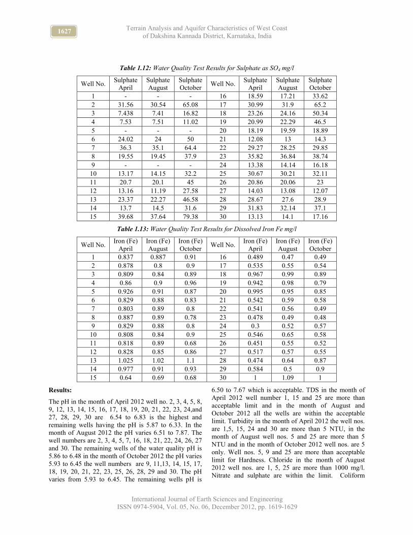
1627 Terrain Analysis and Aquifer Characteristics of West Coast
of Dakshina Kannada District, Karnataka, India
International Journal of Earth Sciences and Engineering
ISSN 0974-5904, Vol. 05, No. 06, December 2012, pp. 1619-1629
Table 1.12: Water Quality Test Results for Sulphate as SO4 mg/l
Well No. Sulphate
April
Sulphate
August
Sulphate
October Well No.
Sulphate
April
Sulphate
August
Sulphate
October
1 - - - 16 18.59 17.21 33.62
2 31.56 30.54 65.08 17 30.99 31.9 65.2
3 7.438 7.41 16.82 18 23.26 24.16 50.34
4 7.53 7.51 11.02 19 20.99 22.29 46.5
5 - - - 20 18.19 19.59 18.89
6 24.02 24 50 21 12.08 13 14.3
7 36.3 35.1 64.4 22 29.27 28.25 29.85
8 19.55 19.45 37.9 23 35.82 36.84 38.74
9 - - - 24 13.38 14.14 16.18
10 13.17 14.15 32.2 25 30.67 30.21 32.11
11 20.7 20.1 45 26 20.86 20.06 23
12 13.16 11.19 27.58 27 14.03 13.08 12.07
13 23.37 22.27 46.58 28 28.67 27.6 28.9
14 13.7 14.5 31.6 29 31.83 32.14 37.1
15 39.68 37.64 79.38 30 13.13 14.1 17.16
Table 1.13: Water Quality Test Results for Dissolved Iron Fe mg/l
Well No. Iron (Fe)
April
Iron (Fe)
August
Iron (Fe)
October Well No.
Iron (Fe)
April
Iron (Fe)
August
Iron (Fe)
October
1 0.837 0.887 0.91 16 0.489 0.47 0.49
2 0.878 0.8 0.9 17 0.535 0.55 0.54
3 0.809 0.84 0.89 18 0.967 0.99 0.89
4 0.86 0.9 0.96 19 0.942 0.98 0.79
5 0.926 0.91 0.87 20 0.995 0.95 0.85
6 0.829 0.88 0.83 21 0.542 0.59 0.58
7 0.803 0.89 0.8 22 0.541 0.56 0.49
8 0.887 0.89 0.78 23 0.478 0.49 0.48
9 0.829 0.88 0.8 24 0.3 0.52 0.57
10 0.808 0.84 0.9 25 0.546 0.65 0.58
11 0.818 0.89 0.68 26 0.451 0.55 0.52
12 0.828 0.85 0.86 27 0.517 0.57 0.55
13 1.025 1.02 1.1 28 0.474 0.64 0.87
14 0.977 0.91 0.93 29 0.584 0.5 0.9
15 0.64 0.69 0.68 30 1 1.09 1
Results:
The pH in the month of April 2012 well no. 2, 3, 4, 5, 8,
9, 12, 13, 14, 15, 16, 17, 18, 19, 20, 21, 22, 23, 24,and
27, 28, 29, 30 are 6.54 to 6.83 is the highest and
remaining wells having the pH is 5.87 to 6.33. In the
month of August 2012 the pH varies 6.51 to 7.87. The
well numbers are 2, 3, 4, 5, 7, 16, 18, 21, 22, 24, 26, 27
and 30. The remaining wells of the water quality pH is
5.86 to 6.48 in the month of October 2012 the pH varies
5.93 to 6.45 the well numbers are 9, 11,13, 14, 15, 17,
18, 19, 20, 21, 22, 23, 25, 26, 28, 29 and 30. The pH
varies from 5.93 to 6.45. The remaining wells pH is
6.50 to 7.67 which is acceptable. TDS in the month of
April 2012 well number 1, 15 and 25 are more than
acceptable limit and in the month of August and
October 2012 all the wells are within the acceptable
limit. Turbidity in the month of April 2012 the well nos.
are 1,5, 15, 24 and 30 are more than 5 NTU, in the
month of August well nos. 5 and 25 are more than 5
NTU and in the month of October 2012 well nos. are 5
only. Well nos. 5, 9 and 25 are more than acceptable
limit for Hardness. Chloride in the month of August
2012 well nos. are 1, 5, 25 are more than 1000 mg/l.
Nitrate and sulphate are within the limit. Coliform

1628 S. S. HONNANAGOUDAR, D. VENKAT REDDY and MAHESHA. A
International Journal of Earth Sciences and Engineering
ISSN 0974-5904, Vol. 05, No. 06, December 2012, pp. 1619-1629
count is found in the well nos.1, 4, 5, 8, 11, 15, 17, 22,
25, 29 and 30 for all the season.
This contamination is more pronounced in wells along
the stream courses up to the distance where tidal effect
extends. Further, Ground water in proximity to stream
course is contaminated with seepage of domestic waste.
As a general rule, pumpage must be distributed in time
and space and there should not be any concentration of
wells to avoid saline water ingress.
Conclusions:
The intersection between rock, water, wind and
vegetation are responsible for the dramatic landforms
we see along the coast. Dakshina kannada district is
situated in peninsular region.
The slope density and stream frequency of the study
area are characteristically high along the eastern part of
the terrain because the streams originate on the scarps of
the Western Ghats.
The land use and land cover pattern of the terrain is
suggestive of probable stress on the terrain in future in
terms of expansion of built-up land and loss of
agricultural land due to a probable increase in the
number of industries and population.
From the field study some of the area is affected by
saltwater intrusion during the summer period and some
of the areas are affected almost throughout the year.
Ground water in proximity to stream course is
contaminated with seepage of domestic waste. As a
general rule, pumpage must be distributed in time and
space and there should not be any concentration of wells
to avoid saline water ingress.
References:
[1] Adyalkar, P. G., and Shrihari Rao, S. (1979).
Hydrodynamic method of assessing groundwater
recharge by precipitation in Deccan trap region-
case study. Jour. Geol. Soc. Ind., V. 20, pp. 134-
137.
[2] Adrian D. Werner, James D. Ward, Leanne K.
Morgan, Craig T. Simmons, Niville I. Robinson,
and Michael D, Teubner., (2012).“Vulnerability
indicators of seawater intrusion.” Ground Water 50
(1), pp.48-58.
[3] Aghashe, R.M. (1994). Artificial recharge of
groundwater in critical and semi-critical areas.
Proc. Natl. Workshop Development of groundwater
in critical and semi-critical areas: Alternatives,
Options and Strategies, NewDelhi, pp. 75-88.
[4] Alley,William M. and C. J.
Taylor.(2001).“Groundwater level monitoring and
the importance of long term waterlevel data.”
U.S.Geol. Survey Circular: pp.1217.
[5] Anbazhagan, S., and Ramasamy, S.M., (1993).
Role of Remote Sensing in geomorphic analysis for
water harvesting structures, In: S.M. Ramasamy,
(Ed.) Trends in Geological Remote Sensing, Rawat
Publications, New Delhi, pp. 208-212.
[6] Anning, D., (2008). “Dissolved solids in basin-fill
aquifers of the southwest”. Hydrogeol. J., pp.18-19.
[7] Bloom, A. L. (1978). Geomorphology - A
systematic analysis of late Cenozoic Landforms.
Prentice Hall, pp. 1-510.
[8] Boulton (1970). “Analysis of data from pumping
tests in unconfined anisotropic aquifers.” J.
Hydrol., 10, 369-381.
[9] Chitea. F. (2011). “Geophysical detection of marine
intrusions in Black sea coastal areas (Rommania)
using VES and ERT data”, Geo-Eco-Marina,
pp.95-102.
[10] Coates, D. R. and Vitek, J. D. (1980). Threshold in
Geomorphology, George Allen, London, pp. 223.
[11] Kelly W.E., (1977).“Geoelectric sounding for
estimating aquifer hydraulic conductivity”, Ground
Water, 15(6), pp.420-425.
[12] Mahesha A., (1996).“Control of seawater intrusion
through injection – extraction well system”, J.
Irrig. Drain. Eng., ASCE, pp.314-317.
[13] Manjunath B.R. and Harry N.A. (1994). “Geology
of Western Coastal Karnataka, GeoKarnataka”,
MGD Centenary Volume, pp. 109-116.
[14] Moench, A.F., (1994). “Specific yield as
determined by type curve analysis of aquifer test
data”, Ground Water, 32(6), pp.949-957.
[15] Moench, A.F., (1997). “Flow to a well of finite
diameter in a homogeneous, anisotropic water table
aquifer”, Water Resour. Res., 33 (6), pp.1397-1407.
[16] Mohsen Sheriff., (1999). “Seawater intrusion in the
Nile delta aquifer: An overview”,
http://aguas.igme.es/igme/publica/tiac-02/EGIPTO-
I.pdf. pp.296-308 (April 10, 2012).
[17] Polemio. M.V., Dragone and Limoni, P.P., (2009),
“Monitoring and methods to analyse the
groundwater quality degradation risk in coastal
karstic aquifers (Apulia, Southern Italy)”, Environ.
Geol., 58, pp. 299-312.
[18] Ravindra, B. M., Venkata Reddy, D. (2011).
“Neotectonic Evolution of Coastal Rivers of
Mangalore Karavali Karnataka, India”. Int. Jour.
Of Earth Science and Engineering, V.04. No. 04,
pp. 561-574.
[19] Reddy, N. and Prakasam, P. (1982). “Evaluation of
artificial recharge projects in Granitic Terrains of
Andhra Pradesh”. Workshop on Artificial Recharge
of Groundwater in Granitic Terrain, pp. 194-210.
[20] Singh, O. P. (1981), “Morphometric evalution of
landforms in Palamau Upland.” In: H. S. Sharma
(Ed) Perspectives in Geomorphology”, Concept
Publishing Co., New Delhi, V. 4, pp. 109-131.

1629 Terrain Analysis and Aquifer Characteristics of West Coast
of Dakshina Kannada District, Karnataka, India
International Journal of Earth Sciences and Engineering
ISSN 0974-5904, Vol. 05, No. 06, December 2012, pp. 1619-1629
[21] Singh (2006). “Semi-analytical model for
drawdown due to pumping a partially penetrating
large diameter well”, J.Irrig. Drain., ASCE, 133(2),
pp.155-161.
[22] Sridharan. K, D. Sathyanarayana, A. Siva Reddy.,
(1990), “Analysis of flow near a dug well in an
unconfined aquifer, J.Hydrol., 119, pp.89-103.
[23] Sreedharamurthy, T. R., Raghavan, B. R. and Bhat,
V.T., (2002). “Terrain Analysis of Coastal
Karnataka”, Sponsored project by Ministry of
Environment and forests, Mangalore University,
Mangalore.
[24] Sung-Ho Song, Jin Yong Lee and Namsik Park.,
(2006). “Use of vertical electrical sounding to
delineate seawater intrusion in coastal area of
Byunsan, Korea”, Environ. Geol. (2007), Vol 52:1,
pp.1207-1219.
[25] Todd, D. K. (1980). “ Groundwater Hydrology.”
John Willey and Sons, Newyork, pp. 1-535.
[26] Ward, R. C. (1968), “Some hydrological
characteristics of British Rivers”, Jour. Hydrol., V.
pp. 358-372.
[27] Way, D. A. (1973). “Terrain Analysis,” Hutchinson
and Ross, Stroudsburg, Pasadina, Dowden, pp. 72-
124.

www.cafetinnova.org
Indexed in
Scopus Compendex and Geobase Elsevier, Chemical
Abstract Services-USA, Geo-Ref Information Services-USA
ISSN 0974-5904, Volume 05, No. 06
December2012,P.P.1630-1638
#02050621 Copyright ©2012 CAFET-INNOVA TECHNICAL SOCIETY. All rights reserved.
Water Quality Modeling and Management of Karanja River in
India
BASAPPA. B. KORI1, SHASHIKANTH MISE
1 and SHASHIDHAR
2
1Dept. of Civil Engineering, PDA Engineering College, Gulbarga, Karnataka, India
2Department of Civil Engineering, IIT- Hydrabad, India
Email: [email protected]
Abstract: The river Karanja, a major drinking water source for the Bhalki municipality is under threat by the
disposal of effluents from the industries such as Sugar, Paper and distilleries. To study the effect of effluent disposal
on this river, one dimensional steady-state stream water quality model was developed using QUAL2Kw. In this
model pre-monsoon data is used for calibration. From the sensitivity analysis, it was observed that the model is
sensitive for temperature, bottom width, discharge and biochemical oxygen demand. Simulations were carried out
for several scenarios such as bottom algae, head water release, shade and temperature under dry weather flow
condition. All these profile did not meet the requirement of minimum DO concentration, to get it bottom algae is to
be reduced to 75%, head water BOD is to be reduced to 8mg/L, and shade is to be increased up to 30%.
Keywords: Stream Water Quality, Water Quality Management and QUAL2Kw
1. Introduction:
Environmental pollution is one of the serious threats
faced by mankind. This has accelerated the discovery of
environmental problems during the past few decades.
Rapid population growth, urbanization, industrialization
and land development along the stream have increased
the stress on river pollution and have resulted in its
deterioration (Surindrasuthar, 2009). The deterioration
of aquatic ecosystem results from decrease in the
dissolved oxygen concentration and also, due to
pollutant degradation by micro-organisms, chemical
oxidation, plant, algal and phytoplankton respiration
(Drolc and Konkan, 1996). It also results in unpleasant
odors, and other aesthetic damage (Arruda
Camargo,2010). Hence, it is essential to monitor water
quality changes in the entire river, but it is tedious, time
consuming and un-economical.
The mathematical models are the alternative way to
describe the relation between waste loads and water
bodies. QUAL2Kw is one-dimensional steady state
stream water quality model; it uses unequally-spaced
reaches. It is well documented and is freely available.
QUAL2Kw includes many new elements (Pelletier and
Chapra, 2005).
A conventional sensitivity analysis is performed by
varying important parameters that which has effect on
the model output (Nikolaos P. Nikolaidis et al. 2006).
For the management of water quality, several scenarios
are studied by changing model input parameters during
the dry period (Ritu Paliwal and Prateek Sharma 2007).
considering i) Bottom algae modification, ii)
temperature modification iii) head water modification
and iv)Shade modification.
2. Material and Methods:
2.1. Study Area:
The Karanja river is one of the tributaries to the
Godavari river. It originates near Kohir village of
Andhra Pradesh state of India and joins another
tributary of Godavari i.e. Manjera river at 122 km
downstream. This river has a dam called Karanja which
in near Bhyalhalli village. Fig.1 shows the study area,
which has spread between N 17o 49
׀ , E 77
o 20
׀ and N
18o
02׀ , E 77
o 12
with an altitude of 554-575m above
MSL. The average annual rain fall is 830mm and
average temperature ranges between 35oc to 42
oc.
2.2. Water Quality Monitoring Sites:
Based on the topographical, nature of water flow, nature
of river bed, and disposal of effluent and considering the
accessibility for sampling, a total of four sampling
points were selected covering 21.85km stretch of
Karanja river for the present investigation. The samples
were collected at various locations along the river.
2.3. River Descretization:
The stretch of the river between karanja reservoir and
Bhalki pump station was selected for the study. The
length of 21.85km was deseretization into 19 reaches
with unequal lengths, based on the geography of the
study area. The releases from the Karanja reservoir were

1631 BASAPPA. B. KORI, SHASHIKANTH MISE and SHASHIDHAR
International Journal of Earth Sciences and Engineering
ISSN 0974-5904, Vol. 05, No. 06, December 2012, pp. 1630-1638
taken as head water data. Fig. 2 shows the river system
unequal segmentation along with the reservoir in which
effluents are being dischared.
2.4. Sampling and Analysis:
The studies were carried out on hourly basis for 24
hours pre-monsoon (30th
June 2010) and analyzed for
the parameters such as temperature, pH, dissolved
oxygen(DO), (BOD)5, nitrate nitrogen (NO3-N),
ammonia nitrogen (NH4-N), conductivity, velocity, and
water depth were measured along the river at sampling
locations. All the activities such as sample collection,
preservation, transportation and analysis were carried
out as per the standard methods (APHA-1995).
2.5. Modeling Tool:
The modeling tool QUAL2Kw has a general mass
balance equation for a constituent concentration ci
(Fig.3) in the water column (excluding hyporheic) of a
reach i (the transport and loading terms are omitted
from the mass balance equation for bottom algae
modeling) as (Pelletier et al., 2006).
Where Qi= flow at reach i(L/day), Qab,i= abstraction
flow at reach i(L/day), Vi= volume of reach i(L), Wi=
the external loading of the constituent to reach i
(mg/day), Si= sources and sinks of the constituent due to
reactions and mass transfer mechanisms (mg/L/day),
Ei= bulk dispersion coefficient between reaches
(L/day), Ei−1, Ei are bulk dispersion coefficients between
reaches i−1 and i and i and i + 1 (L/day),ci=
concentration of water quality constituent in reach
i(mg/L)and t= time (day). Figure 4 Represents the
Schematic Diagram of Interacting Water Quality State
Variables
For auto-calibration, the model uses genetic algorithm
(GA) to maximize the goodness of the fit of the model
results compared with measured data by adjusting a
large number of parameters. The GA maximizes the
fitness function f(x) as:
Where Oi,j= observed values, Pi,j= predicted values,
m=number of pairs of predicted and observed values, wi
= weighting factors and n=number of different state
variables included in the reciprocal of the weighted
normalized RMSE. Detailed descriptions of auto-
calibration method can be found in Pelletier et al.
(2006).
3. Model Calibration:
3.1. Model Input:
The model allows the use of input data for the hydraulic
characteristics of various reaches. Each reach is
idealized as a trapezoidal channel. Under condition of
steady flow, the Manning’s equation was used to
calculate mean velocity and depth as a function of the
stream width, bottom slopes and manning’s roughness
co-efficient. The Karanja river is a natural stream
channel with weeds, windings and pools. For such a
stream, manning’s roughness co-efficient may be
assumed between 0.06-0.07 (Pelletier et al. 2006).
(3)
Where Q = flow rate [m3/s], So = bottom slope [m/m],
n = the manning’s roughness coefficient, Ac = the cross-
sectional area [m2], and P = the wetted perimeter [m In
the head water boundary condition sheet of the model,
the required parameters such as flow rate, temperature,
conductivity, dissolved oxygen, ultimate carbonaceous
biochemical oxygen demand, ammonia nitrogen, nitrate
nitrogen, alkalinity and pH are given as input. The
phytoplankton and pathogen were not measured and the
inputs were left blank. During sampling, it was observed
that the maximum surface of the river bed was covered
by algae and bottom sediment; therefore the algae cover
and bottom-sediment oxygen demand were both
assumed to be 100%. The sediment/hyporheic zone
thickness, sediment porosity and hyporheic exchange
flow were assumed to be 10 cm, 40%, and 5%
respectively.
3.2. Kinetic Parameters:
The ranges of model kinetic parameters were obtained
from QUAL2Kw user manual (Pelletier and Chapra,
2005) and documentation for the enhanced stream water
quality model QUAL2E and QUAL2E-UNCAS (Brown
and Barnwell, 1987).To calculate re-aeration rate
coefficient, Owens–Gibbs formula (Owens et al., 1964)
was applied. The other parameters were set as default in
QUAL2Kw.The model was calibrated by using pre-
monsoon data. Hence, the pre-monsoon calibrated
model was used for further study and the calibrated
kinetic rate parameter for pre-monsoon was presented in
Table 1.

1632 Water Quality Modeling and Management of Karanja River in India
International Journal of Earth Sciences and Engineering
ISSN 0974-5904, Vol. 05, No. 06, December 2012, pp. 1630-1638
Figure 1: Location Map of the Study Area
Figure 2: Discritization of Karanja River
Figure 3: Mass Balance in a Reach Segment i. Source: (Pelletier and Chapra, 2005)
(Note: ab: Bottom Algae, ap: Phytoplankton, mo: Detritus, cs: Slow BOD, c f : Fast BOD, cT: Total Inorganic
Carbon, o: Oxygen, no: Organic Nitrogen, na: Ammonia Nitrogen, nn: Nitrite and Nitrate Nitrogen)
Figure 4: Schematic diagram of interacting water quality state variables Source: (Pelletier and Chapra, 2005)

1633 BASAPPA. B. KORI, SHASHIKANTH MISE and SHASHIDHAR
International Journal of Earth Sciences and Engineering
ISSN 0974-5904, Vol. 05, No. 06, December 2012, pp. 1630-1638
Table 1: Calibrated Kinetic Parameters for the Karanja River Water Quality Modeling in 2010
Parameters Values Units Min.
Value
Max.
Value
Carbon 40 gC 3 50
Nitrogen 7.2 gN 3 9
Phosphorous 1 gP 0.4 2
Dry weight 100 gD 100 100
Chlorophyll 1 Ga 0.4 2
Inorganic Suspended Solids
Setting Velocity 0.8705 m/d 0 2
Slow CBOD Hydrolysis Rate 2.59355 /d 0 5
Slow CBOD Oxidation Rate 0.06117 /d 0 0.5
Fast CBOD Oxidation Rate 0.873 /d 0 5
Organic N Hydrolysis 4.3187 /d 0 5
Organic N Setting Velocity 1.1737 m/day 0 2
Ammonia Nitrification 0.3379 /d 0 10
Nitrate de-nitrification 1.77236 /d 0 2
Sediment de-nitrification Transfer
Coefficient 0.22872 m/d 0 1
Organic Hydrolysis 1.86105 /d 0 5
Organic P setting Velocity 0.28358 /d 0 2
Inorganic P setting velocity 1.40378 m/d 0 2
Inorganic P sediment oxygen
Attenuation half saturation
constant
1.97752 mgO2/L 0 2
Bottom Plants:
Maximum Growth Rate 49.628 gD/m2/d 0 100
Excretion Rate 0.416735 /d 0 0.5
Death Rate 0.31285 /d 0 0.5
External nitrogen half Saturation
constant 242.451 mgN/L 0 300
External phosphorous half
Saturation constant 97.458 mgP/L 0 100
Inorganic carbon half saturation
constant 7.54E-05 moles/L
1.30E
-06 1.30E-04
Light constant 88.15366 Layers/d 1 100
Ammonia preference 10.9891 mgN/L 1 100
Subsistence quota for nitrogen 1.0466244 mgN/L 0.072 72
Subsistence quota for phosphorous 7.2045982 mgN/L 0.01 10
Maximum uptake for nitrogen 363.662 mgN/gD/d 350 1500
Maximum uptake for phosphorous 111.9995 Mg P/gD/d 50 200
Internal nitrogen half saturation
ratio 4.1545502 1.05 5
Internal phosphorous half
saturation ratio 2.7959 1.05 5
Detritus dissolution rate 1.16205 /d 0 5
Detritus setting rate 1.13735 m/d 0 5

1634 Water Quality Modeling and Management of Karanja River in India
International Journal of Earth Sciences and Engineering
ISSN 0974-5904, Vol. 05, No. 06, December 2012, pp. 1630-1638
Table 2: Water Quality Measurement at Monitoring Station along the Karanja, River as on 30th June 2010
Station Length
(km)
Cond.
(mg/L)
D O
(mg/L)
UBOD5
(mg/L)
NH4
(µg/L)
NO3
(µg/L)
Alk
(mg/L)
PH
HBB 21.85 140 3.8 11.24 510 1800 100 7.9
RB 17.65 170 4.52 10.00 440 1520 100 7.6
DV 7.75 170 5.00 7.40 380 750 105 7.7
HBR 0.00 160 5.95 6.42 320 630 108 7.7
3.3. Model Implementation:
The measured data of pre-monsoon season (30thJune
2010) were used for calibration. The calculation step
was set at 5.625 minutes. The solution of integration
was done with Euler’s method, as Euler’s method is
suggested. For the pH modeling, we used the Brent
method. To obtain the best adjustment, the modeling
system assigns standard weights to various parameters.
The weight for dissolved oxygen was given as 50 and is
justifiable as it is the most influenced parameter. Weight
5 was given for BOD and weight 1 was given to other
parameter. The model was run until the system
parameters were appropriately adjusted and the
reasonable agreement between model results and field
measurements were achieved. The model was run for a
population size of 100 with 100 generations. (Pelletier
et al., 2005).
4. Result and Discussion:
The results for the water quality parameters are shown
in Table 2(water quality measurement as on 30th
June
2010). Calibration results are shown in Fig. 5. The
various scenarios of water quality for Karanja river are
shown in Fig. 6.
4.1. Calibration:
The model was calibrated by using pre-monsoon water
quality data. Hence, the pre-monsoon calibrated model
was used to simulate water quality with different
scenarios. The model calibration results for the water
quality data at four monitoring stations are shown in
Fig.5. The model calibration result is well in agreement
with the measured data with some exceptions. As seen
in Fig.5 dissolved oxygen increase continuously as
distance from head water increases, but at 16.33km and
9.65km dissolved oxygen slightly decreases due to
constant washing clothes, goat, cattle by villagers,
which probably decreases the dissolved oxygen at
16.33km and 9.65km. Biochemical oxygen demand
continuously decreases up to a distance of 9.65km, from
this point onwards BOD remains constant with slight
variation may be due to conversion of algal death to
carbonaceous biochemical oxygen demand (park and
ucbrin 1997). Ammonia nitrogen was increasing up to
15km and decreasing slowly towards the end, and
nitrate nitrogen rapidly decreasing from head water
towards downstream. pH is slightly decreasing at
16.33km and 9.65km, may be due to constant human
activity, and again slightly increases with distance;
Finally alkalinity remains constant from head water to
towards the of river.
4.3. Sensitivity Analysis:
Model sensitivity analysis is carried out in order to
identify the parameters of river water quality that have
the greatest effect on the model output. The analysis
was performed for six parameters (Table 3), by keeping
all the parameters constant, one being increased or
decreased by 20%. It was found that the model was
sensitive for temperature, bottom width, discharge and
biochemical oxygen demand.
4.4. Scenario for Water Quality:
In order to identify what strategies should be adopted to
protect water quality in the study area, the calibrated
model was applied to develop several management
scenarios. Dissolved oxygen profiles obtained from
different management scenario are shown in Fig.6.
i)The simulated dissolved oxygen profile was produced
by different bottom algae modification, in which the
bottom algae was kept below 75% to maintain minimum
dissolved oxygen (i.e.5 mg/L) along the selected length
of river. ii) The biochemical oxygen demand from the
head water is maximum (i.e.17.52 mg/L) during
summer, due to which the dissolved oxygen level along
the river is less than minimum permissible limit. From
this it was observed that, the biochemical oxygen
demand is to be reduced to minimum (i.e.8 mg/L) in
summer from head water to ensure minimum dissolved
oxygen along the study area. Hence to achieve this, the
load from head is to be reduced (i.e.8 mg/L). iii) During
the study period the maximum air temperature observed
is 450c, and minimum air temperature is 13.5
0c, whereas
average temperature is 290c, Temperature affects the
physiology and behavior of fish and other aquatic life.
Highest temperature typically occurs in the month of
April and May, which is critical for both air and water
temperature. iv)To minimize the temperature of water,
shade is an important parameter that controls the stream
heating resulting from solar radiation, from this, it was
observed that the minimum percentage of shade
(i.e.30%) is to be maintained to minimize the
undesirable water temperature and to maintain
minimum dissolved oxygen (i.e.5 mg/L).

1635 BASAPPA. B. KORI, SHASHIKANTH MISE and SHASHIDHAR
International Journal of Earth Sciences and Engineering
ISSN 0974-5904, Vol. 05, No. 06, December 2012, pp. 1630-1638
Figure 5: Model Calibration Results for the Water Quality Parameters in Karanja River

1636 Water Quality Modeling and Management of Karanja River in India
International Journal of Earth Sciences and Engineering
ISSN 0974-5904, Vol. 05, No. 06, December 2012, pp. 1630-1638
Figure 6: Various Scenario of Karanja River for Water Quality Management

1637 BASAPPA. B. KORI, SHASHIKANTH MISE and SHASHIDHAR
International Journal of Earth Sciences and Engineering
ISSN 0974-5904, Vol. 05, No. 06, December 2012, pp. 1630-1638
Table 3: Sensitivity Analysis for the Data on Karanja River in 2010
%DO change
Sl. No. Parameters + 20%Parameters -20% parameters
1 Temperature -3.38 +3.70
2 Bottom width -2.73 +2.89
3 Discharge +2.09 -3.22
4 Biochemical
oxygen demand -0.97 +0.97
5 Nitrate Nitrogen -1.61 +0.00
6 Ammonia Nitrite 0.000 +1.61
5. Conclusion:
The steady- state stream water quality model
QUAL2Kw, was calibrated by using pre-monsoon
(30th
June-2010) data. Model sensitivity analysis was
carried out in order to identify the parameters of river
water quality which have the greatest effect on the
model output. The calibrated model was applied to
develop several scenarios by changing the model input
parameters during pre-monsoon period. They are i) by
bottom algae modification, ii) head water modification
iii) temperature modification and iv)shade modification.
The results show that the bottom algae should be
maintained below 75% to maintain minimum dissolved
oxygen of 5mg/L along the selected length of river, and
in summer, biochemical oxygen demand of the head
water should be minimized (i.e.8mg/L) to maintain
minimum dissolved oxygen level along the river. To
minimize temperature of water, shade is an important
parameter that controls the stream heating resulting
from solar radiation, Trees provide shade to stream and
minimize the undesirable water temperature and
increase the dissolved oxygen level. The combination of
bottom algae modification, head water modification and
minimization of water temperature is necessary to
ensure minimum dissolved oxygen concentration along
the study area.
Acknowledgement:
The authors express their deep sense of gratitude to
Greg.Pelletier, Department of Ecology, Olympia, WA
for the insight given by him in this subject. The authors
also wish to express their gratitude to prof. Shesharao
M. Wanjerkhede, professor of Computer Science and
Engineering, GNDEC Bidar, for his technical
assistance, especially in preparaion of the manuscript.
At the same time they express their gratitude to shri
V.S. Suryan the former Principal of C.B.College Bhalki
for having made emendations in the final draft of this
article.
References:
[1] Ambrose, R.B., Wool, T.A., Connolly, J.P., Shanz,
R.W., 1987. WASP5, A Hydrodynamic and Water
Quality Model. U.S. Environmental Protection
Agency, Athens, GA, EPA/600/3-87/039.0).
[2] APHA., 1995. Standard method’s for the
examination of water and wastewater (19th
edition).American public Health association.
[3] Brown, L.C., Barnwell, T.O. Jr., 1987. The
Enhanced Stream Water Quality Models QUAL2E
and QUAL2E-UNCAS: Documentation and User
Manual. USEPA, Environmental Research
Laboratory, Athens, GA, EPA/600/3-87/007.
[4] Chapra, S.C., Pelletier, G.J., 2003. QUAL2K: A
Modeling Framework for Simulating River and
Stream Water Quality (Beta Version):
Documentation and Users Manual. Civil and
Environmental Engineering Dept., Tufts University
[5] Drolc, A., Konkan, J.Z.Z., 1996. Water quality
modeling of the river Sava, Slovenia. Water Res. 30
(11), 2587–2592.
[6] FláviaBottino, IveCiolaFerraz, Eduardo Mario
Mendiondoand Maria do CarmoCalijuri.,
2010.Calibration of QUAL2K model in Brazilian
micro watershed: effects of the land use on water
quality. Acta Limnologica Brasiliensia vol. 22, no.
4, p. 474-485.
[7] Ghosh, N.C., Mcbean, E.A., 1998. Water quality
modeling of the Kali river, India. Water Air Soil
Pollut. 102, 91–103.
[8] Nikolaos P. Nikolaidis, et al. 2006.Circulation and
nutrient modeling of Thermaikos Gulf, Greece.J.of
marine systems. 60, 51-62.
[9] Owens, M., Edwards, R.W., Gibbs, J.W., 1964.
Some reaeration studies in streams. Int. J. Air
Water Pollut. 8, 469–486.
[10] Ritu Paliwal, et al., 2007.Water quality modeling of
the river Yamuna (India) QUAL2E-UNCAS. J.
Env.management. 83,131-144.
[11] Park, S.S., Lee, Y.S., 2002. A water quality
modeling study of the Nakdong River, Korea. Ecol.
Model. 152, 65–75.
[12] Park, S.S., & Uchrin, C.G., 1990. Water quality
modelingof the lower south branch of the Raritan
River, New Jersey.Bulletin of N.J. Academy of
Science, 35(1), 17–23.

1638 Water Quality Modeling and Management of Karanja River in India
International Journal of Earth Sciences and Engineering
ISSN 0974-5904, Vol. 05, No. 06, December 2012, pp. 1630-1638
[13] Park, S.S., & Lee, Y.S., 1996. A multiconstituent
movingsegment model for the water quality
predictions in steep andshallow streams.Ecological
Modeling, 89, 121–131.
[14] Park, S.S., & Uchrin, C.G., 1997. A stoichiometric
model for water quality interactions in macrophyte
dominated water bodies.Ecol. Model. 96, 165–174.
[15] Prakash R. Kannel. Seockheon Lee., 2007.
Application of QUAL2Kw for water quality
modeling and dissolved oxygen control in the river
Bhagamati. Environ.Monit. Assess. 125, 201-217
[16] Prakash Raj Kannel.S Lee., 2007. Application of
automated QUAL2Kw for water quality modeling
and management in the Bhagamati river, Nepal.
Ecological modeling 202, 503-517.
[17] Pelletier, G.J., Chapra, S.C., 2005. QUAL2Kw
theory and documentation (version 5.1), A
Modeling Framework forSimulating River and
Stream Water Quality, retrieved 10 May2005 from:
http://www.ecy.wa.gov/programs/eap/models/.
[18] Pelletier, G.J., Chapra, C.S., Tao, H., 2006.
QUAL2Kw, A framework for modeling water
quality in streams and rivers using a genetic
algorithm for calibration. Environ. Model Software
21, 419–425.
[19] Rodrigo de Arruda Camargo, Maria LúciaCalijuri,
Aníbal da Fonseca Santiago,Eduardo de Aguiar de
Couto and Marcos DornelasFreitas Machado e
Silva., 2010.Water quality prediction using the
QUAL2Kw model in a small karstic watershed in
Brazil. ActaLimnologicaBrasiliensia, vol. 22, no. 4,
p. 486-498.
[20] Surindarsuthar, et al. 2009. Assessment of metals in
water and sediment of Hindan river; impact of
industrial and urban discharges. J. of hazardous
materials. 171, 1088-1095.

www.cafetinnova.org
Indexed in
Scopus Compendex and Geobase Elsevier, Chemical
Abstract Services-USA, Geo-Ref Information Services-USA
ISSN 0974-5904, Volume 05, No. 06
December2012,P.P.1639-1644
#02050622 Copyright ©2012 CAFET-INNOVA TECHNICAL SOCIETY. All rights reserved.
Prediction of Penetration Rate and Sound Level Produced during
Percussive Drilling using Regression and Artificial Neural Network
S. B. KIVADE, Ch. S. N. MURTHY and HARSHA VARDHAN Dept. of Mining Engg, National Institute of Technology Karnataka (NITK,) Suratkal, Srinivasnagar-575025,
Mangalore-D.K, India
Email: [email protected], [email protected], [email protected]
Abstract: The main objective of this investigation is to develop a general prediction model and to study the effect of
predictor variables such as uniaxial compressive strength, air pressure and thrust on penetration rate and sound level
produced during percussive drilling of rocks. The experiment was carried out using three levels Box-Behnken
design with full replication in 15 trials. Modeling was done using artificial neural network (ANN) and
multipleregression analysis (MRA). These techniques can be utilized for the prediction of process parameters.
Comparison of artificial neural network and multiple linear regression models was made and found that error rate
was smaller in ANN than that predicted by MRA in terms of sound level and penetration rate.
Keywords: Percussive Drill; Artificial Neural Network; Multiple Regression Analysis; Uniaxial Compressive
Strength; Sound Level; Penetration Rate.
1. Introduction:
In this study, two mathematical models, multiple regress
ion analysis (MRA) and artificial neural network (AN-
N) were used to predict the penetration rate and sound
level produced during percussive drilling of rocks. The
effect of input parameters i.e., uniaxial compressive
strength (UCS), air pressure (AP) and thrust (T) on the
sound level and penetration rate (output parameters)
was observed. The experiment was carried out using
three levels Box-Behnken design with full replication in
15 trials. Neural network is a massively parallel
distributed processor that has a natural propensity for
storing experimental knowledge and making it available
for use. Also, nonlinearity and input – output mapping
are the two most important benefits in the use of neural
networks. Hence neural networks have been adopted to
model the input – output relationship of non-linear and
interconnected systems. The most common network
used is back propagation, which is essentially a
stochastic approximation to non-linear regression.
In this investigation, the sound level and penetration
rates of percussive drills were measured in the
laboratory and correlated with the rock properties for
the development of reliable equations. Noise
measurements were carried out in open space (outdoor
location) to reduce the effect of reflecting noise. Integral
steel chisel bits of 30, 34, and 40 mm diameters and 42,
43, and 62 cm length were used.
2. Previous Investigations:
The physicomechanical properties of rocks are the most
important parameters in the design of ground workings
and in the classification of rocks for
engineering purposes. The measurement of rock
strength has been standardized by both the American
Society for Testing and Materials [ASTM 1984] and
the International Society for Rock Mechanics [ISRM
1981]. Standard sample preparation is time
consuming and expensive. ANN models are suitable for
complex problems where many factors influence the
mechanism and the result. In this technique many
competing correlations can be examined using massive
parallel networks composed of many computational
elements connected by links of variable weights
[Kalogirou, 2000]. To overcome inaccuracy resulted
from application of empirical methods, it is necessary to
adopt newly developed scientific concepts [Lu Y 2005].
Neural networks may be used as a direct substitute for
auto correlation, multivariable regression, linear
regressi-on, trigonometric and other statistical analysis
and techniques [Singh et al. 2003]. A trained neural
network can be thought of as an ‘‘expert’’ in the
category of information it has been given to analyze.
Thus, the neural network can act as an expert. The
particular network can be defined by three fundamental
components: transfer function, network architecture and
learning law [Simpson, 1990]. It is essential to define
these components, to solve the problem satisfactorily.
Neural networks consist of a large class of different
architectures. Multi Layer perceptron (MLP) and Radial

1640 S. B. KIVADE, Ch. S. N. MURTHY and HARSHA VARDHAN
International Journal of Earth Sciences and Engineering
ISSN 0974-5904, Vol. 05, No. 06, December 2012, pp. 1639-1644
Basis Function (RBF) are two of the most widely used
neural network architecture in literature for
classification or regression problems [Cohen and
Intrator, 2002, 2003; Kenneth,et al; 2001; Loh and Tim,
2000].
Some of the recent research on estimating UCS using
Multiple Regression (MR), artificial neural network
(ANN) and ANFIS models was carried out by Yilmaz
and Yuksek [2008, 2009]. A higher prediction
performance of adaptive neuro-fuzzy inference system
(ANFIS) over MR and ANN models was reported by
Yilmaz and Yuksek [2009]. Majdi and Beiki [2010]
used Genetic Algorithms (GA) in design and optimizing
the Back Propagation Neural Network (BPNN) structure
and applied the GA–ANN to predict the modulus of
deformation of rock masses. In general, the models
developed are successful in predicting the mechanical
properties of rocks with index properties. However,
there have been few attempts found in the literature on
the identification of the parameters and functions which
play a vital role in defining strength properties of rocks
with regard to the aforementioned rock properties.
3.0 Laboratory Investigations:
3. 1 Experimental Work:
The experiments were designed based on a three level
Box-Behnken design with full replication. Uniaxial
compressive strength, air pressure and thrust are the
independent input variables. Sound level and
penetration rate are the dependent output variables.
Fifteen experimental trials were carried out and the
output data were recorded. Table 1 shows the uncoded
and coded levels of the independent variables.
Table 1: Uncoded and Coded Levels of the Independent
Variables
Independent variables Coded levels
-1 0 1
Uniaxial compressive
strength (MPa) 30.8 81.2 129.7
Air pressure (kPa) 392 490 588
Thrust (N) 100 550 1000
3.2 Percussive Drill Machine:
The experimental set up used in the present work was
the same as given by Vardhan and Murthy (2007) and as
shown in Fig 1.The important specifications of the
jackhammer are: (a) Weight of the machine – 28 kg (b)
Number of blows per minute - 2200 (c) Type of drill
rod- Integral steel chisel (30 mm, 34 mm and 40 mm)
(d) Recommended optimum air pressure- 589.96 kPa.
Figure 1: Jackhammer Drill Setup for Drilling Vertical
Holes in Rock Samples
3.3 Rock Samples Used In the Investigation:
For this study, rocks were collected from different
localities of India. During sample collection, each block
was inspected for macroscopic defects so that it would
provide test specimens free from fractures and joints.
The different rocks used in the investigation and their
physical properties are given in Table 2. The size of the
rock blocks was approximately 30 cm × 20 cm × 20 cm.
3.4 Instrumentation for Noise Measurement:
Sound pressure levels were measured with a CENTER
make Model 320, IEC 651 Type II sound level meter.
The instrument was equipped with a CENTER make
windscreen for minimizing the sound effect produced
from wind, ½ inch electret condenser microphone,
digital display, time weighting and level ranges. The
microphone and the preamplifier assembly were
mounted directly on the sound level meter. The sound
level meter was calibrated before taking up any
measurement using an acoustic calibrator available in
the institute. For all measurements, the sound level
meter was hand held. The instrument was set to measure
A – weighted sound pressure levels in the range of 30
dB to 130 dB.
4. Multiple Regression Analysis (MRA):
The mathematical models for the mechanical properties
with parameters under consideration can be expressed
as Y = f (x1, x2, x3, …) + ∈ where Y represents the
response and x1, x2, x3 are the independent process
variables and ∈ is fitting error. The second order
polynomial equation used to represent response surface
for the factor is given by

1641 Prediction of Penetration Rate and Sound Level Produced during
Percussive Drilling using Regression and Artificial Neural Network
International Journal of Earth Sciences and Engineering
ISSN 0974-5904, Vol. 05, No. 06, December 2012, pp. 1639-1644
2
0
1 1 1
n n n
i i ij i i j i j
i i ii j
Y b b x b x b x x= = =
<
= + + + + ∈∑ ∑ ∑ (1)
When there is a curvature in the response surface the
first-order model is insufficient. A second-order model
is useful in approximating a portion of the true response
surface with parabolic curvature. The second-order
model includes all the terms in the first-order model,
plus all quadratic terms like and all cross product
terms like b13 x1i x3j.The second-order model is flexible,
because it can take a variety of functional forms and
approximates the response surface locally. Therefore,
this model is usually a good estimation of the true
response surface.
The above second order response model can be
expressed as
Y = bo + b1 × UCS + b2 × AP + b3 × T + b11 × UCS2 +
b22 × AP2 + b33 × T
2 + b12 × UCS × AP + b13 × UCS
× T + b23 × AP × T (2)
Where b0 is the constant of the regression equation,
coefficients b1, b2, b3, are linear terms, the coefficients
b11, b22, b33, are quadratic terms and the coefficients b12,
b13 and b23 are interaction terms. The value of the
coefficients of the polynomial equation for depth of
penetration and sound level were calculated using
Minitab 15 software. After determining the coefficients,
the mathematical models were developed and are given
in equation Eq. (3) and (4). All the data is used to
generate the regression equations for the prediction of
penetration rate (PR) and sound level (SL).
PR = - 2.10 - 0.0239 × UCS + 0.0158 × AP + 0.00607 ×
T - 0.000051 × UCS2 - 0.000022 × AP
2 - 0.000005 × T
2
+ 0.000047 × UCS × AP - 0.000018 × UCS × T +
0.000006 × AP ×T ……(3)
SL = 115 + 0.0378 × UCS - 0.0020 × AP + 0.00895 × T
+ 0.000054 ×UCS2 + 0.000016 × AP
2- 0.000008 × T
2 -
0.000039 × UCS × AP + 0.000001 × UCS × T +
0.000001× AP × T ……(4)
4.1. Analyzing the Adequacy of the Developed
Model:
The adequacy of the model is tested using the analysis
of variance technique (ANOVA). As per the technique,
if the calculated F-ratio values of the model exceeds the
standard tabulated value i.e., 3.48 of the F-ratio for a
desired level of confidence (say 95%), then the model
may be considered adequate within the confidence limit
( Myer, and Montgomery, 2002). Table 3 shows
analysis of variance for testing adequacy of models and
infers that the model is adequate.
F-ratio (9, 5, 0.05) = 3.48
The R2 value obtained for penetration rate (PR) and sou-
nd level (SL) were nearer to 0.934 and 0.953, which
shows the adequacy of the model. Table 4 shows the
comparison of measured value, ANN simulated and
MRA value.
5. Artificial Neural Network (ANN):
Artificial neural networks are composed of simple
elements operating in parallel. These elements are
inspired by biological nervous systems. The ANN
modeling is carried out in two steps; the first step is to
train the network, whereas the second is to test the
network with data, which were not used for training
neural networks, or artificial neural networks (ANN) to
be more precise, represent the emerging technology
rooted in many disciplines. The behavior of a neural
network is defined by the way its individual computing
elements are connected and by the strength of those
connections or weights. The weights are automatically
adjusted by training the network according to a
specified learning rule until it performs the desired task
correctly. The neural networks consists of a set of
sensory units (source nodes) that constitute the input
layer, one or more hidden layers of computation nodes
as shown in Fig. 2. The back propagation algorithm is
based on the error correction learning rule, and it has
been used successfully to solve some difficult and
diverse problems. The term back propagation refers to
the manner in which the gradient is compared for non-
linear multilayer networks. The back propagation
consists of two passes through the different layers of the
network, and its effect propagates through the network,
layer by layer.
Back propagation is most often applied in the modeling
of non-linear and interconnected parameters systems.
Neurons in the input layer do not have transfer function,
while in the hidden layers a logistic sigmoid (logsig)
transfer function and in output layer linear (purelin)
transfer have been used. MATLAB platform is used to
train and test the ANN. In the training, varied numbers
of neurons (3-7) and the hidden layer (3-9) have been
used in order to predict accurately the output process
parameter. Figure 3 shows the decrease of the mean
square error (MSE) during the training process of
1HX3N. In this study, the input layer consists of three
vector elements, which are UCS, AP, and Thrust.
Levenberg – Marquardt (LM) Back- propagation
training algorithm is used to train the network. In this
network, hidden layer with ‘Tansig’ transfer function
are chosen initially.

1642 S. B. KIVADE, Ch. S. N. MURTHY and HARSHA VARDHAN
International Journal of Earth Sciences and Engineering
ISSN 0974-5904, Vol. 05, No. 06, December 2012, pp. 1639-1644
Table 2: Uniaxial Compressive Strength of different Rock
Sample Shale Dolomite Sand
stone
Lime
stone Hematite Dolerite
Soda
granite
Black
granite Basalt Gabbros
Uniaxial
compressive
strength
(MPa)
30.8 38.9 63.6 68.1 73.6 81.2 98.4 112.3 119.8 129.7
Table 3: Analysis of Variance for Testing Adequacy of Models
Sum of Squares Degree of freedom
F-ratio P value Models Regression Residual Regression Residual
PR 16.2735 1.9684 9 5 4.59 0.054 adequate
SL 37.3253 2.2371 9 5 9.27 0.012 adequate
Table 4: Design Matrixes with Process Variables and Experimental Measured Responses
Expt.
no
UCS Air
pressure
Thrust Measured value ANN
Simulated value
MRA
Simulated value
SL PR SL PR SL PR
1 -1 -1 0 119.40 2.61 119.39 2.6 119.4 2.61
2 1 -1 0 123.55 0.765 123.52 0.763 123.53 0.764
3 -1 1 0 121.50 4.065 121.48 4.065 121.49 4.066
4 1 1 0 125.25 0.925 125.22 0.923 125.24 0.924
5 -1 0 -1 119.50 0.78 119.49 0.76 119.49 0.77
6 1 0 -1 122.30 0.2 122.26 0.19 122.28 0.21
7 -1 0 1 120.40 2.87 120.37 2.84 120.39 2.85
8 1 0 1 123.30 0.69 123.3 0.68 123.31 0.69
9 0 -1 -1 119.90 0.37 119.87 0.35 119.89 0.36
10 0 1 -1 122.10 0.62 122.08 0.62 122.09 0.63
11 0 -1 1 120.70 0.95 120.71 0.94 120.71 0.96
12 0 1 1 123.0 2.18 122.98 2.16 122.99 2.17
13 0 0 0 122.80 2.35 122.78 2.33 122.77 2.34
14 0 0 0 122.80 2.35 122.78 2.33 122.77 2.34
15 0 0 0 122.80 2.35 122.78 2.33 122.77 2.34
Figure 2: Neural Network Architecture of 3 Input Neurons and Two Output Neurons with Three Hidden Layer
The ‘Purelin’ transfer function is used in the output
layer for the prediction of SL and PR. The logistic
sigmoid transfer function used for hidden layer is given
in Eq. 5.
……(5)
Were x is the weighted sum of the input. The general
form of ‘Purelin’ transfer function used for output layer
is given in Eq. 6.
F(x) =x ……(6)
Training of the neural network is initiated by selecting
number of neurons, momentum correction factor,
learning rate and activation function. The network is
validated using the validation set as input to the network
and the predicted output (SL, PR) is compared with the
actual values. If the predicted values and actual values
are not in close agreement then the network retained by
varying the number of neurons, and hidden layers. The

1643 Prediction of Penetration Rate and Sound Level Produced during
Percussive Drilling using Regression and Artificial Neural Network
International Journal of Earth Sciences and Engineering
ISSN 0974-5904, Vol. 05, No. 06, December 2012, pp. 1639-1644
decision as to the number of neurons used in the hidden
layer usually depends on the arithmetical mean of the
number of inputs and outputs.
Figure 3: Training Results based on the 3-3-2
Configuration
In this application 3 to 12 neurons in the hidden layers
are employed. The computations are performed using
the NN toolbox of MATLAB. In order to calculate the
SL and PR, mathematical formulations can be derived
from the resulting weights and the activation functions
used in the ANN. Ten networks are trained and
validated to obtain the results by varying the number of
neurons and hidden layers. Of the ten networks selected
for training (1HX3N, 2HX3N, 3HX5N, 1HX7N,
2HX9N, 1HX12N, 2HX9N, 3HX9N, 1HX12N,
3HX12N) the network with one hidden layer with three
neurons give the best coefficient of multiple
determination (R2- value) around 0.9998.
Hence the network 1HX3N is selected for testing the
data.
The effect of process parameters UCS, AP, and T on the
SL and PR are analyzed. The major parameters which
influence the SL and PR are UCS and AP. It is found
that thrust is having less influence on SL and PR. Fig. 4
and 5 shows the cross-correlation graph between
estimated and actual penetration rate and estimated
sound level and actual sound level based on
multiple regression models. Fig. 6 and 7 shows the
cross-correlation graph between estimated and actual
penetration rate and estimated sound level and actual
sound level based on artificial neural network models.
6. Conclusions:
In this paper, use of ANN and MRA for prediction of
sound level and penetration rate of different rocks was
described and compared. The multiple regression
equations for the prediction of the penetration rate and
sound level were developed. R2 value of 0.934 and
0.953 for penetration rate and sound level respectively
were obtai-ned. UCS and AP are the major parameters
influencing the sound level and penetration rate and
thrust is having less influence on these.
Figure 4: Cross-Correlation Graph between Estimated
and Actual Penetration Rate based on Multiple
Regression Model
Figure 5: Cross-Correlation Graph between Estimated
and Actual Sound Level based on Multiple Regression
Model
The input and output parameters are analyzed using
neural networks model (NN) with different network
configurations. Ten networks are trained and validated
to obtain the results by varying the number of neurons
and hidden layers. Of the ten networks selected for
training, the network with one hidden layer with three
neurons gave the best coefficient of multiple
determinations (R2 value) around 0.9998. Hence the
network 1HX3N is selected for testing the data.
Expressions for sound level and penetration rate are
extracted from the neural network model. Comparison
of artificial neural network and multiple linear

1644 S. B. KIVADE, Ch. S. N. MURTHY and HARSHA VARDHAN
International Journal of Earth Sciences and Engineering
ISSN 0974-5904, Vol. 05, No. 06, December 2012, pp. 1639-1644
regression models was made and found that error rate
was smaller in ANN than that predicted by MRA in
terms of sound level and penetration rate and also
observed that R2 value obtained by ANN model is
higher than MRA.
Figure 6: Cross-Correlation Graph between Estimated
and Actual Penetration Rate based on ANN Model
Figure 7: Cross-Correlation Graph between Estimated
and Actual Sound Level Based on ANN Model
7. References:
[1] ASTM, (1984); “American Society for Testing and
Materials, Standard test method for unconfined
compressive strength of intact rock core
specimens”, Soil and Rock, Building Stones:
Annual Book of ASTM Standards, vol. 4.08.
Philadelphia, Pennsylvania.
[2] Brown ET. (1981); “Rock characterization testing
and monitoring”, International Society of Rock
Mechanics (ISRM) suggested methods. Oxford:
Pergamon.
[3] Yilmaz, I.,Yuksek, A.G.,(2009); “Prediction of the
strength and elasticity modulus of gypsum using
multiple regression, ANN,ANFIS models and their
comparison. International Journal of Rock
Mechanics and Mining Sciences 46(4), 803–810.
[4] Yilmaz, I.,Yuksek, A.G.,(2008); “An example of
artificial neural network application for indirect
estimation of rock parameters”. Rock Mechanics
and Rock Engineering 41(5), 781–795.
[5] Majdi, A., Beiki, M., (2010); “Evolving neural
network using a genetic algorithm for predicting the
deformation modulus of rock masses”. International
Journal of Rock Mechanics and Mining Sciences
47 (2), 246–253.
[6] Lu Y. (2005); “Underground blast induced ground
shock and its modeling using artificial neural
network”. Comput Geotech. 32:164–78.
[7] Kalogeria S. (2000); “Applications of artificial
neural networks for energy systems”. Appl Energy
67(2):17–35.
[8] Simpson, P. K. (1990); “Artificial neural system
foundation, paradigm, application and
implementation”. New York: Pergamon Press.
[9] Singh, T. N., Kanchan, R., Verma, A. K., and
Singh, S. (2003); “ An intelligent approach for
prediction of triaxial properties using unconfined
uniaxial strength”. Mining Engineering Journal, 5,
12–16.
[10] Cohen, S., and Intrator, N. (2002); “Automatic
model selection in a hybrid perceptron/ radial
network. Information Fusion.” Special Issue on
Multiple Experts, 3(4), 259–266.
[11] Cohen, S., and Intrator, N. (2003); “A study of
ensemble of hybrid networks with strong
regularization”. Multiple Classifier Systems, 227–
235.
[12] Loh, W., and Tim, L. (2000); “A comparison of
prediction accuracy, complexity, and training time
of thirty three old and new classification
algorithm”. Machine Learning, 40(3), 203–238.
[13] Kenneth, J., Wernter, S., and MacInyre, J. (2001);
“Knowledge extraction from Radial Basis Function
networks and Multi Layer Perceptrons”,
nternational Journal of Computational Intelligence
and Applications, 1(3), 369–382
[14] Vardhan, H. and Murthy, Ch. S. N., (2007); “An
experimental investigation of Jack hammer drill
noise with special emphasis on drilling in rocks of
different compressive strength”; Noise control
Engineering Journal; may- June: Vol. 55(3); pp.
282-293.
[15] Myer, R. and Montgomery, D.C. (2002); “Response
surface methodology”, John Wiley, New York.
www.cafetinnova.org
Indexed in
Scopus Compendex and Geobase Elsevier, Chemical
Abstract Services-USA, Geo-Ref Information Services-USA
ISSN 0974-5904, Volume 05, No. 06
December2012,P.P.1645-1651
#02050623 Copyright ©2012 CAFET-INNOVA TECHNICAL SOCIETY. All rights reserved.
Utility of Red Mud as an Embankment Material
SUBRAT KUMAR ROUT1, TAPASWINI SAHOO
2 and SARAT KUMAR DAS
2
1Civil Engg Department, ITER, SOA University, Bhubaneswar
2Civil Engg. Department, NIT Rourkela
Email: [email protected], [email protected], [email protected]
Abstract: Globally, aluminum industries are producing approximately 75 million tones of red mud every year. Less
than half of this is used. Storage of this unutilized red mud apart from covering vast tracks of usable land also
pollutes land and water in the vicinity. Embankments as part of construction of highways, expressways, railways
and remote area connectivity are using large quantities of natural resources. This paper discusses use of red mud as
an alternate embankment material, based on laboratory findings and finite element analysis. The geotechnical
properties such as specific gravity, classification, compaction characteristics, triaxial shear strength and dispersion
properties of red mud are discussed. A comparison is made with the properties of fly ash. A method to prevent
dispersion of red mud and stability analysis of the embankment using finite element analysis with static and
dynamic load is also presented.
Keywords: CBR, Compaction Characteristics, Finite Element Method, Grain Size Classification, Plasticity Index,
Red Mud, Unconfined Compressive Strength.
1. Introduction:
Aluminum industries are producing huge quantity of
industrial waste known as red mud. Globally there are
approximately 70 million tones of red mud being
produced every year with less than half of this is used.
The red mud is highly alkaline (pH ranges from 10.5 to
13) and caustic.It is typically deposited as slurries with
15 to 40% solids. Storage of this unutilized red mud
takes vast tracks of usable land. This also pollutes the
environment in terms of ground/ surface water and land
contamination. Various efforts have been made to use
red mud such as removal of sulfur compounds from
kerosene oil [1], pozzolanic pigment [2], purification of
waste waters from nuclear power plants [3], plasma
spray coatings (ceramic/cermet) on metal substrates [4].
But the volume of utilization in these cases is limited.
Construction of embankment has become an integral
part of highways, expressways and other connectivities.
Presence of expansive soils and shortage of borrow area
soil creates hindrance to such projects. From
environmental consideration, vast use of top soil is also
a matter of concern. It takes thousands of years to form
the natural top soil, which is essential for agriculture
and growth of vegetation. Hence, there is a great
necessity to use alternate/waste material in place of
natural top soil.
Very limited efforts have been made in various parts of
the world regarding utilization of red mud as an
embankment material. Some of the initial efforts in
geotechnical characterization of red mud are presented
as follows. Vogt [5], observed that the in-situ undrained
shear strengths of red mud vary highly compared to
uncemented clayey soils. It has very high friction angles
(φ), varying from 380-42
0. Somogyi and Gray [6], Fahey
and Newson [7] observed that red mud has a
compression indices (Cc ) of 0.27-0.39 (similar to silty-
clay soils), coefficient of permeability (k) of 2-20 x10-
7cm/s and coefficient of consolidation ( Cv) of 3 – 50
x10-3
cm2/s. Red mud tends to have low plasticity [e.g.,
WL = 45%, IP = 10%] and relatively high specific
gravity (GS = 2.8-3.3). There is lack of clay mineralogy
and these wastes show many geotechnical properties
similar to clayey tailings found in other mineral
processing [8](Vick 1981).
Llimited study has been carried out to find geotechnical
properties of red mud particularly information about
Indian red mud. For the high embankment, stability
analysis is very important, which is generally found by
slope stability analysis. The limit equilibrium method
with circular or wedge/planer slip surface is assumed for
this analysis. But, in limit equilibrium method, it is not
possible to find out the stress and strain. In embankment
analysis it is also important to study the dispersion
properties of material to protect the embankment against
weathering effect.
Hence, in this study an attempt has been made to
characterize red mud as an alternate embankment
material. Accordingly, necessary geotechnical
laboratory investigations have been carried out. Finite
Element Method (FEM) is used to study the stability of
embankment,based on above geotechnical properties.
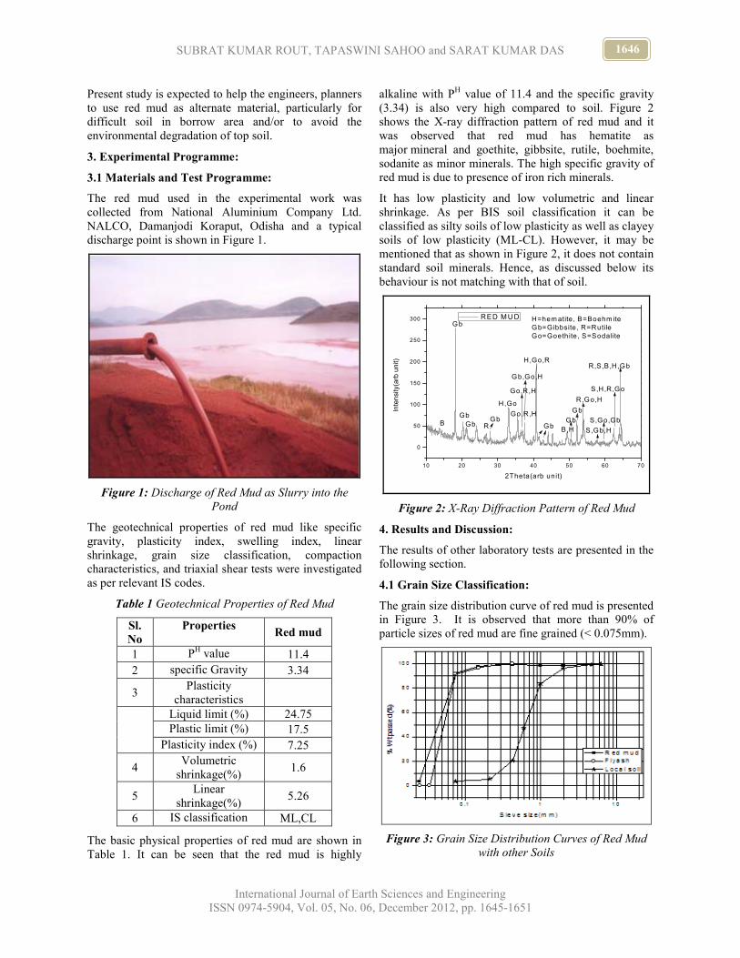
1646 SUBRAT KUMAR ROUT, TAPASWINI SAHOO and SARAT KUMAR DAS
International Journal of Earth Sciences and Engineering
ISSN 0974-5904, Vol. 05, No. 06, December 2012, pp. 1645-1651
Present study is expected to help the engineers, planners
to use red mud as alternate material, particularly for
difficult soil in borrow area and/or to avoid the
environmental degradation of top soil.
3. Experimental Programme:
3.1 Materials and Test Programme:
The red mud used in the experimental work was
collected from National Aluminium Company Ltd.
NALCO, Damanjodi Koraput, Odisha and a typical
discharge point is shown in Figure 1.
Figure 1: Discharge of Red Mud as Slurry into the
Pond
The geotechnical properties of red mud like specific
gravity, plasticity index, swelling index, linear
shrinkage, grain size classification, compaction
characteristics, and triaxial shear tests were investigated
as per relevant IS codes.
Table 1 Geotechnical Properties of Red Mud
Sl.
No
Properties Red mud
1 PH value 11.4
2 specific Gravity 3.34
3 Plasticity
characteristics
Liquid limit (%) 24.75
Plastic limit (%) 17.5
Plasticity index (%) 7.25
4 Volumetric
shrinkage(%) 1.6
5 Linear
shrinkage(%) 5.26
6 IS classification ML,CL
The basic physical properties of red mud are shown in
Table 1. It can be seen that the red mud is highly
alkaline with PH value of 11.4 and the specific gravity
(3.34) is also very high compared to soil. Figure 2
shows the X-ray diffraction pattern of red mud and it
was observed that red mud has hematite as
major mineral and goethite, gibbsite, rutile, boehmite,
sodanite as minor minerals. The high specific gravity of
red mud is due to presence of iron rich minerals.
It has low plasticity and low volumetric and linear
shrinkage. As per BIS soil classification it can be
classified as silty soils of low plasticity as well as clayey
soils of low plasticity (ML-CL). However, it may be
mentioned that as shown in Figure 2, it does not contain
standard soil minerals. Hence, as discussed below its
behaviour is not matching with that of soil.
10 20 30 40 50 60 70
0
50
100
150
200
250
300
Intensity(arb unit)
2Theta(arb unit)
RED MUD
B
Gb
Gb
Gb RGb
H,Go
Go,R,H
Go,R,H
Gb,Go,H
H,Go,R
GbB,H
Gb
Gb
R,Go,H
S,Gb,H
S,Go,Gb
S,H,R,Go
R,S,B,H,Gb
H=hematite, B=Boehm ite
Gb=Gibbsite, R=Rutile
Go=Goethite, S=Sodalite
Figure 2: X-Ray Diffraction Pattern of Red Mud
4. Results and Discussion:
The results of other laboratory tests are presented in the
following section.
4.1 Grain Size Classification:
The grain size distribution curve of red mud is presented
in Figure 3. It is observed that more than 90% of
particle sizes of red mud are fine grained (< 0.075mm).
Figure 3: Grain Size Distribution Curves of Red Mud
with other Soils
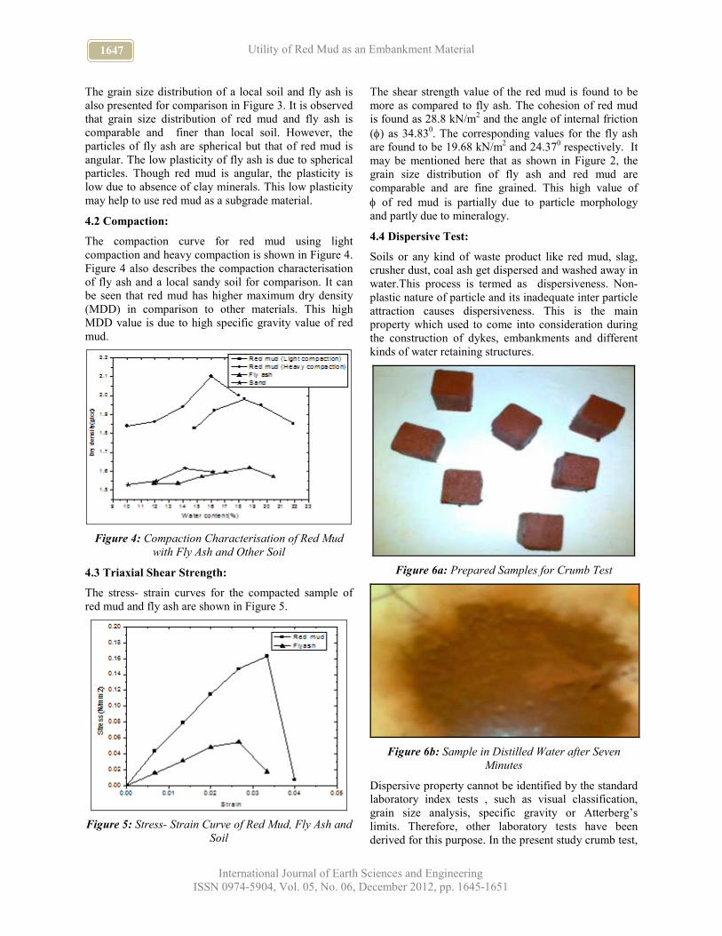
1647 Utility of Red Mud as an Embankment Material
International Journal of Earth Sciences and Engineering
ISSN 0974-5904, Vol. 05, No. 06, December 2012, pp. 1645-1651
The grain size distribution of a local soil and fly ash is
also presented for comparison in Figure 3. It is observed
that grain size distribution of red mud and fly ash is
comparable and finer than local soil. However, the
particles of fly ash are spherical but that of red mud is
angular. The low plasticity of fly ash is due to spherical
particles. Though red mud is angular, the plasticity is
low due to absence of clay minerals. This low plasticity
may help to use red mud as a subgrade material.
4.2 Compaction:
The compaction curve for red mud using light
compaction and heavy compaction is shown in Figure 4.
Figure 4 also describes the compaction characterisation
of fly ash and a local sandy soil for comparison. It can
be seen that red mud has higher maximum dry density
(MDD) in comparison to other materials. This high
MDD value is due to high specific gravity value of red
mud.
Figure 4: Compaction Characterisation of Red Mud
with Fly Ash and Other Soil
4.3 Triaxial Shear Strength:
The stress- strain curves for the compacted sample of
red mud and fly ash are shown in Figure 5.
Figure 5: Stress- Strain Curve of Red Mud, Fly Ash and
Soil
The shear strength value of the red mud is found to be
more as compared to fly ash. The cohesion of red mud
is found as 28.8 kN/m2 and the angle of internal friction
(φ) as 34.830. The corresponding values for the fly ash
are found to be 19.68 kN/m2 and 24.37
0 respectively. It
may be mentioned here that as shown in Figure 2, the
grain size distribution of fly ash and red mud are
comparable and are fine grained. This high value of
φ of red mud is partially due to particle morphology
and partly due to mineralogy.
4.4 Dispersive Test:
Soils or any kind of waste product like red mud, slag,
crusher dust, coal ash get dispersed and washed away in
water.This process is termed as dispersiveness. Non-
plastic nature of particle and its inadequate inter particle
attraction causes dispersiveness. This is the main
property which used to come into consideration during
the construction of dykes, embankments and different
kinds of water retaining structures.
Figure 6a: Prepared Samples for Crumb Test
Figure 6b: Sample in Distilled Water after Seven
Minutes
Dispersive property cannot be identified by the standard
laboratory index tests , such as visual classification,
grain size analysis, specific gravity or Atterberg’s
limits. Therefore, other laboratory tests have been
derived for this purpose. In the present study crumb test,

1648 SUBRAT KUMAR ROUT, TAPASWINI SAHOO and SARAT KUMAR DAS
International Journal of Earth Sciences and Engineering
ISSN 0974-5904, Vol. 05, No. 06, December 2012, pp. 1645-1651
double hydrometer test and turbidity tests [9] have been
performed to identify dispersive clays. The crumb test
has been done [9] and the results are shown in Figure 6.
It is observed that red mud is highly dispersive. Based
on double hydrometer test, dispersion ratio of red mud
is found to be 94%, which is extremely dispersive [5].
Turbidity test also has been done as per [10] also
showed red mud as highly dispersive material.
5. Finite Element Analysis:
In the present study the finite element analysis of the
embankment is done using FEM based software-
PLAXIS [11].
5.1 Finite Element Analysis using PLAXIS:
PLAXIS [11] is a finite element program for
geotechnical applications in which different soil models
are used to simulate the soil behavior. It’s
implementation consists of three stages, known as input
stage, calculation stage and post processing (curves)
stage. Input stage contains model design, assigning the
material parameters, boundary conditions, loading and
meshing. In the present analysis 15-node triangular
element is considered for meshing, which contains 12
stress points. In PLAXIS, stresses and strains are
calculated at individual Gaussian integration points
rather than at nodes. In the calculation stage, analysis
type is chosen such as Plastic, dynamic, consolidation
and phi-c reduction. The assigned loads are activated in
this stage and analyzed. In the post processing stage,
curves are plotted between various calculated
parameters such as load Vs displacement.
To compare with the limit equilibrium method in
addition to stress-strain calculation, the factor of safety
(FOS) of slope is calculated using Phi-c (φ-C) reduction
method.
5.1.1 Φ-C Reduction Method:
Phi-c reduction is an option available in PLAXIS to
compute FOS for the stability problems. This option can
be selected as a separate calculation type in the general
tab sheet. In the Phi-c reduction approach the strength
parameters tanφ and c of the soil are successively
reduced in the same decrement. The total multiplier
∑Msf (MSF) is used to define the value of the soil
strength parameters at a given stage in the analysis:
reduced
input
reduced
input
c
cMsf ==Σ
φ
φ
tan
tan
Where the strength parameters with the subscript ‘input’
refer to the properties entered in the material sets and
parameters with the subscript ‘reduced’ refer to the
reduced values used in the analysis. ∑Msf is set to 1.0 at
the start of calculation to set all material strengths to
their unreduced values. The variation of MSF with
displacement is presented to find out the FOS. The
material properties considered for the FEM analysis is
shown in Table 2.
Table 2: Soil Properties for Mohr-Coulomb Model
Mohr-Coulomb
parameters
Local
soil Red mud
Unit weight (kN/m3) 16 19.8
Permeability (m/day) 5 x 10⁻³
5.832 x 10⁻⁴
Cohesion (kN/m2) 30 28.8
Internal friction (degree) 15 34
Young’s modulus
(kN/m2)
3500 1771
Poisson ratio 0.3 0.34
5.2 Stability Analysis of Embankment Slope:
For the embankment slope analysis the top width of a
typical 2-lane road is taken as 14m (7m carriage
way+1.5X2 paved shoulder+2X2 earth shoulder).
Similarly for 4-lane road it is taken as 26m. The
embankment slope considered are with slope 1:2 (1
vertical: 2 horizontal). The embankment heights
considered are 10m and 15m. The stability analysis of
embankment with red mud only first analysed.
5.2.1 Example 1:
In the 1st attempt to construct the embankment, only red
mud has been used as the base material. The slope
height is kept at 10m with the slope inclination of 1:2.
Model diagram with its deformation mesh is shown in
Figure 7. Figure 8 shows the shear failure results of
PLAXIS analysis. The factor of safety is described in
terms of MSF. The variation of the MSF with
displacement is shown in Figure 9 and the FOS of the
slope is found to be 2.97.
Figure 7: The PLAXIS Model for the Slope Using Only
Red Mud
Some more studies are made for other slopes and the
results are shown in Table 3. It was found that for all the
cases te FOS is found to be more than 1.5.
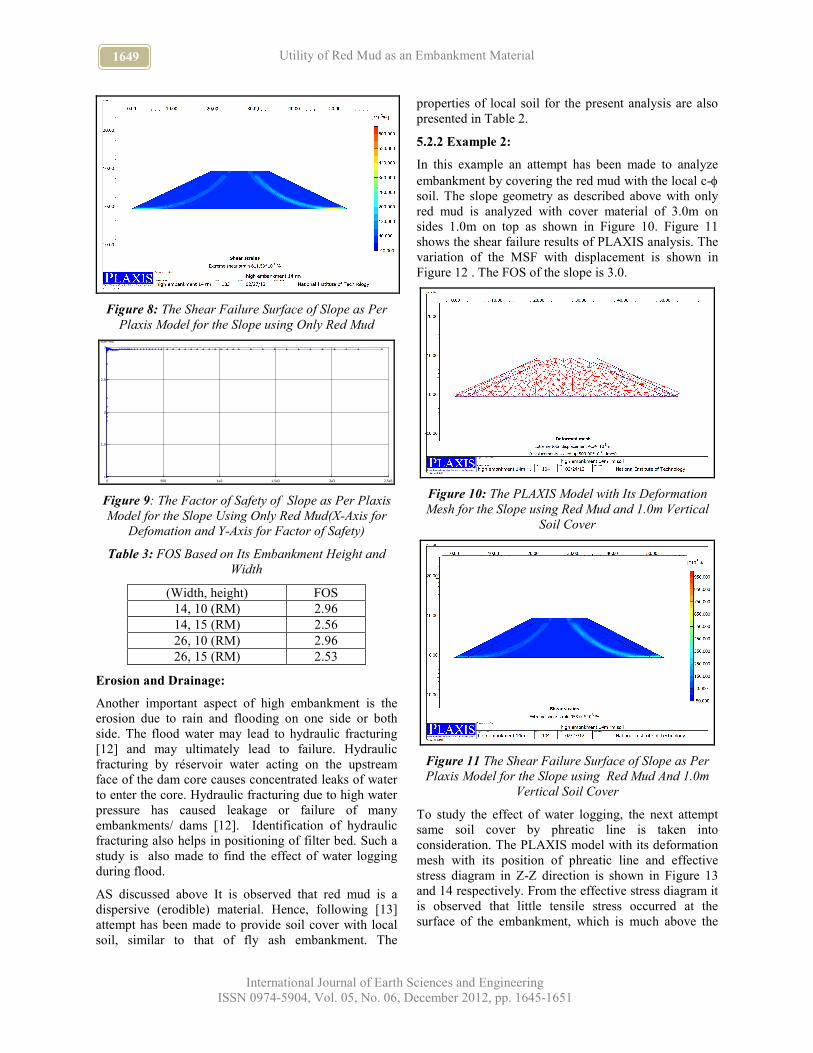
1649 Utility of Red Mud as an Embankment Material
International Journal of Earth Sciences and Engineering
ISSN 0974-5904, Vol. 05, No. 06, December 2012, pp. 1645-1651
Figure 8: The Shear Failure Surface of Slope as Per
Plaxis Model for the Slope using Only Red Mud
0 500 1e3 1.5e3 2e3 2.5e3
1
1.5
2
2.5
3
Sum-Msf
Figure 9: The Factor of Safety of Slope as Per Plaxis
Model for the Slope Using Only Red Mud(X-Axis for
Defomation and Y-Axis for Factor of Safety)
Table 3: FOS Based on Its Embankment Height and
Width
(Width, height) FOS
14, 10 (RM) 2.96
14, 15 (RM) 2.56
26, 10 (RM) 2.96
26, 15 (RM) 2.53
Erosion and Drainage:
Another important aspect of high embankment is the
erosion due to rain and flooding on one side or both
side. The flood water may lead to hydraulic fracturing
[12] and may ultimately lead to failure. Hydraulic
fracturing by réservoir water acting on the upstream
face of the dam core causes concentrated leaks of water
to enter the core. Hydraulic fracturing due to high water
pressure has caused leakage or failure of many
embankments/ dams [12]. Identification of hydraulic
fracturing also helps in positioning of filter bed. Such a
study is also made to find the effect of water logging
during flood.
AS discussed above It is observed that red mud is a
dispersive (erodible) material. Hence, following [13]
attempt has been made to provide soil cover with local
soil, similar to that of fly ash embankment. The
properties of local soil for the present analysis are also
presented in Table 2.
5.2.2 Example 2:
In this example an attempt has been made to analyze
embankment by covering the red mud with the local c-φ
soil. The slope geometry as described above with only
red mud is analyzed with cover material of 3.0m on
sides 1.0m on top as shown in Figure 10. Figure 11
shows the shear failure results of PLAXIS analysis. The
variation of the MSF with displacement is shown in
Figure 12 . The FOS of the slope is 3.0.
Figure 10: The PLAXIS Model with Its Deformation
Mesh for the Slope using Red Mud and 1.0m Vertical
Soil Cover
Figure 11 The Shear Failure Surface of Slope as Per
Plaxis Model for the Slope using Red Mud And 1.0m
Vertical Soil Cover
To study the effect of water logging, the next attempt
same soil cover by phreatic line is taken into
consideration. The PLAXIS model with its deformation
mesh with its position of phreatic line and effective
stress diagram in Z-Z direction is shown in Figure 13
and 14 respectively. From the effective stress diagram it
is observed that little tensile stress occurred at the
surface of the embankment, which is much above the

1650 SUBRAT KUMAR ROUT, TAPASWINI SAHOO and SARAT KUMAR DAS
International Journal of Earth Sciences and Engineering
ISSN 0974-5904, Vol. 05, No. 06, December 2012, pp. 1645-1651
phreatic line. Hence, there is less chance of hydraulic
fracture.
0 500 1e3 1.5e3 2e3 2.5e3
1
1.5
2
2.5
3
3.5
|U| [m]
Sum-Msf
Figure 12: The Factor of Safety of Slope as Per Plaxis
Model for the Slope using Red Mud and 1.0m Vertical
Soil Cover
Figure 13: The PLAXIS Model with its Deformation
Mesh for the Slope using Red Mud and 1.0m Vertical
Soil Cover With its Phreatic Line
Figure 14: Effective Stress Diagrams for the Slope
using Red Mud and Soil Cover of 1.0m Vertically in Zz
Direction
Study has also been made for different heights and
widths of dam with only red mud and with red mud core
and soil cover. The comprehensive results have been
presented in Table 4. It is observed that in all the cases
the FOS is more than 2.5, and [13 and 14].Since more
than 1.5 is sufficient high embankment can be
constructed using red mud.
Table 4: FOS at different Width and Height with Soil
Cover
Width, height (Meter) FOS
14, 10 (RM, soil cover) 3.00
14, 15 (RM, soil cover) 2.57
26,10 (RM, soil cover) 2.99
26, 15 (RM, soil cover) 2.54
The embankments are also been analysed putting the
axle load on it. The results for axle load with static and
dynamic action are shown in Table 5. It can be seen that
with load also the FOS is more than or close to 1.5.
Table 5: FOS at different Width and Height for
Concentrated Load and due to Vibration
Width, height
(red mud, Soil cover) FOS
14, 10 (RM) concentrated load 1.77
14, 10 (RM, soil) concentrated load 1.48
14, 10 (RM) due to vibration 1.78
14, 10 (RM, soil) due to vibration 1.49
Conclusion:
This paper described the design of high embankment
using red mud based on the laboratory geotechnical
investigation and the stability analysis using FEM.
Based on the observations and discussions thereof
following conclusions can be made:
1. The specific gravity of Red mud is very high
compared to soil, due to presence of iron compound
minerals. It has low plasticity and low volumetric and
linear shrinkage with 90% of particle finer than
0.075mm.
2. Red mud has high maximum dry density (MDD) in
comparison to other materials, due to high specific
gravity.
3. The angle of internal friction value of the red mud is
found to be more as compared to fine grained fly ash.
4. Based on crumb test, double hydrometer tests and
turbidity test red mud is found to be highly dispersive.
5. To protect the dispersive red mud against external
weathering it is recommended to cover it with local soil.
The embankment with soil cover is found to have more
than required FOS value (as per standard
specifications).
7. The embankments are also analyzed considering
concentrated load and the load with vibration. The FOS
is found to decrease with static and vibration load.
8. This limited study shows that red mud has the
potential to be used as an embankment material. More
study is being conducted regarding economy,

1651 Utility of Red Mud as an Embankment Material
International Journal of Earth Sciences and Engineering
ISSN 0974-5904, Vol. 05, No. 06, December 2012, pp. 1645-1651
convenience in construction and safety during
construction.
References:
[1] Singh, A.P., Singh, P.C., Singh, V.N (1995)
“Cyclohexanethiol separation from kerosene oil by
red mud”, J. Chem. Technol. Biotechnol. 56 (1993)
167.
[2] Pera, J., Boumaza, R., and Ambroise, J.,
“DEVELOPMENT OF A POZZOLANIC
PIGMENT FROM RED MUD” (Received
December 11, 1996; in final form June 2, 1997)
[3] Mikelic Luka, Orescanin Visnja, Lulic Stipe.
“Utilization of Red Mud for the Purification of
Waste Waters from Nuclear Power Plants.” TA-7
“waste management and decommissioning”.
[4] Mishra, B., Staley, A., Kirkipatrick, D., (2002),
“Recovery of value added products from red mud”,
Minerals and Metallurgical processing. Vol(19),
87-94.
[5] Vogt, M. F. (1974). “Development studies on
dewatering of red mud.” 103rd
Annual Meeting of
AIME, Dallas, Tex., 73-91.
[6] Somogyi, F., and Gray, D. (1977). “Engineering
properties affecting disposal of red mud.” Proc.,
Conf. on Geotechnical Practice for Disposal of
Solid Waste Materials, ACSE, 1-22.
[7] Fahey, M., Newson, T. A., and Fujiyasu, Y. (2002).
“Engineering with tailing.” Invited Lecture, Proc.,
4th
Int. Conf. On Environmental Geotechnics. Rio
de janeiro, Brazil, 2, 947-973, Balkema, Lisse.
[8] Vick, S. G. (1981). Planning, design and analysis of
tailing dams, Wiley, New York, 369.
[9] Bhuvaneshwari, S., Soundra, B., Robinson, R.G.,
and Gandhi, S.R., “Stabilization and
Microstructural Modification of Dispersive Clayey
Soils”, First International Conference on Soil and
Rock Engineering, Columbo, Srilanka, August 5-
11, 2007.
[10] Sridharan, A., Pandian, N.S. and Subranya Prasad,
P. (2001g), Vol. 7: Pin hole studies on Indian coal
ashes, Technical report of task force on
Characterization of fly ash submitted to
Technology Mission-Fly Ash Disposal and
Utilisation, Dept. of Science and Technology, Govt.
of India.
[11] Brinkgreve. R.B.J, Broere.W, Waterman.D (2008).
“PLAXIS -2D (Version 9.0)”, Delft University of
Technology and PLAXIS b.v., The Netherlands.
[12] Sherard, J.L (1986) “Hydraulic fracturing in
embankment dams,” Journal of Geotechnical
Engineering, Vol. 112, No. 10, pp 905-927.
[13] IRC: 58-2001. “Guidelines for use of fly ash in
road embankments”, The Indian Road congress,
Jamnagar house, Shahjahan Road, New Delhi-
110011.
[14] IRC: 75-1979. “Guidelines for the design of high
embankments”, The Indian Road congress,
Jamnagar house, Shahjahan Road, New Delhi-
110011.

www.cafetinnova.org
Indexed in
Scopus Compendex and Geobase Elsevier, Chemical
Abstract Services-USA, Geo-Ref Information Services-USA
ISSN 0974-5904, Volume 05, No. 06
December2012,P.P.1652-1658
#02050624 Copyright ©2012 CAFET-INNOVA TECHNICAL SOCIETY. All rights reserved.
Rapid Chloride Penetration Test on Geopolymer Concrete
SHANKAR H. SANNI and R. B. KHADIRANAIKAR Department of Civil Engg., Basaveshwar Engg. College, Bagalkot, Karnataka
Email: [email protected], [email protected]
Abstract: This paper presents the experimental investigation done on permeability characteristics of geopolymer
concrete. The grades choosen for the investigation were M-30, M-40, M-50 and M-60 with the molarity of 8M. The
alkaline solution used for present study is the combination of sodium silicate and sodium hydroxide solution with
the ratio of 2.50. The test specimens were 150x150x150 mm cubes, 100x200 mm cylinders heat-cured at 60°C in an
oven. The variation was studied on the specimens subjected to ambient air as well as oven heat curing. The test
results indicate that the geopolymer concrete in 6 hours allowed 1560 to 1980 Coulombs giving low rating as per
ASTM 1202. The RCPT values indicate improved resistance for chloride permeability and low rate of corrosion risk
level.
Keywords: Geopolymer Concrete, Rapid Chloride Penetration Test, Molarity, Sodium Hydroxide, Sodium Silicate
Introduction:
In the context of increased awareness regarding the ill-
effects of the over exploitation of natural resources, eco-
friendly technologies are to be developed for effective
management of these resources. Construction industry is
one of the major users of the natural resources like
cement, sand, rocks, clays and other soils. The ever
increasing unit cost of the usual ingredients of concrete
have forced the construction engineer to think of ways
and means of reducing the unit const of its production.
At the same time, increased industrial activity in the
core sectors like energy, steel and transportation has
been responsible for the production of large amounts
like fly ash, blast furnace slag, silica fume and quarry
dust with consequent disposal problem [Narasimhan, et
al., 1997].
The geopolymer technology was first introduced by
Davidovits in 1978. His work considerably shows that
the adoption of the geopolymer technology could reduce
the CO2 emission caused due to cement industries.
Davidovits proposed that an alkaline liquid could be
used to react with aluminosilicate in a source material of
geological origin or in by-product materials such as fly
ash to make a binder [Rangan, 2006]. Geopolymer is
synthesized by mixing aluminosilicate-reactive material
with strong alkaline solutions, such as sodium
hydroxide (NaOH), potassium hydroxide (KOH),
sodium silicate or potassium silicate. The mixture can
be cured at room temperature or temperature cured
[Davidovits, 2008]. Fly ash is the most common source
material for making geopolymers. Normally, good high-
strength geopolymers can be made from class F fly ash
[Schmucker, et al., 2004]. The alkaline activation of
materials can be defined as chemical process that
provides a rapid change of some specific structures,
partial or totally amorphous, into compacted cemented
frame works [Palomo, et al., 2003].
Alkaline activating solution is important for dissolving
of Si and Al atoms to form geopolymer precursors and
finally alumino-silicate material. The most commonly
used alkaline activators are NaOH and KOH
[Davidovits, Fernandez-Jimenez, van Deventer, 1999,
2000]. Durability of concrete is the ability of concrete to
remain fully functional over an extended period under
prevailing service conditions for the purpose for which
it has to be designed. The durability of concrete is
closely related to its permeability. The permeability
indicates the rate at which aggressive agents can
penetrate to attack the concrete and the steel
reinforcement. The chloride permeability of GPC was
varying from ‘Low’ to ‘very low’ as per ASTM 1202
[Rajamane, et al., 2011].
Experimental Investigations:
Materials:
The following materials have been used in the
experimental study [Shankar, et al., 2012]
a) Fly Ash (Class C) collected form Raichur Thermal
power plant having specific gravity 2.00.
b) Fine aggregate: Sand confirming to Zone –III of
IS:383-1970 having specific gravity 2.60 and fineness
modulus of 2.70.
c) Coarse aggregate: Crushed granite metal confirming
to IS:383-1970 having specific gravity 2.72 and fineness
modulus of 6.40.
d) Water : Clean Potable water for mixing
e) Alkaline Media: Specific gravity of

1653 SHANKAR H. SANNI and R. B. KHADIRANAIKAR
International Journal of Earth Sciences and Engineering
ISSN 0974-5904, Vol. 05, No. 06, December 2012, pp. 1652-1658
i) Sodium Hydroxide (NaOH) = 1.16
ii) Sodium Silicate (Na2SiO3) = 1.57
f) Superplasticizer : Conplast (SP-430)
Tests were conducted on specimen of standard size as
per IS: 516-1959. Details of tests conducted and
specimens used are given in Table 1.
Mix Design of Geopolymer Concrete:
In the design of geopolymer concrete mix, coarse and
fine aggregates together were taken as 77% of entire
mixture by mass. This value is similar to that used in
OPC concrete in which it will be in the range of 75 to
80% of the entire mixture by mass. Fine aggregate was
taken as 30% of the total aggregates. The density of
geopolymer concrete is taken similar to that of OPC as
2400 kg/m3 [Rangan, 2008]. The details of mix design
and its proportions for different grades of GPC are
given in Table 3.
Mixing, Casting, Compaction and Curing of
Geopolymer Concrete:
GPC can be manufactured by adopting the conventional
techniques used in the manufacture of Portland cement
concrete. In the laboratory, the fly ash and the
aggregates were first mixed together dry on pan for
about three minutes. The liquid component of the
mixture is then added to the dry materials and the
mixing continued usually for another four minutes.
(Figure 1 and 2). In preparation of NaOH solution,
NaOH pellets were dissolved in one litre of water in a
volumetric flask for concentration of NaOH (12M).
Alkaline activator with the combination of NaOH and
Na2SiO3 was prepared just before the mixing with fly
ash. The ratio of alkaline liquid to fly ash by mass varies
with the grade of concrete [Rangan, 2008]. The alkaline
liquid (Na2SiO3 / NaOH) used in the current study was
2.5 for all the mixes. This ratio was selected, since it
produced the highest compressive strength [Shankar, et
al., 2012]. The chloride penetration inside the concrete
may cause the corrosion of steel hence it was mandatory
to check the pH of alkaline solution [Fig. 6]. The fly ash
and alkaline activator were mixed together in the mixer
until homogeneous paste was obtained. This mixing
process can be handled within 5 minutes for each
mixture with different molarity of NaOH. Fresh fly ash
based geopolymer concrete was usually cohesive. The
workability of the fresh concrete was measured by
means of conventional slump test [Fig. 5]. Heat curing
of GPC is generally recommended, both curing time and
curing temperature influence the compressive strength
of GPC [Hardjito, et al., 2004]. After casting the
specimens, they were kept in rest period for two days
and then they were demoulded. The demoulded
specimens were kept at 60°C for 24 hours in an oven as
shown in Fig. 4.
Rapid Chloride Penetration Test (RCPT):
Whiting in 1981 developed the rapid chloride
permeability test under research sponsored by the
Federal Highway Administration (FHWA). This test
was adopted by the AASHTO in 1983 and was given
the designation AASHTO T-277. In 1991, this test was
adopted by ASTM and was given the designation
ASTM C 1202 ‘Electrical Indication of Concrete’s
ability to resist chloride Ion penetration’ is referred to as
Rapid Chloride Permeability Test (RCPT).
Figure 1: Mixing of Alkaline Solution
Figure 2: Mixing of GPC
Figure 3: View of GPC Specimens

1654 Rapid Chloride Penetration Test on Geopolymer Concrete
International Journal of Earth Sciences and Engineering
ISSN 0974-5904, Vol. 05, No. 06, December 2012, pp. 1652-1658
Figure 4: Curing of GPC Specimens
Figure 5: Slump Cone Test
Figure 6: Ph of Alkaline Solution
The RCPT determines the electrical conductance of the
concrete specimen to provide a rapid indication of its
resistance to the penetration of chloride ions. The
instrument used is designed conforming to the ASTM C
1202.
The RCPT is table mounted unit, which measures the
electrical charges passed through a 2-inch thick slice of
4-inch nominal diameter concrete core or cylinder
during a period of 6 hours. A potential difference of 60
V D.C is maintained across the ends of the specimens.
One end of the specimen is immersed in a sodium
chloride (3% Nacl, -ve node) solution while the other in
sodium hydroxide solution (0.3N, NaOH, +ve node)
solution. The total charge passed, in Columbs, is related
to the resistance of the specimen to chloride ion
penetration. RCPT cell is shown in Fig. 7. The total
charges passed are automatically recorded by RCPT
software which stores charges passed of every time.
Figure 7: RCPT Sample Holding Cell
Specimen Preparation:
The 50 mm thick concrete disk was sliced from 100mm
x 200mm height cylinder (Fig. 8)
Conditioning of Specimen:
The sliced specimen disk was kept in vacuum
desiccators to remove air present in pore for 3 hours.
Then water was allowed into desiccators for 1 hour
under vacuum so that disk gets water saturated. The
specimen was kept for 18 hours in water under
atmospheric pressure.
Measurement of Charge Passing:
In this step well conditioned disk was mounted in
testing cell and chambers were filled with NaOH and
NaCl solution. Then the testing cell was applied to 60 V
D.C through measurement unit as shown in Fig. 8, the
charges were recorded by the computer.
Results and Discussions:
Workability:
The workability of the geopolymer concrete decreases
with increase in the grade of the concrete as presented in
Table 2, this is because of the decrease in the ratio of
water to geopolymer solids. As the molarity of the
NaOH solution increases the workability of the

1655 SHANKAR H. SANNI and R. B. KHADIRANAIKAR
International Journal of Earth Sciences and Engineering
ISSN 0974-5904, Vol. 05, No. 06, December 2012, pp. 1652-1658
geopolymer concrete decreases, because of the decrease
in the water content. Thus we can say that as the grade
of the concrete increases, the mix becomes stiffer
decreasing the workability.
Figure 8: RCPT Working Procedure

1656 Rapid Chloride Penetration Test on Geopolymer Concrete
International Journal of Earth Sciences and Engineering
ISSN 0974-5904, Vol. 05, No. 06, December 2012, pp. 1652-1658
Table 1: Details of Specimen used and Tests Conducted
Type of tests conducted Size of specimen No. of specimen cast for
different grades
Compressive strength 150x150x150mm 5
Split tensile strength 100x200mm 5
Table 2: Slump Values for different Grades of Gpc
Grade Na2SiO3/NaOH Slump (mm)
M-30 2.5 135
M-40 2.5 130
M-50 2.5 110
M-60 2.5 95
Table 3: Mix Proportions of GPC Mix with Molarity of 12M (Na2SiO3/ NaOH as 2.5)
Materials
Mass (kg/m3)
M-30 M-40 M-50 M-60
Coarse
aggregates
20 mm 277.20 277.20 277.20 277.20
14 mm 369.60 369.60 369.60 369.60
7 mm 646.80 646.80 646.80 646.80
Fine sand 554.40 554.40 554.40 554.40
Fly ash 380.69 394.29 408.89 424.62
Na2SiO3/ NaOH 2.50 2.50 2.50 2.50
SiO2/Na2O 2.00 2.00 2.00 2.00
Sodium hydroxide solution 48.95 45.06 40.89 36.4
Sodium silicate solution 122.36 112.65 102.22 91
Super Plasticizer 5.70 5.91 6.13 6.37
Extra water 38.06 39.42 40.88 42.46
Table 4: Chloride Ion Penetrability Based on Charge Passed (ASTM C1202 –2007)
Charge Passed (Coulombs) Chloride Ion Penetrability
> 4000 High
2000 – 4000 Moderate
1000 – 2000 Low
100 – 1000 Very Low
< 100 Negligible
Table 5: Strength for different Grades of Geopolymer Concrete Mixes
S. No Grade Compressive Strength (N/mm
2) Split tensile strength (N/mm
2)
7 Days 28 days 7 Days 28 days
1 M 30 25.50 38.30 3.06 4.23
2 M 40 33.48 44.78 3.43 4.81
3 M 50 41.66 56.46 4.70 5.73
4 M 60 49.40 66.45 5.10 6.13
Table 6: RCPT Values for different Grades at Heat Curing
Sl. No. Grade
RCPT
Charges Passed at 30
minutes
Extrapolated values for 6 hrs
RCPT
(Coulombs)
Chloride Ion permeability
7 Days 28 days 7 Days 28 days 7 Days 28 days
1 M 30 488 164 5856 1968 HIGH LOW
2 M 40 457 142 5484 1704 HIGH LOW
3 M 50 438 136 5256 1632 HIGH LOW
4 M 60 413 129 4956 1548 HIGH LOW

1657 SHANKAR H. SANNI and R. B. KHADIRANAIKAR
International Journal of Earth Sciences and Engineering
ISSN 0974-5904, Vol. 05, No. 06, December 2012, pp. 1652-1658
Ph of Alkaline Solution:
The amount of chloride required for initiating corrosion
is partly dependent on the pH value of alkaline solution.
The pH value of Alkaline solution in the present study
was 13, which is less than the pH computed for the
activator solution (pH = 14). The value of pH more than
14 is due to the molarity of NaOH solution which was
more than unity as more than 40 grams of NaOH was
dissolved per litre of the solution. The results as seen in
the present case were also reported [Rajamane, et al.,
2011].
Compressive Strength and Split Tensile Strength of
Geopolymer Concrete:
The details of compressive strength and split tensile
strength for various grades of concrete are shown in
Table 5.
• As the grade of concrete increases, the compressive
and split tensile strength of geopolymer concrete also
increases, this is quite relevance with the behavior of
ordinary Portland cement concrete.
Rapid Chloride ion Penetration Test:
Rapid Chloride ion Penetration Test (RCPT) is
essentially a measure of concrete’s electrical
conductivity which depends on both pore structure
characteristics and pore solution chemistry (Caijun Shi,
2004). Chloride diffusion is one of the major reasons
for causing corrosion to steel reinforcement inside
concrete. Therefore it is necessary to study concrete for
its chloride ion permeability. Alumino-silicates is the
binder in the GPC, but in the conventional concretes
calcium silicate hydrate (C-S-H) gel is the main binding
system. The results of GPC specimens subjected to
RCPT are presented in Table 6.
During the RCPT the solution temperature was
increasing beyond 80°C hence the RCPT charges passed
at 30 minutes has been extrapolated to 6 hrs RCPT to
decide the chloride ion penetrability as mentioned in
Table 4. Since GPC make use of alkaline activator
solutions that are highly conductive, the unreacted
residual alkaline activator solutions could sometimes
give a false alarm, leading to conclude that GPC are
highly permeable to chlorides.
• As the grade of GPC increases the RCPT charges
decreases. Thus we can say that RCPT of GPC is having
‘low’ chloride ion penetrability for higher grade of
concrete.
• The maximum and minimum charges passed for 28
days was 1968 and 1548 Coulombs for M30 and M60
grade GPC respectively.
• The maximum and minimum charges passed for 7
days was 5856 and 4956 Coulombs for M30 and M60
grade GPC respectively.
Conclusions:
Based on the experimental investigations done the
following conclusions can be drawn:
• The fly ash can be used to produce geopolymeric
binder phase which can bind the aggregate systems
consisting of sand and coarse aggregate to form
geopolymer concrete (GPC).
• Conventional methods of mixing, compaction,
moulding and demoulding can be adopted for GPC’S
also. The only precaution needed is in handling of
catalytic liquids systems (CLS) which is highly alkaline
in ratio (often pH>13).
• As the GPC do not have any Portland cement, they
can be considered as less energy interactive. The GPC
utilize the industrial wastes such as fly ash for
producing the binding system in concrete. Therefore
these concretes should be considered as eco-friendly
materials.
• As the grade of concrete increases, the RCPT
charges decreases. Thus we can say that permeability is
very less in case of GPC. The results of 7 days allow
high charge to pass in concrete specimen due to
incomplete geopolymerisation reaction. Hence 28 days
results were considered for RCPT test in view of
DURABILITY aspects.
References:
[1] Caijun Shi, (2004) Effect of mixing proportions of
concrete on its electrical conductivity and the rapid
chloride permeability test (ASTM C1202 or
ASSHTO T277) results, Cement and Concrete
Research, 2004, 34, pp. 537-545.
[2] Davidovits, J., (2008) Geopolymer chemistry and
application, Institute Geopolymer, France, pp. 585.
[3] Davidovits, J. (1999) Chemistry of Geopolymeric
systems Terminology, 99 International Conference,
Saint-Quentin, France, 30 June-2 July.
[4] Fernandez-Jimenez, A., Palomo, A and Puertas, F.,
(1999) Alkali activated slag mortars, mechanical
strength behavior, Cement and Concrete Research,
29, pp. 1323-1329.
[5] Fenandez-Jimenez, A and Palomo, A (2003)
Characteristics of fly ashes, Potential reactivity as
alkaline cements, Fuel, pp. 2259-2265.
[6] Hua Xu, van Deventer, J.S.J., (2000) The
Geopolymerisation of Alumino-Silicate Minerals,
International Journal of Mineral Processing, 59(3),
pp. 247-266.
[7] Hardjito, D. Wallah, S.E., Sumajouw, DMJ and
Rangan, B.V., (2004) On the development of flyash
based geopolymer concrete, ACI Materials Journal,
101(52), pp. 467-472.
[8] Narasimhan, M. C. Patil, B. T, and Shankar H.
Sanni (1999) Performance of Concrete with Quarry
Dust as fine aggregate – An Experimental Study,

1658 Rapid Chloride Penetration Test on Geopolymer Concrete
International Journal of Earth Sciences and Engineering
ISSN 0974-5904, Vol. 05, No. 06, December 2012, pp. 1652-1658
Civil Engineering and Construction Review,
September, pp. 19-24.
[9] Rangan, B. V., (2006) Studies on low-calcium fly
ash based Geopolymer concrete, Indian Concrete
Institute, Oct-Dec, pp. 9-17.
[10] Rangan, B.V., (2008) Mix design and production of
flyash based geopolymer concrete, The Indian
Concrete Journal, Vol. 82, No. 5, May, pp. 7-14.
[11] Rajamane, N.P, Nataraja, M.C, Lakshmana, N,
Dattatreya, J. K, (2011) Rapid chloride
permeability test on geopolymer and Portland
cement concretes, The Indian Concrete Journal,
Oct., pp. 21-26.
[12] Schmucker, M, and MacKenzine, KJD (2004)
Microstructure of sodium polysialate
siloxogeopolymer, Ceramic International, pp. 433-
437.
[13] Shetty, M.S., (2002) Concrete Technology, S.
Chand and Company, Fifth Revised Edition.
[14] Shankar H. Sanni and Khadirnaikar, R. B. (2012)
Effect of molarity on geopolymer concrete,
International Conference on Sustainability,
Challenges and Advances in Concrete Technology,
(SCAT 2012), PSG College of Technology,
Coimbatore, May 1-3, pp. 203-208.
[15] Shankar H. Sanni et al., (2012) Permeability
characteristics of geopolymer concrete, B.E Project
Report, Basaveshwar Engineering College,
Bagalkot.
[16] Whiting, D., Rapid determination of chloride
permeability of concrete, Report No. FHWA/RD-
81/119, Washington DC.
[17] IS: 2386 (Part-IV)-1963, Methods of test for
aggregates for concrete-mechanical properties,
Bureau of Indian standard, New Delhi.
[18] IS: 456-2000, Code of practice for plain and
reinforced concrete, Bureau of Indian Standard,
New Delhi.
[19] IS: 383-1970, Specification for coarse and fine
aggregates from natural sources for concrete,
Bureau of Indian standard, New Delhi.
[20] IS: 516-1959, Methods of test for strength of
concrete, Bureau of Indian standard, New Delhi.
[21] ASTM C 1202, Standard Test Method for Electrical
Indication of Concrete’s ability to resist chloride
ion penetration, American Society of Testing and
Materials, Pennsylvania, 2007.

i
News Item:
NIT Professor spoke at an International Conference in
SanFransisco, USA.
Forensic engineering is the engineering discipline that focuses on the practices of failure investigations and ensuring
that the failure causes and impacts are reported in a professional and unbiased manner in the judicial proceeding.
The purpose of the Technical Council for Forensic Engineers (TCFE) is to develop practices and procedures to
reduce the number of such failures, to disseminate information on failures and their causes, to provide guidelines for
conducting failure investigations, and to provide guidelines for ethical guidelines for ethical conduct in forensic
engineering.
Dr. C. Natarajan, Professor of Structural Engineering in the Department of Civil Engineering at the National
Institute of Technology, Tiruchirappalli participated the International Conference on Forensic Engineering in
SanFransisco, USA, from October 31st to November 3
rd 2012 and also attended the meeting for the Committee on
Forensic Investigation (CFI). This conference was sponsored and organized by the American Society of Civil
Engineers. The conference was very well attended with over 200 international experts and engineers met and
presented at the conference. The topics of the conference covered from failure case studies to advanced
investigation techniques. The Forensic Congress is organized by a panel of experts lead by Mr. Anthony Dolhon of
Exponent. Dr.C.Natarajan spoke about the Indo – US joint collaboration in advancing Forensic Engineering and
cited the high lights of the Indo-US Forensic workshop conducted at NIT – Tiruchirappalli in December 2010. He
also discussed some of the case studies of structural failure analysis he investigated.
Dr. C. Natarajan is a very well known structural engineer, widely consulted in Tri-states, namely Tamil Nadu,
Kerala and Pondicherry in the design and construction of high rise buildings, multistoried luxury Hotels, Industrial
Parks, long span Highway Bridges, Transmission Towers and Elevated water Tanks. He is also widely referred for
structural failures and buildings collapses, for forensic investigation and failure analysis. He now works on a
publication with Dr. A.Rajaraman (Former Director grade Scientist) of Structural Engineering Research Centre,
Chennai a book on 100 forensic case studies and the lessons learned”.
During his visit to the Forensic Conference, he interacted with International Engineers, Educators and Researchers
and tried to build collaborative bridges with them to organize an International Conference on “Emerging Innovative
Technologies in Civil and Infrastructure Engineering” on the eve of NIT – Trichy Golden Jubilee Celebrations in
2014. In addition to new technologies, design methodologies, new smart materials developed in Civil Engineering
field, health monitoring of existing infrastructures and forensic engineering will also be topics of the conference.
The mission of the Committee on Forensic Investigation (CFI) was to identify needs related to the investigation of
failures of constructed facilities; define the problems related to the methods and process of failure investigation and
to develop effective means of disseminating information on the methods and processes. CFI was previously headed
by Mr. Ron Anthony, a wood material expert. Mr. Anthony is now a member of the Executive Committee of TCFE.
Prof. Shen-en-Chen, Department of Civil Engineering, University of North Carolina at Charlotte, and Dr. Danielle
D. Kleinhans of the American Concrete Reinforcing Steel Institute is now responsible for CFI activities.
Mr. Gregory Di Loreto, the 2013 ASCE (American Society of Civil Engineers) president, was the opening speaker
at the conference. He has addressed the critical issues of financing the US national infrastructure, which is rapidly
deteriorating. Mr. Raymond “Paul” Giroux of the Kiewit Infrastructure West Company was the featured speaker
and gave an outstanding keynote speech on the history of the famous Golden Gate Bridge. His Power point
presentation showed an animated sequence of cranes in action during the bridge construction.
Mr. R. N. Reikar of Mumbai was announced at the sixth Forensic Congress as the recipient of the 2009 Forensic
Engineer of the Year, for his significant contributions to the forensic community. He was nominated by Professor
Ken Carper of Washington State University and the editor of the Journal of Performance of Constructed Facilities.

ii
Dr. Subhash C. Yaragal, is conferred with Prof. Satish Dhawan
Young Engineer State Award -2011
Dr. Subhash C. Yaragal, Faculty, Department of Civil Engineering, National Institute of Technology Karnataka,
Surathkal, is conferred with the prestigious Prof. Satish Dhawan Young Engineer State Award for the year 2011, for
his outstanding contributions in the field of Engineering Science. This award is instituted by Department of
Information Technology, Bio-Technology, and Science & Technology, Government of Karnataka. The award
carries a cash prize of Rs. 50,000, a memento and a citation.

INTERNATIONAL JOURNAL OF BIOLOGICAL SCIENCES AND ENGINEERING
Published by
CAFET-INNOVA Technical Society
The International Journal of Biological Sciences and Engineering (IJBE) ISSN 0976-
1519 is an international forum providing up to the minute information on all scientific
and clinical investigations together with their applications. The journal includes full
length and mini reviews, original articles, book reviews, announcements and scientific
reports to the editor. The journal hopes to attract the most important and highly
innovative papers from the current research from academia, research communities,
most importantly from young investigators and students. IJBE features scholarly
articles in rapidly moving Biosciences related research areas like Botany, Zoology,
Agriculture, Ethno botany, Microbiology, Genetics, Molecular Biology, Bio-Technology,
Bio-Chemistry, Bio-Chemical Engineering, Medical Electronics, Medical
Instrumentation, Bio-Informatics, Pharmacology, Pharma Chem, Pharma Bio,
Placentology, Physiology, Clinical Trials, Crop Research, Agricultural Ornithology and
Organismal sciences, which will be published subject to acceptability after referee and
editorial assessment.
Professors / Academicians / Scientists / Researchers / Engineers / Scholars / Students
can send their papers directly to: [email protected]
CONTACT:
For all editorial queries:
D. Venkat Reddy (Editor-in-Chief)
Professor
NIT-Karnataka, Surathkal, INDIA
� +91-9739536078
All other enquiries:
Hafeez Basha. R (Managing Editor)
� +91-9866587053
Raju. A (Executive Editor)
� +91-7411311091

INTERNATIONAL JOURNAL OF ELECTRONICS, INDUSTRIAL CONTROL & ROBOTICS
Published by
CAFET–INNOVA Technical Society
In the recent years, a number of fruitful research and development activities have been
pursued around the world exploiting advances in industrial electronics, control theory,
soft computing techniques etc. The main theme of the International Journal of
Electronics, Industrial Control & Robotics, ISSN 2231-4903 lies on the current trends
and impacts of these emerging technologies towards industrial automation and modern
societal needs. Some of the topics covered in this journal theme include areas of Control,
Automation, Robotics, Industrial Electronics, Signal Processing, Sensors & Actuators,
Computer Vision, etc.
Professors / Academicians / Scientists / Researchers / Engineers / Scholars / Students
can send their papers directly to: [email protected]
CONTACT:
For all editorial queries:
Prof. Bidyadhar Subbudhi
(Editor-in-Chief)
Professor & Head
Department of Electrical Engineering
NIT-Rourkela, Odhisa, INDIA
All other enquiries:
Hafeez Basha. R (Managing Editor)
� +91-9866587053

INTERNATIONAL JOURNAL OF ENGINEERING AND SCIENCE STUDENTS
Published by
CAFET–INNOVA Technical Society
The International Journal of Engineering and Science Students (IJES) aims at providing
platform to young researchers in the field of Electrical, Mechanical, Civil and Chemical
Engineering along with interdisciplinary branches like Agricultural Engineering,
Applied Engineering, Biological Engineering, Computer Science Engineering,
Electronics & Communication Engineering, Energy Engineering, Industrial
Engineering, Mechatronics, Nano-Engineering, Nuclear Engineering, and Petroleum
Engineering as well as Natural Sciences, Life Sciences and Applied Sciences.
It is one of the first journals to exclusively highlight the research contribution of
undergraduate and graduate students in the field of engineering and science. The
journal believes that the true research potential of students can be realized by
encouraging them to participate in research and acknowledging their achievements. The
journal publishes original research work conducted by students, which is peer reviewed.
However, the papers may not be of the technical rigor as expected in advanced scientific
journal.
The authors can submit their manuscripts directly to: [email protected]
CONTACT:
For all editorial queries:
Hafeez Basha (Editor-in-Chief)
K L University, A.P., INDIA
� +91-9866587053
All other enquiries:
Raju. A (Executive Editor)
NIT-Karnataka, Surathkal
� +91-7411311091