DOI 10.1007/s00170-004-2400-4

O R I G I N A L A R T I C L E

Int J Adv Manuf Technol (2006) 27: 445–454

M. Nataraj · V.P. Arunachalam · G. Ranganathan

Using risk analysis and Taguchi’s method to find optimal conditionsof design parameters: a case study

Received: 17 May 2004 / Accepted: 31 August 2004 / Published online: 1 June 2005© Springer-Verlag London Limited 2005

Abstract Variation in product performance can be seen asa design failure. The fundamental principle of robust designproposed by Taguchi is to improve the quality of a productby minimizing the effect of causes of variation, without to-tally eliminating the causes. A method of robust design isbriefly explained and its application is demonstrated with thehelp of a case study from Roots Industries Ltd., Coimbatore.This paper describes how the inherent modeling of productand process requirements in key characteristics (KCs) can beused to express and capture the product design intent. KCsare those features which significantly affect product functionand performance, or occur when there is variation. A proto-type software program (VRM Tool) was developed to houseall the critical design data for process optimization and itseventual reuse. We establish a systematic process of identify-ing, assessing and mitigating risk in the early stage of designfor a Windtone class of automobile electric horn, using ro-bust design concept. The results suggest that the proposed ro-bust design method is an efficient, disciplined approach thatcan assist a product delivery team in designing for a betterfunctional performance and improved reliability of the entiresystem.

Keywords Automobile electric horn · Key characteristics ·Orthogonal array · Process capability index · Responseanalysis · Robust design · Risk analysis · S/N ratio

M. Nataraj (�) · V.P. ArunachalamDepartment of Mechanical Engineering,Government College of Technology,641013 Coimbatore, IndiaE-mail: m_natanuragct@yahoo.comTel.: +91-42-22450089

G. RanganathanRoots Industries Ltd.,Ganapathy, 641006 Coimbatore, India

1 Introduction

According to Taguchi’s principle, the selection of a “top-down”or a “bottom-up” approach depends on whether the product inquestion is in the design phase or the production phase. Taguchisuggested the experimental design technique [1] to reduce varia-tion in design variables. Taguchi’s robust design approach [2–4]improves quality in order to achieve consistency of performance.This method provides the designer with a systematic and efficientapproach for experimentation [5], using orthogonal arrays (OA)to determine the near-optimum settings of design parameters forperformance and cost.

2 Taguchi’s approach in quality engineering

Robust design [6, 7] is an engineering methodology for optimiz-ing the product and the process conditions that are minimallysensitive to the various causes of variation. It produces high-quality products with low development and manufacturing costs.Taguchi’s parameter design [8] is an important tool for robust de-sign. His tolerance design [9] can also be categorized as robustdesign. In a narrow sense, tolerance design is identical to param-eter design, but in a wider sense, it is a subset of robust design.Signal to noise ratio, which measures quality while emphasizingvariation and orthogonal arrays, which accommodates many de-sign factors (parameters) simultaneously, are the major tool usedin robust design.

3 Parameter design

A parameter is a design variable or control factor which affectsa product’s functional characteristics. In parameter design, thelevels (values) of design variables (control factors) that minimizethe effect of noise on the product’s quality must be determined toreduce the manufacturing cost and obtain the mean quality of theproduct. In order to find the optimum levels, fractional factorial

446

designs using tables of orthogonal arrays are often used becausethere are too many experimental combinations to be tested.

4 Steps in robust design

Robust design enables us to find the near-optimum settings of thecontrol factors to make the product insensitive to noise factors.Robust design methodology uses the orthogonal arrays based de-sign of experiments (DOE) theory to study a large number ofdecision variables with a small number of experiments. The eightsteps in robust design are:

1. Identify the main function.2. Identify the noise factors and testing conditions.3. Identify the quality characteristics to be observed and the ob-

jective function to be optimized.4. Identify the control factors and their alternative levels.5. Design the matrix experiment and define the data analysis

procedure.6. Conduct the experiment.7. Analyze the data and determine the near-optimum levels for

the control factors.8. Predict the performance at these levels.

Here, the first four steps are used for planning the experi-ment. In the fifth step, the matrix experiment is designed anddata analysis is done. To select the appropriate OA fit in a spe-cific case study, we need to count the total degrees of freedomto decide the maximum number of experiments to be performedto reach a near-optimum parameter combination. The optimumlevels of control factors are achieved by conducting the experi-ment and S/N ratio calculation in the sixth step so that the systemis robust to noise factors. In step seven experimental results areanalyzed, and the performance of the system is verified by re-sponse analysis in the eighth step.

5 Orthogonal arrays

The robust design method uses orthogonal arrays (OA) to studythe parameter space, which usually contains a large number ofdecision variables and a small number of experiments. Based ondesign of experiments theory, Taguchi’s orthogonal arrays pro-vide a method for selecting an intelligent subset of the parameterspace. In this array, the columns are mutually orthogonal. Thatis, for any pair of columns, all combinations of factor levelsoccur an equal number of times. The number of configurationsor prototypes to be tested is decided by the row of the table. Thenumber of columns in an orthogonal array indicates the max-imum number of factors that can be studied.

For an example, L9 orthogonal array means that nine experi-ments are carried out in search of the 81 control factor combina-tions, which give the near-optimal mean and the near minimumvariation away from this mean. To achieve this, the robust de-sign method uses a statistical measure of performance called thesignal to noise (S/N) ratio [10], which is borrowed from electri-cal control theory. The S/N ratio is a statistical technique used

Orthogonal array Factors and levels No. of experiments

L4 3 Factors at 2 levels 8L8 7 Factors at 2 levels 128L9 4 Factors at 3 levels 81L16 15 Factors at 2 levels 32 768L27 13 Factors at 3 levels 1 594 323L64 21 Factors at 4 levels 4.4×1012

to choose the control levels that best cope with noise, while ac-counting for both mean and variability. In its simplest form, theS/N ratio is the ratio of the mean (signal) to the standard devia-tion (noise).

S/N = −10 log[1/n

∑(Yij

)2]

(1)

Since log is a monotonic function, maximizing the S/N ratioacts to minimize the quality characteristics.

6 Case study

In our case study, we consider the design of an electric automo-bile horn.

Product description. A horn is a sound-signaling device used forsafe driving and alerting the public. The horn unit comprises ofthe cup assembly, the diaphragm assembly, and the trumpet as-sembly, as shown in Fig. 1. The cup assembly consists of a rootscup, a coil, a spring and a point holder. The diaphragm assemblycomprises of the stem, a spacer, a diaphragm sheet and an insula-tor. The cup and diaphragm assembly are crimped together. Thetrumpet is assembled to the cup and diaphragm assembly.

Working principle. The coil supplied with current gets magne-tized to pull the stem. The stem traverses up to a certain limit. Byloosing contact, it gets demagnetized and the diaphragm springsback. Simultaneously (if the power supply is not switched off),this coil once again gets magnetized and the same processis repeated continuously. Vibrations generate sound throughthe air path.

Fig. 1. Cut-section view of a horn

447

7 Research methodology

7.1 Variation risk analysis of an electrical component

Variation risk analysis (VRA) is a process of continuously iden-tifying, assessing and mitigating risk throughout the design pro-cess. VRA [11, 12] is carried out in three steps:

1. Risk identification2. Risk assessment3. Risk mitigation

7.2 Risk identification

Every dimension in a product varies, but only a few will ul-timately affect the final product quality. In risk identification,a small set of critical parameters that, when they vary, will sig-nificantly affect the customer requirements are identified. Riskidentification is a two-step process: first, the variation-sensitiverequirements are identified. These are called a product’s keycharacteristics (KCs) whose variation has a significant impact onproduct requirements. And second, an iterative decompositionprocess is used to identify the hierarchy of contributing assem-bly, sub-assembly, part and process parameters. Several standardmethods are used to identify and capture the KCs [13]. All ofthem are well known and formalized but have several shortcom-ings when applied to VRA (Fig. 2). Key characteristics are thosefeatures which significantly affect product function, performanceor fit when there is variation. The flowdown of KCs from cus-tomer requirements down to the part feature level provides animportant record of the design process.

7.3 Risk identification for the horn

Risk identification is done using a bottom-up approach of KCflowdown (Fig. 3), since the horn is under production. This KCflowdown approach is an inductive process starting with someproblem of failure to achieve a dimensional KC or a part featureKC. Based upon these failures and knowledge of the product, thehigher level KCs affected by the problem are determined, untilthe entire KC tree is reconstructed. This approach is mainly used

Fig. 3. KC flowdown for horn

Fig. 2. VRA – flow chart

on programs that are currently in production. This helps the prod-uct delivery team to focus their strategies to directly counter thevariation induced by production difficulties.

7.4 Risk assessment

Once the risk is identified by KC flowdown, then risk assess-ment is accomplished using the process capability index (Cpk)measure. Cpk is extensively used to assess process performancein manufacturing industry. Several process capability indiceshave been suggested to assess processes. Among them, Cp andCpk [1, 2] are frequently employed to evaluate process capabil-ity in manufacturing industries. To locate where action must betaken, the risk must be assessed. The assessment process resultsin the qualification of two values: high risk and low risk. Basedon these parameters the design team can take more effective ac-tion. The higher the Cpk value, the better the process’ capability.The method of KC flowdown provides a systematic view of thepotential variation risk factors and captures the design team’scollective knowledge about potential contributors to the productKC’s. However, not all parameters in the KC flowdown requirevariation reduction. In horn manufacturing, the construction pro-cesses of the diaphragm, stem and spacer are deemed to be ofhigher risk.

448

Root sum square (RSS) is one of the most frequently usedmethods to predict system variation. In RSS, the low proba-bility of the worst case combination is taken into account sta-tistically, assuming Normal or Gaussian distribution for com-ponent variations. Tolerances commonly assumed correspondto six different deviations (±3σ or ±6σ). Component toler-ances can be increased significantly since they add up to theroot sum squared. RSS analysis generally predicts too few re-jects when compared to real assembly processes. This is dueto the fact that normal distribution is only an approximationof the true distribution, which may be flatter or skewed. Themean of the distribution may also be shifted from the mid-point of the tolerance range. To account for these uncertainties,a more general form of the model proposed by Bissell [16]for Cpk; and Boyles’ [17] for parametric method (Cpm) is fre-quently used.

dU = C f Z

(∑(∂ f

∂xi

)2 (Ti

Zi

)2) 1

2

< TASM

dU Predicted assembly variation.C f Correction factor added for any non-ideal conditions

(typical values: 1.4 to 1.8).Z The specified assembly tolerance in standard deviations.Zi Expected standard deviation for each component toler-

ance.Ti Component tolerance.f(Xi) Assembly function describing the resulting dimensions

of the assembly.∂ f/∂Xi Sensitivity of assembly tolerances to variation in individ-

ual component dimensions

Once the variation in the product KCs are quantified, theprobability of failure can be measured using the Cpk measure.Cpk is a function of mean, and the standard deviation for a vari-able that has a target tolerance of [LL, UL]. The accuracy andsensitivity of the procedure are analyzed for various samplesizes, process means and standard deviations using this model forhorn unit.

Cpk = min

(UL−µ

3σ,µ−LL

3σ

)(2)

UL Upper limit.LL Lower limit.µ Process mean ( ¯̄X).σ Standard deviation.

In general, a target value of Cpk = 1.33 is considered to behigh quality and translates to a failure rate of less than 63 fail-ures per million. Cpk assumes that part and product tolerancingare correct and consistent. The higher the Cpk measure of the KC,the higher the probability of failure.

7.5 Risk assessment for horn

Employing the X bar chart and R control chart, Cpk for eachprocess (refer to the appendix) is calculated using Eq. 2:

Cpk for manufacturing component A = 1.22Cpk for manufacturing component B = 1.24Cpk for manufacturing component C = 1.27Cpk for manufacturing component D = 1.31Cpk for manufacturing component E = 1.29

7.6 Robust design of horn

The primary problem addressed by classical statistical experi-mental design is the modeling of the response of a product orprocess as a function of many factors called model factors. “Nui-sance factors” that are not included in the model can also in-fluence the response. The primary problem addressed in this re-search work is to reduce the variance of a product’s function forcustomers by finding the near-optimum combination of designparameters so that the product is functionally strong, exhibitsa high level of performance, and is robust to noise factors. In thehorn, the control factors were identified as Comp A, Comp B andComp C.

7.7 Identifying the main function

The system is designed to mitigate variation to minimize cost.So quality improvement and functional reliability are the maincriteria.

Identifying the control factors. Control factors are those that canbe changed by the designer. The control factors with levels iden-tified for the horn are given in Table 1.

Identify the noise matrix. Noise factors are those which cannotbe controlled or are too expensive to control. For the horn, thenoise factors and their levels are shown in Table 2.

Table 1. Control factors with levels

Control factors Level1st 2nd

1. Component (A) 0.7 0.92. Component (B) 13.5 13.73. Component (C) 6.5 6.7

Table 2. Noise factors with levels

Noise factors Level1st 2nd

1. Temperature (N1) 30 402. Hardness (N2) 230 2703. Tensile strength (N3) 760 860

449

7.8 Designing the matrix experimentand data analysis procedure

The objective now is to determine the optimum level of controlfactors so that the system becomes robust to noise factors. Theuse of orthogonal arrays significantly reduces the number of ex-perimental configurations.

Constructing orthogonal arrays. To select the appropriate orth-ogonal array to fit a specific case study, we need to count the totaldegrees of freedom to find the minimum number of experimentsthat must be performed to reach a near-optimum parameter set.One degree of freedom is associated with the overall mean re-gardless of the number of control factors. To this we add thedegrees of freedom associated with each control factor, which isequal to one less than the number of levels. In this case study wehave:

Factor degrees of freedom.

Table 3. a Degrees of freedom

Overall mean = 1

t1 2−1 = 1t2 2−1 = 1t3 2−1 = 1Total = 4

Orthogonal array for the case study.

Table 3. b L4 (23) orthogonal array

A B C

1 1 1 12 1 2 23 2 1 24 2 2 1

Therefore, we need to conduct at least four experiments toreach a near-optimum case in this example. This fits nicely intoTaguchi’s standard L4 array shown in Table 3b. In order for anarray to be a viable choice, the number of rows must at leastbe equal to the degrees of freedom required for the case study.An L4 array has four degrees of freedom and it can handle threefactors at two levels. Since we have only three control factors,one of the columns of the array will be left empty. Keepingone or more columns of an array empty does not lose orthogo-nality. Using the same procedure, an L4 array was selected forthe three noise factors from the tabulated standard L4 (23) orth-ogonal array.

Orthogonal array based simulation. Orthogonal array basedsimulation is used to sample the domain of noise factors. The di-versity of noise factors is studied by crossing the orthoarray of

Table 4. Control matrix

A B C S/N ratio

1 0.7 13.5 6.5 −78.772 0.7 13.7 6.7 −77.753 0.9 13.5 6.7 −78.934 0.9 13.7 6.5 −78.82

Table 5. Noise matrix

1 2 3 4

N1 30 30 40 40N2 230 270 230 270N3 760 860 860 760

Table 6. Resultant Yij matrix

Yij S/N ratio

8066 9256 8723 8613 −78.778264 9482 8941 8819 −77.758224 9434 8903 8773 78.938118 9316 8777 8673 78.82

control factors with an orthoarray of noise factors. The results aredenoted by Yij (Table 6).

Conducting the matrix experiment. The matrix experiment isdone by crossing the control matrix (Table 4) with the noise ma-trix (Table 5). Thus, using an orthogonal array based algorithm,the three control factors are studied against the background ofthree noise factors. The response of the system is evaluated usingEq. 1 by substituting the resultant Yij from Table 6.

S/N ratio = −10 log((1/4)

( (80662

)+

(92562

)+

(87232

)

+(

86132) )

= −78.77

7.9 Data analysis using S/N ratio

Data analysis consists of graphing the effect and visually identi-fying the factors which appear to be significant. The S/N ratiosshown in response Table 7 are determined by taking the averagefor a parameter at a given level every time it was used. Here, “A”is at level one in experiments one and two. The average of thecorresponding ratio is −78.26, which is shown in the responseTable 7 under A at the first level.

7.10 Analysis using response curves

Response curves are graphical representations of the change inperformance characteristics with variation in process parameterlevel. The curves give a pictorial view of the variation of eachfactor and describe its effect on the system performance, when

450

Table 7. Response table

Average S/N ratioA B C

1 −78.26 −78.85 −78.802 −78.88 −78.29 −78.34

Table 8. Near optimum levels

Control factor Optimum value

A 0.7B 13.7C 6.7

given parameter shifts from one level to another. This analysis(Fig. 4) is aimed at determining the influential parameters andtheir optimum levels.

The average S/N ratios from the response table are plotted inFig. 4.

Fig. 4. S/N ratio

Clearly, level one appears to be the best choice for parame-ter A, since it corresponds to largest S/N ratio. As for B and C,level two seems to be the best choice.

From the above analysis, the near-optimum levels for thethree selected controllable parameters are given in Table 8.

8 Discussion

Faced with increasing pressure to dramatically reduce productcycle time and costs, companies are looking to reuse as muchproduct technology and corresponding design data as feasible. Inorder to reuse this information properly, the design intent mustbe captured. This requires a greater understanding of the keyelements which contribute to product functionality, as well as anincreased efficiency in the internal communications of the prod-uct development team.

In this research, we have shown how key characteristicmethods can be utilized to efficiently capture and manage thissubset of important design information. Key characteristics(KCs) are those features that have a significant impact on theproduct requirements when there is variation. The KC processrequires the integration of many supporting practices. Conse-quently, our discussion on methods for capturing design intentusing KCs is coupled with a discussion of the organizational

and implementation issues surrounding KCs. Since the amountof key characteristic parameters and their relationships can becomputationally large and complex for any given product, KCTool, a prototype software program, is commercially available.The tool provides a visual interface that allows the user to defineand develop the entire KC flowdown, including the valuable keydata. As a result, KC Tool greatly facilitates cross-organizationalcommunications with one central repository for shareable de-sign information. Cpk measures [18] provide an assessment ofthe important design parameters and allow concurrent engineer-ing teams to manage, share and manipulate design informationmore readily.

9 Findings of this research work

As product development teams work to improve product qual-ity through the variation risk management methods incorporatedin the KC process, they must remember that the KC flowdownalso provides an important record of the key design characteris-tics. The flowdown shall be used to understand the product tech-nology or functional requirements, and record that knowledge forfuture reuse. To some extent, this method improves the assessmentto the archived information throughout the development process.The ability to readily access this available information becomesan important and useful aid during the redesign of an existingproduct or the design of a new but similar product. In future de-signs, this information will enable the new development team tomore efficiently manage their design process and reduce uncer-tainty and risk in making new design decisions. In this case study,a structured framework for capturing and managing critical designparameters incorporated in KCs has been presented. The readyavailability of this information facilitates the reconstruction of theoriginal product design intent. In addition, a method for evalu-ating the implications of design changes has been included. Theoverall benefits of this research are to improve the communicationof design information among the product development team andto reduce the risk of conflicting design rationale during productredesign. These benefits, along with an increased product under-standing, contribute to a higher product quality and a reduction indevelopment cycle time and costs.

10 Conclusion

Taguchi’s orthogonal arrays have been used to obtain optimumvalues of the control factors for a design, which is insensitive tonoise factors. Thus, variation risk analysis technique is employedto get a robust design for a horn unit. The developed algorithmVRM Tool is very simple and can be easily implemented in PCs.

11 Recommendations for further study

Much of this study has been devoted to develop the conceptualframeworks of how key characteristics can be used to capture

451

design intent through a greater understanding of product designfunctionality. Examples from a sponsor company were used todemonstrate how to capture critical design information on an ex-isting program. This analysis of how the information capturedin a KC flowdown from a previous design generation can bereused to improve the product development process should re-veal any gaps in our theories versus the practical realities of theKC process. Further research can then be conducted to addressthe problematic areas.

The VRM Tool contains the critical design information gen-erated by the KC process. Based on the results of the proof-of-concept, further work can be completed to ascertain how the KCprocess can be augmented to capture more elements of the designintent. Future expansion of the tool’s application could includetracking more information or linking the tool with product datamanagement (PDM) systems.

References

1. Taguchi G (1987) System of experiment design, Volume 1 and 2. In:Clausing D (ed) System of experiment design. UNIPUB/Kraus, New York

2. Phade MS (1989) Quality Engineering using robust design. Prentice-Hall, New York

3. Ross PJ (1988) Taguchi techniques for quality engineering. McGraw-Hill, New York

4. Barker TB (1986) Quality engineering by design: Taguchi’s philosophy.Qual Prog 1:33–42

5. Bendell T (ed) (1989) Taguchi methods, first European conference pa-pers. Elsevier, Amsterdam

6. Taguchi G (1986) Introduction to quality engineering. Asian Productiv-ity Organization, UNIPUB, New York

7. Park SH (1996) Robust design and analysis for quality Engineering.Chapman and Hall, London

8. Kacker RN (1985) Off-line quality control, parameter design and theTaguchi method. J Qual Technol 17(4):176–188

9. Wu Y (1989) Taguchi methods, case studies from the US and Europe.ASI Press, Dearborn, Michigan

10. Chen W (1996) A procedure for robust design: minimizing varia-tions caused by noise factors and control factors. ASME J Mech Des118:478–485

11. Thornton AC (1998) Variation risk management in industry. MIT Press,Cambridge, MA

12. Thornton AC (1999) Variation risk management using modeling andsimulation. ASME J Mech Des 121:297–304

13. Ertan B (1998) Analysis of key characteristic methods and enablersused in various risk management. Dissertation, MIT, Cambridge, MA

14. Chanbonneau HC, Webster GL (1978) Industrial quality control.Prentice-Hall, New York

15. Kane VE (1986) Process capability indices. J Qual Technol 18(1):41–5216. Bissell AF (1990) How reliable is your capability index? Appl Stat

39:331–34017. Boyles RA (1991) The Taguchi capability index. J Qual Technol

23:17–2618. Chen JP, Tong LI (2003) Bootstrap confidence interval of the difference

between to process capability indices. J Adv Manuf Technol 21:249–256

Appendix 1

Part name: Component AMachine: LatheSpecification: 0.6–0.7

Quality characteristics: HeightSample size: 5Sampling interval: 10

Fig. 5. X̄ and R control chart for component A

Date 18/1 19/1 20/1 22/1 23/1 24/1 25/1 27/1 29/1 30/1

1 0.67 0.66 0.67 0.66 0.67 0.66 0.66 0.66 0.66 0.672 0.66 0.67 0.65 0.67 0.64 0.64 0.66 0.67 0.63 0.663 0.67 0.64 0.67 0.65 0.67 0.66 0.64 0.64 0.66 0.674 0.66 0.67 0.66 0.66 0.66 0.66 0.65 0.67 0.66 0.675 0.64 0.66 0.66 0.66 0.67 0.65 0.66 0.67 0.66 0.64

Sam

ple

Sum 3.3 3.3 3.31 3.3 3.31 3.27 3.27 3.31 3.27 3.31Average 0.66 0.66 0.662 0.66 0.662 0.654 0.654 0.665 0.654 0.662Range 0.03 0.03 0.02 0.02 0.03 0.02 0.02 0.03 0.03 0.03

Calculations:

∑X̄ = 6.59

¯̄X = 0.659

CLX̄ = ¯̄X = 0.659

UCLX̄ = ¯̄X + A2 R̄ = 0.674

LCLX̄ = ¯̄X − A2 R̄ = 0.644

CLR = R̄ = 0.026

UCLR = D4 R̄ = 0.055

LCLR = D3 R̄ = 0

∑R = 0.26

R̄ = 0.026

σ = R̄

d2= 0.0111

Cpk = min

⎛⎝UCL− ¯̄X

3σ,

¯̄X −LCL

3σ

⎞⎠

452

= min(1.22, 1.75)

Cpk = 1.22

Appendix 2

Part name: Component BMachine: Automatic LatheSpecification: 13.4–13.5

Quality characteristics: HeightSample size: 5Sampling interval: 10

Fig. 6. X̄ and R control chart for component B

Date 18/1 19/1 20/1 22/1 23/1 24/1 25/1 27/1 29/1 30/1

1 13.47 13.47 13.48 13.48 13.47 13.45 13.46 13.48 13.47 13.452 13.45 13.44 13.46 13.45 13.48 13.45 13.48 13.46 13.46 13.453 13.45 13.44 13.47 13.47 13.46 13.45 13.46 13.16 13.44 13.474 13.45 13.47 13.46 13.46 13.46 13.45 13.46 13.46 13.47 13.455 13.45 13.46 13.46 13.46 13.46 13.45 13.46 13.46 13.47 13.45

Sam

ple

Sum 67.27 67.28 67.33 67.32 67.33 67.27 67.3 67.32 67.3 67.3Avg. 13.45413.45613.46613.46413.46613.456 13.46 13.464 13.46 13.456Rng. 0.02 0.03 0.02 0.03 0.02 0.02 0.04 0.02 0.03 0.02

Calculations:∑

X̄ = 134.6

¯̄X = 13.46

CLX̄ = ¯̄X = 13.46

UCLX̄ = ¯̄X + A2 R̄ = 13.474

LCLX̄ = ¯̄X − A2 R̄ = 13.445

CLR = R̄ = 0.025

UCLR = D4 R̄ = 0.05

LCLR = D3 R̄ = 0

∑R = 0.25

R̄ = 0.025

σ = R̄

d2= 0.0107

Cpk = min

⎛⎝UCL− ¯̄X

3σ,

¯̄X −LCL

3σ

⎞⎠

= min(1.24, 1.86)

Cpk = 1.24

Appendix 3

Part name: Component CMachine: Automatic LatheSpecification: 6.4–6.5

Quality characteristics: HeightSample size: 5Sampling interval: 10

Fig. 7. X̄ and R control chart for component C

Date 18/1 19/1 20/1 22/1 23/1 24/1 25/1 27/1 29/1 30/1

1 6.47 6.48 6.44 6.46 6.48 6.45 6.45 6.48 6.47 6.462 6.44 6.46 6.47 6.46 6.46 6.44 6.45 6.46 6.44 6.463 6.44 6.46 6.44 6.48 6.47 6.47 6.45 6.47 6.44 6.484 6.45 6.47 6.45 6.47 6.44 6.44 6.46 6.46 6.45 6.465 6.47 6.46 6.47 6.46 6.47 6.47 6.47 6.46 6.47 6.47

Sam

ple

Sum 32.27 32.33 32.27 32.33 32.34 32.27 32.32 32.33 32.27 32.33Average 6.454 6.466 6.454 6.466 6.468 6.454 6.456 6.466 6.454 6.466Range 0.03 0.02 0.03 0.02 0.02 0.03 0.02 0.02 0.03 0.02

Calculations:∑

X̄ = 64.604

¯̄X = 6.4604

CLX̄ = ¯̄X = 6.4604

453

UCLX̄ = ¯̄X + A2 R̄ = 6.474

LCLX̄ = ¯̄X − A2 R̄ = 6.446

CLR = R̄ = 0.024

UCLR = D4 R̄ = 0.05

LCLR = D3 R̄ = 0

∑R = 0.24

R̄ = 0.024

σ = R̄

d2= 0.0103

Cpk = min

⎛⎝UCL− ¯̄X

3σ,

¯̄X −LCL

3σ

⎞⎠

= min(1.27, 1.95)

Cpk = 1.27

Appendix 4

Part name: Component DMachine: FixtureSpecification: 0.1–0.2

Quality characteristics: ThicknessSample size: 5Sampling interval: 10

Fig. 8. X̄ and R control chart for component D

Calculations:

∑X̄ = 1.6

¯̄X = 0.16

CLX̄ = ¯̄X = 0.16

UCLX̄ = ¯̄X + A2 R̄ = 0.173

Date 18/1 19/1 20/1 22/1 23/1 24/1 25/1 27/1 29/1 30/1

1 0.17 0.18 0.17 0.17 0.18 0.17 0.17 0.18 0.18 0.162 0.15 0.18 0.15 0.15 0.15 0.15 0.14 0.16 0.15 0.143 0.16 0.15 0.16 0.16 0.16 0.16 0.16 0.17 0.16 0.164 0.16 0.16 0.16 0.15 0.17 0.16 0.15 0.16 0.17 0.165 0.15 0.17 0.16 0.15 0.16 0.16 0.15 0.15 0.17 0.17

Sam

ple

Sum 0.79 0.18 0.8 0.78 0.82 0.8 0.77 0.83 0.83 0.77Average 0.158 0.162 0.16 0.156 0.164 016 0.154 0.166 0.166 0.154Range 0.02 0.03 0.02 0.02 0.03 0.02 0.03 0.02 0.03 0.02

LCLX̄ = ¯̄X − A2 R̄ = 0.146

CLR = R̄ = 0.024

UCLR = D4 R̄ = 0.05

LCLR = D3 R̄ = 0

∑R = 0.24

R̄ = 0.024

σ = R̄

d2= 0.0103

Cpk = min

⎛⎝UCL− ¯̄X

3σ,

¯̄X −LCL

3σ

⎞⎠

= min(1.29, 1.93)

Cpk = 1.29

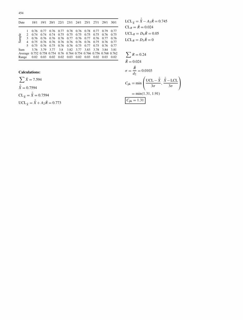
Appendix 5

Part name: Component EMachine: FixtureSpecification: 0.7–0.8

Quality characteristics: ThicknessSample size: 5Sampling interval: 10

Fig. 9. X̄ and R control chart for component E

454

Date 18/1 19/1 20/1 22/1 23/1 24/1 25/1 27/1 29/1 30/1

1 0.76 0.77 0.76 0.77 0.78 0.76 0.78 0.77 0.79 0.772 0.74 0.74 0.74 0.75 0.75 0.75 0.75 0.75 0.76 0.753 0.76 0.76 0.76 0.76 0.77 0.76 0.77 0.76 0.77 0.764 0.75 0.76 0.76 0.76 0.76 0.76 0.76 0.75 0.76 0.775 0.75 0.76 0.75 0.76 0.76 0.75 0.77 0.75 0.76 0.77

Sam

ple

Sum 3.76 3.79 3.77 3.8 3.82 3.77 3.83 3.78 3.84 3.81Average 0.752 0.758 0.754 0.76 0.764 0.754 0.766 0.756 0.768 0.762Range 0.02 0.03 0.02 0.02 0.03 0.02 0.03 0.02 0.03 0.02

Calculations:∑

X̄ = 7.594

¯̄X = 0.7594

CLX̄ = ¯̄X = 0.7594

UCLX̄ = ¯̄X + A2 R̄ = 0.773

LCLX̄ = ¯̄X − A2 R̄ = 0.745

CLR = R̄ = 0.024

UCLR = D4 R̄ = 0.05

LCLR = D3 R̄ = 0

∑R = 0.24

R̄ = 0.024

σ = R̄

d2= 0.0103

Cpk = min

⎛⎝UCL− ¯̄X

3σ,

¯̄X −LCL

3σ

⎞⎠

= min(1.31, 1.91)

Cpk = 1.31