1

USING NWSRFS ESP FOR MAKING EARLY OUTLOOKS OF SEASONAL RUNOFF VOLUMES INTO LAKE POWELL

David G. Brandon

Hydrologist In Charge National Weather Service-Colorado Basin River Forecast Center (CBRFC)

Abstract

The Colorado Basin River Forecast Center (NOAA/NWS-CBRFC) is the office responsible for providing operational daily and weekly river forecasts and seasonal streamflow volumes for Lake Powell in the Upper Colorado River Basin (UCRB). The Lake Powell forecast is extremely important to the USBR, States, Mexico and other water users. During the past 15 years the April through July runoff into Lake Powell has experienced two protracted dry periods, 1988-1992 and 2000-2004. During the most recent drought, the lake level in Lake Powell has dropped to the lowest level since the lake was filled in 1980. Users are asking for earlier than usual outlooks of streamflow. There is more emphasis being placed on creative ways of utilizing climate variability (forecasts and indices) in the forecast process. More detailed analysis of the affects of starting watershed conditions is being investigated. All of this provides interesting challenges for an operational forecast center. The CBRFC utilizes two classes of models to provide outlooks and forecasts for seasonal volumes into Lake Powell. One model uses multiple linear and non-linear regressions using various types of variables regressed against historical observed flow. This model has been used since the late forties. The Ensemble Streamflow Prediction System, part of the NWS River Forecast System (NWSRFS) is the second model. It incorporates a conceptual soil-moisture model, capabilities for pre-adjustment of input (precipitation and temperature ensembles) and post adjustment of output (streamflow) ensembles using climate forecasts and a variety of climate indices. Several other techniques such as Holt-Winters Analysis and statistical analogs have also been investigated for early outlooks made in the late summer and early fall. The paper will discuss the main ‘drivers’ for making an early season outlook and show how the NWSRFS ESP accounts for these drivers. An analysis of ESP reforecasts for Lake Powell is provided. The main conclusions are:

(1) A skill level of 16% (over climatology) can be obtained for a November 1 outlook using the NWSRFS Ensemble Streamflow Prediction System. (2) Initial watershed conditions have a significant impact on seasonal runoff volumes and must be accounted for by a soil moisture accounting model. (3) The variability of seasonal volumes is higher in wetter periods than drier periods. (4) Post weighting of streamflow traces/volumes using climate indices show no increase in skill in the UCRB. It is suggested that the preferred method to incorporate climate variability is to use the pre-adjustment technique of adjusting the atmospheric inputs (ensembles of precipitation and temperature) rather than post weight the runoff traces (which can be influenced by initial watershed conditions).

1.0 Introduction Runoff resulting from a winter snowpack is the main supply of water in the intermountain west. As population and water use increases water managers are relying more upon forecasts of seasonal streamflow volumes for

planning and operations. Water managers are not only expecting higher quality forecasts as the season progresses, but earlier ‘outlooks’ with increasing lead times. Research in climate variability, a better understanding of telleconnections and their affect on precipitation and runoff, and ways to account

2

for initial watershed conditions (e.g. soil moisture) is providing more information for water forecasters. This is true when a strong ENSO pattern exists that could affect the winter/spring precipitation. During these conditions it is expected that an ‘outlook’ for the upcoming runoff season be made in early Fall. The CBRFC has produced forecasts of seasonal ‘spring’ runoff volumes since 1947 (jointly with the NRCS for some basins). The first ‘official’ forecast for an upcoming spring runoff season has routinely been issued in early January, with subsequent updated forecasts issued in Feb, March, April, May and June. These forecasts have historically consisted of the ‘most probable’ (50%) value along with statistical bounds at the 10% and 90% level. Since the 1998 ENSO water users have requested that ‘early-bird’ outlooks be issued prior to the ‘official’ January forecast. Fig 1 shows a time-line for an outlook, forecast, and target seasonal volume. 2.0 Models and Techniques The CBRFC uses two main forecast models to produce outlooks and forecasts: (1) Statistical Multiple Linear (and Non Linear) Regression and (2) Ensemble Streamflow Prediction (ESP) which is a component of the NWSRFS. Other techniques such as statistical analogs and relationships, time series analysis investigating cycles, and neural networks using a variety of variables have been investigated. In a recent internal investigation of model techniques available to the NWS it has been found that the NWSRFS ESP system on the average does as well or better than the other techniques mentioned above in producing early season outlooks (Brandon). This paper will focus on the NWSRFS ESP System. It is the most complete operational model available to the CBRFC and accounts for the ‘drivers’ of a seasonal outlook.

Fig. 1: Time-Line For Outlooks, Forecasts And Seasonal Volumes 3.0 Drivers For A Seasonal Outlook There are four main components that ‘drive’ an early seasonal outlook. A water-supply forecast system at a minimum should possess capabilities to model or account for these drivers. There is uncertainty in all of these drivers. Figs 1 and 2

Fig. 2: Four Drivers For A Seasonal Outlook A general discussion of the drivers, an introduction to the NWSRFS ESP System and a discussion of how the ESP system accounts for each of the drivers follow. 3.1 Historical Observations/Climatology An analysis and understanding of the historical observations when making outlooks should not be underestimated. The properties of the historical distribution provide a useful context,

3

especially when making outlooks/forecasts many months into the future. The distribution of observations provides an important statistical driver. In a tongue and cheek description, the historical distribution is the trivial, ‘forecast for dummies’. If one new nothing else besides the historical distribution it would be a good first guess of what could happen in the future. Besides providing a context to a forecast, it provides the base ‘trivial forecast’ to ‘beat’ (add skill). If you can’t improve over the historical distribution (climatology), your model has no skill. 3.2 Initial Conditions Of The Watershed There are several initial conditions that must be accounted for. They are the antecedent/current flow, the state of the soil moisture, snowpack states, and current reservoir information (if regulated forecasts are required). 3.2.1 Antecedent Flow It has been shown that there is some correlation between the antecedent streamflow (Fall in this case) and the seasonal (spring-summer) volume. There is a rational reason for this correlation. The fall flow is an indicator of the baseflow carryover in a basin. This is especially true in larger basins. The water supply forecasters in the CBRFC have noticed this correlation in other basins as well. If snowmelt basins in the Upper Colorado River Basin (UCRB) begin the water year with higher (lower) baseflows, there is a tendency to have higher (lower) runoff in the spring. This driver can be considered as an indicator of persistence: if high (or low) baseflow already exist therefore it will persist into the future. It will set the starting point (initial condition) and can condition the future forecast. 3.2.2 Soil Moisture The initial state of soil moisture represents how wet or dry the upper and lower soil

conditions are in each sub-basin. From an intuitive sense it is easy to reason that if soil moisture at the start of the water year is high (low) there is a greater chance that the subsequent runoff will be high (low). A historical way of handling soil moisture in typical regression models was to include a variable that represented late summer and/or fall precipitation. Although this method has some merit, it has problems reflecting long protracted wet or dry periods where deficits (surpluses) can build up over several years. Another problem in accounting and understanding the physical connection of spring runoff to antecedent soil moisture is that there is no spatially widespread network of soil moisture observing sensors (over the UCRB). The NRCS has begun to install a limited amount of soil moisture sensors collocated with SNOTEL sites. This network shows promise, but a historical record will be needed for a more thorough analysis can be made. Another way of accounting for soil moisture is to utilize a soil-moisture accounting model. Various soil moisture models exist in the literature and have been used in river and water forecast systems. The soil accounting model should attempt to account for moisture in the topsoil mantel as well as lower zone moisture which reflect in the longer ‘carryover’ between years. This will be discussed in detail in following sections. 3.2.3 Snow States/Reservoir Status For early season outlooks significant snowpacks have usually not begun to form and are not a large factor. They become more important as the winter season progresses and must be accounted for in later period forecasts. Initial reservoir conditions are only needed if outlooks/forecasts are for ‘regulated’ flow. This paper and application assumes ‘un-regulated flow’.

4

3.3 Future Weather/Climate Variability The third driver is the most important of all, and if you can get it ‘right’ your skill will greatly improve. Unfortunately it is the most difficult to ‘get right’. This driver reflects ‘what’ the future weather will be in the upcoming water year (introducing climate variability). It has a definite bearing on the precipitation, snowpack and melt response.

Even though there can be a large error in long range climate/weather forecasting, increases in skill (over climatology) have been shown in certain parts of the country for certain atmospheric/oceanic states and should be accounted for in a forecast system. Global climate forecast models also show some promise for introducing climate variability and will increase in use in the decades to come.

Various indices implying telleconnections have been examined by many researchers. Some of the more widely used indices have been the SOI, MEI, Nino3.4 SST, PDO and the ONI. The historical way of handling climate variability in a typical regression model is to include a ‘variable’ that represented the ENSO state of the equatorial pacific (or other areas). The NWSRFS-ESP model uses various pre and post weighting techniques of the input and/or output traces. These pre and post weights are obtained from the climate indices. ESP can ingest ensembles of meteorological inputs produced by any method (e.g. statistical resampling. Climate Forecast Systems). The pre-adjustment technique weights (or adjusts) the meteorological inputs before the model is executed. The post-adjustment technique first executes the model, and then weights (or adjusts) the output flow traces. 3.4 Model Bias Correction Very few conceptual models are free from bias. Even if the future boundary conditions, such as quantitative precipitation and temperature forecasts, are known, hydrologic prediction is still subject to errors due to uncertainties in the initial conditions, observed

boundary conditions, and model errors. A more reliable forecast may be obtained if the forecast can be corrected for any systematic bias that may exist in the uncertainties. It could be argued whether this should be considered a ‘driver’, but the forecast system should be able to examine for bias and be capable of adjusting the output. This is especially true for probabilistic forecast distributions where bias may exist in different part of the distribution. 4.0 Introduction To The NWSRFS ESP System The NWSRFS ESP system is described in some detail in other publications. A short primer may be useful to understand how it handles the ‘drivers’. The NWSRFS consists of three interconnected components.

(1) Operational Forecast System (2) Calibration System (3) Ensemble Streamflow Prediction System.

The NWSRFS system allows a forecaster to produce streamflow forecasts in a time scale from hours to years. A main point is that all components are ‘linked’ together through calibration so that compatibility is retained, e.g., between initial conditions or states of soil moisture, snow, and flow over the spatial and temporal domain. The ESP system is the component, which provides the capability of making long-range probabilistic forecasts of streamflow. ESP uses conceptual hydrologic/hydraulic models to forecast future streamflow using the current soil moisture, flow, and reservoir conditions with historical meteorological data (or data generated from other techniques). The ESP procedure assumes that meteorological events that occurred in the past are representative of events that may occur in the future. Each year of historical meteorological data is assumed to be a possible representation of the future and is used to simulate a streamflow trace. The simulated streamflow traces can be analyzed for a

5

number of variables for a period in the future. ESP produces a probabilistic forecast for each variable and period of record. There are possible variations available in ESP to account for climate variability and future weather using the pre or post adjustment techniques. See Fig’s 3,4,5,6. There are two key points: (1) simulated flows are ‘conditioned’ by the initial state variables, including the antecedent flow and soil-moisture conditions, (2) the parameters used in the forecast model are the same ones used in the calibration system to produce the simulated spaghetti plots (which was calibrated using the same set of historical years).

Fig. 3: Steps In ESP Trace Generation

Fig. 4: Components of ESP Analysis

Fig. 5: Making the Traces Using ESP

Fig. 6: Analyzing The Trace Window From ESP 5.0 How ESP Accounts For the Drivers An Example Using Lake Powell 5.1 Historical Observations/Climatology ESP ‘by its nature’ includes historical climatology by using historical meteorological inputs both in calibration and forecasting. The hydrologic models within the NWSRFS OFS and ESP are calibrated with historical temperature and precipitation. Thus, it will

6

reflect realistic historical patterns. Second, when ESP is run the meteorological inputs are historical representations of the past. This is the case even if the inputs are weighted or produced from a resampling technique. Even though the forecast distributions may be a result of pre-adjusted inputs or post adjusted outputs (using weighting techniques), they will still ‘reflect’ characteristics of the historical distributions. The last PDF graph in Appendix A shows the distribution of historical observed APR-JUL Volumes (unregulated) into Lake Powell for 1977-2002. It is you first ‘best guess for a forecast’ if you knew nothing else. 5.2 Initial Conditions Of The Watershed The two most important initial watershed conditions are the antecedent flow and the soil moisture states. 5.2.1 Antecedent Flow The antecedent flow is simply the observed flow in the river when ESP is executed. A correlation of 0.56 exists between average monthly streamflow in October and subsequent spring runoff volume into Lake Powell (Fig 7). Note that there exists significant variability when the October flows are in the lower tercile.

Fig. 7: Correlation Plot Between October Streamflow and Seasonal Volume Into Lake Powell

Figure 8 shows the average October flow, prior to the beginning of the water year for historical years. Note the va riability of flows from slightly over 200,000 AF (Acre-Feet) to over one million AF. This will have an affect on the starting point for ESP. It is indicative and usually relates to the overall soil moisture carryover of the basin.

Fig. 8: Historical Plot of October Volumetric Flow Entering Lake Powell 5.2.2 Soil Moisture ESP has the capability to use one of two types of continuous conceptual soil-moisture accounting models: (1) Sacramento Soil Moisture Accounting Model (SAC-SMA used by most NWS River Forecast Centers) and (2) the Continuous API model. The discussion in this paper uses the SAC-SMA. The SAC-SMA has been well documented in other resources. It is a conceptual ‘tank’ model that accounts for the upper zone soil mantel as well as the lower zones. It is a non-linear response model with infiltration and percolation dependent upon the current amount of the water in all of the ‘tanks’. Evaportranspiration is also accounted for. The size of the ‘tanks’, percolation rates, withdraw rates, and impervious areas are determined by the calibration component of the NWSRFS. Two schematics of the SAC-SMA are shown in Figs. 9,10. (Figs. 9, 10 Courtesy of Riverside Technology, INC.)

7

Fig. 9: Schematic Diagram of the SAC-SMA

Fig. 10: More Detailed Flowchart of SAC-SMA The five tanks in the SAC-SMA are: Upper Zone Tension Upper Zone Free Lower Zone Tension Lower Zone Supplemental Lower Zone Primary At any time step the contents of these tanks provide an indication of the ‘state’ of the soil moisture. The ‘upper tanks’ mimic the first couple of inches in the soil mantel. The ‘lower tanks’ represent deeper areas, accounting for basin recharge, and longer term supplemental and base flow. The interaction between available water at the surface, infiltration, percolation, evaporation, and movement of water between tanks is complicated. The accuracy of the physical process is directly related to the quality of the calibration and parameterization.

The CBRFC recently developed a daily history for that past 30 years of all five tanks for many sub-basins in the UCRB. From this history, variability and averages were determined and analyzed. A total basin ‘virtual’ soil moisture index was developed that is simply the summation of the contents of all of the tanks at a daily time steps. By comparing the index for each day and/or month to the averages and standard deviation one can deduce a fairly strong quantitative representation of the state of the soil moisture, especially as an antecedent condition at the start of the water year. It is not the purpose of this paper to provide intricate details on the workings of the SAC-SMA model. It is useful to present a few graphs to show how ESP interacts with the SAC-SMA and how soil moisture surplus and deficits may affect the ESP forecasts. These graphs follow. Fig.11 shows a correlation plot between the total a soil moisture index in the UCRB (average of 8 sub-basins) in late October and the spring runoff volume.

Fig. 11: Correlation Plot Between the SAC-SMA Basin Index and Seasonal Volume To show how the SAC-SMA reflects the soil infiltration process several plots of soil moisture are: one in the northern part of the basin (Green River @ Warren Bridge, WY) and one in the southern basin (San Juan River

8

@ Pagosa Springs, CO). Figures 12 and 13 provide plots of the total soil moisture (sum of all five tanks) for three different years: 1984 wettest in recent history, 2004 recent past year 2005 current year The black line represents the average soil moisture state for each day (26 years of record). The ‘Max’ line at the top is the theoretical maximum that the total of all tanks together could hold (however it will never reach this level do to the way the model works). The black arrow located just after March points to rapid rise that occurred in 1984. This reflects the rapid infiltration of water that occurred during one of the warmest March’s on record. Note the 2005 (short blue line) at Pagosa Springs. It is higher than last year at this time and reflects the high precipitation and recharge that occurred in October 2005 (Water Year) over the San Juan Basin.

Fig. 12

Fig. 13 Total Soil Moisture from the SAC-SMA for Warren Bridge and Pagosa Springs for Selected Years The graphs of total soil moisture index provide an overall current ‘state’ of the basin in relation to soil moisture It is interesting and useful to examine the components of the total index (i.e., contents of each of the five tanks). This is done for the two basins in Figs. 14 and 15. The two graphs show the model states of each of the five ‘tanks’ for 1984 as the year progresses on a daily time step. Notice the relative size of each tank, where the lower tanks are sized larger and hold more than those in the upper area. The upper zone free water does not usually come into play until the peak of the melt season, as is shown in the graphs in April-June. There is basin recharge in the lower zone tension even from the start of the water year at Warren Bridge. The lower zone tension dramatically recharges beginning in May when the melt accelerates. The lower zone primary line shows a decrease from October to April indicating some withdraw (although water can still be percolating into this tank).

9

Fig. 14 SAC-SMA Components for 1984 for the Green River @ Warren Bridge, WY

Fig. 15: SAC-SMA Components for 1984 for the San Juan @ Pagosa Springs, CO The soil moisture surplus and deficits for both basins are shown in Figs: 16-19. The surplus/deficit values are measured from either side of the average for the month. There are two plots for each site. One graph is detailed and shows values for each month. The second graph shows only the surplus/deficit at the beginning of the water year (October). The wet (surplus) and dry (deficit) periods are clearly shown. These watershed conditions will affect the runoff and the forecasts from ESP.

Fig 16,17 Soil Moisture Surplus/Deficits on A Monthly and Yearly Scale (Each October) For Warren Bridge

Fig 18, 19 Soil Moisture Surplus/Deficits on A Monthly and Yearly Scale (Each October) For Pagosa Springs Note the wet periods in 1983-1988 where the surpluses continue from year to year. The recent drought also stands out from 2001 to 2004, especially for Pagosa Springs where the largest deficit for all years is indicated.

10

The starting watershed conditions can have a significant affect on the seasonal runoff. It is not as simple to assume that greater (lesser) precipitation always means more (less) runoff in a basin. To access and demonstrate this, a sensitivity analysis for the UCRB was done. Using ESP, 26 sets of initial watershed conditions for November 1 were saved (these are called carryover dates/states). The meteorological ensembles for a single year were then run for each ‘carryover’ date/state. This produced a distribution of flow volumes for each carryover state using the same precipitation and temperature ensembles as input. This is in effect a reverse process of ESP where you run many inputs for a single carryover state. Figs. 20, 21 and 22 show the results of this analysis. The ‘set numbers’ in the graphs represent the lowest average precipitation over the UCRB to the highest average precipitation. For example, set number one represents the lowest precipitation year and the subsequent flows that would occur with the 26 varying initial watershed conditions. Set 26 represents the same but for the wettest year over the basin. Note that the difference in the range of potential flows can be as much as 5 million AF. What this indicates is that even if you know the precipitation and temperature inputs, you must account for initial watershed conditions. Another result is that the variability (Standard Deviation Fig 22) of flow increases in the wetter years over that of the dryer years. A finding for water supply forecasters is that once you get into the wetter years, the variability of runoff increases and there can be more error in the forecasts. Temperature regimes will also affect the runoff, but for this study they were not explicitly examined (a future study).

R a n g e O f S i m u l a t e d F l o w F o r D i f f e r e n t S t a r t i n g

Watershed Cond i t ions Us ing 26 Se ts o f Meteoro log ica l

I n p u t s F r o m L o w e r A v e r a g e B a s i n P r e c i p i t a t i o n ( s e t 1 ) t o

H i g h e r ( s e t 2 6 )

Upper Co lorado Above Lake Powel l

0

5000

10000

15000

20000

25000

1 3 5 7 9 11 13 15 17 19 21 23 25I n p u t S e t N u m b e r

Bottom Of Range Top Of Range

Fig. 20 See Title and Text

Difference Of The Range Values In Simulated Flow For Different Starting Watershed Conditions

(See Corresponding Graph of Ranges)

01000

2000

30004000

50006000

7000

1 3 5 7 9 11 13 15 17 19 21 23 25

Input Set Number

AP

R-J

UL

VO

L (1

000s

AF)

Fig. 21 See Title and Text

11

Standard Deviation of the Flows For Different Starting Watershed Conditions(See Corresponding Graph of Ranges)

0

500

1000

1500

2000

1 4 7 10 13 16 19 22 25

Input Set Number

AP

R-J

UL

VO

L

(100

0s A

F)

Fig 22 See Title and Text 5.2.3 Future Weather/Climate Variability ESP provides two flexible methods for incorporating future weather scenarios. They are called the ‘CPC Pre-Adjustment Technique’ and the ‘Post Weighting Technique’. They revolve around creatively weighting the historical meteorological inputs in the pre-adjustment technique and weighting the output flow traces for the post technique. A third option is for the user to provide custom input ensembles of meteorological variables from resampling techniques, statistical weather generators, and numerical models. In the CPC pre-adjustment technique historical mean-areal precipitation and temperature time series are adjusted relative to current meteorological forecasts/climate outlooks issued by the Climate Analysis Center (NOAA_CPC) before they are used as an input. The adjustment is based on the comparison of coinciding marginal exceedence probabilities of historical records

and weather forecasts at spatial scales corresponding to weather forecast scales (Internal paper-J. Schaake and S. Perica, NWS-Office of Hydrology). The post adjustment technique is simply a mechanism for a user to apply ‘weights’ to each year of the output flow traces. The weights can be obtained in a variety of methods. Werner/Brandon developed a distance weighting technique that can use any climate index. It optimizes on the number of years to weight, as well as what weights to apply to the remaining years. Another method would be to use composites where you would weight, e.g. ESNO years more than others. These types of techniques only have relevance when a significant ‘signal’ or relationship exists between the ocean-atmospheric state in the late summer/fall and winter precipitation. Unfortunately, for the UCRB this signal is difficult to ‘tune in’. Bandon previously showed that improvements in forecasting seasonal forecasts using SOI and MEI as climate variables were significant in the Green and San Juan in the UCRB and many basins in the Lower Colorado (below Lake Meade). The middle area of the UCRB exhibits no clear ESNO signal (although Tootle/Piechota has suggested that there is some correlation to SSTs in the northern Pacific adjacent to the western U.S.). Figure 23 shows that the greatest percentage of wet El Nino winters occur in southern and western Arizona, whereas the greatest percentages of dry El Nino winters occur in the northern UCRB.

Southern Arizona occurs about twice as often as dry winters, in sharp contrast with the northern UCRB. Fig 24 shows ‘composites’ and indicates shifts in the distribution of average winter precipitation in five sub-basins. The La Nina case leans toward wetter than average in the Green and White-Yampa. It shows dry conditions in the San Juan. The El Nino case indicates dry/neutral for the Green, White Yampa, and Upper Colorado and to some

As an example of using a climate index Fig 25 shows a very weak correlation between the SOI in October and spring runoff in the UCRB.

12

Fig. 23: Ratio of Wet to Dry El Nino Events

Fig. 24: Composites for LaNina and ElNino Cases

Fig. 25: Correlation between SOI in October and Seasonal Volume When you consider the entire UCRB the signals are mixed at best. They are reversed

from the upper area (Green) to the lower area (San Juan), and are non-existent in between. 5.2.4 Model Bias Correction The ESP system indicated a bias in over simulating at almost all probability levels. The correction was in the 5-10 % range. 6.0 ESP – Reforecasts/Validation The ESP Verification Software and local verification software written at the CBRFC allow ESP to be initialized, executed, and provide simulations (forecasts) in ‘reforecast mode.’ Reforecast mode is also known as ‘Jackknifing’ and ‘Cross Validation’. This allows a user to reconstruct what the initial conditions were (e.g. soil moisture conditions in the model) at any date, and to produce spaghetti plots of flow conditioned by the starting conditions. Although these are not and cannot exactly duplicate what forecast would have been issued it does provide valuable information on how the model performs and sensitivity analysis on various drivers, input and output weighting, etc. 6.1 Reforecasts - Beginning November 1 The ESP verification system was initialized to save the carryover model states for every November 1, 1977 to 2002. ESP was then run for every year using the precipitation and temperature traces from all other years (except the year that was being forecast). The outflow traces were weighted using the post-adjustment technique, using the August-September-October ONI as an index. The November or later indices were not used since they would not be available at forecast time. 6.1.1 Reforecasts – Results The UCRB is a complex suite of many sub-basins. It consists of 184 separate basins, most being divided into three watershed areas based on elevation bands. This is required since many of the basins have different climatic regimes at different elevations.

13

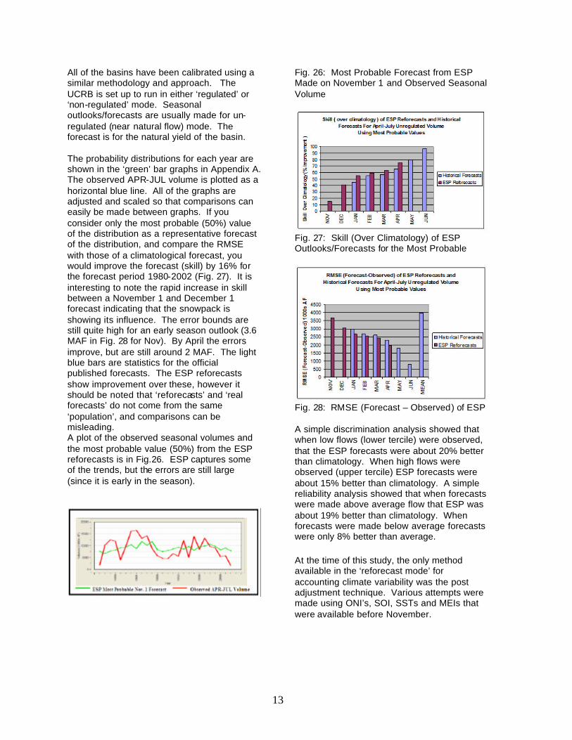
All of the basins have been calibrated using a similar methodology and approach. The UCRB is set up to run in either ‘regulated’ or ‘non-regulated’ mode. Seasonal outlooks/forecasts are usually made for un-regulated (near natural flow) mode. The forecast is for the natural yield of the basin. The probability distributions for each year are shown in the ‘green’ bar graphs in Appendix A. The observed APR-JUL volume is plotted as a horizontal blue line. All of the graphs are adjusted and scaled so that comparisons can easily be made between graphs. If you consider only the most probable (50%) value of the distribution as a representative forecast of the distribution, and compare the RMSE with those of a climatological forecast, you would improve the forecast (skill) by 16% for the forecast period 1980-2002 (Fig. 27). It is interesting to note the rapid increase in skill between a November 1 and December 1 forecast indicating that the snowpack is showing its influence. The error bounds are still quite high for an early season outlook (3.6 MAF in Fig. 28 for Nov). By April the errors improve, but are still around 2 MAF. The light blue bars are statistics for the official published forecasts. The ESP reforecasts show improvement over these, however it should be noted that ‘reforecasts’ and ‘real forecasts’ do not come from the same ‘population’, and comparisons can be misleading. A plot of the observed seasonal volumes and the most probable value (50%) from the ESP reforecasts is in Fig.26. ESP captures some of the trends, but the errors are still large (since it is early in the season).

Fig. 26: Most Probable Forecast from ESP Made on November 1 and Observed Seasonal Volume

Fig. 27: Skill (Over Climatology) of ESP Outlooks/Forecasts for the Most Probable

Fig. 28: RMSE (Forecast – Observed) of ESP A simple discrimination analysis showed that when low flows (lower tercile) were observed, that the ESP forecasts were about 20% better than climatology. When high flows were observed (upper tercile) ESP forecasts were about 15% better than climatology. A simple reliability analysis showed that when forecasts were made above average flow that ESP was about 19% better than climatology. When forecasts were made below average forecasts were only 8% better than average. At the time of this study, the only method available in the ‘reforecast mode’ for accounting climate variability was the post adjustment technique. Various attempts were made using ONI’s, SOI, SSTs and MEIs that were available before November.

14

No significant skill was detected when considering the entire basin. When analyzing the Green by itself a 15% improvement was noted, depending upon the weighting scheme used. A grid of information used in the study is shown in Appendix C. 7.0 Future Study Future studies include: (1) Analyzing affects of temperature in relation to initial watershed conditions, precipitation, and variability in runoff. (2) Incorporating and analyzing pre- adjustment techniques in the reforecast mode (3) Incorporating meteorological ensembles generated from the Climate Forecast System (CFS) (4) Analyzing other basins (5) More in-depth understanding of the initial watershed conditions, especially the soil moisture model states. (6) Performing more rigorous verification using Rank Probability Skill Scores and analyzing the entire distribution (rather than the most probable). 8.0 Conclusions Early season outlooks beginning in October/November for a basin as complicated and diverse as the UCRB show some but small skill over climatology. Outlooks for sub-basins within the UCRB showed improve skill, but large errors still exist. If you use a model that attempts to account for initial watershed

conditions, such as the NWSRFS Ensemble Streamflow Prediction System you can improve the skill to 16% over climatology. The ESP forecast for Dec 1 jumps to just over 40%, indicating the snowpack is beginning to influence the process. The RMSE for an ESP outlook made on November 1 was about 3.6 MAF. By April 1 it drops to 2 MAF. A sensitivity analysis of initial watershed conditions indicated that the affect on seasonal runoff can be large. Simulated seasonal flows ‘could’ theoretically range between 2-6 million AF depending upon initial watershed conditions and subjected to the same meteorological inputs. Post adjustment techniques to account for climate variability over the entire UCRB showed no appreciable skill. It is suggested that any skill that could be obtained in post-weighting flows is masked by the variability caused by the initial watershed states. The pre-adjustment on the precipitation and temperature inputs would be the suggested method to incorporate climate signals/variability. The model bias correction for the UCRB is in the range of 5-10%. Another result is that the variability (Standard Deviation Fig. 22) of flow increases in the wetter years over that of the dryer years. When years are wetter, the variability of runoff increases and there can be more error in the forecasts. Note: The volumetric flows used in this study and for operational ESP forecasts are adjusted (from observed flows) to estimate un-regulated (more like natural flows and yields). These adjustments have been coordinated with the USBR.

15

Appendix A Probability Density Plots Of Reforecasts For April-Jul Volume Inflow to Lake Powell Forecasts are Made on November 1 and Reflect Nov 1 Watershed Conditions Volumes are for Unregulated-Natural Flow (Adjustments Coordinated with the USBR) Horizontal Blue Bars are Observed

Credit: Statistical Package: JMP was developed by SAS Institute Inc., Cary, NC. JMP is not a part of the SAS System, though portions of JMP were adapted from routines in the SAS System, particularly for linear algebra and probability calculations. Version 1 of JMP went into production in October 1989.

Keys:

16

Appendix A - Continued

17

Appendix A - Continued

18

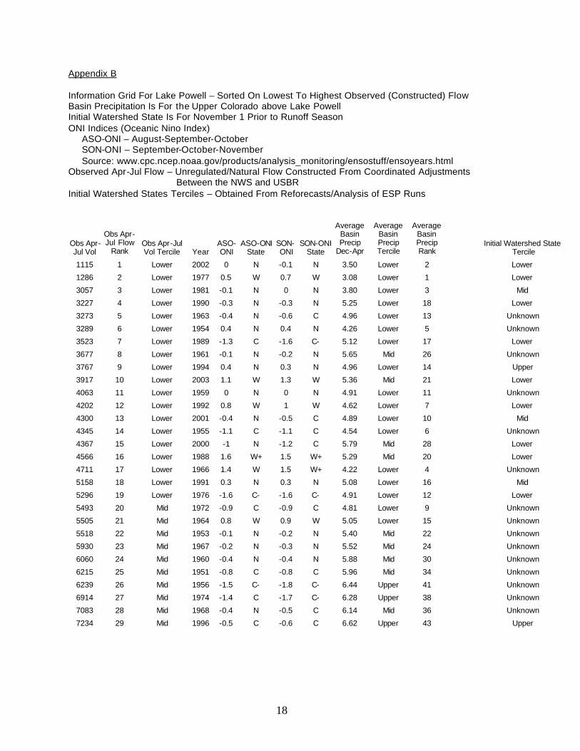
Appendix B Information Grid For Lake Powell – Sorted On Lowest To Highest Observed (Constructed) Flow Basin Precipitation Is For the Upper Colorado above Lake Powell Initial Watershed State Is For November 1 Prior to Runoff Season ONI Indices (Oceanic Nino Index) ASO-ONI – August-September-October SON-ONI – September-October-November Source: www.cpc.ncep.noaa.gov/products/analysis_monitoring/ensostuff/ensoyears.html Observed Apr-Jul Flow – Unregulated/Natural Flow Constructed From Coordinated Adjustments Between the NWS and USBR Initial Watershed States Terciles – Obtained From Reforecasts/Analysis of ESP Runs

Obs Apr-Jul Vol

Obs Apr-Jul Flow

Rank Obs Apr-Jul Vol Tercile Year

ASO-ONI

ASO-ONI State

SON-ONI

SON-ONI State

Average Basin Precip

Dec-Apr

Average Basin Precip Tercile

Average Basin Precip Rank

Initial Watershed State Tercile

1115 1 Lower 2002 0 N -0.1 N 3.50 Lower 2 Lower

1286 2 Lower 1977 0.5 W 0.7 W 3.08 Lower 1 Lower

3057 3 Lower 1981 -0.1 N 0 N 3.80 Lower 3 Mid

3227 4 Lower 1990 -0.3 N -0.3 N 5.25 Lower 18 Lower

3273 5 Lower 1963 -0.4 N -0.6 C 4.96 Lower 13 Unknown

3289 6 Lower 1954 0.4 N 0.4 N 4.26 Lower 5 Unknown

3523 7 Lower 1989 -1.3 C -1.6 C- 5.12 Lower 17 Lower

3677 8 Lower 1961 -0.1 N -0.2 N 5.65 Mid 26 Unknown

3767 9 Lower 1994 0.4 N 0.3 N 4.96 Lower 14 Upper

3917 10 Lower 2003 1.1 W 1.3 W 5.36 Mid 21 Lower

4063 11 Lower 1959 0 N 0 N 4.91 Lower 11 Unknown

4202 12 Lower 1992 0.8 W 1 W 4.62 Lower 7 Lower

4300 13 Lower 2001 -0.4 N -0.5 C 4.89 Lower 10 Mid

4345 14 Lower 1955 -1.1 C -1.1 C 4.54 Lower 6 Unknown

4367 15 Lower 2000 -1 N -1.2 C 5.79 Mid 28 Lower

4566 16 Lower 1988 1.6 W+ 1.5 W+ 5.29 Mid 20 Lower

4711 17 Lower 1966 1.4 W 1.5 W+ 4.22 Lower 4 Unknown

5158 18 Lower 1991 0.3 N 0.3 N 5.08 Lower 16 Mid

5296 19 Lower 1976 -1.6 C- -1.6 C- 4.91 Lower 12 Lower

5493 20 Mid 1972 -0.9 C -0.9 C 4.81 Lower 9 Unknown

5505 21 Mid 1964 0.8 W 0.9 W 5.05 Lower 15 Unknown

5518 22 Mid 1953 -0.1 N -0.2 N 5.40 Mid 22 Unknown

5930 23 Mid 1967 -0.2 N -0.3 N 5.52 Mid 24 Unknown

6060 24 Mid 1960 -0.4 N -0.4 N 5.88 Mid 30 Unknown

6215 25 Mid 1951 -0.8 C -0.8 C 5.96 Mid 34 Unknown

6239 26 Mid 1956 -1.5 C- -1.8 C- 6.44 Upper 41 Unknown

6914 27 Mid 1974 -1.4 C -1.7 C- 6.28 Upper 38 Unknown

7083 28 Mid 1968 -0.4 N -0.5 C 6.14 Mid 36 Unknown

7234 29 Mid 1996 -0.5 C -0.6 C 6.62 Upper 43 Upper

19

7337 30 Mid 1950 -0.2 N 0 N 5.89 Mid 31 Unknown

7757 31 Mid 1987 0.7 W 0.9 W 4.68 Lower 8 Upper

7788 32 Mid 1999 -1.1 C -1.1 C 5.73 Mid 27 Upper

8036 33 Mid 1970 0.6 W 0.7 W 5.27 Lower 19 Unknown

8179 34 Mid 1971 -0.8 C -0.8 C 5.47 Mid 23 Unknown

8200 35 Mid 1969 0.2 N 0.4 N 5.91 Mid 32 Unknown

8209 36 Mid 1982 -0.2 N -0.1 N 6.28 Mid 37 Mid

8625 37 Mid 1998 2.3 W+ 2.4 W+ 5.63 Mid 25 Upper

8676 38 Upper 1978 0.5 W 0.7 W 7.86 Upper 52 Lower

9156 39 Upper 1948 -0.5 C -0.6 C 6.53 Upper 42 Unknown

9872 40 Upper 1958 0.8 W 0.9 W 5.80 Mid 29 Unknown

9951 41 Upper 1975 -0.5 C -0.7 C 6.72 Upper 45 Unknown

9984 42 Upper 1993 -1 C -0.1 N 8.00 Upper 54 Mid

10490 43 Upper 1949 -0.2 N 0 N 7.23 Upper 49 Unknown

10605 44 Upper 1980 0.3 N 0.4 N 7.74 Upper 51 Mid

10658 45 Upper 1962 -0.6 C -0.6 C 6.30 Upper 39 Unknown

11102 46 Upper 1979 -0.5 C -0.4 N 7.93 Upper 53 Lower

11261 47 Upper 1973 1.5 W+ 1.8 W+ 5.91 Mid 33 Unknown

11320 48 Upper 1997 -0.2 N -0.2 N 7.49 Upper 50 Upper

11345 49 Upper 1965 -1 C -1.1 C 7.11 Upper 47 Unknown

11699 50 Upper 1985 -0.3 N -0.6 C 6.72 Upper 44 Upper

11833 51 Upper 1995 0.7 W 0.9 W 7.20 Upper 48 Mid

12599 52 Upper 1986 -0.4 N -0.3 N 6.00 Mid 35 Upper

13057 53 Upper 1957 -0.9 C -0.9 C 8.40 Upper 55 Unknown

13814 54 Upper 1952 0.6 W 0.7 W 8.93 Upper 56 Unknown

14837 55 Upper 1983 1.5 W+ 1.9 W+ 6.40 Upper 40 Upper

15404 56 Upper 1984 -0.5 C -0.8 C 7.04 Upper 46 Upper

20

References Brandon, D. G. 1998. “Forecasting Streamflow in the Colorado and Great Basins using El Nino Indices as Predictors in a Statistical Water Supply Forecast System. Winter 97/98: Year of the Great El Nino? Floodplain Management Association, San Diego, Ca. CLIMAS Web Site: University of Arizona: http://www.ispe.arizona.edu/climas/ Jolliffe, I., Stephenson, D. B., “Forecast Verification-A Practitioner’s Guide in Atmospheric Science”, 2003 John Wiley & Sons Pagano, T. C., Garen, D. C, “Integration of Climate Information and Forecasts into Western US Water Supply Forecasts”, (Accepted: ASCE, Climate Technical Committee, Book Chapter) Tootle, G. A., Piechota, T. C., “Climate Variability, Water Supply, and Drought in the Upper Colorado Basin” (Accepted: ASCE, Climate Technical Committee, Book Chapter) Werner, K., Brandon, D.G., “Incorporating Medium Range Numerical Weather Model Output into ESP of the NWS.” Accepted: Journal of Hydrometeorology Werner, K., Brandon, D. G., “Climate Index Weighting Schemes for NWS ESP-Based Seasonal Volume Forecasts”, Accepted: Journal of Hydrometeorology