Upper Semicontinuity for Attractors of Parabolic Problems with Localized Large Diffusion and...

Journal of Differential Equations 168, 33�59 (2000)

Upper Semicontinuity for Attractors of ParabolicProblems with Localized Large Diffusion and

Nonlinear Boundary Conditions

Jose� M. Arrieta1

Departamento de Matema� tica Aplicada, Facultad de Matema� ticas,Universidad Complutense de Madrid, 28040 Madrid, Spain

E-mail: arrieta�sunma4.mat.ucm.es

Alexandre N. Carvalho2

Departamento de Matema� tica, Instituto de Ciencias Matema� ticas de Sa~ o Carlos,Universidade de Sa~ o Paulo, Caixa Postal 668, 13560-970 Sa~ o Carlos, SP Brazil

E-mail: andcarva�icmsc.sc.usp.br

and

An@� bal Rodr@� guez-Bernal1

Departamento de Matema� tica Aplicada, Facultad de Matema� ticas,Universidad Complutense de Madrid, 28040 Madrid, Spain

E-mail: arober�sunma4.mat.ucm.es

Received May 28, 1999; revised January 26, 2000

dedicated to professor jack k. hale on the occasion of his 70th birthday

1. INTRODUCTION

In this paper we are concerned with second order parabolic problems forwhich the diffusion coefficient becomes large in a sub-region which isinterior to the physical domain of the differential equation. That situationcan be found, for example, in composite materials, where the heat diffusionproperties can change significantly from one part of the region to another;that is, heat may diffuse much faster in some sub-regions than in others. Ifin a reaction-diffusion process the diffusion coefficient behaves as expressedabove, intuitively we expect that the solutions will tend to become homo-geneous in the regions where the diffusion becomes large.

doi:10.1006�jdeq.2000.3876, available online at http:��www.idealibrary.com on

330022-0396�00 �35.00

Copyright � 2000 by Academic PressAll rights of reproduction in any form reserved.

1 Partially supported by DGICYT, PB96-0648, Spain.2 Partially supported by CNPq Grant 300.889�92-5 and by FAPESP Grant *97�11323-0,

Brazil.

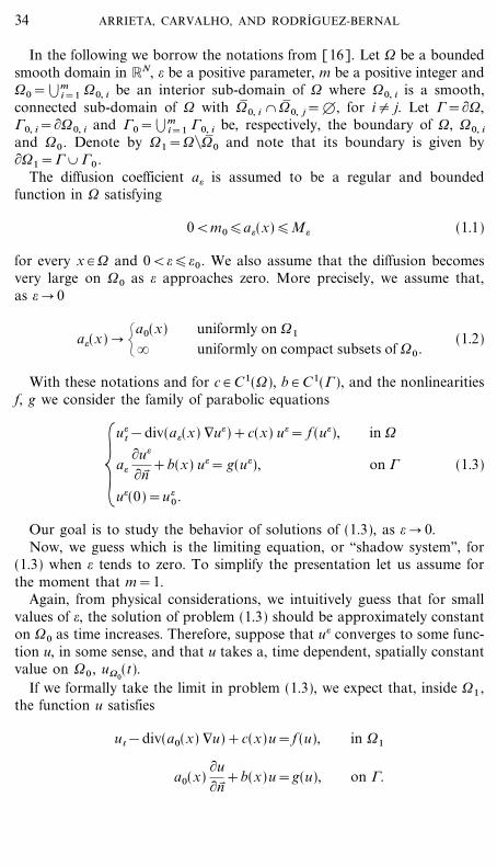
In the following we borrow the notations from [16]. Let 0 be a boundedsmooth domain in RN, = be a positive parameter, m be a positive integer and00=�m

i=1 00, i be an interior sub-domain of 0 where 00, i is a smooth,connected sub-domain of 0 with 0� 0, i & 0� 0, j=<, for i{ j. Let 1=�0,10, i=�00, i and 10=�m

i=1 10, i be, respectively, the boundary of 0, 00, i

and 00 . Denote by 01=0"0� 0 and note that its boundary is given by�01=1 _ 10 .

The diffusion coefficient a= is assumed to be a regular and boundedfunction in 0 satisfying

0<m0�a=(x)�M= (1.1)

for every x # 0 and 0<=�=0 . We also assume that the diffusion becomesvery large on 00 as = approaches zero. More precisely, we assume that,as = � 0

a=(x) � {a0(x)�

uniformly on 01

uniformly on compact subsets of 00 .(1.2)

With these notations and for c # C1(0), b # C1(1 ), and the nonlinearitiesf, g we consider the family of parabolic equations

u=t&div(a=(x) {u=)+c(x) u== f (u=), in 0

{a=�u=

�n�+b(x) u== g(u=), on 1 (1.3)

u=(0)=u =0 .

Our goal is to study the behavior of solutions of (1.3), as = � 0.Now, we guess which is the limiting equation, or ``shadow system'', for

(1.3) when = tends to zero. To simplify the presentation let us assume forthe moment that m=1.

Again, from physical considerations, we intuitively guess that for smallvalues of =, the solution of problem (1.3) should be approximately constanton 00 as time increases. Therefore, suppose that u= converges to some func-tion u, in some sense, and that u takes a, time dependent, spatially constantvalue on 00 , u00

(t).If we formally take the limit in problem (1.3), we expect that, inside 01 ,

the function u satisfies

ut&div(a0(x) {u)+c(x)u=f (u), in 01

a0(x)�u�n�

+b(x)u=g(u), on 1.

34 ARRIETA, CARVALHO, AND RODRI� GUEZ-BERNAL

The constant u00, however, may not be arbitrary. Integrating the equation

in 00 and using the inward normal in the integration by parts, we obtain

|00

u=t+|

10

a=�u=

�n�+|

00

cu==|00

f (u=)

and formally taking the limit and dividing by |00 | we have

u* 00+

1|00 | |10

a0

�u�n�

+cu00= f (u00

),

where c=|00 | &1 �00c(x) dx. Even more, one can expect u to match

appropriately the constant u00(t) across 10 , that is u |00

=u00.

In fact, when m�1 the limiting problem should be

ut&div(a0(x) {u)+c(x) u= f (u) in 01

a0

�u�n� 0

+b(x) u= g(u) on 1

u |00, i=: u00, i

in 00, i , i=1, ..., m

u* 00, i+

1|00, i | |10, i

a0

�u�n�

+ciu00, i= f (u00, i

), i=1, ..., m

u(0)=u0 ,

(1.4)

where ci=|00, i |&1 �00, i

c(x) dx and u0=lim= � 0 u=0 which are constant

on 00, i , i=1, ..., m.The natural spaces to study problem (1.3) are Lq(0) or W1, q(0), see

[3]. We will see that under certain conditions on the nonlinearities f andg problem (1.3) is well posed in Lq(0) or W 1, q(0) and under some dissi-pativeness conditions we have the existence of global attractors A= whichactually are independent of the space chosen to study the equation and thatlie uniformly on a bounded set of C0(0� ), see [4]. This will allow us tocut-off the nonlinearities, reducing to the case where the nonlinearities areglobally Lipschitz and studying both problems (1.3) and (1.4) in H1(0)and H 1

00(0) respectively, where in general for any functional space X we

define X00=[u # X, u is constant on 00, i , i=1, ..., m]. For this globally

Lipschitz nonlinearities we will have the existence of an attractor A0 forproblem (1.4) which will also lie on a bounded set of H 1(0) & C 0(0� ).

In comparing the dynamics of (1.3) and (1.4), we will prove the followingresult

35UPPER SEMICONTINUITY

Theorem 1.1. The global attractors A= , A0 are bounded subsets of H1(0),C0(0� ) and are upper semi-continuous at ==0 relatively to the topology inH1(0) and C0(0� ).

We will also be able to give a result on the convergence of orbits of theattractors:

Proposition 1.2. For every sequence of complete orbits u=k ( } )/A=k

there exists a subsequence =kjand a complete orbit u0( } )/A0 such that

u=kj ( } ) ww�j � �

u0( } ) in C([&T, T], C0(0� )), for any T>0.

These results state, in a precise sense, that the asymptotic set of statesand the asymptotic dynamics of both problems are close as = � 0, see [9].This closeness is obtained in the topology of H1(0) and of C0(0� ).

For related questions in the case of linear boundary conditions see[5�8, 11, 12].

Now we describe the contents of our paper.In Section 2 we recall known results on the well posedness, regularity,

existence of attractors and uniform bounds in different metrics for problem(1.3). These results are taken primarily from [3, 4, 16]. As an importantconsequence of this section is that we will be able to reduce to the casewhere the nonlinearities f and g are globally Lipschitz functions.

In Section 3 we study the local and global well posedness of the limitingproblem in the functional spaces H 1

00(0) and L2

00(0). For the first case

standard theory like the one from [13] can be applied. For the L200

(0)-set-ting we need to apply some results from [2, 3].

In Section 4 we study and compare extensively the linear problemsassociated to equations (1.3) and (1.4). We will prove the convergence inthe H1 and C 0 metric of the resolvents of the linear operators. For theproof of the C0 convergence we need to prove Lemma 4.2, which is anessential ingredient in the analysis of the C0 convergence for the linear and,afterwards, for the nonlinear problems. With this lemma we will alsoimprove certain results from [16] on convergence of the spectra for thelinear operators, see Proposition 4.4. We will also obtain estimates in theconvergence of the linear semigroups, see Proposition 4.6 and Corollary 4.8.

Finally, in Section 5, we study the relation between the asymptoticdynamics of both problems (1.3) and (1.4). We will show first that the attractorof (1.4) lies in a bounded set of C:(0� ). Considering now the uniform estimatesobtained for problem (1.3) and the convergence of the linear semigroupswe will show the upper semicontinuity of the attractors in H 1(0) by com-paring the nonlinear semigroups with the use of the variation of constants


formula. Once the upper semicontinuity in H 1(0) is obtained, Lemma 4.2will give us the key to prove it in C0(0� ).

2. BACKGROUND RESULTS

We summarize in this section the already known results on local andglobal existence of solutions, existence of attractors and their uniformbounds. These results, taken from [3, 4, 16], will be our starting point forthe upper semi-continuity results proved later on in this paper. We refer tothese articles for details, proofs and generalizations.

We consider the family of semi-linear parabolic problems given by equation(1.3) for = # (0, =0) where the nonlinearities f, g: R � R are C2 functions, c, bare C1 functions and the diffusion coefficient a= # C1(0� ) and satisfies (1.1).

We treat this problem as an evolution problem in the spaces Lq(0),W1, q(0) for 1<q<�. Therefore, and in order to simplify the notations,we define the family of spaces

E=[Lq(0), W1, q(0), 1<q<�].

Then we consider (1.3) as a semi-linear problem written in the abstractform as

u* +A=u=h(u),

where A= is a suitable weak formulation of the operator &div(a=(x) {u)+cu with boundary conditions a=(x) �u��n+b(x) u=0, and the nonlinearityis given by h :=f0+ g1 , that is,

(h(u), ,)=|0

f (x, u(x)) ,(x)+|1

g(x, u(x)) ,(x),

for all suitable regular test functions ,, see [3] for details.Assume that f and g satisfy the following growth conditions

(G)X : Let f, g: R � R be locally Lipschitz functions. Assume thefollowing,

1. If X=Lq(0), assume that f and g satisfy a relation of the form

| j(u)& j(v)|�c |u&v| ( |u|\&1+|v|\&1+1), (2.1)


with exponents \f and \g respectively, such that, with N�2 (respectivelyN=1)

\f�\0 :=1+2qN

, and \g�\1 :=1+qN

, (respectively, \g<\1 :=1+q).

2. If X=W1, q(0), assume either

(i) q>N,

(ii) q=N and f, g satisfy that for every '>0, there exists c'>0such that

| j(u)& j(v)|�c'(e' |u| N�(N&1)+e' |v| N�(N&1)

) |u&v|, (2.2)

(iii) 1<q<N and f, g satisfy (2.1), with exponents \f and \g ,respectively, such that

\f�\0 :=1+2q

N&qand \g�\1 :=1+

qN&q

.

The results from [3] can be summarized as follows,

Theorem 2.1 (Local existence). Let = # (0, =0). If X is any space in theclass E and f, g satisfy the growth restriction (G)X , then for any u0 # X thereexists locally a unique (in certain sense) mild solution u=( } , u0) # C([0, {), X),of problem (1.3) satisfying u=(0, u0)=u0 in X. This solution depends continuouslyon the initial data u0 # X and it is a classical solution for t>0. Also, the followingregularizing effect takes place: if u0 # X then u=(t, u0) # Y for any other spaceY in the class E, and t # (0, {).

Remark 2.2. The uniqueness mentioned in the theorem refers to theuniqueness studied in [2] and [3].

In order to obtain that all solutions of (1.3) are globally defined, we willassume some sign conditions on the nonlinear terms. These sign conditionsare independent of the space X and can be expressed in the form:

(S): Assume there exist B0 , C0 # R and B1 , C1�0 such that thefollowing holds for u # R:

u f (u)�&C0u2+C1 |u| ,(2.3)

ug(u)�&B0u2+B1 |u|.

Then we have the following result on global existence (see [4]):


Theorem 2.3 (Global existence). Let = # (0, =0) and let X be a space inthe class E. Assume that the growth condition (G)X and the sign condition(S) hold. Then, for any u0 # X the solution u=(t, u0) of (1.3) starting at u0

exists for all t�0. Therefore, we can define in X the semigroup [S=(t): t�0]associated to (1.3) by S=(t) u0=u=(t, u0), t�0. Moreover, from the regulariz-ing effect of Theorem 2.1, S=(t) u0 # Y for any other space Y in the class E

and for any t>0.

To prove the existence of a global attractor for the problem (1.3) we willimpose, besides condition (S), some dissipativeness condition for (1.3). Thiscondition is expressed as:

(D)= : Assume (S) holds and that with C0 and B0 from (S), the firsteigenvalue, *=

1 , of the following problem is positive

&div(a=(x) {u)+(c(x)+C0) u=*u, in 0(2.4)

a=(x)�u�n

+(b(x)+B0) u=0, on 1

With all these, it is possible to show the following result (see [4])

Theorem 2.4 (Existence of attractors). Let = # (0, =0) and let X be aspace in the class E. Assume that the growth condition (G)X and the dissi-pativeness condition (D)= hold. Then the semigroup [S=(t), t�0] associatedto (1.3) has a global attractor, A=

X , in X. Moreover, for any space Y in theclass E with Y/�X we also have the existence of the attractor A=

Y .Moreover A=

X=A=Y and it attracts bounded sets of X in the topology of Y.

In particular if the diffusion coefficient a= satisfies (1.2), we know from[16] that *=

1 converges to the first eigenvalue, *01 , of the limit eigenvalue

problem

{&div(a0(x) {u)+(c(x)+C0) u=*u in 01

(2.5)

a0(x)�u�n�

+(b(x)+B0) u=0 on 1

#0, i (u)=u00, ion 10, i , i=1, ..., m

1|00, i | |10, i

a0

�u�n�

+(ci+C0) u00, i=*u00, i

, i=1, ..., m,

where ci=|00, i |&1 �00, i

c(x) dx, #0, i is the trace operator on 10, i and u00, i

denotes the constant value of u on 00, i for i=1, ..., m. We will keep thisnotation from now on.


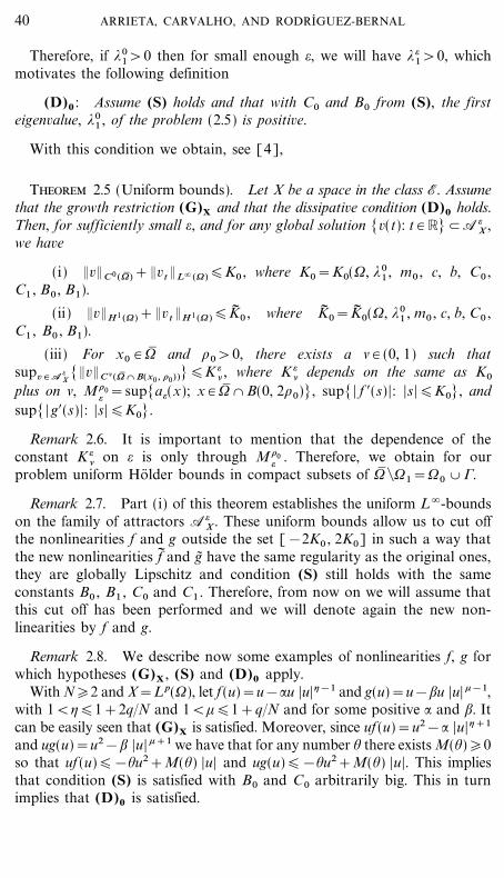
Therefore, if *01>0 then for small enough =, we will have * =

1>0, whichmotivates the following definition

(D)0 : Assume (S) holds and that with C0 and B0 from (S), the firsteigenvalue, *0

1 , of the problem (2.5) is positive.

With this condition we obtain, see [4],

Theorem 2.5 (Uniform bounds). Let X be a space in the class E. Assumethat the growth restriction (G)X and that the dissipative condition (D)0 holds.Then, for sufficiently small =, and for any global solution [v(t): t # R]/A=

X ,we have

(i) &v&C 0 (0� )+&vt &L� (0)�K0 , where K0=K0(0, *01 , m0 , c, b, C0 ,

C1 , B0 , B1).

(ii) &v&H 1 (0)+&vt &H 1 (0)�K� 0 , where K� 0=K� 0(0, *01 , m0 , c, b, C0 ,

C1 , B0 , B1).

(iii) For x0 # 0� and \0>0, there exists a & # (0, 1) such thatsupv # A

=X

[&v&C & (0� & B(x0 , \0))]�K =& , where K =

& depends on the same as K0

plus on &, M\0= =sup[a=(x); x # 0� & B(0, 2\0)], sup[ | f $(s)|: |s|�K0], and

sup[ | g$(s)|: |s|�K0].

Remark 2.6. It is important to mention that the dependence of theconstant K =

& on = is only through M\0= . Therefore, we obtain for our

problem uniform Ho� lder bounds in compact subsets of 0� "01=00 _ 1.

Remark 2.7. Part (i) of this theorem establishes the uniform L�-boundson the family of attractors A=

X . These uniform bounds allow us to cut offthe nonlinearities f and g outside the set [&2K0 , 2K0] in such a way thatthe new nonlinearities f� and g~ have the same regularity as the original ones,they are globally Lipschitz and condition (S) still holds with the sameconstants B0 , B1 , C0 and C1 . Therefore, from now on we will assume thatthis cut off has been performed and we will denote again the new non-linearities by f and g.

Remark 2.8. We describe now some examples of nonlinearities f, g forwhich hypotheses (G)X , (S) and (D)0 apply.

With N�2 and X=Lp(0), let f (u)=u&:u |u|'&1 and g(u)=u&;u |u| +&1,with 1<'�1+2q�N and 1<+�1+q�N and for some positive : and ;. Itcan be easily seen that (G)X is satisfied. Moreover, since uf (u)=u2&: |u|'+1

and ug(u)=u2&; |u| ++1 we have that for any number % there exists M(%)�0so that uf (u)�&%u2+M(%) |u| and ug(u)�&%u2+M(%) |u|. This impliesthat condition (S) is satisfied with B0 and C0 arbitrarily big. This in turnimplies that (D)0 is satisfied.


We may also consider the case where f is as above and g(u)=&|u|+&2 (1+sin(u))+#u, for which (G)X holds. For this case we haveug(u)�#u2. Hence, since (S) is satisfied with C0=% arbitrarily large andwith B0=&#, we have that (D)0 is satisfied. Similarly we may consider thecase where g(u)=sin(u |u| +&1). This is a bounded nonlinearity whichsatisfies (G)X and (S) with B0=0 and B1>0. This implies that (D)0 issatisfied.

3. THE LIMIT PROBLEM

In this section we recall from [16] the functional setting for problem(1.4) and will consider its well posedness and global existence andregularity of solutions in H 1

00(0) and L2

00(0). In Section 5 we will prove

the existence and regularity of the attractor for this problem under thedissipativeness condition (D)0 .

We will assume that the nonlinearities f and g are globally Lipschitz, seeRemark 2.7.

Following [16] we define the space L200

(0)=[u # L2(0), u is constanton 00, i , i=1, ..., m] and H 1

00(0)=[u # H 1(0), u is constant on 00, i ,

i=1, ..., m]. Let X0=L200

(0) and define the operator A0 in X0 with domainD(A0)=[u # H 1

00(0), &div(a0(x) {u) # L2(01), a0(x) �u

�n� +b(x) u=0 on 1]and for u # D(A0),

A0(u)=(&div(a0(x) {u)+c(x) u) X01

+ :m

i=1\ 1

|00, i | |10, i

a0(x)�u�n�

+ciu00, i+ X00, i

where XA denotes the characteristic function of the set A.The operator A0 is selfadjoint and has compact resolvent in X0=L2

00(0).

Moreover, if +>*01 , the first eigenvalue of A0 , then the operator A0++I

is positive. If we denote by X #0 its fractional power spaces, we have that

X10=D(A0), X 1�2

0 =H 100

(0), X 00=L2

00(0), X &1�2

0 =H &100

(0) =def (H 100

(0))$,see [16]. By interpolation X #

0/�H 2#

00(0), for 0�#�1�2. By duality we

obtain H &2#00

(0)/�X &#0 , again for 0�#�1�2.

The operator A0 is the realization in L200

(0) of the operator L0 , betweenH 1

00(0) and its dual defined by means of the bilinear form

(L0(u), v) &1, 1=a0(u, v)=|01

a0 {u {v+|0

cuv+|1

buv

for every u, v # H 100

(0). For the sake of simplicity in the notations we willnot distinguish between L0 and A0 .


The nonlinear terms verify h= f0+ g1 : H 100

(0) � H &s00

(0) for any s>1�2,and since f, g: R � R are globally Lipschitz we obtain that h is globallyLipschitz. In terms of the fractional power spaces we have that h: X 1�2

0 � X &s0

for any s>1�4 and that there exists a constant c�0 such that &h(u)&h(v)&X 0&s

�c &u&v&X01�2 for any u, v # X 1�2

0 . We can prove the following

Proposition 3.1. For any u0 # L200

(0) there exists a unique globallydefined u( } , u0) # C([0, �), L2

00(0)) & C((0, �), H 1

00(0)) mild solution of

ut+A0u=h(u) starting at u0 . Moreover this solution depends continuouslyon the initial data and satisfies u, ut # C((0, �), X #

0), for any #<3�4.Moreover if u0 lies in a bounded set of L2

00(0) then, for t>0 fixed, u(t, u0)

lies in a bounded subset of X #0 for any #<3�4. If the initial data is in H 1

00(0)

=X 1�20 then the solution is also in C([0, �), H 1

00(0)).

Proof. To prove that the problem is well posed for u0 # H 100

(0) we canapply standard semilinear theory like in [13]. The nonlinearity h: X 1�2

0 �X&s

0 and is globally Lipschitz, from where it follows the regularity and theglobal existence stated in the proposition.

The case u0 # L200

(0)=X 00 is different since the nonlinearity h is not even

defined on this space. Nevertheless the general theory developed in [2, 3]applies to this problem and allows to obtain all the results of the proposi-tion. Notice that if we define E:=X :&1

0 then h: E1+1�2 � E1&s, s>1�4, andit is globally Lipschitz. In the notation of [2, 3] this map is an =-regularmap for ==1�2 relative to (E1, E0). Applying Theorem 1 from [2] orTheorem 2.2 from [3] we prove the proposition. K

Note that now u solves

(ut , ,) +a0(u, ,)=( f0(u), ,) +( g1 (u), ,) , for all , # H 100

(0)

which implies

ut&div(a0(x) {u)+c(x) u= f (u) in 01

a0(x)�u�n�

+b(x) u= g(u) on 1

#0, i (u)=u00, ion 10, i , i=1, ..., m

u* 00, i+

1|00, i | |10, i

a0

�u�n�

+ci u00, i= f (u00, i

), i=1, ..., m

u(0)=u0 .

(3.1)


4. COMPARISON OF THE LINEAR PROBLEMS

In this section we compare the linear operators A0 and A= establishingcertain uniform convergence of the solutions of the respective ellipticproblems. In particular, applying these results to the eigenvalue problems,we will improve certain results from [16] and will prove the convergencein the uniform norm of the eigenfunctions of A= to the eigenfunctions of A0 .We will also be able to compare the behavior of the linear semigroups,e&A0 t and e&A=t.

We have the following result:

Proposition 4.1. Let f = # L2(0) and g= # L2(1 ). Assume f = ww�= � 0 f 0

w-L2(0) and g= ww�= � 0 g0 w-L2(1 ) then if u= and u0 are the solutions ofA=u== f =

0+ g =1 and A0u0= f 0

0+ g01 , then

(i) u= ww�= � 0 u0 strongly in H 1(0).

(ii) If f 0 # L p(0), with p>N�2, g0 # L�(1 ) then u0 # C0(0� ).

(iii) If f = # L p(0), with p>N�2, g= # L�(1 ) for all 0�=�=0 and& f =&Lp (0)+&g=&L� (1 )�C independent of =, then u= ww�= � 0 u0 in C0(0� ).

Proof. (i) The first part is obtained directly from [16], Corollary 4.5.

(ii) For the second part let us see first that u0 # L�(0). If we denoteby v= the solution of A=v== f 0

0+ g01 , from (i) we have that v= ww�= � 0 u0 in

H1(0). But from the uniform bounds obtained in [4] we have that &v=&L� (0)

�C independent of =. This implies in particular that &u0 &L � (0)�C andtherefore u0 # L�(0). If we denote by : i

0 the constant value that the func-tion u0 takes on 00, i , then the function u0 in 01 is the solution of thefollowing problem,

&div(a0(x) {u)+c(x) u= f 0 in 01

{a0(x)�u�n�

+b(x) u= g0 on 1 (4.1)

u=: i0 on 10, i , i=1, ..., m,

which is in C0(0� 1), see [4]. Moreover, since u is constant in the connectedcomponents of 00 we deduce that u is in C0(0� ).

(iii) In order to prove this part, we need the following importantlemma,


Lemma 4.2. For a fixed i, with 1�i�m, let 0i* be a domain such that00, i /0i* /0, let : i # R, and consider the family of problems depending on= and 0i*

{&div(a= {u=)=F =i ,

u==:i+; i=(x),

on 0i*on 1i*=�0i* ,

where lim sup= &; i= &L� (1i*)�L, F =

i # L p(0i*), for p>N�2, uniformly boundedin L p(0i*).

Then

lim supdist(1i*, 10, i) � 0

lim sup= � 0

&u=&:i&L� (0i*)�L.

Before proving this lemma let us finish with the proof of the proposition.From (i) and (ii) we obtain that u0 # C0(0� ) and u= ww�= � 0 u0 in H1(0).

From the uniform bounds of [4] we obtain that u= # L�(0) and that&u=&L� (0)�C independent of =. Also, from Theorem 2.5(iii) and Remark2.6, for any 0*=� 0i* as defined in the lemma, we have the existence ofan : # (0, 1) such that &u=&C: (0� "0*)�C(0*), which implies the compact-ness of the sequence u= in C0(0� "0*) and in particular that u= ww�= � 0 u0

in C0(0� "0*).Let $ be a positive number arbitrarily small. We will see that there exists

an =($)>0 such that &u=&u0&C 0(0� )�$ for any 0<=�=($).Since u0 # C0(0� ) we have that there exist a smooth 0*=� 0i* close

enough to 00 with the property that &;i&L� (0 i*)�$�2 where ;i (x)=u0(x)&:0

i , and :0i is the value of u0 in 0 i

0 . Applying the lemma to a 0*sufficiently close to 00 and with F == f =&c(x) u=, we obtain the result.

Now, we only need to prove the lemma

Proof of the lemma. Notice that without loss of generality we canassume that m=1. Therefore, for the proof of this lemma we will drop thesubindex i.

First, working with u=&: we can always assume that :=0. Second, bysuperposition, we can consider separately the cases ;= {0, F ==0 and;==0, F ={0.

In the former case, from [4], Lemma B.1, we get &u=&L� (0*)�&;=&L� (1*)

and we get the result.If ;==0, F ={0, as in [4] Lemma B.1(ii), taking (u=&k)+ as a test

function and after some computations, we get for any 0*, k0>0, such that00 /0*/0 and k>k0 and for some $>0, that

|A = (k)

(u=&k)�C &F =&Lp |A=(k)| 1+$�# |A=(k)|1+$�2,


where A=(k)=[x # 0* : u=(x)>k] and #=C |A=(k0)| $�2. We also get fromhere and [14], Lemma II.5.1 that

sup0*

|u= |�k0+c(#), (4.2)

where c(#) is a monotonic continuous function of # and c(0)=0.Now we show that the right hand side above can be made arbitrarily

small by choosing the domain 0*#00 , close enough to 00 and by choos-ing = small enough. If this is not the case then there exists a sequence ofdomains 0* , n

#00 approaching 00 in the sense that dist(1* , n, 10) � 0,where 1* , n=�0* , n, a sequence of =n, k ww�k � � 0, and a positive number 'such that

&u=n, k &L� (0*, n)�', for all k, n # N. (4.3)

From the results in [16], we know that for fixed n, there exists a sub-sequence of =n, k , that we denote by =n, k again so that F=n, k

ww�k � � Fn*weakly in L p(0* , n) and u=n, k � u* , n in H1(0* , n) and almost everywhere,where u* , n # H 1

0(0* , n) verifies

{&div(a0 {u* , n)=Fn*, in 0* , n"00

u* , n=0, on 1* , n,

u* , n|00

=u00* , n # R

1|00 | |10

a0

�u* , n

�n�=

1|00 | |00

Fn*

Multiplying by u* , n and integrating on 0* , n we get �0*, n a0 |{u* , n|2=�0*, n Fn*u* , n. Therefore extending by zero to 0 and using Poincare� 'sinequality, we get that �0 a0 |{u* , n|2 and �0 |u* , n|2 are bounded by aconstant independent of n and so is |u00

* , n |.By weak compactness, there exists a subsequence of u* , n, that we denote

again by u* , n so that u* , n ww�n � � u*, weakly in H 10(0), strongly in L2(0)

and almost everywhere. It is clear that u* is constant on 00 and u*|00=

limn � � u* , n|00

. Also, it is clear that on any compact set in 0"00 , u* mustvanish and then we get u*=0 on 0"00 . Consequently, u*=0 and we haveproven that u* , n

|00ww�n � � 0.

Let n0 be big enough so that |u00* , n |<'�8 for any n�n0 . Let #' be small

enough so that c(#)<'�4 for any 0<#<#' . Let us see that |A=n, k ('�4)| canbe made arbitrarily small. Notice first that

|A=n, k ('�4)|�|0* , n "00 |+|[x # 00 , u=n, k>'�4]|


and from the convegence of u=n, k ww�k � � u* , n in H1(00) and the fact that|u00

* , n |<'�8, we obtain that there exists k=k(n) such that the second termsatisfies

|[x # 00 , u=n, k&u00*, n>'�4&u00

* , n]|�|[x # 00 , u=n, k&u00* , n>'�8]|

�1�n, for any k�k(n).

In particular we have shown that there exists an integer n0 such that forevery n�n0 there exists a k(n) so that |A=n, k ('�4)|�|0* , n"00 |+1�n forany k�k(n) and |0* , n"00 |+1�n ww�n � � 0. Choose now n1�n0 big enoughso that C |A=n, k('�4)| $�2�#' for any n�n1 and k�k(n). Therefore, from(4.2) we have that sup0* , n |u=n, k |�'�2 for all n�n1 and all k�n(k), whichcontradicts the existence of ' for which (4.3) holds. This proves thelemma. K

With this proposition we can improve a result from [16] on theconvergence of eigenfunctions of the linear operators. We denote by[,=

n]�n=1 , 0<=�=0 , an orthonormal set of eigenfunctions of the problem

&div(a=(x) {u)+c(x) u=*u, in 0(4.4)

a=(x)�u�n

+b(x) u=0, on 1

and consider the limiting eigenvalue problem

{&div(a0(x) {u)+c(x) u=*u in 01

(4.5)

a0(x)�u�n�

+b(x) u=0 on 1

#0, i (u)=u00, ion 10, i , i=1, ..., m

1|00, i | |10, i

a0

�u�n�

+c iu00, i=*u00, i

, i=1, ..., m.

We know from [16] that the following result holds,

Proposition 4.3. We have the following

(i) If [*=n]�

n=1 and [*0n]�

n=1 are the eigenvalues of (4.4) and (4.5)respectively, then for fixed n # N, *=

n ww�= � 0 *0n .

(ii) For any sequence =k ww�k � � 0 there exists a subsequence, that wedenote again by =k , and an orthonormal family of eigenfunctions of (4.5),denoted by [,0

n]�n=1 , such that ,=k

n ww�k � � ,0n in H1(0).

With Proposition 4.1 we can actually prove


Proposition 4.4. For each n # N and = # [0, =0], ,=n # C0(0� ). Moreover,

the convergence of Proposition 4.3(ii) can be improved to ,=kn ww�k � � ,0

n

in C0(0� ).

Proof. A bootstrap argument like the ones from [4], Appendix B,applied to (4.4) will show that ,=

n # L�(0), = # (0, =0] and that for eachn # N there exists a positive constant Kn such that &,=

n&L� (0)�Kn . Apply-ing now Proposition 4.1 we prove this Proposition. K

Observe that this result is an improvement of the H1-convergenceobtained in [16].

We can now obtain important comparison results for the limit problem.The space L2

00(0) has a natural order relation, the restriction of the one

from L2(0). Therefore, if +>*01 , the first eigenvalue of A0 , we have that

A0++I is a positive operator, that is: if f, f� # L200

(0), g, g~ # L2(1 ), and iff� f� and g�g~ , A0u++u= f0+ g1 and A0u~ ++u~ = f� 0+ g~ 1 then u�u~ . Tosee this, we observe that if u= and u~ = are the solutions of A=u=++u==f0+ g1 and A= u~ =++u~ == f� 0+ g~ 1 we have, from the comparison resultsapplied to the operators A= , that u=�u~ =, see [4]. Passing to the limit as= � 0 and using Proposition 4.1(i) we obtain that u�u~ .

The fact that the operator A0 is positive allows us to apply all abstractcomparison results from [4] Appendix A. In particular, if we denote byu(t, u0 , f, g) the solution of

ut&div(a0(x) {u)+c(x) u= f (t, u) in 01

a0(x)�u�n�

+b(x) u= g(t, u) on 1

#0, i (u)=u00, ion 10, i , i=1, ..., m

u* 00, i+

1|00, i | |10, i

a0(x)�u�n�

+c iu00, i= f (t, u00, i

), i=1, ..., m

u(0)=u0 ,

(4.6)

we have

Lemma 4.5. (i) Assume f (t, 0)�0 and g(t, 0)�0 for every t>0. Thenu0�0 implies u(t, u0 , f, g)�0 as long as the solution exists.

(ii) If u1�u0 then u(t, u1 , f, g)�u(t, u0 , f, g) as long as the solutionexist.

(iii) If f1(t, u)� f0(t, u), g1(t, u)�g0(t, u) and u1�u0 then u(t, u1 , f1 , g1)�u(t, u0 , f0 , g0) as long as the solution exist.


Proof. We apply the results from Appendix A of [4] to the problemabove, which can be written as ut+A0u= f0(t, u)+ g1 (t, u). K

We analize now the behavior of the linear semigroups.We define the projection P: L2(0) � L2

00(0) given by Pf =|00, i |

&1

�00, if (x) dx on 00, i and Pf =f on 01 . We have the following,

Proposition 4.6. Assume *01>0. Then, for any # # [0, 1) there exists an

: # ((1+#)�2, 1) and a function c(=)�0 with c(=) ww�= � 0 0, such that for anyh # H &#(0)#(H #(0))$

&e&A= t h&e&A0t h*&H 1 (0)�c(=) t&: &h&H&# (0) , t>0, (4.7)

where we denote by h* # (H #00

)$ the restriction of h to the space H #00

.

Remark 4.7. Notice that if f # L2(0) is identified with the linear mapf : H #(0) � R by f (,)=�0 f,, then the restriction of f to H #

00(0) denoted

by f * is identified with the element Pf # L200

(0).

Proof. Notice first that if we denote by X #= the fractional power spaces

associated to the operators A= , then X 0= #L2(0), with the same norm, and

that from (1.2) X 1�2=

/�H1(0), with a uniform constant embedding. Thatis, there exist a constant C such that &,&H 1 (0)�C &,&X =

1�2 for any 0<=�=0 .By interpolation we have that X #

=/�H 2#(0) for 0<#�1�2 with a uniform

constant embedding and by a duality argument we have that H&2#(0)#(H2#(0))$/�X &#

= for 0<#�1�2 with a uniform constant embedding.To prove (4.7) it is sufficient to prove if for sequences, that is, to prove

that for each sequence [=k] with =k ww�k � � 0, there exists a subsequence,denoted again by =k and a $k ww�k � � 0 such that

&e&A=kth&e&A0 t h*&H1 (0)�$k t&: &h&H&# (0) , t>0. (4.8)

We denote by [*=n , ,=

n] a set of eigenvalues and eigenfunctions of theoperator A= for 0�=�=0 and recall from Proposition 4.3(ii) that for eachsequence =k ww�k � � 0, there exists a subsequence, denoted again by =k andan orthonormal family of eigenfunctions of (4.5), denoted by [,0

n]�n=1 ,

such that ,=kn ww�k � � ,0

n in H 1(0).If the function h # C �(0� )/H&2#(0), then from the spectral decomposi-

tion we have h=��n=1 (h, ,=k

n ) ,=kn where we denote by ( } , } ) the inner

product in L2(0). We know that e&A=kt h=��

n=1 (h, ,=kn ) e&*

n=k t ,=k

n . Similarlywe have that Ph=��

n=1 (Ph, ,0n) ,0

n=��n=1 (h, ,0

n) ,0n and e&A0 tPh=

��n=1 (Ph, ,0

n) e&*0nt,0

n=��n=1 (h, ,0

n) e&*0nt ,0

n where we have used that Phand ,0

n are constant on 00, i .


Let $>0 be a parameter and let us consider two different cases

(i) Assume 0<t�$. For this case, we easily check that

&e&A=kth&e&A0 tPh&H 1 (0)�C &e&A=k

t h&X=k1�2+C &e&A0 t Ph&X0

1�2

�Ct&1�2&#�2 &h&X=k&#�2+Ct&1�2&#�2 &Ph&X0

&#�2

�Ct&(1+#)�2(&h&H&# (0)+&Ph&H&# (0))

�2Ct&(1+#)�2 &h&H&# (0)

�2Ct:&(1+#)�2t&: &h&H&#(0) ,

�2C$+t&: &h&H&# (0) ,

where +=:&(1+#)�2>0.

(ii) Assume t>$. Let ; # (0, 1) be a fixed number. Since we have*=k

n ww�= � 0 *0n and *0

n ww�n � � +�, there exists N($), k1($) # N, such that*=k

n e&*n=k t�$t&; for all n�N($), k�k1($) and t>$. Without loss of

generality we can assume that we have *0N($)<*0

N($)+1 . Hence from thespectral decompositions of the linear semigroups, we obtain

&e&A=kth&e&A0 t Ph&H 1 (0)

�" :N($)

n=1

e&*n=k t(h, ,=k

n ) ,=kn & :

N($)

n=1

e&*0n t(Ph, ,0

n) ,0n"H 1(0)

+" :�

N($)+1

e&*n=k t(h, ,=k

n ) ,=kn "H 1 (0)

+" :�

N($)+1

e&*0nt (Ph, ,0

n) ,0n&H 1(0)

but

" :�

N($)+1

e&*n=k t (h, ,=k

n ) ,=kn "H 1 (0)

�C " :�

N($)+1

e&*n=kt(h, ,=k

n ) ,=kn "X =k

1�2

=C _ :�

N($)+1

*=kn e&2*n

=k(h, ,=k

n )2&1�2

�C$t&; \ :�

N($)+1

1*=k

n

|(h, ,=kn )|2+

1�2

�C$t&; &h&H&1(0)


and with a similar argument

" :�

N($)+1

e&*0n t (Ph, ,0

n) ,0n"H 1 (0)

�C$t&; &Ph&H&1(0) .

Moreover,

" :N($)

n=1

e&* n= k t (h, ,=k

n ) ,=kn & :

N($)

n=1

e&*0nt(Ph, ,0

n) ,0n"H1(0)

�" :N($)

n=1

(e&*n= kt&e&*0

nt)(h, ,=kn ) ,=k

n "H 1 (0)

+" :N($)

n=1

e&* 0nt ((h, ,=k

n ) ,=kn &(Ph, ,0

n) ,0n)"H 1 (0)

� :N($)

n=1

*=kn |e&*n

= k t&e&*0nt | &h&H&1 (0)

+ :N($)

n=1

e&*0nt &(h, ,=k

n ) ,=kn &(h, ,0

n) ,0n)&H1 (0) .

For the first sum we have that for n # N and for = small enough such that*=

n�*01 �2, we have that for any t, |e&*=

nt&e&*0n t |�|* =

n&*0n | te&t* 0

1 �2. Thisimplies that

:N($)

n=1

* =kn |e&*n

= k t&e&*0nt | &h&H&1(0)�|*=k

N($)| |*=

n&*0n | te&t* 0

1 �2 &h&H&1(0)

�$t&; &h&H&1 (0)

for all k�k2($)�k1($).For the second sum we have

:N($)

n=1

e&*0n t &(h, ,=k

n ) ,=kn &(h, ,0

n) ,0n)&H 1(0)

�e&*01 t :

N($)

n=1

&(h, ,=kn &,0

n) ,=kn &H 1(0)+&(h, ,0

n)(,=kn &,0

n)&H1 (0)

�e&*01 t :

N($)

i=1

&,=kn &,0

n &H 1 (0) (&,=kn &H 1 (0)+&,0

n&H 1(0)) &h&H&1 (0)

�$t&; &h&H&1(0)

for all k�k3($)�k2($).


In particular we have proved that there exists a constant C such that foran ; # (0, 1) and a given $ arbitrarily small there exists a k3 satisfying

&e&A=kt h&e&A0 t Ph&H 1 (0)�C$t&; &h&H&1 (0) , k�k3 , t>$

Using the continuity of the embedding H&#(0)/�H &1(0) and puttingtogether (i) and (ii) we prove the result for h # C�(0� ). A density argumentcompletes now the proof for h # H&#(0). K

In particular we obtain the following

Corollary 4.8. There exists an : # (3�4, 1) and a function c( } )>0 withc(=) ww�= � 0 0 such that for any f # L2(0) and any g # L2(1), we have

&e&A= t( f0+ g1)&e&A0 t( f *0+ g1)&H1 (0)

�c(=) t&:(& f &L2 (0)+&g&L2(1 )), t>0.

Once we have established the convergence result given by Proposition4.6 and Corollary 4.8 it is clear that uniform estimates on the semigroupe&A= t can be transformed into estimates on the semigroup e&A0 t. In partic-ular we can prove,

Corollary 4.9. There exist k>0 and M>0 such that for any f # L2(0),g # L2(1 ), we have

&e&A0 t( f *0+ g1)&L� (0)�Mt&k(& f &L2 (0)+&g&L2 (1 )).

Proof. We know from [4], Lemma 4.4, applied to A= that there existsM� and N� , independent of =, such that &e&A= t �&L� (0)�M� t&N� &�&L2 (0) .Passing to the limit as = � 0 and using Corollary 4.8 we have that&e&A0 t�*&L� (0)�M� t&N� &�&L2 (0) . We also have that &e&A0 t h&L2 (0)=&e&A0 th&X 0

0�Ct&# &h&X0

&# .

Writting e&A0 t as e&A0t�2be&A0t�2, and using the continuous embeddings L2(0)+L2(1)/�(H2#

00)$/�X&#

0 , for #>1�4, we obtain &e&A0t( f0*+ g1)&L�(0)�M� (t�2)&N� &e&A0 t�2 ( f *0 + g1)&L2 (0) � M� (t�2)&N� Ct&#�2 & f *0 + g1 &X 0

&# �Mt&k(& f &L2(0)+&g&L2(1)) which proves the corollary. K

5. UPPER SEMICONTINUITY OF ATTRACTORS

In this section we will compare the asymptotic dynamics of (1.3) and(1.4) in the metrics of H1(0) and C0(0� ). From now on we will denote byA= the global attractor of (1.3) which, by the results of Section 2 areuniformly bounded in H 1(0) and C0(0� ). Since we will be dealing withsolutions lying on A= we will make no further reference to the space X in


the class E where (1.3) was initially set. Also, recall that after Remark 2.7the nonlinear terms are assumed to be globally Lipschitz.

Before establishing any relation between the asymptotic dynamics ofboth problems we will prove the existence and certain regularity of theattractor of the limiting problem. We have,

Proposition 5.1. Assume that the nonlinearities f, g # C2(R, R) areglobally Lipschitz functions and that condition (D)0 is satisfied. Then (1.4)is well-posed in H 1

00(0) and has an attractor A0 . Moreover, A0 attracts

bounded sets of L200

(0) in the topology of H 1(0) and it lies in a boundedsubset of C:(0� ) for some positive :.

Proof. The fact that (1.4) is well posed in H 100

(0) and that we haveglobal existence of solution has been already established in Proposition 3.1.Also from Proposition 3.1, if we denote by T0(t): H 1

00(0) � H 1

00(0) the

nonlinear semigroup generated by (1.4), we have that if B is a bounded setof H 1

00(0) then T0(t) B is a bounded set of X #

0 for any #<3�4 which iscompactly embedded into X 1�2

0 =H 100

(0) from where it follows that T0(t)is a compact map for any t>0. The fact that T0(t) is point dissipativefollows by standard arguments: multiplying the equation by u, integratingby parts and using the dissipation condition (D)0 it can be proved theexistence of an R so that all orbits enter eventually the ball of radious Rin H 1

00(0). The existence of the global attractor A0 can be obtained by

Theorem 3.4.6 from [9].If B0 is a bounded set of L2

00(0) then from Proposition 3.1 we have that

for t>0 fixed there exists B1 , a bounded set of H 100

(0), such thatu(t, u0) # B1 for any u0 # B0 . Since now B1 is attracted by A0 in H1 then B0

is also attracted by A0 in H 1(0).The fact that the attractor A0 lies in a bounded set of L�(0) follows

from the comparison results obtained in Lemma 4.5, Corollary 4.9 andhypothesis (D)0 . Since for u0 # H 1

00(0) we have that |T0(t) u0 |�U(t, |u0 | )

where U( } , |u0 | ) is the solution of

Ut&div(a0(x) {U )+(c(x)+C0) U=C1 in 01

a0(x)�U�n�

+(b(x)+B0) U=B1 on 1

U |00, i=: U00, i

in 00, i , i=1, ..., m

U4 00, i+

1|00, i | |10, i

a0

�U�n�

+(c i+C0) U00, i=C1 , i=1, ..., m

U(0)=|u0 |.(5.1)


That is, Ut+A� 0U=(C1)0+(B0)1 , where A� 0 is the appropriate linearoperator. If we denote now by V the solution of A� 0 V=(C1)0+(B0)1 wehave that V�0 and W=U&V=e&A� 0 t( |U0 |&V). Applying Corollary 4.9we have that &U(t)&V&L� (0)�Mt&k(&u0&L2 (0)+&V&L2(0)) which implies,since from Proposition 4.1 we know that V # L�(0), that U(t) # L�(0),and moreover, &U(t)&L� (0)�&V&L�(0)+Mt&k(&U0&L2(0)+&V&L2 (0)). Thisin turn implies that the attractor A0 lies in the bounded set of L�(0) givenby B�=[,: &,&L� (0)�&V&L� (0)] (as a matter of fact A0 lies in the boundedset of L�(0) given by [,: |,(x)|�|V(x)|]).

Moreover, if u( } ) is an orbit on the attractor A0 , then we know that it isdefined for all t # R and that u, ut # C(R, H 1

00(0)), that is u # C1(R, H 1

00(0)).

Multiplying equation (1.4) by ut , integrating by parts and in time for t # (0, 1),and using that the attractor is a bounded set of H1(0) and L�(0),we can show that for any orbit u(t) on the attractor A0 , we have that�1

0 &ut(s)&2L2 (0) ds�C for some constant C independent of the orbit on the

attractor.Now, if we denote by v(t)=ut(t) then, v satisfies the variational equation

around u(t), given by

{vt&div(a0(x) {v)+c(x) v= f $(u(t)) v in 01

a0

�v�n�

+b(x) v= g$(u(t)) v on 1

#0, i (v)=v00, ion 10, i , i=1, ..., m

v* 00, i+

1|00, i | |10, i

a0

�v�n�

+civ00, i= f $(u00, i

) v00, i, i=1, ..., m

(5.2)

By the comparison results of Lemma 4.5, denoting by D0=sup[& f $(,)&L� (0) :, # A0] and E0=sup[&g$(,)&L� (0) : , # A0] then |v|�w where w is thesolution of the linear problem

wt&div(a0(x) {w)+c(x) w=D0 w in 01

a0(x)�w�n�

+b(x) w=E0 w on 1

#0, i (w)=w00, ion 10, i , i=1, ..., m

w* 00, i+

1|00, i | |10, i

a0(x)�w�n�

+c iw00, i=D0 w00, i

, i=1, ..., m

w(0)=|v(0)|

(5.3)


for which by Corollary 4.9 we have that w # L� and &w(2)&L� (0)�M0 &v(t)&L2(0) for any t # (0, 1), which implies that &v(2)&2

L�(0)�M2

0 �10 &v(s)&2

L2(0) ds�M 20C. By the invariance of the attractor we obtain

that there exists a constant M2 , such that &ut(t)&L� (0)�M2 for any orbitu( } ) of the attractor.

Now, for t fixed, we can rewrite equation (3.1) as an elliptic equationin 01 , as

&div(a0(x) {u)+c(x) u= f (u)&ut in 01

{a0(x)�u�n�

+b(x) u= g(u) on 1 (5.4)

#0, i (u)=u00, ion 10, i , i=1, ..., m.

Since f (u)&ut # L�(0), g(u) # L�(1), and u00, i# L�(10, i), with uniform

bounds for t # R and u( } ) on the attractor, by the results of [4], see LemmaB.1, we obtain that u lies in a bounded set of C:(0� 1). Since u is constantin 00 we obtain that u lies in a bounded set of C :(0� ). K

5.1. Upper Semicontinuity in H1(0)

In this subsection we compare the asymptotic dynamics of (1.3) and(1.4) in the metric of H1(0) by proving the following result

Theorem 5.2. The global attractors, A= and A0 , are upper semicontinuousat ==0 in H1(0� ).

Proof. Notice first that we have obtained uniform estimates in H1(0)& C0(0� ) on the attractors of (1.3) and (1.4). Therefore, we can assume theexistence of a constant K0 such that

sup,= # A=

(&,=&H1 (0)+&,=&L� (0)+& f (,=)&L� (0)+&g(,=)&L� (1 ))�K0 ,

0�=�=0 .

Denote by T= and T0 the nonlinear semigroups associated to (1.3) and(1.4) respectively. We have from the variation of constants formula and for,= # A= , that

T=(t, ,=)=e&A=t,=+|t

0e&A= (t&s)( f0(T=(s, ,=))+ g1 (T=(s, ,=))) ds

T0(t, P,=)=e&A0 tP,=+|t

0e&A0 (t&s)( f0(T0(s, P,=))+ g1 (T0(s, P,=))) ds.


In particular, taking into account Proposition 4.6 and Corollary 4.8 wehave, for t # (0, {),

&T=(t, ,=)&T0(t, P,=)&H 1(0)

�&e&A= t,=&e&A0 tP,=&H 1 (0)

+|t

0&e&A= (t&s)( f0(T=(s, ,=))+ g1 (T=(s, ,=))

&e&A0 (t&s)(Pf0(T=(s, ,=))+ g1 (T=(s, ,=)))&H1 (0) ds

+|t

0&e&A0(t&s)(Pf0(T=(s, ,=))+ g1 (T=(s, ,=))

& f0(T0(s, P,=))& g1 (T0(s, P,=)))&H 1 (0) ds

�c(=) t&:K0+|t

0c(=)(t&s)&: K0 ds

+|t

0(t&s)&; L &T=(t, ,=)&T0(t, P,=)&H 1 (0) ds

�c(=) K0

{1&:

t&:+L |t

0(t&s)&; &T=(t, ,=)&T0(t, P,=)&H1 (0) ds,

where : # (3�4, 1) is given by Corollary 4.8 and ; # (0, 1). By the singularGronwall lemma, see [13], we obtain that there exists a constant M=M(:, ;, L, {) and a positive function c( } ) with c(=) ww�= � 0 0, such that

&T=(t, ,=)&T0(t, P,=)&H 1(0)�Mc(=) K0 t&:, t # (0, {), ,= # A= .

(5.5)

Notice now that if $>0 is fixed, there exists a {={($) such thatdistH 1(T0({, P,=), A0)�$�2, for all ,= # A= and for all = # (0, =0). This is sosince �= A= lies in a bounded set of L2(0) and therefore �= PA= lies in abounded set of L2

00(0) and from Proposition 5.1 A0 attracts bounded sets

of L200

(0). Moreover, since the attractors are invariant, we have that forany v= # A= there exist ,= # A= with T=({, ,=)=v= and therefore if we choose=1 # (0, =0) so that Mc(=) K0{&:�$�2, for all = # (0, =1), we have

distH 1(v= , A0)�&v=&T0({, ,=)&H1+dist(T0({, ,=), A0)�$,

v= # A= , = # (0, =1)

and this implies the upper semicontinuity in H1. K


We can also give a result on convergence of orbits in the attractor:

Proposition 5.3. For any sequence =k # (0, =0) with =k ww�k � � 0, and,=k

# A=ksuch that ,=k

ww�k � � ,0 in H1(0), then if u=k ( } )/A=kis the positive

orbit passing through ,=kand u0( } ) is the positive orbit passing through ,0 ,

we have u0( } )/A0 and

u=k ww�k � � u0 in C([0, T], H1(0)), for any T>0. (5.6)

Proof. Observe first that if =k ww�k � � 0 and ,=k# A=k

in H 1(0) then, bythe upper semicontinuity in H1(0) we get that ,0 # A0 and thereforeu0( } )/A0 .

Assume statement (5.6) is not true. This means that we can chose asequence =k and functions ,=k

# A=ksuch that ,=k

ww�k � � ,0 # A0 and '>0,so that

&u=k ( } )&u0( } )&C([0, T], H 1 (0))�', k # N. (5.7)

But, from the invariance of the attractors, there exist �=k# A=k

, withT=k

(1, �=k)=,=k

.From the upper semicontinuity result proved in Theorem 5.2 we can

choose a subsequence, denoted again by =k and a function �0 # A0 so that�=k

ww�k � � �0 . By the fact that P�=kww�k � � P�0=�0 , the continuous

dependence of the semigroup T0 and using (5.5) we obtain that

u=k (t)=T=k(t+1, �=k

) ww�k � � T0(t+1, �0) in C([0, T], H1(0)).

In particular taking t=0 above, we get that ,=k=T=k

(1, �=k) ww�k � �

T0(1, �0) and therefore T0(1, �0)=,0 . Hence, by uniqueness of solutionsin forward time, we have T0(t+1, �0)=u0(t) which contradicts the existenceof '>0 satisfying (5.7). K

With this result we can prove,

Corollary 5.4. For every sequence =k with =k ww�k � � 0 and for everysequence of complete orbits u=k ( } )/A=k

there exists a subsequence =kjand a

complete orbit u0( } )/A0 such that

u=kj ( } ) ww�j � � u0( } ) in C([&T, T], H1(0)), for any T>0.

Proof. We just need to use the invariance and compactness of theattractors, the result from Proposition 5.3 and a standard diagonalizationprocedure to obtain the subsequence.


5.2. Upper Semicontinuity in C0(0� )

We have already proved that the attractor A0 is in C 0(0� ). To prove theuppersemicontinuity of attractors in C0(0� ) we need to prove the following,

Lemma 5.5. If for a sequence =k # (0, =0], with =k ww�k � � 0, we haveu=k # A=k

and u=k ww�k � � u0 # A0 in H1(0), then u=k ww�k � � u0 in C0(0� ).

Proof. Let $>0 be a small number and choose subdomains 0i* #00, i

near enough to 00, i so that &u0&u000, i

&L� (0i*)�$�2, where u000, i

denotes theconstant value of u0 in 00, i . This can be done due to the continuity of thefunction u0 in 0. Denote by 0*=�m

i=1 0 i*.From the uniform estimates given above by Theorem 2.5(iii), we have

that u=k is uniform Ho� lder continuous in 0� "0* and therefore, from thecompact embedding of the space of Ho� lder continuous functions into thespace of continuous functions and the fact that u=k ww�k � � u0 in H1(0), weobtain that u=k

ww�k � � u0 in C0(0� "0*). In particular we can choose k0 # N,such that &u=k&u0&C 0(0� "0*)�$�2 for k�k1 and therefore if we denote by;i

=k(x)=u=k (x)&u0

00, i, defined in �0i* , we have that u=k (x)=u0

00, i+; i

=k(x)

on �0i* and &; i=k

&L� (�0i*)�$. But, considering the complete trajectory onA=k

passing through u=k and denoting by H =k=&cu=k&u=kt + f (u=k ), we

have that u=k is the unique solution of

{&div(a=k{u=k)=H =k,

u==u000, i

+;=k(x),

on 0i*on 1i*=�0i*.

From the uniform bounds of Theorem 2.5(ii) we have that &H =k &L� (0)�Kindependent of =k . Applying Lemma 4.2 we obtain the existence of k2�k1

such that &u=k&u00i

&L�(0 i*)�2$ for k�k2 and therefore &u=k&u0 &L� (0i*)

�3$. Since $ is arbitrarily small we prove the lemma. K

Once this lemma is proved it is not difficult to prove the following,

Theorem 5.6. The global attractors, A= and A0 , are upper semicon-tinuous at ==0 in C0(0� ).

Proof. If it were not true then there would exist a positive number ',a sequence of =n ww�n � � 0, and un # A=n

, such that distC 0(0� )(un, A0)�'. Bythe uppersemicontinuity in H1(0) and the compactness of A0 in H1(0), wehave the existence of u0 # A0 such that un ww�n � � u0 in H1(0) and from thelemma in C0(0� ). This contradicts the existence of '>0. K

In a similar way as in the case of the previous subsection we can obtainsome convergence results for complete orbits in the C0(0� ) topology. It isnot difficult to show,


Proposition 5.7. For every sequence =k # (0, =0) with =k ww�k � � 0 wehave,

(i) If ,=k# A=k

and ,=kww�k � � ,0 # A0 , in H1(0), then if u=k ( } )/A=k

isthe positive orbit passing through ,=k

and u0( } )/A0 is the positive orbit passingthrough ,0 , we have

u=k ww�k � � u0 in C([0, T], C0(0� )), for any T>0.

(ii) For every sequence of complete orbits u=k ( } )/A=kthere exists a

subsequence =kjand a complete orbit u0( } )/A0 such that

u=kj ( } ) ww�j � � u0( } ) in C([&T, T], C0(0� )), for any T>0.

Proof. For the proof of this result we need to use Proposition 5.3,Corollary 5.4 and Lemma 5.5. K

Remark 5.8. We note that by using the uniform estimates in H1(0)and C0(0� ) for the time derivative of solutions on the attractors A= , theresults on the convergence of orbits obtained above could be also obtainedby using Ascoli�Arzela's theorem.

REFERENCES

1. H. Amann, Nonhomogeneous linear and quasilinear elliptic and parabolic boundary valueproblems, in ``Schmeisser�Triebel: Function Spaces, Differential Operators and NonlinearAnalysis,'' Teubner Texte zur Mathematik, Vol. 133, pp. 9�126, Teubner, Leipzig, 1993.

2. J. M. Arrieta and A. N. Carvalho, Abstract parabolic problems with critical nonlinearitiesand applications to Navier�Stokes and heat equations, Trans. Amer. Math. Soc. 352(2000), 285�310.

3. J. M. Arrieta, A. N. Carvalho, and A. Rodriguez-Bernal, Parabolic problems withnonlinear boundary conditions and critical nonlinearities, J. Differential Equations 156(1999), 376�406.

4. J. M. Arrieta, A. N. Carvalho, and A. Rodriguez-Bernal, Attractors of parabolic problemswhith nonlinear boundary conditions: Uniform bounds, Comm. Partial DifferentialEquations 25 (2000), 1�37.

5. A. N. Carvalho and J. K. Hale, Large diffusion with dispersion, Nonlinear Anal. 17 (1991),1139�1151.

6. A. N. Carvalho and A. L. Pereira, A scalar parabolic equation whose asymptotic behavioris dictated by a system of ordinary differential equations, J. Differential Equations 112(1994), 81�130.

7. E. Conway, D. Hoff, and J. Smoller, Large time behavior of solutions of systems ofnonlinear reaction-diffusion equations, SIAM J. Appl. Math. 35 (1978), 1�16.

8. J. Hale, Large diffusivity and asymptotic behavior in parabolic systems, J. Math. Anal.Appl. 118 (1986), 455�466.

9. J. K. Hale, ``Asymptotic Behavior of Dissipative Systems,'' Mathematical Surveys andMonographs, Vol. 25, Amer. Math. Soc., Providence, RI, 1988.


10. J. K. Hale and G. Raugel, Upper semicontinuity of the attractor for a singularly perturbedhyperbolic equation, J. Differential Equations 73 (1988), 197�214.

11. J. Hale and C. Rocha, Varying boundary conditions and large diffusivity, J. Math PuresAppl. 66 (1987), 139�158.

12. J. K. Hale and K. Sakamoto, Shadow systems and attractors in reaction-diffusionequations, Appl. Anal. 32 (1989), 287�303.

13. D. Henry, ``Geometric Theory of Semilinear Parabolic Equations,'' Lecture Notes inMathematics, Vol. 840, Springer-Verlag, Berlin, 1981.

14. O. Ladyzenskaya and N. Uraltseva, ``Linear and Quasilinear Elliptic Equations,'' AcademicPress, New York, 1968.

15. A. Pazy, ``Semigroups of Linear Operators and Applications to Partial DifferentialEquations,'' Applied Math. Sci., Vol. 44, Springer-Verlag, New York, 1983.

16. A. Rodriguez-Bernal, Localized spatial homogenization and large diffusion, SIAM J.Math. Anal. 29 (1998), 1361�1380.


Upper Semicontinuity for Attractors of Parabolic Problems with Localized Large Diffusion and...

Documents

Transcript of Upper Semicontinuity for Attractors of Parabolic Problems with Localized Large Diffusion and...