Update and extension of the inventory data for energy gases
69
Update and extension of the inventory data for energy gases Final Report Commissioned by: Federal Office for the Environment (FOEN) Prepared by: Quantis Mireille Faist Emmenegger Andrea Del Duce Rainer Zah 24.08.2015 LAUSANNE – PARIS – MONTREAL - BOSTON | www.quantis-intl.com
-
Upload
khangminh22 -
Category
Documents
-
view
2 -
download
0
Transcript of Update and extension of the inventory data for energy gases
Update and extension of the inventory
data for energy gases
Final Report
Commissioned by:
Federal Office for the Environment (FOEN)
Prepared by:
Quantis
Mireille Faist Emmenegger
Andrea Del Duce
Rainer Zah
24.08.2015
LAUSANNE – PARIS – MONTREAL - BOSTON | www.quantis-intl.com

Quantis Update and extension of the inventory data for energy gases
August 28, 2015 Page 2

Quantis Update and extension of the inventory data for energy gases
August 28, 2015 Page 3
Quantis ist ein führendes Beratungsunternehmen für Ökobilanzen (Life Cycle Assessment - LCA). Es
unterstützt Unternehmen und die öffentliche Hand bei der Messung, Bewertung und Verwaltung der
Umweltauswirkungen ihrer Produkte und Dienstleistungen. Quantis bildet ein globales
Unternehmen mit Niederlassungen in den Vereinigten Staaten, Kanada, der Schweiz und Frankreich
und beschäftigt mehr als 60 Personen, darunter international führende LCA-Forscher.
Quantis bietet state-of-the-art Dienstleistungen zu Ökobilanzierung, Öko-Design, nachhaltigen
Lieferketten und Umweltkommunikation. Quantis entwickelt auch innovative LCA-Software - Quantis
SUITE 2.0 - die es Unternehmen ermöglicht, ihren ökologischen Fußabdruck, einfach selber zu
analysieren, zu bewerten und zu verwalten. Des Weiteren entwickelt Quantis Sektor-spezifische
Umweltinventardatenbanken gemäss den Qualitätsrichtlinien von Ecoinvent (water footprint
database, world food database). Durch die enge Verbindung zur Wissenschaft mittels strategischen
Forschungskooperationen ist Quantis bestens gewappnet, um Kunden bei der Transformation von
LCA-Resultaten in Entscheidungen und Aktionspläne zu begleiten. Weitere Informationen finden Sie
unter www.quantis-intl.com.
Quantis Schweiz/Deutschland
Reitergasse 11
8004 Zürich
Tel. +41 44 552 08 39
www.quantis-intl.com

Quantis Update and extension of the inventory data for energy gases
August 28, 2015 Page 4
PROJECT INFORMATION
Project title Update and extension of the inventory data for energy gases
Aktualisierung und Ergänzung der Inventardaten zu den Energiegasen
Commissioned by Federal Office for the Environment (FOEN), Economics and Environmental
Monitoring Division, CH 3003 Bern
The FOEN is an agency of the Federal Department of the Environment,
Transport, Energy and Communications (DETEC).
Liability statement Information contained in this report has been compiled from and/or
computed from sources believed to be credible. Application of the data is
strictly at the discretion and the responsibility of the reader. Quantis is not
liable for any loss or damage arising from the use of the information in this
document.
Version Schlussbericht, dritte, nach den Schlusssitzung-Kommentaren überarbeitete
Version
Project team Rainer Zah, Project Director ([email protected])
Mireille Faist Emmenegger, Project Manager (mireille.faist@quantis-
intl.com)
Andrea Del Duce, Analyst ([email protected])
FOEN support: Peter Gerber, Frank Hayer
Client contacts Peter Gerber
Bundesamt für Umwelt BAFU
Abteilung Ökonomie und Umweltbeobachtung
Sektion Konsum und Produkte
CH- 3003 Bern
Tel +41 58 462 80 57
External reviewer(s) Christian Bauer, PSI
Associated files
Note This study was prepared under contract to the Federal Office for the
Environment (FOEN). The contractor bears sole responsibility for the
content.

Quantis Update and extension of the inventory data for energy gases
August 28, 2015 Page 5
Zusammenfassung
Einleitung
Ziel des Projekts
Erdgas spielt heute als Energieträger eine wichtige Rolle, welche in Zukunft wohl bedeutender
werden wird, wie die nachfolgende Prognose von BP (Abbildung links) zeigt. Gleichzeitig befinden
wir uns in einem raschen Umbruch der Fördertechnologien (hin zu mehr shale gas), der
Verteiltechnologie (von Pipelines zu Flüssigtransport als LNG – siehe Abbildung rechts) und dem
Trend hin zu erneuerbaren Energiegasen.
Figure 1: Trends im Gassektor (BP Amoco 2014): (links) Gasproduktion bei Typ und Region und (rechts) globale Importanteile.
Ziel dieses Projekts ist es daher, einerseits die für Ecoinvent verfügbare Datenbasis zu Energiegasen1
zu aktualisieren und gegebenenfalls zu harmonisieren. Andererseits sollen die in verschiedenen
Studien bereits bilanzierten neuen Energiegase un djene, von denen gegenwärtig eine Bilanz erstellt
wird, für die Aufnahme in die Ecoinvent-Datenbank aufbereitet werden.
Vorgehen
Für die Erdgas-Produktionskette wurden die Datensätze von ecoinvent v2.2 als Basis für die
aktualisierten Datensätze eingesetzt und folgende Daten integriert:
1 Gasförmige Energieträger aus fossilen oder erneuerbaren Quellen

Quantis Update and extension of the inventory data for energy gases
August 28, 2015 Page 6
Die erarbeiteten Daten der Studie „Methanemissionen des Erdgas-Netzes“, welche durch
den Schweizerischen Verein des Gas- und Wasserfaches (SVGW) und das Bundesamt für
Umwelt (BAFU) finanziert worden ist (Del Duce & Faist, 2014)
Die aktuellen Daten zur Erdgasproduktion in Russland, Nigeria und dem Mittleren Osten
sowie Korrekturen aus www.lc-inventories.ch (Natural gas supply (Schori and Frischknecht
2012))
Die aktualisierten Datensätze zur konventionellen Erdgasförderung, insbesondere der
Produktion und des Transports von LNG, wo eine neue Datengrundlage verfügbar ist (Heede
2006; Norwegian Oil and Gas Association 2014; UNFCCC 2014a; UNFCCC 2014b).
Für die Energiegase aus biogenen Quellen wurden folgende Vorgehensweisen gewählt:
Biogas: ecoinvent beinhaltet verschiedene Biogas-Datensätze, die nicht ganz konsistent
modelliert worden sind und nicht dem neusten Technologiestand entsprechen. Die
verfügbaren Datensätze wurden aufdatiert und harmonisiert. Als Grundlage wurden die
neusten Inventarstudien zu Biogas aus Bioabfall, aus Energiepflanzen und anderen
Substraten (Dinkel et al. 2012; Stucki et al. 2012), die auf www.lc-inventories.ch
veröffentlicht worden sind, sowie Studien von Quantis für Energie 360° (Biogasproduktion
vom Bioabfall, Aufbereitung von Biogas aus Klärschlamm und Bioabfall (Del Duce and Zah
2015a) verwendet .
Holzmethan: die Inventare für die Holzvergasung mit den Festbett- und
Wirbelschichttechnologie wurden aktualisiert resp. erneuert, um den Technologiemix in der
Schweiz besser abbilden zu können.
PtG (Power-to-Gas): In einer weiteren Studie von Quantis im Auftrag des BAFU wurden die
Umweltauswirkungen verschiedener Power-to-Gas Produktionsketten untersucht. Aus
dieser Arbeit wurden typische Inventare für diese Technologie entwickelt.
Erdgas
Übersicht der Struktur der Erdgasproduktionskette
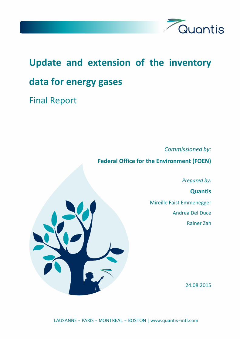
Das folgende Bild stellt vereinfacht die Modellierung der Erdgasproduktionskette in der ecoinvent v3
Datenbank dar. Die Exploration, Förderung und Aufbereitung werden in den Datensätzen “natural
gas production” beschrieben. Der Ferntransport in Pipelines wird durch die Datensätze “transport,
pipeline, long-distance, NG (natural gas)” dargestellt. Diese Datensätze beinhalten die Verluste
während dem Transport sowie den Energiebedarf für die Rekompression und die Infrastruktur für
die Pipelines. Die importierenden Länder beziehen Erdgas aus verschiedenen produzierenden
Quantis Update and extension of the inventory data for energy gases
August 28, 2015 Page 7
Ländern, teilweise über Transitländer. Hier wird wie in den früheren Versionen von ecoinvent nur die
schlussendliche Herkunft des Erdgases dargestellt. Der Herkunftmix wird in den Datensätzen
“market for NG, high pressure” zusammengestellt. Der Markt-Datensatz beinhaltet die Emissionen
für die Verteilung im Netz. Der Datensatz “natural gas reduction from high to low pressure” stellt die
Verbindung zwischen den Märkten für Hochdruck- resp. Niederdruckerdgas dar.
Figure 2: Übersicht der Modellierung von der Erdgasproduktions- und Verteilungskette in der ecoinvent v3 Datenbank.
Die LNG (Liquid Natural Gas)-Transportkette beinhaltet zusätzlich die Datensätze für die
Verflüssigung, den Schiffstransport und die Verdampfung vom Erdgas.
Aktualisierungen
Die aktualisierten Datensätze werden im Detail in den Kapiteln 3.2, 3.3, 3.4, 3.5 und 3.6 beschrieben.
Die Produktion von Erdgas und Erdöl in Norwegen konnte basierend auf dem neusten Bericht der
Norwegian Oil and Gas Association (Norwegian Oil and Gas Association 2014) auf den aktuellsten
Stand gebracht werden. Dies ist wichtig, da aus diesem Land ein grosser Teil der Erdgasproduktion
für Europa stammt (s. Kap. 3.5). Die Produktionsdaten anderer Förderländer (Niederlanden,
Russland) wurden punktuell verbessert, u.a. basierend auf dem Bericht von (Schori and Frischknecht
2012) zur Produktion in der Russischen Föderation. Die aktualisierten Datensätze werden im Detail
im Kapitel 3.2 und 3.3 beschrieben.
Der Ferntransport von Erdgas in Pipelines und als LNG wurde bzgl. der Verluste und dem
Energieverbrauch beim Schiffstransport aktualisiert. Dafür konnten neuere Quellen (Wuppertal
Institute 2005; Sevenster and Croezen 2006; UNFCCC 2014a) genutzt werden. Die Angaben zu den
neuen Inventarflüssen werden im Kapitel 3.4 präsentiert.

Quantis Update and extension of the inventory data for energy gases
August 28, 2015 Page 8
Die Zusammensetzung der Herkunftsländer im Konsummix von achtzehn europäischen Ländern
wurde anhand der neusten BP-Statistik (BP Amoco 2014) aufdatiert. Die Herkunftsmixe werden im
Detail im Kapitel 3.5 beschrieben.
Die Verluste sowie die Materialzusammensetzung der Erdgaspipelines im Schweizer Erdgasnetz
wurden anhand der kürzlich erarbeiteten Studie (Del Duce and Faist Emmenegger 2014) in
aktualisierten Datensätzen zusammengefasst. Diese werden im Kapitel 3.6 ausführlich beschrieben.
Biogas, Holz-SNG und strombasierte Treibstoffe
Übersicht
Das Ziel in diesem Projekt bezüglich der Energieträger Biogas, synthetisches Gas aus Holz (Holz-SNG)
und strombasierte Treibstoffe („Power-to-Gas“) ist es, die verfügbare Datensätze (hauptsächlich aus
ecoinvent v2.2 und aus jüngsten Inventarprojekten) zu sammeln und zu harmonisieren.
Aktualisierungen
Die Harmonisierung der aktuell verfügbaren Inventare erfolgte, indem neue Datensätze für die
Biogasproduktion und Bioabfallentsorgung erstellt wurden, welche die ecoinvent-Datensätze als
Grundlage nehmen und spezifische Werte aus den Datensätzen von (Dinkel et al. 2012) integrieren.
Die Ecoinvent-Inventare wurden gewählt, da sie die detaillierteste Dokumentation aufweisen. Die
Werte von Dinkel et al. ( 2012) wurden dann genutzt, um die ecoinvent-Inventare zu
vervollständigen oder wenn der Vergleich mit der Studie von Del Duce and Zah ( 2015a) darauf
hinwies, dass diese Werte geeigneter sind. Die Datensätze werden in Detail im Kapitel 4.1
beschrieben.
Synthetisches Erdgas (SNG) aus Holz ensteht durch Holzvergasung mit anschliessendem
Methanisierungsschritt (Jungbluth et al. 2007). Ecoinvent v2.2 berücksichtigt zwei mögliche
Vergasungsprozesse: Festbett- und Wirbelschichtvergasung. Die Daten, die in der Hotspot-Analyse
von Del Duce and Zah ( 2015b) gesammelt wurden, erlaubten eine Aktualisiserung der Datensätze
für die Holzvergasung. Diese Datensätze beinhalten die nötige Infrastruktur und notwendigen
Ressourcen für die Vorbereitung des Holzes, die Vergasung, die Reinigung des Synthesegases und die
Aufbereitung des SNG zu Erdgasqualität. Die Datensätze werden ausführlich im Kapitel 4.2
beschrieben.
Für strombasierte Energieträger (Power-to-Gas) existieren noch keine Inventare in der ecoinvent
Datenbank. Die kürzlich erarbeitete Studie von Quantis über diese Technologie erlaubt es, typische
Prozesse für die Herstellung von Methan oder Wasserstoff aus Strom zu bilden. Die in dieser Kette
beschriebenen Schritte sind die Elektrolyse, die CO2-Abscheidung aus Abgasen und aus der
Atmosphäre sowie die Methanproduktion.

Quantis Update and extension of the inventory data for energy gases
August 28, 2015 Page 9
Contents
Zusammenfassung .................................................................................................................................. 5
List of figures ......................................................................................................................................... 11
List of the tables .................................................................................................................................... 12
Abbreviations and acronyms ................................................................................................................ 15
1 Introduction .................................................................................................................................. 16
1.1 Energy gases .......................................................................................................................... 16
1.2 Aim of the project and used approach ................................................................................. 16
1.2.1 Natural gas .................................................................................................................... 17
1.2.2 Gas from alternative sources ........................................................................................ 17
2 Methodology ................................................................................................................................. 18
2.1 Data sources .......................................................................................................................... 18
2.1.1 Natural gas .................................................................................................................... 18
2.1.2 Methane and fuels from renewable pathways: biogas from biowaste, synthetic
natural gas from wood and electricity based fuels. ...................................................................... 19
2.2 Characteristics of the gases .................................................................................................. 19
2.2.1 Composition of the Swiss natural gas ........................................................................... 19
2.2.2 Standardized calorific value for natural gas in ecoinvent v3 ........................................ 20
2.2.3 Properties of biogas and SNG ....................................................................................... 20
2.3 Inventories and documentation ........................................................................................... 20
3 Natural gas, updated datasets ...................................................................................................... 21
3.1 Overview ............................................................................................................................... 21
3.2 Natural gas production ......................................................................................................... 21
3.2.1 Petroleum and gas production in Norway .................................................................... 21
3.2.2 Natural gas production in Russia .................................................................................. 25
3.2.3 Petroleum and gas production in the Netherlands ...................................................... 26
3.2.4 Natural gas production in Algeria, Middle East, Germany, Petroleum and gas
production in the United Kingdom ............................................................................................... 26
3.2.5 Updated datasets .......................................................................................................... 27
3.3 Processing ............................................................................................................................. 27
3.3.1 Natural gas sweetening ................................................................................................. 27
3.4 Transport of natural gas for import ...................................................................................... 28
3.4.1 Transport per pipeline .................................................................................................. 28
3.4.2 LNG transport ................................................................................................................ 30
3.5 Representation of the trade movements ............................................................................. 33

Quantis Update and extension of the inventory data for energy gases
August 28, 2015 Page 10
3.5.1 European countries (1).................................................................................................. 35
3.5.2 European countries (2).................................................................................................. 36
3.5.3 Updated datasets .......................................................................................................... 37
3.6 Natural gas distribution in Switzerland ................................................................................. 38
3.6.1 Infrastructure of the Swiss high and low pressure network ......................................... 38
3.6.2 Emissions due to leakage in the natural gas distribution system ................................. 42
3.6.3 Updated datasets .......................................................................................................... 46
4 Biogas from biowaste, SNG from wood and electricity based fuels ............................................. 46
4.1 Biogas from biowaste............................................................................................................ 46
4.1.1 Upgrade of biogas to natural gas quality ...................................................................... 52
4.2 Synthetic natural gas from wood .......................................................................................... 53
4.3 Power-to-Gas ........................................................................................................................ 55
4.3.1 Power-to-Hydrogen ...................................................................................................... 56
4.3.2 Power-to-Methane ....................................................................................................... 57
5 References .................................................................................................................................... 60
6 Appendices .................................................................................................................................... 63
6.1 Tables .................................................................................................................................... 63
6.2 Replies to review comments ................................................................................................. 64
6.2.1 introduction / natural gas ............................................................................................. 64
6.2.2 Replies to review comments: biogas/SNG part ............................................................ 68
6.2.3 Replies to review comments: PtX ................................................................................. 69
6.2.4 Replies to review comments: References ..................................................................... 69

Quantis Update and extension of the inventory data for energy gases
August 28, 2015 Page 11
List of figures
Figure 1: Trends im Gassektor (BP Amoco 2014): (links) Gasproduktion bei Typ und Region und
(rechts) globale Importanteile. ........................................................................................... 5
Figure 2: Übersicht der Modellierung von der Erdgasproduktions- und Verteilungskette in der
ecoinvent v3 Datenbank. .................................................................................................... 7
Figure 3: Trends in the gas sector (BP Amoco 2014): (left) gas production by type and region and
(right) global import shares. ............................................................................................. 16
Figure 4: Overview of the modelling of the natural gas supply chain in the ecoinvent v3 database.
XX, YY, ZZ stand for a specific country or region. ............................................................. 21
Figure 5: Products and services of a biogas plant. ........................................................................... 46
Figure 6: Simplified scheme of the power-to-gas production chain. ............................................... 55
Figure 7: System boundaries for the assessment of CO2 capture and methanation. ..................... 58

Quantis Update and extension of the inventory data for energy gases
August 28, 2015 Page 12
List of the tables
Table 1: Composition of the natural gas distributed in Switzerland. The concentrations were
where necessary scaled to Nm3. Sources: (Del Duce and Faist Emmenegger 2014
(methane); Faist Emmenegger et al. 2007 (other substances)). ........................................ 19
Table 2: Oil and gas production on the Norwegian continental shelf (NCS) since 2000, for oil in
million Sm3, for gas in billion Sm3 (Norwegian Oil and Gas Association 2014). NGL: Natural
Gas Liquids. ......................................................................................................................... 22
Table 3: Inventory of the oil and gas production on the Norwegian continental shelf 2010 and
2013. Sources: (Schori and Frischknecht 2012; Norwegian Oil and Gas Association 2014).
25
Table 4: Comparison of key figures of the natural gas production in the Russian Federation. ....... 25
Table 5: Calculation of the flaring rate (UNFCCC 2014, Table 3.39). ................................................ 26
Table 6: Total methane emissions of the oil and gas producing sector and derived emission factors
(UNFCCC 2014b). ................................................................................................................. 26
Table 7: Updated datasets (names v2.2) and their equivalent (activity name and reference flow) in
ecoinvent data version 3. .................................................................................................... 27
Table 8: Updated datasets (names v2.2) and their equivalent (activity name and reference flow) in
ecoinvent data version 3. .................................................................................................... 27
Table 9: Emission factors of the pipeline transport from the Russian Federation in various
sources.For the rest of the data, we use the updated data as in Schori and Frischknecht (
2012). .................................................................................................................................. 29
Table 10: Updated datasets (names v2.2) and their equivalent (activity name and reference flow) in
ecoinvent data version 3. .................................................................................................... 30
Table 11: Gas consumption, flaring and fugitive rates for the liquefaction plant. This includes the
refrigeration system, auxiliary electricity and hot oil system. ............................................ 31
Table 12: Review of the energy consumption of LNG carriers, literature ............................................ 31
Table 13: Emission factors used for the calculation of the LNG consumption and total emission
values per tkm. The factors are the same as the one used in the ecoinvent v 2.2. ........... 32
Table 14: Exchanges of the activity dataset “transport, freight, sea, liquefied natural gas, GLO 2006”.
............................................................................................................................................ 32
Table 15: Fugitive emissions, combustion rate and electricity rate at the evaporation plant. Sources:
Faist Emmenegger et al. (2007) and Sevenster and Croezen (2006) for the energy
consumption and Del Duce and Faist Emmenegger (2014) for the fugitive emissions. ..... 33

Quantis Update and extension of the inventory data for energy gases
August 28, 2015 Page 13
Table 16: Updated datasets (names v2.2) and their equivalent (activity name and reference flow) in
ecoinvent data version 3. .................................................................................................... 33
Table 17: Supply mix based on (BP Amoco 2014) and corresponding amounts of imported natural
gas from the origin countries. In the datasets, Denmark is approximated with Norwegian
production, as the Danish production is also situated in the North Sea. Own production is
shown in the corresponding row. All values in Sm3. ........................................................... 35
Table 18: Supply mix based on (BP Amoco 2014) and corresponding amounts of imported natural
gas from the origin countries. In the datasets, Denmark is approximated with Norwegian
production, as the Danish production is also situated in the North Sea. Own production is
shown in the corresponding row. All values in Sm3. ........................................................... 36
Table 19: Updated datasets (names v2.2) and their equivalent (activity name and reference flow) in
ecoinvent data version 3. XX in the new activity name makes clear that the dataset is
specific and exists for each importing country of Table 17 and Table 18. 2012-2012
indicates the time range of the data in the dataset. .......................................................... 37
Table 20: Pipeline length of the Swiss distribution network according to the 2012 statistics of the
Swiss gas industry (Del Duce and Faist Emmenegger 2014). .............................................. 38
Table 21: Pipeline length, specific and total material requirements of the low pressure network.
The values of the category “other materials” are added to the steel. The total material
requirements were calculated with unrounded values for pipeline length. Data sources:
Faist Emmenegger et al. (2007) and Del Duce and Faist Emmenegger (2014)................... 39
Table 22: Pipeline length, specific and total material requirements for the pipeline beddings. The
total material requirements were calculated with unrounded values for pipeline length.
Data sources: Faist Emmenegger et al. (2007) and Del Duce and Faist Emmenegger
(2014). ................................................................................................................................. 40
Table 23: Average material requirements per km network, updated values and values from the
ecoinvent v2.2. Data sources: own calculations; (Faist Emmenegger et al. 2007). ............ 40
Table 24: Pipeline length, specific and total material requirements of the high pressure network.
The values of the category “other materials” are added to the steel. Data sources: (Faist
Emmenegger et al. 2007; Del Duce and Faist Emmenegger 2014)..................................... 41
Table 25: Average material requirements per km network, updated values and values from the
ecoinvent v2.2. Data sources: own calculations; (Faist Emmenegger et al. 2007). ............ 42
Table 26: Leakages 2012 in the Swiss distribution network. .............................................................. 42
Table 27: Total consumption in the low and middle/high pressure network 2012 according to
statistics (Del Duce and Faist Emmenegger 2014), repartition on the low and middle/high

Quantis Update and extension of the inventory data for energy gases
August 28, 2015 Page 14
pressure network (assumption according to (Faist Emmenegger et al. 2007)) and
calculated consumption in the different networks. ........................................................... 43
Table 28: Main exchanges of the new "natural gas, low pressure" dataset and values in the former
datasets. .............................................................................................................................. 44
Table 29: Main exchanges of the new "natural gas, high pressure" dataset and values in the former
datasets. .............................................................................................................................. 45
Table 30: Updated datasets (names v2.2) and their equivalent (activity name and reference flow) in
ecoinvent data version 3. .................................................................................................... 46
Table 31: Methane leakage data for biogas production. ...................................................................... 48
Table 32: Methane leakage data for biowaste disposal. ...................................................................... 48
Table 33: Main exchanges of the biogas production dataset.In the table below, a fixed deviation can
be noted in the updated values as opposed to the original ecoinvent values, even when
the original source indicated is ecoinvent. This is related to the slightly different allocation
factor of 63% used here compared to the original value of 69%. Moreover, the original
ecoinvent dataset also included a list of soil emissions due to the application of digestate
matter as a fertilizer. These have been omitted from the list since, as mentioned above, in
the new models presented in Dinkel et al. (2012), all exchanges related to the application
of digestate in agriculture are taken into account in specific processes (“digestate, liquid,
applicated on field/CH U” and digestate, solid, applicated on field/CH U”). ..................... 50
Table 34: Main exchanges of the biowaste disposal dataset. .............................................................. 52
Table 35: Main exchanges of the SNG production datasets. ................................................................ 55
Table 36: New electrolysis datasets generated for the PtX value chain. .............................................. 57
Table 37: New methane production datasets generated for the PtX value chain. .............................. 59
Table 36: Emission factor of pipelines depending on their material and network type (Xinmin 2004).
............................................................................................................................................ 63

Quantis Update and extension of the inventory data for energy gases
August 28, 2015 Page 15
Abbreviations and acronyms
CO2 Carbon Dioxide
DZ Algeria
GHG Greenhouse gas
GLO Global / world average
HDPE High density polyethylene
IPCC
ISO
Intergovernmental Panel on Climate Change
International Organization for Standardization
kWh Kilowatt-hour = 3,600,000 joules (j)
LCA Life Cycle Assessment
LCI Life Cycle Inventory
LCIA Life Cycle Impact Assessment
LNG Liquefied natural gas
MJ Megajoule = 1,000,000 joules, (948 Btu)
NG Natural gas
NGL Natural Gas Liquids
Nm3 Norm cubic meter
OCE Ocean
PEM Polymer electrolyte membrane
RME Middle East Region
Sm3 Standard cubic meter; 1 Sm
3 equals approximately 1 Nm3
SNG Synthetic natural gas
SOEL High temperature electrolysis

Quantis Update and extension of the inventory data for energy gases
August 28, 2015 16
1 Introduction
1.1 Energy gases
The available life cycle inventory data for energy gases (gaseous energy sources from fossil or
biogenic origin) in the ecoinvent database is partly outdated with regard to natural gas and, with
regard to biogenic sourced gas, incomplete and partly not consistent. Natural gas and gas from
biogenic sources, however, play today an important role as fuel sources and will be even more in the
future, as the projected future consumption from BP shows in Figure 3 (left). Simultaneously, the
technologies for transport of natural gas change rapidly, as Figure 3 on the right shows, with a trend
to more LNG distribution.
Figure 3: Trends in the gas sector (BP Amoco 2014): (left) gas production by type and region and (right) global import shares.
1.2 Aim of the project and used approach
Aim of this project was therefore to update the data basis for energy gases. Moreover, the data and
inventories gathered in various completed or current studies should be made available for the
ecoinvent version 3 database.

Quantis Update and extension of the inventory data for energy gases
August 28, 2015 17
1.2.1 Natural gas
In this part of the project, starting from ecoinvent v2.2 original natural gas datasets, new inventories
were developed by:
Integrating the data from the study „Methanemissionen des Erdgas-Netzes“ (methane
emissions of the natural gas network in Switzerland and the upstream processes) from the
study mandated by the Swiss natural gas association (SVGW) and the Swiss Federal Office for
the Environment (FOEN/BAFU) (Del Duce & Faist, 2014)
Taking into account recent data for natural gas production in the Russian Federation, North
African Countries and the Middle East from www.lc-inventories.ch (Natural gas supply
(Schori and Frischknecht 2012))
Updating the upstream supply chain (production, processing and transport of natural gas)
where new data were available.
1.2.2 Gas from alternative sources
Biogas: ecoinvent contains various biogas datasets, which are however not modelled
consistently and do not represent the latest state of the technology. The available datasets
were updated and harmonised in this project based on recent studies published on www.lc-
inventories.ch (biogas from biowaste, from energy crops and from other substrates) and the
studies made for Energie 360° by Quantis (biogas production from biowaste, processing
(upgrading) of biogas from sewage sludge and biowaste to biomethane quality). The specific
references and data sources are detailed in Chapter 3.6.
PtG (Power-to-Gas): Quantis conducted a study on the environmental impacts of several
power-to-gas pathways mandated by the the Swiss Federal Office for the Environment
(FOEN/BAFU). Typical inventories for this technology were developed in this project.
Methane from wood: An inventory for synthetic natural gas production already exists in
ecoinvent v2.2. It is based on the process developed in Güssing, Austria (fluidized bed
reactor). Since it is expected that fixed bed gasification will also become a relevant option in
Switzerland, an inventory for this technology was developed.

Quantis Update and extension of the inventory data for energy gases
August 28, 2015 18
2 Methodology
2.1 Data sources
2.1.1 Natural gas
In this study we updated the ecoinvent v2.2 datasets on natural gas and energy gases based on the
original v2.2 datasets and new and more recent sources. The new datasets and the datasets they
replace are described in the following chapters. The original datasets were published in the natural
gas ecoinvent report (Faist Emmenegger et al. 2007) and had been partly updated in Schori and
Frischknecht ( 2012). We based our update on these datasets, together with the newest publication
like the one on methane emissions (Del Duce and Faist Emmenegger 2014) as well as further
literature such as the latest environmental report for the Norwegian gas production (Norwegian Oil
and Gas Association 2014), the study of the Wuppertal institute on methane emissions from the
pipeline transport from the Russian Federation (Wuppertal Institute 2005) or national reporting to
UNFCCC from producing countries (MATET 2010; UNFCCC 2014a; UNFCCC 2014b). The literature
used in this project is described in the single chapters and listed in the reference list at the end of
this document.
Moreover, (Exergia - E3M Lab -COWI 2014) presents a review of available recent data and
description of planned data collection from industry. As the publication is only an interim report, the
data provided is still scarce. However, this publication is very promising in terms of update of the
natural gas supply chain. We used this study to derive and update the transport distances from the
natural gas production fields to the importing country, as the modelling of the supply chain in
version 3 of the ecoinvent database allows differentiating the import distance for each country. This
is particularly relevant in the case of import from Russia, where the leakages from gas transport via
pipeline are significant for the overall results of the supply chain and where the distance can vary
between 3’000km (distance from Urengoy field to Finland) and 6’000km (to the Netherlands).
While it was possible for the first versions of the ecoinvent database (1.0 to 2.2) to rely on
environmental reports in the data collection for natural gas production, this source of data almost
disappeared, as the EHS or sustainability reports nowadays contain only little specific data. Further,
as many natural gas companies have been integrated in bigger holdings (e.g. NAM was integrated
into Shell), the sustainability reports focus on the data of the entire holding without addressing the
details of local infrastructure. It is therefore to hope that the study on actual data for diesel, petrol,
kerosene and natural gas (Exergia - E3M Lab -COWI 2014) will be able to provide actual and accurate
industry data in the next years.

Quantis Update and extension of the inventory data for energy gases
August 28, 2015 19
2.1.2 Methane and fuels from renewable pathways: biogas from biowaste, synthetic natural gas
from wood and electricity based fuels.
Next to fossil natural gas, available datasets addressing biogas from biowaste, synthetic natural gas
from wood and fuels from renewable electricity have also been harmonised and made public within
this project.
Data concerning biogas form biowaste and the disposal of biowaste has been published in the
original ecoinvent v2.2 report nr. 17 “Life Cycle Inventories of Bioenergy” (Jungbluth et al. 2007), as
well as in two more recent reports (Stucki et al. 2011; Dinkel et al. 2012). Further, data on a current-
technology biowaste disposal and biogas production plant in Switzerland is available from(Del Duce
and Zah 2015a).
With respect to synthetic natural gas (SNG) from wood, the main source of data is the ecoinvent
report on Bioenergy (Jungbluth et al. 2007) with an update of some aspects presented in Del Duce
and Zah ( 2015b).
Finally, data addressing the production of fuels from renewable electricity has been published in
Spielmann et al. ( 2015).
2.2 Characteristics of the gases
2.2.1 Composition of the Swiss natural gas
For the methane content of Swiss natural gas, we use actual industry data as shown in Table 1.
Natural gas, CH
kg / Nm3
Methane 0.652
Ethane 0.033
Propane 0.014
Butane 0.007
Other HC 0.003
CO2 0.012
N2 0.066
Table 1: Composition of the natural gas distributed in Switzerland. The concentrations were where necessary scaled to Nm
3. Sources: (Del Duce and Faist Emmenegger 2014 (methane); Faist
Emmenegger et al. 2007 (other substances)).
The lower heating value is 36.4 MJ/Nm3 and the higher heating value 40.5 MJ/Nm3 (Del Duce and
Faist Emmenegger 2014).

Quantis Update and extension of the inventory data for energy gases
August 28, 2015 20
For raw natural gas and natural gas from other origins, we use the data as provided in Faist
Emmenegger et al. ( 2007), which was also taken over in Schori and Frischknecht ( 2012).
2.2.2 Standardized calorific value for natural gas in ecoinvent v3
The ecoinvent version 3 database uses a standardized calorific value for natural gas (39 MJ/m3),
while the energy content as well as the composition of natural gas can vary depending on the origin.
For the calculations of the dataset exchanges, we use the specific natural gas composition as
described in in (Faist Emmenegger et al. 2007) / (Schori and Frischknecht 2012). We adapt the
datasets to the standard calorific value of the version 3 by scaling the reference flow and the
production volumes according to the energy content of the gas as described in Faist Emmenegger et
al. (2007) and Schori and Frischknecht ( 2012).
BP (BP Amoco 2014) gives in its statistics a conversion value of 37.8 MJ/m3 for natural gas2. We use
this value here to scale production and trade data from this statistic to cubic meters in ecoinvent v3.
For the statistics of the Norwegian Oil and Gas Association, the LHV value is 36.04 MJ/Sm3 3. This
value is applied in the Norwegian gas production.
2.2.3 Properties of biogas and SNG
The new biogas datasets have been modelled starting from the original ecoinvent v2.2 inventories
and are based on the same biogas properties. As such, with respect to the gas composition, 67 %
methane and 32 % carbon dioxide were assumed for the two major contributions in biogas from
biowaste (Jungbluth et al. 2007). After upgrading, these two components reach ≥ 96 % for methane
and ≤ 2 % in the case of carbon dioxide. For SNG, the same composition as upgraded biogas has
been assumed.
2.3 Inventories and documentation
The present report describes the methodological choices as well as the data used to produce the
inventories. Where necessary it refers to previous studies without repeating their content.
The inventories are available in the ecospold 2 format for the natural gas supply chain to comply
with the ecoinvent version 3 structure of the chain and so to allow a swifter integration in the
version 3.3 of the ecoinvent database. For the biogas chain, the inventories are available in the
Simapro 8 format csv.
2 1 cubic meter natural gas in (BP Amoco 2014) corresponds to 0.9 kg oil equivalent. 1 kg oil equivalent
corresponds to 42 MJ. The source does not precise if the cubic meters are standard or norm cubic meters. 3 Using following conversion factors: 7.33 barrels/tonne (BP Amoco 2014); 0.159 Sm
3 (standard cubic meter)
per barrel; 1’000 Sm3per Sm
3oil equivalent (oe) (Norwegian Oil and Gas Association 2014); 42 MJ/kg oe (BP
Amoco 2014).

Quantis Update and extension of the inventory data for energy gases
August 28, 2015 21
3 Natural gas, updated datasets
3.1 Overview
The following picture describes the modelling of the natural gas supply chain in the ecoinvent v3
database. The exploration and production of natural gas is described in the datasets “natural gas
production (YY)4”. The transport in long-distance pipelines is described in the datasets “transport,
pipeline, long-distance, NG (natural gas), (YY)”. These datasets contain the leakage of natural gas
during transport as well as the energy consumption for re-compression and the infrastructure
needed for the pipeline. The natural gas is then mixed in the markets of the various countries, on the
level high pressure, representing the consumption mix. The market contains the emissions due to
distribution in the network. The dataset “natural gas reduction from high to low pressure” makes
the link to the market for low pressure natural gas.
Figure 4: Overview of the modelling of the natural gas supply chain in the ecoinvent v3 database. XX, YY, ZZ stand for a specific country or region.
For the LNG supply chain, the model contains more datasets to describe the liquefaction, transport
as LNG and evaporation of the natural gas.
3.2 Natural gas production
3.2.1 Petroleum and gas production in Norway
Norway is the major natural gas producer in Europe. The natural gas production on the Norwegian
continental shelf has been continuously growing since 2000, while the oil production has been
decreasing in the same time.
4 YY stands for a specific country or region.

Quantis Update and extension of the inventory data for energy gases
August 28, 2015 22
Table 2: Oil and gas production on the Norwegian continental shelf (NCS) since 2000, for oil in million Sm3,
for gas in billion Sm3 (Norwegian Oil and Gas Association 2014). NGL: Natural Gas Liquids.
The Norwegian Oil and Gas Association publishes a very detailed environmental report every year.
We used the latest at the moment of the project (Norwegian Oil and Gas Association 2014) to
update the data for oil and gas production for 2013. We use the same structure and assumptions as
in Schori and Frischknecht (2012), which describes the situation for the year 2010.
This source reports an overall quantity of 4.32 E+08 Nm3 flared gas and 2.01 E+07 kg of methane,
which corresponds to 6.01 E-05 m3 flared gas /MJ produced and 2.58 E-06 kg methane emissions
/MJ.

Quantis Update and extension of the inventory data for energy gases
August 28, 2015 23
Production Norway OLF 2011;
(Schori and
Frischknecht
2012)
(Norwegian
Oil and Gas
Association
2014)
Comment / Table number
from (Norwegian Oil and
Gas Association 2014)
Reference products
Crude oil production kg 1.07E+11 8.25E+10 Incl. condensates
Natural gas production Nm3 1.12E+11 1.04E+11 without injected gas; converted
from Sm3 5
Intermediate exchanges
Oil crude in ground kg 1.07E+11 8.25E+10 based on oil production
Natural gas in ground Nm3 1.12E+11 1.04E+11 based on natural gas production
water salt ocean m3 1.67E+08 1.30E+08 Table 2: injected sea water
water salt sole m3 1.73E+08 1.61E+08 Table 17, produced water
chemicals organic kg 7.24E+07 6.25E+08 Table 18
Sweet gas, burned in gas
turbine, production
Nm3 3.78E+09 4.24E+09 Table 2
Natural gas burned in
production flare
Nm3 3.72E+08 4.32E+08 Table 2
Diesel burned in electric
generator
MJ 1.17E+10 1.082E+10 scaled from 2010 data with oil& gas
production
Transport lorry tkm 1.66E+06 transport is automatically included
in the market activities
Well for exploration m 5.86E+05 5.97E+05 scaled from 2010 data with natural
gas production
drying natural gas Nm3 6.74E+10 6.87E+10 same proportion as 2010
platform crude oil / offshore
platform, petroleum
unit 5.44E+00 4.214E+00 standard data, based on production
volume
plant offshore gas / offshore
platform, natural gas
unit 4.09E+00 3.740E+00 standard data, based on production
volume
waste, non-hazardous kg 1.48E+07 2.90E+07 Table 28
hazardous waste kg 1.81E+06 7.93E+06 Table 29, without drilling waste
Emissions in air
methane fossil kg 1.97E+07 2.01E+07 Table 24,25,27
5 Unfortunately neither Nm3 (normal cubic meter) or Sm3 (standard cubic meter) are complete definitions in
themselves. It is essential to know the standard reference conditions of temperature and pressure to define the gas volume since there are various debates about what normal and standard should be.
Most commonly used reference conditions are: Normal cubic meter (Nm3) - Temperature: 0 °C, Pressure: 1.01325 barA; Standard cubic meter (Sm3) - Temperature: 15 °C, Pressure: 1.01325 barA. (http://www.oxywise.com/en/content/news/what-is-the-difference-between-nm3-and-sm3) The 5% correspond also to the conversion value given in (Norwegian Oil and Gas Association 2014).

Quantis Update and extension of the inventory data for energy gases
August 28, 2015 24
Production Norway OLF 2011;
(Schori and
Frischknecht
2012)
(Norwegian
Oil and Gas
Association
2014)
Comment / Table number
from (Norwegian Oil and
Gas Association 2014)
ethane kg 2.03E+06 2.07E+06 based on composition of natural
gas
propane kg 5.22E+05 5.33E+05 based on composition of natural
gas
butane kg 1.65E+05 1.68E+05 based on composition of natural
gas
carbon dioxide kg 1.13E+09 3.55E+07 Table 24, other sources (without
well testing, flaring, combustion)
nmVOC kg 2.67E+06 2.73E+07 Table 25,27
Nitrogen oxides kg 1.70E+04 2.00E+03 Table 24, other sources (without
well testing, flaring, combustion)
Sulfur dioxide kg 3.99E+05 0.00E+00 Table 24, other sources (without
well testing, flaring, combustion)
PAH kg 9.00E+01 5.00E+01 Table 23
polychlorinated biphenyls kg 1.70E+00 0.87 Table 23
dioxin kg 8.00E-05 3.96E-05 Table 23
mercury kg 2.75E-01 2.80E-01 scaled from 2010 data with natural
gas production
radon kBq 1.10E+07 1.12E+07 scaled from 2010 data with natural
gas production
Emissions in water (ocean)
Oils kg 9.55E+04 1.69E+06 Table 9
PAH kg 1.57E+05 Table 9
phenols kg 5.03E+05 Table 12
arsenic kg 8.95E+02 6.22E+02 Table 11
barite kg 7.07E+06 7.32E+06 Table 11
cadmium kg 2.20E+01 6.00E+00 Table 11
chromium kg 2.25E+02 1.07E+02 Table 11
copper kg 8.90E+01 1.09E+02 Table 11
lead kg 2.39E+02 6.40E+01 Table 11
mercury kg 9.00E+00 8.00E+00 Table 11
nickel kg 2.00E+02 1.18E+02 Table 11
zinc kg 6.95E+03 3.64E+03 Table 11
iron kg 8.26E+05 6.45E+05 Table 11
Benzene kg 8.92E+05 Table 10: ethylbenzene
approximated with benzene
Toluene kg 7.11E+05 Table 10
Xylene kg 2.52E+05 Table 10

Quantis Update and extension of the inventory data for energy gases
August 28, 2015 25
Production Norway OLF 2011;
(Schori and
Frischknecht
2012)
(Norwegian
Oil and Gas
Association
2014)
Comment / Table number
from (Norwegian Oil and
Gas Association 2014)
Acetic acid kg 4.85E+07 Table 13
Formic acid kg 1.29E+06 Table 13
Propionic acid kg 3.09E+06 Table 13
Carboxylic acid, unspecified kg 8.61E+05 Table 13
Water kg 1.61E+08 Table 17, produced water
Table 3: Inventory of the oil and gas production on the Norwegian continental shelf 2010 and 2013. Sources: (Schori and Frischknecht 2012; Norwegian Oil and Gas Association 2014).
3.2.2 Natural gas production in Russia
The dataset on natural gas production of ecoinvent v2.2 was updated in Schori and Frischknecht (
2012). We compared the key figures used in the recent report with those indicated in the Wuppertal
Institute study (Wuppertal Institute 2005), in ecoinvent v2.2 and in the UNFCCC report 2014 with
reference year 2012 (UNFCCC 2014a).
Ecoinvent
v2.2
(Wuppertal
Institute 2005)
(Schori and
Frischknecht
2012)
UNFCCC 2014
(reference year
2012)
Fugitive emission rates 0.375 % 0.11 % 0.5 % N/A
Flaring rate 0.250 % N/A 0.206 % 0.33 %
Combustion 0.989 % N/A 0.536 % N/A
Table 4: Comparison of key figures of the natural gas production in the Russian Federation.
The Ecoinvent v2.2 and Schori 2012 data for fugitive emission rates are global data for the Russian
production, whereas the Wuppertal figure is based on measurement in a single gas production field.
There is no value for the venting in the UNFCCC report. We therefore do not change the data from
the study of Schori and Frischknecht ( 2012), which also have more recent data for combustion. For
flaring, we use information from the UNFCCC report 2014, which reports and overall burning of
associated petroleum gas of 17.08 billion m3 with a recovery rate of 76 %. We allocate the flared gas
to both petroleum and gas production based on their calorific value.

Quantis Update and extension of the inventory data for energy gases
August 28, 2015 26
Name Value Unit Comment
Flared quantity 17.08 billion m3 Overall associated petroleum gas flared
4.099 billion m3 Calculated with 76 % recovery rate
Gas production 2.38E+13 MJ Original value: 654‘650*10E+6 m3
Oil produced 2.09E+13 MJ Original value: 497‘425 kt
Specific flared quantity 9.17E-05 m3/MJ
Flaring rate 0.33 % m3/m3
Table 5: Calculation of the flaring rate (UNFCCC 2014, Table 3.39).
For the rest of the inventory flows, we use the data from Schori and Frischknecht ( 2012).
3.2.3 Petroleum and gas production in the Netherlands
NAM (Nederlandse Aardolie Maatschappij BV – NAM), the main producer of gas in the Netherlands,
does not publish an environmental report containing technical data anymore. We therefore update
the flaring and venting of the natural gas production based on the Dutch national inventory report
(UNFCCC 2014b). The Dutch national inventory reports 318 ton of methane emission from flaring
and 14’540 ton of methane emissions from venting. The overall production of oil and gas is 44 TJ oil
and 2419 PJ gas.
Methane
emission (total)
Unit Emission
factor
Unit
Flaring 318.04 ton 1.31E-07 kg CH4 /MJ
Venting 14540 ton 6.01E-06 kg CH4 /MJ
Table 6: Total methane emissions of the oil and gas producing sector and derived emission factors (UNFCCC 2014b).
The emission factor for venting corresponds to a share of 0.0322 % natural gas vented, which is
similar to the value in ecoinvent v.2.2 (0.026 %) or of a previous report from NAM in 2004 (0.02 %).
The flaring factor (0.0007 %) derived from the UNFCCC figures is however much lower as previously
(v2.2:0.09 %; NAM 2004: 0.058 %).
3.2.4 Natural gas production in Algeria, Middle East, Germany, Petroleum and gas production in
the United Kingdom
The datasets on natural gas production in the North African Countries (Algeria, Lybia, Egypt) and in
the Middle East were updated in (Schori and Frischknecht 2012). The dataset for North African
Countries is based on the Algeria data, where most of the flows are approximations from the Russian
dataset. The Middle East dataset is the copy of the Algerian dataset. We use this data as they base
on 2010 data and no more recent or more accurate data was readily available.

Quantis Update and extension of the inventory data for energy gases
August 28, 2015 27
The datasets for the production in Germany and in the United Kingdom (combined oil and gas
production) were not updated in (Schori and Frischknecht 2012). It was not possible in this project
budget to update this data, as no data was easily available for these countries..
3.2.5 Updated datasets
Dataset v2.2 Location Activity name (new) Reference products Unit
combined offshore gas
and oil production
NO petroleum and gas production, off-shore,
NO, 2013-2013
natural gas, high pressure
petroleum
m3
natural gas, at
production onshore
RU natural gas, at production onshore, RU,
2000 - 2012
natural gas, high pressure m3
combined offshore gas
and oil production
NL petroleum and gas production, off-shore,
NL, 2000 - 2012
natural gas, high pressure m3
combined offshore gas
and oil production
NL petroleum and gas production, on-shore,
NL, 2000 - 2012
natural gas, high pressure m3
Table 7: Updated datasets (names v2.2) and their equivalent (activity name and reference flow) in ecoinvent data version 3.
3.3 Processing
3.3.1 Natural gas sweetening
No new information is readily available for gas sweetening. Schori and Frischknecht ( 2012) reports a
natural gas consumption of 0.0325 Nm3 per Nm3 sweetened, which should correspond to the
quantity vented. This is however not consistent with the reported methane emissions (2.0 E-05
kg/Nm3) and the methane content of German natural gas (0.69 kg/Nm3). We therefore correct this
value to 2.9 E-05 Nm3 per Nm3, which corresponds to a venting rate of 0.003 %.
3.3.1.1 Updated datasets
Dataset v2.2 Location Activity name (new) Reference flow Unit
Sweetening, natural gas, GLO, 2012 -
2012
Sweetening, natural gas m3
Sweetening, natural gas DE Sweetening, natural gas, DE, 2012 - 2012 Sweetening, natural gas m3
Table 8: Updated datasets (names v2.2) and their equivalent (activity name and reference flow) in ecoinvent data version 3.

Quantis Update and extension of the inventory data for energy gases
August 28, 2015 28
3.4 Transport of natural gas for import
3.4.1 Transport per pipeline
3.4.1.1 Transmission from Russia
The transport from natural gas from the Russian Federation to Europe occurs on a long distance
(over 4’000 km) with a high emission factor in comparison to transmission in Europe. It is therefore
important that this emission factor is well up to date.
The best documented and most detailed study on this subject is the study from the Wuppertal
institute (Wuppertal Institute 2005), which conducted a measurement campaign on the export
pipeline system from Siberia to West Germany through the Northern and Central Corridor. The
authors report an overall average leakage of 1 % (0.6 %-2.4 %) for the transport from Siberia to the
West German border. Related to an average distance of 4’900 km (the Northern Corridor has a
length of 4’300 km, the Central Corridor 5’500 km), this gives a value of 0.2 % per 1’000 km, which is
the value we use here.
As a comparison, the national inventory of the Russian Federation reports in (UNFCCC 2014a) a
methane leakage rate of 0.89 kg methane/kg natural gas or 0.91 % on a volume basis (m3 gas / m3
gas)6. This rate applies to the total amount transmitted in the Russian Federation (541’000 million
m3); it therefore also contains the amount consumed in the Russian Federation (exports amounted
to about 200’000 million m3 in 2013). Gazprom reports an average transmission distance of 3’300
km7. With these figures, we obtain a leakage rate of 0.28 %, which is about 30 % higher than the
rate calculated with the values in (Wuppertal Institute 2005) or in (Schori and Frischknecht 2012),
who uses for a similar figure in the UNFCCC inventory from 2011 a distance of 4'200 km (distance
from Siberia to the Russian border), with a result of 0.218 % per 1’000km. Because the UNFCCC
value is a very global one, the distance this value should be related to has high uncertainties and as
the UNFCCC value also contains transmission in the land itself, we prefer to use the value from
(Wuppertal Institute 2005).
6 Assuming the natural gas composition of the Russian Federation as described in (Faist Emmenegger et al.
2007; Schori and Frischknecht 2012) with 0.716 kg methane / Nm3 and 0.73 kg natural gas / Nm
3.
7 “In 2010, average distance of gas transmission was over 2’500 kilometers for domestic supplies and almost
3’300 kilometers for export supplies”.http://www.gazprominfo.com/articles/natural-gas-transportation/, retrieved on the June 18, 2015.

Quantis Update and extension of the inventory data for energy gases
August 28, 2015 29
Source Total Emission factor per
1’000 km
Comment
Ecoinvent 2.2 1.4 % 0.23 % Value Zittel 1998
Schori 2012 1.31 % 0.218 % UNFCCC 2011 (0.9 % total), 4’200 km,
scaled to 6’000 km
Eigene Berechnungen,
UNFCCC 2014
0.28 % UNFCCC 2014 (0.9 % total), average
distance of 3’300 km (according to
Gazprom).
Wuppertal institute 2005 1 % (0.6-2.4
%)
0.18 % (Marcogaz, 5’500
km)
0.204 % (4’900 km)
0.233 % (4’300 km)
Measurement campaign of Wuppertal
Institute and the Max Planck Institute,
corridors to Europe, 4’300 / 5’500 km long
(average = 4’900km)
Table 9: Emission factors of the pipeline transport from the Russian Federation in various sources.For
the rest of the data, we use the updated data as in Schori and Frischknecht ( 2012).
3.4.1.2 Transmission in Europe
The leakage rate (0.026 %) used in existing datasets (Faist Emmenegger et al. 2007; Schori and
Frischknecht 2012) for transmission in Europe stem from literature from 1994/2000 (Battelle 1994;
Reichert and Schön 2000). We use here a more recent source (Sevenster and Croezen 2006), which is
based on data collected by Marcogaz from several natural gas companies. The new leakage rate is
0.019 %. It is applied to all Western European countries8 .
3.4.1.3 Transmission in North African Countries and Middle East
The report on greenhouse gas emissions for Algeria (MATET 2010) does not give any specific figures
for natural gas transmission in this country.
Similarly to (Marcogaz 2010), we use the same leakage rate for these countries as for the Russian
Federation as a conservative assumption.
8 Portugal, Spain, France, Italy, Greece, Austria, Germany, Luxemburg, Belgium, The Netherlands, United
Kingdom, Denmar, Norway, Sweden, Finland.

Quantis Update and extension of the inventory data for energy gases
August 28, 2015 30
3.4.1.4 Updated datasets
Dataset v2.2 Location Activity name (new) Reference flow Unit
transport, natural gas,
pipeline, long distance
DE transport, pipeline, long distance, natural
gas, DE 2000-2012
natural gas, high
pressure
metric ton *
km
transport, natural gas,
pipeline, long distance
NL transport, pipeline, long distance, natural
gas, NL 2000-2012
natural gas, high
pressure
metric ton *
km
transport, natural gas,
pipeline, long distance
RU transport, pipeline, long distance, natural
gas, RU 2000-2012
natural gas, high
pressure
metric ton *
km
transport, natural gas,
pipeline, long distance
RER transport, pipeline, long distance, natural
gas, RER without DE+NL+NO, 2000-2012
natural gas, high
pressure
metric ton *
km
transport, natural gas,
offshore pipeline, long
distance
DZ transport, pipeline, offshore, long
distance, natural gas, DZ, 2000-2012
natural gas, high
pressure
metric ton *
km
transport, natural gas,
offshore pipeline, long
distance
NO transport, pipeline, offshore, long
distance, natural gas, NO, 2000-2012
natural gas, high
pressure
metric ton *
km
- - transport, pipeline, offshore, long
distance, natural gas, GLO, 2000-2012
natural gas, high
pressure
metric ton *
km
transport, natural gas,
onshore pipeline, long
distance
DZ transport, pipeline, onshore, long
distance, natural gas, DZ, 2000-2012
natural gas, high
pressure
metric ton *
km
transport, natural gas,
onshore pipeline, long
distance
NO transport, pipeline, onshore, long
distance, natural gas, NO, 2000-2012
natural gas, high
pressure
metric ton *
km
- - transport, pipeline, onshore, long
distance, natural gas, GLO, 2000-2012
natural gas, high
pressure
metric ton *
km
Table 10: Updated datasets (names v2.2) and their equivalent (activity name and reference flow) in ecoinvent data version 3.
3.4.2 LNG transport
3.4.2.1 Liquefaction plant
Data for the liquefaction plant in existing datasets (Faist Emmenegger et al. 2007; Schori and
Frischknecht 2012) is based relatively old data, partly stemming from a reference book on natural
gas of 1999. We use here the global average data for the existing capacity at that time as shown in a
more recent study (Sevenster and Croezen 2006). This is a conservative assumption as the values
reported in that publication for capacity under construction show lower gas consumption in this
process (7.9-8.7 % compared to 9.9-12.9 % for 2006 existing capacity).

Quantis Update and extension of the inventory data for energy gases
August 28, 2015 31
Ecoinvent v2.2 Sevenster and
Croezen 2006
Fugitive rate 0.05 % 0 %
Flaring rate N/A 0.3 %
Gas consumption (total) 15 % 10.3 %
Table 11: Gas consumption, flaring and fugitive rates for the liquefaction plant. This includes the refrigeration system, auxiliary electricity and hot oil system.
3.4.2.2 LNG carriers
The dataset “transport, liquefied natural gas, freight ship” of ecoinvent version 2.2 was based on
Italian data from 1999 and included only LNG as a fuel for the ship. The dataset was updated to
reflect the fact that LNG carriers are operating globally and that they are mostly using both natural
gas and heavy fuel oil as fuels (Heede 2006). We use here the scenario “middle use of energy” as
described in Heede ( 2006).
LNG Unit Heavy fuel oil Unit
ecoinvent (SNAM 1999/2000) 0.73 % %/1'000km
Sagisaka & Inaba (1999) 0.51 % %/1'000km
MAN B&W 0.10 % %/1'000 km 0.20 % %/1'000 km
Heede 2006 0.17 % %/1'000 km 0.034 MJ/tkm
This study (incl. return trip,
empty); Based on Heede 2006
0.34 % %/1'000 km
0.00429 Nm3/tkm 0.06789 MJ/tkm
Table 12: Review of the energy consumption of LNG carriers, literature
The emissions of the energy consumption are modelled for natural gas resp. LNG with standard
emissions factor of a turbine in ecoinvent for the LNG consumption and for heavy fuel oil with the
dataset “heavy fuel oil, burned in refinery furnace”.

Quantis Update and extension of the inventory data for energy gases
August 28, 2015 32
Emission
factor turbine
Emissions
from turbine
kg/Nm3 kg/tkm
Methane, fossil 2.27E-04 9.72E-07
Carbon dioxide, fossil 2.27E+00 9.72E-03
Carbon monoxide, fossil 1.59E-03 6.83E-06
NMVOC, non-methane volatile organic
compounds, unspecified origin
3.98E-05 1.71E-07
Nitrogen oxides 7.72E-03 3.31E-05
Dinitrogen monoxide 3.98E-05 1.71E-07
Table 13: Emission factors used for the calculation of the LNG consumption and total emission values per tkm. The factors are the same as the one used in the ecoinvent v 2.2.
Table 14: Exchanges of the activity dataset “transport, freight, sea, liquefied natural gas, GLO 2006”.
3.4.2.3 Gasification (evaporation plant)
In the regasification terminals, LNG is evaporated at pipeline pressure. Key figures for the
evaporation plant in Ecoinvent v2.2 (Faist Emmenegger et al. 2007; Schori and Frischknecht 2012)
stem from data of an Italian company in a report dating from 2002. Here we use data based on a
more recent European study (Sevenster and Croezen 2006), as in Del Duce and Faist Emmenegger (
2014),.

Quantis Update and extension of the inventory data for energy gases
August 28, 2015 33
Ecoinvent v2.2 Updated values
fugitive emissions 0 % 0.01 %
combustion rate 1.6 % 0.43 %
Electricity (MJ/Nm3) - 0.042
Table 15: Fugitive emissions, combustion rate and electricity rate at the evaporation plant. Sources: Faist Emmenegger et al. (2007) and Sevenster and Croezen (2006) for the energy consumption and Del Duce and Faist Emmenegger (2014) for the fugitive emissions.
3.4.2.4 Updated datasets
Dataset v2.2 Location Activity name (new) Reference flow
natural gas, liquefied, at
liquefaction plant
GLO natural gas production, liquefied,
GLO, 2012 - 2012
natural gas, high pressure
natural gas, at liquefaction
plant
DZ natural gas production, liquefied, DZ,
2012 - 2012
natural gas, high pressure
natural gas, liquefied, at
liquefaction plant
RME natural gas production, liquefied,
RME, 2012 - 2012
natural gas, high pressure
transport, liquefied natural
gas, freight ship
OCE transport, freight, sea, liquefied
natural gas, GLO 2006
transport, freight, sea, liquefied
natural gas
natural gas, at evaporation
plant
CH Evaporation of natural gas, GLO, 2012
- 2012
natural gas, high pressure
Table 16: Updated datasets (names v2.2) and their equivalent (activity name and reference flow) in ecoinvent data version 3.
3.5 Representation of the trade movements
The country of origin of the natural gas imported in various European countries is calculated based
on the trade movements of the natural gas in 2013 as described in (BP Amoco 2014) and, for the
import from Norway and the Russian Federation to Switzerland, on the statistics of the Swiss natural
gas industry for 2012 (Del Duce and Faist Emmenegger 2014).
The trade movements are modelled as following in the ecoinvent v3 database. The regional market
(e.g. market for natural gas (NG), high pressure, CH) imports high pressure natural gas according to
the production volumina of the datasets “natural gas (NG), high pressure, import from XX (CH)”,
where XX here symbolises an origin country for the natural gas imported in Switzerland. The
“production volumina” correspond to the import quantity of natural gas. The datasets “natural gas
(NG), high pressure, import from XX (CH)” have a fixed link to the corresponding production country
of the natural gas. The supply mix corresponds to the imports plus the domestic production. If a
country has no specific dataset for its production, the supply mix consists only of the import shares.
This is the case for Italy and Poland.
The imported quantities are described in the following chapters. In ecoinvent v2, only one dataset
per origin was available, using an average distance. In ecoinvent v3, each market refers to specific

Quantis Update and extension of the inventory data for energy gases
August 28, 2015 34
import datasets, which use specific distances from the country of origin to the market. The datasets
were created for all countries shown in Table 17 and Table 18.

Quantis Update and extension of the inventory data for energy gases
August 28, 2015 35
3.5.1 European countries (1)
Switzerland Austria Belgium Czech Republic
Denmark Finland France Germany Greece
PIPELINE % bn m3 % bn m
3 % bn m
3 % bn m
3 % bn m
3 % bn m
3 % bn m
3 % bn m
3 % bn m
3
Germany 5.2% 0.176 0.2% 0.02 0.0% 0.00 0.0% 0.00 0.3% 0.00 0.0% 0.00 0.0% 0.01 0.0% 8.22 0.7% 0.02
Netherlands 35.8% 1.203 0.3% 0.02 18.2% 5.40 0.0% 0.00 0.7% 0.01 0.0% 0.00 21.4% 6.51 23.4% 22.41 0.7% 0.02
Russian Federation
23.8% 0.800 79.4% 5.41 41.4% 12.25 65.2% 7.20 1.0% 0.01 100.0%
3.50 27.1% 8.27 41.6% 39.84 89.0% 2.67
France 0.3% 0.010 0.0% 0.00 0.0% 0.00 0.0% 0.00 0.00 0.0% 0.00 0.0% 0.00 0.0% 0.00 0.0% -
Italy 0.3% 0.010 0.0% 0.00 0.0% 0.00 0.0% 0.00 0.00 0.0% 0.00 0.0% 0.00 0.0% 0.00 0.0% -
United Kingdom
0.4% 0.014 0.0% 0.00 8.5% 2.52 0.0% 0.00 0.1% 0.00 0.0% 0.00 0.0% 0.00 0.0% 0.00 0.0% 0.00
Norway 24.9% 0.835 20.1% 1.37 31.9% 9.45 34.8% 3.84 97.9% 1.33 0.0% 0.00 51.3% 15.66 35.0% 33.56 7.7% 0.23
Denmark 0.00 0.00 0.00 0.00 0.00 0.00 0.00
Qatar 1.1% 0.035 0.0% 0.00 0.0% 0.00 0.0% 0.00 0.00 0.0% 0.00 0.0% 0.00 0.0% 0.00 0.0% -
Algeria 5.8% 0.195 0.0% 0.00 0.0% 0.00 0.0% 0.00 0.00 0.0% 0.00 0.1% 0.04 0.0% 0.00 2.0% 0.06
Nigeria 2.4% 0.082 0.0% 0.00 0.0% 0.00 0.0% 0.00 0.00 0.0% 0.00 0.0% 0.00 0.0% 0.00 0.0% -
Total import 100.0%
3.360 100.0%
6.81 100.0%
29.62 100.0%
11.04 100.0%
1.36 100.0%
3.50 100.0%
30.50 100.0%
95.80 100.0%
3.00
LNG % bn m3 bn m
3 % bn m
3 % bn m
3 % bn m
3 % bn m
3 % bn m
3 % bn m
3 % bn m
3
Qatar 0 % 0.00 0 % 0.00 100.0%
3.20 0 % 0.00 0 % 0.00 0 % 0.00 21.2% 1.75 0 % 0.00 0 % 0.00
Algeria 0 % 0.00 0 % 0.00 0.0% 0.00 0 % 0.00 0 % 0.00 0 % 0.00 64.3% 5.31 0 % 0.00 0 % 0.00
Nigeria 0 % 0.00 0 % 0.00 0.0% 0.00 0 % 0.00 0 % 0.00 0 % 0.00 14.5% 1.20 0 % 0.00 0 % 0.00
Total 0 % 0.00 0 % 0.00 100.0%
3.20 0 % 0.00 0 % 0.00 0 % 0.00 100.0%
8.26 0 % 0.00 0 % 0.00
Own production
0.00 0.00 0.00 0.00 2.61 0 % 0.00 0 % 0.00 7.51 0.00
Table 17: Supply mix based on (BP Amoco 2014) and corresponding amounts of imported natural gas from the origin countries. In the datasets, Denmark is approximated with Norwegian production, as the Danish production is also situated in the North Sea. Own production is shown in the corresponding row. All values in Sm
3.

Quantis Update and extension of the inventory data for energy gases
August 28, 2015 36
3.5.2 European countries (2)
Hungary Ireland Italy Netherlands Poland Slovakia Spain Sweden United Kingdom
PIPELINE % bn m3 % bn m
3 % bn m
3 % bn m
3 % bn m
3 % bn m
3 % bn m
3 % bn m
3 % bn m
3
Germany 0.00 0.0% 0.00 0.0% 0.01 3.9% 0.83 0.5% 0.06 0.0% 0.00 0.3% 0.04 0.0% 0.00 0.0% -
Netherlands 0.0% 0.00 0.0% 0.00 18.6% 9.58 - 0.5% 0.06 0.0% 0.00 0.3% 0.04 0.0% 0.00 24.0% 10.05
Russian Federation
100.0%
5.90 0.0% 0.00 54.0% 27.88 38.1% 8.20 91.7% 10.48 100.0%
5.33 3.9% 0.60 0.0% 0.00 3.7% 1.54
France 0.00 0.0% 0.00 0.0% 0.00 0.0% - 0.0% 0.00 0.0% 0.00 0.0% 0.00 0.0% 0.00 0.0% -
Italy 0.00 0.0% 0.00 0.0% 0.00 0.0% - 0.0% 0.00 0.0% 0.00 0.0% 0.00 0.0% 0.00 0.0% -
United Kingdom
0.0% 0.00 100.0%
4.87 0.0% 0.00 7.3% 1.56 0.0% 0.00 0.0% 0.00 0.0% 0.00 0.0% 0.00 0.0% 0.00
Norway 0.0% 0.00 0.0% 0.00 2.7% 1.39 45.0% 9.69 5.8% 0.67 0.0% 0.00 21% 3.16 0.0% 0.00 72.4% 30.33
Denmark 0.00 0.00 0.00 0.00 0.00 0.00 100.0%
1.09
Qatar 0.0% 0.00 0.0% 0.00 0.0% 0.00 0.0% - 0.0% 0.00 0.0% 0.00 0% 0.00 0.0% 0.00 0.0% -
Algeria 0.0% 0.00 0.0% 0.00 24.7% 12.75 5.7% 1.22 1.5% 0.17 0.0% 0.00 75% 11.48 0.0% 0.00 0.0% -
Nigeria 0.0% 0.00 0.0% 0.00 0.0% 0.00 0.0% - 0.0% 0.00 0.0% 0.00 0% 0.00 0.0% 0.00 0.0% -
Total import 100.0%
5.90 100.0%
4.87 100.0%
51.61 100.0%
21.51 100.0%
11.43 100.0%
5.33 100.0%
15.33 100.0%
1.09 100.0%
41.91
LNG % bn m3 % bn m
3 % bn m
3 % bn m
3 % bn m
3 % bn m
3 % bn m
3 % bn m
3 % bn m
3
Qatar 0 % 0.00 0 % 0.00 99.2% 5.20 0 % 0.00 0 % 0.00 0 % 0.00 35.5% 3.49 0 % 0.00 95.5% 8.61
Algeria 0 % 0.00 0 % 0.00 0.8% 0.04 0 % 0.00 0 % 0.00 0 % 0.00 32.9% 3.24 0 % 0.00 4.5% 0.41
Nigeria 0 % 0.00 0 % 0.00 0.0% 0.00 0 % 0.00 0 % 0.00 0 % 0.00 31.6% 3.11 0 % 0.00 0.0% -
Total 0 % 0.00 0 % 0.00 100.0%
5.24 0 % 0.00 0 % 0.00 0 % 0.00 100.0%
9.83 0 % 0.00 100.0%
9.01
Own production
0.00 0.00 7.09 68.68 4.18 0.00 0.00 0.00 36.48
Table 18: Supply mix based on (BP Amoco 2014) and corresponding amounts of imported natural gas from the origin countries. In the datasets, Denmark is approximated with Norwegian production, as the Danish production is also situated in the North Sea. Own production is shown in the corresponding row. All values in Sm
3.

Quantis Update and extension of the inventory data for energy gases
August 28, 2015 37
3.5.3 Updated datasets
Dataset v2.2 Location Activity name (new) Reference flow Unit
natural gas, production DE, at
long-distance pipeline
RER natural gas, high pressure, import
from DE, XX, 2012 - 2012
natural gas, high
pressure
m3
natural gas, production DZ, at
long-distance pipeline
RER natural gas, high pressure, import
from DZ, XX, 2012 - 2012
natural gas, high
pressure
m3
natural gas, production GB, at
long-distance pipeline
RER natural gas, high pressure, import
from GB, XX, 2012 - 2012
natural gas, high
pressure
m3
natural gas, production NL, at
long-distance pipeline
RER natural gas, high pressure, import
from NL, XX, 2012 - 2012
natural gas, high
pressure
m3
natural gas, production NO, at
long-distance pipeline
RER natural gas, high pressure, import
from NO, XX, 2012 - 2012
natural gas, high
pressure
m3
natural gas, production RU, at
long-distance pipeline
RER natural gas, high pressure, import
from RU, XX, 2012 - 2012
natural gas, high
pressure
m3
Table 19: Updated datasets (names v2.2) and their equivalent (activity name and reference flow) in ecoinvent data version 3. XX in the new activity name makes clear that the dataset is specific and exists for each importing country of Table 17 and Table 18. 2012-2012 indicates the time range of the data in the dataset.

Quantis Update and extension of the inventory data for energy gases
August 28, 2015 38
3.6 Natural gas distribution in Switzerland
3.6.1 Infrastructure of the Swiss high and low pressure network
Between 1998 and 2012, several changes took place in the Swiss distribution network: the length of
the pipelines for distribution in the Swiss network grew from around 14600 km to almost 19000 km.
Furthermore, the cast iron pipelines were continuously replaced by polyethylene pipelines which
have a lower methane leakage rate.
The new datasets developed within this study are based on the updated length of the distribution
network according to the 2014 study (Del Duce and Faist Emmenegger 2014) using the 2012
statistics from the Swiss natural gas industry. A description of the pipe materials and lengths in the
Swiss distribution network is shown in Table 20. We assume a life span of 40 years for both high
pressure and low pressure networks as in Faist Emmenegger et al. (2007).
Low
pressure
connection
Medium
pressure
connection
High
pressure
connection
Low
pressure
Medium
pressure
High
pressure
Transit
transport
km km km km km km km
Cast iron 66.1 0.0 0.6 142.9 0.0 7.0
Ductile cast iron 846.3 16.7 7.5 1830.2 68.9 93.0
Steel, not
cathodically
protected
893.1 36.0 31.9 1931.4 148.6 395.0
Steel,
cathodically
protected
4.8 24.4 105.4 10.4 100.6 1304.0 2161.0
Polyethylene 3079.3 226.2 206.5 6659.3 933.7 2554.0
Other materials 44.4 5.8 2.0 96.0 24.0 25.0
Rehabilitated -
Polyethyleneor
hose relining
126.3 7.1 0.1 273.0 29.4 1.3
Rehabilitated -
other methods
11.4 2.2 0.9 24.6 9.0 11.7
Total 5071.6 318.4 355.0 10967.9 1314.1 4391.0 2161.0
Table 20: Pipeline length of the Swiss distribution network according to the 2012 statistics of the Swiss gas industry (Del Duce and Faist Emmenegger 2014).
Data for the calculation of the infrastructure requirements (see following sections) is based on the
ecoinvent dataset from v2.2 (Faist Emmenegger et al. 2007). Further, we use the specific material

Quantis Update and extension of the inventory data for energy gases
August 28, 2015 39
requirements per kilometre pipeline as in Faist Emmenegger et al. (2007) with regard to the specific
weight of the pipelines per kilometre, the requirements of polyethylene foil and pitch (bitumen) for
the coating of metallic pipelines as well as the sand and gravel requirements for the bedding of the
pipelines. Separate datasets address the low- and high-pressure part of the network.
3.6.1.1 Material requirements of the low-pressure network
The following table shows the specific and the overall material requirements for the pipelines in the
low-pressure distribution network. The new data is integrated in the dataset “pipeline construction,
natural gas, low pressure distribution network, CH, 2012 – 2012”.
Pipeline length Specific material
requirements
Total material
requirements
Low-pressure network km kg/km t
Steel 1'942 18'300 35'535
Ductile cast iron 1'830 34'700 63'507
Cast iron 143 25'200 3'602
High density polyethylene 6'659 9'600 63'929
Low density polyethylene foils 273 1'000 273
Other materials 121 18'300 2'208
Household connecting network km kg/km t
Steel 898 4'500 4'041
Ductile cast iron 846 34'700 29'366
Cast iron 66 25'200 1'666
High density polyethylene 3'079 1'200 3'695
Low density polyethylene foils 126 1'000 126
Other materials 56 4'500 251
Table 21: Pipeline length, specific and total material requirements of the low pressure network. The values of the category “other materials” are added to the steel. The total material requirements were calculated with unrounded values for pipeline length. Data sources: Faist Emmenegger et al. (2007) and Del Duce and Faist Emmenegger (2014).
The sand and gravel requirements are adapted to the 2012 length of the pipelines.

Quantis Update and extension of the inventory data for energy gases
August 28, 2015 40
Low-pressure
network
Household
connecting network
Length of pipes km 10‘968 5‘072
Specific sand requirements kg/m 500 350
Specific gravel requirements kg/m 150 100
Total sand (80 % of pipelines) Mio t 4.39 1.42
Total gravel (20 % of pipelines) Mio t 0.33 0.10
Table 22: Pipeline length, specific and total material requirements for the pipeline beddings. The total material requirements were calculated with unrounded values for pipeline length. Data sources: Faist Emmenegger et al. (2007) and Del Duce and Faist Emmenegger (2014).
The updated values (Table 23) show a diminution of the steel and cast iron requirements in favour of
polyethylene use. The polyethylene value decreases between version 2.2 and the updated value.
However, according to our new calculations and the data collected in Del Duce and Faist
Emmenegger (2014), the v2.2 value should read 3’900 kg, which would result in an increase of the kg
HDPE per km of pipeline between 2000 and 2012.
Material
requirements per
km network
(updated)
Ecoinvent v2.2
Reinforcing steel, at plant/RER U kg 3‘310 5‘240
Cast iron, at plant/RER U kg 6‘120 6‘300
Polyethylene, HDPE, granulate, at plant/RER U kg 4‘220 4‘630
Polyethylene, LDPE, granulate, at plant/RER U kg 25 490
Gravel, round, at mine/CH U kg 26‘800 28‘000
Sand, at mine/CH U kg 362‘000 376’000
Transport pkm 27‘200 37’700
Table 23: Average material requirements per km network, updated values and values from the ecoinvent v2.2. Data sources: own calculations; (Faist Emmenegger et al. 2007).
3.6.1.2 Material requirements of the high-pressure network
The following table shows the specific and the overall material requirements for the pipelines in the
high-pressure distribution network. The new data is included in the ecoinvent v3.X dataset “pipeline
construction, natural gas, high pressure distribution network, CH, 2012 – 2012”.

Quantis Update and extension of the inventory data for energy gases
August 28, 2015 41
Pipeline length Specific material
requirements
Total material
requirements
km kg/km t
Transit transport
Steel 2'161 42'000 90'762
High pressure
Cast iron 8 36'200 274
Ductile cast iron 101 36'200 3'639
Steel, not cathodically protected 427 31'500 13'448
Steel, cathodically protected 1'409 31'500 44'397
HD Polyethylene 2'760 4'600 12'698
Other materials 27
Medium pressure
Cast iron - -
Ductile cast iron 86 25'200 2'157
Steel, not cathodically protected 185 19'200 3'544
Steel, cathodically protected 125 19'200 2'400
HD Polyethylene 1'160 3'300 3'828
Table 24: Pipeline length, specific and total material requirements of the high pressure network. The values of the category “other materials” are added to the steel. Data sources: (Faist Emmenegger et al. 2007; Del Duce and Faist Emmenegger 2014).
As for the low-pressure network, the values for the coating and bedding of the pipelines were
adapted to the new length of the network.
The following table shows the original and the updated values, which have similarly to the low
pressure network a distinct diminution of the steel and cast iron requirements in favour of
polyethylene use.

Quantis Update and extension of the inventory data for energy gases
August 28, 2015 42
Material
requirements per
km network
(updated)
Ecoinvent v2.2
Steel kg 19'648 23'400
Cast iron kg 772 949
HD Polyethylene kg 2'101 938
LD Polyethylene kg 1'200 1'090
Bitumen kg 600 769
Sand, at mine/CH U kg 793'200 786'000
Table 25: Average material requirements per km network, updated values and values from the ecoinvent v2.2. Data sources: own calculations; (Faist Emmenegger et al. 2007).
3.6.2 Emissions due to leakage in the natural gas distribution system
The change from cast iron pipelines to polyethylene reduced the leakages of natural gas from the
Swiss distribution network. The emissions of the distribution network were updated multiplying the
length of each pipeline type in the Swiss network (Table 20) with the specific leakage rates of
pipeline types (see also Table 38) presented in Xinmin (Xinmin 2004), which was based on Battelle (
1994). The following table summarizes the leakages for the year 2012 in the Swiss distribution
networks as calculated in Del Duce and Faist Emmenegger( 2014).
Leakages (2012)
Nm3 natural gas/year
Leakages high / middle pressure network 4.3E+05
Leakages low pressure network 6.7E+06
Leakages transit 5.4E+05
Total 7.1E+06
Table 26: Leakages 2012 in the Swiss distribution network.
The specific emissions of the different gases contained in natural gas are calculated according to
following formula:
𝐸𝑖,𝑃𝑙[𝑘𝑔
𝑀𝐽, 𝐻𝑢] = 𝐿𝑡𝑜𝑡,𝑃𝑙[
𝑘𝑔
𝑎] ∗ 𝐶𝑖[
𝑘𝑔
𝑁𝑚3]/(𝑄𝑡𝑜𝑡 [
𝐺𝑊ℎ,𝐻𝑜
𝑎] ∗ 1′000′000 [
𝑘𝑊ℎ
𝐺𝑊ℎ] ∗ 3.6 [
𝑀𝐽
𝑘𝑊ℎ] ∗ 36.4 40.5⁄ )

Quantis Update and extension of the inventory data for energy gases
August 28, 2015 43
Where:
𝐸𝑖,𝑃𝑙[𝑘𝑔
𝑀𝐽,𝐻𝑢]: specific emission of gas i for the pressure level Pl (in proportion to 1 MJ, net calorific
value.
𝐿𝑡𝑜𝑡,𝑃𝑙[𝑘𝑔
𝑎]: total natural gas leakages per year in pressure level Pl
𝐶𝑖[𝑘𝑔
𝑁𝑚3] : Concentration of gas i in the natural gas CH (Table 1)
36.440.5⁄ : Proportion of net to gross calorific value of natural gas CH.
The specific gas consumption at the different pressure level (low / high-middle) were calculated with
the same methodology as in (Faist Emmenegger et al. 2007), using the statistics on total specific
consumption of the different consumer categories (Del Duce and Faist Emmenegger 2014) and
assumption on their repartition in the networks (Faist Emmenegger et al. 2007).
Total
consumption
2012
Pressure
level
Consumption
in network
Low Middle / High Low Middle / High
GWh % % GWh GWh
Households 14’577 100 % 0 % 14’577 0
Commerce,
agriculture, services
9’136 95 % 5 % 8’679 457
District heating 2’479 0 % 100 % 0 2’479
Industry 10’997 63 % 37 % 6’928 4’069
Total 33’871 30’184 7’005
Table 27: Total consumption in the low and middle/high pressure network 2012 according to statistics (Del Duce and Faist Emmenegger 2014), repartition on the low and middle/high pressure network (assumption according to (Faist Emmenegger et al. 2007)) and calculated consumption in the different networks.
3.6.2.1 Energy use and emissions in the low-pressure network
The new data is integrated in the ecoinvent v3.X dataset “market for natural gas, low pressure, CH,
2012 - 2013” (Table 28). The updated values were scaled to 1 MJ instead of m3 (as in the original v3
dataset) to allow comparison with the former data.

Quantis Update and extension of the inventory data for energy gases
August 28, 2015 44
Materials/fuels Updated
values
Values
Schori and
Frischkne
cht (2012)
Values v2.2 Unit
Reference flow
natural gas, low pressure 1 MJ
Technosphere inputs
heat, central or small-scale, natural gas 1.48E-03 MJ
natural gas, low pressure 1.002 MJ
pipeline, natural gas, low pressure distribution
network
3.78E-09 km
Emissions to air
Methane, fossil 4.44E-05 7.85E-05 1.34E-04 kg
Ethane 2.25E-06 3.80E-06 6.47E-06 kg
Propane 9.75E-07 1.45E-06 2.47E-06 kg
Butane 4.50E-07 6.58E-07 1.12E-06 kg
Carbon dioxide, fossil 8.25E-07 1.25E-06 2.13E-06 kg
NMVOC, non-methane volatile organic compounds,
unspecified origin
2.25E-07 3.63E-07 6.18E-07 kg
Table 28: Main exchanges of the new "natural gas, low pressure" dataset and values in the former datasets.
The reduction in the emissions is mainly due to the replacement of cast iron with polyethylene in
pipelines, which result in less leakages.
3.6.2.2 Energy use and emissions in the high-pressure network
The new data is integrated in the ecoinvent v3.X dataset “market for natural gas, high pressure, CH,
2012 - 2013” (Table 29). The updated values were scaled to 1 MJ instead of m3 (as in the original v3
dataset) to allow comparison with the former data.

Quantis Update and extension of the inventory data for energy gases
August 28, 2015 45
Materials/fuels Updated
values
Value
Schori and
Frischknech
t (2012)
Values v2.2 Unit
Reference flow
natural gas, high pressure 1 MJ
Technosphere inputs
heat, central or small-scale, natural gas 5.93E-03 MJ
natural gas, high pressure 2.74E-02 m3
electricity, medium voltage 7.12E-05 kWh
pipeline, natural gas, high pressure distribution network 1.45E-09 km
Emissions to air
Methane, fossil 2.54E-06 6.42E-06 8.70E-06 kg
Ethane 1.29E-07 3.11E-07 4.22E-07 kg
Propane 5.58E-08 1.19E-07 1.61E-07 kg
Butane 2.58E-08 5.38E-08 7.30E-08 kg
Carbon dioxide, fossil 4.72E-08 0.000000102 1.39E-07 kg
NMVOC, non-methane volatile organic compounds,
unspecified origin
1.29E-08 2.97E-08 4.03E-08 kg
Table 29: Main exchanges of the new "natural gas, high pressure" dataset and values in the former datasets.
In the high pressure network also, cast iron pipelines have been continuously replaced with
polyethylene, which has less leakages.

Quantis Update and extension of the inventory data for energy gases
August 28, 2015 46
3.6.3 Updated datasets
The following table is a list of the updated datasets.
Dataset v2.2 Location Activity name (new) Reference product Unit
Pipeline, natural gas, low pressure distribution network
CH pipeline construction, natural gas, low pressure distribution network, CH, 2012 - 2012
pipeline, natural gas, low pressure distribution network
km
Pipeline, natural gas, high pressure distribution network
CH pipeline construction, natural gas, high pressure distribution network, CH, 2012 - 2012
pipeline, natural gas, high pressure distribution network
km
Natural gas, low pressure, at consumer
CH market for natural gas, low pressure, CH, 2012 - 2013
natural gas, low pressure MJ
Natural gas, high pressure, at consumer
CH market for natural gas, high pressure, CH, 2012 - 2013
natural gas, high pressure MJ
Table 30: Updated datasets (names v2.2) and their equivalent (activity name and reference flow) in ecoinvent data version 3.
4 Biogas from biowaste, SNG from wood and electricity based fuels
With respect to biogas, SNG from wood and electricity based fuels, the aim was to gather the
available datasets – mostly from ecoinvent v2.2 and from new data generation projects – and to
harmonize these and bring them together into a common platform.
4.1 Biogas from biowaste
A biogas plant fed with biowaste fulfils 3 services (Figure 5).
Figure 5: Products and services of a biogas plant.
It performs the service of biowaste disposal and produces biogas as well as liquid and solid digestate
which is used in agriculture as fertilizer. The biogas, which can have a methane content of around

Quantis Update and extension of the inventory data for energy gases
August 28, 2015 47
50-70 %, can be used directly in cogeneration units to produce heat and electricity or it can be
upgraded to natural gas quality and then be fed into the natural gas system.
In ecoinvent v2.2, these 3 processes were modelled through the datasets:
Biogas, from biowaste, at storage/CH U
Disposal, biowaste, to anaerobic digestion/CH U
Digested matter, application in agriculture/CH U
as documented in (Jungbluth et al. 2007). More recently, following datasets have been presented in
conjunction with the study reported in Dinkel et al. (2012):
biogas from biowaste/CH U
disposal, biowaste, to anaerobic digestion/CH U
digestate, solid, applicated on field/CH U
digestate, liquid, applicated on field/CH U
together with further datasets required to model the digestate datasets. While, to the best of the
authors’ knowledge, little information on the modelling of the biogas production and the biowaste
disposal service is available in the report by Dinkel et al, the data and processes behind the digestate
datasets are very well documented. Moreover, as can be seen from the lists above, in Dinkel et al.
(2012) separate datasets for solid and liquid digestate application have been realized whereas in
ecoinvent v2.2 the two had been modeled together.
In the harmonization of the currently available data for a biogas/biowaste disposal plant, new
datasets for biogas production and biowaste disposal were realized using the ecoinvent datasets as
the starting point and updating these with specific entries from the datasets originating from Dinkel
et al. (2012). Ecoinvent data was chosen as the starting point for the datasets due to the high
amount of documentation available for these datasets. These datasets rely on an economic
allocation with 31 % of the impacts on the biogas production and 69 % on the waste disposal. Data
originating from Dinkel et al. (2012) was used when this was more complete or when the
comparison with information from (Del Duce and Zah 2015a) suggested it being more appropriate. In
the datasets from Dinkel et al. (2012), the allocation used is 30 % on biogas production, 64 % on the
biowaste disposal and the rest on the digestate co-products.
An important aspect is the update of the methane leakage, since this is responsible for an important
part of the impacts. Table 31 summarizes the ecoinvent value for methane leakage in biogas
production, as well as the one from the dataset of Dinkel et al. (2012) and the value from Del Duce
and Zah (2015a).

Quantis Update and extension of the inventory data for energy gases
August 28, 2015 48
Emission ecoinvent Dinkel et al. (Del Duce and Zah
2015a)
Methane leakage (kg methane/m3 biogas) 0.0263 0.0101 0.00676
Table 31: Methane leakage data for biogas production.
Due to the closeness of the value originating from Dinkel et al. (2012) to the one from Del Duce and
Zah (2015a), the one from Dinkel et al. (2012) was chosen for the biogas production dataset. For the
biowaste disposal process, the average from the value proposed in the original ecoinvent dataset
and the one from Dinkel et al. (2012) was chosen, since the value from Del Duce and Zah (2015a) lies
between the two (Table 32).
Emission ecoinvent Dinkel
et al.
Del Duce and Zah This project
Methane leakage (kg methane/kg
biowaste)
5.38E-03 6.69E-04 1.41E-03 3.03E-03
Table 32: Methane leakage data for biowaste disposal.
Also, all emissions to water were taken from the datasets originating from (Dinkel et al. (2012) since
no emissions to water are included in the ecoinvent v2.2 datasets. Following the datasets released
within Dinkel et al. (2012), all exchanges related to the digestate application were taken out of the
biogas production and biowaste disposal processes. No modifications have been implemented on
the digestate application datasets presented in (Dinkel et al. (2012), which describe the exchanges
related to the application of liquid and solid digestate matter on an agricultural field as a fertilizer.
Overall, the new biogas production and biowaste disposal datasets are based on an economic
allocation with 31 % of the impacts of the biogas/biowaste disposal plant allocated to the biogas
production, 63 % to the biowaste disposal service, with the rest of the impacts being accounted for
in the digestate datasets (Jungbluth et al. 2007; Dinkel et al. 2012). The untreated biogas coming out
of the anaerobic digestion plant is assumed to have a methane content of 67 %. The updated
datasets (and the original ecoinvent values) for biogas production and biowaste disposal are shown
in Table 33 and Table 34.

Quantis Update and extension of the inventory data for energy gases
August 28, 2015 49
Exchanges ecoinvent 2.2 Updated
value
Unit Comment/source
Reference flow
Biogas, from biowaste, at storage 1.00E+00 1.00E+00 m3
Resources
Carbon dioxide, in air 3.27E+00 3.27E+00 kg ecoinvent
Materials/fuels
heat, biogas from biowaste, at cogen 1.83249 2.42E+00 MJ (Dinkel et al. 2012)
electricity, biogas from biowaste, at
cogen
1.23E-01 1.23E-01 kWh ecoinvent
Anaerobic digestion plant,
biowaste/CH/I U
1.234E-08 1.67E-08 p (Dinkel et al. 2012)
Tap water, at user/CH U 0 2.60E-01 kg (Del Duce and Zah 2015a)
Transport, lorry 20-28t, fleet average/CH
U
0.030613
3.06E-02 tkm ecoinvent
Transport, municipal waste collection,
lorry 21t/CH U
0.027011 2.70E-02 tkm ecoinvent
Emissions to air
Methane, biogenic 2.63E-02 1.01E-02 kg (Dinkel et al. 2012)
Dinitrogen monoxide 3.08E-04 3.30E-04 kg ecoinvent
Hydrogen sulfide 7.56E-04 7.56E-04 kg ecoinvent
Heat, waste 4.44E-01 4.44E-01 MJ ecoinvent
Carbon dioxide, biogenic 1.26E+00 1.26E+00 kg ecoinvent
Ammonia 7.05E-04 7.05E-04 kg ecoinvent
Emissions to water
Ammonium, ion 0 9.28E-08 kg (Dinkel et al. 2012)
COD, Chemical Oxygen Demand 0 1.28E-05 kg (Dinkel et al. 2012)
Nitrate 0 2.97E-06 kg (Dinkel et al. 2012)
Nitrite 0 9.28E-08 kg (Dinkel et al. 2012)
Nitrogen, organic bound 0 1.09E-07 kg (Dinkel et al. 2012)
Phosphorus 0 7.04E-08 kg (Dinkel et al. 2012)

Quantis Update and extension of the inventory data for energy gases
August 28, 2015 50
Exchanges ecoinvent 2.2 Updated
value
Unit Comment/source
Waste to treatment
Disposal, municipal solid waste, 22.9 %
water, to municipal incineration/CH U
3.09E-02 3.09E-02 kg ecoinvent
Table 33: Main exchanges of the biogas production dataset.
In the table below, a fixed deviation can be noted in the updated values as opposed to the original
ecoinvent values, even when the original source indicated is ecoinvent. This is related to the slightly
different allocation factor of 63% used here compared to the original value of 69%. Moreover, the
original ecoinvent dataset also included a list of soil emissions due to the application of digestate
matter as a fertilizer. These have been omitted from the list since, as mentioned above, in the new
models presented in Dinkel et al. (2012), all exchanges related to the application of digestate in
agriculture are taken into account in specific processes (“digestate, liquid, applicated on field/CH U”
and digestate, solid, applicated on field/CH U”).
Exchange ecoinvent 2.2 Updated
value
Unit Comment/source
Reference flow
Disposal, biowaste, to anaerobic
digestion
1.00E+00 1.00E+00 kg
Materials/fuels

Quantis Update and extension of the inventory data for energy gases
August 28, 2015 51
Exchange ecoinvent 2.2 Updated
value
Unit Comment/source
heat, biogas from biowaste, at cogen 4.11E-01 3.75E-01 MJ ecoinvent
electricity, biogas from biowaste, at
cogen
2.77E-02 2.53E-02 kWh ecoinvent
Anaerobic digestion plant,
biowaste/CH/I U
2.77E-09 2.53E-09 p ecoinvent
Tap water, at user/CH U 0 4.38E-02 kg (Del Duce and Zah 2015a)
Transport, lorry 20-28t, fleet average/CH
U
6.86E-03 6.27E-03 tkm ecoinvent
Transport, lorry 3.5-20t, fleet
average/CH U
7.50E-03 6.85E-03 tkm ecoinvent
Solid manure loading and
spreading, by hydraulic loader
and spreader 9
5.00E-01 0 kg See footnote 9.
Electricity/heat
Transport, municipal waste collection,
lorry 21t/CH U
6.05E-03 5.53E-03 tkm ecoinvent
Emissions to air
Methane, biogenic 5.90E-03 3.03E-03 kg Average of values
presented in ecoinvent
and in the datasets from
Dinkel et al.
Dinitrogen monoxide 6.90E-05 6.30E-05 kg ecoinvent
Hydrogen sulfide 1.69E-04 1.55E-04 kg ecoinvent
Heat, waste 9.96E-02 9.09E-02 MJ ecoinvent
Carbon dioxide, biogenic 5.79E-01 5.29E-01 kg ecoinvent
Ammonia 2.03E-04 1.85E-04 kg ecoinvent
Emissions to water
9 Not taken into account in the updated dataset, since, as mentioned above, 2 additional datasets have been
introduced in Dinkel et al. (2012) for the application of digestate as fertilizer.

Quantis Update and extension of the inventory data for energy gases
August 28, 2015 52
Exchange ecoinvent 2.2 Updated
value
Unit Comment/source
Ammonium, ion 0 1.94E-07 kg (Dinkel et al. 2012)
COD, Chemical Oxygen Demand 0 2.69E-05 kg (Dinkel et al. 2012)
Nitrate 0 6.20E-06 kg (Dinkel et al. 2012)
Nitrite 0 1.94E-07 kg (Dinkel et al. 2012)
Nitrogen, organic bound 0 2.27E-07 kg (Dinkel et al. 2012)
Phosphorus 0 1.48E-07 kg (Dinkel et al. 2012)
Waste to treatment
Disposal, municipal solid waste, 22.9 %
water, to municipal incineration/CH U
6.915E-3 6.31E-03 kg ecoinvent
Table 34: Main exchanges of the biowaste disposal dataset.
For both processes it is assumed that internal electricity and heat requirements are covered through
combustion of the biogas produced in the plant in a cogeneration unit. About 0.0853m3 of biogas are
required per m3 of biogas produced while 0.0155m3 of biogas are allocated on the disposal of 1kg of
biowaste. The emissions of the cogeneration unit have been modelled based on the dataset
“operation, biogas combustion, in cogen with biogas engine” proposed in Stucki et al. (2011).
4.1.1 Upgrade of biogas to natural gas quality
Stucki et al. presented data on 3 biogas upgrading processes in Stucki et al. (2011). The data
addresses upgrading through amino-washing, glycol-washing and pressure swing adsorption (PSA).
However, in the dataset proposed by Stucki et al. (2011), only the material, infrastructure and
energy resources required for the upgrading processes are considered and not the untreated biogas
input. The corresponding datasets are termed:
biogas purification to methane, 96 vol- %, pressure swing adsorption/CH U
biogas purification to methane, 97 vol- %, glycol washing process/CH U
biogas purification to methane, 99 vol- %, amino washing process/CH U
The reader is referred to Stucki et al. (2011) for the documentation concerning these processes and
the related exchanges.
In order to use these datasets with the developed untreated biogas datasets, 3 new datasets were
here implemented which use all the exact exchanges defined in Stucki et al. (2011) but also include
the untreated biogas from biowaste input. An input of 1.5m3 of untreated biogas is assumed for
each m3 of natural-gas-quality upgraded biogas. The new datasets are termed:
biogas from biowaste purified to methane, 96 vol- %, pressure swing adsorption/CH U
biogas from biowaste purified to methane, 97 vol- %, glycol washing process/CH U

Quantis Update and extension of the inventory data for energy gases
August 28, 2015 53
biogas from biowaste purified to methane, 99 vol- %, amino washing process/CH U
4.2 Synthetic natural gas from wood
Synthetic natural gas (SNG) from wood can be obtained by gasifying wood with a subsequent
methanation step (Jungbluth et al. 2007). In ecoinvent v2.2 two gasification steps were considered:
fixed bed and fluidized bed gasification. However, only one dataset for the production of synthetic
natural gas based on fluidized bed gasification is available in ecoinvent v2.2. In Del Duce and Zah
(2015b) a hot-spot analysis of the ecoinvent SNG dataset was performed which led to the
development of a new dataset featuring some minor changes compared to the original process and
a new dataset for the production of SNG with fixed bed gasification. The two datasets are termed:
Synthetic natural gas, fixed bed gasification, CH
Synthetic natural gas, fluidized bed gasification, CH
Their main exchanges are shown in Table 35. The datasets cover the infrastructure and resources
required for the preparation of the wood, the gasification, the cleaning of the syngas, the
methanation and the upgrade of the SNG to natural gas quality. More information about the
processes is available in Del Duce and Zah (2015b). As mentioned above and visible in the table
below, some small changes were implemented in the updated fluidised bed SNG dataset compared
to the original ecoinvent dataset. These are mainly due to some open points in the ecoinvent report
on biofuels (Jungbluth et al. 2007) with respect to the data presented for a gasification process when
addressing synthetic gas production only as opposed to the complete SNG production process. To
overcome these small open points, the modeling was based on the more specific data on gasification
for synthetic gas production which was then scaled with the amount of synthetic gas (3.906m3)
required for the production of 1m3 SNG (Jungbluth et al. 2007).

Quantis Update and extension of the inventory data for energy gases
August 28, 2015 54
Production of 1m3 of SNG from wood ecoinvent 2.2
Fluidized bed SNG
Fixed bed SNG
Unit
Reference flow
Synthetic natural gas, fixed bed gasification 1 m3
Synthetic natural gas, fluidised bed gasification 1 m3
Methane, 96 vol.-%, from synthetic gas, wood, at plant (ecoinvent 2.2)
1 m3
Materials/fuels
Wood chips, mixed, u=120 %, at forest/RER U 1.26E-02 1.26E-02 1.30E-02 m3
Wood chips, mixed, from industry, u=40 %, at plant/RER U
4.32E-03 4.32E-03 4.46E-03 m3
Waste wood chips, mixed, from industry, u=40 %, at plant/CH U
2.75E-03 2.75E-03 2.84E-03 m3
Electricity, medium voltage, at grid/CH U 8.29E-01 8.29E-01 8.36E-01 kWh
heat, SNG combustion for gasification10
0.00E+00 7.40E+00 7.65E+00 MJ
Industrial furnace, natural gas/RER/I U 2.06E-08 0.00E+00 0.00E+00 p
Tap water, at user/CH U 1.05E+00 5.59E-01 5.77E-01 kg
Sodium hydroxide, 50% in H2O, production mix, at plant/RER U
1.22E-03 3.28E-03 3.28E-03 kg
Sulphuric acid, liquid, at plant/RER U 1.03E-02 1.03E-02 1.30E-02 kg
Aluminium oxide, at plant/RER U 4.29E-10 4.29E-10 4.29E-10 kg
Zinc, primary, at regional storage/RER U 1.87E-03 1.87E-03 1.87E-03 kg
Nickel, 99.5, at plant/GLO U 4.29E-10 4.29E-10 4.29E-10 kg
Light fuel oil, burned in boiler 100kW, non-modulating/CH U
6.13E-04 6.13E-04 6.13E-04 MJ
Rape methyl ester, at esterification plant/CH U 1.46E-02 1.46E-02 1.46E-02 kg
Charcoal, at plant/GLO U 1.98E-02 1.98E-02 1.98E-02 kg
Dolomite, at plant/RER U 0.00E+00 3.96E-02 0.00E+00 kg
Zeolite, powder, at plant/RER S 0.00E+00 8.12E-03 0.00E+00 kg
Silica sand, at plant/DE U 3.52E-02 3.52E-02 0.00E+00 kg
Synthetic gas plant/CH/I U 2.90E-09 2.90E-09 2.90E-09 p
10 This process models the combustion of biogas for heat purposes in the production (industrial furnace,
emissions, etc.). In the ecoinvent model, these exchanges were taken into account in the production dataset itself. This is why the ecoinvent process has an industrial furnace input while in the datasets here presented it is not directly visible. It is included in the “heat, SNG combustion for gasification” process.

Quantis Update and extension of the inventory data for energy gases
August 28, 2015 55
Production of 1m3 of SNG from wood ecoinvent 2.2
Fluidized bed SNG
Fixed bed SNG
Unit
Transport, lorry 3.5-20t, fleet average/CH U 3.54E-01 3.54E-01 3.54E-01 tkm
Transport, lorry 20-28t, fleet average/CH U 4.15E-03 4.15E-03 4.15E-03 tkm
Transport, freight, rail/CH U 5.39E-02 5.39E-02 5.39E-02 tkm
Waste to treatment
Disposal, wood ash mixture, pure, 0% water, to municipal incineration/CH U
1.99E-02 1.70E-02 1.70E-02 kg
Disposal, wood ash mixture, pure, 0 % water, to sanitary landfill/CH U
1.51E-02 1.28E-02 1.28E-02 kg
Disposal, used mineral oil, 10 % water, to hazardous waste incineration/CH U
1.46E-02 1.46E-02 1.46E-02 kg
Treatment, sewage, from residence, to wastewater treatment, class 2/CH U
1.08E-03 3.96E-04 3.96E-04 m3
Table 35: Main exchanges of the SNG production datasets.
4.3 Power-to-Gas
Power-to-gas (PTG) means the production of hydrogen from water using electrolysis and the
subsequent methanation of the hydrogen (Figure 6). The resulting energy gases are Hydrogen and
Methane.
Figure 6: Simplified scheme of the power-to-gas production chain.

Quantis Update and extension of the inventory data for energy gases
August 28, 2015 56
4.3.1 Power-to-Hydrogen
4.3.1.1 Elektrolysis-Process
Nowadays, hydrogen production via electrolysis is a niche market compared to the reforming of H2
from hydrocarbons. According to IEA the current production of H2 by electrolysis amounts only to 4
% of global production due to the high electricity costs for electrolysis (Kasten et al. 2013).
In general, three different technologies are available for the H2 production by (Kasten et al. 2013):
alkaline electrolysis
Polymer electrolyte membrane (PEM) electrolysis
High temperature electrolysis (SOEL)
In the frame of this study we are focusing on technologies already available on the market - alkaline
electrolysis and PEM electrolysis.
According to the study of the Ökoinstitut 2013 (Kasten et al. 2013), alkaline electrolysis and PEM
electrolysis are similar applications, while PEM electrolysis needs less space. The partial load
characteristics of both technologies are not restricted by the electrolysis itself, but by the system
components. A partial load of 20 % of the nominal load is possible for both technologies and load
change occurs within seconds. Both technologies are also suitable for storing excess electricity, since
a cold start of the electrolysis system takes only about half an hour. Because of the relatively similar
properties there is no distinction in this study between PEM and alkaline electrolysis.
The efficiency for both technologies in the MW-scale, is given between 62 % and 70 % (Kasten et al.
2013). In addition, power conditioning when taken from the AC power must be carried out as
electrolysers are operated with direct current. In this study, therefore a conservative efficiency of 62
% is assumed for the reference scenario (Lo). In a sensitivity analysis, we examined the influence of a
higher efficiency of 70 % (Hi) on the GHG emissions and the overall environmental impact
(Frischknecht and Steiner 2006).
4.3.1.2 Sources of power supply for electrolysis and subsequent process steps
The following energy sources for electricity production are considered: Photovoltaic (PV), wind
power (WK) and the European energy mix based on ENTSO-E (European Union). In addition, an initial
estimate for the production of methanol with the use of electricity from geothermal energy is
performed.
Power sources (wind, PV, EU Mix) are selected as examples to cover a large range of potential
environmental impacts. Therefore, a renewable power source with low CO2 emissions and low
environmental impacts (Frischknecht and Steiner 2006) has been selected (Wind), a renewable
power source compared to wind power with higher CO2 emissions and higher environmental impact

Quantis Update and extension of the inventory data for energy gases
August 28, 2015 57
(PV) and a predominantly fossil source with high CO2 emissions and a high total environmental
impact (EU electricity mix). Hydropower, which is comparable from the environmental profile with
wind power is not considered, since no additional insights can be expected. The consideration of a
scenario "waste power" (GHG potential and overall environmental impact = 0) is waived for the
following reasons:
Such a scenario was not the aim of this study in identifying the major inputs and lifecycle
phases.
The concept of "waste power" is not compatible with today's electricity LCAs. Even excess
power cannot be regarded as waste, since the entire amount of electricity generated is
allocated to the respective inventory..
There is at the present time in Switzerland no definition of waste power.
new dataset location reference flow
hydrogen, electrolysis, PV at storage/CH U CH hydrogen, high pressure
hydrogen, electrolysis, wind power at
storage/CH U
CH hydrogen, high pressure
Table 36: New electrolysis datasets generated for the PtX value chain.
4.3.2 Power-to-Methane
4.3.2.1 CO2-Capture
The routes Power-to-methane and power-to-methanol require carbon dioxide (CO2) as a carbon
source. In principle, different sources of concentrated CO2are possible, as shown in Figure 7:
a. fossil, production-related CO2from exhaust gas (e.g. from coal power plant or cement
production)
b. biogenic CO2from the CO2capture of biogas plants
c. atmospheric CO2 (Air Capture, atmospheric CO2)
The CO2-feedstock is defined as a waste, as the economic value of all three CO2-sources is currently
0. This might change however in the future, where a certain demand for concentrated CO2 from
biogas plants could start.
Depending on the CO2concentration in the medium, the energy consumption needed for the CO2
capture varies greatly. Biogenic CO2stemming from the methane upgrade process of a biogas plant
does already exhibit a concentration of > 99 % and can be used without additional effort. Exhaust
gases of combustion processes require a low energy consumption for capture as the CO2content is

Quantis Update and extension of the inventory data for energy gases
August 28, 2015 58
already at about 12 %. The CO2capture from ambient air (CO2content: 0.04 %) is most energy
demanding but also most flexible with respect to location.
Figure 7: System boundaries for the assessment of CO2 capture and methanation.
The CO2capture from the flue gas stream is done via leaching with monoethanolamine (MEA). The
regeneration of the scrubbing and separation of CO2is done using heat. In addition, electricity is
required to operate pumps and fans. Then the CO2is compressed from ambient pressure to 0.5 MPa.
If CO2capture and methanation take place at the same location, the heat demand can be at least
partially covered by the heat released during the methanation. In this study, we assume that only
electricity is required (23,6 kWh/t CO2 (Koornneef et al. 2008)) and that the heat demand can be
fully covered by the surplus heat from other manufacturing processes. The calculated greenhouse
gas emissions and overall environmental impact (Frischknecht and Steiner 2006) thus represent the
lower limit for the CO2provision.
In the recovery of CO2from the ambient air with the air capture technology, CO2separation is carried
out through leaching with potassium hydroxide (KOH) and regeneration of the scrubbing through
electrodialysis. Air capture systems function as closed circuits without adding chemicals. In this
study, a power requirement of 2,000 kWh / t CO2will be used as basis (Specht et al. 2000). When
implementing a possible thermal energy supply for the regeneration process the electricity demand
could be lowered to approximately one quarter (= 500 kWhel/t CO2) (Kasten et al. 2013). The
company Climeworks defined a development target of 95 % heat (= 100 KWhel/t CO2) (Wurzbacher
2013).
4.3.2.2 Methane Production
For methanation it is assumed that it is realized on the basis of the Sabatier process: In a chemical
process carbon and hydrogen are converted into methane and water. When hydrogen and carbon
dioxide are available in sufficient quantity and purity, there are various technical methods to realize
this process. In so-called fixed bed or fluidized bed reactors a heterogeneous catalysis may be
performed, wherein the synthesis of hydrogen and carbon dioxide takes place under controlled

Quantis Update and extension of the inventory data for energy gases
August 28, 2015 59
conditions. Based on the current Fraunhofer study (Jentsch and Trost 2014) we assume in this study
the use of a fixed bed reactor.
The following assumptions were applied:
ixed-bed reactor with nickel / aluminium oxide catalyst.
Provision of electricity through renewable energy sources (wind and PV) and from grid
(ENTSO-E)
Transport via the gas network and compression at the gas station in Switzerland
4.3.2.3 Resulting datasets
new dataset location reference flow
methane, 99.9 %, at storage, CH U,
electrolysis PV, atmospheric CO2 capture
CH methane, high pressure
methane, 99.9 %, at at storage, CH U,
electrolysis wind power, atmospheric CO2
capture
CH methane, high pressure
methane, 99.9 %, at at storage, CH U,
electrolysis PV, coal power CO2 capture
CH methane, high pressure
methane, 99.9 %, at at storage, CH U,
electrolysis wind power, coal power CO2
capture
CH methane, high pressure
methane, 99.9 %, at at storage, CH U,
electrolysis PV, biogas plant waste CO2
CH methane, high pressure
methane, 99.9 %, at at storage, CH U,
electrolysis wind power, biogas plant waste
CO2
CH methane, high pressure
Table 37: New methane production datasets generated for the PtX value chain.

Quantis Update and extension of the inventory data for energy gases
August 28, 2015 60
5 References
Battelle (1994) Ermittlung der Methan-Freisetzung durch Stoffverluste bei der
Erdgasversorgung der Bundesrepublik Deutschland.
BP Amoco (2014) BP Statistical Review of World Energy June 2014.
http://www.bp.com/statisticalreview
Del Duce A, Faist Emmenegger M (2014) Methanemissionen der Schweizer Gaswirtschaft:
Zeitreihe 1990 bis 2012. Bern / Zürich,
http://www.bafu.admin.ch/klima/13879/13880/14577/15536/index.html?lang=en&down
load=NHzLpZeg7t,lnp6I0NTU042l2Z6ln1ad1IZn4Z2qZpnO2Yuq2Z6gpJCHdn96gmy
m162epYbg2c_JjKbNoKSn6A--.
Del Duce A, Zah R (2015a) Ökobilanz des Vergärwerks und der Biogas-Aufbereitungsanlage
Werdhölzli.
Del Duce A, Zah R (2015b) Identifizierung der Datengrundlage und Rahmenbedingungen für
die Anwendung der MinöStV bei Holzgassystemen.
Dinkel F, Schleiss K, Zschokke M (2012) Ökobilanzen zur Biomasseverwertung.
Autragnehmer: Carbotech AG. Bundesamt für Energie BFE, Bern,
http://www.bfe.admin.ch/forschungbiomasse/02390/02720/03176/index.html?lang=de&
dossier_id=05471
Exergia - E3M Lab -COWI (2014) STUDY ON ACTUAL GHG DATA FOR DIESEL,
PETROL, KEROSENE AND NATURAL GAS; INTERIM REPORT.
https://ec.europa.eu/energy/sites/ener/files/documents/Study on Actual GHG Data Oil
Gas_Project Interim Report.pdf
Faist Emmenegger M, Heck T, Jungbluth N, Tuchschmid M (2007) Erdgas. Paul Scherrer
Institut&Swiss Centre for Life Cycle Inventories, Villigen& Dübendorf, CH
Frischknecht R, Steiner R (2006) Swiss Ecological Scarcity Method: The New Version 2006.
Heede R (2006) LNG Supply Chain Greenhouse Gas Emissions for the Cabrillo Deepwater
Port: Natural Gas from Australia to California. Snowmass, USA,
http://www.climatemitigation.com/publications/LNGrptMay06.pdf
Jentsch M, Trost T (2014) Analyse von Power‐to‐Gas‐Energiespeichern im regenerativen
Energiesystem. Fraunhofer IWES
Jungbluth N, Faist Emmenegger M, Dinkel F, et al (2007) Life Cycle Inventories of
Bioenergy - ecoinvent report No. 17. Dübendorf
Kasten P, Blanck R, Loreck C, et al (2013) Working Paper: Strombasierte Kraftstoffe im
Vergleich – Stand heute und die Langfristperspektive. Freiburg, Deutschland

Quantis Update and extension of the inventory data for energy gases
August 28, 2015 61
Koornneef J, van Keulen T, Faaij A, Turkenburg W (2008) Life cycle assessment of a
pulverized coal power plant with post-combustion capture, transport and storage of
CO2. Int J Greenh Gas Control 2:448–467. doi: 10.1016/j.ijggc.2008.06.008
Marcogaz (2010) Life Cycle Assessment of the European Natural Gas Chain focused on three
environmental impact indicators.
MATET (2010) Inventaire national des émissions de gaz à effet de serre de l’année 2000.
Alger, http://unfccc.int/resource/docs/natc/algnc2add1.pdf
Norwegian Oil and Gas Association (2014) 2014 ENVIRONMENTAL REPORT;
ENVIRONMENTAL WORK BY THE OIL AND GAS INDUSTRY FACTS AND
DEVELOPMENT TRENDS. http://www.eninorge.com/Documents/Environmental
report 2014.pdf
Reichert J, Schön M (2000) Methanemissionen durch den Einsatz von Gas in Deutschland
von 1990 bis 1997 mit einem Ausblick auf 2010. Untersuchung für den Deutschen
Verein des Gas- und Wasserfaches e.V., unter Mitarbeit von Lars Behnke. Karlsruhe
Schori S, Frischknecht R (2012) Life Cycle Inventory of Natural Gas Supply.
Sevenster M, Croezen H (2006) The natural gas chain Toward a global life cycle assessment.
Delft
Specht M, Bandi A, Elser M (2000) CO2-Recycling zur Herstellung von Methanol.
Endbericht. Stuttgart
Spielmann M, Zah R, Ruiz S (2015) Analyse der Umwelt-Hotspots von Strombasierten
Treibstoffen.
Stucki M, Jungbluth N, Leuenberger M (2012) Life Cycle Assessment of Biogas Production
from Different Substrates - Schlussbericht. Auftragnehmer: ESU-Services Ltd.
Bundesamt für Energie BFE, Bern
Stucki M, Jungbluth N, Leuenberger M (2011) Life Cycle Assessment of Biogas Production
from Different Substrates. BfE, Bern
UNFCCC (2014a) National Inventory Submission of the Russian Federation - vol. 1 (RUS-
NIR-2014_vol1.
http://unfccc.int/national_reports/annex_i_ghg_inventories/national_inventories_submis
sions
UNFCCC (2014b) National emission inventory - CRF; submission 2014 v1.3 Netherlands.
http://unfccc.int/national_reports/annex_i_ghg_inventories/national_inventories_submis
sions
Wuppertal Institute (2005) Greenhouse Gas Emissions from the Russian Natural Gas Export
Pipeline System. http://epub.wupperinst.org/files/2136/2136_GEPS_en.pdf

Quantis Update and extension of the inventory data for energy gases
August 28, 2015 62
Wurzbacher J (2013) Climeworks - Capturing CO2 from Air. In: CO2 arme Treibstoffe der
Zukunft. Empa Technology Briefing, Dübendorf, Schweiz, pp 1–21
Xinmin J (2004) Die Methanemissionen der Schweizer Gasindustrie. Abschätzung der
Gasemissionen. Gas, Wasser, Abwasser 5:337–345.
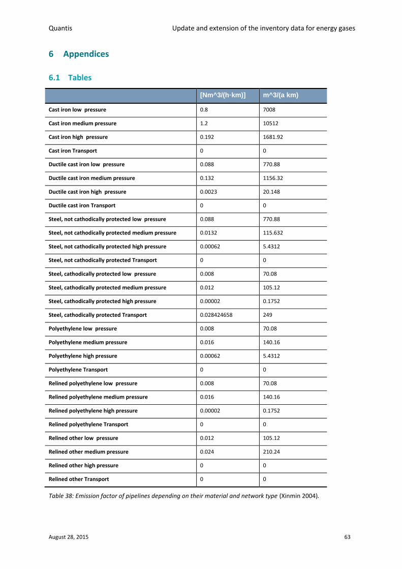
Quantis Update and extension of the inventory data for energy gases
August 28, 2015 63
6 Appendices
6.1 Tables
[Nm^3/(h·km)] m^3/(a km)
Cast iron low pressure 0.8 7008
Cast iron medium pressure 1.2 10512
Cast iron high pressure 0.192 1681.92
Cast iron Transport 0 0
Ductile cast iron low pressure 0.088 770.88
Ductile cast iron medium pressure 0.132 1156.32
Ductile cast iron high pressure 0.0023 20.148
Ductile cast iron Transport 0 0
Steel, not cathodically protected low pressure 0.088 770.88
Steel, not cathodically protected medium pressure 0.0132 115.632
Steel, not cathodically protected high pressure 0.00062 5.4312
Steel, not cathodically protected Transport 0 0
Steel, cathodically protected low pressure 0.008 70.08
Steel, cathodically protected medium pressure 0.012 105.12
Steel, cathodically protected high pressure 0.00002 0.1752
Steel, cathodically protected Transport 0.028424658 249
Polyethylene low pressure 0.008 70.08
Polyethylene medium pressure 0.016 140.16
Polyethylene high pressure 0.00062 5.4312
Polyethylene Transport 0 0
Relined polyethylene low pressure 0.008 70.08
Relined polyethylene medium pressure 0.016 140.16
Relined polyethylene high pressure 0.00002 0.1752
Relined polyethylene Transport 0 0
Relined other low pressure 0.012 105.12
Relined other medium pressure 0.024 210.24
Relined other high pressure 0 0
Relined other Transport 0 0
Table 38: Emission factor of pipelines depending on their material and network type (Xinmin 2004).

Quantis Update and extension of the inventory data for energy gases
August 28, 2015 64
6.2 Replies to review comments
The report was revised by Christian Bauer, PSI.
6.2.1 introduction / natural gas
Chapter (Nr) Reviewer’s comment Reply
Table of contents Not so important, but I’d change the order in chapter 3; production first, then transport, distribution, infra
Changed
Introduction 1.1
Energy gases
Specification of the term “energy gases” would help
We added a paragraph defining energy gases.
1st
sentence: In ecoinvent, or in
general, for which regions. etc??
Added: “in the ecoinvent database”
Legend of Fig. 1: To Europe? To
CH?
Added: “global import shares”
A little more context would help: commissioner? Purpose of the update? Geographical and temporal scope of the new data? Data formats? Who are the intended users?
What’s the “product” of your work? Which new/updated DS in which formats? Are the DS openly accessible?
We think the chapters “approach” and “methodology”
provide the information which was missed here. We moved
therefore the sentence beginning with “aim of this project
was…” to the chapter “approach”.and renamed the latter
“aim of the project”
For all data from this site: please
refer to a specific documentation
(report), if available.
done
2.1.1 Please provide a list of old and
new corresponding DS. And
additional DS, if any. As appendix,
I guess
The lists are provided in each chapter for more clarity. A
sentence was added to make this more clear: “The new
datasets and the datasets they replace are described in the
following chapters.”
Which ones (were updated)? Please more specific
We changed the wording of this paragraph to “The original
datasets were published in the natural gas ecoinvent report
(Faist Emmenegger et al. 2007) and had been
partlyupdated in (Schori and Frischknecht 2012). We based
our update on these datasets, together with the newest
publication like the one on methane emissions (Del Duce
and Faist Emmenegger 2014) as well as further literature
(see reference list at the end of this document).”
Is there a difference between m3
and Nm3?
Nm3 stands for “Norm cubic meter”. The N had been
omitted at this place and was added.
2.2.2 Standardized
calorific value for
HHV, right? Yes

Quantis Update and extension of the inventory data for energy gases
August 28, 2015 65
Chapter (Nr) Reviewer’s comment Reply
natural gas in
ecoinvent v3
This needs to be discussed. The standardization was introduced by Bo without asking anybody.
I would be in favour of reintroducing country-specific values, if not too much effort.
We think that this should indeed be discussed within the
ecoinvent expert group. However, we cannot decide this
for ourselves as this might influence other supply chains.
3.1 Overview For re-compression? Yes, added.
3.2 Natural gas
production
Please be explicit in which countries we have joint production of oil and gas and in which “gas only”
Done.
3.2.1 Joint oil and
natural gas production
in Norway
Table 2.What’s NGL? NGL = Natural Gas Liquids. Explained in the legend and
added to the abbreviations.
Is that joint production? What’s the reference product?
Yes, it is joint production. Added.
What’s the difference between Nm3 and Sm3?
This corresponds to different volume measurements based
on different temperature and pressure. We added this
precision and the abbreviations in the table.
Zero losses for gas resource Same assumption as in ecoinvent until now.
3.2.4 Natural gas production in Algeria, Middle East, Germany, Petroleum and gas production in the United Kingdom
Please be explicit concerning data content: North Africa is represented by Algeria, which is almost entirely a copy of RU. And middle east in turn is equivalent to Algeria.
Added: “The dataset for North African Countries is based
on the Algeria data, where most of the flows are
approximations from the Russian dataset. The Middele East
dataset is the copy of the Algerian dataset. We use this
data as they base on 2010 data and no more recent or
more accurate data are was readily available.”
3.4.1.4 Updated datasets
Wrong DS in this table
Corrected
3.4.2.2 LNG carriers Table Empty (Return trip)? Yes, we assume an empty return trip with a similar
consumption as in the loaded trip.
What does it mean in terms of %?
The figures are based on the scenario of Heede 2006 and
take his % over.
3.5 Representation of the trade movements
Which year is represented? We changed the text to: “The country of origin of the
natural gas imported in various European countries is
calculated based on the trade movements of the natural
gas in 2013 as described in (BP Amoco 2014) and, for
Switzerland, on the statistics of the Swiss natural gas
industry for 2012 (Del Duce and Faist Emmenegger 2014).”
3.5.1 Switzerland Can you explain, please, the meaning of “direct import” and “country of origin”?
Cannot reconstruct the numbers: e.g. why is import quantity = 0 for NO; why is it higher for Nigeria than for Algeria? Etc…
The table was wrong and was corrected.

Quantis Update and extension of the inventory data for energy gases
August 28, 2015 66
Chapter (Nr) Reviewer’s comment Reply
Numbers are different from those for CH in next table
3.5.2 European countries (1)
Does that mean we’ll have markets for high and low pressure nat gas for all these countries?
What about the NG losses and the transport distances?
Only market for high pressure natural gas. No new data for
the losses in the high pressure network. The explanation
about the transport distance was moved to the chapter 3.5
beginning.
3.5.4 Updated datasets
DE? (as a location for the dataset “
No, the location for the dataset “natural gas, production
DE, at long-distance pipeline” in ecoinvent 2 is “RER”,
whereas in ecoinvent 3 the dataset “natural gas, high
pressure, import from DE, XX, 2012 – 2012” is specific for
each importing country.
3.6.1 Infrastructure of the Swiss high and low pressure network
Could you specify the assumed lifetime somewhere?
Added (40 years, as in ecoinvent 2)
I don’t get it, sorry. The table above shows new data and in this paragraph you describe using old ones from v2.2. Which data in your new DS are based on v2.2 and which ones are new, exactly?
We add in the text “Data for the calculation of the
infrastructure requirements (see following chapter) is
based on the ecoinvent dataset from v2.2 (Faist
Emmenegger et al. 2007)” as it seems that it was not clear
that the sentence referred to the following calculations and
tables.
3.6.1.1 Material requirements of the low-pressure network
for all DS: can you provide the reference product and its unit along with the activity name? (either in the text or the appendix table)
- What about the GLO activites? Same inputs as for CH? I’d mention it at least in a footnote, similar for other DS
Added
3.6.2 Emissions due to leakage in the natural gas distribution system
How is this accounted for?
The emissions of the distribution network were updated
multiplying the length of each pipeline type in the Swiss
network (Table 3 and Table 5) with the specific leakage
rates of pipeline types presented in (Battelle 1994; Del
Duce and Faist Emmenegger 2014). However, the transit
emissions are excluded from the emissions of the high
pressure natural gas network, as they do not belong to the
same network.
3.6.2.1 Energy use and emissions in the low-pressure network
Where is the energy for gas distribution (compression?) accounted for? Same for high pressure
Explanation will be added. This part of the data was taken
over from ecoinvent 2.
What is the heat needed for? Same for high pressure
Explanation will be added. This part of the data was taken
over from ecoinvent 2.
3.6.2.2 Energy use and emissions in the
Why m3? (natural gas flow) It was an typing error; changed to MJ

Quantis Update and extension of the inventory data for energy gases
August 28, 2015 67
Chapter (Nr) Reviewer’s comment Reply
high-pressure network
3..6.2.3 Updated datasets
Ok, now there is a list I was asking for before. Please mention that already in the beginning
See comment above
You’ll need GLO activities for DS submission. Probably not relevant in this context
Not expected to be needed.
Unit of the reference product would help
Added in the respective tables.

Quantis Update and extension of the inventory data for energy gases
August 28, 2015 68
6.2.2 Replies to review comments: biogas/SNG part
Reviewer’s comment Reply
Concerning paragraph 1.2.2: Please refer to specific references, which are 1:1 in the reference list in case the data were available from previous studies
References are described in another paragraph (Chapter 4). A
comment on where the information will be found has been
introduced.
Concerning paragraph 1.2.2: Any source for this statement? Are there wood methanation plants right now operating in CH?
Data on the most relevant technology in Switzerland is unclear.
The text has been changed so that the new datasets represent
a new possible option.
Concerning chapter 4.1.: It’s confusing that we’re back in ev2 logic. Can you add a paragraph explaining, please?
A comment on the specific aim of the biogas/SNG part of the
project and its data sources has been introduced which explains
the link to ecoinvent version 2.
Concerning Table 26 on biogas leakage in biogas production: Don’t get it, sorry.
There is one process, biowaste disposal or biowaste treatment. This joint production activity has 2 products: biogas and digestate.
You present it here as separate independent products/activities. Does this include implicit allocation?
Yes, economic allocation is assumed. A comment on the
allocation system in the various datasets has been introduced
before the table.
Concerning the function of the digestate
datasets: What’s the purpose of these?
What’s the product?
A comment has been introduced which specifies what is
covered by these datasets.
Concerning Table 28: Don’t you want to show the joint production DS here instead of the DS after allocation?
The source datasets were already separated. It was therefore
preferred to continue the comparison on the separated
datasets.
Concerning the own biogas consumption for heat and electricity processes in the biogas plant: Which fraction of gas is required?
The required quantity of consumed biogas per m3 of produced
biogas (and per kg of disposed biowaste) have been calculated
and added in the text.

Quantis Update and extension of the inventory data for energy gases
August 28, 2015 69
6.2.3 Replies to review comments: PtX
Chapter Reviewer’s comment Reply
4.3.2.1 CO2-Capture Sorry, but this is not acceptable from my perspective. There’s a methodological inconsistency.
Separation of co2 from power plants needs to be considered as joint production of electricity and CO2. I’d recommend this paper to read: “von der Assen et al. (2013) Life-cycle assessment of carbon dioxide capture and utilization: avoiding the pitfalls”.
You can either apply allocation or system expansion including the whole process of power plant operation with CO2 capture.
Your procedure seems to be
incorrect, or is not sufficiently
described.
This point was thoroughly discussed in a
separate telephone conference which
showed that there were no disagreements
on the method but rather a
misunderstanding. The chapter was
consequently re-written and a Figure has
been added to show the system boundaries
4.3.2.3 Resulting datasets Not compatible with the way you deal with/describe the CO2 capture in the previous chapter
It is more clearly described now!
4.3.2.3 Resulting datasets Contradicts your statement above: “Biogenes CO2 als CO2-Quelle wird im Rahmen dieser Studie nicht explizit betrachtet”
You are right. I deleted the sentence saying
(wrongly) that it will not be assessed
6.2.4 Replies to review comments: References
Chapter Reviewer’s comment Reply
References For all reports which are
available on the web: please
provide the link for download
Done where possible
In general: most of these reports are not accessible. A reviewer should have access to the majority of primary sources.
The references were missing in the report
due to a problem with the library system.
This was corrected.