
Untitled - Journal of Renewable Energy and Environment
89
-
Upload
khangminh22 -
Category
Documents
-
view
1 -
download
0
Transcript of Untitled - Journal of Renewable Energy and Environment


Journal of Renewable Energy and Environment (JREE): Vol. 8, No. 1, (Winter 2021), 1-76
CONTENTS
Seyed Ali Akbar Fallahzadeh Navid Reza Abjadi Abbas Kargar Frede Blaabjerg
Applying Sliding-Mode Control to a Double-Stage Single-Phase Grid-Connected PV System
1-12
Ramasamy Dhivagar Murugesan Mohanraj
Optimization of Performance of Coarse Aggregate-Assisted Single-Slope Solar Still via Taguchi Approach
13-19
Aryan Tabrizi Mehdi Rahmani
Assessing and Evaluating Reliability of Single-Stage PV Inverters 20-27
Aychar Khajavi Pour Mohammad Reza Shahraki Faranak Hosseinzadeh Saljooghi
Solar PV Power Plant Site Selection Using GIS-FFDEA Based Approach with Application in Iran
28-43
Paulina Krystosiak Laudable Intentions, Parochial Thinking: Climate Change, Global
Warming and Clean Energy Concerns in Investment Decisions Regarding Renewable Energy Projects in Poland
44-48
Leila Samiee Fatemeh Goodarzvand-Chegini Esmaeil Ghasemikafrudi Kazem Kashefi
Hydrogen Recovery in an Industrial Chlor-Alkali Plant Using Alkaline Fuel Cell and Hydrogen Boiler Techniques: Techno-Economic Assessment and Emission Estimation
49-57
Seyed Saeed Hoseini Mohammad Amin Sobati
Assessment of the Performance and Exhaust Emission of a Diesel Engine Using Water Emulsion Fuel (WEF) in Different Engine Speed and Load Conditions
58-68
Muhamad Mustafa Mundu Stephen Ndubuisi Nnamchi Onyinyechi Adanma Nnamchi
Development of a Model for Estimation of Sunshine Hour Data for Different Regions of Uganda
69-76

AIMS AND SCOPE
Journal of Renewable Energy and Environment (JREE) publishes original papers, review articles, short communications and technical notes in the field of science and technology of renewable energies and environmental-related issues including:
• Generation • Storage • Conversion • Distribution • Management (economics, policies and planning) • Environmental Sustainability
INSTRUCTIONS FOR AUTHORS
Submission of manuscript represents that it had neither been published nor submitted for publication elsewhere and is result of research carried out by author(s). Only the extended and upgraded articles presented in a conference and/or appeared in a symposium proceedings could be evaluated for publication. Authors are required to include a list describing all the symbols and abbreviations in the paper. Use of the international system of measurement units is mandatory.
• On-line submission of manuscripts results in faster publication process and is recommended. Instructions are given in the JREE web sites: www.jree.ir
• References should be numbered in brackets and appear in sequence through the text. List of references should be given at the end of the paper. All journal articles listed in the References section must follow with article doi.
• Figure captions are to be indicated under the illustrations. They should sufficiently explain the figures.
• Illustrations should appear in their appropriate places in the text. • Tables and diagrams should be submitted in a form suitable for reproduction. • Photographs should be of high quality saved as jpg files. • Tables’ illustrations, figures and diagrams will be normally printed in single column width (8
cm). Exceptionally large ones may be printed across two columns (17 cm).

JREE: Vol. 8, No. 1, (Winter 2021) 1-12
Please cite this article as: Fallahzadeh, S.A.A., Abjadi, N.R., Kargar, A. and Blaabjerg, F., "Applying sliding-mode control to a double-stage single-phase grid-connected PV system", Journal of Renewable Energy and Environment (JREE), Vol. 8, No. 1, (2021), 1-12. (https://doi.org/10.30501/jree.2020.233358.1114).
2423-7469/© 2021 The Author(s). Published by MERC. This is an open access article under the CC BY license (https://creativecommons.org/licenses/by/4.0/).
Research Article
Journal of Renewable Energy and Environment
J o u r n a l H o m e p a g e : w w w . j r e e . i r
Applying Sliding-Mode Control to a Double-Stage Single-Phase Grid-Connected PV System
Seyed Ali Akbar Fallahzadeha, Navid Reza Abjadia*, Abbas Kargara, Frede Blaabjergb
a Faculty of Technology and Engineering, Shahrekord University, Shahrekord, Chaharmahal and Bakhtiari, Iran. b Department of Energy Technology, Aalborg University, Aalborg, Denmark.
P A P E R I N F O
Paper history: Received 09 June 2020 Accepted in revised form 20 September 2020
Keywords: Sliding Mode, POSLLC, Grid Connected, Photovoltaic
A B S T R A C T
This study investigates a new double-stage single-phase Grid-Connected (GC) Photo-Voltaic (PV) system. This PV system includes a DC-DC Positive Output Super Lift Luo Converter (POSLLC) and a single-phase inverter connected to a grid through an RL filter. Due to its advantages, the POSLLC was used between PV panel and inverter instead of the conventional boost converter. The state space equations of the system were solved. By using two Sliding Mode Controls (SMCs), PV panel voltage and POSLLC inductor current were controlled and the designed controls were compared. Two of these SMCs included a simple Sign Function Control (SFC) and a conventional SMC. To control the power injected into the grid with a unity power factor, an SMC was used. Perturb and Observe (P&O) method was employed to reach maximum power of the PV panel. The Maximum Power Point Tracking (MPPT) control generated the voltage reference of the PV panel. Similar controls were used for the boost converter instead of POSLLC. The obtained results were compared.
https://doi.org/10.30501/jree.2020.233358.1114
1. INTRODUCTION1
Among the available renewable energy resources, PV energy, which enjoys low cost and government support, is used more and more every day. Energy harvesting from PV panels is quite dependent on solar irradiation and temperature. Elaborate control methods should be used along with Maximum Power Point Tracking (MPPT) to achieve maximum power extraction [1]. A PV system can work in the off-grid or on-grid mode [2]. The use of grid-tie or on-grid PV systems is increasing nowadays [3]. Usually, grid-tie PV systems are characterized by two stages of conversion [4-5]. Two-stage conversion is generally required because of the very high voltage conversion ratio [6]. Industry has shown that this topology can achieve more than 96 % efficiency [7]. In the first stage, a DC-DC converter is used and, in the second stage, an inverter is connected to the grid. Failure to apply the DC-DC converter to the single-phase grid-connected PV system causes some difficulties such as double-frequency power ripple and inverter input voltage fluctuations [8]. Recently, the application of single-phase grid-connected PV systems has attracted considerable attention because there are many residential and commercial customers for single-phase grid- *Corresponding Author’s Email: [email protected] (N.R. Abjadi) URL: http://www.jree.ir/article_114504.html
connected PV systems, which generate extra PV energy for some hours a day [1]. Such advanced applications require precise control. DC-DC converters are applied to many commercial and industrial equipment. The main objective of these converters is to ensure high conversion voltage ratio, high efficiency, and high-power density. To increase the gain of a conventional DC-DC boost converter in renewable energy applications, cascade boost converters [9, 10] or double boost converters are used; however, such topologies are complicated and, thus, need sophisticated control techniques. In fact, these converters have many inductors and capacitors (or semiconductor switches) that promote the order of the system. Recently, a family of DC-DC converters, called Luo converters, has received notable attention and one of the most remarkable DC-DC converters in this family is POSLLC [11-13]. In fact, there are three types of Luo converter: elementary circuit, re-lift circuit, and triple-lift circuit. The analysis of POSLLCs in different operation modes was conducted in [14]. One of the main indices of DC-DC converters is their efficiency. Vinoth and Ramesh [15] compared the efficiency rates of Luo and Boost converters in a hybrid grid-connected topology based on photovoltaic system and permanent magnet synchronous generator. They found that the efficiency of the system that used Luo converter was 5 % higher than the system with a boost converter. Narmadha et al. [16] proposed a stand-alone PV system based on POSLLC and controlled the
S.A.A. Fallahzadeh et al. / JREE: Vol. 8, No. 1, (Winter 2021) 1-12
2
output voltage. Gnanavadivel et al. [17] incorporated Lou converter in the AC-DC converter to improve power factor. Classical linear control is usually used to achieve the control objectives of GC solar PV systems [18]. Linear controllers are unable to achieve the desired control objectives at different operating points, i.e. under fast-changing weather conditions [19]. In [20], a double-stage PV system using DC-DC Buck converter was presented. Two-cascade Proportional Resonant (PR) controllers were used to control the injected current into the grid. In [21], two PI controllers were employed to control the current injected to the grid and the panel voltage in a two-stage system connected to a single-phase utility grid. In [22], a double-stage PV system using DC-DC boost converter was presented. Conventional PI controls were used and a high-order observer was proposed. PI and fuzzy control of output voltage for a POSLLC was presented in [16]. The drawbacks of these plans include the difficulty of adjusting the parameters of controllers and the inability of linear controllers to fast track the voltage reference in the event of a change in weather conditions. Using nonlinear control can be advantageous for overcoming the problems associated with different operating points in GC PV systems [23-26]. There are different types of current nonlinear control schemes for PV systems such as SMC [23, 24], feedback linearization control [25, 27], and backstepping control [28]. Nonlinear control of output voltage for a POSLLC using an observer-based scheme was presented in [29]. The nonlinear control proposed in [29] was characterized by a complicated structure, which made its tuning difficult. In [30], by using a boost converter in a PV system, the output voltage was controlled, which is not suitable for MPPT purposes; moreover, the stabilty of internal dynamic was not investigated. In [31], a robust backstepping controller was designed for a buck boost DC-DC converter in a PV system which has a complicated structure to implement. In [32], the control of a stand-alone PV system consisting of a POSLLC was presented, and an ohmic load was fed by the PV system. In [33], two controllers were used to optimize the PV energy injected into the three-phase grid. The first controller was used to predict the DC voltage that would allow the three-phase inverter to track the maximum power point of photovoltaic generator under variable climatic conditions and variable load. This new controller used a multivariate polynomial interpolation based on Lagrange’s theory. The second controller was based on the robust SMC. It was used to control the active and reactive powers injected into the network. This system was of single-stage type and the contollers were cascaded, not independent. Therefore, failure to set one controller can have a negative effect on the other controller and thus on the system as a whole. In [34], an adaptive fuzzy SMC was designed for a boost converter in a PV system; by using fuzzy conrtol, there is no guaranty for the overall system stability and the process of design is complicted. In the current study, POSLLC and a prototype of the single-phase inverter are suggested for transferring the power of a
PV panel to the grid. PV panel voltage, inductor current of DC- DC converter, and injected current to the grid are controlled to achieve maximum power and high performance. Since the POSLLC works in the lower range of duty cycles, parasitic effects and losses are reduced to minimum and a highly efficient operation is achieved. PV panels have nonlinear characteristics and are expensive. It is indispensable to extract the maximum power from PV panels. Providing voltage through PV panel and the connected circuit depends on climate conditions and the operating point. In this condition, an MPPT algorithm is necessary to provide reference voltage for PV panel. SMC is a robust method that shows significant tracking effectiveness and provides a swift reaction to climate changes. In [24], a simple sign function control was used to control the DC link voltage of POSLLC. In this study, the DC link voltage was controlled by two nonlinear control methods and the methods were compared using POSLLC and boost converter. Voltage gain of POSLLC was higher and, at the same time, its average inductor current was lower than those of other conventional converters. Consequently, POSLLC is widely popular in higher power applications. Furthermore, it has an additional capacitor that strictly regulates output voltage. To control the current injected to the grid, an SMC method was also applied and the commands for the inverter switches were produced. To obtain the maximum power from the panel, the P&O MPPT technique was used. The main innovations of this paper include (a) the application of DC-DC POSLLC to a single-phase double-stage grid-connected PV system that outperforms other similar systems with DC-DC boost converter and (b) simultaneous nonlinear controlling of the injected current to the grid and the DC-DC converter capacitor voltage. To confirm the advantages of the proposed PV system and controllers, simulation software with PSIM module at different irradiation rates and temperatures is presented and discussed. 2. PV SYSTEM STRUCTURE
Fig. 1 shows the overall double-stage PV system. The DC side contains PV panel connected to capacitor Cpv and POSLLC. AC side contains the inverter, RL filter, and utility grid. 2.1. Positive output super lift Luo converter
Fig. 2 illustrates the elementary circuit of POSLLC, its equivalent circuit when the switch S is closed (on), and its equivalent circuit when the switch S is open (off). According to Fig. 2-b, C1 is charged on Vin while switch S is on. Because L1 and C1 are parallel, the current of inductor L1 (
1Li ) experiences an increase. In the switched-off mode, as shown in Fig. 2-c, the voltage across inductor L1 becomes –(Vo-2Vin) and hence,
1Li is reduced. The average of the inductor voltages is zero in a steady state. It is assumed that DTs is the switch-on period and (1-D)Ts is the switch-off period. Therefore, the Voltage Gain (VG) of the POSLLC is obtained through the following relation [13]:
o
in
V 2-DVG= =
V 1-D (1)

S.A.A. Fallahzadeh et al. / JREE: Vol. 8, No. 1, (Winter 2021) 1-12
3
Let C1 and 1CV be a large value and a constant, respectively, as
given in Vin=1CV . The average model of the POSLLC in
Continuous Conduction Mode (CCM) is expressed as follows [5]:
1
1 1
L in in
L L2
1
D
1i = (2v -v +(v -v )D)o oL
1 vov = (i - -i )o C R
(2)
where D (0,1)∈ .
Figure 1. Configuration of the PV system
(a) (b)
(c)
Figure 2. (a) Elementary circuit diagram, (b) Equivalent circuit when switch is on, and (c) Equivalent circuit when switch S is off 2.2. DC side model
According to Relation (2), the overall DC side state variables shown in Fig. 1 and their state equations are well defined as follows:
1 1
TL pv C ox=[i v v v ] (3)
1 1 2
1
1
1
C L D CD
1 1 11 1 1 1
C pvDpv
pv D pv Dpvpv
Cpv L
1 1 D 1 D 1
L
2 2 2
-v i R v-R 1 1 -1 + +L L LL L L L 0
-v v-R - i0 0 0C R C RC
CX= X + u (t)+v-v1 i0 0 0 - - 0
C C R C R C0
1 -1 i0 0 -C RC C
(4)
The voltage of capacitor C2 is controlled using a PI controller, as shown in Fig. 3 and regulated into its reference value. Therefore, (4) is reduced to a second-order equation as follow:
1 1 1
1
C L D o C oD
1 1 1 1
C pv pv
pv pvpv D
-v +i R +v v -v-R 1L L L L
z= z + u (t) +-1 v -v i0
C CC R
(5)
where
1
TL pvz=[i v ] (6)
The above equation is written in the following compact canonical form:
z=f(z)+g(z)u(t) (7)
S.A.A. Fallahzadeh et al. / JREE: Vol. 8, No. 1, (Winter 2021) 1-12
4
where
1 11
1
1 1
1
D L pv C oC oD
1 1 11
L pvpv
pv pv pv
C L D o
C pv
pv D
-R i +v +V -VV -V-R 1L L LL
f(z)= z+ =-1 -i +ii0
C C C
-V +i R +VL
g(z)= V -VC R
(8)
2.3. AC side model
The AC side including an H-bridge inverter and an LR filter is connected to the utility grid. As shown in Fig. 1, the switch positions are represented by the simple input command χ of switches as follows:
1 4 2 3
2 3 1 4
χ=+1 if S ,S :on, S ,S :off
χ=-1 if S ,S :on,S ,S :off (9)
when χ=+1 , the state equations can be written as follows:
o g o
2
g g g i g
g
1v = (-i +i )
C
1i = (-i R +v +e )
L
(10)
The grid voltage is assumed to be sinusoidal given by:
g me = V sinωt (11)
when χ=-1 , the state equations can be given as follows:
o g o
2
g g g i g
g
1v = (i +i )
C
-1i = (i R +v +e )
L
(12)
Combining relations (10) and (12), one can obtain:
o g o
2
g g g i g
g
1v = (-i (t)+i )
C
1i = (-i R +v (t)-e )
L
r
r
(13)
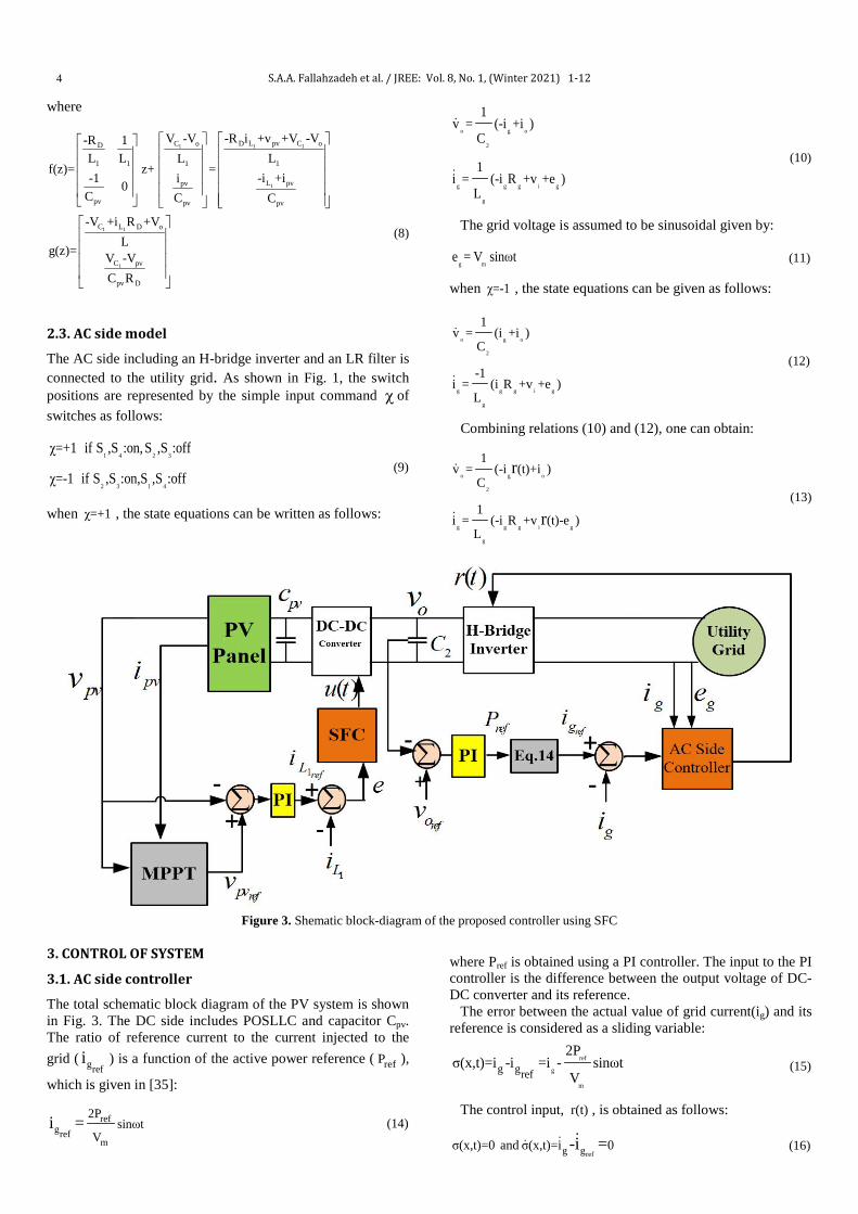
Figure 3. Shematic block-diagram of the proposed controller using SFC
3. CONTROL OF SYSTEM
3.1. AC side controller
The total schematic block diagram of the PV system is shown in Fig. 3. The DC side includes POSLLC and capacitor Cpv. The ratio of reference current to the current injected to the grid ( gref
i ) is a function of the active power reference ( refP ),
which is given in [35]:
refgref
m
2Psinωt
Vi =
(14)
where Pref is obtained using a PI controller. The input to the PI controller is the difference between the output voltage of DC-DC converter and its reference. The error between the actual value of grid current(ig) and its reference is considered as a sliding variable:
ref
g
m
g gref
2Pσ(x,t)=i -i =i - sinωt
V (15)
The control input, r(t) , is obtained as follows:
refg gσ(x,t)=0 and σ(x,t)=i 0-i = (16)

S.A.A. Fallahzadeh et al. / JREE: Vol. 8, No. 1, (Winter 2021) 1-12
5
Substituting (13) into (16), one obtains the following:
ref gg g g
i m
2P L ωcosωt1r(t)= ( +e +R i )+bsgn(σ
v V)
(17)
where sgn(σ) is the sign function aimed at achieving robustness in the face of parametric uncertainties in the control law and b is a positive constant.
Figure 4. Shematic diagram of the proposed controller using conventional SMC 3.2. DC side control using Sign Function Control (SFC)
Consider the following sliding variable for inductor current:
1 1refL Le(z)=i -i
(18)
where 1refLi is the reference value of
1Li obtained by
comparing PV panel voltage pvv with its reference refpvv
using a Proportional Integrator (PI) controller. One can drive the output function e(z) to zero through discontinuous control, indicating that
1Li converges to its desired value. The Lie derivative theory is applied in the following manner [36]:
1 1
1 1
D L pv C of 1 2
1 2
C L D og 1 2
1 2
-R i +v +V -Ve(z) e(z)L e(z)= f (z)+ f (z)=z z L
-V +i R +Ve(z) e(z)L e(z)= g (z)+ g (z)=z z L
∂ ∂∂ ∂
∂ ∂∂ ∂∂
(19)
where f1 and f2 are the rows of f(z) and g1 and g2 are the rows of g(x). fL e(z) is the Lie derivative of e(z) with respect to f(z). The equivalent control is obtained as follows:
1
1 1
D L pv C of
g C L D o
R i -v +V -VL e(z)u(z)=- =L e(z) -V +i R +V
(20)
Fig. 3 shows the block diagram of the proposed controller. 3.3. DC side control using Sliding Mode Controller (SMC)
In this section, a conventional sliding mode control is designed to control the inductor current
1Li and the capacitor voltage Vpv, as shown in Fig. 4. The following sliding variable is defined for this purpose:
2 1 1 2 2s (z,t)=K e +K e
(21)
where K1 and K2 are positive constants and e1 and e2 are defined as follows:
1 1ref
ref
1 L L
2 pv pv
e =i -i
e =v -v
(22)
By substituting (5) into the following equation, the control law of POSLLC can be obtained as in (24):
2 1 1 2 2s (z,t)=K e +K e =0 (23)
1
ref ref
1 1
D L pv c o L PV1 L 2 pv
pv3 2
c D L o pv c1 2
pv D
R i -v -v +v i -i-K (i + )-K (v + )L C
u(t)= +K sgn(s )v -R i -v v -vK ( )+K ( )
L C R
(24)
where K3 is a positive constant. 4. SIMULATION AND DISCUSSION
The simulation results show the performance of the proposed controls in handling the GC single-phase PV system and DC-DC converters. Table 1 shows technical specifications of the PV panel. The step time for simulation and switching frequency are considered as 1 sµ and 20 KHz, respectively. The Pulse Width Modulation (PWM) technique is applied to the case of a single-phase inverter. 4.1. Comparison of two SMC strategies
In Fig. 3, the POSLLC is controlled using SFC method to achieve MPPT by regulating the PV panel voltage. Fig. 4 shows the DC-DC converter control by conventional SMC with the sliding variable given in (15). Table 2 shows the parameter values of POSLLC.

S.A.A. Fallahzadeh et al. / JREE: Vol. 8, No. 1, (Winter 2021) 1-12
6
Table 1. PV panel parameters and specifications
Reference cell temperature 25 °C
Maximum power 110 W
Number of cells 72
Voltage at maximum power 34.8 V
Open-circuit voltage 43.4 V
Standard light intensity at 25 °C 1000 w/m2
Short circuit current 3.4 A
Current at maximum power 3.16 A
Table 2. DC-DC converters, RL filter, and input capacitor values
Boost converter values L1 0.2 mH
C1 0.2 mF
POSLLC values
L1 0.2 mH
C1 0.1 mF
C2 0.1 mF
RL filter values Lg 5 mH
Rg 50 mΩ
Input capacitor value Cpv 0.1 mF
The simulation results of this section were affected by the variations in radiation and temperature. The characteristic of output power of the PV panel was dependent on sun irradiation and ambient temperature. The output characteristics of PV cells or modules are commonly represented by the current–voltage (I–V) and power–voltage (P–V) curves. In some special cases, voltage–current (V–I) and power–current (P–I) curves were used to represent the PV output characteristics [37]. Standard Test Conditions (STC) are conditions in which the solar modules are tested in a laboratory. Module testing is carried out in the following conditions: solar radiation intensity of 1000 W/m2, optical air mass of AM 1.5, temperature of solar module of 25 °C, and wind speed of 1 m/s [38]. Figs. 5 and 6 include Power-Voltage (P-V) curves of PV panel at different irradiances and temperatures, respectively. Figs. 7 and 8 display Current-Voltage (I-V) curves of the panel under different conditions.
Figure 5. Power-voltage curves at different irradiances (T=25 °C)
Figure 6. Power-voltage curves at different tempartures
(G=1000 W/m2)
Figure 7. I-V curves at different irradiances (T=25 °C)
Figure 8. I-V curves at different temperatures (G=1000 W/m2)
Figs. 9-15 compare the simulation results for the PV system using SFC and SMC at different values of irradiance and temperatures including T=25 °C. The value of irradiance G increases from 800 to 1200 W/m2 at t=0.2 s and is reduced from 1200 to 1000 W/m2 at t=0.4 s, as shown in Fig. 9. According to Fig. 6, when irradiation steps up, the obtained PV power increases, which, in turn, elevates the amplitude of the injected current to the grid. The POSLLC inductor current will also increase. These results are shown in Figs. 10-14. Besides, according to Figs. 11 and 14, the MPPT technique at different values of radiation shows a suitable performance. Fig. 10 shows the function of AC side controller in tracking the injected current to the utility grid and its reference at different irradiance values. A comparison between SFC and SMC in the DC side controller is made and given in Figs. 11 and 12. Fig. 11 shows that voltage fluctuations around the reference in SMC are fewer in number than those in SFC. In

S.A.A. Fallahzadeh et al. / JREE: Vol. 8, No. 1, (Winter 2021) 1-12
7
addition, SMC has better performance for input capacitor Cpv (shown in Fig. 1) and ensures longer life of Cpv. Fig. 12 compares SMC-based inductor current with SFC-based inductor current. The SFC method has better functionality than SMC because the former is subject to less fluctuations and a lower average value.
Figure 9. Irradiance changes of the PV panel
(a)
(b)
Figure 10. Grid current and its reference at different values of irradiance using (a) SFC and (b) SMC
(a)
(b)
Figure 11. PV extracted voltage and its reference at different values of irradiance using (a) SFC and (b) SMC
Fig. 13 compares maximum power with delivered power of the PV panel. This figure demonstrates that MPPT method has proper performance using both of the proposed controllers despite different radiation values. Fig. 14 shows how the PV panel current varies due to irradiance changes. The PV panel current using SMC is more acceptable than that using SFC. Satisfactory Unity Power Factor (UPF) with respect to the power supply network is proven, as shown in Fig. 15, which shows utility grid voltage and injected current to the grid.
(a)
(b)
Figure 12. POSLLC inductor current and PV current at different values of irradiance using (a) SFC and (b) SMC
(a)

S.A.A. Fallahzadeh et al. / JREE: Vol. 8, No. 1, (Winter 2021) 1-12
8
(b)
Figure 13. Maximum power and delivered power of PV panel at different values of irradiance using (a) SFC and (b) SMC
(a)
(b)
Figure 14. Delivered PV panel current at different values of irradiance using (a) SFC and (b) SMC
(a)
(b)
Figure 15. UPF checking by (a) SFC and (b) SMC
This study carried out another experiment at temperature T ranging from 25 °C to 40 °C at t=0.25 s (Fig. 16) and irradiance G=1000 W/m2 using the controllers (Figs. 3 and 4). The simulation results of the proposed controllers are presented and compared in Figs. 17 to 20. According to Fig. 6, as the temperature of the PV panel decreases, the extracted power increases. By increasing the temperature of PV panel, the its voltage is reduced and current increases, as shown in Figs. 17 and 19, respectively. At varying temperatures, SMC outperforms SFC. Figs. 17-18 show that the fluctuations of inductor current of DC-DC converter and PV voltage panel in the system using SMC are less than those in the system using SFC. These fluctuations increase the efficiency and lifespan of capacitor Cpv in the system using SMC.
Figure 16. Temperature changes of PV panel
(a)
(b)
Figure 17. PV extracted voltage and its reference at different temperatures using (a) SFC and (b) SMC
(a)

S.A.A. Fallahzadeh et al. / JREE: Vol. 8, No. 1, (Winter 2021) 1-12
9
(b)
Figure 18. POSLLC inductor current using (a) SFC and (b) SMC
(a)
(b)
Figure 19. Unity power factor checking by (a) SFC and (b) SMC
(a)
(b)
Figure 20. Inductor current and its reference: (a) the proposed system using boost converter and (b) the proposed system using
POSLLC
4.2. Comparison of performances of POSLLC and boost converter in the proposed system
In this section, the performances of DC-DC, POSLLC, and boost converter in the PV system are compared. Besides its higher voltage gain than the boost converter, POSLLC enjoys another advantage, to be presented later in the paper. Table 2 shows the parameters of the DC-DC boost converter. The inductor value of the boost converter is set equal to the output value ‘one’ of the POSLLC and the value of its capacitor is equal to the sum of the values of POSLLC capacitors. Fig. 20-a shows the inductor current of boost converter in the proposed system shown in Fig. 3. The average value of inductor current
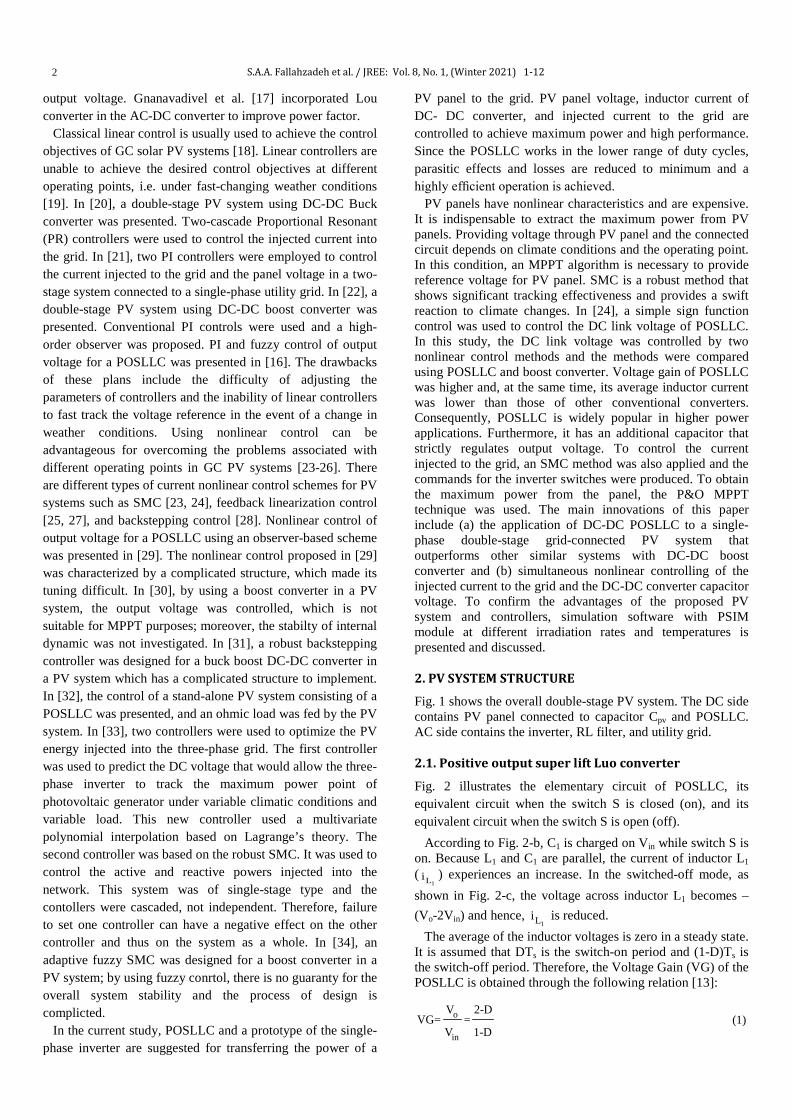
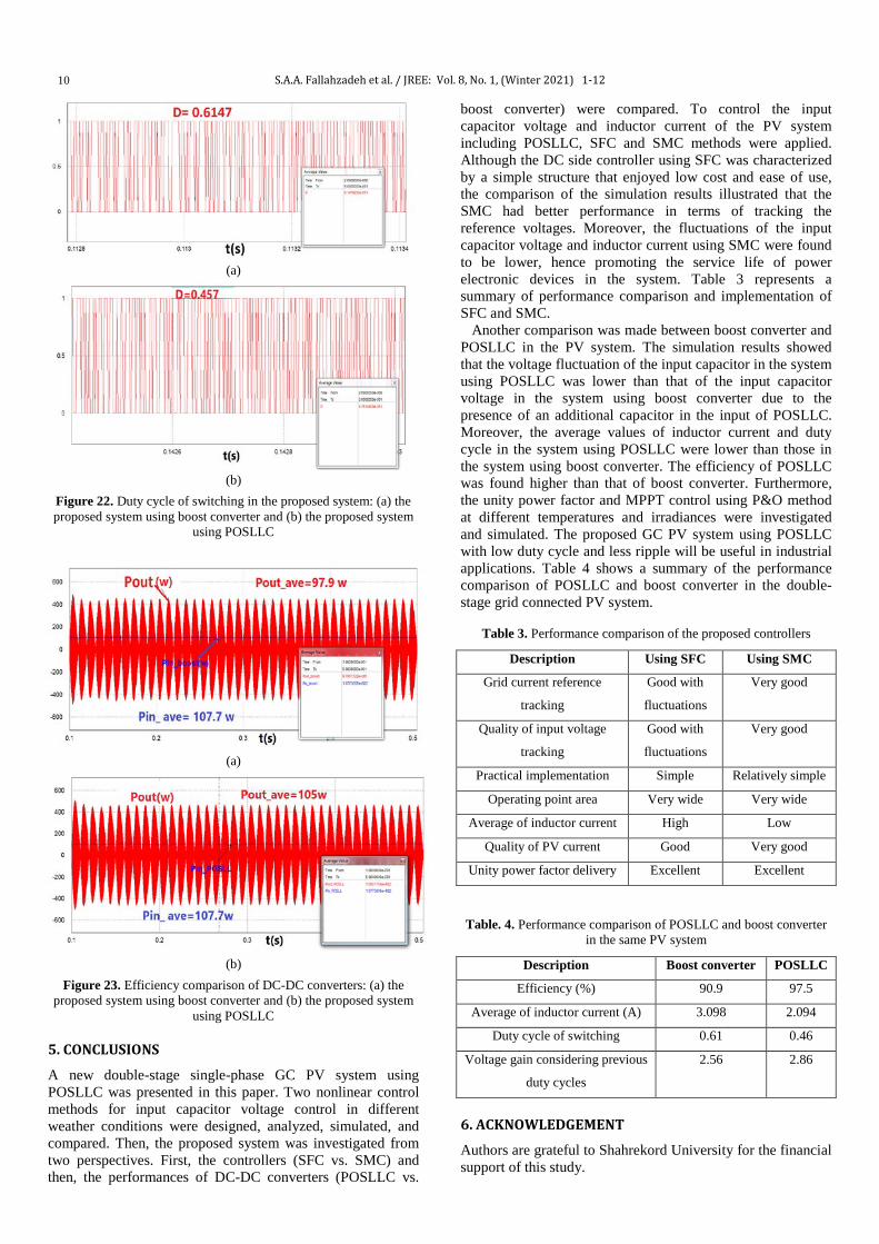
1Li is equal to 3.47 A, while the average value of inductor current of the POSLLC in a similar system equals 2.094 A (Fig. 20-b). A lower inductor current value yields lower loss. The proposed system using POSLLC is subject to less voltage fluctuations than the system using boost converter, as shown in Fig. 21, and this ensures the longer lifespan of capacitor Cpv using POSLLC. Furthermore, D with POSLLC is less than D with boost converter. Fig. 22-a shows D using POSLLC. The value of D using POSLLC is close to 0.5 (D=0.475), while it equals 0.615 using boost converter (Fig. 22-b). According to Fig. 23, the efficiency of the PV system with boost converter is lower than that of PV system with POSLLC. Input power of both converters is 107.7 W; however, the output power values of POSLLC and boost converter are 105 W and 97.9 W, respectively. Therefore, the POSLLC and the boost converter enjoy efficiency rates of 97.5 % and 90.9 %, respectively, in the same condition.
(a)
(b)
Figure 21. PV extracted voltage and its reference (zoomed in): (a) the proposed system using boost converter and (b) the proposed
system using POSLLC
S.A.A. Fallahzadeh et al. / JREE: Vol. 8, No. 1, (Winter 2021) 1-12
10
(a)
(b)
Figure 22. Duty cycle of switching in the proposed system: (a) the proposed system using boost converter and (b) the proposed system
using POSLLC
(a)
(b)
Figure 23. Efficiency comparison of DC-DC converters: (a) the proposed system using boost converter and (b) the proposed system
using POSLLC 5. CONCLUSIONS
A new double-stage single-phase GC PV system using POSLLC was presented in this paper. Two nonlinear control methods for input capacitor voltage control in different weather conditions were designed, analyzed, simulated, and compared. Then, the proposed system was investigated from two perspectives. First, the controllers (SFC vs. SMC) and then, the performances of DC-DC converters (POSLLC vs.
boost converter) were compared. To control the input capacitor voltage and inductor current of the PV system including POSLLC, SFC and SMC methods were applied. Although the DC side controller using SFC was characterized by a simple structure that enjoyed low cost and ease of use, the comparison of the simulation results illustrated that the SMC had better performance in terms of tracking the reference voltages. Moreover, the fluctuations of the input capacitor voltage and inductor current using SMC were found to be lower, hence promoting the service life of power electronic devices in the system. Table 3 represents a summary of performance comparison and implementation of SFC and SMC. Another comparison was made between boost converter and POSLLC in the PV system. The simulation results showed that the voltage fluctuation of the input capacitor in the system using POSLLC was lower than that of the input capacitor voltage in the system using boost converter due to the presence of an additional capacitor in the input of POSLLC. Moreover, the average values of inductor current and duty cycle in the system using POSLLC were lower than those in the system using boost converter. The efficiency of POSLLC was found higher than that of boost converter. Furthermore, the unity power factor and MPPT control using P&O method at different temperatures and irradiances were investigated and simulated. The proposed GC PV system using POSLLC with low duty cycle and less ripple will be useful in industrial applications. Table 4 shows a summary of the performance comparison of POSLLC and boost converter in the double-stage grid connected PV system.
Table 3. Performance comparison of the proposed controllers
Description Using SFC Using SMC
Grid current reference
tracking
Good with
fluctuations
Very good
Quality of input voltage
tracking
Good with
fluctuations
Very good
Practical implementation Simple Relatively simple
Operating point area Very wide Very wide
Average of inductor current High Low
Quality of PV current Good Very good
Unity power factor delivery Excellent Excellent
Table. 4. Performance comparison of POSLLC and boost converter in the same PV system
Description Boost converter POSLLC
Efficiency (%) 90.9 97.5
Average of inductor current (A) 3.098 2.094
Duty cycle of switching 0.61 0.46
Voltage gain considering previous
duty cycles
2.56 2.86
6. ACKNOWLEDGEMENT
Authors are grateful to Shahrekord University for the financial support of this study.

S.A.A. Fallahzadeh et al. / JREE: Vol. 8, No. 1, (Winter 2021) 1-12
11
NOMENCLATURE
Vin, Vo Average input/output voltage of POSLLC
D Duty cycle
VG Voltage gain
Ts Switching period of POSLLC
Vin Input voltage of POSLLC
RD Resistance of diodes D1 and D2
Vpv, refpvv PV panel voltage and its reference
1Li , 1refLi POSLLC inductor current and its reference
1Cv POSLLC capacitor C1 voltage
Rg, Lg Resistance and inductance of the filter and the line
Vo, io Output voltage/current of DC-DC converter or input voltage/current of inverter
eg Grid voltage
ig, grefi Injected current to the grid and its reference
Pref Reference power delivered to the grid
χ Inverter switches command
r(t) Average value of χ in the inverter switching period REFERENCES 1. Yang, Y. and Blaabjerg, F., "Overview of single-phase grid-connected
photovoltaic systems", Electric Power Components and Systems, Vol. 43, No. 12, (2015), 1352-1363. (https://doi.org/10.1080/15325008.2015.1031296).
2. Jafari, M., Ghadamian, H. and Seidabadi, L., "An experimental and comparative analysis of the battery charge controllers in off-grid PV systems", Journal of Renewable Energy and Environment (JREE), Vol. 5, No. 4, (2018), 46-53. (http://www.jree.ir/&url=http://www.jree.ir/article_95298.html).
3. Rahmani, M., Faghihi, F., Moradi CheshmehBeigi, H. and Hosseini S.M., "Frequency control of islanded microgrids based on fuzzy cooperative and influence of STATCOM on frequency of microgrids", Journal of Renewable Energy and Environment (JREE), Vol. 5, No. 4, (2018), 27-33. (http://www.jree.ir/article_94119.html).
4. Kjaer, S.B., Pedersen, J.K. and Blaabjerg, F., "A review of single-phase grid-connected inverters for photovoltaic modules", IEEE Transactions on Industry Applications, Vol. 41, No. 5, (2005), 2649-2663. (https://doi.org/10.1109/tia.2005.853371).
5. Fallahzadeh, S.A.A., Abjadi, N.R. and Kargar, A., "Double-stage grid-connected photovoltaic system with POSLL converter using PI resonant controller", Proceedings of 5th International IEEE Conference on Control, Instrumentation, and Automation (ICCIA), Iran, (2017), 155-160. (https://doi.org/10.1109/icciautom.2017.8258670).
6. Khan, O. and Xiao, W., "An efficient modeling technique to simulate and control submodule integrated PV system for single phase grid connection", IEEE Transactions on Sustainable Energy ,Vol. 7, No. 1, (2016), 96-107.(https://doi.org/10.1109/tste.2015.2476822).
7. Xiao, W., Edwin, F.F., Spagnuolo, G. and Jatskevich, J., "Efficient approaches for modelingand simulating photovoltaic power systems", IEEE Journal of Photovoltaics, Vol. 3, (2013), 500-508. (https://doi.org/10.1109/jphotov.2012.2226435).
8. Harb, S., Hu, H., Kutkut, N., Batarseh, I. and John Shen, Z., "A three-port photovoltaic (PV) micro-inverter with power decoupling capability", Proceedings of 2011 Twenty-Sixth Annual IEEE Applied Power Electronics Conference and Exposition (APEC), (2011). (https://doi.org/10.1109/APEC.2011.5744598).
9. Lotfi Nejad, M., Poorali, B., Adib, E. and Motie Birjandi, A.A., "New cascade boost converter with reduced losses", IET Power Electronics, Vol. 9, No. 6, (2016), 1213-1219. (https://doi.org/10.1049/iet-pel.2015.0240).
10. Sosa, J.M., Martinez-Rodriguez, P.R., Vazquez, G. and Nava-Cruz, J.C., "Control design of a cascade boost converter based on the averaged model", Proceedings of 2013 IEEE International Autumn Meeting on Power Electronics and Computing (ROPEC), (2013). (https://doi.org/10.1109/ROPEC.2013.6702718).
11. Miao, Z. and Luo, F.L., "Analysis of positive output super-lift converter in discontinuous conduction mode", Proceedings of 2004 International Conference on Power System Technology, Singapore, (2004), 828-833. (https://doi.org/10.1109/icpst.2004.1460108).
12. Jiao, Y., Luo, F.L. and Zhu, M., "Generalised modelling and sliding mode control for n-cell cascade super-lift DC-DC converters", IET Power Electronics, Vol. 4, (2011), 532-540. (https://doi.org/10.1049/iet-pel.2010.0049).
13. Luo, F.L. and Ye, H., "Positive output super-lift converters", IEEE Transactions on Power Electronics, Vol. 18, No. 1, (2003), 105-113. (https://doi.org/10.1109/TPEL.2002.807198).
14. Luo, F.L., "Analysis of super-lift Luo-converters with capacitor voltage drop", Proceedings of 2008 3rd IEEE Conference on Industrial Electronics and Applications, Singapore, (2008), 417-422. (https://doi.org/10.1109/iciea.2008.4582550).
15. Vinoth, K. and Ramesh, B., "A modified Luo converter for hybrid energy system FED grid tied inverter", International Journal of Engineering and Advanced Technology (IJEAT), Vol. 9, No. 1, (2019), 1515-1521. (https://doi.org/10.35940/ijeat.a1288.109119).
16. Narmadha, T.V., Velu, J. and Sudhakar, T.D., "Comparison of performance measures for PV based super-lift Luo-converter using hybrid controller with conventional controller", Indian Journal of Science and Technology, Vol. 9, No. 29, (2016), 1-8. (https://doi.org/10.17485/ijst/2016/v9i29/89937).
17. Gnanavadivel, J., Yogalakshmi, P., Senthil Kumar, N. and Krishna Veni, K.S., "Design and development of single phase AC–DC discontinuous conduction mode modified bridgeless positive output Luo converter for power quality improvement", IET Power Electronics, Vol. 12, No. 11, (2019), 2722-2730. (https://doi.org/10.1049/iet-pel.2018.6059).
18. Selvaraj, J. and Rahim, N.A., "Multilevel inverter for grid-connected PV system employing digital PI controller", IEEE Transactions on Industrial Electronics, Vol. 56, No. 1, (2009), 149-158. (https://doi.org/10.1109/tie.2008.928116).
19. Chowdhury, M.A., "Dual-loop H1 controller design for a grid-connected singlephase photovoltaic system", Solar Energy, Vol. 139, (2016), 640-649. (https://doi.org/10.1016/j.solener.2016.10.039).
20. Bourguiba, I., Houari, A., Belloumi, H. and Kourda, F., "Control of single-phase grid connected photovoltaic inverter", Proceedings of 2016 4th International Conference on Control Engineering & Information Technology (CEIT-2016), Tunisia, (2016). (https://doi.org/10.1109/ceit.2016.7929116).
21. Sangwongwanich, A., Yang, Y. and Blaabjerg., F., "A sensorless power reserve control strategy for two-stage grid-connected PV systems", IEEE Transactions on Power Electronics, Vol. 32, (2019), 8859-8869. (https://doi.org/10.1109/tpel.2017.2648890).
22. Huang, L., Qiu, D., Xie, F., Chen, Y. and Zhang, B., "Modeling and stability analysis of a single-phase two-stage grid-connected photovoltaic system", Energies, Vol. 10, No. 12, (2017), 1-14. (https://doi.org/10.3390/en10122176).
23. Hao, X., Xu, Y., Liu, T., Huang, L. and Chen, W., "A sliding-mode controller with multiresonant sliding surface for single-phase grid-connected VSI with an LCL filter", IEEE Transactions on Power Electronics, Vol. 28, No. 5, (2013), 2259-2268. (https://doi.org/10.1109/tpel.2012.2218133).
24 Fallahzadeh, S.A.A., Abjadi, N.R., Kargar, A. and Mahdavi. M., "Sliding mode control of single phase grid connected PV system using sign function", Proceedings of 2017 IEEE 4th International Conference on Knowledge-Based Engineering and Innovation (KBEI), (2017), 391-397. (https://doi.org/10.1109/KBEI.2017.8325009).
25. Mahmud, M.A., Pota, H.R., Hossain, M.J. and Roy, N., "Robust partial feedback linearization stabilization scheme for three-phase grid-connected photovoltaic systems", IEEE Transactions on Power Delivery, Vol. 29, No. 3, (2014), 1221-1230. (https://doi.org/10.1109/jphotov.2013.2281721).
26. Aourir, M., Aboulooifa, A., Lachkar, I., Hamdoun, A., Giri, F. and Cuny, F., "Nonlinear control of PV system connected to single phase grid through half bridge power inverter", Proceedings of 20th IFAC

S.A.A. Fallahzadeh et al. / JREE: Vol. 8, No. 1, (Winter 2021) 1-12
12
World Congress, Vol. 50, No. 1, (2017), 741-746. (https://doi.org/10.1016/j.ifacol.2017.08.241).
27. Fallahzadeh S.A.A., Abjadi, N.R. and Kargar, A., "Decoupled active and reactive power control of a grid-connected inverter-based DG using adaptive input-output feedback linearization", Iranian Journal of Science and Technology, Transactions of Electrical Engineering, (2020), 1-10. (https://doi.org/10.1007/s40998-020-00319-3).
28. Roy, T.K., Mahmud, M.A., Hossain, M.J. and Oo, A.M.T., "Nonlinear backstepping controller design for sharing active and reactive power in three phase grid-connected photovoltaic systems", Australasian Universities Power Engineering Conference (AUPEC), NSW, (2015), 1-6. (https://doi.org/10.1109/aupec.2015.7324866).
29. Mahdavi, M., Shahriari-Kahkehi M. and Abjadi, N.R., "An adaptive estimator-based sliding mode control scheme for Uncertain POESLL converter", IEEE Transactions on Aerospace and Electronic systems, (2019), Vol. 55, No. 6, 3551-3560. (https://doi.org/10.1109/TAES.2019.2908272).
30. Chaibi, Y., Salhi, M. and El-Jouni, A., "Sliding mode controllers for standalone pv systems: Modeling and approach of control", International Journal of Photoenergy, Vol. 2019, (2019), 1-12. (https://doi.org/10.1155/2019/5092078).
31. Ali, K., Khan, L., Khan, Q., Ullah, S., Ahmad, S., Mumtaz, S., Karam, F.W. and Naghmash, A., "Robust integral backstepping based nonlinear mppt control for a pv system", Energies, Vol. 12, No. 16, (2019), 1-20. (https://doi.org/10.3390/en12163180).
32. Fallahzadeh, S.A.A., Abjadi, N.R., Kargar, A. and Blaabjerg. F., "Nonlinear control for positive output super lift Luo converter in stand alone photovoltaic system", International Journal of Engineering, Vol. 33, (2020), 237-247. (https://doi.org/10.5829/ije.2020.33.02b.08).
33. Jendoubia, A., Tlilia, F., and Faouzi Bachaa, F., "Sliding mode control for a grid connected PV-system using interpolation polynomial MPPT approach", Elsevier Mathematics and Computers in Simulation, Vol. 167, (2020), 208-218. (https://doi.org/10.1016/j.matcom.2019.09.007).
34. Miqoi, S., Ougli, A.E. and Tidhaf, B., "Adaptive fuzzy sliding mode based MPPT controller for a photovoltaic water pumping system", International Journal of Power Electronics and Drive System (IJPEDS), Vol. 10, No. 1, (2019), 414-422. (https://doi.org/10.11591/ijpeds.v10.i1.pp414-422).
35. Kim, I.S., "Sliding mode controller for the single-phase grid-connected photovoltaic system", Applied Energy, Vol. 83, (2006), 1101-1115. (https://doi.org/10.1016/j.apenergy.2005.11.004).
36. Ramirez H.R. and Ortigoza, R.S., Control design and techniques in power electronics devices, Springer-Verlag, London, (2006). (https://doi.org/10.1007/1-84628-459-7_3).
37. Xiao, W., Photovoltaic power system modeling, design, and control, Wiely, Australia, (2017). (https://doi.org/10.1002/9781119280408).
38. Pavlovic., T., The Sun and photovoltaic technologies, Springer, University of Niš, Serbia, (2020). (https://doi.org/10.1007/978-3-030-22403-5).

JREE: Vol. 8, No. 1, (Winter 2021) 13-19
Please cite this article as: Dhivagar, R. and Mohanraj, M., "Optimization of performance of coarse aggregate-assisted single-slope solar still via Taguchi approach", Journal of Renewable Energy and Environment (JREE), Vol. 8, No. 1, (2021), 13-19. (https://doi.org/10.30501/jree.2020.232742.1112).
2423-7469/© 2021 The Author(s). Published by MERC. This is an open access article under the CC BY license (https://creativecommons.org/licenses/by/4.0/).
Research Article
Journal of Renewable Energy and Environment
J o u r n a l H o m e p a g e : w w w . j r e e . i r
Optimization of Performance of Coarse Aggregate-Assisted Single-Slope Solar Still via Taguchi Approach
Ramasamy Dhivagar*, Murugesan Mohanraj
Department of Mechanical Engineering, Hindusthan College of Engineering and Technology, Coimbatore 641032, Tamil Nadu, India.
P A P E R I N F O
Paper history: Received 27 May 2020 Accepted in revised form 21 September 2020
Keywords: Coarse Aggregate, Energy Efficiency, Optimization, Solar Still, Taguchi Analysis
A B S T R A C T
In this experimental work, the energy efficiency and performance parameters of a coarse aggregate-assisted single-slope solar still were analyzed using Taguchi analysis. The preheated inlet saline water was sent to the solar still using thermal energy accumulated in coarse aggregate to enhance its productivity and energy efficiency. The daily distillate of the proposed model was observed to be about 4.21 kg/m2 with the improved efficiency of around 32 %. Furthermore, the parameters that influenced the performance of the solar stills and their levels were identified using Taguchi analysis. The Signal to Noise (S/N) ratios of the coarse aggregate temperature, saline water temperature, glass temperature and energy efficiency were observed to be about 45.4 °C, 41.4 °C, 36.7 °C and 20.07 %, respectively. The results revealed that, the percentage difference between predicted and experimental values was observed to be about 1.6 %, 0.6 %, 1.5 % and 3.3 %, respectively. The optimization method confirmed that there was good agreement between the predicted and experimental values.
https://doi.org/10.30501/jree.2020.232742.1112
1. INTRODUCTION1
The demand for pure water is rising worldwide due to the growing density of population and industrial expansion. Desalination is the best and effective method to convert saline water into pure water. Solar still using the desalination process is known as one of the best low-cost effective techniques [1-4]. The performance of a solar still has mainly influenced the solar irradiation which has zero fuel cost. Even though some of the interior modifications have been made to the solar still, external heat sources are required to improve the heat transfer rate and productivity. The main objective of using this external heat source is that, there is a lot of unutilized heat energy emitted into the atmosphere. Therefore, sensible heat storage materials can be used to enhance the effectiveness of the solar still. Yerzhan Belyayev et al. [5] employed a heat pump coupled solar still and found that, the daily yield of the proposed system improved by 80 %. The energy efficiency of this model was improved by 62 % with the daily yield of about 12.5 kg/m2 during summer climate conditions. R. Dhivagar and S. Sundararaj [6] reviewed different types of solar still and concluded that the daily productivity of the solar still was improved by a higher saline water temperature. R. Dhivagar and S. Sundararaj [7] proposed the method of solar still assisted sensible heat storage material to preheat inlet saline water and achieved the enhanced efficiency of 28 % during higher sunshine hours. R. Dhivagar et al. [8] performed *Corresponding Author’s Email: [email protected] (R. Dhivagar) URL: http://www.jree.ir/article_114569.html
experiments on solar still using 4E analysis and obtained the improved energy and exergy efficiency rates of about 32 % and 4.7 %, respectively. Pounraj et al. [9] tested the hybrid photovoltaic thermal collector active solar still using a thermo-electric cooler with the improved efficiency of about 30 % than the simple conventional solar still. Modi and Modi [10] investigated the effectiveness of the double basin solar stills using cotton cloth and jute cloth and showed the improved yield rates of about 18.1 % and 21.5 % for jute cloth than the cotton cloth, respectively. Hardik K. Jani and Kalpesh V. Modi [11] conducted experimental works on the effectiveness of double-slope solar still using circular and square cross-sectional hollow fins. They improved the efficiency of the proposed model by 54.2 % (circular fins) and 26.8 % (square cross-sectional hollow fins), respectively. The results also revealed that, the higher productivity was achieved at a 1 cm water depth when compared to other different water depths. Dumka et al. [12] improved the effectiveness of the single slope solar still using sand filled in cotton bags as sensible heat storage material for different quantities of basin saline water. The result showed the overall improved efficiency rates of about 31.3 % (40 kg) and 28.9 % (50 kg), respectively. S. Joe Patrick Gnanaraj and V. Velmurugan [13] conducted experiments on different sensible heat storage materials such as fins, black granite, wick, reflector, and internal and external modifications and enhanced the effectiveness of the double-slope single and slope solar still systems by 58.4 %, 69.8 %, 42.3 %, 93.3 % and 171.4 %, respectively, when this proposed was compared to the conventional solar still. Sakthivel et al. [14] evaluated the performance of the single-slope solar still using jute cloth
R. Dhivagar and M. Mohanraj / JREE: Vol. 8, No. 1, (Winter 2021) 13-19
14
and enhanced the effectiveness and distillate by 8 % and 20 %, respectively, when compared to the effectiveness of the conventional solar still. Hidouri and Mohanraj [15] conducted experiments on heat pump-assisted solar still with different glass position configurations and improved the effectiveness by 84.5 %. They proved that, the glass positions in the solar still were playing a significant role in the daily distillate. S.W. Sharshir [16] conducted experiments on a solar still using graphite nanoparticles, film cooling and phase change materials. They showed that, the enhanced distillate of the proposed system was about 73.8 % when compared to the conventional solar still. Cai et al. [17] found that, the magnetic field would have considerable impact to reduce the surface tension of the water. Wang et al. [18] found that, the magnetic field was used to reduce specific heat capacity and enhance the evaporation rate through less surface tension. 2. TAGUCHI ANALYSIS
Taguchi analysis is a technique used for designing and performing experiments to investigate the dependency of the process upon several factors without having to run the process tediously and uneconomically using all possible combinations of values [19]. In Taguchi methodology, the desired design was finalized by selecting the best performance under the given condition. The orthogonal arrays were used for designing the solar still system due to its easy adaptability and simplicity [20, 21]. It is also recommended for the complex experiments that involve the number of factors and levels. The desired information can be attained with the minimum number of trails. In Taguchi method, the desirable signal value and undesirable noise value are determined at a signal-to-noise ratio. The S/N ratio is meant to be used as a measure of the effect of noise factor on the performance characteristic. S/N ratio is takes into account the variation in the reposed data and closeness of average response to targets. The equation for S/N ratio is performed based on the quality characteristics of the solar still parameters and is required to evaluate the experimental results. Gupta and Singh [22] performed Taguchi and ANOVA analyses to determine the impact of parameters of the solar still yield. The outcome proved that, the saline water temperature was the significant parameter influencing the efficiency of the proposed system. Singh and Francis [23] analyzed the influence of saline water temperature and glass cover angle using Taguchi technique and found that both saline water temperature and inclination angle were found to be significant factors in increasing the effectiveness of the
solar still. Verma et al. [19] employed Taguchi analysis to reveal the optimal set of factors of the single-slope solar still. The outcome of the experiment proved that saline water and glass were important factors in optimizing the productivity of the system. The three types of S/N ratio are given as follows: i) smaller is better, ii) nominal is best and iii) larger is better [24]. The S/N ratios including larger is Better (LB) Smaller is Better (SB) and Nominal is Best (NB) are calculated through the following equation. SN
ratio for LB = −10log10 �1n∑ 1Y2� (1)
SN
ratio for SB = −10log10 �∑Y2
n� (2)
SN
ratio for NB = 10 log YS2
(3)
where, ‘Y’, ‘n, and ‘s’ are the response, the number of responses and variance of the observed data in the factor-level combination. As derived from the above literatures, there are many sensible heat storage materials that have been used to enhance the effectiveness of the solar still. However, there is no experimental work related on coarse aggregate sensible heat storage assisted solar still and optimizing the performance parameters using Taguchi analysis. Hence, in this present work, the effectiveness of a solar still is investigated to determine the performance parameters that are influencing the distillate. The process parameters include coarse aggregate temperature, saline water temperature, glass temperature and efficiency. Solar irradiance, ambient temperature, relative humidity and wind velocity are considered as performance factors in this current study. The main objective of this work is to optimize the energy efficiency of the solar still using Taguchi analysis 3. EXPERIMENTAL
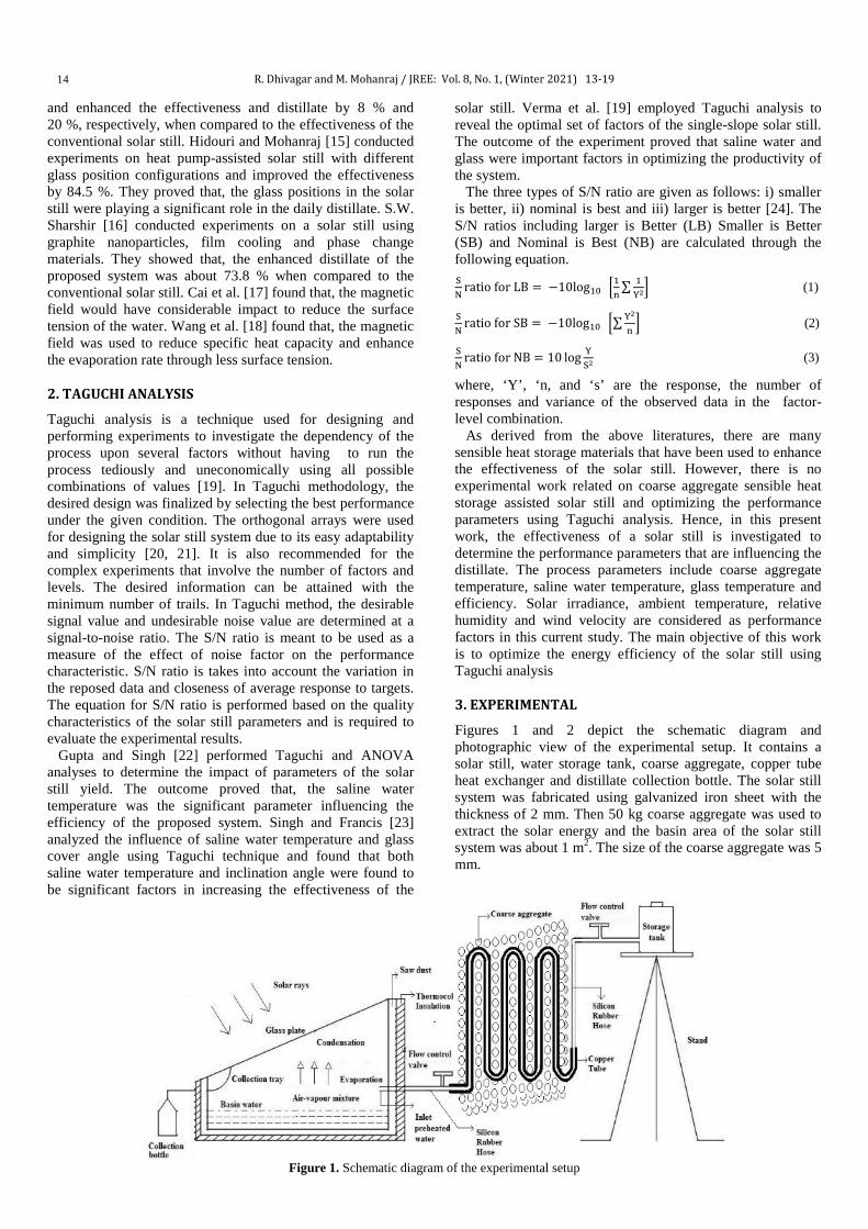
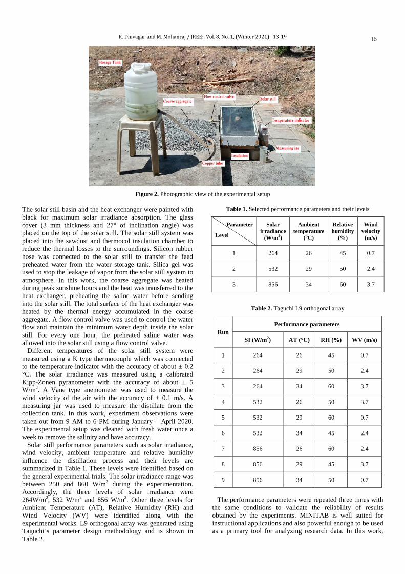
Figures 1 and 2 depict the schematic diagram and photographic view of the experimental setup. It contains a solar still, water storage tank, coarse aggregate, copper tube heat exchanger and distillate collection bottle. The solar still system was fabricated using galvanized iron sheet with the thickness of 2 mm. Then 50 kg coarse aggregate was used to extract the solar energy and the basin area of the solar still system was about 1 m2. The size of the coarse aggregate was 5 mm.
Figure 1. Schematic diagram of the experimental setup
R. Dhivagar and M. Mohanraj / JREE: Vol. 8, No. 1, (Winter 2021) 13-19
15
Figure 2. Photographic view of the experimental setup
The solar still basin and the heat exchanger were painted with black for maximum solar irradiance absorption. The glass cover (3 mm thickness and 27° of inclination angle) was placed on the top of the solar still. The solar still system was placed into the sawdust and thermocol insulation chamber to reduce the thermal losses to the surroundings. Silicon rubber hose was connected to the solar still to transfer the feed preheated water from the water storage tank. Silica gel was used to stop the leakage of vapor from the solar still system to atmosphere. In this work, the coarse aggregate was heated during peak sunshine hours and the heat was transferred to the heat exchanger, preheating the saline water before sending into the solar still. The total surface of the heat exchanger was heated by the thermal energy accumulated in the coarse aggregate. A flow control valve was used to control the water flow and maintain the minimum water depth inside the solar still. For every one hour, the preheated saline water was allowed into the solar still using a flow control valve. Different temperatures of the solar still system were measured using a K type thermocouple which was connected to the temperature indicator with the accuracy of about ± 0.2 °C. The solar irradiance was measured using a calibrated Kipp-Zonen pyranometer with the accuracy of about ± 5 W/m2. A Vane type anemometer was used to measure the wind velocity of the air with the accuracy of ± 0.1 m/s. A measuring jar was used to measure the distillate from the collection tank. In this work, experiment observations were taken out from 9 AM to 6 PM during January – April 2020. The experimental setup was cleaned with fresh water once a week to remove the salinity and have accuracy. Solar still performance parameters such as solar irradiance, wind velocity, ambient temperature and relative humidity influence the distillation process and their levels are summarized in Table 1. These levels were identified based on the general experimental trials. The solar irradiance range was between 250 and 860 W/m2 during the experimentation. Accordingly, the three levels of solar irradiance were 264W/m2, 532 W/m2 and 856 W/m2. Other three levels for Ambient Temperature (AT), Relative Humidity (RH) and Wind Velocity (WV) were identified along with the experimental works. L9 orthogonal array was generated using Taguchi’s parameter design methodology and is shown in Table 2.
Table 1. Selected performance parameters and their levels
Parameter
Level
Solar irradiance
(W/m2)
Ambient temperature
(°C)
Relative humidity
(%)
Wind velocity
(m/s)
1 264 26 45 0.7
2 532 29 50 2.4
3 856 34 60 3.7
Table 2. Taguchi L9 orthogonal array
Run Performance parameters
SI (W/m2) AT (°C) RH (%) WV (m/s)
1 264 26 45 0.7
2 264 29 50 2.4
3 264 34 60 3.7
4 532 26 50 3.7
5 532 29 60 0.7
6 532 34 45 2.4
7 856 26 60 2.4
8 856 29 45 3.7
9 856 34 50 0.7
The performance parameters were repeated three times with the same conditions to validate the reliability of results obtained by the experiments. MINITAB is well suited for instructional applications and also powerful enough to be used as a primary tool for analyzing research data. In this work,

R. Dhivagar and M. Mohanraj / JREE: Vol. 8, No. 1, (Winter 2021) 13-19
16
MINITAB 19 version was used to optimize the conditions and analyze the results. 4. RESULTS AND DISCUSSION
The performance of the coarse aggregate-assisted single-slope solar still was investigated and the process parameters like coarse aggregate temperature, saline water temperature, glass temperature and energy efficiency were analyzed at different hours. Taguchi analysis was performed to establish the optimum values of the performance parameters such as solar irradiance, ambient temperature, relative humidity and wind velocity. 4.1. Thermal performance
The effect the solar irradiance and wind velocity is shown in Figure 3. The maximum solar irradiation of about 856.2 W/m2 was observed during the noon hours and the minimum of about 45.1 W/m2 during evening hours. However, the average solar irradiance was observed as 486.4 W/m2 during the 10 hours of observations. The maximum and minimum wind velocities of about 0.7 m/s and 3.7 m/s were recorded, respectively during the experimental observations. However, it is noted that the wind velocity and solar irradiance have an average deviation from morning to evening during the experiments.
Figure 3. Effect of solar irradiance and wind velocity with time
Figure 4 shows the different temperatures at the still observed during the experimental observations. High temperature variation between the solar still and glass cover was used to improve the evaporation process and yield of the system. It is noted that, the maximum temperature of the coarse aggregate was about 66.1 °C at 13:00 hour which is higher than all other temperatures. It happens due to the accumulation of heat from the solar energy. The maximum ambient and glass temperature were about 34.2 °C and 52.4 °C at 13:00 hour. The gradual movement of wind velocity and the moisture content were applied to reduce the ambient and glass temperatures. Furthermore, the maximum saline water temperature was about 62.1 °C during noon hours. It is 24.2 % higher than saline water temperature for conventional still [6]. This happens due to the preheated saline water used as inlet in the solar still. Figure 5 depicts the effect of hourly yield and efficiency with time. The rate of yield increases in a day time due to the accumulation of heat from the coarse aggregate. During the evening hours, it was reduced slowly with respect to the low solar irradiance and heat losses to the surroundings. This
proposed solar still achieved 32 % of enhanced efficiency with the cumulative yield of about 4.21 kg/m2/day. This solar still system has 4.98 % higher distillate than the previous experimental work done using jute cloth as an energy-storing medium [14].
Figure 4. Effect of various temperatures with time
The energy efficiency was estimated as the quantity of thermal energy utilized for distillate to the quantity of solar irradiance observed in the solar still. Hence, the energy efficiency of the solar still was measured as follows [7]:
Energy efficiency, ηE = mw × hfgAs × ∑ I(t)s ×3600
(4)
Figure 5. Effect of hourly yield and energy efficiency with time
4.2. Analysis of S/N ratio
The Taguchi method gives importance to the single to noise ratio to find the significant optimum value [25]. In this proposed solar system, the process parameters include coarse aggregate temperature, saline water temperature, glass temperature and energy efficiency. For this, the quality characteristic of coarse aggregate temperature was considered as “larger is better” in the still because of the temperature rise. Figure 6 shows the effect of S/N ratio of coarse aggregate with parameters. It was shown that the solar irradiance with higher influence was employed to enhance the heat accumulation rate during the experimentations. Relative humidity is the second important performance parameter that affects the temperature of the coarse aggregate effectively during the evening hours. This effect leads to enhancing the

R. Dhivagar and M. Mohanraj / JREE: Vol. 8, No. 1, (Winter 2021) 13-19
17
evaporation rate due to the temperature difference of systems and surroundings. The higher the S/N ratio parameter is the more significant the performance of the solar still [19].
Figure 6. Effect of S/N ratio of coarse aggregate temperature
Figure 7 shows the effect of the S/N ratio of saline water temperature with parameters. Here, the quality characteristic of “larger is better” was assumed to know a factor which is mostly affecting the performance of the solar still. It was observed that solar irradiance with the major influence to affect the saline water temperature due to the maximum heat was accumulated by the coarse aggregate. The amount of moisture content (relative humidity) present in the ambient air also affected the saline water temperature after solar irradiance. As a result, the ambient temperature was affected which slightly decelerated the performance of the solar still system [20]. The higher the S/N ratio parameter the greater the importance of the performance of the solar still.
Figure 7. Effect of S/N ratio of saline water temperature
Figure 8 shows the effect of the S/N ratio of glass temperature with parameters. The quality characteristic called “larger is better” was assumed to determine the factor that mostly affected the performance of the solar still. Herein, solar irradiance and relative humidity were ranked first and second in affecting the glass cover temperature with major impact on the saline water temperature to enhance the rate of the hourly yield. The influencing rate of ambient temperature and wind velocity were comparatively lower than all other factors [22]. However, these two parameters are mainly related to the effect of solar irradiance and relative humidity. The higher the S/N ratio parameter is the greater the significance the performance of the solar still will be.
Figure 8. Effect of S/N ratio of glass temperature
Figure 9 shows the effect of the S/N ratio of energy efficiency with parameters. The quality characteristic known as the concept of “larger is better” was assumed to determine the factor mainly influenced by the system. It was shown that the solar irradiance and ambient temperature had the highest impact on the energy efficiency rating of the system. The accepted fact is that, the solar still productivity was mainly dependent on the effect of solar irradiance and the effect of ambient temperature during the noon hours [23]. Moreover, the influencing level of relative humidity and wind velocity is sharing their next positions. It may be differing from the different places. The higher the S/N ratio parameter the greater the significance of the performance of the solar still.
Figure 9. Effect of S/N ratio of energy efficiency
The S/N ratios for different levels of the parameters including coarse aggregate temperature, saline water temperature, glass temperature and energy efficiency were calculated. They were having the S/N ratios of 45.4 °C, 41.4 °C, 36.7 °C and 20.07 % respectively. In order to check the experimental results with optimal value, validation was required. The best operating factors were found and their value were compared to the predicted values using Taguchi method as shown in Table 3. The comparison shows that there is good agreement between predicted and experimental data. The percentage difference between predicted and experimental coarse aggregate temperature, saline water temperature, glass temperature and energy efficiency was 1.6 %, 0.6 %, 1.5 % and 3.3 % respectively. From this, the predicted results from optimization were more desirable than the experimental results.

R. Dhivagar and M. Mohanraj / JREE: Vol. 8, No. 1, (Winter 2021) 13-19
18
Table 3. Experimental and predicted optimal conditions for process parameters
Results Coarse aggregate temperature (°C)
Saline water temperature (°C)
Glass temperature (°C)
Energy efficiency (%)
Predicted 67.1 62.4 52.8 33.2 Experimental 66 62 52 32.1
5. CONCLUSIONS
Experimental investigation was performed on coarse aggregate assisted single slope solar still and the enhanced efficiency of about 32 % with a daily yield of 4.21 kg/m2 was found. Furthermore, Taguchi analysis was carried out to identify the performance characteristics of the process parameters. The S/N ratios for different levels of the process parameters were calculated. Accordingly, coarse aggregate temperature, basin saline water temperature, glass temperature and energy efficiency were measured with the S/N ratios of about 45.4 °C, 41.4 °C, 36.7 °C and 20.07 % respectively. The percentage difference between predicted and experimental values of process parameters was 1.6 %, 0.6 %, 1.5 % and 3.3 %, respectively and the optimization method confirmed that there was good agreement between the predicted and experimental values. 6. ACKNOWLEDGEMENT
Authors would like to thank the anonymous reviewers for their useful comments and suggestions. NOMENCLATURE
hfg Laten heat of vaporization (kJ/kg) m Productivity (kg) As Solar still area (m2) I(t)s Solar irradiance (W/m2) ɳE Energy efficiency (%) Abbreviation AT Ambient temperature CT Coarse aggregate temperature GT Glass temperature RH Relative humidity ST SSaline water temperature WV Wind velocity
REFERENCES 1. Kariman, H., Hoseinzadeh, S., Shirkhani, A., Heyns, P.S. and
Wannenburg, J., "Energy and economic analysis of evaporative vacuum easy desalination system with brine tank", Journal of Thermal Analysis and Calorimetry, Vol. 140, (2019), 1935-1944. (https://doi.org/10.1007/s10973-019-08945-8).
2. Hoseinzadeh, S., Yargholi, R., Kariman, H. and Heyns, P.S., "Exergeoeconomic analysis and optimization of reverse osmosis desalination integrated with geothermal energy", Environmental Progress and Sustainable Energy, Vol. 39, (2020), 1-7. (https://doi.org/10.1002/ep.13405).
3. Kariman, H., Hoseinzadeh, S. and Heyns, P.S., "Energetic and exergetic analysis of evaporation desalination system integrated with mechanical vapor recompression circulation", Case Studies in Thermal Engineering, Vol. 16, (2019), 100548. (https://doi.org/10.1016/j.csite.2019.100548).
4. Hoseinzadeh, S., Ghasemi, M.H. and Heyns, P.S., "Application of hybrid systems in solution of low power generation at hot seasons for micro hydro systems", Renewable Energy, Vol. 160, (2020), 323-332. (https://doi.org/10.1016/j.renene.2020.06.149).
5. Belyayev, Y., Mohanraj, M., Jayaraj, S. and Kaltayev, A., "Thermal performance simulation of a heat pump assisted solar desalination system for Kazakhstan climatic conditions", Heat Transfer
Engineering, Vol. 40, (2019), 60-72. (https://doi.org/10.1080/01457632.2018.1451246)
6. Dhivagar, R. and Sundararaj, S., "A review on methods of productivity improvement in solar desalination", Applied Mechanics and Materials, Vol. 877, (2018), 414-429. (http://doi.org/10.4028/www.scientific.net/AMM.877.414).
7. Dhivagar, R. and Sundararaj, S., "Thermodynamic and water analysis on augmentation of a solar still with copper tube heat exchange in coarse aggregate", Journal of Thermal Analysis and Calorimetry, Vol. 136, (2019), 89-99. (https://doi.org/10.1007/s10973-018-7746-1).
8. Dhivagar, R., Mohanraj, M., Hidouri, K. and Belyayev, Y., "Energy, exergy, economic and enviro-economic (4E) analysis of gravel coarse aggregate sensible heat storage-assisted single-slope solar still", Journal of Thermal Analysis and Calorimetry, (2020). (In press). (https://doi.org/10.1007/s10973-020-09766-w).
9. Pounraj, P., Winston, D.P., Kabeel, A.E., Kumar, B.P., Manokar, A.M., Sathyamurthy, R. and Christabel, S.C., "Experimental investigation on Peltier based hybrid PV/T active solar still for enhancing the overall performance", Energy Conversion and Management, Vol. 168, (2018), 371-381. (https://doi.org/10.1016/j.enconman.2018.05.011).
10. Modi, K.V. and Modi, J.G., "Performance of single-slope double-basin solar stills with small pile of wick materials", Applied Thermal Engineering, Vol. 149, (2019), 723-730. (https://doi.org/10.1016/j.applthermaleng.2018.12.071).
11. Jani, H.K. and Modi, K.V., "Experimental performance evaluation of single basin dual slope solar still with circular and square cross-sectional hollow fins", Solar Energy, Vol. 416, (2017), 86-93. (https://doi.org/10.1016/j.solener.2018.12.054).
12. Dumka, P., Sharma, A., Kushwah, Y., Raghav, A.S. and Mishra, D.R., "Performance evaluation of single slope solar still augmented with sand filled cotton bags", Journal of Energy Storage, Vol. 25, (2019), 100888. (https://doi.org/10.1016/j.est.2019.100888).
13. Patrick, J., Gnanaraj, S. and Velmurugan, V., "An experimental study on the efficacy of modifications in enhancing the performance of single basin double slope solar still", Desalination, Vol. 467, (2019), 12-28. (https://doi.org/10.1016/j.desal.2019.05.015).
14. Sakthivel, M., Shanmugasundram, S. and Alwarsamy, T., "An experimental study on a regenerative solar still with energy storage medium–Jute cloth", Desalination, Vol. 264, (2010), 24-31. (https://doi.org/10.1016/j.desal.2010.06.074).
15. Hidouri, K. and Mohanraj, M., "Thermodynamic analysis of a heat pump assisted active solar still", Desalination and Water Treatment, Vol. 154, (2019), 101-110. (https://doi.org/10.5004/dwt.2019.24047).
16. Sharshir, S.W., Peng, G., Wu, L., Essa, F.A., Kabeel, A.E. and Yang, N., "The effects of flake graphite nanoparticles, phase change material, and film cooling on the solar still performance", Applied Energy, Vol. 191, (2017), 358-366. (http://dx.doi.org/10.1016/j.apenergy.2017.01.067).
17. Cai, R., Yang, H., He, J. and Zhu, W., "The effects of magnetic fields on water molecular hydrogen bonds", Journal of Molecule Structure, Vol. 938, (2009), 15-19. (https://doi.org/10.1016/j.molstruc.2009.08.037).
18. Wang, Y., Wei, H. and Li, Z., "Effect of magnetic field on the physical properties of water", Results in Physics, Vol. 8, (2018), 262-267. (https://doi.org/10.1016/j.rinp.2017.12.022).
19. Verma, V.K., Rout, I.S., Rai, A.K. and Gaikwad, A., "Optimization of parameters affecting the performance of passive solar distillation system by using Taguchi method", Journal of Mechanical and Civil Engineering, Vol. 7, (2013), 37-42. (https://doi.org/10.9790/1684-0723742).
20. Hoseinzadeh, S. and Azadi, R., "Simulation and optimization of a solar-assisted heating and cooling system for a house in Northern of Iran", Journal of Renewable and Sustainable Energy, Vol. 9, (2017), 045101. (http://dx.doi.org/10.1063/1.5000288).
21. Hoseinzadeh, S., Ghasemiasl, R., Javadi, M.A. and Heyns, P.S., "Performance evaluation and economic assessment of a gas power plant with solar and desalination integrated systems", Desalination and

R. Dhivagar and M. Mohanraj / JREE: Vol. 8, No. 1, (Winter 2021) 13-19
19
Water Treatment, Vol. 174, (2020), 11-25. (https://doi.org/0.5004/dwt.2020.24850).
22. Gupta, P. and Singh, N., "Investigation of the effect of process parameters on the productivity of single slope solar still: A Taguchi approach", International Journal of Current Engineering and Technology, Vol. 4, (2015), 320-322. (http://inpressco.com/category/ijcet).
23. Singh, N. and Francis, V., "Investigating the effect of water temperature and inclination angle on the performance of single slope solar still: A Taguchi approach", International Journal of Engineering Research and Applications, Vol. 3, (2013), 404-407. (http://www.ijera.com/).
24. Ghani, J.A., Choudhury, I.A. and Hassan, H.H., "Application of Taguchi method in the optimization of end milling parameters", Journal of Materials Processing Technology, Vol. 145, (2004), 84-92. (https://doi.org/10.1016/S0924-0136(03)00865-3).
25. Rama Rao, S. and Padmanabhan, G., "Application of Taguchi methods and ANOVA in optimization of process parameters for metal removal rate in electrochemical machining of Al/5%SiC composites", International Journal of Engineering Research and Application, Vol. 2, (2012), 192-197. (http://www.ijera.com).
JREE: Vol. 8, No. 1, (Winter 2021) 20-27
Please cite this article as: Tabrizi, A. and Rahmani, M., "Assessing and evaluating reliability of single-stage PV inverters", Journal of Renewable Energy and Environment (JREE), Vol. 8, No. 1, (2021), 20-27. (https://doi.org/10.30501/jree.2020.237113.1123).
2423-7469/© 2021 The Author(s). Published by MERC. This is an open access article under the CC BY license (https://creativecommons.org/licenses/by/4.0/).
Technical Note
Journal of Renewable Energy and Environment
J o u r n a l H o m e p a g e : w w w . j r e e . i r
Assessing and Evaluating Reliability of Single-Stage PV Inverters
Aryan Tabrizi, Mehdi Rahmani*
Department of Electrical Engineering, Imam Khomeini International University, Qazvin, Qazvin, Iran.
P A P E R I N F O
Paper history: Received 28 June 2020 Accepted in revised form 29 September 2020
Keywords: PV, Single-Stage Inverter, Reliability, Monte Carlo
A B S T R A C T
Reliability is an essential factor in Photovoltaic (PV) systems. Solar power has become one of the most popular renewable power resources in recent years. Solar power has drawn attention because it is free and almost available worldwide. Moreover, the price of maintenance is lower than other power resources. Since there are no moving parts in PV systems, their reliability is relatively high. It is assumed that a typical PV system can operate 20–25 years with minimum possible interruptions. However, solar power systems may fail, the same as any other systems. It is indicated by several studies that the PV inverters are responsible for major failures in PV systems, as other components are almost passive. Hence, the reliability of the inverter has maximum impact on the reliability of the whole PV system. Thus, not only assessing and calculating the reliability value of inverter is highly crucial, but also increasing its value is essential, as well. This paper calculates and evaluates the reliability of PV single-stage inverters exclusively. Furthermore, there are suggestions that improve their reliability value.
https://doi.org/10.30501/jree.2020.237113.1123
1. INTRODUCTION1
The level of energy consumption is growing due to population growth and progress in the industry. Therefore, sustainable energy systems with effective cost methods are required to meet the growing demand of energy [1]. Solar power is known as one of the most common renewable energy resources all over the world as it is pollution-free, is available in almost every region, and requires low maintenance effort. Solar power can be transformed into electricity directly utilizing PV panels. The output of a PV panel is Direct Current (DC); however, most of the electronic devices require Alternating Current (AC). Hence, the output voltage of a PV panel/array must be transformed into AC voltage by an inverter. PV panel(s)/array(s) and inverter(s) alongside some optional elements form a typical PV system. PV inverters are the most important parts of PV systems. They are the brain of the system and their main function is to convert the DC power produced by the PV array to AC power [2]. Inverters can be categorized in various ways; however, in this paper, inverters are categorized into Single-Stage Inverters (SSIs) and Multi-Stage Inverters (MSIs) [3-8]. SSIs have advantages including low cost, low weight, less bulkiness, and fewer elements, which lead to better efficiency and minor loss. Increasing the input DC voltage and converting it into AC voltage with the desired amplitude and frequency are done in separate steps in MSIs; however, they are done in a single step in SSIs. With a proper design in structure and appropriate switching method, SSIs can have higher efficiency, greater reliability, and lower *Corresponding Author’s Email: [email protected] (M. Rahmani) URL: http://www.jree.ir/article_115103.html
cost due to the smaller number of elements [9-11]. The rate of operating safe and on schedule is called reliability. The assessment of reliability is one of the most important issues to be studied in distribution systems. Even sometimes these studies may recommend some new elements to improve the reliability value in the system [12, 13]. The reliability of a PV system is highly dependent on the inverter, as most of failures are caused by the inverter. Hence, the main part of assessing reliability in PV systems is to calculate the reliability value of their inverter. According to the above discussion, the calculation of reliability value of a PV system is highly necessary and the main step is to evaluate the reliability of its inverter. Various studies have been done on evaluating the reliability of renewable energy resources, especially in the case of PV systems. F. Blaabjerg studied reliability of both wind turbines and PV applications [14]. The effect of PV array sizing on reliability was investigated in [15]. One of the main approaches to reliability is using the Markov method. This method was used to study the reliability in PV systems [16] and PV inverters [17]. The solutions to enhancing the PV inverter reliability through the control of the battery system (three different control strategies for self-consumption operation) were explored in [18] and their impact on the PV inverter loading was investigated. The first purpose of this paper is to propose a method to evaluate the reliability of PV SSIs by their containing elements. The second purpose is to use the proposed method to study and compare the reliability values in some of the PV SSIs’ structures to discover the characteristics of the structures with higher and lower reliability values. Hence, it can be help figure out how to increase reliability value in PV SSIs.

A. Tabrizi and M. Rahmani / JREE: Vol. 8, No. 1, (Winter 2021) 20-27
21
There are some methods for evaluating the reliability of these systems; however, they have some limitations and are not adequately accurate. This paper proposes a new simulation-based method to evaluate the reliability of SSIs. This method can be used for any desired period of time. Its accuracy is extremely high and it is determined by the number of iterations defined by the user (any desired value). Another advantage of this method is that if any new element is added to the structure of the inverter or be removed from it, still the reliability can be evaluated. Moreover, this method can consider the impact of using the same elements that are obtained from different manufacturers with different identical specifications. The reliability value of some of the SSIs [19-24] is evaluated. Moreover, there are some suggestions for increasing reliability values which are deduced by comparing and studying the output results. The reliability of PV single-stage inverters has been exclusively studied in this paper. Hence, Section 2 includes a brief explanation of SSI, reliability in systems, and main different approaches to evaluating its value. Section 3 explains the reliability evaluation method which is used in this paper step by step. In Section 4, the simulation results by the proposed method for some of the most well-known SSIs in MATLAB are presented in different conditions. Finally, the conclusion is presented in Section 5 alongside some suggestions to improve the value of reliability in SSIs. 2. RELIABILITY CONCEPT IN SSI
Figure 1 represents a brief and general preview of SSI and MSI. SSI is studied in this paper.
(a)
(b)
Figure 1. On-grid PV system with (a) multi-stage inverter and (b) single-stage inverter
The system reliability is defined as “the probability that a system, including all hardware, firmware, and software, will satisfactorily perform the task for which it was designed or intended, for a specified time and in a specified environment” [25]. Reliability is an intrinsic quality in every system. Trying to increase reliability after design and manufacturing is impractical and even if possible, it is extremely expensive. In the PV systems, inverters are highly important. Table 1 includes data from [26] and indicates that the major failures and energy losses in a typical PV system are caused by the inverter. Therefore, assessing the reliability of the inverter is essential.
Reliability can be calculated by various methods in different periods of time. Generally, reliability assessment methods are divided into two main groups:
• Analytical • Simulation
In this paper, the reliability of single-stage PV inverters in different structures in PV systems is simulated, calculated, and assessed by the Monte Carlo method at the design and manufacturing phase (Figure 2). For this simulation and calculation, the design layout of elements (series or parallel), quality of used elements (elements failure rate), and quality of elements are needed.
Table 1. Data from 3500 reports of 350 commercial PV systems with
an approximate capacity of 150 kW from January 2010 to March 2012 [26]
Failure area % of Tickets % of kWh lost
Inverter 43 36
AC subsystem 14 20
External 12 20
Other 9 7
Support structure 6 3
DC subsystem 6 4
Planned outage 5 8
Module 2 1
Weather station 2 0
Meter 1 0
Figure 2. Assessment methods of reliability in the single-stage PV
inverter in different phases 3. PROPOSED METHOD FOR RELIABILITY EVALUATION IN PV SSIS
If a component or a system be intact at time t=0, the probability of failure at time t=0 is equal to “zero”. The failure probability of the system will be increased through time and it will reach “one/unity”, and the system will surely fail in a long period of operation. This property is equivalent to the Cumulative Distribution Function. It is designated by Q(t) and is shown in Figure 3. Moreover, Survivor Function is designated by R(t) and is calculated as follows [16, 27]:
(1) R(t)=1-Q(t)

A. Tabrizi and M. Rahmani / JREE: Vol. 8, No. 1, (Winter 2021) 20-27
22
where
(2)
(3)
where N0 is the total number of studied elements, NS(t) is the number of intact elements until t=t0, and Nf(t) is the number of defective elements until t=t0. In calculating the reliability value for a single-stage PV inverter in the proposed topology, it is assumed that all equipment and elements must operate properly so that the inverter operates properly. Otherwise, the inverter may continue to operate, but not in the predicted way and with desired quality. Moreover, the proposed topology can assess the reliability even if:
• Extra elements are added to the structure of inverter for increasing the reliability or other purposes;
• Some elements are removed due to modifying the structure of inverter or other purposes;
• Some elements are changed due to maintenance or other purposes.
Figure 3. The relation between Q(t) and R(t)
The commonly used elements in inverters are inductors, capacitors, resistors, diodes, MOSFETs (or IGBTs), switches, wires, maybe transformer, and other optional elements. For assessing the reliability, the number of each element in the structure must be determined and the Hazard Rate Function (λ) of each element must be attained of its datasheet or handbook.
(4)
where λP is the part failure rate, λb is the base failure rate (usually expressed by a model relating to the influence of electrical and temperature stresses on the part), πT is temperature sensitivity factor (it is usually changed for MOSFET), πQ is a quality factor (quality of structure phase of elements), πE is an environmental factor (including humidity, vibration, noise, dust, pressure, shock, etc.), and other factors (πA, πR, πS, πC) are just determined if they are necessary [28]. In this paper, λ𝑃𝑃 is used to calculate the reliability of single-stage inverters:
(5)
The inputs for the proposed simulation method are:
• Number of each element in the structure of the single-stage PV inverter
• Hazard rate for each component • Number of iterations • Time period (years)
Moreover, the main steps of the proposed simulation method are as follows:
1. Create random numbers with uniform distribution. 2. Convert random numbers to time values using an
equation or system data and by the conversion methods such as inverse conversion method.
3. Whenever the calculated time is equal to or greater than the mission time, it is considered as the success of the system. Likely, whenever this value is shorter than the mission time, it is regarded as a failure.
4. Repeating Steps 1 to 3 leads to a cumulative number of successes and a number of failures (for the desired number of iterations).
5. The system reliability is obtained by dividing the number of successes by the number of simulations (iterations).
To compare the reliability values of different inverters, it is assumed that the same components in different inverters are supplied from similar manufacturers with identical λ values. Table 2 shows the λ used in calculations.
Table 2. λ values for some used components in single-stage PV
inverters [29]
No. Description λ (Failures/106
Hours) 1 Diodes, High frequency 0.22 2 Transistor, High frequency, MOSFET 0.060
3 Resistor, Fixed, Wire-wound (Power
type) 0.0024
4 Capacitor, Fixed, Electrolytic 0.00040 5 Inductive devices, Coils 0.000030 6 Low power transformer (<300W) 0.022 7 High power transformer (≥300W) 0.049 8 Connectors, General 0.0010
9 Printed wiring assembly/ Printed circuit board
0.000017
10 Thyristor 0.0022 Several methods are used for reliability prediction. Some methods have their statistical data, others depend on additional data from other sources, and the rest are the updated versions of older methods. Some data is only appropriate for special systems, while other data can be used for any system. The reliability prediction of the methods cannot be compared because each analysis method is dependent on different data and each focuses on different factors and assumptions [30]. However, the authors claim that the proposed method has advantages over the previous methods including:
• Reliability of inverter can be evaluated accurately by the proposed method even if some elements are added, removed, or changed.
• Reliability can be calculated not just for a specific period of time, but for any desired period of time.
f 0
0
( )N tQ(t)= N
s 0
0
( )N tR(t)= N
p b T A R S C Q Eλ =λ ×π ×π ×π ×π ×π ×π ×π
pnumber of failure per unit timeλ (t)=
number of components exposed failure

A. Tabrizi and M. Rahmani / JREE: Vol. 8, No. 1, (Winter 2021) 20-27
23
• The accuracy of the reliability investigation can be changed. As it is studied in the next section, the accuracy of reliability for iteration of 100,000 is acceptable. However, for critical consumption, the number of iterations can be increased. Hence, the accuracy will be increased to a greater extent.
• The proposed method is capable of evaluating reliability in SSIs even if its element is provided by different manufacturers (for instance, 3 inductors with 3 different λ’s).
By comparing reliability values of different structures using the proposed method, it can be observed that the failure is caused more by which elements, then consumers have two options: first, try to modify the structure which is hard and not practical, or use the same element with a lower λ value from different manufacturers. Although it costs more, it leads to a higher reliability value in the long run. 4. SIMULATION RESULTS
In this section, first, the simulation results of the proposed method in different situations (different numbers of iterations and different periods of time) are studied for Barbi and Caceres topology [19]. Then, the reliability evaluation of some other PV SSIs is studied and compared in the most realistic and optimum conditions with the proposed method. The proposed single-stage inverter by Barbi and Caceres [19] and its output result for 500 iterations (which is 0.8360) are represented in Figure 4. However, the result is not stabilized and valid as it is shown. Hence, the number of iterations must be increased. Figure 5 and Table 3 shows the reliability values for different iterations in this topology. Given that probability functions are used in this computation and simulation proposed method, it is not expected that the output results remain constant in every run as it is not in any other probability function. However, the results of multiple attempts must be in an acceptable range. This goal is achieved
by increasing the number of iterations. Table 4 shows the results for two more runs.
(a)
(b)
Figure 4. (a) The proposed single-stage inverter topology by Barbi and Caceres [19] and (b) its output result in 500 iterations and 20
years As the reliability value of a single-stage inverter varies in time, the assessment of reliability must be maintained for a specific period of time. The reliability decreases with increasing the computational time. The results of the reliability calculation over a period of 1 year to 35 years with 100,000 iterations for Barbi and Caceres proposed topology are shown in Table 5 and Figure 6. it can be deduced that the reliability of the single-stage inverter varies relatively linearly in relation with the duration of the evaluation.
(a) (b) (c)
(d) (e) (f)
Figure 5. The reliability values of Barbi and Caceres proposed topology for iteration of (a) 500, (b) 1,000, (c) 5,000, (d) 10,000, (e) 50,000, and (f) 100,000
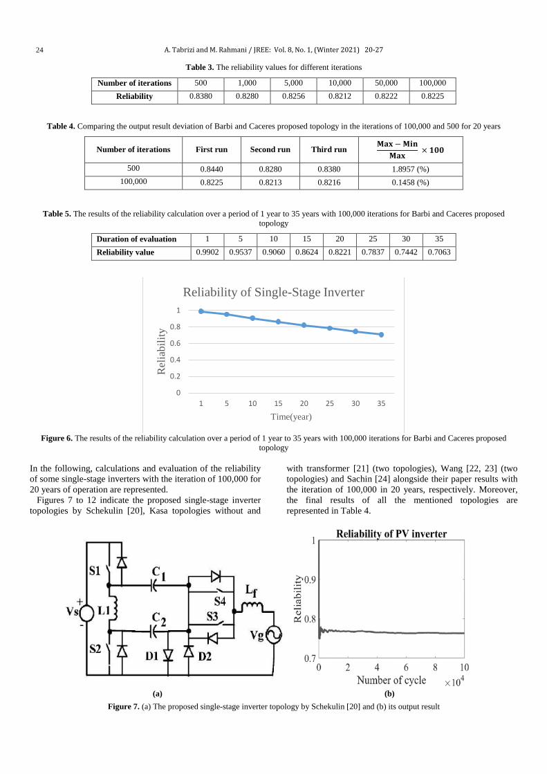
A. Tabrizi and M. Rahmani / JREE: Vol. 8, No. 1, (Winter 2021) 20-27
24
Table 3. The reliability values for different iterations
Number of iterations 500 1,000 5,000 10,000 50,000 100,000 Reliability 0.8380 0.8280 0.8256 0.8212 0.8222 0.8225
Table 4. Comparing the output result deviation of Barbi and Caceres proposed topology in the iterations of 100,000 and 500 for 20 years
Number of iterations First run Second run Third run 𝐌𝐌𝐌𝐌𝐌𝐌 −𝐌𝐌𝐌𝐌𝐌𝐌
𝐌𝐌𝐌𝐌𝐌𝐌 × 𝟏𝟏𝟏𝟏𝟏𝟏
500 0.8440 0.8280 0.8380 1.8957 (%) 100,000 0.8225 0.8213 0.8216 0.1458 (%)
Table 5. The results of the reliability calculation over a period of 1 year to 35 years with 100,000 iterations for Barbi and Caceres proposed topology
Duration of evaluation 1 5 10 15 20 25 30 35 Reliability value 0.9902 0.9537 0.9060 0.8624 0.8221 0.7837 0.7442 0.7063
Figure 6. The results of the reliability calculation over a period of 1 year to 35 years with 100,000 iterations for Barbi and Caceres proposed
topology In the following, calculations and evaluation of the reliability of some single-stage inverters with the iteration of 100,000 for 20 years of operation are represented. Figures 7 to 12 indicate the proposed single-stage inverter topologies by Schekulin [20], Kasa topologies without and
with transformer [21] (two topologies), Wang [22, 23] (two topologies) and Sachin [24] alongside their paper results with the iteration of 100,000 in 20 years, respectively. Moreover, the final results of all the mentioned topologies are represented in Table 4.
(a) (b)
Figure 7. (a) The proposed single-stage inverter topology by Schekulin [20] and (b) its output result
0
0.2
0.4
0.6
0.8
1
1 5 10 15 20 25 30 35
Rel
iabi
lity
Time(year)
Reliability of Single-Stage Inverter
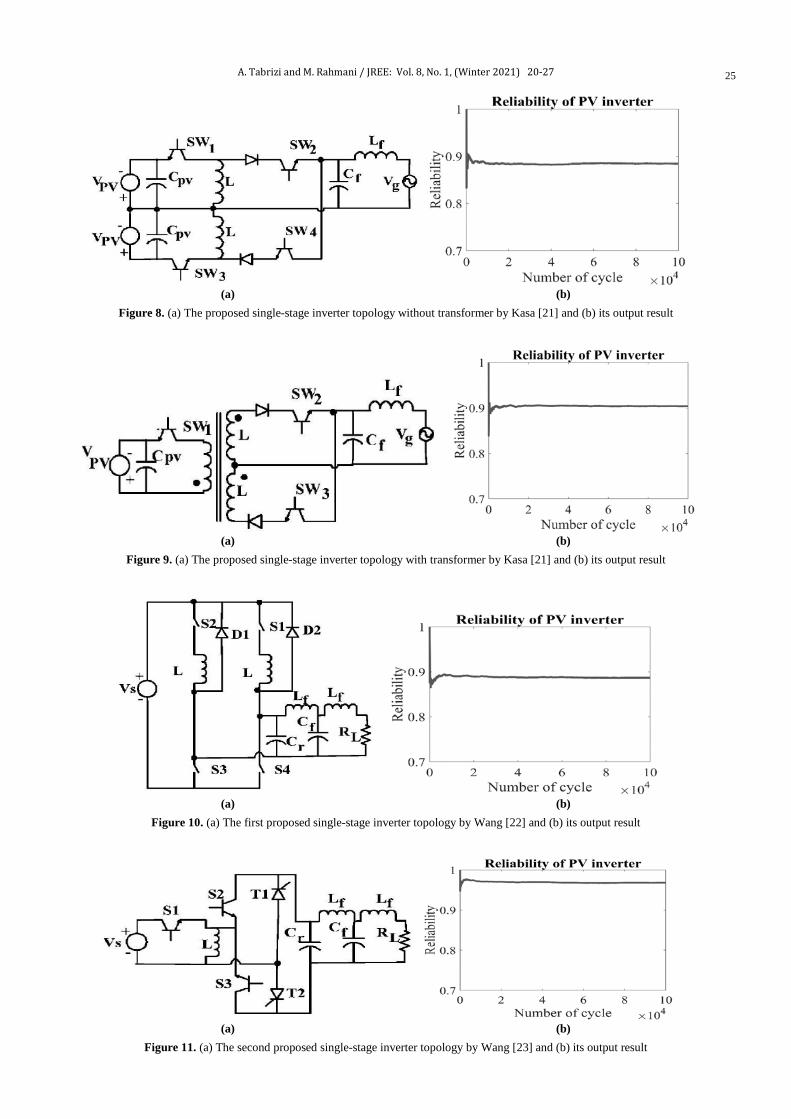
A. Tabrizi and M. Rahmani / JREE: Vol. 8, No. 1, (Winter 2021) 20-27
25
(a) (b)
Figure 8. (a) The proposed single-stage inverter topology without transformer by Kasa [21] and (b) its output result
(a) (b)
Figure 9. (a) The proposed single-stage inverter topology with transformer by Kasa [21] and (b) its output result
(a) (b)
Figure 10. (a) The first proposed single-stage inverter topology by Wang [22] and (b) its output result
(a) (b)
Figure 11. (a) The second proposed single-stage inverter topology by Wang [23] and (b) its output result
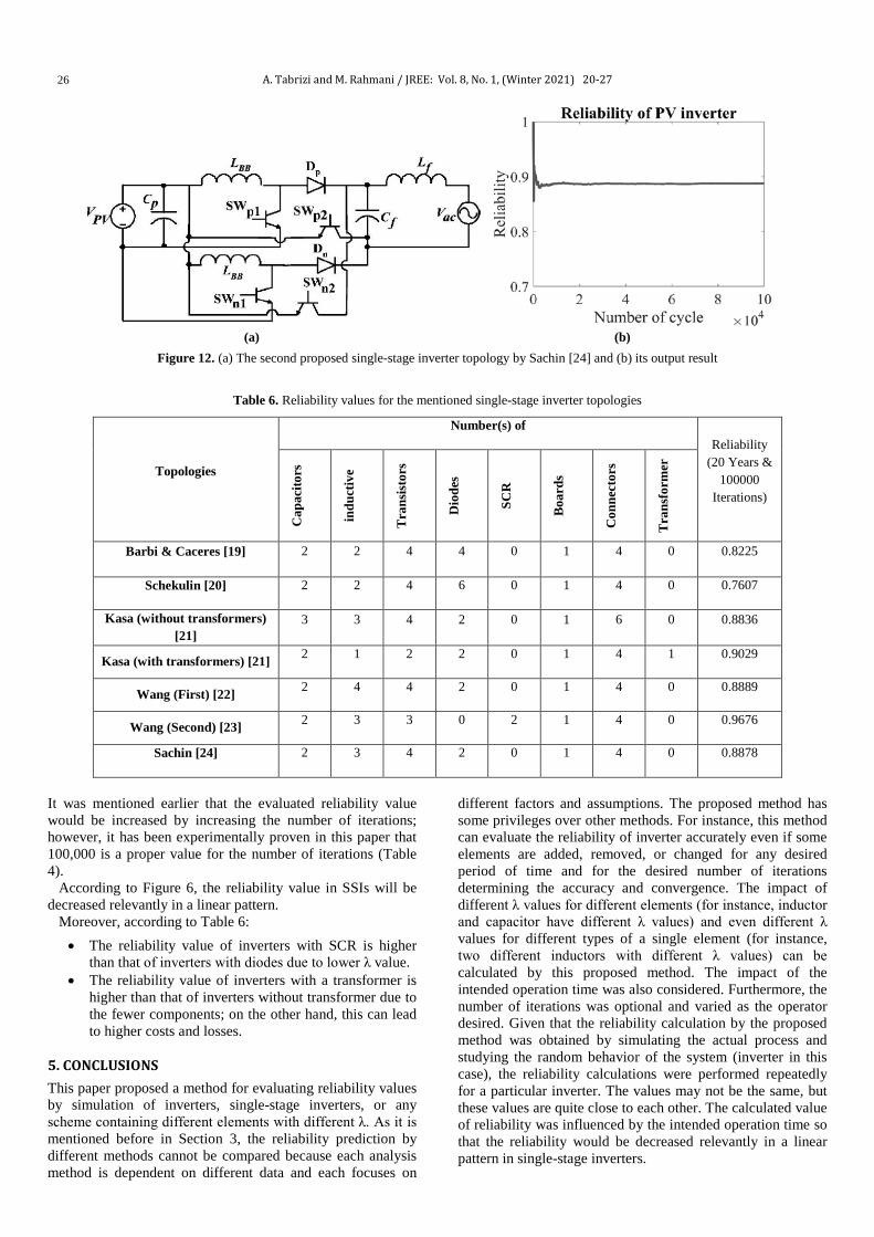
A. Tabrizi and M. Rahmani / JREE: Vol. 8, No. 1, (Winter 2021) 20-27
26
(a) (b)
Figure 12. (a) The second proposed single-stage inverter topology by Sachin [24] and (b) its output result
Table 6. Reliability values for the mentioned single-stage inverter topologies
Reliability (20 Years &
100000 Iterations)
Number(s) of
Topologies
Tra
nsfo
rmer
Con
nect
ors
Boa
rds
SCR
Dio
des
Tra
nsis
tors
indu
ctiv
e
Cap
acito
rs
0.8225 0 4 1 0 4 4 2 2 Barbi & Caceres [19]
0.7607 0 4 1 0 6 4 2 2 Schekulin [20]
0.8836 0 6 1 0 2 4 3 3 Kasa (without transformers) [21]
0.9029 1 4 1 0 2 2 1 2 Kasa (with transformers) [21]
0.8889 0 4 1 0 2 4 4 2 Wang (First) [22]
0.9676 0 4 1 2 0 3 3 2 Wang (Second) [23]
0.8878 0 4 1 0 2 4 3 2 Sachin [24]
It was mentioned earlier that the evaluated reliability value would be increased by increasing the number of iterations; however, it has been experimentally proven in this paper that 100,000 is a proper value for the number of iterations (Table 4). According to Figure 6, the reliability value in SSIs will be decreased relevantly in a linear pattern. Moreover, according to Table 6:
• The reliability value of inverters with SCR is higher than that of inverters with diodes due to lower λ value.
• The reliability value of inverters with a transformer is higher than that of inverters without transformer due to the fewer components; on the other hand, this can lead to higher costs and losses.
5. CONCLUSIONS This paper proposed a method for evaluating reliability values by simulation of inverters, single-stage inverters, or any scheme containing different elements with different λ. As it is mentioned before in Section 3, the reliability prediction by different methods cannot be compared because each analysis method is dependent on different data and each focuses on
different factors and assumptions. The proposed method has some privileges over other methods. For instance, this method can evaluate the reliability of inverter accurately even if some elements are added, removed, or changed for any desired period of time and for the desired number of iterations determining the accuracy and convergence. The impact of different λ values for different elements (for instance, inductor and capacitor have different λ values) and even different λ values for different types of a single element (for instance, two different inductors with different λ values) can be calculated by this proposed method. The impact of the intended operation time was also considered. Furthermore, the number of iterations was optional and varied as the operator desired. Given that the reliability calculation by the proposed method was obtained by simulating the actual process and studying the random behavior of the system (inverter in this case), the reliability calculations were performed repeatedly for a particular inverter. The values may not be the same, but these values are quite close to each other. The calculated value of reliability was influenced by the intended operation time so that the reliability would be decreased relevantly in a linear pattern in single-stage inverters.

A. Tabrizi and M. Rahmani / JREE: Vol. 8, No. 1, (Winter 2021) 20-27
27
6. ACKNOWLEDGEMENT
The authors would like to thank the members of the Electrical Engineering Faculty of Imam Khomeini International University. REFERENCES 1. Noorollahi, Y., Itoi, R., Yousefi, H., Mohammadi, M., and Farhadi, A.,
"Modeling for diversifying electricity supply by maximizing renewable energy use in Ebino city southern Japan", Sustainable Cities and Society, Vol. 34, (2017), 371-384. (https://doi.org/10.1016/J.Scs.2017.06.022).
2. Matiushkin, O., Husev, O., Roncero-Clemente, C., Ivanets, S. and Fesenko, A., "Component design guidelines for new single-stage buck-boost inverter with unfolding circuit", Proceedings of 2017 IEEE International Young Scientists Forum on Applied Physics and Engineering (YSF), IEEE, (2017). (https://doi.org/10.1109/YSF.2017.8126589).
3. Abramovitz, A., Zhao, B. and Smedley, K.M., "High-gain single-stage boosting inverter for photovoltaic applications", IEEE Transactions on Power Electronics, Vol. 31, No. 5, (2016), 3550-3558. (https://doi.org/10.1109/TPEL.2015.2457454).
4. Kjaer, S.B., Pedersen, J.K. and Blaabjerg, F., "A review of single-phase grid-connected inverters for photovoltaic modules", IEEE Transactions on Industry Applications, Vol. 41, No. 5, (2005), 1292-1306. (https://doi.org/10.1109/TIA.2005.853371).
5. Abramovitz, A., Zhao, B. and Smedley, K.M., "High-gain single-stage boosting inverter for photovoltaic applications", IEEE Transactions on Power Electronics, Vol. 31, No. 5, (2015), 3550-3558. (https://doi.org/10.1109/TPEL.2015.2457454).
6. Sahoo, S.K., Sukchai, S. and Yanine, F.F., "Review and comparative study of single-stage inverters for a PV system", Renewable and Sustainable Energy Reviews, Vol. 91, (2018), 962-986. (https://doi.org/10.1016/J.Rser.2018.04.063).
7. Aouadi, C., Abouloifa, A., Lachkar, I., Aourir, M., Boussairi, Y. and Hamdoun, A., "Nonlinear controller design and stability analysis for single-phase grid-connected photovoltaic systems", International Review of Automatic Control (IREACO), Vol. 10, No. 4, (2017), 306. (https://doi.org/10.15866/ireaco.v10i4.12322).
8. Ciobotaru, M., Teodorescu, R. and Blaabjerg, F., "Control of single-stage single-phase PV inverter", EPE Journal, Vol. 16, No. 3, (2006), 20-26. (https://doi.org/10.1080/09398368.2006.11463624).
9. Eghtedarpour, N. and Farjah, E., "Distributed charge/discharge control of energy storages in a renewable-energy-based DC micro-grid", IET Renewable Power Generation, Vol. 8, No. 1, (2014), 45-57. (https://doi.org/10.1049/iet-rpg.2012.0112).
10. Blaabjerg, F., Iov, F., Kerekes, T., Teodorescu, R. and Ma, K., "Power electronics-key technology for renewable energy systems-status and future", Proceedings of 2013 3rd International Conference on Electric Power and Energy Conversion Systems, IEEE, (2013). (https://doi.org/10.1109/EPECS.2013.6712980).
11. Sahan, B., Vergara, A.N., Henze, N., Engler, A. and Zacharias, P., "A single-stage PV module integrated converter based on a low-power current-source inverter", IEEE Transactions on Industrial Electronics, Vol. 55, No. 7, (2008), 2602-2609. (https://doi.org/10.1109/TIE.2008.924160).
12. Khazraj, H., da Silva, F.F., Bak, C.L. and Hajibashi, M., "Markov model of renewable resources for reliability assessment of distribution systems", Proceedings of 2018 IEEE International Conference on Environment and Electrical Engineering and 2018 IEEE Industrial and Commercial Power Systems Europe (EEEIC/I&CPS Europe), IEEE, (2018). (https://doi.org/10.1109/EEEIC.2018.8493814).
13. Kuznetsova, E., Li, Y.F., Ruiz, C. and Zio, E., "An integrated framework of agent-based modelling and robust optimization for microgrid energy management", Applied Energy, Vol. 129, (2014), 70-88. (https://doi.org/10.1016/j.apenergy.2014.04.024).
14. Blaabjerg, F., Ma, K. and Zhou, D., "Power electronics and reliability in renewable energy systems", Proceedings of 2012 IEEE International Symposium on Industrial Electronics, IEEE, (2012), 19-30. (https://doi.org/10.1109/ISIE.2012.6237053).
15. Sangwongwanich, A., Yang, Y., Sera, D., Blaabjerg, F. and Zhou, D., "On the impacts of PV array sizing on the inverter reliability and lifetime", IEEE Transactions on Industry Applications, Vol. 54, No. 4, (2018), 3656-3667. (https://doi.org/10.1109/TIA.2018.2825955).
16. Theristis, M. and Papazoglou, I.A., "Markovian reliability analysis of standalone photovoltaic systems incorporating repairs", IEEE Journal of Photovoltaics, Vol. 4, No. 1, (2013), 414-422. (https://doi.org/10.1109/JPHOTOV.2013.2284852).
17. Dhople, S.V., Davoudi, A., Chapman, P.L. and Domínguez-García, A.D., "Integrating photovoltaic inverter reliability into energy yield estimation with Markov models", Proceedings of 2010 IEEE 12th Workshop on Control and Modeling for Power Electronics (COMPEL), IEEE, (2010), 1-5. (https://doi.org/10.1109/COMPEL.2010.5562393).
18. Sangwongwanich, A., Angenendt, G., Zurmühlen, S., Yang, Y., Sera, D., Sauer, D.U. and Blaabjerg, F., "Enhancing PV inverter reliability with battery system control strategy", CPSS Transactions on Power Electronics and Applications, Vol. 3, No. 2, (2018), 93-101. (https://doi.org/10.24295/CPSSTPEA.2018.00009).
19. Caceres, R.O. and Barbi, I., "A boost DC-AC converter: analysis, design, and experimentation", IEEE Transactions on Power Electronics, Vol. 14, No. 1, (1999), 134-141. (https://doi.org/10.1109/63.737601).
20. Jana, J., Saha, H. and Bhattacharya, K.D., "A review of inverter topologies for single-phase grid-connected photovoltaic systems", Renewable and Sustainable Energy Reviews, Vol. 72, (2017), 1256-1270. (https://doi.org/10.1016/J.RSER.2016.10.049).
21. Kasa, N. and Iida, T., "Flyback type inverter for small scale photovoltaic power system", Proceedings of IEEE 2002 28th Annual Conference of the Industrial Electronics Society, IECON 02, IEEE, (2002). (https://doi.org/10.1109/IECON.2002.1185424).
22. Wang, C.-M., "A novel single-stage full-bridge buck-boost inverter", Proceedings of Eighteenth Annual IEEE Applied Power Electronics Conference and Exposition, 2003 APEC'03, IEEE, (2003). (https://doi.org/10.1109/APEC.2003.1179175).
23. Wang, C.-M., "A novel single-stage series-resonant buck-boost inverter", IEEE Transactions on Industrial Electronics, Vol. 52, No. 4, (2005), 1099-1108. (https://doi.org/10.1109/TIE.2005.851642).
24. Jain, S. and Agarwal, V., "A single-stage grid connected inverter topology for solar PV systems with maximum power point tracking", (2007). (https://doi.org/10.1109/TPEL.2007.904202).
25. Golnas, A., "PV system reliability: An operator's perspective", Proceedings of 2012 IEEE 38th Photovoltaic Specialists Conference (PVSC), PART 2, IEEE, (2012). (https://doi.org/10.1109/PVSC-Vol2.2012.6656744).
26. Formica, T.J., Khan, H.A. and Pecht, M.G., "The effect of inverter failures on the return on investment of solar photovoltaic systems", IEEE Access, Vol. 5, (2017), 21336-21343. (https://doi.org/10.1109/ACCESS.2017.2753246).
27. Billinton R. and Allan, R.N., Reliability evaluation of engineering systems, Plenum Press, New York, (1992). (https://doi.org/10.1007/978-1-4615-7728-7).
28. Blaabjerg, F., Zhou, D., Sangwongwanich, A. and Wang, H., "Design for reliability in renewable energy systems", Proceedings of 2017 International Symposium on Power Electronics (Ee), IEEE, (2017). (https://doi.org/10.1109/PEE.2017.8171658).
29. MIL-HDBK-217. (https://snebulos.mit.edu/projects/reference/MIL-STD/MIL-HDBK-217F-Notice2.pdf).
30. Obeidat, F. and Shuttleworth, R., "PV inverters reliability prediction", World Applied Sciences Journal, Vol. 35, No. 2, (2017), 275-287. (https://doi.org/10.5829/idosi.wasj.2017.275.287).

JREE: Vol. 8, No. 1, (Winter 2021) 28-43
Please cite this article as: Khajavi Pour, A., Shahraki, M.R. and Hosseinzadeh Saljooghi, F., "Solar PV power plant site selection using GIS-FFDEA based approach with application in Iran", Journal of Renewable Energy and Environment (JREE), Vol. 8, No. 1, (2021), 28-43. (https://doi.org/10.30501/jree.2020.230490.1110).
2423-7469/© 2021 The Author(s). Published by MERC. This is an open access article under the CC BY license (https://creativecommons.org/licenses/by/4.0/).
Research Article
Journal of Renewable Energy and Environment
J o u r n a l H o m e p a g e : w w w . j r e e . i r
Solar PV Power Plant Site Selection Using GIS-FFDEA Based Approach with Application in Iran
Aychar Khajavi Poura, Mohammad Reza Shahrakia*, Faranak Hosseinzadeh Saljooghib
a Department of Industrial Engineering, School of Engineering, University of Sistan and Baluchestan, Zahedan, Sistan and Baluchestan, Iran. b Department of Mathematics, School of Mathematics, University of Sistan and Baluchestan, Zahedan, Sistan and Baluchestan, Iran.
P A P E R I N F O
Paper history: Received 30 May 2020 Accepted in revised form 26 October 2020
Keywords: Renewable Energy, Full Fuzzy Data Envelopment Analysis, Delphi Method, Location Planning, Geographic Information System, Iran
A B S T R A C T
Photovoltaic energy is a good alternative to fossil fuels due to the abundance of solar energy. In this research, the criteria for locating photovoltaic solar power plants were identified using previous studies and experts’ views and by using the Delphi method based on five socioeconomic, topographic, power generation and distribution issues, climatological, and environmental criteria. Then, by using the GIS software, the layers of sub-criteria were classified for locating photovoltaic solar power plants. Upon identifying the proposed decision-maker units for location finding, their efficiency was calculated using the full fuzzy data envelopment analysis method in three steps. The information extracted from the layers of the sub-criteria of GIS was coded using the MATLAB software in the first step of the full fuzzy data envelopment analysis model and the decision-making units were classified into three classes of efficient, weak, and inefficient. In the second step, the values of output shortages and input surplus were determined. Finally, in the third step, efficient decision-making units were ranked using Anderson-Pearson Super Efficiency Method in full fuzzy data envelopment analysis. In order to validate the proposed method, a case study was carried out. The results of calculations showed that the north, central, and southeast areas of Sistan and Baluchestan province were among the favorable areas for photovoltaic solar power plant construction. Therefore, approximately 66 % of the province’s area has appropriate efficiency matching the sub-criteria considered to construct a photovoltaic solar power plant.
https://doi.org/10.30501/jree.2020.230490.1110
1. INTRODUCTION1
Growing population and the ensuing high energy consumption will increase the pollution from use of fossil fuels; thus, energy supply chains have shifted to the use of clean and renewable energies [1]. In the past years, the high initial cost of photovoltaic solar systems and the supply of cheap oil and gas have prevented the use of photovoltaic solar energy systems. In 1973, an increase in oil prices forced developed countries to use other strategies to supply energy from other sources. Due to the abundance and availability compared to renewable energies, solar energy is an appropriate alternative to supplying sustainable energy [2]. Based on the scientific estimates, about six thousand million years have passed since the birth of the sun. Moreover, the sun’s weight is three hundred and thirty-three times the weight of the earth; therefore, it can be considered a huge source of energy for the next five billion years [3]. Photovoltaic solar power plants are used to convert sunlight into electrical energy [4]. The rapid growth and development of photovoltaic solar power plants over the recent few years to meet community demand has led countries to take *Corresponding Author’s Email: [email protected] (M.R. Shahraki) URL: http://www.jree.ir/article_118411.html
photovoltaic solar power plants more seriously [5]. Determining an optimal location has a major impact on the efficiency ratio of storing energy for power supply in exploiting photovoltaic solar power plants. Since the amount of energy produced by photovoltaic solar power plants is influenced by various criteria [6, 7], the criteria for selecting the optimum location for the construction of a photovoltaic solar power plant should be in line with these criteria. Identifying effective criteria for locating a photovoltaic solar power plant requires using the knowledge of experts in this field [8]. The Delphi method is one of the methods for summarizing and compiling comprehensive criteria based on the group decisions of experts and this research has used this method to identify effective criteria for locating photovoltaic solar power plants. The previous researchers have identified effective criteria for locating and have applied TOPSIS, ELECTRE, Hierarchical Analysis, and Data Envelopment Analysis methods to evaluate deployment locations. In recent years, researchers have also used Geographic Information System (GIS) along with decision-making methods in locating researches. Given that GIS is an electronic system for managing and analyzing geographic information, by exploiting it, all locating-related information is displayed in a layered format and the possibility to make spatial decision makings by
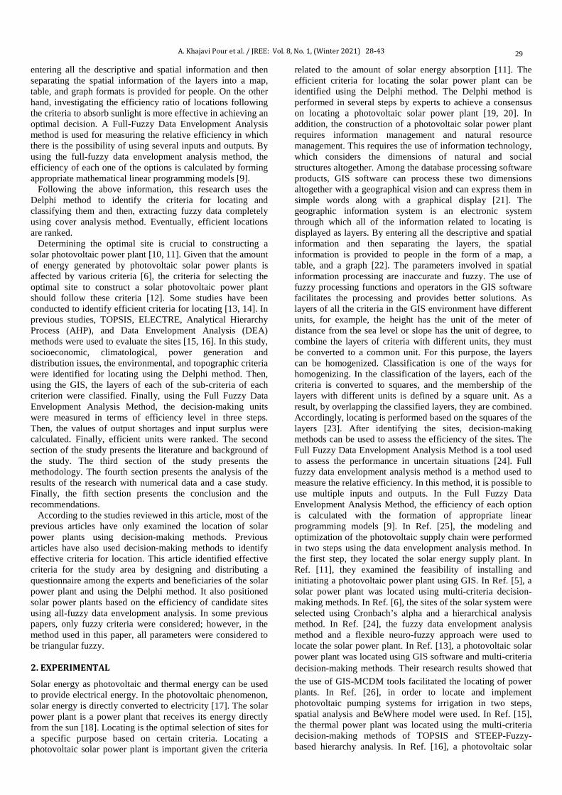
A. Khajavi Pour et al. / JREE: Vol. 8, No. 1, (Winter 2021) 28-43
29
entering all the descriptive and spatial information and then separating the spatial information of the layers into a map, table, and graph formats is provided for people. On the other hand, investigating the efficiency ratio of locations following the criteria to absorb sunlight is more effective in achieving an optimal decision. A Full-Fuzzy Data Envelopment Analysis method is used for measuring the relative efficiency in which there is the possibility of using several inputs and outputs. By using the full-fuzzy data envelopment analysis method, the efficiency of each one of the options is calculated by forming appropriate mathematical linear programming models [9]. Following the above information, this research uses the Delphi method to identify the criteria for locating and classifying them and then, extracting fuzzy data completely using cover analysis method. Eventually, efficient locations are ranked. Determining the optimal site is crucial to constructing a solar photovoltaic power plant [10, 11]. Given that the amount of energy generated by photovoltaic solar power plants is affected by various criteria [6], the criteria for selecting the optimal site to construct a solar photovoltaic power plant should follow these criteria [12]. Some studies have been conducted to identify efficient criteria for locating [13, 14]. In previous studies, TOPSIS, ELECTRE, Analytical Hierarchy Process (AHP), and Data Envelopment Analysis (DEA) methods were used to evaluate the sites [15, 16]. In this study, socioeconomic, climatological, power generation and distribution issues, the environmental, and topographic criteria were identified for locating using the Delphi method. Then, using the GIS, the layers of each of the sub-criteria of each criterion were classified. Finally, using the Full Fuzzy Data Envelopment Analysis Method, the decision-making units were measured in terms of efficiency level in three steps. Then, the values of output shortages and input surplus were calculated. Finally, efficient units were ranked. The second section of the study presents the literature and background of the study. The third section of the study presents the methodology. The fourth section presents the analysis of the results of the research with numerical data and a case study. Finally, the fifth section presents the conclusion and the recommendations. According to the studies reviewed in this article, most of the previous articles have only examined the location of solar power plants using decision-making methods. Previous articles have also used decision-making methods to identify effective criteria for location. This article identified effective criteria for the study area by designing and distributing a questionnaire among the experts and beneficiaries of the solar power plant and using the Delphi method. It also positioned solar power plants based on the efficiency of candidate sites using all-fuzzy data envelopment analysis. In some previous papers, only fuzzy criteria were considered; however, in the method used in this paper, all parameters were considered to be triangular fuzzy. 2. EXPERIMENTAL
Solar energy as photovoltaic and thermal energy can be used to provide electrical energy. In the photovoltaic phenomenon, solar energy is directly converted to electricity [17]. The solar power plant is a power plant that receives its energy directly from the sun [18]. Locating is the optimal selection of sites for a specific purpose based on certain criteria. Locating a photovoltaic solar power plant is important given the criteria
related to the amount of solar energy absorption [11]. The efficient criteria for locating the solar power plant can be identified using the Delphi method. The Delphi method is performed in several steps by experts to achieve a consensus on locating a photovoltaic solar power plant [19, 20]. In addition, the construction of a photovoltaic solar power plant requires information management and natural resource management. This requires the use of information technology, which considers the dimensions of natural and social structures altogether. Among the database processing software products, GIS software can process these two dimensions altogether with a geographical vision and can express them in simple words along with a graphical display [21]. The geographic information system is an electronic system through which all of the information related to locating is displayed as layers. By entering all the descriptive and spatial information and then separating the layers, the spatial information is provided to people in the form of a map, a table, and a graph [22]. The parameters involved in spatial information processing are inaccurate and fuzzy. The use of fuzzy processing functions and operators in the GIS software facilitates the processing and provides better solutions. As layers of all the criteria in the GIS environment have different units, for example, the height has the unit of the meter of distance from the sea level or slope has the unit of degree, to combine the layers of criteria with different units, they must be converted to a common unit. For this purpose, the layers can be homogenized. Classification is one of the ways for homogenizing. In the classification of the layers, each of the criteria is converted to squares, and the membership of the layers with different units is defined by a square unit. As a result, by overlapping the classified layers, they are combined. Accordingly, locating is performed based on the squares of the layers [23]. After identifying the sites, decision-making methods can be used to assess the efficiency of the sites. The Full Fuzzy Data Envelopment Analysis Method is a tool used to assess the performance in uncertain situations [24]. Full fuzzy data envelopment analysis method is a method used to measure the relative efficiency. In this method, it is possible to use multiple inputs and outputs. In the Full Fuzzy Data Envelopment Analysis Method, the efficiency of each option is calculated with the formation of appropriate linear programming models [9]. In Ref. [25], the modeling and optimization of the photovoltaic supply chain were performed in two steps using the data envelopment analysis method. In the first step, they located the solar energy supply plant. In Ref. [11], they examined the feasibility of installing and initiating a photovoltaic power plant using GIS. In Ref. [5], a solar power plant was located using multi-criteria decision-making methods. In Ref. [6], the sites of the solar system were selected using Cronbach’s alpha and a hierarchical analysis method. In Ref. [24], the fuzzy data envelopment analysis method and a flexible neuro-fuzzy approach were used to locate the solar power plant. In Ref. [13], a photovoltaic solar power plant was located using GIS software and multi-criteria decision-making methods. Their research results showed that the use of GIS-MCDM tools facilitated the locating of power plants. In Ref. [26], in order to locate and implement photovoltaic pumping systems for irrigation in two steps, spatial analysis and BeWhere model were used. In Ref. [15], the thermal power plant was located using the multi-criteria decision-making methods of TOPSIS and STEEP-Fuzzy-based hierarchy analysis. In Ref. [16], a photovoltaic solar

A. Khajavi Pour et al. / JREE: Vol. 8, No. 1, (Winter 2021) 28-43
30
power plant was located in two steps and the efficiency of selected sites was assessed using fuzzy hierarchy process analysis and data envelopment analysis, respectively. In Ref. [27], a photovoltaic power plant was located using a multi-criteria decision-making method. In Ref. [28], the selection of the most appropriate solar house system package was examined using hierarchical analysis method. In Ref. [29], the combined wind and solar power plant was located using the hierarchical analysis method. The results showed that knowing the advantages and disadvantages of candidate sites contributes significantly to making decisions by project managers. In Ref. [30], the installation of a thermal power plant was investigated using GIS, TOPSIS, AHP, and ELECTRE Methods. In Ref. [31], the solar power plant was located using the NDEA algorithm. Their results showed that the selected sites had a high potential for absorbing sunlight. In this paper, socioeconomic, climatological, power generation and distribution issues, environmental, and topographic criteria were identified for locating solar power plants. As the parameters involved in the spatial information
processing are inaccurate and fuzzy, the layers of each of the criteria are classified in the GIS environment. Then, using the full-fuzzy data envelopment super analysis method, the relative efficiency of the sites was assessed and ranked. 3. METHOD
In this paper, the efficient criteria for locating the solar power plant were first identified based on the studies conducted and the views of the experts in this area using the Delphi method. Then, GIS software was a fuzzy data envelopment analysis method and the efficiency of the proposed sites was assessed in three steps. In the first step, the sites extracted from the GIS environment were classified into three classes of efficient, weak, and inefficient. In the second step, the value of inputs surplus and output shortages were calculated. In the third step, efficient sites were ranked using the full fuzzy data envelopment analysis method. Figure (1) shows this procedure.
Figure 1. Research steps
Design a criteria questionnaire based on literature and background Select solar power plant specialists
Distribute and collect questionnaires among experts
Perform criteria analysis
Calculate the Kendall Coordination Rate
0<0.95
Stop the questionnaire and formulate criteria
Yes
No
Preparation of sub-criteria criteria
Convert layers to a single unit
Carry out criteria analysis
Place classification into three categories: efficient, poor, and inefficient
Calculating the amount of output shortages and excess inputs
Ranking efficient places using Andersen-Petersen method
Delphi method
Select the effective criteria for locating a photovoltaic solar energy plant
Extract the data from the geographic information system
Solar PV power plant site selection
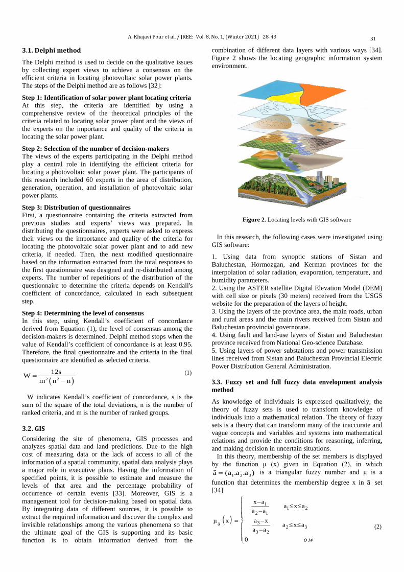
A. Khajavi Pour et al. / JREE: Vol. 8, No. 1, (Winter 2021) 28-43
31
3.1. Delphi method
The Delphi method is used to decide on the qualitative issues by collecting expert views to achieve a consensus on the efficient criteria in locating photovoltaic solar power plants. The steps of the Delphi method are as follows [32]:
Step 1: Identification of solar power plant locating criteria At this step, the criteria are identified by using a comprehensive review of the theoretical principles of the criteria related to locating solar power plant and the views of the experts on the importance and quality of the criteria in locating the solar power plant.
Step 2: Selection of the number of decision-makers The views of the experts participating in the Delphi method play a central role in identifying the efficient criteria for locating a photovoltaic solar power plant. The participants of this research included 60 experts in the area of distribution, generation, operation, and installation of photovoltaic solar power plants.
Step 3: Distribution of questionnaires First, a questionnaire containing the criteria extracted from previous studies and experts’ views was prepared. In distributing the questionnaires, experts were asked to express their views on the importance and quality of the criteria for locating the photovoltaic solar power plant and to add new criteria, if needed. Then, the next modified questionnaire based on the information extracted from the total responses to the first questionnaire was designed and re-distributed among experts. The number of repetitions of the distribution of the questionnaire to determine the criteria depends on Kendall's coefficient of concordance, calculated in each subsequent step.
Step 4: Determining the level of consensus In this step, using Kendall’s coefficient of concordance derived from Equation (1), the level of consensus among the decision-makers is determined. Delphi method stops when the value of Kendall’s coefficient of concordance is at least 0.95. Therefore, the final questionnaire and the criteria in the final questionnaire are identified as selected criteria.
( )2 2
12sWm n n
=−
(1)
W indicates Kendall’s coefficient of concordance, s is the sum of the square of the total deviations, n is the number of ranked criteria, and m is the number of ranked groups. 3.2. GIS Considering the site of phenomena, GIS processes and analyzes spatial data and land predictions. Due to the high cost of measuring data or the lack of access to all of the information of a spatial community, spatial data analysis plays a major role in executive plans. Having the information of specified points, it is possible to estimate and measure the levels of that area and the percentage probability of occurrence of certain events [33]. Moreover, GIS is a management tool for decision-making based on spatial data. By integrating data of different sources, it is possible to extract the required information and discover the complex and invisible relationships among the various phenomena so that the ultimate goal of the GIS is supporting and its basic function is to obtain information derived from the
combination of different data layers with various ways [34]. Figure 2 shows the locating geographic information system environment.
Figure 2. Locating levels with GIS software
In this research, the following cases were investigated using GIS software:
1. Using data from synoptic stations of Sistan and Baluchestan, Hormozgan, and Kerman provinces for the interpolation of solar radiation, evaporation, temperature, and humidity parameters. 2. Using the ASTER satellite Digital Elevation Model (DEM) with cell size or pixels (30 meters) received from the USGS website for the preparation of the layers of height. 3. Using the layers of the province area, the main roads, urban and rural areas and the main rivers received from Sistan and Baluchestan provincial governorate. 4. Using fault and land-use layers of Sistan and Baluchestan province received from National Geo-science Database. 5. Using layers of power substations and power transmission lines received from Sistan and Baluchestan Provincial Electric Power Distribution General Administration. 3.3. Fuzzy set and full fuzzy data envelopment analysis method
As knowledge of individuals is expressed qualitatively, the theory of fuzzy sets is used to transform knowledge of individuals into a mathematical relation. The theory of fuzzy sets is a theory that can transform many of the inaccurate and vague concepts and variables and systems into mathematical relations and provide the conditions for reasoning, inferring, and making decision in uncertain situations. In this theory, membership of the set members is displayed by the function μ (x) given in Equation (2), in which
1 2 3 )a (a .a .a= is a triangular fuzzy number and μ is a function that determines the membership degree x in a� set [34].
( )
11 2
2 1
3a2 3
3 2
x a a x aa a
μ x a x a x aa a
0 .o w
− ≤ ≤
−= −
≤ ≤ −
(2)

A. Khajavi Pour et al. / JREE: Vol. 8, No. 1, (Winter 2021) 28-43
32
For a triangular fuzzy number, if a�. b� are two triangular fuzzy numbers, a b= is true only when a1=b1 , a2=b2 , a3=b3 are the mathematical relations between fuzzy numbers and fuzzy and definite numbers in Relations (3) to (6).
( )1 2 3ka ka ,ka ,ka if k 0 = ≥ (3)
( )3 2 1ka ka ,ka ,ka if k 0 = ≤ (4)
( )1 1 2 2 3 3a b a b ,a b ,a b+ = + + + (5)
( )1 1 2 2 3 3 1 1a b a b ,a b ,a b if a , b 0 × = ≥ (6)
K is a real and definite number. The parameters are involved in the processing of information related to performance assessment to calculate the efficiency, inaccurate, and fuzzy state. One of the methods for assessing the efficiency of the options is the full fuzzy data envelopment analysis method. The full fuzzy data envelopment analysis method is a mathematical programming method for generating an efficiency boundary to assess the efficiency of the options with multiple inputs and outputs. In the full fuzzy data envelopment analysis method, all variables, parameters, and the efficiency of the options are calculated in a fuzzy manner, and the options are divided into three classes of efficient, weak, and inefficient. As inefficient options do not displace the boundary of efficiency, efficient options are ranked by using the full fuzzy data envelopment analysis method. In the fuzzy data envelopment analysis method, a set with n to DMU of inputs
ijx generates outputs of rjy . A set
with the possibility of generating rjy by
ijx is called Tγ (Tγ can be introduced based on the return to the CRS constant scale or return to the VRS variable scale). Equation (7) represents the set of possible input and output combinations of the full fuzzy data envelopment analysis method [34].
( ){ }m sT x.y R | x can produce y ++= ò (7)
One of the capabilities of the full fuzzy data envelopment analysis method is the application of models with the input and output nature corresponding to return to the same and different scales. In the input nature with a return to constant scale, each number of inputs generates the same number of outputs displayed by TCRS. In the nature of the output with return to the variable scale, each number of inputs can generate the same, small or large number of outputs displayed by the TVRS. Equation (8) displays a model with the nature of input and output.
( ) ( ) ( ){ }p p pF F( x.y ,θ max θ R | x ,θ y T γ ) += = ò ò (8)
where pθ is the efficiency score for each DMU. The full fuzzy
data envelopment analysis method is performed in three steps.
Step 1: Calculation of relative efficiency In this step, the relative efficiency of the DMUs using the CRS input model is as follows:
CRSpmin θ (9)
s.t. n
CRSj ij i p ip
j 1
λ x s θ x i 1, 2, ,m −
=
× + = × =∑ (10)
n
j rj r rpj 1
λ y s y r 1, 2, ,s +
=
× = + =∑ (11)
( )jλ TF R , j 1, 2, , n + = ò
( )is TF R , i 1, 2, ,m +− = ò
( )is TF R , r 1, 2, , n ++ = ò
Phrase (9) is the objective function of the problem and represents the minimization of the efficiency of the decision-making units. Phrases (10) and (11) represent the set of constraints related to inputs and outputs, respectively. The numerical value 0 < θp ≤ 1. θ�p
CRS is the variable of efficiency in model with input nature, x�ij is the ith input of DMUj and its value is fuzzy.
rjy is the jth output of DMUj,
and jλ is DMUj weight. In addition, i rs sand− + are auxiliary
variables. Given that all variables and parameters are triangular fuzzy numbers, by using Relations (3) to (6), the above phrases can be rewritten as follows:
( )CRS CRS CRSp,1 p,2 p,3min θ ,θ ,θ (12)
s. t.
( ) ( ) ( )n
CRS CRS CRSj,1 ij,1 j,2 ij,2 j,3 ij,3 i,1 i,2 i,3 p,1 ip,1 p,2 ip,2 p,3 ip,3
j 1
λ x , λ x , λ x s ,s ,s θ x ,θ x ,θ x− − −
=
+ =∑
i 1, 2, ,m =
( ) ( ) ( )n
j,1 rj,1 j,2 rj,2 j,3 rj,3 r,1 r,2 r,3 rp,1 rp,2 rp,3j 1
λ y , λ y ,λ y s ,s ,s y , y , y + + +
=
= +∑
r 1, 2, ,s =
j,1 j,2 j,1 j,3 j,2λ 0; λ λ 0; λ λ 0 j 1, 2, , n ≥ − ≥ − ≥ =
i,1 i,2 i,1 i,3 i,2s 0; s s 0; s s 0 i 1, 2, ,m − − − − −≥ − ≥ − ≥ =
r,1 r,2 r,1 r,3 r,2s 0; s s 0; s s 0 r 1, 2, ,s + + + + +≥ − ≥ − ≥ = VRS VRS VRS VRSp,2 p,1 p,3 p,2θ θ 0; θ θ 0 − ≥ − ≥
In this section, in order to solve the multi-objective programming problem function while maintaining the triangular shape, Phrase (12) is transformed to three separate objective functions (13), (14), and (15).
CRSp,1min θ (13) CRSp,2min θ (14) CRSp,3min θ (15)
s.t. n
CRS.*j,k ij,k i,k p,k ip,k
j 1
λ x s θ x i 1, 2, ,m , k 1,2,3 −
=
+ = = =∑
n
j,k rj,k r,k rp,kj 1
λ y s y r 1, 2, ,s , k 1,2,3 +
=
= + = =∑
jλ 0 j 1, 2, , n ≥ =
i,1 i,2 i,1 i,3 i,2s 0; s s 0; s s 0 i 1, 2, ,m − − − − −≥ − ≥ − ≥ =
r,1 r,2 r,1 r,3 r,2s 0; s s 0; s s 0 r 1, 2, ,s + + + + +≥ − ≥ − ≥ =
CRS CRS CRS CRSp,2 p,1 p,3 p,2θ θ 0; θ θ 0 − ≥ − ≥
A. Khajavi Pour et al. / JREE: Vol. 8, No. 1, (Winter 2021) 28-43
33
The problem is solved by the Lexographic method. Accordingly, the problem is first solved for the objective function (15) and the best value of the phrase (15) is obtained. Then, by maintaining this optimal value, the objective function (14) is optimized and by maintaining the optimal value of the objective functions (15) and (14), the optimal value of the objective function (13) is obtained. Finally, by calculating the value of the efficiency variable of each decision-making unit relative to other decision-making unit, the decision-making units are classified in terms of efficiency. Therefore, decision-making units fall into three classes:
i: DMUp is efficient if ( )CRS*pθ 1,1,1= and for all is
( ) ( )* *i rs 0,0,0 and for all rs s 0,0,0+ += =
ii: DMUp has low efficiency if
( ) ( )m s
CRS* * *p i r
i 1 r 1
θ 1,1,1 , s s 0,0,0and + +
= =
= + ≠∑ ∑
iii: DMUp is inefficient if ( )CRS*pθ 1,1,1≠
Step 2: Calculating the amount of output shortage and input surplus consumed Inefficient options cannot displace the border of efficiency; however, in inefficient decision-making units, some inputs remain and a shortage of outputs occurs. In this step, the number of inputs remained and the number of shortages of outputs of inefficient decision-making units is calculated using Equation (16).
( ) ( )m s
i,1 i,2 i,3 r,1 r,2 r,3i 1 r 1
max s s s s s s − − − + + +
= =
+ + + + +∑ ∑ (16)
s.t.n
CRS.*j,k ij,k i,k p,k ip,k
j 1
λ x s θ x i 1, 2, ,m , k 1,2,3 −
=
+ = = =∑
n
j,k rj,k r,k rp,kj 1
λ y s y r 1, 2, ,s , k 1,2,3 +
=
= + = =∑
j,1 j,2 j,1 j,3 j,2λ 0; λ λ 0; λ λ 0 j 1, 2, , n ≥ − ≥ − ≥ =
i,1 i,2 i,1 i,3 i,2s 0; s s 0; s s 0 i 1, 2, , m − − − − −≥ − ≥ − ≥ =
r,1 r,2 r,1 r,3 r,2s 0; s s 0; s s 0 r 1, 2, ,s + + + + +≥ − ≥ − ≥ =
Step 3: Ranking efficient decision-making units Several efficient decision-making units might exist. In order to rank efficient decision-making units, the decision-making units are assessed in relation to the decision-making units of the reference set. Thus, the Anderson-Peterson super-efficiency model of the full fuzzy data envelopment analysis is written as follows [35]:
min�θp,1CRS, θp,2
CRS, θp,3CRS� (17) (17)
s.t.
( ) ( ) ( )n
CRS CRS CRSj,1 ij,1 j,2 ij,2 j,3 ij,3 i,1 i,2 i,3 p,1 ip,1 p,2 ip,2 p,3 ip,3
j 1, j p
λ x ,λ x ,λ x s ,s ,s θ x ,θ x ,θ x− − −
= ≠
+ =∑
; i 1, 2, ,m =
( ) ( ) ( )n
j,1 rj,1 j,2 rj,2 j,3 rj,3 r,1 r,2 r,3 rp,1 rp,2 rp,3j 1, j p
λ y , λ y ,λ y s ,s ,s y , y , y + + +
= ≠
= +∑
r 1, 2, ,s =
j,1 j,2 j,1 j,3 j,2λ 0; λ λ 0; λ λ 0 j 1, 2, , n ≥ − ≥ − ≥ =
i,1 i,2 i,1 i,3 i,2s 0; s s 0; s s 0 i 1, 2, , m − − − − −≥ − ≥ − ≥ =
r,1 r,2 r,1 r,3 r,2s 0; s s 0; s s 0 r 1, 2, ,s + + + + +≥ − ≥ − ≥ =
CRS CRS CRS CRSp,2 p,1 p,3 p,2θ θ 0; θ θ 0 − ≥ − ≥
Here, CRS*p,3θ 1≥ is the super efficiency. Thus, by solving
Phrase (17), efficient decision-making units are ranked. 4. RESULTS AND DISCUSSION
In order to validate the proposed method, a case study was carried out for locating a photovoltaic solar power plant. The study area in this research is Sistan and Baluchestan Province, located in the southeastern of Iran. This province covers 11 percent of Iran’s area with an area of about 180726 km2. The province has a mainly warm and dry climate, while it has a climate diversity. The province has a latitude of 25 degrees and 3 minutes to 31 degrees and 27 minutes north latitude from the equator. In terms of geographical longitude, it has been located 58 to 50 degrees to 63 degrees and 21 minutes east longitude from the meridian. Moreover, it is very suitable for establishing solar power plants. Given the possibility of using many criteria in locating the solar power plant and their effect on the performance of the solar power plant, the criteria considered should be appropriate in regional conditions [19]. The level of solar radiation, humidity, temperature, and evaporation affect the absorption and power of the power plant [35]. In addition, the construction of a solar power plant in different applications brings about different costs. The user layer reflects the way of using a piece of land [28]. It is important to have proper information on land use and distance to rivers for the construction of a solar power plant from the economic and environmental points of view [23, 36]. The height, slope, and direction of slope significantly affect the cost of construction of a solar power plant; thus, finding the height, slope, and direction of slope greatly reduces the cost of constructing a solar power plant and increases the power of generating the solar energy of plants. The proximity of the solar power plant to the main roads, power posts, and power lines reduces the cost of transportation of equipment to the power plant [37]. The proximity of power plants to the urban and rural areas reduces power transmission and distribution costs and reduces energy waste. Moreover, it is important to construct the power plants away from earthquake centers to ensure the security of the power plant equipment economically [37, 38]. In this research, for locating a photovoltaic solar energy system, the efficient criteria for locating the solar power plant were identified based on the previous studies and views of the experts in this area and using the Delphi method. Table (1) displays several locating studies along with the criteria considered for the construction of a solar photovoltaic power plant. Questionnaire was distributed among 60 experts in solar power plant locating and they were asked to classify the criteria and express their views and opinions on the importance and quality of the criteria. After collecting the questionnaire and entering the data in SPSS software, Kendall’s coefficient of concordance was calculated as 0.68. Then, another questionnaire was designed according to the information extracted from the first questionnaire and distributed among the experts. In the second questionnaire, the criteria increased and changed. The value of Kendall’s coefficient of concordance of the second questionnaire was calculated as 0.87. The third questionnaire was designed and distributed according to the views of experts. Kendall’s coefficient of concordance was calculated 0.95; thus, the
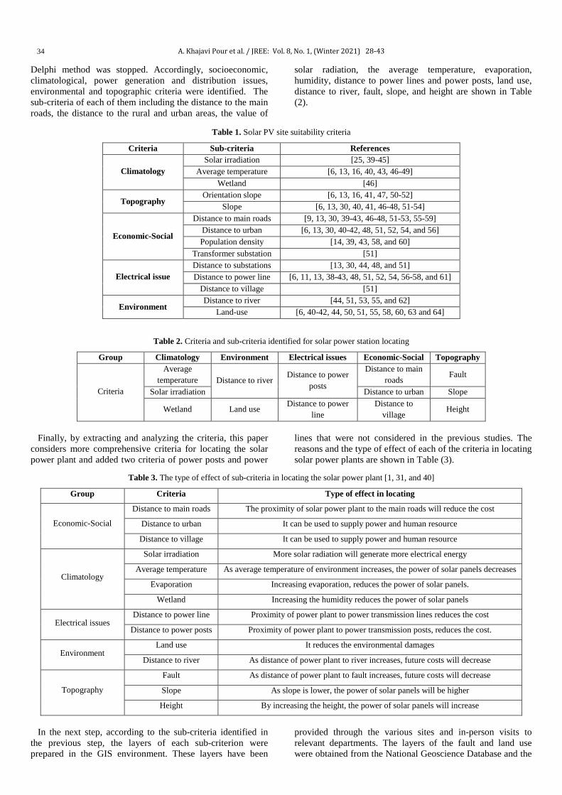
A. Khajavi Pour et al. / JREE: Vol. 8, No. 1, (Winter 2021) 28-43
34
Delphi method was stopped. Accordingly, socioeconomic, climatological, power generation and distribution issues, environmental and topographic criteria were identified. The sub-criteria of each of them including the distance to the main roads, the distance to the rural and urban areas, the value of
solar radiation, the average temperature, evaporation, humidity, distance to power lines and power posts, land use, distance to river, fault, slope, and height are shown in Table (2).
Table 1. Solar PV site suitability criteria
Criteria Sub-criteria References
Climatology Solar irradiation [25, 39-45]
Average temperature [6, 13, 16, 40, 43, 46-49] Wetland [46]
Topography Orientation slope [6, 13, 16, 41, 47, 50-52]
Slope [6, 13, 30, 40, 41, 46-48, 51-54]
Economic-Social
Distance to main roads [9, 13, 30, 39-43, 46-48, 51-53, 55-59] Distance to urban [6, 13, 30, 40-42, 48, 51, 52, 54, and 56] Population density [14, 39, 43, 58, and 60]
Transformer substation [51]
Electrical issue Distance to substations [13, 30, 44, 48, and 51] Distance to power line [6, 11, 13, 38-43, 48, 51, 52, 54, 56-58, and 61]
Distance to village [51]
Environment Distance to river [44, 51, 53, 55, and 62]
Land-use [6, 40-42, 44, 50, 51, 55, 58, 60, 63 and 64]
Table 2. Criteria and sub-criteria identified for solar power station locating
Group Climatology Environment Electrical issues Economic-Social Topography
Criteria
Average temperature Distance to river
Distance to power posts
Distance to main roads
Fault
Solar irradiation Distance to urban Slope
Wetland Land use Distance to power line
Distance to village
Height
Finally, by extracting and analyzing the criteria, this paper considers more comprehensive criteria for locating the solar power plant and added two criteria of power posts and power
lines that were not considered in the previous studies. The reasons and the type of effect of each of the criteria in locating solar power plants are shown in Table (3).
Table 3. The type of effect of sub-criteria in locating the solar power plant [1, 31, and 40]
Group Criteria Type of effect in locating
Economic-Social
Distance to main roads The proximity of solar power plant to the main roads will reduce the cost
Distance to urban It can be used to supply power and human resource
Distance to village It can be used to supply power and human resource
Climatology
Solar irradiation More solar radiation will generate more electrical energy
Average temperature As average temperature of environment increases, the power of solar panels decreases
Evaporation Increasing evaporation, reduces the power of solar panels.
Wetland Increasing the humidity reduces the power of solar panels
Electrical issues Distance to power line Proximity of power plant to power transmission lines reduces the cost
Distance to power posts Proximity of power plant to power transmission posts, reduces the cost.
Environment Land use It reduces the environmental damages
Distance to river As distance of power plant to river increases, future costs will decrease
Topography
Fault As distance of power plant to fault increases, future costs will decrease
Slope As slope is lower, the power of solar panels will be higher
Height By increasing the height, the power of solar panels will increase
In the next step, according to the sub-criteria identified in the previous step, the layers of each sub-criterion were prepared in the GIS environment. These layers have been
provided through the various sites and in-person visits to relevant departments. The layers of the fault and land use were obtained from the National Geoscience Database and the
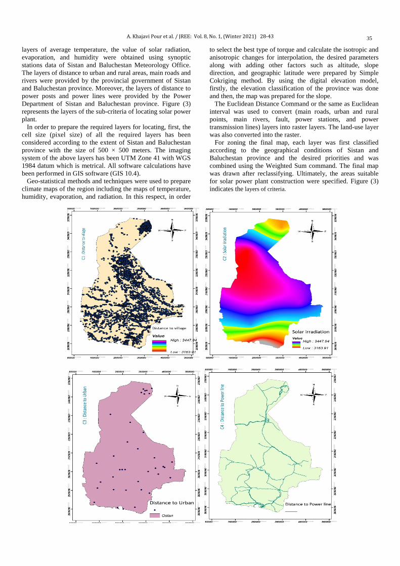
A. Khajavi Pour et al. / JREE: Vol. 8, No. 1, (Winter 2021) 28-43
35
layers of average temperature, the value of solar radiation, evaporation, and humidity were obtained using synoptic stations data of Sistan and Baluchestan Meteorology Office. The layers of distance to urban and rural areas, main roads and rivers were provided by the provincial government of Sistan and Baluchestan province. Moreover, the layers of distance to power posts and power lines were provided by the Power Department of Sistan and Baluchestan province. Figure (3) represents the layers of the sub-criteria of locating solar power plant. In order to prepare the required layers for locating, first, the cell size (pixel size) of all the required layers has been considered according to the extent of Sistan and Baluchestan province with the size of 500 × 500 meters. The imaging system of the above layers has been UTM Zone 41 with WGS 1984 datum which is metrical. All software calculations have been performed in GIS software (GIS 10.4). Geo-statistical methods and techniques were used to prepare climate maps of the region including the maps of temperature, humidity, evaporation, and radiation. In this respect, in order
to select the best type of torque and calculate the isotropic and anisotropic changes for interpolation, the desired parameters along with adding other factors such as altitude, slope direction, and geographic latitude were prepared by Simple Cokriging method. By using the digital elevation model, firstly, the elevation classification of the province was done and then, the map was prepared for the slope. The Euclidean Distance Command or the same as Euclidean interval was used to convert (main roads, urban and rural points, main rivers, fault, power stations, and power transmission lines) layers into raster layers. The land-use layer was also converted into the raster. For zoning the final map, each layer was first classified according to the geographical conditions of Sistan and Baluchestan province and the desired priorities and was combined using the Weighted Sum command. The final map was drawn after reclassifying. Ultimately, the areas suitable for solar power plant construction were specified. Figure (3) indicates the layers of criteria.

A. Khajavi Pour et al. / JREE: Vol. 8, No. 1, (Winter 2021) 28-43
36
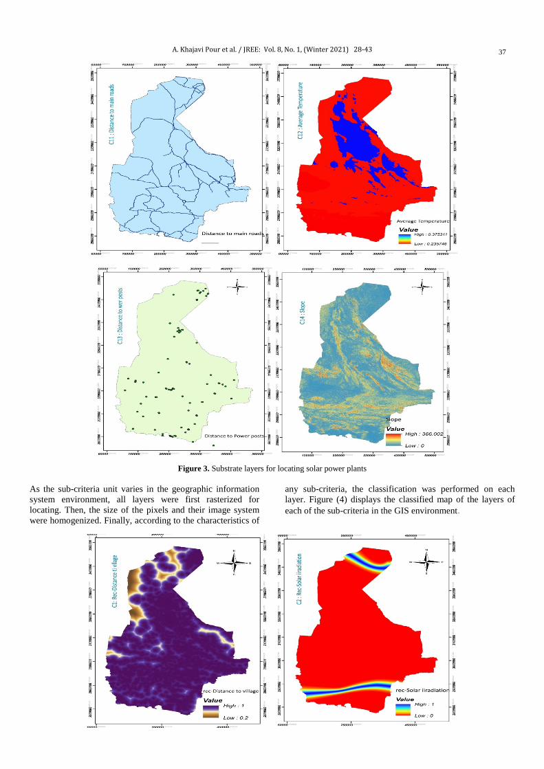
A. Khajavi Pour et al. / JREE: Vol. 8, No. 1, (Winter 2021) 28-43
37
Figure 3. Substrate layers for locating solar power plants
As the sub-criteria unit varies in the geographic information system environment, all layers were first rasterized for locating. Then, the size of the pixels and their image system were homogenized. Finally, according to the characteristics of
any sub-criteria, the classification was performed on each layer. Figure (4) displays the classified map of the layers of each of the sub-criteria in the GIS environment.

A. Khajavi Pour et al. / JREE: Vol. 8, No. 1, (Winter 2021) 28-43
38

A. Khajavi Pour et al. / JREE: Vol. 8, No. 1, (Winter 2021) 28-43
39
Figure 4. Classified sub-criteria
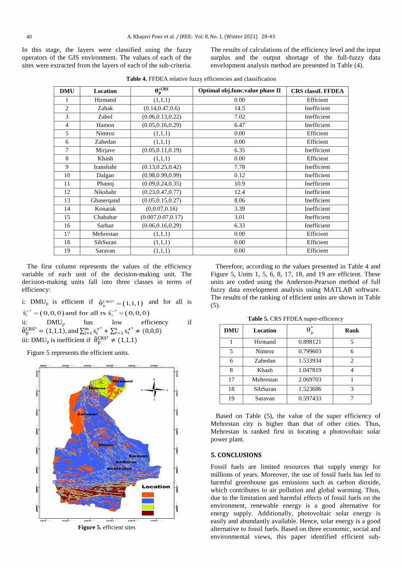
A. Khajavi Pour et al. / JREE: Vol. 8, No. 1, (Winter 2021) 28-43
40
In this stage, the layers were classified using the fuzzy operators of the GIS environment. The values of each of the sites were extracted from the layers of each of the sub-criteria.
The results of calculations of the efficiency level and the input surplus and the output shortage of the full-fuzzy data envelopment analysis method are presented in Table (4).
Table 4. FFDEA relative fuzzy efficiencies and classification
DMU Location 𝛉𝛉𝐩𝐩∗𝐂𝐂𝐂𝐂𝐂𝐂 Optimal obj.func.value phase II CRS classif. FFDEA 1 Hirmand (1,1,1) 0.00 Efficient 2 Zahak (0.14,0.47,0.6) 14.5 Inefficient 3 Zabol (0.06,0.13,0.22) 7.02 Inefficient 4 Hamon (0.05,0.16,0.29) 6.47 Inefficient 5 Nimroz (1,1,1) 0.00 Efficient 6 Zahedan (1,1,1) 0.00 Efficient 7 Mirjave (0.05,0.11,0.19) 6.35 Inefficient 8 Khash (1,1,1) 0.00 Efficient 9 Iranshahr (0.13,0.25,0.42) 7.78 Inefficient 10 Dalgan (0.98,0.99,0.99) 0.12 Inefficient 11 Phanoj (0.09,0.24,0.35) 10.9 Inefficient 12 Nikshahr (0.23,0.47,0.77) 12.4 Inefficient 13 Ghaserqand (0.05,0.15,0.27) 8.06 Inefficient 14 Konarak (0,0.07,0.16) 3.39 Inefficient 15 Chabahar (0.007,0.07,0.17) 3.01 Inefficient 16 Sarbaz (0.06,0.16,0.29) 6.33 Inefficient 17 Mehrestan (1,1,1) 0.00 Efficient 18 SibSuran (1,1,1) 0.00 Efficient 19 Saravan (1,1,1) 0.00 Efficient
The first column represents the values of the efficiency variable of each unit of the decision-making unit. The decision-making units fall into three classes in terms of efficiency:
i: DMUp is efficient if ( )CRS*pθ 1,1,1= and for all is
( ) ( )* *i rs 0,0,0 and for all rs s 0,0,0+ += =
ii: DMUp has low efficiency if θ�pCRS* = (1,1,1), and∑ si+*m
i=1 + ∑ sr+*sr=1 ≠ (0,0,0)
iii: DMUp is inefficient if θ�pCRS* ≠ (1,1,1)
Figure 5 represents the efficient units.
Figure 5. efficient sites
Therefore, according to the values presented in Table 4 and Figure 5, Units 1, 5, 6, 8, 17, 18, and 19 are efficient. These units are coded using the Anderson-Pearson method of full fuzzy data envelopment analysis using MATLAB software. The results of the ranking of efficient units are shown in Table (5).
Table 5. CRS FFDEA super-efficiency
Rank *pθ Location DMU
5 0.898121 Hirmand 1 6 0.799603 Nimroz 5 2 1.533934 Zahedan 6 4 1.047819 Khash 8 1 2.069703 Mehrestan 17 3 1.523686 SibSuran 18 7 0.597433 Saravan 19
Based on Table (5), the value of the super efficiency of Mehrestan city is higher than that of other cities. Thus, Mehrestan is ranked first in locating a photovoltaic solar power plant. 5. CONCLUSIONS
Fossil fuels are limited resources that supply energy for millions of years. Moreover, the use of fossil fuels has led to harmful greenhouse gas emissions such as carbon dioxide, which contributes to air pollution and global warming. Thus, due to the limitation and harmful effects of fossil fuels on the environment, renewable energy is a good alternative for energy supply. Additionally, photovoltaic solar energy is easily and abundantly available. Hence, solar energy is a good alternative to fossil fuels. Based on three economic, social and environmental views, this paper identified efficient sub-
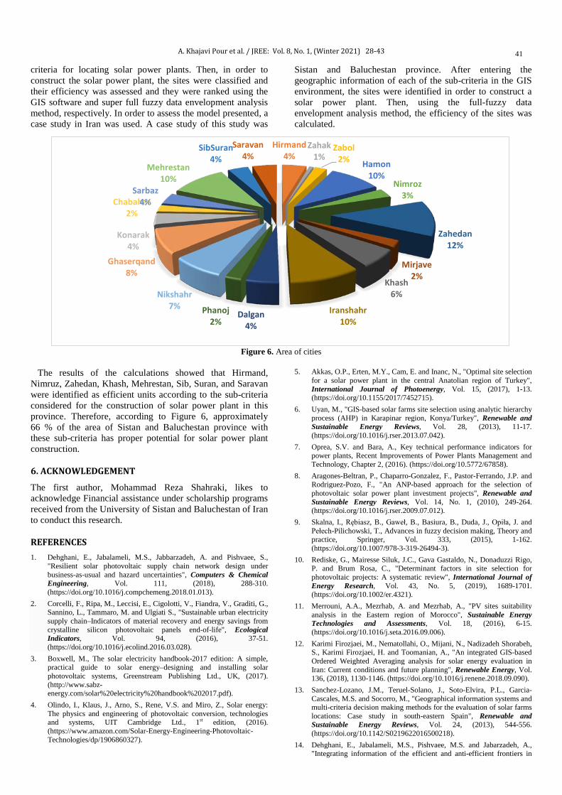
A. Khajavi Pour et al. / JREE: Vol. 8, No. 1, (Winter 2021) 28-43
41
criteria for locating solar power plants. Then, in order to construct the solar power plant, the sites were classified and their efficiency was assessed and they were ranked using the GIS software and super full fuzzy data envelopment analysis method, respectively. In order to assess the model presented, a case study in Iran was used. A case study of this study was
Sistan and Baluchestan province. After entering the geographic information of each of the sub-criteria in the GIS environment, the sites were identified in order to construct a solar power plant. Then, using the full-fuzzy data envelopment analysis method, the efficiency of the sites was calculated.
Figure 6. Area of cities
The results of the calculations showed that Hirmand, Nimruz, Zahedan, Khash, Mehrestan, Sib, Suran, and Saravan were identified as efficient units according to the sub-criteria considered for the construction of solar power plant in this province. Therefore, according to Figure 6, approximately 66 % of the area of Sistan and Baluchestan province with these sub-criteria has proper potential for solar power plant construction. 6. ACKNOWLEDGEMENT
The first author, Mohammad Reza Shahraki, likes to acknowledge Financial assistance under scholarship programs received from the University of Sistan and Baluchestan of Iran to conduct this research. REFERENCES 1. Dehghani, E., Jabalameli, M.S., Jabbarzadeh, A. and Pishvaee, S.,
"Resilient solar photovoltaic supply chain network design under business-as-usual and hazard uncertainties", Computers & Chemical Engineering, Vol. 111, (2018), 288-310. (https://doi.org/10.1016/j.compchemeng.2018.01.013).
2. Corcelli, F., Ripa, M., Leccisi, E., Cigolotti, V., Fiandra, V., Graditi, G., Sannino, L., Tammaro, M. and Ulgiati S., "Sustainable urban electricity supply chain–Indicators of material recovery and energy savings from crystalline silicon photovoltaic panels end-of-life", Ecological Indicators, Vol. 94, (2016), 37-51. (https://doi.org/10.1016/j.ecolind.2016.03.028).
3. Boxwell, M., The solar electricity handbook-2017 edition: A simple, practical guide to solar energy–designing and installing solar photovoltaic systems, Greenstream Publishing Ltd., UK, (2017). (http://www.sabz-energy.com/solar%20electricity%20handbook%202017.pdf).
4. Olindo, I., Klaus, J., Arno, S., Rene, V.S. and Miro, Z., Solar energy: The physics and engineering of photovoltaic conversion, technologies and systems, UIT Cambridge Ltd., 1st edition, (2016). (https://www.amazon.com/Solar-Energy-Engineering-Photovoltaic-Technologies/dp/1906860327).
5. Akkas, O.P., Erten, M.Y., Cam, E. and Inanc, N., "Optimal site selection for a solar power plant in the central Anatolian region of Turkey", International Journal of Photoenergy, Vol. 15, (2017), 1-13. (https://doi.org/10.1155/2017/7452715).
6. Uyan, M., "GIS-based solar farms site selection using analytic hierarchy process (AHP) in Karapinar region, Konya/Turkey", Renewable and Sustainable Energy Reviews, Vol. 28, (2013), 11-17. (https://doi.org/10.1016/j.rser.2013.07.042).
7. Oprea, S.V. and Bara, A., Key technical performance indicators for power plants, Recent Improvements of Power Plants Management and Technology, Chapter 2, (2016). (https://doi.org/10.5772/67858).
8. Aragones-Beltran, P., Chaparro-Gonzalez, F., Pastor-Ferrando, J.P. and Rodriguez-Pozo, F., "An ANP-based approach for the selection of photovoltaic solar power plant investment projects", Renewable and Sustainable Energy Reviews, Vol. 14, No. 1, (2010), 249-264. (https://doi.org/10.1016/j.rser.2009.07.012).
9. Skalna, I., Rębiasz, B., Gaweł, B., Basiura, B., Duda, J., Opiła, J. and Pełech-Pilichowski, T., Advances in fuzzy decision making, Theory and practice, Springer, Vol. 333, (2015), 1-162. (https://doi.org/10.1007/978-3-319-26494-3).
10. Rediske, G., Mairesse Siluk, J.C., Gava Gastaldo, N., Donaduzzi Rigo, P. and Brum Rosa, C., "Determinant factors in site selection for photovoltaic projects: A systematic review", International Journal of Energy Research, Vol. 43, No. 5, (2019), 1689-1701. (https://doi.org/10.1002/er.4321).
11. Merrouni, A.A., Mezrhab, A. and Mezrhab, A., "PV sites suitability analysis in the Eastern region of Morocco", Sustainable Energy Technologies and Assessments, Vol. 18, (2016), 6-15. (https://doi.org/10.1016/j.seta.2016.09.006).
12. Karimi Firozjaei, M., Nematollahi, O., Mijani, N., Nadizadeh Shorabeh, S., Karimi Firozjaei, H. and Toomanian, A., "An integrated GIS-based Ordered Weighted Averaging analysis for solar energy evaluation in Iran: Current conditions and future planning", Renewable Energy, Vol. 136, (2018), 1130-1146. (https://doi.org/10.1016/j.renene.2018.09.090).
13. Sanchez-Lozano, J.M., Teruel-Solano, J., Soto-Elvira, P.L., Garcia-Cascales, M.S. and Socorro, M., "Geographical information systems and multi-criteria decision making methods for the evaluation of solar farms locations: Case study in south-eastern Spain", Renewable and Sustainable Energy Reviews, Vol. 24, (2013), 544-556. (https://doi.org/10.1142/S0219622016500218).
14. Dehghani, E., Jabalameli, M.S., Pishvaee, M.S. and Jabarzadeh, A., "Integrating information of the efficient and anti-efficient frontiers in
Hirmand 4%
Zahak 1%
Zabol 2% Hamon
10% Nimroz
3%
Zahedan 12%
Mirjave 2%
Khash 6%
Iranshahr 10%
Dalgan 4%
Phanoj 2%
Nikshahr 7%
Ghaserqand 8%
Konarak 4%
Chabahar 2%
Sarbaz 4%
Mehrestan 10%
SibSuran 4%
Saravan 4%

A. Khajavi Pour et al. / JREE: Vol. 8, No. 1, (Winter 2021) 28-43
42
DEA analysis to assess location of solar plants: A case study in Iran", Journal of Industrial and Systems Engineering, Vol. 11, No. 1, (2018), 163-179. (www.jise.ir/article_50883.html).
15. Choudhary, D. and Shankar, R., "An STEEP-fuzzy AHP-TOPSIS framework for evaluation and selection of thermal power plant location: A case study from India", Energy, Vol. 42, (2012), 510-521. (https://doi.org/10.1016/j.energy.2012.03.010).
16. Lee, A., Kang, H.Y., Lin, C.Y. and Shen, K.C., "An integrated decision-making model for the location of a PV solar plant", Sustainability, Vol. 7, No. 10, (2015), 13522-13541. (https://doi.org/10.3390/su71013522).
17. Srivastava, Sh., Lohia, P. and Dwivedi, D.K., "Impact of hole transport layer on performance of perovskite solar cell", AIP Conference Proceedings, Vol. 2220, No. 1, (2020), 1-288. (https://doi.org/10.1063/5.0001790).
18. Isabella, O., Jager, K., Smets, A., Swaaij, R.V. and Zeman, M., Solar energy: The physics and engineering of photovoltaic conversion technologies and systems, UIT Cambridge Ltd., (2016). (https://www.amazon.com/Solar-Energy-Engineering-Photovoltaic-Technologies/dp/1906860327).
19. Ozdemir, S. and Sahin, G., "Multi-criteria decision-making in the location selection for a solar PV power plant using AHP", Measurement, Vol. 129, (2018), 218-226. (https://doi.org/10.1016/j.measurement.2018.07.020).
20. Bal, H., Orkcü, H. and Çelebioglu, S., "A new method based on the dispersion of weights in data envelopment analysis", Computers & Industrial Engineering, Vol. 54, No. 3, (2008), 502-512. (https://doi.org/10.1016/j.cie.2007.09.001).
21. Tomlinson, R.F., Thinking about GIS: Geographic information system planning for managers, Fifth edition, Esri Press, (2007). (https://www.amazon.com/Thinking-About-GIS-Geographic-Information/dp/1589483480).
22. Sui D., "Opportunities and impediments for open GIS", Transactions in GIS, Vol. 18, No. 1, (2014), 1-24. (https://doi.org/10.1111/tgis.12075).
23. Low, M. and Collins, A., Getting to know Arc GIS, Fourth edition, Esri Press, (2015). (https://www.amazon.com/Getting-Know-ArcGIS-10-3-10-3-1/dp/1589483820).
24. Azadeh, A., Sheikhalishahi, M., Firoozi, M. and Khalili, S.M., "An integrated multi-criteria Taguchi computer simulation-DEA approach for optimum maintenance policy and planning by incorporating learning effects", International Journal of Production Research, Vol. 51, No. 18, (2013), 5374-5385. (https://doi.org/10.1080/00207543.2013.774496).
25. Dehghani, E., Jabalameli, M.S. and Jabbarzadeh, A., "Robust design and optimization of solar photovoltaic supply chain in an uncertain environment", Energy, Vol. 142, (2018), 139-156. (https://doi.org/10.1016/j.energy.2017.10.004).
26. Campana, P.E., Leduc, S., Kim, M., Liu, J., Kraxner, F., Callum, I.M., Li, H. and Yan, J., "Optimal grassland locations for sustainable photovoltaic water pumping systems in China", Energy Procedia, Vol. 75, (2015), 301-307. (https://doi.org/10.1016/j.egypro.2015.07.355).
27. Wang, T.C. and Tsai, S.Y., "Solar panel supplier selection for the photovoltaic system design by using fuzzy Multi-criteria decision making (MCDM) approaches", Energies, Vol. 11, (2018), 1-22. (https://doi.org/10.3390/en11081989).
28. Ahammed, F. and Azeem, A., "Selection of the most appropriate package of Solar Home System using Analytic Hierarchy Process model in rural areas of Bangladesh", Renewable Energy, Vol. 55, (2013), 6-11. (https://doi.org/10.1016/j.renene.2012.12.020).
29. Wu, Y. and Geng, Sh., "Multi-criteria decision making on selection of solar–wind hybrid power station location: A case of China", Energy Conversion and Management, Vol. 81, (2014), 527-533. (https://doi.org/10.1016/j.enconman.2014.02.056).
30. Sanchez-Lozano, J.M., Garcia-Cascales, M.S. and Lamata, M.T., "Evaluation of suitable locations for the installation of solar thermoelectric power plants", Computers & Industrial Engineering, Vol. 87, (2015), 343-355. (https://doi.org/10.1016/j.cie.2015.05.028).
31. Khanjarpanah, H., Jabbarzadeh, A. and Seyedhosseini, S.M., "A novel multi-period double frontier network DEA to sustainable location optimization of hybrid wind-photovoltaic power plant with real application", Energy Conversion and Management, Vol. 159, (2018),175-188. (https://doi.org/10.1016/j.enconman.2018.01.013).
32. Habibi. A., Sarfarazi, R. and Izadyar, S., "Delphi technique theoretical framework in qualitative research", The International Journal Of
Engineering And Science (IJES), Vol. 3, No. 4, (2014), 8-13. (https://doi.org/v3-i4/Version-4/B03404008013).
33. DeMers, M.N., GIS for dummies, 1st Edition, Kindle Edition, Wiley Publishing, (2009). (https://www.amazon.com/GIS-Dummies-Michael-N-DeMers-ebook/dp/B001FA0GMQ).
34. Hatami-Marbini, A., Tavana, M., Emrouznejad, A. and Saati, S., "Efficiency measurement in fuzzy additive data envelopment analysis", Industrial and Systems Engineering, Vol. 10, (2017), 1-20. (https://doi.org/10.1504/IJISE.2012.044041).
35. Andersen, P. and Petersen, N.C., "A procedure for ranking efficient units in data envelopment analysis", Management Science, Vol. 39, (1993), 1261-1264. (https://doi.org/10.1287/mnsc.39.10.1261).
36. Ghose, D., Naskar, S., Uddin, Sh. and Roy, A.K., "An open source software: Q-GIS based analysis for solar potential of Sikkim (India)", International Journal of Open Source Software and Processes, Vol. 10, No. 1, (2019), 49-68. (https://doi.org/10.4018/IJOSSP.2019010104).
37. Aguayo, P., "Solar energy potential analysis at building scale using LiDAR and satellite data", University of Waterloo, Canada, (2013), 1-164. (http://hdl.handle.net/10012/7603).
38. Olufemi, A., Omitaomu, K., Brandon, R., Blevins, C., Gary, T., Stanton, W., Hadley, J., Harrison, J., Budhendra, L. and Amy, N., "Adapting a GIS based multicriteria decision analysis approach for evaluating new power generating sites", Applied Energy, Vol. 96, (2012), 292-301. (https://doi.org/10.1016/j.apenergy.2011.11.087).
39. Yushchenko, A., Bono, A., Chatenoux, B., Patel, M.K. and Ray, N., "GIS-based assessment of photovoltaic (PV) and concentrated solar power (CSP) generation potential in West Africa", Renewable and Sustainable Energy Reviews, Vol. 81, (2018), 2088-2103. (https://doi.org/10.1016/j.rser.2017.06.021).
40. Garni, H.Z.A. and Awasthi, A., "Solar PV power plant site selection using a GIS-AHP based approach with application in Saudi Arabia", Applied Energy, Vol. 206, (2017), 1225-1240. (https://doi.org/10.1016/j.apenergy.2017.10.024).
41. Carrion, J.A., Espin Estrella, A., Aznar Dols, F. and Ramos Ridao, A., "The electricity production capacity of photovoltaic power plants and the selection of solar energy sites in Andalusia (Spain)", Renewable Energy, Vol. 33, (2008), 545-552. (https://doi.org/10.1016/j.renene.2007.05.041).
42. Janke, J.R., "Multicriteria GIS modeling of wind and solar farms in Colorado", Renewable Energy, Vol. 35, (2010), 2228-2234. (https://doi.org/10.1016/j.renene.2010.03.014).
43. Charabi, Y. and Gastli, A., "PV site suitability analysis, using GIS based spatial fuzzy multi-criteria evaluation", Renewable Energy, Vol. 36, (2011), 2554-2561. (https://doi.org/10.1016/j.renene.2010.10.037).
44. Saracoglu, B.O., Ohunakin, O.S., Adelekan, D.S., Gill, J., Atiba, O.E., Okokpujie, I.P. and Atayero, A.A., "A framework for selecting the location of very large photovoltaic solar power plants on a global/supergrid", Energy Reports, Vol. 4, (2018), 586-602. (https://doi.org/10.1016/j.egyr.2018.09.002).
45. Dawson, L. and Schlyter, P., "Less is more: Strategic scale site suitability for concentrated solar thermal power in Western Australia", Energy Policy, Vol. 47, (2012), 91-101. (https://doi.org/10.1016/j.enpol.2012.04.025).
46. Doorga, J.R.S., Rughooputh, S.D.D.V. and Boojhawon, R., "Multi-criteria GIS-based modelling technique for identifying potential solar farm sites: A case study in Mauritius", Renewable Energy, Vol. 133, (2019), 1201-1219. (https://doi.org/10.1016/j.renene.2018.08.105).
47. Gherboudj, I. and Ghedira, H., "Assessment of solar energy potential over the United Arab Emirates using remote sensing and weather forecast data", Renewable and Sustainable Energy Reviews, Vol. 55, (2016), 1210-1224. (https://doi.org/10.1016/j.rser.2015.03.099).
48. Sanchez-Lozano, J.M., Garcia-Cascales, M.S. and Lamata, M.T., "Comparative TOPSIS-ELECTRE TRI methods for optimal sites for photovoltaic solar farms. Case study in Spain", Journal of Cleaner Production, Vol. 127, (2016), 387-398. (https://doi.org/10.1016/j.jclepro.2016.04.005).
49. Borgogno Mondino, E., Fabrizio, E. and Chiabrando, R., "Site selection of large ground-mounted photovoltaic plants: A GIS decision support system and an application to Italy", International Journal of Green Energy, Vol. 12, No. 5, (2015), 515-525. (https://doi.org/10.1080/15435075.2013.858047).
50. Wang, Q., M'Ikiugu, M. and Kinoshita, I., "A GIS-based approach in support of spatial planning for renewable energy: A case study of

A. Khajavi Pour et al. / JREE: Vol. 8, No. 1, (Winter 2021) 28-43
43
Fukushima, Japan", Sustainability, Vol. 6, No. 4, (2014), 2087-2117. (https://doi.org/10.3390/su6042087).
51. Sanchez-Lozano, J.M., Henggeler Antunes, C., Garcia-Cascales, M.S. and Dias, L.C., "GIS-based photovoltaic solar farms site selection using ELECTRE-TRI: Evaluating the case for Torre Pacheco, Murcia, Southeast of Spain", Renewable Energy, Vol. 66, (2014), 478-494. (https://doi.org/10.1016/j.renene.2013.12.038).
52. Effat, H.A., "Selection of potential sites for solar energy farms in Ismailia Governorate, Egypt using SRTM and multicriteria analysis", International Journal of Advanced Remote Sensing and GIS, Vol. 2, Cloud Publications, (2013), 205-220. (http://technical.cloud-journals.com/index.php/IJARSG/article/view/Tech-125).
53. Merrouni, A.A., Elalaoui, F.E., Mezrhab, A., Mezrhab, A. and Ghennioui, A., "Large scale PV sites selection by combining GIS and Analytical Hierarchy Process. Case study: Eastern Morocco", Renewable Energy, Vol. 119, (2018), 863-873. (https://doi.org/10.1016/j.renene.2017.10.044).
54. Aydin, N.Y., Kentel, E., Sebnem Duzgun, H., "GIS-based site selection methodology for hybrid renewable energy systems: A case study from western Turkey", Energy Conversion and Management, Vol. 70, (2013), 90-106. (https://doi.org/10.1016/j.enconman.2013.02.004).
55. Majumdar, D. and Pasqualetti, M.J., "Analysis of land availability for utility-scale power plants and assessment of solar photovoltaic development in the state of Arizona, USA", Renewable Energy, Vol. 134, (2019), 1213-1231. (https://doi.org/10.1016/j.renene.2018.08.064).
56. Watson, J.J.W. and Hudson, M.D., "Regional scale wind farm and solar farm suitability assessment using GIS-assisted multi-criteria evaluation", Landscape and Urban Planning, Vol. 138, (2015), 20-31. (https://doi.org/10.1016/j.landurbplan.2015.02.001).
57. Mentis, D., Welsch, M., Fuso Nerini, F., Broad, O., Howells, M., Bazilian, M. and Rogner., H., "A GIS-based approach for electrification planning—A case study on Nigeria", Energy for Sustainable Development, Vol. 29, (2015), 142-150. (https://doi.org/10.1016/j.esd.2015.09.007).
58. Sabo, M.L., Mariun, N., Hizam, H., Mohd Radzi, M.A. and Zakaria, A., "Spatial matching of large-scale grid-connected photovoltaic power generation with utility demand in Peninsular Malaysia", Apllied Energy, Vol. 191, (2017), 663-688. (https://doi.org/10.1016/j.apenergy.2017.01.087).
59. Tavana, M., Arteaga, F.J.S., Mohammadi, S. and Alimohammadi, M., "A fuzzy multi-criteria spatial decision support system for solar farm location planning", Energy Strategy Reviews, Vol. 18, (2017), 93-105. (https://doi.org/10.1016/j.esr.2017.09.003).
60. Massimo, A., Dell'Isola, M., Frattolillo, A. and Ficco, G., "Development of a Geographical Information System (GIS) for the integration of solar energy in the energy planning of a wide area", Sustainability, Vol. 6, No. 9, (2014), 5730-5744. (https://doi.org/10.3390/su6095730).
61. Yunna, W. and Geng, S., "Multi-criteria decision making on selection of solar–wind hybrid power station location: A case of China", Energy Conversion and Management, Vol. 81, (2014), 527-533. (https://doi.org/10.1016/j.enconman.2014.02.056).
62. Kengpol, A., Rontlaong, P. and Tuominen, M., "A decision support system for selection of solar power plant locations by applying fuzzy AHP and TOPSIS: An empirical study", Journal of Software Engineering and Applications, Vol. 6, No. 9, (2013), 1-12. (https://doi.org/10.4236/jsea.2013.69057 ).
63. Aly, A., Jensen, S.S. and Pedersen, A.B., "Solar power potential of Tanzania: Identifying CSP and PV hot spots through a GIS multicriteria decision making analysis", Renewable Energy, Vol. 113, (2017), 159-175. (https://doi.org/10.1016/j.renene.2017.05.077).
64. Anwarzai, M.A. and Nagasaka, K., "Utility-scale implementable potential of wind and solar energies for Afghanistan using GIS multi-criteria decision analysis", Renewable and Sustainable Energy Reviews, Vol. 71, (2017), 150-160. (https://doi.org/10.1016/j.rser.2016.12.048).

JREE: Vol. 8, No. 1, (Winter 2021) 44-48
Please cite this article as: Krystosiak, P., "Laudable intentions, parochial thinking: Climate change, global warming and clean energy concerns in investment decisions regarding renewable energy projects in Poland", Journal of Renewable Energy and Environment (JREE), Vol. 8, No. 1, (2021), 44-48. (https://doi.org/10.30501/jree.2020.222916.1090).
2423-7469/© 2021 The Author(s). Published by MERC. This is an open access article under the CC BY license (https://creativecommons.org/licenses/by/4.0/).
Research Article
Journal of Renewable Energy and Environment
J o u r n a l H o m e p a g e : w w w . j r e e . i r
Laudable Intentions, Parochial Thinking: Climate Change, Global Warming and Clean Energy Concerns in Investment Decisions Regarding Renewable Energy Projects in Poland
Paulina Krystosiaka,b*
a Institute of Computer Science, Polish Academy of Sciences, Warsaw, Poland. b Warsaw School of Economics, Warsaw, Poland.
P A P E R I N F O
Paper history: Received 30 April 2020 Accepted in revised form 27 October 2020
Keywords: Renewable Energy Investments, Social Cost-Benefit Analysis, Local and Global Concerns about Renewable Energy Projects, Wind Energy Projects in Poland
A B S T R A C T
The issue of renewable energy is an important one in Poland. The Polish economy heavily relies on coal. Polish cities are among the most polluted in Europe. Therefore, there is a considerable societal support for renewable energy projects. Some people, however, keep having objections, e.g. to windfarms. This paper analyzes social costs and benefits identified by representatives of municipalities in whose territories renewable energy investments have been carried out and by representatives of companies investing in renewable energy projects. The data come from a series of surveys conducted in the period of 2013-18. It has been found out that municipalities and companies significantly differ in their identification of the key social costs and benefits related to renewable energy projects. They are alike in one aspect: such problems like climate change, global warming, energy security, air pollution, energy diversification, etc. are replaced in their thinking by more parochial concerns of land price shifts, social tensions, and others. The article finishes with discussion of reasons explaining why the Poles declare to be staunchly pro-environmental in general and at the same time turn out to be benefit-seeking when asked about particular solutions.
https://doi.org/10.30501/jree.2020.222916.1090
1. INTRODUCTION1
Poles are exceptionally pro-European, favoring and supporting closer ties with the European Union and counting on a stronger role that Poland could perform in EU affairs. On average about 80 % of Poles declare that they are in favor of EU membership and only 10 % say they are against [1]. Among the EU countries Poland has consistently been placed as the one with the largest percentage of EU enthusiasts [2]. As Piotr Cichocki argues “by referring to a simple line of thought, where Euro-sceptics are opposed to Euro-enthusiasts, one could claim that Polish society and public discourse remain to a large extent enthusiastic towards integration” [3]. The recent European Union Parliament elections indirectly confirmed it as the turnout surged to 45 % and all the key parties declared that Poland needs the European Union [4]. This attitude of the Polish people may come as a surprise to those who follow only political reports about what governments of the EU countries do. At the governmental level, especially in a given parliamentary constellation with the ruling Law and Justice party, Poland is frequently viewed as a country opposing many EU policies (the issue of migrants, refugees and asylum seekers, the issue of the Nord *Corresponding Author’s Email: [email protected] (P. Krystosiak) URL: http://www.jree.ir/article_118476.html
Stream 2, the adoption of euro, cooperation with the US, the court reform, etc.) [5]. A similar situation can be observed vis-à-vis renewable energy sources (RES). In general Poles warmly embrace the idea of renewable energy (RE). They demonstrate unmitigated support for the development and use of RE installations like wind farms or solar panels [6]. At the same time at the governmental level Warsaw fights with Brussels for CO2 emission quotas and allowances, the future of Poland’s coal sector, etc. [7] Also Poland will most likely not reach its 15 % renewable energy target for 2020 as established in the Renewable Energy Directive (2009/28/EC) regarding shares of RE in the overall consumption of energy [8]. The above remarks do not mean that Poland does not want to develop RES at the state level. Although preferences for particular types of RE have varied (e.g. at present off-shore wind farms seem to be favored over land windmills at least officially) and the system of financial support has drastically changed (the green certificate mechanism introduced in 2005 was replaced by energy auctions in 2016) Poland still aims at having a robust and vibrant RE sector in the near future [9]. It also executes a verity of supporting programs for RES. Analyzing his research on public support for RE in Poland Michał Ptak contends that “the financial support is disbursed to many categories of beneficiaries and is delivered through

P. Krystosiak / JREE: Vol. 8, No. 1, (Winter 2021) 44-48
45
grants or soft loans. Loans are likely to become increasingly important in the coming years” [10]. If the Polish people think highly of renewable energy and care about climate change how strongly do considerations about global warming, pollution, diversification of energy resources, sustainable development, etc. figure in their decisions regarding investments in RE projects [11]? This is the question I tackle in this paper. Between 2013 and 2018 I conducted a series of surveys combined with selected in-depth interviews targeting representatives of companies investing in RE projects and representatives of municipalities in which such projects were carried out. The main goal of these surveys and interviews was to identify what social costs and benefits the companies and the municipalities deemed to be the most important in RE projects and what methods of analysis of these costs and benefits the companies and municipalities applied. Large RE projects, especially those using EU funds, in their preparation stage are required to be supplemented with a social cost-benefit analysis. Such an analysis naturally requires establishing what social costs and benefits are necessary to take into account [12]. Smaller projects, in effect majority of windmills, solar farms and biogas plants, may be implemented without careful examination of social costs and benefits generated by such investments [13]. Both in the case of larger and smaller projects I intended to find out how municipal officials and company managers thought about social costs and benefits and whether their perception and understanding of these costs and benefits were congruous.
2. RESEARCH
The surveys were based on a questionnaire designed to elicit the respondents’ views on key social costs and benefits accompanying renewable energy projects. The most significant social costs and benefits were listed and respondents were asked to pick three of them and rank them in the order of importance. In this paper I will attempt to demonstrate that despite proclaimed concerns for global warming, climate change, polluted air, etc. both top managers of the companies investing in RE projects and high-ranked officials in municipalities where such projects were located opted for down-to-earth and pragmatic categories of social costs and benefits as the most salient and consequential from their perspectives. In 2013 the survey reached 396 municipalities of which only 112 responded correctly (some questionnaires received in this survey were filled out inaccurately and therefore were discarded form further examination). If it comes to companies investing in RES 354 of them were covered in this survey. 87 valid responses were received. Both the municipalities and the companies were engaged with reviewable energy mostly of the wind and sun types with some occurrences of biogas installations. When asked to identify the most important category of social costs in the case of RE projects the representatives of the self-governments and companies chose the following.
Table 1. Results of the 2013 survey regarding the most decisive and far-reaching social costs accompanying investments in RE projects
Drop in land prices
Social tensions
Crowding out other investments
Negative consequences for people
Negative aesthetic impacts to landscape
Environmental dangers
Companies 8 29 10 10 18 12 Municipalities 31 14 39 13 12 3 Source: the results of own research.
In the above and further tables the numbers indicate the total of respondent opting for a particular alternative. Also in the tables the drop in land prices stands for the phenomenon of decreased land prices in the close proximity to RE installations (e.g. in the neighborhood of windmills). All types of land (the recreational, transport, agricultural, residential and commercial type) may be affected [14]. To illustrate what the classification of social tensions refers to it suffices to mention jealousy felt by farmers whose land borders the patch upon which a windmill has been built. They reap all the negative externalities of the windmill’s operation missing on any direct financial reimbursement whereas the owner of the patch cashes in on his land being used for the windmill’s construction. The crowding out effect may occur when, for instance, a biogas plant is constructed and because of unpleasant smell it may produce it is unlikely that in the neighborhood any recreational complex is put up. The classification “negative consequences” in the above table implies mostly negative consequences for people like the noise produced by the rotor blades of turbines in windfarms, the stroboscopic effect, or electro-magnetic waves. The negative aesthetic impact to landscape is a social cost stemming from worsened landscape qualities when windmills or solar farms are constructed. Finally, environmental dangers cover threats to birds and
other animals, soil erosion, excessive use of water, the need for land restoration, shading, etc. The representatives of the companies investing in RE were mostly concerned with social tensions which might undermine the realization of the project and least worried about the land prices in the vicinity of their investment. In contrast, the representatives of local communities expressed their highest apprehension that RE projects might deter other investors who could think about business enterprises nearby. They were least disturbed by environmental dangers. A Chi-square test was performed to establish whether there was a connection between the selected category of social cost and the belonging to a company or a municipality. The Chi Square test is commonly used for verifying relationships between categorical variables to establish whether there is a relationship between them or they are rather independent. In the present case the intention was to check out whether there is a relationship between which social costs people deem vital and which group they belong to (representatives of companies or municipalities). A statistically significant difference in how municipal officials and company managers identified social costs of a given RE project was detected (Chi-square value = 40.449, df = 5, p = 0.05; the probability of occurring the difference when actually it is absent is less than 0.05, df stands for degrees of freedom usually calculated as the

P. Krystosiak / JREE: Vol. 8, No. 1, (Winter 2021) 44-48
46
number of columns in a table minus 1, the calculated Chi-square value is compared to the value from the Chi-square distribution table and if it is larger than the null hypothesis is to be rejected where the null hypothesis says that no relationship exists between the categorical variables and that they are independent). It may be asserted then that whether the respondent works in a company or in municipality determines which categories of social cost she or he deems the most important. To determine the strength of this connection a Cramer’s V test was conducted (a Chi-square test tells us whether there is a relationship between the studied variables;
in order to ascertain the relationship’s strength a Cramer’s V test is typically carried out). The Cramer’s V value was found to be equal to 0.451 which means that there is a fairly strong relationship between the type of organization a respondent belongs to (a company or a municipality) and the choice she or he makes regarding the key social cost in carrying out a RE project. In the same survey I tried to verify what category of social benefits was regarded to be the most compelling in the process of realization of RE projects. The results are presented in Table 2.
Table 2. Results of the 2013 survey regarding the most decisive and far-reaching social benefits accompanying investments in RE projects
Revenue Prestige Local economy Electricity Jobs Infrastructure Companies 12 6 6 18 19 26
Municipalities 36 21 18 8 12 17 Source: the results of own research.
In the above table “Revenue” stands for revenues from local taxes levied on RE projects (as well as some non-tax fees and fines). “Prestige” refers to an enhanced status of the municipality on whose territory modern technological investments are being carried out. “Local economy” means a greater degree of local economic development and activity due to the implementation of a given RE investment. “Electricity” refers to the use of electricity in the local grid that is produced by RE installations. “Jobs” stands for the creation of employment for local people through the realization of a RE project. Finally, “Infrastructure” implies that the implementation of a RE projects leads to improvement of local infrastructure. The representatives of RE investing companies held the view that the key social benefits from their projects were infrastructure development and additional jobs. From the
perspective of the representatives of municipalities the most important social benefit was extra local budget revenue. Using a Chi-square test it was established that there is a noticeable connection between the type of organization a respondent belongs to (either a company or a municipality) and the category of social benefit she or he viewed as the crucial in RE projects (the Chi-square value = 30.992, df = 5, p = 0.05). The strength of this connection was ascertained by applying a Cramer’s V test. The Cramer’s V value worked out to be equal to 0.395 which indicates a moderately strong connection. The survey was repeated in 2018. Altogether 442 municipalities were targeted along with 387 companies investing in RES. There were 124 responses received from the municipalities and 79 from the companies. The results of this survey are displayed in Table 3 and Table 4.
Table 3. Results of the 2018 survey regarding the most decisive and far-reaching social costs accompanying investments in RE projects
Drop in
land prices
Social
tensions
Crowding out other
investments
Negative consequences
for people
Negative aesthetic
impacts to landscape
Environmental
dangers
Companies 7 27 8 9 17 11
Municipalities 32 16 40 16 15 5 Source: the results of own research.
Table 4. Results of the 2018 survey regarding the most decisive and far-reaching social benefits accompanying investments in RE projects
Revenue Prestige Local economy Electricity Jobs Infrastructure
Companies 10 6 7 14 18 24
Municipalities 37 25 22 12 15 13 Source: the results of own research.
In the 2018 study, similarly to the earlier one, the representatives of companies investing in RE projects opted for “social tensions” as the most essential social cost from their angle of view. This is understandable as local protests have frequently been a huge hindrance for carrying our RE enterprises in Poland. “Crowding out other investments” remained the imperative concern for the representatives of local communities who tried to avoid blocking other business undertakings in the region. Also, in line with the earlier
survey, the representatives of companies and of municipalities were lest worried about “drop in land prices” and “environmental dangers” respectively. It is instructive to note that the preferences expressed by the representatives of RE investing companies and local communities did not change as compared to their choices in the 2013 survey. From the companies’ perspective their contribution to local infrastructure and to creation of jobs for local people persisted to be the key social benefits of their RE

P. Krystosiak / JREE: Vol. 8, No. 1, (Winter 2021) 44-48
47
projects. At the same time the local communities’ view was that an increase in budget revenues and overall prestige for municipalities constituted the most significant social benefits. The corresponding Chi-square analyses and Cremer’s V tests showed that there is reasonably strong connection between whom respondents represent (either companies or municipalities) and what choices they make regarding the key social costs and benefits. Tables 3 and 4 manifest in a palpable way which social costs and benefits are regarded as the most vital for local communities (Municipalities) and firms investing in RE projects (Companies). It is important to see that both in the 2013 study and in the 2018 study the representatives of RE investing companies and of municipalities where such investments took place think first and foremost about immediate consequences from RE investments and regard issues like environmental protection and energy diversification as less weighty. 3. DISCUSSION
The top managers and high-ranked officials may differ in their perception of what the most significant social costs and benefits are in the case of RE projects. They are similar, however, in their disregard for such lofty issues like climate change, global warming, energy security, air pollution, energy diversification, etc. [15]. Between 2013 and 2018 selected municipalities and companies were visited and in-depth interviews were conducted concerning, among other topics, the perception of social costs and benefits in carrying out RE projects. It was typical experience when the interlocutor started to talk about how important and consequential the problems of global warming, pollution by fossil fuels, etc. were in the world and, in particular, in Poland. However, when asked to rank various categories of social costs and benefits the interlocutor tended to opt for down-to-earth, concrete, and locally pertinent social costs and benefits. Both the surveys and the interviews point to the same observation: people are aware of global concerns regarding climate and environment, they vigorously side with those who actively supports the restriction of CO2 emissions, etc., yet when confronted with various options they tend to pick those that have direct relevance to local community. Managers of the companies investing in RE projects and officials of self-governments dealing with these investments tend to believe that major effects such investments have at the local level. There may be several explanations for this phenomenon. One of them is that Poles consider themselves as those who are catching up with the more developed countries of the European Union. A typical argument in popular discourse is that in Poland we still cannot afford many luxuries which are prevalent in the West, and thinking about global issues instead of focusing on one’s own courtyard is thought to be such a luxury. Another explanation is related to the controversial nature of renewable energy projects [16, 17, 18]. Are windmills save for people? Do they constitute a treat to flying birds? Is it possible that solar farms make an ineffective use of available land? There are many other questions regarding disadvantages of renewable energy solutions. Since these questions are not settled yet, at least not entirely, the respondents may have felt the need to justify the realization of a RE investment by referring to tangible social benefits they generate and by
delineating concrete social costs that are easier to measure as compared to such costs as harm to environment and climate. The main conclusions for policy making is the following. The social cost-benefit analysis should be used on each occasion where perceptions on what constitute key social costs and benefits of an intended investment are contentious. The more the diverging views are made known to all the parties and the more effort the parties spend on discerning the long-lasting consequences of a project as opposed to short-term effects, the more successful the project is likely to be. If it comes to policy recommendations it is important to point out that the sides which are intimately related to carrying out RE projects, i.e. the local communities and companies investing in RE, will first and foremost regard the direct consequences of investments as the most pivotal in their view. If we intend to motivate them to care about environment and energy diversification we will need to create corresponding incentives by means of specific regulations. Despite the coronavirus pandemic and the ensuing slowdown of the world economy the need for development of renewable energy solutions is well understood both in Poland and in other countries of the European Union. The recent forecasts for Poland suggest that the share of energy produced from renewable sources will increase in coming years, although this increase will be not be as significant as in other EU countries [19, 20]. It might well be the case that Poland would be the last country in the European Union to give up coal-fired power plants [21]. 4. ACKNOWLEDGEMENT
I would like to offer my special thanks to Professor Stanisław Kasiewicz (Warsaw School of Economics, Warsaw, Poland) for his unflagging and wholehearted encouragement during my research. I also owe my deepest gratitude to Warsaw School of Economics for its financial support of my project at the first phase of its realization. REFERENCES 1. Balcer, A., Buras, P., Gromadzki, G. and Smolar, E., "Polish views of
the EU: The illusion of consensus", Stefan Batory Foundation, Warsaw, (2017, accessed March 22, 2020), 5. (http://www.batory.org.pl/upload/files/pdf/rap_otw_eu/Polish%20views%20of%20the%20EU.pdf).
2. Stokes, B., Wike, R. and Manevich. D., "Post-Brexit, Europeans more favorable toward EU", Pew Research Center, (2017, accessed March 22, 2020), 3. (https://www.pewresearch.org/global/wp-content/uploads/sites/2/2017/06/Pew-Research-Center-EU-Brexit-Report-UPDATED-June-15-2017.pdf).
3. Cichocki, P., "Polish attitudes towards the European union", Prezegląd Zachodni, No 3, (2011, accessed March 22, 2020), 265-277. (https://www.iz.poznan.pl/plik,pobierz,811,b2deca2b26e72619a96003b28ed90e2f/9-13.%20Cichocki.pdf).
4. "Turnout increased in other countries of the European Union too. Across the EU it was the highest turnout in 20 years and the first time since the first direct elections in 1979 that turnout rose", Source: The European Parliament, (accessed March 9, 2020). (https://www.europarl.europa.eu/news/en/headlines/eu-affairs/20190523STO52402/elections-2019-highest-turnout-in-20-years).
5. Karolewski, I.P. and Wilga, M., "Call Poland a troublemaker in the EU and a country punching above its own weight, Poland and the European Union", Oxford Research Encyclopedia of Politics, (2018), 1-42. (https://doi.org/10.1093/acrefore/9780190228637.013.258).
6. Wojciechowska-Solis, J. and Soroka, A., "Polish society in the light of the use of renewable energy sources", Applied Ecology and Environmental Research, Vol 16, No. 1, (2018), 893-901. (https://doi.org/http://dx.doi.org/10.15666/aeer/1601_893901).

P. Krystosiak / JREE: Vol. 8, No. 1, (Winter 2021) 44-48
48
7. Jankowska, K., Poland’s clash over energy and climate policy: Green economy or grey status quo?, The European union in international climate change politics: Still taking a lead?, Chapter 10, Wurzel, R.K.W., Connelly, J. and Liefferink, D. eds., Routledge, London, UK and New York, NY, USA, (2017), 145-158.
8. "Renewable energy progress report", Report from the commission to the European parliament, The council, the European economic and social committee and the committee of the regions, Brussels, (2019, accessed March 22, 2020). (https://ec.europa.eu/commission/sites/beta-political/files/report-progress-renewable-energy-april2019_en.pdf).
9. "Energy policy of Poland until 2040", The Ministry of Energy, (2018, accessed March 22, 2020). (https://www.gov.pl/web/aktywa-panstwowe/polityka-energetyczna-polski-do-2040-r-zapraszamy-do-konsultacji).
10. Ptak, M., "Public support for renewable energy in Poland", Economic and Environmental Studies, Vol. 17, No. 4, (2017), 707-724. (https://doi.org/10.25167/ees.2017.44.5).
11. Barbiroglio, E., "It is worth mentioning that the COP24 UN climate summit was held in Katowice in 2018 and it was the third summit organized in Poland. Also Poland is one of the most polluted countries in the European union, Europe’s 100 most polluted cities", Forbes, (February 2020, accessed on March 22, 2020). (https://www.forbes.com/sites/emanuelabarbiroglio/2020/02/29/cities-in-poland-and-italy-among-europes-100-most-polluted/#58d95c7558fd).
12. Mishan, E.J. and Quah, E., Cost benefit analysis", 5th Edition, Routledge, (2007).
13. Lewandowski, M., "Other legal aspects of renewable energy production in Poland, Tax policy and taxation of renewables: Better tax solutions to enhance production of electricity from Renewable sources", Environmental Policy & Law, Vol. 49, Issue 1, (2019), 88-95. (https://doi.org/10.3233/EPL-190131).
14. Ostwald, C., Blackwell, D., Stuart, A., McKenzie, R. and Yeung, B., "The decrease of land prices nearby RE installations is still a moot
point, Review of the impact of wind farms on property values", Urbis, (2016, accessed March 22, 2020). (https://www.environment.nsw.gov.au/resources/communities/wind-farm-value-impacts-report.pdf).
15. Simmons, R.A., Coyle, E.D. and Chapman, B., On global energy perspectives and climate change policies, Understanding the global energy crisis, Purdue University Press, (2014).
16. Wustenhagen, R., Wolsink, M. and Burer, M.J., "Social acceptance of renewable energy innovation: An introduction to the concept", Energy Policy, Vol. 35, (2007), 2683-2691. (https://doi.org/10.1016/j.enpol.2006.12.001).
17. Stigka, E.K., Paravantis, J.A. and Mihalakakou, G.K., "Social acceptance of renewable energy sources: A review of contingent valuation applications", Renewable and Sustainable Energy Reviews, Vol. 32, (2014), 100-106. (https://doi.org/10.1016/j.rser.2013.12.026).
18. Breitschopf, B., Held, A. and Resch, G., "A concept to assess the costs and benefits of renewable energy use and distributional effects among actors: The example of Germany", Energy & Environment, Vol. 27, No. 1, (2016), 55-81. (https://doi.org/10.1177/0958305X16638572).
19. Brodny, J., Tutak, M. and Saki, S.A., "Forecasting the structure of energy production from renewable energy sources and biofuels in Poland", Energies, Vol. 13, Issue 10, (2020), 25-39. (https://doi.org/10.3390/en13102539).
20. Wójcik, A. "Share of renewable energy in Poland compared to EU countries", Scientific Papers of Silesian University of Technology- Organization & Management Series, Issue 139, (2019), 607-619. (https://doi.org/10.29119/1641-3466.2019.139.47).
21. Kajánek, T., "The future of coal-fired power plants in Poland and Slovakia", Geopolitics of Energy, Vol. 42, Issue 4, (2020), 20-27. (https://ceri.ca/publications/geopolitics-of-energy/issues).

JREE: Vol. 8, No. 1, (Winter 2021) 49-57
Please cite this article as: Samiee, L., Goodarzvand-Chegini, F., Ghasemikafrudi, E. and Kashefi, K., "Hydrogen recovery in an industrial chlor-alkali plant using alkaline fuel cell and hydrogen boiler techniques: Techno-economic assessment and emission estimation", Journal of Renewable Energy and Environment (JREE), Vol. 8, No. 1, (2021), 49-57. (https://doi.org/10.30501/jree.2020.236413.1124).
2423-7469/© 2021 The Author(s). Published by MERC. This is an open access article under the CC BY license (https://creativecommons.org/licenses/by/4.0/).
Research Article
Journal of Renewable Energy and Environment
J o u r n a l H o m e p a g e : w w w . j r e e . i r
Hydrogen Recovery in an Industrial Chlor-Alkali Plant Using Alkaline Fuel Cell and Hydrogen Boiler Techniques: Techno-Economic Assessment and Emission Estimation
Leila Samiee, Fatemeh Goodarzvand-Chegini*, Esmaeil Ghasemikafrudi*, Kazem Kashefi
Energy Technology Research Division, Research Institute of Petroleum Industry (RIPI), West Blvd. Azadi Sport Complex, P. O. Box: 14665-137, Tehran, Tehran, Iran.
P A P E R I N F O
Paper history: Received 01 July 2020 Accepted in revised form 27 October 2020
Keywords: Chlor-Alkali, Hydrogen Recovery, Fuel Cell, Hydrogen Boiler, Emission
A B S T R A C T
Some chemical processes, like the chlor-alkali industry, produce a considerable amount of hydrogen as by-product, which is wasted and vented to the atmosphere. Hydrogen waste can be recovered and utilized as a significant clean energy resource in the processes. This paper describes the thermodynamic analysis of hydrogen recovery at an industrial chlor-alkali plant by installation of hydrogen boiler and alkaline fuel cell. In addition, emission reduction potentials for the proposed systems were estimated. However, the goal of this work is to analyze the techno-economic feasibility and environmental benefits of using utilization systems of hydrogen waste. The results showed that hydrogen boiler scenario could produce 28 ton/hr steam at pressure of 25 bar and temperature of 245 °C, whereas the alkaline fuel cell system could produce 7.65 MW of electricity as well as 3.83 m3/h of deionized water based on the whole surplus hydrogen. In comparison, the alkaline fuel cell scenario has negative IRR (Internal Return Rate) and NPV (Net Present Value) due to cheap electricity and high cost of capital investment. However, regarding the steam price, the hydrogen boiler project has reasonable economic parameters in terms of IRR and NPV. Therefore, the hydrogen recovery scenario is proposed to install a hydrogen boiler as a feasible and economic idea for steam production in our case. Furthermore, in terms of emission reduction, hydrogen boiler and alkaline fuel cell techniques can significantly reduce greenhouse gas emission by 49300 and 58800 tons/year, respectively, whereas other pollutants can also be reduced by 141 and 95 tons/year in hydrogen boiler and alkaline fuel cell scenarios, respectively.
https://doi.org/10.30501/jree.2020.236413.1124
1. INTRODUCTION1
Hydrogen as a clean energy has many applications. Due to increasing demand for clean energy, the potential consumption of hydrogen becomes significant. Thus, its consumption by a diverse range of applications such as electronic industry, production of fine chemicals and pharmaceutical intermediates, metallurgy industry, food processing, float glass production, and scientific research is increasing year by year [1]. Hydrogen production is carried out in different ways. The most conventional way is the thermo-chemical production of gasoline, natural gas, propane, and methanol through reforming processes [2]. This production can also be renewably obtained by solar and wind power. The reformate hydrogen often requires an extremely precious purification process to minimize the concentration of impurities due to the reforming processes© such as CO and H2S, resulting in increasing the hydrogen production cost. In addition, if all the emissions from tailpipe to upstream (such as feedstock extraction and transport, fuel production, storage, transport, *Corresponding Author’s Email: [email protected], [email protected] (F. Goodarzvand-Chegini, E. Ghasemikafrudi) URL: http://www.jree.ir/article_118477.html
and delivery) are considered, the hydrogen produced from reformate fuel will not be “zero emission”. On the other hand, the renewably derived hydrogen is a truly “zero-emission” fuel; however, the cost-consuming nature of renewable energy resources makes the produced hydrogen so expensive [3]. In this context, employing alternative hydrogen sources such as waste hydrogen from the chlor-alkali industry will be quite beneficial and cost-effective [3, 4]. Chlorine is industrially produced at so-called chlor-alkali plants, besides which sodium hydroxide and hydrogen are produced by brine electrolysis. This process is also one of the highest energy-consuming processes due to the high electricity utilization that becomes the critical issue to the process feasibility. Of course, attempts have been made to reduce the energy consumption of the chlor-alkali process using alternative sources of energy or by replacing the standard hydrogen-evolving cathode in membrane technology by an oxygen-depolarized cathode [5, 6]. Usually, chlorine and sodium hydroxide are considered as the only valuable products of this process and hydrogen is often discarded as a waste stream [1]. Given that chlorine production is one of the most energy-intensive industrial processes in the world, a significant reduction of energy demand in the chlor-alkali industry is
L. Samiee et al. / JREE: Vol. 8, No. 1, (Winter 2021) 49-57
50
highly desirable. Therefore, several approaches have investigated the viability of using hydrogen gas by-product as a fuel source on site of chlor-alkali process based on cleaner production and pollution prevention assessment [7-9]. The hydrogen gas from chlor-alkali cells is normally used to produce hydrochloric acid burned as a fuel to produce steam using as a fuel to generate electricity or simply vented into the atmosphere. In recent years, some fuel cell companies have made efforts to design electrochemical systems that can directly use waste hydrogen from chemical plants as an alternative fuel substitute for reformate hydrogen or electrolytic hydrogen. For example, Ballard Power Systems have recently entered the distributed power generation market using waste hydrogen from chemical plants [10, 11]. The world production of chlor-alkali plants in 2010 has been 53 million tons of chlorine, yielding 1.5 million ton or 16 billion Nm3 of hydrogen by-product. Highly efficient electrochemical systems can convert this quantity of hydrogen to around 2.7×10⁷ MWh (27 TWh) of electricity. At present, the vented fraction of hydrogen could be converted into 4×10⁶ MWh (4 TWh) of electricity [10]. AFC energy (AFCEN) has started the first ‘KORE’ system installation in AkzoNobel during 2014 with a total 500 kW electrical output funded through the European Fuel Cells and Hydrogen Joint Undertaking (FCH JU) [12, 13]. Furthermore, the European Project DEMCOPEM-2MW[14], led by AkzoNobel (NL), aims at demonstrating polymeric fuel cell technology scale-up, integrated in a chlorine production unit. The project objectives include high system efficiency (over 50 % electrical and 85 % total with cogeneration) and lifetime improvement. The resulting demonstration plant was installed in 2016 at the site of Ynnovate Sanzheng Fine Chemicals Co. Ltd. in Yingkou, Liaoning province, China. The high electricity prices (2 times higher than in Europe and even more rising) in most geographical areas along with the availability of waste hydrogen by currently chlor-alkali plants make the perspective use of this technology so attractive for this country[15]. In addition, steam production by using the surplus hydrogen in hydrogen boilers is another configuration that can be considered for hydrogen recovery. The hydrogen gas combustion is carried out according to Reaction (1):
H2 + 12� O2 → H2O (1)
In one chlor-alkali plant producing NaOH and Cl2 for domestic customers, the steam cost produced by natural gas equals 1.5 million US$ per year. The steam production costs are reduced by 80 % when the surplus hydrogen is used instead of natural gas. Moreover, in terms of emission issues, it can reduce the level of NOx and CO2 rather than burning natural gas to produce the same amount of steam [16]. Furthermore in Kashima plant [6], in order to balance the amount of hydrogen generated by salt electrolysis equipment with the amount of hydrogen used by the users, a hydrogen fired boiler with a high turndown ratio was installed. By this installation, the following results were obtained: • Steam reductions 89540 t/year (crude oil conversion of
6552 kl/year) • The proportion of hydrogen released into the air reduced
from 28.1 % to 3.3 %. In addition, in another studied case [17], the hydrogen produced from chlor-alkali plants in Jordan, which is typically
wasted and vented to the atmosphere, has been recovered by a hydrogen boiler next to the existing fuel boiler and utilized to generate steam for on-site process heating purposes. In this case, the effectiveness of this cleaner production option was discussed in terms of technical and environmental feasibility. The results showed that the on-site utilization of hydrogen could provide 34 % of the total steam needed at full capacity. This in return yields a saving percent-age of around 33.37 % and a payback period of 0.947 year. Also, from the environmental viewpoint, the carbon dioxide emission reductions can be up to 1810 tons based on the chlor-alkali productions pattern for 24 consecutive months. Also, the JOC (Jiangsu Overseas Group) Company has supplied more than 50 boilers in both China and India. For example, one of the implemented projects has been in Gujarat Fluorochemicals Ltd. in which 1 set hydrogen boiler with capacity of 10 t/h H2 was installed in 2012 [18]. In the paper, technical and economic assessment of a hydrogen recovery system is thermodynamically analyzed via alkaline fuel cell and hydrogen boiler systems considering an operational chlor-alkali plant as a case study. The selection of the recovery technology is discussed based on technical and economic issues; the work also discusses energetic and environmental considerations of applying alkaline fuel cell and hydrogen boiler systems. To the best of our knowledge, no studies have yet been reported on the comparison of these proposed recovery systems in an industrial chlor-alkali plant from technical, economic, and environmental viewpoints. The paper is organized as follows: Section 1 describes the case study process description in terms of block diagram, gas analyses (flow rate, chemical composition, LHV (Low Heating Value)) and operational data. Section 2 illustrates the design of the proposed recovery systems including alkaline fuel cell and hydrogen boiler. Section 3 reports the results of the study in terms of energy, economic analyses, and emission reduction. Finally, conclusions are reported. 2. CASE STUDY PROCESS DESCRIPTION In the case of chlor-alkali plant studied here, the electrolysis process is carried out by the membrane process and products such as chlorine, hydrogen, javalle water (NaOCl), and caustic soda solution 32 % are produced, as well. Fig. 1 illustrates the PFD (Process Flow Diagram) of the chlor-alkali plant studied here. The process consists of 24 electrolyzer each of which contains of 168 electrolysis cells. In each electrolysis cell, the concentrated brine is decomposed between two positive and negative poles or anode and a cathode and converted to Na+ and Cl- ions. The Cl- ion is converted to chlorine gas by electrons and Na+ produces a mixture of OH- and NaOH through the membrane. One of the important issues in this process is the considerable amount of the hydrogen stream with high purity, which is being flared now. With the assistance of the technical team at the facility, the most valuable operational data were obtained through detailed walk-through assessment and consultations with experts. The operational data analysis and material balance (thermodynamic analysis) in this process show that more than 6200 tons of hydrogen gas with relative humidity around 53 % is annually being vented. The thermodynamic analysis consists of material and energy balance for the hydrogen waste stream in the whole chlor-alkali process. Table 1 shows the physical properties of the surplus hydrogen stream.
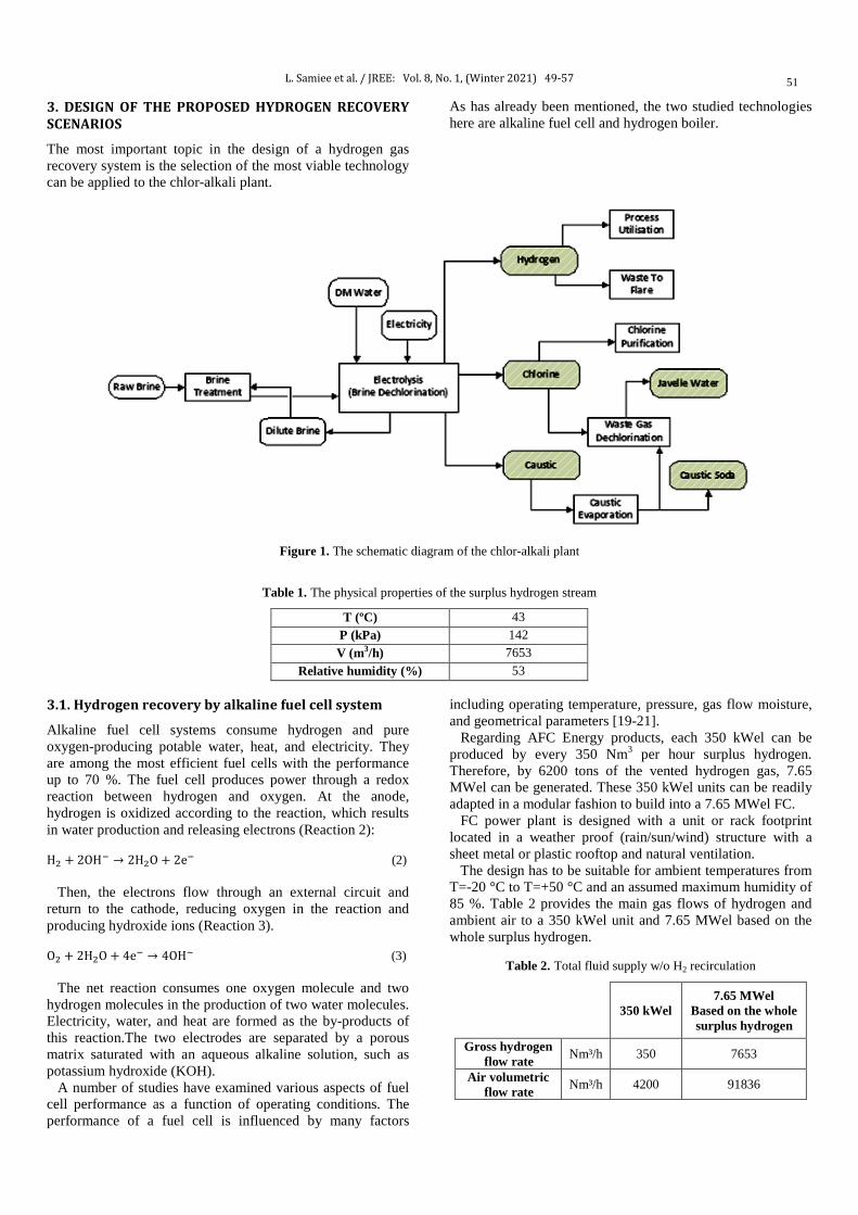
L. Samiee et al. / JREE: Vol. 8, No. 1, (Winter 2021) 49-57
51
3. DESIGN OF THE PROPOSED HYDROGEN RECOVERY SCENARIOS
The most important topic in the design of a hydrogen gas recovery system is the selection of the most viable technology can be applied to the chlor-alkali plant.
As has already been mentioned, the two studied technologies here are alkaline fuel cell and hydrogen boiler.
Figure 1. The schematic diagram of the chlor-alkali plant
Table 1. The physical properties of the surplus hydrogen stream
T (ºC) 43 P (kPa) 142 V (m3/h) 7653
Relative humidity (%) 53 3.1. Hydrogen recovery by alkaline fuel cell system
Alkaline fuel cell systems consume hydrogen and pure oxygen-producing potable water, heat, and electricity. They are among the most efficient fuel cells with the performance up to 70 %. The fuel cell produces power through a redox reaction between hydrogen and oxygen. At the anode, hydrogen is oxidized according to the reaction, which results in water production and releasing electrons (Reaction 2):
H2 + 2OH− → 2H2O + 2e− (2)
Then, the electrons flow through an external circuit and return to the cathode, reducing oxygen in the reaction and producing hydroxide ions (Reaction 3).
O2 + 2H2O + 4e− → 4OH− (3)
The net reaction consumes one oxygen molecule and two hydrogen molecules in the production of two water molecules. Electricity, water, and heat are formed as the by-products of this reaction.The two electrodes are separated by a porous matrix saturated with an aqueous alkaline solution, such as potassium hydroxide (KOH). A number of studies have examined various aspects of fuel cell performance as a function of operating conditions. The performance of a fuel cell is influenced by many factors
including operating temperature, pressure, gas flow moisture, and geometrical parameters [19-21]. Regarding AFC Energy products, each 350 kWel can be produced by every 350 Nm3 per hour surplus hydrogen. Therefore, by 6200 tons of the vented hydrogen gas, 7.65 MWel can be generated. These 350 kWel units can be readily adapted in a modular fashion to build into a 7.65 MWel FC. FC power plant is designed with a unit or rack footprint located in a weather proof (rain/sun/wind) structure with a sheet metal or plastic rooftop and natural ventilation. The design has to be suitable for ambient temperatures from T=-20 °C to T=+50 °C and an assumed maximum humidity of 85 %. Table 2 provides the main gas flows of hydrogen and ambient air to a 350 kWel unit and 7.65 MWel based on the whole surplus hydrogen.
Table 2. Total fluid supply w/o H2 recirculation
350 kWel 7.65 MWel
Based on the whole surplus hydrogen
Gross hydrogen flow rate Nm³/h 350 7653
Air volumetric flow rate Nm³/h 4200 91836

L. Samiee et al. / JREE: Vol. 8, No. 1, (Winter 2021) 49-57
52
In addition to electricity, the reaction between hydrogen and oxygen in the alkaline cells produces approximately 0.5 l/kWhel of water (Table 3).
Table 3. Formation of water from reaction
400 kWel
7.65 MWel Based on the whole surplus
hydrogen Process water
flow rate Nm³/h 0.18 3.83
At the start time of the alkaline fuel cell power plant, the ambient air is discharged with the nitrogen entry from the hydrogen-containing tubes and the anode compartment for fuel cell. Nitrogen is also used at the decommissioning time to remove all the remaining hydrogen in the system. This operation is performed to prevent the formation of any explosive atmospheres in the system. Moreover, due to the fact that the input pressure in the fuel cell should be in the range of 1.1-1.5 bara, it is fully compatible with the hydrogen outlet pressure of 1.42 bara. The schematic diagram of hydrogen recovery by alkaline fuel cell technique is presented in Fig. 2.
Figure 2. The schematic diagram of hydrogen recovery by alkaline fuel cell technique
3.2. Hydrogen recovery by hydrogen boiler system
Basically, boilers are divided into two categories: waterpipe (water in the pipe) and firewall (fire in the tube), depending on the operation type. Boilers can also be designed horizontally or vertically, single-burned or combined fuel or with the ability to fuel type change. One of the boiler types is hydrogen boilers. Hydrogen boiler is referred to as a steam generator which produces heat by burning hydrogen and oxygen at a stoichiometric ratio in a combustion chamber. The reaction heat of oxygen and hydrogen, transmitted through three methods of radiation, convection, and conduction, heats the water and produces steam or hot water [22]. Various industrial samples from these boilers have been designed and utilized in the world. These boilers can be
horizontal or vertical, in which the efficiency is usually higher than 90 %. Hydrogen flow rate for burning varies from 400 m3/hr to 30,000 m3/hr. This kind of boilers can [22] also produce vapor up to the pressure of 4000 kPa according to the present technology. Also, the temperature in the range of 190 to 400 °C can be changed. In comparison to gas-fueled boilers, the NOx amount is lower and the combustion output is water and nitrogen [18]. In some cases, by heat recycling, the water vapor in the outlet of the combustion chamber can be recovered and used as the deionized water. In the following, the schematic diagram of hydrogen recovery by hydrogen boiler technique in our case is presented in Fig. 3.
Figure 3. The schematic diagram of hydrogen recovery by hydrogen boiler technique
As can be seen, in case of hydrogen boiler installation in order to solve the high humidity issue of the inlet hydrogen (for burning in a hydrogen boiler), some treatment should be
provided. In order to reduce moisture, the best way is to increase the hydrogen pressure by a compressor system, reduce its temperature, and isolate the liquid moisture. By

L. Samiee et al. / JREE: Vol. 8, No. 1, (Winter 2021) 49-57
53
increasing the pressure and cooling to very low temperatures, the hydrogen stream humidity also decreases. In other words, at first, the H2 wasted stream with a temperature of 43 ºC, pressure of 142 KPa, and humidity of 53 % enters the compressor and after increasing the pressure and cooling in the after-cooler with temperature 43 ºC and pressure 1410 KPa, it enters the drum. The water vapor cooling to a liquid in the drum separates from the hydrogen stream and is sent to the hydrogen boiler as fuel at a temperature of 43 ºC and pressure 1410 KPa. Table 4 shows the results of this compressor system simulation.
Table 4. Physical characteristics of the vented hydrogen stream at two compression stages
Compressor Stage 1 Stage 2 Tin oC 43 43 Tout
oC 216 200 Pin kPa 142 470 Pout kPa 471 1410 Vin m3/h 7653 2214 Vout m3/h 3571 1110
mo(H2O) kg/h 319.2 86.93
Power consumption kW 577 500
In general, for the steam production, the main equipment includes hydrogen boiler, compressor, pipe, and control devices. In order to increase hydrogen pressure as a fuel, two compressor packages, one of which is stand-by, are considered and each package includes two stages. Table 5 provides the main flow rate of hydrogen and ambient air consumed in, generated steam pressure and temperature, and the amount of water produced based on the whole surplus hydrogen. Given the fact that 7653 m3/h of hydrogen is normally available at present, the choice of two boilers with different capacities of 8 and 20 tons of steam per hour, which totally require 7840 m3/h of hydrogen as fuel, provides the flexibility to prevent shutdown of the boilers due to fluctuations in hydrogen flow. Moreover, if the produced hydrogen flow rate is less than 7840 m3/h, the smaller boiler can continue to operate down to 60 % of its capacity. Also, reduction of production capacity for larger boiler can be operational. Thus, choosing two boilers with capacities of 8 and 20 tons per hour can be a good choice for process flexibility.
Table 5. The results of hydrogen boiler calculation [18]
H2O production (kg/h)
Air consumption (kg/h)
Temperature (°C)
Steam pressure (bar)
H2 consumption (m3/h)
Steam production capacity (ton/h)
897 3446 198 14 1120 4 1346 5169 198 14 1680 6 1795 6892 198 14 2240 8 2243 8615 220 20 2800 10 3365 12923 220 20 4200 15 4487 17230 245 25 5600 20 5608 21538 245 25 7000 25 7852 30153 245 25 9800 35
15703 60305 245 25 19600 70 4. RESULTS AND DISCUSSION
In the following section, the techno-economic assessment of the above scenarios will be discussed in terms of payback, NPV, and IRR. The required data for technical and economic analysis will be provided from Table 6.
Table 6. The required data for technical and economic analysis
Hydrogen L H V (kJ/kg) 119960 Power cost (€/kWh) 0.03
Natural gas L H V (kJ/kg) 48370 HP steam (€/ton) 9.97
Interest rate (I), (%) 15 Maximum payback
(Yr) 5
* All the utility prices are from project owner. 4.1. Energy analysis As the average mass flow rate of hydrogen gas (782.83 kg/h), its average LHV value (120000 kJ/kg), and the running time of the chlor-alkali plant (8000 h/year based on process operating hours) are known, it is possible to evaluate the energy obtained by the combustion of the vented hydrogen gas. The yearly primary energy saving obtained by the recovery of the vented hydrogen gas equals about 93.9 TJ corresponding to 1992.5 kg of natural gas.
The investigations of hydrogen boiler scenario show that hydrogen boiler can produce 28 ton/hr steam at pressure of 25 bar and temperature of 245 °C. The thermodynamic analysis of the hydrogen boiler shows that the input energy by the hydrogen waste equals 26 MW; however, the energy output by the steam generated is about 21 MW. Therefore, the amount of 5 MW wasted energy is released to the atmosphere by the exhaust steam. As explained in Section 3.2, in the case of hydrogen recovery by hydrogen boiler system, a compressor should be used for removal of hydrogen stream moisture. So, in order to assess a correct energetic and economic analysis of hydrogen boiler, the electricity required for compressor consumption was calculated. The compressor can be couplet with an electric motor and the final electrical energy consumed by the compressor is equal to 8610 MWh for 8000 h. In addition, the alkaline fuel cell system (based on the calculations in Section 3.1) also can produce 7.65 MW of electricity as well as 3.83 m3/h of deionized water. 4.2. Economic analysis In this section, the main capital costs of the installation of the recovery system including alkaline fuel cell and hydrogen boiler systems are reported and a techno-economic assessment

L. Samiee et al. / JREE: Vol. 8, No. 1, (Winter 2021) 49-57
54
is performed. Of course, as it was mentioned in the case of capital costs of hydrogen boiler, the compressor cost for increasing pressure should also be considered. The main considered costs are the civil works required for the installation of the above systems and the engineering works for the system design [23]. Based on the manufacturing scale and 28 ton/hr steam generation, two-boiler package with a conventional capacity of 20 and 8 ton/hr (JOC Company) was considered. The economic parameters of steam production using hydrogen boiler are shown in Table 7. In this table, the Internal Rate of Return (IRR), Net Present Value (NPV), and Payback time are calculated. In this scenario, the results of NPV and IRR are relatively reasonable. The following formula is used to calculate NPV:
NPV= �∑ Net Cash Inflowt(1+r)t
nt=1 � -Initial Investment (1)
where t represents the time in years, r is R/100 (R= the interest or discount rate), and n is the number of periods or years. Furthermore, IRR formula is the following one:
IRR=ra+ NPVa
NPVa-NPVb�rb-ra� (2)
where ra and rb represent the lower and the higher discount rates, respectively, NPVa is the net present value at ra, and NPVb is the net present value at rb. Regarding the steam price (9.97 €/ton), the hydrogen boiler project revenue is estimated showing that the IRR is fairly good at around 29 %. Moreover, considering a 15 % discount rate, the NPV is also positive. Thus, the option of using a hydrogen boiler could be an appropriate and economical idea for steam production in our case. Furthermore, the IRR, NPV, and Payback time are calculated for alkaline fuel cell approach in Table 8. In the case of the alkaline fuel cell scenario, the IRR and NPV are negative. Thus, in terms of calculations based on electricity prices (0.03 €/kwh), because of the high cost of investment and the cheapness of the unit price of electricity, the alkaline fuel cell scenario will not be cost-effective. The NPV of the base case configuration is negative, thus with the assumed prices and conditions, the alkaline fuel cell scenario is not an attractive choice. The value of the NPV is -8270000€.
Table 7. Economic parameters for steam production using hydrogen boiler
Items Unit Scenario 1 2 Boiler package (8 ton/hr+20 ton/hr)
Euro
2,411,450* 2 Compressor package 1,590,350
Piping, instruments, controls and electrical 298,350 Commissioning, installation cost 197,200
Direct cost 4,497,350 Indirect cost 296,650
Fixed capital investment Euro 4,794,000 Annual cost Euro/y 575,450
Annual benefit 2,076,550 Discount rate % 15
IRR % 29 NPV Euro 2,739,550
Payback time year 4 One compressor package is standby mode.
* The price reference is from JOC Company.
Table 8. Economic parameters of electricity and water production using alkaline fuel cell
Items Unit Alkaline Fuel cell scenario Alkaline fuel cell package
Euro
9476403* Installation cost 1895280
Total direct cost (carbon steal) 11371684.29 Total indirect cost 947640
Fixed capital investment Euro 12319324 Annual cost Euro/y 1231932
IRR % -7.03 NPV Euro -8.27E+06
Payback time year 15.3 * The price reference is from AFC Company.
According to the sensitivity analysis (Fig. 4), variations in the electricity price have significant impact on NPV value. With increase in electricity value to 0.15 €/kWh which is a normal average price in the world, this scenario will become completely reasonable and profitable. In addition, Fig. 5 shows the rate of IRR fluctuations versus the surplus hydrogen volume. Fig. 5 Sensitivity analysis of the surplus
hydrogen volume variable in a fuel cell and hydrogen boiler scenarios. With an increase in hydrogen flow rate due to the energy-saving increment generated by steam or electricity, the IRR rises. However, because of the electricity cheapness (0.03 €/kWh) and high cost of initial investment, the IRR is still very small even at the large flow rate of hydrogen, thus confirming the results obtained from Fig. 4.

L. Samiee et al. / JREE: Vol. 8, No. 1, (Winter 2021) 49-57
55
4.3. Emissions reduction estimation
The increase in the concentration of greenhouse gases causes the temperature rise of the earth [23]. The gases that have greenhouse effect can be reduced by the implementation of the proposed ideas (using hydrogen boiler and alkaline fuel cell instead of fossil fuel technologies). The emission of greenhouse gases and the resultant pollutants due to fossil fuel from the equipment is referred to as combustion emissions. Most of the greenhouse gases emitted from combustion include CO2, N2O, and CH4 (due to incomplete combustion). The most accurate and reliable method for estimating the amount of carbon dioxide from combustion sources is the mass balance method based on fuel consumption and carbon content of the fuel [24].
Figure 4. Sensitivity analysis of the electricity price variable in the
fuel cell scenario
Figure 5. Sensitivity analysis of the surplus hydrogen volume
variable in a fuel cell and hydrogen boiler scenarios
Generally, the hydrocarbon combustion with the assumption of complete combustion follows Reaction (4):
CxHyOz + �x + y4− z
2�O2 → (x)CO2 + �y
2�H2O (4)
The carbon content of the fuel mixture is the average of carbon content of each component. To achieve this, at first, the percentage of carbon per fuel component is calculated and then, is completed by multiplication of the molecular weight of carbon in the number of carbon molecules divided by the molecular weight of the compound. The carbon content, which is equal to the average carbon content of the constituent components of a compound, is calculated through Equation (3).
Wt %CMixture = 1100
∑ (Wt %i × Wt %Ci) #componentsi=1 (3)
In this equation, Wt %i is the weight percentage of i component in the fuel mixture and Wt%Ci is the carbon content based on the weight. Therefore, the amount of carbon dioxide emissions from combustion sources with natural gas is calculated using Equation (4).
ECO2 = FC × 1molar volume conversion
× MWMixture × Wt %CMixture × 4412
(4)
where FC is the amount of fuel consumed (Sm3), MWmixture is the molecular weight of the fuel mixture, and the molar volume conversion is the conversion factor of molecular volume to mass, which is equal to 23,685 m3/kgmole. In addition to estimating CO2 emissions based on 100 % carbon oxidation, the Compendium API estimates the emission of CH4 and N2O from the combustion source based on emission factors, as presented in Table 7. After calculating the amount of greenhouse gas emissions using their heating potential, they are converted to carbon dioxide equivalents which are equal to 1, 25, and 298 for CO2, CH4, and N2O, respectively [24]. To estimate the emission of pollutants from combustion, the global emission factors related to AP-42 reference presented in Table 9 are used.
Table 9. Greenhouse gas emissions factors and pollutants in the
combustion process with natural gas [25]
CH4 N2O NOx CO PM VOCs
kg/106 Nm3 Unit
37.88 10.55 4237.84 1271.35 115.03 83.24 Emission factor
Thus, by determining the amount and percentage of the fuel, the amount of emission reductions and greenhouse gas emissions can be calculated. Obviously, all the actions that are taken to reduce fossil fuel consumption can be considered as one way to reduce greenhouse gas emissions in the energy sector. This study shows that the implementation of each scenario can reduce the average annual consumption of natural gas with the composition given in Table 10 and their corresponding greenhouse gas emissions, significantly.Now, using Equation (6), the amount of CO2 emitted from each of the scenarios can be calculated. Also, with the coefficients given in Table 11, the amounts of N2O, CH4, pollutants, and greenhouse gases can be calculated for each of the scenarios presented in Table 12.
L. Samiee et al. / JREE: Vol. 8, No. 1, (Winter 2021) 49-57
56
Table 10. The composition of the natural gas consumed in our case study
Unit CH4 C2H6 C3H8 C4H10 C4H12 C6H14 N2 CO2
Methane Ethane Propane Butane Butane Hexane Nitrogen Carbon dioxide
% 84.98 5.47 2.09 0.87 0.31 0.35 3.02 2.91
Table 11. The amounts of greenhouse gases emission reduction per year
Scenario CO2 CH4 N2O Total
kg CO2 kg CH4 kg CO2e kg N2O kg CO2e kg CO2e Alkaline fuel cell 58,776,900 1,830.3 45,600 223.7 66,700 58,889,200 Hydrogen boiler 49,287,700 917.2 22,900 255.3 76,100 49,386,700
Table 12. The amounts of pollutants emission reduction per year
Scenario NOx (kg) CO (kg) PM (kg) VOCs (kg) Total (kg) Alkaline fuel cell 44,416.1 37,908.2 10,331.2 2,521.8 95,200 Hydrogen boiler 104,733.1 31,419.9 2,842.8 2,057.2 141,000
The basis of the CO2e reduction calculation in the two scenarios is the power generation using gas turbine and boiler fuel, respectively. The results in Table 11 show that if the surplus hydrogen is used to generate electricity using fuel cell, approximately 58800 tons of CO2e will annually be emitted and if steam hydrogen boiler is used for steam productions, the CO2e emissions reduction will be around 49300 tons. The reduction in greenhouse gas emissions for the electricity generation scenario is higher than that for the steam generation scenario, because the electricity generation in this study is based on a gas turbine with less than 30 % efficiency in the best conditions of a gas turbine, whereas the boilers have an efficiency rate of at least 60 %. On the other hand, due to the fact that boilers use heavy fuel like gasoline, they produce more emissions than gas turbines. Thus, the emission reductions in the steam generation scenario are higher than that in the electricity generation scenario using the fuel cell (Table 12). 5. CONCLUSIONS
In the work presented here, two important technologies for the hydrogen gas recovery in one industrial chlor-alkali plant were reported: (a) the alkaline fuel cell for electricity and water production and (b) the hydrogen boiler for steam generation. The use of an alkaline fuel cell system can be a suitable solution for hydrogen recovery in chlor-alkali plants, where energy consumptions are high and high-purity hydrogen is available as by-product. Furthermore, using hydrogen boiler systems can be beneficial as they can produce half of the steam needed in the chlor-alkali plant. According to the running conditions of an industrial chlor-alkali plant, the concept design and the performance of the two proposed technologies for hydrogen recovery were reported. The results showed that almost 6200 tons hydrogen gas with a pressure of 142 kPa and 99 % purity was annually being vented. In the case of hydrogen boiler system, a two-stage compressor was adopted to increase the hydrogen pressure to a level that can be used as input pressure in the boiler system: its main characteristics and energy consumption are evaluated. The steam amounts that can be produced are 28 ton/hr steam at pressure of 25 bar and temperature of 245 °C. Whereas this
pressure increase is not required in alkaline fuel cell scenario as the input pressure should be in the range of 0.1-0.5 bar which is completely compatible with the hydrogen outlet pressure from the vent stream. This approach can generate 7.65 MW of electricity and 3.83 m3/h of deionized water. Moreover, an economic analysis is reported considering the capital and operating cost of the system to evaluate IRR and NPV parameters: with an interest rate of 15 %, the alkaline fuel cell scenario has negative IRR and NPV, whereas the hydrogen boiler project has the fairly good IRR and positive NPV. Moreover, in terms of emission reduction, hydrogen boiler and alkaline fuel cell techniques can significantly reduce greenhouse gas emission by 49300 and 58800 tons/year, respectively. Also, the other pollutants can be diminished by 141 and 95 tons/year in hydrogen boiler and alkaline fuel cell scenarios, respectively. Therefore, the obtained results showed that by applying the hydrogen boiler solution, all the technical, economic and environmental advantages could be achieved. 6. ACKNOWLEDGEMENT
We would like to acknowledge the support made available by the Research Institute of Petroleum Industries (RIPI). NOMENCLATURE
IRR Internal Return Rate
NPV Net Present Value
FCH JU Fuel Cells and Hydrogen Joint Undertaking
AFCEN AFC energy
JOC Jiangsu Overseas Group
LHV Low Heating Value
PFD Process Flow Diagram
T Temperature (ºC)
P Pressure (kPa)
V Gas volumetric flow rate (m3/h)
mo Gas mass flow rate (kg/h)
t Time in years
R The interest or discount rate

L. Samiee et al. / JREE: Vol. 8, No. 1, (Winter 2021) 49-57
57
n The number of periods or years
ra The lower discount rate
rb The higher discount rate
Wt %i The weight percentage of i component
Wt %Ci The carbon content based on the weight
FC The amount of fuel consumed (Sm3)
MWmixture The molecular weight of the fuel mixture
REFERENCES 1. Zhou, J., Xu, H. and Gao, L., "New process of separation and
purification byproduct hydrogen in chlor-alkali plants", Proceedings of 2010 International Conference on Mechanic Automation and Control Engineering, (2010). (https://doi.org/10.1109/MACE.2010.5535424).
2. Faur Ghenciu, A., "Review of fuel processing catalysts for hydrogen production in PEM fuel cell systems", Current Opinion in Solid State and Materials Science, Vol. 6, No. 5, (2002), 389-399. (https://doi.org/10.1016/S1359-0286(02)00108-0).
3. Li, H., Wang, H., Qian, W. and Zhang, Sh., "Chloride contamination effects on proton exchange membrane fuel cell performance and durability", Journal of Power Sources, Vol. 196, No. 15, (2011), 6249-6255. (https://doi.org/10.1016/j.jpowsour.2011.04.018).
4. Bommaraju, T.V. and O’Brien, T.F., Brine Electrolysis, Electrochemistry Encyclopedia, (2007). (https://knowledge.electrochem.org/encycl/art-b01-brine.htm).
5. Garcia-Herrero, I., Margallo, M., Onandía, R., Aldaco, R. and Irabien, A., "Environmental challenges of the chlor-alkali production: Seeking answers from a life cycle approach", Science of the Total Environment, Vol. 580, (2017), 147-157. (https://doi.org/10.1016/j.scitotenv2016.10.202).
6. Garcia-Herrero, I., Margallo, M., Onandía, R., Aldaco, R. and Irabien, A., "Life Cycle Assessment model for the chlor-alkali process: A comprehensive review of resources and available technologies", Sustainable Production and Consumption, Vol. 12, (2017), 44-58. (https://doi.org/10.1016/j.spc.2017.05.001).
7. Chaubey, R., Sahu, S., James, O. and Maity, S., "A review on development of industrial processes and emerging techniques for production of hydrogen from renewable and sustainable sources", Renewable and Sustainable Energy Reviews, Vol. 23, (2013), 443-462. (https://doi.org/10.1016/j.rser.2013.02.019).
8. Dutta, S., "A review on production, storage of hydrogen and its utilization as an energy resource", Journal of Industrial and Engineering Chemistry, Vol. 20, No. 4, (2014), 1148-1156. (https://doi.org/10.1016/j.jiec.2013.07.037).
9. Hamad, T.A., Agll, A.A., Hamad, Y.M., Bapat, S., Thomas, M., Martin, K.B. and Sheffield, J.W., "Hydrogen recovery, cleaning, compression, storage, dispensing, distribution system and End-Uses on the university campus from combined heat, hydrogen and power system", International Journal of Hydrogen Energy, Vol. 39, No. 2, (2014), 647-653. (https://doi.org/10.1016/j.ijhydene.2013.10.111).
10. Chlorine industry review 2011-2012, (2012). (https://www.eurochlor.org/publication/chlorine-industry-review-2011-2012).
11. Verhage, A.J.L., Coolegem, J.F., Mulder, M.J.J., Yildirim, M.H. and de Bruijn, F.A., "30,000 h operation of a 70 kW stationary PEM fuel cell system using hydrogen from a chlorine factory", International Journal
of Hydrogen Energy, Vol. 38, No. 11, (2013), 4714-4724. (https://doi.org/10.1016/j.ijhydene.2013.01.152).
12. Air products in AFC project to use surplus industrial hydrogen. (Available from: http://www.afcenergy.com/).
13. Lin, B.Y.S., Kirk, D.W. and Thorpe, S.J., "Performance of alkaline fuel cells: A possible future energy system?", Journal of Power Sources, Vol. 161, No. 1, (2006), 474-483. (https://doi.org/10.1016/j.jpowsour.2006.03.052).
14. DEMCOPEM-2MW Project official website, (2015). (https://demcopem-2mw.eu/).
15. Guandalini, G., Foresti, S., Campanari, S., Coolegem, J.F. and Have, J.T., "Simulation of a 2 MW PEM fuel cell plant for hydrogen recovery from chlor-alkali industry", Energy Procedia, Vol. 105, (2017), 1839-1846. (http://doi.org/10.1016/j.egypro.2017.03.538).
16. Peantong, S. and Tangjitsitcharoen, S., "A study of using hydrogen gas for steam boiler", Proceedings of IOP Conference Series: Materials Science and Engineering, Vol. 215, (2017), 012018. (https://doi.org/10.1088/1757-899X/215/1/012018).
17. Khasawneh. H., Saidan, M. and Al-Addous, M., "Utilization of hydrogen as clean energy resource in chlor-alkali process", Energy Exploration & Exploitation, Vol. 39, No. 3, (2019), 1053-1072. (https://doi.org/10.1177/0144598719839767).
18. Waste hydrogen utilization system. (Available from: http://www.jocite.com/en/ctt/1/79.htm).
19. Ahmadi, N., Rezazadeh, S., Dadvand, A. and Mirzaee, I., "Study of the effect of gas channels geometry on the performance of polymer electrolyte membrane fuel cell", Periodica Polytechnica Chemical Engineering, Vol. 62, (2018), 97-105. (https://doi.org/10.3311/PPch.9369).
20. Ahmadi, N., Rezazadeh, S., Dadvand, A. anf Mirzaee, I., "Numerical investigation of the effect of gas diffusion layer with semicircular prominences on polymer exchange membrane fuel cell performance and species distribution", Journal of Renewable Energy and Environment (JREE), Vol. 2, (2015), 36-46. (https://doi.org/10.30501/JREE.2015.70069).
21. Ahmadi, N. and Kõrgesaar, M., "Analytical approach to investigate the effect of gas channel draft angle on the performance of PEMFC and species distribution", International Journal of Heat and Mass Transfer, Vol. 15, (2020), 119529. (https://doi.org/10.1016/j.ijheatmasstransfer.2020.119529).
22. Ditaranto, M., Anantharaman, R. and Weydahl, T., "Performance and NOx emissions of refinery fired heaters retrofitted to hydrogen combustion", Energy Procedia, Vol. 37, (2013), 7214-7220. (https://doi.org/10.1016/j.egypro.2013.06.659).
23. TSS Consultants, 2724 Kilgore Road, Rancho Cordova, CA 95670, "Cost estimates for capital expenditure and operations & maintenance based on technology review", (2009). (https://ucanr.edu/sites/WoodyBiomass/newsletters/Feasibility_Studies_-_Reports47400.pdf.)
24. Shires, T.M., Loughran, C. J., Jones, S. and Hopkins, E., "Compendium of greenhouse gas emissions methologies for the oil and natural gas industry", (2009). (https://www.api.org/~/media/files/ehs/climate-change/2009_ghg_compendium.ashx).
25. Intergovernmental Panel on Climate Change (IPCC), Greenhouse gas inventory reference manual: 2006 IPCC guidelines for national greenhouse gas inventories, United Nations. (Available from: http://www.ipcc-nggip.iges.or.jp/public/2006gl/).

JREE: Vol. 8, No. 1, (Winter 2021) 58-68
Please cite this article as: Hoseini, S.S. and Sobati, M.A., "Assessment of the performance and exhaust emission of a diesel engine using water emulsion fuel (WEF) in different engine speed and load conditions", Journal of Renewable Energy and Environment (JREE), Vol. 8, No. 1, (2021), 58-68. (https://doi.org/10.30501/jree.2020.233709.1115).
2423-7469/© 2021 The Author(s). Published by MERC. This is an open access article under the CC BY license (https://creativecommons.org/licenses/by/4.0/).
Research Article
Journal of Renewable Energy and Environment
J o u r n a l H o m e p a g e : w w w . j r e e . i r
Assessment of the Performance and Exhaust Emission of a Diesel Engine Using Water Emulsion Fuel (WEF) in Different Engine Speed and Load Conditions
Seyed Saeed Hoseini, Mohammad Amin Sobati*
Department of Chemical, Petroleum and Gas Engineering, Iran University of Science and Technology,Tehran, Tehran, Iran.
P A P E R I N F O
Paper history: Received 27 June 2020 Accepted in revised form 08 December 2020
Keywords: Water Emulsion Fuel, Engine Performance, Exhaust Emission, Engine Speed, Engine Load
A B S T R A C T
The performance characteristics and exhaust emission of a diesel engine using Water Emulsion Fuel (WEF) have been investigated under different engine speeds (1600 to 2400 rpm) and load conditions (25 to 100 %). The experiments were carried out on an air-cooled diesel engine of single cylinder using the WEF containing 5 % water, 2 % surfactant with Hydrophilic-Lipophilic Balance (HLB) of 6.8. The engine performance and exhaust emission using WEF were also compared with the Neat Diesel Fuel (NDF). According to the results, average reduction of 9.7 % in the engine torque and brake power was observed using WEF at all engine speeds. In addition, a 7.9 % increase in the Brake Specific Fuel Consumption (BSFC) and a 3.7 % increase in the Brake Thermal Efficiency (BTE) were observed for WEF in comparison with NDF in all loading conditions. In case of emission, significant lower hydrocarbon emission (i.e., 14.6 % on average) was observed for WEF comparing to NDF at all engine speeds. Moreover, a considerable reduction in the NOx emission (i.e., 31.1 % on average) was observed for the WEF comparing to the NDF in every engine load. In summary, the application of WEF leads to the reduction in the emission of different pollutants with a positive impact on the environment.
https://doi.org/10.30501/jree.2020.233709.1115
1. INTRODUCTION1
Diesel devices are broadly engaged in the industrial sectors, the agricultural applications, and the commercial transportation. Emissions from the diesel engines are a substantial source of Particulate Matters (PM) and the greenhouse gasses which in turn have negative effect on the environment. In addition, the combustion of neat diesel fuel in the diesel engines leads to the production of harmful gasses like Carbon Monoxide (CO), Nitrogen Oxides (NOx), and Unburnt Hydrocarbon (UHC) that are categorized among the significant sources of the air pollution . Therefore, the researchers are always looking for new fuels that can reduce the harmful emissions and enhance the engine performance. An improvement in the engine performance and exhaust emission is a substantial issue when using an alternate fuel in the diesel engine. Accordingly, the researchers have investigated the use of various fuel mixtures such as biodiesel and Water Emulsion Fuel (WEF). Gardy et al. [1] investigated the effect of different catalysts on the biodiesel production. They focused on the challenges such as corrosion and the high cost of biodiesels on the industrial scale. The advantage of WEF is its lower viscosity than the biodiesel, because high viscosity leads to the creation of disturbances in the combustion, pumping, and atomization of the diesel engine injection system. On the other hand, biofuels are more
*Corresponding Author’s Email: [email protected] (M.A. Sobati) URL: http://www.jree.ir/article_120192.html
corrosive than WEF [2]. Furthermore, the application of WEF decreases the combustion enclosure temperature and, as a result, the NOx formation in the exhaust gas. The combustion of WEF is associated with the micro explosion. In this phenomenon, the size of fuel droplets is suddenly reduced and the fuel burns with high efficiency as a result of increasing the contact surface. Examinations of the impact of WEF on the engine
performance and emission of pollutants have been studied by various researchers. Yang et al. [3] and Fahd et al. [4] stated a decrease in the brake power of WEF compared to Neat Diesel Fuel (NDF) in different engine speed conditions. In addition, according to Alenezi et al. [5], the engine power was decreased slightly using WEF compared to the NDF in the all engine load conditions. On the contrary, Seifi et al. [6] and Alahmer et al. [7] reported an opposite trend in which the brake power was higher for the WEF compared to the NDF at different engine speeds. Venu et al. [8] conducted the experimental runs on a single cylinder diesel engine using the emulsified fuel at diverse engine loads. They reported a 6.58 % increment in the Brake Thermal Efficiency (BTE) of the emulsified fuel and a 7.38 % decrement in the Brake Specific Fuel Consumption (BSFC) of the emulsified fuel in all engine load conditions. On the other hand, Ninawe et al. [9] reported the opposite conclusion. They stated the Specific Fuel Consumption (SFC) of the emulsified fuel reduced and the BTE of the emulsified increased by 7.69 % and 5.5 %, respectively, at every engine load. Armas et al. [10] carried

S.S. Hoseini and M.A. Sobati / JREE: Vol. 8, No. 1, (Winter 2021) 58-68
59
out experiments on a Renault F8Q 4-cylinder and turbocharged using the emulsion fuel with constant water percentage of 10 % by weight. According to their results, the brake thermal efficiency has improved slightly compared to NDF. They found that the improvement of the fuel spray atomization, as a consequence of the micro-explosion phenomenon, resulted in the enhancement of the BTE. Baskar et al. [11] examined the performance of a single cylinder air-cooled engine at different loads. They indicated the water emulsion fuel containing 10 % water with the higher BTE (i.e., 33 %) at 100 % load compared to the BTE of the NDF (i.e., 30.5 %). Lin et al. [12] investigated the performance of a water-cooled four-cylinder diesel engine using the Water in Oil (W/O) and the Oil in Water in Oil (O/W/O) emulsion fuel containing the water content of 15 % and the surfactant content of 2 % (Span 80 & Tween 80) by volume. They found that the BTE of O/W/O emulsion fuel did not differ much from the NDF, while the efficiency of W/O emulsion fuel was slightly higher than the NDF considering every load condition. Moreover, Fahd et al. [4] found that the BTE of WEF was lower than the NDF under every engine speed and load conditions due to the reduced heating value of WEF. Saravanan et al. [13] and Lin et al. [12, 14] reported the increment of the BSFC of WEF than the NDF. On the contrary, Ithnin et al. [15] and Suresh et al. [16] only considered the content of the diesel available in WEF in the calculation of BSFC and hence, they found out the BSFC reduced substantially in all operating conditions compared to the NDF. In addition, Tsukahara et al. [17] presented various reasons for the decrement of BSFC. Generally, most of researchers [18-20] reported a reduction in the NOx formation for the diesel-water emulsified, O/W/O emulsion fuel, and the diesel fuel with dissolved methane compared to the NDF due to the reduction of the combustion enclosure temperature. According to El Shenawy et al. [21], the emission of NOx of the emulsion fuel was reduced by 33.6 % compared to the NDF in various engine load conditions. Fahd et al. [4] examined the CO emission of WEF containing 10 % water at different engine speeds (800-4000 rpm) at the engine loads of 10 % and 25 %, experimentally. They found that the CO emission was reduced by increment of the engine speed for both WEF and NDF. They also noted that the emission of CO was higher for the WEF than the NDF at part load. Moreover, according to Yang et al. [22], the CO emission of WEF with 10 % and 15 % water and NDF was increased by increasing the engine speed. Besides, according to their report, there was no difference between the emission of the CO using the WEF and the NDF at 100 % load. However, a slight increment in the CO emission of the WEF was observed compared to NDF in the partial load condition. They noted that the WEF had a lower combustion temperature than the NDF and hence, the CO emission was higher in the low load condition. On the contrary, according to Saravanan et al. [13] and Sudrajad et al. [23], the emission of CO was lower for the WEF than the NDF. They concluded that the micro-explosion phenomenon led to the production of richer air-fuel mixture and as a consequence of enhanced combustion, the CO formation was reduced. Yang et al. [22] reported that the HC emission using the WEF did not differ much from the NDF in the full-load condition. However, a slightly higher HC emission was reported using the WEF than the NDF in the partial-load condition. They concluded that the evaporation of the contained water in the WEF resulted in a decrease in the temperature of the combustion enclosure and
led to incomplete combustion, which in turn increasd the HC emission for the WEF compared to the NDF. Kannan et al. [24] pointed out that the emission of HC was lower for the WEF than the NDF in different load conditions. They reported 26.5 % and 42.5 % decrements in the emission of HC for the WEF with the water content of 10 % and 20 %, respectively. They mentioned that the micro-explosion phenomenon resulted in the enhanced fuel combustion and the improvement of the air-fuel mixing. On the contrary, Subramanian [25] reported that the HC emission was higher using the WEF instead of NDF in the all load conditions. Table 1 summarizes the different researches considering the engine performance and exhaust emission using WEF. Moreover, the effect of using diverse additives in the WEFs on the engine performance and exhaust emission can be observed in other works [26-28]. Based on the literature review, WEF is an efficient fuel that can improve the diesel engine performance and reduce the harmful exhaust emission. Nevertheless, contradictory results regarding the engine performance and exhaust emission can be figured out in the work of researchers. In our previous paper, the optimized formulation of the water in diesel emulsion fuels was found considering different criteria including fuel stability, engine performance, and emission at a constant engine speed under the full-load condition [29]. In continuation of our first paper, the principal goal of this investigation is to examine the performance and exhaust emission of a diesel engine considering the optimized WEF under different engine speed and load conditions. Therefore, the effects of engine speed and load on the performance and emission characteristics of the diesel engine were investigated using the optimized formulation of the WEF. In addition, the engine performance and exhaust emission using the WEF were compared with the NDF in detail. 2. EXPERIMENTAL DETAIL
2.1. Materials
In the present investigation, the NDF was supplied from the domestic fuel station in Tehran, Iran. The specifications of NDF are indicated in Table 2. It should be noted that the application of surfactant as the emulsifier is essential for the emulsion formation using two immiscible liquids of water and diesel. Therefore, a blend of two surfactants of Span 80 (hydrophobic) and Tween 80 (hydrophilic) supplied from Merck company (Germany) was used. More details regarding the specifications of the surfactant mixture and the stability of the prepared emulsion fuel can be found elsewhere [29]. 2.2. The procedure of preparation of water emulsion fuel (WEF)
A 400 W ultrasonic transducer equipped with a titanium horn with 12 mm diameter and constant frequency of 20 kHz was employed in the procedure of the WEF preparation. Based on our previous paper, the best formulation for the WEF was considered with the water content of 5 %, the surfactant content of 2 %, and Hydrophilic-Lipophilic Balance (HLB) of 6.8 [29]. In order to produce the emulsion fuel, the required amount of distilled water was introduced into the cylindrical container at first and a defined amount of Tween 80 was added gradually. Then, the power of 300 W was adjusted for the ultrasound apparatus. The immersion depth of the probe was selected as 1 cm. Next, the distillated water and Tween 80
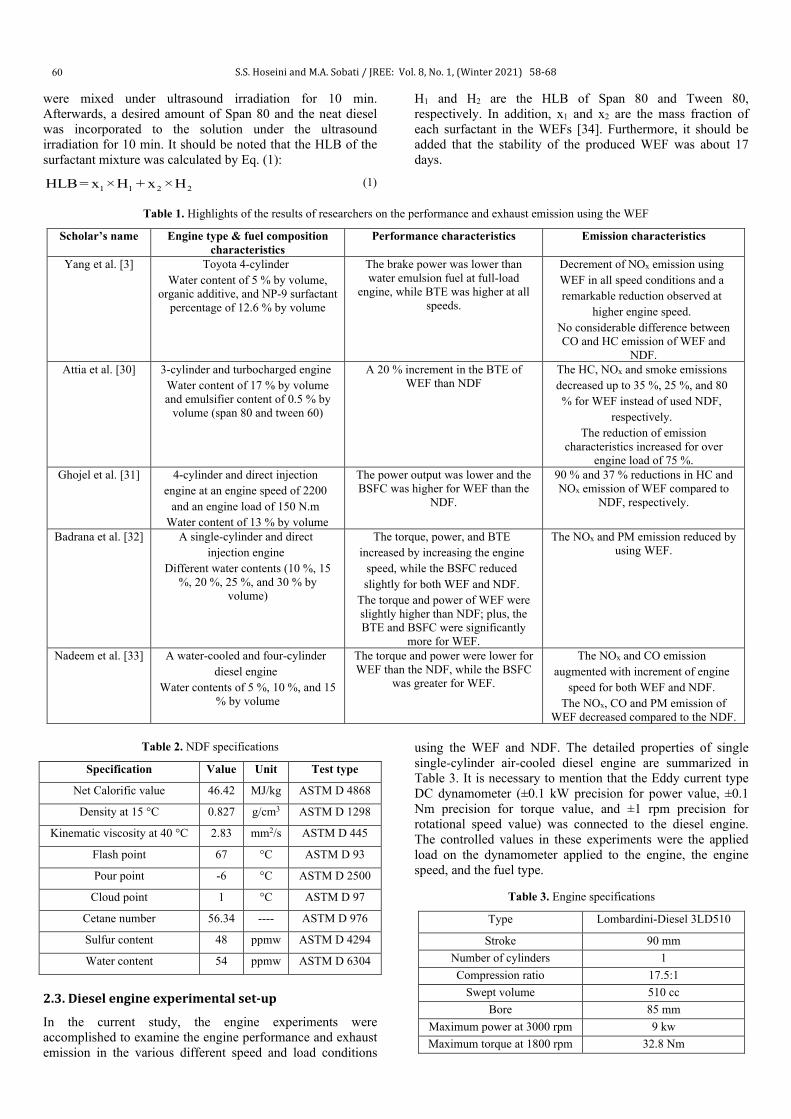
S.S. Hoseini and M.A. Sobati / JREE: Vol. 8, No. 1, (Winter 2021) 58-68
60
were mixed under ultrasound irradiation for 10 min. Afterwards, a desired amount of Span 80 and the neat diesel was incorporated to the solution under the ultrasound irradiation for 10 min. It should be noted that the HLB of the surfactant mixture was calculated by Eq. (1):
1 1 2 2HLB= x ×H + x ×H (1)
H1 and H2 are the HLB of Span 80 and Tween 80, respectively. In addition, x1 and x2 are the mass fraction of each surfactant in the WEFs [34]. Furthermore, it should be added that the stability of the produced WEF was about 17 days.
Table 1. Highlights of the results of researchers on the performance and exhaust emission using the WEF
Scholar’s name Engine type & fuel composition characteristics
Performance characteristics Emission characteristics
Yang et al. [3] Toyota 4-cylinder Water content of 5 % by volume,
organic additive, and NP-9 surfactant percentage of 12.6 % by volume
The brake power was lower than water emulsion fuel at full-load
engine, while BTE was higher at all speeds.
Decrement of NOx emission using WEF in all speed conditions and a remarkable reduction observed at
higher engine speed. No considerable difference between CO and HC emission of WEF and
NDF. Attia et al. [30] 3-cylinder and turbocharged engine
Water content of 17 % by volume and emulsifier content of 0.5 % by
volume (span 80 and tween 60)
A 20 % increment in the BTE of WEF than NDF
The HC, NOx and smoke emissions decreased up to 35 %, 25 %, and 80 % for WEF instead of used NDF,
respectively. The reduction of emission
characteristics increased for over engine load of 75 %.
Ghojel et al. [31] 4-cylinder and direct injection engine at an engine speed of 2200
and an engine load of 150 N.m Water content of 13 % by volume
The power output was lower and the BSFC was higher for WEF than the
NDF.
90 % and 37 % reductions in HC and NOx emission of WEF compared to
NDF, respectively.
Badrana et al. [32] A single-cylinder and direct injection engine
Different water contents (10 %, 15 %, 20 %, 25 %, and 30 % by
volume)
The torque, power, and BTE increased by increasing the engine
speed, while the BSFC reduced slightly for both WEF and NDF.
The torque and power of WEF were slightly higher than NDF; plus, the BTE and BSFC were significantly
more for WEF.
The NOx and PM emission reduced by using WEF.
Nadeem et al. [33] A water-cooled and four-cylinder diesel engine
Water contents of 5 %, 10 %, and 15 % by volume
The torque and power were lower for WEF than the NDF, while the BSFC
was greater for WEF.
The NOx and CO emission augmented with increment of engine
speed for both WEF and NDF. The NOx, CO and PM emission of
WEF decreased compared to the NDF.
Table 2. NDF specifications
Specification Value Unit Test type
Net Calorific value 46.42 MJ/kg ASTM D 4868
Density at 15 °C 0.827 g/cm3 ASTM D 1298
Kinematic viscosity at 40 °C 2.83 mm2/s ASTM D 445
Flash point 67 °C ASTM D 93
Pour point -6 °C ASTM D 2500
Cloud point 1 °C ASTM D 97
Cetane number 56.34 ---- ASTM D 976
Sulfur content 48 ppmw ASTM D 4294
Water content 54 ppmw ASTM D 6304
2.3. Diesel engine experimental set-up
In the current study, the engine experiments were accomplished to examine the engine performance and exhaust emission in the various different speed and load conditions
using the WEF and NDF. The detailed properties of single single-cylinder air-cooled diesel engine are summarized in Table 3. It is necessary to mention that the Eddy current type DC dynamometer (±0.1 kW precision for power value, ±0.1 Nm precision for torque value, and ±1 rpm precision for rotational speed value) was connected to the diesel engine. The controlled values in these experiments were the applied load on the dynamometer applied to the engine, the engine speed, and the fuel type.
Table 3. Engine specifications
Type Lombardini-Diesel 3LD510
Stroke 90 mm Number of cylinders 1 Compression ratio 17.5:1
Swept volume 510 cc Bore 85 mm
Maximum power at 3000 rpm 9 kw Maximum torque at 1800 rpm 32.8 Nm
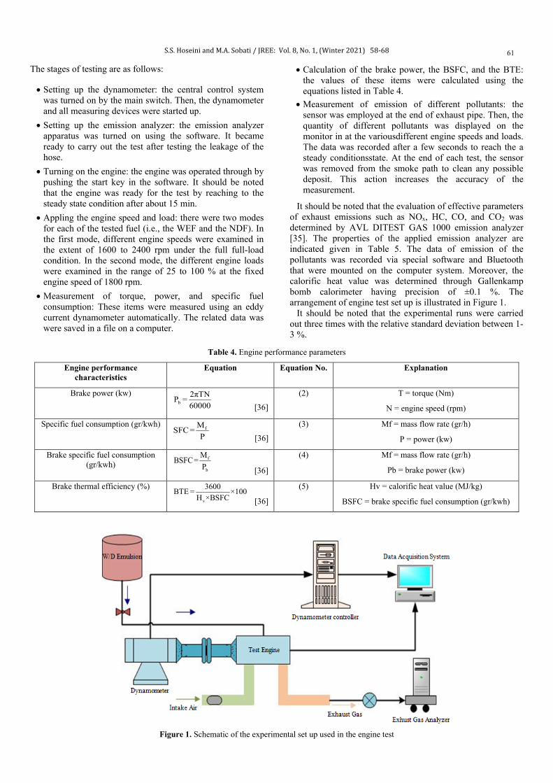
S.S. Hoseini and M.A. Sobati / JREE: Vol. 8, No. 1, (Winter 2021) 58-68
61
The stages of testing are as follows :
• Setting up the dynamometer: the central control system was turned on by the main switch. Then, the dynamometer and all measuring devices were started up .
• Setting up the emission analyzer: the emission analyzer apparatus was turned on using the software. It became ready to carry out the test after testing the leakage of the hose .
• Turning on the engine: the engine was operated through by pushing the start key in the software. It should be noted that the engine was ready for the test by reaching to the steady state condition after about 15 min .
• Appling the engine speed and load: there were two modes for each of the tested fuel (i.e., the WEF and the NDF). In the first mode, different engine speeds were examined in the extent of 1600 to 2400 rpm under the full full-load condition. In the second mode, the different engine loads were examined in the range of 25 to 100 % at the fixed engine speed of 1800 rpm .
• Measurement of torque, power, and specific fuel consumption: These items were measured using an eddy current dynamometer automatically. The related data was were saved in a file on a computer .
• Calculation of the brake power, the BSFC, and the BTE: the values of these items were calculated using the equations listed in Table 4 .
• Measurement of emission of different pollutants: the sensor was employed at the end of exhaust pipe. Then, the quantity of different pollutants was displayed on the monitor in at the variousdifferent engine speeds and loads. The data was recorded after a few seconds to reach the a steady conditionsstate. At the end of each test, the sensor was removed from the smoke path to clean any possible deposit. This action increases the accuracy of the measurement.
It should be noted that the evaluation of effective parameters of exhaust emissions such as NOx, HC, CO, and CO2 was determined by AVL DITEST GAS 1000 emission analyzer [35]. The properties of the applied emission analyzer are indicated given in Table 5. The data of emission of the pollutants was recorded via special software and Bluetooth that were mounted on the computer system. Moreover, the calorific heat value was determined through Gallenkamp bomb calorimeter having precision of ±0.1 %. The arrangement of engine test set up is illustrated in Figure 1 . It should be noted that the experimental runs were carried out three times with the relative standard deviation between 1-3 %.
Table 4. Engine performance parameters
Engine performance characteristics
Equation Equation No. Explanation
Brake power (kw) b
2πTNP =60000 [36]
(2) T = torque (Nm)
N = engine speed (rpm)
Specific fuel consumption (gr/kwh) fMSFC =P [36]
(3) Mf = mass flow rate (gr/h)
P = power (kw)
Brake specific fuel consumption (gr/kwh)
f
b
MBSFC =P [36]
(4) Mf = mass flow rate (gr/h)
Pb = brake power (kw)
Brake thermal efficiency (%) v
3600BTE = ×100H ×BSFC [36]
(5) Hv = calorific heat value (MJ/kg)
BSFC = brake specific fuel consumption (gr/kwh)
Figure 1. Schematic of the experimental set up used in the engine test

S.S. Hoseini and M.A. Sobati / JREE: Vol. 8, No. 1, (Winter 2021) 58-68
62
Table 5. Specifications of AVL DITEST GAS 1000 emission analyzer
Parameter Evaluation extent Evaluation precision
NOx 0-5000 ppm vol 1 ppm vol
HC 0-3000 ppm vol 1 ppm vol
CO 0-15 % vol 0.01 % vol
CO2 0-20 % vol 0.01 % vol
3. RESULTS AND DISCUSSION
In order to investigate the impact of the engine load, several experimental runs were accomplished at different engine loads (25 to 100 % with 25 % increment) at a constant engine speed of 1800 rpm for the WEF and NDF. Furthermore, several experimental runs were performed at different engine speeds (1600 to 2400 rpm with 200 rpm increment) under full load for the WEF and NDF. It should be mentioned that the formulation of the WEF was optimized in our previous study using response surface methodology considering performance parameters and emission [29]. The RSM suggested that the appropriate formulation for the WEF was water content of 5 %, surfactant content of 2 %, and HLB of 6.8. The same formulation is selected in the current investigation for the WEF. 3.1. Impact of the engine speed and load on the torque
The values of the engine torque for the WEF and NDF are compared in Figure 2 in the different engine speed and the load conditions. According to Figure 2, the engine torque increases with the decrement of the engine speed and the increment of the engine load. The reason for the lower values of the torque at a high speed is that the engine does not have enough capability of ingesting the entire charge of air. The high values of the torque at the high loads can be ascribed to the reduction of the frictional losses [37]. At all speeds and loads of the engine, the WEF has the lower values of torque compared to the NDF because of the existence of water in the WEF. Generally, the average decrement in the values of the torque for the WEF, compared to the NDF, was 9.7 % and 13.4 % at different speeds and loads in the examined range, respectively. Researchers found that the high value of the required energy for the water vaporization, which is greater than 10 times than the diesel vaporization, led to lower values of the engine torque for the emulsion fuels [3, 4, 30, 38]. Calorific value of the examined WEF was 41.12 MJ/kg and the calorific value of NDF was 46.42 MJ/kg. Accordingly, the reduction of the calorific value of the WEF resulted in the lower values for the engine torque. 3.2. Impact of the engine speed and load on the brake power
The values of the engine brake power for the WEF and NDF are compared in Figure 3 at different engine speeds and loads. According to Figure 3, the brake power raises with the increment of the engine speed and the load condition. Besides, the values of the brake power are lower for the WEF compared to the NDF. Generally, the average decrease in the brake power of the WEF compared to the NDF was 9.7 % and 11.3 % at different speeds and loads in the examined range, respectively. This is because of the increment of the power
stroke per unit time by the increment of the engine speed as well as the decrement of the friction losses with the rise of engine load [6]. According to the existence of the water in the WEF, the brake power for the WEF is lower than the NDF. The decrement of the brake power using the WEF compared to the NDF was also reported elsewhere [3, 4, 39]. Moreover, it should be mentioned that the lower calorific value of the WEF in turn decreased the brake power. From another perspective, the increment of the maximum pressure and the ignition delay increased the pressure before the top dead center. As a result, the compression work increased which in turn reduced the power output of the engine [38, 40]. 3.3. Impact of the engine speed and load on the BSFC
Figure 4a shows the BSFC values for the WEF and NDF at different engine speeds. As can be observed, increasing the engine speed up to a certain value leads to a decrease in the BSFC. The further increment of the engine speed beyond the mentioned limit leads to an increment in the BSFC. It should be considered that at lower speeds, the loss of the heat from the combustion enclosure walls is higher and the thermal efficiency is lower; as a consequence, more fuel is burned in the engine for power generation. Note that at high speeds, the fuel consumption increases to some extent due to an increment in the frictional power in the engine. The values of the BSFC are higher for the WEF than the NDF at different engine speeds and loads. Generally, the average increase in the values of BSFC for the WEF compared to the NDF was 8 % and 7.9 % at different speeds and loads in the examined range, respectively. In fact, considering the same volume of fuel, there is a lower amount of diesel in the WEF than neat diesel [3, 37, 41]. The BSFC values of the WEF and NDF are compared at different engine loads in Figure 4b. As can be observed, the BSFC is reduced by an increment in the engine load. It should be mentioned that the engine consumes the fuel with better efficiency at high load and hence, the fuel consumption decreases [15, 42]. 3.4. Impact of the engine speed and the load on BTE
Figure 5a shows the values of the BTE for the WEF and NDF at different engine speeds. As can be observed, the BTE raises with the increment of the engine speed until it attains its highest value and then, decreases. At low speeds, the larger time is available for the heat transfer to the cylinder, which in turn results in the higher heat loss. The BTE decreases at higher speeds according to the increment of the frictional power of the engine, which is followed by more fuel consumption. In addition, the BTE of the WEF is greater than the NDF at different engine speeds. The micro-explosion phenomenon causes large droplets of the WEF to convert into small droplets, which accelerate the process of vaporization of the fuel and improve the mixing of the fuel with air, which leads to better combustion and thermal efficiency increment. Moreover, the existence of the water droplets in the WEF results in the decrement of the calorific value of the fuel and the subsequent increment of BTE [3, 37, 41]. Figure 5b compares the BTE values for the WEF and NDF at different engine loads. As can be seen, the BTE increases by an increment in the engine load due to the decrement of friction losses and increment of the brake power. Furthermore, the values of BTE for the WEF are higher than the NDF in all load conditions [15, 42]. Generally, the average increase in the

S.S. Hoseini and M.A. Sobati / JREE: Vol. 8, No. 1, (Winter 2021) 58-68
63
values of BTE for the WEF compared to the NDF was 3.6 % and 3.7 % at different speeds and loads in the examined range,
respectively.
Figure 2. Comparison of the engine torque using the emulsion fuel and neat diesel fuel (a) in different speeds and full load condition, (b) in different loads and engine speed of 1800 rpm
Figure 3. Comparison of the brake power using the emulsion fuel and neat diesel fuel (a) in different speeds and full load, (b) in different loads
and engine speed of 1800 rpm
Figure 4. Comparison of BSFC using the emulsion fuel and neat diesel fuel (a) in different speeds and full load condition, (b) in different loads
and engine speed of 1800 rpm
17
18
19
20
21
22
1500 1700 1900 2100 2300 2500
Tor
que
(Nm
)
Engine speed (rpm)
Diesel
Emulsion fuel
a0
5
10
15
20
25
20 40 60 80 100
Tor
que
(Nm
)
Engine load (%)
Diesel
Emulsion fuel
3
3.3
3.6
3.9
4.2
4.5
4.8
1500 1700 1900 2100 2300 2500
Bra
ke p
ower
(kw
)
Engine speed (rpm)
Diesel
Emulsion Fuel
0.5
1.5
2.5
3.5
4.5
20 40 60 80 100
Bra
ke p
ower
(kw
)
Engine load (%)
Diesel
Emulsion Fuel
300
325
350
375
400
425
450
1500 1700 1900 2100 2300 2500
BSF
C (g
r/kw
h)
Engine speed (rpm)
Diesel
Emulsion Fuel
300
400
500
600
700
20 40 60 80 100
BSF
C (g
r/kw
h)
Engine load (%)
Diesel
Emulsion Fuel
b
a b
a b
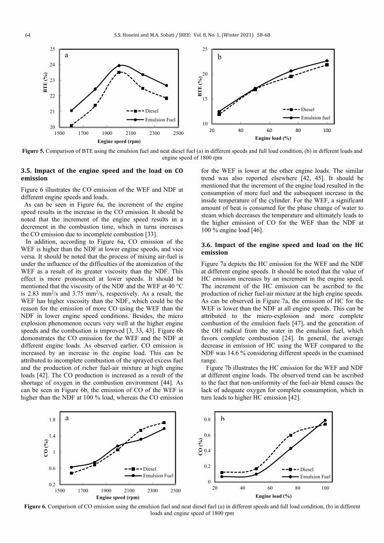
S.S. Hoseini and M.A. Sobati / JREE: Vol. 8, No. 1, (Winter 2021) 58-68
64
Figure 5. Comparison of BTE using the emulsion fuel and neat diesel fuel (a) in different speeds and full load condition, (b) in different loads and
engine speed of 1800 rpm 3.5. Impact of the engine speed and the load on CO emission
Figure 6 illustrates the CO emission of the WEF and NDF at different engine speeds and loads. As can be seen in Figure 6a, the increment of the engine speed results in the increase in the CO emission. It should be noted that the increment of the engine speed results in a decrement in the combustion time, which in turns increases the CO emission due to incomplete combustion [33]. In addition, according to Figure 6a, CO emission of the WEF is higher than the NDF at lower engine speeds, and vice versa. It should be noted that the process of mixing air-fuel is under the influence of the difficulties of the atomization of the WEF as a result of its greater viscosity than the NDF. This effect is more pronounced at lower speeds. It should be mentioned that the viscosity of the NDF and the WEF at 40 °C is 2.83 mm2/s and 3.75 mm2/s, respectively. As a result, the WEF has higher viscosity than the NDF, which could be the reason for the emission of more CO using the WEF than the NDF in lower engine speed conditions. Besides, the micro explosion phenomenon occurs very well at the higher engine speeds and the combustion is improved [3, 33, 43]. Figure 6b demonstrates the CO emission for the WEF and the NDF at different engine loads. As observed earlier, CO emission is increased by an increase in the engine load. This can be attributed to incomplete combustion of the sprayed excess fuel and the production of richer fuel-air mixture at high engine loads [42]. The CO production is increased as a result of the shortage of oxygen in the combustion environment [44]. As can be seen in Figure 6b, the emission of CO of the WEF is higher than the NDF at 100 % load, whereas the CO emission
for the WEF is lower at the other engine loads. The similar trend was also reported elsewhere [42, 45]. It should be mentioned that the increment of the engine load resulted in the consumption of more fuel and the subsequent increase in the inside temperature of the cylinder. For the WEF, a significant amount of heat is consumed for the phase change of water to steam which decreases the temperature and ultimately leads to the higher emission of CO for the WEF than the NDF at 100 % engine load [46]. 3.6. Impact of the engine speed and load on the HC emission
Figure 7a depicts the HC emission for the WEF and the NDF at different engine speeds. It should be noted that the value of HC emission increases by an increment in the engine speed. The increment of the HC emission can be ascribed to the production of richer fuel-air mixture at the high engine speeds. As can be observed in Figure 7a, the emission of HC for the WEF is lower than the NDF at all engine speeds. This can be attributed to the micro-explosion and more complete combustion of the emulsion fuels [47], and the generation of the OH radical from the water in the emulsion fuel, which favors complete combustion [24]. In general, the average decrease in emission of HC using the WEF compared to the NDF was 14.6 % considering different speeds in the examined range. Figure 7b illustrates the HC emission for the WEF and NDF at different engine loads. The observed trend can be ascribed to the fact that non-uniformity of the fuel-air blend causes the lack of adequate oxygen for complete consumption, which in turn leads to higher HC emission [42].
Figure 6. Comparison of CO emission using the emulsion fuel and neat diesel fuel (a) in different speeds and full load condition, (b) in different
loads and engine speed of 1800 rpm
20
21
22
23
24
25
1500 1700 1900 2100 2300 2500
BT
E (%
)
Engine speed (rpm)
Diesel
Emulsion Fuel10
15
20
25
20 40 60 80 100
BT
E (%
)
Engine load (%)
DieselEmulsion fuel
0.2
0.6
1
1.4
1.8
1500 1700 1900 2100 2300 2500
CO
(%)
Engine speed (rpm)
DieselEmulsion Fuel
a
0
0.2
0.4
0.6
0.8
20 40 60 80 100
CO
(%)
Engine load (%)
DieselEmulsion Fuel
a b
b
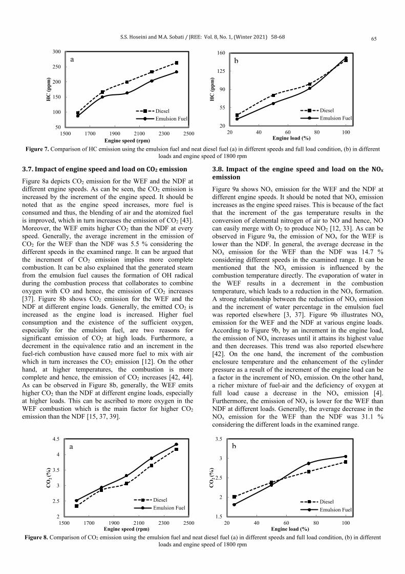
S.S. Hoseini and M.A. Sobati / JREE: Vol. 8, No. 1, (Winter 2021) 58-68
65
Figure 7. Comparison of HC emission using the emulsion fuel and neat diesel fuel (a) in different speeds and full load condition, (b) in different
loads and engine speed of 1800 rpm 3.7. Impact of engine speed and load on CO2 emission
Figure 8a depicts CO2 emission for the WEF and the NDF at different engine speeds. As can be seen, the CO2 emission is increased by the increment of the engine speed. It should be noted that as the engine speed increases, more fuel is consumed and thus, the blending of air and the atomized fuel is improved, which in turn increases the emission of CO2 [43]. Moreover, the WEF emits higher CO2 than the NDF at every speed. Generally, the average increment in the emission of CO2 for the WEF than the NDF was 5.5 % considering the different speeds in the examined range. It can be argued that the increment of CO2 emission implies more complete combustion. It can be also explained that the generated steam from the emulsion fuel causes the formation of OH radical during the combustion process that collaborates to combine oxygen with CO and hence, the emission of CO2 increases [37]. Figure 8b shows CO2 emission for the WEF and the NDF at different engine loads. Generally, the emitted CO2 is increased as the engine load is increased. Higher fuel consumption and the existence of the sufficient oxygen, especially for the emulsion fuel, are two reasons for significant emission of CO2 at high loads. Furthermore, a decrement in the equivalence ratio and an increment in the fuel-rich combustion have caused more fuel to mix with air which in turn increases the CO2 emission [12]. On the other hand, at higher temperatures, the combustion is more complete and hence, the emission of CO2 increases [42, 44]. As can be observed in Figure 8b, generally, the WEF emits higher CO2 than the NDF at different engine loads, especially at higher loads. This can be ascribed to more oxygen in the WEF combustion which is the main factor for higher CO2 emission than the NDF [15, 37, 39].
3.8. Impact of the engine speed and load on the NOx emission
Figure 9a shows NOx emission for the WEF and the NDF at different engine speeds. It should be noted that NOx emission increases as the engine speed raises. This is because of the fact that the increment of the gas temperature results in the conversion of elemental nitrogen of air to NO and hence, NO can easily merge with O2 to produce NO2 [12, 33]. As can be observed in Figure 9a, the emission of NOx for the WEF is lower than the NDF. In general, the average decrease in the NOx emission for the WEF than the NDF was 14.7 % considering different speeds in the examined range. It can be mentioned that the NOx emission is influenced by the combustion temperature directly. The evaporation of water in the WEF results in a decrement in the combustion temperature, which leads to a reduction in the NOx formation. A strong relationship between the reduction of NOx emission and the increment of water percentage in the emulsion fuel was reported elsewhere [3, 37]. Figure 9b illustrates NOx emission for the WEF and the NDF at various engine loads. According to Figure 9b, by an increment in the engine load, the emission of NOx increases until it attains its highest value and then decreases. This trend was also reported elsewhere [42]. On the one hand, the increment of the combustion enclosure temperature and the enhancement of the cylinder pressure as a result of the increment of the engine load can be a factor in the increment of NOx emission. On the other hand, a richer mixture of fuel-air and the deficiency of oxygen at full load cause a decrease in the NOx emission [4]. Furthermore, the emission of NOx is lower for the WEF than NDF at different loads. Generally, the average decrease in the NOx emission for the WEF than the NDF was 31.1 % considering the different loads in the examined range.
Figure 8. Comparison of CO2 emission using the emulsion fuel and neat diesel fuel (a) in different speeds and full load condition, (b) in different
loads and engine speed of 1800 rpm
50
100
150
200
250
300
1500 1700 1900 2100 2300 2500
HC
(ppm
)
Engine speed (rpm)
DieselEmulsion Fuel
20
55
90
125
160
20 40 60 80 100
HC
(ppm
)
Engine load (%)
DieselEmulsion Fuel
2
2.5
3
3.5
4
4.5
1500 1700 1900 2100 2300 2500
CO
2 (%
)
Engine speed (rpm)
DieselEmulsion Fuel
1.5
2
2.5
3
3.5
20 40 60 80 100
CO
2 (%
)
Engine load (%)
DieselEmulsion Fuel
a b
a b

S.S. Hoseini and M.A. Sobati / JREE: Vol. 8, No. 1, (Winter 2021) 58-68
66
Figure 9. Comparison of NOx emission using the emulsion fuel and neat diesel fuel (a) in different speeds and full load, (b) in different loads and
engine speed of 1800 rpm 4. CONCLUSIONS In the current study, a blend of diesel, water, and surfactant (combination of 80 and span 80) was applied to generate WEF. The best formulation of the water emulsion fuel based on our previous study was considered with 5 % of water content, 2 % of surfactant content, and HLB of 6.8 for the surfactant. The engine performance and exhaust emission of the WEF examined in the aforementioned conditions and the NDF was compared under different engine speed and load conditions. The main results are as follows:
• The engine torque and brake power were lower for the WEF than NDF in engine speed and load conditions. This can be ascribed to the lower calorific value of the WEF than the NDF due to the existence of water in the WEF.
• The values of BSFC and BTE of the WEF were higher than the NDF. In case of the BSFC, the lower content of diesel in the WEF results in the higher fuel consumption of WEF than the NDF. The phenomenon of micro-explosion in the combustion of WEF has a substantial role in the improvement of the combustion which increases the BTE.
• Significant lower HC formation was observed for the WEF than the NDF. The existence of water in the WEF results in the production of OH radical, which is an essential cause of the decrement of the HC concentration of the WEF compared to NDF.
• The emission of NOx was reduced considerably for the WEF compared to the NDF in the engine speed and load condition. This is directly associated to the decrement of the combustion temperature due to the existence of water in the WEF.
As a consequence, it should be mentioned that the application the water emulsion fuel instead of petro-diesel leads to a substantial decrement of the emission of some important pollutants such as HC and NOx. 5. ACKNOWLEDGEMENT
The authors would like to thank the Renewable Energy Institute of Tarbiat Modares University for their supports in the engine tests.
NOMENCLATURE WEF Water emulsion fuel NDF Neat diesel fuel HLB Hydrophilic-lipophilic balance BSFC Brake specific fuel consumption BTE Brake thermal efficiency CO Carbon monoxide HC Hydrocarbon CO2 Carbon dioxide NOx Nitrogen oxide RPM Revolution per minute
REFERENCES 1. Gardy, J., Rehan, M., Hassanpour, A., Lai, X. and Nizami, A.S.,
"Advances in nano-catalysts based biodiesel production from non-food feedstocks", Journal of Environmental Management, Vol. 249, (2019), 109316. (https://doi.org/10.1016/j.jenvman.2019.109316).
2. Hassan, M.H. and Kalam, M.A., "An overview of biofuel as a renewable energy source: Development and challenges", Procedia Engineering, Vol. 56, (2013), 39-53. (https://doi.org/10.1016/j.proeng.2013.03.087).
3. Yang, W.M., An, H., Chou, S.K., Chua, K.J., Mohan, B., Sivasankaralingam, V., Raman, V., Maghbouli, A. and Li, J., "Impact of emulsion fuel with nano-organic additives on the performance of diesel engine", Applied Energy, Vol. 112, (2013), 1206-1212. (https://doi.org/10.1016/j.apenergy.2013.02.027).
4. Fahd, M.E.A., Wenming, Y., Lee, P.S., Chou, S.K. and Yap, C.R., "Experimental investigation of the performance and emission characteristics of direct injection diesel engine by water emulsion diesel under varying engine load condition", Applied Energy, Vol. 102, (2013), 1042-1049. (https://doi.org/10.1016/j.apenergy.2012.06.041).
5. Alenezi, R.A., Erdiwansyah, Mamat, R., Norkhizan, A.M. and Najafi, G., "The effect of fusel-biodiesel blends on the emissions and performance of a single cylinder diesel engine", Fuel, Vol. 279, (2020), 118438. (https://doi.org/10.1016/j.fuel.2020.118438).
6. Seifi, M.R., Hassan-Beygia, S.R., Ghobadian, B., Desideri, U. and Antonelli, M., "Experimental investigation of a diesel engine power, torque and noise emission using water-diesel emulsions", Fuel, Vol. 166, (2016), 392-399. (https://doi.org/10.1016/j.fuel.2015.10.122).
7. Alahmer, A., "Influence of using emulsified diesel fuel on the performance and pollutants emitted from diesel engine", Energy Conversion and Management, Vol. 73, (2013), 361-369. (https://doi.org/10.1016/j.enconman.2013.05.012).
8. Venu, H. and Appavu, P., "Al2O3 nano additives blended Polanga biodiesel as a potential alternative fuel for existing unmodified DI diesel engine", Fuel, Vol. 279, (2020), 118518. (https://doi.org/10.1016/j.fuel.2020.118518).
9. Ninawe, G. and Tariq, M., "Influence of carbon nanotubes as additive in diesel-biodiesel blends in CI engine-an experimental investigation",
50
100
150
200
250
1500 1700 1900 2100 2300 2500
NO
x(p
pm)
Engine speed (rpm)
Diesel
Emulsion Fuel
50
100
150
200
250
20 40 60 80 100
NO
x(p
pm)
Engine load (%)
DieselEmulsion Fuel
a b

S.S. Hoseini and M.A. Sobati / JREE: Vol. 8, No. 1, (Winter 2021) 58-68
67
International Journal of Sustainable Engineering, (2020), 1-12. (https://doi.org/10.1080/19397038.2020.1790059).
10. Armas, O., Ballesteros, R., Martos, F.J. and Agudelo, J.R., "Characterization of light duty diesel engine pollutant emissions using water-emulsified fuel", Fuel, Vol. 84, No. 7-8, (2005), 1011-1018. (https://doi.org/10.1016/j.fuel.2004.11.015).
11. Baskar, P. and Kumar, A.S., "Experimental investigation on performance characteristics of a diesel engine using diesel-water emulsion with oxygen enriched air", Alexandria Engineering Journal, Vol. 56, No. 1, (2017), 137-146. (https://doi.org/10.1016/j.aej.2016.09.014).
12. Lin, C.Y. and Chen, L.W., "Engine performance and emission characteristics of three-phase diesel emulsions prepared by an ultrasonic emulsification method", Fuel, Vol. 85, No. 5, (2006), 593-600. (https://doi.org/10.1016/j.fuel.2005.09.007).
13. Saravanan, M., Anbarasu, A. and Gnanasekaran, B.M., "Study of performance and emission characteristics of IC engines by using diesel-water emulsion", The International Journal of Advanced Manufacturing Technology, Vol. 69, No. 9-12, (2013), 2531-2544. (https://doi.org/10.1007/s00170-013-5132-5).
14. Lin, C.Y. and Chen, L.W., "Comparison of fuel properties and emission characteristics of two-and three-phase emulsions prepared by ultrasonically vibrating and mechanically homogenizing emulsification methods", Fuel, Vol. 87, No. 10-11, (2008), 2154-2161. (https://doi.org/10.1016/j.fuel.2007.12.017).
15. Ithnin, A.M., Ahmad, M.A., Bakar, M.A.A., Rajoo, S. and Yahya, W.J., "Combustion performance and emission analysis of diesel engine fuelled with water-in-diesel emulsion fuel made from low-grade diesel fuel", Energy Conversion and Management, Vol. 90, (2015), 375-382. (https://doi.org/10.1016/j.enconman.2014.11.025).
16. Suresh, V. and Amirthagadeswaran, K., "Combustion and performance characteristics of water-in-diesel emulsion fuel", Energy Sources Part A: Recovery Utilization and Environmental Effects, Vol. 37, No. 18, (2015), 2020-2028. (https://doi.org/10.1080/15567036.2015.1072605).
17. Tsukahara, M., Yoshimoto, Y. and Murayama, T., "Influence of emulsified fuel properties on the reduction of BSFC in a diesel engine", Technical Paper, SAE Transactions, Vol. 98, Section 3: Journal of Engine, (1989), 1795-1804. (https://www.jstor.org/stable/44581063).
18. Park, S., Woo, S., Kim, H. and Lee, K., "Effect of diesel-water emulsified fuel on the NOx and PM emissions of a diesel engine", Energy & Fuels, Vol. 30, No. 7, (2016), 6070-6079. (https://doi.org/10.1021/acs.energyfuels.6b00089).
19. Lin, C.Y. and Wang, K.H., "Effects of a combustion improver on diesel engine performance and emission characteristics when using three-phase emulsions as an alternative fuel", Energy & Fuels, Vol. 18, No. 2, (2004), 477-484. (https://doi.org/10.1021/ef0300848).
20. Zhang, J., Jiang, D., Huang, Z., Wang, X. and Wei, Q., "Performance and emissions of direct injection diesel engine fueled with diesel fuel containing dissolved methane", Energy & Fuels, Vol. 20, No. 2, (2006), 504-511. (https://doi.org/10.1021/ef0502094).
21. El Shenawy, E.A., Elkelawy, M., Bastawissi, H.A.E., Shams, M.M., Panchal, H., Sadasivuni, K. and Thakar, N., "Investigation and performance analysis of water-diesel emulsion for improvement of performance and emission characteristics of partially premixed charge compression ignition (PPCCI) diesel engines", Sustainable Energy Technologies and Assessments, Vol. 36, (2019), 100546. (https://doi.org/10.1016/j.seta.2019.100546).
22. Yang, W., An, H., Chou, S.K., Vedharaji, S., Vallinagam, R., Balaji, M., Mohammad, F.E.A. and Chua, K.J.E., "Emulsion fuel with novel nano-organic additives for diesel engine application", Fuel, Vol. 104, (2013), 726-731. (https://doi.org/10.1016/j.fuel.2012.04.051).
23. Sudrajad, A., Hirotsugu, F. and Ali, I., "Experimental study of exhaust emissions of W/O emulsion fuel in DI single cylinder diesel engine", Modern Applied Science, Vol. 5, No. 5, (2011), 73-79. (https://doi.org/10.5539/mas.v5n5p73).
24. Kannan, K. and Udayakumar, M., "NOx and HC emission control using water emulsified diesel in single cylinder diesel engine", ARPN Journal of Engineering and Applied Sciences, Vol. 4, No. 8, (2009), 59-62. (https://www.researchgate.net/publication/239528260).
25. Subramanian, K.A., "A comparison of water-diesel emulsion and timed injection of water into the intake manifold of a diesel engine for simultaneous control of NO and smoke emissions", Energy Conversion and Management, Vol. 52, No. 2, (2011), 849-857. (https://doi.org/10.1016/j.enconman.2010.08.010).
26. Bidita, B.S, Suraya, A.R, Shazed, A., Mohd Salleh, M.A. and Idris, A., "Influence of fuel additive in the formulation and combustion characteristics of water-in-diesel nanoemulsion fuel", Energy & Fuels, Vol. 28, No. 6, (2014), 4149-4161. (https://doi.org/10.1021/ef5002259).
27. Chen, Z.B., Wang, X.C., Pei, Y.Q., Zhang, C., Xiao, M. and He, J., "Experimental investigation of the performance and emissions of diesel engines by a novel emulsified diesel fuel", Energy Conversion and Management, Vol. 95, (2015), 334-341. (https://doi.org/10.1016/j.enconman.2015.02.016).
28. Basha, J.S. and Anand, R.B., "An experimental investigation in a diesel engine using carbon nanotubes blended water-diesel emulsion fuel", Proceedings of the Institution of Mechanical Engineers, Part A: Journal of Power and Energy, Vol. 225, No. 3, (2011), 279-288. (https://doi.org/10.1177/2041296710394247).
29. Hoseini, S.S. and Sobati M.A., "Performance and emission characteristics of a diesel engine operating on different water in diesel emulsion fuels: Optimization using response surface methodology (RSM)", Frontiers in Energy, Vol. 13, (2019), 636-657. (https://doi.org/10.1007/s11708-019-0646-7).
30. Attia, A.M.A. and Kulchitskiy, A.R., "Influence of the structure of water-in-fuel emulsion on diesel engine performance", Fuel, Vol. 116, (2014), 703-708. (https://doi.org/10.1016/j.fuel.2013.08.057).
31. Ghojel, J., Honnery, D. and Al-Khaleefi, K., "Performance, emissions and heat release characteristics of direct injection diesel engine operating on diesel oil emulsion", Applied Thermal Engineering, Vol. 26, No. 17-18, (2006), 2132-2141. (https://doi.org/10.1016/j.applthermaleng.2006.04.014).
32. Badrana, O., Emeish, S., Abu-Zaid, M., Abu-Rahma, T., Al-Hasan, M. and Al-Ragheb, M., "Impact of emulsified water/diesel mixture on engine performance and environment", International Journal of Thermal & Environmental Engineering, Vol. 3, No. 1, (2011), 1-7. (https://doi.org/10.5383/ijtee.03.01.001).
33. Nadeem, M., Rangkuti, C., Anuar, K., Haq, M.R.U., Tan, I.B. and Shah, S.S., "Diesel engine performance and emission evaluation using emulsified fuels stabilized by conventional and gemini surfactants", Fuel, Vol. 85, No. 14, (2006), 2111-2119. (https://doi.org/10.1016/j.fuel.2006.03.013).
34. Noor El-Din, M.R., El-Hamouly, S.H., Mohamed, H.M., Mishrif, M.R. and Ragab, A.M., "Water-in-diesel fuel nanoemulsions: Preparation, stability and physical properties", Egyptian Journal of Petroleum, Vol. 22, No. 4, (2013), 517-530. (https://doi.org/10.1016/j.ejpe.2013.11.006).
35. Sharma, M. and Kaushal, R., "Performance and emission analysis of a dual fuel variable compression ratio (VCR) CI engine utilizing producer gas derived from walnut shells", Energy, Vol. 192, (2020), 116725. (https://doi.org/10.1016/j.energy.2019.116725).
36. Sayin, C. and Canakci, M., "Effects of injection timing on the engine performance and exhaust emissions of a dual-fuel diesel engine", Energy Conversion and Management, Vol. 50, No. 1, (2009), 203-213. (https://doi.org/10.1016/j.enconman.2008.06.007).
37. Alahmer, A., Yamin, J., Sakhrieh, A. and Hamdan, M.A., "Engine performance using emulsified diesel fuel", Energy Conversion and Management, Vol. 51, No. 8, (2010), 1708-1713. (https://doi.org/10.1016/j.enconman.2009.11.044).
38. Selim, M.Y.E. and Ghannam, M.T., "Combustion study of stabilized water-in-diesel fuel emulsion", Energy Sources, Part A: Recovery, Utilization, and Environmental Effects, Vol. 32, No. 3, (2009), 256-274. (https://doi.org/10.1080/15567030802467621).
39. Koc, A.B. and Abdullah, M., "Performance and NOx emissions of a diesel engine fueled with biodiesel-diesel-water nanoemulsions", Fuel Processing Technology, Vol. 109, (2013), 70-77. (https://doi.org/10.1016/j.fuproc.2012.09.039).
40. Selim, M.Y.E. and Ghannam, M.T., "Performance and engine roughness of a diesel engine running on stabilized water diesel emulsion", Proceedings of 8th International Conference on Engines for Automobiles, (2007). (https://doi.org/10.4271/2007-24-0132).
41. Abu-Zaid, M., "Performance of single cylinder, direct injection diesel engine using water fuel emulsions", Energy Conversion and Management, Vol. 45, No. 5, (2004), 697-705. (https://doi.org/10.1016/S0196-8904(03)00179-1).
42. Raheman, H. and Kumari, S., "Combustion characteristics and emissions of a compression ignition engine using emulsified jatropha biodiesel blend", Biosystems Engineering, Vol. 123, (2014), 29-39. (https://doi.org/10.1016/j.biosystemseng.2014.05.001).

S.S. Hoseini and M.A. Sobati / JREE: Vol. 8, No. 1, (Winter 2021) 58-68
68
43. Lin, C.Y. and Lin, H.A., "Engine performance and emission characteristics of a three-phase emulsion of biodiesel produced by peroxidation", Fuel Processing Technology, Vol. 88, No. 1, (2007), 35-41. (https://doi.org/10.1016/j.fuproc.2006.07.008).
44. Seifi, M.R., Desideri, U., Ghorbani, Z., Antonelli, M., Frigo, S., Hassan-Beygi, S.R. and Ghobadian, B., "Statistical evaluation of the effect of water percentage in water-diesel emulsion on the engine performance and exhaust emission parameters", Energy, Vol. 180, (2019), 797-806. (https://doi.org/10.1016/j.energy.2019.04.093).
45. Kinoshita, E., Hamasaki, K., Jaqin, C. and Takasaki, K., "Combustion characteristics for diesel engines with emulsified biodiesel without
adding emulsifier", Proceedings of 2004 SAE Fuels & Lubricants Meeting & Exhibition, (2004). (https://doi.org/10.4271/2004-01-1860).
46. Lin, C.Y. and Wang, K.H., "Diesel engine performance and emission characteristics using three-phase emulsions as fuel", Fuel, Vol. 83, No. 4-5, (2004), 537-545. (https://doi.org/10.1016/j.fuel.2003.08.012).
47. Kumar, M.S., Kerihuel, A., Bellettre, J. and Tazerout, M., "Ethanol animal fat emulsions as a diesel engine fuel-Part 2: Engine test analysis", Fuel, Vol. 85, No. 17, (2006), 2646-2652. (https://doi.org/10.1016/j.fuel.2006.05.023).

JREE: Vol. 8, No. 1, (Winter 2021) 69-76
Please cite this article as: Mundu, M.M., Nnamchi, S.N. and Nnamchi, O.A., "Development of a model for estimation of sunshine hour data for different regions of Uganda", Journal of Renewable Energy and Environment (JREE), Vol. 8, No. 1, (2021), 69-76. (https://doi.org/10.30501/jree.2020.235651.1119).
2423-7469/© 2021 The Author(s). Published by MERC. This is an open access article under the CC BY license (https://creativecommons.org/licenses/by/4.0/).
Research Article
Journal of Renewable Energy and Environment
J o u r n a l H o m e p a g e : w w w . j r e e . i r
Development of a Model for Estimation of Sunshine Hour Data for Different Regions of Uganda
Muhamad Mustafa Mundua*, Stephen Ndubuisi Nnamchib, Onyinyechi Adanma Nnamchic
a Department of Physical Sciences, School of Engineering and Applied Sciences (SEAS), Kampala International University, P. O. Box: 20000, Kampala, Uganda. b Department of Mechanical Engineering, School of Engineering and Applied Sciences (SEAS), Kampala International University, P. O. Box: 20000, Kampala, Uganda. c Department of Agricultural Engineering and Bio Resources, Michael Okpara University of Agriculture, Umudike, Umuahia, Nigeria.
P A P E R I N F O
Paper history: Received 24 June 2020 Accepted in revised form 06 January 2021
Keywords: Model Development, Model Estimation, Sunshine Hours, Uganda
A B S T R A C T
The present study is concerned with the development, estimation and validation of sunshine hours models (SHM) in Uganda. The SHM is based on geographical (latitude) and climatological (clearness index) indices. The meteosat data (1984-2018) acquired from the National Aeronautics and Space Administration were used to compute the coefficients of the models which, yielded a coefficient of determination close to unity, signifying a good association between the sunshine hours (SH) and the associated indices. The models become distributed by introducing a longitudinal function of clearness index into the primary SHM developed. Moreover, the models were subjected to statistical validation using; mean absolute relative error (MARE), root mean square error (RMSE) and mean absolute percentage difference (APD). Consequently, the primary SHM showed strong agreement with the measured SH data in the three regions with the exception of the northern region with flawed on-station data. Also, validation of the models by; {MARE, RMSE, APD} for Eastern, Central and Western regions, yielding the following results; {0.0788, 0.5441, 7.8778}, {0.0390, 0.1453, 3.9013} and {0.0124, 0.0528, 1.2436}, respectively. The following maximum SH; 11.16, 7.87, 9.52, 8.86 and 6.06 h were recorded for Non-regional, Northern, Eastern, Central and Western regions, respectively. Further, comparative validation with redeveloped global SHM showed that the present model stands in all the regions, whereas the global models validated only in the Eastern region. This is attributed to the synergy of geographical and climatological indices against the global models only based on climatological index. The model results show the order of regional SH distribution; eastern>northern>central>western region. These results could be employed in solar power, exploitation and agrometeorology development. This study further recommends for adoption of the present model to non-equatorial regions upon redevelopment as a meaningful extension of this work.
https://doi.org/10.30501/jree.2020.235651.1119
1. INTRODUCTION1
Sunshine Hour (SH) is an indicator of solar potential of a location and plays a central role in defining global solar radiation, clearness index, and relative sunshine hours for various applications in solar technologies [1-7]. Sunshine hour has diverse applications in agriculture, hydrology, and meteorology researches with encompassing applications, in atmospheric and building thermal balance [7], evaluation of agricultural resources [7-10], and in the development of global solar radiation models [11-13]. Meteorologically, the sunshine hour is measured using recorders (Campbell-Stokes), sensors (Kipp and Zonen CSD3), pyranometer, and pyrheliometer [7, 14, 15]. The accuracy of the efficiency of these sensors and recorders is influenced by the susceptibility to genera of clouds: cumulus, altostratus, cirrostratus, cirrus, and nimbus [16]. The reliability of sunshine hour recorder depends on a regular maintenance and calibration; if neglected for a long *Corresponding Author’s Email: [email protected] (M.M. Mundu) URL: http://www.jree.ir/article_122115.html
time, it would culminate in the failure of the equipment as observed in Lira district of Uganda, which tracked a series of negative sunshine hour values for the district against the expected positive sunshine hours, when compared to the other regions in Uganda with positive values. The negative sunshine hour values observed could be attributed to the poor maintenance and calibration of the meteorological equipment in the region [5, 17, 18]. In order to avail a practical sunshine hour data for the region, the present work is geared towards developing a sunshine hour model based on both geographical and climatological indices using satellite data from [19] to generate direct sunshine hour models for the nation. However, the present work tends to convert the indirect sunshine hour models [5, 20-33] to suit the present application. Furthermore, the redeveloped sunshine model for the region will be compared with the present work through empirical validation [34-37] and statistical validation [38-41] of the sunshine hour models. For the purpose of distribution or estimation of the sunshine hours over the regions, the present work has delved into estimation of the developed sunshine hour models by substituting the clearness index component of the developed
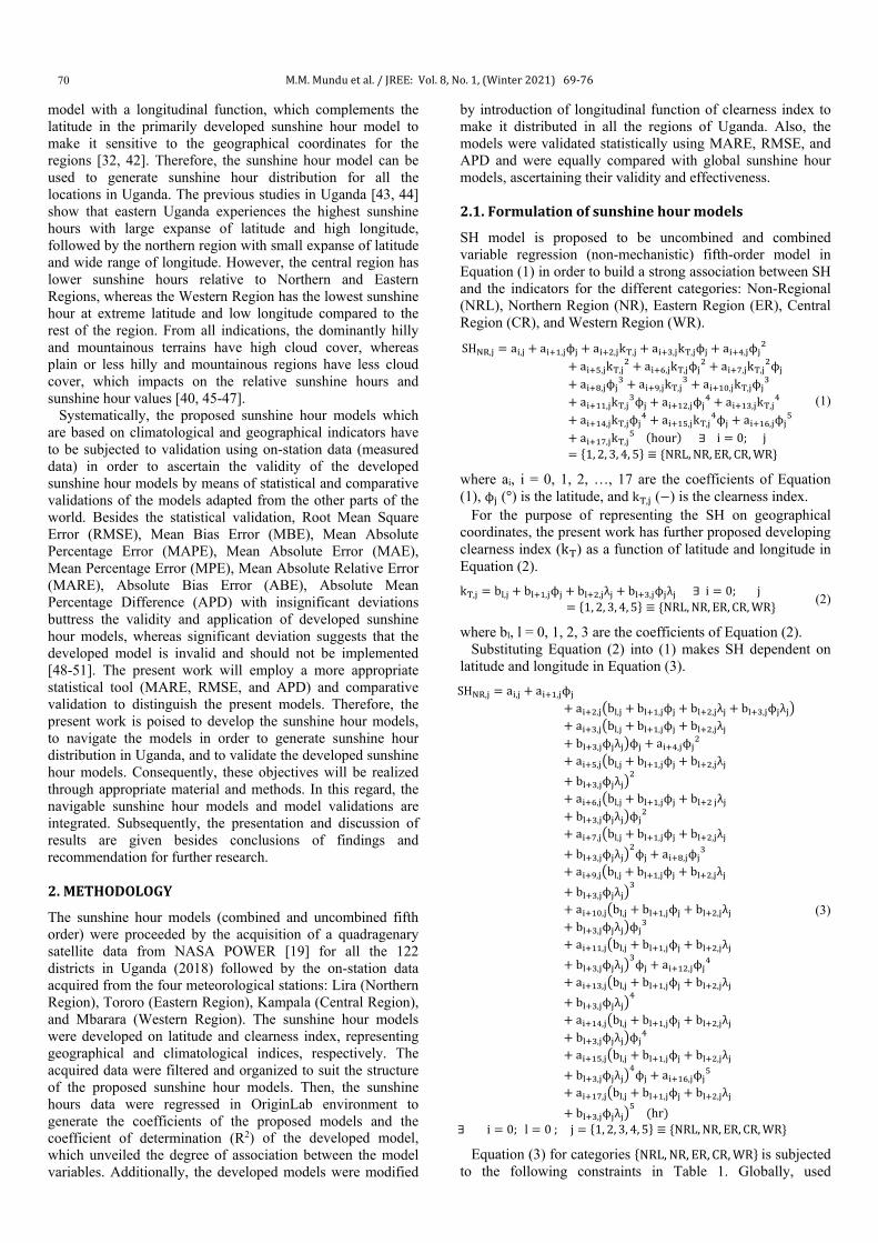
M.M. Mundu et al. / JREE: Vol. 8, No. 1, (Winter 2021) 69-76
70
model with a longitudinal function, which complements the latitude in the primarily developed sunshine hour model to make it sensitive to the geographical coordinates for the regions [32, 42]. Therefore, the sunshine hour model can be used to generate sunshine hour distribution for all the locations in Uganda. The previous studies in Uganda [43, 44] show that eastern Uganda experiences the highest sunshine hours with large expanse of latitude and high longitude, followed by the northern region with small expanse of latitude and wide range of longitude. However, the central region has lower sunshine hours relative to Northern and Eastern Regions, whereas the Western Region has the lowest sunshine hour at extreme latitude and low longitude compared to the rest of the region. From all indications, the dominantly hilly and mountainous terrains have high cloud cover, whereas plain or less hilly and mountainous regions have less cloud cover, which impacts on the relative sunshine hours and sunshine hour values [40, 45-47]. Systematically, the proposed sunshine hour models which are based on climatological and geographical indicators have to be subjected to validation using on-station data (measured data) in order to ascertain the validity of the developed sunshine hour models by means of statistical and comparative validations of the models adapted from the other parts of the world. Besides the statistical validation, Root Mean Square Error (RMSE), Mean Bias Error (MBE), Mean Absolute Percentage Error (MAPE), Mean Absolute Error (MAE), Mean Percentage Error (MPE), Mean Absolute Relative Error (MARE), Absolute Bias Error (ABE), Absolute Mean Percentage Difference (APD) with insignificant deviations buttress the validity and application of developed sunshine hour models, whereas significant deviation suggests that the developed model is invalid and should not be implemented [48-51]. The present work will employ a more appropriate statistical tool (MARE, RMSE, and APD) and comparative validation to distinguish the present models. Therefore, the present work is poised to develop the sunshine hour models, to navigate the models in order to generate sunshine hour distribution in Uganda, and to validate the developed sunshine hour models. Consequently, these objectives will be realized through appropriate material and methods. In this regard, the navigable sunshine hour models and model validations are integrated. Subsequently, the presentation and discussion of results are given besides conclusions of findings and recommendation for further research. 2. METHODOLOGY
The sunshine hour models (combined and uncombined fifth order) were proceeded by the acquisition of a quadragenary satellite data from NASA POWER [19] for all the 122 districts in Uganda (2018) followed by the on-station data acquired from the four meteorological stations: Lira (Northern Region), Tororo (Eastern Region), Kampala (Central Region), and Mbarara (Western Region). The sunshine hour models were developed on latitude and clearness index, representing geographical and climatological indices, respectively. The acquired data were filtered and organized to suit the structure of the proposed sunshine hour models. Then, the sunshine hours data were regressed in OriginLab environment to generate the coefficients of the proposed models and the coefficient of determination (R2) of the developed model, which unveiled the degree of association between the model variables. Additionally, the developed models were modified
by introduction of longitudinal function of clearness index to make it distributed in all the regions of Uganda. Also, the models were validated statistically using MARE, RMSE, and APD and were equally compared with global sunshine hour models, ascertaining their validity and effectiveness. 2.1. Formulation of sunshine hour models
SH model is proposed to be uncombined and combined variable regression (non-mechanistic) fifth-order model in Equation (1) in order to build a strong association between SH and the indicators for the different categories: Non-Regional (NRL), Northern Region (NR), Eastern Region (ER), Central Region (CR), and Western Region (WR).
SHNR,j = ai,j + ai+1,jϕj + ai+2,jkT,j + ai+3,jkT,jϕj + ai+4,jϕj2
+ ai+5,jkT,j2 + ai+6,jkT,jϕj
2 + ai+7,jkT,j2ϕj
+ ai+8,jϕj3 + ai+9,jkT,j
3 + ai+10,jkT,jϕj3
+ ai+11,jkT,j3ϕj + ai+12,jϕj
4 + ai+13,jkT,j4
+ ai+14,jkT,jϕj4 + ai+15,jkT,j
4ϕj + ai+16,jϕj5
+ ai+17,jkT,j5 (hour) ∃ i = 0; j
= {1, 2, 3, 4, 5} ≡ {NRL, NR, ER, CR, WR}
(1)
where ai, i = 0, 1, 2, …, 17 are the coefficients of Equation (1), ϕj (°) is the latitude, and kT,j (−) is the clearness index. For the purpose of representing the SH on geographical coordinates, the present work has further proposed developing clearness index (kT) as a function of latitude and longitude in Equation (2). kT,j = bl,j + bl+1,jϕj + bl+2,jλj + bl+3,jϕjλj ∃ i = 0; j
= {1, 2, 3, 4, 5} ≡ {NRL, NR, ER, CR, WR} (2)
where bl, l = 0, 1, 2, 3 are the coefficients of Equation (2). Substituting Equation (2) into (1) makes SH dependent on latitude and longitude in Equation (3). SHNR,j = ai,j + ai+1,jϕj
+ ai+2,j�bl,j + bl+1,jϕj + bl+2,jλj + bl+3,jϕjλj�+ ai+3,j�bl,j + bl+1,jϕj + bl+2,jλj+ bl+3,jϕjλj�ϕj + ai+4,jϕj
2
+ ai+5,j�bl,j + bl+1,jϕj + bl+2,jλj+ bl+3,jϕjλj�
2
+ ai+6,j�bl,j + bl+1,jϕj + bl+2 jλj+ bl+3,jϕjλj�ϕj2
+ ai+7,j�bl,j + bl+1,jϕj + bl+2,jλj+ bl+3,jϕjλj�
2ϕj + ai+8,jϕj
3
+ ai+9,j�bl,j + bl+1,jϕj + bl+2,jλj+ bl+3,jϕjλj�
3
+ ai+10,j�bl,j + bl+1,jϕj + bl+2,jλj+ bl+3,jϕjλj�ϕj
3
+ ai+11,j�bl,j + bl+1,jϕj + bl+2,jλj+ bl+3,jϕjλj�
3ϕj + ai+12,jϕj
4
+ ai+13,j�bl,j + bl+1,jϕj + bl+2,jλj+ bl+3,jϕjλj�
4
+ ai+14,j�bl,j + bl+1,jϕj + bl+2,jλj+ bl+3,jϕjλj�ϕj4
+ ai+15,j�bl,j + bl+1,jϕj + bl+2,jλj+ bl+3,jϕjλj�
4ϕj + ai+16,jϕj
5
+ ai+17,j�bl,j + bl+1,jϕj + bl+2,jλj+ bl+3,jϕjλj�
5 (hr)
∃ i = 0; l = 0 ; j = {1, 2, 3, 4, 5} ≡ {NRL, NR, ER, CR, WR}
(3)
Equation (3) for categories {NRL, NR, ER, CR, WR} is subjected to the following constraints in Table 1. Globally, used

M.M. Mundu et al. / JREE: Vol. 8, No. 1, (Winter 2021) 69-76
71
clearness index (KT) according to the following researchers [52-56] is algebraically given in Equation (4).
KT = a(RSH)2 + b(RSH) + c (4)
Sequel to the redevelopment of Equation (4) with the local data to obtain coefficients a, b, c and further rearrangement of Equation (4) yielded the corresponding RSH model in Equation (5).
RSH = −0.171875 + (2.232143KT− 0.61331613)0.5 ∃ KT ≥ 0.275 (5)
Expressing RSH in its components, i.e., sunshine hours and daylength, Equation (5) is expounded in Equation (6) as follows:
RSH =nN = −0.171875
+ (2.232143KT− 0.61331613)0.5 ∃ KT ≥ 0.275
(6)
Equation (7) gives an explicit expression for sunshine hours for comparative validation.
⟹ SH = n = N(−0.171875+ (2.232143KT− 0.61331613)0.5) ∃ KT ≥ 0.275
(7)
The daylength, N is defined in Equation (8) as in [57].
N =2
15 cos−1(−tanδtanϕ); δ = 23.45 sin �360 �284 + n
365 �� (8)
where 𝑛𝑛 is the number of days from January first and δ is the declination angle. Statistically, Equations (1) to (3) are to be validated with RMSE, MARE, and APD. The RMSE is defined in Equation (4) as follows:
RMSEj = �1n∑ �RSHm,j,i − RSHs,j,i�
2ni=1 �
0.5
∃ j = {1, 2, 3, 4, 5} ≡ {NRL, NR, ER, CR, WR}
(4)
Table 1 shows the boundaries of the sunshine hour models developed.
Table 1. Boundary conditions (constraints) in Equation (3)
Category Operation Latitude (degree) Longitude (degree)
𝐣𝐣 j, j NRL NRL, NRL −0.750000 ≤ ϕNRL ≤ 3.649997 29.683331 ≤ λNRL ≤ 34.94999722 NR NR, NR 1.633330556 ≤ ϕNR ≤ 3.64999 30.899997 ≤ λNR ≤ 34.9499972 ER ER, ER 0.283333 ≤ ϕER ≤ 2.03333 33.050000 ≤ λER ≤ 34.73333 CR CR, CR 0.066667 ≤ ϕCR ≤ 1.33333 29.783331 ≤ λCR ≤ 33.266667 WR WR, WR −0.750000 ≤ ϕWR ≤ 2.183333 29.683331 ≤ λWR ≤ 32.00000
The MARE is expressed in Equation (5) as follows:
MAREj =1n��
�SHm,j,i − SHs,j,i�SHm,j,i
�n
i=1
∃ j = {1, 2, 3, 4, 5} ≡ {NRL, NR, ER, CR, WR}
(5)
The mean Absolute Percentage Difference (APD) is given in Equation (6) as follows:
APDj =1n��
�SHm,j,i − SHs,j,i�SHm,j,i
� × 100%n
i=1
∃ j = {1, 2, 3, 4, 5} ≡ {NRL, NR, ER, CR, WR}
(6)
3. RESULTS AND DISCUSSION
This section presents the results and discussion of the study in Subsections 4.1 and 4.2, respectively.
3.1. Presentation of results
Firstly, the regression coefficients generated for the fifth-order model in Equation 1 which is both uncombined (KT,ϕ) and combined (KTϕ) variable sunshine hours model is represented in Table 2 for NRL, NR, ER, CR, and WR. Similarly, Table 3 gives the clearness index coefficients of Equation 2 (KT =f(ϕ, λ)) for non-regional and the different regions of Uganda. Furthermore, Table 3 provides the goodness of fit or coefficient of determination (R2) which shows the level of association between the variables (latitude and longitude) and clearness index. The R2 values reported for the mentioned categories tend to unity, showing a close association between the variables. All the categories have quadratic coefficients except the northern region, which shows a good association with a linear model. Lastly, Table 4 gives the results of statistical tools (RMSE, MARE, and APD) employed in the validation of the sunshine hour models in Uganda.
Table 2. Coefficients of Equation (1) for sunshine hours
Category 𝐚𝐚𝟎𝟎 𝐚𝐚𝟏𝟏 𝐚𝐚𝟐𝟐 𝐚𝐚𝟑𝟑 𝐚𝐚𝟒𝟒 𝐚𝐚𝟓𝟓 𝐚𝐚𝟔𝟔 𝐚𝐚𝟕𝟕 𝐚𝐚𝟖𝟖 𝐚𝐚𝟗𝟗 Non-regional -238 167 1530 -1070 2.05 -3620 -3.87 2560 -0.758 3830
Northern 23.443 83.063 -0.186 -626.653 -4.178 -472.751 10.031 1807.904 0.939 1267.508 Eastern -126.793 3618.276 -3.44584 -17558.84 74.3881 1187.509 -125.277 28128.73 -19.5588 -1348.8 Central -7.92 206 1.27 -1530 14.9 236 -27.9 4190 -16.7 -745 Western -0.101 2.894 0.151 -13.957 -0.048 -1.687 0.089 21.582 0.047 86.417
Category 𝐚𝐚𝟏𝟏𝟎𝟎 𝐚𝐚𝟏𝟏𝟏𝟏 𝐚𝐚𝟏𝟏𝟐𝟐 𝐚𝐚𝟏𝟏𝟑𝟑 𝐚𝐚𝟏𝟏𝟒𝟒 𝐚𝐚𝟏𝟏𝟓𝟓 𝐚𝐚𝟏𝟏𝟔𝟔 𝐚𝐚𝟏𝟏𝟕𝟕 𝐑𝐑𝟐𝟐
Non-regional 1.53 -2700 0.0778 -1490 -0.199 1050 0.00395 0.11 0.9926
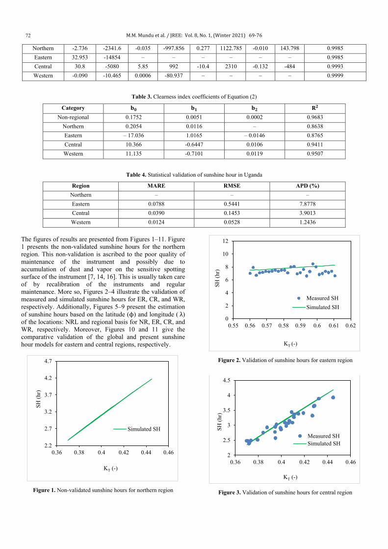
M.M. Mundu et al. / JREE: Vol. 8, No. 1, (Winter 2021) 69-76
72
Northern -2.736 -2341.6 -0.035 -997.856 0.277 1122.785 -0.010 143.798 0.9985 Eastern 32.953 -14854 – – – – – – 0.9985 Central 30.8 -5080 5.85 992 -10.4 2310 -0.132 -484 0.9993 Western -0.090 -10.465 0.0006 -80.937 – – – – 0.9999
Table 3. Clearness index coefficients of Equation (2)
Category 𝐛𝐛𝟎𝟎 𝐛𝐛𝟏𝟏 𝐛𝐛𝟐𝟐 𝐑𝐑𝟐𝟐 Non-regional 0.1752 0.0051 0.0002 0.9683
Northern 0.2054 0.0116 – 0.8638 Eastern – 17.036 1.0165 – 0.0146 0.8765 Central 10.366 -0.6447 0.0106 0.9411 Western 11.135 -0.7101 0.0119 0.9507
Table 4. Statistical validation of sunshine hour in Uganda
Region MARE RMSE APD (%) Northern – – – Eastern 0.0788 0.5441 7.8778 Central 0.0390 0.1453 3.9013 Western 0.0124 0.0528 1.2436
The figures of results are presented from Figures 1–11. Figure 1 presents the non-validated sunshine hours for the northern region. This non-validation is ascribed to the poor quality of maintenance of the instrument and possibly due to accumulation of dust and vapor on the sensitive spotting surface of the instrument [7, 14, 16]. This is usually taken care of by recalibration of the instruments and regular maintenance. More so, Figures 2–4 illustrate the validation of measured and simulated sunshine hours for ER, CR, and WR, respectively. Additionally, Figures 5–9 present the estimation of sunshine hours based on the latitude (ϕ) and longitude ( λ) of the locations: NRL and regional basis for NR, ER, CR, and WR, respectively. Moreover, Figures 10 and 11 give the comparative validation of the global and present sunshine hour models for eastern and central regions, respectively.
Figure 1. Non-validated sunshine hours for northern region
Figure 2. Validation of sunshine hours for eastern region
Figure 3. Validation of sunshine hours for central region
2.2
2.7
3.2
3.7
4.2
4.7
0.36 0.38 0.4 0.42 0.44 0.46
SH (h
r)
KT (-)
Simulated SH
0
2
4
6
8
10
12
0.55 0.56 0.57 0.58 0.59 0.6 0.61 0.62
SH (h
r)
KT (-)
Measured SHSimulated SH
2
2.5
3
3.5
4
4.5
0.36 0.38 0.4 0.42 0.44 0.46
SH (h
r)
KT (-)
Measured SHSimulated SH
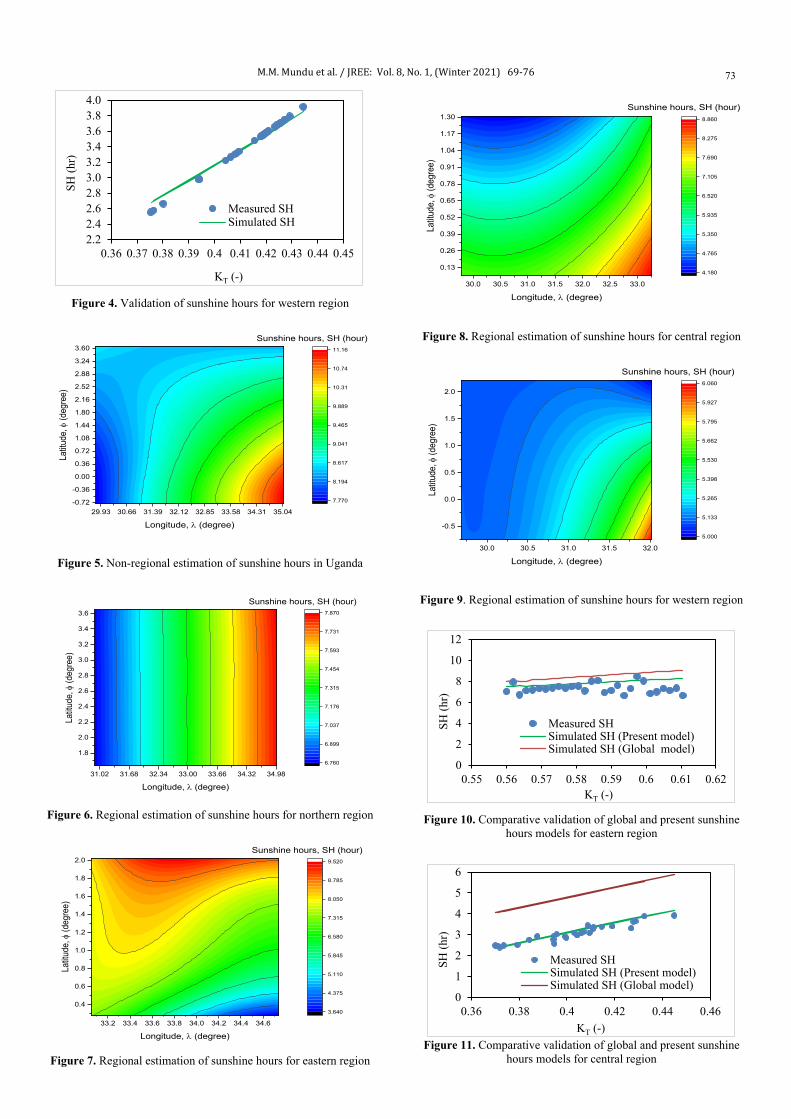
M.M. Mundu et al. / JREE: Vol. 8, No. 1, (Winter 2021) 69-76
73
Figure 4. Validation of sunshine hours for western region
29.93 30.66 31.39 32.12 32.85 33.58 34.31 35.04-0.72
-0.36
0.00
0.36
0.72
1.08
1.44
1.80
2.16
2.52
2.88
3.24
3.60
Longitude, λ (degree)
Latitu
de, φ
(deg
ree)
7.770
8.194
8.617
9.041
9.465
9.889
10.31
10.74
11.16
Sunshine hours, SH (hour)
Figure 5. Non-regional estimation of sunshine hours in Uganda
31.02 31.68 32.34 33.00 33.66 34.32 34.98
1.8
2.0
2.2
2.4
2.6
2.8
3.0
3.2
3.4
3.6
Longitude, λ (degree)
Latit
ude,
φ (d
egre
e)
6.760
6.899
7.037
7.176
7.315
7.454
7.593
7.731
7.870
Sunshine hours, SH (hour)
Figure 6. Regional estimation of sunshine hours for northern region
33.2 33.4 33.6 33.8 34.0 34.2 34.4 34.6
0.4
0.6
0.8
1.0
1.2
1.4
1.6
1.8
2.0
Longitude, λ (degree)
Latitu
de, φ
(deg
ree)
3.640
4.375
5.110
5.845
6.580
7.315
8.050
8.785
9.520
Sunshine hours, SH (hour)
Figure 7. Regional estimation of sunshine hours for eastern region
30.0 30.5 31.0 31.5 32.0 32.5 33.0
0.13
0.26
0.39
0.52
0.65
0.78
0.91
1.04
1.17
1.30
Longitude, λ (degree)
Latitu
de, φ
(deg
ree)
4.180
4.765
5.350
5.935
6.520
7.105
7.690
8.275
8.860
Sunshine hours, SH (hour)
Figure 8. Regional estimation of sunshine hours for central region
30.0 30.5 31.0 31.5 32.0
-0.5
0.0
0.5
1.0
1.5
2.0
Longitude, λ (degree)
Latitu
de, φ
(deg
ree)
5.000
5.133
5.265
5.398
5.530
5.662
5.795
5.927
6.060
Sunshine hours, SH (hour)
Figure 9. Regional estimation of sunshine hours for western region
Figure 10. Comparative validation of global and present sunshine
hours models for eastern region
Figure 11. Comparative validation of global and present sunshine
hours models for central region
2.22.42.62.83.03.23.43.63.84.0
0.36 0.37 0.38 0.39 0.4 0.41 0.42 0.43 0.44 0.45
SH (h
r)
KT (-)
Measured SHSimulated SH
0
2
4
6
8
10
12
0.55 0.56 0.57 0.58 0.59 0.6 0.61 0.62
SH (h
r)
KT (-)
Measured SHSimulated SH (Present model)Simulated SH (Global model)
0
1
2
3
4
5
6
0.36 0.38 0.4 0.42 0.44 0.46
SH (h
r)
KT (-)
Measured SHSimulated SH (Present model)Simulated SH (Global model)
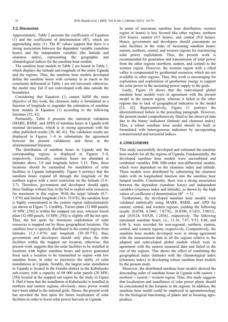
M.M. Mundu et al. / JREE: Vol. 8, No. 1, (Winter 2021) 69-76
74
3.2. Discussion
Approximately, Table 2 presents the coefficients of Equation (1) and the coefficients of determination (R2), which are approaching unity (1). The R2 values support that there is a strong association between the dependent variable (sunshine hours) and the independent variables (the latitude and clearness index), representing the geographic and climatological indices for the sunshine hour models. The sunshine hour models in Table 2 are bound in Table 1, which displays the latitude and longitude of the entire Uganda and the regions. Thus, the sunshine hour models developed define the sunshine hours with certainty in as much as the constraints delineated in Table 1 are not traversed; otherwise, the model may fail if not redeveloped with data outside the boundaries. Considering that Equation (1) cannot fulfill the main objective of this work, the clearness index is formulated as a function of longitude to engender the estimation of sunshine hour models in Equation (1) according to the following literature [32, 42]. Pertinently, Table 4 presents the statistical validation (MARE, RMSE, and APD) of sunshine hours in Uganda with minimal deviations, which is in strong agreement with the other published results [38, 40, 41]. The validation results are displayed in Figures 1–4 to substantiate the agreement between the present validations and those in the aforementioned literature. The distribution of sunshine hours in Uganda and the corresponding regions is displayed in Figures 5–9, respectively. Generally, sunshine hours are abundant at latitudes above 3.0 and longitude below 3.15. Thus, these locations should be earmarked for installation of solar facilities in Uganda indisputably. Figure 6 portrays that the sunshine hours expand all through the longitude of the northern region with a strict restriction on the latitude (3.4–3.7). Therefore, government and developers should apply these findings without bias in the bid to exploit solar resources for maximum in this region. With the target latitude (0.7–1.8°N) and limited longitude (34.6–35.0°E), the sunshine hour is highly concentrated in the eastern region indiscriminately (as shown in Figure 7). Credibly, Tororo plant (32 000 panels; 10 MW; [58]) is within the mapped out area, whereas Soroti plant (32 680 panels; 10 MW; [58]) is slightly off the hot spot. Thus, the hot spots for enormous exploitation of solar resources is mapped out by these geographical locations. The sunshine hour is sparsely distributed in the central region from latitudes (1.2–1.4°N) and longitude (30–30.7°E); thus, government and developers should only place the solar facilities within the mapped out location; otherwise, this present work suggests that the solar facilities to be installed in locations with higher sunshine hours and power generated from such a location to be transmitted to region with low sunshine hours in order to maximize the utility of solar installations in Uganda. Notably, the largest solar installation in Uganda is located in the Gomba district in the Kabulasoke sub-county with a capacity of 68 000 solar panels (20 MW; [58]) located in the mapped out region by the study in Figure 8. Had it been that the installation at Kabulasoke is installed in northern and eastern regions, obviously, more power would have been added to the national grids. Hence, the present work has unveiled the best spots for future localization of solar facilities in order to boost solar power harvests in Uganda.
In terms of maximum sunshine hour distribution, western region (6 hours) is less favored like other regions: northern (8.0 hours), eastern (9.5 hours), and central (9.0 hours). Hence, government and developers should concentrate on solar facilities in the order of increasing sunshine hours: eastern, northern, central, and western regions for maximizing solar power exploitation. Thus, the present work is recommended for generation and transmission of solar power from the other regions (northern, eastern, and central) to the western region. However, the western region with a rifted valley is compensated by geothermal resources, which are not available in other regions. Thus, this work is encouraging for exploration and exploitation of geothermic energy to support the solar power in the sustaining power supply to the grids. Lastly, Figure 10 shows that the redeveloped global sunshine hour models were in agreement with the present model in the eastern region, whereas it failed in the other regions due to lack of geographical indicators in the model [32, 42]. Representatively, Figure 11 portrays the aforementioned failure in the preceding paragraph. However, the present model comprehensively fitted to the observed data due to the binary indicators (latitude and clearness index). Thus, a robust sunshine hour model should be built or formulated with heterogeneous indicators by incorporating extraterrestrial and terrestrial indices. 4. CONCLUSIONS
This study successfully developed and estimated the sunshine hour models for all the regions of Uganda. Fundamentally, the developed sunshine hour models were uncombined and combined variables fifth fifth-order non-differential models, which were dependent on the clearness index and latitude. These models were distributed by substituting the clearness index with its longitudinal function into the sunshine hour lumped models. Consistently, there was a strong association between the dependent (sunshine hours) and independent variables (clearness index and latitude), as shown by the high values of coefficient of determination (R2 → 1). Furthermore, the developed sunshine hour models were validated statistically using MARE, RMSE, and APD for eastern, central, and western regions, yielding the following results {0.0788, 0.5441, 7.8778}, {0.0390, 0.1453, 3.9013}, and {0.0124, 0.0528, 1.2436}, respectively. The following maximum sunshine hours, i.e., 11.16, 7.87, 9.52, 8.86, and 6.06 h, were recorded for non-regional, northern, eastern, central, and western regions, respectively. Comparatively, the sunshine hour models developed were in strong agreement with the measurement data in all the regions relative to the adapted and redeveloped global models which were in agreement with the eastern measured data and failed in the rest of the regions. This shows the effect of combining the geographical index (latitude) with the climatological index (clearness index) in developing robust sunshine hour models by the present study. Moreover, the distributed sunshine hour models showed the descending order of sunshine hours in Uganda with eastern > northern > central > western region. Thus, this study suggests that localization and installation of solar power plants should be concentrated in the hotspots in the regions. In addition, the sunshine hour model could be employed in agrometeorology for the biological functioning of plants and in boosting agro-produce.

M.M. Mundu et al. / JREE: Vol. 8, No. 1, (Winter 2021) 69-76
75
This study strongly recommends the adaption and redevelopment of the present models outside the equatorial regions as a further study. 5. ACKNOWLEDGEMENT
The authors recognize the two sources of data, NASA POWER and the Department of Physics, Makerere University, for making available the data used in the formulation and validation of the sunshine hour models in Uganda. NOMENCLATURE
SH Sunshine hours (hr) KT Clearness index (-) RSH Relative sunshine hours (-) λ Latitude (°) ϕ Latitude (°) δ Solar declination angle (°) SHM Sunshine hour models MARE Mean absolute relative error RMSE Root mean square error APD Mean absolute percentage difference R2 Coefficient of determination N Daylength NRL Non-regional NR Northern region ER Eastern region CR Central region WR Western region ai, i = 0 1, 2⋯ , 17 Regression coefficients bl, l = 0, 1, 2, 3 Regression coefficients
REFERENCES 1. Yang, L., Cao, Q., Yu, Y. and Liu, Y., ''Comparison of daily diffuse
radiation models in regions of China without solar radiation measurement", Energy, Vol. 191, (2020), 116571. (https://doi.org/10.1016/j.energy.2019.116571).
2. Mundu, M.M., Nnamchi, S.N. and Ukagwu, K.J., "Algorithmized modelling, simulation and validation of clearness index in four regions of Uganda", Journal of Solar Energy Research, Vol. 5, No. 2, (2020), 432-452. (https://doi.org/10.22059/jser.2020.300924.1150).
3. Jahani, B. and Mohammadi, B., "A comparison between the application of empirical and ANN methods for estimation of daily global solar radiation in Iran", Theoretical and Applied Climatology, Vol. 137, No. 1-2, (2019), 1257-1269. (https://doi.org/10.1007/s00704-018-2666-3).
4. Jamil, B. and Bellos, E., "Development of empirical models for estimation of global solar radiation exergy in India", Journal of Cleaner Production, Vol. 207, (2019), 1-16. (https://doi.org/10.1016/j.jclepro.2018.09.246).
5. Bakirci, K., "Models of solar radiation with hours of bright sunshine: A review", Renewable Sustainable Energy Reviews, Vol. 13, No. 9, (2009), 2580-2588.(https://doi.org/10.1016/j.rser.2009.07.011).
6. Jervase, J., Al-Lawati, A. and Dorvlo, A., "Contour maps for sunshine ratio for Oman using radial basis function generated data", Renewable Energy, Vol. 28, No. 3, (2003), 487-497. (https://doi.org/10.1016/s0960-1481(02)00035-6).
7. Wu, B., Liu, S., Zhu, W., Yu, M., Yan, N. and Xing, Q., "A method to estimate sunshine duration using cloud classification data from a geostationary meteorological satellite (FY-2D) over the Heihe River Basin", Sensors, Vol. 16, No. 11, (2016), 1859. (https://doi.org/10.3390/s16111859).
8. Xue, L., Wang, C., Wang, C. and Shen, S., "Agricultural climatic regionalization for Longyan cultivation in Guangdong province", Journal of Tropical Meteorology, Vol. 27, (2011), 403-409. (http://en.cnki.com.cn/Article_en/CJFDTotal-RDQX201103014.htm).
9. Huang, Y., Xiu, S., Zhong, S., Zheng, L. and Sun, H., "Division of banana for climatic suitability based on a decision tree", Journal of Tropical Meteorology, Vol. 28, (2012), 140-144. (http://en.cnki.com.cn/Article_en/CJFDTotal-RDQX201201016.htm).
10. Mubiru, J., Banda, E., D’Ujanga, F. and Senyonga, T., "Assessing the performance of global solar radiation empirical formulations in Kampala, Uganda", Theoretical Applied Climatology, Vol. 87, No. 1-4, (2007), 179-184. (https://doi.org/10.1007/s00704-005-0196-2).
11. Rabehi, A., Guermoui, M. and Lalmi, D., "Hybrid models for global solar radiation prediction: A case study", International Journal of Ambient Energy, Vol. 41, No. 1, (2020), 31-40. (https://doi.org/10.1080/01430750.2018.1443498).
12. Suthar, M., Singh, G. and Saini, R., "Effects of air pollution for estimating global solar radiation in India", International Journal of Sustainable Energy, Vol. 36, No. 1, (2017), 20-27. (https://doi.org/10.1080/14786451.2014.979348).
13. Adnan, S., Hayat Khan, A., Haider, S. and Mahmood, R., "Solar energy potential in Pakistan", Journal of Renewable Sustainable Energy, Vol. 4, No. 3, (2012), 032701. (https://doi.org/10.1063/1.4712051).
14. Qian, H., "Study on the measurement method of direct radiation sunshine hour", Doctoral Dissertation, Master’s Thesis, Nanjing University of Information Science and Technology, Nanjing, China, (2013).
15. Rijks, D. and Huxley, P., "The empirical relation between solar radiation and hours of bright sunshine near Kampala, Uganda", Journal of Applied Ecology, Vol 1, No. 2, (1964), 339-345. (https://doi.org/10.2307/2401317).
16. Matuszko, D., "A comparison of sunshine duration records from the Campbell-Stokes sunshine recorder and CSD3 sunshine duration sensor", Theoretical and Applied Climatology, Vol. 119, No. 3-4, (2015), 401-406. (https://doi.org/10.1007/s00704-014-1125-z).
17. Fan, J., Wang, X., Wu, L., Zhang, F., Bai, H., Lu, X. and Xiang, Y., "New combined models for estimating daily global solar radiation based on sunshine duration in humid regions: A case study in South China", Energy Conversion Management, Vol. 156, (2018), 618-625. (https://doi.org/10.1016/j.enconman.2017.11.085).
18. Jahani, B., Dinpashoh, Y. and Nafchi, A.R., "Evaluation and development of empirical models for estimating daily solar radiation", Renewable Sustainable Energy Reviews, Vol. 73, (2017), 878-891. (https://doi.org/10.1016/j.rser.2017.01.124).
19. NASA, "Prediction of world energy resources, power data access viewer", (2018). (Available from: https://power.larc.nasa.gov/data-access-viewer/).
20. Al-Aboosi, F.Y., "Models and hierarchical methodologies for evaluating solar energy availability under different sky conditions toward enhancing concentrating solar collectors use: Texas as a case study", International Journal of Energy Environmental Engineering, Vol. 11, No. 3, (2019), 1-29. (https://doi.org/10.1007/s40095-019-00326-z).
21. Samanta, S., Patra, P.K., Banerjee, S., Narsimhaiah, L., Chandran, M.S., Kumar, P.V. and Bandyopadhyay, S., "Generation of common coefficients to estimate global solar radiation over different locations of India", Theoretical Applied Climatology, Vol. 136, No. 3-4, (2019), 943-953. (https://doi.org/10.1007/s00704-018-2531-4).
22. Sahin, A.Z., Rehman, S. and Al-Sulaiman, F., "Global solar radiation and energy yield estimation from photovoltaic power plants for small loads", International Journal of Green Energy, Vol. 14, No. 5, (2017), 490-498. (https://doi.org/10.1080/15435075.2016.1278374).
23. Yaniktepe, B., Kara, O. and Ozalp, C., "The global solar radiation estimation and analysis of solar energy: Case study for Osmaniye, Turkey", International Journal of Green Energy, Vol. 14, No. 9, (2017), 765-773. (https://doi.org/10.1080/15435075.2017.1329148).
24. Quej, V.H., Almorox, J., Ibrakhimov, M. and Saito, L., "Empirical models for estimating daily global solar radiation in Yucatán Peninsula, Mexico", Energy Conversion Management, Vol. 110, (2016), 448-456. (https://doi.org/10.1016/j.enconman.2015.12.050).
25. Namrata, K., Sharma, S. and Seksena, S., "Empirical models for the estimation of global solar radiation with sunshine hours on horizontal surface for Jharkhand (India)", Applied Solar Energy, Vol. 52, No. 3, (2016), 164-172. (https://doi.org/10.3103/s0003701x16030099).
26. Kirmani, S., Jamil, M. and Rizwan, M., "Empirical correlation of estimating global solar radiation using meteorological parameters", International Journal of Sustainable Energy, Vol. 34, No. 5, (2015), 327-339. (https://doi.org/10.1080/14786451.2013.826222).
27. Dumas, A., Andrisani, A., Bonnici, M., Graditi, G., Leanza, G., Madonia, M. and Trancossi, M., "A new correlation between global solar energy radiation and daily temperature variations", Solar Energy, Vol. 116, (2015), 117-124. (https://doi.org/10.1016/j.solener.2015.04.002).
28. Teke, A. and Yıldırım, H.B., "Estimating the monthly global solar radiation for Eastern Mediterranean Region", Energy Conversion Management, Vol. 87, (2014), 628-635. (https://doi.org/10.1016/j.enconman.2014.07.052).

M.M. Mundu et al. / JREE: Vol. 8, No. 1, (Winter 2021) 69-76
76
29. Li, H., Ma, W., Bu, X., Lian, Y. and Wang, X., "A multiple linear regression model for estimating global solar radiation in Guangzhou, China", Energy Sources, Part A: Recovery, Utilization, Environmental Effects, Vol. 35, No. 4, (2013), 321-327. (https://doi.org/10.1080/15567036.2010.499422).
30. Luis, M.A., Felipe, D.R. and Pilar N.R, "Estimation of global solar radiation by means of sunshine duration", Proceedings of ISES World Congress 2007, Vol. I–Vol. V, Springer, (2008). (https://doi.org/10.1007/978-3-540-75997-3_530).
31. Sen, Z., Solar energy fundamentals and modeling techniques: Atmosphere, environment, climate change and renewable energy, Springer Science & Business Media, (2008). (https://doi.org/10.5860/choice.46-2687).
32. Matzarakis, A. and Katsoulis, V., "Sunshine duration hours over the Greek region", Theoretical Applied Climatology, Vol. 83, No. 1-4, (2006), 107-120. (https://doi.org/10.1007/s00704-005-0158-8).
33. Almorox, J. and Hontoria, C., "Global solar radiation estimation using sunshine duration in Spain", Energy Conversion Management, Vol. 45, No. 9-10, (2004), 1529-1535. (https://doi.org/10.1016/j.enconman.2003.08.022).
34. Samadianfard, S., Majnooni-Heris, A., Qasem, S.N., Kisi, O., Shamshirband, S. and Chau, K., "Daily global solar radiation modeling using data-driven techniques and empirical equations in a semi-arid climate", Engineering Applications of Computational Fluid Mechanics, Vol. 13, No. 1, (2019), 142-157. (https://doi.org/10.1080/19942060.2018.1560364).
35. Lockart, N., Kavetski, D. and Franks, S.W., "A new stochastic model for simulating daily solar radiation from sunshine hours", International Journal of Climatology, Vol. 35, No. 6, (2015), 1090-1106. (https://doi.org/10.1002/joc.4041).
36. Ineichen, P., "Validation of models that estimate the clear sky global and beam solar irradiance", Solar Energy, Vol. 132, (2016), 332-344. (https://doi.org/10.1016/j.solener.2016.03.017).
37. Arslan, T., Yavuz, A.A. and Açikkalp, E., "The importance of the chosen technique to estimate diffuse solar radiation by means of regression", International Journal of Green Energy, Vol. 12, No. 1, (2015), 23-27. (https://doi.org/10.1080/15435075.2014.889010).
38. Bailek, N., Bouchouicha, K., Abdel-Hadi, Y.A., El-Shimy, M., Slimani, A., Jamil, B. and Djaafari, A., "Developing a new model for predicting global solar radiation on a horizontal surface located in Southwest Region of Algeria", NRIAG Journal of Astronomy Geophysics, Vol. 9, No. 1, (2020), 341-349. (https://doi.org/10.1080/20909977.2020.1746892).
39. Ramgolam, Y.K. and Soyjaudah, K.M.S., "Assessment and validation of global horizontal radiation: A case study in Mauritius", International Journal of Green Energy, Vol. 16, No. 14, (2019), 1317-1328. (https://doi.org/10.1080/15435075.2019.1671407).
40. Rahimikhoob, A., "Estimating sunshine duration from other climatic data by artificial neural network for ET 0 estimation in an arid environment", Theoretical Applied Climatology, Vol. 118, No. 1-2, (2014), 1-8. (https://doi.org/10.1007/s00704-013-1047-1).
41. Shamim, M.A., Remesan, R., Han, D., Ejaz, N. and Elahi, A., "An improved technique for global daily sunshine duration estimation using satellite imagery", Journal of Zhejiang University SCIENCE A, Vol. 13, No. 9, (2012), 717-722. (https://doi.org/10.1631/jzus.a1100292).
42. Dolinar, M., "Spatial interpolation of sunshine duration in Slovenia", Meteorological Applications, Vol. 13, No. 4, (2006), 375-384. (https://doi.org/10.1017/s1350482706002362).
43. Biira, S., "Analysis of solar radiation in Uganda", International Journal of Current Research, Vol. 6, No. 8, (2014), 8110-8115. (http://www.journalcra.com/sites/default/files/issue-pdf/6062.pdf).
44. Karume, K., Banda, E., Mubiru, J. and Majaliwa, M., "Correlation between sunshine hours and climatic parameters at four locations in Uganda", Tanzania Journal of Science, Vol. 33, No. 1, (2007). (https://doi.org/10.4314/tjs.v33i1.44279).
45. Kandirmaz, H., Kaba, K. and Avci, M., "Estimation of monthly sunshine duration in Turkey using artificial neural networks", International Journal of Photoenergy, Vol. 2014, (2014). (https://doi.org/10.1155/2014/680596).
46. Yadav, A.K. and Chandel, S., "Solar radiation prediction using Artificial Neural Network techniques: A review", Renewable Sustainable Energy Reviews, Vol. 33, (2014), 772-781. (https://doi.org/10.1016/j.rser.2013.08.055).
47. Frei, C., Willi, M., Stöckli, R. and Dürr, B., "Spatial analysis of sunshine duration in complex terrain by non‐contemporaneous combination of station and satellite data", International Journal of Climatology, Vol. 35, No. 15, (2015), 4771-4790. (https://doi.org/10.1002/joc.4322).
48. Ali, M.H. and Abustan, I., "A new novel index for evaluating model performance", Journal of Natural Resources Development, Vol. 4, (2014), 1-9. (https://doi.org/10.5027/jnrd.v4i0.01).
49. Chai, T. and Draxler, R.R., "Root mean square error (RMSE) or mean absolute error (MAE)?–Arguments against avoiding RMSE in the literature", Geoscientific Model Development, Vol. 7, No. 3, (2014), 1247-1250. (https://doi.org/10.5194/gmd-7-1247-2014).
50. Moreno, J.J.M., Pol, A.P., Abad, A.S. and Blasco, B.C., "Using the R-MAPE index as a resistant measure of forecast accuracy", Psicothema, Vol. 25, No. 4, (2013), 500-506. (10.7334/psicothema2013.23).
51. Muzathik, A., Nik, W., Ibrahim, M., Samo, K., Sopian, K. and Alghoul, M., "Daily global solar radiation estimate based on sunshine hours", International Journal of Mechanical and Materials Engineering, Vol. 6, No. 1, (2011), 75-80. (https://www.researchgate.net/publication/259479118_Daily_global_solar_radiation_estimate_based_on_sunshine_hours).
52. Anis, M.S., Jamil, B., Ansari, M.A. and Bellos, E., "Generalized models for estimation of global solar radiation based on sunshine duration and detailed comparison with the existing: A case study for India", Sustainable Energy Technologies Assessments, Vol. 31, (2019), 179-198. (https://doi.org/10.1016/j.seta.2018.12.009).
53. Onyango, A.O. and Ongoma, V., "Estimation of mean monthly global solar radiation using sunshine hours for Nairobi City, Kenya", Journal of Renewable Sustainable Energy, Vol. 7, No. 5, (2015), 053105. (https://doi.org/10.1063/1.4930530).
54. Che, H., Shi, G., Zhang, X., Zhao, J. and Li, Y., "Analysis of sky conditions using 40 year records of solar radiation data in China", Theoretical Applied Cimatology, Vol. 89, No. 1-2, (2007), 83-94. (https://doi.org/10.1007/s00704-006-0258-0).
55. Jin, Z., Yezheng, W. and Gang, Y., "General formula for estimation of monthly average daily global solar radiation in China", Energy Conversion Management, Vol. 46, No. 2, (2005), 257-268. (https://doi.org/10.1016/j.enconman.2004.02.020).
56. Akinoǧlu, B. and Ecevit, A., "Construction of a quadratic model using modified Ångstrom coefficients to estimate global solar radiation", Solar Energy, Vol. 45, No. 2, (1990), 85-92. (https://doi.org/10.1016/0038-092x(90)90032-8).
57. Duffie, J.A., Beckman, W.A. and Blair, N., Solar engineering of thermal processes, photovoltaics and wind, John Wiley & Sons, (2020). (https://doi.org/10.1002/9781119540328).
58. ERA, "Electricity supply industry performance report for the year 2018", (2019). (Available from: https://www.era.or.ug/index.php/resource-centre/publications/reports.

ABSTRACTS

S.A.A. Fallahzadeh et al. / JREE: Vol. 8, No. 1, (Winter 2021)
Applying Sliding-Mode Control to a Double-Stage Single-Phase Grid-Connected PV System
Seyed Ali Akbar Fallahzadeha, Navid Reza Abjadia*, Abbas Kargara, Frede Blaabjergb
a Faculty of Technology and Engineering, Shahrekord University, Shahrekord, Chaharmahal and Bakhtiari, Iran. b Department of Energy Technology, Aalborg University, Aalborg, Denmark.
P A P E R I N F O
Paper history: Received 09 June 2020 Accepted in revised form 20 September 2020
Keywords: Sliding Mode, POSLLC, Grid Connected, Photovoltaic
A B S T R A C T
This study investigates a new double-stage single-phase Grid-Connected (GC) Photo-Voltaic (PV) system. This PV system includes a DC-DC Positive Output Super Lift Luo Converter (POSLLC) and a single-phase inverter connected to a grid through an RL filter. Due to its advantages, the POSLLC was used between PV panel and inverter instead of the conventional boost converter. The state space equations of the system were solved. By using two Sliding Mode Controls (SMCs), PV panel voltage and POSLLC inductor current were controlled and the designed controls were compared. Two of these SMCs included a simple Sign Function Control (SFC) and a conventional SMC. To control the power injected into the grid with a unity power factor, an SMC was used. Perturb and Observe (P&O) method was employed to reach maximum power of the PV panel. The Maximum Power Point Tracking (MPPT) control generated the voltage reference of the PV panel. Similar controls were used for the boost converter instead of POSLLC. The obtained results were compared.
https://doi.org/10.30501/jree.2020.233358.1114
2423-7469/© 2021 The Author(s). Published by MERC. This is an open access article under the CC BY license (https://creativecommons.org/licenses/by/4.0/).
چکیده
مبدل کی، PVسامانه نی. اردیگیقرار م یفاز مورد بررسمتصل به شبکه تک ي ادو مرحله دی) جدPV( کیسامانه فتوولتائ کیمقاله، ن یا درDC-DC یشیمثبت فوق افزا یخروج Luo موسوم بهPOSLLC لتریف کی قیفاز متصل به شبکه از طرتک نورتریا کیو RL شود. یرا شامل م
. معادالت حالت سامانه به گرفتقرار نورتریو ا کیصفحه فتوولتائ نیب POSLLCمرسوم، DC-DC ي هامبدل ي ها، به جاتیمز از یبعض لیبه دل یطراح ي هاکنترل و کنترل POSLLCسلف انی و جر کی)، ولتاژ صفحه فتوولتائSMC( یکنترل مود لغزش دو ي ری. با به کارگشددست آورده
ي مرسوم. برا یلغزش مود کنترل ي گری) ساده و دSFC( عالمت تابع کنترل از بودعبارت یلغزش مود ي هاکنترل ن یاز ا یکی. شد سهیشده مقابه حداکثر توان دنیرس ي ) براP&Oو مشاهده ( ی. روش آشفتگشداستفاده گرید SMC کی از ک،یتوان بیبه شبکه با ضر یقی تزر انیکنترل جر
مشابه ي ها. کنترلکرد دیرا تول کی)، ولتاژ مرجع صفحه فتوولتائMPPTنقطه حداکثر توان ( یابی. کنترل ردشد به کار گرفته کیصفحه فتوولتائ .شد سهیمقا آمده، دست به جیو نتا بردهبه کار POSLLC ي ) به جاboost( ندهیمبدل افزا ي برا

R. Dhivagar and M. Mohanraj / JREE: Vol. 8, No. 1, (Winter 2021)
Optimization of Performance of Coarse Aggregate-Assisted Single-Slope Solar Still via Taguchi Approach
Ramasamy Dhivagar*, Murugesan Mohanraj
Department of Mechanical Engineering, Hindusthan College of Engineering and Technology, Coimbatore 641032, Tamil Nadu, India.
P A P E R I N F O
Paper history: Received 27 May 2020 Accepted in revised form 21 September 2020
Keywords: Coarse Aggregate, Energy Efficiency, Optimization, Solar Still, Taguchi Analysis
A B S T R A C T
In this experimental work, the energy efficiency and performance parameters of a coarse aggregate-assisted single-slope solar still were analyzed using Taguchi analysis. The preheated inlet saline water was sent to the solar still using thermal energy accumulated in coarse aggregate to enhance its productivity and energy efficiency. The daily distillate of the proposed model was observed to be about 4.21 kg/m2 with the improved efficiency of around 32 %. Furthermore, the parameters that influenced the performance of the solar stills and their levels were identified using Taguchi analysis. The Signal to Noise (S/N) ratios of the coarse aggregate temperature, saline water temperature, glass temperature and energy efficiency were observed to be about 45.4 °C, 41.4 °C, 36.7 °C and 20.07 %, respectively. The results revealed that, the percentage difference between predicted and experimental values was observed to be about 1.6 %, 0.6 %, 1.5 % and 3.3 %, respectively. The optimization method confirmed that there was good agreement between the predicted and experimental values.
https://doi.org/10.30501/jree.2020.232742.1112
2423-7469/© 2021 The Author(s). Published by MERC. This is an open access article under the CC BY license (https://creativecommons.org/licenses/by/4.0/).
چکیده
هاي درشت با استفاده از شیب بهبود یافته به کمک توده -کن خورشیدي تکبازده انرژي و پارامترهاي عملکرد یک آب شیرین ،در کار تجربی حاضروري وري تولید و بهره گرم شده با استفاده از انرژي حرارتی تجمیع شده در توده براي افزایش بهره آنالیز تاگوچی تحلیل شد. آب شور ورودي پیش
درصد 32کیلوگرم بر مترمربع با راندمان بهبود یافته حدود 21/4شود. تقطیر روزانه مدل پیشنهادي در حدود کن ارسال مییرینانرژي به آب شگذارند و سطح آنها با استفاده از روش آنالیز تاگوچی کن خورشیدي تأثیر میمشاهده شد. عالوه بر این، پارامترهایی که بر عملکرد آب شیرین
،C 4/45° دماي توده درشت، دماي آب شور، دماي شیشه و بازده انرژي به ترتیب در حدود (S/N) بت سیگنال به نوسانمشخص شد. نس°C 4/41، °C 7/36 بینی شده و تجربی به ترتیب حدوددرصد مشاهده شد. نتایج مشخص کردند که اختالف درصد بین مقادیر پیش 07/20و
.بینی شده و تجربی وجود داردسازي نشان داد که توافق خوبی بین مقادیر پیشمشاهده شدند. روش بهینه% 3/3و % 5/1، % 6/0، % 6/1

A. Tabrizi and M. Rahmani / JREE: Vol. 8, No. 1, (Winter 2021)
Assessing and Evaluating Reliability of Single-Stage PV Inverters
Aryan Tabrizi, Mehdi Rahmani*
Department of Electrical Engineering, Imam Khomeini International University, Qazvin, Qazvin, Iran.
P A P E R I N F O
Paper history: Received 28 June 2020 Accepted in revised form 29 September 2020
Keywords: PV, Single-Stage Inverter, Reliability, Monte Carlo
A B S T R A C T
Reliability is an essential factor in Photovoltaic (PV) systems. Solar power has become one of the most popular renewable power resources in recent years. Solar power has drawn attention because it is free and almost available worldwide. Moreover, the price of maintenance is lower than other power resources. Since there are no moving parts in PV systems, their reliability is relatively high. It is assumed that a typical PV system can operate 20–25 years with minimum possible interruptions. However, solar power systems may fail, the same as any other systems. It is indicated by several studies that the PV inverters are responsible for major failures in PV systems, as other components are almost passive. Hence, the reliability of the inverter has maximum impact on the reliability of the whole PV system. Thus, not only assessing and calculating the reliability value of inverter is highly crucial, but also increasing its value is essential, as well. This paper calculates and evaluates the reliability of PV single-stage inverters exclusively. Furthermore, there are suggestions that improve their reliability value.
https://doi.org/10.30501/jree.2020.237113.1123
2423-7469/© 2021 The Author(s). Published by MERC. This is an open access article under the CC BY license (https://creativecommons.org/licenses/by/4.0/).
چکیده
ترین منابع انرژي انرژي خورشیدي در سال هاي اخیر به یکی از محبوب ) است.PVقابلیت اطمینان یک عامل اساسی در سیستم هاي فتوولتائیک ( در سراسر جهان بدون هزینه در دسترس است، مورد توجه قرار گرفته است. پذیر تبدیل شده است. از آن جایی که انرژي خورشیدي تقریباًتجدید
، قسمت گردان و متحرکی وجود ندارد هاي خورشیدي، قیمت نگهداري آن در مقایسه با سایر منابع انرژي کم است. از آنجا که در سیستماینوه برعالهاي ممکن کار سال با حداقل وقفه 25تا 20قابلیت اطمینان نسبتاً باال است. فرض بر این است که یک سیستم خورشیدي معمولی می تواند بین
هاي دیگر با شکست در عملکرد مواجه شوند. با مطالعات موارد متعددي هاي خورشیدي هم مانند سایر سیستمکند. با این حال، ممکن است سیستمها در سیستم خورشیدي هستند، چراکه سایر المان ها تقریباً منفعل هستند. از مشخص شده است که اینورترهاي خورشیدي مسئول عمده شکست
ت اطمینان ، نه تنها ارزیابی و محاسبه قابلیکل سیستم خورشیدي دارد. بنابراین، قابلیت اطمینان اینورتر حداکثر تأثیر را در قابلیت اطمینان رواینهاي تک مرحله محاسبه و ارزیابی قابلیت اطمینان در اینورتر ، بلکه افزایش مقدار آن نیز ضروري است. در این مقاله منحصراًاینورتر بسیار مهم است
ها ارائه شده است.اي خورشیدي بررسی شده است. عالوه بر این، پیشنهادهایی براي بهبود قابلیت اطمینان آن
A. Khajavi Pour et al. / JREE: Vol. 8, No. 1, (Winter 2021)
Solar PV Power Plant Site Selection Using GIS-FFDEA Based Approach with Application in Iran
Aychar Khajavi Poura, Mohammad Reza Shahrakia*, Faranak Hosseinzadeh Saljooghib
a Department of Industrial Engineering, School of Engineering, University of Sistan and Baluchestan, Zahedan, Sistan and Baluchestan, Iran. b Department of Mathematics, School of Mathematics, University of Sistan and Baluchestan, Zahedan, Sistan and Baluchestan, Iran.
P A P E R I N F O
Paper history: Received 30 May 2020 Accepted in revised form 26 October 2020
Keywords: Renewable Energy, Full Fuzzy Data Envelopment Analysis, Delphi Method, Location Planning, Geographic Information System, Iran
A B S T R A C T
Photovoltaic energy is a good alternative to fossil fuels due to the abundance of solar energy. In this research, the criteria for locating photovoltaic solar power plants were identified using previous studies and experts’ views and by using the Delphi method based on five socioeconomic, topographic, power generation and distribution issues, climatological, and environmental criteria. Then, by using the GIS software, the layers of sub-criteria were classified for locating photovoltaic solar power plants. Upon identifying the proposed decision-maker units for location finding, their efficiency was calculated using the full fuzzy data envelopment analysis method in three steps. The information extracted from the layers of the sub-criteria of GIS was coded using the MATLAB software in the first step of the full fuzzy data envelopment analysis model and the decision-making units were classified into three classes of efficient, weak, and inefficient. In the second step, the values of output shortages and input surplus were determined. Finally, in the third step, efficient decision-making units were ranked using Anderson-Pearson Super Efficiency Method in full fuzzy data envelopment analysis. In order to validate the proposed method, a case study was carried out. The results of calculations showed that the north, central, and southeast areas of Sistan and Baluchestan province were among the favorable areas for photovoltaic solar power plant construction. Therefore, approximately 66 % of the province’s area has appropriate efficiency matching the sub-criteria considered to construct a photovoltaic solar power plant .
https://doi.org/10.30501/jree.2020.230490.1110
2423-7469/© 2021 The Author(s). Published by MERC. This is an open access article under the CC BY license (https://creativecommons.org/licenses/by/4.0/).
چکیده
ابتدا با استفاده از ،قیتحق نیاست. در ا یلیفس ي هاسوخت ي برا یمناسب نیگزیجا ي دیخورش ي انرژ یفراوان لیبه دل کیفتوولتائ ي دیخورش ي انرژ يارهایمع ،یطیمحستیو ز یشناسمیاقل برق، عیو توز دیمرتبط با تول مسائل ،یتوپوگراف ،یاجتماع-ي اقتصاد دگاهیبا توجه به پنج د یروش دلف
يهاهیاز ال کیهر ،ییایاطالعات جغراف ستمیافزار سسپس با استفاده از نرم. شدند ییشناسا کیفتوولتائ ي دیخورش ي هاروگاهین یابیمکان رثردؤممکان ي برا ي شنهادیپ رندهیگمیتصم ي واحدها ییشدند. پس از شناسا ي بندکالسه کیفتوولتائ ي دیخورش روگاهین یابیبه منظور مکان ارهایرمعیز يهاهیاطالعات استخراج شده از ال سه مرحله محاسبه شد.در ي فازتمام يهاداده یپوشش لیها با استفاده از روش تحلآن ییکارا زانیم ،یابی شد و واحد یسیکدنو ي فازتمام ي هاداده یپوشش لیمرحله اول مدل تحلدر افزار متلب با استفاده از نرم ییایاطالعات جغراف ستمیاز س ارهایرمعیز
مصرف شده ي ها و مازاد ورودیکمبود خروج زانیشدند. در مرحله دوم م يبندو ناکارا دسته فیضع ي به سه دسته کارا، کارا رندهیگمیتصم ي ها تمام ي هاداده یشپوش لیدر تحل رسونیپ-اندرسون ییکاراکارا با استفاده از روش ابر رندهیگمیتصم ي هادر مرحله سوم واحد تاًی. نهادیگرد نییتع
محاسبات نشان داد که مناطق جیانجام شده است. نتا ي مطالعه مورد کی ،روش ارائه شده یسنجبه منظور اعتبار نیچنشدند. هم ي رتبه بند ي فاز % 66 باًیتقر ن،یااست. بنابر کیفتوولتائ ي دیخورش روگاهیساخت ن ي و بلوچستان از مناطق مطلوب برا ستانیاستان س یشرقو جنوب ي ، مرکزیشمال
.برخوردار است کیفتوولتائ ي دیخورش روگاهیساخت ن ي در نظر گرفته شده برا یفرع يارهامعی با متناسب مناسب راندمان از استان مساحت

P. Krystosiak / JREE: Vol. 8, No. 1, (Winter 2021)
Laudable Intentions, Parochial Thinking: Climate Change, Global Warming and Clean Energy Concerns in Investment Decisions Regarding Renewable Energy Projects in Poland
Paulina Krystosiaka,b*
a Institute of Computer Science, Polish Academy of Sciences, Warsaw, Poland. b Warsaw School of Economics, Warsaw, Poland.
P A P E R I N F O
Paper history: Received 30 April 2020 Accepted in revised form 27 October 2020
Keywords: Renewable Energy Investments, Social Cost-Benefit Analysis, Local and Global Concerns about Renewable Energy Projects, Wind Energy Projects in Poland
A B S T R A C T
The issue of renewable energy is an important one in Poland. The Polish economy heavily relies on coal. Polish cities are among the most polluted in Europe. Therefore, there is a considerable societal support for renewable energy projects. Some people, however, keep having objections, e.g. to windfarms. This paper analyzes social costs and benefits identified by representatives of municipalities in whose territories renewable energy investments have been carried out and by representatives of companies investing in renewable energy projects. The data come from a series of surveys conducted in the period of 2013-18. It has been found out that municipalities and companies significantly differ in their identification of the key social costs and benefits related to renewable energy projects. They are alike in one aspect: such problems like climate change, global warming, energy security, air pollution, energy diversification, etc. are replaced in their thinking by more parochial concerns of land price shifts, social tensions, and others. The article finishes with discussion of reasons explaining why the Poles declare to be staunchly pro-environmental in general and at the same time turn out to be benefit-seeking when asked about particular solutions.
https://doi.org/10.30501/jree.2020.222916.1090
2423-7469/© 2021 The Author(s). Published by MERC. This is an open access article under the CC BY license (https://creativecommons.org/licenses/by/4.0/).
چکیده
يشهرها نیترلهستان از آلوده ي سنگ است. شهرهابه زغال یاست. اقتصاد لهستان به شدت متک یمسئله مهم ریپذدیتجد ي هاي انرژدر لهستان با موضوعاتی از مردم همچنان یحال، برخنیبا ا .کندمی یقابل توجه تیحما ریدپذیتجد ي انرژ با محوریتي هاپروژهاز ، جامعهنیاروپا هستند. بنابرا
ی که در حوزه انرژي تجدیدپذیر توسط در مناطق یاجتماع ي ایها و مزانهیهز لیمقاله به تحل نیادر .کنندیم مخالفت ي بادهاي رعهمز انندم يارگذهیسرما ریدپذیتجد ي انرژ ي هاکه در پروژهي شاخص هاشرکتبه شناسایی و شده پرداخته ي انجام شده،گذارهیسرماها نمایندگان شهرداري
يهانهیهز مشخص شد کهدر این مقاله شده است. سنجی گردآوري در یک نظر 2018تا 2013 بازه زمانی ها درداده نیاپردازد. می ،کنند یمهایی آنها از جنبه دارند. ي ریچشمگ تفاوت هاها و شرکتي شهرداردر ریدپذیتجد ي هاي انرژ ي هاپروژهشناسایی مربوط به ي ایو مزا یاجتماع ی،اصل
ذهن شان با نظرات محدود در رهیو غ ي هوا، تنوع انرژ ی، آلودگي انرژ تی، امننیآب و هوا، گرم شدن کره زم رییمانند تغ یمشکالتمانند هم هستند: ادعاي ردبا بحث در موکوشد تا میمقاله ،در پایان .جایگزین شده است موارد ریو سا یاجتماع ي ها، تنشات ملکرییتغ اي مانند ارزشکننده
. مقاله را به پایان برساند ،کنندیم ییجوفعتشود، منیمال ؤخاص س ي هاحل از آنها در مورد راهو اینکه وقتی ستیزطیمحاز هایلهستان ي طرفدار
L. Samiee et al. / JREE: Vol. 8, No. 1, (Winter 2021)
Hydrogen Recovery in an Industrial Chlor-Alkali Plant Using Alkaline Fuel Cell and Hydrogen Boiler Techniques: Techno-Economic Assessment and Emission Estimation
Leila Samiee, Fatemeh Goodarzvand-Chegini*, Esmaeil Ghasemikafrudi*, Kazem Kashefi
Energy Technology Research Division, Research Institute of Petroleum Industry (RIPI), West Blvd. Azadi Sport Complex, P. O. Box: 14665-137, Tehran, Tehran, Iran.
P A P E R I N F O
Paper history: Received 01 July 2020 Accepted in revised form 27 October 2020
Keywords: Chlor-Alkali, Hydrogen Recovery, Fuel Cell, Hydrogen Boiler, Emission
A B S T R A C T
Some chemical processes, like the chlor-alkali industry, produce a considerable amount of hydrogen as by-product, which is wasted and vented to the atmosphere. Hydrogen waste can be recovered and utilized as a significant clean energy resource in the processes. This paper describes the thermodynamic analysis of hydrogen recovery at an industrial chlor-alkali plant by installation of hydrogen boiler and alkaline fuel cell. In addition, emission reduction potentials for the proposed systems were estimated. However, the goal of this work is to analyze the techno-economic feasibility and environmental benefits of using utilization systems of hydrogen waste. The results showed that hydrogen boiler scenario could produce 28 ton/hr steam at pressure of 25 bar and temperature of 245 °C, whereas the alkaline fuel cell system could produce 7.65 MW of electricity as well as 3.83 m3/h of deionized water based on the whole surplus hydrogen. In comparison, the alkaline fuel cell scenario has negative IRR (Internal Return Rate) and NPV (Net Present Value) due to cheap electricity and high cost of capital investment. However, regarding the steam price, the hydrogen boiler project has reasonable economic parameters in terms of IRR and NPV. Therefore, the hydrogen recovery scenario is proposed to install a hydrogen boiler as a feasible and economic idea for steam production in our case. Furthermore, in terms of emission reduction, hydrogen boiler and alkaline fuel cell techniques can significantly reduce greenhouse gas emission by 49300 and 58800 tons/year, respectively, whereas other pollutants can also be reduced by 141 and 95 tons/year in hydrogen boiler and alkaline fuel cell scenarios, respectively.
https://doi.org/10.30501/jree.2020.236413.1124
2423-7469/© 2021 The Author(s). Published by MERC. This is an open access article under the CC BY license (https://creativecommons.org/licenses/by/4.0/).
چکیده
به جو کنند که هدر رفته و برخی فرآیندهاي شیمیایی، مانند صنایع کلر آلکالی، مقدار قابل توجهی هیدروژن را به عنوان محصول جانبی تولید میتجزیه و ،شوند. در این مقالهشود. جریانهاي تلفاتی هیدروژن به عنوان یک منبع انرژي پاك قابل توجه در فرآیندها بازیابی و استفاده میمنتقل میشده است. عالوه بر یک واحد صنعتی کلر قلیایی با نصب بویلر هیدروژن و پیل سوختی قلیایی توضیح داده مودینامیکی بازیابی هیدروژن درتحلیل تر
محیطی براي تجزیه و تحلیل فنی، اقتصادي و زیست ،هاي کاهش انتشار براي سیستمهاي پیشنهادي نیز برآورد گردید. هدف از این کارآن پتانسیلناریوي بویلر هیدروژنی دهد که بر اساس کل هیدروژن مازاد، سنتایج نشان می باشد.هاي بازیافت و تبدیل از جریانهاي تلفاتی هیدروژن میسیستم
برق و MW 65/7تواند تولید کند در حالی که سیستم پیل سوختی قلیایی می C 245°و دماي bar 25بخار با فشار ton/hr 28تواند می NPVاخلی) و منفی (نرخ بازده د IRRآب دیونیزه شده را تولید کند. در مقام مقایسه، سناریوي پیل سوختی قلیایی داراي h/3m 83/3همچنین
گذاري است. در حالی که با توجه به قیمت منفی (ارزش فعلی خالص) است که این مسئله به دلیل ارزان بودن قیمت واحد برق و هزینه باالي سرمایه، یک ایده عملی و داراي پارامترهاي اقتصادي معقول است. بنابراین سناریوي بویلر هیدروژنی NPVو IRRبخار، سناریوي بویلر هیدروژنی از نظر
باشد. عالوه بر این، از نظر میزان کاهش انتشار، سناریوهاي بویلر هیدروژنی و پیلهاي سوختی قلیایی اقتصادي براي تولید بخار در پژوهش حاضر میها به ترتیب حالیکه سایر آالیندهتن در سال کاهش دهند در 58800و 49300اي را به ترتیب توانند به طور قابل توجهی انتشار گازهاي گلخانهمی
یابد.تن در سال کاهش می 95و 141در سناریوهاي بویلر هیدروژنی و پیلهاي سوختی قلیایی
S.S. Hoseini and M.A. Sobati / JREE: Vol. 8, No. 1, (Winter 2021)
Assessment of the Performance and Exhaust Emission of a Diesel Engine Using Water Emulsion Fuel (WEF) in Different Engine Speed and Load Conditions
Seyed Saeed Hoseini, Mohammad Amin Sobati*
Department of Chemical, Petroleum and Gas Engineering, Iran University of Science and Technology,Tehran, Tehran, Iran.
P A P E R I N F O
Paper history: Received 27 June 2020 Accepted in revised form 08 December 2020
Keywords: Water Emulsion Fuel, Engine Performance, Exhaust Emission, Engine Speed, Engine Load
A B S T R A C T
The performance characteristics and exhaust emission of a diesel engine using Water Emulsion Fuel (WEF) have been investigated under different engine speeds (1600 to 2400 rpm) and load conditions (25 to 100 %). The experiments were carried out on an air-cooled diesel engine of single cylinder using the WEF containing 5 % water, 2 % surfactant with Hydrophilic-Lipophilic Balance (HLB) of 6.8. The engine performance and exhaust emission using WEF were also compared with the Neat Diesel Fuel (NDF). According to the results, average reduction of 9.7 % in the engine torque and brake power was observed using WEF at all engine speeds. In addition, a 7.9 % increase in the Brake Specific Fuel Consumption (BSFC) and a 3.7 % increase in the Brake Thermal Efficiency (BTE) were observed for WEF in comparison with NDF in all loading conditions. In case of emission, significant lower hydrocarbon emission (i.e., 14.6 % on average) was observed for WEF comparing to NDF at all engine speeds. Moreover, a considerable reduction in the NOx emission (i.e., 31.1 % on average) was observed for the WEF comparing to the NDF in every engine load. In summary, the application of WEF leads to the reduction in the emission of different pollutants with a positive impact on the environment.
https://doi.org/10.30501/jree.2020.233709.1115
2423-7469/© 2021 The Author(s). Published by MERC. This is an open access article under the CC BY license (https://creativecommons.org/licenses/by/4.0/).
چکیده
تحت سرعت یزل آب در د یونیبا استفاده از سوخت امولس یزل حاصل از موتور د یندهآال ي عملکرد موتور و انتشار گازها هاي یژگیو یق،تحق یندر ا یلندرتک س یزلیموتور د یکتوسط یشاتقرار گرفت. آزما ی) مورد بررس% 25-100بار متفاوت ( یط ) و شراrpm 2400-1600مختلف ( ي موتورها
ینانجام شدند. ا 8/6 گریزيو آب دوستیآب یاسسورفکتانت و مق % 2% آب، 5 ي حاو یزل آب در د امولسیونی سوخت با هوا کنندهبا خنک همراهنشان داده است و یآب یونیحاصل از سوخت امولس هاي یندهعملکرد موتور و انتشار آال روي بر را موتور بار و سرعت زمانهم یرتأث ی،مطالعه تجرب
در تمام یونیامولس گشتاور و توان ترمز سوخت ي % برا 7/9کاهش یانگیناست. م دادهقرار یسهمورد مقا یزل حاصل از آن را با سوخت د یجنتابه یآب یونیسوخت امولس ي برا یحرارت یترمز و بازده یژهمصرف سوخت و ،موتور ي در تمام بارها ین،موتور مشاهده شد. عالوه بر ا هاي سرعت
یونیسوخت امولس ي برا یدروکربنکمتر ه یندگیآال یزانم ،موتور هاي در تمام سرعت ی،% باالتر بود. به طور قابل توجه 7/3% و 9/7حدود یبترتسوخت یداکس ي کربن د یندگیآال یزانم یزي،مشاهده شد؛ و به مقدار ناچ ) یانگین% به طور م 6/14در حدود ( یزل با سوخت د یسهدر مقا یآب
سوخت ي برا ) % 1/31 یزانم به( یداکس یتروژنن یندهکاهش قابل توجه آال ،چنینبود. هم یشتر% ب 5/5حدود یزل با سوخت د یسهدر مقا یونیامولسمنجر به بهبود یونیموتور مشاهده شد. الزم به ذکر است که استفاده از سوخت امولس ي در تمام بارها یزل با سوخت د یسهدر مقا یآب یونیامولس
د. دارن یستز یطمح ي بر رو یمثبت یرکه تأث شودیم هایندهو کاهش آال ي حمل و نقل تجار و یصنعت ي کاربردها

M.M. Mundu et al. / JREE: Vol. 8, No. 1, (Winter 2021)
Development of a Model for Estimation of Sunshine Hour Data for Different Regions of Uganda
Muhamad Mustafa Mundua*, Stephen Ndubuisi Nnamchib, Onyinyechi Adanma Nnamchic
a Department of Physical Sciences, School of Engineering and Applied Sciences (SEAS), Kampala International University, P. O. Box: 20000, Kampala, Uganda. b Department of Mechanical Engineering, School of Engineering and Applied Sciences (SEAS), Kampala International University, P. O. Box: 20000, Kampala, Uganda. c Department of Agricultural Engineering and Bio Resources, Michael Okpara University of Agriculture, Umudike, Umuahia, Nigeria.
P A P E R I N F O
Paper history: Received 24 June 2020 Accepted in revised form 06 January 2021
Keywords: Model Development, Model Estimation, Sunshine Hours, Uganda
A B S T R A C T
The present study is concerned with the development, estimation and validation of sunshine hours models (SHM) in Uganda. The SHM is based on geographical (latitude) and climatological (clearness index) indices. The meteosat data (1984-2018) acquired from the National Aeronautics and Space Administration were used to compute the coefficients of the models which, yielded a coefficient of determination close to unity, signifying a good association between the sunshine hours (SH) and the associated indices. The models become distributed by introducing a longitudinal function of clearness index into the primary SHM developed. Moreover, the models were subjected to statistical validation using; mean absolute relative error (MARE), root mean square error (RMSE) and mean absolute percentage difference (APD). Consequently, the primary SHM showed strong agreement with the measured SH data in the three regions with the exception of the northern region with flawed on-station data. Also, validation of the models by; {MARE, RMSE, APD} for Eastern, Central and Western regions, yielding the following results; {0.0788, 0.5441, 7.8778}, {0.0390, 0.1453, 3.9013} and {0.0124, 0.0528, 1.2436}, respectively. The following maximum SH; 11.16, 7.87, 9.52, 8.86 and 6.06 h were recorded for Non-regional, Northern, Eastern, Central and Western regions, respectively. Further, comparative validation with redeveloped global SHM showed that the present model stands in all the regions, whereas the global models validated only in the Eastern region. This is attributed to the synergy of geographical and climatological indices against the global models only based on climatological index. The model results show the order of regional SH distribution; eastern>northern>central>western region. These results could be employed in solar power, exploitation and agrometeorology development. This study further recommends for adoption of the present model to non-equatorial regions upon redevelopment as a meaningful extension of this work.
https://doi.org/10.30501/jree.2020.235651.1119
2423-7469/© 2021 The Author(s). Published by MERC. This is an open access article under the CC BY license (https://creativecommons.org/licenses/by/4.0/).
چکیده
(عرض ییایجغراف يهابر اساس شاخص SHM شاخص .می پردازد در اوگاندا SHM ی مدلآفتاب هايساعت یمطالعه حاضر به توسعه، برآورد و اعتبارسنج بیمحاسبه ضرا يو فضا برا يهوانورد ی) سازمان مل2018-1984سنگ (دست آمده از شهاببه يهاداده. ) استتی(شاخص شفاف یشناسم ی) و اقلییایجغراف، مورد استفاده استمربوطه هاي و شاخص SHساعات تابش آفتاب نیب یدهنده ارتباط خوبرا به همراه دارد، نشان واحدي کینزد نییتع بیها که ضرمدل
يآمار یسنجاعتباردر معرض هامدل، نیاعالوه بر ند.افتیتوسعه هیاول SHMبه شفافیتاز شاخص یک عملکرد طولی یها با معرفمدلتوزیع قرار گرفت. توافق هیاول SHM، جهیدر نت . APDاختالف درصد مطلق نیانگیو م RMSEمربع ن یانگیم ي، خطاMAREمطلق ینسب ي خطا نی انگیم :قرار گرفتند
يهامدل یاعتبارسنج ن یهمچن نشان داد. ستگاه ینادرست در ا يهابا داده یمنطقه شمال يدر سه منطقه به استثنا SHشده يریگاندازه يهاداده با يقو{MARE, RMSE, APD} 1453/0، 9013/3} ، {0788/0، 5441/0، 8778/7{: ترتیب بدست آورد هبراي شرق، مرکز و مناطق غربی اعداد زیر را ب ،
، ی، شرقی، شماليمنطقه اریمناطق غ يبرا ب یساعت به ترت 06/6و SH :16/11 ،87/7 ،52/9 ،86/8حداکثر .}0124/0، 0528/0، 2436/1} و {0390/0 همه مناطق وجود دارد، در درنشان داد که مدل حاضر افتهیدوباره توسعه یجهان SHMبا ياسهی مقا یسنج، اعتبارنیابرعالوه .ثبت شد یو غرب يمرکز
تنها بر یجهان يهادر برابر مدل یمیو اقل یی ایجغراف يهاشاخص یبه همبستگ جنبه نیا. معتبر هستند یفقط در منطقه شرق یجهان يهاکه مدلیحال جینتا نیا دهد.یرا نشان می غرب >يمرکز >یشمال >یشرق نطقهم ي، امنطقه SH عیتوز بیمدل ترت جینتا شود.ینسبت داده م یشناسمی اساس شاخص اقل
استوا ر یرا به مناطق غ یکند که مدل فعلیم هی توص شتریمطالعه ب نیا .ردیمورد استفاده قرار گ یو توسعه هواشناس يبردار، بهرهيدیخورش يانرژتواند در یم . دیکار استفاده کن نیدار از ایگسترش معن کیدر هنگام توسعه مجدد به عنوان