Unravelling strings at the CERN LHC

arX

iv:0

709.

4259

v1 [

hep-

ph]

26

Sep

2007

Unravelling Strings at the LHC

Gordon L. Kane, Piyush Kumar, and Jing Shao

Michigan Center for Theoretical Physics,

University of Michigan, Ann Arbor, MI 48109, USA

(Dated: February 2, 2008)

We construct LHC signature footprints for four semi-realistic string/M theory vacua with

an MSSM visible sector. We find that they all give rise to limited regions in LHC signature

space, and are qualitatively different from each other for understandable reasons. We also

propose a technique in which correlations of LHC signatures can be effectively used to dis-

tinguish among these string theory vacua. We expect the technique to be useful for more

general string vacua. We argue that further systematic analysis with this approach will allow

LHC data to disfavor or exclude major “corners” of string/M theory and favor others. The

technique can be used with limited integrated luminosity and improved.

http://arXiv.org/abs/0709.4259v1

2

Contents

I. Introduction 2

II. Realistic String Vacua 4

A. String-Susy Models 4

B. Description of String-Susy Models 5

1. (Original) KKLT MSSM vacua - SUSY breaking by D3-branes (KKLT-1) 5

2. KKLT MSSM vacua - SUSY breaking by hidden sector F -terms (KKLT-2) 6

3. LARGE Volume MSSM vacua (LGVol) 7

4. Fluxless M theory G2-MSSM vacua (G2 ) 9

5. Comments on the KKLT and LARGE Volume vacua 10

III. Footprint of “String-Susy Models” at the LHC 10

A. How to construct a Footprint in general 10

B. Generic Features of Footprints 12

C. Origin of Distinguishibility - Correlations 15

D. Details of Constructing Footprints for String-Susy Models 21

IV. Distinguishing String-Susy Models from LHC Signatures 23

A. Extracting Correlations from 2D Plots 24

B. A Quantitative Definition of Distinguishibility 29

V. Discussion and Conclusion 30

Acknowledgments 33

VI. Appendix: Counting Signatures used in our Study 33

References 33

I. INTRODUCTION

The progress of string theory in the last decade has brought us closer to the ambitious

goal of connecting string theory to reality and testing it in various experiments. However,

developments in the past few years seem to suggest that instead of predicting a unique

well-defined vacuum from some underlying dynamical principle, string theory gives rise to

a vast “landscape” of string vacua. From a particle physics perspective, this implies the

existence of a vast class of effective theories for beyond-the-Standard-Model physics based

on different choices of string compactifications to four dimensions. Nevertheless, we would

like to learn more about string vacua, particularly about aspects soon to be illuminated by

LHC data.

If one is interested in connecting string theory with reality, it is important to know if

it is possible to differentiate the effective theories arising in string compactifications from

each other based on real experimental observables, such as LHC signatures. This question

3

was investigated in [1], where it was argued that specific string constructions usually lead

to a specific pattern of LHC signatures. In [1], the general idea and a simple method to

differentiate different classes of string constructions was proposed. In this paper we continue

our exploration along this direction. The goals of this paper are two-fold. The first is to

demonstrate convincingly that the “footprint” of a well-defined class of string constructions

is limited, so in particular it is not the case that any arbitrary signature is compatible with

these “stringy” effective theories. The second is to propose a systematic technique based on

the correlation of signatures to tell whether two classes of constructions can be distinguished

or not.

Suppose the LHC detector groups report a signal beyond the Standard Model (SM).

We expect and assume here that experimenters and SM theorists will get that right. We

want to focus on interpreting the data in terms of an underlying theory. Most work in

this direction has tried to build a bottom-up approach by deducing which new particles

are produced, and constructing an effective Lagrangian at the Electroweak (EW) scale.

Such work should of course be pursued. But we have increasingly learned how difficult

it may be because of issues like large number of parameters [2], degeneracies [3], etc., so

complementary alternative approaches are good.

If we knew the underlying theory at the unification scale, it would be possible to express

the many low scale effective theory parameters in terms of perhaps a few microscopic pa-

rameters and many degeneracies would disappear. Of course we do not know the correct

underlying theory. We argue in the following that it may be possible to overcome this by

studying a number of classes of underlying theories and by systematically using the pat-

tern and correlations of LHC signatures and related data. In a sense, we are arguing for a

mapping of LHC data onto underlying theories.

Our approach can be used for any kind of underlying theory, at any scale. We prefer

to work with string/M theory however, because we expect that it will be how nature is

described. Within various string/M theory models, we want to work with those which

have moduli stabilized so that reliable predictions can be made. Our attitude is that

LHC signatures and related data depend on new particle masses and couplings and on the

constraints imposed by the underlying theory, but in a very complicated way that is difficult

to extract. By studying patterns of signatures [1, 4] we can learn the implications of the

data. Insights from low scale effective theory analysis carried out in parallel can also be

included in our analysis.

Ideally, we hope there is a progress when one not only compares different theories, e.g.

Type II vs. heterotic etc., but also takes a given type of theory and compactifies several

ways, for each compactification one can break supersymmetry several ways, etc. One can

systematically study what kinds of data can distinguish them.

The basic idea of this paper is as follows. Based on the mapping from model parame-

ter space to signature space, any Beyond-the-Standard-Model construction corresponds to

a high-dimensional sub-manifold in the signature space, which we call the “footprint” of

the construction. Sometimes we will be sloppy and also refer to a particular 2D slice as

its footprint. This should be clear from the context. By taking into account the current

experimental data, we may constrain the footprint. So, the shape, size and position of a

4

footprint carries non-trivial information about the original construction, which is encoded in

the correlation of different signatures of the entire construction, and also about constraints

from existing data. We develop a technique by which one could extract this information

effectively and use it to distinguish different string-theoretical constructions. The construc-

tions we study have already been studied in the literature, in particular calculations for

them have been done. But for consistency we do our own calculations for all the models.

In this paper we do not focus on details of how one scans the microscopic parameters,

their metric, SM and detector, background and fluctuations, etc. All of these kinds of issues

should be treated in detail in application when there is data, and in a more computer inten-

sive study that is underway, but they do not affect qualitative conclusions about footprints

and distinguishing theories.

II. REALISTIC STRING VACUA

In order to be precise, we list the criteria required for a class of string vacua to be realistic.

For concreteness, we only focus on string vacua with low-energy supersymmetry since it

appears to be the most well motivated solution to the Hierarchy Problem; however realistic

string vacua with other methods of explaining the Hierarchy can be similarly defined.

A. String-Susy Models

To qualify as what we call a “String-Susy Model”, we require a class of string vacua

arising from a compactification to four dimensions to have the following properties:

• It has N = 1 supersymmetry in four dimensions which is broken in a controlled

approximation.

• The moduli are stabilized in a metastable dS vacuum and a stable hierarchy between

the Electroweak and Planck Scales is generated.

• The visible sector accommodates the MSSM particle content and gauge group (maybe

with additional matter and gauge groups) and their properties.

• It has a mechanism for breaking the Electroweak symmetry.

• It is consistent with all experimental constraints.

In addition, the fact that gauge couplings in the MSSM unify with great precision at ∼2 × 1016 GeV seems to be tantalizing evidence for gauge coupling unification and a unified

theory framework. Although some string-susy models give rise to gauge coupling unification

naturally and some don’t (for example, LARGE Volume models do not give rise to gauge

coupling unification with an MSSM visible sector), gauge coupling unification is still an

important criterion in our opinion and should serve as an important guide for constructing

realistic string theory vacua.

5

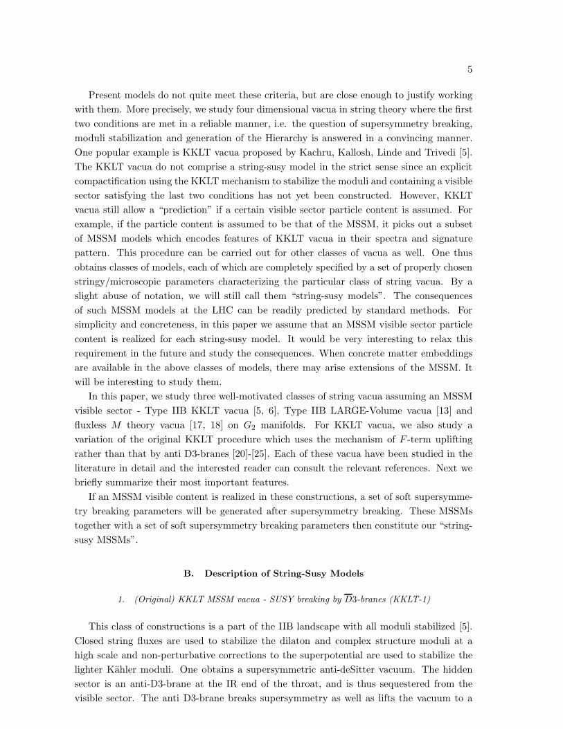
Present models do not quite meet these criteria, but are close enough to justify working

with them. More precisely, we study four dimensional vacua in string theory where the first

two conditions are met in a reliable manner, i.e. the question of supersymmetry breaking,

moduli stabilization and generation of the Hierarchy is answered in a convincing manner.

One popular example is KKLT vacua proposed by Kachru, Kallosh, Linde and Trivedi [5].

The KKLT vacua do not comprise a string-susy model in the strict sense since an explicit

compactification using the KKLT mechanism to stabilize the moduli and containing a visible

sector satisfying the last two conditions has not yet been constructed. However, KKLT

vacua still allow a “prediction” if a certain visible sector particle content is assumed. For

example, if the particle content is assumed to be that of the MSSM, it picks out a subset

of MSSM models which encodes features of KKLT vacua in their spectra and signature

pattern. This procedure can be carried out for other classes of vacua as well. One thus

obtains classes of models, each of which are completely specified by a set of properly chosen

stringy/microscopic parameters characterizing the particular class of string vacua. By a

slight abuse of notation, we will still call them “string-susy models”. The consequences

of such MSSM models at the LHC can be readily predicted by standard methods. For

simplicity and concreteness, in this paper we assume that an MSSM visible sector particle

content is realized for each string-susy model. It would be very interesting to relax this

requirement in the future and study the consequences. When concrete matter embeddings

are available in the above classes of models, there may arise extensions of the MSSM. It

will be interesting to study them.

In this paper, we study three well-motivated classes of string vacua assuming an MSSM

visible sector - Type IIB KKLT vacua [5, 6], Type IIB LARGE-Volume vacua [13] and

fluxless M theory vacua [17, 18] on G2 manifolds. For KKLT vacua, we also study a

variation of the original KKLT procedure which uses the mechanism of F -term uplifting

rather than that by anti D3-branes [20]-[25]. Each of these vacua have been studied in the

literature in detail and the interested reader can consult the relevant references. Next we

briefly summarize their most important features.

If an MSSM visible content is realized in these constructions, a set of soft supersymme-

try breaking parameters will be generated after supersymmetry breaking. These MSSMs

together with a set of soft supersymmetry breaking parameters then constitute our “string-

susy MSSMs”.

B. Description of String-Susy Models

1. (Original) KKLT MSSM vacua - SUSY breaking by D3-branes (KKLT-1)

This class of constructions is a part of the IIB landscape with all moduli stabilized [5].

Closed string fluxes are used to stabilize the dilaton and complex structure moduli at a

high scale and non-perturbative corrections to the superpotential are used to stabilize the

lighter Kahler moduli. One obtains a supersymmetric anti-deSitter vacuum. The hidden

sector is an anti-D3-brane at the IR end of the throat, and is thus sequestered from the

visible sector. The anti D3-brane breaks supersymmetry as well as lifts the vacuum to a

6

deSitter one. Supersymmetry breaking is then mediated to the visible sector by gravity.

The flux superpotential (W0) has to be tuned very small to get a gravitino mass of O(1-10

TeV). The soft supersymmetry breaking terms at the unification scale are calculated in [6]:

Ma = Ms

[

laα + bαg2a

]

,

m2i = M2

s

[

(1 − ni)α2 + 4αξi − γi

]

,

Aijk = −Ms

[

(3 − ni − nj − nk)α − γi − γj − γk

]

, (1)

where ba are the β function coefficients, γi is the anomalous dimension and γi = 8π2 ∂γi

∂ lnµ .

The coefficient ξi is a complicated function of trilinear couplings, Yukawa couplings and

gauge couplings [6]. Here Ms ≡ m3/2/(16π2) characterizes the size of the AMSB contribu-

tion and α is the ratio of the modulus-mediated contribution to the AMSB contribution,

defined as in [10] 1. The parameter α is determined by the form of the uplifting poten-

tial and the flux contribution. In [12], it was argued that typically α can take a generic

value of order unity, which in the definition of [10] is of order 16π2/ ln(Mp/m3/2) ∼ 5 for

m3/2 = (1 − 10) TeV.

The SM gauge fields can live on D7-branes or D3-branes, which corresponds to la = 1 or 0

respectively. We will focus on the former case and set la = 1. The chiral matter fields can be

constructed by adding intersecting D7-branes with magnetic fluxes in their worldvolume.

In the case of toroidal (orbifold) compactifications and no magnetic fluxes, the modular

weights ni can take values 0, 1/2 or 1 depending on whether the matter fields are on the D7-

brane, D3-D7 intersection or D3-brane respectively. For compactifications with more general

Calabi-Yau manifolds or with more general intersecting D7-brane models with worldvolume

magnetic fluxes, ni will be model dependent and have to be computed in each model[11].

Generally if the modular weighs are equal to 1, all the scalars will be tachyonic as a result

of the mixing of the moduli and AMSB contribution in Eq.(1). So modular weights of 1

are normally excluded. In addition, the ratios of gaugino masses at low scale are roughly

(1 + 3.3/α) : (2 + 1/α) : (6 − 9/α). For a typical value of α = 5, the ratio is 1.5 : 2 : 3.8.

The LSP is predominantly bino-like for a sizable range of α around 5. The constraint on

the relic density of neutralino dark matter favors the region in the parameter space where

there is some bino-wino mixing (not necessarily large), or, a stop or stau with mass close

to that of LSP.

2. KKLT MSSM vacua - SUSY breaking by hidden sector F -terms (KKLT-2)

There is a variation of the original KKLT proposal in which the anti D3-brane is replaced

by a hidden sector which spontaneously breaks supersymmetry and lifts the AdS minimum.

This is also known as F -term uplifting. Several examples of this type of vacua are discussed

in the literature [20]-[25]. A notable example is to use the recently discovered ISS model [32]

as the hidden section, which can potentially have a dual stringy construction via AdS/CFT

1 Note this definition is different from that in [12].

7

duality [26]. In this example, dS vacua with zero cosmological constant and TeV scale

gravitino mass can both be realized naturally at the same time [24].

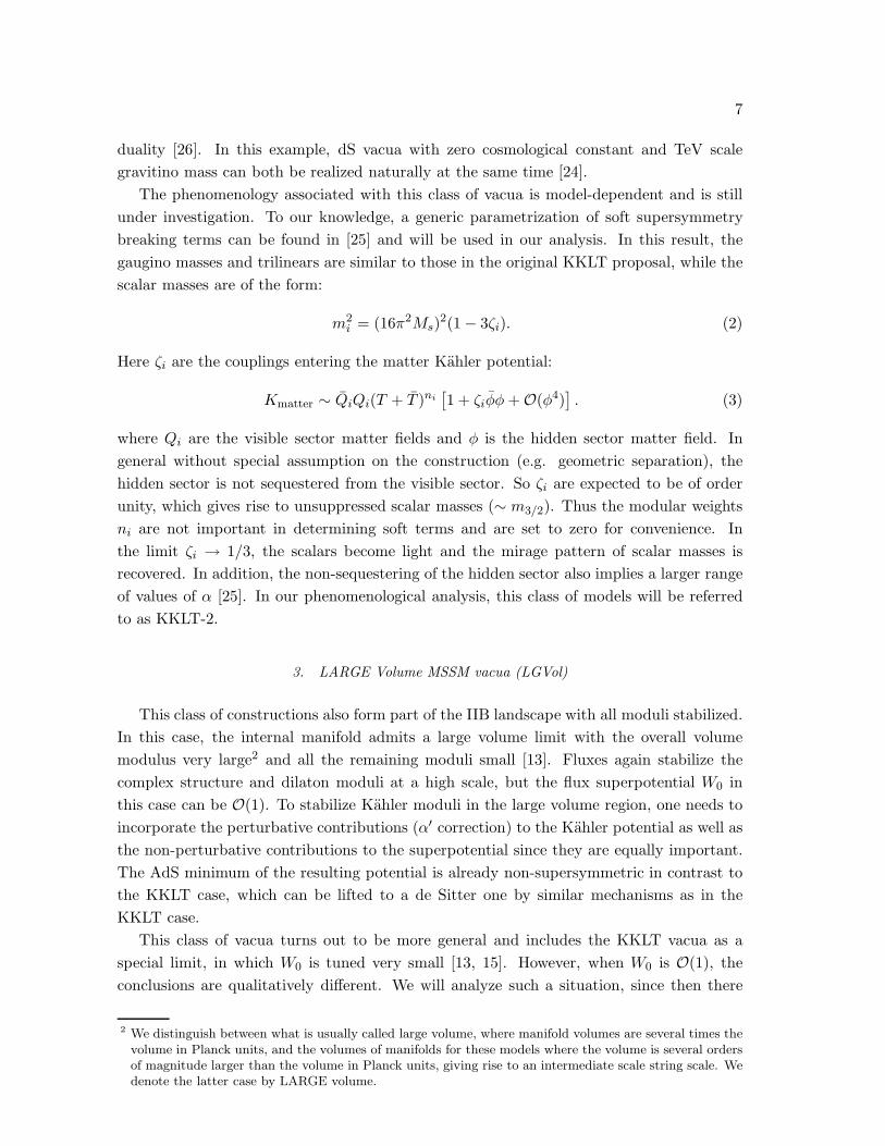
The phenomenology associated with this class of vacua is model-dependent and is still

under investigation. To our knowledge, a generic parametrization of soft supersymmetry

breaking terms can be found in [25] and will be used in our analysis. In this result, the

gaugino masses and trilinears are similar to those in the original KKLT proposal, while the

scalar masses are of the form:

m2i = (16π2Ms)

2(1 − 3ζi). (2)

Here ζi are the couplings entering the matter Kahler potential:

Kmatter ∼ QiQi(T + T )ni[

1 + ζiφφ + O(φ4)]

. (3)

where Qi are the visible sector matter fields and φ is the hidden sector matter field. In

general without special assumption on the construction (e.g. geometric separation), the

hidden sector is not sequestered from the visible sector. So ζi are expected to be of order

unity, which gives rise to unsuppressed scalar masses (∼ m3/2). Thus the modular weights

ni are not important in determining soft terms and are set to zero for convenience. In

the limit ζi → 1/3, the scalars become light and the mirage pattern of scalar masses is

recovered. In addition, the non-sequestering of the hidden sector also implies a larger range

of values of α [25]. In our phenomenological analysis, this class of models will be referred

to as KKLT-2.

3. LARGE Volume MSSM vacua (LGVol)

This class of constructions also form part of the IIB landscape with all moduli stabilized.

In this case, the internal manifold admits a large volume limit with the overall volume

modulus very large2 and all the remaining moduli small [13]. Fluxes again stabilize the

complex structure and dilaton moduli at a high scale, but the flux superpotential W0 in

this case can be O(1). To stabilize Kahler moduli in the large volume region, one needs to

incorporate the perturbative contributions (α′ correction) to the Kahler potential as well as

the non-perturbative contributions to the superpotential since they are equally important.

The AdS minimum of the resulting potential is already non-supersymmetric in contrast to

the KKLT case, which can be lifted to a de Sitter one by similar mechanisms as in the

KKLT case.

This class of vacua turns out to be more general and includes the KKLT vacua as a

special limit, in which W0 is tuned very small [13, 15]. However, when W0 is O(1), the

conclusions are qualitatively different. We will analyze such a situation, since then there

2 We distinguish between what is usually called large volume, where manifold volumes are several times thevolume in Planck units, and the volumes of manifolds for these models where the volume is several ordersof magnitude larger than the volume in Planck units, giving rise to an intermediate scale string scale. Wedenote the latter case by LARGE volume.

8

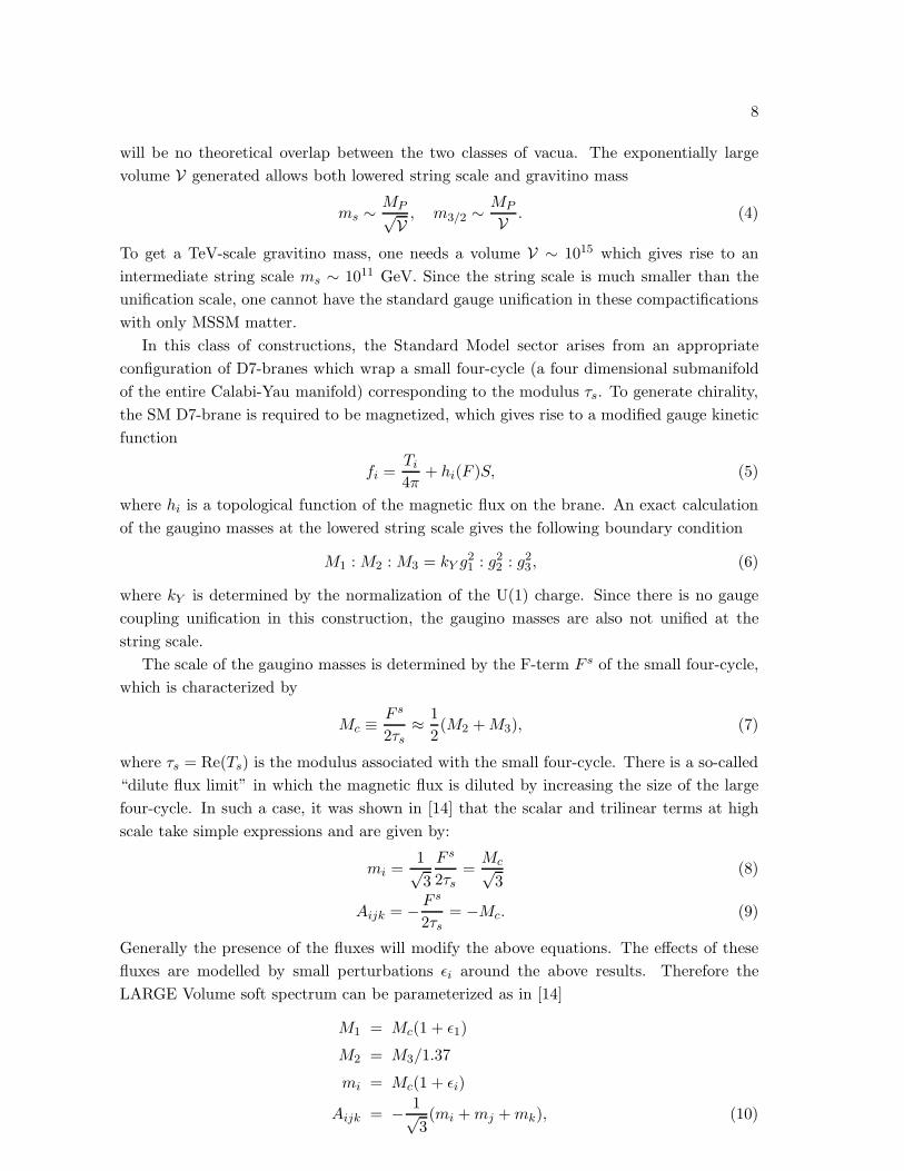
will be no theoretical overlap between the two classes of vacua. The exponentially large

volume V generated allows both lowered string scale and gravitino mass

ms ∼MP√V

, m3/2 ∼ MP

V . (4)

To get a TeV-scale gravitino mass, one needs a volume V ∼ 1015 which gives rise to an

intermediate string scale ms ∼ 1011 GeV. Since the string scale is much smaller than the

unification scale, one cannot have the standard gauge unification in these compactifications

with only MSSM matter.

In this class of constructions, the Standard Model sector arises from an appropriate

configuration of D7-branes which wrap a small four-cycle (a four dimensional submanifold

of the entire Calabi-Yau manifold) corresponding to the modulus τs. To generate chirality,

the SM D7-brane is required to be magnetized, which gives rise to a modified gauge kinetic

function

fi =Ti

4π+ hi(F )S, (5)

where hi is a topological function of the magnetic flux on the brane. An exact calculation

of the gaugino masses at the lowered string scale gives the following boundary condition

M1 : M2 : M3 = kY g21 : g2

2 : g23 , (6)

where kY is determined by the normalization of the U(1) charge. Since there is no gauge

coupling unification in this construction, the gaugino masses are also not unified at the

string scale.

The scale of the gaugino masses is determined by the F-term F s of the small four-cycle,

which is characterized by

Mc ≡F s

2τs≈ 1

2(M2 + M3), (7)

where τs = Re(Ts) is the modulus associated with the small four-cycle. There is a so-called

“dilute flux limit” in which the magnetic flux is diluted by increasing the size of the large

four-cycle. In such a case, it was shown in [14] that the scalar and trilinear terms at high

scale take simple expressions and are given by:

mi =1√3

F s

2τs=

Mc√3

(8)

Aijk = −F s

2τs= −Mc. (9)

Generally the presence of the fluxes will modify the above equations. The effects of these

fluxes are modelled by small perturbations ǫi around the above results. Therefore the

LARGE Volume soft spectrum can be parameterized as in [14]

M1 = Mc(1 + ǫ1)

M2 = M3/1.37

mi = Mc(1 + ǫi)

Aijk = − 1√3(mi + mj + mk), (10)

9

where ǫi were randomly generated within a domain 0 < ǫi < ǫ0. A reasonable value for

ǫ0 can be taken to be 0.2 as in [14]. The low scale gaugino mass ratios calculated from

the above boundary conditions are (1.5 − 2) : 2 : 6. As we see, the ratio of M2 and M3

is fixed but the ratio of M1 and M2 or M3 is not completely fixed. This can be seen from

(10) as open string fluxes lead to uncertainties for M1. At high scale, gaugino masses and

squark masses are roughly the same, and are both boosted by the SU(3) interaction when

RG evolved to the low scale. So generically the gluino is the heaviest particle and the first

and second generation squarks are only a little lighter than the gluino. The tau slepton is

extremely light (close to the mass of the LSP) which is needed to not overclose the universe

by the bino LSP relics.

4. Fluxless M theory G2-MSSM vacua (G2 )

The M-theory vacua we consider here follow reference [17]-[19]. One studies fluxless M

theory compactifications on G2 manifolds with at least two hidden sectors undergoing strong

gauge dynamics, at least one of which has charged matter. This leads to a stabilization of

all moduli and the spontaneous breaking of supersymmetry. The supersymmetry breaking

is dominated by the hidden sector meson field φ, which is not sequestered from the visible

sector. The gauge kinetic function is a linear combination of all geometric moduli si. For

the case where the matter Kahler metric does not depend on φ, the gaugino masses receive

comparable contributions from moduli and anomaly mediation, but is different from mirage

mediation in the KKLT string-susy model. The high scale gaugino masses have the following

form:

Ma ≈ − 1

4π(α−1M + δ)

ba +

(

4π α−1M

Peff

− b′aφ20

)

(

1 +2

φ20(Q − P )

)

m3/2 (11)

where b1 = 33/5, b2 = 1.0, b3 = −3.0, b′1 = −33

5, b′2 = −5.0, b′3 = −3.

αM is the tree-level universal gauge coupling and δ is the threshold correction from the

Kaluza-Klein modes. φ0 is the vev of the meson field, which is of order unity. P and Q are

the ranks of the hidden sector gaugino condensation groups. Low scale supersymmetry can

be obtained only if Q − P = 3. To get dS vacua, it is also necessary that the combination

Peff ≡ P ln(A1Q/A2P ) is less than 84, and larger than about 50 to get a gravitino mass

below 100 TeV. The scalar masses are about equal to m3/2 as there is no sequestering in

general. Thus, the soft supersymmetry breaking pattern is such that there is a large mass

splitting between gauginos and scalars, and the low energy effective theory at the weak scale

is mainly determined by the gaugino sector. Unlike split-SUSY, the higgsinos in these vacua

are as heavy as scalars and also decoupled. This gives the low scale gaugino masses large

finite threshold corrections from the higgs-higgsino loop. Generically the wino is the LSP for

G2-MSSM models with light spectra, but a wino-bino mixture is also allowed particularly

for heavier spectra.

10

5. Comments on the KKLT and LARGE Volume vacua

The three classes of type IIB MSSM vacua we described above are related in some

ways. As seen in Sections IIB 1 and IIB 2, KKLT-1 and KKLT-2 are different in the

supersymmetry breaking and uplifting mechanism and they generically give rise to different

soft supersymmetry breaking terms. KKLT-2 in some sense a broader class of constructions

as the explicit structure of the hidden sector is not completely specified, while that in

KKLT-1 is completely specified. Thus it is in principle possible to make a model within the

KKLT-2 class which has exactly the same soft supersymmetry breaking terms as KKLT-1.

This happens for example when the hidden section is sequestered from the visible section

and ζi goes to 1/3 as has been already shown. So, in terms of the soft susy breaking

pattern, models of KKLT-1 are a subset of those of KKLT-2. One should keep in mind that

this overlap is a “theoretical overlap”3 and cannot be distinguished at the LHC. So in the

distinguishibility analysis in the rest of the paper, we will focus on the region of KKLT-2

which does not overlap with KKLT-1. Further study is needed to learn whether cosmological

or additional visible sector physics can distinguish these constructions phenomenologically.

The KKLT and LARGE Volume MSSM vacua (described in II B 1 and IIB 3) are two

distinct regions in the type IIB landscape. However they can be smoothly connected by

dialing some parameters. The same scalar potential which gives rise to the large-volume

minimum also has a KKLT minimum if W0 ≪ 1 [13]. As W0 decreases, the two minimums

approach each other and eventually merge. So one could in principle start with LARGE

Volume MSSM vacua and decrease W0 while keeping m3/2 fixed by decreasing the volume V.

In this way, the large-volume minimum will gradually lose its “large volume” property and

become more and more like a KKLT vacua with TeV scale gravitino mass. We do not know

much about the properties of these intermediate vacua. One possibility is that they lead

to a set of soft supersymmetry breaking terms which interpolate in between the LARGE

Volume MSSM vacua and KKLT MSSM vacua. Even if this is true, phenomenologically it

is not clear whether these intermediate vacua will survive after all kinds of experimental and

consistency constraints. It may be that a continuous set of intermediate vacua consistent

with data and theory do not exist.

III. FOOTPRINT OF “STRING-SUSY MODELS” AT THE LHC

A. How to construct a Footprint in general

As was explained in section IIA, a string-susy model is specified by a set of microscopic

parameters characteristic of the class of string vacua. A complete analysis for the whole

(microscopic) parameter space is necessary if one hopes to discriminate between different

string-susy models. The prediction of a given string-susy model at the LHC is a map from

this parameter space to LHC signature space. This is a multi-dimensional region which

we call the “footprint” of the particular string-susy model. In this paper we construct

3 in the sense that the two class of models give rise to the same soft terms from a theoretical point of view.

11

a footprint for the three string-susy models described earlier - KKLT MSSM vacua (two

variations), LARGE Volume MSSM vacua and G2-MSSM vacua. We first start with a

general discussion of constructing a footprint of any string-susy model.

As seen in the last section, a set of MSSM soft supersymmetry breaking parameters

can be obtained at the compactification scale4. Below this scale, heavy stringy and Kaluza-

Klein states decouple and the soft parameters of the MSSM fields are governed by the MSSM

renormalization group equations. Gauge couplings and Yukawa couplings are determined

from current experimental data. The µ parameter is determined by the correct electroweak

symmetry breaking and Z boson mass. It would of course be preferable to calculate µ and

tan β from the microscopic theory as well, but that is not yet possible. In the G2 case tan β

is calculated from the theory, but not µ.

In addition the low scale soft supersymmetry spectrum is subject to various constraints

from current observation. There are lower bounds on the masses of the various sparticles

from the SUSY searches at LEP and Tevatron. The most important ones are the chargino

mass limit and the higgs mass limit. There are also constraints from observations in cos-

mology, i.e. dark matter relic abundance Ωh2. Although one can compute the thermal relic

density reliably, there may be other contributions from non-thermal production or other

unknown sources, so one should impose an upper limit constraint but not a lower limit one.

In order to connect to LHC experiments, the next step is to simulate the p p collision

and the decay of particles produced at the LHC followed by detection of the surviving

particles in the final state. In our analysis, we use the PGS4 [31] package which generates

events using PYTHIA6.4 [28] and then perform the detector simulation, where the default

configuration of the detector parameters are used. While PGS is not a fully realistic detector

simulator for the LHC, it is simple, fast and gives a “pretty good” simulation result, as its

name suggests. The result from PGS usually agrees fairly well with the result one might

obtain with a full-fledged detector simulation. In many cases the agreement is good, of the

order of 20%. To construct the footprint of the string-susy models described earlier, we

sample the high-scale (microscopic) parameter space with a large number of points. For

collider phenomenology, the simplest assumption of equal probability distribution on the

parameter space is presumably sufficient. For each point we sample, the corresponding

signatures are computed through the aforementioned procedure. For our purposes here,

where we compare predictions of different models, these procedures are adequate. Later the

analysis can be sharpened. The procedure to go from string/M theory to signatures may

seem complicated, but now user-friendly softwares exist to do that. One can access much

of the software through the LHC Olympics website [27].

To demonstrate the general approach shown above, we construct footprints of the four

string-susy models discussed for an integrated luminosity of 5 fb−1. In the simulation, we

use the L2 trigger in PGS to get better S/B ratios [27]. For signatures, we use the following

selection cuts for objects in each event

• Jet PT > 50 GeV; Lepton and Photon PT > 10 GeV; 6ET > 100 GeV.

4 This is typically the unification scale

12

This means only objects satisfying the above cuts are kept in the event record. For back-

grounds, we use the background sample in the LHC Olympics webpage [27] which includes

dijets, tt and W,Z+jets processes and scale it up to get an estimate of the background for

an integrated luminosity of 5 fb−1. Other backgrounds may be important and should be

taken into account in a more thorough analysis of the backgrounds, but as will be seen

below the treatment of backgrounds will not have much affect on our main results. The

condition for a (counting) signature to be observable above the background is:

S√B

> 4, S > 5, (12)

where S is the number of signal events that pass the selection cuts, while B is number of

background events that pass the same cuts. Thus we can assign an observable limit for each

(counting) signature below which the signal is not likely to be observed.

Figures 1 and 2 represent some simple 2D slices of footprints. There is no particular rea-

son for the above choice of signature plots, they are just meant to illustrate general features.

Some of these plots however have the added advantage that they are also useful in distin-

guishing some string-susy models. In all the (counting) signature plots, the approximate

regions where the SM dominates are entirely blacked out 5. Immediately one can see from

these plots that the footprints for these string-susy models are finite regions in signature

space. This implies that a well-defined string-susy model is not likely to cover the whole

signature space, but only a part of it. In addition, based on these footprints, one can readily

distinguish among the string-susy models in many cases. For example, the plot of 1-b jet vs.

3-b jets clearly separates the KKLT-1 and G2 string-susy MSSMs. By definition a footprint

covers all possible signatures that might come out from a string-susy model. Therefore

plots of footprints demonstrate the overall difference between different string-susy models.

In this sense the footprint analysis generalizes the familiar benchmark analysis, where one

does not get an overall picture of signatures for a given model thereby making it difficult to

distinguish two classes of models. We emphasize that a (n-dim) footprint is the full region

on a (n-dim) signature plot or any 2-D slice generated as the microscopic parameters are

varied over their entire allowed ranges respectively.

B. Generic Features of Footprints

Some generic features of these footprints can be easily understood as follows. For simplic-

ity, we will only focus on simple counting signatures, which illustrate many of the important

points we want to emphasize. Counting signatures are always bounded by the maximum

cross section, which is related to existing lower limits on masses. Hence the 2D projection of

a footprint for counting signatures must be bounded along the radial direction. In addition,

if no upper bound is imposed on sparticle masses, the footprint can continuously approach

the origin. However the region below the observable limit is not interesting.

5 More precisely, it is the region bounded by the observable limits

13

FIG. 1: Two-dimensional slices of the footprint of the three string-susy models. All models are

simulated with 5fb−1 luminosity in PGS4 with L2 trigger. If not explicitly stated, all signatures

include a least two hard jets and large missing transverse energy. For each example, the points are

generated by varying the microscopic parameters over their full ranges, as explained in Section III D.

The angular dispersion of the footprint is due to the variation in the spectrum, which

leads to a variation in branching ratios and in turn, the signatures. The smaller the angular

dispersion the larger the correlation in the low scale soft spectrum and the more predictive

the string-susy model. However, the exact spread depends on the particular signatures used

because of many factors. For example, even a completely random MSSM soft spectrum will

not cover the entire angular range from 0 to π/2. One also has to take into account real-

14

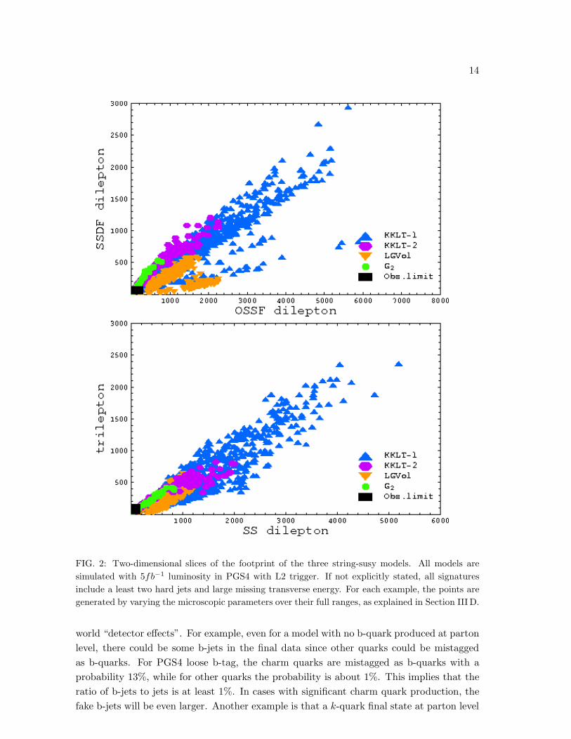
FIG. 2: Two-dimensional slices of the footprint of the three string-susy models. All models are

simulated with 5fb−1 luminosity in PGS4 with L2 trigger. If not explicitly stated, all signatures

include a least two hard jets and large missing transverse energy. For each example, the points are

generated by varying the microscopic parameters over their full ranges, as explained in Section III D.

world “detector effects”. For example, even for a model with no b-quark produced at parton

level, there could be some b-jets in the final data since other quarks could be mistagged

as b-quarks. For PGS4 loose b-tag, the charm quarks are mistagged as b-quarks with a

probability 13%, while for other quarks the probability is about 1%. This implies that the

ratio of b-jets to jets is at least 1%. In cases with significant charm quark production, the

fake b-jets will be even larger. Another example is that a k-quark final state at parton level

15

can be read-off as an event with k − 1 jets if one of the jets is soft and thereby fails to pass

selection cuts, or if two jets merge together to form a single jet. The limited statistics of

our simulations are not a problem since the precise regions are not needed for our main

conclusions, and since we understand why the regions have the boundaries they do. Later,

analysis with more statistics can be done.

C. Origin of Distinguishibility - Correlations

It is desirable and important to qualitatively understand the footprint boundaries and the

difference between footprints. The features in footprints can be connected to the underlying

theory by understanding correlations between soft parameters which in turn have their origin

in the structure of the underlying theory. One could understand this as follows. Formally,

the collider signatures (si) are functions of the MSSM masses and couplings (call them mi in

general), which are themselves parameterized by the underlying “microscopic” parameters

(call them ξk). One has:

si = si(mj) = si

(

mj(ξk))

. (13)

For an arbitrary set of MSSM parameters, one would get a very broad set of signatures6,

or equivalently, the corresponding footprint would cover a very large region in signatures

space. However if there is a non-trivial dependence on the more fundamental (microscopic)

parameters ξk, the MSSM parameters are correlated with each other and so are the signa-

tures. Therefore by understanding how correlations between soft parameters are connected

to the structure of the underlying theory, one can understand why a given footprint occu-

pies a given region in signature space and not some other region. In order to make the task

easier, it is helpful to first understand the footprint in terms of the pattern of spectra of the

class of models and then understand the spectra in terms of the soft parameters determined

from the underlying theory. For simplicity, here we only explain the former. The latter can

also be done in a straightforward manner, the interested reader can refer to the references

available for the string-susy models studied here. The features described here are not used

in constructing the plots, but are valuable in understanding the plots.

Let us start with colored particle production. For KKLT-1 and LARGE Volume string-

susy models, the squarks are lighter than the gluino and the dominant production is squark

pair production and the squark-gluino production. For G2-MSSM models, the dominant

production is gluino pair production since all squarks are extremely heavy. The KKLT-2

models also have a large scalar mass and are dominated by gluino pair production. This

difference in the dominant production channel already leads to a difference in the lepton-

charge asymmetry, as seen in Figure 3. Below we list some broad distinguishing features in

the spectra of the string-susy models and their related signatures.

1. Sleptons in KKLT-1 and LARGE Volume MSSM models are relatively light (lighter

than the gluino). Moreover τ is generically the lightest slepton. On the other hand,

6 The signatures will still not be uncorrelated due to the structure of the MSSM itself and also due todetector effects. However, we are interested in correlations which are present in addition to these.

16

FIG. 3: A particular slice of footprint for the models studied. The one-lepton charge asymmetry

(only include e and µ) is defined as A(1)c ≡ N

+

l−N

−

l

N+

l+N

−

l

. The SSDF/1tau signaturea is defined as the

ratio of the number of events with SSDF dilepton and the number of events with 1 tau lepton. All

models are simulated with 5fb−1 luminosity in PGS4 with L2 trigger. If not explicitly stated, all

signatures include a least two hard jets and large missing transverse energy. For each example, the

points are generated by varying the microscopic parameters over their full ranges, as explained in

Section III D.aRatios of counting signatures are independent of the total rate and are sometimes useful. This gives an

example.

sleptons in G2-MSSM models are very heavy (around O(10) TeV). So, signature

plots sensitive to lepton flavor asymmetry could differentiate KKLT-1 and LARGE

Volume from G2.

2. The gaugino mass ratios are different for different models, which lead to a difference

in the jet multiplicity. For KKLT-1, the difference between M3 and the LSP mass

is much smaller than that of LARGE Volume and G2 models (for the same gluino

mass). So if we use a hard pT cut on the jets (e.g. PT (jet) ≥ 200 GeV), then most of

the four-jet events in KKLT-1 cannot pass the cuts since they are mostly from gluino

pair production. However, for two-jet events, since the mass difference mq −MLSP is

large enough, most of them will pass the cuts. Thus we can probably use signature

plots of events with 2 jets and events with 4 jets to distinguish models of KKLT-1

with those of LARGE Volume and G2. However in our plots, it can be seen there is

still an overlap between KKLT-1 and LARGE Volume regions. The KKLT-1 models

in the overlap region are exactly those with heavier gluinos.

17

3. Since the top Yukawa coupling is large, from RGE running the stop is lighter com-

pared to other squarks. This is more pronounced for G2 models since the tan β is

particularly small (∼ 1.5). The gluino will preferentially decay via a virtual stop and

lead to b-rich events. For KKLT-1 and LARGE Volume models, the stop is again light

and its production rate is big. However since all other squarks are also copiously pro-

duced, the overall branching ratio for the events with b-jets is not particularly large,

so signature plots involving numbers of b-jets can distinguish G2 models from those

of KKLT-1 and LARGE Volume. In cases with very light stops, the stop production

rate is very large, but they will decay into charm quarks instead of bottom quarks if

the stop is lighter than C17. Therefore these models will again give relatively small

number of events with b-jets.

4. The KKLT-2 models appear in the signature space similar to G2 models because they

both have very heavy scalar masses. However they extend to a much bigger region in

many plots and have some overlap with KKLT-1 models. Because of the large scalar

masses, KKLT-2 models can be in the focus point region which is consistent with

the dark matter constraints. This means in these models the LSP has a significant

higgsino component. We also know that because of the higgsino mixture, gluinos tend

to decay into b-jets through the large Yukawa couplings. As the consequence of the

variation in the higgsino fraction, there is a large spreading in the b-jet signatures.

In Fig. 4 and 5, we show how the b-jet multiplicity affects the relative positions of these

footprints. It can be seen that as the b-jet multiplicity increases, the footprints of G2 and

KKLT-2 models become isolated from the other two with a larger angular separation. This

demonstrates that the b-jet multiplicity is related to a certain structure of the underlying

theory. Thus, this is an example of a signature which is directly correlated with underlying

structure of the theory and is particularly useful. For KKLT and LARGE Volume models,

their relative position does not change much as the b-jet multiplicity changes, implying they

have similar structure with regard to b-jet multiplicity. To summarize, the boundaries and

the distinguishibility of footprints can be understood in terms of the spectra, and in turn in

terms of the correlations between the soft supersymmetry breaking parameters determined

by the underlying string-susy model.

Finally one should remember that although in principle we can have a large number of

signatures, they are not orthogonal to each other. It was shown explicitly in [3] that for

a set of MSSM models with 15 parameters, the effective dimensionality of signature space

(with 1808 signatures) is only ∼ 5 or 6. This means differences in the spectra may be lost

in the process of mapping to signatures. This can also be seen in the various signature

plots we have made, where only a few of them are quite different. The origin of this is

related to the nature of hadron collision where signatures are usually polluted by large

combinatorial backgrounds. Therefore figuring out analytically how to pick out mutually

independent signatures which can distinguish classes of models is very difficult in general.

7 In this case, the decays t→ bC1 and t→ tN1 are kinematically closed.

18

FIG. 4: Slices of footprints for the models studied. All models are simulated with 5fb−1 luminosity

in PGS4 with L2 trigger. If not explicitly stated, all signatures include a least two hard jets and large

missing transverse energy. For each example, the points are generated by varying the microscopic

parameters over their full ranges, as explained in Section III D.

In practice, as demonstrated in Section IV, distinguishing classes of models can be done by

adding lots of signature plots since the overlap region always decreases. By doing this one

can identify useful independent signatures. Sometimes it also helps to pick signature plots

sensibly based on the qualitative features described above. We will discuss more about this

issue in Section IV A.

19


in PGS4 with L2 trigger. If not explicitly stated, all signatures include a least two hard jets and large

missing transverse energy. For each example, the points are generated by varying the microscopic


We have mostly focused on counting signatures, but one can also study various distribu-

tions. Distributions can be used similarly to counting signatures if they are converted into

quantiles. In our initial analysis, we have implemented the following basic distributions:

• Effective mass of all objects meff =∑

a P aT , divided into 12 categories labelled by

20


in PGS4 with L2 trigger. For each example, the points are generated by varying the microscopic


number of jets and leptons in the event: nj = 2, 3, 4, 5+, nl = 0, 1, 2+

• Missing ET distributions, divided into 3 categories labelled by the number of leptons

nl = 0, 1, 2+

• Invariant mass of all objects minv =(∑

a P aµ

)2, divided into 12 categories labelled by

number of jets and leptons in the event: nj = 2, 3, 4, 5+, nl = 0, 1, 2+

To get quantile (decile for example) signatures, the entries in a distribution are sorted

into ten bins such that each bin contains 10% of the total events. The boundaries of the

bins are taken as signatures, with no signatures related to the lower and upper boundaries

of the whole distribution. Therefore each distribution gives 9 signatures and we have 243

signatures for the 27 distributions above. We have examined many different quantile signa-

ture plots. There are a few plots which can separate some string-susy models, two of them

are shown in Figures 6 and 7.

We have seen not only that footprints are generally limited, but that we can always get

a qualitative understanding of the boundaries of the footprint region. Therefore one can

obtain a lot of insight even without a high statistics simulation of the footprint region in

many cases, although in some cases when there is data increasing statistics could turn out

to be important.

21


in PGS4 with L2 trigger. For each example, the points are generated by varying the microscopic


D. Details of Constructing Footprints for String-Susy Models

In this subsection, we explain in more detail the construction of the footprint of the

various string-susy MSSMs. Starting with the KKLT-1 string-susy model, the high scale

parameter space is defined in section 2. Explicitly, the low scale soft spectrum is specified

by the following parameters:

Ms, α, nl, nq, nh, tan β, sgn(µ). (14)

To sample the parameter space, one has to set the ranges for scanning these parameters.

First, based on the previous works [7, 8, 9, 10] we already know that for α below 4 − 5,

the model is excluded either by the presence of tachyons or a stop/stau LSP, while for α

above ∼ 10 the model (satisfying the dark matter constraint) usually gives rise to a very

light spectrum. So we choose to vary α from 4 to 10, which we think covers the most

interesting region of KKLT-1. As can be seen in Eq.(1), Msα controls the scale of the

sparticle masses. To avoid those cases with very small masses which are excluded by the

SUSY search limits as well as those with very large masses which are too heavy to be

interesting at low luminosities, we take Ms to be in the range 25 GeV to 100 GeV. As usual

tan β is taken to be from 1 to 50 (this is also used for all other models). As mentioned in

Sec. II B 1, modular weights nl, nq and nh are not fixed unless the string construction is

22

explicitly specified. So in order to be general we allow a continuous variation of the modular

weights from 0 to 1/2 independently. In addition, for a practical step-by-step analysis of the

scan of these modular weights, we divide the task of the complete scan into several pieces

choice 1 : 0 < nh, nq, nl < 0.1

choice 2 : 0 < nh < 0.1, 0 < nl, nq < 0.5

choice 3 : 0 < nh, nq, nl < 0.5

(15)

The first choice corresponds to a perturbation of zero-modular-weight models with an un-

certainty 0.1. The size of the error is somewhat arbitrary but will not affect any of our

conclusions. The second choice is to allow for a large variation for quark and lepton modu-

lar weights. The third one should capture most of the cases with non-zero-modular weights,

as those with modular weights beyond 0.5 are very likely to be excluded by the presence of

tachyonic scalars. Clearly the first choice is a subset of the second one, which is in turn a

subset of the third choice. Each choice is randomly sampled with 500 points.

For a given set of these parameters, we compute the corresponding soft terms at the

unification scale8 and then evolve them using SOFTSUSY 2.0 [29] to the TeV scale to

get the sparticle spectrum. The relic density of neutralino dark matter is calculated using

MicrOMEGAs v1.3.6 [30]. Only models with ΩLSP h2 < 0.12 are allowed by the relic density

constraint. In the scan, models with tachyonic scalar masses as well as those which violate

the chargino mass constraint (mχ1≥ 104 GeV) or higgs mass constraint (mh ≥ 114 GeV)

are rejected. We also impose a cutoff for stop mass less than 300 GeV. This is a convenient

choice for simulation due to limited computing time and can be relaxed. It is clear this cutoff

will remove the large cross section region of the footprint. However it will not affect the

essential feature of the correlations between signatures and therefore, is not very important

for our analysis.

For the KKLT-2 string-susy model, the scalar masses are generically heavy. To focus

on this region, we take parameters ζi in the range from 0 to 1/6. ζi are assumed to be

different for the lepton, quark and higgs fields but the same among different generations.

The parameter α in this model can have a larger variation, which is taken from 4 to 20.

The gravitino mass is chosen to vary from 1 TeV to 10 TeV.

For the footprint of LARGE Volume string-susy models, we generate sample points by

varying M3 from 400 GeV to 500 GeV and ǫi from 0 to 0.2. The lower value of M3 is chosen

so that the light higgs mass is above the current experimental limit. We have examined

cases with M3 less than 400 GeV and have found that almost all models generated are

excluded by the higgs mass limit. The upper value set here is to avoid having too heavy a

gluino.

G2-MSSM models are generated by varying the parameters δ, Peff and VX in the fol-

lowing ranges:

− 10 ≤ δ ≤ 0, 60 ≤ Peff ≤ 84, VX,min ≤ VX ≤ VX,max, (16)

8 we assume that these models give rise to gauge coupling unification as is suggested from the unificationof couplings in the MSSM.

23

where VX,min and VX,max are functions of other parameters and can be found in [19]. We

only consider the case in which Q − P = 3, since other cases either give rise to extremely

heavy gravitinos or lead to AdS vacua [18]. The gauge couplings and Yukawa couplings

at GUT scale are determined to match the low scale values. The RG evolution is carried

out at 1-loop level with the “match and run” method to accommodate large scalar masses.

Another consequence of heavy scalar masses is that the higgs bilinear parameter Zeff is

finely tuned to get EWSB breaking with correct Z boson mass. tan β is predicted in these

vacua to be of O(1) [19].

IV. DISTINGUISHING STRING-SUSY MODELS FROM LHC SIGNATURES

Thus far we have constructed footprints for four (including two versions of KKLT) string-

susy models. The choices here are made basically to illustrate the results and techniques

with limited computing. As data approaches and more string-susy models are added, more

systematic calculations can be done. We have shown that footprints of string theories cover

limited regions in LHC signature space, for understandable reasons. We now examine how

to use these footprints to distinguish among string-susy models at the LHC. There have

of course been discussions on how to distinguish different beyond-the Standard-Model con-

structions. There may be a signature which is sensitive to some features in the spectra and

behaves differently for different models. For example, same-sign(SS) dileptons is a signature

which has been widely discussed in the literature in distinguishing supersymmetric models

from non-supersymmetric ones. However, this is often not very useful for distinguishing

among various supersymmetric models, particularly those with an underlying high-scale.

This is because the overall mass scale in each of these models is not fixed implying that the

signatures can vary in a big range, which will wash out some simple correlations between

(counting) signatures and features in spectrum. So it often happens that for most of the

signatures the two scenarios overlap a lot and one can not tell them apart completely. But

as we have seen there are correlations between certain pairs of signatures because of the

structure of the underlying theory. This implies that it is likely that overlapping models of

two different string-susy models do not overlap for other signatures. So systematically one

would try to scan combinations of two signatures and check if the footprints are completely

separated in the corresponding plots. This method was first explored in [1] and was found

to be useful in some simple situations where the spectra of different string-susy models have

big differences. For the string-susy models considered in this paper, the G2 models can be

distinguished from those of KKLT-1 and LARGE Volume by this method. For KKLT-1 and

LARGE Volume models, we have found that no single 2D plot, i.e. no pair of signatures,

can distinguish these models completely. However, as we will see below, these can still be

distinguished by a combination of several 2D plots.

24

A. Extracting Correlations from 2D Plots

In this section we consider a more systematic way to extract correlations from signatures.

Intuitively, one keeps track of the microscopic parameters associated with points in the

overlap regions and eliminates parameters whenever they are not in an overlap region.

In the remainder of this section and the next subsection we present some more technical

and quantitative procedures. One should not lose sight of the essential point that one is

distinguishing the theories by adding signature plots and keeping track of the microscopic

parameters of the points in overlap region.

Conventionally one might try distinguishing classes of models by directly calculating the

distance in the multi-dimensional signature space including a large number of signatures.

A χ2-like quantity [3] could be defined with Nsig signatures as:

(∆SAiBj)2 =

1

Nsig

Nsig∑

a=1

(

sAia − s

Bja

σAiBja

)2

. (17)

Here sAia is signature a of model Ai and similarly for B. The quantity σ

AiBja

9 characterizes

the uncertainty in the ath signature for the classes of models A and B. If the quantity

(∆SAiBj)2 is greater than the statistical fluctuation (∆S0)

2 for all i’s and j’s, then one

should be able to distinguish the two classes of models. However this method is not as

effective as what we are proposing here. The average over a large number of signatures in

Eq.(17) will diminish the difference between two classes of models if most of the signatures

included are not effective in distinguishing them. A pre-selection of “useful” signatures

could help but there is no systematic a priori way of knowing that. Indeed, this conventional

method might not be useful at all, while the method we describe below always is.

Let us start with the following toy example. Suppose there are two signature plots a and

b, each of which partially distinguishes footprint A and B. In other words, there is a sizable

overlap between A and B for each plot, denoted as (A∩B)a and (A∩B)b respectively. If the

signatures in plot a are correlated non-trivially with signatures in plot b, one would expect

that at least some of the models of footprint A in the overlap (A∩B)a can be differentiated

from footprint B by signatures in the plot b, and so the set of models of footprint A in the

overlap (A ∩ B)a will have a smaller intersection with footprint B in (A ∩ B)b. In other

words, (A ∩ B)a ∩ (A ∩ B)b is smaller than either (A ∩ B)a or (A ∩ B)b. Therefore, the

overlap region in 2D signature plots a or b does not imply a real degeneracy as it is lifted

(at least partially) when more signatures are included. This idea is illustrated in Fig.8. In

principle one can continue adding more signature plots and the overlap region is expected

to be significantly reduced in the end. To technically realize the above idea, we need to

make a few definitions to quantify the overlap of footprints in the following. First of all, we

define the notion of degeneracy for two points Ai ∈ A and Bj ∈ B:

Defn: Two points Ai ∈ A and Bj ∈ B are said to be degenerate in the 2D signature

space (x, y) if the χ2-like quantity (∆SAiBj)2 of the two points is smaller than the statistical

9 The definitions of σAiBja and (∆S0)

2 can be found below Eq.(18)

25

Signature a-x

Signature b-x

Signature Plot b

Signature Plot a

Sign

atur

e a-

y Si

gnat

ure

b-y

A

B

A

B

Parameter Space of B

Parameter Space of A

FIG. 8: Figure illustrating the idea that correlation between different signature plots can be used

to reduce “false degeneracy”.

fluctuation (∆S0)2.

For two signatures, (∆S)2 in Eq.(17) becomes:

(∆SAiBj)2 =

1

2

(

sAix − s

Bjx

σAiBjx

)2

+

(

sAiy − s

Bjy

σAiBjy

)2

, (18)

which characterizes the distance in the 2D signature space. Here sAix is signature x of

model Ai and similarly for others. The variance (σAiBjx ) is defined as (σ

AiBjx )2 = (δsAi

x )2 +

(δsBjx )2 +

(

fi(sAix + s

Bjx )/2

)2

, where fi = 0.01 for all counting signatures and δs =√

s + 1

for counting signatures [3]. ∆S0 characterizes the statistical error, which is determined by

simulating a large number of models with different random number seeds and taking the

95th percentile of the ∆S’s.

Defn: The model Ai is said to be degenerate with the entire footprint B with respect to

the 2D signature plot (x, y) if there exists at least a model Bj ∈ B such that Ai and Bj are

degenerate.

In our convention the number of models of footprint A which are degenerate with B is

denoted by NA,B, similarly the number of models of footprint B which are degenerate with A

is denoted by NB,A. One can also notice that NA,B and NB,A are in general different, because

the densities of models of the two footprints in the overlap region are different in general.

So the overlap can be characterized by the algebraic mean N(A,B) ≡ 1

2(NA,B + NB,A). It

is clear from this definition that if the overlap calculated for footprints A and B vanishes,

then the corresponding constructions can be completely distinguished.

As an example, we use the above method to distinguish (original) KKLT and LARGE

Volume string-susy models. To estimate ∆S0, we have resimulated 100 KKLT models with

26

FIG. 9: Signature plots used for eliminating degeneracy between KKLT-1 (blue) and LGVol (orange)

string-susy models. All models are simulated with 5fb−1 luminosity in PGS4 with L2 trigger. For

the signature - “1 b-jet and 2 leptons” and “clean dilepton”, there is no requirement of two hard

jets. For all other signatures, there are at least two hard jets and large missing transverse energy.

For each example, the points are generated by varying the microscopic parameters over their full

ranges, as explained in Section III D.

27

different random numbers and calculated ∆S for them. The 95th percentile of the ∆S

distribution gives ∆S0 ≈ 1.5. For different pairs of signatures ∆S0 will vary by ∼ ±0.1.

As we have mentioned before, the first step of our strategy is to construct a large set of

signature pairs. Without knowing which ones are better in distinguishing the two classes of

models, one has to add all of them one by one. However to make the demonstration simple,

we first do some trial-and-error analysis and find some signature plots which can partially

distinguish these two classes of models. This will make the overlap decrease faster. For the

present case, it is actually not difficult to find these if the PT cut for jets is increased to

200 GeV based on the features in spectrum as explained in IIIC. Three of these plots are

shown in Fig. 9. First we consider those models of KKLT-1 obtained with scan choice 1

(explained in (15)) and use the three plots in Figure 9 in our analysis:

• 1 tau lepton vs. 1 tau lepton and ≥ 1 b-jets.

• clean dilepton10 vs. 4 jets.

• 1 lepton vs. clean dileptons.

Starting from the first plot, distances ∆SAiBjbetween models in the two classes are calcu-

lated and those models of each class in the overlap region are selected. Then for the second

plot the same procedure is performed except that those selected models in the previous plot

are used instead. After that we will have a selection of models for each class which still

remain in the overlap region for both plots. This procedure is carried out by adding more

2D signature plots until either the number of models in the intersection vanishes or does

not decrease further. For the three plots in the order they are listed, we find the number of

models in each class remained after each operation decreases monotonically as follows:

KKLT-1 (scan choice 1): 119 → 4 → 0

LARGE Volume: 237 → 17 → 0. (19)

To test the stability of this sequence upon changes in ∆S0, we use ∆S0 = 1.7 and find a

similar sequence

KKLT-1 (scan choice 1): 129 → 5 → 0

LARGE Volume: 259 → 21 → 0. (20)

One can see that the number of models in the intersection quickly decreases as more plots

are included. The final overlap of the two string-susy models is zero, which indicates that

they can be distinguished readily at the LHC even with low luminosities. Furthermore, the

models in the overlap region of each plot as well as the intersections of these overlap regions

can be mapped back to the parameter space of the underlying string-susy model.

The exact number of models in the final overlap depends on how the parameter space is

scanned and also how densely it is scanned. To make the method statistically robust, one

10 Clean dilepton signature is defined as the number of dilepton events with no hard jets passing the eventselection cuts.

28

should sample the parameter space with a large enough number of points. Furthermore,

to have a reliable count of models in the overlap region, the density of the points in the

footprint should be large enough (at least for one class of models). In order to confirm that

our result obtained with a sample of 500 points for these classes of models is robust11, we

include 1000 more points for the KKLT string-susy models (corresponding to scan choices

2 and 3)12, and try to construct the sequence (19) again. We find the following:

KKLT-1 (All scan choices): 451 → 37 → 6

LARGE Volume: 477 → 289 → 69. (21)

Now the number of models in the overlap does not vanish as before. However, when we

consider three different combinations of the same signatures as that used earlier, namely:

• 1 lepton vs. 1 tau lepton

• 1 lepton vs. 4 jets

• 1 lepton vs. 1 tau lepton and ≥ 1 b-jets

in addition to the previous combinations, the sequence again converge to zero as follows

KKLT-1 (All scan choices): 451 → 37 → 6 → 4 → 1 → 0

LARGE Volume: 477 → 289 → 69 → 11 → 1 → 0. (22)

For ∆S0 = 1.7, we have

KKLT-1 (All scan choices): 506 → 49 → 10 → 8 → 7 → 4

LARGE Volume: 488 → 331 → 114 → 56 → 18 → 5, (23)

which is almost as good as the sequence (22). We learn from the above that the overlap

N(A,B) can increase with a denser scan of parameters. However if two classes of models

can be distinguished intrinsically then N(A,B) will eventually vanish as more signature

plots are included. If one finds N(A,B) approaches a nonzero value even when all possible

combinations of signatures are included (for a given luminosity), then the two classes of

models can not be distinguished completely. We will see in the next section that it is

possible to define a quantity (which is independent of N(A,B)) to characterize the extent

to which two classes of models can be distinguished.

In the above examples, the (close to) optimal set of useful signatures was arrived at by

a judicious use of the trial-and-error method, i.e. by trying various signature plots sensibly

based on the qualitative features of the classes of models described above. This procedure

should work for other classes of models as well. However the main purpose of doing this here

11 Of course, for different models, one would need to sample a different number of points in general dependingon the structure of the microscopic parameter space.

12 KKLT-1 models with these two choices have very similar footprints in the signature space and so includingthem will increase the footprint density significantly.

29

is to illustrate the idea without making it too complicated. In practice, a more systematic

way to distinguish classes of models and pick out useful signatures is to simply add all kinds

of possible signatures and keep track of the overlap. A sharp decrease in the overlap usually

indicates that the signature pair just added is “good”. In doing this, one does not need to

know much about the features in the models and how they are related to the signatures,

and so the procedure can be implemented in an automatic way. In future studies, the

above procedure could be supplemented with modern statistical techniques such as neural

networks, boosted decision trees, etc.

B. A Quantitative Definition of Distinguishibility

In this subsection, we propose a quantitative way to characterize the distinguishibility

of two string-susy models. Let us denote the two classes of models as A and B. Suppose we

can properly define a metric on signature space and hence the volume of the overlapping

submanifold. Then a proper definition of the distinguishibility could be something like:

η(A,B) = 1 − S(A ∩ B)

2S(A)− S(A ∩ B)

2S(B), (24)

where S(A) denotes the volume occupied by A in signature space and similarly for others.

From this definition, we can see 0 ≤ η(A,B) ≤ 1. Clearly if there is no overlap, i.e.

S(A∩B) = 0, η(A,B) is equal to 1 indicating that the two footprints can be distinguished

completely. On the other hand, if the two footprints completely overlap with each other,

i.e. S(A ∩ B) = S(A) = S(B), then η(A,B) is zero indicating that they can not be

distinguished at all. For other intermediate cases, η(A,B) is between 0 and 1 indicating

partial distinguishibility, which is still useful depending on the location of experimental

data. This will be discussed in detail in the next section.

In practice,the footprint is sampled by a large number of points instead of being a

smooth manifold. For simplicty we will first assume that the points we sample are evenly

distributed in the signature space, or more precisely, the number of point in a given region

is proportional to its volume. This is not a realistic assumption, and we will relax it soon.

In this case, the definition of η can be rewritten as:

η(A,B) = limNA,NB→∞

(

1 − NA,B

2NA− NB,A

2NB

)

, (25)

where NA and NB are the total number of models in footprint A and B respectively, while

NA,B and NB,A are as defined in the previous subsection. This gives a practical definition for

distinguishibility. One can see that it is the ratio of the number of models in the overlapping

region and the total number of models for a given class of models which contributes to its

distinguishibility with another class of models. In practice, as long as NA and NB are large

enough, the η value obtained will be very close to the formal value obtained after taking

the limit to ∞. For example, for KKLT-1 and LARGE Volume (with ǫ0 = 0.2), we found

that none of the models in the two classes are degenerate. Thus, using this definition we

get η → 1, suggesting that the two string-susy models can be distinguished quite well.

30

In generic and more realistic cases the distribution of the models in the signature space

is not flat. We now show that the definition (25) is a more natural one to use compared to

definition (24) in such cases. It is reasonable to assume that sample points are generated

uniformly in model parameter space. If we take into account the mapping to signature space,

the points which sample the footprint are therefore not likely to be evenly distributed, but

are rather assigned with a probability which is determined by the non-trivial mapping

function. Suppose in the overlap region of two footprints this probability is small, then the

number of points in that region is also comparatively small relative to the total number of

points even though the volume of the overlap region is not. From definition (24), η and

hence the distinguishibility would be small. However, using definition (25), η would and

hence the distinguishibility would be large. This seems more natural since by assumption,

it is much less likely to populate the overlap region compared to the non-overlap region

by scanning model-parameters. Therefore we see that the definition (25) in terms of the

number of points is quite reasonable and convenient in practice.

V. DISCUSSION AND CONCLUSION

In this paper, we have introduced the idea of constructing footprints of “string-susy

models” (defined in Section IIA), and a general technique to distinguish different models by

correlations of signatures. Focusing on four classes of string-susy models where calculations

are reliable, our first major result is that they all give limited footprints in signature space.

In addition, the LHC signatures of a particular class of models are sensitive to at least

some of the underlying theoretical structure. This information is not only encoded in the

values of signatures themselves but also in their correlations. Familiar inclusive dilepton and

trilepton signatures are not very helpful in distinguishing among these string-susy models.

However they can be distinguished by systematically adding and studying the pattern of

signature plots and qualitatively understanding their origin. We have explicitly shown that

the overlap area of two footprints becomes smaller and finally vanishes as more signatures

plots are included.

Of course, it may be possible to recognize and interpret what is discovered rather easily.

Our approach will worthwhile particularly even when superpartner masses and properties

can not be untangled, and when degeneracies are present, so more traditional approaches

work poorly. These methods can be applied with very limited data, and improved as

integrated luminosities increase and more signatures become available.

The construction of footprints will of course be especially useful when the LHC data

is available, which will appear as a box in the signature space. Suppose there are two

string-susy models which can be distinguished from each other using the method described

in this paper, with low luminosity data at the LHC. In the event of actual data, if the box

corresponding to the data is far away from the footprints of both models, then both string-

susy models are excluded. If the box is inside one of the footprints but not the other one,

then the corresponding string-susy model is favored while the other is excluded. However,

31

FIG. 10: Cartoon to illustrate the various possibilities once there is data. The square box de-

notes “data” while the elliptical regions denote slices of footprints of two string-susy models in two

signature plots.

if the box lies in the overlap region of two footprints13, this means that both string-susy

models are consistent with data at that particular luminosity. The cartoon in figure 10

illustrates the point. In this case, one can focus on all such models and both improve the

theoretical constructions and add experimental observables and associated signature plots

to distinguish among them further.

We have focussed on LHC counting signatures to demonstrate the methods. Other LHC

data such as asymmetries (Figure 3), distributions in ET/ , pT , mass pairs, etc. all have

limited footprints as well, and can be valuable. Dark matter detection and relic density

involve the same physics and are meaningful to include for the signatures of an underlying

microscopic theory (but not for a low-scale effective theory), as is gµ − 2. Adding these

signatures will make the approach even more powerful. Since one has a full theory, it is

meaningful to add them.

In the steps from high-scale string construction to LHC signatures, there are various

kinds of uncertainties which were not yet considered properly. These include uncertainties

in the ranges of the high-scale parameter space, uncertainties arising from the RG evolution

codes, uncertainties arising from those in the SM parameters (the top quark mass for exam-

ple), uncertainties in experimental constraints, as well as those arising from simulations -

event generation, parton showering and hadronization and detector simulation. One might

worry whether these uncertainties will change the effectiveness of our method. Of course,

13 That is the box lies in the overlap of the entire footprints, not just some 2D footprints.

32

the boundary of the footprint will become fuzzy when these uncertainties are included.

However since our analysis is based on the correlations of signatures, the distinguishibility

of any two scenarios should not be affected. A better investigation of these issues is left for

the future, as is the study of theories that give extended MSSMs for the visible sector. We

expect the study of patterns of signature plots to be equally valuable in such cases.

Although particular classes of string-susy models with the same visible sector - the

MSSM - can be distinguished, it may be more challenging to distinguish classes of string

vacua with different matter and gauge spectra. If it turns out that there are some exotic

fields beyond the MSSM which are light enough to be produced (on-shell or off-shell), there

could be a substantial change in LHC signatures.

For all the string-susy models considered here, Electroweak symmetry breaking (EWSB)

is accommodated but not predicted, in the sense that the µ parameter is chosen by hand

so as to satisfy the EWSB condition. If one could find a natural dynamical mechanism

giving EWSB in the future, it would be important to know what the effect of this natural

mechanism would be on the pattern of signatures computed by just accommodating EWSB.

The answer to this question is not definitive, since it depends on the particle spectrum and

the exact mechanism. For example, within the context of the MSSM, it is well known

that consistent EWSB requires a precise relation between the supersymmetric µ parameter

and some soft supersymmetry breaking parameters. Therefore, one natural solution to

the problem of EWSB is that this precise relation can be predicted or explained from the

structure of a string-susy model. In this case, there would be no effect on the pattern of

signatures. However, if the visible sector of the string-susy model consists of particles in

addition to the MSSM which are light enough to be produced at the LHC and play a non-

trivial role in the EWSB mechanism (additional U(1) models are an example), then the

pattern of signatures could be affected significantly. Nevertheless, the methods described

in the paper are still applicable.

We have proposed a new approach to relating collider data and an underlying theory.

In the case where the underlying theory is a string construction with stabilized moduli and

softly broken supersymmetry, we have seen that particular constructions give very limited

footprints in signature space, and that LHC signatures for a particular class of vacua are

sensitive to at least some of the underlying structure of the theory. Not all theories agree

with data, and the subset that do can be distinguished by considering the pattern of a

number of signatures. The software techniques needed to carry out such a program for a

variety of constructions mostly already exist, and are improving. Our analysis needs to be

extended in a number of directions, perhaps most by examining a number of constructions

from different corners of string/M theory, with different compactifications, different ways

of generating de Sitter vacua and different ways of breaking supersymmetry in a controlled

manner.

We think that string theorists will learn about string theory by studying collider phe-

nomenology. This has happened from studying the visible sector, particularly in heterotic

and Type II toroidal constructions, and we expect it to happen from the study of super-

partner properties. Given the large number of string vacua one could ask whether it is very

unlikely that the ones we study could be like our vacuum? We think it is not so unlikely

33

because we do not study random string/M theory constructions - we select for study those

that can give SM-like matter, softly broken N = 1 supersymmetry, dark matter, inflation,

and so on. The approach described here may help us learn if we live in a string/M theory

vacuum, and learn more about its properties.

Acknowledgments

The authors appreciate encouragement and helpful conversations with and suggestions

from Bobby Acharya, Joseph Lykken, Arjun Menon, David Morrissey, Brent Nelson, Aaron

Pierce, Albert de Roeck, Maria Spiropulu and Liantao Wang. The research of GLK, PK

and JS is supported in part by the US Department of Energy.

VI. APPENDIX: COUNTING SIGNATURES USED IN OUR STUDY

As we have discussed before, we are particularly interested in extracting information from

the low luminosity data (5-10 fb−1) corresponding to 1-2 year running of LHC. For this

purpose, we will select a special set of counting signatures as our observables. A complete

set of counting signatures can be found in [3]. Here we consider the following counting

signatures:

• 1 lepton, OS dilepton, SS dilepton, trilepton, 1 tau lepton, 2 tau leptons, 3 tau leptons,

OSSF dilepton, OSDF dilepton, SSSF dilepton, SSDF dilepton, OS dilepton(e,µ), SS

dilepton(e,µ)

• 1 jet, 2 jets, 3 jets, 4 jets, 1 b-jet, 2 b-jets, 3 b-jets, 4 b-jets

• 2 leptons and 1 jet, 2 leptons and 2 jets, 2 leptons and 3 jets, 2 leptons and 4 jets

• 0 lepton and 2 b-jets, 0 lepton and ≥ 3 b-jets, 1 lepton and ≥ 2 b-jets, 2 leptons

and 0 b-jet, 2 leptons and 1 b-jet, 2 leptons and 2 b-jets, 2 leptons and ≥ 3 b-jets, 3

leptons and 1 b-jet

• 1 tau and ≥ 1 b-jets, 1 tau and ≥ 2 b-jets, 2 tau and ≥ 2 b-jets, ≥ 2 tau and 1 b-jet

• 1 positive lepton, 1 negative lepton, clean dilepton

[1] G. L. Kane, P. Kumar and J. Shao, arXiv:hep-ph/0610038.

[2] D. J. H. Chung, L. L. Everett, G. L. Kane, S. F. King, J. D. Lykken and L. T. Wang, Phys.

Rept. 407, 1 (2005) [arXiv:hep-ph/0312378].

[3] N. Arkani-Hamed, G. L. Kane, J. Thaler and L. T. Wang, JHEP 0608, 070 (2006)

[arXiv:hep-ph/0512190].

[4] P. Binetruy, G. L. Kane, B. D. Nelson, L. T. Wang and T. T. Wang, Phys. Rev. D 70, 095006

(2004) [arXiv:hep-ph/0312248].

http://arXiv.org/abs/hep-ph/0610038




34

[5] S. Kachru, R. Kallosh, A. Linde and S.P. Trivedi, Phys.Rev. D68 (2003) 046005;

[6] K. Choi, A. Falkowski, H. P. Nilles, M. Olechowski and S. Pokorski, JHEP 0411, 076 (2004)

[arXiv:hep-th/0411066]. K. Choi, A. Falkowski, H. P. Nilles and M. Olechowski, Nucl. Phys. B

718, 113 (2005) [arXiv:hep-th/0503216].

[7] K. Choi, K. S. Jeong and K. i. Okumura, JHEP 0509, 039 (2005) [arXiv:hep-ph/0504037].

[8] A. Falkowski, O. Lebedev and Y. Mambrini, JHEP 0511, 034 (2005) [arXiv:hep-ph/0507110].

[9] K. Choi, K. S. Jeong, T. Kobayashi and K. i. Okumura, Phys. Lett. B 633, 355 (2006)


[10] H. Baer, E. K. Park, X. Tata and T. T. Wang, JHEP 0608, 041 (2006) [arXiv:hep-ph/0604253].

[11] L. E. Ibanez, Phys. Rev. D 71, 055005 (2005) [arXiv:hep-ph/0408064].

[12] K. Choi and H. P. Nilles, JHEP 0704, 006 (2007) [arXiv:hep-ph/0702146].

[13] V. Balasubramanian, P. Berglund, J. P. Conlon and F. Quevedo, JHEP 0503, 007 (2005)

[arXiv:hep-th/0502058]. J. P. Conlon, F. Quevedo and K. Suruliz, JHEP 0508, 007 (2005)

[arXiv:hep-th/0505076].

[14] J. P. Conlon, C. H. Kom, K. Suruliz, B. C. Allanach and F. Quevedo, arXiv:0704.3403 [hep-ph].

[15] F. Quevedo, Talk at KITP: http://online.itp.ucsb.edu/online/strings06/quevedo/Private Com-

munication.

[16] B. C. Allanach, F. Quevedo and K. Suruliz, JHEP 0604, 040 (2006) [arXiv:hep-ph/0512081].

J. P. Conlon, S. S. Abdussalam, F. Quevedo and K. Suruliz, JHEP 0701, 032

(2007) [arXiv:hep-th/0610129]. J. P. Conlon and F. Quevedo, JHEP 0606, 029 (2006)


[17] B. Acharya, K. Bobkov, G. Kane, P. Kumar and D. Vaman, Phys. Rev. Lett. 97, 191601 (2006)


[18] B. S. Acharya, K. Bobkov, G. L. Kane, P. Kumar and J. Shao, arXiv:hep-th/0701034.

[19] B. S. Acharya, K. Bobkov, G. L. Kane, P. Kumar and J. Shao, to appear.

[20] O. Lebedev, H. P. Nilles and M. Ratz, Phys. Lett. B 636, 126 (2006) [arXiv:hep-th/0603047].

[21] H. Abe, T. Higaki, T. Kobayashi and Y. Omura, Phys. Rev. D 75, 025019 (2007)


[22] R. Kallosh and A. Linde, JHEP 0702, 002 (2007) [arXiv:hep-th/0611183].

[23] H. Abe, T. Higaki and T. Kobayashi, arXiv:0707.2671 [hep-th].

[24] E. Dudas, C. Papineau and S. Pokorski, JHEP 0702, 028 (2007) [arXiv:hep-th/0610297].

[25] O. Lebedev, V. Lowen, Y. Mambrini, H. P. Nilles and M. Ratz, JHEP 0702, 063 (2007)


[26] R. Argurio, M. Bertolini, S. Franco and S. Kachru, JHEP 0706, 017 (2007)

[arXiv:hep-th/0703236]

[27] http://physics.princeton.edu∼verlinde/research/lhco/

http://ph-dep-th.web.cern.ch/ph-dep-th/lhcOlympics/2ndWin06/program.html

http://www.jthaler.net/olympicswiki/doku.php

[28] T. Sjostrand, P. Eden, C. Friberg, L. Lonnblad, G. Miu, S. Mrenna and E. Norrbin, Comput.

Phys. Commun. 135, 238 (2001) [arXiv:hep-ph/0010017].

http://www.thep.lu.se∼torbjorn/Pythia.html

[29] B. C. Allanach, Comput. Phys. Commun. 143, 305-331 (2002) [arXiv:hep-ph/0104145].

http://projects.hepforge.org/softsusy/

[30] G. Blanger, F. Boudjema, A. Pukhov, A. Semenov, Comput. Phys. Commun. 176, 367-382

(2007) [arXiv:hep-ph/0607059]

http://wwwlapp.in2p3.fr/lapth/micromegas/

[31] PGS, Simple simulation package for generic collider detectors

http://www.physics.ucdavis.edu∼conway/research/software/pgs/pgs.html

http://arXiv.org/abs/hep-th/0411066










http://arXiv.org/abs/0704.3403

http://online.itp.ucsb.edu/online/strings06/quevedo/Private









http://arXiv.org/abs/0707.2671




http://physics.princeton.edu~verlinde/research/lhco/

http://ph-dep-th.web.cern.ch/ph-dep-th/lhcOlympics/2ndWin06/program.html

http://www.jthaler.net/olympicswiki/doku.php


http://www.thep.lu.se~torbjorn/Pythia.html


http://projects.hepforge.org/softsusy/


http://wwwlapp.in2p3.fr/lapth/micromegas/

http://www.physics.ucdavis.edu~conway/research/software/pgs/pgs.html

35

[32] K. Intriligator, N. Seiberg and D. Shih, JHEP 0604, 021 (2006) [arXiv:hep-th/0602239].


Unravelling strings at the CERN LHC

Documents

Transcript of Unravelling strings at the CERN LHC