Uniting Cheminformatics and Chemical Theory To Predict theIntrinsic Aqueous Solubility of Crystalline Druglike MoleculesJames L. McDonagh,†,‡ Neetika Nath,†,‡ Luna De Ferrari,†,‡ Tanja van Mourik,‡

and John B. O. Mitchell*,†,‡

†Biomedical Sciences Research Complex and ‡EaStCHEM, School of Chemistry, Purdie Building, University of St. Andrews, NorthHaugh, St. Andrews, Scotland, KY16 9ST, United Kingdom

*S Supporting Information

ABSTRACT: We present four models of solution free-energy prediction fordruglike molecules utilizing cheminformatics descriptors and theoreticallycalculated thermodynamic values. We make predictions of solution free energyusing physics-based theory alone and using machine learning/quantitativestructure−property relationship (QSPR) models. We also develop machinelearning models where the theoretical energies and cheminformaticsdescriptors are used as combined input. These models are used to predictsolvation free energy. While direct theoretical calculation does not giveaccurate results in this approach, machine learning is able to give predictionswith a root mean squared error (RMSE) of ∼1.1 log S units in a 10-fold cross-validation for our Drug-Like-Solubility-100 (DLS-100) dataset of 100 druglikemolecules. We find that a model built using energy terms from our theoreticalmethodology as descriptors is marginally less predictive than one built onChemistry Development Kit (CDK) descriptors. Combining both sets ofdescriptors allows a further but very modest improvement in the predictions. However, in some cases, this is a statisticallysignificant enhancement. These results suggest that there is little complementarity between the chemical information provided bythese two sets of descriptors, despite their different sources and methods of calculation. Our machine learning models are alsoable to predict the well-known Solubility Challenge dataset with an RMSE value of 0.9−1.0 log S units.

■ INTRODUCTION

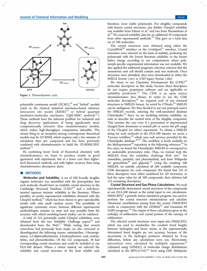
Poor aqueous solubility remains a major cause of attrition in thedrug development process. Despite theoretical developments,the solubility of druglike molecules still eludes truly quantitativecomputation. In recent work,1 we have shown that accuratefirst-principles calculation is now becoming possible, providedthat both the crystalline and solution phases are described byaccurate theoretical models. Before this, energy terms from acomputed thermodynamic cycle (see Figure 1) had been usedas descriptors in a multilinear regression model for intrinsicsolubility, delivering accuracy much better than from directcomputation and comparable with the leading informaticsapproaches.2

Since then, sophisticated machine learning techniques havebeen applied to many problems in the chemical sciences, while,as we have shown,2,3 the accuracy of direct computation ofhydration energies and solubilities has improved significantly.This led us to revisit the idea of hybrid informatics-theoreticalmodels for solubility.Cheminformatics methods have seen widespread use for

property prediction, particularly in the pharmaceutical industrywhere they have been applied to; aqueous solubility, meltingpoint, boiling point, log P (where P is the partition coefficientbetween octanol and water), binding affinities, and toxicologypredictions.4 Such methods are usually much quicker than pure

chemical theory calculations, making high throughput virtualscreening (HTVS) a possibility. Some methods have becomeaccessible and easy-to-use web-based tools.5 However,informatics methods suffer from the difficulty of decomposingthe results into intuitive, physically meaningful understandingand cannot reflect the physical details of the system. Tounderstand the underlying physics and chemistry, it is necessaryto carry out an atomistic physics-based calculation.Many chemical theory methods have been developed to

specifically address one phase. The exact nature of the theoryvaries between these methods and the phase being studied.Crystal structures are often modeled using one of the latticeenergy minimizing simulation methods,6 plane-wave densityfunctional theory (DFT) methods,7 or periodic DFT usingatom-centered basis sets.8 The latter two methods come from aquantum-chemical standpoint. The results are often very goodbut have a high computational cost. The simulation methodsoften contain empirical parameters, which lowers the cost ofthese methods significantly, compared to DFT.Popular solution-phase models include atomistic simulation

methods based on molecular mechanics and dynamics,9

quantum-mechanical implicit solvation methods (such as the

Received: October 7, 2013Published: February 24, 2014

Article

pubs.acs.org/jcim

© 2014 American Chemical Society 844 dx.doi.org/10.1021/ci4005805 | J. Chem. Inf. Model. 2014, 54, 844−856

Terms of Use CC-BY

polarizable continuum model (PCM)),10 and “hybrid” models(such as the classical statistical mechanics-based referenceinteraction site model (RISM)11 or hybrid quantummechanics/molecular mechanics (QM/MM) methods12).These methods have the inherent problem for industrial anddrug discovery applications of being significantly morecomputationally intensive than cheminformatics models,which makes high-throughput computation infeasible. Theclosest thing to an exception among contemporary theoreticalmodels may be 1D RISM, which requires only a few minutes ofcalculation time per compound and has been previouslycombined with cheminformatics to build the 1D-RISM/SDCmethod.13

By combining lower levels of theoretical chemistry withcheminformatics, we hope to produce results in goodagreement with experiment, but at a lower cost than higher-level theoretical methods, and with higher accuracy than usingcheminformatics descriptors alone.

■ METHODSMolecules and Solubility. A set of 100 broadly druglike

organic molecules was assembled with the prerequisites thateach molecule should have an available crystal structure in theCambridge Structural Database (CSD)14 and a well-docu-mented aqueous intrinsic solubility in the literature. Wherepossible, we prefer experimental solubilities obtained with theCheqSol method,15 which has been shown to give reproducibleresults with only small random errors. The possibility ofsignificant systematic errors between different experimentalmethodologies remains an issue and may possibly limit theaccuracy with which modeling-based studies can be validated.A total of 122 potentially useful CheqSol solubilities were

obtained from the two Solubility Challenge papers16 anddownloaded from the Web.17 While noting that severalcorrections had previously been made, we also corrected ordisambiguated the following names: amitriptyline, 5-bromogr-amine, 5,5-diphenylhydantoin, 4-hydroxybenzoic acid, nortrip-tyline, and phenanthroline. Of the 122 compounds, 38 hadcorresponding crystal structures and could be included in ourDLS-100 dataset. Where a choice existed, we selected thesolubility and crystal structure of the least soluble and,

therefore, most stable polymorph. For druglike compoundswith known crystal structures, one further CheqSol solubilitywas available from Palmer et al.2 and two from Narasimham etal.18 We sourced solubility data for an additional 59 compoundsfrom other experimental methods.19 This gave us a total dataset of 100 molecules.The crystal structures were obtained using either the

CrystalWeb20 interface or the ConQuest21 interface. Crystalstructures were selected on the basis of stability, preferring thepolymorph with the lowest literature solubility or the lowestlattice energy according to our computations where poly-morph-specific experimental information was not available. Wealso applied the additional pragmatic selection criterion that theasymmetric unit cell should contain only one molecule. Oncestructures were identified, they were downloaded in either theSHELX format (.res) or CSD legacy format (.dat).We chose to use Chemistry Development Kit (CDK)22

molecular descriptors in this study, because these descriptorsdo not require proprietary software and are applicable tosolubility prediction.23 The CDK is an open sourcecheminformatics Java library. In order to use the CDKmolecular descriptors,22 we required each of our chemicalstructures in SMILES format. As noted by O’Boyle,24 SMILEScan be ambiguous. We thus decided to use one principal sourcefor SMILES records, selecting the well-annotated databaseChemSpider.25 Since we are modeling intrinsic solubility, wewish to describe the neutral form of the druglike compound.This remains the case even if a protonated or deprotonatedcharged form dominates at neutral pH or across the pH rangeof the CheqSol (or other) experiment. To obtain a SMILESstring for each molecule in the DLS-100 dataset, we wrote aTaverna workflow,26 which uses web services provided by theChemSpider database.25,27 The workflow is freely available onthe MyExperiment28 repository at the following reference.29 Infive cases, we found the ChemSpider SMILES to correspond toan undesirable protonation state. Thus, we instead took theSMILES from the solubility challenge Web site17 forcimetidine, pindolol, and phenobarbital, and from Wikipediafor griseofulvin30 and glipizide.31 Using the resulting 100SMILES, we initially calculated all 268 available nonproteinCDK descriptors for each compound. We found that 145 ofthese descriptors were either undefined for 2D structures, orhad the same value for all 100 compounds; their deletion left123 remaining descriptors.

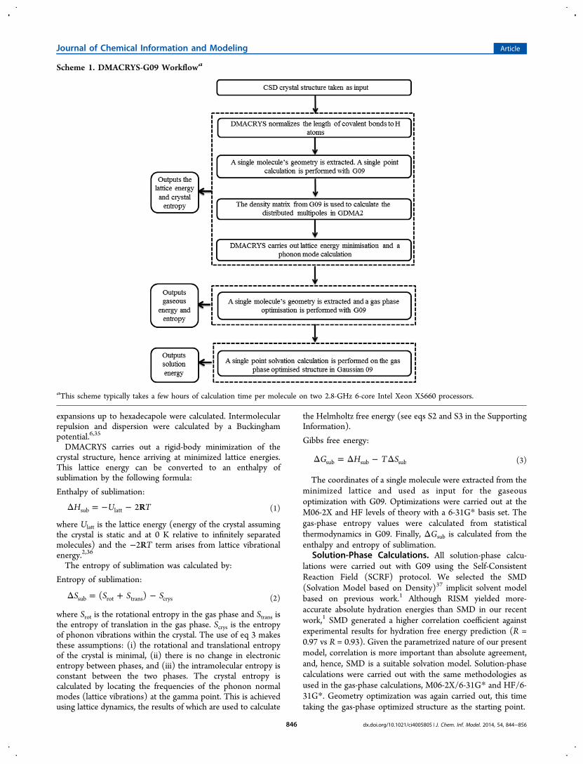
Crystal Structure and Gas-Phase Calculations. We tookexperimentally determined crystal structures of the compoundsin our DLS-100 dataset as the initial input to our calculations.DMACRYS,6 a periodic lattice simulation program, was used toperform the crystal structure minimizations and calculatevibrational contributions arising from the crystal. DMACRYSworks in conjunction with the GDMA232 and Gausssian 09(G09) programs.33 The output of these calculations gives us theenthalpy of sublimation and crystal portion of the entropy ofsublimation.The selected crystal structures were input into DMACRYS,

which was used to standardize the covalent bond lengthsbetween hydrogens and heavy atoms, as the experimentallydetermined bond lengths are not accurate, because of theuncertainty in the hydrogen positions obtained by X-raydiffraction, before any calculations were run. Electrostaticinteractions were calculated by multipole expansions34

(obtained using GDMA2) of molecular charge distributionscalculated at the MP2/6-31G** level using G09. Multipolar

Figure 1. Thermodynamic cycle.

Journal of Chemical Information and Modeling Article

dx.doi.org/10.1021/ci4005805 | J. Chem. Inf. Model. 2014, 54, 844−856845

expansions up to hexadecapole were calculated. Intermolecularrepulsion and dispersion were calculated by a Buckinghampotential.6,35

DMACRYS carries out a rigid-body minimization of thecrystal structure, hence arriving at minimized lattice energies.This lattice energy can be converted to an enthalpy ofsublimation by the following formula:

Enthalpy of sublimation:

Δ = − −H U TR2sub latt (1)

where Ulatt is the lattice energy (energy of the crystal assumingthe crystal is static and at 0 K relative to infinitely separatedmolecules) and the −2RT term arises from lattice vibrationalenergy.2,36

The entropy of sublimation was calculated by:

Entropy of sublimation:

Δ = + −S S S S( )sub rot trans crys (2)

where Srot is the rotational entropy in the gas phase and Strans isthe entropy of translation in the gas phase. Scrys is the entropyof phonon vibrations within the crystal. The use of eq 3 makesthese assumptions: (i) the rotational and translational entropyof the crystal is minimal, (ii) there is no change in electronicentropy between phases, and (iii) the intramolecular entropy isconstant between the two phases. The crystal entropy iscalculated by locating the frequencies of the phonon normalmodes (lattice vibrations) at the gamma point. This is achievedusing lattice dynamics, the results of which are used to calculate

the Helmholtz free energy (see eqs S2 and S3 in the SupportingInformation).

Gibbs free energy:

Δ = Δ − ΔG H T Ssub sub sub (3)

The coordinates of a single molecule were extracted from theminimized lattice and used as input for the gaseousoptimization with G09. Optimizations were carried out at theM06-2X and HF levels of theory with a 6-31G* basis set. Thegas-phase entropy values were calculated from statisticalthermodynamics in G09. Finally, ΔGsub is calculated from theenthalpy and entropy of sublimation.

Solution-Phase Calculations. All solution-phase calcu-lations were carried out with G09 using the Self-ConsistentReaction Field (SCRF) protocol. We selected the SMD(Solvation Model based on Density)37 implicit solvent modelbased on previous work.1 Although RISM yielded more-accurate absolute hydration energies than SMD in our recentwork,1 SMD generated a higher correlation coefficient againstexperimental results for hydration free energy prediction (R =0.97 vs R = 0.93). Given the parametrized nature of our presentmodel, correlation is more important than absolute agreement,and, hence, SMD is a suitable solvation model. Solution-phasecalculations were carried out with the same methodologies asused in the gas-phase calculations, M06-2X/6-31G* and HF/6-31G*. Geometry optimization was again carried out, this timetaking the gas-phase optimized structure as the starting point.

Scheme 1. DMACRYS-G09 Workflowa

aThis scheme typically takes a few hours of calculation time per molecule on two 2.8-GHz 6-core Intel Xeon X5660 processors.

Journal of Chemical Information and Modeling Article

dx.doi.org/10.1021/ci4005805 | J. Chem. Inf. Model. 2014, 54, 844−856846

The SMD model is a parametrized implicit solvation model.SMD solves for the free energy of solution (ΔGhyd) as a sum ofthe electrostatic contributions and nonelectrostatic contribu-tions. The electrostatic contributions are calculated by thesolution of the nonhomogeneous Poisson equation;23,37 thisequation is a second-order differential equation linking theelectrostatic potential, dielectric constant, and charge distribu-tion. The nonelectrostatic contributions of cavitation, dis-persion, and solvent structure are calculated as a sum of atomicand molecular contributions using parameters inherent to theSMD method. SMD has been shown to provide significantimprovements over some other implicit solvent models fordatasets containing molecules similar to those used in thisstudy.1 The hydration free energy is given by eq 4,

Gibbs free energy of hydration:

Δ = −G E Ehyd solution gaseous (4)

where Esolution is the total energy of the system in the SMDsolvation model and Egaseous is the total energy of the system ina vacuum. Scheme 1 represents the workflow for making suchpredictions.Standard States. Sublimation energies were calculated in

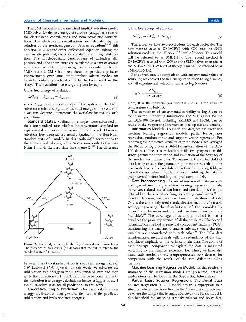
the 1 atm standard state, which is the conventional standard forexperimental sublimation energies to be quoted. However,solvation free energies are usually quoted in the Ben-Naimstandard state of 1 mol/L. In this work, ΔG° corresponds tothe 1 atm standard state, while ΔG* corresponds to the Ben-Naim 1 mol/L standard state (see Figure 2).38 The difference

between these two standard states is a constant energy value of1.89 kcal/mol (7.91 kJ/mol). In this work, we calculate thesublimation free energy in the 1 atm standard state and thenapply the correction to 1 mol/L in order to be consistent withthe hydration free energy calculations; hence, ΔGsolu is in the 1mol/L standard state for all predictions in this work.Theoretical Log S Prediction. Our final solution free-

energy prediction is then given as the sum of the predictedsublimation and hydration free energies:

Gibbs free energy of solution:

Δ * = Δ * + Δ *G G Gsolu sub hyd (5)

Therefore, we have two predictions for each molecule: Thefirst method couples DMACRYS with G09 and the SMDsolvation model at the HF/6-31G* level of theory. This modelwill be referred to as SMD(HF). The second method isDMACRYS coupled with G09 and the SMD solvation model atthe M06-2X/6-31G* level of theory. This will be referred to asSMD(M06-2X).For convenience of comparison with experimental values of

solubility, we convert the free energy of solution to log S values,and all experimental solubility values to log S values:

=Δ

−S

GTR

log2.303

solu

(6)

Here, R is the universal gas constant and T is the absolutetemperature (in Kelvin).The conversion of experimental solubility to log S can be

found in the Supporting Information (eq S7). Values for thefull DLS-100 dataset, including SMILES and InChI, can befound in the Supporting Information (see zip file and dataset).

Informatics Models. To model the data, we use linear andmachine learning regression models: partial least-squaresregression, random forest and support vector regression. Forreporting the predictive accuracy of these models, we averagedthe RMSE of log S over a 10-fold cross-validation of the DLS-100 dataset. The cross-validation fulfils two purposes in thisstudy: parameter optimization and evaluation of the accuracy ofthe models on unseen data. To ensure that each test fold ofdata is truly unseen, the parameter optimization is carried out ina separate layer of cross-validation within the training folds, aswe will discuss below. In order to avoid overfitting, the data arepreprocessed before building the predictive models.

Data Preprocessing. The use of multivariate data presentsa danger of overfitting machine learning regression models;moreover, redundancy of attributes and correlation within thedata add to the risk of reaching misleading conclusions.39 Toavoid such issues, we have used two normalization methods.One is the commonly used standardization method of variablescaling, equalizing the distributions of the variables bynormalizing the mean and standard deviation of each column(variable).40 The advantage of using this method is that itequalizes the prior importance of all the attributes. The secondnormalization method is principal component analysis (PCA),transforming the data into a smaller subspace where the newvariables are uncorrelated with each other.39 The PCA datatransformation method deals with the redundancy of the data,and places emphasis on the variance of the data. The ability ofeach principal component to explain the data is measuredaccording to the variance accounted for. Third, we have alsofitted each model on the nonpreprocessed raw dataset, forcomparison with the results of the two different scalingmethods.

Machine Learning Regression Models. In this section, asummary of the regression models are presented; detailedexplanations can be found in the Supporting Information.

Partial Least Squares Regression. The Partial LeastSquares Regression (PLSR) model design is appropriate in asituation where there is no limit to the X variables or predictors,or where the sample size is small. Moreover, the PLSR model isalso beneficial for analyzing strongly colinear and noisy data.

Figure 2. Thermodynamic cycle showing standard state corrections.The presence of an asterisk (*) denotes that the values refer to thestandard state of 1 mol/L.

Journal of Chemical Information and Modeling Article

dx.doi.org/10.1021/ci4005805 | J. Chem. Inf. Model. 2014, 54, 844−856847

The goal of a PLSR model is to predict the output variable Yfrom the input variables X and to describe the structure of X.For this, PLSR finds a set of components from X that arerelevant to Y; these components are known as latent variables.The intention of PLSR is to capture the information in the X-variables that is most useful to predict Y.41 A graphicalrepresentation is supplied in the Supporting Information FigureS1(A).Random Forest Regression. Random Forest (RF), a

method for classification and regression analysis, has veryattractive properties that have previously been found toimprove the prediction of quantitative structure−activityrelationship (QSAR) data.42 An ensemble of many decisiontrees constitutes a random forest, and each is tree constructedusing the Classification and Regression Trees (CART)algorithm.43 The RF method is efficient in handling high-dimensional data sets and is tolerant of redundant descriptors.Support Vector Regression. The main idea in Support

Vector Regression (SVR) is to minimize the risk factor basedon the structural risk minimization44 from structure theory, to

obtain a good generalization of the limited patterns available inthe given data. First, the given data D are mapped onto a higherdimensional feature space, using the kernel function k(xi,xj) andthen a predictive function is computed on a subset of supportvectors. Here, we have used the radial basis kernel function (eq7) to map the data onto a higher dimensional space. A graphicalrepresentation is supplied in the Supporting Information(Figure S1(B)).

SVR mapping on radial basis kernel function:

δ=

−∥ − ∥⎛⎝⎜⎜

⎞⎠⎟⎟k x x

x x( , ) exp

2i ji j

2

2(7)

Statistical Measures. To evaluate the performance ofvarious machine learning models, we report two statistics: theroot mean squared estimate (RMSE) and squared Pearsoncorrelation coefficient R2 (not to be confused with thecoefficient of determination).45 Formulas for these are givenin the Supporting Information (eq S5). We have also assessedstatistical significance using Menke and Martinez’s method,46

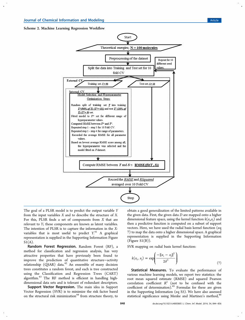
Scheme 2. Machine Learning Regression Workflow

Journal of Chemical Information and Modeling Article

dx.doi.org/10.1021/ci4005805 | J. Chem. Inf. Model. 2014, 54, 844−856848

which we have used previously for similar analysis47 (seeSupporting Information (eq S6, Tables S3−S9 for R2, andBoxes S1−S3) for statistical significance). We also analyzed thevariable importance for the RF method (see Table S17 in theSupporting Information). Variable importance was calculated inthe CART program as implemented in R.42b,48,49

10-Fold Cross-Validation. In order to compute andcompare the performance of the various regression models,we consider RMSE scores averaged over a 10-fold cross-validation.50 In the 10-fold cross-validation, the dataset israndomly split into 10 partitions, where the training set consistsof 90% of the data and the test set consists of 10% of the data.A predictive regression model is fitted on the training set. Thepredictivity on the test fold is considered as an external measureto compute the accuracy of the fitted model. The entire processis repeated 10 times in order to cover the entire dataset, witheach fold forming the test set on one occasion, and we recordthe average RMSE. The complete design of the workflow isrepresented in a flowchart (Scheme 2); similar workflows havebeen used for classification in other studies.47,51 The completeworkflow of this analysis was written in R52 using the CARETpackage;53 all scripts are available in the SupportingInformation.In out-of-bag validation, one evaluates the performance of

the model by separating training and test data throughbootstrap sampling; this is convenient only for the RF method.It is not appropriate to compare RF out-of-bag predictions withother models such as PLS and SVR, which are not based onbootstrap sampling. So, we used 10-fold cross-validation toevaluate the performance of our various models.10-Fold Cross-Validation for Parameter Tuning. For

each model, we use 90% of the total data designated as thetraining set in order to find the optimum values for theseparameters. We selected a range incorporating 20 differentpossible values for each model parameter, in order to select itsbest value. For each parameter, a further level of 10-fold cross-validation is carried out in order to retrieve the RMSE of themodels using each possible parameter value. Here, the trainingportion of 90% of the original data is further split into 10 newfolds of 9%, with nine (81% of the original data) being used tobuild each model and one (9%) as an internal validation; thisprocess of model building and internal validation is repeated topredict each of the 10 possible internal validation folds. Thisinternal cross-validation step is repeated 20 times, once for eachpossible value of the parameter being assessed. Then, based onthe value giving the lowest average RMSE score in the internalvalidation folds, the optimum parameter value is selected.Finally, the model is fitted on the complete training set of 90%of the original data using the selected parameter values.Assessing the Final Models by 10-Fold Cross-

Validation. The given 90%:10% split of the data into trainingand test sets was used to fit the final model for each fold of themain 10-fold cross-validation, once the optimum parametervalues have been selected. The average RMSE and R2 valuesover the 10 folds were considered in order to compare theusefulness of different descriptor sets and to evaluate theperformance of the fitted models.Dataset. The full DLS-100 dataset, with the experimental

log S values, can be found as Supporting Information ordownloaded from the Mitchell group web server (http://chemistry.st-andrews.ac.uk/staff/jbom/group/Informatics_Solubility.html; see the Supporting Information (csv_smiles_-SI.csv and Table S1)), which is consistent with the excellent

suggestions from Walters.54 The dataset includes CSD refcodes,Chemspider numbers, SMILES, experimental log S values andInChI for all molecules. The log S values in this work comefrom refs 2, 16, 18, and 19. Where possible, we have selecteddata obtained from the CheqSol method; where this was notavailable, we have selected reliable sources using differentdetermination techniques. A good solubility prediction can beconsidered as a prediction of approximately the same error asthat of the experiment. The experimental values have beenshown in a number of previous papers to vary considerably.55

Here, we consider the experimental accuracy limit to bebetween 0.6 and 1 log S unit (where 1 log S unit represents 5.7kJ/mol at 298 K). Previous work has reported the experimentalerror in solubility prediction to be as great as 1.5 log S unitsand, on average, the error to be at least 0.6 log S units.56 In2006, Dearden55a noted, as was later reiterated in the SolubilityChallenge, that models with RMSE predictions of <0.5 log Sunits are likely to be overfitted.16b,55a For a prediction to beuseful, it must have an RMSE within the standard deviation ofthe experimental data; otherwise, a trivial prediction using themean of the experimental data is a more accurate prediction ofthe log S value.1 For the DLS-100 dataset, the experimentalstandard deviation is 1.71 log S units.

■ RESULTS AND DISCUSSIONWe have compiled four sets of results for our DLS-100 dataset.First, a purely theoretical prediction, in which no machine

learning is used and where predictions are made using onlyphysics-based calculations. Second, theoretical energies are usedas the sole descriptors in machine learning models. Third,cheminformatics descriptors, calculated using the CDK, areused as the sole input to machine learning methods. Finally,cheminformatics descriptors and theoretically computedenergies are combined as input to machine learning methods.For each of these methods, we present the results anddiscussion, with comparison between the methods made on thebasis of RMSE and R2 (correlation coefficients for chem-informatics and combined models can be found in theSupporting Information (Tables S3−S9); RMSE values canbe found in the Supporting Information (Tables S10−S16)). Inaddition to these results, we have replicated the solubilitychallenge using 2D molecular descriptors alone.

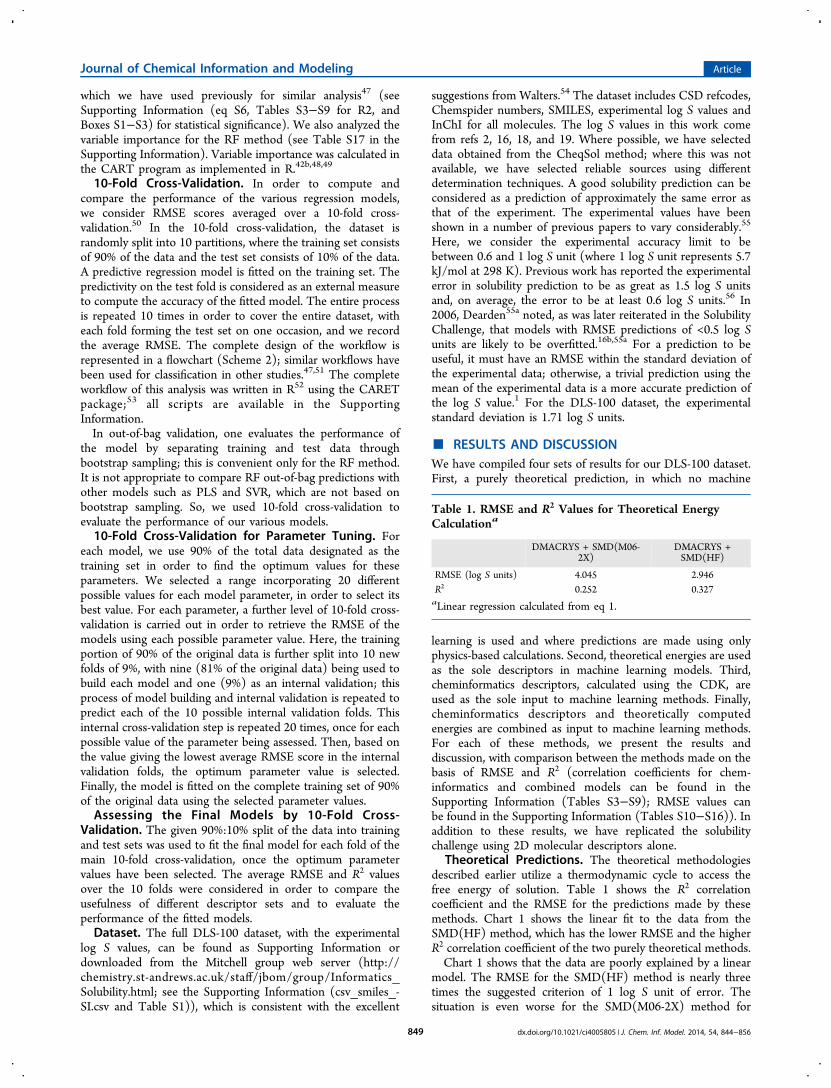
Theoretical Predictions. The theoretical methodologiesdescribed earlier utilize a thermodynamic cycle to access thefree energy of solution. Table 1 shows the R2 correlationcoefficient and the RMSE for the predictions made by thesemethods. Chart 1 shows the linear fit to the data from theSMD(HF) method, which has the lower RMSE and the higherR2 correlation coefficient of the two purely theoretical methods.Chart 1 shows that the data are poorly explained by a linear

model. The RMSE for the SMD(HF) method is nearly threetimes the suggested criterion of 1 log S unit of error. Thesituation is even worse for the SMD(M06-2X) method for

Table 1. RMSE and R2 Values for Theoretical EnergyCalculationa

DMACRYS + SMD(M06-2X)

DMACRYS +SMD(HF)

RMSE (log S units) 4.045 2.946R2 0.252 0.327aLinear regression calculated from eq 1.

Journal of Chemical Information and Modeling Article

dx.doi.org/10.1021/ci4005805 | J. Chem. Inf. Model. 2014, 54, 844−856849

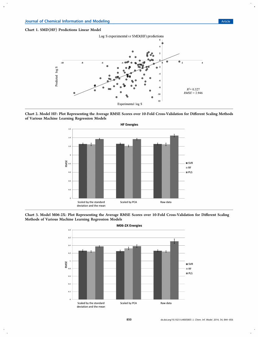
Chart 1. SMD(HF) Predictions Linear Model

Chart 2. Model HF: Plot Representing the Average RMSE Scores over 10-Fold Cross-Validation for Different Scaling Methodsof Various Machine Learning Regression Models

Chart 3. Model M06-2X: Plot Representing the Average RMSE Scores over 10-Fold Cross-Validation for Different ScalingMethods of Various Machine Learning Regression Models

Journal of Chemical Information and Modeling Article

dx.doi.org/10.1021/ci4005805 | J. Chem. Inf. Model. 2014, 54, 844−856850

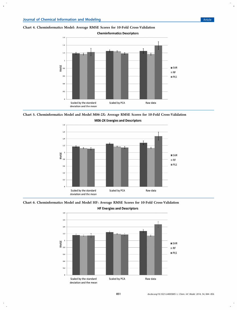
Chart 4. Cheminformatics Model: Average RMSE Scores for 10-Fold Cross-Validation

Chart 5. Cheminformatics Model and Model M06-2X: Average RMSE Scores for 10-Fold Cross-Validation

Chart 6. Cheminformatics Model and Model HF: Average RMSE Scores for 10-Fold Cross-Validation

Journal of Chemical Information and Modeling Article

dx.doi.org/10.1021/ci4005805 | J. Chem. Inf. Model. 2014, 54, 844−856851

which the RMSE is just over four times this criterion (seeCharts S4−S6 in the Supporting Information). Both methodsproduce results outside the useful prediction criterion of 1.71log S units. From these results, we can draw a couple ofconclusions. First, it is clear that the given methodologies donot adequately quantify the physics occurring in the solutionprocess (i.e., solid to solution). Second, we can conclude that, ifit is possible to explain the underlying structure of these datausing a general model, based on the predicted log S values, sucha model will be inherently nonlinear.Compared with our previous work,1 in which theoretical

models provided a good prediction of log S, our theoreticalmethodology here differs only marginally, in the use of MP2multipoles, and still produces good results (see SupportingInformation (Chart S1 and Table S2)) for the same 25molecules in this work (dataset DLS-25). The predictions forthe additional 75 molecules alone show worse predictions thanfor the full 100-molecule set presented above (see Charts S2and S3 in the Supporting Information). The additional 75molecules therefore appear to form a more difficult dataset topredict. It is likely that improved results can be obtained frompurely theoretical calculations, if some of the approximationsmade here are improved; for example, improved modeling of

the solvated phase to more accurately describe the solvent andits effects on the solute could increase accuracy. Also, we notethat the intramolecular degrees of freedom are neglected in theDMACRYS calculations, and further assumptions are made byusing eqs 2 and 3 in the Methods section.We subsequently applied machine learning methods to the

theoretical energies in order to carry out nonlinear regressionanalysis. The average RMSE scores over 10-fold cross-validation (see the Methods section for details) is representedas two-dimensional (2-D) column charts (see Charts 2 and 6).Different grayscale column bars represent the different machinelearning methods used in this study. The standard deviation isshown as an error bar (black line).

Theoretical Energies as Sole Descriptors in MachineLearning. The use of the calculated energies as descriptors inthe machine learning models yields considerably improvedresults, compared to those from the predictions made withoutmachine learning. The results now, while still missing the 1 logS unit error criterion, do make useful predictions in which theRMSE is within the standard deviation of the experimental data(1.71 log S units). The RF and SVR models produce notablybetter results than PLS. Charts 2 and 3 show that the methodminimizing the RMSE (1.21 log S units) is RF with HF whenscaled with PCA.

Cheminformatics Descriptors as the Sole Input toMachine Learning. An additional point of interest is that thechemical descriptors alone using RF or SVR can provide amarginally better prediction of log S than the machine learningmethods with only the energies as descriptors. In particular, wenoticed that fitting the RF model on data that are scaled to agiven mean and standard deviation produces a statisticallysignificant improvement in its prediction with cheminformaticsdescriptors alone rather than theoretical energies (see theSupporting Information (Boxes S1−S3)). In all other cases, thechanges are not significant. This suggests that slightly moreuseful information about the molecules’ log S values isconveyed by the cheminformatics descriptors than by thetheoretical energies alone (see Chart 4).

Theoretical Energies and Cheminformatics Descrip-tors as Input to Machine Learning. When the descriptorsand energies are combined as input for the machine learning

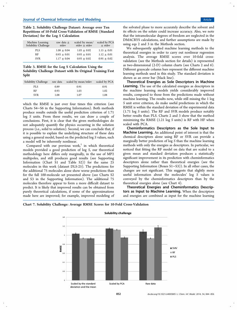
Table 2. Solubility Challenge Dataset: Average over TenRepetitions of 10-Fold Cross-Validation of RMSE (StandardDeviation) for the Log S Calculation

Machine LearningSolubility Challenge

raw data ±stdev

scaled by mean/stdev ± stdev

scaled by PCA± stdev

PLS 1.08 ± 0.04 1.03 ± 0.02 1.15 ± 0.01RF 0.93 ± 0.01 0.93 ± 0.01 1.12 ± 0.01SVR 1.17 ± 0.04 0.93 ± 0.02 0.95 ± 0.02

Table 3. RMSE for the Log S Calculation Using theSolubility Challenge Dataset with Its Original Training:TestSplit

Solubility Challenge raw data scaled by mean/stdev scaled by PCA

PLS 0.89 0.91 0.91RF 0.93 1.03 1.02SVR 1.08 1.07 1.08

Chart 7. Solubility Challenge: Average RMSE Scores for 10-Fold Cross-Validation

Journal of Chemical Information and Modeling Article

dx.doi.org/10.1021/ci4005805 | J. Chem. Inf. Model. 2014, 54, 844−856852

methods, we obtain results that are generally only very slightlybetter than those obtained from cheminformatics descriptorsalone. This implies that the theoretical energies contain verylittle extra useful information not already present in thedescriptors. The joint results do present a statistically significantimprovement for PLS and RF, once scaled by the mean/standard deviation, compared to those for the theoreticalenergies alone. In light of this, and given that the descriptorsalone produce a marginally improved result compared tochemical theory, it is fair to say the cheminformatics descriptorsare seen to contain a modest amount of additional informationnot incorporated in the theoretical energy terms. This suggeststhat the 123 descriptors of the cheminformatics descriptors andthe 10 theoretical energy descriptors convey similar informa-tion, with only a small amount of additional information beingconveyed by adding the descriptors to the energies and almostno information gained by adding the energies to the set ofdescriptors. We can conclude that these two sets of features arenot generally complementary.Interestingly, the best result in terms of RMSE is from the

descriptors with the M06-2X energies, which, on their own,produced the worse of the two pure theory results in this work(see Charts 5 and 6). The RF model performs particularly wellover all descriptor sets, even without any type of scaling, thebest RMSE result being only 0.13 units outside the 1 log S unittarget. The best single prediction, in terms of the RMSE, wasmade by the PLS model, using descriptors and the M06-2Xenergies scaled by the standard deviation and the mean, with anRMSE of 1.11 ± 0.04 log S units. All of these methods makepredictions inside the standard deviation of the experimentaldata; therefore, all of the predictions are useful. We also notethat the RF model shows small but statistically significantimprovements with all scaling methods (using the theoreticalenergies and cheminformatics descriptors combined) whencompared to some models trained on the theoretical energiesonly (see Supporting Information (Boxes S1−S3)). This is theonly model to show such improvements with all scalingmethods in the present work.We analyzed the relative variable importance (see Table S17

in the Supporting Information) and found that X log P (fromref 57) was consistently rated as the most important feature. Xlog P is a computed estimate of the base-10 logarithm of theoctanol:water partition coefficient (the ratio of concentrationsof solute solvated in the two different solvents). This has beenseen in many previous studies and is not so surprising giventhat it provides information specifically about the solvatedphase.4,56 X log P uses an atom additive model for theprediction of log P. In the Supporting Information, we includetables (Table S17 in the Supporting Information) displayingthe 10 most important descriptors; here, we will brieflycomment upon these. We find Kier and Hall’s χ path and chainindices58 to be of importance; these quantify the degree ofbonding to heavy atoms within a given path or chain length. Inaddition, the Moreau−Broto autocorrelation,59 which describesthe charge and mass distribution along a given path length, isfound in the top 10. Finally, we also note Randic’s weightedpath descriptors,60 which are used to account for molecularbranching. Once the theoretical energies are added to thedescriptor set, the free energies of hydration and solution areranked in the top 10, along with the theoretical log Sprediction. Explanations of the molecular descriptors used inthis work can be found in ref 61.

Chemically, we can see logic in the most importantdescriptors. One may expect that molecular branching wouldplay an important role, because it gives information on theextent and flexibility of the molecule, hence contributing someentropic information. Coupling this descriptor with the KierHall descriptors, information can be acquired on thecomposition of such chains, in terms of heavy atoms. Theautocorrelation descriptor provides charge and mass distribu-tion information. Again, here, information is impartedconcerning the distribution of heavy atoms and electronicfactors. For example, the degree of charge separation across amolecule and the localization of charges are important factorsin determining particularly enthalpic but also entropiccontributions. The theoretical energies in the top 10 are allclosely related quantities; it is not surprising that the (purelytheoretical) prediction of log S is found in the top 10: since thisis the quantity we are trying to predict, it is expected to providesufficient information to the model to be found in the top 10.The free energies of solution and hydration provide directinformation from electronic structure theory and statisticalthermodynamics on the interactions of a given molecule, in agiven conformation, within its environment, and on theenergetics of phase transitions.As a benchmark, we also present our method’s predictions of

the solubility challenge set based solely on cheminformaticsdescriptors (see Table 2). As suitable crystal structures are notavailable for all molecules in the solubility challenge, we couldnot calculate the theoretical energies.Tables 2 and 3, and Chart 7, demonstrate that our method

can make predictions for the solubility challenge dataset withinthe coveted 1 log S unit RMSE error and, in fact, makespredictions that are consistent with some commerciallyavailable methods and deep-learning methods. A recentpublication56 reported RMSE scores of 0.95 log S units56 forthe commercially available package MLR-SC62 and 0.90 log Sunits for a deep-learning method.56 However, these results arenot directly comparable with ours, for two reasons. First, ourresults have been calculated for a 10-fold cross-validation andfor the canonical training:test split (see Tables 2 and 3).Second, the deep-learning result (RMSE = 0.90) given by Lusciet al.56 is contingent on correcting eight putative errors in theCheqSol solubility data, the most substantial of which is forindomethacin, a compound that has been shown to hydrolyzeunder alkaline conditions.63 While we have corrected namesand SMILES for the solubility challenge set, we have notadjusted any solubility values therein. It is also reasonable tosuggest that, using the solubility challenge set as a benchmark,our 100-molecule set could be considered as a “difficult set”,given the improved prediction offered by our method when thesolubility challenge set is used instead.

■ CONCLUSIONSOur current work shows that accurate solution free energies arenot calculable via the simple theoretical procedure that wepresent here. A significant portion of the important physics inthe solution process is not captured using the approximatemethodologies that we utilize in this work. This reaffirms that,currently, QSPR methodologies are the most-accurate andtime-efficient methods for accurate solution free energypredictions. In addition, we show that state-of-the-art machinelearning methods, with a modest number of cheminformaticsdescriptors, are capable of making solution free-energypredictions that are consistent with those of commercially

Journal of Chemical Information and Modeling Article

dx.doi.org/10.1021/ci4005805 | J. Chem. Inf. Model. 2014, 54, 844−856853

available programs and newer deep-learning approaches. Here,theoretical energies and cheminformatics descriptors aregenerally shown to not be complementary for such predictions.Since both sets of descriptors (theoretical energies andcheminformatics descriptors) produce a similar level ofaccuracy when used alone in the machine learning methods,and little improvement is seen when they are combined, we canconclude that the information conveyed is of a similar natureand that the theoretical energies are, for this reason, a moreefficient form of information storage, as 10 descriptors containequivalent information to 123 molecular descriptors. However,in terms of time, the molecular descriptors are much lessexpensive to calculate and their use is therefore more time-efficient. Additionally, we note that the RF method hasproduced promising predictions in this work, with relatively lowRMSE. This method has consistently produced good resultsand would be our recommended method to make solubilitypredictions.

■ ASSOCIATED CONTENT*S Supporting InformationInformatics_Solubilty_datasets_and_scripts.zip, including Rcodes, Bash scripts, Python scripts, macro (.xlsb), DLS-100.csv and Solubility_Challenge_dataset.xlsx. DLS-100.csvcontains experimental log S values, references, SMILES, sourcesof smiles, CSD refcodes, molecules names, InChI andChemspider numbers. SI_document.pdf: Structure data, 2Dimages of the molecular structures, experimental log S values,CSD refcodes, R2, statistical significance, variable importance.This material is available free of charge via the Internet athttp://pubs.acs.org. All scripts and datasets used in this workare available for download from the Mitchell Group web server(http://chemistry.st-andrews.ac.uk/staff/jbom/group/Informatics_Solubility.html, as well as in the SupportingInformation.

■ AUTHOR INFORMATIONCorresponding Author*E-mail: jbom@st-andrews.ac.uk.Author ContributionsThe manuscript was written through contributions of allauthors. All authors have given approval to the final version ofthe manuscript. Datasets were curated by J.L.M. and J.B.O.M.Machine learning R scripts were produced by N.N. and L.D.F.The Taverna workflow was produced by L.D.F. Bash scripts,Excel macros, and the R script to run over multiple directorieswere produced by J.L.McD. DMACRYS and Gaussiancalculations were run by J.L.McD. Advice on computationalchemistry and machine learning methods was provided byT.v.M. and J.B.O.M. R calculations were run by J.L.McD. andN.N.NotesThe authors declare no competing financial interest.

■ ACKNOWLEDGMENTSScottish Universities Life Science Alliance (SULSA), this workwas partly supported by Biotechnology and Biological SciencesResearch Council (BBSRC) (No. BB/I00596X/1), ScottishFunding Council (SFC). We thank EaStCHEM for access tothe EaStCHEM Research Computing Facility, and Dr. HerbertFruchtl for its maintenance. We are grateful to Dr. Graeme Day(University of Southampton) for providing additional scripts

for DMACRYS. We thank Dr. David Palmer (University ofStrathclyde) for a script to help automate running DMACRYS.We also thank our colleagues at the University of St. Andrewsfor useful discussions, particularly Dr. Lazaros Mavridis andRachael Skyner. We thank the BBSRC for Grant No. BB/I00596X/1 to J.B.O.M., which supports L.D.F.’s research. Wethank the Scottish Universities Life Sciences Alliance (SULSA)for supporting J.B.O.M., J.L.McD., and N.N., and we also thankthe Scottish Overseas Research Student Awards Scheme of theScottish Funding Council (SFC) for financial support of N.N.’sstudentship.

■ ABBREVIATIONSCDK = Chemistry Development Kit; HTP = high-throughputscreening; DFT = density functional theory; HF = Hartree−Fock; PCM = polarizable continuum model; RISM = referenceinteraction site model; CSD = Cambridge Structural Database;G09 = Gaussian 09; SCRF = self-consistent reaction field; SMD= Solvation Model based on Density; PLSR = partial leastsquares regression; RF = random forest; SVR = support vectorregression; RMSE = root mean squared error; PCA = principalcomponent analysis; CART = classification and regressiontrees; QSAR = quantitative structure−activity relationship;QSPR = quantitative structure−property relationship; SRM =structural risk minimization; SMILES = Simplified Molecular-Input Line-Entry System; DLS-100 = Drug-Like-Solubility-100

■ REFERENCES(1) Palmer, D. S.; McDonagh, J. L.; Mitchell, J. B. O.; van Mourik, T.;Fedorov, M. V. First-Principles Calculation of the Intrinsic AqueousSolubility of Crystalline Druglike Molecules. J. Chem. Theory Comput.2012, 8, 3322−3337.(2) Palmer, D. S.; Llinas, A.; Morao, I.; Day, G. M.; Goodman, J. M.;Glen, R. C.; Mitchell, J. B. O. Predicting intrinsic aqueous solubility bya thermodynamic cycle. Mol. Pharm. 2008, 5 (2), 266−279.(3) Mitchell, J. B. O. Informatics, machine learning and computa-tional medicinal chemistry. Future Med. Chem. 2011, 3 (4), 451−67.(4) Hughes, L. D.; Palmer, D. S.; Nigsch, F.; Mitchell, J. B. O. WhyAre Some Properties More Difficult To Predict than Others? A Studyof QSPR Models of Solubility, Melting Point, and Log P. J. Chem. Inf.Model 2008, 48 (1), 220−232.(5) (a) Tetko, I. V. Computing chemistry on the web. Drug DiscoveryToday 2005, 10 (22), 1497−1500. (b) Tetko, I. V.; Gasteiger, J.;Todeschini, R.; Mauri, A.; Livingstone, D.; Ertl, P.; Palyulin, V. A.;Radchenko, E. V.; Zefirov, N. S.; Makarenko, A. S.; Tanchuk, V. Y.;Prokopenko, V. V. Virtual computational chemistry laboratoryDesign and description. J. Comput. Aid. Mol. Des 2005, 19, 453−63.(6) Price, S. L.; Leslie, M.; Welch, G. W. A.; Habgood, M.; Price, L.S.; Karamertzanis, P. G.; Day, G. M. Modelling organic crystalstructures using distributed multipole and polarizability-based modelintermolecular potentials. Phys. Chem. Chem. Phys. 2010, 12 (30),8478−8490.(7) Segall, M. D.; Lindan, P. J. D.; Probert, M. J.; Pickard, C. J.;Hasnip, P. J.; Clark, S. J.; Payne, M. C. First-principles simulation:Ideas, illustrations and the CASTEP code. J. Phys. Condens. Matter2002, 14 (11), 2717−2744.(8) Dovesi, R.; Orlando, R.; Civalleri, B.; Roetti, C.; Saunders, V. R.;Zicovich-Wilson, C. M. CRYSTAL: a computational tool for the abinitio study of the electronic properties of crystals. Z Kristallogr. 2005,220 (5-2005−6-2005), 571−573.(9) (a) Luder, K.; Lindfors, L.; Westergren, J.; Nordholm, S.;Kjellander, R. In silico prediction of drug solubility: 2. Free energy ofsolvation in pure melts. J. Phys. Chem. B 2007, 111 (7), 1883−1892.(b) Luder, K.; Lindfors, L.; Westergren, J.; Nordholm, S.; Kjellander,R. In silico prediction of drug solubility. 3. Free energy of solvation inpure amorphous matter. J. Phys. Chem. B 2007, 111 (25), 7303−7311.

Journal of Chemical Information and Modeling Article

dx.doi.org/10.1021/ci4005805 | J. Chem. Inf. Model. 2014, 54, 844−856854

(c) Luder, K.; Lindfors, L.; Westergren, J.; Nordholm, S.; Persson, R.;Pedersen, M. In Silico Prediction of Drug Solubility: 4. Will SimplePotentials Suffice? J. Comput. Chem. 2009, 30 (12), 1859−1871.(d) Westergren, J.; Lindfors, L.; Hoglund, T.; Luder, K.; Nordholm, S.;Kjellander, R. In silico prediction of drug solubility: 1. Free energy ofhydration. J. Phys. Chem. B 2007, 111 (7), 1872−1882.(10) Tomasi, J.; Mennucci, B.; Cammi, R. Quantum MechanicalContinuum Solvation Models. Chem. Rev. 2005, 105 (8), 2999−3094.(11) (a) Ten-no, S. Free energy of solvation for the referenceinteraction site model: Critical comparison of expressions. J. Phys.Chem. 2001, 115 (8), 3724−3731. (b) Palmer, D. S.; Frolov, A. I.;Ratkova, E. L.; Fedorov, M. V. Towards a universal method forcalculating hydration free energies: A 3D reference interaction sitemodel with partial molar volume correction. J. Phys.: Condens. Matter2010, 22 (49), 492101.(12) Stanton, R. V.; Hartsough, D. S.; Merz, K. M. Calculation ofsolvation free energies using a density functional/molecular dynamicscoupled potential. J. Phys. Chem. 1993, 97 (46), 11868−11870.(13) Ratkova, E. L.; Fedorov, M. V. Combination of RISM andCheminformatics for Efficient Predictions of Hydration Free Energy ofPolyfragment Molecules: Application to a Set of Organic Pollutants. J.Chem. Theory Comput. 2011, 7 (5), 1450−1457.(14) Allen, F. H. The Cambridge Structural Database: a quarter of amillion crystal structures and rising. Acta Crystallogr B 2002, B58,380−388.(15) Box, K.; Comer, J. E.; Gravestock, T.; Stuart, M. New Ideasabout the Solubility of Drugs. Chem. Biodiversity 2009, 6 (11), 1767−1788.(16) (a) Hopfinger, A. J.; Esposito, E. X.; Llinas, A.; Glen, R. C.;Goodman, J. M. Findings of the Challenge To Predict AqueousSolubility. J. Chem. Inf. Model. 2008, 49 (1), 1−5. (b) Llinas, A.; Glen,R. C.; Goodman, J. M. Solubility Challenge: Can You PredictSolubilities of 32 Molecules Using a Database of 100 ReliableMeasurements? J. Chem. Inf. Model. 2008, 48 (7), 1289−1303.(17) The Goodman group. http://www-jmg.ch.cam.ac.uk/data/solubility/ (accessed Feb. 8, 2013).(18) Narasimham, L.; Barhate, V. D. Kinetic and intrinsic solubilitydetermination of some β-blockers and antidiabetics by potentiometry.J. Pharm. Res. 2011, 4 (2), 532−536.(19) (a) Bergstrom, C. A. S.; Luthman, K.; Artursson, P. Accuracy ofcalculated pH-dependent aqueous drug solubility. Eur. J. Pharm. Sci.2004, 22 (5), 387−398. (b) Bergstrom, C. A. S.; Wassvik, C. M.;Norinder, U.; Luthman, K.; Artursson, P. Global and LocalComputational Models for Aqueous Solubility Prediction of Drug-Like Molecules. J. Chem. Inf. Comput. Sci. 2004, 44 (4), 1477−1488.(c) Ran, Y.; Yalkowsky, S. H. Prediction of Drug Solubility by theGeneral Solubility Equation (GSE). J. Chem. Inf. Comput. Sci. 2001, 41(2), 354−357. (d) Rytting, E.; Lentz, K.; Chen, X.-Q.; Qian, F.;Venkatesh, S. Aqueous and cosolvent solubility data for drug-likeorganic compounds. AAPS J. 2005, 7 (1), E78−E105. (e) Shareef, A.;Angove, M. J.; Wells, J. D.; Johnson, B. B. Aqueous Solubilities ofEstrone, 17β-Estradiol, 17α-Ethynylestradiol, and Bisphenol A. J.Chem. Eng. Data 2006, 51 (3), 879−881.(20) CrystalWeb unfortunately withdrawn in 2013. http://cds.dl.ac.uk/cds/datasets/crys/cweb/cweb.html.(21) Bruno, I. J.; Cole, J. C.; Edgington, P. R.; Kessler, M.; Macrae, C.F.; McCabe, P.; Pearson, J.; Taylor, R. New software for searching theCambridge Structural Database and visualizing crystal structures. ActaCrystallogr., Sect. B: Struct. Sci. 2002, 58 (3 Part 1), 389−397.(22) Steinbeck, C.; Han, Y.; Kuhn, S.; Horlacher, O.; Luttmann, E.;Willighagen, E. The Chemistry Development Kit (CDK): An Open-Source Java Library for Chemo- and Bioinformatics. J. Chem. Inf.Comput. Sci. 2003, 43 (2), 493−500.(23) Gupta, R. R.; Gifford, E. M.; Liston, T.; Waller, C. L.; Hohman,M.; Bunin, B. A.; Ekins, S. Using Open Source Computational Toolsfor Predicting Human Metabolic Stability and Additional Absorption,Distribution, Metabolism, Excretion, and Toxicity Properties. DrugMetab. Dispos. 2010, 38 (11), 2083−2090.

(24) O’Boyle, N. Towards a Universal SMILES representation - Astandard method to generate canonical SMILES based on the InChI. J.Cheminform. 2012, 4 (1), 22.(25) RSC ChemSpider. (accessed Feb. 8, 2013).(26) Wolstencroft, K.; Haines, R.; Fellows, D.; Williams, A.; Withers,D.; Owen, S.; Soiland-Reyes, S.; Dunlop, I.; Nenadic, A.; Fisher, P.;Bhagat, J.; Belhajjame, K.; Bacall, F.; Hardisty, A.; Nieva de la Hidalga,A.; Balcazar Vargas, M. P.; Sufi, S.; Goble, C. The Taverna workflowsuite: designing and executing workflows of Web Services on thedesktop, web or in the cloud. Nucleic Acids Res. 2013, 41 (W1),W557−W561.(27) Little, J. L.; Williams, A. J.; Pshenichnov, A.; Tkachenko, V.Identification of “Known Unknowns” Utilizing Accurate Mass Dataand ChemSpider. J. Am. Soc. Mass. Spectrom. 2012, 23 (1), 179−185.(28) Goble, C. A.; Bhagat, J.; Aleksejevs, S.; Cruickshank, D.;Michaelides, D.; Newman, D.; Borkum, M.; Bechhofer, S.; Roos, M.;Li, P.; De Roure, D. myExperiment: A repository and social networkfor the sharing of bioinformatics workflows. Nucleic Acids Res. 2010, 38(suppl 2), W677−W682.(29) De Ferrari, L. Workflow Entry: From molecule name to SMILEand InchI using ChemSpider. http://www.myexperiment.org/workflows/3603.html. (accessed 10th February 2014).(30) Griseofulvin. http://en.wikipedia.org/wiki/Griseofulvin (ac-cessed 11th December 2012. SMILES source).(31) Glipizide. http://en.wikipedia.org/wiki/Glipizide (accessed11th December 2012. SMILES source).(32) Stone, A. Distributed Multipole Analysis of Gaussian wave-functions GDMA version 2.2.02. http://www-stone.ch.cam.ac.uk/documentation/gdma/manual.pdf (accessed Feb. 10, 2014).(33) Frisch, M. J.; Trucks, G. W.; Schlegel, H. B.; Scuseria, G. E.;Robb, M. A.; Cheeseman, J. R.; Scalmani, G.; Barone, V.; Mennucci,B.; Petersson, G. A.; Nakatsuji, H.; Caricato, M.; Li, X.; Hratchian, H.P.; Izmaylov, A. F.; Bloino, J.; Zheng, G.; Sonnenberg, J. L.; Hada, M.;Ehara, M.; Toyota, K.; Fukuda, R.; Hasegawa, J.; shida, M.; Nakajima,T.; Honda, Y.; Kitao, O.; Nakai, H.; Vreven, T.; Montgomery, J. A.Jr.;Peralta, J. E.; Ogliaro, F.; Bearpark, M.; Heyd, J. J.; Brothers, E.; Kudin,K. N.; Staroverov, V. N.; Kobayashi, R.; Normand, J.; Raghavachari, K.;Rendell, A.; Burant, J. C.; Iyengar, S. S.; Tomasi, J.; Cossi, M.; Rega,N.; Millam, N. J.; Klene, M.; Knox, J. E.; Cross, J. B.; Bakken, V.;Adamo, C.; Jaramillo, J.; Gomperts, R.; Stratmann, R. E.; Yazyev, O.;Austin, A. J.; Cammi, R.; Pomelli, C.; Ochterski, J. W.; Martin, R. L.;Morokuma, K.; Zakrzewski, V. G.; Voth, G. A.; Salvador, P.;Dannenberg, J. J.; Dapprich, S.; Daniels, A. D.; Farkas, O.;Foresman, J. B.; Ortiz, J. V.; Cioslowski, J.; Fox, D. J. Gaussian 09,Gaussian, Inc: Wallingford, CT, 2009.(34) Stone, A. J. Distributed multipole analysis, or how to describe amolecular charge distribution. Chem. Phys. Lett. 1981, 83 (2), 233−239.(35) Buckingham, R. The classical equation of state of gaseoushelium, neon and argon. Proc. R. Soc. Lon. Ser-A 1938, 168 (933),264−283.(36) Gavezzotti, A.; Filippini, G. Theoretical Aspects and ComputerModeling.; Gavezzotti, A., Ed. Wiley and Sons: Chichester, 1997; pp61−97.(37) Marenich, A. V.; Cramer, C. J.; Truhlar, D. G. UniversalSolvation Model Based on Solute Electron Density and on aContinuum Model of the Solvent Defined by the Bulk DielectricConstant and Atomic Surface Tensions. J. Phys. Chem. B 2009, 113(18), 6378−6396.(38) (a) Ben-Naim, A. Standard thermodynamics of transfer. Usesand misuses. J. Phys. Chem. 1978, 82 (7), 792−803. (b) Ben-Naim, A.;Marcus, Y. Solvation thermodynamics of nonionic solutes. J. Phys.Chem. 1984, 81 (4), 2016−2027.(39) Howley, T.; Madden, M. G.; O’Connell, M.-L.; Ryder, A. G.The effect of principal component analysis on machine learningaccuracy with high-dimensional spectral data. Knowl.-Based Syst. 2006,19 (5), 363−370.(40) Wold, H. Partial Least Squares (PLS) Regression 2003, 1−7.

Journal of Chemical Information and Modeling Article

dx.doi.org/10.1021/ci4005805 | J. Chem. Inf. Model. 2014, 54, 844−856855

(41) (a) Abdi, H. Partial Least Squares (PLS) Regression 2003, 1−7.(b) Wold, S.; Sjostrom, M.; Eriksson, L. PLS-regression: A basic toolof chemometrics. Chemometr. Intell. Lab. 2001, 58 (2), 109−130.(c) Mevik, B.; Wehrens, R. The pls Package: Principal Componentand Partial Least Squares Regression in R. J Stat Softw. 2007, 18 (2),1−24.(42) (a) Palmer, D. S.; O’Boyle, N. M.; Glen, R. C.; Mitchell, J. B. O.Random Forest Models To Predict Aqueous Solubility. J. Chem. Inf.Model 2006, 47 (1), 150−158. (b) Svetnik, V.; Liaw, A.; Tong, C.;Culberson, J. C.; Sheridan, R. P.; Feuston, B. P. Random Forest: AClassification and Regression Tool for Compound Classification andQSAR Modeling. J. Chem. Inf. Comput. Sci. 2003, 43 (6), 1947−1958.(43) Breiman, L. Random Forests. Mach. Learning 2001, 45 (1), 5−32.(44) (a) Cao, D.-S.; Xu, Q.-S.; Liang, Y.-Z.; Chen, X.; Li, H.-D.Prediction of aqueous solubility of druglike organic compounds usingpartial least squares, back-propagation network and support vectormachine. J. Chemometr. 2010, 24 (9), 584−595. (b) Vapnik, V. N. Anoverview of statistical learning theory. IEEE Trans. Neural Netw. 1999,10 (5), 988−999.(45) Hu, S. In R2 Vs. r2, SCEA/ISPA Conference, 2008; pp 1 - 15.(46) Menke, J.; Martinez, T. R. In Using permutations instead ofstudent’s t distribution for p-values in paired-difference algorithmcomparisons, IEEE IJCNN, July 25−29, 2004; 2004; Vol. 2, pp 1331-1335.(47) Nath, N.; Mitchell, J. B. O. Is EC class predictable from reactionmechanism? BMC Bioinformatics 2012, 13 (1), 60.(48) Kuhn, M. Variable Importance Using The caret Package 2012;Available via the Internet at http://cran.open-source-solution.org/web/packages/caret/vignettes/caretVarImp.pdf, accessed Feb. 10,2014.(49) Kuhn, M. Variable Importance Using The caret Package 2010, 1−7.(50) Varma, S.; Simon, R. Bias in error estimation when using cross-validation for model selection. BMC Bioinform. 2006, 7 (1), 91.(51) Simon, R. M.; Subramanian, J.; Li, M.-C.; Menezes, S. Usingcross-validation to evaluate predictive accuracy of survival riskclassifiers based on high-dimensional data. Brief. Bioinform. 2011, 12(3), 203−214.(52) R Development Core Team. R: A language and environment forstatistical computing; R Foundation for Statistical Computing, Vienna,Austria, 2011.(53) (a) Kuhn, M. Building Predictive Models in R Using the caretPackage. J. Stat. Software 2008, 28, 1−26. (b) Kuhn, M.; Wing, J.;Weston, S.; Williams, A.; Keefer, C.; Engelhardt, A.; Cooper, T.;Mayer, Z. R Core Team. caret: Classification and Regression Training.R Package “caret”. http://CRAN.R-project.org/package=caret.(54) Walters, W. P. Modeling, Informatics, and the Quest forReproducibility. J. Chem. Inf. Model 2013, 53 (7), 1529−1530.(55) (a) Dearden, J. C. In silico prediction of aqueous solubility.Expert Opin. Drug Discovery 2006, 1 (1), 31−52. (b) Jorgensen, W. L.;Duffy, E. M. Prediction of drug solubility from structure. Adv. DrugDelivery Rev. 2002, 54 (3), 355−366.(56) Lusci, A.; Pollastri, G.; Baldi, P. Deep Architectures and DeepLearning in Chemoinformatics: The Prediction of Aqueous Solubilityfor Drug-Like Molecules. J. Chem. Inf. Model. 2013, 53, 1563−1575.(57) Wang, R.; Gao, Y.; Lai, L. Calculating partition coefficient byatom-additive method. Perspect. Drug Discovery Des. 2000, 19 (1), 47−66.(58) Kier, L. B.; Hall, L. H. Molecular Connectivity in Chemistry andDrug Research; Academic Press: New York, 1976.(59) Moreau, G.; Broto, P. The autocorrelation of a topologicalstructure: A new molecular descriptor. New J. Chem. 1980, 359−360.(60) Randic, M. On molecular identification numbers. J. Chem. Inf.Comput. Sci. 1984, 24 (3), 164−175.(61) CDK Descriptor Summary (2011−05−28). http://pele.farmbio.uu.se/nightly-1.2.x/dnames.html, accessed Feb. 10, 2014.(62) Hewitt, M.; Cronin, M. T. D.; Enoch, S. J.; Madden, J. C.;Roberts, D. W.; Dearden, J. C. In Silico Prediction of Aqueous

Solubility: The Solubility Challenge. J. Chem. Inf. Model. 2009, 49 (11),2572−2587.(63) Tsvetkova, B.; Pencheva, I.; Zlatkov, A.; Peikov, P. HighPerformance Liquid Chromatographic Assay of Indomethacin and itsRelated Substances in Tablet Dosage Forms. Int. J. Pharm. Pharm. Sci.2012, 4 (Supplement 3), 549−552.

Journal of Chemical Information and Modeling Article

dx.doi.org/10.1021/ci4005805 | J. Chem. Inf. Model. 2014, 54, 844−856856