A REDETERMINATION OF THE SOLUBILITY OF OXYGEN IN SEA WATER

AND SOME THERMODYNAMIC IMPLICATIONS

OF THE SOLUBILITY RELATIONS01

by

EDWARD JEWETT GREEN

B.A., University of CaliforniaSanta Barbara, 1958

tNST. TECH

SUBMITTED IN PARTIAL FULFILLMENT

OF THE REQUIREMENTS FOR THE

DEGREE OF DOCTOR OF

PHILOSOPHY

at the

MASSACHUSETTS INSTITUTE OF

TECHNOLOGY

April 1965

Signature of Authorepartment of Geology and Geophysics

1 April 1965

Certified byCertified by Thesis Supervisor

Accepted byChpfrman, epartmental Committee on Graduate Students

ABSTRACT

A REDETERMINATION OF THE SOLUBILITY OF OXYGEN IN SEA WATER

AND SOME THERMODYNAMIC IMPLICATIONS

OF THE SOLUBILITY RELATIONS

by

E. J. Green

Submitted to the Department of Geology and Geophysics on April 1, 1965,

in partial fulfillment of the requirement for the degree of Doctor of Philosophy.

In order to resolve the discrepancy between the two sets of modern mea-

surements of the solubility of oxygen in sea water the solubility coefficients

have been redetermined at temperatures between 00 and 35* C. The method used

was the simultaneous saturation of distilled and sea water samples with atmos-

pheric air at normal pressure, followed by the determination of the oxygen dis-

solved therein using a modification of the WINKLER method.

The measurements of distilled water agree to better than 0.39% with

the manometric measurements of KLOTS and BENSON. The sea water used varied in

chlorinity between 6 and 30 0/00. The sea water solubilities have a reproduci-

bility of 0.27% and evidence suggests that the accuracy is also of this magni-

tude.

The high precision of the measurements reveals that the solubility

declines exponentially with increasing salt concentration according to the em-

pirical SETSCHENOW relation rather than linearly as previously assumed. Salting-

out theories are reviewed and it is seen that the simple hydration theory pre-

dicts a linear relation. Although the DEBYE theory predicts an exponential

dependence it is seen to predict an unsatisfactory temperature dependence. The

experimental data of this work, as well as of a number of other published

studies, reveal that, in contrast to the effect predicted by the DEBYE theory,

the salting-out decreased with increasing temperature.

The activity coefficient of oxygen in sea salt solutions is shown to

be simply related to the salting-out coefficient. A quasi-lattice model of a

regular solution is developed from which the exponential salting-out relation-

ship is derived. The derived relationship has a temperature dependence of the

same order as that experimentally observed. The model and experimental observa-

tions are shown to be consistent with FRANK'S "iceberg" concept of aqueous

solution of gases and the role of sea salt is seen to be "iceberg breaking".

Because of the failure of previous workers to correctly characterize

the salting-out effect, none of the published solubility tables are reliable at

2

low and high sea water chlorinities. For normal sea water we find the valuesof FOX to be high by about 1% and the values of TRUESDALE et al. to be low byabout 3% over most of the temperature range. Tables of solubility coefficientscomputed from the new data are presented.

Thesis supervisor: Dayton E. CarrittProfessor of Chemical Oceanography

TABLE OF CONTENTS

Page

ABSTRACT 1

LIST OF FIGURES 5

LIST OF TABLES 6

PART ONETHE SOLUBILITY OF OXYGEN IN SEA WATER

Abstract 8

Introduction 9

Previous work-oxygen solubility 10

Experimental methods 13Experimental design 13Sources of error in sample equilibration 15

The saturator 18Sea water samples 26Sources of error in the Winkler method 27Modifications in the Winkler method 35

Results and discussion 57The salting-out effect 57A precision test of the data 58Choice of smoothing function 65

Representation of the data 67Analysis of errors 69

Summary and conclusions 75

Solubility tables for oxygen in sea water 78Bunsen coefficient 78Solubility of atmospheric oxygen 84

References 90

PART TWOTHE SALTING-OUT EFFECT IN THE TERNARY SYSTEM:

OXYGEN-WATER-SEA SALT

Abstract 94

Introduction 95

Review of salting-out theories

Page

Experimental 101

Discussion of results 102

Some thermodynamic considerations 106

A quasi-lattice model of solvent-solute interaction 107

Considerations of the structure of water 118

References 119

ACKNOWLEDGEMENTS 121

APPENDICES 122

I. Gas-liquid equilibration during pressure changes 123II. Sample calculation of the solubility coefficients 125

III. Bibliography 128

BIOGRAPHICAL NOTE 136

5

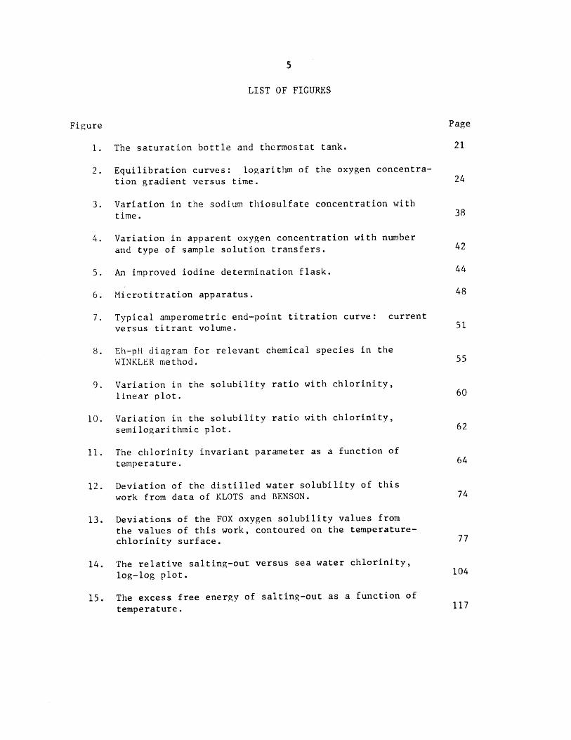
LIST OF FIGURES

Figure Page

i. The saturation bottle and thermostat tank. 21

2. Equilibration curves: logarithm of the oxygen concentra-

tion gradient versus time. 24

3. Variation in the sodium thiosulfate concentration with

time. 38

4. Variation in apparent oxygen concentration with number

and type of sample solution transfers. 42

5. An improved iodine determination flask. 44

6. Microtitration apparatus. 48

7. Typical amperometric end-point titration curve: current

versus titrant volume. 51

8. Eh-pH diagram for relevant chemical species in the

WINKLER method. 55

9. Variation in the solubility ratio with chlorinity,

linear plot. 60

10. Variation in the solubility ratio with chlorinity,

semilogarithmic plot. 62

11. The chlorinity invariant parameter as a function of

temperature. 64

12. Deviation of the distilled water solubility of this

work from data of KLOTS and BENSON. 74

13. Deviations of the FOX oxygen solubility values from

the values of this work, contoured on the temperature-chlorinity surface. 77

14. The relative salting-out versus sea water chlorinity,log-log plot. 104

15. The excess free energy of salting-out as a function of

temperature. 117

6

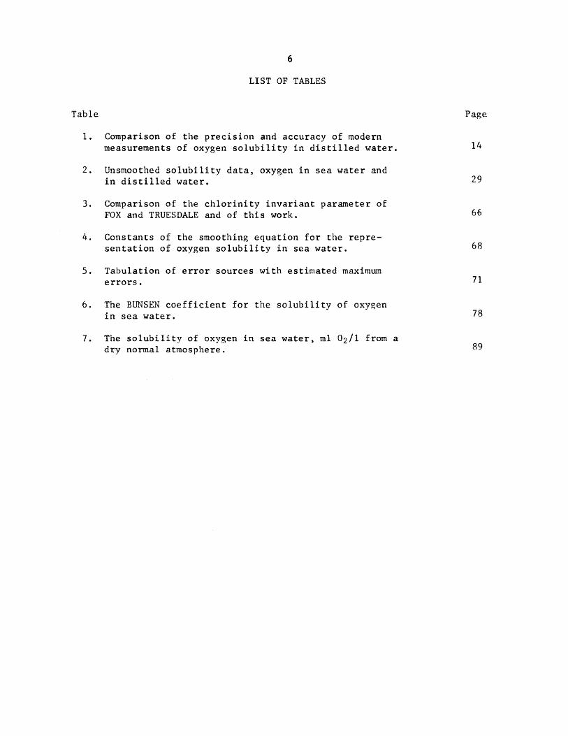
LIST OF TABLES

Table Page

1. Comparison of the precision and accuracy of modernmeasurements of oxygen solubility in distilled water. 14

2. Unsmoothed solubility data, oxygen in sea water andin distilled water. 29

3. Comparison of the chlorinity invariant parameter ofFOX and TRUESDALE and of this work. 66

4. Constants of the smoothing equation for the repre-sentation of oxygen solubility in sea water. 68

5. Tabulation of error sources with estimated maximumerrors. 71

6. The BUNSEN coefficient for the solubility of oxygenin sea water. 78

7. The solubility of oxygen in sea water, ml 02/1 from adry normal atmosphere. 89

PART I

THE SOLUBILITY OF OXYGEN IN SEA WATER

8

PART I

THE SOLUBILITY OF OXYGEN IN SEA WATER

ABSTRACT

In order to resolve the discrepancy between the two sets of modern mea-

surements of the solubility of oxygen in sea water the solubility coefficients

have been redetermined at temperatures between 0* and 350 C. The method used

was the simultaneous saturation of distilled and sea water samples with atmos-

pheric air at normal pressure, followed by the determination of the oxygen dis-

solved therein using a modification of the WINKLER method.

The measurements of distilled water agree to better than 0.39% with

the manometric measurements of KLOTS and BENSON. The sea water used varied in

chlorinity between 6 and 30 o/oo. The sea water solubilities have a reproduci-

bility of 0.27% and evidence suggests that the accuracy is also of this magni-

tude.

The high precision of the measurements reveals that the salting-out

relationship depends exponentially upon salt concentration and not linearly as

previously assumed. For this reason none of the published solubility tables

are reliable at low and high sea water chlorinities. For normal sea water we

find the values of FOX to be high by about 1% and the values of TRUESDALE et al.

to be low by about 3% over most of the temperature range.

Tables of solubility coefficients are presented.

9

INTRODUCTION

As contrasted with other oft-measured constituents of sea water, dis-

solved oxygen is not a major component. A liter of sea water of 19 o/oo

chlorinity and at a temperature of 200 C, saturated with oxygen at a partial

pressure of 0.2094 atm , contains 5.3 ml of oxygen measured at S.T.P. (Stan-

dard temperature and applied pressure being 00 C and 1 atm , respectively.)

Such a concentration corresponds to 0.23 millimoles/l or a mole fraction of

4 x 10- 6 . By weight this representative concentration is 7.4 mg/l. By any

criterion dissolved oxygen must be classified as a trace constituent. Nonethe-

less, the measurement of dissolved oxygen in sea water has been an important and

useful oceanographic tool since the early days of the study of the sea and, in-

deed, apart from temperature and chlorinity, oxygen concentration is the most

frequently measured property of sea water.

As a result of a large number of measurements, the gross features of the

structure of oxygen concentration in the oceans are well known and have been

satisfactorily explained. Moreover, the availability of oxygen data has provided

impetus for its use by biologists and physical oceanographers. REDFIELD (1942)

combined oxygen data with saturation solubility values to obtain what he calls

apparent oxygen utilization and further with dissolved phosphate data to construct

a model of, and to provide information about, the sources and supply of nutrients

in sea water. His model was sensitive to 0.02 mg-atoms P/m 3 which corresponds

to oxidation by 0.05 ml 02/1. WORTHINGTON (1954) attempted to use dissolved

oxygen data to estimate the long-term circulation rate of north Atlantic deep

water. His model was limited by uncertainties in the available oxygen data.

At the present time the usefulness of oxygen data is limited mainly by

the accuracy and precision of the WINKLER titration method used almost exclusively

for its determination aboard ship. The WINKLER method is said to be good to

10.02 ml 02/1 but recent work of CARRITT (1965) indicates that although preci-

sion may be that good the absolute accuracy of the WINKLER method, as it is now

generally used, is probably not better than 5% or 0.20 ml 02/1. Moreover, oxygen

data are reported in two ways: as absolute concentration and as precent satura-

tion or deficit, under the assumption that the water mass in question has not

varied temperature or salinity since it was saturated at the surface. In view

of the uncertainty of the solubility of oxygen in sea water the relative satura-

tion values of 0.1% found in the literature have no quantitative meaning.

If absolute data are to be useful then, the absolute accuracy of the

determination method must be upgraded. If relative data are to be useful, not

only must the determination be improved, but in addition the saturation values

must be known accurately. Moreover there exists the possibility of using

saturated standards to calibrate a precise but inaccurate method so as to deter-

mine absolute values with accuracy.

Previous work: oxygen solubility. Oxygen, because of its biological

importance has been studied extensively with respect to its solubility in dis-

tilled water. The values most often quoted are those of FOX (1907) as in the

Smithsonian Physical Tables (FORSYTHE, 1956), although the WINKLER (1888)

coefficients are quoted in the Handbook of Chemistry and Physics (WEAST, 1962).

WINKLER'S values are from 1% to 2% lower than FOX'S. There are some earlier

determinations by BUNSEN (1857), DITTMAR (1884), ROESCOE and LUNT (1889), BOHR

and BOCK (1891) and JACOBSEN (1905); but these are now only of historical interest.

In 1955 TRUESDALE and co-workers cast some doubt on the validity of pre-

11

vious work by publishing distilled water solubility coefficients for oxygen that

were about 4% lower than FOX'S over the temperature range from 00 to 20* C. These

lower values have been applied and quoted, perhaps prematurely, in the oceano-

graphic literature by RICHARDS and CORWIN (1956) and in the limnological litera-

ture by MORTIMER (1956). However, the discrepancy of the two sets of values

spurred further interest, and oxygen solubilities have been measured by STEEN

(1955), ELMORE and HAYES (1960), MORRIS et al. (1961), KLOTS and BENSON (1963)

and DOUGLAS (1964). The oxygen solubility coefficients of all these workers

have fallen between those of WINKLER and of FOX, and the general consensus has

been that, while the frequently quoted values of FOX are probably about 1% too

large, the measurements of TRUESDALE et al. are much too low.

One of the most careful sets of measurements are those of KLOTS and

BENSON and, although they cover a somewhat limited temperature range (3-270 C),

we have taken these coefficients as our distilled water reference values on the

basis of the apparently unimpeachable technique used to obtain them. (It is

interesting to note that WINKLER'S very early work remains among the "best" as

judged by its concordance to the values of KLOTS and BENSON).

With this background concerning the measurement of the distilled water

solubility of oxygen it is of interest to examine the data for oxygen in sea

water. Here we find that, excluding DITTMAR'S, only two sets of measurements

have been made, one by FOX and one by TRUESDALE et al. These differ from one

another like their respective distilled water coefficients by about 4%. It is

the aim of this work to provide an independent set of measurements of the solu-

bility of oxygen in sea water of a sufficient accuracy to resolve the conflict

in the previous work and to determine the true saturation values throughout the

temperature and chlorinity range of natural sea water.

12

Anticipating somewhat, we do find, as might have been supposed from the

distilled water solubility work, that our normal sea water values are about 1%

lower than those of FOX and considerably higher than those of TRUESDALE et al.

whose sea water solubilities appear to suffer nearly the same systematic error

as his distilled water solubilities. However, because of an inadequate repre-

sentation by these workers of the salting-out effect (the decrease of the solu-

bility of oxygen in water with the addition of sea salt) we find that at high

(ca. 30 0/oo) chlorinities the extrapolations of neither can be safely used.

13

EXPERIMENTAL METHODS

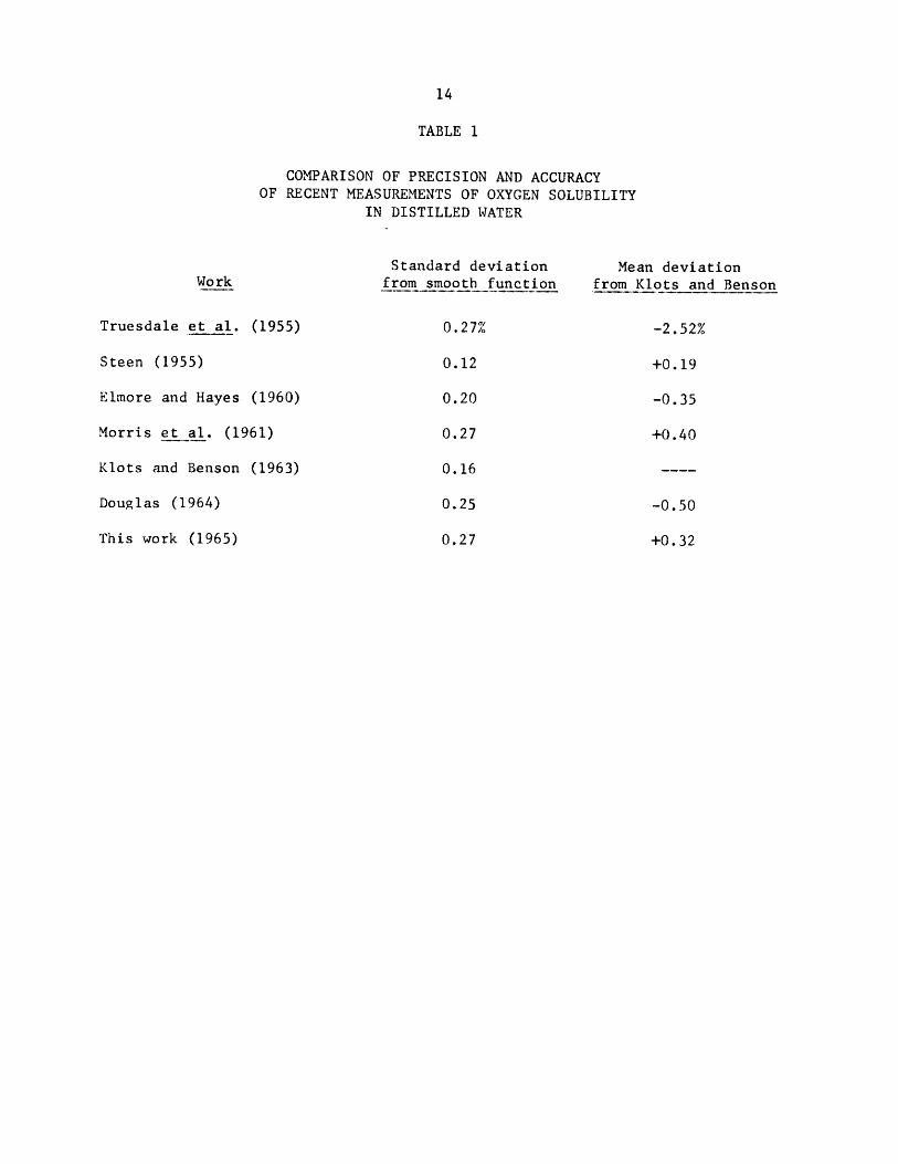
Exerimental designg the monitor method. Previous work on oxygen solu-

bility has been characterized by a rather high precision, as judged by the abi-

lity to get repeatable results by the same experimental method. The root-mean-

square (standard) deviations from the smooth functions of various workers are

shown in Table I along with their mean deviation from the values of KLOTS and

BENSON. It is immediately apparent that the precision is no measure of the

accuracy of a method, for, no matter whose values we take as reference, the

balance of the determinations, even excluding TRUESDALE'S, will spread over a

range of more than 1% in spite of a general precision of the order of 0.2%. We

must presume that unknown systematic errors are several times larger than the

random errors of experimental measurement.

It is appropriate to inquire how the accuracy of a method for measuring

the solubility of oxygen in sea water may be determined. In many analytical

methods the analyst takes a known or standard sample and compares his determina-

tion with the amount taken. This is, in fact, the way in which CARPENTER (1965)

has tested his modifications of the WINKLER method, by comparing with standards

prepared by dissolving known amounts of oxygen in oxygen-free water. As usually

applied, the WINKLER method is standardized not against known quantities of

oxygen but rather against a previously standardized iodine or iodine-generating

solution.

This work uses a variant of the WINKLER method discussed in a following

section. Accuracy here is determined using the considerable amount of informa-

tion that has been acquired about- the solubility of oxygen in distilled water.

In this work for each determination of oxygen in sea water a concurrent deter-

mination is made of oxygen in distilled water equilibrated in the same temperature

14

TABLE 1

COMPARISON OF PRECISION AND ACCURACYOF RECENT MEASUREMENTS OF OXYGEN SOLUBILITY

IN DISTILLED WATER

WorkStandard deviation

from smooth function

Truesdale et al. (1955)

Steen (1955)

Elmore and Hayes (1960)

Morris et al. (1961)

Klots and Benson (1963)

Douglas (1964)

0.27%

0.12

0.20

0.27

0.16

0.25

This work (1965)

Mean deviationfrom Klots and Benson

-2.52%

+0.19

-0.35

+0.40

-0.50

+0.320.27

15

bath and with the same gas stream. The evidence suggests that KLOTS and BENSON'S

own estimate of ±0.16% for the accuracy of their work is not unreasonable. If

our distilled water values compare satisfactorily with these reference measure-

ments we conclude that our sea water measurements are unlikely to be affected

by a larger error. Moreover, the ratio of the solubilities of oxygen in sea

water and in distilled water may be measured directly without a knowledge of the

partial pressure of oxygen in the gas phase, the exact concentration of our

titrant, or even the exact temperature of the bath, provided it is the same for

both distilled and seawater samples, because, unlike the solubility coefficients,

the solubility ratio is not greatly influenced by the temperature.

In actual practice all of these quantities were carefully measured so

that the solubility coefficients could be determined. It should be noted, how-

ever, that their absolute accuracy hinges on the work of KLOTS and BENSON: and,

even in the unlikely event that KLOTS and BENSON'S values should be shown to be

affected by a larger inaccuracy than estimated, the solubility ratios as deter-

mined by this work are likely to remain unaffected. Whattev u Inknown systematic

errors are present in the determinations of the solubility coefficients, they

are likely to be canceled out in the measurement of the solubility ratio. Fur-

thermore, the solubility ratio is of more direct thermodynamic interest in under-

standing solute-solvent interaction.

Sources of error in sample equilibration. The pronounced temperature

dependence of the aqueous solubility of oxygen is of the order of 2.5% per OC.

Constant temperature baths can be stabilized to within 0.010 C without great dif-

ficulty, which variation should result in an error not greater than 0.03% in

oxygen solubility.

3

For all inert gases (as contrasted with those like carbon dioxide which

dissolve with chemical reaction), which obey HENRY'S and DALTON'S laws at low

partial pressures, the solubility is proportional to the partial pressure of the

gas and independent of the presence of other inert gases. KLOTS and BENSON

(1963) observed no deviations from HENRY'S law for the solubility of oxygen,

nitrogen, and argon at partial pressures up to 1 atm. The conformity of the be-

havior of oxygen and nitrogen at 1 atm to DALTON'S law has been recently recon-

firmed by the ratio measurements of BENSON and PARKER (1961). The total pres-

sure may be easily measured to within 0.02% with a mercury manometer or barometer

but the accurate determination of the partial pressure of oxygen requires that

the composition of the gas phase be known. Over aqueous solutions water vapor

will make up a significant part of the gas phase, and it is probable that, al-

though the gas phase is probably always saturated with water in the laminar layer

at the gas-solution interface, final equilibrium is controlled by the composition

of the bulk gas which may have a very different relative humidity. Most modern

work, including this, has been done with the gas stream carefully presaturated

with water vapor. It also should be noted that the vapor pressure of sea salt

solutions is, for normal sea water, about 2% lower than that for distilled water.

As the vapor pressure itself amounts to 6% of one atmosphere at 35*C the vapor

pressure lowering effect may amount to 0.12%.

In addition to the change in the oxygen partial pressure caused by the

water vapor pressure, failure to saturate the gas stream will result in evapora-

tion from and consequent cooling of the sample as well as a change of chlorinity.

It should not be thought that the production of gas saturated water is

a trivial exercise. The increase in pressure within bubbles of 0.1 mm diameter

I

is 3% of one atmosphere (TRUESDALE'S calculation is in error); for 0.01 and Imm

diameter bubbles the increase is 29% and 0.3% of one atmosphere respectively.

It has been suggested that the reason for FOX'S values being slightly high lies

in his vigorous agitation of the phases. Thus it is of prime importance that

the equilibration interface have a large radius of curvature. On the other

hand it is desirable to have as large a surface area as possible to speed equi-

libration. The saturator described in the following section seems to meet the

requirements well.

As further source of error it should be remarked that mass transport

of the equilibrating gas stream moves under the influence of a pressure gradient

and it should not be assumed a priori that the pressure within the equilibrating

vessel is equal to the external ambient pressure. It is not clear from the pub-

lished data available to us whether TRUESDALE and co-workers applied pressure

to the upstream side or vacuum to the downstream side of their apparatus, but

if we suppose, as their drawing (figure 2) suggests, that each of their two wash

bottles was about 15 cm deep and if we further suppose that they applied vacuum

on the exhaust side of their system then the pressure drop within their equili-

bration flask is calculated to be 3% of one atmosphere, enough to account for

all of the apparent error of their results at low temperatures.

Finally the temperature correction of a mercury barometer might be noted.

For a laboratory at 25*C this amounts to a negative correction of about 0.4%.

This is a standard, well tabulated correction and may appear to be too trivial

to be mentioned to workers accustomed to making barometric measurements. It has

been cited, however, by MORRIS et al. (1961) as a possible source of error in

the work of ELMORE and HAYES.

W-to

18

The saturator. 'The water bath thermostat was contained by a rectangu-

lar wooden tank coated with epoxy resin. The 15 cm hollow walls of the tank were

filled with vermiculite insulation. The tank measured 60 cm by 122 cm by 64 cm

deep. Insulation on the top, when needed, was provided by floating on the water

surface several inches of 2 cm styrofoam cubes. These allowed free access of

equipment to the water bath. Temperature control was achieved by 2 submersed

750 watt heaters, one controlled by a variable voltage supply and the other by

a thermistor actuated relay. The thermistor-relay system was sensitive to 0.03*C

temperature change and, in fact, both short- and long-term temperature fluctua-

tions in the bath never exceeded 0.037*C. Temperature control within the equi-

libration vessels was better than tO.01*C due to the damping-out of short-term

cycling by the thick-walled vessel.

For control at low temperatures the bath contained a small commercial

refrigeration unit with a rated 3500 BTU/hr (882 kcal/hr) removal rate. This

was operated continuously with temperature control being performed by the heaters.

Massive circulation of the bath was achieved with a high capacity (190 11min)

pump, the output of which passed through the heatihg and cooling coils and then

immediately impinged on the thermistor. The temperature gradient throughout

the tank never exceeded 0.01C and then only for very low temperature runs. Tem-

perature measurements were made with two National Bureau of Standards (NBS) cer-

tified thermometers corrected to tO.01lC; temperature differences were measured

with two Beckman differential thermometers, one of which bears NBS certification.

These thermometers could be read to 0.001C.

Immersed to their necks in the tank were two 12-liter round-bottom long-

neck flasks inclined at a 45* angle and arranged to rotate about their axes of

symmetry by variable speed sewing machine motors. The water samples half filling

ita~'

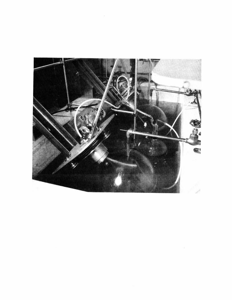
the flasks were thus held at constant temperature and a thin film of water was

drawn over the inside surface of the flask by its rotation. In this way a large

surface area of water was constantly renewed and exposed to the gas phase in the

flask. The saturation bottle and enclosing tank thermostat is shown in figure

1. This sort of rotating bottle saturator has been used by many workers in dif-

ferent fields. The earliest reference known to this writer is JACOBSEN (1905)

who used the system for oxygen equilbration.

The gas phase of ordinary laboratory air was passed through 15 meters

of polyethylene tubing coiled to a diameter of about 30 cm and immersed in the

thermostat bath. The lower half of each coil contained distilled water to sa-

turate the air with water vapor and bring the air to the bath temperature. The

air was given a final distilled water wash in a gas scrubbing bottle immersed in

the bath, then was passed via polyethylene tubing into the equilibration flasks

whose 5 cm diameter necks were open and vented to the laboratory air at ambient

pressure. A small diaphram pump equipped with a dust filter circulated the gas

stream at 430 in3/min (7 1/min)

Water saturation of the gas stream was measured with a wet bulb thermo-

mater at 15* and 25* C and was found to vary between 96% and 100% relative humi-

dity. No detectable (<0.0070/oo Cl) change of chlorinity was noted for sea water

exposed to the air stream for periods up to 18 hours.

No attempt was made to control the carbon dioxide content of the air,

but the pH of the sea water samples was monitored to check for anomalies in the

CO2 content of laboratory air large enough to affect the results. None were noted.

Upon storage in polyethylene bottles with attendent oxidation of organic matter,

charactistically the pH of 180/oo.Cl sea water would be about 7.6. After a few

hours of equilibration the pH would return to its normal value of about 8.2.

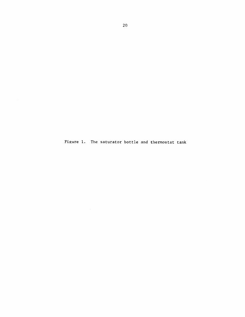
Figure 1. The saturator bottle and thermostat tank

22

ELMORE and HAYES have calculated the effect of the presence or absence of CO2

in the equilibrating gas due solely to the change in the partial pressure of

oxygen. In a normal atmosphere carbon dioxide is about 0.03% mole fraction and

it is unlikely that its presence in laboratory air would be more than double this.

Doubling the CO2 pressure would have lowered the pH of sea water by about 0.2

pH units.

In addition to the effect of the presence of carbon dioxide on the par-

tial pressure of oxygen, there is another potential source of error in the solu-

bility measurement as a consequence of the fact that carbon dioxide dissolves

with the formation of ionic species in aqueous solution. In distilled water un-

der a normal atmosphere dissolved CO2 is present principally as bicarbonate with

an ionic concentration of about 2 pequil/l. This ionic concentration cannot pos-

sibly be significant in salting-out oxygen as will be seen in later section.

The rotation speed of the equilibration flasks was held at about 22

rev/min. Cavitation did not become apparent below a rotation speed of 62 rev/min,

but the lower speed gave a satisfactory equilibration rate and was deemed safer.

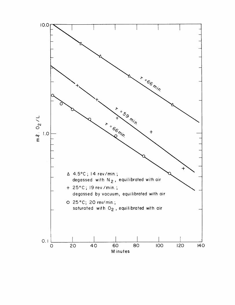
The equilibration rate was measured in three ways: (1) The solution

was degassed with nitrogen and then its oxygen concentration measured as it was

allowed to equilibrate with air. (2) The solution was saturated with oxygen at

a partial pressure of slightly over one atmosphere then allowed to equilibrate

with air. (3) The solution was partially degassed under vacuum and then allowed

to equilibrate with air. The results of these experiments are shown in figure 2,

in which the logarithm of the concentration gradient (i.e., the difference be-

tween the concentration at a time t and the equilibrium concentration, which

latter is a constant for a given temperature and partial oxygen pressure) is plotted

versus time. These plots are reasonably straight lines as required by the ADENEY-

Figure 2. Equilibration curves: Saturation concentration less concentra-tion at time t (logarithmic plot) versus time t (min).

14020 40 60 80 100 120Minutes

10.0

-J

0

E1.0

0. I

BECKER law (1919):

C - C(t)dC t) e uildt T

where Cequil is the asymptotically approached equilibrium concentration, C(t) isequil

the concentration at time t, and T is the mean period of the system.

The plots show that the mean period varies from 60 to 70 min depending

upon the rotation speed and the temperature. The temperature effect is probably

a consequence of the change in the diffusivity of oxygen which varies with tem-

perature as T/n, where T is the absolute temperature and n is the viscosity of

the solvent. This quantity decreases at OC by 48% from its value at room tem-

perature. The equilibration rate in sea water was not measured but, as the de-

pendence of the viscosity ( and hence the molecular diffusivity) on the chlorinity

is negligible compared to the temperature dependence (KRLMEL [19071), we do not

expect the variation to be significant.

All our samples were equilibrated for not less than 8 hours during a

period when the barometric pressure variation was not greater than 4 millibars.

The pressure prior to and during sampling was observed with a mercurial observa-

tory barometer and recorded by microbarograph. The pressure used in the calcula-

tion of the solubility coefficient was that which obtained one mean period (approx.

I hour) prior to sampling time. This procedure is justified in Appendix I, but

in no case did this effective pressure differ from the actual pressure at sampling

time by more than 0.03%. The vapor pressure, computed from the Smithsonian

Meteorological Tables (LIST, 1963) and from the tabulations of vapor pressure lower-

ing by sea salt of ARONS and KIENTZLER (1954), was subtracted from the total pres-

sure to give the pressure of dry air. Then the partial pressure of oxygen was

calculated on the assumption that dry laboratory air was 0.2094 mol fraction oxygen.

26

Sea water samples. Natural sea water obtained in three different places

was used in the determinations. The sea water used in series I was obtained in

Vineyard Sound at a point approximately midway between Woods Hole and Martha's

Vineyard, Massachusetts. The surface sea water used in Experiments II through X

was obtained in Cape Cod Bay shortly after high tide three miles offshore SSE of

Wood End lighthouse, Provincetown, Massachusetts. The sea water of the last

series, XI, came from the beach on the south side of Nahant, Massachusetts.

For the determinations at low and high chlorinities the samples were di-

luted with distilled water or evaporated by boiling, respectively. Immediately

prior to equilibration they were vacuum filtered through a Type SS Millipore fil-

ter of 3 micron nominal pore size.

According to SEIWELL (1937) the biological oxygen demand (BOD) of this

water may be expected to be no greater than 0.2 ml 02/1 per day. We may be con-

fident that after filtration the biological removal rate was negligible compared

with the equilibration rate.

Nominal precautions were taken to keep the equilibration flasks biologi-

cally clean. Following each series of determinations the flasks were scrubbed

with serological detergent.

Chlorinity determinations were made, with the cooperation of Woods Hole

Oceanographic Institution, on their BRADSHAW-SCHLEICHER conductivity bridge cali-

brated against Copenhagen standard water, :'Eau de Mer normale'. The probable

errors of and the assumptions inherent in the use of this instrument have been

discussed by PAQUETTE (1959) who concludes that the probable error in the range

of normal sea water is about ±0.0020/oo Cl.

Two to four tightly stoppered replicate samples of each sea water batch

were submitted to the salinometer operator at periods up to two months apart.

27

The operator was unaware that replications were being performed. Precision of

these replications was ±0.0070/oo Cl root-mean-square deviation. As the chlori-

nity of this sea water was about 17.60/oo the relative error was a negligible

0.04%. The relative imprecision for chlorinities much higher and much lower

than normal ran slightly higher due, no doubt, to the associated additional

errors of dilution. These samples were diluted with distilled water or concen-

trated with a high salinity substandard to bring the resulting chlorinities into

the normal range prior to determination. This avoided the necessity of recali-

brating the salinometer. The mean values of the replications together with the

standard deviation of the mean is listed for each series of experiments in

Table 2.

Sources of error in the WINKLER method. Potential errors in the WINK-

LER method have recently been exhaustively discussed by CARPENTER (1965) and by

CARRITT (1965).

In the WINKLER method freshly precipitated manganous hydroxide is

oxidized by the dissolved oxygen to manganic hydroxide. This reaction is favored

by high pH.

Mn+ + + 20H- + Mn(OH)2

2Mn(OH) 2 + 1/202 + H20 - 2Mn(OH) 3

The solution is then made acidic under which conditions tripositive

is caused to oxidize iodide.

2Mn(OH) 3+ 4H+ + 31- - 2Mn4 + + 13 + 5 H20

In the presence of excess iodide the iodine is largely complexed as

12 + I 13

Finally the iodine is titrated with thiosulfate,

12 + 2S203 - 21 + S406

(2)

(3)

manganese

(4)

triiodide.

(5)

(6)

which is oxidized to tetrathionate.

The stochiometry of the reactions depend upon strict control of pH and

iodide concentration. Under alkaline conditions sulfate rather than tetrathio-

nate is the oxidation product of thiosulfate with the consequence that much less

thiosulfate is required to reach the iodine endpoint. The other horn of this

dilemma is that under acid conditions iodide is air oxidized to iodine according

to:

02 + 411+ + 61- 21120 + 213 (7)

with the consequence that additional thiosulfate is required to reach the end-

point. The extent of oxidation is rate- rather than equilibrium-controlled but

will be favored by increasing acidity, iodide concentration, and oxygen tension.

The problem is compounded by the volatility of iodine which may be

decreased by complexing as the triiodide in the presence of excess iodide acccrd-

ing to equation (5). The volatility is also decreased by the hydrolysis of io-

dine which is disfavored by excess iodide. The predominant reactions are given

below:

I H+ + IO+ t+12 + 1120 HI + HIO

13 H + I

Equilibrium constants are as follows at 250 C:

(12 )(I ) _3= 1.40 x 10 (9)

(13 )

AWTREY and CONNICK (1951)

(HIO)(H )(I - ) 3 x 10- 13

(12) (10)

BRAY and CONNOLLY (1911)

Table 2

UNSMOOTHED SOLUBILITY DATA

Experimental Bunsen solubility coefficient Solubility RatioConditions

Sea Water Distilled Water3 3 B = aIso

a * 10 3o * 10

Series I 23.652 28.494 0.83007t = 24.92°C 23.865 28.549 0.83593C1 = 17.632±.0090/oo 23.901 28.730 0.83192

23.905 28.682 0.8334523.856 28.670 0.8320923.770 28.661 0.82935

Series mean 23.825t.056 28.631±.037 0.83214t.00097

20.172 24.086 0.83750Series II 20.197 24.129 0.83704t = 34.810 C 20.194 24.132 0.83681C1 = 17.562±.0120/oo 20.231 24.181 0.83665

20.200 24.085 0.8387020.246 24.199 0.83665

Series mean 20.207±.011 24.135±.019 0.83722*.00020

28.177 34.299 0.82151Series III 28.161 34.228 0.82275t = 15.090 C 28.206 34.244 0.82368Cl = 17.551±.0050/oo 28.162 34.208 0.82326

28.203 34.153 0.8257828.067 34.356 0.81694

Series mean 28.167±.014 34.248±.029 0.82245*.00130

34.860 43.118 0.80847Series IV 34.930 42.890 0.81441t = 5.03°C 34.890 42.932 0.81268Cl = 17.419±.0010/oo 34.695 42.920 0.80837

34.723 42.972 0.8080434.821 42.857 0.81249

Series mean 34.820'.038 42.948±.038 0.81074*.00113

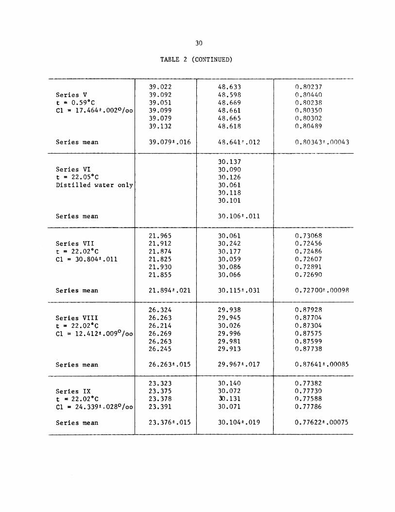
TABLE 2 (CONTINUED)

39.022 48.633 0.80237Series V 39.092 48.598 0.80440t = 0.59C 39.051 48.669 0.80238Cl = 17.464±.0020/oo 39.099 48.661 0.80350

39.079 48.665 0.8030239.132 48.618 0.80489

Series mean 39.079±.016 48.641±.012 0.80343±.00043

30.137Series VI 30.090t = 22.050C 30.126Distilled water only 30.061

30.11830.101

Series mean 30.106±.011

21.965 30.061 0.73068Series VII 21,912 30.242 0.72456t = 22.02*C 21.874 30.177 0.72486C1 = 30.8045.011 21.825 30.059 0.72607

21.930 30.086 0.7289121.855 30.066 0.72690

Series mean 21.894.021 30.115 ± .031 0.72700±.00098

26.324 29.938 0.87928Series VIII 26.263 29.945 0.87704t = 22.02°C 26.214 30.026 0.87304Cl = 12.412±.0090/oo 26.269 29.996 0.87575

26.263 29.981 0.8759926.245 29.913 0.87738

Series mean 26.263±.015 29.967'.017 0.87641±.00085

23.323 30.140 0.77382Series IX 23.375 30.072 0.77730t = 22.020C 23.378 30.131 0.77588Cl = 24.339±.0280/oo 23.391 30.071 0.77786

Series mean 23.376±.015 30.104.019 0.77622±.00075

TABLE 2 (CONTINUED)

28.099 30.049 0.93511Series X 28.139 30.074 0.93566t = 22.02*C 28.165 30.083 0.93624Cl = 6.3491.022 28.262 29.990 0.94238

Series mean 28.166±.028 30.049±.021 0.93735±.00169

24.961 30.092 0.82949

Series XI 25.108 30.080 0.83471

t = 22.020 C 25.091 30.103 0.83350Cl = 17.487'.002 30.156

Series mean 25.053±.046 30.108'.017 0.83257±.00158

(H)(I0-)= 1 x 10- 11 (11)

(HIO)

FURTH (1922)

(H+)(I-) = 3.2 x 109 (12)(HI)

McCOUBREY (1955)

From the magnitudes of the equilibrium constants it is apparent that the influence

of the iodide concentration in suppressing hydrolysis of iodine is negligible

compared with its influence in complexing the iodine as triiodide. We should

therefore expect that volatilization losses will always be hindered by high io-

dide concentrations.

Inasmuch as the solubility product of manganic hydroxide is small

(K = 10-36), the final iodine solution will necessarily be acid. Experiencesp

has shown that a final pH of between 2.0 and 2.7 will result in solution and re-

duction of the manganic hydroxide at a rapid rate without an unnecessarily high

air oxidation rate of the iodide.

It is apparent that the presence in the sample of reagents of any

substance capable of oxidizing manganous hydroxide in basic solution or iodide

in acid solution will result in a positive error. Likewise the presence of a

reducing agent more powerful than iodide will result in a negative error. Among

the offenders of the first kind are known to be higher valence manganese and

iodine compounds present in the reagents, and nitrate, nitrite and ferric iron

in normal sea water. Among the substances to which negative errors are attri-

buted are sulfite from industrially polluted waters and hydrogen sulfide from

essentially anaerobic samples. CARPENTER has attributed a negative reagent

blank to undetermined dark-colored impurities in the sodium iodide.

Any error due to the presence of organic or inorganic redox agents in

33

the sample may be removed by appropriate blanking procedure. The failure to re-

cognize the existence of both positive and negative blanks and concomitant

failure to run frequent blanks probably accounts for a large part of the error

of the WINKLER method as commonly used.

Thiosulfate solutions are ultimately unstable with respect to air

oxidation,

S20 3 + 1/2 02 S04 + S-- (13)

but the reaction proceeds very slowly in the absence of catalytic agents of

which copper is said to be the most common offender. Thiosulfate is also un-

stable in acid solution, and consequently care should be taken to exclude CO2.

S2 0 3 + H+ - HSO3 + S (14)

KOLTHOFF and SANDELL (1943) recommend stabilizing thiosulfate solutions by the

addition of 0.1% sodium carbonate. The sodium carbonate serves the dual pur-

pose of buffering the solution slightly alkaline and of complexing trace copper.

Thiosulfate solutions are also attacked by thiobacteria which convert

it to sulfite which in turn is quickly oxidized to sulfate by air. FOX recom-

mends stabilizing against bacterial action by the addition of 0.02% carbon di-

sul fide.

A number of different methods are in use for standardization of the

thiosulfate titrant in the WINKLER method. As we have noted, the accuracy of

our solubility ratios do not depend upon an accurate knowledge of the thiosulfate

concentration; nevertheless our absolute values do, and it is of interest to con-

sider possible errors in the standardization.

In experiments conducted by CARRITT (1965) it has been shown that

apparent thiosulfate concentrations may vary by 0.6% depending upon whether

34

potassium biniodate [KH(IO3 )2 1 or potassium iodate [KIO31 is used as the stan-

dardizing reagent and depending further upon whether the reagent is dried under

vacuum or with heat. (Potassium dichromate is no longer considered to be suit-

able as a standard because of air oxidation in acid solution.) Standardization

with either potassium biniodate or potassium iodate appears to yield thiosulfate

concentrations slightly in excess of those determined by the sodium arsenite method.

THOMPSON and ROBINSON (1939) had earlier found that use of the biniodate stan-

dard yielded thiosulfate concentrations about 0.4% higher than the NBS method,

but they considered this difference to be insignificant. The NBS recommended

procedure was used to standardize the thiosulfate solution used in this work.

Potassium biniodate was used as a secondary standard to check for day-to-day

variation in the thiosulfate normality because of the particular ease in using

it as a reference. The absolute value of the thiosulfate concentration as deter-

mined with vacuum-dried potassium biniodate was 0.7% higher than that determined

by the NBS method.

End-point errors in the titration of iodine with thiosulfate have been

discussed by KNOWES and LOWDEN (1953) and by BRADBURY and HAMBLY (1952). The

visual blue starch end-point as ordinarily used is found by KNOWES and LOWDEN

to give an end-point short of the equivalence point by about 3 vequiv/l. For

normal sea water at 25*C the solubility of oxygen is 885 uequiv/1; thus, the

starch end-point error may amount to more than 0.3%.

All the authors cited agree that the amperometric end-point is the

most accurate in the determination of iodine with thiosulfate. There will, of

course, be a finite error in the amperometric end-point due to the small amount

of iodine required to depolarize the cathode. This has been calculated by

BRADBURY and HAMBLY to be 0.04 pequiv/1, a neglible amount compared to the

oxygen concentrations of air saturated water.

From data of GILBERT and MARRIOTT (1948) the error due to adsorption

of iodine on glass is seen to be negligible at pH less than 6.

Finally, and not to be ignored, is the change in the volume concentra-

tion of reagent solutions due to thermal expansion in a laboratory where the

temperature may vary over several degrees. Dilute solutions will have nearly

the same thermal expansion as pure water which is 0.03% per degree near room

temperature. Temperature variations of 3*C have occurred in our laboratory

during the course of the experiments here described, and as a consequence there

is an uncertainty of 0.1% in our measurements due to this effect alone.

All volumetric glassware used was precision grade (class A) meeting

NBS tolerance requirements. All chemicals were ACS reagent grade. The distilled

water used had a conductivity of I umho/cm.

Modifications in the WINKLER technique. The modifications in techni-

que in the WINKLER method described herein represent an attempt to minimize many

of the errors described in the previous section. In choice of reagents we have

essentially followed CARPENTER and he also first suggested the use of a micro-

titrator.

A. Reagents for the WINKLER method.

Manganous solution. 2.5 MnC12*4H20

(500 g/1). We use 2 ml for a 240 ml sample bottle. The maximum solubility of

atmospheric oxygen (OC, 0 o/oo Cl, 0.2094 atm P0 2) is about 1.7 mequiv/l, thus

we use over a ten-fold excess both to speed the reaction to completion and to

allow for the occlusion of some manganese in the magnesium hydroxide precipi-

tated in sea water samples.

I -

36

Alkaline iodide solution. 3.0 M Nal (450 g/1), 6.0 M NaOH

(240 g/l). Two ml of alkaline iodide reagent used for a 240 ml sample bottle.

The amount of iodide oxidized being begligible, the resulting acidified solution

will be 0.025 N in iodide. This concentration is recommended for poising the

sampling and sharpening the end-point during the amperometric titration.

Sulfuric acid. 8.0 N H2S04 (220 ml conc/1) 2 ml of acid in

240 ml of distilled sample results in a final pH of 2.0. The final pH of sea

water samples is slightly higher and may be adjusted with a few extra drops of

acid.

B. Titration and standardization reagents.

Sodium thiosulfate solution. 0.2 N Na2S203*5H20 (70 g/1),

0.02% CS2 (0.2 ml/1), 0.01% Na2CO3 (0.1 g/l). Freshly boiled distilled water

is used. The solution is stored in a tightly stoppered brown bottle. Over the

four months duration of the sea water solubility measurements, the thiosulfate

was periodically checked against a previously standardized potassium biniodate

solution. The results of these periodic standardizations are shown in Figure 3.

These values suggest that there was no detectable change of thiosulfate concen-

tration over the duration of the experiments.

Potassium biniodate solution. 0.01 N KH(IO 3)2 (325 mg/l).

High quality potassium biniodate with stated assay of 99.968% was dried to con-

stant weight over silica gel under 60 mm total pressure and made to volume in

a volumetric flask.

Iodine solution. 0.01 N I (1.27 g/1), 0.09 N KI (15 g/l).

The potassium iodide is dissolved in about 10 ml of water, then the iodine is

added. When completely dissolved the volume is made up. The reagent is stored

in a tightly stoppered brown bottle.

Figure 3. Variation in thiosulfate concentration with time. The mean of re-

plicate determinations is shown together with the root-mean-square

deviation; replication as noted.

0.28 15

0.2805-

0.2801 -

2X

3X

0. 2795 --

20 60 80after Preparation

3X4X

4X

40Days

100 120

39

Sodium arsenite solution. 0.2 N Na2HAs20 3. NBS primary

oxidimetric standard (NBS 83b) resublimed arsenic trioxide with stated assay of

99.99% was dried to constant weight over silica gel under 60 mm total pressure.

Three aliquots each weighing about 9.9 grams were taken to 3 one-liter volumetric

flasks and dissolved therein with approximately 25 ml of 10 N NaOH. After solu-

tion was complete about 50 ml of distilled water and one drop of 1% phenolphtha-

lein solution was added. Nearly 10 ml of 5 N HCl was added dropwise until the

solution was neutral or weakly acidic.

As20 3 + 40H- + 2HAsO3 + H20 (15)

The neutral arsenite is quite stable, but is air oxidized to arsenate under basic

conditions.

As20 3 + 02 + 40H + 2HAs0 4 + H20 (16)

For this reason we think FOX's recommendation of adding a bicarbonate buffer to

the arsenite solution unwise. Another unfortunate feature of the bicarbonate

buffer is the resulting exsolution during titration of carbon dioxide which may

carry iodine vapor along with it. The titration of iodine with arsenite must

nevertheless be buffered, for it will not proceed rapidly in solution more acidic

than about pH 6.

HAsO 3 + 13 + H20 - HAs04 + 31 + 2H1+ (17)

In addition the titration solution must not be buffered to a pH greater than 9

or the iodine will escape titration by the formation of the iodate.

3I2 + 60H + 51 + IO03 + 3H20 (18)

The procedure used in this work is to add to the reaction flask just before the

arsenite titration the following phosphate buffer.

Buffer concentrate. 1.0 M Na2HP0 4 (140 g/l). About 4 ml

of the buffer concentrate in a 240 ml sample gave a resulting pH of 8.

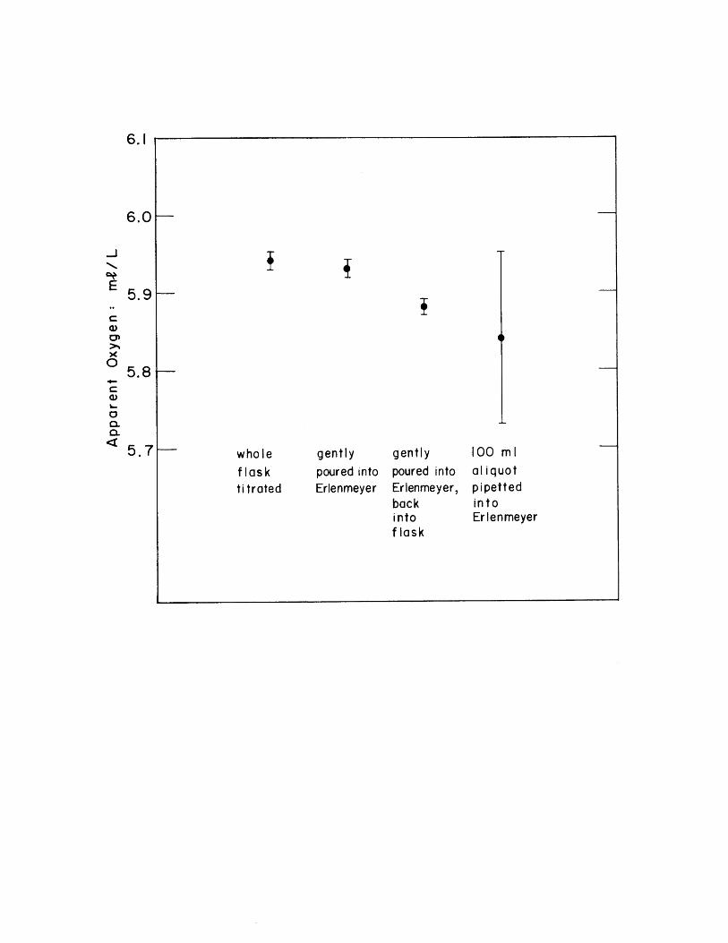
C. The improved sample bottle. Most frequently used in the WINKLER

method are biological oxygen demand (BOD) bottles. These have a narrow neck

with a flanged collar and a solid ground glass stopper which has a pointed base.

They have the advantage of being easy to fill without entrapping air bubbles.

They have the unavoidable disadvantage of requiring that the sample be trans-

ferred before titration. In a series of experiments conducted prior to the sea

water solubility determinations the amount of thiosulfate required to titrate

samples identical except for the number of transfer steps was measured. The

results are shown in Figure 4. It is seen that even a careful transfer by

pouring may result in an apparent 0.5% loss of iodine, no doubt by volatilization.

The loss during transfer by pipetting is both greater and more variable. These

results lead us to suggest that the current oceanographic practice of pipetting

iodine aliquots prior to the thiosulfate titration be discontinued in favor

of whole bottle titrations.

In order to overcome volatilization losses, the improved iodine deter-

mination bottle shown in Figure 5 was developed. It consists in part of the

ordinary 250 ml Erlenmeyer-shape iodine flask available commercially (Corning

#5400) with a standard taper 22 solid glass stopper. The solid glass stoppers

were discarded and substituted with long nipples blown from standard taper 24/40

full length inner joints with sealed tube (Corning #6710). The closed sealed

tube which projected into the flask to within 3 cm from the bottom displaced a

volume of about 10 cc. Thus when the stopper is removed titrations may be per-

formed right in the flask, evenr with an ordinary burette. Bottles and stoppers

were matched and engraved with numbers to avoid mismatching then the flasks

were calibrated "to contain" by weighing. Repeated fillings and weighings gave

Figure 4. Volatilization losses during sample transfers. Apparent oxygen

concentration of identically equilibrated samples. 4X replica-

tion performed on each group; means and extremes are indicated.

6.1

6.0

E5.9

05.80.-

C.

<5.7 100 mlaliquotpipettedintoErlenmeyer

gently gently

poured into poured into

Erlenmeyer Erlenmeyer,backintoflask

wholeflasktitrated

Figure 5. An improved iodine determination flask.

Co.

8 cm

Corning part no. 5400

S24/40

sealed

Corning part no. 6710

45

a precision of better than 0.01%. No attempt was made to make the flask volumes

identical. Made as described, the stoppered flasks contained on the average 242 ml

with a range of 14.4 ml. The variation in flask volume removed any unconscious

bias on the part of the operator to try to get the same result on replication.

The sample temperatures ranged from 00 to 350C. The bulk expansion

coefficient of Pyrex glass is 10.8 x 10 deg . Thus over the temperatures of

interest the variation in the flask volume was only ±0.02%, and flask expansion

could be ignored.

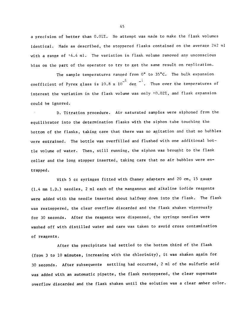
D. Titration procedure. Air saturated samples were siphoned from the

equilibrator into the determination flasks with the siphon tube touching the

bottom of the flasks, taking care that there was no agitation and that no bubbles

were entrained. The bottle was overfilled and flushed with one additional bot-

tle volume of water. Then, still running, the siphon was brought to the flask

collar and the long stopper inserted, taking care that no air bubbles were en-

trapped.

With 5 cc syringes fitted with Chaney adapters and 20 cm, 15 gauge

(1.4 mm I.D.) needles, 2 ml each of the manganous and alkaline iodide reagents

were added with the needle inserted about halfway down into the flask. The flask

was restoppered, the clear overflow discarded and the flask shaken vigorously

for 30 seconds. After the reagents were dispensed, the syringe needles were

washed off with distilled water and care was taken to avoid cross contamination

of reagents.

After the precipitate had settled to the bottom third of the flask

(from 3 to 10 minutes, increasing with the chlorinity), it was shaken again for

30 seconds. After subsequente settling had occurred, 2 ml of the sulfuric acid

was added with an automatic pipette, the flask restoppered, the clear supernate

overflow discarded and the flask shaken until the solution was a clear amber color.

46

As soon as possible thereafter the stopper was removed, the drop hang-

ing from the long nipple was caught inside the neck of the flask and the whole

sample was titrated in the flask.

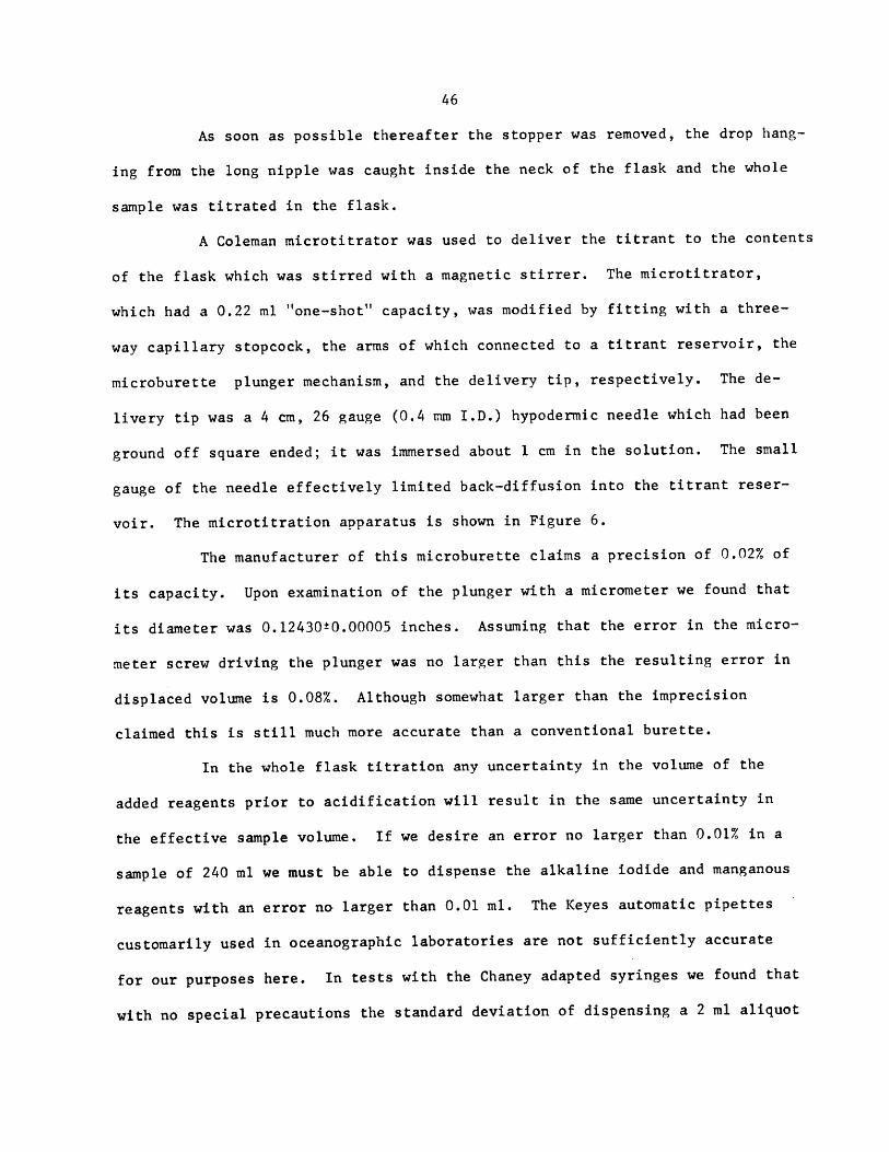
A Coleman microtitrator was used to deliver the titrant to the contents

of the flask which was stirred with a magnetic stirrer. The microtitrator,

which had a 0.22 ml "one-shot" capacity, was modified by fitting with a three-

way capillary stopcock, the arms of which connected to a titrant reservoir, the

microburette plunger mechanism, and the delivery tip, respectively. The de-

livery tip was a 4 cm, 26 gauge (0.4 mm I.D.) hypodermic needle which had been

ground off square ended; it was immersed about 1 cm in the solution. The small

gauge of the needle effectively limited back-diffusion into the titrant reser-

voir. The microtitration apparatus is shown in Figure 6.

The manufacturer of this microburette claims a precision of 0.02% of

its capacity. Upon examination of the plunger with a micrometer we found that

its diameter was 0.1243010.00005 inches. Assuming that the error in the micro-

meter screw driving the plunger was no larger than this the resulting error in

displaced volume is 0.08%. Although somewhat larger than the imprecision

claimed this is still much more accurate than a conventional burette.

In the whole flask titration any uncertainty in the volume of the

added reagents prior to acidification will result in the same uncertainty in

the effective sample volume. If we desire an error no larger than 0.01% in a

sample of 240 ml we must be able to dispense the alkaline iodide and manganous

reagents with an error no larger than 0.01 ml. The Keyes automatic pipettes

customarily used in oceanographic laboratories are not sufficiently accurate

for our purposes here. In tests with the Chaney adapted syringes we found that

with no special precautions the standard deviation of dispensing a 2 ml aliquot

Figure 6. Microtitration apparatus.

titrant reservoir: - 14/35 outer joint

3-way capillary stopcock

SJ 12/1 balland socket joint

ColemanmicrotratorunitShohl joint

hypodermic needle

was only 0.008 ml.

E. End-point detection. Immersed into the flask beside the microti-

trator delivery tip was a glass tube through the sealed end of which extended

two platinum wires, 14 mm long, 0.8 mm in diameter, and 10 mm apart. 182 milli-

volts was imposed across these from a source with 9.1 K ohms internal resistance.

The high iodide concentration of the reacting solution poised it to the extent

that the current, monitored with a Keithley low impedance microammeter, fell

from its maximum of 20 microamps only very near the end-point. Near the end-

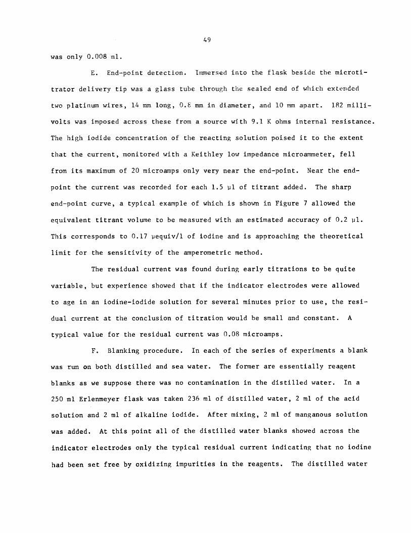
point the current was recorded for each 1.5 pl of titrant added. The sharp

end-point curve, a typical example of which is shown in Figure 7 allowed the

equivalent titrant volume to be measured with an estimated accuracy of 0.2 Il.

This corresponds to 0.17 vequiv/l of iodine and is approaching the theoretical

limit for the sensitivity of the amperometric method.

The residual current was found during early titrations to be quite

variable, but experience showed that if the indicator electrodes were allowed

to age in an iodine-iodide solution for several minutes prior to use, the resi-

dual current at the conclusion of titration would be small and constant. A

typical value for the residual current was 0.08 microamps.

F. Blanking procedure. In each of the series of experiments a blank

was run on both distilled and sea water. The former are essentially reagent

blanks as we suppose there was no contamination in the distilled water. In a

250 ml Erlenmeyer flask was taken 236 ml of distilled water, 2 ml of the acid

solution and 2 ml of alkaline iodide. After mixing, 2 ml of manganous solution

was added. At this point all of the distilled water blanks showed across the

indicator electrodes only the typical residual current indicating that no iodine

had been set free by oxidizing impurities in the reagents. The distilled water

Amperometric end-point titration curve.Figure 7.

6

5

a4

E

o End - point

21-

780 785 790 795 800 805 810 815 820

Thiosulfate Volume: microliters

52

blanks were then titrated with potassium biniodate and it was found that a finite

quantity of biniodate was required to cause the current to increase. The non-

zero intercept gives the "negative" blank of the reagents. It was found that

over several months use of the same reagents this blank became gradually more

positive (smaller in absolute value). This is probably a consequence of the in-

evitable trace cross-contamination between reagents in spite of the precautions

taken. The reagent blank varied from between 11.8 to 0.4 lambda of 0.01 N

biniodate which corresponded to from -0.59 to -0.02 lambda of 0.2 N thiosulfate.

In contrast, the sea water blanks were positive; i.e., upon adding the

reagents in the reverse order, making certain that the sea water was clear and

acidic before adding the manganese, a titration could be performed in the usual

way with thiosulfate.

If the negative reagent blank is algebraically subtracted from the sea

water blank, the resulting value must represent the amount of material present

in the sea water which will oxidize iodide. This quantity was found to be

variable depending upon sea water source and roughly proportional to the chlorin-

ity. The mean value was 0.11±0.02 pequiv/unit chlorinity kg of sea water. This

is not an unusual value for an oxidizing substance such as nitrate in sea water.

Recent halogen investigations, including those of BARKLEY and THOMPSON (1960),

suggest that a substantial fraction of sea water iodine may be present as iodate;

but according to the tabulations of RICHARDS (1957) sea water iodine concentra-

tion probably does not exceed 0.02 vequiv/unit chlorinity kg of sea water.

It will be noted that the blanking procedure does have a flaw. It fails

to test for redox substances which might bias the manganous-manganic couple in

basic solution but which fail to act upon the iodide-iodine couple in acid solu-

tion. Such substances include nitrite, as the N03 /NO2 couple is lower than

53

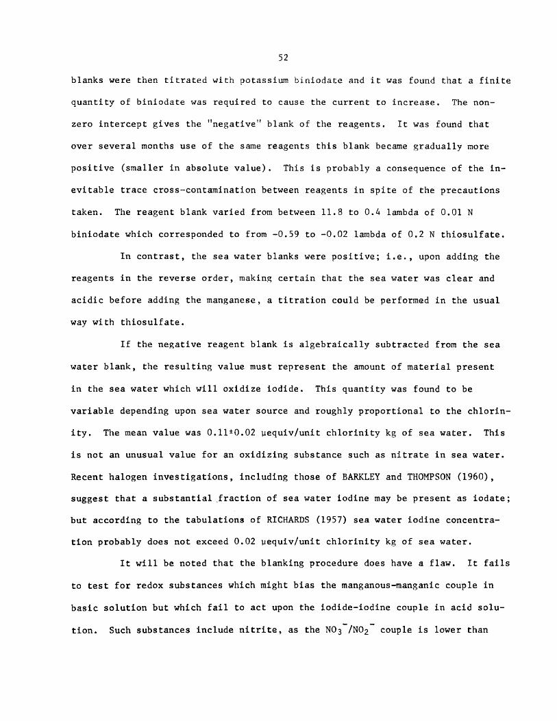
that of Mn(OH) 3/Mn(OH)2 in basic solution but higher than that of I2/1I in acid

solution. The situation is shown graphically in the Eh-pH diagram in Figure 8

where the manganese, iodine and nitrogen fields are superimposed. Also shown

for reference on this same diagram are the relevant thio-fields.

G. Standardization of the thiosulfate. The iodine solution was used

as an intermediate and the thiosulfate was standardized against the sodium ar-

senite solutions made up with carefully dried and weighed arsenic trioxide.

The burette was filled with sodium arsenite solution. In a 250 ml

Erlenmeyer flask were taken 226 ml of distilled water and 4 ml of phosphate

buffer. The pH was checked and did not exceed 8.7. 10 ml of iodine solution

were pipetted into the flask and immediately titrated with the arsenite solu-

tion to the amperometric end-point. In the standardization performed for this

work two replicates each of the three similar arsenite solutions were performed.

The six determinations yielded a mean iodine concentration of 0.009820 N with

a standard deviation of a single determination of 0.000014 giving a precision

of 0.15% for this step.

The burette was then carefully washed and filled with sodium thiosul-

fate solution. 236 ml of distilled water, 2 ml of sulfuric acid and 2 ml of

alkaline iodide were taken to a 250 ml Erlenmeyer flask. After mixing, adding

2 ml of manganous solution and again mixing, 10 ml of iodine solution were

pipetted into the flask and immediately titrated with thiosulfate. Care was

exercised to avoid leaving the iodine solution unstoppered longer than necessary.

Following this the concentration of the potassium biniodate was checked

by titrating a 10 ml aliquot of it substituted in the above procedure for the

iodine. The thiosulfate concentration as determined from the iodine titration

was 0.2801 N. The thiosulfate concentration as determined from the biniodate

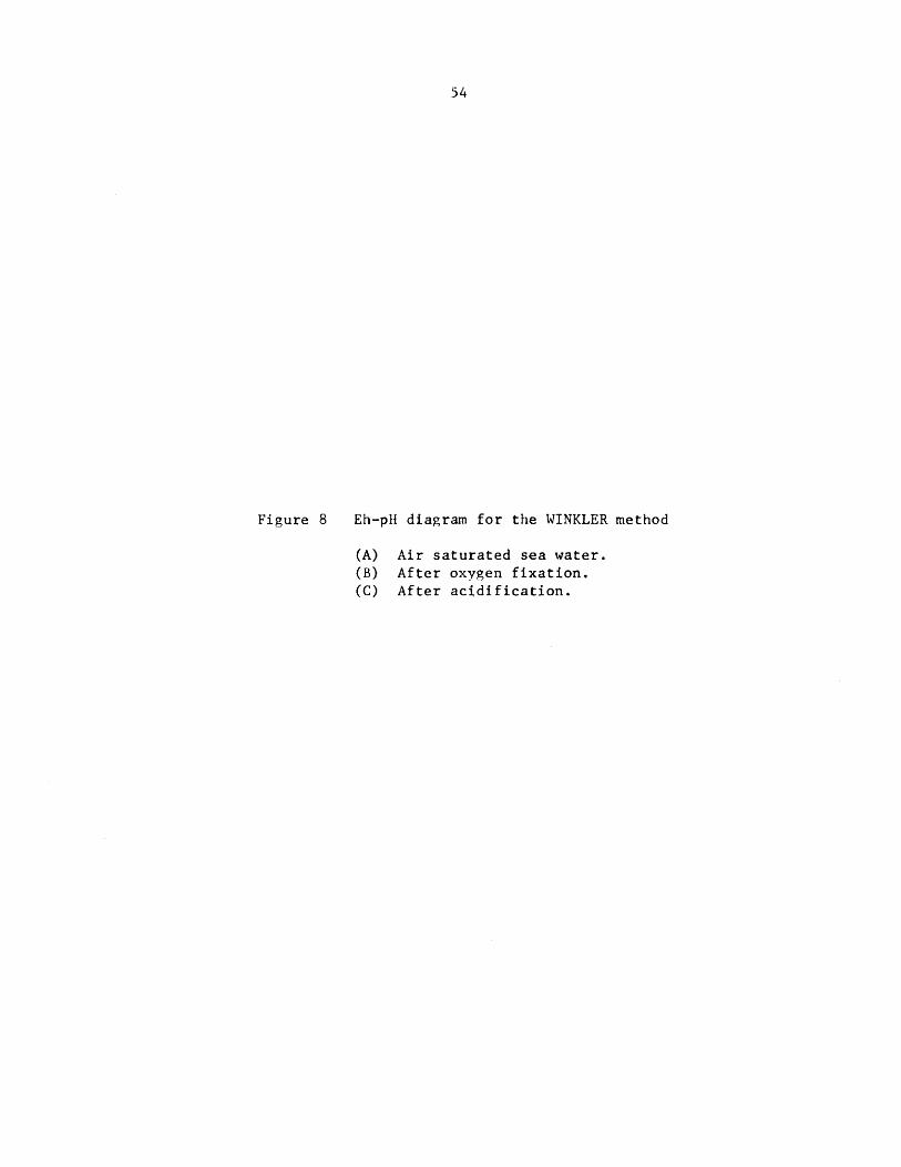
Figure 8 Eh-pH diagram for the WINKLER method

(A) Air saturated sea water.(B) After oxygen fixation.(C) After acidification.

+ 1 .

Kl~L-a

+0.5 'NONO X- .

N \\ I M Mn(O .H)3..NO-2' M n

Mn(OH )2

a '

a %

-I--0.

- 1.0 S406 S 04

0 2 4 6 8 12 14pH ,e-0.5

0 2 4 6 8 10 12 14pH

v L --,

56

titration directly, whose concentration, in tun, was known from weighing was

0.7% higher than the NBS method detenrination. For reasons that have been dis-

cussed in the previous section we accept the NBS method value.

57

RESULTS AND DISCUSSION

The salting-out effect. Both of the previous investigators, (FOX and

TRUESDALE) of the sea water solubility of oxygen have represented their data as:

a(t,Cl) = ao(t) - Cl'f(t) (19)

where a is the sea water solubility, ao is the distilled water solubility, Cl

is the chlorinity in O/oo and f(t) is some function of the temperature only.

Actually, TRUESDALE et al. represented their data as a linear function of the

salinity but, as the salinity is a linear function of the chlorinity, their re-

lation may be transformed into equation (19). FOX examined the solubility at

7 temperatures between 0* and 310 C for sea water of 3 chlorinities of approxi-

mately 8, 14 and 200/00. The root-mean-square deviation from linearity of his

values is 0.6%.

TRUESDALE and co-workers accepted FOX's assumption of a linear salting-

out relation. They made 16 determinations in sea water all but three of which

were in water of approximately 170/oo Cl. The other three were in water of 80 /oo

C1 and had a root-mean-square deviation from linearity of 0.9%. In view of the

limited chlorinity range and the large uncertainties in the data of these workers,

it is not surprising that the salting-out relation revealed by the present work

has not previously been observed. We decided to examine the solubility ratio

of oxygen in sea water to oxygen in distilled water at a carefully controlled

temperature over an extended chlorinity range. Several replicate determinations

were made at chlorinities near 6, 12, 18, 24 and 30 0/oo. As the solubility

ratio must be unity at a zero chlorinity, this point is obtained gratis. Equa-

tion (19) may be rearranged to yield the solubility ratio B.

a fS -- = 1 - Cl (20)0 0o

58

The quantity f/ao is a constanat at cons a at em.Ceraure, and if the sal ting,-out

relationship is linear the so ulubii .y ratio iust decli tie iieariy.

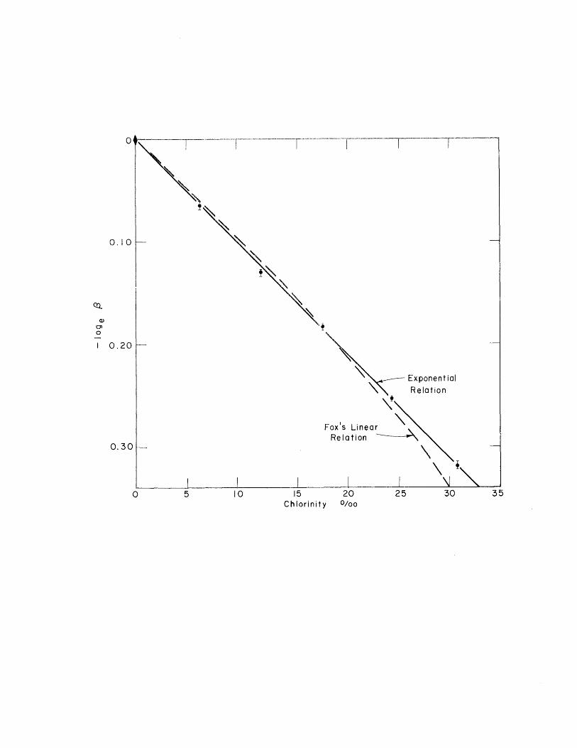
Figure 9 shows a distinct regular deviation of our data from the

linear relation. The shape of the t urve suggests an exponential decay and, in-

deed, Figure 10 in which the logarithm of i is plotted against chlorinity shows

that a very satisfactory representation of the data may be made by

C = co(t) exp[k(t)Cl] (21)

Between 0 and 20 O/oo Cl the two curves of Figure 9 deviate from one another by

a maximum of only 0.6% so it is not surprising that the non-linearity has not

been previously observed. The non-linearity does result, however, in the conse-

quence that whatever random errors of precious workers may have been removed by

smoothing, their tables must have systematic errors at least as large as 0.6%.

Moreover the exponential deviates so dramatically from the linear relation for

chlorinities greater than 20 O/oo that extrapolation of previous published

values for use in, say, the Red Sea must incur errors as large as 1%.

A precision test of the data. If the sea water solubility data may

be represented by the exponential relation of equation (21) then

-_ = k(t) (22)Cl

must be a chlorinity invariant parameter. In other words, all values of k(t)

computed from measured solubilities must fall on one smooth temperature curve

regardless of the chlorinity of the water used in the solubility determination.

Such a plot is shown in Figure 11 where is also plotte d the raw data of FOX

(his 21 original unsmoothed sea water solubilities combined with distilled water

values from his tables), FOX's smoothed curve (computed from his equation at

20 o/oo Cl), and the smoothed curve of TRUESDALE et al., their raw data not

Figure 9 Variation in the solubility ratio, B, with chlorinity, linear plot.Constant temperature of 22.02°C.

1.0 T - i

0.9

0.8

0.7

This Work

Fox'sRela

0 5 10 15 20 25 30Chlorinity : O/oo

i

Figure 10 Variation of the solubility ratio, B, with chlorinity, semilogarith-mic plot. Constant temperature of 22.02C.

ExponentialRelation

Fox's LineRelation

___ I30 3515 20

Chlorinity O/oo

0. 10 -

0.20 I-

0. 30-

The chlorinity invariant parameter as a function of temperature.Figure 11

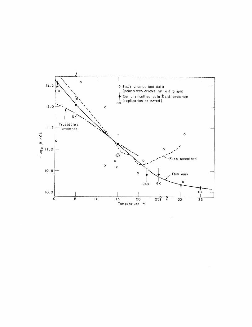
o Fox's unsmoothed data

(points with arrows fall off graph)Our unsmoothed data ±std. deviation(replication as noted)6X

T 0

o 0

6X o _, Fox's smoothed0X 0

This work

5 20

Temperature : OC

smoothed

12.5

12.0

11 .5

11.0

10.5

10.0

65

being available to us. It is immediately apparent that this kind of a plot

is a rather severe test of precision; for, as the spectacular temperature de-

pendence of the gas solubility obscures deviations, the weak temperature de-

pendence of the salting-out coefficient, k, reveals them.

A comparison of the goodness-of-fit of our data to the two kinds of

salting-out relationships may be made by examining the chlorinity invariant

parameters: C-l if the relation is linear, and - if the relation isClr C1

exponential. These parameters are calculated in Table 3. It is seen that the

error band of the exponential relation is less than one-third as wide as that

of the linear relation.

Choice of smoothing function. For purposes of interpolation previous

investigators have fitted a smooth curve to their solubility data and then used

this fitted function to generate tables of solubility coefficients at integer

values of temperature and chlorinity. The same has been done in this work

and the resulting tables are given at the end of this paper (Tables 6, 7).

FOX (1907) and TRUESDALE, et al. (1955) used a polynomial function of the tem-

perature as their smooth curve. Although the power-series form will represent

any continuous function to any desired degree of accuracy, provided enough

terms are used, it is desirable to represent the data with a function which

has as few terms as possible for ease in hand calculation. Moreover, as MORRIS,

et al. (1961) have pointed out, it is desirable to use a type of equation which

has a theoretical basis, especially when the correct shape of the smoothed

curve is to be determined near the ends of the range of experimental values.

The curve fitted to the data presented in Table 2 herein was of the

following form:

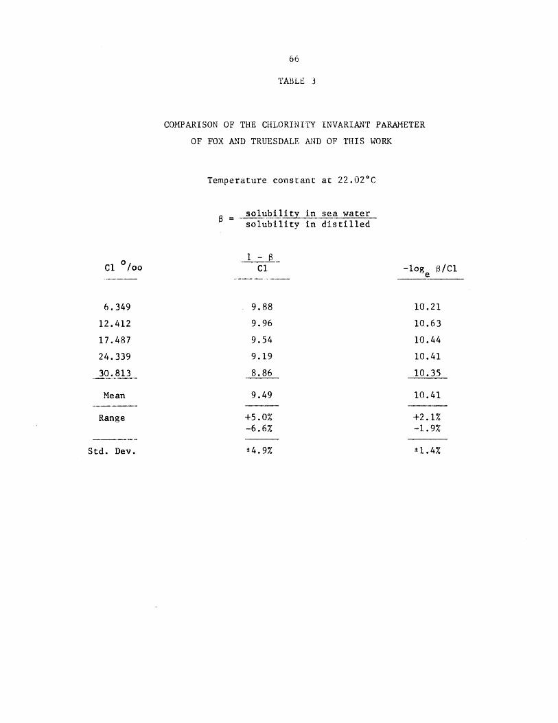
TABLE 3

COMPARISON OF THE CHLORINITY INVARIANT PARAMETER

OF FOX AND TRUESDALE AND OF THIS WORK

Temperature constant at 22.02C

solubility in sea water

solubility in distilled

1 -

ClC1 /0oo

6.349

12.412

17.487

24.339

30.813

Mean

Range

Std. Dev.

-log e B/Cl-e

9.88

9.96

9.54

9.19

8.86

9.49

+5.0%-6.6%

t4.9%

10.21

10.63

10.44

10.41

10.35

10.41

+2.1%-1.9%

±1.4%

e T

b (23)-Cl(bl + T + bLo T + b'T)

where a is the Bunsen coefficient and CI is the chlorinitv of the sea water in

°/oo. The constants were determined by least-squares analysis and are shown,

together with their respective root-mean-square errors, in Table 4.

The functional form of equation (23) is derived by integrating tile

VAN'T HOFF equation,

d log e x ALt

d T -= T (24)

after having expanded the enthalpy in a power series of the temperature.

Representation of the data. The solubility coefficient a, known as

the BUNSEN coefficient, is a useful and widely accepted quantity with which

to represent the data. For inert gases at low pressures obeying HENRY's and

DALTON's laws (i.e., the gas dissolves without chemical reaction, the solubility

is proportional to the partial pressure and is independent of the presence of

other inert gases), the BUNSEN coefficient is independent of the partial pres-

sure of the gas, is only weakly dependent on the total pressure and is a func-

tion of the temperature and the concentration of dissolved electrolytes. In

this work we will define the BUNSEN coefficient as

= o (25)Vp

where vo is the volume the dissolved gas would have at standard temperature

and pressure were it ideal, V is the volume of solvent containing the dissolved

gas and p is the partial pressure of the gas in equilibrium with the solution.

As herein defined the BUNSEN coefficient closely coincides with that coefficient

first defined by R. BUNSEN (1857): "Wir nennen die auf O0C und 0.76 m

68

TABLE 4

CONSTANTS OF THE SEMI-EMPIRICAL SMOOTHING EQUATION

loge(103 a) = (a, + +T + a3 log T + a 4 T)

-C1(b + + b 3 logeT + b 4 T)

al: (-7.424 ±1.600) x I0 0

a2 : ( 4.417 t0.195) x 103

a 3 : (--2.927 ±0.323) x 100

a4: ( 4.238 ±0.294) x 10- 2

bl: (-1.288 ±0.642) x 10- 1

b2 : ( 5.344 ±0.764) x 101

b3 : (-4.442 ± 1 .290 ) x 10- 2

b4: ( 7.145 ±1.150) x 10- 4

69

Quecksilberdruck reducirten Gasvolumina, welche von der Volwueneinheit einer

Flussigkeit unter dem Quecksilberdruck 0.76 m absorbirt werden, Absorption-

scoefficienten." This definition is not without ambiguity and perhaps for

this reason the coefficient has been redefined by succeeding investigators.

The subsequent definitions miay hinge upon any of the three terms of equation

(25).

(1) v may be defined as the actual volume that would be occupied

by the real gas at standard temperature and pressure.

(2) V may be defined as the volume of solution rather than solvent.

(3a) p may be defined as the fugacity of the gas in equilibrium.

(3b) p may be defined as unity when the partial pressure of the gas

plus the vapor pressure of the solvent equals one atmosphere.

WINKLER uses (2) and (3b), STEEN uses (1), DOUGLAS uses (1), KLOTS

and BENSON use (2) and (3a), and it is not always clear how others have arrived

at their values. At present, except for the vapor pressure effect, the distinc-

tions between these variants are smaller than the accuracy of the data. For

oxygen the mol volume is 22,393.1 ml compared with the ideal 22,414.0 ml, a

difference of only 0.09%. The difference between the volumes of solvent and

solution may be calculated from the partial molal volume given by ANGSTRON (1882).

At the maximum solubility (0°C, 00koCl, 0.2094 atm P0 2) oxygen solutions are

expanded only 0.001% compared to pure water. The deviation between fugacity

and pressure at 1 atmosphere is 0.09% at O0C. At that future time when solu-

bility coefficients are determined to an accuracy of better than 0.1% these

distinctions will become important.

Analysis of errors. One correction that has not so far been discussed

70

is the adjustment of the mieasured solubility coefficien: ts to a tocal pressure

of 1 atmosphere. The solubility coefficient is a weak function of the total

applied pressure. From simple thermodynamic arguments it can be shown that,

at constant temperature:

p

log ._ -- i V1 dp) (26)e al RT J V

i atm

Where a is the solubility coefficient at total applied pressure p, al is the

coefficient at 1 atmosphere, and V0) is the partial molal volume of oxygen in

solution. The partial molal volume in distilled water is constant at 26 cc/mole

over the temDerature and concentration range of interest. Evaluating the inte-

gral:

a - 02loeg = (p-1) (27)ea RT

Substituting a = o1 + Aa and expanding the left hand side in series, we ob-

tain:V0 2

At 2+ ..... = - (p-l)

Ua "RT (28)

valid if the adjustment is small. The maximum deviation of total pressure ob-

served during our experiments was 0.0416 atm. This, substituted into equation

(28) with the temperature, yields a maximum correction of 0.006%, which, being

small compared with other errors, has been neglected.

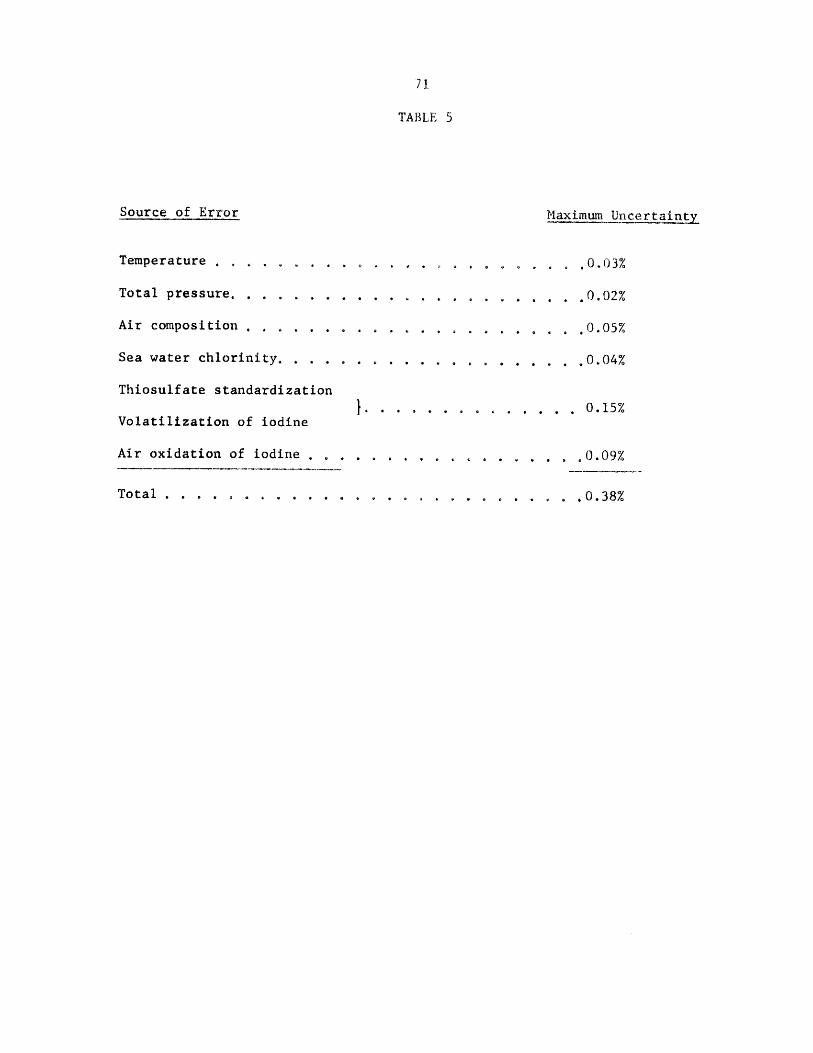
Other sources of known errors have been discussed in the foregoing

section. They are listed again for review in Table 5. Assuming the worst case,

that they are all additive, they result in a total relative error of 0.38%.

This coincides closely with the root-mean-square (standard) deviation of 0.27%

of our smoothed curve from the raw data (Table 2).

71

TABLE 5

Source of Error

Temperature ........

Total pressure . . . . . .

Air composition . . . . . .

Sea water chlorinity. . . .

Thiosulfate standardization

Volatilization of iodine

Air oxidation of iodine

Total . . . . . . . . . . .

Maximum Uncertaint

S, .0.03%

.. .0.02%

.. .0.05%

. . .0.04%

). . . . . . . . . . . . . . 0.15%

. . . . . . . . . 0.09%

.. . . . . . . . .. 0.38%

ISpp~

o c r

uo r~

u

72

The deviation of the distilled water values fLa.und from this work is

compared in Figure 12 with the values of KLOTS and BENSON. It is seen that a

maximum deviation of 0.39% is observed,

From these independent lines of evidence we conclude that the accuracy

of the solubility coefficients presented herein is probably as good as t0.4%.

Figure 12. Deviation of the distilled water solubility of this work from dataof KLOTS and BENSON.

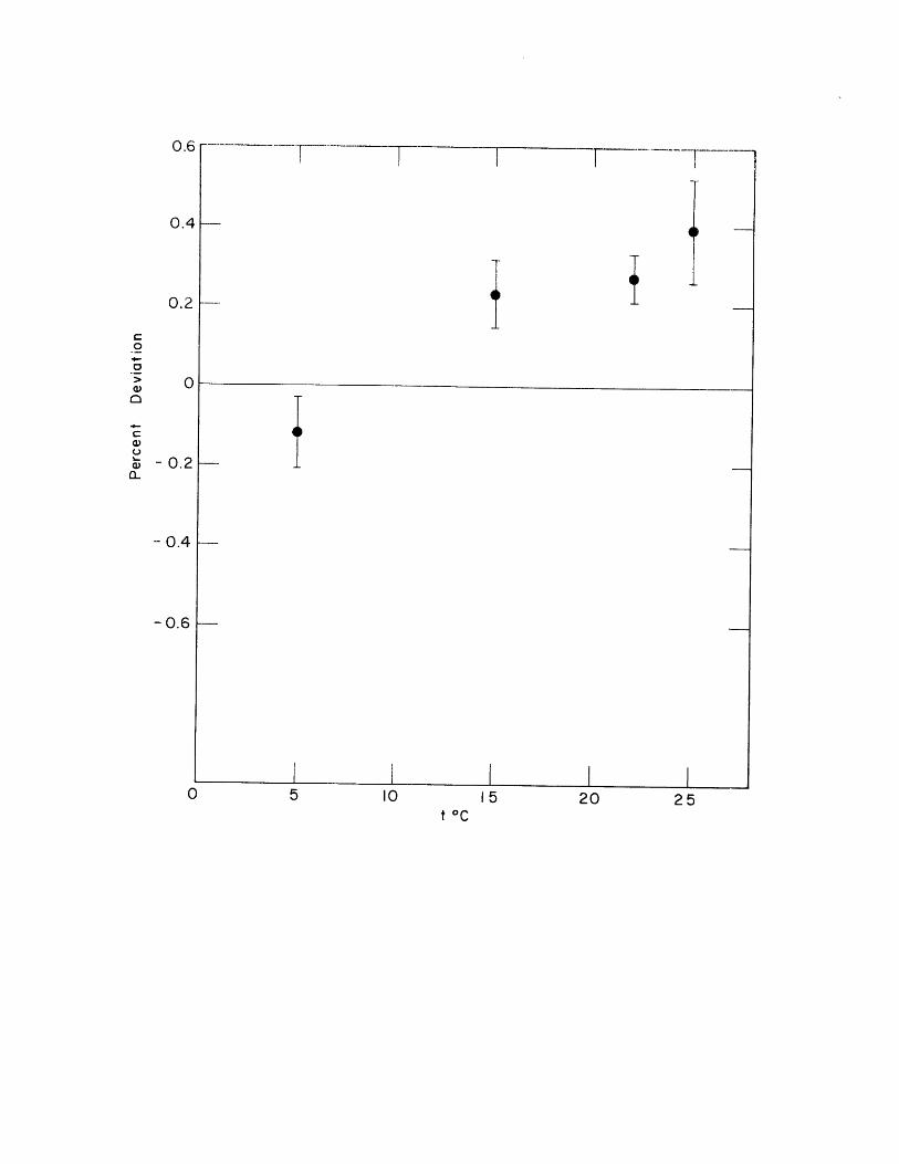
0.6

0.4

0.2

0.2

- 0.4

-0.6

5 10 15 20 25t oC

75

SUMMARY AND CONCLUSIONS

The tables of the solubility of oxygen presented herein diverge from

the widely used tables of FOX in two ways. Firstly, the smoothing function

used in this work presumes an exponential rather than a linear dependence upon

the chlorinity. As a consequence the tables of FOX tend to be high, relative

to those of this work, at chlorinities between 0 and 19 O/oo; and lower, at

chlorinities greater than 19 o/oo. Figure 10 demonstrates this. Secondly,

the distilled water oxygen solubilities as determined by this work are lower

than those of FOX and this divergence is more pronounced at high temperatures.

The total effect is shown in Figure 13 where the deviations of the FOX solu-

bilities from those of this work are contoured on the temperature-chlorinity

surface.

Deviations of the FOX cxygen solubility values from the values ofthis work, contoured on the temperature-chlorinity surface. De-viations in ml 02/1 from a dry normal atmosphere.

Figure 13

0.5

-0.5

+0.5

+1.0

5 10 15CL O/oo

5

I0

oC

15

20

25-

300 20

TABLE 6

THE BUNSEN COEFFICIENTFOR OXYGEN IN SEA WATER

CHLCRINITY 0/00CENT.TEMP. 2 3

49.43

48.1046.8345.6144.4343.31

42.2441.2340.2539.2938.39

37.5236.6935.8935.1434.39

33.6833.0032.3531.7231.12

3C.5429.9829.4628.9328.43

27.9727.5127.0526.6426.23

25.8225.4425.0924.7424.40

1

48.79

47.5046.2545.0543.8942.81

41.7640.7539.7738.8437.97

37.1C36.2835.5134.7434.03

33.3232.6532.0231.4030.79

30.2229.6729.1428.6328.14

27.6827.2326.7926.3725.95

25.5625.2024.8224.4924.15

48.17

46.8945.6644.5043.3642.30

41.2540.2639.3138.4137.52

36".7035.8935.1234.3633.66

32.9632.3031.6831.0730.48

29.9229.3628.8528.3527.85

27.4026.9526.5226.1025.70

25.3024.9324.5724.2423.89

47.56

46.3045.1143.9642.8441.78

40.7639.7938.8737.9737.11

36.2735.4934.7334.0033.28

32.6231.9731.3430.7430.16

29.5929.0728.5428.0427.58

27.1226.6626.2525.8225.44

25.0624.6924.3223.9823.65

4

46.96

45.7244.5443.4242.3241.28

40.2839.3438.4237.5436.69

35.8835.0834.3333.6132.92

32.2531.6131.013C.4029.83

29.2828.7528.2627.7727.28

26.8426.4025.9825.5625.18

24.7924.4424.0923.7523.41

5

46.36

45.1543.9942.8941.814C.80

39.8238.8837.9637.1136.26

35.4634.6933.9733.2632.56

31.9231.2730.6830.0829.53

28.9928.4727.9527.4827.00

26.5526.1225.7025.3024.91

24.5524.1923.8323.5123.19

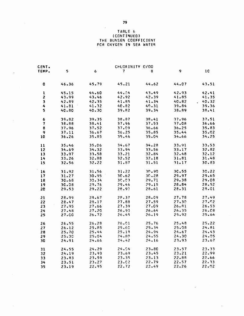
TABLE 6(CONTINUED)

THE BUNSEN COEFFICIENTFCR OXYGEN IN SEA WATER

CENT. CHLORINITY 0/00TEMP. 5 6 7 8 9 1c

0 46.36 45.79 45.21 44.62 44.07 43.51

1 45.15 44.60 44.04 43.49 42.93 42.412 43.99 43.46 42.92 42.39 41.85 41.353 42.89 42.35 41.85 41.34 40.82 40.324 41.81 41.32 40.82 40.31 39.84 39.365 40.80 40.30 39.82 39.34 38.89 38.41

6 39.82 39.35 38.87 38.41 37.96 37.517 38.88 38.41 37.96 37.53 37.08 36.668 37.96 37.52 37.09 36.66 36.25 35.839 37.11 36.67 36.25 35.85 35.44 35.02

10 36.26 35.85 35.46 35.04 34.66 34.25

11 35.46 35.06 34.67 34.28 33.91 33.5312 34.69 34.32 33.94 33.56 33.17 32.8213 33.97 33.58 33.21 32.84 32.48 32.1214 33.26 32.88 32.52 32.18 31.81 31.4815 32.56 32.22 31.87 31.51 31.17 30.83

16 31.92 31.56 31.22 30.90 3C.55 30.2217 31.27 30.95 30.62 3C.28 29.97 29.6518 30.68 30.34 3C.03 29.71 29.38 29.0819 30.08 29.76 29.46 29.15 28.84 28.5220 29.53 29.22 28.90 28.61 28.31 28.01

21 28.99 28.67 28.37 28.09 27.78 27.4922 28.47 28.17 27.88 27.59 27.30 27.n223 27.95 27.66 27.39 27.09 26.81 26.5324 27.48 27.20 26.90 26.64 26.35 26.C825 27.00 26.72 26.45 26.19 25.92 25.64

26 26.55 26.28 26.01 25.76 25.48 25.2227 26.12 25.85 25.60 25.34 25.08 24.8128 25.70 25.44 25.18 24.94 24.67 24.4329 25.30 25.04 24.80 24.55 24.30 24.0530 24.91 24.66 24.42 24.16 23.93 23.67

31 24.55 24.29 24.04 23.80 23.57 23.3332 24.19 23.93 23.69 23.45 23.21 22.9933 23.83 23,59 23.35 23.13 22.88 22.6634 23.51 23.27 23.0C2 22.79 22.57 22.3335 23.19 22.95 22.72 22.49 22.26 22.02

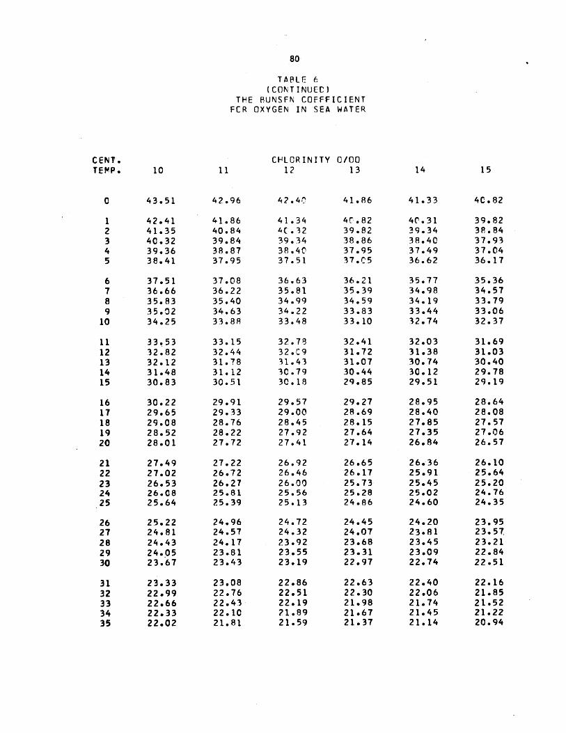
TABLE 6(CONTINUEO)

THE BUNSFN COFFFICIENTFCR OXYGEN IN SEA WATER

CENT. CHLORINITY 0/00TEMP. 10 11 12 13 14 15

0 43.51 42.96 42.40 41.86 41.33 40.82

1 42.41 41.86 41.34 4C.82 40.31 39.822 41.35 40.84 4C.32 39.82 39.34 38.843 40.32 39.84 39.34 38.86 38.40 37.934 39.36 38.87 38.40 37.95 37.49 37.045 38.41 37.95 37.51 37.C5 36.62 36.17

6 37.51 37.08 36.63 36.21 35.77 35.367 36.66 36.22 35.81 35.39 34.98 34.578 35.83 35.40 34.99 34.59 34.19 33.799 35.02 34.63 34.22 33.83 33.44 33.06

10 34.25 33.88 33.48 33.10 32.74 32.37

11 33.53 33.15 32.78 32.41 32.03 31.6912 32.82 32.44 32.C9 31.72 31.38 31.0313 32.12 31.78 31.43 31.07 30.74 30.4014 31.48 31.12 30.79 30.44 30.12 29.7815 30.83 30.51 30.18 29.85 29.51 29.19

16 30.22 29.91 29.57 29.27 28.95 28.6417 29.65 29.33 29.00 28.69 28.40 28.0818 29.08 28.76 28.45 28.15 27.85 27.5719 28.52 28.22 27.92 27.64 27.35 27.0620 28.01 27.72 27.41 27.14 26.84 26.57

21 27.49 27.22 26.92 26.65 26.36 26.1022 27.02 26.72 26.46 26.17 25.91 25.6423 26.53 26.27 26.00 25.73 25.45 25.2024 26.08 25.81 25.56 25.28 25.02 24.7625 25.64 25.39 25.13 24.86 24.60 24.35

26 25.22 24.96 24.72 24.45 24.20 23.9527 24.81 24.57 24.32 24.07 23.81 23.5728 24.43 24.17 23.92 23.68 23.45 23.2129 24.05 23.81 23.55 23.31 23.09 22.8430 23.67 23.43 23.19 22.97 22.74 22.51

31 23.33 23.08 22.86 22.63 22.40 22.16

32 22.99 22.76 22.51 22.30 22.06 21.8533 22.66 22.43 22.19 21.98 21.74 21.5234 22.33 22.10 21.89 21.67 21.45 21.2235 22.02 21.81 21.59 21.37 21.14 20.94

---~~~-~~~--~--

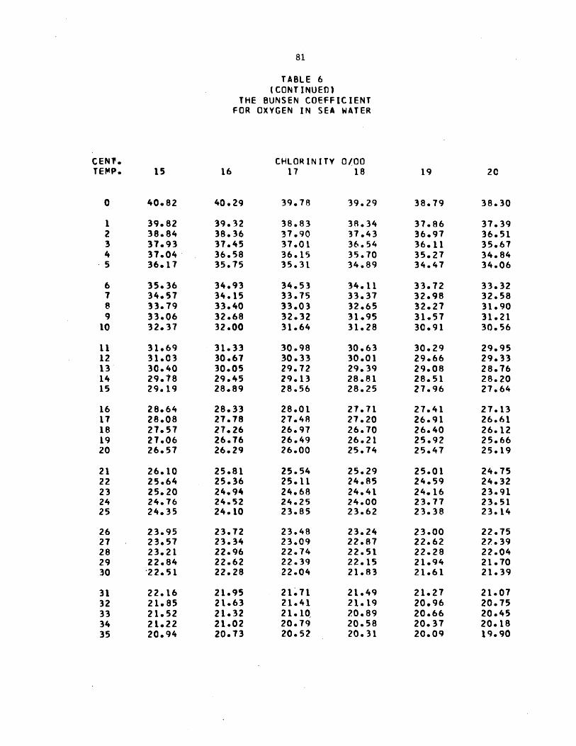
TABLE 6(CONTINUED)

THE BUNSEN COEFFICIENTFOR OXYGEN IN SEA WATER

CENT. CHLORINITY 0/00TEMP. 15 16 17 18 19 20

0 40.82 40.29 39.78 39.29 38.79 38.30

1 39.82 39.32 38.83 38.34 37.86 37.392 38.84 38.36 37.90 37.43 36.97 36.513 37.93 37.45 37.01 36.54 36.11 35.674 37.04 36.58 36.15 35.70 35.27 34.845 36.17 35.75 35.31 34.89 34.47 34.06

6 35.36 34.93 34.53 34.11 33.72 33.327 34.57 34.15 33.75 33.37 32.98 32.588 33.79 33.40 33.03 32.65 32.27 31.909 33.06 32.68 32.32 31.95 31.57 31.21

10 32.37 32.00 31.64 31.28 30.91 30.56

11 31.69 31.33 30.98 30.63 30.29 29.9512 31.03 30.67 30.33 30.01 29.66 29.3313 30.40 30.05 29.72 29.39 29.08 28.7614 29.78 29.45 29.13 28.81 28.51 28.2015 29.19 28.89 28.56 28.25 27.96 27.64

16 28.64 28.33 28.01 27.71 27.41 27.1317 28.08 27.78 27.48 27.20 26.91 26.6118 27.57 27.26 26.97 26.70 26.40 26.1219 27.06 26.76 26.49 26.21 25.92 25.6620 26.57 26.29 26.00 25.74 25.47 25.19

21 26.10 25.81 25.54 25.29 25.01 24.7522 25.64 25.36 25.11 24.85 24.59 24.3223 25.20 24.94 24.68 24.41 24.16 23.9124 24.76 24.52 24.25 24.00 23.77 23.5125 24.35 24.10 23.85 23.62 23.38 23.14

26 23.95 23.72 23.48 23.24 23.00 22.7527 23.57 23.34 23.09 22.87 22.62 22.3928 23.21 22.96 22.74 22.51 22.28 22.0429 22.84 22.62 22.39 22.15 21.94 21.7030 22.51 22.28 22.04 21.83 21.61 21.39

31 22.16 21.95 21.71 21.49 21.27 21.0732 21.85 21.63 21.41 21.19 20.96 20.7533 21.52 21.32 21.10 20.89 20.66 20.4534 21.22 21.02 20.79 20.58 20.37 20.1835 20.94 20.73 20.52 20.31 20.09 19.90

~_

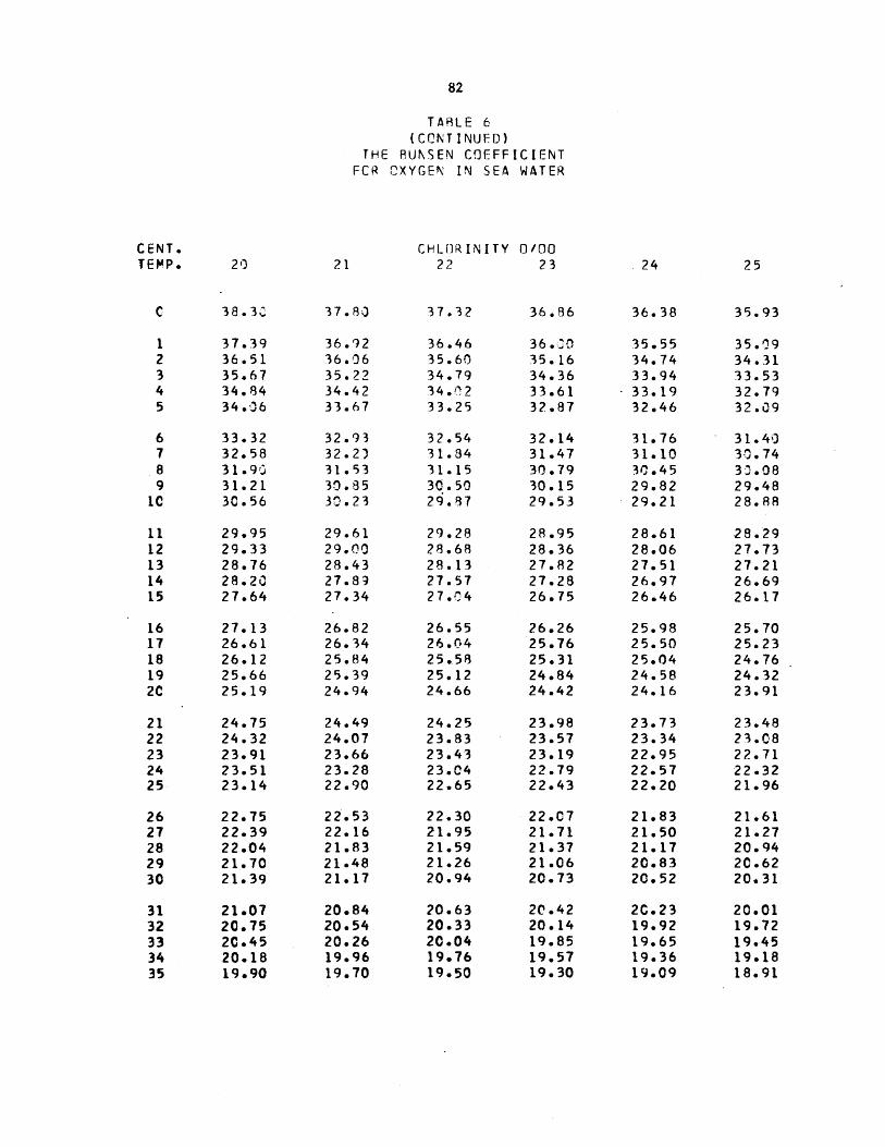
TABLE 6(CONTINUED)

THE RUNSEN COEFFICIENTFCR OXYGEN IN SEA WATER

CENT. CHLORINITY 0/00TEMP. 20 21 22 23 24 25

C 38.3% 37.80 37.32 36.86 36.38 35.93

1 37.39 36.92 36.46 36.0 35.55 35.092 36.51 36.06 35.60 35.16 34.74 34.313 35.67 35.22 34.79 34.36 33.94 33.534 34.84 34.42 34.02 33.61 33.19 32.795 34.06 33.67 33.25 32.87 32.46 32.09

6 33.32 32.93 32.54 32.14 31.76 31.407 32.58 32.2) 31.84 31.47 31.10 30.748 31.93 31.53 31.15 30.79 30.45 30.089 31.21 30.85 30.50 30.15 29.82 29.48

I0 30,.56 30.23 29.87 29.53 29.21 28.88

11 29.95 29.61 29.28 28.95 28.61 28.2912 29.33 29.00 28.68 28.36 28.06 27.7313 28.76 28.43 28.13 27.82 27.51 27.2114 28.20 27.89 27.57 27.28 26.97 26.6915 27.64 27.34 27.04 26.75 26.46 26.17

16 27.13 26.82 26.55 26.26 25.98 25.7017 26.61 26.34 26.04 25.76 25.50 25.2318 26.12 25.84 25.58 25.31 25.04 24.7619 25.66 25.39 25.12 24.84 24.58 24.322C 25.19 24.94 24.66 24.42 24.16 23.91

21 24.75 24.49 24.25 23.98 23.73 23.4822 24.32 24.07 23.83 23.57 23.34 23.C823 23.91 23.66 23.43 23.19 22.95 22.7124 23.51 23.28 23.04 22.79 22.57 22.3225 23.14 22.90 22.65 22.43 22.20 21.96

26 22.75 22.53 22.30 22.07 21.83 21.6127 22.39 22.16 21.95 21.71 21.50 21.2728 22.04 21.83 21.59 21.37 21.17 20.9429 21.70 21.48 21.26 21.06 20.83 20.6230 21.39 21.17 20.94 20.73 20.52 20.31

31 21.07 20.84 20.63 20,.42 20.23 20.0132 20.75 20.54 20.33 20.14 19.92 19.7233 2C.45 20.26 20.04 19.85 19.65 19.4534 20.18 19.96 19.76 19.57 19.36 19.1835 19.90 19.70 19.50 19.30 19.09 18.91

__ I-"~I---~ ~~_.___.L__ __L_____s__ll____~~....... .

TABLE 6(CONT INUED)

THE BUNSEN COEFFICIENTFOR OXYGEN IN SEA WATER

CENT. CHLORINITY 0/00TEMP. 25 26 27 28 29 30

C 35.93 35.46 35.01 34.57 34.13 33.71

1 35.09 34.65 34.23 33.79 33.38 32.952 34.31 33.87 33.45 33.04 32.63 32.243 33.53 33.12 32.73 32.33 31.92 31.534 32.79 32.39 32.00 31.63 31.23 30.875 32.09 31.69 31.33 30.94 30.57 30.22

6 31.40 31.C3 30.65 30.30 29.93 29.597 30.74 30.38 30.01 29.66 29.31 28.978 30.08 29.75 29.39 29.05 28.73 28.389 29.48 29.14 28.81 28.48 28.15 27.83

10 28.88 28.54 28.23 27.91 27.58 27.28

11 28.29 27.97 27.67 27.36 27.04 26.7512 27.73 27.44 27.12 26.83 26.53 26.2213 27.21 26.91 26.61 26.32 26.03 25.7414 26.69 26.38 26.99 25.82 25.54 25.2615 26.17 25.90 25.62 25.34 25.05 24.78

16 25.70 25.42 25.15 24.86 24.61 24.3317 25.23 24.96 24.69 24.41 24.15 23.8918 24.76 24.51 24.25 23.99 23.72 23.4719 24.32 24.06 23.82 23.57 23.32 23.0620 23.91 23.64 23.41 23.16 22.92 22.68

21 23.48 23.25 22.99 22.75 22.53 22.2822 23.08 22.84 22.62 22.37 22.15 21.9223 22.71 22.46 22.24 22.01 21.77 21.5624 22.32 22.09 21.88 21.65 21.43 21.2125 21.96 21.75 21.51 21.29 21.07 20.87

26 21.61 21.40 21.18 20.95 21.75 20.5427 21.27 21.V5 20.85 20.62 20.41 20.2228 20.94 20.74 20.53 20.32 20.11 19.8929 20.62 20.41 20.20 20.01 19.79 19.5930 20.31 2,.12 19.90 19.71 19.51 19.30

31 20.01 19.82 19.62 19.42 19.21 19.0332 19.72 19.52 19.32 19.14 18.93 18.7433 19.45 19.24 19.06 18.85 18.66 18.4734 19.18 18.97 18.79 18.60 18.41 18.2135 18.91 18.72 18.53 18.33 18.14 17.96

L _ _~ _______~~______ _~ _~___~____________~__ ------ru~~.~~ ~--~--ryi.-

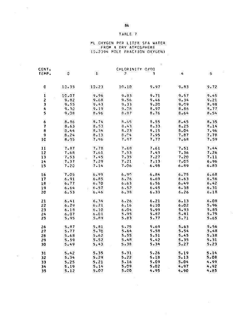
TARLE 7

ML OXYGEN PER LITER SEA WATERFROM A DRY ATMOSPHERE

(0.2394 MOLE FRACTION OXYGEN)

CENT.TEMP.

CHLORINITY 0/00? 3

10.35

10.079.829.559.309.08

8.868.638.448.248.05

7.877.687.537.377.20

1

10.23

9.969.689.439.198.96

8.748.538.348.137.96

7.787.617.457.297.14

6.996.856.706.576.46

6.346.216.106.015.89

5.815.705.625.525.43

5.355.295.215.145.07

10.10

9.839.569.339.088.87

8.658.438.238 ."47.87

7.687.537.357.217.06

6.906.766.636.526.38

6.266.166.045.955.83

5.755.645.555.485.38

5.315.225.165.095.00

9.97

9.719.469.208.978.76

8.558.338.157.957.77

7.617.437.277.136.98

6.846.696.566.456.33

6.216.105.995.875.77

5.695.585.515.425.34

5.265.185.095.024.95

7.056.916.776.646.53

6.416.296.186.075.95

5.875.775.685.595.49

5.425.345.255.195.12

9.83

9.579.349.098.868.64

e.458.258.047.877.68

7.517.367.207.056.89

6.756.636.496.386.26

6.136.025.935.815.71

5.635.545.455.355.27

5.195.135.044.974.90

9.72

9.459.218.988.778.54

8.358.147.967.787.59

7.447.267.116.966.83

6.686.566.426.316.18

6.085.965.855.755.65

5.565.485.385.315.23

5.145.084.994.924.85

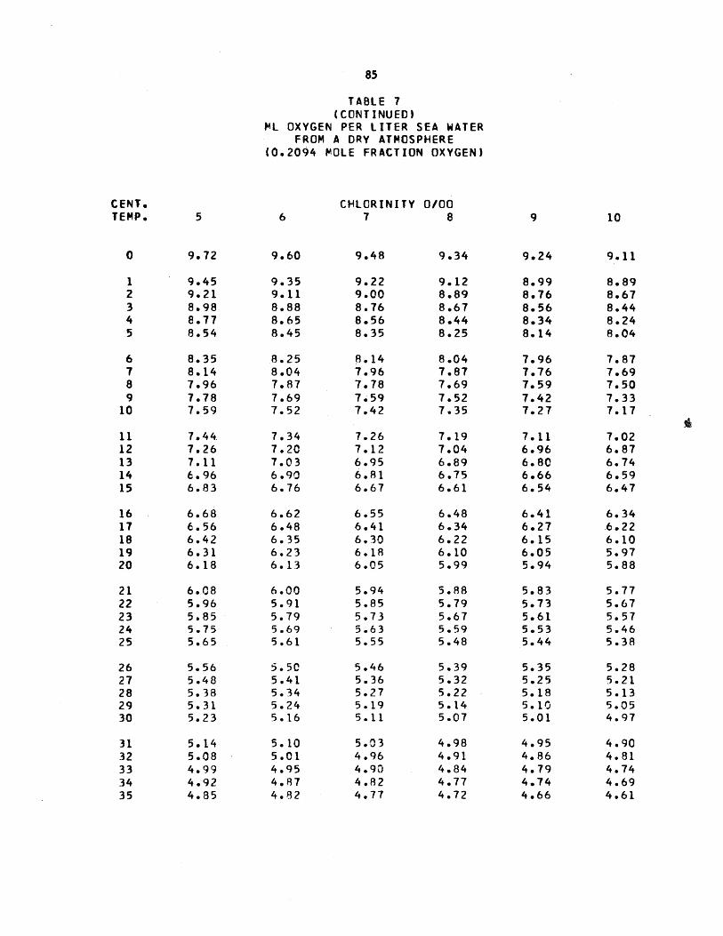
TABLE 7(CONTINUED)

ML OXYGEN PER LITER SEA WATERFROM A DRY ATMOSPHERE

(0.2094 POLE FRACTION OXYGEN)

CENT. CHLORINITY 0/00TEMP. 5 6 7 8 9 10

0 9.72 9.60 9.48 9.34 9.24 9.11

1 9.45 9.35 9.22 9.12 8.99 8.892 9.21 9.11 9.00 8.89 8.76 8.673 8.98 8.88 8.76 8.67 8.56 8.444 8.77 8.65 8.56 8.44 8.34 8.245 8.54 8.45 8.35 8.25 8.14 8.04

6 8.35 8.25 8.14 8.04 7.96 7.877 8.14 8.04 7.96 7.87 7.76 7.698 7.96 7.87 7.78 7.69 7.59 7.509 7.78 7.69 7.59 7.52 7.42 7.33

10 7.59 7.52 7.42 7.35 7.27 7.17

11 7.44 7.34 7.26 7.19 7.11 7.0212 7.26 7.20 7.12 7.04 6.96 6.8713 7.11 7.03 6.95 6.89 6.80 6.7414 6.96 6.90 6.81 6.75 6.66 6.5915 6.83 6.76 6.67 6.61 6.54 6.47

16 6.68 6.62 6.55 6.48 6.41 6.3417 6.56 6.48 6.41 6.34 6.27 6.2218 6.42 6.35 6.30 6.22 6.15 6.1019 6.31 6.23 6.18 6.10 6.05 5.9720 6.18 6.13 6.05 5.99 5.94 5.88

21 6.08 6.00 5.94 5.88 5.83 5.7722 5.96 5.91 5.85 5.79 5.73 5.6723 5.85 5.79 5.73 5.67 5.61 5.5724 5.75 5.69 5.63 5.59 5.53 5.4625 5.65 5.61 5.55 5.48 5.44 5.38

26 5.56 5.50 5.46 5.39 5.35 5.2827 5.48 5.41 5.36 5.32 5.25 5.2128 5.38 5.34 5.27 5.22 5.18 5.1329 5.31 5.24 5.19 5.14 5.10 5.0530 5.23 5.16 5.11 5.07 5.01 4.97

31 5.14 5.10 5.03 4.98 4.95 4.9032 5.08 5.01 4.96 4.91 4.86 4.8133 4.99 4.95 4.90 4.84 4.79 4.7434 4.92 4,87 4.82 4.77 4.74 4.6935 4.85 4.82 4.77 4.72 4.66 4.61

TABLE 7(CONT INUED)

NL r)XYGEN PER LITER SEA WATERFROM A ORY ATMCSPHERE

('.2C94 POLE FRACTION OXYGEN)

CENT. CHLORINITY 0/00TEMP. 10 11 12 13 14 15

0 9.11 9.01 1.89 8.78 8.67 8.56

1 8.89 8.78 8.67 8.56 8.44 8.352 8.67 8.55 8.44 8.35 8.25 8.133 8.44 8.34 9.25 8.15 8.04 7.944 8.24 8.15 8.04 7.96 7.85 7.775 8.04 7.96 7.85 7.77 7.68 7.57

6 7.87 7.76 7.67 7.58 7.49 7.407 7.69 7.58 7.51 7.41 7.32 7.258 7.50 7.41 7.34 7.24 7.17 7.099 7.33 7.25 7.18 7.08 7.00 6.92

1C 7.17 7.09 7.01 6.93 6.85 6.79

11 7.02 6.94 6.86 6.80 6.72 6.6312 6.87 6.79 6.73 6.64 6.57 6.5113 6.74 6.65 6.59 6.52 6.45 6.3814 6.59 6.53 6.46 6.37 6.32 6.2515 6.47 6.40 6.33 6.25 6.18 6.11

16 6.34 6.26 6.19 6.14 6.06 6.0117 6.22 6.14 6.C7 6.02 5.96 5.8818 6.10 6.02 5.97 5.91 5.83 5.7719 5.97 5.92 5.86 5.80 5.74 5.682C 5.88 5.80 5.74 5.68 5.62 5.56

21 5.77 5.71 5.65 5.58 5.52 5.4622 5.67 5.61 5.55 5.48 5.44 5.3823 5.57 5.50 5.44 5.40 5.34 5.2924 5.46 5.40 5.35 5.29 5.25 5.2025 5.38 5.33 5.26 5.22 5.15 5.11

26 5.28 5.24 5.19 5.12 5.08 5.0327 5.21 5.14 5.^9 5.04 5.00 4.9528 5.13 5.06 5.02 4.97 4.91 4.8629 5.05 4.98 4.93 4.88 4.83 4.7830 4.97 4.92 4.87 4.82 4.76 4.71

31 4.90 4.83 4.80 4.75 4.69 4.6432 4.81 4.76 4.71 4.68 4.63 4.5733 4.74 4.71 4.66 4.60 4.55 4.5234 4.69 4.64 4.58 4.55 4.49 4.4435 4.61 4.58 4.52 4.47 4.44 4.38

0 a - .- .-

TABLE 7(CONTINUED)

ML OXYGEN PER LITER SEA WATERFROM A DRY ATMOSPHERE

(0.2094 MOLE FRACTION OXYGEN)

CENT. CHLORINITY 0/00TEMP. 15 16 17 18 19 20

0 8.56 8.45 8.33 8.24 8.12 8.03

1 8.35 8.23 8.13 8.C4 7.94 7.842 8.13 8.03 7.95 7.85 7.74 7.663 7.94 7.84 7.76 7.65 7.56 7.484 7.77 7.67 7.58 7.49 7.40 7.315 7.57 7.50 7.39 7.32 7.23 7.13

6 7.40 7.31 7.23 7.14 7.06 6.997 7.25 7.15 7.08 7.)0 6.92 6.828 7.C9 6.99 6.93 6.85 6,77 6.699 6.92 6.84 6.78 6.69 6.61 6.55

10 6.79 6.70 6.62 6.56 6.47 6.41

11 6.63 6.56 6.50 6.41 6.34 6.2712 6.51 6.42 6.35 6.28 6.21 6.1413 6.38 6.29 6.22 6.15 6.10 6.0214 6.25 6.18 6.10 6.03 5.98 5.9015 6.11 6.06 5.98 5.93 5.85 5.80

16 6.01 5.93 5.88 5.80 5.74 5.6817 5.88 5.83 5.77 5.71 5.63 5.5718 5.77 5.72 5.66 5.59 5.54 5.4819 5.68 5.60 5.56 5.50 5.44 5.3720 5.56 5.52 5.46 5.40 5.33 5.29

21 5.46 5.42 5.36 5.29 5.25 5.1822 5.38 5.31 5.27 5.20 5.16 5.0923 5.29 5.22 5.18 5.11 5.07 5.0224 5.20 5.13 5.09 5.04 4.99 4.9225 5.11 5.06 4.99 4.96 4.89 4.84

26 5.03 4.98 4.93 4.88 4.83 4.7627 4.95 4.90 4.85 4.80 4.75 4.7028 4.86 4.82 4.76 4.71 4.68 4.6329 4.78 4.75 4.70 4.65 4.59 4.5430 4.71 4.66 4.63 4.57 4.52 4.49

31 4.64 4.61 4.56 4.50 4.45 4.4132 4.57 4.54 4.48 4.45 4.40 4.3633 4.52 4.46 4.43 4.37 4.34 4.2834 4.44 4.40 4.35 4.32 4.28 4.2435 4.38 4.34 4.31 4.25 4.22 4.18

____~_.._... ______~_ ______~ ~e;

TABLE 7(CONTINUED)

PL OXYGEN PER LITER SEA WATERFROM A DRY ATMOSPHERE

(0.2094 MOLE FRACTION OXYGEN)

CENT. CHLORINITY 0100TEMP. 20 21 22 23 24 25

0 8.03 7.93 7.83 7.73 7.63 7.52

1 7.84 7.73 7.63 7.55 7.44 7.362 7.66 7.55 7.47 7.36 7.27 7.183 7.48 7.39 7.30 7.21 7.12 7.024 7.31 7.22 7.12 7.05 6.95 6.885 7.13 7.06 6.96 6.88 6.81 6.73

6 6.99 6.89 6.81 6.73 6.65 6.577 6.82 6.74 6.68 6.60 6.51 6.458 6.69 6.60 6.52 6.46 6.39 6.319 6.5 5 6.46 6.40 6.31 6.24 6.1710 6.41 6.34 6.27 6.18 6.13 6.06

11 6.27 6.20 6.13 6.06 5.99 5.9212 6.14 6.07 6.02 5.95 5.89 5.8213 6.02 5.95 5.90 5.82 5.76 5.7114 5.90 5.85 5.77 5.71 5.66 5.6015 5.80 5.74 5.66 5.60 5.54 5.48

16 5.68 5.63 5.57 5.51 5.45 5.3817 5.57 5.51 5.45 5.41 5.35 5.2818 5.48 5.41 5.37 5.31 5.24 5.1819 5.37 5.33 5.27 5.20 5.16 5.0920 5.29 5.22 5.16 5.11 5.07 5.02

21 5.18 5.14 5.09 5.02 4.98 4.9322 5.09 5.04 5.00 4.95 4.90 4.8323 5.02 4.97 4.92 4.85 4.80 4.7524 4.92 .4.87 4.82 4.77 4.74 4.6725 4.84 4.79 4.74 4.71 4.66 4.61

26 4.76 4.73 4.68 4.62 4.57 4.5427 4.70 4.64 4.61 4.56 4.50 4.4528 4.63 4.57 4.52 4.49 4.43 4.3829 4.54 4.51 4.45 4.42 4.36 4.3330 4.49 4.43 4.40 4.34 4.31 4.25

31 4.41 4.36 4.32 4.29 4.25 4.1932 4.36 4.30 4.27 4.23 4.17 4.1433 4.28 4.24 4.21 4.17 4.11 4.0734 4.24 4.,18 4.15 4.11 4.05 4.0335 4.18 4.12 4.08 4.04 4.01 3.97

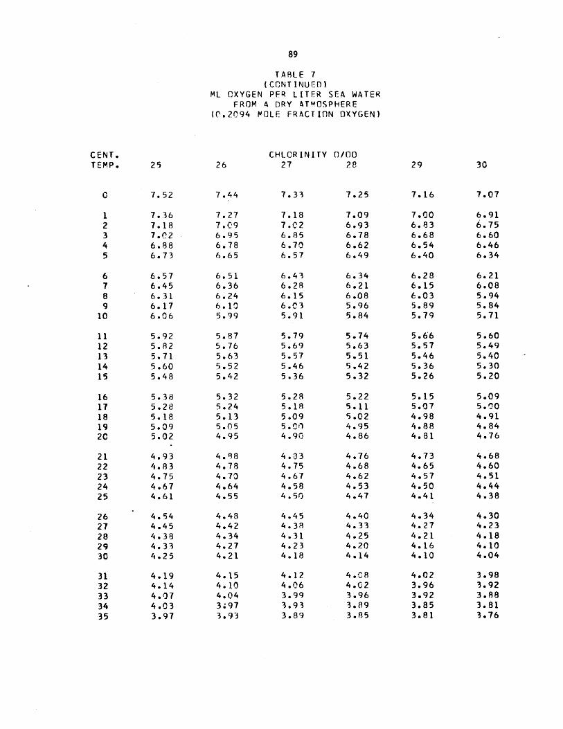
TABLE 7(CONTINUED)

ML OXYGEN PER LITER SEA WATERFROM A DRY ATMOSPHERE

(0.2094 MOLE FRACTION OXYGEN)

CENT. CHLCRINITY 0/00TEMP. 25 26 27 28 29 30

0 7.52 7.44 7.33 7.25 7.16 7.07

1 7.36 7.27 7.18 7.09 7.00 6.912 7.18 7.C9 7.02 6.93 6.83 6.753 7.02 6.95 6.85 6.78 6.68 6.604 6.88 6.78 6.70 6.62 6.54 6.465 6.73 6.65 6.57 6.49 6.40 6.34

6 6.57 6.51 6.43 6.34 6.28 6.217 6.45 6.36 6.28 6.21 6.15 6.088 6.31 6.24 6.15 6.08 6.03 5.949 6.17 6.10 6.03 5.96 5.89 5.84

10 6.06 5.99 5.91 5.84 5.79 5.71

11 5.92 5.87 5.79 5.74 5.66 5.6012 5.82 5.76 5.69 5.63 5.57 5.4913 5.71 5.63 5.57 5.51 5.46 5.4014 5.60 5.52 5.46 5.42 5.36 5.3015 5.48 5.42 5.36 5.32 5.26 5.20

16 5.38 5.32 5.28 5.22 5.15 5.0917 5.28 5.24 5.18 5.11 5.07 5.0018 5.18 5.13 5.09 5.02 4.98 4.9119 5.09 5.05 5.010 4.95 4.88 4.8420 5.02 4.95 4.90 4.86 4.81 4.76

21 4.93 4.88 4.33 4.76 4.73 4.6822 4.83 4.78 4.75 4.68 4.65 4.6023 4.75 4.70 4.67 4.62 4.57 4.5124 4.67 4.64 4.58 4.53 4.50 4.4425 4.61 4.55 4.50 4.47 4.41 4.38

26 4.54 4.48 4.45 4.40 4.34 4.3027 4.45 4.42 4.38 4.33 4.27 4.2328 4.38 4.34 4.31 4.25 4.21 4.1829 4.33 4.27 4.23 4.20 4.16 4.1030 4.25 4.21 4.18 4.14 4.10 4.04

31 4.19 4.15 4.12 4.08 4.02 3.9832 4.14 4.10 4.06 4.02 3.96 3.92

33 4.07 4.04 3.99 3.96 3.92 3.88

34 4.03 3;97 3.93 3.89 3.85 3.81

35 3.97 3.93 3.89 3.85 3.81 3.76

90

REFERENCES: PART I

Adeney W. E. and Becker H. G. (1919) Phil. Mag., 38, 317.

Angstrom K. (1882) Wied. Ann., 15, 297.

Arons A. B. and Kientzler C. F. (1954) Trans. Am. Geophys. Un., 35(, 722-728.

Awtrey A. D. and Connick R. E. (1951) J. Am. Chem. Soc., 73, 1341.

Barkley R. A. and Thompson T. G. (1960) De__ Sea Res., 7, 24-34.

Benson B. B. and Parker P. D. M. (1961) J. Phys. Chem., 65, 1489-1496.

Bohr C. and Boch J. (1891) Weid. Ann., 44, 316.

Bradbury J. H. and Hambly A. N. (1952) Aus. J. Scientif. Res., AS, 541-554.

Bray W. C. and Connolly E. L. (1911) J. Am. Chem. Soc., :33, 1485.

Bunsen R. (1857) Gasometrische Methoden. von Friedrich und Sohn, Braunschweig.

Carpenter J. H. (1965) Limno. and Oceanog. In press.

Carritt D. E. (1965) Nat'l. Acad. Scie.-Nat'l.Res. Council, Committee onOceanography Report. In Press.

Dittmar W. (1884) Challenger Reports, Vol 1, Physics and Chemistry.

Douglas E. (1964) J. Phys. Chem., 68, 169-174.

Elmore H. L. and Hayes T. W. (1960) Proc. Am. Soc. Civil Eng., 86(SA4), 2556,

41-53.

Forsythe W. E. (1956) Editor: Smithsonian Physical Tables. Publ. SmithsonianInst., Washington, D. C.

Fox C. J. J. (1909) Trans. Far. Soc., 5, 68-87.

Fox C. J. J. (1907) Conseil. Perm. Internat. p. 1'Explor. de la Mer, Pub. de

Circonstance, No. 41.

Furth A. (1922) Zeit. Electrochem., 28, 57.

Gilbert G. A. and Marriott J. V. R. (1948) Trans. Far. Soc., 44, 84.

Jacobsen J. P. (1905) Meddelelser fra Kommissionen for Havundersogelser, Serie,Hydrografi, Bd. 1, No. 8. Copenhagen.

91

Klots C. E. and Benson B. B. (1963a) Jour. 1Mar. Res., 21, 48-54.

Klots C. E. and Benson B. B. (1963b) J. Phys. Chem., 67, 933-934.

Knowles G. and Lowden G. F. (1953) Analyst, 78, 159-164.

Kolthoff I. M. and Sandell E. B. (1943) Textbook of Ouantitative InorganicAPnalysis, Macmillan Co., New York.

Krummel 0. (1907) lHandbuch der Ozeanya~hie Bd. 1i Die raumlich chemischenund physikalischen Verhaltnisse des Meeres. J. Engelhorn, Stutgart.

List R. J. (1963) Editor: Smithsonian Meteorological Tables. Publ. SmithsonianInst., Washington, D. C.

McCoubrey J. C. (1955) Trans. Far. Soc., 51, 743.

Morris J. C. et al. (1961) Proc. Am. Soc. Civil Eng., 85 (SAl), 81-86.

Mortimer C. H. (1956) Internat. Assoc. of Theor. and Appl,. Limno. Communications,No. 6.

Paquette R. G. (1959) Natl. Acad. Sci.-Natl. Res. Council, Committee on Oceano-graphyReport, Publ. 600.

Redfield A. C. (1942) Papers Physic. Oceano . Meteorol., 9(2), 1-22.

Richards F. A. (1957) Physics and Chemis try of the Earth, Vol. 2, ed. L. H.Ahrens et al. Pergamon Press.

Roescoe A. E. and Lunt J. (1889) J. Chem. Soc., 55, 532.

Seiwell H. R. (1937) Nature, 140, 506-507.

Steen H. (1955) Limno. and Oceanog., 3, 423-426.

Thompson T. G. and Robinson R. J. (1939) Jour. Mar. Res., 2, 1.

Truesdale G. A., et al. (1955) J. Appl. Chem., 5, 53-62.

Weast R. C. (1962) Handbook of Chemistry and Physics, Chemical Rubber Publ.Co., Cleveland, Ohio.

Winkler L. W. (1888) Ber. Deutch Chem. Ges., 21, 2843-2854.

Winkler L. W. (1891) Ber. Deutch Chem. Ges., 24, 3602-3610.

PART II

THE SALTING-OUT EFFECT IN THE TERNARY SYSTEM:

OXYGEN-WATER-SEA SALT

PART 11

THE SALTING-OUT EFFECT IN THE TERNARY SYSTEM:

OXYGEN-WATER-SEA SALT

ABSTRACT

Measurements of the solubility of oxygen in sea salt solutions show

that, contrary to the assumptions of previous workers, the solubility declines

exponentially according to the empirical SETSCHENOW (1875) relation rather

than linearly with increasing salt concentration.

Salting-out theories are reviewed and it is seen that the simple

hydration theory predicts a linear relation. Although the DEBYE (1925) theory

predicts an exponential dependence it is seen to predict an unsatisfactory

temperature dependence. The experimental data of this work, as well as of

a number of other published studies, reveal that, in contrast to the effect

predicted by the DEBYE theory, the salting-out decreases with increasing tem-

perature.

The activity coefficient of oxygen in sea salt solutions is shown to

be simply related to the salting-out coefficient. A quasi-lattice model of

a regular solution is developed from which the exponential salting-out relation-

ship is derived. The derived relationship has a temperature dependence of the

same order as that experimentally observed.

The model and experimental observations are shown to be consistent

with FRANK'S "iceberg" concept of aqueous solution of gases and the role of

sea salt is seen to be "iceberg breaking".

95

INTRODUCTION

During the course of the redetermination of the solubility of oxygen

in sea water it became pertinent to inquire whether the linear dependence of

the solubility on the sea water chlorinity previously assumed did in fact

hold true over the chlorinity range of interest. If the chlorinity dependence

may be characterized by some simple mathematical relation, the task of deter-

mining the solubility surface is greatly eased and the number of observations

needed to adequately determine the surface is greatly reduced.

The change in the solubility of non-electrolytes upon the addition

of an electrolyte has been the subject of physical chemical inquiry since the

turn of the century. Early investigations were made by EULER (1899, 1904),

ROTHMUND (1900) and HOFFMAN (1905). Usually the addition of a salt results

in a decrease in the solubility of a non-electrolyte and this phenomenon has

been termed the salting-out effect. In the rare cases when an increase has

been observed it is known as salting-in.

While most work has been concerned with the solubility of organic

solids and liquids, investigations of the salting-out of the inert -ases have

been conducted by STEINER (1894), GORDON (1895), ROTIH (1897), BRAUN (1900),

KNOPP (1904) and HUFNER (1907). There seems to be no theoretical or experimen-

tal reason for distinguishing the salting-out behavior of non-electrolytes on

the basis of the phase (solid, liquid, or gas) with which they are in equili-

brium. Consequently, we shall consider the salting-out of non-electrolytes

in general.

96

REVIEW OF SALTING-OUT THEORIES

A number of equations have been proposed to express the relation be-

tween the change in the solubility of the non-electrolyte and the salt concen-

tration. For purposes of this discussion we shall define a solubility ratio:

_(t,c) -(29)t o (29)

where a0 is the solubility coefficient of the non-electrolyte in pure solvent

and a is its solubility coefficient in salt solution of concentration C. 3

will in general also depend upon the temperature t.

One of the earliest empirical salting-out relations proposed by

GORDON (1895) was

; = 1-k(t)C2 / 3 (30)

reflecting the fact that the addition of equal increments of salt had less

effect the more were added. This relation has the unfortunate aspect of giving

an infinite slope as the salt becomes infinitely dilute. As we shall see, all

the theories proposed require, and experimental evidence indicates, that the

limiting law has a finite slope.

Another relation proposed as early as 1875 by SETSCHENOW was

logF = -k(t)C (31)

This relation also had no theoretical basis, but it was found to well represent

salting-out over an extended salt concentration range and it has been employed

by ALBRIGHT (1937) and ALBRIGHT and WILLIAMS (1937). ROTIMUND expanded SETSCHENOW'S

relation in series and, dropping all but the first power term, obtained for

dilute solutions

8 = l-k(t)C (32)

Early theoretical explanations included the work of EULER (1899) and

97

GEFFCKEN (1904) who related the salting-out effect to the increase in internal

pressure of the solution due to electrolyte volume. In 1907 PHILIP, following

a suggestion of LOWRY (1905), attempted to place the salting-out effect on a

theoretical basis with reference to the hydration theory. This has as its

basis the supposition that the intrinsic solubility of the non-electrolyte is

not changed by the addition of salt to the solvent. He supposed that part of

the solvent water which is bound to the salt in hydration is no longer free

to absorb the gas. Thus the apparent solubility based upon the amount of both

unbound and hydrated water decreases with addition of salt.

Let n be the number of water molecules bound to each salt "molecule"

in hydration. (We may suppose that n is the sum of the hydration numbers of

each ion formed per molecule in solution.) In the salt solution the fraction

of free water is equal to B if ao is the intrinsic solubility and a is the apparent

solubility.

18.02 x 10-3nC8 = 1 - 3 (33)P - IO-3MC

where C is the molal salt concentration, p ii the density of the solution and M

is the molecular weight of the salt. If the salt solution is fairly dilute

the denominator in equation (33) will be nearly unity as 10-3MC will represent

just the excess density of the solution over water. For dilute solutions

B = 1 - (18.02 x 10-3nC) (34)

where, as before, C is the molal salt concentration. Hydration numbers calcu-

lated by this relation from gas solubility measurements are in satisfactory

agreement with those estimated by studies of electrolyte conduction according

to GLASSTONE (1946). However, overemphasis should not be placed on this perhaps

fortuitous agreement.

98

This success of the hydration theory may have reassured FOX (1907)

that his observation of a linear salting-out dependence for oxygen in sea

water was valid. At any rate, FOX was led to represent his data in this way.

In 1955 TRUESDALE remeasured oxygen solubility in sea water and also used

the linear salting-out relation after seeking only minimal confirmation of

its applicability.

A major advance in the theory of salting-out was made in 1925 and

succeeding years when, following the spectacular success of the DEBYE-HUCKEL

theory of strong electrolytes, DEBYE (1925, 1927) and McAULAY (1926) followed

by BUTLER (1929) and BELTON (1937) were led to apply the electrostatic theory

to the problem.

In the DEBYE theory the electrolyte ions are considered as rigid

spheres in a continuous medium of solvent and non-electrolyte. As a result

of the electric field surrounding the charged ions, the medium of higher

dielectric constant is preferentially drawn near the ion and the medium with

the lower displaced. Thus the latter medium has a lower concentration in the

bulk liquid than it has in the first medium far from an ion. Generally the

non-electrolyte will have a lower dielectric constant that water, which will

result in salting-out. For the cases where the solvent has the lower dielec-

tric constant, salting-in will occur. In its simplest form the DEBYE theory

predicts

log a DT (35)DT

where P is the ionic strength of the electrolyte, D is the dielectric constant

of the solvent, T is the absolute temperature and A is a measure of the effect

of the solute non-electrolyte on the dielectric constant of the solvent.

To a first approximation A is independent of temperature and salt concentration.

99

The DEBYE theory has had experimental confirmation by ALBRIGHT and

WILLIAMS (1937) with data on ethyl acetate in aqueous solutions of alkali

metal halides. RANDALL and FAILEY (1927), however, find, "There seems to be

a qualitative agreement...in most cases but not a quantitative one." BOCKRIS

and EGAN (1948) find that the DEBYE theory quite inapplicable to benzoic acid

in ethanol- and dioxane-water solutions of NaCl. Furthermore, it has been

pointed out by MORRISON (1944, 1952, and 1955) that while the experimental

magnitude of log 8 is often in general agreement with theory, the temperature

dependence of this quantity is generally unsatisfactory. Equation (35) leads

to the conclusion that the fractional change in log 8 between temperatures

T2 and T1 would be independent of both the nature and concentration of the

electrolyte.

Log 82 - Log 8 1 D 1T 1 - D2 T2

Log B1 D2T2 (36)

The data for water show that the product DT decreases with temperature. There-

fore according to the DEBYE theory -log 8 should increase with temperature

at a rate of about 0.1% per degree C near room temperature. It should be

noted, however, that the DEBYE theory, like the DEBYE-HUCKEL theory, is valid

only in very dilute solution. Extensions and modifications of the theory

have been made by BARANOWSKI and SARNOWSKI (1958) and by SAMOILOV and TIKHOMIROV

(1962).

Recent contributions to the understanding of salting-out have been

made by NAKAJIMA (1953) whose theory presumes that the dissolved non-electro-

lyte is partitioned among four quasi-phases: pure solvent, hydrated cations,

hydrated anions and undissociated electrolyte. The theory gives a formula

which may be rearranged to yield

1,00

aC + bC3/21 + 0.707C /2 (37)

where a and b are constants which depend on the nature of the system. The

inclusion of the various powers of the salt concentration plus two adjustable

constants enable this equation to fit almost any data, but for this reason

it is difficult to test and not very useful in evaluating the data.

The hydration theory has been revived by EUCKEN and HERTZBERG (1950)

who find ion hydration numbers of about 10 from the salting-out of oxygen

from aqueous solution by alkali metal halides. McDEVIT and LONG (1952) have

reinvoked the useful concept of internal pressure in the employ of the salting-

out effect.

101

EXPERIMENTAL

The experimental procedure, which has been discussed in detail in

another section, involved the simultaneous saturation of distilled water and

sea salt solutions with air at atmospheric pressure. The solutions were equi-

librated concurrently in 12-liter rotating flasks immersed in a large thermo-

stat bath capable of holding the solutions to within a temperature range of

~0.010C.

When the solutions were saturated, the dissolved oxygen concentra-

tions were determined using a modification of the WINKLER method. The ratio

of the equivalent volume of titrant necessary to titrate the oxygen in the

salt solution to the corresponding volume for the distilled water gave the

solubility ratio, B, directly without requiring that either the partial pres-

sure of oxygen in the air or the exact titrant concentration be known.

A total of 53 determinations were made at temperatures ranging

from 0° to 350 C and at sea water chlorinities of from 6 to 30 o/oo. The re-

sults of these are shown in Table 2.

102

DISCUSSION OF RESULTS

FOX (1907) and TRUESDALE et al (1955), the only previous investiga-

tors of the solubility of oxygen in sea salt solutions, characterized the

salting-out relationship as depending linearly upon the chlorinity. As is

apparent from Figures 9 and 10, we find that the data are much better repre-

sented by the SETSCHENOW relation, equation (31). This is a particularly

fortunate circumstance because this one-parameter relation allows that, with

a solubility determination at one chlorinity plus a determination in distilled

water, the solubility over a wide range of chlorinities may be calculated.

The only other simple one-parameter expression that might be expected to apply

is a generalization of equation (28):

8 = l-k(t)Cn (38)

where the exponent n is to be evaluated from the data. This may be rearranged

to yield

log(l - B) = log(k) + n log(C) (39)

A plot of log(l - ) versus log(C) should reveal a constant slope n if this

equation is to apply. But as is seen from Figure 14 no such relation is ob-

served over any but the most limited chlorinity range.

For the purposes of this investigation we shall define k(t) of equa-

tion (31) to be the salting-out coefficient when C is in units of chlorinity.

Then, from the data of Table 2, the temperature dependence of the salting-out

coefficient may be determined. This is shown in Figure 11 where the data of

previous investigators is also collected for comparison.

If the DEBYE theory is expected to apply we should anticipate that

the salting-out coefficient should increase by about 0.1% per degree C. We

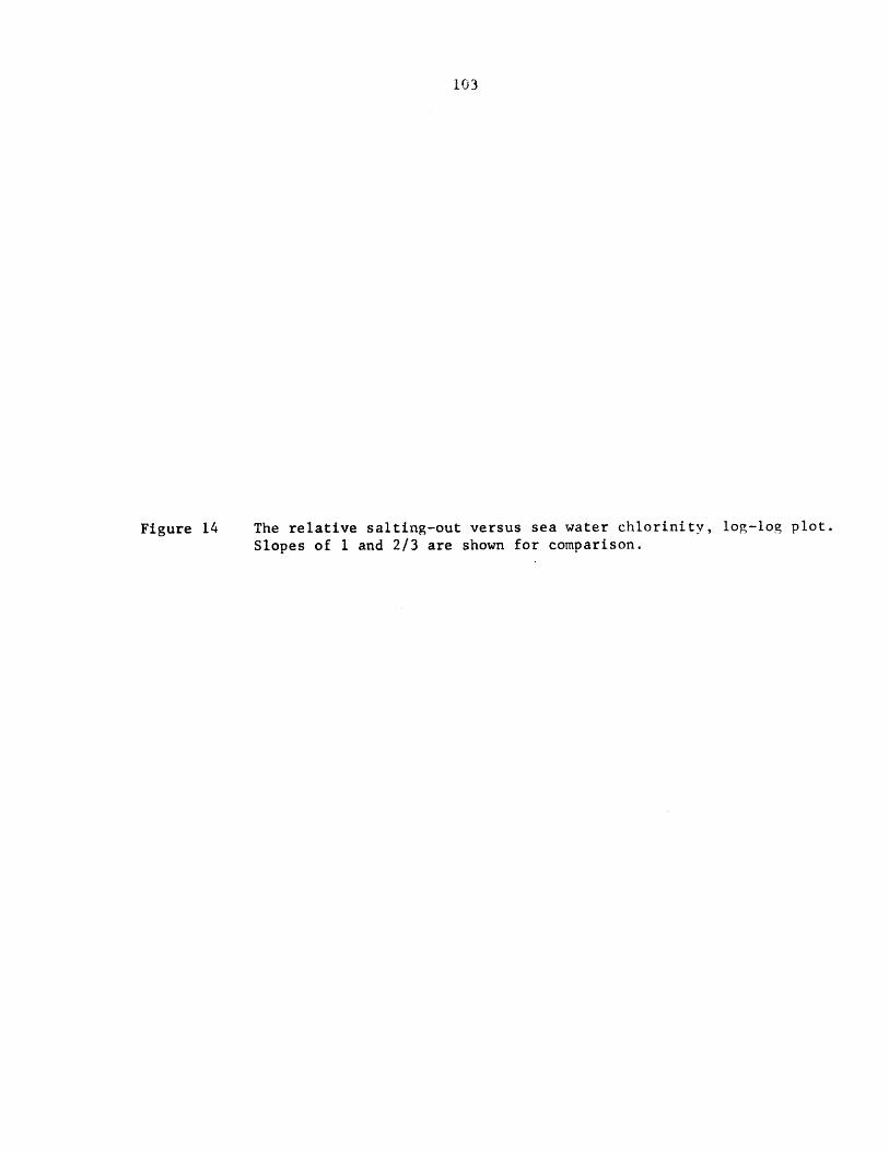
103

The relative salting-out versus sea water chlorinity, log-log plot.

Slopes of 1 and 2/3 are shown for comparison.Figure 14

0.3

0.10 /

0.034 10 20

CL /oo40

105

find , however, that the coefficient decreases by about 7% per degree at low

temperatures and somewhat less that this above room temperature. It is clear

that the simple DEBYE theory does not well apply to the data for the system

under discussion.

106

SOME THERMODYNAMIC CONSIDERATIONS

Consider the reaction

02 (gas) Z 02 (aqueous solution)

The stochiometrical (or apparent) equilibrium constant is

K' = m/p = a22 .4 1 (40)22.414

where m is the molality of the oxygen in solution and p is the partial pres-

sure of the gas. From the definition of the BUNSEN solubility coefficient,

a, we see that it is proportional to the stochiometrical equilibrium constant.

The thermodynamic (or true) equilibrium constant is

K = a0 2/f0 2 = Y 0 2m/f 0 2 (41)

where a0 2 is the activity of the oxygen in solution, f0 2 the fugacity of the

gas and y0 2 the Henry's Law activity coefficient of the dissolved gas.

In pure water gases are so dilute that we may consider that y is

unity, and for gases at moderate pressures the fugacity is very nearly equal

to the partial pressure. Then:

oK 0 (42)

22.414

where mo is the solubility coefficient for pure water. But in any solution

Y aK = K' = -0-- (43)

02 22.414

Hence

to 1y _ - (44)02 a

from our previous definition of 8. We see that a is simply the reciprocal of

the activity coefficient of dissolved oxygen in salt solutions.

107

A QUASI-LATTICE MODEL OF SOLVENT-SOLUTE INTERACTION

The theory of what have been termed "strictly regular solutions"

has been developed by GUGGENHEIM (1952 and earlier) and by PRIGOGINE (1957)

on the basis of certain simplifying assumptions regarding the partition

function for the solution. These authors start with the assumption that the

total partition function may be written as a product of independent partition

functions for the vibrational, rotational, translational and configurational

contributions. As the free energy of the system depends functionally upon

the logarithm of the partition function, this assumption is equivalent to

assuming that the total free energy may be represented as the independent

sums of the contributing energy modes.

While employing the partition function is probably more elegant,

the method we shall use has the advantage of assigning a simple meaning to

the undetermined parameters. It is a generalization of the derivation used by

SLATER (1939) for binary metallic solid solutions. While the assumptions

necessary to justify the model are admittedly outrageous with reference to the

aqueous ionic solution to which the model shall eventually apply, we ask the

reader to suspend disbelief temporarily until that point at which we shall

attempt to rationalize the assumptions.

Consider a liquid made of constituent molecules of type (1), (2),

(3),..., etc. We suppose that the different molecules are all about the same

size and that intermolecular forces are weak, short range, and spherically

symmetrical such that there are no strong orientation effects and no tendency

to establish long range order. We might suppose that these spherical molecules,

although they do not occupy sites on a strict crystal lattice, have, neverthe-

108

less, on the average, z nearest neighboring molecules around them. As the

molecules are all about the same size, z does not depend upon composition and

is the same for the pure liquids of each component.

If we now supercool the liquid without a phase change down to the

absolute zero, the vibrational and rotational energy contributions will be

absent. As we have supposed the intermolecular forces to be short range, the

internal energy of the system at the absolute zero may be written as the sum

of the potential energies of all the nearest neighbor pairs in the system.

U(T = 0) Nlle+ N2 2 e 22 + N33 e 33 + ...

(45)+ N1 2e1 2 + N13e13 + N2 3e2 3 +

where Nij is the number of i-j pairs and eij is the potential energy of one of

these pairs.

As we have assumed that the forces are weak and without strong orien-

tation effects we may suppose that any central molecule sees, of the z mole-

cules around it, the same fraction, on the average, of each kind as that species

mole fraction is in the liquid. This assumption allows us immediately to

write the entropy of mixing and to calculate the number of pairs of each kind.

As the system is randomly mixed the configurational entropy is ideal.

ASm ix = - Nk[xllog x + x21og x2 + x31og x3 + ... ] (46)

where N is the total number of particles, and xi is the mole fraction of the

thi component.

The number of pairs of each kind is

Nz 2N Nz x 2 (47)ii 2 i

Nij Nz xix (48)

The factor 2 in equation (47) arises because we do not wish to count like pairs

109

twice. It is easily verified that the sum of all pairs is Nz/2.

Substituting (47) and (48) into (45) and rearranging is obtained

U(T = 0) = Nz/2 [xle 1 1 + x2 e 2 2 + x3e33 + "

+ [XlX2W 2 + X1X3 13 + x2x3 23 + ... ] (49)

where the interaction parameters are defined as

w. = Nz/2(2e -eii-ejj) (50)xj ij ii

The enthalpy of the system at the absolute zero is

H(T = 0) = PV + Nz/2 [xlell + x2e22 + x3e33 +...

+[X1X2W12 + XlX3W 3 + x2x3w23 + ...] (51)

The sum of the pressure-volume term and the first term in brackets must repre-

sent the free energies of the pure liquid components. Making this identifica-

tion we write

H(T = 0) = x 1 + x 2 2 + x3 P3 +

+X1X2W12 + XlX3W13 + x2x3w23 + ... (52)

Integrating the enthalpy of the system to temperature T from the absolute zero

at constant pressure, then adding the entropy contribution from equation (46),

we obtain for the free energy

G + + x3o + . + x112+ X 1X 3 1 + x2 3W 23 ..

+NkT [xllog x + x2log x2 + x3 log x3 + ...] + AC mix dTo P

(53)

Though it will later prove to be unacceptable we shall assume, for the time

being, that the heat capacity of the system is independent of composition. If

this is true the last, integral, term in (53) is zero.

Having now evaluated the free energy of the system, the chemical poten-

110

tials of the individual components in tn system are easily evaluated by partial

differentiation. For a three component system that is described by equation

(53) we obtain

2 21i = W1 + RTlogxl + x, w2 + x 3 w13 + x2x323 (54)

where the new parameter is defined by

I23 = w1 2 + w13 - w2 3 (55)

and expressions similar to (54) ar, )btained for the chemical potentials of

the other components

2 2u 3 = I2 + RT log x2 + x I w1

2 + x3 w2 3 + X1X3 13 (56)2 2

3 = 3 + RT log x 3 + xl w13 + x 2 23 + XlX2 12 (57)

Let us suppose that we have a diLute solltion of solutes (2) and (3) in solvent

(1). Then in the limit as x2 and x3 go to zero and xl goes to unity

1 = 1P + RT log x l (58)

2 = (P20 + w1 2 ) + RT log x2 (59)

13 (G3 + W1 3 ) + RT log x 3 (60)

We see that this model predicts that dilute solutions will be ideal: in the

limit of infinite dilution the solvent obeys RAOULT'S law and the solutes obey

HENRY'S law.

Now consider the salting-out of component (2) by component (3). Sup-

pose that the solution is saturated with (2). Then v2 = 20 and

-1 ( 2 2log x2 NkT (x w1 2 + x3 1 3 + x1x3 1 3) (61)

When there is no component (3), x 3 = 0 and

o -1 2log x - (x 2 ) (62)

2 NkT 1 12

111

If the solubility ratio is 6, = x2/x 2 and

-xlog (xw Xl 3) (63)log NkT 3 13 13

If the solution is rather dilute x 3 <<X"= 1 and

-x3 Q13log B = 31NkT (64)

13which is the SETSCHENOW relation. The parameter which we have identified

NkT

as the salting-out coefficient in a preceeding chapter, is seen to be a measure

of the greater strength of the (1)-(3) bond over the (1)-(2) bond.

Q1 3 = Nz[(e 1 2 -e 2 3 ) + (e 1 3 -e 1 1 )] (65)

It should be noted that the more negative energies correspond to the more stable

bonds. If the (1)-(2) bonds are very stable then Q 1 3 may have a negative sign

and salting-in will occur.

It is seen that the quasi-lattice model sucessfully predicts a number

of features observed in the ternary system under investigation:

(1) In the limit of infinite dilution the solvent obeys RAOULT'S law

and the solute obeys HENRY'S law.

(2) The salting-out effect is seen to follow the SETSCHENOW equation.

(3) The salting-out coefficient is seen to depend only weakly upon

the temperature. If the interaction parameter is independent of temperature,

the salting-out coefficient will decrease with increasing temperature. (The

assumption that the specific heat of mixing is zero means that the interaction

terms and hence Q13 are temperature independent.)

(4) The fact that component (2) is salted-out rather than -in is sug-

gested by the model, when the solubility of (2) has a negative temperature co-

efficient. This is seen by comparison of equations (62) and (65). From the

former we see that if the temperature coefficient is negative then el2 must be

112

a rather positive quantity; from the latter we see that if el2 is a positive

or small negative quantity then the salting-out coefficient is also likely to

be positive.

The question now arises as to how the model, resting as it does on

the assumptions which have been made, may be applied to the system water-inert

gas-electrolyte. For the use of the model to be at all justified it is neces-

sary that the components be in similar aggregation states and that the ions of

the electrolyte have their strong coulombic forces largely saturated.

Consider the inert gas, component (2), to be at its boiling point,

Tb, such that there is liquid (2) in equilibrium with the gas at one atmosphere

pressure. Now suppose the liquid is brought to temperature T, metastably with-

out a phase change. The pressure of the vapor phase in equilibrium with it

will have fallen to

SHvapdTP = exp PAV T (66)vap PAV T

Tb

where AHvap is the heat of vaporization and AV is the volume change from liquid

to gas. If the vapor phase is ideal its chemical potential, and hence also the

chemical potential of the metastable liquid, is given by

P2 w U22 + RT log P (67)yap

U2 " U2 +T A vaPdTJi)I JPAV T (68)

Tb

where 2*2 refers to the standard state of perfect gas at one atmosphere. The

inert gas is now in anaggregation state (pure liquid) very nearly like the

hypothetical component with which the model was created.

With the salt we are free to choose any standard state we wish, so

-- -- J af~-

113

we choose the standard state to be the hydrated ions at unit molality. We might

suppose that the hydrated ions are not only more nearly the same size as the

uncharged molecules, but also that the coulombic field about the ion should be

largely satisfied by the polar water molecules.

For the solvent we take pure water at temperature T to be the stan-

dard state.

If now we assemble our model with the three hypothetical liquids, we

obtain for the chemical potential of the dissolved gas:

P2 m 12o + RT log x2 + RT T AHvaP dTPAV T

Tb (69)

2 2

+1 w12 +3 w23 + l1X3 13

Evaluating the solubilities as before2X1 w12 T AHvaPdT

log x 2 -[ R + T p (70)2 RT PAV T

The entropy of solution may be evaluated from this expression.

soltn o -AHvap T AHvapdTAS2 =S - S =-R - -R (71)2 2 2 PAV TbPAV T

Assuming that the heat of vaporization is constant and that the volume of the

liquid is negligible compared with the gas, which is assumed to be perfect,

the integral may be approximately evaluated.

AHvap 7f

2 Tb

For oxygen the entropy of vaporization at the normal boiling-point is

AHvapS 36.1 cal/mole-deg

Tb

------- -;; I- 1 ;;;- ----- ---

114

which compares fairly well with the measured entropy of solution of oxygen in

water at 25C according to both HIMMELBLAU (1959) and KLOTS and BENSON (1963).

-AS2 = 30.9 cal/mole-deg

The difference between these values as well as the temperature dependence of

the entropy of solution is no doubt a consequence of the polar nature of the

solvenat *~r. IIILDEBPAND and SCOTT (1962) have pointed out that for non-polar

solvents the correspondence between entropy of solution of the inert gases

and the entropy of vaporization at the normal boiling point is very good.

In the regular solution derivation herein presented the tacit assump-

tion was made that the interaction energies, wij, were temperature independent

and hence their contribution to the excess free energies was purely enthalpic.

If we now choose to absorb the excess entropy terms resulting both from the

non-regular aggregation states for the standard states of the pure components

and also from the excess specific heats into the interaction energies, we may

write for the salting-out relation

x3log 8 = -

RT (73)

which bears a resemblance to equation (64) but where the interaction parameter

is now a temperature dependent excess free energy. It is simply related to

the activity coefficient of the gas in salt solutions, derived in the preceed-

ing section, equation (44).

If the excess free energy of salting-out, Q, is not strongly tempera-

ture dependent, then the salting-out coefficient will decrease with increasing

temperature. This is, in fact, what we observe.

Values of the excess free energy of salting-out, as determined from

solubility measurements, are shown in figure 15 as a function of the temperature.

115

The large standard deviations indicated on this figure are a consequence of

the fact that the excess free energy depends upon the logarithm of B so that

relative errors in B are magnified by a factor of (log 8)-1 to yield larger

relative errors in Q.

In view of the large uncertainties in the data it would be a mistake

to attach too much importance to the second derivative of the free energy-tem-

perature plot, this quantity being related to the excess specific heat of salt-

ing-out. However, the data suggest that the excess entropy of salting-out

(being the negative first derivative) is fairly constant at low temperatures,

then decreases rapidly and becomes very small near 22* C. This in turn sug-

gests that there is a negative excess specific heat due to the addition of

the salt.

116

The excess free energy of salting-out for dissolved oxygen in seawater.

Figure 15

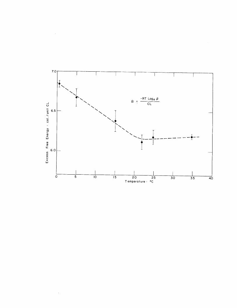
NN

-RT Loge /

CL

Ni--

6.0

II I 1 I1 I I0 5 10 15 20 25 30 35 40

Temperature : OC

L T T --

N

6.5 -

118

CONSIDERATIONS OF THE STRUCTURE OF WATER

Liquid water, due to its highly polar nature, has certain thermo-

dynamic and atomic characteristics which have been explained on the basis of

what has been termed by FRANK and EVANS (1945) and others its "ice-like" or

"iceberg" structure. The rather large specific heats of solution have been

said to be due to the disorganization or "melting" with increasing temperature

of the ice structure around the solute molecules. Observing that the icebergs

need not have the same structure for ions as for inert gases, FRANK and EVANS

succeeded in explaining some of the peculiarities of the entropies of gas

molecules in salt solutions. FRANK and WEN (1957) spoke of an iceberg tightly

bount to an ion surrounded in turn by a region in which neither the iceberg

nor the normal water structure could exist. Thus ions could be classified

as structure-breaking or structure-promoting as one or the other influence

dominated.

Our observations of a suggested negative excess specific heat of

salting-out is consistent with the explanation that NaCI (the predominant com-

ponent of sea salt) is structure-breaking.

119

REFERENCES: PART II

Albright P. S. (1937) Jour. Am. Chem. Soc., 59, 2098-2104.

Albright P. S. and Williams J. W. (1937) Trans. Far. Soc., 33, 247-256.

Baranowski B. and Sarnowski M. (1958) Roczniki, Chem., 32, 135-138 (Englishsummary).

Belton J. W. (1937) Trans. Far. Soc., 33, 653-659.

Bockris J. O'M. and Egan H. (1948) Trans. Far. Soc., 44, 151-159.

Braun L. (1900) Zeit. Physik. Chem., 33, 721-739.

Butler J. A. V. (1929) Jour. Phys. Chem., 33, 1015-1023.

Debye P. (1927) Zeit. Physik. Chem., 130, 56-64.

Debye P. and McAulay J. (1925) Physik Zeit., 26, 22-29.

Eucken A. and Hertzberg G. (1950) Zeit. Physik. Chem., 195, 1-23.

Euler H. (1899) Zeit. Physik Chem., 31, 360-369.

Euler H. (1904) Zeit. Physik. Chem., 49, 303-316.

Fox C. J. J. (1907) Conseil. Perm. Internat. p. 1'Explor. de la Mer Pub. deCirconstance. no. 41.

Frank H. S. and Evans M. W. (1945) Jour. Chem. Physics, 13, 507-523.

Frank H. S. and Wen W-Y. (1957) Dis. Far. Soc., 24, 133-140.

Geffecken G. (1904) Zeit. Physik. Chem., 49, 257-302.

Glasstone S. (1946) Textbook of Physical Chemistry, Van Nostrand, New York.

Gordon V. (1895) Zeit. Physik. Chem., 18, 1-16.

Hildebrand J. H. and Scott R. L. (1962) Regular Solutions, Prentice Hall, NewJersey.

Himmelblau D. M. (1959) Jour. Phys. Chem., 63, 1803-1808.

Hoffman F. and Langbeck K. (1905) Zeit. Physik. Chem., 51, 385-434.

Hufner G. (1907) Zeit. Physik. Chem., 57 , 611-625.

Klots C. E. and Benson B. B. (1963) Jour. Phys. Chem., 67, 933-934.

Knopp W. (1904) Zeit. Physik. Chem., 48, 97-108.

Lowry T. M. (1905) Trans. Far. Soc., 1, 197-214.

120

McAulay J. (1926) Jour. Phys. Chem., 30, 1202-1208.

McDevit W. F. and Long F. A. (1952) Jour. Am. Chem. Soc., 74, 1773-1781.

Morrison T. J. (1944) Trans. Far. Soc., 40, 43-48,

Morrison T. J. (1952) Jour. Chem. Soc., 3814-3818.

Morrison T. J. and Billett F. (1952) Jour. Chem. Soc., 3819-3822.

Morrison T. J. and Johnstone N. B. B. (1955) Jour. Chem. Soc., 3655-3659.

Nakajima M. (1953) Jour. Electrochem. Soc. Japan, 21, 166-168.

Nakajima M. (1953) Jour. Electrochem. Soc. Japan, 21, 237-239.

Philip J. C. (1907) Jour. Chem. Soc., 91, 711-717.

Randall M. and Failey C. F. (1927) Chem. Rev., 4, 271-284.

Randall M. and Failey C. F. (1927) Chem. Rev., 4, 285-290.

Roth W. (1897) Zeit. Physik. Chem., 24, 114-151.

Rothmund, V. (1900) Zeit. Physik. Chem., 33, 401-414.

Samoilov, 0. Y. and Tikhomirov V. I. (1962) Ekstraktsiya. Teoriya Primenenie,Apparatura Sb. Statei, no. 2: 34-36 (English summary in C.A., 58,10781d).

Setschenow J. (1875) Memoirs Acad. Imperial Sci. St. Petersburg, 22, no. 6.

Setschenow J. (1889) Zeit. Physik. Chem., 4, 117-125.

Slater J. C. (1939) Introduction to Chemical Physics, McGraw Hill, New York.

Steiner W. (1894) Weid. Ann., 52, 275.

Truesdale G. A. et al. (1955) Jour. Appl. Chem., 5, 53-62.

121

ACKNOWLEDGEMENTS

The writer wishes to thank Professor Dayton E. Carritt, who suggested

the problem, for his encouragement and invaluable guidance throughout this

investigation.

The cooperation of the Woods Hole Oceanographic Institution and of

Miss Vivian Randall in particular in making the chlorinity determinations is

appreciated.

Special credit is due Mr. Kenneth R. Harper of the M.I.T. Geology

Shop for designing and building the saturator and for the continuing helpful-

ness and competence of himself and his staff.

For stimulating discussions and ideas we wish to thank Professor J. W.

Winchester, Dr. R. A. Duce, and F. MacIntyre.

In addition to Professor Carritt, appreciation is expressed to Pro-

fessor W. S. von Arx, Professor P. M. Hurley, and G. C. MacDonald, Jr. for

their critical reading of the manuscript.

The financial support of the National Science Foundation thrpugh Grant

GP486 (M.I.T.: DSR 9337) to Professor Carritt is gratefully acknowledged.

Computational work was done in part at the Computation Center at M.I.T.

with the assistance of the staff of the Center. Professor T. R. Madden kindly

supplied us with his own computer subprogram for matrix inversion used in the

least-squares analysis.

122

APPENDICES

123

APPENDIX I

GAS-LIQUID EQUILIBRATION DURING PRESSURE CHANGES

It has been noted that the concentration of a dissolved aas in a

well-stirred vessel follows the ADENEY-BECKER law

C -C(t)dC(t) _eguil (74)

dt T

where C equil is the asymptotically approached equilibrium value of the concen-

tration, C(t) is the concentration at time t, and T is the mean period, a con-

stant depending upon the gqometry and nature of the system. The mean period

is simply related to the more familiar half period.

tl/ 2 t1/2T = (75

log 2 0.69315

For a constant pressure and temperature C equil is a constant and the solution

to equation (74) is

C(t) = C equil + (C -C equil)exp(-t/) (76)

where C is the initial concentration: C = C(O).o 0

We now seek to inquire as to how the equilibrium concentration is

approached when the pressure (or temperature) and hence the equilibrium con-

centration is a function of time.

Inasmuch as the pressure, temperature and equilibrium concentration

are real physical quantities they are unlikely to exhibit mathematical singu-

larities and we may express the eqilibrum concentration as a power series or

polynomial in the time.

C = P(t) (77)equil

124

Substituting this into equation (74) and obtaining the general solution

C(t) = A exp(-t/T) + P(t) - TP'(t)

+ TP"(t) -(t) .... (-)n3 (t) .... (T) P (t(78)

where Pn(t) is the nth derivative of the polynomial P(t) and where A is a

constant determined by the initial conditions.

If the concentration is changing slowly we may terminate P(t) after

the linear term in which case the solution reduces to

C(t) = A exp(-t/T) + P(t - T) (79)

If t > (after several mean lives) the first term is negligible and the con-

centration will simply lap the equilibrium concentration by a period T.

Thus under conditions when the pressure is slowly changing in a

linear manner, the effective pressure which the solution concentration reflects

is just that pressure which obtained a time T previously.

125

APPENDIX II

A SAMPLE CALCULATION OF THE SOLUBILITY COEFFICIENTS

In order to show the method of calculating the solubility coefficients

and to demonstrate the magnitudes of the various corrections, a typical calcu-

lation follows, being the first determination of series I.

The solution temperature: The NBS certified thermometer read 24.940 C

when immersed in the flask to the 0.00*C mark. The auxilliary (stem-tempera-

ture) thermometer taped to its side read 23.8°C. The immersior correction is-4

(24.94-0.00) x (24.94-23.8) x (1.64*10 ) = +0.0040 C

where the last factor is the differential expansion coefficient per degree of

mercury in borosilicate glass.

The basic correction, obtained from the NBS calibration report on

this thermometer, was -0.020 C. Hence the true temperature of the solution was

24.94 + 0.004 - 0.02 = 24.92 0 C

In English units this corresponds to 76.86*F.

The effective pressure: At the time of sampling the total uncorrec-

ted barometric pressure was 30.129 in Hg. The room temperature was 73.6 0 F.

One mean period earlier the uncorrected pressure had been 30.136 in. Hg. Using

the tabulated temperature corrections of the Smithsonian Meteorological Tables,

p. 161, we correct the total pressure for expansion of the mercury column.

30.136 - 0.123 = 30.013 in. Hg.

Also from these tables, p. 356, the vapor pressure of water at 76.86F is ob-

126

tained and subtracted.

30.013 - 0.931 = 29.082 in. Hg for dry air over pure water.

The vapor pressure lowering of sea water of chlorinity 17.630/oo is obtained

from the tables of ARONS and KIENTZLER and found to be 0.015 in Hg. Then

the dry pressure over the sea water is

29.082 + 0.015 = 29.097 in Hg for dry air over sea water.

Bottle volumes: The bottle volume of the distilled sample was 243.27m1;

that of the sea water sample was 231.34 ml. The volume of manganous reagent

plus the volume of alkaline iodide was 4.00 ml. Then the effective sample

volumes were:

distilled water sea water

243.47 241.34

- 4.00 - 4.00

239.47 ml 237.34 ml

Titration: Titrant volumes were corrected for blanks determined as

described in Part I.

distilled water sea waterapparent endpoint 883.68 730.00 ilreagent blank +0.52 -1.35corrected endpoint 884.20 728.65 Wl

Bunsen coefficient: The titrant concentration was determined to

be 0.2801 equiv/l. The BUNSEN coefficient as herein defined is given by:

For the distilled water:

(0.88420 ml titrant)(29.9213 in.Hg/atm)(22,414 ml gas/mole) x(239.47 ml sample)(29.082 in. Hg dry air)(4 equiv/mole)

-3(0.2801 * 10 equiv/ml) a 0.028494(0.2094 fraction 02/air) o

127

For the sea water:

(0.72865 ml titrant)(29.9213 in.1 /atm)(22 414 ml gas/mole)(237.34 ml sample)(29.097 in. Hg dry air)(4 equiv/mole)

-3(0.2801 10- equiv/ml)

(0.2094 fraction 02/air)" 2= a = 0.023652

The solubi ity ratio:

S = 0.83007

The salting-out coefficient: As herein defined the salting-out

coefficient is given by:

-lge !3 0.18625 -3 -1k 0.18625 10.563 x 10 C1

Cl 17.632

The excess free energy of salting-out: As herein defined this quan-

tity is

0 = RTk = (1.987 cal/mole-deg)(298.10K)(0.01056 Cl-)

2 = 6.26 cal/unit Cl-mole 02

Note that k here is the salting-out coefficient, not to be confused with the

BOLTZMAN constant.

128

APPENDIX III

BIBLIOGRAPHY

Adeney W. E. and Becker H. G. (1919) Phil. Mag., _38, 317-337, "The determina-tion of the rate of solution of atmospheric nitrogen and oxygen inwater."

Albright P. S. (1937) Jour. Am. Chem. Soc., 59, 2098-2104, 'Experimental testsof recent theories descriptive of the salting-out effect."

Albright P. S. and Williams J. W. (1937) Trans. Far. Soc., 33, 247-256, 'Elec-trical forces between ions and neutral molecules in aqueous solution;a study of the salting-out effect."

American Public Health Association (1946) Standard Methods for the Examinationof Water and Sewage, 9th ed.

Angstrom K. (1882) Wied. Ann., 15, 297.

Arons A. B. and Kientzler C. F. (1954) Trans. Am. Geophys. Un., 35, 722-728,"Vapor pressure of sea-salt solutions."

Awtrey A. D. and Connick R. E. (1951) Jour. Am. Chem. Soc., 73, 1341-1348,"The rate law of the reaction of iodine with thiosulfate ion."

Baranowski B. and Sarnowski M. (1958) Roczniki, Chem., 32, 135-138, "Extensionof Debye's theory of salting-out and salting-in effects." (Englishsummary).

Barkley R. A. and Thompson T. G. (1960) Deep Sea Res., 7, 24-34, "The totaliodine and iodate-iodine of sea water."

Barnett G. R. and Jurwitz E. (1939) Sewage Works Jour., 11, 781.

Belton J. W. (1937) Trans. Far. Soc., 33, 653-659, "The salting-out of gasesand volatile non-electrolytes."

Benson B. B. and Parker P. D. M. (1961) De.e_p Sea Res., 7, 237-253, "Nitrogen/Argon and nitrogen isotope ratios in aerobic sea water."

Benson B. B. and Parker P. D. M. (1961) Jour. Phys. Chem.,_65, 1489-1496,"Relations among the solubilities of nitrogen, argon, and oxygenin distilled water."

Bishop E. (1953) Analyst, 78, 149-159, "Replacement of standard cell and saltbridge by indicator electrodes and the use of non aqueous solutionsin potentiometry: II. Iodometry and iodimetry in aqueous solution."

Bockris J. O'M. and Egan H. (1948) Trans. Far. Soc., 44, 151-159, "The salting-out effect and dielectric constant."

Bohr C. and Bock J. (1891) Wied. Ann., 44, 316.

Bradbury J. H. and Hambly A. N. (1952) Aus. Journ. Scientif. Res., A5, 541-554,"An investigation of errors in the amperometric and starch indicatormethods for the titration of millinormal solutions of iodine andthiosulfate."

129

Braun L. (1900) Zeit. Physik. Chem., 33, 721-739, "Uber die Absorption vonStickstoff und von Wasserstoff in Wasserigen Losungen verschiedendissociierter Stoffe."

Bray W. C. and Connolly E. L. (1911) Jour. Am. Chem. Soc., 33, 1485-1487, "Thehydrolysis of iodine and of bromine; a correction."

Bunsen R. (1857) Gasometrische Methoden, von Friedrich und Sohn, Braunschweig,305 pp.

Butler J. A. V. (1929) Jour. Phys. Chem., 33, 1015-1023, "The mutual salting-out of ions."

Carpenter J. H. (1965) Limno. and Oceanog., In press, "The accuracy of theWinkler method for dissolved oxygen analysis."

Carritt D. E. (1954) Deep Sea Res., 2, 59-62, "Atmospheric pressure changesand gas solubility."

Carritt D. E. (1954) )atl. Acad. Sci.-Natl. Res. Council, Committee on Oceano-graphy Report, In p r~ss, "Intercomparison of methods in chemicaloceanography, I: Dissolved oxygen by the Winkler method."

Claussen U. F. and Pclglase M. F. (1952) Jour. Am. Chem. Soc., 74, 4817-4819,'Solubilities and structures in aqueous aliphatic hydrocarbon solu-tions."

Debye P. and McAulay, J. (1925) Physik Zeit., 26, 22-29, "Das elektrische Feldder Ionen und die Neutralsalzwirkung."

Debye P. (1927) Zeit. Physik. Chem., 130, 56-64, "Das elektrische Ionfeld unddas Aussalzen."

Derjaguin B. (1945) Acta Physicochimica (URSS), 20, 349-352, "On the thicknessof the liquid film adhering to the walls of a vessel after emptying."

Dittmar W. (1884) Challenger Reports, vol. 1, Physics and Chemistry, 1-251,"Report on researches into the composition of ocean water, collectedby HMS Challenger."

Douglas E. (1964) Jour. Phys. Chem., 68, 169-174, "Solubilities of oxygen, argon,and nitrogen in distilled water."

Eley D. D. (1939) Trans.Far. Soc., 35, 1281-1293, "On the solubility of gases,I: The inert gases in water."

Elmore H. L. and Hayes T. W. (1960) Proc. Am. Soc. Civil Eng., 86(SA4), 2556:41-53, "Solubility of atmospheric oxygen in water."

130

Eucken A. and Hertzberg G. (1950) Zeit. Physik. Chem., 195, 1-23, "The salting-out effect and ion hydration."

Euler H. (1899) Zeit. Physik. Chem., 31, 360-369, "Uber die Loslichkeit vonAthylacetat in wasserigen Salzlosungen."

Euler H. (1904) Zeit. Physik. Chem., 49, 303-316, "Uber Loslichkeitserniedrigung."

Forsythe W. E. (1956) Editor, Smithsonian Physical Tables. Publ. SmithsonianInst., Washington, D. C., pp. 358-360, "Solubility of gases in water."

Fox C. J. J. (1907) Conseil. Perm. Internat. P. l'Explor. de la Mer, Publ. deCirconstance, no. 41, 27 pp., "On the coefficients of absorption ofthe atmospheric gases in distilled and sea water."

Fox C. J. J. (1909) Trans. Far. Soc., 5, 68-87, "On the coefficients of absorp-tion of nitrogen and oxygen in distilled water and sea water, and ofatmospheric carbonic acid in sea water."

Frank H. S. and Evans M. W. (1945) Jour. Chem. Physics, 13, 507-523, "Freevolume and entropy in condensed systems, III: Entropy in binary liquidmixtures; partial molal entropy in dilute solutions; structure andthermodynamics in aqueous electrolytes."

Frank H. S. and Wen W-Y. (1957) Dis. Far. Soc., 24, 133-140, "Ion-solvent inter-action, III: Structural aspects of ion-solvent interaction in aqueoussolutions; a suggested picture of water structure."

Furth A. (1922) Zeit. Electrochem., 28, 57-58, "Notiz uber die starke derunterjodigen saure."

Geffcken G. (1904) Zeit. Physik. Chem., 49, 257-302, "Beitrage zur Kenntnisder Loslichkeitsbeeinflussung."

Gilbert G. A. and Marriott J. V. R. (1948) Trans. Far. Soc., 44, 84-93, "Starch-iodine complexes, part I."

Glasstone S. (1946) Textbook of Physical Chemistry, Van Nostrand, New York,1320 pp.

Gordon V. (1895) Zeit. Physik. Chem., 18, 1-16, "Uber die Absorption des Stick-oxyduls in Wasser und in Salzlosungen."

Gross P. M. (1933) Chem. Rev., 13, 91-101, "The salting-out of non-electrolytesfrom aqueous solution."

Guggenheim, E. A. (1952) Mixtures, Oxford Press, London, 270 pp.

Hildebrand J. H. and Scott R. L. (1962) Regular Solutions, Prentice Hall, NewJersey, 180 pp.

131

Himmelblau D. M. (1959) Jour. Phys. Chem., 63, 1803-1808,"Partial molal heatsand entropies of solution for gases dissolved in water from thefreezing to near the critical point."

Himmelblau D. M. (1960) Jour. Chem. Eng. Data, 5, 10-15, "Solubilities of inertgases in H20: 0.C to near the critical point of H20.

Himmelblau D. M. and Arends E. (1959) Chem. Ing.. Tech., 31, 791-795, "The solu-bility of inert gases in water at high temperatures and pressures."

Hirschfelder J. O. et al. (1954) Molecular theory of gases and liquids, JohnWiley and Sons, New York, 1219 pp.

Hoffman F. and Langbeck K. (190() Zeit. Physik. Chem., 51_ 385-434, "Studienuber Loslichkeitsbeeinflussung."

Hufner G. (1907) Zeit. Physik. Chem., 57, 611-625, "Untersuchungen uber dieAbsorption von Stickgas und Wasserstoff durch wasserige Losungen."

Jacobsen J. P. (1905) Meddelelser fra Kommissionen for Havundersogelser, Serie,Hydrografi. Bind. 1, no. 8, Copenhagen.

Jacobsen J. P. et Al. (1950) Assoc. D'Oceanographie Physique (IUGG), Publ.Scientifique no. 11, 22 pp., "A review of the determination of dis-solved oxygen in sea water by the Winkler method."

Katzin L. I. and Gebert E. (1955) Jour. Am. Chem. Soc., 77, 5814-5819, "Theiodide-iodine-triiodide equilibrium and ion activity coefficientratios."

Klots C. E. (1961) Limno. and Oceanog., 6, 365-366, "Effect of hydrostaticpressure upon the solubility of gases."

Klots C. E. and Benson B. B. (1963) Jour. Mar. Res., 21, 48-56, "Solubilitiesof nitrogen, oxygen and argon in distilled water."

Klots C. E. and Benson B. B. (1963) Jour. Phys. Chem., 67, 933-934, "Thermody-namic properties of the atmospheric gases in aqueous solutions."

Knopp W. (1904) Zeit. Physik. Chem., 48, 97-108, "Uber die Loslichkeitsbeein-flussung von Wasserstoff und Stickoxydul in wasserigen Losungen ver-schieden dissoziierter Stoffe."

Knowles G. and Lowden G. F. (1953) Analyst, 78, 159-164, "Methods for detectingthe end point in the titration of iodine with thiosulfate."

Kolthoff I. M. and Sandell E. B. (1943) Textbook of quantitative inorganic analysis,MacMillan Co., New York, 794 pp.

Kolthoff I. M. and Belcher R. (1957) Volumetric Analysis, III, Titration methods,oxidation reduction reactions, Interscience Publ., New York, 714 pp.

132

Kritchevsky I. and Iliinslaya A. (1945) Acta Physicochimica, (URSS) 20, 327-348,"Partial molal volumes of gases dissolved in liquids."

Krummel 0. (1907) Handbuch der Ozeanographie; Bd,I, Die raumlich, chemischenund physikalischen Verhaltnisse des Meeres, J. Engelhorn, Stuttgart,526 pp.

List R. J. (1963) Editor: Smithsonian Meteorological Tables. Publ. SmithsonianInst., Washington, D. C., 527 pp.

Lowry T. M. (1905) Trans. Far. Soc., 1, 197-214, "An application to electrolytesof the hydrate theory of solutions."

McAulay J. (1926) Jour. Phys. Chem., 30, 1202-1208, "Influence of the solubili-ties of salts in water by the addition of a non-electrolyte to thesolution."

McCoubrey J. C. (1955) Trans. Far. Soc., 51, 743-747, "The acid strength of thehydrogen halides."

McDevit W. F. and Long F. A. (1925) Jour. Am . Chem. Soc., 74, 1773-1781, "Theactivity coefficient of benzene in aqueous salt solutions."

Morris J. C. et al. (1961) Proc. Am. Soc. Civil Eng., 85(SA1), 81-86, "Solu-bility of atmospheric oxygen in water."

Morrison T. J. (1944) Trans. Far. Soc., 40, 43-48, "The salting-out effect."

Morrison T. J. (1952) Jour. Chem. Soc., 3814-3818, "The salting-out of non-electrolytes, I: The effect of ionic size, ionic charge, and tempera-ture."

Morrison T. J. and Billett F. (1952) Jour. Chem. Soc., 3819-3822, "The salting-out of non-electrolytes, II: The effect of variation in non-electro-lyte."

Morrison T. J. and Johnstone N. B. B. (1955) Jour. Chem. Soc, 3655-3659, "Thesalting-out of non-electrolytes, III: The inert gases and sulphurhexafluoride."

Mortimer C. H. (1956) Internat. Assoc. of Theoret. and Appl. Limno. Communica-tions, no. 6.

Nakajima M. (1953) Jour. Electrochem. Soc. Japan, 21, 166-168, "Studies onsalting-out effects, I: A new theory on salting-out effects."

Nakajima M. (1953) Jour. Electrochem. Soc. Japan, 21, 237-239, "Studies onsalting-out effects, II: Comparison with Albricht's data."

133

Paquette R. G. (1959) Natl. Acad. Sci.-Natl. Res. Council, Committee on Oceano-graphy Report, publ. 600, 202 pp., 'Physical and chemical propertiesof sea water.'

Philip J. C. (1907) Jour. Chem. Soc., 91, 711-717, "Influence of non-electro-lytes on the solubility of sparingly soluble gases in water; the ques-tion of hydrates in solution."

Placak 0. R. and Ruchhoft C. C. (1941) Ind. Epng. Chem.LAnal. Ed., 13, 12.

Pomeroy R. and Kirschman H. D. (1945) Ind. Eng. Chem., Anal., Ed., 17, 715.

Prigogine I. (1957) The molecular theory of solutions, North-Holland Publ. Co.,Amsterdam, 448 pp.

Randall M. and Failey C. F. (1927) Chem. Rev., 4, 271-284, "The activity coef-ficient of gases in aqueous salt solutions."

Randall M. and Failey C. F. (1927) Chem. Rev., 4, 285-290, "The activity co-efficient of non-electrolytes in aqueous salt solutions from solubilitymeasurements: the salting-out order of the ions."

Redfield A. C. (1942) Papers Physic. Oceanog. Meteorol., 9(2), 1-22, "The pro-cesses determining the concentration of oxygen, phosphate and otherorganic derivatives within the depths of the Atlantic Ocean."

Redfield A. C. (1948) Jour. Mar. Res., 7, 347-361, "The exchange of oxygenacross the sea surface."

Richards F. A. and Corwin N. (1956) Limno. and Oceanog., 1, 263-267, "Some oceano-graphic applications of recent determinations of the solubility ofoxygen in sea water."

Richards F. A. (1957) Physics and chemistry of the earth, vol. II, ed. L. H.Ahrens et al., Pergamon Press, Pp. 77-128, "Some current aspects ofchemical oceanography."

Rideal S. and Stewart G. G. (1901) Analyst, 26, 141-148, "Determination of dis-solved oxygen in waters in the presence of nitrites and of organicmatter."

Roescoe H. E. and Lunt J. (1889) Jour. Chem. Soc., 55, 552-576, "On Schutzen-berger's process for the estimation of dissolved oxygen in water."

Roth W. (1897) Zeit. Physik. Chem., 24, 114-151, "Uber die Absorption desStickoxyduls in wasserigen Losungen verschieden dissociierter Stoffe."

Rothmund V. (1900) Zeit. Physik, Chem., 33, 401-414, Die Anderung der Loslich-keit durch Salze."

134

Ruchhoft C. C. et al. (1938) Ind. Eng. Chem., Anal. Ed., 10, 701.

Samoilov 0. Y. and Tikhomirov V. I. (1962) Ekstraktsiya. Teoriya Primenenie,Apparatura, Sb. Statei, no. 2: 34-36, "Molecular-kinetic nature ofthe salting-out effect." (English summary in C.A., 58, 10781d).

Seiwell H. R. (1937) Nature, 140, 506-508, "Consumption of oxygen in seawater under controlled laboratory conditions."

Setschenow J. (1875) Memoirs Acad. Imperial Sci. St. Petersburg, 22, no. 6.

Setschenow J. (1889) Zeit. Physik. Chem., 4, 117-125, "Uber die Konstitutionder Salzlosungen auf Grund ihres Verhaltens zu Kohlensaure."

Setschenow J. (1892) Ann. Chim. Phys., 25, 226-270, "Action de l'acide car-bonique sur les solutions des sels a acides forts."

Silver P. Y. (1963) Zh. Fiz. Khim., 37, 1769-1775, "Determination of thesalting-out and activity coefficients in ternary solutions by thelowering of the freezing point."

Slater J. C. (1939) Introduction to chemical physics, McGraw Hill, New York,521 pp.

Steen H. (1955) Limno. and Oceanog., 3, 423-426, "Determinations of the solu-bility of oxygen in pure water."

Steiner W. (1894) Weid. Ann., 52, 275.

Theriault E. J. (1925) Public Health Bulletin No. 151, Gov't Printing Office,"The determination of dissolved oxygen by the Winkler method."

Theriault E. J. and McNamee P. D. (1932) Ind. Eng. Chem., Anal. Ed., 4, 59.

Thompson T. G. and Robinson R. J. (1939) Jour. Mar. Res., 2, 1-8, "Notes onthe determination of dissolved oxygen in sea water."

Truesdale G. A. et al. (1955) Jour. Appl. Chem., 5, 53-62, "The solubility ofoxygen in pure water and sea water."

Wada G. and Ito C. (1957) Jour. Chem. Soc. Japan, 78, 1694-1699, "Ionic solva-tion in solution, IV: Salting-out effect of strong 1:1 electrolyteson the aqueous solution of diethyl ether."

Weast R. C. Handbook of Chemistry and Physics, Chemical Rubber Publ. Co.,Cleveland, Ohio, pp. 1706-1708.

Wheatland A. B. and Smith L. J. (1955) Jour. Appl. Chem., 5, 144-148, "Gaso-metric determination of dissolved oxygen in pure and saline wateras a check of titrimetric methods."

135

Winkler L. W. (1888) Ber. Deutsch. Chem. Ges., 21, 2843-2854, "Die Bestimmungdes im Wasser gelosten Sauerstoffes."

Winkler L. W. (1889) Ber. Deutsch. Chem. Ges., 22, 1764-1777), "Die Loslichkeitdes Sauerstoffs in Wasser."

Winkler L. W. (1891) Ber. Deutsch. Chem., Ges., 24, 3602-3610, "Die Loslichkeitdes Gase in Wasser."

Winkler L. W. (1906) Zeit. Physik. Chem., 55, 344-354, "Gesetsmassigkeit beider Absorption der Case in Flussigkeiten."

Winkler L. W. (1914) Zeit. Anal. Chem., 53, 665-672, "Uber die Bestimmung desim Wasser Gelosten Sauerstoffes."

Winkler L. W. (1915) Zeit. Untersuch. Nahr. u. Genussm., 29, 121.

Winkler L. W. (1916) Zeit. Angew. Chem., 29, 44.

Winkler L. W. (1931) Die chemische Analyse: Ausgewahlte Untersuchungsverfahrenfur das chemische Laboratorium, Enke, Stutgart.

Worthington L. V. (1954) Deep Sea Res., 1, 244-250, "A preliminary note onthe time scale in north Atlantic circulation."

Wright R. W. et al. (1939) Jour. Am. Chem. Soc., 61, 228-230, "The phenylthiourea-ethanol and urea-methanol systems and the Debye salting-out theory."

136

BIOGRAPHICAL NOTE

The author, Edward Jewett Green, was born in Bakersfield, California

on 31 October 1931, the son of Letha Jewett and Edward Ernest Green. He com-

pleted his high school education at Bakersfield High School in 1949. From

September 1949 to February 1952 he attended the University of Southern Cali-

fornia. In 1955 he returned to school at the University of California, Santa

Barbara, where he was elected to Sigma Phi Epsilon. He held the John and Ina

Campbell Scholarship (1956) and the La Verne Noyes Scholarship (1957). During

the summer of 1956 he worked as geologic field assistant with the U. S. Geo-

logical Survey in Alaska. In August 1958 the author received the degree of

Bachelor of Arts, cum laude, in geology. His bachelor's thesis was entitled,

The geology of the central part of the Sutter Creek quadrangle, Amador County,

California.

In September 1958 the author entered the Department of Geology and

Geophysics at M.I.T., where he has held a junior staff appointment as Research

Assistant. In 1959 he received a Woods Hole Oceanographic Institution Summer

Fellowship and he subsequently worked at the Oceanographic Institution as

Research Assistant and aboard the Research Vessel Chain on the Romanche Trench

Cruise of 1961. While at M.I.T. he was elected to associate then to full mem-

bership in the Society of Sigma Xi. He is also a member of the Geochemical

Society, The Society of Economic Paleontologists and Mineralogists, The Amer-

ican Geophysical Union, and the American Association for the Advancement of

Science.

The author's professional experience includes work for the Division

of Sponsored Research, M.I.T. on the Vela Uniform Project under subcontract

137

from the U. S. Air Force, work on semiconductor chemistry under contract from

Avco Research Corporation, and some preliminary studies of the kinetics of

mixed carbonate precipitation. In addition to the sponsored research reports

he has published a short paper: Some comments on the bi-normal distribution

(Geochim. et Cosmochim. Acta, 27, 1071, 1963) concerning geostatistics.

During the spring 1965 the author will be a Research Associate in

the Department of Geology and Geophysics, M.I.T.