UNDERSTANDING POST DISASTER RECOVERY ...
82
ADVISOR: S. Ghaffarian, PhD Candidate UNDERSTANDING POST DISASTER RECOVERY THROUGH ASSESSMENT OF LAND COVER AND LAND USE CHANGES USING REMOTE SENSING MOHAMMADREZA SHEYKHMOUSA February, 2018 SUPERVISORS: Prof. Dr. N. Kerle Dr. M. Kuffer
-
Upload
khangminh22 -
Category
Documents
-
view
2 -
download
0
Transcript of UNDERSTANDING POST DISASTER RECOVERY ...

ADVISOR:
S. Ghaffarian, PhD Candidate
UNDERSTANDING POST DISASTER
RECOVERY THROUGH
ASSESSMENT OF LAND COVER
AND LAND USE CHANGES USING
REMOTE SENSING
MOHAMMADREZA SHEYKHMOUSA
February, 2018
SUPERVISORS:
Prof. Dr. N. Kerle
Dr. M. Kuffer


SUPERVISORS:
Prof. Dr. N. Kerle
Dr. M. Kuffer
ADVISOR:
S. Ghaffarian, PhD Candidate
THESIS ASSESSMENT BOARD:
Prof. Dr. V. Jetten (Chair)
Dr. Maik Netzband (External Examiner, University of Wuerzburg)
MOHAMMADREZA SHEYKHMOUSA
Enschede, The Netherlands, February, 2018
Thesis submitted to the Faculty of Geo-Information Science and Earth
Observation of the University of Twente in partial fulfilment of the
requirements for the degree of Master of Science in Geo-information
Science and Earth Observation.
Specialization: Applied Earth Sciences
UNDERSTANDING POST DISASTER
RECOVERY THROUGH
ASSESSMENT OF LAND COVER
AND LAND USE CHANGES USING
REMOTE SENSING

DISCLAIMER
This document describes work undertaken as part of a programme of study at the Faculty of Geo-Information Science and
Earth Observation of the University of Twente. All views and opinions expressed therein remain the sole responsibility of the
author, and do not necessarily represent those of the Faculty.

i
ABSTRACT
Post-disaster recovery is a complex phenomenon, and distinct from physical reconstruction (physical
recovery) in that it includes relevant processes such as economic and social (functional recovery). The
recovery is reported to be the least understood phase of disaster cycle, where existing literature mostly
focus on physical recovery, neglecting functional recovery. Disasters introduce changes to the affected
land and in subsequent post-disaster activities through land cover and land use change (LCLUC). LCLU
information extracted from satellite imagery is widely used in the RS disciplines. However, the value of
this information in the recovery context has not yet been explored.
The main purpose of this study was to support the recovery assessment through LCLUC analysis
using RS and specifically to investigate the value of LCLU information in the recovery assessment.
Tacloban city in the Philippines was selected as a test area. On 8 November 2013, Tacloban city was
devastated by super typhoon Haiyan, the strongest typhoon on record to make landfall. Despite the
crippling damage, the local government tried to coordinate recovery efforts towards a more resilient city.
The available data were 3 WV2 images from 8 months before, right after, and 4 years after typhoon
Haiyan. First, a methodology was developed based on a generic, action-oriented, forward-looking
conceptual framework (CF), comprised of transition patterns (TPs) to characterize different recovery
statuses. Here it is understood that recovery information is a geographic phenomenon and related TPs are
geographic objects. Moreover, it is found that some TPs can specifically characterize short- and some
long-term recovery. Second, for classification purposes support vector machine (SVM) was employed, and
a detailed comparison of the performance of linear- and RBF-based SVM relying on the various settings
of hand-crafted features was conducted. The best combination of SVM with image features
(SVM+GLCM+NDVI2, SVM+LBP+NDVI2; LC and LU tasks respectively) were applied in 3 time-span
images to produce LCLU maps. The result showed (OA: 89.4%, 82.2%, 90.8%; 76.3%, 69.9%, 77.8%; LC
and LU respectively) that well designed hand-crafted features could show competitive performance in a
complex task involving classes from simple and small to abstract and big regarding complexity and size,
respectively. However, more investigation is needed when it comes to vegetation related classes in “use”
level.
Lastly, The LCLU maps were stacked and, based on the developed CF, different TPs from the
stacked LC and LU maps were extracted. The final products are LC- and LU-based recovery maps which
were further up-scaled to a region level. It was found that the characteristic of the post-Haiyan recovery in
Tacloban city can be explained through the LCLUC information. Results of this study showed that 168 ha
of the area had positively recovered by the time of the most recent image, while 69 ha showed negative
recovery in both LC- and LU-based recovery maps. Positive recovery was mainly related to the recovery
projects and was in part effective to build back the damaged area and build impervious surfaces back
better. However, the recovery project fails where slum areas were rebuilt again along the coastline, where
study suggests considering slum areas in the readjustment projects. Additionally, it is concluded that the
general understanding of the recovery could be provided by LC information and LU information can be
used, where LC information cannot provide useful recovery evidence (area of uncertainty). The other
finding was that due to the different recovery rate of regions and practicality issues, an adaptive approach
should be considered for the timing of the imagery. Meaning that while a 3-time-based framework
provides an initial recovery (assessment) insight of a region, a 5-time-based framework can be used as a
normal framework which can give an overall assessment of the area, when the timing of the imagery
should be well adjusted with different recovery rate of specific activities (adaptive approach). Another
important purpose of this research was to establish the relation between the existing recovery indicators

ii
and advanced RS methods. The study provides 3 tables, where all relevant indicators are grouped based on
their utilities ranging from low and medium to high; micro, meso, and macro indicators, respectively.
The overall findings emphasis that the LC-based recovery map contributes to the general recovery
understanding, while detailed functional recovery is revealed by LU-based recovery map.
THESIS IN ONE SENTENCE: LCLU-based information is useful in the most aspects of recovery
measurement, while also providing (from a basic to a deep) understanding of recovery assessment.

iii
ACKNOWLEDGEMENTS
Thank God for finally writing this thesis! One of the most challenging and at the same time fruitful
periods in my life. Sincere appreciation to my supervisors Prof. Norman Kerle and Dr. Monika Kuffer,
and my advisor Saman Ghaffarian, who have dedicated their time and effort to guide me through this
thesis.
I would also like to thank the UT-ITC for the opportunity given to me through the excellence
scholarship. This unique opportunity enabled me to pursue my dreams at ITC. In addition, I salute my
classmates from all over the world, with whom we toiled daily.
The satellite imagery were provided from Digital Globe Foundation, which were granted for an
ongoing project at ITC entitled “post-disaster recovery assessment using remote sensing data and spatial
economic modeling.”
Lastly, I extend the warmest appreciation to my dear parents in Iran for their constant support, to my
lovely balio for always being there and providing moral support, to other members of family and friends,
and I dedicate this to Ghochak. “This is us!”
Follow Your Dreams!

iv
LIST OF ABBREVIATION
Build Back Better BBB
Change Detection CD
Conceptual Framework CF
Comprehensive Land use Plan CLP
Convolutional Neural Network CNN
Disaster Risk Management DRM
Food and Agriculture Organization of the United Nations FAO
Geographic Information System GIS
Grey Level Co-occurrence Matrix GLCM
Hilbert-Schmidt Independence Criterion HSIC
Local Binary Pattern LBP
Land Cover Land Use Change LCLUC
Light Detection and Ranging LIDAR
Machine Learning ML
Overall Accuracy OA
Object-Based Change Detection OBCD
Object-Based Image Analysis OBIA
Open Street Maps OSM
Producer Accuracy PA
Pixel-Based Change Detection PBCD
Random Forest RF
Remote Sensing RS
Support Vector Machine SVM
Transition Pattern TP
User Accuracy UA
Volunteered Geographic Information VGI
Very High Resolution VHR
World View 2 WV2

v
TABLE OF CONTENTS
1. Introduction ........................................................................................................................................................... 1
1.1. Background ...................................................................................................................................................................1 1.2. Research Motivation ...................................................................................................................................................2 1.3. Research Identification ...............................................................................................................................................3 1.4. Objectives and Research Questions .........................................................................................................................3 1.5. Thesis Structure ...........................................................................................................................................................4
2. Understanding post disaster recovery ............................................................................................................... 5
2.1. Post Disaster Recovery ...............................................................................................................................................5 2.2. Physical vs. Functional Recovery ..............................................................................................................................6 2.3. Importance of Recovery Assessment ......................................................................................................................6 2.4. Link between Recovery, Rehabilitation, Reconstruction, and Resilience ..........................................................7 2.5. Recovery Assessment .................................................................................................................................................8 2.6. Recovery Outcome .................................................................................................................................................. 10 2.7. Stakeholders in the Recovery Process .................................................................................................................. 10 2.8. Urban-rural Dynamics and Existing Literature ................................................................................................... 11
3. Test Area and data ............................................................................................................................................. 14
3.1. Test Area and Datasets ............................................................................................................................................ 14
4. Methodology ....................................................................................................................................................... 16
4.1. Conceptual Framework ........................................................................................................................................... 16 4.2. Land Cover and Land Use Analysis ...................................................................................................................... 24 4.3. Develop a Practical Guide ...................................................................................................................................... 29
5. Results and analysis ........................................................................................................................................... 30
5.1. Land Cover and Land Use Analysis ...................................................................................................................... 30 5.2. Practical Guide .......................................................................................................................................................... 41
6. Discussion ........................................................................................................................................................... 45
6.1. Utility of the Conceptual Framework ................................................................................................................... 45 6.2. Utility of SVM Relying on GLCM and LBP Features ....................................................................................... 45 6.3. Utility of LCLU and Recovery Maps .................................................................................................................... 46 6.4. Utility of the Number of Imagery in Recovery Assessment ............................................................................. 49 6.5. Utility of Practical Guide ......................................................................................................................................... 49 6.6. Final Remarks ............................................................................................................................................................ 50
7. Conclusion .......................................................................................................................................................... 51
7.1. Recommendations and Future Works .................................................................................................................. 53
List of references ........................................................................................................................................................ 54
ANNEX ....................................................................................................................................................................... 63
Annex 1: A complete list of LC-based transition patterns in the study area .............................................................. 63 Annex 2: A complete list of LU-based transition patterns in the study area .............................................................. 65 Annex 3: LU plan of study area (CLP, 2016) ................................................................................................................... 70

vi
LIST OF FIGURES
Figure 1-1 Disaster risk management cycle (Coppola, 2015) .......................................................................... 1
Figure 2-1 Different sectors in community recovery (CDEM, 2005) ........................................................... 5
Figure 2-2 Recovery vs. Rehabilitation vs. Reconstruction (Ghaffarian, 2016) ........................................... 7
Figure 2-3 System trajectory (Fiksel, 2003) ........................................................................................................ 8
Figure 2-4 Relation between LC, LU and land function, and possible methods to collect spatial data
(Verburg et al., 2009) .......................................................................................................................................... 11
Figure 3-1 (A) Track of typhoon Haiyan (Maly, 2017). (B) The location of study area .......................... 15
Figure 3-2 three satellite images of the study area; red rectangles show the statuses of the slum areas
which were heavily devastated by the typhoon Haiyan ................................................................................ 15
Figure 4-1 Interaction between post disaster recovery and LCLUC .......................................................... 17
Figure 4-2 Relation between LC and LU recovery, and physical and functional recovery ..................... 17
Figure 4-3 LCLU-based recovery conceptual framework ............................................................................ 19
Figure 4-4 Hierarchy definition of LCLU classes .......................................................................................... 19
Figure 4-5 Damage classes for a single building, (Vertivel et al., 2016) ..................................................... 21
Figure 4-6 Illustration of land cover classes ................................................................................................... 22
Figure 4-7 Illustration of damage classes ........................................................................................................ 23
Figure 4-8 Illustration of land use classes; IBA: Informal Built-up Area, FBA: Formal Built-up Area,
LSI: Large-Scale Industry ................................................................................................................................... 23
Figure 4-9 Test area (500*500 pixel) ................................................................................................................ 25
Figure 4-10 Description of the recovery map ................................................................................................ 29
Figure 5-1 A subset of WV2 imagery, (A) area of confusion between “crop” and “grass” in three time-
span, (B) area of confusion between “palm tree” and “other tree” in three time-span and related multi
spectral and panchromatic zooming window, (C) status of potential grass land ...................................... 33
Figure 5-2 Complex status of built-up-related classes in the three time-span .......................................... 33
Figure 5-3 Complexity of the palm tree and other tree classes; palm trees are shown with red circles;
drone imagery ...................................................................................................................................................... 34
Figure 5-4 LC Classification maps from SVM relying on GLCM features and NDVI2 for T0, T1, and
T2 and corresponding pie charts ...................................................................................................................... 36
Figure 5-5 LU Classification maps from SVM relying on LBP features and NDVI2 for T0, T1, and T2
and related pie charts, LSI: Large Scale Industry, IBA: Informal Built up Area, FBA: Formal Built up
Area ....................................................................................................................................................................... 37
Figure 5-6 (A) LC-based recovery map; (B) LU-based recovery map; data source: WV2 images (T0,
T1, and T2); recovery map approach: based on a code developed in R; main Observation: striking
difference between A and B is mainly due to 2 issues:1) class slightly positive recovery (SP) in A,
where the area is mostly covered by TP “building-rubble-building”, which this TP is changed to other
TPs in B such as IBA-rubble-IBA (N: negative recovery) 2) due to different TPs used in A and B .... 39
Figure 5-7 (A) A comparison between LC- and LU-based recovery map; (B) area per class for LC-
based recovery map; (C) area per class for LU-based recovery map .......................................................... 39
Figure 5-8 Visual examples of LC- LU-based recovery maps ..................................................................... 40
Figure 5-9 (A) Aggregated LC-based recovery map, (B) Aggregated LU-based recovery map ............. 41
Figure 6-1 Recovery vectors (A) concept of build back (B) concept of build back better ..................... 45
Figure 6-2 Utility of LCLU in a holistic recovery, adopted from (CDEM) .............................................. 47

vii
Figure 6-3 (A) Recovery projects after typhoon Haiyan at Santa Elena in the North part of Tacloban
city; (B) project with high recovery rate; (C) project with low recovery rate; both projects are shown in
8-time-span ranging from; 2 months pre-typhoon (-02) to 40 months post-typhoon (+40). ................ 50
Figure 7-1 Proposed framework of combined information ......................................................................... 53

viii
LIST OF TABLES
Table 4-1 LC class definition (H: high, M: medium, and L: low) ................................................................ 20
Table 4-2 LU class definition (H: high, M: medium, and L: low) ............................................................... 21
Table 4-3 Damage class definition (H: high, M: medium, and L: low) ...................................................... 22
Table 4-4 LC- based conceptual framework for post- Haiyan recovery process in Tacloban city ........ 24
Table 4-5 LU- based conceptual framework for post- Haiyan recovery process in Tacloban city........ 24
Table 4-6 Definition of parameters and related methods used in the experiment ................................... 25
Table 4-7 Definition of grid search space for tuning the hyper-parameters SVM ................................... 26
Table 4-8 Extracted features from multispectral image ................................................................................ 27
Table 4-9 Spectral index description ................................................................................................................ 27
Table 5-1 Selected GLCM features for LC classification ............................................................................. 31
Table 5-2 Selected GLCM features for LU classification ............................................................................. 31
Table 5-3 Comparison of LC classification accuracies of test area ............................................................. 32
Table 5-4 Comparison of LU classification accuracies of test area ........................................................... 32
Table 5-5 Comparison of LC classification accuracies for pre-, event, and post-disaster situation.
Overall, user and producer accuracies and corresponding errors are computed across the whole study
area by combining the confusion matrices of T0, T1, and T2. .................................................................... 32
Table 5-6 Comparison of Land Use Classification Accuracies .................................................................... 34
Table 5-7 Macro indicators with high utilities in the recovery assessment ................................................ 42
Table 5-8 Meso Indicators with medium to high utilities in the recovery assessment (list of acronyms
is provided after Table 5-7 on the previous page) ......................................................................................... 43
Table 5-9 Micro indicators with low to medium utilities in the recovery assessment ............................. 44

UNDERSTANDING POST DISASTER RECOVERY THROUGH ASSESSMENT OF LAND COVER AND LAND USE CHANGES USING REMOTE SENSING
1
1. INTRODUCTION
1.1. Background
A disaster is “a serious disruption of the functioning of a community or a society involving
widespread human, material, economic or environmental losses and impacts, which exceeds the ability of
the affected community or society to cope using its own resources” (UNISDR, 2009, p. 9). A disaster
occurs when a hazardous event hits a vulnerable society or community, and the negative consequence of it
surpasses the capacity of the society or community to cope with its own resources, including information
and finance (UNISDR, 2015a). Disaster events, in Disaster Risk Management (DRM) perspective, are
based on four distinct elements: mitigation, preparedness, response, and recovery (Figure 1-1). Post-
disaster recovery - in short, “recovery” - can be seen from three different and in parallel interconnected
aspects; goal, phase, and process. Recovery phase begins with the emergency response activities, and it is
finished when recovery reaches its goals; i.e., restoring before disaster state. Recovery is the process by
which societies rebuild what has been lost during a disaster and return to a functional condition (Coppola,
2015).
After large disasters, a considerable amount of money from donors and governments tends to finance
the recovery process (Brown et al., 2009) to reach the recovery goals (Lindell, 2013). Although it is
important for all stakeholders to monitor and assess the recovery process towards its goals systematically,
it has been described as the least understood phase of disaster management in natural hazards literature.
There are no comprehensive models to measure the complexity of recovery over time ( Haas et al., 1977;
Miles & Chang, 2006). Thus, recovery assessment is vital for policyholders and donors. Supporting their
needs of obtaining reliable and useful indicators can ideally represent the entire recovery process. These
indicators should be cost-effective, measurable, reproducible, sensitive to change over time, and helpful
for decision making on a different dimension of recovery; i.e., policy, executing agency and research
(Horney et al., 2016). In addition, they need a method that allows them to make quick and right decisions
and to give the alarm when the recovery process does not work as planned (Brown et al., 2010). Current
recovery assessment methods comprise of ground-based techniques such as household survey and social
audit, which cannot cover all aspects of integrated recovery (physical and functional recovery), specifically
over large areas, while also are time- and money-consuming (Platt et al., 2016). However, to monitor
Figure 1-1 Disaster risk management cycle (Coppola, 2015)

UNDERSTANDING POST DISASTER RECOVERY THROUGH ASSESSMENT OF LAND COVER AND LAND USE CHANGES USING REMOTE SENSING
2
recovery, conventional methods such as ground survey and social audit can also be combined with satellite
imagery analysis. Remote sensing (RS) allows to quantify and assess recovery over large areas, and the
qualitative methods allow to get details from the ground for small areas.
In the RS-based recovery assessment, most of the developed methods have traditionally been focused
on the reconstruction part of recovery. However, there have been changes in this trend towards a more
holistic recovery process (sustainable recovery), taking other parts of recovery into account (Joyce et al.,
2009b). Brown et al. (2010) used indicator-based methods based on very high resolution (VHR) imagery
combined with the social audit for recovery assessment. However, this work uses a rather conventional
method which has been criticized in recent publications of been not very suitable for VHR imagery (Lu &
Weng, 2007a).
Disasters and their subsequent recovery processes influence land cover (LC) and land use (LU)
(Banba & Shaw, 2017; Platt et al., 2016). Therefore, land cover and land use change (LCLUC) detection
can be used as an important and reliable as well as practical indicator to monitor and assess the recovery
process. It can reveal functional changes (land use) on the ground beside general physical changes (land
cover). Furthermore, out of all possible LCLUCs, some specific changes tend to occur within the
recovery, which can characterize the process. LCLUC, moreover, are two robust indicators with high
explanatory power across the recovery process and over time, which also can be used to assess how well
the affected area is recovered (Banba & Shaw, 2017). In addition, LCLUC can help stakeholders to shift
from expensive recovery assessment to a more sensible one.
The increasing availability of VHR datasets before and after the event, allow the use of change
detection (CD) in recovery assessment (Pitts & So, 2017). Change detection based on remotely sensed
data is an established method in other domains (Joyce et al., 2009b). RS-based change detection is an
ever-growing topic with the most focus on LC and less on LU classification. A large number of RS based
CD methods have been established using conventional pixel-based and object-based approaches (Hussain
et al., 2013).
Machine learning (ML) algorithms are popular in the field of RS where they have demonstrated their
capability in different learning tasks with different data types and potentially are robust enough to handle
high-dimension data (e.g., VHR and high-spectral data) (Hussain et al., 2013). Among ML methods,
support vector machine (SVM) is a non-parametric classifier, which can handle complex learning task with
the small amount of training datasets that produce competitive results (Mboga et al., 2017), while also is
capable of handling high dimensional data (Persello & Bruzzone, 2016).
1.2. Research Motivation
Disaster events tend to receive huge financial and technological supports, which mostly flow from
donors towards executing agencies, within the recovery process. Yet, there is no comprehensive model to
assess and monitor the integrated recovery process, and as a result, the recovery output is not clear
(quantifiable). For example, conventional recovery assessment methods are expensive, time-consuming,
prone to subjectivity, and hard to communicate among stakeholders, while also lacking accuracy,
transparency, and reliability (Brown et al., 2010). One of the motivations of this study is to help
stakeholders involved in the recovery process to avoid an expensive recovery assessment and provide a
more quantifiable recovery assessment, which also covers physical and functional recovery. This can be
done with the help of a recovery (assessment) map based on tracking some trajectories of LCLU changes
(transition patterns). For instance, a disaster and corresponding recovery process affect some special types
of LCs and LUs - not all change patterns are related to the recovery - within the affected area. In the
recovering community, moreover, there are some RS-based recovery assessment indicators (e.g., Brown et
al., 2010) with different levels of practicality, which are also based on visual interpretation. For instance,

UNDERSTANDING POST DISASTER RECOVERY THROUGH ASSESSMENT OF LAND COVER AND LAND USE CHANGES USING REMOTE SENSING
3
local type indicators such as “clean and neat swimming pool” with low practicality to assess recovery.
Thus, there is a need to group them and further link them with more advanced RS methods.
In a recent study, researchers from the recovering community highlighted RS-based recovery
assessment “requires specialized software and trained staff” (Platt et al., 2016, p. 459), which clearly shows
a gap of robust and advanced approaches in RS-based recovery assessment. For instance, the commonly
employed RS methods for recovery assessment are rather dated, not suitable for VHR imagery and do not
use latest developments of the RS community (e.g., machine learning). Besides, in the urban RS
community, there are established methods using abovementioned ML methods coupled with feature
texture for LCLU classification, which potentially can be adapted in this research. However, the use of
LCLUC to understand/characterize recovery has not been sufficiently investigated in an urban-rural
context using VHR satellite imagery. Therefore, there is a need to develop an RS-based methodology
which suits the special properties of the recovery process and VHR data characteristics by a multi-step
approach based on some trajectories of changes.
Moreover, although in studies on recovery assessment there are a few examples of using LC, they are
either limited to a local area or applied to a subcategory of the recovery process (e.g., Khan et al., 2014).
Therefore, this study aims to provide a more holistic understanding of the recovery process through
investigating the value of LCLUC, considering physical and functional recovery, spatially over large areas.
1.3. Research Identification
The research focuses on investigating the utility of LCLUC with RS methods in the post-disaster
recovery assessment, aiming to understand and characterize it over large areas (including rural and urban
areas), using VHR satellite imagery. This study uses Worldview 2 images (3 time-span), acquired over the
Tacloban city 8 months before (pre), 3 days after (event), and 4 years after typhoon Haiyan (post), in the
Philippines. Considering the research problem, the study is broken down into main objective and three
sub-objectives and related research questions.
1.4. Objectives and Research Questions
1.4.1. Main Objective
To investigate the value of land cover and land use changes (LCLUCs) in the post-disaster recovery
assessment, using remote sensing.
1.4.2. Specific Objectives and Research Questions
Specific objectives and related research questions are:
➢ To develop a conceptual framework for the recovery assessment using land cover and land
use changes.
1. How to translate observable, theoretical and potential LCLUC in the post-disaster
recovery process into a conceptual framework? How to implement such a framework
in the study area?
2. Which LCLU classes are the most meaningful to understand the recovery process
and why?
3. How far can recovery be understood by LC information? What is the contribution of
LU information?
➢ To investigate the significance of land cover and land use change to understand the recovery.
4. Which advanced urban RS based method is appropriate for LCLU classification for
Tacloban city?
5. Which image features are suitable for the LCLU classification?

UNDERSTANDING POST DISASTER RECOVERY THROUGH ASSESSMENT OF LAND COVER AND LAND USE CHANGES USING REMOTE SENSING
4
6. How is Tacloban city recovering in terms of LCLU? How many images are
appropriate to assess recovery process in Tacloban city and why?
➢ To develop a practical guide from existing recovery indicators.
7. How can the conceptualization in existing urban-recovery literature (e.g., Brown et
al., 2010 indicators) be linked with RS methods?
8. How well can existing indicators be used in practice? Which indicators from this
thesis or other disciplines can be used in the recovery assessment?
1.5. Thesis Structure
This study is organized into seven chapters. A concise outline explaining the content of each chapter
is given below:
Chapter1
The general background and motivation of this study are provided. Then the research problem is
introduced followed by objectives and research questions.
Chapter 2
In chapter 2, a deep literature review is conducted to understand the recovery aspects, land cover and land
use and their relations with land functions, and methods used to assess recovery and LCLU, where the
focus is given to RS-based methods.
Chapter 3
A brief background about study area and typhoon Haiyan is given together with an overview of the
relevant data set for the purpose of the study.
Chapter 4
This chapter starts by introducing the conceptual framework followed by a class definition and
implementation of the CF in the study area. Next, the methodology is described to carry out the
experiments, to produce recovery maps. In the end, existing RS-based indicators in recovery field are
investigated in terms of practicality and a guide is provided to link them with advanced RS methods.
Chapter 5
This chapter provides the results obtained through the applied methodology.
Chapter 6
A comprehensive discussion is presented in this chapter, including a critical analysis of the data used,
results obtained, and limitations.
Chapter 7
Lastly, conclusions drawn from the study and recommendations for future research opportunities are
presented in this Chapter.

UNDERSTANDING POST DISASTER RECOVERY THROUGH ASSESSMENT OF LAND COVER AND LAND USE CHANGES USING REMOTE SENSING
5
2. UNDERSTANDING POST DISASTER RECOVERY
2.1. Post Disaster Recovery
Definitions of recovery vary in the literature. The term is generally used as the process of returning to
a normal condition after a period of difficulty (Chang, 2010). Recently, recovery has been described as a
complex and arduous process, which in minor cases can be evaluated in months, years and in extreme
cases in decades (Lindell, 2013). That is mainly because recovery is a multi-layer process. Several
researchers have portrayed different aspects of recovery. Early studies conceptualized long-term recovery
as a foreseeable process which happens sequentially (Haas et al., 1977) with the focus on the
reconstruction aspect of recovery (physical recovery). Subsequent criticisms have contested the logic
claimed in this study (Rodríguez et al., 2007). Rather, recovery has later been described as an ambiguous
process, which can be influenced by decision making, social disparities and available resources (Bolin,
1994). Along with this definition, Rodríguez et al. (2007) described the recovery as a complex and
uncertain process which different factors such as race, class, past disaster experience, power, and access to
resources, can influence the process, ranging from individual to community level.
A holistic view of the recovery is introduced by CDEM (2005) (Figure 2-1). In this framework,
community recovery consists of four distinct aspects which partially overlap: social, natural, economic, and
built environment, and they will be referred as recovery sector, which each sector contains some other
subdomains. Lindell (2013) stresses temporal differentiation among different phases in the recovery
process and divides it into four phases; disaster assessment, short-term recovery, long-term recovery, and recovery
management, which can happen either sequentially or simultaneously. Short-term recovery focuses on starting
the recovery process for businesses and households as well as immediate relief activities; i.e., providing
Figure 2-1 Different sectors in community recovery (CDEM, 2005)

UNDERSTANDING POST DISASTER RECOVERY THROUGH ASSESSMENT OF LAND COVER AND LAND USE CHANGES USING REMOTE SENSING
6
shelters and debris removal among others. Among short-term recovery activities, providing temporary
shelter is a challenge specifically after large disasters, in parallel with restoring critical infrastructure.
Long-term recovery or reconstruction phase includes the reconstruction of the affected area and manages
social, psychological, demographic, economic and political impacts due to a disaster. Successful long-term
recovery requires a good planning strategy, a substantial amount of coordination and employment of
policies (Coppola, 2011). Nowadays, the recovery process is generally accepted beyond reconstruction. It
is a multi-dimensional, nonlinear and complex process. It concerns changing from physical recovery to
rebuilding of people’s lives and livelihoods (functional recovery)(Brown et al., 2010). Thus, disaster
recovery can be described as “the differential process of restoring, rebuilding, and reshaping the physical,
social, economic, and natural environment through pre-event planning and post-event actions” (Rodríguez
et al., 2007, p. 237). Moreover, Olshansky et al. (2012) argue that the fundamental difference between
post-disaster situation and the normal condition is “time compression”. The post-disaster environment
consists of a compression of urban development activities in time and in a limited space (Olshansky et al.,
2012).
2.2. Physical vs. Functional Recovery
The definition of urban functions varies depending on author and research goal (Foerstnow, 2017).
The urban function can be characterized based on the land use type such as commercial, residential and
industrial among others, which inherently are related to the corresponding land cover. While land cover
represents physical aspect of the earth surface, land use signifies how the landscape is used and is “about
the functional aspect of land” that differs by the level of human actions (Food and Agriculture
Organization of the United Nations (FAO), 2009). Although urban function can be related to an
operational aspect of land; i.e., if a barely damaged hospital is functioning after the disaster, it can also
relate to the use of land (FAO, 2009). The focus of this study is more based on FAO definition of land
use and functions. The relation between land cover, land use, and land functions is further discussed in
section 2.8.1.
Disasters cause socio-economic and physical damages in urban systems. Accordingly, disaster
recovery includes not only physical reconstruction (physical recovery) but also the more challenging re-
establishment of the whole damaged socio-economic system (functional recovery) in the affected area.
Functional recovery of the affected area may be much more complicated to be attained than physical
recovery (Dong, 2012). Sustainable recovery requires not only to look at the physical recovery but also
functional recovery and provides an opportunity to improve the pre-disaster vulnerability (Passerini,
2000).
2.3. Importance of Recovery Assessment
Many people and societies suffer from (large) natural disasters’ impacts, such as social and physical
impacts (for more background on disasters' impacts see Lindell, 2013). For example, between 2005 and
2014, 169 million people were affected on average by disasters on a yearly basis (CRED, 2014).
Accordingly, the annual average damage (due to disaster) to economy and assets -in the past 50 years-
jumped from US$10bn to US$100bn. Although large-scale natural disasters extremely damage the affected
area, many researchers have also shown that disasters and subsequent recovery processes can bring
specific opportunities for disaster-stricken communities. For example, to solve pre-existing vulnerabilities
and to further advance remarkable changes and betterment which is well known as the “windows of
opportunity that opens following a natural disaster” (Olshansky, 2006). When stakeholders are ambitious
to restore the damage and disruption and further to maximize the benefits, it is vital to know how long
would the process take for a society to recover (Platt et al., 2016). Moreover, how well it would be (Saito
et al., 2009) or how much have been reached so far and what should be done next (Brown et al., 2008).

UNDERSTANDING POST DISASTER RECOVERY THROUGH ASSESSMENT OF LAND COVER AND LAND USE CHANGES USING REMOTE SENSING
7
Post-disaster recovery creates the opportunity for mitigation to reshape the community in a way that
can either improve or hinder sustainability. A careless recovery process can lead to numerous negative
impacts on the community including losing jobs, shoddy reconstruction, missing mitigation opportunities,
and losing people’s trust among others (Johnson, 2012) as well as making unpractical decisions (Dong,
2012). Conversely, successful recovery introduces a significant window of opportunity for mitigation
(Nakabayashi, 2014) and to rebuild a stronger structure compare to the pre-disaster situation, alter land-
use plan with the focus on risk reduction and meaningfully reshape the current socio-political and
economic landscape (Rodríguez et al., 2007). Moreover, the recovery process is important for people’s
safety, well-being and is the main subject of long-term planning for the affected area. Recovery assessment
improves aid policy, transparency of the process, the capability of executing agency for on-going works
and provides liability (Brown et al., 2009). Comprehensive knowledge of recovery (especially over large
areas) helps stakeholders to act quicker, more efficient, and better for both short- and long-term recovery.
A better understanding of recovery also helps post-disaster actions, increase societies resilience rather than
regain pre-disaster stage (Miles & Chang, 2007).
2.4. Link between Recovery, Rehabilitation, Reconstruction, and Resilience
Terms recovery, rehabilitation, and reconstruction are often confused. Rehabilitation is a short-term
process and refers to an elementary restoration of facilities and services in a way that the affected
community can continue functioning (UNDP, 1993). The focus should be on helping victims to
(temporarily) repair physical damages to prevent secondary damage in a disaster situation such as
explosion due to gas leakage. Reconstruction, however, is a long-term process and refers to the rebuilding
of all damaged physical structures and restoration of facilities, services, and livelihoods which are needed
for the full functioning of an affected community in a timely and efficient manner (UNISDR, 2015a)
(Figure 2-2). Moreover, in the reconstruction phase, it is important to take many issues into account: i.e.,
building codes and program standards (technical construction assistance to disaster-stricken community),
regulations (land use control) as well as social policies (for more background see EPC, 2004), equity and
relocation (EPC, 2004). However, displaced people mostly care about the availability of services to meet
their basic needs, before returning to the before disaster place. Reconstruction can also be seen as a basis
for functional recovery. Rehabilitation and reconstruction collectively are referred as recovery (Chang,
2010).
The recovery process, moreover, is in a close relationship with the resiliency of a society. The concept
of resilience has been imprecise in the disaster-related literature (Platt et al., 2016). According to UNISDR
(2015), resilience is “the ability to “resile from” or “spring back from” a shock. Measuring resilience is a
complex issue, or as Cutter (2016) has described “is messy and increasingly hard to navigate”. Next to
Cutter, Alexander (2013) in an etymological study described resilience comprises a community’s capacity
to bounce back after a disaster, its preparedness level, and capability to recover quickly. Additionally, the
social aspect of resilience comprises of coping capacity (i.e., to cope with and overcome hardship),
adaptive capacity (i.e., ability to transfer past experience), and transformative capacity (i.e., the ability to
foster people) (Keck & Sakdapolrak 2013). Resilience is recently being used in the land use planning
Figure 2-2 Recovery vs. Rehabilitation vs. Reconstruction (Ghaffarian, 2016)

UNDERSTANDING POST DISASTER RECOVERY THROUGH ASSESSMENT OF LAND COVER AND LAND USE CHANGES USING REMOTE SENSING
8
framework called ‘resilience planning’ which is often confused with sustainability (Saunders & Becker,
2015). To analyze resilience, Fiksel (2003) adopted a simple graphic from thermodynamic systems to
describe different types of resilience. Cities can be seen as (complicated) systems which have their own
stable state (i.e., normal state) and resources. While system 1 is resistant to a small shock but unable to
cope with a larger event, system 2, shows a better resiliency to disturbances, and ultimately, system 3
offers even a greater resilience in the case of a significant disturbance (Figure 2-3).
The quality and the speed of the recovery process can be used as indicators of the resilience of an
affected area (Platt et al., 2016). Lin & Wang (2017) argue that the resilience of a community can be
assessed by its residual functionality after a disaster (robustness) and by the speed of functional recovery
to a normal situation; i.e., pre-disaster norm or a new equilibrium.
2.5. Recovery Assessment
Post-disaster recovery assessment is an important issue in terms of providing accountability,
enhancing aid policies, helping decision makers and executing agencies with reliable information from on-
going work on the ground and to further check whether they are in the right track or not (Saito et al.,
2009). This assessment requires valid data from different involved sectors in the process such as physical,
social, economic and environmental sectors. In addition, the level of analysis (i.e., individual, households,
neighborhoods, community, city or regions) plays an important role in the assessment. Besides,
understanding the recovery is essential for assessing and reaching to community resilience (Lin & Wang,
2017).
Recovery assessment necessitates robust methods and reliable data (Brown et al., 2008). This requires
a “comprehensive understanding of post-disaster circumstances and conditions, including damage and
serviceability of buildings and lifelines, their interactions with social and economic systems, availability of
human and financial resources for recovery activities, and decisions made by relevant stakeholders”(Lin &
Wang, 2017, p. 96) at each stage of the recovery process. Many techniques and methods and data are
available in the literature; satellite imagery analysis, volunteered geographic information (VGI), official
publications and statistics, social audit (key informant interviews and focus groups), ground survey and
observation, household surveys, and insurance data (Platt et al., 2016). These methods and data-types can
be categorized into two main groups: direct observation; i.e., remote sensing, and social audit; i.e., ground-
based surveys (Brown et al., 2010). Since the focus of these study is remote sensing based recovery, the
recovery assessment is categorized into remote sensing based and in-situ based methods (here is called
ground-based methods). The following sections provide examples from the literature on recovery
assessment for both groups.
2.5.1. Ground-Based Methods
A growing body of literature from different disciplines has been directed towards assessing and
monitoring recovery (Brown et al., 2009). Conventional studies in the post-disaster recovery assessment
Figure 2-3 System trajectory (Fiksel, 2003)

UNDERSTANDING POST DISASTER RECOVERY THROUGH ASSESSMENT OF LAND COVER AND LAND USE CHANGES USING REMOTE SENSING
9
focus on built-up environment and short-term evaluation of damaged buildings. However, recovery
assessment is vastly related to the scale (i.e. individual, household, business, and community) and timespan
(i.e., different recovery output is possible for the same place but different timeframe) being studied, as well
as the perception of the evaluator (i.e., the result may vary per individual, aiding agency, and local people)
(Brown et al., 2008). Some researchers have assessed recovery considering household and housing unit
(Bolin & Bolton, 1983), while others focused on business recovery (Webb et al., 2000). Assessing recovery,
moreover, at a community level has captured the attention of the scientific community (Rubin et al.,
1985), including various social audit methods (Brown et al., 2008) from ground survey (Dong, 2012), semi-
structured interviews to household surveys (Yi et al., 2015). Social audit is mainly used to collect and
combine the data regarding the timing and the quality of the process, as well as people’s perception of the
process. Additionally, published materials including official and statistical reports mainly from local
governments, census data, and archived documents serve as sources of information for validating the
extent and timing of different parts of the recovery process (Platt et al., 2016).
Recently, social media such as Twitter has been recognized by researchers and practitioners as a key to
communicate and coordinate the recovery process, especially in its early stage. In a new research, for
example, Yan et al. (2017) discussed how geo-tagged social media data in Flicker, as VGI, can contribute
to monitor and assess tourism recovery. However, alternative ways of communication and awareness
raising such as mass media campaigns, should not be neglected (Khan & Sayem, 2013). In 2015, Takahashi
et al. used Twitter within and after typhoon Haiyan in the Philippines where results showed social media
mostly used to disseminate second-hand information, in coordinate with relief and recovery efforts.
2.5.2. Remote Sensing-Based Methods
Remote sensing has been proven as an ideal tool for spatial information and related utilities in case of
natural disasters around the world (Kerle, 2016). However, there are different data types (e.g., radar, and
optical) and techniques (i.e., different image processing techniques) regarding remote sensing, and
different disaster types (e.g., volcanic activity, earthquake, and typhoon). In disaster risk management cycle
perspective, disasters consist of four phases (Figure 1-1) where, the use of remote sensing to support or
monitor recovery is the least developed application of this technology (Joyce et al., 2009). However,
remote sensing can greatly contribute to monitor and assess the recovery process through facilitating time-
series analysis over large areas and at short intervals.
In RS-based recovery assessment, most of the developed methods and data-types have traditionally
been focused on the reconstruction part of recovery. However, there have been changes towards a more
holistic recovery process (sustainable recovery), taking other parts of recovery into account (Joyce et al.,
2009b). Curtis et al. (2010), for instance, used video dataset in recovery assessment analyzing accessibility
problems of remote places. In an extensive study, Brown et al. (2010) used indicator-based methods based
on VHR imagery combined with the social audit for recovery assessment. Their indicators were mostly
local-types indicators, which were expensive and time-consuming to collect while also lacking practicality.
For instance, they used “clean/dirty swimming pool” as an indication of the recovery. Although the
indicator can be helpful to a limited extent, it does not reveal information about recovery on a practical
scale, unless for one specific building which has a swimming pool. Besides, the image analysis technique
used (maximum likelihood classification) is not appropriate for VHR imagery (Lu & Weng, 2007).
2.5.3. Remote Sensing Based Indicators
In the recovering community, there are remote sensing based indicators for recovery assessment.
Indicators, in general, are informative tools, which can efficiently help recovery assessment. However, to
address the recovery assessment, the indicators require some systematic level of standardization (Chang,
2010). Some of the indicators include a range of environmental, physical, social and economic factors
where together provide a more comprehensive view of the recovery process (Platt et al., 2016). Building
and corresponding removal of medium to long-term emergency shelters, commencement, and completion

UNDERSTANDING POST DISASTER RECOVERY THROUGH ASSESSMENT OF LAND COVER AND LAND USE CHANGES USING REMOTE SENSING
10
of new infrastructures such as roads, bridges and buildings, and vegetation regrowth among others are
examples of these indicators for recovery assessment (Joyce et al., 2009).
Built-up and infrastructure sectors and corresponding indicators are more physical recovery-related
indicators which are normally visible from satellite imagery. For example, the spatial location of recovery
and the development-stage of it, debris removal, and roads are of large-scale indicators (macro indicators).
Change in building morphology is an important indicator of living condition, and debris removal is an
indicator of the speed of the recovery process in a time-series analysis (Brown et al., 2010). Although there
are few researches using indicators for functional recovery, e.g., infrastructure-related indicators
(accessibility and vehicle counts) to assess functional recovery (Foerstnow, 2017).
Economic related indicators and related factors are different (Brown et al., 2010) in different contexts.
For example, shops and mini scale businesses in the developing countries should reopen quickly. Some
remote sensing-based indicators of economic recovery are; the presence of large-scale industries, cooling
towers, the presence of heavy vehicles, railroads, pipelines, roof color and material, and warehouses. Post-
disaster reconstruction, in addition, highlights opportunities for manufacturers to move to a safer area
based on the recovery plan which also has direct and unavoidable impacts on the transportation system
(Hagelman et al., 2012). Social-type recovery indicators can also be extracted by RS methods. Built-up
related activities impact social recovery, and consequently physical related indicators can be employed to
assess social recovery (Carpenter, 2012). Temporary transition camps, the longevity of camps and local
amenities are examples of physical-based social indicators, which can be detected and monitored in a
timely manner to assess social recovery.
2.6. Recovery Outcome
It is difficult to define a precise goal for recovery and further to check whether the process was
successful or not (Platt et al., 2016). There are different states described as recovery goals in the recovering
community, aiming at different angels and dimensions of recovery. However, in general, the recovery
process should achieve two goals; to replace lost housing stock (Brown et al., 2008) and to return to the
pre-disaster level of economic function and finish the physical reconstruction; like infrastructure, housing,
and public facilities. The ultimate recovery goal is to reach to long-term reconstruction to make the new
permanent city with regards to a sustainable development plan (Olshansky, 2006).
The UNDP describes the aim of disaster recovery as “restore the capacity of national institutions and
communities to recover from conflict or a natural disaster, enter transition or ‘build back better’, and
avoid relapses” (UNOCHA, 2008, p. 28). Achieving to a sustainable recovery goes beyond restoring and
reconstruction of the physical landscape, but it contributes similarly to risk and vulnerability reduction
(Rodríguez et al., 2007). Sustainable recovery confirms that future generation will not suffer from the
recovery process. Besides, recovery process should leave room for technological advancement and
increase of awareness. Recovery, moreover, should boost mobility, accessibility and ensure building
liveability (UNDP, 2013). Recovery outcomes are different based on their contexts; for example, the US
government aims to return buildings to their previous state and avoid people profiting from the disaster.
In a way, the government makes sure that there is no need for repeated construction. Other countries like
Japanese and EU administrations aims to return to normality over a regional-scale when assessing
recovery (Zorn & Shamseldin, 2015). Moreover, the goal of a non-physical aspect of recovery is to
promote security and safety, health care, wellbeing, and engage psychological support for the people
affected (Chang, 2010). Resilience is also one of the outcomes of the recovery process from policymakers
and experts perspectives (Woolf et al., 2016).
2.7. Stakeholders in the Recovery Process
One of the important challenges in coordinating the recovery process is the large number of
stakeholders (Brown et al., 2012). The potential users of the recovery process differ by level and context

UNDERSTANDING POST DISASTER RECOVERY THROUGH ASSESSMENT OF LAND COVER AND LAND USE CHANGES USING REMOTE SENSING
11
of disaster. For example, scientists and researchers from universities, institutes and research companies,
planners from government and coordinating agencies, and NGOs can benefit from recovery information.
Planners are involved throughout all the phases of the recovery process and are in charge of the decision
making and support within and after recovery phases, where they require to act quickly and get together to
make recovery plans and fund necessary resources. Besides, scientists can use the outcome of the decision
making to explain the event and to provide further insight on the event. Additionally, NGOs need to
access information about the transport, infrastructure, residential, etc. in their areas of interest and to
inform the community (Brown et al., 2010).
2.8. Urban-rural Dynamics and Existing Literature
An effective post-disaster disaster recovery requires taking complexity of urban-rural components into
account. In the previous sections, an overview of the recovery process was given. This section covers
physical and functional aspects of the recovery process in an urban-rural setting through land cover, land
use, and land functions and tries to explore their relations.
2.8.1. Relation Between Land Cover, Land Use, and Land Functions
The urban-rural setting can be divided into separate land covers, and their associated land uses. For
example, bare soil can represent a dirt road, fallow land (agricultural land), and recreational area. Each of
abovementioned examples has its own function; road, for instance, functions as a network. Definition of
LCLU varies in the literature, mostly by the purpose of studies. However, in a broad term, LC refers to
physical characteristics of the Earth surface (e.g., vegetation and concrete), whereas LU is attributed to the
purpose of those characteristics or how they transformed by human activities (e.g., agriculture for
vegetation), including land management practice. LC and LU are tightly related, but the relations are
complex (nonlinear). Their changes are driven by natural activities and by human developments motivated
by economic goals. (Verburg et al., 2009).
Land cover as a physical characteristic of the land surface is directly observable; either in the field or
from remote sensing imagery. Land use, however, is more difficult to observe and may be inferred by
observable activities; like grazing (Verburg et al., 2009), or by using appropriate image based features
(Kuffer et al., 2016) in the remote sensing field. Monitoring and assessment of land function are often
impossible based on LC data only (Pontius et al., 2008), and additional socio-economic data is needed.
Mapping land functions are complicated. Taking spatio-contextual and ability to provide goods and
services of land into account, common approaches for land cover mapping may not be used for land
Figure 2-4 Relation between LC, LU and land function, and possible methods to collect spatial data (Verburg et al., 2009)

UNDERSTANDING POST DISASTER RECOVERY THROUGH ASSESSMENT OF LAND COVER AND LAND USE CHANGES USING REMOTE SENSING
12
functions analysis; i.e., land functions may frequently change while the land cover remains the same and
vice versa. Verburg et al. (2009) asserted that there is no one-to-one relation between land cover and
functionality. Thus, land cover is not a comprehensive indicator for land functions quantification. For
instance, the non-linear relation between grassland and its function (e.g., grazing or natural grassland)
exemplifies the limitation on information derived from land cover data provided by satellite imagery.
However, land functions assessment is often restricted to land cover-based (change) map (Metzger et al.,
2006) or an inconsistent mixture of LC and LU classes (Jansen & Gregorio, 2002). Alternative methods to
map land functions could be using observable and/or modeled proxies (For more detail see Chan et al.,
2006).
2.8.2. Urban Remote Sensing and Existing Literature
The availability of VHR datasets before and after the event in one hand, and a growing image records,
on the other hand, allow the use of change detection in recovery assessment in a complex setting such as
urban-rural areas. Change detection based on remotely sensed data is an established method in other
domains (Joyce et al., 2009); however, it is mostly related to land cover change classification.
RS-based CD is an ever-growing topic with the most focus on LC and less on LU classification
(Hussain et al., 2013). A large number of RS-based CD methods have been established, using pixel-based
and object-based approaches. The pixel-based method compares corresponding pixels, while the object-
based method compares related objects, both in time series images (Hussain et al., 2013). Both methods
point to find different types of changes and associated locations, quantification, and accuracy. The
conventional pixel-based change detection (PBCD) methods mostly focus on the spectral value of pixels
and more recently exploit the spatial context of an image (Hussain et al., 2013). In contrast, the focus of
object-based change detection (OBCD) is mostly on spatial correlation between neighboring pixels and
tries to find changes within-objects (spectral changes) and in the objects (geometric changes) (Tewkesbury
et al., 2015). Giving merit to one of the OBCD or PBCD is a controversial issue in the RS literature and
demands considering many different aspects ranging from the purpose of the study to data types
(Tewkesbury et al., 2015). In a comprehensive study, Duro et al. (2012) concluded there is no significant
difference in statistical accuracy between these two approaches when the same machine learning methods
are employed. Among many techniques for CD such as image differencing, image rationing, regression
analysis, vegetation index analysis, multi-date direct analysis, and post-classification comparison, the latter
is widely used due to reducing the need of image pre-processing. The accuracy of post classification image
is dependent on the classification accuracy of the individual result (Hussain et al., 2013).
The result of OBIA is dependent to the accuracy of segmentation, and also it has problems with
searching objects, which spatially correlated in time-series images as well as expert knowledge requirement
for defining rule sets (Tewkesbury et al., 2015). On the other hand, image-pixels have been considered the
basic unit of image processing and its spectral characteristics are used to provide thematic maps, mostly
neglecting the spatial context of the image (Hussain et al., 2013). However, there have been changes in
pixel-based approach to using texture features as an effective method in different image analysis
disciplines to overcome context-related problems, ranging from urban disaster analysis (Tomowski et al.,
2011) to land cover and land use change detection (Gevaert et al., 2016). These examples highlight the
benefit of adding contextual information to pixel-based approaches. According to Clarke et al. (2014),
pixel-based analysis works better for urban LCC, whereas in urban LUC it is recommended to use image
context, pattern, and texture.
ML algorithms are a hot topic in the urban and other fields of RS. These algorithms have shown their
robustness in different contexts and data types like, optical, radar, and UAV data (Ali et al., 2015). They
are potentially capable of handling complex spectral measurement space, large volume data and high-
dimensional data, while also they reduce computational time in comparison with conventional classifiers,
such as maximum likelihood (Persello, 2017). Although these algorithms need many ground truth datasets,
they are flexible and can be applied to any learning tasks, like image classification (Ali et al., 2015). Kuffer

UNDERSTANDING POST DISASTER RECOVERY THROUGH ASSESSMENT OF LAND COVER AND LAND USE CHANGES USING REMOTE SENSING
13
et al. (2016), in a review study ascertained among different approaches, machine learning methods
obtained the “highest mean accuracy” and can handle learning tasks with very high-resolution imagery in
complex urban, whereas “the variance of the performance of OBIA is rather large” and performs well for
differentiating objects (e.g., roads) on neighbourhood scale.
In urban remote sensing discipline, non-parametric classifiers such as neural networks (Mboga et al.,
2017), random forest (RF) (Stumpf & Kerle, 2011) and support vector machines (SVM) (Mathur & Foody,
2008) are of interest among machine learning methods. However, the methods are based on image-pixel
and cannot exploit the potential of very high-resolution images (Kuffer et al., 2016), that might also be
influenced by the impact of mixed pixel problem (Lu & Weng, 2007). Thus, contextual information of
neighboring pixels is needed as well as image-based proxies; such as image-based features (Pelizari et al.,
2017). However, the choice of image features is highly important, and sometimes a careless use of textural
features reduce the overall accuracy (Vetrivel et al., 2016).
Artificial Neural Network (ANN) and more recent Convolutional Neural Network (CNN) has the
ability to retrieve complex patterns from the data (Ali et al., 2015) and even “learning features” from the
data. CNN has shown advantages over other ML methods (Vetrivel et al., 2016); however, its hidden layer
is a “black box,” and the overall accuracy is highly dependent on the amount of training data while also
the user has no control on the process “except providing large input data” (Hussain et al., 2013).
Moreover, CNN is not easy to use and computationally is extensive, that normally needs special hardware
to handle the process. On the other hand, recent studies prove the classification result of the ML methods
is highly dependent on the data characteristics (Foody & Mathur, 2004; Vetrivel et al., 2016). For instance,
the performance of SVM is very well for complex datasets; such as urban-rural setting in developing
countries, where the performance of random forest (RF) is highly data dependent and only performs well
for “non-complex” datasets. Vertivel et al. (2016) concluded that “the SVM-based, supervised models
were more reliable and mostly showed better generalization performance than RF, particularly for the
complex datasets”. Although SVM models have difficulty in kernel selection and computational time for
optimization, they can handle learning tasks with a small amount of training dataset (unlike CNN), which
show competitive results. Moreover, SVM has demonstrated to be very effective in solving nonlinear
classification problems while also is capable of handling high dimensional data (Bruzzone & Persello,
2009). Comparative studies have shown more accurate results by an SVM in combination with texture
features than conventional ML methods or comparable result with CNN (Gevaert et al., 2016b; Mathur &
Foody, 2008; Mboga et al., 2017; Tewkesbury et al., 2015) Other advantages of SVM are; higher
generalization capability and robustness to high dimensionality phenomenon and lower struggle needed
for model selection in the learning stage as well as “optimality of the solution obtained by the learning
algorithm” compare to conventional ML methods (Bruzzone & Persello, 2009).
To summarize, a deep literature review was conducted to develop an understanding of recovery
process and the ways to assess it. The relation between LC and LU and land functions was discussed, and
in the end, RS methods to measure LCLU were reviewed. There is a substantial amount of literature
regarding image classification and CD in the remote sensing community under pixel and object-based
categories. Numerous classification methods have been established, where post classification CD is a
popular method. Moreover, ML methods provide more consistent results compared to other image
analysis methods. ML methods are capable of dealing with very high-resolution imagery where more
accurate and consistent results are achieved by CNN and SVM. SVM coupled with texture features
approaches have the potential to solve the learning tasks especially when it comes to complex urban-rural
setting. In next chapter concise information regarding study area, data used, and typhoon Haiyan will be
given.

UNDERSTANDING POST DISASTER RECOVERY THROUGH ASSESSMENT OF LAND COVER AND LAND USE CHANGES USING REMOTE SENSING
14
3. TEST AREA AND DATA
In this chapter, a description of typhoon Haiyan, the study area, and raw data used is provided.
3.1. Test Area and Datasets
Tacloban city in the Philippines has been chosen to test LCLUCs methods for post-disaster recovery
assessment which in this case is post-Haiyan recovery. The city stretches from 11º15´- 11º12´N to
124º59´- 125º17´E. The total land area of Tacloban is about 200 km2. The city was hit by super typhoon
Haiyan on November 8, 2013. The eye of the typhoon passed through Tacloban city directly causing
massive destruction. Based on official news, just in the city itself, 2678 people died (45% of the total
number of fatalities in the country), and approximately 40,000 homes, representing 88% of all households,
were demolished or damaged (Mejri et al., 2017) with the majority of informal coastal communities (Maly,
2017). While based on the unofficial news, number of fatalities is more than 15,000. Besides, in 2014,
typhoon Rubi struck. It was less significant than typhoon Haiyan and “the worst affected areas from Rubi
were outside of Typhoon Haiyan affected areas” (the Philippines, 2014). As a result of the typhoon and –
short-term and long-term - recovery process a wide range of changes occurred in terms of LC and LU.
For example, there were changes due to short-term recovery in reconstruction, trading, and agricultural
sectors as well as changes in medium to long-term recovery in industrial development, tourism, economic,
and infrastructure development (Tacloban Recovery and Sustainable Development Group, 2014). Besides,
the rate of recovery has been diverse in different parts of the city (Evangelista, 2015). All above mentioned
making this area suitable to study recovery assessment in terms of LCLUC. Below there is a list of
available dataset and its description related to the study area:
The dataset for this study was consist of five multispectral WV2&3 imagery. Selection is made based
on the time of imagery, cloud-free scenes, and coverage. Among selected images (Figure 3-2), some area in
the event time is hazy. However, since haze reduction is not necessary for LCLU classification at the level
of 2-meter image resolution, when also spectral information of all bands are normalized (which is the case
in this study), haze reduction did not apply (Lin et al., 2015). Figure 3-1(A) shows the track of typhoon
Haiyan across the Philippines and (B) shows the selected of the study area for this study. Moreover, Figure
3-2 shows the imagery used in this study (~25 km2), as T0 shows pre-Haiyan, T1 shows event time, and
T2 shows post-Haiyan situations.
ID Acquired
Date Timeline Satellite
MS Resolution
Description
1 3/17/2013 8 months before disaster
(T0) Worldview-2, 8bands {C, B, G, Y, R, RE, NIR1, NIR2}
2 m Tacloban city, in the Philippines, Area~26 sq.km
2 11/11/2013 3 days after disaster (T1)
3 3/18/2017 4 years after disaster (T2)

UNDERSTANDING POST DISASTER RECOVERY THROUGH ASSESSMENT OF LAND COVER AND LAND USE CHANGES USING REMOTE SENSING
15
Figure 3-2 three satellite images of the study area; red rectangles show the statuses of the slum areas which were heavily devastated by the typhoon Haiyan
Figure 3-1 (A) Track of typhoon Haiyan (Maly, 2017). (B) The location of study area
Pre disaster (T0) Event (T1) Post disaster (T2)

UNDERSTANDING POST DISASTER RECOVERY THROUGH ASSESSMENT OF LAND COVER AND LAND USE CHANGES USING REMOTE SENSING
16
4. METHODOLOGY
The first section of this chapter describes the developed conceptual framework. It is constructed
based on a comprehensive literature review and understanding gained from this study, which is an original
contribution to recovery studies. It serves both as a result and methodology, as the remaining
methodology is developed based on it. Therefore, the conceptual framework becomes the first output and
necessary part of the methodology. In the second section, the classification method is selected based on
both a deep literature review from remote sensing studies as well as preliminary experiments carried out
within the study. Then, employed image features and spectral indices are described followed by the
approach of creating recovery maps. The third section describes the development trajectory of a practical
guide. Throughout this study, typhoon Haiyan in Tacloban city is referred to as “(the) typhoon”.
4.1. Conceptual Framework
This section addresses the first research objective and the related research questions, as described in
chapter one. It aims to demonstrate a comprehensive conceptual framework as a guide for the second
objective. In the first part, a generic conceptual framework is developed, and the related transition patterns
are defined. Then, to implement the conceptual framework in relation to the study area, different LCLU
classes are identified. In the last part, the conceptual framework is implemented in the post-Haiyan
recovery context considering the Comprehensive Land use Plan (CLP) of Tacloban city.
4.1.1. LCLU-based Conceptual Framework
The conceptual framework is based on the LCs and LUs and their inherent relation to physical and
functional aspects of recovery, which potentially can cover an integrated recovery model. The CF is
generic, meaning that it is neither disaster- nor country-specific. It is based on Transition Patterns (TP),
which is grounded in multitemporal image analysis. TPs are the trajectories of change related to an
identical pixel in an “n” time-span imagery (n is at least 3 and relates to the number of imagery, here is 3).
These trajectories of change describe the state of identical pixels in each time; e.g., in T0, T1, and T2. It is
evident that the state of pixels is defined by LCLU classes. Thus, TPs traces the state of pixels which
implies a change; i.e., at least there are two different classes in a transition pattern.
TPs are restricted to the disaster-stricken area and normally happen within a certain time frame, with
respect to recovery goals. These TPs are normally different from normal changes such as phenology. For
example, one of the well-known TPs with respect to LC and conventional recovery definition, build back,
is building (T0) - rubble (T1) - building (T2). Where, T0 corresponds to pre-disaster situation and imagery
(here 8 months before disaster) which also serves as a basis for the concept of “Build Back (BB)” and
“Build Back Better (BBB)” in the Sendai framework (UNISDR, 2015b), T1 corresponds to after the
disaster situation (here an imagery 3 day after disaster), and T2 is related to the post-disaster recovery
situation (here 4 years after disaster).
Figure 4-1 illustrates a simplified interaction between post-disaster recovery and LCLUC based on BB.
The time-difference between satellite imageries T0 and T1 should be as low as possible, and it is better to
be defined based on the resilience of the area and data availability. Post-disaster recovery happens between
T1 and T2, here the red color represents short-term recovery, and the other colors represent a medium- to
long-term recovery. The suitable timing between T1 and T2 imageries should be defined based on the
purpose of the study, fund, policies, former experience of natural disasters in the affected area, and data
availability among others. The higher the number of imagery is, the more detail information can be

UNDERSTANDING POST DISASTER RECOVERY THROUGH ASSESSMENT OF LAND COVER AND LAND USE CHANGES USING REMOTE SENSING
17
extracted from the recovery process. However, the number of imagery is a function of the purpose of the
study, where each of post-disaster images can characterize different recovery outputs.
Figure 4-2 provides detailed insights on the role of LC and LU separately in the post-disaster recovery
process with respect to multi-temporal image analysis. The hypothesis here is that an LC-based recovery
map; reveals physical aspects of recovery, while an LU-based recovery map reveals functional aspects of
the recovery. In essence, the developed recovery maps are a special type of change maps providing
meaningful recovery information.
There are two simplistic recovery statuses in the conventional perspective of recovery in literature;
positive and negative recovery. Positive recovery is when the damaged class is rebuilt to the pre-disaster
level, whereas negative recovery is when it does not. Nevertheless, as mentioned in chapter 2, the recovery
process is more complicated than a simple positive or negative recovery. It needs a more comprehensive
framework to cover the process. Therefore, this study provides a basis for a more nuanced interpretation
of recovery by introducing six recovery classes:
1. Negative recovery (N)
2. Slightly negative recovery (SN)
3. Neutral recovery (NT)
4. Slightly positive recovery (SP)
5. Positive recovery (P)
6. Other transitions (OT)
The definition of these classes is based on the most relevant LC-based and LU-based TPs within three
time-span; e.g., building-rubble-building and are based on the land use plan of the study area (Annex 3)
Figure 4-1 Interaction between post disaster recovery and LCLUC
Figure 4-2 Relation between LC and LU recovery, and physical and functional recovery

UNDERSTANDING POST DISASTER RECOVERY THROUGH ASSESSMENT OF LAND COVER AND LAND USE CHANGES USING REMOTE SENSING
18
and the BBB perspective. Class NT (Figure 4-3) refers to those TPs that are not informative enough, as
the classes have the same parent class (Figure 4-4). For example, the TP “building-building-impervious
surface” represents a change from building to impervious surface from T1 to T2 which both classes have
the same parent class (built-up). Negative recovery (N) and positive recovery (P) refer to those TPs, where
the state of the class at the time of the event (T1) remains the same as before the disaster (T0), while it
faces changes in the post-disaster time (T2). These changes, therefore, determine if the pattern is negative
or positive based on the land use plan of the study area (CLP, 2016). Moreover, this definition is based on
an assumption that if a class can retain its state at the time of event; i.e., T1 is the same as T0, and survive
the disaster, it will not be vulnerable to that specific disaster; meaning that the class is either located in the
safe zone or is well-adapted to that specific disaster. For example, in this study, patterns “building-
building-bare land” and “grassland-grassland-impervious surface” represent N and P respectively. Classes
SN and SP are the middle-level classes between negative and positive recovery with inherent uncertainty.
More information such as additional satellite images, (multi)hazard map of the area, and in-situ data is
required for SN and SP to be further precisely defined as N and or S. However, in the absence of such
information, class SN tends to be negative, and SP tends to be positive. For instance, patterns “building-
rubble-bare land” and “building-rubble-building” exemplify the SN and SP respectively. The last class,
“other transition” (OT) comprises of either minor and/or rare TPs (e.g., “building-building-open water”)
or no change TPs (e.g., “building-building-building”). However, one exception exists in this class such as
slum-slum-slum. This TP is always considered as negative recovery. The reason is that from BBB
perspective, the rebuilding of IBA always weakens urban resilience (Ahmed, 2014).
One of the potential uncertainties with this framework that might arise is that how to characterize
those patterns which are difficult to interpret. For instance, pattern “tree-flattened tree-non-tree
vegetation” could be NT (same root), SP (rebuild), and P (alternative crop instead of palm tree). The
uncertainty will be mitigated by introducing more relevant and detailed information; i.e., LU information
of the area. For LC level, such TP is characterized as NT, and further, in LU level, they will be assigned to
the correct class. This is one of the limitations of LC-based recovery assessment, which will be solved by
LU information. Figure 4-3 illustrates the TPs in a color scheme which has been chosen to depict TP
variation.
4.1.2. Class Definition
Defining relevant classes is the basis for implementing the conceptual framework and further
classification and producing recovery maps. Based on the main objective of this study and image data
characteristics, the most relevant classes are selected and categorized into three parent groups; built-up,
vegetation, and water. Land cover and land use classes are defined based on the parent groups
hierarchically (Figure 4-4).
Although class definition should signify the whole thematic structures in the scene of interest, there
should be a balance between the generalized and detailed definition of classes in a specific study. While the
former may result in a “too homogeneous” representation of landscape (may fail to detect important
features), the latter may lead to a loss of relevant features in heterogeneous data (Herold et al., 2014). In
terms of the number of classes, it is reported (Herold et al., 2014) that the overall accuracy usually
decreases as the number of classes increase. Besides, a successful class definition should take into account
the thematic definition of classes according to the objective of the study, and spectral and spatial
resolution of the mapping sensor (Herold et al., 2003) as well as number of images for multi-temporal
analysis. Furthermore, in a taxonomic class definition, a large similarity among classes would predict vague
classes that will be more prone to confusion and hence, image misclassification (Giri, 2012). Mixed classes
do not follow standard principles and very often increase the ambiguity of classification tasks (Giri, 2012).

UNDERSTANDING POST DISASTER RECOVERY THROUGH ASSESSMENT OF LAND COVER AND LAND USE CHANGES USING REMOTE SENSING
19
However, some urban-related classes such as slum areas, need an abstract semantic class definition,
making it hard to be automatically discriminated from the image (Mboga, 2017).
Based on the literature and comprehensive visual observation (multi-source data; e.g., Google Earth,
OSM, etc.) of Tacloban city as well as field data gathered by the supervision team, among many potential
classes the following seven LC classes are selected: building, impervious surface, bare land (built-up
category), tree and non-tree (vegetation category), inland water and open water (water category). However,
not all classes are equally important. A detailed description of the LC classes and their importance in this
study is given in Table 4-1. Generally, the importance of LCLU and damage classes are ranked in a
qualitative manner and range from high (H) to medium (M) and low (L). In the next paragraph, the
importance of the classes for LC and LU and damage is explained which addresses research question 2.
Figure 4-4 Hierarchy definition of LCLU classes
Pattern 1
N
Pattern 2
SN
Pattern 3NT
Pattern 4
SP
Transition patternsrecovery
status
Pattern 5
P
T0 T1 T2
Parent level LC level LU level
Figure 4-3 LCLU-based recovery conceptual framework

UNDERSTANDING POST DISASTER RECOVERY THROUGH ASSESSMENT OF LAND COVER AND LAND USE CHANGES USING REMOTE SENSING
20
Class building and its states across the time frame is one of the important indicators of long-term
recovery. A big portion of the money is normally invested in rebuilding by aid agencies, which as a result
runs many businesses. The permeability of surfaces is an important indication of the degree of
urbanization and environmental quality. Impervious surfaces can both positively and/or negatively
contribute to the long-term recovery process and its goals (for more detail see: Weng, 2012). Bare land can
represent a temporary transition stage of development (i.e., plantation, re-vegetation, and building
development) or a permanent stage (i.e., abandoned area and no-build zone). Furthermore, the class tree
represents natural and economic sectors in the holistic recovery view and includes palm, banana, fruit and
natural trees (Mas et al., 2015). The class non-tree vegetation represents all vegetation types of the study
area except the class tree. However, vegetation related classes in LC level are not highly informative
regarding the recovery process. The class inland water comprises of lakes, aquacultures, and rivers while
the class open water represents the ocean.
Although LC classes can represent some aspects of recovery, there are other aspects to be explored.
For example, the class building is a general class that can directly reveal physical recovery but is unable to
reveal the functional recovery directly, thus, LU classes are defined towards the main objective of this
study (Table 4-2). Based on Figure 4-4, the “building” category is divided into 3 finer classes namely; large-
scale industry (LSI), informal built-up area (IBA), and formal built-up area (FBA) in the land use level. The
class LSI represents the economic activity of the area comprising of institutional, light-industries and
commercial buildings (Journal of Philippine Statistics, 2012). Although IBA is not included in the CLP,
the majority of 30,000 destroyed houses were from IBA. Based on Maly (2017), most vulnerable residents
live in IBA, which are located mostly along the coastline. Accordingly, the status of IBA and FBA are
informative to understand the post-Haiyan recovery. The region is the top national producer of coconut
where the palm tree is the main source of income and economic activity for the majority of people.
Around 60% of the population is directly engaged in palm production or indirectly in palm processing,
which makes the palm production and processing the main industry in the area (Mayans, 2014; Yi et al.,
2015b). Therefore, it is vital to differentiate palm trees from other trees. In addition, typhoon Haiyan
destroyed almost all recreational facilities (CLP, 2016). Creating new green spaces such as recreational
areas in high-risk zones can reduce the risk of the disaster (Coppola, 2011; Mader et al., 1980) and
ID
Inland Water
Land covered by building
Pavements that are covered by impenetrable materials such as
asphalt, concrete, and compacted soil (not building)
Urban fabric, discontinuous urban areas, bare rocks, bare soil
Any of the inland waters such as lakes, aquacultures, rivers,
and swamps
4M
Class name Class description
Building
Impervious surface
Bare Land
1
2
3
Importance
H
H
M
5 Mixed trees (i.e. palm, banana, fruit tree)
Mixed group of (non-tree) vegetation such as crop, pasture,
grass
Sea/ocean water
Tree
Non-Tree Vegetation
Open Water
6
7
M
M
L
Table 4-1 LC class definition (H: high, M: medium, and L: low)
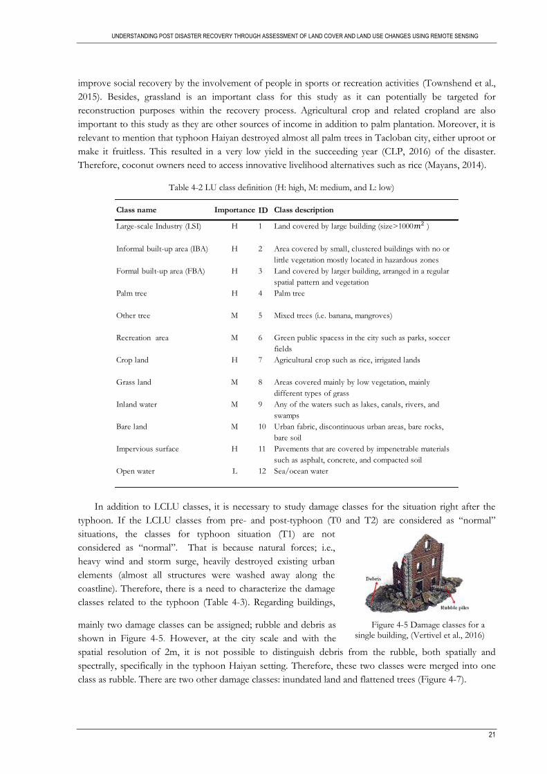
UNDERSTANDING POST DISASTER RECOVERY THROUGH ASSESSMENT OF LAND COVER AND LAND USE CHANGES USING REMOTE SENSING
21
improve social recovery by the involvement of people in sports or recreation activities (Townshend et al.,
2015). Besides, grassland is an important class for this study as it can potentially be targeted for
reconstruction purposes within the recovery process. Agricultural crop and related cropland are also
important to this study as they are other sources of income in addition to palm plantation. Moreover, it is
relevant to mention that typhoon Haiyan destroyed almost all palm trees in Tacloban city, either uproot or
make it fruitless. This resulted in a very low yield in the succeeding year (CLP, 2016) of the disaster.
Therefore, coconut owners need to access innovative livelihood alternatives such as rice (Mayans, 2014).
In addition to LCLU classes, it is necessary to study damage classes for the situation right after the
typhoon. If the LCLU classes from pre- and post-typhoon (T0 and T2) are considered as “normal”
situations, the classes for typhoon situation (T1) are not
considered as “normal”. That is because natural forces; i.e.,
heavy wind and storm surge, heavily destroyed existing urban
elements (almost all structures were washed away along the
coastline). Therefore, there is a need to characterize the damage
classes related to the typhoon (Table 4-3). Regarding buildings,
mainly two damage classes can be assigned; rubble and debris as
shown in Figure 4-5. However, at the city scale and with the
spatial resolution of 2m, it is not possible to distinguish debris from the rubble, both spatially and
spectrally, specifically in the typhoon Haiyan setting. Therefore, these two classes were merged into one
class as rubble. There are two other damage classes: inundated land and flattened trees (Figure 4-7).
Table 4-2 LU class definition (H: high, M: medium, and L: low)
Figure 4-5 Damage classes for a single building, (Vertivel et al., 2016)
ID
Inland water
Bare land
Impervious surface
Open water
H
H
H
H
M
M
H
M
M
M
H
L
Any of the waters such as lakes, canals, rivers, and
swamps
Urban fabric, discontinuous urban areas, bare rocks,
bare soil
Pavements that are covered by impenetrable materials
such as asphalt, concrete, and compacted soil
Sea/ocean water
9
10
11
12
Class name Class description
Large-scale Industry (LSI) 1 Land covered by large building (size>1000 )
Importance
Palm tree 4 Palm tree
Other tree 5 Mixed trees (i.e. banana, mangroves)
Informal built-up area (IBA) 2 Area covered by small, clustered buildings with no or
little vegetation mostly located in hazardous zones
Formal built-up area (FBA) 3 Land covered by larger building, arranged in a regular
spatial pattern and vegetation
Green public spacess in the city such as parks, soccer
fields
Crop land 7 Agricultural crop such as rice, irrigated lands
Grass land 8
Recreation area 6
Areas covered mainly by low vegetation, mainly
different types of grass

UNDERSTANDING POST DISASTER RECOVERY THROUGH ASSESSMENT OF LAND COVER AND LAND USE CHANGES USING REMOTE SENSING
22
Figures 4-6, 4-7 and 4-8 show land cover, damage, and land use classes, respectively. These photos
have been taken from the study area and provide an insight of the classes showing ground- and satellite-
based views.
To better understand recovery, there is a need to go from a coarse to a finer level (e.g., LC to LU) in a
hierarchical manner as shown in Figure 4-4. However, the hierarchical division should be fit with respect
to the recovery goals and the characteristics of the study area. In addition, except built-up related classes,
LC information is not informative enough to understand the recovery process. However, LC information,
as it is easier to extract from RS imagery, gives a general and quick overview of the area in the immediate
aftermath of a disaster and further in other phases of recovery. The reason is that in large natural disasters
and a short-term recovery a general overview of the process is required and can be used as an auxiliary
tool in order to effectively enhance other recovery-related activities in the ground (which can be
represented by LC information). On the other hand, LU can be used to understand medium- to long-term
recovery, especially for large natural disasters, where mostly land use plan is defined in relation to the
recovery process. In long-term recovery, more detailed information is needed to characterize the process
and to further check with LU plan to see if it is on track or not. Although LCLU collectively can help to
characterize different parts of recovery, it cannot characterize all aspects of the recovery process such as
accessibility analysis. However, in the recovery literature there are many local indicators which together
with LCLU information can help to cover this gap.
Table 4-3 Damage class definition (H: high, M: medium, and L: low)
Figure 4-6 Illustration of land cover classes
LC Non-Tree Tree Inland Water Open Water Building Impervious Surface Bare Land
Satellite View
Ground Based View
Importance
Flattened tree Lnad covered by fallen or toppled tree branches,
uprooting of smaller trees
Class name Class description
Rubble Damage patterns corresponding to a mix wind- water-
borne objects (rubble, debris, cars, building fragments)
Inundated land Rising of a body of water and its overflowing onto
normally dry land
H
H
H

UNDERSTANDING POST DISASTER RECOVERY THROUGH ASSESSMENT OF LAND COVER AND LAND USE CHANGES USING REMOTE SENSING
23
4.1.3. Framework Implementation
To implement the CF in the Tacloban city, first, complete TPs for LC and LU, which might occur in
the post-Haiyan recovery in the Tacloban city are listed (Annexes 1 and 2). The most relevant TPs are
selected and illustrated in Table 4-4 (LC) and Table 4-5 (LU). The characterization of the TPs is based on
the conceptual framework (section 4.1.1).
Figure 4-7 Illustration of damage classes
LU Grass Land Crop Land Palm Tree Other Trees Recreational Area IBA FBA LSI
Satellite View
Ground Based View
Figure 4-8 Illustration of land use classes; IBA: Informal Built-up Area, FBA: Formal Built-up Area, LSI: Large-Scale Industry
DM Derbis Rubble Inundated Land Flattened Trees
Satellite View
Ground Based View

UNDERSTANDING POST DISASTER RECOVERY THROUGH ASSESSMENT OF LAND COVER AND LAND USE CHANGES USING REMOTE SENSING
24
Table 4-4 LC- based conceptual framework for post- Haiyan recovery process in Tacloban city
Table 4-5 LU- based conceptual framework for post- Haiyan recovery process in Tacloban city
4.2. Land Cover and Land Use Analysis
In this section to investigate the utility of LCLU in recovery assessment, image analysis is performed
based on objective 2. This section addresses the research questions 4, 5, and 6.
4.2.1. A Brief Review of SVM
Based on the preliminary experiment carried out for a small subset of the area (Figure 4-9) and the
literature review (2.8.2), SVM classifier is used for the classification task. SVM is a very effective technique,
and it relies on both classification procedure and the elegance of the theoretical advances (Bruzzone &
Persello, 2009). The classification strategy of SVMs exploits a margin-based “geometrical” principle rather
than a purely “statistical” principle, meaning that it does not require an estimation of the statistical
distribution of the classes for the classification task (non-parametric classifier). Rather, the classification is
Transition
IDT0 T1 T2
Recovery
Status
252 Informal built-up area Rubble Informal built-up area
222 Informal built-up area Informal built-up area Informal built-up area
844 Grass land Flattened tree Palm tree
444 Palm tree Flattened tree Palm tree
747 Crop land Flattened tree Crop land
3510 Formal built-up area Rubble Bare land
3511 Formal built-up area Rubble Impervious surface
3311 Formal built-up area Formal built-up area Impervious surface
544 Other tree Flattened tree Palm tree
353 Formal built-up area Rubble Formal built-up area
1153 Impervious surface Rubble Formal built-up area
393 Formal built-up area Inundated land Formal built-up area
756 Crop land Rubble Recreation area
253 Informal built-up area Rubble Formal built-up area
2511 Large-Scale industry Rubble Large-Scale industry
N
SN
NT
SP
P
Transition
IDT0 T1 T2
Recovery
Status
644 Non-tree vegetation Non-tree vegetation Inland water
554 Tree Flattened tree Inland water
285 Impervious surface Rubble Tree
185 Building Rubble Tree
556 Tree Flattened tree Non-tree vegetation
221 Impervious surface Impervious surface Building
181 Building Rubble Building
281 Impervious surface Rubble Building
282 Impervious surface Rubble Impervious surface
552 Non-tree vegetation Non-tree vegetation Impervious surfaceP
N
SN
NT
SP

UNDERSTANDING POST DISASTER RECOVERY THROUGH ASSESSMENT OF LAND COVER AND LAND USE CHANGES USING REMOTE SENSING
25
based on the concept of margin maximization and structural risk minimization, minimizing the
misclassification error on the training set. SVM seeks an optimal hyperplane as a decision function in high-
dimensional space which maximizes the margin between classes via a small number of training samples
(support vectors) in feature space, which makes the SVM a suitable method to exploit the VHR imagery
potential (Volpi et al., 2013).
When classes are linearly separable (the simplest scenario),
SVM finds the separating hyperplane in away the distance
between the classes to the hyperplane (margin) is maximized.
For linearly non-separable classes a “slack variable” is
introduced. In this case, SVM seeks for the hyperplane that
maximizes the margin, while minimizing a quantity proportional
to the number of misclassification errors. The trade-off
mentioned above is controlled by a positive regularization
parameter C.
Moreover, for nonlinear decision surfaces a kernel function
is introduced by Vapnik (1995) where among different kernels,
RBF is widely used in the RS literature. The RBF kernel maps
sample into a higher dimensional space in a nonlinear way. The
accuracy of SVM-based RBF kernel is dependent on parameters C and 𝛾. The constant parameter C
controls the magnitude related to training data where lies in the wrong side of hyperplane and 𝛾 controls
the width of the kernel. A large value of 𝛾 and/or C tends to over-fit the training data which may yield a
low level of generalization ability which is unfavourable (Pal & Foody, 2010). There are some situations
where the linear kernel performs better than RBF kernel; i.e., when the number of features is very large
(Hsu et al., 2016). A detailed discussion on SVM and its mathematical background can be found in
Bruzzone & Persello (2009).
To make the best use of the performance of SVM, the RBF parameters (C and γ) should be optimized
and tuned (Foody & Mathur, 2004). It is suggested a grid-search using a cross-validation approach as the
most effective method to optimize RBF parameters (Hamedianfar & Shafri, 2015). The goal is to identify
the best parameter(s) so that the classifier can effectively predict previously unseen data (i.e., test data).
The best value of parameters (C and γ) will differ in a different dataset. Hence the parameters need to be
determined for each dataset (Richards & Jia, 2006) (Table 4-6).
For the SVM, both linear and RBF kernel is adopted, and the one with higher accuracy is picked and
presented. The best values for penalty (C) and kernel (γ) parameters of SVM are determined via grid
search algorithm and 10-fold cross-validation (Hsu et al., 2016). With the help of a training set, the
approach provides many learning models for a number of hyper-parameters. Each model is assessed using
the cross-validation procedure. The best model then is selected as the final model with tuned parameters
and further the performance is evaluated using a test set. To facilitate the procedure, R package ‘e1071’,
Table 4-6 Definition of parameters and related methods used in the experiment
Figure 4-9 Test area (500*500 pixel)

UNDERSTANDING POST DISASTER RECOVERY THROUGH ASSESSMENT OF LAND COVER AND LAND USE CHANGES USING REMOTE SENSING
26
which was implemented in LIBSVM library by Chang & Lin (2011) is employed. Exponentially growing
sequences of C and γ are used to identify best parameters, which is a one- and two-dimensional parameter
for linear and RBF kernel along 2𝑑, where d= {-5, -4, …} for γ and d= {5, 6, …} for C (Table 4-7).
Table 4-7 Definition of grid search space for tuning the hyper-parameters SVM
4.2.2. Utilization of Image Features and Spectral Indices
Since in this study, some of the LU classes need a high semantic definition (e.g., informal built-up
area) and also to decrease the spectral complexities of some similar classes (e.g., different types of
impervious surface and bare land), texture feature and spectral indices are used to help the classification
task. An example of the complexity is different road types in the study area: 1) concrete, 2) asphalt and 3)
compact bare soil, which together with other classes such as building, bare land, and rubble create a highly
complex scene.
Pixels, in very high (spatial) resolution imagery, are commonly smaller than the object of interest and
holds a small amount of contextual information to identify a class of interest accurately. The contextual
information describes the information derived from a neighborhood (image features). Image features are
hidden representation in data that help the learning and classification task by providing supplementary
information about image properties (Mboga et al., 2017). They are used to characterize the tonal or grey-
level variations in an image. Many image feature extractions are used in the urban remote sensing
literature. Image features such as those based on the calculation of the grey-level co-occurrence matrix
(GLCM) and local binary pattern (LBP). The GLCM and LBP, due to their discriminative power and
computational plainness are reported as the most useful for analyzing the content of VHR imagery for
urban studies (Gevaert et al., 2016; Kuffer et al., 2016; Mboga et al., 2017).
GLCM method computes the occurrence of pairs of grey-level value pixels in an image. The
maximum grey value of a pixel determines the size of the GLCM. The association between the pixels in
GLCM is determined by varying lag and direction (Rao et al., 2002). LBP features (Ojala et al., 2002) are
rotationally-invariant (image-based) texture features, which identify uniform features, such as corners and
edges, based on a well-defined number of neighboring pixels (P) at a distance (R) from the pixel located in
the center. For more information about LBP, see Ojala et al. (2002).
In this study, a code (in python) is used for LBP extraction using a variety combination of R= {2~4}
and P= {6~12}. Moreover, ENVI software is used to extract texture features with different lag distances
and windows sizes (e.g., 3*3, 5*5, 7*7, 9*9 and 3*3, 5*5, 7*7,15*15 for LC and LU tasks, respectively)
(Table 4-8). Although there are eight types of GLCM features (mean, contrast, angular second moment,
variance, dissimilarity, correlation, homogeneity, and entropy) which can be extracted from the image, not
all of them are helpful, and some are highly correlated, resulting in redundancy (Graesser et al., 2012). In
addition, 18 different types of spectral indices (Table 4-9) from the most recent literature (mostly using
Worldview 2 imagery) are used in order to help classification task.
Classifier Parameters Grid-search space Description
C
SVM
Regularization parameter which has a
significant impact on the generalization
performance of the classifier.
Regularization parameter in RBF kernel
with a great impact on the performance
of the kernel.
logarithmically spaced
logarithmically spaced
𝛾
2 2
2 2

UNDERSTANDING POST DISASTER RECOVERY THROUGH ASSESSMENT OF LAND COVER AND LAND USE CHANGES USING REMOTE SENSING
27
Table 4-8 Extracted features from multispectral image
Literature suggest that accuracy increases when combining textural and spectral features (Dhumal et
al., 2015). To prevent redundancy and to increase the effectiveness of classification task a feature selection
is employed. The feature selection reduces computational costs and avoids over-fitting the classifier.
Hilbert – Schmidt independence criterion (HSIC) is one of the popular methods in the RS community
(Song et al., 2012). HSIC is a nonparametric dependence measure, which takes not only into account
linear correlation, but also all modes of dependence between the features.
4.2.3. Experiment Setup
The main focus of the classification section is to employ the methodology that works well for both
LC and LU classification in order to either achieve the acceptable accuracy or improve the classification
accuracy for creating corresponding recovery maps. It is proposed that acceptable accuracy limits to LC
classification are when OA is higher than 80% (Manandhar et al., 2009). Since the experiments are
computationally intensive and due to hardware limitation, they are first applied in a small but
representative area (Figure 4-9), and once the best setting of features is defined, they will be applied for
the whole study area in order to produce the final results. The experiment setup is summarized as follow:
1) Using only the spectral bands of the WorldView-2 images for LC and LU classification (test area).
Type of Feature Features count Description
186
GLCM 256GLCM textural measures calculated
for multispectral bands
(b1:b8) reflectance values of
multispectral imageOriginal bands 8
Spectral indicies
Local Binary Pattern
18spectral indices calculated based on
the table …
ID Spectral index
Coastal - NIR 2 / Coastal + NIR 2
NDVI 1(Wolf, 2012)
15
16
14
17
18
(Aguilar et al., 2016)
(Hamedianfar & Shafri, 2015)
(Shahi et al., 2015)
NHFD Rededge - Coastal / Rededge + Coastal
Green - NIR 2 / Green + NIR 2
NDVI NIR 1 - Red / NIR 1 + Red
NDSI Green - Yellow / Green + Yellow
Red - NIR 2 / Red + NIR 2
NDWI 1
7
8
9
10
11
NDWI
12
13
1
2
3
4
5
6
R3 NIR 1 - Yellow / NIR 1 + Yellow
BSI Yellow - (2*NIR 1) / Yellow + (2*NIR 1) (Sameen & Pradhan, 2016)
(Elsharkawy et al., 2012)
R1 Red - NIR 1 / Red + NIR 1
R2 Coastal - Red / Coastal + Red
BAI Blue - NIR 2 / Blue + NIR 2
REI NIR 2 - Blue / (NIR 2 + (Blue * NIR 2))
NDBC Blue - Coastal / Blue + Coastal
NDN2C NIR 2 - Coastal / NIR 2 + Coastal
NDRR Rededge - Red / Rededge + Red
NDGR Green - Rededge / Green + Rededge
Equation Reference
Blue - NIR 1 / Blue + NIR 1NDNB
NDVI 2 NIR 2 - Red / NIR + Red
Table 4-9 Spectral index description

UNDERSTANDING POST DISASTER RECOVERY THROUGH ASSESSMENT OF LAND COVER AND LAND USE CHANGES USING REMOTE SENSING
28
2) Extract relevant spectral indices, then select the most informative ones and add them into spectral
bands for LC and LU classification (test area).
3) Calculate the GLCM measures (varying windows size with respect to LC and LU classes), then
select the most informative ones and add them into spectral bands for LC and LU classification
(test area).
4) Calculate the LBP features (varying P and R for LU classification), then select the most informative
ones and add them into spectral bands for LU classification (test area).
5) Combine the relevant spectral and textural features, then select the most informative ones and add
them into spectral bands for LC and LU classification (test area).
6) Perform final LC and LU classification based on the most useful setting of spectral and textural
features and produce the final LCLU maps (whole study area).
4.2.4. Accuracy Assessment
Accuracy assessment of classified map helps assign credibility to a map. The overall accuracy of the
classification is calculated from the confusion matrix, which is widely accepted in the remote sensing
works. As a derivative of confusion matrix, the global accuracy gives the proportion of correctly classified
pixels, by comparing the classified pixel to the reference data. The user’s and producer’s accuracies (UA
and PA rescpecitvely) of each class are calculated in order to show the error contribution of each class.
User’s accuracy refers to the error of assigning an incorrect label to a specific class, and it is measured by
dividing the total number of correct pixels in a category by the total number of pixels classified into that
class. On the other hand, producer’s accuracy is the error of failing to assign a correct label to a specific
class (Foody & Mathur, 2004). While the user’s accuracy is the degree of reliability of a classification,
producer’s accuracy is the degree of the ability to classify a particular class (Congalton, 1991). Moreover,
visual quality evaluation of the classified maps is carried out.
A common strategy for sampling method is used; the dataset is separated into two parts, one part for
training the classifier, and one (previously unseen) part of the study area for testing the accuracy of the
classifier, using stratified random sampling method. Reference data is obtained using visual interpretation
(Sliuzas, 2004). The prediction accuracy obtained from the previously unseen set more accurately reflects
the performance on classifying an independent data set (Hsu et al., 2016). Seven LC and twelve LU classes
were considered for accuracy assessment with the minimum of 500 sample pixels of each considered
classes, which provide a representative basis for accuracy assessment (Foody, 2002). In the absence of
fieldwork data, visual interpretation is used based on multi-source data such as Google Earth Pro (GE),
Open Street Maps (OSM), Google street view, and panchromatic bands of WV2 imagery.
4.2.5. Recovery Map
In order to address the research question 6, there is a need to define a methodology to assess the
recovery process after typhoon Haiyan. The recovery map is basically based on the implemented
conceptual framework and LCLU classified maps. It is pertinent to mention that, like the classification
approach, recovery maps are also pixel-based. To develop the recovery maps, first LC maps from three
time-spans (T0, T1, and T2) are stacked and then, for each map, the state of identical pixels is investigated.
For example, pixels “a”, “b” and “c” in Figure 4-10, represent the state of the identical pixels in LC
classification maps in three time-spans, which collectively represent a TP (e.g., a-b-c). The same is done
for all pixels in the maps, and all possible TPs are identified. In this study, a code in “R” is developed to
identify all possible TPs and to further select TPs based on the implemented conceptual framework in
section 4.1.1. The TPs are then illustrated in the output map. This map is referred as LC-based recovery
map. The same procedure is done for LU maps to create LU-based recovery map.

UNDERSTANDING POST DISASTER RECOVERY THROUGH ASSESSMENT OF LAND COVER AND LAND USE CHANGES USING REMOTE SENSING
29
4.3. Develop a Practical Guide
There are many RS-based indicators in the recovery literature. Although these indicators are helpful
for ground-based recovery analysis, their exploratory power and practicality in the RS perspective are not
investigated so far. Moreover, as mentioned earlier in chapter 2 there are some concerns about the
indicators; i.e., they are: expensive to collect, mostly local-type indicators and prone to subjectivity which
also are difficult to collect in a disastrous situation. Remote sensing data and methods are appropriate
alternatives to address those concerns. This section aims to address research questions 7 and 8, by
categorizing the indicators in relation to the recovery understanding gained from this study.
The practical guide is more a summary of an evaluation of existing recovery indicators. The guide
checks which ancillary data might help to detect the indicators by advance RS methods better, as currently,
they are not operationally usable. In order to address user needs, besides, the indicators categorized based
on their utility in the recovery assessment; i.e., macro, meso, micro indicators. The categorization method
is described in next paragraphs.
Among recovery indicators, there are some standards and well-established indicators in the recovery
discipline, which have already been used with conventional RS methods, such as visual interpretation, and
NDVI analysis (Brown et al., 2010). These indicators have high utilities in the recovery process. Meaning
that they extract recovery information spatially over large areas such as city scale. These indicators are
grouped under “macro indicators”. Moreover, there are indicators with medium to high utilities in the
recovery community. Although these indicators have the potential to reveal the recovery process spatially
within the city level, they are not frequently used in practice. Moreover, some indicators have been used in
other RS domains and have not yet been applied in recovery studies. Collectively, these indicators are
gathered as “meso indicators.” Thirdly, there are other types of indicators, which are local-types and
represent elementary units such as individual buildings within the recovery process. These indicators are
hardly visible and/or not visible by RS means. These indicators have low utility in the recovery assessment
and are grouped in “micro indicators.” In this study, a practical guide is developed in order to link meso
and micro indicators to remote sensing. In addition, these indicators are analyzed with respect to the
recovery process.
Overall, this chapter introduced the methods used in this study in three main sections. It was started
by introducing a generic LCLU-based CF which succeeded by LCLU analysis in the study area leading to
create recovery maps. However, the CF was described in the methodology part (as one of the results of
this study) which was needed for the remaining parts of this chapter, which is also mentioned in (Parsons
et al., 2016). The last section introduced the logic behind the practical guide. The next chapter will show
and analyze the result of methods employed.
Figure 4-10 Description of the recovery map

UNDERSTANDING POST DISASTER RECOVERY THROUGH ASSESSMENT OF LAND COVER AND LAND USE CHANGES USING REMOTE SENSING
30
5. RESULTS AND ANALYSIS
This chapter provides the result of this study. The first section represents the results of experiments
(method selection and parameter tuning) and their interpretations, and two recovery maps (LC- and LU-
based) are shown and interpreted. In the second section, a practical guide for existing indicators is
developed.
5.1. Land Cover and Land Use Analysis
This study used SVM classifier for a multi-temporal classification task; i.e., pre-disaster (T0), event
time (T1), and post-disaster (T2). In total, seven and twelve classes were identified (section 4.1.2) for LC
and LU analysis, respectively. Since the LCLU classification maps are highly important for creating
recovery maps, different experiments were conducted (section 4.2.3). A combined set of SVM,
SVM+GLCM, and SVM+GLCM+indicies were used, and the one with the highest accuracy was selected,
using both linear and RBF kernel. Feature selection was carried out based on HSIC method. Due to
hardware limitation, feature selection was applied for a small but representative subset of the study area
(Figure 4-9), and then the selected features in combination with original WV2 bands of the whole study
area were used to create the final classified maps.
5.1.1. Selected Features for Classification Task
From 18 different spectral indices (Table 4-9), based on the HSIC, NDVI2 was selected as the most
important spectral index. An experiment was carried out to select the most important GLCM measures
while varying the window size. Here, the GLCM variance and contrast measures of the first five bands of
WV2 imagery were selected as the most informative features for LC classification task (Table 5-1).
Similarly, the GLCM experiment was carried out for the LU task, where the different setting of features -
compare to LC features- were selected (Table 5-2). GLCM contrast is a suitable measure to differentiate
built-up areas such as building and impervious surface from the other classes. GLCM variance mainly
represents building structures in formally developed areas which help to differentiate between buildings
and impervious surface (Kuffer et al., 2016).
An experiment to explore the effect of varying the window size of the extracted GLCM features on
the LC and LU classification result was conducted. For the LC task, increasing the window size results in a
corresponding decrease in the overall accuracy. For the LU task, some of the larger window sizes are
selected in combination with 3*3 window size (Table 5-2). For LC classification a large window size such
as 9*9 (324 m2 on the ground) implies that features extracted from a larger context are less informative
than those extracted from a smaller context. This is sensible, as detection of simple LC classes does not
require abstract definition like informal built-up area (Mboga et al., 2017). To differentiate non-built up
areas from vegetation areas NDVI2 shows a good discriminative power which also helps to improve the
classification accuracy as also mentioned in the Kuffer et al. (2016) study.

UNDERSTANDING POST DISASTER RECOVERY THROUGH ASSESSMENT OF LAND COVER AND LAND USE CHANGES USING REMOTE SENSING
31
5.1.1.1. Utility Analysis of Image-Features in LC Classification
The LC classification results from SVM, SVM+NDVI2, SVM+GLCM, SVM+GLCM+NDVI2 are
compared in Table 5-3. The combination of SVM+GLCM+NDVI2, achieved the highest classification
accuracy with an RBF kernel. Classifications relying on spectral bands alone result in lower classification
accuracies. Addition of image-features causes an increase in the classification accuracy as shown for
SVM+NDVI2, SVM+GLCM, and SVM+GLCM+NDVI2. As the SVM+GLCM+NDVI2 setting
performs slightly better than (only 0.4%) SVM+GLCM using RBF kernel, this setting is selected to be
applied to the whole study area in order to produce the final LC classification maps.
Several insights can be drawn by comparing the performance of the different experiment setups. First,
linear-based SVM consistently shown lower performances than RBF-based SVM for LC classifications.
The classification accuracy of linear-based SVM, are 76.3%, 79.6.2%, 81.2%, and 83.4%, whereas the
classification accuracy of RBF-based SVM, are 81.2%, 83.7%, 94.3%, and 94.7% for SVM, SVM+NDVI2,
SVM+GLCM, SVM+GLCM+NDVI2 respectively. Moreover, Table 5-3 shows spectral information
alone is insufficient to discriminate the land cover classes. However, adding image-features improve the
classification accuracy. For example, by adding GLCM, there is an increase of 10.6%.
5.1.1.2. Utility Analysis of Image-Features in LU Classification
The LU classification results from SVM, SVM+GLCM, SVM+GLCM+NDVI2, SVM+LBP,
SVM+LBP+GLCM, SVM+LBP+NDVI2 are compared in Table 5-4. The SVM+LBP+NDVI2 and
SVM+LBP show the highest classification accuracies with RBF kernel. However, as the
SVM+LBP+NDVI2 setting performs slightly better than (only 0.5%) SVM+LBP, this setting is selected
to be applied to the whole study area in order to produce the final LU classification maps. Classification
relying on spectral bands alone results in low classification accuracy. Addition of image features leads to an
increase in the classification accuracy as shown in SVM+GLCM and SVM+LBP. For example, by adding
GLCM, there is an increase of 20.1%. This value increased by 8.7% when LBP is added. The linear-based
SVM shows a lower performance than the RBF-based SVM. Moreover, SVM+LBP performs better as
compared to SVM+GLCM. Surprisingly, SVM+LBP+GLCM has led to a lower accuracy as compared to
SVM+LBP.
band feature window size
variance
contrast
variance
contrast
variance
contrast
variance
contrast
variance
contrast
3*3
Coastal
Blue
Green
Yellow
Red
band feature window size
variance 3*3
contrast 3*3
variance 7*7
variance 15*15
variance 3*3
contrast 3*3
variance 7*7
variance 15*15
variance 3*3
contrast 3*3
variance 3*3
contrast 3*3
NIR2 contrast 3*3
Blue
Rededge
NIR1
Red
Table 5-1 Selected GLCM features for LC classification
Table 5-2 Selected GLCM features for LU classification

UNDERSTANDING POST DISASTER RECOVERY THROUGH ASSESSMENT OF LAND COVER AND LAND USE CHANGES USING REMOTE SENSING
32
5.1.2. Accuracy Assessment
The classification result of both LCLU maps is analyzed and discussed in this section.
5.1.2.1. LC Accuracy Assessment
For creating the LC classification maps, SVM+GLCM+NDVI2 was applied to the whole study area
for the three-time span. In Table 5-5, UA and PA for three time-span (T0, T1, and T2) are presented.
In general, SVM set has higher values for pre- and post-disaster as compared to the event time. The
Overall Accuracy (OA) for T0 and T2 are 89.4% and 90.8% respectively, while the OA for T1 is 82.2%.
This is sensible because of the disaster in the area, a new setting of spectral reflectance of the classes exist
as compared to spectral reflectance of the classes in the normal situation. For instance, bare land in a
normal situation does not hold water, whereas in the disaster situation (although visually the class in the
imagery seems the same) bare land contains a higher amount of water, which leads to a variation in its
SVM+LBP+NDVI_2 72.2 75.6
SVM+GLCM 62.6 66.4
SVM+GLCM+NDVI_2 61.1 68.3
OA%
SVM+LBP+GLCM 69.8 72.4
SVM+LBP 71.3 75.1
Experiment setup
SVM 45.6 46.3
RBFLinear
Table 5-3 Comparison of LC classification accuracies of test area
Table 5-5 Comparison of LC classification accuracies for pre-, event, and post-disaster situation. Overall, user and producer accuracies and corresponding errors are computed across the whole study area by combining the confusion
matrices of T0, T1, and T2.
Table 5-4 Comparison of LU classification accuracies of test area
UA% PA% OA% Commission Omission UA% PA% OA% Commission Omission UA% PA% OA% Commission Omission
Building 95.5 83.8 4.5 16.2 68.0 55.0 32.0 45.0 82.2 94.2 17.8 5.8
Impervious
Surface83.8 96.3 16.2 3.7 82.0 68.8 18.0 31.2 84.3 99.5 15.7 0.5
Bare 88.0 83.4 12.0 16.6 76.9 50.2 23.1 49.8 98.0 62.3 2.0 37.7
Inland Water 87.3 90.3 12.7 9.7 95.2 94.2 4.8 5.8 98.8 99.9 1.2 0.1
(Flattened)
Tree77.9 88.9 22.1 11.1 83.1 96.1 16.9 3.9 96.5 92.9 3.5 7.1
Non_tree
vegetation93.5 85.2 6.5 14.8 89.5 61.0 10.5 39.0 92.7 90.9 7.3 9.1
Rubble *** *** *** *** 64.4 87.7 35.6 12.3 *** *** *** ***
Open
Water99.8 96.5 0.2 3.5 98.5 100.0 1.5 0.0 98.3 98.9 1.7 1.1
89.4 82.2 90.8
Class
Pre Disaster (T0) Event (T1) Post Disaster (T2)
Accuracy Error Accuracy Error Accuracy Error

UNDERSTANDING POST DISASTER RECOVERY THROUGH ASSESSMENT OF LAND COVER AND LAND USE CHANGES USING REMOTE SENSING
33
spectral reflectance (Figure 5-1 (A1)). This is also exemplified in the high value of omission error in the
bare land class (49.8%). One possible solution for this is using another imagery from a time when holding
water is evaporated. However, this could potentially lead to losing damage class information. The other
reason for a lower OA for T1 is due to low PA and UA of the building, impervious surface, and rubble
classes, see Figure 5-2 (T1). The UA of the classes building and rubble are 68.0% and 64.4%, respectively,
which highlights the error of commission in these two classes and related uncertainty. This is sensible as
they are spectrally similar, and the classifier confused these two classes, leading to the high amount of
commission error. The problem potentially can be solved by introducing more useful information (data
fusion) to classifier such as LIDAR data and or using pan-sharpened data. The former would differentiate
the building from rubble due to the inherent height difference of these two classes, while the latter would
potentially help to enhance the spatial discriminative power of the classifier. There is also confusion and
relatively high amount of commission error for building and impervious class, ranging from 4.5% and
16.2% in T0, and 32.0% and 18% in T1, to 17.8% and 15.7% in T2, respectively. This confusion is
unavoidable due to the presence of concrete and asphalt roads, making it difficult to differentiate between
asphalt roads, concrete roads, and other built-up classes.
Figure 5-2 Complex status of built-up-related classes in the three time-span
Figure 5-1 A subset of WV2 imagery, (A) area of confusion between “crop” and “grass” in three time-span, (B) area of confusion between “palm tree” and “other tree” in three time-span and
related multi spectral and panchromatic zooming window, (C) status of potential grass land

UNDERSTANDING POST DISASTER RECOVERY THROUGH ASSESSMENT OF LAND COVER AND LAND USE CHANGES USING REMOTE SENSING
34
5.1.2.2. LU Accuracy Assessment
SVM+LBP+NDVI2 is applied to the whole study area for a three-time span in order to create LU
classification maps. Table 5-6 presents the UA and PA for three time-span.
The accuracies are computed for T0, T1, and T2. In general, higher accuracies are achieved for the
pre- and post-disaster as compared to the event time. This highlights the complexity of the scene in the
event time, as it is reflected in the LC result as well. Moreover, the OA of the LC
classification consistently is higher than the OA of the LU classification. LU
classes are rather heterogeneous and are more classes as compared to LC
classification, as also mentioned in Herold et al. (2014, 2003). For example, LU
classes range from palm tree to large-scale industry and informal settlements;
from a very fine and simple class to a very large and abstract class in terms of the
size and definition. Although such classes are needed from the recovery
perspective, they make the image classification more complex as they cannot rely
only on spectral information. Moreover, there is a confusion between the class
“palm tree” and “other tree” (Figure 5-3), which is rooted in the high spectral
similarity of the classes coupled with the low spatial resolution of WV2 imagery
(2m) for such discrimination as shown in Figure 5-1 (B). The potential solution
could be using higher spectral and spatial resolution imagery, including pan-
sharpening images (Santoso et al., 2016), where due to the inherent variation of
the class “other tree” (like crop) range of subclasses can also be defined to solve
the ambiguity. However, introducing subclasses can restrict the study to a local
context, and would demand more data; e.g., hyperspectral and radar (Dhumal et
al., 2015; Ozdogan et al., 2010). For instance, radar data allow detecting rice
fields, especially where it is characterized by wide inter-field variability in addition
to being fragmented by other LUs as mentioned in the work of Mansaray et al.
(2017). Another uncertainty is the confusion within classes “crop”, “grass”, and “recreational area”. If
UA% PA% OA% Commission Omission UA% PA% OA% Commission Omission UA% PA% OA% Commission Omission
Large Scale
Industry88.3 59.7 11.7 40.3 84.2 86.6 15.8 13.4 77.7 77.2 22.3 22.8
Large Scale
Industry
Informal
Built up
Area
76.7 81 23.3 19.0 93.7 59.7 6.3 40.3 97.6 37.0 2.4 63.0
Informal
Built up
Area
Formal Built
up Area53.7 90.8 46.3 9.2 69.8 72.7 30.2 27.3 68.3 39.1 31.7 60.9
Formal
Built up
Area
Palm Tree 66.1 93.4 33.9 6.6 58 56.6 42.0 43.4 84.6 83.5 15.4 16.5Flattened
Tree
Other Tree 64.4 42.1 35.6 57.9 75.3 82.8 24.7 17.2 38.3 86.5 61.7 13.5 Rubble
Recreation
Area91.8 68.8 8.2 31.2 97.2 73.8 2.8 26.2 64.4 19.1 35.6 80.9
Recreation
Area
Crop Land 72.8 73.2 27.2 26.8 80.7 43.2 19.3 56.8 50.1 85.0 49.9 15.0 Crop Land
Grass Land 66.7 65.6 33.3 34.4 58.2 86.2 41.8 13.8 40.5 33.4 59.5 66.6 Grass Land
Inland Water 97.2 92.3 2.8 7.7 96.2 99.1 3.8 0.9 84.4 94.5 15.6 5.5Inundated
Land
Bare Land 95 75.1 5.0 24.9 94.5 73.7 5.5 26.3 87.4 45.9 12.6 54.1 Bare Land
Impervious
Surface79.5 82.7 20.5 17.3 62.6 95.7 37.4 4.3 74.5 69.6 25.5 30.4
Impervious
Surface
Open Water 100 98.9 0.0 1.1 99.3 98.5 0.7 1.5 98.6 99.1 1.4 0.9Open
Water
T1 Class
76.3 77.8 69.9
Error Accuracy ErrorAccuracy ErrorT0, T2 Class
Pre Disaster (T0) Event (T1)Post Disaster (T2)
Accuracy
Figure 5-3 Complexity of the palm tree and other tree classes; palm trees are shown with red circles; drone imagery
Table 5-6 Comparison of Land Use Classification Accuracies

UNDERSTANDING POST DISASTER RECOVERY THROUGH ASSESSMENT OF LAND COVER AND LAND USE CHANGES USING REMOTE SENSING
35
“crop” is considered as an irrigated land, then a multi-temporal (phenology) analysis has a great potential
to define cropland from the other two classes (Ozdogan et al., 2010). For instance, by adding images from
the time when a specific crop-type is matured and, adding another from the time when the crop-type is
harvested (2 images of pre-disaster and other 2 of post-disaster), which can also solve the confusion
related to bare land and harvested land.
5.1.3. Visualization of Classified Maps
From LC classified maps (Figure 5-4), it is observed that the boundary is much smoother in T0 and
T2 over T1. Furthermore, T0 and T2 have less noisy classified maps than T1 map. For T1, there is a
misclassification in the built-up area among the “bare land, “impervious surface, “building”, and “rubble”
which is also reflected in the confusion matrix. This confusion is worse in the LU classification, (Figure 5-
5 and Figure 5-2), where the presence of the classes LSI, IBA, and FBA inherently add more confusion as
they are spectrally similar. However, this misclassification is reduced in both T0 and T2 for both LC and
LU maps. Zooming in at the raw image, it is clear that there is an open field in the South-East part of the
area, which covered by “crops”, “grass”, “other trees”, and “palm tree” see Figure 5-1 (A). This could be
an example of existential uncertainty, whereby there is some doubt on the presence of the grass class in a
given area. The classification results show the SVM with data of a spatial resolution of 2m perform well in
LC level, while it faces difficulty in LU level, as mentioned earlier. GLCM features work well in LC
classification, while more information could improve the accuracy of LC classification.
Figure 5-4 also shows the LC-related pie charts. The class building covers 15%, 8%, and 15% of the
area in T0, T1, and T2 respectively. This implies that almost all buildings are reconstructed within 4 years
after the typhoon, which also can be seen by visual interpretation of raw imagery. The above-mentioned
rebuilding can be considered a positive sign of recovery. However, more information is needed to
characterize that recovery status. Impervious surface shows an increase of 3% in T2 compared with T0.
This also can be visually seen in the raw image, where, for instance, a national road that is constructed in
T2 in the West part of the city (Figure 5-8 (F)). For the vegetation category, the area covered by tree
decreased by 2% in T2 as opposed to T0, while conversely, the area of non-tree vegetation increased by
2% in T2 against T0. Considering the damage classes in the disaster situation (T1), 37% of the area is
occupied by rubble, while 8% of the land is inundated and 27% of the land is covered by flattened tree.
The damage classes show huge destruction in Tacloban city leading to a massive human and property loss
(Adriano et al., 2015; Yi et al., 2015).
Figure 5-5, on the other hand, shows the LU related pie charts. In the sub-building category, the size
of LSI is remained the same in T2 as like T0 (3%), though it shows a very slight decrease of about a mere
1% to 2% in T1, which in general indicates a good sign of business recovery. The area covered by IBA cut
half in the event time from 4% (T0) to 2% (T1). This is sensible as typhoon heavily destroyed the slum
areas in Tacloban city (Mas et al., 2015). Although the IBA class increased by 1%, from 2% to 3% in 2017
(T2), it is not a good sign of the recovery process. The FBA class showed a decrease of 5% in T2 as
compared to T0. This is not very sensible and is mainly due to uncertainty in the classification of FBA in
T2 as discussed earlier. The size of covered land by palm tree shows a decrease by 7%, from 18% in T0 to
11% in T2, which is sensible due to both CLP and required time for growing of a palm tree (Yi et al.,
2015). With regards to subclasses of non-tree in LC level, in the recreational area increased by 1%, from
3% in 2013 to 4% in 2017. Moreover, there is an approximate 3% growth in cropland in 2017, compared
to T0 in 2013. The increase in recreational area is a good sign of recovery, as the size of the recreational
area also planned to be increased in the CLP (2016). However, the growth of the size of cropland is not
necessarily a good sign of recovery as the CLP (2016) planned to reduce the size of cropland. On the
other hand, the palm farmers need to replace flattened palm trees by another crop type in order to live

UNDERSTANDING POST DISASTER RECOVERY THROUGH ASSESSMENT OF LAND COVER AND LAND USE CHANGES USING REMOTE SENSING
36
(cash crop). However, more information would be required to investigate the role of cropland change in
the recovery process.
Overall, in both T0 and T2, the most significant changes in LC is the increase in the area covered by
the impervious surface in T2, while the building is reconstructed almost to the size of the pre-disaster
situation which initially can be seen as a good sign of recovery. However, LU information revealed that
the rebuilding is a negative sign of recovery, where slum areas (IBA) are reconstructed in the same area in
T2.
Figure 5-4 LC Classification maps from SVM relying on GLCM features and NDVI2 for T0, T1, and T2 and
corresponding pie charts
Area per class
Eve
nt
(T1)
Po
st (
T2)
Raw image Classified map
Pre
(T
0)

UNDERSTANDING POST DISASTER RECOVERY THROUGH ASSESSMENT OF LAND COVER AND LAND USE CHANGES USING REMOTE SENSING
37
5.1.4. Errors Due to Uncertainty
Existential and extensional uncertainties are two factors of accuracy assessment. Existential
uncertainty relates to whether an object is existing in the geographical location it is said to be, while
extensional uncertainty is related to lack of an exact definition of the boundary of a phenomenon (Kohli,
Area per classP
ost
(T
2)E
ven
t (T
1)Raw image Classified map
Pre
(T
0)
Figure 5-5 LU Classification maps from SVM relying on LBP features and NDVI2 for T0, T1, and T2 and related pie charts, LSI: Large Scale Industry, IBA: Informal Built up Area, FBA: Formal Built up Area

UNDERSTANDING POST DISASTER RECOVERY THROUGH ASSESSMENT OF LAND COVER AND LAND USE CHANGES USING REMOTE SENSING
38
2015). In the context of understanding the recovery process through LC and LU from VHR, these
concepts are important. First, in the absence of fieldwork, normally important for the creation of
reference data, visual interpretation of Google Earth imagery (same time of the satellite images) was used
to digitize the requisite classes. In this process, instances were encountered whether an area was the class
supposed to be or not. For instance, the most doubtful classes were grass, crop, palm tree, other tree, and
bare land, such as the presence of green space (potentially grassland) next to an open cropland (Figure 5-1
(C)). Examples of existential uncertainties for palm tree and other tree are shown in Figure 5-1 (B), and
for bare land in Figure 5-1 (A1). Second, defining the exact delineation between an area that is IFA, FBA,
and rubble was a source of uncertainty (Figure 5-2). Uncertainty in the location and boundary of a
phenomenon such as slum, probably will affect the accuracy of the reference data and the quality of the
metrics calculated using it (Kohli, 2015).
However, this study was aware of the above-mentioned uncertainties and tried to mitigate them by
using a multi-source data ranging from Google Earth at the same time of the satellite images, open street
maps data, panchromatic band of WV2, street view of GE, to LC map from Tacloban as the first input to
the visual interpretation process. In addition, morphological characteristics based on literature and
described in Kuffer et al. (2014) were used to identify FBA and IBA. It would be favorable to measure
these uncertainties in future research.
5.1.5. Recovery Maps
Based on the developed conceptual framework for Tacloban city and LCLU classified maps, two
recovery maps are developed (Figure 5-6). With regards to the LC-based recovery map (Figure 5-6 (A)), it
is observed that the recovery class “slightly positive” (SP) is the dominant class (226 ha.), followed by
classes “positive” (P) and “neutral” (NT), where the class “negative” (N) has the lowest portion by 12 ha
as shown in Figure 5-7 (B). The reason why SP class is dominant is that the LC classes are mostly broad
categories which can be divided into many subclasses. Therefore, most of the transition patterns need
more information to be precisely characterized. For instance, slum areas are part of the “building” class in
LC level, while it is “IBA” in the LU level. The transition pattern (TP) “building-rubble-building” in the
LC-based recovery map, is the most responsible TP and is characterized as the class SP recovery.
However, the TP mentioned above can be “IBA-rubble-IBA” in LU-based recovery map and is
categorized as negative (N) recovery, see Figure 5-8 (A). Thereby, LU provides more effective information
in some transitions, compared to LC information. Moreover, it seems LC information is enough to
characterize some classes and related TPs. For instance, a new national road in the West part of the area is
well-captured by LC-based recovery map, see Figure 5-8 (F). This is also exemplified in the Figure 5-8 (E),
where a parking lot is added to a commercial building. Thereby, there is no need for more information to
characterize P recovery in LC-based recovery map; i.e., land use information. A negative example of
recovery, in LC level, is also shown in Figure 5-8 (C), where “non-tree” is turned to “inland water”. The
NT recovery also covers a large area in LC-based recovery map. This is related to the broad definition of
the LC classes, where there are more chances for TPs to be categorized as NT compared to LU-based
recovery map. Figure 5-8 (D), moreover, shows a potential positive recovery TP which has not been
captured by both recovery maps. This can highlight lack of image data from other times to track some
specific TPs which cannot be grasped by only a 3-time based recovery map. Considering LU-based
recovery map (Figure 5-6 (B)), it can be seen that the recovery classes are almost equally distributed in
terms of area covered in ha. The class SN is the dominant class (area covered is 87 ha.), which closely
followed by SP (74 ha.), see Figure 5-7 (C). This is sensible as in LU regulation after Haiyan it was decided
to reduce the amount of crop and increase the amount of FBA by CLP (2016). However, since the

UNDERSTANDING POST DISASTER RECOVERY THROUGH ASSESSMENT OF LAND COVER AND LAND USE CHANGES USING REMOTE SENSING
39
geographic location of the place where this reduction should be implemented is not defined in CLP
(2016), it is characterized as SN.
Moreover, in the Figure 5-7 (A), it is illustrated that the area covered by class “other transition” (OT),
is almost equal for both LC- and LU-based recovery maps. More area is classified as SN and N in the LU-
based recovery map compared to the LC-based recovery map. Conversely, classes NT, SP, and P are more
dominant in the LC-based recovery map as compared to LU-based recovery map.
Figure 5-7 (A) A comparison between LC- and LU-based recovery map; (B) area per class for LC-based recovery map; (C) area per class for LU-based recovery map
Figure 5-6 (A) LC-based recovery map; (B) LU-based recovery map; data source: WV2 images (T0, T1, and T2); recovery map approach: based on a code developed in R; main Observation: striking difference between A and B is mainly due to 2 issues:1) class slightly positive recovery (SP) in A, where the area is mostly covered by TP “building-rubble-building”, which this TP is changed to other TPs in B such as IBA-rubble-IBA (N: negative recovery) 2) due
to different TPs used in A and B

UNDERSTANDING POST DISASTER RECOVERY THROUGH ASSESSMENT OF LAND COVER AND LAND USE CHANGES USING REMOTE SENSING
40
In order to avoid noise introduced by isolated pixels a majority filter with the kernel size of 5*5 is
applied to both recovery maps, see Figure 5-9. It is evident that more area in both maps are accounted for
the class OT, and those which are not in the OT class are resilient enough to this aggregation. Although
up-scaling of the map removes some information, the maps with majority filtering provide more efficient
information for policymakers at city level. The reason for that is policymakers need more concise
information than a detailed map full of information, while also an aggregate map is easier to communicate.
A detailed map is appropriate for stakeholders at the neighbourhood level, where they can benefit from
detailed recovery information for their needs at a local scale. Overall, an aggregated map is potentially
useful in a city level while for a neighborhood level a detailed recovery map is more desirable.
Figure 5-8 Visual examples of LC- LU-based recovery maps
C
C
C

UNDERSTANDING POST DISASTER RECOVERY THROUGH ASSESSMENT OF LAND COVER AND LAND USE CHANGES USING REMOTE SENSING
41
5.2. Practical Guide
An effective way to assess the recovery process and or to compare different events and related
recovery processes is using indicators (Chang, 2010). In the recovery literature, there are some indicators
with different levels of practicality. These indicators are categorized into 3 groups based on definitions
given in section 4.3. Moreover, some indicators from other disciplines are included (with the potential to
provide recovery information). Indicators are grouped as macro, meso, and micro indicators (Table 5-7,
Table 5-8, and Table 5-9).
The first group of the indicators “macro indicators” are those with a high utility in the recovery
context, where already well-established RS method(s) exist. For example, nighttime lights can be well
captured by visible infrared imaging radiometer suite (VIIRS). These indicators can easily reveal important
information about the recovery process over a large scale; i.e., city scale, see Table 5-7.
The second group of indicators are “meso indicators”, which in comparison with macro indicators are
less practical and mostly are applicable within the city scale. Although these indicators have the potential
to be used in the recovery context, they have not frequently been used so far. Thereby, there is a need for
a guide to distinguish them in RS data and proposed which kind of data processing can be employed for
their recognition. By using the provided practical guide, they can be used more frequently and effectively
in the recovery context. The practical guide aims to best link these indicators to RS methods. Moreover, a
short recovery analysis for these indicators is done in Table 5-8. This table first, checks which spatial
resolution is suitable for the specific indicator for both visual interpretation and semi-automatic analysis.
Then, lists, which auxiliary data type, time of the day (ToD), unit of analysis, RS method, field of view, and
number of images, is required. Auxiliary data type provides a list of potential auxiliary data in addition to
optical RS to help to best detect and analyze a specific indicator. The indicators are checked whether they
are related to physical and or functional recovery and also if they are more useful in the short- or long-
term recovery.
As already mentioned earlier in chapter 2, there are some local type indicators with a low utility in the
recovery, which are hard or impossible to detect by RS. These indicators are categorized in “micro
indicator” as they have low utility in the recovery context; i.e., they can be used at the neighbourhood level
(Table 5-9). They either can be visually detected with spatial resolution of 1-10 cm by super resolution
Figure 5-9 (A) Aggregated LC-based recovery map, (B) Aggregated LU-based recovery map

UNDERSTANDING POST DISASTER RECOVERY THROUGH ASSESSMENT OF LAND COVER AND LAND USE CHANGES USING REMOTE SENSING
42
visible (SRV), or there is no existing RS method to detect them. Moreover, for those that visually are
detectable, there is no existing semi-automatic method allowing for monitoring.
Key for Tables 5-8 and 5-9
Optical RS: MRV, moderate resolution visible (spatial resolution >10–30 m); HRV, high resolution visible (spatial
resolution >2–10 m); VHRV, very high resolution visible (spatial resolution better than 2 m); SRV, super resolution
visible (spatial resolution >1–10 cm);
Auxiliary data type: Hyp, hyperspectral imagery; IR, infrared (typically a NIR band in optical sensors); VIIRS, Visible
Infrared Imaging Radiometer Suite; Vin, vegetation index; BuI, built-up index; TF, texture feature; DF, data fusion;
Unit of analysis: PB, pixel based; OB, object based; RB, region based;
RS Method: ML, machine learning; DL, deep learning; LM, landscape metrics;
FoV (field of view): V, vertical; Obl, oblique;
Recovery analysis Type: Phs, physical; Fnc, functional;
Recovery analysis Time: STR, short term recovery; LTR, long term recovery
EM, existing method
: from ecology discipline
Indicator Methods Reference
Change in urban morphology landscape metrics (Hagelman et al., 2012)
Night time lightVisible Infrared Imaging Radiometer
Suite (VIIRS)(Deville et al., 2014; Sutton et al., 2007)
Deforestation NDVI analysis
Impervious surface visual interpretation, maximum likelihood
Reconstruction of bridges and
public transportation facilitiesstandard CD methods
Proportion of built up and
vegetated area
NDVI analysis, standard CD methods
combined with GIS(Ebert et al., 2009)
Debris removalvisual interpretation, standard CD
methods(Hill et al., 2011)
Vegetation recovery NDVI analysis, visual interpretation,
standards CD methods(Wagner et al., 2012)
Reservoirs visual interpretation, NDVI analysis,
maximum likelihood(Harb et al., 2015)
Roads visual interpretation, maximum likelihood (Weng, 2012)
(Brown et al., 2010; Curtis et al., 2010)
Table 5-7 Macro indicators with high utilities in the recovery assessment

UN
DE
RS
TA
ND
ING
PO
ST
DIS
AS
TE
R R
EC
OV
ER
Y T
HR
OU
GH
AS
SE
SS
ME
NT
OF
LA
ND
CO
VE
R A
ND
LA
ND
US
E C
HA
NG
ES
US
ING
RE
MO
TE
SE
NS
ING
43
Tab
le 5
-8 M
eso
In
dic
ato
rs w
ith
med
ium
to
hig
h u
tilit
ies
in t
he
reco
ver
y as
sess
men
t (l
ist
of
acro
nym
s is
pro
vid
ed a
fter
Tab
le 5
-7 o
n t
he
pre
vio
us
pag
e)
MR
VH
RV
VH
RV
SR
VH
ypIR
VII
RS
Rad
arV
InB
uI
TF
LiD
AR
DF
Mor
No
oE
veN
igP
BO
BR
BM
LD
LL
MV
Obl
1>
1P
hs
Fnc
Mix
ST
RL
TR
Build
ing
hei
ght
and
area
**
**
**
**
**
**
(B
runner
et
al.,
2010
; Shak
er
et a
l., 2
011;
Xie
et
al.,
2017
)
Par
king
lots
**
**
**
**
**
**
(W
ei e
t al
., 20
13; X
iao
et
al.,
&
Pap
aroditis
, 20
16)
Pre
sence
of
boat
s
(fis
her
y in
dust
ry)
**
**
**
**
**
**
* (
Elv
idge
et
al.,
2015
; X
u e
t al
.,
2014
)
Ara
ble
lan
d (
dif
fere
nt
crop t
ype)
**
**
**
**
**
**
**
**
* (
Dh
um
al e
t al
., 20
14;
Ozd
oga
n e
t al
., 20
10)
Rec
onst
ruct
ion o
f
gove
rnm
ent
build
ings
**
**
**
**
**
**
(X
ie &
Zhou, 20
17)
War
ehouse
s*
**
**
**
**
**
**
**
(H
uif
eng
& A
igo
ng,
20
08
)
rail
road
s*
**
**
**
**
* (
Ara
stounia
, 20
15; G
edra
nge
et a
l., 2
011)
Str
uct
ure
unch
ange
d
since
dis
aste
r ev
ent
**
**
**
**
**
**
Str
uct
ure
reb
uilt
in
sam
e fo
otp
rint
**
**
**
**
**
**
Str
uct
ure
reb
uilt
dif
fere
nt
footp
rint
**
**
**
**
**
**
Sta
ge o
f dev
elopm
ent
(iden
tifi
cati
on o
f la
nd
clea
rance
and
foundat
ions)
**
**
**
**
**
**
**
(B
row
n e
t al
., 20
10)
Tra
ffic
act
ivity
(pre
sence
of
vehic
le)
**
**
**
**
**
**
**
**
(W
ei e
t al
., 20
13; X
iao
et
al.,
2016
)
Cam
p l
onge
vity
**
**
**
**
**
(P
eliz
ari et
al.,
201
7; S
prö
hnle
et a
l., 2
014;
Tie
de
et a
l., 2
017)
Acc
essi
bili
ty/ R
oad
acce
ss (
conditio
n)
**
**
**
**
**
(A
ndre
ou e
t al
., 20
11; H
erold
& R
ober
ts, 20
05)
Bri
dge
conditio
n
**
**
**
**
**
**
**
(A
hlb
orn
et
al.,
2010
;
Ch
audhuri
& S
amal
, 20
08;
Endsl
ey e
t al
., 20
12)
Nu
mb
er o
f st
reet
inte
rsec
tion
**
**
**
**
**
**
* (
Sch
neb
ele
et a
l., 2
015;
Wan
g
et a
l., 2
016)
Slo
p p
osi
tion
**
**
**
**
**
(V
annes
chi et
al.,
201
7)
Turb
idity,
Susp
ended
sedim
ent
**
**
**
**
**
*(P
etto
relli
et
al.,
2017
)
Pre
sence
of
was
te
pro
duct
s in
the
soil
**
**
**
**
* (
Pen
g et
al.,
201
6)
Pre
sence
of
ship
s in
har
bor
**
**
**
**
**
* (
Elv
idge
et
al.,
2015
; M
arga
rit
et a
l., 2
009;
Xu e
t al
., 20
14)
pre
sence
of
air
pla
ne
in t
he
airp
ort
**
**
**
**
* (
Ch
en e
t al
., 20
14; Q
inhan
Luo, 20
16)
Pre
sence
of
coco
nut
tree
**
**
**
**
**
**
**
**
(San
toso
et
al.,
2016
;
Sre
stas
athie
rn &
Rak
wat
in,
2014
)
(R
athfo
n e
t al
., 20
13)
na
na
na
na
na
na
na
na
na
na
na
na
na
na
na
na
Ref
eren
ce
Rec
ove
ry a
nal
ysis
typ
eT
ime
Opti
cal R
SIn
dic
ator
Pra
ctic
al g
uid
e
Unit o
f an
alys
isR
S M
ethod
na
FoV
# i
mag
eA
uxi
liary
dat
a ty
pe
ToD
na

UNDERSTANDING POST DISASTER RECOVERY THROUGH ASSESSMENT OF LAND COVER AND LAND USE CHANGES USING REMOTE SENSING
44
Overall, this chapter provided and analyzed the result of LCLU analysis and practical guide. In LCLU
analysis the selected image features were illustrated and succeeded by accuracy assessment of LC and LU
maps. Two recovery maps based on LC and LU were showed, and the results were analyzed. Moreover, in
the practical guide, three tables regarding macro, meso, and micro indicators were showed and analyzed.
In the coming chapter, the results will be discussed.
VI V Obl Phs Fnc Mix STR LTR
Clean/dirty swimming pools * * * *
Indoor parking place * * * *
Proximity to services na *Distribution and connectivity of
water points na *
Tanks and towers (water towers) * * * * * *
Playground * * * * *
Chimneys * * * *
State of garden * * * *
Window flower pot na na * *
Construction of stable housing na na * *
Presence of trash bins * * * * *
Neat front yards * * * *
Pedestrian access * * * * * * (Song & Knaap, 2004)
Lifeline utility na na * * * (Ruiter, 2009)
Recovery analysis
Type TimeFoV
IndicatorEM
Reference
(Brown et al., 2010)
(Curtis et al.,2010)
Table 5-9 Micro indicators with low to medium utilities in the recovery assessment

UNDERSTANDING POST DISASTER RECOVERY THROUGH ASSESSMENT OF LAND COVER AND LAND USE CHANGES USING REMOTE SENSING
45
6. DISCUSSION
This chapter discusses main findings of this research, considering and reflecting upon limitation of
methods applied and experimental results. A comparison with existing research is made where applicable
and, in some cases, possible future research items are mentioned. The main objective of this study was to
understand and conceptualize post-disaster recovery through LCLU assessment using RS, and also
investigate the value of LCLU information in the recovery assessment.
6.1. Utility of the Conceptual Framework
The developed conceptual framework was both a philosophical justification of recovery process
within three time-span and one of the important outputs of this study which remainder outputs were
sensitive to it. The conceptual framework is helpful to understand the recovery processes involved in each
TP and to classify mapping approaches and further providing recovery maps. Thus, as Parsons et al.
(2016) mentioned, the CF should be published before results. In the light of the CF, both physical and
functional recovery were explored, leading to a more holistic understanding of recovery process. However,
in order to increase the generalization capacity and to make a deeper understanding of recovery process,
the conceptual framework could be refined from a theoretical viewpoint. One possibility would be to
bring the population information of the affected area corresponds to each image which would improve
the functional understanding of recovery.
There is an uncertainty in the developed CF regarding TPs, specifically on the event (T1) and post-
disaster (T2) times. In the developed CF degree of damage and rebuilding are assumed to be discrete.
Nevertheless, in reality, different levels of damage exist, ranging from complete collapse to cracks on the
building roof or façades (Vetrivel et al., 2016) as well as different degrees of rebuilding (Coppola, 2011). If
TPs are considered as “recovery vectors” (see Figure 6-1), disaster damage will imply a negative change
(between T0 and T1), while rebuilding (between T1 and T2) will imply a positive change. Therefore, from
conventional recovery perspective, at least three recovery vectors V1, V2, V3 can be anticipated which
have corresponding damage depths; i.e., moderate, high, and total damaged d1, d2, and d3 respectively
(Figure 6-1 (A)). Moreover, with respect to the concept of BBB, other 3 recovery vectors can be expected
with different degrees of positive and negative changes as, e.g., V1, V2, and V3 as shown in Figure 6-1 (B).
Clearly, such enhancements would claim substantially greater data than what is currently required.
However, this new insight would provide valuable opportunities for deeper understanding regarding
recovery.
6.2. Utility of SVM Relying on GLCM and LBP Features
The study area was a complex setting of both urban and rural, which makes the scene very
heterogeneous. A low inter-class spectral variation and intra-class separability of the LCLU classes led to
Figure 6-1 Recovery vectors (A) concept of build back (B) concept of build back better
V1 V1
V2 V2
V3 V3
d1
d3T0
v1
BA
T1 T2 T0 T1 T2
d2

UNDERSTANDING POST DISASTER RECOVERY THROUGH ASSESSMENT OF LAND COVER AND LAND USE CHANGES USING REMOTE SENSING
46
an inaccurate result when SVM performed solely on spectral bands of the WV2 images, and especially for
the event time (T1). Utilizing image feature, inherent in the image, in the classification leads to an increase
of class separability and accordingly improves the classification accuracy (Kuffer et al., 2016). In this study,
several spectral and textural measures were extracted from the WV2 images and then employed in SVM.
Results showed that such measures increase the overall classification accuracy. In LC classification, SVM
relying on GLCM and NDVI2 improved the classification accuracy which corresponds with the finding of
Kuffer et al., (2016) and Salehi et al., (2011). In LU classification, SVM relying on LBP and NDVI2
provided the highest accuracy among different settings of SVM and image features which showed an
agreement with the result of Mboga et al., (2017) and Ella & Wyk, (2008). Besides, the resulting LCLU
classified maps were of good visual quality, meaning that hand-crafted features can give a competitive
performance when carefully considered, although it is time-consuming.
Some inaccuracies (uncertainty) in the classified maps were shown in Table 5-5 and Table 5-6. There
are different reasons for incorrect classification. For instance, an area having spectral characteristics of
grassland, which occurring within a cropland, an area with morphological appearance of informal built-up
area (IBA) yet occurring within a formal built-up area (FBA), and low spatial resolution and high spectral
similarity to differentiate palm from other trees make classification difficult. Some work on uncertainty
analyzing for image interpretation of informal settlements has been done in Kohli et al. (2016).
Nevertheless, the quantification of the extent and nature of these uncertainties could be assessed in future
studies, where CNN-learned features from the image (especially over event image) can be used as an input
into SVM as suggested in the work of Razavian et al., (2014). Overall, the utility of SVM combined with
image features provide a good result in built-up related classes which agreed with the result of Mboga et al.
(2017). Regarding vegetation-related classes, the result of SVM was correlated with the result of Ozdogan
et al. (2010) over a large area, while it was not corresponding to the result of Mathur et al. (2008) over the
local scale. Uncertainty due to mixed-unit classes in LU level is conditional upon the temporal and spatial
variability of the spectral signature of the classes in question. Thus, a careful definition of mixed-unit
classes in LU level would improve mapping of the heterogeneous scene as mentioned in the work of
Herold et al. (2008). Moreover, appropriate images (pre-disaster) must be available for the temporal
approach to providing a complete inventory of all irrigated fields in a study area (Ozdogan et al., 2010).
Therefore, understanding vegetation-related classes change after a disaster requires an understanding of
corresponding vegetation changes before the disaster. Meaning that a five time-span framework would be
more informative than a three time-span framework in vegetation-related recovery assessment.
6.3. Utility of LCLU and Recovery Maps
In this study, the utility of LCLU and related changes were examined in Tacloban city with regards to
the post-Haiyan recovery process. From LC maps (Figure 5-4), it is evident that there is an increase in the
size of impervious surface within recovery process in 2017, which can be considered as a good sign of
recovery (Brown et al., 2010). Moreover, in 2017, the area related to non-tree is increased, while the class
“tree” is decreased as the same size. This is sensible and can be considered as a good sign of recovery due
to huge damage in tree class and the required time for growing of a palm tree (4-7 years), which leads
people to adjust their source of income from palm tree to other cash crops that is in an agreement with
the work of Mayans (2014). However, the recovery status is different if the reduction in tree means that
the area got abandoned. With regards to LU maps (Figure 5-5), it is observed that class large-scale industry
remained the same which is a positive sign of recovery, as the CLP (2016) decided not to relocate large
scale industries. Regarding the state of activity of LSI, a visual interpretation based on indicators was made
in the image of 2017 for 10 samples. The indicator used were presence of truck, car, and storage
containers in combination with Google street view. The result showed that the LSI samples were active in

UNDERSTANDING POST DISASTER RECOVERY THROUGH ASSESSMENT OF LAND COVER AND LAND USE CHANGES USING REMOTE SENSING
47
2017. Decreasing in the size of IBA in 2017, moreover, is considered a good sign of recovery. However,
the remaining part of IBA is still relatively high and is related to a region along the coastline. Thus, there is
a need that the policymakers modify the comprehensive CLP and consider the situation of IBA to
improve the area and become more disaster resilient. As mentioned earlier growth in cropland is clearly
due to decrease in palm tree, while the overall increase in non-tree is attributed to both anthropogenic
activities and typhoon Haiyan (Mayans, 2014). Furthermore, some uncertainties were related to the quality
of data; for instance, uncertainties related to the damage classes and palm tree are functions of the spatial
resolution of the image. Moreover, recreational area proved to be a meaningful class to assess social
recovery (EPC, 2004).
As mentioned earlier in chapter 2, CDEM (2005) is a well-accepted holistic recovery framework. The
utility of LCLU, from the evolving understanding of recovery within this study, is investigated in different
aspects of recovery process formed by CDEM (Figure 6-2). Utility of LCLU in each aspects of recovery in
a colour-coded manner is shown in Figure 6-2, where LCLU has a low to high utility in CDEM recovery
framework (almost seventy percent of different aspects of recovery) except health (social), biodiversity
(natural), individual, infrastructure, government (economic), and lifeline (built-up).
Figure 6-2 Utility of LCLU in a holistic recovery, adopted from (CDEM)
In this study, 7 LC and 12 LU classes were selected based on the context of Tacloban city and
typhoon Haiyan. In LC level, classes building, and impervious surface proved to be important. In LU
level, however, classes LSI, IBA, FBA, palm tree, and cropland were the most informative ones. LU
classes showed high exploratory power more on a local scale, while LC classes were informative over a
larger area. The other insight is that LCLU information can complement the recovery insight and smart
use of LCLU information can produce a robust recovery map and consequently, provide a deeper
2
3
Moderate to High LC Utility
Moderate to High LU Utility
Low to Moderate LC Utility
Low to Moderate LU Utility
NO LCLU Utility

UNDERSTANDING POST DISASTER RECOVERY THROUGH ASSESSMENT OF LAND COVER AND LAND USE CHANGES USING REMOTE SENSING
48
understanding of recovery process. Meaning that, as providing LC information is easier and probably
cheaper than LU, LC can serve as a basis layer which can give sufficient vision as well as an accurate result
over large areas. While LU-derived information can be effectively used in the area of uncertainty in
“cover” level, where more detailed information is required within a city level.
The “balancing point” for using different levels of information is a trade-off of the purpose of the
study, data availability, and scale of study. However, from this study can be perceived that the LC-derived
information can be sufficient to talk about built-up and vegetation recovery and specifically about the
status of the impervious surface over city level. This study, moreover, proved the initial hypothesis and
showed LC-derived information largely reveal physical aspects of recovery and LU information can
expose functional recovery. Overall, LC information is helpful in a blanket classification over large areas,
and LU information is more helpful in a focused target classification for some aspects of recovery such as
economy recovery, while also LU can be best employed to detect long-term recovery activities.
With regards to recovery maps developed in this study and related TPs, it is evident that some TPs
can characterize short-term recovery such as impervious surface-rubble-impervious surface, while some
characterize specifically long-term recovery such as grass-grass-impervious surface. Regarding LC-based
recovery map, it is observed that the area belongs to the classes SP and SN are the areas of extensional
uncertainty, where they ultimately need to be defined as N and or P by providing more relevant data.
There was, moreover, a striking difference between LC- and LU-based recovery maps, where the former
mostly was covered by class SP (green) and the latter was mostly covered by classes SN and N (red). This
was sensible as in LC-based recovery map class SP was the dominant class (226 ha.), which mostly
characterized by TP “building-rubble-building”. However, in LU-based recovery map, this TP was divided
into other detailed TPs. These new TPs necessarily did not hold the same class-value as LC level due to a
detailed level of information. Accordingly, these new TPs changed their class-values mostly from SP to
SN and N from LC to LU level respectively. For instance, IBA-rubble-IBA (N: negative recovery). Thus
LC-based recovery map is more useful for initial assessment of recovery over large areas, and LU-based
recovery map is more useful to assess specific recovery activities, a certain process, and certain LU on a
local scale. The aggregation level used in this study might not be applicable in other studies as the context
of disasters and cities varies and could be a potential area of further research. However, it is observed that
the bigger and the more consistent the classes are (in terms of size and connectedness), the more resilient
to the aggregation (based on a majority filter) they are.
Recovery information is specifically for a disaster-stricken area and is related to a certain period. From
GIS perspective, thus, the recovery information is a geographic phenomenon that is made up of transition
patterns (geographic objects) (Tolpekin & Stein, 2013), which potentially come in different “flavors”.
Perhaps the most desirable recovery information comes in a “region-based” manner, where noises can
also be avoided. This means that recovery information is not “everywhere” in the area of question. Thus,
not all pixels hold recovery information. Thereby, those which hold relevant (recovery) information
should be unified meaningfully. Transition patterns (geographic objects) should not be studied in isolation,
but instead investigated in a collection of TPs. It is important to highlight that transition patterns -based
on the law of “mutual non-overlap” of geographic objects- do not occupy the same location in the scene
(Tolpkein & Stein, 2013). It is sometimes useful to present TPs at a more aggregated level, where “pixel”
is not the best unit for analyzing recovery map, and pixel-based recovery map is, thereby, perhaps
somewhat difficult to grasp. For example, those moments that policymakers need approximate
information (spatial analysis) to answer the questions like which part of the city is positively recovered?
What is the shortest route of two area assigned as negative recovery? Thus, when the recovery information
about coverage, capacity, and connectedness is needed in a city level, the recovery information can be
aggregated.

UNDERSTANDING POST DISASTER RECOVERY THROUGH ASSESSMENT OF LAND COVER AND LAND USE CHANGES USING REMOTE SENSING
49
It is also worthwhile to mention that, as there are many TPs which can be selected to create recovery
maps, it potentially could be misused and be manipulated. For example, by emphasizing just on the
positive side of recovery for larger areas, while highlighting negative recovery for a small subset of the area
which potentially can be eliminated in an aggregated map. This misuse of information can also be
happened in LC-based recovery map in classes SP and SN (the area of uncertainty), which may give a false
insight of recovery status.
Lastly, to portrait the whole procedure of producing the aggregated recovery map, this study reminds
the aggregated recovery map is a function of majority filter applied on pixel-based recovery map, and
recovery map is a function of post-classification change analysis of the classified map (based on the CF).
Each classified map, moreover, is a function of SVM (and related parameters, reference, and trained data,
etc.) applied on raw imagery, and each raw imagery is a function of factors defined by image provider. The
study is provided an extensive discussion in chapters 5 and 6 about uncertainty in each steps mentioned
above and possible solutions for each. However, developing the LCLU-based recovery maps is providing
a deeper insight into this complicated process.
6.4. Utility of the Number of Imagery in Recovery Assessment
The number of imagery is highly important in RS-based recovery assessment. The optimum number
of imagery used in a CF is a trade-off between the purpose of the study, dynamic activity of the area, and
analysis practicality. A 3-time-based framework provides a basic recovery insight of the region. An
interesting area to illustrate different “recovery rate” (dynamic of the recovery process) is Santa Elena
(Figure 6-3 (A)) in the North part of Tacloban city. TP grass-grass-FBA (2 months pre-disaster, disaster
time, 40 months post-disaster; -02, 00, +40, respectively) (Figure 6-3 B), can exemplify a 3-time-based
framework. However, this TP shows a very steep change 40 months after the typhoon where the recovery
progression is neglected. Thus, the area with a high recovery rate requires more than 3-time-based
framework to cover the recovery evolution which in this example could be an 8-time-based framework
ranging from 2 months before the disaster (T0) to 40 months after the disaster (T7) (Figure 6-3 B). The
recovery rate varies project by project due to many issues such as policy and finance. An interesting
example of this is the different recovery rates of project C compare to project B (Figure 6-3), which are
only 500 meters apart from each other. Although images were taken at the same time, clearly the recovery
rate is totally different, suggesting a 4-time based framework for project C (-02, 00, +21, +40).
In the vegetation related recovery analysis, to understand the change in post-disaster situation, it is
better first to understand the change in pre-disaster situation, where “grass” can be differentiated from
“crop”. The greenness (amount of biomass) in grassland varies gently throughout the year, whereas the
changes of greenness in the crop are sinusoidal (Homolová et al., 2013). Ideally, acquiring 2 images from
the start and the end of the dry season (for pre- and post-disaster situation) would help to differentiate
grass from the crop, when at the end of the dry season crops are cultivated, and lands are being prepared
for next crop. In this way, crops can be differentiated from grass which is still green. Therefore, ideally, a
5-time-based framework is suggested in a way that images were taken from the start and the end of the dry
season which is correlated to the harvesting pattern of the crop (pre-event1, pre-event2, event, post-
event1, post-event2).
6.5. Utility of Practical Guide
A set of indicators were categorized based on their practicalities and utiliti in the RS-based recovery
assessment under “macro”, “meso”, and “micro” indicators. The relationship between the set of
indicators and the aggregation method was inspected via the related tables usiesng a practical guide. The

UNDERSTANDING POST DISASTER RECOVERY THROUGH ASSESSMENT OF LAND COVER AND LAND USE CHANGES USING REMOTE SENSING
50
extracted information would then be used for detecting and analyzing meso and macro indicators. Meso
indicators would support RS-based recovery assessment methodologies, while still holding rooms for
improvement in terms of completeness and quality assessment of the indicators. For example, one can
comprehensively investigate the utility of indicators from a wider range of disciplines in the recovery
context. Most important is that the key reference is provided for each indicator which can help researchers
to explore the capability of them.
Figure 6-3 (A) Recovery projects after typhoon Haiyan at Santa Elena in the North part of Tacloban city; (B) project with high recovery rate; (C) project with low recovery rate; both projects are shown in 8-time-span ranging
from; 2 months pre-typhoon (-02) to 40 months post-typhoon (+40).
6.6. Final Remarks
Key insights that were evident in the course of this research are discussed. LCLU information is very promising evidence, especially in the analysis of satellite imagery. Several limitations were identified which mainly were concerned with efficiency and probable solutions suggested. In addition to this, strategies to advance the accuracy of the classification and quality of the maps need to be explored. In next chapter, the conclusion will be drawn, and some suggestions will be given.

UNDERSTANDING POST DISASTER RECOVERY THROUGH ASSESSMENT OF LAND COVER AND LAND USE CHANGES USING REMOTE SENSING
51
7. CONCLUSION
LCLU information extracted from satellite imagery is widely used in the RS disciplines. However, the
value of this information in the recovery context has not yet been explored. The principal purpose of this
study was to understand post-disaster recovery through LCLUC specifically through RS over large areas
and to understand the value and utility of LCLU-derived information from RS in post-disaster recovery
assessment (urban-rural setting). The available data were 3 WV2 images from 8 months before, right after,
and 4 years after typhoon Haiyan in Tacloban city in the Philippines. A methodology was developed based
on a generic conceptual framework, comprised of transition patterns to characterize different recovery
statuses. Moreover, for classification purposes, SVM was employed, and a detailed comparison of the
performance of linear- and RBF-based SVM relying on the various setting of hand crafted features
(GLCM, LBP, spectral indices) was conducted. The best combination of SVM with image features
(SVM+GLCM+NDVI2, SVM+LBP+NDVI2) was applied in 3 time-span images in order to produce
LCLU maps. The LCLU maps were stacked and, based on the developed CF different TPs from the
stacked LC and LU maps were extracted. The final products were referred as LC- and LU-based recovery
maps which further were up-scaled to a region level.
The developed CF introduces a nuanced definition of recovery statuses based on TPs, which were
categorized into five groups: positive, slightly positive, neutral, slightly negative, and negative recovery.
Based on the definition and evolving understanding of this study, it is understood that recovery
information is a geographic phenomenon and related transition patterns are geographic objects. Moreover,
it is found that some TPs can specifically characterize short- and some long-term recovery.
Furthermore, the conducted experiments showed that SVM relying on GLCM+NDVI2 features
resulted in high LC classification accuracy with an overall accuracy of 89.4%, 82.2%, 90.8% for T0, T1,
and T2 respectively. SVM relying on LBP+NDVI2, moreover, resulted in an acceptable LU classification
accuracy with an overall accuracy of 76.3%, 69.9%, 77.8% for T0, T1, and T2 respectively. In both LCLU
maps, the least accuracies were belonged to the event time. In general, the quality of the LC maps was
better than LU maps. The main uncertainty in LU maps was due to the misclassification in the vegetation
related classes. Overall, results showed that well designed hand-crafted features could show competitive
performance in a complex task involving classes from simple and small to abstract and big in terms of
complexity and size, respectively. However, more investigation is needed when it comes to vegetation
related classes in “use” level.
In this thesis, it was found that the characteristic of the post-Haiyan recovery in Tacloban city can be
explained through the LCLUC information. By the result of this study, in both LC- and LU-based
recovery maps, it was observed that 168 ha of the area was positively recovered, while 69 ha was assigned
as negative recovery. Positive recovery was mainly related to the recovery projects were in part effective to
build back the damaged area and build impervious surfaces back better. However, the recovery project
fails where IBA has rebuilt again along the coastline and crop types was increased (as they had to be
decreased in CLP). Thereby the study suggests reviewing land use policy and considering slum area in the
planning and land readjustment projects in order to strengthen the resilience of Tacloban city. However,
to achieve successful readjustment projects such as slum relocation, the location of the new settlement and
award of compensation in the presence of strong leadership and active participation of community
members (Hong & Brain, 2012; Viratkapan & Perera, 2006) should be considered in the CLP. Thus,
resilience should be used in the land use planning where bottom-up participation of affected people
should be well-adjusted with regards to the top down regularization.

UNDERSTANDING POST DISASTER RECOVERY THROUGH ASSESSMENT OF LAND COVER AND LAND USE CHANGES USING REMOTE SENSING
52
Additionally, it was understood that the general understanding of the recovery could be provided by
LC-based recovery map and LC information, which are easier to produces and normally have high
accuracy. LC-based recovery map can give planners the basic idea of how recovery and reconstruction
planning could entirely consider the pre-disaster situation and deal with the dramatically changed situation
after the event, however the area of uncertainty in the LC-based recovery map (SN, SP) require more
information to be further precisely characterized. LU information and LU-based recovery map are not
necessarily effective in the early stage of the recovery process. However, smart use of LU information can
effectively improve the understanding of the recovery in medium- to the long-term recovery phase. It is
recommended that not to use LU information in the whole study area, but only in the area of uncertainty
(which is a derivative of LC-based recovery map) as creating it, is also expensive and less accurate
specifically over large areas. With doing so, a robust recovery map can be created. Moreover, the impact of
the level of aggregation was investigated. The result suggested that stakeholders can use a pixel-based
recovery map within a neighborhood level, while policymakers need a more summary of information
where isolated pixels can be avoided, thus a region-based recovery map is more desirable for them.
The other finding was regard to the optimum number of imagery used in a CF, which is a trade-off
between the purpose of the study, dynamic activity of the area, and analysis practicality. A 3-time-based
framework provides an initial recovery (assessment) insight of the region. However, it can potentially
neglect recovery progression for the region with high recovery rate or recovery for specific LU, function,
and neighborhood. Thus, a 5-time-based framework is suggested when an overall assessment of the area
(for instance Tacloban city) is required. The timing of these 5 imagery should be adjusted with regards to
the recovery rate. However, as recovery rate for the different area is different, an adaptive approach can be
employed to cover different recovery activities. Meaning that, a region with high recovery rate should
employ more than 5-time-based and region with low recovery rate should employ 3-time-based
framework, which in the former it should be less than 10-time-based due to practically issues (operational,
time, and cost). The other added value of a 5-time-based framework is that for hazard-prone areas such as
the Philippines, it can, cover not only large natural disasters but also the minor ones which happen
frequently. This study recommends, in order to understand the changes in vegetation recovery in a post-
disaster situation, it is better first to understand the change in pre-disaster situation. Thus a 5-time-based
framework is suggested for vegetation recovery assessment in a way that two images relate to the pre-
disaster situation and two for post-disaster (in the start and the end of dry season) and one for the event
time. The other added value of this timing is that for tropical countries such as the Philippines there are
more chances to acquire cloud-free images which are highly important.
The other important objective of this study was to investigate how existing indicators previously
proposed by the recovery community can be linked with RS data and techniques. The study provides 3
tables, where all relevant indicators grouped based their utilities in the recovering community ranging from
low and medium to high; micro, meso, and macro indicators respectively.
Overall, LCLU information is two of the indicators to understand recovery (among many). It is
shown that they are capable of providing from a basic (LC) understanding to a more deeper insight (LU)
of the recovery process, while also LC and LU could reveal physical and functional recovery, respectively.
However, this information cannot cover whole aspects of the recovery process (Figure 6-2). Therefore,
LCLU can be combined with other data to provide a full view of the recovery process. This can be
achieved by the proposed CF in Figure 7-1.

UNDERSTANDING POST DISASTER RECOVERY THROUGH ASSESSMENT OF LAND COVER AND LAND USE CHANGES USING REMOTE SENSING
53
7.1. Recommendations and Future Works
The recommended future works are following:
• Investigate the capacity of crowd sourced information to validate LCLU maps as well as
recovery maps in the absence of fieldwork data which is time-money consuming.
• Investigate the value of transfer learning to directly train a classifier for automatic recovery
characterization.
• Investigate the optimal number of imagery can be used in the recovery assessment and to
characterize the situation which that optimal number of imagery is based on.
• Investigating transferability of the developed conceptual framework in other geographical
regions.
• Investigate the potential of a region-based recovery map based on a region-based
classification approach.
• Examine the value of providing a 3-D recovery map in order to get a full view of the recovery process, where 2-D recovery map can be LCLUC information (X, Y), and Z value would be in-situ based information (could be potentially provided by citizen-powered information).
• To improve the understanding of transitions patterns and their related recovery statuses developed in this study in order to enhance the concept of BBB mentioned in the Sendai framework (UNISDR, 2015b).
Figure 7-1 Proposed framework of combined information

UNDERSTANDING POST DISASTER RECOVERY THROUGH ASSESSMENT OF LAND COVER AND LAND USE CHANGES USING REMOTE SENSING
54
LIST OF REFERENCES
Adriano, B., Mas, E., & Koshimura, S. (2015). Buildings damage due to the 2013 Haiyan Typhoon inferred from SAR intensity images. Proceedings of the 2015 IEEE 5th Asia-Pacific Conference on Synthetic Aperture Radar, APSAR 2015, 667–671. https://doi.org/10.1109/APSAR.2015.7306294
Ahlqvist, O., & Gahegan, M. (2005). Probing the Relationship Between Classification Error and Class Similarity. Photogrammetric Engineering & Remote Sensing, 71(12), 1365–1373. https://doi.org/10.14358/PERS.71.12.1365
Ahmed, I. (2014). Factors in building resilience in urban slums of Dhaka, Bangladesh. Procedia Economics and Finance, 18(September), 745–753. https://doi.org/10.1016/S2212-5671(14)00998-8
Alexander, D. (2013). Resilience and disaster risk reduction: An etymological journey. Natural Hazards and Earth System Sciences, 13(11), 2707–2716. https://doi.org/10.5194/nhess-13-2707-2013
Ali, I., Greifeneder, F., Stamenkovic, J., Neumann, M., & Notarnicola, C. (2015). Review of machine learning approaches for biomass and soil moisture retrievals from remote sensing data. Remote Sensing, 7(12), 16398–16421. https://doi.org/10.3390/rs71215841
Arastounia, M. (2015). Automated recognition of railroad infrastructure in rural areas from LIDAR data. Remote Sensing, 7(11), 14916–14938. https://doi.org/10.3390/rs71114916
Banba, M., & Shaw, R. (2017). Land Use Management in Disaster Risk Reduction. Land Use Management in Disaster Risk Reduction Practice and Cases from a Global Prespective. Kobe , Japan: Springer Japan 2017. https://doi.org/10.1007/978-4-431-56442-3 ISSN
Berke, P. R., Kartz, J., & Wenger, D. (1993). Recovery after Disaster: Achieving Sustainable Development, Mitigation and Equity. Disasters. https://doi.org/10.1111/j.1467-7717.1993.tb01137.x
Bolin, R. C. (1994). Household and community recovery after earthquakes. Colorado: Institute of Behavioral Science, University of Colorado.
Bolin, R. C., & Bolton, P. A. (1983). Recovery in Nicaragua and the USA. International Journal of Mass Emergencies and Disasters.
Brown, D., Platt, S., & Bevington, J. (2010). Disaster Recovery Indicators (First edit). CURBE, Cambridge University Centre for Risk in the Built Environment. Retrieved from http://www.pacificdisaster.net/pdnadmin/data/original/Disaser_Recovery_Indicators.pdf
Brown, D., Platt, S., Bevington, J., Saito, K., Adams, B., Chenvidyakarn, T., … Spence, R. (2009). Monitoring and Evaluating Post-Disaster Recovery Using High-Resolution Satellite Imagery – Towards Standardised Indicators for Post-Disaster Recovery Reference :, (March).
Brown, D., Saito, K., Liu, M., Spence, R., So, E., & Ramage, M. (2012). The use of remotely sensed data and ground survey tools to assess damage and monitor early recovery following the 12.5.2008 Wenchuan earthquake in China. Bulletin of Earthquake Engineering, 10(3), 741–764. https://doi.org/10.1007/s10518-011-9318-7
Brown, D., Saito, K., Spence, R., Chenvidyakarn, T., Adams, B., Mcmillan, A., & Platt, S. (2008). Indicators for Measuring, Monitoring and Evaluating Post-Disaster Recovery. 6th International Workshop on Remote Sensing for Disaster Applications, (4), 1–8.
Brown, M., Gunn, S. R., & Lewis, H. G. (1999). Support vector machines for optimal classification and spectral unmixing. Ecological Modelling, 120(2–3), 167–179. https://doi.org/10.1016/S0304-3800(99)00100-3
Brunner, D., Lemoine, G., Bruzzone, L., & Greidanus, H. (2010). Building height retrieval from VHR SAR imagery based on an iterative simulation and matching technique. IEEE Transactions on Geoscience and Remote Sensing, 48(3 PART2), 1487–1504. https://doi.org/10.1109/TGRS.2009.2031910
Bruzzone, L., & Persello, C. (2009). Approaches based on support vector machines to classification of remote sensing data. In Handbook of Pattern Recognition and Computer Vision (pp. 329–352). Trento: Dept. of Information Engineering and Computer Science,.
Burby, R. J., Beatley, T., Berke, P. R., Deyle, R. E., French, S. P., Godschalk, D. R., … Platt, R. H. (1999). Unleashing the power of planning to create Disaster-Resistant communities. Journal of the American Planning Association, 65(3), 247–258. https://doi.org/10.1080/01944369908976055
Carpenter, A. (2012). A safe haven from the storm? Disaster recovery and space. Eighth International Space Syntax Symphosium.
CDEM. (2005). A Holistic Framework for Recovery in New Zealand. Wellington. Retrieved from

UNDERSTANDING POST DISASTER RECOVERY THROUGH ASSESSMENT OF LAND COVER AND LAND USE CHANGES USING REMOTE SENSING
55
www.civildefence.govt.nz Chan, K. M. A., Shaw, M. R., Cameron, D. R., Underwood, E. C., & Daily, G. C. (2006). Conservation
planning for ecosystem services. PLoS Biology, 4(11), 2138–2152. https://doi.org/10.1371/journal.pbio.0040379
Chang, C., & Lin, C. (2011). LIBSVM -- A Library for Support Vector Machines. Retrieved January 8, 2018, from https://www.csie.ntu.edu.tw/~cjlin/libsvm/
Chang, S. E. (2010). Urban disaster recovery: A measurement framework and its application to the 1995 Kobe earthquake. Disasters, 34(2), 303–327. https://doi.org/10.1111/j.1467-7717.2009.01130.x
Chang, S. E., & Falit-Baiamonte, A. (2002). Disaster vulnerability of businesses in the 2001 Nisqually earthquake. Environmental Hazards, 4(2–3), 59–71. https://doi.org/10.1016/S1464-2867(03)00007-X
Chang, S. E., & Miles, S. B. (2004). The Dynamics of Recovery: A Framework. In Y. Okuyama & S. E. Chang (Eds.), Modeling Spatial and Economic Impacts of Disasters (pp. 181–204). Berlin, Heidelberg: Springer Berlin Heidelberg. https://doi.org/10.1007/978-3-540-24787-6_10
CLP. (2016a). Tacloban City Comprehensive Land Use Plan. Tacloban. CLP. (2016b). Volume 1 -The Comprehensive Land Use Plan of the City of Tacloban. Semikron (Vol. I).
https://doi.org/10.1002/ejoc.201200111 Congalton, R. G. (1991). A review of assessing the accuracy of classifications of remotely sensed data.
Remote Sensing of Environment, 37(1), 35–46. https://doi.org/10.1016/0034-4257(91)90048-B Coppola, D. P. (2011). Recovery. Introduction to International Disaster Management, 377–423.
https://doi.org/10.1016/B978-0-12-382174-4.00007-0 Coppola, D. P. (2015). The Management of Disasters. In A. Chester (Ed.), Introduction to International
Disaster Management (2nd ed., pp. 1–39). Burlington: 2011 Elsevier Inc. https://doi.org/10.1016/B978-0-12-801477-6.00001-0
CRED. (2014). Centre for Research on Epidemiology of Disasters (CRED) for the Period: 2005– 2014. Retrieved from http://www.cred.be/
Curtis, A., Duval-Diop, D., & Novak, J. (2010). Identifying Spatial Patterns of Recovery and Abandonment in the Post-Katrina Holy Cross Neighborhood of New Orleans. Cartography and Geographic Information Science, 37(January 2015), 45–56. https://doi.org/10.1559/152304010790588043
Cutter, S. L. (2016). The landscape of disaster resilience indicators in the USA. Natural Hazards, 80(2), 741–758. https://doi.org/10.1007/s11069-015-1993-2
Deville, P., Linard, C., Martin, S., Gilbert, M., Stevens, F. R., Gaughan, A. E., … Nordhaus, W. D. (2014). Using luminosity data as a proxy for economic statistics. Proceedings of the National Academy of Sciences, 108(45), 8589–8594. https://doi.org/10.1073/pnas.1408439111
Dhumal, R. K., Vibhute, A. D., Nagne, A. D., Rajendra, Y. D., Kale, K. V, & Suresh, C. (2015). Advances in Classification of Crops using Remote Sensing Data. International Journal of Advanced Remote Sensing and GIS, 4(1), 1410–1418. https://doi.org/10.23953/cloud.ijarsg.130
Dong, X. (2012). Post-disaster recovery planning and sustainable development – a lesson from the Wenchuan earthquake, China, 2008. University of Illinois, MSc thesis.
Duro, D. C., Franklin, S. E., & Dubé, M. G. (2012). A comparison of pixel-based and object-based image analysis with selected machine learning algorithms for the classification of agricultural landscapes using SPOT-5 HRG imagery. Remote Sensing of Environment, 118, 259–272. https://doi.org/10.1016/j.rse.2011.11.020
Ebert, A., Kerle, N., & Stein, A. (2009). Urban social vulnerability assessment with physical proxies and spatial metrics derived from air- and spaceborne imagery and GIS data. Natural Hazards, 48(2), 275–294. https://doi.org/10.1007/s11069-008-9264-0
Ella, L. P. A., & Wyk, B. J. Van. (2008). A COMPARISON OF TEXTURE FEATURE ALGORITHMS FOR URBAN SETTLEMENT French South African Technical Institute in Electronics Tshwane University of Technology Pretoria , South Africa Remote Sensing Research Unit Meraka Institute Pretoria , South Africa. Building, 1(c), 1308–1311.
Elvidge, C. D., Zhizhin, M., Baugh, K., & Hsu, F. C. (2015). Automatic boat identification system for VIIRS low light imaging data. Remote Sensing, 7(3), 3020–3036. https://doi.org/10.3390/rs70303020
EPC. (2004). Participatory Planning Guide for Post-Disaster Reconstruction. EPC-Environmental Planning Collaborative, TCG International, LLC, (January), 1–22. https://doi.org/10.1111/j.1467-7717.1977.tb00024.x
Erener, A., & Technologies, G. I. (2009). A methodology for land use change detection of high resolution pan images based on texture analysis. Italian Journal of Remote Sensing, 41(2), 47–59.

UNDERSTANDING POST DISASTER RECOVERY THROUGH ASSESSMENT OF LAND COVER AND LAND USE CHANGES USING REMOTE SENSING
56
https://doi.org/10.5721/ItJRS20094124 Evangelista, A. (2015). Recovery from Typhoon Haiyan : Two Years After Pacific Typhoon Belt. Danang, Vietnam.
Retrieved from http://www.recoveryplatform.org/outfile.php?id=1237&href=http://www.recoveryplatform.org/assets/publication/Publication2015/Recovery from Typhoon Haiyan_2015.pdf
Evgeniou, T., Pontil, M., & Poggio, T. A. (2000). Regularization Networks and Support Vector Machines. Advanced in Computational Mathematics, 53. https://doi.org/10.1023/A:1018946025316
Fiksel, J. (2003). Designing Resilient, Sustainable Systems. Environmental Science and Technology, 37(23), 5330–5339. https://doi.org/10.1021/es0344819
Foerstnow, L. P. (2017). Functional post-disaster damage assessment in urban setting with remote sensing. University of Twente, MSc Thesis.
Foody, G. M. (2002). Status of land cover classification accuracy assessment. Remote Sensing of Environment, 80(1), 185–201. https://doi.org/10.1016/S0034-4257(01)00295-4
Foody, G. M., & Mathur, A. (2004). Toward intelligent training of supervised image classifications: Directing training data acquisition for SVM classification. Remote Sensing of Environment, 93(1–2), 107–117. https://doi.org/10.1016/j.rse.2004.06.017
French, S. P., Feser, D., & Peacock, W. G. (2008). Mid-America Earthquake Center Project SE-2. University of Illinois at Urbana-Champaign.
Gedrange, C., Beger, R., Neubert, M., & Hecht, R. (2011). Extraction of railroad infrastructure objects from extremely high resolution aerial imagery and LiDAR data. 2nd European LiDAR Mapping Forum (ELMF).
Gevaert, C. M., Persello, C., Sliuzas, R., & Vosselman, G. (2016). Classification of Informal Settlements Through the Integration of 2D and 3D Features Extracted From Uav Data. ISPRS Annals of Photogrammetry, Remote Sensing and Spatial Information Sciences, III-3(July), 317–324. https://doi.org/10.5194/isprsannals-III-3-317-2016
Gevaert, C. M., Persello, C., & Vosselman, G. (2016). Optimizing multiple kernel learning for the classification of UAV data. Remote Sensing, 8(12). https://doi.org/10.3390/rs8121025
Ghaffarian, S. (2016). Post-disaster recovery assessment using remote sensing data analysis and spatial economic modeling. Faculty of Geo-Information Science and Earth Observation (ITC) of the University of Twente Enschede, The Netherlands.
Giri, C. P. (2012). Remote Sensing of Land Use and Land Cover;Principles and Application. (C. P. Giri, Ed.). Indiana: Taylor & Francis Group. Retrieved from http://www.crcpress.com
Gong, X., Marklund, L. G., & Tsuji, S. (2009). Land Use Classification. 14th Meeting of the London Group on Environmental Accounting, (April), 18. Retrieved from http://unstats.un.org/unsd/envaccounting/londongroup/meeting14/LG14_10a.pdf
Graesser, J., Cheriyadat, A., Vatsavai, R. R., Chandola, V., Long, J., & Bright, E. (2012). Image based characterization of formal and informal neighborhoods in an urban landscape. IEEE Journal of Selected Topics in Applied Earth Observations and Remote Sensing, 5(4), 1164–1176. https://doi.org/10.1109/JSTARS.2012.2190383
Greene, M. (1993). Planning for Earthquakes: Risk, Politics and Policy. Earthquake Spectra, 9(1), 157–159. https://doi.org/10.1193/1.1585710
Haas, J. E., Kates, R. W., & Bowden, M. J. (1977). Reconstruction Following Disaster. In 1977. Haas, J. E., R. W. Kates, and M. J. Bowden (eds.) (Ed.) (Vol. 8, pp. 327–339). The MIT Press.
Hagelman, R., Connolly, M. H., Zavar, E. M., & Khila, R. (2012). Disaster reconstruction and business geography following the 2007 Greensburg , Kansas Tornado Disaster reconstruction and business geography following the 2007 Greensburg , Kansas Tornado. Environmental Hazards, 7891(December). https://doi.org/10.1080/17477891.2012.689249
Hamedianfar, A., & Shafri, H. Z. M. (2015). Detailed intra-urban mapping through transferable OBIA rule sets using WorldView-2 very-high-resolution satellite images. International Journal of Remote Sensing, 36(13), 3380–3396. https://doi.org/10.1080/01431161.2015.1060645
Hansen, M. C., & Reed, B. (2000). A comparison of the IGBP DISCover and university of maryland 1 km global land cover products. International Journal of Remote Sensing, 21(6–7), 1365–1373. https://doi.org/10.1080/014311600210218
Herold, M., Clarke, K. C., Hoppen, S., Gaydos, L., Marcotullio, P. J., Hughes, S., … Clarke, K. C. (2014). The role of spatial metrics in the analysis and modeling of urban land use change. Computers, Environment and Urban Systems, 24(4), 369–399. https://doi.org/10.1016/j.compenvurbsys.2003.12.001

UNDERSTANDING POST DISASTER RECOVERY THROUGH ASSESSMENT OF LAND COVER AND LAND USE CHANGES USING REMOTE SENSING
57
Herold, M., Gardner, M. E., & Roberts, D. a. (2003). Spectral resolution requirements for mapping urban areas. IEEE Transactions on Geoscience and Remote Sensing, 41(9), 1907–1919. https://doi.org/10.1109/TGRS.2003.815238
Herold, M., Mayaux, P., Woodcock, C. E., Baccini, A., & Schmullius, C. (2008). Some challenges in global land cover mapping: An assessment of agreement and accuracy in existing 1 km datasets. Remote Sensing of Environment, 112(5), 2538–2556. https://doi.org/10.1016/j.rse.2007.11.013
Hirayama, Y. (2000). Collapse and Reconstruction: Housing Recovery Policy in Kobe after the Hanshin Great Earthquake. Housing Studies, 15(1), 111–128. https://doi.org/10.1080/02673030082504
Homolová, L., Malenovský, Z., Clevers, J. G. P. W., García-Santos, G., & Schaepman, M. E. (2013). Review of optical-based remote sensing for plant trait mapping. Ecological Complexity, 15, 1–16. https://doi.org/10.1016/j.ecocom.2013.06.003
Hong, Y.-H., & Brain, I. (2012). Land readjustment for urban development and post-disaster reconstruction. Land Lines, Lincoln Institute of Land Policy, 24, 2–9. https://doi.org/10.1016/j.cities.2018.01.009
Horney, J., Aminto, M., Berke, P., & Smith, G. (2016). Developing indicators to measure post- disaster community recovery in the United States. Disasters, 41(i), 124–149. https://doi.org/10.1111/disa.12190
Hsu, C., Chang, C., & Lin, C. (2016). A Practical Guide to Support Vector Classification. Computers & Geosciences, 1(1), 1–16. Retrieved from http://www.csie.ntu.edu.tw/~cjlin
Huifeng, J., & Aigong, X. (2008). the Method of Warehouse Location Selection Based on Gis and Remote Sensing Images. Proceedings of the International Archives of the Photogrammetry, Remote Sensing and Spatial Information Sciences, XXXVII. Part B 2, (3), 545–548.
Hussain, M., Chen, D., Cheng, A., Wei, H., & Stanley, D. (2013). Change detection from remotely sensed images: From pixel-based to object-based approaches. ISPRS Journal of Photogrammetry and Remote Sensing, 80, 91–106. https://doi.org/10.1016/j.isprsjprs.2013.03.006
Iuchi, K., & Olshansky, R. (2017). Revisiting Tohoku’s 5-Year Recovery: Community Rebuilding Policies, Programs and Implementation BT - The 2011 Japan Earthquake and Tsunami: Reconstruction and Restoration: Insights and Assessment after 5 Years. In V. Santiago-Fandiño, S. Sato, N. Maki, & K. Iuchi (Eds.) (pp. 91–111). Cham: Springer International Publishing. https://doi.org/10.1007/978-3-319-58691-5_6
Jansen, L. J. M., & Gregorio, A. Di. (2002). Parametric land cover and land-use classifications as tools for environmental change detection. Agriculture, Ecosystems and Environment, 91(1–3), 89–100. https://doi.org/10.1016/S0167-8809(01)00243-2
Jiang, W.-G., Jia, K., Wu, J.-J., Tang, Z.-H., Wang, W.-J., & Liu, X.-F. (2015). Evaluating the Vegetation Recovery in the Damage Area of Wenchuan Earthquake Using MODIS Data. Remote Sensing, 7(7), 8757–8778. https://doi.org/10.3390/rs70708757
Johansen, K., Sohlbach, M., Sullivan, B., Stringer, S., Peasley, D., & Phinn, S. (2014). Mapping banana plants from high spatial resolution orthophotos to facilitate plant health assessment. Remote Sensing, 6(9), 8261–8286. https://doi.org/10.3390/rs6098261
Johnson, L. A. (2012). Synthesis Efforts in Disaster Recovery Research. International Journal of Mass Emergencies and Disasters, 30(2), 212–238.
Joyce, K. E., Belliss, S. E., Sergey, V., Mcneill, S. J., & Glassey, P. J. (2009). A review of the status of satellite remote sensing and image processing techniques for mapping natural hazards and disasters. Progress in Physical Geography, 33(2), 183–207. https://doi.org/10.1177/0309133309339563
Joyce, K., Wright, K., & Samsonov, S. (2009). Remote sensing and the disaster management cycle. Advances in Geoscience and Remote Sensing. In Advances in Geoscience and Remote Sensing. https://doi.org/10.5772/8341
Kaiser, G., Burkhard, B., Römer, H., Sangkaew, S., Graterol, R., Haitook, T., … Sakuna-Schwartz, D. (2013). Mapping tsunami impacts on land cover and related ecosystem service supply in Phang Nga, Thailand. Natural Hazards and Earth System Sciences, 13(12), 3095–3111. https://doi.org/10.5194/nhess-13-3095-2013
Karen E. Joyce, Kim C. Wright, S. V. S. and V. G. A. (2009). Remote sensing and the disaster management cycle. Advances in Geoscience and Remote Sensing, (January 2009), 317–346.
Keck, M., & Sakdapolrak, P. (2013). What is social resilience? lessons learned and ways forward. Erdkunde, 67(1), 5–19. https://doi.org/10.3112/erdkunde.2013.01.02
Kerle, N. (2016). Disasters: Risk Assessment, Management, and Post-Disaster Studies Using Remote Sensing. In N. Kerle (Ed.), Remote Sensing of Water Resources, Disasters, and Urban Studies (pp. 455–477).

UNDERSTANDING POST DISASTER RECOVERY THROUGH ASSESSMENT OF LAND COVER AND LAND USE CHANGES USING REMOTE SENSING
58
Enschede: Taylor & Francis. Retrieved from http://taylorandfrancis.com/ Khan, M. A. U., & Sayem, M. A. (2013). Understanding recovery of small enterprises from natural
disaster. Environmental Hazards, 12(3–4), 218–239. https://doi.org/10.1080/17477891.2012.761593 Khan, M. M. H., Bryceson, I., Kolivras, K. N., Faruque, F., Rahman, M. M., & Haque, U. (2014). Natural
disasters and land-use/land-cover change in the southwest coastal areas of Bangladesh. Regional Environmental Change, 15(2), 241–250. https://doi.org/10.1007/s10113-014-0642-8
Kohli, D. (2015). Identifying and classifying slum areas using remote sensing (Doctoral dissertation). ITC Printing Department Copyright, Enschede. https://doi.org/10.3990/1.9789036540087
Kohli, D., Stein, A., & Sliuzas, R. (2016). Uncertainty analysis for image interpretations of urban slums. Computers, Environment and Urban Systems, 60, 37–49. https://doi.org/10.1016/j.compenvurbsys.2016.07.010
Kuffer, M., Barros, J., & Sliuzas, R. V. (2014). The development of a morphological unplanned settlement index using very-high-resolution (VHR) imagery. Computers, Environment and Urban Systems, 48, 138–152. https://doi.org/10.1016/j.compenvurbsys.2014.07.012
Kuffer, M., Pfeffer, K., & Sliuzas, R. (2016). Slums from space-15 years of slum mapping using remote sensing. Remote Sensing, 8(6). https://doi.org/10.3390/rs8060455
Kuffer, M., Pfeffer, K., Sliuzas, R., & Baud, I. (2016). Extraction of Slum Areas From VHR Imagery Using GLCM Variance. IEEE Journal of Selected Topics in Applied Earth Observations and Remote Sensing, 9(5), 1830–1840. https://doi.org/10.1109/JSTARS.2016.2538563
Kumar, P., Gupta, D. K., Mishra, V. N., & Prasad, R. (2015). Comparison of support vector machine, artificial neural network, and spectral angle mapper algorithms for crop classification using LISS IV data. International Journal of Remote Sensing, 36(6), 1604–1617. https://doi.org/10.1080/2150704X.2015.1019015
Li, M., Stein, A., Bijker, W., & Zhan, Q. (2016). Urban land use extraction from Very High Resolution remote sensing imagery using a Bayesian network. ISPRS Journal of Photogrammetry and Remote Sensing, 122, 192–205. https://doi.org/10.1016/j.isprsjprs.2016.10.007
Lin, C., Wu, C. C., Tsogt, K., Ouyang, Y. C., & Chang, C. I. (2015). Effects of atmospheric correction and pansharpening on LULC classification accuracy using WorldView-2 imagery. Information Processing in Agriculture, 2(1), 25–36. https://doi.org/10.1016/j.inpa.2015.01.003
Lin, P., & Wang, N. (2017). Stochastic post-disaster functionality recovery of community building portfolios II: Application. Structural Safety, 69, 106–117. https://doi.org/10.1016/j.strusafe.2017.05.004
Lindell, M. K. (2013). Encyclopedia of Natural Hazards. In P. T. Bobrowsky (Ed.), Encyclopedia of Natural Hazards (pp. 812–824). Texas. https://doi.org/10.1007/978-1-4020-4399-4
Liu, W., Matsuoka, M., Adriano, B., Mas, E., & Koshimura, S. (2014). Damage detection due to the typhoon haiyan from high-resolution SAR images. International Geoscience and Remote Sensing Symposium (IGARSS), 4828–4831. https://doi.org/10.1109/IGARSS.2014.6947575
Lu, D., & Weng, Q. (2007). A survey of image classification methods and techniques for improving classification performance. International Journal of Remote Sensing, 28(5), 823–870. https://doi.org/10.1080/01431160600746456
Mader, G. G., Spangle, W. E., Blair, M. L., Meehan, R. L., Bilodeau, S. W., Degenkolb, H. J., … Williams, N. J. (1980). Land use planning after earthquakes. Washington: Office of Planning and Resources Management (OPRM).
Maly, E. (2017). Rethinking “build Back Better” in housing reconstruction: A proposal for “people Centered Housing Recovery.” IOP Conference Series: Earth and Environmental Science, 56(1). https://doi.org/10.1088/1755-1315/56/1/012025
Manandhar, R., Odeh, I. O. A., & Ancev, T. (2009). Improving the Accuracy of Land Use and Land Cover Classification of Landsat Data Using Post-Classification Enhancement. Remote Sensing, 1(3), 330–344. https://doi.org/10.3390/rs1030330
Mansaray, L. R., Huang, W., Zhang, D., Huang, J., & Li, J. (2017). Mapping rice fields in urban Shanghai, southeast China, using Sentinel-1A and Landsat 8 datasets. Remote Sensing, 9(3). https://doi.org/10.3390/rs9030257
Mas, E., Bricker, J., Kure, S., Adriano, B., Yi, C., Suppasri, A., & Koshimura, S. (2015). Field survey report and satellite image interpretation of the 2013 Super Typhoon Haiyan in the Philippines. Natural Hazards and Earth System Sciences, 15(4), 805–816. https://doi.org/10.5194/nhess-15-805-2015
Mathur, A., & Foody, G. M. (2008). Crop classification by support vector machine with intelligently selected training data for an operational application. International Journal of Remote Sensing, 29(8), 2227–

UNDERSTANDING POST DISASTER RECOVERY THROUGH ASSESSMENT OF LAND COVER AND LAND USE CHANGES USING REMOTE SENSING
59
2240. https://doi.org/10.1080/01431160701395203 Maxwell, A. E., Warner, T. A., Strager, M. P., Conley, J. F., & Sharp, A. L. (2015). Assessing machine-
learning algorithms and image- and lidar-derived variables for GEOBIA classification of mining and mine reclamation. International Journal of Remote Sensing, 36(4), 954–978. https://doi.org/10.1080/01431161.2014.1001086
Mayans, J. (2014). Food Security and Livelihood Rapid Assessment in inland municipalities of Leyte. FSL Rapid Assessment Leyte.
Mboga, N. O. (2017). DETECTION OF INFORMAL SETTLEMENTS FROM VHR SATELLITE IMAGES USING CONVOLUTIONAL NEURAL NETWORKS DETECTION OF INFORMAL SETTLEMENTS FROM VHR SATELLITE IMAGES USING. University of Twente (ITC), MSc thesis.
Mboga, N., Persello, C., Bergado, J., & Stein, A. (2017). Detection of Informal Settlements from VHR Images Using Convolutional Neural Networks. Remote Sensing, 9(11), 1106. https://doi.org/10.3390/rs9111106
Mejri, O., Menoni, S., Matias, K., & Aminoltaheri, N. (2017). Crisis information to support spatial planning in post disaster recovery. International Journal of Disaster Risk Reduction, 22(June 2016), 46–61. https://doi.org/10.1016/j.ijdrr.2017.02.007
Metzger, M. J., Rounsevell, M. D. A., Acosta-Michlik, L., Leemans, R., & Schröter, D. (2006). The vulnerability of ecosystem services to land use change. Agriculture, Ecosystems & Environment, 114(1), 69–85. https://doi.org/10.1016/j.agee.2005.11.025
Miles, S. B., & Chang, S. E. (2006). Modeling Community Recovery from Earthquakes. Earthquake Spectra, 22(2), 439–458. https://doi.org/10.1193/1.2192847
Miles, S., & Chang, S. E. (2007). A Simulation Model of Urban Disaster Recovery and Resilience: Implementation for the 1994 Northridge Earthquake. Earthquake Engineering, 130. Retrieved from c:%5CCS%5Call refs%5Ctechnical%5CMCEER reports%5C07-0014.pdf
Mileti, D. (1999). DISASTERS BY DESIGN. An Activity of the International Decade for Natural Disaster Reduction, (1975), 1–16.
Nakabayashi, I. (2014). East Japan Mega Earthquake and Dual Reconstruction Scheme-Regional and National Planning of Post-Disaster and Pre-Disaster Recovery. In Traditional Wisdom and Modern Knowledge for the Earth’s Future: Lectures given at the plenary sessions of the international geographical conference, 2013 (pp. 135–165). https://doi.org/10.1007/978-4-431-54406-7
Ojala, T., Pietikäinen, M., & Mäenpää, T. (2002). Multiresolution gray-scale and rotation invariant texture classification with local binary patterns. IEEE Transactions on Pattern Analysis and Machine Intelligence, 24(7), 971–987. https://doi.org/10.1109/TPAMI.2002.1017623
Olshansky, R. B. (2006). Planning after Hurricane Katrina. Journal of the American Planning Association, 72(2), 147–153. https://doi.org/10.1080/01944360608976735
Olshansky, R. B., Hopkins, L. D., & Johnson, L. A. (2012). Disaster and Recovery: Processes Compressed in Time. Natural Hazards Review, 13(3), 173–178. https://doi.org/10.1061/(ASCE)NH.1527-6996.0000077
Ozdogan, M., Yang, Y., Allez, G., & Cervantes, C. (2010). Remote sensing of irrigated agriculture: Opportunities and challenges. Remote Sensing, 2(9), 2274–2304. https://doi.org/10.3390/rs2092274
Pagot, E., Pesaresi, M., Buda, D., & Ehrlich, D. (2008). Development of an object‐oriented classification model using very high resolution satellite imagery for monitoring diamond mining activity. International Journal of Remote Sensing, 29(June 2014), 499–512. https://doi.org/10.1080/01431160601047771
Pal, M., & Foody, G. M. (2010). Feature selection for classification of hyperspectral data by SVM. IEEE Transactions on Geoscience and Remote Sensing, 48(5), 2297–2307. https://doi.org/10.1109/TGRS.2009.2039484
Parsons, M., Glavac, S., Hastings, P., Marshall, G., McGregor, J., McNeill, J., … Stayner, R. (2016). Top-down assessment of disaster resilience: A conceptual framework using coping and adaptive capacities. International Journal of Disaster Risk Reduction, 19, 1–11. https://doi.org/10.1016/j.ijdrr.2016.07.005
Passerini, E. (2000). Disasters as Agents of Social Change in Recovery and Reconstruction. Natural Hazards Review. https://doi.org/https://doi.org/10.1061/(ASCE)1527-6988(2000)1:2(67)
Pelizari, P., Spröhnle, K., Geiß, C., Schoepfer, E., Plank, S., & Taubenbock, H. (2017). Multi-sensor feature fusion for very high spatial resolution built-up area extraction in temporary settlements. Remote Sensing of Environment.

UNDERSTANDING POST DISASTER RECOVERY THROUGH ASSESSMENT OF LAND COVER AND LAND USE CHANGES USING REMOTE SENSING
60
Persello, C., & Bruzzone, L. (2016). Kernel-Based Domain-Invariant Feature Selection in Hyperspectral Images for Transfer Learning. IEEE Transactions on Geoscience and Remote Sensing, 54(5), 2615–2626.
Philippines, I. (2014). IOM Philippines - Typhoon Hagupit Response. Tacloban. Retrieved from http://philippineresponse.iom.int
Pitts, D. A. D. A., & So, E. (2017). Enhanced change detection index for disaster response , recovery assessment and monitoring of accessibility and open spaces ( camp. International Journal of Applied Earth Observations and Geoinformation, 57, 49–60. https://doi.org/10.1016/j.jag.2016.12.004
Platt, S., Brown, D., & Hughes, M. (2016). Measuring resilience and recovery. International Journal of Disaster Risk Reduction, 19(May), 447–460. https://doi.org/10.1016/j.ijdrr.2016.05.006
Platt, S., & Drinkwater, B. D. (2016). Post-earthquake decision making in Turkey: Studies of Van and I˙zmir. International Journal of Disaster Risk Reduction, 17, 220–237. https://doi.org/10.1016/j.ijdrr.2016.03.010
Pontius, R. G., Boersma, W., Castella, J. C., Clarke, K., Nijs, T., Dietzel, C., … Verburg, P. H. (2008). Comparing the input, output, and validation maps for several models of land change. Annals of Regional Science, 42(1), 11–37. https://doi.org/10.1007/s00168-007-0138-2
Rao, P. V. N., Sai, M. V. R. S., Sreenivas, K., Rao, M. V. K., Rao, B. R. M., Dwivedi, R. S., … Sesha Sai, M. V. R. (2002). International Journal of Remote Sensing Textural analysis of IRS-1D panchromatic data for land cover classification Textural analysis of IRS-1D panchromatic data for land cover classi cation. International Journal of Remote Sensing Int. J. Remote Sensing, 2317(17), 3327–3345. https://doi.org/10.1080/01431160110104665
Rathfon, D., Davidson, R., Bevington, J., Vicini, A., & Hill, A. (2013). Quantitative assessment of post-disaster housing recovery: a case study of Punta Gorda, Florida, after Hurricane Charley. Disasters, 37(2), 333–355. https://doi.org/10.1111/j.1467-7717.2012.01305.x
Richards, J. a, & Jia, X. (2006). Remote Sensing Digital Image Analysis. Methods. https://doi.org/10.1007/3-540-29711-1
Rodríguez, H., Quarantelli, E. L., & Dynes, R. R. (2007). Handbook of Disaster Research. https://doi.org/10.1007/978-0-387-32353-4
Rubin, C. B., Saperstein, M. D., & Barbee, D. G. (1985). Community recovery from a major natural disaster.
Ruiter, M. (2011). Post-Disaster Community Recovery Linking Environmental and Economic. THE UNIVERSITY OF BRITISH COLUMBIA,MSc Thesis.
Saito, K., Brown, D., Spence, R., Chenvidyakarn, T., Adams, B., Bevington, J., & Platt, S. (2009). Monitoring and evaluating recovery from natural disasters using remote sensing – towards creating guidelines on the use of satellite images in the context of disaster recovery. Assembly, 11(February).
Salehi, B., Zhang, Y., & Zhong, M. (2011). Combination of object-based and pixel-based image analysis for classification of vhr imagery over urban areas. American Society for Photogrammetry and Remote Sensing Annual Conference 2011, (2006), 454–460. Retrieved from http://www.scopus.com/inward/record.url?eid=2-s2.0-84868613965&partnerID=40&md5=f2c756d1a03f5f319f4db065d2a4e134
Santoso, H., Tani, H., & Wang, X. (2016). A simple method for detection and counting of oil palm trees using high-resolution multispectral satellite imagery. International Journal of Remote Sensing, 37(21), 5122–5134. https://doi.org/10.1080/01431161.2016.1226527
Saunders, W. S. A., & Becker, J. S. (2015). A discussion of resilience and sustainability: Land use planning recovery from the Canterbury earthquake sequence, New Zealand. International Journal of Disaster Risk Reduction, 14, 73–81. https://doi.org/10.1016/j.ijdrr.2015.01.013
Shaker, I. F., Abd-Elrahman, A., Abdel-Gawad, A. K., & Sherief, M. A. (2011). Building extraction from high resolution space images in high density residential areas in the Great Cairo region. Remote Sensing, 3(4), 781–791. https://doi.org/10.3390/rs3040781
Sharif Razavian, A., Azizpour, H., Sullivan, J., & Carlsson, S. (2014). CNN Features Off-the-Shelf: An Astounding Baseline for Recognition. IEEE Computer Society Conference on Computer Vision and Pattern Recognition Workshops, 806–813. https://doi.org/http://doi.org/10.1109/CVPRW.2014.131
Sliuzas, R. R. V. (2004). Managing Informal Settlements: A Study Using Geo-Information in Dar es Salaam, Tanzania. Urban Planning and Geoinformation Management.
Song, L., Smola, A., Gretton, A., Bedo, J., & Borgwardt, K. (2012). Feature selection via dependence maximization. Journal of Machine Learning Research, 13, 1393–1434. https://doi.org/10.1145/1273496.1273600
Song, L., Smola, A., Gretton, A., Borgwardt, K. M., & Bedo, J. (2007). Supervised feature selection via

UNDERSTANDING POST DISASTER RECOVERY THROUGH ASSESSMENT OF LAND COVER AND LAND USE CHANGES USING REMOTE SENSING
61
dependence estimation. Proceedings of the 24th International Conference on Machine Learning - ICML ’07, 823–830. https://doi.org/10.1145/1273496.1273600
Song, Y., & Knapp, G.-J. (2004). Song_Measuring urban form - Is Portland winning the war on sprawl.pdf. Journal of American Planning Asscociation. https://doi.org/10.1080/01944360408976371
Song, Y., Li, C., Olshansky, R., Zhang, Y., & Xiao, Y. (2017). Are we planning for sustainable disaster recovery? Evaluating recovery plans after the Wenchuan earthquake. Journal of Environmental Planning and Management, 60(12), 2192–2216. https://doi.org/10.1080/09640568.2017.1282346
Statistics, J. of P. (2012). JOURNAL OF PHILIPPINE STATISTICS. Manila. https://doi.org/ISSN 0022-3603
Strahler, A. H., Boschetti, L., Foody, G. M., Friedl, M. a., Hansen, M. C., Herold, M., … Woodcock, C. E. (2006). Global Land Cover Validation: Recommendations for Evaluation and Accuracy Assessment of Global Land Cover Maps. Change, 48pp(25), 51. https://doi.org/10.1080/01431160512331326521
Stumpf, A., & Kerle, N. (2011). Combining Random Forests and object-oriented analysis for landslide mapping from very high resolution imagery. Procedia Environmental Sciences, 3, 123–129. https://doi.org/10.1016/j.proenv.2011.02.022
Sutton, P., Elvidge, C., & Ghosh, T. (2007). Estimation of gross domestic product at sub-national scales using nighttime satellite imagery. International Journal of Ecological Economics & Statistics, 8(S07), 5–21. Retrieved from http://urizen-geography.nsm.du.edu/~psutton/AAA_Sutton_WebPage/Sutton/Publications/Sut_Pub_13.pdf
Tacloban Recovery and Sustainable Development Group. (2014). Proposed Tacloban Recovery and Rehabilitation Plan. Tacloban.
Takahashi, B., Tandoc, E. C., & Carmichael, C. (2015). Communicating on Twitter during a disaster: An analysis of tweets during Typhoon Haiyan in the Philippines. Computers in Human Behavior, 50, 392–398. https://doi.org/10.1016/j.chb.2015.04.020
Tewkesbury, A. P., Comber, A. J., Tate, N. J., Lamb, A., & Fisher, P. F. (2015). A critical synthesis of remotely sensed optical image change detection techniques. Remote Sensing of Environment, 160, 1–14. https://doi.org/10.1016/j.rse.2015.01.006
Tolpkein, V. A., & A.Stein. (2013). The core of GIScience: a process-based approach. The core of GIScience: a process-based apprach. Enschede: University of Twente Faculty of Geo-Information and Earth Observation (ITC).
Tomowski, D., Ehlers, M., & Klonus, S. (2011). Colour and texture based change detection for urban disaster analysis. 2011 Joint Urban Remote Sensing Event, JURSE 2011 - Proceedings, 329–332. https://doi.org/10.1109/JURSE.2011.5764786
Townshend, I., Awosoga, O., Kulig, J., & Fan, H. Y. (2015). Social cohesion and resilience across communities that have experienced a disaster. Natural Hazards, 76(2), 913–938. https://doi.org/10.1007/s11069-014-1526-4
Uba, N. K. (2016). Land Use and Land Cover Classification Using Deep Learning Techniques. ARIZONA STATE UNIVERSITY, MSc thesis.
UNDP. (1993). Rehabilitation and Reconstruction. Disaster Management Training Programme (DMTP) in association with the University of Wisconsin Disaster Management Center.
UNDP. (2013). Livelihoods & Economic Recovery in Crisis Situations. Retrieved from http://www.undp.org/content/undp/en/home/librarypage/crisis-prevention-and-recovery/guide-on-livelihoods-and- economic-recovery-programming-in-crisis.html
UNISDR. (2009). Terminology on Disaster Risk Reduction. https://doi.org/978-600-6937-11-3 UNISDR. (2015a). Proposed Updated Terminology on Disaster Risk Reduction: A Technical Review.
Retrieved May 30, 2017, from http://www.preventionweb.net/english/ UNISDR. (2015b). Sendai Framework for Disaster Risk Reduction 2015 - 2030. Third World Conference on
Disaster Risk Reduction, Sendai, Japan, 14-18 March 2015., (March), 1–25. https://doi.org/A/CONF.224/CRP.1
UNOCHA. (2008). Guidance note on early recovery. Vapnik, V. N. (1995). The nature of statistical learning theory. IEEE Transactions on Neural Networks, 8(6),
1564–1564. https://doi.org/10.1109/TNN.1997.641482 Verburg, P. H., van de Steeg, J., Veldkamp, A., & Willemen, L. (2009). From land cover change to land
function dynamics: A major challenge to improve land characterization. Journal of Environmental Management, 90(3), 1327–1335. https://doi.org/10.1016/j.jenvman.2008.08.005
Vetrivel, A., Gerke, M., Kerle, N., Nex, F., & Vosselman, G. (2016). Disaster damage detection through synergistic use of deep learning and 3D point cloud features derived from very high resolution

UNDERSTANDING POST DISASTER RECOVERY THROUGH ASSESSMENT OF LAND COVER AND LAND USE CHANGES USING REMOTE SENSING
62
oblique aerial images, and multiple-kernel-learning. ISPRS Journal of Photogrammetry and Remote Sensing. https://doi.org/10.1016/j.isprsjprs.2017.03.001
Vetrivel, A., Gerke, M., Kerle, N., & Vosselman, G. (2016). Identification of structurally damaged areas in airborne oblique images using a Visual-Bag-of-Words approach. Remote Sensing, 8(3), 1–22. https://doi.org/10.3390/rs8030231
Vetrivel, A., Kerle, N., Gerke, M., & Vosselman, G. (2016). Towards Automated Satellite Image Segmentation and Classification for Assessing Disaster Damage Using Data-Specific Features with Incremental Learning. GEOB IA 2016 - Solutions & Synergies.
Viratkapan, V., & Perera, R. (2006). Slum relocation projects in Bangkok: What has contributed to their success or failure? Habitat International, 30(1), 157–174. https://doi.org/10.1016/j.habitatint.2004.09.002
Volpi, M., Tuia, D., Bovolo, F., Kanevski, M., & Bruzzone, L. (2013). Supervised change detection in VHR images using contextual information and support vector machines. International Journal of Applied Earth Observation and Geoinformation, 20, 77–85. https://doi.org/10.1016/j.jag.2011.10.013
Wagner, M. A., Myint, S. W., & Cerveny, R. S. (2012). Geospatial assessment of recovery rates following a tornado disaster. IEEE Transactions on Geoscience and Remote Sensing, 50(11 PART1), 4313–4322. https://doi.org/10.1109/TGRS.2012.2191973
Webb, G. R., Tierney, K. J., & Dahlhamer, J. M. (2000). Businesses and disasters: Empirical patterns and unanswered questions. Natural Hazards Review, 1(2), 83–90. https://doi.org/10.1061/(ASCE)1527-6988(2000)1:2(83)
Wei, H., Zhou, G., & Zhang, Y. (2013). Vehicle detection from parkinglot aerial images. IEEE Geoscience and Remote Sensing Letters, 86(773), 4002–4005.
Weng, Q. (2012). Remote sensing of impervious surfaces in the urban areas: Requirements, methods, and trends. Remote Sensing of Environment, 117, 34–49. https://doi.org/10.1016/j.rse.2011.02.030
Wisner, B., Cannon, T., Davis, I. & Blaikie, P. (2005). At Risk: Natural Hazards, People’s Vulnerability, and Disasters. Journal of Homeland Security and Emergency Management (second, Vol. 2). New York and London: Routledge. https://doi.org/10.2202/1547-7355.1131
Woolf, S., Twigg, J., Parikh, P., Karaoglou, A., & Cheab, T. (2016). Towards measurable resilience: A novel framework tool for the assessment of resilience levels in slums. International Journal of Disaster Risk Reduction, 19, 280–302. https://doi.org/10.1016/j.ijdrr.2016.08.003
Xiao, W., Vallet, B., Schindler, K., & Paparoditis, N. (2016). Street-side vehicle detection, classification and change detection using mobile laser scanning data. ISPRS Journal of Photogrammetry and Remote Sensing, 114, 166–178. https://doi.org/10.1016/j.isprsjprs.2016.02.007
Xie, J., & Zhou, J. (2017). Classification of Urban Building Type from High Spatial Resolution Remote Sensing Imagery Using Extended MRS and Soft BP Network. IEEE Journal of Selected Topics in Applied Earth Observations and Remote Sensing, 10(8), 3515–3528. https://doi.org/10.1109/JSTARS.2017.2686422
Xu, C., Zhang, D., Zhang, Z., & Feng, Z. (2014). BgCut: Automatic ship detection from UAV images. The Scientific World Journal, 2014. https://doi.org/10.1155/2014/171978
Yan, Y., Eckle, M., Kuo, C., Herfort, B., & Fan, H. (2017). Monitoring and Assessing Post-Disaster Tourism Recovery Using Geotagged Social Media Data. ISPRS International Journal of Geo-Information, 6(5), 144. https://doi.org/10.3390/ijgi6050144
Yi, C. J., Suppasri, A., Kure, S., Bricker, J. D., Mas, E., Quimpo, M., & Yasuda, M. (2015). Storm surge mapping of typhoon Haiyan and its impact in Tanauan, Leyte, Philippines. International Journal of Disaster Risk Reduction, 13, 207–214. https://doi.org/10.1016/j.ijdrr.2015.05.007
Yu, H., Liu, S., Guo, S., Hu, Y., Zheng, Z., & She, T. (2012). The impact of catastrophic natural disaster on land-use changes of Qingping town and the selection of suitable land for settlement construction. Journal of Mountain Science, 9(6), 827–834. https://doi.org/10.1007/s11629-012-2370-1
Zakharova, M. (2017). Automated Coconut Tree Detection In Aerial Imagery Using Deep Learning. KU Leuven. Zhang, Y., Zhang, C., Drake, W., & Olshansky, R. (2014). Planning and Recovery Following the Great
1976 Tangshan Earthquake. Journal of Planning History, 14(3), 224–243. https://doi.org/10.1177/1538513214549435
Zorn, C. R., & Shamseldin, A. Y. (2015). International Journal of Disaster Risk Reduction Post-disaster infrastructure restoration : A comparison of events for future planning. International Journal of Disaster Risk Reduction, 13, 158–166. https://doi.org/10.1016/j.ijdrr.2015.04.004

UNDERSTANDING POST DISASTER RECOVERY THROUGH ASSESSMENT OF LAND COVER AND LAND USE CHANGES USING REMOTE SENSING
63
ANNEX
Annex 1: A complete list of LC-based transition patterns in the study area
ID T0 T1 T2 Transition ID
1 Building Building Building 111
2 Building Building Impervious surface 112
3 Building Building Bare Land 113
4 Building Building Inland Water 114
5 Building Building Tree 115
6 Building Building Non-Tree (Vegetation) 116
7 Building Rubble Building 181
8 Building Rubble Impervious surface 182
9 Building Rubble Bare Land 183
10 Building Rubble Inland Water 184
11 Building Rubble Tree 185
12 Building Rubble Non-Tree (Vegetation) 186
13 Impervious surface Impervious surface Building 221
14 Impervious surface Impervious surface Impervious surface 222
15 Impervious surface Impervious surface Bare Land 223
16 Impervious surface Impervious surface Inland Water 224
17 Impervious surface Impervious surface Tree 225
18 Impervious surface Impervious surface Non-Tree (Vegetation) 226
19 Impervious surface Inundated Land Building 241
20 Impervious surface Inundated Land Impervious surface 242
21 Impervious surface Inundated Land Bare Land 243
22 Impervious surface Inundated Land Inland Water 244
23 Impervious surface Inundated Land Tree 245
24 Impervious surface Inundated Land Non-Tree (Vegetation) 246
25 Impervious surface Rubble Building 281
26 Impervious surface Rubble Impervious surface 282
27 Impervious surface Rubble Bare Land 283
28 Impervious surface Rubble Inland Water 284
29 Impervious surface Rubble Tree 285
30 Impervious surface Rubble Non-Tree (Vegetation) 286
31 Bare Land Bare Land Building 331
32 Bare Land Bare Land Impervious surface 332
33 Bare Land Bare Land Bare Land 333
34 Bare Land Bare Land Inland Water 334
35 Bare Land Bare Land Tree 335
36 Bare Land Bare Land Non-Tree (Vegetation) 336
37 Bare Land Inundated Land Building 341
38 Bare Land Inundated Land Impervious surface 342
39 Bare Land Inundated Land Bare Land 343

UNDERSTANDING POST DISASTER RECOVERY THROUGH ASSESSMENT OF LAND COVER AND LAND USE CHANGES USING REMOTE SENSING
64
ID T0 T1 T2 Transition ID
40 Bare Land Inundated Land Inland Water 344
41 Bare Land Inundated Land Tree 345
42 Bare Land Inundated Land Non-Tree (Vegetation) 346
43 Bare Land Rubble Building 381
44 Bare Land Rubble Impervious surface 382
45 Bare Land Rubble Bare Land 383
46 Bare Land Rubble Inland Water 384
47 Bare Land Rubble Tree 385
48 Bare Land Rubble Non-Tree (Vegetation) 386
49 Inland Water Inundated Land Building 441
50 Inland Water Inundated Land Impervious surface 442
51 Inland Water Inundated Land Bare Land 443
52 Inland Water Inundated Land Inland Water 444
53 Inland Water Inundated Land Tree 445
54 Inland Water Inundated Land Non-Tree (Vegetation) 446
55 Inland Water Rubble Building 481
56 Inland Water Rubble Impervious surface 482
57 Inland Water Rubble Bare Land 483
58 Inland Water Rubble Inland Water 484
59 Inland Water Rubble Tree 485
60 Inland Water Rubble Non-Tree (Vegetation) 486
61 Tree Flattened Tree Building 551
62 Tree Flattened Tree Impervious surface 552
63 Tree Flattened Tree Bare Land 553
64 Tree Flattened Tree Inland Water 554
65 Tree Flattened Tree Tree 555
66 Tree Flattened Tree Non-Tree (Vegetation) 556
67 Non-Tree (Vegetation) Non-Tree (Vegetation) Building 661
68 Non-Tree (Vegetation) Non-Tree (Vegetation) Impervious surface 662
69 Non-Tree (Vegetation) Non-Tree (Vegetation) Bare Land 663
70 Non-Tree (Vegetation) Non-Tree (Vegetation) Inland Water 664
71 Non-Tree (Vegetation) Non-Tree (Vegetation) Tree 665
72 Non-Tree (Vegetation) Non-Tree (Vegetation) Non-Tree (Vegetation) 666
73 Non-Tree (Vegetation) Inundated Land Building 641
74 Non-Tree (Vegetation) Inundated Land Impervious surface 642
75 Non-Tree (Vegetation) Inundated Land Bare Land 643
76 Non-Tree (Vegetation) Inundated Land Inland Water 644
77 Non-Tree (Vegetation) Inundated Land Tree 645
78 Non-Tree (Vegetation) Inundated Land Non-Tree (Vegetation) 646

UNDERSTANDING POST DISASTER RECOVERY THROUGH ASSESSMENT OF LAND COVER AND LAND USE CHANGES USING REMOTE SENSING
65
Annex 2: A complete list of LU-based transition patterns in the study area
ID T0 T1 T2 Transition ID
1 LSI LSI LSI 111
2 LSI LSI IBA 112
3 LSI LSI FBA 113
4 LSI LSI Palm Tree 114
5 LSI LSI Other Tree 115
6 LSI LSI Recreation Area 116
7 LSI LSI Crop Land 117
8 LSI LSI Grass Land 118
9 LSI LSI Inland Water 119
10 LSI LSI Bare Land 1110
11 LSI LSI Impervious Surface 1111
12 LSI Rubble LSI 151
13 LSI Rubble IBA 152
14 LSI Rubble FBA 153
15 LSI Rubble Palm Tree 154
16 LSI Rubble Other Tree 155
17 LSI Rubble Recreation Area 156
18 LSI Rubble Crop Land 157
19 LSI Rubble Grass Land 158
20 LSI Rubble Inland Water 159
21 LSI Rubble Bare Land 1510
22 LSI Rubble Impervious Surface 1511
23 IBA IBA LSI 221
24 IBA IBA IBA 222
25 IBA IBA FBA 223
26 IBA IBA Palm Tree 224
27 IBA IBA Other Tree 225
28 IBA IBA Recreation Area 226
29 IBA IBA Crop Land 227
30 IBA IBA Grass Land 228
31 IBA IBA Inland Water 229
32 IBA IBA Bare Land 2210
33 IBA IBA Impervious Surface 2211
34 IBA Rubble LSI 251
35 IBA Rubble IBA 252
36 IBA Rubble FBA 253
37 IBA Rubble Palm Tree 254
38 IBA Rubble Other Tree 255

UNDERSTANDING POST DISASTER RECOVERY THROUGH ASSESSMENT OF LAND COVER AND LAND USE CHANGES USING REMOTE SENSING
66
ID T0 T1 T2 Transition ID
39 IBA Rubble Recreation Area 256
40 IBA Rubble Crop Land 257
41 IBA Rubble Grass Land 258
42 IBA Rubble Inland Water 259
43 IBA Rubble Bare Land 2510
44 IBA Rubble Impervious Surface 2511
45 IBA Inundated Land LSI 291
46 IBA Inundated Land IBA 292
47 IBA Inundated Land FBA 293
48 IBA Inundated Land Palm Tree 294
49 IBA Inundated Land Other Tree 295
50 IBA Inundated Land Recreation Area 296
51 IBA Inundated Land Crop Land 297
52 IBA Inundated Land Grass Land 298
53 IBA Inundated Land Inland Water 299
54 IBA Inundated Land Bare Land 2910
55 IBA Inundated Land Impervious Surface 2911
56 FBA FBA LSI 331
57 FBA FBA IBA 332
58 FBA FBA FBA 333
59 FBA FBA Palm Tree 334
60 FBA FBA Other Tree 335
61 FBA FBA Recreation Area 336
62 FBA FBA Crop Land 337
63 FBA FBA Grass Land 338
64 FBA FBA Inland Water 339
65 FBA FBA Bare Land 3310
66 FBA FBA Impervious Surface 3311
67 FBA Rubble LSI 351
68 FBA Rubble IBA 352
69 FBA Rubble FBA 353
70 FBA Rubble Palm Tree 354
71 FBA Rubble Other Tree 355
72 FBA Rubble Recreation Area 356
73 FBA Rubble Crop Land 357
74 FBA Rubble Grass Land 358
75 FBA Rubble Inland Water 359
76 FBA Rubble Bare Land 3510

UNDERSTANDING POST DISASTER RECOVERY THROUGH ASSESSMENT OF LAND COVER AND LAND USE CHANGES USING REMOTE SENSING
67
ID T0 T1 T2 Transition ID
77 FBA Rubble Impervious Surface 3511
78 Palm Tree Flattened Tree LSI 441
79 Palm Tree Flattened Tree IBA 442
80 Palm Tree Flattened Tree FBA 443
81 Palm Tree Flattened Tree Palm Tree 444
82 Palm Tree Flattened Tree Other Tree 445
83 Palm Tree Flattened Tree Recreation Area 446
84 Palm Tree Flattened Tree Crop Land 447
85 Palm Tree Flattened Tree Grass Land 448
86 Palm Tree Flattened Tree Inland Water 449
87 Palm Tree Flattened Tree Bare Land 4410
88 Palm Tree Flattened Tree Impervious Surface 4411
89 Other Tree Flattened Tree LSI 541
90 Other Tree Flattened Tree IBA 542
91 Other Tree Flattened Tree FBA 543
92 Other Tree Flattened Tree Palm Tree 544
93 Other Tree Flattened Tree Other Tree 545
94 Other Tree Flattened Tree Recreation Area 546
95 Other Tree Flattened Tree Crop Land 547
96 Other Tree Flattened Tree Grass Land 548
97 Other Tree Flattened Tree Inland Water 549
98 Other Tree Flattened Tree Bare Land 5410
99 Other Tree Flattened Tree Impervious Surface 5411
100 Recreation Area Recreation Area LSI 661
101 Recreation Area Recreation Area IBA 662
102 Recreation Area Recreation Area FBA 663
103 Recreation Area Recreation Area Palm Tree 664
104 Recreation Area Recreation Area Other Tree 665
105 Recreation Area Recreation Area Recreation Area 666
106 Recreation Area Recreation Area Crop Land 667
107 Recreation Area Recreation Area Grass Land 668
108 Recreation Area Recreation Area Inland Water 669
109 Recreation Area Recreation Area Bare Land 6610
110 Recreation Area Recreation Area Impervious Surface 6611
111 Recreation Area Rubble LSI 651
112 Recreation Area Rubble IBA 652
113 Recreation Area Rubble FBA 653
114 Recreation Area Rubble Palm Tree 654

UNDERSTANDING POST DISASTER RECOVERY THROUGH ASSESSMENT OF LAND COVER AND LAND USE CHANGES USING REMOTE SENSING
68
ID T0 T1 T2 Transition ID
115 Recreation Area Rubble Other Tree 655
116 Recreation Area Rubble Recreation Area 656
117 Recreation Area Rubble Crop Land 657
118 Recreation Area Rubble Grass Land 658
119 Recreation Area Rubble Inland Water 659
120 Recreation Area Rubble Bare Land 6510
121 Recreation Area Rubble Impervious Surface 6511
122 Recreation Area Inundated Land LSI 691
123 Recreation Area Inundated Land IBA 692
124 Recreation Area Inundated Land FBA 693
125 Recreation Area Inundated Land Palm Tree 694
126 Recreation Area Inundated Land Other Tree 695
127 Recreation Area Inundated Land Recreation Area 696
128 Recreation Area Inundated Land Crop Land 697
129 Recreation Area Inundated Land Grass Land 698
130 Recreation Area Inundated Land Inland Water 699
131 Recreation Area Inundated Land Bare Land 6910
132 Recreation Area Inundated Land Impervious Surface 6911
133 Crop Land Crop Land LSI 771
134 Crop Land Crop Land IBA 772
135 Crop Land Crop Land FBA 773
136 Crop Land Crop Land Palm Tree 774
137 Crop Land Crop Land Other Tree 775
138 Crop Land Crop Land Recreation Area 776
139 Crop Land Crop Land Crop Land 777
140 Crop Land Crop Land Grass Land 778
141 Crop Land Crop Land Inland Water 779
142 Crop Land Crop Land Bare Land 7710
143 Crop Land Crop Land Impervious Surface 7711
144 Crop Land Inundated Land LSI 791
145 Crop Land Inundated Land IBA 792
146 Crop Land Inundated Land FBA 793
147 Crop Land Inundated Land Palm Tree 794
148 Crop Land Inundated Land Other Tree 795
149 Crop Land Inundated Land Recreation Area 796
150 Crop Land Inundated Land Crop Land 797
151 Crop Land Inundated Land Grass Land 798
152 Crop Land Inundated Land Inland Water 799

UNDERSTANDING POST DISASTER RECOVERY THROUGH ASSESSMENT OF LAND COVER AND LAND USE CHANGES USING REMOTE SENSING
69
ID T0 T1 T2 Transition ID
153 Crop Land Inundated Land Bare Land 7910
154 Crop Land Inundated Land Impervious Surface 7911
155 Grass Land Grass Land LSI 881
156 Grass Land Grass Land IBA 882
157 Grass Land Grass Land FBA 883
158 Grass Land Grass Land Palm Tree 884
159 Grass Land Grass Land Other Tree 885
160 Grass Land Grass Land Recreation Area 886
161 Grass Land Grass Land Crop Land 887
162 Grass Land Grass Land Grass Land 888
163 Grass Land Grass Land Inland Water 889
164 Grass Land Grass Land Bare Land 8810
165 Grass Land Grass Land Impervious Surface 8811
166 Grass Land Rubble LSI 851
167 Grass Land Rubble IBA 852
168 Grass Land Rubble FBA 853
169 Grass Land Rubble Palm Tree 854
170 Grass Land Rubble Other Tree 855
171 Grass Land Rubble Recreation Area 856
172 Grass Land Rubble Crop Land 857
173 Grass Land Rubble Grass Land 858
174 Grass Land Rubble Inland Water 859
175 Grass Land Rubble Bare Land 8510
176 Grass Land Rubble Impervious Surface 8511
177 Grass Land Inundated Land LSI 891
178 Grass Land Inundated Land IBA 892
179 Grass Land Inundated Land FBA 893
180 Grass Land Inundated Land Palm Tree 894
181 Grass Land Inundated Land Other Tree 895
182 Grass Land Inundated Land Recreation Area 896
183 Grass Land Inundated Land Crop Land 897
184 Grass Land Inundated Land Grass Land 898
185 Grass Land Inundated Land Inland Water 899
186 Grass Land Inundated Land Bare Land 8910
187 Grass Land Inundated Land Impervious Surface 8911

UNDERSTANDING POST DISASTER RECOVERY THROUGH ASSESSMENT OF LAND COVER AND LAND USE CHANGES USING REMOTE SENSING
70
Annex 3: LU plan of study area (CLP, 2016)