Chemometrics and Intelligent Laboratory Systems 129 (2013) 53–63

Contents lists available at ScienceDirect

Chemometrics and Intelligent Laboratory Systems

j ourna l homepage: www.e lsev ie r .com/ locate /chemolab

Understanding data fusion within the framework of coupled matrixand tensor factorizations

Evrim Acar a,⁎, Morten Arendt Rasmussen a, Francesco Savorani a, Tormod Næs a,b, Rasmus Bro a

a Faculty of Science, University of Copenhagen, Frederiksberg C, Denmarkb Nofima Mat, Ås, Norway

⁎ Corresponding author. Tel.: +90 5326780120.E-mail addresses: evrim@life.ku.dk (E. Acar), morten

frsa@life.ku.dk (F. Savorani), tormod.naes@nofima.no (T

0169-7439/$ – see front matter © 2013 Elsevier B.V. Allhttp://dx.doi.org/10.1016/j.chemolab.2013.06.006

a b s t r a c t

a r t i c l e i n f o

Article history:Received 3 May 2012Received in revised form 10 June 2013Accepted 14 June 2013Available online 27 June 2013

Keywords:Data fusionMatrix factorizationTensor factorizationMissing dataCANDECOMPPARAFAC

Recent technological advances enable us to collect huge amounts of data from multiple sources. Jointly ana-lyzing such multi-relational data from different sources, i.e., data fusion (also called multi-block, multi-viewor multi-set data analysis), often enhances knowledge discovery. For instance, in metabolomics, biologicalfluids are measured using a variety of analytical techniques such as Liquid Chromatography–Mass Spectrom-etry and Nuclear Magnetic Resonance Spectroscopy. Data measured using different analytical methods maybe complementary and their fusion may help in the identification of chemicals related to certain diseases.Data fusion has proved useful in many fields including social network analysis, collaborative filtering, neuro-science and bioinformatics.In this paper, unlike many studies demonstrating the success of data fusion, we explore the limitations aswell as the advantages of data fusion. We formulate data fusion as a coupled matrix and tensor factorization(CMTF) problem, which jointly factorizes multiple data sets in the form of higher-order tensors and matricesby extracting a common latent structure from the shared mode. Using numerical experiments on simulatedand real data sets, we assess the performance of coupled analysis compared to the analysis of a single data setin terms of missing data estimation and demonstrate cases where coupled analysis outperforms analysis of asingle data set and vice versa.

© 2013 Elsevier B.V. All rights reserved.

1. Introduction

Technological advances, e.g., the Internet, communication andmulti-media devices, and new medical diagnostic techniques, provideabundance of relational data. Consequently, nowadays, many fields arefaced with the challenge of extracting information from data sets frommultiple sources. For instance, metabolomics studies involve the detec-tion of a wide range of chemical substances in biological fluids using anumber of analytical techniques including Liquid Chromatography–Mass Spectrometry (LC–MS) and proton Nuclear Magnetic Resonance(NMR). These techniques generate data sets often complementary toeach other [1]. Similarly, in sensory data analysis, both descriptive senso-ry data, i.e., data showing the assessment of products based on variousattributes such as visual appearance, smell and taste, and instrumentalmeasurements are collected. Such data may need to be jointly analyzedto capture groups of attributes and understand how they relate to con-sumer liking [2].

Analysis of data frommultiple sources has been a topic of interest fordecades dating back to one of the earliest models capturing the commonvariation in two data sets, i.e., Canonical Correlation Analysis [3]. Earlier

r@life.ku.dk (M.A. Rasmussen),. Næs), rb@life.ku.dk (R. Bro).

rights reserved.

approaches in data fusion have focused on joint analysis of multiple ma-trices [3–10] and formulated data fusion problem as collective factoriza-tion of matrices. However, in many applications, analysis of data frommultiple sources requires handling of data sets of different orders (alsoreferred to as heterogeneous data sets), i.e., matrices and/or higher-order tensors [11–13]. For instance, Banerjee et al. [11] discuss the prob-lem of analyzing heterogeneous data sets with a goal of simultaneouslyclustering different classes of entities based on multiple relations,where each relation is represented as a matrix (e.g., movies by reviewwords matrix showing movie reviews) or a higher-order tensor (e.g.,movies by viewers by actors tensor showing viewers' ratings). Similarly,coupled analysis of matrices and higher-order tensors has been a topicof interest in the areas of community detection [14], collaborative filter-ing [15,16], bioinformatics [17], psychometrics [18,19] and chemometrics[13].

Despite many successful applications demonstrating the useful-ness of data fusion, it is still difficult to assess when joint analysis ofdata from multiple sources enhances knowledge discovery. In thispaper, our goal is to understand when and to which extent data fu-sion is useful. In order to do that, we study the performance of jointanalysis of data sets with different underlying structures, i.e., with/without or partially common factors, and assess the knowledge dis-covery performance in terms of missing data estimation. We formu-late data fusion as coupled matrix and tensor factorization (CMTF)

1 We multiply with 12 for ease of computation of the gradient.

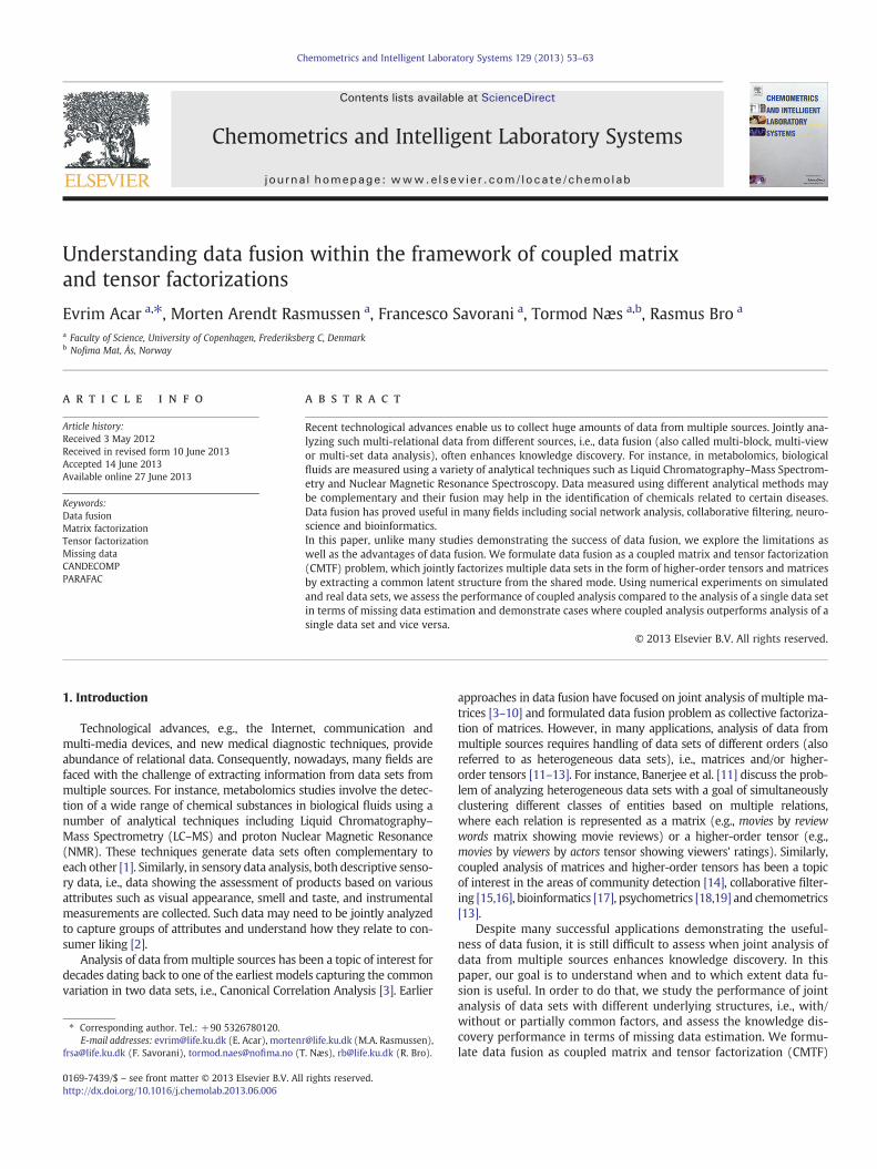
Fig. 1. (a)A third-order tensor with randomly-scattered missing entries coupled with a matrix. (b)A third-order tensor with randomly-scattered missing entries coupled with twomatrices in two different modes.

54 E. Acar et al. / Chemometrics and Intelligent Laboratory Systems 129 (2013) 53–63

since it is the common formulation used for joint analysis of hetero-geneous data [14–20]. Suppose we have a third-order tensor,X ∈RI�J�K , and a matrix, Y∈RI�M , coupled in the first dimension(mode) of each. An R-component CMTFmodel of a tensorX and a ma-trix Y, for Euclidean loss, is defined as [18–20]:

f A;B;C;Vð Þ ¼ X−〚A;B;C〛k k2 þ Y−AVT��� ���2: ð1Þ

Here, tensor X and matrix Y are jointly factorized through theminimization of (1), which fits a CANDECOMP/PARAFAC(CP)[21–23] toX and factorizes matrix Y in such a way that the factor ma-trix corresponding to the common mode, i.e., A∈RI�R, is the same.B∈RJ�R and C∈RK�R are the factor matrices of X corresponding tothe second and third modes, respectively. We use the notation X ¼〚A;B;C〛 to denote the CP model. Matrix V∈RM�R is the factor matrixthat corresponds to the second mode of matrix Y. In CMTF formula-tion, CP model has been used to model the tensor since it has numer-ous successful applications in various disciplines [24–26]. Theformulation in (1) can be considered as a special case of Linkedmode PARAFAC models mentioned by Harshman and Lundy [27](p.65) as well as multi-way multi-block models studied by Smildeet al. [13].

In this paper, we focus on the CMTF formulation (1) and explorethe limitations and advantages of data fusion within the frameworkof CMTF using numerical experiments. We study coupled data setswith different underlying structures, i.e., common, partially common,no common components, and demonstrate that performance ofcoupled analysis, in terms of missing data estimation, depends onthe underlying structures of coupled data sets. Our experimentsfocus on the case where an incomplete third-order tensor is coupledwith a matrix in one mode (Fig. 1a) and we illustrate (i) caseswhere coupled analysis outperforms analysis of a single data set aswell as (ii) cases where coupled analysis performs worse than theanalysis of a single data set in terms of estimation of the missing en-tries in the third-order tensor. Note that the model for CMTF general-izes to multiple higher-order tensors and matrices coupled in severalmodes, e.g., Fig. 1b, as well.

The paper is organized as follows. In Section 2, we discuss coupledmatrix and tensor factorization formulation and its extension to in-complete data sets, i.e., data with missing entries, as well as anall-at-once optimization algorithm for fitting a CMTF model. Section3 describes numerical experiments on both simulated data sets andreal data from sensory data analysis and metabolomics. Finally, weconclude with discussions in Section 4.

2. Coupled matrix and tensor factorization

In this section, we consider joint analysis of a matrix and annth-order tensor with one mode in common, where the tensor isfactorized using an R-component CP model and the matrix isfactorized by extracting R factors using matrix factorization. Let

X ∈RI1�I2�⋯�IN and Y∈RIn�M have the nth mode in common, wheren ∈ {1,…,N}. The objective function for coupled analysis of thesetwo data sets is defined by

f A 1ð Þ;A 2ð Þ

;…;A Nð Þ;V

� �¼ X−〚A 1ð Þ

;…;A Nð Þ〛

��� ���2 þ Y−A nð ÞVT��� ���2 ð2Þ

where Xk k ¼ffiffiffiffiffiffiffiffiffiffiffiffiffiffiffiffiffiffiffiffiffiffiffiffiffiffiffiffiffiffiffiffiffiffiffiffiffiffiffiffiffiffiffiffiffiffiffiffiffiffiffiffiffiffiffiffiffiffi∑I1

i1¼1∑I2i2¼1⋯∑

INiN¼1 x

2i1 i2⋯iN

q. Similarly, ‖.‖ refers to

Frobenius norm for matrices. Our goal is to find matrices A ið Þ ∈RIi�R,for i = 1,2,…N, and matrix V∈RM�R that minimize the objective in(2). This formulation extends to multiple matrices and higher-ordertensors coupled in various modes [20]. As an alternative to CMTF,unfolding the higher-order tensor and concatenating with the matrixcan also be used to jointly analyze X and Y; however, this schemedoes not generalize to higher-order tensors coupled with matricesin various modes, e.g., Fig. 1b. For instance, in collaborative filtering,if we were to recommend users certain activities based on their loca-tions, we might analyze a users × activities × locations tensor show-ing how often users perform activities at various locations, coupledwith a users by users similarity matrix as well as a matrix in theform of locations by features indicating the number of points of inter-est at various locations [15,16]. In this case, simply unfolding andconcatenating data sets will not work. Furthermore, unfolding ahigher-order tensor ignores the multi-way structure of the data and,recently, it has been shown that using a tensor model outperforms amatrix model on the unfolded data in terms of missing data recovery[28] (chapter 11).

In the presence of missing data, we can still jointly factorize het-erogeneous data sets by ignoring missing entries and fitting the ten-sor and/or the matrix model to the known data entries. Here, westudy the case where tensor X has missing entries as in Fig. 1a andmodify the objective function (2) as1

fW A 1ð Þ;A 2ð Þ

;…;A Nð Þ;V

� �¼ 1

2W � X−〚A 1ð Þ

;…;A Nð Þ〛

� ���� ���2|fflfflfflfflfflfflfflfflfflfflfflfflfflfflfflfflfflfflfflfflfflfflfflfflfflfflffl{zfflfflfflfflfflfflfflfflfflfflfflfflfflfflfflfflfflfflfflfflfflfflfflfflfflfflffl}fW1

A 1ð Þ ;A 2ð Þ ;…;A Nð Þð Þ

þ12

Y−A nð ÞVT��� ���2|fflfflfflfflfflfflfflfflfflfflffl{zfflfflfflfflfflfflfflfflfflfflffl}

fW2

ð3Þ

where ∗ denotes the Hadamard product. Tensor W ∈RI1�I2�⋯�IN indi-cates the missing entries of X such that

wi1 i2…iN¼ 1 if xi1 i2…iN

isknown;0 if xi1 i2…iN

ismissing;

�ð4Þ

for all in ∈ {1,…,In} and n ∈ {1,…,N}.

2.1. All-at-once optimization for CMTF

In order to minimize functions (2) and (3), we use an all-at-onceoptimization approach called CMTF-OPT [20] that solves the

2 We do not assume orthogonality among the columns of each factor matrix; howev-er, note that when entries are randomly drawn from standard normal, the data gener-ation scheme may result in nearly orthogonal columns in the factor matricescorresponding to the modes with large dimensions, e.g., 100.

55E. Acar et al. / Chemometrics and Intelligent Laboratory Systems 129 (2013) 53–63

optimization problem for CMTF for all factor matrices simultaneously.CMTF problem can also be solved using an alternating least squares(ALS) approach, which solves the problem for one factor matrix at atime by fixing the others. However, while ALS methods are easy toimplement and flexible in terms of incorporating constraints, directnonlinear optimization methods solving for all factor matrices simul-taneously have shown to be more accurate in the case of CP factoriza-tion [29,30] and CMTF [20]. The computational cost per iteration is thesame for both ALS and CMTF-OPT. Both approaches compute the par-tial derivatives of the objective with respect to each factor matrix;while ALS solves the partials for one factor matrix at a time fixingthe others, CMTF-OPT concatenates the partials, forms the gradientand uses a gradient-based optimization algorithm.

Here we briefly describe the all-at-once algorithm used to mini-mize fW in (3). Initially, we compute the partial derivatives of fWwith respect to A(i), for i = 1,…,N. The partial of the first part, fW1

,with respect to A(i), for i = 1,…,N, is as follows:

∂fW1

∂A ið Þ ¼ W ið Þ � Z ið Þ−W ið Þ � X ið Þ� �

A −ið Þ;

where Z ¼ 〚A 1ð Þ;…;A Nð Þ

〛;Z ið Þ indicates the matricized version oftensor Z in the ith mode (see [25] for matricization/unfolding), andA(−i) = A(N) ⊙ ⋯ ⊙ A(i + 1) ⊙ A(i − 1) ⊙ ⋯ ⊙ A(1), for i = 1,…,N. ⊙denotes the Khatri-Rao product.

The partial derivatives of the second part, fW2, with respect to A(i)

and V can be computed as

∂fW2

∂A ið Þ ¼(−YV þ A ið ÞVTV; for i ¼ n;

0 for i≠n;∂fW2

∂V ¼ −YTA ið Þ þ VA ið ÞTA ið Þ:

Combining the results, we write the partial of fW with respect to A(i)

as:

∂fW∂A ið Þ ¼

(∂fW1

∂A ið Þ for i∈ 1;…;Nf g= nf g;∂fW1

∂A ið Þ þ∂fW2

∂A ið Þ for i ¼ n:

∂fW∂V ¼

∂fW2

∂V

The gradient of fW , ∇fW , which is a vector of size P ¼R ∑N

n¼1 In þM�

, can finally be formed by vectorizing the partial deriv-atives with respect to each factor matrix and concatenating them all.

Once we have the function, fW , and gradient, ∇fW , we use agradient-based optimization algorithm, i.e., Nonlinear Conjugate Gra-dient (NCG) [31] with the Moré–Thuente line search, from the Pobla-no Toolbox [32], to compute the factor matrices. In this section, wehave studied the case where there are missing entries only in tensorX but note that both the CMTF model and the all-at-once algorithmgeneralize to coupled factorization of incomplete data sets in theform of matrices or higher-order tensors (See CMTF Toolbox availablefrom http://www.models.life.ku.dk).

In our formulations in (2) and (3), we have used equal weights fordifferent parts of the objective function and in the experiments, wedivide each data set by its Frobenius norm so that the model doesnot favor one part of the objective. However, determining the rightweighting scheme remains to be an open research question [18,33].

3. Experiments

3.1. Simulated coupled data sets

Our goal with simulated experiments is to understand when and towhich extent CMTF is useful. In order to observe the behavior of CMTFon different types of coupled data sets, we generate coupled data, i.e.,a third-order tensor X of size I × J × K and a matrix Y of size I × M,with different characteristics using the following formulation:

X ¼ α〚A 1ð Þ;A 2ð Þ

;A 3ð Þ〛þ 1−αð Þ〚B 1ð Þ

;B 2ð Þ;B 3ð Þ

〛; ð5Þ

Y ¼ αA 1ð ÞVT þ 1−αð ÞC 1ð ÞC 2ð ÞT;

where 0 ≤ α ≤ 1. A 1ð Þ ∈RI�Ro represents the factor matrix common toboth data sets;A 2ð Þ ∈RJ�Ro andA 3ð Þ ∈RK�Ro are the factor matrices cor-responding to the other modes of the tensor whileV∈RM�Ro is the fac-tor matrix corresponding to the second mode of matrix Y. Ro indicatesthe number of common (overlapping) components. Factors that areonly present in tensor X are represented by B 1ð Þ ∈RI�Rno ;B 2ð Þ ∈RJ�Rno

and B 3ð Þ ∈RK�Rno ; factors that are only present in the matrix Y are rep-resented by C 1ð Þ ∈RI�Rno and C 2ð Þ ∈RM�Rno . Rno indicates the number ofnon-overlapping components.

TensorX and matrix Y are constructed based on the above formu-lation for a set of α values using factor matrices with entries randomlydrawn from the standard normal distribution and columns normal-ized to unit norm.2 In our experiments, we add noise to tensor Xand construct Xnoisy as Xnoisy ¼ X þ η N

Nk k Xk k, where N is a tensor ofsame size asX with entries drawn from the standard normal distribu-tion. Similarly, Ynoisy is constructed asYnoisy ¼ Y þ η N

Nk k Yk k, whereNis a matrix of same size as Y with entries drawn from the standardnormal.

3.1.1. Performance measureIn order to assess the performance of data fusion, we randomly set

some tensor entries to missing and use missing data recovery error asa performance measure. To set entries to missing, a binary indicatortensor W, defined in (4), is generated such that out of its IJK entries,⌊SIJK⌋ entries are set to zero uniformly at random, where S indicatesthe percentage of missing entries.

We estimate missing tensor entries using two different approaches:(i) Analysis of only the third-order tensor: modeling the third-order ten-sor with missing entries using a CP model and then using the CP factormatrices to reconstruct the tensor and recover missing values and (ii)Coupled Analysis of the third-order tensor and the matrix: modeling theincomplete third-order tensor jointly with matrix Y using a CMTFmodel and then using the CMTF factor matrices to reconstruct thetensor and estimate missing entries. Let the extracted factors by either

model from Xnoisy be U1ð Þ ∈RI�R; U

2ð Þ ∈RJ�R and U3ð Þ ∈RK�R. In order

to quantify the missing data recovery error, we define tensor comple-tion score (TCS), that computes the error between the original and esti-mated values of missing entries as follows:

TCS ¼1−Wð Þ � Xnoisy−X

� ���� ���1−Wð Þ � Xnoisy

��� ��� ; ð6Þ

whereX corresponds to thedata reconstructedusing the extracted factor

matrices, i.e., X ¼ 〚U 1ð Þ; U 2ð Þ

; U 3ð Þ〛.

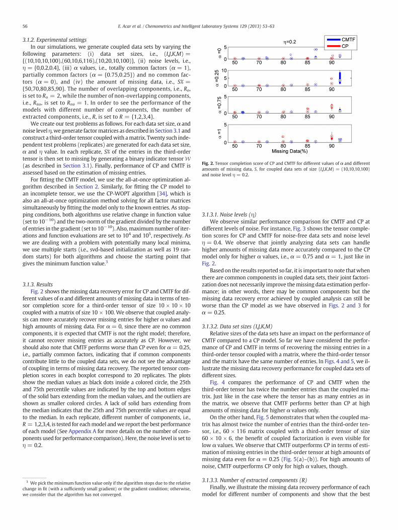
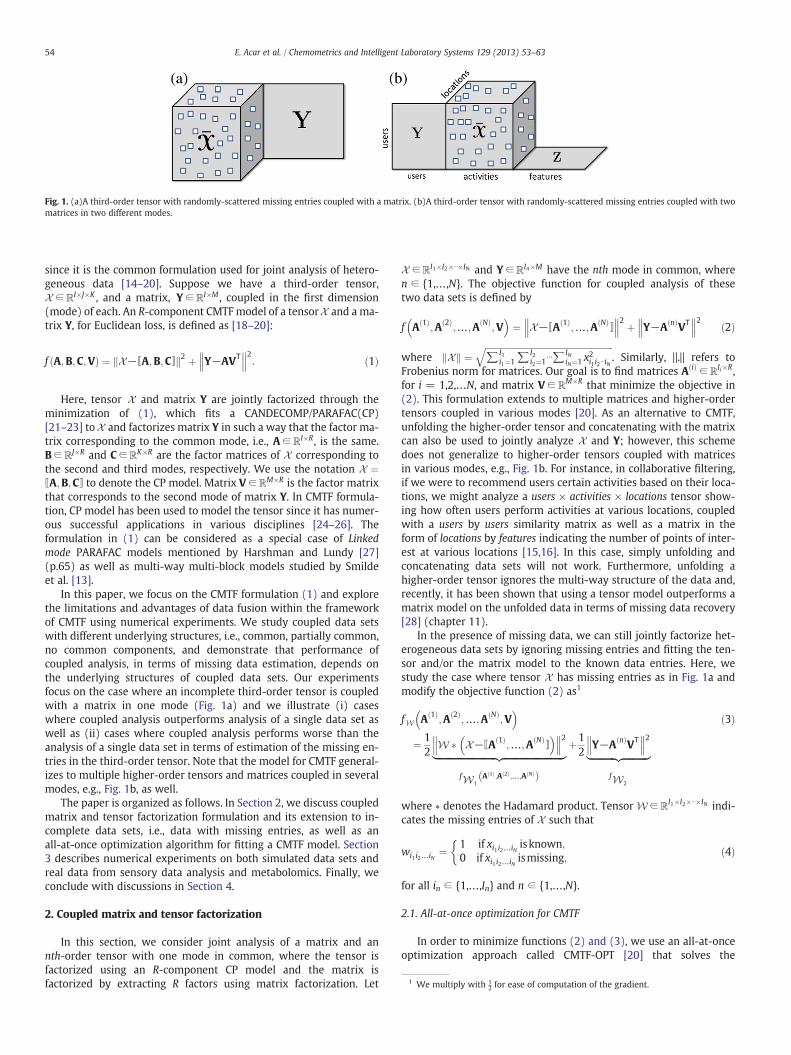
Fig. 2. Tensor completion score of CP and CMTF for different values of α and differentamounts of missing data, S, for coupled data sets of size (I,J,K,M) = (10,10,10,100)and noise level η = 0.2.

56 E. Acar et al. / Chemometrics and Intelligent Laboratory Systems 129 (2013) 53–63

3.1.2. Experimental settingsIn our simulations, we generate coupled data sets by varying the

following parameters: (i) data set sizes, i.e., (I,J,K,M) ={(10,10,10,100),(60,10,6,116),(10,20,10,100)}, (ii) noise levels, i.e.,η = {0,0.2,0.4}, (iii) α values, i.e., totally common factors (α = 1),partially common factors (α = {0.75,0.25}) and no common fac-tors (α = 0), and (iv) the amount of missing data, i.e., S% ={50,70,80,85,90}. The number of overlapping components, i.e., Ro,is set to Ro = 2, while the number of non-overlapping components,i.e., Rno, is set to Rno = 1. In order to see the performance of themodels with different number of components, the number ofextracted components, i.e., R, is set to R = {1,2,3,4}.

We create our test problems as follows. For each data set size, α andnoise level η, we generate factormatrices as described in Section 3.1 andconstruct a third-order tensor coupledwith amatrix. Twenty such inde-pendent test problems (replicates) are generated for each data set size,α and η value. In each replicate, S% of the entries in the third-ordertensor is then set to missing by generating a binary indicator tensor W(as described in Section 3.1). Finally, performance of CP and CMTF isassessed based on the estimation of missing entries.

For fitting the CMTF model, we use the all-at-once optimization al-gorithm described in Section 2. Similarly, for fitting the CP model toan incomplete tensor, we use the CP-WOPT algorithm [34], which isalso an all-at-once optimization method solving for all factor matricessimultaneously by fitting themodel only to the known entries. As stop-ping conditions, both algorithms use relative change in function value(set to 10−10) and the two-norm of the gradient divided by the numberof entries in the gradient (set to 10−10). Also, maximumnumber of iter-ations and function evaluations are set to 104 and 105, respectively. Aswe are dealing with a problem with potentially many local minima,we use multiple starts (i.e., svd-based initialization as well as 19 ran-dom starts) for both algorithms and choose the starting point thatgives the minimum function value.3

3.1.3. ResultsFig. 2 shows themissing data recovery error for CP and CMTF for dif-

ferent values of α and different amounts of missing data in terms of ten-sor completion score for a third-order tensor of size 10 × 10 × 10coupled with a matrix of size 10 × 100. We observe that coupled analy-sis can more accurately recover missing entries for higher α values andhigh amounts of missing data. For α = 0, since there are no commoncomponents, it is expected that CMTF is not the right model; therefore,it cannot recover missing entries as accurately as CP. However, weshould also note that CMTF performs worse than CP even for α = 0.25,i.e., partially common factors, indicating that if common componentscontribute little to the coupled data sets, we do not see the advantageof coupling in terms of missing data recovery. The reported tensor com-pletion scores in each boxplot correspond to 20 replicates. The plotsshow the median values as black dots inside a colored circle, the 25thand 75th percentile values are indicated by the top and bottom edgesof the solid bars extending from the median values, and the outliers areshown as smaller colored circles. A lack of solid bars extending fromthe median indicates that the 25th and 75th percentile values are equalto the median. In each replicate, different number of components, i.e.,R = 1,2,3,4, is tested for eachmodel andwe report the best performanceof each model (See Appendix A for more details on the number of com-ponents used for performance comparison). Here, the noise level is set toη = 0.2.

3 We pick the minimum function value only if the algorithm stops due to the relativechange in fit (with a sufficiently small gradient) or the gradient condition; otherwise,we consider that the algorithm has not converged.

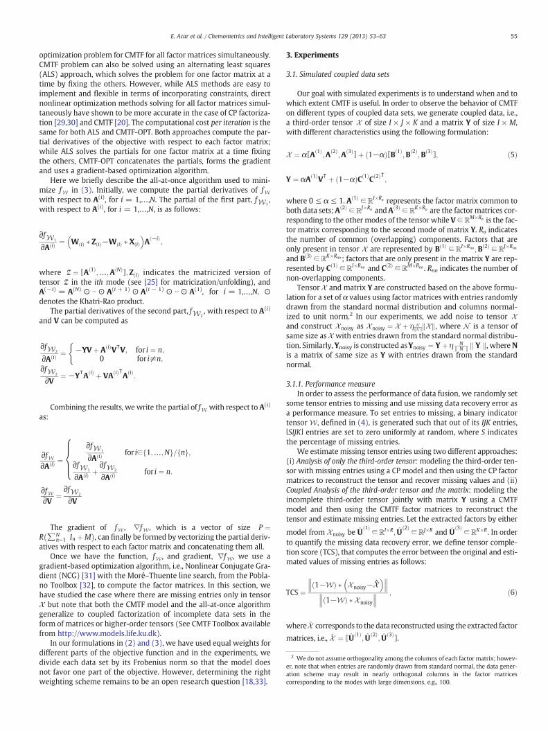
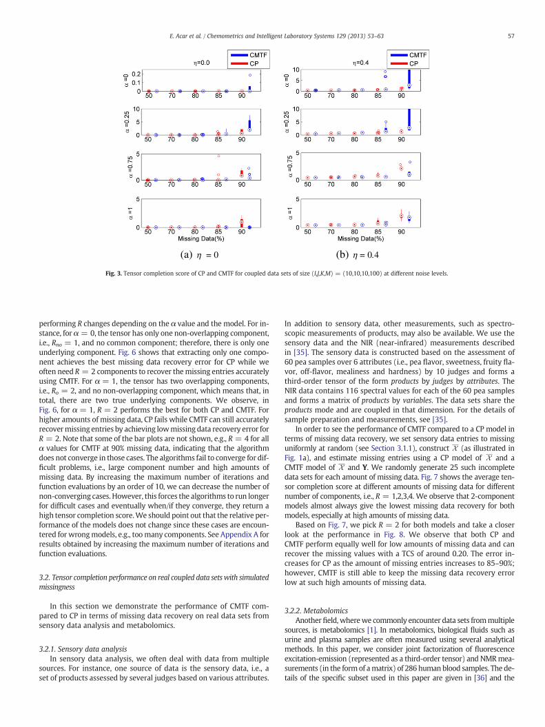
3.1.3.1. Noise levels (η)We observe similar performance comparison for CMTF and CP at

different levels of noise. For instance, Fig. 3 shows the tensor comple-tion scores for CP and CMTF for noise-free data sets and noise levelη = 0.4. We observe that jointly analyzing data sets can handlehigher amounts of missing data more accurately compared to the CPmodel only for higher α values, i.e., α = 0.75 and α = 1, just like inFig. 2.

Based on the results reported so far, it is important to note thatwhenthere are common components in coupled data sets, their joint factori-zation does not necessarily improve themissing data estimation perfor-mance; in other words, there may be common components but themissing data recovery error achieved by coupled analysis can still beworse than the CP model as we have observed in Figs. 2 and 3 forα = 0.25.

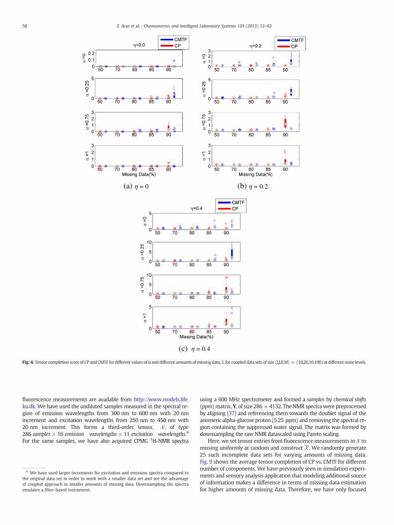
3.1.3.2. Data set sizes (I,J,K,M)Relative sizes of the data sets have an impact on the performance of

CMTF compared to a CP model. So far we have considered the perfor-mance of CP and CMTF in terms of recovering the missing entries in athird-order tensor coupled with a matrix, where the third-order tensorand the matrix have the same number of entries. In Figs. 4 and 5, we il-lustrate the missing data recovery performance for coupled data sets ofdifferent sizes.

Fig. 4 compares the performance of CP and CMTF when thethird-order tensor has twice the number entries than the coupled ma-trix. Just like in the case where the tensor has as many entries as inthe matrix, we observe that CMTF performs better than CP at highamounts of missing data for higher α values only.

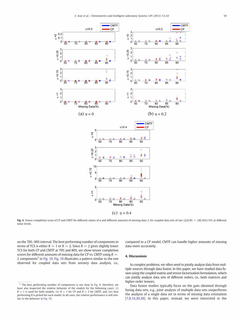
On the other hand, Fig. 5 demonstrates that when the coupled ma-trix has almost twice the number of entries than the third-order ten-sor, i.e., 60 × 116 matrix coupled with a third-order tensor of size60 × 10 × 6, the benefit of coupled factorization is even visible forlow α values. We observe that CMTF outperforms CP in terms of esti-mation of missing entries in the third-order tensor at high amounts ofmissing data even for α = 0.25 (Fig. 5(a)–(b)). For high amounts ofnoise, CMTF outperforms CP only for high α values, though.

3.1.3.3. Number of extracted components (R)Finally, we illustrate the missing data recovery performance of each

model for different number of components and show that the best

(a) (b)

Fig. 3. Tensor completion score of CP and CMTF for coupled data sets of size (I,J,K,M) = (10,10,10,100) at different noise levels.

57E. Acar et al. / Chemometrics and Intelligent Laboratory Systems 129 (2013) 53–63

performing R changes depending on the α value and the model. For in-stance, for α = 0, the tensor has only one non-overlapping component,i.e., Rno = 1, and no common component; therefore, there is only oneunderlying component. Fig. 6 shows that extracting only one compo-nent achieves the best missing data recovery error for CP while weoften need R = 2 components to recover themissing entries accuratelyusing CMTF. For α = 1, the tensor has two overlapping components,i.e., Ro = 2, and no non-overlapping component, which means that, intotal, there are two true underlying components. We observe, inFig. 6, for α = 1, R = 2 performs the best for both CP and CMTF. Forhigher amounts of missing data, CP fails while CMTF can still accuratelyrecovermissing entries by achieving lowmissing data recovery error forR = 2. Note that some of the bar plots are not shown, e.g., R = 4 for allα values for CMTF at 90% missing data, indicating that the algorithmdoes not converge in those cases. The algorithms fail to converge for dif-ficult problems, i.e., large component number and high amounts ofmissing data. By increasing the maximum number of iterations andfunction evaluations by an order of 10, we can decrease the number ofnon-converging cases. However, this forces the algorithms to run longerfor difficult cases and eventually when/if they converge, they return ahigh tensor completion score.We should point out that the relative per-formance of the models does not change since these cases are encoun-tered for wrongmodels, e.g., toomany components. See Appendix A forresults obtained by increasing the maximum number of iterations andfunction evaluations.

3.2. Tensor completion performance on real coupled data sets with simulatedmissingness

In this section we demonstrate the performance of CMTF com-pared to CP in terms of missing data recovery on real data sets fromsensory data analysis and metabolomics.

3.2.1. Sensory data analysisIn sensory data analysis, we often deal with data from multiple

sources. For instance, one source of data is the sensory data, i.e., aset of products assessed by several judges based on various attributes.

In addition to sensory data, other measurements, such as spectro-scopic measurements of products, may also be available. We use thesensory data and the NIR (near-infrared) measurements describedin [35]. The sensory data is constructed based on the assessment of60 pea samples over 6 attributes (i.e., pea flavor, sweetness, fruity fla-vor, off-flavor, mealiness and hardness) by 10 judges and forms athird-order tensor of the form products by judges by attributes. TheNIR data contains 116 spectral values for each of the 60 pea samplesand forms a matrix of products by variables. The data sets share theproducts mode and are coupled in that dimension. For the details ofsample preparation and measurements, see [35].

In order to see the performance of CMTF compared to a CP model interms of missing data recovery, we set sensory data entries to missinguniformly at random (see Section 3.1.1), construct X (as illustrated inFig. 1a), and estimate missing entries using a CP model of X and aCMTF model of X and Y. We randomly generate 25 such incompletedata sets for each amount of missing data. Fig. 7 shows the average ten-sor completion score at different amounts of missing data for differentnumber of components, i.e., R = 1,2,3,4. We observe that 2-componentmodels almost always give the lowest missing data recovery for bothmodels, especially at high amounts of missing data.

Based on Fig. 7, we pick R = 2 for both models and take a closerlook at the performance in Fig. 8. We observe that both CP andCMTF perform equally well for low amounts of missing data and canrecover the missing values with a TCS of around 0.20. The error in-creases for CP as the amount of missing entries increases to 85–90%;however, CMTF is still able to keep the missing data recovery errorlow at such high amounts of missing data.

3.2.2. MetabolomicsAnother field, wherewe commonly encounter data sets frommultiple

sources, is metabolomics [1]. In metabolomics, biological fluids such asurine and plasma samples are often measured using several analyticalmethods. In this paper, we consider joint factorization of fluorescenceexcitation-emission (represented as a third-order tensor) and NMRmea-surements (in the formof amatrix) of 286 human blood samples. The de-tails of the specific subset used in this paper are given in [36] and the

(a) (b)

(c)

Fig. 4. Tensor completion score of CP and CMTF for different values ofα and different amounts ofmissing data, S, for coupled data sets of size (I,J,K,M) = (10,20,10,100) at different noise levels.

58 E. Acar et al. / Chemometrics and Intelligent Laboratory Systems 129 (2013) 53–63

fluorescence measurements are available from http://www.models.life.ku.dk. We have used the undiluted samples measured in the spectral re-gion of emission wavelengths from 300 nm to 600 nm with 20 nmincrement and excitation wavelengths from 250 nm to 450 nm with20 nm increment. This forms a third-order tensor, X , of type286 samples × 16 emission wavelengths × 11 excitation wavelengths.4

For the same samples, we have also acquired CPMG 1H-NMR spectra

4 We have used larger increments for excitation and emission spectra compared tothe original data set in order to work with a smaller data set and see the advantageof coupled approach in smaller amounts of missing data. Downsampling the spectraemulates a filter-based instrument.

using a 600 MHz spectrometer and formed a samples by chemical shifts(ppm)matrix, Y, of size 286 × 4132. The NMR spectrawere preprocessedby aligning [37] and referencing them towards the doublet signal of theanomeric alpha-glucose proton (5.25 ppm) and removing the spectral re-gion containing the suppressed water signal. The matrix was formed bydownsampling the raw NMR datascaled using Pareto scaling.

Here, we set tensor entries from fluorescencemeasurements inX tomissing uniformly at random and construct X . We randomly generate25 such incomplete data sets for varying amounts of missing data.Fig. 9 shows the average tensor completion of CP vs. CMTF for differentnumber of components. We have previously seen in simulation experi-ments and sensory analysis application thatmodeling additional sourceof information makes a difference in terms of missing data estimationfor higher amounts of missing data. Therefore, we have only focused

(a) (b)

(c)

Fig. 5. Tensor completion score of CP and CMTF for different values of α and different amounts of missing data, S, for coupled data sets of size (I,J,K,M) = (60,10,6,116) at differentnoise levels.

59E. Acar et al. / Chemometrics and Intelligent Laboratory Systems 129 (2013) 53–63

on the 70%–90% interval. The best performingnumber of components interms of TCS is either R = 1 or R = 2. Since R = 2 gives slightly lowerTCS for both CP and CMTF at 70% and 80%, we show tensor completionscores for different amounts of missing data for CP vs. CMTF using R =2 components5 in Fig. 10. Fig. 10 illustrates a pattern similar to the oneobserved for coupled data sets from sensory data analysis, i.e.,

5 The best performing number of components is not clear in Fig. 9; therefore, wehave also inspected the relative behavior of the models for the following cases: (i)R = 1 is used for both models, (ii) R = 1 for CP and R = 2 for CMTF, and (iii) bestperforming R is picked for each model. In all cases, the relative performance is still sim-ilar to the behavior in Fig. 10.

compared to a CP model, CMTF can handle higher amounts of missingdata more accurately.

4. Discussions

In complex problems, we often need to jointly analyze data frommul-tiple sources through data fusion. In this paper, we have studied data fu-sion using the coupledmatrix and tensor factorization formulation,whichcan jointly analyze data sets of different orders, i.e., both matrices andhigher-order tensors.

Data fusion studies typically focus on the gain obtained throughfusing data sets, e.g., joint analysis of multiple data sets outperformsthe analysis of a single data set in terms of missing data estimation[7,8,16,20,38]. In this paper, instead, we were interested in the

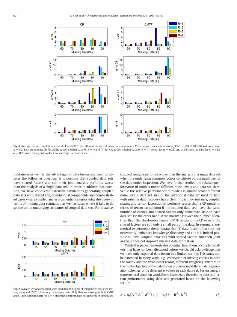
Fig. 6. Average tensor completion score of CP and CMTF for different number of extracted components, R, for coupled data sets of size (I,J,K,M) = (10,10,10,100) and noise levelη = 0.2. Bars are missing (i) for CMTF, at 90% missing data for R = 4 and (ii) for CP, at 90% missing data for R = 3 (except for α = 0.25) and at 85% missing data for R = 4 forα = 0.25 since the algorithm does not converge in those cases.

60 E. Acar et al. / Chemometrics and Intelligent Laboratory Systems 129 (2013) 53–63

limitations as well as the advantages of data fusion and tried to an-swer the following question: Is it possible that coupled data setshave shared factors and still their joint analysis performs worsethan the analysis of a single data set? In order to address that ques-tion, we have conducted extensive simulations generating coupleddata sets with shared and/or individual components and demonstrat-ed cases where coupled analysis can enhance knowledge discovery interms of missing data estimation as well as cases where it fails to doso due to the underlying structures of coupled data sets. For instance,

Fig. 7. Average tensor completion score for different number of components for CP (of sen-sory data) and CMTF (of sensory data coupled with NIR). Bars are missing for both CMTFand CP at 90%missing data for R = 4 since the algorithm does not converge in those cases.

coupled analysis performs worse than the analysis of a single data setwhen the underlying common factors constitute only a small part ofthe data under inspection. We have further studied the relative per-formance of models under different noise levels and data set sizes.While the relative performance of models is similar across differentnoise levels, data set size of the additional data set used to helpwith missing data recovery has a clear impact. For instance, coupledmatrix and tensor factorization performs worse than a CP model interms of tensor completion if the coupled data sets have the samenumber of entries and shared factors only contribute little to eachdata set. On the other hand, if the matrix has twice the number of en-tries than the third-order tensor, CMTF outperforms CP even if theshared factors are still only a small part of the data. In summary, nu-merical experiments demonstrate that (i) data fusion often (but notnecessarily) enhances knowledge discovery and (ii) it is indeed pos-sible to have coupled data sets with shared factors and their jointanalysis does not improve missing data estimation.

While this paper demonstrates potential limitations of coupled anal-ysis that have not been discussed before, we should acknowledge thatwe have only explored data fusion in a limited setting. This study canbe extended in many ways, e.g., estimation of missing entries in boththe matrix and the third-order tensor, different weighting schemes inthemulti-objective of the data fusion problem and different data gener-ation schemes using different α values in each data set. For instance, amore general situationwould be to investigate themissing data estima-tion performance using data sets generated based on the followingset-up:

X ¼ αt〚A1ð Þ;A 2ð Þ

;A 3ð Þ〛þ 1−αtð Þ〚B 1ð Þ

;B 2ð Þ;B 3ð Þ

〛; ð7Þ

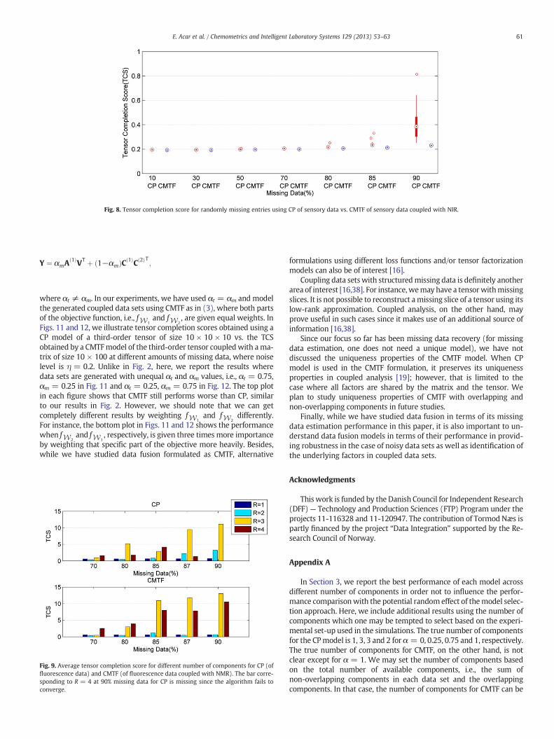
Fig. 8. Tensor completion score for randomly missing entries using CP of sensory data vs. CMTF of sensory data coupled with NIR.

61E. Acar et al. / Chemometrics and Intelligent Laboratory Systems 129 (2013) 53–63

Y ¼ αmA1ð ÞVT þ 1−αmð ÞC 1ð ÞC 2ð ÞT

;

where αt ≠ αm. In our experiments, we have used αt = αm and modelthe generated coupled data sets using CMTF as in (3), where both partsof the objective function, i.e., fW1

and fW2, are given equal weights. In

Figs. 11 and 12, we illustrate tensor completion scores obtained using aCP model of a third-order tensor of size 10 × 10 × 10 vs. the TCSobtained by a CMTFmodel of the third-order tensor coupledwith ama-trix of size 10 × 100 at different amounts of missing data, where noiselevel is η = 0.2. Unlike in Fig. 2, here, we report the results wheredata sets are generated with unequal αt and αm values, i.e., αt = 0.75,αm = 0.25 in Fig. 11 and αt = 0.25, αm = 0.75 in Fig. 12. The top plotin each figure shows that CMTF still performs worse than CP, similarto our results in Fig. 2. However, we should note that we can getcompletely different results by weighting fW1

and fW2differently.

For instance, the bottom plot in Figs. 11 and 12 shows the performancewhen fW2

and fW1, respectively, is given three times more importance

by weighting that specific part of the objective more heavily. Besides,while we have studied data fusion formulated as CMTF, alternative

Fig. 9. Average tensor completion score for different number of components for CP (offluorescence data) and CMTF (of fluorescence data coupled with NMR). The bar corre-sponding to R = 4 at 90% missing data for CP is missing since the algorithm fails toconverge.

formulations using different loss functions and/or tensor factorizationmodels can also be of interest [16].

Coupling data setswith structuredmissing data is definitely anotherarea of interest [16,38]. For instance, wemay have a tensorwithmissingslices. It is not possible to reconstruct amissing slice of a tensor using itslow-rank approximation. Coupled analysis, on the other hand, mayprove useful in such cases since it makes use of an additional source ofinformation [16,38].

Since our focus so far has been missing data recovery (for missingdata estimation, one does not need a unique model), we have notdiscussed the uniqueness properties of the CMTF model. When CPmodel is used in the CMTF formulation, it preserves its uniquenessproperties in coupled analysis [19]; however, that is limited to thecase where all factors are shared by the matrix and the tensor. Weplan to study uniqueness properties of CMTF with overlapping andnon-overlapping components in future studies.

Finally, while we have studied data fusion in terms of its missingdata estimation performance in this paper, it is also important to un-derstand data fusion models in terms of their performance in provid-ing robustness in the case of noisy data sets as well as identification ofthe underlying factors in coupled data sets.

Acknowledgments

This work is funded by the Danish Council for Independent Research(DFF) — Technology and Production Sciences (FTP) Program under theprojects 11-116328 and 11-120947. The contribution of Tormod Næs ispartly financed by the project “Data Integration” supported by the Re-search Council of Norway.

Appendix A

In Section 3, we report the best performance of each model acrossdifferent number of components in order not to influence the perfor-mance comparisonwith the potential random effect of themodel selec-tion approach. Here, we include additional results using the number ofcomponents which one may be tempted to select based on the experi-mental set-up used in the simulations. The true number of componentsfor the CPmodel is 1, 3, 3 and 2 for α = 0, 0.25, 0.75 and 1, respectively.The true number of components for CMTF, on the other hand, is notclear except for α = 1. We may set the number of components basedon the total number of available components, i.e., the sum ofnon-overlapping components in each data set and the overlappingcomponents. In that case, the number of components for CMTF can be

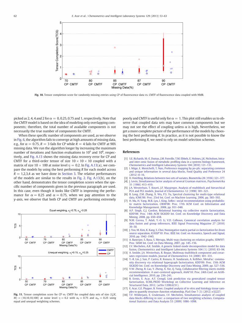
Fig. 10. Tensor completion score for randomly missing entries using CP of fluorescence data vs. CMTF of fluorescence data coupled with NMR.

62 E. Acar et al. / Chemometrics and Intelligent Laboratory Systems 129 (2013) 53–63

picked as 2, 4, 4 and 2 forα = 0, 0.25, 0.75 and 1, respectively. Note thatthe CMTFmodel is based on the idea ofmodeling only overlapping com-ponents; therefore, the total number of available components is notnecessarily the true number of components for CMTF.

When these specific number of components are used, aswe observein Fig. 6, the algorithm fails to converge at high amounts ofmissing data,e.g., for α = 0.75, R = 3 fails for CP while R = 4 fails for CMTF at 90%missing data. We run the algorithm longer by increasing the maximumnumber of iterations and function evaluations to 105 and 106, respec-tively, and Fig. A.13 shows the missing data recovery error for CP andCMTF for a third-order tensor of size 10 × 10 × 10 coupled with amatrix of size 10 × 100 at noise level η = 0.2. In Fig. A.13(a), we com-pare the models by using the best performing R for each model acrossR = 1,2,3,4 as we have done in Section 3. The relative performancesof the models are similar to the results in Fig. 2. Fig. A.13(b), on theother hand, demonstrates the tensor completion scores when the spe-cific number of components given in the previous paragraph are used.In this case, even though it looks like CMTF is improving the perfor-mance for α = 0.25 and α = 0.75, when we pay attention to they-axis, we observe that both CP and CMTF are performing extremely

Fig. 11. Tensor completion score for CP vs. CMTF for coupled data sets of size (I,J,K,M) = (10,10,10,100) at noise level η = 0.2 with αt = 0.75 and αm = 0.25 usingequal and unequal weighting schemes.

poorly and CMTF is useful only forα = 1. This plot still enables us to ob-serve that coupled data sets may have common components but wemay not see the effect of coupling unless α is high. Nevertheless, weget amore complete picture of the performance of themodels by choos-ing the best performing R. In practice, as it is not possible to know thebest performing R, we need to rely on model selection schemes.

References

[1] S.E. Richards, M.-E. Dumas, J.M. Fonville, T.M. Ebbels, E. Holmes, J.K. Nicholson, Intra-and inter-omic fusion of metabolic profiling data in a systems biology framework,Chemometrics and Intelligent Laboratory Systems 104 (2010) 121–131.

[2] I. Måge, E. Menichelli, T. Næs, Preference mapping by po-pls: separating commonand unique information in several data blocks, Food Quality and Preference 24(2012) 8–16.

[3] H. Hotelling, Relations between two sets of variates, Biometrika 28 (1936) 321–377.[4] J. Levin, Simultaneous factor analysis of several Gramian matrices, Psychometrika

31 (1966) 413–419.[5] J.A. Westerhuis, T. Kourti, J.F. Macgregor, Analysis of multiblock and hierarchical

PCA and PLS models, Journal of Chemometrics 12 (1998) 301–321.[6] B. Long, Z.M. Zhang, X. Wu, P.S. Yu, Spectral clustering for multi-type relational

data, ICML'06: Proc. 23rd Int. Conf. on Machine Learning, 2006, pp. 585–592.[7] H. Ma, H. Yang, M.R. Lyu, I. King, SoRec: social recommendation using probabilis-

tic matrix factorization, CIKM'08: Proc. 17th ACM Conf. on Information andKnowledge Management, 2008, pp. 931–940.

[8] A.P. Singh, G.J. Gordon, Relational learning via collective matrix factorization,KDD'08: Proc. 14th ACM SIGKDD Int. Conf. on Knowledge Discovery and DataMining, 2008, pp. 650–658.

[9] N.M. Correa, T. Adali, Y.-O. Li, V.D. Calhoun, Canonical correlation analysis fordata fusion and group inferences, IEEE Signal Processing Magazine 27 (2010)39–50.

[10] J. Yoo, M. Kim, K. Kang, S. Choi, Nonnegativematrix partial co-factorization for drumsource separation, ICASSP'10: Proc. IEEE Int. Conf. on Acoustics, Speech and Signal,2010, pp. 1942–1945.

[11] A. Banerjee, S. Basu, S. Merugu, Multi-way clustering on relation graphs, SDM'07:Proc. SIAM Int. Conf. on Data Mining, 2007, pp. 145–156.

[12] I.V. Mechelen, A.K. Smilde, A generic linked-mode decomposition model for datafusion, Chemometrics and Intelligent Laboratory Systems 104 (1) (2010) 83–94.

[13] A. Smilde, J.A. Westerhuis, R. Boque, Multiway multiblock component and covar-iates regression models, Journal of Chemometrics 14 (2000) 301–331.

[14] Y.-R. Lin, J. Sun, P. Castro, R. Konuru, H. Sundaram, A. Kelliher, MetaFac: commu-nity discovery via relational hypergraph factorization, KDD'09: Proc. 15th ACMSIGKDD Int. Conf. on Knowledge Discovery and Data Mining, 2009, pp. 527–536.

[15] V.W. Zheng, B. Cao, Y. Zheng, X. Xie, Q. Yang, Collaborative filtering meets mobilerecommendation: A user-centered approach, AAAI'10: Proc. 24th Conf. on Artifi-cial Intelligence, 2010, pp. 236–241.

[16] B. Ermis, E. Acar, A.T. Cemgil, Link prediction via generalized coupled tensorfactorisation, ECML/PKDD Workshop on Collective Learning and Inference onStructured Data, 2012, (arXiv:1208.6231).

[17] E. Acar, G.E. Plopper, B. Yener, Coupled analysis of in vitro and histology tissue sam-ples to quantify structure–function relationship, PLoS One 7 (3) (2012) e32227.

[18] T.F. Wilderjans, E. Ceulemans, I.V. Mechelen, Simultaneous analysis of coupleddata blocks differing in size: a comparison of two weighting schemes, Computa-tional Statistics and Data Analysis 53 (2009) 1086–1098.

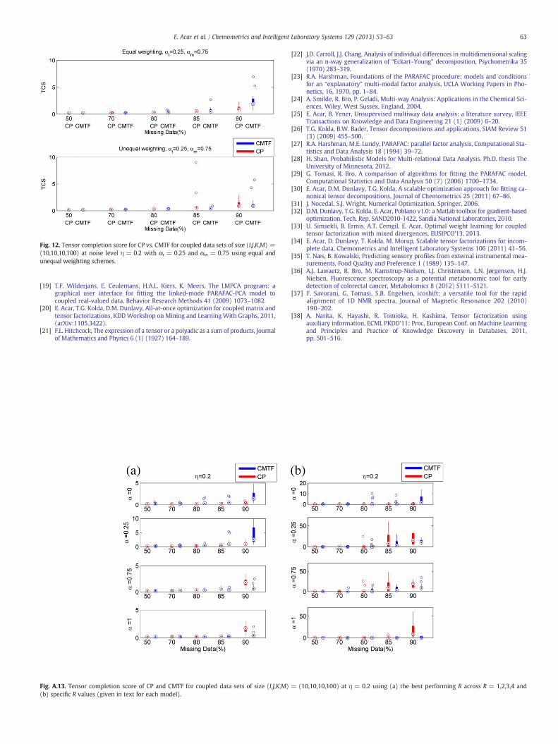
Fig. 12. Tensor completion score for CP vs. CMTF for coupled data sets of size (I,J,K,M) =(10,10,10,100) at noise level η = 0.2 with αt = 0.25 and αm = 0.75 using equal andunequal weighting schemes.

63E. Acar et al. / Chemometrics and Intelligent Laboratory Systems 129 (2013) 53–63

[19] T.F. Wilderjans, E. Ceulemans, H.A.L. Kiers, K. Meers, The LMPCA program: agraphical user interface for fitting the linked-mode PARAFAC-PCA model tocoupled real-valued data, Behavior Research Methods 41 (2009) 1073–1082.

[20] E. Acar, T.G. Kolda, D.M. Dunlavy, All-at-once optimization for coupled matrix andtensor factorizations, KDDWorkshop on Mining and Learning With Graphs, 2011,(arXiv:1105.3422).

[21] F.L. Hitchcock, The expression of a tensor or a polyadic as a sum of products, Journalof Mathematics and Physics 6 (1) (1927) 164–189.

Fig. A.13. Tensor completion score of CP and CMTF for coupled data sets of size (I,J,K,M)(b) specific R values (given in text for each model).

[22] J.D. Carroll, J.J. Chang, Analysis of individual differences in multidimensional scalingvia an n-way generalization of “Eckart–Young” decomposition, Psychometrika 35(1970) 283–319.

[23] R.A. Harshman, Foundations of the PARAFAC procedure: models and conditionsfor an “explanatory” multi-modal factor analysis, UCLA Working Papers in Pho-netics, 16, 1970, pp. 1–84.

[24] A. Smilde, R. Bro, P. Geladi, Multi-way Analysis: Applications in the Chemical Sci-ences, Wiley, West Sussex, England, 2004.

[25] E. Acar, B. Yener, Unsupervised multiway data analysis: a literature survey, IEEETransactions on Knowledge and Data Engineering 21 (1) (2009) 6–20.

[26] T.G. Kolda, B.W. Bader, Tensor decompositions and applications, SIAM Review 51(3) (2009) 455–500.

[27] R.A. Harshman, M.E. Lundy, PARAFAC: parallel factor analysis, Computational Sta-tistics and Data Analysis 18 (1994) 39–72.

[28] H. Shan, Probabilistic Models for Multi-relational Data Analysis. Ph.D. thesis TheUniversity of Minnesota, 2012.

[29] G. Tomasi, R. Bro, A comparison of algorithms for fitting the PARAFAC model,Computational Statistics and Data Analysis 50 (7) (2006) 1700–1734.

[30] E. Acar, D.M. Dunlavy, T.G. Kolda, A scalable optimization approach for fitting ca-nonical tensor decompositions, Journal of Chemometrics 25 (2011) 67–86.

[31] J. Nocedal, S.J. Wright, Numerical Optimization, Springer, 2006.[32] D.M. Dunlavy, T.G. Kolda, E. Acar, Poblano v1.0: a Matlab toolbox for gradient-based

optimization, Tech. Rep. SAND2010-1422, Sandia National Laboratories, 2010.[33] U. Simsekli, B. Ermis, A.T. Cemgil, E. Acar, Optimal weight learning for coupled

tensor factorization with mixed divergences, EUSIPCO'13, 2013.[34] E. Acar, D. Dunlavy, T. Kolda, M. Morup, Scalable tensor factorizations for incom-

plete data, Chemometrics and Intelligent Laboratory Systems 106 (2011) 41–56.[35] T. Næs, B. Kowalski, Predicting sensory profiles from external instrumental mea-

surements, Food Quality and Preference 1 (1989) 135–147.[36] A.J. Lawaetz, R. Bro, M. Kamstrup-Nielsen, I.J. Christensen, L.N. Jørgensen, H.J.

Nielsen, Fluorescence spectroscopy as a potential metabonomic tool for earlydetection of colorectal cancer, Metabolomics 8 (2012) S111–S121.

[37] F. Savorani, G. Tomasi, S.B. Engelsen, icoshift: a versatile tool for the rapidalignment of 1D NMR spectra, Journal of Magnetic Resonance 202 (2010)190–202.

[38] A. Narita, K. Hayashi, R. Tomioka, H. Kashima, Tensor factorization usingauxiliary information, ECML PKDD'11: Proc. European Conf. on Machine Learningand Principles and Practice of Knowledge Discovery in Databases, 2011,pp. 501–516.

= (10,10,10,100) at η = 0.2 using (a) the best performing R across R = 1,2,3,4 and