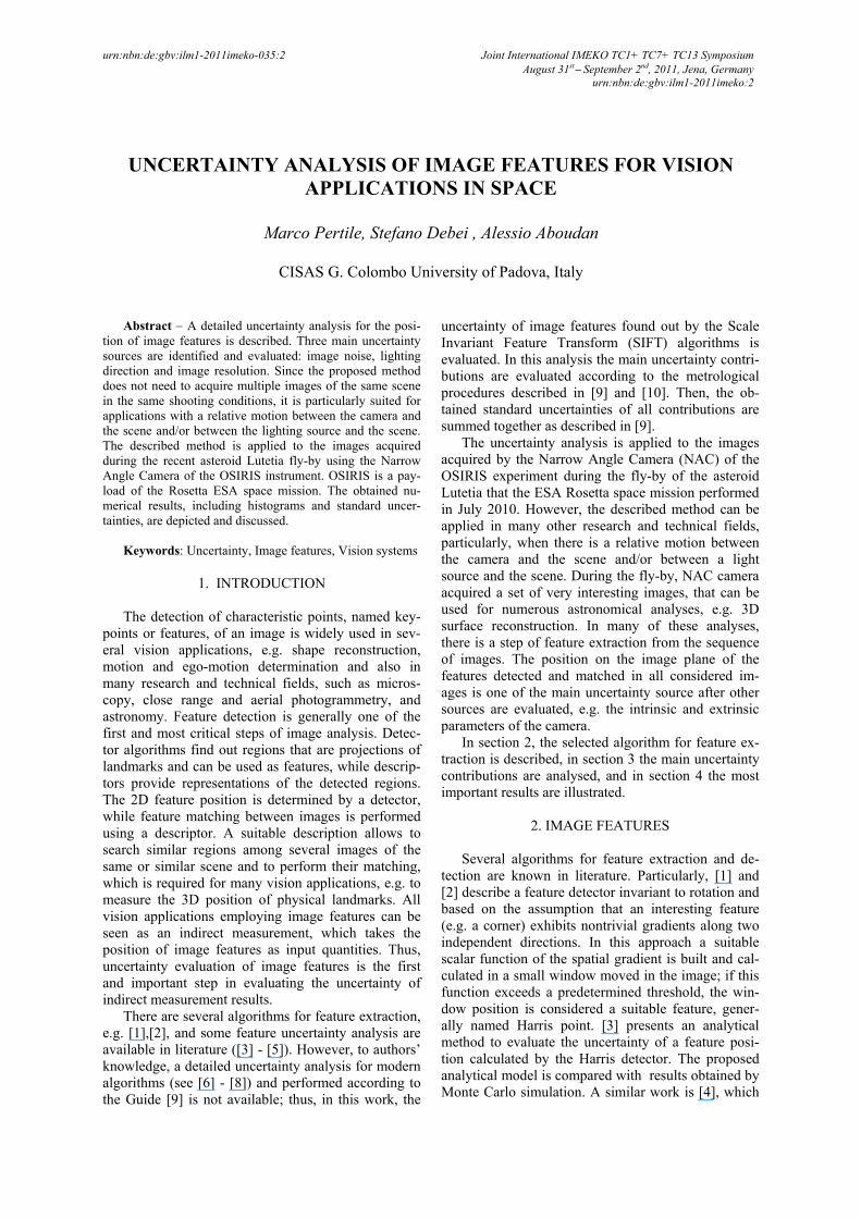
urn:nbn:de:gbv:ilm1-2011imeko-035:2 Joint International IMEKO TC1+ TC7+ TC13 Symposium August 31st− September 2nd, 2011, Jena, Germany

urn:nbn:de:gbv:ilm1-2011imeko:2

UNCERTAINTY ANALYSIS OF IMAGE FEATURES FOR VISION APPLICATIONS IN SPACE

Marco Pertile, Stefano Debei , Alessio Aboudan

CISAS G. Colombo University of Padova, Italy

Abstract − A detailed uncertainty analysis for the posi-tion of image features is described. Three main uncertainty sources are identified and evaluated: image noise, lighting direction and image resolution. Since the proposed method does not need to acquire multiple images of the same scene in the same shooting conditions, it is particularly suited for applications with a relative motion between the camera and the scene and/or between the lighting source and the scene. The described method is applied to the images acquired during the recent asteroid Lutetia fly-by using the Narrow Angle Camera of the OSIRIS instrument. OSIRIS is a pay-load of the Rosetta ESA space mission. The obtained nu-merical results, including histograms and standard uncer-tainties, are depicted and discussed.

Keywords: Uncertainty, Image features, Vision systems

1. INTRODUCTION The detection of characteristic points, named key-

points or features, of an image is widely used in sev-eral vision applications, e.g. shape reconstruction, motion and ego-motion determination and also in many research and technical fields, such as micros-copy, close range and aerial photogrammetry, and astronomy. Feature detection is generally one of the first and most critical steps of image analysis. Detec-tor algorithms find out regions that are projections of landmarks and can be used as features, while descrip-tors provide representations of the detected regions. The 2D feature position is determined by a detector, while feature matching between images is performed using a descriptor. A suitable description allows to search similar regions among several images of the same or similar scene and to perform their matching, which is required for many vision applications, e.g. to measure the 3D position of physical landmarks. All vision applications employing image features can be seen as an indirect measurement, which takes the position of image features as input quantities. Thus, uncertainty evaluation of image features is the first and important step in evaluating the uncertainty of indirect measurement results.

There are several algorithms for feature extraction, e.g. [1],[2], and some feature uncertainty analysis are available in literature ([3] - [5]). However, to authors’ knowledge, a detailed uncertainty analysis for modern algorithms (see [6] - [8]) and performed according to the Guide [9] is not available; thus, in this work, the

uncertainty of image features found out by the Scale Invariant Feature Transform (SIFT) algorithms is evaluated. In this analysis the main uncertainty contri-butions are evaluated according to the metrological procedures described in [9] and [10]. Then, the ob-tained standard uncertainties of all contributions are summed together as described in [9].

The uncertainty analysis is applied to the images acquired by the Narrow Angle Camera (NAC) of the OSIRIS experiment during the fly-by of the asteroid Lutetia that the ESA Rosetta space mission performed in July 2010. However, the described method can be applied in many other research and technical fields, particularly, when there is a relative motion between the camera and the scene and/or between a light source and the scene. During the fly-by, NAC camera acquired a set of very interesting images, that can be used for numerous astronomical analyses, e.g. 3D surface reconstruction. In many of these analyses, there is a step of feature extraction from the sequence of images. The position on the image plane of the features detected and matched in all considered im-ages is one of the main uncertainty source after other sources are evaluated, e.g. the intrinsic and extrinsic parameters of the camera.

In section 2, the selected algorithm for feature ex-traction is described, in section 3 the main uncertainty contributions are analysed, and in section 4 the most important results are illustrated.

2. IMAGE FEATURES

Several algorithms for feature extraction and de-

tection are known in literature. Particularly, [1] and [2] describe a feature detector invariant to rotation and based on the assumption that an interesting feature (e.g. a corner) exhibits nontrivial gradients along two independent directions. In this approach a suitable scalar function of the spatial gradient is built and cal-culated in a small window moved in the image; if this function exceeds a predetermined threshold, the win-dow position is considered a suitable feature, gener-ally named Harris point. [3] presents an analytical method to evaluate the uncertainty of a feature posi-tion calculated by the Harris detector. The proposed analytical model is compared with results obtained by Monte Carlo simulation. A similar work is [4], which

urn:nbn:de:gbv:ilm1-2011imeko-035:2 Joint International IMEKO TC1+ TC7+ TC13 Symposium August 31st− September 2nd, 2011, Jena, Germany

urn:nbn:de:gbv:ilm1-2011imeko:2

)

uses Taylor expansion approximation to evaluate a feature covariance matrix suitable for real time data fusion. Both in [3] and [4], only the Harris detector is analyzed and only the image noise (of additive type) is taken into account as uncertainty source.

An interesting work is [5], which evaluates uncer-tainty of image features detected by the Foerstner operator propagating the uncertainty of the intensity level of each pixel. This method considers the inten-sity levels as the input quantities and propagates their covariance matrix with the well known propagation formula to evaluate the covariance matrix of feature positions. In [5] a non-uniform additive noise is deemed the main uncertainty source for the intensity levels of pixels, and the noise of each pixel is also considered correlated with the noise of the neighbor-ing pixels. However, no other uncertainty sources are examined.

[6] compares several improved detectors, and ad-vices that one of the best performing algorithm is the detector employed in the method known as Scale Invariant Feature Transform (SIFT). This approach tries to find out features also in presence of scale and orientation variations. For this reason the SIFT ap-proach is usually reported as invariant to variations of scale and orientation. The detector is based on the difference-of-Gaussian function convolved with the image:

(1) ( )

( ) ( ) (, ,

, , , , ,

D x y

G x y k G x y I x y

σ

σ σ

=

⎡ ⎤= − ∗⎣ ⎦

where the I(x,y) is the grey level of the image at the point (x,y); G(x,y,σ) is the 2D Gaussian function with variance σ2; the scale varies with σ ; ∗ denotes the 2D convolution; k is a constant multiplicative factor suitably selected. The image features are lo-cated at the minima or maxima of D function, varying the position x, y and the scale σ. An orientation, calcu-lated using the local gradient, is also associated with each identified feature. For more details, see [7].

After features are detected, their local regions have to be represented by a descriptor. Many different methods are known for describing local image re-gions, see [8] for details. The performance of these methods can be evaluated by the number of correct or false matches between two images. [8] uses this crite-rion to compare different descriptors and concludes that the Scale Invariant Feature Transform SIFT and the Gradient Location and Orientation Histogram GLOH descriptors are the best ones. For the reasons described above, in the present work, the SIFT detec-tor and descriptor was chosen. The SIFT descriptor is of type based on a distribution, which describes the region around each detected feature by a 3D histogram of positions and orientations. The Euclidean distance is used to compare the descriptors of two different images and find out the corresponding features be-tween images. Particularly, each feature detected in a first image is associated with the feature detected in a

second image having the minimum Euclidean dis-tance, provided that the distance is lower than a prede-termined value.

3. UNCERTAINTY SOURCES

In this work three main contributions to the uncer-

tainty of feature positions are evaluated: the image noise, the variation of lighting conditions among im-ages, the finite resolution of NAC camera.

3.1. Image noise contribution The uncertainty of image features is particularly

tricky since it depends on the scene. When the same scene is acquired in the same conditions, different images are obtained due to the uncertainty (commonly referred to as image noise in computer vision) associ-ated with the image sensor and its electronics. This reading uncertainty is the first analyzed contribution to the uncertainty of image features; it depends mainly on the camera sensor and on the acquired scene. In general, images acquired by digital imaging systems are corrupted by a number of noise sources such as photon shot noise, dark current noise, readout noise, and quantization noise. In OSIRIS images some noise sources are reduced or suppressed by hardware means and/or software algorithms. However, a reduced level of noise remains in images, and should be analysed to evaluate the 2D position uncertainty of detected fea-tures. Thus, the remaining noise contribution is evalu-ated using the images acquired during the Lutetia fly-by after preliminary elaboration.

Images are supposed to be corrupted by additive noise. Our goal is to estimate the noise variance using only the degraded image. A very limiting requirement of this analysis is that only one image is available for a particular acquired scene and lighting conditions, since the relative position and orientation between Lutetia and OSIRIS system is continuously changing. Thus, two images with the same scene and the same acquiring conditions are not available. To address this problem, a large number of algorithms was published in the open literature. Usually these algorithms contain as a first step a procedure to remove the original im-age (not affected by noise) and the noise variance estimation is based on some local variances computed from the residual.

In [11], an algorithm for noise variance estimation, comprising three steps, is proposed. In a first step the image is preprocessed by a difference operator to minimize the influence of the original image. A sec-ond step computes a histogram of local standard de-viations and in a third step the histogram is evaluated in order to calculate the estimated variance. In the preprocessing phase, the noisy image is filtered by a cascade of two l-D difference operators: the first one along the vertical direction and the second one along the horizontal one. In this method, the noise signal is assumed to be statistically independent of the original

urn:nbn:de:gbv:ilm1-2011imeko-035:2 Joint International IMEKO TC1+ TC7+ TC13 Symposium August 31st− September 2nd, 2011, Jena, Germany

urn:nbn:de:gbv:ilm1-2011imeko:2

2

image and the noise statistics to be constant over the whole image.

[12] describes an image noise estimation algorithm which seems very effective. The algorithm comprises as the first step the application of the Laplacian opera-tor to remove the image structure. Then the image is divided on adjacent non-overlapping small windows and an edge detection algorithm is applied. Only for local windows that do not contain edges, the local variances are calculated and are grouped in a histo-gram. In the last step, the noise variance is evaluated using an averaging procedure.

In [13], a method for image noise estimation is presented. It comprises an edge detection to exclude pixels belonging to edges and a Laplacian operator to suppress the image structure. The Sobel operator is used for edge detection, and the obtained values are grouped in an histogram. The threshold value that allows to identify the edge pixels is selected from the accumulated histogram. In this way, the threshold value is adapted to different images. The noise vari-ance is evaluated by an averaging operator applied to the Laplacian output, excluding the identified edge pixels. This method is similar to the algorithm de-scribed in [12], but seems simpler.

There are several known methods for combined noise estimation and filtering. As an example, in [14], the proposed technique is based on a nonlinear algo-rithm for detail-preserving smoothing, whose filter depends on one parameter only. The filter parameter is automatically tuned using a step-by-step procedure that takes into consideration the mean square error (MSE) between subsequent pairs of processed images. In this kind of approaches, a drawback is that the noise variance of images is usually not explicitly esti-mated.

There are several methods, e.g. [15] - [20], for im-age noise estimation and filtering based on wavelet decomposition. In these approaches, noise variance is usually estimated through the scaled Median Absolute Deviation (MAD) method. This algorithm assumes that the coefficients of the finest decomposition level (the diagonal direction of decomposition level one) are associated only to noise and uses the median of abso-lute value of these coefficients for variance estimation. A possible improvement is described in [20], which presents a noise variance estimator called Residual Autocorrelation Power (RAP).

The non-wavelet most interesting approaches seem to be the ones described in [12], [13]. In this paper, the method described in [13] is selected for noise evalua-tion, since it seems as effective as the other one, and simpler than it, particularly when the salt and pepper noise is low, as in the OSIRIS images.

In the selected method, the Sobel operator is used for edge detection:

( )1 2 1

, 0 0 01 2 1

xE I x y− − −⎡ ⎤⎢ ⎥= ∗ ⎢ ⎥⎢ ⎥⎣ ⎦

( )1 0 1

, 2 01 0 1

yE I x y−⎡ ⎤⎢ ⎥= ∗ −⎢ ⎥⎢ ⎥−⎣ ⎦

(2)

x yE E E= +

To decide if an image pixel belongs to an edge or not, the histogram of E is calculated, and a threshold value Eth is selected as the value of E when the accu-mulated histogram reaches a predetermined percent-age p% of the whole image. A pixel is deemed an edge if its E value is greater than Eth. Fixing a percent-age p% value, instead of a fixed threshold, makes Eth adaptive (even if p is constant for all analyzed images, the threshold values Eth will depend on the image). After edges are detected, the selected method follows the approach described in [21], but excludes the pixels corresponding to the identified edges. Since a noise estimator should be insensitive to the image Lapla-cian, the difference between two kernels L1 and L2, each approximating the Laplacian of the image, is used as noise estimation kernel:

1

0 1 01 4 10 1 0

L⎡ ⎤⎢ ⎥= −⎢ ⎥⎢ ⎥⎣ ⎦

; 2

1 0 11 0 4 02

1 0 1L

⎡ ⎤⎢ ⎥= ⋅ −⎢ ⎥⎢ ⎥⎣ ⎦

( )2 12N L L1 2 12 4

1 2 1

−2

⎡ ⎤⎢ ⎥= ⋅ − = − −⎢ ⎥⎢ ⎥−⎣ ⎦

. (3)

Thus, assuming that the noise at each pixel of I(x,y) has standard deviation σnoise, noise variance can be evaluated averaging the convolution of image I(x,y) and noise estimation kernel N:

( )( ) ( )( 22 1 ,36 2 2noise )I x y N

W Hσ = ∗

− − ∑ . (4)

Once the reading uncertainty (image noise) is es-timated, it is used to evaluate the 2D position uncer-tainty of the image features detected and matched by the detector and descriptor employing a Monte Carlo simulation. This method of uncertainty propagation is selected since the feature extraction algorithms are very complex and non-linear. The Monte Carlo simu-lation employs a numerical function that applies detec-tor and descriptor algorithms to two images and finds out the positions of corresponding features. One of the two employed images is kept constant, while the other one is calculated from the first one adding pixel by pixel the noise contribution every Monte Carlo itera-tion. Finally, the feature displacements between the two images, calculated for all matched features and for all Monte Carlo iterations, are grouped in a histogram, that is used to evaluate the standard uncertainty uF,N due to image noise and associated with feature posi-tions.

3.2. Lighting contribution The lighting variation is the second analyzed con-

tribution to feature uncertainty; it is evaluated taking

urn:nbn:de:gbv:ilm1-2011imeko-035:2 Joint International IMEKO TC1+ TC7+ TC13 Symposium August 31st− September 2nd, 2011, Jena, Germany

urn:nbn:de:gbv:ilm1-2011imeko:2 into account a simplified geometrical model of Lu-tetia, the OSIRIS movements and the Lutetia rotation. The images used for Lutetia analysis are taken in different time instants; thus, solar elevation θs between images varies mainly due to asteroid rotation with its sidereal period; the movement of Lutetia on its orbit is neglected in this analysis, since the time delay be-tween the first and last analysed images is about 40 s, while the orbit period is about 3.8 Julian years. θs depends on the surface shape and on the considered position on the surface. Using a simple spherical model of the asteroid, if an uniform distribution of craters is assumed, the variations of θs between images can be computed by:

( ) ( ) ( ) ( ) ( ) ( )sin cos cos cos sin sins hθ δ ϕ δ= + ϕ (5)

Where h is the hour angle; δ is the sun declination; ϕ is the local latitude on the asteroid surface. θs values calculated by (5) with a sun declination equal to 52° (the expected value during Lutetia fly-by) are depicted in Fig. 1.

Fig. 1. Solar elevation as a function of hour angle and local latitude.

Craters on the asteroid surface are assumed to be

the main cause of shadows movements.Then, if a simplified crater geometrical shape is assumed (circu-lar with a substantially flat bottom surface), the dis-placements of shadows on the surface can be evalu-ated. These movements of shadows are then projected on the image plane taking into account the relative position between Lutetia and OSIRIS; the displace-ments of image features due to the variation of light-ing conditions between images are assumed to be equal to the movements of shadows projected on the image plane. All the calculated movements can be grouped in a histogram, which allows to calculate the standard uncertainty uF,L of feature positions due to lighting.

The performed analysis takes into account that Lu-tetia has an obliquity of 95° and that during Rosetta fly-by the northern hemisphere of the asteroid will be in constant sunlight (sub-solar point SSPβ equal to +52°), while regions below –35◦ latitude will be in a constant shadow, as said in [22]. The asteroid shape, dimensions and sidereal period are taken form [23]

and [24]. The hypotheses about diameter and depth of craters are assumed according to [25] and [26].

3.3. Resolution contribution The third considered contribution to feature uncer-

tainty is due to the finite resolution of each image. Particularly, the resolution contribution is computed assuming an uniform probability density function (PDF) of width equal to the resolution value. Then, the computation of the standard uncertainty associated with an uniform PDF is performed applying the well known formula:

, 2 3F RAu = . (6)

Where A is the resolution value. Finally, the standard uncertainty uF associated with

the position of features and due to all three considered contributions is evaluated according to [9], by:

( ) ( ) ( )2 2, , ,F F N F L F Ru u u u= + +

2. (7)

4. RESULTS

For the image noise contribution, in this analysis,

the percentage p% used to calculate the threshold value Eth from the accumulated histogram is chosen equal to 50%. Assuming this value, (4) is applied to all images to be analyzed (6 images during the fly-by in this paper), and the standard deviation σnoise is evaluated averaging the values obtained from all im-ages: the mean σnoise obtained is equal to 0,46, ex-pressed in gray levels. This evaluated noise contribu-tion is added pixel by pixel every Monte Carlo itera-tion to the selected image; the deviation along x axis of all corresponding features obtained from all itera-tions are gathered in the histogram depicted in Fig. 2, while displacements along y axis are shown in Fig. 3.

Fig. 2 Histogram of feature displacements along x axis due to image noise.

The obtained histograms can be employed to

evaluate the PDFs associated to image features and

urn:nbn:de:gbv:ilm1-2011imeko-035:2 Joint International IMEKO TC1+ TC7+ TC13 Symposium August 31st− September 2nd, 2011, Jena, Germany

urn:nbn:de:gbv:ilm1-2011imeko:2 standard uncertainties uF,N,Y along x axis and uF,N,Y along y axis.

Fig. 3 Histogram of feature displacements along y axis due to image noise.

In the considered images, noise yields slightly dif-

ferent uncertainties along x and y axes: the histogram along x axis is a little wider than along y axis; a possi-ble explanation of this particular result can be the shape and orientation of detected features, which are not only points but can be also slightly elongated blob-like features; thus, these features can exhibit unequal noise sensitivity along different directions. In the remaining of the paper, the two standard uncertain-ties uF,N,X along x axis and uF,N,Y along y axis are used, instead of the standard uncertainty uF,N of total dis-placement (see Tab.1). In this application, the image noise and the corresponding uncertainty contribution are relatively small, due to the pre-processing of OSIRIS images.

TABLE I. Evaluated standard uncertainties

Uncertainty Value [pixels] uF,N,X 0.12 uF,N,Y 0.08 uF,L 0.12 uF,R 0.29 uF,X 0.34 uF,Y 0.32

Fig. 4 Histogram of solar elevation variations evaluated on the Lutetia surface due to the rotation about its spin axis.

For the lighting contribution, the analyzed images are acquired with a maximum time distance equal to 40s; this time interval is used to calculate the varia-tions of solar elevation on Lutetia surface. The ob-tained histogram of these variations is depicted in Fig. 4.

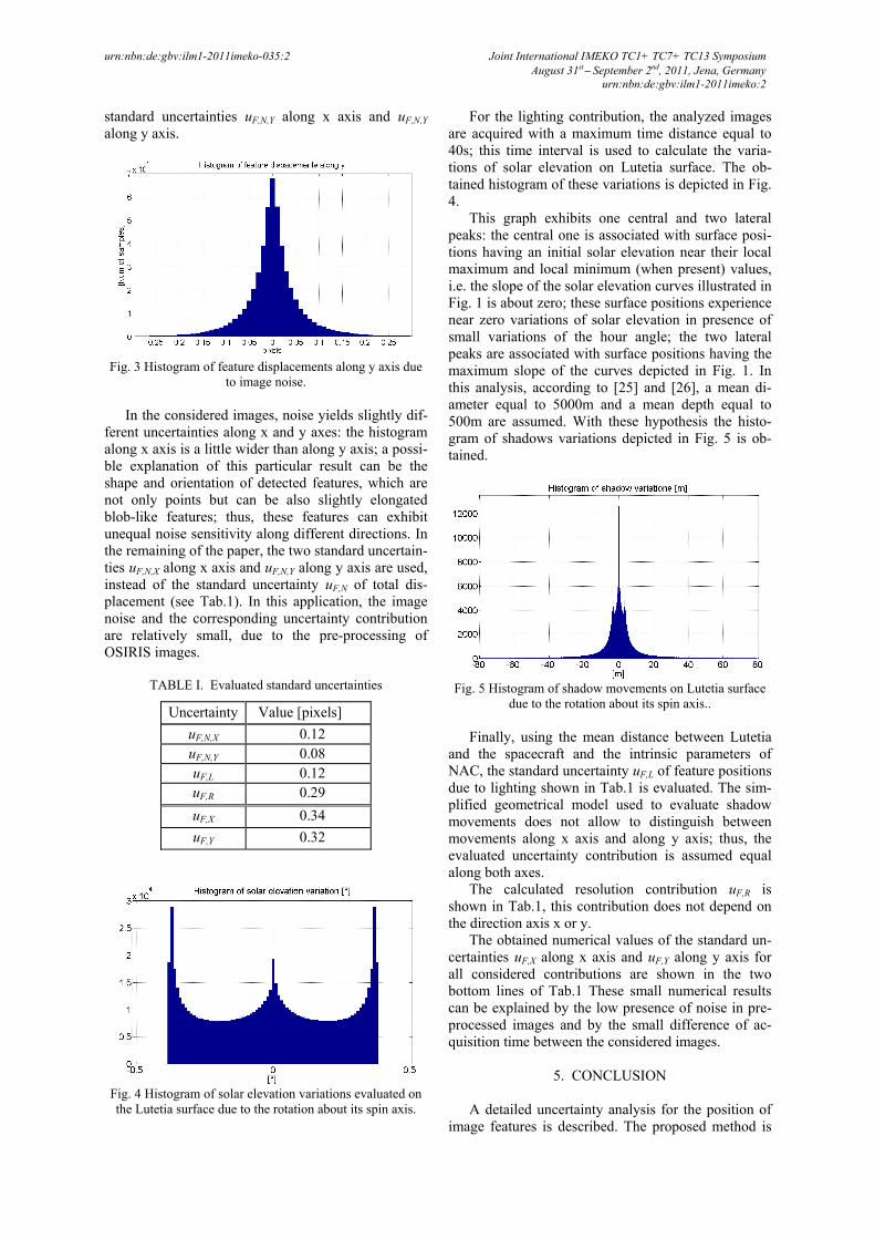
This graph exhibits one central and two lateral peaks: the central one is associated with surface posi-tions having an initial solar elevation near their local maximum and local minimum (when present) values, i.e. the slope of the solar elevation curves illustrated in Fig. 1 is about zero; these surface positions experience near zero variations of solar elevation in presence of small variations of the hour angle; the two lateral peaks are associated with surface positions having the maximum slope of the curves depicted in Fig. 1. In this analysis, according to [25] and [26], a mean di-ameter equal to 5000m and a mean depth equal to 500m are assumed. With these hypothesis the histo-gram of shadows variations depicted in Fig. 5 is ob-tained.

Fig. 5 Histogram of shadow movements on Lutetia surface due to the rotation about its spin axis..

Finally, using the mean distance between Lutetia

and the spacecraft and the intrinsic parameters of NAC, the standard uncertainty uF,L of feature positions due to lighting shown in Tab.1 is evaluated. The sim-plified geometrical model used to evaluate shadow movements does not allow to distinguish between movements along x axis and along y axis; thus, the evaluated uncertainty contribution is assumed equal along both axes.

The calculated resolution contribution uF,R is shown in Tab.1, this contribution does not depend on the direction axis x or y.

The obtained numerical values of the standard un-certainties uF,X along x axis and uF,Y along y axis for all considered contributions are shown in the two bottom lines of Tab.1 These small numerical results can be explained by the low presence of noise in pre-processed images and by the small difference of ac-quisition time between the considered images.

5. CONCLUSION

A detailed uncertainty analysis for the position of

image features is described. The proposed method is

urn:nbn:de:gbv:ilm1-2011imeko-035:2 Joint International IMEKO TC1+ TC7+ TC13 Symposium August 31st− September 2nd, 2011, Jena, Germany

urn:nbn:de:gbv:ilm1-2011imeko:2 particularly suited for applications with a relative motion between the camera and the scene and/or be-tween the lighting source and the scene, since it does not need to acquire multiple images of the same scene in the same shooting conditions. Three main uncer-tainty sources are identified and evaluated: image noise, lighting direction and image resolution. The described method is applied to the images acquired by the Narrow Angle Camera of the OSIRIS instrument, which is flying with the ESA Rosetta space mission. The obtained numerical results, including histograms and standard uncertainties, are depicted and discussed. The evaluated standard uncertainty of all contributions is below 1 pixel, which is a very good result. This achievement is due to the low noise present in the OSIRIS images and to the reduced delay between the first and the last analyzed images.

REFERENCES [1] Y Ma, S Soatto, J Kosecka, S S Sastry, 2004, An

invitation to 3-D Vision, Springer. [2] C Harris, M Stephens, “A combined corner and edge

detector”, Proc. Alvey Vision Conf., pp. 147-151, 1988.

[3] M Bertrandl, F Boucharal, S Ramdani, “Estimation of uncertainty for Harris corner detector”, IEEE Int. Conf. On Image Proc. Theory, Tools and Applications, 2010.

[4] U Orguner, F Gustafsson, “Statistical characteristics of harris corner detector”, IEEE 14th Workshop on Statistical Signal Processing, 2007.

[5] R M Steele, C Jaynes, “Feature uncertainty arising from covariant image noise”, IEEE Conf. on Computer Vision and Pattern Recognition, 2005.

[6] K Mikolajczyk, T Tuytelaars, C Schmid, A Zisserman, J Matas, F Schaffalitzky, T Kadir, VanGool, “A comparison of affine region detectors”, Int. J. Computer Vision, No. 65, pp. 43–72, 2005.

[7] D G Lowe, “Distinctive image features from scale-invariant keypoints”, Int. J. of Computer Vision, No. 60 (2), pp. 91–110, 2004.

[8] K Mikolajczyk, C Schmid, “A performance evaluation of local descriptors”, IEEE Trans On PAMI, Vol. 27, No. 10, October 2005.

[9] BIPM, IEC, IFCC, ISO, IUPAC, IUPAP, OIML, 2008, Guide to the Expression of Uncertainty in Measurement, Geneva, Switzerland: International Organization for Standardization.

[10] BIPM, IEC, IFCC, ILAC, ISO, IUPAC, IUPAP, OIML, Evaluation of measurement data—Supplement 1 to the Guide to the Expression of Uncertainty in Measurement—Propagation of distributions using a Monte Carlo method.

[11] K Rank, M Lendl, R Unbehauen, “Estimation of image noise variance”, Vision, Image and Signal Processing, IEE Proc., Vol. 146, Issue 2, 1999.

[12] R C Bilcu, M Vehvilainen, “A new method for noise estimation in images”, Proc. IEEE EURASIP Int. Workshop on Nonlinear Signal and Image Processing, Sapporo, Japan, 2005.

[13] S-C Tai, S-M Yang, “A fast method for image noise estimation using laplacian operator and adaptive edge detection”, 3rd Int. Symposium on Communications, Control and Signal Processing, Malta, 2008.

[14] F Russo, “A method for estimation and filtering of gaussian noise in images”, IEEE Trans. on Instr. and Meas., Vol. 52, No. 4, 2003.

[15] S G Chang, Y Bin, M Vetterli, “Spatially adaptive wavelet thresholding with context modeling for image denoising”, IEEE Trans. Image Process., vol. 9, no. 9, pp. 1522–1531, 2000.

[16] S G Chang, B Yu, M Vetterli, “Adaptive wavelet thresholding for image denoising and compression”, IEEE Trans. Image Process., vol. 9, no. 9, pp. 1532–1546, 2000.

[17] D L Donoho, I M Johnstone, “Ideal spatial adaption via wavelet shrinkage”, Biometrika, vol. 81, pp. 425–455, 1994.

[18] D L Donoho, I M Johnstone, “Adapting to unknown smoothness via wavelet shrinkage”, J. Amer. Statist. Assoc., vol. 90, pp. 1200–1224, 1995.

[19] S Beheshti, M A Dahleh, ““A new information-theoretic approach to signal denoising and best basis selection”, IEEE Trans. Signal Processing, vol. 53, no. 10, pp. 3613–3624, 2005.

[20] M Hashemi, S Beheshti, “Adaptive noise variance estimation in BayesShrink”, IEEE Signal Processing Letters, vol. 17, no. 1, 2010.

[21] J Immerkaer, “Fast noise variance estimation”, Computer Vision and Image Understanding, Vol. 64, No. 2, pp. 300-302, 1996.

[22] B Carry et Al., “Physical properties of the ESA Rosetta target asteroid (21) Lutetia – part II”, Astronomy & Astrophysics, 523, A94, 2010.

[23] P L Lamy et Al., “Multi-color, rotationally resolved photometry of asteroid 21 Lutetia from OSIRIS/Rosetta observations”, Astronomy & Astrophysics, 521, A19, 2010.

[24] J D Drummond et Al., “Physical properties of the ESA Rosetta target asteroid (21) Lutetia – part I”, Astronomy & Astrophysics, 523, A93, 2010.

[25] J B Vincent et Al., “Physical properties of craters on asteroid (21)Lutetia”, 42nd Lunar and Planetary Science Conf., 2011.

[26] H Sierks et Al., “The unique nature of asteroid 21 Lutetia”, Science, (in press).

Author(s): AUTHOR(S): Marco Pertile, Alessio Aboudan, Stefano Debei CISAS G. Colombo University of Padova, Via Venezia 15, 35131, Padova Italy; ++390498276794 marco.pertile@unipd.it.