Ultrafast Method for the Analysis of Fluorescence LifetimeImaging Microscopy Data Based on the Laguerre ExpansionTechnique

Javier A. Jo [Member, IEEE],J. A. Jo is with the Biophotonics Research and Technology Development, Department of Surgery,Cedars-Sinai Medical Center, Los Angeles, CA 90048 USA (e-mail: joj@cshs.org).

Qiyin Fang [Member, IEEE], andQ. Fang is with the Department of Engineering Physics, McMaster University, Hamilton, ON L8S4L8,Canada (e-mail: gfang@mcmaster.ca).

Laura MarcuL. Marcu is with Biophotonics Research and Technology Development, Department of Surgery,Cedars-Sinai Medical Center, Los Angeles, CA 90048 USA and the Departments of Electrical andBiomedical Engineering, University of Southern California, Los Angeles, CA 90048 USA (e-mail:lmarcu@bmsrs.usc.edu).

AbstractWe report a new deconvolution method for fluorescence lifetime imaging microscopy (FLIM) basedon the Laguerre expansion technique. The performance of this method was tested on synthetic andreal FLIM images. The following interesting properties of this technique were demonstrated. 1) Thefluorescence intensity decay can be estimated simultaneously for all pixels, without a prioriassumption of the decay functional form. 2) The computation speed is extremely fast, performing atleast two orders of magnitude faster than current algorithms. 3) The estimated maps of Laguerreexpansion coefficients provide a new domain for representing FLIM information. 4) The number ofimages required for the analysis is relatively small, allowing reduction of the acquisition time. Thesefindings indicate that the developed Laguerre expansion technique for FLIM analysis represents arobust and extremely fast deconvolution method that enables practical applications of FLIM inmedicine, biology, biochemistry, and chemistry.

Index TermsDiscrete Laguerre basis expansion; fluorescence decay deconvolution method; fluorescence lifetimeimaging microscopy (FLIM); global analysis

I. INTRODUCTIONFluorescence lifetime imaging microscopy (FLIM) is based on the measurement of the timethat a fluorescence system spends in the excited state before returning to the ground state afterlight excitation. Thus, lifetime measurement provides information about the localization of aspecific fluorophore and its surrounding environment [1]–[4]. This functionality of FLIM hasbeen exploited to study cell metabolism, including measurements of pH [5]–[7], Ca+

This work was supported by the National Institute of Health under Grant R01 HL 67377 and by The Whitaker Foundation.

NIH Public AccessAuthor ManuscriptIEEE J Quantum Electron. Author manuscript; available in PMC 2009 May 13.

Published in final edited form as:IEEE J Quantum Electron. 2005 ; 11(4): 835–845. doi:10.1109/JSTQE.2005.857685.

NIH

-PA Author Manuscript

NIH

-PA Author Manuscript

NIH

-PA Author Manuscript

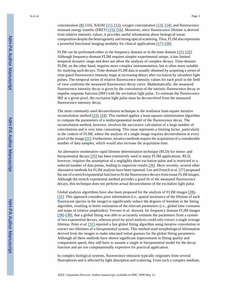
concentration [8]–[10], NADH [11], [12], oxygen concentration [13], [14], and fluorescenceresonant energy transfer (FRET) [15], [16]. Moreover, since fluorescence lifetime is derivedfrom relative intensity values, it provides useful information about biological tissuecomposition despite the heterogeneity and strong optical scattering. Thus, FLIM also representsa powerful functional imaging modality for clinical applications [17]–[20].

FLIM can be performed either in the frequency domain or in the time domain [21], [22].Although frequency-domain FLIM requires simpler experimental setups, it has limitedtemporal dynamic range and does not allow the analysis of complex decays. Time-domainFLIM, on the other hand, requires more complex instrumentation, but is often more suitablefor studying such decays. Time-domain FLIM data is usually obtained by acquiring a series oftime-gated fluorescence intensity maps at increasing delays after excitation by ultrashort lightpulses. The temporal series of relative fluorescence intensity values for each pixel in the fieldof view conforms the measured fluorescence decay curve. Mathematically, the measuredfluorescence intensity decay is given by the convolution of the intrinsic fluorescence decay orimpulse response function (IRF) with the excitation light pulse. To estimate the fluorescenceIRF at a given pixel, the excitation light pulse must be deconvolved from the measuredfluorescence intensity decay.

The most commonly used deconvolution technique is the nonlinear least-square iterativereconvolution method [23], [24]. This method applies a least-squares minimization algorithmto compute the parameters of a multiexponential model of the fluorescence decay. Thereconvolution method, however, involves the successive calculation of a large number ofconvolutions and is very time consuming. This issue represents a limiting factor, particularlyin the context of FLIM, where the analysis of a single image requires deconvolution at everypixel of the image [21]. Furthermore, iterative methods require the acquisition of a considerablenumber of data samples, which would also increase the acquisition time.

An alternative noniterative rapid lifetime determination technique (RLD) for mono- andbiexponential decays [25] has been extensively used in many FLIM applications. RLD,however, requires the assumption of a negligibly short excitation pulse and is restricted to areduced number of data points, leading to imprecise results [26]. More recently, several otheralternative methods for FLIM analysis have been reported. Lee and French et al. [27] proposedthe use of a stretch exponential function to fit the fluorescence decays from tissue FLIM images.Although the stretch exponential method provides a good fit of the measured fluorescencedecays, this technique does not perform actual deconvolution of the excitation light pulse.

Global analysis algorithms have also been proposed for the analysis of FLIM images [28]–[31]. This approach considers prior information (i.e., spatial invariance of the lifetime of eachfluorescent species in the image) to significantly reduce the degrees of freedom in the fittingalgorithm, resulting in better estimation of the relevant parameters (i.e., global time constantsand maps of relative amplitudes). Verveer et al. showed, for frequency domain FLIM images[28]–[30], that a global fitting was able to accurately estimate the parameters from a systemof two exponential decays, whereas pixel-by-pixel analysis could only extract a single averagelifetime. Pelet et al. [31] reported a fast global fitting algorithm using iterative convolution toextract two lifetimes of a biexponential system. This method used morphological informationderived from the images to make educated initial guesses for the global fitting parameters.Although all these methods have shown significant improvement in fitting quality andcomputation speed, they still have to assume a single or biexponential model for the decayfunction and are too computationally expensive for practical application.

In complex biological systems, fluorescence emission typically originates from severalfluorophores and is affected by light absorption and scattering. From such a complex medium,

Jo et al. Page 2

IEEE J Quantum Electron. Author manuscript; available in PMC 2009 May 13.

NIH

-PA Author Manuscript

NIH

-PA Author Manuscript

NIH

-PA Author Manuscript

however, it is not entirely adequate to analyze the time-resolved fluorescence decay transientin terms of multiexponential functions [27], [32]. Moreover, different multiexponentialexpressions can reproduce experimental fluorescence decay data equally well, suggesting anadvantage in avoiding any a priori assumption about the functional form of the IRF decayphysics. Recently, we reported a novel model-free deconvolution method for time-resolvedfluorescence point spectroscopy data [33], in which the IRF is expanded on the discrete timeLaguerre basis [34]. We demonstrated that this method is able to expand any fluorescenceintensity decay of arbitrary form, converging to a correct solution significantly faster thanconventional multiexponential approximation methods [33]. Extending on the early work, thegoal of the present study was to develop a new method for fluorescence lifetime imagingmicroscopy analysis, based on the Laguerre expansion technique [33], [34]. The proposedmethod, which can also be viewed as a global analysis approach, has been tested on syntheticand experimental FLIM images, and its performance was compared against other methods forFLIM analysis.

II. MethodsA. Laguerre FLIM Deconvolution Method

The Laguerre deconvolution technique expands the fluorescence impulse response functions(IRF) on the discrete time Laguerre basis [33]. The Laguerre functions (LF) have beensuggested as an appropriate orthonormal basis for expanding asymptotically exponentialrelaxation dynamics, due to their built-in exponential term [34]. Because the Laguerre basis iscomplete and orthonormal, a unique characteristic of this approach is that it can reconstruct afluorescence response of arbitrary form.

In the context of time-domain FLIM, the series of measured time-gated fluorescence intensitymaps H(r, t) are given by the convolution of IRF h(r, t) with the excitation light pulse x(t)

(1)

where r denotes pixel location, t denotes time gate, K determines the extent of the systemmemory, T is the sampling interval, h(r, t) is the intrinsic IRF at the pixel r, and N is the numberof time-gated images.

The Laguerre deconvolution technique uses the orthonormal set of LF to expand the IRF

(2)

where cj (r) are the unknown Laguerre expansion coefficients (LEC) at the pixel r, which areto be estimated from the input-output data; denotes the jth order LF; and L is the numberof LFs used to model the IRF.

The LF basis is defined as

Jo et al. Page 3

IEEE J Quantum Electron. Author manuscript; available in PMC 2009 May 13.

NIH

-PA Author Manuscript

NIH

-PA Author Manuscript

NIH

-PA Author Manuscript

(3)

The order j of each LF is equal to its number of zero-crossing (roots). The Laguerre parameter(0 < α < 1) determines the rate of exponential decline of the LF and defines the time scale forwhich the Laguerre expansion of the system impulse response is most efficient in terms ofconvergence [34]. Thus, fluorescence IRF with longer lifetime may require a larger α forefficient representation. Commonly, the parameter α is selected based on the kernel memorylength K and the number of Laguerre functions L, so that all the LFs decline sufficiently closeto zero by the end of the impulse response [33], [34].

By inserting (2) into (1), the convolution equation (1) becomes

(4)

where is the discrete convolution of the excitation input with the LF of order j, commonlydenoted as the “key variable” [34]. The unknown expansion coefficients cj (r) are thenestimated by generalized linear least-square fitting, using the data H(r, t) and .

The proposed FLIM deconvolution method takes advantage of the orthogonality of theLaguerre functions [34], which implies that the expansion coefficients are independent fromeach other and can be estimated separately. This condition allows us to reformulate thecomputation of the Laguerre expansion coefficients given in (4) as follows. Let us first resamplethe key variables at the times tk, k = 1, 2,…, N, at which the images H(r, t) were acquired.By considering the case when j = 0 in (4), the first expansion coefficient can be estimated usingthe images H(r, tk) and the first resampled key variable by solving the following systemof linear equations:

(5)

The analytical solution of c0(r) as defined in (5) using a least-square approach is given by

(6)

Where is a vector containing the N values of the key variable, and is defined as

(7)

Jo et al. Page 4

IEEE J Quantum Electron. Author manuscript; available in PMC 2009 May 13.

NIH

-PA Author Manuscript

NIH

-PA Author Manuscript

NIH

-PA Author Manuscript

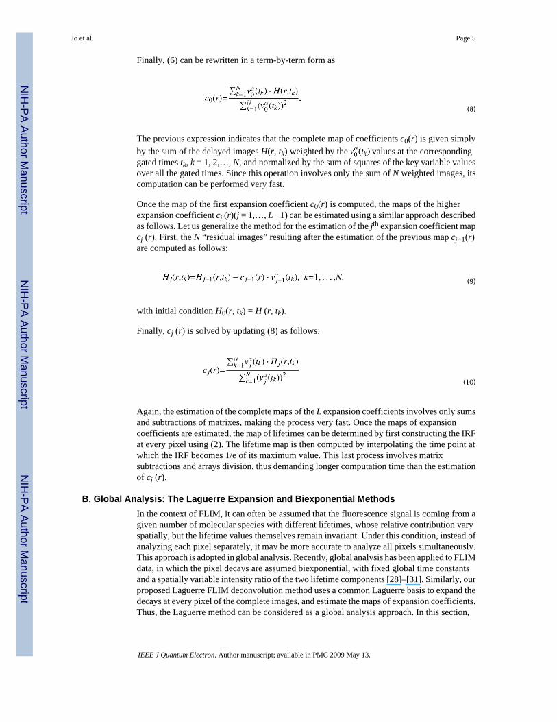
Finally, (6) can be rewritten in a term-by-term form as

(8)

The previous expression indicates that the complete map of coefficients c0(r) is given simplyby the sum of the delayed images H(r, tk) weighted by the values at the correspondinggated times tk, k = 1, 2,…, N, and normalized by the sum of squares of the key variable valuesover all the gated times. Since this operation involves only the sum of N weighted images, itscomputation can be performed very fast.

Once the map of the first expansion coefficient c0(r) is computed, the maps of the higherexpansion coefficient cj (r)(j = 1,…, L −1) can be estimated using a similar approach describedas follows. Let us generalize the method for the estimation of the jth expansion coefficient mapcj (r). First, the N “residual images” resulting after the estimation of the previous map cj−1(r)are computed as follows:

(9)

with initial condition H0(r, tk) = H (r, tk).

Finally, cj (r) is solved by updating (8) as follows:

(10)

Again, the estimation of the complete maps of the L expansion coefficients involves only sumsand subtractions of matrixes, making the process very fast. Once the maps of expansioncoefficients are estimated, the map of lifetimes can be determined by first constructing the IRFat every pixel using (2). The lifetime map is then computed by interpolating the time point atwhich the IRF becomes 1/e of its maximum value. This last process involves matrixsubtractions and arrays division, thus demanding longer computation time than the estimationof cj (r).

B. Global Analysis: The Laguerre Expansion and Biexponential MethodsIn the context of FLIM, it can often be assumed that the fluorescence signal is coming from agiven number of molecular species with different lifetimes, whose relative contribution varyspatially, but the lifetime values themselves remain invariant. Under this condition, instead ofanalyzing each pixel separately, it may be more accurate to analyze all pixels simultaneously.This approach is adopted in global analysis. Recently, global analysis has been applied to FLIMdata, in which the pixel decays are assumed biexponential, with fixed global time constantsand a spatially variable intensity ratio of the two lifetime components [28]–[31]. Similarly, ourproposed Laguerre FLIM deconvolution method uses a common Laguerre basis to expand thedecays at every pixel of the complete images, and estimate the maps of expansion coefficients.Thus, the Laguerre method can be considered as a global analysis approach. In this section,

Jo et al. Page 5

IEEE J Quantum Electron. Author manuscript; available in PMC 2009 May 13.

NIH

-PA Author Manuscript

NIH

-PA Author Manuscript

NIH

-PA Author Manuscript

we demonstrate how the Laguerre expansion technique is analytically related to the globalbiexponential fitting approach.

Let us assume that the deconvolved image h(r, t) given in (2) can also be expressed as abiexponential expansion as follows:

(11)

Here, the global time constants (τ1, τ2) and the intensity ratio of the two lifetime componentsA1(r) at every pixel r have to be estimated from the data by global analysis. The parameter srepresents a scaling factor, which for simplicity, is not carried on in the rest of the analysis.

Let us also assumed that each exponential component in (11) is expanded using the sameLaguerre basis as in (2), yielding the following relations:

(12)

Inserting (12) in (11), the expression of the deconvolved image becomes

(13)

Finally, from (2) and (13), we can relate the expansion coefficients cj (r) of the deconvolvedimage h(r, t) to the intensity ratio of the two lifetime components A1(r) as follows:

(14)

Equation (14) clearly shows that each Laguerre expansion coefficient cj (r) is linearly relatedto the intensity ratio of the two lifetime components A1(r). In practice, we may not need toestimate the global time constants (τ1, τ2) and compute their expansion coefficients {a1,j,a2,j} and the actual values of A1(r). The relation given by (14) demonstrated that the relativecontribution of the two exponential components can be indirectly monitored extremely quicklyby means of the expansion coefficients cj (r).

C. Synthetic FLIM Image GenerationThe synthetic FLIM images of 64 × 64 pixels were generated by means of a biexponentialmodel, with fixed decay constants (2 and 12 ns) and increasing relative contributions of the

Jo et al. Page 6

IEEE J Quantum Electron. Author manuscript; available in PMC 2009 May 13.

NIH

-PA Author Manuscript

NIH

-PA Author Manuscript

NIH

-PA Author Manuscript

shortest lifetime. White noise of zero mean and two different variance levels was added to thedata, yielding two different sets of images, at approximately 40- and 26-dB signal-to-noiseratios (SNRs). A laser pulse (see Section II-E) was used as the excitation signal for oursimulation. All the data sets were convolved with the laser signal and arranged accordingly toform the synthetic FLIM image series for our simulation.

D. Validation of the Laguerre Method Against Standard and Global AlgorithmsThe Laguerre deconvolution technique was applied to the synthetic FLIM images, using modelorders ranging from 3–6 LFs. Three other deconvolution algorithms were also applied tovalidate our technique. The first was based upon the standard “biexponential” fitting, whereall three parameters (two time constants and relative amplitude) are estimated independentlyat every pixel. The second was a “time invariant” fit method [28], where the two time constantsare extracted from a decay curve calculated from the sum of all pixels, and kept fixed for thecomputation of the relative amplitudes at every pixel. The third was a recently developed“global” analysis approach that uses iterative convolutions to extract the two global lifetimecomponents corresponding to the whole image, and the map of relative amplitudes. The codefor the global analysis was provided by Dr. Serge Pelet, from the Department of MechanicalEngineering and Division of Biological Engineering, at the Massachusetts Institute ofTechnology [31].

E. Experimental FLIM Images AcquisitionFour sets of measured FLIM images were used for algorithm validation. Data was collectedfrom: 1) a solution of Rose Bengal (R3877, Sigma-Aldrich, St. Louis, MO) in ethanol; 2) asolution of Rhodamine B (25 242, Sigma-Aldrich) in ethanol; 3) rat glioma C6 cells (ATCCCCL-107) stained with JC-1 (J-aggregate formation of the lipophilic cation, Molecular Probes);and 4) rat glioma C6 cells (ATCC CCL-107) stained with Rhodamine 123 (Molecular Probes).An inverted microscope (Axiovert 200, Carl Zeiss, Germany) operating in epi-illuminationmode was utilized for the FLIM image acquisition. A subnanosecond nitrogen laser (MNL200,Lasertechnik Berlin, Berlin, Germany) was used to provide excitation at 337.1 nm with a full-width at half-maximum (FWHM) pulse duration of ~700 ps (maximum pulse energy 100 μJ,repetition rate 0–50 Hz). A picosecond gated ICCD imaging system (PicoStar HR12, LaVision,Gottingen, Germany) was used for gated time-domain image acquisition.

III. ResultsA. Laguerre Method Accuracy Tested on Synthetic FLIM Images

Fig. 1 depicts the map of the model-derived lifetimes of the synthetic FLIM images at 40 dBSNR and the corresponding maps of estimated lifetimes, normalized mean square error(NMSE), and first three Laguerre expansion coefficients (LEC-0 to LEC-2). The map ofestimated lifetime values closely resembled the map of the synthetic lifetime values. Thenormalized mean square errors (NMSE) estimated from the reconstructed decays computed atevery pixel of the image showed values below 2%. The maps of LEC-0 and LEC-2 resembledthe variation in the lifetime values, while LEC-3 showed the opposite trend. These findingssuggested that the Laguerre expansion coefficients are correlated with the lifetime values. Asynthetic and estimated decay at a sample pixel and the corresponding normalized error (Nerr)and residual autocorrelation function (ACorr) are shown in Fig. 1 (bottom panels). The Nerrwas below 5% and the ACorr was mostly contained within the 95% confidence interval (dottedlines). These observations indicate an excellent fit between the synthetic and estimatedfluorescence decays, showing that the fluorescence IRF was properly estimated by the Laguerredeconvolution.

Jo et al. Page 7

IEEE J Quantum Electron. Author manuscript; available in PMC 2009 May 13.

NIH

-PA Author Manuscript

NIH

-PA Author Manuscript

NIH

-PA Author Manuscript

Similar results were obtained from the analysis of the synthetic FLIM images at 26-dB SNR(Fig. 2). In this case, however, the map of estimated lifetimes appeared noisy and biasedcomparing to the synthetic lifetime map, although still resembling the lifetime variation. TheNMSE values were higher (about 10%) than in the 40-dB case. The maps of LECs were noisierwhen compared to the ones obtained at 40-dB SNR but still resembled the variation in thelifetime values. The NErr was below 10% and the ACorr was mostly contained within the 95%confidence interval (dotted lines). These observations also indicate a good fit between thesynthetic and estimated fluorescence decays in spite of the considerable noise level, suggestingrobustness of the Laguerre technique.

B. Global Analysis: The Laguerre Expansion and Biexponential MethodsTo quantify the accuracy of the Laguerre technique for estimating the lifetime values of theimage pixel decays, we applied a correlation analysis between the synthetic and the estimatedlifetimes. The results (Fig. 3) showed a perfect (r = 1) and near perfect (r = 0.99) correlationbetween estimated and synthetic lifetimes at 40-dB and 26-dB SNR, respectively.

As shown in (14), each LEC cj (r) is linearly related to the intensity ratio of the two underlyinglifetime components A1(r) from the biexponential model. By means of analysis of the syntheticbiexponential FLIM images, it was possible to confirm experimentally the linear relationbetween cj (r) and A1(r). As observed in Fig. 3 at both 40-dB and 26-dB SNR, the first threeLECs were linearly related to the relative intensity A1(r) of the two underlying lifetimecomponents. More interestingly, these linear relations were unaffected by the noise level (40dB left, 26 dB right), as shown by the linear equations derived from least-square fitting of theLECs versus A1(r) data. Furthermore, these linear relations derived from data fitting werecompared against the ones obtained analytically using (14). The results (Table I) indicate thatthe analytical derivation of the cj (r) equations under both noise levels resembled very closelythe actual cj (r) versus A1(r) relations obtained by data fitting.

C. Validation of the Laguerre Methods Against Current AlgorithmsThe results obtained from the analysis of the synthetic FLIM images by the Laguerredeconvolution technique were compared against the performance by standard and globalmethods. The results of this intermethodology comparison are summarized in Fig. 4 and TableII. The true intensity ratios A1(r) and their estimated values using the standard biexponential,time invariant, global analysis, and Laguerre methods, at 40- and 26-dB SNR are shown inFig. 4. All tested algorithms provided a good estimation of the A1(r). The Laguerre and thetime invariant algorithms were almost insensitive to the noise level and provided goodestimation of A1(r) at both 40- and 26-dB SNR. The global analysis and the standardbiexponential algorithms performed well at 40-dB SNR, but were sensitive to the noise levelproviding less accurate estimation at 26-dB SNR. The standard biexponential algorithmprovided the less accurate estimation overall. The histograms of the deviations of the estimatedA1(r) from their true values by all the algorithms tested are also given in Fig. 4. The Laguerreand the time invariant methods presented small deviations from the true A1(r) values (less than0.03 ns and 0.1 ns at 40- and 26-dB SNR, respectively), although the time invariant methodperformed slightly better. The global fitting and the standard biexponential methods presentedlarger deviation from the true A1(r) values (less than 0.05 ns and 0.2 ns at 40- and 26-dB SNR,respectively).

In addition, the computation time spent by each algorithm to analyze the synthetic FLIM imageswere assessed and compared (Table II). By far, the Laguerre deconvolution approach was thefastest of all methods tested (0.4 s to compute the LECs, and 1.1 s to compute the lifetimevalues). The computational time was also insensitive to the noise level. The global fitting andthe time invariant algorithms showed similar computation time (~380–700 s), and the standard

Jo et al. Page 8

IEEE J Quantum Electron. Author manuscript; available in PMC 2009 May 13.

NIH

-PA Author Manuscript

NIH

-PA Author Manuscript

NIH

-PA Author Manuscript

biexponential method presented by far the slowest performance (> 3000 s). These resultsindicate that the Laguerre method was at least two orders of magnitude faster than the globalanalysis and the time invariant algorithms, and at least three orders of magnitude faster thanthe standard biexponential method.

D. Analysis of the Measured FLIM Images1) Fluorescence Lifetime Standards—Results of the analysis of FLIM images from thesolution of Rose Bengal in ethanol are presented in Fig. 5. The intensity map showed highervalues at the center of the image, while the lifetime map was uniform with values at about 750ps. The maps of Laguerre expansion coefficients were also uniform. The map of NMSE showedvalues below 10%, indicating a very good fitting for every pixel of the image. The Nerr werebelow 20% and randomly distributed around zero. The autocorrelation function of the residualswas mostly contained within the 95% confidence interval (dotted lines). These observationsalso indicate a good fit between the measured and estimated fluorescence decays. The maphistograms indicate the range of lifetime and LECs values present in the image. All theparameters showed a narrow distribution. The lifetime was centered at 771 ps, the LEC-0 at0.448, the LEC-1 at 0.314, and the LEC-2 at 0.106. The average lifetime value was very closeto the lifetime of 769 ps obtained from spectroscopy measurements of equivalent solution witha time-resolved fluorescence spectroscopy system, as previously reported [33].

Results of the analysis of FLIM images from the solution of Rhodamin B in ethanol are alsopresented in Fig. 6. For this case, the lifetime map was uniform with values ~2500 ps. Themaps of Laguerre expansion coefficients were also uniform. The map of NMSE showed valuesbelow 5%. The Nerr and ACorr also indicate good fit. The parameter histograms also showeda narrow distribution, with the lifetime centered at 2642 ps, the LEC-0 at 0.692, the LEC-1 at0.264, and the LEC-2 at 0.044. The average lifetime value was very close to the lifetime of2872 ps obtained spectroscopically [33].

2) Live Cell Imaging—The FLIM images from the glioma cells stained with JC-1 arepresented in Fig. 6. The intensity image presented a large variability across the cell, while themaps of lifetime and Laguerre expansion coefficients were also uniform. The map of NMSE,and the Nerr and ACorr showed good fit between measured and estimated decays. All theparameter histograms showed a narrow distribution. The lifetime was centered at 884 ps, theLEC-0 at 0.505, the LEC-1 at 0.302, and the LEC-2 at 0.193.

The FLIM images from the glioma cells stained with R-123 dye are also given in Fig. 6. Theintensity image presented different levels with higher values on the cell membrane. The lifetimemap was uniform in the areas corresponding to the glioma cells, presenting values around1800–2000 ps. Longer lifetimes, in the order of 2000–2500 ps, were also present in the vicinityof the cells, but were less representative. The map of LEC-0 showed values in the order of0.85–0.9 within the cell areas, and lower values (<0.85) in the vicinity of the cells. The mapof LEC-1 presented similar distribution as LEC-0, although showing negative values in therange of −0.2– 0, where the cell areas corresponded to the less negative values. The map ofLEC-2 showed values between 0 and 0.1. The map of NMSE showed values below 5%, andthe Nerr was below 5% and randomly distributed around zero. The autocorrelation function ofthe residuals was contained within the 95% confidence interval (dotted lines). The lifetimehistogram was centered at 1891 ps and was broad covering a range of 1500–2500 ps. Thehistogram of LEC-0 and LEC-1 were also broad (covering values between 0.7–0.9 and −0.2–0, respectively) and centered at 0.827 and −0.085, respectively. The histogram of LEC-2presented a short tail towards the lower values and was centered at 0.095.

Jo et al. Page 9

IEEE J Quantum Electron. Author manuscript; available in PMC 2009 May 13.

NIH

-PA Author Manuscript

NIH

-PA Author Manuscript

NIH

-PA Author Manuscript

IV. DiscussionValidation in synthetic FLIM images

The Laguerre deconvolution technique was successfully tested in a set of synthetic FLIMimages covering a broad range of lifetime values (2–12 ns) derived from a biexponential model.This lifetime range was chosen intentionally, since a number of biologically relevantfluorophores emit in this time scale. The choice of a biexponential model was also adequate,since current FLIM analytical methods (including the ones compared in this study) are notusually applied for more than two exponential components. The proposed Laguerredeconvolution method was found versatile and robust as demonstrated by its ability toaccurately retrieve the underlying IRFs at every pixel of the synthetic FLIM images coveringa broad dynamic range under moderate noise condition (40- and 26-dB SNR).

Our results demonstrated that each Laguerre expansion coefficient is highly correlated withthe intrinsic lifetime value. For the case of the multiexponential deconvolution, the estimatedaverage lifetime usually correlates with the intrinsic radiative lifetime. However, the individualmultiexponential parameters (decay constants and pre-exponential coefficients) may notnecessarily correlate to the intrinsic lifetimes. This was shown in Fig. 4, where the standardbiexponential method was not able to accurately estimate the intensity ratio of the twounderlying lifetime components A1(r). The lack of correlation between individualmultiexponential parameters and the radiative lifetime is a result of the intrinsic nature of themultiexponential model. This model does not represent an orthogonal expansion of thefluorescence IRF. Therefore, the estimated fitting parameters are not independent from eachother (the value of one parameter would be determined by both the data to be fitted and thevalue of the other fitting parameters) [32]. In contrast, the Laguerre basis provides anorthogonal expansion of the IRF. Consequently, the value of each LEC depends exclusivelyon the data to be fitted, making them highly correlated to the actual decay lifetime values[33].

Global analysisAnother interesting observation is that the Laguerre deconvolution technique represents a wayof performing global analysis on the FLIM images. In the context of classical global analysisfor FLIM, the spatial invariance of the lifetimes of each exponential component (fluorescencespecie) is often assumed [28], [31]. That is, a global analysis algorithm will estimate a uniqueset of time constants for the entire image, and maps of relative intensities of the underlyingexponential components. Similarly, the Laguerre technique uses a unique Laguerre basis(defined by the Laguerre parameter α) to expand the complete set of IRFs at every pixel of theimages. Thus, only a single parameter α and the maps of LECs are to be estimated from thedata. Thus, the estimation of the spacial invariant time constants can be related to the estimationof the Laguerre parameter α, and the computation of the maps of relative exponential intensitiesto the computation of the maps of LECS. One advantage of the Laguerre method, however, isthat for any value of the Laguerre parameter α, the corresponding basis of LF is complete andorthonormal. Thus, it is certain that the maps of expansion coefficients can always be foundand are unique for the defined Laguerre basis. In contrast, deconvolution with themultiexponential approach may yield more than one solution, even when the number ofexponential or the values of the time constants are prefixed.

We also demonstrated, both mathematically (14) and experimentally (from the analysis of thesynthetic data, Table I), that for the specific case of two fluorescence species in a single image,each LEC is linearly related to the relative intensity A1(r) of the two lifetime components. Thus,the maps of LECs are correlated to the map of A1(r) and indirectly reflect the spatial variationof the biexponential relative intensities. These two findings indicates that the maps of Laguerre

Jo et al. Page 10

IEEE J Quantum Electron. Author manuscript; available in PMC 2009 May 13.

NIH

-PA Author Manuscript

NIH

-PA Author Manuscript

NIH

-PA Author Manuscript

expansion coefficients constitute an extremely fast and original way of representing spatialdistribution of time-resolved characteristics of fluorescence species in a field of view, and hasthe potential for quantitative interpretation of FLIM data.

It is important to note that, for the case of the synthetic data, the two exponential componentswere known a priori, so it was possible to compute their Laguerre expansion coefficients{a1,j, a2,j} and the relative intensity values A1(r). In practice, however, we may not need toestimate the global time constants of the fluorescence species to compute the map of relativeamplitudes. The relation given by (14) demonstrated that the map of relative intensities can beindirectly but extremely fast monitored by means of the maps of Laguerre expansioncoefficients. And even when the actual values of A1(r) be required, a globally biexponentialfit can always be performed on the estimated IRFs obtained by the Laguerre technique. Thevalues of A1(r) can then be estimated using {a1,j, a2,j} from the derived global time constantson (14). This approach will represent a much faster way of performing global analysis on thecomplete FLIM image, since only curve fittings instead of deconvolution operations arerequired.

Validation against other methodsThis study also demonstrates the advantages of the proposed Laguerre deconvolution techniquewith respect to conventional and other recently proposed deconvolution methods [28], [31].Our results indicated that the Laguerre and the time invariant methods provide the bestperformance in terms of estimating the A1(r) values of the synthetic images. One explanationfor the good performance of the time invariant method is that the synthetic FLIM images were,in fact, generated by two exponential components with fixed time constants. This is exactlythe assumption made by the time invariant method. However, when the data diverges from thisstrict assumption, as is often the case in practical application, the time invariant method wouldprobably perform less accurately, as it has been demonstrated in other studies [26], [28], and[31]. In contrast, the Laguerre method does not make any assumption about the functional form(decay function) of the data. Moreover, and due to the orthogonality of the Laguerre basis, ourmethod has the capability of always expanding any IRF of arbitrary form. Thus, the Laguerredeconvolution technique is a suitable approach for the analysis of time-domain fluorescencedata from complex systems. It is also relevant to notice that the global analysis methodsprovided a good estimation of the relative intensities from the synthetic data, in spite of notreaching the accuracy of the Laguerre method (especially under noisy conditions). Thisparticular result together with the poor performance showed by the standard biexponentialmethod indicate that global approaches outperform pixel-by-pixel methods for the analysis ofFLIM data, as it has already been supported by other studies [28], [31].

Computation speedOne of the most important finding of this study was the clear advantage in terms of computationspeed of the Laguerre deconvolution technique over the other methods considered. Theproposed Laguerre method takes advantages of the orthogonality of the Laguerre functions.This implies that the expansion coefficients are independent from each other, and therefore,each of them can be estimated separately. Unlike standard FLIM global methods, which involvethe iterative computation of convolutions, the estimation of the complete maps of the LECsinvolves only sums and subtractions of the complete delayed images, making this processextremely fast. Furthermore, since the set of expansion coefficients summarize the temporalproperties of the IRF [33], a complete characterization of the fluorescence decay at every pixelof the image can be achieved in a few seconds. Due to its ultrafast performance, the Laguerremethod has the potential to be applied for the study of dynamics events, allowing for monitoringtemporal and spatial variation of time-resolved characteristics of fluorescence specimens.Thus, we consider that the proposed Laguerre deconvolution technique for FLIM analysis

Jo et al. Page 11

IEEE J Quantum Electron. Author manuscript; available in PMC 2009 May 13.

NIH

-PA Author Manuscript

NIH

-PA Author Manuscript

NIH

-PA Author Manuscript

could have a great impact in a broad range of applications in medicine, biology, biochemistry,and chemistry.

Validation in experimental FLIM imagesThe Laguerre deconvolution method was also successfully tested on measured FLIM imagesfrom both fluorescence lifetime standards and glioma cells stained with fluorescence probes.The fact that the fluorescence standard lifetime values obtained by the Lagurre method werevery close to their literature reported values [33], confirms the accuracy of our technique. Alsoimportant was our finding that short lifetimes (rose Bengal in ethanol) could be accuratelyretrieved by the Laguerre technique, suggesting the convenience of performing actualdeconvolution for the analysis of fast fluorescence decays. For the case of the FLIM imagesfrom glioma cells stained with Rhodamine 123, the lifetimes obtained (~2000 ps) were slightlyshorter than the ones (2500–2800 ps) reported in a previous study [35]. One possibleexplanation for this difference may be related to the analytical methods used. The referredabove study applied plain curve fitting to analyze the FLIM data, while our method performedactual deconvolution of the excitation pulse from the complete images. Since the width of theexcitation pulse cannot always be infinitesimally short, the convolved IRF (which correspondsto the measured decay curved fitted by standard methods) is always broader than the actualIRF (estimated by our method). Thus, a shorter but more realistic lifetime value by ourtechnique is expected.

The observations that the maps of the LEC resemble the distribution of lifetimes in the cellimages also support the idea of using the LEC as a new domain of representing spatialdistribution of time-resolve information for FLIM applications. These results could betranslated to other more interesting application, such as fluorescence energy resonance transfer(FRET) experiments [15], [16]. In FRET experiments, one expects to measure two differentlifetimes produced by interacting and noninteracting proteins. The noninteracting labeledproteins exhibit a natural lifetime of the dye, whereas the interacting proteins will exhibit ashorter lifetime due to the quenching of the emission by energy transfer. The spatialconfiguration of the donor and acceptor is fixed upon binding, which determines the decreasein the donor lifetime. When FRET is imaged with FLIM, the decay model is assumed to bebiexponential with spatially invariant lifetimes. Therefore, an ultrafast global analysisapproach, such as the Laguerre deconvolution method, could represent a powerful tool forevaluating the populations and properties of bound and unbound proteins states in cells.Although the results of the present study are encouraging, we realize that the proposed Laguerremethod still need to be thoroughly validated on a broad variety of FLIM applications.

Another observation is that the Laguerre method needs only half or less of the acquired delayedimages available for the analysis of the measured FLIM data. This indicates that accurateestimation of the IRF at every pixel can be achieved with considerably few data points withthe proposed technique, in contrast to standard FLIM deconvolution methods that require theacquisition of tens of delayed images [21]. Therefore, since less delayed images would beneeded, our method would not only allow for a significant reduction of the computation timebut also of the acquisition time. This would be highly desirable in the context of functionalfluorescence lifetime imaging, where real-time acquisition is required.

Finally, most algorithms used on current FLIM systems require the assumption that theexcitation light pulses are negligibly short, so that the fluorescence emission can beapproximated to the intrinsic IRF [21]. To accommodate this requirement, these systems needto use ultrafast (i.e., femtosecond) light sources, which are in general too expensive andsophisticated to be used in practical applications. Since our proposed Laguerre techniquedeconvolves the excitation light pulse from the measured images within seconds, therequirement of an ultrashort excitation pulse can be relaxed. Thus, our technique has the

Jo et al. Page 12

IEEE J Quantum Electron. Author manuscript; available in PMC 2009 May 13.

NIH

-PA Author Manuscript

NIH

-PA Author Manuscript

NIH

-PA Author Manuscript

potential for promoting the development of less expensive and less complex FLIM systemsthat could be used in a variety of practical applications.

V. ConclusionWe have developed and tested a new method for analysis of fluorescence lifetime imagingmicroscopy data based on the Laguerre expansion technique [33], [34]. The results of this studydemonstrated a number of interesting properties. 1) The intrinsic fluorescence intensity decaysof any form can be estimated at every pixel of the image as an expansion on a Laguerre basis,without a priori assumption of its functional form, thus providing a robust and versatile methodfor FLIM analysis. 2) Since the fluorescence IRF at every pixel is expanded in parallel usinga common Laguerre basis, the computation speed is extremely high, performing at least twoorders of magnitude faster than standard deconvolution algorithms. 3) The estimated maps ofLaguerre expansion coefficients offer a new domain for representing the spatial distributionof the time-resolved characteristics of the fluorescence specimens imaged by FLIM. 4) TheLaguerre deconvolution technique represents a way of performing global analysis in the FLIMimages very fast and accurate. 5) The number of images required to expand the fluorescenceIRF is relatively low, thus allowing the reduction of the acquisition time. In addition, sinceactual deconvolution of the excitation pulse is performed, ultrafast light sources are not longerrequired, allowing to promote the development of less expensive FLIM systems.

Although our method still have to be validated on a broad variety of FLIM applications, theresults of this study indicate that the Laguerre deconvolution technique represents a more robustand extremely fast analytical method. The developed technique will likely enable the use ofFLIM in practical real-time applications in medicine, biology, biochemistry, and chemistry.

AcknowledgementsThe authors would like to thank Prof. M. Gundersen from the Department of Electrical Engineering/Electro-Physics,University of Southern California, Los Angeles, for his support on the experimental aspects of this study. The authorsare also grateful to Dr. S. Pelet from the Department of Mechanical Engineering and Division of BiologicalEngineering, Massachusetts Institute of Technology, for providing the codes for the global analysis algorithm used inthis study.

References1. Dowling K, Dayel MJ, Hyde SCW, French PMW, Lever MJ, Hares JD, Dymoke-Bradshaw AKL.

High resolution time-domain fluorescence lifetime imaging for biomedical applications. J Modern Opt1999;46:199–209.

2. Tadrous PJ. Methods for imaging the structure and function of living tissues and cells: 2. Fluorescencelifetime imaging. J Pathology 2000;191:229–234.

3. Sauer M, Tinnefeld P. Spectrally-resolved fluorescence lifetime imaging of single molecules onsurfaces and in living cells. Biophys J 2001;80:789. [PubMed: 11159446]

4. Elson D, Requejo-Isidro J, Munro I, Reavell F, Siegel J, Suhling K, Tadrous P, Benninger R, LaniganP, McGinty J, Talbot C, Treanor B, Webb S, Sandison A, Wallace A, Davis D, Lever J, Neil M, PhillipsD, Stamp G, French P. Time-domain fluorescence lifetime imaging applied to biological tissue.Photochem Photobiol Sci 2004;3:795–801. [PubMed: 15295637]

5. Sanders R, Draaijer A, Gerritsen HC, Houpt PM, Levine YK. Quantitative pH imaging in cells usingconfocal fluorescence lifetime imaging microscopy. Anal Biochem 1995;227:302–308. [PubMed:7573951]

6. Carlsson K, Liljeborg A, Andersson RM, Brismar H. Confocal pH imaging of microscopic specimensusing fluorescence lifetimes and phase fluorometry: Influence of parameter choice on systemperformance. J Microscopy-Oxford 2000;199:106–114.

7. Lin HJ, Herman P, Lakowicz JR. Fluorescence lifetime-resolved pH imaging of living cells. CytometryA 2003;52A:77–89. [PubMed: 12655651]

Jo et al. Page 13

IEEE J Quantum Electron. Author manuscript; available in PMC 2009 May 13.

NIH

-PA Author Manuscript

NIH

-PA Author Manuscript

NIH

-PA Author Manuscript

8. Lakowicz JR, Szmacinski H, Nowaczyk K, Johnson ML. Fluorescence lifetime imaging of calciumusing quin-2. Cell Calcium 1992;13:131–147. [PubMed: 1576634]

9. Szmacinski H, Lakowicz JR, Lederer WJ, Nowaczyk K, Johnson ML. Fluorescence lifetime imagingmicroscopy (FLIM)—Calcium imaging in living cells using quin-2. Biophys J 1994;66:A275.

10. Christensen KA, Christensen KA. Measurement of calcium in macrophage vacuolar compartmentsusing ratiometric and fluorescence lifetime imaging microscopy. Mol Biol Cell 2000;11:730.

11. Lakowicz JR, Szmacinski H, Nowaczyk K, Johnson ML. Fluorescence lifetime imaging of free andprotein-bound nadh. Proc Nat Acad Sci USA 1992;89:1271–1275. [PubMed: 1741380]

12. Urayama P, Zhong W, Beamish JA, Minn FK, Sloboda RD, Dragnev KH, Dmitrovsky E, MycekMA. A UV-visible-NIR fluorescence lifetime imaging microscope for laser-based biological sensingwith picosecond resolution. Appl Phys B 2003;76:483–496.

13. Gerritsen HC, Sanders R, Draaijer A, Levine YK. Fluorescence lifetime imaging of oxygen in cells.J Fluoresc 1997;7:11–16.

14. Hartmann P, Ziegler W, Holst G, Lubbers DW. Oxygen flux fluorescence lifetime imaging. SensActuators B, Chem 1997;38:110–115.

15. Elangovan M, Day RN, Periasamy A. Nanosecond fluorescence resonance energy transfer-fluorescence lifetime imaging microscopy to localize the protein interactions in a single living cell.J Microscopy-Oxford 2002;205:3–14.

16. Murata S, Herman P, Lin HJ, Lakowicz JR. Fluorescence lifetime imaging of nuclear DNA: Effectof fluorescence resonance energy transfer. Cytometry 2000;41:178–185. [PubMed: 11042614]

17. Mizeret J, Stepinac T, Hansroul M, Studzinski A, van den Bergh H, Wagnieres G. Instrumentationfor real-time fluorescence lifetime imaging in endoscopy. Rev Sci Instrum 1999;70:4689–4701.

18. Cubeddu R, Pifferi A, Taroni P, Torricelli A, Valentini G, Rinaldi F, Sorbellini E. Fluorescencelifetime imaging: An application to the detection of skin tumors. IEEE J Sel Topics Quantum ElectronJul/Aug;1999 5(4):923–929.

19. Siegel J, Elson DS, Webb SED, Lee KCB, Vlanclas A, Gambaruto GL, Leveque-Fort S, Lever MJ,Tadrous PJ, Stamp GWH, Wallace AL, Sandison A, Watson TF, Alvarez F, French PMW. Studyingbiological tissue with fluorescence lifetime imaging: Microscopy, endoscopy, and complex decayprofiles. Appl Opt 2003;42:2995–3004. [PubMed: 12790450]

20. Tadrous PJ, Siegel J, French PMW, Shousha S, Lalani EN, Stamp GWH. Fluorescence lifetimeimaging of unstained tissues: Early results in human breast cancer. J Pathology 2003;199:309–317.

21. Cubeddu R, Comelli D, D’Andrea C, Taroni P, Valentini G. Time-resolved fluorescence imaging inbiology and medicine. J Phys D, Appl Phys 2002;35:R61–R76.

22. Gratton E, Breusegem S, Sutin J, Ruan Q, Barry N. Fluorescence lifetime imaging for the two-photonmicroscope: Time-domain and frequency-domain methods. J Biomed Opt 2003;8:381–390.[PubMed: 12880343]

23. Ware WR, Doemeny LJ, Nemzek TL. Deconvolution of fluorescence and phosphorescence decaycurves. A least square method. J Phys Chem 1973;77:2038–2048.

24. Johnson ML, Frasier SG. Non-linear least-square analysis. Methods Enzymol 1985;117:301–342.25. Periasamy A, Sharman KK, Demas JN. Fluorescence lifetime imaging microscopy using rapid

lifetime determination method: Theory and applications. Biophys J 1999;76:A10.26. Niesner R, Peker B, Schlusche P, Gericke KH. Noniterative biexponential fluorescence lifetime

imaging in the investigation of cellular metabolism by means of NAD(P)H autofluorescence.Chemphyschem 2004;5:1141–1149. [PubMed: 15446736]

27. Lee KCB, Siegel J, Webb SED, Leveque-Fort S, Cole MJ, Jones R, Dowling K, Lever MJ, FrenchPMW. Application of the stretched exponential function to fluorescence lifetime imaging. BiophysJ 2001;81:1265–1274. [PubMed: 11509343]

28. Verveer PJ, Squire A, Bastiaens PIH. Global analysis of fluorescence lifetime imaging microscopydata. Biophys J 2000;78:2127–2137. [PubMed: 10733990]

29. Verveer PJ, Squire A, Bastiaens PIH. Improved spatial discrimination of protein reaction states incells by global analysis and deconvolution of fluorescence lifetime imaging microscopy data. JMicroscopy-Oxford 2001;202:451–456.

Jo et al. Page 14

IEEE J Quantum Electron. Author manuscript; available in PMC 2009 May 13.

NIH

-PA Author Manuscript

NIH

-PA Author Manuscript

NIH

-PA Author Manuscript

30. Verveer PJ, Bastiaens PIH. Evaluation of global analysis algorithms for single frequency fluorescencelifetime imaging microscopy data. J Microscopy-Oxford 2003;209:1–7.

31. Pelet S, Previte MJR, Laiho LH, So PTC. A fast global fitting algorithm for fluorescence lifetimeimaging microscopy based on image segmentation. Biophys J 2000;87:2807–2817. [PubMed:15454472]

32. Lakowicz, JR. Principles of Fluorescence Spectroscopy. Vol. 2. Norwell, MA: Kluwer/Plenum; 1999.33. Jo JA, Fang Q, Papaioannou T, Marcu L. Fast nonparametric deconvolution of fluorescence decay

for analysis of biological systems. J Biomed Opt 2004;9(4):743–752. [PubMed: 15250761]34. Marmarelis VZ. Identification of nonlinear biological systems using Laguerre expansion of kernels.

Ann Biomed Eng 1993;21:573–589. [PubMed: 8116911]35. Schneckenburger H, Stock K, Lyttek M, Strauss WS, Sailer R. Fluorescence lifetime imaging (FLIM)

of rhodamine 123 in living cells. Photochem Photobiol Sci 2004;3:127–131. [PubMed: 14768629]

BiographiesJavier A. Jo (M’98) received the Diploma in electrical engineering from the Pontifical CatholicUniversity of Peru, Lima, Peru, in 1997, and the M.S. degree in electrical engineering and thePh.D. degree in biomedical engineering from the University of Southern California, LosAngeles, in 2000 and 2002, respectively.

He is currently a Research Scientist in the Department of Surgery of Cedars-Sinai MedicalCenter, Los Angeles. His research interests include developing advanced analytical methodsfor time-resolved fluorescence spectroscopy and imaging with application in cardiovascularand cancer diagnosis.

Jo et al. Page 15

IEEE J Quantum Electron. Author manuscript; available in PMC 2009 May 13.

NIH

-PA Author Manuscript

NIH

-PA Author Manuscript

NIH

-PA Author Manuscript

Qiyin Fang (M’02) received the B.S. degree in physics from Nankai University in 1995, andthe M.S. degree in 1998 in applied physics and the Ph.D. degree in 2002 in biomedical physics,both from East Carolina University.

He is currently an Assistant Professor in the Department of Engineering Physics, McMasterUniversity, Hamilton, ON, Canada. Prior to his current position, he was a Research Scientistin the Biophotonics Research and Technology Development Laboratory at Cedars-SinaiMedical Center, Los Angeles, CA. His research interests include optical spectroscopy andimaging for biomedical and clinical applications and ultrafast laser pulse interaction withbiological systems.

Jo et al. Page 16

IEEE J Quantum Electron. Author manuscript; available in PMC 2009 May 13.

NIH

-PA Author Manuscript

NIH

-PA Author Manuscript

NIH

-PA Author Manuscript

Laura Marcu received the Diploma in mechanical engineering (precision mechanics andoptical instruments) from the Polytechnic Institute of Bucharest, Bucharest, Romania, in 1984,and the M.S. and Ph.D. degrees in biomedical engineering from the University of SouthernCalifornia, Los Angeles, in 1995 and 1998, respectively.

Presently, she is Director of the Biophotonics Research and Technology Development Lab inthe Department of Surgery at the Cedars-Sinai Medical Center, Los Angeles, where she hasestablished a research program in biophotonics. She is also a Research Associate Professor inthe Departments of Electrical Engineering-Electrophysics and Biomedical Engineering at the

Jo et al. Page 17

IEEE J Quantum Electron. Author manuscript; available in PMC 2009 May 13.

NIH

-PA Author Manuscript

NIH

-PA Author Manuscript

NIH

-PA Author Manuscript

University of Southern California, Los Angeles. Her current research involves application ofoptical spectroscopy and imaging to medicine and biology.

Jo et al. Page 18

IEEE J Quantum Electron. Author manuscript; available in PMC 2009 May 13.

NIH

-PA Author Manuscript

NIH

-PA Author Manuscript

NIH

-PA Author Manuscript

Fig. 1.Synthetic images. Top panels: Analysis of the FLIM images at 40-dB SNR, showing the mapsof the model-derived lifetimes, the estimated lifetimes, the normalized mean square error(NMSE), and the first three Laguerre expansion coefficients (LEC-0 to LEC-2). The bar-scales(left side of the maps) show the range of values on the maps. Bottom panels: Synthetic andestimated decays from a sample pixel of the image are shown with the correspondingnormalized estimation error (NErr) and its autocorrelation function (Acorr).

Jo et al. Page 19

IEEE J Quantum Electron. Author manuscript; available in PMC 2009 May 13.

NIH

-PA Author Manuscript

NIH

-PA Author Manuscript

NIH

-PA Author Manuscript

Fig. 2.Synthetic images. Top panels: Analysis of the FLIM images at 26-dB SNR, showing the mapsof the model-derived lifetimes, the estimated lifetimes, the normalized mean square error(NMSE), and the first three Laguerre expansion coefficients (LEC-0 to LEC-2). The bar-scales(left side of the maps) show the range of values on the maps. Bottom panels: Synthetic andestimated decays from a sample pixel of the image are shown with the corresponding NErr andAcorr.

Jo et al. Page 20

IEEE J Quantum Electron. Author manuscript; available in PMC 2009 May 13.

NIH

-PA Author Manuscript

NIH

-PA Author Manuscript

NIH

-PA Author Manuscript

Fig. 3.Synthetic images. Correlation between synthetic and estimated lifetimes; and the linearrelations between the LECs and the intensity ratio A1 of the two underlying lifetimecomponents. Top panels: 40-dB images. Bottom panels: 26-dB images. The equationscorrespond to the least-square solution of a linear fitting to the LEC versus A1 data.

Jo et al. Page 21

IEEE J Quantum Electron. Author manuscript; available in PMC 2009 May 13.

NIH

-PA Author Manuscript

NIH

-PA Author Manuscript

NIH

-PA Author Manuscript

Fig. 4.Comparison of the deconvolution methods. Top panels: True intensity ratio A1 (ranging from0 to 1) of the two lifetime components, and the corresponding estimated values using thestandard biexpoential, time invariant, global, and Laguerre methods, at 40-dB and 26-dB SNR.Bottom panels: Histogram of the deviations of the estimated A1 from their true values by eachof the algorithms tested.

Jo et al. Page 22

IEEE J Quantum Electron. Author manuscript; available in PMC 2009 May 13.

NIH

-PA Author Manuscript

NIH

-PA Author Manuscript

NIH

-PA Author Manuscript

Fig. 5.Results of the analysis of FLIM images from Rose Bengal in ethanol (Upper panels). Colorpanels: maps of normalized intensity values, lifetimes, NMSE, and normalized LECs. The bar-scales on the bottom of the maps show the range of values on the maps. Upper right panels:measured and estimated decays corresponding to a sample pixel of the image and thecorresponding NErr and Acorr. Bottom panels: map histograms indicating the distribution oflifetime and LECs values in the image. Results of the analysis of FLIM images from RhodaminB in ethanol are also shown below.

Jo et al. Page 23

IEEE J Quantum Electron. Author manuscript; available in PMC 2009 May 13.

NIH

-PA Author Manuscript

NIH

-PA Author Manuscript

NIH

-PA Author Manuscript

Fig. 6.Results of the analysis of FLIM images from glioma cells in JC-1 (upper panels). Colorpanels: maps of normalized intensity values, lifetimes, NMSE and normalized LECs. The bar-scales on the bottom of the maps show the range of values on the maps. Upper right panels:measured and estimated decays corresponding to a sample pixel of the image and thecorresponding NErr and Acorr. Bottom panels: map histograms indicating the distribution oflifetime and LEC values in the image. Results of the analysis of FLIM images from gliomacellsin R123 are also shown below.

Jo et al. Page 24

IEEE J Quantum Electron. Author manuscript; available in PMC 2009 May 13.

NIH

-PA Author Manuscript

NIH

-PA Author Manuscript

NIH

-PA Author Manuscript

NIH

-PA Author Manuscript

NIH

-PA Author Manuscript

NIH

-PA Author Manuscript

Jo et al. Page 25

TABLE ILinear Relations Between LECS (cj ) and A1 Derived Analytically and From Data Fitting

cj = (a1j − a2j)·A1 + a2j (Eq. 14) Least Square Fitting from LEC vs. A1 data (Fig. 3)

40 dB 26 dB

c0 = −2.94*A1 + 5.02 c0 = −3.00*A1 + 5.09 c0 = −2.95*A1 + 5.03

c1 = 3.10*A1 −2.48 c1 = 2.94*A1 − 2.56 c1 = 3.09*A1 − 2.47

c2 = −1.00*A1 + 1.18 c2 = −1.07*A1 + 1.24 c2 = −1.00*A1 + 1.18

IEEE J Quantum Electron. Author manuscript; available in PMC 2009 May 13.

NIH

-PA Author Manuscript

NIH

-PA Author Manuscript

NIH

-PA Author Manuscript

Jo et al. Page 26

TABLE IIComputation Time by The Four Methods

Computation Time (s)

BiExp Time Invar. Global Laguerre*

SNR 40 dB 5007.2 508.3 380.8 (0.4) 1.1

26 dB 3954.5 534.1 683.9 (0.4) 1.1*The value within paranthesis is the time spent for computing the maps of LEC, while the second value is the total time spent for computing the maps of

LEC and lifetime.

IEEE J Quantum Electron. Author manuscript; available in PMC 2009 May 13.